References

[1] K. Takenaka et al., Phys. Rev. B 46, 5833 (1992).

[2] Z. Schlesinger et al., Phys. Rev. Lett. 65, 801 (1990).

[3] L. D. Rotter et al., Phys. Rev. Lett. 67, 2741 (1991).

[4] S. L. Cooper et al., Phys. Rev. B 45, 2549 (1992).

[5] J. Schutzmann et al., Phys. Rev. B 46, 512 (1992).

[6] R. Fehrenbacher and T. M. Rice, Phys. Rev. Lett. 70, 3471 (1993).

[7] W. Stephan and P. Horsch, Phys. Rev. B 42, 8736 (1990).

[8] W. E. Pickett, Rev. Mod. Phys. 61, 433 (1989).

[9] V. J. Emery, Phys. Rev. Lett. 58, 2794 (1987).

[10] M. S. Hybertsen et al., Phys. Rev. B 41, 11068 (1990).

[11] Y. Tokura et al., Phys. Rev. B 41, 11657 (1990).

[12] F. C. Zhang and T. M. Rice, Phys. Rev. B 37, 3759 (1988).

[13] B. S. Shastry and B. Sutherland, Phys. Rev. Lett. 65, 243 (1990).

[14] F. D. M. Haldane, J. Phys. C 14, 2585 (1981).

[15] P. A. Bares and G. Blatter, Phys. Rev. Lett. 64, 2567 (1990).

[16] M. Ogata and H. Shiba, Phys. Rev. B 41, 2326 (1990).

[17] T. Saso, Y. Suzumura, and H. Fukuyama, Prog. Theor. Phys. S. 84, 269 (1985).

[18] W. A. Harrison, Electronic Structure and the Properties of Solids, Dover Publications, Inc.,

New York, 1989.

[19] D. Mihailovic et al., Phys. Rev. B 44, 237 (1991).

[20] J. Humlicek et al., Physica C 206, 345 (1993).

[21] T. Holstein, Ann. Phys. (N.Y.) 8, 343 (1959).

[22] V. Gurevich et al., Sov. Phys. Solid State 4, 918 (1962).

[23] J. Devreese et al., Phys. Stat. Sol. (b) 48, 77 (1971).

[24] H. G. Reik and D. Heese, J. Phys. Chem. Solids 28, 581 (1967).

[25] R. Fehrenbacher, ETH-preprint 93/32.

[26] J. E. Hirsch and E. Fradkin, Phys. Rev. B 27, 4302 (1983).

[27] E. R. Gagliano and C. A. Balseiro, Phys. Rev. Lett. 59, 2999 (1987).

42

of the apical oxygen from O16 to O18 should lead to a reduced phonon frequency Ω, and hence

to an increased renormalization factor in which Ω enters exponentially. In this case a shift of

the main peak to higher frequency would be expected. Furthermore, one should observe a sign

of short-range CDW order resulting from the polaron-polaron interactions in this case.

Acknowledgements

The author would like to thank Prof. T.M. Rice for suggesting this problem to him, for many

helpful and clarifying discussions, and his continous support. Many useful conversations and

comments by H. Fukuyama, E. Heeb, R. Hlubina, D. Poilblanc, P. Prelovsek, H.B. Schuttler,

M. Troyer, H. Tsunetsugu, and F.C. Zhang are gratefully acknowledged. I would also like to

thank G. Blatter for his continous support. This work was supported partially by the Swiss

National Science Foundation.

41

open boundary conditions, which is the simplest way to include the effect of the oxygen va-

cancies. We found that the effective electron correlations lead to the appearance of the high-

frequency tail also in this situation, provided the density is close to 1/2, which represents the

estimated experimental value. In the low-frequency region, we also found the characteristic

peak, the origin of which can be traced back to the lowest particle-hole excitation of the non-

interacting system. At even lower energies, the absorption due to the renormalized motion of

the domain walls partly closes the quasi-gap.

When faced with the experimental spectrum, the agreement is fairly good. While the

high-frequency tail is reproduced very well, at low-energy there is some discrepancy: The

conductivity falls off two sharply on the low-energy side of the main peak, and the quasi-

gap leaves some missing weight. Most likely, this shortcoming is due to the fact that only

chains with length N ≤ 14 could be considered in our calculations. The contribution of longer

chains has to be expected to close the quasi-gap, since its size diminishes for increasing chain

lengths. Adding the spin degrees of freedom was shown to lead to additional absorption in the

low-frequency region, and a slight shift of the main peak to lower energies, without strongly

affecting the high-frequency tail. However, for physical values of J/t . 0.5, the overall in-

fluence of the spin degrees of freedom was found not to be very significant, as expected due

to charge-spin separation. The inclusion of additional phonon states mainly has the effect of

renormalizing the e-ph coupling strength to larger values. Apart from a slight smoothening of

the spectra, it does not alter the results.

In conclusion, there are two likely mechanisms which could give rise to the observed

conductivity of the CuO3-chains in the 1-2-3 materials: While the first one (strong potential

disorder) gives excellent agreement with the experimental spectrum it suffers from the difficult

justification of the required disorder strength. The proposed polaronic e-ph coupling can be

well justified assuming reasonable physical parameters, and also gives fair agreement with the

experiment.

It would be highly desirable to have an experimental verification for one or the other mech-

anism. The total spectral weight expressed in the effective carrier number per unit cell was

found to be very similar in both models neff ≈ 0.4 − 0.45, and compared well with experiment

neff ≈ 0.5. One possibility to distinguish the two mechanisms could be the investigation of the

‘isotope effect’ on the conductivity spectrum. If the e-ph model is applicable, the substitution

40

show (i) a low-energy peak, the position of which depends on the disorder strength, and (ii) a

high-energy tail. Therefore it appears to be a promising candidate to explain the experiment.

Indeed, we found that it is possible to fit the measured spectrum very accurately by this model.

However, a quantitative analysis revealed that a very large disorder strength (W ≈ 1.2 − 1.6eV)

is needed to obtain the correct peak position. There is no experimental evidence for such strong

disorder in the real materials, so it remains unclear whether this is the correct model. A possible

type of defect, which could in principle produce such strong potentials, is an interstitial oxygen

atom between two Cu(1) belonging to neighbouring chains. But the density of such defects

(≈ 10%) required to produce such a strong random potential on each site seems unphysically

large.

As a third likely source of strong scattering in the chains we considered polaronic electron-

phonon coupling. In particular, we argued that the phonon mode which involves the displace-

ment of the apical oxygen (O(4) site) in c-direction, should couple rather strongly to the holes

in the chains. We showed that this coupling is well described by an additional Holstein term

in the Hamiltonian, the local ion displacement being linearly coupled to the local charge den-

sity. For simplicity, we assumed this phonon mode to be dispersion-less. Again neglecting the

spin degrees of freedom, the effective model becomes the standard Holstein molecular-crystal

model for spinless fermions.

In consideration of the importance of the effective electron-electron interactions, we chose

a numerical technique for the calculation of σ (ω), which is capable of dealing with such

interactions in a clean way, the Lanczos-method. Apart from the limitation to finite lattices, the

drawback of this method when applied to an e-ph Hamiltonian is, that one is forced to restrict

the possible phonon states to some finite subspace, in order to obtain a finite-dimensional total

Hilbert space.

In an accompanying paper [25], we investigated different possible variational subspaces

for the phonons, each of them allowing two states at a given lattice site. The best choice for

the two local phonon states, which we called Ansatz II, was found to be the vacuum states of

the undisplaced, and the displaced oscillator |0il , |e0il . The agreement from Ansatz II of the

parameters entering the effective Hamiltonian with the exact ones, as well as with the QMC

data was excellent.

For a comparison with the experimental spectrum, we used Ansatz II in the presence of

39

VII. Conclusions

In this article, we discussed different physical mechanisms which could be responsible for the

experimentally observed frequency dependence of the optical conductivity in the CuO3-chains

of the 1-2-3 compounds. The main features of the conductivity are a broad mid-infrared peak

at ω ≈ 0.2eV, and a subsequent slowly falling (much slower than 1/ω2) high-frequency tail.

In view of the similarity between the CuO bonding patterns of the CuO2-planes, and the

CuO3-chains, we argued that a 1D t-J-model, derived from a multi-band Hubbard model should

capture the relevant low-energy physics of the chains. However, the known fact that this model

does not show any substantial optical absorption (due to the charge-spin decoupling in 1D),

forced us to consider additional terms in the Hamiltonian, which could lead to the observed

strong scattering, and the resulting absorption.

The inherent tendency of oxides towards the formation of defects naturally suggests to

include the resulting perturbations of the charge motion in a model of the electronic structure.

In the case of the 1-2-3 compounds, the oxygen vacancies on the O(1)-site connecting two

neighbouring Cu(1) in the chains present the most serious and also most common type of

defect.

The simplest way to model the vacancy disorder is to assume that a vacancy acts as an

almost impenetrable barrier. This leads to a decomposition of an individual chain into effec-

tively disconnected segments, between which charge motion is severely hindered. This effect

can be incorporated in the Hamiltonian by a strongly reduced hopping matrix element between

the lattice sites next to a vacancy. For the optical conductivity, this has the consequence that

the dc conductivity vanishes, and its weight is transferred to finite frequencies.

Neglecting the magnetic term in the t-J-model, we calculated the optical conductivity for

such a model, assuming a uniform random distribution of vacancies, characterized by the mean

length of an individual segment. Fixing the energy scale by setting t = 0.4eV, we found that

this model exhibits a low-energy peak, but it is neither able to correctly reproduce the peak

position nor does it show the observed high-frequency tail. For a more realistic model, where

in addition to the disorder in t, we also included a repulsive potential on the sites neighbouring

the vacancy, we did not find any better agreement with the experimental spectrum.

As a second possibility, we included potential disorder, which can be modeled by random

on-site energies on each lattice site. The ac conductivity of such models is well known to

38

0.0 1.0 2.0 3.0 4.0ω/t

0.0

1.0

2.0

3.0

4.0

5.0

σ 1reg (ω

) [a

rb. u

nits

]

J = 0.0J = 0.5J = 1.0

0.0 1.0 2.0 3.0 4.0ω/t

0.0

1.0

2.0

3.0

4.0

5.0

σ 1reg (ω

) [a

rb. u

nits

] EB = 0.65, J = 0.5EB = 0.55, J = 0

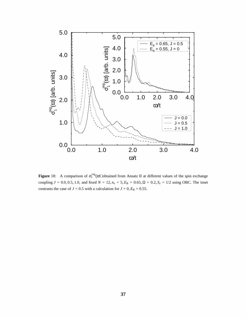
Figure 18: A comparison of σ reg1 (ω) obtained from Ansatz II at different values of the spin exchange

coupling J = 0.0, 0.5, 1.0, and fixed N = 12, ne = 5, EB = 0.65, Ω = 0.2, Sz = 1/2 using OBC. The inset

contrasts the case of J = 0.5 with a calculation for J = 0, EB = 0.55.

37

showed in Ref.[25], at small density, and Ω/t ≤ 0.1, excitations on the scale Ω become relevant,

and this leads to a qualitative difference between the results from Ansatz II and those from the

true Hamiltonian. Note, also, that the additional phonon states lead to a slight smoothening of

the spectra as compared to Ansatz II.

(iii) Finally, we should consider the possibility that the scattering from spin exchange could

be enhanced by the e-ph coupling as compared to the simple t-J model (see the discussion

in section II). Naively, one expects a competition between the spin and the polaronic e-ph

coupling. The former favours singlet bonds between electrons on neighbouring sites, i. e., an

effective attraction, whereas the latter leads to an effective nearest neighbour repulsion, i. e.,

CDW correlations. This competition might lead to interesting effects, which we investigate in

more detail in Ref. [25].

In Fig. 18 we show the spectra calculated for a 12-site lattice with ne = 5, total spin

z-component of Sz = 1/2, parameters EB = 0.65, Ω = 0.2, and different values of the spin

exchange coupling J. The ground state for all the parameters has the lowest possible value

for the total spin, S = 1/2, as found in the simple t-J model. We note that the spin degrees of

freedom enhance the low-frequency weight below the main peak, and shift the latter to lower

energy, while the high-frequency weight is reduced. The additional low-frequency weight in-

creases as a function of J. This effect of the spin exchange on the low-frequency region is

very similar to what happens when the e-ph coupling strength is reduced. A possible explana-

tion for this behaviour could therefore be that the nearest neighbour spin exchange coupling,

which favours electrons on neighbouring sites, leads to an effective weakening of the repul-

sive CDW-correlations on the scale ω . J. This can be verified in the inset of Fig. 18, where

one observes a strong similarity between a spectrum at J ≠ 0 and some EB, with a spectrum at

J = 0 and a smaller E0

B < EB. Apart from this effect, the spin degrees of freedom do not play

a significant role.

From these considerations, it seems most likely that the missing weight should come from

the contributions of larger chains. We expect that this should fill in the quasi-gap. Even

though we cannot explicitly calculate a spectrum for this situation, our results strongly suggest

that a spectra obtained from a superposition of random length chain segments (similar to the

case we calculated in section III without e-ph coupling) would give good agreement with the

experimental one.

36

0.0 0.5 1.0 1.5 2.0 2.5ω/t

0

1

2

3

4σ 1re

g (ω)

[arb

. uni

ts] N = 10, ne = 4

N = 12, ne = 5N = 14, ne = 6

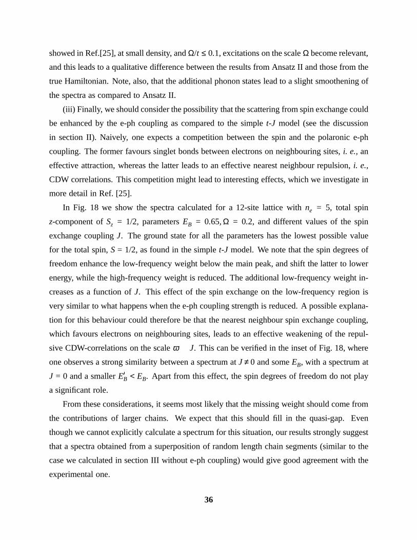
Figure 16: A comparison of spectra σ reg1 (ω) obtained

for different combinations of lattice sizes and fillings

[N, ne] = ([10, 4], [12, 5], [14, 6]) using OBC and fixed

values of EB = 0.65, Ω = 0.2.

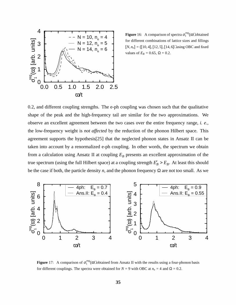
0.2, and different coupling strengths. The e-ph coupling was chosen such that the qualitative

shape of the peak and the high-frequency tail are similar for the two approximations. We

observe an excellent agreement between the two cases over the entire frequency range, i. e.,

the low-frequency weight is not affected by the reduction of the phonon Hilbert space. This

agreement supports the hypothesis[25] that the neglected phonon states in Ansatz II can be

taken into account by a renormalized e-ph coupling. In other words, the spectrum we obtain

from a calculation using Ansatz II at coupling EB presents an excellent approximation of the

true spectrum (using the full Hilbert space) at a coupling strength E0

B > EB. At least this should

be the case if both, the particle density n, and the phonon frequency Ω are not too small. As we

0 1 2 3 4ω/t

0

2

4

6

8

σ 1reg (ω

) [a

rb. u

nits

]

4ph: EB = 0.7Ans.II: EB = 0.4

0 1 2 3 4ω/t

0

1

2

3

4

5

σ 1reg (ω

) [a

rb. u

nits

]

4ph: EB = 0.9Ans.II: EB = 0.55

Figure 17: A comparison of σ reg1 (ω) obtained from Ansatz II with the results using a four-phonon basis

for different couplings. The spectra were obtained for N = 9 with OBC at ne = 4 and Ω = 0.2.

35

0.0 0.2 0.4 0.6 0.8 1.0ω [eV]

0

1

2

3

4σ 1re

g (ω)

[arb

. uni

ts] Theory: (a) N = 14

Theory: (b) N = 13Exp. (PrBa2Cu3O7)

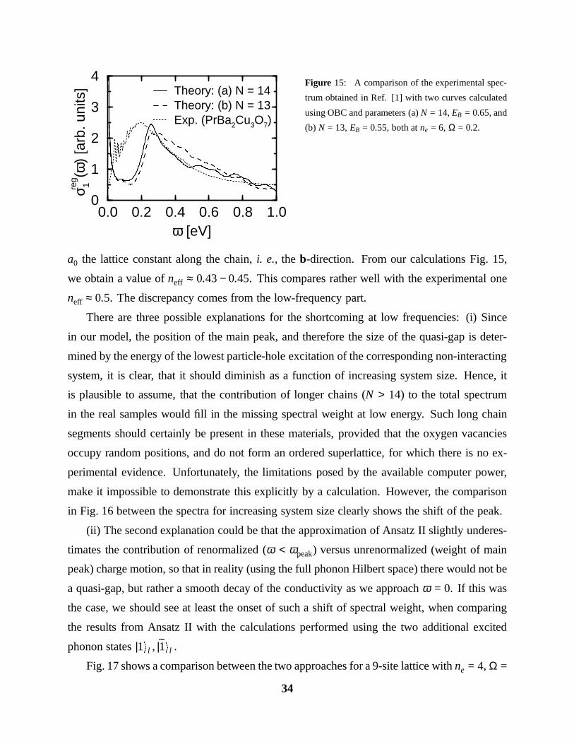
Figure 15: A comparison of the experimental spec-

trum obtained in Ref. [1] with two curves calculated

using OBC and parameters (a) N = 14, EB = 0.65, and

(b) N = 13, EB = 0.55, both at ne = 6, Ω = 0.2.

a0 the lattice constant along the chain, i. e., the b-direction. From our calculations Fig. 15,

we obtain a value of neff ≈ 0.43 − 0.45. This compares rather well with the experimental one

neff ≈ 0.5. The discrepancy comes from the low-frequency part.

There are three possible explanations for the shortcoming at low frequencies: (i) Since

in our model, the position of the main peak, and therefore the size of the quasi-gap is deter-

mined by the energy of the lowest particle-hole excitation of the corresponding non-interacting

system, it is clear, that it should diminish as a function of increasing system size. Hence, it

is plausible to assume, that the contribution of longer chains (N > 14) to the total spectrum

in the real samples would fill in the missing spectral weight at low energy. Such long chain

segments should certainly be present in these materials, provided that the oxygen vacancies

occupy random positions, and do not form an ordered superlattice, for which there is no ex-

perimental evidence. Unfortunately, the limitations posed by the available computer power,

make it impossible to demonstrate this explicitly by a calculation. However, the comparison

in Fig. 16 between the spectra for increasing system size clearly shows the shift of the peak.

(ii) The second explanation could be that the approximation of Ansatz II slightly underes-

timates the contribution of renormalized (ω < ωpeak) versus unrenormalized (weight of main

peak) charge motion, so that in reality (using the full phonon Hilbert space) there would not be

a quasi-gap, but rather a smooth decay of the conductivity as we approach ω = 0. If this was

the case, we should see at least the onset of such a shift of spectral weight, when comparing

the results from Ansatz II with the calculations performed using the two additional excited

phonon states |1il , |e1il .

Fig. 17 shows a comparison between the two approaches for a 9-site lattice with ne = 4, Ω =

34

0 1 2 3 4ω/t

0

1

2

3

4

σ 1reg (ω

) [a

rb. u

nits

] EB = 0.55EB = 0.6

0

2

4

6

8

σ 1reg (ω

) [a

rb. u

nits

] EB = 0.4EB = 0.8

0

2

4

6σ 1re

g (ω)

[arb

. uni

ts] EB = 0.4

EB = 0.8

0 1 2 3 4ω/t

0

2

4

6

σ 1reg (ω

) [a

rb. u

nits

] EB = 0.45EB = 0.5

0

1

2

3

4

5

σ 1reg (ω

) [a

rb. u

nits

] EB = 0.55EB = 0.7

0

2

4

6

8

σ 1reg (ω

) [a

rb. u

nits

] EB = 0.4EB = 0.8

ne = 7ne = 6

ne = 5ne = 4

ne = 3ne = 2

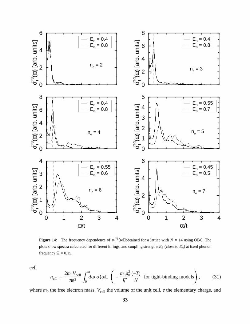
Figure 14: The frequency dependence of σ reg1 (ω) obtained for a lattice with N = 14 using OBC. The

plots show spectra calculated for different fillings, and coupling strengths EB (close to EcB) at fixed phonon

frequency Ω = 0.15.

cell

neff :=2m0Vcell

πe2

Z ∞

0dω σ (ω)

=m0a2

0

h2

h−TiN

for tight-binding models

!

, (31)

where m0 the free electron mass, Vcell the volume of the unit cell, e the elementary charge, and

33

0.0 0.1 0.2 0.3 0.4 0.5ω / t

0

1

2

3σ 1re

g (ω)

[arb

. uni

ts]

EB = 0.4EB = 0.5EB = 0.6

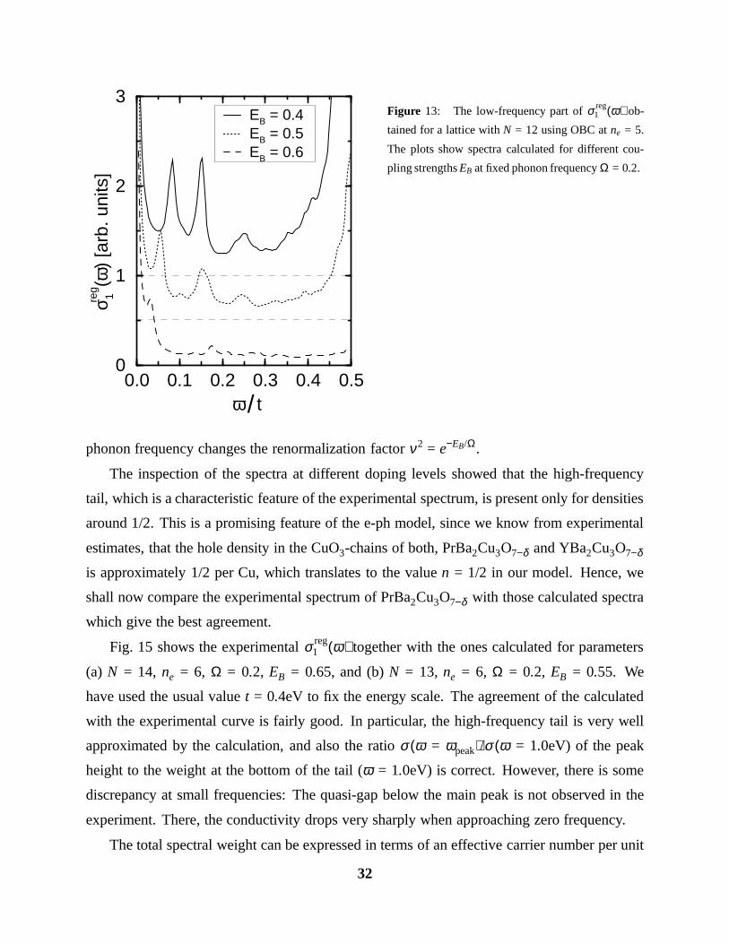
Figure 13: The low-frequency part of σ reg1 (ω) ob-

tained for a lattice with N = 12 using OBC at ne = 5.

The plots show spectra calculated for different cou-

pling strengths EB at fixed phonon frequency Ω = 0.2.

phonon frequency changes the renormalization factor ν2 = e−EB/Ω.

The inspection of the spectra at different doping levels showed that the high-frequency

tail, which is a characteristic feature of the experimental spectrum, is present only for densities

around 1/2. This is a promising feature of the e-ph model, since we know from experimental

estimates, that the hole density in the CuO3-chains of both, PrBa2Cu3O7−δ and YBa2Cu3O7−δ

is approximately 1/2 per Cu, which translates to the value n = 1/2 in our model. Hence, we

shall now compare the experimental spectrum of PrBa2Cu3O7−δ with those calculated spectra

which give the best agreement.

Fig. 15 shows the experimental σ reg1 (ω) together with the ones calculated for parameters

(a) N = 14, ne = 6, Ω = 0.2, EB = 0.65, and (b) N = 13, ne = 6, Ω = 0.2, EB = 0.55. We

have used the usual value t = 0.4eV to fix the energy scale. The agreement of the calculated

with the experimental curve is fairly good. In particular, the high-frequency tail is very well

approximated by the calculation, and also the ratio σ (ω = ωpeak)/σ (ω = 1.0eV) of the peak

height to the weight at the bottom of the tail (ω = 1.0eV) is correct. However, there is some

discrepancy at small frequencies: The quasi-gap below the main peak is not observed in the

experiment. There, the conductivity drops very sharply when approaching zero frequency.

The total spectral weight can be expressed in terms of an effective carrier number per unit

32

pearance of the low-energy peak can clearly be related to an optical excitation, which is al-

ready present in the non-interacting case, namely the lowest particle-hole excitation of the free

electron system. The corresponding energy is largest at half-filling (due to the simple cosine

band-structure), and decreases monotonically with the density. This peak dominates the opti-

cal conductivity in the presence or absence of the e-ph interactions, at least for not too strong

coupling (where it is suppressed for densities close to 1/2). However, in the interacting case,

the peak is shifted to higher energies (as compared to the free system), and also broadened as

the coupling increases.

(ii) The second new feature is the appearance of spectral weight at very low energy below

the dominant peak, which partly fills in the quasi-gap. This weight decreases as a function of

increasing coupling in much the same way as the weight under the peak decreases. The com-

bined reduction of weight of these two features can be related to the corresponding decrease of

the Drude weight obtained for PBC. Physically, the low-energy weight can be associated with

the renormalized charge motion, which occurs on the energy scale ∼ et. For PBC, this motion

contributes to the dc conductivity, whereas here, due to the reflecting walls, the corresponding

spectral weight appears at finite frequencies of the order of ω ∼et.

This effect can be observed, when we concentrate on the low-energy spectrum below the

main peak, and use a smaller broadening δ = 0.01 for our plots. Fig. 13 shows this part of the

spectrum for the case N = 12, ne = 5, Ω = 0.2, and three different coupling strengths. Note,

how the dominant peak in this low-energy part is shifted towards lower frequencies as the

coupling is increased, according to the dependence of et = te−EB/Ω. A detailed analysis of the

peak position revealed exactly the exponential dependence. Furthermore, for strong coupling

EB > EcB, the inspection of the change in this low-energy spectral weight as a function of doping

reveals a very similar dependence as obtained for the Drude weight in the case of PBC (see

Fig. 11): For densities close to 1/2, this weight increases with the number of domain walls,

whereas for n & 0, it increases with the number of electrons. In summary, we can say that the

low-energy spectrum clearly shows the presence of simultaneous renormalized (ω ∼ et), and

unrenormalized charge motion (ω ∼ t).

In Fig. 14, we show the same spectra for lower phonon frequency Ω = 0.15, and various

coupling strengths. The qualitative shape of σ (ω) is very similar to the previous case, but note,

that the coupling strength needed to obtain the high-frequency tail is now smaller, because the

31

0 1 2 3 4ω/t

0

1

2

3

4

σ 1reg (ω

) [a

rb. u

nits

] EB = 0.65EB = 0.7

0

1

2

3

4

5

σ 1reg (ω

) [a

rb. u

nits

] EB = 0.65EB = 0.8

0

2

4

6σ 1re

g (ω)

[arb

. uni

ts] EB = 0.6

EB = 1.0

0 1 2 3 4ω/t

0

1

2

3

4

σ 1reg (ω

) [a

rb. u

nits

] EB = 0.55EB = 0.6

0

1

2

3

4

σ 1reg (ω

) [a

rb. u

nits

] EB = 0.65EB = 0.75

0

1

2

3

4

5

σ 1reg (ω

) [a

rb. u

nits

] EB = 0.65EB = 0.8

ne = 7ne = 6

ne = 5ne = 4

ne = 3ne = 2

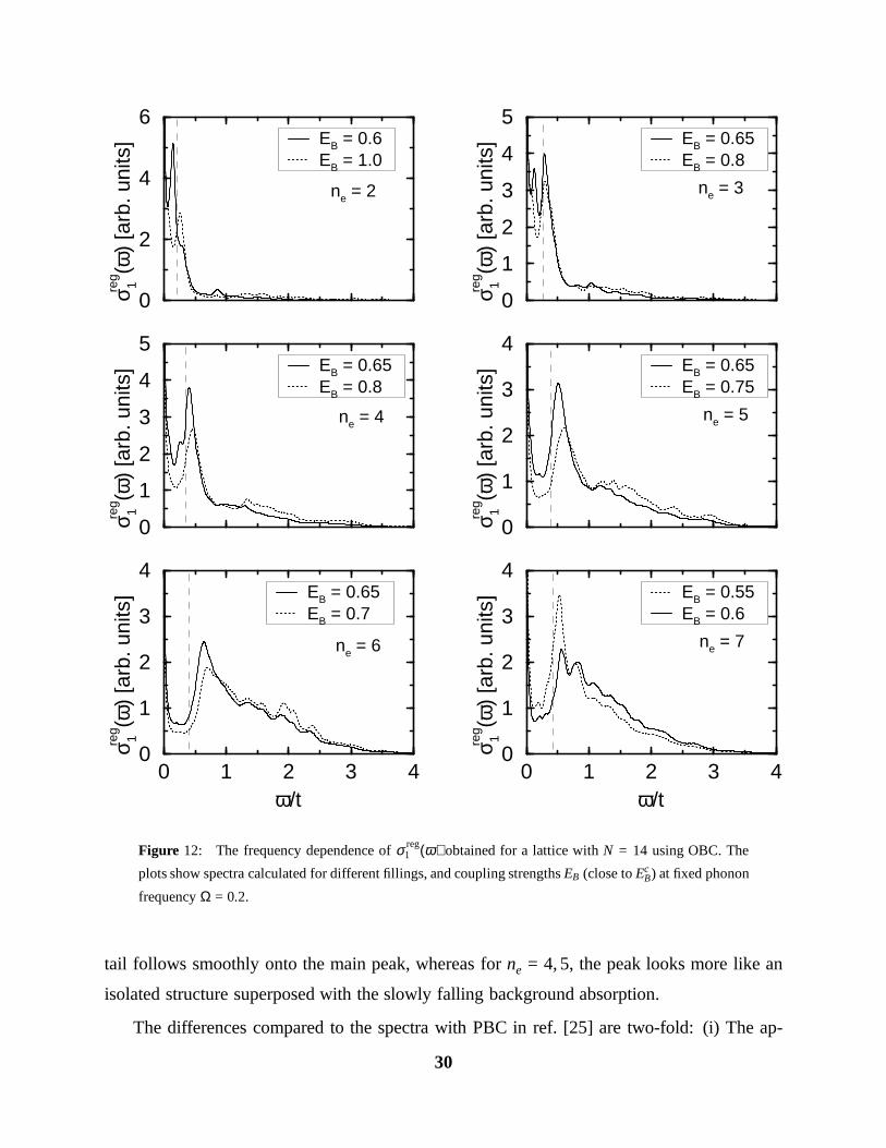
Figure 12: The frequency dependence of σ reg1 (ω) obtained for a lattice with N = 14 using OBC. The

plots show spectra calculated for different fillings, and coupling strengths EB (close to EcB) at fixed phonon

frequency Ω = 0.2.

tail follows smoothly onto the main peak, whereas for ne = 4, 5, the peak looks more like an

isolated structure superposed with the slowly falling background absorption.

The differences compared to the spectra with PBC in ref. [25] are two-fold: (i) The ap-

30

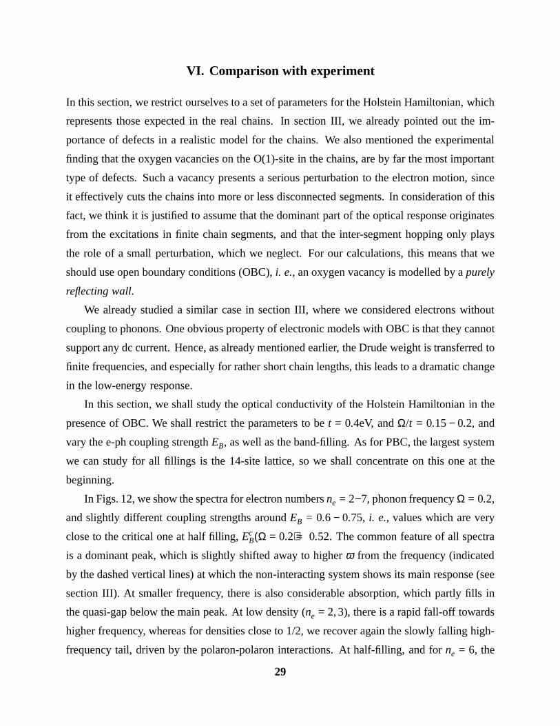
VI. Comparison with experiment

In this section, we restrict ourselves to a set of parameters for the Holstein Hamiltonian, which

represents those expected in the real chains. In section III, we already pointed out the im-

portance of defects in a realistic model for the chains. We also mentioned the experimental

finding that the oxygen vacancies on the O(1)-site in the chains, are by far the most important

type of defects. Such a vacancy presents a serious perturbation to the electron motion, since

it effectively cuts the chains into more or less disconnected segments. In consideration of this

fact, we think it is justified to assume that the dominant part of the optical response originates

from the excitations in finite chain segments, and that the inter-segment hopping only plays

the role of a small perturbation, which we neglect. For our calculations, this means that we

should use open boundary conditions (OBC), i. e., an oxygen vacancy is modelled by a purely

reflecting wall.

We already studied a similar case in section III, where we considered electrons without

coupling to phonons. One obvious property of electronic models with OBC is that they cannot

support any dc current. Hence, as already mentioned earlier, the Drude weight is transferred to

finite frequencies, and especially for rather short chain lengths, this leads to a dramatic change

in the low-energy response.

In this section, we shall study the optical conductivity of the Holstein Hamiltonian in the

presence of OBC. We shall restrict the parameters to be t = 0.4eV, and Ω/t = 0.15 − 0.2, and

vary the e-ph coupling strength EB, as well as the band-filling. As for PBC, the largest system

we can study for all fillings is the 14-site lattice, so we shall concentrate on this one at the

beginning.

In Figs. 12, we show the spectra for electron numbers ne = 2−7, phonon frequency Ω = 0.2,

and slightly different coupling strengths around EB = 0.6 − 0.75, i. e., values which are very

close to the critical one at half filling, EcB(Ω = 0.2) ≈ 0.52. The common feature of all spectra

is a dominant peak, which is slightly shifted away to higher ω from the frequency (indicated

by the dashed vertical lines) at which the non-interacting system shows its main response (see

section III). At smaller frequency, there is also considerable absorption, which partly fills in

the quasi-gap below the main peak. At low density (ne = 2, 3), there is a rapid fall-off towards

higher frequency, whereas for densities close to 1/2, we recover again the slowly falling high-

frequency tail, driven by the polaron-polaron interactions. At half-filling, and for ne = 6, the

29

DomainWall

n > 1/2n < 1/2

CDW Doped CDW

High-Energy Process Low-Energy Process

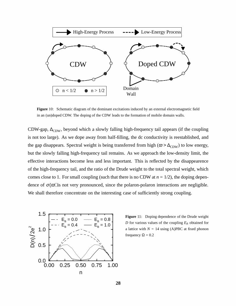
Figure 10: Schematic diagram of the dominant excitations induced by an external electromagnetic field

in an (un)doped CDW. The doping of the CDW leads to the formation of mobile domain walls.

CDW-gap, ∆CDW, beyond which a slowly falling high-frequency tail appears (if the coupling

is not too large). As we dope away from half-filling, the dc conductivity is reestablished, and

the gap disappears. Spectral weight is being transferred from high (ω > ∆CDW) to low energy,

but the slowly falling high-frequency tail remains. As we approach the low-density limit, the

effective interactions become less and less important. This is reflected by the disappearence

of the high-frequency tail, and the ratio of the Drude weight to the total spectral weight, which

comes close to 1. For small coupling (such that there is no CDW at n = 1/2), the doping depen-

dence of σ (ω) is not very pronounced, since the polaron-polaron interactions are negligible.

We shall therefore concentrate on the interesting case of sufficiently strong coupling.

0.00 0.25 0.50 0.75 1.00n

0.0

0.5

1.0

1.5

D(n

) /2e

2

EB = 0.0EB = 0.4

EB = 0.8EB = 1.0

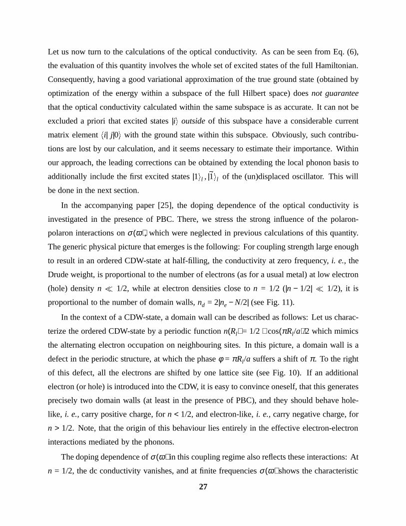
Figure 11: Doping dependence of the Drude weight

D for various values of the coupling EB obtained for

a lattice with N = 14 using (A)PBC at fixed phonon

frequency Ω = 0.2

28

Let us now turn to the calculations of the optical conductivity. As can be seen from Eq. (6),

the evaluation of this quantity involves the whole set of excited states of the full Hamiltonian.

Consequently, having a good variational approximation of the true ground state (obtained by

optimization of the energy within a subspace of the full Hilbert space) does not guarantee

that the optical conductivity calculated within the same subspace is as accurate. It can not be

excluded a priori that excited states |ii outside of this subspace have a considerable current

matrix element hi| j|0i with the ground state within this subspace. Obviously, such contribu-

tions are lost by our calculation, and it seems necessary to estimate their importance. Within

our approach, the leading corrections can be obtained by extending the local phonon basis to

additionally include the first excited states |1il , |e1il of the (un)displaced oscillator. This will

be done in the next section.

In the accompanying paper [25], the doping dependence of the optical conductivity is

investigated in the presence of PBC. There, we stress the strong influence of the polaron-

polaron interactions on σ (ω), which were neglected in previous calculations of this quantity.

The generic physical picture that emerges is the following: For coupling strength large enough

to result in an ordered CDW-state at half-filling, the conductivity at zero frequency, i. e., the

Drude weight, is proportional to the number of electrons (as for a usual metal) at low electron

(hole) density n 1/2, while at electron densities close to n = 1/2 (|n − 1/2| 1/2), it is

proportional to the number of domain walls, nd = 2|ne − N/2| (see Fig. 11).

In the context of a CDW-state, a domain wall can be described as follows: Let us charac-

terize the ordered CDW-state by a periodic function n(Rl) = 1/2 + cos(πRl/a)/2 which mimics

the alternating electron occupation on neighbouring sites. In this picture, a domain wall is a

defect in the periodic structure, at which the phase φ = πRl/a suffers a shift of π . To the right

of this defect, all the electrons are shifted by one lattice site (see Fig. 10). If an additional

electron (or hole) is introduced into the CDW, it is easy to convince oneself, that this generates

precisely two domain walls (at least in the presence of PBC), and they should behave hole-

like, i. e., carry positive charge, for n < 1/2, and electron-like, i. e., carry negative charge, for

n > 1/2. Note, that the origin of this behaviour lies entirely in the effective electron-electron

interactions mediated by the phonons.

The doping dependence of σ (ω) in this coupling regime also reflects these interactions: At

n = 1/2, the dc conductivity vanishes, and at finite frequencies σ (ω) shows the characteristic

27

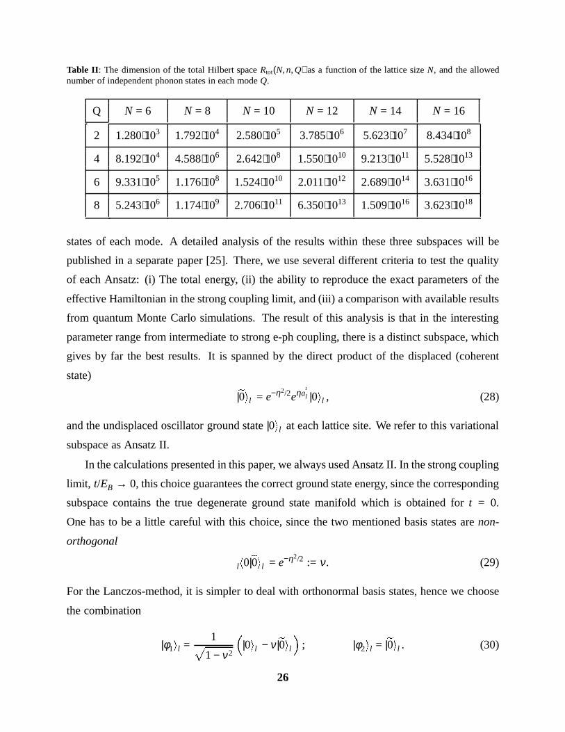
Table II: The dimension of the total Hilbert space Rtot(N, n, Q) as a function of the lattice size N, and the allowednumber of independent phonon states in each mode Q.

Q N = 6 N = 8 N = 10 N = 12 N = 14 N = 16

2 1.280⋅103 1.792⋅104 2.580⋅105 3.785⋅106 5.623⋅107 8.434⋅108

4 8.192⋅104 4.588⋅106 2.642⋅108 1.550⋅1010 9.213⋅1011 5.528⋅1013

6 9.331⋅105 1.176⋅108 1.524⋅1010 2.011⋅1012 2.689⋅1014 3.631⋅1016

8 5.243⋅106 1.174⋅109 2.706⋅1011 6.350⋅1013 1.509⋅1016 3.623⋅1018

states of each mode. A detailed analysis of the results within these three subspaces will be

published in a separate paper [25]. There, we use several different criteria to test the quality

of each Ansatz: (i) The total energy, (ii) the ability to reproduce the exact parameters of the

effective Hamiltonian in the strong coupling limit, and (iii) a comparison with available results

from quantum Monte Carlo simulations. The result of this analysis is that in the interesting

parameter range from intermediate to strong e-ph coupling, there is a distinct subspace, which

gives by far the best results. It is spanned by the direct product of the displaced (coherent

state)

|e0il = e−η2/2eηa†l |0il , (28)

and the undisplaced oscillator ground state |0il at each lattice site. We refer to this variational

subspace as Ansatz II.

In the calculations presented in this paper, we always used Ansatz II. In the strong coupling

limit, t/EB → 0, this choice guarantees the correct ground state energy, since the corresponding

subspace contains the true degenerate ground state manifold which is obtained for t = 0.

One has to be a little careful with this choice, since the two mentioned basis states are non-

orthogonal

lh0|e0il = e−η2/2 := ν . (29)

For the Lanczos-method, it is simpler to deal with orthonormal basis states, hence we choose

the combination

|φ1il =1

p

1 − ν2

|0il − ν |e0il

; |φ2il = |e0il . (30)

26

Unfortunately, the Lanczos method is not applicable to an e-ph system without further ap-

proximation. The reason is simply the fact that the phonon Hilbert space is infinite-dimensional

already for a single phonon mode, whereas the Lanczos algorithm can only be used for finite-

dimensional Hilbert spaces, since convergence to the true ground state is only guaranteed if

the vectors |Φni =P

m anm|φmi are expressed in a complete set of basis states |φmi of the full

(in each symmetry sector) Hilbert space. This requires computer storage of the coefficients

anm of at least two vectors at one time. For an infinite-dimensional Hilbert space, clearly, one

would require an infinite amount of computer memory in order to obtain exact results.

Therefore, the only possible way to apply the Lanczos method to an e-ph Hamiltonian

is to use a variational approximation for the phonon Hilbert space, which makes it finite-

dimensional. Since variational approximations are most often motivated by physical intuition

or/and computational convenience, obviously, there are many possible choices for a variational

ansatz. For our Hamiltonian, we considered the three ‘most natural’ variational approximations

to the phonon Hilbert space, which are within the limits set by current computer power and

the Lanczos algorithm.

The basic computational limitation we encounter is the maximum number of independent

phonon states that can be allowed for each mode. If we denote this number by Q, then on an N-

site lattice, the total number of linearly independent phonon states is given by Rph(N, Q) = QN.

On the other hand, the size of the electron Hilbert space (neglecting spin) on a N-site lattice

with n electrons is given by Re(N, n) =N

n

, so that the total Hilbert space has the dimension

Rtot(N, n, Q) = QN =N!QN

n!(N−n)!. As an illustration, in table I, we show this number for different

values of N, Q, and fixed n = N/2, where the electron Hilbert space is maximal for a given N.

Bearing in mind the size of core memory of present supercomputers (∼ 1GByte, corresponding

to a maximum size Rtot(N, n, Q) ≈ 4.5 ⋅ 107), we can extract from these numbers that the

maximum tractable lattice sizes are N = 15 for Q = 2, N = 9 for Q = 4, N = 7 for Q = 6,

and N = 6 for Q = 8. We have performed calculations mainly for Q = 2. The quality of this

approximation, i. e., the influence of additional phonon degrees of freedom, was then tested

by a comparison with results for Q = 4. As we shall see later, the qualitative features obtained

from the Q = 2 calculation are not altered. The lattice sizes for Q > 4 that are tractable are too

small to extract meaningful results. Therefore we did not consider them.

Restricting ourselves to the case Q = 2, there are three plausible choices for the two phonon

25

tridiagonal matrix in the basis f|Φnig. In more detail, one obtains

H|Φ0i = α0|Φ0i + β0|Φ1i, (24)

α0 = hΦ0| H|Φ0i, β0 =q

hΦ0| H2|Φ0i − α20 .

The nth iteration is

H|Φni = βn−1|Φn−1i + αn|Φni + βn|Φn+1i, (25)

αn = hΦn| H|Φni, βn =q

hΦn| H2|Φni − α2n − β2

n−1,

In practice, these operations are performed on a computer. The main difficulty is to find an

effective way for obtaining H|Φni from |Φni.

The extreme eigenvalues and -vectors of the such generated M × M tridiagonal matrix

converge extremely fast to the real ones of H. Starting from a completely random |Φ0i (which

is the safest choice), one typically needs M = 60 − 100 iterations to obtain an accuracy to 12

decimal places in the lowest eigenvalue E0, and an error ∆ = (hΨ0| H − E0|Ψ0i)1/2 ≈ 10−7 − 10−8

for the ground state |Ψ0i. The number of iterations needed for convergence of the ground

state energy depends strongly on the splitting E1 − E0 to the first excited state, and increases

significantly as the two levels get close.

For the calculation of the optical conductivity at zero temperature, one usually employs

the continued fraction expansion of the Greens function [27]

G(Z) = hΨ0| j(Z − H)−1j|Ψ0i =hΨ0| jj |Ψ0i

Z − eα0 −eβ2

1

Z − eα1 −eβ2

2

Z − eα2 − ⋅ ⋅ ⋅

, (26)

where the coefficients (eαn, eβn) of the continued fraction are the usual Lanczos coefficients

obtained from a second Lanczos run using the starting vector |eΦ0i = j|Ψ0i. The continued

fraction is truncated after M iterations (typically M = 300), when a good convergence of the

spectrum is obtained. The real part of the optical conductivity is then given by

σ reg1 (ω) = −

1πω

Im G(ω + E0 + iδ ), (27)

where we introduced a small imaginary part iδ , which gives a finite Lorentzian width to the

delta peaks appearing in the original definition (6).

24

V. Numerical treatment of the t-J Holstein Hamiltonian

A numerical method suitable for dealing with strong correlations would in principle be the

quantum Monte Carlo (QMC) method. This technique was used by Hirsch and Fradkin [26] to

investigate the CDW transition at half filling. They presented strong evidence that for arbritrary

finite values of the phonon frequency Ω, the spinless Holstein model exhibits a transition from

a metallic to a CDW state at a finite critical value of the e-ph coupling constant EcB. They

derived the et-eV model as the effective second order Hamiltonian in the strong coupling limit,

and showed that the ratio of the effective parameters limEB→∞et/eV = 0. We recall, that most

standard analytical approaches only take into account the hopping renormalization from the

first order correction, which defines a small polaron band with a bandwidth ∼ et = te−EB/Ω. As

Hirsch and Fradkin noted, the fact that the et-eV model exhibits a CDW transition at et/eV = 1/2,

gives strong evidence for an analogous CDW ground state in the strong coupling limit of the

Holstein model.

The drawback of the QMC method is that it is not straightforward to calculate dynamical

quantities such as σ (ω), because the simulation gives direct results for dynamical quantities

only as a function of imaginary frequencies. Therefore one needs to analytically continue to the

real axis, which is not always a well-defined procedure. In contrast, the Lanczos method has

been successfully applied to calculate σ (ω) at zero temperature for purely electronic Hamilto-

nians on finite lattices [27]. This algorithm allows for the exact determination of the low-lying

eigenvalues and -vectors of the Hamiltonian matrix. From the calculated ground state, it is

then possible to extract dynamical quantities such as, e. g., the spectral function A(k, ω), or

the optical conductivity σ (ω), in principle with arbitrary accuracy. The big advantage of the

method is that the results are exact, the disadvantage is the limitation (imposed by the com-

puter memory available) to rather small lattices, so that often an accurate finite-size scaling is

impossible.

The algorithm works as follows: One generates an arbitrary initial vector |Φ0i, with the

only restriction that |Φ0i should have a finite overlap with the ground state in the symmetry sec-

tor of the Hilbert space one is interested in. Starting from |Φ0i, one generates an orthonormal

set of states f|Φnig by successively operating with H on |Φni, n = 0, ⋅ ⋅ ⋅ , M, and orthonormal-

izing to all the previous vectors, such that the Hamiltonian is represented by a real symmetric

23

well as in the strong coupling case [24] using perturbative methods. However, in none of the

approaches used were the polaron-polaron interactions taken into account, i. e., the results are

only trustworthy (especially in the strong coupling limit) in the single polaron limit.

There are a number of reasons, why we consider these approaches do not to apply for our

problem: (i) We are interested in a situation with high carrier concentrations, i. e., polaron-

polaron interactions are important, particularly in the vicinity close to density n = 1/2. (ii) The

estimated value of the e-ph coupling corresponds neither to weak nor strong coupling, so there

is no guarantee that perturbation series rapidly converge. (iii) We are also interested in the

effect of the spin degrees of freedom, even though we do not expect them to be very important

at realistic values of the spin-exchange constant. (iv) We would like to include the effect of

vacancy disorder by choosing open boundary conditions as already explained in section III.

An analytical treatment in the interesting parameter regime including the additional ef-

fects of spin-exchange coupling and disorder is hopelessly difficult. Consequently, we chose

to study the model using a numerical technique, the Lanczos method. In an accompanying

paper [25], we present a detailed discussion of our numerical results for the simple Holstein

model and contrast them with the analytic results mentioned above.

22

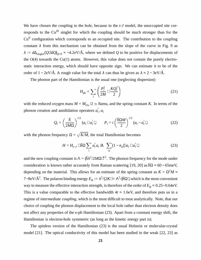
We have chosen the coupling to the hole, because in the t-J model, the unoccupied site cor-

responds to the CuIII singlet for which the coupling should be much stronger than for the

CuII configuration which corresponds to an occupied site. The contribution to the coupling

constant λ from this mechanism can be obtained from the slope of the curve in Fig. 9 as

λ := d∆singlet(Q)/dQ|Q=0 ≈ −4.2eV/A, where we defined Q to be positive for displacements of

the O(4) towards the Cu(1) atoms. However, this value does not contain the purely electro-

static interaction energy, which should have opposite sign. We can estimate it to be of the

order of 1 − 2eV/A. A rough value for the total λ can thus be given as λ ≈ 2 − 3eV/A.

The phonon part of the Hamiltonian is the usual one (neglecting dispersion)

Hph =X

l

P2l

2M+

KQ2l

2

!

(21)

with the reduced oxygen mass M = MOx./2 ' 8amu, and the spring constant K. In terms of the

phonon creation and annihilation operators a†l , al

Ql =

h2MΩ

1/2

(al + a†l ), Pl = i

hΩM2

1/2

(al − a†l ), (22)

with the phonon frequency Ω =p

K/M, the total Hamiltonian becomes

H = Ht−J + hΩX

l

a†l al + Λ

X

ls

(1 − nls)(al + a†l ), (23)

and the new coupling constant is Λ = (hλ2/2MΩ)1/2. The phonon frequency for the mode under

consideration is known rather accurately from Raman scattering [19, 20] as hΩ ≈ 60 − 65meV,

depending on the material. This allows for an estimate of the spring constant as K = Ω2M ≈

7−8eV/A2. The polaron binding energy EB := λ2/(2K) = Λ2/(hΩ), which is the most convenient

way to measure the effective interaction strength, is therefore of the order of EB ≈ 0.25−0.64eV.

This is a value comparable to the effective bandwidth 4t ≈ 1.6eV, and therefore puts us in a

regime of intermediate coupling, which is the most difficult to treat analytically. Note, that our

choice of coupling the phonon displacement to the local hole rather than electron density does

not affect any properties of the e-ph Hamiltonian (23). Apart from a constant energy shift, the

Hamiltonian is electron-hole symmetric (as long as the kinetic energy part is).

The spinless version of the Hamiltonian (23) is the usual Holstein or molecular-crystal

model [21]. The optical conductivity of this model has been studied in the weak [22, 23] as

21

O(1,4)

Cu(1)

(a)

(b)

c

b

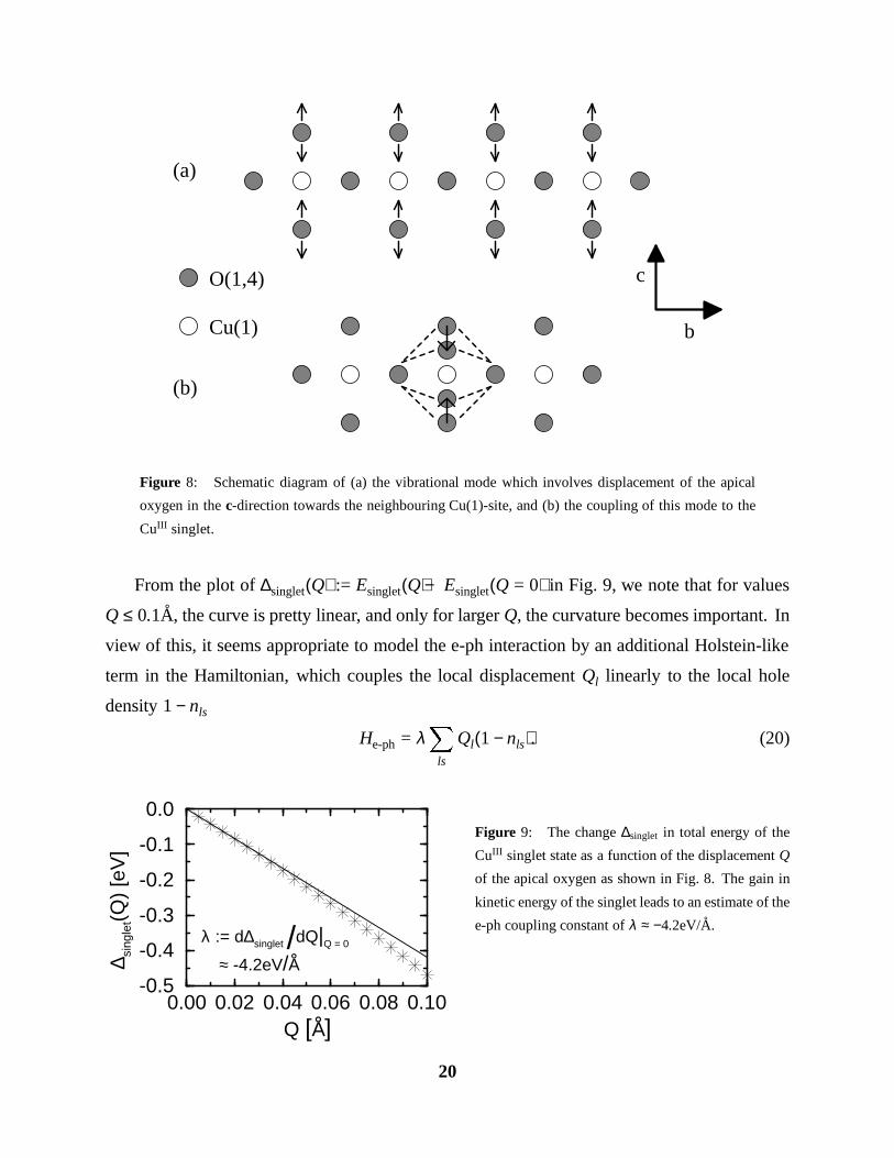
Figure 8: Schematic diagram of (a) the vibrational mode which involves displacement of the apical

oxygen in the c-direction towards the neighbouring Cu(1)-site, and (b) the coupling of this mode to the

CuIII singlet.

From the plot of ∆singlet(Q) := Esinglet(Q) − Esinglet(Q = 0) in Fig. 9, we note that for values

Q ≤ 0.1A, the curve is pretty linear, and only for larger Q, the curvature becomes important. In

view of this, it seems appropriate to model the e-ph interaction by an additional Holstein-like

term in the Hamiltonian, which couples the local displacement Ql linearly to the local hole

density 1 − nls

He-ph = λX

ls

Ql(1 − nls). (20)

0.00 0.02 0.04 0.06 0.08 0.10Q [A]

-0.5

-0.4

-0.3

-0.2

-0.1

0.0

∆ sing

let(Q

) [e

V]

λ := d∆singlet /dQ|Q = 0

≈ -4.2eV/A

Figure 9: The change ∆singlet in total energy of the

CuIII singlet state as a function of the displacement Q

of the apical oxygen as shown in Fig. 8. The gain in

kinetic energy of the singlet leads to an estimate of the

e-ph coupling constant of λ ≈ −4.2eV/A.

20

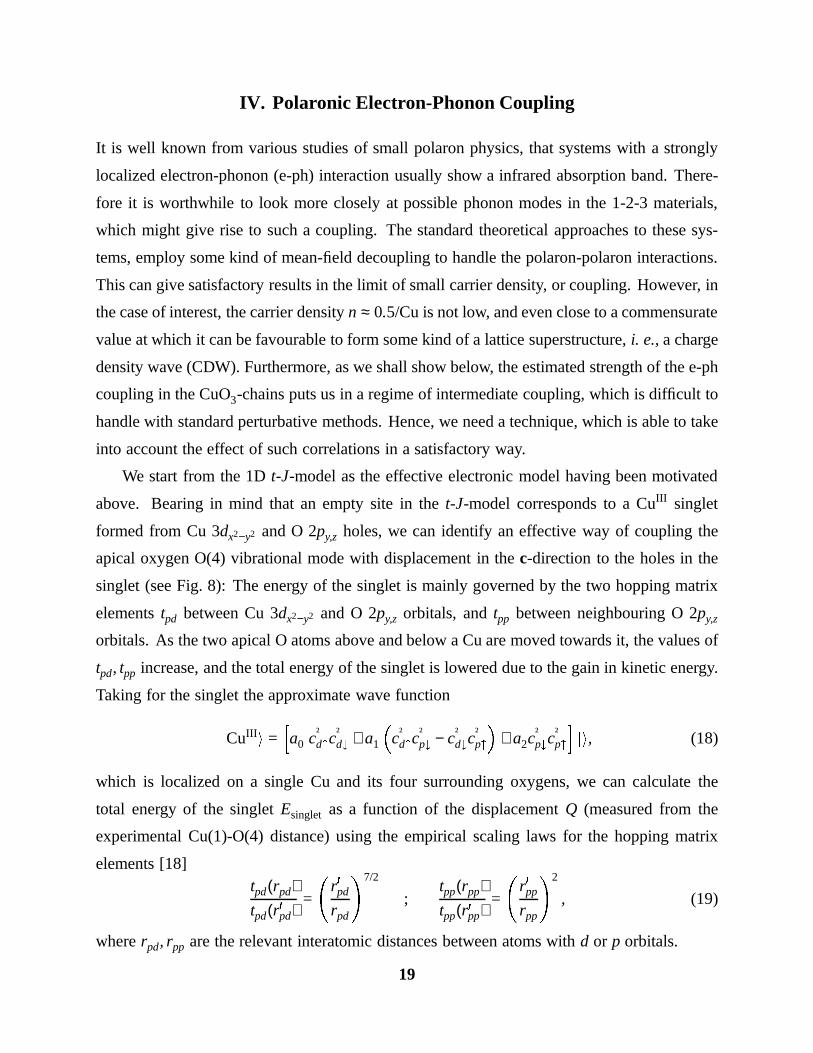
IV. Polaronic Electron-Phonon Coupling

It is well known from various studies of small polaron physics, that systems with a strongly

localized electron-phonon (e-ph) interaction usually show a infrared absorption band. There-

fore it is worthwhile to look more closely at possible phonon modes in the 1-2-3 materials,

which might give rise to such a coupling. The standard theoretical approaches to these sys-

tems, employ some kind of mean-field decoupling to handle the polaron-polaron interactions.

This can give satisfactory results in the limit of small carrier density, or coupling. However, in

the case of interest, the carrier density n ≈ 0.5/Cu is not low, and even close to a commensurate

value at which it can be favourable to form some kind of a lattice superstructure, i. e., a charge

density wave (CDW). Furthermore, as we shall show below, the estimated strength of the e-ph

coupling in the CuO3-chains puts us in a regime of intermediate coupling, which is difficult to

handle with standard perturbative methods. Hence, we need a technique, which is able to take

into account the effect of such correlations in a satisfactory way.

We start from the 1D t-J-model as the effective electronic model having been motivated

above. Bearing in mind that an empty site in the t-J-model corresponds to a CuIII singlet

formed from Cu 3dx2−y2 and O 2py,z holes, we can identify an effective way of coupling the

apical oxygen O(4) vibrational mode with displacement in the c-direction to the holes in the

singlet (see Fig. 8): The energy of the singlet is mainly governed by the two hopping matrix

elements tpd between Cu 3dx2−y2 and O 2py,z orbitals, and tpp between neighbouring O 2py,z

orbitals. As the two apical O atoms above and below a Cu are moved towards it, the values of

tpd, tpp increase, and the total energy of the singlet is lowered due to the gain in kinetic energy.

Taking for the singlet the approximate wave function

jCuIIIi =h

a0 c†d"c†

d# + a1

c†d"c†

p# − c†d#c†

p"

+ a2c†p#c†

p"

i

ji, (18)

which is localized on a single Cu and its four surrounding oxygens, we can calculate the

total energy of the singlet Esinglet as a function of the displacement Q (measured from the

experimental Cu(1)-O(4) distance) using the empirical scaling laws for the hopping matrix

elements [18]tpd(rpd)tpd(r0pd)

=

r0pd

rpd

!7/2

;tpp(rpp)tpp(r0pp)

=

r0pp

rpp

!2

, (19)

where rpd, rpp are the relevant interatomic distances between atoms with d or p orbitals.

19

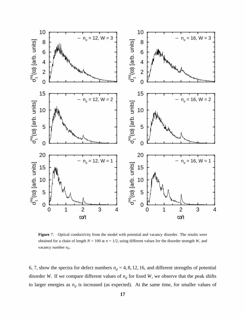
W/t . 2, and nd & 8, we recover in the high frequency tail, the structure of the isolated quasi

Drude peaks which correspond to very short chain segments.

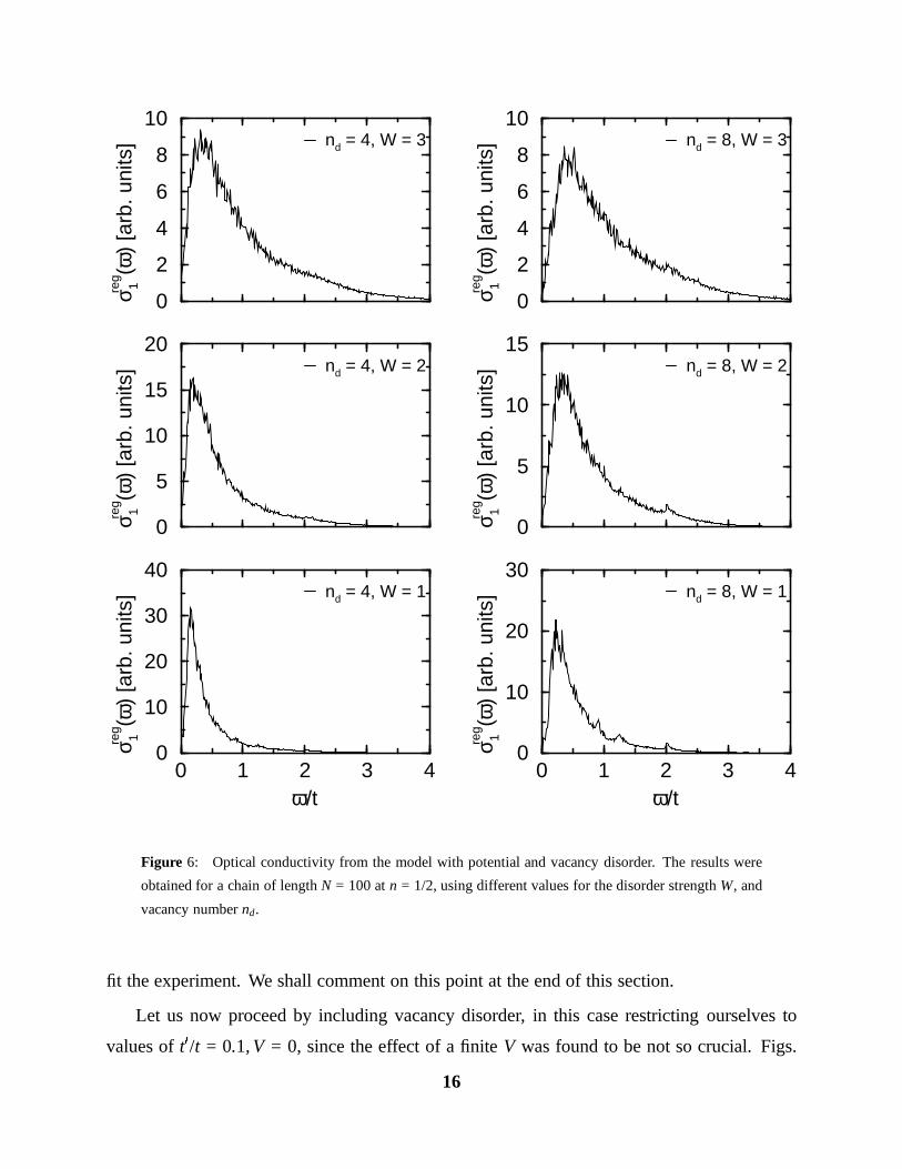
A comparison of e. g., the nd = 8 calculation to the Pr spectrum, shows that now only a

value of W ≈ 1.2eV is needed to obtain a fit as good as the one for nd = 0, W/t = 4. However,

going to an even larger nd = 16, the correct peak position requires a value of W/t ≈ 1, in which

case the high-frequency tail is not very well fitted anymore, especially regarding the strong

quasi Drude peaks in the calculated spectrum.

In summary, a model including both potential and vacancy disorder exhibits an optical

conductivity spectrum which is extremely close to the measured one. However, the potential

disorder strength needed to fit the experiment, W ≈ 1.2 − 1.6eV, is rather large, and the source

of such a strong random potential on each site is not obvious. A possible type of defect

producing such a strong potential could be an oxygen interstitial between two Cu(1) belonging

to neighbouring chains (see Fig. 1). The corresponding electrostatic potential energy Vc =

e2/(ε r) can be estimated to be Vc ≈ 1.2eV (using a rather small value for the dielectric constant

ε = 5) at the regular oxygen sites nearest neighbour to the interstitial. Nevertheless, it seems a

rather high density of such defects would be necessary to produce the required random potential

on each site.

In the next chapter, we shall investigate a third mechanism which could give rise to the

observed optical response, namely polaronic electron-phonon coupling.

18

0 1 2 3 4ω/t

0

5

10

15

20

σ 1reg (ω

) [a

rb. u

nits

] nd = 12, W = 1

0

5

10

15

σ 1reg (ω

) [a

rb. u

nits

] nd = 12, W = 2

0

2

4

6

8

10σ 1re

g (ω)

[arb

. uni

ts] nd = 12, W = 3

0 1 2 3 4ω/t

0

5

10

15

20

σ 1reg (ω

) [a

rb. u

nits

] nd = 16, W = 1

0

5

10

15

σ 1reg (ω

) [a

rb. u

nits

] nd = 16, W = 2

0

2

4

6

8

10

σ 1reg (ω

) [a

rb. u

nits

] nd = 16, W = 3

Figure 7: Optical conductivity from the model with potential and vacancy disorder. The results were

obtained for a chain of length N = 100 at n = 1/2, using different values for the disorder strength W, and

vacancy number nd.

6, 7, show the spectra for defect numbers nd = 4, 8, 12, 16, and different strengths of potential

disorder W. If we compare different values of nd for fixed W, we observe that the peak shifts

to larger energies as nd is increased (as expected). At the same time, for smaller values of

17

0 1 2 3 4ω/t

0

10

20

30

40

σ 1reg (ω

) [a

rb. u

nits

] nd = 4, W = 1

0

5

10

15

20

σ 1reg (ω

) [a

rb. u

nits

] nd = 4, W = 2

0

2

4

6

8

10σ 1re

g (ω)

[arb

. uni

ts] nd = 4, W = 3

0 1 2 3 4ω/t

0

10

20

30

σ 1reg (ω

) [a

rb. u

nits

] nd = 8, W = 1

0

5

10

15

σ 1reg (ω

) [a

rb. u

nits

] nd = 8, W = 2

0

2

4

6

8

10

σ 1reg (ω

) [a

rb. u

nits

] nd = 8, W = 3

Figure 6: Optical conductivity from the model with potential and vacancy disorder. The results were

obtained for a chain of length N = 100 at n = 1/2, using different values for the disorder strength W, and

vacancy number nd.

fit the experiment. We shall comment on this point at the end of this section.

Let us now proceed by including vacancy disorder, in this case restricting ourselves to

values of t0/t = 0.1, V = 0, since the effect of a finite V was found to be not so crucial. Figs.

16

0 1 2 3 4ω/t

0

50

100

150

σ 1reg (ω

) [a

rb. u

nits

] W = 1

0

10

20

30σ 1re

g (ω)

[arb

. uni

ts] W = 2

0 1 2 3 4ω/t

0

2

4

6

8

σ 1reg (ω

) [a

rb. u

nits

] W = 4

0

1

2

3

4

σ 1reg (ω

) [a

rb. u

nits

] W = 6

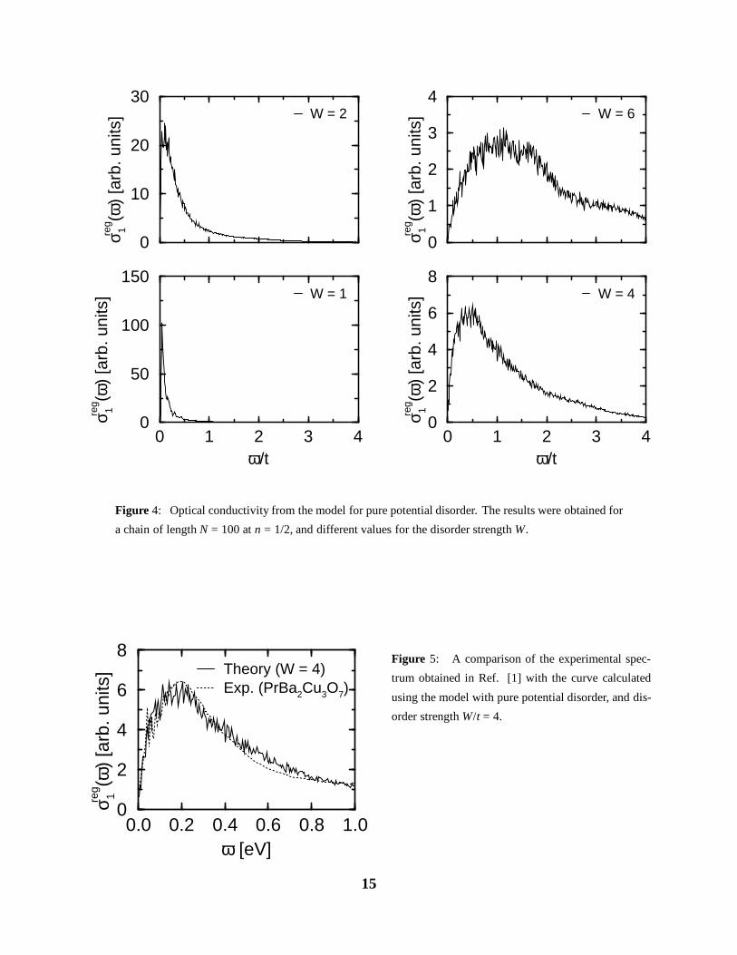
Figure 4: Optical conductivity from the model for pure potential disorder. The results were obtained for

a chain of length N = 100 at n = 1/2, and different values for the disorder strength W.

0.0 0.2 0.4 0.6 0.8 1.0ω [eV]

0

2

4

6

8

σ 1reg (ω

) [a

rb. u

nits

] Theory (W = 4)Exp. (PrBa2Cu3O7)

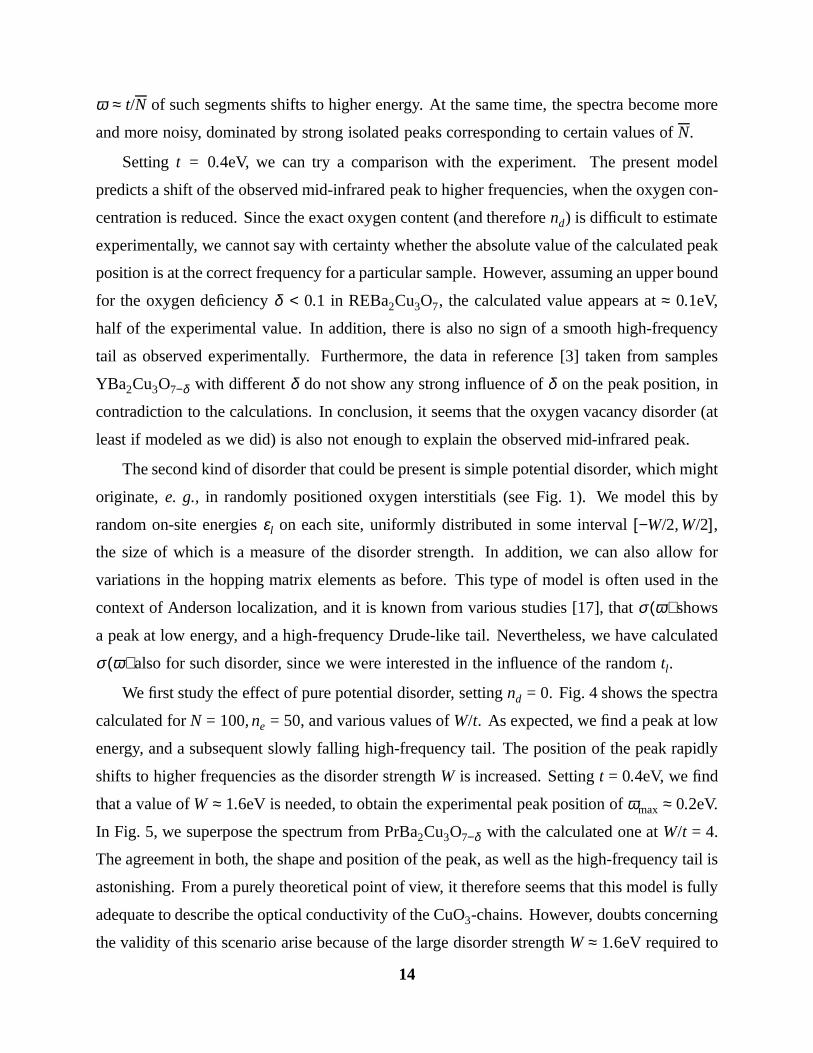
Figure 5: A comparison of the experimental spec-

trum obtained in Ref. [1] with the curve calculated

using the model with pure potential disorder, and dis-

order strength W/t = 4.

15

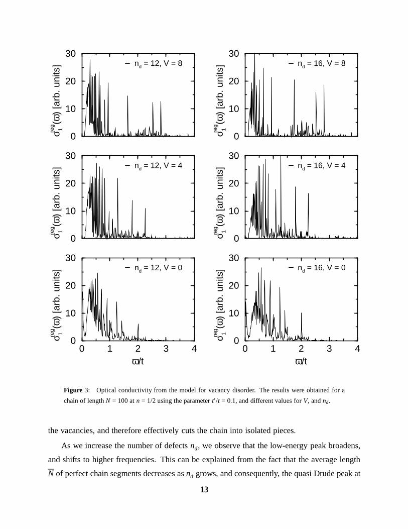
ω ≈ t/N of such segments shifts to higher energy. At the same time, the spectra become more

and more noisy, dominated by strong isolated peaks corresponding to certain values of N.

Setting t = 0.4eV, we can try a comparison with the experiment. The present model

predicts a shift of the observed mid-infrared peak to higher frequencies, when the oxygen con-

centration is reduced. Since the exact oxygen content (and therefore nd) is difficult to estimate

experimentally, we cannot say with certainty whether the absolute value of the calculated peak

position is at the correct frequency for a particular sample. However, assuming an upper bound

for the oxygen deficiency δ < 0.1 in REBa2Cu3O7, the calculated value appears at ≈ 0.1eV,

half of the experimental value. In addition, there is also no sign of a smooth high-frequency

tail as observed experimentally. Furthermore, the data in reference [3] taken from samples

YBa2Cu3O7−δ with different δ do not show any strong influence of δ on the peak position, in

contradiction to the calculations. In conclusion, it seems that the oxygen vacancy disorder (at

least if modeled as we did) is also not enough to explain the observed mid-infrared peak.

The second kind of disorder that could be present is simple potential disorder, which might

originate, e. g., in randomly positioned oxygen interstitials (see Fig. 1). We model this by

random on-site energies εl on each site, uniformly distributed in some interval [−W/2, W/2],

the size of which is a measure of the disorder strength. In addition, we can also allow for

variations in the hopping matrix elements as before. This type of model is often used in the

context of Anderson localization, and it is known from various studies [17], that σ (ω) shows

a peak at low energy, and a high-frequency Drude-like tail. Nevertheless, we have calculated

σ (ω) also for such disorder, since we were interested in the influence of the random tl.

We first study the effect of pure potential disorder, setting nd = 0. Fig. 4 shows the spectra

calculated for N = 100, ne = 50, and various values of W/t. As expected, we find a peak at low

energy, and a subsequent slowly falling high-frequency tail. The position of the peak rapidly

shifts to higher frequencies as the disorder strength W is increased. Setting t = 0.4eV, we find

that a value of W ≈ 1.6eV is needed, to obtain the experimental peak position of ωmax ≈ 0.2eV.

In Fig. 5, we superpose the spectrum from PrBa2Cu3O7−δ with the calculated one at W/t = 4.

The agreement in both, the shape and position of the peak, as well as the high-frequency tail is

astonishing. From a purely theoretical point of view, it therefore seems that this model is fully

adequate to describe the optical conductivity of the CuO3-chains. However, doubts concerning

the validity of this scenario arise because of the large disorder strength W ≈ 1.6eV required to

14

0 1 2 3 4ω/t

0

10

20

30

σ 1reg (ω

) [a

rb. u

nits

] nd = 12, V = 0

0

10

20

30

σ 1reg (ω

) [a

rb. u

nits

] nd = 12, V = 4

0

10

20

30σ 1re

g (ω)

[arb

. uni

ts] nd = 12, V = 8

0 1 2 3 4ω/t

0

10

20

30

σ 1reg (ω

) [a

rb. u

nits

] nd = 16, V = 0

0

10

20

30

σ 1reg (ω

) [a

rb. u

nits

] nd = 16, V = 4

0

10

20

30

σ 1reg (ω

) [a

rb. u

nits

] nd = 16, V = 8

Figure 3: Optical conductivity from the model for vacancy disorder. The results were obtained for a

chain of length N = 100 at n = 1/2 using the parameter t0/t = 0.1, and different values for V, and nd.

the vacancies, and therefore effectively cuts the chain into isolated pieces.

As we increase the number of defects nd, we observe that the low-energy peak broadens,

and shifts to higher frequencies. This can be explained from the fact that the average length

N of perfect chain segments decreases as nd grows, and consequently, the quasi Drude peak at

13

0 1 2 3 4ω/t

0

20

40

60

σ 1reg (ω

) [a

rb. u

nits

] nd = 4, V = 0

0

20

40

60

σ 1reg (ω

) [a

rb. u

nits

] nd = 4, V = 4

0

20

40

60σ 1re

g (ω)

[arb

. uni

ts] nd = 4, V = 8

0 1 2 3 4ω/t

0

10

20

30

σ 1reg (ω

) [a

rb. u

nits

] nd = 8, V = 0

0

10

20

30

σ 1reg (ω

) [a

rb. u

nits

] nd = 8, V = 4

0

10

20

30

σ 1reg (ω

) [a

rb. u

nits

] nd = 8, V = 8

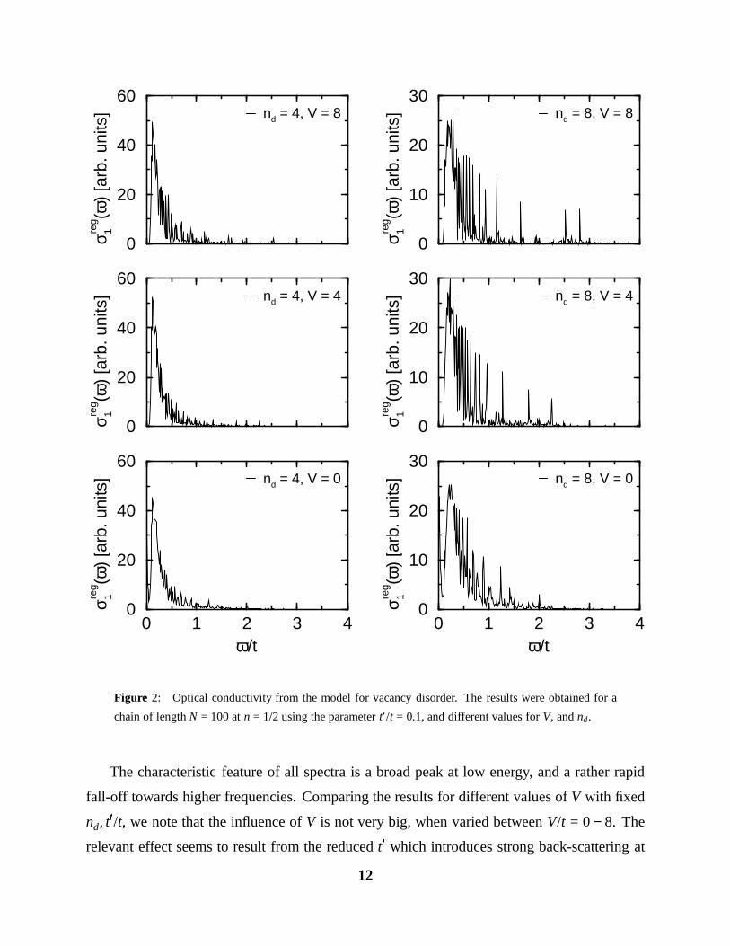
Figure 2: Optical conductivity from the model for vacancy disorder. The results were obtained for a

chain of length N = 100 at n = 1/2 using the parameter t0/t = 0.1, and different values for V, and nd.

The characteristic feature of all spectra is a broad peak at low energy, and a rather rapid

fall-off towards higher frequencies. Comparing the results for different values of V with fixed

nd, t0/t, we note that the influence of V is not very big, when varied between V/t = 0 − 8. The

relevant effect seems to result from the reduced t0 which introduces strong back-scattering at

12

with

eαrs =X

l

tl (αlrαl+1,s − αl+1,rαls). (16)

With the help of Eq. (15) it becomes very easy to calculate σ (ω) at T = 0, since jx creates only

single particle-hole excitations above the ground state, and hence σ reg1 (ω) can be written as

σ reg1 (ω) =

πe2

N

X

s ≤ ne,r > ne

j

eαrsj2

eεr − eεsδ [ω − (eεr − eεs)]. (17)

In all of the calculations of this section, we shall use open boundary conditions. Consequently,

the Drude weight must vanish (more precisely, it is shifted to a delta peak at a frequency of

the order t/N), and the entire spectral weight appears at finite frequencies. However, for chain

lengths N & 100, one has essentially reached the thermodynamic limit for the shape of σ reg1 (ω)

at frequencies ω t/N, in which we are interested here.

A realistic model for a situation where the oxygen vacancies are the dominant source of

disorder (as seems to be the case for the CuO3-chains) can be constructed by an appropriate

choice of the coefficients εl, tl: For a single vacancy between Cu sites l and l + 1, we assume

a strongly reduced hopping matrix element t0/t 1, and in addition, a screened Coulomb

potential which we can model, e. g., by a repulsive εl, εl+1 = V > 0 possibly extending to the

neighbouring sites l+2, l−1, etc. with an exponential tail. According to the oxygen deficiency

in REBa2Cu3O7−δ , we can then assume a certain concentration δ = nd/N of such defects (nd

the total number of defects), and distribute them randomly.

In Figs. 2, 3, we show the spectra for a chain of length N = 100 with t0/t = 0.1, and different

values of V, and nd. A length of N = 100 is sufficient, since we are not interested in the very

low frequency behaviour. We compared the results for chain lengths of 100, 200, and 400,

and found no significant difference at frequencies ω & t/50. The precise value of t0/t does not

affect the shape of the spectra as long as t0/t 1 (which is the physically relevant region). In

these calculations, we used a potential which extends to the three sites neighbouring a vacancy

falling off exponentially with a screening length equal to the lattice constant.

We always used a band filling of n := ne/N = 0.5, in accordance with the experimentally

estimated value mentioned in the introduction. Each curve represents the average over 1000

samples of the disorder, and for clarity of presentation, we introduced a smoothening of the

delta functions by averaging the points over small frequency intervals typically of size t/200.

11

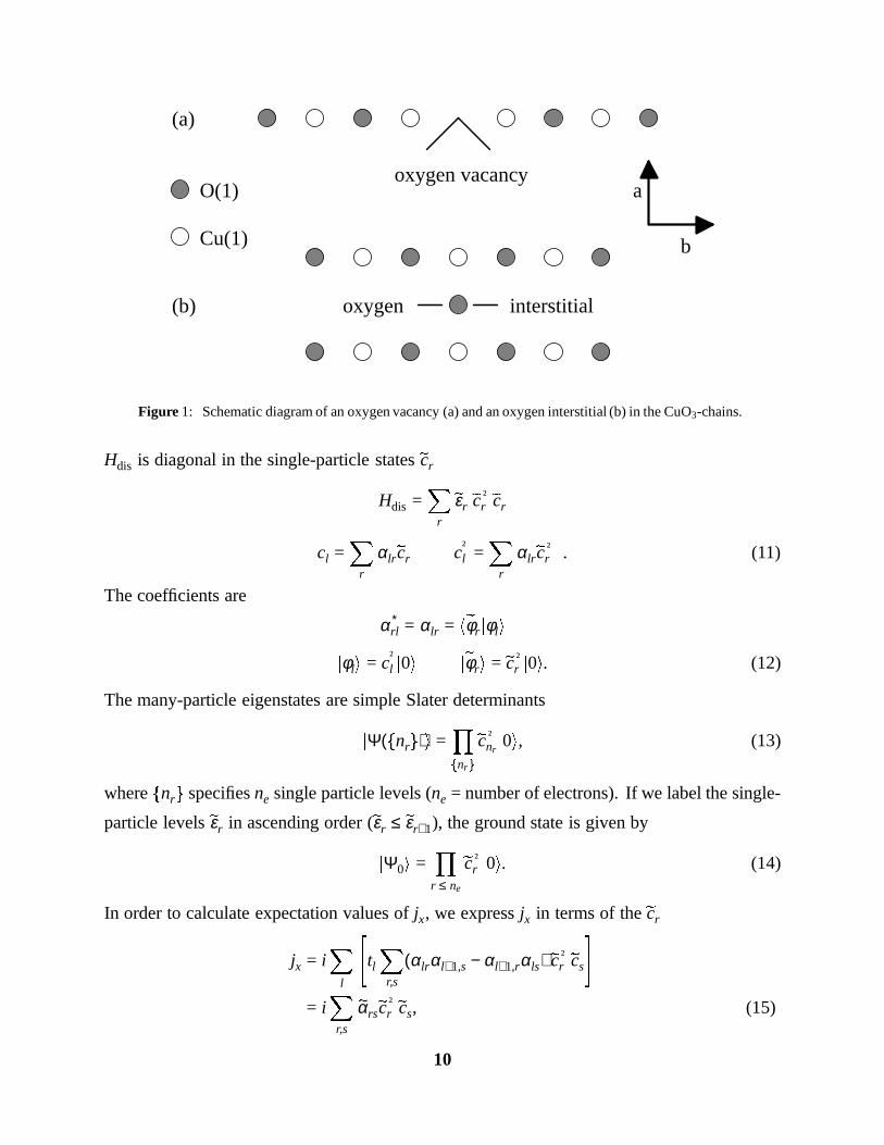
(a)

(b) interstitial

oxygen vacancy

oxygen

Cu(1)

O(1) a

b

Figure 1: Schematic diagram of an oxygen vacancy (a) and an oxygen interstitial (b) in the CuO3-chains.

Hdis is diagonal in the single-particle states ecr

Hdis =X

r

eεr ec†r ecr

cl =X

r

αlrecr c†l =X

r

αlrec†r . (11)

The coefficients are

α∗rl = αlr = h

eφrjφli

jφli = c†l j0i j

eφri = ec †r j0i. (12)

The many-particle eigenstates are simple Slater determinants

jΨ(fnrg)i =Y

fnrg

ec †nrj0i, (13)

where fnrg specifies ne single particle levels (ne = number of electrons). If we label the single-

particle levels eεr in ascending order (eεr ≤ eεr+1), the ground state is given by

jΨ0i =Y

r ≤ ne

ec †r j0i. (14)

In order to calculate expectation values of jx, we express jx in terms of the ecr

jx = iX

l

"

tlX

r,s

(αlrαl+1,s − αl+1,rαls) ec†r ecs

#

= iX

r,s

eαrsec†r ecs, (15)

10

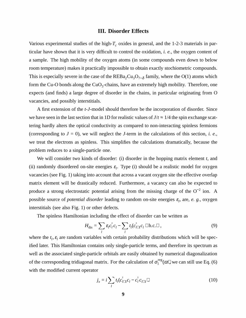
III. Disorder Effects

Various experimental studies of the high-Tc oxides in general, and the 1-2-3 materials in par-

ticular have shown that it is very difficult to control the oxidation, i. e., the oxygen content of

a sample. The high mobility of the oxygen atoms (in some compounds even down to below

room temperature) makes it practically impossible to obtain exactly stochiometric compounds.

This is especially severe in the case of the REBa2Cu3O7−δ family, where the O(1) atoms which

form the Cu-O bonds along the CuO3-chains, have an extremely high mobility. Therefore, one

expects (and finds) a large degree of disorder in the chains, in particular originating from O

vacancies, and possibly interstitials.

A first extension of the t-J-model should therefore be the incorporation of disorder. Since

we have seen in the last section that in 1D for realistic values of J/t ≈ 1/4 the spin exchange scat-

tering hardly alters the optical conductivity as compared to non-interacting spinless fermions

(corresponding to J = 0), we will neglect the J-term in the calculations of this section, i. e.,

we treat the electrons as spinless. This simplifies the calculations dramatically, because the

problem reduces to a single-particle one.

We will consider two kinds of disorder: (i) disorder in the hopping matrix element t, and

(ii) randomly disordered on-site energies εl. Type (i) should be a realistic model for oxygen

vacancies (see Fig. 1) taking into account that across a vacant oxygen site the effective overlap

matrix element will be drastically reduced. Furthermore, a vacancy can also be expected to

produce a strong electrostatic potential arising from the missing charge of the O−2 ion. A

possible source of potential disorder leading to random on-site energies εl, are, e. g., oxygen

interstitials (see also Fig. 1) or other defects.

The spinless Hamiltonian including the effect of disorder can be written as

Hdis =X

l

εlc†l cl −

X

l

tl(c†l+1cl + h.c.) , (9)

where the tl, εl are random variables with certain probability distributions which will be spec-

ified later. This Hamiltonian contains only single-particle terms, and therefore its spectrum as

well as the associated single-particle orbitals are easily obtained by numerical diagonalization

of the corresponding tridiagonal matrix. For the calculation of σ reg1 (ω), we can still use Eq. (6)

with the modified current operator

jx = iX

l

tl(c†l+1cl − c†

l cl+1). (10)

9

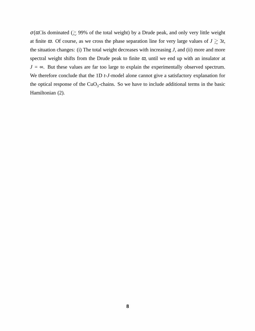
σ (ω) is dominated (& 99% of the total weight) by a Drude peak, and only very little weight

at finite ω. Of course, as we cross the phase separation line for very large values of J & 3t,

the situation changes: (i) The total weight decreases with increasing J, and (ii) more and more

spectral weight shifts from the Drude peak to finite ω, until we end up with an insulator at

J = ∞. But these values are far too large to explain the experimentally observed spectrum.

We therefore conclude that the 1D t-J-model alone cannot give a satisfactory explanation for

the optical response of the CuO3-chains. So we have to include additional terms in the basic

Hamiltonian (2).

8

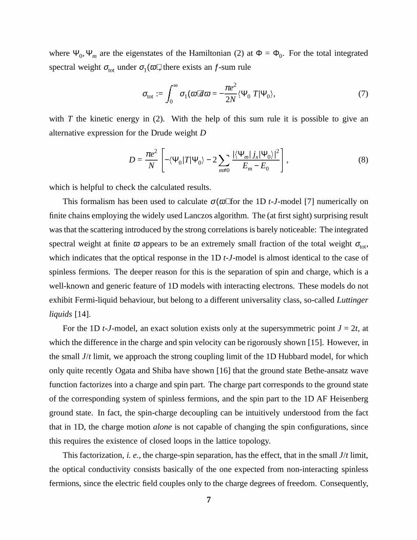
where Ψ0, Ψm are the eigenstates of the Hamiltonian (2) at Φ = Φ0. For the total integrated

spectral weight σtot under σ1(ω), there exists an ƒ-sum rule

σtot :=Z ∞

0σ1(ω)dω = −

πe2

2NhΨ0jTjΨ0i, (7)

with T the kinetic energy in (2). With the help of this sum rule it is possible to give an

alternative expression for the Drude weight D

D =πe2

N

"

−hΨ0jTjΨ0i − 2X

m≠0

jhΨmj jxjΨ0ij2

Em − E0

#

, (8)

which is helpful to check the calculated results.

This formalism has been used to calculate σ (ω) for the 1D t-J-model [7] numerically on

finite chains employing the widely used Lanczos algorithm. The (at first sight) surprising result

was that the scattering introduced by the strong correlations is barely noticeable: The integrated

spectral weight at finite ω appears to be an extremely small fraction of the total weight σtot,

which indicates that the optical response in the 1D t-J-model is almost identical to the case of

spinless fermions. The deeper reason for this is the separation of spin and charge, which is a

well-known and generic feature of 1D models with interacting electrons. These models do not

exhibit Fermi-liquid behaviour, but belong to a different universality class, so-called Luttinger

liquids [14].

For the 1D t-J-model, an exact solution exists only at the supersymmetric point J = 2t, at

which the difference in the charge and spin velocity can be rigorously shown [15]. However, in

the small J/t limit, we approach the strong coupling limit of the 1D Hubbard model, for which

only quite recently Ogata and Shiba have shown [16] that the ground state Bethe-ansatz wave

function factorizes into a charge and spin part. The charge part corresponds to the ground state

of the corresponding system of spinless fermions, and the spin part to the 1D AF Heisenberg

ground state. In fact, the spin-charge decoupling can be intuitively understood from the fact

that in 1D, the charge motion alone is not capable of changing the spin configurations, since

this requires the existence of closed loops in the lattice topology.

This factorization, i. e., the charge-spin separation, has the effect, that in the small J/t limit,

the optical conductivity consists basically of the one expected from non-interacting spinless

fermions, since the electric field couples only to the charge degrees of freedom. Consequently,

7

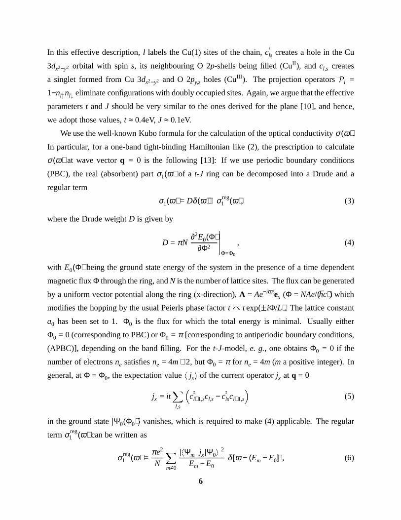
In this effective description, l labels the Cu(1) sites of the chain, c†ls creates a hole in the Cu

3dx2−y2 orbital with spin s, its neighbouring O 2p-shells being filled (CuII), and cl,s creates

a singlet formed from Cu 3dx2−y2 and O 2py,z holes (CuIII). The projection operators Pl =

1−nl"nl# eliminate configurations with doubly occupied sites. Again, we argue that the effective

parameters t and J should be very similar to the ones derived for the plane [10], and hence,

we adopt those values, t ≈ 0.4eV, J ≈ 0.1eV.

We use the well-known Kubo formula for the calculation of the optical conductivity σ (ω).

In particular, for a one-band tight-binding Hamiltonian like (2), the prescription to calculate

σ (ω) at wave vector q = 0 is the following [13]: If we use periodic boundary conditions

(PBC), the real (absorbent) part σ1(ω) of a t-J ring can be decomposed into a Drude and a

regular term

σ1(ω) = Dδ (ω) + σ reg1 (ω), (3)

where the Drude weight D is given by

D = πN∂2E0(Φ)

∂Φ2

Φ=Φ0

, (4)

with E0(Φ) being the ground state energy of the system in the presence of a time dependent

magnetic flux Φ through the ring, and N is the number of lattice sites. The flux can be generated

by a uniform vector potential along the ring (x-direction), A = Ae−iω tex (Φ = NAe/(hc)) which

modifies the hopping by the usual Peierls phase factor ty t exp(iΦ/L). The lattice constant

a0 has been set to 1. Φ0 is the flux for which the total energy is minimal. Usually either

Φ0 = 0 (corresponding to PBC) or Φ0 = π [corresponding to antiperiodic boundary conditions,

(APBC)], depending on the band filling. For the t-J-model, e. g., one obtains Φ0 = 0 if the

number of electrons ne satisfies ne = 4m + 2, but Φ0 = π for ne = 4m (m a positive integer). In

general, at Φ = Φ0, the expectation value h jxi of the current operator jx at q = 0

jx = itX

l,s

c†l+1,scl,s − c†

lscl+1,s

(5)

in the ground state jΨ0(Φ0)i vanishes, which is required to make (4) applicable. The regular

term σ reg1 (ω) can be written as

σ reg1 (ω) =

πe2

N

X

m≠0

jhΨmj jxjΨ0ij2

Em − E0δ [ω − (Em − E0)], (6)

6

II. The Electronic Structure of CuO3-chains

When trying to construct a model for the electronic structure of the CuO3-chains, the first thing

one should note is the fact that the chain Cu(1) site has the same four-fold oxygen coordination

as the planar Cu(2,3) (neglecting the buckling of the O(2,3) atoms out of the plane). Therefore,

we can expect a similar Cu-O bonding pattern in both cases. This is confirmed by band-

structure calculations for YBa2Cu3O7−δ [8], which apart from the common strongly dispersive

planar CuO pdσ -band also find a chain-band crossing the Fermi energy EF. This band is

formed from an antibonding pdσ combination of O(1)2py-Cu(1)3dz2−y2-O(4)2pz orbitals, and

shows a dispersion similar to the planar band, but only along the chain axis.

Regarding the similarity between planes and chains, it seems reasonable to try a description

of the electronic structure by the 1D analog of the Emery model [9]

HEm =X

ijs

εij c†iscjs +

X

i

Ui c†i"ci"c†

i#ci#, (1)

where i, j label the Cu(1) and O(1,4) sites, the operators c†is create 3dx2−y2-Cu and 2py,z-O holes,

and s is the spin index. The εij include the usual on-site energies εd = 0 (by convention), εp

= 3.6 (which we assume to be the same for O(1,4)), and the nearest neighbour (n.n) hopping

integrals tpd = 1.3, tpp = 0.65 (all values in eV). The cited values correspond to the ones found

for the plane [10], which, regarding the above mentioned similarities, and the similar CuO

bond lengths, also seem realistic for the chains. Further justification for the use of these values

comes from measurements of the optical gap in the compound Ca2CuO3 [11], in which one

finds the same CuO3-chains with a CuII oxidation state, i. e., in the insulating charge-transfer

regime. The observed value of the optical gap is ≈ 2eV, which agrees well with the values

found in the planar antiferromagnetic charge-transfer insulators like YBa2Cu3O6, and therefore

suggests a similar value of εp − εd.

In the light of this, it seems appropriate to apply the same procedure, as for the CuO2-

planes [12], to derive an effective low-energy Hamiltonian from (1), which consists of a single,

strongly correlated tight-binding band (projected on the subspace of singly occupied sites), and

a nearest-neighbour antiferromagnetic exchange interaction, i. e., the 1D t-J-model

Heff = −tX

l,s

Pl c†lscl+1,sPl+1 + J

X

l,s

Sl ⋅ Sl+1 −14

nlnl+1

. (2)

5

rather strongly coupled to the electrons. Using the t-J-model as the effective electronic model,

we will show that this coupling can be included in the form of a Holstein term, in which

the local ionic displacement couples linearly to the local charge. Employing a variational

approximation for the phonon Hilbert space, we calculate σ (ω) for finite systems using the

Lanczos technique. The effect of the vacancy disorder can be incorporated by the choice of

open boundary conditions.

Finally, we will discuss the results of our different approaches in the light of the experi-

mental data, and also suggest possible experimental tests of the different mechanisms.

4

tail falls off much slower than the simple Drude formula (σ ∼ 1/ω2 at high frequency) would

suggest. At energies below 0.2eV, there seems to be a difference between the two compounds:

while in YBa2Cu3O7−δ , the conductivity joins onto a Drude-peak above Tc,1 in PrBa2Cu3O7−δ

it drops sharply to zero, reflecting the insulating nature of the latter compound. Note, that in

the Pr-compound, this behaviour of the conductivity has important implications for possible

mechanisms explaining the observed Tc-suppression[6]. The above described shape of σch(ω)

clearly indicates that the electronic structure of the chains is non-trivial, and it stimulated our

interest to find a possible explanation.

In this article, we offer two likely mechanisms which could lead to the observed σch(ω): (i)

the presence of very strong potential disorder, and (ii) moderately strong polaronic electron-

phonon (e-ph) interactions, possibly combined with the effect of vacancy disorder. While

the first explanation gives a better (in fact excellent) fit to the experimental data, the second

one seems to be more reasonable from a physical point of view, since, as we shall show, the

potential disorder strength needed to obtain agreement with the experimental data is hard to

justify.

The plan of this paper is as follows: First we shall identify the one-dimensional (1D) t-J-

model to be a good starting point for the description of the electronic structure of the CuO3-

chains. However, as is well known by now from various studies, the optical conductivity of

the 1D t-J-model is more or less identical to that of spinless fermions (as long as J is below the

threshold for phase separation) because of charge-spin separation. There is barely any spectral

weight at finite frequencies [7]. Thus, one is forced to include other interaction terms in the

Hamiltonian, which could possibly reproduce the experimentally observed strong scattering.

We continue with a simple extension of the model by including the disorder from oxygen

vacancies on the bridging O(1) site. This is expected to be the main source of disorder in the 1-

2-3 materials. It is mainly due to the large mobility of the oxygen atoms at higher temperatures.

Such vacancies can be modeled by interrupted 1D t-J chains, but we will show that such a

scenario cannot reproduce the observed σch(ω). However, as mentioned above, the inclusion

of strong potential disorder turns out to yield an excellent fit to the experiment.

As an alternative explanation, we then consider moderately strong e-ph interactions. We

suggest that the apical oxygen mode with a displacement in the c-direction is likely to be

1This point is still somewhat controversial. More recent reflectivity measurements of YBa2Cu3O7−δ down to lowerfrequencies [5], indicated that even above Tc there is no upturn in the conductivity as the dc limit is approached.

3

I. Introduction

The 1-2-3 family of high-Tc oxides with its most prominent member YBa2Cu3O7−δ is the

only example of the new superconductors which in addition to the common CuO2 planes also

contains one-dimensional CuO3-chains contributing to the electronic density of states at the

Fermi level.1 At the same time, this class of compounds is the best characterized among

the high-Tc materials, and furthermore, many of the technological applications are based on

YBa2Cu3O7−δ . However, in the interpretation of many experimental data, it is not obvious

how the features of the chains can be separated from those of the planes. The latter are known

to drive the superconductivity in all high-Tc compounds, and are therefore of primary interest.

Only recently, with the availability of single-domain crystals, a clearer picture of the interplay

between chains and planes has emerged. In any case, for a complete understanding of the

properties of the 1-2-3 compounds, it is absolutely necessary to distinguish, and where possible

isolate the features of the CuO3-chains.

One of the physical quantities which contains valuable information about the electronic

structure of a system is the optical conductivity σ (ω). Its frequency dependence is determined

by both, the character of the ground state, as well as (in principle) all the excited states.

Experimentally, σ (ω) can be determined quite easily, e. g., from reflectivity measurements

by applying a Kramers-Kronig transformation.

The synthesis of detwinned YBa2Cu3O7−δ , and PrBa2Cu3O7−δ crystals made it possible

to extract the anisotropy of σ (ω) in the crystallographic a- (perpendicular), and b-direction

(parallel to the chains), by polarizing the electric field E in one or the other direction. This

revealed an interesting and important property of these compounds, namely that σb(ω) (with

E k b) shows a strongly enhanced spectral weight compared to σa(ω) especially in the infrared

region (ω . 1.5eV). A procedure which suggests itself is then to subtract σa(ω) from σb(ω),

and to associate the corresponding oscillator strength with the CuO3-chains, the main source

of anisotropy in these materials.

In all published data (Ref.[1] for PrBa2Cu3O7−δ , and Ref.[2, 3, 4] for YBa2Cu3O7−δ ),

these difference spectra σch(ω) := σb(ω) - σa(ω) show a characteristic broad mid-infrared peak

centered around 0.2eV, and a slowly falling high-frequency tail extending beyond 1eV. This

1In fact, this statement is not quite correct. There exists a slight variation of these materials, the so-called 1-2-4compounds, with its prototype YBa2Cu4O8. They contain one-dimensional CuO3 double-chains, which also providestates at the Fermi level.

2

cond

-mat

/931

2058

14

Dec

93

ETH-TH/93-31

Conductivity of CuO3-Chains:

Disorder versus Electron-Phonon Coupling

R. Fehrenbacher

Theoretische Physik, ETH-Honggerberg, CH-8093 Zurich, Switzerland1

(Received )

Abstract. The optical conductivity of the CuO3-chains, a subsystem of the 1-2-3 materials, is dominated

by a broad peak in the mid-infrared (ω ≈ 0.2eV), and a slowly falling high-frequency tail. The 1D t-

J-model is proposed as the relevant low-energy Hamiltonian describing the intrinsic electronic structure

of the CuO3-chains. However, due to charge-spin decoupling, this model alone cannot reproduce the

observed σ (ω). We consider two additional scattering mechanisms: (i) Disregarding the not so crucial spin

degrees of freedom, the inclusion of strong potential disorder yields excellent agreement with experiment,

but suffers from the unreasonable value of the disorder strength necessary for the fit. (ii) Moderately

strong polaronic electron-phonon coupling to the mode involving Cu(1)-O(4) stretching, can be modeled

within a 1D Holstein Hamiltonian of spinless fermions. Using a variational approximation for the phonon

Hilbert space, we diagonalize the Hamiltonian exactly on finite lattices. As a result of the experimental

hole density ≈ 1/2, the chains can exhibit strong charge-density-wave (CDW) correlations, driven by

phonon-mediated polaron-polaron interactions. In the vicinity of half filling, charge motion is identified

as arising from moving domain walls, i. e., defects in the CDW. Incorporating the effect of vacancy

disorder by choosing open boundary conditions, good agreement with the experimental spectra is found.

In particular, a high-frequency tail arises as a consequence of the polaron-polaron interactions.

PACS Numbers: 71.38, 71.45.L, 74.25, 74.72, 78.30, 78.30.L

1New Address: Science and Technology Center for Superconductivity, Materials Science Division, Argonne NationalLaboratory, 9700 South Cass Avenue, Argonne, Illinois 60439