Embed Size (px)
Citation preview

13-16 septembre, 2005, Nancy, France
Organisées durant l'école d'été temps réel 2005 ETR'05http://etr05.loria.fr
ACTES
http://rjcitr05.loria.fr
RJCITR'051ères Rencontres Jeunes Chercheurs en Informatique Temps Réel


PREFACE
Parallèlement à l'école d'été temps réel ETR'05, les premières rencontres des jeunes chercheurs en informatique temps réel (RJCITR'05) sont organisées. Cet événement est une excellente occasion pour nous, les jeunes chercheurs, de présenter nos travaux à la communauté temps réel, de favoriser l'échange d'idées, d'expériences, d'information entre chercheurs dans le domaine de l'informatique temps réel ; et ainsi de connaître le point de vue des participants à ETR 2005 sur nos travaux. Les thèmes abordés par les jeunes chercheurs durant ces rencontres seront les suivants:
• approche par composants, • évaluation, validation, vérification d’applications et de systèmes temps réel, • ordonnancement temps réel, • pires temps d’exécution et conception faible consommation d’énergie.
Nous voudrions adresser nos remerciements les plus sincères au comité local d'organisation de l' ETR'05 qui a rendu possible l'organisation de ces rencontres et ainsi offert l'opportunité aux doctorants de présenter leurs travaux.
Bienvenue aux rencontres des jeunes chercheurs en informatique temps réel 2005.
Mathieu Grenier
Doctorant au LORIA
Pour les comités d'organisation et de programme de RJCITR'05

COMITE DE PROGRAMME ET D’ORGANISATION
• Frédéric Ridouard – Laboratoire d'Informatique Scientifique et Industrielle - Lyon • Gaëlle Largeteau - Laboratoire d'Informatique Scientifique et Industrielle - Lyon • Jean-Philippe Georges – Centre de Recherches en Automatique de Nancy - Nancy • Jérome Hugues – Ecole Nationale Supérieur des Télécommunication - Paris • Karen Godary – Institut Nationale des Sciences Appliquées - Lyon • Mathieu Grenier – Laboratoire Lorrain de Recherche en Informatique et ses Applications
- Nancy • Morgan Magnin - Institut de Recherche en Communications et Cybernétique de Nantes –
Nantes. • Mohamed Khalgui – Laboratoire Lorrain de Recherche en Informatique et ses
Applications - Nancy • Ning Jia – Laboratoire Lorrain de Recherche en Informatique et ses Applications - Nancy • Olfa Mosbahi - Laboratoire Lorrain de Recherche en Informatique et ses Applications -
Nancy
COMITE LOCAL D’ORGANISATION
• Mathieu Grenier – Laboratoire Lorrain de Recherche en Informatique et ses Applications - Nancy
• Mohamed Khalgui – Laboratoire Lorrain de Recherche en Informatique et ses Applications - Nancy
• Ning Jia – Laboratoire Lorrain de Recherche en Informatique et ses Applications - Nancy
TABLE DES MATIERES
THEME 1 - APPROCHE PAR COMPOSANTS
Exploitation du Raffinement pour Vérifier les Modèles Hiérarchiques. M. Al Achhab, A. Hammad et H. Mountassir. --------------------------------------------------------------------------------------------------------------------- 9
Utilisation de l'Approche par Composants pour la Conception d'Applications Temps Réel. J.-P. Etienne et S. Bouzefrane. ---------------------------------------------------------------------------------------------------------------- 13
System Dependability Evaluation using AADL. A.-E. Rugina.----------------------------------------------------- 17
THEME 2 - EVALUATION, VALIDATION, VERIFICATION D’APPLICATIONS ET DE SYSTEMES TEMPS REEL
Evaluation Formelle de la Qualité de Service pour les Systèmes d'Acquisition. B. Ben Hedia, F. Jumel et J.-P. Babau. ------------------------------------------------------------------------------------------------------------------- 23
Evaluation of Real-Time Capabilities of Ethernet-based Automation Systems using Formal Verification and Simulation. G. Marsal, D. Witch, B. Denis, Faure J.-M. et G. Frey.----------------------------------------- 27
Utilisation Conjointe de B et TLA+ pour la Modélisation et la Vérification des Systèmes Réactifs. O. Mosbahi.----------------------------------------------------------------------------------------------------------------------- 31
Statistical Study of Firm Real-Time Transactions Behavior. S. Semghouni, L. Amanton, B. Sadeg et A. Berred.------------------------------------------------------------------------------------------------------------------------- 35
THEME 3 - ORDONNANCEMENT TEMPS REEL
Quantification de l'Ordonnançabilité des Systèmes Temps Réel à Contraintes Strictes par l'Analyse Markovienne. B. Chauvière et D. Geniet.------------------------------------------------------------------------------- 41
New On-Line Preemptive Scheduling Policies for Improving Real-Time Behavior. M. Grenier. ----------- 45
Temporal Validation of an IEC 61499 Control Application. M. Khalgui. --------------------------------------- 49
Impact de l'Ordonnancement Temps Réel de Tâches d'un Superviseur de Ligne d'Assemblage. L. Plassart, F. Singhoff, P. Le Parc et L. Marcé.-------------------------------------------------------------------------- 53
THEME 4 - PIRES TEMPS D’EXECUTION ET CONCEPTION FAIBLE CONSOMMATION D’ENERGIE
Calcul de Temps d'Exécution au Pire Cas pour Code Mobile. N. Bel Hadj Aissa et G. Grimaud.---------- 59
Safe Measurement-Based WCET Estimation. J.-F. Deverge et I. Puaut. ---------------------------------------- 63
Application Coopérative et Gestion de l'Energie du Processeur. R. Urunuela. --------------------------------- 67

Thème 1
Approche par Composants


Exploitation du Raffinement pour Vérifier les Modèles Hiérarchiques
Mohammed Al AchhabLaboratoire d’Informatique
de l’Université de Franche-Comté16, route de Gray 25030 Besançon Cedex
Ahmed Hammad, Hassan MountassirLaboratoire d’Informatique
de l’Université de Franche-Comté16, route de Gray 25030 Besançon Cedex{hammad, mountass}@lifc.univ-fcomte.fr
Résumé
Cet article traite de la spécification et de la vérificationpar model-checking des systèmes hiérarchiques réactifs.Le modèle utilisé est celui des automates hiérarchiquesdans lesquels nous exploitons la décomposition d’un étaten un ensemble d’automates. Pour pallier au problème del’explosion combinatoire du nombre d’états induit par lemodel-checking, nous proposons d’utiliser la technique duraffinement. La contribution de ce papier est de définir lesconditions de raffinement entre automates hiérarchiquesavec cycles.
1. Motivations et problématique
Ces dernières années, la vérification des systèmes in-formatiques critiques est devenue un sujet de rechercheimportant en raison du développement croissant de logi-ciels appliqués à la médecine, aux moyens de transportsou aux centrales nucléaires. Dans ces domaines, une er-reur de programmation peut coûter très cher financière-ment ou en vies humaines. Il convient donc, lors du dé-veloppement de telles applications, de s’assurer qu’ellessatisfont un certain nombre de propriétés, notammentdes propriétés de sûreté (comme l’absence de défaillancegrave).
Notre travail s’articule autour de la spécification et lavérification de systèmes hiérarchique réactifs. Grâce à lapopularité grandissante de StateCharts [6] et d’UnifiedModeling Language (UML) [5], la modélisation hiérar-chique devient quasiment incontournable pour les déve-loppements logiciels industriels. Cette modélisation pos-sède, en outre, des concepts puissants tels que le raffine-ment d’états, des transitions qui ont plusieurs états de dé-part et plusieurs états d’arrivée (Interlevel Transitions), lapriorité entre les transitions et l’exécution simultanée destransitions. Ces concepts rendent difficile l’utilisation di-recte de méthodes formelles.
Dans [10], les auteurs ont proposé une sémantique opé-rationnelle de StateCharts, ce sont les automates hiérar-chiques qui couvrent le raffinement d’états, la prioritéentre les transitions et l’exécution simultanée de transi-tions. Dans [11], les auteurs montrent comment les Sta-teCharts peuvent être traduits en Promela (le langage de
programmation de SPIN [7]) en utilisant les automateshiérarchiques comme format intermédiaire. Cette mé-thode est également employée pour la vérification des dia-grammes d’états transitions d’UML [8]. Les techniquesde vérification utilisées sont algorithmiques, en particulierle model-checking. Les propriétés sont exprimées à l’aided’une logique comme la LTL (Linear Temporal Logic)[9]. Le principal problème réside dans la complexité desprocédures de décision lors de la vérification de proprié-tés.
Nous proposons le raffinement d’automates hiérar-chiques comme solution pour vérifier les systèmes hiérar-chiques de grande taille. L’idée est d’introduire pas à pasdes détails supplémentaires sur le système en éclatant lesétats de base1 du système abstrait. Cette approche permetde décrire des spécifications abstraites de plus petite taillesur lesquelles on vérifie les propriétés exprimables au ni-veau des détails considérés. Puis le système est raffiné parintroduction de nouveaux détails sous forme de compo-sants qui peuvent être des automates ou un ensemble d’au-tomates parallèles. Cette démarche ne résout le problèmequ’à condition que l’opération de raffinement préserve surle système raffiné les propriétés vérifiées sur le systèmeabstrait. La notion de raffinement de systèmes de transi-tions, définies dans [4], issue de celle de raffinement desystèmes d’événements [1], préserve les propriétés de lo-gique temporelle linéaire. Donc, si une propriété LTL estvérifiée au niveau abstrait alors elle l’est également au ni-veau raffiné.
Dans [3], nous avons défini une relation de raffinemententre automates hiérarchiques, limités à des nouveaux au-tomates acycliques. Ce raffinement permet de préserverles propriétés LTL du niveau abstrait. L’hypothèse del’absence de cycles dans les nouveaux automates est trèsforte. La contribution de ce travail est de définir une re-lation de raffinement entre automates hiérarchiques aveccycles.
La suite de ce papier est organisée en trois sections.Dans la section deux, nous présentons les concepts debase : automate hiérarchique et structure de Kripke. Dansla section trois, nous définissons la relation de raffinement
1Nous appelons état de base l’état qui n’a pas une structure interne.
9

entre automates hiérarchiques et dans la section quatre,nous concluons et nous traçons quelques perspectives à cetravail.
2. Préliminaires
2.1. Automate séquentielSoit V un ensemble de variables d’états, chacune de
domaine fini. Soit APV l’ensemble des propositions ato-miques de la forme v = d, v ∈ V et d ∈ domaine(v).
Définition 1 Un automate A est un 5-uplet A =〈S, s0, Σ, →, L〉 où : S est un ensemble fini d’états,s0 ∈ S est l’état initial, Σ est un alphabet fini de nomsd’actions, →⊆ S ×Σ×S est l’ensemble des transitions,L : S → 2APV est l’interprétation des états de S sur V .
Une exécution σ de A est une séquence finie ou infiniedes états et des actions s0
a0→ · · ·ai→ si
ai→ . . . telle ques0 est l’état initial et pour chaque i ≥ 0, nous avons si
ai→si+1 ∈→. On note Exec(A) l’ensemble des exécutionsde l’automate A.
Soit σdef= s0
a1→ · · ·ai→ si
ai+1
→ . . . une exécution de
A. Nous appelons trace de σ, tr(σ)def= a0 . . . ai . . . , la
séquence d’actions, telle que tr(σ) ∈ Σω.On appelle cycle d’un automate A une séquence finie
d’états et d’actions cydef= s0
a0→ · · ·an−1
→ sn, telle quesn = s0, et pour chaque 0 ≤ i < n nous avons si
ai→si+1 ∈→.
2.2. Automate hiérarchiqueUn automate hiérarchique, notée AH , est un ensemble
d’automates qui sont liés entre eux par une fonction decomposition. La fonction de composition fait le lien entreun état s d’un automate séquentiel et un ensemble d’auto-mates.
Définition 2 AH est un trip-let 〈F, E, γ〉, où : F ={A1, . . . An} est un ensemble d’automates ayant un en-semble d’états distincts, E est un alphabet fini de nomsd’actions, γ :
⋃A∈F SA → 2F est une fonction de com-
position sur F telle que : (1) dans l’ensemble F il y aun seul automate racine Aracine, (2) chaque automateA ∈ F\{Aracine} a un état père et (3) la fonction decomposition ne doit pas contenir de cycle.
On considére l’exemple de TV-Set décrit dans la fi-gure 1. Au premier niveau d’observation le TV-Set peutêtre dans deux états : EnService et EnAttente (étatinitial). L’état EnAttente, qui est raffiné par l’automatePower, peut être aussi dans deux états : V eille (état ini-tial) et Deconnecte. L’automate hiérarchique, AH1 =〈F1, E1, γ1〉, qui modélise le fonctionnement de TV-Set,est composé de deux automates F1 = {TV, Power} quisont liés avec la fonction de composition γ1 = {s0 →{Power}} ∪ {s → ∅|s ∈ {s1, s2, s3}}.
On note χ l’application qui lie un état raffiné avec lesétats de l’automate fils. Nous définissons χ+ comme la
out in1AH
TV 0onoffout
1
Power
2 =Veille
3
ss
s
s
=EnService=EnAttente EtEt
Power
=DeconnectePower
FIG. 1. TV-Set au niveau abstrait
fermeture transitive non-réflexive, χ∗ comme la fermeturetransitive réflexive de χ et χ−1 est la fonction d’ancêtreoù : χ−1(s) = s′ si s ∈ χ(s′).
Soit St l’ensemble des états de l’automate hiérarchiqueAH . On note γ−∗ : St → F l’application qui constitue lelien entre un état s et son ancêtre A.
Dans l’automate hiérarchique AH1 de la figure 1 :χ(s0) = {s2, s3}, χ−1(s3) = {s0} et γ−∗(s3) = {TV }.
Soit AH = 〈F, E, γ〉 un automate hiérarchique, larestriction de la fonction de composition γ aux étatsd’un automate A ∈ F nous permet de définir le sous-automate hiérarchique AHA = 〈FA, EA, γA〉 telleque : FA = F\{Ai|SAi
∩ χ∗(SA) = ∅}, EA = E etγA = γ|χ∗(SA) (On considère A comme l’automateracine de AHA).
Définition 3 Soit AH un automate hiérarchique et soit St
l’ensemble des états de AH . C ⊆ St est une configura-tion2 de AH ssi : (1) l’automate racine participe par unseul état à la configuration et (2) la fermeture en bas :pour chaque état s dans C si s est raffiné par un automateA alors A participe aussi par un seul état à C.
L’étiquetage d’une transition t = s → s′ dans un au-tomate A ∈ F est défini par le triplet (sr, a, td) tel que :source(t) = s est la source de la transition, but(t) = s′
est l’état d’arrivée de la transition t, action(t) = a
est l’action de t, sr est employée pour déterminer dansquelles configurations t est activable, et td est employéepour déterminer les états d’arrivée de t.
Les transitions de l’automate hiérarchique AH1 sont
définies comme suit : (s0
{s2},on,∅→ s1), (s1
∅,off,{s2}→ s0)
et (s1
∅,out,{s3}→ s0).
Remarque 2.1 (Priorité entre les transitions) Nous com-mençons par exécuter les transitions de l’automate racine,puis les transitions des sous-automates sont effectuées siaucune transition n’est activable à partir de l’automatepère.
2Une configuration d’un automate hiérarchique permet de décritl’état global de système hiérarchique à un instant précis.
RJCITR 2005 10

2.3. Structure de KripkeDans cette section, nous décrivons la sémantique de
l’automate hiérarchique définie comme une structure deKripke. Cette présentation nous permet de vérifier les sys-tèmes hiérarchiques par le model-checking des systèmesréactifs à nombre d’états fini.
Soient AH = 〈F, E, γ〉 un automate hiérarchique, A
un automate dans F , C une configuration de AH et e
un ensemble d’actions dans E. On dit que la transition
ssr, a, td→ s′ de l’automate A est activable à partir de la
configuration C et sur l’ensemble e si C ∪ {s} ∈ sr eta ∈ e.
Définition 4 La sémantique de AH est une structure deKripke SK = 〈Conf, C0,→K , E, LK〉 où : Conf estl’ensemble des configurations de AH , C0 est la configura-tion initiale, E est l’ensemble d’actions, LK : Conf →2APV tel que LK(C) = ∪si∈CL(si) et →K⊆ Conf ×2E × Conf est la relation des transitions de SK.
Soit tdef= C
e→ C ′ une transition, t ∈→K ssi elle est
définie par une des trois règles suivantes :– Règle de progrès :
{s} = C ∩ SA
∃t ∈→A .(activable(C|e)(t)) ∧ t = (ssr,a,td→ s′)
A :: Ce→ ({s′} ∪ td)
– Règle de composition :{s} = C ∩ SA
∀t.(t ∈→A .(t = (ssr,a,td→ s′) ⇒ ¬activable(C|e)(t)))
γ(s) = {A1, . . . Am} 6= ∅A1 :: C
e→ C′
1
Am :: Ce→ C′
m
A :: Ce→ {{s} ∪ C′
1 ∪ · · · ∪ C′m}
– Règle de bégaiement :{s} = C ∩ SA Basic(s)
∀t ∈→A .(t = (ssr,a,td→ s′)) ⇒ ¬activable(C|e)(t)
A :: Ce→ {s}
La structure de Kripke associée à AH1 de la figure 1est représentée dans la figure 2.
C 0
0
on
off
C 1
1
out in
0 3C 2
SK1
out
s , s2 s
s , s
FIG. 2. SK1 associe AH1
3. Résultat : raffinement entre automates hié-rarchiques
Dans cette section, nous définissons les conditions deraffinement entre automates hiérarchiques. Le raffinementconsiste à éclater les états de base du système abstrait. Cesétats sont remplacés par un ou plusieurs automates. Ces
automates sont notés Aτ . Les transitions de Aτ sont dési-gnées par τ .
Nous définissons d’abord la relation d’invariant decollage sur (V1 et V2)3 et la relation de collage µ entreles états de système raffiné et ceux du système abstrait.
Définition 5 Un invariant de collage, notée I12, est unerelation entre les variables d’état du système abstrait (∈V1) et celles du système raffiné (∈ V2) définie par uneproposition de la forme suivante :
q ::= ap1 | ap2 |x1 = x2 | q ∧ q | ¬q
où : ap1 ∈ APV1, ap2 ∈ APV2
, x1 ∈ V1 et x2 ∈ V2.
Définition 6 La relation de collage entre les états deAH1 = 〈F1, E1, γ1〉 et AH2 = 〈F2, E2, γ2〉, notée µ,est une relation binaire µ ⊆ ∪A2∈F2
SA2× ∪A1∈F1
SA1
qui exprime le fait que les états sont collés si leurs pro-priétés d’états satisfont le collage. Autrement dit, les étatss2 ∈ ∪A2∈F2
SA2et s1 ∈ ∪A1∈F1
SA1sont collés par la
relation µ, notée s2 µ s1, ssi :0
@
^
ap2∈L2(s2)
ap2 ∧ I12
1
A =⇒
0
@
^
ap1∈L1(s1)
ap1
1
A
Définition 7 On dit que AH1 est raffiné par AH2 et onnote AH1 vH AH2 ssi sracine02
ρ sracine01où sracine01
et sracine02sont respectivement les états initiaux de l’au-
tomate racine de AH1 et de AH2 et ρ est la plus granderelation incluse dans µ vérifiant les conditions suivantes :
1. Raffinement de transitions(a) les anciennes transitions sont raffinées :
s2 ρ s1 ∧ s2sr2,a,td2→ s
′2 ∈→2 ⇒
∃s′1 . (s1
sr1,a,td1→ s′1 ∈→1 ∧s
′2 ρ s
′1∧
(∀s ∈ sr2 ⇒ ∃s′ ∈ sr1 ∧ sρs
′ ∨ ∃Aτ ∈ γ(s2))∧
(∀s ∈ td2 ⇒ ∃s′ ∈ td1 ∧ sρs
′ ∨ ∃Aτ ∈ γ(s′2))∧
(b) les τ -transitions bégaient :
s2 ρ s1 ∧ s2τ→ s
′2 ∈→2⇒ s
′2 ρ s1
(c) pour les états terminaux4 :
s2 ρ s1 ∧ s2 6→⇒ s1 6→ ∨
(s2 ∈ SAτ∧ ∃t.(t ∈→γ−∗(s2) ∧s2 ∈ sr(t)))
(d) conditions sur les nouveaux cycles :
cydef= si
τ1→ · · ·τn→ sn ∈ Exec(Aτ ) ⇒
∃t, j.(t ∈→γ−∗(si)∧i ≤ j < n ∧ sj ∈ sr(t))
2. Préservation de la hiérarchie entre les états(a) dans le système abstrait :
s2ρs1 ∧A1 ∈ γ(s1) ⇒ ∃A2 ∈ γ(s2)∧ s0A2ρs0A1
(b) dans le système raffiné :
s2ρs1 ∧ A2 ∈ γ(s2) ∧ ∃t ∈→A2∧
action(t) ∈ E1 ⇒ ∃A1 ∈ γ(s1) ∧ s0A2ρs0A1
3V1 dénote l’ensemble des variables de la spécification de système
abstrait et V2 l’ensemble des variables de la spécification raffinée.4s est dit terminal s’il n’est l’état source d’aucun transition et on le
note s 6→.
11
4. Conclusion et Perspectives
Dans ce travail, nous avons défini une relation de raf-finement entre automates hiérarchiques. Dans [3], nousprouvons que si les nouveaux automates Aτ ne contientpas de cycles alors la relation de raffinement préserve lespropriétés LTL du niveau abstrait.
Nous envisageons d’étendre la préservation des pro-priétés LTL au raffinement présenté dans cet article. Pourgénéraliser cette préservation, nous pensons pouvoir ex-ploiter la notion de priorité entre les actions du systèmeabstrait pour établir des conditions d’équité sur la struc-ture de Kripke associée, c’est-à-dire, définir une séman-tique d’automate hiérarchique sous forme d’une structurede Kripke équitable. Ce choix nous permettera de repré-senter les priorités entre les transitions de l’automate hié-rarchique, sous forme d’hypothèses d’équité.
Références
[1] J.-R. Abrial. The B-book : assigning programs to mea-nings. Cambridge University Press, New York, NY, USA,1996.
[2] M. Al’Achhab. Specification and verification of hierarchi-cal systems by refinement. In Winter School on Modellingand Verifying Parallel Processes, MOVEP’04, pages 103–109, Bruxelles, Belgique, Dec. 2004.
[3] M. Al’Achhab, A. Hammad, and H. Mountassir. Vérifica-tion de systèmes hiérarchiques par raffinement. Grenoble,France, Oct. 2005. À paraître In Colloque MSR’05, Mo-délisation des Systèmes Réactifs.
[4] F. Bellegarde, J. Julliand, and O. Kouchnarenko. Ready-simulation is not ready to express a modular refinementrelation. In Fondamental Aspects of Software Engineering2000, FASE’2000, volume 1783 of LNCS, pages 266–283,Berlin, Mar. 2000.
[5] G. Booch, J. Rumbaugh, and I. Jacobson. The Unified Mo-deling Language user guide. Addison Wesley LongmanPublishing Co., Inc., Redwood City, CA, USA, 1999.
[6] D. Harel. Statecharts : A visual formalism for complexsystems. Science of Computer Programming, 8(3) :231–274, June 1987.
[7] G. J. Holzmann. The model checker SPIN. Software En-gineering, 23(5) :279–295, 1997.
[8] D. Latella, I. Majzik, and M. Massink. Automatic ve-rification of a behavioural subset of uml statechart dia-grams using the spin model-checker. Formal Asp. Com-put., 11(6) :637–664, 1999.
[9] Z. Manna and A. Pnueli. The temporal logic of reactiveand concurrent systems. Springer-Verlag New York, Inc.,New York, NY, USA, 1992.
[10] E. Mikk, Y. Lakhnech, and M. Siegel. Hierarchical au-tomata as model for statecharts. In ASIAN ’97 : Procee-dings of the Third Asian Computing Science Conferenceon Advances in Computing Science, pages 181–196, Lon-don, UK, 1997. Springer-Verlag.
[11] E. Mikk, Y. Lakhnech, M. Siegel, and G. J. Holzmann.Implementing statecharts in promela/spin. In Proceedingsof the 2nd IEEE Workshop on Industrial-Strength FormalSpecification Techniques, pages 90–101. IEEE ComputerSociety, October 1998.
RJCITR 2005 12

Utilisation de l’approche par composants pour la conception d’applicationstemps reel
Jean-Paul Etienne et Samia BouzefraneLaboratoire CEDRIC, Conservatoire National des Arts et Metiers
292 rue Saint Martin75141 Paris Cedex 03
[email protected], [email protected]
Abstract
L’introduction de l’approche par composants dans ledeveloppement des systemes temps reel permet de facili-ter leur conception en les construisant par assemblage decomposants preexistants, d’accelerer leur developpementet leur deploiement par le principe de reutilisation lo-gicielle et de faciliter leur evolution en offrant uneseparation claire entre specification et implementationdes composants. Dans cet article, nous avons voulu mon-trer comment concevoir une application temps reel enutilisant cette approche. Pour cela, nous avons defini unmodele de composants offrant une description explicitedes differents types d’entites logicielles (actives, passives,mecanismes de communication) que nous rencontrons ha-bituellement dans les systemes temps reel, qui permet dedecrire explicitement les besoins temporelles de chaqueentite ou de l’ensemble des composants du systeme etqui offre des moyens permettant d’analyser et de vali-der l’assemblage tant au niveau fonctionnel que temporel.L’ordonnancabilite de l’assemblage de composants tempsreel a ete analysee a l’aide des automates temporises.
Mots Cles : Systeme temps reel, ordonnancementtemps reel, approche par composants, automates tempo-rises.
1. Introduction
Comme tous les domaines de l’informatique, le do-maine du temps reel n’est pas epargne par le besoinde developper de plus en plus vite des systemes deplus en plus complexes. Traditionnellement, l’utilisa-tion de langages de bas niveau etait de rigueur dansle developpement de tels systemes afin de garantir uncontrole total de leur comportement. Cependant, au fil desannees, cette complexite accrue, resultant de l’evolutiondes besoins et l’arrivee de nouvelles technologies, a rendule developpement de ces systemes beaucoup plus dif-ficile. Vient alors le besoin d’introduire de nouvellesmethodologies qui faciliteraient la conception et la ges-
tion des systemes temps reel en se basant notamment sur(( l’augmentation du niveau d’abstraction ))afin d’allegerla complexite logicielle et sur (( la reutilisation du logi-ciel ))pour accelerer le developpement et faciliter la certi-fication des logiciels. L’objectif de cet article est de pro-poser une methodologie pour la conception d’applicationstemps reel a base de composants. Cette methodologie per-met :
– de suivre toutes les etapes du cycle dedeveloppement, de l’expression des besoinsjusqu’au deploiement du systeme temps reel sur uneplate-forme d’execution et
– d’apporter un cadre formel pour une conceptionrigoureuse et sure des systemes temps reel.
La suite de cet article est organisee comme suit. Nouscommencons par rappeler ce qu’est une approche parcomposants dans la section 2 pour presenter ensuite notrearchitecture a base de composants temps reel dans la sec-tion 3 en definissant differents types de composants. Dansla section 4, nous distinguons differents types de contratsqui correspondent aux specifications associees aux com-posants temps reel. La section 5 presente les differents ni-veaux de compatibilite a verifier en vue d’assembler lescomposants d’une application. Dans la section 6, nousetudions le comportement temporel de l’architecture enanalysant son ordonnancabilite a l’aide d’automates tem-porises. Enfin, nous concluons dans la section 7.
2. L’approche par composants
Le developpement a base de composants a pris un es-sor considerable depuis ces quinze dernieres annees. L’in-troduction de cette approche dans le developpement dessystemes informatiques permet notamment de :
– reduire la complexite des systemes en les concevantpar assemblage de composants preexistants.
– accelerer le developpement et le deploiementdes systemes car, si les composants ont desspecifications bien-definies et une implementationconforme a ces specifications, ils peuvent etre
13

reutilises efficacement dans differentes applicationstemps reel (du moment que leurs specifications sa-tisfont les exigences des applications) et
– faciliter l’evolution des systemes, car la notion deseparation entre specification et implementation per-met aux composants d’etre mis a jour ou remplacessans aucun redeploiement du systeme tout entier.
Du fait des benefices apportes, cette approche se trouveetre la methodologie de choix pour repondre aux be-soins rencontres dans la conception des systemes tempsreel. Cependant, les principaux modeles de composantsdisponibles sur le marche (CORBA/CCM de l’OMG,(D)COM/COM+ de MicroSoft et Enterprise JavaBeans deSUN) sont rarement utilises en temps reel en raison deleurs besoins gourmands en memoire, du manque de sup-port pour les proprietes temporelles et leur comportementimprevisible. Neanmoins dans le monde academique, plu-sieurs modeles de composants sont proposes. Nous pou-vons citer : la technologie AutoComp de [6], le modeleRTCOM du projet ACCORD [1] qui utilise le paradigmede la programmation par aspects, le modele SaveCCM duprojet SAVE [4], PECOS [9] et ROBOCOP mais aussi destechnologies orientees composants utilisees dans l’indus-trie telles que KOALA [10] et RUBUS [3]. Le but prin-cipal de ce travail est de proposer une methodologie deconception permettant la construction de systemes tempsreel par assemblage de composants. Le travail qui estpresente dans cet article consiste a :
– determiner quelles doivent etre les caracteristiquesd’un composant temps reel. Cela nous permettradans un premier temps d’etablir une specificationbien definie pour les composants et dans un secondtemps de determiner comment verifier la compatibi-lite de leurs specifications lors de la phase d’assem-blage,
– etablir une relation entre le domaine structurel descomposants et le domaine temporel des taches et
– etablir des methodes visant a verifierl’ordonnancabilite ainsi que le bon fonction-nement d’un assemblage de composants tempsreel.
3. L’architecture a composants
Nous presentons dans les paragraphes suivants, leselements faisant partie de notre architecture logicielletemps reel.
3.1. Entite de base : le composantLe composant est une entite logicielle de calcul, inter-
agissant avec son environnement uniquement au moyend’interfaces a des fins de composition et de reutilisation.Ces interfaces vont non seulement decrire les services of-ferts par le composant mais aussi ceux dont il requiertafin de pouvoir remplir son role. De ce fait, le compo-sant sera constitue a la fois d’interfaces offertes et d’in-
terfaces requises. Une interface est definie par un nom, unsens (requise ou offerte) et une liste d’operations qu’ellecomprend. Une operation est definie par un nom, une listede parametres, des proprietes fonctionnelles definies enterme de pre et de post-conditions, le type du parametreen sortie ainsi que des proprietes temporelles (exemple,pire temps d’execution).
3.2. Types de composantsNotre modele de composants definit trois types de
composants comme dans [7].
3.2.1 Composant actif
Un composant actif est un composant ayant son proprecycle d’execution. En jargon temps reel, cela equivauta une tache. Au niveau temporel, le composant actifcomprend aussi des proprietes faisant reference a saperiodicite, son echeance et sa priorite. D’un point devue fonctionnel, le composant actif n’offre pas de servicesmais fait appel aux services offerts par les autres types decomposants. Pour se faire, il comprend uniquement desinterfaces requises. En plus des interfaces fonctionnelles,le composant actif est aussi compose d’une interface decontrole utilisee pour reguler son cycle d’execution. Cetteinterface permet notamment d’initier son execution, dansle cas ou son reveil depend d’un evenement ou d’un autrecomposant actif, et de le reveiller suite a sa mise en attentede ressource.
3.2.2 Composant passif
Un composant passif represente generalement des li-braires de programmes ou des modules specialises utilisespar les composants actifs. Dans le cas ou le composantpassif est utilise par plusieurs composants actifs, l’accesa ses operations visibles est contraint par des mecanismesd’exclusion mutuelle (moniteurs ou semaphores) afin degarantir la coherence de son etat interne. Afin de rendreexplicite ces mecanismes d’exclusion mutuelle, chaquecomposant passif comprend une interface offerte conte-nant les operations permettant son verrouillage et sondeverrouillage.
3.2.3 Connecteur : Composant de communication
La notion de connecteur regroupe l’ensemble desmecanismes de communication distante (exemple, le pro-tocole RPC) permettant aux composants d’interagir entreeux. Un connecteur peut etre percu comme un type decomposant special. Il est utilise dans notre architecturepour modeliser l’interaction entre les composants actifsdistants.
3.3. Exemple d’illustrationNous presentons dans la figure 1 l’architecture d’un
modele producteur-consommateur temps reel. L’architec-ture est composee de trois composants actifs, deux de
RJCITR 2005 14

FIG. 1. Description de l’architecture
type producteur et un de type consommateur, intercon-nectes a travers un composant passif representant une fileayant une taille bornee. Les trois composants actifs sontrelies au composant Buffer par le biais de ses deux in-terfaces IBuffer et ILock. Les composants de type Produ-cer sont periodiques tandis que l’execution du composantConsumer est dependante du comportement de ces der-niers. Les producteurs reveillent le consommateur via soninterface de controle IControl une fois qu’ils ont stockeleurs donnees a travers le composant Buffer. Dans le casou la file est pleine, les deux producteurs se mettent enattente, jusqu’a ce qu’ils soient reveilles par le consom-mateur via leurs interfaces de controle respectives.
4. Specification des interfaces ou Contrat
Etant donne qu’un composant est une boıte noire, ilest primordial de l’equiper de specifications bien definiesafin de comprendre precisement non seulement ce qu’ilpermet d’accomplir mais aussi les besoins dont il re-quiert afin qu’il puisse remplir son role correctement. Cesspecifications nous permettent de decrire les proprietesstructurelles, comportementales et temporelles du com-posant. Lors de la phase d’assemblage, les specifications(ou contrats) offertes et requises des composants vontetre confrontees entre elles afin de determiner si leurscontraintes d’utilisation sont valides une fois que les com-posants sont mis en relation. Nous definissons les contratssuivants : un contrat syntaxique qui permet de decrire lessignatures des services, c’est-a-dire le nom du service, lesnoms et types de parametres d’entrees sorties. Un contratassertionnel, base sur les travaux de Meyer [8], qui definitles proprietes fonctionnelles des operations a l’aide d’unformalisme de type pre-post condition et invariant. Parexemple, dans la specification de l’interface IBuffer ducomposant Buffer, l’operation get ne peut etre executeeque si la file n’est pas vide.
long get() { Pre : ¬ empty() ; Post : true }
Un contrat d’interaction qui decrit le comportement d’uncomposant et son interaction avec son environnement enterme de transitions sur ses operations visibles (offertes etrequises). Enfin, un contrat temporel qui prend en compte
les aspects temporels relatifs a l’execution et a l’interac-tion entre composants. Ainsi, ce type de contrat peut etregreffe soit sur le contrat assertionnel ou sur le contrat d’in-teraction, afin de decrire des proprietes temporelles sui-vant les proprietes fonctionnelles des operations ou sui-vant les differents flots d’execution ou d’interaction entrecomposants. Par exemple, une fois qu’un composant Pro-ducer a stocke une donnee, le composant Consumer doiteffectuer le retrait avant 10ms. Cela pourrait se traduiredans une logique temporelle temporisee comme suit :
G((p1.put ∨ p2.put) → F<10(c1.get))
5. La compatibilite
Valider un assemblage de composants temps reel re-vient a verifier que toute paire de composants a assemblerest compatible de differents points de vues : syntaxique,comportemental, interactionnel et temporel.
5.1. Compatibilite syntaxiqueUne compatibilite syntaxique entre operations offertes
et requises se ramene a determiner si les types des pa-rametres d’entree ainsi que ceux des parametres de sortiesont dans une relation de sous-typage [2].
5.2. Compatibilite comportementaleA ce niveau, l’objectif est de determiner si les fonc-
tionnalites definies par l’operation offerte sont bien cellesattendues par l’operation requise. Suivant un formalisea la pre-post condition, la compatibilite fonctionnelleentre operations offertes et requises consiste a verifiersi la pre-condition de l’operation offerte satisfait cellede l’operation requise et que la post-condition de cettederniere satisfait celle de l’operation offerte.
5.3. Compatibilite interactionnelleDans le cas d’une compatibilite interactionnelle, l’ob-
jectif est de determiner si les enchaınements d’appels etde requetes de methodes entre composants ne sont pasconflictuels. Ceci peut etre verifie en utilisant divers for-malismes (CSP, CCS, FSP, automates communicants).
5.4. Compatibilite temporelleD’un point de vue temporel, une compatibilite entre
composants consiste a etablir si les proprietes tempo-relles (pire temps d’execution (WCET), echeance) desoperations offertes et requises des composants sont com-patibles. Ces proprietes temporelles, inserees au ni-veau des contrats assertionnels et interactionnels, nouspermettent de verifier la compatibilite temporelle desoperations en assurant que les valeurs temporelles as-sociees aux operations requises sont superieures ou egalesa celles des operations offertes. Dans l’exemple de laFigure 2, nous considerons une description en auto-mates temporises des contrats d’interaction simplifiesdes composants Producer et Buffer augmentes avec
15

Period <=25 Period<=25 andexec<=3
Period<=25 andexec<=2
Period<=25andexec<= 3
Period<=25 and exec<=2
Period==25Period:=0,exec:=0
acquire!exec:=0
release!exec:=0
Period:=0endRelease? put!
exec:=0
exec==2
(a) Producer
exec<=2
exec<=2
exec<=2
acquire?exec:=0
put?exec==2
exec:=0
release?exec:=0
exec==2endRelease!
(b) Buffer
FIG. 2. Contrats d’interaction des compo-sants Producer et Buffer
des contraintes temporelles. Le composant Producer estexecute toutes les 25 unites de temps. A chaque reveil,il effectue une execution interne pendant 2 unites detemps avant d’entamer une serie d’interactions avec lecomposant Buffer. Les contraintes temporelles relativesa l’execution des actions sont specifiees comme des in-variants sur les places succedant aux transitions de cesdernieres.
6. Analyse d’ordonnancabilite
Dans toutes les analyses que nous avons exposees jus-qu’a present, nous n’avons en aucun cas statuer sur leprobleme d’ordonnancabilite de l’assemblage de compo-sants, meme dans le cas ou nous avons pris en compte lescontraintes temporelles des composants. Cette omissionest justifiee car dans le cas contraire, nous aurions eu afaire lors des analyses a des espaces d’etats trop grands acause des contraintes d’ordonnancabilite. Pour cela, nousavons choisi d’effectuer une abstraction des specificationsfonctionnelles de l’assemblage de composants afin deconsiderer uniquement les composants actifs du systeme,les proprietes temporelles associees a leur execution ainsique les actions de controle regissant leur execution, of-frant donc uniquement une vision temporelle du systeme.Nous effectuons l’analyse d’ordonnancabilite de l’assem-blage de composants a l’aide d’automates temporises.Le choix d’un tel formalisme a ete motive d’une part
par le fait qu’il nous permet de considerer des modelesd’execution beaucoup plus complexes et d’autre partparce qu’il nous permet d’etablir des estimations qui sontbeaucoup plus precises que celles fournies par des ana-lyses classiques. Le formalisme fourni par les automatestemporises permet de modeliser explicitement les com-portements des taches ainsi que leurs interactions. L’ana-lyse d’ordonnancabilite est transformee en un problemed’atteignabilite en effectuant une exploration exhaustivede tous les comportements possibles de l’ensemble destaches. Nous effectuons cette modelisation a l’aide del’outil UPPAAL [5].
7. Conclusion
Dans cet article, nous avons voulu montrer commentconcevoir une application temps reel en utilisant l’ap-proche par composants. Pour atteindre cet objectif, nousavons montre comment caracteriser un composant tempsreel tout en mettant en evidence les differents types decomposants constituant notre modele. En vue d’assemblerles composants d’une application temps reel, nous avonspropose d’une part differents niveaux de compatibilite averifier et d’autre part l’analyse d’ordonnancabilite de cetassemblage a l’aide des automates temporises.
References
[1] J. A. Tesanovic, D. Nystrom and C. Norstrom. Towardsaspectual component-based development of real-time sys-tems. Proc. of the 9th Intern. Conf. of Real-Time and Em-bedded Computing Systems and Applications, 2003.
[2] L. Cardelli. Structural subtyping and the notion of powertype. Conf. Record of the 15th Annual ACM Symp. onPrinciples of Programming Languages, California, pages70–79, January 1988.
[3] C. N. D. Isovic. Components in real-time systems. Proc.of the 8th Inter. Conf. on Real-Time Computing Systemsand Applications, Japan, 2002.
[4] I. C. H. Hansson, M. Akerholm and M. Torngren. Sa-veccm : a component model for safety-critical real-timesystems. EuroMicro Conference, Special Session Com-ponent Models for Dependable Systems, Rennes, France,September 2004.
[5] http ://www.uppaal.com/.[6] M. A. K. Sandstrom, J. Fredriksson. Introducing a com-
ponent technology for safety critical embedded real-timesystems. Intern. Symp. On Component-based SoftwareEngineering (CBSE7), Springer Verlag, Scottland, May2004.
[7] L. L. M. Diaz, D. Garriddo and J. Troya. Integrating real-time analysis in a component model for embedded sys-tems. Proc. of the 30th EuroMicro Conference, 2004.
[8] B. Meyer. Object Oriented Software Construction, 2ndedition. Prentice Hall, Englewood Cliffs NJ, 1997.
[9] C. Z. P. Muller, C. Stich. Components@work : Com-ponent technology for embedded systems. 27th Internatio-nal Worshop on Component-based Software Engineering,EUROMICRO, 2001.
[10] J. K. R. Van Ommering, F. Van der Linden. Thekoala component model for consumer electronics soft-ware. IEEE Computer, Vol. 33, NA˚ 3, pages 78–85, March2000.
RJCITR 2005 16

System Dependability Evaluation using AADL (Architecture Analysis and Design Language)*
* This work is partially supported by 1) ASSERT (Automated proof based System and Software Engineering for Real-Time applications) - European
Integrated Project No. IST 004033. www.mayeticvillage.com/assert and 2) the European Social Fund.
Ana – Elena Rugina LAAS-CNRS
7 avenue Colonel Roche 31077 Toulouse Cedex 4, France
Abstract
In the context of an increasing complexity of new-generation embedded real-time systems, the work presented in this paper aims at facilitating the evaluation of dependability measures of prime importance, such as reliability or availability. To fulfil this objective, our work focuses on defining a modelling framework allowing the automatic generation of dependability-oriented analytical models from high-level AADL models that are easier to handle for users. This paper presents a stepwise approach for system dependability modelling and evaluation, using AADL and GSPNs (Generalised Stochastic Petri Nets). The AADL dependability models are built on the architecture skeleton by using features of the AADL Error Model Annex, a draft annex to the AADL standard. The modelling and evaluation approach is illustrated on a simple example.
1. Introduction
In order to remain competitive with regards to costs and delays, the European real-time embedded systems industry must solve crucial problems related to the increasing complexity of new-generation systems. These problems are addressed in the FP6 European Integrated Project ASSERT (Automated proof based System and Software Engineering for Real-Time applications) coordinated by the European Space Agency [4]. This project aims mainly at i) identifying reference architectures for different system families, ii) replacing the classical system engineering approach by a proof-based method and iii) demonstrating the validity of the newly introduced concepts on real industrial case studies. In this context, high guarantees on the dependability properties are required at lower costs. Mature dependability-oriented analytical modelling techniques do exist ([1], [3], [6]). They are mainly based
on the use of Petri nets and Markov chains. Existing tools support the analysis of such analytical models. However, analytical modelling techniques require substantial amount of training to be used effectively. On the other hand, description languages such as UML (Unified Modelling Language) and AADL (Architecture Analysis and Design Language) have emerged. They are more and more extensively used by industry. In the context of the ASSERT project, we aim at developing a modelling framework allowing the automatic generation of dependability-oriented analytical models from high-level AADL architecture models. This approach is meant to hide the complexity of analytical models to the end-user and, in this way, to facilitate the evaluation of dependability measures, such as reliability, availability and maintainability.
The remainder of the paper is organised as follows. Section 2 presents possible links between AADL and dependability-oriented analytical modelling techniques. Section 3 is an overview of our stepwise approach for system dependability modelling and evaluation, using AADL. Section 4 illustrates our approach on a simple example and section 5 concludes the paper.
2. AADL and analytical modelling
System analysis using AADL [8] can reveal the impact of different architecture choices such as scheduling policy or redundancy scheme on the system’s architecture [5]. An architecture specification in AADL describes how components are combined in sub-systems and how they interact. Architectures are described hierarchically.
17

AADL is a core language that can be extended. Extensions can be analysis-specific notations that are associated to components. This is the case of the AADL error models. AADL error models are described in the AADL Error Model Annex, which was created by the AADL Working Group. This document is still a “work in progress”1. It is to be published together with the next version of the AADL standard and it is intended to support qualitative and quantitative analysis of dependability attributes. The AADL Error Model Annex defines a sub-language that can be used to declare error models within an error annex library. The AADL architecture model serves as a skeleton for the error models as they can be associated to AADL components. They describe the behaviour of the components to which they are associated in presence of internal faults and repair events, as well as in presence of external propagations from the component’s environment. An architecture specification containing error models provides a dependability-centered view of the system and may be subject to a variety of analysis methods. Classical dependability models such as fault trees or Markov chains can be generated as specified in the AADL Error Model Annex itself. Unlike Markov chains, fault trees are not appropriate for modelling real-life systems exhibiting stochastic dependencies that result for example from error propagations between components. The AADL Error Model Annex does not mention possible generation of (Stochastic / Time) Petri nets. A dependability model under the form of Generalised Stochastic Petri Nets (GSPNs) has the advantage to allow structural verification before deriving the Markov chain from which the dependability measures are evaluated. Also, it is widely recognised that GSPNs facilitate the generation of complex Markov chains characterising the behaviour of real-life systems. Our research objective is to develop a modelling approach allowing GSPN models to be automatically derived from AADL models.
As stated in the introduction, we propose a stepwise approach for system dependability modelling and analysis using AADL. The ultimate aim is to evaluate quantitative dependability measures. In the next section we summarise this approach, which is then applied to a simple example.
3. Overview of the modelling approach
This approach supposes that a description of the system to be analysed is available. The system description must contain i) its structure, ii) its functional behaviour and iii) its behaviour in presence of faults. Interactions between architectural components of the system must be analysed at this stage, as such
1 Copies of the draft AADL Error Model Annex can be asked by e-
mail to [email protected].
interactions induce dependencies between components and consequently between their models.
An overview of our modelling approach, which is composed of four main steps, is illustrated in Figure 1 and it is more detailed hereafter.
Figure 1: General approach
The first step is devoted to the modelling of the system architecture in AADL (i.e., its structure in terms of components and operational modes of these components). Sometimes the AADL system architecture is already available, as it may have been already built for other analyses.
The second step concerns the modelling of the behaviour of the system in presence of faults through AADL error models associated to components of the AADL architecture model. The set of error models associated to components of the architecture forms the AADL system error model. In order to master the complexity and the evolution of the system error model, this second step is incremental and consequently, multi-phased. More concretely, in a first phase we model the behaviour of each component, as if it were isolated from its environment, in presence of its own faults and repair events. Then, dependencies are modelled in an incremental manner. In this way, the final model represents the behaviour of each component not only in presence of its own faults and repair events, but also in its environment, i.e., faults and repair events in components with which it interacts.
The third step aims at constructing a global analytical dependability model that can be processed by existing tools. The information that is necessary to the generation of an analytical dependability model is extracted from the AADL dependability model. The global analytical dependability model is generated in the form of a Generalised Stochastic Petri Net (GSPN) by applying model transformation rules. Already existing dependability analysis tools can then process the GSPN. Note that this third step can also be incremental; as it is possible to enrich the global analytical model each time the second step is iterated. In this way, the GSPN model can be validated progressively using classical methods and tools. So, if validation problems arise at GSPN level
RJCITR 2005 18

during phase i, only the part of the current AADL error model corresponding to phase i is questioned. It is worth stressing that in the case of an isolated system or in the case of a set of systems considered to be independent, the AADL to GSPN transformation is rather straightforward. However, the transformation becomes complex in the case of realistic systems formed of dependent components as shown in [7]. Also, some of the problems linked to the relationship between abstract and concrete stochastic automata models obtained from AADL error models have been mentioned in [2].
The fourth step is devoted to the GSPN model processing that aims at obtaining dependability measures. We stress that this fourth step is entirely based on classical GSPN processing algorithms and existing tools. This step includes both i) syntactic and semantic validation of the model and ii) evaluation of quantitative dependability measures.
4. Example
This section illustrates our approach on a simple example. A more realistic one is presented in [7]. The system considered here is formed of two communicating software components. One of them is considered to be completely dependent on the other one. The system is described as follows. • structure: two software components linked in order
to allow transfer of data from one to another; • functional behaviour: every component has only one
operational mode; • behaviour in presence of faults: every component
can be either error free, or failed. The dependent component fails if the other component fails. The components are restarted independently.
4.1. First step - AADL architecture model Figure 2 shows the AADL architecture model of the
system described above. Two AADL components (S1 and S2) of type system are linked through a unidirectional port connection, as the data transfer is considered unidirectional. The behaviour in presence of faults will be described in the second step by error models associated to each component.
Figure 2: AADL architecture
4.2. Second step - AADL error models An error model is specified under the form of one
error model type and one or more error model implementations, declared to be suitable for different dependability analyses. The error model type declares error states, events and propagations. Error model implementations declare transitions between error states, as well as stochastic characteristics of error events and out propagations. A simple error model that can be associated to both AADL components is given in Error Model 1.
error model forSoftware features -- Phase 1 Error_Free:initial error state; Failed: error state; Fail, Restart: error event; -- Phase 2 (inter component dependency) Software_KO: in out error propagation; end forSoftware;
error model implementation forSoftware.Basic transitions -- Phase 1 Error_Free-[Fail] -> Failed; Failed-[Restart] -> Error_Free; -- Phase 2 (inter component dependency) Error_Free-[in Software_KO] -> Failed; Failed-[out Software_KO] -> Failed; properties -- Phase 1 occurrence => poisson 10e-4 applies to Fail; occurrence => poisson 5 applies to Restart; -- Phase 2 (inter component dependency) occurrence => fixed 1 applies to Software_KO; end forSoftware.Basic;
Error Model 1: Simple error model
The error model type forSoftware, from Error Model 1, specifies two error states: Error_Free (the initial state) and Failed, two error events: Fail and Restart, and one in out error propagation Software_KO. The error model implementation forSoftware.Basic, from the same Error Model 1, declares transitions between the states declared in the error model type forSoftware. Transitions are triggered by error events and propagations (named between right brackets between the source and the destination state). The error model implementation forSoftware.Basic associates occurrence properties to error events (Fail and Restart follow Poisson distributions) and propagations (Software_KO occurs with a probability of 1).
19

This step is two-phased: error states and error events (with associated stochastic properties) are declared together with transitions triggered by these events in a first phase. The propagation Software_KO together with its stochastic property and with the transitions that it triggers is introduced in a second phase to explicit the unidirectional dependency from one software component to the other one, as highlighted in Error Model 1.
4.3. Third step - AADL model transformation As the previous step, this third step is two-phased.
Error states and transitions triggered by error events are transformed respectively into places and transitions of the Petri net in a first phase. Transitions triggered by error propagations are transformed in a second phase. Also, sub models obtained from the error models associated to the two AADL components are merged. In a general case, the sub model composition is a rather complicated task. However, in this simple example, the composition is done by matching the Software_KO out propagation from the error model associated to component S1 to the in propagation Software_KO from the error model associated to component S2. The resulting GSPN is shown in Figure 3. Blocks S1 and S2 correspond to the AADL sub models for the two software components. The interface block describes the interaction between these two components.
Figure 3: GSPN model
4.4. Fourth step – model processing This step is not detailed here as it is supposed to be
completely automated by using existing analytical model processing tools proven to be efficient (i.e., SURF2 - www.laas.fr/surf/surf.html).
5. Conclusion
This paper presented a stepwise approach for system dependability modelling and evaluation using AADL. The aim of this approach, which was illustrated on a simple example, is to ease the task of evaluating dependability measures, by hiding the complexity of classical analytical models to the end-user. Our approach has two main characteristics: i) it is incremental, as it
needs to support and trace model evolution and ii) it is based on model transformation, from AADL dependability models (architecture + dependability-related information) to GSPNs that can be processed by existing tools.
After having defined the approach, the main purpose of the work carried out until now was to assess its feasibility. So, we applied it to a complex enough case study, presented in [7]. The next step of the work concerns the formalisation of transformation rules in order to automate model transformation.
Acknowledgements
I would like to thank my research advisors, Karama Kanoun and Mohamed Kaâniche, for their support and assistance.
References
[1] C. Betous-Almeida and K. Kanoun, “Construction and stepwise refinement of dependability models”, Performance Evaluation, 56 (1-4), pp.277-306, 2004.
[2] P. Binns and S. Vestal, “Hierarchical composition and abstraction in architecture models”, in 18th IFIP World Computer Congress, ADL Workshop, (Toulouse, France), pp.43-52, 2004.
[3] A. Bondavalli, I. Mura and K. S. Trivedi, “Dependability Modelling and Sensitivity Analysis of Scheduled Maintenance Systems”, in 3rd European Dependable Computing Conference (EDCC-3), (Prague, Czech Republic), pp.7-23, Springer, 1999.
[4] E. Conquet and P. David, “Preparing the System and Software engineering of the 21st century for critical systems with the ASSERT project”, in Fifth European Dependable Computing Conference, Supplementary Volume, (Budapest, Hungary), pp.27-32, 2005.
[5] P. H. Feiler, D. P. Gluch, J. J. Hudak and B. A. Lewis, “Pattern-Based Analysis of an Embedded Real-time System Architecture”, in 18th IFIP World Computer Congress, ADL Workshop, (Toulouse, France), pp.83-91, 2004.
[6] K. Kanoun and M. Borrel, “Fault-tolerant systems dependability. Explicit modeling of hardware and software component-interactions”, IEEE Transactions on Reliability, 49 (4), pp.363-376, 2000.
[7] A. E. Rugina, K. Kanoun, M. Kaâniche and J. Guiochet, Dependability modelling of a fault tolerant duplex system using AADL and GSPNs, LAAS-CNRS, N°05315, 2005.
[8] SAE-AS5506, Architecture Analysis and Design Language, Society of Automotive Engineers, 2004.
RJCITR 2005 20
Thème 2
Evaluation, validation, vérification d’Applications et de Systèmes Temps Réel


Evaluation formelle de la Qualité de Service pour les systèmes d’acquisition
Belgacem Ben Hedia, Fabrice Jumel, Jean-Philippe Babau
CITI - INSA Lyon – CPE, F69621 Villeurbanne Cedex - FRANCE
e_mail : {belgacem.ben-hedia ; fabrice.jumel; jean-philippe.babau}@insa-lyon.fr
Résumé
Dans le domaine des applications temps réel de contrôle des procédés, la validation se fonde sur une connaissance précise des caractéristiques temporelles des données utilisées comme le retard et le taux de pertes. Ces données sont fournies par un logiciel dédié appelé pilote. En conséquence, il est nécessaire d'évaluer l'impact du pilote sur la QoS (Qualité de Service) des données. Ce travail propose un modèle formel des pilotes d’acquisition de données basé sur les automates temporisés communicants et montre l’influence des paramètres du pilote sur la QoS fournie par le système d’acquisition.
MOTS-CLÉS : temps réel, automates temporises, pilotes d’équipements, validation, qualité de service
1. Introduction
L’utilisation de l’informatique dans le cadre du
contrôle des procédés est de plus en plus courante.
Elle permet d’implémenter des lois de contrôle
utilisant les données délivrées par les capteurs pour
produire des commandes au niveau des actionneurs.
Actuellement ces systèmes sont de plus en plus
complexes et la réutilisation des composants
logiciels doit permettre de réduire les coûts de
développement. Dans le domaine du contrôle des
procédés, les composants réutilisables sont
classiquement des services fournis par un système
d’exploitation temps réel respectant les normes
OSEK [ZAH 98] ou POSIX [ISO 96] ; des services
de communication distants (FT layer de TTA [TTA
99]); et enfin des services de communication avec
le procédé contrôlé via des pilotes d’équipements
(systèmes d’entrée/sortie). Le but de ce pilote
d’équipement et de fournir un interface entre le
capteur physique et l’application. Dans ce travail
nous considérons les pilotes d’acquisition des
données des systèmes de contrôle des procédés
[FOK 02]
Due aux contraintes de QoS inhérentes a ces
systèmes, il est nécessaire de pouvoir caractériser la
QoS du pilote. Dans ce travail nous considérons
trois critères classiques de QoS pour un systèmes
de contrôle des procédés : retard minimum et
maximum, le pourcentage de perte maximal, le
nombre maximal de pertes consécutifs.
Les techniques le plus connues pour calculer un
retard maximum sont basés sur un analyse
d’ordonnancement des tâches et des messages
[MIG 03]. Ces techniques considèrent des
architectures simples, généralement statiques, et
produisent des bornes généralement non réalistes.
Dans le but de remédier a ce problème, plusieurs
travaux se basent sur des techniques permettant
d’avoir une modélisation exhaustive du
comportement temporel des systèmes. Il s’agit en
particulier d’utiliser les automates temporisés
communicants ou les automates hybrides [BEL 04],
[DAV 03] [VES 00].
Nous avons choisi d’utiliser ce type d’approche
pour l’étude de la Qos des pilotes (à l’aide de l’outil
IF [BOZ 99], [BOZ 02]). Ceci permet d’avoir des
caractéristiques temporelles plus réalistes de
l’application pour des architectures plus complexes
(prise en compte du comportement dynamique).
Le reste de l’article est organisé de la manière
suivante. La partie suivante présente le système
d’acquisition des données et les critères de QoS à
évaluer. La troisième partie présente la stratégie de
modélisation. Enfin la dernière partie illustre
l’approche en analysant l’impact de paramètres de
systèmes d’acquisition sur les critères de QoS.
Nous terminons par une conclusion générale et
quelques perspectives.
2. Contexte
2.1. Système d’acquisition des données
Figure 1. Système d’acquisition de données
23

Un système d’acquisition des données (c.f figure
1) est composés de quatre éléments:
- Capteur physique: Il permet de convertir les
informations (température, vitesse) produites par
l’environnement en données numériques.
- Interface de communication: Il connecte le
capteur à la partie logiciel de système. Il récupère
les données produites par le capteur physique et la
sauvegarde dans des registres accessibles par le
pilote.
- Pilote d’équipement: C’est un logiciel dédié
intégré au système d’exploitation et indépendant de
l’application. Il permet l’abstraction de la couche
matérielle. Il permet à l’application d’accéder aux
données.
- L’application temps réel: une application
temps réel récupère les données de pilote.
On distingue ici le pilote matérielle (appelé ici
interface de communication) et le pilote logiciel
(appelé ici pilote d’équipement).
2.2. Définition des critères de QoS
Suivant les applications, les critères de QoS les
plus appropriés peuvent être différents [RAM 99].
Pour la suite, les critères de QoS considérés sont:
- Retard: les données utilisées par l’application
reflètent bien l’état du procédé mais à un instant
plus ou moins passé. Nous considérons le retard
minimum et le retard maximum.
- Taux de perte: certaines informations ne
seront jamais rendues disponibles pour l’application
et sont donc perdues. Le taux de perte est le
pourcentage des données perdu par rapport aux
données produites. Nous considérons uniquement le
taux de perte maximum.
3. Modèles formels de système
d’acquisition de données.
3.1. Principe de Modélisation du système
Cette partie présente le principe de modélisation
de système d’acquisition de données en IF:
- Chaque élément de système est modélisé par
un processus IF (c.f. figure2).
- Le modèle de communication étant
asynchrone en IF, une opération lecture
synchrone est modéliser par une émission de
signal getxx() ou read() et l’attente d’un signal retxx() (c.f figure 2).
- Seul le comportement temporel est modélisé,
les valeurs des données sont utilisées à des fins
d’observation sur le modèle.
- Nous considérons trois lois de production de
données par le capteurs: périodique (avec ou
sans gigue), sporadique, ou en rafale [MEM
98].
- Le registre du stockage de données est de type
FIFO ou LIFO.
Puisque la durée d’une transition en IF est nulle,
l’évolution du temps est considérée uniquement à
travers les gardes temporelles sur les horloges. Ces
gardes peuvent représenter un intervalle discret par
l’intermédiaire de mot clé IF (delayable). Due à la sémantique temporelle de IF, modéliser une durée
d’exécution (relier à la durée d’exécution et
d’attente de processeur d’une tâche) peut ère
obtenue grâce à l’ajout d’un état d’attente dans les
processus concerné.
FIG. 2 – Modèle de système d’acquisition pour une émission périodique (période Pc de 10), un pilote à scrutation (période Pp de 15, durée Cp de 2) et une application en mode scrutation (période Pa de 20, durée Ca de 6 à 7)
3.2. Modélisation de la QoS
Pour évaluer les critères de QoS nous proposons
deux approches.
La première consiste à introduire des variables
d’observation dans le modèle. Les variables sont
des compteurs d’instance des signaux (reçu par
l’application, produite par le capteur) et des
compteurs temporels (date de production et de
consommation des données).
La deuxième approche consiste à introduire des
processus observateurs dans le modèle. Un
observateur est un processus spécifique qui
modélise un critère de QoS.
4. Expérimentations
Dans le but d’évaluer l’intérêt de l’approche
proposée, on considère les hypothèses suivantes et
les résultants sont présentés dans les figures 3.x:
Processus Processus Légende Pilote Application
x :=0 : reset d’horloge
x=10 garde temporelle
reg :=d : affectation
! valP : émission de valP
?valP: consommation de valP
état de départ
transition
état
Pp :=0
Pp=15
Cp :=0, Pp := 0
Cp =2 !getIC
?valIC(r)
buf :=r
Pa :=0
Pa=20
Ca :=0 Pa := 0 Delayable
5 < Ca < 8 !read
?valP(b)
v := b
?read
!valP(buf)
?read
! valP(buf)
RJCITR 2005 24

- La période de capteur physique Pc à 10 unités
de temps.
- Le registre de l’interface de communication est
de taille 1.
- Le pilote est en mode scrutation et sa période
Pp est inconnu a priori, la taille de son registre
est de 1 avec écrasement de donnée si
nécessaire, il a un temps de réponse égale a 2
unité de temps pour (3a, 3c, 3b) et égale à [1,2]
pour (3d).
- La période de l’application Pa est égale à 20
unités de temps pour (3a, 3c, 3d) et égale à 15
unités de temps pour (3b) et son temps de
réponse est égale à 7 unité de temps pour (3a,
3b) et égale à [6,7] pour (3c, 3d).
- En fin, nous considérons que tous les processus
du système (capteur, pilote et application)
commencent au même instant.
Dans la figure 3a. Le retard minimal est de 7
(lecture toutes les (20 k +7) unités de temps d’une
donnée à priori produites par le capteur toutes les
(20 k) unités de temps). Quelques points
remarquables demeurent, correspondants à un
séquencement particulier, par exemple pour 10 et
20 où la synchronisation entre l’application, le
capteur et le pilote amène à l’existence d’un unique
retard possible de 7 unités de temps. Les courbes de
la figure 3c sont plus lissées, on retrouve comme
uniques points particuliers, les points de
synchronisation 5, 10 et 20. La figure 3d, est très
semblable à la figure 3c, à part quelques petites
différences de +/- 1 liés à l’influence de l’intervalle
[1,2]. Enfin sur la figure 3b, le fait de changer la
période de l’application de 20 unités de temps à 15
unités de temps entraîne des changements
considérables au niveau, bien sûr, des valeurs
obtenues, mais aussi de la forme de la courbe.
(a) Temps de réponse du pilote : 2
Période application : 20, Temps de réponse : 7
(b) Temps de réponse du pilote 2
Période application 15, Temps de réponse : 7
(c) Temps de réponse du pilote 2
Période application 20, Temps de réponse dans
[6,7]
(d) Temps de réponse du pilote [1 2]
Période application 20, Temps de réponse dans
[6,7]
Figure 3. Evolution du retard vis-à-vis de la période de scrutation du pilote pour différentes configurations du système
4.1. Analyse Nous avons sur cet exemple montré la grande
richesse d’expression des modèles proposés. En
particulier, il est possible de prendre en compte
l’existence de propriétés temporelles définis sous
forme d’intervalles. Les résultats des analyses
analytiques n’ont généralement pas de formes
clauses et ne présentent donc pas d’intérêt
particulier vis-à-vis de ceux obtenus par analyse
exhaustive.
0
5
10
15
20
25
30
35
0 5 10 15 20 25 30
period
dela
y
min delay
max delay
0
5
10
15
20
25
30
35
0 5 10 15 20 25 30
pe r i od
min delaymax delay
0
5
10
15
20
25
30
35
0 5 10 15 20 25 30
periodd
ela
y
min delay
max delay
0
5
10
15
20
25
30
35
0 5 10 15 20 25 30
period
dela
y
min delay
max delay
25

L’intérêt de l’analyse exhaustive est de
concentrer le travail sur la création des modèles
alors que pour une analyse classique un travail
important doit être fait pour l’obtention des
résultats. Bien entendu, le problème majeur de
l’analyse exhaustif est le risque d’explosion
combinatoire. Le tableau 1 présente l’évolution du
nombre d’états du graphe généré (sans compteurs).
Les exemples a et b traités au niveau de la figure 5
ne posent pas de difficultés. On remarque, par
contre, qu’un exemple plus complexe incluant une
non périodicité de la production augmente
considérablement le nombre d’états du graphe
généré. Cet exemple n’a donc pas pu être traité car
l’analyse des modèles (en rajoutant les compteurs)
explose sur la machine de faible puissance utilisée
pour réaliser les expérimentations
TAB.1 – Evolution du nombre d’états en fonction de la complexité de l’exemple
5. Conclusion
Nous avons proposé des modèles de
spécification comportementale et temporelle d’un
système d’acquisition de données. Ces modèles
permettent de caractériser un pilote d’acquisition du
point de vue de la qualité de service. Ces modèles
ont été réalisés en IF et prennent en compte le
capteur, l’interface de communication, le pilote et
l’application. Les résultats présentés ont montré que
la forme des propriétés de la qualité de service est
complexe et dépend de plusieurs paramètres.
Les perspectives de cette étude portent sur la
prise en compte d’architectures plus complexes
(multitâche, multiplexage des données de plusieurs
capteurs, structuration en couches) et sur
l’utilisation de formalismes plus riches (temps
continu, modèles stochastiques) permettant
d’évaluer d’autres critères de QoS.
Les problèmes d’explosion combinatoire
soulevés aux paragraphes précédents feront bien
entendu l’objet d’une étude approfondie. Nous
évaluerons les réductions par équivalence et/ou
l’introduction de résultats analytiques évalués a
priori.
Références
[BOZ 99] M. Bozga Symbolic verification for
communication les protocols. Phd thesis, Verimag,
University Joseph Fourrier, 1999.
[BEL 04] M. Belarbi, J.-P. Babau, J.-J. Schwarz,
"Temporal Verification of Real-Time Multitasking
Application Properties Based on Communicating
Timed Automata", Proc. in 8-th IEEE International
Symposium on Distributed Simulation and Real
Time Applications, Budapest, 2004.
[ZAH 98] A. Zahir, P. Palmieri, "OSEK/VDX-operating
systems for automotive applications", in
OSEK/VDX Open Systems in Automotive
Networks, 1998
[BOZ 02] M. Bozga, S. Graf, L. Mounier, "IF-2.0: A
Validation Environment for Component-Based
Real-Time Systems", In Ed Brinksma, K.G. Larsen
(Eds.) Proceedings of CAV'02 (Copenhagen,
Denmark) LNCS vol. 2404 Springer-Verlag July
2002.
[DAV 03] A. David and all "A tool architecture for the
next generation of uppaal", Technical report,
Uppsala University, 2003.
[FOK 02] F.J. Fokkink, and all "Refinement and
verification applied to an in-flight data acquisition
unit", in Proc. 13th Conference on Concurrency
Theory - CONCUR'02, Brno, Lecture Notes in
Computer Science 2421, pp. 1-23, Springer, 2002.
[ISO 96] ISO/IEC Standard 9945-1: 1996 [IEEE/ANSI
Std 1003.1, 1996 Edition] Information
Technology—Portable Operating System Interface
(POSIX)—Part 1: System Application: Program
Interface (API) [C Language]. IEEE ISBN: 1-
55937-573-6, 1996.
[TTA 99] Time-Triggered Technology TTTech
Computertechnik AG. "Specification of the TTP/C
protocol". ,Technical report, Vienna, Austria, July
1999.
[VES 00] S. Vestal “Modeling and Verification of Real-
Time Software Using Extended Linear Hybrid
Automata” Proc Fifth NASA Langley Formal
Methods Workshop 2000.
[MEM 98] Z. Mammeri., "Expression and derivation of
temporal constraints on real time applications". In:
“Journal Européen des Systèmes Automatisés”,
JESA-APII, Hermès, V. 32 N. 5-6, p. 609-644,
1998. (In French)
[MIG 03] J. Migge, A. Jean-Marie, N. Navet "Timing
analysis of compound scheduling policies :
Application to posix1003.b " Journal of
Scheduling, Kluwer Academic Publishers, 6 (5),
457-482, 2003.
[RAM 99] P. Ramanathan,,. “Overload Management in
Real-Time Control Applications Using (m, k)-Firm
Guarantee”. IEEE Transactions on Parallel and
Distributed Systems 10(6): 549-559, 1999
Exemple
période de production
période du pilote
durée pilote
Période de l’application
durée de l’application
a
10
7
2
20
7
b
10
7
[1,2]
20
[6,7]
C
[10,11]
7
[1,2]
20
[6,7]
nombre d’états (sans compteur) 387 1676 19331
RJCITR 2005 26

Evaluation of Real-Time Capabilities of Ethernet-based Automation Systemsusing Formal Verification and Simulation
Marsal G. a
a-LURPA, ENS de Cachan/Univ. Paris-Sud 1161, av. du président Wilson
94235 Cachan [email protected]
Witsch D.a, Denis B.a, Faure J.-M.a,c, Frey G.d c- SUPMECA
3, rue Fernand Hainaut-93407 St Ouen Cedexd- JPA2 University of Kaiserslautern
Postfach 3049 67653 Kaiserslautern - Germany
Abstract
Two main time features are identified in distributedautomation systems, the update rate of Input and Outputvalues and the end-to-end delay between a process eventand its consequence. For the first feature, only the upperbound is needed, while for the second one, this is thewhole distribution of delay values that shall beevaluated. In this paper, two methods are proposed toassess them in Ethernet-based automation systems usingclient-server protocols. First, timed model checkingenables to determine a strict upper bound of updaterate of Input and Output values. Secondly, Colored PetriNet simulation is used to forecast the whole distributionof end-to-end delays.
1.Introduction
Several industrial solutions are nowadays available todevelop Ethernet-based automation systems. Some ofthem, like ProfiNet, employ specific protocols usingmaster-slave or producer-consumer mechanisms tomanage closely communication. It is also possible toadopt a whole open solution based on a client-serverprotocol. This choice enables a polymorphic hardwareand software structure independent of any manufacturer.
Whatever the communication protocol, two majorreal-time performances are to be assessed for anyEthernet-based automation system:• First, the Input and Output (IO) scanning cycle time,
which enables a correct update rate of data in thecontroller.
• Secondly, the end-to-end delay between an eventissued from the process and its consequence. Thisdelay is derived from the application requirements.For the first one, the maximum value is needed while,
for the second one, both the maximum and thedistribution of delay values are required.
The maximum IO scanning cycle time can bedetermined by timed model checking. However, todetermine the end-to-end delay distribution, model-checking is not suitable. Indeed, this technique is aimed
at proving whether a given property holds or not andprovides therefore only boolean answers, as if amaximum time is reached or not. Therefore, in ourapproach, the simulation of a model of the automationsystem is used to enable the determination of thedistribution with a good accuracy [PER04].
Analytic approaches as Network Calculus or queuingmodels have been already used to evaluate the delaysintroduced by Ethernet networks [GEO02][SON01], butthese methods are very pessimistic and are limited tonetwork communication without considering resourcesharing and dependency in controllers and DistributedInput-Output Devices (DIODs).
Before presenting the verification and simulationmodels, the next section gives the main characteristics ofEthernet-based automation systems and their real-timecapabilities. Then, the two following sections deal withthe two models, beginning with the timed automata forformal verification. The fifth section highlights thecomplementarity of the two results based on an examplebefore concluding and drafting some prospects.
2.Ethernet-based automation
2.1.Hardware & software architectureEthernet-based automation systems are composed of a
hardware and a software part. The hardware architecturestudied in this paper is limited to switched Ethernet andcan be viewed as a set of nodes and connections. Thenodes are PLCs (Programmable Logic Controllers),DIODs and switches. The connections are the Ethernetcables between the different nodes (PLC-switch, DIOD-switch and switch-switch). Figure 1 gives an example ofsuch an hardware architecture with two PLCs (PLC1 andPLC2), two switches (SW1 and SW2) and eight DIODs(DIOD1 to DIOD8). Each PLC is composed of twomodules, the Ethernet module (EthM1 and EthM2) andthe CPU module (CPU1 and CPU2).
The software components can be automation orcommunication softwares. In PLCs, for control purposes,the CPU module deals with cyclic execution of the userprogram. For communication, the Ethernet module dealswith the cyclic scanning of DIOD, called IO scanning.
27

Figure 1. Example of Ethernet-basedautomation hardware architecture.
This function is done by an Ethernet client that sendsrequests by means of Ethernet frames to the DIODs,which integrate servers. The DIOD has also a filteringpart of the digital signal for IO. The switches implementa “Store and Forward” algorithm for the treatment ofEthernet frames.
2.2.Real-time capabilitiesThe IO scanning cycle time of the Ethernet module
corresponds to the time between two requests sent to aDIOD. To have a regular update of data, it is necessaryto have a periodic IO scanning cycle. For this, it ispossible to set a constant cycle time. However, if a PLCscans several DIODs within a short period (for instance,less than 10 ms), sharing of resources can induce that aDIOD does not answer within this time. In this case, thenext IO scan waits until the DIOD's response arrives, andthe IO scanning is no longer periodic. So, it is importantto check that all DIODs requested by a PLC are able toanswer in the given period. Here, simulation does notlead to satisfying results because it is not exhaustive. Asa consequence, a formal verification method should beused. It is presented in the next section.
The end-to-end delay is defined as the time betweenan event occurrence in the process and the correspondingaction also in the process. For instance, “the timebetween detection of a high level of water in a tank andstopping of the pump filling this tank” is an end-to-enddelay. Depending on the application, the maximum,minimum or jitter values of delay are functional.Obtaining these values leads to identifying the delaydistribution, as exactly as possible. So, in the designphase, simulation of dynamic behaviour is the mostconvenient method for determining the end-to-end delay.It is presented in the section 4.
Figure 2 pictures the sequence diagram ofcommunication between one PLC and one DIOD, froman input I1 to an Output O1, with the indication of the
end-to-end delay and the IO scanning cycle time. Severaltime delays are represented on this figure:• The execution of user program by CPU module of the
PLC, also called PLC cycle time,• the IO scanning cycle time by Ethernet module,• the networking delay, gathering all delays caused by
Ethernet nodes and connections between a controllerand a DIOD,
• the filtering time of binary signals and the treatmentof Ethernet frames in the DIOD.
Figure 2. Sequence diagram ofcommunication between one PLC and oneDIOD.
It seems quite easy to calculate any delays in thearchitecture on this diagram. However, the reality ismore complex because one PLC scans several DIODs,and one DIOD may be scanned by several PLCs. Indeed,one of the critical point of these architectures is resourcesharing combined with resource dependency.
3.Formal verification of IO scanningcapability
Formal verification aims to ensure that a givennumber of DIODs can be scanned by a PLC during agiven period. As this is a timed property, we use timedmodel checking.
The timed automata designed, according to theUPPAAL formalism [BEH04], represent the dynamicbehaviour of devices in the IO scanning process:Ethernet modules, switches and DIODs.
The Ethernet module is modeled by two automata.One deals with sending and receiving requests to andfrom the DIODs. The other enables the cyclic executionof sending requests.
The switch is modeled by one automaton forforwarding frames between two devices.
The DIOD is modeled by an automaton for processingrequest and producing the answer (Figure 3).
For a correct behaviour, one buffer is added to eachdevice.
RJCITR 2005 28

The communication among the automata is realizedby shared variables and synchronisation. These variablesare parametrized to change the number of hardwaredevices represented in the model, and theirinterconnection.
Figure 3. Timed automata of DIOD
More details about the models and the modellingstrategy are available in [WIT05].
4.Simulation for end-to-end delayassessment
The simulation aims to evaluate delays in the architecturetaking into account both resource sharing anddependency. To reach this goal, Coloured Petri Net(CPN) models of the dynamic behaviour of Ethernet-based automation architecture components have beendesigned in CPN Tools [RAT03].The features of CPN Tools software and its CPNMLlanguage are used to enable a component-based model,parametrizable regarding the number of devices, theirinterconnection and their internal configuration. Thisimplies a complex model by the introduction of anumeric coding for devices and connections, and also bythe presence of numerous functions, and finally by theuse of complex tokens that support many data. Thesestructures are not detailed here, for more details see[POU04].
Figure 4 shows the higher level of the model. Eachtype of device (PLC, switch, DIOD) is modelled by oneCPN independently of the others and of the number ofdevices. They are linked by two interface places, the twobolded on the figure. At the top, the placeEthernet_frame enables the communication betweenEthernet devices. At the bottom, the place Process_eventenables the communication of digital signals. Each eventand each frame are modelled by a token. Theirpropagation in the architecture (Figure 2) corresponds tothe token propagation via the two interface places. Theparts of the model for each type of data are separated bythe dashed line. The modelling of the building of a framefrom an event and vice versa is made inside the modelsof the Ethernet device of the PLC and of the DIOD.The values of delays set in the models come fromtechnical documentation or from experimental
measurements. This model has been validated bycomparison of simulation results of model instantiationsto experimental measurement on particular architectures[POU04].
Figure 4. CPN model of Ethernet-basedautomation system
5.Validation of an architecture
The two techniques described above are now applied tothe architecture given Figure 1. In this case, first, model-checking is used to find out the limit of the IO scanningperiods possible for the two PLCs. Then, correct periodsare chosen and the end-to-end delay between an input onDIOD4 and an output on DIOD5 can be evaluated bysimulation.This architecture is set up with the following parameters:• PLC1 cycle time: 7ms• PLC2 cycle time: 7.005ms• IO scanning 1 configured list: (DIOD1, DIOD2,
DIOD3, DIOD4, DIOD5)• IO scanning 2 configured list: (DIOD4, DIOD5,
DIOD6, DIOD7, DIOD8)The PLC cycle time depends on the program size and isconsidered periodic, the 5µs difference between the twocycles models the non-synchronisation which existsbetween them in the real system. The DIODs DIOD4 andDIOD5 are scanned by both PLCs to ensure theapplication requirements.
5.1.Verification of IO scanning periodicity To determine feasible IO scanning periods for the twoPLCs, the verification is performed on several pairs ofIO scanning period values as presented on Figure 6. ForPLC1, the periods tested are from 4.4ms to 5ms with aminimum increment of 10µs. While for PLC2, theperiods tested are 5ms, 6ms and 7ms. On the figure, anuncertain zone appears in the middle where from ten to
29

ten microseconds the property is satisfied or not. Itcorresponds to synchronisations occurring between theprocesses in the model. However, it is difficult todetermine whether the property is satisfied or not.Therefore, the periods for IO scanning are chosen in theright part.
5.2.End to end delay evaluation For the simulation of the automation system, a processevent is generated, and is followed in the architectureuntil it comes back to the process. Then the end-to-enddelay is obtained by calculating the time between itsgeneration and its arrival. To complete the configurationof the system in the CPN model, two IO scanning periodsand one event generation period are chosen:• IO scanning 1 configured period: 5.5ms• IO scanning 2 configured period: 13.003ms• Event generation period: 11.05msThe event generation period is set to sweep the IOscanning 1 period. Indeed, with a quite long simulation,the results obtained are covering all possible cases. Theresult for about 3000 end-to-end delays evaluated isgiven Figure 5.
Figure 5. Delay between the event occurson DIOD4 and the reaction occurs onDIOD5
The histogram enables to have the maximum, minimumor any other feature needed, as average value. Now thearchitecture is evaluated regarding its real-timecapabilities.
6.Conclusions and Outlook
After finding out two main time features of Ethernet-based automation systems with open protocols, anefficient method for their evaluation has been developedcombining timed model checking and simulation. For agiven architecture, it enables to determine a priorifeasible IO scanning periods and the end-to-end delaydistribution. For the example treated in section 5, themaximum time for the whole analysis (timed modelchecking and simulation) is about 5 hours.Currently, a relative work deals with the automaticgeneration of the instantiation of the two models forparticular architectures.Finally, a study of the scalability of both models infunction of the size and the complexity of thearchitecture is prospected.
References
[BEH04] G. Behrmann, A. David, K.G. Larsen. A Tutorial onUPPAAL. Dep. of Comp. Science, Aalborg University,Denmark, 2004.[GEO02] J-P. Georges, E. Rondeau, T. Divoux. How to besure that Ethernet networks will satisfy the real-timerequirements ? IEEE ISIE'2002, Aquila, Italy, 2002.[PER04] N. Pereira, E. Tovar, L. Pinho. Timeliness in COTSFactory-Floor Distributed Systems: What Role for Simulation.In Proc. of 5th IEEE WFCS, Vienna, Austria, 2004.[POU04] G. Poulard, B. Denis, J.-M. Faure, Modélisation parréseau de Petri coloré des architectures de commandedistribuées sur réseau de terrain Ethernet et TCP/IP,MOSIM04, Nantes, France, 2004[RAT03] A. V. Ratzer et al. CPN Tools for Editing,Simulating, and Analysing Coloured Petri Net. LNCS,2679:450 - 462, 2003.[SON01] Y. Song. Time Constrained Communication overSwitched Ethernet. In 4th IFAC FeT'2001, Nancy, France2001.[WIT05] D. Witsch. A Generic UML-Modeling Approach forEthernet Control Networks and Formal Verification of theirReal-Time Capability. Master Thesis, University of Wuppertal,Germany, 2005.
Figure 6. Verification result: Are the IO scanning cycles periodic ?
4,4 4,5 4,6 4,7 4,8 4,9 5IO Scanning
cycle PLC1 [ms]
IO Scanning cycle PLC2 [ms]
87654
next IO scanning cycle sent before previous IO scanning cycle received (undesired behavior)
next IO scanning cycle sent after previous IO scanning cycle received (desired behavior)
area of undesired behavior
area of uncertain behavior
area of desired behavior
RJCITR 2005 30

Utilisation conjointe de B et TLA+ pour la modélisation et la vérification dessystèmes réactifs
Olfa MOSBAHI Leila JEMNI BEN AYED
Faculté des Sciences de Tunis, LORIA-INPL Faculté des sciences de Tunis
[email protected] [email protected]
Abstract
La méthode B fournit un cadre rigoureux de déve-loppement de systèmes mais sa limitation concerne letype des propriétés exprimées car seuls les invariantssont considérés. Notre travail a pour objectif d’utiliserle B événementiel pour exprimer des propriétés tempo-relles de fatalité et d’équité. La logique temporelle desactions TLA+ a prouvé son efficacité dans l’expressionet la vérification de propriétés d’équité. Elle se basesur le concept de raffinement, d’action et de transitionqui exprime une compatibilité avec une modélisationB événementiel. Notre contribution consiste à proposerune méthode de spécification et de vérification utilisantconjointement B et TLA+ et leur outils de vérificationl’AtelierB et le prouveur de théorèmes Isabelle.
Mots-clés : Modélisation, Preuve, Propriétésd’équité, Propriété de fatalité, Méthode B, Raffinement,Systèmes réactifs, Vérification.
1 Introduction
Dans le cadre de notre étude, nous nous intéressonsaux systèmes de contrôle commande sûrs de fonction-nement et à leur modélisation au moyen de l’approchepar événements de B (B événementiel)[2]. Comme undes aspects les plus importants à traiter dans le cas dela modélisation des systèmes réactifs est le respect descontraintes temporelles, plusieurs travaux de recherchese sont intéressés à étendre le B événementiel pour trai-ter les propriétés temporelles. Jean Raymond Abrial etLouis Mussat ont proposé dans [3] d’introduire dans lesspécifications la description de contraintes dynamiquespermettant d’exprimer des propriétés qui ne peuvent êtredécrites en terme d’invariants. Le travail de Jacques Jul-liand [6] a consisté en l’ajout de notations PLTL dans
un module et en la coopération vérification par preuvede théorèmes et par model checking. Dans notre travail,on s’intéresse à l’utilisation de la méthode B événemen-tiel pour traiter le temps et pour assurer l’équité dansles systèmes réactifs. Les invariants de la machine Bexpriment les propriétés de sûreté ou d’invariance maisles propriétés de fatalité et d’équité ne peuvent pas êtreexprimées au niveau de ces invariants. La méthode Bconcerne des transitions et son extension pour prendreen compte la notion d’équité requiert l’intégration d’unesémantique fondée sur les traces d’exécution. Dans cecontexte, nous nous intéressons à la description, avec leB événementiel, de propriétés de fatalité et d’équité enétendant la modélisation B par l’ajout de clauses conte-nant une description de propriétés en utilisant la nota-tion de la logique temporelle des actions TLA+ dispo-sant d’un prouveur de théorèmes qu’on peut utiliser pourprouver des propriétés temporelles à partir d’une spéci-fication transformée de B vers TLA+. Dans la section2, nous allons commencer par donner quelques notionssur la méthode B événementiel. Dans la section 3, nousprésentons la logique temporelle des actions TLA+. Lasection 4 présentera l’utilisation conjointe du B événe-mentiel avec la notation de TLA+ [8, 9]. Nous illustronspar la suite notre méthode sur le cas d’un système réali-sant un time_out.
2 Apercu sur la méthode B événementiel
La méthode B évenementiel, permet la spécificationde systèmes réactifs [1, 2, 3]. Cette notion d’événementsest proche des actions de Back [5, 4] ou des commandesde Dijkstra [7]. Ces systèmes abstraits peuvent être vuscomme des systèmes fermés, qui modélisent le systèmed’intérêt et son environnement, et dont l’état peut évo-luer par l’application des événements. Ceux-ci sont dé-crits en terme d’actions gardées, et ils sont susceptiblesd’être déclenchés quand leur garde devient vraie. L’un
31
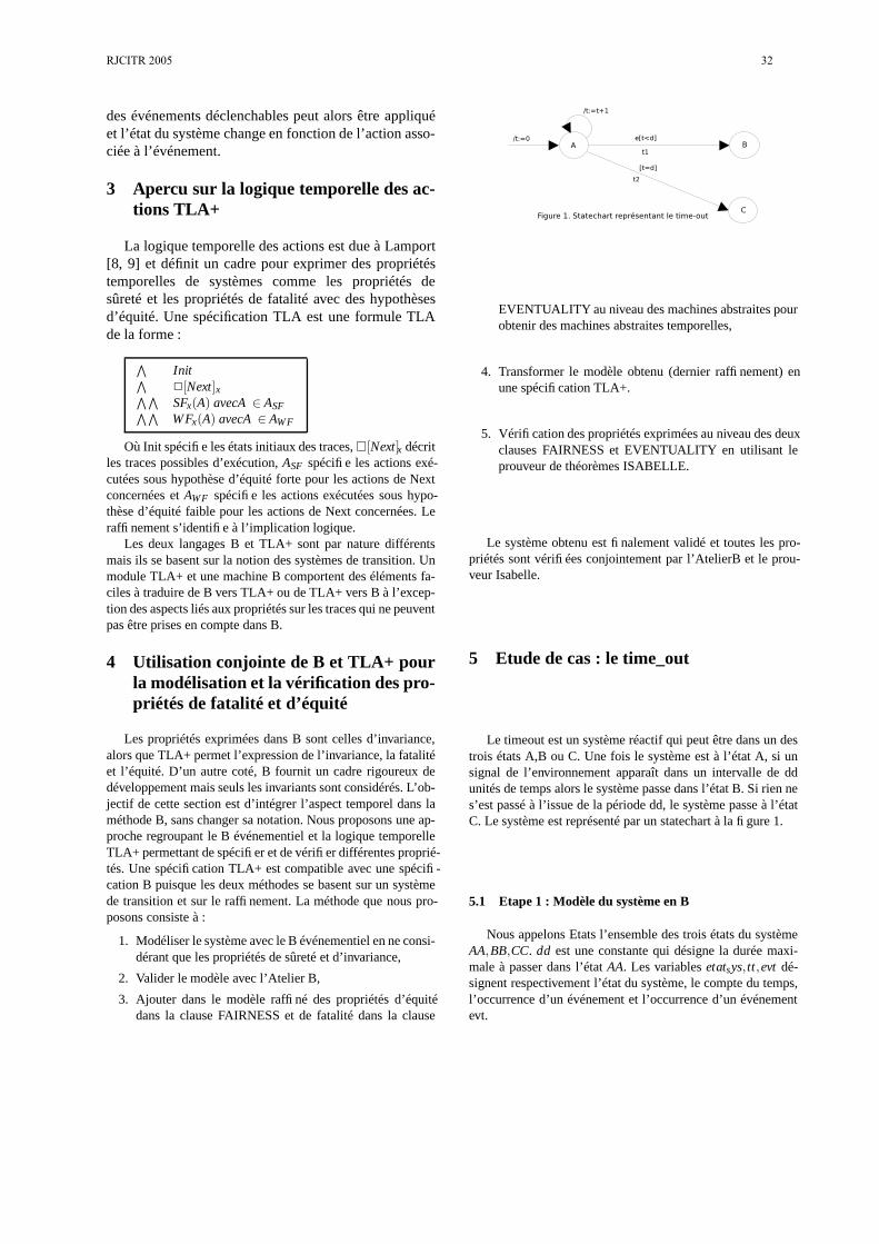
des événements déclenchables peut alors être appliquéet l’état du système change en fonction de l’action asso-ciée à l’événement.
3 Apercu sur la logique temporelle des ac-tions TLA+
La logique temporelle des actions est due à Lamport[8, 9] et définit un cadre pour exprimer des propriétéstemporelles de systèmes comme les propriétés desûreté et les propriétés de fatalité avec des hypothèsesd’équité. Une spécification TLA est une formule TLAde la forme :
V
InitV
2[Next]xVV
SFx(A) avecA ∈ ASFVV
WFx(A) avecA ∈ AW F
Où Init spécifie les états initiaux des traces,�[Next]x décritles traces possibles d’exécution, ASF spécifie les actions exé-cutées sous hypothèse d’équité forte pour les actions de Nextconcernées et AWF spécifie les actions exécutées sous hypo-thèse d’équité faible pour les actions de Next concernées. Leraffinement s’identifie à l’implication logique.
Les deux langages B et TLA+ sont par nature différentsmais ils se basent sur la notion des systèmes de transition. Unmodule TLA+ et une machine B comportent des éléments fa-ciles à traduire de B vers TLA+ ou de TLA+ vers B à l’excep-tion des aspects liés aux propriétés sur les traces qui ne peuventpas être prises en compte dans B.
4 Utilisation conjointe de B et TLA+ pourla modélisation et la vérification des pro-priétés de fatalité et d’équité
Les propriétés exprimées dans B sont celles d’invariance,alors que TLA+ permet l’expression de l’invariance, la fatalitéet l’équité. D’un autre coté, B fournit un cadre rigoureux dedéveloppement mais seuls les invariants sont considérés. L’ob-jectif de cette section est d’intégrer l’aspect temporel dans laméthode B, sans changer sa notation. Nous proposons une ap-proche regroupant le B événementiel et la logique temporelleTLA+ permettant de spécifier et de vérifier différentes proprié-tés. Une spécification TLA+ est compatible avec une spécifi-cation B puisque les deux méthodes se basent sur un systèmede transition et sur le raffinement. La méthode que nous pro-posons consiste à :
1. Modéliser le système avec le B événementiel en ne consi-dérant que les propriétés de sûreté et d’invariance,
2. Valider le modèle avec l’Atelier B,
3. Ajouter dans le modèle raffiné des propriétés d’équitédans la clause FAIRNESS et de fatalité dans la clause
EVENTUALITY au niveau des machines abstraites pourobtenir des machines abstraites temporelles,
4. Transformer le modèle obtenu (dernier raffinement) enune spécification TLA+.
5. Vérification des propriétés exprimées au niveau des deuxclauses FAIRNESS et EVENTUALITY en utilisant leprouveur de théorèmes ISABELLE.
Le système obtenu est finalement validé et toutes les pro-priétés sont vérifiées conjointement par l’AtelierB et le prou-veur Isabelle.
5 Etude de cas : le time_out
Le timeout est un système réactif qui peut être dans un destrois états A,B ou C. Une fois le système est à l’état A, si unsignal de l’environnement apparaît dans un intervalle de ddunités de temps alors le système passe dans l’état B. Si rien nes’est passé à l’issue de la période dd, le système passe à l’étatC. Le système est représenté par un statechart à la figure 1.
5.1 Etape 1 : Modèle du système en B
Nous appelons Etats l’ensemble des trois états du systèmeAA,BB,CC. dd est une constante qui désigne la durée maxi-male à passer dans l’état AA. Les variables etatsys,tt,evt dé-signent respectivement l’état du système, le compte du temps,l’occurrence d’un événement et l’occurrence d’un événementevt.
RJCITR 2005 32

MACHINE time_outSETS Etat_sys = {AA,BB, CC} ;CONSANTS ddPROPERTIES dd= 10VARIABLES etat_sys, tt, eeINVARIANT etat_sys ∈ Etat_sys ∧ tt∈ NATU-RAL ∧ ee∈ BOOL∧ tt ≤ ddINITIALISATIONetat_sys :=AA || tt :=0 || ee :=FALSEOPERATIONSAtoA , SELECT etat_sys=AA ∧ ee= FLASE ∧ tt<ddTHEN etat_sys :=AA || tt := tt+1 END ;AtoB , SELECT etat_sys=AA ∧ ee= TRUE ∧ tt<ddTHEN etat_sys :=BB END ;AtoC , SELECT etat_sys=AA ∧ tt<ddTHEN etat_sys :=CC END ;Change , SELECT ee=FALSE ∧ etat_sys = AATHEN ee :=TRUE END ;END
L’événement "AtoA" exprime les conditions sous lesquelles lesystème reste dans l’état AA (pas de réception de l’événement"evt" et la valeur de tt n’ a pas atteint dd unités de temps).L’événement "AtoB" exprime la condition de transit de l’étatAA vers BB sous l’occurrence de l’événement "evt". L’événe-ment "AtoC" exprime la condition de transit de l’état AA versCC. L’événement “occurevt" permet d’avoir une valeur aléa-toire pour l’événement "evt".
5.2 Etape 2 : Preuves
Le modèle a été prouvé par le prouveur automatique del’AtelierB et les invariants sont préservés par les événements.
5.3 Etape 3 : Adjonction de clauses
Une spécification B décrit un système par un ensembled’événements et par un invariant qui doit être préservé par lesévénements. Une extension de B qui intégrerait des aspects liésà la fatalité et à l’équité pourrait être obtenue sur le plan syn-taxique par l’ajout de clauses spécifiques. Deux clauses ont étéajoutées :
1. Une clause FAIRNESS qui décrit l’équité : les évé-nements AtoB et AtoC sont exécutées sous hypothèsed’équité faible.
2. Une clause EVENTUALITY qui décrit les propriétés defatalité.
MACHINE time_outSETS Etat_sys = {AA,BB, CC} ;CONSANTS ddPROPERTIES dd= 10VARIABLES etat_sys, tt, eeINVARIANT etat_sys ∈ Etat_sys ∧ tt∈ NATURAL
∧ ee∈ BOOL∧ tt ≤ ddINITIALISATIONetat_sys :=AA || tt :=0 || ee :=FALSEOPERATIONSAtoA , SELECT etat_sys=AA ∧ ee= FLASE ∧ tt<ddTHEN etat_sys :=AA || tt := tt+1 END ;AtoB , SELECT etat_sys=AA ∧ ee= TRUE ∧ tt<ddTHEN etat_sys :=BB END ;AtoC , SELECT etat_sys=AA ∧ tt<ddTHEN etat_sys :=CC END ;Change , SELECT ee=FALSE ∧ etat_sys = AATHEN ee :=TRUE END ;FAIRNESSWF(AtoB)WF(AtoC)EVENTUALITYetat_sys = AA ∧ ee = TRUE ∧ tt < dd etat_sys = BBetat_sys = AA ∧ tt = dd etat_sys = CCEND
5.4 Etape 4 : Transformation du modèle B en un modèleTLA+
MODULE time_out
PARAMETERSdd : CONSTANTSetat_sys , tt, evt : VARIABLES
TypeInvariant = ∧ tt ∈ NATURAL ∧ dd = 10∧ etat_sys ∈ {AA, BB, CC} ∧ ee ∈ {TRUE, FALSE}∧ tt ≤ ddPREDICATEInit = ∧ etat_sys = AA ∧ tt = 0 ∧ ee = FALSEACTIONSAtoA = ∧ etat_sys = AA ∧ tt < dd ∧ ee = FALSE∧ UNCHANGED<etat_sys> ∧ tt’ = tt + 1AtoB = ∧ etat_sys = AA ∧ tt < dd ∧ ee = TRUE∧ etat_sys’ = BBAtoC = ∧ etat_sys = AA ∧ tt = dd ∧ etat_sys’ = CCchange = ∧ etat_sys = AA ∧ ee = FALSE ∧ ee’ =TRUENext = AtoA ∨ AtoB ∨ AtoC ∨ changeTEMPORALSpecification General = ∧ Init∧ � [Next]<etat_sys,tt,ee> ∧ W F<etat_sys,ee,tt>(Next)
Pour pouvoir vérifier les propriétés d’équité et de fatalité,nous devons transformer la spécification B en une spécificationTLA+. Un module TLA+ décrit les paramètres, les prédicatset les actions de la spécification. La traduction d’une spécifica-tion B en une spécification TLA+ est triviale, les événements
33

B sont des actions TLA+ et les invariants B sont des invariantsen TLA+.
5.5 Etape 5 : Vérification du modèle TLA+ obtenu par leprouveur de théorèmes Isabelle
Avant d’utiliser le prouveur de théorèmes général Isabellepour vérifier les propriétés d’équité et de fatalité, nous devonstransformer le modèle TLA vers un modèle compréhensiblepar Isababelle utilisant le codage de TLA en Isabelle. Le mo-dèle ci-dessous est modèle TLA en Isabelle.
time_out.thy
Timeout = TLA+datatype etat_sys = AA || BB || CCconstdefs dd : : nat "dd==10"constdefs etat_sys : : Etat_sys stfun
tt : : nat stfun ee : : stpredrules base "basevars (etat_sys, tt, ee)"constdefs InitTimeout : : stpred"InitTimeout == PRED etat_sys = #AA & tt=#0 & ee =#False"AtoA : : action"AtoA == ACT $ etat_sys = #AA & $ tt < #dd & $ ee =#False & etat_sys $= # AA & tt $ = $ tt + # 1 & unchangedee "AtoB : : action"AtoB == ACT $ etat_sys = #AA & $ tt < #dd & $ ee =#TRUE & etat_sys $= # BB & unchanged (tt, ee) "AtoC : : action"AtoC == ACT $ etat_sys = #AA & $ tt = #dd &etat_sys $= # CC & unchanged (tt, ee) "change : : action"change == ACT $ etat_sys = #AA & $ ee = #False &ee $= # True & unchanged (tt, etat_sys) "Next : : action"Next == ACT $ (AtoA | AtoB | AtoC | change)"Timeout : : temporal
"Timeout == TEMP (Init InitTimeout& �[Next](−etat_sys,tt,ee)& �WF(AtoB)−(etat_sys,tt,ee)& �WF(AtoC)−(etat_sys,tt,ee))"
Live1 : : temporal"Live1 == TEMP (( etat_sys = #AA & ee = #True & tt < #dd ) etat_sys = #BB)"Live2 : : temporal"Live2 == TEMP (( etat_sys = #AA & tt = # dd ) etat_sys = #CC)"
Les propriétés d’équité et de fatalité ont été prouvées par leprouveur de théorèmes Isabelle.
6 Conclusion
Dans ce papier, nous avons présenté une méthode de spé-cification et de vérification des systèmes réactifs et sûrs defonctionnement en utilisant conjointement la méthode B évé-nementiel et la logique temporelle des actions TLA+. L’apportde regroupement de ces deux notations s’explique par le traite-ment des propriétés d’équité qui à notre connaissance constitueune contribution originale par rapport aux extensions appor-tées à la méthode B. Nous avons présenté une démarche re-groupant les deux méthodes et utilisant les deux outils de vé-rification associés l’AtelierB et le prouveur Isabelle. Commeperspectives, nous tenons à valider la préservation des proprié-tés exprimées dans les nouvelles clauses FAIRNESS et EVEN-TUALITY par le raffinement et à automatiser le processus detransformation d’un modèle B vers une spécification équiva-lente en TLA+.
Références
[1] J.-R. Abrial. The B-Book : Assigning Programs to Mea-nings. Cambridge University Press, 1996.
[2] J.-R. Abrial. Extending B without changing it (for deve-loping distributed systems). In H. Habrias, editor, Pro-ceedings of the 1st Conference on the B method, pages169–191, Nov. 1996.
[3] J.-R. Abrial and L. Mussat. Introducing dynamicconstraints in B. In D. Bert, editor, B’98 : The 2nd In-ternational B Conference, volume 1393 of Lecture Notesin Computer Science (Springer-Verlag), pages 83–128,Montpellier, Apr. 1998. Springer Verlag.
[4] R.-J. Back. Refinement calculus, part II : Parallel and reac-tive programs. In J. W. de Bakker, W.-P. de Roever, andG. Rozenberg, editors, Stepwise Refinement of Distribu-ted Systems, volume 430 of Lecture Notes in ComputerScience. Springer-Verlag, 1990.
[5] R.-J. Back and K-Sere. Stepwise refinement of action sys-tems. In Mathematics of Program Construction., pages115–138, Berlin - Heidelberg - New York, June 1989.Springer.
[6] D. Berry, S. Moisan, and J. Rigault. Esterel : Towards asynchronous and semantically sound high level languagefor real-time applications. In Proceedings of the 1983IEEE Real-Time Systems Symposium, pages 30–37, Dec.1983.
[7] G. Berry and L. Cosserat. The esterel synchronous pro-gramming language and its mathematical semantics. InA. W. R. S. D. Brookes and G. Winskel, editors, Pro-ceedings of the Seminar on Concurrency, volume 197 ofLNCS, pages 389–448. Springer, July 1984.
[8] M. Büchi and E. Sekerinski. Formal methods for com-ponent software : The refinement calculus perspective.Lecture Notes in Computer Science, 1357 :332–350, 1998.
[9] K-M. Chandy and J. Misra. Parallel Program Design.Addison-Wesley, Austin, Texas, May 1989.
RJCITR 2005 34

Statistical Study of Firm Real-Time Transactions Behavior ∗
S. Semghouni*, L. Amanton*, B. Sadeg* and A. Berred**Laboratoire d’Informatique du Havre*,
Laboratoire de Mathematiques Appliquees du Havre**Universite du Havre,25 rue Philippe Lebon BP 540
76058 Le Havre Cedex, FRANCETel :(33) 02-32-74-43-84 Fax : (33) 02-32-74-43-14
{samy-rostom.semghouni, laurent.amanton, alexandre.berred, bruno.sadeg}@univ-lehavre.fr
Abstract
In this paper, we study statistically firm real-time trans-actions behavior under a pessimistic and an optimisticconcurrency control and scheduling protocols. Up to now,all the studies have been done on RTDBS performancesby measuring the transactions success ratio (number oftransactions meeting their deadlines over the total numberof transactions), which is the well-known and acceptedcriterion for this purpose. Our study focuses among oth-ers, on the number of operations composing a transactionand the concurrency control protocols used. We proposea reasonable approximation of transactions success ratiobehavior by a probability distribution and we suggest amethod to predict the system performances. We have car-ried out simulations where we vary different parametersincluding the arrival rate, the transactions sizes and theslack factor.
1 Introduction
A real-time database system (RTDBS) can be viewedas a system which inherits mechanisms of both traditionaldatabase systems and real-time systems (RTSs). RTDBSsmust guarantee simultaneously the transactions ACID(Atomicity, Consistency, Isolation, Durability) propertiesand schedule the transactions in order to meet their indi-vidual deadlines [14].
In RTDBSs, the main issue is the transactions concur-rency control and scheduling (CC&S). These mechanismsare designed to cooperate tightly in order to assign trans-actions priorities in the case of data access conflicts. Manyconcurrency control and scheduling policies have beenproposed to manage the real-time transactions accordingto their categories [1, 15]. Three classes of real-time trans-actions are defined according to the consequences theylead to in case of missing their deadlines: hard, firm and
∗This work is supported by the research ministry of France (ACI-JC #1055)
soft. Hard transactions must meet their deadlines other-wise disastrous effects may occur. Firm transactions mustalso meet their deadlines, but a transaction is only abortedwhen it misses its deadline, as it becomes useless. Softtransactions are still useful even after their deadlines, butthey provide less quality of service to the application.
Up to now, almost all the studies of RTDBS perfor-mances deal with the transaction success ratio using onlya simple measure: the percentage of successful transac-tions (transactions which have met their deadlines). Tothe best of our knowledge, there is no statistical study re-lated to RTDBs performances, even if several statisticalstudies investigated RTSs and DBSs. For instance, Bernatet al. [3] have dealt with a probabilistic study of hard real-time systems. They have combined both measurement andanalytical approaches into a model for computing proba-bilistic bounds of the worst case execution time (WCET).Edgar et al. [7] have proposed a statistical analysis forthe problem of WCET in hard RTSs. Their paper givesan alternative analysis based on the estimation of WCETfrom test data within a specific level of probabilistic con-fidence. Other studies are devoted to periodic RTSs prob-lems. Diaz et al. [6] have described a stochastic analysisof periodic RTS. The description contains a method forcomputing the response time distribution of each task inthe system. That makes it possible to determine the miss-ing deadline probability of individual tasks. Atlas et al.[2] have presented statistical rate monotonic scheduling(SRMS).
A few work has been done on transactions probabilis-tic/statistical analysis in traditional DBMSs. Among theseresearches, Singhal et al. [17] have studied the workloadsin three commercial relational DBMSs, running commer-cial applications and production environment. Their studyconsiders topics such as frequency of locking and un-locking, deadlock and blocking, duration of locks, typesof locks, correlations between applications of lock types,two-phase versus non-two-phase locking, when locks areheld and released, etc. There are non statistically studieson real-time concurrency control protocols. In RTDBS,
35

Notations Definitions Values
λ Transaction arrival rate 0.1 to 0.8DB-size Number of data in the DB 1000Slack Factor H(x) initialization α and β α = 1, 3 and β = 0.3
Tr-size short/ middle/ long 5-10, 5-70, 5-160Capacity Capacity of execution coefficient 10 tasks/cpu-cycleTime Duration of one test 1000 cpu-cycleCC&S CC protocols & scheduling policy (2PL-HP or Wait-50) & EDF
Table 1. Simulation parameters.
we can quote the work of Haritsa et al. [11, 10] that havestudied optimistic concurrency control protocols in par-ticular OPT-BC, OPT-Wait and Wait-50. However, theydidn’t propose a statistical study.
In this paper, we consider firm transactions and we pro-pose a stochastical study of their success ratio, under sev-eral conditions corresponding to parameters such as theirsize (short, middle or long), the arrival process, the systemload, the conflicts level and the probability of ”read” and”write” operations. This study is carried out under both apessimistic and an optimistic approach. To this purpose,we have developed a simulator including the componentsgenerally encountered in an RTDBS [12, 15]. After sev-eral simulations, we have obtained the probability densityfunction which approximates reasonably the behavior ofthe transactions success ratio.
The remainder of this paper is organized as follows. InSection 2, we describe the simulator architecture and re-lated parameters. Section 3 is devoted to simulations ex-periments and the interpretations. Finally, Section 4 sum-marizes the main ideas of the paper and outlines some as-pects of our future work.
Rejection queue
Admission controller
Reject
Transactions
Transactions generator
Freshness Manager
Real−time
Normal Data
Deadline controller
Blocked queue
Tr Scheduler Concurrency controller
Data
Complete transactions
OCC−Wait−50
or2PL−HP
Periodic sensor Tr
Active queue
EDF
Figure 1. Simulator architecture.
2 System model
Figure 1 shows the architecture of our centralizedRTDB simulator 1. Transactions arrive in the system ac-cording to a Poisson process with average rate λ. The setof operations of each transaction is randomly generatedand built according to a level of data conflicts. Given thatdata is selected, the transactions execute with the sameprobability a ”read” or a ”write” operation.
1The simulator is available on line at the following address:http://www-lih.univ-lehavre.fr/∼semghouni/Applet/PageSimulateur.html
When a transaction is submitted to the system, an ad-mission controller mechanism (ACM) is employed to de-cide whether to admit or reject that transaction into theexecution queue. The primary task of the ADM is to per-form schedulability test of new transactions upon their ar-rival, to decide whether or not a new transaction should beadmitted for execution [8]. Transaction deadlines are con-trolled by the Deadline Controller. Deadlines are verifiedevery CPU cycle and the scheduler is informed immedi-ately when a transaction is likely to exceed its deadline.
Scheduling is the mechanism by which a transactionis chosen to execute on the processor. There are severaltypes of real-time schedulers. We quote for examples:HPF (Highest Priority First), LLF (Least Laxity First orLeast Slack Time) [5], EDF (Earliest Deadline First) [19]and RM (Rate Monotonic) [13]. Our Scheduler is basedon EDF algorithm for the determination of the transac-tions priorities. There exist a lot of work on concurrencycontrol and scheduling in RTDBSs [11, 18]. In our sim-ulator, we chose the two well-known concurrency controland scheduling protocols: a pessimistic (2PL-HP proto-col) [1, 4] and an optimistic (OCC-Wait-50 protocol) [9].
2.1 Conflicts levelData conflicts emerge from the behavior of the transac-
tions in the database. Generally, in a database, we knowa priori that some data are more important than others be-cause they are frequently requested. We thus assign toeach data item a probability proportional to its importance.
Let r1, r2, . . . , rk, . . . , rn denote the ranking of thedata item D1, D2, . . ., Dk, . . ., Dn. The probability ofdrawing the data item i is given by the following formula:
Pi =ri
Ri
where Ri =∑i=n
i=1ri, is the sum of all ranks.
2.2 Deadline assignment functionThe deadline assignment policy we have used to gen-
erate the transactions is given by the following formula:
DT = AT + BT ∗ (H(BT ) + 1)
where DT denotes the deadline of the transaction T , AT
the arrival time (or release time) of T , BT the best (min-imum) estimated execution time of T and H(x) = α ∗(1− exp(−β ∗x)) a slack function, scaled by the α and β
parameters. Note that the value of the best execution time
RJCITR 2005 36

Figure 2. 2PL-HP Frequency distribution of the random success rates.
(BT ) is always greater than or equal to 0. The values ofH(BT ) are then ranging from 0 to α. Note also that thesmallest is the best execution time, the tightest is the Slacktime. This characteristic allows the transactions with shortexecution times, particularly update transactions, to be as-signed the highest priorities (EDF policy), when a conflictwith transactions with longer execution times occurs.
3 Simulation results
To assess the performances of our database, we car-ried out simulation experiments (the simulations parame-ters are summarized in Table 1) which evaluate the successratio of transactions. Each experiment is repeated 1000times. Transactions are classified into three categories:short, e.g. transaction in navigation system; middle, e.g.transaction in stock market; and long, e.g. multimediatransaction.
Figure 2 shows the frequency of short, middle and longtransactions when λ = 0.3 (normal workload' 300 trans-actions) and λ = 0.7 (high workload ' 700 transactions).The frequency distribution of the success ratio could rea-sonably be approximated by a Beta random variable [16](see Appendix A), according to the Kolmogorov-Smirnovstatistical test with a confidence interval equal to 95%.
Simulations results revealed that the best performancesare given with short transactions, particularly with OCC-Wait-50. However, this situation is reversed rapidly in fa-vor of 2PL-HP protocol when we use middle or long trans-actions. This is explained by the inherent characteristicsof each protocol. With the OCC-Wait-50 protocol, con-flicting transactions have to wait for the resolution of theconflict as long as their deadlines are not reached. Thiscauses the system overload and appears clearly when weuse middle and long transactions. In the case of the 2PL-HP protocol, the transactions are aborted and restarted im-mediately when a conflict occurs [10].The study of suc-cess ratio frequency has revealed that the RTDBSs arevery complex to control. The success rate is very sensi-tive to the variation of slack function, size of transaction
and the choice of the CC protocol. These two last param-eters play a major role in the optimization of the systemperformances. In the following of the paper, we proposeto use regression method of Beta parameters to predict thesystem performances.
3.1 Non-linear regression of p and q parametersWe have estimated all the values of p and q parame-
ters (see Appendix B) of the Beta density for all resultsaccording to the simulations hypothesis (transaction sizeand λ). Figure 3 shows the layout of the estimated p and qvalues according to both the average of the arrivals λ andthe transaction size when using 0CC-Wait-50. To deter-mine the approximated values of p and q for all the valuesof λ, we propose to use the Non-Linear Regression, whichwe note NLR. The regression model is given by the fol-lowing function: F (X) = exp(a + x ∗ b)/(x + 1)c +exp(d + x ∗ e)/(x + 1)f , where a, b, c, d, e, f are valuesadjusted continuously by the regression.
The functions obtained by the non-linear regression areused to deduce the values p and q. That gives the awaitedparameters of the Beta density according to the systemparameters (CC protocol and α, λ, etc.). This allows us toderive the mean of the density which is interpreted as theexpected average success ratio of the system states. Thebest and the worst execution scenario can be deduced fromthe distribution. Theses indications, particularly the lowerbound of the success ratio, makes it possible to see if thesystem overshoot2 will not be violated.
4 Conclusion
We have studied in this paper the statistical perfor-mances of centralized RTDBS. We have particularly pre-sented for the first time a comprehensive evaluation ofreal-time transactions behavior according to optimisticand pessimistic concurrency control and scheduling proto-cols. In this statistical study, we have modeled the success
2Fixed by the system manager, it represents the limit beyond whichthe system becomes unprofitable.
37
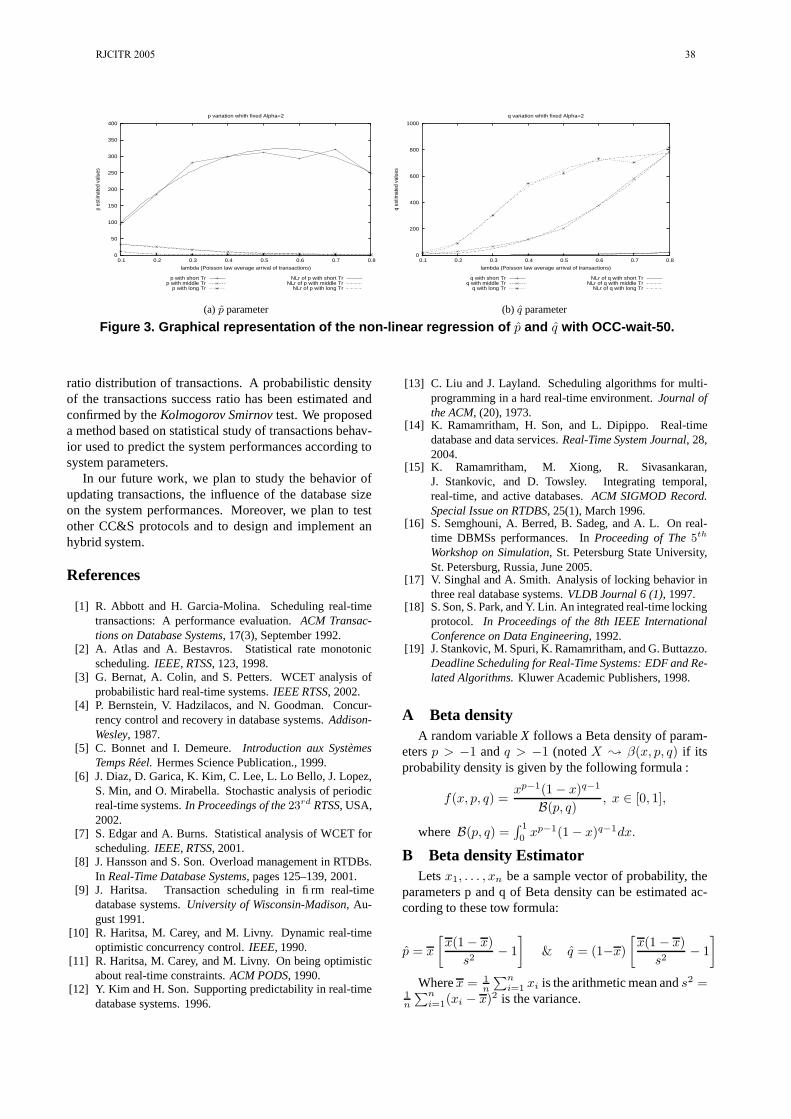
0
50
100
150
200
250
300
350
400
0.1 0.2 0.3 0.4 0.5 0.6 0.7 0.8
p es
timat
ed v
alue
s
lambda (Poisson law average arrival of transactions)
p variation whith fixed Alpha=2
p with short Trp with middle Tr
p with long Tr
NLr of p with short TrNLr of p with middle Tr
NLr of p with long Tr
(a) p parameter
0
200
400
600
800
1000
0.1 0.2 0.3 0.4 0.5 0.6 0.7 0.8
q es
timat
ed v
alue
s
lambda (Poisson law average arrival of transactions)
q variation whith fixed Alpha=2
q with short Trq with middle Tr
q with long Tr
NLr of q with short TrNLr of q with middle Tr
NLr of q with long Tr
(b) q parameter
Figure 3. Graphical representation of the non-linear regression of p and q with OCC-wait-50.
ratio distribution of transactions. A probabilistic densityof the transactions success ratio has been estimated andconfirmed by the Kolmogorov Smirnov test. We proposeda method based on statistical study of transactions behav-ior used to predict the system performances according tosystem parameters.
In our future work, we plan to study the behavior ofupdating transactions, the influence of the database sizeon the system performances. Moreover, we plan to testother CC&S protocols and to design and implement anhybrid system.
References
[1] R. Abbott and H. Garcia-Molina. Scheduling real-timetransactions: A performance evaluation. ACM Transac-tions on Database Systems, 17(3), September 1992.
[2] A. Atlas and A. Bestavros. Statistical rate monotonicscheduling. IEEE, RTSS, 123, 1998.
[3] G. Bernat, A. Colin, and S. Petters. WCET analysis ofprobabilistic hard real-time systems. IEEE RTSS, 2002.
[4] P. Bernstein, V. Hadzilacos, and N. Goodman. Concur-rency control and recovery in database systems. Addison-Wesley, 1987.
[5] C. Bonnet and I. Demeure. Introduction aux SystemesTemps Reel. Hermes Science Publication., 1999.
[6] J. Diaz, D. Garica, K. Kim, C. Lee, L. Lo Bello, J. Lopez,S. Min, and O. Mirabella. Stochastic analysis of periodicreal-time systems. In Proceedings of the 23rd RTSS, USA,2002.
[7] S. Edgar and A. Burns. Statistical analysis of WCET forscheduling. IEEE, RTSS, 2001.
[8] J. Hansson and S. Son. Overload management in RTDBs.In Real-Time Database Systems, pages 125–139, 2001.
[9] J. Haritsa. Transaction scheduling in firm real-timedatabase systems. University of Wisconsin-Madison, Au-gust 1991.
[10] R. Haritsa, M. Carey, and M. Livny. Dynamic real-timeoptimistic concurrency control. IEEE, 1990.
[11] R. Haritsa, M. Carey, and M. Livny. On being optimisticabout real-time constraints. ACM PODS, 1990.
[12] Y. Kim and H. Son. Supporting predictability in real-timedatabase systems. 1996.
[13] C. Liu and J. Layland. Scheduling algorithms for multi-programming in a hard real-time environment. Journal ofthe ACM, (20), 1973.
[14] K. Ramamritham, H. Son, and L. Dipippo. Real-timedatabase and data services. Real-Time System Journal, 28,2004.
[15] K. Ramamritham, M. Xiong, R. Sivasankaran,J. Stankovic, and D. Towsley. Integrating temporal,real-time, and active databases. ACM SIGMOD Record.Special Issue on RTDBS, 25(1), March 1996.
[16] S. Semghouni, A. Berred, B. Sadeg, and A. L. On real-time DBMSs performances. In Proceeding of The 5th
Workshop on Simulation, St. Petersburg State University,St. Petersburg, Russia, June 2005.
[17] V. Singhal and A. Smith. Analysis of locking behavior inthree real database systems. VLDB Journal 6 (1), 1997.
[18] S. Son, S. Park, and Y. Lin. An integrated real-time lockingprotocol. In Proceedings of the 8th IEEE InternationalConference on Data Engineering, 1992.
[19] J. Stankovic, M. Spuri, K. Ramamritham, and G. Buttazzo.Deadline Scheduling for Real-Time Systems: EDF and Re-lated Algorithms. Kluwer Academic Publishers, 1998.
A Beta densityA random variable X follows a Beta density of param-
eters p > −1 and q > −1 (noted X ; β(x, p, q) if itsprobability density is given by the following formula :
f(x, p, q) =xp−1(1 − x)q−1
B(p, q), x ∈ [0, 1],
where B(p, q) =∫ 1
0xp−1(1 − x)q−1dx.
B Beta density EstimatorLets x1, . . . , xn be a sample vector of probability, the
parameters p and q of Beta density can be estimated ac-cording to these tow formula:
p = x
[x(1 − x)
s2− 1
]
& q = (1−x)
[x(1 − x)
s2− 1
]
Where x = 1
n
∑ni=1
xi is the arithmetic mean and s2 =1
n
∑n
i=1(xi − x)2 is the variance.
RJCITR 2005 38

Thème 3
Ordonnancement Temps Réel


Quantification de l’ordonnançabilité des systèmes temps-réel à contraintes strictes par l’analyse markovienne
Bernard Chauvière Laboratoire d’Informatique Scientifique et Industrielle
Université de Poitiers & ENSMA Téléport 2 – 1 avenue Clément Ader - BP 40109
86961 Futuroscope Chasseneuil cedex [email protected]
Dominique Geniet Laboratoire d’Informatique Scientifique et Industrielle
Université de Poitiers & ENSMA Téléport 2 – 1 avenue Clément Ader - BP 40109
86961 Futuroscope Chasseneuil cedex [email protected]
Abstract
In this paper, we propose a quantitative approach of feasability : we plan to diagnose the behavior of a real-time system. Our analysis is based on dynamic stochastic processes, and more particularly on Markov chains. First of all, we present a model of real-time applications obtained by the use of dynamic aggregations of states. Then, we show how this model can be used to validate a real-time application. Finally, we give some prospects on the quantification of feasability.
1. Introduction
La validation des systèmes temps-réel est un problème complexe largement traité par la communauté temps-réel. Il conduit généralement à l’étude de l’ordonnançabilité et de la production d’ordonnancements valides. Cette approche est peu flexible : lors de la phase de validation, lorsqu’une application est détectée non-ordonnançable, les méthodes actuelles ne fournissent aucune précision sur la nature du problème, on sait seulement qu’il faut revenir à la phase de conception. Pour enrichir les informations obtenues lors de la phase de validation, nous souhaitons établir un diagnostic du comportement du procédé. Celui-ci doit permettre d’améliorer la qualité de la conception (pour obtenir de meilleures performances), de déterminer comment modifier la spécification d’une application non valide, et enfin de détecter le plus tôt possible lors de la phase de conception les applications qui ne sont pas valides.
Les méthodes classiques pour l’analyse comportementale des systèmes sont classées en trois groupes : déterministes, non-déterministes et stochastiques. Les méthodes déterministes ne permettent pas d’étudier le comportement du procédé en général, on ne peut considérer qu’une seule alternative à la fois (par exemple, celle engendrée par un algorithme en-ligne [2]). Cette approche ne
répondant pas à nos objectifs, nous nous sommes tournés vers les méthodes non-déterministes (réseaux de Petri [5,7], automates finis [1,6], etc. [4]). Ces méthodes ont été largement étudiées : elles se heurtent généralement au problème de l’explosion combinatoire [3]. Les méthodes stochastiques présentent deux avantages : une meilleure maîtrise de l’explosion combinatoire [8], et l’obtention de résultats sur le comportement moyen du procédé. Cette dernière propriété permettant d’approcher nos objectifs, nous avons décidé d’utiliser les chaînes de Markov. Il nous ait alors possible d’exploiter les outils d’analyse associés, notamment les Processus de Décision Markovien [10].
Dans la section 2, nous introduisons les systèmes temps-réel auxquels nous nous sommes consacrés. Dans la section 3, nous définissons le modèle que nous avons utilisé, et dans la suivante, nous présentons les résultats expérimentaux que nous avons obtenus. Finalement, dans la section 5, nous donnons quelques perspectives.
2. Systèmes temps-réel étudiés
Nous avons étudié les applications temps-réel constituées de tâches périodiques que l’on caractérise par le modèle dit de Liu-Layland [9] :
–
!
ri : la date de réveil est l’instant où la tâche s’active pour la première fois
–
!
Ci : la charge est la durée maximale pour l’exécution d’une instance
–
!
Di : le délai critique est la durée maximale dont dispose chaque instance de la tâche pour exécuter toutes ses instructions
–
!
Ti : la période de la tâche est la durée séparant deux activations successives
Les tâches périodiques que nous considérons ici ne sont pas réentrantes et une même instance n’est pas parallélisable, nous supposons donc
!
Ci " Di "Ti . Les tâches interagissent les unes avec les autres.
Pour représenter ces interactions, on utilise généralement l’exclusion mutuelle, le partage de
41

ressources et les relations de précédence. Nous avons intégré ces interactions à notre modèle.
Le support informatique choisi pour exécuter une application temps-réel influe fortement sur ses performances. Nous avons étudié les architectures mono ou multi processeurs. Nous avons aussi développé un modèle permettant d’interdire les migrations d’instances entre les processeurs.
3. Modèle markovien
L’analyse markovienne peut être réalisée de deux manières [10] : en horizon fini ou infini. La majorité des travaux traitent de l’horizon infini. Cependant, l’analyse dans ce contexte-là porte sur des systèmes stationnaires : les probabilités de transition et les fonctions de coût, qui décrivent l’évolution du système, sont indépendantes du temps. Or dans le cas des systèmes temps-réel, le temps a un rôle central : nous avons donc été amenés à considérer l’analyse en horizon fini. Par ailleurs, une application temps-réel devant s’exécuter indéfiniment, l’utilisation des théorèmes de cyclicité est indispensable pour obtenir une borne supérieure à la longueur de l’intervalle d’étude.
Maintenant, présentons brièvement la chaîne de Markov que nous avons utilisée.
Définition 1 : Soit
!
" r,C,D,T une tâche périodique, on appelle
!
I t la variable aléatoire qui compte le nombre d’instructions exécutées par toutes les instances de la tâche
!
" entre l’instant 0 et l’instant
!
t , et on note
!
E l’ensemble des valeurs possibles des variables
!
I t . Pour modéliser l’exécution de l’application, on
utilise donc une variable
!
I tk pour chaque tâche
!
" k . Dans la suite, lorsque nous utiliserons la notation
!
I t , ce sera pour indiquer le n-uplet constitué par la variable
!
I tk associée à chaque tâche.
Le comportement de l’application doit respecter les contraintes décrites dans la spécification. On peut associer à ces contraintes un prédicat
!
Q équivalent, ainsi une séquence d’exécution
!
I0, I1,... est valide si et seulement si on a
!
Q I0, I1,...( ) . Cependant, les chaînes de Markov ne permettent pas
de vérifier directement les contraintes portant sur des séquences de longueur supérieure à 2, nous devons donc décomposer
!
Q en contraintes sur les transitions. Définition 2 : On appelle contrainte d’évolution
locale (CEL) tout prédicat
!
Ql dépendant des transitions et du temps, et vérifiant pour tout
!
T " N et tout
!
i0,...,iT " E :
!
Q i0,...,iT( ) "#t $ 0..T %1{ },Ql t,it ,it+1( ) Grâce à cette décomposition de
!
Q en
!
Ql , nous pouvons utiliser les résultats classiques des chaînes de Markov. En particulier, on détermine la probabilité que
l’application soit valide en utilisant une matrice de transition
!
Mt = mi, j[ ]i, j"E
construite de la manière
suivante :
!
mi, j = " I t+1 = j | I t = i( ) # " Ql t,i, j( )( ) La décomposition de
!
Q en
!
Ql est la clé de voûte permettant d’intégrer une contrainte, nous l’avons réalisée pour celles indiquées dans la section 2.
Cependant, nous ne pouvons pas utiliser la chaîne de Markov sous cette forme : la complexité de calcul est bien trop élevée (le nombre d’états contenus dans le modèle est infini). Nous avons donc cherché à réduire au maximum le nombre d’états à considérer en fonction de l’instant courant. Ceci nous a amenés à définir les agrégations dynamiques d’états que nous présentons ci-dessous.
3.1. Réduction aux premières instances La première réduction que nous avons utilisée
permet de ramener le nombre d’états global à une quantité finie. Elle repose sur le fait que les différentes instances d’une même tâche ont des comportements équivalents. Ceci est parfaitement vérifié puisqu’elles exécutent les mêmes instructions. On peut donc ramener le comportement de la kè instance à celui de la première. De plus les tâches n’étant pas réentrantes, on peut utiliser un modèle contenant
!
Ck +1 états pour chaque tâche
!
" k . La figure 1 illustre cette réduction.
Figure 1. Réduction aux premières instances.
Cette réduction ramène le nombre d’états à considérer à un nombre fini, et indique aussi que les différentes instances d’une même tâche ont des comportements équivalents. Elle ouvre donc la voie à des résultats de cyclicité permettant d’étudier les tâches à départs différés. Cette réduction possède donc un intérêt théorique que nous souhaitons explorer ultérieurement.
3.2. Réduction à la laxité Cette deuxième réduction repose sur les états
interdits par la contrainte
!
Q : tous les états qui vérifient
!
" Q I0,..., I t( )# I t = e( ) = 0 sont inutiles pour représenter l’exécution de l’application. En général, on ne peut pas déterminer cette probabilité sans effectuer une évaluation globale du système (calculer
!
" Q I0,..., I t( )( ) ), cependant, on peut, dans certains cas, montrer qu’elle est nulle.
RJCITR 2005 42

Définition 3 : On appelle contrainte d’évolution globale (CEG) tout prédicat
!
Qg dépendant des états et du temps, et vérifiant pour tout
!
T " N et tout
!
i0,...,iT " E :
!
Q i0,...,iT( ) "#t $ 0..T{ },Qg t,it( ) En conséquence, tout état
!
e qui ne vérifie pas
!
Qg à un instant
!
t , vérifie aussi :
!
" Q I0,..., I t( )# I t = e( ) = 0 Ainsi tous les états qui ne vérifient pas
!
Qg peuvent être supprimés du modèle.
En utilisant la contrainte de validité temporelle (chaque instance respecte son échéance), on ramène les états à prendre en compte à ceux indiqués par les parties grisées de la figure 2.
Figure 2. Réduction à la laxité
Ainsi à chaque instant
!
t , on n’utilise pour chaque tâche
!
" k que
!
laxk t( ) états. En moyenne, l’ordre de grandeur du nombre d’états à considérer par tâche est équivalent à
!
Ck /Tk( ). Dk "Ck( ) . REMARQUE. — Contrairement à la réduction aux
premières instances, on ne suppose pas ici que les différentes instances d’une même tâche ont des comportements équivalents.
4. Expérimentations
Actuellement, nous avons implémenté et testé notre méthode pour déterminer si une application est ordonnançable. Bien que ce résultat ne réponde pas directement à nos objectifs de quantification, il permet d’évaluer les performances de notre méthode, et en particulier l’efficacité des réductions.
Nous ne présentons ici que les résultats d’expérimentations. Indiquons toutefois que l’implémentation s’articule autour des éléments suivants : le stockage en mémoire des états valides (complexité des accesseurs), la détermination des états atteignables par un état valide, la transformation de la distribution courante lors d’un saut (c’est-à-dire lors d’une discontinuité de la réduction utilisée, par exemple, la réduction aux premières instances effectue un saut dès qu’une tâche se réactive, i.e.
!
t > rk " (t # rk ) modTk = 0 ). Considérons le système S de tâches défini par les
paramètres temporels suivants : –
!
"k # 1..n,rk = 0,Ck = 5,Tk = 100 –
!
"k # 1..n,Dk = 5+10.(kmod9)
Nous avons appliqué notre méthode, en utilisant la réduction à la laxité, pour valider le système S en monoprocesseur (existence d’un ordonnancement valide). La figure 3 présente les variations du temps de calcul en fonction du nombre de tâches.
Figure 3. Temps de calcul
Ainsi notre algorithme répond toujours en moins d’une minute pour valider S, ce qui nous paraît encourageant puisque S possède jusqu’à 12 tâches.
Le nombre d’états manipulés par notre algorithme constitue un indicateur intéressant de ses performances (voir figure 4). La courbe « valides » correspond au nombre maximum d’états valides à un instant donné, c’est l’optimum. La courbe « réduits » correspond au nombre maximum d’états représentés à un instant donné, en utilisant la réduction à la laxité.
Figure 4. Nombre d’états
Pour les nombres de tâches compris entre 1 et 6, la réduction à la laxité correspond donc à l’optimal, au delà elle contient plus d’états que nécessaire (tous ne sont pas atteignables). Ainsi cette réduction prend bien en compte les restrictions propres aux tâches, mais pas celles propres à leurs interactions (ex : partage du processeur). Toutefois, la complexité temporelle de notre méthode « suit » la courbe « valides », ainsi nous perdons peu en temps de calcul. En implémentant notre méthode à l’aide d’une structure de donnée creuse, notre complexité spatiale serait proche de « l’optimale », mais notre complexité temporelle serait élevée (coût des accesseurs).
5. Perspectives
Nous présentons ici deux applications possibles de notre approche en accord avec nos objectifs de quantification.
43

5.1. Temps de réponses Considérons un ordonnancement de durée
!
T " N et représenté par la suite
!
I0, I1,..., IT . A partir de cette séquence, on peut déterminer précisément les instants où une instance de la tâche
!
" k se termine : ce sont les dates
!
t " rk correspondant aux transitions
!
I t , I t+1( )
vérifiant
!
I tk
= Ck "1+ # et
!
I t+1k
= Ck + " , avec
!
" = (t # rk ) /Tk$ %.Ck . Par une marche aléatoire, nous calculons la
probabilité qu’une instance de la tâche
!
" k se termine à l’instant
!
t +1 et que l’ordonnancement soit valide de l’instant 0 jusqu’à cet instant :
!
" Q I0, I1,..., I t+1( )# I tk = Ck $1+ %# I t+1
k = Ck + %( )
En réalisant une rétro-marche, on calcule la probabilité « duale », c’est-à-dire la probabilité qu’une instance de la tâche
!
" k se termine à l’instant
!
t +1 et que l’ordonnancement soit valide à partir de cet instant :
!
" I tk = Ck #1+ $% I t+1
k = Ck + $%Q It , I t+1,..., IT( )( )
En associant ces deux résultats, nous déterminons la probabilité qu’une instance de la tâche
!
" k se termine à l’instant
!
t +1 et que l’ordonnancement soit valide :
!
" I tk = Ck #1+ $% I t+1
k = Ck + $%Q I0,..., IT( )( )
En réalisant une « double » marche aléatoire, nous pouvons donc déterminer la distribution de probabilité des temps de réponses des instances de chaque tâche.
5.2. Priorités fixes Considérons un ordonnancement de durée
!
T " N et représenté par la suite
!
I0, I1,..., IT . Chaque transition de cette séquence induit une relation d’ordre partiel sur les tâches actives. Par exemple, considérons l’ensemble
!
A des tâches actives à l’instant
!
t défini par :
!
A = k " 1..n{ } | t # rk $ I tk < Ck + (t % rk ) /Tk& '.Ck{ }
Connaissant la transition
!
I t , I t+1( ) , on peut déterminer l’ensemble
!
B des tâches s’exécutant :
!
B = k " 1..n{ } | I tk# I t+1
k{ } . Sous l’hypothèse que cette
séquence est engendrée par un algorithme à priorités fixes, on doit alors avoir :
!
"k # B, $ k # A % B, prio & k( ) ' prio & $ k ( ) Ainsi chaque transition engendre une relation
d’ordre partiel. En les unissant, on obtient une description des configurations de priorités fixes engendrant cet ordonnancement. Remarquons que l’on peut la représenter par un graphe orienté. Tout cycle apparaissant dans ce graphe signifie qu’il n’existe pas d’algorithme à priorités fixes engendrant cette séquence, puisqu’à un certain instant une tâche doit être plus prioritaire qu’une autre, et qu’à un autre instant, on a la situation inverse : les priorités de ces tâches doivent alors être dynamiques.
6. Conclusion
Les méthodes stochastiques permettent d’établir un diagnostic des applications temps-réel, en particulier, nous avons déterminé la distribution de probabilités du temps de réponse des tâches. D’autre part, les chaînes de Markov permettent d’intégrer des dépendances explicites vis-à-vis du temps : nous avons pu modéliser efficacement le comportement des systèmes temps-réel en utilisant des agrégations dynamiques d’états.
Une autre équipe du LISI est chargée de la conception d’un drone, nous travaillons actuellement avec eux sur la phase de validation pour tester notre méthode sur un exemple réel.
En collaboration avec le LORIA, nous souhaitons paralléliser nos algorithmes de validation et intégrer les résultats propres aux MDP dynamiques à notre méthode.
References
[1] A. Arnold, M. Nivat, Les mathématiques de l’informatique, AFCET, pp. 35-68, 1982.
[2] N.C. Audsley, A. Burns, R.I. David, K.W. Tindell, A.J. Welling, Fixed priority preemptive scheduling : an historical perspective, The journal or Real-Time Systems, 8 :173-198, 1995.
[3] S.K. Baruah, R.R. Howell, L.E. Rosier, Algorithms and complexity concerning the preemptive scheduling of periodic, real-time tasks on one processor, Real-Time Systems, 2, pp. 301-324, 1990.
[4] J.P. Beauvais, « Etude d’algorithmes de placement de tâches temps-réel périodiques complexes dans un système réparti », Thèse de doctorat en automatique et informatique appliquée, Ecole centrale de Nantes, 182 p., 1996.
[5] A. Choquet-Geniet, G. Vidal-Naquet, Réseaux de Pétri et systèmes parallèles, Ed. Armand Colin, 1993.
[6] D. Geniet, Validation d’applications temps-réel à contraintes strictes à l’aide de langages rationnels, Real-Time Systems, Tekna, 2000.
[7] E. Grolleau, A. Choquet-Geniet, Offline computation of real-time schedules by means of Petri nets, Journal of Discrete Event Dynamic Systems, 12 :311-333, 2002.
[8] P. Laroche, « Processus décisionnels de Markov appliqués à la planification sous incertitude », Thèse de doctorat en informatique, Université Henri Poincaré – Nancy 1, 154 p., 2000.
[9] C.L. Liu et J.W. Layland. Scheduling algorithms for multiprogramming in real-time environnement, Journal of the ACM, 1973, vol. 20, p. 46-61.
[10] M.L. Puterman, Markov Decision Processes : discrete stochastic dynamic programming, John Wiley & Sons, New York, 1994.
RJCITR 2005 44

New On-Line Preemptive Scheduling Policies for Improving Real-TimeBehavior
Mathieu GrenierLORIA-INRIA
Campus Scientifique, BP 239 54506 Vandoeuvre-lès-Nancy - [email protected] tel: +33 3 83 58 17 68, fax: +33 3 83 58 17 01
Abstract
In real-time systems, schedulability is mandatory butother application-dependent performance criteria aremost generally of interest. We first define the propertiesthat a “good” real-time scheduling algorithm must pos-sess. Then, we exhibit a class of easily-implementablepolicies that should be well suited to various applicativecontexts because, in our experiments, these policies pro-vide good trade-off between feasibility and the satisfac-tion of the application-dependent criteria. The study isillustrated in the framework of computer-controlled sys-tems that are known to be sensitive to various delays in-duced by resource sharing. We evaluate criteria othersthan feasibility by simulation. An extended version of thisarticle, comprising feasibility analyses for the consideredpolicies, is accepted in the ETFA conference, see [10].
1. Introduction
Context of the paper. In real-time systems, feasibilityof the task set is the basic requirement, but, usually, othercriteria besides feasibility are of interest. A prominentexample are computer-controlled systems [2] where it iswell-known that other temporal characteristics than dead-line respect affect the performances of the controlled sys-tem [16, 2].
Goal of our paper. The goal is here to take into ac-count others criteria than feasibility in the scheduling de-sign. The aim of the study is to find on-line schedulingpolicies that are well suited to the satisfaction of applica-tion dependent criteria. In the following, we will illus-trate our approach through computer-controlled systemswhere, most usually, reducing delays and their variabili-ties improve the performances.
Related Work. Many studies have been dedicated tofind scheduling solutions that improve the performance ofcomputer-controlled systems (a more complete state of theart can be found in [10]).
To better fit to the processing requirements of a controlsystem, new task models have been conceived. In [7, 5],it is proposed that control tasks are Subdivided in threedifferent parts: sampling, computation, actuation. Sam-pling and actuation Sub-tasks are assigned a high priorityin order to reduce the jitters.
Another solution, is to adjust the parameters of thetasks to achieve the desired goals. In [3], the worst-caseend-of-execution jitter is minimized by choosing appro-priate deadlines. In [8], initial offsets and priorities areadjusted to reduce jitter by minimizing preemption.
Improvements can also be brought by well choosingthe parameters of the scheduling policies. In [9], a pri-ority allocation scheme is proposed to reduce the aver-age response time while, in [15], the problem of choos-ing scheduling policies and priorities on a Posix 1003.1bcompliant operating system (OS) is tackled.
Finally, another way is to create new scheduling poli-cies. In [1], the scheduler is synthetized as a timed au-tomata from the Petri net modeling the system and theproperties expected from the system. In [11], also startingfrom a Petri net model of the system, an optimal schedul-ing sequence is found by examining the marking graphsof the Petri net.
Our approach. In this paper, we propose a techniquefor building new on-line scheduling policies that ensurefeasibility and perform well with regard to applicationdependent criteria such as the ones that are crucial incomputer-controlled systems. We do not merely tune theparameters of a scheduling policy, as the priorities [9] forFPP scheduling, but tune the scheduling algorithm itself.The main advantage with regard to [1] and [11] is thelower complexity. Finally, the approach could be used inconjunction with task splitting schemes [7, 5]. Our pro-posal is made of two distinct steps:
1. define the characteristics that a “good” real-timescheduling policies must possess. This class of goodpolicies constitutes the search space of our problem,
2. explore the search space for finding policies that per-form well in terms of feasibility and with respect to
45

the other criteria.
Organization. In Section 2, the model of the system andthe assumptions made are presented. In Section 3, the re-quirements for an acceptable policies are defined. Then,in Section 4, we define the criteria beside feasibility andthe search space of the scheduling policies. In Section 5,the experimental results are presented.
2. System model
This study deals with the non-idling scheduling of peri-odic tasks on a single resource which can be either a CPUor a communication network.
Task model. The task model is very similar to the oneused in [13]. A periodic task τi is characterized by a triple(Ci, Di, Ti) where Ci is the worst case execution time(WCET), Di the relative deadline (i.e. maximum allow-able response time of an instance - equal for all instancesof the same task) and Ti the inter-arrival time betweentwo instances of τi. The release time of jth instance ofthe ith task is denoted by Ai,j ((Ai,1) is thus the initialoffset of the task).
Defining scheduling policies through priority func-tions. Priority functions, introduced in [14], is a con-venient way of formally defining scheduling policies.The priority function Γk,n(t) indicates the priority of aninstance τk,n at time t. The resource is assigned, ateach time, according to the Highest Priority First (HPF)paradigm.
Function Γk,n(t) takes its value from a totally orderedset P which is chosen in [14] to be the set of multi-dimensional IR-valued vectors P = {(p1, ..., pn) ∈ Rn |n ∈ N} provided with a lexicographical order, with con-vention (p1, ..., pn) ≺ (p′1, ..., p
′n′) iff (∃i ≤ min(n, n′) `
pi = p′j , ∀j < i and pi > p′i) or (n′ < n and pj =p′j , ∀j ∈ [1, ..., n′]). Example: (3, 4, 5) ≤ (3, 2, 5),(2, 4, 5) ≥ (3, 2, 5), (2, 3) ≥ (2, 3, 1).
Most real-time scheduling policies can be defined eas-ily using priority functions. For instance, the priority ofan instance τk,n under preemptive Earliest Deadline First(EDF), is ΓEDF
k,n (t) = (Ak,n + Dk, k, n) (the last twocoordinates are needed to ensure decidability, see defini-tion 3).
Besides providing non-ambiguous definition of thescheduling policy, priority functions enable us to distin-guish classes of scheduling policies and to derive genericresults that are valid for whatever the policy belonging to acertain class. The next Section presents requirements thata scheduling policy must fulfill.
3. “Good” scheduling policies
An arbitrary priority function does not necessarily de-fine an implementable scheduling of interest for real-time
computing. In this Section, we precise the requirementsexpected from an acceptable policy (termed “good” pol-icy in the following). A “good” policy must meet a certainnumber of criteria, which are needed for the policy to beimplemented in a real-time context.
Decidable policies. Policies are needed to be decidable:at any time t, there is exactly one instance of maximal pri-ority among the set of active instances (i.e. instances withpending work). This concept of decidability was intro-duced in [14]. For instance, the last two components ofΓEDF
k,n (t) = (Ak,n + Dk, k, n) ensure decidability.
Implementable policies. For being implementable inpractice, a policy must induce a finite number of con-text switches over a finite time interval. This first con-dition, called “piecewise order preserving”, was exhibitedin [14]. Furthermore, components of the priority vectorshave to be representable by machine numbers. In the fol-lowing, coordinates of a priority vector belong to the setof rational numbers Q.
“Shift temporal invariant” policies. In this study, forthe sake of predictability of the system, we are only inter-ested in scheduling policies such that the relative prioritybetween two instances does not depend on the numericalvalue of the clock: relative priority must remain the sameif we “shift” the arrival of all instances to the left or theright. The policy is thus independent of the value of thesystem’s clock at start up time. We call such policies shifttemporal invariant (STI) policies. EDF is a STI policysince the priority between two instances only depends onthe offset between arrival dates and on relative deadlines.
We have defined a minimum set of requirements that a“good” policy must fulfill in the context of real-time com-puting.
4. Performance criteria and study domain
In this section, the performance criteria take into ac-count in this study are precised. Then, among the set ofall good policies, we define the particular class of schedul-ing policies considered in this study.
4.1. Performance criteriaWe consider periodic control loops where the control
algorithm is modeled by a periodic task τk with period Tk
(i.e. the sampling period). In classical control theory, themain parts of a control loop are sampling, control com-putation and actuation. Some assumptions are made: thedata collection from sensors (i.e. sampling) is assumed tobe done at the beginning of each instance (at time Bk,n),the computation of the control law is performed in a con-stant time Ck, and actuation, that is the transmission ofoutput data to the actuators, is done at the end of execu-tion of each task instance (at time Ek,n).
RJCITR 2005 46

Specific delays of control loops have been identifiedto be of particular importance for the stability of the sys-tem, and, more generally, for its performances (see, forinstance, studies in [16, 2, 6]). These delays are:
• Input-output latency (or response time) of an instanceτk,n is the time elapsed between the sampling and theactuation (equal to Ek,n − Bk,n with our notations),
• Sampling interval is the time interval between twoconsecutive sampling instants (i.e. Bk,n+1 − Bk,n),
• Sampling latency of an instance τk,n is the timeelapsed between the theoretical sampling time (i.e.Ak,n), and its actual occurrence (i.e. Bk,n).
In classical discrete control theory, input-output latenciesand sampling intervals are assumed to be constant withno sampling latency. In practice, when resources are notdedicated to a single control loop, these delays exists andgreatly impact the performances (see [16, 12]). The aim isthus to keep these delays and their variabilities (jitters) asclose as possible to the assumptions made by the theory.
4.2. Search spaceIn order to be able to analyze the scheduling policies
and to define more precisely the search space, this one islimited to the class of “Arrival Time Dependent” policies.
“Arrival Time Dependent” policies. In the following,our domain of study is a Sub-class of Time Independentpolicies (i.e. ∀t Γk,n(t) = constant) that we call ArrivalTime Dependent Priority (ATDP).
Definition 1 An Arrival Time Dependent policy is a pol-icy whose priority function can be put under the form
Γk,n(t) = (Ak,n + pk, k, n) (1)
where pk: k 7→ Q.
pk is an arbitrary function, which returns a constant valuefor all instances of task τk. For instance, for EDF, thevalue returned by pk is equal to the relative deadline Dk.
In the following, to achieve the desired goal (feasibil-ity + performance), experiments will be done within aSub-class of ATDP policies having a priority vector of theform:
Γk,n = (Ak,n + c.Ck + d.Dk, k, n) (2)
where d ∈ [0, 1] and c ∈ [0, 100] (i.e. pk = c.Ck + d.Dk
in definition 1). A point C in our search space is a policydefined by a priority function of the form of equation 2.
Motivations for Arrival Time Dependent policies.First of all, ATD policies are “good” scheduling policies:
• decidability is ensured by the last two components ofthe priority vectors,
• the policies are implementable in the sense of defi-nition 3; the priority functions are “piecewise orderpreserving” due to constant priority over time andthey can be represented by machine numbers.
Secondly, this sub-class of ATD policies has been cho-sen because we expect that it contains policies providinga good trade-off between feasibility and the satisfaction ofthe other criteria important for control systems (see 4.1).EDF actually belongs to this class and policies whosepriority function is “close” to EDF are expected to havenearly the same behavior in terms of schedulability. Onthe other hand, introducing a term dependent of the exe-cution time should help to improve the other criteria. In-deed, it has been shown that Shortest Remaining Process-ing Time First is optimal for average response times invarious contexts (see [4]).
5. Experiments
Experiments in this study are performed in the frame-work of computer-controlled systems. Corresponding per-formance criteria were presented in §4.1 and the space ofscheduling policies is defined in §4.2.
Case study. In this experiments, several control taskssharing a CPU where the initial offsets of the tasks arenot known. The task sets are generated with a global loadrandomly chosen in the interval [0.8, 0.9] with Di = Ti.
We consider the case where the policy is tuned for aparticular application (see [10] for case where the policyhas to be efficient on average). The aim is here to find thepolicy that leads to a feasible schedule and that providesthe greatest improvement for the other criteria. The searchspace, defined by equation 2, is exhaustively search withsteps of granularity d = 0.1 and c = 0.5 (the search spacecomprises approximately 2000 policies).
Evaluation of criteria. Feasibility of our policies iscomputed with the generic feasibility analysis presentedin [10], which is an extension of the EDF response timeanalysis.
The two performance criteria are the improvement inpercent over EDF of the average sampling latency and ofthe average sampling interval jitter (measured as the stan-dard deviation of the sampling intervals). The values ofthe criteria are computed with the data collected duringsimulation runs, as to our best knowledge there is no ana-lytic technique. A given criterion is evaluated for a policyas the average value of the criterion for all tasks (for eachtask set 20 different initial offsets are simulated).
Results. Results are depicted on figure 1. Each pointis the average improvement over 100 runs (only the bestpolicy at each run is considered), where a run is definedby a task set randomly generated with an average load of0.85.
47

26
28
30
32
34
36
38
6 8 10 12 14 16
Impr
ovem
ent i
n pe
rcen
t ove
r E
DF
Cardinality of task set
avg sampling latencyavg sampling interval jitter
Figure 1. Average sampling latency and av-erage sampling interval jitter with compari-son to EDF for the best feasible policy foundin the search space defined by equation 2.
On figure 1, one sees that for a particular application,improvements are always larger than 32% for averagesampling latency and larger than 26% for average sam-pling interval jitter whatever the cardinality of the set oftasks. For example, the average improvement achievedfor 10 tasks is 35% for average sampling latency and 30%for average sampling interval jitter.
Overall, the technique is efficient, even on heavilyloaded systems (average load of 0.85 in our experiments)and the improvement over EDF for average sampling la-tency and average sampling interval jitter is really signif-icant whilst always ensuring feasibility. Similar results,not shown here, were found for the average input-outputlatency and the input-output latency jitter.
6. Conclusion and future work
In this paper, we highlight a class of on-line schedulingalgorithms that are both easy to implement and that canprovide interesting performances for feasibility and, espe-cially, for other application-dependent criteria. We pro-pose an algorithm to compute worst-case response timebounds that is generic for all policies of the class. Exper-iments show that, in the context of computer-controlledsystems where delays and jitters impact the performancesof the control loop, well chosen policies can bring impor-tant improvements over plain EDF.
In the future, we intend to evaluate more preciselythe impact of the scheduling policies using software toolssuch as TrueTime [6] or the tool described in [12], thatallow to integrate delays induced by the scheduling in thecontrol loops. It is also planed to experiment new searchtechniques for exploring the policy search space; prelim-inary experiments show that simple neighborhood tech-niques such hill-climbing are much more efficient than ex-haustive search.
This work could be extended to other class of policies
such as time-sharing policies (e.g. Round-Robin, Pfair).The main problem will be here to come up with a genericschedulability analysis.
References
[1] K. Altisen, G. Goessler, A. Pnueli, J. Sifakis, S. Tripakis,and S. Yovine. A framework for scheduler synthesis. InProc. of the 20th IEEE Real-Time Systems Symphosium(RTSS 1999), 1999.
[2] K. Astrom and B. Wittenmark. Computer-Controlled Sys-tems. Prentice Hall ISBN 0-13-168600-3, third editionedition, 1997.
[3] S. Baruah, G. Buttazzo, S. Gorinsky, and G. Lipari.Scheduling periodic task systems to minimize output jit-ter. In Proc. of the 6th International Conference on Real-Time Computing Systems and Applications (RTCSA 1998),1998.
[4] D. P. Bunde. SPT is optimally competitive for uniproces-sor flow. Information Processing Letters, 90(5):233–238,2004.
[5] A. Cervin. Integrated Control and Real-Time Scheduling.PhD thesis, Department of Automatic Control, Lund Insti-tute of Technology, 2003.
[6] A. Cervin, D. Henriksson, B. Lincoln, J. Eker, and K.-E. Årzén. How does control timing affect performance?IEEE Control Systems Magazine, 23(3):16–30, 2003.
[7] A. Crespo, I. Ripoll, and P. Albertos. Reducing delays inrt control: the control action interval. In Proc. of the 14thIFAC World Congress, 1999.
[8] L. David, F. Cottet, and N. Nissanke. Jitter control inon-line scheduling of dependent real-time tasks. In Proc.of the 22nd IEEE Real-time Systems Symposium (RTSS2001), 2001.
[9] J. Goossens and P. Richard. Performance optimization forhard real-time fixed priority tasks. In Proc. of the 12thinternational conference on real-time systems (RTS 2004),2004.
[10] M. Grenier and N. Navet. New preemptive schedulingpolicies for improving real-time behavior. To appear inIEEE ETFA conference, Catania, Italy, sep 2005.
[11] E. Grolleau, A. Choquet-Cheniet, and F. Cottet. Val-idation de systèmes temps réel à l’aide de réseaux depetri. In Proc. of Approches Formelles dans l’Assistanceau Développement de Logiciels (AFADL’98), 1998.
[12] F. Jumel, N. Navet, and F. Simonot-Lion. Evaluation de laqualité de fonctionnement d’une application de contrôle-commande en fonction de caractéristiques de son implan-tation. to appear in Technique et Science Informatiques,2005.
[13] C. Liu and J. Layland. Scheduling algorithms for multi-programming in hard-real time environnement. Journal ofthe ACM, 20(1):40–61, 1973.
[14] J. Migge. Scheduling under Real-Time Constraints: aTrajectory Based Model. PhD thesis, University of NiceSophia-Antipolis, 1999.
[15] N. Navet and J. Migge. Fine tuning the scheduling of tasksthrough a genetic algorithm: Application to posix1003.1bcompliant os. In Proc. of IEE Proceedings Software, vol-ume 150, pages 13–24, 2003.
[16] B. Wittenmark, J. Nilsson, and M. Törngren. Timing prob-lems in real-time control systems. In Proc. of the AmericanControl Conference, 1995.
RJCITR 2005 48

Temporal validation of an IEC 61499 control application
Mohamed KHALGUI LORIA (UMR CNRS 7503) - INPL
Campus Scientifique B.P 239. 54506 Vandoeuvre-lés-Nancy cedex. France.
Abstract
This paper deals with the temporal correctness of
control applications designed using the component-
based standard IEC 61499. In this standard, a function
block is defined as an event trigger component
containing its own data. To validate temporal behavior
of an application, we have to take into account its
scheduling on the execution support. We propose an
abstraction of component behavior taking into account
all its possible executions. We propose to verify the
temporal correctness of the application with regard to
global temporal properties (end to end delays). Thanks
to such characterization, we show that it is possible to
check deadlines for the application to ensure its
correctness. To reach this goal, we transform the
application into a dependant tasks model.
Keywords. Function Blocks, IEC 61499, Real Time,
schedulability analysis, offline scheduling.
1. Introduction
The IEC 61499 standard [2,3] is a component-based
methodology allowing to design applications as well as
the execution support [5]. In the standard, the Function
Block is defined as an event trigger component. It is a
reusable functional unit of software owning data. A
control application is specified by a "function blocks
network" which can be distributed on one or more
devices.
The standard allows to validate static
interoperability between blocks. Nevertheless,
temporal behavior depends on dynamic data.
Therefore, it is difficult to a priori validate temporal
interoperability. We propose an abstraction of each
block behavior taking into account all its possible
executions. Such abstraction allows to compute an
upper bound of the application execution time. We
show that it is possible to verify the temporal
correctness of the application with regard to global
temporal properties (end to end delays).
To validate temporal interoperability, we propose a
schedulability analysis of a function blocks network
distributed on one device. To perform such analysis,
we propose to transform the application into a
particular dependent tasks model in the order to take
advantages of the results in this field. We show that it
is possible to generate a safe off-line scheduling for a
function blocks network.
In the next section 2, we briefly present the IEC
61499 standard. Then we present our behavior
characterization of an application. The section 4 deals
with its transformation into a tasks model. In the
section 5, we propose tasks deadlines generation
according to the application delays. Finally, we present
a schedulability analysis based on the generated
deadlines.
2. The IEC 61499 standard
We present the main concepts of the IEC 61499
Function Blocks standard [2,3]. This standard is an
extension of the IEC 61131.3 [4] for the Programmable
Logic Controllers. We can divide its description into
two parts: the architecture description and the block
behavior through the events selection mechanism.
2.1. Architecture description
An application function block (FB) is a functional
unit of software that supports some functionalities of
an application. It is composed by an interface and an
implementation. The interface contains data/event
inputs and outputs supporting the interaction with the
environment. Events are responsible for the activation
of the function block while data contain valued
information.
The implementation consists of a body and a head.
The body is composed of internal data and algorithms
implementing the block functionalities. Each algorithm
gets values in the input data channels and produces
values in the output data ones. They are programmed in
structured text (ST) language [4].
The block head is connected to event flows. It
selects the sequence of algorithms to execute with
regard to an input event occurrence. The selection
mechanism of an event occurrence is encoded in a state
machine called Execution Control Chart (ECC). At the
49

end of the algorithms execution, the ECC sends the
corresponding output event(s).
In the standard, a function blocks network defines
the functional architecture of a control application.
Each function block event input (resp. output) is linked
to an event output (resp. input) by a channel.
Otherwise, it corresponds to a global application input
(resp. output). Data inputs and outputs follow the same
rules.
The execution support architecture is defined by a
devices network. A device is composed of one
processing unit, sensors, actuators and network
interfaces. In order to manage interactions with a given
physical processes, a device contains several resources.
A resource contains FBs networks interacting with a
physical process. Considered as a logic execution unit
corresponding to time slots of the processing unit, the
resource provides scheduling function for its local FBs
networks.
The operational architecture corresponds to a
distribution of the application function blocks over the
different resources of the execution support
architecture. The advantage of such approach is to take
into account hardware as well as software components.
For sake of simplicity, we consider in this paper only
one function blocks network distributed on a single
resource of a device.
2.2. Events selection mechanism
Let turn to the internal description of a function
block. Note that only algorithms executions spend
time. In a given function block, the ECC is said idle if
there is no algorithm to execute. Otherwise, the ECC is
busy.
According to the standard [2,3], the FB contains an
internal buffer for input occurrences [10]. The ECC
behavior is devised into three steps:
* First, it selects one input event occurrence
according to priority rules defined in the resource.
* It activates the algorithms sequence corresponding
to the selected event. Then, it waits for the resource
scheduler to execute this sequence.
* When the execution ends, it emits corresponding
output events occurrences.
We note that an algorithms sequence is atomic.
Moreover, the resource scheduling function applies
only non preemptive policies. On the other hand, the
policy of events priorities in the ECC is not specified in
the standard. Therefore, it is up to the designer to fix
such priority for each function block [8].
Note that the ECC is specified as a state machine
where each trace is composed by a waiting of an input
event, invocations of algorithms and sending of output
events.
3. Behavior characterization
To characterize temporal behavior of a function
block, we have to take into account the execution of
the ECC. Indeed, the ECC decides not only algorithms
to execute but also the output events to send.
Nevertheless, the selection of transitions inside the
ECC may depend on internal state variables. Then we
propose to define sets of output events corresponding
to all possible executions.
To validate the temporal correctness of the
application, we propose to define end to end delays
corresponding to time constraints imposed by the
problem specification. In this section, we first present
the abstraction of the function block behavior. Then we
propose formalization for end to end delays. For all the
continuation, we denote by fbn the function blocks
network.
3.1. Function block behavior
We propose to compute an abstraction of the
function block behavior. The difficulty is to identify
the output events sent corresponding to an input event
occurrence. Such association is specified in the ECC
state machine. Nevertheless, firing a transition in the
ECC can depend on internal variables of the block.
Therefore, we propose to identify the supersets of
output events possibly occurring simultaneously.
For each trace of the ECC automaton (i.e. each
possible execution), we associate a superset gathering
all the output event occurring in this trace.
Let denote by IE (resp OE) the set of input (resp
output) events in fbn. Let consider IEFB (resp OEFB) the
set of input (resp output) events in a function block FB.
Let tr be a trace in ECCFB, we denote by
* IE(tr) the input event occurring in tr.
* OE(tr) the set of output events occurring in tr.
We propose a function follow associating to an input
event ie ∈ IEFB, the sets of simultaneous output events.
follow(fb,ie) = {OE(tr) / ie = IE(tr), tr ∈ ECCFB}
3.2. fbn temporal constraint
We propose a function cause that specifies
causalities between an event input of a function block
and an output of another one according to the function
blocks network. Note that effect specifies the opposite
function.
We define inputs (respectively outputs ) the set of
input (respectively output) events in fbn which is not
linked to another event.
inputs = { ie ∈ IE /cause(ie) ∉ OE}
outputs ={ oe ∈ OE /effect(oe) ∉ IE}
We propose the function delay that encodes all the
end to end deadlines for fbn. delay(ie,oe) denotes the
maximum duration that can take the execution between
RJCITR 2005 50

the receive of an ie ∈ inputs occurrence and the sent
of an oe ∈ outputs one.
4. Transformation into a Task Model
In this part, we propose to transform fbn to a tasks
system S with precedence constraints [1]. The purpose
is to exploit the results on this topic to perform the
shedulability analysis of fbn.
In this section, we define the task characterization in
the system S. A task corresponds to one execution of a
function block. Then, we define a trace as a causality
sequence of tasks.
4.1. Task definition starting from a FB
network
An application task T corresponds to the execution
of a FB activated by an input occurrence ie. We define
the function generate(ie) that constructs for an input
event ie the correspondent task T. Note that is_
generated_ by is the opposite function. We denote by
Task the tasks set of S.
Let setOE be a set of output events. We define the
function target(setOE) associating for setOE the
following set of tasks,
target(setOE)={T ∈ Task /
∃oe ∈ setOE, oe = cause(is_ generated_ by(T))}
A task T is characterized as follows,
T = {WCET, pred, succ}
Such as,
* WCET : the worst case execution time of the
algorithms sequence corresponding to ie.
* pred : The task that corresponds to the execution
of the FB producing cause(ie).
* succ : a set of tasks sets such as,
T.succ = {setT / setT ⊂ Task,
∃setOE ∈ follow(fb,is_ generated_ by(T)),
setT = target(setOE)}
We define first (resp last) the tasks set that they
have not a predecessor (resp successor). These sets
correspond to the inputs and outputs sets,
4.2. Trace definition
To specify a causality sequence of tasks, we define
in S a trace tr as a Tasks sequence,
tr = {T0,T1,.....,Tn-1}
such as,
* T0 ∈ first
* Tn-1 ∈ last
* ∀ i ∈]1,n-1], Ti-1 = Ti.pred
Let Trace be the traces set in S. We denote by
first(tr) the first task of the trace tr . In this paper, we
consider the case of not reentry traces [6,11]: the
execution of the k-th instance of the first task must
not start before the execution end of the (k-1)-th
instance of the last task. Otherwise the system is not
feasible.
Note that we can classically define an operation
op(T) in S as the set of traces having the same root. It
corresponds to all possible executions of fbn when T is
activated (the correspondent input event occurs)
op(T) = { tr ∈ Trace / first(tr)=T}
5. Task deadline generation
We classically define delay(tr) as the end to end
delay of a trace tr ∈ Trace. This temporal constraint
corresponds to the delay(ie,oe) where ie corresponds
to the first(tr) and oe corresponds to an event produced
by the last task of tr .
We define d(T) the deadline of the task T ∈ tr. d(T)
has to take into account the time for executing all the
successors belonging to the same set of T.succ before
their respective deadlines.
We characterize d(T) as follows,
If T ∈ last
Then d(T)=delay(tr)
Else
d(T) =
mins∈T.succ{minTi∈s{d(Ti)- .( ) ( )
Tj WCETd Tj d TiTj s
∑≤
∈ }}
6. Schedulability analysis
In this part, we propose a schedulability analysis of
an IEC 61499 control application. Let S be the tasks
system corresponding to the application.
We propose a temporal characterization of S. Since
all input events of fbn are periodic, then each task T
belonging to first is activated periodically. We
characterize such task by a release time r , a period p
and a jitter j (the maximum deviation of the period).
T = { r, p, j}
To perform the schedulability analysis of S, we
propose to construct an accessibility graph. This graph
is a set of scheduling trajectories. Each trajectory
represents a possible execution scenario of the
application. Therefore, several traces of S are used to
construct a trajectory. We apply the EDF algorithm
during each trajectory construction.
Let lcm be the least common multiple of the tasks
periods. Let Tmax = {rmax, pmax, jmax} and Tmin={ rmin,
pmin, jmin} be two tasks of first as follows,
∀Ti ∈ first, rmin +jmin ≤ ri+ji ≤ rmax +jmax
As we treat only not reentry traces, we can exploit
the result on the hyper period proposed for the
51

schedulability analysis of asynchronous systems [7].
By analogy with our case, the analysis may be done in
[rmin + jmin, rmax+ jmax + 2.lcm] .
Let G be the accessibility graph corresponding to
the schedulability analysis of S. We define a tasks state
C of G as follows:
C = {S, T, t}
Where,
• S : a tasks set to execute.
• T : a selected task to execute using EDF
between all the activated ones of S.
• t : the start time of the T execution.
We propose the following algorithm to construct G
[9]. Note that it analyses all the executions scenarios in
the interval [rmin+jmin, rmax+jmax+2.lcm]. The first
algorithm step lets to construct the first tasks state C0.
First step: Let C0 = {S0, Tmin, tmin = rmin + jmin} be
the first state in G. S0 contains the tasks belonging to
first.
S0 = first
We generate then step by step the different tasks
states in the different G trajectories as follows,
Step: Let Ci = {Si, Ti, ti} be a state in the graph G
where Ti = {WCETi, predi, succi}.
if Ti ∉∉∉∉ last
Let suppose that succi contains k tasks sets.
Ti.succ = { ts1,...,tsk}
We construct k tasks states C0,...., Ck-1 target of Ci
as follows,
∀j∈[0,k-1], Sj = (Si \{Ti}) ∪ tsj
if Ti ∈∈∈∈ last
Let tr be the trace containing Ti . We construct Cj
target of Ci as follows
Sj =(Si \{Ti})∪{first(tr)}
Thanks to this graph, the application is not
schedulable if one deadline of a task belonging to a
tasks state is not satisfied.
7. Conclusion and future works
This paper presents a contribution to develop an
industrial control application according to the IEC
61499 standard. This contribution lets to validate the
temporal interoperability of such application. First of
all, we propose an abstraction of the function block
behavior to take into account all its possible
executions. Moreover, we propose to verify the
correctness of the application with regard to end to end
delays. To perform such validation, we propose to
transform the application into a particular dependant
tasks model. We propose then the generation of tasks
deadlines to guarantee the temporal correctness of the
application. Finally, we propose a schedulability
analysis and an off-line scheduling generation.
We are currently working to find heuristics reducing
the number of states in the accessibility graph in order
to reduce the combinatory explosion. Moreover, we are
plan to perform the schedulability analysis of an
application distributed over several resources of a
device. We also will extend our work to the
distribution over resources of several devices. Such
extension imposes to take into account the
communication interface inside each device and the
networks delays.
Acknowledgement.
I would like to thank the Professor Françoise
Simonot-Lion and the Doctor Xavier Rebeuf who
supervised this work as a part of my PhD searches.
Reference.
[1] Babanov. A, Collins. J, Gini. M, "Scheduling tasks
with precedence constraints to solicit desirable bid
combinations". International Conference on
Autonomous Agents. Melbourne, Australia. 2003.
[2] International Standard IEC TC65 WG6. Function
Blocks for Industrial Process Measurements and
Control Systems. Committee Draft. 2003.
[3] International Standard IEC TC65 WG6. Industrial
Process Measurements and Control Systems.
Committee Draft. 2004.
[4] International Standard IEC 1131-3. Programmable
Controllers Part 3. Bureau Central de la commission
Electrotechnique Internationale. Switzerland. 1993.
[5] Lewis. R, Modelling Control systems using IEC 61499.
The Institution Of Electrical Engineers. ISBN 0 85296
796 9.
[6] Liu. J W S, " Real-Time Systems". Prentice Hall, 2000.
[7] Leung. J, Whitehead. J, "On the complexity of fixed-
priority scheduling of periodic real-time tasks".
Performance Evaluation 2 (1982), 237250.
[8] Khalgui. M, Rebeuf. X, Simonot-Lion. F, "A behavior
model for IEC 61499 function blocks ". Third
Workshop on Modelling of Objects, Components and
Agents. Denmark. 2004.
[9] Khalgui. M, Rebeuf. X, Simonot-Lion. F, "A
schedulability analysis of an IEC 61499 control
application". FET 05. Puebla. Mexico. 2005.
[10] Khalgui. M, Rebeuf. X, Simonot-Lion. F, "A
schedulability condition of an IEC 61499 control
application with limited buffers". OMER3. Paderborn.
Germany. 2005.
[11] Klein. M H, Ralya. T, Pollack. B, Obenza. R, Harbour
M G. "A practioner's handbook for real-time analysis.
Guide to Rate Monotonic Analysis for Real-Time
Systems". Kluwer Academic Publisher, 1993.
RJCITR 2005 52

Impact de l’ordonnancement temps reel des tachesd’un superviseur de ligne d’assemblage
Loıc PLASSART, Frank SINGHOFF, Philippe LE PARC, Lionel MARCE
EA 3883 – LISyC – Universite de Bretagne Occidentale20 avenue Le Gorgeu29285 Brest Cedex
{loic.plassart, frank.singhoff, philippe.le-parc, lionel.marce}@univ-brest.fr
Resume
Cet article presente une etude sur l’influence de la miseen œuvre d’un superviseur pour la coordination de sta-tions d’une ligne d’assemblage automatisee.
L’impact sur les cadences de production etantdemontre, nous proposons un prototype de superviseurbase sur un noyau temps reel permettant d’accroıtre laproductivite des equipements pilotes.
1. Introduction
Au cours des dernieres decennies, l’ameliorationdes performances des systemes de production s’estprincipalement appuyee sur un perfectionnement desequipements agissant directement sur l’ecoulement desflux de matieres. Elle a alors uniquement ete obtenuepar l’utilisation des techniques issues des domaines del’automatique et de la productique. Il a en effet souvent eteadmis que le rendement global des systemes de productionn’etait limite que par leurs caracteristiques mecaniques ettechnologiques et que leur capacite de production n’etaiten aucun cas significativement penalisee par la fonctionde pilotage.
Cependant, le comportement d’un equipement de pro-duction est aussi conditionne par les caracteristiques dusysteme qui en assure le controle [GRI-01]. La perfor-mance attendue des systemes de production, pour satis-faire pleinement les imperatifs economiques, ne peut etreatteinte sans prise en compte conjointe de leurs limitesmecaniques intrinseques et de celles des equipements decontrole et de commande.
L’etude de cas presentee ici est menee pour lecompte d’un equipementier automobile, la societe Livbagdu groupe suedois Autoliv1. Elle s’applique a deslignes d’assemblage de generateurs de gaz pour airbagsdont le pilotage est assure conjointement par une bat-terie d’automates programmables industriels (API) et un
1http://www.autoliv.com
equipement central de controle et de surveillance (super-viseur). La fonction majeure du superviseur consiste arepondre aux sollicitations des API. Ces derniers sontsitues au niveau des machines de production constituantla ligne d’assemblage. Ils sont directement charges desactivites de commande en liaison avec les equipements deterrain (capteurs et actionneurs). La communication en-tre les API et le superviseur est supportee par un bus deterrain industriel de type Profibus2.
Pour repondre aux besoins d’elevation des cadencesde production, la premiere phase de notre travail a con-siste a evaluer l’influence du superviseur sur les cadencesde production ainsi que le temps de reponse de sa fonc-tion de traitement des messages emis par les API. Pourcela nous avons modelise, a l’aide des reseaux de Petricolores temporises, les lignes d’assemblage et simule leurcomportement en prenant en compte differentes config-urations. Le superviseur actuel fonctionnant en tempspartage sous Windows NT, nous avons alors propose unprototype base sur un noyau temps reel lui permettant degarantir une forte reactivite.
Le premier point aborde par l’article en section 2est une description du systeme de production et del’architecture de pilotage. Les performances evaluees etle diagnostic obtenu sont ensuite indiques en section 3.Le prototypage d’une solution est presente en section 4.Enfin, la section 5 presente un bilan de l’etude et proposeune autre perspective d’amelioration de la productivite dusysteme de production.
2. Presentation du systeme
Le systeme de production considere correspond a unprocede d’assemblage automatise constitue de plusieursmachines de production, appelees stations, organisees enligne [Figure 1]. Il s’agit d’une serie de ressources de pro-duction successivement visitees dans l’ordre de leur po-sition par les pieces a manufacturer. La commande dechaque station est assuree par un API.
2http://www.profibus.com
53

La circulation sur la ligne d’assemblage se derouleselon une discipline FIFO et le deplacement des piecesest, dans la plupart des cas, assure par un convoyeur. Dansce mode de production lineaire, egalement designe parle terme ”flow-shop”, les produits subissent les memesoperations avec des temps operatoires individualises pourchaque station mais dans un ordre unique. L’heterogeneitedes temps de cycle des stations induit des situationsd’encours.
Figure 1. Production en ligne
Les stations fonctionnent de maniere independanteles unes des autres et deroulent individuellement leursequence operatoire. Il n’existe pas de synchronisationde leur cycle respectif. Lorsqu’une station est disponible(aucun traitement en cours) et qu’une piece est presente ason entree, elle entame systematiquement l’execution deson programme de prise en charge de la piece.
Une station ne peut, a un instant donne, retenir et traiterqu’une seule piece.
Superviseur
Commande localeCommande locale Commande localeCommande locale
Partie opérativePartie opérative Partie opérativePartie opérative
OrdresInformations de suivi
Coordination
Station Station Station Station
Figure 2. Systeme de pilotage
Pour assurer la commande de la partie operative dusysteme d’assemblage, les API interrogent et renseignentle superviseur de faon reguliere afin de conditionner etde coordonner leurs actions [Figure 2]. Ces echangesse deroulent au rythme de la production. Le superviseurdispose alors d’une fonction de centralisation de donneesqu’il enrichit a partir des informations transmises par lesAPI et qu’il peut restituer. Le superviseur constitue ainsiune ressource partagee par tous les API.
Au cours d’un echange, un API sollicite, sous la formed’un envoi de requete, un service de la part du superviseur.Le message supportant la requete est alors place dans untampon de communication du superviseur. Le superviseurgere la selection des messages presents dans ce tampon decommunication et execute le service en adequation avecles parametres du message.
Au terme du traitement, le superviseur etablit un mes-sage de reponse qu’il transmet directement a l’API en
attente. Les delais cumules correspondent au temps dereponse du superviseur. Le mode de selection des mes-sages (discipline de service) presents dans le tampon decommunication est de type FIFO.
La mise en œuvre de l’architecture de pilotage decriteimplique des echanges frequents entre les API et le su-perviseur de la ligne d’assemblage. La cadence de cesechanges est conditionnee par le rythme de la prise encharge successive des pieces produire par les differentesstations.
L’envoi d’une requete par un API provoque une situa-tion de gel dans le deroulement de leur cycle. La reprised’activite est declenchee par la reception de la reponse enprovenance du superviseur. Le delai d’attente induit cor-respond a une periode d’inactivite de la station et impactele volume de pieces produites.
3. Evaluation de performances et diagnostic
Le travail decrit a consiste a evaluer la capacite du su-perviseur a supporter le rythme d’emission de requetes parles API et a produire des resultats dans des delais suff-isamment courts et conformes aux contraintes de tempsimposees par la cadence de production.
Les performances ont ete evaluees a partir del’execution d’un modele elabore selon le formalisme desreseaux de Petri colores temporises a l’aide du logicielDesign/CPN3. Ce choix se justifie par leur interet pour laconception et l’evaluation des systemes de production quia souvent ete souligne [BAR-98, PRO-94, ZIM-96].
Le modele etabli [PLA-05] decrit principalement lesflux d’informations lies aux activites de controle quiregissent le comportement d’une ligne d’assemblage. Ilrepresente essentiellement la batterie de stations, le tam-pon de communication et la ressource de traitement desmessages. La coloration permet de simplifier le modeleen distinguant les stations par differentes couleurs.
Figure 3. Evolution du delai d’inter-sortiesde pieces
L’evaluation de performances s’est attachee a apprecierl’impact du superviseur sur les cadences de produc-tion [Figure 3] pour un grand nombre de configurations
3http://www.daimi.au.dk/designCPN
RJCITR 2005 54
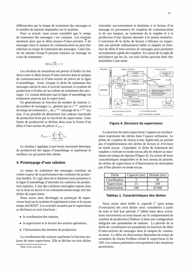
differenciees par le temps de traitement des messages etle nombre de stations implantees sur le systeme.
Pour ce travail, nous avons considere que le tempsde traitement des messages t est constant. Les resultatsmontrent alors que le delai moyen d’inter-arrivees A demessages dans le tampon de communication ne peut etreinferieur au temps de traitement des messages. Cette lim-ite est atteinte lorsqu’il persiste toujours un message encours de traitement :
Min (A) = t
Les resultats de simulation ont permis d’etablir un liendirect entre le delai moyen d’inter-arrivees dans le tamponde communication et d’inter-sorties de pieces de la ligned’assemblage. Ainsi, lorsque la tache de traitement desmessages atteint le taux d’activite maximal, le systeme deproduction n’evolue qu’au rythme de traitement des mes-sages. Ce constat demontre que la ligne d’assemblage esttotalement asservie par le superviseur.
En generalisant en fonction du nombre de stations k,du nombre de messages mi generes par la ieme station etdu temps de traitement tij du jeme message de la ieme sta-tion, il est possible de determiner une cadence maximalede production fixee par la reactivite du superviseur. Cettelimite de productvite se decline alors sous la forme d’undelai d’inter-sorties de pieces Smin :
Smin =k∑
i=1
mi∑
j=1
tij
Le resultat s’applique a une borne maximale theoriquede productivite des lignes d’assemblage et represente lemeilleur cas qui puisse etre atteint.
4. Prototypage d’une solution
Le temps de traitement des messages constitue uncritere majeur de la performance des systemes de produc-tion etudies. Il s’agit alors de le diminuer pour permettre ala ligne d’assemblage d’atteindre les cadences de produc-tion esperees. L’une des solutions envisagees repose ainsisur la mise en œuvre d’un ordonnancement temps reel destaches du superviseur.
Nous avons alors developpe un prototype de super-viseur base sur le systeme d’exploitation Linux et le noyautemps reel RTAI4. Les activites assurees par le superviseurse declinent en trois fonctions :
• la coordination des stations,
• la supervision et la lecture des actions operateurs,
• l’historisation des donnees de production.
La coordination des stations represente la fonction ma-jeure de notre superviseur. Elle se decline en trois taches
4http://www.rtai.org
executees successivement et destinees a la lecture d’unmessage en provenance du coupleur de communicationet de son tampon, au traitement de la requete et a laproduction d’une reponse destinee a la station emettrice.L’execution de la tache de lecture s’effectue en respec-tant une periode suffisamment faible et adaptee en fonc-tion du delai d’inter-arrivees de messages pour permettreun traitement rapide des requetes. En raison de la regle deprecedence qui les lie, ces trois taches peuvent donc etreassimilees a une seule.
Figure 4. Structure du superviseur
La structure de notre superviseur s’appuie sur un place-ment majoritaire des taches dans l’espace utilisateur. Lepilote du coupleur de reseau (carte Applicom) ne permetpas d’implementation des taches de lecture et d’ecritureen mode noyau. Cependant, la tache de traitement desrequetes s’execute en mode noyau afin de reduire au max-imum son temps de reponse [Figure 4]. En raison de leurscaracteristiques temporelles et de leur niveau de priorite,les taches de supervision et d’historisation ne necessitentpas d’etre placees en mode noyau.
Tache Capacite (ms) Periode (ms)
Coordination 2 30Supervision 15 100Historisation 100 10 000
Tableau 1. Caracteristiques des taches
Nous avons alors etabli la capacite C (pire tempsd’execution) des trois taches ainsi considerees a partirde tests et fixe leur periode P (delai entre deux activa-tions successives) en nous basant sur le comportement dusysteme de production [Tableau 1] dans une configurationintegrant une quarantaine de stations. La periode de latache de coordination est parametree en fonction du delaid’inter-arrivees de messages dans le tampon de commu-nication. Ce delai est directement dependant du temps descrutation du reseau Profibus reliant le superviseur et lesAPI. Les valeurs presentees correspondent a des situationspessimistes.
55

L’algorithme Rate Monotonic [LIU-73] est retenu pourordonnancer les taches. La tache de coordination se voitevidemment attribuer la plus forte priorite.
L’ordonnanabilite du jeu de taches se determine clas-siquement par le calcul du taux d’occupation U du pro-cesseur du superviseur. Elle est verifiee lorsque :
U =n∑
i=1
Ci
Pi≤ n (2
1n − 1)
Le taux d’occupation obtenu est proche de 0.23. Cettevaleur correspond donc a un taux d’occupation voisin de23% et reste bien inferieure a la borne n (2
1n − 1) garan-
tissant ainsi que toutes les contraintes de temps seront re-spectees [Figure 5].
0 5 10 15 20 25 30 35 40 45 50 55 60 65 70 75 80 85 90 95 100
0 5 10 15 20 25 30 35 40 45 50 55 60 65 70 75 80 85 90 95 100
0 5 10 15 20 25 30 35 40 45 50 55 60 65 70 75 80 85 90 95 100
Coordination
Supervision
Historisation
1 2 3
1
1 1 1
4
100 105 110 115 120 125 130 135 140 145 150 155 160 165 170 175 180 185 190 195 200
100 105 110 115 120 125 130 135 140 145 150 155 160 165 170 175 180 185 190 195 200
100 105 110 115 120 125 130 135 140 145 150 155 160 165 170 175 180 185 190 195 200
Coordination
Supervision
Historisation
5 6 7
2
1 1 1 1
Figure 5. Ordonnancement des taches
Les bornes sur les temps de reponse ont ete verifiees al’aide du logiciel Cheddar [SIN-04]. Elle est de 2 ms pourla tache de coordination. Pour la tache de supervision, elleest de 17 ms. Enfin, la borne sur le temps de reponse estde 140 ms pour la tache d’historisation.
5. Conclusion et perspectives
L’objectif de ce travail etait en premier lieu d’analyserl’influence d’un superviseur sur les cadences de produc-tion de lignes d’assemblage automatisees. Il s’agissait en-suite de proposer une solution apportant les possibilites depilotage des procedes consideres avec un nombre impor-tant de stations.
En effet, les contraintes du superviseur, en terme dereactivite, peuvent etre fortes pour permettre d’atteindreles volumes de production souhaites. Nous avons alorsmontre que la mise en œuvre d’un noyau temps reel as-sociee a un ordonnancement adapte des taches permetd’accroıtre la performance du superviseur etudie et derepondre aux objectif de production. Il est alors possi-ble d’asservir des lignes d’assemblage dont le nombre destations est eleve.
Bien que les resultats obtenus representent un fortinteret du point de vue de la productivite, il paraıt
interessant de mener une reflexion sur le mode de consom-mation des messages. Ce travail sera destine a l’evaluationdes possibilites complementaires d’amelioration de la per-formance des systemes de production par un ordonnance-ment des messages jusque la consommes dans l’ordre deleur arrivee dans le tampon de communication.
References
[BAR-98] M. BARAD – Timed Petri nets as a verificationtool – Proccedings of the 1998 Winter Simula-tion Conference, 1998.
[GRI-01] A. GRIECO, Q. SEMERARO, T. TOLIO – A re-view of different approaches to the FMS load-ing problem – The International Journal ofFlexible Manufacturing Systems, vol. 13, p.361-384, 2001.
[LIU-73] C.L. LIU, J.W. LAYLAND – Scheduling algo-rithms for multi-programming in a hard real-time environment – Journal of the Associationfor Computing Machinery, vol. 10(1), p. 40-61, 1973.
[PLA-05] L. PLASSART, P. LE PARC, F. SINGHOFF,L. MARCE – Modelling and simulation of in-teractions between the local command unitsand the supervisor of an automated assemblyline: a case study – XVI Workshop on Super-vising and Diagnostics Systems, n 1-2, chap.5, p. 210-221, 2005.
[PRO-94] J.M. PROTH, X. XIE – Les reseaux de Petripour la conception et la gestion des systemesde production – Masson, 1994.
[SIN-04] F. SINGHOFF, J. LEGRAND, L. NANA,L. MARCE – Cheddar: a flexible real-timescheduling framework – ACM Ada LettersJournal, vol. 24(4), p. 1-8, 2004.
[ZIM-96] A. ZIMMERMANN, K. DALKOWSKI,G. HOMMEL – A case study in modellingand performance evaluation of manufacturingsystems using colored Petri nets – Proceedingsof the 8th European Simulation Symposium(ESS’96), p. 282-286, 1996.
RJCITR 2005 56

Thème 4
Pires Temps d’Exécution et Conception Faible Consommation d’Energie.


Calcul de temps d’exécution au pire cas pour code mobile
Nadia Bel Hadj Aissa, Gilles GrimaudIRCICA/LIFL, UMR CNRS 8022
INRIA Futurs, projet POPSBâtiment M3, Cité Scientifique, 59650 - Villeneuve d’ascq Cedex
{Nadia.Bel-Hadj-Aissa,Gilles.Grimaud}@lifl.fr
Abstract
Nous nous proposons de définir une approche distri-buée de calcul de temps d’exécution au pire cas en consi-dérant les problèmes liés à la mobilité du code. En effet,l’utilisation de supports d’exécution distincts (i.ei.e. pro-ducteurs et consommateurs de code), qui ne se font pasmutuellement confiance et qui n’ont pas des ressourceséquitables, soulève de nouveaux problèmes quand le res-pect des échéances doit être assuré. La distribution effi-cace du processus de calcul de WCET devra permettre,en premier lieu, d’alléger la charge attribuée au consom-mateur qui dispose d’une architecture minimaliste. Endeuxième lieu, le processus distribué devra garantir quela sécurité de l’hôte n’est pas menacée. Nous nous addres-sons plus précisément à des problèmes de sécurité souventnégligés tels que la disponibilité des ressources et la ga-rantie de temps de réponse.
1 Introduction
Nous nous proposons de définir une approche distri-buée de calcul de temps d’exécution au pire cas en consi-dérant les problèmes liés à la mobilité du code. En ef-fet, l’utilisation de supports d’exécution distincts (i.e. pro-ducteurs et consommateurs de code) qui ne se font pasmutuellement confiance soulève de nouveaux problèmesquand le respect des échéances doit être assuré. Dansnos hypothèses de départ, le producteur, qui compile lecode source dans une forme intermédiaire, dispose de res-sources matérielles (mémoire, CPU,. . .) considérées infi-nies. D’autre part, le consommateur, qui reçoit le code in-termédiaire et l’exécute, est un Petit Objet Portable et Sé-curisé (POPS) tel qu’une carte à puce,. . .Deux questionsmajeures se posent généralement quand on s’adresse à cetype de dispostif dans le cadre d’un scénario de mobiltédu code : Est-ce que le peu de ressources dont dispose leconsommateur est suffisant pour exécuter le code et véri-fier sa sûreté ? Comment garantir que le code envoyé par leproducteur peut s’exécuter sur l’hôte sans compromettresa sécurité ?
Nous essayerons, dans ce qui suit, de présenter une
ébauche de notre réponse à ses questions en considérantdes problèmes de sécurité essentiels qui restent en suspensdans les travaux actuels, et cela tant en termes de disponi-bilité des ressources qu’en termes de garantie de temps deréponse dans des systèmes temps réels désormais ouverts.
2 Pourquoi distribuer le calcul de WCET ?
Plusieurs approches de calcul de WCET existent au-jourd’hui [1, 2, 3]. Toutefois, les travaux qui considèrentles problèmes liés à la mobilité du code ne sont pasnombreux [4]. En effet, le processus de calcul du piretemps d’exécution sur du code mobile diffère du pro-cessus atomique classique qui s’exécute dans une plate-forme dont les propriétés (architecture matérielle, envi-ronnement d’exécution, stratégie de compilation ou d’in-terprétation. . .) sont connues à l’avance.
Quand on se place dans le contexte de code mobile,le code est d’abord compilé sur un producteur puis misà la disposition de consommateurs potentiels qui devrontle déployer sur leur propre environnement d’exécution.Au moment de la compilation, le producteur ne peutémettre aucune supposition préalable sur le consomma-teur de code. La forme intermédiaire du code source qu’ilfournit est complètement indépendante de la plate-formesur laquelle il va s’exécuter. Ce schéma de fonctionne-ment distribué a un impact sur l’algorithme de calcul deWCET. Ce dernier, intimement lié à l’architecture maté-rielle du consommateur (i.e. nombre de cycles du proces-seur consommés par le programme), doit donc être exé-cuté au moment du déploiement du code sur le consom-mateur plutôt qu’au moment de la compilation sur le pro-ducteur.
Toutefois, les dispositifs visés étant fortementcontraints en terme de puissance de calcul, d’espacemémoire . . ., on peut difficilement envisager de laisser lecalcul du WCET à la charge du consommateur. L’analysestatique de code, la recherche du plus long chemin dansun arbre, par exemple, sont des composantes essentiellesdans un tel algorithme et sollicitent généralement beau-coup de ressources. De ce fait, la distribution efficacedu processus de calcul de WCET devrait profiter desressources considérés infinies du producteur de code pour
59
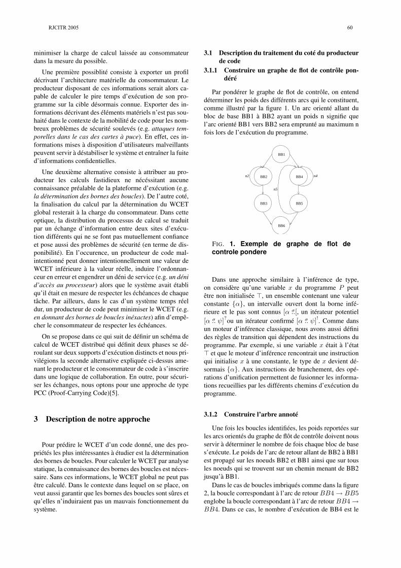
minimiser la charge de calcul laissée au consommateurdans la mesure du possible.
Une première possiblité consiste à exporter un profildécrivant l’architecture matérielle du consommateur. Leproducteur disposant de ces informations serait alors ca-pable de calculer le pire temps d’exécution de son pro-gramme sur la cible désormais connue. Exporter des in-formations décrivant des éléments matériels n’est pas sou-haité dans le contexte de la mobilité de code pour les nom-breux problèmes de sécurité soulevés (e.g. attaques tem-porelles dans le cas des cartes à puce). En effet, ces in-formations mises à disposition d’utilisateurs malveillantspeuvent servir à déstabiliser le système et entraîner la fuited’informations confidentielles.
Une deuxième alternative consiste à attribuer au pro-ducteur les calculs fastidieux ne nécéssitant aucuneconnaissance préalable de la plateforme d’exécution (e.g.la détermination des bornes des boucles). De l’autre coté,la finalisation du calcul par la détermination du WCETglobal resterait à la charge du consommateur. Dans cetteoptique, la distribution du processus de calcul se traduitpar un échange d’information entre deux sites d’exécu-tion différents qui ne se font pas mutuellement confianceet pose aussi des problèmes de sécurité (en terme de dis-ponibilité). En l’occurence, un producteur de code mal-intentionné peut donner intentionnellement une valeur deWCET inférieure à la valeur réelle, induire l’ordonnan-ceur en erreur et engendrer un déni de service (e.g. un dénid’accès au processeur) alors que le système avait établiqu’il était en mesure de respecter les échéances de chaquetâche. Par ailleurs, dans le cas d’un système temps réeldur, un producteur de code peut minimiser le WCET (e.g.en donnant des bornes de boucles inéxactes) afin d’empê-cher le consommateur de respecter les échéances.
On se propose dans ce qui suit de définir un schéma decalcul de WCET distribué qui définit deux phases se dé-roulant sur deux supports d’exécution distincts et nous pri-vilégions la seconde alternative expliquée ci-dessus ame-nant le producteur et le consommateur de code à s’inscriredans une logique de collaboration. En outre, pour sécuri-ser les échanges, nous optons pour une approche de typePCC (Proof-Carrying Code)[5].
3 Description de notre approche
Pour prédire le WCET d’un code donné, une des pro-priétés les plus intéressantes à étudier est la déterminationdes bornes de boucles. Pour calculer le WCET par analysestatique, la connaissance des bornes des boucles est néces-saire. Sans ces informations, le WCET global ne peut pasêtre calculé. Dans le contexte dans lequel on se place, onveut aussi garantir que les bornes des boucles sont sûres etqu’elles n’induiraient pas un mauvais fonctionnement dusystème.
3.1 Description du traitement du coté du producteurde code
3.1.1 Construire un graphe de flot de contrôle pon-déré
Par pondérer le graphe de flot de contrôle, on entenddéterminer les poids des différents arcs qui le constituent,comme illustré par la figure 1. Un arc orienté allant dubloc de base BB1 à BB2 ayant un poids n signifie quel’arc orienté BB1 vers BB2 sera emprunté au maximum nfois lors de l’exécution du programme.
BB1
BB2 BB4
BB5BB3
BB6
n2
n5
n4
FIG. 1. Exemple de graphe de flot decontrole pondere
Dans une approche similaire à l’inférence de type,on considère qu’une variable x du programme P peutêtre non initialisée >, un ensemble contenant une valeurconstante {α}, un intervalle ouvert dont la borne infé-rieure et le pas sont connus [α σ..[, un itérateur potentiel[α σ.. ψ]?ou un itérateur confirmé [α σ.. ψ]!. Comme dansun moteur d’inférence classique, nous avons aussi définides règles de transition qui dépendent des instructions duprogramme. Par exemple, si une variable x était à l’état> et que le moteur d’inférence rencontrait une instructionqui initialise x à une constante, le type de x devient dé-sormais {α}. Aux instructions de branchement, des opé-rations d’unification permettent de fusionner les informa-tions recueillies par les différents chemins d’exécution duprogramme.
3.1.2 Construire l’arbre annoté
Une fois les boucles identifiées, les poids reportées surles arcs orientés du graphe de flôt de contrôle doivent nousservir à déterminer le nombre de fois chaque bloc de bases’exécute. Le poids de l’arc de retour allant de BB2 à BB1est propagé sur les noeuds BB2 et BB1 ainsi que sur tousles noeuds qui se trouvent sur un chemin menant de BB2jusqu’à BB1.
Dans le cas de boucles imbriqués comme dans la figure2, la boucle correspondant à l’arc de retour BB4 → BB5englobe la boucle correspondant à l’arc de retour BB4 →BB4. Dans ce cas, le nombre d’exécution de BB4 est le
RJCITR 2005 60
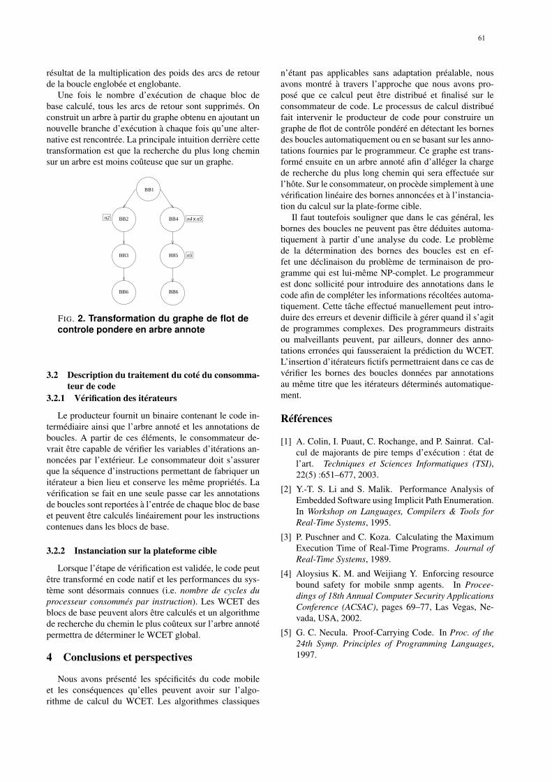
résultat de la multiplication des poids des arcs de retourde la boucle englobée et englobante.
Une fois le nombre d’exécution de chaque bloc debase calculé, tous les arcs de retour sont supprimés. Onconstruit un arbre à partir du graphe obtenu en ajoutant unnouvelle branche d’exécution à chaque fois qu’une alter-native est rencontrée. La principale intuition derrière cettetransformation est que la recherche du plus long cheminsur un arbre est moins coûteuse que sur un graphe.
BB1
n2
n5
BB4BB2
BB6 BB6
BB3 BB5
n5n4 x
FIG. 2. Transformation du graphe de flot decontrole pondere en arbre annote
3.2 Description du traitement du coté du consomma-teur de code
3.2.1 Vérification des itérateurs
Le producteur fournit un binaire contenant le code in-termédiaire ainsi que l’arbre annoté et les annotations deboucles. A partir de ces éléments, le consommateur de-vrait être capable de vérifier les variables d’itérations an-noncées par l’extérieur. Le consommateur doit s’assurerque la séquence d’instructions permettant de fabriquer unitérateur a bien lieu et conserve les même propriétés. Lavérification se fait en une seule passe car les annotationsde boucles sont reportées à l’entrée de chaque bloc de baseet peuvent être calculés linéairement pour les instructionscontenues dans les blocs de base.
3.2.2 Instanciation sur la plateforme cible
Lorsque l’étape de vérification est validée, le code peutêtre transformé en code natif et les performances du sys-tème sont désormais connues (i.e. nombre de cycles duprocesseur consommés par instruction). Les WCET desblocs de base peuvent alors être calculés et un algorithmede recherche du chemin le plus coûteux sur l’arbre annotépermettra de déterminer le WCET global.
4 Conclusions et perspectives
Nous avons présenté les spécificités du code mobileet les conséquences qu’elles peuvent avoir sur l’algo-rithme de calcul du WCET. Les algorithmes classiques
n’étant pas applicables sans adaptation préalable, nousavons montré à travers l’approche que nous avons pro-posé que ce calcul peut être distribué et finalisé sur leconsommateur de code. Le processus de calcul distribuéfait intervenir le producteur de code pour construire ungraphe de flot de contrôle pondéré en détectant les bornesdes boucles automatiquement ou en se basant sur les anno-tations fournies par le programmeur. Ce graphe est trans-formé ensuite en un arbre annoté afin d’alléger la chargede recherche du plus long chemin qui sera effectuée surl’hôte. Sur le consommateur, on procède simplement à unevérification linéaire des bornes annoncées et à l’instancia-tion du calcul sur la plate-forme cible.
Il faut toutefois souligner que dans le cas général, lesbornes des boucles ne peuvent pas être déduites automa-tiquement à partir d’une analyse du code. Le problèmede la détermination des bornes des boucles est en ef-fet une déclinaison du problème de terminaison de pro-gramme qui est lui-même NP-complet. Le programmeurest donc sollicité pour introduire des annotations dans lecode afin de compléter les informations récoltées automa-tiquement. Cette tâche effectué manuellement peut intro-duire des erreurs et devenir difficile à gérer quand il s’agitde programmes complexes. Des programmeurs distraitsou malveillants peuvent, par ailleurs, donner des anno-tations erronées qui fausseraient la prédiction du WCET.L’insertion d’itérateurs fictifs permettraient dans ce cas devérifier les bornes des boucles données par annotationsau même titre que les itérateurs déterminés automatique-ment.
Références
[1] A. Colin, I. Puaut, C. Rochange, and P. Sainrat. Cal-cul de majorants de pire temps d’exécution : état del’art. Techniques et Sciences Informatiques (TSI),22(5) :651–677, 2003.
[2] Y.-T. S. Li and S. Malik. Performance Analysis ofEmbedded Software using Implicit Path Enumeration.In Workshop on Languages, Compilers & Tools forReal-Time Systems, 1995.
[3] P. Puschner and C. Koza. Calculating the MaximumExecution Time of Real-Time Programs. Journal ofReal-Time Systems, 1989.
[4] Aloysius K. M. and Weijiang Y. Enforcing resourcebound safety for mobile snmp agents. In Procee-dings of 18th Annual Computer Security ApplicationsConference (ACSAC), pages 69–77, Las Vegas, Ne-vada, USA, 2002.
[5] G. C. Necula. Proof-Carrying Code. In Proc. of the24th Symp. Principles of Programming Languages,1997.
61

RJCITR 2005 62

Safe measurement-based WCET estimation
Jean-François Deverge and Isabelle PuautUniversité de Rennes 1 - IRISA
Campus Universitaire de Beaulieu35042 Rennes Cedex, France
{Jean-Francois.Deverge|Isabelle.Puaut}@irisa.fr
Abstract
This paper explores the issues to be addressed to providesafe worst-case execution time (WCET) estimation methodsbased on measurements. We suggest to use structural test-ing for the exhaustive exploration of paths in a program.Since test data generation is in general too complex to beused in practice for most real-size programs, we proposeto generate test data for program segments only, using pro-gram clustering. Moreover, to be able to combine executiontime of program segments and to obtain the WCET of thewhole program, we advocate the use of compiler techniquesto reduce (ideally eliminate) the timing variability of pro-gram segments and to make the time of program segmentsindependent from one another.1
1. Motivation
Computation of WCET is an important issue for hardreal-time systems. Common approaches for WCET com-putations deal with static analysis of program structures.They rely on hardware models to produce execution timeestimations. Latest processors have performance increas-ing features like caches, branch predictors or multiple-issuepipelines that maintain an internal state that is difficult topredict. As a consequence, these complex hardware mod-els are harder and harder to design [7], leading to safe butpessimistic estimations.
An alternative approach is to use measurements on realhardware (or a cycle accurate simulator) to obtain WCETestimates. However, exhaustive enumeration of all programinputs is intractable for most programs. Heuristics, like evo-lutionary algorithms [16], might be used to generate inputtest data that may cover the worst case path of the pro-gram. While yielding realistic WCET estimations, there isno guarantee to measure the worst case execution path ofthe program. Therefore, these methods have almost beenused to increase confidence of static WCET analysis meth-ods only [13].
On one hand, program testing may produce unsafe butrealistic results. On the other hand, static WCET analy-
1This paper was previously published in Proceedings of the 5th Inter-national Workshop on Worst Case Execution Time Analysis, pages 7-10,Palma de Mallorca, Spain, July 2005.
sis approaches produce safe but pessimistic WCET estima-tions. However, safe and tight estimations of the WCET arehighly desirable. Ideally, one would desire WCET tools thatproduce safe and tight results without harness developmentof timing models for the next generation processors.
This paper explores the issues to be addressed to design ameasurement-based method that produces safe results. Wepropose to rely on structural testing [20] methods to gen-erate input test data and to exhaustively measure the ex-ecution time of program paths. We advocate the use ofcompiler techniques to reduce (ideally eliminate) the tim-ing variability of program measurements. In Section 2, weoutline our method for WCET timing analysis and we givesome properties on hardware measurements our method re-lies on. Section 3 describes how the properties are met,through the control of the unpredictability of some hard-ware mechanisms, and contains some preliminary resultsof path measurements on a PowerPC 7450. Related work,some concluding remarks and directions of our ongoingwork are given in Section 4.
2. Method outline
One would obtain the program’s WCET by measuring allprogram executions with any of the possible input data forthis program. However, exhaustive enumeration of a pro-gram input is unfeasible for most programs. Another ap-proach is to measure all paths of the program. This reducesthe number of measurements because a set of possible in-put data may activate the same program path. However, thepath coverage is impracticable for program with unboundedloops, yielding an infinite number of paths [20].
In this paper, we propose to employ structural testingmethods [8, 18, 20] to automatically generate input data.These methods generate the input data set from the analysisof the program structures.
A key assumption we make is that the measurement ofthe executions of the same program path, with different datavalues, yields the same timing results. Meeting this assump-tion requires to control the hardware: this issue is discussedin Section 3.
Program clustering. Test data generation methods aremostly based on equations [8] or constraint solving tech-niques [18]. Due to solver tools and their potentially lack of
63

scalability, the analysis of complete paths of the whole pro-gram could be unachievable in practice. Moreover, numberof paths could be exponential even for small program. Asa consequence, we suggest splitting paths into segments tolower the complexity of test data generation.
An example, the program of Figure 1 contains���������
paths. For small values of ���� (for example ���� �������), it is conceivable to exhaustively make measurements
of this code.
A
B
op
op
op
op op: observation point
3
7
9
10
Figure 1. Path clustering.
However, for greater values of ���� , it would be suit-able to split the program and apply measurements on seg-ments. This process is called program clustering. An in-tuitive solution to tackle test data generation complexity ofthe code of Figure 1 is to build two clusters � and � . Inthis configuration, there are only two paths in cluster � anda single path on cluster � .
Application of clustering on the program works as fol-lows. The automated test data generation is first applied tothe whole program. If it produces too many results or ifit does not terminate before a limited amount of time, westop it. We then launch test data generation on smaller partsof the program (e.g. sub trees of the program syntax tree).This iterative process is repeated until segments are smallenough to make exhaustive path enumeration inside a seg-ment tractable. We obtain leaf cluster like � .
Program measurement. We focus on the exploitation ofprogram measurements but we don’t address methods to ob-tain program execution times: there exist multiple hardwareand software methods described in [11, 14]. Observationspoints provide execution traces and give the execution timesof the program units observed [11]. In our approach, wehave to place observations points at the cluster boundaries.For example, there are four observation points ����� , ����� , ���� and ����!#" on Figure 1.
We first measure the two paths of cluster � and we ob-tain values $ � and %�& cycles for instance. The worst valueis the WCET of the cluster � and ')(* ,+.- is %/& . Then,we execute and we measure the single path of cluster � .Table 1 contains the measurement trace of this execution.
The value of +��01 �2 is not the WCET for the wholeprogram, because this execution could have covered theshortest path of cluster � . Consequently, we have to add thedifference between ')(* 3+ - and each +��01 - measuredduring the execution of cluster � . In this way, we obtain anupper bound of the global WCET. Program clustering en-ables automated test data generation on subprogram pathsor program segments. The longer the program segmentswill be, the tighter the WCET estimation will be.
Observation point Time stamp Observation interval465�7 8465:9 ;=<465�> ?@< ACBEDGFCHJIGK�8465 9 ;�8L<465 > M 8@8 ACBEDGF H IONL<. . . . . .465:9 <@<�K@<�?@<465 > <@<�K�PL<�< ACBEDGF H IGK�8465�QSR <@<�K�P@N@< ATBEDOFTUVIO<@<�K�P@N@<
Table 1. Measurement trace of the path exe-cution of the cluster � .
In this section, we have proposed to assemble WCETof leaves clusters using measurement. We could also in-vestigate for hybrid approach that couples testing and staticWCET analysis. In such an approach, we should measureprogram segments using testing methods and we should usestatic methods to combine these context-independent seg-ments timings.
3. Obtaining safe program segment measure-ments
In previous section, we have assumed that any measure-ments of the different executions of the same program pathgives the same results. In this section, we focus on obtain-ing such safe and context-independent measurements.
There are three main sources of unpredictability in com-plex processor architectures:
1. Global mechanisms, like caches, virtual memory trans-lation (TLB) or branch predictors. Their internal stateand the contents of their tables have direct impact onthe execution time of future instructions of the wholeprogram [5, 9].
2. Variable latency instructions. Some operations, as theinteger multiplication instruction, may have variabletiming behaviour because the result should be com-puted faster on small valued input data operands.
Processor may partially implement some operations,as the float division or the square root instruction. Thismeans that, in order to support unimplemented opera-tions in hardware, an exception is raised and operationshould be computed by an exception handler providedby the operating system.
3. Statistic execution interference phenomenon [12], dueto unpredictability introduced by DRAM refresh. Sim-ilarly to variable latency instructions, load/store oper-ations to the main memory may have varying timingbehaviour. Moreover, processors have a built-in multi-ple level cache hierarchy, and some cache clock speedsmay be different to the clock speed of the core proces-sor. A tiny deviation on timings may occur if a loadrequest is received immediately or on the next clockcycle of the slower cache level.
RJCITR 2005 64

Gaining control of processor unpredictability. Obtain-ing safe and context-independent measurements requires toeliminate (or at least drastically decrease) the sources oftiming variability. For that purpose, we are currently con-sidering a few approaches relying on hardware control andcompilation methods.
Regarding the first source of unpredictability, globalmechanisms might be disabled or we should clear their his-tory tables before the execution of each program segment.Cache conscious data placement [4] and cache locking [15]reduce varying timings of memory accesses. Likewise,static branch prediction enable to fix behaviour of specu-lative execution at compilation time [3].
In order to support variable latency operations, [19] pro-poses to add the difference between the BCET and theWCET of all the operations of the program path. Anotherapproach consists in avoiding the use of these operationsand to replace them by predictable instructions.
We could forbid the varying timing behaviour of partiallyunimplemented instruction by disabling the execution of theexception handler. However, this may affect operationalsemantics of instructions [10]. It should be preferable torewrite temporally predictable exception handler and to ap-ply the same strategies as those applied for variable latencyoperations.
It is not possible to control variability on latency of mem-ory access. However, we feel that such a fluctuation in mea-surements follows a true statistical distribution. Models toquantify pessimism to apply on results of measurements arerelated in [2]. In addition, variability of load/store opera-tions latency may be due to the input-dependent memoryaccesses of the program.
Figure 2. Single path program with unpre-dictable timings of data access.
The sample code from Figure 2 is a single path program.Nevertheless, the number of cache misses on array � de-pends on the contents of
�. To make this code temporally
deterministic, we could disable the cache feature before thememory access to contents of � [15]. We could also set thewhole array � as non cachable introducing program perfor-mance penalty. In order to enhance data access latency, wecould employ data cache locking [15] or to do scratchpadmemory allocation [1] of data subject to unknown memoryaccess patterns.
Preliminary experiments. In order to evaluate if the tim-ing variability of program segments can be controlled bysoftware, we conducted experiments on a PowerPC 7450processor [10]. This 32-bit processor is able to dispatch 3instructions per cycles on an in-order, seven stage pipeline.
It features two dynamic branch prediction mechanisms: a2-bit prediction scheme with a branch target buffer, and areturn stack predictor. Our chip has a 64-Kbyte level-one(L1) cache, and a 256-Kbyte L2 cache. A load will take 3cycles if the data is in the L1 cache. There is a maximumlatency of 9 processor cycles for L1 data cache miss thathits in the L2.
For our preliminary evaluation, we evaluated the impactof hardware control on the execution time of a program seg-ment (SNU-RT jfdctint) made of a single path. We achievedthese experiments in isolation from asynchronous activitiesby disabling operating system’s context switches and dis-abling external interrupts.
Figure 3 shows the timings of two sets of 25 mea-surements. Before each jfdctint execution measurement,we first executed one of twenty-five pollution codes: theprogram itself, random generator, load and writes of bigamount of memory, intensive control code, and somecode taken from http://www.c-lab.de/home/en/download.html.
0
500
1000
1500
2000
2500
3000
1 2 3 4 5 6 7 8 9 10 11 12 13 14 15 16 17 18 19 20 21 22 23 24 25
Exe
cutio
n tim
e in
cyc
les
with hardware controlwithout hardware control
Time−ordered measures of 25 executions
Figure 3. Measurements of jfdctint executiontimes.
The first set of measurements are made with hard-ware control. After execution of the pollution code, wehave cleared branch predictor buffers, and we have flushedcaches (TLB, L1 and L2). The second set of measurementsis made without any hardware control.
We can note that the variability of program running timesis largely reduced with hardware control. We observe thatmeasurement variability is decreased from
�E�E�/�cycles to� & � cycles. Without hardware control, the best case exe-
cution time is obtained after the execution of the programitself (warm caches effect). The worst case execution timeis due to a pollution code that fills the entire data cache withdirty lines. Consequently, for many data accesses of themeasured program, the processor had to update the mem-ory with the victim cache contents before its replacementwith program data.
We have investigated the sources of variability onmeasurement with hardware control. The memoryperformance-monitoring counters on the PowerPC 7450 re-veal that main sources of variability, for program measure-ments with hardware control, are due to main memory andL2 variable access latency.
It can be remarked that average program running timesare almost the same with or without hardware control.
65
There is no performance degradation on that specific exper-iment because we did neither deactivate the cache nor thebranch predictor. This suggests that long program segmentscan take advantage of dynamic mechanisms if history tablesor related internal states could be cleared before execution.
4. Conclusion and future work
In this paper, we have proposed to compute the WCETfrom execution measurements. We advocate the use ofstructural testing methods and program clustering to en-able measurements of the worst case execution path. Thismeasurement-based approach would produce safe and tightresults.
Recently, the use of another software unit test approachhas been proposed in [17]. Model checking methods pro-duce input data to exhaustively cover paths of automaticallygenerated programs from MatLab/Simulink specifications.This approach enables to measure WCET of straight-line Cprograms with no loops.
Previously, [19] has used data flow analysis to detectsingle feasible path segments of the program. In their ap-proach, only single path segments are measured, and staticWCET analysis is employed on the rest of the program. [19]gives conditions to obtain safe measurements on processorswith cache.
Clustering techniques have been applied to static WCETanalysis methods to enhance their scalability [6]. The clus-tering is applied on the syntax tree of the program and themain criterion used is a limit on the number of generatedconstraints. We propose to apply a similar strategy in ourapproach, our objective being to reduce the complexity oftest data generation.
Traditional static WCET analysis and measurement arecombined in [2]. There is no control of the hardware andstatistical models are applied, thus providing a probabilisticsafety on the global WCET [2]. The combination of testdata generation methods and these techniques would repre-sent a fruitful area of study.
Our method has to control any processor features likecache or branch prediction to reduce the unpredictabilityof these advanced processors mechanisms. We plan to fur-ther study the balance between hardware control, necessaryyielding negative performance impact on execution time,and the benefit with respect to measurements variability.
References
[1] O. Avissar, R. Barua, and D. Stewart. An optimal mem-ory allocation scheme for scratch-pad-based embedded sys-tems. ACM Transactions on Embedded Computing Systems,1(1):6–26, Nov. 2002.
[2] G. Bernat, A. Colin, and S. M. Petters. WCET analysis ofprobabilistic hard real-time system. In Proceedings of the23rd IEEE Real-Time Systems Symposium, pages 279–288,Austin, TX, Dec. 2002.
[3] F. Bodin and I. Puaut. A WCET-oriented static branch pre-diction scheme for real time systems. In Proceedings of the17th Euromicro Conference on Real-Time Systems, pages33–40, Palma de Mallorca, Spain, July 2005.
[4] B. Calder, C. Krintz, S. John, and T. Austin. Cache-conscious data placement. In Proceedings of the 8th Inter-national Conference on Architectural Support for Program-ming Languages and Operating Systems, pages 139–149,San Jose, CA, Oct. 1998.
[5] J. Engblom. Analysis of the execution time unpredictabilitycaused by dynamic branch prediction. In Proceedings of the9th IEEE Real-Time and Embedded Technology and Appli-cations Symposium, pages 152–159, Toronto, Canada, May2003.
[6] A. Ermedahl, F. Stappert, and J. Engblom. Clustered calcu-lation of worst-case execution times. In Proceedings of theInternational Conference on Compilers, Architectures andSynthesis for Embedded Systems, pages 51–62, San Jose,CA, Oct. 2003.
[7] R. Heckmann, M. Langenbach, S. Thesing, and R. Wil-helm. The influence of processor architecture on the designand the results of WCET tools. Proceedings of the IEEE,91(7):1038–1054, 2003.
[8] G. Lee, J. Morris, K. Parker, G. A. Bundell, and P. Lam.Using symbolic execution to guide test generation. Soft-ware Testing, Verification and Reliability, 15(1):41–61, Mar.2005.
[9] T. Lundqvist and P. Stenström. Timing anomalies in dy-namically scheduled microprocessors. In Proceedings ofthe 20th IEEE Real-Time Systems Symposium, pages 12–21,Phoenix, AZ, Dec. 1999.
[10] MPC7450 RISC microprocessor family processor manualrevision 5. Freescale Semiconductor, Jan. 2005.
[11] S. M. Petters. Comparison of trace generation methods formeasurement based WCET analysis. In Proceedings of the3rd International Workshop on Worst Case Execution TimeAnalysis, pages 61–64, Porto, Portugal, June 2003.
[12] S. M. Petters and G. Färber. Making worst case executiontime analysis for hard real-time tasks on state of the art pro-cessors feasible. In Proceedings of the 6th InternationalWorkshop on Real-Time Computing and Applications Sym-posium, pages 442–449, Hong Kong, China, Dec. 1999.
[13] P. Puschner and R. Nossal. Testing the results of staticworst-case execution-time analysis. In Proceedings of the19th IEEE Real-Time Systems Symposium, pages 134–143,Madrid, Spain, Dec. 1998.
[14] B. Sprunt. The basics of performance-monitoring hardware.IEEE Micro, 22(4):64–71, July 2002.
[15] X. Vera, B. Lisper, and J. Xue. Data cache locking for higherprogram predictability. In Proceedings of the ACM SIG-METRICS International Conference on Measurement andModeling of Computer Systems, pages 272–282, San Diego,CA, June 2003.
[16] J. Wegener and M. Grochtmann. Verifying timing con-straints of real-time systems by means of evolutionary test-ing. Real-Time Systems, 15(3):275–298, Nov. 1998.
[17] I. Wenzel, B. Rieder, R. Kirner, and P. Puschner. Automatictiming model generation by CFG partitioning and modelchecking. In Proceedings of the Conference on Design, Au-tomation, and Test in Europe, pages 606–611, Munich, Ger-many, Mar. 2005.
[18] N. Williams, B. Marre, and P. Mouy. On-the-fly generationof k-path tests for C functions. In Proceedings of the 19thIEEE International Conference on Automated Software En-gineering, pages 290–293, Linz, Austria, Sept. 2004.
[19] F. Wolf, R. Ernst, and W. Ye. Path clustering in softwaretiming analysis. IEEE Transactions on Very Large Scale In-tegration Systems, 9(6):773–782, Dec. 2001.
[20] H. Zhu, P. A. V. Hall, and J. H. R. May. Software unittest coverage and adequacy. ACM Computing Surveys,29(4):366–427, Dec. 1997.
RJCITR 2005 66

Application cooperative et gestion de l’energie du processeur
Richard UrunuelaEcole des mines de nantes
projet Obasco EMN/[email protected]
Resume :La puissance de calcul des systemes mobiles rend pos-
sible l’exploitation d’application multimedia. C’est sou-vent au detriment de l’autonomie. Ce probleme est d’au-tant plus complexe que l’element clef, le processeur,est gere par l’ordonnanceur et le gestionnaire d’energie.Notre solution repose sur une cooperation entre les appli-cations et le systeme pour realiser les objectifs suivants,Maximiser la duree de vie des batteries et fournir la puis-sance de calcul necessaire aux applications.
1. Introduction
Les applications multimedias sur des systemes mobilesgeneralistes connaissent de plus en plus de succes aupresdu grand public. Ces applications sont caracterisees parune consommation tres importante en ressource proces-seur. Cette consommation de puissance de calcul entraıneune consommation electrique importante, qui diminued’autant l’autonomie attendue par l’utilisateur. Le systemedoit gerer soigneusement l’energie et le processeur. Cettegestion est particulierement delicate pour les applicationsmultimedias car le besoin en ressource processeur peutvarier enormement d’une trame a une autre. De plus, lesapplications multimedias sont des applications temps reelmolles pour lesquelles un retard d’execution de quelquesdixiemes de secondes a un impact sur la qualite du trai-tement. La plupart des gestionnaires d’energie sur lessystemes d’exploitation generalistes ne sont pas adaptesa l’execution d’applications avec des changements rapidede leurs besoins processeur. Cette inefficacite a souventpour consequence une gestion mediocre de la consomma-tion electrique. Dans ce papier nous proposons une solu-tion pour qu’une application coopere avec le systeme pourspecifier ses besoins energetiques. De ce point de vue, lecomposant critique est le processeur de par l’ordonnan-ceur et de sa consommation electrique.
Gestionnaire de «DVS» et application multimediaDe nombreuses recherches ont ete menees pour mini-
miser la consommation electrique du processeur. Certainsde ces travaux portent sur la modification de l’ordonnan-ceur de processus [5, 9]. Dans ces approches la techniquela plus utilisee est l’adaptation dynamique de tension et
de frequence du processeur nommee «DVS» («dynamicvoltage scaling») [6].
Certaines solutions reposent sur l’observation de lacharge processeur et l’application d’algorithme de ges-tion de «DVS». Par exemple l’ordonnanceur de proces-sus PAST [8] calcule sur des intervalles de temps de 10a 50 milli-secondes l’utilisation passee du processeur. Sile temps d’inactivite du processeur est important alorsl’ordonnanceur diminue la frequence du processeur. Si cetemps d’inactivite est faible l’ordonnanceur augmente lafrequence. Cet algorithme n’est pas optimum s’il y a degrandes variations de charge du processeur a l’interieur del’intervalle de temps considere.
L’approche Vertigo [3] repond en partie a ce probleme.Cette solution consiste a ajuster automatiquement les per-formances du processeur sans participation de l’applica-tion. Il coexiste avec l’ordonnanceur natif. Vertigo uti-lise une hierarchie d’algorithmes tous specialises dansdifferents types de situations. Pour les applications inter-actives, Vertigo utilise un algorithme specifique pour di-minuer l’impact du ralentissement du systeme vis a visde l’utilisateur. Par exemple si le systeme detecte le lance-ment d’une application interactive la frequence du proces-seur est augmentee. Cette approche est efficace avec desapplications multimedias. Les algorithmes de gestion du«DVS» utilises ne sont pas modifiables.
Pouwelse et al [7] deplacent l’algorithme de decisionde la frequence du processeur dans l’application mul-timedia. Ils proposent que l’application multimediaprevoit la quantite de traitement necessaire au decodagede chaque trame. L’application indique au systeme la vi-tesse du processeur necessaire pour son execution. L’utili-sation du gestionnaire est dependante de l’execution del’application multimedia. Cette solution est uniquementadaptee sur un systeme d’exploitation mono-tache.
Application multimedia cooperativePour illustrer l’inefficacite des gestionnaires de «DVS»
nous etudions dans la seconde section de ce papier laconsommation processeur d’une application multimedia.A partir de cette analyse nous proposons une solution decooperation a la problematique de decision entre l’ordon-nanceur de processus et l’application multimedia. Notresolution met en œuvre une participation de la part de l’ap-
67

plication pour choisir une frequence de fonctionnement duprocesseur. Notre solution s’adapte aisement avec d’autresalgorithmes d’ordonnancement de processus et d’autresalgorithmes de gestion de «DVS». La frequence calculeepar une application est prioritaire sur celle calculee parle systeme. Dans le cas ou plusieurs applications choi-sissent une frequence l’ordonnanceur choisit la plus im-portante. L’ordonnanceur utilise un algorithme de gestionde «DVS» par defaut qui est supplante par ceux des ap-plications a calcul de frequence.
2 Application Multimedia et charge du pro-cesseur
Nous etudions la consommation de la ressource pro-cesseur par une application multimedia. Nous avons ef-fectue nos tests sur un Dell Inspiron 510m equipe d’unprocesseur Pentium M 735. Ce processeur fonctionne avecdes frequences de 600 Mhz a 1,7 Ghz. Pour la lecturevideo nous avons utilise l’application Mplayer (www.mplayerhq.hu) executee sur un systeme Linux 2.4.24.
0
20
40
60
80
100
0 20 40 60 80 100
cpu
load
%
time s
DIVXMPEG
FIG. 1. Lecture video et charge processeur
La figure 1 represente la charge du processeur dansle temps lors de la lecture de deux videos par Mplayer.Il s’agit de la meme video, la bande annonce du filmd’animation «Madagascar» dans deux formats d’enco-dage differents, divx 5 pour la video DIVX et mpeg 2 pourla video MPEG. Pour les deux fichiers le format est de 25images de 1024 par 768 pixels par seconde, d’une dureede 110 secondes. Nous avons utilise l’outil de monitoringmpstat [1] pour calculer la charge du processeur. Mplayerest execute dans un environnement sans gestionnaire defrequence du processeur ou la frequence du processeur estde 1,7 Ghz. Mplayer ne supprime pas de trames a la lec-ture qui s’effectue avec un rendu optimal.
Un algorithme de gestion du «DVS» comme PASTutilise sur des systemes d’exploitations generalistes estinefficace lors de l’execution d’une application telle queMplayer dont la charge processeur varie enormement dans
le temps et pour lequel les seuils de charge frequemmentutilises sont 20% et 80%. Nous constatons que la chargeprocesseur est comprise entre ces valeurs. Pourtant lesysteme peut realiser une economie significative de laconsommation electrique. Par exemple durant les 20premieres secondes de la lecture du fichier DIVX la chargeprocesseur est inferieur a 50 %. Le processeur utiliseconsomme 7 W a 900 MHz contre 21 W a 1,7 Ghz,alors en appliquant une reduction de performance de 50%l’economie theorique d’energie est de 66%.
3 Application cooperative et «DVS»
nous proposons une solution qui est de permettre al’application Mplayer d’interagir avec le gestionnaire de«DVS». En utilisant au mieux la ressource processeur oneconomise de l’energie tout en respectant les contraintestemporelles de l’application. Notre solution est mixte. Lesysteme exploite par defaut l’algorithme PAST. Si uneapplication est executee et qu’elle est instrumentee pourchoisir une frequence de fonctionnement alors l’algo-rithme PAST devient inactif.
OrdonnanceurNous effectuons notre evaluation sur un systeme Linux
avec un noyau Bossa [2]. Bossa permet de developperet d’integrer facilement et de facon sur des ordonnan-ceurs de processus. La politique d’ordonnancement deprocessus initial Linux est modifiee pour integrer l’algo-rithme PAST. Tout les n clockticks l’ordonnanceur ap-plique l’heuristique suivante. (1) Si la charge processeurest superieure a 80% la frequence du processeur est aug-mentee. (2) Si la charge processeur est inferieure a 20%cette frequence est diminuee. La valeur de la variable n estcalculee en fonction de la duree d’un clocktick systeme.La duree entre n clockticks est comprise entre 10 et 50ms suivant les specifications de l’algorithme PAST. Pourpermettre a une application de specifier sa frequence pro-cesseur de fonctionnement dans la politique d’ordonnan-cement Bossa Linux + PAST nous implementons la fonc-tion d’interface set_freq. Ce choix de frequence estprioritaire par rapport a l’algorithme PAST. A la fin del’execution d’une application a calcul de frequence l’or-donnaneur recherche la plus grande frequence de fonc-tionnement dans la liste des processus. Si ce resultat egala 0 le gestionnaire PAST est reactive.
Application multimediaL’etude de la charge processeur dans la seconde section
illustre l’inefficacite d’un gestionnaire de «DVS» tel quePAST avec des applications multimedias. Il est donc plusinteressant dans le cas de l’execution d’une applicationmultimedia que celle ci calcule sa frequence de fonction-nement. Ce calcul peut etre effectue avant ou apres le trai-tement de decodage du media. En utilisant une approche aposteriori notre solution fonctionne quel que soit le formatde compression de la video.
RJCITR 2005 68
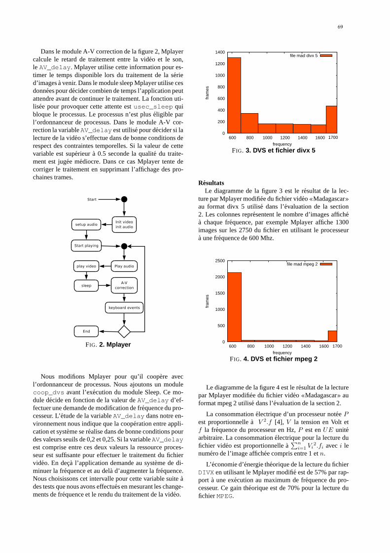
Dans le module A-V correction de la figure 2, Mplayercalcule le retard de traitement entre la video et le son,le AV_delay. Mplayer utilise cette information pour es-timer le temps disponible lors du traitement de la seried’images a venir. Dans le module sleep Mplayer utilise cesdonnees pour decider combien de temps l’application peutattendre avant de continuer le traitement. La fonction uti-lisee pour provoquer cette attente est usec_sleep quibloque le processus. Le processus n’est plus eligible parl’ordonnanceur de processus. Dans le module A-V cor-rection la variableAV_delay est utilise pour decider si lalecture de la video s’effectue dans de bonne conditions derespect des contraintes temporelles. Si la valeur de cettevariable est superieur a 0.5 seconde la qualite du traite-ment est jugee mediocre. Dans ce cas Mplayer tente decorriger le traitement en supprimant l’affichage des pro-chaines trames.
FIG. 2. Mplayer
Nous modifions Mplayer pour qu’il coopere avecl’ordonnanceur de processus. Nous ajoutons un modulecoop_dvs avant l’execution du module Sleep. Ce mo-dule decide en fonction de la valeur de AV_delay d’ef-fectuer une demande de modification de frequence du pro-cesseur. L’etude de la variable AV_delay dans notre en-vironnement nous indique que la cooperation entre appli-cation et systeme se realise dans de bonne conditions pourdes valeurs seuils de 0,2 et 0,25. Si la variableAV_delayest comprise entre ces deux valeurs la ressource proces-seur est suffisante pour effectuer le traitement du fichiervideo. En deca l’application demande au systeme de di-minuer la frequence et au dela d’augmenter la frequence.Nous choisissons cet intervalle pour cette variable suite ades tests que nous avons effectues en mesurant les change-ments de frequence et le rendu du traitement de la video.
0
200
400
600
800
1000
1200
1400
600 800 1000 1200 1400 1600
fram
es
frequency
1700
file mad divx 5
FIG. 3. DVS et fichier divx 5
ResultatsLe diagramme de la figure 3 est le resultat de la lec-
ture par Mplayer modifiee du fichier video «Madagascar»au format divx 5 utilise dans l’evaluation de la section2. Les colonnes representent le nombre d’images affichea chaque frequence, par exemple Mplayer affiche 1300images sur les 2750 du fichier en utilisant le processeura une frequence de 600 Mhz.
0
500
1000
1500
2000
2500
600 800 1000 1200 1400 1600
fram
es
frequency
1700
file mad mpeg 2
FIG. 4. DVS et fichier mpeg 2
Le diagramme de la figure 4 est le resultat de la lecturepar Mplayer modifiee du fichier video «Madagascar» auformat mpeg 2 utilise dans l’evaluation de la section 2.
La consommation electrique d’un processeur notee P
est proportionnelle a V 2.f [4], V la tension en Volt etf la frequence du processeur en Hz, P est en UE unitearbitraire. La consommation electrique pour la lecture dufichier video est proportionnelle a
∑ni=1
Vi2.fi avec i le
numero de l’image affichee compris entre 1 et n.
L’economie d’energie theorique de la lecture du fichierDIVX en utilisant le Mplayer modifie est de 57% par rap-port a une execution au maximum de frequence du pro-cesseur. Ce gain theorique est de 70% pour la lecture dufichier MPEG.
69

4 Conclusion
La gestion cooperative de la ressource energetiqueentre une application et le systeme d’exploitation est ef-ficace. Cette approche est adaptee au cas des applica-tions multimedias et de leurs contraintes temporelles. Leseconomies theoriques realisees au niveau du processeursont significative. Dans le cas des hierarchies d’ordonnan-ceurs l’integration de plusieurs gestionnaires de «DVS»
reste a etudier.Dans la suite de nos travaux nous desirons valider nos
approches en les confrontant a des mesures reelles de laconsommation electrique du systeme. Nous developponsactuellement une plate-forme, la Bossa-Box (www.emn.fr/x-info/bossa/bossabox/) pour tester et vali-der ces approches de gestions energetiques avec des appli-cations necessitant beaucoup de ressources. Par exemplenous effectuons la lecture differee d’un enregistrementvideo en cours d’acquisition.
References
[1] R. Andresen. Monitoring linux with native tools. In 30thAnnual International Conference of The Computer Measu-rement Group, Inc., Las Vegas, Nevada USA, Dec. 2004.
[2] L. P. Barreto and G. Muller. Bossa : A DSL frameworkfor application-specific scheduling policies. In IEEE, edi-tor, Eighth IEEE Workshop on Hot Topics in Operating Sys-tems (HotOS-VIII). May 20–23, 2001, Schloss Elmau, Ger-many, pages 161–161, 1109 Spring Street, Suite 300, Sil-ver Spring, MD 20910, USA, 2001. IEEE Computer SocietyPress.
[3] K. Flautner and T. N. Mudge. Vertigo : Automaticperformance-setting for linux. In Proceedings of the 5thACM Symposium on Operating System Design and Imple-mentation (OSDI-02), Operating Systems Review, pages105–116, New York, Dec. 9–11 2002. ACM Press.
[4] D. Genossar and N. Shamir. Intel pentium m processor po-wer estimation, budgeting, optimization and validation. In-tel Technology Journal, 7(2) :44–49, May 2003.
[5] K. Govil, E. Chan, and H. Wassermann. Comparing algo-rithms for dynamic speed-setting of a low-power CPU. InProceedings of the first Conference on Mobile Computingand Networking MOBICOM’95, Mar. 1995. also as techni-cal report TR-95-017, ICSI Berkeley, Apr. 1995.
[6] J. Lorch and A. Smith. Software strategies for portable com-puter energy management. IEEE Personal CommunicationsMagazine, 5(3) :60–73, June 1998.
[7] J. Pouwelse, K. Langendoen, and H. Sips. Dynamic voltagescaling on a low-power microprocessor. In MobiCom ’01 :Proceedings of the 7th annual international conference onMobile computing and networking, pages 251–259, NewYork, NY, USA, 2001. ACM Press.
[8] M. Weiser, B. Welch, A. Demers, and S. Shenker. Schedu-ling for reduced CPU energy. In Proceedings of the FirstUSENIX Symposium on Operating Systems Design and Im-plementation (OSDI), pages 13–23, 1994.
[9] A. Weissel and F. Bellosa. Process cruise control : Event-driven clock scaling for dynamic power management. InProceedings of the International Conference on Compi-lers, Architecture, and Synthesis for Embedded Systems CA-SES’02, Oct. 2002.
RJCITR 2005 70