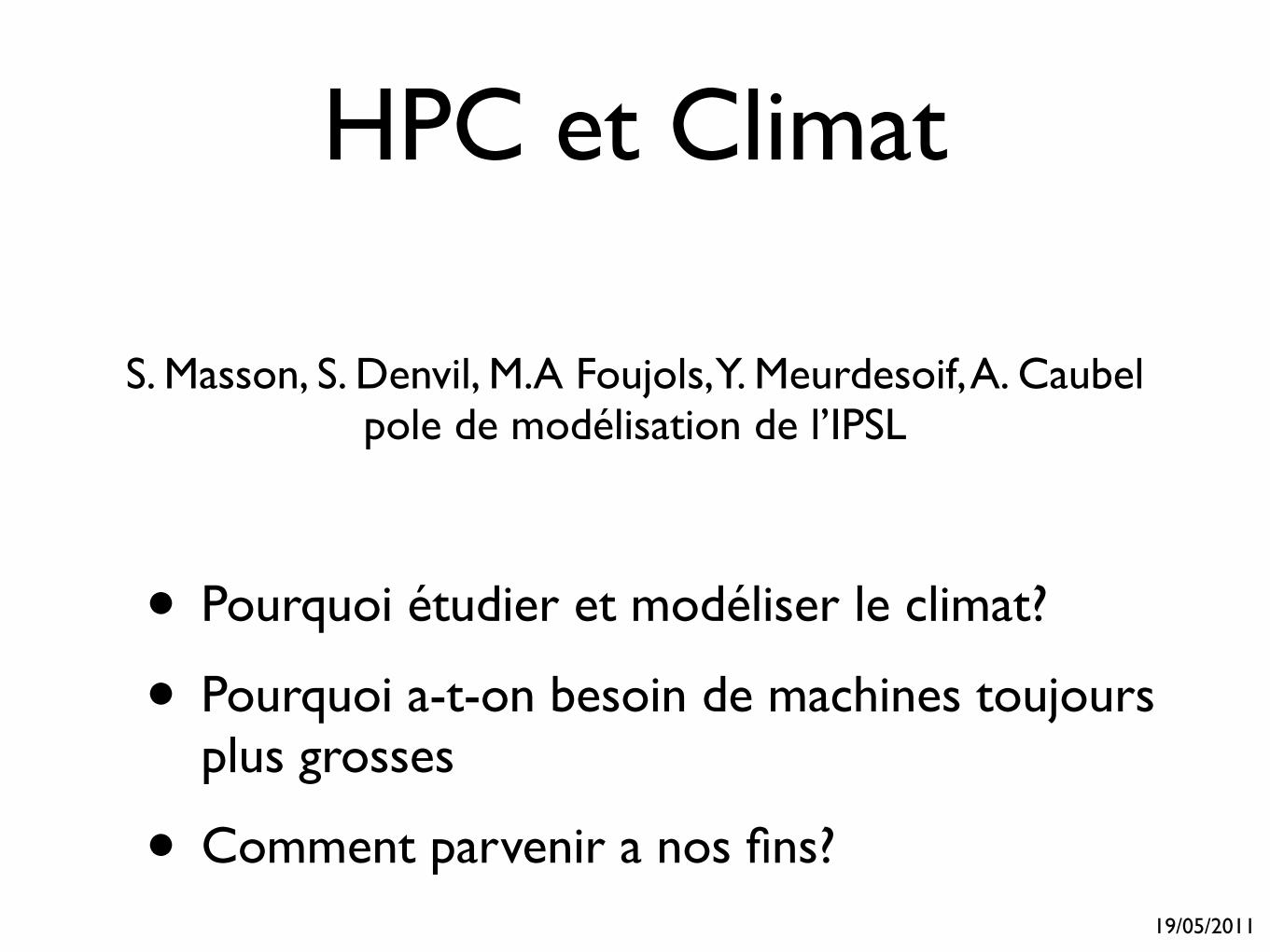
HPC et Climat

• Pourquoi étudier et modéliser le climat?

• Pourquoi a-t-on besoin de machines toujours plus grosses

• Comment parvenir a nos fins?

S. Masson, S. Denvil, M.A Foujols, Y. Meurdesoif, A. Caubelpole de modélisation de l’IPSL

19/05/2011

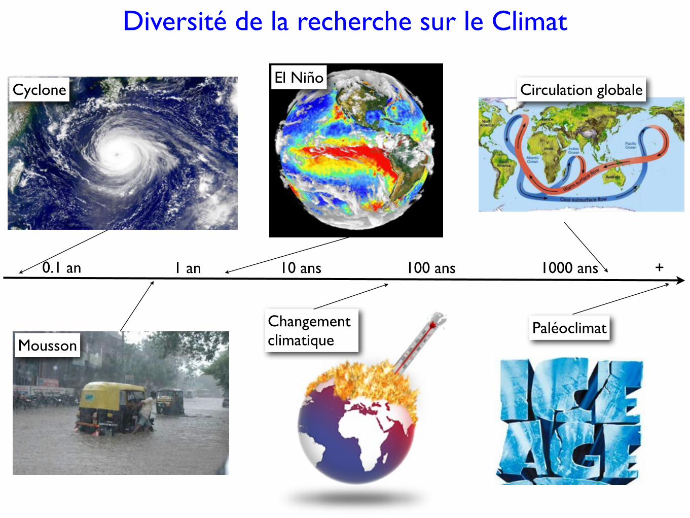
0.1 an 1 an 10 ans 100 ans 1000 ans

Diversité de la recherche sur le Climat

+

Mousson

CycloneEl Niño

Changement climatique

Circulation globale

Paléoclimat

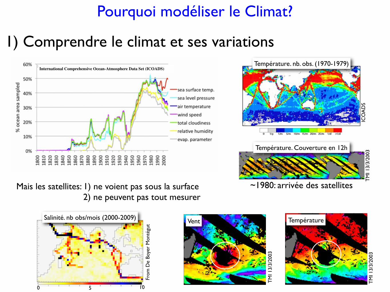
Pourquoi modéliser le Climat?

Mais les satellites: 1) ne voient pas sous la surface 2) ne peuvent pas tout mesurer

1) Comprendre le climat et ses variations

Température

TM

I 13/

3/20

03

Vent

TM

I 13/

3/20

03

~1980: arrivée des satellites

Température. Couverture en 12h

TM

I 13/

3/20

03

International Comprehensive Ocean-Atmosphere Data Set (ICOADS)Température. nb. obs. (1970-1979)

ICO

AD

S

0 10

Salinité. nb obs/mois (2000-2009)

From

De

Boye

r M

onté

gut

5

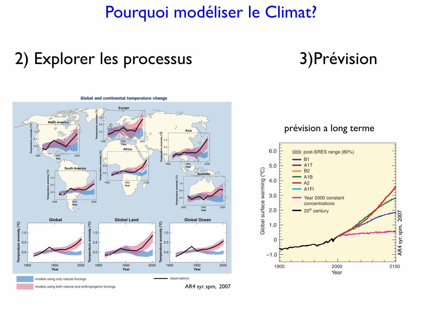
Pourquoi modéliser le Climat?

2) Explorer les processus

prévision a long terme

3)Prévision

7

Summary for Policymakers

8 For an explanation of SRES emissions scenarios, see Box ‘SRES scenarios’ in Topic 3 of this Synthesis Report. These scenarios do not includeadditional climate policies above current ones; more recent studies differ with respect to UNFCCC and Kyoto Protocol inclusion.9 Emission pathways of mitigation scenarios are discussed in Section 5.

3. Projected climate changeand its impacts

There is high agreement and much evidence that withcurrent climate change mitigation policies and related sus-tainable development practices, global GHG emissionswill continue to grow over the next few decades. {3.1}

The IPCC Special Report on Emissions Scenarios (SRES,2000) projects an increase of global GHG emissions by 25 to90% (CO2-eq) between 2000 and 2030 (Figure SPM.5), withfossil fuels maintaining their dominant position in the global en-ergy mix to 2030 and beyond. More recent scenarios withoutadditional emissions mitigation are comparable in range.8,9 {3.1}

Continued GHG emissions at or above current rateswould cause further warming and induce many changesin the global climate system during the 21st century thatwould very likely be larger than those observed duringthe 20th century (Table SPM.1, Figure SPM.5). {3.2.1}

For the next two decades a warming of about 0.2°C per de-cade is projected for a range of SRES emissions scenarios. Evenif the concentrations of all GHGs and aerosols had been keptconstant at year 2000 levels, a further warming of about 0.1°Cper decade would be expected. Afterwards, temperature projec-tions increasingly depend on specific emissions scenarios. {3.2}

The range of projections (Table SPM.1) is broadly con-sistent with the TAR, but uncertainties and upper ranges fortemperature are larger mainly because the broader range ofavailable models suggests stronger climate-carbon cycle feed-backs. Warming reduces terrestrial and ocean uptake of atmo-spheric CO2, increasing the fraction of anthropogenic emis-sions remaining in the atmosphere. The strength of this feed-back effect varies markedly among models. {2.3, 3.2.1}

Because understanding of some important effects drivingsea level rise is too limited, this report does not assess thelikelihood, nor provide a best estimate or an upper bound forsea level rise. Table SPM.1 shows model-based projections

Scenarios for GHG emissions from 2000 to 2100 (in the absence of additional climate policies)and projections of surface temperatures

Figure SPM.5. Left Panel: Global GHG emissions (in GtCO2-eq) in the absence of climate policies: six illustrative SRES marker scenarios(coloured lines) and the 80th percentile range of recent scenarios published since SRES (post-SRES) (gray shaded area). Dashed lines show thefull range of post-SRES scenarios. The emissions include CO2, CH4, N2O and F-gases. Right Panel: Solid lines are multi-model global averagesof surface warming for scenarios A2, A1B and B1, shown as continuations of the 20th-century simulations. These projections also take intoaccount emissions of short-lived GHGs and aerosols. The pink line is not a scenario, but is for Atmosphere-Ocean General Circulation Model(AOGCM) simulations where atmospheric concentrations are held constant at year 2000 values. The bars at the right of the figure indicate thebest estimate (solid line within each bar) and the likely range assessed for the six SRES marker scenarios at 2090-2099. All temperatures arerelative to the period 1980-1999. {Figures 3.1 and 3.2}

A1B

B1

A2

B2G

loba

l GH

G e

mis

sion

s (G

tCO

2-eq

/ yr

)

Glo

bal s

urfa

ce w

arm

ing

(o C)

Year 2000 constantconcentrations

post-SRES (max)

post-SRES (min)

post-SRES range (80%)

A1FI

A1T

20 centuryth

2000 2100 1900 2000 2100Year Year

AR

4 sy

r. sp

m,

2007

Summary for Policymakers

6

Figure SPM.4. Comparison of observed continental- and global-scale changes in surface temperature with results simulated by climate modelsusing either natural or both natural and anthropogenic forcings. Decadal averages of observations are shown for the period 1906-2005 (blackline) plotted against the centre of the decade and relative to the corresponding average for the period 1901-1950. Lines are dashed where spatialcoverage is less than 50%. Blue shaded bands show the 5 to 95% range for 19 simulations from five climate models using only the naturalforcings due to solar activity and volcanoes. Red shaded bands show the 5 to 95% range for 58 simulations from 14 climate models using bothnatural and anthropogenic forcings. {Figure 2.5}

Global and continental temperature change

models using only natural forcings

models using both natural and anthropogenic forcings

observations

Advances since the TAR show that discernible humaninfluences extend beyond average temperature to otheraspects of climate. {2.4}

Human influences have: {2.4}

! very likely contributed to sea level rise during the latterhalf of the 20th century

! likely contributed to changes in wind patterns, affectingextra-tropical storm tracks and temperature patterns

! likely increased temperatures of extreme hot nights, coldnights and cold days

! more likely than not increased risk of heat waves, areaaffected by drought since the 1970s and frequency of heavyprecipitation events.

Anthropogenic warming over the last three decades has likelyhad a discernible influence at the global scale on observedchanges in many physical and biological systems. {2.4}

Spatial agreement between regions of significant warm-ing across the globe and locations of significant observedchanges in many systems consistent with warming is veryunlikely to be due solely to natural variability. Several model-ling studies have linked some specific responses in physicaland biological systems to anthropogenic warming. {2.4}

More complete attribution of observed natural system re-sponses to anthropogenic warming is currently prevented bythe short time scales of many impact studies, greater naturalclimate variability at regional scales, contributions of non-climate factors and limited spatial coverage of studies. {2.4}

AR4 syr. spm, 2007

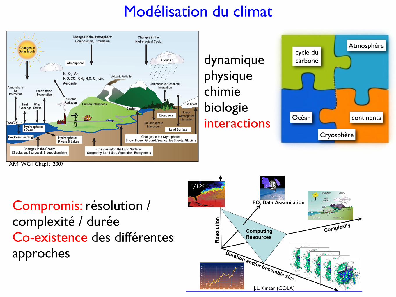
Modélisation du climat

Océan

Atmosphèrecycle du carbone

continents

Cryosphère

dynamiquephysiquechimiebiologieinteractions

104

Historical Overview of Climate Change Science Chapter 1

Frequently Asked Question 1.2What is the Relationship between Climate Changeand Weather?

Climate is generally defi ned as average weather, and as such, climate change and weather are intertwined. Observations can show that there have been changes in weather, and it is the statis-tics of changes in weather over time that identify climate change. While weather and climate are closely related, there are important differences. A common confusion between weather and climate arises when scientists are asked how they can predict climate 50 years from now when they cannot predict the weather a few weeks from now. The chaotic nature of weather makes it unpredictable beyond a few days. Projecting changes in climate (i.e., long-term average weather) due to changes in atmospheric composition or other factors is a very different and much more manageable issue. As an analogy, while it is impossible to predict the age at which any particular man will die, we can say with high confi dence that the average age of death for men in industrialised countries is about 75. Another common confusion of these issues is thinking

that a cold winter or a cooling spot on the globe is evidence against global warming. There are always extremes of hot and cold, al-though their frequency and intensity change as climate changes. But when weather is averaged over space and time, the fact that the globe is warming emerges clearly from the data.

Meteorologists put a great deal of effort into observing, un-derstanding and predicting the day-to-day evolution of weath-er systems. Using physics-based concepts that govern how the atmosphere moves, warms, cools, rains, snows, and evaporates water, meteorologists are typically able to predict the weather successfully several days into the future. A major limiting factor to the predictability of weather beyond several days is a funda-mental dynamical property of the atmosphere. In the 1960s, me-teorologist Edward Lorenz discovered that very slight differences in initial conditions can produce very different forecast results.

FAQ 1.2, Figure 1. Schematic view of the components of the climate system, their processes and interactions.

(continued)

AR4 WG1 Chap1, 2007

Center of Ocean-Land-Atmosphere Studies Jim Kinter - ICTP High Resolution Climate Modeling Workshop - Trieste, Italy - 13 August 2009

!"#"$%&$'()*+*,-(.-/"$01(2$(32/4*+&$'(526-,

Duration and/or Ensemble size

Res

olut

ion

ComputingResources

Complexity

1/120

EO, Data Assimilation

J.L. Kinter (COLA)

Compromis: résolution / complexité / duréeCo-existence des différentes approches

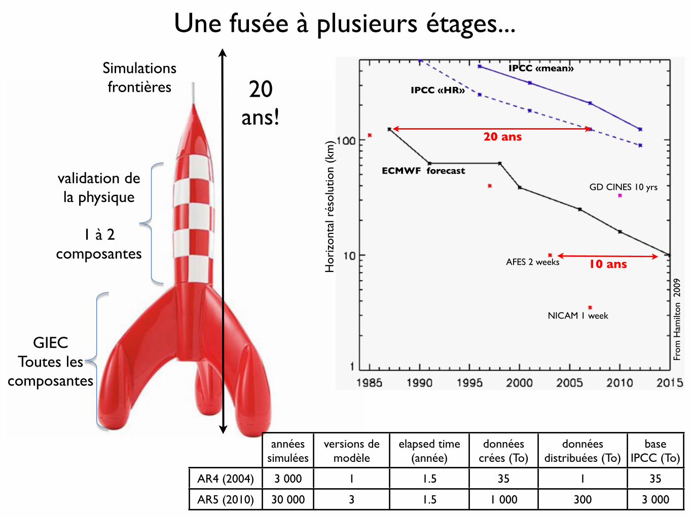
Une fusée à plusieurs étages...

Simulations frontières

validation de la physique

1 à 2 composantes

GIECToutes les

composantes

20 ans!

From

Ham

ilton

200

9

Hor

izon

tal r

ésol

utio

n (k

m)

NICAM 1 week

AFES 2 weeks

ECMWF forecast

IPCC «HR»

IPCC «mean»

GD CINES 10 yrs

20 ans

10 ans

années simulées

versions de modèle

elapsed time(année)

données crées (To)

données distribuées (To)

base IPCC (To)

AR4 (2004) 3 000 1 1.5 35 1 35

AR5 (2010) 30 000 3 1.5 1 000 300 3 000

!"#$%&'(%)(*+,-./(0%123(#"452(6778(

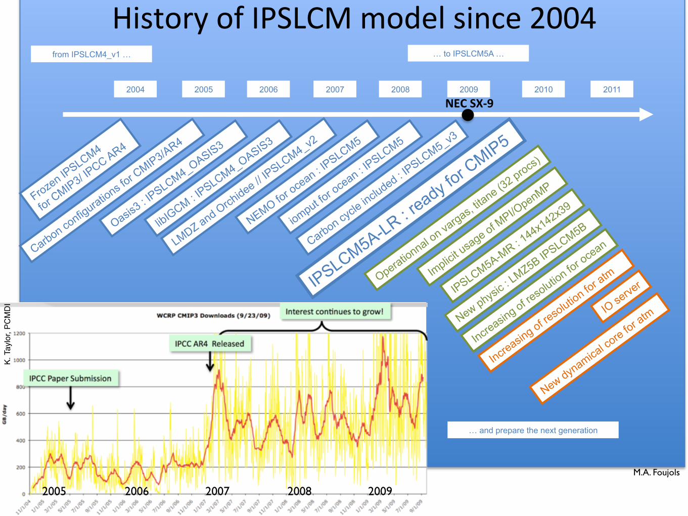
Frozen IPSLCM4

for CMIP3/ IP

CC AR4

Carbon configurations fo

r CMIP3/AR4

2004 2005

from IPSLCM4_v1 …

2006 2007 2008 2009

IPSLCM5A-LR : ready fo

r CMIP5

… to IPSLCM5A …

Oasis3 : IP

SLCM4_OASIS3

LMDZ and Orchidee // I

PSLCM4_v2

NEMO for ocean : IP

SLCM5

Carbon cycle

included : IP

SLCM5_v3

2011 2010

IPSLCM5A-MR : 1

44x142x39

New physic :

LMZ5B IPSLCM5B

IO serve

r

iomput for o

cean : IPSLCM5

libIGCM : IPSLCM4_OASIS3

Increasin

g of resolution for a

tm

New dynamical co

re for atm

Increasin

g of resolution for o

cean

!"#$%&'($

Operationnal on vargas, t

itane (32 procs)

… and prepare the next generation

Implicit usage of M

PI/OpenMP

M.A. Foujols

2005 2006 2007 2008 2009

K. T

aylo

r, PC

MD

I

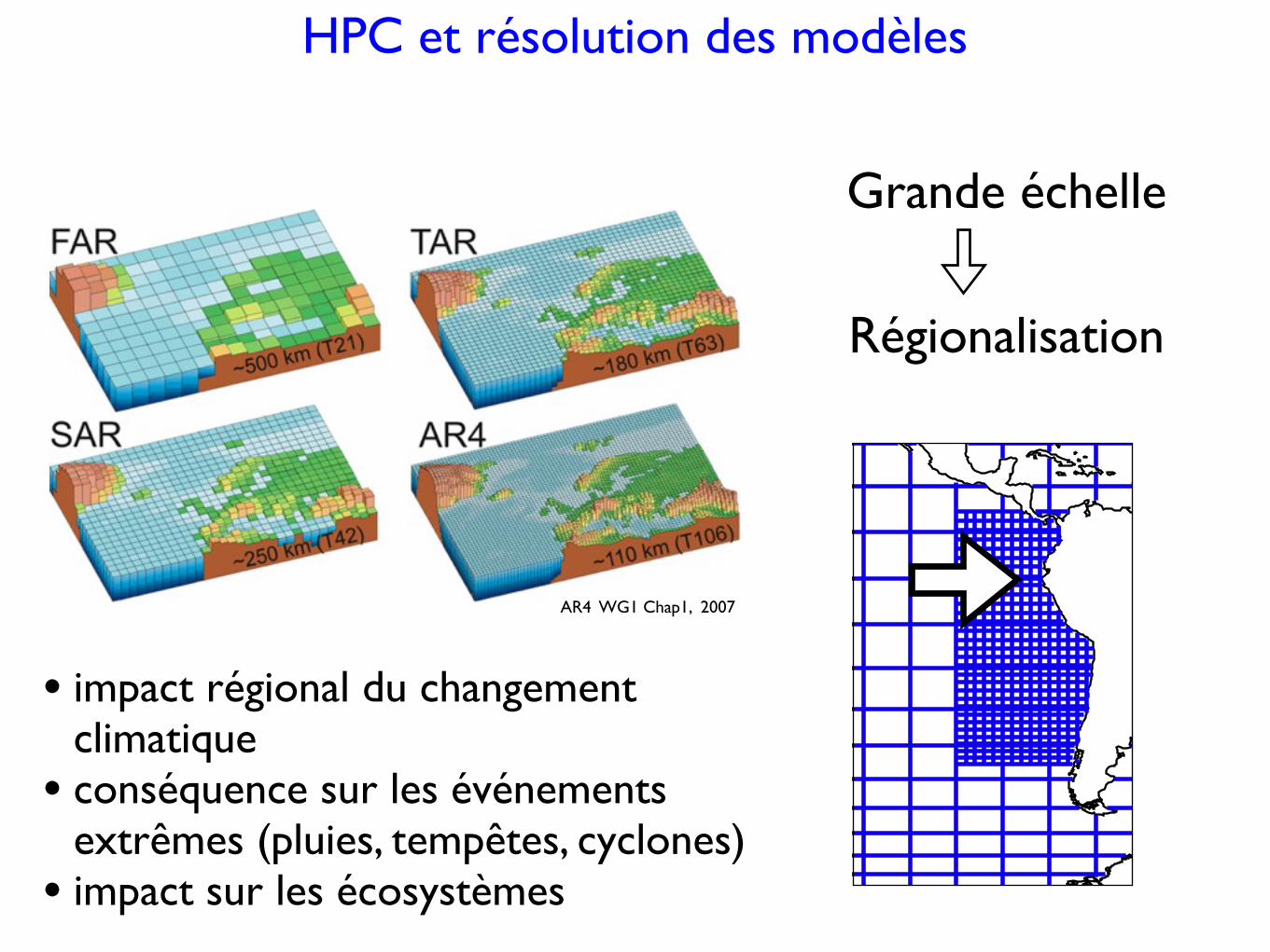
HPC et résolution des modèles

Régionalisation

Grande échelle

AR4 WG1 Chap1, 2007

• impact régional du changement climatique

• conséquence sur les événements extrêmes (pluies, tempêtes, cyclones)

• impact sur les écosystèmes

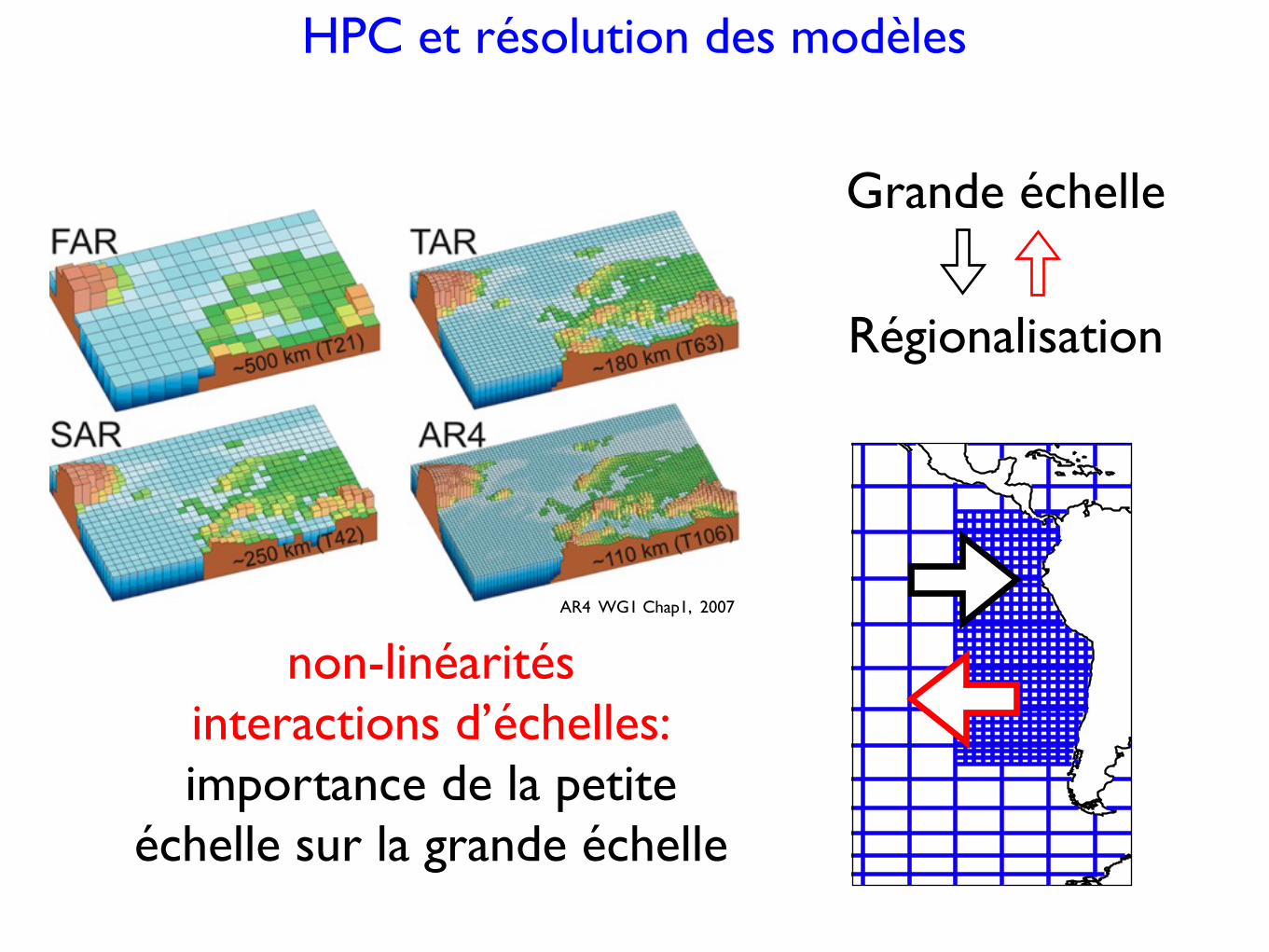
HPC et résolution des modèles

non-linéaritésinteractions d’échelles:importance de la petite

échelle sur la grande échelle

Régionalisation

Grande échelle

AR4 WG1 Chap1, 2007

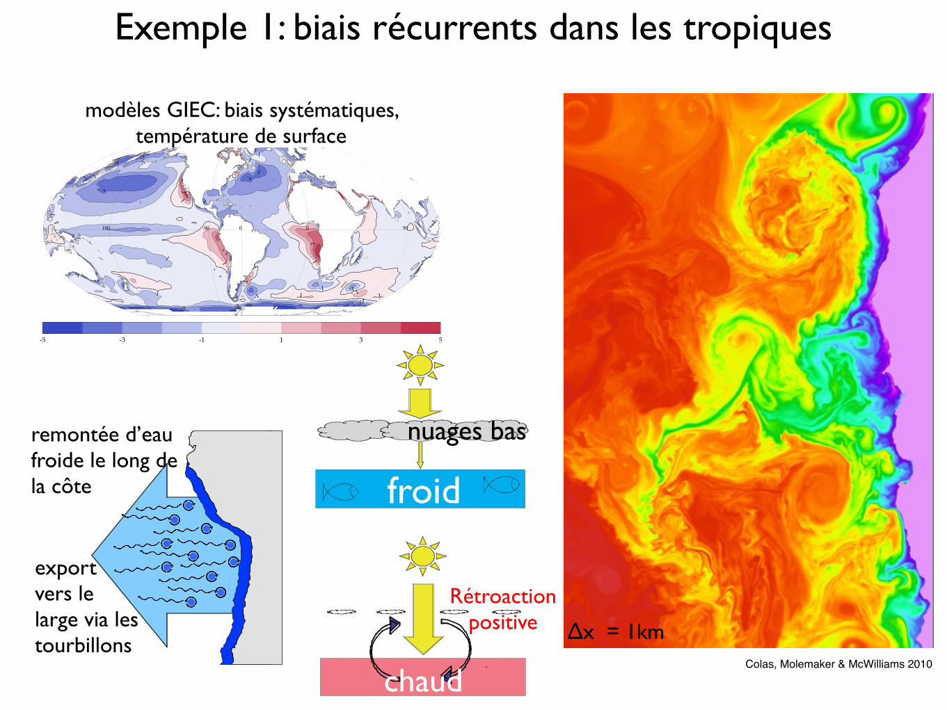
Exemple 1: biais récurrents dans les tropiques

-3

-3

-3 -3 -3

-3

-3

-3

-3

-3

-3 -3

-3-3

-3

-3-3

-3 -3

-3-3-3

-3

-1-1

-1

-1

-1

-1

-1

-1

-1

-1

-1

-1

-1 -1

-1

-1

-1

-1-1 -1

-1

-1

-1

-1

-1

-1

-1

-11

1

1

1

11

1 1 1

1

1 1 1

1

1

1 1

1

1

13 3 3

3 33

33

3

3

3

3

3 3

3

90180 -90 00

-5 -3 -1 1 3 5

modèles GIEC: biais systématiques, température de surface

remontée d’eau froide le long de la côte

export vers le large via les tourbillons

nuages bas

froid

chaud

Rétroaction positive

Colas, Molemaker & McWilliams 2010

Δx = 1km

S. Flavoni. Equipe system NEMO

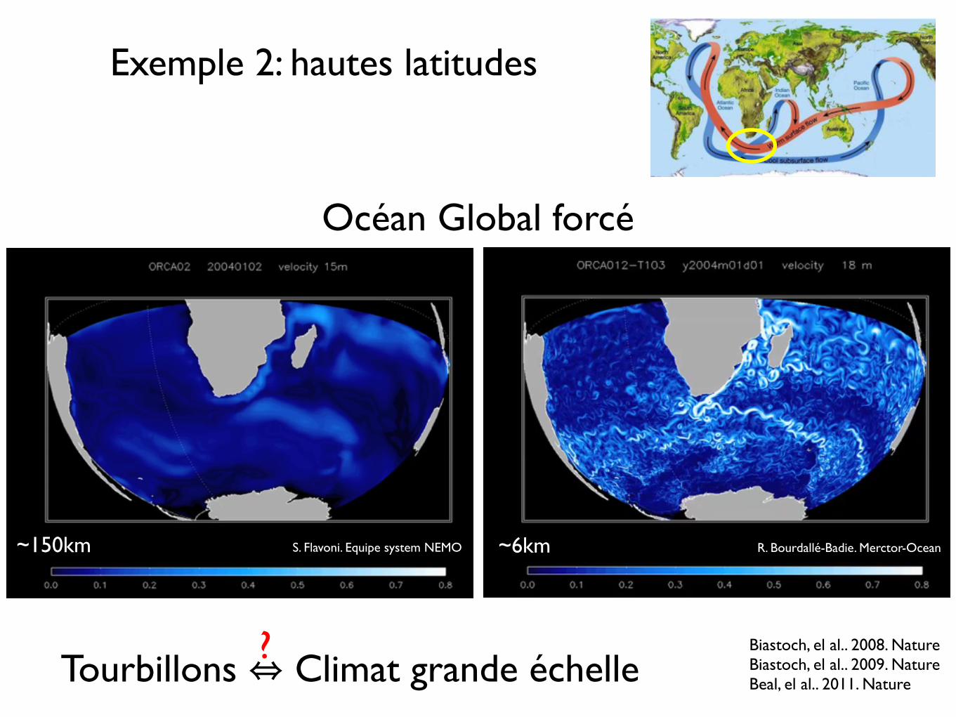
Exemple 2: hautes latitudes

~150km

~6km

Océan Global forcé

R. Bourdallé-Badie. Merctor-Ocean

Biastoch, el al.. 2008. Nature Biastoch, el al.. 2009. Nature Beal, el al.. 2011. Nature Tourbillons ⇔ Climat grande échelle

?

~6km

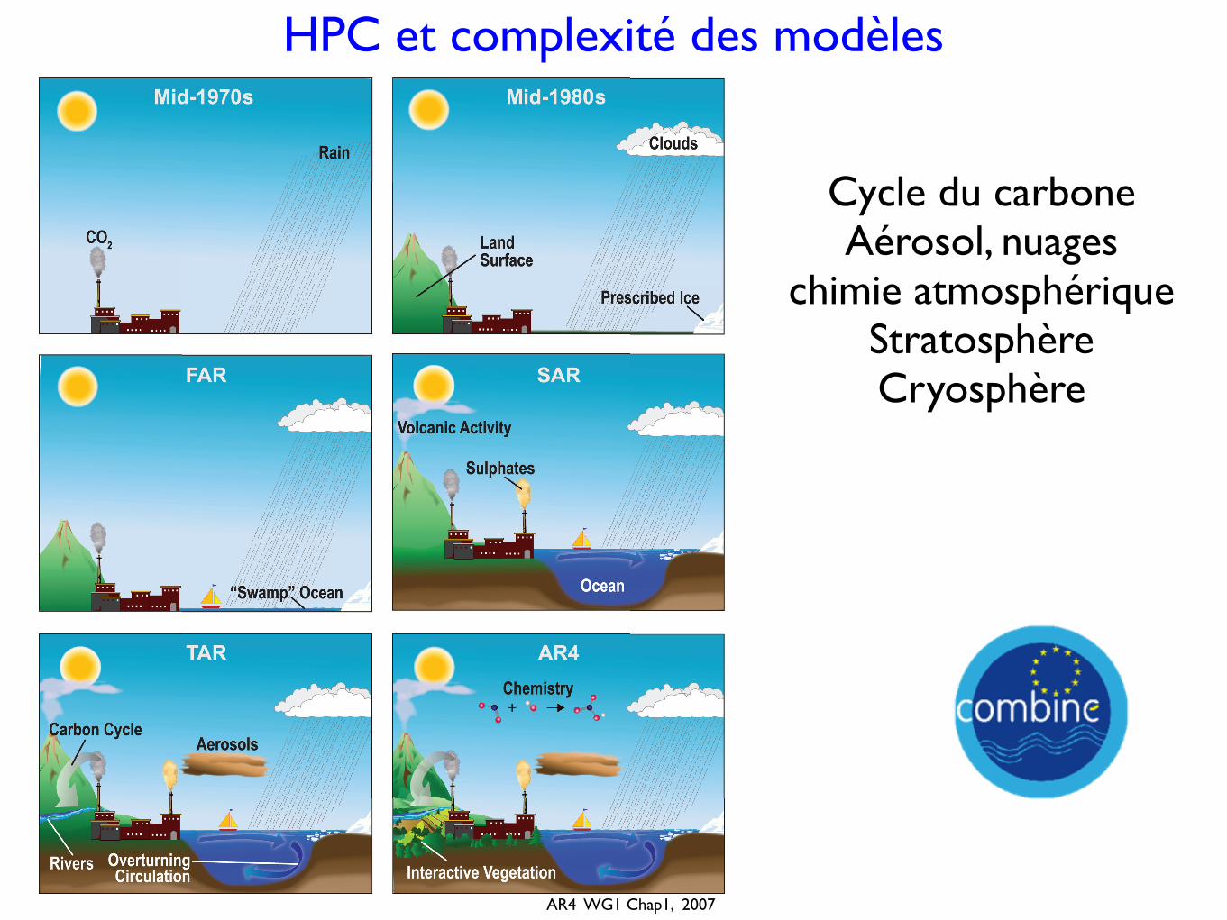
HPC et complexité des modèles

99

Chapter 1 Historical Overview of Climate Change Science

Figure 1.2. The complexity of climate models has increased over the last few decades. The additional physics incorporated in the models are shown pictorially by the different features of the modelled world.

AR4 WG1 Chap1, 2007

Cycle du carboneAérosol, nuages

chimie atmosphériqueStratosphèreCryosphère

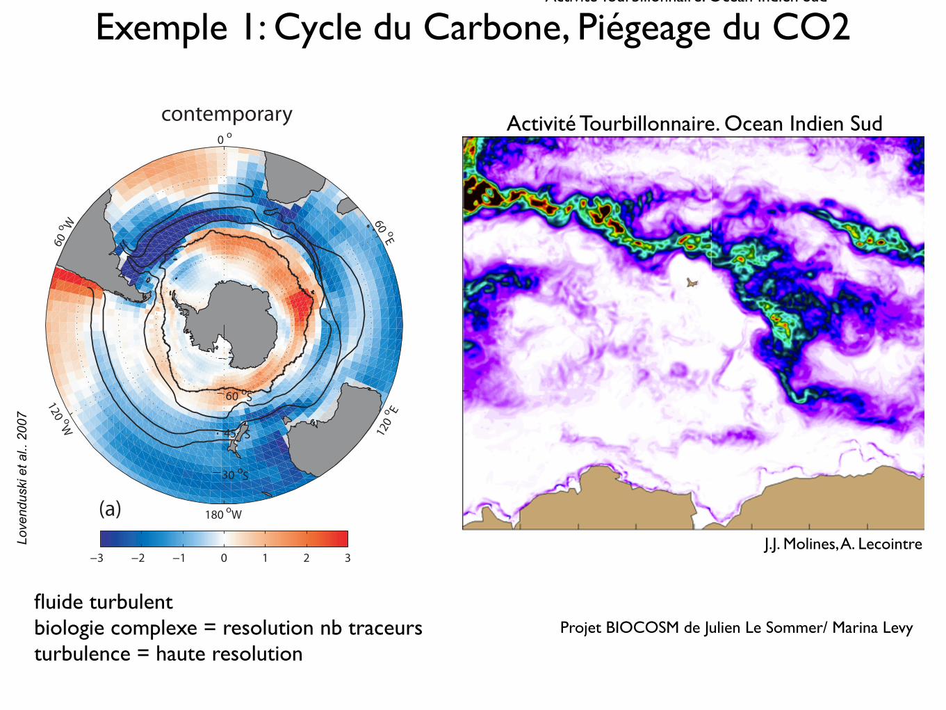
Exemple 1: Cycle du Carbone, Piégeage du CO2

exhibits a negative trend. With regard to variations aroundthese trends, Figure 4 suggests that most of the contempo-rary flux variability originates from variability in naturalrather than anthropogenic CO2. We first investigate thevariability by focusing our analysis on model output thathas been both deseasonalized and detrended, and return tothe trends at the end.[18] The contemporary and natural air-sea CO2 flux

anomalies shown in Figure 5 exhibit large variability forthe Southern Ocean: ±0.19 PgC yr!1 and ±0.18 PgC yr!1,respectively (1s). These flux variances are substantiallylarger than those obtained previously for the SouthernOcean from ocean model simulations (e.g., ±0.1 PgC yr!1

from Peylin et al. [2005] and ±0.05 PgC yr!1 fromWetzel etal. [2005]). The model simulated contemporary and naturalCO2 flux variability from the Southern Ocean accounts for

30% of the global variance in these fluxes, which is in linewith the estimated contribution from the Southern Ocean inother models [Wetzel et al., 2005; LeQuere et al., 2000]. Thecontemporary and natural monthly time series are wellcorrelated (r = 0.96), and exhibit similar spatial patternsof variance (Figure 6). In contrast, interannual variability inthe air-sea flux of anthropogenic CO2 does not exhibit highcorrelations with either contemporary or natural flux anoma-lies and is considerably smaller(±0.05 Pg C yr!1 (1s),Figure 6). As atmospheric CO2 concentrations growthroughout the simulation, variability in the anomalousanthropogenic CO2 fluxes increases slightly.[19] Variance in the CO2 flux anomalies is elevated in the

region south of "45!S (Figure 6), where the SAM is likelyto have an influence on air-sea flux variability. Indeed, thereis a clear connection between both the contemporary and

Figure 4. Mean Southern Ocean (<35!S) air-sea CO2 flux, smoothed with an 12-month running average(PgC yr!1). Negative fluxes indicate ocean uptake.

Figure 3. Annual mean air-sea flux of (a) contemporary CO2 (natural + anthropogenic CO2), (b) naturalCO2, and (c) anthropogenic CO2 (mol m!2 yr!1). The fluxes have been averaged using output from thehistorical simulation for Figure 3a, preindustrial simulation for Figure 3b, and from their difference forFigure 3c. Positive fluxes indicate ocean outgassing. Note difference in scale for the anthropogenic flux.

GB2026 LOVENDUSKI ET AL.: SAM AND SOUTHERN OCEAN CO2 FLUX

6 of 14

GB2026

Projet BIOCOSM de Julien Le Sommer/ Marina Levyfluide turbulentbiologie complexe = resolution nb traceursturbulence = haute resolution

Love

ndus

ki e

t al..

200

7

Activité Tourbillonnaire. Ocean Indien Sud

Activité Tourbillonnaire. Ocean Indien Sud

J.J. Molines, A. Lecointre

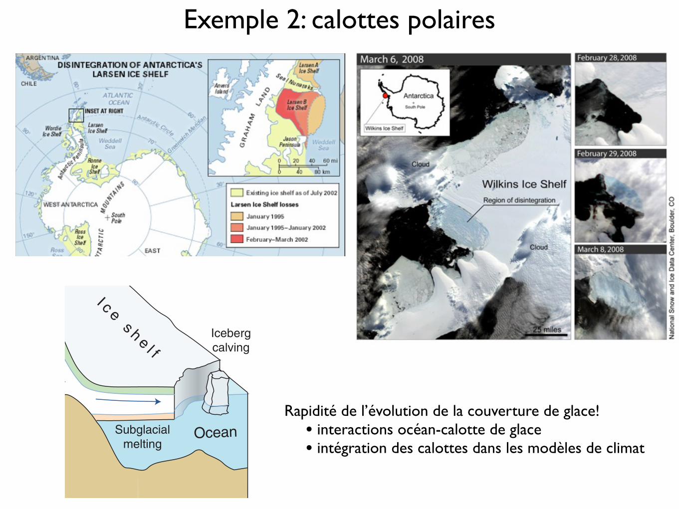
Exemple 2: calottes polaires

101ICE SHEETSCHAPTER 6A

climate and air composition dating back hundreds of mil-lennia. During glacial periods, ice sheets contained more than twice as much ice as that in Greenland and Antarc-tica today. Sea level would rise by about 64 m if the cur-rent mass of ice in Greenland and Antarctica were to melt

completely. Although this would take many thousands of years, recent observations show a marked increase in ice-sheet contributions to sea-level rise. In addition, ice-sheet melting strongly influences ocean salinity and tempera-ture, and also global thermohaline circulation as a con-

Equilibriumline

B e d r o c k

Ocean

O c e a n

I c e s h e e tI c e s h e l f

G r e e n l a n d

M e l t i n g o n t h e l o w e r

p a r t s o f t h e s u r f a c e ,

i c e b e r g s c a l v e o f f f r o m

i c e s h e e t e d g e s i n t o i c e

f j o r d s a n d t h e s e a

A n t a r c t i c aI c e s h e l v e s , w i t h

s u b g l a c i a l m e l t i n g .

I c e b e r g s c a l v e o f f

f r o m i c e s h e l v e s

Abl

atio

n

Icebergcalving

Subglacialmelting

Icebergcalving

Snow accumulation

Ice fl

ow

Ice flow

Figure 6A.1: Ice sheets.

Source: based on material provided by K. Steffen, CIRES/Univ. of Colorado

Rapidité de l’évolution de la couverture de glace!• interactions océan-calotte de glace• intégration des calottes dans les modèles de climat

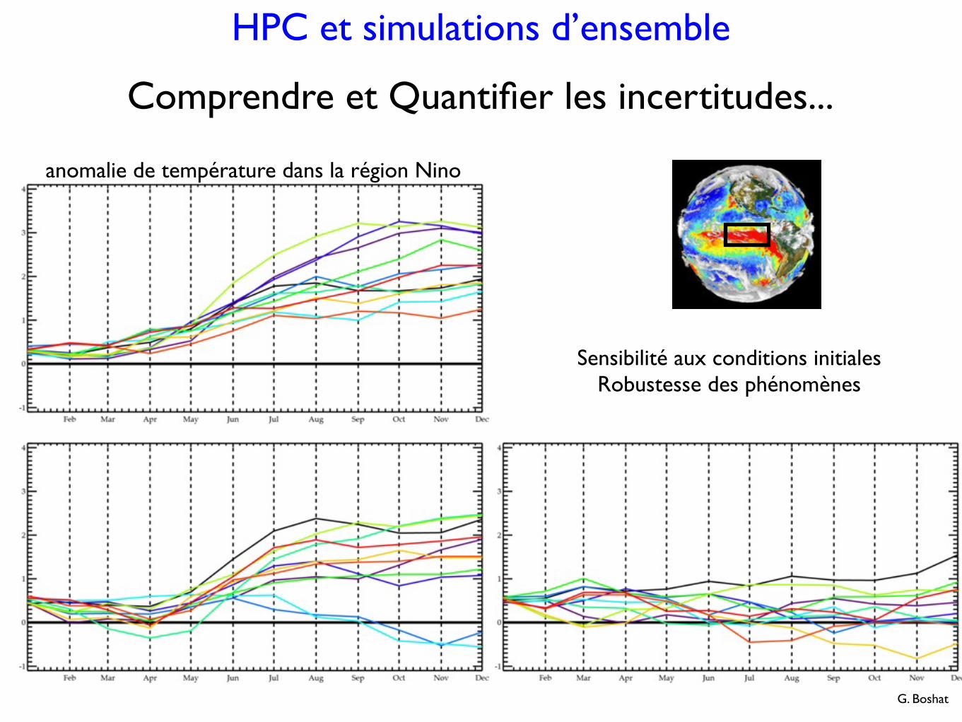
HPC et simulations d’ensemble

Comprendre et Quantifier les incertitudes...

G. Boshat

Sensibilité aux conditions initialesRobustesse des phénomènes

anomalie de température dans la région Nino

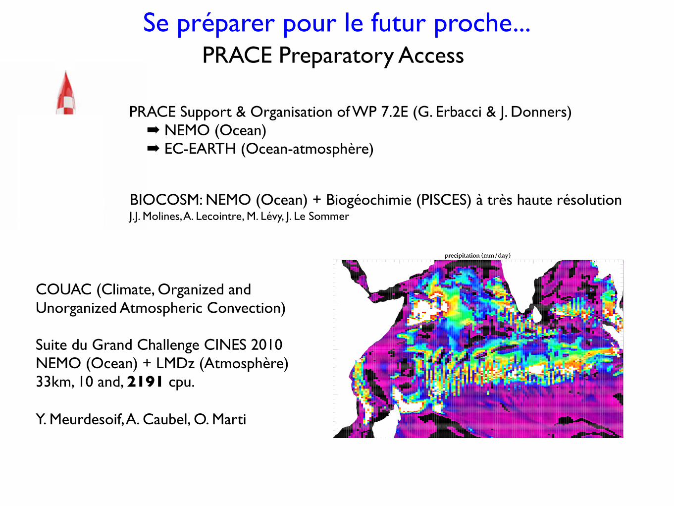
Se préparer pour le futur proche...

COUAC (Climate, Organized and Unorganized Atmospheric Convection)

Suite du Grand Challenge CINES 2010NEMO (Ocean) + LMDz (Atmosphère)33km, 10 and, 2191 cpu.

Y. Meurdesoif, A. Caubel, O. Marti

precipitation (mm/day)precipitation (mm/day)

40E 50E 60E 70E 80E 90E 100ELongitude

20S

10S

0

10N

20N

Latit

ude

40E 50E 60E 70E 80E 90E 100ELongitude

20S

10S

0

10N

20N

Latit

ude

PRACE Support & Organisation of WP 7.2E (G. Erbacci & J. Donners)➡ NEMO (Ocean)➡ EC-EARTH (Ocean-atmosphère)

PRACE Preparatory Access

BIOCOSM: NEMO (Ocean) + Biogéochimie (PISCES) à très haute résolutionJ.J. Molines, A. Lecointre, M. Lévy, J. Le Sommer

RMS BB12 2003 2006: BB12_DFS4_4

6

8

8

8

10

10

12

12

14

14

16

16

18

RMS BB12 2003 2006: BB12_DFS4_4

(cm): Min= 4.68, Max= 21.65, Int= 1.00

80E 85E 90E 95E 100ELongitude

12N

14N

16N

18N

20N

22N

Lat

itu

de

0.00 2.00 4.00 6.00 8.00 10.0012.0014.0016.0018.0020.00

AVISO DAILY

4

6

8

8

8

10

10

10

12

12

12

14

14

16

AVISO DAILY

(cm): Min= 3.31, Max= 24.24, Int= 1.00

80E 85E 90E 95E 100ELongitude

12N

14N

16N

18N

20N

22N

Lat

itu

de

0.00 2.00 4.00 6.00 8.00 10.0012.0014.0016.0018.0020.00

RMSdiff

6

68 8

88

8

8

10

10

1214

16 18

RMSdiff

(): Min= 3.64, Max= 21.94, Int= 1.00

80E 85E 90E 95E 100ELongitude

12N

14N

16N

18N

20N

22N

Lat

itu

de

2.00 4.00 6.00 8.00 10.0012.0014.0016.0018.0020.0022.00

observations

RMS BB12 2003 2006: BB12_DFS4_4

6

8

88

10

10

12

12

14

14

16

16

18

RMS BB12 2003 2006: BB12_DFS4_4

(cm): Min= 4.68, Max= 21.65, Int= 1.00

80E 85E 90E 95E 100ELongitude

12N

14N

16N

18N

20N

22N

Lat

itu

de

0.00 2.00 4.00 6.00 8.00 10.0012.0014.0016.0018.0020.00

AVISO DAILY

4

6

8

8

8

10

10

10

12

12

12

14

14

16

AVISO DAILY

(cm): Min= 3.31, Max= 24.24, Int= 1.00

80E 85E 90E 95E 100ELongitude

12N

14N

16N

18N

20N

22N

Lat

itu

de

0.00 2.00 4.00 6.00 8.00 10.0012.0014.0016.0018.0020.00

RMSdiff

6

68 8

8

8

8

8

10

10

1214

16 18

RMSdiff

(): Min= 3.64, Max= 21.94, Int= 1.00

80E 85E 90E 95E 100ELongitude

12N

14N

16N

18N

20N

22N

Lat

itu

de

2.00 4.00 6.00 8.00 10.0012.0014.0016.0018.0020.0022.00

trop fort...

RMS BB12 2003 2006: BB12_DFS4_VISCWW_2

4

6

66

8

8

10

10

12

1416

RMS BB12 2003 2006: BB12_DFS4_VISCWW_2

(cm): Min= 3.59, Max= 20.81, Int= 1.00

80E 85E 90E 95E 100ELongitude

12N

14N

16N

18N

20N

22N

Lat

itu

de

0.00 2.00 4.00 6.00 8.00 10.0012.0014.0016.0018.0020.00

AVISO DAILY

4

6

8

8

8

10

10

10

12

12

12

14

14

16

AVISO DAILY

(cm): Min= 3.31, Max= 24.24, Int= 1.00

80E 85E 90E 95E 100ELongitude

12N

14N

16N

18N

20N

22N

Lat

itu

de

0.00 2.00 4.00 6.00 8.00 10.0012.0014.0016.0018.0020.00

RMSdiff

4

6

66

68

8

88

10

1012

RMSdiff

(): Min= 3.09, Max= 21.73, Int= 1.00

80E 85E 90E 95E 100ELongitude

12N

14N

16N

18N

20N

22N

Lat

itu

de

2.00 4.00 6.00 8.00 10.0012.0014.0016.0018.0020.0022.00

trop faible...

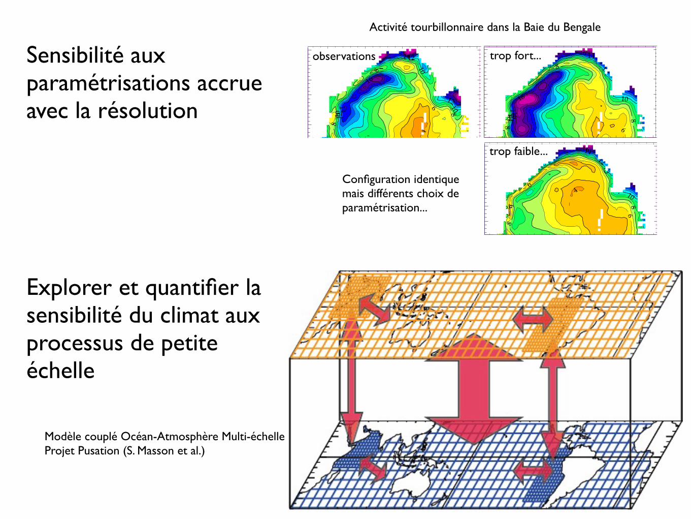
Sensibilité aux paramétrisations accrue avec la résolution

Explorer et quantifier la sensibilité du climat aux processus de petite échelle

Activité tourbillonnaire dans la Baie du Bengale

Modèle couplé Océan-Atmosphère Multi-échelleProjet Pusation (S. Masson et al.)

Configuration identique mais différents choix de paramétrisation...

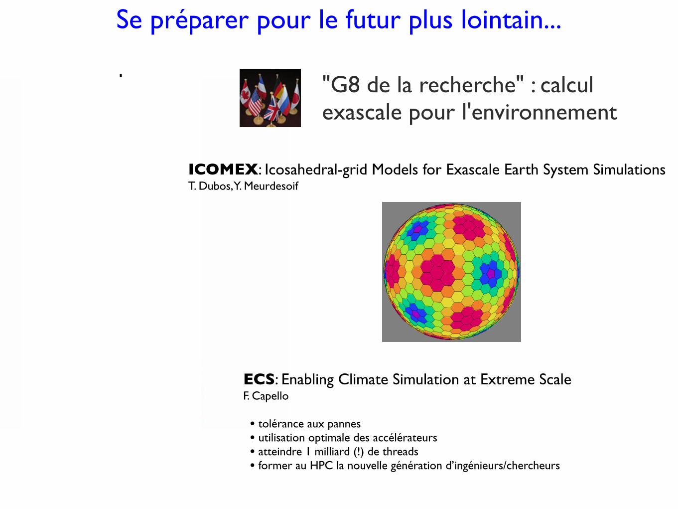
Se préparer pour le futur plus lointain...

"G8 de la recherche" : calcul exascale pour l'environnement

ICOMEX: Icosahedral-grid Models for Exascale Earth System SimulationsT. Dubos, Y. MeurdesoifFilename : Ai.nc

Variable : Ai ( scaled by 1e+04) k= 1/1 l= 1/1

101 107 112.9 118.9 124.8 130.8 136.7 142.7 148.6 154.6 160.6 166.5 172.5 178.4 184.4

ECS: Enabling Climate Simulation at Extreme ScaleF. Capello

• tolérance aux pannes• utilisation optimale des accélérateurs• atteindre 1 milliard (!) de threads• former au HPC la nouvelle génération d’ingénieurs/chercheurs

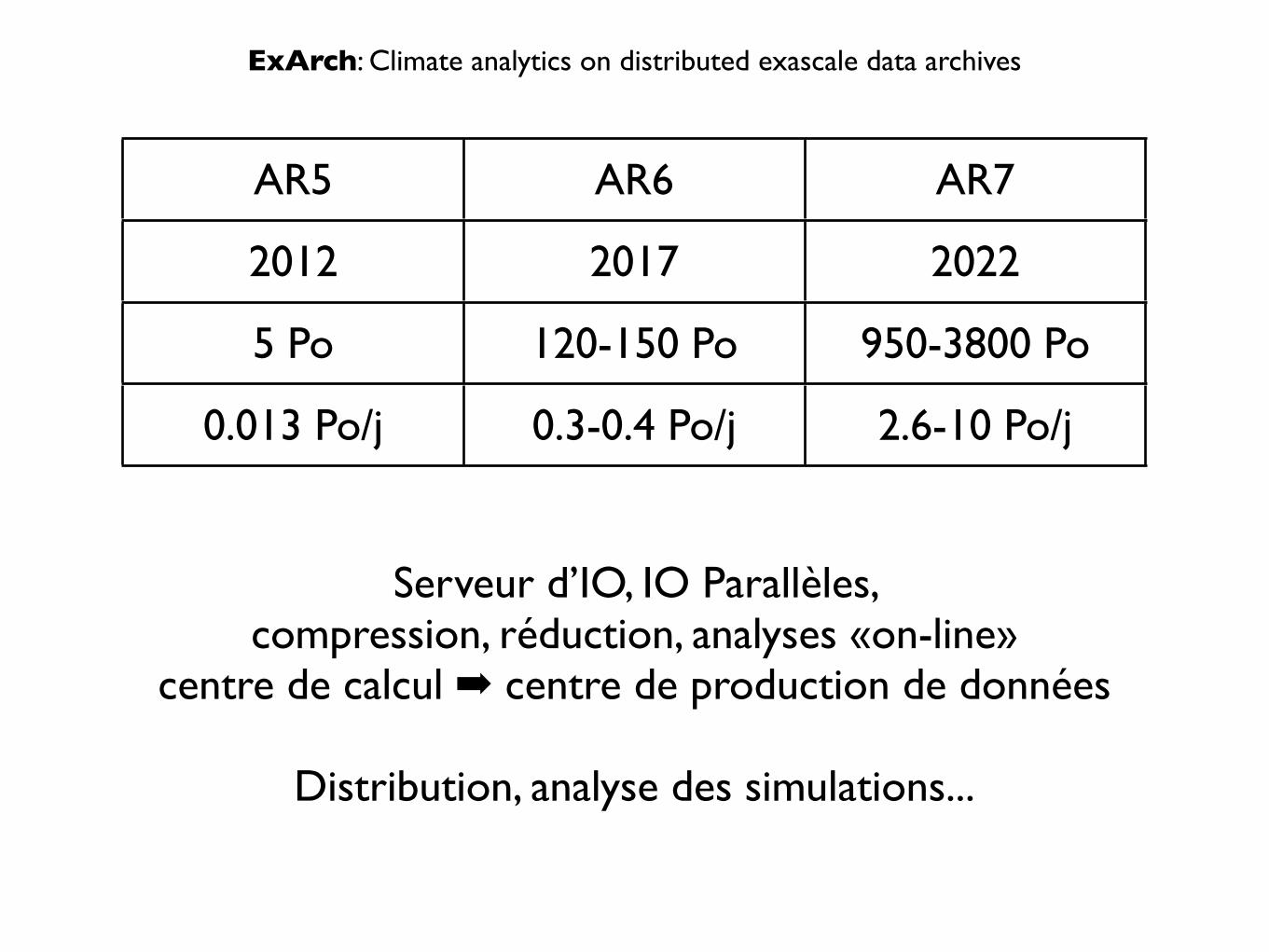
ExArch: Climate analytics on distributed exascale data archives

AR5 AR6 AR7

2012 2017 2022

5 Po 120-150 Po 950-3800 Po

0.013 Po/j 0.3-0.4 Po/j 2.6-10 Po/j

Serveur d’IO, IO Parallèles, compression, réduction, analyses «on-line»

centre de calcul ➡ centre de production de données

Distribution, analyse des simulations...

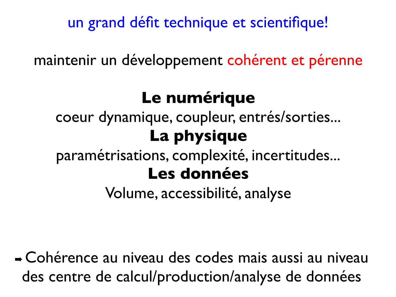
un grand défit technique et scientifique!

maintenir un développement cohérent et pérenne

Le numériquecoeur dynamique, coupleur, entrés/sorties...

La physique paramétrisations, complexité, incertitudes...

Les données Volume, accessibilité, analyse

➡ Cohérence au niveau des codes mais aussi au niveau des centre de calcul/production/analyse de données