Société de Calcul Mathématique, S. A

Siège social et bureaux : 111, Faubourg Saint Honoré, 75008 Paris. Tel : 01 42 89 10 89. Fax : 01 42 89 10 69. www.scmsa.com

Société Anonyme au capital de 56 200 Euros. RCS : Paris B 399 991 041. SIRET : 399 991 041 00035. APE : 7219Z

The joint probability law of extreme events

by

Bernard Beauzamy and Olga Zeydina

Société de Calcul Mathématique SA

Paris

April 2011

Summary

We develop the probabilistic tools to handle the extreme events appearing simultaneously in

two or several places, under the form of a "joint law" : this is a continuation of the work [BB1]

done by the first-named author for a single situation. The difficulty comes here from the

dependances which may exist between these places.

Mathematically speaking, the problem reduces to the evaluation of the integral of a monomial

in many variables on a complicated simplex, in a high dimensional space. We show that the

dependances between places can be converted into partial orderings on this simplex ; such an

approach is completely original.

Then we show how to apply the theory to a concrete example: the water heights, in the sea, in

the two cities of Marseille and Nice, on the South French coast. The dimension is here 44. The

integrals might be computed explicitly, but we prefer to use the Devroye-Robinson method

([Robinson]), which is of Monte-Carlo type ; in order to use it, we generate at each step an

order compatible with the constraints. The complete evaluation of the joint law for these two

cities does not take more than a few minutes.

The present work originates in a contract we had in 2010-2011 with the French "Caisse

Centrale de Réassurance" ; we thank the CCR for their help, interest and support.

Société de Calcul Mathématique, S. A. Algorithmes et Optimisation

2 Bernard Beauzamy & Olga Zeydina : Joint Law for Extreme Events, 2011/04

First Part : Theory

I. Introduction

In the present article, we continue to investigate the theory of a probabilistic evaluation for

extreme events, which was started by the first-named author in [BB1]. We deal here with the

joint law, which means that we wish to evaluate the probability of simultaneous extreme

events in several places.

This preoccupation comes from a contract we had in 2010-2011 with the "Caisse Centrale de

Réassurance", Paris. Indeed, CCR is interested mostly by extreme events which touch several

places at the same time, since in such cases the damages will be more important.

The events we consider here may be of any type, but should be characterized by scalar values :

temperature, water height (in case of flooding), earthquakes (characterized by a magnitude),

heavy rain, tornadoes, and so on. As an example, we work here with water heights on the

coasts, above normal sea level. The data below come from CCR.

Let 1S and 2S be two measure stations and let 1X and 2X be the two variables characterizing

the phenomenon, in 1S and 2S respectively. They may be viewed as random variables. Let 1h

and 2h be two arbitrary thresholds.

Let us define a unit of time, which strongly depends on the phenomenon. In [1], we were

interested in the maximum temperature over a year ; for heavy rain, the unit of time might be

the day. In the present case, high level of sea water depends on the tide, which is related to

the moon, so our unit of time will be the month.

Our basic question may now be stated : evaluate the probability to have, during a given unit of

time, simultaneously 1 1X h and 2 2X h .

II. What do we have ?

The data that are necessary in order to approach this question are easy to describe : we need a

list of records, for both stations at the same time. For a certain number N of units of time, we

need the values recorded for 1X and 2X ; in the present case, for a number N of months.

These months do not need to be consecutive (because we do not try to investigate the effect of

the season), but obviously the larger N is, the better.

As usual in probabilities, we will discretize the results, and consider "classes" instead of

precise values. For instance here, we will consider intervals of width 10 cm, which means that

we will put into the same class (same interval) the result 1.02 m and the result 1.08 m. We

assume here for simplicity that this discretization will be the same for both stations. Each

class kC will be referred to by a single value, usually the center of the class, denoted by kx .


Observe, however, that the joint law may concern two phenomena of completely different

nature : we may observe the temperature in one place and the pressure in the other, in which

case the scales and discretization will be different.

So, we are given from our records a certain number of classes for each station ; assume for

simplicity that they are the same in each place and denote their common value by K : we have

classes 1,..., KC C and the set of records gives a square matrix : in the cell ,i j we put the

number ,i jn of times where we observed simultaneously ix at the first place and

jx at the

second place ; of course ,

, 1

K

i j

i j

n N

.

This table will be called the table of joint occurrences ; we will treat a concrete example in the

second part of this paper.

III. Preliminary mathematical definition of our problem

A. Using the occurrence table

From the occurrence table, we can give a more precise presentation of our problem. Let ,i jp be

the (unknown) probability to be simultaneously in the class iC at the first station and in the

class jC at the second station ; in mathematical terms :

, 1 2andi j i jp P X C X C

Of course, from the table of occurrences, a simple estimate for each ,i jp is :

,

,

i j

i j

np

N

This estimate is asymptotically correct when N is large (this follows from the law of large

numbers), but very unsatisfactory in the case of extreme events, for two reasons :

Many situations have not been observed at all, so , 0i jn ;

But conversely, more extreme situations may have been observed !

So, before we solve our question, we need to think about the "logics" behind the probabilities

we are looking for.

B. The logics behind the probabilities

In our paper [1], dealing with temperatures in a single station, we had simple logics : we

simply said that the probabilities of extreme events must be decreasing ; the more extreme the

event is, the less often we will see it. The probability to see 40°C in Paris is smaller than the

probability to see 39°C : this is obvious, despite the fact that 40°C has been recorded and 39°C

has never been recorded (on 137 years of observation). But for a joint law, such a simple logics

fail, because of dependances : if the two stations are very close to each other, the conditional

law of the second, knowing the first, is very concentrated near the main diagonal ; we cannot


expect a decrease of the numbers. Let us investigate this more completely, because this is

central to our problem.

Let us start with the case of two classes only, for each place. So our table of occurrences looks

like this :

1 2/X X 1C 2C

1C 1,1n 1,2n

2C 2,1n 2,2n

Table (1) occurrences

and we want to build a table of probabilities :

1 2/X X 1C 2C

1C 1,1p 1,2p

2C 2,1p 2,2p

Table (2) probabilities

We discuss here what assumptions should be made on the table (2). These assumptions might

not be satisfied by the table of occurrences (1), because the observations might be quite rare.

Quite clearly :

The marginal laws (individual laws, for each station) must be decreasing :

1 1 1 2P X x P X x ; 2 1 2 2P X x P X x

This comes from the fact that, for a given station, the more extreme the event is, the less

frequent it is.

The diagonal must be decreasing :

1 1 2 1 1 2 2 2P X x and X x P X x and X x

This means that it is less likely to have a more extreme event at two places at the same time.

Let us now look at the conditional laws. Assume that we know 1 1X x ; then, clearly :

2 1 2 2P X x P X x

This is true if the stations are far away from each other, because then they are independent

and the information 1 1X x does not count, or if they are close to each other, because in this

case the event 2 1X x is very likely.

The same way, if we know 2 1X x , we can conclude that :

1 1 1 2P X x P X x


Let us consider now the assumption 1 2.X x If both stations are independent, we can say that

2 1 2 2P X x P X x as before, but not if they are close to each other, since then the

assumption 1 2X x implies that the event 2 2X x is very likely.

So, in our table of probabilities (2) we may put the assumptions :

1,1 1,2p p and 1,1 2,1p p

but we have no comparison between 2,1 2,2 1,2, ,p p p .

C. Taking into account several classes

We now have two stations, but the water heights may take more than two values : let us say

that they can take K values, the same number for both stations. So we have a square matrix.

Let ,i jp be defined as above : probability that

1 2andi jX x X x . We have the following

properties :

Each individual law is decreasing :

1 1 1 2 2 1;i i i iP X x P X x P X x P X x

Each diagonal is decreasing :

, 1, 1i j i jp p

which means that a situation which is more extreme at both places is less likely.

Let us now look at the conditional laws ; assume 1 iX x . Then the condition:

2 2 1j jP X x P X x

holds if j i but only in this case. Indeed, if j i , it holds if the stations are far apart, and

also if they are close, since the event 1 iX x is assumed. But if j i it may not hold, as we

saw in the case of two values. So we have the conditions :

, , 1i j i jp p if j i and , 1,i j i jp p if i j .

They mean that each row and each column is decreasing after the main diagonal. No

assumption should be made upon the rows or the columns before the diagonal.

D. General case

In general, we can define the joint law of two events which are not of the same nature, so we

will change our notation : for instance, A might be a temperature and B be a pressure. So the

size does not need to be the same for the width and the height of the matrix, and the units do

not need to be the same. The "main diagonal" does not exist.


Let 1,..., ma a be the possible values for A and 1,..., nb b the possible values for B . The table of

occurrences is ,i jn and we are looking for estimates of ,i j i jp P A a and B b . We consider

that the 'ia s are ordered and more and more extreme, and the same for the 'jb s . We do not

know if A and B are close to each other, and we might have a strong correlation, for instance

between 1a and 4b , between 2a and 7b , and so on.

It is reasonable to assume, as before, that all individual laws are decreasing (sums on each

row or on each column), and that all diagonals are decreasing. This gives the conditions:

, 1, , , 1;i j i j i j i j

j j i i

p p p p

, 1, 1i j i jp p

Let us now look at the conditional laws. Assume iA a ; we may assume that B is decreasing,

after some value which is the highest value for B , assuming iA a ; this highest value will be

computed from the table of occurrences (hoping that this table is complete enough, but there is

no other way).

This coincides with the previous settings. Assume that we measure the same thing, and that

the measurements are water heights between 4.0 and 5.0 (in meters). Assume 4.4A . If B is

close to A , then the event 4.4B is the most likely one. In the case where A and B are far

apart, then the value for B are decreasing from the beginning, so to assume that the values of

B are decreasing starting with the diagonal is correct in all cases, and coincides with the

assumption "decreasing from the highest value", since this highest value is (more or less) the

diagonal.

IV. General mathematical formulation of the problem

A. Abstract formulation

We are not only interested in estimates of the numbers , and ,i j i jp P A x B x but we also

want to have confidence intervals on these numbers. In other words, each ,i jp should be

treated as a random variable, of which we want to know the law.

Since the sentence "the probability law of a probability" would sound strange, we change our

terminology. Our notation is consistent with the book [BB2].

Let ,i j be the "risk rate" of the event andi jA x B x , that is its probability, considered as

a random variable; then the number ,i jp above is an estimate of ,i j (usually the expectation).

Then we know by [BB2], Chapter II, Proposition 1, that the joint law of the ,i j 's is given by

the formula :

1,1 ,

1,1 , 1,1 ,,..., 1 K Kn n n

K K S K Kf c


where c is a normalisation constant (so the integral of f with respect to all variables should

be 1), and S is a simplex which we now define. In the formula above, the ,i jn are simply taken

from the observation occurrence table.

Indeed, the general theory of risk evaluation, from [BB2], applies to the present settings : we

have some number of occurrences, for some classes of results. It does not matter whether or

not these occurrences come from a pair of variables.

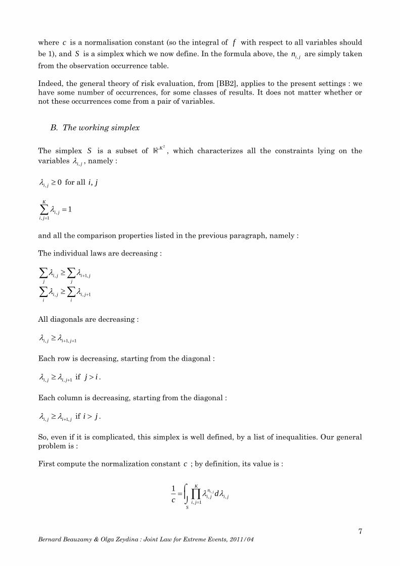
B. The working simplex

The simplex S is a subset of 2K, which characterizes all the constraints lying on the

variables ,i j , namely :

, 0i j for all ,i j

,

, 1

1K

i j

i j

and all the comparison properties listed in the previous paragraph, namely :

The individual laws are decreasing :

, 1,i j i j

j j

, , 1i j i j

i i

All diagonals are decreasing :

, 1, 1i j i j

Each row is decreasing, starting from the diagonal :

, , 1i j i j if j i .

Each column is decreasing, starting from the diagonal :

, 1,i j i j if i j .

So, even if it is complicated, this simplex is well defined, by a list of inequalities. Our general

problem is :

First compute the normalization constant c ; by definition, its value is :

,

, ,

, 1

1i j

Kn

i j i j

i jS

dc


Then, we can obtain estimates for each ,i jp ; for instance, the value chosen for

1,1p will be :

,

1,1 1,1 , ,

, 1

i j

Kn

i j i j

i jS

p c d

In other words, in the estimate of 0 0,i jp , the number

0 0,i jn is increased by one unit.


Second Part : A concrete example

I. The data

We now treat a numerical example: water heights in the cities of Marseille and Nice

(Mediterranean coast, France); the distance between both cities is approximately 160 km.

The data consist in 263 monthly measurements, from August 1981 till June 2010, for both

cities. For Marseille, the minimum height ever recorded is 56 cm and the maximum is 137.

For Nice, they are respectively 41 and 104 (all numbers below are given in cm).

We first build an histogram for each station, and we fix the threshold of 90, above which the

situation will be called "extreme". This threshold is the same for both places, and it results

from the examination of the histograms.

Since we are interested in the examination of dependance questions (as it was clear from the

first part of this paper), we also construct the conditional histograms : Marseille when Nice is

90 and Nice when Marseille is 90 . Here are the graphs we obtain:

Histograms for Marseille : raw data and conditional data

0

2

4

6

8

10

12

90

92

94

96

98

10

0

10

2

10

4

10

6

10

8

11

0

11

2

11

4

11

6

11

8

12

0

12

2

12

4

12

6Marseille and M/N>90

Marseille

M/N>90


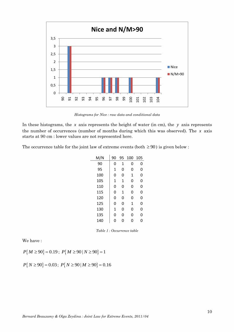
Histograms for Nice : raw data and conditional data

In these histograms, the x axis represents the height of water (in cm), the y axis represents

the number of occurrences (number of months during which this was observed). The x axis

starts at 90 cm : lower values are not represented here.

The occurrence table for the joint law of extreme events (both 90 ) is given below :

M/N 90 95 100 105

90 0 1 0 0

95 1 0 0 0

100 0 0 1 0

105 1 1 0 0

110 0 0 0 0

115 0 1 0 0

120 0 0 0 0

125 0 0 1 0

130 1 0 0 0

135 0 0 0 0

140 0 0 0 0

Table 1 : Occurrence table

We have :

90 0.19P M ; 90 | 90 1P M N

90 0.03P N ; 90 | 90 0.16P N M

0

0,5

1

1,5

2

2,5

3

3,5

90

91

92

93

94

95

96

97

98

99

10

0

10

1

10

2

10

3

10

4

Nice and N/M>90

Nice

N/M>90


II. Relationships between probabilities

So the cities are certainly not independent : the information that an extreme result has been

observed in one substantially increases the probability to see it also in the other. We observe

however that the link is not symmetric : if Nice is high, it forces Marseille to be, but if

Marseille is high, Nice has only a low probability to be high. In fact, Nice is very rarely high ;

this situation is much more extreme than Marseille, which has a wider range.

On the general joint law (not reproduced here), we observe that, for Marseille 90 , the larger

number of occurrences appears for low values in Nice. For instance, this is the table for

90M :

M/N 40 45 50 55 60 65 70 75 80 85 90 95 100 105

90 0 0 0 0 0 0 1 4 5 2 0 1 0 0

The same holds for values 90M . The highest occurrences are obtained for 70 85N ;

therefore, it is legitimate to make the assumption (as we explained in the First Part), that our

probabilities will be decreasing after 90, on each row. So we get the assumption , , 1i j i j for

all i . This means that the conditional probabilities of Nice, knowing 90M , are decreasing.

If we now look at the columns, there is no such result. In fact, as we already said, the values

90M have been observed only if 90N , so there is no occurrence at all of small values of

M when 90N . We want to investigate the following question : if 90N , how does M

depend on N ?

In order to solve this question, we build a simplified occurrence table, putting together the

values 90 and 95, 100 and 105 for Nice, and the values 90-115, 120-140 for Marseille. We get:

M\N 90-95 100-105

90-115 0,43 0,14 0,57

120-140 0,29 0,14 0,43

0,71 0,29

Table 2 : simplified occurrence table

From this table, we deduce that, for 90, 95N , the probability laws of Marseille may be

regarded as decreasing (higher values have smaller probability), but for 100,105N they are

not. In fact, for very large N , all values of M may have the same probability. In simpler

words, a very severe situation in Nice may or not be extremely severe in Marseille, with equal

probability.

So we have the inequalities , 1,i j i j , for 90, 95.j It means that in our 11 4 probability

table, the first two columns are decreasing, but not necessarily the last two.

Let us summarize the constraints. In the table containing the ,i j , the lines indicate

inequalities ; they concern :

all rows ;

all diagonals ;


the first two columns.

Table 3 : the order constraints

Of course, for the first two columns, the decrease on the diagonals is the consequence of the

decrease for the rows and columns, and may be omitted. But for the last two columns, the

decrease on the diagonals is significant.

III. The numerical algorithm

Let ,i jn be the entries in the occurrence table (1) above, that is, after change of numeration :

M/N 1 2 3 4

1 0 1 0 0

2 1 0 0 0

3 0 0 1 0

4 1 1 0 0

5 0 0 0 0

6 0 1 0 0

7 0 0 0 0

8 0 0 1 0

9 1 0 0 0

10 0 0 0 0

11 0 0 0 0

Table 4 : the occurrence table

We observe that only 8 among them are non-zero. We want to compute the integral of the

monomial :

1,2 2,1 3,3 4,1 4,2 6,2 8,3 9,1x x x x x x x x

over the simplex defined by the above inequalities. Certainly, exact integration is possible, but

would be complicated and lengthy, since the inequalities are numerous. So we prefer to use a

Monte-Carlo method for numerical integration. Such a method relies upon the production of a

number of points, uniformly distributed in the simplex. But the monomial has very low


degrees (only one for each variable which appears), so there are no sharp "peaks" and the

number of points in the sample does not need to be high.

Let 44K : this is the total size of the table (11x4). We will use the Devroye-Robinson method

(see [Robinson] for details) as follows :

We generate 1K uniformly distributed random numbers in 0,1

We order them in increasing order and call them 1 2 1, ,..., Ku u u

We calculate the "spacings" 1 1 2 2 1 1 1, ,..., ,..., 1k k k K Kx u x u u x u u x u

So, the points 1,..., Kx x are positive, have sum 1, and are uniformly distributed in the simplex :

1 1

1

( ,..., ) ; 0, 1K

K k k

k

S x x x x

First, we put these points in our 11 4 table in the order of appearance : 1x goes to cell 1,1 ,

2x to cell 1,2 , 5x to cell 2,1 and so on. Then, we will proceed to permutations of points, in

order to fulfill the requirements described above.

We say that a set A of cells is "controlled" by a cell 0 0,i j if all cells in A must be smaller

than the cell 0 0,i j , for the order constraints defined in the previous paragraph. It is quite

easy to determine, for each cell 0 0,i j , what is the controlled set :

For the left half of the rectangle (that is, 0 1,2j ), the controlled set is the rectangle with

upper left corner in that cell, that is 0 0,i i j j ;

For the right half of the rectangle,

If 0 3j , the controlled set is 0 0,i j and the two cells 0 0 0 01, , , 1i j i j ;

If 0 4j , the controlled set is just this cell itself.

We have defined the set controlled by any cell. We may now proceed in our construction.

From this point, we forget about the table structure 11 4 ; everything will be put in lists of

length 44K , starting at 0 and ending at 1.K

Step 1

Let rl (0 to K-1) be the random list of 44 elements, generated above. So :

0 1,..., Krl x x .

The link between the list and the table is easy to describe : from a rank k in the list, one

deduces the coordinates in the table by :


\ 4i k (integer division of k by 4)

mod 4j k (rest of the division of k by 4).

Conversely, if ,i j are given, one gets k from the formula :

4k i j

We want to rearrange the list rl by proper permutations, so that its components satisfy the

order defined above. We write k j if j is below k in this order.

Step 2

Beginning of the induction, for 0k .

We define

(0 to 1)fixed K as integer

which will be the list of "fixed" cells at each step of the induction. A cell is "fixed" if it will not

be touched later in the induction : its component satisfies the order requirements.

( )fixed k j means that at the k th step, the j th cell was chosen. We also need the

converse list :

(0 to 1)ret K as integer

with, in the previous situation, ( )ret j k .

We denote by ( )D k the set of descendants of the k th cell, that is :

D k j k

which is the set "controlled" by the k th cell. We also write :

max ;jM k x j k

which is the greatest element in the set dominated by the k th cell. Finally, we put:

0( )ind k k

if 0

( )kx M k , that is the index of the cell where the maximum is attained.

The first cell to be fixed is the 0-th cell, so we get:

(0) 0fixed

The 0-th cell dominates the whole list, so its value should be the largest. We compute 0M ,

which is simply the largest of all 'kx s and (0)ind , which is the index of the largest value. We


make a permutation between 0 and (0)ind , that is, we exchange 0x and (0)indx . Now, at the 0-

th place, we have the largest value amont all 'kx s and the 0-th value is fixed.

Step 3

General case, 1k .

We want to define 0( )fixed k j , number of the cell chosen in the list at the k th step. As we

saw, (0) 0fixed . Assume we have defined (0),..., ( 1)fixed fixed k .

Step 3.a

We determine the cells which are "candidates" to be chosen at the k th step. A cell is

candidate if it is free (not yet fixed) and if its immediate predecessors (when they exist) are

fixed.

Let (0 43)cand to as integer, with ( ) 1cand j if the j th cell is candidate at the k th step,

0 otherwise.

For a given cell j , we let ( ,0)ipr j and ( ,1)ipr j be its two possible immediate predecessors.

We assign the value -1 to these numbers if the corresponding predecessor does not exist.

The list cand is made of 0 and 1. We build from it the list of candidate cells, by keeping only

the values 1.

Let candN be the number of candidates.

Step 3.b

We choose at random a cell among the candidates. For this, let ()x rnd be a random choice

between 0 and 1 (uniform law). Then :

0 candn x N

is the index we are looking for. Indeed, we have to choose a number with equal probability

between 0 and candN .

Let now:

0 0( )j lc n

be the index (between 0 and 1K ) of the cell which was chosen.

We add this cell to the fixed list:

0( )fixed k j


We look at the descendants of 0j , that is at the set 0D j ; we find its greatest element, that is

0( )M j and the index of the place where it stands, that is 0( )ind j and we exchange the values

0jx and

0( )ind jx .

Let us, for clarification, give the construction for 1k (second step) in the table settings.

The cell 1,1 is directly above two cells, namely 1,2 and 2,1 . We choose one of them, at

random (probability 1/2). Assume for instance that we choose 1,2 ; it controls the rectangle

1, 2i j , so it must contain the largest value in this rectangle : we make a proper

permutation to ensure that. We now turn to 2,1 and make a proper permutation, in order to

ensure that (2,1) max ( , ) ; 2, 1c c i j i j .

Let us observe – this is quite important – that there is no danger that this choice spoils the

previous one. Indeed, 1,2 ,c c i j , 1, 2i j , so a fortiori if 2, 2i j . If at the last stage

we make a permutation between 2,1c and any cell ,c i j , 2, 2i j , it is because 2,1c

is smaller than some cell in the rectangle 2, 2i j , and this will remain true after the

permutation. More generally, any set is affected by "outer" permutations, but it is only

"weakened" by such permutations (that is, some elements will be replaced by smaller ones), so

this does not spoil the domination property, at any step.

We repeat this procedure runsN times, in order to get a sample for numerical evaluation of the

integrals. The points obtained after these runs will be kept in memory (or in a specific sheet of

the Excel file), because they are appropriate for any problem concerning these two places. In

our case, we might call them "Marseille-Nice grid of points".

IV. The results

A. Expectations

Using these methods, this is the table we obtain for the expectations for the conditional

probabilities :

M/N 90 95 100 105

90 0,097 0,063 0,029 0,011

95 0,066 0,049 0,024 0,009

100 0,056 0,041 0,024 0,009

105 0,049 0,034 0,018 0,008

110 0,041 0,028 0,016 0,007

115 0,034 0,024 0,014 0,006

120 0,030 0,020 0,012 0,006

125 0,025 0,017 0,012 0,006

130 0,022 0,014 0,009 0,005

135 0,017 0,011 0,007 0,004

140 0,012 0,007 0,005 0,003

Table 5 : the computed values for conditional probabilities


What we have in this table is the following : assuming that 90M and 90N , the cell ,i j

contains the computed probability of the corresponding event ; for instance the probability of

130M and 95N is 0.014. Recall that these numbers are expectations (average values) of

the risk rates.

Now, if we want to know the absolute (not conditional) probability of such an event, we have to

multiply by 8

263, since this is the probability of the conditioning event. We get the following

table :

M/N 90 95 100 105

90 0,0029 0,0019 0,0009 0,0003

95 0,0020 0,0015 0,0007 0,0003

100 0,0017 0,0012 0,0007 0,0003

105 0,0015 0,0010 0,0005 0,0002

110 0,0012 0,0009 0,0005 0,0002

115 0,0010 0,0007 0,0004 0,0002

120 0,0009 0,0006 0,0004 0,0002

125 0,0008 0,0005 0,0004 0,0002

130 0,0007 0,0004 0,0003 0,0002

135 0,0005 0,0003 0,0002 0,0001

140 0,0004 0,0002 0,0002 0,0001

Table 6 : the evaluated joint law for extreme events

In practice, this last table is the one which is useful for applications.[2[

These results were obtained from a set of 100,000 grid points, but we checked that 50,000

would be enough. This is due to the fact that the monomial we want to integrate is very

simple: a product of 8 variables, each with exponent 1. Such a situation is very different from

the one we meet for the evaluation of risks, where the population may reach millions or

billions, see [BB2].

B. Confidence intervals

Confidence intervals are very easy to obtain using Monte-Carlo methods. Our function f is

defined on a set S (the simplex given above) ; let A be any subset of S . Let iX be the set of

K values obtained at the i th run (that is, iX stands for ,1 ,,...,i i Kx x ). We set :

1

( )N

i

i

T f X

, ( )i

A i

X A

T f X

where N is the number of runs ; let AN be the number of runs for which iX A .

Then we have :

( )S

NT f dm

m S , where m is the usual Lebesgue measure, and similarly:

( )

AA

A

NT f dm

m A


But ( )

( )

AN m A

N m S , and since 1

S

f dm , we get :

A

A

Tf dm

T

a formula which is easy to implement. As an application, let us find a confidence interval for

the 37th variable, that is the probability 135, 95M N . We found the estimate (for the

conditional probability) 0.011. Let us find the probability that 37 0.02p . Then our set A is

simply the intersection:

37 0.02A S x

According to the formula above, all we have to do is to sum the values of f when iX is in A

and divide by the sum of values of f over all runs. In the present case, we find 0.9987 , which

means that there are more than 99 % chances that the probability of the event

135, 95M N will be below 0.02.

The meaning of these results

The meaning of probabilistic results should always be considered by the means of the law of

large numbers. Recall that here our unit of time is the month.

Let A be the event 135 140,95 100M N . When we say that the probability of A ,

knowing 90, 90M N , is 0.011 ( table 5 above), it means that among 1000 months with

90, 90M N , on average 11 will satisfy .A In fact, using the law of large numbers, we

identify 37p with the quotient 1000

An, where An is the number of times where A occurs, among

1000 months.

When we say that the estimate 37 0.02p holds with probability 0.9987, it means that 20An

for any period of 1000 months, with probability 0.9987. For any period of 1000 months, we

have 20An with probability 0.013. Take 10,000 periods of 1000 months each (that is 10

millions months), at most 13 of them will have 20An .

V. References

[BB1] Bernard Beauzamy : Robust Mathematical Methods for Extremely Rare Events, 2009.

Published in the Robust Mathematical Modeling web site:

http://www.scmsa.eu/RMM/BB_rare_events_2009_08.pdf

[BB2] Bernard Beauzamy : Nouvelles Méthodes Probabilistes pour l'évaluation des risques.

Société de Calcul Mathématique SA. ISBN 978-2-9521458-4-8. ISSN 1767-1175, April 2010.

[Robinson] Peter Robinson : Efficient Calculation of Certain Integrals For Modelling

Extremely Rare Events, 2009. Published in the Robust Mathematical Modeling web site:

http://www.scmsa.eu/RMM/ART_2010_Peter_Robinson_Efficient_Integration.pdf

http://www.scmsa.eu/archives/brochure_livre_NMP.pdf

http://www.scmsa.eu/archives/brochure_livre_NMP.pdf


Appendix

VBA codes and tricks

We have a 11 4 table ; in practice, as we said, it will be best to make an enumeration of the

cells from 0 to 43. We set Ktot=44. If 0,...,43k , we write the Euclidean division 4k a b ,

with 4b , and we have i a , with 0,...,10i and j b , 0,...,3j . In VBA, / 4i k (integer

division) and mod 4j k (rest of the division). So each cell will be represented by a unique

number, from 0 to 43, and not by two coordinates.

We have two programs: computing the points for the evaluation, and then computing the

integrals. When we write ";", it means "next line", in order to save some space.

1. Program 1 : Grid points

Option Explicit; Const Ktot = 44

Sub macro1()

Dim desc(0 To Ktot - 1, 0 To Ktot - 1) As Integer

'the descendants

Dim i As Integer; Dim j As Integer; Dim k As Integer; Dim u As Integer; Dim tmp As Double

For k = 0 To Ktot - 1

i = k \ 4; j = k Mod 4

For u = 0 To Ktot - 1

If j = 0 And u >= k Then; desc(k, u) = 1; End If

If j = 1 And u Mod 4 >= 1 And u >= k Then; desc(k, u) = 1; End If

If j = 2 And (u = k Or u = k + 1 Or u = k + 5) Then; desc(k, u) = 1; End If

If j = 3 And (u = k) Then; desc(k, u) = 1; End If

Next u; Next k

Dim ipr(0 To Ktot - 1, 0 To 1) As Integer

'immediate predecessor

For k = 0 To Ktot – 1; For j = 0 To 1

ipr(k, j) = -1 'initialization

Next j; Next k

For k = 0 To Ktot - 1

j = k Mod 4

If j = 0 Then; ipr(k, 0) = -1

Else; ipr(k, 0) = k – 1; End If

If k < 4 Then; ipr(k, 1) = -1; Else; If j = 0 Or j = 1 Then; ipr(k, 1) = k – 4; End If

If j = 2 Or j = 3 Then; ipr(k, 1) = k – 5; End If

End If

Next k

Dim Nruns As Long; Nruns = 100000

Dim nu As Long

For nu = 1 To Nruns

Dim x(0 To Ktot - 2) As Double

For k = 0 To Ktot – 2; Randomize; x(k) = Rnd(); Next k

For k = 0 To Ktot – 2'put the x's in ascending order

For j = k + 1 To Ktot - 2

If x(j) < x(k) Then; tmp = x(j); x(j) = x(k); x(k) = tmp; End If

Next j


Next k

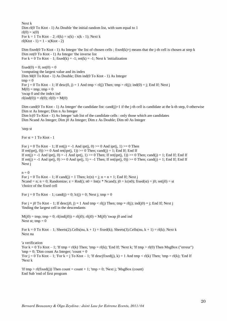
Dim rl(0 To Ktot - 1) As Double 'the initial random list, with sum equal to 1

rl(0) = x(0)

For k = 1 To Ktot – 2; rl(k) = x(k) - x(k - 1); Next k

rl(Ktot - 1) = 1 - x(Ktot - 2)

Dim fixed(0 To Ktot - 1) As Integer 'the list of chosen cells ; fixed(k)=j means that the j-th cell is chosen at step k

Dim ret(0 To Ktot - 1) As Integer 'the inverse list

For k = 0 To Ktot – 1; fixed(k) = -1; ret(k) = -1; Next k 'initialization

fixed(0) = 0; ret(0) = 0

'computing the largest value and its index

Dim M(0 To Ktot - 1) As Double; Dim ind(0 To Ktot - 1) As Integer

tmp = 0

For j = 0 To Ktot – 1; If desc(0, j) = 1 And tmp < rl(j) Then; tmp = rl(j); ind(0) = j; End If; Next j

M(0) = tmp; tmp = 0

'swap 0 and the index ind

rl(ind(0)) = rl(0); rl(0) = M(0)

Dim cand(0 To Ktot - 1) As Integer' the candidate list: cand(j)=1 if the j-th cell is candidate at the k-th step, 0 otherwise

Dim st As Integer; Dim n As Integer

Dim lc(0 To Ktot - 1) As Integer 'sub list of the candidate cells : only those which are candidates

Dim Ncand As Integer; Dim j0 As Integer; Dim z As Double; Dim n0 As Integer

'step st

For st = 1 To Ktot - 1

For j = 0 To Ktot – 1; If ret(j) = -1 And ipr(j, 0) >= 0 And ipr(j, 1) >= 0 Then

If ret(ipr(j, 0)) >= 0 And ret(ipr(j, 1)) >= 0 Then; cand(j) = 1; End If; End If

If ret(j) = -1 And ipr(j, 0) = -1 And ipr(j, 1) >= 0 Then; If ret(ipr(j, 1)) >= 0 Then; cand(j) = 1; End If; End If

If ret(j) = -1 And ipr(j, 0) >= 0 And ipr(j, 1) = -1 Then; If ret(ipr(j, 0)) >= 0 Then; cand(j) = 1; End If; End If

Next j

n = 0

For j = 0 To Ktot – 1; If cand(j) = 1 Then; lc(n) = j; n = n + 1; End If; Next j

Ncand = n; n = 0; Randomize; z = Rnd(); n0 = Int(z * Ncand); j0 = lc(n0); fixed(st) = j0; ret(j0) = st

'choice of the fixed cell

For j = 0 To Ktot – 1; cand(j) = 0; lc(j) = 0; Next j; tmp = 0

For j = j0 To Ktot – 1; If desc(j0, j) = 1 And tmp < rl(j) Then; tmp = rl(j); ind(j0) = j; End If; Next j

'finding the largest cell in the descendants

M(j0) = tmp; tmp = 0; rl(ind(j0)) = rl(j0); rl(j0) = M(j0) 'swap j0 and ind

Next st; tmp = 0

For k = 0 To Ktot – 1; Sheets(2).Cells(nu, k + 1) = fixed(k); Sheets(3).Cells(nu, k + 1) = rl(k); Next k

Next nu

'a verification

'For k = 0 To Ktot – 1; 'If tmp < rl(k) Then; 'tmp = rl(k); 'End If; 'Next k; 'If tmp > rl(0) Then MsgBox ("erreur")

'tmp = 0; 'Dim count As Integer; 'count = 0

'For j = 0 To Ktot – 1; 'For k = j To Ktot – 1; 'If desc(fixed(j), k) = 1 And tmp < rl(k) Then; 'tmp = rl(k); 'End If

'Next k

'If tmp > rl(fixed(j)) Then count = count + 1; 'tmp = 0; 'Next j; 'MsgBox (count)

End Sub 'end of first program


2. Program 2 : Evaluation of Integrals

Option Explicit; Const Itot = 100000; Const Jtot = 44

Sub macro1()

Dim n(0 To Jtot - 1) As Integer; n(1) = 1; n(4) = 1; n(10) = 1; n(12) = 1; n(13) = 1; n(21) = 1; n(30) = 1; n(32) = 1

Dim A As Variant ; A = Sheets(3).Range("A1").Resize(Itot, Jtot) 'reads data and puts them into memory

Dim prod As Double; prod = 1; Dim j As Integer; Dim sum0 As Double; Dim sum As Double; Dim i As Long; Dim

sumA as double

For i = 1 To Itot; For j = 1 To Jtot; prod = prod * A(i, j) ^ n(j - 1); Next j; sum0 = sum0 + prod; prod = 1;

If A(i, 38) <= 0.02 Then sumA = sumA + prod

'we want to compute a confidence interval on the 37th

variable, and A starts at 1, not at 0.

Next i

Dim k As Integer; Dim i0 As Integer; Dim j0 As Integer; sum = 0; prod = 1

For k = 0 To Jtot – 1; n(k) = n(k) + 1'increase the k-th number by 1 in order to compute the expectation

For i = 1 To Itot; For j = 1 To Jtot; prod = prod * A(i, j) ^ n(j - 1); Next j; sum = sum + prod; prod = 1; Next i

i0 = k \ 4; j0 = k Mod 4; Sheets(4).Cells(i0 + 1, j0 + 1) = sum / sum0; n(k) = n(k) – 1; sum = 0: Next k

End Sub

Documents

Société de Calcul Mathématique, S. A