Embed Size (px)
Citation preview
Solid-State Storage and Work Sharing
for
Efficient Scaleup Data Analytics
Thèse n. 6032 (2013)présenté le 12 Décembre 2013à la Faculté Informatique et Communicationslaboratoire de systèmes et applications de traitement de don-nées massivesprogramme doctoral en Informatique et CommunicationsÉcole Polytechnique Fédérale de Lausanne
pour l’obtention du grade de Docteur ès Sciencespar
Manoussos-Gavriil Athanassoulis
acceptée sur proposition du jury:
Prof. George Candea, président du juryProf. Anastasia Ailamaki, directeur de thèseProf. Willy Zwaenepoel, rapporteurProf. Kenneth A. Ross, rapporteurDr Phillip B. Gibbons, rapporteur
Lausanne, EPFL, 2013


I was never more certain ofhow far away I was from my goal
than when I was standing right beside it.
To my family, to my teachers, to my friends.All of them teachers in so many ways . . .

AcknowledgementsThe author of this book is only one, however, without the support of a number of people it wouldnot have been possible to produce this work. Many people deserve recognition both for their tech-nical and their general support which helped me complete this thesis. If I missed anyone below,it is because I was lucky to have many such people in my life and unlucky to have a lousy memory.
My advisor Natassa Ailamaki, reignited the research bug when she visited the University ofAthens and gave an inspiring talk, at the time that I was about to complete my Master studies andcontemplating for my future. Soon thereafter I joined her lab, DIAS, at EPFL where she taughtme nearly everything about database and systems research. Natassa is an enthusiastic advisorand researcher - one could say a research evangelist - who can give technical and motivationaladvices when most needed.
I would also like to thank Shimin Chen and Phil Gibbons for our excellent collaboration. Theirresearch rigor and focus on the detail was a great lesson to me.
Phil Gibbons also participated in my PhD committee, and along with him I thank WillyZwaenepoel, Ken Ross, and George Candea for agreeing to be part of my PhD committee.
The members of the DIAS lab were a big part of my PhD journey. Following chronologi-cal order, I would like to thank Ryan Johnson, Radu Stoica, Ippokratis Pandis, Ioannis Alagiannis,Iraklis Psaroudakis, and Stratos Idreos for our fruitful collaboration during my PhD years. RyanJohnson was my first office-mate, and in fact a perfect one, dedicated to high quality researchand eager to offer any help I ever needed. Ioannis Alagiannis, a lifelong friend, is just the personthat is most natural to collaborate with. In addition to these people, I would like to thank eachand every DIAS lab member for creating a healthy work environment I was happy to go to everyday during my PhD years. Verena Kantere, Debabrata Dash, Adrian Popescu, Renata Borovica,Danica Porobic, Pınar Tözün, Farhan Tauheed, Thomas Heinis, Erietta Liarou, Miguel Branco,Manos Karpathiotakis, Mirjana Pavlovic, Eleni Tzirita-Zacharatou, and Matthaios Olma offered,as well, invaluable discussions and comments for my ongoing research and my presentations.
I also spent four great months in IBM Watson Research Center in New York, USA. For this greatexperience I would like to thank Bishwaranjan Bhattacharjee, Ken Ross, Mustafa Canim, andYuan-chi Chang.
v
Acknowledgements
The bug of research has been plugged into me since I was a child, having endless discus-sions with the first researcher I ever met, my father. His passion for research was inspiring forme: before the age of ten I announced to my parents, Makis and Eleni, that I want to be an"experimentalist". My parents gave all the help I ever needed to study what I liked most and gaveme the bug to seek for answers of interesting questions. My older brother, Agis, who follows theacademic path as well, was always giving to me a first-hand taste of what this path looks like,and offered – during both undergraduate and graduate studies – invaluable help and advice.
I was lucky to complete my undergraduate studies in an excellent school, the Departmentof Informatics and Telecommunications of University of Athens, Greece. During my studies I hadinspiring teachers including Alex Delis who exemplifies research excellence and integrity, andStathes Hadjiefthymiades who supervised both my undergraduate and masters thesis, introducingme for real into the research world.
I greatly appreciate the effort made by Pierre Grydbeck and Dimitra Tsaoussis to help mewrite the French abstract of my thesis.
Finally, I gratefully acknowledge the funding supporting my PhD research, as part of my IBMPhD Fellowship Award, from the Swiss National Science Foundation EURYI Award, Grant NoPE0022-117125/1, and from the European Commission Collaborative Project “BigFoot”, GrantAgreement Number 317858.
Lausanne, 12 December 2013 M. A.
vi
AbstractToday, managing, storing and analyzing data continuously in order to gain additional insight isbecoming commonplace. Data analytics engines have been traditionally optimized for read-onlyqueries assuming that the main data reside on mechanical disks. The need for 24x7 operations inglobal markets and the rise of online and other quickly-reacting businesses make data freshnessan additional design goal. Moreover, the increased requirements in information quality makesemantic databases a key (often represented as graphs using the RDF data representation model).Last but not least, the performance requirements combined with the increasing amount of storedand managed data call for high-performance yet space-efficient access methods in order to supportthe desired concurrency and throughput.
Innovative data management algorithms and careful use of the underlying hardware platform helpus to address the aforementioned requirements. The volume of generated, stored and querieddata is increasing exponentially, and new workloads often are comprised of time-generateddata. At the same time the hardware is evolving with dramatic changes both in processing unitsand storage devices, where solid-state storage is becoming ubiquitous. In this thesis, we buildworkload-aware data access methods for data analytics - tailored for emerging time-generatedworkloads - which use solid-state storage, either (i) as an additional level in the memory hierarchyto enable real-time updates in a data analytics, or (ii) as standalone storage for applicationsinvolving support for knowledge-based data, and support for efficiently indexing archival andtime-generated data.
Building workload-aware and hardware-aware data management systems allows to increasetheir performance and to augment their functionality. The advancements in storage have ledto a variety of storage devices with different characteristics (e.g., monetary cost, access times,durability, endurance, read performance vs. write performance), and the suitability of a methodto an application depends on how it balances the different characteristics of the storage medium ituses. The data access methods proposed in this thesis - MaSM and BF-Tree - balance the benefitsof solid-state storage and of traditional hard disks, and are suitable for time-generated data ordatasets with similar organization, which include social, monitoring and archival applications.The study of work sharing in the context of data analytics paves the way to integrating shareddatabase operators starting from shared scans to several data analytics engines, and the workload-aware physical data organization proposed for knowledge-based datasets - RDF-tuple - enablesintegration of diverse data sources into the same systems.
vii

Acknowledgements
Keywords: databases, data analytics, solid-state storage, data freshness, work sharing, accessmethods
viii
RésuméDe nos jours, la gestion, le stockage et l’analyse de données en continu, afin d’obtenir desinformations supplémentaires, devient courant. Les systèmes d’analyse de données ont été tra-ditionnellement optimisés pour des requêtes en lecture seule en supposant que les donnéesprincipales résidaient sur des disques mécaniques. Le besoin d’opérer 24 heures sur 24, 7 jourssur 7 dans le contexte de marchés globaux et suite à l’accroissement des activités commerciales enligne ont fait de la « fraîcheur des données » un objectif supplémentaire. En outre, les exigencesaccrues en matière de qualité de l’information rendent les bases de données sémantiques clés(souvent représentées comme des graphes utilisant le modèle de représentation de données RDF).Finalement, les contraintes de performances combinées avec l’augmentation du volume desdonnées stockées et gérées nécessitent des méthodes d’accès performantes mais efficaces entermes de stockage afin de garantir le niveau de concurrence et de débit souhaité.
Des algorithmes de gestion de données innovants et l’utilisation attentive de la plateformematérielle sous-jacente nous aident à répondre aux exigences citées. Le volume des donnéesgénérées, stockées et demandées augmente exponentiellement et les nouvelles charges de travailcontiennent souvent des données temporelles. En même temps, le matériel informatique évolueavec des changements drastiques autant dans les unités de traitement que dans le stockage où leslecteurs à état solide deviennent omniprésents. Dans cette thèse, nous construisons des méthodesd’accès s’adaptant aux charges de travail d’analyse de données. Elles sont faites sur mesurepour les données temporelles qui utilisent le stockage à l’état solide soit (i) comme un niveausupplémentaire dans la hiérarchie de stockage permettant des mises à jour en temps réel desanalyses de données ou (ii) comme stockage indépendant pour des applications nécessitant lesupport de données basées sur la connaissance et le soutient pour l’indexation efficace de donnéesd’archive.
Les systèmes de gestion de données utilisant la connaissance de la charge de travail et dela plateforme matérielle sous-jacente peuvent augmenter leurs performances et fonctionnalités.L’avance dans le domaine des périphériques de stockage a mené au développement d’une va-riété de caractéristiques différentes (par exemple : coûts monétaires, temps d’accès, durabilité,endurance, performance de lecture contre écriture, etc.). L’efficacité d’une méthode d’accès pourune application donnée dépend de comment ces caractéristiques sont conciliées. Les méthodesd’accès proposées dans cette thèse, MaSM et BF-Tree, équilibrent les gains du stockage à l’étatsolide avec le stockage sur disques durs traditionnels et sont appropriées pour les données tem-
ix

Acknowledgements
porelles ou avec une structure similaire. Ceci comprend les applications sociales, de contrôleou d’archivage. L’étude du partage du travail dans le contexte des analyses de données ouvrela voie à l’intégration d’opérateurs de bases de données partagés à partir de scans communsà plusieurs systèmes d’analyse de données et avec l’organisation physique des données baséesur les charges de travail et les ensembles de données liées à des connaissances (RDF-tuple)permettent l’intégration de plusieurs sources de données dans un même système.
Mots-clés : bases de données, analyse de données, stockage à l’état solide, fraîcheur des données,partage du travail, méthodes d’accès
x
ContentsAcknowledgements v
Abstract (English/Français) vii
Table of Contents xv
List of figures xix
List of tables xxi
1 Introduction 11.1 The Information Age . . . . . . . . . . . . . . . . . . . . . . . . . . . . . . . . . . . 11.2 Data Management . . . . . . . . . . . . . . . . . . . . . . . . . . . . . . . . . . . . 11.3 Data Analytics . . . . . . . . . . . . . . . . . . . . . . . . . . . . . . . . . . . . . . 3
1.3.1 Data Analytics Challenges . . . . . . . . . . . . . . . . . . . . . . . . . . . 41.4 Implications on the DBMS architecture . . . . . . . . . . . . . . . . . . . . . . . . 41.5 Solid-State Storage and Work Sharing for Efficient Scaleup Data Analytics . . . . 5
1.5.1 Evolution of the storage hierarchy . . . . . . . . . . . . . . . . . . . . . . . 61.5.2 Summary and Contributions . . . . . . . . . . . . . . . . . . . . . . . . . . 71.5.3 Published papers . . . . . . . . . . . . . . . . . . . . . . . . . . . . . . . . 8
1.6 Outline (How to read this thesis) . . . . . . . . . . . . . . . . . . . . . . . . . . . . 9
2 Related Work and Background 112.1 Hardware Trends in Storage . . . . . . . . . . . . . . . . . . . . . . . . . . . . . . . 11
2.1.1 Fifty years of hard disks . . . . . . . . . . . . . . . . . . . . . . . . . . . . 112.1.2 From hard disks to solid-state storage . . . . . . . . . . . . . . . . . . . . . 122.1.3 Flash-based solid-state storage . . . . . . . . . . . . . . . . . . . . . . . . . 132.1.4 Phase Change Memory . . . . . . . . . . . . . . . . . . . . . . . . . . . . . 142.1.5 Flash vs. PCM . . . . . . . . . . . . . . . . . . . . . . . . . . . . . . . . . . 152.1.6 More solid-state storage technologies . . . . . . . . . . . . . . . . . . . . . 172.1.7 Sequential Reads and Random Writes in Storage Systems . . . . . . . . . 18
2.2 Data Analysis Systems . . . . . . . . . . . . . . . . . . . . . . . . . . . . . . . . . . 182.2.1 High-Throughput Updates and Data Analysis . . . . . . . . . . . . . . . . 192.2.2 Adaptive organization of data and updates . . . . . . . . . . . . . . . . . . 20
xi
Contents
2.2.3 Orthogonal Uses of SSDs for Data Warehouses . . . . . . . . . . . . . . . 212.3 Optimizing Data Analysis Queries Using Work-Sharing . . . . . . . . . . . . . . . 21
2.3.1 Sharing in the I/O layer and in the execution engine . . . . . . . . . . . . 222.3.2 Simultaneous Pipelining . . . . . . . . . . . . . . . . . . . . . . . . . . . . 232.3.3 The QPipe execution engine . . . . . . . . . . . . . . . . . . . . . . . . . . 232.3.4 Global Query Plans with shared operators . . . . . . . . . . . . . . . . . . 242.3.5 The CJOIN operator . . . . . . . . . . . . . . . . . . . . . . . . . . . . . . 252.3.6 Quantifying work sharing opportunities . . . . . . . . . . . . . . . . . . . 27
2.4 Bloom filters . . . . . . . . . . . . . . . . . . . . . . . . . . . . . . . . . . . . . . . 282.4.1 Bloom filters’ applications in data management . . . . . . . . . . . . . . . 282.4.2 Bloom filters for evolving workloads and storage . . . . . . . . . . . . . . 28
2.5 Indexing for Data Analysis . . . . . . . . . . . . . . . . . . . . . . . . . . . . . . . 292.5.1 SSD-aware indexing . . . . . . . . . . . . . . . . . . . . . . . . . . . . . . 292.5.2 Specialized optimizations for tree indexing . . . . . . . . . . . . . . . . . 292.5.3 Indexing for data warehousing . . . . . . . . . . . . . . . . . . . . . . . . . 30
2.6 Knowledge-based Data Analysis . . . . . . . . . . . . . . . . . . . . . . . . . . . . 302.6.1 RDF datasets and benchmarks . . . . . . . . . . . . . . . . . . . . . . . . . 302.6.2 Storing RDF data . . . . . . . . . . . . . . . . . . . . . . . . . . . . . . . . 31
2.7 Summary . . . . . . . . . . . . . . . . . . . . . . . . . . . . . . . . . . . . . . . . . 32
3 Online Updates for Data Analytics using Solid-State Storage 333.1 Introduction . . . . . . . . . . . . . . . . . . . . . . . . . . . . . . . . . . . . . . . . 33
3.1.1 Efficient Online Updates for DW: Limitations of Prior Approaches . . . . 343.1.2 Our Solution: Cache Updates in SSDs for online updates in DWs . . . . . 353.1.3 Contributions . . . . . . . . . . . . . . . . . . . . . . . . . . . . . . . . . . 38
3.2 Efficient Online Updates and Range Scans in Data Warehouses . . . . . . . . . . 383.2.1 Basic Concepts and Focus of the Study . . . . . . . . . . . . . . . . . . . . 393.2.2 Conventional Approach: In-Place Updates . . . . . . . . . . . . . . . . . . 403.2.3 Prior Proposals: Indexed Updates (IU) . . . . . . . . . . . . . . . . . . . . 41
3.3 MaSM Design . . . . . . . . . . . . . . . . . . . . . . . . . . . . . . . . . . . . . . 423.3.1 Basic Ideas . . . . . . . . . . . . . . . . . . . . . . . . . . . . . . . . . . . . 433.3.2 MaSM-2M . . . . . . . . . . . . . . . . . . . . . . . . . . . . . . . . . . . . 443.3.3 MaSM-M . . . . . . . . . . . . . . . . . . . . . . . . . . . . . . . . . . . . . 463.3.4 MaSM-αM . . . . . . . . . . . . . . . . . . . . . . . . . . . . . . . . . . . . 493.3.5 Further Optimizations . . . . . . . . . . . . . . . . . . . . . . . . . . . . . . 493.3.6 Transaction Support . . . . . . . . . . . . . . . . . . . . . . . . . . . . . . . 503.3.7 Achieving The Five Design Goals . . . . . . . . . . . . . . . . . . . . . . . 52
3.4 Analysis and Modeling of MaSM . . . . . . . . . . . . . . . . . . . . . . . . . . . . 533.4.1 Theorems About MaSM Behavior . . . . . . . . . . . . . . . . . . . . . . . 543.4.2 SSD Wear vs. Memory Footprint . . . . . . . . . . . . . . . . . . . . . . . 553.4.3 Memory Footprint vs. Performance . . . . . . . . . . . . . . . . . . . . . . 563.4.4 Modeling the I/O Time of Range Queries . . . . . . . . . . . . . . . . . . 58
xii
Contents
3.4.5 LSM analysis and comparison with MaSM . . . . . . . . . . . . . . . . . 623.5 Experimental Evaluation . . . . . . . . . . . . . . . . . . . . . . . . . . . . . . . . . 64
3.5.1 Experimental Setup . . . . . . . . . . . . . . . . . . . . . . . . . . . . . . . 643.5.2 Experiments with Synthetic Data . . . . . . . . . . . . . . . . . . . . . . . 653.5.3 TPC-H Replay Experiments . . . . . . . . . . . . . . . . . . . . . . . . . . 71
3.6 Discussion . . . . . . . . . . . . . . . . . . . . . . . . . . . . . . . . . . . . . . . . . 713.6.1 Shared-Nothing Architectures . . . . . . . . . . . . . . . . . . . . . . . . . 713.6.2 MaSM for deeper memory hierarchies and new storage technologies . . . 723.6.3 Can SSDs Enhance Performance and Be Cost Efficient? . . . . . . . . . . 733.6.4 General support of MaSM . . . . . . . . . . . . . . . . . . . . . . . . . . . 733.6.5 Applying MaSM to Cloud Data Management . . . . . . . . . . . . . . . . 75
3.7 Conclusion . . . . . . . . . . . . . . . . . . . . . . . . . . . . . . . . . . . . . . . . 75
4 Enhancing Data Analytics with Work Sharing 774.1 Introduction . . . . . . . . . . . . . . . . . . . . . . . . . . . . . . . . . . . . . . . . 77
4.1.1 Methodologies for sharing data and work . . . . . . . . . . . . . . . . . . 774.1.2 Integrating Simultaneous Pipelining and Global Query Plans . . . . . . . 784.1.3 Optimizing Simultaneous Pipelining . . . . . . . . . . . . . . . . . . . . . 794.1.4 Simultaneous Pipelining vs. Global Query Plans . . . . . . . . . . . . . . 794.1.5 Contributions . . . . . . . . . . . . . . . . . . . . . . . . . . . . . . . . . . 804.1.6 Outline . . . . . . . . . . . . . . . . . . . . . . . . . . . . . . . . . . . . . . 81
4.2 Integrating SP and GQP . . . . . . . . . . . . . . . . . . . . . . . . . . . . . . . . . 814.2.1 Benefits of applying SP to GQP . . . . . . . . . . . . . . . . . . . . . . . . 814.2.2 CJOIN as a QPipe stage . . . . . . . . . . . . . . . . . . . . . . . . . . . . 824.2.3 SP for the CJOIN stage . . . . . . . . . . . . . . . . . . . . . . . . . . . . . 83
4.3 Shared Pages Lists for SP . . . . . . . . . . . . . . . . . . . . . . . . . . . . . . . . 844.3.1 Design of a SPL . . . . . . . . . . . . . . . . . . . . . . . . . . . . . . . . . 874.3.2 Linear Window of Opportunity . . . . . . . . . . . . . . . . . . . . . . . . 87
4.4 Experimental Methodology . . . . . . . . . . . . . . . . . . . . . . . . . . . . . . . 884.5 Experimental Analysis . . . . . . . . . . . . . . . . . . . . . . . . . . . . . . . . . . 89
4.5.1 Impact of concurrency . . . . . . . . . . . . . . . . . . . . . . . . . . . . . 904.5.2 Impact of data size . . . . . . . . . . . . . . . . . . . . . . . . . . . . . . . 924.5.3 Impact of Similarity . . . . . . . . . . . . . . . . . . . . . . . . . . . . . . . 954.5.4 SSB query mix evaluation . . . . . . . . . . . . . . . . . . . . . . . . . . . 96
4.6 Discussion . . . . . . . . . . . . . . . . . . . . . . . . . . . . . . . . . . . . . . . . . 974.7 Conclusions . . . . . . . . . . . . . . . . . . . . . . . . . . . . . . . . . . . . . . . . 98
5 BF-Tree: Approximate Tree Indexing 1015.1 Introduction . . . . . . . . . . . . . . . . . . . . . . . . . . . . . . . . . . . . . . . . 101
5.1.1 Implicit Clustering . . . . . . . . . . . . . . . . . . . . . . . . . . . . . . . 1015.1.2 The capacity-performance trade-off . . . . . . . . . . . . . . . . . . . . . . 1025.1.3 Indexing for modern storage . . . . . . . . . . . . . . . . . . . . . . . . . . 1035.1.4 Approximate Tree Indexing . . . . . . . . . . . . . . . . . . . . . . . . . . 103
xiii
Contents
5.2 Making approximate indexing competitive . . . . . . . . . . . . . . . . . . . . . . 1055.3 Bloom Filter Tree (BF-Tree) . . . . . . . . . . . . . . . . . . . . . . . . . . . . . . 106
5.3.1 BF-Tree architecture . . . . . . . . . . . . . . . . . . . . . . . . . . . . . . 1065.3.2 Creating and Updating a BF-Tree . . . . . . . . . . . . . . . . . . . . . . . 107
5.4 Read-optimized BF-Trees . . . . . . . . . . . . . . . . . . . . . . . . . . . . . . . . 1105.5 Modeling BF-Trees and B+-Trees . . . . . . . . . . . . . . . . . . . . . . . . . . . 111
5.5.1 Parameters and model . . . . . . . . . . . . . . . . . . . . . . . . . . . . . 1115.5.2 Discussion on BF-Tree size and compression . . . . . . . . . . . . . . . . 115
5.6 Experimental evaluation . . . . . . . . . . . . . . . . . . . . . . . . . . . . . . . . . 1165.6.1 Experimental Methodology . . . . . . . . . . . . . . . . . . . . . . . . . . 1165.6.2 BF-Tree for primary key . . . . . . . . . . . . . . . . . . . . . . . . . . . . 1175.6.3 BF-Tree for non-unique attributes . . . . . . . . . . . . . . . . . . . . . . . 1215.6.4 BF-Tree for TPCH . . . . . . . . . . . . . . . . . . . . . . . . . . . . . . . 1235.6.5 Summary . . . . . . . . . . . . . . . . . . . . . . . . . . . . . . . . . . . . . 125
5.7 BF-Tree as a general index . . . . . . . . . . . . . . . . . . . . . . . . . . . . . . . 1255.7.1 BF-Tree vs. interpolation search . . . . . . . . . . . . . . . . . . . . . . . . 1255.7.2 Range scans . . . . . . . . . . . . . . . . . . . . . . . . . . . . . . . . . . . 1265.7.3 Querying in the presence of inserts and deletes . . . . . . . . . . . . . . . 126
5.8 Optimizations . . . . . . . . . . . . . . . . . . . . . . . . . . . . . . . . . . . . . . . 1295.9 Conclusions . . . . . . . . . . . . . . . . . . . . . . . . . . . . . . . . . . . . . . . . 129
6 Graph Data Management using Solid-State Storage 1316.1 Introduction . . . . . . . . . . . . . . . . . . . . . . . . . . . . . . . . . . . . . . . . 131
6.1.1 Contributions . . . . . . . . . . . . . . . . . . . . . . . . . . . . . . . . . . 1326.1.2 Outline . . . . . . . . . . . . . . . . . . . . . . . . . . . . . . . . . . . . . . 133
6.2 Path Processing . . . . . . . . . . . . . . . . . . . . . . . . . . . . . . . . . . . . . . 1336.3 RDF processing on PCM . . . . . . . . . . . . . . . . . . . . . . . . . . . . . . . . 137
6.3.1 The RDF-tuple . . . . . . . . . . . . . . . . . . . . . . . . . . . . . . . . . . 1396.3.2 The Internals of Pythia . . . . . . . . . . . . . . . . . . . . . . . . . . . . . 1406.3.3 Experimental Workload . . . . . . . . . . . . . . . . . . . . . . . . . . . . . 1416.3.4 Experimental Evaluation . . . . . . . . . . . . . . . . . . . . . . . . . . . . 1426.3.5 Comparison with RDF-3X . . . . . . . . . . . . . . . . . . . . . . . . . . . 143
6.4 PCM Opportunities . . . . . . . . . . . . . . . . . . . . . . . . . . . . . . . . . . . . 1446.4.1 Algorithm redesign . . . . . . . . . . . . . . . . . . . . . . . . . . . . . . . 145
6.5 SPARQL code for test queries . . . . . . . . . . . . . . . . . . . . . . . . . . . . . 1456.6 Conclusions . . . . . . . . . . . . . . . . . . . . . . . . . . . . . . . . . . . . . . . . 146
7 The Big Picture 1497.1 What we did . . . . . . . . . . . . . . . . . . . . . . . . . . . . . . . . . . . . . . . . 1497.2 Storage is constantly evolving: Opportunities and challenges . . . . . . . . . . . . 150
7.2.1 Persistent main memory: Database Management Systems vs. OperatingSystems . . . . . . . . . . . . . . . . . . . . . . . . . . . . . . . . . . . . . . 151
7.2.2 Software stack is too slow . . . . . . . . . . . . . . . . . . . . . . . . . . . 151
xiv
Contents
7.3 Ever increasing concurrency in analytics . . . . . . . . . . . . . . . . . . . . . . . 1517.3.1 Extending support of work sharing . . . . . . . . . . . . . . . . . . . . . . 1527.3.2 Column-stores and high concurrency . . . . . . . . . . . . . . . . . . . . . 152
Bibliography 153
Curriculum Vitae 167
xv

List of Figures2.1 Fifty years of HDD . . . . . . . . . . . . . . . . . . . . . . . . . . . . . . . . . . . . 122.2 Read latency for (a) flash (zoomed in the most relevant part) and (b) PCM . . . . 162.3 Write latency for (a) flash (zoomed in the most relevant part) and (b) PCM . . . 172.4 (a) SP example with two queries having a common sub-plan below the join
operator. (b) A step and a linear WoP. . . . . . . . . . . . . . . . . . . . . . . . . . 232.5 Example of shared selection and hash-join operators. . . . . . . . . . . . . . . . . 242.6 CJOIN evaluates a GQP for star queries. . . . . . . . . . . . . . . . . . . . . . . . . 26
3.1 An analysis of migration overheads for differential updates as a function of thememory buffer size. Overhead is normalized to the prior state-of-the-art using16GB memory. . . . . . . . . . . . . . . . . . . . . . . . . . . . . . . . . . . . . . . 34
3.2 Framework for SSD-based differential updates. . . . . . . . . . . . . . . . . . . . . 373.3 TPC-H queries with random updates on a row store. . . . . . . . . . . . . . . . . . 403.4 TPC-H queries with emulated random updates on a column store. . . . . . . . . . 403.5 Extending prior proposals of Indexed Updates (IU) to SSDs: (a) in-memory
indexed updates (PDT (Héman et al., 2010)), (b) extending IU to SSDs, and (c)applying LSM (O’Neil et al., 1996) to IU. . . . . . . . . . . . . . . . . . . . . . . . 41
3.6 Illustrating the MaSM algorithm using 2M memory. . . . . . . . . . . . . . . . . . 443.7 MaSM-2M algorithm . . . . . . . . . . . . . . . . . . . . . . . . . . . . . . . . . . 453.8 Illustrating MaSM algorithm using M memory. . . . . . . . . . . . . . . . . . . . . 473.9 MaSM-M algorithm . . . . . . . . . . . . . . . . . . . . . . . . . . . . . . . . . . . 483.10 The tradeoff between SSD wear and memory footprint. . . . . . . . . . . . . . . . 563.11 Memory footprint vs. short range performance. . . . . . . . . . . . . . . . . . . . . 573.12 Modeling MaSM performance for reading main data and fetching the updates
using the characteristics of the storage used in our experimentation. . . . . . . . . 613.13 The ratio of the time to fetch the updates from SSD to the time to read the main
data for index granularity 64KB. . . . . . . . . . . . . . . . . . . . . . . . . . . . . 613.14 The ratio of the time to fetch the updates from SSD to the time to read the main
data for index granularity 4KB. . . . . . . . . . . . . . . . . . . . . . . . . . . . . . 613.15 Modeling MaSM performance for reading main data and fetching the updates
using the characteristics of a high-end storage system. . . . . . . . . . . . . . . . . 623.16 Comparing the impact of online update schemes on the response time of primary
key range scans (normalized to scans without updates). . . . . . . . . . . . . . . . 66
xvii
List of Figures
3.17 MaSM range scans varying updates cached in SSD. . . . . . . . . . . . . . . . . . 673.18 Range scan with MaSM varying update speed. . . . . . . . . . . . . . . . . . . . . 673.19 Comparing the impact of online update schemes, with MaSM using both SSD
and HDD, on the response time of primary key range scans (normalized to scanswithout updates). . . . . . . . . . . . . . . . . . . . . . . . . . . . . . . . . . . . . . 68
3.20 MaSM update migration. . . . . . . . . . . . . . . . . . . . . . . . . . . . . . . . . 683.21 Sustained updates per second varying SSD size in MaSM. . . . . . . . . . . . . . 683.22 Range scan and MaSM performance while emulating CPU cost of query process-
ing (10GB ranges). . . . . . . . . . . . . . . . . . . . . . . . . . . . . . . . . . . . . 693.23 Comparing in-place updates with MaSM performance (using both coarse-grain
and fain-grain run indexes) when both data and updates are stored in memory(10GB table size). . . . . . . . . . . . . . . . . . . . . . . . . . . . . . . . . . . . . 70
3.24 Replaying I/O traces of TPC-H queries on a real machine with online updates. . . 71
4.1 Evaluation of three concurrent queries using (a) a query-centric model, (b) sharedscans, (c) SP, and (d) a GQP. . . . . . . . . . . . . . . . . . . . . . . . . . . . . . . 78
4.2 Integration scheme of CJOIN as a QPipe stage. . . . . . . . . . . . . . . . . . . . . 834.3 Evaluating multiple identical TPC-H Q1 queries (a) with a push-only model
during SP (FIFO), and (b) with a pull-based model during SP (SPL). In (c), weshow the corresponding speedups of the two methods of SP, over not sharing, forlow concurrency. . . . . . . . . . . . . . . . . . . . . . . . . . . . . . . . . . . . . . 84
4.4 Sharing identical results during SP with: (a) push-only model and (b) a SPL. . . . 854.5 Design of a shared pages list. . . . . . . . . . . . . . . . . . . . . . . . . . . . . . . 864.6 Same experiment as in Figure 4.3b, for the case of 8 concurrent queries, with a
varying maximum size for SPL. . . . . . . . . . . . . . . . . . . . . . . . . . . . . . 874.7 The SSB Q3.2 SQL template and the query plan. . . . . . . . . . . . . . . . . . . . 904.8 Memory-resident database of SF=1. The table includes measurements for the
case of 256 queries. . . . . . . . . . . . . . . . . . . . . . . . . . . . . . . . . . . . 904.9 Same as Figure 4.8, with a disk-resident database. . . . . . . . . . . . . . . . . . . 914.10 8 queries with a memory-resident database of SF=10. The table includes mea-
surements for 30% selectivity. . . . . . . . . . . . . . . . . . . . . . . . . . . . . . 924.11 Memory-resident database of SF=10 and 30% selectivity. The table includes
measurements for 256 queries. . . . . . . . . . . . . . . . . . . . . . . . . . . . . . 934.12 8 concurrent queries with disk-resident databases. The table includes measure-
ments for the case of SF=100. . . . . . . . . . . . . . . . . . . . . . . . . . . . . . . 944.13 Disk-resident database of SF=1 and 16 possible plans. The table includes mea-
surements for 256 queries. . . . . . . . . . . . . . . . . . . . . . . . . . . . . . . . . 954.14 Evaluating 512 concurrent queries with a varying similarity factor, for a SF=100.
The table includes the SP sharing opportunities (average of all iterations), in theformat 1st/2nd/3rd hash-join for QPipe-SP. . . . . . . . . . . . . . . . . . . . . . 96
4.15 Disk-resident database of SF=30. The table includes measurements for the caseof 256 queries. . . . . . . . . . . . . . . . . . . . . . . . . . . . . . . . . . . . . . . 97
xviii
List of Figures
4.16 Throughput while evaluating concurrent queries with a disk-resident database ofSF=30. The table includes measurements for the case of 256 clients. . . . . . . . 98
5.1 Clustering of shipdate, commitdate, and receiptdate. . . . . . . . . . . . . . . . . . 1025.2 The capacity/performance storage trade-off. . . . . . . . . . . . . . . . . . . . . . . 1045.3 BF-tree . . . . . . . . . . . . . . . . . . . . . . . . . . . . . . . . . . . . . . . . . . . 1075.4 BF-tree leaves . . . . . . . . . . . . . . . . . . . . . . . . . . . . . . . . . . . . . . . 1105.5 Analytical comparison of BF-Tree vs. B+-Tree. . . . . . . . . . . . . . . . . . . . 1155.6 BF-Tree and B+-Tree performance for the PK index for five storage configura-
tions for storing the index and the main data. . . . . . . . . . . . . . . . . . . . . . 1175.7 The break-even points when indexing PK . . . . . . . . . . . . . . . . . . . . . . . 1195.8 BF-Tree and B+-Tree performance for PK index: cold caches vs. warm caches. . 1205.9 BF-Tree and B+-Tree performance for ATT1 index for five storage configurations
for storing the index and the main data. . . . . . . . . . . . . . . . . . . . . . . . . 1215.10 The break-even points when indexing ATT1 . . . . . . . . . . . . . . . . . . . . . 1225.11 BF-Tree and B+-Tree performance for ATT1 index: cold caches vs. warm caches.1235.12 BF-Tree for point queries on TPCH dates varying hit rate. . . . . . . . . . . . . . 1245.13 IOs for range scans using BF-Trees vs. B+-Trees. . . . . . . . . . . . . . . . . . . 1265.14 False positive probability ( f pp) in the presence of inserts. . . . . . . . . . . . . . 1285.15 False positive probability ( f pp) in the presence of inserts (zoomed in). . . . . . . 128
6.1 Latency for 4K, 8K, 16K, 32K page size when varying concurrent queries. Notethe logarithmic scale on both axes. . . . . . . . . . . . . . . . . . . . . . . . . . . . 135
6.2 Bandwidth for 4K, 8K, 16K, 32K page size when varying concurrent queries . . 1366.3 Custom path processing benchmark: Speedup of PCM over flash . . . . . . . . . 1376.4 Latency per page request size for PCM and flash, varying page size and number
of concurrent threads issuing requests. . . . . . . . . . . . . . . . . . . . . . . . . . 1386.5 Bandwidth for PCM and flash, varying page size and number of concurrent
threads issuing requests. . . . . . . . . . . . . . . . . . . . . . . . . . . . . . . . . . 1386.6 RDF-tuple in the SPO-store . . . . . . . . . . . . . . . . . . . . . . . . . . . . . . . 1396.7 RDF-tuple layout . . . . . . . . . . . . . . . . . . . . . . . . . . . . . . . . . . . . . 1406.8 Pythia Architecture . . . . . . . . . . . . . . . . . . . . . . . . . . . . . . . . . . . . 1416.9 Bandwidth for Pythia for 1, 2, 4, 8, 16, 32 concurrent clients submitting queries . 1436.10 Latency for Pythia for 1, 2, 4, 8, 16, 32 concurrent clients submitting queries . . . 1436.11 Query latency using Pythia for Q1, Q2 and Q3 . . . . . . . . . . . . . . . . . . . . 144
xix

List of Tables2.1 HDD trends compared and flash characteristics . . . . . . . . . . . . . . . . . . . . 132.2 Sharing methodologies employed by query-centric models and the research
prototypes we examine. . . . . . . . . . . . . . . . . . . . . . . . . . . . . . . . . . 21
3.1 Parameters used in the MaSM-M algorithm. . . . . . . . . . . . . . . . . . . . . . 493.2 The parameters of MaSM-M’s performance model and their values. . . . . . . . . 593.3 Computing the optimal height, h for an LSM tree, using the size ratio between
adjacent levels, r , and the I/O write rate normalized by input insertion rate,(h −0.5)(1+ r ). (The C0 tree is in memory, and C1, ..., Ch trees are on SSDs.Suppose memory size allocated to the C0 tree is 16MB, and the SSD spaceallocated to the LSM tree is 4GB.) . . . . . . . . . . . . . . . . . . . . . . . . . . . 62
4.1 Rules of thumb for when and how to share data and work across typical concurrentanalytical queries in DW. . . . . . . . . . . . . . . . . . . . . . . . . . . . . . . . . 80
5.1 Parameters of the model . . . . . . . . . . . . . . . . . . . . . . . . . . . . . . . . . 1125.2 B+-Tree & BF-Tree size (pages) for 1GB relation . . . . . . . . . . . . . . . . . . 1185.3 False reads/search for the experiments with 1GB data . . . . . . . . . . . . . . . . 118
6.1 Description of the benchmark . . . . . . . . . . . . . . . . . . . . . . . . . . . . . . 1336.2 Hardware specification of the PCM device . . . . . . . . . . . . . . . . . . . . . . 1346.3 Hardware specification of the flash device . . . . . . . . . . . . . . . . . . . . . . . 1346.4 Custom graph benchmark parameters. . . . . . . . . . . . . . . . . . . . . . . . . . 134
xxi

1 Introduction
1.1 The Information Age
The saying "Knowledge is power"1, lays the groundwork for how the era we live in, the Infor-mation Age, is affecting humanity. The Information Age is characterized by the growing needto gather, manage, access and analyze information to support the operation of any commercial,research or government organization. It is based upon the digital revolution - also known as thethird industrial revolution. In turn the digital revolution is based on the enormous and contin-uous advancements in technology which allows us to create digital circuits capable of storing,processing, exchanging, analyzing and generating exponentially more digital data every year.
Information and data management, however, is not a recent discipline. Centuries before the digi-talization of data, businesses and governments used centralized data repositories to keep financial,managerial and organizational information. Such applications required functionality guarantees;namely, correctness, consistency and permanence of the information. The growing need to storeand manage data combined with the technological advancements led to the development of datamanagement systems as a result of both research efforts and commercial applications.
1.2 Data Management
The need to store data in order to facilitate governmental organization and business transactionswas met when technology started offering ways to automate such processes. In fact, this needfueled the explosion of research and development in computer-based systems to centrally maintainbank, business and governmental information which started in the 1950s when the notion ofelectronic computers became reality. In a few years time a new market had been created andalready by the 1960s companies were working on building complex software systems on top ofexpensive computers to store, manage and query data: the data managements systems market hadbeen created.
1"Scientia potentia est" in Latin, attributed to Sir Francis Bacon
1
Chapter 1. Introduction
One of the first widely used database management system was IBM’s IMS (Information Man-agement System), initially designed for the 1966 Apollo Program. IMS used a hierarchicalconceptual model where data were organized in a tree-structure which is capable of representingparent-child relationships: one parent may have many children, but each child has one parent.Apart from supporting travel in space, IMS was widely used in the banking sector supportingevery-day transactions by banks and bank customers. In 1970s Edgar Codd introduced theRelational Model (Codd, 1970) which shaped how the majority of the systems to follow representand store data. The Relational Model, which is based on first-order logic, represents data usingtuples which, when grouped, form relations. In the Relational Model the logical organizationof the data (tuples and relations) is decoupled from the physical organization of the data. Thisflexibility and the clarity of representing information lead to a wide adoption of the RelationalModel which became the standard way to represent information in database systems.
Following the development of the Relational Model, several relational database managementsystems (RDBMS) were developed either as research prototypes or as commercial products. Theevolution of the database market led to the development of a query language which today isknown as SQL. While the initial domain of application for database systems was mostly thegovernmental and the banking applications, the development of the Internet since the mid-1990scaused an exponential growth of the database market. The ease in connectivity led to the creationof numerous client-server applications that required database support, and at the same time, moreand more data were generated. The trend of increasing data generation and, consequently, theneed to store it and manage it, is still growing at exponential rates.
Soon after the first simple web applications, the data generated by users of online services, bycustomers of online and offline shops, and in general by any user of any digitalized service wasstored to ensure the correct operation of all these businesses and services. At the same time,archived data can reveal additional information if one has the means to analyze it efficiently.Starting from the late 1990s an increasing number of database systems vendors started focusing onbuilding systems to efficiently manage and analyze enormous amounts of data. Initially, databasemanagement systems vendors needed to address the requirements of two major application genres.First, to keep safely the accurate and up-to-date information of transactions between businessesand people leading to the development of On-line Transactional Processing (OLTP). Second,to manage and analyze huge and increasing quantities of data resulting in the development ofOn-line Analytical Processing (OLAP). These two main categories shaped the database systemsscenery in terms of what each system is addressing and what type of optimizations - and researchin order to achieve them - are necessary for each category.
The crystallization of the goals of database systems had a very important implication. The designof database systems as software systems rapidly evolved to a standardized architecture (Hellersteinet al., 2007), which then allowed the researchers and the database systems developers to speak acommon language. They were able to devise techniques that could be used in different systemsbecause they were using the same high-level constructs despite having different implementations.This ease of interaction sped up the progress and the evolution of database systems and helped to
2
1.3. Data Analytics
build a large community and a large market with a variety of solutions optimized for differentapplications and use cases.
The architecture of a typical database system includes (1) the parser, (2) the optimizer, (3) thequery engine, and (4) the storage manager. In a modern database system, the parser is responsibleto parse a SQL query and analyze it syntactically, making sure it is consistent with the data athand, and then, to forward it to the optimizer. The optimizer, in turn, evaluates what are thepossible ways to execute the given query, and tries to find the fastest way (optimal query plan) toexecute it.2 After the query optimization phase, the query engine activates the chosen algorithmsto execute the query and, when needed, it requests the data from the storage manager, whichretrieves data from the memory and storage components.
The standardized architecture of database systems at the high-level enabled deep research for eachand every module. Research on database systems covers query optimization, query execution, dataaccess, but also transaction execution, security and distributed processing. The work presentedin this thesis is related with query execution and techniques to access the data from the storagemanager. A key observation is that the largest bulk of research on the internal modules of adatabase system is based on the assumption that the system uses hard disk drives as permanentstorage. While there are approaches making different assumptions (e.g., in-memory databaseswith redundancy) the common denominator between most of the existing approaches is thepresence of hard disks at some level to ensure durability of the data. Below we discuss how thetrends in what data we generate and we analyze create new requirements for the internal modulesof database systems motivating the research path taken.
1.3 Data Analytics
OLAP applications have been popular and crucial to business operation since the 1980s, however,the recent trends in the pace of data generation and the consequent needs for storing and analyzingdata created a new set of requirements. Today, data have the following five key characteristics: (i)the data volume itself is large and growing exponentially, (ii) the data are constantly evolvingand new information or updates are constantly generated, leading to high data velocity, (iii) alarge variety of data sources include useful information for any given application making it veryimportant to integrate diverse sources, (iv) as the data and the number of sources grow it is crucialto ensure the veracity of the data in order to have meaningful insights and (v) produce highvalue analysis which can help the scientific, business or organizational goals of the data analysisperformed. Below we focus on the characteristics of volume, velocity, variety and value of data,to introduce data analytics requirements and the challenges that are addressed in this thesis.
2The optimizer is not always able to find the optimal query plan because it uses heuristics when searching for theappropriate combination of algorithms to minimize its response time.
3
Chapter 1. Introduction
1.3.1 Data Analytics Challenges
The above characteristics - volume, velocity, variety, veracity and value - are known as the 5 V’sof Big Data. "Knowledge is power", however, only when we know how to extract knowledge.Hence, the above characteristics combined with data analytics requirements create researchchallenges, which research on data analytics systems is attempting to address.
The sheer volume of the data and its velocity creates the data freshness requirement. The datamanagement challenge is how to use the most recent version of the data when executing dataanalysis queries. Data freshness is a challenge because updating data and running analyticalqueries at the same time typically causes workload interference, mainly as a result of the disruptionof analytical query access patterns (involving sequential scans of the hard disks) by scatteredupdates.
Velocity and value show that the value of our insights drops precipitously as the analysis queriesare delayed. Hence, it is important to optimize for query response time and at the same time,transform the destructive interference to collaborative execution when possible.
Combining volume and velocity a new challenge is raised: how to efficiently index, and conse-quently access, continuously generated data - one very common use case. This challenge stemsfrom the fact that traditional indexing techniques are built assuming no knowledge of the dataattributes (e.g., distribution) since they mostly target data with no apriori knowledge or uniformdistribution of the indexed values. Real-time data typically has a time dimension, on which itshows implicit clustering (Moerkotte, 1998), something that can be used to offer indexing withhigh performance and smaller size.
Variety surfaces the need to use and perform data analytics on data from diverse data sourcesincluding as much knowledge as possible for the question at hand. Knowledge-based datasetshave been generated and are maintained in the context of the efforts of the semantic web.Typically, knowledge is represented using the Resource Description Framework (RDF) (RDf,2013). Integrating the knowledge from RDF data in data analytics increases the value of thegenerated insights, however, the different way to represent information in RDF compared to therelational model makes it hard (i) to integrate RDF in the physical layer, and (ii) to exploit theresearch that has already been done on database system engines to execute RDF queries.
Before exploring the approaches taken to address these challenges we will dive in more detailsinto which parts of the DBMS architectures play a key role in the aforementioned challenges.
1.4 Implications on the DBMS architecture
As we discussed in Section 1.2 the four layers of a DBMS are (i) the parser, (ii) the optimizer, (iii)the query engine, and (iv) the storage manager. Only the storage manager is copying data backand forth to its physical storage, typically hard disk drives (HDD). Nevertheless, the underlying
4
1.5. Solid-State Storage and Work Sharing for Efficient Scaleup Data Analytics
assumption that data are ultimately stored on HDD plays a key role in the design of the optimizerand the query engine, in addition to the storage manager.
In particular, the query engine is equipped with algorithms implementing database operators -such as projection, selection, join, aggregates and so on - that are optimized for data residing onHDD. In turn, the optimizer selects the optimal variant of an algorithm using the cost assumptionsof a HDD-equipped storage manager. The disk page assumption had to be maintained evenwhen specialized algorithmic optimizations were proposed. For example, cache-consciousoptimizations, like both the PAX data layout (Ailamaki et al., 2001) where a database disk pageis internally organized in per-attribute minipages, and the Fractal B+-Trees (Chen et al., 2002)where cache-optimized trees were embedded in disk-optimized trees, were optimized for cacheperformance, maintaining, however, the HDD page assumption. Moreover, even fundamentalchanges in the query engine architecture such as the design of pure column-store systems (Abadi,2008; Boncz, 2002) are motivated by the characteristics of the memory hierarchy including bothmain memory and secondary storage. While HDD is the most commonly used technology forsecondary storage, a wealth of new storage technologies has been under development (Freitas,2009) the last few years creating new storage devices - Solid State Drives (SSD) - with differentcharacteristics (more details in Section 2.1). By re-designing DBMS so as to exploit SSD we havethe opportunity to augment their functionality and their capabilities to address the aforementioneddata analytics challenges.
In fact, the data analytics challenges presented in Section 1.3.1 are connected very well withthe storage layers used by DBMS. Data freshness hurts query response time because of theinterference between the sequential reads of range scans and the random updates. Recentapproaches that have been proposed to address this problem either increase the memory overheadof the system, or they cannot offer competitive performance (more details in Section 2.2.1).Supporting analytical queries with high concurrency can easily create contention of the resourcesof the storage layer. Tree indexing structures have been traditionally designed assuming that theywill be stored on HDD, which have large and cheap capacity and slow random access performance.Finally, RDF management systems have been battling between an application-tailored storagesolution and a DBMS backed-up storage solution. The first can offer typically better performancefor a specific application, while the latter offers compatibility with other applications and usesthe benefits of several decades of research on the storage layer and the query engine.
1.5 Solid-State Storage and Work Sharing for Efficient Scaleup DataAnalytics
In this thesis we study the evolving requirements of data analytics engines and identify hownew non-volatile solid state storage and query execution run-time optimizations help addressingthese requirements. We outline the differences between traditional and solid-state storage andpropose new algorithms, data organizations and indexing structures, that are solid-state aware.Furthermore, we study existing run-time optimizations based on work sharing, and we compare,
5
Chapter 1. Introduction
integrate and redesign work sharing techniques.
To query and analyze data efficiently there have been two fundamental approaches: (i) distributionof the work in embarrassingly parallel tasks (when possible), and (ii) aggressive internal redesignof query engines. We extend these two approaches by adding in the equation the need ofhardware-aware and, in particular, solid-state storage aware redesign of query engines focusingon optimizing the performance of a single node. The shared-nothing approach of findingembarrassingly parallel tasks was largely-based on the fact that in order to increase the processingpower and the storage performance one would need the aggregate performance of multiple nodes.For example, parallelism was achieved by using several single-core machines and I/O bandwidthwas achieved by huge arrays of disks or aggregate bandwidth of disks in different machines. Therecent advancements of hardware, however, change these trends drastically. The evolution ofsolid-state storage with flash-based devices as the most popular example allows us to use a singlesolid-state device to achieve the same bandwidth as multiple disks and, at the same time, thetrend towards multi-core and many-core processors gives huge processing power to a single node.Thus, we propose techniques to optimize the behavior of our systems in the single-node case - asan orthogonal direction of distributing the work to multiple nodes - by building hardware-aware,storage-aware and workload-aware query engines.
Using solid-state storage as an additional level in the memory hierarchy, combined withintelligent data sharing, we enable data analytics engines to improve throughput and responsetimes, while maintaining data freshness.
1.5.1 Evolution of the storage hierarchy
The placement of solid-state storage in the memory hierarchy is an evolving research problemsince the available technologies themselves are evolving. While the first widespread solid-statestorage technology is flash, today a wealth of technologies is under research and development (Fre-itas, 2009), with Memristor and Phase Change Memory (PCM) being two of the most researchedtechnologies. Flash-based SSD have been used either as a layer in between main memory andsecondary storage or as alternative secondary storage. Future research of solid-state storageincludes, however, studying the implication of using non-volatile main memory either exclusivelyor side-by-side with (volatile) main memory. Solid-state storage characteristics are different thanHDD and main memory, nevertheless there exist partial commonalities. Therefore, integratingsolid-state storage in the DBMS hierarchy requires designing new algorithms as well as reusingalgorithms that were initially developed for other purposes.
The first step to understand how to integrate new storage technologies in a DBMS is to placethese in the memory hierarchy. Traditionally, the top part of the memory hierarchy consists ofthe CPU registers and the cache memories, while moving towards its bottom part there is mainmemory, and various layers of secondary storage. The fundamental tradeoff between differentlevels of the memory hierarchy is capacity vs. access latency. The higher levels have small access
6
1.5. Solid-State Storage and Work Sharing for Efficient Scaleup Data Analytics
latency while the lower levels have larger capacity. Contrary to the aforementioned memoryhierarchy levels, solid-state storage equipped devices have asymmetric read and write latency.The asymmetry makes it unclear whether such devices should be yet another level of the hierarchy- in-between main memory and secondary storage - or they should be used side by side with mainmemory or secondary storage depending on the application.
In this thesis we synthesize the benefits of solid-state storage with the benefits of the other levelsof the memory hierarchy. To that end, we use solid-state storage to exploit its fast random readperformance and we complement the large capacity offered by hard disks. Moreover, we identifythe need to redesign data structures and algorithms in order to take advantage the benefits ofsolid-state storage to offer to enhance data analytics performance, applicability and functionality.
We build hardware-aware data structures by studying the changes of the available storagetechnologies and by integrating efficiently to the existing systems. Furthermore, we buildworkload-aware algorithms which are capable of supporting the requirements of data analyticsapplications; data freshness and concurrency.
1.5.2 Summary and Contributions
Databases systems today are used for workloads with ever evolving requirements and character-istics. As more and more applications use the power of data analytics in their operations, dataanalytics systems face new challenges regarding the volume, the velocity, and the variety of data.We find that the new data analytics challenges can be addressed by careful integration of newsolid-state storage technologies in the system.
This thesis makes the following key technical contributions:
1. Efficient on-line updates in analytical queries. We exploit fast random reads from SSDsand introduce the MaSM algorithms to support high-update rate with near-zero overhead inconcurrent analytical queries. MaSM scales for different data sizes and delivers the sameresponse time benefits for a variety of different storage configurations.
2. Quantify the benefits of work sharing in data analytics. We show that work sharingin the query engine of a data analytics system offers increased throughput and minimallatency overhead. As the number of concurrent queries in today’s analytics applicationsincreases, there are more opportunities to exploit work sharing to offer higher throughputwith small latency overhead and sublinear increase in processing and storage resources.
3. Competitive, space efficient approximate tree indexing. We combine pre-existing work-load knowledge of archival, social or monitoring data with probabilistic data structures tooffer tailored indexing with smaller size footprint by one order of magnitude or more thantraditional index structures, yet with competitive search performance.
4. Data page layout for knowledge-based data. We propose a new data layout for knowledge-
7
Chapter 1. Introduction
based data (using the RDF data model), which offers (i) increased locality for the propertiesof each subject, and (ii) low overhead for linkage queries. This approach outperforms thestate-of-the-art for queries over a popular RDF datasets.
The work presented in this thesis, leading to the aforementioned technical contributions, serve asa platform to show the following key insights:
1. Solid-state storage helps us to offer increased functionality by complementing traditionalhard disk drives with fast random reads and supporting reading sequential streams. Theaugmented functionality mitigates workload interference and changes the optimizationgoals since random reads are not the major bottleneck anymore.
2. Using solid-state storage devices as drop-in replacements of traditional storage does notlead to the desired benefits. On the contrary, successfully integrating solid-state storagedevices in DBMS requires to (i) respect their limitations - e.g., avoid excessive number ofwrites and minimize random writes - and to (ii) use solid-state devices in tandem with harddisks using the strong points of both.
3. Sharing work amongst queries that have commonalities in their respective query plans iskey to offering judicious resource utilization for workloads with increasing concurrency.We show that both (i) ad-hoc sharing, and (ii) batching queries using global query plans,offer stable performance with lower resource utilization than traditional query-centricexecution.
This work paves the way for databases engines to address the requirements of emerging workloadsby carefully integrating emerging storage technologies and redesigning execution algorithms.Furthermore, we believe that the methodology and the principles used generalize to other systemsand applications that face the challenge to integrate new storage hardware in their stack.
1.5.3 Published papers
The material in this thesis has been the basis for a number of publications in major internationalrefereed venues in the area of databases and database management systems.
1. M. Athanassoulis, A. Ailamaki, S. Chen, P. Gibbons and R. Stoica. Flash in a DBMS:Where and How?, in IEEE Data Engineering Bulletin, vol. 33, num. 4, 2010.
2. M. Athanassoulis, S. Chen, A. Ailamaki, P. Gibbons and R. Stoica. MaSM: Efficient OnlineUpdates in Data Warehouses. ACM SIGMOD International Conference on Managementof Data, Athens, Greece, 2011.
3. M. Athanassoulis, B. Bhattacharjee, M. Canim and K. A. Ross. Path Processing using SolidState Storage. 3rd International Workshop on Accelerating Data Management SystemsUsing Modern Processor and Storage Architectures (ADMS), Istanbul, Turkey, 2012.
8
1.6. Outline (How to read this thesis)
4. I. Psaroudakis, M. Athanassoulis and A. Ailamaki. Sharing Data and Work Across Concur-rent Analytical Queries. 39th International Conference on Very Large Data Bases (VLDB),2013.
5. M. Athanassoulis and A. Ailamaki. BF-Tree: Approximate Tree Indexing. Submitted forpublication.
6. M. Athanassoulis, S. Chen, A. Ailamaki, P. Gibbons and R. Stoica. Online Updates onData Warehouses via Judicious Use of Solid-State Storage. Submitted for publication.
1.6 Outline (How to read this thesis)
The rest of the thesis is organized as follows. Chapter 2 discusses previous research on dataanalytics engines, storing and managing RDF data, and work sharing. Moreover, Chapter 2 detailskey hardware and storage trends that drive design decision in database systems. Regarding datafreshness in analytical queries, we discuss relevant work which inspired the proposed algorithms,and its shortcomings when it comes to offering the necessary design guarantees for solid-statestorage. In Chapter 2 we further discuss indexing techniques for archival data and indexingtechniques for data stored on solid-state storage and we outline how the proposed approximateindexing combines the best of both words. Finally, Chapter 2 discusses the state-of-the-art forstoring and managing RDF data and for implementing work-sharing in query engines.
After reading Chapter 2, Chapters 3-6 can be read independently. Chapter 3 shows how to exploitthe fast random reads of solid-state disks in order to support high-update rate and concurrentanalytical queries with near-zero overhead. We introduce MaSM, a set of algorithms to organizedata on SSDs and merge them efficiently combining SSDs random read performance, and HDDsequential scan performance with an efficient external merging scheme. We use a solid-statestorage cache to store the incoming updates, which are organized in sorted runs, similar to thesort order of the main data. Any query that needs to use some of the cached updates merges atrun-time the updates with main data. We model this merge as an external merge-sort join. Weshow that the proposed techniques achieve negligible overhead in the query execution time andincrease the sustained update rate by orders of magnitude when compared with in-place updates.
Chapter 4 discusses how existing work-sharing techniques for analytical query engines can beused to use the available resources efficiently in the presence of analytical workloads with highnumber of concurrent queries. We compare the two main categories of work-sharing, we integratethem and propose a different approach of ad-hoc work-sharing which make work-sharing alwaysbeneficial. We find that existing approaches for ad-hoc sharing are based on the assumption ofuni-core processors, hence failing to deliver performance benefits in the multi-core case.
Chapter 5 shows how the combination of workload knowledge and probabilistic data structuresenables us to build a space efficient, yet competitive tree index tailored for solid-state storage.The proposed index, BF-Tree, departs from both paradigms of indexes for archival data and
9
Chapter 1. Introduction
solid-state aware indexes and addresses the union of the requirements of the two. The proposedtree structure exploits the implicit clustering or ordering of archival data and stores locationinformation with high granularity, using a probabilistic data structure (Bloom filters). This resultsin a small increase in number of unnecessary reads which can be tolerated either if the underlyingstorage does not suffer from random access interference (i.e., if it is solid-state storage), or if thefalse positives are very low and on average do not hurt performance. We show that on averagethe proposed tree structure can achieve competitive search times, with smaller index size, whencompared with traditional indexing techniques.
Chapter 6 introduces a new data page organization, RDF-tuple, in order to allow knowledge-based data, stored as RDF data, to be compatible with traditional data analytics systems. RDF-tuple offers better performance by increasing locality and minimizing unnecessary reads whentraversing the data. We build a prototype repository which used the proposed data layout. Weshow that it offers competitive performance in a set of experiments against the research state-of-the-art system and, further, investigate the impact of the proposed data layout when used on topof novel storage such as flash-based and PCM-based 3 solid-state drives.
Chapter 7 discusses some of the future research goals regarding integrating solid-state storageand building run-time optimizations in data analytics engines. We discuss the forthcomingchanges in terms of the storage hierarchy and their impact in data analysis systems design. Weoutline research directions based on deeper integration of solid-state storage in the DBMS stack.Moreover, we observe the similar pattern of challenges that computer systems will face whenpersistent main memory becomes available, and we outline the parallel between DBMS andpersistent storage, and operating systems and persistent main memory. Then, we discuss howwork sharing techniques can be used in the context of column-stores or hybrid (between row andcolumn oriented storage) data analysis systems. Last but not least, we discuss the benefits ofintegrating solid-state storage in the storage hierarchy used in the context of systems employingwork sharing.
3See Chapter 2 for more details on the storage technologies under development.
10
2 Related Work and Background
In this thesis we highlight the importance of understanding the characteristics and the requirementsof the workloads before we decide how to best exploit solid-state storage. There has been alot of related work regarding the usage of flash as caching layers and regarding specializedoptimizations in accessing data (e.g. flash-aware indexing structures). Our study works towardsthe thesis that the variability of storage technologies – and hence of the behavior of storagedevices – leads to the necessity to assess how solid-state storage can address the requirements ofeach workload and we present four studies for workloads with different characteristics.
2.1 Hardware Trends in Storage
2.1.1 Fifty years of hard disks
For the past fifty years, hard disk drives (HDDs) have been the building blocks of storagesystems. They have been the slowest component of many computer systems, because of long dataaccess times as well as limitations to the maximum bandwidth offered. HDDs have the slowestincrease in performance compared to main memory and CPU, and the gap widens with everyhardware generation. Since the 1980s, HDD’s access time is almost the same and bandwidthlags behind capacity growth (in 1980, reading an entire disk took about a minute; the sameoperation takes four hours today as shown in Table 2.1). CPU power increased dramatically byorders of magnitude, memory size and memory bandwidth grew exponentially, and larger anddeeper cache hierarchies are increasingly successful in hiding main memory latency. The reasonsbehind this trend lie deeply in the physical limitations of HDDs where moving parts put a hardconstraint on how fast data can be accessed and retrieved (HDD’s performance is dictated bythe seek time due to the movement of the arm and the rotational delay due to the rotation of theplatter (Ramakrishnan and Gehrke, 2002, Chapter 9.1.1)).
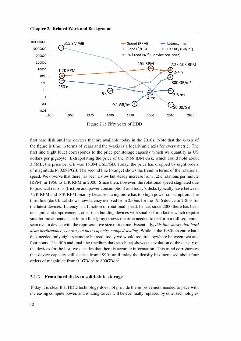
Figure 2.1 shows in more detail the evolution of hard disks over the last fifty years. In the figurewe can see the evolution of five metrics throughout time, from 1956 where IBM introduced the
11
Chapter 2. Related Work and Background
Figure 2.1: Fifty years of HDD
first hard disk until the devices that are available today in the 2010s. Note that the x-axis ofthe figure is time in terms of years and the y-axis is a logarithmic axis for every metric. Thefirst line (light blue) corresponds to the price per storage capacity which we quantify as USdollars per gigabyte. Extrapolating the price of the 1956 IBM disk, which could hold about3.5MB, the price per GB was 15.3M USD/GB. Today, the price has dropped by eight ordersof magnitude to 0.08$/GB. The second line (orange) shows the trend in terms of the rotationalspeed. We observe that there has been a slow but steady increase from 1.2K rotations per minute(RPM) in 1956 to 15K RPM in 2000. Since then, however, the rotational speed stagnated dueto practical reasons (friction and power consumption) and today’s disks typically have between7.2K RPM and 10K RPM, mainly because having more has too high power consumption. Thethird line (dark blue) shows how latency evolved from 250ms for the 1956 device to 2-8ms forthe latest devices. Latency is a function of rotational speed, hence, since 2000 there has beenno significant improvement, other than building devices with smaller form factor which requiresmaller movements. The fourth line (gray) shows the time needed to perform a full sequentialscan over a device with the representative size of its time. Essentially, this line shows that harddisks performance, contrary to their capacity, stopped scaling. While in the 1980s an entire harddisk needed only eight second to be read, today we would require anywhere between two andfour hours. The fifth and final line (medium darkness blue) shows the evolution of the density ofthe devices for the last two decades that there is accurate information. This trend corroboratesthat device capacity still scales: from 1990s until today the density has increased about fourorders of magnitude from 0.1GB/in2 to 800GB/in2.
2.1.2 From hard disks to solid-state storage
Today it is clear that HDD technology does not provide the improvement needed to pace withincreasing compute power, and rotating drives will be eventually replaced by other technologies.
12
2.1. Hardware Trends in Storage
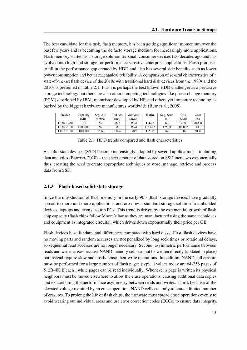
The best candidate for this task, flash memory, has been getting significant momentum over thepast few years and is becoming the de facto storage medium for increasingly more applications.Flash memory started as a storage solution for small consumer devices two decades ago and hasevolved into high-end storage for performance sensitive enterprise applications. Flash promisesto fill in the performance gap created by HDD and also has several side benefits such as lowerpower consumption and better mechanical reliability. A comparison of several characteristics of astate-of-the-art flash device of the 2010s with traditional hard disk devices from the 1980s and the2010s is presented in Table 2.1. Flash is perhaps the best known HDD challenger as a pervasivestorage technology but there are also other competing technologies like phase-change memory(PCM) developed by IBM, memristor developed by HP, and others yet immature technologiesbacked by the biggest hardware manufactures worldwide (Burr et al., 2008).
Device Capacity Seq. BW Rnd acc. Rnd acc. Ratio Seq. Scan Cost Cost(MB) (MB/s) (ms) (MB/s) (s) ($/MB) ($)
HDD 1980 100 1.2 28.3 0.28 1:4.35 83 200 20000HDD 2010 1000000 80 8 0.98 1:81.92 12500 0.0003 300Flash 2010 100000 700 0.026 300 1:2.33 143 0.02 2000
Table 2.1: HDD trends compared and flash characteristics
As solid-state devices (SSD) become increasingly adopted by several applications – includingdata analytics (Barroso, 2010) – the sheer amount of data stored on SSD increases exponentiallythus, creating the need to create appropriate techniques to store, manage, retrieve and processdata from SSD.
2.1.3 Flash-based solid-state storage
Since the introduction of flash memory in the early 90’s, flash storage devices have graduallyspread to more and more applications and are now a standard storage solution in embeddeddevices, laptops and even desktop PCs. This trend is driven by the exponential growth of flashchip capacity (flash chips follow Moore’s law as they are manufactured using the same techniquesand equipment as integrated circuits), which drives down exponentially their price per GB.
Flash devices have fundamental differences compared with hard disks. First, flash devices haveno moving parts and random accesses are not penalized by long seek times or rotational delays,so sequential read accesses are no longer necessary. Second, asymmetric performance betweenreads and writes arises because NAND memory cells cannot be written directly (updated in place)but instead require slow and costly erase-then-write operations. In addition, NAND cell erasuremust be performed for a large number of flash pages (typical values today are 64-256 pages of512B-4KiB each), while pages can be read individually. Whenever a page is written its physicalneighbors must be moved elsewhere to allow the erase operations, causing additional data copiesand exacerbating the performance asymmetry between reads and writes. Third, because of theelevated voltage required by an erase operation, NAND cells can only tolerate a limited numberof erasures. To prolong the life of flash chips, the firmware must spread erase operations evenly toavoid wearing out individual areas and use error correction codes (ECCs) to ensure data integrity.
13
Chapter 2. Related Work and Background
Flash device manufacturers try to hide the aforementioned issues behind a dedicated controllerembedded in the flash drive. This abstraction layer, called the Flash Translation Layer (FTL),deals with the technological differences and presents a generic block device to the host OS.The main advantage of an FTL is that it helps to maintain backward compatibility, under theassumption that the generic block device is the prevailing abstraction at the application level. Inpractice, however, most performance-critical applications developed over the last 30 years areheavily optimized around the model of a rotating disk. As a result, simply replacing a magneticdisk with a flash device does not yield optimal device or DBMS performance, and query optimizerdecisions based on HDD behavior become irrelevant for flash devices. Moreover, the complexand history-dependent nature of the interposed layer affects predictability.
2.1.4 Phase Change Memory
PCM stores information using resistance in different states of phase change materials: amorphousand crystalline. The resistance in the amorphous state is about five orders of magnitude higher thanthe crystalline state, and it differentiates between 0 (high resistance) and 1 (low resistance) (Chenet al., 2011; Papandreou et al., 2011). Storing information on PCM is performed throughtwo operations: set and reset. During the set operation, current is applied on the device for asufficiently long period to crystallize the material. During the reset operation higher current isapplied for shorter duration in order to melt the material and then cool it abruptly, leaving thematerial in the amorphous state. Unlike flash, PCM does not need the time consuming eraseoperation to write the new value. PCM devices can employ a simpler driver than the complexFTL that flash devices use to address the wear leveling and performance issues (Akel et al., 2011).In the recent literature there is already a discussion about how to place PCM in the existingmemory hierarchy. While proposed ideas (Chen et al., 2011) include placing PCM side-by-sideDRAM as an alternative non-volatile main memory, or even using PCM as the main memory ofthe system, current prototype approaches consider PCM as a secondary storage device providingPCIe connectivity. There are three main reasons why this happens: (i) the endurance of each PCMcell is typically 106–108, which is higher than flash (104–105 with a decreasing trend (Abraham,2010)) but still not enough for a main memory device, (ii) the only available interface to date isPCIe, and (iii) the PCM technology is new, so the processors and the memory hierarchy do notyet have the appropriate interfaces for it.
The Moneta system is a hardware-implemented PCIe storage device with PCM emulation byDRAM (Caulfield et al., 2010, 2012). Performance studies on this emulation platform havehighlighted the need for improved software I/O latency in the operating system and file system.The Onyx system (Akel et al., 2011) replaces the DRAM chips of Moneta with first-generationPCM chips,1 yielding a total capacity of 10 GB. Onyx is capable of performing a 4KB randomread in 38µs and a 4KB write request2 in 179µs. For a hash-table based workload, Onyx
1The PCM chips used by Onyx are the same as those used in our profiled device, but the devices themselves aredifferent.
2The write numbers for Onyx use early completion, in which completion is signaled when the internal buffers have
14
2.1. Hardware Trends in Storage
performed 21% better than an ioDrive, while the ioDrive performed 48% better than Onyx for aB-Tree based workload (Akel et al., 2011).
The software latency (as a result of operating system and file system overheads) is measured tobe about 17µs (Akel et al., 2011). On the other hand, the hardware latency for fetching a 4Kpage from a hard disk is on the order of milliseconds and for a high-end flash device is about50µs. Early PCM prototypes need as little as 20µs to read a 4K page increasing the softwarecontribution in relative latency from 25% (17µs out of 67µs) for a flash device like FusionIO, to46% (17µs out of 37µs) for a PCM prototype. Minimizing the impact of software latency is arelatively new research problem acknowledged by the community (Akel et al., 2011). Caulfieldet al. (Caulfield et al., 2012) point out this problem and propose a storage hardware and softwarearchitecture to mitigate the overheads to take better advantage of low latency devices such asPCM. The architecture provides a private, virtualized interface for each process and moves filesystem protection checks into hardware. As a result, applications can access file data withoutoperating system intervention, eliminating OS and file system costs entirely for most accesses.The experiments show that the new interface improves latency and bandwidth for 4K writes by60% and 7.2x respectively, OLTP database transaction throughput by up to 2.0x, and Berkeley-DBthroughput by up to 5.7x (Caulfield et al., 2012).
Jung et al. (Jung et al., 2011) ran the fio profiler over the same Micron PCM prototype availableto us and a popular flash device (OCZ Revodrive), showing qualitative differences between thePCM device and the flash device. The PCM device, unlike the flash device, shows no differencebetween latency for random and sequential accesses for different values of IO depth (number ofconcurrent outstanding requests) or page sizes.
Lee et al. (Lee et al., 2010) introduce a new In-Page Logging (IPL) design that uses PCRAMas a storage device for log records. They claim that the low latency and byte addressability ofPCRAM can allow one to avoid the limitations of flash-only IPL. Papandreou et al. (Papandreouet al., 2011) present various programming schemes for multilevel storage in PCM. The proposedschemes are based on iterative write-and-verify algorithms that exploit the unique programmingcharacteristics of PCM in order to achieve significant improvements in resistance-level packingdensity, robustness to cell variability, programming latency, energy per-bit and cell storagecapacity. They present experimental results from PCM test-arrays to validate the proposedprogramming schemes. In addition, the reliability issues of multilevel PCM in terms of resistancedrift and read noise are discussed.
2.1.5 Flash vs. PCM
In this section we perform a head-to-head comparison between a state-of-the-art PCI-basedFusionIO flash device and an early PCI-based PCM-based prototype. This comparison provides
enough information to complete the write, but before the data is physically in the PCM. Early completion is also usedby SSD devices, supported by large capacitors to ensure that the writes actually happen in case of a power failure.
15
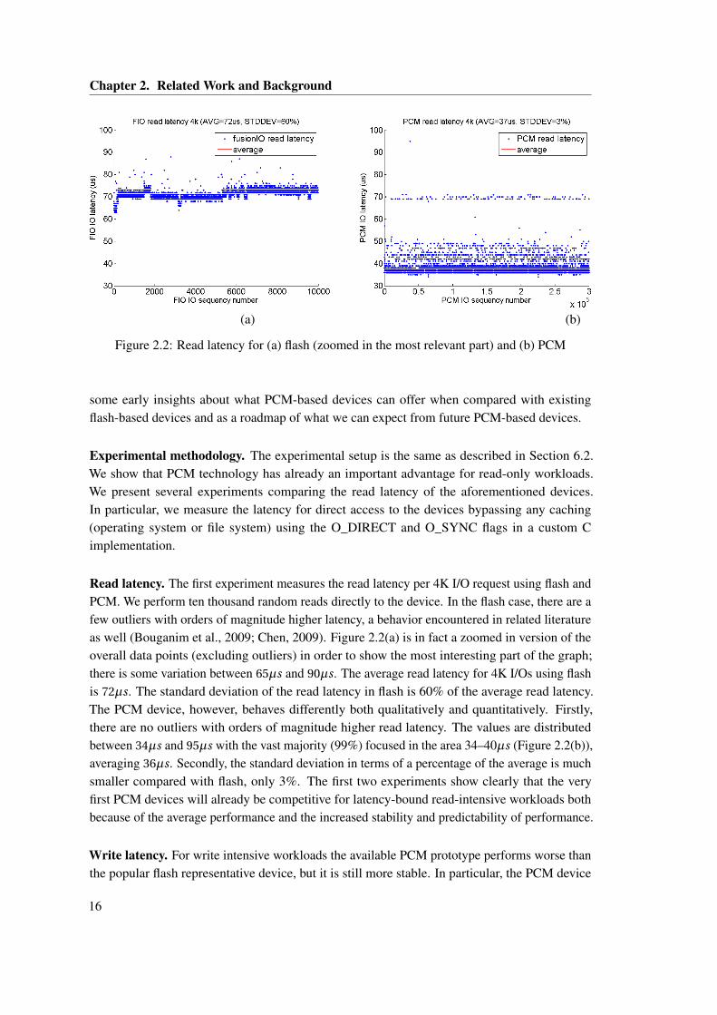
Chapter 2. Related Work and Background
(a) (b)
Figure 2.2: Read latency for (a) flash (zoomed in the most relevant part) and (b) PCM
some early insights about what PCM-based devices can offer when compared with existingflash-based devices and as a roadmap of what we can expect from future PCM-based devices.
Experimental methodology. The experimental setup is the same as described in Section 6.2.We show that PCM technology has already an important advantage for read-only workloads.We present several experiments comparing the read latency of the aforementioned devices.In particular, we measure the latency for direct access to the devices bypassing any caching(operating system or file system) using the O_DIRECT and O_SYNC flags in a custom Cimplementation.
Read latency. The first experiment measures the read latency per 4K I/O request using flash andPCM. We perform ten thousand random reads directly to the device. In the flash case, there are afew outliers with orders of magnitude higher latency, a behavior encountered in related literatureas well (Bouganim et al., 2009; Chen, 2009). Figure 2.2(a) is in fact a zoomed in version of theoverall data points (excluding outliers) in order to show the most interesting part of the graph;there is some variation between 65µs and 90µs. The average read latency for 4K I/Os using flashis 72µs. The standard deviation of the read latency in flash is 60% of the average read latency.The PCM device, however, behaves differently both qualitatively and quantitatively. Firstly,there are no outliers with orders of magnitude higher read latency. The values are distributedbetween 34µs and 95µs with the vast majority (99%) focused in the area 34–40µs (Figure 2.2(b)),averaging 36µs. Secondly, the standard deviation in terms of a percentage of the average is muchsmaller compared with flash, only 3%. The first two experiments show clearly that the veryfirst PCM devices will already be competitive for latency-bound read-intensive workloads bothbecause of the average performance and the increased stability and predictability of performance.
Write latency. For write intensive workloads the available PCM prototype performs worse thanthe popular flash representative device, but it is still more stable. In particular, the PCM device
16
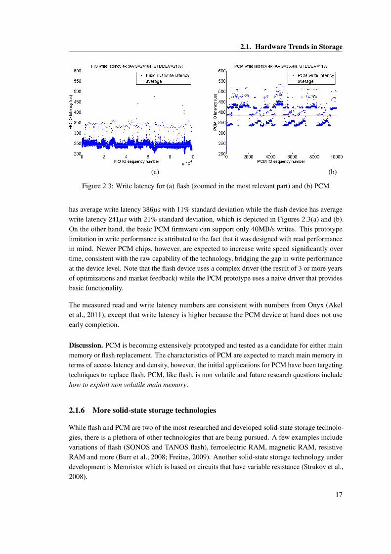
2.1. Hardware Trends in Storage
(a) (b)
Figure 2.3: Write latency for (a) flash (zoomed in the most relevant part) and (b) PCM
has average write latency 386µs with 11% standard deviation while the flash device has averagewrite latency 241µs with 21% standard deviation, which is depicted in Figures 2.3(a) and (b).On the other hand, the basic PCM firmware can support only 40MB/s writes. This prototypelimitation in write performance is attributed to the fact that it was designed with read performancein mind. Newer PCM chips, however, are expected to increase write speed significantly overtime, consistent with the raw capability of the technology, bridging the gap in write performanceat the device level. Note that the flash device uses a complex driver (the result of 3 or more yearsof optimizations and market feedback) while the PCM prototype uses a naive driver that providesbasic functionality.
The measured read and write latency numbers are consistent with numbers from Onyx (Akelet al., 2011), except that write latency is higher because the PCM device at hand does not useearly completion.
Discussion. PCM is becoming extensively prototyped and tested as a candidate for either mainmemory or flash replacement. The characteristics of PCM are expected to match main memory interms of access latency and density, however, the initial applications for PCM have been targetingtechniques to replace flash. PCM, like flash, is non volatile and future research questions includehow to exploit non volatile main memory.
2.1.6 More solid-state storage technologies
While flash and PCM are two of the most researched and developed solid-state storage technolo-gies, there is a plethora of other technologies that are being pursued. A few examples includevariations of flash (SONOS and TANOS flash), ferroelectric RAM, magnetic RAM, resistiveRAM and more (Burr et al., 2008; Freitas, 2009). Another solid-state storage technology underdevelopment is Memristor which is based on circuits that have variable resistance (Strukov et al.,2008).
17
Chapter 2. Related Work and Background
2.1.7 Sequential Reads and Random Writes in Storage Systems
Concurrently with this thesis, Schindler et al. (Schindler et al., 2011) proposed exploitingflash as a non-volatile write cache in storage systems for efficient servicing of I/O patternsthat mix sequential reads and random writes. Compared to the online update problem in datawarehouses, the settings in storage systems are significantly simplified: (i) an “update record”in storage systems is (a new version of) an entire I/O page and (ii) ACID is not supported foraccessing multiple pages. As a result, the proposal employs a simple update management scheme:modifying the I/O mapping table to point to the latest version of pages. Interestingly, the proposalexploits a disk access pattern, called Proximal I/O, for migrating updates that write to only 1% ofall disk pages.
2.2 Data Analysis Systems
Data analytics provides business and research insight from a massive collection of data beingcontinuously augmented. Historically, however, updates to the data were performed offline usingbulk insert/update features – executed mainly during extensive idle-times (e.g., at night). Thequick reacting, 24x7 nature of business today cannot tolerate long delays in updates, because thevalue of the insights gained drops fast when the data used are stale (Inmon et al., 2003). Thus,data analysis systems supporting efficient real-time updates have been the goal of recent researchand business efforts (Becla and Lim, 2008; Oracle, 2004, 2013; White, 2002; Polyzotis et al.,2008). State-of-the-art data analysis systems, however, today often fail to support fast analysisqueries over fresh data.
A demanding data-intensive application is the utilization of systematically organized knowledgeto increase the quality of the performed analysis. The semantic web (Shadbolt et al., 2006)is an effort to allow storing, managing and searching machine readable information using theResource Description Framework (RDF) (RDf, 2013) model to represent the data. Severalapplications, including scientific (Apweiler et al., 2004), business and governmental (Data.gov,2013; Data.gov.uk, 2013), use this data representation model, a trend which is strengthened byefforts like Linked Open Data (LOD) (Bizer et al., 2009a). LOD, to date, consists of more than25 billion RDF triples collecting data from more than 200 data sources. Data analytics enginesrecently started considering semantic RDF databases as sources for their analysis. A celebratedexample of the combination of traditional data analytics, knowledge representation and reasoningand other techniques (e.g., machine learning) is the IBM Watson Computer (Ferrucci et al., 2010)which participated successfully in the knowledge game "Jeopardy!". Querying RDF datasets,however, poses a new challenge for data analytics engines: efficiently querying semantic datathat form graphs which have edges for both semantic and relational connections.
The majority of data stored and used by data analytics engines are stored based on a specificdimension, often a time one. Accessing ordered, or partitioned, data efficiently by data analyticsengines is already a design goal by the Netezza (Francisco, 2011) engine. Moreover, the advent of
18
2.2. Data Analysis Systems
solid-state storage results in storing more and more data on such devices. The capacity, however,is much more expensive in terms of $ per GB compared with that of traditional hard disks. Hence,a key problem is indexing data with small capacity requirements taking into account that thisdata are often sorted or partitioned.
2.2.1 High-Throughput Updates and Data Analysis
The need to augment the functionality of analysis systems with high-throughput update capabilityhas been recognized in the literature.
In-Memory and External Data Structures. In Chapter 3 we present MaSM, a novel approachto offer online updates in data analytics with the usage of solid-state storage. MaSM extendsprior work on in-memory differential updates (Héman et al., 2010; Stonebraker et al., 2005) toovercome the limitation on high migration costs vs. large memory footprint. We assume I/O to bethe main bottleneck for data warehousing queries and therefore the focus of our design is mainlyon the I/O behaviors. On the other hand, prior differential update approaches propose efficientin-memory data structures, which is orthogonal to the MaSM design, and may be applied toMaSM to improve CPU performance for CPU-intensive workloads.
Handling Updates with Stacked Tree Structures. The state-of-the-art approach to supportonline updates with minimal overhead is differential updates. Positional delta trees (Hémanet al., 2010) provide efficient maintenance and ease in merging differential updates in columnstores. They defer touching the read-optimized image of the data as long as possible and bufferdifferential updates in a separate write-store. The updates from the write-store are merged withthe main data during the column scans in order to present to the user an up-to-date version ofthe data. O’Neil et al. (1996) proposed log-structured merge tree (LSM) which is organized asa collection of trees (two or more) stacked vertically, supporting high update rate of indexingstructures of a database, like B-trees. The first level of LSM is always in-memory and the laston disk. The updates are initially saved in the first level and they are consequently moved to thenext levels (in batches) in order to reach the last level. Searching using LSM requires to traverseall stacked trees as each one is not inclusive of the subsequent trees. While LSM is capable ofsustaining a high update rate, and – if tuned appropriately – delivering good read performance, itapplies more writes per update than MaSM as we detail in Chapter 3 (Section 3.4.5).
LSM has inspired other approaches that maintain, index and query data. FD-Tree (Li et al.,2010) is a tree-structure which extends LSM by reducing the read overhead and by allowingflash-friendly writes. The key ideas are to limit random writes to a small part of the index andto transform random writes to sequential writes. FD-Tree assumes a fixed ratio between twoconsecutive levels in order to offer the best insertion cost amortization, which is the optimal casefor LSM as well. As we discuss in Chapter 3 (Sections 3.2.3 and 3.4.5), this setup incurs anincreased number of writes per update since every update is propagated a number of times.
19
Chapter 2. Related Work and Background
The stepped-merge algorithm (Jagadish et al., 1997) stores updates lazily in a B+-Tree organiza-tion by first maintaining updates in memory in sorted runs and, eventually, form a B+-Tree ofthese updates using an external merge-sort. The stepped-merge approach aims at minimizing ran-dom I/O requests. On the other hand, MaSM focuses on minimizing main memory consumptionand the unnecessary writes on the flash device at the expense of more, yet efficient, random readI/O requests.
The quadtree-based storage algorithm (McCarthy and He, 2011) was proposed concurrently andindependently of the MaSM algorithms presented in Chapter 3. It uses in-memory ∆-quadtrees toorganize incoming updates for a data cube. The ∆-quadtrees are used to support the computationof specific operations like SUM, COUNT and AVG over a predefined data cube. When theavailable memory is exhausted, the ∆-quadtrees are flushed to an SSD. Subsequent range queriesare answered by merging the ∆-quadtrees in memory, the ∆-quadtrees on flash, and the maindata in the data cube. Contrary to the quadtree-based storage algorithm, MaSM is not part of theaggregate calculation allowing for a general purpose solution to handle incoming updates in aDW.
Extraction-Transformation-Loading for Data Warehouses. We focus on supporting efficientquery processing given online, well-formed updates. An orthogonal problem is an efficientETL (Extraction-Transformation-Loading) process for data warehouses (Oracle, 2013; Polyzotiset al., 2008). ETL is often performed at a data integration engine outside the data warehouseto incorporate changes from front-end operational data sources. Streamlining the ETL processhas been both a research topic (Polyzotis et al., 2008; Simitsis et al., 2009) and a focus of adata warehouse product (Oracle, 2013). These ETL solutions can be employed to generate thewell-formed updates to be applied to the data warehouse.
2.2.2 Adaptive organization of data and updates
Database cracking and adaptive indexing. There is a wealth of differential approaches tomaintain indexes and other data structures in order to enhance query performance. Databasecracking (Idreos et al., 2007) reorganizes the data in memory to match how queries access data.Adaptive indexing (Graefe and Kuno, 2010; Graefe et al., 2012) follows the same principleas database cracking by focusing the index optimization on key ranges used in actual queries.Their hybrids for column stores (Idreos et al., 2011) take the best of the two worlds. Contraryto MaSM, database cracking, adaptive index, and their hybrids focus on static data which aredynamically reorganized (or the corresponding indexes optimized) according to the incomingqueries. The MaSM algorithms enable long running queries to see no performance penalty byallowing concurrent updates.
Partitioned B-trees. Graefe proposed partitioned B-trees (Graefe, 2003) in order to offer efficientresource allocation during index creation, or data loading into an already indexed database. The
20
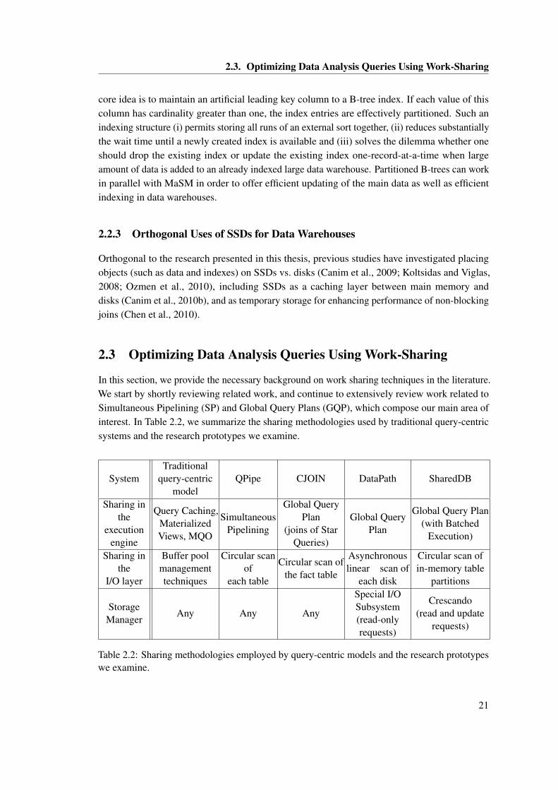
2.3. Optimizing Data Analysis Queries Using Work-Sharing
core idea is to maintain an artificial leading key column to a B-tree index. If each value of thiscolumn has cardinality greater than one, the index entries are effectively partitioned. Such anindexing structure (i) permits storing all runs of an external sort together, (ii) reduces substantiallythe wait time until a newly created index is available and (iii) solves the dilemma whether oneshould drop the existing index or update the existing index one-record-at-a-time when largeamount of data is added to an already indexed large data warehouse. Partitioned B-trees can workin parallel with MaSM in order to offer efficient updating of the main data as well as efficientindexing in data warehouses.
2.2.3 Orthogonal Uses of SSDs for Data Warehouses
Orthogonal to the research presented in this thesis, previous studies have investigated placingobjects (such as data and indexes) on SSDs vs. disks (Canim et al., 2009; Koltsidas and Viglas,2008; Ozmen et al., 2010), including SSDs as a caching layer between main memory anddisks (Canim et al., 2010b), and as temporary storage for enhancing performance of non-blockingjoins (Chen et al., 2010).
2.3 Optimizing Data Analysis Queries Using Work-Sharing
In this section, we provide the necessary background on work sharing techniques in the literature.We start by shortly reviewing related work, and continue to extensively review work related toSimultaneous Pipelining (SP) and Global Query Plans (GQP), which compose our main area ofinterest. In Table 2.2, we summarize the sharing methodologies used by traditional query-centricsystems and the research prototypes we examine.
SystemTraditional
query-centricmodel
QPipe CJOIN DataPath SharedDB
Sharing inthe
executionengine
Query Caching,MaterializedViews, MQO
SimultaneousPipelining
Global QueryPlan
(joins of StarQueries)
Global QueryPlan
Global Query Plan(with Batched
Execution)
Sharing inthe
I/O layer
Buffer poolmanagementtechniques
Circular scanof
each table
Circular scan ofthe fact table
Asynchronouslinear scan of
each disk
Circular scan ofin-memory table
partitions
StorageManager
Any Any Any
Special I/OSubsystem(read-onlyrequests)
Crescando(read and update
requests)
Table 2.2: Sharing methodologies employed by query-centric models and the research prototypeswe examine.
21
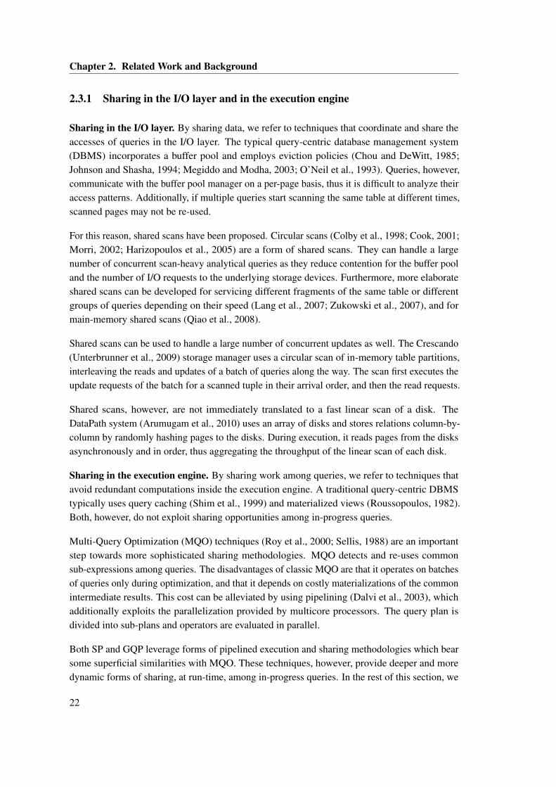
Chapter 2. Related Work and Background
2.3.1 Sharing in the I/O layer and in the execution engine
Sharing in the I/O layer. By sharing data, we refer to techniques that coordinate and share theaccesses of queries in the I/O layer. The typical query-centric database management system(DBMS) incorporates a buffer pool and employs eviction policies (Chou and DeWitt, 1985;Johnson and Shasha, 1994; Megiddo and Modha, 2003; O’Neil et al., 1993). Queries, however,communicate with the buffer pool manager on a per-page basis, thus it is difficult to analyze theiraccess patterns. Additionally, if multiple queries start scanning the same table at different times,scanned pages may not be re-used.
For this reason, shared scans have been proposed. Circular scans (Colby et al., 1998; Cook, 2001;Morri, 2002; Harizopoulos et al., 2005) are a form of shared scans. They can handle a largenumber of concurrent scan-heavy analytical queries as they reduce contention for the buffer pooland the number of I/O requests to the underlying storage devices. Furthermore, more elaborateshared scans can be developed for servicing different fragments of the same table or differentgroups of queries depending on their speed (Lang et al., 2007; Zukowski et al., 2007), and formain-memory shared scans (Qiao et al., 2008).
Shared scans can be used to handle a large number of concurrent updates as well. The Crescando(Unterbrunner et al., 2009) storage manager uses a circular scan of in-memory table partitions,interleaving the reads and updates of a batch of queries along the way. The scan first executes theupdate requests of the batch for a scanned tuple in their arrival order, and then the read requests.
Shared scans, however, are not immediately translated to a fast linear scan of a disk. TheDataPath system (Arumugam et al., 2010) uses an array of disks and stores relations column-by-column by randomly hashing pages to the disks. During execution, it reads pages from the disksasynchronously and in order, thus aggregating the throughput of the linear scan of each disk.
Sharing in the execution engine. By sharing work among queries, we refer to techniques thatavoid redundant computations inside the execution engine. A traditional query-centric DBMStypically uses query caching (Shim et al., 1999) and materialized views (Roussopoulos, 1982).Both, however, do not exploit sharing opportunities among in-progress queries.
Multi-Query Optimization (MQO) techniques (Roy et al., 2000; Sellis, 1988) are an importantstep towards more sophisticated sharing methodologies. MQO detects and re-uses commonsub-expressions among queries. The disadvantages of classic MQO are that it operates on batchesof queries only during optimization, and that it depends on costly materializations of the commonintermediate results. This cost can be alleviated by using pipelining (Dalvi et al., 2003), whichadditionally exploits the parallelization provided by multicore processors. The query plan isdivided into sub-plans and operators are evaluated in parallel.
Both SP and GQP leverage forms of pipelined execution and sharing methodologies which bearsome superficial similarities with MQO. These techniques, however, provide deeper and moredynamic forms of sharing, at run-time, among in-progress queries. In the rest of this section, we
22
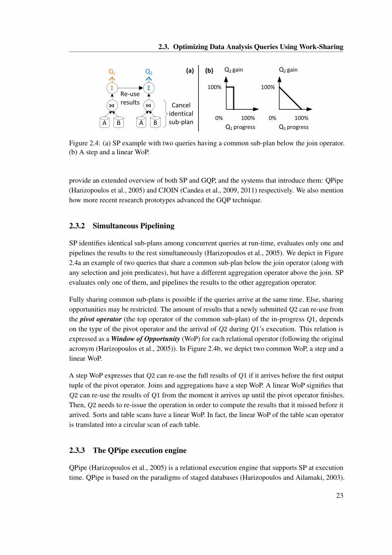
2.3. Optimizing Data Analysis Queries Using Work-Sharing
100%
100%0%
Q1 progress
Q2 gain
100%
100%0%
Q1 progress
Q2 gain
Α
Q1
⋈
Σ
Β Α
Q2
⋈
Σ
Β
Re-use results
(a) (b)
Cancel identical sub-plan
Figure 2.4: (a) SP example with two queries having a common sub-plan below the join operator.(b) A step and a linear WoP.
provide an extended overview of both SP and GQP, and the systems that introduce them: QPipe(Harizopoulos et al., 2005) and CJOIN (Candea et al., 2009, 2011) respectively. We also mentionhow more recent research prototypes advanced the GQP technique.
2.3.2 Simultaneous Pipelining
SP identifies identical sub-plans among concurrent queries at run-time, evaluates only one andpipelines the results to the rest simultaneously (Harizopoulos et al., 2005). We depict in Figure2.4a an example of two queries that share a common sub-plan below the join operator (along withany selection and join predicates), but have a different aggregation operator above the join. SPevaluates only one of them, and pipelines the results to the other aggregation operator.
Fully sharing common sub-plans is possible if the queries arrive at the same time. Else, sharingopportunities may be restricted. The amount of results that a newly submitted Q2 can re-use fromthe pivot operator (the top operator of the common sub-plan) of the in-progress Q1, dependson the type of the pivot operator and the arrival of Q2 during Q1’s execution. This relation isexpressed as a Window of Opportunity (WoP) for each relational operator (following the originalacronym (Harizopoulos et al., 2005)). In Figure 2.4b, we depict two common WoP, a step and alinear WoP.
A step WoP expresses that Q2 can re-use the full results of Q1 if it arrives before the first outputtuple of the pivot operator. Joins and aggregations have a step WoP. A linear WoP signifies thatQ2 can re-use the results of Q1 from the moment it arrives up until the pivot operator finishes.Then, Q2 needs to re-issue the operation in order to compute the results that it missed before itarrived. Sorts and table scans have a linear WoP. In fact, the linear WoP of the table scan operatoris translated into a circular scan of each table.
2.3.3 The QPipe execution engine
QPipe (Harizopoulos et al., 2005) is a relational execution engine that supports SP at executiontime. QPipe is based on the paradigms of staged databases (Harizopoulos and Ailamaki, 2003).
23
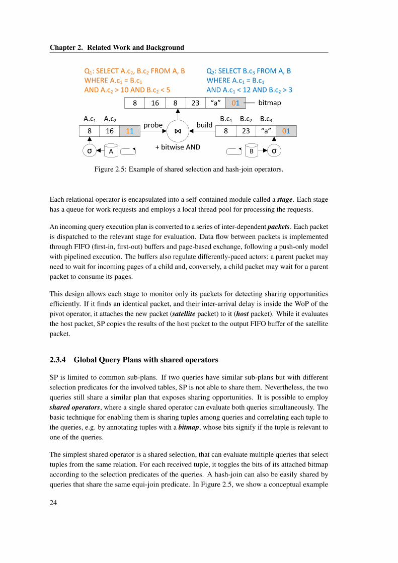
Chapter 2. Related Work and Background
⋈
Α
8 16 11 23 “a” 018
Q1: SELECT A.c2, B.c2 FROM A, BWHERE A.c1 = B.c1
AND A.c2 > 10 AND B.c2 < 5
Q2: SELECT Β.c3 FROM A, BWHERE A.c1 = B.c1
AND A.c1 < 12 AND B.c2 > 3
+ bitwise ANDσ Β σ
A.c1 A.c2 B.c1 B.c2 B.c3
8 16 23 “a” 018
buildprobe
bitmap
Figure 2.5: Example of shared selection and hash-join operators.
Each relational operator is encapsulated into a self-contained module called a stage. Each stagehas a queue for work requests and employs a local thread pool for processing the requests.
An incoming query execution plan is converted to a series of inter-dependent packets. Each packetis dispatched to the relevant stage for evaluation. Data flow between packets is implementedthrough FIFO (first-in, first-out) buffers and page-based exchange, following a push-only modelwith pipelined execution. The buffers also regulate differently-paced actors: a parent packet mayneed to wait for incoming pages of a child and, conversely, a child packet may wait for a parentpacket to consume its pages.
This design allows each stage to monitor only its packets for detecting sharing opportunitiesefficiently. If it finds an identical packet, and their inter-arrival delay is inside the WoP of thepivot operator, it attaches the new packet (satellite packet) to it (host packet). While it evaluatesthe host packet, SP copies the results of the host packet to the output FIFO buffer of the satellitepacket.
2.3.4 Global Query Plans with shared operators
SP is limited to common sub-plans. If two queries have similar sub-plans but with differentselection predicates for the involved tables, SP is not able to share them. Nevertheless, the twoqueries still share a similar plan that exposes sharing opportunities. It is possible to employshared operators, where a single shared operator can evaluate both queries simultaneously. Thebasic technique for enabling them is sharing tuples among queries and correlating each tuple tothe queries, e.g. by annotating tuples with a bitmap, whose bits signify if the tuple is relevant toone of the queries.
The simplest shared operator is a shared selection, that can evaluate multiple queries that selecttuples from the same relation. For each received tuple, it toggles the bits of its attached bitmapaccording to the selection predicates of the queries. A hash-join can also be easily shared byqueries that share the same equi-join predicate. In Figure 2.5, we show a conceptual example
24
2.3. Optimizing Data Analysis Queries Using Work-Sharing
of how a single shared hash-join is able to evaluate two queries. It starts with the build phaseby receiving tuples from the shared selection operator of the inner relation. Then, the probephase begins by receiving tuples from the shared selection operator of the outer relation. Thehash-join proceeds as normal, by additionally performing a bit-wise AND between the bitmapsof the joined tuples.
The most significant advantage is that a single shared operator can evaluate many more similarqueries. For example, a shared hash-join can evaluate many queries having the same equi-joinpredicate, and possibly different selection predicates. In the worst case, the union of the selectionpredicates may force it to join the whole two relations. The disadvantage of a shared operatorin comparison to a query-centric one is that it reduces parallelism in order to gain throughput,entailing increased book-keeping. For example, a shared hash-join maintains a hash table for theunion of the tuples of the inner relation selected by all queries, and performs bit-wise operationsbetween the bitmaps of the joined tuples. For low concurrency, as shown by our experiments (seeSection 4.5), query-centric operators outperform shared operators. A similar tradeoff is found forthe specific case of shared aggregations on CMP (Cieslewicz and Ross, 2007).
By using shared scans and shared operators, a GQP can be built for evaluating all concurrentqueries. GQP are introduced by CJOIN (Candea et al., 2009, 2011), an operator based on sharedselections and shared hash-joins for evaluating the joins of star queries (Kimball and Ross, 2002).GQP are advanced by the DataPath system (Arumugam et al., 2010) for more general schemas,by tackling the issues of routing and optimizing the GQP for a newly incoming query. DataPathalso adds support for a shared aggregate operator, that calculates a running sum for each groupand query.
Both CJOIN and DataPath handle new queries immediately when they arrive. This is feasibledue to the nature of the supported shared operators: selections, hash-joins and aggregates. Someoperators, however, cannot be easily shared. For example, a sort operator cannot easily handlenew queries that select more tuples than the ones being sorted (Arumugam et al., 2010). Toovercome this limitation, SharedDB (Giannikis et al., 2012) batches queries for every sharedoperator. Batching allows standard algorithms to be easily extended to support shared operators,as they work on a fixed set of tuples and queries. SharedDB supports shared sorts and variousshared join algorithms, not being restricted only to equi-joins. Nevertheless, batched executionhas drawbacks: A new query may suffer increased latency, and the latency of a batch is dominatedby the longest-running query.
2.3.5 The CJOIN operator
The selection of CJOIN (Candea et al., 2009, 2011) for our analysis is based on the facts thatit introduced GQP, and that it is optimized for the simple case of star queries. Without loss ofgenerality, we restrict our evaluation to star schemas, and correlate our observations to moregeneral schemas (used, e.g., by DataPath (Arumugam et al., 2010) or SharedDB (Giannikis et al.,
25
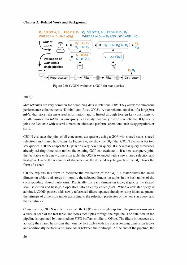
Chapter 2. Related Work and Background
F
D1
Q1: σ(D1)Q2: σ’(D1)
σ
Q1: F ⋈ D1
Q2: F ⋈ D1⋈ Q2: (F ⋈ D1) ⋈ D2⋈
Q1
Q2
Q1: SELECT A, B, … FROM F, D1 WHERE F ⋈ D1 AND σ(D1)
Q2: SELECT A, B, … FROM F, D1, D2 WHERE F ⋈ D1 ⋈ D2 AND σ’(D1) AND σ’(D2)
D2
Q2: σ’(D2)σ
Filter Filter Distributor
Q1 Q2
Preprocessor
GQP of CJOIN
Evaluation of GQP with a single pipeline
F
Figure 2.6: CJOIN evaluates a GQP for star queries.
2012)).
Star schemas are very common for organizing data in relational DW. They allow for numerousperformance enhancements (Kimball and Ross, 2002). A star schema consists of a large facttable, that stores the measured information, and is linked through foreign-key constraints tosmaller dimension tables. A star query is an analytical query over a star schema. It typicallyjoins the fact table with several dimension tables and performs operations such as aggregations orsorts.
CJOIN evaluates the joins of all concurrent star queries, using a GQP with shared scans, sharedselections and shared hash-joins. In Figure 2.6, we show the GQP that CJOIN evaluates for twostar queries. CJOIN adapts the GQP with every new star query. If a new star query referencesalready existing dimension tables, the existing GQP can evaluate it. If a new star query joinsthe fact table with a new dimension table, the GQP is extended with a new shared selection andhash-join. Due to the semantics of star schemas, the directed acyclic graph of the GQP takes theform of a chain.
CJOIN exploits this form to facilitate the evaluation of the GQP. It materializes the smalldimension tables and stores in-memory the selected dimension tuples in the hash tables of thecorresponding shared hash-joins. Practically, for each dimension table, it groups the sharedscan, selection and hash-join operators into an entity called filter. When a new star query isadmitted, CJOIN pauses, adds newly referenced filters, updates already existing filters, augmentsthe bitmaps of dimension tuples according to the selection predicates of the new star query, andthen continues.
Consequently, CJOIN is able to evaluate the GQP using a single pipeline: the preprocessor usesa circular scan of the fact table, and flows fact tuples through the pipeline. The data flow in thepipeline is regulated by intermediate FIFO buffers, similar to QPipe. The filters in-between areactually the shared hash-joins that join the fact tuples with the corresponding dimension tuplesand additionally perform a bit-wise AND between their bitmaps. At the end of the pipeline, the
26
2.3. Optimizing Data Analysis Queries Using Work-Sharing
distributor examines the bitmaps of the joined tuples and forwards them to the relevant queries.For every new query, the preprocessor admits it, marking its point of entry on the circular scanof the fact table and signifies its completion when it wraps around to its point of entry on thecircular scan.
2.3.6 Quantifying work sharing opportunities
Earlier in this section we introduced the fundamental approaches in sharing in relational databasesystems, i.e., in the storage layer and in the query engine. The motivation stems from the fact thatconcurrent queries access common base data and perform common database operations on thedata as pointed out by the MQO work (Sellis, 1988). In addition, as concurrency in analyticalworkloads increases exponentially (Russom, 2012) the opportunities of sharing increase aswell. A fundamental question, however, is to quantify the opportunities of work sharing orthe headroom of improvement through work sharing techniques. Using the definition of worksharing by Johnson et al. (2007) as "any operation that reduces the total amount of work in asystem by eliminating redundant computation or data accesses" the need to define a metric toquantify the opportunity for performance or resource utilization improvement surfaces. In fact, aprincipled framework for work sharing opportunities can also be the basis for a fundamentallynew multi-query optimization. In the literature to date one can find detailed experiments andmeasurements on the performance benefits of specific work sharing implementations in termsof response time, throughput or even resource utilization. Such analysis can be found for theDataPath system (Arumugam et al., 2010), the CJOIN operator (Candea et al., 2011), the QPipequery engine (Harizopoulos et al., 2005; Johnson et al., 2007), the integration of CJOIN intoQPipe (Psaroudakis et al., 2013) and the SharedDB query engine (Giannikis et al., 2012). A firststep to work sharing headroom quantification is the MQO and its different approaches (Sellis,1988; Chen and Dunham, 1998), which was further advanced by a practical realization (Roy et al.,2000). Existing work, however, does not include an analysis for what would be the maximumpossible benefit given a workload and up to what extent does each specific approach realize thisbenefit.
In addition, in the context of stream processing work sharing has been extensively studied (Chenet al., 2000; Madden et al., 2002; Chandrasekaran et al., 2003; Agrawal et al., 2008; Liu et al.,2008; Majumder et al., 2008). Precision sharing (Krishnamurthy et al., 2004) introduces a veryimportant relevant aspect: work sharing without introducing unnecessary work, which is key inorder to quantify correctly the work sharing opportunities. Similarly to work sharing literaturefor database engines, existing work for work sharing in stream processing, does not include ananalysis to quantify the work sharing opportunities.
27
Chapter 2. Related Work and Background
2.4 Bloom filters
A Bloom filter (BF) (Bloom, 1970) is a space-efficient probabilistic data structure supportingmembership tests with non-zero probability for false positives (and zero probability for falsenegatives). Typically in a BF one can only add new elements and never remove elements. Adeletable BF has been discussed (Rothenberg et al., 2010) but it is not generally adopted.
2.4.1 Bloom filters’ applications in data management
BFs have been extensively used in networking (Broder and Mitzenmacher, 2002; Lim and Kim,2010) and as auxiliary data structures in database systems (Antognini, 2008; Chang et al., 2006;Condie et al., 2010; Dean and Ghemawat, 2004; Mullin, 1990). Modern database systems utilizeBFs while implementing several algorithms, like semi-joins (Mullin, 1990), where BFs helpin implementing faster the join algorithm. Google’s Bigtable (Chang et al., 2006) uses BFs toreduce the number of accesses to internal storage components and a study (Antognini, 2008)shows that Oracle systems use BFs for tuple pruning, to reduce data communication betweenslave processes in parallel joins and to support result caches.
2.4.2 Bloom filters for evolving workloads and storage
BFs have been used for changing workloads and different storage technologies. Scalable BloomFilters (Almeida et al., 2007) study how a BF can adapt dynamically to the numbers of ele-ments stored while assuring a bound for maximum false positive probability. Buffered Bloomfilters (Canim et al., 2010a) use flash, as well, as a cheaper alternative to main memory. The BFis allocated in blocks equal to the typical block size of the storage device and both reads andwrites are buffered in memory to improve locality during the build and the probe phase. Theforest-structured Bloom filter (Lu et al., 2011) aims at designing an efficient flash-based BF byusing the memory to capture the frequent updates. Memory is used to capture the updates andhide them from the flash storage and, on flash, the BF is organized in a forest-structure in orderto improve the lookup performance. Bender et al. (Bender et al., 2012) propose three variationsof BFs: the quotient filter, the buffered quotient filter and the cascade filter. The first uses morespace than traditional BF but shows better insert/lookup performance and supports deletes. Thelast two variations are designed on top of quotient filter supporting larger workloads, serving, aswell, as alternatives of BF for SSD.
In Chapter 5 we extend the usage of BFs in DBMS by proposing BF-Tree, an indexing treestructure which uses BFs to trade off capacity for indexing accuracy by applying approximateindexing. BF-Tree is orthogonal to the optimizations described above. In fact, a BF-Tree cantake advantage of such optimizations in order to fine-tune its performance.
28
2.5. Indexing for Data Analysis
2.5 Indexing for Data Analysis
Both analytical workloads and storage technologies evolve, and as a result an increasing amountof data is stored on SSDs. In Chapter 5 we propose an SSD-aware indexing for analyticalworkloads which departs from the traditional SSD-aware index structure. We do so by creating anew tree index structures which is tailored for SSD by understanding that SSD is the diametricalopposite than HDD in two aspects: random access performance and capacity price. The proposedstructure combines capacity and performance optimizations of different prior approaches.
2.5.1 SSD-aware indexing
We find that approximate indexing is suitable for modern storage devices (e.g. flash or PCM-based) because of their principal difference compared to traditional disks: random accessesperform virtually the same as sequential accesses3. Since the rise of flash as an importantcompetitor of disks for non-volatile storage (Gray, 2007) there have been several efforts increating a flash-friendly indexing structure (often a flash-aware version of a B+-Tree). LA-Tree (Agrawal et al., 2009) uses lazy updates, adaptive buffering and memory optimizationsto minimize the overhead of updating flash. In µ-Tree (Kang et al., 2007) the nodes along thepath from the root to the leaf are stored in a single flash memory page in order to minimize thenumber of flash write operations during the update of a leaf node. IPLB+-tree (Na et al., 2011)avoids costly erase operations - often caused by small random write requests common in databaseapplications - in order to improve the overall write performance. SILT (Lim et al., 2011) is aflash-based memory-efficient key-value store based on cuckoo hashing and tries, which offersfast search performance using minimal amount of main memory.
What SSD-aware indexing does not do. Related work focuses, mostly, on optimizing forspecific flash characteristics (read/write asymmetry, lifetime) maintaining the same high-levelindexing structure and does not address the shifting trade-off in terms of capacity. The BF-treeswe present in this thesis, orthogonally to flash optimizations, trade off capacity for indexingaccuracy.
2.5.2 Specialized optimizations for tree indexing
SB-Tree (O’Neil, 1992) is designed to support high-performance sequential disk access forlong range retrievals. It is designed assuming an array of disks from which it retrieves dataor intermediate nodes should they not be in memory, by employing multi-page reads duringsequential access to any node level below the root. Moreover, SB-Tree and B+-Tree havesimilar capacity requirements. On the contrary, BF-Tree aims at indexing partitioned data, atdecreasing the size of the index, and at taking advantage of the characteristics of SSD. Litwin and
3In early flash devices random reads were one order of magnitude faster than random writes (Bouganim et al.,2009; Stoica et al., 2009), but later devices are more balanced.
29
Chapter 2. Related Work and Background
Lomet (Litwin and Lomet, 1986) introduce a generic framework for index methods called thebounded disorder access method. The method, similarly to BF-Trees, aims at increasing the ratioof file size to index size (i.e., to decrease the size of the index) by using hashing for distributingthe keys in a multi-bucket node. The bounded disorder access method does not decrease the indexsize aggressively for good reason, since by doing that it would cause more random accesses onthe storage medium which is assumed to be traditional hard disks. On the contrary, BF-Treespropose aggressive reduction of the index size by utilizing a probabilistic membership-testing datastructure as a form of compression. The performance of such an approach is competitive becausethe SSD can sustain several concurrent read requests with zero or small penalty (Athanassouliset al., 2012; Roh et al., 2011) and the penalty of (randomly) reading pages due to a false positiveis lower on SSD compared with HDD.
2.5.3 Indexing for data warehousing
Efficiently indexing of ordered data having small space requirements is recognized as a desiredfeature by commercial systems. Typically data warehousing systems use some form of sparseindexes to fulfill this requirement. The Netezza data warehousing appliance uses ZoneMapacceleration (Francisco, 2011), a lightweight method to maintain a coarse-index, to avoid scanningrows that are irrelevant to the analytic workload, by exploiting the natural ordering of rows ina data warehouse. Netezza’s ZoneMap indexing structure is based on the Small MaterializedAggregates (SMA) earlier proposed by Moerkotte (Moerkotte, 1998). SMA is a generalizedversion of a Projection Index (O’Neil and Quass, 1997). A Projection Index is an auxiliary datastructure containing an entire column - similar to how column-store systems (MonetDB, 2013;Vertica, 2013) today physically store data. Instead of saving the entire column, SMA store anaggregate per group of contiguous rows or pages, thus, enhancing queries calculating aggregatesthan can be inferred by the stored aggregate. In addition to primary indexes or indexes on theorder attribute, secondary, hardware-conscious data warehouse indexes have been designed tolimit access to slow IO devices (Sidirourgos and Kersten, 2013).
2.6 Knowledge-based Data Analysis
In this section we present related work in terms of representing knowledge-based data using theResource Description Framework (RDF) data model, as well as relevant benchmarks and thesystems that are typically used to store, manage and query RDF data.
2.6.1 RDF datasets and benchmarks
The wide adoption of RDF format has led to the design of numerous benchmarks and datasets (Duanet al., 2011) each one focusing on the different usage scenarios of RDF data. Benchmarks include:
30
2.6. Knowledge-based Data Analysis
• LUBM (Guo et al., 2005): a benchmark consisting of university data.
• BSBM (Bizer and Schultz, 2009): a benchmark built around an e-commerce data use casethat models the search and navigation pattern of a consumer looking for a product.
• SP2Bench (Schmidt et al., 2009): a benchmark based on the DBLP database of articlepublications, modelling several search patterns.
• Yago2 (Hoffart et al., 2011, 2013): data from Wikipedia, WordNet and GeoNames.
• UniProt (Apweiler et al., 2004): a comprehensive, high-quality and freely accessibledatabase comprised of protein sequences.
• DBpedia (Bizer et al., 2009b): a dataset consisting of data extracted from Wikipedia andstructured in order to make them easily accessible.
Several of the aforementioned benchmarks and workloads include path processing queries thatcould be inefficiently evaluated if the graph-like form of data is not taken into account. ViewingRDF data as relational data may make it more difficult to apply optimizations for graph-like dataaccess patterns such as search. While each triple can conceptually be represented as a row, it hasmore information than a single row since it signifies a relation between two nodes of a graph.Two neighboring nodes may end up in the same search very often (a simple locality case) ornodes connected with two neighboring nodes may end up in the same search often. Moreover, aspecific path between two nodes can be the core of the query. In this case, and especially if thereare few or no branches in the path, evaluating a path of length k as k −1 joins can substantiallyincrease the cost of answering one such query.
2.6.2 Storing RDF data
RDF data are comprised by statements, each represented as a triple of the form <Subject, Predi-cate, Object>. Each triple forms a statement which represents information about the Sub j ect .In particular, Sub j ect is connected to the Ob j ect using a specific Pr edi cate modelling eithera connection4 between the Sub j ect and the Ob j ect or the value of a property of the Sub j ect .5
In fact, in RDF triples, sometimes, the Pr edi cate is called Pr oper t y and the Ob j ect is calledV alue. We will maintain the terminology <Subject, Predicate, Object>.
RDF data form naturally sparse graphs but the underlying storage model in existing systems isnot always tailored for graph processing (Hassanzadeh et al., 2011). There are two trends asfar as how to physically store RDF data: (i) using as underlying storage a relational databasesystem (either a row-store (Alexander et al., 2005; Neumann and Weikum, 2008) or a column
4 For example, the triple <Alice, isFriendWith, Bob> shows that a friendship connection between Ali ce and Bobexists.
5 For example, the triple <Alice, birthday, 01/04/1980> shows that the property bi r thd ay of Ali ce has value01/04/1980.
31
Chapter 2. Related Work and Background
store (Abadi et al., 2007)) or (ii) design a native store (Virtuoso, 2011; Wilkinson, 2006), astorage system designed particularly for RDF data which can be tailored to the needs of a specificworkload. Support for RDF storage and processing assuming an underlying relational datamanagement system is proposed from the industrial perspective (Bhattacharjee et al., 2011) aswell.
The RDF data layout we present in this thesis is different in three ways. First, it does not assumea traditional relational data layout but only the notion of variable sized tuples (having in effecta variable number of columns). Second, while our approach resembles prior art (Bhattacharjeeet al., 2011) as far as storing several triples with the same Sub j ect (or Ob j ect ) physically closeby, it is not bound by the limitations of relational storage, and it avoids repetition of information(e.g., for the Ob j ect s that are connected to a specific Sub j ect with the same Pr oper t y theidentifier of the Pr oper t y is stored only once). Third, we depart from the relational executionmodel, which is vital because graph traversals using relational storage lead to repetitive self-joins.We can support optimized graph-traversal algorithms without paying the overheads that comewith relational query evaluation.
2.7 Summary
In this chapter we briefly discussed very interesting research and technological advancementsthat promoted solid-state storage to a key player in the memory hierarchy research, which inturn is tightly connected with the design and the characteristics of data management and dataanalytics systems.
In the path to efficiently integrate solid-state storage in data analytics systems we present ourcontributions in a storage-aware, workload-aware system. In the next Chapters we present indetail our approaches towards ensuring data freshness, supporting concurrency and new archivalworkloads, and integrating diverse data sources.
In the last chapter, we discuss the role of storage in data management and data analytics systems.We attempt to lay the groundwork of future research directions that will become necessary topursue in order to exploit what the future technologies offer to meet what the future applicationsneed.
32
3 Online Updates for Data Analyticsusing Solid-State Storage1
3.1 Introduction
Data warehouses (DW) are typically designed for efficient processing of read-only analysisqueries over large data. Historically, updates to the data were performed using bulk insert/updatefeatures that executed offline—mainly during extensive idle-times (e.g., at night). Two importanttrends lead to a need for a tighter interleaving of analysis queries and updates. First, theglobalization of business enterprises means that analysis queries are executed round-the-clock,eliminating any idle-time window that could be dedicated to updates. Second, the rise of onlineand other quickly-reacting businesses means that it is no longer acceptable to delay updatesfor hours, as older systems did: the business value of the answer often drops precipitously asthe underlying data becomes more out of date (Inmon et al., 2003; White, 2002). In responseto these trends, data warehouses must now support a much tighter interleaving of analysisqueries and updates, so that analysis queries can occur 24/7 and take into account very recentdata updates (Becla and Lim, 2008). The large influx of data is recognized as one of the keycharacteristics of modern workloads, often referred to as Velocity of data (Zikopoulos et al., 2012).Thus, Active (or Real-Time) Data Warehousing has emerged as both a research topic (Polyzotiset al., 2008) and a business objective (Oracle, 2013; White, 2002; IBM, 2013; Russom, 2012)aiming to meet the increasing demands of applications for the latest version of data. Unfortunately,state-of-the-art data warehouse management systems fall short of the business goal of fast analysisqueries over fresh data. A key unsolved problem is how to efficiently execute analysis queries inthe presence of online updates that are needed to preserve data freshness.
1The material of this chapter has been the basis for the IEEE Data Engineering Bulletin paper "Flash in a DBMS :Where and How ?" (Athanassoulis et al., 2010), the ACM SIGMOD 2011 paper "MaSM : Efficient Online Updates inData Warehouses" (Athanassoulis et al., 2011), and for a paper submitted for publication entitled "Online Updates onData Warehouses via Judicious Use of Solid-State Storage" (Athanassoulis et al., 2013).
33
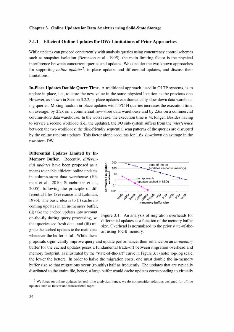
Chapter 3. Online Updates for Data Analytics using Solid-State Storage
3.1.1 Efficient Online Updates for DW: Limitations of Prior Approaches
While updates can proceed concurrently with analysis queries using concurrency control schemessuch as snapshot isolation (Berenson et al., 1995), the main limiting factor is the physicalinterference between concurrent queries and updates. We consider the two known approachesfor supporting online updates2, in-place updates and differential updates, and discuss theirlimitations.
In-Place Updates Double Query Time. A traditional approach, used in OLTP systems, is toupdate in place, i.e., to store the new value in the same physical location as the previous one.However, as shown in Section 3.2.2, in-place updates can dramatically slow down data warehous-ing queries. Mixing random in-place updates with TPC-H queries increases the execution time,on average, by 2.2x on a commercial row-store data warehouse and by 2.6x on a commercialcolumn-store data warehouse. In the worst case, the execution time is 4x longer. Besides havingto service a second workload (i.e., the updates), the I/O sub-system suffers from the interferencebetween the two workloads: the disk-friendly sequential scan patterns of the queries are disruptedby the online random updates. This factor alone accounts for 1.6x slowdown on average in therow-store DW.
Figure 3.1: An analysis of migration overheads fordifferential updates as a function of the memory buffersize. Overhead is normalized to the prior state-of-the-art using 16GB memory.
Differential Updates Limited by In-Memory Buffer. Recently, differen-tial updates have been proposed as ameans to enable efficient online updatesin column-store data warehouse (Hé-man et al., 2010; Stonebraker et al.,2005), following the principle of dif-ferential files (Severance and Lohman,1976). The basic idea is to (i) cache in-coming updates in an in-memory buffer,(ii) take the cached updates into accounton-the-fly during query processing, sothat queries see fresh data, and (iii) mi-grate the cached updates to the main datawhenever the buffer is full. While theseproposals significantly improve query and update performance, their reliance on an in-memorybuffer for the cached updates poses a fundamental trade-off between migration overhead andmemory footprint, as illustrated by the “state-of-the-art” curve in Figure 3.1 (note: log-log scale,the lower the better). In order to halve the migration costs, one must double the in-memorybuffer size so that migrations occur (roughly) half as frequently. The updates that are typicallydistributed to the entire file, hence, a large buffer would cache updates corresponding to virtually
2 We focus on online updates for real-time analytics, hence, we do not consider solutions designed for offlineupdates such as master and transactional tapes.
34
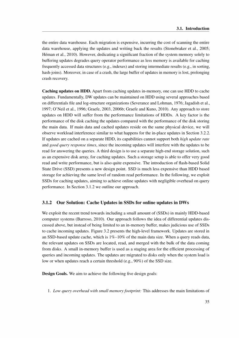
3.1. Introduction
the entire data warehouse. Each migration is expensive, incurring the cost of scanning the entiredata warehouse, applying the updates and writing back the results (Stonebraker et al., 2005;Héman et al., 2010). However, dedicating a significant fraction of the system memory solely tobuffering updates degrades query operator performance as less memory is available for cachingfrequently accessed data structures (e.g., indexes) and storing intermediate results (e.g., in sorting,hash-joins). Moreover, in case of a crash, the large buffer of updates in memory is lost, prolongingcrash recovery.
Caching updates on HDD. Apart from caching updates in-memory, one can use HDD to cacheupdates. Fundamentally, DW updates can be maintained on HDD using several approaches basedon differentials file and log-structure organizations (Severance and Lohman, 1976; Jagadish et al.,1997; O’Neil et al., 1996; Graefe, 2003, 2006b; Graefe and Kuno, 2010). Any approach to storeupdates on HDD will suffer from the performance limitations of HDDs. A key factor is theperformance of the disk caching the updates compared with the performance of the disk storingthe main data. If main data and cached updates reside on the same physical device, we willobserve workload interference similar to what happens for the in-place updates in Section 3.2.2.If updates are cached on a separate HDD, its capabilities cannot support both high update rateand good query response times, since the incoming updates will interfere with the updates to beread for answering the queries. A third design is to use a separate high-end storage solution, suchas an expensive disk array, for caching updates. Such a storage setup is able to offer very goodread and write performance, but is also quite expensive. The introduction of flash-based SolidState Drive (SSD) presents a new design point. SSD is much less expensive than HDD basedstorage for achieving the same level of random read performance. In the following, we exploitSSDs for caching updates, aiming to achieve online updates with negligible overhead on queryperformance. In Section 3.1.2 we outline our approach.
3.1.2 Our Solution: Cache Updates in SSDs for online updates in DWs
We exploit the recent trend towards including a small amount of (SSDs) in mainly HDD-basedcomputer systems (Barroso, 2010). Our approach follows the idea of differential updates dis-cussed above, but instead of being limited to an in-memory buffer, makes judicious use of SSDsto cache incoming updates. Figure 3.2 presents the high-level framework. Updates are stored inan SSD-based update cache, which is 1%–10% of the main data size. When a query reads data,the relevant updates on SSDs are located, read, and merged with the bulk of the data comingfrom disks. A small in-memory buffer is used as a staging area for the efficient processing ofqueries and incoming updates. The updates are migrated to disks only when the system load islow or when updates reach a certain threshold (e.g., 90%) of the SSD size.
Design Goals. We aim to achieve the following five design goals:
1. Low query overhead with small memory footprint: This addresses the main limitations of
35
Chapter 3. Online Updates for Data Analytics using Solid-State Storage
prior approaches.
2. No random SSD writes: While SSDs have excellent sequential read/write and random readperformance, random writes perform poorly because they often incur expensive erase andwear-leveling operations (Bouganim et al., 2009). Moreover, frequent random writes cantransition an SSD into sub-optimal states where even the well-supported operations sufferfrom degraded performance (Bouganim et al., 2009; Stoica et al., 2009).
3. Low total SSD writes per update: A NAND flash cell can endure only a limited number ofwrites (e.g., 105 writes for enterprise SSDs). Therefore, the SSDs’ lifetime is maximized ifwe minimize the amount of SSD writes per incoming update.
4. Efficient migration: Migrations should occur infrequently while supporting high sustainedupdate rate. A naive approach is to migrate updates to a new copy of the data warehouseand swap it in after migration completes, essentially doubling the disk capacity requirement.We want to remove such requirement by migrating to the main data in place.
5. Correct ACID support: We must guarantee that traditional concurrency control and crashrecovery techniques still work.
Prior differential update approaches (Stonebraker et al., 2005; Héman et al., 2010) maintainindexes on the cached updates in memory, which we call Indexed Updates (IU). We find thatnaïvely extending IU to SSDs incurs up to 3.8x query slowdowns (Section 3.2.3 and 3.5.2). Whileemploying log structured merge-trees (LSM) (O’Neil et al., 1996) can address many of IU’sperformance problems, LSM incurs a large number of writes per update, significantly reducingthe SSDs’ lifetime (Section 3.2.3).
At a high level, our framework is similar to the way many popular key-value store implementations(e.g., Bigtable (Chang et al., 2006), HBase (HBase, 2013), and Cassandra (Lakshman and Malik,2010)) handle incoming updates by caching them in HDDs and merging related updates intoquery responses. In fact, their design follows the principle of LSM. However, the design ofthese key-value stores is focused on neither low overhead for data warehousing queries withsmall memory footprint, using SSDs and minimizing SSD writes, nor correct ACID supportfor multi-row transactions. Using SSDs instead of HDDs for the update cache is crucial to ourdesign, as it reduces range scan query overhead by orders of magnitude for small ranges.
Using SSDs to support online updates: MaSM. We use MaSM (materialized sort-merge)algorithms that achieve the five design goals with the following techniques.
First, we observe that the “Merge” component in Figure 3.2 is essentially an outer join betweenthe main data on disks and the updates cached on SSDs. Among various join algorithms, wefind that sort-merge joins fit the current context well: cached updates are sorted according tothe layout order of the main data and then merged with the main data. MaSM exploits externalsorting algorithms both to achieve small memory footprint and to avoid random writes to SSDs.
36
3.1. Introduction
To sort ‖SSD‖ pages of cached updates on SSD, two-pass external sorting requires M =p‖SSD‖pages of memory. The number of passes is limited to two because one of the design goals is tominimize the amount of writes our algorithms perform on the SSDs. Compared with differentialupdates limited to an in-memory update cache, the MaSM approach can effectively use a smallmemory footprint, and exploits the larger on-SSD cache to greatly reduce migration frequency,as shown in the “our approach” curve in Figure 3.1.
Figure 3.2: Framework for SSD-based differential up-dates.
Second, we optimize the two passesof the “Merge” operation: generatingsorted runs and merging sorted runs.For the former, because a query shouldsee all the updates that an earlier queryhas seen, we materialize and reusesorted runs, amortizing run generationcosts across many queries. For the lat-ter, we build simple read-only indexeson materialized runs in order to reducethe SSD read I/Os for a query. Com-bined with the excellent sequential/ran-dom read performance of SSDs, thistechnique successfully achieves lowquery overhead (at most only 7% slow-downs in our experimental evaluation).
Third, we consider the trade-off between memory footprint and SSD writes. The problem iscomplicated because allocated memory is used for processing both incoming updates and queries.We first present a MaSM-2M algorithm, which achieves the minimal SSD writes per update,but allocates M memory for incoming updates and M memory for query processing. Then, wepresent a more sophisticated MaSM-M algorithm that reduces memory footprint to M but incursextra SSD writes. We select optimal algorithm parameters to minimize SSD writes for MaSM-M.After that, we generalize the two algorithms into a MaSM-αM algorithm. By varying α, we canobtain a spectrum of algorithms with different trade-offs between memory footprint and SSDwrites.
Fourth, in order to support in-place migration and ACID properties, we propose to attachtimestamps to updates, data pages, and queries. That is, there is a timestamp per update when itis cached on SSDs, a timestamp per data page in the main data, and a timestamp for every query.Using timestamps, MaSM can determine whether or not a particular update has been applied toa data page, thereby enabling concurrent queries during in-place migration. Moreover, MaSMguarantees serializability in the timestamp order among individual queries and updates. This canbe easily extended to support two-phase locking and snapshot isolation for general transactionsinvolving both queries and updates. Furthermore, crash recovery can use the timestamps todetermine and recover only the updates in the memory buffer (updates on SSDs survive the
37
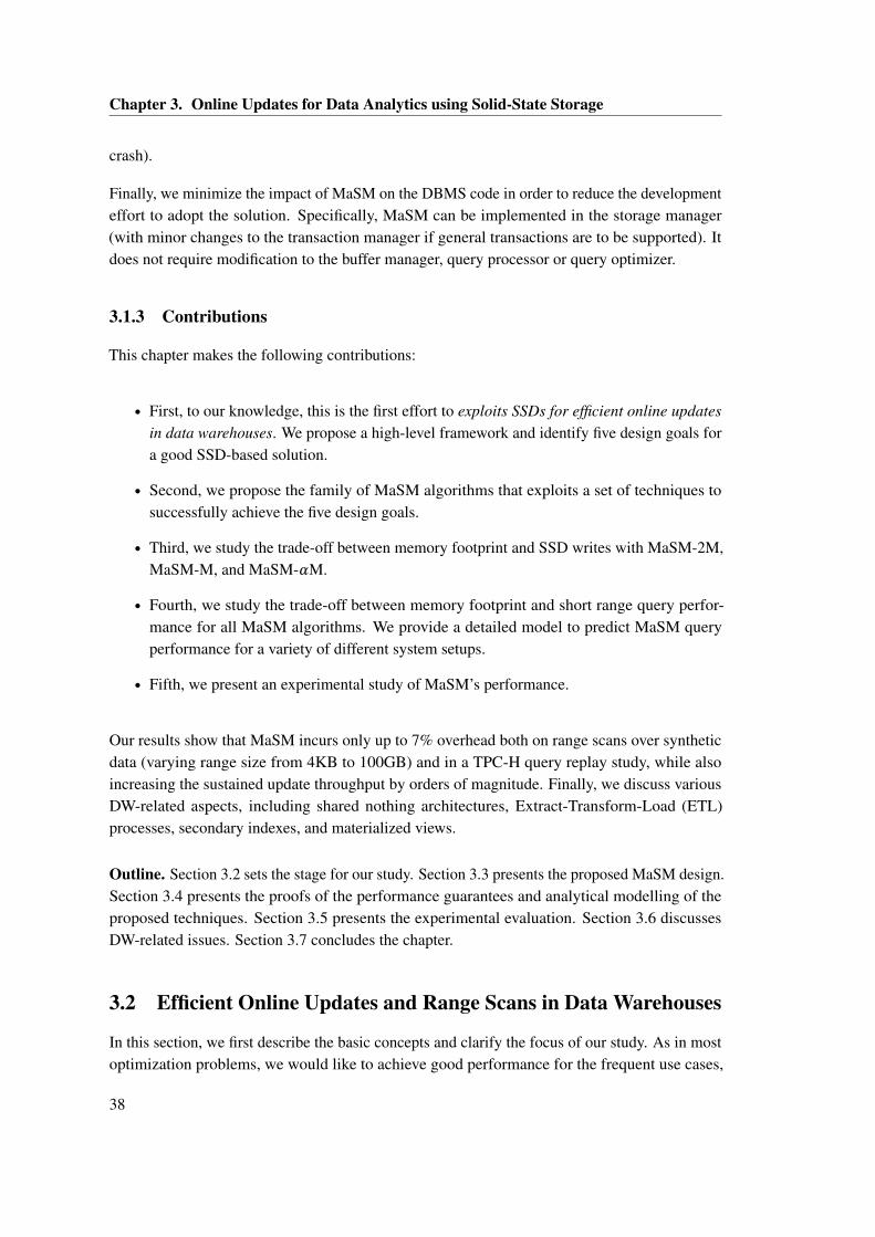
Chapter 3. Online Updates for Data Analytics using Solid-State Storage
crash).
Finally, we minimize the impact of MaSM on the DBMS code in order to reduce the developmenteffort to adopt the solution. Specifically, MaSM can be implemented in the storage manager(with minor changes to the transaction manager if general transactions are to be supported). Itdoes not require modification to the buffer manager, query processor or query optimizer.
3.1.3 Contributions
This chapter makes the following contributions:
• First, to our knowledge, this is the first effort to exploits SSDs for efficient online updatesin data warehouses. We propose a high-level framework and identify five design goals fora good SSD-based solution.
• Second, we propose the family of MaSM algorithms that exploits a set of techniques tosuccessfully achieve the five design goals.
• Third, we study the trade-off between memory footprint and SSD writes with MaSM-2M,MaSM-M, and MaSM-αM.
• Fourth, we study the trade-off between memory footprint and short range query perfor-mance for all MaSM algorithms. We provide a detailed model to predict MaSM queryperformance for a variety of different system setups.
• Fifth, we present an experimental study of MaSM’s performance.
Our results show that MaSM incurs only up to 7% overhead both on range scans over syntheticdata (varying range size from 4KB to 100GB) and in a TPC-H query replay study, while alsoincreasing the sustained update throughput by orders of magnitude. Finally, we discuss variousDW-related aspects, including shared nothing architectures, Extract-Transform-Load (ETL)processes, secondary indexes, and materialized views.
Outline. Section 3.2 sets the stage for our study. Section 3.3 presents the proposed MaSM design.Section 3.4 presents the proofs of the performance guarantees and analytical modelling of theproposed techniques. Section 3.5 presents the experimental evaluation. Section 3.6 discussesDW-related issues. Section 3.7 concludes the chapter.
3.2 Efficient Online Updates and Range Scans in Data Warehouses
In this section, we first describe the basic concepts and clarify the focus of our study. As in mostoptimization problems, we would like to achieve good performance for the frequent use cases,
38
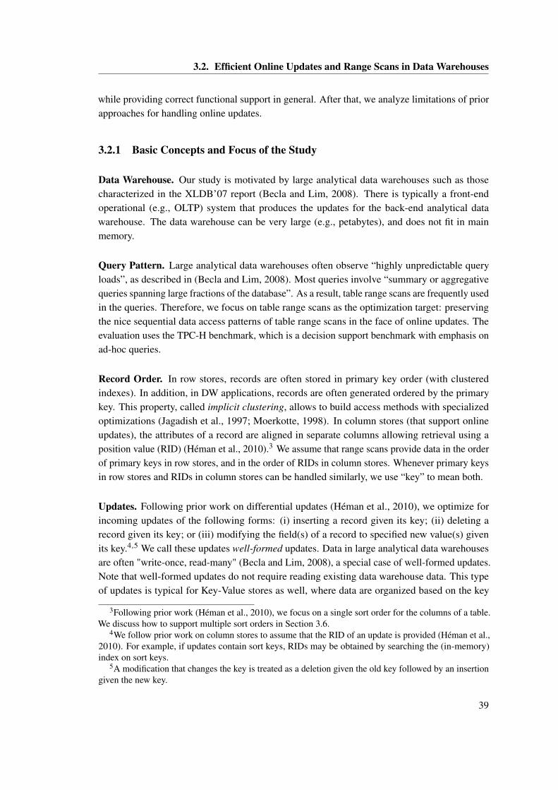
3.2. Efficient Online Updates and Range Scans in Data Warehouses
while providing correct functional support in general. After that, we analyze limitations of priorapproaches for handling online updates.
3.2.1 Basic Concepts and Focus of the Study
Data Warehouse. Our study is motivated by large analytical data warehouses such as thosecharacterized in the XLDB’07 report (Becla and Lim, 2008). There is typically a front-endoperational (e.g., OLTP) system that produces the updates for the back-end analytical datawarehouse. The data warehouse can be very large (e.g., petabytes), and does not fit in mainmemory.
Query Pattern. Large analytical data warehouses often observe “highly unpredictable queryloads”, as described in (Becla and Lim, 2008). Most queries involve “summary or aggregativequeries spanning large fractions of the database”. As a result, table range scans are frequently usedin the queries. Therefore, we focus on table range scans as the optimization target: preservingthe nice sequential data access patterns of table range scans in the face of online updates. Theevaluation uses the TPC-H benchmark, which is a decision support benchmark with emphasis onad-hoc queries.
Record Order. In row stores, records are often stored in primary key order (with clusteredindexes). In addition, in DW applications, records are often generated ordered by the primarykey. This property, called implicit clustering, allows to build access methods with specializedoptimizations (Jagadish et al., 1997; Moerkotte, 1998). In column stores (that support onlineupdates), the attributes of a record are aligned in separate columns allowing retrieval using aposition value (RID) (Héman et al., 2010).3 We assume that range scans provide data in the orderof primary keys in row stores, and in the order of RIDs in column stores. Whenever primary keysin row stores and RIDs in column stores can be handled similarly, we use “key” to mean both.
Updates. Following prior work on differential updates (Héman et al., 2010), we optimize forincoming updates of the following forms: (i) inserting a record given its key; (ii) deleting arecord given its key; or (iii) modifying the field(s) of a record to specified new value(s) givenits key.4,5 We call these updates well-formed updates. Data in large analytical data warehousesare often "write-once, read-many" (Becla and Lim, 2008), a special case of well-formed updates.Note that well-formed updates do not require reading existing data warehouse data. This typeof updates is typical for Key-Value stores as well, where data are organized based on the key
3Following prior work (Héman et al., 2010), we focus on a single sort order for the columns of a table.We discuss how to support multiple sort orders in Section 3.6.
4We follow prior work on column stores to assume that the RID of an update is provided (Héman et al.,2010). For example, if updates contain sort keys, RIDs may be obtained by searching the (in-memory)index on sort keys.
5A modification that changes the key is treated as a deletion given the old key followed by an insertiongiven the new key.
39
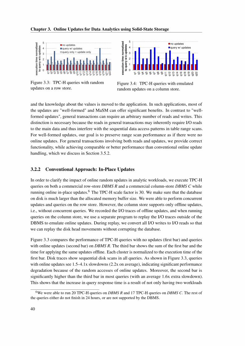
Chapter 3. Online Updates for Data Analytics using Solid-State Storage
0
1
2
3
4
5
q1
q2
q3
q4
q5
q6
q7
q8
q9
q10
q11
q12
q13
q14
q15
q16
q18
q19
q21
q22
ex
ec
uti
on
tim
e n
orm
alize
dto
qu
ery
w/o
up
da
tes no updates
query w/ updates
query only + update only
Figure 3.3: TPC-H queries with randomupdates on a row store.
2
3
4
5
me n
orm
alized
w/o
up
da
tes no updates
query w/ updates
0
1
2
3
4
5
q1
q3
q4
q5
q6
q7
q8
q9
q1
1
q1
2
q1
3
q1
4
q1
6
q1
8
q1
9
q2
0
q2
2
execu
tio
n t
ime n
orm
alized
to q
ue
ry w
/o u
pd
ate
s no updates
query w/ updates
0
1
2
3
4
5
q1
q3
q4
q5
q6
q7
q8
q9
q1
1
q1
2
q1
3
q1
4
q1
6
q1
8
q1
9
q2
0
q2
2
execu
tio
n t
ime n
orm
alized
to q
ue
ry w
/o u
pd
ate
s no updates
query w/ updates
Figure 3.4: TPC-H queries with emulatedrandom updates on a column store.
and the knowledge about the values is moved to the application. In such applications, most ofthe updates are "well-formed" and MaSM can offer significant benefits. In contrast to "well-formed updates", general transactions can require an arbitrary number of reads and writes. Thisdistinction is necessary because the reads in general transactions may inherently require I/O readsto the main data and thus interfere with the sequential data access patterns in table range scans.For well-formed updates, our goal is to preserve range scan performance as if there were noonline updates. For general transactions involving both reads and updates, we provide correctfunctionality, while achieving comparable or better performance than conventional online updatehandling, which we discuss in Section 3.5.2.
3.2.2 Conventional Approach: In-Place Updates
In order to clarify the impact of online random updates in analytic workloads, we execute TPC-Hqueries on both a commercial row-store DBMS R and a commercial column-store DBMS C whilerunning online in-place updates.6 The TPC-H scale factor is 30. We make sure that the databaseon disk is much larger than the allocated memory buffer size. We were able to perform concurrentupdates and queries on the row store. However, the column store supports only offline updates,i.e., without concurrent queries. We recorded the I/O traces of offline updates, and when runningqueries on the column store, we use a separate program to replay the I/O traces outside of theDBMS to emulate online updates. During replay, we convert all I/O writes to I/O reads so thatwe can replay the disk head movements without corrupting the database.
Figure 3.3 compares the performance of TPC-H queries with no updates (first bar) and querieswith online updates (second bar) on DBMS R. The third bar shows the sum of the first bar and thetime for applying the same updates offline. Each cluster is normalized to the execution time of thefirst bar. Disk traces show sequential disk scans in all queries. As shown in Figure 3.3, querieswith online updates see 1.5–4.1x slowdowns (2.2x on average), indicating significant performancedegradation because of the random accesses of online updates. Moreover, the second bar issignificantly higher than the third bar in most queries (with an average 1.6x extra slowdown).This shows that the increase in query response time is a result of not only having two workloads
6We were able to run 20 TPC-H queries on DBMS R and 17 TPC-H queries on DBMS C. The rest ofthe queries either do not finish in 24 hours, or are not supported by the DBMS.
40
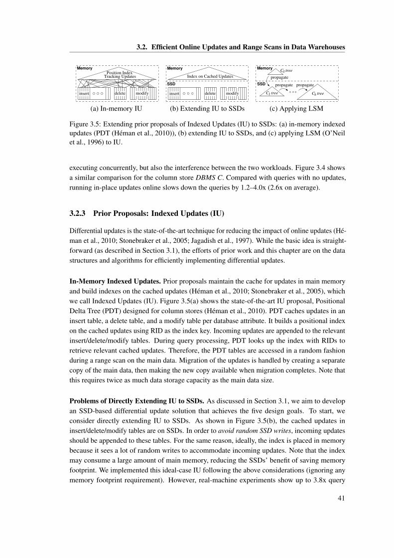
3.2. Efficient Online Updates and Range Scans in Data Warehouses
Tracking UpdatesPosition Index
Memory
insert delete modify
Memory
SSD
Index on Cached Updates
insert delete modify C treehC tree1
C tree0Memory
SSD propagate propagate
propagate
(a) In-memory IU (b) Extending IU to SSDs (c) Applying LSM
Figure 3.5: Extending prior proposals of Indexed Updates (IU) to SSDs: (a) in-memory indexedupdates (PDT (Héman et al., 2010)), (b) extending IU to SSDs, and (c) applying LSM (O’Neilet al., 1996) to IU.
executing concurrently, but also the interference between the two workloads. Figure 3.4 showsa similar comparison for the column store DBMS C. Compared with queries with no updates,running in-place updates online slows down the queries by 1.2–4.0x (2.6x on average).
3.2.3 Prior Proposals: Indexed Updates (IU)
Differential updates is the state-of-the-art technique for reducing the impact of online updates (Hé-man et al., 2010; Stonebraker et al., 2005; Jagadish et al., 1997). While the basic idea is straight-forward (as described in Section 3.1), the efforts of prior work and this chapter are on the datastructures and algorithms for efficiently implementing differential updates.
In-Memory Indexed Updates. Prior proposals maintain the cache for updates in main memoryand build indexes on the cached updates (Héman et al., 2010; Stonebraker et al., 2005), whichwe call Indexed Updates (IU). Figure 3.5(a) shows the state-of-the-art IU proposal, PositionalDelta Tree (PDT) designed for column stores (Héman et al., 2010). PDT caches updates in aninsert table, a delete table, and a modify table per database attribute. It builds a positional indexon the cached updates using RID as the index key. Incoming updates are appended to the relevantinsert/delete/modify tables. During query processing, PDT looks up the index with RIDs toretrieve relevant cached updates. Therefore, the PDT tables are accessed in a random fashionduring a range scan on the main data. Migration of the updates is handled by creating a separatecopy of the main data, then making the new copy available when migration completes. Note thatthis requires twice as much data storage capacity as the main data size.
Problems of Directly Extending IU to SSDs. As discussed in Section 3.1, we aim to developan SSD-based differential update solution that achieves the five design goals. To start, weconsider directly extending IU to SSDs. As shown in Figure 3.5(b), the cached updates ininsert/delete/modify tables are on SSDs. In order to avoid random SSD writes, incoming updatesshould be appended to these tables. For the same reason, ideally, the index is placed in memorybecause it sees a lot of random writes to accommodate incoming updates. Note that the indexmay consume a large amount of main memory, reducing the SSDs’ benefit of saving memoryfootprint. We implemented this ideal-case IU following the above considerations (ignoring anymemory footprint requirement). However, real-machine experiments show up to 3.8x query
41
Chapter 3. Online Updates for Data Analytics using Solid-State Storage
slowdowns even for this ideal-case IU (Section 3.5.2). We find that the slowdown is because theinsert/delete/modify tables are randomly read during range scan operations. This is wasteful asan entire SSD page has to be read and discarded for retrieving a single update entry.
Problems of Applying LSM to IU. The log-structured merge-tree (LSM) is a disk-based indexstructure designed to support a high rate of insertions (O’Neil et al., 1996). An LSM consists ofmultiple levels of trees of increasing sizes. PDT employs the idea of multiple levels of trees tosupport snapshot isolation in memory (Héman et al., 2010). The stepped-merge algorithm (Ja-gadish et al., 1997) is based, as well, on the principle of storing updates in memory and organizethem in progressively larger sorted runs, merging them eventually into a B+-Tree. Here, weconsider the feasibility of combining LSM and IU as an SSD-based solution.
As shown in Figure 3.5(c), LSM keeps the smallest C0 tree in memory, and C1, ..., Ch trees onSSDs, where h ≥ 1. Incoming updates are first inserted into C0, then gradually propagate tothe SSD-resident trees. There are asynchronous rolling propagation processes between everyadjacent pair (Ci , Ci+1) that (repeatedly) sequentially visit the leaf nodes of Ci and Ci+1, andmove entries from Ci to Ci+1. This scheme avoids many of IU’s performance problems. Randomwrites can be avoided by using large sequential I/Os during propagation. For a range scan query,it performs corresponding index range scans on every level of LSM, thereby avoiding wastefulrandom I/Os as in the above ideal-case IU.
Unfortunately, LSM incurs a large amount of writes per update entry, violating the third designgoal. The additional writes arise in two cases: (i) An update entry is copied h times from C0 toCh ; and (ii) the propagation process from Ci to Ci+1 rewrites the old entries in Ci+1 to SSDs onceper round of propagation. According to (O’Neil et al., 1996), in an optimal LSM, the sizes ofthe trees form a geometric progression. That is, si ze(Ci+1)/si ze(Ci ) = r , where r is a constantparameter. It can be shown that in LSM the above two cases introduce about r +1 writes perupdate for levels 1, . . . ,h −1 and (r +1)/2 writes per update for level h. As an example, with4GB SSD space and 16MB memory (which is our experimental setting in Section 3.5.1), we cancompute that a 2-level (h = 1) LSM writes every update entry ≈ 128 times. The optimal LSMthat minimizes total writes has h = 4 and it writes every update entry ≈ 17 times! In other words,compared to a scheme that writes every update entry once, applying LSM on an SSD reduces itslifetime 17 fold (e.g., from 3 years to 2 months). For a more detailed comparison of the amountof writes performed by LSM and MaSM see Section 3.4.5.
3.3 MaSM Design
In this section, we propose MaSM (materialized sort-merge) algorithms for achieving the fivedesign goals. We start by describing the basic ideas in Section 3.3.1. Then we present two MaSMalgorithms: MaSM-2M in Section 3.3.2 and MaSM-M in Section 3.3.3. MaSM-M halves thememory footprint of MaSM-2M but incurs extra SSD writes. In Section 3.3.4, we generalizethese two algorithms into a MaSM-αM algorithm, allowing a range of trade-offs between
42
3.3. MaSM Design
memory footprint and SSD writes by varying α. After that, we discuss a set of optimizations inSection 3.3.5, and describe transaction support in Section 3.3.6. Finally, we analyze the MaSMalgorithms in terms of the five design goals in Section 3.3.7.
3.3.1 Basic Ideas
Consider the operation of merging a table range scan and the cached updates. For every recordretrieved by the scan, it finds and applies any matching cached updates. Records without updatesor new insertions must be returned too. Essentially, this is an outer join operation on the recordkey (primary key/RID).
Among various join algorithms, we choose to employ a sort-based join that sorts the cachedupdates and merges the sorted updates with the table range scan. This is because the most efficientjoins are typically sort-based or hash-based, but hash-based joins have to perform costly I/Opartitioning for the main data. The sort-based join also preserves the record order in table rangescans, which allows hiding the implementation details of the merging operation from the queryoptimizer and upper-level query operators.
To reduce memory footprint, we keep the cached updates on SSDs and perform external sortingof the updates; two-pass external sorting requires M =p‖SSD‖ pages in memory to sort ‖SSD‖pages of cached updates on SSDs. However, external sorting may incur significant overheadfor generating sorted runs and merging them. We exploit the following two ideas to reducethe overhead. First, we observe that a query should see all the cached updates that a previousquery has seen. Thus, we materialize sorted runs of updates, deleting the generated runs onlyafter update migration. This amortizes the cost of sorted run generation across many queries.Second, we would like to prune as many irrelevant updates to the current range scan query aspossible. Because materialized runs are read-only, we can create a simple, read-only index, calleda run index. A run index is a compact tree based index which records the smallest key (primarykey/RID) for every fixed number of SSD pages in a sorted run. It is created after the sorted runsare formed, and, hence, it does not need to support insertion/deletion. Then we can search thequery’s key range in the run index to retrieve only those SSD pages that fall in the range. We callthe algorithm combining the above ideas the Materialized Sort-Merge (MaSM) algorithm.
The picture of the above design is significantly complicated by the interactions among incomingupdates, range scans, and update migrations. For example, sharing the memory buffer betweenupdates and queries makes it difficult to achieve a memory footprint of M . In-place migrationsmay conflict with ongoing queries. Concurrency control and crash recovery must be re-examined.In the following, we first present a simple MaSM algorithm that requires 2M memory and a moresophisticated algorithm that reduces the memory requirement to M , then generalize them into analgorithm requiring αM memory. We propose a timestamp-based approach to support in-placemigrations and ACID properties.
43
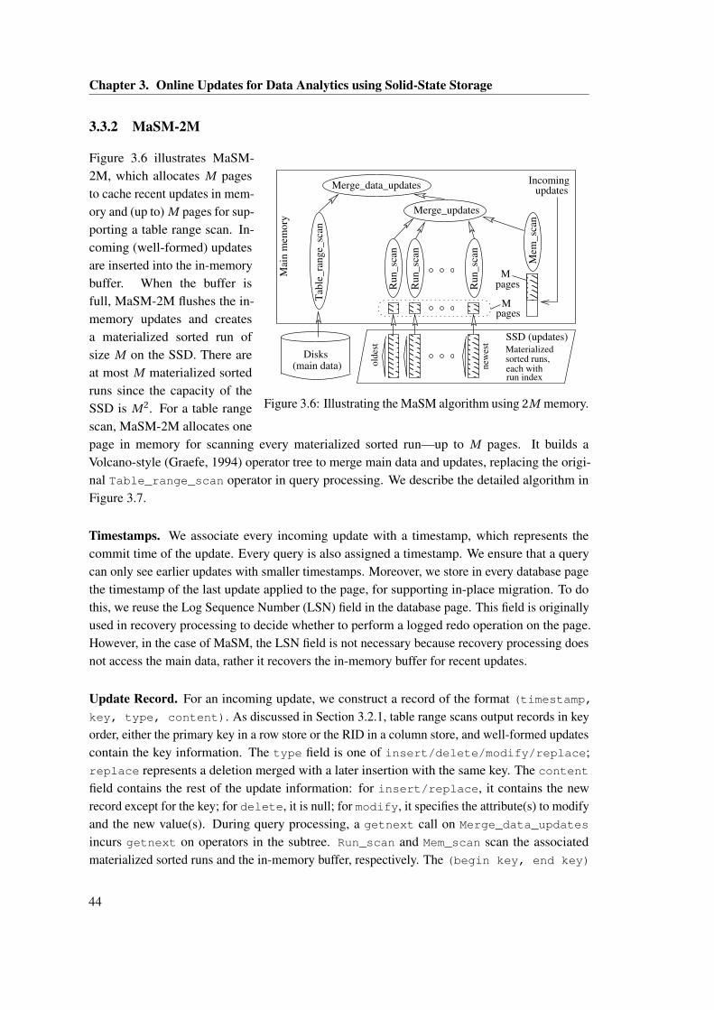
Chapter 3. Online Updates for Data Analytics using Solid-State Storage
3.3.2 MaSM-2M
Run_sc
an
Run_sc
an
Run_sc
an
Merge_updates
Mem
_sc
an
Tab
le_ra
nge_
scan
pagesM
pagesMM
ain m
emory
Merge_data_updates
(main data)Disks
updatesIncoming
SSD (updates)
new
est
old
est
Materializedsorted runs,each withrun index
Figure 3.6: Illustrating the MaSM algorithm using 2M memory.
Figure 3.6 illustrates MaSM-2M, which allocates M pagesto cache recent updates in mem-ory and (up to) M pages for sup-porting a table range scan. In-coming (well-formed) updatesare inserted into the in-memorybuffer. When the buffer isfull, MaSM-2M flushes the in-memory updates and createsa materialized sorted run ofsize M on the SSD. There areat most M materialized sortedruns since the capacity of theSSD is M 2. For a table rangescan, MaSM-2M allocates onepage in memory for scanning every materialized sorted run—up to M pages. It builds aVolcano-style (Graefe, 1994) operator tree to merge main data and updates, replacing the origi-nal Table_range_scan operator in query processing. We describe the detailed algorithm inFigure 3.7.
Timestamps. We associate every incoming update with a timestamp, which represents thecommit time of the update. Every query is also assigned a timestamp. We ensure that a querycan only see earlier updates with smaller timestamps. Moreover, we store in every database pagethe timestamp of the last update applied to the page, for supporting in-place migration. To dothis, we reuse the Log Sequence Number (LSN) field in the database page. This field is originallyused in recovery processing to decide whether to perform a logged redo operation on the page.However, in the case of MaSM, the LSN field is not necessary because recovery processing doesnot access the main data, rather it recovers the in-memory buffer for recent updates.
Update Record. For an incoming update, we construct a record of the format (timestamp,key, type, content). As discussed in Section 3.2.1, table range scans output records in keyorder, either the primary key in a row store or the RID in a column store, and well-formed updatescontain the key information. The type field is one of insert/delete/modify/replace;replace represents a deletion merged with a later insertion with the same key. The contentfield contains the rest of the update information: for insert/replace, it contains the newrecord except for the key; for delete, it is null; for modify, it specifies the attribute(s) to modifyand the new value(s). During query processing, a getnext call on Merge_data_updates
incurs getnext on operators in the subtree. Run_scan and Mem_scan scan the associatedmaterialized sorted runs and the in-memory buffer, respectively. The (begin key, end key)
44
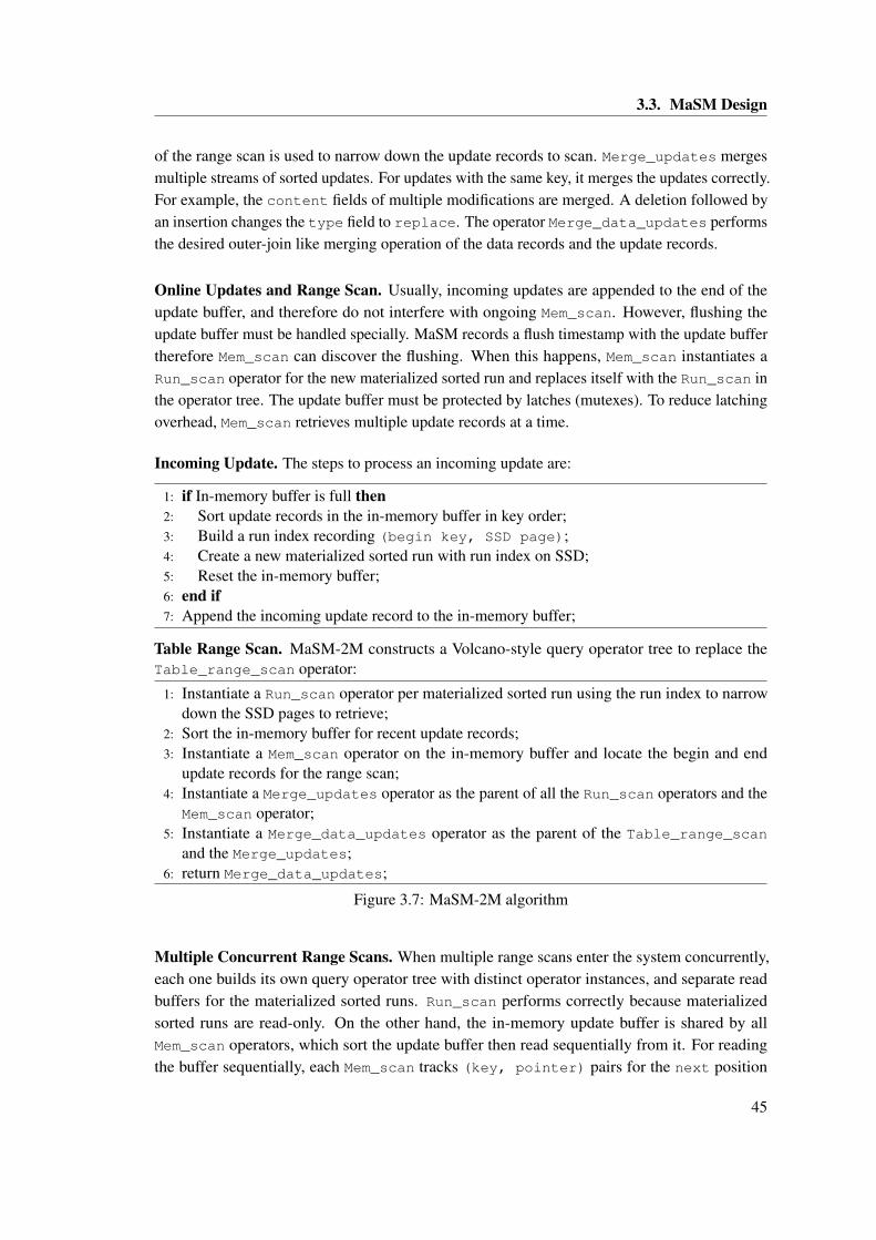
3.3. MaSM Design
of the range scan is used to narrow down the update records to scan. Merge_updates mergesmultiple streams of sorted updates. For updates with the same key, it merges the updates correctly.For example, the content fields of multiple modifications are merged. A deletion followed byan insertion changes the type field to replace. The operator Merge_data_updates performsthe desired outer-join like merging operation of the data records and the update records.
Online Updates and Range Scan. Usually, incoming updates are appended to the end of theupdate buffer, and therefore do not interfere with ongoing Mem_scan. However, flushing theupdate buffer must be handled specially. MaSM records a flush timestamp with the update buffertherefore Mem_scan can discover the flushing. When this happens, Mem_scan instantiates aRun_scan operator for the new materialized sorted run and replaces itself with the Run_scan inthe operator tree. The update buffer must be protected by latches (mutexes). To reduce latchingoverhead, Mem_scan retrieves multiple update records at a time.
Incoming Update. The steps to process an incoming update are:
1: if In-memory buffer is full then2: Sort update records in the in-memory buffer in key order;3: Build a run index recording (begin key, SSD page);4: Create a new materialized sorted run with run index on SSD;5: Reset the in-memory buffer;6: end if7: Append the incoming update record to the in-memory buffer;
Table Range Scan. MaSM-2M constructs a Volcano-style query operator tree to replace theTable_range_scan operator:
1: Instantiate a Run_scan operator per materialized sorted run using the run index to narrowdown the SSD pages to retrieve;
2: Sort the in-memory buffer for recent update records;3: Instantiate a Mem_scan operator on the in-memory buffer and locate the begin and end
update records for the range scan;4: Instantiate a Merge_updates operator as the parent of all the Run_scan operators and the
Mem_scan operator;5: Instantiate a Merge_data_updates operator as the parent of the Table_range_scan
and the Merge_updates;6: return Merge_data_updates;
Figure 3.7: MaSM-2M algorithm
Multiple Concurrent Range Scans. When multiple range scans enter the system concurrently,each one builds its own query operator tree with distinct operator instances, and separate readbuffers for the materialized sorted runs. Run_scan performs correctly because materializedsorted runs are read-only. On the other hand, the in-memory update buffer is shared by allMem_scan operators, which sort the update buffer then read sequentially from it. For readingthe buffer sequentially, each Mem_scan tracks (key, pointer) pairs for the next position
45
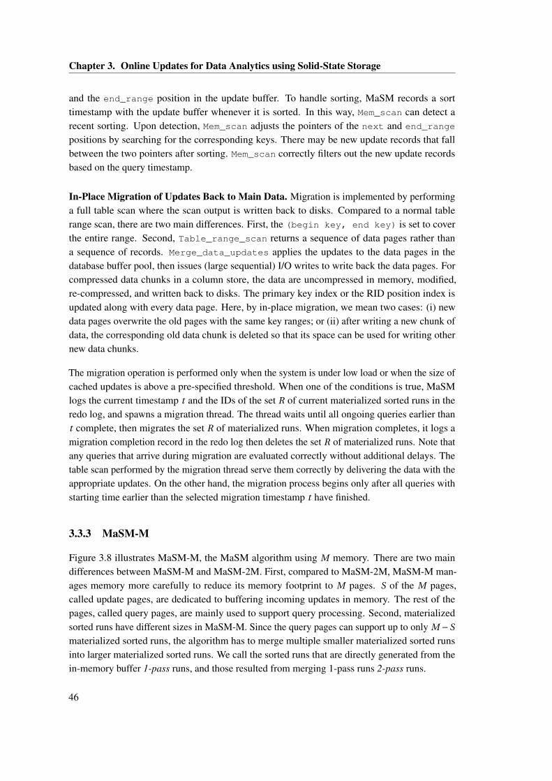
Chapter 3. Online Updates for Data Analytics using Solid-State Storage
and the end_range position in the update buffer. To handle sorting, MaSM records a sorttimestamp with the update buffer whenever it is sorted. In this way, Mem_scan can detect arecent sorting. Upon detection, Mem_scan adjusts the pointers of the next and end_range
positions by searching for the corresponding keys. There may be new update records that fallbetween the two pointers after sorting. Mem_scan correctly filters out the new update recordsbased on the query timestamp.
In-Place Migration of Updates Back to Main Data. Migration is implemented by performinga full table scan where the scan output is written back to disks. Compared to a normal tablerange scan, there are two main differences. First, the (begin key, end key) is set to coverthe entire range. Second, Table_range_scan returns a sequence of data pages rather thana sequence of records. Merge_data_updates applies the updates to the data pages in thedatabase buffer pool, then issues (large sequential) I/O writes to write back the data pages. Forcompressed data chunks in a column store, the data are uncompressed in memory, modified,re-compressed, and written back to disks. The primary key index or the RID position index isupdated along with every data page. Here, by in-place migration, we mean two cases: (i) newdata pages overwrite the old pages with the same key ranges; or (ii) after writing a new chunk ofdata, the corresponding old data chunk is deleted so that its space can be used for writing othernew data chunks.
The migration operation is performed only when the system is under low load or when the size ofcached updates is above a pre-specified threshold. When one of the conditions is true, MaSMlogs the current timestamp t and the IDs of the set R of current materialized sorted runs in theredo log, and spawns a migration thread. The thread waits until all ongoing queries earlier thant complete, then migrates the set R of materialized runs. When migration completes, it logs amigration completion record in the redo log then deletes the set R of materialized runs. Note thatany queries that arrive during migration are evaluated correctly without additional delays. Thetable scan performed by the migration thread serve them correctly by delivering the data with theappropriate updates. On the other hand, the migration process begins only after all queries withstarting time earlier than the selected migration timestamp t have finished.
3.3.3 MaSM-M
Figure 3.8 illustrates MaSM-M, the MaSM algorithm using M memory. There are two maindifferences between MaSM-M and MaSM-2M. First, compared to MaSM-2M, MaSM-M man-ages memory more carefully to reduce its memory footprint to M pages. S of the M pages,called update pages, are dedicated to buffering incoming updates in memory. The rest of thepages, called query pages, are mainly used to support query processing. Second, materializedsorted runs have different sizes in MaSM-M. Since the query pages can support up to only M −S
materialized sorted runs, the algorithm has to merge multiple smaller materialized sorted runsinto larger materialized sorted runs. We call the sorted runs that are directly generated from thein-memory buffer 1-pass runs, and those resulted from merging 1-pass runs 2-pass runs.
46
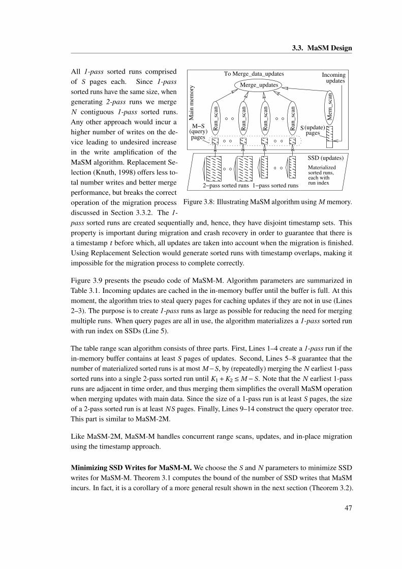
3.3. MaSM Design
Ru
n_
scan
Ru
n_
scan
Ru
n_
scan
Ru
n_
scan
Merge_updates
Mem
_sc
an
2−pass sorted runs 1−pass sorted runs
To Merge_data_updates
updatesIncoming
Mai
n m
emo
ry
SSD (updates)
Materialized
each withrun index
sorted runs,
pagespages
S(update)(query)M−S
Figure 3.8: Illustrating MaSM algorithm using M memory.
All 1-pass sorted runs comprisedof S pages each. Since 1-passsorted runs have the same size, whengenerating 2-pass runs we mergeN contiguous 1-pass sorted runs.Any other approach would incur ahigher number of writes on the de-vice leading to undesired increasein the write amplification of theMaSM algorithm. Replacement Se-lection (Knuth, 1998) offers less to-tal number writes and better mergeperformance, but breaks the correctoperation of the migration processdiscussed in Section 3.3.2. The 1-pass sorted runs are created sequentially and, hence, they have disjoint timestamp sets. Thisproperty is important during migration and crash recovery in order to guarantee that there isa timestamp t before which, all updates are taken into account when the migration is finished.Using Replacement Selection would generate sorted runs with timestamp overlaps, making itimpossible for the migration process to complete correctly.
Figure 3.9 presents the pseudo code of MaSM-M. Algorithm parameters are summarized inTable 3.1. Incoming updates are cached in the in-memory buffer until the buffer is full. At thismoment, the algorithm tries to steal query pages for caching updates if they are not in use (Lines2–3). The purpose is to create 1-pass runs as large as possible for reducing the need for mergingmultiple runs. When query pages are all in use, the algorithm materializes a 1-pass sorted runwith run index on SSDs (Line 5).
The table range scan algorithm consists of three parts. First, Lines 1–4 create a 1-pass run if thein-memory buffer contains at least S pages of updates. Second, Lines 5–8 guarantee that thenumber of materialized sorted runs is at most M−S, by (repeatedly) merging the N earliest 1-passsorted runs into a single 2-pass sorted run until K1 +K2 ≤ M −S. Note that the N earliest 1-passruns are adjacent in time order, and thus merging them simplifies the overall MaSM operationwhen merging updates with main data. Since the size of a 1-pass run is at least S pages, the sizeof a 2-pass sorted run is at least N S pages. Finally, Lines 9–14 construct the query operator tree.This part is similar to MaSM-2M.
Like MaSM-2M, MaSM-M handles concurrent range scans, updates, and in-place migrationusing the timestamp approach.
Minimizing SSD Writes for MaSM-M. We choose the S and N parameters to minimize SSDwrites for MaSM-M. Theorem 3.1 computes the bound of the number of SSD writes that MaSMincurs. In fact, it is a corollary of a more general result shown in the next section (Theorem 3.2).
47

Chapter 3. Online Updates for Data Analytics using Solid-State Storage
Incoming Updates:
1: if In-memory buffer is full then2: if At least one of the query pages is not used then3: Steal a query page to extend the in-memory buffer;4: else5: Create a 1-pass materialized sorted run with run index from the updates in the in-memory
buffer;6: Reset the in-memory buffer to have S empty pages;7: end if8: end if9: Append the incoming update record to the in-memory buffer;
Table Range Scan Setup:
1: if In-memory buffer contains at least S pages of updates then2: Create a 1-pass materialized sorted run with run index from the updates in the in-memory
buffer;3: Reset the in-memory buffer to have S empty update pages;4: end if5: while K1 +K2 > M −S do {merge 1-pass runs}6: Merge N earliest adjacent 1-pass runs into a 2-pass run;7: K1 = K1 −N ; K2++;8: end while9: Instantiate a Run_scan operator per materialized sorted run using the run index to narrow
down SSD pages to retrieve;10: if In-memory buffer is not empty then11: Sort the in-memory buffer and create a Mem_scan operator;12: end if13: Instantiate a Merge_updates operator as the parent of all the Run_scan operators and the
Mem_scan operator;14: Instantiate a Merge_data_updates operator as the parent of the Table_range_scan
and the Merge_updates;15: return Merge_data_updates;
Figure 3.9: MaSM-M algorithm
48

3.3. MaSM Design
Table 3.1: Parameters used in the MaSM-M algorithm.
‖SSD‖ SSD capacity (in pages), ‖SSD‖ = M 2
M memory size (in pages) allocated for MaSM-MS memory buffer (in pages) allocated for incoming updates
K1 number of 1-pass sorted runs on SSDsK2 number of 2-pass sorted runs on SSDsN merge N 1-pass runs into a 2-pass run, N ≤ M −S
Theorem 3.1. The MaSM-M algorithm minimizes the number of SSD writes in the worst casewhen Sopt = 0.5M and Nopt = 0.375M +1. The average number of times that MaSM-M writesevery update record to SSD is 1.75+ 2
M .
3.3.4 MaSM-αM
We generalize the MaSM-M algorithm to a MaSM-αM algorithm that uses αM memory, whereα ∈ [ 2
M13
,2]. The algorithm is the same as MaSM-M except that the total allocated memory sizeis αM pages. The lower bound on α ensures that the memory is sufficiently large to make 3-passsorted runs unnecessary. MaSM-M is a special case of MaSM-αM when α= 1, and MaSM-2Mis a special case of MaSM-αM when α= 2. Similar to Theorem 3.1, we can obtain the followingtheorem for minimizing SSD writes for MaSM-αM.
Theorem 3.2. Let α ∈ [ 2
M13
,2]. The MaSM-αM algorithm minimizes the number of SSD writes
in the worst case when Sopt = 0.5αM and Nopt = 1b 4α2 c
( 2α −0.5α)M +1. The average number of
times that MaSM-αM writes every update record to SSD is roughly 2−0.25α2.
We can verify that MaSM-M incurs roughly 2−0.25∗12 = 1.75 writes per update record, whileMaSM-2M writes every update record once (2−0.25∗22 = 1).
Theorem 3.2 shows the trade-off between memory footprint and SSD writes for a spectrum ofMaSM algorithms. At one end of the spectrum, MaSM-2M achieves minimal SSD writes with2M memory. At the other end of the spectrum, one can achieve a MaSM algorithm with verysmall memory footprint (2M
23 ) while writing every update record at most twice.
3.3.5 Further Optimizations
Granularity of Run Index. Because run indexes are read-only, their granularity can be chosenflexibly. For example, suppose the page size of the sorted runs on SSDs is 64KB. Then we cankeep the begin key for a coarser granularity, such as one key per 1MB, or a finer granularity, suchas one key per 4KB. The run index should be cached in memory for efficient accesses (especiallyif there are a lot of small range scans). Coarser granularity saves memory space, while finer
49
Chapter 3. Online Updates for Data Analytics using Solid-State Storage
granularity makes range scans on the sorted run more precise. The decision should be madebased on the query workload. The former is a good choice if very large ranges are typical, whilethe latter should be used if narrower ranges are frequent. For indexing purpose, one can keepa 4-byte prefix of the actual key in the run index. Therefore, the fine-grain indexes that keep 4bytes for every 4KB updates are ‖SSD‖/1024 large. If keeping 4 bytes for every 1MB updates,the total run index size is ‖SSD‖/256K large. In both cases the space overhead on SSD is verysmall: ≈ 0.1% and ≈ 4 ·10−4% respectively. Note that there is no reason to have finer granularitythan one value (4 bytes in our setup) every 4KB of updates because this is the access granularityas well. Hence, the run index overhead is never going to be more than 0.1%.
Handling Skews in Incoming Updates. When updates are highly skewed, there may be manyduplicate updates (i.e., updates to the same record). The MaSM algorithms naturally handleskews: When generating a materialized sorted run, the duplicates can be merged in memoryas long as the merged update records do not affect the correctness of concurrent range scans.That is, if two update records with timestamp t1 and t2 are to be merged, there should not beany concurrent range scans with timestamp t , such that t1 < t ≤ t2. In order to further reduceduplicates, one can compute statistics about duplicates at the range scan processing time. If thebenefits of removing duplicates outweigh the cost of SSD writes, one can remove all duplicatesby generating a single materialized sorted run from all existing runs.
Improving Migration. There are several ways to improve the migration operation. First,similar to several techniques to share scans (coordinated scans (Fernandez, 1994), circularscans (Harizopoulos et al., 2005), cooperative scans (Zukowski et al., 2007)), we can combinethe migration with a table scan query in order to avoid the cost of performing a table scan formigration purposes only. Hence, any queries that arrives during the migration process can beattached to the migration table scan and use the newly merged data directly as their output. Incase they did not attach at the very beginning of the migration process, the queries spawn a newrange scan from the beginning of the fact table until the point they actually started from. Sincethe data residing on disk is the same in the two parts of the query, i.e., the version of the dataafter the latest migration, a simple row id is enough to signify the ending of the second rangescan. Second, one can migrate a portion (e.g., every 1/10 of table range) of updates at a time todistribute the cost across multiple operations, shortening any delays for queries arriving during anongoing migration. To do this, each materialized sorted run records the ranges that have alreadybeen migrated and the ranges that are still active.
3.3.6 Transaction Support
The lifetime of an update. A new update, U , arriving in the system is initially logged onthe transactional log and, subsequently, stored in the in-memory buffer. The transactional logguarantees that in an event of a crash, the updates stored in-memory will not be lost. When thebuffer gets full it is sorted and it is sequentially written as a 1-pass materialized sorted run on
50
3.3. MaSM Design
the SSD. Once this step is completed the record for U on the transactional log is not needed,because MaSM guarantees the durability of U on the SSD. Hence, the transactional log can betruncated as often as the in-memory buffer is flushed to flash. For MaSM-αM and α< 2 (and,hence, MaSM-M as well) 1-pass sorted runs are merged and written a second time on the SSD on2-pass materialized sorted runs. For MaSM-2M this step is skipped. When the SSD free capacityis less than a given threshold, the migration process is initiated. During this process, all updatesare applied on the main data during a full table scan. Each data page has its timestamp updated tobe equal to the timestamp of the last added update. The migration process is protected with logrecords that make sure that in an event of a crash the process will start over. When the migrationprocess completes correctly, the sorted-runs including migrated updates are removed from theSSD and the relevant updates are now part only of the main data.
Serializability among Individual Queries and Updates. By using timestamps, MaSM algo-rithms guarantee that queries see only earlier updates. In essence, the timestamp order defines atotal serial order, and thus MaSM algorithms guarantee serializability among individual queriesand updates.
Supporting Snapshot Isolation for General Transactions. In snapshot isolation (Berensonet al., 1995), a transaction works on the snapshot of data as seen at the beginning of the transaction.If multiple transactions modify the same data item, the first committer wins while the othertransactions abort and roll back. Note that snapshot isolation alone does not solve the onlineupdates problem in data warehouses. While snapshot isolation removes the logical dependenciesbetween updates and queries so that they may proceed concurrently, the physical interferencesbetween updates and queries present major performance problems. Such interferences are thetarget of MaSM algorithms.
Similar to prior work (Héman et al., 2010), MaSM can support snapshot isolation by maintainingfor every ongoing transaction a small private buffer for the updates performed by the transaction.(Note that such private buffers may already exist in the implementation of snapshot isolation.) Aquery in the transaction has the timestamp of the transaction start time so that it sees only thesnapshot of data at the beginning of the transaction. To incorporate the transaction’s own updates,we can instantiate a Mem_scan operator on the private update buffer, and insert this operator inthe query operator tree in Figure 3.6 and 3.8. At commit time, if the transaction succeeds, weassign the commit timestamp to the private updates and copy them into the global in-memoryupdate buffer.
Supporting Locking Schemes for General Transactions. Shared (exclusive) locks are used toprotect reads (writes) in many database systems. MaSM can support locking schemes as follows.First, for an update, we ensure that it is globally visible only after the associated exclusive lockis released. To do this, we allocate a small private update buffer per transaction (similar tosnapshot isolation), and cache the update in the private buffer. Upon releasing the exclusive lockthat protects the update, we assign the current timestamp to the update record and append it to
51
Chapter 3. Online Updates for Data Analytics using Solid-State Storage
MaSM’s global in-memory update buffer. Second, we assign the normal start timestamp to aquery so that it can see all the earlier updates.
For example, two phase locking is correctly supported. In two phase locking, two conflictingtransactions A and B are serialized by the locking scheme. Suppose A happens before B . Ourscheme makes sure that A’s updates are made globally visible at A’s lock releasing phase, and B
correctly see these updates.
The In-Memory Update Buffer. The incoming updates are first stored in an in-memory bufferbefore they are sorted and written on the SSD. During query execution (one or more concurrentqueries) this buffer can be read by every active query without any protection required. In fact,even in the presence of updates only minimal protection is needed because no query will ever needto read updates made by subsequent transactions. Hence, the buffer is protected for consistencywith a simple latch. However, when updates are issued concurrently the in-memory buffer isbound to get full. In this case the buffer is locked, sorted and flushed to the SSD. During thein-memory buffer flush MaSM delays the writes. A different approach is to have a second bufferand switch the pointers between the two buffers when one gets full, sorted and flushed to theSSD.
Crash Recovery. Typically, MaSM needs to recover only the in-memory update buffer for crashrecovery. This can be easily handled by reading the database redo log for the update records.It is easy to use update timestamps to distinguish updates in memory and updates on SSDs. Inthe rare case, the system crashes in the middle of an update migration operation. To detect suchcases, MaSM records the start and the end of an update migration in the log. Note that we do notlog the changes to data pages in the redo log during migration, because MaSM can simply redothe update migration during recovery processing; by comparing the per-data-page timestampswith the per-update timestamps, MaSM naturally determines whether updates should be appliedto the data pages. Cached updates are removed only after the migration succeeds. Therefore, thisprocess is idempotent, so in an event of multiple crashes it can still handle correctly the updates.
The primary key index or RID position index is examined and updated accordingly.
3.3.7 Achieving The Five Design Goals
As described in Sections 3.3.2–3.3.6, it is clear that the MaSM algorithms perform no randomSSD writes and provide correct ACID support. We analyze the other three design goals in thefollowing.
Low Overhead for Table Range Scan Queries. Suppose that updates are uniformly distributedacross the main data. If the main data size is ‖Di sk‖ pages, and the table range scan queryaccesses R disk pages, then MaSM-αM reads max(R ‖SSD‖
‖Di sk‖ ,0.5αM) pages on SSDs. Thisformula has two parts. First, when R is large, run indexes can effectively narrow down the accesses
52
3.4. Analysis and Modeling of MaSM
to materialized sorted runs, and therefore MaSM performs (R ‖SSD‖‖Di sk‖ ) SSD I/Os, proportional to
the range size. Compared to reading the disk main data, MaSM reads fewer bytes from SSD, as‖SSD‖‖Di sk‖ is 1%–10%. Therefore, the SSD I/Os can be completely overlapped with the table rangescan on main data, leading to very low overhead. A detailed analysis of the impact of the SSDI/Os is presented both through an analytical model in Section 3.4.4 and through experimentationin Section 3.5.2.
Second, when the range R is small, MaSM-αM performs at least one I/O per materialized sortedrun: the I/O cost is bounded by the number of materialized sorted runs (up to 0.5αM). (Ourexperiments in Section 3.5.2 see 128 sorted runs for 100GB data.) Note that SSDs can support100x–1000x random 4KB reads per second compared to disks (Intel, 2009). Therefore, MaSMcan overlap most latencies of the 0.5αM random SSD reads with the small range scan on disks,achieving low overhead.
Bounded memory footprint. Theorem 3.2 shows that our MaSM algorithms use [2M23 ,2M ]
pages of memory, where M =p‖SSD‖.
Bounded number of total writes on SSD. MaSM has a limited effect in the device lifetime bybounding the number of writes per update according to Theorem 3.2. All MaSM algorithms usefewer than 2 SSD writes per update, with MaSM-2M using only 1 write per update.
Efficient In-Place Migration. MaSM achieves in-place update migration by attaching times-tamps to updates, queries, and data pages as described in Section 3.3.2.
We discuss two aspects of migration efficiency. First, MaSM performs efficient sequential I/Owrites in a migration. Because update cache size is non-trivial (1%–10%) compared to main datasize, it is likely that there exist update records for every data page. Compared to conventionalrandom in-place updates, MaSM can achieve orders of magnitude higher sustained update rate,as is shown in Section 3.5.2. Second, MaSM achieves low migration frequency with a smallmemory footprint. If SSD page size is P , then MaSM-αM uses F = αMP memory capacityto support an SSD-based update cache of size M 2P = F 2
α2P . Note that as the memory footprintdoubles, the size of MaSM’s update cache increases by a factor of 4, and the migration frequencydecreases by a factor of 4, as compared to a factor of 2 with prior approaches that cache updatesin memory (see Figure 3.1). For example, for MaSM-M, if P = 64KB, a 16GB in-memory updatecache in prior approaches has the same migration overhead as just an F = 32MB in-memorybuffer in our approach, because F 2/(64KB) = 16GB.
3.4 Analysis and Modeling of MaSM
In this section, we present the proofs of the theorems in Section 3.3 and provide an in-depthanalysis of the behavior of the MaSM algorithm.
53

Chapter 3. Online Updates for Data Analytics using Solid-State Storage
3.4.1 Theorems About MaSM Behavior
We start by proving Theorem 3.2 for the general case and then we show how to deduce Theorem3.1.
Theorem 3.2. Let α ∈ [ 2
M13
,2]. The MaSM-αM algorithm minimizes the number of SSD writes
in the worst case when Sopt = 0.5αM and Nopt = 1b 4α2 c
( 2α −0.5α)M +1. The average number of
times that MaSM-αM writes every update record to SSD is roughly 2−0.25α2.
Proof. Every update record is written at least once to a 1-pass run. Extra SSD writes occur when1-pass runs are merged into a 2-pass run. We choose S and N to minimize the extra writes.
The worst case scenario happens when all the 1-pass sorted runs are of the minimal size S. In thiscase, the pressure for generating 2-pass runs is the greatest. Suppose all the 1-pass runs have sizeS and all the 2-pass runs have size N S. We must make sure that when the allocated SSD space isfull, MaSM-αM can still merge all the sorted runs. Therefore:
K1S +K2N S = M 2 (3.1)
and
K1 +K2 ≤αM −S (3.2)
Compute K1 from (3.1) and plugging it into (3.2) yields:
K2 ≥ 1
N −1(S −αM + M 2
S) (3.3)
When the SSD is full, the total extra writes is equal to the total size of all the 2-pass sorted runs:
E xtr aW r i tes = K2N S ≥ N
N −1(S2 −αMS +M 2) (3.4)
To minimize E xtr aW r i tes, we would like to minimize the right hand side and achieve theequality sign as closely as possible. The right hand side achieves the minimum when N takes the
54
3.4. Analysis and Modeling of MaSM
largest possible value and Sopt = 0.5αM . Plug it into (3.3) and (3.4):
K2 ≥ 1
N −1(
2
α−0.5α)M (3.5)
E xtr aW r i tes = 0.5αMK2N ≥ N
N −1(1−0.25α2)M 2 (3.6)
Note that the equality signs in the above two inequalities are achieved at the same time. Given afixed K2, the smaller the N , the lower the E xtr aW r i tes. Therefore, E xtr aW r i tes is minimizedwhen the equality signs are held. We can rewrite mi n(E xtr aW r i tes) as a function of K2:
mi n(E xtr aW r i tes) = (0.5αK2
M+1−0.25α2)M 2 (3.7)
The global minimum is achieved with the smallest non-negative integer K2. Since N ≤ αM −Sopt = 0.5αM , we know K2 > 4
α2 −1 according to (3.5).
Therefore, E xtr aW r i tes achieves the minimum when Sopt = 0.5αM , K2,opt = b 4α2 c, and Nopt =
1K2,opt
( 2α −0.5α)M +1. We can compute the minimum E xtr aW r i tes
' (1−0.25α2)M 2. In this setting, the average number of times that MaSM-αM writes everyupdate record to SSD is roughly 2−0.25α2. Moreover, since K2 ≤αM −Sopt iff b 4
α2 c ≤ 0.5αM ,we know that α≥ 2
M13
.
Theorem 3.1. The MaSM-M algorithm minimizes the number of SSD writes in the worst casewhen Sopt = 0.5M and Nopt = 0.375M +1. The average number of times that MaSM-M writesevery update record to SSD is 1.75+ 2
M .
Proof. When α = 1, Theorem 3.2 yields Sopt = 0.5M and Nopt = 14 (2− 0.5)M + 1 = 3
8 M + 1.Moreover, equation 3.7 with K2 = b 4
α2 c = 4 yields E xtr aW r i tes = ( 2M +1–0.25)M 2 = 0.75M 2 +
2M . In this setting, the average number of times that MaSM-M writes every update record toSSD is 1+ (0.75M 2 +2M)/M 2 = 1.75+ 2
M ' 1.75.
3.4.2 SSD Wear vs. Memory Footprint
MaSM-αM specifies a spectrum of MaSM algorithms trading off SSD writes for memoryfootprint. By varying α from 2 to 2
M13
, the memory footprint reduces from 2M pages to 2M23
pages, while the average times that an update record is written to SSDs increases from the(minimal) 1 to close to 2. In all MaSM algorithms, we achieve small memory footprint and low
55
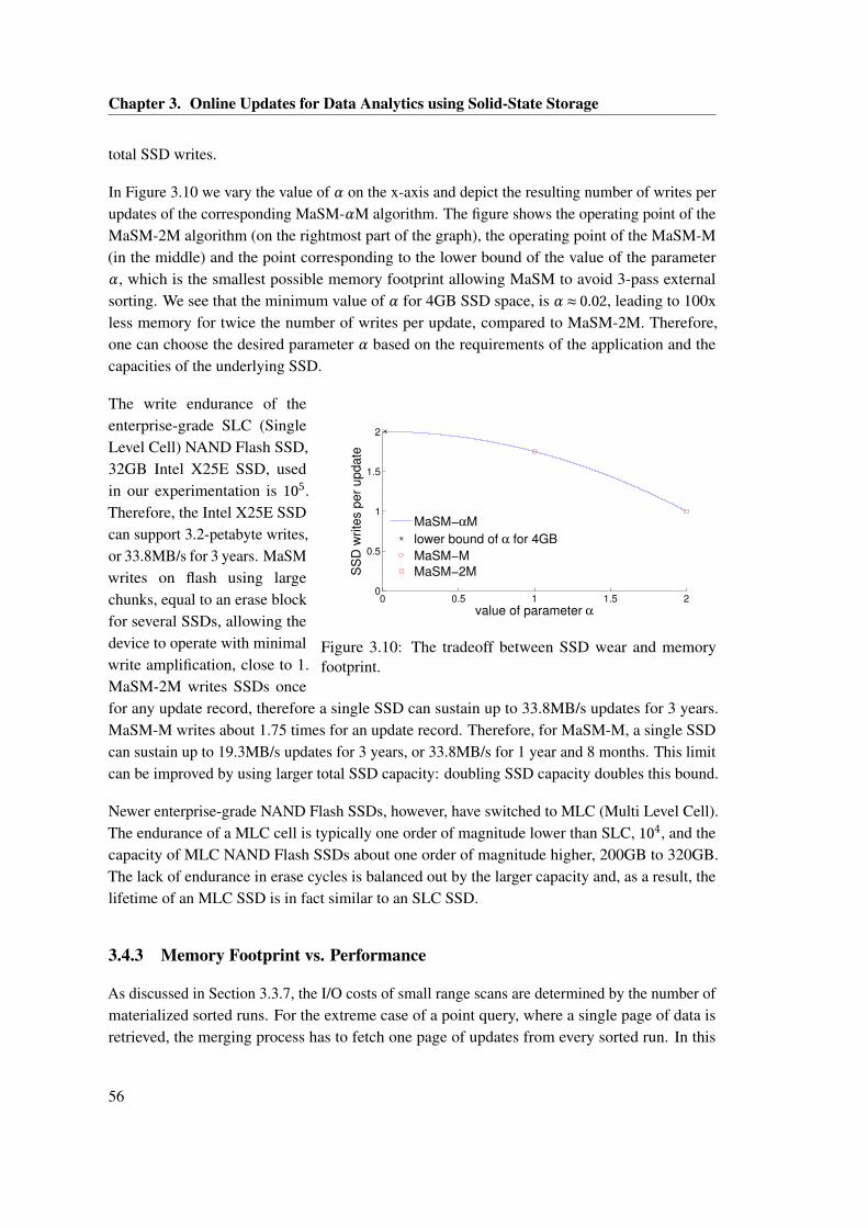
Chapter 3. Online Updates for Data Analytics using Solid-State Storage
total SSD writes.
In Figure 3.10 we vary the value of α on the x-axis and depict the resulting number of writes perupdates of the corresponding MaSM-αM algorithm. The figure shows the operating point of theMaSM-2M algorithm (on the rightmost part of the graph), the operating point of the MaSM-M(in the middle) and the point corresponding to the lower bound of the value of the parameterα, which is the smallest possible memory footprint allowing MaSM to avoid 3-pass externalsorting. We see that the minimum value of α for 4GB SSD space, is α≈ 0.02, leading to 100xless memory for twice the number of writes per update, compared to MaSM-2M. Therefore,one can choose the desired parameter α based on the requirements of the application and thecapacities of the underlying SSD.
0 0.5 1 1.5 20
0.5
1
1.5
2
value of parameter α
SS
D w
rite
s p
er
up
da
te
MaSM−αM
lower bound of α for 4GB
MaSM−M
MaSM−2M
Figure 3.10: The tradeoff between SSD wear and memoryfootprint.
The write endurance of theenterprise-grade SLC (SingleLevel Cell) NAND Flash SSD,32GB Intel X25E SSD, usedin our experimentation is 105.Therefore, the Intel X25E SSDcan support 3.2-petabyte writes,or 33.8MB/s for 3 years. MaSMwrites on flash using largechunks, equal to an erase blockfor several SSDs, allowing thedevice to operate with minimalwrite amplification, close to 1.MaSM-2M writes SSDs oncefor any update record, therefore a single SSD can sustain up to 33.8MB/s updates for 3 years.MaSM-M writes about 1.75 times for an update record. Therefore, for MaSM-M, a single SSDcan sustain up to 19.3MB/s updates for 3 years, or 33.8MB/s for 1 year and 8 months. This limitcan be improved by using larger total SSD capacity: doubling SSD capacity doubles this bound.
Newer enterprise-grade NAND Flash SSDs, however, have switched to MLC (Multi Level Cell).The endurance of a MLC cell is typically one order of magnitude lower than SLC, 104, and thecapacity of MLC NAND Flash SSDs about one order of magnitude higher, 200GB to 320GB.The lack of endurance in erase cycles is balanced out by the larger capacity and, as a result, thelifetime of an MLC SSD is in fact similar to an SLC SSD.
3.4.3 Memory Footprint vs. Performance
As discussed in Section 3.3.7, the I/O costs of small range scans are determined by the number ofmaterialized sorted runs. For the extreme case of a point query, where a single page of data isretrieved, the merging process has to fetch one page of updates from every sorted run. In this
56
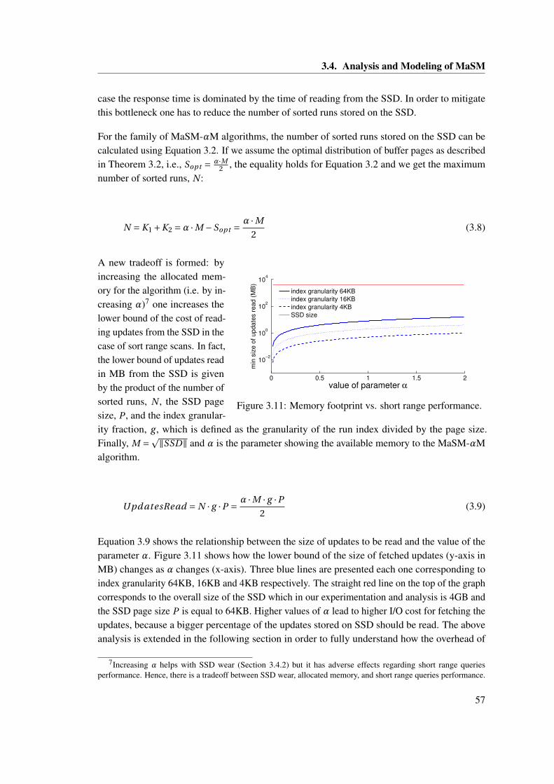
3.4. Analysis and Modeling of MaSM
case the response time is dominated by the time of reading from the SSD. In order to mitigatethis bottleneck one has to reduce the number of sorted runs stored on the SSD.
For the family of MaSM-αM algorithms, the number of sorted runs stored on the SSD can becalculated using Equation 3.2. If we assume the optimal distribution of buffer pages as describedin Theorem 3.2, i.e., Sopt = α·M
2 , the equality holds for Equation 3.2 and we get the maximumnumber of sorted runs, N :
N = K1 +K2 =α ·M −Sopt = α ·M
2(3.8)
0 0.5 1 1.5 2
10−2
100
102
104
min
siz
e o
f update
s r
ead (
MB
)
value of parameter α
index granularity 64KB
index granularity 16KB
index granularity 4KB
SSD size
Figure 3.11: Memory footprint vs. short range performance.
A new tradeoff is formed: byincreasing the allocated mem-ory for the algorithm (i.e. by in-creasing α)7 one increases thelower bound of the cost of read-ing updates from the SSD in thecase of sort range scans. In fact,the lower bound of updates readin MB from the SSD is givenby the product of the number ofsorted runs, N , the SSD pagesize, P , and the index granular-ity fraction, g , which is defined as the granularity of the run index divided by the page size.Finally, M =p‖SSD‖ and α is the parameter showing the available memory to the MaSM-αMalgorithm.
Upd atesRead = N · g ·P = α ·M · g ·P
2(3.9)
Equation 3.9 shows the relationship between the size of updates to be read and the value of theparameter α. Figure 3.11 shows how the lower bound of the size of fetched updates (y-axis inMB) changes as α changes (x-axis). Three blue lines are presented each one corresponding toindex granularity 64KB, 16KB and 4KB respectively. The straight red line on the top of the graphcorresponds to the overall size of the SSD which in our experimentation and analysis is 4GB andthe SSD page size P is equal to 64KB. Higher values of α lead to higher I/O cost for fetching theupdates, because a bigger percentage of the updates stored on SSD should be read. The aboveanalysis is extended in the following section in order to fully understand how the overhead of
7Increasing α helps with SSD wear (Section 3.4.2) but it has adverse effects regarding short range queriesperformance. Hence, there is a tradeoff between SSD wear, allocated memory, and short range queries performance.
57
Chapter 3. Online Updates for Data Analytics using Solid-State Storage
reading the updates affects the performance of the MaSM algorithms.
3.4.4 Modeling the I/O Time of Range Queries
In this section we present an analytical model for range queries, which considers the I/O time ofreading updates from SSDs, and the I/O time of reading the main data. We model various aspectsof the range queries, including relation size, disk capacity, SSD capacity, range size, and disk andSSD performance characteristics. The parameters used in the performance model, including theones detailed in the discussion about the MaSM algorithms in Section 3.3.4 (see Table 3.1), aresummarized in Table 3.2.
In Sections 3.3.7 and 3.4.3 it is argued that the lower bound for the cost of retrieving updatesfrom SSD is given by the number of sorted runs. The cost of retrieving updates for larger ranges,however, is a function of the range of the relation we retrieve. More specifically, if we assume thatthe updates are uniformly distributed over the main data then the number of SSD pages retrievedis proportional to the range size of the query. Hence, the time needed to fetch the updates is givenby Equation 3.10.
FetchUpd ates = max(‖SSD‖ · r, N · g ) · P
F BW(3.10)
The size of the range, r % is expressed as a percentage of the total size of the relation (T ). ‖SSD‖is the number of SSD pages devoted to the MaSM algorithm, g is the granularity of the runindex as a fraction of SSD pages, which in turn have size P . The bandwidth that updates arefetched from the SSD, F BW , defines how fast MaSM can read updates. In Equation 3.10 we firstcalculate the number of pages containing updates to be read, which is equal to max(‖SSD‖r, N g ),and then we take the worst case scenario regarding the I/O time per page.
MaSM overlaps SSD I/Os for retrieving updates with HDD I/Os for retrieving the main data. Inorder to model this behavior, we devise a simple HDD model. For a query that requires a rangescan of r % of the main data (with total size T ) the time needed to retrieve the data is given byEquation 3.11.
Read M ai nDat a = s + r ·T
DBW(3.11)
The seek time, s, plays an important role since it dominates the response time for short ranges.For large ranges, however, the most important factor is the disk bandwidth, DBW .
Achieving perfect I/O overlapping using MaSM. Using Equations 3.10 and 3.11 we compute
58
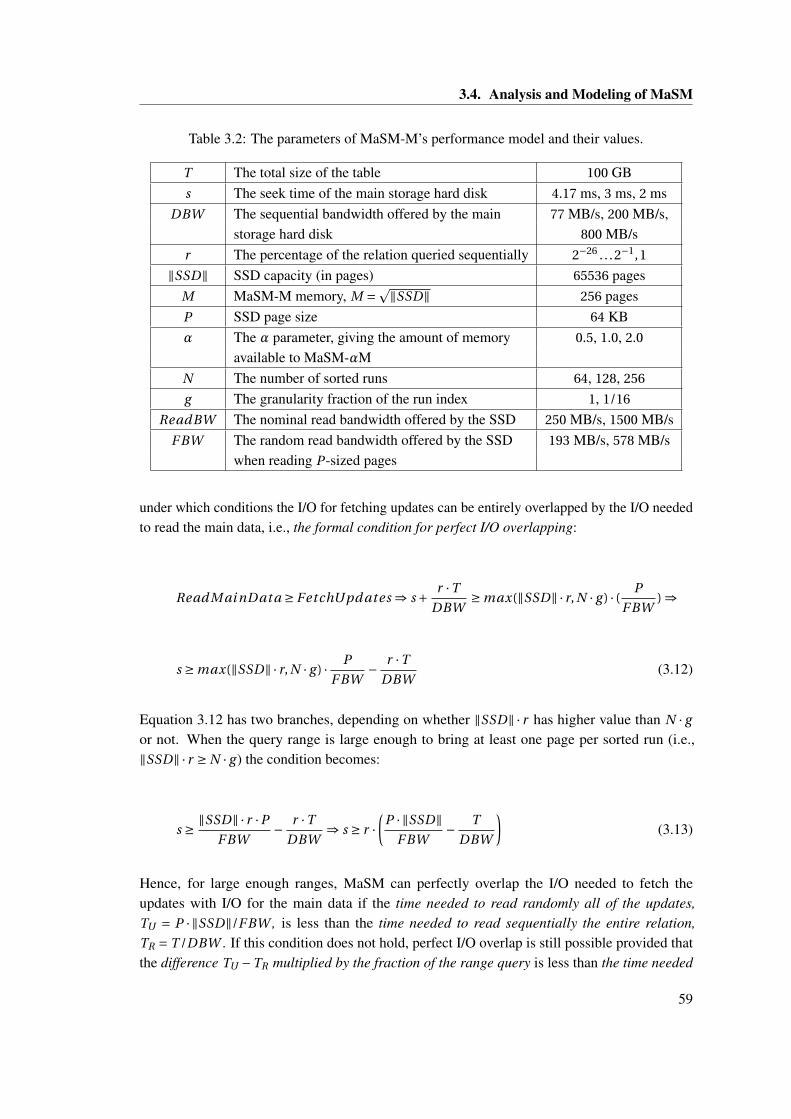
3.4. Analysis and Modeling of MaSM
Table 3.2: The parameters of MaSM-M’s performance model and their values.
T The total size of the table 100 GBs The seek time of the main storage hard disk 4.17 ms, 3 ms, 2 ms
DBW The sequential bandwidth offered by the main 77 MB/s, 200 MB/s,storage hard disk 800 MB/s
r The percentage of the relation queried sequentially 2−26 . . .2−1,1
‖SSD‖ SSD capacity (in pages) 65536 pagesM MaSM-M memory, M =p‖SSD‖ 256 pagesP SSD page size 64 KBα The α parameter, giving the amount of memory 0.5, 1.0, 2.0
available to MaSM-αMN The number of sorted runs 64, 128, 256
g The granularity fraction of the run index 1, 1/16
ReadBW The nominal read bandwidth offered by the SSD 250 MB/s, 1500 MB/sF BW The random read bandwidth offered by the SSD 193 MB/s, 578 MB/s
when reading P-sized pages
under which conditions the I/O for fetching updates can be entirely overlapped by the I/O neededto read the main data, i.e., the formal condition for perfect I/O overlapping:
Read M ai nDat a ≥ FetchUpd ates ⇒ s + r ·T
DBW≥ max(‖SSD‖ · r, N · g ) · (
P
F BW) ⇒
s ≥ max(‖SSD‖ · r, N · g ) · P
F BW− r ·T
DBW(3.12)
Equation 3.12 has two branches, depending on whether ‖SSD‖ · r has higher value than N · g
or not. When the query range is large enough to bring at least one page per sorted run (i.e.,‖SSD‖ · r ≥ N · g ) the condition becomes:
s ≥ ‖SSD‖ · r ·P
F BW− r ·T
DBW⇒ s ≥ r ·
(P · ‖SSD‖
F BW− T
DBW
)(3.13)
Hence, for large enough ranges, MaSM can perfectly overlap the I/O needed to fetch theupdates with I/O for the main data if the time needed to read randomly all of the updates,TU = P · ‖SSD‖/F BW , is less than the time needed to read sequentially the entire relation,TR = T /DBW . If this condition does not hold, perfect I/O overlap is still possible provided thatthe difference TU −TR multiplied by the fraction of the range query is less than the time needed
59
Chapter 3. Online Updates for Data Analytics using Solid-State Storage
to initiate a main data I/O, i.e., the seek time of the HDD storing the main data. Regarding thesecond branch of Equation 3.12, i.e., for short ranges that ‖SSD‖ · r < N · g the condition is:
s ≥ N · g ·P
F BW− r ·T
DBW(3.14)
Equation 3.14 implies that for short ranges, MaSM can perfectly overlap the I/O needed to fetchthe updates with I/O for the main data if the time needed to read randomly the minimal number ofpages per sorted run, TmU = N ·g ·P
F BW , is less than the time needed to read sequentially the queriedrange of the relation, Tr R = r ·T
DBW , or, if this does not hold, the difference TmU −Tr R is less thanthe seek time of the HDD storing the main data.
Analysis of MaSM Behavior. We use the analytical model from the previous section to predictthe anticipated behavior of the MaSM algorithms for our experimental setup in Section 3.5, aswell as, for different setups with varying performance capabilities of the disk subsystem storingthe main data and varying capabilities of the SSD storing the updates.
Table 3.2 shows the parameter values considered in our analysis8. In particular, for the disksubsystem we use seek time s = 4.17ms and disk bandwidth DBW = 77MB/s which are eitherdirectly measured or taken from device manuals for the experimental machine in the next section.The SSD used shows 75µs read latency and offers 250MB/s read bandwidth. Please note thatF BW is not equal to read bandwidth, but it is calculated as the effective bandwidth to read aP-sized page.
In Figure 3.12 we see the I/O time of (i) reading the main data and (ii) reading the updates fromthe SSD as a function of the query range. The x-axis shows the range in MB for a relationwith total size T = 100GB. The vertical dashed lines correspond to the ranges we used for ourexperimentation in Section 3.5.2: 4KB, 1MB, 10MB, 100MB, 1GB, 10GB, 100GB. The blueScan only line shows the I/O time of accessing the main data for the given range, the red linesshow the I/O of fetching the updates for different values of α (0.5, 1, 2) and index granularity64KB. Finally, in the black lines the only change is the granularity which is now 4KB. We observethat for any combination of g and α, MaSM can hide the cost of reading updates if the range ismore than 10MB. For α≤ 1 and index granularity 4KB, the cost of reading the updates can behidden for every possible range, even for the smallest possible range of 4KB which models thepoint query. To detail the comparison between the time to fetch the updates and the time to readthe main data we depict the ratio between these two values in Figure 3.13 for index granularity64KB and in Figure 3.14 for index granularity 4KB.
Figure 3.13 shows that this ratio quickly rises when the range goes below 10MB: fetching theupdates may need 5x to 20x times more time than reading the main data for short ranges. In these
8Some explanations: the total SSD capacity used is 4GB in 64KB pages: 64K B ·65536 = 4GB . M =p‖SSD‖ = 256.N =αM/2. The index granularity fraction g is 1 for granularity 64K B and 1/16 for granularity 4K B .
60
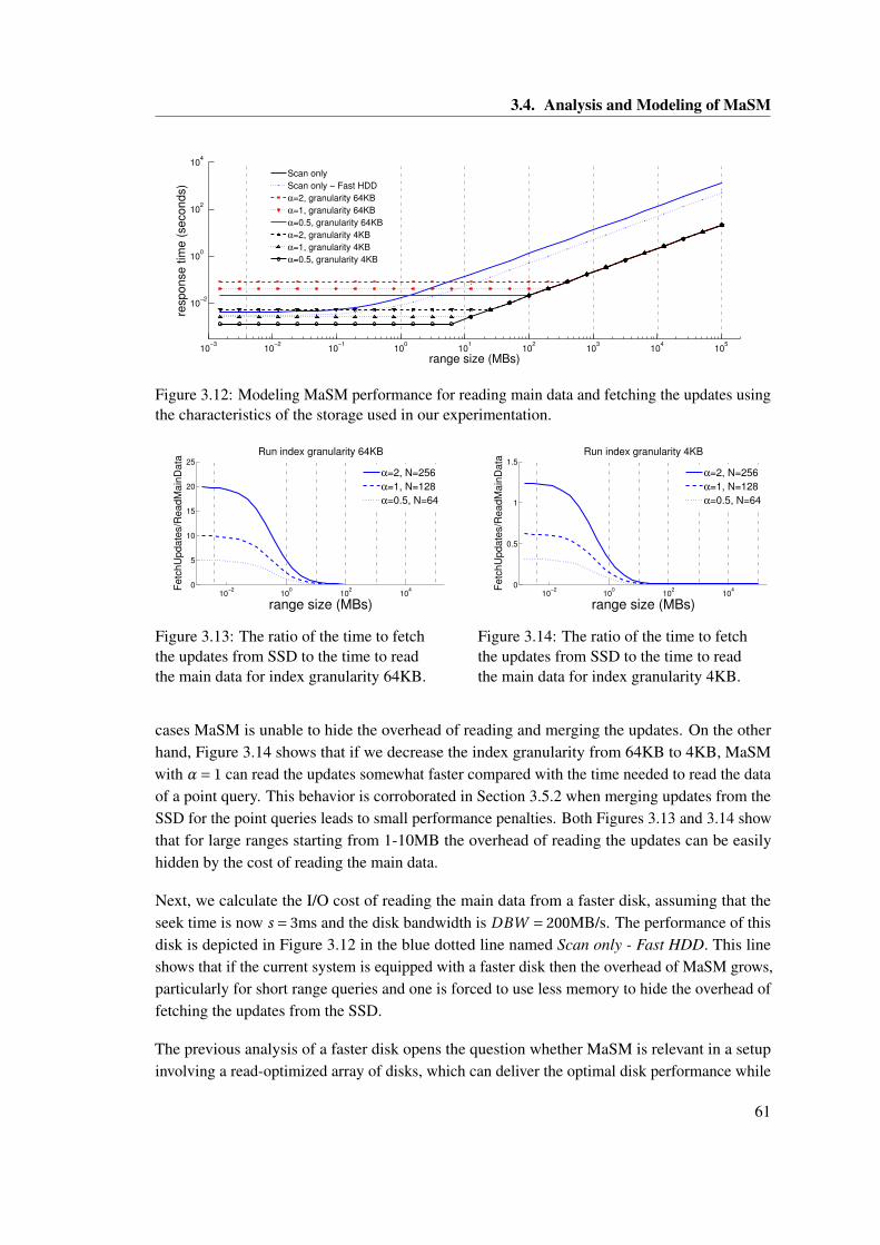
3.4. Analysis and Modeling of MaSM
10−3
10−2
10−1
100
101
102
103
104
105
10−2
100
102
104
resp
on
se
tim
e (
se
co
nd
s)
range size (MBs)
Scan only
Scan only − Fast HDD
α=2, granularity 64KB
α=1, granularity 64KB
α=0.5, granularity 64KB
α=2, granularity 4KB
α=1, granularity 4KB
α=0.5, granularity 4KB
Figure 3.12: Modeling MaSM performance for reading main data and fetching the updates usingthe characteristics of the storage used in our experimentation.
10−2
100
102
104
0
5
10
15
20
25
range size (MBs)
Fe
tch
Up
da
tes/R
ea
dM
ain
Da
ta
Run index granularity 64KB
α=2, N=256
α=1, N=128
α=0.5, N=64
Figure 3.13: The ratio of the time to fetchthe updates from SSD to the time to readthe main data for index granularity 64KB.
10−2
100
102
104
0
0.5
1
1.5
range size (MBs)
Fe
tch
Up
da
tes/R
ea
dM
ain
Da
ta
Run index granularity 4KB
α=2, N=256
α=1, N=128
α=0.5, N=64
Figure 3.14: The ratio of the time to fetchthe updates from SSD to the time to readthe main data for index granularity 4KB.
cases MaSM is unable to hide the overhead of reading and merging the updates. On the otherhand, Figure 3.14 shows that if we decrease the index granularity from 64KB to 4KB, MaSMwith α= 1 can read the updates somewhat faster compared with the time needed to read the dataof a point query. This behavior is corroborated in Section 3.5.2 when merging updates from theSSD for the point queries leads to small performance penalties. Both Figures 3.13 and 3.14 showthat for large ranges starting from 1-10MB the overhead of reading the updates can be easilyhidden by the cost of reading the main data.
Next, we calculate the I/O cost of reading the main data from a faster disk, assuming that theseek time is now s = 3ms and the disk bandwidth is DBW = 200MB/s. The performance of thisdisk is depicted in Figure 3.12 in the blue dotted line named Scan only - Fast HDD. This lineshows that if the current system is equipped with a faster disk then the overhead of MaSM grows,particularly for short range queries and one is forced to use less memory to hide the overhead offetching the updates from the SSD.
The previous analysis of a faster disk opens the question whether MaSM is relevant in a setupinvolving a read-optimized array of disks, which can deliver the optimal disk performance while
61
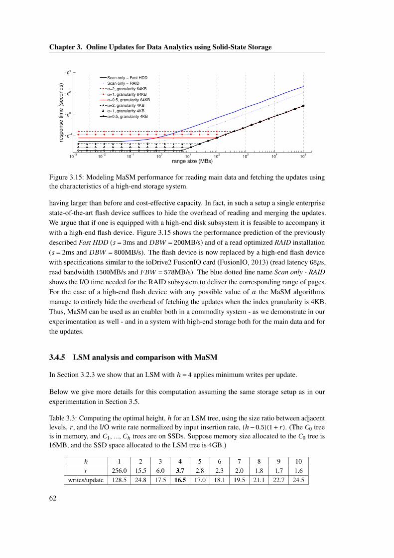
Chapter 3. Online Updates for Data Analytics using Solid-State Storage
10−3
10−2
10−1
100
101
102
103
104
105
10−2
100
102
104
resp
on
se
tim
e (
se
co
nd
s)
range size (MBs)
Scan only − Fast HDD
Scan only − RAID
α=2, granularity 64KB
α=1, granularity 64KB
α=0.5, granularity 64KB
α=2, granularity 4KB
α=1, granularity 4KB
α=0.5, granularity 4KB
Figure 3.15: Modeling MaSM performance for reading main data and fetching the updates usingthe characteristics of a high-end storage system.
having larger than before and cost-effective capacity. In fact, in such a setup a single enterprisestate-of-the-art flash device suffices to hide the overhead of reading and merging the updates.We argue that if one is equipped with a high-end disk subsystem it is feasible to accompany itwith a high-end flash device. Figure 3.15 shows the performance prediction of the previouslydescribed Fast HDD (s = 3ms and DBW = 200MB/s) and of a read optimized RAID installation(s = 2ms and DBW = 800MB/s). The flash device is now replaced by a high-end flash devicewith specifications similar to the ioDrive2 FusionIO card (FusionIO, 2013) (read latency 68µs,read bandwidth 1500MB/s and F BW = 578MB/s). The blue dotted line name Scan only - RAIDshows the I/O time needed for the RAID subsystem to deliver the corresponding range of pages.For the case of a high-end flash device with any possible value of α the MaSM algorithmsmanage to entirely hide the overhead of fetching the updates when the index granularity is 4KB.Thus, MaSM can be used as an enabler both in a commodity system - as we demonstrate in ourexperimentation as well - and in a system with high-end storage both for the main data and forthe updates.
3.4.5 LSM analysis and comparison with MaSM
In Section 3.2.3 we show that an LSM with h = 4 applies minimum writes per update.
Below we give more details for this computation assuming the same storage setup as in ourexperimentation in Section 3.5.
Table 3.3: Computing the optimal height, h for an LSM tree, using the size ratio between adjacentlevels, r , and the I/O write rate normalized by input insertion rate, (h −0.5)(1+ r ). (The C0 treeis in memory, and C1, ..., Ch trees are on SSDs. Suppose memory size allocated to the C0 tree is16MB, and the SSD space allocated to the LSM tree is 4GB.)
h 1 2 3 4 5 6 7 8 9 10r 256.0 15.5 6.0 3.7 2.8 2.3 2.0 1.8 1.7 1.6
writes/update 128.5 24.8 17.5 16.5 17.0 18.1 19.5 21.1 22.7 24.5
62
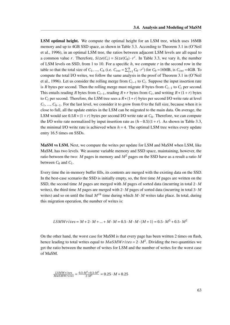
3.4. Analysis and Modeling of MaSM
LSM optimal height. We compute the optimal height for an LSM tree, which uses 16MBmemory and up to 4GB SSD space, as shown in Table 3.3. According to Theorem 3.1 in (O’Neilet al., 1996), in an optimal LSM tree, the ratios between adjacent LSM levels are all equal toa common value r . Therefore, Si ze(Ci ) = Si ze(C0) · r i . In Table 3.3, we vary h, the numberof LSM levels on SSD, from 1 to 10. For a specific h, we compute r in the second row in thetable so that the total size of C1, ..., Ch (i.e. Ctot =∑h
i=1 C0 · r i ) for C0 =16MB, is Ctot =4GB. Tocompute the total I/O writes, we follow the same analysis in the proof of Theorem 3.1 in (O’Neilet al., 1996). Let us consider the rolling merge from Ci−1 to Ci . Suppose the input insertion rateis R bytes per second. Then the rolling merge must migrate R bytes from Ci−1 to Ci per second.This entails reading R bytes from Ci−1, reading R ∗ r bytes from Ci , and writing R ∗ (1+ r ) bytesto Ci per second. Therefore, the LSM tree sees a R∗(1+r ) bytes per second I/O write rate at levelC1, ..., Ch−1. For the last level, we consider it to grow from 0 to the full size, because when it isclose to full, all the update entries in the LSM can be migrated to the main data. On average, theLSM would see 0.5R ∗ (1+ r ) bytes per second I/O write rate at Ch . Therefore, we can computethe I/O write rate normalized by input insertion rate as (h −0.5)(1+ r ). As shown in Table 3.3,the minimal I/O write rate is achieved when h = 4. The optimal LSM tree writes every updateentry 16.5 times on SSDs.
MaSM vs LSM. Next, we compare the writes per update for LSM and MaSM when LSM, likeMaSM, has two levels. We assume variable memory and SSD space, maintaining, however, theratio between the two: M pages in memory and M 2 pages on the SSD have as a result a ratio M
between C0 and C1.
Every time the in-memory buffer fills, its contents are merged with the existing data on the SSD.In the best-case scenario the SSD is initially empty, so, the first time M pages are written on theSSD, the second time M pages are merged with M pages of sorted data (incurring in total 2 ·M
writes), the third time M pages are merged with 2 ·M pages of sorted data (incurring in total 3 ·M
writes) and so on until the final M th time during which M ·M writes take place. In total, duringthis migration operation, the number of writes is:
LSMW r i tes = M +2 ·M + ...+M ·M = 0.5 ·M ·M · (M +1) = 0.5 ·M 3 +0.5 ·M 2
On the other hand, the worst case for MaSM is that every page has been written 2 times on flash,hence leading to total writes equal to M aSMW r i tes = 2 ·M 2. Dividing the two quantities weget the ratio between the number of writes for LSM and the number of writes for the worst caseof MaSM.
LSMW r i tesM aSMW r i tes = 0.5·M 3+0.5·M 2
2·M 2 = 0.25 ·M +0.25
63
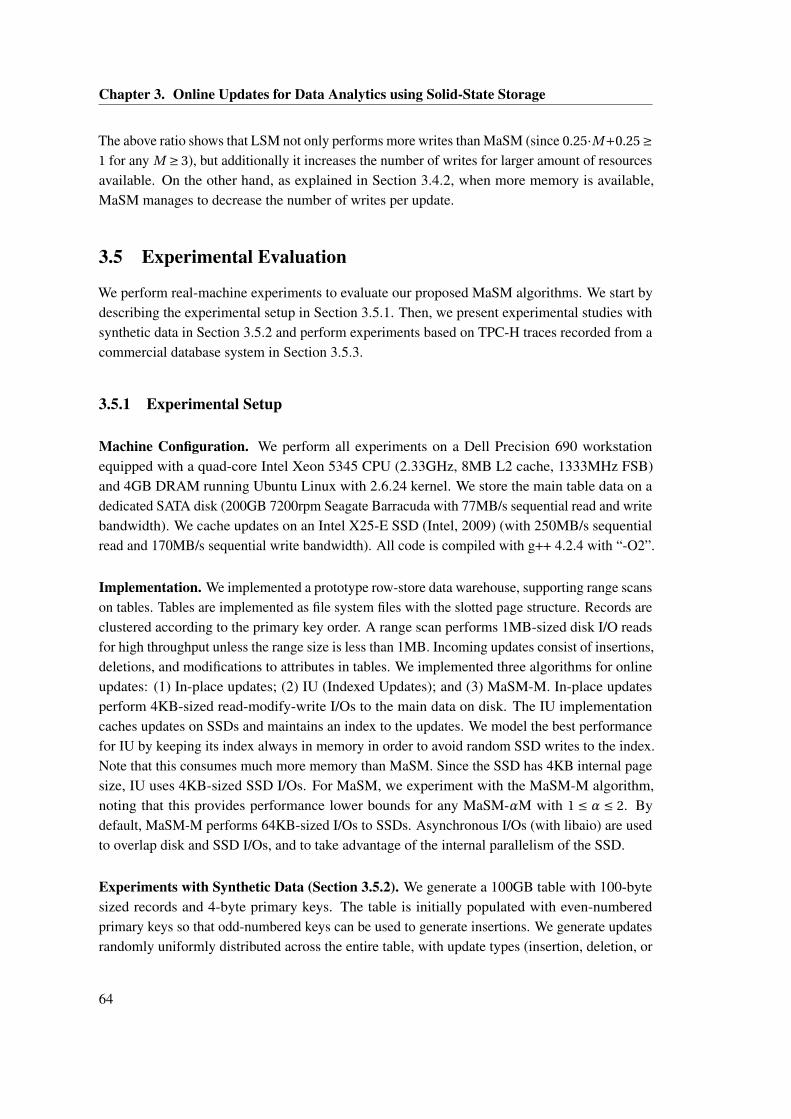
Chapter 3. Online Updates for Data Analytics using Solid-State Storage
The above ratio shows that LSM not only performs more writes than MaSM (since 0.25·M+0.25 ≥1 for any M ≥ 3), but additionally it increases the number of writes for larger amount of resourcesavailable. On the other hand, as explained in Section 3.4.2, when more memory is available,MaSM manages to decrease the number of writes per update.
3.5 Experimental Evaluation
We perform real-machine experiments to evaluate our proposed MaSM algorithms. We start bydescribing the experimental setup in Section 3.5.1. Then, we present experimental studies withsynthetic data in Section 3.5.2 and perform experiments based on TPC-H traces recorded from acommercial database system in Section 3.5.3.
3.5.1 Experimental Setup
Machine Configuration. We perform all experiments on a Dell Precision 690 workstationequipped with a quad-core Intel Xeon 5345 CPU (2.33GHz, 8MB L2 cache, 1333MHz FSB)and 4GB DRAM running Ubuntu Linux with 2.6.24 kernel. We store the main table data on adedicated SATA disk (200GB 7200rpm Seagate Barracuda with 77MB/s sequential read and writebandwidth). We cache updates on an Intel X25-E SSD (Intel, 2009) (with 250MB/s sequentialread and 170MB/s sequential write bandwidth). All code is compiled with g++ 4.2.4 with “-O2”.
Implementation. We implemented a prototype row-store data warehouse, supporting range scanson tables. Tables are implemented as file system files with the slotted page structure. Records areclustered according to the primary key order. A range scan performs 1MB-sized disk I/O readsfor high throughput unless the range size is less than 1MB. Incoming updates consist of insertions,deletions, and modifications to attributes in tables. We implemented three algorithms for onlineupdates: (1) In-place updates; (2) IU (Indexed Updates); and (3) MaSM-M. In-place updatesperform 4KB-sized read-modify-write I/Os to the main data on disk. The IU implementationcaches updates on SSDs and maintains an index to the updates. We model the best performancefor IU by keeping its index always in memory in order to avoid random SSD writes to the index.Note that this consumes much more memory than MaSM. Since the SSD has 4KB internal pagesize, IU uses 4KB-sized SSD I/Os. For MaSM, we experiment with the MaSM-M algorithm,noting that this provides performance lower bounds for any MaSM-αM with 1 ≤ α ≤ 2. Bydefault, MaSM-M performs 64KB-sized I/Os to SSDs. Asynchronous I/Os (with libaio) are usedto overlap disk and SSD I/Os, and to take advantage of the internal parallelism of the SSD.
Experiments with Synthetic Data (Section 3.5.2). We generate a 100GB table with 100-bytesized records and 4-byte primary keys. The table is initially populated with even-numberedprimary keys so that odd-numbered keys can be used to generate insertions. We generate updatesrandomly uniformly distributed across the entire table, with update types (insertion, deletion, or
64
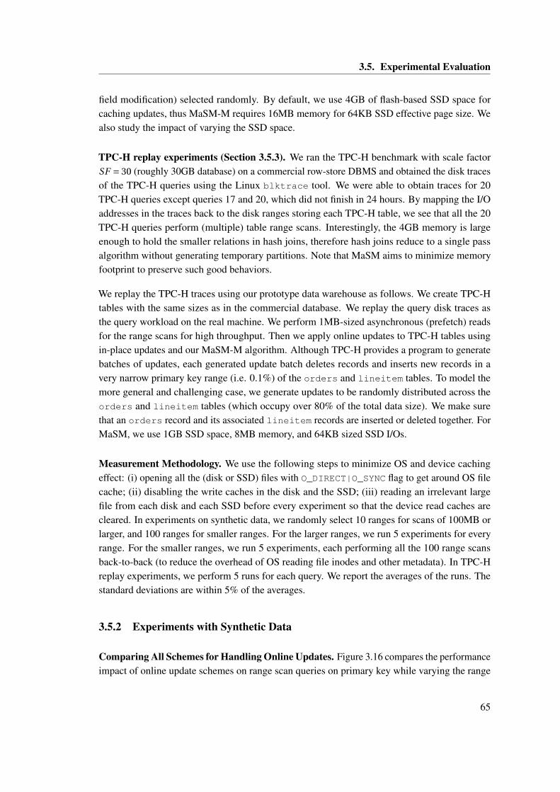
3.5. Experimental Evaluation
field modification) selected randomly. By default, we use 4GB of flash-based SSD space forcaching updates, thus MaSM-M requires 16MB memory for 64KB SSD effective page size. Wealso study the impact of varying the SSD space.
TPC-H replay experiments (Section 3.5.3). We ran the TPC-H benchmark with scale factorSF = 30 (roughly 30GB database) on a commercial row-store DBMS and obtained the disk tracesof the TPC-H queries using the Linux blktrace tool. We were able to obtain traces for 20TPC-H queries except queries 17 and 20, which did not finish in 24 hours. By mapping the I/Oaddresses in the traces back to the disk ranges storing each TPC-H table, we see that all the 20TPC-H queries perform (multiple) table range scans. Interestingly, the 4GB memory is largeenough to hold the smaller relations in hash joins, therefore hash joins reduce to a single passalgorithm without generating temporary partitions. Note that MaSM aims to minimize memoryfootprint to preserve such good behaviors.
We replay the TPC-H traces using our prototype data warehouse as follows. We create TPC-Htables with the same sizes as in the commercial database. We replay the query disk traces asthe query workload on the real machine. We perform 1MB-sized asynchronous (prefetch) readsfor the range scans for high throughput. Then we apply online updates to TPC-H tables usingin-place updates and our MaSM-M algorithm. Although TPC-H provides a program to generatebatches of updates, each generated update batch deletes records and inserts new records in avery narrow primary key range (i.e. 0.1%) of the orders and lineitem tables. To model themore general and challenging case, we generate updates to be randomly distributed across theorders and lineitem tables (which occupy over 80% of the total data size). We make surethat an orders record and its associated lineitem records are inserted or deleted together. ForMaSM, we use 1GB SSD space, 8MB memory, and 64KB sized SSD I/Os.
Measurement Methodology. We use the following steps to minimize OS and device cachingeffect: (i) opening all the (disk or SSD) files with O_DIRECT|O_SYNC flag to get around OS filecache; (ii) disabling the write caches in the disk and the SSD; (iii) reading an irrelevant largefile from each disk and each SSD before every experiment so that the device read caches arecleared. In experiments on synthetic data, we randomly select 10 ranges for scans of 100MB orlarger, and 100 ranges for smaller ranges. For the larger ranges, we run 5 experiments for everyrange. For the smaller ranges, we run 5 experiments, each performing all the 100 range scansback-to-back (to reduce the overhead of OS reading file inodes and other metadata). In TPC-Hreplay experiments, we perform 5 runs for each query. We report the averages of the runs. Thestandard deviations are within 5% of the averages.
3.5.2 Experiments with Synthetic Data
Comparing All Schemes for Handling Online Updates. Figure 3.16 compares the performanceimpact of online update schemes on range scan queries on primary key while varying the range
65
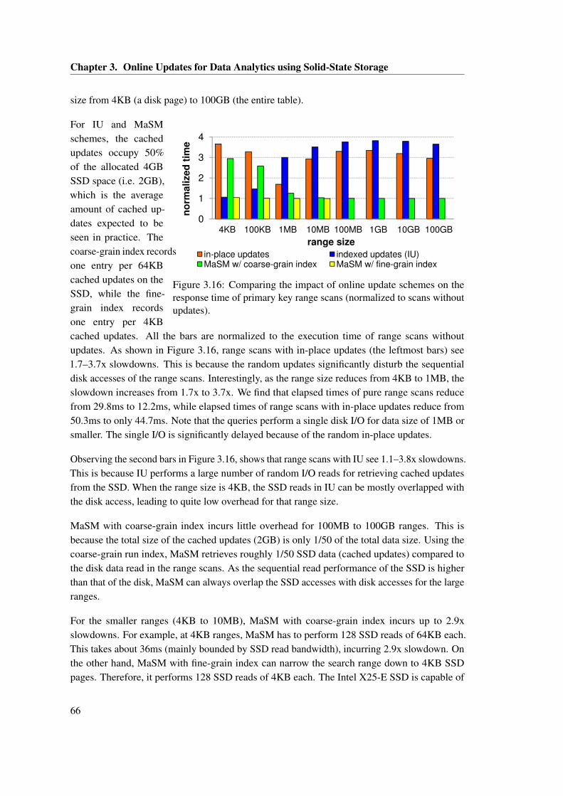
Chapter 3. Online Updates for Data Analytics using Solid-State Storage
size from 4KB (a disk page) to 100GB (the entire table).
2
3
4
zed
tim
e
0
1
2
3
4
4KB 100KB 1MB 10MB 100MB 1GB 10GB 100GB
no
rma
lize
d t
ime
range size
in-place updates indexed updates (IU)M SM / i i d M SM / fi i i d
0
1
2
3
4
4KB 100KB 1MB 10MB 100MB 1GB 10GB 100GB
no
rma
lize
d t
ime
range size
in-place updates indexed updates (IU)MaSM w/ coarse-grain index MaSM w/ fine-grain index
Figure 3.16: Comparing the impact of online update schemes on theresponse time of primary key range scans (normalized to scans withoutupdates).
For IU and MaSMschemes, the cachedupdates occupy 50%of the allocated 4GBSSD space (i.e. 2GB),which is the averageamount of cached up-dates expected to beseen in practice. Thecoarse-grain index recordsone entry per 64KBcached updates on theSSD, while the fine-grain index recordsone entry per 4KBcached updates. All the bars are normalized to the execution time of range scans withoutupdates. As shown in Figure 3.16, range scans with in-place updates (the leftmost bars) see1.7–3.7x slowdowns. This is because the random updates significantly disturb the sequentialdisk accesses of the range scans. Interestingly, as the range size reduces from 4KB to 1MB, theslowdown increases from 1.7x to 3.7x. We find that elapsed times of pure range scans reducefrom 29.8ms to 12.2ms, while elapsed times of range scans with in-place updates reduce from50.3ms to only 44.7ms. Note that the queries perform a single disk I/O for data size of 1MB orsmaller. The single I/O is significantly delayed because of the random in-place updates.
Observing the second bars in Figure 3.16, shows that range scans with IU see 1.1–3.8x slowdowns.This is because IU performs a large number of random I/O reads for retrieving cached updatesfrom the SSD. When the range size is 4KB, the SSD reads in IU can be mostly overlapped withthe disk access, leading to quite low overhead for that range size.
MaSM with coarse-grain index incurs little overhead for 100MB to 100GB ranges. This isbecause the total size of the cached updates (2GB) is only 1/50 of the total data size. Using thecoarse-grain run index, MaSM retrieves roughly 1/50 SSD data (cached updates) compared tothe disk data read in the range scans. As the sequential read performance of the SSD is higherthan that of the disk, MaSM can always overlap the SSD accesses with disk accesses for the largeranges.
For the smaller ranges (4KB to 10MB), MaSM with coarse-grain index incurs up to 2.9xslowdowns. For example, at 4KB ranges, MaSM has to perform 128 SSD reads of 64KB each.This takes about 36ms (mainly bounded by SSD read bandwidth), incurring 2.9x slowdown. Onthe other hand, MaSM with fine-grain index can narrow the search range down to 4KB SSDpages. Therefore, it performs 128 SSD reads of 4KB each. The Intel X25-E SSD is capable of
66
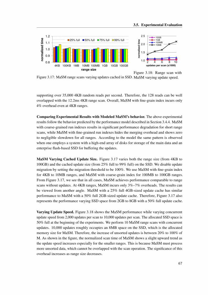
3.5. Experimental Evaluation
1.0
1.1
1.2
ali
ze
d t
ime
25% full 50% full 75% full 99% full
0.8
0.9
1.0
1.1
1.2
4KB 100KB 1MB 10MB 100MB 1GB 10GB 100GB
no
rma
lize
d t
ime
range size
25% full 50% full 75% full 99% full
0.8
0.9
1.0
1.1
1.2
4KB 100KB 1MB 10MB 100MB 1GB 10GB 100GB
no
rma
lize
d t
ime
range size
25% full 50% full 75% full 99% full
Figure 3.17: MaSM range scans varying updates cached in SSD.
1 0
1.5
2.0
2.5
no
rmalized
tim
e
10GB
1GB
100MB
10MB
1.0
1.5
2.0
2.5
no
rmalized
tim
e
updates per scan (x1000)
10GB
1GB
100MB
10MB
2 4 6 8 10
Figure 3.18: Range scan withMaSM varying update speed.
supporting over 35,000 4KB random reads per second. Therefore, the 128 reads can be welloverlapped with the 12.2ms 4KB range scan. Overall, MaSM with fine-grain index incurs only4% overhead even at 4KB ranges.
Comparing Experimental Results with Modeled MaSM’s behavior. The above experimentalresults follow the behavior predicted by the performance model described in Section 3.4.4. MaSMwith coarse-grained run indexes results in significant performance degradation for short rangescans, while MaSM with fine-grained run indexes hides the merging overhead and shows zeroto negligible slowdown for all ranges. According to the model the same pattern is observedwhen one employs a system with a high-end array of disks for storage of the main data and anenterprise flash-based SSD for buffering the updates.
MaSM Varying Cached Update Size. Figure 3.17 varies both the range size (from 4KB to100GB) and the cached update size (from 25% full to 99% full) on the SSD. We disable updatemigration by setting the migration threshold to be 100%. We use MaSM with fine-grain indexfor 4KB to 10MB ranges, and MaSM with coarse-grain index for 100MB to 100GB ranges.From Figure 3.17, we see that in all cases, MaSM achieves performance comparable to rangescans without updates. At 4KB ranges, MaSM incurs only 3%–7% overheads. The results canbe viewed from another angle. MaSM with a 25% full 4GB-sized update cache has similarperformance to MaSM with a 50% full 2GB-sized update cache. Therefore, Figure 3.17 alsorepresents the performance varying SSD space from 2GB to 8GB with a 50% full update cache.
Varying Update Speed. Figure 3.18 shows the MaSM performance while varying concurrentupdate speed from 2,000 updates per scan to 10,000 updates per scan. The allocated SSD space is50% full at the beginning of the experiments. We perform 10 MaSM range scans with concurrentupdates. 10,000 updates roughly occupies an 8MB space on the SSD, which is the allocatedmemory size for MaSM. Therefore, the increase of unsorted updates is between 20% to 100% ofM. As shown in the figure, the normalized scan time of MaSM shows a slight upward trend asthe update speed increases especially for the smaller ranges. This is because MaSM must processmore unsorted data, which cannot be overlapped with the scan operation. The significance of thisoverhead increases as range size decreases.
67
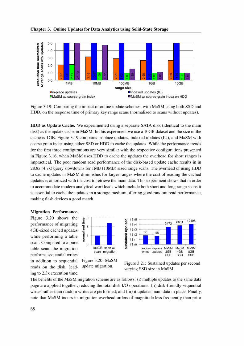
Chapter 3. Online Updates for Data Analytics using Solid-State Storage
2.07
3.19
2.91
2.68
2.69
7.26
10.0
7
9.62
9.25
9.30
2.11
1.09
1.03
1.00
1.00
28.7
9
4.72
1.50
1.05
1.01
0.0
1.0
2.0
3.0
4.0
5.0
1MB 10MB 100MB 1GB 10GB exec
utio
n tim
e no
rmal
ized
to
rang
e sc
ans
w/o
upd
ates
range size in-place updates indexed updates (IU) MaSM w/ coarse-grain index MaSM w/ coarse-grain index on HDD
Figure 3.19: Comparing the impact of online update schemes, with MaSM using both SSD andHDD, on the response time of primary key range scans (normalized to scans without updates).
HDD as Update Cache. We experimented using a separate SATA disk (identical to the maindisk) as the update cache in MaSM. In this experiment we use a 10GB dataset and the size of thecache is 1GB. Figure 3.19 compares in-place updates, indexed updates (IU), and MaSM withcoarse grain index using either SSD or HDD to cache the updates. While the performance trendsfor the first three configurations are very similar with the respective configurations presentedin Figure 3.16, when MaSM uses HDD to cache the updates the overhead for short ranges isimpractical. The poor random read performance of the disk-based update cache results in in28.8x (4.7x) query slowdowns for 1MB (10MB) sized range scans. The overhead of using HDDto cache updates in MaSM diminishes for larger ranges where the cost of reading the cachedupdates is amortized with the cost to retrieve the main data. This experiment shows that in orderto accommodate modern analytical workloads which include both short and long range scans itis essential to cache the updates in a storage medium offering good random read performance,making flash devices a good match.
3
tim
e
0
1
2
3
no
rm
alized
tim
e
100GBscan
scan w/ migration
0
1
2
3
no
rm
alized
tim
e
100GBscan
scan w/ migration
Figure 3.20: MaSMupdate migration.
6631 124981E+5
ec
68 48
3472 6631 12498
1E+0
1E+1
1E+2
1E+3
1E+4
1E+5
randomwrites
in-place updates
MaSM2GB
MaSM4GB
MaSM8GB
su
sta
ine
d u
pd
/se
c
68 48
3472 6631 12498
1E+0
1E+1
1E+2
1E+3
1E+4
1E+5
randomwrites
in-place updates
MaSM2GBSSD
MaSM4GBSSD
MaSM8GBSSD
su
sta
ine
d u
pd
/se
c
Figure 3.21: Sustained updates per secondvarying SSD size in MaSM.
Migration Performance.Figure 3.20 shows theperformance of migrating4GB-sized cached updateswhile performing a tablescan. Compared to a puretable scan, the migrationperforms sequential writesin addition to sequentialreads on the disk, lead-ing to 2.3x execution time.The benefits of the MaSM migration scheme are as follows: (i) multiple updates to the same datapage are applied together, reducing the total disk I/O operations; (ii) disk-friendly sequentialwrites rather than random writes are performed; and (iii) it updates main data in place. Finally,note that MaSM incurs its migration overhead orders of magnitude less frequently than prior
68
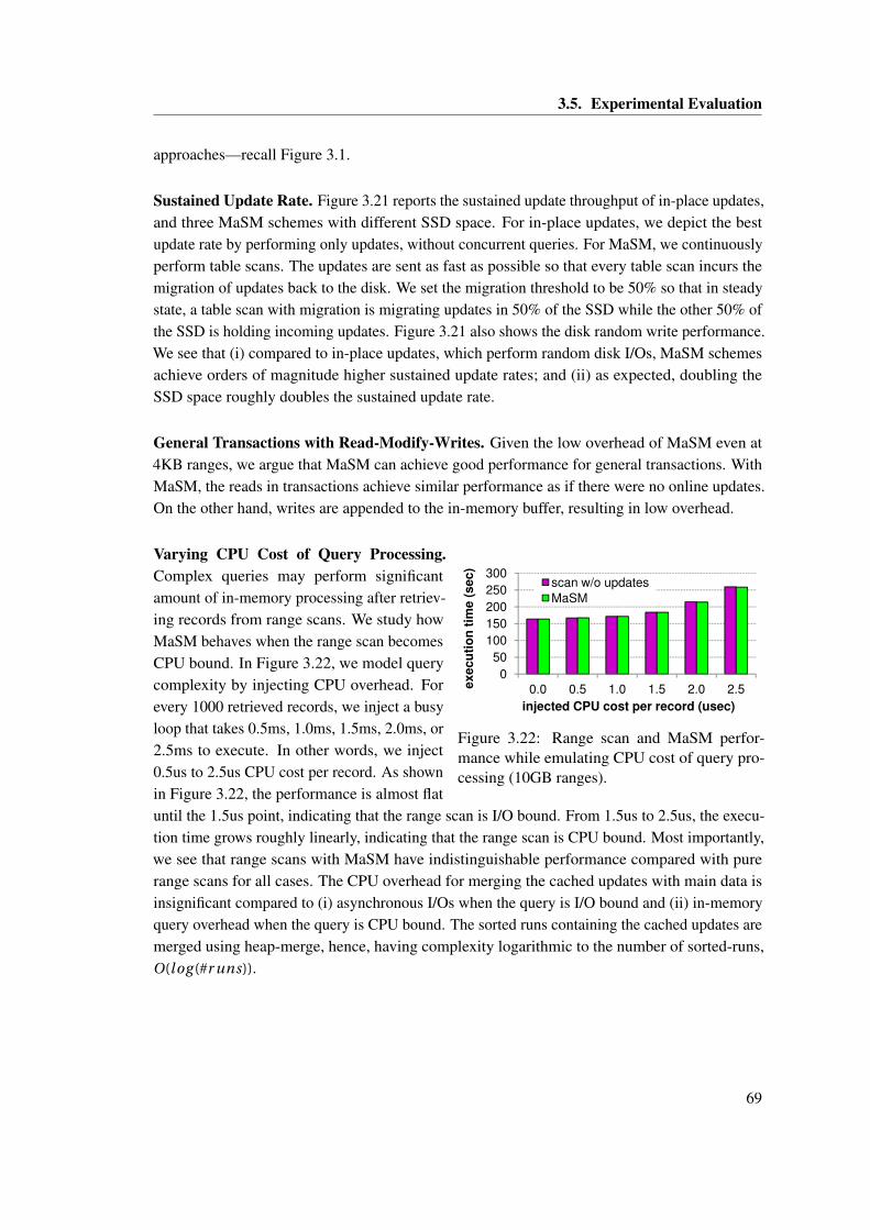
3.5. Experimental Evaluation
approaches—recall Figure 3.1.
Sustained Update Rate. Figure 3.21 reports the sustained update throughput of in-place updates,and three MaSM schemes with different SSD space. For in-place updates, we depict the bestupdate rate by performing only updates, without concurrent queries. For MaSM, we continuouslyperform table scans. The updates are sent as fast as possible so that every table scan incurs themigration of updates back to the disk. We set the migration threshold to be 50% so that in steadystate, a table scan with migration is migrating updates in 50% of the SSD while the other 50% ofthe SSD is holding incoming updates. Figure 3.21 also shows the disk random write performance.We see that (i) compared to in-place updates, which perform random disk I/Os, MaSM schemesachieve orders of magnitude higher sustained update rates; and (ii) as expected, doubling theSSD space roughly doubles the sustained update rate.
General Transactions with Read-Modify-Writes. Given the low overhead of MaSM even at4KB ranges, we argue that MaSM can achieve good performance for general transactions. WithMaSM, the reads in transactions achieve similar performance as if there were no online updates.On the other hand, writes are appended to the in-memory buffer, resulting in low overhead.
250
300
se
c)
scan w/o updates
0
50
100
150
200
250
300
0.0 0.5 1.0 1.5 2.0 2.5ex
ec
uti
on
tim
e (
se
c)
injected CPU cost per record (usec)
scan w/o updates
MaSM
0
50
100
150
200
250
300
0.0 0.5 1.0 1.5 2.0 2.5ex
ec
uti
on
tim
e (
se
c)
injected CPU cost per record (usec)
scan w/o updates
MaSM
Figure 3.22: Range scan and MaSM perfor-mance while emulating CPU cost of query pro-cessing (10GB ranges).
Varying CPU Cost of Query Processing.Complex queries may perform significantamount of in-memory processing after retriev-ing records from range scans. We study howMaSM behaves when the range scan becomesCPU bound. In Figure 3.22, we model querycomplexity by injecting CPU overhead. Forevery 1000 retrieved records, we inject a busyloop that takes 0.5ms, 1.0ms, 1.5ms, 2.0ms, or2.5ms to execute. In other words, we inject0.5us to 2.5us CPU cost per record. As shownin Figure 3.22, the performance is almost flatuntil the 1.5us point, indicating that the range scan is I/O bound. From 1.5us to 2.5us, the execu-tion time grows roughly linearly, indicating that the range scan is CPU bound. Most importantly,we see that range scans with MaSM have indistinguishable performance compared with purerange scans for all cases. The CPU overhead for merging the cached updates with main data isinsignificant compared to (i) asynchronous I/Os when the query is I/O bound and (ii) in-memoryquery overhead when the query is CPU bound. The sorted runs containing the cached updates aremerged using heap-merge, hence, having complexity logarithmic to the number of sorted-runs,O(log (#r uns)).
69
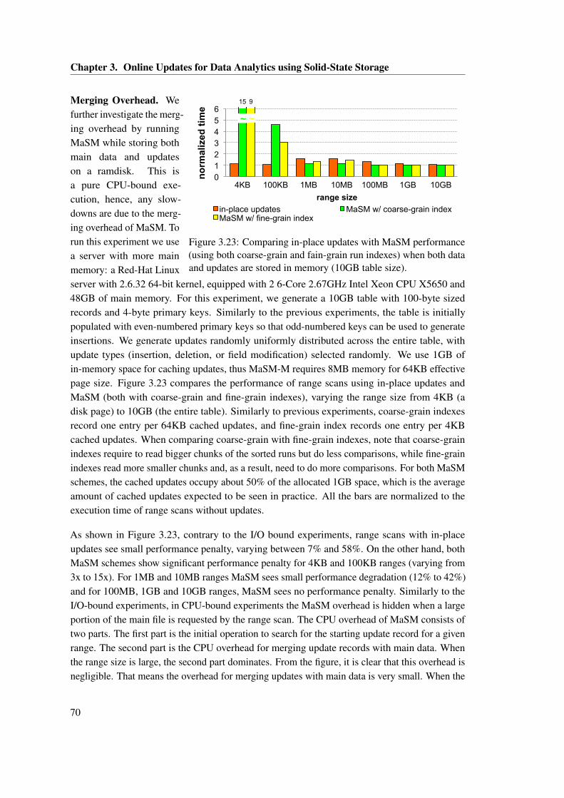
Chapter 3. Online Updates for Data Analytics using Solid-State Storage
0 1 2 3 4 5 6
4KB 100KB 1MB 10MB 100MB 1GB 10GB
norm
aliz
ed ti
me
range size
in-place updates MaSM w/ coarse-grain index MaSM w/ fine-grain index
~ ~
15 9
Figure 3.23: Comparing in-place updates with MaSM performance(using both coarse-grain and fain-grain run indexes) when both dataand updates are stored in memory (10GB table size).
Merging Overhead. Wefurther investigate the merg-ing overhead by runningMaSM while storing bothmain data and updateson a ramdisk. This isa pure CPU-bound exe-cution, hence, any slow-downs are due to the merg-ing overhead of MaSM. Torun this experiment we usea server with more mainmemory: a Red-Hat Linuxserver with 2.6.32 64-bit kernel, equipped with 2 6-Core 2.67GHz Intel Xeon CPU X5650 and48GB of main memory. For this experiment, we generate a 10GB table with 100-byte sizedrecords and 4-byte primary keys. Similarly to the previous experiments, the table is initiallypopulated with even-numbered primary keys so that odd-numbered keys can be used to generateinsertions. We generate updates randomly uniformly distributed across the entire table, withupdate types (insertion, deletion, or field modification) selected randomly. We use 1GB ofin-memory space for caching updates, thus MaSM-M requires 8MB memory for 64KB effectivepage size. Figure 3.23 compares the performance of range scans using in-place updates andMaSM (both with coarse-grain and fine-grain indexes), varying the range size from 4KB (adisk page) to 10GB (the entire table). Similarly to previous experiments, coarse-grain indexesrecord one entry per 64KB cached updates, and fine-grain index records one entry per 4KBcached updates. When comparing coarse-grain with fine-grain indexes, note that coarse-grainindexes require to read bigger chunks of the sorted runs but do less comparisons, while fine-grainindexes read more smaller chunks and, as a result, need to do more comparisons. For both MaSMschemes, the cached updates occupy about 50% of the allocated 1GB space, which is the averageamount of cached updates expected to be seen in practice. All the bars are normalized to theexecution time of range scans without updates.
As shown in Figure 3.23, contrary to the I/O bound experiments, range scans with in-placeupdates see small performance penalty, varying between 7% and 58%. On the other hand, bothMaSM schemes show significant performance penalty for 4KB and 100KB ranges (varying from3x to 15x). For 1MB and 10MB ranges MaSM sees small performance degradation (12% to 42%)and for 100MB, 1GB and 10GB ranges, MaSM sees no performance penalty. Similarly to theI/O-bound experiments, in CPU-bound experiments the MaSM overhead is hidden when a largeportion of the main file is requested by the range scan. The CPU overhead of MaSM consists oftwo parts. The first part is the initial operation to search for the starting update record for a givenrange. The second part is the CPU overhead for merging update records with main data. Whenthe range size is large, the second part dominates. From the figure, it is clear that this overhead isnegligible. That means the overhead for merging updates with main data is very small. When the
70
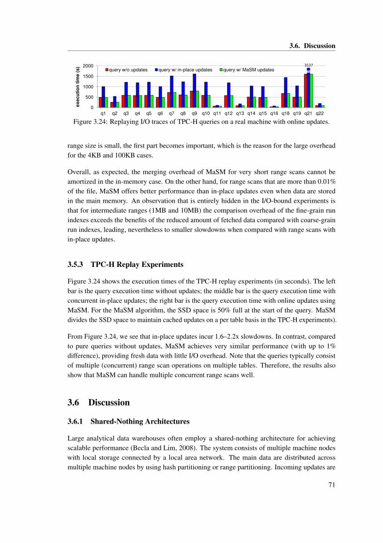
3.6. Discussion
500
1000
1500
2000
cu
tio
n t
ime
(s
)
query w/o updates query w/ in-place updates query w/ MaSM updates3537
~
0
500
1000
1500
2000
q1 q2 q3 q4 q5 q6 q7 q8 q9 q10 q11 q12 q13 q14 q15 q16 q18 q19 q21 q22
execu
tio
n t
ime (
s)
query w/o updates query w/ in-place updates query w/ MaSM updates3537
~
Figure 3.24: Replaying I/O traces of TPC-H queries on a real machine with online updates.
range size is small, the first part becomes important, which is the reason for the large overheadfor the 4KB and 100KB cases.
Overall, as expected, the merging overhead of MaSM for very short range scans cannot beamortized in the in-memory case. On the other hand, for range scans that are more than 0.01%of the file, MaSM offers better performance than in-place updates even when data are storedin the main memory. An observation that is entirely hidden in the I/O-bound experiments isthat for intermediate ranges (1MB and 10MB) the comparison overhead of the fine-grain runindexes exceeds the benefits of the reduced amount of fetched data compared with coarse-grainrun indexes, leading, nevertheless to smaller slowdowns when compared with range scans within-place updates.
3.5.3 TPC-H Replay Experiments
Figure 3.24 shows the execution times of the TPC-H replay experiments (in seconds). The leftbar is the query execution time without updates; the middle bar is the query execution time withconcurrent in-place updates; the right bar is the query execution time with online updates usingMaSM. For the MaSM algorithm, the SSD space is 50% full at the start of the query. MaSMdivides the SSD space to maintain cached updates on a per table basis in the TPC-H experiments).
From Figure 3.24, we see that in-place updates incur 1.6–2.2x slowdowns. In contrast, comparedto pure queries without updates, MaSM achieves very similar performance (with up to 1%difference), providing fresh data with little I/O overhead. Note that the queries typically consistof multiple (concurrent) range scan operations on multiple tables. Therefore, the results alsoshow that MaSM can handle multiple concurrent range scans well.
3.6 Discussion
3.6.1 Shared-Nothing Architectures
Large analytical data warehouses often employ a shared-nothing architecture for achievingscalable performance (Becla and Lim, 2008). The system consists of multiple machine nodeswith local storage connected by a local area network. The main data are distributed acrossmultiple machine nodes by using hash partitioning or range partitioning. Incoming updates are
71
Chapter 3. Online Updates for Data Analytics using Solid-State Storage
mapped and sent to individual machine nodes, and data analysis queries often are executed inparallel on many machine nodes. Because updates and queries are eventually decomposed intooperations on individual machine nodes, MaSM algorithms can be applied on a per-machine-nodebasis. Note that recent data center discussions show that it is reasonable to enhance every machinenode with SSDs (Barroso, 2010).
MaSM addresses the challenge to incorporate the most recent updates in the main data residingin a node with negligible overhead. A similar concept can be implemented for shared-nothingarchitectures where scale-out is the primary goal. In a scale-out setup multiple nodes host thedata, and the updates are stored either in a single or in multiple nodes. There are three possibleapproaches to exploit MaSM in scale-out setup. First, MaSM can enhance the scan operator ofeach node transparently to the rest of the system both in the single node, and in the API betweendifferent nodes. Second, MaSM can be designed in a hierarchical fashion enhancing each nodewith SSDs to cache updates. In order to answer a query a MaSM operator in the inter-nodelevel will be instantiated which will merge updates and data from every node involved. In thiscase, each node holds the updates corresponding to the data residing in the node which couldpotentially lead to unbalanced load. In order to amend this drawback, the third proposal, cachesall updates in all nodes and feeds to the inter-node level MaSM operator only tuples after theyhave been merged with the most recent updates.
3.6.2 MaSM for deeper memory hierarchies and new storage technologies
MaSM is designed to exploit the increased depth of memory hierarchies offered by flash devices.Typically, flash-based SSDs and high-end flash devices are perceived today either as secondarystorage, or as a level of the memory hierarchy residing between main memory and secondarystorage. Flash devices, however, are fundamentally different than the other levels since theyhave a read/write performance asymmetry and endurance limitations (discussed in Section 2.1).Hence, in several approaches that flash is used as a caching layer, including MaSM, flash has aspecialized role tailored for its characteristics and respecting its limitations.
The memory hierarchy is constantly evolving and more technologies are expected to augmentit, potentially by adding more levels. Technologies like PCM, ferroelectric RAM, magneticRAM, and Memristor may achieve a viable memory product which can reside performance-wiseand price-wise between main memory and flash devices, reducing, as well, the effect of limitedendurance that flash devices started hurting from. MaSM can naturally exploit new technologiesby either replacing flash with its successor, or by exploiting a deeper hierarchy. Assuming, forexample, that a new level of PCM non-volatile main memory will be added in the system, MaSMcan be altered as follows. All incoming updates can be safely kept "in-memory" without theneed of an external logging mechanism, while the sorted runs will be written out on the flashdevice (which has limited endurance). Taking this idea a step further, in the generic MaSM-αMalgorithm, incoming updates and first-pass sorted runs will be written on non-volatile mainmemory and second-pass sorted runs on flash. Additionally, some second-pass sorted runs can be
72
3.6. Discussion
kept in the newly introduced level to keep updates that are often used when answering queries ina faster level.
3.6.3 Can SSDs Enhance Performance and Be Cost Efficient?
SSDs have been studied as potential alternatives or enhancements to HDDs in many recentdatabase studies (Bouganim et al., 2009; Canim et al., 2009, 2010b; Chen, 2009; Chen et al.,2010; Koltsidas and Viglas, 2008; Lee et al., 2008; Ozmen et al., 2010; Stoica et al., 2009;Tsirogiannis et al., 2009). In this chapter, we exploit SSDs to cache differential updates. Here,we perform a back-of-the-envelope computation to quantify the cost benefits of using SSDs.
Assuming we have a budget B for storage, we can either spend it on N disks or spend X % fordisks and the rest for SSD. If N ·X % disks can provide the desired capacity then the performancegain of running a table scan when using SSD can be computed as follows. A table scan is linearlyfaster with the number of disks, while random updates slows performance down by a constantfactor FHDD which ranges between 1.5 and 4, as shown in Figure 3.3. When executing a tablescan with concurrent random updates the performance gain is N /FHDD . If we buy SSD with100%− X % of our budget, on the one hand we decrease the performance gain due to disks toN ·X %; on the other hand, the update cost is slowed down with a different constant factor FSSD ,which is close to 1 in our experiments. The performance gain now is (N ·X %)/FSSD . Therefore,the relative performance gain of using SSD is computed as follows:
Rel ati veGai n = N ·X %
FSSD· FHDD
N= FHDD ·X %
FSSD
We can select the budget used for SSD to be low enough to ensure the desired overall capacityand high enough to lead to important performance gain. For example, if X % = 90% of the budgetis used for the disk storage, Rel ati veGai n of using SSD as in our proposal is between 1.35 and3.6.
3.6.4 General support of MaSM
Secondary Index. We discuss how to support index scans in MaSM. Given a secondary indexon Y and a range [Ybeg i n ,Yend ], an index scan is often served in two steps in a database. Similarto index-to-index navigation (Graefe, 2010), in the first step, the secondary index is searched toretrieve all the record pointers within the range. In the second step, the record pointers are usedto retrieve the records. Thus, any query retrieving a range of k records using a secondary indexcan be transformed to k point queries on the primary index. We show that point queries on theprimary index can be handled efficiently, so, a query using a secondary index will be handledcorrectly and efficiently. An optimization for disk performance is to sort the record pointersaccording to the physical storage order of the records between the two steps. In this case, instead
73
Chapter 3. Online Updates for Data Analytics using Solid-State Storage
of k point queries, a query on a secondary index will be transformed to a number of range queries(less than or equal to k), having, as a result, better I/O performance.
For every retrieved record, MaSM can use the key (primary key or RID) of the record to look upcorresponding cached updates and then merge them. However, we must deal with the special casewhere Y is modified in an incoming update: We build a secondary update index for all the updaterecords that contain any Y value, comprised of a read-only index on every materialized sortedrun and an in-memory index on the unsorted updates. The index scan searches this secondaryupdate index to find any update records that fall into the desired range [Ybeg i n ,Yend ]. In this way,MaSM can provide functionally correct support for secondary indexes.
Multiple Sort Orders. Heavily optimized for read accesses, column-store data warehouses canmaintain multiple copies of the data in different sort orders (a.k.a. projections) (Stonebraker et al.,2005; Lamb et al., 2012). For example, in addition to a prevailing sort order of a table, one canoptimize a specific query by storing the columns in an order that is most performance friendly forthe query. However, multiple sort orders present a challenge for differential updates; prior workdoes not handle this case (Héman et al., 2010).
One way to support multiple sort orders would be to treat columns with different sort orders asdifferent tables, and to build different update caches for them. This approach would require thatevery update must contain the sort keys for all the sort orders so that the RIDs for individual sortorders could be obtained.
Alternatively, we could treat sort orders as secondary indexes. Suppose a copy of column X isstored in an order OX different from the prevailing RID order. In this copy, we store the RIDalong with every X value so that when a query performs a range scan on this copy of X , we canuse the RIDs to look up the cached updates. Note that adding RIDs to the copy of X reducescompression effectiveness, because the RIDs may be quite randomly ordered. Essentially, X withRID column looks like a secondary index, and can be supported similarly.
Materialized Views. Materialized views can speed up the processing of well-known querytypes. A recent study proposed lazy maintenance of materialized views in order to remove viewmaintenance from the critical path of incoming update handling (Zhou et al., 2007). Unlike eagerview maintenance where the update statement or the update transaction eagerly maintains anyaffected views, lazy maintenance postpones the view maintenance until the data warehouse hasfree cycles or a query references the view. It is straightforward to extend differential updateschemes to support lazy view maintenance, by treating the view maintenance operations asnormal queries.
74
3.7. Conclusion
3.6.5 Applying MaSM to Cloud Data Management
Key-Value stores are becoming a popular cloud data storage platform because of its scalability,availability and simplicity. Many Key-Value store implementations (e.g., Bigtable, HBase, andCassandra) follow the LSM principle to handle updates. In Section 3.1.2, we have discussedthe difference between these schemes and MaSM. In the past several years, SSD capacity hasbeen increasing dramatically, and its price per capacity ratio is reducing steadily. This makesSSDs increasingly affordable; SSDs have already been considered as standard equipment forcloud machines (Barroso, 2010). When a Key-Value store node is equipped with an SSD, thepresented MaSM algorithm can be applied to improve the performance, reduce memory footprint,and reduce SSD wear in Key-Value stores.
3.7 Conclusion
Efficient analytical processing in applications that require data freshness is challenging. Theconventional approach of performing random updates in place degrades query performancesignificantly, because random accesses disturb the sequential disk access patterns of the typicalanalysis query. Recent studies follow the differential update approach, by caching updatesseparate from the main data and combining cached updates on-the-fly in query processing.However, these proposals all require large in-memory buffers or suffer from high update migrationoverheads.
In this chapter, we proposed to judiciously use solid-state storage to cache differential updates.Our work is based on the principle of using SSD as a performance booster for databases storedprimarily on magnetic disks, since for the foreseeable future, magnetic disks offer cheapercapacity (higher GB/$), while SSDs offer better but more expensive read performance (higherIOPS/$). We presented a high-level framework for SSD-based differential update approaches, andidentified five design goals. We presented an efficient algorithm, MaSM, that achieves low queryoverhead, small memory footprint, no random SSD writes, few SSD writes, efficient in-placemigration, and correct ACID support. Experimental results using a prototype implementationshowed that, using MaSM, query response times remain nearly unaffected even if updates arerunning at the same time. Moreover, update throughput using the MaSM algorithms is severalorders of magnitude higher than in-place updates and, in fact, tunable by selecting different SSDbuffer capacity.
75

4 Enhancing Data Analytics with WorkSharing1
4.1 Introduction
Data warehouses (DW) are database systems specialized for servicing on-line analytical process-ing (OLAP) workloads. OLAP workloads consist mostly of ad-hoc, long running, scan-heavyqueries over relatively static data (new data are periodically loaded). Today, in the era of datadeluge (Kersten et al., 2011), organizations collect massive data for analysis. The increase ofprocessing power and the growing applications’ needs have led to increased requirements forboth throughput and latency of analytical queries over ever-growing datasets.
General-purpose DW, however, cannot easily handle analytical workloads over big data with highconcurrency (Becla and Lim, 2008; Candea et al., 2009). A limiting factor is their typical query-centric model: DW optimize and execute each query independently. Concurrent queries, however,often exhibit overlapping data accesses or computations. The query-centric model misses theopportunities of sharing work and data among them and results in performance degradation dueto the contention of concurrent queries for I/O, CPU and RAM resources.
4.1.1 Methodologies for sharing data and work
A variety of ideas have been proposed to exploit sharing, including diverse buffer pool manage-ment techniques, materialized views, caching and multi-query optimization (see Section 2.3).More recently, query engines started sharing data at the I/O layer using shared scans (a techniquewith variants also known as circular scans, cooperative scans or clock scan) (Colby et al., 1998;Cook, 2001; Morri, 2002; Qiao et al., 2008; Unterbrunner et al., 2009; Zukowski et al., 2007).
In this chapter, we evaluate work sharing techniques at the level of the execution engine, wherewe distinguish two predominant methodologies: (a) Simultaneous pipelining (SP) (Harizopouloset al., 2005), and (b) Global query plans (GQP) (Arumugam et al., 2010; Candea et al., 2009,
1The material of this chapter has been the basis for the VLDB 2013 paper "Sharing Data and Work AcrossConcurrent Analytical Queries" (Psaroudakis et al., 2013).
77
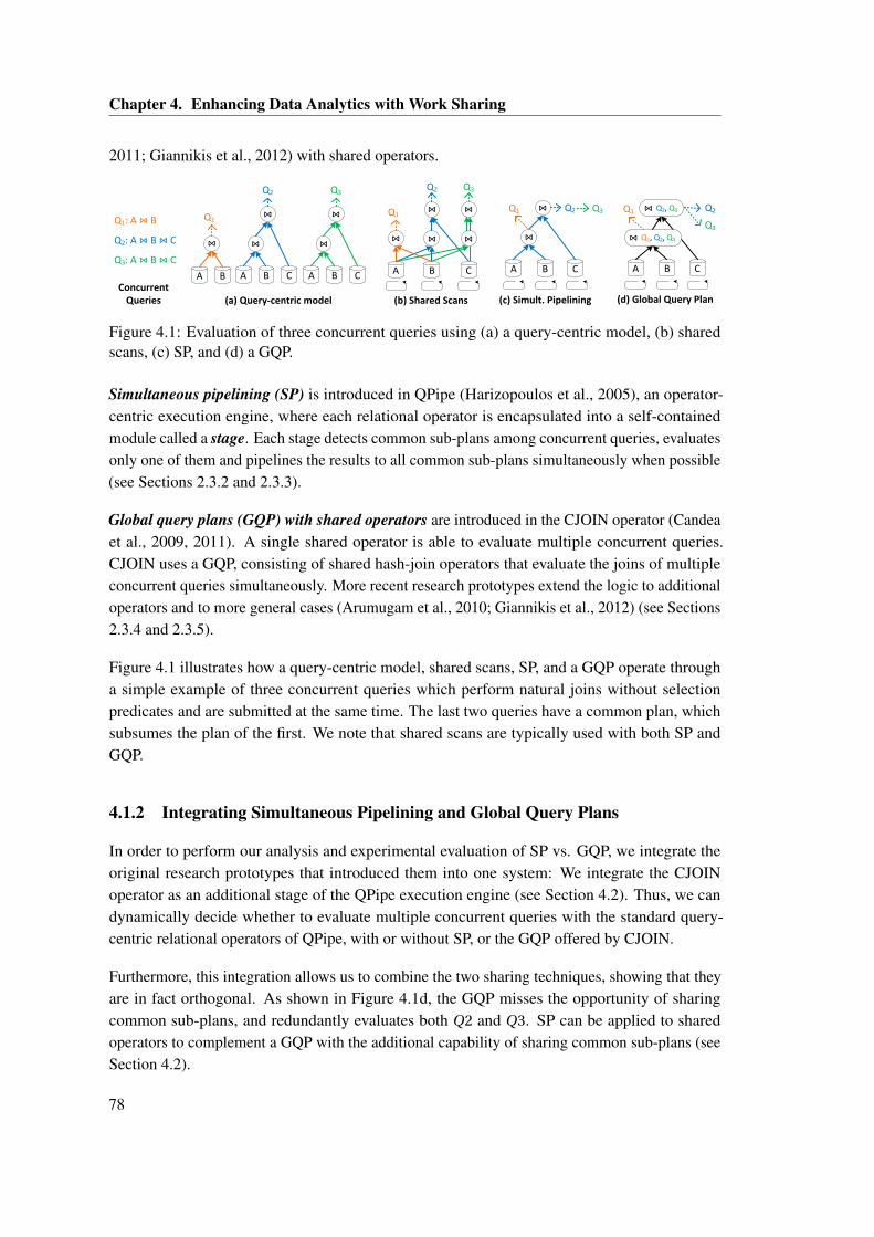
Chapter 4. Enhancing Data Analytics with Work Sharing
2011; Giannikis et al., 2012) with shared operators.
(a) Query-centric model (c) Simult. Pipelining
A B C
Q1 Q2 Q3
(d) Global Query Plan
A B C
⋈
Q3
⋈
A B C
⋈
Q2
⋈
A B
Q1
⋈
Q1: A ⋈ B
Q2: A ⋈ B ⋈ C
Q3: A ⋈ B ⋈ C
Concurrent Queries (b) Shared Scans
⋈
Q2
⋈
A B C
Q3
Q1
⋈ ⋈ ⋈
⋈
A B C
Q2
Q3
Q1, Q2, Q3⋈
Q2, Q3⋈⋈ Q1
Figure 4.1: Evaluation of three concurrent queries using (a) a query-centric model, (b) sharedscans, (c) SP, and (d) a GQP.
Simultaneous pipelining (SP) is introduced in QPipe (Harizopoulos et al., 2005), an operator-centric execution engine, where each relational operator is encapsulated into a self-containedmodule called a stage. Each stage detects common sub-plans among concurrent queries, evaluatesonly one of them and pipelines the results to all common sub-plans simultaneously when possible(see Sections 2.3.2 and 2.3.3).
Global query plans (GQP) with shared operators are introduced in the CJOIN operator (Candeaet al., 2009, 2011). A single shared operator is able to evaluate multiple concurrent queries.CJOIN uses a GQP, consisting of shared hash-join operators that evaluate the joins of multipleconcurrent queries simultaneously. More recent research prototypes extend the logic to additionaloperators and to more general cases (Arumugam et al., 2010; Giannikis et al., 2012) (see Sections2.3.4 and 2.3.5).
Figure 4.1 illustrates how a query-centric model, shared scans, SP, and a GQP operate througha simple example of three concurrent queries which perform natural joins without selectionpredicates and are submitted at the same time. The last two queries have a common plan, whichsubsumes the plan of the first. We note that shared scans are typically used with both SP andGQP.
4.1.2 Integrating Simultaneous Pipelining and Global Query Plans
In order to perform our analysis and experimental evaluation of SP vs. GQP, we integrate theoriginal research prototypes that introduced them into one system: We integrate the CJOINoperator as an additional stage of the QPipe execution engine (see Section 4.2). Thus, we candynamically decide whether to evaluate multiple concurrent queries with the standard query-centric relational operators of QPipe, with or without SP, or the GQP offered by CJOIN.
Furthermore, this integration allows us to combine the two sharing techniques, showing that theyare in fact orthogonal. As shown in Figure 4.1d, the GQP misses the opportunity of sharingcommon sub-plans, and redundantly evaluates both Q2 and Q3. SP can be applied to sharedoperators to complement a GQP with the additional capability of sharing common sub-plans (seeSection 4.2).
78
4.1. Introduction
4.1.3 Optimizing Simultaneous Pipelining
For the specific case of SP, it is shown in the literature (Johnson et al., 2007; Qiao et al., 2008)that if it entails a serialization point, then enforcing aggressive sharing does not always improveperformance. In cases of low concurrency and enough available resources, it is shown that thesystem should first parallelize with a query-centric model before sharing.
To calculate the turning point where sharing becomes beneficial, a prediction model is proposed(Johnson et al., 2007) for determining at run-time whether SP is beneficial. In this chapter,however, we show that the serialization point is due to the push-based communication employedby SP (Harizopoulos et al., 2005; Johnson et al., 2007). We show that pull-based communicationcan drastically minimize the impact of the serialization point, and is better suited for sharingcommon results on multi-core machines.
We introduce Shared Pages Lists (SPL), a pull-based sharing approach that eliminates theserialization point caused by push-based sharing during SP. SPL are data structures that storeintermediate results - of relational operators - and allow for a single producer and multipleconsumers. SPL make sharing with SP always beneficial and reduce response times by 82%-86%in cases of high concurrency, compared to the original push-based SP design and implementation(Harizopoulos et al., 2005; Johnson et al., 2007) (see Section 4.3).
4.1.4 Simultaneous Pipelining vs. Global Query Plans
Having optimized SP, and having integrated the CJOIN operator in the QPipe execution engine,we proceed to perform an extensive analysis and experimental evaluation of SP vs. GQP (seeSection 4.5). Our work answers two fundamental questions: when and how an execution engineshould share in order to improve performance of typical analytical workloads.
Sharing in the execution engine. We identify a performance trade-off between using a query-centric model and sharing. For a high number of concurrent queries, the execution engine shouldshare, as it reduces contention for resources and improves performance in comparison to aquery-centric model. For low concurrency, however, sharing is not always beneficial.
With respect to SP, we corroborate previous related work (Johnson et al., 2007; Qiao et al., 2008),that if SP entails a serialization point, then enforcing aggressive sharing does not always improveperformance in cases of low concurrency. Our newly optimized SP with SPL, however, eliminatesthe serialization point, making SP beneficial in cases of both low and high concurrency.
With respect to GQP, we corroborate previous work (Arumugam et al., 2010; Candea et al.,2009, 2011; Giannikis et al., 2012) that shared operators are efficient in reducing contention forresources and in improving performance for high concurrency (see Section 4.5.1). The designof a shared operator, however, inherently increases book-keeping in comparison to the typicaloperators of a query-centric model. Thus, for low concurrency, we show that shared operators
79
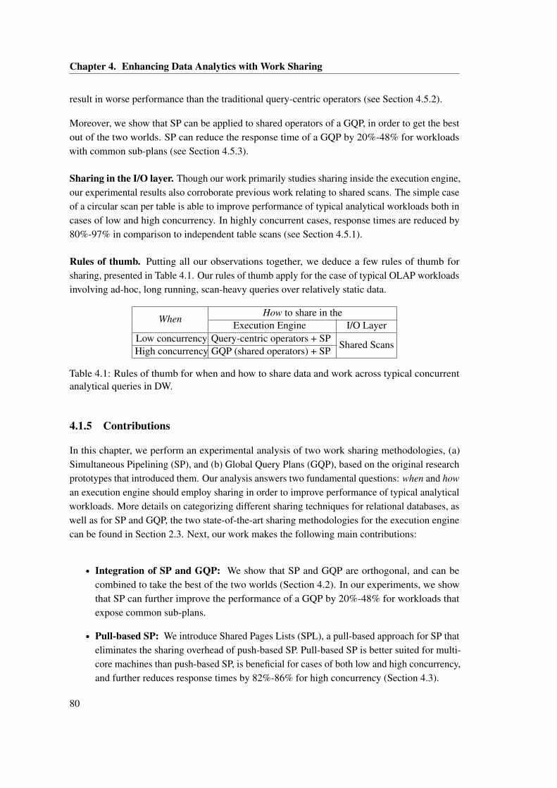
Chapter 4. Enhancing Data Analytics with Work Sharing
result in worse performance than the traditional query-centric operators (see Section 4.5.2).
Moreover, we show that SP can be applied to shared operators of a GQP, in order to get the bestout of the two worlds. SP can reduce the response time of a GQP by 20%-48% for workloadswith common sub-plans (see Section 4.5.3).
Sharing in the I/O layer. Though our work primarily studies sharing inside the execution engine,our experimental results also corroborate previous work relating to shared scans. The simple caseof a circular scan per table is able to improve performance of typical analytical workloads both incases of low and high concurrency. In highly concurrent cases, response times are reduced by80%-97% in comparison to independent table scans (see Section 4.5.1).
Rules of thumb. Putting all our observations together, we deduce a few rules of thumb forsharing, presented in Table 4.1. Our rules of thumb apply for the case of typical OLAP workloadsinvolving ad-hoc, long running, scan-heavy queries over relatively static data.
WhenHow to share in the
Execution Engine I/O LayerLow concurrency Query-centric operators + SP
Shared ScansHigh concurrency GQP (shared operators) + SP
Table 4.1: Rules of thumb for when and how to share data and work across typical concurrentanalytical queries in DW.
4.1.5 Contributions
In this chapter, we perform an experimental analysis of two work sharing methodologies, (a)Simultaneous Pipelining (SP), and (b) Global Query Plans (GQP), based on the original researchprototypes that introduced them. Our analysis answers two fundamental questions: when and howan execution engine should employ sharing in order to improve performance of typical analyticalworkloads. More details on categorizing different sharing techniques for relational databases, aswell as for SP and GQP, the two state-of-the-art sharing methodologies for the execution enginecan be found in Section 2.3. Next, our work makes the following main contributions:
• Integration of SP and GQP: We show that SP and GQP are orthogonal, and can becombined to take the best of the two worlds (Section 4.2). In our experiments, we showthat SP can further improve the performance of a GQP by 20%-48% for workloads thatexpose common sub-plans.
• Pull-based SP: We introduce Shared Pages Lists (SPL), a pull-based approach for SP thateliminates the sharing overhead of push-based SP. Pull-based SP is better suited for multi-core machines than push-based SP, is beneficial for cases of both low and high concurrency,and further reduces response times by 82%-86% for high concurrency (Section 4.3).
80
4.2. Integrating SP and GQP
• Evaluation of SP vs. GQP: We analyze the trade-offs of SP, GQP and their combina-tion, and we detail through an extensive sensitivity analysis when each one is beneficial(Section 4.5). We show that query-centric operators combined with SP result in betterperformance for cases of low concurrency, while GQP with shared operators enhanced bySP are better suited for cases of high concurrency.
4.1.6 Outline
This chapter is organized as follows. Section 4.2 describes our implementation for integrating SPand GQP. Section 4.3 presents shared pages lists, our pull-based solution for sharing commonresults during SP. Section 4.5 includes our experimental evaluation. Section 4.6 includes a shortdiscussion. We present our conclusions in Section 4.7.
4.2 Integrating SP and GQP
By integrating SP and GQP, we can exploit the advantages of both forms of sharing: Sharedoperators in a GQP are efficient in handling a large number of concurrent similar queries, whileSP exploits common sub-plans in the query mix.
In Section 4.2.1, we describe how SP can conceptually improve performance of shared operatorsin a GQP in the presence of common sub-plans. We continue in Sections 4.2.2 and 4.2.3 todescribe our implementation based on CJOIN and QPipe.
4.2.1 Benefits of applying SP to GQP
In this section, we mention several conceptual examples, showing the advantages of applying SPto shared operators in a GQP. These observations apply to general GQP, and are thus applicableto all the research prototypes we mention in Section 2.3.4.
Identical queries. If a new query is completely identical with an on-going query, SP takes careto re-use the final results of the on-going query for the new query. If we assume that the top-mostoperators in a query plan have a full step WoP (e.g. when final results are buffered and givenwholly to the client instead of being pipelined), the new query does not need to participate atall in the GQP, independent of its time of arrival during the on-going query’s evaluation. Thisis the case where the integration of SP and GQP offers the maximum performance benefits.Additionally, admission costs are completely avoided, the tuples’ bitmaps do not need to beextended to accommodate the new query (translating to fewer bit-wise operations), and thelatency of the new query is decreased to the latency of the remaining part of the on-going query.
Shared selections. If a new query has the same selection predicate as an on-going query, SPallows to avoid the redundant evaluation of the same selection predicate from the moment the
81
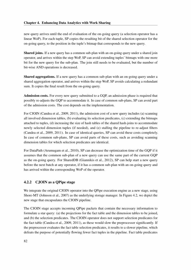
Chapter 4. Enhancing Data Analytics with Work Sharing
new query arrives until the end of evaluation of the on-going query (a selection operator has alinear WoP). For each tuple, SP copies the resulting bit of the shared selection operator for theon-going query, to the position in the tuple’s bitmap that corresponds to the new query.
Shared joins. If a new query has a common sub-plan with an on-going query under a shared joinoperator, and arrives within the step WoP, SP can avoid extending tuples’ bitmaps with one morebit for the new query for the sub-plan. The join still needs to be evaluated, but the number ofbit-wise AND operations is decreased.
Shared aggregations. If a new query has a common sub-plan with an on-going query under ashared aggregation operator, and arrives within the step WoP, SP avoids calculating a redundantsum. It copies the final result from the on-going query.
Admission costs. For every new query submitted to a GQP, an admission phase is required thatpossibly re-adjusts the GQP to accommodate it. In case of common sub-plans, SP can avoid partof the admission costs. The cost depends on the implementation.
For CJOIN (Candea et al., 2009, 2011), the admission cost of a new query includes (a) scanningall involved dimension tables, (b) evaluating its selection predicates, (c) extending the bitmapsattached to tuples, (d) increasing the size of hash tables of the shared hash-joins to accommodatenewly selected dimension tuples (if needed), and (e) stalling the pipeline to re-adjust filters(Candea et al., 2009, 2011). In case of identical queries, SP can avoid these costs completely.In case of common sub-plans, SP can avoid parts of these costs, such as avoiding scanningdimension tables for which selection predicates are identical.
For DataPath (Arumugam et al., 2010), SP can decrease the optimization time of the GQP if itassumes that the common sub-plan of a new query can use the same part of the current GQPas the on-going query. For SharedDB (Giannikis et al., 2012), SP can help start a new querybefore the next batch at any operator, if it has a common sub-plan with an on-going query andhas arrived within the corresponding WoP of the operator.
4.2.2 CJOIN as a QPipe stage
We integrate the original CJOIN operator into the QPipe execution engine as a new stage, usingShore-MT (Johnson et al., 2007) as the underlying storage manager. In Figure 4.2, we depict thenew stage that encapsulates the CJOIN pipeline.
The CJOIN stage accepts incoming QPipe packets that contain the necessary information toformulate a star query: (a) the projections for the fact table and the dimension tables to be joined,and (b) the selection predicates. The CJOIN operator does not support selection predicates forthe fact table (Candea et al., 2009, 2011), as these would slow the preprocessor significantly. Ifthe preprocessor evaluates the fact table selection predicates, it results to a slower pipeline, whichdefeats the purpose of potentially flowing fewer fact tuples in the pipeline. Fact table predicates
82
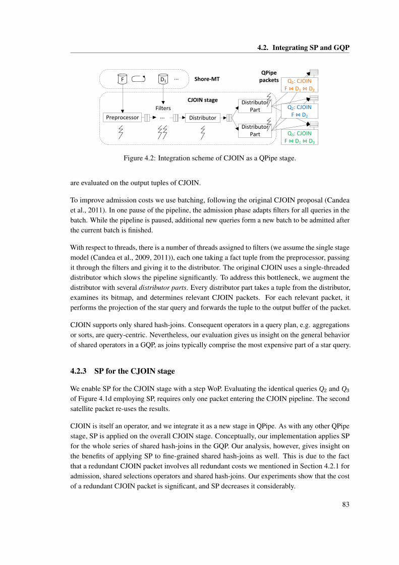
4.2. Integrating SP and GQP
Preprocessor Distributor
F D1 Shore-MTQPipe
packets
Distributor Part
Distributor Part
...
...
Filters
Q1: CJOIN F ⋈ D1 ⋈ D2
Q2: CJOIN F ⋈ D2
Q3: CJOIN F ⋈ D1 ⋈ D3
CJOIN stage
Figure 4.2: Integration scheme of CJOIN as a QPipe stage.
are evaluated on the output tuples of CJOIN.
To improve admission costs we use batching, following the original CJOIN proposal (Candeaet al., 2011). In one pause of the pipeline, the admission phase adapts filters for all queries in thebatch. While the pipeline is paused, additional new queries form a new batch to be admitted afterthe current batch is finished.
With respect to threads, there is a number of threads assigned to filters (we assume the single stagemodel (Candea et al., 2009, 2011)), each one taking a fact tuple from the preprocessor, passingit through the filters and giving it to the distributor. The original CJOIN uses a single-threadeddistributor which slows the pipeline significantly. To address this bottleneck, we augment thedistributor with several distributor parts. Every distributor part takes a tuple from the distributor,examines its bitmap, and determines relevant CJOIN packets. For each relevant packet, itperforms the projection of the star query and forwards the tuple to the output buffer of the packet.
CJOIN supports only shared hash-joins. Consequent operators in a query plan, e.g. aggregationsor sorts, are query-centric. Nevertheless, our evaluation gives us insight on the general behaviorof shared operators in a GQP, as joins typically comprise the most expensive part of a star query.
4.2.3 SP for the CJOIN stage
We enable SP for the CJOIN stage with a step WoP. Evaluating the identical queries Q2 and Q3
of Figure 4.1d employing SP, requires only one packet entering the CJOIN pipeline. The secondsatellite packet re-uses the results.
CJOIN is itself an operator, and we integrate it as a new stage in QPipe. As with any other QPipestage, SP is applied on the overall CJOIN stage. Conceptually, our implementation applies SPfor the whole series of shared hash-joins in the GQP. Our analysis, however, gives insight onthe benefits of applying SP to fine-grained shared hash-joins as well. This is due to the factthat a redundant CJOIN packet involves all redundant costs we mentioned in Section 4.2.1 foradmission, shared selections operators and shared hash-joins. Our experiments show that the costof a redundant CJOIN packet is significant, and SP decreases it considerably.
83
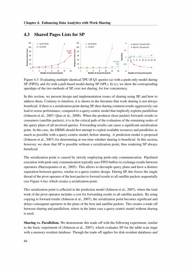
Chapter 4. Enhancing Data Analytics with Work Sharing
4.3 Shared Pages Lists for SP
0
20
40
60
80
100
120
1 2 4 8 16 32 64
Re
spo
nse
tim
e (
sec)
Number of concurrent queries
No SP (FIFO)
CS (FIFO)
60sec 3.1 CPU
0
20
40
60
80
100
120
1 2 4 8 16 32 64
Re
spo
nse
tim
e (
sec)
Number of concurrent queries
No SP (SPL)
CS (SPL)
8sec 19.1 CPU
0
0.5
1
1.5
2
0 2 4 6 8 10 12 14 16 18Sp
ee
du
p
Number of concurrent queries
(No SP / CS) with FIFO
(No SP / CS) with SPL
Figure 4.3: Evaluating multiple identical TPC-H Q1 queries (a) with a push-only model duringSP (FIFO), and (b) with a pull-based model during SP (SPL). In (c), we show the correspondingspeedups of the two methods of SP, over not sharing, for low concurrency.
In this section, we present design and implementation issues of sharing using SP, and how toaddress them. Contrary to intuition, it is shown in the literature that work sharing is not alwaysbeneficial: if there is a serialization point during SP, then sharing common results aggressively canlead to worse performance, compared to a query-centric model that implicitly exploits parallelism(Johnson et al., 2007; Qiao et al., 2008). When the producer (host packet) forwards results toconsumers (satellite packets), it is in the critical path of the evaluation of the remaining nodes ofthe query plans of all involved queries. Forwarding results can cause a significant serializationpoint. In this case, the DBMS should first attempt to exploit available resources and parallelize asmuch as possible with a query-centric model, before sharing. A prediction model is proposed(Johnson et al., 2007) for determining at run-time whether sharing is beneficial. In this section,however, we show that SP is possible without a serialization point, thus rendering SP alwaysbeneficial.
The serialization point is caused by strictly employing push-only communication. Pipelinedexecution with push-only communication typically uses FIFO buffers to exchange results betweenoperators (Harizopoulos et al., 2005). This allows to decouple query plans and have a distinctseparation between queries, similar to a query-centric design. During SP, this forces the singlethread of the pivot operator of the host packet to forward results to all satellite packets sequentially(see Figure 4.4a), which creates a serialization point.
This serialization point is reflected in the prediction model (Johnson et al., 2007), where the totalwork of the pivot operator includes a cost for forwarding results to all satellite packets. By usingcopying to forward results (Johnson et al., 2007), the serialization point becomes significant anddelays consequent operators in the plans of the host and satellite packets. This creates a trade-offbetween sharing and parallelism, where in the latter case a query-centric model without sharingis used.
Sharing vs. Parallelism. We demonstrate this trade-off with the following experiment, similarto the basic experiment of (Johnson et al., 2007), which evaluates SP for the table scan stagewith a memory-resident database. Though the trade-off applies for disk-resident databases and
84
4.3. Shared Pages Lists for SP
(a)Host packet
Satellite packet
Satellite packet
Satellite packet
forward resultsFIFO buffer
Host packet
Satellite packet
Satellite packet
Satellite packet
(b)
Figure 4.4: Sharing identical results during SP with: (a) push-only model and (b) a SPL.
other stages as well, it is more pronounced in this case. Our experimental configuration can befound in Section 4.5. We evaluate two variations of the QPipe execution engine: (a) No SP(FIFO), which evaluates query plans independently without any sharing, and (b) CS (FIFO),with SP enabled only for the table scan stage, thus supporting circular scans (CS). FIFO buffersare used for pipelined execution and copying is used to forward pages during SP, following theoriginal push-only design (Harizopoulos et al., 2005; Johnson et al., 2007). We evaluate identicalTPC-H (TPC, 2013) Q1 queries, submitted at the same time, with a database of scaling factor1. In Figure 4.3a, we show the response times of the variations, while varying the number ofconcurrent queries.
For low concurrency, No SP (FIFO) efficiently uses available CPU resources. Starting withas few as 32 queries, however, there is contention for CPU resources and response times growquickly, due to the fact that our server has 24 available cores and the query-centric model evaluatesqueries independently. For 64 queries it uses all cores at their maximum, resulting in excessiveand unpredictable response times, with a standard deviation up to 30%.
CS (FIFO) suffers from low utilization of CPU resources, due to the aforementioned serializationpoint of SP. The critical path increases with the number of concurrent queries. For 64 queries,it uses an average of 3.1 of available cores. In this experiment, the proposed prediction model(Johnson et al., 2007) would not share in cases of low concurrency, essentially falling back to theline of No SP (FIFO), and would share in cases of high concurrency.
Nevertheless, the impact of the serialization point of SP can be minimized. Simply copyingtuples in a multi-threaded way would not solve the problem, due to synchronization overhead andincreased required CPU resources. A solution would be to forward tuples via pointers, a possibilitynot considered by the original system (Harizopoulos et al., 2005; Johnson et al., 2007). We can,however, avoid unnecessary pointer chasing; by employing pull-based communication, we canshare the results and eliminate forwarding altogether. In essence, we transfer the responsibility ofsharing the results from the producer to the consumers. Thus, the total work of the producer doesnot include any forwarding cost. Our pull-based communication model is adapted for SP for anystage with a step or linear WoP.
The serialization point of push-based SP was not a visible bottleneck in the original implementa-tion, due to experiments being ran on a uni-processor (Harizopoulos et al., 2005). On multi-coremachines its impact grows as the available parallelism increases, and a prediction model (Johnson
85
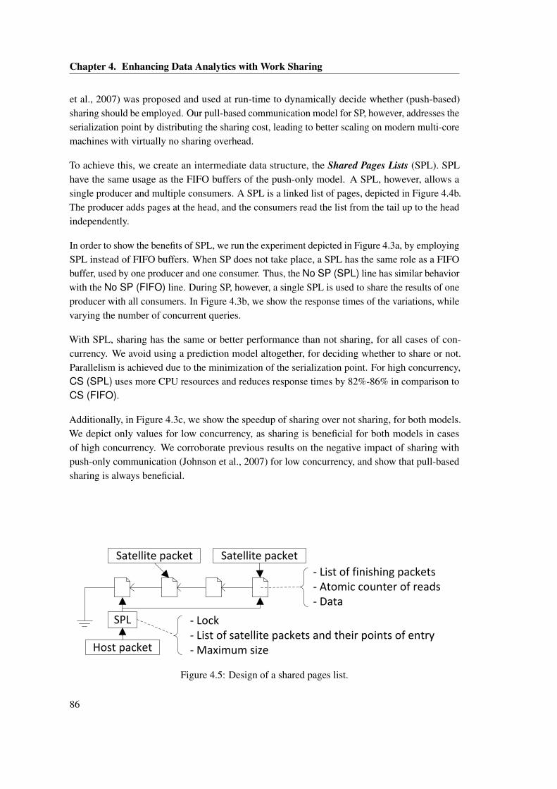
Chapter 4. Enhancing Data Analytics with Work Sharing
et al., 2007) was proposed and used at run-time to dynamically decide whether (push-based)sharing should be employed. Our pull-based communication model for SP, however, addresses theserialization point by distributing the sharing cost, leading to better scaling on modern multi-coremachines with virtually no sharing overhead.
To achieve this, we create an intermediate data structure, the Shared Pages Lists (SPL). SPLhave the same usage as the FIFO buffers of the push-only model. A SPL, however, allows asingle producer and multiple consumers. A SPL is a linked list of pages, depicted in Figure 4.4b.The producer adds pages at the head, and the consumers read the list from the tail up to the headindependently.
In order to show the benefits of SPL, we run the experiment depicted in Figure 4.3a, by employingSPL instead of FIFO buffers. When SP does not take place, a SPL has the same role as a FIFObuffer, used by one producer and one consumer. Thus, the No SP (SPL) line has similar behaviorwith the No SP (FIFO) line. During SP, however, a single SPL is used to share the results of oneproducer with all consumers. In Figure 4.3b, we show the response times of the variations, whilevarying the number of concurrent queries.
With SPL, sharing has the same or better performance than not sharing, for all cases of con-currency. We avoid using a prediction model altogether, for deciding whether to share or not.Parallelism is achieved due to the minimization of the serialization point. For high concurrency,CS (SPL) uses more CPU resources and reduces response times by 82%-86% in comparison toCS (FIFO).
Additionally, in Figure 4.3c, we show the speedup of sharing over not sharing, for both models.We depict only values for low concurrency, as sharing is beneficial for both models in casesof high concurrency. We corroborate previous results on the negative impact of sharing withpush-only communication (Johnson et al., 2007) for low concurrency, and show that pull-basedsharing is always beneficial.
- List of finishing packets- Atomic counter of reads- Data
SPL - Lock - List of satellite packets and their points of entry- Maximum sizeHost packet
Satellite packetSatellite packet
Figure 4.5: Design of a shared pages list.
86
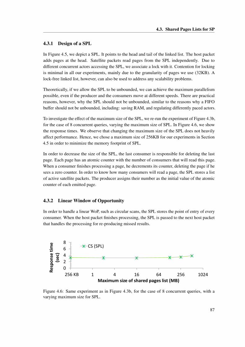
4.3. Shared Pages Lists for SP
4.3.1 Design of a SPL
In Figure 4.5, we depict a SPL. It points to the head and tail of the linked list. The host packetadds pages at the head. Satellite packets read pages from the SPL independently. Due todifferent concurrent actors accessing the SPL, we associate a lock with it. Contention for lockingis minimal in all our experiments, mainly due to the granularity of pages we use (32KB). Alock-free linked list, however, can also be used to address any scalability problems.
Theoretically, if we allow the SPL to be unbounded, we can achieve the maximum parallelismpossible, even if the producer and the consumers move at different speeds. There are practicalreasons, however, why the SPL should not be unbounded, similar to the reasons why a FIFObuffer should not be unbounded, including: saving RAM, and regulating differently paced actors.
To investigate the effect of the maximum size of the SPL, we re-run the experiment of Figure 4.3b,for the case of 8 concurrent queries, varying the maximum size of SPL. In Figure 4.6, we showthe response times. We observe that changing the maximum size of the SPL does not heavilyaffect performance. Hence, we chose a maximum size of 256KB for our experiments in Section4.5 in order to minimize the memory footprint of SPL.
In order to decrease the size of the SPL, the last consumer is responsible for deleting the lastpage. Each page has an atomic counter with the number of consumers that will read this page.When a consumer finishes processing a page, he decrements its counter, deleting the page if hesees a zero counter. In order to know how many consumers will read a page, the SPL stores a listof active satellite packets. The producer assigns their number as the initial value of the atomiccounter of each emitted page.
4.3.2 Linear Window of Opportunity
In order to handle a linear WoP, such as circular scans, the SPL stores the point of entry of everyconsumer. When the host packet finishes processing, the SPL is passed to the next host packetthat handles the processing for re-producing missed results.
0
2
4
6
8
0,25 1 4 16 64 256 1024
Re
spo
nse
tim
e
(se
c)
Maximum size of shared pages list (MB)
CS (SPL)
256 KB
Figure 4.6: Same experiment as in Figure 4.3b, for the case of 8 concurrent queries, with avarying maximum size for SPL.
87
Chapter 4. Enhancing Data Analytics with Work Sharing
When the host packet emits a page, it checks for consumers whose point of entry is this page,and will need to finish when they reach it. The emitted page has attached to it a list of thesefinishing packets, which are removed from the active packets of the SPL (they do not participatein the atomic counter of subsequently emitted pages). When a consumer (packet) reads a page, itchecks whether it is a finishing packet, in which case, it exits the SPL.
4.4 Experimental Methodology
We compare five variations of the QPipe execution engine:
• QPipe, without SP, which is similar to a typical query-centric model that evaluates queryplans separately with pipelining, without any sharing. This serves as our baseline.
• QPipe-CS, supporting SP only for the table scan stage, i.e. circular scans (CS). It improvesperformance over QPipe by reducing contention for CPU resources, the buffer pool andthe underlying storage device.
• QPipe-SP, supporting SP additionally for the join stage. It improves performance overQPipe-CS, in cases of high similarity, i.e. common sub-plans. In cases of low similarity,it behaves similar to QPipe-CS.
• CJOIN, without SP, which is the result of our integration of CJOIN into QPipe, hence thejoins in star queries are evaluated with a GQP of shared hash-joins. We remind that CJOINonly supports shared hash-joins, thus subsequent operators are query-centric. Nevertheless,this configuration allows us to compare shared hash-joins with the query-centric ones usedby the previous variations, giving us insight on the performance characteristics of generalshared operators.
• CJOIN-SP, which additionally supports SP for the CJOIN stage (see Section 4.2.3). Weuse this configuration to evaluate the benefits of combining SP with a GQP. It behavessimilar to CJOIN in cases of low similarity in the query mix.
In all our experiments, SP for the aggregation and sorting stages is off. This is done on purposeto isolate the benefits of SP for joins only, so as to better compare QPipe-SP and CJOIN-SP.
We use the Star Schema Benchmark (O’Neil et al., 2009) and Shore-MT (Johnson et al., 2009) asthe storage manager. SSB is a simplified version of TPC-H (TPC, 2013) where the tables lineitemand order have been merged into lineorder and there are four dimension tables: date, supplier,customer and part. Shore-MT is an open-source multi-threaded storage manager developed toachieve scalability on multicore platforms.
Our server is a Sun Fire X4470 server with four hexa-core processors Intel Xeon E7530 at 1.86GHz, with hyper-threading disabled and 64 GB of RAM. Each core has a 32KB L1 instructions
88
4.5. Experimental Analysis
cache, a 32KB L1 data cache, and a 256KB L2 cache. Each processor has a 12MB L3 cache,shared by all its cores. For storage, we use two 146 GB 10kRPM SAS 2.5” disks, configured as aRAID-0. The O/S is a 64-bit SMP Linux (Red Hat), with a 2.6.32 kernel.
We clear the file system caches before every measurement. All variations use a large buffer poolthat fits SSB datasets of scaling factors up to 30 (corresponding to around 18GB of data producedby the SSB generator). SPL are used for exchanging results among packets. As we explain inSection 4.3, we use 32KB pages and a maximum size of 256KB for a SPL.
Unless stated otherwise, every data point is the average of multiple iterations with standarddeviation less or equal to 5%. In some cases, contention for resources results in higher deviations.In certain experiments, we mention the average CPU usage and I/O throughput of representativeiterations (averaged only over their activity period), to gain insight on the performance of thevariations.
We vary (a) the number of concurrent queries, (b) whether the database is memory-resident ordisk-resident, (c) the selectivity of fact tuples, (e) the scaling factor, and (d) the query similaritywhich is modeled in our experiments by the number of possible different submitted query plans.Queries are submitted at the same time, and are all evaluated concurrently. This single batch forall queries allows us to minimize query admission overheads for CJOIN, and additionally allowsus to show the effects of SP, as all queries with common sub-plans arrive surely inside the WoP oftheir pivot operators. We note that variable inter-arrival delays can decrease sharing opportunitiesfor SP, and refer the interested reader to the original QPipe paper (Harizopoulos et al., 2005) toreview the effects of inter-arrival delays for different cases of pivot operators and WoP.
Finally, in Section 4.5.4, we evaluate QPipe-SP, CJOIN-SP, and Postgres with a mix of SSBqueries and a scaling factor 30. We use PostgreSQL 9.1.4 as another example of a query-centricexecution engine that does not share among concurrent queries. We configure PostgreSQL tomake the comparison with QPipe as fair as possible. We use 32KB pages, large shared buffersthat fit the database, ensure that it never spills to the disk and that the query execution plans arethe same. We disable query result caching, which does not execute a previously seen query at all.We do not want to compare caching of previously executed queries, but the efficiency of sharingamong in-progress queries.
4.5 Experimental Analysis
In this section, we measure performance by evaluating multiple concurrent instances of SSBQ3.2. It is a typical star query that joins three of the four dimension tables with the fact table.The SQL template and the execution plan are shown in Figure 4.7. We selected a single querytemplate for our sensitivity analysis because we can adjust the similarity of the query mix to gaininsight on the benefits of SP, and also, the GQP of CJOIN is the same for all experiments, with 3shared hash-joins for all star queries.
89
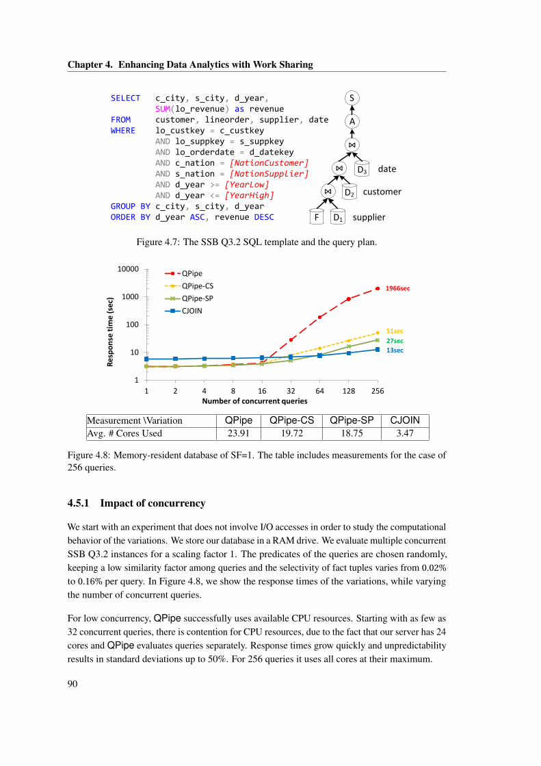
Chapter 4. Enhancing Data Analytics with Work Sharing
F D1
D2⋈
⋈ D3
⋈
A
SSELECT c_city, s_city, d_year, SUM(lo_revenue) as revenueFROM customer, lineorder, supplier, dateWHERE lo_custkey = c_custkey AND lo_suppkey = s_suppkey AND lo_orderdate = d_datekey AND c_nation = [NationCustomer] AND s_nation = [NationSupplier] AND d_year >= [YearLow] AND d_year <= [YearHigh]GROUP BY c_city, s_city, d_yearORDER BY d_year ASC, revenue DESC supplier
customer
date
Figure 4.7: The SSB Q3.2 SQL template and the query plan.
1
10
100
1000
10000
1 2 4 8 16 32 64 128 256
Re
spo
nse
tim
e (
sec)
Number of concurrent queries
QPipe
QPipe-CS
QPipe-SP
CJOIN
1966sec
51sec
27sec
13sec
Measurement \Variation QPipe QPipe-CS QPipe-SP CJOINAvg. # Cores Used 23.91 19.72 18.75 3.47
Figure 4.8: Memory-resident database of SF=1. The table includes measurements for the case of256 queries.
4.5.1 Impact of concurrency
We start with an experiment that does not involve I/O accesses in order to study the computationalbehavior of the variations. We store our database in a RAM drive. We evaluate multiple concurrentSSB Q3.2 instances for a scaling factor 1. The predicates of the queries are chosen randomly,keeping a low similarity factor among queries and the selectivity of fact tuples varies from 0.02%
to 0.16% per query. In Figure 4.8, we show the response times of the variations, while varyingthe number of concurrent queries.
For low concurrency, QPipe successfully uses available CPU resources. Starting with as few as32 concurrent queries, there is contention for CPU resources, due to the fact that our server has 24cores and QPipe evaluates queries separately. Response times grow quickly and unpredictabilityresults in standard deviations up to 50%. For 256 queries it uses all cores at their maximum.
90
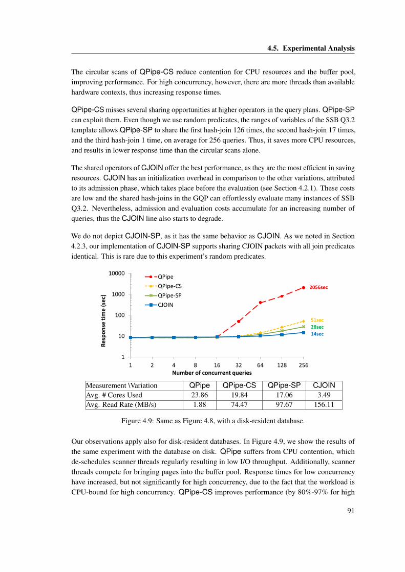
4.5. Experimental Analysis
The circular scans of QPipe-CS reduce contention for CPU resources and the buffer pool,improving performance. For high concurrency, however, there are more threads than availablehardware contexts, thus increasing response times.
QPipe-CS misses several sharing opportunities at higher operators in the query plans. QPipe-SPcan exploit them. Even though we use random predicates, the ranges of variables of the SSB Q3.2template allows QPipe-SP to share the first hash-join 126 times, the second hash-join 17 times,and the third hash-join 1 time, on average for 256 queries. Thus, it saves more CPU resources,and results in lower response time than the circular scans alone.
The shared operators of CJOIN offer the best performance, as they are the most efficient in savingresources. CJOIN has an initialization overhead in comparison to the other variations, attributedto its admission phase, which takes place before the evaluation (see Section 4.2.1). These costsare low and the shared hash-joins in the GQP can effortlessly evaluate many instances of SSBQ3.2. Nevertheless, admission and evaluation costs accumulate for an increasing number ofqueries, thus the CJOIN line also starts to degrade.
We do not depict CJOIN-SP, as it has the same behavior as CJOIN. As we noted in Section4.2.3, our implementation of CJOIN-SP supports sharing CJOIN packets with all join predicatesidentical. This is rare due to this experiment’s random predicates.
1
10
100
1000
10000
1 2 4 8 16 32 64 128 256
Re
spo
nse
tim
e (
sec)
Number of concurrent queries
QPipe
QPipe-CS
QPipe-SP
CJOIN
2056sec
51sec
28sec
14sec
Measurement \Variation QPipe QPipe-CS QPipe-SP CJOINAvg. # Cores Used 23.86 19.84 17.06 3.49Avg. Read Rate (MB/s) 1.88 74.47 97.67 156.11
Figure 4.9: Same as Figure 4.8, with a disk-resident database.
Our observations apply also for disk-resident databases. In Figure 4.9, we show the results ofthe same experiment with the database on disk. QPipe suffers from CPU contention, whichde-schedules scanner threads regularly resulting in low I/O throughput. Additionally, scannerthreads compete for bringing pages into the buffer pool. Response times for low concurrencyhave increased, but not significantly for high concurrency, due to the fact that the workload isCPU-bound for high concurrency. QPipe-CS improves performance (by 80%-97% for high
91
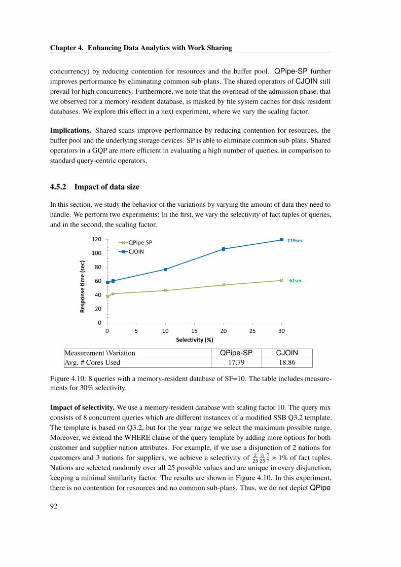
Chapter 4. Enhancing Data Analytics with Work Sharing
concurrency) by reducing contention for resources and the buffer pool. QPipe-SP furtherimproves performance by eliminating common sub-plans. The shared operators of CJOIN stillprevail for high concurrency. Furthermore, we note that the overhead of the admission phase, thatwe observed for a memory-resident database, is masked by file system caches for disk-residentdatabases. We explore this effect in a next experiment, where we vary the scaling factor.
Implications. Shared scans improve performance by reducing contention for resources, thebuffer pool and the underlying storage devices. SP is able to eliminate common sub-plans. Sharedoperators in a GQP are more efficient in evaluating a high number of queries, in comparison tostandard query-centric operators.
4.5.2 Impact of data size
In this section, we study the behavior of the variations by varying the amount of data they need tohandle. We perform two experiments: In the first, we vary the selectivity of fact tuples of queries,and in the second, the scaling factor.
0
20
40
60
80
100
120
0 5 10 15 20 25 30
Re
spo
nse
tim
e (
sec)
Selectivity (%)
QPipe-SP
CJOIN
61sec
119sec
Measurement \Variation QPipe-SP CJOINAvg. # Cores Used 17.79 18.86
Figure 4.10: 8 queries with a memory-resident database of SF=10. The table includes measure-ments for 30% selectivity.
Impact of selectivity. We use a memory-resident database with scaling factor 10. The query mixconsists of 8 concurrent queries which are different instances of a modified SSB Q3.2 template.The template is based on Q3.2, but for the year range we select the maximum possible range.Moreover, we extend the WHERE clause of the query template by adding more options for bothcustomer and supplier nation attributes. For example, if we use a disjunction of 2 nations forcustomers and 3 nations for suppliers, we achieve a selectivity of 2
253
2577 ≈ 1% of fact tuples.
Nations are selected randomly over all 25 possible values and are unique in every disjunction,keeping a minimal similarity factor. The results are shown in Figure 4.10. In this experiment,there is no contention for resources and no common sub-plans. Thus, we do not depict QPipe
92
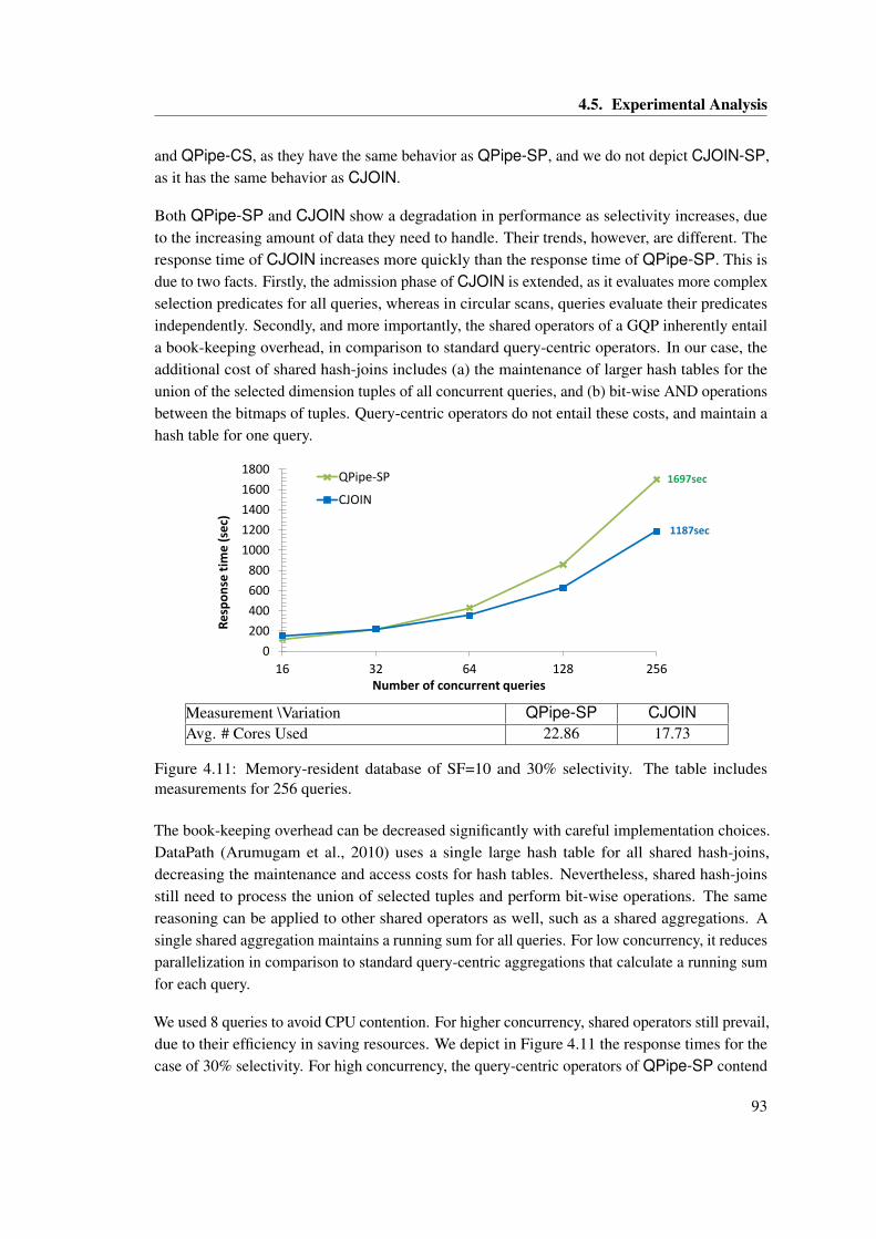
4.5. Experimental Analysis
and QPipe-CS, as they have the same behavior as QPipe-SP, and we do not depict CJOIN-SP,as it has the same behavior as CJOIN.
Both QPipe-SP and CJOIN show a degradation in performance as selectivity increases, dueto the increasing amount of data they need to handle. Their trends, however, are different. Theresponse time of CJOIN increases more quickly than the response time of QPipe-SP. This isdue to two facts. Firstly, the admission phase of CJOIN is extended, as it evaluates more complexselection predicates for all queries, whereas in circular scans, queries evaluate their predicatesindependently. Secondly, and more importantly, the shared operators of a GQP inherently entaila book-keeping overhead, in comparison to standard query-centric operators. In our case, theadditional cost of shared hash-joins includes (a) the maintenance of larger hash tables for theunion of the selected dimension tuples of all concurrent queries, and (b) bit-wise AND operationsbetween the bitmaps of tuples. Query-centric operators do not entail these costs, and maintain ahash table for one query.
0
200
400
600
800
1000
1200
1400
1600
1800
16 32 64 128 256
Re
spo
nse
tim
e (
sec)
Number of concurrent queries
QPipe-SP
CJOIN
1697sec
1187sec
Measurement \Variation QPipe-SP CJOINAvg. # Cores Used 22.86 17.73
Figure 4.11: Memory-resident database of SF=10 and 30% selectivity. The table includesmeasurements for 256 queries.
The book-keeping overhead can be decreased significantly with careful implementation choices.DataPath (Arumugam et al., 2010) uses a single large hash table for all shared hash-joins,decreasing the maintenance and access costs for hash tables. Nevertheless, shared hash-joinsstill need to process the union of selected tuples and perform bit-wise operations. The samereasoning can be applied to other shared operators as well, such as a shared aggregations. Asingle shared aggregation maintains a running sum for all queries. For low concurrency, it reducesparallelization in comparison to standard query-centric aggregations that calculate a running sumfor each query.
We used 8 queries to avoid CPU contention. For higher concurrency, shared operators still prevail,due to their efficiency in saving resources. We depict in Figure 4.11 the response times for thecase of 30% selectivity. For high concurrency, the query-centric operators of QPipe-SP contend
93
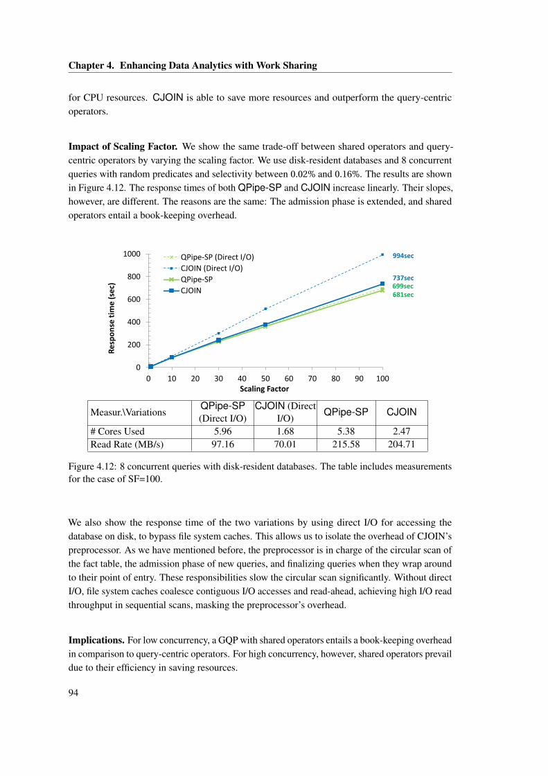
Chapter 4. Enhancing Data Analytics with Work Sharing
for CPU resources. CJOIN is able to save more resources and outperform the query-centricoperators.
Impact of Scaling Factor. We show the same trade-off between shared operators and query-centric operators by varying the scaling factor. We use disk-resident databases and 8 concurrentqueries with random predicates and selectivity between 0.02% and 0.16%. The results are shownin Figure 4.12. The response times of both QPipe-SP and CJOIN increase linearly. Their slopes,however, are different. The reasons are the same: The admission phase is extended, and sharedoperators entail a book-keeping overhead.
0
200
400
600
800
1000
0 10 20 30 40 50 60 70 80 90 100
Re
spo
nse
tim
e (
sec)
Scaling Factor
QPipe-SP (Direct I/O)
CJOIN (Direct I/O)
QPipe-SP
CJOIN681sec
737sec 699sec
994sec
Measur.\VariationsQPipe-SP(Direct I/O)
CJOIN (DirectI/O)
QPipe-SP CJOIN
# Cores Used 5.96 1.68 5.38 2.47Read Rate (MB/s) 97.16 70.01 215.58 204.71
Figure 4.12: 8 concurrent queries with disk-resident databases. The table includes measurementsfor the case of SF=100.
We also show the response time of the two variations by using direct I/O for accessing thedatabase on disk, to bypass file system caches. This allows us to isolate the overhead of CJOIN’spreprocessor. As we have mentioned before, the preprocessor is in charge of the circular scan ofthe fact table, the admission phase of new queries, and finalizing queries when they wrap aroundto their point of entry. These responsibilities slow the circular scan significantly. Without directI/O, file system caches coalesce contiguous I/O accesses and read-ahead, achieving high I/O readthroughput in sequential scans, masking the preprocessor’s overhead.
Implications. For low concurrency, a GQP with shared operators entails a book-keeping overheadin comparison to query-centric operators. For high concurrency, however, shared operators prevaildue to their efficiency in saving resources.
94
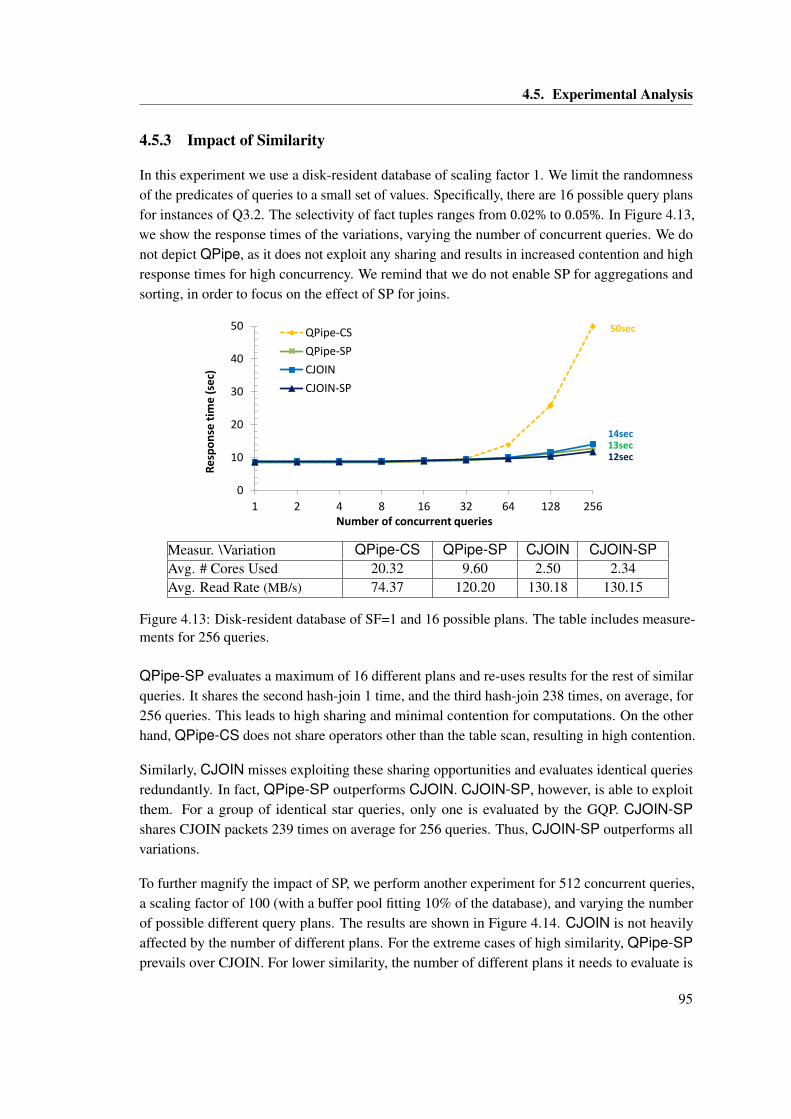
4.5. Experimental Analysis
4.5.3 Impact of Similarity
In this experiment we use a disk-resident database of scaling factor 1. We limit the randomnessof the predicates of queries to a small set of values. Specifically, there are 16 possible query plansfor instances of Q3.2. The selectivity of fact tuples ranges from 0.02% to 0.05%. In Figure 4.13,we show the response times of the variations, varying the number of concurrent queries. We donot depict QPipe, as it does not exploit any sharing and results in increased contention and highresponse times for high concurrency. We remind that we do not enable SP for aggregations andsorting, in order to focus on the effect of SP for joins.
0
10
20
30
40
50
1 2 4 8 16 32 64 128 256
Re
spo
nse
tim
e (
sec)
Number of concurrent queries
QPipe-CS
QPipe-SP
CJOIN
CJOIN-SP
50sec
13sec 14sec
12sec
Measur. \Variation QPipe-CS QPipe-SP CJOIN CJOIN-SPAvg. # Cores Used 20.32 9.60 2.50 2.34Avg. Read Rate (MB/s) 74.37 120.20 130.18 130.15
Figure 4.13: Disk-resident database of SF=1 and 16 possible plans. The table includes measure-ments for 256 queries.
QPipe-SP evaluates a maximum of 16 different plans and re-uses results for the rest of similarqueries. It shares the second hash-join 1 time, and the third hash-join 238 times, on average, for256 queries. This leads to high sharing and minimal contention for computations. On the otherhand, QPipe-CS does not share operators other than the table scan, resulting in high contention.
Similarly, CJOIN misses exploiting these sharing opportunities and evaluates identical queriesredundantly. In fact, QPipe-SP outperforms CJOIN. CJOIN-SP, however, is able to exploitthem. For a group of identical star queries, only one is evaluated by the GQP. CJOIN-SPshares CJOIN packets 239 times on average for 256 queries. Thus, CJOIN-SP outperforms allvariations.
To further magnify the impact of SP, we perform another experiment for 512 concurrent queries,a scaling factor of 100 (with a buffer pool fitting 10% of the database), and varying the numberof possible different query plans. The results are shown in Figure 4.14. CJOIN is not heavilyaffected by the number of different plans. For the extreme cases of high similarity, QPipe-SPprevails over CJOIN. For lower similarity, the number of different plans it needs to evaluate is
95
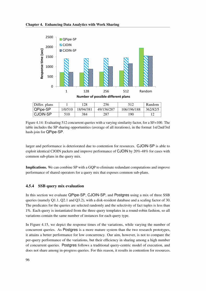
Chapter 4. Enhancing Data Analytics with Work Sharing
0
500
1000
1500
2000
2500
1 128 256 512 Random
Re
spo
nse
tim
e (
sec)
Number of possible different plans
QPipe-SP
CJOIN
CJOIN-SP
Differ. plans 1 128 256 512 RandomQPipe-SP 1/0/510 18/94/381 49/156/287 106/196/188 362/82/5CJOIN-SP 510 384 287 190 12
Figure 4.14: Evaluating 512 concurrent queries with a varying similarity factor, for a SF=100. Thetable includes the SP sharing opportunities (average of all iterations), in the format 1st/2nd/3rdhash-join for QPipe-SP.
larger and performance is deteriorated due to contention for resources. CJOIN-SP is able toexploit identical CJOIN packets and improve performance of CJOIN by 20%-48% for cases withcommon sub-plans in the query mix.
Implications. We can combine SP with a GQP to eliminate redundant computations and improveperformance of shared operators for a query mix that exposes common sub-plans.
4.5.4 SSB query mix evaluation
In this section we evaluate QPipe-SP, CJOIN-SP, and Postgres using a mix of three SSBqueries (namely Q1.1, Q2.1 and Q3.2), with a disk-resident database and a scaling factor of 30.The predicates for the queries are selected randomly and the selectivity of fact tuples is less than1%. Each query is instantiated from the three query templates in a round-robin fashion, so allvariations contain the same number of instances for each query type.
In Figure 4.15, we depict the response times of the variations, while varying the number ofconcurrent queries. As Postgres is a more mature system than the two research prototypes,it attains a better performance for low concurrency. Our aim, however, is not to compare theper-query performance of the variations, but their efficiency in sharing among a high numberof concurrent queries. Postgres follows a traditional query-centric model of execution, anddoes not share among in-progress queries. For this reason, it results in contention for resources.
96
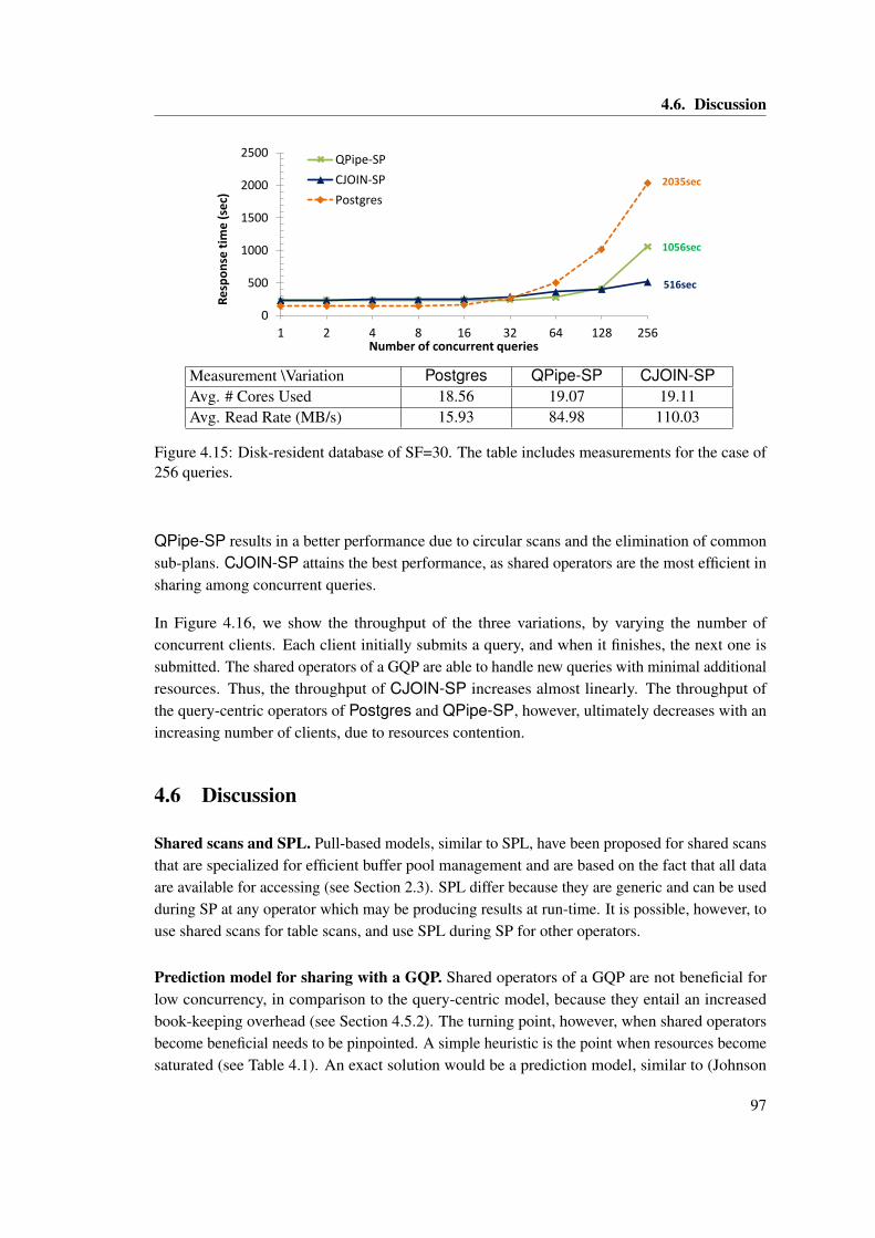
4.6. Discussion
0
500
1000
1500
2000
2500
1 2 4 8 16 32 64 128 256
Re
spo
nse
tim
e (
sec)
Number of concurrent queries
QPipe-SP
CJOIN-SP
Postgres
1056sec
516sec
2035sec
Measurement \Variation Postgres QPipe-SP CJOIN-SPAvg. # Cores Used 18.56 19.07 19.11Avg. Read Rate (MB/s) 15.93 84.98 110.03
Figure 4.15: Disk-resident database of SF=30. The table includes measurements for the case of256 queries.
QPipe-SP results in a better performance due to circular scans and the elimination of commonsub-plans. CJOIN-SP attains the best performance, as shared operators are the most efficient insharing among concurrent queries.
In Figure 4.16, we show the throughput of the three variations, by varying the number ofconcurrent clients. Each client initially submits a query, and when it finishes, the next one issubmitted. The shared operators of a GQP are able to handle new queries with minimal additionalresources. Thus, the throughput of CJOIN-SP increases almost linearly. The throughput ofthe query-centric operators of Postgres and QPipe-SP, however, ultimately decreases with anincreasing number of clients, due to resources contention.
4.6 Discussion
Shared scans and SPL. Pull-based models, similar to SPL, have been proposed for shared scansthat are specialized for efficient buffer pool management and are based on the fact that all dataare available for accessing (see Section 2.3). SPL differ because they are generic and can be usedduring SP at any operator which may be producing results at run-time. It is possible, however, touse shared scans for table scans, and use SPL during SP for other operators.
Prediction model for sharing with a GQP. Shared operators of a GQP are not beneficial forlow concurrency, in comparison to the query-centric model, because they entail an increasedbook-keeping overhead (see Section 4.5.2). The turning point, however, when shared operatorsbecome beneficial needs to be pinpointed. A simple heuristic is the point when resources becomesaturated (see Table 4.1). An exact solution would be a prediction model, similar to (Johnson
97
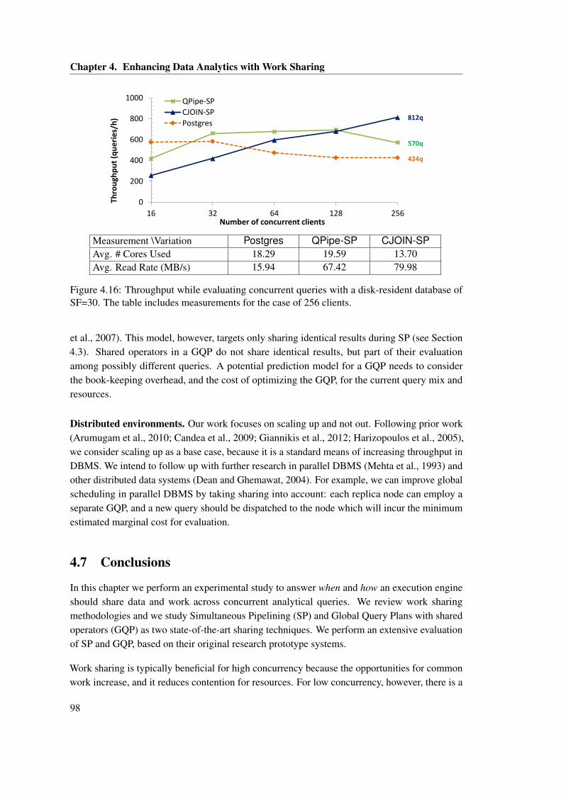
Chapter 4. Enhancing Data Analytics with Work Sharing
0
200
400
600
800
1000
16 32 64 128 256
Thro
ugh
pu
t (q
ue
rie
s/h
)
Number of concurrent clients
QPipe-SP
CJOIN-SP
Postgres
570q
812q
424q
Measurement \Variation Postgres QPipe-SP CJOIN-SPAvg. # Cores Used 18.29 19.59 13.70Avg. Read Rate (MB/s) 15.94 67.42 79.98
Figure 4.16: Throughput while evaluating concurrent queries with a disk-resident database ofSF=30. The table includes measurements for the case of 256 clients.
et al., 2007). This model, however, targets only sharing identical results during SP (see Section4.3). Shared operators in a GQP do not share identical results, but part of their evaluationamong possibly different queries. A potential prediction model for a GQP needs to considerthe book-keeping overhead, and the cost of optimizing the GQP, for the current query mix andresources.
Distributed environments. Our work focuses on scaling up and not out. Following prior work(Arumugam et al., 2010; Candea et al., 2009; Giannikis et al., 2012; Harizopoulos et al., 2005),we consider scaling up as a base case, because it is a standard means of increasing throughput inDBMS. We intend to follow up with further research in parallel DBMS (Mehta et al., 1993) andother distributed data systems (Dean and Ghemawat, 2004). For example, we can improve globalscheduling in parallel DBMS by taking sharing into account: each replica node can employ aseparate GQP, and a new query should be dispatched to the node which will incur the minimumestimated marginal cost for evaluation.
4.7 Conclusions
In this chapter we perform an experimental study to answer when and how an execution engineshould share data and work across concurrent analytical queries. We review work sharingmethodologies and we study Simultaneous Pipelining (SP) and Global Query Plans with sharedoperators (GQP) as two state-of-the-art sharing techniques. We perform an extensive evaluationof SP and GQP, based on their original research prototype systems.
Work sharing is typically beneficial for high concurrency because the opportunities for commonwork increase, and it reduces contention for resources. For low concurrency, however, there is a
98
4.7. Conclusions
trade-off between sharing and parallelism, particularly when the sharing overhead is significant.We show that GQP are not beneficial for low concurrency because shared operators inherentlyinvolve an additional book-keeping overhead, compared to query-centric operators. For SP,however, we show that it can be beneficial for low concurrency as well, if the appropriatecommunication model is employed: we introduce SPL, a pull-based approach for SP that scalesbetter on modern multi-core machines than push-based SP. SPL is a data structure that naturallypromotes parallelism by shifting the responsibility of sharing common results from the producerto the consumers.
Furthermore, we show that SP and GQP are two orthogonal sharing techniques and their integra-tion allows to share operators and handle a high number of concurrent queries, while also sharingany common sub-plans presented in the query mix. In conclusion, analytical query enginesshould dynamically choose between query-centric operators with SP for low concurrency andGQP with shared operators enhanced by SP for high concurrency.
99

5 BF-Tree: Approximate Tree Indexing1
5.1 Introduction
Database Management Systems (DBMS) have been traditionally designed with the assumptionthat the underlying storage is comprised of hard disks (HDD). This assumption impacts most ofthe design choices of DBMS and in particular the ones of the storage and the indexing subsystems.Data stored on the secondary storage of a DBMS can be accessed either by a sequential scan orby using an index for randomly located searches. The most common types of indexes in moderndatabase systems are B+-Trees and hash indexes (Ramakrishnan and Gehrke, 2002). Other typesof indexing include bitmap indexes (O’Neil, 1987).
Tree structures like B+-Trees are widely used because they are optimized for the common storagetechnology - HDD - and they offer efficient indexing and accessing for both sorted and unsorteddata (e.g. in heap files). Tree structures offer logarithmic, to the size of the data, number ofrandom accesses (and, as a result, lookup time) and support ordered range scans. Hash tables arevery efficient for point queries, i.e. for a single value probe, because, once hashing is completedthe search cost is constant. Indexing in today’s systems is particularly important because it needsonly a few random accesses to locate any value, which is sublinear to the size of the data (e.g.,logarithmic for trees, constant for hash indexes).
5.1.1 Implicit Clustering
Big data analysis - often performed in a real-time manner - is becoming increasingly more popularand crucial to business operation. New datasets including data from scientists (e.g., simulations,large-scale experiments and measurements, sensor data), social data (e.g., social status updates,tweets) and, monitoring, archival and historical data (managed by data warehousing systems),all have a time dimension, leading to implicit, time-based clusters of data, often resulting in
1The material of this chapter has been the basis for a paper submitted for publication entitled "BF-Tree: Approxi-mate Tree Indexing" (Athanassoulis and Ailamaki, 2013).
101
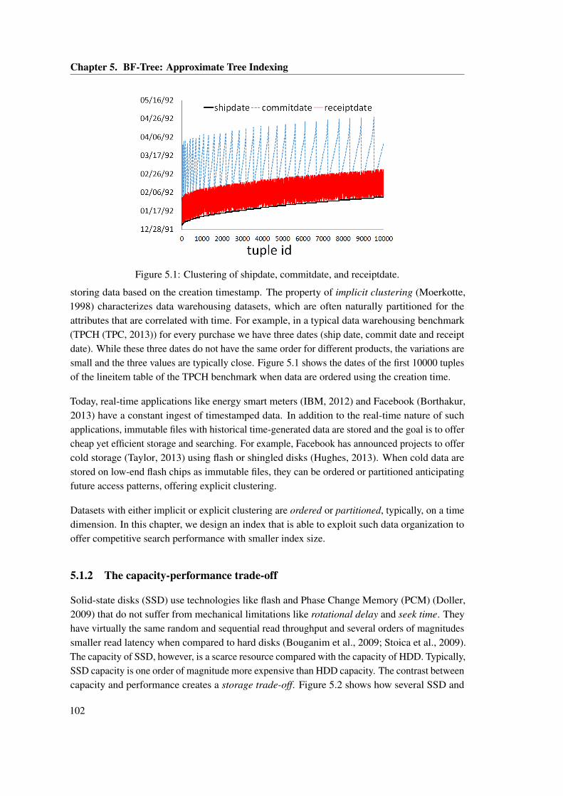
Chapter 5. BF-Tree: Approximate Tree Indexing
Figure 5.1: Clustering of shipdate, commitdate, and receiptdate.
storing data based on the creation timestamp. The property of implicit clustering (Moerkotte,1998) characterizes data warehousing datasets, which are often naturally partitioned for theattributes that are correlated with time. For example, in a typical data warehousing benchmark(TPCH (TPC, 2013)) for every purchase we have three dates (ship date, commit date and receiptdate). While these three dates do not have the same order for different products, the variations aresmall and the three values are typically close. Figure 5.1 shows the dates of the first 10000 tuplesof the lineitem table of the TPCH benchmark when data are ordered using the creation time.
Today, real-time applications like energy smart meters (IBM, 2012) and Facebook (Borthakur,2013) have a constant ingest of timestamped data. In addition to the real-time nature of suchapplications, immutable files with historical time-generated data are stored and the goal is to offercheap yet efficient storage and searching. For example, Facebook has announced projects to offercold storage (Taylor, 2013) using flash or shingled disks (Hughes, 2013). When cold data arestored on low-end flash chips as immutable files, they can be ordered or partitioned anticipatingfuture access patterns, offering explicit clustering.
Datasets with either implicit or explicit clustering are ordered or partitioned, typically, on a timedimension. In this chapter, we design an index that is able to exploit such data organization tooffer competitive search performance with smaller index size.
5.1.2 The capacity-performance trade-off
Solid-state disks (SSD) use technologies like flash and Phase Change Memory (PCM) (Doller,2009) that do not suffer from mechanical limitations like rotational delay and seek time. Theyhave virtually the same random and sequential read throughput and several orders of magnitudessmaller read latency when compared to hard disks (Bouganim et al., 2009; Stoica et al., 2009).The capacity of SSD, however, is a scarce resource compared with the capacity of HDD. Typically,SSD capacity is one order of magnitude more expensive than HDD capacity. The contrast betweencapacity and performance creates a storage trade-off. Figure 5.2 shows how several SSD and
102
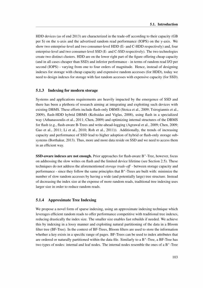
5.1. Introduction
HDD devices (as of end 2013) are characterized in the trade-off according to their capacity (GBper $) on the x-axis and the advertised random read performance (IOPS) on the y-axis. Weshow two enterprise-level and two consumer-level HDD (E- and C-HDD respectively) and, fourenterprise-level and two consumer-level SSD (E- and C-SSD respectively). The two technologiescreate two distinct clusters. HDD are on the lower right part of the figure offering cheap capacity(and in all cases cheaper than SSD) and inferior performance - in terms of random read I/O persecond (IOPS) - varying from one to four orders of magnitude. Hence, instead of designingindexes for storage with cheap capacity and expensive random accesses (for HDD), today weneed to design indexes for storage with fast random accesses with expensive capacity (for SSD).
5.1.3 Indexing for modern storage
Systems and applications requirements are heavily impacted by the emergence of SSD andthere has been a plethora of research aiming at integrating and exploiting such devices withexisting DBMS. These efforts include flash-only DBMS (Stoica et al., 2009; Tsirogiannis et al.,2009), flash-HDD hybrid DBMS (Koltsidas and Viglas, 2008), using flash in a specializedway (Athanassoulis et al., 2011; Chen, 2009) and optimizing internal structures of the DBMSfor flash (e.g., flash-aware B-Trees and write-ahead-logging (Agrawal et al., 2009; Chen, 2009;Gao et al., 2011; Li et al., 2010; Roh et al., 2011)). Additionally, the trends of increasingcapacity and performance of SSD lead to higher adoption of hybrid or flash-only storage sub-systems (Borthakur, 2013). Thus, more and more data reside on SSD and we need to access themin an efficient way.
SSD-aware indexes are not enough. Prior approaches for flash-aware B+-Tree, however, focuson addressing the slow writes on flash and the limited device lifetime (see Section 2.5). Thesetechniques do not address the aforementioned storage trade-off - between storage capacity andperformance - since they follow the same principles that B+-Trees are built with: minimize thenumber of slow random accesses by having a wide (and potentially large) tree structure. Insteadof decreasing the index size at the expense of more random reads, traditional tree indexing useslarger size in order to reduce random reads.
5.1.4 Approximate Tree Indexing
We propose a novel form of sparse indexing, using an approximate indexing technique whichleverages efficient random reads to offer performance competitive with traditional tree indexes,reducing drastically the index size. The smaller size enables fast rebuilds if needed. We achievethis by indexing in a lossy manner and exploiting natural partitioning of the data in a Bloomfilter tree (BF-Tree). In the context of BF-Trees, Bloom filters are used to store the informationwhether a key exists in a specific range of pages. BF-Trees can be used to index attributes thatare ordered or naturally partitioned within the data file. Similarly to a B+-Tree, a BF-Tree hastwo types of nodes: internal and leaf nodes. The internal nodes resemble the ones of a B+-Tree
103
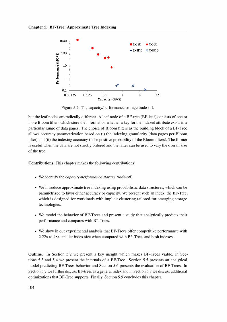
Chapter 5. BF-Tree: Approximate Tree Indexing
Figure 5.2: The capacity/performance storage trade-off.
but the leaf nodes are radically different. A leaf node of a BF-tree (BF-leaf) consists of one ormore Bloom filters which store the information whether a key for the indexed attribute exists in aparticular range of data pages. The choice of Bloom filters as the building block of a BF-Treeallows accuracy parametrization based on (i) the indexing granularity (data pages per Bloomfilter) and (ii) the indexing accuracy (false positive probability of the Bloom filters). The formeris useful when the data are not strictly ordered and the latter can be used to vary the overall sizeof the tree.
Contributions. This chapter makes the following contributions:
• We identify the capacity-performance storage trade-off.
• We introduce approximate tree indexing using probabilistic data structures, which can beparametrized to favor either accuracy or capacity. We present such an index, the BF-Tree,which is designed for workloads with implicit clustering tailored for emerging storagetechnologies.
• We model the behavior of BF-Trees and present a study that analytically predicts theirperformance and compares with B+-Trees.
• We show in our experimental analysis that BF-Trees offer competitive performance with2.22x to 48x smaller index size when compared with B+-Trees and hash indexes.
Outline. In Section 5.2 we present a key insight which makes BF-Trees viable, in Sec-tions 5.3 and 5.4 we present the internals of a BF-Tree. Section 5.5 presents an analyticalmodel predicting BF-Trees behavior and Section 5.6 presents the evaluation of BF-Trees. InSection 5.7 we further discuss BF-trees as a general index and in Section 5.8 we discuss additionaloptimizations that BF-Tree supports. Finally, Section 5.9 concludes this chapter.
104
5.2. Making approximate indexing competitive
5.2 Making approximate indexing competitive
Bloom proposed (Bloom, 1970) BF as a space-efficient probabilistic data structure which supportsmembership tests, with a false positive probability. On the other hand, the small size of a BFallows for its re-computation when needed. Thus, in BF-Trees we do not employ a BF for theentire relation. We use BF to perform a membership test for a specific range, keeping the rangeof values for a single BF small in order to be feasible to recompute it.
Here, we extend the background discussion for BF of Section 2.4 by focusing on a key propertyused to optimize indexing partitioned or ordered data. A BF is comprised of m bits, and it storesmembership information for n elements with false positive probability p. An empty BF is anarray of m bits all set to 0. We need, as well, k different hash functions to be used to map anelement to k different bits during the process of adding an element or checking for membership.When an element is added, the k hash functions are used in order to compute which k out ofm bits have to be set to 1. If a bit is already 1 it maintains this value. To test an element formembership the same k bits are read and, if any of the k bits is equal to 0, then the element isnot in the set. If all k bits are equal to 1 then the element belongs to the set with probability1−p. Assuming optimal number of k hash functions the connection between the BF parametersis approximated by the formula2 (Tarkoma et al., 2012):
n =−m · l n2(2)
l n(p)(5.1)
From this formula we can derive some useful properties:
1. If a BF with size M bits can store the membership information of N elements with falsepositive p, then S BFs with size M
S bits each can store the membership information of NS
elements each with the same p.
2. Decreasing the probability of false positives has a logarithmic effect on the number ofelements we can index using a given space budget (i.e., number of bits).
Property (1) allows to divide the index into smaller BFs that incorporate location information.This process is done hierarchically and is presented in Section 5.3 and Section 5.4. We presenta tree structure with a large BF per leaf, which contains membership information, and internalnodes which help navigating to the desired range before we do the membership test. Each leafnode corresponds to a number of data pages and upon positive membership test we have to searchthese data pages for the desired values. In Section 5.4 we describe how we can store locationinformation more efficiently by storing one – small – BF per data page in the leaf nodes. The leafnode now consists of several BFs which can be checked in parallel and produce the list of datapages to be read more efficiently.
2When modelling the behavior of a BF we will use the given formula unless otherwise stated.
105
Chapter 5. BF-Tree: Approximate Tree Indexing
5.3 Bloom Filter Tree (BF-Tree)
In this section we describe in detail the structure of a BF-tree, highlighting its differences from atypical B+-Tree.
5.3.1 BF-Tree architecture
A BF-tree consists of nodes of two different types. The root and the internal nodes have the samemorphology as a typical B+-Tree node: they contain a list of keys with pointers to other nodesbetween each pair of keys (see Figure 5.3). If the referenced node is internal then it has exactlythe same structure. The leaf nodes (BF-leaves), however, are different. Each leaf node contains aBF which can be used to test any key in the corresponding range of the node, for key membership.Finally, each leaf node contains a list of pairs <key, page id> which is used to enhance the search,called run indexes. The run indexes serve as barriers dividing a range of pages in partitions basedon the key value, hence, both keys and page ids are ordered. Note that the data does not need tobe ordered for a partition scheme to hold, since the run indexes serve as fences. The assumptionis that, for each BF-leaf, we know either implicitly or explicitly a sub-range of pages that we needto search in if the key in question is found to exist according to the BF. This data organizationexists when the data are ordered on the indexing key or partitioned using the indexing key. Incases of composite indexing keys, or for attributes that have values correlated with the order ofthe data, such an assumption can hold for more than one index.
BF-leaf. For simplicity and compatibility with the existing framework, the root, the internalnodes and the leaf nodes have the same size (typically either 4KB or 8KB, we will assume 4KBin the following discussion). The BF of a BF-leaf contains the membership information of thevalues of a specific key in a range of pages. Assuming that the run indexes of a given BF-leaf are< k1, p1 >, . . . ,< kn , pn > the membership test will answer whether a key which has value in theinterval [k1,kn] exists within the range of pages p1, . . . , pn . The run indexes can further assist thesearch once the membership test is positive to eliminate searching in pages which contain keysout of the desired range. In every BF-leaf (Figure 5.4(a)) we store the following information:
• The smallest key of the node’s BF: min_key.
• The largest key of the node’s BF: max_key.
• The number of currently indexed elements: #keys.
• A pointer to the next BF3: next_BFleaf.
• The actual BF to perform the membership test.
• A list of keys and page ids which partition the corresponding contiguous pages into smallersets of pages that contain sub-ranges of the leaf’s range: run indexes.
3Useful for bulk loading, the pointers between BF-Tree leaf nodes are similar to pointers between B+-Trees leafnodes.
106
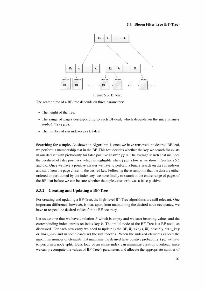
5.3. Bloom Filter Tree (BF-Tree)
Figure 5.3: BF-tree
The search time of a BF-tree depends on three parameters:
• The height of the tree.
• The range of pages corresponding to each BF-leaf, which depends on the false positiveprobability ( f pp).
• The number of run indexes per BF-leaf.
Searching for a tuple. As shown in Algorithm 1, once we have retrieved the desired BF-leaf,we perform a membership test in the BF. This test decides whether the key we search for existsin our dataset with probability for false positive answer f pp. The average search cost includesthe overhead of false positives, which is negligible when f pp is low as we show in Sections 5.5and 5.6. Once we have a positive answer we have to perform a binary search on the run indexesand start from the page closer to the desired key. Following the assumption that the data are eitherordered or partitioned by the index key, we have finally to search in the entire range of pages ofthe BF-leaf before we can be sure whether the tuple exists or it was a false positive.
5.3.2 Creating and Updating a BF-Tree
For creating and updating a BF-Tree, the high-level B+-Tree algorithms are still relevant. Oneimportant difference, however, is that, apart from maintaining the desired node occupancy, wehave to respect the desired values for the BF accuracy.
Let us assume that we have a relation R which is empty and we start inserting values and thecorresponding index entries on index key k. The initial node of the BF-Tree is a BF node, asdiscussed. For each new entry we need to update i) the BF, ii) #ke y s, iii) possibly mi n_ke y
or max_ke y and in some cases iv) the run indexes. When the indexed elements exceed themaximum number of elements that maintains the desired false positive probability f pp we haveto perform a node split. Bulk load of an entire index can minimize creation overhead sincewe can precompute the values of BF-Tree’s parameters and allocate the appropriate number of
107

Chapter 5. BF-Tree: Approximate Tree Indexing
ALGORITHM 1: Search using a BF-TreeSearch key k using BF-Tree
1: Binary search of root node; read the appropriate child node.2: Recursive search the values of the internal node, read the appropriate child node until a leaf is
reached.3: Read mi n_ke y and max_ke y from the leaf node.4: if Key k between mi n_ke y and max_ke y then5: Probe BF with key k.6: if Key k exists in BF then7: Binary search the run indexes.8: Search within the matching data pages for the key (false positive with f pp).9: else
10: Key k does not exist.11: end if12: else13: Key k does not exist.14: end if
nodes more efficiently. If the tree is in update-intensive mode, each node can maintain a list ofinserted/deleted/updated keys (along with their page information) in order to accumulate enoughnumber of such operations to amortize the cost of updating the BF.
ALGORITHM 2: Split a BF-Tree nodeSplit a BF-Tree node N to N1, N2
1: Read mi n_ke y and max_ke y of the node to be split.2: Create new nodes N1 and N2.3: Node split may need to propagate.4: for k = mi n_ke y to max_ke y do5: if Key k exists then6: if Less than half N ’s ∈ N1 then7: Update mi n_ke y , max_ke y , #ke y s and r un_i ndexes of N1 and insert k in N1’s BF.8: else9: Update mi n_ke y , max_ke y , #ke y s and r un_i ndexes of N2 and insert k in N2’s BF.
10: end if11: end if12: end for
The lossy way to keep indexing information for a BF-Tree increases the cost of splitting a BF-leaf.Algorithm 2 shows that in order to split a BF-leaf we need to probe the initial node for all indexedvalues. Thus, splitting a leaf node is computationally expensive, but it can be accelerated becauseit is heavily parallelizable. During a node split several threads can probe the BF of the old nodein order to create the BF of the new nodes.
Algorithm 3 shows how to perform an insert in a BF-Tree. After navigating towards the BF-leafin question, we check the BF-leaf size. If this leaf has already indexed the maximum number ofvalues then we perform a node split as described above. After this step, the values of the BF-leafvariables are updated. First, we increase the number of keys (#ke y s). Second, we may need
108
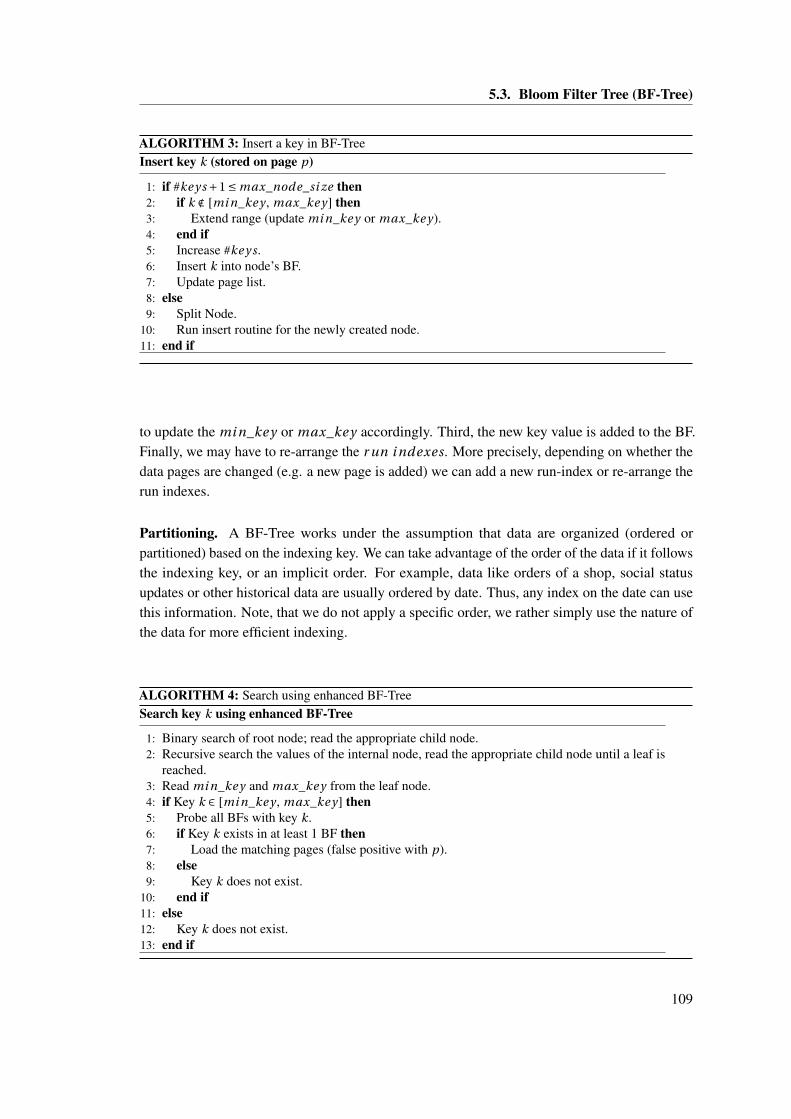
5.3. Bloom Filter Tree (BF-Tree)
ALGORITHM 3: Insert a key in BF-TreeInsert key k (stored on page p)
1: if #ke y s +1 ≤ max_node_si ze then2: if k ∉ [mi n_ke y , max_ke y] then3: Extend range (update mi n_ke y or max_ke y).4: end if5: Increase #ke y s.6: Insert k into node’s BF.7: Update page list.8: else9: Split Node.
10: Run insert routine for the newly created node.11: end if
to update the mi n_ke y or max_ke y accordingly. Third, the new key value is added to the BF.Finally, we may have to re-arrange the r un i ndexes. More precisely, depending on whether thedata pages are changed (e.g. a new page is added) we can add a new run-index or re-arrange therun indexes.
Partitioning. A BF-Tree works under the assumption that data are organized (ordered orpartitioned) based on the indexing key. We can take advantage of the order of the data if it followsthe indexing key, or an implicit order. For example, data like orders of a shop, social statusupdates or other historical data are usually ordered by date. Thus, any index on the date can usethis information. Note, that we do not apply a specific order, we rather simply use the nature ofthe data for more efficient indexing.
ALGORITHM 4: Search using enhanced BF-TreeSearch key k using enhanced BF-Tree
1: Binary search of root node; read the appropriate child node.2: Recursive search the values of the internal node, read the appropriate child node until a leaf is
reached.3: Read mi n_ke y and max_ke y from the leaf node.4: if Key k ∈ [mi n_ke y , max_ke y] then5: Probe all BFs with key k.6: if Key k exists in at least 1 BF then7: Load the matching pages (false positive with p).8: else9: Key k does not exist.
10: end if11: else12: Key k does not exist.13: end if
109
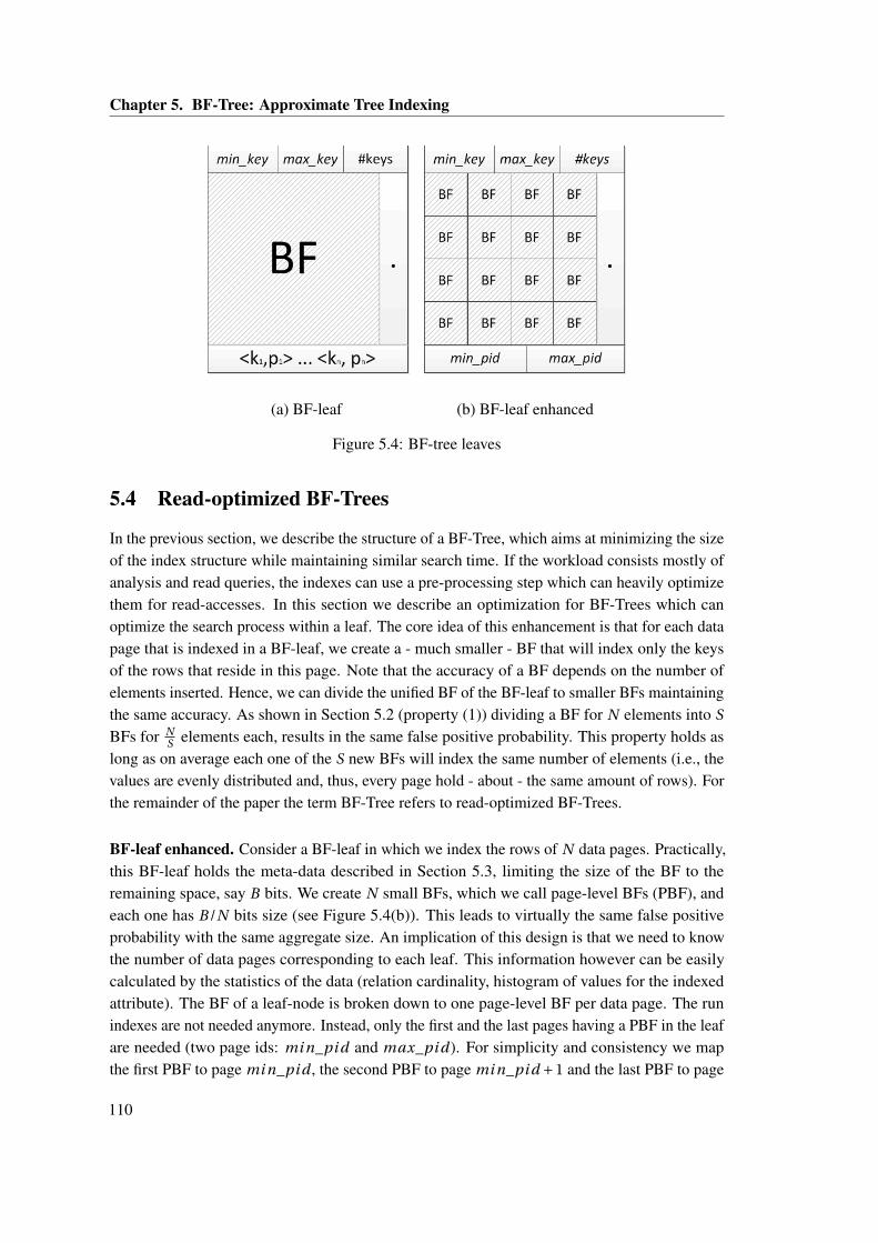
Chapter 5. BF-Tree: Approximate Tree Indexing
(a) BF-leaf (b) BF-leaf enhanced
Figure 5.4: BF-tree leaves
5.4 Read-optimized BF-Trees
In the previous section, we describe the structure of a BF-Tree, which aims at minimizing the sizeof the index structure while maintaining similar search time. If the workload consists mostly ofanalysis and read queries, the indexes can use a pre-processing step which can heavily optimizethem for read-accesses. In this section we describe an optimization for BF-Trees which canoptimize the search process within a leaf. The core idea of this enhancement is that for each datapage that is indexed in a BF-leaf, we create a - much smaller - BF that will index only the keysof the rows that reside in this page. Note that the accuracy of a BF depends on the number ofelements inserted. Hence, we can divide the unified BF of the BF-leaf to smaller BFs maintainingthe same accuracy. As shown in Section 5.2 (property (1)) dividing a BF for N elements into S
BFs for NS elements each, results in the same false positive probability. This property holds as
long as on average each one of the S new BFs will index the same number of elements (i.e., thevalues are evenly distributed and, thus, every page hold - about - the same amount of rows). Forthe remainder of the paper the term BF-Tree refers to read-optimized BF-Trees.
BF-leaf enhanced. Consider a BF-leaf in which we index the rows of N data pages. Practically,this BF-leaf holds the meta-data described in Section 5.3, limiting the size of the BF to theremaining space, say B bits. We create N small BFs, which we call page-level BFs (PBF), andeach one has B/N bits size (see Figure 5.4(b)). This leads to virtually the same false positiveprobability with the same aggregate size. An implication of this design is that we need to knowthe number of data pages corresponding to each leaf. This information however can be easilycalculated by the statistics of the data (relation cardinality, histogram of values for the indexedattribute). The BF of a leaf-node is broken down to one page-level BF per data page. The runindexes are not needed anymore. Instead, only the first and the last pages having a PBF in the leafare needed (two page ids: mi n_pi d and max_pi d). For simplicity and consistency we mapthe first PBF to page mi n_pi d , the second PBF to page mi n_pi d +1 and the last PBF to page
110
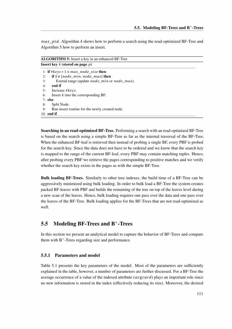
5.5. Modeling BF-Trees and B+-Trees
max_pi d . Algorithm 4 shows how to perform a search using the read-optimized BF-Tree andAlgorithm 5 how to perform an insert.
ALGORITHM 5: Insert a key in an enhanced BF-TreeInsert key k (stored on page p)
1: if #ke y s +1 ≤ max_node_si ze then2: if k ∉ [node_mi n, node_max] then3: Extend range (update node_mi n or node_max).4: end if5: Increase #ke y s.6: Insert k into the corresponding BF.7: else8: Split Node.9: Run insert routine for the newly created node.
10: end if
Searching in an read-optimized BF-Tree. Performing a search with an read-optimized BF-Treeis based on the search using a simple BF-Tree as far as the internal traversal of the BF-Tree.When the enhanced BF-leaf is retrieved then instead of probing a single BF, every PBF is probedfor the search key. Since the data does not have to be ordered and we know that the search keyis mapped to the range of the current BF-leaf, every PBF may contain matching tuples. Hence,after probing every PBF we retrieve the pages corresponding to positive matches and we verifywhether the search key exists in the pages as with the simple BF-Tree.
Bulk loading BF-Trees. Similarly to other tree indexes, the build time of a BF-Tree can beaggressively minimized using bulk loading. In order to bulk load a BF-Tree the system createspacked BF-leaves with PBF and builds the remaining of the tree on top of the leaves level duringa new scan of the leaves. Hence, bulk loading requires one pass over the data and one pass overthe leaves of the BF-Tree. Bulk loading applies for the BF-Trees that are not read-optimized aswell.
5.5 Modeling BF-Trees and B+-Trees
In this section we present an analytical model to capture the behavior of BF-Trees and comparethem with B+-Trees regarding size and performance.
5.5.1 Parameters and model
Table 5.1 presents the key parameters of the model. Most of the parameters are sufficientlyexplained in the table, however, a number of parameters are further discussed. For a BF-Tree theaverage occurrence of a value of the indexed attribute (av g car d) plays an important role sinceno new information is stored in the index (effectively reducing its size). Moreover, the desired
111
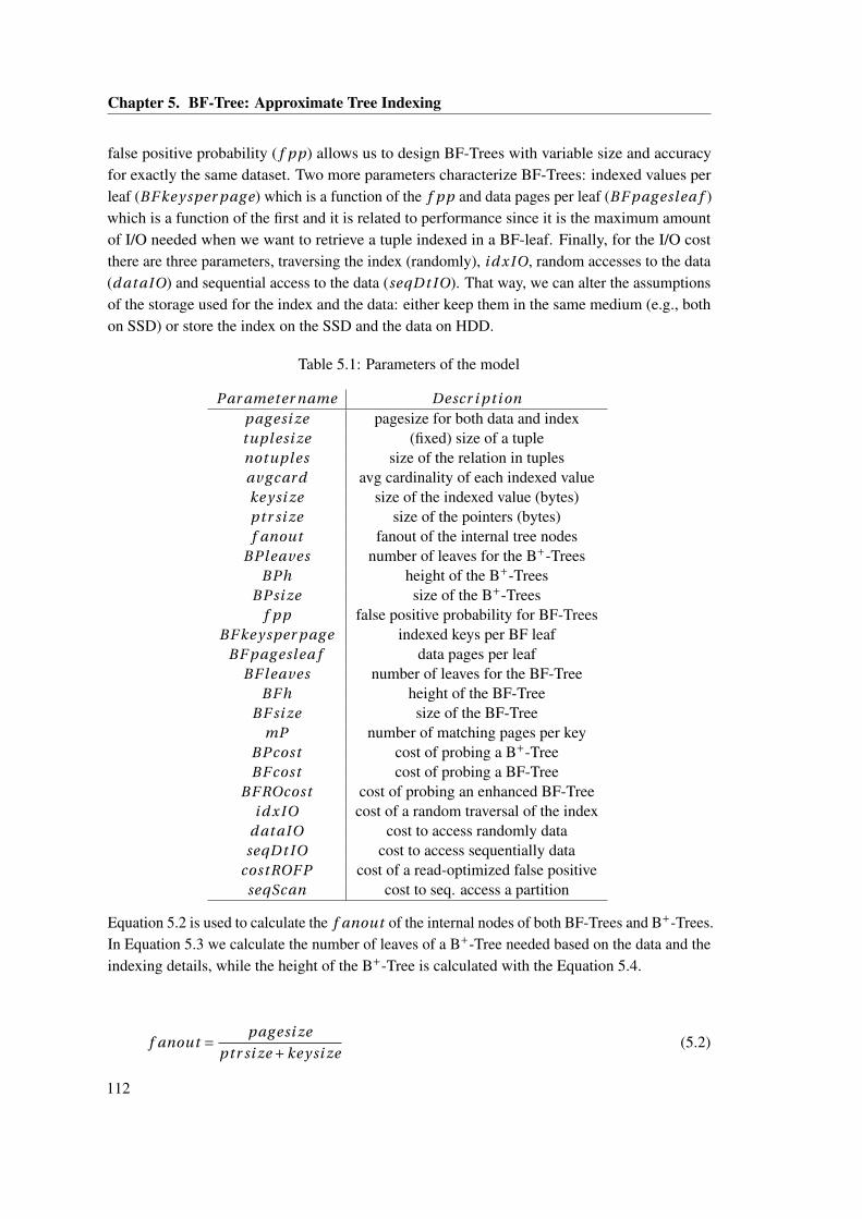
Chapter 5. BF-Tree: Approximate Tree Indexing
false positive probability ( f pp) allows us to design BF-Trees with variable size and accuracyfor exactly the same dataset. Two more parameters characterize BF-Trees: indexed values perleaf (BF ke y sper pag e) which is a function of the f pp and data pages per leaf (BF pag eslea f )which is a function of the first and it is related to performance since it is the maximum amountof I/O needed when we want to retrieve a tuple indexed in a BF-leaf. Finally, for the I/O costthere are three parameters, traversing the index (randomly), i d xIO, random accesses to the data(d at aIO) and sequential access to the data (seqDt IO). That way, we can alter the assumptionsof the storage used for the index and the data: either keep them in the same medium (e.g., bothon SSD) or store the index on the SSD and the data on HDD.
Table 5.1: Parameters of the model
Par ameter name Descr i pti onpag esi ze pagesize for both data and indextuplesi ze (fixed) size of a tuplenotuples size of the relation in tuplesav g car d avg cardinality of each indexed valueke y si ze size of the indexed value (bytes)ptr si ze size of the pointers (bytes)f anout fanout of the internal tree nodes
BPl eaves number of leaves for the B+-TreesBPh height of the B+-Trees
BPsi ze size of the B+-Treesf pp false positive probability for BF-Trees
BF ke y sper pag e indexed keys per BF leafBF pag eslea f data pages per leaf
BF l eaves number of leaves for the BF-TreeBF h height of the BF-Tree
BF si ze size of the BF-TreemP number of matching pages per key
BPcost cost of probing a B+-TreeBF cost cost of probing a BF-Tree
BF ROcost cost of probing an enhanced BF-Treei d xIO cost of a random traversal of the index
d at aIO cost to access randomly dataseqDt IO cost to access sequentially data
costROF P cost of a read-optimized false positiveseqScan cost to seq. access a partition
Equation 5.2 is used to calculate the f anout of the internal nodes of both BF-Trees and B+-Trees.In Equation 5.3 we calculate the number of leaves of a B+-Tree needed based on the data and theindexing details, while the height of the B+-Tree is calculated with the Equation 5.4.
f anout = pag esi ze
ptr si ze +ke y si ze(5.2)
112
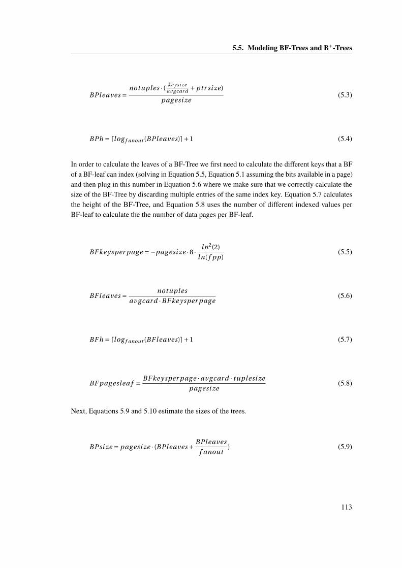
5.5. Modeling BF-Trees and B+-Trees
BPl eaves =notuples · ( ke y si ze
av g car d +ptr si ze)
pag esi ze(5.3)
BPh = dlog f anout (BPl eaves)e+1 (5.4)
In order to calculate the leaves of a BF-Tree we first need to calculate the different keys that a BFof a BF-leaf can index (solving in Equation 5.5, Equation 5.1 assuming the bits available in a page)and then plug in this number in Equation 5.6 where we make sure that we correctly calculate thesize of the BF-Tree by discarding multiple entries of the same index key. Equation 5.7 calculatesthe height of the BF-Tree, and Equation 5.8 uses the number of different indexed values perBF-leaf to calculate the the number of data pages per BF-leaf.
BF ke y sper pag e =−pag esi ze ·8 · ln2(2)
ln( f pp)(5.5)
BF l eaves = notuples
av g car d ·BF ke y sper pag e(5.6)
BF h = dlog f anout (BF l eaves)e+1 (5.7)
BF pag eslea f = BF ke y sper pag e ·av g car d · tuplesi ze
pag esi ze(5.8)
Next, Equations 5.9 and 5.10 estimate the sizes of the trees.
BPsi ze = pag esi ze · (BPl eaves + BPl eaves
f anout) (5.9)
113
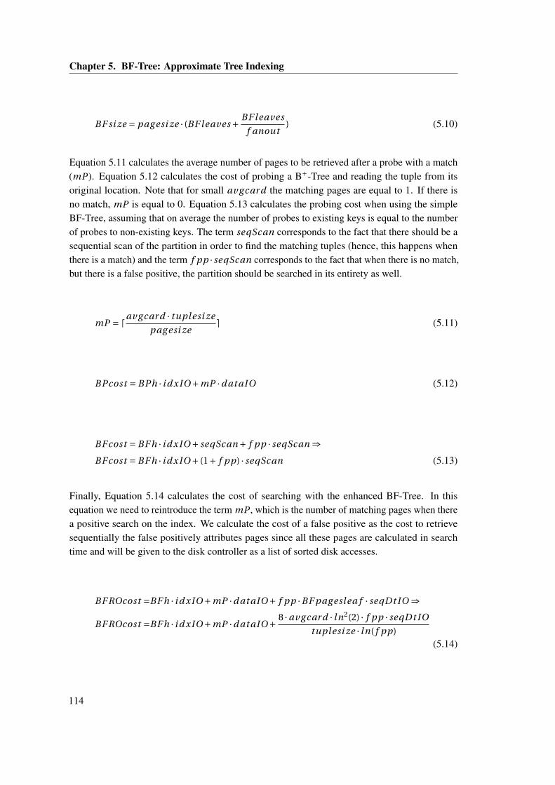
Chapter 5. BF-Tree: Approximate Tree Indexing
BF si ze = pag esi ze · (BF l eaves + BF l eaves
f anout) (5.10)
Equation 5.11 calculates the average number of pages to be retrieved after a probe with a match(mP). Equation 5.12 calculates the cost of probing a B+-Tree and reading the tuple from itsoriginal location. Note that for small av g car d the matching pages are equal to 1. If there isno match, mP is equal to 0. Equation 5.13 calculates the probing cost when using the simpleBF-Tree, assuming that on average the number of probes to existing keys is equal to the numberof probes to non-existing keys. The term seqScan corresponds to the fact that there should be asequential scan of the partition in order to find the matching tuples (hence, this happens whenthere is a match) and the term f pp · seqScan corresponds to the fact that when there is no match,but there is a false positive, the partition should be searched in its entirety as well.
mP = dav g car d · tuplesi ze
pag esi zee (5.11)
BPcost = BPh · i d xIO +mP ·d at aIO (5.12)
BF cost = BF h · i d xIO + seqScan + f pp · seqScan ⇒BF cost = BF h · i d xIO + (1+ f pp) · seqScan (5.13)
Finally, Equation 5.14 calculates the cost of searching with the enhanced BF-Tree. In thisequation we need to reintroduce the term mP , which is the number of matching pages when therea positive search on the index. We calculate the cost of a false positive as the cost to retrievesequentially the false positively attributes pages since all these pages are calculated in searchtime and will be given to the disk controller as a list of sorted disk accesses.
BF ROcost =BF h · i d xIO +mP ·d at aIO + f pp ·BF pag eslea f · seqDt IO ⇒
BF ROcost =BF h · i d xIO +mP ·d at aIO + 8 ·av g car d · ln2(2) · f pp · seqDt IO
tuplesi ze · ln( f pp)(5.14)
114
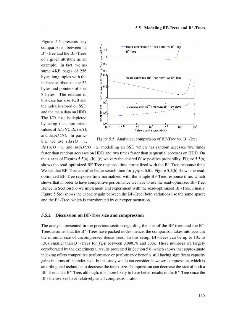
5.5. Modeling BF-Trees and B+-Trees
Figure 5.5: Analytical comparison of BF-Tree vs. B+-Tree.
Figure 5.5 presents keycomparisons between aB+-Tree and the BF-Treesof a given attribute as anexample. In fact, we as-sume 4KB pages of 256bytes long tuples with theindexed attribute of size 32bytes and pointers of size8 bytes. The relation inthis case has size 1GB andthe index is stored on SSDand the main data on HDD.The I/O cost is depictedby using the appropriatevalues of i d xIO, d at aIO,and seqDt IO. In partic-ular we use i d xIO = 1,d at aIO = 5, and seqDt IO = 2, modelling an SSD which has random accesses five timesfaster than random accesses on HDD and two times faster than sequential accesses on HDD. Onthe x axes of Figures 5.5(a), (b), (c) we vary the desired false positive probability. Figure 5.5(a)shows the read-optimized BF-Tree response time normalized with the B+-Tree response time.We see that BF-Tree can offer better search time for f pp ≤ 0.01. Figure 5.5(b) shows the read-optimized BF-Tree response time normalized with the simple BF-Tree response time, whichshows that in order to have competitive performance we have to use the read-optimized BF-Tree.Hence in Section 5.6 we implement and experiment with the read-optimized BF-Tree. Finally,Figure 5.5(c) shows the capacity gain between the BF-Tree (both variations use the same space)and the B+-Tree, which is corroborated by our experimentation.
5.5.2 Discussion on BF-Tree size and compression
The analysis presented in the previous section regarding the size of the BF-trees and the B+-Trees assumes that the B+-Trees have packed nodes, hence, the comparison takes into accountthe minimal size of uncompressed dense trees. In this setup, BF-Trees can be up to 10x to130x smaller than B+-Trees for f pp between 0.0001% and 30%. These numbers are largelycorroborated by the experimental results presented in Section 5.6, which shows that approximateindexing offers competitive performance or performance benefits still having significant capacitygains in terms of the index size. In this study we do not consider, however, compression, which isan orthogonal technique to decrease the index size. Compression can decrease the size of both aBF-Tree and a B+-Tree, although, it is more likely to have better results in the B+-Tree since theBFs themselves have relatively small compression ratio.
115
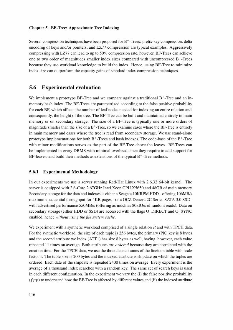
Chapter 5. BF-Tree: Approximate Tree Indexing
Several compression techniques have been proposed for B+-Trees: prefix-key compression, deltaencoding of keys and/or pointers, and LZ77 compression are typical examples. Aggressivelycompressing with LZ77 can lead to up to 50% compression rate, however, BF-Trees can achieveone to two order of magnitudes smaller index sizes compared with uncompressed B+-Treesbecause they use workload knowledge to build the index. Hence, using BF-Tree to minimizeindex size can outperform the capacity gains of standard index compression techniques.
5.6 Experimental evaluation
We implement a prototype BF-Tree and we compare against a traditional B+-Tree and an in-memory hash index. The BF-Trees are parametrized according to the false positive probabilityfor each BF, which affects the number of leaf nodes needed for indexing an entire relation and,consequently, the height of the tree. The BF-Tree can be built and maintained entirely in mainmemory or on secondary storage. The size of a BF-Tree is typically one or more orders ofmagnitude smaller than the size of a B+-Tree, so we examine cases where the BF-Tree is entirelyin main memory and cases where the tree is read from secondary storage. We use stand-aloneprototype implementations for both B+-Trees and hash indexes. The code-base of the B+-Treewith minor modifications serves as the part of the BF-Tree above the leaves. BF-Trees canbe implemented in every DBMS with minimal overhead since they require to add support forBF-leaves, and build their methods as extensions of the typical B+-Tree methods.
5.6.1 Experimental Methodology
In our experiments we use a server running Red-Hat Linux with 2.6.32 64-bit kernel. Theserver is equipped with 2 6-Core 2.67GHz Intel Xeon CPU X5650 and 48GB of main memory.Secondary storage for the data and indexes is either a Seagate 10KRPM HDD - offering 106MB/smaximum sequential throughput for 4KB pages - or a OCZ Deneva 2C Series SATA 3.0 SSD -with advertised performance 550MB/s (offering as much as 80kIO/s of random reads). Data onsecondary storage (either HDD or SSD) are accessed with the flags O_DIRECT and O_SYNCenabled, hence without using the file system cache.
We experiment with a synthetic workload comprised of a single relation R and with TPCH data.For the synthetic workload, the size of each tuple is 256 bytes, the primary (PK) key is 8 bytesand the second attribute we index (ATT1) has size 8 bytes as well, having, however, each valuerepeated 11 times on average. Both attributes are ordered because they are correlated with thecreation time. For the TPCH data, we use the three date columns of the lineitem table with scalefactor 1. The tuple size is 200 bytes and the indexed attribute is shipdate on which the tuples areordered. Each date of the shipdate is repeated 2400 times on average. Every experiment is theaverage of a thousand index searches with a random key. The same set of search keys is usedin each different configuration. In the experiment we vary the (i) the false positive probability( f pp) to understand how the BF-Tree is affected by different values and (ii) the indexed attribute
116
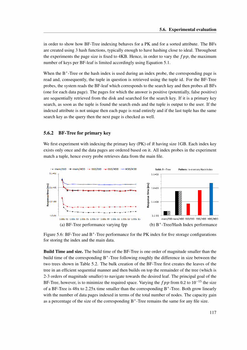
5.6. Experimental evaluation
in order to show how BF-Tree indexing behaves for a PK and for a sorted attribute. The BFsare created using 3 hash functions, typically enough to have hashing close to ideal. Throughoutthe experiments the page size is fixed to 4KB. Hence, in order to vary the f pp, the maximumnumber of keys per BF-leaf is limited accordingly using Equation 5.1.
When the B+-Tree or the hash index is used during an index probe, the corresponding page isread and, consequently, the tuple in question is retrieved using the tuple id. For the BF-Treeprobes, the system reads the BF-leaf which corresponds to the search key and then probes all BFs(one for each data page). The pages for which the answer is positive (potentially, false positive)are sequentially retrieved from the disk and searched for the search key. If it is a primary keysearch, as soon as the tuple is found the search ends and the tuple is output to the user. If theindexed attribute is not unique then each page is read entirely and if the last tuple has the samesearch key as the query then the next page is checked as well.
5.6.2 BF-Tree for primary key
We first experiment with indexing the primary key (PK) of R having size 1GB. Each index keyexists only once and the data pages are ordered based on it. All index probes in the experimentmatch a tuple, hence every probe retrieves data from the main file.
(a) BF-Tree performance varying fpp (b) B+-Tree/Hash Index performance
Figure 5.6: BF-Tree and B+-Tree performance for the PK index for five storage configurationsfor storing the index and the main data.
Build Time and size. The build time of the BF-Tree is one order of magnitude smaller than thebuild time of the corresponding B+-Tree following roughly the difference in size between thetwo trees shown in Table 5.2. The bulk creation of the BF-Tree first creates the leaves of thetree in an efficient sequential manner and then builds on top the remainder of the tree (which is2-3 orders of magnitude smaller) to navigate towards the desired leaf. The principal goal of theBF-Tree, however, is to minimize the required space. Varying the f pp from 0.2 to 10−15 the sizeof a BF-Tree is 48x to 2.25x time smaller than the corresponding B+-Tree. Both grow linearlywith the number of data pages indexed in terms of the total number of nodes. The capacity gainas a percentage of the size of the corresponding B+-Tree remains the same for any file size.
117
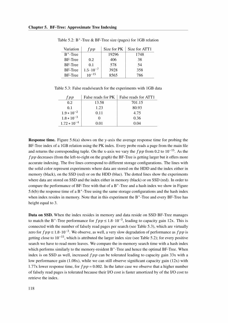
Chapter 5. BF-Tree: Approximate Tree Indexing
Table 5.2: B+-Tree & BF-Tree size (pages) for 1GB relation
Variation f pp Size for PK Size for ATT1B+-Tree 19296 1748BF-Tree 0.2 406 38BF-Tree 0.1 578 54BF-Tree 1.5 ·10−7 3928 358BF-Tree 10−15 8565 786
Table 5.3: False reads/search for the experiments with 1GB data
f pp False reads for PK False reads for ATT10.2 13.58 701.150.1 1.23 80.93
1.9∗10−2 0.11 4.751.8∗10−3 0 0.36
1.72∗10−4 0.01 0.04
Response time. Figure 5.6(a) shows on the y-axis the average response time for probing theBF-Tree index of a 1GB relation using the PK index. Every probe reads a page from the main fileand returns the corresponding tuple. On the x-axis we vary the f pp from 0.2 to 10−15. As thef pp decreases (from the left-to-right on the graph) the BF-Tree is getting larger but it offers moreaccurate indexing. The five lines correspond to different storage configurations. The lines withthe solid color represent experiments where data are stored on the HDD and the index either inmemory (black), on the SSD (red) or on the HDD (blue). The dotted lines show the experimentswhere data are stored on SSD and the index either in memory (black) or on SSD (red). In order tocompare the performance of BF-Tree with that of a B+-Tree and a hash index we show in Figure5.6(b) the response time of a B+-Tree using the same storage configurations and the hash indexwhen index resides in memory. Note that in this experiment the B+-Tree and every BF-Tree hasheight equal to 3.
Data on SSD. When the index resides in memory and data reside on SSD BF-Tree managesto match the B+-Tree performance for f pp ≤ 1.8 ·10−3, leading to capacity gain 12x. This isconnected with the number of falsely read pages per search (see Table 5.3), which are virtuallyzero for f pp ≤ 1.8 ·10−3. We observe, as well, a very slow degradation of performance as f pp isgetting close to 10−15, which is attributed the larger index size (see Table 5.2); for every positivesearch we have to read more leaves. We compare the in-memory search time with a hash indexwhich performs similarly to the memory-resident B+-Tree and hence the optimal BF-Tree. Whenindex is on SSD as well, increased f pp can be tolerated leading to capacity gain 33x with alow performance gain (1.08x), while we can still observe significant capacity gain (12x) with1.77x lower response time, for f pp = 0.002. In the latter case we observe that a higher numberof falsely read pages is tolerated because their I/O cost is faster amortized by of the I/O cost toretrieve the index.
118
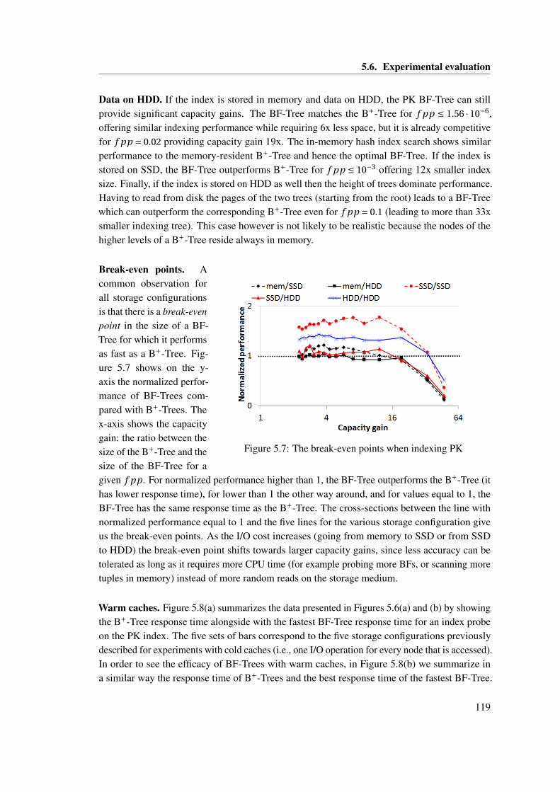
5.6. Experimental evaluation
Data on HDD. If the index is stored in memory and data on HDD, the PK BF-Tree can stillprovide significant capacity gains. The BF-Tree matches the B+-Tree for f pp ≤ 1.56 · 10−6,offering similar indexing performance while requiring 6x less space, but it is already competitivefor f pp = 0.02 providing capacity gain 19x. The in-memory hash index search shows similarperformance to the memory-resident B+-Tree and hence the optimal BF-Tree. If the index isstored on SSD, the BF-Tree outperforms B+-Tree for f pp ≤ 10−3 offering 12x smaller indexsize. Finally, if the index is stored on HDD as well then the height of trees dominate performance.Having to read from disk the pages of the two trees (starting from the root) leads to a BF-Treewhich can outperform the corresponding B+-Tree even for f pp = 0.1 (leading to more than 33xsmaller indexing tree). This case however is not likely to be realistic because the nodes of thehigher levels of a B+-Tree reside always in memory.
Figure 5.7: The break-even points when indexing PK
Break-even points. Acommon observation forall storage configurationsis that there is a break-evenpoint in the size of a BF-Tree for which it performsas fast as a B+-Tree. Fig-ure 5.7 shows on the y-axis the normalized perfor-mance of BF-Trees com-pared with B+-Trees. Thex-axis shows the capacitygain: the ratio between thesize of the B+-Tree and thesize of the BF-Tree for agiven f pp. For normalized performance higher than 1, the BF-Tree outperforms the B+-Tree (ithas lower response time), for lower than 1 the other way around, and for values equal to 1, theBF-Tree has the same response time as the B+-Tree. The cross-sections between the line withnormalized performance equal to 1 and the five lines for the various storage configuration giveus the break-even points. As the I/O cost increases (going from memory to SSD or from SSDto HDD) the break-even point shifts towards larger capacity gains, since less accuracy can betolerated as long as it requires more CPU time (for example probing more BFs, or scanning moretuples in memory) instead of more random reads on the storage medium.
Warm caches. Figure 5.8(a) summarizes the data presented in Figures 5.6(a) and (b) by showingthe B+-Tree response time alongside with the fastest BF-Tree response time for an index probeon the PK index. The five sets of bars correspond to the five storage configurations previouslydescribed for experiments with cold caches (i.e., one I/O operation for every node that is accessed).In order to see the efficacy of BF-Trees with warm caches, in Figure 5.8(b) we summarize ina similar way the response time of B+-Trees and the best response time of the fastest BF-Tree.
119
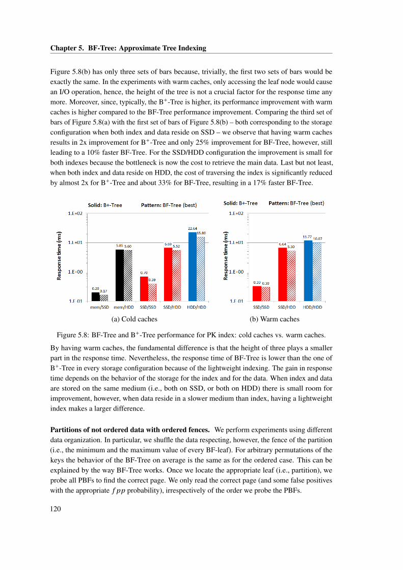
Chapter 5. BF-Tree: Approximate Tree Indexing
Figure 5.8(b) has only three sets of bars because, trivially, the first two sets of bars would beexactly the same. In the experiments with warm caches, only accessing the leaf node would causean I/O operation, hence, the height of the tree is not a crucial factor for the response time anymore. Moreover, since, typically, the B+-Tree is higher, its performance improvement with warmcaches is higher compared to the BF-Tree performance improvement. Comparing the third set ofbars of Figure 5.8(a) with the first set of bars of Figure 5.8(b) – both corresponding to the storageconfiguration when both index and data reside on SSD – we observe that having warm cachesresults in 2x improvement for B+-Tree and only 25% improvement for BF-Tree, however, stillleading to a 10% faster BF-Tree. For the SSD/HDD configuration the improvement is small forboth indexes because the bottleneck is now the cost to retrieve the main data. Last but not least,when both index and data reside on HDD, the cost of traversing the index is significantly reducedby almost 2x for B+-Tree and about 33% for BF-Tree, resulting in a 17% faster BF-Tree.
(a) Cold caches (b) Warm caches
Figure 5.8: BF-Tree and B+-Tree performance for PK index: cold caches vs. warm caches.
By having warm caches, the fundamental difference is that the height of three plays a smallerpart in the response time. Nevertheless, the response time of BF-Tree is lower than the one ofB+-Tree in every storage configuration because of the lightweight indexing. The gain in responsetime depends on the behavior of the storage for the index and for the data. When index and dataare stored on the same medium (i.e., both on SSD, or both on HDD) there is small room forimprovement, however, when data reside in a slower medium than index, having a lightweightindex makes a larger difference.
Partitions of not ordered data with ordered fences. We perform experiments using differentdata organization. In particular, we shuffle the data respecting, however, the fence of the partition(i.e., the minimum and the maximum value of every BF-leaf). For arbitrary permutations of thekeys the behavior of the BF-Tree on average is the same as for the ordered case. This can beexplained by the way BF-Tree works. Once we locate the appropriate leaf (i.e., partition), weprobe all PBFs to find the correct page. We only read the correct page (and some false positiveswith the appropriate f pp probability), irrespectively of the order we probe the PBFs.
120
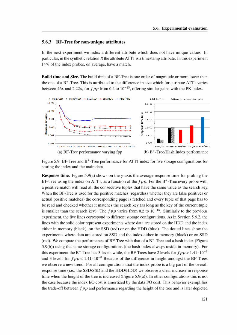
5.6. Experimental evaluation
5.6.3 BF-Tree for non-unique attributes
In the next experiment we index a different attribute which does not have unique values. Inparticular, in the synthetic relation R the attribute ATT1 is a timestamp attribute. In this experiment14% of the index probes, on average, have a match.
Build time and Size. The build time of a BF-Tree is one order of magnitude or more lower thanthe one of a B+-Tree. This is attributed to the difference in size which for attribute ATT1 variesbetween 46x and 2.22x, for f pp from 0.2 to 10−15, offering similar gains with the PK index.
(a) BF-Tree performance varying fpp (b) B+-Tree/Hash Index performance
Figure 5.9: BF-Tree and B+-Tree performance for ATT1 index for five storage configurations forstoring the index and the main data.
Response time. Figure 5.9(a) shows on the y-axis the average response time for probing theBF-Tree using the index on ATT1, as a function of the f pp. For the B+-Tree every probe witha positive match will read all the consecutive tuples that have the same value as the search key.When the BF-Tree is used for the positive matches (regardless whether they are false positives oractual positive matches) the corresponding page is fetched and every tuple of that page has tobe read and checked whether it matches the search key (as long as the key of the current tupleis smaller than the search key). The f pp varies from 0.2 to 10−15. Similarly to the previousexperiment, the five lines correspond to different storage configurations. As in Section 5.6.2, thelines with the solid color represent experiments where data are stored on the HDD and the indexeither in memory (black), on the SSD (red) or on the HDD (blue). The dotted lines show theexperiments where data are stored on SSD and the index either in memory (black) or on SSD(red). We compare the performance of BF-Tree with that of a B+-Tree and a hash index (Figure5.9(b)) using the same storage configurations (the hash index always reside in memory). Forthis experiment the B+-Tree has 3 levels while, the BF-Trees have 2 levels for f pp > 1.41 ·10−8
and 3 levels for f pp ≤ 1.41 ·10−8 Because of the difference in height amongst the BF-Treeswe observe a new trend. For all configurations that the index probe is a big part of the overallresponse time (i.e., the SSD/SSD and the HDD/HDD) we observe a clear increase in responsetime when the height of the tree is increased (Figure 5.9(a)). In other configurations this is notthe case because the index I/O cost is amortized by the data I/O cost. This behavior exemplifiesthe trade-off between f pp and performance regarding the height of the tree and is later depicted
121
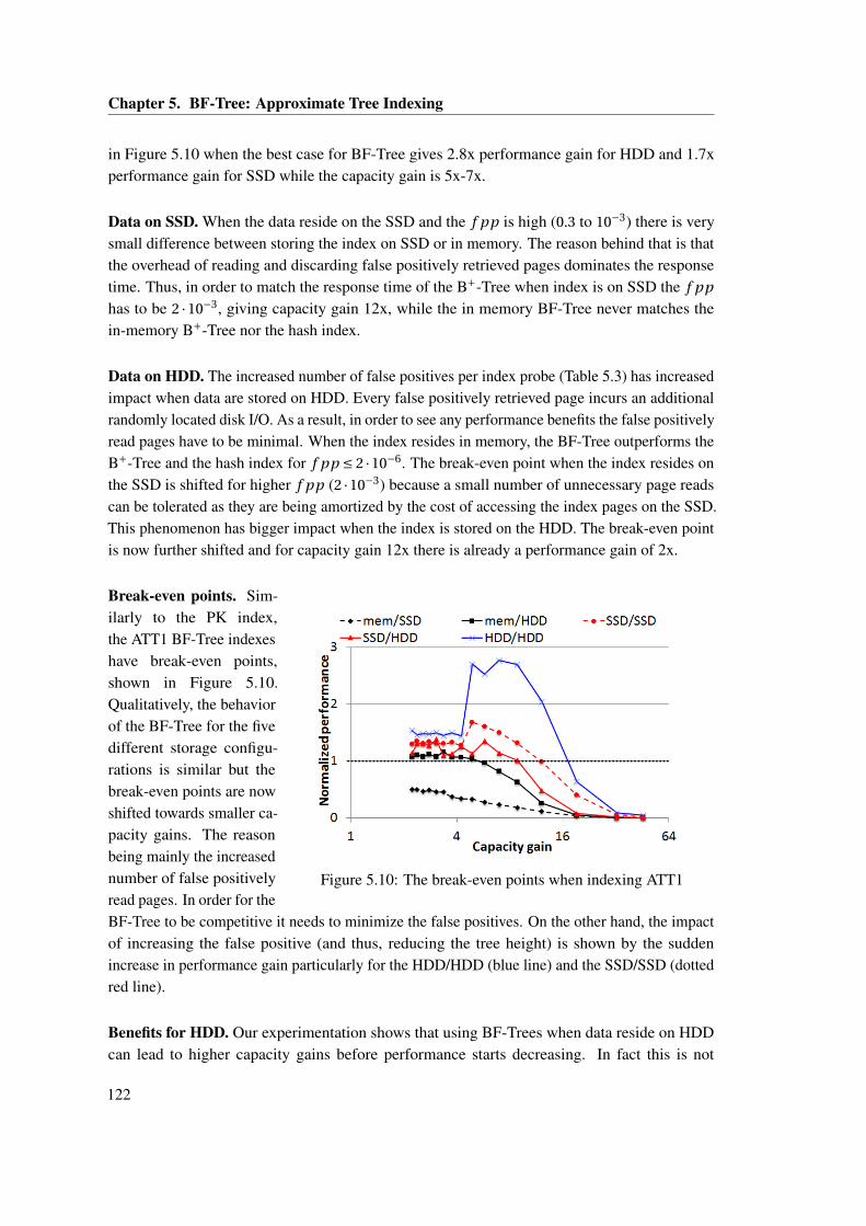
Chapter 5. BF-Tree: Approximate Tree Indexing
in Figure 5.10 when the best case for BF-Tree gives 2.8x performance gain for HDD and 1.7xperformance gain for SSD while the capacity gain is 5x-7x.
Data on SSD. When the data reside on the SSD and the f pp is high (0.3 to 10−3) there is verysmall difference between storing the index on SSD or in memory. The reason behind that is thatthe overhead of reading and discarding false positively retrieved pages dominates the responsetime. Thus, in order to match the response time of the B+-Tree when index is on SSD the f pp
has to be 2 ·10−3, giving capacity gain 12x, while the in memory BF-Tree never matches thein-memory B+-Tree nor the hash index.
Data on HDD. The increased number of false positives per index probe (Table 5.3) has increasedimpact when data are stored on HDD. Every false positively retrieved page incurs an additionalrandomly located disk I/O. As a result, in order to see any performance benefits the false positivelyread pages have to be minimal. When the index resides in memory, the BF-Tree outperforms theB+-Tree and the hash index for f pp ≤ 2 ·10−6. The break-even point when the index resides onthe SSD is shifted for higher f pp (2 ·10−3) because a small number of unnecessary page readscan be tolerated as they are being amortized by the cost of accessing the index pages on the SSD.This phenomenon has bigger impact when the index is stored on the HDD. The break-even pointis now further shifted and for capacity gain 12x there is already a performance gain of 2x.
Figure 5.10: The break-even points when indexing ATT1
Break-even points. Sim-ilarly to the PK index,the ATT1 BF-Tree indexeshave break-even points,shown in Figure 5.10.Qualitatively, the behaviorof the BF-Tree for the fivedifferent storage configu-rations is similar but thebreak-even points are nowshifted towards smaller ca-pacity gains. The reasonbeing mainly the increasednumber of false positivelyread pages. In order for theBF-Tree to be competitive it needs to minimize the false positives. On the other hand, the impactof increasing the false positive (and thus, reducing the tree height) is shown by the suddenincrease in performance gain particularly for the HDD/HDD (blue line) and the SSD/SSD (dottedred line).
Benefits for HDD. Our experimentation shows that using BF-Trees when data reside on HDDcan lead to higher capacity gains before performance starts decreasing. In fact this is not
122
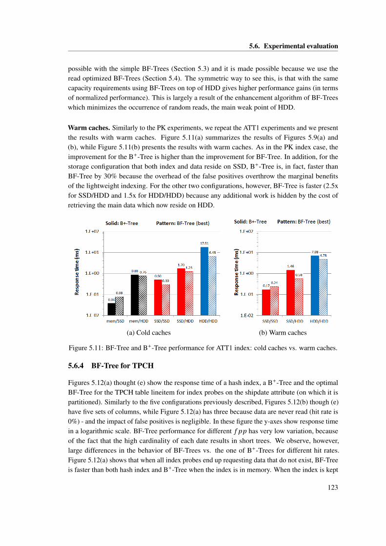
5.6. Experimental evaluation
possible with the simple BF-Trees (Section 5.3) and it is made possible because we use theread optimized BF-Trees (Section 5.4). The symmetric way to see this, is that with the samecapacity requirements using BF-Trees on top of HDD gives higher performance gains (in termsof normalized performance). This is largely a result of the enhancement algorithm of BF-Treeswhich minimizes the occurrence of random reads, the main weak point of HDD.
Warm caches. Similarly to the PK experiments, we repeat the ATT1 experiments and we presentthe results with warm caches. Figure 5.11(a) summarizes the results of Figures 5.9(a) and(b), while Figure 5.11(b) presents the results with warm caches. As in the PK index case, theimprovement for the B+-Tree is higher than the improvement for BF-Tree. In addition, for thestorage configuration that both index and data reside on SSD, B+-Tree is, in fact, faster thanBF-Tree by 30% because the overhead of the false positives overthrow the marginal benefitsof the lightweight indexing. For the other two configurations, however, BF-Tree is faster (2.5xfor SSD/HDD and 1.5x for HDD/HDD) because any additional work is hidden by the cost ofretrieving the main data which now reside on HDD.
(a) Cold caches (b) Warm caches
Figure 5.11: BF-Tree and B+-Tree performance for ATT1 index: cold caches vs. warm caches.
5.6.4 BF-Tree for TPCH
Figures 5.12(a) thought (e) show the response time of a hash index, a B+-Tree and the optimalBF-Tree for the TPCH table lineitem for index probes on the shipdate attribute (on which it ispartitioned). Similarly to the five configurations previously described, Figures 5.12(b) though (e)have five sets of columns, while Figure 5.12(a) has three because data are never read (hit rate is0%) - and the impact of false positives is negligible. In these figure the y-axes show response timein a logarithmic scale. BF-Tree performance for different f pp has very low variation, becauseof the fact that the high cardinality of each date results in short trees. We observe, however,large differences in the behavior of BF-Trees vs. the one of B+-Trees for different hit rates.Figure 5.12(a) shows that when all index probes end up requesting data that do not exist, BF-Treeis faster than both hash index and B+-Tree when the index is in memory. When the index is kept
123
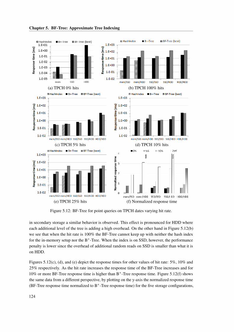
Chapter 5. BF-Tree: Approximate Tree Indexing
(a) TPCH 0% hits (b) TPCH 100% hits
(c) TPCH 5% hits (d) TPCH 10% hits
(e) TPCH 25% hits (f) Normalized response time
Figure 5.12: BF-Tree for point queries on TPCH dates varying hit rate.
in secondary storage a similar behavior is observed. This effect is pronounced for HDD whereeach additional level of the tree is adding a high overhead. On the other hand in Figure 5.12(b)we see that when the hit rate is 100% the BF-Tree cannot keep up with neither the hash indexfor the in-memory setup nor the B+-Tree. When the index is on SSD, however, the performancepenalty is lower since the overhead of additional random reads on SSD is smaller than what it ison HDD.
Figures 5.12(c), (d), and (e) depict the response times for other values of hit rate: 5%, 10% and25% respectively. As the hit rate increases the response time of the BF-Tree increases and for10% or more BF-Tree response time is higher than B+-Tree response time. Figure 5.12(f) showsthe same data from a different perspective, by plotting on the y-axis the normalized response time(BF-Tree response time normalized to B+-Tree response time) for the five storage configurations,
124
5.7. BF-Tree as a general index
varying the hit rate from 0% to 25%. When the bars are lower than one BF-Tree is faster whichhappens for every configuration for hit rate 0% or 5%. One additional observation is that ifboth data and index are stored in the same medium (i.e., both on SSD or both on HDD) theperformance penalty is smaller. Hence, for hit rate 10%, using the configuration SSD/SSD thebest BF-Tree is 20% slower than the B+-Tree and using the configuration SSD/SSD the bestBF-Tree is 10% faster than the B+-Tree (instead of 1.6 to 3x slower which is the case for the otherthree configurations). The explanation is that for these two configurations the cost of traversingthe B+-Tree dominates the overall response time and BF-Tree is competitive because of its shorterheight. In the above experiments the BF-Trees were 1.6x-4x smaller than the B+-Trees.
5.6.5 Summary
In this section we compare BF-Trees with B+-Trees and hash indexes in order to understandwhether BF-Trees can be both space and performance competitive. We show that depending onthe indexed data and the storage configuration there is a BF-Tree design that can be competitivewith B+-Trees both in terms of size and response time. Moreover, for the in-memory indexconfigurations, BF-Trees are competitive against hash indexes as well. The number of falsepositively read pages has an impact in each and every one of the five storage configurations.When data reside on SSD the number of falsely read pages affect the performance only when itdominates the response time. Random reads do not hurt SSD performance, hence, the BF-Treeperformance drops gradually with the number of false positives. When data are stored on HDDthe performance gains are high for no false positives but drop drastically as soon as unnecessaryreads are introduced.
5.7 BF-Tree as a general index
5.7.1 BF-Tree vs. interpolation search
The datasets used to experimentally evaluate BF-Tree are either ordered or partitioned. Forthe case that data are ordered a good alternative candidate would be to use binary search orinterpolation search (Perl et al., 1978). Interpolation search can be very effective for canonicaldatasets achieving log (log (N )) search time, in the specific case that the values are sorted andevenly distributed.4 B+-Trees performance serves as a more general upper bound since binarysearch average response time is log2(N ) and B+-Trees average response time is l ogk (N ), whereN is the size of the dataset and the k is the number of <key, pointer> pairs a B+-Tree page canhold. In addition, B+-Trees serve as a baseline for comparing the size of an index structure usedto enhance search performance.
BF-Trees can be used as a general index which is further discussed in this section. Data do notneed to be entirely ordered (being partitioned is enough), hence, BF-Tree is a more general access
4A more widely applicable version of interpolation search has also been discussed (Graefe, 2006a).
125
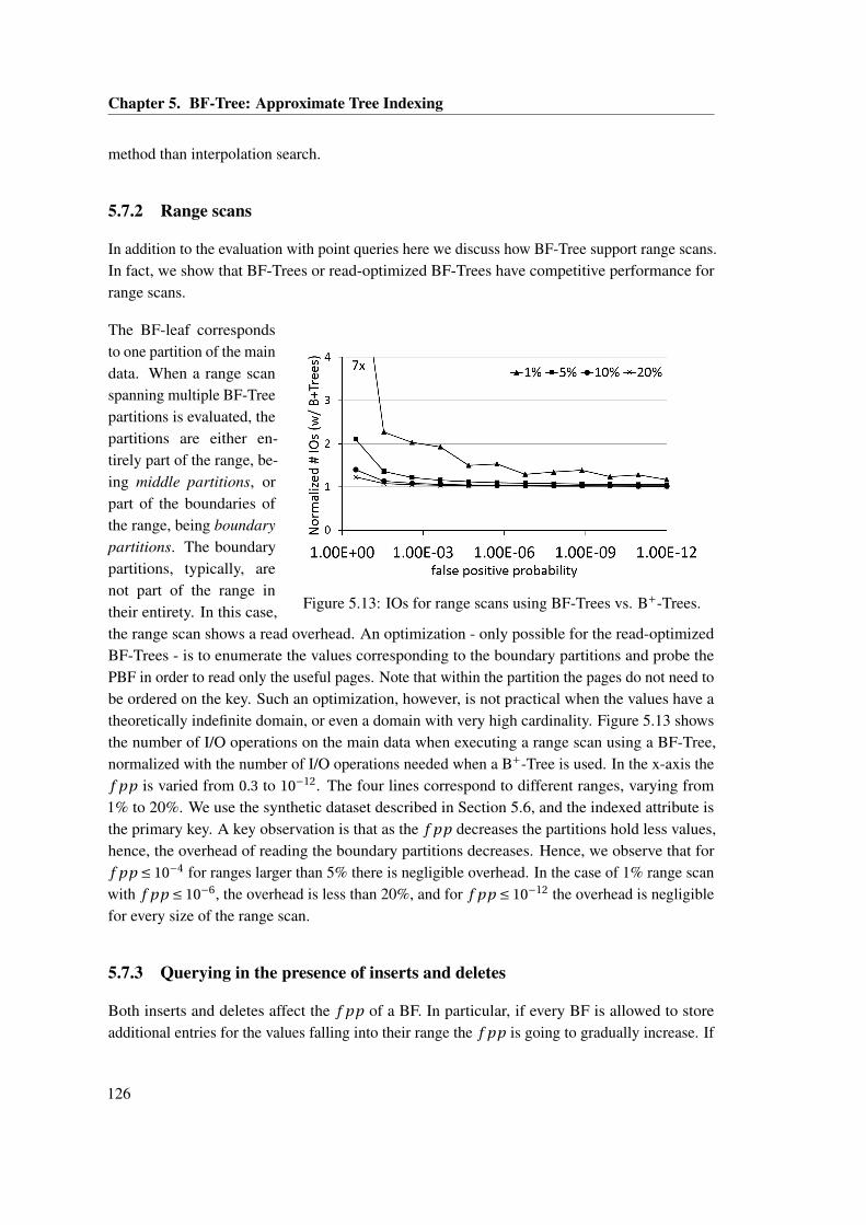
Chapter 5. BF-Tree: Approximate Tree Indexing
method than interpolation search.
5.7.2 Range scans
In addition to the evaluation with point queries here we discuss how BF-Tree support range scans.In fact, we show that BF-Trees or read-optimized BF-Trees have competitive performance forrange scans.
Figure 5.13: IOs for range scans using BF-Trees vs. B+-Trees.
The BF-leaf correspondsto one partition of the maindata. When a range scanspanning multiple BF-Treepartitions is evaluated, thepartitions are either en-tirely part of the range, be-ing middle partitions, orpart of the boundaries ofthe range, being boundarypartitions. The boundarypartitions, typically, arenot part of the range intheir entirety. In this case,the range scan shows a read overhead. An optimization - only possible for the read-optimizedBF-Trees - is to enumerate the values corresponding to the boundary partitions and probe thePBF in order to read only the useful pages. Note that within the partition the pages do not need tobe ordered on the key. Such an optimization, however, is not practical when the values have atheoretically indefinite domain, or even a domain with very high cardinality. Figure 5.13 showsthe number of I/O operations on the main data when executing a range scan using a BF-Tree,normalized with the number of I/O operations needed when a B+-Tree is used. In the x-axis thef pp is varied from 0.3 to 10−12. The four lines correspond to different ranges, varying from1% to 20%. We use the synthetic dataset described in Section 5.6, and the indexed attribute isthe primary key. A key observation is that as the f pp decreases the partitions hold less values,hence, the overhead of reading the boundary partitions decreases. Hence, we observe that forf pp ≤ 10−4 for ranges larger than 5% there is negligible overhead. In the case of 1% range scanwith f pp ≤ 10−6, the overhead is less than 20%, and for f pp ≤ 10−12 the overhead is negligiblefor every size of the range scan.
5.7.3 Querying in the presence of inserts and deletes
Both inserts and deletes affect the f pp of a BF. In particular, if every BF is allowed to storeadditional entries for the values falling into their range the f pp is going to gradually increase. If
126
5.7. BF-Tree as a general index
we assume M bits for the BF, and a given initial f pp, then using Equation 5.1, we calculate thatsuch a BF indexes up to N =−M · ln2(2)/ln( f pp) elements. If we allow to index more elements,i.e., increase N , the effective f pp will in turn increase following a near linear trend for smallchanges of N (note that the new_N is the number of indexed elements after a number of inserts,hence new_N = N + i nser t s):
new_ f pp = e−M ·l n2(2)
new_N , and because,
−M · l n2(2) = N · ln( f pp)
we have,
new_ f pp = eN
new_N ln( f pp) = f ppN
new_N = f ppN
N+i nser t s = f pp1
1+ i nser t sN ⇒
new_ f pp = f pp1
1+i nser t_r ati o (5.15)
The new_ f pp depends on the number of inserts. Equation 5.15 does not depend on the BF size,nor on the number of elements. It depends on the initial f pp and on the relative increase ofindexed elements (i nser t_r ati o = i nser t s
N ).
The behavior of a BF in the presence of inserts is depicted in Figure 5.14. The x-axis is the insertratio, i.e., the number of inserts as a percentage of the initially indexed elements and the y-axisis the resulting f pp. The are three lines corresponding to initial f pp equal to 0.01% (blackline), 0.1% (red dotted line), and 1% (blue dashed line) respectively. In the x-axis the insert ratiovaries between 0 and 60x, meaning that the inserted elements were 60 times more than the initialelements. The new_ f pp for every initial f pp initially increases super-linearly and for insertratio more than 15x it continues to increase sub-linearly. The most interesting part of the graph,however, is the initial part that the insert ratio is a small percentage of the initial elements of theBF.
127
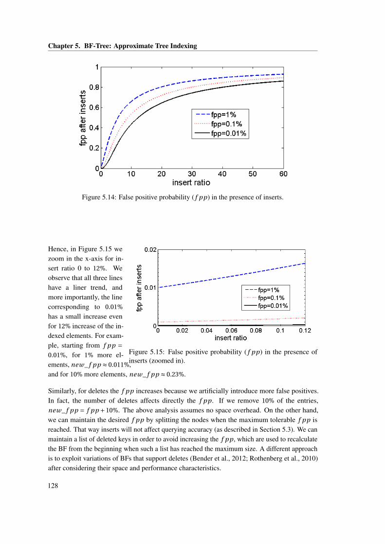
Chapter 5. BF-Tree: Approximate Tree Indexing
Figure 5.14: False positive probability ( f pp) in the presence of inserts.
Figure 5.15: False positive probability ( f pp) in the presence ofinserts (zoomed in).
Hence, in Figure 5.15 wezoom in the x-axis for in-sert ratio 0 to 12%. Weobserve that all three lineshave a liner trend, andmore importantly, the linecorresponding to 0.01%
has a small increase evenfor 12% increase of the in-dexed elements. For exam-ple, starting from f pp =0.01%, for 1% more el-ements, new_ f pp ≈ 0.011%,and for 10% more elements, new_ f pp ≈ 0.23%.
Similarly, for deletes the f pp increases because we artificially introduce more false positives.In fact, the number of deletes affects directly the f pp. If we remove 10% of the entries,new_ f pp = f pp +10%. The above analysis assumes no space overhead. On the other hand,we can maintain the desired f pp by splitting the nodes when the maximum tolerable f pp isreached. That way inserts will not affect querying accuracy (as described in Section 5.3). We canmaintain a list of deleted keys in order to avoid increasing the f pp, which are used to recalculatethe BF from the beginning when such a list has reached the maximum size. A different approachis to exploit variations of BFs that support deletes (Bender et al., 2012; Rothenberg et al., 2010)after considering their space and performance characteristics.
128

5.8. Optimizations
5.8 Optimizations
Exploiting available parallelism. With the current approach the BFs of a leaf node are probedsequentially. A BF-leaf may index several hundreds data pages leading to an equal number ofBFs to probe. These probes can be parallelized if there are enough CPU resources available.In the conducted experiments we do not see a bottleneck in BF probing, however, for differentapplications, BF-Trees may exhibit such a behavior.
Complex index operations with BF-Trees. In this chapter, we cover how the index buildingand the index probing are performed and we briefly discuss how updates and deletes are handled.Traditional indexes, however, offer additional functionality. BF-Trees support index scanssimilarly to a range scan. Since data are partitioned, with one index probe we find the startingpoint of the scan, and then a sequential scan is performed. Index intersections are also possible.In fact, the false positive probability for any key after the intersection of two indexes will be theproduct of the two probabilities (for each index), and hence, typically much smaller than any ofthe two.
5.9 Conclusions
In this chapter, we make a case for approximate tree indexing as a viable competitor of traditionaltree indexing. We propose the Bloom filter tree (BF-Tree) which is a tree structure able to indexa relation with sorted or partitioned attributes. BF-Trees parametrize the accuracy of the indexingas a function of the size of the tree. Thus, B+-Trees are the extreme where accuracy and size aremaximum. BF-Trees allow to decrease the accuracy and, hence, the size of the index structureby introducing (i) a small number of unnecessary reads and (ii) extra work to locate the desiredtuple in a data page. We show, however, through both an analytical model and experimentationwith a prototype implementation, that the introduced overhead can be amortized, hidden, or evensuperseded by reducing the I/O accesses when a desired tuple is retrieved. Secondary storageis moving from HDD - with slow random accesses and cheap capacity - to the diametricallyopposite SSD. BF-Trees achieve competitive performance and minimize index size for SSD, andeven when data reside on HDD, BF-Trees index it efficiently as well.
129

6 Graph Data Management using Solid-State Storage1
6.1 Introduction
Solid State Storage (a.k.a. Storage Class Memory (Freitas, 2009)) is here to stay. Today, a wellknown Solid State Storage technology is NAND flash. Another technology on the horizon isPhase Change Memory (PCM). Both can be used in chip form, for example, as a small storageelement in a portable device. The read and write latencies of PCM cells are very low, alreadyin the same ballpark as DRAM (Chen et al., 2011; Doller, 2009). For large scale storage, manychips can be packaged into a single device that provides the same functionality as disk drives,supporting the same basic APIs. SSDs can provide much faster random I/O than magnetic disksbecause there is no mechanical latency between requests. We focus here on database applicationsthat demand enterprise level storage in this form factor.
NAND flash technology is relatively mature and represents the state-of-the art in the marketplace.Companies have been building storage devices out of flash chips for two decades, and onecan find a huge variety of flash-based devices from consumer to enterprise storage. PCM is arelative newcomer, and until now there has been little opportunity to evaluate the performancecharacteristics of large scale PCM devices. In this chapter we provide insights on where solidstate devices can offer a big advantage over traditional storage and highlight possible differencesbetween two representative technologies, flash and PCM.
As discussed earlier, flash devices have superior random read performance compared to magnetichard-drives but suffer from several limitations. First, there is a significant asymmetry in read andwrite performance. Second, only a limited number of updates can be applied on a flash devicebefore it becomes unusable; this number is decreasing with newer generations of flash (Abraham,2010). Third, writing on flash not only is much slower than reading and destructive of the device,but it has proven to interfere with the redirection software layers, known as Flash TranslationLayers (FTL) (Bouganim et al., 2009).
1The material of this chapter has been the basis for the ADMS 2012 "Path Processing using Solid State Stor-age" (Athanassoulis et al., 2012).
131
Chapter 6. Graph Data Management using Solid-State Storage
PCM addresses some of these challenges. The endurance of PCM cells is significantly higherthan NAND flash (Ovonyx, 2007), although still not close to that of DRAM. Unlike NAND flash,PCM does not require the bulk erasure of large memory units before it can be rewritten. Moreover,while cost is still uncertain, for our purposes, we assume normal cell size competitiveness andstandard volume economics will apply to this technology as it ramps into high volume.
The most pronounced benefit of solid state storage over hard disks is the difference in responsetime for random accesses. Hence, we identify dependent reads as an access pattern that has thepotential for significant performance gains. Latency-bound applications like path processing(Gubichev and Neumann, 2011) in the context of graph processing, or RDF-data processingare typical examples of applications with such access patterns. The Resource DescriptionFramework (RDF) (RDf, 2013) data model is widely adopted for several on-line, scientific orknowledge-based datasets because of its simplicity in modelling and the variety of information itcan represent.
We find that PCM-based storage is an important step towards better latency guarantees with nobandwidth penalties and we identify a trade-off between maximizing bandwidth and minimizinglatency. In order to measure the headroom of performance benefit (decrease of response time) inlong path queries we implement a simple benchmark and we compare the response times whenusing flash and PCM. We observe that PCM can yield 1.5x to 2.5x smaller response times forany bandwidth utilization without any graph-aware optimizations2 some of which we leave forfuture work. We take this observation one step further and we design a new data layout suitablefor RDF data and optimized for a solid state storage layer. The proposed layout increases thelocality of related information and decreases the cost of graph traversals by storing more linkageinformation (i.e., metadata about how to navigate faster when a graph is traversed).
6.1.1 Contributions
We have the following main contributions:
• We devise a custom benchmark to highlight the qualitative and quantitative differencesbetween two representative solid state devices (flash and PCM).
• We find that PCM can natively support higher workload parallelization with near-zerolatency penalty — an observation that can be used to shift the algorithm design.
• We find that applications with dependent reads are natural candidates for exploiting PCM-based devices. Our graph-based benchmark allows us to measure the benefit that pathtraversal queries can have from such devices.
2Such optimizations, in addition to the new data layout presented in this chapter, include complementary pagescomprised of auxiliary data structures such as: (i) cached attributes, (ii) aggregate links, (iii) node popularity, (iv) nodepriority and (v) reverse links.
132
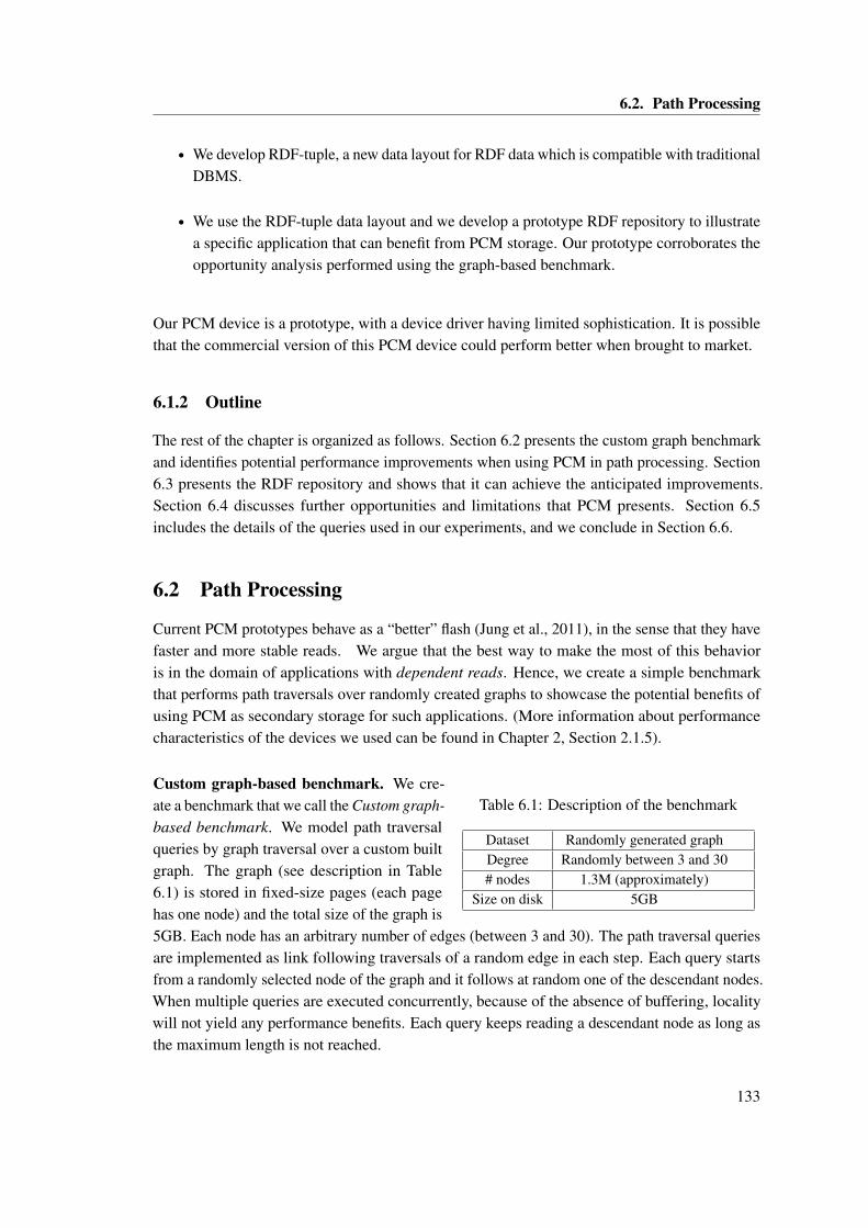
6.2. Path Processing
• We develop RDF-tuple, a new data layout for RDF data which is compatible with traditionalDBMS.
• We use the RDF-tuple data layout and we develop a prototype RDF repository to illustratea specific application that can benefit from PCM storage. Our prototype corroborates theopportunity analysis performed using the graph-based benchmark.
Our PCM device is a prototype, with a device driver having limited sophistication. It is possiblethat the commercial version of this PCM device could perform better when brought to market.
6.1.2 Outline
The rest of the chapter is organized as follows. Section 6.2 presents the custom graph benchmarkand identifies potential performance improvements when using PCM in path processing. Section6.3 presents the RDF repository and shows that it can achieve the anticipated improvements.Section 6.4 discusses further opportunities and limitations that PCM presents. Section 6.5includes the details of the queries used in our experiments, and we conclude in Section 6.6.
6.2 Path Processing
Current PCM prototypes behave as a “better” flash (Jung et al., 2011), in the sense that they havefaster and more stable reads. We argue that the best way to make the most of this behavioris in the domain of applications with dependent reads. Hence, we create a simple benchmarkthat performs path traversals over randomly created graphs to showcase the potential benefits ofusing PCM as secondary storage for such applications. (More information about performancecharacteristics of the devices we used can be found in Chapter 2, Section 2.1.5).
Table 6.1: Description of the benchmark
Dataset Randomly generated graphDegree Randomly between 3 and 30# nodes 1.3M (approximately)
Size on disk 5GB
Custom graph-based benchmark. We cre-ate a benchmark that we call the Custom graph-based benchmark. We model path traversalqueries by graph traversal over a custom builtgraph. The graph (see description in Table6.1) is stored in fixed-size pages (each pagehas one node) and the total size of the graph is5GB. Each node has an arbitrary number of edges (between 3 and 30). The path traversal queriesare implemented as link following traversals of a random edge in each step. Each query startsfrom a randomly selected node of the graph and it follows at random one of the descendant nodes.When multiple queries are executed concurrently, because of the absence of buffering, localitywill not yield any performance benefits. Each query keeps reading a descendant node as long asthe maximum length is not reached.
133
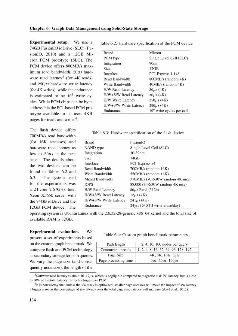
Chapter 6. Graph Data Management using Solid-State Storage
Table 6.2: Hardware specification of the PCM device
Brand MicronPCM type Single Level Cell (SLC)Integration 90nmSize 12GBInterface PCI-Express 1.1x8Read Bandwidth 800MB/s (random 4K)Write Bandwidth 40MB/s (random 4K)H/W Read Latency 20µs (4K)H/W+S/W Read Latency 36µs (4K)H/W Write Latency 250µs (4K)H/W+S/W Write Latency 386µs (4K)Endurance 106 write cycles per cell
Experimental setup. We use a74GB FusionIO ioDrive (SLC) (Fu-sionIO, 2010) and a 12GB Mi-cron PCM prototype (SLC). ThePCM device offers 800MB/s max-imum read bandwidth, 20µs hard-ware read latency3 (for 4K reads)and 250µs hardware write latency(for 4K writes), while the enduranceis estimated to be 106 write cy-cles. While PCM chips can be byte-addressable the PCI-based PCM pro-totype available to us uses 4KBpages for reads and writes4.
Table 6.3: Hardware specification of the flash device
Brand FusionIONAND type Single Level Cell (SLC)Integration 30-39nmSize 74GBInterface PCI-Express x4Read Bandwidth 700MB/s (random 16K)Write Bandwidth 550MB/s (random 16K)Mixed Bandwidth 370MB/s (70R/30W random 4K mix)IOPS 88,000 (70R/30W random 4K mix)H/W Read Latency 50µs Read (512b)H/W+S/W Read Latency 72µs (4K)H/W+S/W Write Latency 241µs (4K)Endurance 24yrs (@ 5TB write-erase/day)
The flash device offers700MB/s read bandwidth(for 16K accesses) andhardware read latency aslow as 50µs in the bestcase. The details aboutthe two devices can befound in Tables 6.2 and6.3. The system usedfor the experiments wasa 24-core 2.67GHz IntelXeon X5650 server withthe 74GB ioDrive and the12GB PCM device. Theoperating system is Ubuntu Linux with the 2.6.32-28-generic x86_64 kernel and the total size ofavailable RAM is 32GB.
Table 6.4: Custom graph benchmark parameters.
Path length 2, 4, 10, 100 nodes per queryConcurrent threads 1, 2, 4, 8, 16, 32, 64, 96, 128, 192
Page Size 4K, 8K, 16K, 32KPage processing time 0µs, 50µs, 100µs
Experimental evaluation. Wepresent a set of experiments basedon the custom graph benchmark. Wecompare flash and PCM technologyas secondary storage for path queries.We vary the page size (and conse-quently node size), the length of the
3Software read latency is about 16–17µs, which is negligible compared to magnetic disk I/O latency, but is closeto 50% of the total latency for technologies like PCM.
4It is noteworthy that, unless the s/w stack is optimized, smaller page accesses will make the impact of s/w latencya bigger issue as the percentage of s/w latency over the total page read latency will increase (Akel et al., 2011).
134
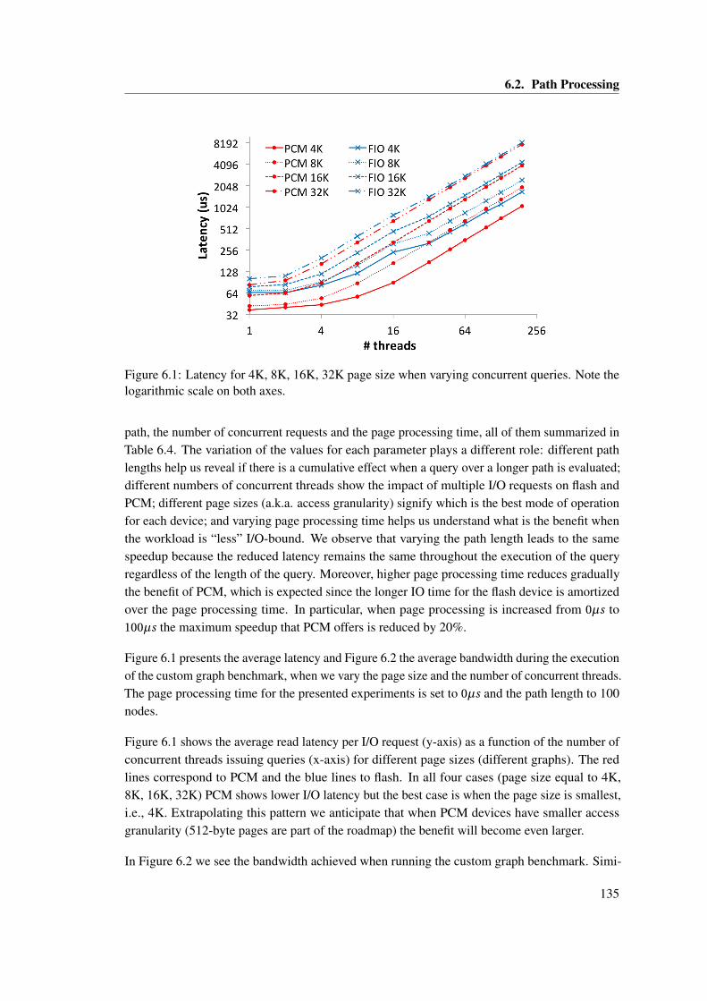
6.2. Path Processing
Figure 6.1: Latency for 4K, 8K, 16K, 32K page size when varying concurrent queries. Note thelogarithmic scale on both axes.
path, the number of concurrent requests and the page processing time, all of them summarized inTable 6.4. The variation of the values for each parameter plays a different role: different pathlengths help us reveal if there is a cumulative effect when a query over a longer path is evaluated;different numbers of concurrent threads show the impact of multiple I/O requests on flash andPCM; different page sizes (a.k.a. access granularity) signify which is the best mode of operationfor each device; and varying page processing time helps us understand what is the benefit whenthe workload is “less” I/O-bound. We observe that varying the path length leads to the samespeedup because the reduced latency remains the same throughout the execution of the queryregardless of the length of the query. Moreover, higher page processing time reduces graduallythe benefit of PCM, which is expected since the longer IO time for the flash device is amortizedover the page processing time. In particular, when page processing is increased from 0µs to100µs the maximum speedup that PCM offers is reduced by 20%.
Figure 6.1 presents the average latency and Figure 6.2 the average bandwidth during the executionof the custom graph benchmark, when we vary the page size and the number of concurrent threads.The page processing time for the presented experiments is set to 0µs and the path length to 100nodes.
Figure 6.1 shows the average read latency per I/O request (y-axis) as a function of the number ofconcurrent threads issuing queries (x-axis) for different page sizes (different graphs). The redlines correspond to PCM and the blue lines to flash. In all four cases (page size equal to 4K,8K, 16K, 32K) PCM shows lower I/O latency but the best case is when the page size is smallest,i.e., 4K. Extrapolating this pattern we anticipate that when PCM devices have smaller accessgranularity (512-byte pages are part of the roadmap) the benefit will become even larger.
In Figure 6.2 we see the bandwidth achieved when running the custom graph benchmark. Simi-
135
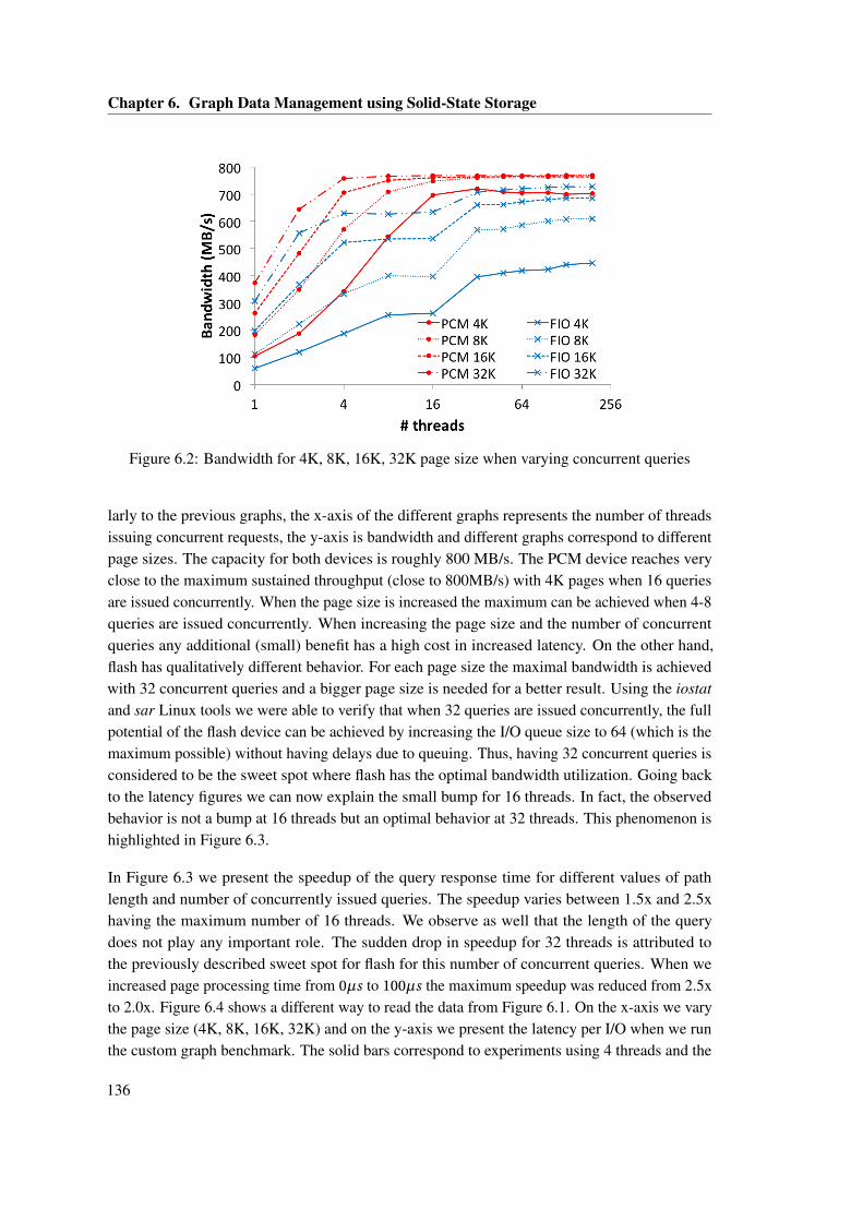
Chapter 6. Graph Data Management using Solid-State Storage
Figure 6.2: Bandwidth for 4K, 8K, 16K, 32K page size when varying concurrent queries
larly to the previous graphs, the x-axis of the different graphs represents the number of threadsissuing concurrent requests, the y-axis is bandwidth and different graphs correspond to differentpage sizes. The capacity for both devices is roughly 800 MB/s. The PCM device reaches veryclose to the maximum sustained throughput (close to 800MB/s) with 4K pages when 16 queriesare issued concurrently. When the page size is increased the maximum can be achieved when 4-8queries are issued concurrently. When increasing the page size and the number of concurrentqueries any additional (small) benefit has a high cost in increased latency. On the other hand,flash has qualitatively different behavior. For each page size the maximal bandwidth is achievedwith 32 concurrent queries and a bigger page size is needed for a better result. Using the iostatand sar Linux tools we were able to verify that when 32 queries are issued concurrently, the fullpotential of the flash device can be achieved by increasing the I/O queue size to 64 (which is themaximum possible) without having delays due to queuing. Thus, having 32 concurrent queries isconsidered to be the sweet spot where flash has the optimal bandwidth utilization. Going backto the latency figures we can now explain the small bump for 16 threads. In fact, the observedbehavior is not a bump at 16 threads but an optimal behavior at 32 threads. This phenomenon ishighlighted in Figure 6.3.
In Figure 6.3 we present the speedup of the query response time for different values of pathlength and number of concurrently issued queries. The speedup varies between 1.5x and 2.5xhaving the maximum number of 16 threads. We observe as well that the length of the querydoes not play any important role. The sudden drop in speedup for 32 threads is attributed tothe previously described sweet spot for flash for this number of concurrent queries. When weincreased page processing time from 0µs to 100µs the maximum speedup was reduced from 2.5xto 2.0x. Figure 6.4 shows a different way to read the data from Figure 6.1. On the x-axis we varythe page size (4K, 8K, 16K, 32K) and on the y-axis we present the latency per I/O when we runthe custom graph benchmark. The solid bars correspond to experiments using 4 threads and the
136
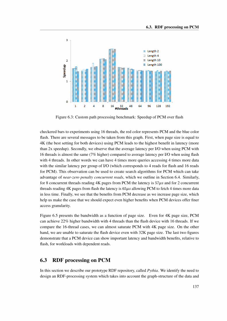
6.3. RDF processing on PCM
Figure 6.3: Custom path processing benchmark: Speedup of PCM over flash
checkered bars to experiments using 16 threads, the red color represents PCM and the blue colorflash. There are several messages to be taken from this graph. First, when page size is equal to4K (the best setting for both devices) using PCM leads to the highest benefit in latency (morethan 2x speedup). Secondly, we observe that the average latency per I/O when using PCM with16 threads is almost the same (7% higher) compared to average latency per I/O when using flashwith 4 threads. In other words we can have 4 times more queries accessing 4 times more datawith the similar latency per group of I/O (which corresponds to 4 reads for flash and 16 readsfor PCM). This observation can be used to create search algorithms for PCM which can takeadvantage of near-zero penalty concurrent reads, which we outline in Section 6.4. Similarly,for 8 concurrent threads reading 4K pages from PCM the latency is 57µs and for 2 concurrentthreads reading 4K pages from flash the latency is 65µs allowing PCM to fetch 4 times more datain less time. Finally, we see that the benefits from PCM decrease as we increase page size, whichhelp us make the case that we should expect even higher benefits when PCM devices offer fineraccess granularity.
Figure 6.5 presents the bandwidth as a function of page size. Even for 4K page size, PCMcan achieve 22% higher bandwidth with 4 threads than the flash device with 16 threads. If wecompare the 16-thread cases, we can almost saturate PCM with 4K page size. On the otherhand, we are unable to saturate the flash device even with 32K page size. The last two figuresdemonstrate that a PCM device can show important latency and bandwidth benefits, relative toflash, for workloads with dependent reads.
6.3 RDF processing on PCM
In this section we describe our prototype RDF repository, called Pythia. We identify the need todesign an RDF-processing system which takes into account the graph-structure of the data and
137
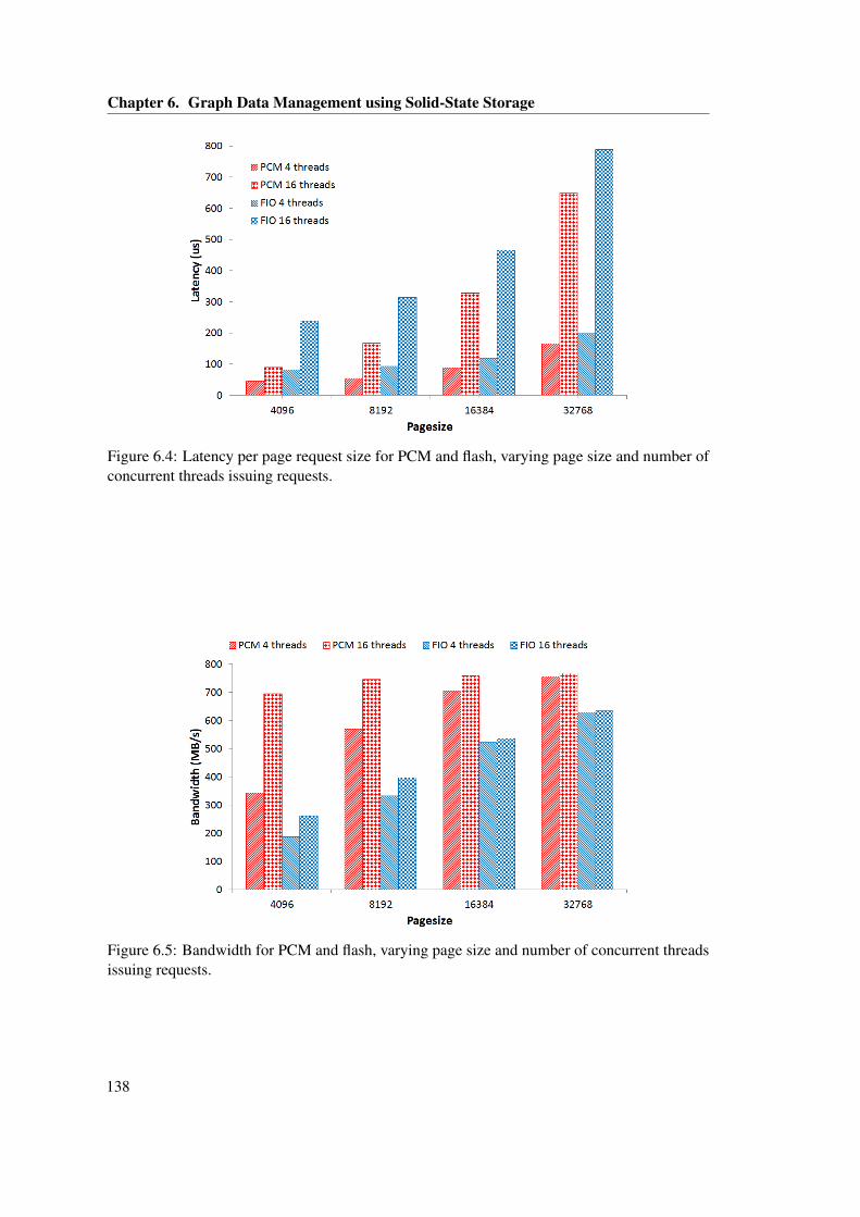
Chapter 6. Graph Data Management using Solid-State Storage
Figure 6.4: Latency per page request size for PCM and flash, varying page size and number ofconcurrent threads issuing requests.
Figure 6.5: Bandwidth for PCM and flash, varying page size and number of concurrent threadsissuing requests.
138
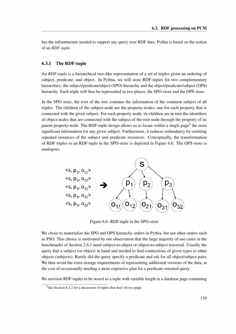
6.3. RDF processing on PCM
has the infrastructure needed to support any query over RDF data. Pythia is based on the notionof an RDF-tuple.
6.3.1 The RDF-tuple
An RDF-tuple is a hierarchical tree-like representation of a set of triples given an ordering ofsubject, predicate, and object. In Pythia, we will store RDF-tuples for two complementaryhierarchies: the subject/predicate/object (SPO) hierarchy and the object/predicate/subject (OPS)hierarchy. Each triple will thus be represented in two places, the SPO-store and the OPS-store.
In the SPO store, the root of the tree contains the information of the common subject of alltriples. The children of the subject-node are the property-nodes, one for each property that isconnected with the given subject. For each property-node, its children are in turn the identifiersof object-nodes that are connected with the subject of the root node through the property of itsparent property-node. The RDF-tuple design allows us to locate within a single page5 the mostsignificant information for any given subject. Furthermore, it reduces redundancy by omittingrepeated instances of the subject and predicate resources. Conceptually, the transformationof RDF triples to an RDF-tuple in the SPO-store is depicted in Figure 6.6. The OPS-store isanalogous.
Figure 6.6: RDF-tuple in the SPO-store
We chose to materialize the SPO and OPS hierarchy orders in Pythia, but not other orders suchas PSO. This choice is motivated by our observation that the large majority of use cases in thebenchmarks of Section 2.6.1 need subject-to-object or object-to-subject traversal. Usually thequery had a subject (or object) in hand and needed to find connections of given types to otherobjects (subjects). Rarely did the query specify a predicate and ask for all object/subject pairs.We thus avoid the extra storage requirements of representing additional versions of the data, atthe cost of occasionally needing a more expensive plan for a predicate-oriented query.
We envision RDF-tuples to be stored as a tuple with variable length in a database page containing
5See Section 6.3.2 for a discussion of tuples that don’t fit in a page.
139
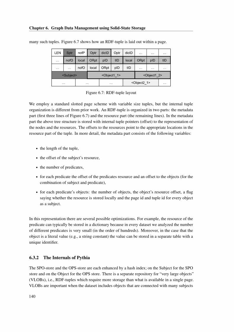
Chapter 6. Graph Data Management using Solid-State Storage
many such tuples. Figure 6.7 shows how an RDF-tuple is laid out within a page.
Figure 6.7: RDF-tuple layout
We employ a standard slotted page scheme with variable size tuples, but the internal tupleorganization is different from prior work. An RDF-tuple is organized in two parts: the metadatapart (first three lines of Figure 6.7) and the resource part (the remaining lines). In the metadatapart the above tree structure is stored with internal tuple pointers (offset) to the representation ofthe nodes and the resources. The offsets to the resources point to the appropriate locations in theresource part of the tuple. In more detail, the metadata part consists of the following variables:
• the length of the tuple,
• the offset of the subject’s resource,
• the number of predicates,
• for each predicate the offset of the predicates resource and an offset to the objects (for thecombination of subject and predicate),
• for each predicate’s objects: the number of objects, the object’s resource offset, a flagsaying whether the resource is stored locally and the page id and tuple id for every objectas a subject.
In this representation there are several possible optimizations. For example, the resource of thepredicate can typically be stored in a dictionary because in every dataset we analyzed the numberof different predicates is very small (in the order of hundreds). Moreover, in the case that theobject is a literal value (e.g., a string constant) the value can be stored in a separate table with aunique identifier.
6.3.2 The Internals of Pythia
The SPO-store and the OPS-store are each enhanced by a hash index; on the Subject for the SPOstore and on the Object for the OPS store. There is a separate repository for “very large objects”(VLOBs), i.e., RDF-tuples which require more storage than what is available in a single page.VLOBs are important when the dataset includes objects that are connected with many subjects
140
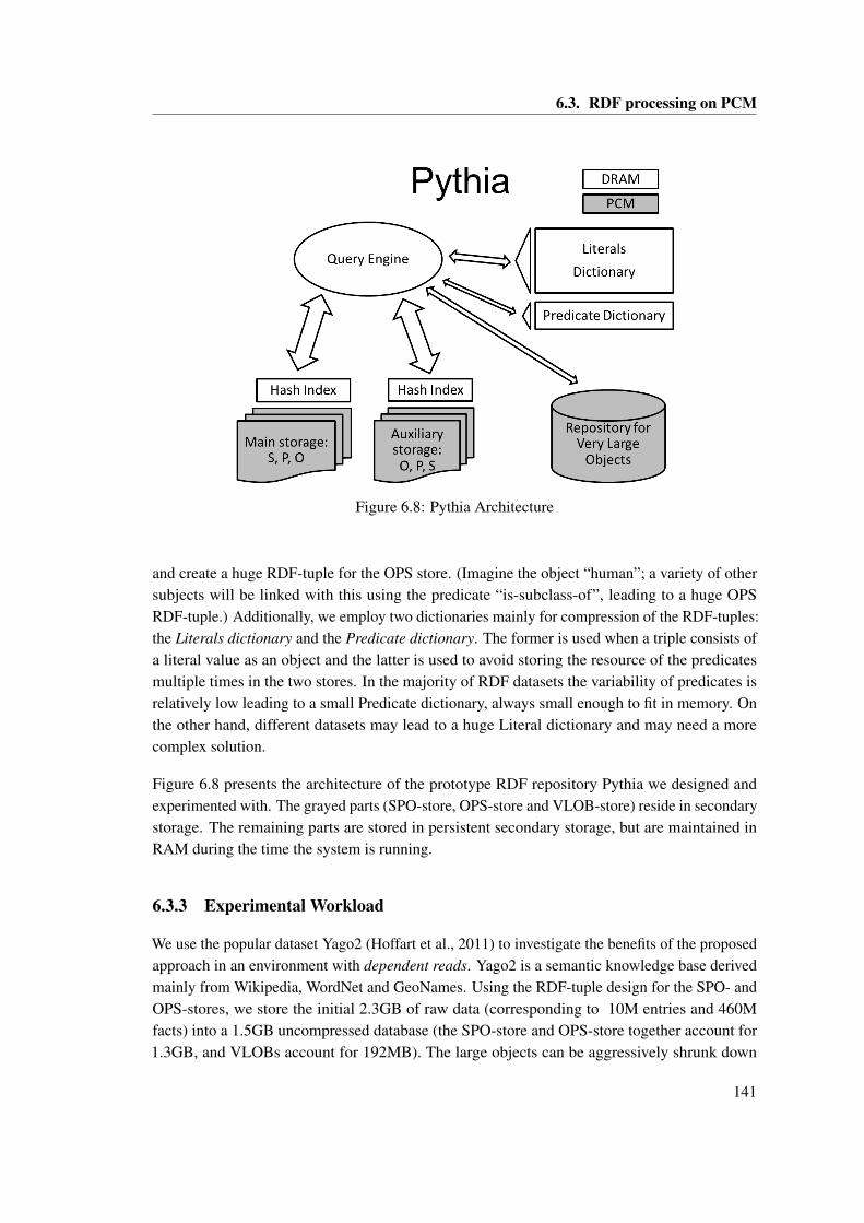
6.3. RDF processing on PCM
Figure 6.8: Pythia Architecture
and create a huge RDF-tuple for the OPS store. (Imagine the object “human”; a variety of othersubjects will be linked with this using the predicate “is-subclass-of”, leading to a huge OPSRDF-tuple.) Additionally, we employ two dictionaries mainly for compression of the RDF-tuples:the Literals dictionary and the Predicate dictionary. The former is used when a triple consists ofa literal value as an object and the latter is used to avoid storing the resource of the predicatesmultiple times in the two stores. In the majority of RDF datasets the variability of predicates isrelatively low leading to a small Predicate dictionary, always small enough to fit in memory. Onthe other hand, different datasets may lead to a huge Literal dictionary and may need a morecomplex solution.
Figure 6.8 presents the architecture of the prototype RDF repository Pythia we designed andexperimented with. The grayed parts (SPO-store, OPS-store and VLOB-store) reside in secondarystorage. The remaining parts are stored in persistent secondary storage, but are maintained inRAM during the time the system is running.
6.3.3 Experimental Workload
We use the popular dataset Yago2 (Hoffart et al., 2011) to investigate the benefits of the proposedapproach in an environment with dependent reads. Yago2 is a semantic knowledge base derivedmainly from Wikipedia, WordNet and GeoNames. Using the RDF-tuple design for the SPO- andOPS-stores, we store the initial 2.3GB of raw data (corresponding to 10M entries and 460Mfacts) into a 1.5GB uncompressed database (the SPO-store and OPS-store together account for1.3GB, and VLOBs account for 192MB). The large objects can be aggressively shrunk down
141
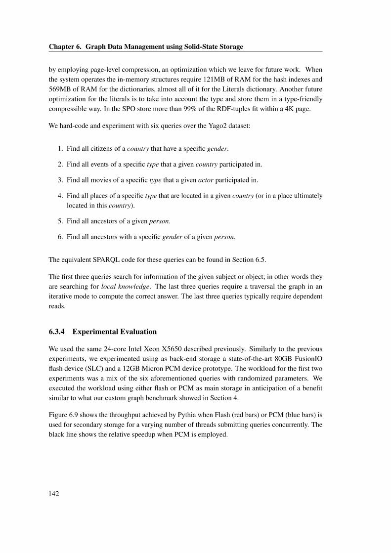
Chapter 6. Graph Data Management using Solid-State Storage
by employing page-level compression, an optimization which we leave for future work. Whenthe system operates the in-memory structures require 121MB of RAM for the hash indexes and569MB of RAM for the dictionaries, almost all of it for the Literals dictionary. Another futureoptimization for the literals is to take into account the type and store them in a type-friendlycompressible way. In the SPO store more than 99% of the RDF-tuples fit within a 4K page.
We hard-code and experiment with six queries over the Yago2 dataset:
1. Find all citizens of a country that have a specific gender.
2. Find all events of a specific type that a given country participated in.
3. Find all movies of a specific type that a given actor participated in.
4. Find all places of a specific type that are located in a given country (or in a place ultimatelylocated in this country).
5. Find all ancestors of a given person.
6. Find all ancestors with a specific gender of a given person.
The equivalent SPARQL code for these queries can be found in Section 6.5.
The first three queries search for information of the given subject or object; in other words theyare searching for local knowledge. The last three queries require a traversal the graph in aniterative mode to compute the correct answer. The last three queries typically require dependentreads.
6.3.4 Experimental Evaluation
We used the same 24-core Intel Xeon X5650 described previously. Similarly to the previousexperiments, we experimented using as back-end storage a state-of-the-art 80GB FusionIOflash device (SLC) and a 12GB Micron PCM device prototype. The workload for the first twoexperiments was a mix of the six aforementioned queries with randomized parameters. Weexecuted the workload using either flash or PCM as main storage in anticipation of a benefitsimilar to what our custom graph benchmark showed in Section 4.
Figure 6.9 shows the throughput achieved by Pythia when Flash (red bars) or PCM (blue bars) isused for secondary storage for a varying number of threads submitting queries concurrently. Theblack line shows the relative speedup when PCM is employed.
142
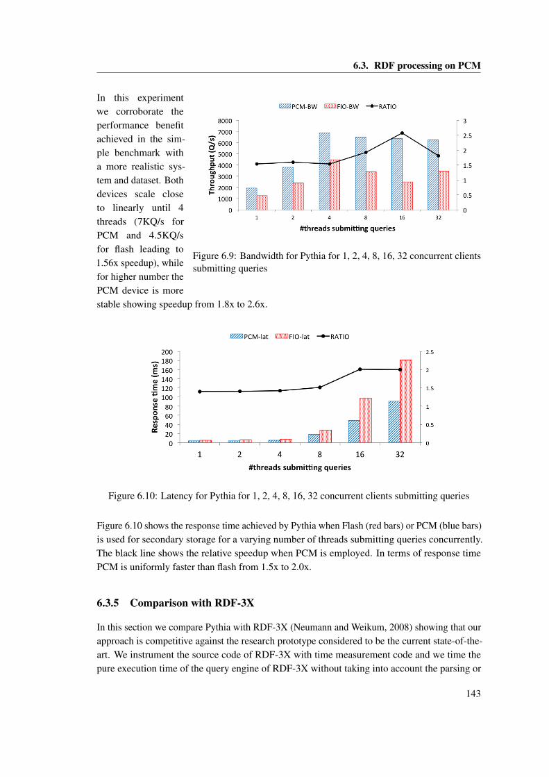
6.3. RDF processing on PCM
Figure 6.9: Bandwidth for Pythia for 1, 2, 4, 8, 16, 32 concurrent clientssubmitting queries
In this experimentwe corroborate theperformance benefitachieved in the sim-ple benchmark witha more realistic sys-tem and dataset. Bothdevices scale closeto linearly until 4threads (7KQ/s forPCM and 4.5KQ/sfor flash leading to1.56x speedup), whilefor higher number thePCM device is morestable showing speedup from 1.8x to 2.6x.
Figure 6.10: Latency for Pythia for 1, 2, 4, 8, 16, 32 concurrent clients submitting queries
Figure 6.10 shows the response time achieved by Pythia when Flash (red bars) or PCM (blue bars)is used for secondary storage for a varying number of threads submitting queries concurrently.The black line shows the relative speedup when PCM is employed. In terms of response timePCM is uniformly faster than flash from 1.5x to 2.0x.
6.3.5 Comparison with RDF-3X
In this section we compare Pythia with RDF-3X (Neumann and Weikum, 2008) showing that ourapproach is competitive against the research prototype considered to be the current state-of-the-art. We instrument the source code of RDF-3X with time measurement code and we time thepure execution time of the query engine of RDF-3X without taking into account the parsing or
143
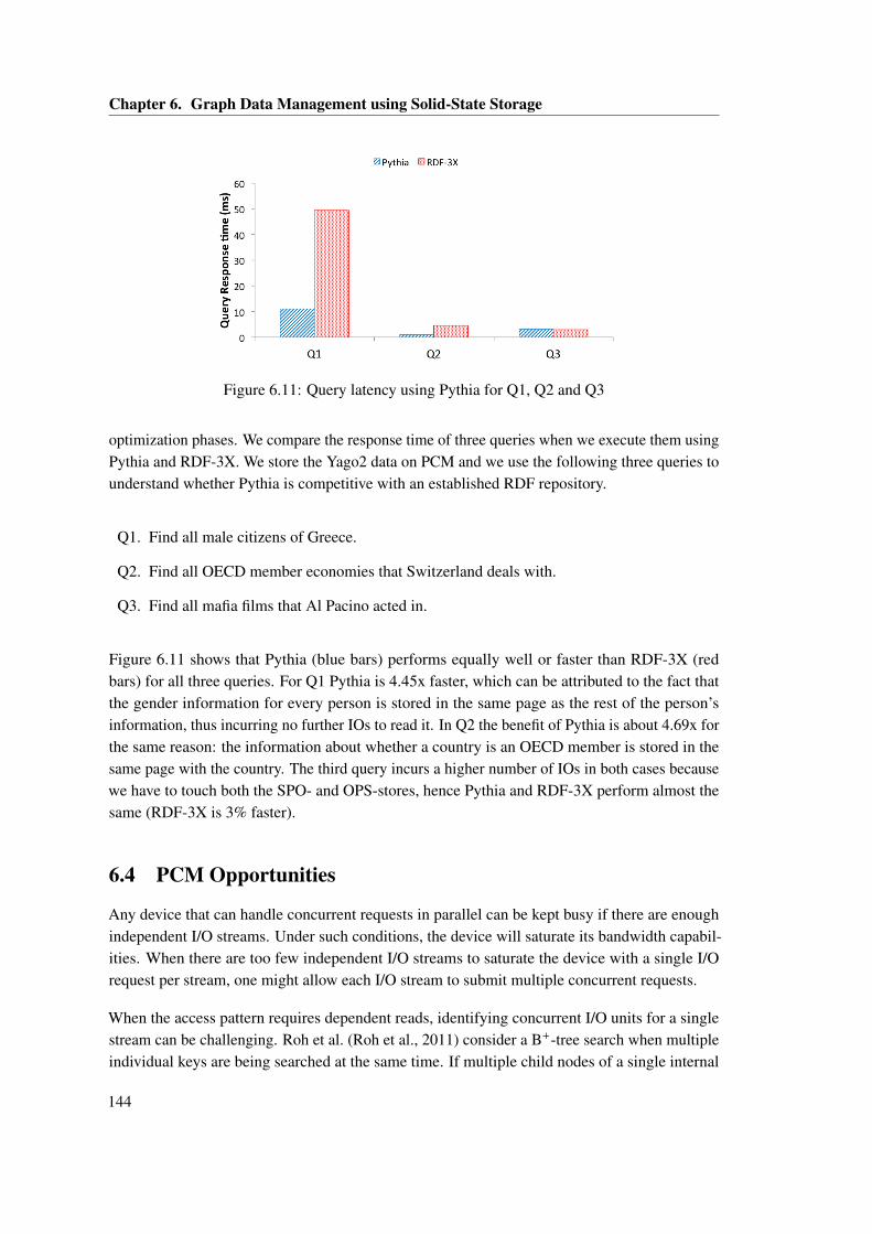
Chapter 6. Graph Data Management using Solid-State Storage
Figure 6.11: Query latency using Pythia for Q1, Q2 and Q3
optimization phases. We compare the response time of three queries when we execute them usingPythia and RDF-3X. We store the Yago2 data on PCM and we use the following three queries tounderstand whether Pythia is competitive with an established RDF repository.
Q1. Find all male citizens of Greece.
Q2. Find all OECD member economies that Switzerland deals with.
Q3. Find all mafia films that Al Pacino acted in.
Figure 6.11 shows that Pythia (blue bars) performs equally well or faster than RDF-3X (redbars) for all three queries. For Q1 Pythia is 4.45x faster, which can be attributed to the fact thatthe gender information for every person is stored in the same page as the rest of the person’sinformation, thus incurring no further IOs to read it. In Q2 the benefit of Pythia is about 4.69x forthe same reason: the information about whether a country is an OECD member is stored in thesame page with the country. The third query incurs a higher number of IOs in both cases becausewe have to touch both the SPO- and OPS-stores, hence Pythia and RDF-3X perform almost thesame (RDF-3X is 3% faster).
6.4 PCM Opportunities
Any device that can handle concurrent requests in parallel can be kept busy if there are enoughindependent I/O streams. Under such conditions, the device will saturate its bandwidth capabil-ities. When there are too few independent I/O streams to saturate the device with a single I/Orequest per stream, one might allow each I/O stream to submit multiple concurrent requests.
When the access pattern requires dependent reads, identifying concurrent I/O units for a singlestream can be challenging. Roh et al. (Roh et al., 2011) consider a B+-tree search when multipleindividual keys are being searched at the same time. If multiple child nodes of a single internal
144
6.5. SPARQL code for test queries
node need to be searched, I/Os for the child nodes can be submitted concurrently. This is adependent-read pattern in which multiple subsequent reads may be dependent on a single initialread. Roh et al. demonstrate performance improvements for this workload on several flashdevices. They implemented an I/O interface that allows the submission of several I/O requestswith a single system call, to reduce software and hardware overheads.
Both PCM devices and flash devices can handle a limited number of concurrent requests with aminor latency penalty. For our PCM device running with 8 concurrent threads, we can achieveroughly double the bandwidth and half the latency of the flash device, without significantlyincreasing the latency beyond what is observed for single-threaded access. Thus our PCM devicehas the potential to outperform flash when I/O streams can submit concurrent I/O requests.
6.4.1 Algorithm redesign
A graph-processing example of such a workload is best-first search (BestFS). In best-first search,the priority of nodes for subsequent exploration is determined by an application-dependentheuristic, and nodes at the current exploration fringe are visited in priority order. Breadth-firstsearch (BFS) and depth-first search (DFS) are special cases in which the priority function issuitably chosen. On a device that efficiently supports n concurrent I/O requests, we can submitthe top n items from the priority queue as an I/O batch, effectively parallelizing the search. Thechildren of the newly fetched nodes are inserted into the priority queue for the next round of thesearch algorithm.
In particular, BestFS, implements a hardware optimized BFS with DFS performance guarantees.The main concepts of a BestFS are (i) the I/O parallelism of the device and (ii) the heuristic tobe used. The execution of BestFS proceeds as follows. The search begins from a given nodeof the graph, and all the neighboring nodes are imported in the ToExamine queue, where theyare ordered based on the heuristic used. Then, n nodes are serviced in parallel. The number n
is dictated by the I/O parallelism of the device. When, n nodes are services in parallel they arefetched by storage in the same time as a single node, and then the addresses of their descendantsare imported in the ToExamine queue, when all the nodes are re-ordered based on the heuristicused. This process continues iteratively, until we find the node we are looking for. It is worthmentioning that, a BestFS execution can reach the furthest descendant in the same time as DFS ifthe execution is I/O bound because every batch of reads happens in the same time as a singleread. In this time, however, the BestFS is capable of testing more than the nodes consisting of thepath to the furthest descendant having performed, in fact, a partial BFS.
6.5 SPARQL code for test queries
In this section we present the equivalent SPARQL version of the queries implemented duringthe evaluation of Pythia in Section 6.3. These queries are used to compare against the research
145
Chapter 6. Graph Data Management using Solid-State Storage
prototype RDF-3X (Neumann and Weikum, 2008) using the pathfilter operator introduced in theliterature (Gubichev and Neumann, 2011).
1. Find all citizens of a country that have a specific gender.SPARQL: select ?s where { ?s <isCitizeonOf> country. ?s <hasGender> gender }
2. Find all type events that a country participated in.SPARQL: select ?s where { country <participatedIn> ?s. ?s <type> eventType }
3. Find all type movies that an actor participated in.SPARQL: select ?s where { ?s <type> movieType. actor <actedIn> ?s }
4. Find all places of a specific type that are located in a country (or in a place ultimatelylocated in this country).SPARQL: select ?s where { ?s <type> placeType. ?s ?path country. pathfilter(containsOnly(??path,<isLocatedIn>)) }
5. Find all ancestors of a person.SPARQL: select ?s where { ?s ??path person.pathfilter(containsOnly(??path, <hasChild>)) }
6. Find all ancestors having gender gender of a person.SPARQL: select ?s where { ?s ??path person. ?s <hasGender> gender. pathfilter(containsOnly(??path,<hasChild>)) }
Q1. Find all male citizens of Greece.select ?s where { ?s <hasGender> <male>. ?s <isCitizenOf> <Greece> }
Q2. Find all OECD member economies that Switzerland deals with.SPARQL: select ?s where{ ?s <type> wikicategory_OECD_member_economies.<Switzerland> <dealsWith> ?s }
Q3. Find all mafia films that Al Pacino acted in.SPARQL: select ?s where { ?s <type> wikicategory_Mafia_films. <Al_Pacino> <actedIn>?s }
6.6 Conclusions
In this chapter we present a new physical data layout for RDF data motivated by the rapid evolutionof the available storage technologies. We use as our secondary storage two representative solid-state storage devices: a state-of-the-art flash device (fusionIO) and a real-life PCM-based (Micron)prototype. The proposed data layout called RDF-tuple is suitable for general RDF queries and
146
6.6. Conclusions
is implemented and tested in a prototype storage engine called Pythia, showing competitiveperformance when compared with the research state-of-the-art system RDF-3X. RDF-tuple cannatively store RDF information in a DBMS friendly way and exploit both existing DB algorithmsand custom graph-based algorithms.
Our experiments with solid-state storage show that graph processing can take advantage of itnaturally because they employ dependent reads. Commercial scale PCM technology is relativelynew, but we see that it is already competitive against mature flash devices. A key observation isthat a PCM device with a very basic device driver can outperform a mature flash rival in terms ofthe read latency and read bandwidth of a single device. Our experimentation with a custom graphbenchmark shows that using an early prototype PCM device can yield significant performancebenefits over flash when running path traversal queries (1.5x-2.5x).
147

7 The Big Picture
In this thesis we set the stage for efficient scaleup data analytics by building hardware-awareand workload-aware system design. We integrate non-volatile solid-state storage in the datamanagement system hierarchy and we build algorithms that use workload characteristics to offerbetter performance and increased functionality. We study different datasets and workloads takenfrom, or similar, to typical data analytics applications.
The reason to choose this research direction stems from the increasing importance of data analyticsin modern applications, including business, research, governmental and scientific applications.The means of collecting and storing information evolves, creating new challenges in supportingmodern analytics applications. Hence, the question of how to store and how to analyze datais of paramount importance. At the same time, the underlying hardware is evolving and newstorage and processing technologies become available allowing for radical system and algorithmredesign.
In this chapter we summarize the contributions of this thesis and we discuss a number ofinteresting research topics related with the current hardware trends and data analytics.
7.1 What we did
In this thesis we build algorithms and tools and we design systems that use solid-state storage inorder to address the requirements of modern data analytics: fast query response times ensuringdata freshness, support for increasing concurrency, efficient storage, indexing and accessingof both archival and knowledge-based datasets. We demonstrate the importance of exploitingnew storage technologies in concert with algorithms tailored for data analytics applications. Byexploiting analytical query patterns and solid-state storage we offer efficient online updates withnear-zero overhead in query response times. For workloads with increased concurrency, we showthat work sharing allows us to use less resources offering better throughput and very small latencypenalty. Moreover, we demonstrate that using the data organization we can offer space efficientand competitive indexing. Finally, we show that in order to integrate knowledge-based data, a
149
Chapter 7. The Big Picture
new data-layout offering both locality for the properties of each subject, and fast linkage retrieval,provides faster response times than the state-of-the-art.
This thesis is a crucial step towards modern data analytics, studying the impact of both hardware-aware optimizations and workload-aware design. In this thesis we discuss the importance of thestorage trends on the way we store, query and analyze data, while at the same time we showthe performance and functionality benefits when pre-existing workload knowledge is taken intoaccount for the system design. In the center of the proposed work is the understanding that theconstant evolution of storage creates the need to study and reconsider database system designsince the characteristics of secondary storage are weaved with the traditional DBMS design. Tothat extent, we discuss in this chapter new research directions that lie ahead stemming from thechanges in storage technologies yet to come. In addition, we discuss one fundamental trend indata analytics which will drive the design of future engine: concurrency in workloads.
7.2 Storage is constantly evolving: Opportunities and challenges
The past decade we have witnessed a tremendous shift in the database systems design fueled bythe emergence of multicore architectures and deeper memory hierarchies as a direct consequenceof the increasing gap between processor and memory speeds. Today we observe an equallyimportant technological shift in the storage layer, which motivated part of the work presentedin this thesis. Flash devices are already used in enterprise deployments but the optimal wayto exploit such devices depends on the application. In fact, flash and other solid-state devicesare used in a wide range of ways, varying from an intermediate caching layer (following thetrend of deeper storage hierarchies) to stand-alone storage. Additionally, new technologies - withPhase Change Memory and Memristor on the edge of being commercially available - create newopportunities and new challenges for research on database system design.
In fact solid-state devices based on flash technology are bound to face two challenges: thecapacity and endurance walls. As the integration granularity of CMOS chips has become finerit is increasingly difficult to pack more flash capacity (i.e., floating gates) in the same surface.Companies building storage devices project that there are a few more generations of increasingthe storage density for flash. In order to delay the capacity wall, flash device vendors shiftedfrom single-level cell (SLC) devices to multi-level cell (MLC) devices which store more than onebit per storage cell. This strategy is causing the endurance wall because erase blocks of MLCdevices can sustain 2-3 orders of magnitude less erasures than the ones of SLC devices beforethey become unreadable. Designing systems that use flash devices for persistent storage in thepresence of this constantly shifting tradeoff between endurance and capacity is an open researchtopic.
150
7.3. Ever increasing concurrency in analytics
7.2.1 Persistent main memory: Database Management Systems vs. OperatingSystems
Storage technologies that are still under research and development - like Phase Change Memory -are expected to offer fine-grained addressability and non-volatility. In order to design a systemwith persistent main memory, however, these two properties are not enough. Similarly to theconsistency and durability properties of database transactions, programs that operate on top ofpersistent main memory need to have data structures that can ensure consistency of the persistentdata. In some cases durability may not be necessary, but when durability is pursued there is needfor a mechanism for consistency. First, in the micro-architectural level current systems do notguarantee the order that writes in memory are performed nor whether a write that returned to thecalling function is completed. Second, unless the response time of accessing a chip of a futurepersistent main memory is in the same order as today’s main memory it will be impossible toexploit the fine-grained addressability because the cost of accessing the persistent memory has tobe amortized. Addressing the research problems of persistent main memories require research onthe micro-architectural level and on the application level in tandem.
7.2.2 Software stack is too slow
The recent advancements in storage technologies have revealed a very important characteristic ofthe software stack sitting on top of the storage devices. The software layers of operating systemand file system have been designed having in mind response times in the order of milliseconds(or more) from the main storage devices (Akel et al., 2011; Caulfield et al., 2012). Today,however, solid-state storage devices have one or more orders of magnitude faster response times.Production flash devices have response times in the order of 50µs and Phase Change Memoryprototypes in the order to 20µs (Athanassoulis et al., 2012), making the latency from the softwarelayers (the software latency) comparable with the access latency for reading from or writing to thedevice (the hardware latency). Trimming down the software layer can be achieved, for example,by exposing directly the device to the application, or by building new lightweight file systems.
7.3 Ever increasing concurrency in analytics
The nature of analytical queries is expanding from offline analysis to ubiquitous queries. Forexample, asking from our smartphone the current consumption of minutes and data of our monthlyplan initiates a personalized analytical query. Moreover, in recent research it is documented thatcustomers of data analytics products indicate that they will have to routinely execute severalhundreds of concurrent queries in the near future (Candea et al., 2011). A report in trends indata warehousing published in 2012 (Russom, 2012) anticipates at least one order of magnitudeincrease in concurrent users submitting queries in data analytics systems over the next fewyears. Hence, rethinking the query-centric approach and building query engines tailored for highconcurrency is key to deliver the data analytics engines of the future.
151
Chapter 7. The Big Picture
7.3.1 Extending support of work sharing
A first step towards data analytics engines supporting high concurrency is the recent introductionof work sharing approaches. A detailed comparison of two such approaches is presented in thisthesis. This analysis paves the way for more query engines to integrate work sharing techniquesin order to exploit both planned and ad hoc sharing. Work sharing in production systems needs amore sophisticated multi-query optimization method and meticulous optimization depending onthe hardware and software platform.
7.3.2 Column-stores and high concurrency
Column-store systems have been designed in order to support analytical workloads, however,ever increasing concurrency is creating new challenges. A study of the behavior of three popularcolumn-store systems when running analytical queries with increasing concurrency (Alagianniset al., 2013) shows that the tested systems cannot sustain stable performance, after they becomesaturated, which is attributed to the lack of aggressive dynamic resource reallocation. Forincreasing concurrency the throughput is decreased drastically but the available processors arenot always fully utilized. Inefficiencies of the query engines and the lack of aggressive dynamicresource reallocation or of CPU-aware admission control leads to queries underutilizing availableresources. This behavior leaves room for further research aiming at efficiently supporting highconcurrency in column-stores. Work sharing is no stranger to column-stores, however, we arguethat query operators in column-stores can be redesigned in order to facilitate ad-hoc and plannedsharing as a means to achieve better scalability.
152
Bibliography
Daniel J. Abadi. Query execution in column-oriented database systems. PhD thesis, MassachusettsInstitute of Technology, 2008.
Daniel J. Abadi, Adam Marcus, Sammuel R. Madden, and Kate Hollenbach. Scalable semanticweb data management using vertical partitioning. In Proceedings of the 33rd IntenationalConference on Very Large Data Bases - VLDB 2007, pages 411–422, 2007.
Michael Abraham. NAND Flash Trends for SSD/Enterprise. In Flash Memory Summit, SantaClara, CA, USA, August 2010.
Devesh Agrawal, Deepak Ganesan, Ramesh Sitaraman, Yanlei Diao, and Shashi Singh. Lazy-Adaptive Tree: An Optimized Index Structure for Flash Devices. Proceedings of the VLDBEndowment, 2(1):361–372, 2009.
Jagrati Agrawal, Yanlei Diao, Daniel Gyllstrom, and Neil Immerman. Efficient pattern matchingover event streams. In Proceedings of the 2008 ACM SIGMOD International Conference onManagement of Data, pages 147–160, Vancouver, Canada, June 2008.
Anastasia Ailamaki, David J. DeWitt, Mark D. Hill, and Marios Skounakis. Weaving Relationsfor Cache Performance. In Proceedings of the 27th International Conference on Very LargeData Bases - VLDB 2001, pages 169–180, September 2001.
Ameen Akel, Adrian M. Caulfield, Todor I. Mollov, Rajesh K. Gupta, and Steven Swanson.Onyx: A Protoype Phase Change Memory Storage Array. In Proceedings of the 3rd USENIXConference on Hot Topics in Storage and File Systems - HotStorage 2011, page 2, Portland,OR, USA, June 2011.
Ioannis Alagiannis, Manos Athanassoulis, and Anastasia Ailamaki. Scaling up analytical querieswith column-stores. In Proceedings of the Sixth International Workshop on Testing DatabaseSystems - DBTest 2013, pages 8:1–8:6, New York, NY, USA, June 2013.
Nicole Alexander, Xavier Lopez, Siva Ravada, Susie Stephens, and Jack Wang. RDF Data Modelin Oracle. Oracle White Paper, 2005.
Paulo Sérgio Almeida, Carlos Baquero, Nuno Preguiça, and David Hutchison. Scalable BloomFilters. Information Processing Letters, 101(6):255–261, March 2007.
153
Bibliography
Christian Antognini. Bloom Filters in Oracle DBMS. Oracle White Paper, 2008.
Rolf Apweiler, Amos Bairoch, Cathy H. Wu, Winona C. Barker, Brigitte Boeckmann, SerenellaFerro, Elisabeth Gasteiger, Hongzhan Huang, Rodrigo Lopez, Michele Magrane, Maria J.Martin, Darren A. Natale, Claire O’Donovan, Nicole Redaschi, and Lai-Su L. Yeh. UniProt:the Universal Protein knowledgebase. Nucleic acids research, 32(Database Issue):D115–9,January 2004.
Subramanian Arumugam, Alin Dobra, Christopher M. Jermaine, Niketan Pansare, and Luis Perez.The DataPath system: a data-centric analytic processing engine for large data warehouses. InProceedings of the 2010 ACM SIGMOD International Conference on Management of Data,pages 519–530, Indianapolis, IN, USA, June 2010.
Manos Athanassoulis and Anastasia Ailamaki. BF-Tree: Approximate Tree Indexing. Submittedfor publication, 2013.
Manos Athanassoulis, Anastasia Ailamaki, Shimin Chen, Phillip B. Gibbons, and Radu Stoica.Flash in a DBMS : Where and How ? IEEE Data Engineering Bulletin, 33(4):28–34, December2010.
Manos Athanassoulis, Shimin Chen, Anastasia Ailamaki, Phillip B. Gibbons, and Radu Stoica.MaSM : Efficient Online Updates in Data Warehouses. In Proceedings of the 2011 ACMSIGMOD International Conference on Management of Data, Athens, Greece, June 2011.
Manos Athanassoulis, Bishwaranjan Bhattacharjee, Mustafa Canim, and Kenneth A. Ross. PathProcessing using Solid State Storage. In Proceedings of the 3rd International Workshop onAccelerating Data Management Systems Using Modern Processor and Storage Architectures -ADMS 2012, Istanbul, Turkey, August 2012.
Manos Athanassoulis, Shimin Chen, Anastasia Ailamaki, Phillip B. Gibbons, and Radu Stoica.Online Updates on Data Warehouses via Judicious Use of Solid-State Storage. Submitted forpublication, 2013.
Luiz Andre Barroso. Warehouse-scale Computing. In Keynote talk at the 2010 ACM SIGMODInternational Conference on Management of Data, Indianapolis, IN, USA, June 2010.
Jacek Becla and Kian-Tat Lim. Report from the first workshop on extremely large databases(XLDB 2007). Data Science Journal, 7, February 2008.
Michael A. Bender, Martin Farach-Colton, Rob Johnson, Russell Kraner, Bradley C. Kuszmaul,Dzejla Medjedovic, Pablo Montes, Pradeep Shetty, Richard P. Spillane, and Erez Zadok. Don’tThrash: How to Cache Your Hash on Flash. Proceedings of the VLDB Endowment, 5(11):1627–1637, July 2012.
Hal Berenson, Philip A. Bernstein, Jim Gray, Jim Melton, Elizabeth J. O’Neil, and Patrick E.O’Neil. A critique of ANSI SQL isolation levels. ACM SIGMOD Record, 24(2):1–10, May1995.
154
Bibliography
Bishwaranjan Bhattacharjee, Kavitha Srinivas, and Octavian Udrea. Method and system to storeRDF data in a relational store. Patent Application, 2011.
Christian Bizer and Andreas Schultz. The Berlin SPARQL Benchmark. International Journal onSemantic Web and Information Systems, 5(2), 2009.
Christian Bizer, Tom Heath, and Tim Berners-Lee. Linked Data - The Story So Far. InternationalJournal on Semantic Web and Information Systems, 5(3), 2009a.
Christian Bizer, Jens Lehmann, Georgi Kobilarov, Sören Auer, Christian Becker, Richard Cyga-niak, and Sebastian Hellmann. DBpedia - A crystallization point for the Web of Data. Journalon Web Semantics, 7(3):154–165, September 2009b.
Burton H. Bloom. Space/Time Trade-offs in Hash Coding with Allowable Errors. Communica-tions of the ACM, 13(7):422–426, July 1970.
Peter Boncz. Monet: A next-Generation DBMS Kernel For Query-Intensive Application. PhDthesis, Universiteit van Amsterdam, 2002.
Dhruba Borthakur. Petabyte scale databases and storage systems at Facebook. In Proceedings ofthe 2013 ACM SIGMOD International Conference on Management of Data, page 1267, NewYork, NY, USA, June 2013.
Luc Bouganim, Björn Þór Jónsson, and Philippe Bonnet. uFLIP: Understanding Flash IO Patterns.In Online Proceedings of the Fourth Biennial Conference on Innovative Data Systems Research- CIDR 2009, Asilomar, CA, USA, January 2009.
Andrei Broder and Michael Mitzenmacher. Network Applications of Bloom Filters: A Survey.Internet Mathematics, 1:636–646, 2002.
Geoffrey W. Burr, Bülent N. Kurdi, J. Campbell Scott, Chung Hon Lam, Kailash Gopalakrishnan,and Rohit S. Shenoy. Overview of Candidate Device Technologies for Storage-Class Memory.IBM Journal of Research and Development, 52(4):449–464, July 2008.
George Candea, Neoklis Polyzotis, and Radek Vingralek. A scalable, predictable join operatorfor highly concurrent data warehouses. Proceedings of the VLDB Endowment, 2(1):277–288,August 2009.
George Candea, Neoklis Polyzotis, and Radek Vingralek. Predictable performance and highquery concurrency for data analytics. The VLDB Journal, 20(2):227–248, February 2011.
Mustafa Canim, Bishwaranjan Bhattacharjee, George A. Mihaila, Christian A. Lang, and Ken-neth A. Ross. An Object Placement Advisor for DB2 Using Solid State Storage. Proceedingsof the VLDB Endowment, 2(2):1318–1329, August 2009.
Mustafa Canim, Christian A. Lang, George A. Mihaila, and Kenneth A. Ross. Buffered Bloomfilters on solid state storage. In Proceedings of the 1st International Workshop on AcceleratingData Management Systems Using Modern Processor and Storage Architectures - ADMS 2010,Singapore, Singapore, September 2010a.
155
Bibliography
Mustafa Canim, George A. Mihaila, Bishwaranjan Bhattacharjee, Kenneth A. Ross, and Chris-tian A. Lang. SSD Bufferpool Extensions for Database Systems. Proceedings of the VLDBEndowment, 3(1-2):1435–1446, September 2010b.
Adrian M. Caulfield, Arup De, Joel Coburn, Todor I. Mollov, Rajesh K. Gupta, and StevenSwanson. Moneta: A High-Performance Storage Array Architecture for Next-Generation,Non-volatile Memories. In Proceedings of the 2010 43rd Annual IEEE/ACM InternationalSymposium on Microarchitecture - MICRO 2010, pages 385–395, Atlanta, GA, USA, December2010.
Adrian M. Caulfield, Todor I. Mollov, Louis Alex Eisner, Arup De, Joel Coburn, and StevenSwanson. Providing safe, user space access to fast, solid state disks. ACM SIGARCH ComputerArchitecture News, 40(1):387–400, April 2012.
Sirish Chandrasekaran, Mehul A. Shah, Owen Cooper, Amol Deshpande, Michael J. Franklin,Joseph M. Hellerstein, Wei Hong, Sailesh Krishnamurthy, Sammuel R. Madden, and FredReiss. TelegraphCQ: continuous dataflow processing. In Proceedings of the 2003 ACMSIGMOD International Conference on Management of Data, page 668, San Diego, CA, USA,June 2003.
Fay Chang, Jeffrey Dean, Sanjay Ghemawat, Wilson C. Hsieh, Deborah A. Wallach, MikeBurrows, Tushar Chandra, Andrew Fikes, and Robert E. Gruber. Bigtable: A DistributedStorage System for Structured Data. In Proceedings of the 7th USENIX Symposium onOperating Systems Design and Implementation - OSDI 2006, Seattle, WA, USA, November2006.
Fa-Chung Fred Chen and Margaret H. Dunham. Common subexpression processing in multiple-query processing. IEEE Transactions on Knowledge and Data Engineering, 10(3):493–499,May 1998.
Jianjun Chen, David J. DeWitt, Feng Tian, and Yuan Wang. NiagaraCQ: a scalable continuousquery system for Internet databases. ACM SIGMOD Record, 29(2):379–390, June 2000.
Shimin Chen. FlashLogging: Exploiting Flash Devices for Synchronous Logging Performance.In Proceedings of the 2009 ACM SIGMOD International Conference on Management of Data,pages 73–86, Providence, RI, USA, 2009.
Shimin Chen, Phillip B. Gibbons, Todd C. Mowry, and Gary Valentin. Fractal prefetching B+-Trees. In Proceedings of the 2002 ACM SIGMOD International Conference on Managementof Data, pages 157–168, Madison, WI, USA, June 2002.
Shimin Chen, Phillip B. Gibbons, and Suman Nath. PR-join: a non-blocking join achievinghigher early result rate with statistical guarantees. In Proceedings of the 2010 ACM SIGMODInternational Conference on Management of Data, pages 147–158, Indianapolis, IN, USA,June 2010.
156
Bibliography
Shimin Chen, Phillip B. Gibbons, and Suman Nath. Rethinking Database Algorithms for PhaseChange Memory. In Online Proceedings of the Fifth Biennial Conference on Innovative DataSystems Research - CIDR 2011, Asilomar, CA, USA, January 2011.
Hong-Tai Chou and David J. DeWitt. An evaluation of buffer management strategies for relationaldatabase systems. In Proceedings of the 11th International Conference on Very Large DataBases - VLDB 1985, pages 127–141, August 1985.
John Cieslewicz and Kenneth A. Ross. Adaptive Aggregation on Chip Multiprocessors. InProceedings of the 33rd International Conference on Very Large Data Bases - VLDB 2007,pages 339–350, Vienna, Austria, September 2007.
Edgar F. Codd. A relational model of data for large shared data banks. Communications of theACM, 13(6):377–387, June 1970.
Latha S. Colby, Richard L. Cole, Edward Haslam, Nasi Jazayeri, Galt Johnson, William J.McKenna, Lee Schumacher, and David Wilhite. Redbrick Vista: Aggregate Computation andManagement. In Proceedings of the Fourteenth International Conference on Data Engineering- ICDE 1998, pages 174–177, Orlando, FL, USA, February 1998.
Tyson Condie, Neil Conway, Peter Alvaro, Joseph M. Hellerstein, John Gerth, Justin Talbot,Khaled Elmeleegy, and Russell Sears. Online Aggregation and Continuous Query Supportin MapReduce. In Proceedings of the 2010 ACM SIGMOD International Conference onManagement of Data, pages 1115–1118, Indianapolis, IN, USA, June 2010.
Cathan Cook. Database Architecture: The Storage Engine. MSDN Library, 2001.
Nilesh N. Dalvi, Sumit K. Sanghai, Prasan Roy, and S. Sudarshan. Pipelining in multi-queryoptimization. Journal of Computer and System Sciences, 66(4):728–762, June 2003.
Data.gov. Online reference. http://www.data.gov/, 2013.
Data.gov.uk. Online reference. http://www.data.gov.uk, 2013.
Jeffrey Dean and Sanjay Ghemawat. MapReduce: Simplified Data Processing on Large Clusters.In Proceedings of the 6th Symposium on Operating System Design and Implementation - OSDI2004, pages 137–150, San Francisco, CA, USA, December 2004.
Edward Doller. PCM and its impacts on memory hierarchy. PDL Seminar, Carnegie MellonUniversity, 2009.
Songyun Duan, Anastasios Kementsietsidis, Kavitha Srinivas, and Octavian Udrea. Apples andoranges: a comparison of RDF benchmarks and real RDF datasets. In Proceedings of the 2011ACM SIGMOD International Conference on Management of Data, pages 145–156, Athens,Greece, June 2011.
157
Bibliography
Phillip M. Fernandez. Red Brick Warehouse: A Read-Mostly RDBMS for Open SMP Platforms.In Proceedings of the 1994 ACM SIGMOD International Conference on Management of Data,page 492, Minneapolis, MN, USA, May 1994.
David Ferrucci, Eric Brown, Jennifer Chu-Carroll, James Fan, David Gondek, Aditya A. Kalyan-pur, Adam Lally, J. William Murdock, Eric Nyberg, John Prager, Nico Schlaefer, and ChrisWelty. Building Watson: An Overview of the DeepQA Project. AI Magazine, 31(3):59–79,2010.
Phil Francisco. The Netezza Data Appliance Architecture: A Platform for High PerformanceData Warehousing and Analytics. IBM Redbooks, 2011.
Richard Freitas. Storage Class Memory: Technology, Systems and Applications. In Proceedingsof the 2009 ACM SIGMOD International Conference on Management of Data, pages 985–986,Providence, RI, USA, July 2009.
FusionIO. ioDrive. http://www.fusionio.com/products/iodrive/, 2010.
FusionIO. ioDrive2. http://www.fusionio.com/products/iodrive2/, 2013.
Shen Gao, Jianliang Xu, Bingsheng He, Byron Choi, and Haibo Hu. PCMLogging: reducingtransaction logging overhead with PCM. In Proceedings of the 20th ACM InternationalConference on Information and Knowledge Management - CIKM 2011, pages 2401–2404,Glasgow, Scotland, UK, October 2011.
Georgios Giannikis, Gustavo Alonso, and Donald Kossmann. SharedDB: killing one thousandqueries with one stone. Proceedings of the VLDB Endowment, 5(6):526–537, February 2012.
Goetz Graefe. Volcano - An Extensible and Parallel Query Evaluation System. IEEE Transactionson Knowledge and Data Engineering, 6(1):120–135, February 1994.
Goetz Graefe. Sorting And Indexing With Partitioned B-Trees. In Online Proceedings of theFirst Biennial Conference on Innovative Data Systems Research - CIDR 2003, Asilomar, CA,USA, January 2003.
Goetz Graefe. B-tree indexes, interpolation search, and skew. In Proceedings of the 2ndInternational Workshop on Data Management on New Hardware - DAMON 2006, Chicago,IL, USA, June 2006a.
Goetz Graefe. B-tree indexes for high update rates. ACM SIGMOD Record, 35(1):39–44, March2006b.
Goetz Graefe. Modern B-Tree Techniques. Foundations and Trends in Databases, 3(4):203–402,2010.
Goetz Graefe and Harumi Kuno. Self-selecting, self-tuning, incrementally optimized indexes. InProceedings of the 13th International Conference on Extending Database Technology - EDBT2010, pages 371–381, Lausanne, Switzerland, March 2010.
158
Bibliography
Goetz Graefe, Felix Halim, Stratos Idreos, Harumi Kuno, and Stefan Manegold. Concurrencycontrol for adaptive indexing. Proceedings of the VLDB Endowment, 5(7):656–667, 2012.
Jim Gray. Tape is dead, Disk is Tape, Flash is Disk. Gong show talk at the Third BiennialConference on Innovative Data Systems Research - CIDR 2007, 2007.
Andrey Gubichev and Thomas Neumann. Path Query Processing on Very Large RDF Graphs. InProceedings of the 14th International Workshop on the Web and Databases - WebDB 2011,Athens, Greece, June 2011.
Yuanbo Guo, Zhengxiang Pan, and Jeff Heflin. LUBM: A benchmark for OWL knowledge basesystems. Journal on Web Semantics, 3(2-3):158–182, October 2005.
Stavros Harizopoulos and Anastasia Ailamaki. A Case for Staged Database Systems. In OnlineProceedings of the First Biennial Conference on Innovative Data Systems Research - CIDR2003, Asilomar, CA, USA, January 2003.
Stavros Harizopoulos, Vladislav Shkapenyuk, and Anastasia Ailamaki. QPipe: a simultaneouslypipelined relational query engine. In Proceedings of the 2005 ACM SIGMOD InternationalConference on Management of Data, SIGMOD ’05, pages 383–394, Baltimore, MD, USA,June 2005.
Oktie Hassanzadeh, Anastasios Kementsietsidis, and Yannis Velegrakis. Publishing RelationalData in the Semantic Web. In Tutorial at the 8th Extended Semantic Web Conference - ESWC2011, Heraklion, Greece, May 2011.
HBase. Online reference. http://hbase.apache.org/, 2013.
Joseph M. Hellerstein, Michael Stonebraker, and James Hamilton. Architecture of a DatabaseSystem. Now Publishers Inc., September 2007.
Sándor Héman, Marcin Zukowski, and Niels J. Nes. Positional update handling in column stores.Proceedings of the 2010 ACM SIGMOD International Conference on Management of Data,pages 543–554, 2010.
Johannes Hoffart, Fabian M. Suchanek, Klaus Berberich, Edwin Lewis-Kelham, Gerard de Melo,and Gerhard Weikum. YAGO2: exploring and querying world knowledge in time, space,context, and many languages. In Proceedings of the 20th International Conference Companionon World Wide Web - WWW 2011, pages 229–232, Hyderabad, India, March 2011.
Johannes Hoffart, Fabian M. Suchanek, Klaus Berberich, and Gerhard Weikum. YAGO2: aspatially and temporally enhanced knowledge base from Wikipedia. Artificial Intelligence,194:28–61, January 2013.
James Hughes. Revolutions in Storage. In IEEE Conference on Massive Data Storage, LongBeach, CA, May 2013.
IBM. Managing big data for smart grids and smart meters. IBM White Paper, 2012.
159
Bibliography
IBM. Keeping the Data in Your Warehouse Fresh. IBM Data Magazine, April 2013.
Stratos Idreos, Martin L. Kersten, and Stefan Manegold. Database Cracking. In Online Proceed-ings of the Third Biennial Conference on Innovative Data Systems Research - CIDR 2007,Asilomar, CA, USA, January 2007.
Stratos Idreos, Stefan Manegold, Harumi Kuno, and Goetz Graefe. Merging what’s cracked,cracking what’s merged: adaptive indexing in main-memory column-stores. Proceedings ofthe VLDB Endowment, 4(9):586–597, June 2011.
William H. Inmon, R. H. Terdeman, Joyce Norris-Montanari, and Dan Meers. Data Warehousingfor E-Business. John Wiley and Sons, 2003.
Intel. Intel X25-E SSD. http://download.intel.com/design/flash/nand/extreme/319984.pdf, 2009.
H. V. Jagadish, P. P. S. Narayan, Sridhar Seshadri, S. Sudarshan, and Rama Kanneganti. Incremen-tal Organization for Data Recording and Warehousing. In Proceedings of 23rd InternationalConference on Very Large Data Bases - VLDB 1997, pages 16–25, Athens, Greece, August1997.
Ryan Johnson, Stavros Harizopoulos, Nikos Hardavellas, Kivanc Sabirli, Ippokratis Pandis,Anastasia Ailamaki, Naju G. Mancheril, and Babak Falsafi. To Share or Not to Share? InProceedings of the 33rd International Conference on Very Large Data Bases - VLDB 2007,pages 351–362, Vienna, Austria, September 2007.
Ryan Johnson, Ippokratis Pandis, Nikos Hardavellas, Anastasia Ailamaki, and Babak Falsafi.Shore-MT: a scalable storage manager for the multicore era. In Proceedings of the 12thInternational Conference on Extending Database Technology: Advances in Database - EDBT2009, pages 24–35, Saint Petersburg, Russia, March 2009.
Theodore Johnson and Dennis Shasha. 2Q: A Low Overhead High Performance Buffer Manage-ment Replacement Algorithm. In Proceedings of 20th International Conference on Very LargeData Bases - VLDB 1994, pages 439–450, September 1994.
Ju-Young Jung, Kelli Ireland, Jiannan Ouyang, Bruce Childers, Sangyeun Cho, Rami Melhem,Daniel Mosse, Jun Yang, Youtao Zhang, and A. J. Camber. Characterizing a Real PCM StorageDevice (poster). In 2nd Annual Non-Volatile Memories Workshop 2011, 2011.
Dongwon Kang, Dawoon Jung, Jeong-Uk Kang, and Jin-Soo Kim. mu-tree: an ordered indexstructure for NAND flash memory. In Proceedings of the 7th ACM & IEEE Internationalconference on Embedded software - EMSOFT 2007, pages 144–153, Salzburg, Austria, October2007.
Martin L. Kersten, Stratos Idreos, Stefan Manegold, and Erietta Liarou. The Researcher’s Guideto the Data Deluge: Querying a Scientific Database in Just a Few Seconds. Proceedings of theVLDB Endowment, 4(12):1474–1477, 2011.
160
Bibliography
Ralph Kimball and Margy Ross. The Data Warehouse Toolkit: The Complete Guide to Dimen-sional Modeling. John Wiley & Sons, Inc., 2nd edition, 2002.
Donald E. Knuth. The art of computer programming, volume 3: (2nd ed.) sorting and searching.Addison Wesley Longman Publishing Co., Inc., 1998.
Ioannis Koltsidas and Stratis D. Viglas. Flashing up the storage layer. Proceedings of the VLDBEndowment, 1(1):514–525, August 2008.
Sailesh Krishnamurthy, Michael J. Franklin, Joseph M. Hellerstein, and Garrett Jacobson. Thecase for precision sharing. In Proceedings of the Thirtieth International Conference on VeryLarge Data Bases - VLDB 2004, pages 972–984, Toronto, Canada, August 2004.
Avinash Lakshman and Prashant Malik. Cassandra - A Decentralized Structured Storage System.ACM SIGOPS Operating Systems Review, 44(2):35, April 2010.
Andrew Lamb, Matt Fuller, and Ramakrishna Varadarajan. The Vertica Analytic Database:C-Store 7 Years Later. Proceedings of the VLDB Endowment, 5(12):1790–1801, 2012.
Christian A. Lang, Bishwaranjan Bhattacharjee, Tim Malkemus, Sriram Padmanabhan, and KwaiWong. Increasing Buffer-Locality for Multiple Relational Table Scans through Grouping andThrottling. In Proceedings of the 23rd IEEE International Conference on Data Engineering -ICDE 2007, pages 1136–1145, Istanbul, Turkey, 2007. Ieee.
Sang-Won Lee, Bongki Moon, Chanik Park, Jae-Myung Kim, and Sang-Woo Kim. A casefor flash memory ssd in enterprise database applications. In Proceedings of the 2008 ACMSIGMOD international conference on Management of data, pages 1075–1086, Vancouver,Canada, June 2008.
Sang-Won Lee, Bongki Moon, Chanik Park, Joo Young Hwang, and Kangnyeon Kim. Acceler-ating In-Page Logging with Non-Volatile Memory. IEEE Data Engineering Bulletin, 33(4):41–47, December 2010.
Yinan Li, Bingsheng He, Jun Yang, Qiong Luo, Ke Yi, and Robin Jun Yang. Tree Indexing onSolid State Drives. Proceedings of the VLDB Endowment, 3(1-2):1195–1206, September 2010.
Hyeontaek Lim, Bin Fan, David G. Andersen, and Michael Kaminsky. SILT: a memory-efficient,high-performance key-value store. In Proceedings of the Twenty-Third ACM Symposium onOperating Systems Principles - SOSP 2011, pages 1–13, Cascais, Portugal, October 2011.
Hyesook Lim and So Yeon Kim. Tuple Pruning using Bloom Filters for packet classification.IEEE Micro, 30(3):48–59, May 2010.
Witold Litwin and David B. Lomet. The Bounded Disorder Access Method. In Proceedings ofthe Second International Conference on Data Engineering - ICDE 1986, pages 38–48, LosAngeles, CA, USA, February 1986.
161
Bibliography
Zhen Liu, Srinivasan Parthasarathy, Anand Ranganathan, and Hao Yang. Near-optimal algorithmsfor shared filter evaluation in data stream systems. In Proceedings of the 2008 ACM SIGMODInternational Conference on Management of Data, pages 133–146, Vancouver, Canada, June2008.
Guanlin Lu, Biplob Debnath, and David H. C. Du. A Forest-structured Bloom Filter withflash memory. In Proceedings of the 27th IEEE Symposium on Mass Storage Systems andTechnologies - MSST 2011, pages 1–6, Denver, CO, USA, May 2011.
Sammuel R. Madden, Mehul Shah, Joseph M. Hellerstein, and Vijayshankar Raman. Continu-ously adaptive continuous queries over streams. In Proceedings of the 2002 ACM SIGMODInternational Conference on Management of Data, page 49, Madison, WI, USA, June 2002.
Anirban Majumder, Rajeev Rastogi, and Sriram Vanama. Scalable regular expression matchingon data streams. In Proceedings of the 2008 ACM SIGMOD International Conference onManagement of Data, pages 161–172, Vancouver, Canada, June 2008.
Mitzi McCarthy and Zhen He. Efficient Updates for OLAP Range Queries on Flash Memory.The Computer Journal, 54(11):1773–1789, February 2011.
Nimrod Megiddo and Dharmendra S. Modha. ARC: A self-tuning, low overhead replacementcache. In Proceedings of the 2nd USENIX Conference on File and Storage Technologies -FAST 2003, pages 115–130, San Francisco, CA, USA, April 2003.
Manish Mehta, Valery Soloviev, and David J. DeWitt. Batch Scheduling in Parallel DatabaseSystems. In Proceedings of the Ninth International Conference on Data Engineering - ICDE1993, pages 400–410, Vienna, Austria, April 1993.
Guido Moerkotte. Small Materialized Aggregates: A Light Weight Index Structure for DataWarehousing. In Proceedings of 24th International Conference on Very Large Data Bases -VLDB 1998, pages 476–487, New York, NY, USA, August 1998.
MonetDB. Online reference. http://www.monetdb.org, 2013.
Mark Morri. Teradata Multi-Value Compression V2R5.0. Teradata White Paper, July 2002.
James K Mullin. Optimal Semijoins for Distributed Database Systems. IEEE Transactions onSoftware Engineering, 16(5):558–560, May 1990.
Gap-Joo Na, Bongki Moon, and Sang-Won Lee. IPLB+-tree for Flash Memory DatabaseSystemsa. Journal of Information Science and Engineering, 27(1):111–127, January 2011.
Thomas Neumann and Gerhard Weikum. RDF-3X: a RISC-style engine for RDF. Proceedingsof the VLDB Endowment, 1(1):647–659, August 2008.
Elizabeth J. O’Neil, Patrick E. O’Neil, and Gerhard Weikum. The LRU-K page replacementalgorithm for database disk buffering. In Proceedings of the 1993 ACM SIGMOD InternationalConference on Management of Data, pages 297–306, Washington, DC, USA, May 1993.
162
Bibliography
Patrick E. O’Neil. Model 204 Architecture and Performance. In Proceedings of the 2ndInternational Workshop on High Performance Transaction Systems - HPTS 1987, pages 40–59,Asilomar, CA, USA, September 1987.
Patrick E. O’Neil. The SB-Tree: An Index-Sequential Structure for High-Performance SequentialAccess. Acta Informatica, 29(3):241–265, June 1992.
Patrick E. O’Neil and Dallan Quass. Improved query performance with variant indexes. ACMSIGMOD Record, 26(2):38–49, June 1997.
Patrick E. O’Neil, Edward Cheng, Dieter Gawlick, and Elizabeth J. O’Neil. The log-structuredmerge-tree (LSM-tree). Acta Informatica, 33(4):351–385, 1996.
Patrick E. O’Neil, Elizabeth J. O’Neil, and Xuedong Chen. Star Schema Benchmark. Technicalreport, UMass/Boston, 2009.
Oracle. On-time data warehousing with oracle10g - information at the speed of your business.Oracle White Paper, 2004.
Oracle. Oracle Database 12c for Data Warehousing and Big Data. Oracle White Paper, 2013.
Ovonyx. Technology Presentation - Ovonic Unified Memory, page 29.http://ovonyx.com/technology/technology.pdf, 2007.
Oguzhan Ozmen, Kenneth Salem, Jiri Schindler, and Steve Daniel. Workload-aware StorageLayout for Database Systems. In Proceedings of the 2010 ACM SIGMOD InternationalConference on Management of Data, pages 939–950, Indianapolis, IN, USA, June 2010.
Nikolaos Papandreou, Haralampos Pozidis, Aggeliki Pantazi, Abu Sebastian, Matthew J. Bre-itwisch, Chung Hon Lam, and Evangelos Eleftheriou. Programming algorithms for multilevelphase-change memory. In Proceedings of the International Symposium on Circuits and Systems- ISCAS 2011, pages 329–332, Rio de Janeiro, Brazil, May 2011.
Yehoshua Perl, Alon Itai, and Haim Avni. Interpolation search—a log logN search. Communica-tions of the ACM, 21(7):550–553, July 1978.
Neoklis Polyzotis, Spiros Skiadopoulos, Panos Vassiliadis, Alkis Simitsis, and Nils-Erik Frantzell.Meshing Streaming Updates with Persistent Data in an Active Data Warehouse. IEEE Trans-actions on Knowledge and Data Engineering, 20(7):976–991, July 2008.
Iraklis Psaroudakis, Manos Athanassoulis, and Anastasia Ailamaki. Sharing data and work acrossconcurrent analytical queries. Proceedings of the VLDB Endowment, 6(9):637–648, July 2013.
Lin Qiao, Vijayshankar Raman, Frederick Reiss, Peter J. Haas, and Guy M. Lohman. Main-memory scan sharing for multi-core CPUs. Proceedings of the VLDB Endowment, 1(1):610–621, August 2008.
163
Bibliography
Raghu Ramakrishnan and Johannes Gehrke. Database Management Systems. McGraw-HillHigher Education, 3rd edition, 2002.
RDf. Resource Description Framework. http://www.w3.org/RDF/, 2013.
Hongchan Roh, Sanghyun Park, Sungho Kim, Mincheol Shin, and Sang-Won Lee. B+-Tree IndexOptimization by Exploiting Internal Parallelism of Flash-based Solid State Drives. Proceedingsof the VLDB Endowment, 5(4):286–297, December 2011.
Christian Esteve Rothenberg, Carlos Macapuna, Fabio Verdi, and Mauricio Magalhaes. Thedeletable Bloom filter: a new member of the Bloom family. IEEE Communications Letters, 14(6):557–559, June 2010.
Nicholas Roussopoulos. View indexing in relational databases. ACM Transactions on DatabaseSystems, 7(2):258–290, June 1982.
Prasan Roy, Sridhar Seshadri, S. Sudarshan, and Siddhesh Bhobe. Efficient and extensiblealgorithms for multi query optimization. ACM SIGMOD Record, 29(2):249–260, June 2000.
Philip Russom. High-Performance Data Warehousing. TDWI Best Practices Report, 2012.
Jiri Schindler, Sandip Shete, and Keith A. Smith. Improving throughput for small disk requestswith proximal I/O. In Proceedings of the 9th USENIX Conference on File and StroageTechnologies - FAST 2011, pages 10–10, San Jose, CA, USA, February 2011.
Michael Schmidt, Thomas Hornung, Georg Lausen, and Christoph Pinkel. SP2Bench: ASPARQL Performance Benchmark. In Proceedings of the 25th International Conference onData Engineering - ICDE 2009, pages 222–233, Shanghai, China, April 2009.
Timos K. Sellis. Multiple-query optimization. ACM Transactions on Database Systems, 13(1):23–52, March 1988.
Dennis G. Severance and Guy M. Lohman. Differential files: their application to the maintenanceof large databases. ACM Transactions on Database Systems, 1(3):256–267, September 1976.
Nigel Shadbolt, Tim Berners-Lee, and Wendy Hall. The Semantic Web Revisited. IEEEIntelligent Systems, 21(3):96–101, May 2006.
Junho Shim, Peter Scheuermann, and Radek Vingralek. Dynamic caching of query results fordecision support systems. In Proceedings of the 11th International Conference on Scientificand Statistical Database Management - SSDBM 1999, pages 254–263, Cleveland, OH, USA,July 1999.
Lefteris Sidirourgos and Martin L. Kersten. Column Imprints: A Secondary Index Structure. InProceedings of the 2013 ACM SIGMOD International Conference on Management of Data,pages 893–904, New York, NY, USA, June 2013.
164
Bibliography
Alkis Simitsis, Kevin Wilkinson, Malu Castellanos, and Umeshwar Dayal. QoX-driven ETLdesign: reducing the cost of ETL consulting engagements. In Proceedings of the 2009 ACMSIGMOD International Conference on Management of Data, pages 953–960, Providence, RI,USA, July 2009.
Radu Stoica, Manos Athanassoulis, Ryan Johnson, and Anastasia Ailamaki. Evaluating andrepairing write performance on flash devices. In Proceedings of the Fifth InternationalWorkshop on Data Management on New Hardware - DAMON 2009, pages 9–14, Providence,RI, USA, June 2009.
Michael Stonebraker, Daniel J. Abadi, Adam Batkin, Xuedong Chen, Mitch Cherniack, MiguelFerreira, Edmond Lau, Amerson Lin, Sammuel R. Madden, Elizabeth J. O’Neil, Patrick E.O’Neil, Alex Rasin, Nga Tran, and Stan Zdonik. C-store: a column-oriented DBMS. InProceedings of the 31st International Conference on Very Large Data Bases - VLDB 2005,pages 553–564, Trondheim, Norway, August 2005.
Dmitri B. Strukov, Gregory S. Snider, Duncan R. Stewart, and R. Stanley Williams. The missingmemristor found. Nature, 453(7191):80–83, May 2008.
Sasu Tarkoma, Christian Esteve Rothenberg, and Eemil Lagerspetz. Theory and Practice ofBloom Filters for Distributed Systems. IEEE Communications Serveys & Tutorials, 14(1):131–155, 2012.
Jason Taylor. Flash at Facebook: The Current State and Future Potential. In Keynote talk at theFlash Memory Summit, Santa Clara, CA, USA, August 2013.
TPC. Specification of TPC-H benchmark. http://www.tpc.org/tpch/, 2013.
Dimitris Tsirogiannis, Stavros Harizopoulos, Mehul A. Shah, Janet L. Wiener, and Goetz Graefe.Query processing techniques for solid state drives. In Proceedings of the 2009 ACM SIGMODInternational Conference on Management of Data, pages 59–72, Providence, RI, USA, July2009.
Philipp Unterbrunner, Georgios Giannikis, Gustavo Alonso, Dietmar Fauser, and Donald Koss-mann. Predictable performance for unpredictable workloads. Proceedings of the VLDBEndowment, 2(1):706–717, August 2009.
Vertica. Online reference. http://www.vertica.com, 2013.
Virtuoso. Online reference. http://www.openlinksw.com/dataspace/dav/wiki/Main/VOSRDF,2011.
Colin White. Intelligent business strategies: Real-time data warehousing heats up. DM Review,August 2002.
Kevin Wilkinson. Jena property table implementation. In Proceedings of the Second InternationalWorkshop on Scalable Semantic Web Knowledge Base - SSWS 2006, Athens, GA, Greece,November 2006.
165
Bibliography
Jingren Zhou, Per-Ake Larson, and Hicham G. Elmongui. Lazy Maintenance of MaterializedViews. In Proceedings of the 33rd International Conference on Very Large Data Bases - VLDB2007, pages 231–242, Vienna, Austria, September 2007.
Paul Zikopoulos, Dirk DeRoos, Krishnan Parasuraman, Thomas Deutsch, David Corrigan, andJames Giles. Harness the Power of Big Data – The IBM Big Data Platform. Mcgraw-Hill,2012.
Marcin Zukowski, Sándor Héman, Niels J. Nes, and Peter Boncz. Cooperative Scans: DynamicBandwidth Sharing in a DBMS. In Proceedings of the 33rd International Conference on VeryLarge Data Bases - VLDB 2007, pages 723–734, Vienna, Austria, September 2007.
166
RESUME MANOUSSOS-GAVRIIL (MANOS) ATHANASSOULIS
Manoussos-Gavriil (Manos) Athanassoulis Ph.D. in Computer Science
Data-Intensive Applications and Systems laboratory School of Computer and Communication Sciences
Ecole Polytechnique Fédérale de Lausanne CH – 1015, Lausanne, Switzerland
[email protected] http://manos.athanassoulis.net
RESEARCH INTERESTS
big data, data analytics, data management systems, database systems design using modern storage technologies and multicore processors
ACADEMIC BACKGROUND
Ph.D. in Computer Science, December 2013 Ecole Polytechnique Fédérale de Lausanne
Thesis: “Solid-State Storage and Work Sharing for Efficient Scaleup Data Analytics”
Advisor: Prof. Anastasia Ailamaki ([email protected])
M.Sc. in Computer Systems Technology, March 2008 University of Athens, Greece
Thesis: “Thread scheduling technique for avoiding page thrashing”
Supervisor: Prof. Stathes Hadjiefthymiades ([email protected])
B.Sc. in Informatics & Telecommunications, September 2005 University of Athens, Greece
Thesis: “A Multi-Criteria Message Forwarding Architecture for Wireless Sensor Networks”
Supervisor: Prof. Stathes Hadjiefthymiades ([email protected])
HONORS & AWARDS
EPFL Outstanding Teaching Assistantship Award 2013
IBM Ph.D. Fellowship, 2011-2012
Prize for having the best record, M.Sc., University of Athens, 2007
Graduate Fellowship from “Public Benefit Foundation Alexander S. Onassis”, 2006-2007
Valedictorian B.Sc., University of Athens, 2005
Scholarship & Prize for the best record each year, B.Sc., University of Athens, 2002-2005
PUBLICATIONS
Data Management Systems:
I. Psaroudakis, M. Athanassoulis, A. Ailamaki, “Sharing Data and Work Across Concurrent Analytical Queries”, In Proc. of Very Large Databases (VLDB), Trento, Italy, August 26-30, 2013.
I. Alagiannis, M. Athanassoulis, and A. Ailamaki, “Scaling Up Analytical Queries with Column-Stores”, 6th International Workshop on Testing Database Systems, (DBTest), New York, NY, June 24, 2013.
M. Athanassoulis, B. Bhattacharjee, M. Canim, K. A. Ross, “Querying Persistent Graphs using Solid State Storage”, 4th Annual Non-Volatile Memories Workshop (NVMW), San Diego, CA, March 3-5, 2013.
M. Athanassoulis, B. Bhattacharjee, M. Canim, K. A. Ross, “Path Processing Using Solid State Storage”, In Proc. of Workshop on Accelerating Data Management Systems Using Modern Processor and Storage Architectures (ADMS), Istanbul, Turkey, August 27, 2012.
R. Johnson, I. Pandis, R. Stoica, M. Athanassoulis, and A. Ailamaki. “Scalability of write-ahead logging on
167
RESUME MANOUSSOS-GAVRIIL (MANOS) ATHANASSOULIS
multicore and multisocket hardware”, The VLDB Journal (VLDBJ), Vol. 21 (2), 2012.
M. Athanassoulis, S. Chen, A. Ailamaki, P. Gibbons, and R. Stoica, “MaSM: Efficient Online Updates in Data Warehouses”, In Proc. of Proceedings of the ACM SIGMOD International Conference on Management of Data (SIGMOD), Athens, Greece, June 12-16, 2011.
M. Athanassoulis, A. Ailamaki, S. Chen, P. Gibbons, and R. Stoica, “Flash in a DBMS: Where and How?”, IEEE Data Engineering Bulletin 2010, Vol. 33(4).
S. Chen, A. Ailamaki, M. Athanassoulis, P. Gibbons, R. Johnson, I. Pandis and R. Stoica, “TPC-E vs. TPC-C: Characterizing the New TPC-E Benchmark via an I/O Comparison Study”, SIGMOD Record, 2010, Vol. 39(4).
R. Johnson, I. Pandis, R. Stoica, M. Athanassoulis, and A. Ailamaki, “Aether: A Scalable Approach to Logging”, In Proc. of Very Large Databases (VLDB), Singapore, September 13-17, 2010.
Invited for publication at the Special Issue of VLDB Journal for VLDB 2010 Best Papers.
R. Johnson, M. Athanassoulis, R. Stoica and A. Ailamaki, “A New Look at the Roles of Spinning and Blocking”, In Proc. of Workshop on Data Management on New Hardware (DaMoN), Providence, RI, USA, June 28, 2009.
R. Stoica, M. Athanassoulis, R. Johnson and A. Ailamaki, “Evaluating and Repairing Write Performance on Flash Devices”. In Proc. of Workshop on Data Management on New Hardware (DaMoN), Providence, RI, USA, June 28, 2009.
Wireless Sensor Networks:
M. Athanassoulis, I. Alagiannis and S. Hadjiefthymiades, “Energy Efficiency in Wireless Sensor Networks: A Utility-Based Architecture”, In Proc. of the 13th European Wireless (EW), Paris, France, April 1-4, 2007.
M. Athanassoulis, I. Alagiannis and S. Hadjiefthymiades, “A Multi-Criteria Message Forwarding Architecture for Wireless Sensor Networks”, In Proc. of the 10th Pan-Hellenic Conference on Informatics (PCI), Volos, Greece, November 11-13, 2005.
WORKING EXPERIENCE
10/2008 – Present Ecole Polytechnique Fédérale de Lausanne Lausanne, Switzerland
Research Assistant & Member of the Data-Intensive Applications and Systems (DIAS) laboratory, advised by Professor Anastasia Ailamaki, on exploiting modern storage technologies (solid-state storage) to enable features and improve performance of data management and data analysis systems.
7/2011 – 10/2011 IBM Watson Research Labs Hawthorne, NY, USA
Summer Intern at the Database Research Group, mentored by Bishwaranjan Bhattacharjee and prof. Kenneth Ross. 10/2006 – 8/2008 University of Athens Athens, Greece
Junior Research Assistant in EU-funded project: SCIER - A technological simulation platform to managing natural hazards (http://www.scier.eu). 1/2004 – 9/2006 National Technical University of Athens Athens, Greece
Junior Research Assistant in several EU-funded projects, responsible for maintaining and updating documentation and manuals.
168
RESUME MANOUSSOS-GAVRIIL (MANOS) ATHANASSOULIS
TEACHING
Spring 2012, 2013 EPFL. TA in undergraduate course Introduction to Database Systems.
Instructor: Prof. Anastasia Ailamaki ([email protected]).
Spring 2010, 2011 EPFL. TA in undergraduate course Databases.
Instructor: Prof. Anastasia Ailamaki ([email protected]).
Spring 2006, 2007 University of Athens. TA in graduate course Foundations of Databases.
Instructor: Prof. Manolis Koumparakis ([email protected]).
Fall 2006 University of Athens. TA in undergraduate course Computer Architecture I.
Instructor: Prof. Antonis Paschalis ([email protected]).
Fall 2005, 2006 University of Athens. TA in undergraduate course Operating Systems.
Instructor: Prof. Stathes Hadjiefthymiades ([email protected]).
REVIEWING
Reviewer ACM Transactions on Storage The Computer Journal Information Systems
External Reviewer SIGMOD 2014
EDBT 2014
ICDE 2014
VLDB 2011, 2013
ASPLOS 2012
DAMON 2009, 2010
LANGUAGES
Greek Native
English Fluent – Cambridge Certificate of Proficiency in English (CPE), 1999
French Intermediate – DELF I, 2003
Last update: Jan 2014.
169