UNIVERSIDADE DA BEIRA INTERIOR Ciências da Saúde

State of the art and challenges in bioprinting technologies

Contribution of the 3D bioprinting in Tissue Engineering

João Bernardo Lopes Fermeiro

Dissertação para obtenção do Grau de Mestre em

Ciências Biomédicas (2º ciclo de estudos)

Orientador: Prof. Doutora Maria do Rosário Alves Calado Co-orientador: Prof. Doutor Ilídio Joaquim Sobreira Correia

Covilhã, Outubro de 2014

ii

iii

Acknowledgements

I would to express my sincere gratitude to my supervisor Maria do Rosario A. Calado and

co-supervisor Ilídio J. S. Correia for their important role to guide me during the realization of

my work. Their patience, knowledge and suggestions were extremely helpful.

I also want to express my sincere gratitude to my wife Tânia Sousa Fermeiro for her

amazing comprehension, patience and invigorating will to aid me and guide me to the best

direction.

I also like to say a special thanks to Professor Silvio J. P. S. Mariano for the help

giddiness on my work and José Pombo the person without whom I wouldn’t be able to finish the

work or at least it would be much, much harder.

I also would like to thanks my fellow workers Rui Mendes, Pestana, Tiago Correia and

Cyrille Feijó for their friendship, knowledge, good temperament and help.

Last but not least I want to thank my parents, Armando Fermeiro and Estela Fermeiro

for their support and for raising me to the man I am today.

iv

v

Resumo

O rápido crescimento da população mundial e a crescente média de vida expectável

tem levado ao aparecimento de uma maior necessidade de órgãos para transplante. Dados da

Organização mundial de saúde têm levado a uma crescente preocupação sobre este tema, visto

que a procura de órgãos ultrapassa em grande escala a demanda e isto tem levado a uma

exploração indevida sobre as populações mais desfavorecidas, o que levanta grandes questões

éticas. Na procura de soluções viáveis para ultrapassar este problema, a engenharia de tecidos

tem surgido com grande pesquisa nesta área. Algumas das mais importantes estratégias que

têm sido pesquisadas vão ser descritas neste trabalho, mostrando as suas, ainda, limitações e

os seus avanços naquele que é o objetivo final de produzir tecido viável para implante. Uma

destas estratégias vai ser mais focada, a bioimpressão de tecido biológico e os vários métodos

desta técnica vão ser abordados e comparados entre si para uma melhor visão geral do que é a

bioimpressão.

Numa tentativa de alcançar os resultados de muitas equipas de investigação, levou-se

a cabo a construção de uma bioimpressora com resolução e precisão necessárias para testar

esta técnica. A bioimpressora foi construída da maneira mais simples possível e com materiais

de baixo custo, não comprometendo a sua fiabilidade e precisão. Para o controlo da impressora

criou-se um algoritmo, tanto em ambiente Matlab como no microcontrolador utilizado, com a

capacidade para analisar e tratar imagens para posterior impressão.

Palavras-chave

Engenharia de tecidos, bioimpressão, bioimpressora, controlo de motores, programação de microcontroladores.

vi

vii

Abstract

The rapid growth of world’s population and the increase in human life expectancy has

been leading to a lack of organs for transplant. Data from WHO leads to a crescent concern

about this issue, because the organ demand largely exceeds the organ supply, an as

consequence there has been an unethical exploitation from wealthier countries over poorer,

disadvantaged populations. In the search to overcome this problem Tissue Engineering has

appeared and is the scientific area where most research is being made. Some of the most

important strategies in Tissue Engineering will be addressed and discussed in this work, to show

its limitations and advances to reach the ultimate goal of producing a viable tissue for

implantation. There is one which will be more focused, called bioprinting and its most

important methods will be described and compared for a better look at what really is

bioprinting.

In an attempt to recreate the research being done worldwide in this area, a bioprinter

was built with good resolution and precision for bioprinting testing. The bioprinter was built

from ground up, with a simple design and with low cost materials, without compromising its

capability. For the bioprinter control an algorithm was created, in Matlab environment and in

the used microcontroller, with the capability to analyse and treat images for posterior printing.

Keywords

Tissue Engineering, bioprinting, bioprinter, drivers control, microcontrollers programming.

viii

ix

Table of contents

1. Introduction ........................................................................................................................ 2

1.1. Organ transplantation .............................................................................................. 2

1.2. Tissue Engineering .................................................................................................... 4

2. Bioprinting .......................................................................................................................... 9

2.1. Laser-based .............................................................................................................. 12

2.2. Extrusion-based ....................................................................................................... 15

2.2.1. Bioprint in tissue spheroids .......................................................................... 15

2.3. Inkjet-based.............................................................................................................. 19

2.3.1. Thermal ............................................................................................................. 20

2.3.2. Piezoelectric .................................................................................................... 22

3. Bioprinter .......................................................................................................................... 25

3.1. Building a bioprinter .............................................................................................. 25

3.2. Testing ....................................................................................................................... 43

3.3. Results ....................................................................................................................... 46

4. Conclusion ......................................................................................................................... 49

5. References ........................................................................................................................ 51

x

xi

Figures list

Figure 1 – Three bioprinting methods, laser-based bioprinting (A), inkjet-based bioprinting (B), (C) extrusion-based bioprinting (B). Adapted from [14]......................................... 10

Figure 2 – Tissue bioassembly. Adapted from [14]. .................................................... 11

Figure 3 – Laser-based bioprinting process represented. The laser absorving layer when excited by a laser pulse projects the bioink onto the substrate layer. ............................ 12

Figure 4 – Printed cell apoptosis were analysed and compared between three types of cells and their controls at 12, 24 and 48 hours after bioprint process (A). Number of cells counted and compared between two printed types of cells and their controls from print process to hour 144 (B). Percentage of mesenchymal marker proteins compared between printed cells and control (C). Adapted from [17]. ..................................................................... 13

Figure 5 – Two different arrangements of the layer printed scaffold, biomaterial printind in a single locus of the biopaper (A) and sequencial layer-by-layer (B). Adapted from [18]. ....... 13

Figure 6 – Luminescent mesurement of the in vitro constructs with both arrangements at days 1, 7 , 14 and 21 (A). Luminescent mesurement of the in vivo constructs with both arrangements at day 1, 10, 15, 23, 30, 47 and 54 (B). Adapted from [17]. ....................... 14

Figure 7 – Spheroid bioprinting process represented in its three steps. Adapted from [18]. .. 16

Figure 8 – Cells maintaining round morphology inside the chambers (A), Cell aggregate formation inside the chambers (B), Detachment of the cell aggregates from the chambers (C, D). Adapted from [19] ...................................................................................... 17

Figure 9 – Capilar printed layers watched by luminescence microscopy (A), Representation of two type of cell capilar printed with the histological cuts after bioprinting (B). Adapted from [20]. ............................................................................................................ 18

Figure 10 – Two most used inkjet printing technic. Thermal inkjet with the heating element at rest (A) and activated (B), Piezoelectric inkjet with the piezoelectric actuator at rest (C) and activated (D). ................................................................................................. 19

Figure 11 – Electrophysiological characterization of rat embryonic hippocampal and cortical neurons after being printed. Representative recordings of sodium and potassium currents obtained from day-16 hippocampal neurons (A) and day-15 cortical neurons (B), Maximum action potential firing rates of hippocampal neuron (C) and cortical neuron (D). Adapted from [23]. ............................................................................................................ 21

Figure 12 – Sketch representation of the two methods to use the piezoelectric actuator. Pull-Push (A), Push- Pull (B), Photographic representation of the Pull- Push method (C) and Push-Pull method (D). Photographic anaylisis of the cell or bead in sequencial photographies of the firing moment (E). Adapted from [24]. .................................................................. 23

Figure 13 – Schematic of the printing process of the bead (A), optic microscopic photograph of the tubular structure produced with the alginate micro beads (B). Adapted from [27]. ... 24

xii

Figure 14. Photographs of the building stage of the X and Y bioprinter axis. .................... 26

Figure 15 – Schematic of the actuation of the 2 H-bridges required to control a motor. At right we can see the signaling sequence to reverse the current direction in order to rotate the motor shaft. .................................................................................................. 27

Figure 16 – Photographs of the Z axis built, with the print head in place. ........................ 28

Figure 17 – Osciloscope picture of the PWM signal for the servo control, the 0º, full up Z axis print head position (A) and the 90º, full down Z axis print head position (B) .................... 35

Figure 18 – Osciloscope picture from the electric signals sent for the nozzle firing (A), the bottom motor, X-axis (B) and to the top motor, Y-axis (C). ......................................... 36

Figure 19 – Circuit schematic of the drv8825 Texas Instruments stepper motor drive used in this work. ..................................................................................................... 40

Figure 20 – Circuit schematic of the TLP250 Toshiba photocoupler used to fire the nozzles of the print head. ............................................................................................... 41

Figure 21 – Circuit schematic of the three DC-DC converters used to supply the 3 voltages needed for the bioprinter components (18 V, 8 V and 5 V). ......................................... 42

Figure 22 – 20 pixels images from the testing fase (A), X axis double step vs single step from the testing fase (B). ......................................................................................... 43

Figure 23 – Images given to the algorithm to print at left and the ink printing result at right. The upper image given to the algorithm was a cut and refitted to size image of the Leonardo Da Vinci’s painting Mona Lisa and below image given to the algorithm was a refitted to size black and white image of Che Guevara. ................................................................. 46

Figure 24 - Images given to the algorithm to print at left and the ink printing result at right. The upper image given to the algorithm was a black and white image representing a naked tree and below image given to the algorithm was a refitted to size image of the Universidade da Beira Interior institution symbol. ..................................................................... 47

Figure 25 – Photograph taken with a Olympus digital camera system microscope with a 10× objective at 0 days after and 5 days after the bioprinting process. ................................ 48

xiii

xiv

Table list

Table 1 – Cell live and lysed count for 4 different printed constructs compared with the control. Adapted from [22]. ............................................................................... 20

xv

xvi

Acronym list

WHO World health organization

NSF National Science Foundation

NASA National Aeronautics and Space Administration

IKVAV Isoleucine-lysine-valine-alanine-valine

VEGF Vascular endothelial growth factor

OBL Organ biofabrication line

PLGA Poly(lactic-co-glycolic acid)

ECM Extracellular matrix

PCL Polycaprlacton

HP Hewlett-Packard

NT2 NTERA-2 cell line

MAP2 Microtubule associated protein antibody 2

NF150 Neurofilament antibody 150

PMMA Poly(methyl methacrylate)

DVD Digital video disc

DC Direct current

GND Ground or earth connection

DPI Dots per inch

PWM Pulse-width modulation

HEPA High-efficiency particulate air

UV Ultraviolet

RGB Red-Green-Blue

DMEM Dulbecco Modified Eagle Medium

EDTA Ethylenediaminetetraacetic acid

xvii

2

1. Introduction

1.1. Organ transplantation

Whether due to illness or injury, organ failure is a worldwide problem and its only

treatment is organ transplantation or tissue replacement. Although it’s the only solution in

these cases, organs demand greatly surpasses the supply. There are three kinds of organ

transplants [1], the autografts where the organ or tissue is transplanted within the patient’s

body, the allografts where the organ or tissue is transplanted between individuals from the

same species and the xenografts where the organ or tissue is transplanted between individuals

from different species [2]. Besides the risks on undertaking surgery the risk of transplant

rejection is the main problem on organ transplantation. The human’s body immune system

protects the individual from substances that may be harmful, from outside of the individual:

such as germs, external tissue and poisons; or from inside: such as dysfunctional cells and

cancer cells. This substances exhibit proteins called antigens coating their surfaces. At the time

the immune system contact this substances, it recognizes, through the antigens, if they are

foreign and if so it attacks them.

Therefore xenografts is set aside because of rejection issues, and autografts simply

does not solve the problem, since the original organ or tissue is already disease. This leaves the

allografts, however recipients and donor individuals must have cell antigens compatible or

“matched”. If organs or tissue have mismatched antigens or not matched closely enough, the

recipient immune system can trigger hemolytic transfusion reaction or transplant reaction. To

help prevent this reaction, immunosuppressive drugs are used. This increases the chances of

no immune rejection, however there are secondary effects with those drugs.

Organs are usually obtained from people who recently have died (up to 24 hours past

the cessation of heartbeat) or from people who are clinically brain dead and their body

functions are maintained artificially, nevertheless living organ donation is becoming more

frequent.

The organs that can be transplanted are the kidneys, heart, liver, lungs, pancreas, small

intestine and thymus. According to, 2 May 2003, WHOs report about Human organ and tissue

transplantation, the most frequent transplant is the kidney followed by the liver and then the

heart. Other transplants are considered tissue, not solid organs, which are the bone marrow,

tendons, cornea, skin, heart valves, nerves and veins. Although the number of human tissue

transplants is increasing in both developed and developing countries the demand is still far

from the supply. It has been recognized to be the most cost-effective treatment in many

settings in the long run, when there are other treatments. For example the kidney

3

transplantation yields survival rates and quality-of-life that are far superior to those obtained

with other treatments for end stage renal disease patients [3].

This need to increase the organ supply has been raising ethical concerns, since this can

result in offers or incentives for donation, profit on donated human organs or even exploitation

of the disadvantaged. In the developed world most countries have a legal system that oversee

organ transplantation, however in poorer countries a black market has been arising, enabling

those who can afford to buy organs, exploiting those who are desperate enough to sell them[4].

Concerned about the trade for profit in human organs the World Health Assembly consolidated

the Guiding Principles with the resolution WHA63.22 on 21 May 2010, identifying areas of

progress to optimize donation and transplantation practices [5].

4

1.2. Tissue Engineering

With the urge to bypass all of these issues, scientist began researching for new

strategies and new fields of science born out of this need. The field of Tissue Engineering

doesn’t have a landmark from when we could call the beginning, it appeared with life sciences

evolution, as for a fact the term “Tissue Engineering” first appearance in print publications,

relates to Wolter JR and Meyer RF, 1984 [6], where it’s described the organization of an

endothelium-like membrane in synthetic ophthalmic prosthesis.

However it is acknowledged today that the origin of “Tissue Engineering” can be traced

to Y.C. Fung who submitted proposals to NSF (National Science Foundation) in 1985 and 1987

to define and cement the term without committee acceptance. At the end of the year 1987,

two definitions were proposed at a NSF meeting on October 28: Allen Zelman, a Program

Director of Bioengineering and Research to Aid the Handicap (BRAH) proposed Tissue

Engineering as “a new-disciplinary initiative which has the goal of growing tissues or organs

directly from a single cell taken an individual”; Maurice Averner, Program manager for NASA’s

Controlled Ecological Life Support Systems Program proposed Tissue Engineering as “the

production of large amounts of functional tissues for research and applications through the

elucidation of basic mechanisms of tissue development combined with fundamental engineering

production processes”. Still no formal definition of the term was adopted until 1993, and all

the meeting proceedings can be said to “have seeded” the term into biomedical literature. At

1993 the famous work of Langer R and Vacanti JP [7] condensed the definition to “an

interdisciplinary field that applies the principles of engineering and the life sciences toward

the development of biological substitutes that restore, maintain, or improve tissue function”.

There are many different approaches in the field of Tissue Engineering however most

of them focuses on the association of living cells with signalling molecules and supports, known

as scaffolds, in order to promote cell attachment, distribution and differentiation to ultimately

lead to new tissue formation. The association of cells with biodegradable porous biomaterials

represents the dominant conceptual framework in Tissue Engineering. This association is called

construct and it derive from several suppositions:

Substrate attachment is required for cell growth and proliferation;

Tissue construct must have organ specific shape, the shape of the construct will

influence the cell behaviour;

The scaffold serves not only as an attachment substrate, but also as a source of

inductive signals for cell differentiation, migration, proliferation and orientation;

The porous structure of a solid scaffold will not only allow optimal cell seeding but

also vascularization;

5

The mechanical properties provided initially by the scaffold will be maintained,

after its biodegradation, by the new morphogenic parenchymal and stromal tissue

that will replace the biomaterial.

In a classical approach all this suppositions leads to certain aspects that have to be

taken into account in Tissue Engineering research:

Scaffold design – this is a very important step to achieve the best results

and it has several parameters which includes:

o The biomaterial or biomaterials used in the scaffold must have

some characteristics according to the tissue the construct will

replace, such as resistance, elasticity, resilience, chemical

composition, biocompatibility among others;

o The 3D form of the scaffold must promote equal cell adhesion

and colonization. To allow this researchers creates porous

biomaterials to allow the cell migration, and to resemble the

extracellular matrix the surfaces of the scaffold can be covered

with protein residues that cells can recognize and adhere, such

as isoleucine-lysine-valine-alanine-valine (IKVAV) residue,

derived from Laminin [8];

o Also the correct reassemble of the cells in the new tissue must

be promoted by the scaffold. Although cell organization is

important for all tissues, there are some tissues that this is

paramount for optimal tissue function. Tissues like the tendons

and muscles need specific cell organization and cell orientation,

without it the tissue function fails.

o Biodegration rate is another important feature that the scaffold

must have. Ideally the biomaterial must be degraded at the same

rate that the new tissue is formed, if the biomaterial degrades

faster than the new tissue is formed, the constructs strength

characteristics disappear the tissue function might be lost, and

if the biomaterial degrades slower than the new tissue is formed

the cells won’t be able to proliferate thus leading to a tissue

malformation.

Cells used – as for the ultimate purpose of Tissue Engineering the cells

used must be or come from the patient that needs the new tissue or

organ, so that no rejection by the patient immune system gets started.

All tissues needs more than one type of cells so according to the tissue

to be replaced the correct type of needs need to be used in the construct.

Another possibility that might be possible in a near future, is to use

6

induce pluripotent stem cells from differentiated patient cells which will

reduce significantly the amount of biopsy material needed from the

patient [9].

Construct maintenance in vitro, this can be achieved in a small scale in

static cultures, because the nutrient diffusion is achieved, however there

is a huge limitation on the maintenance of thick constructs in static

cultures. Bioreactors are used to try to overcome this problem, but even

still there is a thickness limitation [10]. This is perhaps the most

important point of research for Tissue Engineering, the vascularization of

the new tissue.

The ultimate function of the construct is to replace the damaged tissue

on the patient, therefore the implanted construct must promote tissue

integration and viability. The use of vascular endothelial growth factor

(VEGF) and/or other angiogenic growth factors is needed because there

isn’t nutrient medium around the construct in vivo and it needs to get

nutrient supply from the vascular network from the patient.

Scaffolds composition used in Tissue Engineering relies on four main classes of

materials:

Polymer composition, a polymer is a macromolecule composed of many repeated

subunits bonded covalently. They can be synthetic or natural polymers, though in

this case natural polymers are the most used due to biocompatibility.

Ceramic composition, a ceramic is an inorganic non-metallic inert solid with high

compressive strength. Bioceramics like hydroxyapatite, which bone tissue is

composed, are biodegradablea and bioactive, like alumina and zirconia are highly

bioinert. They are used mainly in orthopaedic implants and dental applications.

Metal composition, a metal is an inorganic material (element or alloy) which have

good electrical and thermal conductivity, supports heavy loads without breaking or

cracking. They are used almost exclusively for load bearing applications.

Composite composition, a composite is a mixture of two or more materials in order

to draw this material properties together to get a super-material which is specific

for certain application.

As for cell survivability, continuous supply of nutrient and oxygen is required as well as

removal of waste from metabolism that if accumulated is toxic for the cells. This demand is

done mainly by cell membrane osmosis and in vivo this is achieved with the blood

microvasculature that supply every corner of the living tissue. Although in vitro cell

survivability, in constructs, can be achieved by some strategies including the use of bioreactors,

in vivo none of this strategies are applicable. Only through a vascular system, cells can be

7

supplied with the nutrients needed. This vascular agiogenesis can be achieved with angiogenic

growth factors, however the effectiveness of angiogenic response is far from what is needed

for thick new tissues and the rate of the angiogenic response cannot be accelerated.

In 2009 Se Heang Oh and others [11], released a paper where they demonstrated a

strategy to surpass the cell survivability while the neovascularization is being established after

implantation. They created a scaffold with oxygen generating biomaterial that showed to be

capable of providing adequate amounts of oxygen for cell survival and growth in hypoxic

environments, such as inside the construct implanted. They used Calcium peroxide as the

oxygen generating element encapsulated within Poly(lactic-co-glycolic acid) (PLGA) scaffolds,

and performed sustained and localized oxygen release. Since they couldn’t change the rate of

angiogenesis, they found a solution to maintain cell survivability until the neovasculature is

created. This is a clever strategy however it doesn’t surpass the waste from metabolism

removal problem, which can have negative consequences when thicker constructs are

implanted.

To try to mimic the extracellular matrix (ECM) of a tissue electrospining techniques

have also been considered and tested in Tissue Engineering. This technique has high potential

of producing polymer fiber structures which can resemble the collagen fiber structures on the

ECM living tissue. This fibers can go from the micro to the nanometer scale and the porous can

also be controlled. As expected cells behaviour is determined by the scaffold structure and so

this features, diameter scale and porous size, needs to be conFigured for the final tissue that

is wanted to be made. Still a lot of research needs to be done to overcome the poor cell invasion

that electrospun scaffolds shows, due to this biomaterials being highly compacted.

Perhaps the most used biomaterial used in scaffold creation, in Tissue Engineering, is

the hydrogel. Hydrogels are three-dimensional cross-linked, highly hydrophilic networks of

polymers that have the same physical properties that natural ECM has. Its biocompatibility is

well known to be high and its chemical and mechanical properties can be optimized to levels

that are desirable for scaffold creation. Also drugs can also be incorporated within the scaffold,

to induce cell proliferation like growth factors, or to treat certain tissue diseases at the

required location. This drugs can be encapsulated to reduce the drug release rate to increase

their effectiveness. Although the success in use hydrogels for one cell type composed

constructs, maintaining the viability of high cell density in constructs remain a challenge. The

hydrogel is capable of providing the means for nutrient diffusion in low cell density constructs,

however for high cell density a vascular system is needed for tissue maintenance in vitro and

in vivo.

A relatively novel approach in Tissue Engineering is to use decellularize matrices as the

scaffold. The extracellular matrix represents the three-dimensional fibrilar protein support for

the cells, produced by them which surrounds and anchors them, functioning like a scaffold. Its

8

proteins are tissue specific and depends on the tissue function. It is kept in a state of dynamic

reciprocity with the cells, to respond to changes in the microenvironment, it provides

information to the cells that promotes its migration, proliferation gene expression and

differentiation. This is the reason scaffolds need to mimic this properties to induce the cells to

differentiate and function as they do in the real in vivo tissue.

The ECM properties like chemical composition, surface topology and physical properties

make it the perfect scaffold to be used in Tissue Engineering. To obtain this matrices the tissue

needs to be decellularized, this means to remove the cells from the ECM [12] . To do this the

tissue is processed with various cell extraction methods, using:

Hypertonic solutions, this dissociates DNA from proteins;

Hypotonic solutions, this lyses cells through osmosis with minimal changes in ECM

component and structure;

Ionic, non-ionic and zwitterionic detergents, this solubilize cell membranes which

effectively removes all the cellular material from the tissue;

Acids and bases, this promotes hydrolytic degradation of the cell molecules.

Solvents like alcohol and acetone, this promote dell lysis and removes lipids,

enzymes and chelating agents that act through protein cleavage and ultimately

disrupting the membrane adhesion proteins to the ECM;

Pressure and freezing and thawing cycles, this promotes cell lysis.

These treatments leave the ECM of the organ or tissue virtually intact, ideal to use

them as scaffolds to combine with patient cells. Depending on the tissue characteristics such

as cellular density, lipid content and thickness the extraction method is chosen for the most

effective decellurization [13]. Besides the good characteristics this matrices have, they already

have the vascular network that existed on the tissue, facilitating the job of creating the cell

supply needed facilitating the construct maintenance in vitro and the construct implantation

in vivo. Although the good properties in this approach there is still a lot to be researched due

to some limitation on the maintenance of cell viability on decellularized tissue after cell

invasion.

To overcome the issues that still can’t be solved by the approaches above a new

technique is growing and consists of the use of rapid prototyping system to deposit the biologic

material onto a substrate to create a tissue, called Bioprinting. This technique will be explored

in the next section.

9

2. Bioprinting

As the name states bioprinting is the printing of biologic materials with the use of rapid

prototyping systems that we commonly use in our day to day lives. This computer-aided

bioadditive manufacturing process allows the cell deposition with hydrogel-based supports for

three-dimensional constructs to be used in Tissue Engineering [14]. In opposition to the rest of

the Tissue Engineering approaches, in this technique the cells and the rest of the biomaterials

can be placed at the desired location with great controlled precision. Although this technique

is in its infancy, it appears to be more promising for advancing Tissue Engineering towards organ

fabrication [15]. Its fundamental idea is to create a tissue cell by cell on their natural position,

to best resemble the native tissue, some of this techniques best qualities are:

Rapid prototyping – the rapid deposition of, the ridiculous quantity of, cells needed

to create thick tissues is virtually required since the deposition is made virtually

one by one;

High resolution – in the nowadays printing system the resolution is good enough to

ensure the required resolutions from the natural living tissues;

High precision – perhaps the most well-known feature from this printing systems is

the capable precision for the use in issue engineering;

Computer control – without a computational control it would be virtually impossible

to control the amount of processes to be done in this technique.

Before the printing process can be done it needs to be understood. In 2011 Martin

Gruene and his group published a paper where they studied the fundamentals of the print

dynamics and limitations of lase-assisted printing method [16]. They determined that there is

a relation between bioink viscosity and the droplet size. The droplet size increases with the

increasing viscosity to a certain point where the droplet size starts to decrease with the

increasing viscosity, this means that droplet size can be controlled with the viscosity of the

bioink.

The result of the printing is ultimately to be the construct ready to replace the damaged

tissue in the patient. The construct can be done, or ideally it should be done, in a full 3D shaped

piece in a single print, however due to some limitations most of the research focus the

construction in a layer by layer mode. After the layers are printed, they can be arranged

together to create a thicker tissue.

10

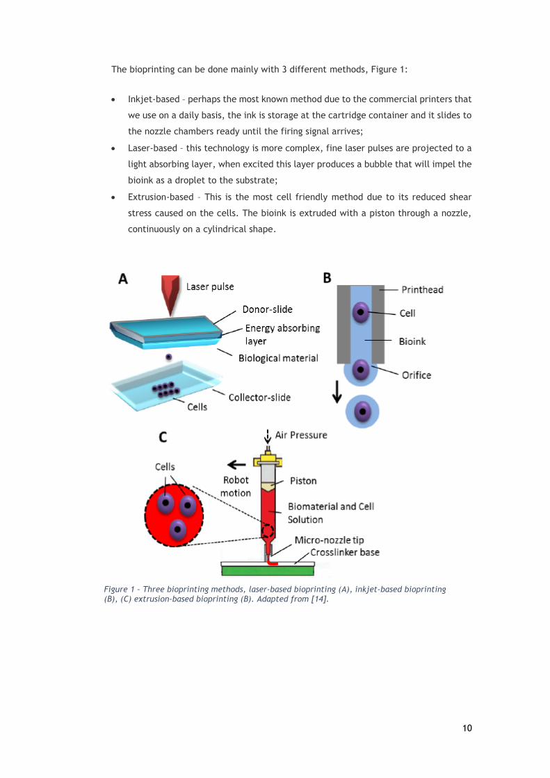
The bioprinting can be done mainly with 3 different methods, Figure 1:

Inkjet-based – perhaps the most known method due to the commercial printers that

we use on a daily basis, the ink is storage at the cartridge container and it slides to

the nozzle chambers ready until the firing signal arrives;

Laser-based – this technology is more complex, fine laser pulses are projected to a

light absorbing layer, when excited this layer produces a bubble that will impel the

bioink as a droplet to the substrate;

Extrusion-based – This is the most cell friendly method due to its reduced shear

stress caused on the cells. The bioink is extruded with a piston through a nozzle,

continuously on a cylindrical shape.

Figure 1 – Three bioprinting methods, laser-based bioprinting (A), inkjet-based bioprinting (B), (C) extrusion-based bioprinting (B). Adapted from [14].

11

In fact according to some authors, the biofabrication process needs to evolve like

automobile and microelectronics industry have done in the past, an automated robotic

approach is required for the successful development of new commercially profitable industries.

The combination of computer assisted printing technology with Tissue Engineering will open

new horizons for tissue biofabrication, enabling large scale industrial tissue and organ

bioassembly and also the necessary level of flexibility for specific customized organ

biofabrication.

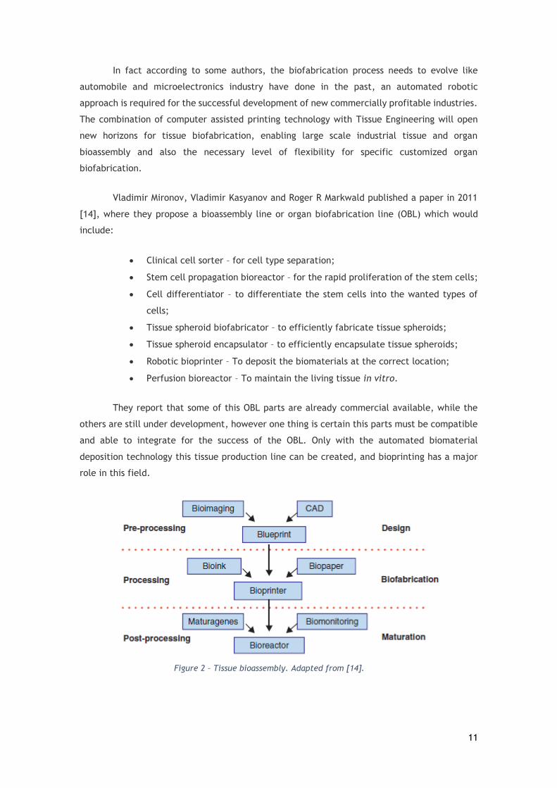
Vladimir Mironov, Vladimir Kasyanov and Roger R Markwald published a paper in 2011

[14], where they propose a bioassembly line or organ biofabrication line (OBL) which would

include:

Clinical cell sorter – for cell type separation;

Stem cell propagation bioreactor – for the rapid proliferation of the stem cells;

Cell differentiator – to differentiate the stem cells into the wanted types of

cells;

Tissue spheroid biofabricator – to efficiently fabricate tissue spheroids;

Tissue spheroid encapsulator – to efficiently encapsulate tissue spheroids;

Robotic bioprinter – To deposit the biomaterials at the correct location;

Perfusion bioreactor – To maintain the living tissue in vitro.

They report that some of this OBL parts are already commercial available, while the

others are still under development, however one thing is certain this parts must be compatible

and able to integrate for the success of the OBL. Only with the automated biomaterial

deposition technology this tissue production line can be created, and bioprinting has a major

role in this field.

Figure 2 – Tissue bioassembly. Adapted from [14].

12

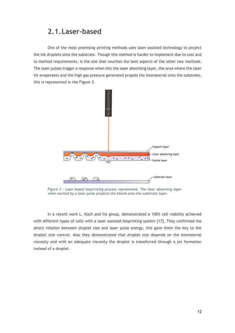
2.1. Laser-based

One of the most promising printing methods uses laser-assisted technology to project

the ink droplets onto the substrate. Though this method is harder to implement due to cost and

to method requirements, is the one that reunites the best aspects of the other two methods.

The laser pulses trigger a response when hits the laser absorbing layer, the area where the laser

hit evaporates and the high gas pressure generated propels the biomaterial onto the substrate,

this is represented in the Figure 3.

In a recent work L. Koch and his group, demonstrated a 100% cell viability achieved

with different types of cells with a laser assisted bioprinting system [17]. They confirmed the

direct relation between droplet size and laser pulse energy, this gave them the key to the

droplet size control. Also they demonstrated that droplet size depends on the biomaterial

viscosity and with an adequate viscosity the droplet is transferred through a jet formation

instead of a droplet.

Laser absobving layer

Support layer

bioink layer

substrate layer

Figure 3 – Laser-based bioprinting process represented. The laser absorving layer when excited by a laser pulse projects the bioink onto the substrate layer.

13

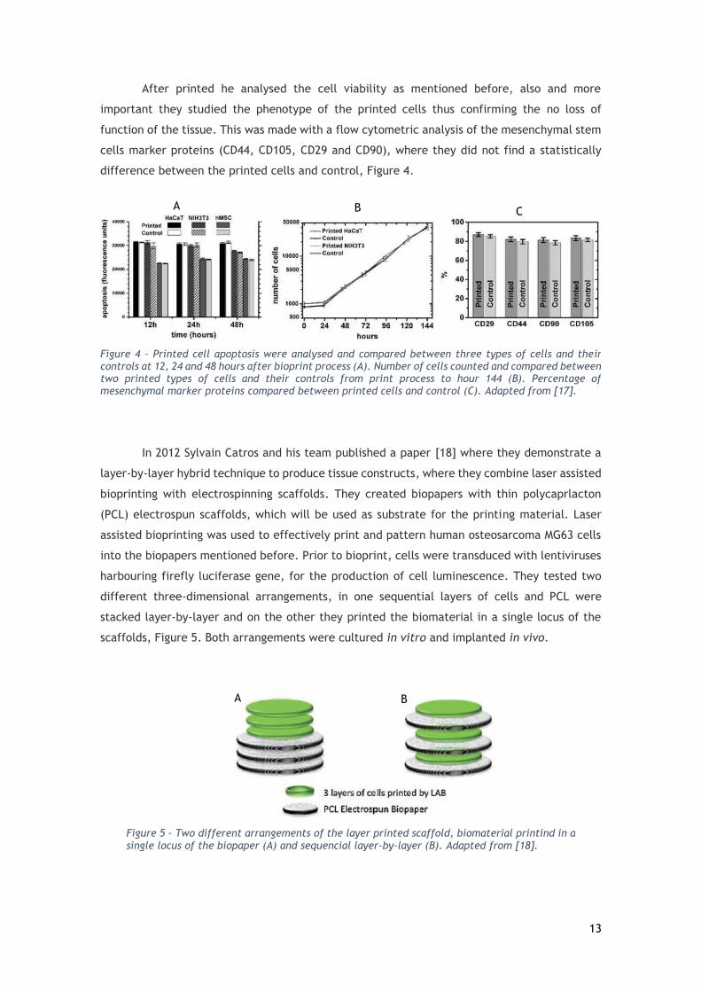
After printed he analysed the cell viability as mentioned before, also and more

important they studied the phenotype of the printed cells thus confirming the no loss of

function of the tissue. This was made with a flow cytometric analysis of the mesenchymal stem

cells marker proteins (CD44, CD105, CD29 and CD90), where they did not find a statistically

difference between the printed cells and control, Figure 4.

In 2012 Sylvain Catros and his team published a paper [18] where they demonstrate a

layer-by-layer hybrid technique to produce tissue constructs, where they combine laser assisted

bioprinting with electrospinning scaffolds. They created biopapers with thin polycaprlacton

(PCL) electrospun scaffolds, which will be used as substrate for the printing material. Laser

assisted bioprinting was used to effectively print and pattern human osteosarcoma MG63 cells

into the biopapers mentioned before. Prior to bioprint, cells were transduced with lentiviruses

harbouring firefly luciferase gene, for the production of cell luminescence. They tested two

different three-dimensional arrangements, in one sequential layers of cells and PCL were

stacked layer-by-layer and on the other they printed the biomaterial in a single locus of the

scaffolds, Figure 5. Both arrangements were cultured in vitro and implanted in vivo.

Figure 4 – Printed cell apoptosis were analysed and compared between three types of cells and their controls at 12, 24 and 48 hours after bioprint process (A). Number of cells counted and compared between two printed types of cells and their controls from print process to hour 144 (B). Percentage of mesenchymal marker proteins compared between printed cells and control (C). Adapted from [17].

A B C

Figure 5 – Two different arrangements of the layer printed scaffold, biomaterial printind in a single locus of the biopaper (A) and sequencial layer-by-layer (B). Adapted from [18].

A B

14

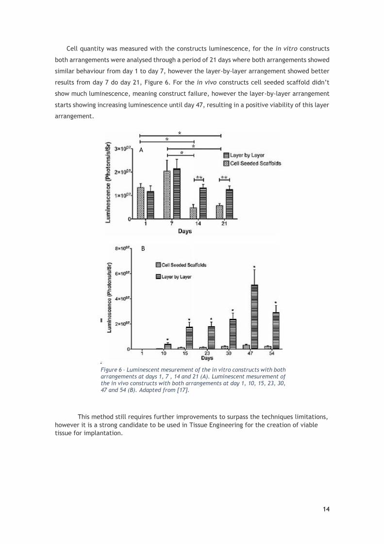
Cell quantity was measured with the constructs luminescence, for the in vitro constructs

both arrangements were analysed through a period of 21 days where both arrangements showed

similar behaviour from day 1 to day 7, however the layer-by-layer arrangement showed better

results from day 7 do day 21, Figure 6. For the in vivo constructs cell seeded scaffold didn’t

show much luminescence, meaning construct failure, however the layer-by-layer arrangement

starts showing increasing luminescence until day 47, resulting in a positive viability of this layer

arrangement.

This method still requires further improvements to surpass the techniques limitations,

however it is a strong candidate to be used in Tissue Engineering for the creation of viable

tissue for implantation.

Figure 6 – Luminescent mesurement of the in vitro constructs with both arrangements at days 1, 7 , 14 and 21 (A). Luminescent mesurement of the in vivo constructs with both arrangements at day 1, 10, 15, 23, 30, 47 and 54 (B). Adapted from [17].

B

A

15

2.2. Extrusion-based

The extrusion method is the most innocuous method in bioprinting due to the reduce

amounts of shear stress. On the other methods the cells are submitted to a quick and high

pressure pulse which might harm some of them. The bioink rests at the cylindrical deposit

waiting for the pressure, as pulse or continued, from a piston which propels the biomaterial

through a nozzle onto the substrate. Compared to the other methods, there is a resolution loss

in this one due to the bigger nozzle required, and precision loss due to the method limitations.

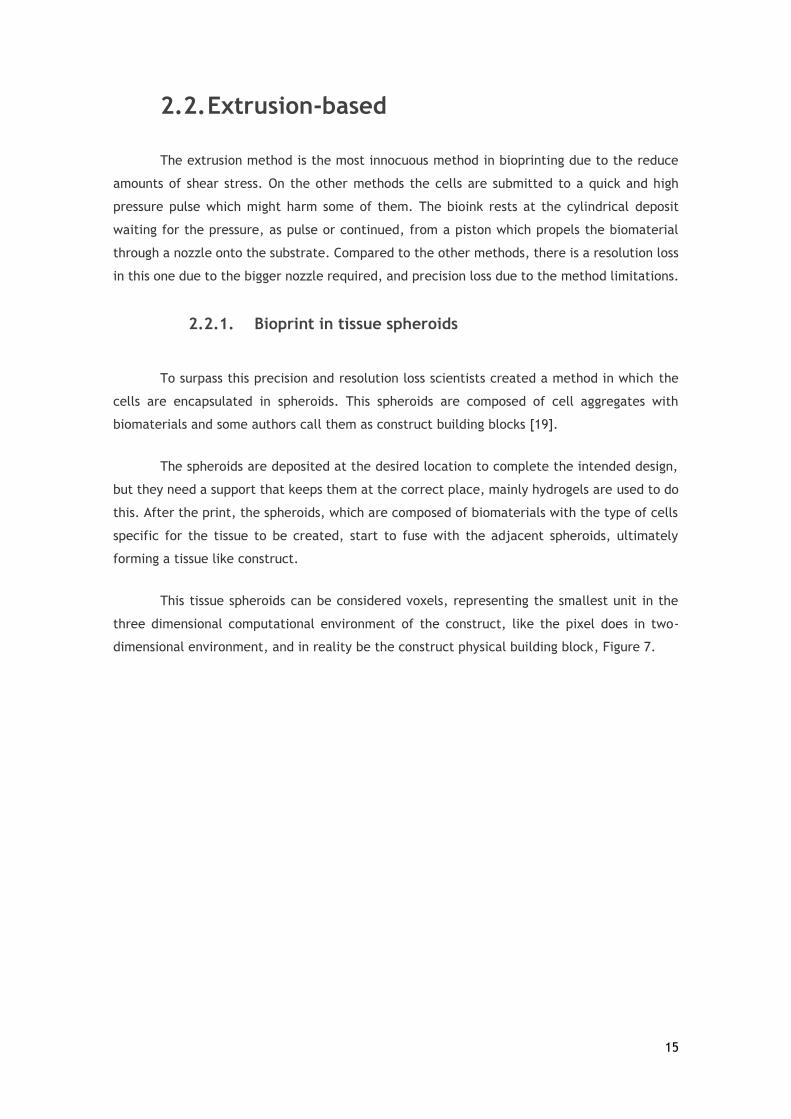
2.2.1. Bioprint in tissue spheroids

To surpass this precision and resolution loss scientists created a method in which the

cells are encapsulated in spheroids. This spheroids are composed of cell aggregates with

biomaterials and some authors call them as construct building blocks [19].

The spheroids are deposited at the desired location to complete the intended design,

but they need a support that keeps them at the correct place, mainly hydrogels are used to do

this. After the print, the spheroids, which are composed of biomaterials with the type of cells

specific for the tissue to be created, start to fuse with the adjacent spheroids, ultimately

forming a tissue like construct.

This tissue spheroids can be considered voxels, representing the smallest unit in the

three dimensional computational environment of the construct, like the pixel does in two-

dimensional environment, and in reality be the construct physical building block, Figure 7.

16

This is a remarkable idea to be implemented, however the spheroid properties like size,

viscosity, cell density and biomaterial integration needs to be optimized for a correct use of

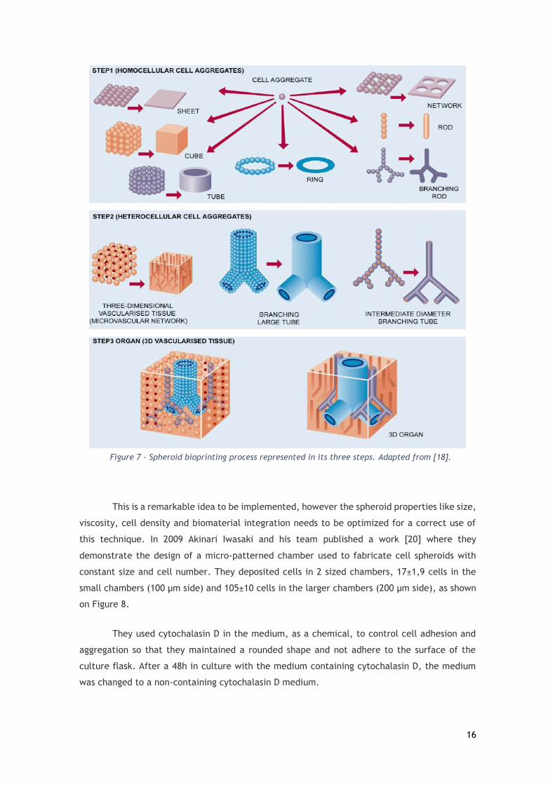
this technique. In 2009 Akinari Iwasaki and his team published a work [20] where they

demonstrate the design of a micro-patterned chamber used to fabricate cell spheroids with

constant size and cell number. They deposited cells in 2 sized chambers, 17±1,9 cells in the

small chambers (100 µm side) and 105±10 cells in the larger chambers (200 µm side), as shown

on Figure 8.

They used cytochalasin D in the medium, as a chemical, to control cell adhesion and

aggregation so that they maintained a rounded shape and not adhere to the surface of the

culture flask. After a 48h in culture with the medium containing cytochalasin D, the medium

was changed to a non-containing cytochalasin D medium.

Figure 7 – Spheroid bioprinting process represented in its three steps. Adapted from [18].

17

In the 12 hour period after the medium change several units of aggregated cell

spheroids was formed. The spheroids obtained showed a diameter of 88,72±12,98 µm on the

small chambers and 148,65±29,44 µm with the same cell density. The spheroids were collected

without the use of proteinase, such as trypsin-EDTA, which represents a step forward in

spheroid research, this is very important because the proteinase generally destroys the cellular

interactions within the spheroid.

Figure 8 – Cells maintaining round morphology inside the chambers (A), Cell aggregate formation inside the chambers (B), Detachment of the cell aggregates from the chambers (C, D). Adapted from [19]

A B

C D

18

In a good attempt to use the spheroid technique to produce viable constructs Cyrille

Norotte and his team published a work in 2009 [21], where they report a vascular tissue

fabrication without the use of a scaffold. To obtain their spheroids they cut equal size

fragments of an extruded cylinder of biomaterial with cells, and were left overnight to round

on a gyratory shaker. Depending on the extruded cylinder biomaterial diameter the procedure

provided regular spheroids of defined size and cell number. To support the spheroids they used

agarose rods as moulding template. Once assembled the multicellular spheroids fused within 5

to 7 days resulting in a tubular shape construct as shown in Figure 8.

The vascular tissue as most of living tissues contains more than one cell type and with

this in mind the these researchers created a tubular construct with two types of cells, smooth

muscle cells and fibroblasts. They used the same technique, agarose rods as support, but this

time with two different kinds of spheroids, each with one different cell type. After fused the

histology of the constructs were analysed, showing cell viability, Figure 8.

Although this techniques shows to be very promising still there are many limitations to

overcome, related to the method times and dimension restrictions.

Figure 9 – Capilar printed layers watched by luminescence microscopy (A), Representation of two type of cell capilar printed with the histological cuts after bioprinting (B). Adapted from [20].

A

B

19

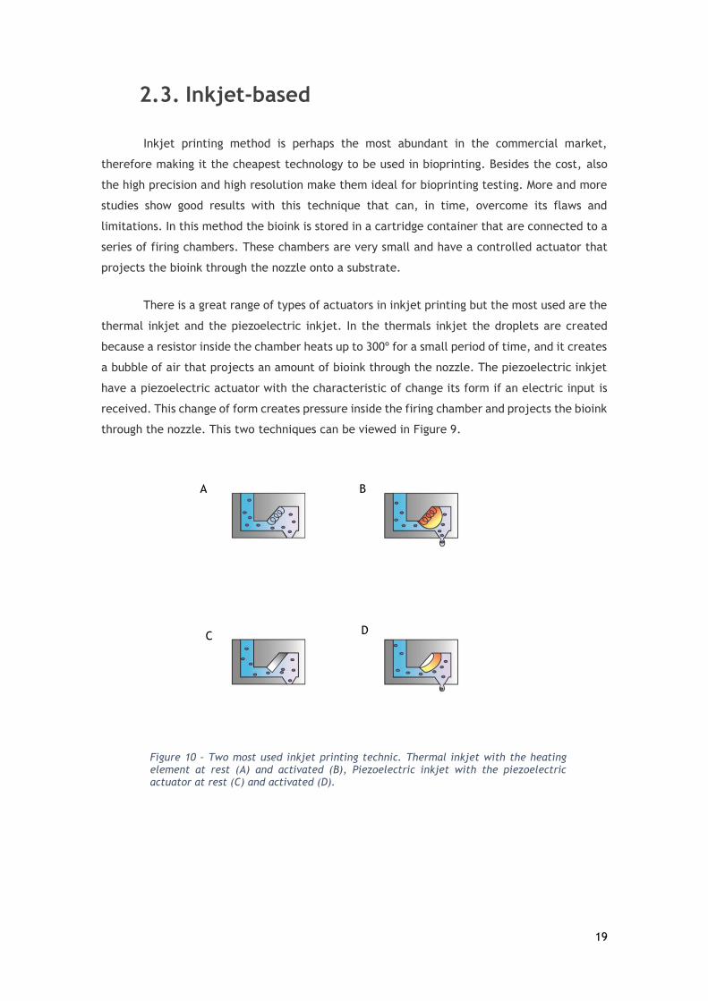
2.3. Inkjet-based

Inkjet printing method is perhaps the most abundant in the commercial market,

therefore making it the cheapest technology to be used in bioprinting. Besides the cost, also

the high precision and high resolution make them ideal for bioprinting testing. More and more

studies show good results with this technique that can, in time, overcome its flaws and

limitations. In this method the bioink is stored in a cartridge container that are connected to a

series of firing chambers. These chambers are very small and have a controlled actuator that

projects the bioink through the nozzle onto a substrate.

There is a great range of types of actuators in inkjet printing but the most used are the

thermal inkjet and the piezoelectric inkjet. In the thermals inkjet the droplets are created

because a resistor inside the chamber heats up to 300º for a small period of time, and it creates

a bubble of air that projects an amount of bioink through the nozzle. The piezoelectric inkjet

have a piezoelectric actuator with the characteristic of change its form if an electric input is

received. This change of form creates pressure inside the firing chamber and projects the bioink

through the nozzle. This two techniques can be viewed in Figure 9.

Figure 10 – Two most used inkjet printing technic. Thermal inkjet with the heating element at rest (A) and activated (B), Piezoelectric inkjet with the piezoelectric actuator at rest (C) and activated (D).

A B

C D

20

2.3.1. Thermal

As mentioned above the thermal inkjet uses a sudden increase of temperature to

project the ink from the firing chamber. At the correct time, a signal pulse heats up a resistor

or heating element inside the firing chamber, temperature rises up to 300º Celsius, but after

the evaporating point of the bioink solvent (most of the times water) starts to evaporate

creating a bubble. The evaporated solvent is a gas, and according to physics the volume of gas

evaporated is a lot bigger than the substance at liquid state, so this sudden increase of volume

creates pressure inside the chamber. The design of the chamber leaves only one exit by which

the pressure can escape, which is through the nozzle, so the droplet of bioink leaves the

chamber followed by the vaporized water, somewhat like a projectile is fired from a gun.

This temperature increase can be potentially harmful for the cells, because they are

sensitive to temperature changes. However more and more studies show better results and

although the temperature on the heat element can rise up to 300º Celsius the biomaterial

average temperature doesn’t rise more than a few degrees [22]. Besides the temperature

change there is another disadvantage in this method, the stress induced by the sudden pressure

change, may cause damage to cells when they have to squeeze through the tiny nozzle. After

all this negative aspects researchers report viabilities up to 90% like Tao Xu and his team in

their work published in 2005 with mammalian cells [23] lifting up hope for this technique in the

future of Tissue Engineering.

In a posterior work Tao Xu and his team demonstrated the viability and

electrophysiology of printed neural cells with thermal inkjet method [24]. They used a modified

HP 5126A ink cartridge to be used to deliver the living neuronal cells. This cartridge has fifty

nozzles with an average diameter of 50 µm. They printed rat hippocampal and cortical neurons

onto collagen-based biopaper and NT2 neuronal precursor cells and they report to have neuron

attachment onto the gel biopaper 3 to 5 hours after the print process.

Table 1 – Cell live and lysed count for 4 different printed constructs compared with the control. Adapted from [22].

21

Two well-established neuronal markers were used, MAP2 to identify dendrites and

axonal filament marker NF150 to identify the axons of the printed neurons. Their results of the

immunostaining strongly suggested the development of the neuron dendrites and axon and

maintenance of the neuronal phenotype after being printed.

To study the electrophysiology of the printed neurons they used a whole-cell voltage

clamp mode to record K+ and Na+ currents, two weeks after the bioprint process. Their results

suggested that printed cortical cells had developed into mature neurons with voltage-gated

potassium and sodium channels on the membranes. Also the neurons excitability was studied

with the current clamp model, and the printed cells proven to be able to perform firing action

potentials, Figure 10. They claim that the data collected are in good agreement with the

published results for normal electrophysiology of the rat neuronal cells.

Figure 11 – Electrophysiological characterization of rat embryonic hippocampal and cortical neurons after being printed. Representative recordings of sodium and potassium currents obtained from day-16 hippocampal neurons (A) and day-15 cortical neurons (B), Maximum action potential firing rates of hippocampal neuron (C) and cortical neuron (D). Adapted from [23].

22

For the use of the NT2 cells they first printed a biopaper made out of fibrin, a

biopolymeric gel that plays an important role in natural wound healing, and there is a good

affinity from neurons to this gel. The NT2 cells showed good adhesion to the fibrin printed

scaffold, which lead to the assumption that the bioprint process don’t print just cells, it may

be used to print the whole construct in the same time.

This studies prove the viability of this method of bioprinting thus boosting the

confidence for its use in Tissue Engineering, there is still much to be researched but the proof

of concept has already been demonstrated.

2.3.2. Piezoelectric

The piezoelectric inkjet instead of a heating element, uses a piezoelectric actuator.

The piezoelectric actuator is a component that has the property of change his form when

excited with an electric current. This piezoelectric effect is very interesting and it is worldwide

studied, because its concept is the transformation of pressure in electricity [25]. However this

can go the other way in which electricity is transformed in pressure, used in this inkjet

technique. Comparing to the other inkjet technique mentioned above, there isn’t temperature

change thus reducing the risk of damaging the printed cells. However there is still the stress

induced by pressure because of the tiny space the bioink has to go through.

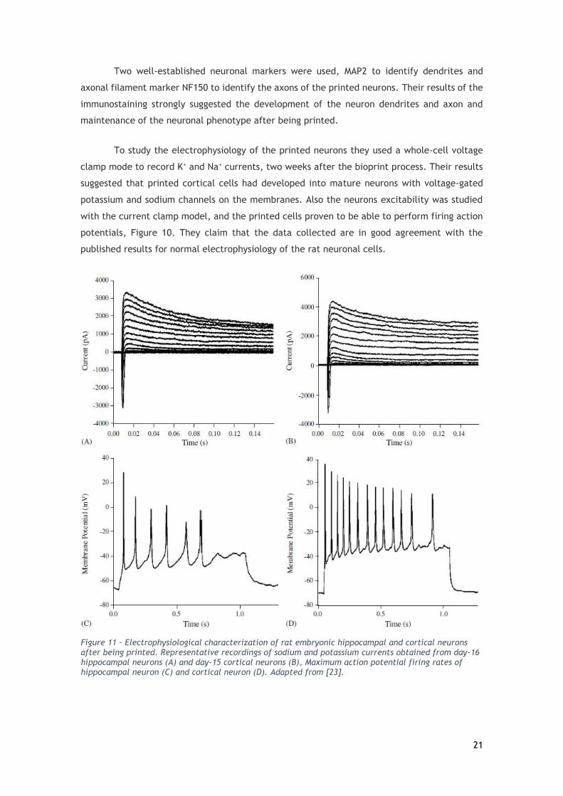
In a recent study Shuichi Yamaguchi and his team published a paper in 2012 [26] where

they demonstrated a technique of the piezoelectric actuation that allowed them to create

droplets with a round formation instead of the usual jet stream droplet. They used a modified

piezoelectric inkjet head with a transparent elliptical nozzle top for easy visualization of the

material inside the firing chamber. They did the experiment with 20 µm polystyrene beads and

Sf9 insect cells, they photographed the firing chamber before each firing pulse. In standard

piezoelectric printers, the method of the actuator to project the droplet happens in a Pull-Push

way, but the authors demonstrated that reverse method Push-Pull have better characteristics.

Their results show that in the standard way the droplet comes out of the nozzle as a

jet stream of liquid, while in the Push-Pull method the droplet come out as a sphere, this can

be visualized in Figure 12. This allows for higher precision since the material land onto the

substrate in a more condensed way thus focusing the printed material on the location, because

it suffers less air influence than the jet stream. Also they used a system that sent feedback the

position of the cell or bead ate the nozzle point and if it was ejected at the firing pulse, Figure

12. This allowed them to print a single cell for each droplet with a 100% accuracy rate. They

also studied the cell viability on the printed material and no statistically difference was found

comparing to control, in insect cells (Sf9).

23

This method can also be used to print biomaterials without the cells for scaffold

creation and/or scaffold characteristic analysis. Printing just the scaffold biomaterial can help

to understand the capabilities and characteristics of the bioprinting process in order to improve

the scaffold design for better cell adhesion and proliferation. Only hydrogels can be used to

fabricate 3D micro-structures with this technique due to the small nozzle size, the bioink

viscosity needs to be low in order to avoid nozzle clogging. With this in mind Nakamura M. and

his team reported the creation of micro-fabrication of a 3D tubular structure [27], with the

Figure 12 – Sketch representation of the two methods to use the piezoelectric actuator. Pull-Push (A), Push- Pull (B), Photographic representation of the Pull- Push method (C) and Push-Pull method (D). Photographic anaylisis of the cell or bead in sequencial photographies of the firing moment (E). Adapted from [24].

A B

E

C D

24

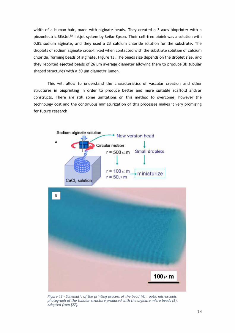
width of a human hair, made with alginate beads. They created a 3 axes bioprinter with a

piezoelectric SEAJetTM inkjet system by Seiko-Epson. Their cell-free bioink was a solution with

0.8% sodium alginate, and they used a 2% calcium chloride solution for the substrate. The

droplets of sodium alginate cross-linked when contacted with the substrate solution of calcium

chloride, forming beads of alginate, Figure 13. The beads size depends on the droplet size, and

they reported ejected beads of 26 µm average diameter allowing them to produce 3D tubular

shaped structures with a 50 µm diameter lumen.

This will allow to understand the characteristics of vascular creation and other

structures in bioprinting in order to produce better and more suitable scaffold and/or

constructs. There are still some limitations on this method to overcome, however the

technology cost and the continuous miniaturization of this processes makes it very promising

for future research.

Figure 13 – Schematic of the printing process of the bead (A), optic microscopic photograph of the tubular structure produced with the alginate micro beads (B). Adapted from [27].

A

B

25

3. Bioprinter

3.1. Building a bioprinter

In the attempt to recreate and adapt the mentioned works in this dissertation we

decided to build our own bioprinter. A bioprinter is a device for precise dispensation of biologic

or/with biocompatible materials and include three essential elements: X, Y and Z axes robotic

precision position system, automated biomaterial dispenser and computer based software for

operational control [14].

There were 2 main paths that we could go for: first was to get a commercial inkjet

printer and try to modulate it to print bioink, and to make it print in z axis; or second was to

build a bioprinter from ground up. The good thing about modulating an existing printing system

is that the hardware and the mechanisms are already built and calibrated, however there is

little information in how to control the hardware and exactly how the hardware operates, and

for that reason we ruled that option out. The challenges of building a 3D printer from ground

up are the correct alignment of the three axes (X, Y and Z), and also having good resolution,

since precision is required for the purpose of this work.

To minimise the cost to build the bioprinter, we decided to build it simple and with

day-to-day materials. The most important axes, X and Y, were built with 1 sheet of Poly(methyl

methacrylate) (PMMA), also known as acrylic glass, with one motor and rails to guide printing-

head or the substrate acrylic sheet. The axes acrylic sheets were held together by four 15 cm

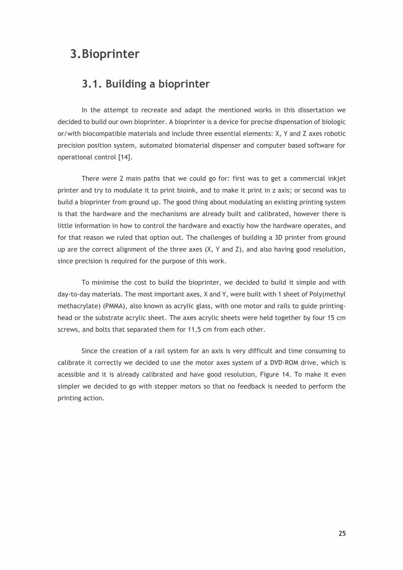
screws, and bolts that separated them for 11,5 cm from each other.

Since the creation of a rail system for an axis is very difficult and time consuming to

calibrate it correctly we decided to use the motor axes system of a DVD-ROM drive, which is

acessible and it is already calibrated and have good resolution, Figure 14. To make it even

simpler we decided to go with stepper motors so that no feedback is needed to perform the

printing action.

26

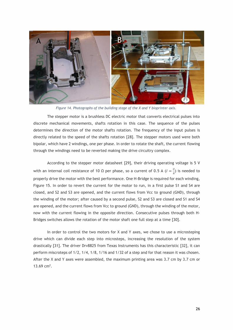
The stepper motor is a brushless DC electric motor that converts electrical pulses into

discrete mechanical movements, shafts rotation in this case. The sequence of the pulses

determines the direction of the motor shafts rotation. The frequency of the input pulses is

directly related to the speed of the shafts rotation [28]. The stepper motors used were both

bipolar, which have 2 windings, one per phase. In order to rotate the shaft, the current flowing

through the windings need to be reverted making the drive circuitry complex.

According to the stepper motor datasheet [29], their driving operating voltage is 5 V

with an internal coil resistance of 10 Ω per phase, so a current of 0.5 A (𝐼 =𝑈

𝑅) is needed to

properly drive the motor with the best performance. One H-Bridge is required for each winding,

Figure 15. In order to revert the current for the motor to run, in a first pulse S1 and S4 are

closed, and S2 and S3 are opened, and the current flows from Vcc to ground (GND), through

the winding of the motor; after caused by a second pulse, S2 and S3 are closed and S1 and S4

are opened, and the current flows from Vcc to ground (GND), through the winding of the motor,

now with the current flowing in the opposite direction. Consecutive pulses through both H-

Bridges switches allows the rotation of the motor shaft one full step at a time [30].

In order to control the two motors for X and Y axes, we chose to use a microsteping

drive which can divide each step into microsteps, increasing the resolution of the system

drastically [31]. The driver Drv8825 from Texas Instruments has this characteristic [32], it can

perform miscroteps of 1/2, 1/4, 1/8, 1/16 and 1/32 of a step and for that reason it was chosen.

After the X and Y axes were assembled, the maximum printing area was 3.7 cm by 3.7 cm or

13.69 cm2.

A B

Figure 14. Photographs of the building stage of the X and Y bioprinter axis.

27

Although the 2 motors are similar, the shaft screws, which run the moving parts, have

different thread leads. The threads are the helical structures that converts rotational to linear

movements. For this reason the two motors perform different step counts for a full length of

the axes (which are the same length). The motor with more step count was used for the bottom

axis, or subtract axis, for two main reasons: first to guarantee the best resolution for the

printing lines; second, the print head used which will be talked later has a specific nozzle to

nozzle spacing, and the step dimensions of both motors won’t increase this resolution. The

bottom motor performs 252 full steps in the length of 3.7 cm, that’s 146 µm each step, a

resolution of 68 dots per centimetre or 173 dots per inch (dpi). The Drv8825 can perform

microsteps which increase the resolution to numbers like 36.7 µm each microstep with a quarter

of a full step (almost reaching the dimension of most human cell diameter when extended),

creating a resolution of 272 dpcm and 692 dpi. The top motor screw thread lead is bigger,

resulting in less step count, so for the 3,7cm of the axis length it only performs 166 full steps.

That means 223 µm for each step, creating a resolution of 45 dpcm and 114 dpi, these values

also increase if microsteps are used. Although in theory the microsteping is a bright idea, the

motors weren’t capable of performing correctly this microsteps, missing some of them. Without

guaranteeing no step miss, we wouldn’t take the risk since we had no feedback system, so we

went for the full step system and started from there.

For the Z axis a different motor was needed since it had to support the weight of the

print head, although another stepper motor could be used, we went for a servo motor due to

its torque and stationary properties added to easy control. These motors are rotary actuators

that allow for precise control of angular position, velocity and acceleration. They have built-in

encoders that allows for precise immediate movements regardless of its previous position.

H-Bridge A

H-Bridge B

Figure 15 – Schematic of the actuation of the 2 H-bridges required to control a motor. At right we can see the signaling sequence to reverse the current direction in order to rotate the motor shaft.

1

2 4

3

28

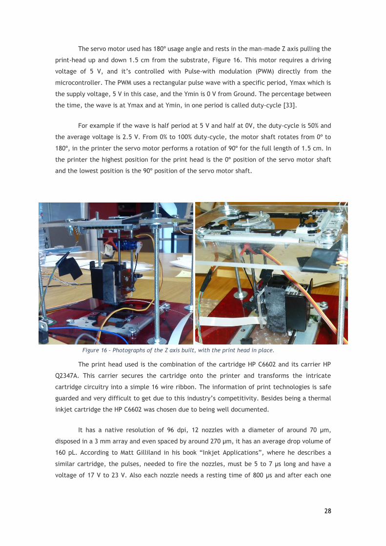
The servo motor used has 180º usage angle and rests in the man-made Z axis pulling the

print-head up and down 1.5 cm from the substrate, Figure 16. This motor requires a driving

voltage of 5 V, and it’s controlled with Pulse-with modulation (PWM) directly from the

microcontroller. The PWM uses a rectangular pulse wave with a specific period, Ymax which is

the supply voltage, 5 V in this case, and the Ymin is 0 V from Ground. The percentage between

the time, the wave is at Ymax and at Ymin, in one period is called duty-cycle [33].

For example if the wave is half period at 5 V and half at 0V, the duty-cycle is 50% and

the average voltage is 2.5 V. From 0% to 100% duty-cycle, the motor shaft rotates from 0º to

180º, in the printer the servo motor performs a rotation of 90º for the full length of 1.5 cm. In

the printer the highest position for the print head is the 0º position of the servo motor shaft

and the lowest position is the 90º position of the servo motor shaft.

The print head used is the combination of the cartridge HP C6602 and its carrier HP

Q2347A. This carrier secures the cartridge onto the printer and transforms the intricate

cartridge circuitry into a simple 16 wire ribbon. The information of print technologies is safe

guarded and very difficult to get due to this industry’s competitivity. Besides being a thermal

inkjet cartridge the HP C6602 was chosen due to being well documented.

It has a native resolution of 96 dpi, 12 nozzles with a diameter of around 70 µm,

disposed in a 3 mm array and even spaced by around 270 µm, it has an average drop volume of

160 pL. According to Matt Gilliland in his book “Inkjet Applications”, where he describes a

similar cartridge, the pulses, needed to fire the nozzles, must be 5 to 7 µs long and have a

voltage of 17 V to 23 V. Also each nozzle needs a resting time of 800 µs and after each one

Figure 16 – Photographs of the Z axis built, with the print head in place.

29

activated there must be a 0.5 µs delay to activate the next one, this means they cannot be

activated at the same time, and the pulses must be consecutive.

For this pulses high speed Toshiba photocouplers TLP250 were used [34], this device

provide electrical insulation for inputs and outputs. It converts an input electric signal into an

optical signal and then converts it back into an electric signal, with a led optically coupled to

a photodedector. It has propagation delays of 0.15 µs to a maximum of 0.5 µs, ideal to use

them to create our 6 µs pulses. Its supply voltage range is 10 V to 35 V, ideal for our 16 V to

23 V pulses, however its best feature is to ground up the outputs every time there isn’t any

signal from the inputs, stabling the nozzle firing process, preventing faulty responses when the

microcontroller is being uploaded with code and damage to the nozzles.

A single power supply wouldn’t provide the quantity of different voltages needed for

the components, however the bioprinting process is done in a small space, so a solution had to

be found. The printing process must be done in a laminar flow chamber to prevent

contaminations of the printed materials. The laminar flow chamber is a carefully enclosed

bench where the air is drawn through a High-efficiency particulate air (HEPA) filter and

projected in a smooth, laminar flow towards the working space of the chamber, in this case

the flow is vertical towards the bottom of the chamber. The HEPA filter removes any impurity

of the air making the laminar flow sterile. The working materials, in this case the printer,

circuitry and the laboratory equipment to manipulate the biologic substances must be

decontaminated with alcohol or UV light, for a period of time. For the chamber usage there is

a small enough opening, for the user to insert the forearms, to prevent outside air currents to

interfere with the laminar flow, this opening is controlled by the user to a certain height, where

from that point, there’s a risk of flow interference.

It’s for that reason, small space and small opening space, that we decided to use a

single power supply with an integrated board with DC-DC converters to convert the voltage

from the power supply to the voltage values needed for the printer components. There are 4

values of voltage needed:

3.3 V for the logic of the motor drivers, without this voltage, even if the driver is

supplied with the 8 V for the motors, and there are input signals the drive does

not respond. This voltage is given from the microcontroller itself, because the

Texas Instruments microcontrollers work with 3.3 V and can supply it.

5 V is required to supply the servo motor. This voltage is given by the DC-DC

converter PTH08080 WAH from Texas Instruments.

8V is required to supply motor drives, because the motor driver supply operating

voltage is between 8 V to 24 V. As said before the motors work at 5 V with an inner

coil of 10 Ω which implies a current of 0.5 A, however the drivers require at least

8 V, this increases the maximum current to 0.8 A which could damage the motors.

30

To prevent motor damage, two 15 Ω resistors per motor, one per winding were

added. This increases the total winding resistance to 25 Ω, reducing the potential

current to 0.32 A (𝐼 =𝑈

𝑅) and effectively prevent motor damage. This decrease of

current doesn’t affect the motor efficiency because the printing process doesn’t

require heavy loads. This voltage is given by the DC-DC converter PTN78060 WAH

from Texas Instruments.

18 V is required for the nozzle firing. As said before, the nozzles with-stand values

from 16 V to 23 V, and the firing pulse time is very small, if 16 V or 23 V would be

used there could be faulty firing, nozzle damage or non-firing from the nozzles.

This voltage is given by the DC-DC converter PTN78000 HAH from Texas

Instruments.

The power supply used was a KPS 613, which can provide 0 V to 30 V and 3 A maximum.

It was set to provide the integrated supply board with the maximum voltage required for the

printing process which was 18 V.

The DC-DC converter is an electronic circuit which convert a source of direct current

(DC) from one voltage level to another. If the output voltage is higher than the input it is called

Step-up (Boost) DC-DC, if the output voltage is lower than the input voltage it is called Step-

down (Buck) DC-DC. Texas Instruments provides components that have this electronic circuit in

the form of a single component with exceptional controlled outputs.

The PTN78000 H is a Step-down DC-DC converter and it was used to provide the 18 V to

the print head [35]. It can provide up to 1.5 A output current with a wide-input voltage of

11.85 V to 22 V and with a wide-output voltage adjust of 11.85 V to 22 V. It was adjusted with

a 3.6 KΩ resistor to provide an output voltage of 18.5 V according to the component datasheet.

The PTN78060 W is a Step-down DC-DC converter and it was used to provide the 8 V for

the motor drives [36]. It can provide up to 3 A output current with a wide-input voltage of 7 V

to 36 V and with a wide-output voltage adjust of 2.5 V to 12.6 V. It was adjusted with a 4.7 KΩ

resistor to provide an output voltage of 8.4 V according to the component datasheet. To simplify

the integrated source board the last DC-DC converter, the PTH08080 W, gets its supply voltage

directly from the PTN78060 W.

The PTH08080 W is also a Step-down DC-DC converter [37], and it can provide up to

2.25 A output current with a wide-input voltage of 4.5 V to 18 V, and an output voltage adjust

of 0.9 V to 5.5 V. It was adjusted with a 348 Ω resistor for an output voltage of 5 V. The major

characteristic of this components is that if there is any fluctuation of voltage from the power

supply, the rest of the printer components won’t get it, avoiding damaged or malfunction.

31

Every electronic component on the bioprinter is controlled by a microcontroller, in this

case a TivaTM TM4C123GH6PM built in its LaunchPad (TIVA C), from Texas Instruments [38]. This

is a low-cost, low-powered yet high performance microcontroller capable of operational

frequencies of 80 MHz, packed with 40 Input/output connectable pins, for digital or analogic

signalling. It runs at low voltage of 3.3 V, as most of the micro controllers from Texas

Instruments nowadays, and it communicates with the computer, in this case with Matlab (for

printing operation) or Energia (for code construction) through serial communication inside the

USB supply cable.

Serial communication is the process of sending or receiving data, one bit at a time

sequentially. There are 2 channels of communication between the two components, in this case

the computer and the microcontroller, with a ground channel as well. In each communication

channel the information is carried in opposite directions, one from the computer transmitter

(TX) pin to the microcontroller receiver (RX) pin and the other from the microcontroller TX pin

to the computer RX pin [39].

The term bit is an abbreviation of binary digit. It is the basic unit of information in

computing and digital communication, it can only have 2 values: 0 or 1. The two values can

also be interpreted as logical values (true or false, yes or no), algebraic signs (+ or −) or

activation states (on or off). Multiple bits may be represented and expressed in several ways,

the most common unit is the byte, coined by Werner Buchholz in 1956 when he proposed for a

generalized code to encode characters of text in a computer [40]. The byte of 8-bits can encode

up to 256 text characters which is the maximum arranges of bit sequence in an octet

configuration. The number of bits per byte may vary according with the hardware design, and

it hasn’t no definite standards that mandate the size. Nowadays computing systems operate

with fixed size groups of bits of 32 or 64 bits, but for the purpose of this work the

communication between the computer (Matlab) and the microcontroller was done in 8 bits and

with a baud rate of 14400. Baud, named after Émille Baudot, is the unit for symbols per second

or pulses per second, used in telecommunication and electronics communication.

For the Bioprinter to produce reliable and biomimetic patterns it needs an image

analysing, image decomposition and full printing command system, to do so the micro wouldn’t

be enough, that’s the reason Matlab was chosen to play that part. Matlab is a powerful tool

developed by MathWorks, which allows matrix manipulation, easy plotting of functions and

data, implementation of algorithms and interaction with other interfaces [41].

An algorithm was created in Matlab environment that can analyse and transform a RGB

image into raw data so that the dot positioning can be retrieved and organized for posterior

communication and print. Before starting to create the program the printing process needed to

be understood. Commercial printers have a standard way to print which is print the lines

consecutively according to the print line size, in our case the print cartridge has 12 nozzles

32

disposed in a 3 mm column. This 12 nozzles will represent the 12 dot column that will run the

printing line, so the image must be converted into 12 line matrixes, that’s our main focus.

The maximum dimension for the images allowed for the printing process is determined

by the resolution of each motor, as mentioned before the motors perform 252 steps by 166

steps in a 3.7 cm by 3.7 cm substrate. However the image pixel size must be smaller than

126×154 (explained later).

The algorithm starts by asking the image from the user, then the RGB image is

transformed into a grey scale image to help with the next step. The image needs to be

converted into a binary image with a filter, the filtering properties can be manipulated by the

user to get optimal results with the input images. This filter converts lighter pixels into white

pixels and darker areas into black pixels creating a black and white picture from the input

image. This picture can be easily converted into a matrix with the picture size and the white

pixels marked as 0 and black pixels marked as 1. At this phase we need to convert this matrix

into printing lines, as mentioned before 12 matrix lines per printing line. In Matlab matrixes

can be multidimensional, we used that property in our favour to simplify the variable list. A

matrix called Slice was created and gather the printing lines information. It is a 12 by n (length

of the matrix) by z (number of printing lines, determined by the equation 𝑛𝑢𝑚𝑏𝑒𝑟 𝑜𝑓 𝑙𝑖𝑛𝑒𝑠

12 ) and

it stores the printing line matrixes in the third dimension. For example to call the first printing

line it would be slice(m,n,1), the second would be slice(m,n,2) and so on. Theoretically the top

motor would need to move 12 steps after each print line, however physically the top motor

step length (22.3 µm) is lower than the spacing of the nozzles (27 µm). This means that to

perform the 3 mm displacement, the motor needs to do more than 12 steps (3000 µ𝑚 ÷

22.3 µ𝑚 = 13.45). 13 steps isn’t enough (13 × 22.3 µ𝑚 = 289.9 µ𝑚) so 14 steps is the most

correct amount of step per print line, so 14 real motor steps per 12 matrix lines. This provides

the maximum amount printing lines that the motor can perform which are 11, and the maximum

image length of the image which is 154 (11 × 14). The image proportion started to be affected

by this limitation due to the 252 steps from bottom motor being almost twice the 154 steps

from top motor, for that reason the amount of bottom motor was divided to half and the final

proportioned allowed image was determined to have 126×154.

With the Slice matrix the algorithm retrieves the printing position of the dots, saving

the numbers of the nozzles to fire in each printing column (representing the Y positions) on a

matrix called Nozzle, and saving the distance values of the dots from the beginning of the

printing line (representing the X positions) on a matrix called Motor1. The values of this last

matrix needs to be converted in distance from last one, so that we get the amount of steps to

perform after each displacement of the motor. For example if we have a printing column at

position 1 and 4 on the printing line, the motor needs to perform 1 step, for the position 1, and

then needs to perform 3 steps, for the position 4.

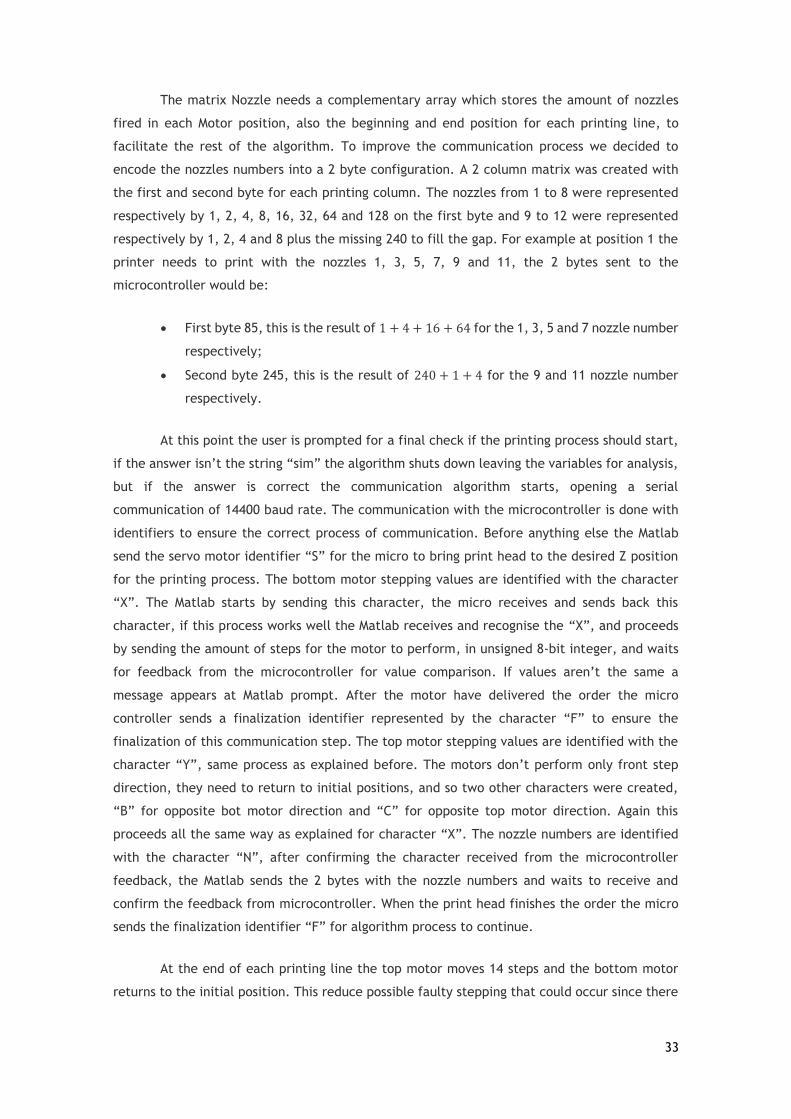
33

The matrix Nozzle needs a complementary array which stores the amount of nozzles

fired in each Motor position, also the beginning and end position for each printing line, to

facilitate the rest of the algorithm. To improve the communication process we decided to

encode the nozzles numbers into a 2 byte configuration. A 2 column matrix was created with

the first and second byte for each printing column. The nozzles from 1 to 8 were represented

respectively by 1, 2, 4, 8, 16, 32, 64 and 128 on the first byte and 9 to 12 were represented

respectively by 1, 2, 4 and 8 plus the missing 240 to fill the gap. For example at position 1 the

printer needs to print with the nozzles 1, 3, 5, 7, 9 and 11, the 2 bytes sent to the

microcontroller would be:

First byte 85, this is the result of 1 + 4 + 16 + 64 for the 1, 3, 5 and 7 nozzle number

respectively;

Second byte 245, this is the result of 240 + 1 + 4 for the 9 and 11 nozzle number

respectively.

At this point the user is prompted for a final check if the printing process should start,

if the answer isn’t the string “sim” the algorithm shuts down leaving the variables for analysis,

but if the answer is correct the communication algorithm starts, opening a serial

communication of 14400 baud rate. The communication with the microcontroller is done with

identifiers to ensure the correct process of communication. Before anything else the Matlab

send the servo motor identifier “S” for the micro to bring print head to the desired Z position

for the printing process. The bottom motor stepping values are identified with the character

“X”. The Matlab starts by sending this character, the micro receives and sends back this

character, if this process works well the Matlab receives and recognise the “X”, and proceeds

by sending the amount of steps for the motor to perform, in unsigned 8-bit integer, and waits

for feedback from the microcontroller for value comparison. If values aren’t the same a

message appears at Matlab prompt. After the motor have delivered the order the micro

controller sends a finalization identifier represented by the character “F” to ensure the

finalization of this communication step. The top motor stepping values are identified with the

character “Y”, same process as explained before. The motors don’t perform only front step

direction, they need to return to initial positions, and so two other characters were created,

“B” for opposite bot motor direction and “C” for opposite top motor direction. Again this

proceeds all the same way as explained for character “X”. The nozzle numbers are identified

with the character “N”, after confirming the character received from the microcontroller

feedback, the Matlab sends the 2 bytes with the nozzle numbers and waits to receive and

confirm the feedback from microcontroller. When the print head finishes the order the micro

sends the finalization identifier “F” for algorithm process to continue.

At the end of each printing line the top motor moves 14 steps and the bottom motor

returns to the initial position. This reduce possible faulty stepping that could occur since there

34

isn’t any positioning feedback system. After the process is finished a message is displayed at

the Matlab prompt “Imagem finalizada”, the algorithm can be viewed in the Annex.

On the microcontroller another algorithm needed to be created to transform the

information computing language in machine language. At first the Pins needs to be defined as

inputs or outputs, in this case the serial communication is done through the USB cable and since

there isn’t any feedback system for the microcontroller no input pins are needed. The amount

of pins needed for the circuitry are:

3 per stepper motor, the drive drv8825 only needs 3 logic inputs, one to enable

the device, other to direction and another for the step inputs.

1 to control the servo motor, this pin must allow analogic write for the creation

of the PWM needed.

12 for the print head, one for each nozzle, a demultiplexer could be used to

reduce the amount of pins, however the pulse times may get altered.

That makes a total of 19 pins set as outputs. The serial communication also needs to

be created and defined with same baud rate as the Matlab algorithm (14400). At first the

microcontroller sends the signal for the servo motor to go to the highest position, until the

servo identifier “S” is received the servo is maintained in the highest position. The

microcontroller algorithm works in a receiving way, this means that it remains at the same

position until an identifier arrives. If the identifier character isn’t one of the mentioned above,

it loops back to the receiving position. However if the character identifier is one of the above

mentioned, it initiates a cascade of processes. At first send a PWM signal to the servo motor to

lower the print head, Figure 17, to the desired position and then sends back what it receives

from the Matlab and awaits for the next value.

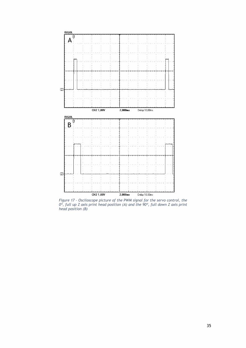
35

A

B

Figure 17 – Osciloscope picture of the PWM signal for the servo control, the 0º, full up Z axis print head position (A) and the 90º, full down Z axis print head position (B)

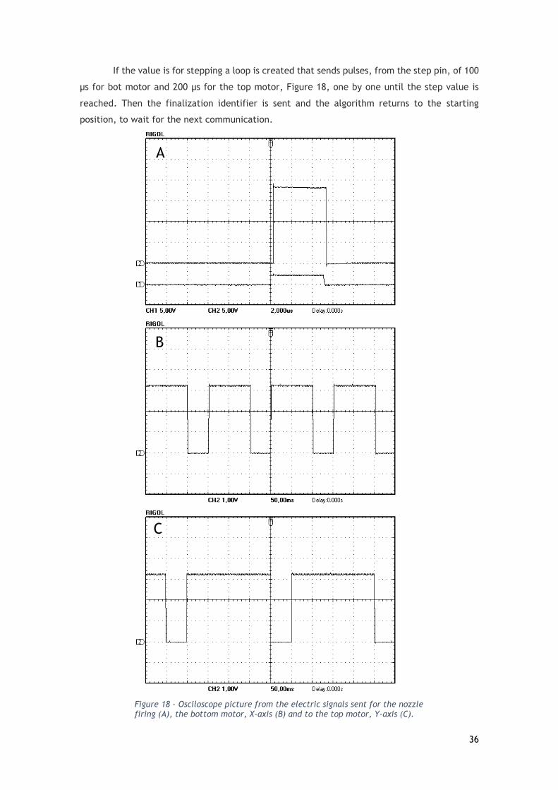
36

If the value is for stepping a loop is created that sends pulses, from the step pin, of 100

µs for bot motor and 200 µs for the top motor, Figure 18, one by one until the step value is

reached. Then the finalization identifier is sent and the algorithm returns to the starting

position, to wait for the next communication.

A

B

C

Figure 18 – Osciloscope picture from the electric signals sent for the nozzle firing (A), the bottom motor, X-axis (B) and to the top motor, Y-axis (C).

37

If the value is the nozzle number information, the algorithm starts by sending back the

2 bytes, then it initiates a loop that grabs each byte and subtracts the corresponding values

from each nozzle number mentioned above. For example if the first byte is equal to 85, it gets

subtracted consecutively with:

128, if the result would be above 0 it would send a pulse to the nozzle number

8;

64, in this case the result is 21 which is above 0, so it sends a pulse to the

nozzle 7 and then 21 is subtracted by the next number;

32, if the result would be above 0 it would send a pulse to the nozzle number

6;

16, in this case the result is 5 which is above 0, so it sends a pulse to the nozzle

5 and then 5 is subtracted by the next number;

8, if the result would be above 0 it would send a pulse to the nozzle number 4;

4, in this case the result is 5 which is above 0, so it sends a pulse to the nozzle

3 and then 1 is subtracted by the next number;

2, if the result would be above 0 it would send a pulse to the nozzle number 2;

1, when the loop reaches this line of code, it sends a pulse to nozzle number 1

and closes the loop so that the algorithm continues to the second byte loop.

Again it ends by sending the finalization identifier to confirm the print head operation

at that position. The pulses for the nozzles are defined with 4 µs pulse long with 800 µs delay

after. For the bottom motor each X movement is defined with two 100ms pulses long and two

50 ms delays, and for the top motor each Y movement is defined with one 200 ms pulse long

and one 50 ms delay.

When the pins were assigned to be the outputs from the microcontroller they had to be

carefully checked to be capable to execute the purpose we needed from them. The Launchpad

where the microcontroller is installed have 40 I/O pins where at least 2 are for 3.3 V and ground

output, this leaves 38 usable pins. Three pins are partially connected with the embedded leds

on the Launchpad and other five pins are partially connected to switches or other hardware,

this pins cannot be used due to the current limitation on the pins. From the 30 pins left a total

of 21 wires get out of the microcontroller board, 2 for the logic supply (3.3 V) and ground, and

the 19 for the components, the pin numbers used were chosen by their proximity to the

component arrangement, the pin number can be checked at microcontroller algorithm in the

Annex.

The Drv8825 stepper motor drive is a 28 pin HTSSOP component. The component pins

are connected as follows: Pins 1 (CP1) and 2 (CP2) were connected with a 0.01 µF ceramic

capacitor as mentioned at the component datasheet; The pin 3 called VCP connects to VM

(motor supply, 8 V) with a 1 MΩ resistor and a 0.1 µF capacitor; The pins 4 (VMA) and 11 (VMB)

38

are the input motor voltage and are connected to VM (8 V) and for each a 0.01 µF capacitor

connected to ground to stabilize the voltage; The pins 5 (AOUT1) and 7 (AOUT2) are the outputs

for the motor connected to the motor winding A with a 7 W and 15 Ω resistor; The pins 6 (ISENA)

and 9 (ISENB) are connected to ground with a sense resistor of 0.2 Ω each; The pins 8 (BOUT2)

and 10 (BOUT1) are the outputs for the motor winding B with a 7 W and 15 Ω resistor; The pins

12 (AVREF) and 13 (BVREF) are the current reference for each winding, and both connects at

the middle point of the voltage divider, this voltage divider connects logic voltage (3.3 V) to

ground (GND); The pins 14 (GND) and 28 (GND) are connected to ground; The pins 15, 18, 19,

23 and 27 have no purpose for this work, and are left disconnected; The pins 16 (nRESET) and

17 (nSLEEP) are connected to logic voltage (3.3 V); The pins 20 (DIR), 21 (ENABLE) and 22 (STEP)

are the inputs from the microcontroller and are connected to it; And finally the pins 24 (MOD0),

25 (MOD1) and 26 (MOD2) are the pins to perform micro stepping and are connected to ground

to avoid interference; At the breadboard VM is connected to GND with a 0.1 µF capacitor. One

circuit per motor is needed and the circuit schematic can be visualized in Figure 17.

The TLP250 photo coupler is an 8-lead DIP component. This component pins are

connected as follows: The pins 1, 4 and 7 are left unconnected; The pin 2 (Anode) is the

microcontroller input, and it’s connected to it; The pin 3 (Cathode) is connected to ground with

a 100 Ω resistor; The pin 5 (GND) is connected directly to ground; The pin 6 (Vout) is the output

connection to the printhead, to a single nozzle; Finally the pin 8 (Vcc) is the supply voltage

input, and is connected to the 18 V supply. To control the print head 12 of this components are

needed, one for each nozzle. Lastly the 18V supply is connected to ground with a 1000 µF

capacitor. The circuit schematic can be visualized in Figure 20.

The Source integrated board with the DC-DC converters from Texas Instruments, was

designed and created for the purpose of this work. The board has 2 inputs (Vcc and GND) from

the Power supply and 4 outputs (5 V, 8 V, 18 V and GND) for the bioprinter. As explained before,

the PTN78000 W was used to supply the 18 V for the printhead. It has 5 pins connected as

follows: The pin 1 (GND) was connected directly to ground; The pin 2 (Vin) was connected

directly to Vcc board input (18 V); The pin 3 (INHIB) was left disconnected; The pin 4 (Vout

adjust) was connected to ground with a 3.6 kΩ resistor; And finally the pin 5 (Vout) was

connected to 18 V output pin, this lead is also connected to ground with a 100 µF capacitor.

The PTN78060 W was used to supply the 8V to the stepper motors. It has 7 pins connected as

follows: The pin 1 (GND) and 7 (GND) were connected directly to ground; The pin 2 (Vin) was

connected directly to Vcc board input (18 V); The pin 3 (INHIB) and 5 (Vout Sense) were left

disconnected; The pin 4 (Vout adjust) was connected to ground with a 4.7 kΩ resistor; And

finally the pin 6 (Vout) was connected to 8 V output pin and to PTH08080 H Vin pin, this lead is

also connected to ground with a 100 µF capacitor. The PTH08080 H was used to supply the 5 V

for the servo motor. It has 5 pins connected as follows: The pin 1 (Vin) was connected to the

PTN78060 Vout pin (8 V); The pin 2 (GND) was connected directly to ground; The pin 3 (Vout)

39

was connected to 5 V output pin, this lead is also connected to ground with a 100 µF capacitor;

The pin 4 (Vout adjust) was connected to ground with a 348 Ω resistor; And finally the pin 5

(INHIB) was left disconnected. The input Vcc and GND were connected with a 100 µF capacitor.

This circuit schematic can be visualized in Figure 21.

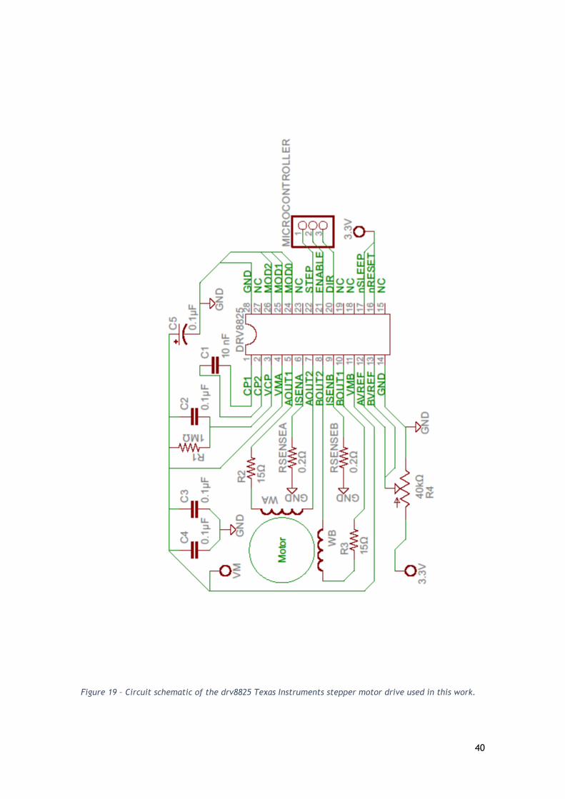
40

Figure 19 – Circuit schematic of the drv8825 Texas Instruments stepper motor drive used in this work.

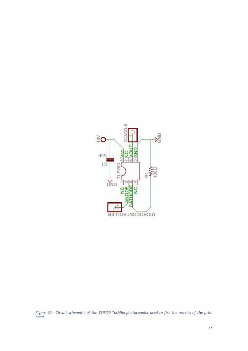
41

Figure 20 – Circuit schematic of the TLP250 Toshiba photocoupler used to fire the nozzles of the print head.

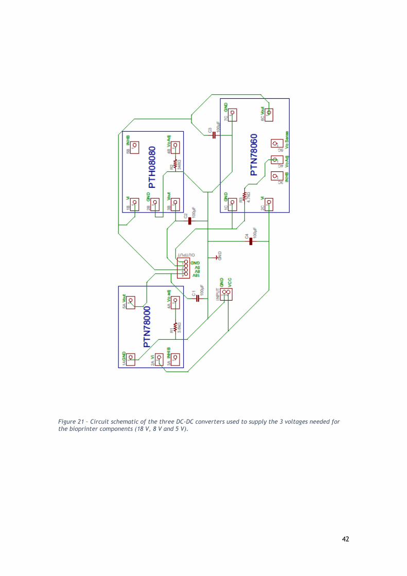
42

Figure 21 – Circuit schematic of the three DC-DC converters used to supply the 3 voltages needed for the bioprinter components (18 V, 8 V and 5 V).

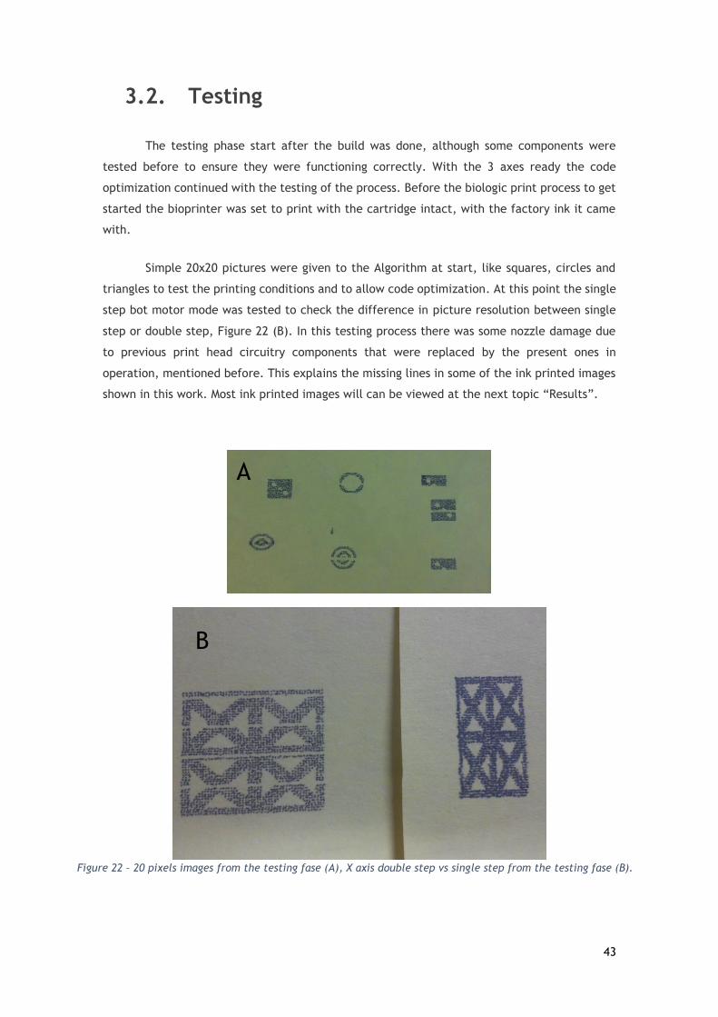
43

3.2. Testing

The testing phase start after the build was done, although some components were

tested before to ensure they were functioning correctly. With the 3 axes ready the code

optimization continued with the testing of the process. Before the biologic print process to get

started the bioprinter was set to print with the cartridge intact, with the factory ink it came

with.

Simple 20x20 pictures were given to the Algorithm at start, like squares, circles and

triangles to test the printing conditions and to allow code optimization. At this point the single

step bot motor mode was tested to check the difference in picture resolution between single

step or double step, Figure 22 (B). In this testing process there was some nozzle damage due

to previous print head circuitry components that were replaced by the present ones in

operation, mentioned before. This explains the missing lines in some of the ink printed images

shown in this work. Most ink printed images will can be viewed at the next topic “Results”.

A

B

Figure 22 – 20 pixels images from the testing fase (A), X axis double step vs single step from the testing fase (B).

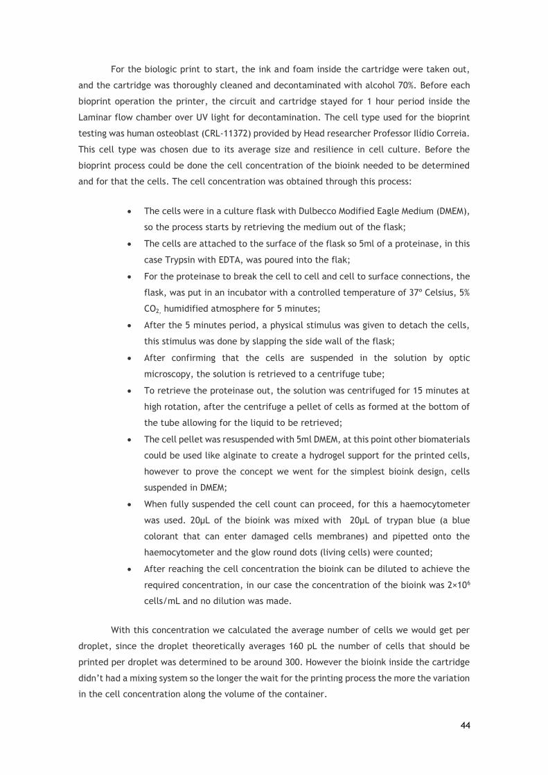
44

For the biologic print to start, the ink and foam inside the cartridge were taken out,

and the cartridge was thoroughly cleaned and decontaminated with alcohol 70%. Before each

bioprint operation the printer, the circuit and cartridge stayed for 1 hour period inside the

Laminar flow chamber over UV light for decontamination. The cell type used for the bioprint

testing was human osteoblast (CRL-11372) provided by Head researcher Professor Ilídio Correia.

This cell type was chosen due to its average size and resilience in cell culture. Before the

bioprint process could be done the cell concentration of the bioink needed to be determined

and for that the cells. The cell concentration was obtained through this process:

The cells were in a culture flask with Dulbecco Modified Eagle Medium (DMEM),

so the process starts by retrieving the medium out of the flask;

The cells are attached to the surface of the flask so 5ml of a proteinase, in this

case Trypsin with EDTA, was poured into the flak;

For the proteinase to break the cell to cell and cell to surface connections, the

flask, was put in an incubator with a controlled temperature of 37º Celsius, 5%

CO2, humidified atmosphere for 5 minutes;

After the 5 minutes period, a physical stimulus was given to detach the cells,

this stimulus was done by slapping the side wall of the flask;

After confirming that the cells are suspended in the solution by optic

microscopy, the solution is retrieved to a centrifuge tube;

To retrieve the proteinase out, the solution was centrifuged for 15 minutes at

high rotation, after the centrifuge a pellet of cells as formed at the bottom of

the tube allowing for the liquid to be retrieved;

The cell pellet was resuspended with 5ml DMEM, at this point other biomaterials

could be used like alginate to create a hydrogel support for the printed cells,

however to prove the concept we went for the simplest bioink design, cells

suspended in DMEM;

When fully suspended the cell count can proceed, for this a haemocytometer

was used. 20µL of the bioink was mixed with 20µL of trypan blue (a blue

colorant that can enter damaged cells membranes) and pipetted onto the

haemocytometer and the glow round dots (living cells) were counted;

After reaching the cell concentration the bioink can be diluted to achieve the

required concentration, in our case the concentration of the bioink was 2×106

cells/mL and no dilution was made.

With this concentration we calculated the average number of cells we would get per

droplet, since the droplet theoretically averages 160 pL the number of cells that should be

printed per droplet was determined to be around 300. However the bioink inside the cartridge

didn’t had a mixing system so the longer the wait for the printing process the more the variation

in the cell concentration along the volume of the container.

45

The bioprinter was programed to print a full 12 nozzle strip onto the substrate without

the use of any hydrogel, again just to prove the concept. The printed material was observed at

optic microscope right after the print process, and again after a period of 5 days, the results

are shown in the next section.

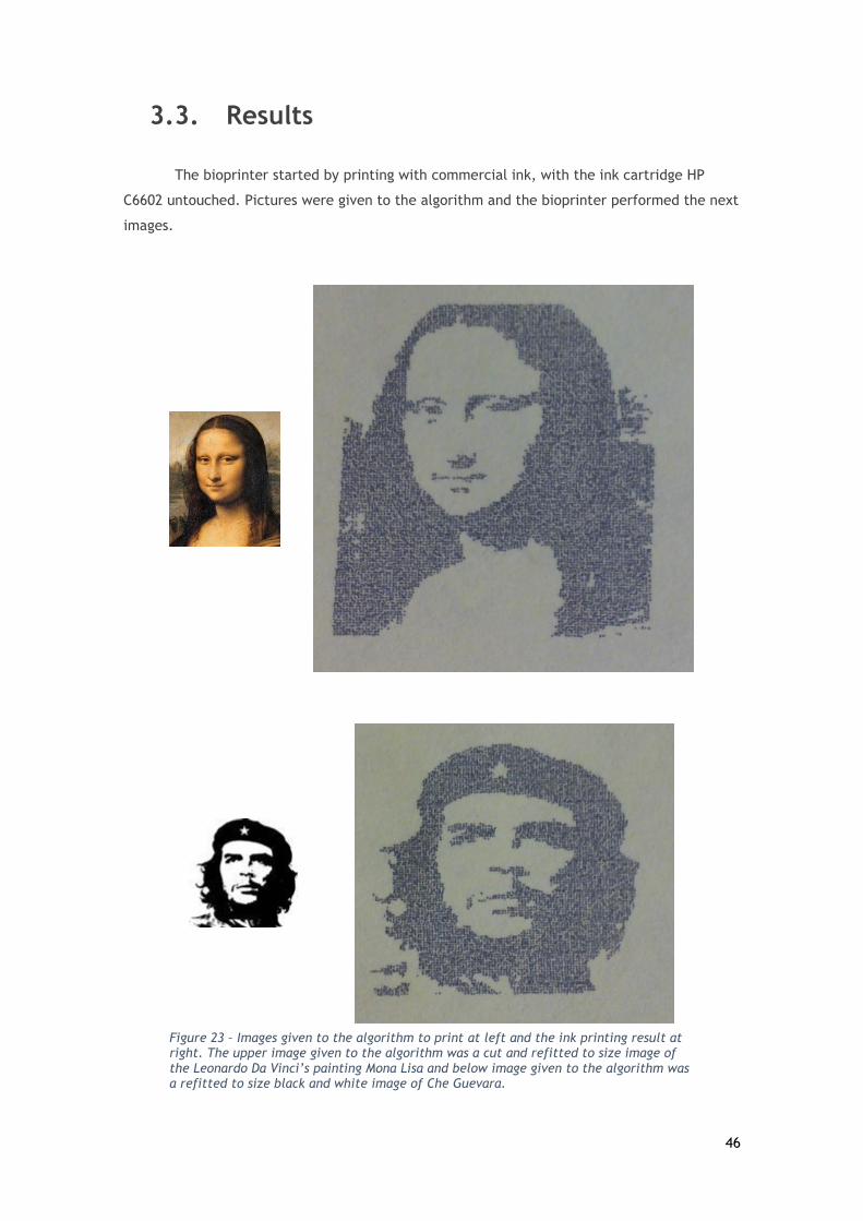
46

3.3. Results

The bioprinter started by printing with commercial ink, with the ink cartridge HP

C6602 untouched. Pictures were given to the algorithm and the bioprinter performed the next

images.

Figure 23 – Images given to the algorithm to print at left and the ink printing result at right. The upper image given to the algorithm was a cut and refitted to size image of the Leonardo Da Vinci’s painting Mona Lisa and below image given to the algorithm was a refitted to size black and white image of Che Guevara.

47

Figure 24 - Images given to the algorithm to print at left and the ink printing result at right. The upper image given to the algorithm was a black and white image representing a naked tree and below image given to the algorithm was a refitted to size image of the Universidade da Beira Interior institution symbol.

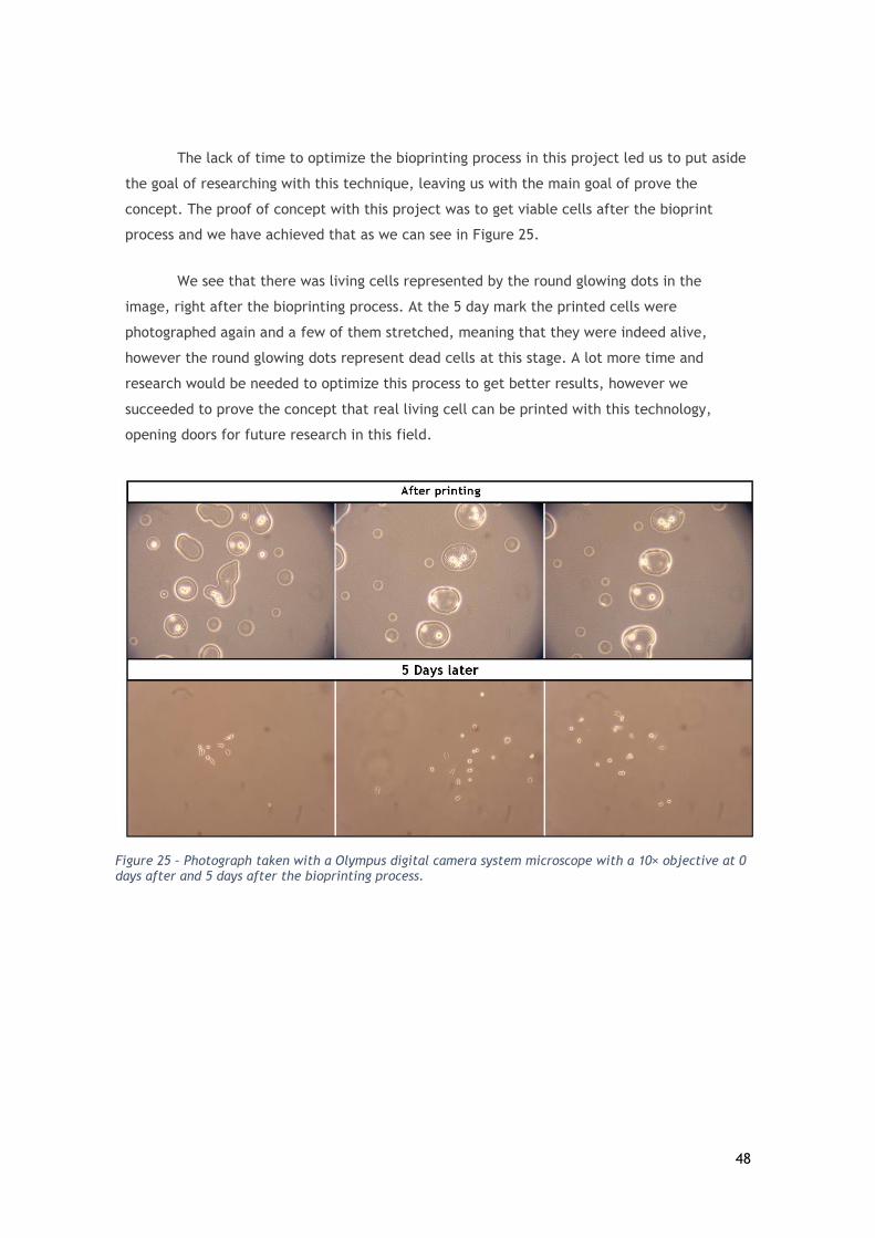
48

The lack of time to optimize the bioprinting process in this project led us to put aside

the goal of researching with this technique, leaving us with the main goal of prove the

concept. The proof of concept with this project was to get viable cells after the bioprint

process and we have achieved that as we can see in Figure 25.

We see that there was living cells represented by the round glowing dots in the

image, right after the bioprinting process. At the 5 day mark the printed cells were

photographed again and a few of them stretched, meaning that they were indeed alive,

however the round glowing dots represent dead cells at this stage. A lot more time and

research would be needed to optimize this process to get better results, however we

succeeded to prove the concept that real living cell can be printed with this technology,

opening doors for future research in this field.

Figure 25 – Photograph taken with a Olympus digital camera system microscope with a 10× objective at 0 days after and 5 days after the bioprinting process.

49

4. Conclusion

With the continuous growth of worlds population, and increase of population life

expectancy more cases of organ failure and tissue damage appear. The classic organ

transplanting method is not enough to supply the huge demand for organ worldwide, because

not only there is a shortage in organs for transplant but also there is the risk of blood

incompatibility, which in many cases leads to organ rejection. So a new way to get viable organ

or living tissue for implantation needs to be found, and is with this in mind that Tissue

Engineering and/or Regenerative Medicine come to aid.

Baby steps are being made by reasearcher in the field of Tissue Engineering, that

ultimately will lead for the ultimate goal. A lot of techniques are being researched each with

its individual characteristics and limitations, some with better results and others with better

future perspectives. Some of the most important techniques to create living tissue in order to

be implanted was mentioned in this work, focusing the promising technique of bioprinting and

its different methods. This methods were discribed and discussed, and results in that area have

been showed.

In an attempt to prove the concept a bioprinter was created from ground up with low

cost components and simple design. The component characteristics, function and choice reason

was mentioned above in this work. The printing volume alowed from the bioprinter is

aproximately 3.7 cm by 3.7 cm by 1.5 cm which is a reasonable volume to test it for bioprinting.

A complete mechanical structure, an hardware layout and a driver system was completely

designed and built. Also, an optimised algorithm was desgined and implemented to guide the

bioprinter to print complex images and it was tested with the ink cartidge. The bioprinter

showed good resolution and precision in the testing fase, as the ink printed pictures show.

After ink testing the bioprinter was used to print biomaterial, the purpose of its build.

The bioink used in the bioprint testing fase was a mixture of osteoblasts with Dulbecco Modified

Eagle Medium, the simplest approach possible. Some challenges came along the testing fase

but against all odds we got biologic printed results. After 5 days in culture some cells revealed

to be live thus proving the concept of the entire work.

Bioprint technology is one of the most interesting and promising techniques being

reasearched in the field of Tissue Engineering. No doubt about it, the combination of bioprinting

with other techniques and technologies will open new horizons for better and more suitable

constructs, and standardization will allow mass production with organ production lines, like

automobile and microelectronic industries does today. Still a lot of research needs to be done

50

to overcome this technology limitations, but we’re heading the right way. Although it’s in its

infancy, many researchers are showing great results with this technique and pointing to feasible

goals in a very near future.

In terms of future perspectives for this work, more bioprinting testing needed to be

done to optimize the bioink, substrate and the process parameters. New biomaterials could be

used to improve cell viability and process optimization. In terms of hardware, little

optimization that can be done with the current components. For better results, as precision

and resolution, new hardware needed to be implemented. Also the print head chosen could be

changed to one with a better method of biomaterial deposition, like piezoelectric or extrusion.

51

5. References

1. Weber, M., et al., Organ transplantation in the twenty-first century. The Urologic

clinics of North America, 1998. 25(1): p. 51-61.

2. Takeuchi, Y., S. Magre, and C. Patience, The potential hazards of

xenotransplantation: an overview. Revue scientifique et technique (International

Office of Epizootics), 2005. 24(1): p. 323-334.

3. Galliford, J. and D.S. Game, Modern renal transplantation: present challenges

and future prospects. Postgraduate medical journal, 2009. 85(1000): p. 91-101.

4. Steering Committee of the Istanbul, S., Organ trafficking and transplant tourism

and commercialism: the Declaration of Istanbul. The Lancet. 372(9632): p. 5-6.

5. Sixty-Third, W.H.A. and W.H. Organization, WHO Guiding Principles on Human

Cell, Tissue and Organ Transplantation. Cell and tissue banking, 2010. 11(4): p.

413.

6. Wolter, J.R. and R.F. Meyer, Sessile macrophages forming clear endothelium-like

membrane on inside of successful keratoprosthesis. Trans Am Ophthalmol Soc,

1984. 82: p. 187-202.

7. Langer, R. and J.P. Vacanti, Tissue engineering. Science, 1993. 260(5110): p.

920-6.

8. Lin, X., et al., Enhancement of cell attachment and tissue integration by a IKVAV

containing multi-domain peptide. Biochim Biophys Acta, 2006. 1760(9): p. 1403-

10.

9. Takahashi, K. and S. Yamanaka, Induction of pluripotent stem cells from mouse

embryonic and adult fibroblast cultures by defined factors. Cell, 2006. 126(4): p.

663-76.

10. Rauh, J., et al., Bioreactor systems for bone tissue engineering. Tissue Eng Part B

Rev, 2011. 17(4): p. 263-80.

11. Oh, S.H., et al., Oxygen generating scaffolds for enhancing engineered tissue

survival. Biomaterials, 2009. 30(5): p. 757-62.

12. Schmidt, C.E. and J.M. Baier, Acellular vascular tissues: natural biomaterials for

tissue repair and tissue engineering. Biomaterials, 2000. 21(22): p. 2215-31.

13. Crapo, P.M., T.W. Gilbert, and S.F. Badylak, An overview of tissue and whole

organ decellularization processes. Biomaterials, 2011. 32(12): p. 3233-43.

14. Mironov, V., V. Kasyanov, and R.R. Markwald, Organ printing: from bioprinter

to organ biofabrication line. Curr Opin Biotechnol, 2011. 22(5): p. 667-73.

52

15. Ozbolat, I.T. and Y. Yu, Bioprinting Toward Organ Fabrication: Challenges and

Future Trends. Ieee Transactions on Biomedical Engineering, 2013. 60(3): p. 691-

699.

16. Gruene, M., et al., Dispensing pico to nanolitre of a natural hydrogel by laser-

assisted bioprinting. Biomed Eng Online, 2011. 10: p. 19.

17. Guillemot, F., et al., Laser-assisted cell printing: principle, physical parameters

versus cell fate and perspectives in tissue engineering. Nanomedicine, 2010. 5(3):

p. 507-515.

18. Catros, S., et al., Layer-by-layer tissue microfabrication supports cell

proliferation in vitro and in vivo. Tissue Eng Part C Methods, 2012. 18(1): p. 62-

70.

19. Mironov, V., et al., Organ printing: tissue spheroids as building blocks.

Biomaterials, 2009. 30(12): p. 2164-74.

20. Iwasaki, A., et al., Mass Fabrication of Small Cell Spheroids by Using Micro-

patterned Tissue Culture Plate. Advanced Engineering Materials, 2009. 11(10):

p. 801-804.

21. Norotte, C., et al., Scaffold-free vascular tissue engineering using bioprinting.

Biomaterials, 2009. 30(30): p. 5910-5917.

22. Cui, X., et al., Cell damage evaluation of thermal inkjet printed Chinese hamster

ovary cells. Biotechnol Bioeng, 2010. 106(6): p. 963-9.

23. Xu, T., et al., Inkjet printing of viable mammalian cells. Biomaterials, 2005. 26(1):

p. 93-9.

24. Xu, T., et al., Viability and electrophysiology of neural cell structures generated

by the inkjet printing method. Biomaterials, 2006. 27(19): p. 3580-8.

25. Wijshoff, H., The dynamics of the piezo inkjet printhead operation. Physics

Reports, 2010. 491(4-5): p. 77-177.

26. Yamaguchi, S., et al., Cell patterning through inkjet printing of one cell per

droplet. Biofabrication, 2012. 4(4): p. 045005.

27. Nakamura, M., Y. Nishiyama, and C. Henmi. 3D Micro-fabrication by Inkjet 3D

biofabrication for 3D tissue engineering. in Micro-NanoMechatronics and

Human Science, 2008. MHS 2008. International Symposium on. 2008. IEEE.

28. Sen, P.C., Electric motor drives and control-past, present, and future. Industrial

Electronics, IEEE Transactions on, 1990. 37(6): p. 562-575.

29. Minebea-Mastushiba, PL15S-020. motor datasheet, 2004.

53

30. Condit, R. and D.W. Jones, Stepping motors fundamentals. Microchip

Application Note: AN907,[Online]. Available: www. microchip. com, 2004.

31. Baluta, G. and M. Coteata. Precision microstepping system for bipolar stepper

motor control. in Electrical Machines and Power Electronics, 2007. ACEMP'07.

International Aegean Conference on. 2007. IEEE.

32. Texas Instruments. DRV8825 Stepper Motor Controller IC. SLVSA73F

datasheet, Apr. 2010 [Revised Jul. 2014].

33. Dote, Y. and S. Kinoshita, Brushless servomotors. Fundamentals and, 1990.

34. TOSHIBA. Photocoupler GaAlAs Ired & Photo−IC TLP250. datasheet, Jun.

2004.

35. Texas Instruments. PTN78000H 1.5-A, WIDE-INPUT ADJUSTABLE

SWITCHING REGULATOR. SLTS230C datasheet, Nov. 2004 [Revised Sept.

2008].

36. Texas Instruments. PTN78060W 3-A, WIDE INPUT ADJUSTABLE SWITCHING

REGULATOR. SLTS229B datasheet, Nov. 2004 [Revised Sept. 2009].

37. Texas Instruments. PTH08080W 2.25-A, WIDE-INPUT ADJUSTABLE

SWITCHING REGULATOR. SLTS235D datasheet, Feb. 2005 [Revised Sept.

2013].

38. Texas Instruments. Tiva™ TM4C123GH6PM Microcontroller. DS-

TM4C123GH6PM-15842.2741, SPMS376E datasheet, Jun. 2014.

39. WANG, Z.-j. and M. SHEN, Serial Communication Program Development Based

on Matlab GUI [J]. Modern Electronics Technique, 2010. 9: p. 013.

40. Bemer, R.W., A proposal for a generalized card code for 256 characters.

Communications of the ACM, 1959. 2(9): p. 19-23.

41. Moore, H. and S. Bhat, MATLAB for Engineers2007: Pearson Prentice Hall.

54

Annex

The Matlab algorithm was created in Matlab R2012b:

“

clc clear [filename, pathname, filterindex] = uigetfile('*.png', 'Pick an image

to start printing'); %In the above line the user is asked for na image. A=imread(filename); %imread transforms the image into a tridimensional matrix A. B=rgb2gray(A); %rgb2gray allows the tranformation of the RGB matrix A into a

%greyscale matrix B. C=im2bw(B,0.75); %Im2bw allows to create a binary matrix C , out of the grey scale

%matrix B, where 1 represents lighter areas and 0 represents darker %areas. Mimg=~C; %this line was created to reverse the binary code, Mimg becomes a

matrix with 0 for lighter áreas and 1 for darker áreas.

M = 1:size(Mimg,1); z=0; for i = 1:12:size(M,2) %This cycle allows the creation of a matrix slice that saves the

%matrix lines numbers that are going to be printed in each printing

%line. z=z+1; for k = i:1:i+11 if k <= size(M,2) x=k-i+1; slice(x,:,z)= M(:,k); end end end

fatia=zeros(12,size(Mimg,2)); for z = 1:size(slice,3) %This cycle allows the creation of a matrix fatia that saves the

%matrix lines used for each printed line (z). for j = 1:size(slice,1) if slice(j,:,z)> 0 fatia(j,:,z) = Mimg(slice(j,:,z),:); else fatia(j,:,z) = 0; end end end

n=1; for z = 1:size(fatia,3) %This cycle allows to create two diferente matrixes. for j = 1:size(fatia,2) for i = 1:size(fatia,1) if fatia(i,j,z)== 1

55

nozzle(n,:,z)= i; %nozzle stores the numbers of the nozzles that are going to be fired. motor1(n,:,z)= j; %motor1 stores the printing positions of the X motor. n=n+1; end end end end

step = zeros(size(motor1)); for z = 1:size(motor1,3) %This cycles allows the creation of the step matrix that stores the

%step count for the motor to perform for each printing position. for n = 1:size(motor1,1); if n == 1 step(n,:,z) = motor1(n,:,z); end if n < size(motor1,1) step(n+1,:,z) = motor1(n+1,:,z) - motor1(n,:,z); end end end

for z = 1:size(step,3)

%This cycle creates 2 array to store the first and last nozzle to be

%fired in each printing line. for h = 1:size(step,1) if step(h,:,z) > 0; array(h,:,z)= h; array2(:,:,z)=find(step(:,:,z) > 0 , 1,

'last')+(find(nozzle(:,:,z) > 0 , 1, 'last')+1-find(step(:,:,z) > 0 ,

1, 'last')); end end end

nnozz = zeros(size(step,1),1,size(step,3)); for z = 1:size(array,3)

%This cycle allows the creation of matrix nnozz that stores the nozzle

%numbers in a correct form for the next process.

A = zeros(size(step,1),1,size(step,3)); A = find(array(:,:,z)); e2(:,:,z) = find(nozzle(:,:,z), 1, 'last'); for e = 1:size(A,1) if e < size(A,1) nnozz(A(e),:,z) = A(e+1,:,1) - A(e,:,1); end if e == size(A,1) nnozz(A(e),:,z) = e2(1,:,z) - A(e,:,1); end end end

nozzcomm=zeros(size(nozzle,1),2,size(nozzle,3)); for z = 1:size(nozzle,3)

%In this cycle a double array is created to store the 2 byte

%information sent to the microcontroller with the nozzle numbers

56

for e = 1:size(array,1) if array(e,:,z)~=0; fbyte(e,:,z)=0; sbyte(e,:,z)=0; for i = array(e,:,z): array(e,:,z) + nnozz(e,:,z)-1 switch nozzle(i,:,z) case 1; fbyte(e,:,z) = fbyte(e,:,z) + 1; case 2; fbyte(e,:,z) = fbyte(e,:,z) + 2; case 3; fbyte(e,:,z) = fbyte(e,:,z) + 4; case 4; fbyte(e,:,z) = fbyte(e,:,z) + 8; case 5; fbyte(e,:,z) = fbyte(e,:,z) + 16; case 6; fbyte(e,:,z) = fbyte(e,:,z) + 32; case 7; fbyte(e,:,z) = fbyte(e,:,z) + 64; case 8; fbyte(e,:,z) = fbyte(e,:,z) + 128; case 9; sbyte(e,:,z) = sbyte(e,:,z) + 1; case 10; sbyte(e,:,z) = sbyte(e,:,z) + 2; case 11; sbyte(e,:,z) = sbyte(e,:,z) + 4; case 12; sbyte(e,:,z) = sbyte(e,:,z) + 8; end end nozzcomm(array(e,:,z),1,z)= fbyte(e,:,z); nozzcomm(array(e,:,z),2,z)= sbyte(e,:,z) + 240; end end end

Resp = inputdlg('Tem a certeza que deseja imprimir esta

imagem?','Resposta tipo: sim, não',1); %This creates a final checkup for the user, to decide whether he wants

%to continue with the printing or not. options.Resize='on'; options.WindowStyle='normal'; options.Interpreter='tex'; disp(Resp); c=1; y=0; if strcmp (Resp, 'sim') == 1; %If the answered string was a ‘sim’ then the communication and

%printing process starts. s=serial('COM1', 'BAUD', 14400); fopen(s); pause(2.5); fwrite(s, 'S', 'char'); pause(0.5); for z = 1:size(step,3) for h = 1:size(step,1)

%This loop will go through the step matrix length searching for the

%printing positions to be reached. x = step(h,:,z);

57

bytes = [nozzcomm(h,1,z), nozzcomm(h,2,z)]; k = nnozz(h,:,z); run mcomsteptest.m;

%the script mcomsteptest.m is used for the communication with the

%microcotroller for the step values. run mcomnozzletest.m; %the script mcomsteptest.m is used for the communication with the

%microcotroller for the nozzle numbers. end if z == size(step,3)

%This stage is for the last printed printing line, the micro receives

%the values for the maximum X and Y displacement reached. y = -(size(step,3)-1)*14; p = sum(step); x = -p(:,:,size(step,3)); run mcomsteptest.m; run mcomsteptest.m; disp('Imagem finalizada'); else

%This condition is reached at the end of each printing line. y=14; run mcomsteptest.m; end end fclose(s); else msgbox('Operação cancelada.') end msgbox('Operação concluída com sucesso.') “

Mcomsteptest.m script

“

if x > 0; pause(0.1); fwrite(s, 'X', 'char'); % X front step identifier. pause(0.2); R = fread(s, 1); disp(char(R)); if R == 'X'; pause(0.1); fwrite(s, x, 'uint8'); pause(0.2); R2 = fread(s, 1); disp(R2); if R2 ~= x; disp('error in x step comm') end else disp('no comm...') end pause(x*0.32); R3 = fread(s, 1); if R3 == 'F'; fwrite(s, 'F', 'char'); else disp('no x finalization identifier'); end

58

disp(char(R3)); pause(0.2); R3=0; R=0; R2=0; x=0;

elseif x < 0; b = -x; pause(0.1); fwrite(s, 'B', 'char'); % X Back step identifier. pause(0.2); R = fread(s, 1); disp(char(R)); if R == 'B'; pause(0.1); fwrite(s, b, 'uint8'); pause(0.2); R2 = fread(s, 1); disp(R2); if R2 ~= b; disp('error in b step comm') end else disp('no comm...') end pause(b*0.32); R3 = fread(s, 1); if R3 == 'F'; fwrite(s, 'F', 'char'); else disp('no b finalization identifier'); end disp(char(R3)); pause(0.2); R3=0; R=0; R2=0; x=0;

elseif y > 0; pause(0.1); fwrite(s, 'Y', 'char'); % Y Front step identifier. pause(0.2); R = fread(s, 1); disp(char(R)); if R == 'Y'; pause(0.1); fwrite(s, y, 'uint8'); pause(0.1); R2 = fread(s, 1); disp(R2); if R2 ~= y; disp('error in y step comm') end else disp('no comm...') end pause(y*0.25); R3 = fread(s, 1); if R3 == 'F';

59

fwrite(s, 'F', 'char'); else disp('wrong y finalization identifier'); end disp(char(R3)); disp(R3); pause(0.2); R3=0; R=0; R2=0; y=0;

elseif y < 0; c = -y; pause(0.1); fwrite(s, 'C', 'char'); % X Back step identifier. R = fread(s, 1); disp(char(R)); if R == 'C'; pause(0.1); fwrite(s, c, 'uint8'); R2 = fread(s, 1); disp(R2); if R2 ~= c; disp('error in c step comm') end else disp('no comm...') end pause(c*0.20); R3 = fread(s, 1); if R3 == 'F'; fwrite(s, 'F', 'char'); else disp('no c finalization identifier'); end disp(char(R3)); pause(0.2); R3=0; R=0; R2=0; y=0; end “

Mcomnozzletest.m script

“

if bytes(1) > 0 || bytes(2) > 0; pause(0.1); fwrite(s, 'N', 'char'); %nozzle char identifier. pause(0.2); R = fread(s, 1); if R == 'N'; disp('fire'); pause(0.1); fwrite(s, bytes); pause(0.2); R2 = fread(s, 2);

60

disp(bytes); disp([R2(1),R2(2)]); if R2(1) ~= bytes(1) || R2(2) ~= bytes(2); disp('error in byte comm') end else disp('no comm...') end R3 = fread(s, 1); if R3 == 'F'; fwrite(s, 'F', 'char'); else disp('no finalization identifier'); end disp(char(R3)); R3=0; R=0; R2=0; end “

The algorithm in the microcontroller was created in energia

“

#include "wiring_analog.c" const int Pin2= 19; //enable const int Pin3= 18; //step const int Pin4= 15; //dir const int Pin5= 14; //enable const int Pin6= 13; //step const int Pin7= 12; //dir const int Pin8= 36; // servo const int PinN1= 32; // nozz1 const int PinN2= 33; // nozz2 const int PinN3= 3; // nozz3 const int PinN4= 4; // nozz4 const int PinN5= 5; // nozz5 const int PinN6= 6; // nozz6 const int PinN7= 7; // nozz7 const int PinN8= 8; // nozz8 const int PinN9= 9; // nozz9 const int PinN10= 10; // nozz10 const int PinN11= 34; // nozz11 const int PinN12= 35; // nozz12 const int Pinled= RED_LED; const int Pinled2= GREEN_LED; char buffer[2]; char buffersb[1]; void setup() Serial.begin(14400); delay(2500); pinMode(Pin2, OUTPUT); pinMode(Pin3, OUTPUT); pinMode(Pin4, OUTPUT); pinMode(Pin5, OUTPUT); pinMode(Pin6, OUTPUT); pinMode(Pin7, OUTPUT);

61

pinMode(Pin8, OUTPUT); pinMode(PinN1, OUTPUT); pinMode(PinN2, OUTPUT); pinMode(PinN3, OUTPUT); pinMode(PinN4, OUTPUT); pinMode(PinN5, OUTPUT); pinMode(PinN6, OUTPUT); pinMode(PinN7, OUTPUT); pinMode(PinN8, OUTPUT); pinMode(PinN9, OUTPUT); pinMode(PinN10, OUTPUT); pinMode(PinN11, OUTPUT); pinMode(PinN12, OUTPUT); pinMode(Pinled, OUTPUT); pinMode(Pinled2, OUTPUT); digitalWrite(Pin2, LOW); digitalWrite(Pin5, HIGH); digitalWrite(Pin3, LOW); digitalWrite(Pin4, HIGH); digitalWrite(Pin6, LOW); digitalWrite(Pin7, HIGH); digitalWrite(Pin8, LOW); digitalWrite(PinN1, LOW); digitalWrite(PinN2, LOW); digitalWrite(PinN3, LOW); digitalWrite(PinN4, LOW); digitalWrite(PinN5, LOW); digitalWrite(PinN6, LOW); digitalWrite(PinN7, LOW); digitalWrite(PinN8, LOW); digitalWrite(PinN9, LOW); digitalWrite(PinN10, LOW); digitalWrite(PinN11, LOW); digitalWrite(PinN12, LOW); digitalWrite(Pinled, LOW); digitalWrite(Pinled2, LOW); PWMWrite(Pin8, 256, 9, 50); void loop() while (!Serial.available()) digitalWrite(Pin2, LOW); digitalWrite(Pin5, HIGH); if (Serial.available() > 0) Serial.readBytes(buffer,1); if (buffer[0] == 'X') Serial.print(buffer[0]); buffer[0]=0; while (!Serial.available()) if (Serial.available() > 0) Serial.readBytes(buffer,1); Serial.print(buffer[0]); for (int i = 1; i <= buffer[0] ; i++) X(); buffer[0]=0; Serial.print('F'); while (!Serial.available()) if (Serial.available() > 0) Serial.readBytes(buffer, 1);

62

if (buffer[0] == 'F'); digitalWrite(Pinled2, HIGH); delay(100); digitalWrite(Pinled2, LOW); buffer[0]=0; else if (buffer[0] == 'B') //------------------------------------ Serial.print(buffer[0]); buffer[0]=0; while (!Serial.available()) if (Serial.available() > 0) Serial.readBytes(buffer,1); Serial.print(buffer[0]); digitalWrite(Pin4, LOW); for (int i = 1; i <= buffer[0] ; i++) X(); digitalWrite(Pin4, HIGH); buffer[0]=0; Serial.print('F'); while (!Serial.available()) if (Serial.available() > 0) Serial.readBytes(buffer, 1); if (buffer[0] == 'F'); digitalWrite(Pinled2, HIGH); delay(100); digitalWrite(Pinled2, LOW); buffer[0]=0; else if (buffer[0] == 'S') //------------------------------------ buffer[0]=0; PWMWrite(Pin8, 256, 20, 50); else if (buffer[0] == 'Y') //------------------------------------------- Serial.print(buffer[0]); buffer[0]=0; while (!Serial.available()) if (Serial.available() > 0) Serial.readBytes(buffer, 1); Serial.print(buffer[0]); digitalWrite(Pin7, LOW); for (int i = 1; i <= buffer[0] ; i++) Y(); digitalWrite(Pin7, HIGH); buffer[0]=0; Serial.print('F'); while (!Serial.available()) if (Serial.available() > 0) Serial.readBytes(buffer, 1); if (buffer[0] == 'F'); digitalWrite(Pinled, HIGH); delay(100); digitalWrite(Pinled, LOW);

63

buffer[0]=0; else if (buffer[0] == 'C') //------------------------------------------- Serial.println(buffer[0]); buffer[0]=0; PWMWrite(Pin8, 256, 9, 50); while (!Serial.available()) if (Serial.available() > 0) Serial.readBytes(buffer, 1); Serial.print(buffer[0]); for (int i = 1; i <= buffer[0] ; i++) Y(); buffer[0]=0; Serial.print('F'); while (!Serial.available()) if (Serial.available() > 0) Serial.readBytes(buffer, 1); if (buffer[0] == 'F'); digitalWrite(Pinled, HIGH); delay(100); digitalWrite(Pinled, LOW); buffer[0]=0; else if (buffer[0] == 'N') //------------------------------------------- Serial.print(buffer[0]); buffer[0]=0; buffersb[0]=0; buffer[1]=0; while (!Serial.available()) if (Serial.available() > 0) Serial.readBytes(buffer,2); Serial.print(buffer [0]); buffersb [0] = buffer [1] - 240 ; Serial.print(buffer [1]); while (buffer [0] > 0) if (buffer[0] >= 128) nozz8(); buffer[0] = buffer[0] - 128; if (buffer[0] >= 64) nozz7(); buffer[0] = buffer [0] - 64; if (buffer [0] >= 32) nozz6(); buffer[0] = buffer [0] - 32; if (buffer [0] >= 16) nozz5(); buffer[0] = buffer [0] - 16; if (buffer [0] >= 8) nozz4();

64

buffer[0] = buffer [0] - 8; if (buffer [0] >= 4) nozz3(); buffer[0] = buffer [0] - 4; if (buffer [0] >= 2) nozz2(); buffer[0] = buffer [0] - 2; if (buffer [0] == 1) nozz1(); buffer[0] = buffer [0] - 1; while (buffersb [0] > 0) if (buffersb [0] >= 8) nozz12(); buffersb [0] = buffersb [0] - 8; if (buffersb [0] >= 4) nozz11(); buffersb [0] = buffersb [0]- 4; if (buffersb [0] >= 2) nozz10(); buffersb [0] = buffersb [0] - 2; if (buffersb [0] == 1) nozz9(); buffersb [0] = buffersb [0] - 1; buffer[0]=0; buffer[1]=0; buffersb[0]=0; Serial.print('F'); while (!Serial.available()) if (Serial.available() > 0) Serial.readBytes(buffer, 1); if (buffer[0] == 'F'); digitalWrite(Pinled2, HIGH); delay(100); digitalWrite(Pinled2, LOW); buffer[0]=0; void nozz1() digitalWrite(PinN1, HIGH); delayMicroseconds(4); digitalWrite(PinN1, LOW); delayMicroseconds(800); void nozz2() digitalWrite(PinN2, HIGH);

65

delayMicroseconds(4); digitalWrite(PinN2, LOW); delayMicroseconds(800); void nozz3() digitalWrite(PinN3, HIGH); delayMicroseconds(4); digitalWrite(PinN3, LOW); delayMicroseconds(800); void nozz4() digitalWrite(PinN4, HIGH); delayMicroseconds(4); digitalWrite(PinN4, LOW); delayMicroseconds(800); void nozz5() digitalWrite(PinN5, HIGH); delayMicroseconds(4); digitalWrite(PinN5, LOW); delayMicroseconds(800); void nozz6() digitalWrite(PinN6, HIGH); delayMicroseconds(4); digitalWrite(PinN6, LOW); delayMicroseconds(800); void nozz7() digitalWrite(PinN7, HIGH); delayMicroseconds(4); digitalWrite(PinN7, LOW); delayMicroseconds(800); void nozz8() digitalWrite(PinN8, HIGH); delayMicroseconds(4); digitalWrite(PinN8, LOW); delayMicroseconds(800); void nozz9() digitalWrite(PinN9, HIGH); delayMicroseconds(4); digitalWrite(PinN9, LOW); delayMicroseconds(800); void nozz10() digitalWrite(PinN10, HIGH); delayMicroseconds(4); digitalWrite(PinN10, LOW); delayMicroseconds(800); void nozz11() digitalWrite(PinN11, HIGH); delayMicroseconds(4); digitalWrite(PinN11, LOW); delayMicroseconds(800); void nozz12() digitalWrite(PinN12, HIGH);

66

delayMicroseconds(4); digitalWrite(PinN12, LOW); delayMicroseconds(800); void X() digitalWrite(Pin3, HIGH); digitalWrite(Pinled, HIGH); delay(100); digitalWrite(Pin3, LOW); digitalWrite(Pinled, LOW); delay(50); digitalWrite(Pin3, HIGH); digitalWrite(Pinled, HIGH); delay(100); digitalWrite(Pin3, LOW); digitalWrite(Pinled, LOW); delay(50); digitalWrite(Pin2, LOW); void Y() digitalWrite(Pin6, HIGH); digitalWrite(Pinled2, HIGH); delay(200); digitalWrite(Pin6, LOW); digitalWrite(Pinled2, LOW); delay(50); digitalWrite(Pin2, LOW); “