Synchronization in Dynamical Networks: Synchronizabi … · Dans ces réseaux, la synchronicité est majoritairement influencée par les connexions entre les sous-réseaux. Par des

POUR L'OBTENTION DU GRADE DE DOCTEUR ÈS SCIENCES

PAR

M.Sc. in electrical engineering, University of Tehran, Iranet de nationalité iranienne

acceptée sur proposition du jury:

Prof. R. Urbanke, président du juryProf. M. Hasler, directeur de thèse

Prof. W. Gerstner, rapporteur Prof. G. Innocenti, rapporteur Prof. H. Robinson, rapporteur

Synchronization in Dynamical Networks: Synchronizabi-lity, Neural Network Models and EEG Analysis

Mahdi JALILI

THÈSE NO 4214 (2008)

ÉCOLE POLYTECHNIQUE FÉDÉRALE DE LAUSANNE

PRÉSENTÉE LE 6 FÉvRIER 2009

À LA FACULTE INFORMATIQUE ET COMMUNICATIONS

LABORATOIRE DE SYSTÈMES NON LINÉAIRES

PROGRAMME DOCTORAL EN INFORMATIQUE, COMMUNICATIONS ET INFORMATION

Suisse2008

ABSTRACT

Complex dynamical networks are ubiquitous in many fields of science from engineering to biology, physics, and sociology. Collective behavior, and in particular synchronization,) is one of the most interesting consequences of interaction of dynamical systems over complex networks. In this thesis we study some aspects of synchronization in dynamical networks.

The first section of the study discuses the problem of synchronizability in dynamical networks. Although synchronizability, i.e. the ease by which interacting dynamical systems can synchronize their activity, has been frequently used in research studies, there is no single interpretation for that. Here we give some possible interpretations of synchronizability and investigate to what extent they coincide. We show that in unweighted dynamical networks different interpretations of synchronizability do not lie in the same line, in general. However, in networks with high degrees of synchronization properties, the networks with properly assigned weights for the links or the ones with well-performed link rewirings, the different interpretations of synchronizability go hand in hand. We also show that networks with nonidentical diffusive connections whose weights are assigned using the connection-graph-stability method are better synchronizable compared to networks with identical diffusive couplings. Furthermore, we give an algorithm based on node and edge betweenness centrality measures to enhance the synchronizability of dynamical networks. The algorithm is tested on some artificially constructed dynamical networks as well as on some real-world networks from different disciplines.

In the second section we study the synchronization phenomenon in networks of Hindmarsh-Rose neurons. First, the complete synchronization of Hindmarsh-Rose neurons over Newman-Watts networks is investigated. By numerically solving the differential equations of the dynamical network as well as using the master-stability-function method we determine the synchronizing coupling strength for diffusively coupled Hindmarsh-Rose neurons. We also consider clustered networks with dense intra-cluster connections and sparse inter-cluster links. In such networks, the synchronizability is more influenced by the inter-cluster links than intra-cluster connections. We also consider the case where the neurons are coupled through both electrical and chemical connections and obtain the synchronizing coupling strength using numerical calculations. We investigate the behavior of interacting locally synchronized gamma oscillations. We construct a network of minimal number of neurons producing synchronized gamma oscillations. By simulating giant networks of this minimal module we study the dependence of the spike synchrony on some parameters of the network such as the probability and strength of excitatory/inhibitory couplings, parameter mismatch, correlation of thalamic input and transmission time-delay.

In the third section of the thesis we study the interdependencies within the time series obtained through electroencephalography (EEG) and give the EEG specific maps for patients suffering from schizophrenia or Alzheimer’s disease. Capturing the collective coherent spatiotemporal activity of neuronal populations measured by high density EEG is addressed using measures estimating the synchronization within multivariate time series. Our EEG power analysis on schizophrenic patients, which is based on a new parametrization of the multichannel EEG, shows a relative increase of power in alpha rhythm over the anterior brain regions against its reduction over posterior regions. The correlations of these patterns with the clinical picture of schizophrenia as well as discriminating of the schizophrenia patients from normal control subjects supports the concept of hypofrontality in schizophrenia and renders the alpha rhythm as a sensitive marker of it. By applying a multivariate synchronization estimator, called S-estimator, we reveal the whole-head synchronization topography in schizophrenia. Our finding shows bilaterally increased synchronization over temporal brain regions and decreased synchronization over the postcentral/parietal brain regions. The

topography is stable over the course of several months as well as over all conventional EEG frequency bands. Moreover, it correlates with the severity of the illness characterized by positive and negative syndrome scales. We also reveal the EEG features specific to early Alzheimer’s disease by applying multivariate phase synchronization method. Our analyses result in a specific map characterized by a decrease in the values of phase synchronization over the fronto-temporal and an increase over temporo-parieto-occipital region predominantly of the left hemisphere. These abnormalities in the synchronization maps correlate with the clinical scores associated to the patients and are able to discriminate patients from normal control subjects with high precision.

Keywords: dynamical networks, scale-free networks, Watts-Strogatz networks, Newman-Watts networks, collective behavior, synchronization, phase synchronization, synchronizability, master-stability-function, connection-graph-stability, Hindmarsh-Rose neuron model, gamma-oscillations, spike synchronization, electroencephalography, alpha rhythm,cooperativeness, S-estimator, schizophrenia, Alzheimer’s disease.

RÉSUMÉ

Les réseaux dynamiques complexes sont omniprésents dans de nombreux domaines de la science, de l'ingénierie à la biologie, de la physique à la sociologie. Le comportement collectif (et en particulier la sychronisation) est une des plus intéressantes conséquences de l'interaction des systèmes dynamiques dans les réseaux complexes. Dans cette thèse nous aborderons certains aspects de la synchronisation dans les réseaux dynamiques.

La première partie de l'étude discute du problème de « synchronisabilité » des réseaux dynamiques. Malgré le fait que la synchronisabilité, c'est-à-dire la facilité par laquelle l'interaction des systèmes dynamiques peut synchroniser ces derniers, a été fréquemment utilisée dans plusieurs domaines de recherche, il n’y a pas d’interprétation unique pour ce terme. Ici nous donnons quelques interprétations possibles de la synchronisabilité et nous étudions dans quelle mesure elles coïncident. Nous montrons que, dans les réseaux dynamiques avec intéractions non-pondérées les interprétations différentes de la synchronisabilité ne vont en général pas dans la même direction. Par contre, nous verrons qu’avec les réseaux à haut degré desynchronisation, une assignation judicieuse de la pondération des liens ou encore une reconnexion performante de ceux-ci les différentes interprétations de la synchronisabilité sont essentiellement équivalentes. Nous montrons aussi que les réseaux de diffusion avec connexions non-identiques dont les poids sont assignés en utilisant la méthode «connection-graph-stability», ont une meilleure synchronisabilité. De plus, nous donnons un algorithme basé sur la caractéristique «betweenness-centrality» visant à renforcer la synchronisation de réseaux dynamiques. L'algorithme est testé sur des réseaux dynamiques construits artificiellement ainsi que sur certains réseaux « concrets » de différentes disciplines.

Dans la deuxième section, nous étudions le phénomène de synchronisation dans les réseaux de neurones Hindmarsh-Rose. Tout d'abord, la synchronisation complète des neurones dans les réseaux Newman-Watts est étudiée. En résolvant numériquement les équations différentielles du réseau dynamique ainsi qu’en utilisant la méthode «master-stability-function» le coefficient d’intéraction minimum nécessaire à la synchronisation est déterminé. Nous considérons également les réseaux composés de sous-réseaux dont les connexions intra-sous-réseaux sont denses et les connexions inter-sous-réseaux sont sont éparses. Dans ces réseaux, la synchronicité est majoritairement influencée par les connexions entre les sous-réseaux. Par des calculs numériques, nous considérons également le cas où les neurones sont couplés à la fois électriquement et chimiquement afin d'obtenir le coefficient minimum d’intéraction nécessaire pour la synchronisation. Nous étudions le comportement d’oscillations gamma localement synchrones et nous construisons un réseau comportant un nombre minimal de neurones capable de produire des oscillations gamma synchronisés. En simulant des réseaux très grands composés de ce module, nous étudions la dépendance de la synchronisation de certains paramètres du réseau tels que la probabilité et la force de couplages excitateurs/inhibiteurs, la corrélation des entrées thalamiques et du décalage temporel.

Dans la troisième partie de la thèse, nous expliquons les interdépendances dans les séries temporelles obtenues par électroencéphalographie (EEG) et nous donnons des cartes de synchronisation spécifiques pour les patients souffrant de schizophrénie ou de la maladie d'Alzheimer. L’activité spatio-temporelle collective de populations de neurones mesurée par EEG à haute densité est analysée par une grandeur exprimant le degré de synchronisation dans des séries temporelles multivariées. Notre analyse de l’EEG des patients schizophrènes, qui se fonde sur un nouveau paramétrage de l’EEG multi-canal, montre une augmentation relative de la puissance dans le rythme alpha sur la partie antérieure du cerveau contre une

réduction sur les régions postérieures. Les corrélations de ces phénomènes avec les données cliniques sur la schizophrénie ainsi que la discrimination entre des sujets atteints ou non de schizophrénie appuie le concept d’hypofrontalité pour la schizophrénie et permet de mettre en évidence le rôle du rythme alpha comme marqueur de la maladie. Par l'application d'un estimateur de synchronisation multivariée, appelé «S-estimator», nous révélons la topographie de synchronisation de la tête entière typique pour la schizophrénie. Nos résultats montrent une carte spécifique caractérisée par des valeurs diminuées de la synchronisation dans les régions postcentraux-pariétaux du cerveau et des valeurs augmentées dans les régions temporaux dans les deux hémisphères. Ces changements de la topographie de synchronisation des patients schizophréniques par rapport aux sujets normaux restent stables pendant plusieurs mois et dans toutes les bandes de fréquence classiques de l’EEG. De plus, il y a une bonne correlation entre ces changements de synchronisation et la sévérité de la maladie charactérisée par l’intensité de syndromes positifs et négatifs constat cliniquement. Nous avons également révélé les EEG caractéristiques propres au début de la maladie d'Alzheimer par l'application de la méthode multivariée de synchronisation de phase. Notre analyse montre une une diminution de la synchronisation de phase dans les régions fronto-temporaux et une augmentation dans les régions temporaux-pariéto-occipitaux, surtout dans l’hémisphère gauche. Ces anomalies dans les cartes de synchronisation sont en bonne corrélation avec les données cliniques et ils nous permettent de faire une discrimination entre sujets atteint ou non avec une grande précision.

Mots-clés: Réseaux dynamiques complexes, Réseaux «scale-free», Réseaux «Watts-Strogatz», Réseaux «Newman-Watts», Comportement collectif, Synchronisation, «master-stability-function», «conenction-graph-stability», Réseaux de neurones Hindmarsh-Rose, Oscillations gamma, Electroencéphalographie, S-estimateur, Schizophrénie, Maladie d'Alzheimer.

iii

gÉ Åç ÄÉäxÄç ã|yx [ÉÅt

gÉ Åç ÑtÜxÇàá

iv

v

ACKNOWLEDGMENTS

This thesis would not have been possible without support of many people. Everywhere in this report where my views, results, opinions and interpretations are presented, the direct or indirect influence of many people surrounding me is inevitably present. I wish to thank my PhD advisor, Prof. Martin Hasler whose expertise, understanding, and patience, added considerably to my graduate experience. I appreciate his vast knowledge and skill in dynamical system theory that allowed me to choose my PhD topic in this area. My gratitude for him is to allow me to have great freedom in the interpretation of my research subject and the direction I chose for my thesis work.

A great part of this thesis (part III) has been done in close collaboration with Dr. Maria Knyazeva and Dr. Oscar De Feo. I learned a lot from Oscar about the engineering knowledge one needs to cope with biological problems. He shared his enthusiasm for engineering with me and always encouraged me along the work. Maria has inevitable impact on the results presented in this part. She was our main collaborator from biology side who indeed had inevitable role in the interpretation of the data and writing the reports. I learned a lot from her view points, suggestions, and thinking about the interpretation of EEG data. This is the place to thank our other medical collaborators who provided the patients used for this study: Suzie Lavoie, Patricia Deppen, Kim Q. Do and Michel Cuénod from schizophrenia units of the Psychiatry Department, Andrea Bioschi, Isabelle Bourquin, and Joseph Ghilka from Neulogy Department of CHUV. I also would like to thank Ms. Dasha Polzik for assistance in the preparation of some of our papers.

I wish to thank the members of my thesis committee: Prof. Rüdiger Urbanke, the president of the jury, Prof. Wulfram Gerstner, Prof. Hugh Robinson, and Prof. Giorgio Innocenti, the members of the jury.

The great atmosphere at LANOS throughout the years I stayed there was essential in the successful accomplishment of my thesis, especially the two daily coffee breaks where I enjoyed a variety of discussions with LNAOS members. I was lucky to have Ali at LANOS; we made a number of joint works some of which included in the thesis. I thank Erika for having coped with a lot of efficiency with the administrative matters. And, less specifically, but not less thankfully: Bertrand, Enno, Cristian, Joseph, Jugoslava, Kumiko, Slobodan, Alireza, Mark, Yuri, Heinz, Hassan, François, Leonidas, Dongchuan, and of course our computing servers (LANOSPC15–LANOSPC65), thank you for the great time I had at LANOS.

Finally, I would like to thank my wife, my parents and my brothers for their constant support and encouragement in my life. Especially, my wife Homa; all this would never been possible without the eternal support of her.

This work has been supported by Swiss National Science Foundation through Grants No 200020-108093 and 200020-117975/1.

vi

vii

TABLE OF CONTENTS

Page I. 1.1 COMPLEX NETWORKS ARE EVERYWHERE ................................................................. 1 1.2 SYNCHRONIZATION .............................................................................................................. 3 1.3 SYNCHRONIZATION IN NEUROPHYSIOLOGY ............................................................. 4 1.4 THESIS OUTLINE..................................................................................................................... 5 II. 2.1 SYNCHRONIZATION AS A COLLECTIVE BEHAVIOR OF DYNAMICAL NETWORKS ............................................................................................................................................ 11 2.2 EQUATIONS OF THE DYNAMICAL NETWORK ........................................................... 12 2.3 SOME CRITERIA FOR SYNCHRONIZATION OF DYNAMICAL NETWORKS ...... 14 2.3.1 Eigenvalue based conjecture on synchronization criterion ........................................................ 14 2.3.2 Master-stability-function method ............................................................................................... 15 2.3.3 Connection-graph-stability method ............................................................................................ 17

2.3.3.2 Calculating synchronizing coupling strength for two mutually coupled Lorenz systems 19 2.3.3.3 Calculating synchronizing coupling strength for two mutually coupled Hindmarsh-Rose systems 20

2.4 A FEW INTERPRETATIONS FOR SYNCHRONIZABILITY OF DYNAMICAL NETWORKS ............................................................................................................................................ 21 2.4.1 Eigenratio λN /λ2 as a measure of synchronizability ................................................................... 22 2.4.2 Algebraic connectivity λ2 as a measure of synchronizability .................................................... 23 2.4.3 Time to synchronize as a measure of synchronizability ............................................................ 23 2.4.4 Phase order parameter as a measure of synchronizability ......................................................... 24 2.5 TO WHAT EXTENT DIFFERENT INTERPRETATIONS OF SYNCHRONIZABILITY COINCIDE? ............................................................................................... 25 2.5.2 Synchronizability of scale-free dynamical networks ................................................................. 26 2.5.3 Synchronizability of dynamical networks with small-world property ...................................... 27 2.6 SUMMARY ............................................................................................................................... 29 III. 3.1 PROPER NON-UNIFORM COUPLING ENHANCES SYNCHRONIZABILITY ......... 31 3.2 SYNCHRONIZABILITY AND CONNECTION-GRAPH-STABILITY METHOD ...... 33 3.3 NUMERICAL SIMULATIONS.............................................................................................. 34 3.3.1 Comparison of the time to synchronize ...................................................................................... 34 3.3.2 Comparison of the degree of phase-synchronization ................................................................. 36 3.4 SUMMARY ............................................................................................................................... 37 IV. 4.1 SYNCHRONIZABILITY IS ENHANCED IN WEIGHTED DYNAMICAL NETWORKS ............................................................................................................................................ 39 4.2 HEURISTICS WEIGHTING PROCEDURES TO ENHANCE THE SYNCHRONIZABILITY ....................................................................................................................... 40 4.3 GRAPH WEIGHTING PROCEDURE BASED ON NODE AND EDGE BETWEENNESS CENTRALITY MEASURES ................................................................................. 42 4.3.1 Application to scale-free and Watts-Strogatz networks ............................................................. 43 4.3.2 Applying the method to some real-world networks ................................................................... 48 4.3.3 The proposed weighting algorithm and phase synchronization................................................. 48 4.3.4 Different interpretations of synchronizability in weighted dynamical networks ...................... 50 4.3.5 Different interpretations of synchronizability coincide in unweighted networks with high synchronizability ....................................................................................................................................... 51 4.4 ENHANCING SYNCHRONIZABILITY PRESERVING THE WEIGHTED NETWORK UNDIRECTED .................................................................................................................. 54 4.4.1 Synchronization cost ................................................................................................................... 54 4.4.2 Metropolis-Hasting weights ....................................................................................................... 55

viii

4.4.3 Optimizing the λ2 by convex optimization ................................................................................. 55 4.4.4 Optimizing synchronization cost using betweenness centrality measures ................................ 56 4.4.5 Synchronizability enhancement in undirected scale-free and Watts-Strogatz networks .......... 57 4.5 SUMMARY ............................................................................................................................... 57 V. 5.1 NEURAL SYNCHRONIZATION .......................................................................................... 63 5.2 NETWORKS WITH SMALL-WORLD PROPERTY......................................................... 64 5.2.1 Newman-Watts networks ............................................................................................................ 65 5.2.2 Clustered Newman-Watts networks ........................................................................................... 65 5.3 HINDMARSH-ROSE NEURON MODEL ............................................................................ 65 5.4 SYNCHRONIZATION OF ELECTRICALLY COUPLED NEURONS .......................... 66 5.4.2 Complete synchronization of identical neurons ......................................................................... 67 5.4.3 Synchronizing non-identical neurons ......................................................................................... 68 5.4.4 Synchronization over clustered Newman-Watts networks ........................................................ 70 5.5 NEURAL SYNCHRONIZATION WITH ELECTRICAL AND CHEMICAL COUPLINGS ........................................................................................................................................... 71 5.6 SUMMARY ............................................................................................................................... 74 VI. 6.1 GAMMA OSCILLATIONS IN NEURONAL SYSTEMS .................................................. 75 6.1.1 Binding by synchrony ................................................................................................................. 75 6.1.2 Gamma-band oscillations in human cortex ................................................................................ 76 6.1.3 How do synchronized gamma oscillations emerge? .................................................................. 77 6.2 MINIMAL NETWORK FOR PRODUCING LOCALLY SYNCHRONIZED GAMMA OSCILLATIONS ..................................................................................................................................... 78 6.3 A MEASURE FOR SPIKE TRAIN SYNCHRONY ............................................................. 80 6.4 HOW DO LOCALLY SYNCHRONIZED GAMMA OSCILLATIONS INTERACT? .. 82 6.4.1 The model ................................................................................................................................... 82 6.4.2 Intermodular electrical and (excitatory/inhibitory) chemical couplings and the level of spike synchrony ................................................................................................................................................... 84 6.4.3 Parameter mismatch and the level of spike synchrony .............................................................. 88 6.4.4 Thalamic inputs and the level of spike synchrony ..................................................................... 88 6.4.5 Synaptic transmission time-delay and the level of spike synchrony ......................................... 91 6.4.6 Spike-timing-dependence-plasticity and spike synchronization................................................ 92 6.5 SUMMARY ............................................................................................................................... 93 VII. 7.1 SCHIZOPHRENIA AS A BRAIN DISORDER .................................................................... 97 7.1.1 Signs and symptoms of schizophrenia ....................................................................................... 98 7.2 HYPOFRONTALITY IN SCHIZOPHRENIA ..................................................................... 99 7.3 SUBJECTS AND EEG RECORDING ................................................................................. 100 7.3.1 Subjects ..................................................................................................................................... 100 7.3.2 EEG recording and pre-processing ........................................................................................... 101 7.4 ANALYSIS TOOLS ............................................................................................................... 102 7.4.1 EEG power analysis .................................................................................................................. 102 7.4.2 Linear discriminant analysis ..................................................................................................... 103 7.4.3 Correlation analysis .................................................................................................................. 103 7.4.4 Statistical analysis ..................................................................................................................... 103 7.5 RESULTS ................................................................................................................................ 105 7.5.1 Absolute EEG power in schizophrenia patients ....................................................................... 105 7.5.2 Inferring EEG power topography in schizophrenia patients ................................................... 105 7.5.3 Correlation of EEG power topography with schizophrenia symptoms and chronicity........... 108 7.6 DISCUSSION .......................................................................................................................... 110 7.6.1 Global-scale cortical abnormalities in schizophrenia from EEG perspective ......................... 110 7.6.2 Mesoscale EEG effects in schizophrenia: alpha rhythm as a marker of hypofrontality ......... 111 7.6.3 Clinical relevance of global and regional abnormalities in alpha power ................................ 112 7.7 SUMMARY ............................................................................................................................. 113 VIII. 8.1 SCHIZOPHRENIA AS A BRAIN DYSCONNECTION DISORDER ............................. 115 8.2 MEASURE OF SYNCHRONIZATION: S-ESTIMATOR ............................................... 117 8.2.1 Assessment of the whole-head topography of synchronization............................................... 118

ix

8.2.2 Assessment of temporal stability of the S-maps ...................................................................... 119 8.2.3 Correlation analysis .................................................................................................................. 119 8.2.4 Comparative analysis of the EEG power and synchronization topography ............................ 120 8.3 RESULTS ................................................................................................................................ 120 8.3.1 Mapping the synchronization landscape in schizophrenia patients and in controls ................ 120 8.3.2 Whole-head S-maps in schizophrenia patients: a replication .................................................. 122 8.3.3 Correlation between S-estimator and schizophrenia symptoms .............................................. 122 8.3.4 The relationship between S-estimator and EEG power ........................................................... 125 8.4 DISCUSSION .......................................................................................................................... 125 8.4.1 Multivariate S-estimator maps and their relevance to the bivariate measurements of synchronization in schizophrenia ............................................................................................................ 125 8.4.2 S-estimator maps and the clinical picture of schizophrenia .................................................... 126 8.4.3 Methodological aspects of the state-space analysis of EEG .................................................... 128 8.4.4 S-maps in schizophrenia versus maps from other neuroimaging modalities .......................... 128 8.4.5 S-maps, neurodevelopmental dynamics, and schizophrenia ................................................... 129 8.5 SUMMARY ............................................................................................................................. 130 IX. 9.1 ALZHEIMER’S DISEASE, A NEURODEGENERATIVE BRAIN DISORDER ......... 131 9.1.1 AD diagnoses and treatment ..................................................................................................... 132 9.2 EEG SYNCHRONIZATION IN AD PATIENTS ............................................................... 133 9.3 SUBJECTS AND EEG RECORDING ................................................................................. 134 9.3.1 AD Patients and control subjects .............................................................................................. 134 9.3.2 EEG recording and pre-processing ........................................................................................... 135 9.4 DATA ANALYSIS .................................................................................................................. 136 9.4.1 Multivariate Phase Synchronization as a measure of cooperativeness .................................... 136 9.4.2 Linear discriminant analysis of MPS ....................................................................................... 137 9.4.3 Correlation analysis of MPS ..................................................................................................... 137 9.4.4 EEG power analysis .................................................................................................................. 138 9.5 RESULTS ................................................................................................................................ 138 9.5.1 EEG power topography in AD patients .................................................................................... 138 9.5.2 Synchronization topography in AD patients ............................................................................ 138 9.5.3 Correlation between MPS and AD symptoms ......................................................................... 141 9.6 DISCUSSION .......................................................................................................................... 143 9.6.1 EEG synchronization maps as a signature of AD .................................................................... 143 9.6.2 Abnormal EEG synchronization and plasticity of cortical circuits in early AD ..................... 145 9.7 SUMMARY ............................................................................................................................. 147 X. 10.1 SYNCHRONIZABILITY OF DYNAMICAL NETWORKS ............................................ 149 10.2 SYNCHRONIZATION IN NETWORKS OF HINDMARSH-ROSE NEURONS ......... 150 10.3 EEG SYNCHRONIZATION IN PATIENTS WITH SCHIZOPHRENIA OR ALZHEIMER’S DISEASE .................................................................................................................. 151

x

1

INTRODUCTION

1.1 Complex networks are everywhere

Complex networks have been extensively studied in recent years and the field is growing at a high rate. Historically, the first network problem was studied by the great mathematician Leonard Euler in 1736. Euler studied the Königsberg Bridge problem and proved the impossibility of existence of a single path that crosses all seven bridges exactly once (the problem of Eulerian Tour). Later on, many scientists contributed to various developments in network science. Networks are everywhere and we confront many networks in our daily life; they are practically present where any kind of information is transmitted or exchanged. Networks such as Internet, World Wide Web, engineering, social, biological and economical networks have been subject to heavy studies in the last decade (Albert R and A-L Barabasi, 2002; Albert R et al., 1999; Barabasi A-L and R Albert, 1999; Boccaletti S et al., 2006; Newman M et al., 2006; Newman MEJ, 2003; Newman MEJ and J Park, 2003; Strogatz SH, 2001; Watts DJ and SH Strogatz, 1998). Researches have found that many real-world networks from physics to biology, engineering and sociology have some common structural properties (Strogatz SH, 2001). Studying the properties of such networks could shed light on understanding the underlying phenomena or developing new insights into the system. By studying social networks, for instance, interesting findings have been obtained on spreading of disease and techniques for controlling them (Colizza V et al., 2007; Pastor-Satorras R and A Vespignani, 2001). Studying the web has enabled researchers to develop efficient algorithms for navigation and search in the web (Kleinberg JM, 2000). Studying biological networks helps us to have better understanding the organization and evolution of their units (Barabasi A-L and ZN Oltvai, 2004). Recent developments in computing facilities let researchers mine the data of real-world networks to discover their topological properties.

Much of graph theory quantifies as pure mathematics, and as such is concerned principally with the combinatorial properties of artificial constructs. Although pure graph theory is elegant and deep, it is not especially relevant to networks arising from real-world systems. By contrast, the works in network science initiated by observing some facts in real-world systems and then trying to construct proper models reproducing some of their properties (Barabasi A-L and R Albert, 1999; Watts DJ and SH Strogatz, 1998). Recent years have also witnessed a dramatic increase in the availability of network datasets comprising many thousands and sometimes even millions of nodes that is a consequence of widespread

2

availability of electronic datasets and more important, the Internet. All of these works focused popular and scientific attention alike in the topic of networks and networked systems, but it has led to data collection methods for social and other networks avoiding many of the difficulties of traditional sociometry, i.e. collecting reliable data.

One of the simplest and oldest network models is random networks that has been extensively studies by Paul Erdős and Alfréd Rényi (Erdős P and A Rényi, 1960). The basic properties of random graphs are a good guide to the way real-world networks behave. The existence (or not) of the giant component, the phase transition, and so forth all seem to be typical of many networks (Bollobás B, 2001). However, random networks are not capable of modeling all structural properties of real-world networks. For example, many real-world networks do not have degree distributions similar to random networks, i.e. Poisson distribution. Considering the drawbacks of random graphs in modeling real-world networks, Watts and Strogatz in their seminal work (Watts DJ and SH Strogatz, 1998) observed that many real-world networks exhibit, in general, two properties. They show the small-world property meaning that average shortest path length scales logarithmically with the network size, a property of random networks. Furthermore, many real-world networks have high clustering (or transitivity); meaning that there is an increased probability that two nodes will be connected directly to one another if they have another neighboring node in common. They also proposed a model to construct networks with such properties, which indeed produces Watts-Strogatz networks that is an interplay between regular and random networks (Watts DJ and SH Strogatz, 1998). Many real-world networks have also a power-law degree distribution, meaning that the probability of a node being connected to other nodes is proportional to its degree; the higher the degree of the node the higher the probability of being connected. Barabási and Albert reported this fact in their work (Barabasi A-L and R Albert, 1999). They also showed that properties of such networks can be explained using a model in which a network grows dynamically, rather than being a static graph, an idea that has been widely adopted in many studies since. They proposed a preferential attachment algorithm for constructing networks with power-law degree distribution, similar to many real-world networks. They named the network constructed in this way scale-free network (Barabasi A-L and R Albert, 1999). Later on, a variety of methods was developed for constructing various classes of networks with small-world and/or scale-free properties.

In its simplest form, a network consists of a set of discrete elements called nodes (or vertices), and a set of connections linking these elements called edges (or links). Generally speaking, research dealing with dynamics and complex networks can be divided into two categories. One type of works deal with dynamics of networks and another type in this field concerns mainly the dynamics on networks. People in the former field are interested in studying the principles behind the evolution of the network itself, i.e. principles governing the relations between the nodes and edges of the networks, whereas research in the latter are about the emergence of collective behavior over complex networks. The work presented in this thesis is of the second type, i.e. dynamics on networks. We study the collective behavior, i.e. synchronization, of individual dynamical units over complex networks. Considering a network of a particular structure (scale-free or Watts-Strogatz, directed or undirected, weighted or unweighted, etc.), a dynamical system is associated to each node of the network. The edges of the underlying connection graph indicate interaction between the individual dynamical systems, meaning that when there is a link between two individuals, they influence each other. Then, an interesting question arises that is “how does the collective behavior of networks of dynamical systems emerge?” Throughout this thesis; we are mainly interested in finding possible answers for this type of question.

3

1.2 Synchronization

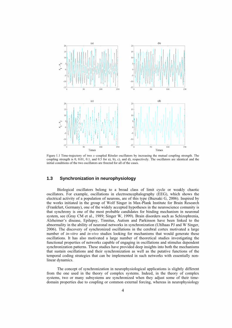
The analysis of synchronization phenomenon has always been subject to active investigations in the field of dynamical systems (Osipov GV et al., 2007; Pikovsky A et al., 2003). It is a basic phenomenon in science and engineering and its origin dates back to Huygens in the 17th century who found that two weakly coupled pendulum clocks became phase synchronized and this was probably the first written notion on synchronization (Hugenii C, 1673). Synchronization is often encountered in living systems such as circadian rhythm, phase locking respiration with mechanical ventilator, phase locking of chicken embrion heart cells with external stimuli, interaction of sinus node with ectopic pacemakers, synchronization of oscillations of human insulin secretion and glucose infusion, locking of spiking from electroreceptors of a paddlefish to weak external electromagnetic field, synchronization of heart rate by external audio or visual stimuli and synchronization of neurons in the brain (Pikovsky A et al., 2003). Indeed, tendency to achieve common rhythms of mutual behavior, or in other words, tendency to synchronization, is an important feature in our living world. During the last couple of decades the notion of synchronization has been generalized to the case of interacting chaotic oscillators (Pecora LM and TL Carroll, 1990), which has led to different concepts of synchronization (Boccaletti S et al., 2002). Consider two uncoupled chaotic oscillators. As coupling between the oscillators is introduced, both oscillators adjust their motion in response to the motion of the other, and when the coupling becomes strong enough, a transition typically occurs where the trajectory of the two oscillators start to coincide (Mosekilde E et al., 2002). An example of transition from unsynchronized motion to completely synchronized motion is shown in Figure 1.1 for two x–coupled Rössler oscillators (parameters and the equations of this system is introduced in the section 0). The mutual coupling strength is 0, 0.01, 0.1, and 0.5 for a), b), c), and d), respectively. As it is seen, when the systems are uncoupled their motion is irrelevant. By introducing coupling with small strength, the motion becomes correlated, but still not synchronized. By further increase of coupling strength, although the oscillators are not completely synchronized, one can state that they are phase synchronized, meaning that although the amplitude of the signals are not perfectly matched they move with each other ( Figure 1.1c). When the mutual coupling strength is set to 0.5, the oscillators become completely synchronized (the synchronizing coupling strength could be obtained through the techniques to be introduced later on). Note that for this example we have chosen the identical oscillators, i.e. oscillators with the same values for their parameters, whereas for nonidentical oscillators, no matter how strong the coupling is, complete synchronization can not be attained. However, for such systems weaker type of synchronization such as approximate or phase synchronization can be achieved.

Synchronization is possible if at least two dynamical systems meet and interact but it much more happens in ensembles including hundreds, thousands, millions and even more individual dynamical systems. The early works on synchronization of dynamical systems were concerned with only a small number of coupled individual systems, but many real-world systems where synchronization is relevant, consist of a large number of dynamical individuals interacting with complex coupling structure. To understand the situation better, imagine neurons in the brain where they may have many short- and/or long- distance connections with other neurons under a complex structure. One important concern in this filed is the dependence of the synchronization on the network’s structural properties. In this context, one might ask the following questions: What kind of definitions could be adopted to measure the degree of synchronizability (complete or phase) of dynamical networks? Do different interpretations of synchronizability, if any, coincide? What kind of networks has better synchronization properties? Which network properties affect the synchronization? Does network weighting have any effect on the synchronization, and if yes, is there any way to assign proper weights for the links in order to enhance the synchronizability of the network? Are directed networks better synchronizable than undirected ones? In this thesis, we try to find possible and proper answers for some of these questions.

4

Figure 1.1 Time-trajectory of two x–coupled Rössler oscillators by increasing the mutual coupling strength. The coupling strength is 0, 0.01, 0.1, and 0.5 for a), b), c), and d), respectively. The oscillators are identical and the initial conditions of the two oscillators are freezed for all of the cases.

1.3 Synchronization in neurophysiology

Biological oscillators belong to a broad class of limit cycle or weakly chaotic oscillators. For example, oscillations in electroencephalography (EEG), which shows the electrical activity of a population of neurons, are of this type (Buzsaki G, 2006). Inspired by the works initiated in the group of Wolf Singer in Max-Plank Institute for Brain Research (Frankfurt, Germany), one of the widely accepted hypotheses in the neuroscience comunity is that synchrony is one of the most probable candidates for binding mechanism in neuronal system, see (Gray CM et al., 1989; Singer W, 1999). Brain disorders such as Schizophrenia, Alzheimer’s disease, Epilepsy, Tinnitus, Autism and Parkinson have been linked to the abnormality in the ability of neuronal networks in synchronization (Uhlhaas PJ and W Singer, 2006). The discovery of synchronized oscillations in the cerebral cortex motivated a large number of in-vitro and in-vivo studies looking for mechanisms that would generate these oscillations. It has also motivated a large number of theoretical studies investigating the functional properties of networks capable of engaging in oscillations and stimulus dependent synchronization patterns. These studies have provided deep insights into both the mechanisms that sustain oscillations and their synchronization as well as the putative functions of the temporal coding strategies that can be implemented in such networks with essentially non-linear dynamics.

The concept of synchronization in neurophysiological applications is slightly different from the one used in the theory of complex systems. Indeed, in the theory of complex systems, two or many subsystems are synchronized when they adjust some of their time-domain properties due to coupling or common external forcing, whereas in neurophysiology

5

synchronization refers to a process that two or many subsystems share specific common frequencies. These two definitions coincide for completely periodic systems, which is not the case in many real-world applications. Traditionally, in neurophysiological studies, synchronizations was assessed by coherence analysis of frequency-domain characteristics of time series obtained through a neuronal activity measures such as electroencephalography or magnetoencephalography techniques. This method is intrinsically bivariate method, which is unable to capture all the information in a multivariate signals like the one obtained through high density electroencephalography. In general, analyses such as coherence studies refer to cooperativeness phenomena among some experimental observations, which are related to the estimation of interdependencies among the measured signals. This means that in order to measure the cooperativeness among the elements of a network, e.g. neurons (or collection of neurons) of the brain, one has to compute the amount of interdependencies within the considered signals. To this end, four main approaches exist in the literature of time series analysis: the linear approach, the phase dynamics, state-space and information theory based approaches (De Feo O and C Carmeli, 2008). Within the phase approach, a multivariate interdependence estimator can be defined via phase order parameter (Boccaletti S et al., 2002). The difficulty of this method lies in the definition of phase itself; there is a lack of a unique definition for general non-periodic signals. Although the state-space based methods do not have the ambiguity of phase analysis, most of the estimators based on state-space approaches proposed in the literature are intrinsically bivariate and their extension for multivariate time series is not straightforward (Carmeli C, 2006). Regarding the information theory based approach mutual information could be extended to multivariate signals. The difficulty of this method is the estimation of high dimensional probability distributions, which requires extremely long time series and heavy computational load and extensive use of memory; the problem that restricts its real world applications. Here, we will make use of two methods: calculating order parameter for quantifying the degree of phase synchronization (Boccaletti S et al., 2002) and S-estimator technique (Carmeli C et al., 2005), both having multivariate nature.

1.4 Thesis outline

This thesis consists of three sections with 10 chapters. The first chapter is dedicated to introduction and the thesis is concluded in the last. The first and third sections comprise of three chapters each and the second section is organized in two chapters. In the first section, the problem of synchronizability of dynamical networks is addressed. The synchronizability of complex dynamical networks is defined precisely and the relevant literature is briefly reviewed. Four possible interpretation of synchronizability in dynamical networks are mentioned and investigated in details. Using the connection-graph-stability method it is shown that the synchronizability of properly weighted networks is better compared to unweighted networks. Also, based on the information of node and edge betweenness centrality measures, a weighting algorithm is introduced for enhancing the synchronizability of dynamical networks. The outperformance of the algorithm is shown on some artificially constructed complex networks as well as on some real-world networks with complex topological properties. The second section of the thesis is dedicated to studying the synchronization properties of ensembles of neurons modeled by Hindmarsh-Rose equations. The synchronizability of Hindmarsh-Rose neurons over Newman-Watts and Meta Newman-Watts (modular) networks is investigated and some general rules are obtained. Also, we look precisely at the mechanisms of the generation of gamma-waves (frequency range 30-80 Hz) in cortical neurons and investigated mechanisms for the interaction of locally emerging gamma oscillations. The third section is the analysis of electroencephalographs obtained from healthy subjects and patients suffering from schizophrenia or Alzheimer’s disease. These electroencephalographs

6

are studied from the point of view of local and regional synchronization. To this end, the topography of regional to local synchronization maps of patients with schizophrenia or Alzheimer’s disease are obtained and the relevance of the maps with the neuropsychological data of the patients is investigated. In the following, a brief story of each chapter is given.

Chapter 2: in this chapter we define the problem of synchronization in dynamical networks and briefly review some existing methods in the literature for analyses of synchronization. For many applications it is useful to have an estimate on the degree of synchronization of the network, which leads to the definition of a term synchronizability that is often used to show the propensity of the dynamical network to synchronize. In this chapter we give some possible interpretations of synchronizability and then investigate to what extent they coincide. Numerical simulations on artificially constructed scale-free and Watts-Strogatz networks show that not in all the cases the different interpretations of synchronizability go hand in hand. Indeed, the results obtained for a particular definition of synchronizability might or might not work for another definition. Therefore, any statement on the synchronizability should be limited to the particular definition studied, and generalization to other definitions should be avoided.

Chapter 3: in this chapter, dynamical networks with diffusive couplings are investigated from the point of view of synchronizability. Arbitrary connection graphs are admitted but the coupling is symmetric. Networks with equal interaction coefficients for all edges of the interaction graph are compared with networks where the interaction coefficients vary from edge to edge according to the bounds for global synchronization obtained by the connection-graph-stability method. Synchronizability is tested numerically by establishing the time to decrease the synchronization error from 1 to 10-5 in the case of networks of identical Lorenz or Rössler systems. Synchronizability from the point of view of phase synchronization is also tested, for networks of non-identical Lorenz or Rössler systems. In this case the phase order parameters are compared, as function of the mean interaction strength. Throughout, as network structures, scale-free and Watts-Strogatz networks are used.

Chapter 4: here, by considering the eigenratio of the Laplacian of the connection graph as synchronizability measure, we propose a procedure for weighting dynamical networks to enhance their synchronizability. The method is based on node and edge betweenness centrality measures and is tested on artificially constructed scale-free and Watts-Strogatz networks as well as on some real-world networks with complex topological properties. It is also numerically shown that the same procedure could be used to enhance the phase synchronizability of networks of nonidentical oscillators. Furthermore, it is shown that unlike the unweighted networks for networks weighted with the proposed algorithm, different interpretations of synchronizability coincide. Also, we investigate optimization of synchronization cost in undirected dynamical networks. To do so, proper weights are assigned to the networks’ edges considering node and edge betweenness centrality measures. The proposed method gives near-optimal results with less complexity of computation compared to the optimal method, i.e. the one based on convex optimization. This property enables us to apply the method to large networks. Through numerical simulations on scale-free and Watts-Strogatz networks of different sizes and topological properties we give evidence that the performance of the proposed method is much better than another heuristic method; namely the Metropolis-Hasting algorithm. The proposed procedure has potential application in many engineering problems where the synchronization of the network is required to be achieved by minimal cost.

Chapter 5: in this chapter, the synchronization behavior of Hindmarsh-Rose neuron models over Newman-Watts networks is addressed. Through numerically solving the network’s differential equations and then determining the synchronizing coupling strength, it is confirmed that the master-stability-function method which gives necessary conditions for linear stability of the synchronization manifold, indeed predicts the synchronizing coupling

7

strength well. We also investigate the influence of topological properties of connection graphs such as the size of the network and probability of shortcut links in the network, on the synchronizability. We find out that for a large class of networks there is a power-law relation between the probability of shortcuts and the synchronizing coupling strength. The synchronization of electrically coupled Hindmarsh-Rose neurons over clustered networks, a class of Newman-Watts networks with dense inter-cluster connections but sparsely in intra-cluster linkage, is also studied. It is found out that the synchronizing coupling strength is influenced mainly by the probability of inter-cluster connections with a power-law relation. Furthermore, we consider ensembles of Hindmarsh-Rose neurons with both electrical and chemical couplings and show that chemical couplings play indeed a complementary role in synchronization, while electrical coupling is the main responsible for providing complete synchrony.

Chapter 6: this chapter studies the behavior of locally emerged synchronized oscillations in gamma frequency range, i.e. 30-100 Hz. Local circuits in the cortex and hippocampus are endowed with resonant, oscillatory firing properties which underlie oscillations in the gamma range in the local field potential, and in EEG. Synchronized gamma-oscillations are thought to play important roles in information binding in the brain. It is believed that there should be a minimal network of a number of fast and regular spiking neurons with specific inputs that is able to reproduce gamma-oscillations. In this chapter we introduce such a minimal network with only five neurons, an excitatory thalamic-relay neuron, two excitatory pyramidal neurons and two inhibitory interneurons, which is able to produce synchronized gamma-oscillations. We try to construct large-scale models using networks of such minimal units which capture the essential features of the dynamics of cells and their connectivity patterns. These models are used to gain insight into the following questions: How do gamma oscillations emerge locally? What are the properties of noise-induced synchronization through gamma-frequency interactions? How do multiple local foci of gamma oscillatory activity meet and interact? How do network structure and interplay between excitatory and inhibitory couplings may influence gamma-oscillations? Does transmission time-delay have a constructive or destructive role on the gamma-synchrony?

Chapter 7: in this chapter, the EEG data of patients with schizophrenia and some matched control subjects are studied. We analyze the EEG power topography in 14 patients and 14 matched controls by applying a new parametrization of the multichannel EEG. In particular, we use power measures tuned for regional surface mapping in combination with power measures that allow evaluation of global effects. The linear discriminant and correlation analyses are used to test to what extent the EEG power changes distinguish patients from controls, and whether they are related to the clinical picture in the patients. The statistics are obtained via the permutation version of Student’s t-test and corrected for multiple comparisons. The analysis reveals schizophrenia-related abnormalities in the topography of EEG power on different spatial scales. These are (i) a global decrease in absolute EEG power robustly manifested in the alpha and beta frequency bands, and (ii) a relative increase in alpha power over the anterior brain regions against its reduction over the posterior regions. Not only are both effects robust in the alpha band but they are also linked to the schizophrenia symptoms (measured with Positive and Negative Syndrome Scale) and to chronicity (measured as the length of illness) in this frequency range. Since alpha activity is related to regional deactivation, our findings support the concept of hypofrontality in schizophrenia and expose the alpha rhythm as a sensitive marker of it. Furthermore, they suggest that the alpha activity of EEG is an important target for further detailed noninvasive research into the neurobiology of schizophrenia.

Chapter 8: to reveal a whole-head synchronization topography in schizophrenia, in this chapter we apply a new method of multivariate synchronization analysis called S-estimator to the resting dense-array (128 channels) EEG obtained from 14 schizophrenic patients and 14 matched control subjects. This method determines synchronization from the embedding

8

dimension in a state-space domain based on the theoretical consequence of the cooperative behavior of simultaneous time series — the shrinking of the state-space embedding dimension. The S-estimator imaging reveals a specific synchronization landscape in schizophrenia patients. Its main features include bilaterally increased synchronization over temporal brain regions and decreased synchronization over the postcentral/parietal region neighboring the midline. The synchronization topography is stable over the course of several months and correlates with the severity of schizophrenia symptoms. In particular, direct correlations links positive, negative, and general psychopathological symptoms to the hyper-synchronized temporal clusters over both hemispheres. Along with these correlations, general psychopathological symptoms inversely correlate within the hypo-synchronized postcentral midline region. While being similar to the structural maps of cortical changes in schizophrenia, the S-maps go beyond the topography limits, demonstrating a novel aspect of the abnormalities of functional cooperation: namely, regionally reduced or enhanced connectivity. The new method of multivariate synchronization significantly boosts the potential of EEG as an imaging technique compatible with other imaging modalities. Its application to schizophrenia research shows that schizophrenia can be explained within the concept of neural dysconnection across and within large-scale brain networks.

Chapter 9: Alzheimer’s disease is likely to disrupt synchronization of the bioelectrical processes in the distributed cortical networks underlying cognition. In this chapter we aim at revealing the Alzheimer’s-specific features of EEG synchronization by making a whole-head synchronization map. We analyze surface topography of the multivariate phase synchronization of multichannel (128) EEG in 17 patients (all in their early stages of Alzheimer’s disease confirmed by neuropsychological and psychophysiological examinations) compared to 17 age-matched controls by applying a combination of global and regional measures for multivariate phase synchronization to the resting EEG. In early Alzheimer’s disease, the whole-head mapping reveals a specific landscape of synchronization characterized by a decrease in the values of phase synchronization over the fronto-temporal and an increase over temporo-parieto-occipital region predominantly of the left hemisphere. These features manifest themselves through the EEG delta-beta bands and discriminate patients from controls with accuracy up to 94% (in alpha2 band, i.e. 9.5–13 Hz). Moreover, the abnormal phase synchrony in both anterior and posterior clusters correlates with Mini Mental State Examination score, binding the EEG regional synchronization to the cognitive decline in patients with Alzheimer’s disease. The multivariate phase synchronization technique used for this study reveals the EEG phenotype of early Alzheimer’s disease relevant to the clinical picture and may ultimately prove its sensitive and specific biomarker.

9

SECTION I

11

SYNCHRONIZABILITY OF DYNAMICAL NETWORKS

Personal Contribution — This chapter mainly contains the review of the literature in the field of synchronization in dynamical networks, i.e. criteria for determining the stability of the synchronization manifold in dynamical networks. However, we present our original results on the coincidence of different interpretations of synchronizability in undirected and unweighted dynamical networks.

1.5 Synchronization as a collective behavior of dynamical networks

The term synchronization usually refers to time-correlated behavior between two or more different (or identical) dynamical systems. However, synchronization is not defined in a unique and standard way and a particular definition is adapted according to the corresponding application (Brown R and L Kocarev, 2000). Due to strong enough interaction of a network of identical dynamical systems (e.g. chaotic systems), their states can coincide, while the dynamics in time remains as the dynamics of the uncoupled individual systems, e.g. chaotic if the individual systems show chaotic behavior while they are uncoupled (Chen M, 2008; Pecora LM and TL Carroll, 1990; Pikovsky A et al., 2003). This phenomenon is referred to as complete or cluster synchronization (Boccaletti S et al., 2002; Brown R and L Kocarev, 2000; Guan S et al., 2008). However, complete synchronization is not the only phenomenon observed in collective behavior of large interconnecting systems. Coupled dynamical systems may exhebit another type of synchronous behavior such as phase synchronization (Arizmendi F and DH Zanette, 2008; Pikovsky AS et al., 1997; Rosenblum M et al., 2001; Rosenblum MG et al., 1996), lag synchronization (Rosenblum MG et al., 1997), bubbling synchronization (Ashwin P et al., 1994; Ashwin P et al., 1996; Hasler M and YL Maistrenko, 1997) and generalized synchronization (Abarbanel HDI et al., 1996; Rulkov NF et al., 1995). The only concept we deal with in this chapter is complete synchronization and to be more abstract we will mention it only by synchronization afterwards. In other words, when one deals with coupled identical systems, synchronization (complete synchronization) appears as the equality of the state variables while evolving in time. There are some other names for this kind of synchronization in the literature such as conventional or identical synchronization (Boccaletti S et al., 2002). While our discussion will focus on continuous-time systems, most of the

12

exposed ideas can be easily extended to discrete-time ones such as various chaotic maps. For the coupling schema, one has to distinguish between two different situations: unidirectional and bidirectional. In the unidirectional coupling scheme, the evolution of one of the coupled systems is unaltered by the coupling; while in the bidirectional coupling case both systems are connected in such a way that they mutually influence each other’s behavior. In this chapter we consider only dynamical networks of diffusive type, i.e. bidirectional coupling between dynamical systems.

The crucial questions in studying synchronization in complex dynamical networks are the ones dealing with dependence of synchronization on the network structural properties, dynamics of the individual systems, and strength of coupling. A particular network structure might ease synchronization for a particular dynamical system and coupling strength compared to another network structure. To address these issues we can define a term, synchronizability, which refers to the ease of synchronization of dynamical networks. One can find a number of works in the literature with different interpretations of synchronizability, e.g. see (Almendral JA and A Dıaz-Guilera, 2007; Barahona M and LM Pecora, 2002; Chavez M et al., 2006; Chavez M et al., 2005; Donetti L et al., 2005; Donetti L et al., 2006; Jalili M, A Ajdari Rad et al., 2007; Motter AE, C Zhou et al., 2005; Zhou C, AE Motter et al., 2006). The different interpretations of synchronizability might not coincide, in general. In other words, it might happen under one definition of synchronizability network N1 is more synchronizable than network N2, while as the definition of synchronizability changes, network N2 becomes more synchronizable. In this chapter we address the problem of synchronizability of dynamical networks in a proper way and compare various interpretations of synchronizability to check to what extent they go hand in hand.

Let us make the following assumptions to be able to define the problem of complete synchronization (Boccaletti S et al., 2002):

A1. The coupled individual dynamical systems are all identical (all dynamical systems have the same dynamical equations with the same parameters).

A2. The same function of the components from each dynamical system is used to couple to other dynamical systems, e.g. if the individual dynamical systems are systems with three state variables x, y and z, all of them are coupled through their x–component.

A3. The synchronization manifold is an invariant manifold. A4. The coupling is a linear coupling, i.e. the effective coupling term in the dynamical

equation of the individual systems is a linear combination of the state variables of the system.

A5. The connection topology is arbitrary, e.g. random, regular, Watts-Strogatz or scale-free networks.

Assumptions A1 and A3 guarantee the existence of a unified synchronization hyperplane and A2 allows us to make the stability diagram specific to the different choice of dynamical systems. Assumptions A4 and A5 allow us to choose a large class of coupling structures and network models, which themselves include many real-world applications (Pecora LM and TL Carroll, 1998).

1.6 Equations of the dynamical network

Let us consider an undirected and unweighted network with N nodes. On each node of the connection graph a dynamical system sits and the equations of the motion of the dynamical network read

13

1

( ) ; 1,2,...,N

i i ij jj

F l H i Nσ=

= − =∑&x x x , (2.1)

where di ∈x R are the state vectors, : d dF →R R defines the individual system’s dynamical

equation. These dynamical systems are coupled via a unified coupling strength σ and coupling matrix L = (lij). L that is called Laplacian is a symmetric matrix with vanishing row-sums and positive off-diagonal entries, i.e. Lij = Lji for all pairs of (i,j), Lij > 0 for i ≠ j, and 1 0N

j ijL= =∑ for all i. In other word, L = D – A where A = (aij) is the binary adjacency matrix of (V,E), an undirected graph with nodes in V and edges in E. D = (dii) is a diagonal matrix with

1

; 1,Nii ijj

d a i N=

= =∑ K . (2.2)

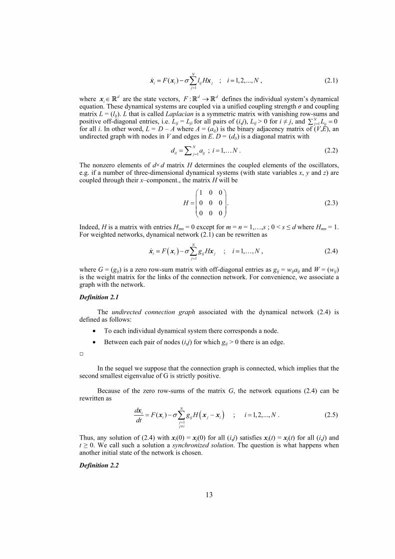
The nonzero elements of d×d matrix H determines the coupled elements of the oscillators, e.g. if a number of three-dimensional dynamical systems (with state variables x, y and z) are coupled through their x–component., the matrix H will be

1 0 00 0 00 0 0

H⎛ ⎞⎜ ⎟= ⎜ ⎟⎜ ⎟⎝ ⎠

. (2.3)

Indeed, H is a matrix with entries Hmn = 0 except for m = n = 1,…,s ; 0 < s ≤ d where Hmn = 1. For weighted networks, dynamical network (2.1) can be rewritten as

( )1

; 1, ,N

i i ij jj

F g H i Nσ=

= − =∑& Kx x x , (2.4)

where G = (gij) is a zero row-sum matrix with off-diagonal entries as gij = wijaij and W = (wij) is the weight matrix for the links of the connection network. For convenience, we associate a graph with the network.

Definition 2.1

The undirected connection graph associated with the dynamical network (2.4) is defined as follows:

• To each individual dynamical system there corresponds a node. • Between each pair of nodes (i,j) for which gij > 0 there is an edge.

In the sequel we suppose that the connection graph is connected, which implies that the second smallest eigenvalue of G is strictly positive.

Because of the zero row-sums of the matrix G, the network equations (2.4) can be rewritten as

( )1

( ) ; 1,2,...,N

ii ij j i

jj i

d F g H i Ndt

σ=≠

= − − =∑x x x x . (2.5)

Thus, any solution of (2.4) with xi(0) = xj(0) for all (i,j) satisfies xi(t) = xj(t) for all (i,j) and t ≥ 0. We call such a solution a synchronized solution. The question is what happens when another initial state of the network is chosen.

Definition 2.2

14

Synchronization might be weather global or local and we distinguish local and global synchronization.

a) The dynamical network described by (2.4) synchronizes globally (and completely), if for any solution of (2.4) we have

( ) ( ) 0 , 1,i j tt t i j N→∞− ⎯⎯⎯→ ∀ =x x K . (2.6)

b) The dynamical network (2.4) synchronizes locally, if there exists an ε > 0 such that for any solution with

( ) ( )0 0i j ε− <x x , (2.7)

we have

( ) ( ) 0 , 1,i j tt t i j N→∞− ⎯⎯⎯→ ∀ =x x K . (2.8)

Whether or not the network synchronizes depends mainly on three causes:

a) The dynamics of the individual systems, expressed by F(·) in (2.4). b) The type and strength of the interaction between the individual dynamical systems.

In (2.4) this is represented by the fact that the interaction is linear with strength σ and the interaction matrix G is of diffusive type.

c) The network structure, represented by the connection graph.

1.7 Some criteria for synchronization of dynamical networks

Studying synchronization of dynamical networks leads to two fundamental considerations: finding the synchronous solution and determining its stability. In this context the central question is: When is such synchronous manifold stable, especially in regard to the coupling configuration and strength? Some works have tried to formulate this issue, which have resulted in necessary (Pecora LM and TL Carroll, 1998) or sufficient (Belykh VN et al., 2004) conditions for the stability of the synchronization manifold (local stability condition for the former and global for the latter). Here, we give a brief overview of some existing methods providing the conditions (sufficient or necessary) on the stability (global or local) of the synchronized manifold.

1.7.1 Eigenvalue based conjecture on synchronization criterion

Wu and Chua proposed a conjecture on a criterion for synchronization in an array of diffusively coupled dynamical systems (Wu CW and L Chua, 1996), which involves a relation between the coupling coefficients in various arrays. For two networks of coupled dynamical systems with N1 and N2 identical individuals, connection topology as A1 and A2, and unified coupling coefficients σ1 and σ2, respectively, we have the following relations:

( ) ( )1 1 2 2A Aσ λ σ λ= , (2.9)

where λ(A1) and λ(A2) are the largest negative eigenvalues of the coupling matrices A1 and A2, respectively. Network A1 is globally synchronized if and only if network A2 is globally synchronized (Wu CW and L Chua, 1996).

An immediate result of this statement is that we can predict the synchronization of a network of any size for a chosen connection matrix just by knowing the synchronization

15

threshold for a network of two mutually connected dynamical systems, i.e. if σ* be the coupling threshold for synchronizing two mutually coupled systems, then the coupling threshold σ*

N for a network of size N and the largest negative eigenvalue of the coupling matrix λ* will be

*

**

2N

σσλ

= . (2.10)

However, it has been shown that the above conjecture does not hold in general and can be true only in some special cases (Pecora LM, 1998). Indeed, (2.9) holds for the stability of the least stable mode, and by its stability the stability of the other modes are concluded (Wu CW and L Chua, 1996). But, in case of desynchronization this assumption fails (Pecora LM, 1998). Therefore, in networks of limit cycle and chaotic oscillators (e.g. Lorenz, and Hodgkin–Huxley-type systems) where there is no desynchronization with increasing coupling (unlike the case of Rössler system), it correctly predicts the synchronization threshold for networks of any sizes and any coupling structures (Belykh I, M Hasler et al., 2005).

1.7.2 Master-stability-function method

Master-stability-function formalism proposed by Pecora and Carroll gives necessary conditions for the local stability of the synchronization manifold x1(t) = x2(t) = … = xN(t) = s(t) (Pecora LM and TL Carroll, 1998). Considering the dynamical network equations (2.4), the stability of the synchronization manifold can be determined by the variational equations, i.e. each dynamical system is considered to have extremely small perturbation ζi from the synchronous state; xi(t) = s(t) + ζi. The variational equations are

( )1

; 1,2,...,N

i i ij jjj i

DF s g H i Nσ=≠

= − =∑&ζ ζ ζ , (2.11)

where D stands for Jacobian.

Although (2.11) allows considering connection graphs of any type, i.e. unidirectional and bidirectional, we assume bidirectional coupling, i.e. G is symmetric (G = GT). One can write the symmetric matrix G as G = ΓΩΓT, where Ω is a diagonal matrix of real eigenvalues of G and Γ is the orthogonal matrix whose columns are the corresponding real eigenvectors of G. Let define ζ = (ζ1, ζ2 , …, ζN) = ηΓT, where η = (η1, η2 , …, ηN). Then, (2.11) is equivalent to

( ) ; 1,2,...,i i i iDF s H i Nη η σλ η= − =& , (2.12)

where λi are the eigenvalues of G, ordered as 0 = λ1 ≤ λ2 ≤ … ≤ λN, in which λ1 = 0 is associated with the synchronized manifold s(t). Indeed, ηi is the weight of i-th eigenvector of G in the perturbation ζ.

The largest Lyapunov exponent of the variational equation (2.12) Λ(a = σλi), called master-stability-function (Pecora LM and TL Carroll, 1998), accounts for the linear stability of the synchronization manifold, i.e. if Λ(a) < 0, the synchronized state is linearly stable. The master-stability-function depends only on the coupling configuration expressed by H and the dynamics of the individual dynamical systems expressed by F(·) in (2.4). In other words, this method breaks the process of determining the stability of the synchronization manifold into two components; one comes from the dynamics of the individuals, i.e. the master-stability-function, and the other one comes from the network structure, i.e. λi’s. In this way, a necessary condition for the local stability of the synchronization manifold is obtained. It is worth mentioning that the master-stability-function is computed for a dynamical system with

16

specific H once and one only needs to compute λ2 and λN of G for determining the synchronization conditions of the dynamical network (2.4).

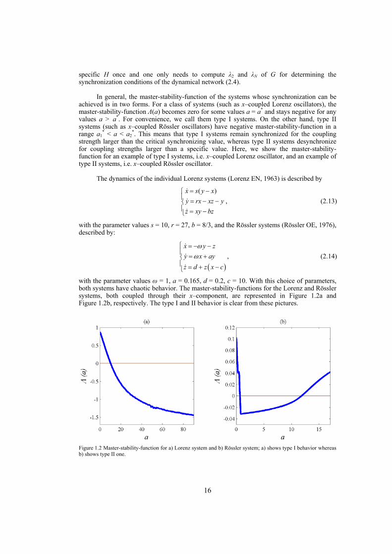
In general, the master-stability-function of the systems whose synchronization can be achieved is in two forms. For a class of systems (such as x–coupled Lorenz oscillators), the master-stability-function Λ(a) becomes zero for some values a = a* and stays negative for any values a > a*. For convenience, we call them type I systems. On the other hand, type II systems (such as x–coupled Rössler oscillators) have negative master-stability-function in a range a1

* < a < a2*. This means that type I systems remain synchronized for the coupling

strength larger than the critical synchronizing value, whereas type II systems desynchronize for coupling strengths larger than a specific value. Here, we show the master-stability-function for an example of type I systems, i.e. x–coupled Lorenz oscillator, and an example of type II systems, i.e. x–coupled Rössler oscillator.

The dynamics of the individual Lorenz systems (Lorenz EN, 1963) is described by

( )x s y x

y rx xz yz xy bz

= −⎧⎪ = − −⎨⎪ = −⎩

&

&

&

, (2.13)

with the parameter values s = 10, r = 27, b = 8/3, and the Rössler systems (Rössler OE, 1976), described by:

( )

x y zy x ayz d z x c

ωω

⎧ = − −⎪

= +⎨⎪ = + −⎩

&

&

&

, (2.14)

with the parameter values ω = 1, a = 0.165, d = 0.2, c = 10. With this choice of parameters, both systems have chaotic behavior. The master-stability-functions for the Lorenz and Rössler systems, both coupled through their x–component, are represented in Figure 1.2a and Figure 1.2b, respectively. The type I and II behavior is clear from these pictures.

Figure 1.2 Master-stability-function for a) Lorenz system and b) Rössler system; a) shows type I behavior whereas b) shows type II one.

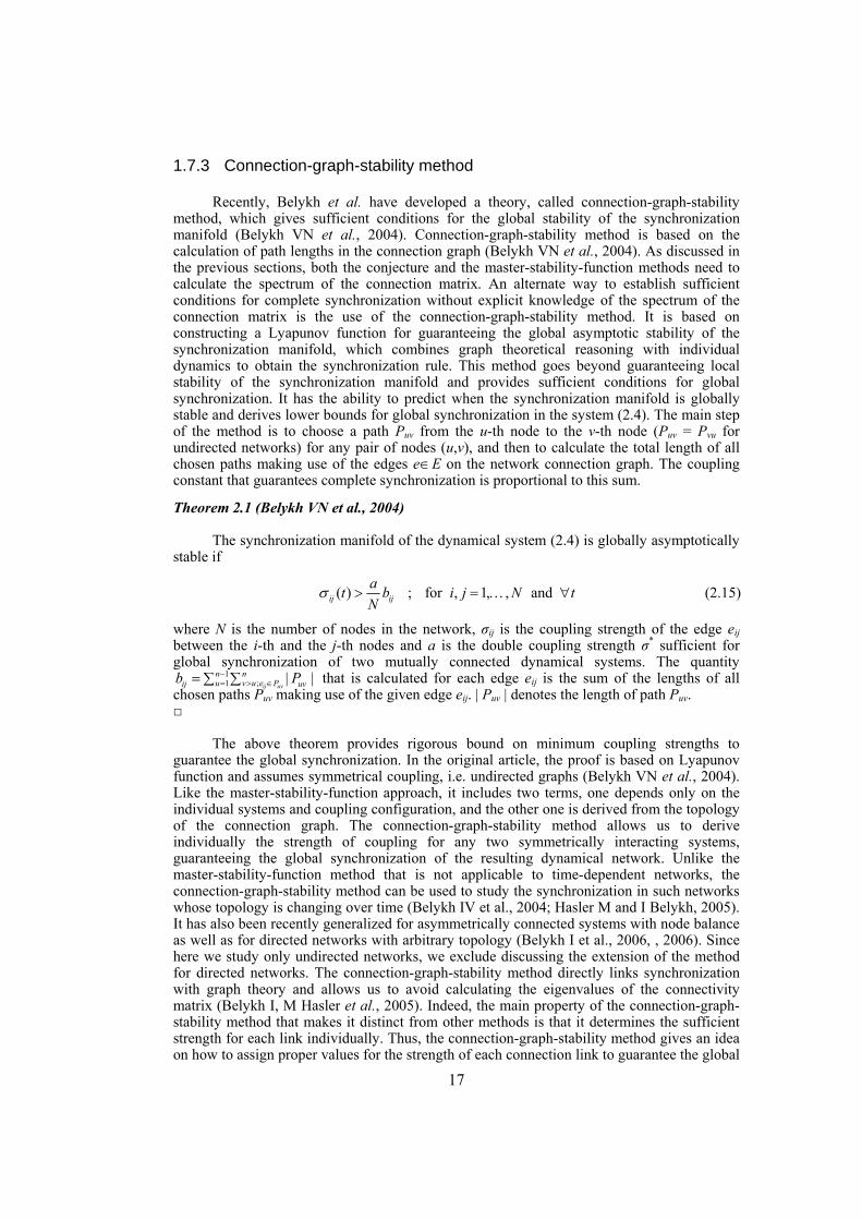
17

1.7.3 Connection-graph-stability method

Recently, Belykh et al. have developed a theory, called connection-graph-stability method, which gives sufficient conditions for the global stability of the synchronization manifold (Belykh VN et al., 2004). Connection-graph-stability method is based on the calculation of path lengths in the connection graph (Belykh VN et al., 2004). As discussed in the previous sections, both the conjecture and the master-stability-function methods need to calculate the spectrum of the connection matrix. An alternate way to establish sufficient conditions for complete synchronization without explicit knowledge of the spectrum of the connection matrix is the use of the connection-graph-stability method. It is based on constructing a Lyapunov function for guaranteeing the global asymptotic stability of the synchronization manifold, which combines graph theoretical reasoning with individual dynamics to obtain the synchronization rule. This method goes beyond guaranteeing local stability of the synchronization manifold and provides sufficient conditions for global synchronization. It has the ability to predict when the synchronization manifold is globally stable and derives lower bounds for global synchronization in the system (2.4). The main step of the method is to choose a path Puv from the u-th node to the v-th node (Puv = Pvu for undirected networks) for any pair of nodes (u,v), and then to calculate the total length of all chosen paths making use of the edges e∈E on the network connection graph. The coupling constant that guarantees complete synchronization is proportional to this sum.

Theorem 2.1 (Belykh VN et al., 2004)

The synchronization manifold of the dynamical system (2.4) is globally asymptotically stable if

( ) ; for , 1, , and ij ijat b i j N tN

σ > = … ∀ (2.15)

where N is the number of nodes in the network, σij is the coupling strength of the edge eij between the i-th and the j-th nodes and a is the double coupling strength σ* sufficient for global synchronization of two mutually connected dynamical systems. The quantity

11 ; | |

ij uv

n nu v u e Pij uvb P−= > ∈= ∑ ∑ that is calculated for each edge eij is the sum of the lengths of all

chosen paths Puv making use of the given edge eij. | Puv | denotes the length of path Puv.

The above theorem provides rigorous bound on minimum coupling strengths to guarantee the global synchronization. In the original article, the proof is based on Lyapunov function and assumes symmetrical coupling, i.e. undirected graphs (Belykh VN et al., 2004). Like the master-stability-function approach, it includes two terms, one depends only on the individual systems and coupling configuration, and the other one is derived from the topology of the connection graph. The connection-graph-stability method allows us to derive individually the strength of coupling for any two symmetrically interacting systems, guaranteeing the global synchronization of the resulting dynamical network. Unlike the master-stability-function method that is not applicable to time-dependent networks, the connection-graph-stability method can be used to study the synchronization in such networks whose topology is changing over time (Belykh IV et al., 2004; Hasler M and I Belykh, 2005). It has also been recently generalized for asymmetrically connected systems with node balance as well as for directed networks with arbitrary topology (Belykh I et al., 2006, , 2006). Since here we study only undirected networks, we exclude discussing the extension of the method for directed networks. The connection-graph-stability method directly links synchronization with graph theory and allows us to avoid calculating the eigenvalues of the connectivity matrix (Belykh I, M Hasler et al., 2005). Indeed, the main property of the connection-graph-stability method that makes it distinct from other methods is that it determines the sufficient strength for each link individually. Thus, the connection-graph-stability method gives an idea on how to assign proper values for the strength of each connection link to guarantee the global

18

synchronization of the dynamical network. It is worth mentioning that due to the use of Lyapunov function in proving the global stability of the synchronization manifold, the connection-graph-stability method usually overestimates the true synchronizing coupling strength. However, it gives the distribution of the coupling weights which might be useful in improving the synchronizability of the dynamical networks. In the next chapter we will show that synchronizability of dynamical networks whose distribution of their connection weights follow b-scores described in (2.15) is better than that of the networks with the same synchronization effort (cost) but with identical coupling strength.

The connection-graph-stability method has two steps; one solely depends on the dynamics of the individual dynamical systems and coupling configuration, i.e. a in (2.15), and the other one is exclusively dependent on the connection topology, i.e. bij for each edge eij. The first step is to calculate the parameter a and to prove that two diffusively coupled systems globally synchronize when coupling strength exceeds the half of a, which has to be proved for each particular situation (for the concrete individual system and the matrix H). Although for many systems analytical calculation of bounds for a is possible (It usually results in very conservative bounds), one can obtain them numerically by solving the differential equations and checking whether the system synchronizes or not. In the next section we will analytically compute a lower bound for a in some dynamical systems. The next step in the algorithm is to calculate bij-scores for each edge between nodes i and j. To this end, we first choose a set of paths (often shortest paths) Pij|i ; j = 1,…,N(j > i), and determine their lengths |Pij| (the total number of edges in each Pij). Then, for each edge eij of the connection graph we calculate bij as the sum of the lengths of all of the paths passing through the edge eij. Having a and bij one can use the results of Theorem 2.1 and find an lower bound for the coupling strength of the edge eij. In the following example, we show how to determine the amounts of b-scores for a simple network with few nodes and edges.

Example 2.1

Consider the network shown in Figure 1.3 with 7 nodes and 8 edges. One could simply choose the shortest paths between any two nodes of the graph as: P12 = e12, P13 = e13, P14 = e12e24, P15 = e16e46e45, P16 = e16, P17 = e12e77, P23 = e23, P24 = e24, P25 = e24e45, P26 = e24e46, P27 = e27, P34 = e23e24, P35 = e23e24e45, P36 = e13e16, P37 = e23e27, P45 = e45, P46 = e46, P47 = e24e27, P56 = e45e46, P57 = e45e24e27, P67 = e16e12e27. Therefore, by calculating the sum of path lengths passing through the edges, the corresponding b-scores (in (2.15)) are obtained as

12 12 14 17 67

13 13 36

16 15 16 36 67

23 23 34 35 37

24 14 24 25 26 34 35 47 57

27 17 27 37 47 57 67

1 2 2 3 8,

1 2 3,

3 1 2 3 9,

1 2 3 2 8,

2 1 2 2 2 3 2 3 17,

2 1 2 2 3

b P P P P

b P P

b P P P P

b P P P P

b P P P P P P P P

b P P P P P P

= + + + = + + + =

= + = + =

= + + + = + + + =

= + + + = + + + =

= + + + + + + + = + + + + + + + =

= + + + + + = + + + +

45 15 25 35 45 56 57

46 15 26 46 56

3 13,

3 2 3 1 2 3 14,

3 2 1 2 8.

b P P P P P P

b P P P P

+ =

= + + + + + = + + + + + =

= + + + = + + + =

Note that for this simple example, we have chosen the set of the shortest paths in order to compute the b-scores. However, as pointed out, one might adopt other choices of the paths and still results in a good bunds.

19

Figure 1.3 Sample network consisting of 7 nodes and 8 edges.

1.7.3.2 Calculating synchronizing coupling strength for two mutually coupled Lorenz systems

In this section we calculate a lower bound for the coupling strength of two mutually coupled Lorenz oscillators described by (2.13) guaranteeing their global synchronization. The dynamics of two mutually x–coupled identical Lorenz oscillators with state variables (x1,y1,z1) and (x2,y2,z2) is described as

( )

( )

1 1 1 2 1

1 1 1 1 1

1 1 1 1

2 2 2 1 2

2 2 2 2 2

2 2 2 2

( )

( )

x s y x x xy rx x z yz x y bzx s y x x xy rx x z yz x y bz

ε

ε

⎧ = − + −⎪

= − −⎪⎪ = −⎪⎨

= − + −⎪⎪ = − −⎪

= −⎪⎩

&

&

&

&

&

&

. (2.16)

Let us define the following difference equations and study the global stability of their equilibrium point (the origin)

2 2 2 1 2 1; ;X x x Y y y Z z z= − = − = − . (2.17)

The dynamical equations of the difference variables read

1 1

1 1

2X sY sX XY rX Y XZ x Z z X

Z XY x Y y X bZ

ε⎧ = − −⎪

= − − − −⎨⎪ = + + −⎩

&

&

&

. (2.18)

To show the asymptotic stability of the origin of the above system, the following positive definite function W is considered as a candidate for Lyapunov function (Pogromsky AY et al., 2003)

2 2 212 2 2rW X Y Zs

γ= + + . (2.19)

One can obtain the time-derivative of W as

20

( ) ( )2 2 21 1

22

r sW X Y bZ r z XY y XZ

sε+

= − − − + − +& . (2.20)

Having the following bound for the trajectories of the Lorenz system (Pogromsky AY et al., 2003)

( )2

2 2112 4 for ( 2 and 2 4)y r z r b s b

b+ − ≤ < ≤ ≤ , (2.21)

one can show that a lower bound for the global stability of the synchronization manifold is

( )12

s rε

−> . (2.22)

Another more conservative bound is given in (Belykh VN et al., 2004). It is remarkable that the real synchronizing value obtained by numerical simulations is much less than (2.22).

1.7.3.3 Calculating synchronizing coupling strength for two mutually coupled Hindmarsh-Rose systems

Hindmarsh-Rose neuron model is a system with three ordinary differential equations, which is frequently used as a neuron model in studying the neuronal behaviors1. Considering two identical Hindmarsh-Rose oscillators with state variables (x1,y1,z1) and (x2,y2,z2), and diffusively coupled though their x–components, the equation of the motion is as follows

( )

( )( )( )

( )( )

2 31 1 1 1 1 2 1

21 1

1 0 1

2 31 2 2 2 2 1 2

22 2

2 0 2

1

1

x y ax x z I x x

y dx y

z b x x z

x y ax x z I x x

y dx y

z b x x z

ε

μ

ε

μ

⎧ = + − − + + −⎪

= − −⎪⎪ = − −⎪⎨

= + − − + + −⎪⎪ = − −⎪⎪ = − −⎩

&

&

&

&

&

&

. (2.23)

By introducing the differences of the state variables as (2.17) and the following simple algebraic equations

( )

2 22 2

2 23 32 2

2 1

3

4

x x XU

X X Ux x

U x x

⎧ − =⎪

+⎪− =⎨

⎪= +⎪

⎩

, (2.24)

One can obtain the dynamic equations of the difference variable

1 This model is introduced in details in chapter 5.

21

( )3 20.25 0.75 2X Y Z X X aU U

Y dXU Yz bX Z

ε

μ μ

⎧ = − − + − −⎪⎪ = − −⎨⎪ = −⎪⎩

&

&

&

. (2.25)

Since the origin is an equilibrium point of the above system, its stability accounts for the stability of the synchronization manifold. To prove the stability let us consider the following function as a candidate for Lyapunov function (Belykh I, M Hasler et al., 2005)

2 2 21 12 2 2

W X Y Zb

γμ

= + + , (2.26)

where γ is a positive parameter to be defined later on. The asymptotic stability of the equilibrium point requires that the time-derivative of W to be negative definite. One can obtain the time-derivative of W as

4 2

2 2

4X ZW AX BXY Y

bγ⎡ ⎤= − − − + +⎣ ⎦

& , (2.27)

where

23 2 ; 14

A U aU B dUε γ= − + = − . (2.28)

Thus, we should obtain the conditions that the expression 2 2AX BXY Yγ+ + becomes positive definite. To this end, we should have 2 / 4 0A Bγ − > that finally results in the following conditions

( )( )

22

2

21 ; 3 8 8 3

d add

γ εγ γ

−< > +

−. (2.29)

It is worth mentioning that the above bound is a sufficient condition for the stability of the synchronization manifold and usually gives an overestimate for the real synchronizing parameter. Although the real synchronizing coupling strength could be than the above obtained bound, it gives an idea on limiting the search for finding the real synchronizing strength.

1.8 A few Interpretations for synchronizability of dynamical networks

Synchronizability of a dynamical network is the ease by which synchronization can be achieved. There is no single interpretation of synchronizability and a particular choice is adopted for each study. In this section we try to formularize the problem of synchronizability and give some possible interpretations of synchronizability (Jalili M, A Ajdari Rad et al., 2007). We also investigate to what extent the various interpretations of synchronizability coincide for different network structures. Network N1 may be called more synchronizable than network N2, if

22

a) For a larger range of parameters, it is possible to synchronize N1 as compared to N2. By the master stability function, This concept of synchronizability is related to the eigenratio λN /λ2, where λ2 and λN are the second smallest and the largest eigenvalues of the Laplacian (L is (2.1) and G in (2.4)) of the connection graph. In other words, the smaller the eigenratio λN /λ2 the better the synchronizability of the network.

b) Less effort2 has to be made to achieve synchronization in N1 than in N2. This concept is related to λ2; for the same synchronization cost, the larger the λ2 the better the synchronizability of the network. λ2 is often referred to as the algebraic connectivity of the graph (Fiedler M, 1973). Thus, graphs with higher algebraic connectivity have better synchronization properties.

c) With the same effort, N1 synchronizes faster than N2. This means that for the same synchronization cost, the less the time to synchronize the better the synchronizability of the network.

d) With the same effort, the degree of phase synchronization, measured for example by the phase order parameter, is larger in N1 than in N2; i.e. for the same synchronization cost, the larger the phase order parameter the better the synchronizability of the network.

Each work has adopted an appropriate concept of synchronizability depending on its specific application. For example, the works of (Chavez M et al., 2005; Donetti L et al., 2005; Motter AE, C Zhou et al., 2005; Nishikawa T et al., 2003) use a) as the criterion of synchronizability and relate it to the eigenratio of the spectrum of the connection graph (Barahona M and LM Pecora, 2002; Pecora LM and TL Carroll, 1998). In (Jalili M et al., 2008; Nishikawa T and AE Motter, 2006), the synchronization cost is introduced and b) is used for characterizing the synchronizability of networks. (Jalili M, A Ajdari Rad et al., 2007; Timme M et al., 2004) argue the speed of synchronization and the work of (Boccaletti S et al., 2002) proposes the notion of phase-order parameter to measure the phase synchronizability of networks.

1.8.1 Eigenratio λN /λ2 as a measure of synchronizability

As pointed out in section 0, the master-stability-function accounts for the local stability of the synchronization manifold (Barahona M and LM Pecora, 2002; Pecora LM and TL Carroll, 1998). For a number of systems such as x–coupled Rössler systems (i.e. type II systems), the master-stability-function is negative (and hence the synchronization manifold is locally stable) only within a bounded interval (a1,a2); e.g. see Figure 1.2b. Indeed, the master-stability-function has a decreasing (increasing) positive value below (above) this range. Requiring all coupling strengths to lie within such an interval, i.e. a1 < σλ2 ≤ … ≤ σλN < a2, one concludes that if the synchronization manifold is locally stable

2

2 1

N aa

λλ

< , (2.30)

for the corresponding graph. As it can be seen in (2.30), the left-hand side of the inequality depends solely on the structure of the graph, while the right-hand side depends on the dynamics of the individual systems and coupling configuration.

2 Synchronization effort (cost) will be defined later on.

23

Interpretation a) of synchronizability points out that the larger the range of connection strengths stabilizing the synchronization manifold the better the synchronizability of the network. Therefore, it relates the synchronizability to the eigenratio λN /λ2, and concludes that the smaller the eigenratio λN /λ2 of a network the better its synchronizability. Considering the synchronizing coupling strength within an interval (σ1,σ2), the master-stability-function formalism requires

1 1 2 2 2 ; Na aσ λ σ λ< < . (2.31)

Since a1 and a2 are fixed for any dynamical system and coupling configuration, to extend the interval of synchronizing parameter (σ1,σ2), and consequently enhance the synchronizability, one should make the eigenratio λN /λ2 as small as possible. This interpretation of synchronizability has been extensively used in the literature and indeed is the most frequent expression accounted for the synchronizability of dynamical networks, for example see (Chavez M et al., 2005; Donetti L et al., 2006; Motter AE, C Zhou et al., 2005; Nishikawa T et al., 2003; Wang X et al., 2007).

1.8.2 Algebraic connectivity λ2 as a measure of synchronizability

The situation where the master-stability-function is negative only in an interval is not the general case for all dynamical systems. Indeed, the master-stability-function for many dynamical systems (e.g. x–coupled Lorenz oscillators, and type I systems in general) shows a behavior like the one depicted in Figure 1.2a; i.e. the master-stability-function is negative in an interval (a1,∞). Thus, for the stability of the synchronization manifold one requires a1 < σλ2 and λN plays no role in determining the synchronization properties of the network. It is clear that for such cases increasing λ2 means that with smaller σ synchronization could be achieved, and thus, for the same synchronization cost, the larger the λ2 the better the synchronizability of the network.

Note that the range of variability of λN is limited and in many cases minimizing the eigenratio λN /λ2 gives very similar results to maximizing λ2 (Ajdari Rad A et al., 2008). However, this is not always the case and here we will investigate to what extent these two concepts lie in the same line for different network structures. For many applications, the synchronization needed to be achieved with a cost as minimum as possible (Nishikawa T and AE Motter, 2006). For such cases, this interpretation of synchronizability makes sense. It only deals with the least coupling strength necessary for local stability of the synchronization manifold. Indeed, this interpretation of synchronizability can be linked to the cost of synchronization, CSyn, where the synchronization is desired to be achieved by minimal cost.

1.8.3 Time to synchronize as a measure of synchronizability

The other possibility to define the synchronizability of dynamical networks is to consider the time to synchronize (Almendral JA and A Dıaz-Guilera, 2007; Jalili M, A Ajdari Rad et al., 2007). When a network clearly synchronizes, the synchronization error converges distinctly to zero. Thus, by putting a threshold on the synchronization error and some proper stopping conditions one can obtain the time to synchronize.

Definition 2.3

Consider the dynamical network (2.4). The average synchronization error of the network at time t is defined as

( ) ( ) ( ) ( ) 221 i j

i jE t t t

N N <

= −− ∑ x x . (2.32)

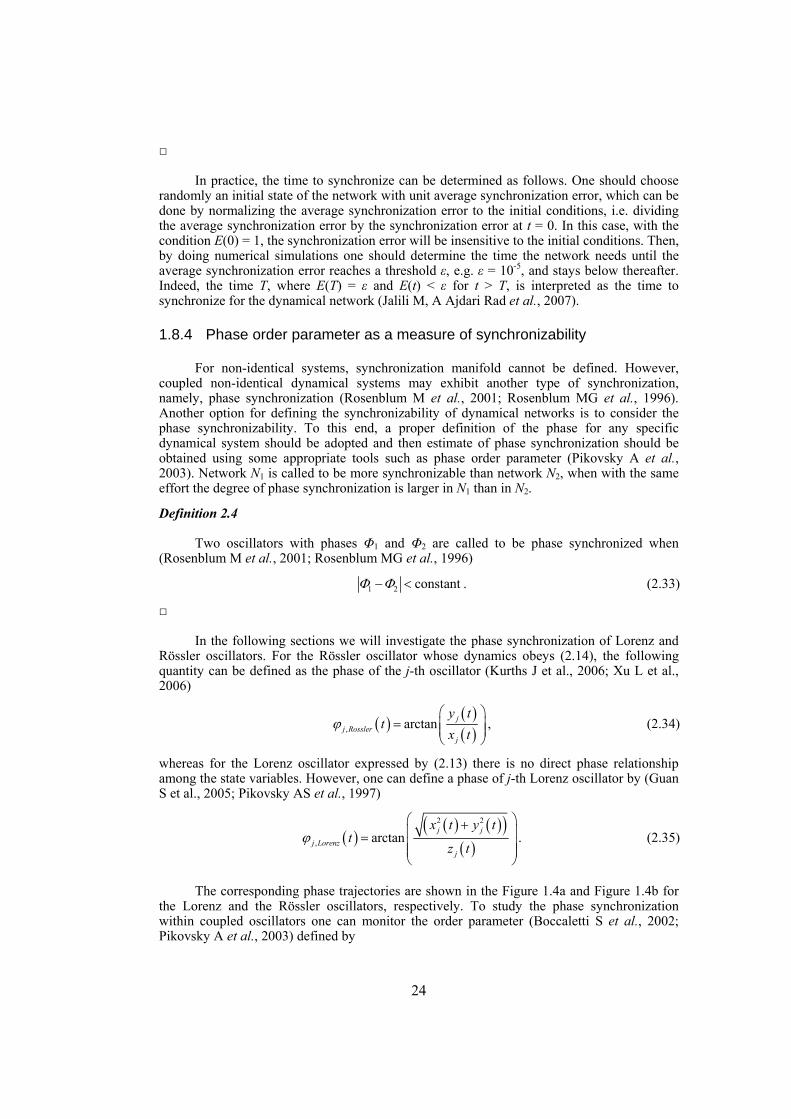
24

In practice, the time to synchronize can be determined as follows. One should choose randomly an initial state of the network with unit average synchronization error, which can be done by normalizing the average synchronization error to the initial conditions, i.e. dividing the average synchronization error by the synchronization error at t = 0. In this case, with the condition E(0) = 1, the synchronization error will be insensitive to the initial conditions. Then, by doing numerical simulations one should determine the time the network needs until the average synchronization error reaches a threshold ε, e.g. ε = 10-5, and stays below thereafter. Indeed, the time T, where E(T) = ε and E(t) < ε for t > T, is interpreted as the time to synchronize for the dynamical network (Jalili M, A Ajdari Rad et al., 2007).

1.8.4 Phase order parameter as a measure of synchronizability

For non-identical systems, synchronization manifold cannot be defined. However, coupled non-identical dynamical systems may exhibit another type of synchronization, namely, phase synchronization (Rosenblum M et al., 2001; Rosenblum MG et al., 1996). Another option for defining the synchronizability of dynamical networks is to consider the phase synchronizability. To this end, a proper definition of the phase for any specific dynamical system should be adopted and then estimate of phase synchronization should be obtained using some appropriate tools such as phase order parameter (Pikovsky A et al., 2003). Network N1 is called to be more synchronizable than network N2, when with the same effort the degree of phase synchronization is larger in N1 than in N2.

Definition 2.4

Two oscillators with phases Φ1 and Φ2 are called to be phase synchronized when (Rosenblum M et al., 2001; Rosenblum MG et al., 1996)

1 2 constantΦ Φ− < . (2.33)

In the following sections we will investigate the phase synchronization of Lorenz and Rössler oscillators. For the Rössler oscillator whose dynamics obeys (2.14), the following quantity can be defined as the phase of the j-th oscillator (Kurths J et al., 2006; Xu L et al., 2006)

( ) ( )( ), arctan j

j Rosslerj

y tt

x tϕ

⎛ ⎞= ⎜ ⎟⎜ ⎟

⎝ ⎠, (2.34)

whereas for the Lorenz oscillator expressed by (2.13) there is no direct phase relationship among the state variables. However, one can define a phase of j-th Lorenz oscillator by (Guan S et al., 2005; Pikovsky AS et al., 1997)

( )( ) ( )( )

( )

2 2

, arctanj j

j Lorenzj

x t y tt

z tϕ

⎛ ⎞+⎜ ⎟= ⎜ ⎟⎜ ⎟⎝ ⎠

. (2.35)

The corresponding phase trajectories are shown in the Figure 1.4a and Figure 1.4b for the Lorenz and the Rössler oscillators, respectively. To study the phase synchronization within coupled oscillators one can monitor the order parameter (Boccaletti S et al., 2002; Pikovsky A et al., 2003) defined by

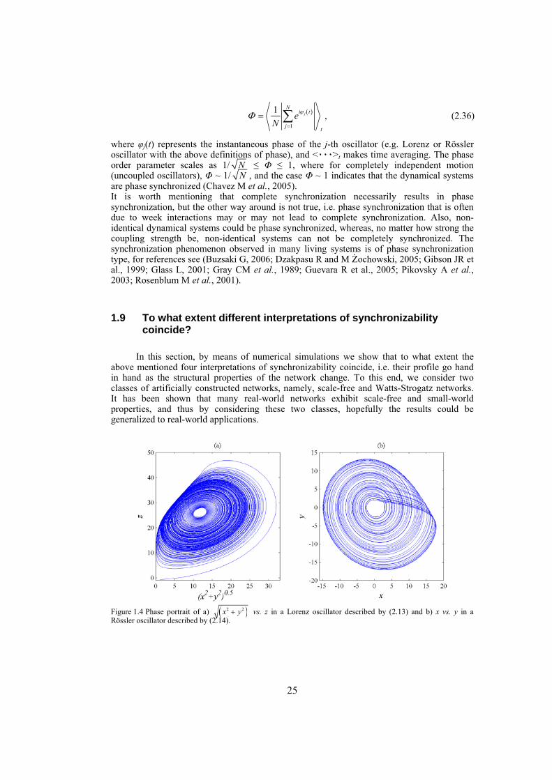
25

( )

1

1 jN

i t

j t

eN

ϕΦ=

= ∑ , (2.36)

where φj(t) represents the instantaneous phase of the j-th oscillator (e.g. Lorenz or Rössler oscillator with the above definitions of phase), and < ٠٠٠>t makes time averaging. The phase order parameter scales as 1/ N ≤ Φ ≤ 1, where for completely independent motion (uncoupled oscillators), Φ ~ 1/ N , and the case Φ ~ 1 indicates that the dynamical systems are phase synchronized (Chavez M et al., 2005). It is worth mentioning that complete synchronization necessarily results in phase synchronization, but the other way around is not true, i.e. phase synchronization that is often due to week interactions may or may not lead to complete synchronization. Also, non-identical dynamical systems could be phase synchronized, whereas, no matter how strong the coupling strength be, non-identical systems can not be completely synchronized. The synchronization phenomenon observed in many living systems is of phase synchronization type, for references see (Buzsaki G, 2006; Dzakpasu R and M Żochowski, 2005; Gibson JR et al., 1999; Glass L, 2001; Gray CM et al., 1989; Guevara R et al., 2005; Pikovsky A et al., 2003; Rosenblum M et al., 2001).

1.9 To what extent different interpretations of synchronizability coincide?

In this section, by means of numerical simulations we show that to what extent the above mentioned four interpretations of synchronizability coincide, i.e. their profile go hand in hand as the structural properties of the network change. To this end, we consider two classes of artificially constructed networks, namely, scale-free and Watts-Strogatz networks. It has been shown that many real-world networks exhibit scale-free and small-world properties, and thus by considering these two classes, hopefully the results could be generalized to real-world applications.

Figure 1.4 Phase portrait of a) ( )2 2x y+ vs. z in a Lorenz oscillator described by (2.13) and b) x vs. y in a Rössler oscillator described by (2.14).

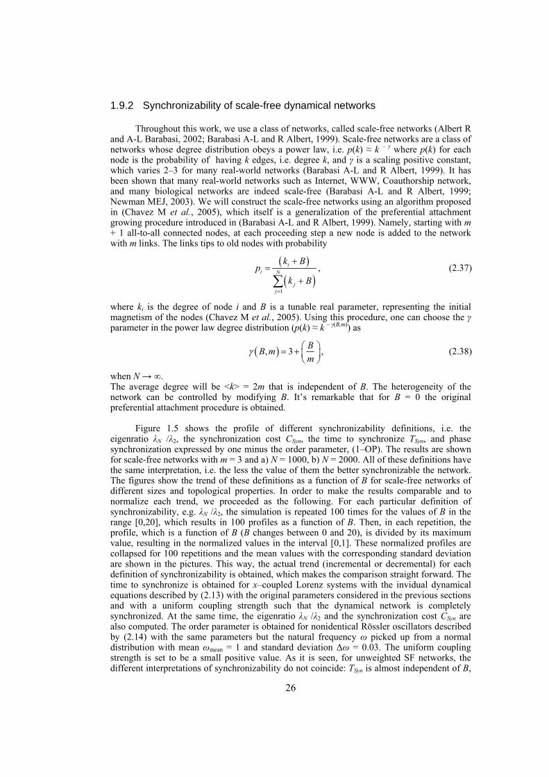
26

1.9.2 Synchronizability of scale-free dynamical networks

Throughout this work, we use a class of networks, called scale-free networks (Albert R and A-L Barabasi, 2002; Barabasi A-L and R Albert, 1999). Scale-free networks are a class of networks whose degree distribution obeys a power law, i.e. p(k) ≈ k – γ where p(k) for each node is the probability of having k edges, i.e. degree k, and γ is a scaling positive constant, which varies 2–3 for many real-world networks (Barabasi A-L and R Albert, 1999). It has been shown that many real-world networks such as Internet, WWW, Coauthorship network, and many biological networks are indeed scale-free (Barabasi A-L and R Albert, 1999; Newman MEJ, 2003). We will construct the scale-free networks using an algorithm proposed in (Chavez M et al., 2005), which itself is a generalization of the preferential attachment growing procedure introduced in (Barabasi A-L and R Albert, 1999). Namely, starting with m + 1 all-to-all connected nodes, at each proceeding step a new node is added to the network with m links. The links tips to old nodes with probability

( )

( )1

ii N

jj

k Bp

k B=

+=

+∑, (2.37)

where ki is the degree of node i and B is a tunable real parameter, representing the initial magnetism of the nodes (Chavez M et al., 2005). Using this procedure, one can choose the γ parameter in the power law degree distribution (p(k) ≈ k – γ(B,m)) as

( ), 3 BB mm

γ ⎛ ⎞= + ⎜ ⎟⎝ ⎠

, (2.38)

when N → ∞. The average degree will be <k> = 2m that is independent of B. The heterogeneity of the network can be controlled by modifying B. It’s remarkable that for B = 0 the original preferential attachment procedure is obtained.

Figure 1.5 shows the profile of different synchronizability definitions, i.e. the eigenratio λN /λ2, the synchronization cost CSyn, the time to synchronize TSyn, and phase synchronization expressed by one minus the order parameter, (1–OP). The results are shown for scale-free networks with m = 3 and a) N = 1000, b) N = 2000. All of these definitions have the same interpretation, i.e. the less the value of them the better synchronizable the network. The figures show the trend of these definitions as a function of B for scale-free networks of different sizes and topological properties. In order to make the results comparable and to normalize each trend, we proceeded as the following. For each particular definition of synchronizability, e.g. λN /λ2, the simulation is repeated 100 times for the values of B in the range [0,20], which results in 100 profiles as a function of B. Then, in each repetition, the profile, which is a function of B (B changes between 0 and 20), is divided by its maximum value, resulting in the normalized values in the interval [0,1]. These normalized profiles are collapsed for 100 repetitions and the mean values with the corresponding standard deviation are shown in the pictures. This way, the actual trend (incremental or decremental) for each definition of synchronizability is obtained, which makes the comparison straight forward. The time to synchronize is obtained for x–coupled Lorenz systems with the invidual dynamical equations described by (2.13) with the original parameters considered in the previous sections and with a uniform coupling strength such that the dynamical network is completely synchronized. At the same time, the eigenratio λN /λ2 and the synchronization cost CSyn are also computed. The order parameter is obtained for nonidentical Rössler oscillators described by (2.14) with the same parameters but the natural frequency ω picked up from a normal distribution with mean ωmean = 1 and standard deviation Δω = 0.03. The uniform coupling strength is set to be a small positive value. As it is seen, for unweighted SF networks, the different interpretations of synchronizability do not coincide: TSyn is almost independent of B,

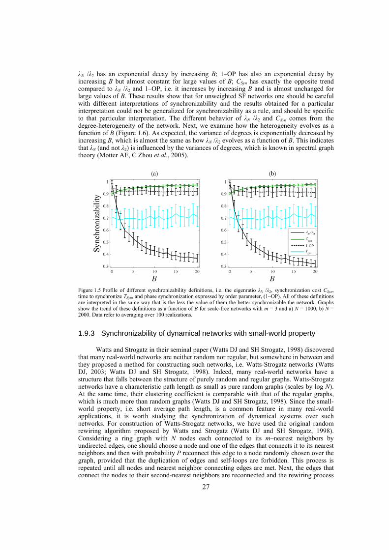
27

λN /λ2 has an exponential decay by increasing B; 1–OP has also an exponential decay by increasing B but almost constant for large values of B; CSyn has exactly the opposite trend compared to λN /λ2 and 1–OP, i.e. it increases by increasing B and is almost unchanged for large values of B. These results show that for unweighted SF networks one should be careful with different interpretations of synchronizability and the results obtained for a particular interpretation could not be generalized for synchronizability as a rule, and should be specific to that particular interpretation. The different behavior of λN /λ2 and CSyn comes from the degree-heterogeneity of the network. Next, we examine how the heterogeneity evolves as a function of B ( Figure 1.6). As expected, the variance of degrees is exponentially decreased by increasing B, which is almost the same as how λN /λ2 evolves as a function of B. This indicates that λN (and not λ2) is influenced by the variances of degrees, which is known in spectral graph theory (Motter AE, C Zhou et al., 2005).

Figure 1.5 Profile of different synchronizability definitions, i.e. the eigenratio λN /λ2, synchronization cost CSyn, time to synchronize TSyn, and phase synchronization expressed by order parameter, (1–OP). All of these definitions are interpreted in the same way that is the less the value of them the better synchronizable the network. Graphs show the trend of these definitions as a function of B for scale-free networks with m = 3 and a) N = 1000, b) N = 2000. Data refer to averaging over 100 realizations.

1.9.3 Synchronizability of dynamical networks with small-world property

Watts and Strogatz in their seminal paper (Watts DJ and SH Strogatz, 1998) discovered that many real-world networks are neither random nor regular, but somewhere in between and they proposed a method for constructing such networks, i.e. Watts-Strogatz networks (Watts DJ, 2003; Watts DJ and SH Strogatz, 1998). Indeed, many real-world networks have a structure that falls between the structure of purely random and regular graphs. Watts-Strogatz networks have a characteristic path length as small as pure random graphs (scales by log N). At the same time, their clustering coefficient is comparable with that of the regular graphs, which is much more than random graphs (Watts DJ and SH Strogatz, 1998). Since the small-world property, i.e. short average path length, is a common feature in many real-world applications, it is worth studying the synchronization of dynamical systems over such networks. For construction of Watts-Strogatz networks, we have used the original random rewiring algorithm proposed by Watts and Strogatz (Watts DJ and SH Strogatz, 1998). Considering a ring graph with N nodes each connected to its m–nearest neighbors by undirected edges, one should choose a node and one of the edges that connects it to its nearest neighbors and then with probability P reconnect this edge to a node randomly chosen over the graph, provided that the duplication of edges and self-loops are forbidden. This process is repeated until all nodes and nearest neighbor connecting edges are met. Next, the edges that connect the nodes to their second-nearest neighbors are reconnected and the rewiring process

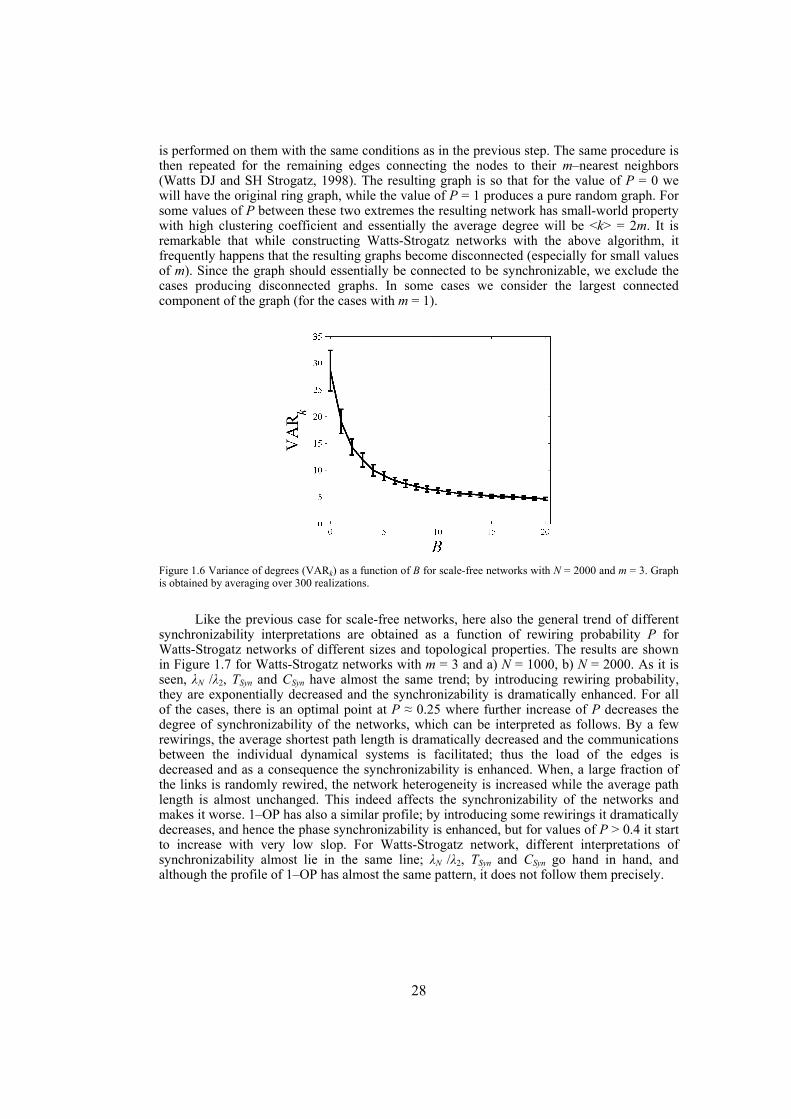
28

is performed on them with the same conditions as in the previous step. The same procedure is then repeated for the remaining edges connecting the nodes to their m–nearest neighbors (Watts DJ and SH Strogatz, 1998). The resulting graph is so that for the value of P = 0 we will have the original ring graph, while the value of P = 1 produces a pure random graph. For some values of P between these two extremes the resulting network has small-world property with high clustering coefficient and essentially the average degree will be <k> = 2m. It is remarkable that while constructing Watts-Strogatz networks with the above algorithm, it frequently happens that the resulting graphs become disconnected (especially for small values of m). Since the graph should essentially be connected to be synchronizable, we exclude the cases producing disconnected graphs. In some cases we consider the largest connected component of the graph (for the cases with m = 1).

Figure 1.6 Variance of degrees (VARk) as a function of B for scale-free networks with N = 2000 and m = 3. Graph is obtained by averaging over 300 realizations.

Like the previous case for scale-free networks, here also the general trend of different synchronizability interpretations are obtained as a function of rewiring probability P for Watts-Strogatz networks of different sizes and topological properties. The results are shown in Figure 1.7 for Watts-Strogatz networks with m = 3 and a) N = 1000, b) N = 2000. As it is seen, λN /λ2, TSyn and CSyn have almost the same trend; by introducing rewiring probability, they are exponentially decreased and the synchronizability is dramatically enhanced. For all of the cases, there is an optimal point at P ≈ 0.25 where further increase of P decreases the degree of synchronizability of the networks, which can be interpreted as follows. By a few rewirings, the average shortest path length is dramatically decreased and the communications between the individual dynamical systems is facilitated; thus the load of the edges is decreased and as a consequence the synchronizability is enhanced. When, a large fraction of the links is randomly rewired, the network heterogeneity is increased while the average path length is almost unchanged. This indeed affects the synchronizability of the networks and makes it worse. 1–OP has also a similar profile; by introducing some rewirings it dramatically decreases, and hence the phase synchronizability is enhanced, but for values of P > 0.4 it start to increase with very low slop. For Watts-Strogatz network, different interpretations of synchronizability almost lie in the same line; λN /λ2, TSyn and CSyn go hand in hand, and although the profile of 1–OP has almost the same pattern, it does not follow them precisely.

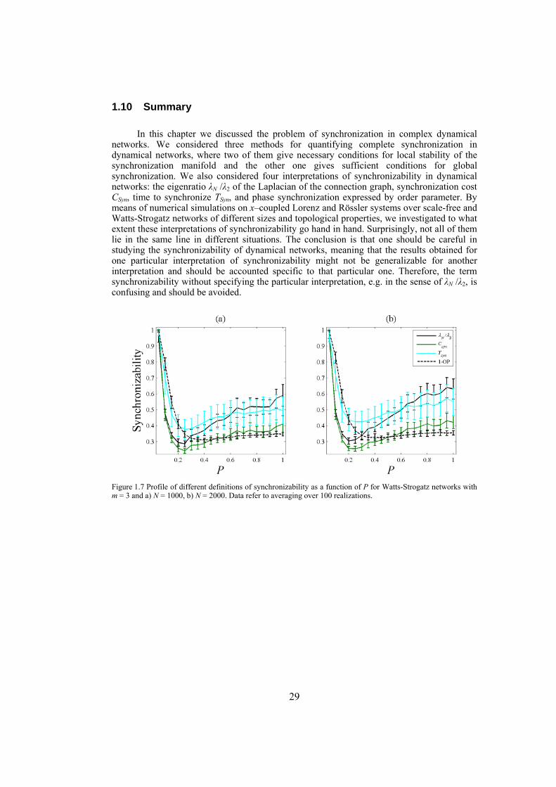
29

1.10 Summary

In this chapter we discussed the problem of synchronization in complex dynamical networks. We considered three methods for quantifying complete synchronization in dynamical networks, where two of them give necessary conditions for local stability of the synchronization manifold and the other one gives sufficient conditions for global synchronization. We also considered four interpretations of synchronizability in dynamical networks: the eigenratio λN /λ2 of the Laplacian of the connection graph, synchronization cost CSyn, time to synchronize TSyn, and phase synchronization expressed by order parameter. By means of numerical simulations on x–coupled Lorenz and Rössler systems over scale-free and Watts-Strogatz networks of different sizes and topological properties, we investigated to what extent these interpretations of synchronizability go hand in hand. Surprisingly, not all of them lie in the same line in different situations. The conclusion is that one should be careful in studying the synchronizability of dynamical networks, meaning that the results obtained for one particular interpretation of synchronizability might not be generalizable for another interpretation and should be accounted specific to that particular one. Therefore, the term synchronizability without specifying the particular interpretation, e.g. in the sense of λN /λ2, is confusing and should be avoided.

Figure 1.7 Profile of different definitions of synchronizability as a function of P for Watts-Strogatz networks with m = 3 and a) N = 1000, b) N = 2000. Data refer to averaging over 100 realizations.

31

ENHANCING SYNCHRONIZABILITY OF DYNAMICAL NETWORKS USING CONNECTION-GRAPH-STABILITY METHOD

Personal Contribution — This chapter is a reproduction of our recent paper published in International Journal of Circuit Theory and Application (Jalili M, A Ajdari Rad et al., 2007).

1.11 Proper non-uniform coupling enhances synchronizability

In the field of studying the synchronization phenomenon in dynamical networks a basic assumption of many works is that the individual dynamical systems are coupled symmetrically with identical coupling strength (undirected and unweighted coupling). However, most complex networks where synchronization is relevant to them are inherently weighted and undirected. Neurons are organized in complex networks with diffusive weighted connections (through gap junctions) and directional weighted connections (through excitatory and inhibitory chemical synapses) (Buzsaki G et al., 2004). Technological networks are often weighted networks (and usually undirected) (Colizza V et al., 2006; Korniss G et al., 2003; Strogatz SH, 2001). Social networks are also weighted where interaction between individuals is never equal and symmetric and depends on some social factors such as age, personal leadership and social influence (Dorogovtsev SN and JFF Mendes, 2000; Ramasco JJ et al., 2004). Other examples of weighted networks can be found in ecological systems (Polis GA, 1998), traffic load of a road (Latora V and M Marchiori, 2001), and metabolic networks (Almaas E et al., 2004). Weighted networks might have better synchronizability than unweighted ones if proper distribution of weights is adopted. The study of synchronization in properly weighted networks may provide us with insights into the behavior of real-world complex dynamical networks and guide us in designing large artificial networks. Technological networks with desirable synchronizability are such prototypic examples that assigning the interaction weights between dynamical units are of extreme importance, e.g. designing interaction schemes to optimize the performance of computational tasks based on

32

the synchronization of processes in computer networks (Korniss G et al., 2003). In this chapter we show that properly weighted networks have better synchronization properties than networks with uniform connection weights. To this end, we will make use of the connection-graph-stability method (Belykh VN et al., 2004), introduced in the previous chapter, which gives sufficient conditions for the global synchronization of dynamical networks. Using this method, the network will be weighted based on the b-scores obtained for each edge (see section 1.7.3). In other words, the weight of each edge will be proportional to its b-score (that is specific to each edge) obtained through the connection-graph-stability method.

Here, we consider networks of diffusively coupled identical dynamical systems described by (2.4). Let us rewrite (2.4) as

( )1

( ) ; 1,2,...,N

ii ij j i

jj i

d F d H i Ndt =

≠

= + − =∑x x x x , (3.1)

where D = [dij] is the symmetric coupling matrix which carries information on both connection structure and strength. We call the dij‘s the interaction or diffusion coefficients.

Here, we investigate how much easier it is, for a given connection graph, to achieve synchronization when using different diffusion coefficients dij for different edges of the connection graph as compared to a single value for all edges. We use the relative size of the dij’s obtained by the connection-graph-stability method, which is computationally very efficient, and, as will be shown, gives good results. In other words, the weights of the links will be proportional to their b-scores.

Here, we are interested in synchronization properties of large networks. In such networks it is difficult to determine numerically the limit between synchronization and failure to synchronize. For this reason, many authors compare the synchronizability of different networks using a synchronization criterion rather than an actual synchronization limit. Such criteria are either only necessary (e.g. the master-stability-function method) or only sufficient (e.g. the connection-graph-stability method) conditions for synchronization and therefore may give unreliable results. On the other hand, when a network clearly synchronizes, the synchronization error converges distinctly to zero. For this reason, we choose interpretation c) of synchronizability discussed in the section 1.8, i.e. the less the time to synchronize the better the synchronizability of the dynamical network (see section 1.8.3). We shall also use the approach of d) of the section 1.8, which states that the larger the phase order parameter, i.e. the better the degree of phase synchronization, the better the synchronizability of the network (see section 1.8.4). As effort made by the network to achieve synchronization we take the average interaction strength per vertex.

Definition 3.1

Consider the dynamical network (3.1). The average interaction strength per vertex is defined as

12 ij

i jI d

N ≠

= ∑ . (3.2)

The factor 2 is introduced in the denominator because dij for a given edge is counted twice, once as dij and once as dji and dij = dji.

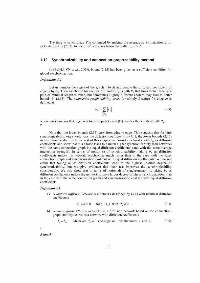
33

The time to synchronize T is computed by making the average synchronization error E(T), defined by (2.32), to reach 10-5 and stays below thereafter for t > T.

1.12 Synchronizability and connection-graph-stability method

In (Belykh VN et al., 2004), bound (2.15) has been given as a sufficient condition for global synchronization.

Definitions 3.2

Let us number the edges of the graph 1 to M and denote the diffusion coefficient of edge m by dm. Then we choose for each pair of nodes (i,j) a path Pij that links them. Usually, a path of minimal length is taken, but sometimes slightly different choices may lead to better bounds in (2.15). The connection-graph-stability score (or simply b-score) for edge m is defined as

ij

m iji jm P

b P<∈

= ∑ , (3.3)

where m∈Pij means that edge m belongs to path Pij and |Pij| denotes the length of path Pij.

Note that the lower bounds (2.15) vary from edge to edge. This suggests that for high synchronizability, one should vary the diffusion coefficients in (3.1); the lower bounds (2.15) indicate how to do this. In the rest of this chapter we consider networks with bm as diffusion coefficients and show that this choice leads to a much higher synchronizability than networks with the same connection graph but equal diffusion coefficients (and with the same average interaction strength). In terms of notion c) of synchronizability, taking bm as diffusion coefficients makes the network synchronize much faster than in the case with the same connection graph and synchronization cost but with equal diffusion coefficients. We do not claim that taking bm as diffusion coefficients leads to the highest possible degree of synchronizability, but we give evidence that their use improves the synchronizability considerably. We also show that in terms of notion d) of synchronizability, taking bm as diffusion coefficients makes the network to have larger degree of phase synchronization than in the case with the same connection graph and synchronization cost but with equal diffusion coefficients

Definition 3.3 a) A uniform diffusion network is a network described by (3.1) with identical diffusion

coefficients

0 for all , with 0 ij ijd d i j d= > ≠ . (3.4)

b) A non-uniform diffusion network, i.e. a diffusion network based on the connection-graph-stability scores, is a network with diffusion coefficients

whenever 0 and edge links the nodes and ij m ijd b d m i j= ≠ . (3.5)

Remark

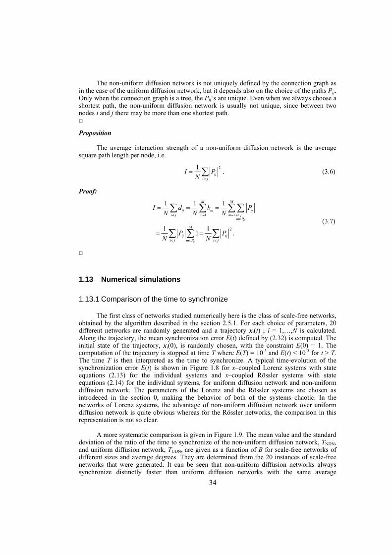
34

The non-uniform diffusion network is not uniquely defined by the connection graph as in the case of the uniform diffusion network, but it depends also on the choice of the paths Pij. Only when the connection graph is a tree, the Pij‘s are unique. Even when we always choose a shortest path, the non-uniform diffusion network is usually not unique, since between two nodes i and j there may be more than one shortest path.

Proposition

The average interaction strength of a non-uniform diffusion network is the average square path length per node, i.e.

21

iji j

I PN <

= ∑ . (3.6)

Proof:

1 1

2

1 1 1

1 1 1 .

ij

ij

M M

ij m iji j m m i j

m P

M

ij iji j m P i j

I d b PN N N

P PN N

≠ = = <∈

< ∈ <

= = =

= =

∑ ∑ ∑∑

∑ ∑ ∑ (3.7)

1.13 Numerical simulations

1.13.1 Comparison of the time to synchronize

The first class of networks studied numerically here is the class of scale-free networks, obtained by the algorithm described in the section 2.5.1. For each choice of parameters, 20 different networks are randomly generated and a trajectory xi(t) ; i = 1,…,N is calculated. Along the trajectory, the mean synchronization error E(t) defined by (2.32) is computed. The initial state of the trajectory, xi(0), is randomly chosen, with the constraint E(0) = 1. The computation of the trajectory is stopped at time T where E(T) = 10-5 and E(t) < 10-5 for t > T. The time T is then interpreted as the time to synchronize. A typical time-evolution of the synchronization error E(t) is shown in Figure 1.8 for x–coupled Lorenz systems with state equations (2.13) for the individual systems and x–coupled Rössler systems with state equations (2.14) for the individual systems, for uniform diffusion network and non-uniform diffusion network. The parameters of the Lorenz and the Rössler systems are chosen as introdeced in the section 0, making the behavior of both of the systems chaotic. In the networks of Lorenz systems, the advantage of non-uniform diffusion network over uniform diffusion network is quite obvious whereas for the Rössler networks, the comparison in this representation is not so clear.

A more systematic comparison is given in Figure 1.9. The mean value and the standard deviation of the ratio of the time to synchronize of the non-uniform diffusion network, TNDN, and uniform diffusion network, TUDN, are given as a function of B for scale-free networks of different sizes and average degrees. They are determined from the 20 instances of scale-free networks that were generated. It can be seen that non-uniform diffusion networks always synchronize distinctly faster than uniform diffusion networks with the same average

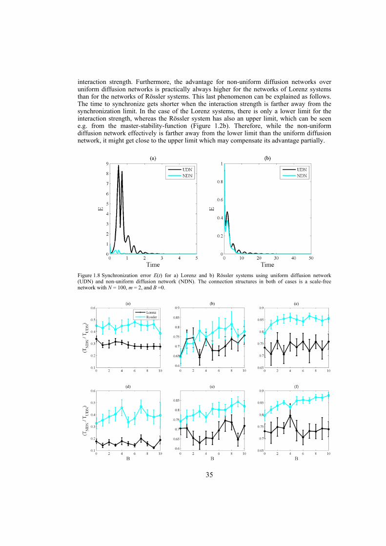
35

interaction strength. Furthermore, the advantage for non-uniform diffusion networks over uniform diffusion networks is practically always higher for the networks of Lorenz systems than for the networks of Rössler systems. This last phenomenon can be explained as follows. The time to synchronize gets shorter when the interaction strength is farther away from the synchronization limit. In the case of the Lorenz systems, there is only a lower limit for the interaction strength, whereas the Rössler system has also an upper limit, which can be seen e.g. from the master-stability-function ( Figure 1.2b). Therefore, while the non-uniform diffusion network effectively is farther away from the lower limit than the uniform diffusion network, it might get close to the upper limit which may compensate its advantage partially.

Figure 1.8 Synchronization error E(t) for a) Lorenz and b) Rössler systems using uniform diffusion network (UDN) and non-uniform diffusion network (NDN). The connection structures in both of cases is a scale-free network with N = 100, m = 2, and B =0.

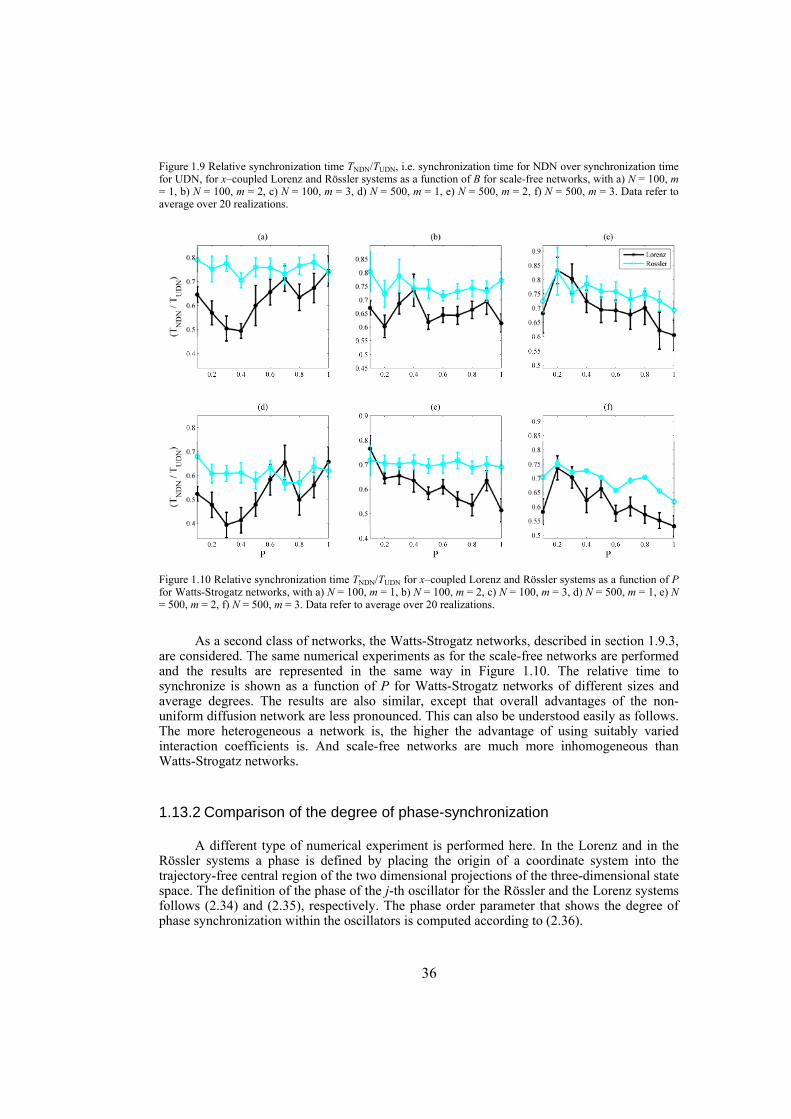
36

Figure 1.9 Relative synchronization time TNDN/TUDN, i.e. synchronization time for NDN over synchronization time for UDN, for x–coupled Lorenz and Rössler systems as a function of B for scale-free networks, with a) N = 100, m = 1, b) N = 100, m = 2, c) N = 100, m = 3, d) N = 500, m = 1, e) N = 500, m = 2, f) N = 500, m = 3. Data refer to average over 20 realizations.

Figure 1.10 Relative synchronization time TNDN/TUDN for x–coupled Lorenz and Rössler systems as a function of P for Watts-Strogatz networks, with a) N = 100, m = 1, b) N = 100, m = 2, c) N = 100, m = 3, d) N = 500, m = 1, e) N = 500, m = 2, f) N = 500, m = 3. Data refer to average over 20 realizations.

As a second class of networks, the Watts-Strogatz networks, described in section 1.9.3, are considered. The same numerical experiments as for the scale-free networks are performed and the results are represented in the same way in Figure 1.10. The relative time to synchronize is shown as a function of P for Watts-Strogatz networks of different sizes and average degrees. The results are also similar, except that overall advantages of the non-uniform diffusion network are less pronounced. This can also be understood easily as follows. The more heterogeneous a network is, the higher the advantage of using suitably varied interaction coefficients is. And scale-free networks are much more inhomogeneous than Watts-Strogatz networks.

1.13.2 Comparison of the degree of phase-synchronization

A different type of numerical experiment is performed here. In the Lorenz and in the Rössler systems a phase is defined by placing the origin of a coordinate system into the trajectory-free central region of the two dimensional projections of the three-dimensional state space. The definition of the phase of the j-th oscillator for the Rössler and the Lorenz systems follows (2.34) and (2.35), respectively. The phase order parameter that shows the degree of phase synchronization within the oscillators is computed according to (2.36).

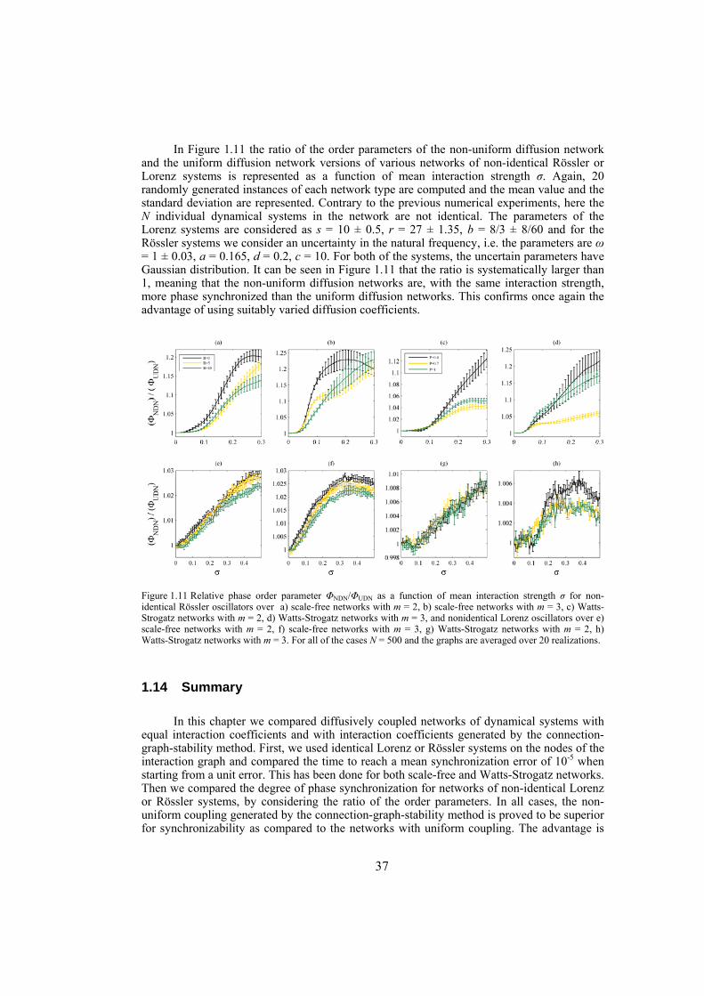
37

In Figure 1.11 the ratio of the order parameters of the non-uniform diffusion network and the uniform diffusion network versions of various networks of non-identical Rössler or Lorenz systems is represented as a function of mean interaction strength σ. Again, 20 randomly generated instances of each network type are computed and the mean value and the standard deviation are represented. Contrary to the previous numerical experiments, here the N individual dynamical systems in the network are not identical. The parameters of the Lorenz systems are considered as s = 10 ± 0.5, r = 27 ± 1.35, b = 8/3 ± 8/60 and for the Rössler systems we consider an uncertainty in the natural frequency, i.e. the parameters are ω = 1 ± 0.03, a = 0.165, d = 0.2, c = 10. For both of the systems, the uncertain parameters have Gaussian distribution. It can be seen in Figure 1.11 that the ratio is systematically larger than 1, meaning that the non-uniform diffusion networks are, with the same interaction strength, more phase synchronized than the uniform diffusion networks. This confirms once again the advantage of using suitably varied diffusion coefficients.

Figure 1.11 Relative phase order parameter ΦNDN/ΦUDN as a function of mean interaction strength σ for non-identical Rössler oscillators over a) scale-free networks with m = 2, b) scale-free networks with m = 3, c) Watts-Strogatz networks with m = 2, d) Watts-Strogatz networks with m = 3, and nonidentical Lorenz oscillators over e) scale-free networks with m = 2, f) scale-free networks with m = 3, g) Watts-Strogatz networks with m = 2, h) Watts-Strogatz networks with m = 3. For all of the cases N = 500 and the graphs are averaged over 20 realizations.

1.14 Summary

In this chapter we compared diffusively coupled networks of dynamical systems with equal interaction coefficients and with interaction coefficients generated by the connection-graph-stability method. First, we used identical Lorenz or Rössler systems on the nodes of the interaction graph and compared the time to reach a mean synchronization error of 10-5 when starting from a unit error. This has been done for both scale-free and Watts-Strogatz networks. Then we compared the degree of phase synchronization for networks of non-identical Lorenz or Rössler systems, by considering the ratio of the order parameters. In all cases, the non-uniform coupling generated by the connection-graph-stability method is proved to be superior for synchronizability as compared to the networks with uniform coupling. The advantage is

38

more pronounced for networks of Lorenz systems than for networks of Rössler systems, which can be explained.

39

ENHANCING SYNCHRONIZABILITY USING BETWEENNESS CENTRALITY MEASURES

Personal Contribution — This chapter is our original contribution. It has largely been reproduced from our two publications; one published in the proceedings of 2008 IEEE International Symposium on Circuit and Systems (Jalili M et al., 2008) and another one published in Physical Review E (Jalili M et al., 2008). Also, some of the results of our recent publication in Chaos (Ajdari Rad A et al., 2008) have been used.

1.15 Synchronizability is enhanced in weighted dynamical networks

In the previous chapter we showed that dynamical networks with properly assigned weights to their connection links have better synchronizability compared to unweighted networks. Many real-world networks where synchronization is relevant to them are weighted and directed, and nature might have assigned the optimal structure and weights to do the job, if the synchronization is the goal of the network optimization. Indeed, in many neural and biochemical networks there are evidences that the synchronized and coordinated behavior may play important roles in the system’s functionality (Buzsaki G, 2006; Glass L, 2001; Gray CM et al., 1989; Huang L et al., 2008; Nishikawa T and AE Motter, 2006; Singer W, 1999). Note that nature should consider not only synchronizability optimization in the evolution of real-world networks but also other factors such as the robustness, stability and adaptability. The problem of synchronizability enhancement is relevant to many real-world networks. In computer networks, for example, designing proper weights and directions for the connection links may enhance the ability of the network for synchronization of processes and result in boosting the performance of the computational tasks (Korniss G et al., 2003). The other example is metabolic networks, where the weights and direction of the metabolic fluxes (links) are adopted in a way to optimize fitness, which itself influences the robustness and synchronizability of the network against external disturbances to the system such as environmental changes (Fischer E and U Sauer, 2005). Another example is neuronal networks where constructing weighted networks with optimal synchronizability may help us to build artificial neural networks that mimic the behavior of the neural systems. Thus, a question arises: Given a complex undirected and unweighted network, how can one assign proper

40

weights to the links to obtain a weighted network (directed or undirected, depending on the particular application) with enhanced synchronizability?

This question initiated a stream of research on studying the synchronization in weighted networks. But, which factors of the connection graph characterize the synchronizability of the network? Studying networks with different structural properties revealed that scale-free networks and networks with small-world properties, in general, have better synchronizability than regular networks, which was linked to their shorter average path length (Barahona M and LM Pecora, 2002; Wang XF and G Chen, 2002; Wang XF and G Chen, 2002). Short average path length facilitates the communication between the nodes and enhances the synchronizability of the network. But, this is not always the case. It has been shown that degree heterogeneity is one of the key factors influencing the synchronizability of networks; homogenous networks show better synchronizability than corresponding heterogeneous ones (Nishikawa T et al., 2003). Indeed, synchronizability is suppressed as the degree distribution becomes more heterogeneous, even for shorter characteristic path length. For example, Watts-Strogatz networks have better synchronization properties than random scale-free networks that is mainly due to the more heterogeneous degree distribution in scale-free networks (Nishikawa T et al., 2003). Some other factors such as node and edge betweenness centrality measures influence the synchronizability of dynamical networks (Hong H et al., 2004).

Inspired by the fact that the more the heterogeneous the network the more difficult to achieve synchronization in the network, some researchers have proposed methods to assign proper weights to enhance the synchronizability, for example see (Chavez M et al., 2006; Chavez M et al., 2005; Motter AE, C Zhou et al., 2005; Motter AE, CS Zhou et al., 2005; Wang X et al., 2007). Here, we propose a new way of graph weighting based on node and edge betweenness centrally measures that enhances the synchronizability more than all existing methods. These methods (including our proposed method) start with an unweighted and undirected graph and end up with a weighted and directed one. However, this might not be desired in some application such as sensor networks (Olfati-Saber R et al., 2007), where the networks is needed to be undirected. Therefore, we also propose another method of graph weighting preserving the graph undirected and compare its performance to some existing methods.

1.16 Heuristics weighting procedures to enhance the synchronizability

In general, there are two possible ways to enhance the synchronizability of dynamical networks: rewiring of the links (Ajdari Rad A et al., 2008; Donetti L et al., 2005) and/or assigning proper weights for the existing links (Chavez M et al., 2005; Jalili M, A Ajdari Rad et al., 2007; Jalili M et al., 2008). For many applications it is not possible to change the network topology and the only option to enhance the synchronizability is weighting of the links. To get better synchronizability, couplings between nodes are neither necessarily uniform nor symmetric (Nishikawa T and AE Motter, 2006). A very first attempt to assign the proper weights for the edges to enhance the synchronizability was proposed by Motter et al (Motter AE, C Zhou et al., 2005; Motter AE, CS Zhou et al., 2005). Considering the synchronizability criterion a) and b) (discussed in sections 1.8.1 and 1.8.2, respectively), they proposed a weighting method to decrease the heterogeneity of the network and consequently enhance the synchronizability (we refer to this method by MZK method). They proposed to scale the coupling of each link considering the degree of its ascending node. In this case, any undirected link will have different weights in each of the directions. Considering the

41

undirected network (2.1), the equations of the motion of the weighted network will be (Motter AE, C Zhou et al., 2005; Motter AE, CS Zhou et al., 2005)

( )1

( ) ; 1,2,...,N

i i ij i jji

F l H i Nk β

σ=

= − − =∑&x x x x , (4.1)

where ki is the degree of node i and β is a real tunable parameter. Indeed, the total strength of all in-links at the obtained weighted network for each node will be a function of its degree. This type of asymmetric connections provides a spectrum of real eigenvalues for the Laplacian of the weighted network, and the optimal condition β = 1 for synchronizability was obtained (Motter AE, C Zhou et al., 2005; Motter AE, CS Zhou et al., 2005). This method needs only the local information of the network, i.e. the degrees, and by considering some other properties of the network one might be able to enhance the synchronizability further.

Chavez et al proposed another method for further enhancement in the synchronizability by scaling the weight of each edge to its load, which is the traffic of shortest paths passing though the edge (Chavez M et al., 2006; Chavez M et al., 2005). In their proposed algorithm, the network equations read

( )1

( ) ; 1,2,...,

i

N

i i ij i jjij

j N

F H i Nββ

σ ρρ =

∈

= − − =∑∑&x x x x , (4.2)

where Ni is the set of the neighbors of node i and β is a real tunable parameter (β ≈ 1 was obtained as the optimal condition for the synchronizability (Chavez M et al., 2005)). ρij is the betweenness centrality (load) of the edge between nodes i and j. Let us denote the edge between the i-th and the j-th nodes by eij. The edge betweenness centrality ρij of eij is defined by (Freeman LC, 1977)

( )pu ij

ijp u pu

eρ

≠

Γ=

Γ∑ , (4.3)

where Γpu is the number of shortest paths from nodes p to u in the graph and Γpu(eij) is the number of these shortest paths making use of eij.

In this way of graph weighting, not only the local structural information but also the effects of network structure at a global level such as average shortest path are considered. Thus, the edge between two nodes will be strongly influenced by the overall connectivity structure and is not solely dependent on the node’s degree. It frequently happens that nodes with low degree are directly connected through links with very high betweenness centrality. In such a case, stronger weights should be assigned to such links, proportional to their betweenness centrality (Chavez M et al., 2005). We call this approach CHAHB method. Note that for the values of β = 0, CHAHB method is equal to the optimal case of MZK method.

Another scheme of weighting was proposed by Wang et al using the properties of gradient networks (Wang X et al., 2007), which we refer to WLL method. They supposed that the network can be regarded as a superposition of two networks: a weighted undirected network, and a weighted directed network that is actually a gradient network. They hypothesized an appropriate gradient field based on some elementary considerations of realistic networks. The equations for the weighted network using WLL method are (Wang X et al., 2007)

42

( )1

( ) ; 1,2,...,

i

N

i i j i jjj

j N

F k H i Nk

ββ

σ=

∈

= − − =∑∑&x x x x , (4.4)

where β is a real tunable parameter.

Indeed, WLL method is similar to CHAHB one, but instead of edge betweenness centrality it make use of the degree of the descending nodes. There is no concrete value for β as the optimal condition for synchronizability and by increasing β the synchronizability is always enhanced. However, it is remarkable that high values of β makes the network almost disconnected, which should be avoided.

1.17 Graph weighting procedure based on node and edge betweenness centrality measures

Here, we show that further enhancement in synchronizability can be achieved by considering not only the edge betweenness centrality but also another important global structural property of networks, namely, node betweenness centrality. Node betweenness centrality Ci is a centrality measure of node i in a graph, which shows the number of shortest paths making use of node i (except those between the i-th node with the other nodes) (Freeman LC, 1977). More precisely,

( )jk

ij i k jk

iC

≠ ≠

Γ=

Γ∑ , (4.5)

where Γjk is the number of shortest paths between nodes j and k and Γjk(i) is the number of these shortest paths making use of node i. In our proposed weighting procedure, the weight of each edge will be a function of its load and the betweenness centrality of the tail node. More precisely, the network equation reads

( ) ( ) ( ) ( ) ; 1,2,...,i

i

N

i i j ij i jj Nj ij

j N

F C H i NC

αα

σ ε ρε ρ ∈

∈

= − + − =+

∑∑&x x x x , (4.6)

where ρij is the between centrality of the edge between nodes i and j, Cj is the betweenness centrality of node j, Ni is the set of the neighbors of node i, α is a real tunable parameter, and ε is a small positive value to make (ε + Cj

α) > 0 (some nodes may have betweenness centrality equal to zeros). Here, we consider ε = 1. Indeed, with the above weighting algorithm, the Laplacian G in (2.4) is

( ) ( )( ); where , 1; , 1,2,...

i

j ijij ij i j ii

t itt N

CG g g g i j N

C

α

α

ε ρ

ε ρ≠

∈

+= = − = =

+∑. (4.7)

In the following we refer to this method by BC method.

By this construction of connection weights, the diagonal elements of G are always normalized to one, thus preventing the coupling to be arbitrary large or small. Although G becomes asymmetric for any value of α, it can be written as G = DlWDr, where W is a zero row-sum matrix with off-diagonal elements as Wij = – ρij and

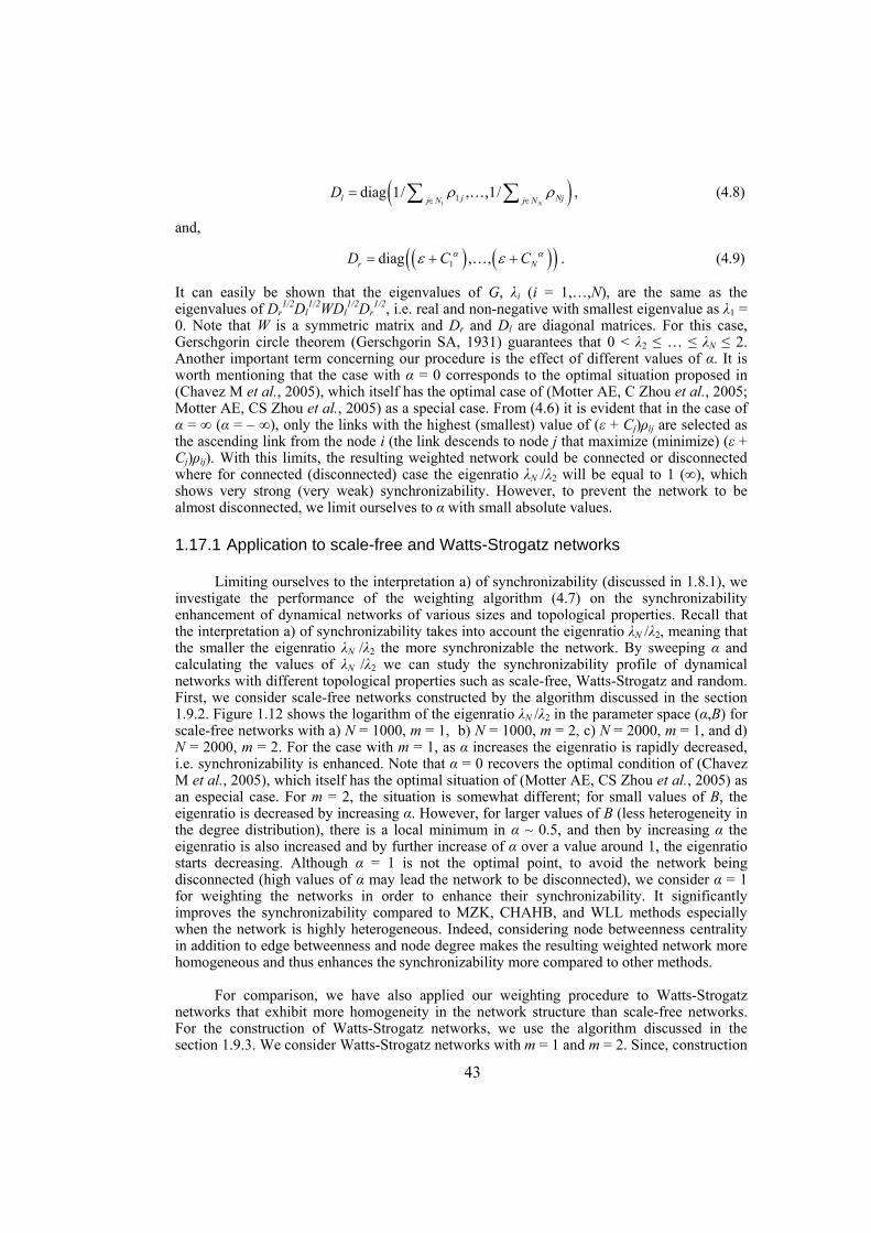
43

( )1

1diag 1/ , ,1/N

l j Njj N j ND ρ ρ

∈ ∈= ∑ ∑K , (4.8)

and,

( ) ( )( )1diag , ,r ND C Cα αε ε= + +K . (4.9)

It can easily be shown that the eigenvalues of G, λi (i = 1,…,N), are the same as the eigenvalues of Dr

1/2Dl1/2WDl

1/2Dr1/2, i.e. real and non-negative with smallest eigenvalue as λ1 =

0. Note that W is a symmetric matrix and Dr and Dl are diagonal matrices. For this case, Gerschgorin circle theorem (Gerschgorin SA, 1931) guarantees that 0 < λ2 ≤ … ≤ λN ≤ 2. Another important term concerning our procedure is the effect of different values of α. It is worth mentioning that the case with α = 0 corresponds to the optimal situation proposed in (Chavez M et al., 2005), which itself has the optimal case of (Motter AE, C Zhou et al., 2005; Motter AE, CS Zhou et al., 2005) as a special case. From (4.6) it is evident that in the case of α = ∞ (α = – ∞), only the links with the highest (smallest) value of (ε + Cj)ρij are selected as the ascending link from the node i (the link descends to node j that maximize (minimize) (ε + Cj)ρij). With this limits, the resulting weighted network could be connected or disconnected where for connected (disconnected) case the eigenratio λN /λ2 will be equal to 1 (∞), which shows very strong (very weak) synchronizability. However, to prevent the network to be almost disconnected, we limit ourselves to α with small absolute values.

1.17.1 Application to scale-free and Watts-Strogatz networks

Limiting ourselves to the interpretation a) of synchronizability (discussed in 1.8.1), we investigate the performance of the weighting algorithm (4.7) on the synchronizability enhancement of dynamical networks of various sizes and topological properties. Recall that the interpretation a) of synchronizability takes into account the eigenratio λN /λ2, meaning that the smaller the eigenratio λN /λ2 the more synchronizable the network. By sweeping α and calculating the values of λN /λ2 we can study the synchronizability profile of dynamical networks with different topological properties such as scale-free, Watts-Strogatz and random. First, we consider scale-free networks constructed by the algorithm discussed in the section 1.9.2. Figure 1.12 shows the logarithm of the eigenratio λN /λ2 in the parameter space (α,B) for scale-free networks with a) N = 1000, m = 1, b) N = 1000, m = 2, c) N = 2000, m = 1, and d) N = 2000, m = 2. For the case with m = 1, as α increases the eigenratio is rapidly decreased, i.e. synchronizability is enhanced. Note that α = 0 recovers the optimal condition of (Chavez M et al., 2005), which itself has the optimal situation of (Motter AE, CS Zhou et al., 2005) as an especial case. For m = 2, the situation is somewhat different; for small values of B, the eigenratio is decreased by increasing α. However, for larger values of B (less heterogeneity in the degree distribution), there is a local minimum in α ~ 0.5, and then by increasing α the eigenratio is also increased and by further increase of α over a value around 1, the eigenratio starts decreasing. Although α = 1 is not the optimal point, to avoid the network being disconnected (high values of α may lead the network to be disconnected), we consider α = 1 for weighting the networks in order to enhance their synchronizability. It significantly improves the synchronizability compared to MZK, CHAHB, and WLL methods especially when the network is highly heterogeneous. Indeed, considering node betweenness centrality in addition to edge betweenness and node degree makes the resulting weighted network more homogeneous and thus enhances the synchronizability more compared to other methods.

For comparison, we have also applied our weighting procedure to Watts-Strogatz networks that exhibit more homogeneity in the network structure than scale-free networks. For the construction of Watts-Strogatz networks, we use the algorithm discussed in the section 1.9.3. We consider Watts-Strogatz networks with m = 1 and m = 2. Since, construction

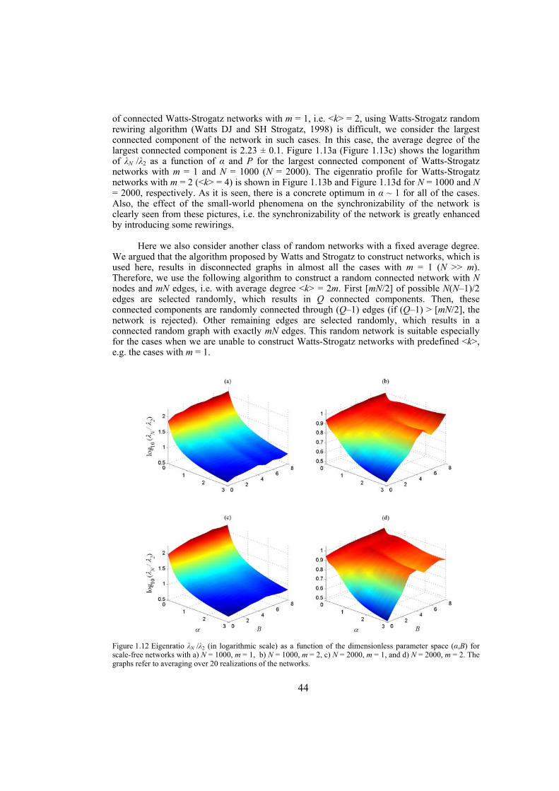
44

of connected Watts-Strogatz networks with m = 1, i.e. <k> = 2, using Watts-Strogatz random rewiring algorithm (Watts DJ and SH Strogatz, 1998) is difficult, we consider the largest connected component of the network in such cases. In this case, the average degree of the largest connected component is 2.23 ± 0.1. Figure 1.13a ( Figure 1.13c) shows the logarithm of λN /λ2 as a function of α and P for the largest connected component of Watts-Strogatz networks with m = 1 and N = 1000 (N = 2000). The eigenratio profile for Watts-Strogatz networks with m = 2 (<k> = 4) is shown in Figure 1.13b and Figure 1.13d for N = 1000 and N = 2000, respectively. As it is seen, there is a concrete optimum in α ~ 1 for all of the cases. Also, the effect of the small-world phenomena on the synchronizability of the network is clearly seen from these pictures, i.e. the synchronizability of the network is greatly enhanced by introducing some rewirings.

Here we also consider another class of random networks with a fixed average degree. We argued that the algorithm proposed by Watts and Strogatz to construct networks, which is used here, results in disconnected graphs in almost all the cases with m = 1 (N >> m). Therefore, we use the following algorithm to construct a random connected network with N nodes and mN edges, i.e. with average degree <k> = 2m. First [mN/2] of possible N(N–1)/2 edges are selected randomly, which results in Q connected components. Then, these connected components are randomly connected through (Q–1) edges (if (Q–1) > [mN/2], the network is rejected). Other remaining edges are selected randomly, which results in a connected random graph with exactly mN edges. This random network is suitable especially for the cases when we are unable to construct Watts-Strogatz networks with predefined <k>, e.g. the cases with m = 1.

Figure 1.12 Eigenratio λN /λ2 (in logarithmic scale) as a function of the dimensionless parameter space (α,B) for scale-free networks with a) N = 1000, m = 1, b) N = 1000, m = 2, c) N = 2000, m = 1, and d) N = 2000, m = 2. The graphs refer to averaging over 20 realizations of the networks.

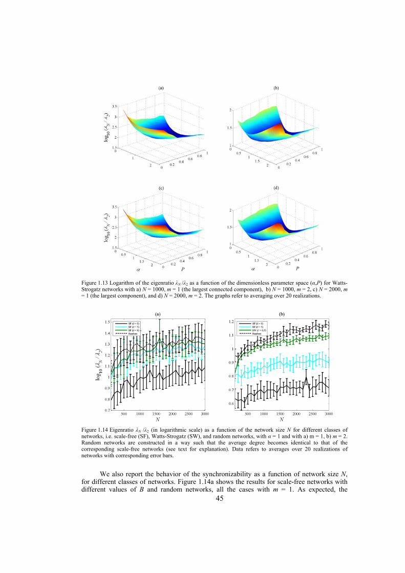
45

Figure 1.13 Logarithm of the eigenratio λN /λ2 as a function of the dimensionless parameter space (α,P) for Watts-Strogatz networks with a) N = 1000, m = 1 (the largest connected component), b) N = 1000, m = 2, c) N = 2000, m = 1 (the largest component), and d) N = 2000, m = 2. The graphs refer to averaging over 20 realizations.

Figure 1.14 Eigenratio λN /λ2 (in logarithmic scale) as a function of the network size N for different classes of networks, i.e. scale-free (SF), Watts-Strogatz (SW), and random networks, with α = 1 and with a) m = 1, b) m = 2. Random networks are constructed in a way such that the average degree becomes identical to that of the corresponding scale-free networks (see text for explanation). Data refers to averages over 20 realizations of networks with corresponding error bars.

We also report the behavior of the synchronizability as a function of network size N, for different classes of networks. Figure 1.14a shows the results for scale-free networks with different values of B and random networks, all the cases with m = 1. As expected, the

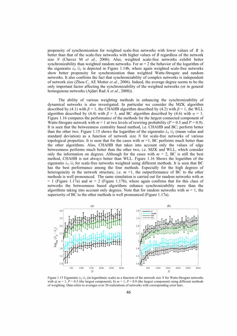
46

propensity of synchronization for weighted scale-free networks with lower values of B is better than that of the scale-free networks with higher values of B regardless of the network size N (Chavez M et al., 2006). Also, weighted scale-free networks exhibit better synchronizability than weighted random networks. For m = 2 the behavior of the logarithm of the eigenratio λN /λ2 is depicted in Figure 1.14b, where again weighted scale-free networks show better propensity for synchronization than weighted Watts-Strogatz and random networks. It also confirms the fact that synchronizability of complex networks is independent of network size (Zhou C, AE Motter et al., 2006). Indeed, the average degree seems to be the only important factor affecting the synchronizability of the weighted networks (or in general homogenous networks (Ajdari Rad A et al., 2008)).

The ability of various weighting methods in enhancing the synchronizability of dynamical networks is also investigated. In particular we consider the MZK algorithm described by (4.1) with β = 1, the CHAHB algorithm described by (4.2) with β = 1, the WLL algorithm described by (4.4) with β = 3, and BC algorithm described by (4.6) with α = 1. Figure 1.16 compares the performance of the methods for the largest connected component of Watts-Strogatz network with m = 1 at two levels of rewiring probability (P = 0.5 and P = 0.9). It is seen that the betweenness centrality based method, i.e. CHAHB and BC; perform better than the other two. Figure 1.15 shows the logarithm of the eigenratio λN /λ2 (mean value and standard deviation) as a function of network size N for scale-free networks of various topological properties. It is seen that for the cases with m =1, BC performs much better than the other algorithms. Also, CHAHB that takes into account only the values of edge betweenness performs much better than the other two, i.e. MZK and WLL, which consider only the information on degrees. Although for the cases with m = 2, BC is still the best method, CHAHB is not always better than WLL. Figure 1.16 Shows the logarithm of the eigenratio λN /λ2 for scale-free networks weighted using different methods. It is seen that BC has the best performance among the four methods. Especially for the high degrees of heterogeneity in the network structure, i.e. m =1, the outperformance of BC to the other methods is well pronounced. The same simulation is carried out for random networks with m = 1 ( Figure 1.17a) and m = 2 ( Figure 1.17b), where again confirms that for this class of networks the betweenness based algorithms enhance synchronizability more than the algorithms taking into account only degrees. Note that for random networks with m = 1, the superiority of BC to the other methods is well pronounced ( Figure 1.17a).

Figure 1.15 Eigenratio λN /λ2 (in logarithmic scale) as a function of the network size N for Watts-Strogatz networks with a) m = 1, P = 0.5 (the largest component), b) m = 1, P = 0.9 (the largest component) using different methods of weighting. Data refers to averages over 20 realizations of networks with corresponding error bars.

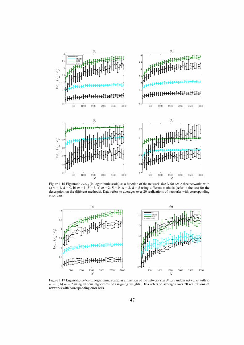
47

Figure 1.16 Eigenratio λN /λ2 (in logarithmic scale) as a function of the network size N for scale-free networks with a) m = 1, B = 0, b) m = 1, B = 5, c) m = 2, B = 0, m = 2, B = 5 using different methods (refer to the text for the description on the different methods). Data refers to averages over 20 realizations of networks with corresponding error bars.

Figure 1.17 Eigenratio λN /λ2 (in logarithmic scale) as a function of the network size N for random networks with a) m = 1, b) m = 2 using various algorithms of assigning weights. Data refers to averages over 20 realizations of networks with corresponding error bars.

48

1.17.2 Applying the method to some real-world networks

Although in the previous section we showed that applying the weighting algorithm described by (4.7) for assigning proper weighs for the links of dynamical networks greatly enhances the synchronizability of the network (reduces the eigenratio λN /λ2), many real-world networks cannot be simply modeled by these scale-free, Watts-Strogatz or random models. In other words, real-world networks may possess very complex topological properties, which can make it difficult to construct a model that mimics all of their properties. Thus, in this section we consider some available real-world undirected networks3 and apply the weighting procedures described in the previous sections to study the profile of λN /λ2 in the resulting weighted networks. We consider some real-world networks including protein structure networks (Milo R et al., 2004), network of power grid (Watts DJ and SH Strogatz, 1998), US airport network4 (Colizza V et al., 2006), Dolphins’ social network (Lusseau D et al., 2003), Email network (Guimera R et al., 2003), protein-protein interaction network (Ito T et al., 2001), yeast protein interaction network (Jeong H et al., 2001), Internet in the level of autonomous system (Krishnamurthy V et al., 2005), and network of coauthorship (Newman MEJ, 2004). Table 4.1 summarizes the results. For all of these networks, BC is the most influential algorithm in reducing λN /λ2. CHAHB method always performs better than MZK, as expected. But, this is not the case for WLL; for some networks WLL is better than CHAHB and for some other ones CHAHB works better. Let us remark that since for WLL algorithm there is no optimal value of β in (4.4), for each network we adopted the least λN /λ2 among the cases with β = 1, β = 2, and β = 3. For some of the networks the case with β = 1 is the best while for some others the cases with β = 2 or β = 3 result in the best performance.

Since MZK is a simple scaling based on the degree of the nodes, it is incapable of capturing all the useful information, and thus, its performance is always worse than that of the one proposed by CHAHB that indeed considers the edge betweenness centrality as well as scaling based on the nodes. The method of WLL uses the degree of nodes in a different way, and its performance is not always better than CHAHB. Indeed, it can be seen that by increase of the heterogeneity of the network, i.e. increase of the standard deviation of the node-degrees, the algorithm of WLL performs better than CHAHB. Our proposed algorithm is an intelligent extension of CHAHB; to consider the heterogeneity of the network, it considers the node betweenness centrality in addition to the edge betweenness centrality. Thus, it always outperforms to CHAHB. However, for networks with high levels of heterogeneity, WLL gives results better than CHAHB and close to our results.

1.17.3 The proposed weighting algorithm and phase synchronization

The rational behind getting the eigenratio λN /λ2 as the synchronizability measure of dynamical networks is the master-stability-function (Barahona M and LM Pecora, 2002; Pecora LM and TL Carroll, 1998). Since the theory of the master-stability-function is developed for linear stability of identical oscillators (complete synchronization), it can not be directly applied to coupled nonidentical oscillators (Barahona M and LM Pecora, 2002;

3 All of these networks are downloadable from Internet in the web site provided by the authors of the original works; interested readers may refer to the cited work. 4 The original version of the US airport network is a weighted network, but here we have considered only the unweighted version, i.e. changing all the weights in the adjacency matrix, except zero weights, to 1.

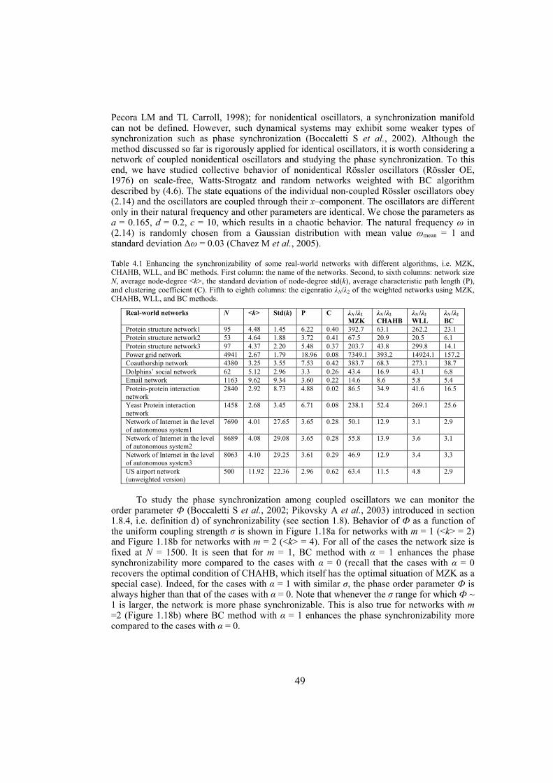
49

Pecora LM and TL Carroll, 1998); for nonidentical oscillators, a synchronization manifold can not be defined. However, such dynamical systems may exhibit some weaker types of synchronization such as phase synchronization (Boccaletti S et al., 2002). Although the method discussed so far is rigorously applied for identical oscillators, it is worth considering a network of coupled nonidentical oscillators and studying the phase synchronization. To this end, we have studied collective behavior of nonidentical Rössler oscillators (Rössler OE, 1976) on scale-free, Watts-Strogatz and random networks weighted with BC algorithm described by (4.6). The state equations of the individual non-coupled Rössler oscillators obey (2.14) and the oscillators are coupled through their x–component. The oscillators are different only in their natural frequency and other parameters are identical. We chose the parameters as a = 0.165, d = 0.2, c = 10, which results in a chaotic behavior. The natural frequency ω in (2.14) is randomly chosen from a Gaussian distribution with mean value ωmean = 1 and standard deviation Δω = 0.03 (Chavez M et al., 2005).

Table 4.1 Enhancing the synchronizability of some real-world networks with different algorithms, i.e. MZK, CHAHB, WLL, and BC methods. First column: the name of the networks. Second, to sixth columns: network size N, average node-degree <k>, the standard deviation of node-degree std(k), average characteristic path length (P), and clustering coefficient (C). Fifth to eighth columns: the eigenratio λN/λ2 of the weighted networks using MZK, CHAHB, WLL, and BC methods.

Real-world networks N <k> Std(k) P C λN /λ2 MZK

λN /λ2 CHAHB

λN /λ2 WLL

λN /λ2 BC

Protein structure network1 95 4.48 1.45 6.22 0.40 392.7 63.1 262.2 23.1 Protein structure network2 53 4.64 1.88 3.72 0.41 67.5 20.9 20.5 6.1 Protein structure network3 97 4.37 2.20 5.48 0.37 203.7 43.8 299.8 14.1 Power grid network 4941 2.67 1.79 18.96 0.08 7349.1 393.2 14924.1 157.2 Coauthorship network 4380 3.25 3.55 7.53 0.42 383.7 68.3 273.1 38.7 Dolphins’ social network 62 5.12 2.96 3.3 0.26 43.4 16.9 43.1 6.8 Email network 1163 9.62 9.34 3.60 0.22 14.6 8.6 5.8 5.4 Protein-protein interaction network

2840 2.92 8.73 4.88 0.02 86.5 34.9 41.6 16.5

Yeast Protein interaction network

1458 2.68 3.45 6.71 0.08 238.1 52.4 269.1 25.6

Network of Internet in the level of autonomous system1

7690 4.01 27.65 3.65 0.28 50.1 12.9 3.1 2.9


8689 4.08 29.08 3.65 0.28 55.8 13.9 3.6 3.1


8063 4.10 29.25 3.61 0.29 46.9 12.9 3.4 3.3

US airport network (unweighted version)

500 11.92 22.36 2.96 0.62 63.4 11.5 4.8 2.9

To study the phase synchronization among coupled oscillators we can monitor the order parameter Ф (Boccaletti S et al., 2002; Pikovsky A et al., 2003) introduced in section 1.8.4, i.e. definition d) of synchronizability (see section 1.8). Behavior of Ф as a function of the uniform coupling strength σ is shown in Figure 1.18a for networks with m = 1 (<k> = 2) and Figure 1.18b for networks with m = 2 (<k> = 4). For all of the cases the network size is fixed at N = 1500. It is seen that for m = 1, BC method with α = 1 enhances the phase synchronizability more compared to the cases with α = 0 (recall that the cases with α = 0 recovers the optimal condition of CHAHB, which itself has the optimal situation of MZK as a special case). Indeed, for the cases with α = 1 with similar σ, the phase order parameter Ф is always higher than that of the cases with α = 0. Note that whenever the σ range for which Ф ~ 1 is larger, the network is more phase synchronizable. This is also true for networks with m =2 ( Figure 1.18b) where BC method with α = 1 enhances the phase synchronizability more compared to the cases with α = 0.

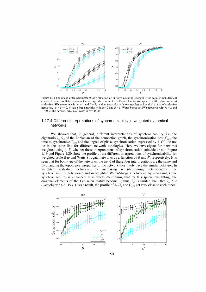
50

Figure 1.18 The phase order parameter Ф as a function of uniform coupling strength σ for coupled nonidentical chaotic Rössler oscillators (parameters are specified in the text). Data refers to averages over 20 realization of a) scale-free (SF) networks with m = 1 and B = 5, random networks with average degree identical to that of scale-free networks, i.e. <k> = 2, b) scale-free networks with m = 2 and B = 5, Watts-Strogatz (SW) networks with m = 2 and P = 0.5. The network size in all cases is N = 1500.

1.17.4 Different interpretations of synchronizability in weighted dynamical networks

We showed that, in general, different interpretations of synchronizability, i.e. the eigenratio λN /λ2 of the Laplacian of the connection graph, the synchronization cost Csyn, the time to synchronize Tsyn, and the degree of phase synchronization expressed by 1–OP, do not lie in the same line for different network topologies. Here we investigate for networks weighted using (4.7) whether these interpretations of synchronization coincide or not. Figure 1.19 and Figure 1.20 show the profile of the different interpretations of synchronizability for weighted scale-free and Watts-Strogatz networks as a function of B and P, respectively. It is seen that for both type of the networks, the trend of these four interpretations are the same and by changing the topological properties of the network they likely have the similar behavior. In weighted scale-free networks, by increasing B (decreasing heterogeneity) the synchronizability gets worse and in weighted Watts-Strogatz networks, by increasing P the synchronizability is enhanced. It is worth mentioning that by this special weighting, the diagonal elements of the Laplacian matrix become 1; thus, λN is limited such that λN ≤ 2 (Gerschgorin SA, 1931). As a result, the profile of λN /λ2 and CSyn get very close to each other.

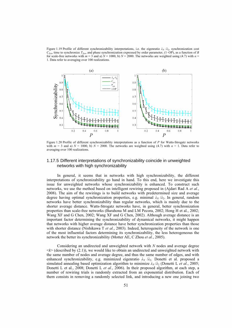
51

Figure 1.19 Profile of different synchronizability interpretations, i.e. the eigenratio λN /λ2, synchronization cost CSyn, time to synchronize TSyn, and phase synchronization expressed by order parameter, (1–OP), as a function of B for scale-free networks with m = 3 and a) N = 1000, b) N = 2000. The networks are weighted using (4.7) with α = 1. Data refer to averaging over 100 realizations.

Figure 1.20 Profile of different synchronizability interpretations as a function of P for Watts-Strogatz networks with m = 3 and a) N = 1000, b) N = 2000. The networks are weighted using (4.7) with α = 1. Data refer to averaging over 100 realizations.

1.17.5 Different interpretations of synchronizability coincide in unweighted networks with high synchronizability

In general, it seems that in networks with high synchronizability, the different interpretations of synchronizability go hand in hand. To this end, here we investigate this issue for unweighted networks whose synchronizability is enhanced. To construct such networks, we use the method based on intelligent rewiring proposed in (Ajdari Rad A et al., 2008). The aim of the rewirings is to build networks with predetermined size and average degree having optimal synchronization properties, e.g. minimal λN /λ2. In general, random networks have better synchronizability than regular networks, which is mainly due to the shorter average distance. Watts-Strogatz networks have, in general, better synchronization properties than scale-free networks (Barahona M and LM Pecora, 2002; Hong H et al., 2002; Wang XF and G Chen, 2002; Wang XF and G Chen, 2002). Although average distance is an important factor determining the synchronizability of dynamical networks, it might happen that networks with higher average distance have better synchronization properties than those with shorter distance (Nishikawa T et al., 2003). Indeed, heterogeneity of the network is one of the most influential factors determining its synchronizability, the less heterogeneous the network the better its synchronizability (Motter AE, C Zhou et al., 2005).

Considering an undirected and unweighted network with N nodes and average degree <k> (described by (2.1)), we would like to obtain an undirected and unweighted network with the same number of nodes and average degree, and thus the same number of edges, and with enhanced synchronizability, e.g. minimized eigenratio λN /λ2. Donetti et al. proposed a simulated annealing based optimization algorithm to minimize λN /λ2 (Donetti L et al., 2005; Donetti L et al., 2008; Donetti L et al., 2006). In their proposed algorithm, at each step, a number of rewiring trials is randomly extracted from an exponential distribution. Each of them consists in removing a randomly selected link, and introducing a new one joining two

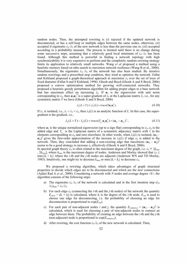
52

random nodes. Then, the attempted rewiring is (i) rejected if the updated network is disconnected, or has a self-loop or multiple edges between the same nodes, otherwise, (ii) accepted if eigenratio λN /λ2 of the new network is less than the previous one or, (iii) accepted according to a probability measure. The process is iterated until there is no change during some successive steps, assuming that a relatively good local minimum of λN /λ2 has been found. Although this method is powerful in finding a network topology with high synchronizability it is very expensive to perform and the completely random rewiring strategy limits its application to relatively small networks. Wang et al proposed a method using a heuristic memory based on tabu search to maximize network resilience (Wang B et al., 2006). Simultaneously, the eigenratio λN /λ2 of the network has also been studied. By iterative random rewirings and a prescribed stop condition, they tried to optimize the network. Fallat and Kirkland proposed a graph-theoretical approach to maximize λ2 over the set of trees of fixed diameter (Fallat S and S Kirkland, 1998). Ghosh and Boyd (Ghosh A and S Boyd, 2006) proposed a convex optimization method for growing well-connected networks. They proposed a heuristic greedy perturbation algorithm for adding proper edges to a base network that has maximum effect on increasing λ2. If u2 is the eigenvector with unit norm corresponding to λ2, then u2u2

T is a super-gradient of λ2 at the Laplacian matrix L, i.e., for any symmetric matrix Y we have (Ghosh A and S Boyd, 2006)

2 2 2 2( ) ( ) ( )TL Y L trace Yλ λ+ ≤ + u u . (4.10)

If λ2 is isolated, i.e., λ1 < λ2 < λ3, then λ2(L) is an analytic function of L. In this case, the super-gradient is the gradient, i.e.,

22 2 2 2 2 2( ) ( ) ( ) ( )

ij

Te i jL Y L trace Yλ λ+ − = = −u u u u , (4.11)

where u2 is the unique normalized eigenvector (up to a sign flip) corresponding to λ2, eij is the added edge and

ijeY is the Laplacian matrix of a symmetric adjacency matrix with 1 in the elements corresponding to eij and zero elsewhere. In other words, when λ2(L) is isolated, (u2i – u2j)2 gives the first-order approximation of the increase in λ2(L) if edge eij is added to the network. Then, they concluded that adding a non-existing edge that maximizes (u2i – u2j)2 seems to be a good strategy to increase λ2 effectively (Ghosh A and S Boyd, 2006). In spectral graph theory λN is often related to the maximum degree of the graph, i.e. λN ∈ [kmax , 2kmax], where kmax is the maximum degree of nodes. Anderson and Morley showed that λN ≤ maxki + kj where the i-th and the j-th nodes are adjacent (Anderson WN and TD Morley, 1985). Intuitively, one might try to decrease kmax or maxki + kj to decrease λN.

We proposed a rewiring algorithm, which takes advantages of graph structural properties to decide which edges are to be disconnected and which are the new connections (Ajdari Rad A et al., 2008). Considering a network with N nodes and average degree <k>, the algorithm consists of the following steps:

a) The eigenratio λN /λ2 of the network is calculated and in the first iteration step (λN /λ2)min = λN /λ2.

b) For each edge eij (connecting the i-th and the j-th nodes) of the network the quantity Ecut,ij = (ki + kj) is calculated, where ki is the degree of the i-th node. Ecut is used to choose one edge for disconnecting, i.e. the probability of choosing an edge for disconnection is proportional to exp(Ecut).

c) For each pair of non-adjacent nodes i and j, the quantity Econnect,ij = (u2i – u2j)2 is calculated, which is used for choosing a pair of non-adjacent nodes to connect an edge between them. The probability of creating an edge between the i-th and the j-th (non-adjacent) node is proportional to exp(Econnect,ij).

d) After rewiring, the cost function λN /λ2 of the new network is calculated. Then,

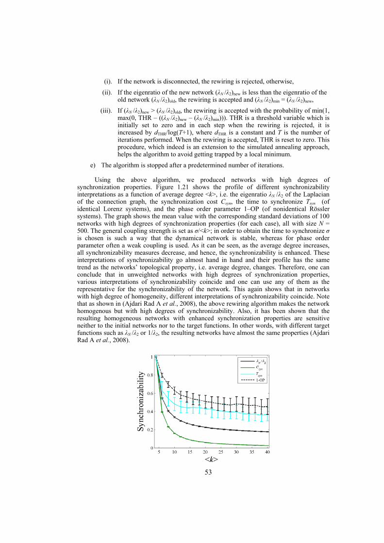
53

(i). If the network is disconnected, the rewiring is rejected, otherwise,

(ii). If the eigenratio of the new network (λN /λ2)new is less than the eigenratio of the old network (λN /λ2)old, the rewiring is accepted and (λN /λ2)min = (λN /λ2)new,

(iii). If (λN /λ2)new > (λN /λ2)old, the rewiring is accepted with the probability of min(1, max(0, THR – ((λN /λ2)new – (λN /λ2)min))). THR is a threshold variable which is initially set to zero and in each step when the rewiring is rejected, it is increased by dTHR/log(T+1), where dTHR is a constant and T is the number of iterations performed. When the rewiring is accepted, THR is reset to zero. This procedure, which indeed is an extension to the simulated annealing approach, helps the algorithm to avoid getting trapped by a local minimum.

e) The algorithm is stopped after a predetermined number of iterations.

Using the above algorithm, we produced networks with high degrees of synchronization properties. Figure 1.21 shows the profile of different synchronizability interpretations as a function of average degree <k>, i.e. the eigenratio λN /λ2 of the Laplacian of the connection graph, the synchronization cost Csyn, the time to synchronize Tsyn (of identical Lorenz systems), and the phase order parameter 1–OP (of nonidentical Rössler systems). The graph shows the mean value with the corresponding standard deviations of 100 networks with high degrees of synchronization properties (for each case), all with size N = 500. The general coupling strength is set as σ/<k>; in order to obtain the time to synchronize σ is chosen is such a way that the dynamical network is stable, whereas for phase order parameter often a weak coupling is used. As it can be seen, as the average degree increases, all synchronizability measures decrease, and hence, the synchronizability is enhanced. These interpretations of synchronizability go almost hand in hand and their profile has the same trend as the networks’ topological property, i.e. average degree, changes. Therefore, one can conclude that in unweighted networks with high degrees of synchronization properties, various interpretations of synchronizability coincide and one can use any of them as the representative for the synchronizability of the network. This again shows that in networks with high degree of homogeneity, different interpretations of synchronizability coincide. Note that as shown in (Ajdari Rad A et al., 2008), the above rewiring algorithm makes the network homogenous but with high degrees of synchronizability. Also, it has been shown that the resulting homogeneous networks with enhanced synchronization properties are sensitive neither to the initial networks nor to the target functions. In other words, with different target functions such as λN /λ2 or 1/λ2, the resulting networks have almost the same properties (Ajdari Rad A et al., 2008).

54

Figure 1.21 Profile of different synchronizability interpretations as a function of average degree <k> for networks with N = 500 and high degrees of synchronization properties. By taking the eigenratio λN /λ2 as the synchronizability measure and using rewiring approach proposed in (Ajdari Rad A et al., 2008), the networks are optimized (approximately) for synchronization. Data represent the mean value with the corresponding errorbars for standard deviation for 100 networks with high degrees of synchronization properties.

1.18 Enhancing synchronizability preserving the weighted network undirected

One drawback of all weighting methods discussed in the section 1.17 is that the weighted network with enhanced synchronizability becomes directed while the original unweighted network is undirected. This may limit their applications in systems where the connection graph is required to be undirected. This is the case in sensor networks where the nodes communicate diffusively with each other (Barbarossa S and G Scutari, 2007; Olfati-Saber R et al., 2007). Another example is computer networks where computers exchange data in both directions. Also, in some applications, synchrony is required to be achieved with minimal cost that should be considered when optimizing the network. Indeed, synchronization requires existence of links between the individuals. Having such links demands energy (cost), which is desired to be kept as low as possible. As stated in the previous chapters, synchronization can be regarded as a phenomenon depending mainly on three factors: the dynamics of individual dynamical systems, the strength of the connection links and the topological properties of the underlying graph. Here, by considering the interpretation b) of synchronizability (discussed in the section 1.8.2) we give a weighting method for undirected networks to enhance their synchronizability. At the same time, it keeps the weighted network undirected. Recall that the interpretation b) of synchronizability is related to λ2; the larger the λ2 the more the synchronizability of the network (for the same synchronization cost). In other words, network N1 is more synchronizable than network N2 if less effort is needed to synchronize N1 than N2, i.e. synchronization cost of N1 is less than N2.

1.18.1 Synchronization cost

Let us consider the network described by (2.4), where the second smallest eigenvalue of G is λ2. Due to Pecora and Carroll, the lower bound of the synchronizing coupling strength σSyn is determined by the master-stability-function of the individual dynamical systems and λ2 as

2

MSFSyn

σσ

λ> , (4.12)

where σMSF is the limit for making the master-stability-function negative and depends only on the dynamics of individual dynamical systems and their coupling configuration (Pecora LM and TL Carroll, 1998). This limit can be clearly observed in Figure 1.2 for x–coupled Lorenz and Rössler systems, i.e. the least quantity a that makes the master-stability-function Λ(a) negative.

Definition 4.1 Let define the MSF-average synchronization cost CMSF per vertex as

2

MSFMSF ij

i jC g

Nσλ >

= ∑ . (4.13)

55

Note that in (4.13) σMSF depends on the individual dynamical systems while the other terms depend only on the network structural properties. Here, we investigate the synchronization cost of networks without considering any specific individual dynamical system, i.e. by eliminating the effect of individual dynamics, i.e. MSFσ , (4.13) is modified to

2

1Syn ij

i jC g

Nλ >

= ∑ . (4.14)

Note that the lower bound on σSyn for global synchronization given in (Belykh VN et al., 2004) has the same form as (4.13) but with another constant linked to the individual dynamical systems instead of σMSF. This gives additional motivation for considering (4.14).

In the following sections, first some existing methods to reduce the synchronization cost are given and then we present our proposed method, which indeed makes a trade-off between these approaches in terms of computational complexity and optimality.

1.18.2 Metropolis-Hasting weights

Let us denote the degree of node i by ki and E be the set of the edges of the network. The Metropolis-Hasting weights is defined as (Hastings W, 1970)

( ) ( )1 ,1 max ,

0 otherwisei jij

i j Ek kg

⎧ ∈⎪ += ⎨⎪⎩

. (4.15)

In other words, the weight on each edge is defined as one over one plus the larger degree at its two incident nodes. It is adopted from the Metropolis-Hasting algorithm (Hastings W, 1970) originally proposed in the literate of Markov chain Monte Carlo. Since this algorithm needs only the local information of the network, i.e. the degree of neighbors, it is easy to implement and is the first choice in many applications. However, in many cases it results in a solution far from the optimum.

1.18.3 Optimizing the λ2 by convex optimization

Recently Boyd (2006) proposed a convex optimization method to maximize the second smallest eigenvalue of G (or minimize the cost (4.14)) (Boyd S, 2006). λ2 is expressed as λ2 = minλ2,…,λN, which is a concave function of edge weights G (Sun J et al., 2006). To maximize λ2 and consequently minimize CSyn one can state the following problem

2

;

maximize subject to 0

1ij i j

iji j

g

g

λ

≠

≠

≥

≥∑. (4.16)

An alternative approach to solve the above convex optimization problem is to convert it to the following problem

56

2

;

minimize

subject to 1, 0

iji j

ij i j

g

gλ≠

≠

≥≥

∑. (4.17)

In the later formulation the aim is to find gij so as to minimize the total weighted cost, subject to the constraint that the λ2 exceeds 1 (in the optimal case λ2 = 1). We know that (Sun J et al., 2006)

( )2 1 1/ TL I Nλ ≥ ⇔ ≥ − 11 , (4.18)

where I is the identity matrix, L is the Laplacian of the unweighted network (2.1), and 1 is a vector with all entries equal to 1. Thus, the problem can be formulated in the standard semidefinite programming as

( ) ;

minimize

subject to 1/ 0

iji j

T

ij i j

g

L I Ng

≠

≠

≥ −

≥

∑11 . (4.19)

The above semidefinite programming can be solved using standard convex optimization tools (Sun J et al., 2006). This is very powerful method that gives the optimal weights for reducing the synchronization cost. However, this method has a drawback that is for large networks (in practice for networks with more than about 600 edges) standard interior-point methods can not be used.

1.18.4 Optimizing synchronization cost using betweenness centrality measures

In the previous sections we argued two weighting procedures: one of them was Metropolis-Hasting method that is simple to compute but far from the optimum and the other one convex optimization procedure that is optimal but expensive to compute. Here, we propose a method whose performance (and somehow the complexity of computations) lies in between; simple to compute like the Metropolis-Hasting method while resulting in a near-optimal solution (much better than what is obtained by the Metropolis-Hasting method). The proposed method makes use of edge and node betweenness centrality measures defined by (4.3) and (4.5), respectively. We propose the following heuristic weighting algorithm

( ) ( )/ 1 max , ,

0 otherwiseij i j j i

ij

i j Eg

ρ → →⎧ + Ω Ω ∈⎪= ⎨⎪⎩

, (4.20)

where

( )

,

1

i

i ii j

rr N r j

k NBCNBC→

∈ ≠

−Ω =

∑, (4.21)

and Ni is the set of the neighbors of node i. Indeed, Ωi→j indicates the importance of node i for its neighbors to communicate through node j.

57

This algorithm is much simpler than the convex optimization to compute and since it needs global information of the graph, it is a bit more complex than the Metropolis-Hasting method. Next, we will test its performance on some network examples.

1.18.5 Synchronizability enhancement in undirected scale-free and Watts-Strogatz networks

We used the CVX toolbox (available for free at http://www.stanford.edu/~boyd/cvx/) to solve the convex optimization problems. Let us first study scale-free networks. Figure 1.22 shows the logarithm of CSyn as a function of B for scale-free networks with m = 1 (<k> = 2), N = 100 ( Figure 1.22a) and N = 300 ( Figure 1.22b). Figure 1.22c ( Figure 1.22d) shows the results for scale-free networks with N = 100 (N = 300) and m = 2. As it is seen, for all of the cases CSyn based on betweenness centrality is near the optimal one based on convex optimization but much better than the one obtained through the Metropolis-Hasting algorithm. Also, it is observed that for B > 5 the cost is almost unchanged by increasing B (decreasing the heterogeneity of the network). As a second class of networks, the Watts-Strogatz networks are considered. Since we are interested in the most heterogeneous case, we consider m = 1. But in this case, the resulting graph is often disconnected; thus we take its largest connected component. Figure 1.23a shows the results for Watts-Strogatz networks with the largest connected component with N = 100 ± 2.8 and <k> = 2.22 ± 0.1. In other words, these results refer to Watts-Strogatz networks where their largest connected component has in average 100 nodes (2.8 is the standard deviation). The results for Watts-Strogatz network with the largest connected component with N = 300 ± 8.1 and <k> = 2.24 ± 0.1 is shown in Figure 1.23b. Figure 1.23c and Figure 1.23d show the logarithm of CSyn for Watts-Strogatz networks with <k> = 4 and N = 100 and N = 300, respectively. As expected, by increasing P the synchronizability is enhanced and CSyn is reduced for all of the cases. Like the case for scale-free networks, here also the CSyn based on betweenness centrality lies between CSyn based on the convex optimization and the Metropolis-Hasting methods.

Let us remark that the computational complexity of the method based on the betweenness centrality is O(NE), where N and E are the number of nodes and edges in the network, respectively. Whereas, the computational complexity of the fastest interior-point methods for convex optimization is O(N3), which is, in any case, more complex compared to the proposed method. Furthermore, solving the convex optimization problem for networks with more than about 600 edges can not be performed through standard interior-point methods; thus we limited ourselves to networks with rather small size to show the power of our proposed method. The method based on betweenness centrality (and the Metropolis-Hasting algorithm as well) can be applied to large networks. This is the main advantage of this method over the one based on the convex optimization.

1.19 Summary

In this chapter we introduced algorithms for weighting of dynamical networks to enhance their synchronizability. By considering local (i.e. degree) and global (i.e. node- and edge-betweenness centrality measures) structural properties of dynamical networks we proposed a procedure for assigning proper connection weights to enhance the synchronizability of the networks. We tested the algorithm in enhancing the synchronizability in the sense of the eigenratio λN /λ2 of the Laplacian of the connection graph on artificially constructed scale-free, Watts-Strogatz and random networks of various sizes and topological properties. Also, the advantages of the method in improving the synchronizability in some

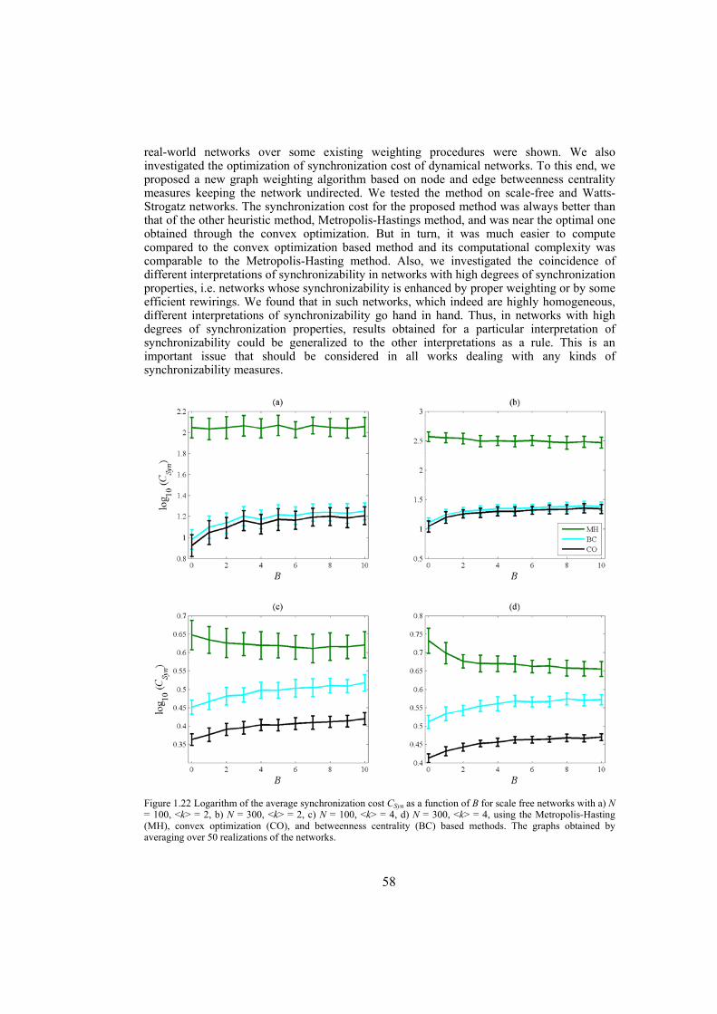
58

real-world networks over some existing weighting procedures were shown. We also investigated the optimization of synchronization cost of dynamical networks. To this end, we proposed a new graph weighting algorithm based on node and edge betweenness centrality measures keeping the network undirected. We tested the method on scale-free and Watts-Strogatz networks. The synchronization cost for the proposed method was always better than that of the other heuristic method, Metropolis-Hastings method, and was near the optimal one obtained through the convex optimization. But in turn, it was much easier to compute compared to the convex optimization based method and its computational complexity was comparable to the Metropolis-Hasting method. Also, we investigated the coincidence of different interpretations of synchronizability in networks with high degrees of synchronization properties, i.e. networks whose synchronizability is enhanced by proper weighting or by some efficient rewirings. We found that in such networks, which indeed are highly homogeneous, different interpretations of synchronizability go hand in hand. Thus, in networks with high degrees of synchronization properties, results obtained for a particular interpretation of synchronizability could be generalized to the other interpretations as a rule. This is an important issue that should be considered in all works dealing with any kinds of synchronizability measures.

Figure 1.22 Logarithm of the average synchronization cost CSyn as a function of B for scale free networks with a) N = 100, <k> = 2, b) N = 300, <k> = 2, c) N = 100, <k> = 4, d) N = 300, <k> = 4, using the Metropolis-Hasting (MH), convex optimization (CO), and betweenness centrality (BC) based methods. The graphs obtained by averaging over 50 realizations of the networks.

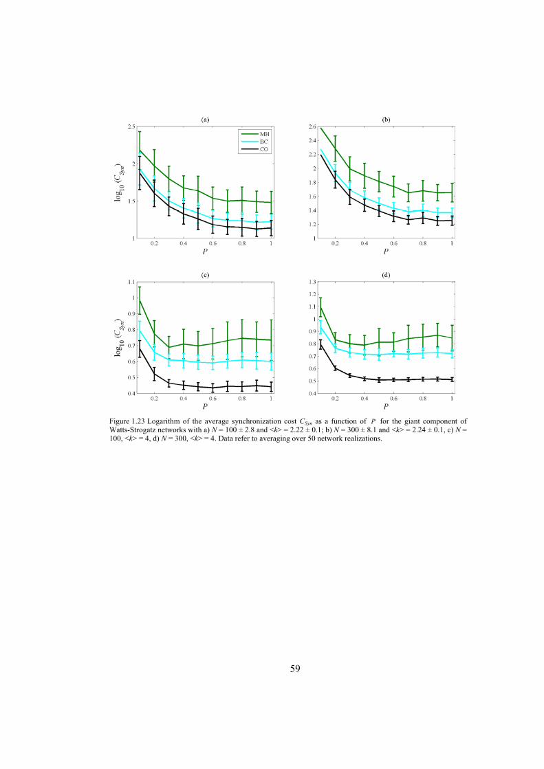
59

Figure 1.23 Logarithm of the average synchronization cost CSyn as a function of P for the giant component of Watts-Strogatz networks with a) N = 100 ± 2.8 and <k> = 2.22 ± 0.1; b) N = 300 ± 8.1 and <k> = 2.24 ± 0.1, c) N = 100, <k> = 4, d) N = 300, <k> = 4. Data refer to averaging over 50 network realizations.

61

SECTION II

63

SYNCHRONIZING HINDMARSH-ROSE NEURONS OVER NEWMAN-WATTS NETWORKS

Personal Contribution — The results presented in this chapter are our original contribution.

1.20 Neural synchronization

Synchronization, time-correlated activity of two or many interconnected dynamical systems, is believed to play an important role in information processing in the brain both in macroscopic and cellular levels (Dzakpasu R and M Żochowski, 2005; Glass L, 2001; Gray CM et al., 1989; Neuenschwander S and W Singer, 1996; Singer W, 1999; Uhhaas PJ and W Singer, 2006). Brain oscillations that are ubiquitous phenomena in all brain areas get into synchrony and consequently allow the brain to process various tasks from cognitive to motor tasks (Buzsaki G, 2006). Indeed, it is hypothesized that synchronous brain activity is the most likely mechanism for many cognitive functions such as attention and feature binding, as well as learning, development and memory formation (Buzsaki G, 2006). Neurons in a population synchronize their activity using electrical (via gap junctions) and chemical synapses with the other neurons in the same population as well as with neurons from other populations. However, synchronization is not useful all the time; high levels of synchrony may proceed to epileptic behaviors. In other words, brain disorders such as Epilepsy, Schizophrenia, Alzheimer’s disease and Parkinson influence functional synchronyization maps of different brain areas (Jacobsen LK et al., 2004; Jalili M, S Lavoie et al., 2007; Knyazeva MG, M Jalili, A Brioschi et al., 2008; Micheloyannis S et al., 2006; Stam CJ et al., 2006; Uhhaas PJ and W Singer, 2006). Thus, understanding the mechanisms behind the neural synchronization is of high importance in order to understand various brain functions.

There are about 1011 neurons with an estimated 2×1014 connection links between them; all packed in about 1.5 liter volume of human brain. A potential remedy to the brain wiring problem emerged from seminal work of Watts and Strogatz who introduced a model to mimic

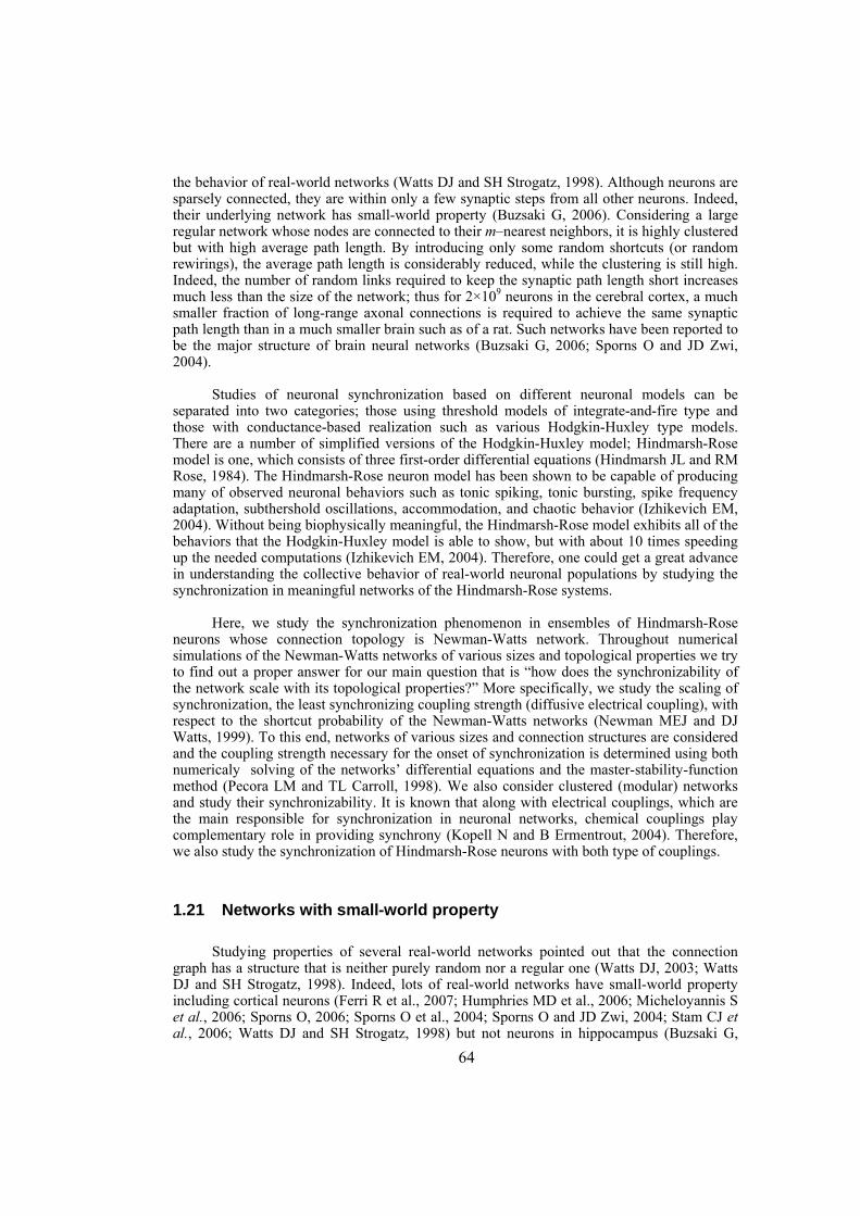
64

the behavior of real-world networks (Watts DJ and SH Strogatz, 1998). Although neurons are sparsely connected, they are within only a few synaptic steps from all other neurons. Indeed, their underlying network has small-world property (Buzsaki G, 2006). Considering a large regular network whose nodes are connected to their m–nearest neighbors, it is highly clustered but with high average path length. By introducing only some random shortcuts (or random rewirings), the average path length is considerably reduced, while the clustering is still high. Indeed, the number of random links required to keep the synaptic path length short increases much less than the size of the network; thus for 2×109 neurons in the cerebral cortex, a much smaller fraction of long-range axonal connections is required to achieve the same synaptic path length than in a much smaller brain such as of a rat. Such networks have been reported to be the major structure of brain neural networks (Buzsaki G, 2006; Sporns O and JD Zwi, 2004).

Studies of neuronal synchronization based on different neuronal models can be separated into two categories; those using threshold models of integrate-and-fire type and those with conductance-based realization such as various Hodgkin-Huxley type models. There are a number of simplified versions of the Hodgkin-Huxley model; Hindmarsh-Rose model is one, which consists of three first-order differential equations (Hindmarsh JL and RM Rose, 1984). The Hindmarsh-Rose neuron model has been shown to be capable of producing many of observed neuronal behaviors such as tonic spiking, tonic bursting, spike frequency adaptation, subthershold oscillations, accommodation, and chaotic behavior (Izhikevich EM, 2004). Without being biophysically meaningful, the Hindmarsh-Rose model exhibits all of the behaviors that the Hodgkin-Huxley model is able to show, but with about 10 times speeding up the needed computations (Izhikevich EM, 2004). Therefore, one could get a great advance in understanding the collective behavior of real-world neuronal populations by studying the synchronization in meaningful networks of the Hindmarsh-Rose systems.

Here, we study the synchronization phenomenon in ensembles of Hindmarsh-Rose neurons whose connection topology is Newman-Watts network. Throughout numerical simulations of the Newman-Watts networks of various sizes and topological properties we try to find out a proper answer for our main question that is “how does the synchronizability of the network scale with its topological properties?” More specifically, we study the scaling of synchronization, the least synchronizing coupling strength (diffusive electrical coupling), with respect to the shortcut probability of the Newman-Watts networks (Newman MEJ and DJ Watts, 1999). To this end, networks of various sizes and connection structures are considered and the coupling strength necessary for the onset of synchronization is determined using both numericaly solving of the networks’ differential equations and the master-stability-function method (Pecora LM and TL Carroll, 1998). We also consider clustered (modular) networks and study their synchronizability. It is known that along with electrical couplings, which are the main responsible for synchronization in neuronal networks, chemical couplings play complementary role in providing synchrony (Kopell N and B Ermentrout, 2004). Therefore, we also study the synchronization of Hindmarsh-Rose neurons with both type of couplings.

1.21 Networks with small-world property

Studying properties of several real-world networks pointed out that the connection graph has a structure that is neither purely random nor a regular one (Watts DJ, 2003; Watts DJ and SH Strogatz, 1998). Indeed, lots of real-world networks have small-world property including cortical neurons (Ferri R et al., 2007; Humphries MD et al., 2006; Micheloyannis S et al., 2006; Sporns O, 2006; Sporns O et al., 2004; Sporns O and JD Zwi, 2004; Stam CJ et al., 2006; Watts DJ and SH Strogatz, 1998) but not neurons in hippocampus (Buzsaki G,

65

2006). In such networks, average characteristic path length scales almost logarithmically with network size, like random networks, while the clustering coefficient is as high as regular networks (Newman MEJ, 2003; Newman MEJ et al., 2000). In such networks, the number of nodes within a distance d of a central node grows exponentially with d (Newman MEJ, 2003). The small-world property has an obvious effect on dynamical processes taking place on a network; the spread of information, i.e. communication between nodes in networks with this property takes place faster and better compared to networks without that. Because of short average path length and also degree-homogeneity of networks with small-world property and consequently better communication between the nodes, it’s a common belief that these networks have good synchronizability (Barahona M and LM Pecora, 2002; Lago-Fernández LF et al., 2000; Nishikawa T et al., 2003). However, it has been shown that this is not true in general and other factors also affect the synchronizability of complex networks (Nishikawa T et al., 2003).

1.21.1 Newman-Watts networks

In the previous chapters we considered the Watts-Strogatz networks with a model proposed by Watts and Strogatz (Watts DJ and SH Strogatz, 1998). Here, we consider a different model proposed by Newman and Watts (Newman MEJ and DJ Watts, 1999), which guarantees connectedness of the network. The algorithm for the construction of the network is as the following. Starting with a ring graph with N nodes each connected to its m–nearest neighbors by undirected links, the unconnected nodes get connected with probability P. For P = 1, an all-to-all connected graph is obtained, but for some values of P, a network with small-world property is obtained. It is easy to show that the average degree of these networks is 2m(1 – P) + P(N – 1).

1.21.2 Clustered Newman-Watts networks

Following some observations in neural networks which revealed clustered (modular) structure in their connection topology (Girvan M and MEJ Newman, 2002; Humphries MD et al., 2006; Zhou C, L Zemanova et al., 2006), we also consider synchronization in such networks. To construct the clustered networks, we consider a network of k clusters each of which consists of Newman-Watts networks of size Nk. The intra-cluster probability of shortcuts Pintra is equal for all of the clusters. Moreover, nodes in each cluster are connected to other nodes in the other clusters with inter-cluster shortcut probability Pinter.The network is constructed in this way is a network with small-world property, i.e. a Meta Newman-Watts network.

1.22 Hindmarsh-Rose neuron model

Neural synchronization is believed to play an important role in information binding in the nervous system and it is well established in some special areas such as the olfactory system or the hippocampus region that neurons are synchronized to perform specific tasks (Glass L, 2001; Gray CM et al., 1989; Neuenschwander S and W Singer, 1996; Singer W, 1999; Uhhaas PJ and W Singer, 2006). There are millions of neurons in the nervous system. An interesting question while studying networks of such huge number of neurons arises that is “how do networks of interacting neurons behave collectively considering the individual dynamics of the neurons and their coupling structure?” To find out proper answers for the questions of this type, along with in vivo and in vitro measurements, computer simulations using model neurons should also be performed. In many works different models of the family

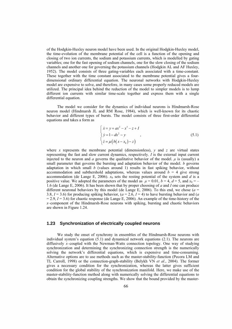
66

of the Hodgkin-Huxley neuron model have been used. In the original Hodgkin-Huxley model, the time-evolution of the membrane potential of the cell is a function of the opening and closing of two ion currents, the sodium and potassium currents, which is modelled by gating variables; one for the fast opening of sodium channels, one for the slow closing of the sodium channels and another one for governing the potassium channels (Hodgkin AL and AF Huxley, 1952). The model consists of three gating-variables each associated with a time-constant. These together with the time constant associated to the membrane potential gives a four-dimensional ordinary differential equation. The neuronal networks with Hodgkin-Huxley model are expensive to solve, and therefore, in many cases some properly reduced models are utilized. The principal idea behind the reduction of the model to simpler models is to lump different ion currents with similar time-scale together and express them with a single differential equation.

The model we consider for the dynamics of individual neurons is Hindmarsh-Rose neuron model (Hindmarsh JL and RM Rose, 1984), which is well-known for its chaotic behavior and different types of bursts. The model consists of three first-order differential equations and takes a form as

( )( )

2 3

2

0

1x y ax x z Iy dx y

z b x x zμ

⎧ = + − − +⎪

= − −⎨⎪ = − −⎩

&

&

&

, (5.1)

where x represents the membrane potential (dimensionless), y and z are virtual states representing the fast and slow current dynamics, respectively. I is the external input current injected to the neuron and a governs the qualitative behavior of the model. μ is (usually) a small parameter that governs the bursting and adaptation behavior of the model. b governs adaptation in which small b (values around 1) results in fast spiking behavior, without accommodation and subthershold adaptations, whereas values around b = 4 give strong accommodation (de Lange E, 2006). x0 sets the resting potential of the system and d is a positive value. We adopted the parameters of the model as μ = 0.01, b = 4, d = 5, and x0 = –1.6 (de Lange E, 2006). It has been shown that by proper choosing of a and I one can produce different neuronal behaviors by this model (de Lange E, 2006). To this end, we chose (a = 3.8, I = 3.6) for producing spiking behavior, (a = 2.6, I = 4) to have bursting behavior and (a = 2.9, I = 3.6) for chaotic response (de Lange E, 2006). An example of the time-history of the x–component of the Hindmarsh-Rose neurons with spiking, bursting and chaotic behaviors are shown in Figure 1.24.

1.23 Synchronization of electrically coupled neurons

We study the onset of synchrony in ensembles of the Hindmarsh-Rose neurons with individual system’s equation (5.1) and dynamical network equations (2.1). The neurons are diffusively x–coupled with the Newman-Watts connection topology. One way of studying synchronization and determining the synchronizing connection strength is the numerically solving the network’s differential equations, which is expensive and time-consuming. Alternative options are to use methods such as the master-stability-function (Pecora LM and TL Carroll, 1998) or the connection-graph-stability (Belykh VN et al., 2004). The former gives a necessary condition for the synchronization, whereas the latter gives sufficient condition for the global stability of the synchronization manifold. Here, we make use of the master-stability-function method along with numerically solving the differential equations to obtain the synchronizing coupling strengths. We show that the bound provided by the master-

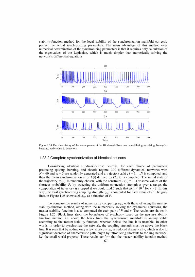
67

stability-function method for the local stability of the synchronization manifold correctly predict the actual synchronizing parameters. The main advantage of this method over numerical determination of the synchronizing parameters is that it requires only calculation of the eigenvalues of the Laplacian, which is much simpler than numerically solving the network’s differential equations.

Figure 1.24 The time history of the x–component of the Hindmarsh-Rose neuron exhibiting a) spiking, b) regular bursting, and c) chaotic behaviors.

1.23.2 Complete synchronization of identical neurons

Considering identical Hindmarsh-Rose neurons, for each choice of parameters producing spiking, bursting, and chaotic regime, 300 different dynamical networks with N = 60 and m = 3 are randomly generated and a trajectory xi(t) ; i = 1,…,N is computed, and then the mean synchronization error E(t) defined by (2.32) is computed. The initial state of the trajectory, xi(0), is randomly chosen, with the constraint E(0) = 1. For some values of the shortcut probability P, by sweeping the uniform connection strength σ over a range, the computation of trajectory is stopped if we could find T such that E(t) < 10–5 for t > T. In this way, the least synchronizing coupling strength σSyn is computed for each value of P. The gray lines in Figure 1.25 show such σSyn as a function of P.

To compare the results of numerically computing σSyn with those of using the master-stability-function method, along with the numerically solving the dynamical equations, the master-stability-function is also computed for each pair of P and σ. The results are shown in Figure 1.25. Black lines show the boundaries of synchrony based on the master-stability-function method, i.e. above the black lines the synchronized manifold is locally stable according to the master-stability-function, whereas below the line it is unstable. In other words, in order to synchronize the network, the coupling strength must be above the black line. It is seen that by adding only a few shortcuts σSyn is reduced dramatically, which is due to significant decrease of characteristic path length by introducing shortcuts to the ring network, i.e. the small-world property. These results confirm that the master-stability-function method

68

correctly predicts σSyn; the numerically obtained σSyn is near to the one obtained through the master-stability-function method. Note that numerically solving differential equations to determine E(t) and subsequently σSyn is too expensive. In the sequal and for large networks we limit ourselves to the results obtained through the master-stability-function method.

Limiting ourselves to the master-stability-function method and neurons with bursting behavior, we performed analysis on Newman-Watts networks of various sizes and topological properties. Figure 1.26 shows the logarithm of σSyn as a function of P and N with a) m = 1 b) m = 5 c) m = 10, and d) m = 20. As it is seen, for almost all of the cases σSyn is independent of N and is influenced only by the average degree and P. Also, it is observed that the logarithm of σSyn scales linearly with logarithm of P for the cases where N/m >> 1. Indeed, for such cases, there is a power-law relationship such as σSyn = αP–γ, where γ∈(1,2) and α is a small positive value as α∈(0.1,0.0001).

1.23.3 Synchronizing non-identical neurons

Although complete synchronization can not be attained for coupled non-identical systems, i.e. synchronization manifold can not be defined for such oscillators, some weaker types of synchronization such as approximate or phase synchronization may be achieved. In other words, for values of E(t) small enough, we argue that the network is approximately synchronized. It is notable that unlike the complete synchronization case that E(t) → 0 as t → ∞, for non-identical systems E(t) will not be exactly zero even for very large values of coupling strengths. We investigate the behavior of the synchronization error E(t) as a function of P and σ for non-identical neurons coupled over the Newman-Watts networks with N = 60 and m = 3. The dynamical network is run for a predetermined time; and by neglecting some initial transients, E(t) is averaged over the time-course. 10% of uncertainty is considered in the parameter domain. Indeed, the model parameters were adopted as μ = 0.01 ± 0.001, b = 4 ± 0.4, d = 5 ± 0.5, x0 = –1.6 ± 0.16, and a = 3.8 ± 0.38, I = 3.6 ± 0.36 (spiking), a = 2.6 ± 0.26, I = 4 ± 0.4 (bursting), a = 2.9 ± 0.29, I = 3.6 ± 0.36 (chaotic). The spiking (bursting) parameter range is such that all of the oscillators produce only spiking (bursting) behavior. For chaotic case, the pattern might be chaotic, spiking or bursting depending on the parameters’ value. (i.e. small drift from chaos-producing parameters changes the chaotic regime to spiking or bursting regimes). Figure 1.27 shows E(t) as a function of σ and P for different regimes. It is seen that for non-identical bursting neurons, E(t) is always decreased by increasing σ and P ( Figure 1.27b). For some intervals of σ and P where E(t) is near zero, we can argue that the neurons are approximately synchronized (the region in dark blue). But, the situation is somewhat different for spiking and chaotic regimes. For neurons with spiking behavior, the graph consists of a saddle; for some values of P, i.e. P < 0.05, an interesting phenomenon happens. Starting from a small value of σ and by increasing σ, E(t) decreases, but suddenly E(t) starts increasing by further increase of σ and more increase of σ makes E(t) decrease ( Figure 1.27a). The shadow of this type of behavior is also exhibited for the chaotic regime ( Figure 1.27c). We mentioned that with randomly drifting the parameters of the chaotic regime, the model may fall into spiking or bursting regimes, and thus, it is expected that the results of chaotic regime have some properties of spiking mode. Let us remark that despite this variability among the behavior of E(t) among different neuronal behaviors, if we look at the necessary coupling strength σSyn for approximate synchronization, i.e. where E(t) is less than a fixed small value, we will obtain results similar to the gray lines in Figure 1.25, where σSyn shows a similar pattern for spiking, bursting and chaotic regimes.

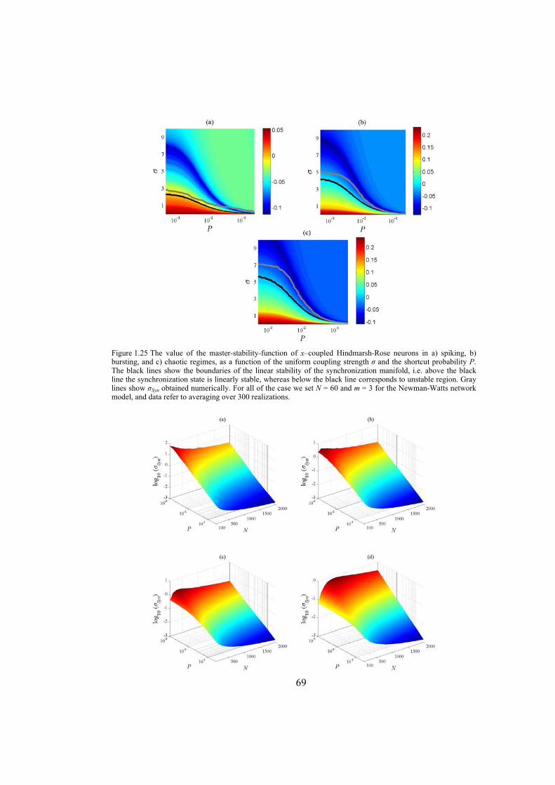
69

Figure 1.25 The value of the master-stability-function of x–coupled Hindmarsh-Rose neurons in a) spiking, b) bursting, and c) chaotic regimes, as a function of the uniform coupling strength σ and the shortcut probability P. The black lines show the boundaries of the linear stability of the synchronization manifold, i.e. above the black line the synchronization state is linearly stable, whereas below the black line corresponds to unstable region. Gray lines show σSyn obtained numerically. For all of the case we set N = 60 and m = 3 for the Newman-Watts network model, and data refer to averaging over 300 realizations.

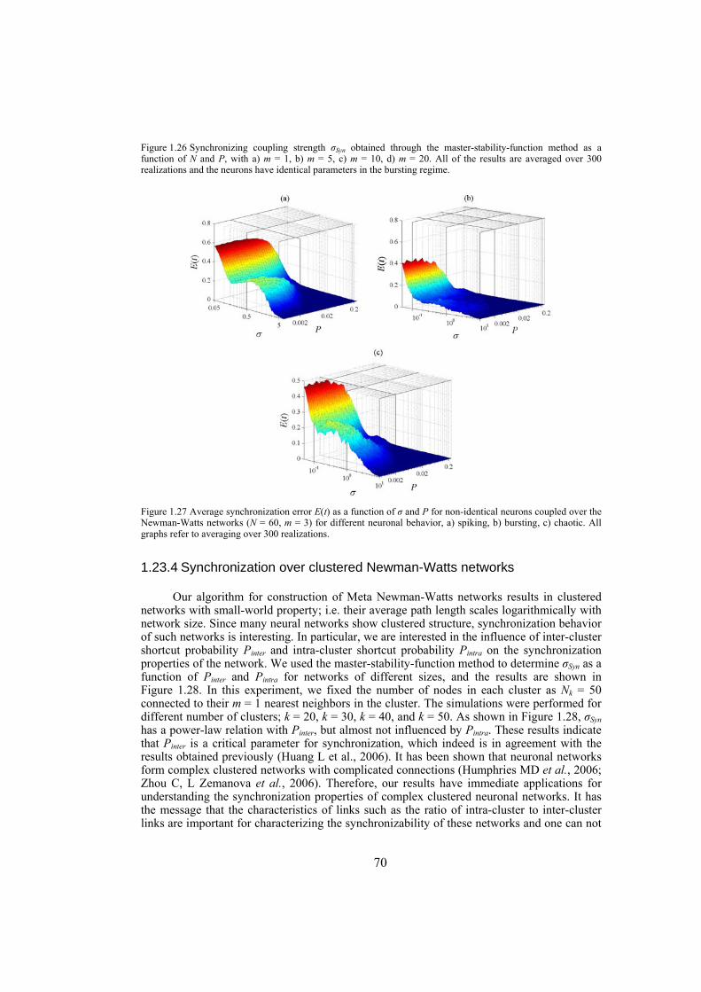
70

Figure 1.26 Synchronizing coupling strength σSyn obtained through the master-stability-function method as a function of N and P, with a) m = 1, b) m = 5, c) m = 10, d) m = 20. All of the results are averaged over 300 realizations and the neurons have identical parameters in the bursting regime.

Figure 1.27 Average synchronization error E(t) as a function of σ and P for non-identical neurons coupled over the Newman-Watts networks (N = 60, m = 3) for different neuronal behavior, a) spiking, b) bursting, c) chaotic. All graphs refer to averaging over 300 realizations.

1.23.4 Synchronization over clustered Newman-Watts networks

Our algorithm for construction of Meta Newman-Watts networks results in clustered networks with small-world property; i.e. their average path length scales logarithmically with network size. Since many neural networks show clustered structure, synchronization behavior of such networks is interesting. In particular, we are interested in the influence of inter-cluster shortcut probability Pinter and intra-cluster shortcut probability Pintra on the synchronization properties of the network. We used the master-stability-function method to determine σSyn as a function of Pinter and Pintra for networks of different sizes, and the results are shown in Figure 1.28. In this experiment, we fixed the number of nodes in each cluster as Nk = 50 connected to their m = 1 nearest neighbors in the cluster. The simulations were performed for different number of clusters; k = 20, k = 30, k = 40, and k = 50. As shown in Figure 1.28, σSyn has a power-law relation with Pinter, but almost not influenced by Pintra. These results indicate that Pinter is a critical parameter for synchronization, which indeed is in agreement with the results obtained previously (Huang L et al., 2006). It has been shown that neuronal networks form complex clustered networks with complicated connections (Humphries MD et al., 2006; Zhou C, L Zemanova et al., 2006). Therefore, our results have immediate applications for understanding the synchronization properties of complex clustered neuronal networks. It has the message that the characteristics of links such as the ratio of intra-cluster to inter-cluster links are important for characterizing the synchronizability of these networks and one can not

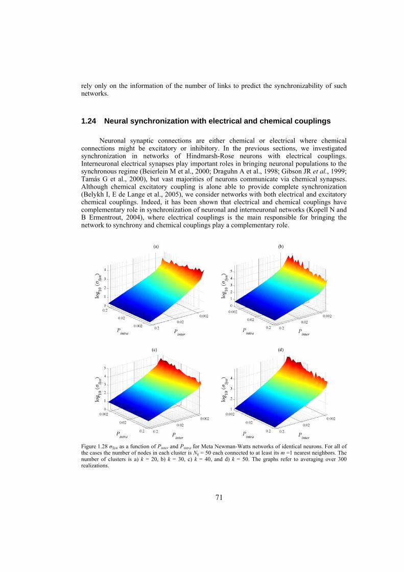
71

rely only on the information of the number of links to predict the synchronizability of such networks.

1.24 Neural synchronization with electrical and chemical couplings

Neuronal synaptic connections are either chemical or electrical where chemical connections might be excitatory or inhibitory. In the previous sections, we investigated synchronization in networks of Hindmarsh-Rose neurons with electrical couplings. Interneuronal electrical synapses play important roles in bringing neuronal populations to the synchronous regime (Beierlein M et al., 2000; Draguhn A et al., 1998; Gibson JR et al., 1999; Tamás G et al., 2000), but vast majorities of neurons communicate via chemical synapses. Although chemical excitatory coupling is alone able to provide complete synchronization (Belykh I, E de Lange et al., 2005), we consider networks with both electrical and excitatory chemical couplings. Indeed, it has been shown that electrical and chemical couplings have complementary role in synchronization of neuronal and interneuronal networks (Kopell N and B Ermentrout, 2004), where electrical couplings is the main responsible for bringing the network to synchrony and chemical couplings play a complementary role.

Figure 1.28 σSyn as a function of Pinter and Pintra for Meta Newman-Watts networks of identical neurons. For all of the cases the number of nodes in each cluster is Nk = 50 each connected to at least its m =1 nearest neighbors. The number of clusters is a) k = 20, b) k = 30, c) k = 40, and d) k = 50. The graphs refer to averaging over 300 realizations.

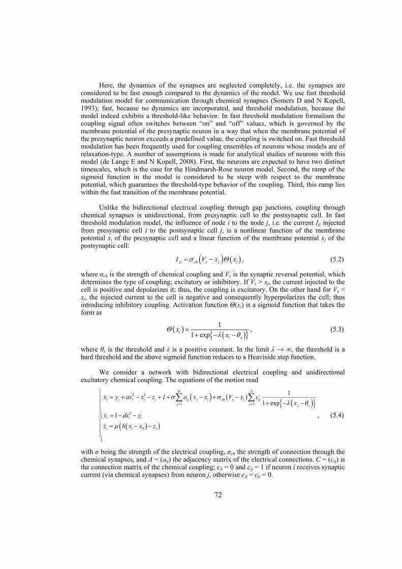
72

Here, the dynamics of the synapses are neglected completely, i.e. the synapses are considered to be fast enough compared to the dynamics of the model. We use fast threshold modulation model for communication through chemical synapses (Somers D and N Kopell, 1993); fast, because no dynamics are incorporated, and threshold modulation, because the model indeed exhibits a threshold-like behavior. In fast threshold modulation formalism the coupling signal often switches between “on” and “off” values, which is governed by the membrane potential of the presynaptic neuron in a way that when the membrane potential of the presynaptic neuron exceeds a predefined value, the coupling is switched on. Fast threshold modulation has been frequently used for coupling ensembles of neurons whose models are of relaxation-type. A number of assumptions is made for analytical studies of neurons with this model (de Lange E and N Kopell, 2008). First, the neurons are expected to have two distinct timescales, which is the case for the Hindmarsh-Rose neuron model. Second, the ramp of the sigmoid function in the model is considered to be steep with respect to the membrane potential, which guarantees the threshold-type behavior of the coupling. Third, this ramp lies within the fast transition of the membrane potential.

Unlike the bidirectional electrical coupling through gap junctions, coupling through chemical synapses is unidirectional, from presynaptic cell to the postsynaptic cell. In fast threshold modulation model, the influence of node i to the node j, i.e. the current Iji injected from presynaptic cell i to the postsynaptic cell j, is a nonlinear function of the membrane potential xi of the presynaptic cell and a linear function of the membrane potential xj of the postsynaptic cell:

( ) ( )ji ch s j iI V x xσ Θ= − , (5.2)

where σch is the strength of chemical coupling and Vs is the synaptic reversal potential, which determines the type of coupling; excitatory or inhibitory. If Vs > xj, the current injected to the cell is positive and depolarizes it; thus, the coupling is excitatory. On the other hand for Vs < xj, the injected current to the cell is negative and consequently hyperpolarizes the cell; thus introducing inhibitory coupling. Activation function Θ(xi) is a sigmoid function that takes the form as

( )( )

11 expi

i s

xx

Θλ θ

=+ − −

, (5.3)

where θs is the threshold and λ is a positive constant. In the limit λ → ∞, the threshold is a hard threshold and the above sigmoid function reduces to a Heaviside step function.

We consider a network with bidirectional electrical coupling and unidirectional excitatory chemical coupling. The equations of the motion read

( ) ( )( )

( )( )

2 3

1 1

2

0

11 exp

1

N N

i i i i i ij j i ch s i ijj j j s

i i i

i i i

x y ax x z I a x x V x cx

y dx y

z b x x z

σ σλ θ

μ

= =

⎧ = + − − + + − + −⎪ + − −⎪⎪

= − −⎨⎪ = − −⎪⎪⎩

∑ ∑&

&

&

, (5.4)

with σ being the strength of the electrical coupling, σch the strength of connection through the chemical synapses, and A = (aij) the adjacency matrix of the electrical connections. C = (cij) is the connection matrix of the chemical coupling; cii = 0 and cij = 1 if neuron i receives synaptic current (via chemical synapses) from neuron j, otherwise cij = cji = 0.

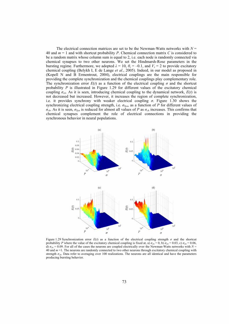
73

The electrical connection matrices are set to be the Newman-Watts networks with N = 40 and m = 1 and with shortcut probability P. Chemical connection matrix C is considered to be a random matrix whose column sum is equal to 2, i.e. each node is randomly connected via chemical synapses to two other neurons. We set the Hindmarsh-Rose parameters in the bursting regime. Furthermore, we adopted λ = 10, θs = –0.1, and Vs = 2 to provide excitatory chemical coupling (Belykh I, E de Lange et al., 2005). Indeed, in our model as proposed in (Kopell N and B Ermentrout, 2004), electrical couplings are the main responsible for providing the complete synchronization and the chemical couplings play complementary role. The synchronization error E(t) as a function of the electrical coupling σ and the shortcut probability P is illustrated in Figure 1.29 for different values of the excitatory chemical coupling σch. As it is seen, introducing chemical coupling to the dynamical network, E(t) is not decreased but increased. However, it increases the region of complete synchronization, i.e. it provides synchrony with weaker electrical coupling σ. Figure 1.30 shows the synchronizing electrical coupling strength, i.e. σSyn, as a function of P for different values of σch. As it is seen, σSyn is reduced for almost all values of P as σch increases. This confirms that chemical synapses complement the role of electrical connections in providing the synchronous behavior in neural populations.

Figure 1.29 Synchronization error E(t) as a function of the electrical coupling strength σ and the shortcut probability P where the value of the excitatory chemical coupling is fixed at, a) σch = 0, b) σch = 0.03, c) σch = 0.06, d) σch = 0.09. For all of the cases the neurons are coupled electrically over the Newman-Watts networks with N = 40 and m =1. The neurons are randomly connected to two other neurons through excitatory chemical coupling with strength σch. Data refer to averaging over 100 realizations. The neurons are all identical and have the parameters producing bursting behavior.

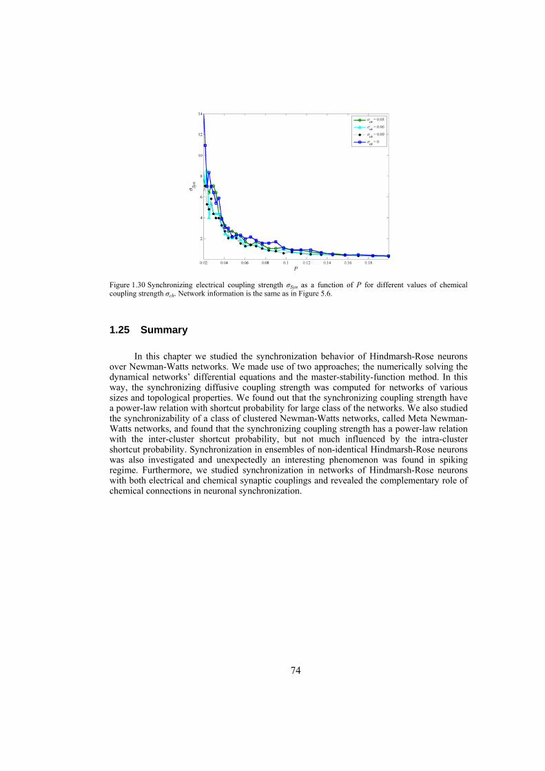
74

Figure 1.30 Synchronizing electrical coupling strength σSyn as a function of P for different values of chemical coupling strength σch. Network information is the same as in Figure 5.6.

1.25 Summary

In this chapter we studied the synchronization behavior of Hindmarsh-Rose neurons over Newman-Watts networks. We made use of two approaches; the numerically solving the dynamical networks’ differential equations and the master-stability-function method. In this way, the synchronizing diffusive coupling strength was computed for networks of various sizes and topological properties. We found out that the synchronizing coupling strength have a power-law relation with shortcut probability for large class of the networks. We also studied the synchronizability of a class of clustered Newman-Watts networks, called Meta Newman-Watts networks, and found that the synchronizing coupling strength has a power-law relation with the inter-cluster shortcut probability, but not much influenced by the intra-cluster shortcut probability. Synchronization in ensembles of non-identical Hindmarsh-Rose neurons was also investigated and unexpectedly an interesting phenomenon was found in spiking regime. Furthermore, we studied synchronization in networks of Hindmarsh-Rose neurons with both electrical and chemical synaptic couplings and revealed the complementary role of chemical connections in neuronal synchronization.

75

MODELING SYNCHRONIZATION IN LOCALLY EMERGING GAMMA OSCILLATIONS

Personal Contribution — Apart from a brief introduction to the gamma oscillations and its relation with binding phenomenon, the results presented in this chapter are our original contribution.

1.26 Gamma oscillations in neuronal systems

1.26.1 Binding by synchrony

Our cognitive systems have the capability to understand objects and events as related if they are continuous in space or time, although the brain receives the information in a discrete manner, or if they exhibit similarities in certain feature domains. Thus, shapes that touch one another with similar features, or move with the same rate in the same direction are more likely to be interpreted as components of the same object than spatially distant contours or contours that have no features in common. Here, the brain’s ability in information processing plays its role. It is a scientific fact that spatially distant cells synchronize their activity when activated by a single object (Milner PM, 1974; von der Malsburg C, 1999). It has been reported that binding, i.e. integration of separately processed information of one object in the brain to recognize the object as a whole, is through synchrony, or at least synchronous behavior is one of the consequences of information binding in the brain (Buzsaki G, 2006; Engel AK et al., 1999; Engel AK et al., 2001; Fell J et al., 2003; Gray CM et al., 1989; Singer W, 1993; Singer W, 1999; Singer W and CM Gray, 1995; Varela F et al., 2001; Ward LM, 2003). Although there is a debate among neuroscientists, the hypothesis of binding by temporal coherence, i.e. synchrony, is now the most accepted among others. The first experiment supporting this hypothesis was carried out by Singer and Gray reported in their pioneering work (Gray CM et al., 1989; Gray CM and W Singer, 1989). They recorded the multi-unit activity as well as the local field potentials from a single electrode placed in the V1 area of visual cortex of anesthetized and paralyzed cats. Using simple cross-correlation of the firing patterns of the recording signals, they discovered that a significant portion of the recorded signals display synchronous oscillations in 30-50 Hz, i.e. gamma frequency range. Their finding also provided exclusive evidence that these oscillatory events emerge locally. They reported that

76

neurons in the V1 area tend to synchronize their discharges with a precision in the millisecond range when activated with a single shape, whereas when activated by different shapes moving in different directions, they fail to do so (Gray CM et al., 1989; Gray CM and W Singer, 1989). Two aspects make their results interesting. First, it is a consequence of internal coordination of spike trains and not simply caused by stimulus-locked changes in discharge rate. Second, modifying the perceptual coherence of stimulus constellations may results in changing the synchronization in a systematic way. Thus, this type of synchrony is a result of context-dependent functional connectivity within the cortical network rather than being a trivial consequence of anatomical connectivity such as shared input through bifurcating axons (Singer W, 1999).

Fries et al. recorded neurons in the cortical area V4 of macaque monkeys while they attended to behaviorally relevant stimuli and observed that neurons activated by the attended stimulus showed increased gamma-frequency synchronization but reduced low-frequency synchronization (Fries P et al., 2001). Womelsdorf et al showed that behavioral response times to change of a stimulus can be predicted specifically by the degree of synchronization in the gamma-band among those neurons in the visual area V4 of monkey that are activated by the behaviorally relevant stimulus (Womelsdorf T et al., 2006). Furthermore, synchronization can be achieved very rapidly in neuronal ensembles. It has been shown that neurons in the visual area establish synchronous activity at the same speed they increase their firing rate in response to the light stimulus (Arieli A et al., 1996). These are just some examples of thousands of reports on the role of gamma-band synchronization in information binding in the brain, which indicate the importance of effort on modeling of this phenomenon. Indeed, the goal of synchrony for neuronal populations is the same as the goal of action potentials for single neurons: the role in forwarding messages to the downstream neurons in the most effective manner (Buzsaki G, 2006). The purpose of modeling studies is to use proper neuron models and realistic scenarios to mimic and/or predict the behavior of real systems.

1.26.2 Gamma-band oscillations in human cortex

Although many of the early works confirming the hypothesis “the binding by gamma oscillations” have been performed on the visual areas in the brain of animals, this hypothesis has a clear prediction for the human brain, as well. Every part of the cerebral cortex should be able to support gamma oscillations under proper conditions (Buzsaki G, 2006). In humans, gamma-band oscillations have been shown both in scalp recordings, through electroencephalography and magnetoencephalography (Csibra G et al., 2000; Kaiser J and W Lutzenberger, 2003; Llinás R and U Ribary, 1993; Miltner WHR et al., 1999), and in intracortical recording (Lachaux P et al., 2000). Also, the direct participation of synchrony in a binding problem (cognitive task) has been shown, where the long-distance gamma synchronization has been a consequence of (or as a cause of) visual perception (Keil A et al., 1999; Rodriguez E et al., 2001). Gamma oscillations have also been related to processing of auditory stimuli in the human brain (Pantev C et al., 1991). Dysfunctions of gamma synchronization is thought to play a role in various brain disorders (Uhlhaas PJ and W Singer, 2006). For example, the gamma synchronization pattern of neuronal systems is changed in patients suffering from schizophrenia (Jalili M, S Lavoie et al., 2007; Yeragani V et al., 2006). Electroencephalographic studies linked the abnormalities in gamma-range synchronization to disordered binding in autism (Grice SJ et al., 2001). Extratemporal and regional onset of seizures in neocortical epilepsy has been observed to be in gamma range (Lee S-A et al., 2000). Patients with Alzheimer’s disease show decreased level of neuronal synchronization in gamma-band frequencies (Koenig T et al., 2005).

Spike-timing-dependent-plasticity is one of the most important discoveries in neuroscience, which highlights the essential role of spike timing in changing network

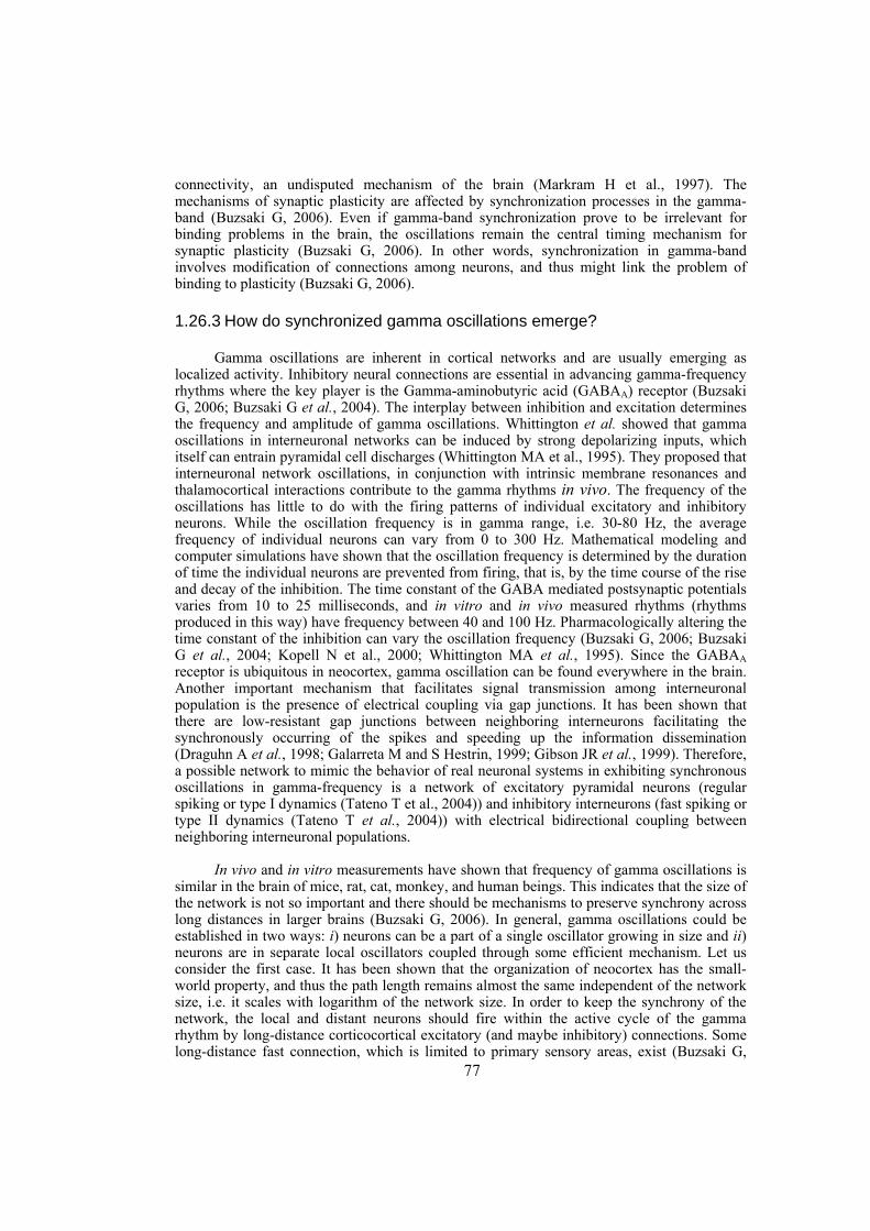
77

connectivity, an undisputed mechanism of the brain (Markram H et al., 1997). The mechanisms of synaptic plasticity are affected by synchronization processes in the gamma-band (Buzsaki G, 2006). Even if gamma-band synchronization prove to be irrelevant for binding problems in the brain, the oscillations remain the central timing mechanism for synaptic plasticity (Buzsaki G, 2006). In other words, synchronization in gamma-band involves modification of connections among neurons, and thus might link the problem of binding to plasticity (Buzsaki G, 2006).

1.26.3 How do synchronized gamma oscillations emerge?

Gamma oscillations are inherent in cortical networks and are usually emerging as localized activity. Inhibitory neural connections are essential in advancing gamma-frequency rhythms where the key player is the Gamma-aminobutyric acid (GABAA) receptor (Buzsaki G, 2006; Buzsaki G et al., 2004). The interplay between inhibition and excitation determines the frequency and amplitude of gamma oscillations. Whittington et al. showed that gamma oscillations in interneuronal networks can be induced by strong depolarizing inputs, which itself can entrain pyramidal cell discharges (Whittington MA et al., 1995). They proposed that interneuronal network oscillations, in conjunction with intrinsic membrane resonances and thalamocortical interactions contribute to the gamma rhythms in vivo. The frequency of the oscillations has little to do with the firing patterns of individual excitatory and inhibitory neurons. While the oscillation frequency is in gamma range, i.e. 30-80 Hz, the average frequency of individual neurons can vary from 0 to 300 Hz. Mathematical modeling and computer simulations have shown that the oscillation frequency is determined by the duration of time the individual neurons are prevented from firing, that is, by the time course of the rise and decay of the inhibition. The time constant of the GABA mediated postsynaptic potentials varies from 10 to 25 milliseconds, and in vitro and in vivo measured rhythms (rhythms produced in this way) have frequency between 40 and 100 Hz. Pharmacologically altering the time constant of the inhibition can vary the oscillation frequency (Buzsaki G, 2006; Buzsaki G et al., 2004; Kopell N et al., 2000; Whittington MA et al., 1995). Since the GABAA receptor is ubiquitous in neocortex, gamma oscillation can be found everywhere in the brain. Another important mechanism that facilitates signal transmission among interneuronal population is the presence of electrical coupling via gap junctions. It has been shown that there are low-resistant gap junctions between neighboring interneurons facilitating the synchronously occurring of the spikes and speeding up the information dissemination (Draguhn A et al., 1998; Galarreta M and S Hestrin, 1999; Gibson JR et al., 1999). Therefore, a possible network to mimic the behavior of real neuronal systems in exhibiting synchronous oscillations in gamma-frequency is a network of excitatory pyramidal neurons (regular spiking or type I dynamics (Tateno T et al., 2004)) and inhibitory interneurons (fast spiking or type II dynamics (Tateno T et al., 2004)) with electrical bidirectional coupling between neighboring interneuronal populations.

In vivo and in vitro measurements have shown that frequency of gamma oscillations is similar in the brain of mice, rat, cat, monkey, and human beings. This indicates that the size of the network is not so important and there should be mechanisms to preserve synchrony across long distances in larger brains (Buzsaki G, 2006). In general, gamma oscillations could be established in two ways: i) neurons can be a part of a single oscillator growing in size and ii) neurons are in separate local oscillators coupled through some efficient mechanism. Let us consider the first case. It has been shown that the organization of neocortex has the small-world property, and thus the path length remains almost the same independent of the network size, i.e. it scales with logarithm of the network size. In order to keep the synchrony of the network, the local and distant neurons should fire within the active cycle of the gamma rhythm by long-distance corticocortical excitatory (and maybe inhibitory) connections. Some long-distance fast connection, which is limited to primary sensory areas, exist (Buzsaki G,

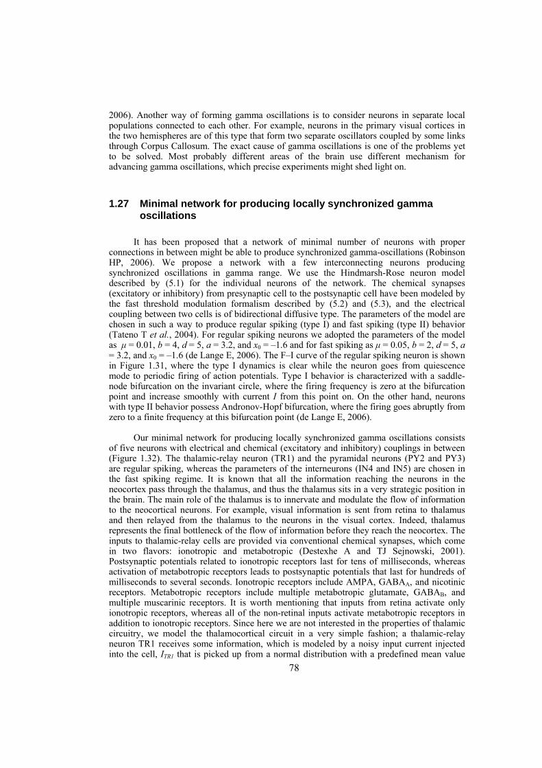
78

2006). Another way of forming gamma oscillations is to consider neurons in separate local populations connected to each other. For example, neurons in the primary visual cortices in the two hemispheres are of this type that form two separate oscillators coupled by some links through Corpus Callosum. The exact cause of gamma oscillations is one of the problems yet to be solved. Most probably different areas of the brain use different mechanism for advancing gamma oscillations, which precise experiments might shed light on.

1.27 Minimal network for producing locally synchronized gamma oscillations

It has been proposed that a network of minimal number of neurons with proper connections in between might be able to produce synchronized gamma-oscillations (Robinson HP, 2006). We propose a network with a few interconnecting neurons producing synchronized oscillations in gamma range. We use the Hindmarsh-Rose neuron model described by (5.1) for the individual neurons of the network. The chemical synapses (excitatory or inhibitory) from presynaptic cell to the postsynaptic cell have been modeled by the fast threshold modulation formalism described by (5.2) and (5.3), and the electrical coupling between two cells is of bidirectional diffusive type. The parameters of the model are chosen in such a way to produce regular spiking (type I) and fast spiking (type II) behavior (Tateno T et al., 2004). For regular spiking neurons we adopted the parameters of the model as μ = 0.01, b = 4, d = 5, a = 3.2, and x0 = –1.6 and for fast spiking as μ = 0.05, b = 2, d = 5, a = 3.2, and x0 = –1.6 (de Lange E, 2006). The F–I curve of the regular spiking neuron is shown in Figure 1.31, where the type I dynamics is clear while the neuron goes from quiescence mode to periodic firing of action potentials. Type I behavior is characterized with a saddle-node bifurcation on the invariant circle, where the firing frequency is zero at the bifurcation point and increase smoothly with current I from this point on. On the other hand, neurons with type II behavior possess Andronov-Hopf bifurcation, where the firing goes abruptly from zero to a finite frequency at this bifurcation point (de Lange E, 2006).

Our minimal network for producing locally synchronized gamma oscillations consists of five neurons with electrical and chemical (excitatory and inhibitory) couplings in between ( Figure 1.32). The thalamic-relay neuron (TR1) and the pyramidal neurons (PY2 and PY3) are regular spiking, whereas the parameters of the interneurons (IN4 and IN5) are chosen in the fast spiking regime. It is known that all the information reaching the neurons in the neocortex pass through the thalamus, and thus the thalamus sits in a very strategic position in the brain. The main role of the thalamus is to innervate and modulate the flow of information to the neocortical neurons. For example, visual information is sent from retina to thalamus and then relayed from the thalamus to the neurons in the visual cortex. Indeed, thalamus represents the final bottleneck of the flow of information before they reach the neocortex. The inputs to thalamic-relay cells are provided via conventional chemical synapses, which come in two flavors: ionotropic and metabotropic (Destexhe A and TJ Sejnowski, 2001). Postsynaptic potentials related to ionotropic receptors last for tens of milliseconds, whereas activation of metabotropic receptors leads to postsynaptic potentials that last for hundreds of milliseconds to several seconds. Ionotropic receptors include AMPA, GABAA, and nicotinic receptors. Metabotropic receptors include multiple metabotropic glutamate, GABAB, and multiple muscarinic receptors. It is worth mentioning that inputs from retina activate only ionotropic receptors, whereas all of the non-retinal inputs activate metabotropic receptors in addition to ionotropic receptors. Since here we are not interested in the properties of thalamic circuitry, we model the thalamocortical circuit in a very simple fashion; a thalamic-relay neuron TR1 receives some information, which is modeled by a noisy input current injected into the cell, ITR1 that is picked up from a normal distribution with a predefined mean value

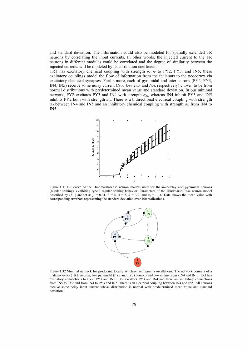
79

and standard deviation. The information could also be modeled for spatially extended TR neurons by correlating the input currents. In other words, the injected current to the TR neurons in different modules could be correlated and the degree of similarity between the injected currents will be modeled by its correlation coefficient. TR1 has excitatory chemical coupling with strength σex-TR to PY2, PY3, and IN5; these excitatory couplings model the flow of information from the thalamus to the neocortex via excitatory chemical synapses. Furthermore, each of pyramidal and interneurons (PY2, PY3, IN4, IN5) receive some noisy current (IPY2, IPY3, IIN4, and IIN5, respectively) chosen to be from normal distributions with predetermined mean value and standard deviation. In our minimal network, PY2 excitates PY3 and IN4 with strength σex, whereas IN4 inhibit PY3 and IN5 inhibits PY2 both with strength σin. There is a bidirectional electrical coupling with strength σel between IN4 and IN5 and an inhibitory chemical coupling with strength σin from IN4 to IN5.

Figure 1.31 F–I curve of the Hindmarsh-Rose neuron models used for thalamic-relay and pyramidal neurons (regular spiking), exhibiting type I regular spiking behavior. Parameters of the Hindmarsh-Rose neuron model described by (5.1) are set as μ = 0.01, b = 4, d = 5, a = 3.2, and x0 = –1.6. Data shows the mean value with corresponding errorbars representing the standard deviation over 100 realizations.

Figure 1.32 Minimal network for producing locally synchronized gamma oscillations. The network consists of a thalamic-relay (TR1) neuron, two pyramidal (PY2 and PY3) neurons and two interneurons (IN4 and IN5). TR1 has excitatory connections to PY2, PY3 and IN5. PY2 excitates PY3 and IN4 and there are inhibitory connections from IN5 to PY2 and from IN4 to PY3 and IN5. There is an electrical coupling between IN4 and IN5. All neurons receive some noisy input current whose distribution is normal with predetermined mean value and standard deviation.

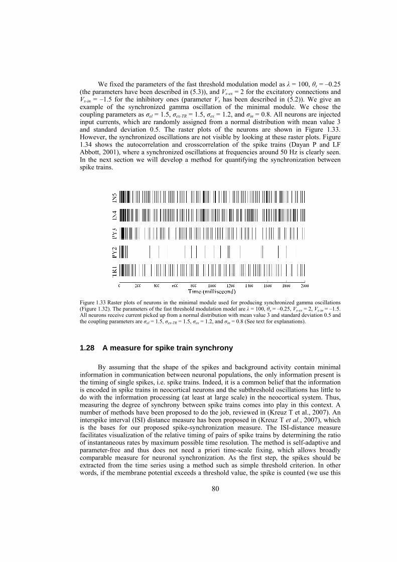
80

We fixed the parameters of the fast threshold modulation model as λ = 100, θs = –0.25 (the parameters have been described in (5.3)), and Vs-ex = 2 for the excitatory connections and Vs-in = –1.5 for the inhibitory ones (parameter Vs has been described in (5.2)). We give an example of the synchronized gamma oscillation of the minimal module. We chose the coupling parameters as σel = 1.5, σex-TR = 1.5, σex = 1.2, and σin = 0.8. All neurons are injected input currents, which are randomly assigned from a normal distribution with mean value 3 and standard deviation 0.5. The raster plots of the neurons are shown in Figure 1.33. However, the synchronized oscillations are not visible by looking at these raster plots. Figure 1.34 shows the autocorrelation and crosscorrelation of the spike trains (Dayan P and LF Abbott, 2001), where a synchronized oscillations at frequencies around 50 Hz is clearly seen. In the next section we will develop a method for quantifying the synchronization between spike trains.

Figure 1.33 Raster plots of neurons in the minimal module used for producing synchronized gamma oscillations ( Figure 1.32). The parameters of the fast threshold modulation model are λ = 100, θs = –0.25, Vs-ex = 2, Vs-in = –1.5. All neurons receive current picked up from a normal distribution with mean value 3 and standard deviation 0.5 and the coupling parameters are σel = 1.5, σex-TR = 1.5, σex = 1.2, and σin = 0.8 (See text for explanations).

1.28 A measure for spike train synchrony

By assuming that the shape of the spikes and background activity contain minimal information in communication between neuronal populations, the only information present is the timing of single spikes, i.e. spike trains. Indeed, it is a common belief that the information is encoded in spike trains in neocortical neurons and the subthreshold oscillations has little to do with the information processing (at least at large scale) in the neocortical system. Thus, measuring the degree of synchrony between spike trains comes into play in this context. A number of methods have been proposed to do the job, reviewed in (Kreuz T et al., 2007). An interspike interval (ISI) distance measure has been proposed in (Kreuz T et al., 2007), which is the bases for our proposed spike-synchronization measure. The ISI-distance measure facilitates visualization of the relative timing of pairs of spike trains by determining the ratio of instantaneous rates by maximum possible time resolution. The method is self-adaptive and parameter-free and thus does not need a priori time-scale fixing, which allows broadly comparable measure for neuronal synchronization. As the first step, the spikes should be extracted from the time series using a method such as simple threshold criterion. In other words, if the membrane potential exceeds a threshold value, the spike is counted (we use this

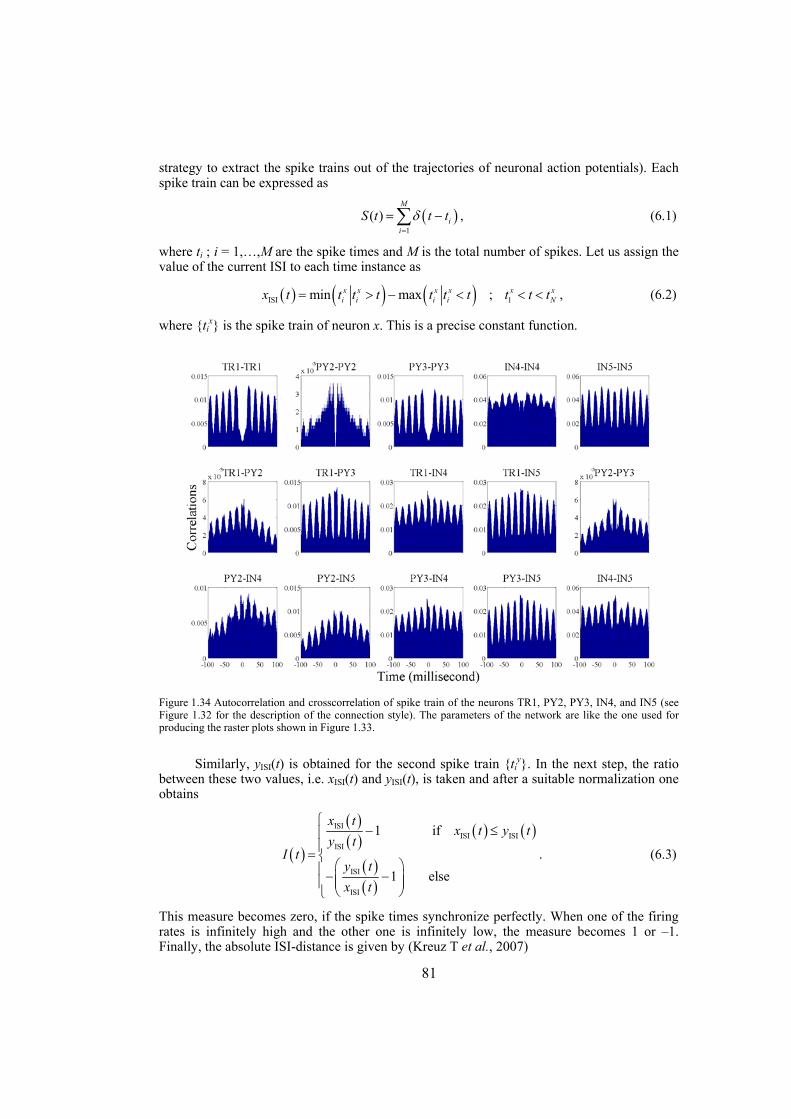
81

strategy to extract the spike trains out of the trajectories of neuronal action potentials). Each spike train can be expressed as

( )1

( )M

ii

S t t tδ=

= −∑ , (6.1)

where ti ; i = 1,…,M are the spike times and M is the total number of spikes. Let us assign the value of the current ISI to each time instance as

( ) ( ) ( )ISI 1min max ; x x x x x xi i i i Nx t t t t t t t t t t= > − < < < , (6.2)

where tix is the spike train of neuron x. This is a precise constant function.

Figure 1.34 Autocorrelation and crosscorrelation of spike train of the neurons TR1, PY2, PY3, IN4, and IN5 (see Figure 1.32 for the description of the connection style). The parameters of the network are like the one used for producing the raster plots shown in Figure 1.33.

Similarly, yISI(t) is obtained for the second spike train tiy. In the next step, the ratio

between these two values, i.e. xISI(t) and yISI(t), is taken and after a suitable normalization one obtains

( )

( )( ) ( ) ( )

( )( )

ISIISI ISI

ISI

ISI

ISI

1 if

1 else

x tx t y t

y tI t

y tx t

⎧− ≤⎪

⎪= ⎨⎛ ⎞⎪− −⎜ ⎟⎪ ⎜ ⎟⎝ ⎠⎩

. (6.3)

This measure becomes zero, if the spike times synchronize perfectly. When one of the firing rates is infinitely high and the other one is infinitely low, the measure becomes 1 or –1. Finally, the absolute ISI-distance is given by (Kreuz T et al., 2007)

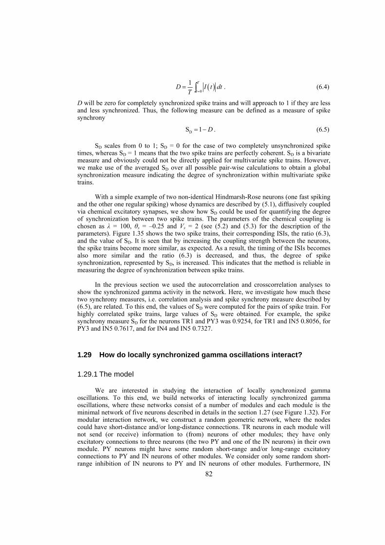
82

( )0

1 T

tD I t dt

T == ∫ . (6.4)

D will be zero for completely synchronized spike trains and will approach to 1 if they are less and less synchronized. Thus, the following measure can be defined as a measure of spike synchrony

DS 1 D= − . (6.5)

SD scales from 0 to 1; SD = 0 for the case of two completely unsynchronized spike times, whereas SD = 1 means that the two spike trains are perfectly coherent. SD is a bivariate measure and obviously could not be directly applied for multivariate spike trains. However, we make use of the averaged SD over all possible pair-wise calculations to obtain a global synchronization measure indicating the degree of synchronization within multivariate spike trains.

With a simple example of two non-identical Hindmarsh-Rose neurons (one fast spiking and the other one regular spiking) whose dynamics are described by (5.1), diffusively coupled via chemical excitatory synapses, we show how SD could be used for quantifying the degree of synchronization between two spike trains. The parameters of the chemical coupling is chosen as λ = 100, θs = –0.25 and Vs = 2 (see (5.2) and (5.3) for the description of the parameters). Figure 1.35 shows the two spike trains, their corresponding ISIs, the ratio (6.3), and the value of SD. It is seen that by increasing the coupling strength between the neurons, the spike trains become more similar, as expected. As a result, the timing of the ISIs becomes also more similar and the ratio (6.3) is decreased, and thus, the degree of spike synchronization, represented by SD, is increased. This indicates that the method is reliable in measuring the degree of synchronization between spike trains.

In the previous section we used the autocorrelation and crosscorrelation analyses to show the synchronized gamma activity in the network. Here, we investigate how much these two synchrony measures, i.e. correlation analysis and spike synchrony measure described by (6.5), are related. To this end, the values of SD were computed for the pairs of spike train. For highly correlated spike trains, large values of SD were obtained. For example, the spike synchrony measure SD for the neurons TR1 and PY3 was 0.9254, for TR1 and IN5 0.8056, for PY3 and IN5 0.7617, and for IN4 and IN5 0.7327.

1.29 How do locally synchronized gamma oscillations interact?

1.29.1 The model

We are interested in studying the interaction of locally synchronized gamma oscillations. To this end, we build networks of interacting locally synchronized gamma oscillations, where these networks consist of a number of modules and each module is the minimal network of five neurons described in details in the section 1.27 (see Figure 1.32). For modular interaction network, we construct a random geometric network, where the nodes could have short-distance and/or long-distance connections. TR neurons in each module will not send (or receive) information to (from) neurons of other modules; they have only excitatory connections to three neurons (the two PY and one of the IN neurons) in their own module. PY neurons might have some random short-range and/or long-range excitatory connections to PY and IN neurons of other modules. We consider only some random short-range inhibition of IN neurons to PY and IN neurons of other modules. Furthermore, IN

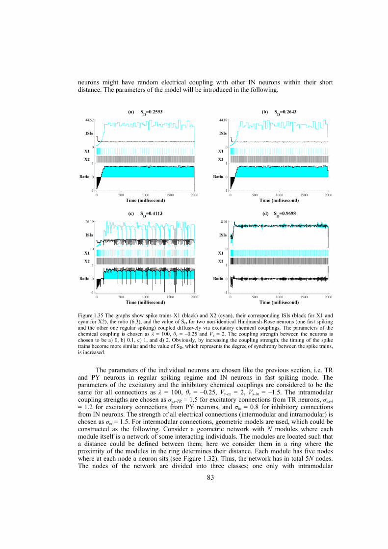
83

neurons might have random electrical coupling with other IN neurons within their short distance. The parameters of the model will be introduced in the following.

Figure 1.35 The graphs show spike trains X1 (black) and X2 (cyan), their corresponding ISIs (black for X1 and cyan for X2), the ratio (6.3), and the value of SD for two non-identical Hindmarsh-Rose neurons (one fast spiking and the other one regular spiking) coupled diffusively via excitatory chemical couplings. The parameters of the chemical coupling is chosen as λ = 100, θs = –0.25 and Vs = 2. The coupling strength between the neurons is chosen to be a) 0, b) 0.1, c) 1, and d) 2. Obviously, by increasing the coupling strength, the timing of the spike trains become more similar and the value of SD, which represents the degree of synchrony between the spike trains, is increased.

The parameters of the individual neurons are chosen like the previous section, i.e. TR and PY neurons in regular spiking regime and IN neurons in fast spiking mode. The parameters of the excitatory and the inhibitory chemical couplings are considered to be the same for all connections as λ = 100, θs = –0.25, Vs-ex = 2, Vs-in = –1.5. The intramodular coupling strengths are chosen as σex-TR = 1.5 for excitatory connections from TR neurons, σex-l = 1.2 for excitatory connections from PY neurons, and σin = 0.8 for inhibitory connections from IN neurons. The strength of all electrical connections (intermodular and intramodular) is chosen as σel = 1.5. For intermodular connections, geometric models are used, which could be constructed as the following. Consider a geometric network with N modules where each module itself is a network of some interacting individuals. The modules are located such that a distance could be defined between them; here we consider them in a ring where the proximity of the modules in the ring determines their distance. Each module has five nodes where at each node a neuron sits (see Figure 1.32). Thus, the network has in total 5N nodes. The nodes of the network are divided into three classes; one only with intramodular

84

connections, i.e. TR neurons leaving some predetermined connections to the nodes in their own modules. Another class of nodes (two IN neurons in each module) has only random short-distance connections. In addition of deterministic electrical coupling between IN neurons in the module, with probability Pel these neurons have electrical coupling with strength σel with the other IN neurons in their kel-nearest modules (modules within the distance equal or less than k of a module are considered to be its k-nearest neighboring modules). Furthermore, IN neurons inhibit PY and IN neurons in their kin-nearest modules with probability Pin and coupling strength σin-inter. PY neurons have short-distance and/or long-distance excitatory connections to other PY and IN neurons. These neurons excitate other PY and IN neurons located in their kex-nearest neighboring modules with probability Pex-short and coupling strength σex-short. They have excitatory connections to PY and IN neurons of modules other than those of in their kex-nearest neighborhood, where the probability of connection is Pex-long and the coupling strength is σex-long. In addition to these parameters, each neuron receives a current picked up from a normal distribution with mean value Imean,i, i = 1,…,5N and standard deviation Isd,i , i = 1,…,5N. The model has almost all possible connections observed in real neuronal networks, i.e. excitatory connections from thalamic-relay neurons to the pyramidal and interneurons, electrical coupling between adjacent interneurons, short-range inhibition of interneurons and short- and long- range excitatory links from pyramidal neurons to other neurons in the network.

1.29.2 Intermodular electrical and (excitatory/inhibitory) chemical couplings and the level of spike synchrony

In this section, we investigate the synchronization profile obtained between different neuronal species as a function of various parameters of the network. To do so, some parameters such as the probability of short-range electrical coupling between neighboring IN neurons, the probability and the strength of short-range inhibition of IN neurons, those of short- and long- range excitatory connections from PY neurons, are considered and the average values of synchronization index SD described by (6.5) are obtained. The spike-time synchronization value SPY,IN is obtained by averaging SD over all possible pairs of PY and IN neurons. Since TR neurons have only connections to the PY and IN neurons in their own module and their spike patterns are not influenced by the parameters of the network, they are not considered in the computation of SPY,IN (note that the only parameter controlling the spiking behavior of TR neurons is the input current injected to the cell).

By fixing the number of modules at N = 50 we performed some numerical simulations; the differential equations of the dynamical network is solved and then by thresholding the trajectories of the membrane potentials the spike trains are extracted and analyzed. The parameters of the TR and PY neurons (parameters of the Hindmarsh-Rose neuron model described in (5.1)) were chosen in the regular spiking regime (type I dynamics), i.e. μ = 0.01, b = 4, d = 5, a = 3.2, and x0 = –1.6, whereas μ = 0.05, b = 2, d = 5, a = 3.2, and x0 = –1.6 were chosen for IN neurons producing fast spiking (type II) dynamics. The parameters of the chemical synapses described by the fast threshold modulation model (see (5.2) and (5.3)) were chosen as λ = 100, θs = –0.25, Vs-ex = 2 (excitatory connections), and Vs-in = –1.5 (inhibitory connections). The strength of the intramodular connections were set in a way that locally synchronized oscillations in gamma frequency range appeared, i.e. σel = 1.5, σex-TR = 1.5, σex = 1.2, and σin = 0.8. Wherever necessary we chose the parameters for the intermodular connections as σel = 1.5, kel = kin = kex = 2, Pel = 0.2, Pin = Pex-short = Pex-long = 0.05, σin-inter = σex-

short = σex-long = 0.05. Furthermore, TR neurons receive input current whose distribution is normal with mean value 6 and standard deviation 0.5. All other neurons receive input currents picked up from a normal distribution with mean value Imean = 3 and four different values of standard deviation, Isd = 0.3, Isd = 0.6, Isd = 0.9, and Isd = 1.2. With this selection of the values

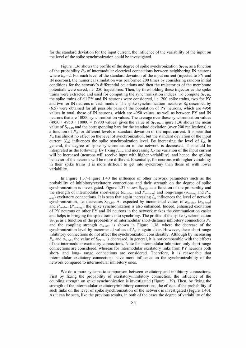
85

for the standard deviation for the input current, the influence of the variability of the input on the level of the spike synchronization could be investigated.

Figure 1.36 shows the profile of the degree of spike synchronization SPY,IN as a function of the probability Pel of intermodular electrical connections between neighboring IN neurons where kel =2. For each level of the standard deviation of the input current (injected to PY and IN neurons), the numerical simulation was performed 200 times by considering random initial conditions for the network’s differential equations and then the trajectories of the membrane potentials were saved, i.e. 250 trajectories. Then, by thresholding these trajectories the spike trains were extracted and used for computing the synchronization indices. To compute SPY,IN, the spike trains of all PY and IN neurons were considered, i.e. 200 spike trains, two for PY and two for IN neurons in each module. The spike synchronization measures SD described by (6.5) were obtained for all possible pairs of the population of PY neurons, which are 4950 values in total, those of IN neurons, which are 4950 values, as well as between PY and IN neurons that are 10000 synchronization values. The average over these synchronization values (4950 + 4950 + 10000 = 19900 values) gives the value of SPY,IN. Figure 1.36 shows the mean value of SPY,IN and the corresponding bars for the standard deviation (over 200 realizations) as a function of Pel for different levels of standard deviation of the input current. It is seen that Pel has almost no effect on the level of synchronization, but the standard deviation of the input current (Isd) influences the spike synchronization level. By increasing the level of Isd, in general, the degree of spike synchronization in the network is decreased. This could be interpreted as the following. By fixing Imean and increasing Isd the variation of the input current will be increased (neurons will receive input with higher variability), and hence, the spiking behavior of the neurons will be more different. Essentially, for neurons with higher variability in their spike trains it is more difficult to get into synchrony than those of with lower variability.

In Figure 1.37– Figure 1.40 the influence of other network parameters such as the probability of inhibitory/excitatory connections and their strength on the degree of spike synchronization is investigated. Figure 1.37 shows SPY,IN as a function of the probability and the strength of intermodular short-range (σex-short and Pex-short) and long-range (σex-long and Pex-

long) excitatory connections. It is seen that again increasing Isd influences the level of network synchronization, i.e. decreases SPY,IN. As expected by incremental values of σex-short (σex-long) and Pex-short (Pex-long), the spike synchronization is also enhanced. Indeed, enhanced excitation of PY neurons on other PY and IN neurons in the network makes the communication easier and helps in bringing the spike trains into synchrony. The profile of the spike synchronization SPY,IN as a function of the probability of intermodular short-distance inhibitory connections Pin and the coupling strength σin-inter is shown in Figure 1.38, where the decrease of the synchronization level by incremental values of Isd is again clear. However, these short-range inhibitory connections do not affect the synchronization considerably. Although by increasing Pin and σin-inter the value of SPY,IN is decreased, in general, it is not comparable with the effects of the intermodular excitatory connections. Note for intermodular inhibition only short-range connections are considered, whereas for intermodular excitatory links from PY neurons both short- and long- range connections are considered. Therefore, it is reasonable that intermodular excitatory connections have more influence on the synchronizability of the network compared to intermodular inhibitory ones.

We do a more systematic comparison between excitatory and inhibitory connections. First by fixing the probability of excitatory/inhibitory connection, the influence of the coupling strength on spike synchronization is investigated ( Figure 1.39). Then, by fixing the strength of the intermodular excitatory/inhibitory connections, the effects of the probability of such links on the level of spike synchronization of the network is investigated ( Figure 1.40). As it can be seen, like the previous results, in both of the cases the degree of variability of the

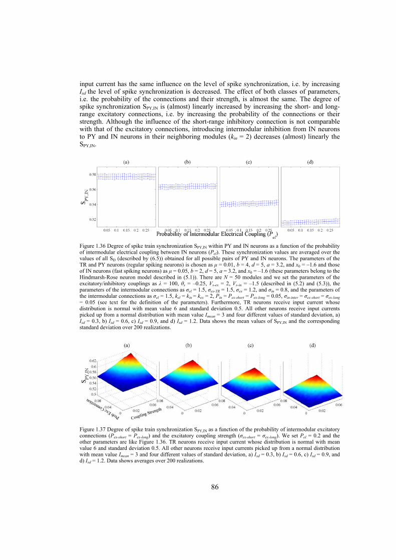
86

input current has the same influence on the level of spike synchronization, i.e. by increasing Isd the level of spike synchronization is decreased. The effect of both classes of parameters, i.e. the probability of the connections and their strength, is almost the same. The degree of spike synchronization SPY,IN is (almost) linearly increased by increasing the short- and long- range excitatory connections, i.e. by increasing the probability of the connections or their strength. Although the influence of the short-range inhibitory connection is not comparable with that of the excitatory connections, introducing intermodular inhibition from IN neurons to PY and IN neurons in their neighboring modules (kin = 2) decreases (almost) linearly the SPY,IN.

Figure 1.36 Degree of spike train synchronization SPY,IN within PY and IN neurons as a function of the probability of intermodular electrical coupling between IN neurons (Pel). These synchronization values are averaged over the values of all SD (described by (6.5)) obtained for all possible pairs of PY and IN neurons. The parameters of the TR and PY neurons (regular spiking neurons) is chosen as μ = 0.01, b = 4, d = 5, a = 3.2, and x0 = –1.6 and those of IN neurons (fast spiking neurons) as μ = 0.05, b = 2, d = 5, a = 3.2, and x0 = –1.6 (these parameters belong to the Hindmarsh-Rose neuron model described in (5.1)). There are N = 50 modules and we set the parameters of the excitatory/inhibitory couplings as λ = 100, θs = –0.25, Vs-ex = 2, Vs-in = –1.5 (described in (5.2) and (5.3)), the parameters of the intermodular connections as σel = 1.5, σex-TR = 1.5, σex = 1.2, and σin = 0.8, and the parameters of the intermodular connections as σel = 1.5, kel = kin = kex = 2, Pin = Pex-short = Pex-long = 0.05, σin-inter = σex-short = σex-long = 0.05 (see text for the definition of the parameters). Furthermore, TR neurons receive input current whose distribution is normal with mean value 6 and standard deviation 0.5. All other neurons receive input currents picked up from a normal distribution with mean value Imean = 3 and four different values of standard deviation, a) Isd = 0.3, b) Isd = 0.6, c) Isd = 0.9, and d) Isd = 1.2. Data shows the mean values of SPY,IN and the corresponding standard deviation over 200 realizations.

Figure 1.37 Degree of spike train synchronization SPY,IN as a function of the probability of intermodular excitatory connections (Pex-short = Pex-long) and the excitatory coupling strength (σex-short = σex-long). We set Pel = 0.2 and the other parameters are like Figure 1.36. TR neurons receive input current whose distribution is normal with mean value 6 and standard deviation 0.5. All other neurons receive input currents picked up from a normal distribution with mean value Imean = 3 and four different values of standard deviation, a) Isd = 0.3, b) Isd = 0.6, c) Isd = 0.9, and d) Isd = 1.2. Data shows averages over 200 realizations.

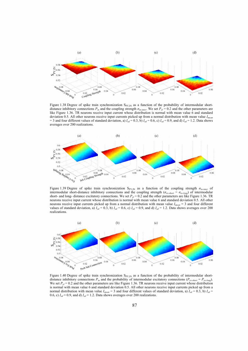
87

Figure 1.38 Degree of spike train synchronization SPY,IN as a function of the probability of intermodular short-distance inhibitory connections Pin and the coupling strength σin-inter. We set Pel = 0.2 and the other parameters are like Figure 1.36. TR neurons receive input current whose distribution is normal with mean value 6 and standard deviation 0.5. All other neurons receive input currents picked up from a normal distribution with mean value Imean = 3 and four different values of standard deviation, a) Isd = 0.3, b) Isd = 0.6, c) Isd = 0.9, and d) Isd = 1.2. Data shows averages over 200 realizations.

Figure 1.39 Degree of spike train synchronization SPY,IN as a function of the coupling strength σin-inter of intermodular short-distance inhibitory connections and the coupling strength (σex-short = σex-long) of intermodular short- and long- distance excitatory connections. We set Pel = 0.2 and the other parameters are like Figure 1.36. TR neurons receive input current whose distribution is normal with mean value 6 and standard deviation 0.5. All other neurons receive input currents picked up from a normal distribution with mean value Imean = 3 and four different values of standard deviation, a) Isd = 0.3, b) Isd = 0.6, c) Isd = 0.9, and d) Isd = 1.2. Data shows averages over 200 realizations.

Figure 1.40 Degree of spike train synchronization SPY,IN as a function of the probability of intermodular short-distance inhibitory connections Pin and the probability of intermodular excitatory connections (Pex-short = Pex-long). We set Pel = 0.2 and the other parameters are like Figure 1.36. TR neurons receive input current whose distribution is normal with mean value 6 and standard deviation 0.5. All other neurons receive input currents picked up from a normal distribution with mean value Imean = 3 and four different values of standard deviation, a) Isd = 0.3, b) Isd = 0.6, c) Isd = 0.9, and d) Isd = 1.2. Data shows averages over 200 realizations.

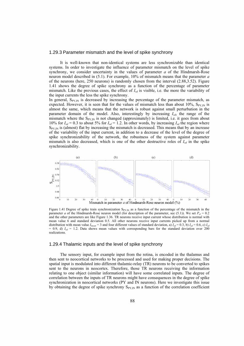
88

1.29.3 Parameter mismatch and the level of spike synchrony

It is well-known that non-identical systems are less synchronizable than identical systems. In order to investigate the influence of parameter mismatch on the level of spike synchrony, we consider uncertainty in the values of parameter a of the Hindmarsh-Rose neuron model described in (5.1). For example, 10% of mismatch means that the parameter a of the neurons (here, 250 neurons) is randomly chosen from the interval (2.88,3.52). Figure 1.41 shows the degree of spike synchrony as a function of the percentage of parameter mismatch. Like the previous cases, the effect of Isd is visible, i.e. the more the variability of the input currents the less the spike synchrony. In general, SPY,IN is decreased by increasing the percentage of the parameter mismatch, as expected. However, it is seen that for the values of mismatch less than about 10%, SPY,IN is almost the same, which means that the network is robust against small perturbation in the parameter domain of the model. Also, interestingly by increasing Isd, the range of the mismatch where the SPY,IN is not changed (approximately) is limited, i.e. it goes from about 10% for Isd = 0.3 to about 5% for Isd = 1.2. In other words, by increasing Isd the region where SPY,IN is (almost) flat by increasing the mismatch is decreased. This means that by an increase of the variability of the input current, in addition to a decrease of the level of the degree of spike synchronizability of the network, the robustness of the system against parameter mismatch is also decreased, which is one of the other destructive roles of Isd in the spike synchronizability.

Figure 1.41 Degree of spike train synchronization SPY,IN as a function of the percentage of the mismatch in the parameter a of the Hindmarsh-Rose neuron model (for description of the parameter, see (5.1)). We set Pel = 0.2 and the other parameters are like Figure 1.36. TR neurons receive input current whose distribution is normal with mean value 6 and standard deviation 0.5. All other neurons receive input currents picked up from a normal distribution with mean value Imean = 3 and four different values of standard deviation, a) Isd = 0.3, b) Isd = 0.6, c) Isd = 0.9, d) Isd = 1.2. Data shows mean values with corresponding bars for the standard deviation over 200 realizations.

1.29.4 Thalamic inputs and the level of spike synchrony

The sensory input, for example input from the retina, is encoded in the thalamus and then sent to neocortical networks to be processed and used for making proper decisions. The spatial input is modulated into different thalamic-relay (TR) neurons to be converted to spikes sent to the neurons in neocortex. Therefore, those TR neurons receiving the information relating to one object (similar information) will have some correlated inputs. The degree of correlation between the inputs of TR neurons might have consequences in the degree of spike synchronization in neocortical networks (PY and IN neurons). Here we investigate this issue by obtaining the degree of spike synchrony SPY,IN as a function of the correlation coefficient

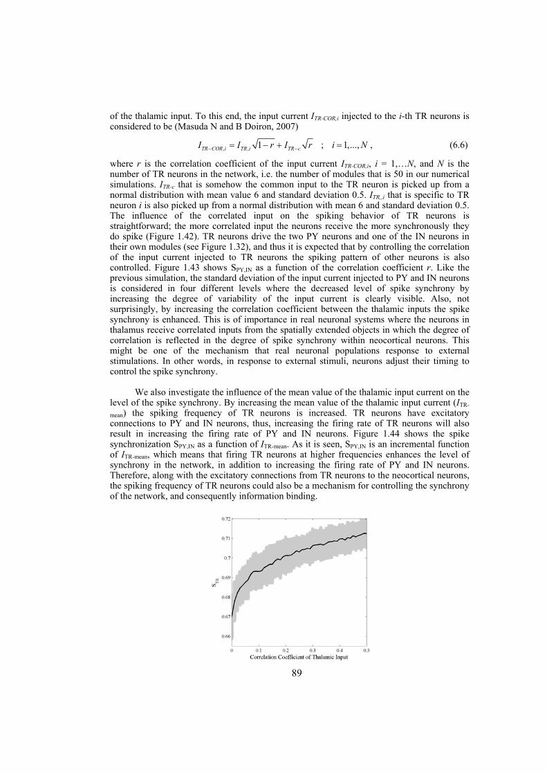
89

of the thalamic input. To this end, the input current ITR-COR,i injected to the i-th TR neurons is considered to be (Masuda N and B Doiron, 2007)

, , 1 ; 1,...,TR COR i TR i TR cI I r I r i N− −= − + = , (6.6)

where r is the correlation coefficient of the input current ITR-COR,i, i = 1,…N, and N is the number of TR neurons in the network, i.e. the number of modules that is 50 in our numerical simulations. ITR-c that is somehow the common input to the TR neuron is picked up from a normal distribution with mean value 6 and standard deviation 0.5. ITR,,i that is specific to TR neuron i is also picked up from a normal distribution with mean 6 and standard deviation 0.5. The influence of the correlated input on the spiking behavior of TR neurons is straightforward; the more correlated input the neurons receive the more synchronously they do spike ( Figure 1.42). TR neurons drive the two PY neurons and one of the IN neurons in their own modules (see Figure 1.32), and thus it is expected that by controlling the correlation of the input current injected to TR neurons the spiking pattern of other neurons is also controlled. Figure 1.43 shows SPY,IN as a function of the correlation coefficient r. Like the previous simulation, the standard deviation of the input current injected to PY and IN neurons is considered in four different levels where the decreased level of spike synchrony by increasing the degree of variability of the input current is clearly visible. Also, not surprisingly, by increasing the correlation coefficient between the thalamic inputs the spike synchrony is enhanced. This is of importance in real neuronal systems where the neurons in thalamus receive correlated inputs from the spatially extended objects in which the degree of correlation is reflected in the degree of spike synchrony within neocortical neurons. This might be one of the mechanism that real neuronal populations response to external stimulations. In other words, in response to external stimuli, neurons adjust their timing to control the spike synchrony.

We also investigate the influence of the mean value of the thalamic input current on the level of the spike synchrony. By increasing the mean value of the thalamic input current (ITR-

mean) the spiking frequency of TR neurons is increased. TR neurons have excitatory connections to PY and IN neurons, thus, increasing the firing rate of TR neurons will also result in increasing the firing rate of PY and IN neurons. Figure 1.44 shows the spike synchronization SPY,IN as a function of ITR-mean. As it is seen, SPY,IN is an incremental function of ITR-mean, which means that firing TR neurons at higher frequencies enhances the level of synchrony in the network, in addition to increasing the firing rate of PY and IN neurons. Therefore, along with the excitatory connections from TR neurons to the neocortical neurons, the spiking frequency of TR neurons could also be a mechanism for controlling the synchrony of the network, and consequently information binding.

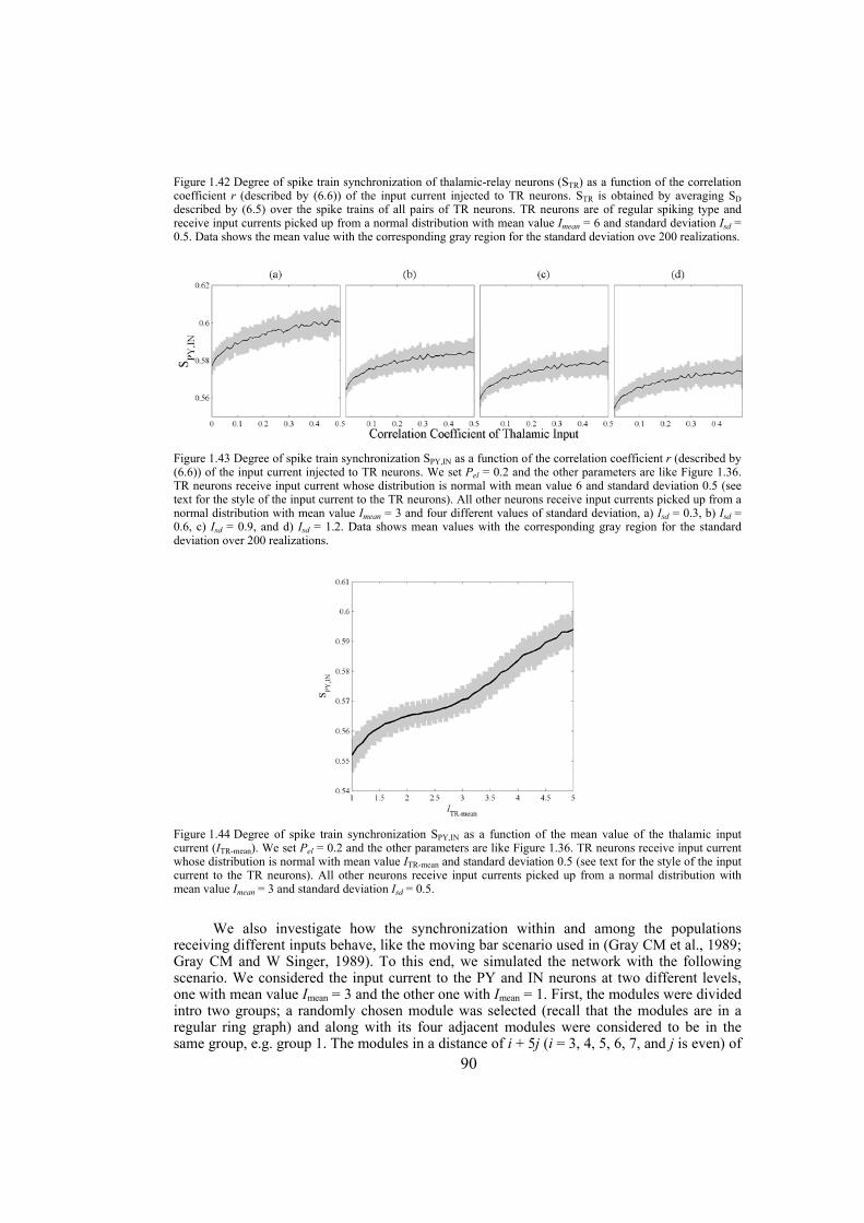
90

Figure 1.42 Degree of spike train synchronization of thalamic-relay neurons (STR) as a function of the correlation coefficient r (described by (6.6)) of the input current injected to TR neurons. STR is obtained by averaging SD described by (6.5) over the spike trains of all pairs of TR neurons. TR neurons are of regular spiking type and receive input currents picked up from a normal distribution with mean value Imean = 6 and standard deviation Isd = 0.5. Data shows the mean value with the corresponding gray region for the standard deviation ove 200 realizations.

Figure 1.43 Degree of spike train synchronization SPY,IN as a function of the correlation coefficient r (described by (6.6)) of the input current injected to TR neurons. We set Pel = 0.2 and the other parameters are like Figure 1.36. TR neurons receive input current whose distribution is normal with mean value 6 and standard deviation 0.5 (see text for the style of the input current to the TR neurons). All other neurons receive input currents picked up from a normal distribution with mean value Imean = 3 and four different values of standard deviation, a) Isd = 0.3, b) Isd = 0.6, c) Isd = 0.9, and d) Isd = 1.2. Data shows mean values with the corresponding gray region for the standard deviation over 200 realizations.

Figure 1.44 Degree of spike train synchronization SPY,IN as a function of the mean value of the thalamic input current (ITR-mean). We set Pel = 0.2 and the other parameters are like Figure 1.36. TR neurons receive input current whose distribution is normal with mean value ITR-mean and standard deviation 0.5 (see text for the style of the input current to the TR neurons). All other neurons receive input currents picked up from a normal distribution with mean value Imean = 3 and standard deviation Isd = 0.5.

We also investigate how the synchronization within and among the populations receiving different inputs behave, like the moving bar scenario used in (Gray CM et al., 1989; Gray CM and W Singer, 1989). To this end, we simulated the network with the following scenario. We considered the input current to the PY and IN neurons at two different levels, one with mean value Imean = 3 and the other one with Imean = 1. First, the modules were divided intro two groups; a randomly chosen module was selected (recall that the modules are in a regular ring graph) and along with its four adjacent modules were considered to be in the same group, e.g. group 1. The modules in a distance of i + 5j (i = 3, 4, 5, 6, 7, and j is even) of

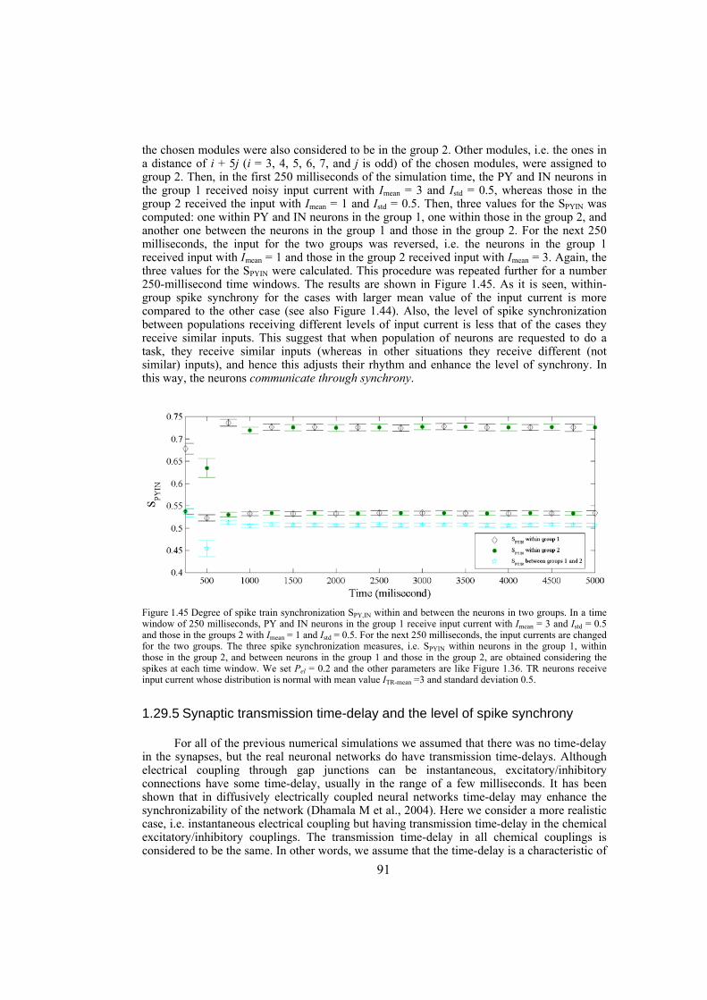
91

the chosen modules were also considered to be in the group 2. Other modules, i.e. the ones in a distance of i + 5j (i = 3, 4, 5, 6, 7, and j is odd) of the chosen modules, were assigned to group 2. Then, in the first 250 milliseconds of the simulation time, the PY and IN neurons in the group 1 received noisy input current with Imean = 3 and Istd = 0.5, whereas those in the group 2 received the input with Imean = 1 and Istd = 0.5. Then, three values for the SPYIN was computed: one within PY and IN neurons in the group 1, one within those in the group 2, and another one between the neurons in the group 1 and those in the group 2. For the next 250 milliseconds, the input for the two groups was reversed, i.e. the neurons in the group 1 received input with Imean = 1 and those in the group 2 received input with Imean = 3. Again, the three values for the SPYIN were calculated. This procedure was repeated further for a number 250-millisecond time windows. The results are shown in Figure 1.45. As it is seen, within-group spike synchrony for the cases with larger mean value of the input current is more compared to the other case (see also Figure 1.44). Also, the level of spike synchronization between populations receiving different levels of input current is less that of the cases they receive similar inputs. This suggest that when population of neurons are requested to do a task, they receive similar inputs (whereas in other situations they receive different (not similar) inputs), and hence this adjusts their rhythm and enhance the level of synchrony. In this way, the neurons communicate through synchrony.

Figure 1.45 Degree of spike train synchronization SPY,IN within and between the neurons in two groups. In a time window of 250 milliseconds, PY and IN neurons in the group 1 receive input current with Imean = 3 and Istd = 0.5 and those in the groups 2 with Imean = 1 and Istd = 0.5. For the next 250 milliseconds, the input currents are changed for the two groups. The three spike synchronization measures, i.e. SPYIN within neurons in the group 1, within those in the group 2, and between neurons in the group 1 and those in the group 2, are obtained considering the spikes at each time window. We set Pel = 0.2 and the other parameters are like Figure 1.36. TR neurons receive input current whose distribution is normal with mean value ITR-mean =3 and standard deviation 0.5.

1.29.5 Synaptic transmission time-delay and the level of spike synchrony

For all of the previous numerical simulations we assumed that there was no time-delay in the synapses, but the real neuronal networks do have transmission time-delays. Although electrical coupling through gap junctions can be instantaneous, excitatory/inhibitory connections have some time-delay, usually in the range of a few milliseconds. It has been shown that in diffusively electrically coupled neural networks time-delay may enhance the synchronizability of the network (Dhamala M et al., 2004). Here we consider a more realistic case, i.e. instantaneous electrical coupling but having transmission time-delay in the chemical excitatory/inhibitory couplings. The transmission time-delay in all chemical couplings is considered to be the same. In other words, we assume that the time-delay is a characteristic of

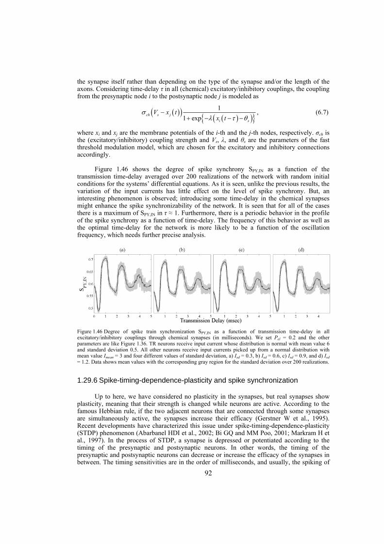
92

the synapse itself rather than depending on the type of the synapse and/or the length of the axons. Considering time-delay τ in all (chemical) excitatory/inhibitory couplings, the coupling from the presynaptic node i to the postsynaptic node j is modeled as

( )( )( )( )

11 expch s j

i s

V x tx t

σλ τ θ

−+ − − −

, (6.7)

where xi and xj are the membrane potentials of the i-th and the j-th nodes, respectively. σch is the (excitatory/inhibitory) coupling strength and Vs, λ, and θs are the parameters of the fast threshold modulation model, which are chosen for the excitatory and inhibitory connections accordingly.

Figure 1.46 shows the degree of spike synchrony SPY,IN as a function of the transmission time-delay averaged over 200 realizations of the network with random initial conditions for the systems’ differential equations. As it is seen, unlike the previous results, the variation of the input currents has little effect on the level of spike synchrony. But, an interesting phenomenon is observed; introducing some time-delay in the chemical synapses might enhance the spike synchronizability of the network. It is seen that for all of the cases there is a maximum of SPY,IN in τ ≈ 1. Furthermore, there is a periodic behavior in the profile of the spike synchrony as a function of time-delay. The frequency of this behavior as well as the optimal time-delay for the network is more likely to be a function of the oscillation frequency, which needs further precise analysis.

Figure 1.46 Degree of spike train synchronization SPY,IN as a function of transmission time-delay in all excitatory/inhibitory couplings through chemical synapses (in milliseconds). We set Pel = 0.2 and the other parameters are like Figure 1.36. TR neurons receive input current whose distribution is normal with mean value 6 and standard deviation 0.5. All other neurons receive input currents picked up from a normal distribution with mean value Imean = 3 and four different values of standard deviation, a) Isd = 0.3, b) Isd = 0.6, c) Isd = 0.9, and d) Isd = 1.2. Data shows mean values with the corresponding gray region for the standard deviation over 200 realizations.

1.29.6 Spike-timing-dependence-plasticity and spike synchronization

Up to here, we have considered no plasticity in the synapses, but real synapses show plasticity, meaning that their strength is changed while neurons are active. According to the famous Hebbian rule, if the two adjacent neurons that are connected through some synapses are simultaneously active, the synapses increase their efficacy (Gerstner W et al., 1995). Recent developments have characterized this issue under spike-timing-dependence-plasticity (STDP) phenomenon (Abarbanel HDI et al., 2002; Bi GQ and MM Poo, 2001; Markram H et al., 1997). In the process of STDP, a synapse is depressed or potentiated according to the timing of the presynaptic and postsynaptic neurons. In other words, the timing of the presynaptic and postsynaptic neurons can decrease or increase the efficacy of the synapses in between. The timing sensitivities are in the order of milliseconds, and usually, the spiking of

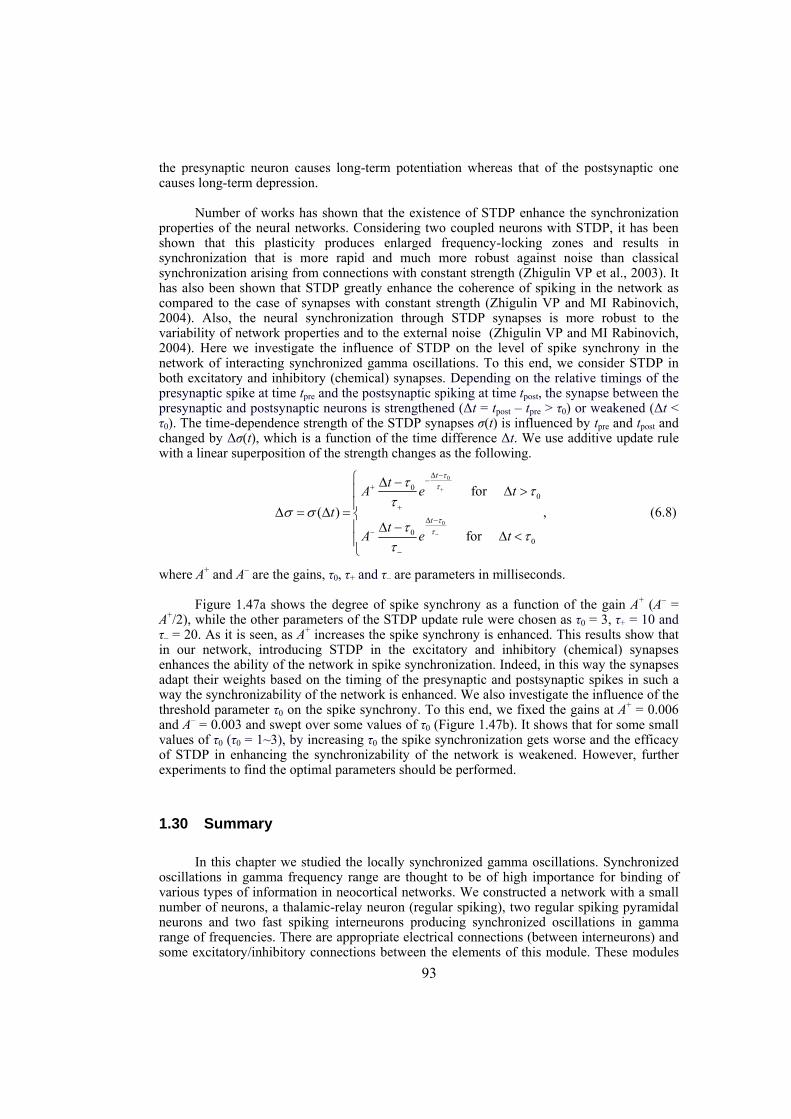
93

the presynaptic neuron causes long-term potentiation whereas that of the postsynaptic one causes long-term depression.

Number of works has shown that the existence of STDP enhance the synchronization properties of the neural networks. Considering two coupled neurons with STDP, it has been shown that this plasticity produces enlarged frequency-locking zones and results in synchronization that is more rapid and much more robust against noise than classical synchronization arising from connections with constant strength (Zhigulin VP et al., 2003). It has also been shown that STDP greatly enhance the coherence of spiking in the network as compared to the case of synapses with constant strength (Zhigulin VP and MI Rabinovich, 2004). Also, the neural synchronization through STDP synapses is more robust to the variability of network properties and to the external noise (Zhigulin VP and MI Rabinovich, 2004). Here we investigate the influence of STDP on the level of spike synchrony in the network of interacting synchronized gamma oscillations. To this end, we consider STDP in both excitatory and inhibitory (chemical) synapses. Depending on the relative timings of the presynaptic spike at time tpre and the postsynaptic spiking at time tpost, the synapse between the presynaptic and postsynaptic neurons is strengthened (Δt = tpost – tpre > τ0) or weakened (Δt < τ0). The time-dependence strength of the STDP synapses σ(t) is influenced by tpre and tpost and changed by Δσ(t), which is a function of the time difference Δt. We use additive update rule with a linear superposition of the strength changes as the following.

0

0

00

00

for ( ) ,

for

t

t

tA e tt

tA e t

ττ

ττ

ττ

τσ σ

ττ

τ

+

−

Δ −−

+

+

Δ −−

−

⎧ Δ −Δ >⎪

⎪Δ = Δ = ⎨Δ −⎪ Δ <⎪

⎩

(6.8)

where A+ and A– are the gains, τ0, τ+ and τ– are parameters in milliseconds.

Figure 1.47a shows the degree of spike synchrony as a function of the gain A+ (A– = A+/2), while the other parameters of the STDP update rule were chosen as τ0 = 3, τ+ = 10 and τ– = 20. As it is seen, as A+ increases the spike synchrony is enhanced. This results show that in our network, introducing STDP in the excitatory and inhibitory (chemical) synapses enhances the ability of the network in spike synchronization. Indeed, in this way the synapses adapt their weights based on the timing of the presynaptic and postsynaptic spikes in such a way the synchronizability of the network is enhanced. We also investigate the influence of the threshold parameter τ0 on the spike synchrony. To this end, we fixed the gains at A+ = 0.006 and A– = 0.003 and swept over some values of τ0 ( Figure 1.47b). It shows that for some small values of τ0 (τ0 = 1~3), by increasing τ0 the spike synchronization gets worse and the efficacy of STDP in enhancing the synchronizability of the network is weakened. However, further experiments to find the optimal parameters should be performed.

1.30 Summary

In this chapter we studied the locally synchronized gamma oscillations. Synchronized oscillations in gamma frequency range are thought to be of high importance for binding of various types of information in neocortical networks. We constructed a network with a small number of neurons, a thalamic-relay neuron (regular spiking), two regular spiking pyramidal neurons and two fast spiking interneurons producing synchronized oscillations in gamma range of frequencies. There are appropriate electrical connections (between interneurons) and some excitatory/inhibitory connections between the elements of this module. These modules

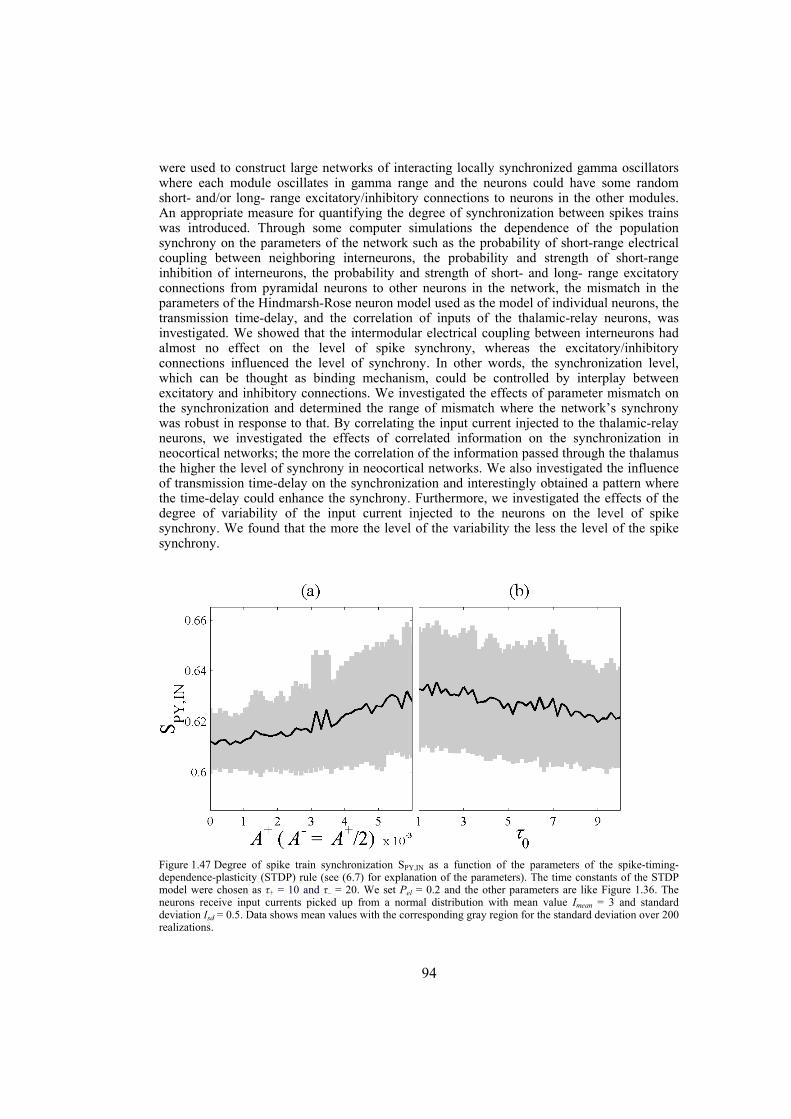
94

were used to construct large networks of interacting locally synchronized gamma oscillators where each module oscillates in gamma range and the neurons could have some random short- and/or long- range excitatory/inhibitory connections to neurons in the other modules. An appropriate measure for quantifying the degree of synchronization between spikes trains was introduced. Through some computer simulations the dependence of the population synchrony on the parameters of the network such as the probability of short-range electrical coupling between neighboring interneurons, the probability and strength of short-range inhibition of interneurons, the probability and strength of short- and long- range excitatory connections from pyramidal neurons to other neurons in the network, the mismatch in the parameters of the Hindmarsh-Rose neuron model used as the model of individual neurons, the transmission time-delay, and the correlation of inputs of the thalamic-relay neurons, was investigated. We showed that the intermodular electrical coupling between interneurons had almost no effect on the level of spike synchrony, whereas the excitatory/inhibitory connections influenced the level of synchrony. In other words, the synchronization level, which can be thought as binding mechanism, could be controlled by interplay between excitatory and inhibitory connections. We investigated the effects of parameter mismatch on the synchronization and determined the range of mismatch where the network’s synchrony was robust in response to that. By correlating the input current injected to the thalamic-relay neurons, we investigated the effects of correlated information on the synchronization in neocortical networks; the more the correlation of the information passed through the thalamus the higher the level of synchrony in neocortical networks. We also investigated the influence of transmission time-delay on the synchronization and interestingly obtained a pattern where the time-delay could enhance the synchrony. Furthermore, we investigated the effects of the degree of variability of the input current injected to the neurons on the level of spike synchrony. We found that the more the level of the variability the less the level of the spike synchrony.

Figure 1.47 Degree of spike train synchronization SPY,IN as a function of the parameters of the spike-timing-dependence-plasticity (STDP) rule (see (6.7) for explanation of the parameters). The time constants of the STDP model were chosen as τ+ = 10 and τ– = 20. We set Pel = 0.2 and the other parameters are like Figure 1.36. The neurons receive input currents picked up from a normal distribution with mean value Imean = 3 and standard deviation Isd = 0.5. Data shows mean values with the corresponding gray region for the standard deviation over 200 realizations.

95

SECTION III

97

ALPHA RHYTHM AND HYPOFRONTALITY IN SCHIZOPHRENIA

Personal Contribution — The chapter starts with a brief introduction to schizophrenia, followed by our original results published in Acta Psychiatry Scandinavica (Knyazeva MG, M Jalili, R Meuli et al., 2008), where I am the joint first-author with Maria G. Knyazeva. The neuropsychological and psychopathological assessments have been carried out in schizophrenia units of the Psychiatry Department, Lausanne University Hospital (Suzie Lavoie, Patricia Deppen, Kim Q. Do and Michel Cuénod). EEG data have been collected by Maria G. Knyazeva and I’ve done the data analysis.

1.31 Schizophrenia as a brain disorder

Schizophrenia is perhaps the most overwhelming brain disorder in humankind, which is mostly manifesting as auditory hallucinations, paranoid or bizarre delusions or disorganized speech and thinking in the context of significant social or occupational dysfunction. The term “schizophrenia” is originally a Greek word meaning “split mind”. About 1% of the population worldwide suffer from different levels of schizophrenia where men are slightly affected more than women (Kandel ER, 2000). Additionally, another 3% of the population has schizophrenia-type personality disorders. Schizophrenia is the fourth leading cause of disability in the developed counties for people at the age of 15-44. It is a devastating illness resulting in significant costs. The overall cost of schizophrenia in the US was estimated to be $62.7 billion in 2002, with $22.7 billion excess direct health care cost (Wu EQ et al., 2005). The indirect excess cost due to unemployment is the largest component of overall schizophrenia excess annual costs. It is generally estimated that today only approximately 10-15% of schizophrenic people are able to maintain full-time employment of any type (Wu EQ et al., 2005). Schizophrenia usually starts between the late teens and the mid 30s, and is rarely

98

observed prior to adolescence or later in life. It usually happens a few years earlier in men than in women. It often starts gradually manifested by negative symptoms such as social withdrawal, outbursts of anger, and loss of interest in school or work. Negative symptoms tend to predominate in men, whereas depressive episodes, paranoid delusions, and hallucinations tend to predominate in women. The disease usually persists for a life-time. Some patients appear to experience a relatively stable course, whereas others show a progressive worsening associated with severe disorder.

It has been suspected for over many years that schizophrenia and bipolar disorder are disorders of brain. In 1837, Dr. Browne, one of the best-known psychiatrists of his period generation, wrote: “Insanity, then, is inordinate or irregular, or impaired action of the mind, of the instincts, sentiments, intellectual, or perceptive powers, depending upon and produced by an organic change in the brain.” In that same year, Dr. Brigham, one of the founders of American psychiatry, also wrote: “Insanity is now considered a physical disorder, a disease of the brain.” Since the early 1980s, with the availability of sophisticated various brain imaging techniques and other developments in neuroscience, the evidence has become overwhelming that schizophrenia is a disorder of the brain. The causes of schizophrenia are not exactly known. Additional research done during the past two decades has shown that schizophrenia is caused by a combination of genetic or biological predisposition as well as other factors such as prepregnancy factors, pregnancy stress, other prenatal factors, social stress, family stress or environmental stressors during a person's life. Genetic factors are important in the course of the disease and the risk of illness in an identical twin of a person with schizophrenia is 40-50%. A child of a parent suffering from schizophrenia has a 10% chance of developing the illness. The disease is primarily thought to affect cognition, but it also usually contributes to chronic problems with behavior and emotion. Social problems, such as long-term unemployment, poverty and homelessness are common and life expectancy is decreased in such patients; the average life expectancy of people with the disorder is 10 to 12 years less than those without, owing to increased physical health problems and a high suicide rate (Brown S et al., 2000). It is important for doctors to investigate all reasonable medical causes for any acute change in someone’s mental health or behavior. Sometimes a medical condition that might be treated easily, if diagnosed, is responsible for symptoms that resemble those of schizophrenia.

1.31.1 Signs and symptoms of schizophrenia

A schizophrenic person may exhibit different type of symptoms such as delusions, auditory hallucinations and disorganized thought. In more severs states of the disease, the person might be largely mute, remain motionless in bizarre postures, or exhibit purposeless agitation. The first signs of schizophrenia often appear as confusing, or even shocking changes in behavior. Coping with the symptoms of schizophrenia can be especially difficult for family members who remember how involved or vivacious a person was before they became ill. The sudden onset of severe psychotic symptoms is referred to as an “acute” phase of schizophrenia. “Psychosis,” a common condition in schizophrenia, is a state of mental impairment marked by hallucinations, which are disturbances of sensory perception, and/or delusions, which are false yet strongly held personal beliefs that result from an inability to separate real from unreal experiences. Less obvious symptoms, such as social isolation or withdrawal, or unusual speech, thinking, or behavior, may precede, be seen along with, or follow the psychotic symptoms. Some people have only one such psychotic episode; others have many episodes during a lifetime, but lead relatively normal lives during the interim periods. However, the individual with “chronic” schizophrenia, or a continuous or recurring pattern of illness, often does not fully recover normal functioning and typically requires long-term treatment, generally including medication, to control the symptoms. The frequently used symptom scales for schizophrenia is Positive and Negative Syndrome Scale (PANSS) (Kay S

99

et al., 1987) that indeed quantify the severity of the disease. Positive symptoms include hearing voices, suspiciousness, feeling under constant surveillance, delusions, or making up words without a meaning (neologisms). Patients with negative (or deficit) symptoms have some experiences such as social withdrawal, difficulty in expressing emotions (in extreme cases called blunted affect), difficulty in taking care of themselves, inability to feel pleasure, difficulties in processing of information, in understanding the environment, and in remembering simple tasks.

1.32 Hypofrontality in Schizophrenia

In 1974 Ingvar and Franzen described the abnormal distribution of regional cerebral blood flow in schizophrenia patients (Ingvar DH and G Franzen, 1974). It was characterized by low frontal values and thus by a reduction of the normal anterior-to-posterior gradient. Under the name of “hypofrontality” this phenomenon turned out to be one of the most intriguing findings in the neurobiology of schizophrenia. Much of what we know about hypofrontality in schizophrenia comes from imaging studies, which measured cortical metabolism or activation with Positron Emission Tomography (PET) or functional Magnetic Resonance Imaging (fMRI) methods (Andreasen NC et al., 1992; Semkovska M et al., 2001; Velakoulis D and C Pantelis, 1996). Despite a number of studies that failed to replicate the phenomenon (for discussion see (Gur RC and RE Gur, 1995; Weinberger D and K Berman, 1988; Williamson P, 1987)), meta-analyses of more than a hundred reports published between 1974 and 2004 confirmed the reality of resting and task-related hypofrontality in schizophrenia (Glahn DC et al., 2005; Hill K et al., 2004). More recent neuroimaging studies also provide evidence supporting abnormally low anterior-to-posterior gradients in schizophrenia (Hoshi Y et al., 2006; Molina V et al., 2005; Molina V et al., 2007; Pae CU et al., 2004; Snitz BE et al., 2005).

Based on these observations of absolutely or relatively decreased (pre)frontal activation in schizophrenia, one might expect associated changes in Electroencephalography (EEG) and, in particular, in alpha activity. Indeed, in normal adults, EEG/fMRI and EEG/PET co-registration studies consistently demonstrate an inverse relationship between the subjects’ alpha power in population analysis (or its temporal fluctuations in individual analysis) and regional cortical activation or metabolism (for review see (Salek-Haddadi A et al., 2003)). Such a link was shown for occipital (de Munck JC et al., 2007; Feige B et al., 2005; Goldman RI et al., 2002; Goncalves SI et al., 2006; Moosmann M et al., 2003; Sadato N et al., 1998), parietal (de Munck JC et al., 2007; Goncalves SI et al., 2006; Laufs H et al., 2003), and sensorimotor (Oishi N et al., 2007) cortices. Therefore, in the eyes-closed resting state (a paradigm used in the majority of combined EEG/FMRI studies), alpha activity is related to regional deactivation and reduced metabolism. Considering these relationships, it seems reasonable to expect that the decreased prefrontal metabolism in schizophrenia should be linked to increased power in the alpha frequency range over anterior brain regions. However, the existing EEG literature suggests that, if any difference exists, it consists instead in a decreased power in the schizophrenia patients compared to controls (Alper K, 1995). Indeed, a diffuse decrease in alpha power was frequently reported in schizophrenia patients either compared to controls (Alper K, 1995; Begić D et al., 2000; Fenton GW et al., 1980; Mientus S et al., 2002; Shagass C et al., 1982; Sponheim SR et al., 1994), or related to negative symptoms (Merrin E and T Floyd, 1996; Sponheim SR et al., 2000), or else to schizophrenia type (Miyauchi T et al., 1996). However, increased alpha power was occasionally observed (Gattaz WF et al., 1992; Kahn EM et al., 1993; Miyauchi T et al., 1996), and some studies failed to demonstrate differences in alpha power between schizophrenia patients and controls (Karson CN et al., 1987; Knott V, A Labelle et al., 2001; Winterer G et al., 2001).

100

Among the issues that fuel this controversy, the complex nature of alpha rhythm is an important one. On one hand, experimental and modeling studies show that the most probable sources of alpha oscillations, recorded with non-invasive surface EEG techniques, are dipole layers distributed predominantly in extensive gyral crowns (Nunez P and R Srinivasan, 2006; Nunez P et al., 2001). On the other hand, according to the electrophysiological experiments in animals (Hughes SW and V Crunelli, 2005; Lopes da Silva FH et al., 1980) and neuroimaging studies in humans (de Munck JC et al., 2007; Feige B et al., 2005; Goldman RI et al., 2002; Goncalves SI et al., 2006; Sadato N et al., 1998), cortically generated alpha activity is modulated by the thalamus. These two main contributors to alpha activity provide various effects at local, regional, and global scales (Goldman RI et al., 2002; Nunez P and R Srinivasan, 2006; Ohmoto T et al., 1978; Schreckenberger M et al., 2004). Hence, considering presumed cortical and thalamic abnormalities in schizophrenia (reviewed in (Andreasen NC, 1997; de Haan L and JM Bakker, 2004; Lewis D and P Levitt, 2002; Wong AH and HH Van, 2003)), the alpha rhythm changes associated with this disease are likely to have a multifactorial nature and a distributed pattern, whose analysis calls for whole-head EEG mapping. However, by and large, previous studies reported findings obtained with conventional EEG techniques, sometimes limited to 3-4 electrodes located over an a priori defined region of interest. While being justified for screening large populations of schizophrenia patients, such an approach has a very limited capacity for understanding the pathophysiology of the disease.

In this chapter we revisit the relationship between hypofrontality in schizophrenia and the EEG alpha rhythm. We hypothesize that the phenomenon of hypofrontality is bound to be reflected in an increase of the alpha rhythm power over the prefrontal brain regions, though this regional effect can be masked by global power changes. To reveal both global and regional changes related to schizophrenia, we follow a topographical approach based on multichannel EEG. In particular, we apply EEG power measures that are tuned for regional surface mapping in combination with power measures that allow evaluation of global effects. The analysis indeed confirms our hypothesis by revealing both global (power decrease) and regional (relative power increase over the anterior cortex) phenomena specific to the alpha band in schizophrenia patients. Finally, with a correlation analysis, we show how the abnormal EEG power topography is linked to the clinical picture of schizophrenia.

The aim of this study is to reveal the EEG correlates of resting hypofrontality and, in particular, to revisit its relationship with the alpha rhythm by using a new parameterization of the multichannel EEG capable of distinguishing between regional and global changes related to schizophrenia.

1.33 Subjects and EEG recording

1.33.1 Subjects

Fourteen patients with mean age of 32.8 ± 9.8 with schizophrenia or schizoaffective disorder were recruited from the in/outpatient schizophrenia units of the Psychiatry Department, Lausanne University Hospital. The group included 11 men and 1 lefthander. All diagnoses were made according to DSM-IV criteria on the basis of the Diagnostic Interview for Genetic Studies (DIGS) (Nurnberger JJ et al., 1994), or by a consensus of two experienced psychiatrists after a systematic review of medical records. The illness duration was 10.4 ± 7.2 years. Patients with a history of neurological illness or head trauma, with mental retardation (IQ below 60), or with a diagnosis of drug/alcohol dependence or abuse were excluded. Twelve of them were receiving antipsychotic medication (11 atypical, 1 typical), one was

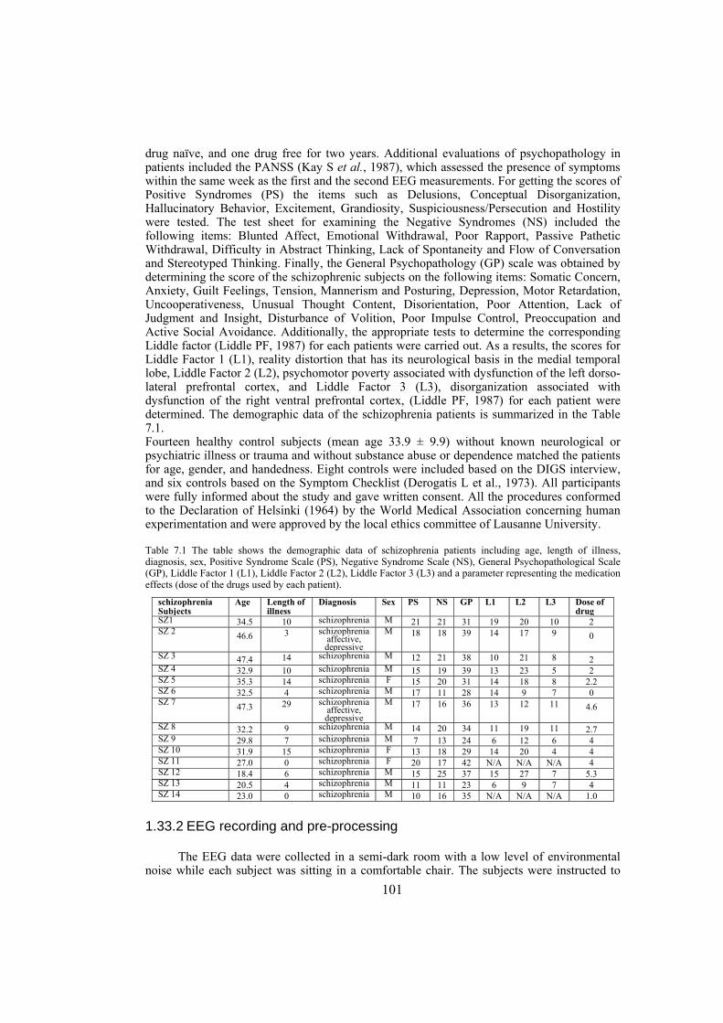
101

drug naïve, and one drug free for two years. Additional evaluations of psychopathology in patients included the PANSS (Kay S et al., 1987), which assessed the presence of symptoms within the same week as the first and the second EEG measurements. For getting the scores of Positive Syndromes (PS) the items such as Delusions, Conceptual Disorganization, Hallucinatory Behavior, Excitement, Grandiosity, Suspiciousness/Persecution and Hostility were tested. The test sheet for examining the Negative Syndromes (NS) included the following items: Blunted Affect, Emotional Withdrawal, Poor Rapport, Passive Pathetic Withdrawal, Difficulty in Abstract Thinking, Lack of Spontaneity and Flow of Conversation and Stereotyped Thinking. Finally, the General Psychopathology (GP) scale was obtained by determining the score of the schizophrenic subjects on the following items: Somatic Concern, Anxiety, Guilt Feelings, Tension, Mannerism and Posturing, Depression, Motor Retardation, Uncooperativeness, Unusual Thought Content, Disorientation, Poor Attention, Lack of Judgment and Insight, Disturbance of Volition, Poor Impulse Control, Preoccupation and Active Social Avoidance. Additionally, the appropriate tests to determine the corresponding Liddle factor (Liddle PF, 1987) for each patients were carried out. As a results, the scores for Liddle Factor 1 (L1), reality distortion that has its neurological basis in the medial temporal lobe, Liddle Factor 2 (L2), psychomotor poverty associated with dysfunction of the left dorso-lateral prefrontal cortex, and Liddle Factor 3 (L3), disorganization associated with dysfunction of the right ventral prefrontal cortex, (Liddle PF, 1987) for each patient were determined. The demographic data of the schizophrenia patients is summarized in the Table 7.1. Fourteen healthy control subjects (mean age 33.9 ± 9.9) without known neurological or psychiatric illness or trauma and without substance abuse or dependence matched the patients for age, gender, and handedness. Eight controls were included based on the DIGS interview, and six controls based on the Symptom Checklist (Derogatis L et al., 1973). All participants were fully informed about the study and gave written consent. All the procedures conformed to the Declaration of Helsinki (1964) by the World Medical Association concerning human experimentation and were approved by the local ethics committee of Lausanne University.

Table 7.1 The table shows the demographic data of schizophrenia patients including age, length of illness, diagnosis, sex, Positive Syndrome Scale (PS), Negative Syndrome Scale (NS), General Psychopathological Scale (GP), Liddle Factor 1 (L1), Liddle Factor 2 (L2), Liddle Factor 3 (L3) and a parameter representing the medication effects (dose of the drugs used by each patient).

schizophrenia Subjects

Age Length of illness

Diagnosis Sex PS NS GP L1 L2 L3 Dose of drug

SZ1 34.5 10 schizophrenia M 21 21 31 19 20 10 2 SZ 2 46.6

3 schizophrenia

affective, depressive

M 18 18 39 14 17 9 0

SZ 3 47.4 14 schizophrenia M 12 21 38 10 21 8 2 SZ 4 32.9 10 schizophrenia M 15 19 39 13 23 5 2 SZ 5 35.3 14 schizophrenia F 15 20 31 14 18 8 2.2 SZ 6 32.5 4 schizophrenia M 17 11 28 14 9 7 0 SZ 7 47.3

29 schizophrenia

affective, depressive

M 17 16 36 13 12 11 4.6

SZ 8 32.2 9 schizophrenia M 14 20 34 11 19 11 2.7 SZ 9 29.8 7 schizophrenia M 7 13 24 6 12 6 4 SZ 10 31.9 15 schizophrenia F 13 18 29 14 20 4 4 SZ 11 27.0 0 schizophrenia F 20 17 42 N/A N/A N/A 4 SZ 12 18.4 6 schizophrenia M 15 25 37 15 27 7 5.3 SZ 13 20.5 4 schizophrenia M 11 11 23 6 9 7 4 SZ 14 23.0 0 schizophrenia M 10 16 35 N/A N/A N/A 1.0

1.33.2 EEG recording and pre-processing

The EEG data were collected in a semi-dark room with a low level of environmental noise while each subject was sitting in a comfortable chair. The subjects were instructed to

102

stay relaxed and motionless with eyes closed for 3-4 minutes. The resting state EEGs were recorded with the 128-channel Geodesic Sensor Net (EGI, USA). All the electrode impedances were kept under 30 kΩ; the recommended limit for the high-input-impedance EGI amplifiers is 50 kΩ. To keep the quality of recording under steady watch and to control vigilance in the subjects, the on-going EEG tracings were constantly monitored. The recordings were made with vertex reference using a low-pass filter set to 100 Hz. The signals were digitized at a rate of 1000 samples/s with a 12-bit analog-to-digital converter. They were further filtered (FIR, band-pass of 1–70 Hz, notch at 50 Hz), re-referenced against the common average reference, and segmented into non-overlapping epochs using the NS3 software (EGI, USA).

Artifacts in all channels were edited off-line: first, automatically, based on an absolute voltage threshold (100 μV) and on a transition threshold (50 μV), and then by thorough visual inspection, which allowed us to identify and reject epochs or channels with moderate muscle artifacts not reaching threshold values. The optimal artifact processing strategy depends on the nature of the EEG features under analysis. Since interpolation adds a common component to signals at different electrodes, it may artificially increase synchronization measures. Therefore, we took a conservative approach by excluding from further analysis the sensors that recorded artifactual EEG in at least one subject. Finally, 100 sensors were used for further computation. Data were inspected in 1-second epochs and the number of artifact-free epochs entered into the analysis was 185 ± 51 (first EEG) and 164 ± 35 (second EEG5) for the schizophrenia patients, and 195 ± 45 for the normal control subjects. Any estimates of synchronization depend on the EEG reference (Nunez P et al., 1997). For the dense array EEG, the common average reference was shown to be an optimal choice (Knyazeva MG et al., 2006). Furthermore, in our recent studies we demonstrated that interhemispheric coherence computed for common average reference EEG signals reliably correlates with the fMRI activation of neural assemblies presumably involved in synchronized activity (Knyazeva M et al., 1999; Knyazeva MG et al., 2006).

1.34 Analysis tools

1.34.1 EEG power analysis

To address the EEG changes related to schizophrenia at different spatial scales, we applied three measures of EEG power; one of them being a global (cumulative) measure and the other two sensor specific, hence resulting in a whole-head topography. The global EEG power measure was the subjects’ absolute power averaged across the sensor montage (AAP), which we considered an index of general (diffuse) changes in EEG power. The topography of global changes in EEG power has been addressed via the maps of absolute EEG power (AP). For each subject they were computed as follows. First, for each sensor and epoch the power spectral density (PSD) was computed by means of Welch's averaged modified periodogram (Welch P, 1967) with 50% overlapping smoothing windows of 0.125 second each. The PSDs were calculated with frequency resolution of 0.125 Hz. Then, these resulting PSDs were, first,

5 The data of second EEG are used in the next chapter for analyzing the temporal stability of the local synchronization-map in schizophrenia.

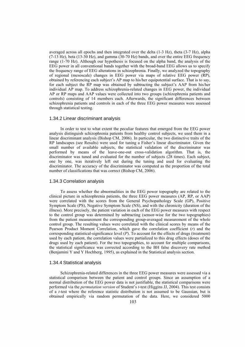
103

averaged across all epochs and then integrated over the delta (1-3 Hz), theta (3-7 Hz), alpha (7-13 Hz), beta (13-30 Hz), and gamma (30-70 Hz) bands, and over the entire EEG frequency range (1-70 Hz). Although our hypothesis is focused on the alpha band, the analysis of the EEG power in all conventional bands together with the broad-band EEG allows us to specify the frequency range of EEG alterations in schizophrenia. Finally, we analyzed the topography of regional (mesoscale) changes in EEG power via maps of relative EEG power (RP), obtained by referencing each subject’s AP map to his/her equipotential surface. That is to say, for each subject the RP map was obtained by subtracting the subject’s AAP from his/her individual AP map. To address schizophrenia-related changes in EEG power, the individual AP or RP maps and AAP values were collected into two groups (schizophrenia patients and controls) consisting of 14 members each. Afterwards, the significant differences between schizophrenia patients and controls in each of the three EEG power measures were assessed through statistical testing.

1.34.2 Linear discriminant analysis

In order to test to what extent the peculiar features that emerged from the EEG power analysis distinguish schizophrenia patients from healthy control subjects, we used them in a linear discriminant analysis (Bishop CM, 2006). In particular, the two distinctive traits of the RP landscapes (see Results) were used for tuning a Fisher’s linear discriminator. Given the small number of available subjects, the statistical validation of the discriminator was performed by means of the leave-one-out cross-validation algorithm. That is, the discriminator was tuned and evaluated for the number of subjects (28 times). Each subject, one by one, was iteratively left out during the tuning and used for evaluating the discriminator. The accuracy of the discriminator was computed as the proportion of the total number of classifications that was correct (Bishop CM, 2006).

1.34.3 Correlation analysis

To assess whether the abnormalities in the EEG power topography are related to the clinical picture in schizophrenia patients, the three EEG power measures (AP, RP, or AAP) were correlated with the scores from the General Psychopathology Scale (GP), Positive Symptom Scale (PS), Negative Symptom Scale (NS), and with the chronicity (duration of the illness). More precisely, the patient variation in each of the EEG power measures with respect to the control group was determined by subtracting (sensor-wise for the two topographies) from the patient measurement the corresponding group-averaged measurement of the whole control group. The resulting values were correlated with the clinical scores by means of the Pearson Product Moment Correlation, which gave the correlation coefficient (r) and the corresponding statistical-significance level (P). To account for the effects of drugs (treatment) used by each patient, the correlation values were partialized to this drug effects (doses of the drugs used by each patient). For the two topographies, to account for multiple comparisons, the statistical significance was corrected according to the BH false discovery rate method (Benjamini Y and Y Hochberg, 1995), as explained in the Statistical analysis section.

1.34.4 Statistical analysis

Schizophrenia-related differences in the three EEG power measures were assessed via a statistical comparison between the patient and control groups. Since an assumption of a normal distribution of the EEG power data is not justifiable, the statistical comparisons were performed via the permutation version of Student’s t-test (Higgins JJ, 2004). This test consists of a t-test where the reference statistic distribution is not assumed to be Gaussian, but is obtained empirically via random permutation of the data. Here, we considered 5000

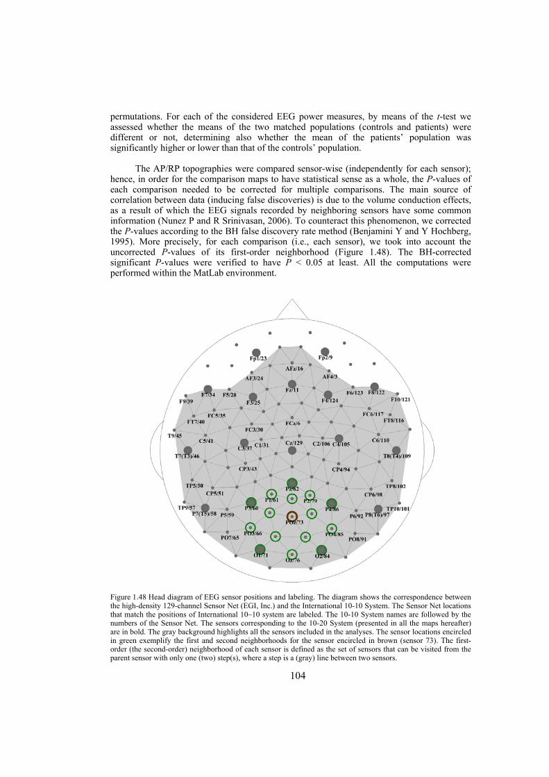
104

permutations. For each of the considered EEG power measures, by means of the t-test we assessed whether the means of the two matched populations (controls and patients) were different or not, determining also whether the mean of the patients’ population was significantly higher or lower than that of the controls’ population.

The AP/RP topographies were compared sensor-wise (independently for each sensor); hence, in order for the comparison maps to have statistical sense as a whole, the P-values of each comparison needed to be corrected for multiple comparisons. The main source of correlation between data (inducing false discoveries) is due to the volume conduction effects, as a result of which the EEG signals recorded by neighboring sensors have some common information (Nunez P and R Srinivasan, 2006). To counteract this phenomenon, we corrected the P-values according to the BH false discovery rate method (Benjamini Y and Y Hochberg, 1995). More precisely, for each comparison (i.e., each sensor), we took into account the uncorrected P-values of its first-order neighborhood ( Figure 1.48). The BH-corrected significant P-values were verified to have P < 0.05 at least. All the computations were performed within the MatLab environment.

Figure 1.48 Head diagram of EEG sensor positions and labeling. The diagram shows the correspondence between the high-density 129-channel Sensor Net (EGI, Inc.) and the International 10-10 System. The Sensor Net locations that match the positions of International 10–10 system are labeled. The 10-10 System names are followed by the numbers of the Sensor Net. The sensors corresponding to the 10-20 System (presented in all the maps hereafter) are in bold. The gray background highlights all the sensors included in the analyses. The sensor locations encircled in green exemplify the first and second neighborhoods for the sensor encircled in brown (sensor 73). The first-order (the second-order) neighborhood of each sensor is defined as the set of sensors that can be visited from the parent sensor with only one (two) step(s), where a step is a (gray) line between two sensors.

105

1.35 Results

1.35.1 Absolute EEG power in schizophrenia patients

We have found that, in general, EEG power is reduced in the schizophrenia patients compared to the control subjects (Table 7.2). The effect is highly significant for the broad-band AAP (P = 0.001). The breakdown of the AAP data into conventional EEG bands showed that there are two bands, namely, alpha (P = 0.0002) and beta (P = 0.0006), that most significantly contribute to this effect. To clear up whether these AAP differences are due to diffuse or regional EEG changes, we performed AP surface mapping. Figure 1.49A shows the broad-band (1-70 Hz) AP averaged over the groups of schizophrenia patients and controls, as well as the difference map presenting the topography of AP changes in the patients. As can be seen from the difference map, the vast majority of sensors (95%) showed a significant decrease of AP (P < 0.05, BH-corrected). This diffuse topography is fully replicated in the alpha and beta-bands, but is less pronounced in other bands ( Figure 1.49B). The largest clusters that fail to demonstrate significant differences include the frontal ones in the delta and theta bands, parietal and occipital clusters in the theta- and gamma-bands, and the right temporal cluster in the gamma-band. However, with a more liberal level of significance (P < 0.1, BH-corrected) the same trend of the AP decrease is true nearly for all sensors (95%). Therefore, in schizophrenia patients, the analysis of absolute power has revealed its generalized decrease clearly visible in the broad-band EEG. The alpha and beta frequency bands predominantly contribute to this effect.

1.35.2 Inferring EEG power topography in schizophrenia patients

The strong AP effects at a global scale described in the previous paragraph might well mask the regional landscape features in schizophrenia patients. To remove these global effects, we subtracted the individual AAP from the AP of each sensor. The resulting RP maps are shown in Figure 1.50. Let us first consider the broad-band EEG maps ( Figure 1.50A). Although the RP landscapes, shown separately for patients and controls, point to reduced inter-regional differences in the schizophrenia compared to the control subjects, the difference map provides a clue rather than a clear support for this observation. Indeed, only two small clusters (each of two sensors) show significant between-group differences. These are the right prefrontal cluster, with increased RP, and the midline parietal cluster, with reduced RP. The spectral breakdown of the map is shown in Figure 1.50B. Note that only the significant changes at P < 0.05 (BH-corrected) are depicted in red or in blue. In contrast to the AP difference maps, which have a diffuse topography similar across all the bands studied, the RP landscapes appear to be frequency- and region-specific. While both slow (delta and theta) and fast (gamma) frequency bands show no significant differences over the entire head surface, the alpha-band landscape clearly differentiates the schizophrenia patients from controls. Its main feature is a significant increase in RP over the entire anterior brain region (P < 0.05, BH-corrected). The RP decrease over posterior regions is mostly pronounced over the midline occipito-parietal and left parieto-temporal regions (P < 0.05, BH-corrected). A shadow of these effects can be seen in the beta-band as well. That is, the two small frontal clusters (the right and midline sensors close to F8 and Fz, respectively) show an increase, while the two posterior clusters (around P7 and P8) show a decrease of RP in schizophrenia patients (P < 0.05, BH-corrected).

To assess to which extent these features (relative increase of power in the anterior region and relative decrease of in the posterior area) are peculiar to schizophrenia patients and how they are distributed among them, we performed a simple linear discriminant analysis. That is, we considered the following schizophrenia-related features to be potential

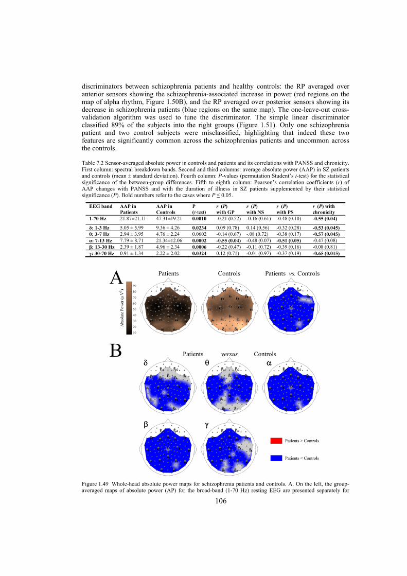
106

discriminators between schizophrenia patients and healthy controls: the RP averaged over anterior sensors showing the schizophrenia-associated increase in power (red regions on the map of alpha rhythm, Figure 1.50B), and the RP averaged over posterior sensors showing its decrease in schizophrenia patients (blue regions on the same map). The one-leave-out cross-validation algorithm was used to tune the discriminator. The simple linear discriminator classified 89% of the subjects into the right groups ( Figure 1.51). Only one schizophrenia patient and two control subjects were misclassified, highlighting that indeed these two features are significantly common across the schizophrenias patients and uncommon across the controls.

Table 7.2 Sensor-averaged absolute power in controls and patients and its correlations with PANSS and chronicity. First column: spectral breakdown bands. Second and third columns: average absolute power (AAP) in SZ patients and controls (mean ± standard deviation). Fourth column: P-values (permutation Student’s t-test) for the statistical significance of the between-group differences. Fifth to eighth column: Pearson’s correlation coefficients (r) of AAP changes with PANSS and with the duration of illness in SZ patients supplemented by their statistical significance (P). Bold numbers refer to the cases where P ≤ 0.05.

EEG band AAP in Patients

AAP in Controls

P (t-test)

r (P) with GP

r (P) with NS

r (P) with PS

r (P) with chronicity

1-70 Hz 21.87±21.11 47.31±19.21 0.0010 -0.21 (0.52) -0.16 (0.61) -0.48 (0.10) -0.55 (0.04)

δ: 1-3 Hz 5.05 ± 5.99 9.36 ± 4.26 0.0234 0.09 (0.78) 0.14 (0.56) -0.32 (0.28) -0.53 (0.045) θ: 3-7 Hz 2.94 ± 3.95 4.76 ± 2.24 0.0602 -0.14 (0.67) -.08 (0.72) -0.38 (0.17) -0.57 (0.045) α: 7-13 Hz 7.79 ± 8.71 21.34±12.06 0.0002 -0.55 (0.04) -0.48 (0.07) -0.51 (0.05) -0.47 (0.08) β: 13-30 Hz 2.39 ± 1.87 4.96 ± 2.34 0.0006 -0.22 (0.47) -0.11 (0.72) -0.39 (0.16) -0.08 (0.81) γ: 30-70 Hz 0.91 ± 1.34 2.22 ± 2.02 0.0324 0.12 (0.71) -0.01 (0.97) -0.37 (0.19) -0.65 (0.015)

Figure 1.49 Whole-head absolute power maps for schizophrenia patients and controls. A. On the left, the group-averaged maps of absolute power (AP) for the broad-band (1-70 Hz) resting EEG are presented separately for

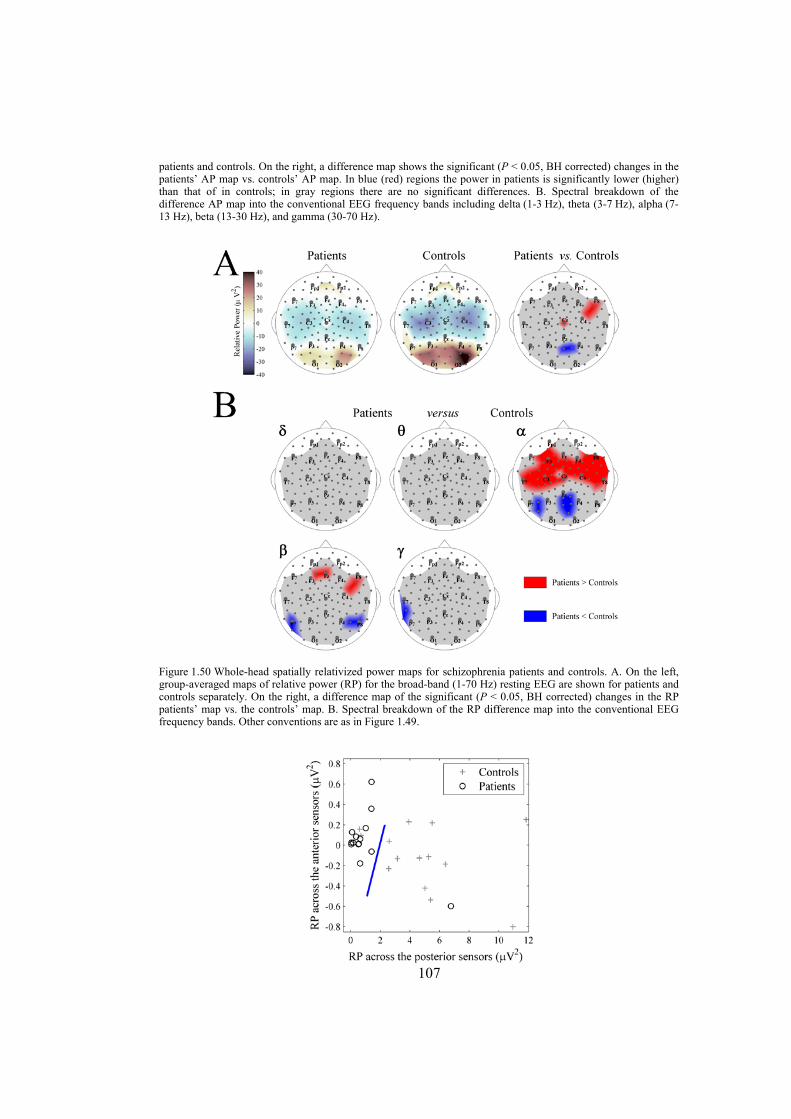
107

patients and controls. On the right, a difference map shows the significant (P < 0.05, BH corrected) changes in the patients’ AP map vs. controls’ AP map. In blue (red) regions the power in patients is significantly lower (higher) than that of in controls; in gray regions there are no significant differences. B. Spectral breakdown of the difference AP map into the conventional EEG frequency bands including delta (1-3 Hz), theta (3-7 Hz), alpha (7-13 Hz), beta (13-30 Hz), and gamma (30-70 Hz).

Figure 1.50 Whole-head spatially relativized power maps for schizophrenia patients and controls. A. On the left, group-averaged maps of relative power (RP) for the broad-band (1-70 Hz) resting EEG are shown for patients and controls separately. On the right, a difference map of the significant (P < 0.05, BH corrected) changes in the RP patients’ map vs. the controls’ map. B. Spectral breakdown of the RP difference map into the conventional EEG frequency bands. Other conventions are as in Figure 1.49.

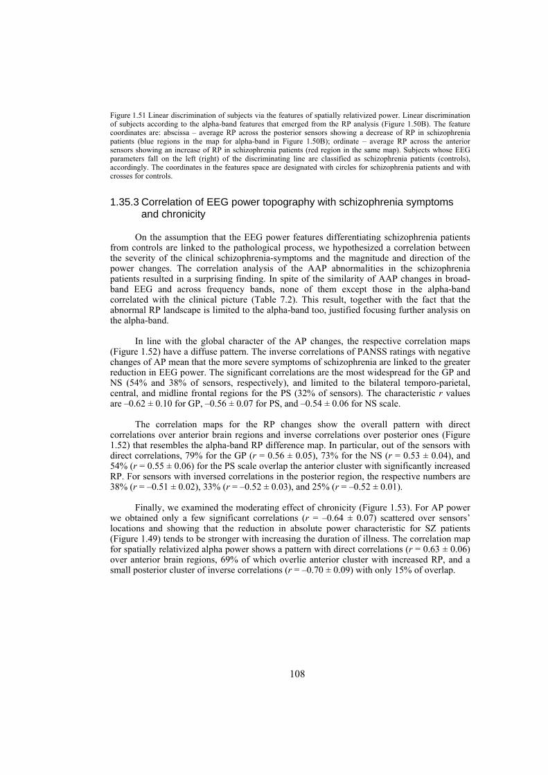
108

Figure 1.51 Linear discrimination of subjects via the features of spatially relativized power. Linear discrimination of subjects according to the alpha-band features that emerged from the RP analysis ( Figure 1.50B). The feature coordinates are: abscissa – average RP across the posterior sensors showing a decrease of RP in schizophrenia patients (blue regions in the map for alpha-band in Figure 1.50B); ordinate – average RP across the anterior sensors showing an increase of RP in schizophrenia patients (red region in the same map). Subjects whose EEG parameters fall on the left (right) of the discriminating line are classified as schizophrenia patients (controls), accordingly. The coordinates in the features space are designated with circles for schizophrenia patients and with crosses for controls.

1.35.3 Correlation of EEG power topography with schizophrenia symptoms and chronicity

On the assumption that the EEG power features differentiating schizophrenia patients from controls are linked to the pathological process, we hypothesized a correlation between the severity of the clinical schizophrenia-symptoms and the magnitude and direction of the power changes. The correlation analysis of the AAP abnormalities in the schizophrenia patients resulted in a surprising finding. In spite of the similarity of AAP changes in broad-band EEG and across frequency bands, none of them except those in the alpha-band correlated with the clinical picture (Table 7.2). This result, together with the fact that the abnormal RP landscape is limited to the alpha-band too, justified focusing further analysis on the alpha-band.

In line with the global character of the AP changes, the respective correlation maps ( Figure 1.52) have a diffuse pattern. The inverse correlations of PANSS ratings with negative changes of AP mean that the more severe symptoms of schizophrenia are linked to the greater reduction in EEG power. The significant correlations are the most widespread for the GP and NS (54% and 38% of sensors, respectively), and limited to the bilateral temporo-parietal, central, and midline frontal regions for the PS (32% of sensors). The characteristic r values are –0.62 ± 0.10 for GP, –0.56 ± 0.07 for PS, and –0.54 ± 0.06 for NS scale.

The correlation maps for the RP changes show the overall pattern with direct correlations over anterior brain regions and inverse correlations over posterior ones ( Figure 1.52) that resembles the alpha-band RP difference map. In particular, out of the sensors with direct correlations, 79% for the GP (r = 0.56 ± 0.05), 73% for the NS (r = 0.53 ± 0.04), and 54% (r = 0.55 ± 0.06) for the PS scale overlap the anterior cluster with significantly increased RP. For sensors with inversed correlations in the posterior region, the respective numbers are 38% (r = –0.51 ± 0.02), 33% (r = –0.52 ± 0.03), and 25% (r = –0.52 ± 0.01).

Finally, we examined the moderating effect of chronicity ( Figure 1.53). For AP power we obtained only a few significant correlations (r = –0.64 ± 0.07) scattered over sensors’ locations and showing that the reduction in absolute power characteristic for SZ patients ( Figure 1.49) tends to be stronger with increasing the duration of illness. The correlation map for spatially relativized alpha power shows a pattern with direct correlations (r = 0.63 ± 0.06) over anterior brain regions, 69% of which overlie anterior cluster with increased RP, and a small posterior cluster of inverse correlations (r = –0.70 ± 0.09) with only 15% of overlap.

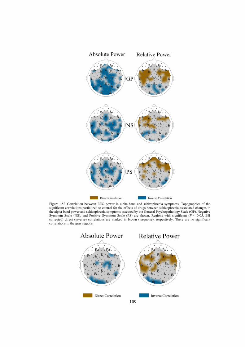
109

Figure 1.52 Correlation between EEG power in alpha-band and schizophrenia symptoms. Topographies of the significant correlations partialized to control for the effects of drugs between schizophrenia-associated changes in the alpha-band power and schizophrenia symptoms assessed by the General Psychopathology Scale (GP), Negative Symptom Scale (NS), and Positive Symptom Scale (PS) are shown. Regions with significant (P < 0.05, BH corrected) direct (inverse) correlations are marked in brown (turquoise), respectively. There are no significant correlations in the gray regions.

110

Figure 1.53 Effects of chronicity on EEG power in alpha-band. Topographies of correlations partialized to control for the effects of drugs between the alpha-band power and the duration of illness are shown using the same conventions as in Figure 1.52.

1.36 Discussion

Our results can be summarized as the following main findings. The analysis of the surface topography of EEG power reveals the schizophrenia-related abnormalities at different spatial scales. The first effect is a global decrease in absolute EEG power robustly manifested in the alpha and beta frequency bands as well as in the broad-band EEG. The second effect, observed at a mesoscale, is expressed as a relative increase in the alpha power over the prefrontal brain regions against its decrease over the postcentral regions. Importantly, not only are both effects robust in the alpha band but they are also associated with the schizophrenia symptoms in this frequency range. In sum, our findings support the concept of hypofrontality in schizophrenia and expose the alpha rhythm as a marker of it.

1.36.1 Global-scale cortical abnormalities in schizophrenia from EEG perspective

The whole-head decrease of EEG power in schizophrenia patients reported here gains support from other EEG studies of schizophrenia (Begić D et al., 2000; Merrin E and T Floyd, 1996; Sponheim SR et al., 1994; Stevens JR and A Livermore, 1982). To account for this abnormality, let us take a closer look at the neural substrate of resting EEG dominated by large-magnitude alpha oscillations. Its most powerful source is the dipole layers of extensive gyral surfaces (Srinivasan R et al., 2006). For this type of EEG, local synchronization at the macrocolumn scale crucially impacts its amplitude in surface noninvasive recordings (Nunez P et al., 2001). Therefore, the abnormalities of cortical circuitry in the schizophrenia cortex, such as reduced dendritic arborization of neurons, suggest a plausible mechanism of dysconnection that could result in the relatively small alpha amplitude (power) in schizophrenia patients. Indeed, neuropil abnormalities in schizophrenia have been observed (Black JE et al., 2004; Casanova MF et al., 2005; Garey LJ et al., 1998; Glantz LA and DA Lewis, 2000; Selemon LD et al., 2003; Vogeley K et al., 2003); for review see (Glantz LA et al., 2006; Jarskog LF et al., 2007; Selemon L and P Goldman-Rakic, 1999).

However, the reduced neuropil was predominantly documented for the prefrontal cortex, whereas the widespread alpha power reduction suggests circuitry abnormalities across the entire neocortex or at least over broad regions defined by the correlation maps in the left column of Figure 1.52. This inconsistency may be apparent rather than real. Indeed, the schizophrenia patients with diminished alpha-band power demonstrate brain abnormalities including larger ventricles and increased width of cortical sulci in comparison with the patients without such an EEG feature (Sponheim SR et al., 2000). Since such structural alterations point to an extensive gray matter loss in schizophrenia, they match the hypothesis that a widespread intracortical neuropil reduction in schizophrenia is behind the widespread alpha power reduction. Furthermore, recent neuroimaging evidence confirms that the progressive loss of cortical gray matter, which is compatible both with the neuropil hypothesis and with our data, is an extensive phenomenon (Thompson PM et al., 2001; Vidal C et al., 2006). The maps of cortical tissue loss in early-onset schizophrenia patients presented in these reports include broad regions of temporal cortex, superior parietal, sensorimotor, and superior prefrontal cortices that strongly overlap with our correlation maps for the absolute power changes. Also, extensive changes in cortical synaptic plasticity in schizophrenia

111

(Stephan K et al., 2006) could lead to cortical circuitry problems with similar impacts on EEG.

Alternatively, the involvement of the reticular activating system in the schizophrenia pathological process (Garcia-Rill E, 1997) might be the cause of global flattening of EEG, the more so as the hallucinations and disturbances of the sleep-wake cycle and of sensory gating inherent in schizophrenia make such a hypothesis quite plausible. Yet if the brain stem activating system is involved, then the observed EEG changes might be the consequence of hyperarousal. However, our patient group did not exhibit an increase in the higher frequency EEG activity characteristic of arousal. Indeed, the reduction in power was even more robust across higher frequencies, comprising on average 46% in the delta, 38% in theta, 64% in alpha, 52% in beta, and 59% in gamma band. Therefore, even if the reticulo-cortical communication was changed in these schizophrenia patients, it did not generate any EEG signs of hyperarousal.

1.36.2 Mesoscale EEG effects in schizophrenia: alpha rhythm as a marker of hypofrontality

The global changes in absolute power discussed in the previous paragraph mask the topographical abnormalities in the patients’ EEG rather than reveal them. That is why the true landscape characteristics for schizophrenia patients were extracted from the maps of alpha-band power by referencing them to their mean level in each individual (RP). The group difference maps ( Figure 1.50B) clearly show a relative increase in the alpha-rhythm power over the (pre)frontal cortex, i.e, the hypofrontal pattern in the schizophrenia patients. In this connection, several previously published observations attracted our attention. In particular, the alpha band amplitude in the frontal electrodes has been found to be larger in the schizophrenia patients compared to the control group and interpreted as an expression of frontal dysfunction (Kahn EM et al., 1993). While being an undoubtedly interesting attempt to consider the alpha rhythm of EEG a marker of hypofrontality, this report is based on conventional monopolar EEG and is not supported by rigorous statistics, which severely limits the reliability of its conclusions. However, a more recent analysis of the current density distribution by the low resolution brain electromagnetic tomography method also showed anteriorization of alpha activity in first-episode schizophrenia patients (Begré S et al., 2003) that agrees with our data.

It should be mentioned that the frontal abnormalities in the other (than alpha) rhythmic components of EEG have also been reported. In particular, several EEG studies have shown frontal slowing in schizophrenia (Gattaz WF et al., 1992; Knott V, A Labelle et al., 2001; Morihisa JM et al., 1983; Morstyn R et al., 1983; Wuebben Y and G Winterer, 2001). Yet other researchers have pointed out that the increase in the delta band power is more likely to be diffuse than local (Fenton GW et al., 1980; Karson CN et al., 1987), and/or is more characteristic for long-stay chronic schizophrenia patients (Fenton GW et al., 1980). In such patients the presence of generalized slowing in EEG might depend on the effects of medication or of chronicity itself. Turning back to our patient data shown in Figure 1.49 and Figure 1.50, we see neither diffuse nor regional frontal delta-power increase in schizophrenia patients. Moreover, a probable moderating effect of chronicity as seen through correlation analysis (Table 7.2) points to the reduction of slow (delta and theta) EEG components with increasing duration of illness.

With respect to the relationship between the EEG delta activity and frontal metabolism, the literature is also not univocal. While in normal subjects, delta activity and metabolism are positively correlated (Alper KR et al., 2006; Laufs H et al., 2006), in schizophrenia patients,

112

at least one PET study showed their negative correlation in the frontal region (Guich SM et al., 1989), while another one revealed a positive correlation (Alper K et al., 1998). Therefore, we are inclined to conclude that, although increased delta-power can be an expression of frontal lobe dysfunction in a number of schizophrenia patients, it is unlikely that it is the general feature of hypofrontality in schizophrenia.

By contrast, being a prominent rhythmic component of resting EEG, the alpha rhythm is proved to be sensitive to the fluctuations of local metabolism even within the normal range. Moreover, with our alpha measures we managed to reproduce an important feature of metabolic hypofrontality: its progression with the duration of illness (Hill K et al., 2004). This suggests that an approach exploiting the alpha rhythm properties potentially can provide a sensitive marker of the hypofrontality in schizophrenia. From the neurobiological perspective, the distortion of the anterior-to-posterior gradient of alpha rhythm in schizophrenia seems quite plausible. In particular, this phenomenon is consistent with the abnormalities of thalamic metabolism and of thalamo-cortical circuitry in schizophrenia. Compared to healthy subjects, schizophrenia patients have higher relative glucose metabolism in the pulvinar, which is connected to many posterior areas, and lower metabolism in the mediodorsal and centromedian nuclei of the thalamus, which widely project to the fronto-temporal cortices (Hazlett EA et al., 2004). Furthermore, while stronger-than-normal metabolic intercorrelations have been shown between the pulvinar and superior temporal, some parietal, posterior cingulate, and occipital areas, a metabolic disconnection has been documented between the mediodorsal nucleus and widespread frontotemporal cortical regions in schizophrenia patients (Mitelman SA et al., 2005). Such metabolic disconnection might be a result of the anatomical disconnection. Indeed, a reduced number of neurons in the mediodorsal nucleus of the thalamus has been shown in schizophrenia brains (Pakkenberg B, 1990; Popken GJ et al., 2000). This may lead to the decrease of thalamic input to the cortex (discussed in (Innocenti GM et al., 2003)). In turn, relative cortical deafferentation is bound to result in autorhythmicity (Niedermeyer E, 1997). Therefore, considering that alpha rhythm over the prefrontal cortex is generated by the prefrontal neural networks (Meng NF et al., 2007; Oishi N et al., 2007; Srinivasan R et al., 2006), such a disconnection would promote the relative overproduction of rhythmic activity.

Therefore, as a whole, our data suggest that the power abnormalities manifested in the EEG alpha band originate from several sources. The most plausible causes are the widespread abnormalities of local cortical circuitry and the damaged thalamo-cortical circuits. They might affect the EEG over anterior brain regions in opposite directions. In particular, thalamo-cortical deafferentation of prefrontal cortex favors inherent cortical autorhythmicity that provokes the hypofrontality phenomenon (increase in the alpha power over the (pre)frontal areas), whereas deficient cortico-cortical circuits favor global decrease in EEG power. These mechanisms may be affected to a variable extent in different forms of schizophrenia and, hence, depending on the patient group composition, be differently manifested in the EEG power changes. In this sense, a combination of the global and regional EEG power measurements forms a basis for the harmonizing of apparently contradictory evidence about the EEG correlates of hypofrontality in schizophrenia.

1.36.3 Clinical relevance of global and regional abnormalities in alpha power

The alpha range appears to be the most accurate EEG correlate of schizophrenia symptoms. Indeed, in spite of similar reduction in average absolute power (AAP, see Table 7.2) across frequency bands, only the alpha band correlates with PANSS scales. The patients with the greater decrease in EEG average absolute power demonstrate more severe symptoms. The maps reveal wide-spread correlation fields for the PANSS. In spite of evident differences between the correlation maps across the symptom scales, all of them include the same clusters

113

of sensors over the temporo-parietal and midline frontal regions. The correlation maps for the relative power changes reveal direct correlations over the anterior brain regions and inverse correlations over the posterior ones, matching the RP difference map (cf. Figure 1.50 and Figure 1.52) and thus confirming the clinical relevance of the hypofrontality and regionally specific changes of cortical networks. Once more, with the exception that the association of the RP changes with GP ratings seems to be stronger than with other scales, these correlation maps do not differentiate topographically the symptomatic scales used. Such a similarity reflects heavy involvement of vast distributed territories in the schizophrenia pathological processes. Furthermore, it suggests that some basic properties, which affect divergent aspects of human cognition and behavior, are disrupted in the cortical networks.

Although inverse correlations between the schizophrenia symptoms and the absolute alpha power have previously been reported (e.g., (Merrin E and T Floyd, 1996)), in general, a comparison of our data with those existing in the literature is hampered, since we present the first attempt to analyze the whole-head correlation maps for power measurements from dense-array EEG. The published accounts provide only correlations for selected EEG derivations.

Recently the clinical relevance of alpha activity was supported by the study of the effects of repetitive transcranial magnetic stimulation in schizophrenia patients (Jin Y et al., 2006). These patients received repetitive transcranial magnetic stimulation over the dorsolateral prefrontal cortex either at individual alpha-peak frequency, or at other frequencies. Not only did the stimulation exclusively at alpha-frequencies result in a positive therapeutic effect, but also this effect correlated with the individual increase in alpha power. Thus, our findings, considered alongside other recent results, suggest that alpha power (amplitude) and its anterior-to-posterior gradient are worth examining with yet underutilized in psychiatry research modern EEG methods (Bolwig TG, 2008) as an accurate and cost-effective marker for monitoring the efficiency of SZ treatment.. Experimental designs that combine EEG and neuroimaging methods seem to be especially promising for that. Furthermore, such parameters as alpha power (amplitude) and its anterior-to-posterior gradients are worth examining as potential markers for monitoring the schizophrenia treatment efficiency.

1.37 Summary

In this chapter we investigated the relation of EEG alpha rhythm and hypofrontality in schizophrenia patients. We suggested that the changes of alpha rhythm could be a marker of resting hypofrontality in schizophrenia. In particular, we used a combination of power measures tuned for regional surface mapping in combination with power measures that allow evaluation of global effects. The analysis of the surface topography revealed the schizophrenia-related abnormalities at different spatial scales. These were a global decrease in absolute EEG power robustly manifested in the alpha and beta frequency bands and a relative increase in the alpha power over the prefrontal brain regions against its reduction over the postcentral regions. Not only both effects were robust in the alpha band but they were linked to the schizophrenia symptoms measured with Positive and Negative Symptom Scales exclusively in this frequency range. Our findings support the concept of hypofrontality in schizophrenia and expose the alpha rhythm as a sensitive marker of it.

115

DYSCONNECTION TOPOGRAPHY IN SCHIZOPHRENIA REVEALED WITH STATE-SPACE ANALYSIS OF EEG

Personal Contribution — This chapter has been reproduced from our paper published in PLoS ONE (Jalili M, S Lavoie et al., 2007). We have used the same EEG data used in the previous chapter. My contribution was data analysis and the interpretation of the data was done mainly by me, Maria G. Knyazeva, Oscar De Feo and Martin Hasler.

1.38 Schizophrenia as a brain dysconnection disorder

The hypothesis that schizophrenia is a condition characterized by abnormal brain integration can be traced back to Bleuler, who emphasized that a splitting of the psychic functions (‘loosening of associations’) is a core problem in schizophrenia (Bleuler E, 1911). The testable biological counterparts of such a clinical phenomenology of the disorder are anomalous structural integrity and/or functional connectivity of the brain. The morphometric evidence in favor of the dysconnectivity model of schizophrenia includes subtle but wide-spread morphological abnormalities observed in postmortem studies. Among supporting although indirect findings there are enlarged ventricles (reviewed in (Woods BT, 1998)), decreased cortical volume or thickness coupled with increased cell packing density (Cotter D et al., 2002; Pakkenberg B, 1987; Selemon LD et al., 1995), and reduced clustering of neurons (Beasley CL et al., 2005). The myelin of long-range connecting fibers can also be damaged in schizophrenia (Uranova N et al., 2007); also reviewed in (Bartzokis G and L Altshuler, 2005; Kubicki M et al., 2007).

The in vivo neuroimaging studies largely confirm the reduced volume of cortical gray matter in schizophrenia. In particular, associative areas including prefrontal, temporal, parietal, and limbic cortices are consistently found to be affected (Goldstein JM et al., 1999; McCarley R et al., 1999; Takahashi T et al., 2007; Zhou S et al., 2007); for review see (DeLisi L et al., 2006; Honea R et al., 2005; Shenton M et al., 2001). In line with this evidence, longitudinal studies revealed progressive loss of cortical gray matter in early-onset schizophrenia (Greenstein D et al., 2006; Kasai K et al., 2003; Rapoport J et al., 1999; Vidal C et al., 2006). A possible interpretation of these structural abnormalities is considered in the

116

neuropil hypothesis (Selemon L and P Goldman-Rakic, 1999), which claims that the reductions are caused by the pathological changes in the neuronal architecture and local circuitry. Yet the structural abnormalities seem to be quite subtle and were not replicated in a number of studies. That gave rise to another dysconnection hypothesis which emphasizes aberrant control of synaptic plasticity in schizophrenia (Friston K, 1998; Stephan K et al., 2006). However, the two hypotheses are not mutually exclusive, and both mechanisms should lead to cortical circuitry problems in schizophrenia.

A necessary link between abnormal circuitry and basic schizophrenia symptoms is functional connectivity. Bearing in mind that functional connectivity is different from anatomical connectivity (although it is affected by) and following current views, by “functional connectivity” we understand cooperation between distributed neural assemblies in the brain. A common way of assessing the cooperation among cortical networks is measuring their synchronization by means of some deterministic (e.g. phase synchronization) or statistical (e.g. correlation) measure. Here, in agreement with deterministic dynamical systems theory, synchronization refers to the process by means of which two or more interacting subsystems adjust some of their temporal properties, i.e., synchronize their activities (Pikovsky A et al., 2003).

Synchronization as a measure of functional connectivity has been extensively used in the EEG studies of schizophrenia. These studies, largely applying bivariate methods, e.g., (phase) coherence analysis of time series in pairs of EEG signals, exemplified abnormalities in EEG synchronization at rest and during the performance of cognitive tasks (Ford J et al., 2002; Higashima M et al., 2006; Hoffman R et al., 1991; Norman R et al., 1997; Shaw J et al., 1983; Spencer K et al., 2003; Uhlhaas PJ et al., 2006). However, the limitations of bivariate synchronization analysis inevitably led to the region-of-interest approach that is an analysis of several pre-selected pairs of signals. In particular, based on a priori evidence, the synchronization abnormalities in schizophrenia were largely tested for the EEG electrode pairs located over frontal, temporal, and parietal cortices, whereas reconstruction of the whole-head topography of synchronization remained unattainable. Modern multichannel EEG techniques, combined with the advances in dynamical systems theory and in signal processing, allow a construction of multivariate synchronization measures readily translatable into synchronization maps. Indeed, recent work in nonlinear dynamical systems resulted in new application-independent multivariate measures of synchronization (Allefeld C and J Kurths, 2004; Carmeli C et al., 2005; Stam CJ and BW van Dijk, 2002; Wiesenfeldt M et al., 2001). Here, we address synchronization phenomena by means of the S-estimator, which, initially proposed for an EEG application (Carmeli C et al., 2005), was also successfully applied to assess synchronization phenomena within other contexts such as cardio-encephalic-pulmonary interactions in anesthesia (Oshima K et al., 2006) and athletics electrocardiography (Celka P and B Kilner, 2006).

The S-estimator exploits a theoretical consequence of cooperative (synchronization-like) phenomena in order to estimate the amount of synchronization within a set of measurements of arbitrary cardinality (Carmeli C et al., 2005), i.e., the fact that the portion of the visited state-space of two (or more) interacting dynamical systems is smaller than that visited by the same putatively non-interacting systems (Boccaletti S et al., 2002). The S-estimator properties, including robustness with respect to measurement and dynamical noise, resiliency and scalability with respect to the number of measurements (channels), and sensitivity with respect to the amount of data (the length of measurements), were extensively tested (Carmeli C, 2006; Carmeli C et al., 2005). The S-estimator was proved to be a robust and easily scalable multivariate measure of synchronization, highly sensitive even with a reasonably small amount of data. Hence, it represents a perfectly suitable measure of the whole-head synchronization topography. We applied the S-estimator technique to the resting

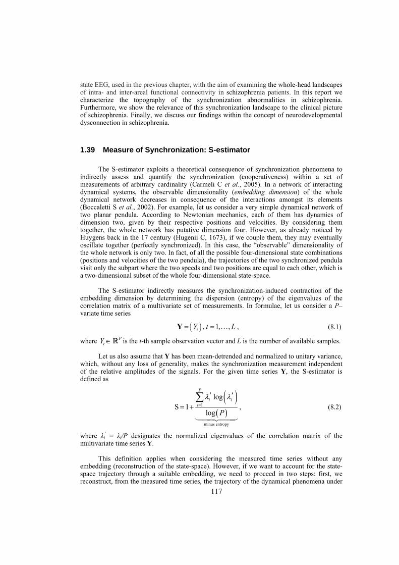
117

state EEG, used in the previous chapter, with the aim of examining the whole-head landscapes of intra- and inter-areal functional connectivity in schizophrenia patients. In this report we characterize the topography of the synchronization abnormalities in schizophrenia. Furthermore, we show the relevance of this synchronization landscape to the clinical picture of schizophrenia. Finally, we discuss our findings within the concept of neurodevelopmental dysconnection in schizophrenia.

1.39 Measure of Synchronization: S-estimator

The S-estimator exploits a theoretical consequence of synchronization phenomena to indirectly assess and quantify the synchronization (cooperativeness) within a set of measurements of arbitrary cardinality (Carmeli C et al., 2005). In a network of interacting dynamical systems, the observable dimensionality (embedding dimension) of the whole dynamical network decreases in consequence of the interactions amongst its elements (Boccaletti S et al., 2002). For example, let us consider a very simple dynamical network of two planar pendula. According to Newtonian mechanics, each of them has dynamics of dimension two, given by their respective positions and velocities. By considering them together, the whole network has putative dimension four. However, as already noticed by Huygens back in the 17 century (Hugenii C, 1673), if we couple them, they may eventually oscillate together (perfectly synchronized). In this case, the “observable” dimensionality of the whole network is only two. In fact, of all the possible four-dimensional state combinations (positions and velocities of the two pendula), the trajectories of the two synchronized pendula visit only the subpart where the two speeds and two positions are equal to each other, which is a two-dimensional subset of the whole four-dimensional state-space.

The S-estimator indirectly measures the synchronization-induced contraction of the embedding dimension by determining the dispersion (entropy) of the eigenvalues of the correlation matrix of a multivariate set of measurements. In formulae, let us consider a P–variate time series

, 1, ,tY t L= =Y K , (8.1)

where PtY ∈R is the t-th sample observation vector and L is the number of available samples.

Let us also assume that Y has been mean-detrended and normalized to unitary variance, which, without any loss of generality, makes the synchronization measurement independent of the relative amplitudes of the signals. For the given time series Y, the S-estimator is defined as

( )

( )1

minus entropy

logS 1

log

P

i ii

P

λ λ=

′ ′= +

∑

1442443

, (8.2)

where λi' = λi/P designates the normalized eigenvalues of the correlation matrix of the

multivariate time series Y.

This definition applies when considering the measured time series without any embedding (reconstruction of the state-space). However, if we want to account for the state-space trajectory through a suitable embedding, we need to proceed in two steps: first, we reconstruct, from the measured time series, the trajectory of the dynamical phenomena under

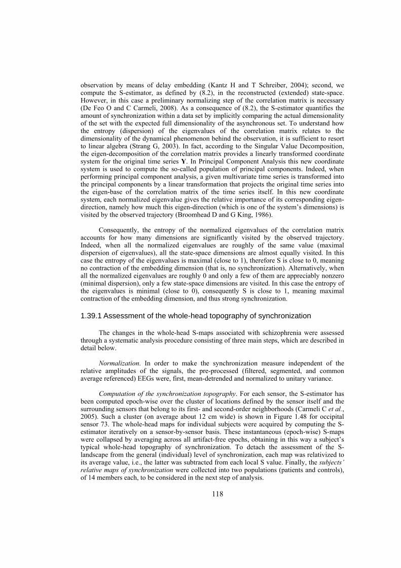
118

observation by means of delay embedding (Kantz H and T Schreiber, 2004); second, we compute the S-estimator, as defined by (8.2), in the reconstructed (extended) state-space. However, in this case a preliminary normalizing step of the correlation matrix is necessary (De Feo O and C Carmeli, 2008). As a consequence of (8.2), the S-estimator quantifies the amount of synchronization within a data set by implicitly comparing the actual dimensionality of the set with the expected full dimensionality of the asynchronous set. To understand how the entropy (dispersion) of the eigenvalues of the correlation matrix relates to the dimensionality of the dynamical phenomenon behind the observation, it is sufficient to resort to linear algebra (Strang G, 2003). In fact, according to the Singular Value Decomposition, the eigen-decomposition of the correlation matrix provides a linearly transformed coordinate system for the original time series Y. In Principal Component Analysis this new coordinate system is used to compute the so-called population of principal components. Indeed, when performing principal component analysis, a given multivariate time series is transformed into the principal components by a linear transformation that projects the original time series into the eigen-base of the correlation matrix of the time series itself. In this new coordinate system, each normalized eigenvalue gives the relative importance of its corresponding eigen-direction, namely how much this eigen-direction (which is one of the system’s dimensions) is visited by the observed trajectory (Broomhead D and G King, 1986).

Consequently, the entropy of the normalized eigenvalues of the correlation matrix accounts for how many dimensions are significantly visited by the observed trajectory. Indeed, when all the normalized eigenvalues are roughly of the same value (maximal dispersion of eigenvalues), all the state-space dimensions are almost equally visited. In this case the entropy of the eigenvalues is maximal (close to 1), therefore S is close to 0, meaning no contraction of the embedding dimension (that is, no synchronization). Alternatively, when all the normalized eigenvalues are roughly 0 and only a few of them are appreciably nonzero (minimal dispersion), only a few state-space dimensions are visited. In this case the entropy of the eigenvalues is minimal (close to 0), consequently S is close to 1, meaning maximal contraction of the embedding dimension, and thus strong synchronization.

1.39.1 Assessment of the whole-head topography of synchronization

The changes in the whole-head S-maps associated with schizophrenia were assessed through a systematic analysis procedure consisting of three main steps, which are described in detail below.

Normalization. In order to make the synchronization measure independent of the relative amplitudes of the signals, the pre-processed (filtered, segmented, and common average referenced) EEGs were, first, mean-detrended and normalized to unitary variance.

Computation of the synchronization topography. For each sensor, the S-estimator has been computed epoch-wise over the cluster of locations defined by the sensor itself and the surrounding sensors that belong to its first- and second-order neighborhoods (Carmeli C et al., 2005). Such a cluster (on average about 12 cm wide) is shown in Figure 1.48 for occipital sensor 73. The whole-head maps for individual subjects were acquired by computing the S-estimator iteratively on a sensor-by-sensor basis. These instantaneous (epoch-wise) S-maps were collapsed by averaging across all artifact-free epochs, obtaining in this way a subject’s typical whole-head topography of synchronization. To detach the assessment of the S-landscape from the general (individual) level of synchronization, each map was relativized to its average value, i.e., the latter was subtracted from each local S value. Finally, the subjects’ relative maps of synchronization were collected into two populations (patients and controls), of 14 members each, to be considered in the next step of analysis.

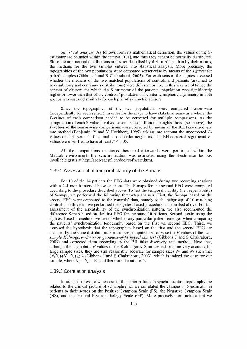
119

Statistical analysis. As follows from its mathematical definition, the values of the S-estimator are bounded within the interval [0,1], and thus they cannot be normally distributed. Since the non-normal distributions are better described by their medians than by their means, the medians for the two samples entered into statistical analysis. More precisely, the topographies of the two populations were compared sensor-wise by means of the signtest for paired samples (Gibbons J and S Chakraborti, 2003). For each sensor, the signtest assessed whether the medians of the two matched populations of controls and patients (assumed to have arbitrary and continuous distributions) were different or not. In this way we obtained the centers of clusters for which the S-estimator of the patients’ population was significantly higher or lower than that of the controls’ population. The interhemispheric asymmetry in both groups was assessed similarly for each pair of symmetric sensors.

Since the topographies of the two populations were compared sensor-wise (independently for each sensor), in order for the maps to have statistical sense as a whole, the P-values of each comparison needed to be corrected for multiple comparisons. As the computation of each S-value involved several sensors from the neighborhood (see above), the P-values of the sensor-wise comparisons were corrected by means of the BH false discovery rate method (Benjamini Y and Y Hochberg, 1995), taking into account the uncorrected P-values of each sensor’s first- and second-order neighbors. The BH-corrected significant P-values were verified to have at least P < 0.05.

All the computations mentioned here and afterwards were performed within the MatLab environment: the synchronization was estimated using the S-estimator toolbox (available gratis at http://aperest.epfl.ch/docs/software.htm).

1.39.2 Assessment of temporal stability of the S-maps

For 10 of the 14 patients the EEG data were obtained during two recording sessions with a 2-4 month interval between them. The S-maps for the second EEG were computed according to the procedure described above. To test the temporal stability (i.e., repeatability) of S-maps, we performed the following three-step analysis. First, the S-maps based on the second EEG were compared to the controls’ data, namely to the subgroup of 10 matching controls. To this end, we performed the signtest-based procedure as described above. For fair assessment of the repeatability of the synchronization pattern, we also recomputed the difference S-map based on the first EEG for the same 10 patients. Second, again using the signtest-based procedure, we tested whether any particular pattern emerges when comparing the patients’ synchronization topography based on the first vs. second EEG. Third, we assessed the hypothesis that the topographies based on the first and the second EEG are spanned by the same distribution. For that we computed sensor-wise the P-values of the two-sample Kolmogorov-Smirnov goodness-of-fit hypothesis test (Gibbons J and S Chakraborti, 2003) and corrected them according to the BH false discovery rate method. Note that, although the asymptotic P-values of the Kolmogorov-Smirnov test become very accurate for large sample sizes, they are still reasonably accurate for sample sizes N1 and N2 such that (N1N2)/(N1+N2) ≥ 4 (Gibbons J and S Chakraborti, 2003), which is indeed the case for our sample, where N1 = N2 = 10, and therefore the ratio is 5.

1.39.3 Correlation analysis

In order to assess to which extent the abnormalities in synchronization topography are related to the clinical picture of schizophrenia, we correlated the changes in S-estimator in patients to their scores on the Positive Symptom Scale (PS), the Negative Symptom Scale (NS), and the General Psychopathology Scale (GP). More precisely, for each patient we

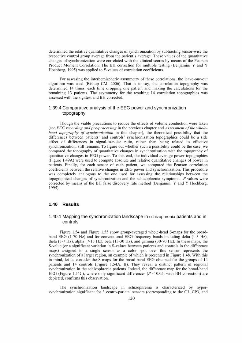
120

determined the relative quantitative changes of synchronization by subtracting sensor-wise the respective control group average from the patient’s average. These values of the quantitative changes of synchronization were correlated with the clinical scores by means of the Pearson Product Moment Correlation. The BH correction for multiple testing (Benjamini Y and Y Hochberg, 1995) was applied to P-values of correlation coefficients.

For assessing the interhemispheric asymmetry of these correlations, the leave-one-out algorithm was used (Bishop CM, 2006). That is to say, the correlation topography was determined 14 times, each time dropping one patient and making the calculations for the remaining 13 patients. The asymmetry for the resulting 14 correlation topographies was assessed with the signtest and BH corrected.

1.39.4 Comparative analysis of the EEG power and synchronization topography

Though the viable precautions to reduce the effects of volume conduction were taken (see EEG recording and pre-processing in the previous chapter and Assessment of the whole-head topography of synchronization in this chapter), the theoretical possibility that the differences between patients’ and controls’ synchronization topographies could be a side effect of differences in signal-to-noise ratio, rather than being related to effective synchronization, still remains. To figure out whether such a possibility could be the case, we compared the topography of quantitative changes in synchronization with the topography of quantitative changes in EEG power. To this end, the individual average power topographies ( Figure 1.49A) were used to compute absolute and relative quantitative changes of power in patients. Finally, for each sensor of each patient, we computed the Pearson correlation coefficients between the relative changes in EEG power and synchronization. This procedure was completely analogous to the one used for assessing the relationships between the topographical changes of synchronization and the schizophrenia symptoms. P-values were corrected by means of the BH false discovery rate method (Benjamini Y and Y Hochberg, 1995).

1.40 Results

1.40.1 Mapping the synchronization landscape in schizophrenia patients and in controls

Figure 1.54 and Figure 1.55 show group-averaged whole-head S-maps for the broad-band EEG (1-70 Hz) and for conventional EEG frequency bands including delta (1-3 Hz), theta (3-7 Hz), alpha (7-13 Hz), beta (13-30 Hz), and gamma (30-70 Hz). In these maps, the S-value (or a significant variation in S-values between patients and controls in the difference maps) assigned to a single sensor as a color spot over this sensor represents the synchronization of a larger region, an example of which is presented in Figure 1.48. With this in mind, let us consider the S-maps for the broad-band EEG obtained for the groups of 14 patients and 14 controls ( Figure 1.54A, B). They reveal a distinct pattern of regional synchronization in the schizophrenia patients. Indeed, the difference map for the broad-band EEG ( Figure 1.54C), where only significant differences (P < 0.05, with BH correction) are depicted, confirms this observation.

The synchronization landscape in schizophrenia is characterized by hyper-synchronization significant for 3 centro-parietal sensors (corresponding to the C3, CP3, and

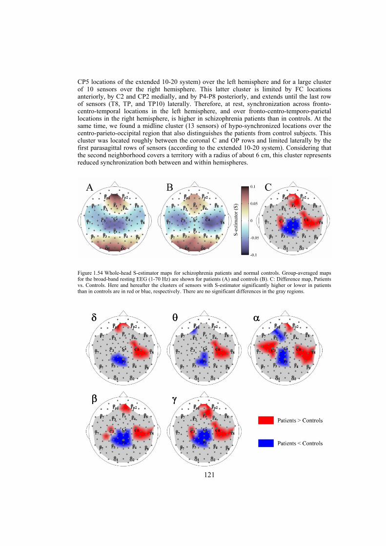
121

CP5 locations of the extended 10-20 system) over the left hemisphere and for a large cluster of 10 sensors over the right hemisphere. This latter cluster is limited by FC locations anteriorly, by C2 and CP2 medially, and by P4-P8 posteriorly, and extends until the last row of sensors (T8, TP, and TP10) laterally. Therefore, at rest, synchronization across fronto-centro-temporal locations in the left hemisphere, and over fronto-centro-temporo-parietal locations in the right hemisphere, is higher in schizophrenia patients than in controls. At the same time, we found a midline cluster (13 sensors) of hypo-synchronized locations over the centro-parieto-occipital region that also distinguishes the patients from control subjects. This cluster was located roughly between the coronal C and OP rows and limited laterally by the first parasagittal rows of sensors (according to the extended 10-20 system). Considering that the second neighborhood covers a territory with a radius of about 6 cm, this cluster represents reduced synchronization both between and within hemispheres.

Figure 1.54 Whole-head S-estimator maps for schizophrenia patients and normal controls. Group-averaged maps for the broad-band resting EEG (1-70 Hz) are shown for patients (A) and controls (B). C: Difference map, Patients vs. Controls. Here and hereafter the clusters of sensors with S-estimator significantly higher or lower in patients than in controls are in red or blue, respectively. There are no significant differences in the gray regions.

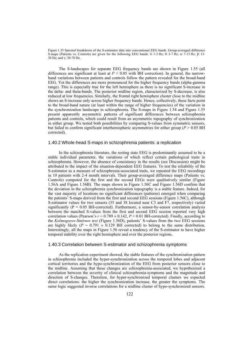
122

Figure 1.55 Spectral breakdown of the S-estimator data into conventional EEG bands. Group-averaged difference S-maps (Patients vs. Controls) are given for the following EEG bands: δ: 1-3 Hz; θ: 3-7 Hz; α: 7-13 Hz; β: 13-30 Hz; and γ: 30-70 Hz.

The S-landscapes for separate EEG frequency bands are shown in Figure 1.55 (all differences are significant at least at P < 0.05 with BH correction). In general, the narrow-band variations between patients and controls follow the pattern revealed for the broad-band EEG. Yet the differences are more pronounced for the higher frequency bands (alpha-gamma range). This is especially true for the left hemisphere as there is no significant S-increase in the delta- and theta-bands. The posterior midline region, characterized by S-decrease, is also reduced at low frequencies. Similarly, the frontal right hemisphere cluster close to the midline shows an S-increase only across higher frequency bands. Hence, collectively, these facts point to the broad-band nature (at least within the range of higher frequencies) of the variation in the synchronization landscape in schizophrenia. The S-maps in Figure 1.54 and Figure 1.55 present apparently asymmetric patterns of significant differences between schizophrenia patients and controls, which could result from an asymmetric topography of synchronization in either group. We tested both possibilities by comparing S-values from symmetric sensors, but failed to confirm significant interhemispheric asymmetries for either group (P > 0.05 BH corrected).

1.40.2 Whole-head S-maps in schizophrenia patients: a replication

In the schizophrenia literature, the resting state EEG is predominantly assumed to be a stable individual parameter, the variations of which reflect certain pathological traits in schizophrenia. However, the absence of consistency in the results (see Discussion) might be attributed to the impact of the situation-dependent EEG features. To test the reliability of the S-estimator as a measure of schizophrenia-associated traits, we repeated the EEG recordings in 10 patients with 2-4 month intervals. Their group-averaged difference maps (Patients vs. Controls) computed for the first and the second EEGs were qualitatively similar ( Figure 1.56A and Figure 1.56B). The maps shown in Figure 1.56C and Figure 1.56D confirm that the deviation in the schizophrenia synchronization topography is a stable feature. Indeed, for the vast majority of locations no significant differences (patterns) emerged when comparing the patients’ S-maps derived from the first and second EEG sessions ( Figure 1.56C), although S-estimator values for two sensors (35 and 38 located near C3 and F7, respectively) varied significantly (P ≈ 0.05 BH-corrected). Furthermore, a sensor-by-sensor correlation analysis between the matched S-values from the first and second EEG session reported very high correlation values (Pearson’s r = 0.789 ± 0.142, P < 0.01 BH-corrected). Finally, according to the Kolmogorov-Smirnov test ( Figure 1.56D), patients’ S-values from the two EEG sessions are highly likely (P = 0.791 ± 0.129 BH corrected) to belong to the same distribution. Interestingly, all the maps in Figure 1.56 reveal a tendency of the S-estimator to have higher temporal stability over the right hemisphere and over the posterior regions.

1.40.3 Correlation between S-estimator and schizophrenia symptoms

As the replication experiment showed, the stable features of the synchronization pattern in schizophrenia included the hyper-synchronization across the temporal lobes and adjacent cortical territories and the hypo-synchronization of the EEG from posterior sensors close to the midline. Assuming that these changes are schizophrenia-associated, we hypothesized a correlation between the severity of clinical schizophrenia-symptoms and the magnitude and direction of S-changes. Therefore, for hyper-synchronized temporal clusters we expected direct correlations: the higher the synchronization increase, the greater the symptoms. The same logic suggested inverse correlations for a midline cluster of hypo-synchronized sensors.

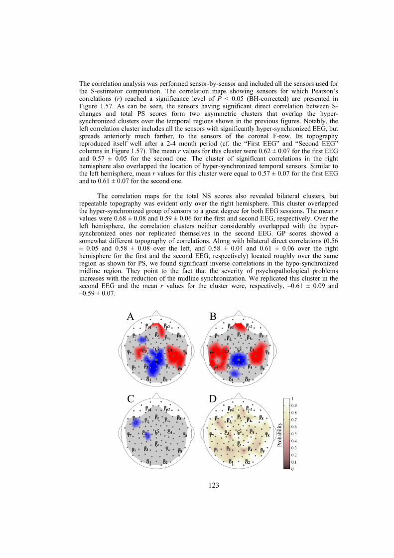
123

The correlation analysis was performed sensor-by-sensor and included all the sensors used for the S-estimator computation. The correlation maps showing sensors for which Pearson’s correlations (r) reached a significance level of P < 0.05 (BH-corrected) are presented in Figure 1.57. As can be seen, the sensors having significant direct correlation between S-changes and total PS scores form two asymmetric clusters that overlap the hyper-synchronized clusters over the temporal regions shown in the previous figures. Notably, the left correlation cluster includes all the sensors with significantly hyper-synchronized EEG, but spreads anteriorly much farther, to the sensors of the coronal F-row. Its topography reproduced itself well after a 2-4 month period (cf. the “First EEG” and “Second EEG” columns in Figure 1.57). The mean r values for this cluster were 0.62 ± 0.07 for the first EEG and 0.57 ± 0.05 for the second one. The cluster of significant correlations in the right hemisphere also overlapped the location of hyper-synchronized temporal sensors. Similar to the left hemisphere, mean r values for this cluster were equal to 0.57 ± 0.07 for the first EEG and to 0.61 ± 0.07 for the second one.

The correlation maps for the total NS scores also revealed bilateral clusters, but repeatable topography was evident only over the right hemisphere. This cluster overlapped the hyper-synchronized group of sensors to a great degree for both EEG sessions. The mean r values were 0.68 ± 0.08 and 0.59 ± 0.06 for the first and second EEG, respectively. Over the left hemisphere, the correlation clusters neither considerably overlapped with the hyper-synchronized ones nor replicated themselves in the second EEG. GP scores showed a somewhat different topography of correlations. Along with bilateral direct correlations (0.56 ± 0.05 and 0.58 ± 0.08 over the left, and 0.58 ± 0.04 and 0.61 ± 0.06 over the right hemisphere for the first and the second EEG, respectively) located roughly over the same region as shown for PS, we found significant inverse correlations in the hypo-synchronized midline region. They point to the fact that the severity of psychopathological problems increases with the reduction of the midline synchronization. We replicated this cluster in the second EEG and the mean r values for the cluster were, respectively, –0.61 ± 0.09 and –0.59 ± 0.07.

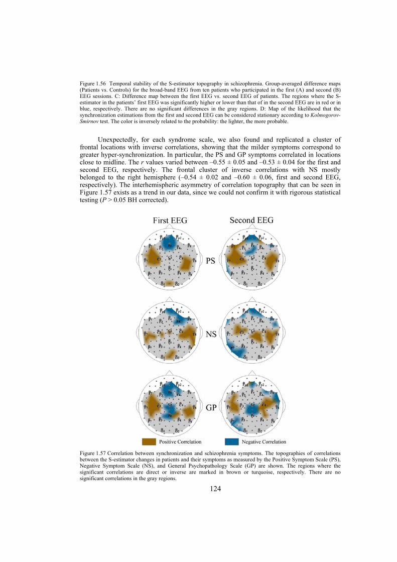
124

Figure 1.56 Temporal stability of the S-estimator topography in schizophrenia. Group-averaged difference maps (Patients vs. Controls) for the broad-band EEG from ten patients who participated in the first (A) and second (B) EEG sessions. C: Difference map between the first EEG vs. second EEG of patients. The regions where the S-estimator in the patients’ first EEG was significantly higher or lower than that of in the second EEG are in red or in blue, respectively. There are no significant differences in the gray regions. D: Map of the likelihood that the synchronization estimations from the first and second EEG can be considered stationary according to Kolmogorov-Smirnov test. The color is inversely related to the probability: the lighter, the more probable.

Unexpectedly, for each syndrome scale, we also found and replicated a cluster of frontal locations with inverse correlations, showing that the milder symptoms correspond to greater hyper-synchronization. In particular, the PS and GP symptoms correlated in locations close to midline. The r values varied between –0.55 ± 0.05 and –0.53 ± 0.04 for the first and second EEG, respectively. The frontal cluster of inverse correlations with NS mostly belonged to the right hemisphere (–0.54 ± 0.02 and –0.60 ± 0.06, first and second EEG, respectively). The interhemispheric asymmetry of correlation topography that can be seen in Figure 1.57 exists as a trend in our data, since we could not confirm it with rigorous statistical testing (P > 0.05 BH corrected).

Figure 1.57 Correlation between synchronization and schizophrenia symptoms. The topographies of correlations between the S-estimator changes in patients and their symptoms as measured by the Positive Symptom Scale (PS), Negative Symptom Scale (NS), and General Psychopathology Scale (GP) are shown. The regions where the significant correlations are direct or inverse are marked in brown or turquoise, respectively. There are no significant correlations in the gray regions.

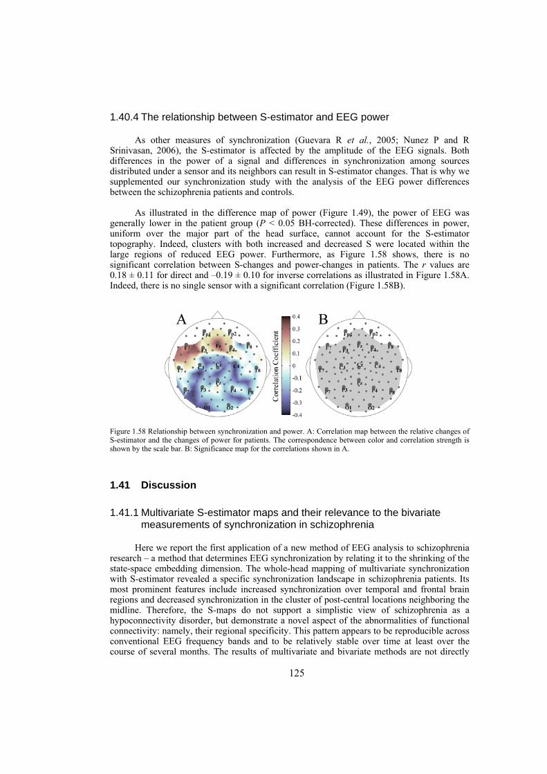
125

1.40.4 The relationship between S-estimator and EEG power

As other measures of synchronization (Guevara R et al., 2005; Nunez P and R Srinivasan, 2006), the S-estimator is affected by the amplitude of the EEG signals. Both differences in the power of a signal and differences in synchronization among sources distributed under a sensor and its neighbors can result in S-estimator changes. That is why we supplemented our synchronization study with the analysis of the EEG power differences between the schizophrenia patients and controls.

As illustrated in the difference map of power ( Figure 1.49), the power of EEG was generally lower in the patient group (P < 0.05 BH-corrected). These differences in power, uniform over the major part of the head surface, cannot account for the S-estimator topography. Indeed, clusters with both increased and decreased S were located within the large regions of reduced EEG power. Furthermore, as Figure 1.58 shows, there is no significant correlation between S-changes and power-changes in patients. The r values are 0.18 ± 0.11 for direct and –0.19 ± 0.10 for inverse correlations as illustrated in Figure 1.58A. Indeed, there is no single sensor with a significant correlation ( Figure 1.58B).

Figure 1.58 Relationship between synchronization and power. A: Correlation map between the relative changes of S-estimator and the changes of power for patients. The correspondence between color and correlation strength is shown by the scale bar. B: Significance map for the correlations shown in A.

1.41 Discussion

1.41.1 Multivariate S-estimator maps and their relevance to the bivariate measurements of synchronization in schizophrenia

Here we report the first application of a new method of EEG analysis to schizophrenia research – a method that determines EEG synchronization by relating it to the shrinking of the state-space embedding dimension. The whole-head mapping of multivariate synchronization with S-estimator revealed a specific synchronization landscape in schizophrenia patients. Its most prominent features include increased synchronization over temporal and frontal brain regions and decreased synchronization in the cluster of post-central locations neighboring the midline. Therefore, the S-maps do not support a simplistic view of schizophrenia as a hypoconnectivity disorder, but demonstrate a novel aspect of the abnormalities of functional connectivity: namely, their regional specificity. This pattern appears to be reproducible across conventional EEG frequency bands and to be relatively stable over time at least over the course of several months. The results of multivariate and bivariate methods are not directly

126

comparable, since they approach different aspects of the synchronization phenomenon. Nevertheless, being used in the analysis of the same data, various measures of synchronization detect coupling, although with different sensitivity (Carmeli C et al., 2005; Quiroga R et al., 2002). In particular, the S-estimator and spectral coherence analyses yield similar results (cf. (Carmeli C et al., 2005; Knyazeva MG et al., 2006)). With this in mind, we turn to the qualitative comparison of our results with those from preceding studies.

The analysis of the resting-state EEG synchronization in schizophrenia with bivariate methods has resulted in quite a mixed picture, which includes both increased and decreased synchrony between a few pre-selected pairs of EEG signals. Increased EEG coherence values in schizophrenia patients have frequently been shown occurring both intra- (Mann K et al., 1997; Merrin E et al., 1989; Wada Y et al., 1998) and inter-hemispherically (Merrin E et al., 1989; Nagase Y et al., 1992). Yet a reduction in coherence has also commonly been reported (Flor-Henry P and Z Koles, 1984; Merrin E and T Floyd, 1996; Tauscher J et al., 1998; Winterer G et al., 2001; Yeragani V et al., 2006). Unfortunately, the coherence estimates obtained with the common vertex or linked ears references, as was the case for some of these reports, are difficult to interpret. Moreover, our synchronization estimates do not include long-distance connections (> 12 cm). That leaves us with only several qualitatively compatible papers reporting (phase) coherence for common average reference, bipolar, or Laplacian EEG.

In a broad sense, the hyper-synchronized temporal clusters shown here are consistent with the intrahemispheric coherence increase shown previously for the pairs composed by frontal, central, temporal, and parietal electrodes (Mann K et al., 1997; Merrin E et al., 1989; Wada Y et al., 1998). Furthermore, a common trend is revealed by the S-estimator decrease in the parietal midline cluster and by the reduction in inter-hemispheric coherence reported earlier (Flor-Henry P and Z Koles, 1984; Merrin E and T Floyd, 1996; Pinkofsky H et al., 1997; Winterer G et al., 2001). Yet it should be noted that the S-maps reported here present overwhelmingly more detailed evidence of the surface topography of synchronization than bivariate measurements do. Such maps of abnormal regional coordination among the neurophysiological processes distributed across cortical areas might greatly boost the potential of EEG as a diagnostic tool, provided that they correlate with the fundamental features of schizophrenia.

1.41.2 S-estimator maps and the clinical picture of schizophrenia

We have chosen to correlate S-maps with the PANSS which is a conventional diagnostic tool, although there are disadvantages to this choice. In particular, the PANSS subscales represent constellations of various features, the brain counterparts of which might partially overlap. That does not allow us to reveal the full potential of the state-space mapping of EEG synchronization for topographically dissociating the brain sources underlying schizophrenia. Yet this drawback is outweighed by the advantages of addressing the summarized picture of schizophrenia and of obtaining results compatible with previous observations. According to our findings, the severity of both positive and negative symptoms directly correlates with the S-increase within the hyper-synchronized temporal clusters and in their neighborhood (cf. Figure 1.54, Figure 1.55, Figure 1.56, and Figure 1.57). Although we found bilateral correlations for both scales, the positive symptoms show a more stable pattern over the left hemisphere, while the negative symptoms reveal a repeatable pattern over the right hemisphere.

These findings are consistent with different lines of evidence relating left-side temporal lobe abnormalities to the positive type of symptoms. Specifically, the reduction of the entire volume of the superior temporal gyrus correlates with the positive syndrome (Flaum M et al.,

127

1995; Nestor P et al., 2007), whereas the decrease of its anterior part correlates with auditory hallucinations (Barta P et al., 1990). The abnormalities of regional cerebral blood flow in the left temporal lobe might also be related to the positive symptoms in schizophrenia (Klemm E et al., 1996). Interestingly, the schizophrenia-like psychoses with positive symptoms in epilepsy are associated with the left temporal lobe lesions (Roberts G et al., 1990). Electrical stimulation of the superior temporal gyrus results in auditory hallucinations and disordered thinking (Haglund M et al., 1992). Recent findings specifically support both the increase in temporal connectivity and its association with positive symptoms in schizophrenia. In patients with hallucinations, a diffusion tensor imaging study (Hubl D et al., 2004) found increased white matter directionality in the arcuate fasciculus compared with controls or patients without hallucinations, these differences being most prominent in the left hemisphere. Thus, our findings are both consistent with and complementary to the evidence reported previously. They suggest that functional intra-hemispheric hyper-connectivity might be the basis of the positive symptoms.

The correlation pattern between the S-estimator and the negative symptoms is consistent with current knowledge of the relationship between the underlying functional deficits and the functional specialization of the right hemisphere. This refers to such functions as perception and/or expression of affect controlled by the right hemisphere (Heilman K and R Gilmore, 1998; Kyle N, 1988; Pell M, 2006) and compromised in schizophrenia (Kucharska-Pietura K, 2006). This is also valid for the higher-order language functions including discourse planning and comprehension, understanding humor and metaphors, and generation and comprehension of emotional prosody mediated by the right hemisphere (Mitchell RL and TJ Crow, 2005). They are essential for social communication, which is also impaired in schizophrenia (Cutting J, 1992; Mitchell RL and TJ Crow, 2005; Ross E et al., 2001). Although the negative symptoms are mostly associated with the frontal lobe changes (see further in this Discussion), recent imaging studies support the involvement of the bilateral or right-hemisphere temporal structures. Among them is an MRI study that found a bilateral reduction of superior temporal gyrus gray matter in schizophrenia patients with predominantly negative symptoms (Anderson J et al., 2002). A PET study showed that patients with mainly negative symptoms had lower metabolic rates in the right hemisphere, especially in the temporal and ventral prefrontal cortices, compared both to patients with positive symptoms and to normal subjects (Potkin S et al., 2002). The General Psychopathology Scale showed a somewhat different topography of correlations. Along with bilateral temporal clusters of direct correlations similar to those found for the positive syndrome, we demonstrated inverse correlations within the hypo-synchronized postcentral midline region (cf. Figure 1.54, Figure 1.55, Figure 1.56, and Figure 1.57), which point to the fact that the severity of the symptoms increases with a decrease in synchronization. This is not surprising, considering that in schizophrenia many fundamental psychotic features, including the lack of awareness, impaired control of actions, poor attention, increased reaction times, etc., are associated with the abnormal functioning of the superior parietal cortex (Gallagher S, 2004; Honey G et al., 2002).

In contrast to the intrahemispheric temporal and midline postcentral clusters, the frontal correlations shown here were omnipresent across all the types of symptoms, and, surprisingly, revealed an inverse relationship between the severity of schizophrenia symptoms and synchronization abnormality. Although such counter-intuitive links were previously found between clinical improvement and medial frontal gray matter loss (Vidal C et al., 2006), or between clinical improvement and hemisphere volume reduction (DeLisi L et al., 1998), more observations are required for a meaningful interpretation of these data. On the whole, with the correlation analysis, we confirmed the clinical relevance of the S-estimator maps. Specifically, the topography of correlations overlapped with the topography of synchronization changes in schizophrenia patients compared to the control subjects.

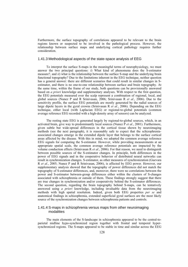
128

Furthermore, the surface topography of correlations appeared to be relevant to the brain regions known or suspected to be involved in the pathological process. However, the relationship between surface maps and underlying cortical pathology requires further consideration.

1.41.3 Methodological aspects of the state-space analysis of EEG

To interpret the surface S-maps in the meaningful terms of neurophysiology, we must answer the two principal questions: i) What kind of phenomena does the S-estimator measure?, and ii) what is the relationship between the surface S-map and the underlying brain functional topography? Due to the limitations inherent in the EEG technique, neither question has a general answer: there are different scenarios that could result in similar changes in S-estimator, and there is no one-to-one relationship between surface and brain topography. At the same time, within the frame of our study, both questions can be provisionally answered based on a priori knowledge and supplementary analyses. With respect to the first question, the EEG potentials measured over the scalp represent a combination of regional, local, and global sources (Nunez P and R Srinivasan, 2006; Srinivasan R et al., 2006). Due to the sensitivity profile, the surface EEG potentials are mostly generated by the radial sources of large dipole layers in the gyral crowns (Srinivasan R et al., 2006). Depending on the EEG technique, either local (with Laplacian EEG) or regional-to-global potentials (common average reference EEG recorded with a high-density array of sensors) can be analyzed.

The resting state EEG is generated largely by regional-to-global sources, which, in an activated brain, give way to predominantly local sources (Nunez P et al., 2001). Furthermore, given subtle but wide-spread differences in the cortical tissue shown by neuroimaging methods (see the next paragraph), it is reasonably safe to expect that the schizophrenia-associated changes emerge in the extended dipole layer that belongs to the surface cortical areas affected by the disease. With this in mind, we adopted the common average reference EEG signals for computing the S-estimator. However, while providing measurements at an appropriate spatial scale, the common average reference potentials are impacted by the volume conduction effects (Srinivasan R et al., 2006). For that reason, we need to distinguish between possible sources of the S-estimator changes. In principle, both differences in the power of EEG signals and in the cooperative behavior of distributed neural networks can result in synchronization changes. S-estimator, as other measures of synchronization (Guevara R et al., 2005; Nunez P and R Srinivasan, 2006), is affected by EEG power. However, our supplementary analysis showed that the topography of power differences did not match the topography of S-estimator differences, and, moreover, there were no correlations between the power and S-estimator between-group differences either within the clusters of S-changes associated with schizophrenia or outside of them. These findings strongly suggest that there are true changes in synchronization and/or cooperativity behind the S-estimator differences. The second question, regarding the brain topography behind S-maps, can be tentatively answered using a priori knowledge, including invaluable data from the neuroimaging methods with high spatial resolution. Indeed, given both EEG properties per se and anatomical findings in schizophrenia, extended superficial gyral surfaces are the most likely source of the synchronization changes between schizophrenia patients and controls.

1.41.4 S-maps in schizophrenia versus maps from other neuroimaging modalities

The main elements of the S-landscape in schizophrenia appeared to be the central-to-parietal midline hypo-synchronized region together with frontal and temporal hyper-synchronized regions. The S-maps appeared to be stable in time and similar across the EEG

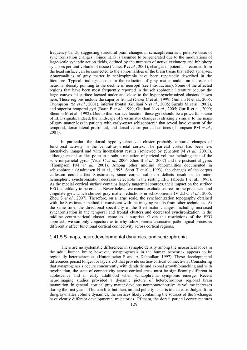
129

frequency bands, suggesting structural brain changes in schizophrenia as a putative basis of synchronization changes. Since EEG is assumed to be generated due to the modulations of large-scale synaptic action fields, defined by the numbers of active excitatory and inhibitory synapses per unit volume of tissue (Nunez P et al., 2001), changes in potentials recorded from the head surface can be connected to the abnormalities of the brain tissue that affect synapses. Abnormalities of gray matter in schizophrenia have been repeatedly described in the literature. Typical findings consist in the reduction of gray matter and/or an increase of neuronal density pointing to the decline of neuropil (see Introduction). Some of the affected regions that have been most frequently reported in the schizophrenia literature occupy the large convexital surface located under and close to the hyper-synchronized clusters shown here. These regions include the superior frontal (Gaser C et al., 1999; Giuliani N et al., 2005; Thompson PM et al., 2001), inferior frontal (Giuliani N et al., 2005; Suzuki M et al., 2002), and superior temporal gyri (Barta P et al., 1990; Giuliani N et al., 2005; Gur R et al., 2000; Shenton M et al., 1992). Due to their surface location, these gyri should be a powerful source of EEG signals. Indeed, the landscape of S-estimator changes is strikingly similar to the maps of gray matter loss in patients with early-onset schizophrenia that reveal involvement of the temporal, dorso-lateral prefrontal, and dorsal centro-parietal cortices (Thompson PM et al., 2001).

In particular, the dorsal hypo-synchronized cluster probably captured changes of functional activity in the central-to-parietal cortex. The parietal cortex has been less intensively imaged and with inconsistent results (reviewed by (Shenton M et al., 2001)), although recent studies point to a subtle reduction of parietal volume including that of the superior parietal gyrus (Vidal C et al., 2006; Zhou S et al., 2007) and the postcentral gyrus (Thompson PM et al., 2001). Among other midline abnormalities documented in schizophrenia (Andreasen N et al., 1995; Scott T et al., 1993), the changes of the corpus callosum could affect S-estimator, since corpus callosum defects result in an inter-hemispheric synchronization decrease detectable in the resting EEG (Koeda T et al., 1995). As the medial cortical surface contains largely tangential sources, their impact on the surface EEG is unlikely to be crucial. Nevertheless, we cannot exclude sources in the precuneus and cingulate gyri, which showed gray matter reductions in schizophrenia (Vidal C et al., 2006; Zhou S et al., 2007). Therefore, on a large scale, the synchronization topography obtained with the S-estimator method is consistent with the imaging results from other techniques. At the same time, the directional specificity of the S-estimator changes, including increased synchronization in the temporal and frontal clusters and decreased synchronization in the midline centro-parietal cluster, came as a surprise. Given the restrictions of the EEG approach, we can only conjecture as to why schizophrenia-associated pathological processes differently affect functional cortical connectivity across cortical regions.

1.41.5 S-maps, neurodevelopmental dynamics, and schizophrenia

There are no systematic differences in synaptic density among the neocortical lobes in the adult human brain; however, synaptogenesis in the human neocortex appears to be regionally heterochronous (Huttenlocher P and A Dabholkar, 1997). These developmental differences persist longer for layers 2-3 that provide cortico-cortical connectivity. Considering that synaptogenesis occurs concurrently with dendritic and axonal growth/branching and with myelination, the state of connectivity across cortical areas must be significantly different in adolescence and in early adulthood when schizophrenia symptoms emerge. Recent neuroimaging studies provided a dynamic picture of heterochronous regional brain maturation. In general, cortical gray matter develops nonmonotonously: its volume increases during the first years of human life, but then, around puberty it starts to decrease. Judged from the gray-matter volume dynamics, the cortices likely containing the sources of the S-changes have clearly different developmental trajectories. Of them, the dorsal parietal cortex matures

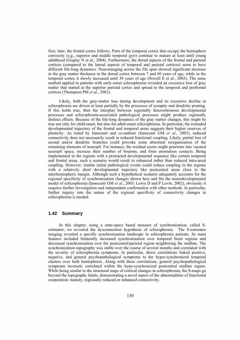
130

first; later, the frontal cortex follows. Parts of the temporal cortex that occupy the hemisphere convexity (e.g., superior and middle temporal gyri) continue to mature at least until young adulthood (Gogtay N et al., 2004). Furthermore, the dorsal aspects of the frontal and parietal cortices (compared to the lateral aspects of temporal and parietal cortices) seem to have different life-long dynamics. Neuroimaging across the life span showed significant decrease in the gray matter thickness in the dorsal cortex between 7 and 60 years of age, while in the temporal cortex it slowly increased until 30 years of age (Sowell E et al., 2003). The same method applied to patients with early-onset schizophrenia revealed an excessive loss of gray matter that started at the superior parietal cortex and spread to the temporal and prefrontal cortices (Thompson PM et al., 2001).

Likely, both the gray-matter loss during development and its excessive decline in schizophrenia are driven at least partially by the processes of synaptic and dendritic pruning. If this holds true, then the interplay between regionally heterochronous developmental processes and schizophrenia-associated pathological processes might produce regionally distinct effects. Because of the life-long dynamics of the gray matter changes, this might be true not only for child-onset, but also for adult-onset schizophrenia. In particular, the extended developmental trajectory of the frontal and temporal areas suggests their higher reserves of plasticity. As noted by Innocenti and co-authors (Innocenti GM et al., 2003), reduced connectivity does not necessarily result in reduced functional coupling. Likely, partial loss of axonal and/or dendritic branches could provoke some abnormal reorganization of the remaining elements of neuropil. For instance, the residual axons might penetrate into vacated neuropil space, increase their number of boutons, and form anomalous contacts. Being implemented in the regions with a protracted developmental sequence like certain temporal and frontal areas, such a scenario would result in enhanced rather than reduced intra-areal coupling. However, similar initial pathological events could reduce coupling in the regions with a relatively short developmental trajectory like postcentral areas close to the interhemispheric margin. Although such a hypothetical scenario adequately accounts for the regional specificity of synchronization changes shown here and fits the neurodevelopmental model of schizophrenia (Innocenti GM et al., 2003; Lewis D and P Levitt, 2002), obviously it requires further investigation and independent confirmation with other methods. In particular, further inquiry into the nature of the regional specificity of connectivity changes in schizophrenia is needed.

1.42 Summary

In this chapter, using a state-space based measure of synchronization, called S-estimator, we revealed the dysconnection hypothesis of schizophrenia. The S-estimator imaging revealed a specific synchronization landscape in schizophrenia patients. Its main features included bilaterally increased synchronization over temporal brain regions and decreased synchronization over the postcentral/parietal region neighboring the midline. The synchronization topography was stable over the course of several months and correlated with the severity of schizophrenia symptoms. In particular, direct correlations linked positive, negative, and general psychopathological symptoms to the hyper-synchronized temporal clusters over both hemispheres. Along with these correlations, general psychopathological symptoms inversely correlated within the hypo-synchronized postcentral midline region. While being similar to the structural maps of cortical changes in schizophrenia, the S-maps go beyond the topography limits, demonstrating a novel aspect of the abnormalities of functional cooperation: namely, regionally reduced or enhanced connectivity.

131

TOPOGRAPHY OF EEG MULTIVARIATE PHASE SYNCHRONIZATION IN EARLY ALZHEIMER’S DISEASE

Personal Contribution — After a brief introduction to Alzheimer’s disease, this chapter represents our original work published in Neurobiology of Aging, where I am the joint first-author with Maria G. Knyazeva. Patients with Alzheimer’s disease were recruited from the Memory Clinic of the Neurology Department, Lausanne University Hospital. The clinical diagnosis was made by Andrea Bioschi, Isabelle Bourquin, and Joseph Ghilka and EEG data was collected by Maria G. Knyazeva. I analyzed the data and together with Maria G. Knyazeva and M. Hasler, we interpreted the results.

1.43 Alzheimer’s disease, a neurodegenerative brain disorder

Alzheimer's disease (AD) is the most common cause of dementia accounting for the 50-70% of the cases, named for German physician Alois Alzheimer, who first described in 1906 (Alzheimer A, 1907). The disease is usually manifested in persons older than 60. In average, 2% of the individuals aging 65-74, 19% aging 75-84 and 42% older than 85 have AD. The average cost of care for a person with AD is about $77000. AD destroys brain cells, causing lots of problems with memory, thinking and behavior severe enough to affect work, lifelong hobbies or social life. It also gets worse over time, and is a fatal disease. Just like the rest of the body, brains change- as people age. Most of aged persons show some kind of slowed thinking and occasional problems remembering certain things. However, serious memory loss, confusion and other major changes in the way the mind works are not a normal part of aging. They may be a sign that brain cells are failing. They may be the signs of AD. Some other signs of the disease are difficulty in performing familiar tasks, problems with language, disorientation with time and place, poor or decreased judgment, problems with abstract thinking, misplacing things, change in mood or behavior, changes in personality, and loss of initiative. Although the symptoms are not common, people commonly experience them in a unique way. The duration of the disease is between 5 and 20 years. The brains of individuals with AD have an abundance of plaques and tangles. Plaques are deposits of a

132

protein fragment called beta-amyloid that build up in the spaces between nerve cells. Tangles are twisted fibers of another protein called tau that build up inside cells. They are developed first in the areas important for memory and then spread to the regions of the brain until affect the whole brain. However, scientists do not know exactly what the role of plaques and tangles is in AD. Most of them believe that they somehow play a critical role in blocking communication among nerve cells and disrupting processes the cells need to survive. It’s the destruction and death of nerve cells that causes the memory failure, personality changes, problems in carrying out daily activities and other symptoms of AD. The most important risk factor of AD is age; as people age, the probability that they are affected by AD increases. Other factors are family history and genetics, eating a healthy diet, staying socially active, avoiding tobacco and excess alcohol, and exercising both body and mind.

AD is usually developed in a number of stages, starting from some memory problem to a very severe case of AD and finally death6. The first stage of AD is very mild cognitive decline when individuals may feel as if they have memory lapses. They may forget some familiar words, location of thing in the kitchen, or any everyday subject. However, the problems are not evident to the family members until the person is diagnosed. The second stage is mild cognitive decline when family members and friends begin to notice the problem. At this stage, the individual has problems such as name-finding, remembering names, misplacing an object, and decline in the ability to plan. The next stage is moderate cognitive decline. At this stage, the patient shows decreased ability to organize complex planning, reduced memory of personal history, and decreased knowledge of recent or current events. Forth stage is moderately severe cognitive decline, which is the moderate or mid-stage AD. Patients, in this stage, are unable to remember their telephone number, their address, and the name of their high school. They become confused all the time and need help choosing proper clothing for the season. However, they retain substantial knowledge about themselves, know their own name, name of their children, and require no assistance with eating or using the toilet. The next stage is moderately severe AD when memory deficits continue to worsen and the patients need extensive help for handling their daily activities. At this stage, individuals may loose most awareness of recent experiences, occasionally forget the name of their children, need help getting dressed, experience disruption of their normal sleep, and experiencing significant personality changes. The last stage is severe or late-stage AD with very severe cognitive decline. This is the final stage of the disease when patients lose the ability to respond to the environment, the ability to speak, and the ability to control movement. They need full help for their daily activities, their reflexes become abnormal and muscles grow rigid. Unfortunately, the disease is ended with death of the individual.

1.43.1 AD diagnoses and treatment

AD by definition is a clinical condition and can be diagnosed with careful testing. AD is usually clinically diagnosed based on the presence of characteristic neurological and neuropsychological features and the absence of alternative diagnoses. Neurological diagnoses is made by utilizing the individual’s history and clinical history, where neuropsychological evaluation includes memory testing and assessment of intellectual functioning. The diagnostic criterion NINCDS-ADRAD (McKhann G, Drachman D et al., 1984) is among the most

6 Detailed explanation of these stages could be found at (www.alz.org); interested readers are adviced to refere to this web page.

133

frequently used in AD-related clinical studies. It requires that the presence of cognitive impairment or by testing for a clinical diagnoses of probable AD while they need histopathological confirmation for the definitive diagnosis, i.e. by microscopic examination of brain tissue. The method has shown good validity and reliability. It tests eight cognitive factors that maybe impaired in AD, These factors include memory, perceptual skills, attention, language, constructive abilities, orientation, problem solving, and functional abilities. Neuropsychological tests such as mini mental state examination (MMSE) are frequently used for evaluating the cognitive impairments needed for diagnosis. In addition, interviews with family members are also utilized in the assessment of the disease. This is especially important, since an individual with AD is usually unaware of his/her own deficit. Supplement test such as blood test provide extra information on some features of the disease. Also, increasingly neuroimaging techniques such as PET are being used to diagnose AD.

Unfortunately, currently there is no cure for AD and no way to stop the underlying death of brain cells, but scientific research is bringing us closer to a cure every day. Because there is no cure, managing the disease usually involves medications to control symptoms, in combination with various non-drug strategies designed to ease the suffering of the person afflected by the disease as well as his/her family and caregiver. The drugs cannot stop the disease, but they can slow the progression of symptoms in some people, at least for a while. Although drug therapy is important and beneficial, especially in early stages, the management of AD has evolved to include non-drug therapies as integral aspects of care. These include various strategies aimed at managing problematic behaviors, including involvement in therapeutic activities, home or environmental modifications, and the use of appropriate communication techniques. Support and education for caregivers and family members is also crucial to the best care of people with AD. Outstanding progress has already been made in unraveling the mysteries of AD. New understandings about these processes have already provided critical information about how doctors might prevent, delay, stop or even reverse the nerve cell damage that leads to the devastating symptoms of AD. All around the world, scientists and pharmaceutical companies are now racing to develop treatments that address the underlying disease processes, some (or a combination) of which might effectively solve the puzzle of AD.

1.44 EEG Synchronization in AD patients

AD is a neurodegenerative disorder characterized by progressive cognitive deterioration starting with memory loss and leading to the impairment of daily life activities, to neuropsychiatric symptoms, to mental and behavioral disturbances, and finally to motor deficits. The key features of AD include the accumulation of beta-amyloid and tau-protein fragments predominantly in the associative cortical areas, the dysfunction and loss of synapses, and, as recently emphasized, myelination breakdown. These abnormalities are likely to disrupt cortical circuitry and, therefore, cooperation between and within the distributed neural populations underlying human cognition.

The EEG/MEG synchronization studies of cooperation in the brain networks have been mostly implemented with spectral analysis using power and coherence functions. With these techniques, a decrease in local and distant synchronization has been repeatedly shown in AD. In particular, the recognized EEG sign of AD is a reduction in the power of alpha and higher frequencies (the so called “EEG slowing”) supposedly due to the failure in local synchronization (Fernández A et al., 2006; Jelic V et al., 1996; Lindau M et al., 2003). Similarly, the EEG coherence (or phase) analysis revealed a decrease in distant (intra- and inter-hemispheric) synchronization typical for (although not limited to) the alpha frequencies

134

(Adler G et al., 2003; Brandes U, 2001; Comi G and L Leocani, 1999; Hogan MJ et al., 2003; Locatelli T et al., 1998; Pijnenburg YA et al., 2004). Unfortunately, these EEG signs cannot adequately specify the type of cognitive impairment and accompany various types of dementia. Moreover, these methods reveal abnormalities only in moderate to severe dementia, while in patients with mild impairment the EEGs may seem normal (Jeong J, 2004). Conventionally, the EEG studies in AD have applied a bivariate analysis of synchronization. Its limitations have been discussed previously (Jalili M, S Lavoie et al., 2007). They are especially noticeable in the modern multichannel EEG applications and particularly critical for the studies of distributed brain (dys)functions as AD. Recently, multivariate measures of synchronization have been coming into use (Allefeld C and J Kurths, 2004; Carmeli C et al., 2005; Stam CJ et al., 2003; Stam CJ and BW van Dijk, 2002). In particular, the measure of synchronization likelihood was successfully applied to AD research ((Babiloni C et al., 2006; Stam CJ et al., 2003) among others). Converging evidence from these studies points to the decreased synchronization at least across the alpha to beta range of the resting EEG. However, these multivariate measures were used in AD research either to estimate global synchronization, or were reduced to just measuring synchronization in pairs of predetermined EEG signals.

In principle, the multivariate measures combined with high-density EEG can provide the whole-head surface topography of synchronization. Our recent application of the S-estimator technique to schizophrenia research resulted in the specific synchronization landscape relevant to the clinical picture of the disease (Jalili M, S Lavoie et al., 2007). Therefore, the multivariate measures might be more efficient both for detecting the EEG signature of a particular brain pathology and for the early diagnostics and monitoring of a treatment or progression of diseases with distributed brain lesions. Here we report the whole-head mapping of multivariate phase synchronization (MPS) in patients with early AD. Two (or more) systems are argued to be phase synchronized if their relative phases evolve in the same manner regardless of their amplitudes. The MPS measures the degree of phase synchronization within multivariate time series and allows synchronization-mapping in spatially extended systems.

With this multivariate approach to synchronization analysis, we test the hypothesis that early AD is accompanied by changes in regional EEG synchronization related to the known damage of associative cortical areas and correlated with the severity of AD symptoms. To this end, we apply the MPS technique to the resting state EEG of AD patients and matched elderly controls. We characterize the surface topography of the synchronization abnormalities in AD by a decrease in MPS over the fronto-temporal and an increase over the temporo-parieto-occipital regions and show their relevance to the clinical picture of AD.

1.45 Subjects and EEG recording

1.45.1 AD Patients and control subjects

Seventeen newly diagnosed AD patients were recruited from the Memory Clinic of the Neurology Department (CHUV, Lausanne). The AD group included 6 women and 11 men (Table 9.1). Seventeen control subjects (11 women and 6 men) were volunteers enrolled mostly from partners, caregivers, or family members of the patients. The patient and control groups differed neither in age (P = 0.63) nor in their level of education (P = 0.18). All the patients, caregivers, and control subjects gave written informed consent. All the applied procedures conform to the Declaration of Helsinki (1964) by the World Medical Association

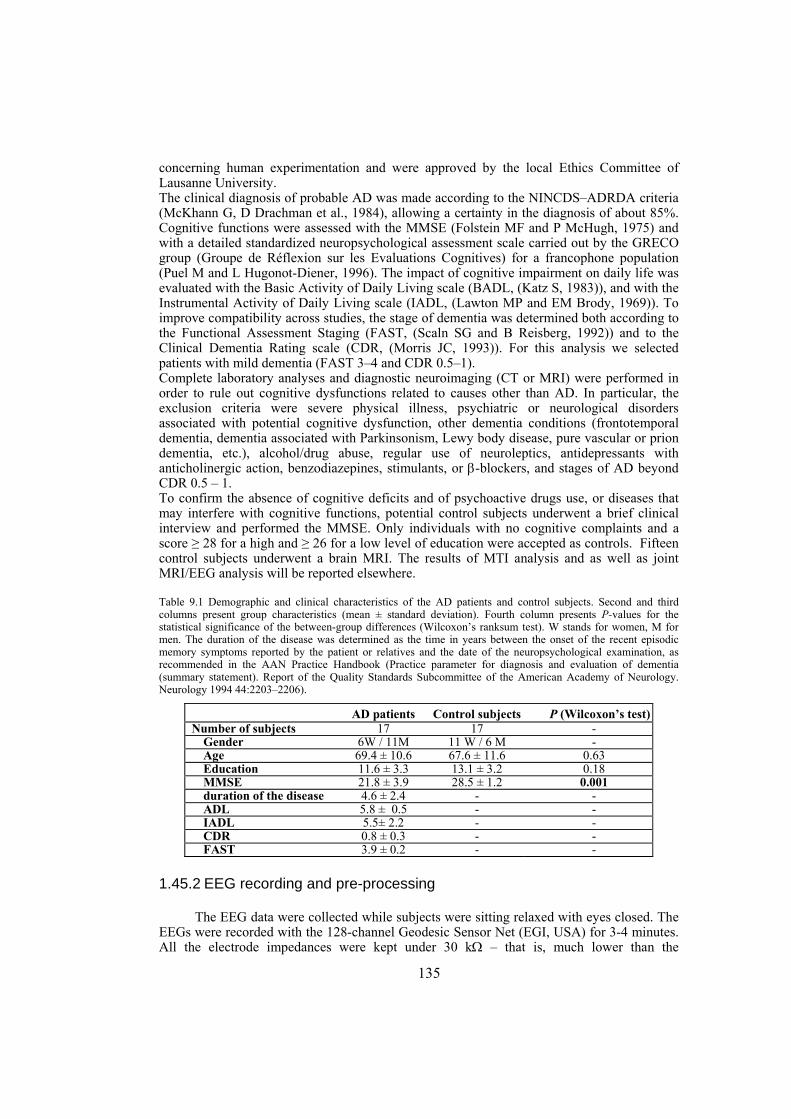
135

concerning human experimentation and were approved by the local Ethics Committee of Lausanne University. The clinical diagnosis of probable AD was made according to the NINCDS–ADRDA criteria (McKhann G, D Drachman et al., 1984), allowing a certainty in the diagnosis of about 85%. Cognitive functions were assessed with the MMSE (Folstein MF and P McHugh, 1975) and with a detailed standardized neuropsychological assessment scale carried out by the GRECO group (Groupe de Réflexion sur les Evaluations Cognitives) for a francophone population (Puel M and L Hugonot-Diener, 1996). The impact of cognitive impairment on daily life was evaluated with the Basic Activity of Daily Living scale (BADL, (Katz S, 1983)), and with the Instrumental Activity of Daily Living scale (IADL, (Lawton MP and EM Brody, 1969)). To improve compatibility across studies, the stage of dementia was determined both according to the Functional Assessment Staging (FAST, (Scaln SG and B Reisberg, 1992)) and to the Clinical Dementia Rating scale (CDR, (Morris JC, 1993)). For this analysis we selected patients with mild dementia (FAST 3–4 and CDR 0.5–1). Complete laboratory analyses and diagnostic neuroimaging (CT or MRI) were performed in order to rule out cognitive dysfunctions related to causes other than AD. In particular, the exclusion criteria were severe physical illness, psychiatric or neurological disorders associated with potential cognitive dysfunction, other dementia conditions (frontotemporal dementia, dementia associated with Parkinsonism, Lewy body disease, pure vascular or prion dementia, etc.), alcohol/drug abuse, regular use of neuroleptics, antidepressants with anticholinergic action, benzodiazepines, stimulants, or β-blockers, and stages of AD beyond CDR 0.5 – 1. To confirm the absence of cognitive deficits and of psychoactive drugs use, or diseases that may interfere with cognitive functions, potential control subjects underwent a brief clinical interview and performed the MMSE. Only individuals with no cognitive complaints and a score ≥ 28 for a high and ≥ 26 for a low level of education were accepted as controls. Fifteen control subjects underwent a brain MRI. The results of MTI analysis and as well as joint MRI/EEG analysis will be reported elsewhere.

Table 9.1 Demographic and clinical characteristics of the AD patients and control subjects. Second and third columns present group characteristics (mean ± standard deviation). Fourth column presents P-values for the statistical significance of the between-group differences (Wilcoxon’s ranksum test). W stands for women, M for men. The duration of the disease was determined as the time in years between the onset of the recent episodic memory symptoms reported by the patient or relatives and the date of the neuropsychological examination, as recommended in the AAN Practice Handbook (Practice parameter for diagnosis and evaluation of dementia (summary statement). Report of the Quality Standards Subcommittee of the American Academy of Neurology. Neurology 1994 44:2203–2206).

AD patients Control subjects P (Wilcoxon’s test)Number of subjects 17 17 -

Gender 6W / 11M 11 W / 6 M - Age 69.4 ± 10.6 67.6 ± 11.6 0.63 Education 11.6 ± 3.3 13.1 ± 3.2 0.18 MMSE 21.8 ± 3.9 28.5 ± 1.2 0.001 duration of the disease 4.6 ± 2.4 - - ADL 5.8 ± 0.5 - - IADL 5.5± 2.2 - - CDR 0.8 ± 0.3 - - FAST 3.9 ± 0.2 - -

1.45.2 EEG recording and pre-processing

The EEG data were collected while subjects were sitting relaxed with eyes closed. The EEGs were recorded with the 128-channel Geodesic Sensor Net (EGI, USA) for 3-4 minutes. All the electrode impedances were kept under 30 kΩ – that is, much lower than the

136

recommended limit (50 kΩ) for the high-input-impedance EGI amplifiers. The recordings were made with vertex reference using a low-pass filter set to 100 Hz. The signals were digitized at a rate of 500 samples/s with a 12-bit analog-to-digital converter. They were filtered (FIR, band-pass of 1–50 Hz) and re-referenced against the common average reference. In multichannel EEG applications, this montage closely approximates reference-free potentials. The common-average-reference EEG signals from a high-density array of sensors provide the spatial scale appropriate for measuring the regional-to-global potentials dominating the resting state EEG (Srinivasan R et al., 2006). To obtain a higher confidence in the synchronization estimates, the signals were segmented into non-overlapping 1-second epochs (Nunez P and R Srinivasan, 2006). Using short segments for analysis allowed us to reach 205 ± 58 artifact-free epochs for the patients and 193 ± 72 for the controls. Artifacts in all channels were edited off-line: first, automatically, based on an absolute voltage threshold (100 μV) and on a transition threshold (50 μV), and then on the basis of a thorough visual inspection. The sensors that recorded artifactual EEG (> 20% of the recording time) were corrected using the bad channel replacement tool (NS 4.2 EGI, USA).

1.46 Data analysis

1.46.1 Multivariate Phase Synchronization as a measure of cooperativeness

Although several synchronization measures have been fruitfully used in EEG studies of AD, here we suggest a new strategy of Multivariate Phase Synchronization (MPS), mapping that has an obvious advantage due to the fact that the MPS method extends assessing synchronization from bivariate to multivariate time series. The bivariate methods are suitable for the analysis of several pairs of signals, but they become less efficient as the number of pairs is increased. In contrast, the MPS method successfully exploits the potential of modern multichannel EEG techniques by creating easily readable synchronization maps and, eventually, providing an unbiased overview of the changes in functional connectivity related to AD and other distributed brain pathologies. We computed MPS based on the instantaneous phase of the EEG time series determined by means of the Hilbert transform (Quiroga R et al., 2002). First, we obtained a phase value from each univariate filtered EEG time series at sensor position i, i.e. Yi(t), t = 1,…,L, where t indicates a sample in a single epoch and L is the number of available samples. In our case, an epoch of 1-second is sampled at 500 Hz, making L equal to 500. The Hilbert transform of Yi(t) is defined as

( )1( ) PI i

i

YY t d

tτ

τπ τ

+∞

−∞

=−∫% , (9.1)

where PI means the Cauchy principal value (Hahn SL, 1996). The instantaneous phase of the time series Yi is obtained as (Boccaletti S et al., 2002)

( ) ( )( )

arctan ii

i

Y tt

Y tϕ

⎛ ⎞= ⎜ ⎟⎜ ⎟

⎝ ⎠

%. (9.2)

Second, we estimated the degree of phase synchronization for multivariate phases. Let us consider a multivariate time series Y(t)

( ) ( ) , 1, ,it Y t i I= =Y K , (9.3)

137

where I is the number of univariate time series, i.e. the number of sensors for which the MPS is calculated. At each sample t, Y(t) is an I dimensional vector. In other words, Y is an I×L matrix. For each Y(t), the corresponding multivariate phases are obtained as φi(t), I = 1,…,I. The MPS is defined as (Boccaletti S et al., 2002)

( )

1 1

1MPS i

L Ij t

t ie

LIϕ

= =

= ∑ ∑ , (9.4)

where j is the imaginary unit. Therefore, the MPS is the mean phase synchrony averaged over the observation samples. In other words, for computing the MPS among sensors 1, 2, 3, and 4, first, the instantaneous phases of the corresponding time series are computed for each epoch using (9.2). Then, using (9.4), the value of MPS is calculated as an average of ( )ij te ϕ , i = 1,2,3,4 over these sensors and over the observation samples within an epoch. Finally, to obtain time-reliable measures, the MPS-values are averaged over artifact-free epochs. The MPS ranges from 1/ I for completely non-phase-synchronized systems to 1 for completely phase-synchronized systems.

In this study the MPS was computed for each sensor including its first- and second-nearest neighbors. These MPS values, averaged over all available EEG epochs, were presented as individual whole-head MPS maps for the delta (1-3 Hz), theta (3-7 Hz), alpha1 (7-9.5 Hz), alpha2 (9.5-13), beta1 (13-20 Hz), and beta2 (20-30 Hz) bands. In order to remove the effects of the general level of synchronization, each MPS map was relativized by subtracting its average value from the MPS-value of each sensor. Finally, the subjects’ MPS maps were collected into the two groups of AD patients and controls to be considered in the next step of analysis. The global phase synchronization (GPS), involving all sensors, was also computed using Eq. (3). The GPS values were averaged over epochs and pooled into two groups (patients and controls) for statistical analysis. The statistical analysis of the MPS and GPS values was performed with Student’s permutation t-test (Higgins JJ, 2004). Since the first- and the second-nearest neighbors of each sensor are involved in computing the MPS-value for that sensor, the P-values of the sensor-wise comparisons were corrected using the BH false discovery rate method (Benjamini Y and Y Hochberg, 1995). The BH-corrected P-values were taken as significant at P < 0.05. The computations were performed in MatLab.

1.46.2 Linear discriminant analysis of MPS

In order to test to what extent the distinctive features that emerged from the MPS analysis distinguish individual AD patients from control subjects, we applied a linear discriminant analysis (Bishop CM, 2006). In particular, the distinctive traits of the MPS landscapes were used for tuning a Fisher’s linear discriminator. Given the small number of available subjects, the statistical validation of the discriminator was performed by means of the leave-one-out cross-validation algorithm. That is, the discriminator was tuned and evaluated 34 times. Each subject, one by one, was iteratively left out during the tuning and used for evaluating the discriminator. The accuracy of the discriminator was computed as the proportion of the total number of classifications that were correct (Bishop CM, 2006).

1.46.3 Correlation analysis of MPS

To assess whether the differences in S landscapes of AD patients are linked to the clinical ratings, patients’ GPS- and MPS-values were correlated with the MMSE scores of the patients by means of the Spearman Rank Correlation, resulting in the correlation coefficient (r) and the corresponding level of statistical significance (P). To account for multiple (sensor-

138

wise) comparisons, the statistical significance was corrected according to the BH false discovery rate method (Benjamini Y and Y Hochberg, 1995)).

1.46.4 EEG power analysis

To describe our AD group in conventional EEG terms, we applied two measures of EEG power, one of them being sensor-specific and the other one an across-sensor average. First, for each sensor and epoch the power spectral density (PSD) was computed by means of Welch's averaged modified periodogram (Welch P, 1967). These PSDs were averaged sensor-wise across all available epochs. The whole-head topography of the changes in PSD was addressed via the maps of EEG power integrated over the delta (1–3 Hz), theta (3–7 Hz), alpha1 (7–9.5 Hz), alpha2 (9.5–13), beta1 (13–20 Hz), and beta2 (20–30 Hz) bands. Furthermore, the PSDs were averaged over all sensors, resulting in a single value for each subject. To test AD-related changes in EEG power, the average PSDs and PSD-maps were collected into the groups of AD patients and controls consisting of 17 members each and compared with the permutation Student’s t-test (Higgins JJ, 2004) with 5000 permutations, with BH correction when necessary.

1.47 Results

1.47.1 EEG power topography in AD patients

Considering that our group of patients is less severely affected than the majority of those studied previously (see the Discussion), we begin by presenting the results of the spectral analysis, which confirm that our patients carry the EEG abnormalities typical for AD. As can be seen in Figure 1.59A, the hallmark of EEG changes in AD – a shift of the power spectrum to the lower frequencies – is significant in this group. Indeed, the across-sensor average spectra of absolute power (left), supplemented by the probability graph of between-group differences (right), clearly show a decrease at frequencies over 10 Hz in contrast to an increase in the delta-theta diapason. The between-group difference maps of absolute power provide the surface topography of these abnormalities for conventional EEG bands within the delta-beta range ( Figure 1.59B). In particular, they illustrate that the low frequency activity increases over the frontal areas, whereas decreases in alpha2 and beta1 activity are spread over the whole head. A reduction of the fast beta rhythms is significant post-centrally and predominant over the right hemisphere.

1.47.2 Synchronization topography in AD patients

The GPS, which includes regional and long-distance synchronization across all sensors, showed neither significant between-group difference (P > 0.17), nor correlation with the patients’ MMSE scores (P > 0.39) in any EEG band. Importantly, our data showed a high variation of GPS among subjects. The standard deviations among patients and controls ranged from 51% to 58% of the respective means across EEG bands. To separate these global effects from regional changes, we further analyzed individual maps relativized to their mean MPS level. Figure 1.60 shows the between-group differences of such relative MPS maps for conventional EEG frequency bands. Note that the value of a significant between-group variation in MPS, assigned to a single sensor as a color spot, represents phase synchronization of a region limited to the second-order neighbors of this sensor.

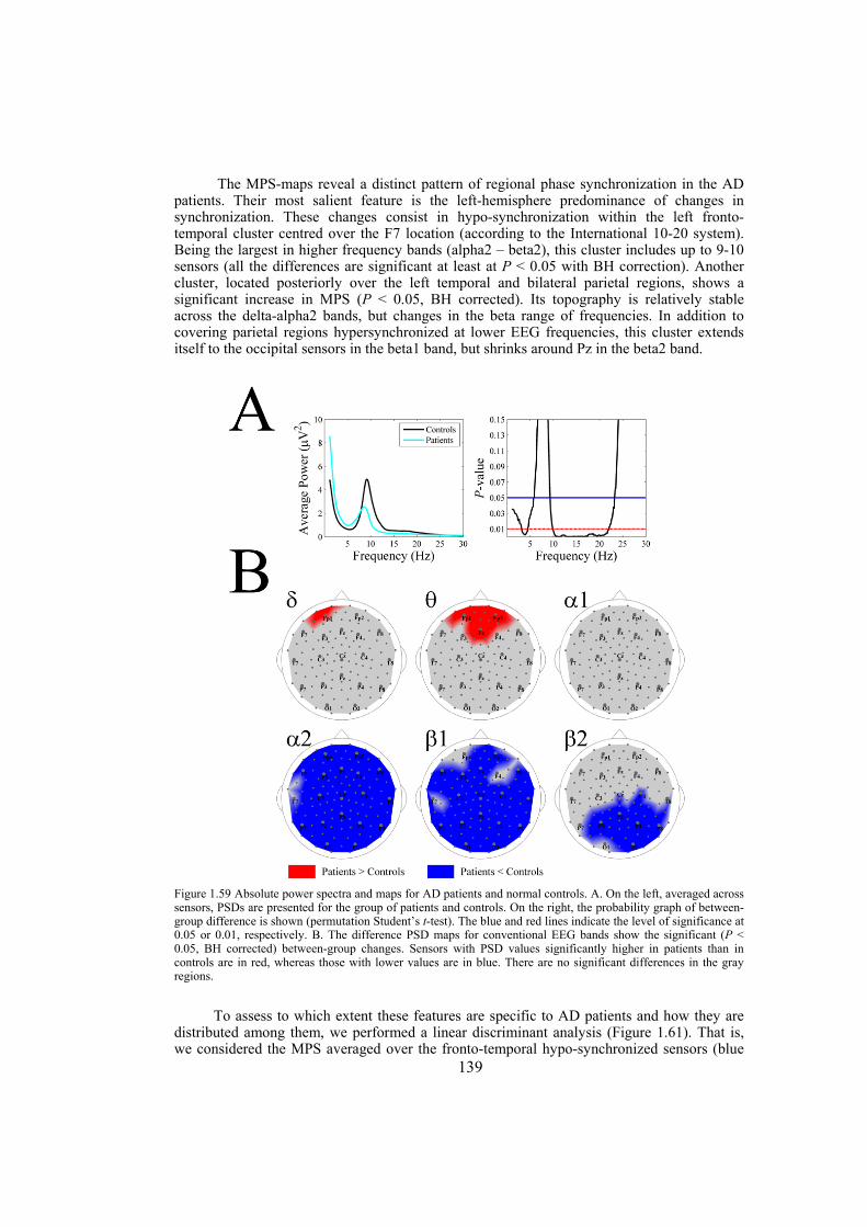
139

The MPS-maps reveal a distinct pattern of regional phase synchronization in the AD patients. Their most salient feature is the left-hemisphere predominance of changes in synchronization. These changes consist in hypo-synchronization within the left fronto-temporal cluster centred over the F7 location (according to the International 10-20 system). Being the largest in higher frequency bands (alpha2 – beta2), this cluster includes up to 9-10 sensors (all the differences are significant at least at P < 0.05 with BH correction). Another cluster, located posteriorly over the left temporal and bilateral parietal regions, shows a significant increase in MPS (P < 0.05, BH corrected). Its topography is relatively stable across the delta-alpha2 bands, but changes in the beta range of frequencies. In addition to covering parietal regions hypersynchronized at lower EEG frequencies, this cluster extends itself to the occipital sensors in the beta1 band, but shrinks around Pz in the beta2 band.

Figure 1.59 Absolute power spectra and maps for AD patients and normal controls. A. On the left, averaged across sensors, PSDs are presented for the group of patients and controls. On the right, the probability graph of between-group difference is shown (permutation Student’s t-test). The blue and red lines indicate the level of significance at 0.05 or 0.01, respectively. B. The difference PSD maps for conventional EEG bands show the significant (P < 0.05, BH corrected) between-group changes. Sensors with PSD values significantly higher in patients than in controls are in red, whereas those with lower values are in blue. There are no significant differences in the gray regions.

To assess to which extent these features are specific to AD patients and how they are distributed among them, we performed a linear discriminant analysis ( Figure 1.61). That is, we considered the MPS averaged over the fronto-temporal hypo-synchronized sensors (blue

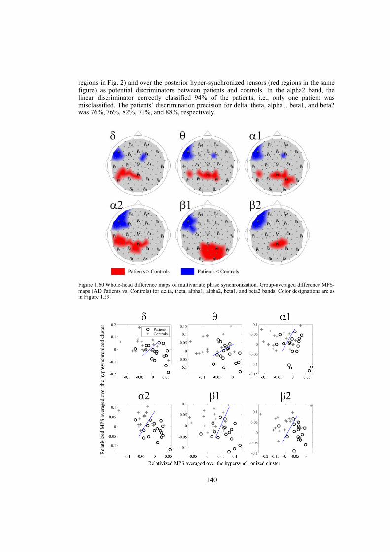
140

regions in Fig. 2) and over the posterior hyper-synchronized sensors (red regions in the same figure) as potential discriminators between patients and controls. In the alpha2 band, the linear discriminator correctly classified 94% of the patients, i.e., only one patient was misclassified. The patients’ discrimination precision for delta, theta, alpha1, beta1, and beta2 was 76%, 76%, 82%, 71%, and 88%, respectively.

Figure 1.60 Whole-head difference maps of multivariate phase synchronization. Group-averaged difference MPS-maps (AD Patients vs. Controls) for delta, theta, alpha1, alpha2, beta1, and beta2 bands. Color designations are as in Figure 1.59.

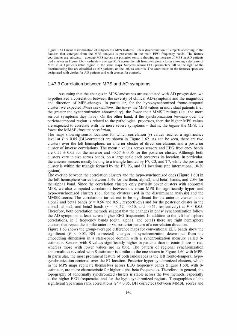
141

Figure 1.61 Linear discrimination of subjects via MPS features. Linear discrimination of subjects according to the features that emerged from the MPS analysis is presented in the main EEG frequency bands. The feature coordinates are: abscissa – average MPS across the posterior sensors showing an increase of MPS in AD patients (red clusters in Figure 1.60); ordinate – average MPS across the left fronto-temporal cluster showing a decrease of MPS in AD patients (blue region in the same map). Subjects whose EEG parameters fall to the right of the discriminating line are classified as AD patients, on the left, as controls. The coordinates in the features space are designated with circles for AD patients and with crosses for controls.

1.47.3 Correlation between MPS and AD symptoms

Assuming that the changes in MPS-landscapes are associated with AD progression, we hypothesized a correlation between the severity of clinical AD-symptoms and the magnitude and direction of MPS-changes. In particular, for the hypo-synchronized fronto-temporal cluster, we expected direct correlations: the lower the MPS values in individual patients (i.e., the greater the synchronization abnormality), the lower their MMSE ratings (i.e., the more serious symptoms they have). On the other hand, if the synchronization increase over the parieto-temporal region is related to the pathological processes, then the higher MPS values are expected to correlate with the more severe symptoms – that is, the higher the MPS, the lower the MMSE (inverse correlation). The maps showing sensor locations for which correlation (r) values reached a significance level at P < 0.05 (BH-corrected) are shown in Figure 1.62. As can be seen, there are two clusters over the left hemisphere: an anterior cluster of direct correlations and a posterior cluster of inverse correlations. The mean r values across sensors and EEG frequency bands are 0.55 ± 0.05 for the anterior and –0.57 ± 0.06 for the posterior cluster. Although both clusters vary in size across bands, on a large scale each preserves its location. In particular, the anterior sensors mostly belong to a triangle limited by F7, C3, and T7, while the posterior cluster is within the triangle formed by the P7, P3, and O1 locations (the International 10/20 system). The overlap between the correlation clusters and the hypo-synchronized ones ( Figure 1.60) in the left hemisphere varies between 50% for the theta, alpha2, and beta1 bands, and 20% for the alpha1 band. Since the correlation clusters only partially cover clusters with abnormal MPS, we also computed correlations between the mean MPS for significantly hyper- and hypo-synchronized clusters (i.e., for the clusters used in the discriminant analysis) and the MMSE scores. The correlations turned out to be significant for the anterior cluster in the alpha2 and beta1 bands (r = 0.56 and 0.51, respectively) and for the posterior cluster in the alpha1, alpha2, and beta2 bands (r = –0.52, –0.50, and –0.51, respectively) at P < 0.05. Therefore, both correlation methods suggest that the changes in phase synchronization follow the AD symptoms at least across higher EEG frequencies. In addition to the left hemisphere correlations, in 3 frequency bands (delta, alpha1, and beta1) there are right hemisphere clusters that repeat the similar anterior vs. posterior pattern of a correlation direction. Figure 1.63 shows the group-averaged difference maps for conventional EEG bands show the significant (P < 0.05, BH corrected) changes in synchronization determined from the embedding dimension in a state-space domain with a synchronization measure called S-estimator. Sensors with S-values significantly higher in patients than in controls are in red, whereas those with lower values are in blue. The pattern of regional synchronization abnormalities revealed with S-estimator is similar to the one shown in Figure 1.60 with MPS. In particular, the most prominent feature of both landscapes is the left fronto-temporal hypo-synchronization centered over the F7 location. Posterior hyper-synchronized clusters, which in the MPS maps replicate themselves across EEG frequency bands ( Figure 1.60), with S-estimator, are more characteristic for higher alpha-beta frequencies. Therefore, in general, the topography of abnormally synchronized clusters is stable across the two methods, especially at the higher EEG frequencies and for the hypo-synchronized regions. Topographies of the significant Spearman rank correlations (P < 0.05, BH corrected) between MMSE scores and

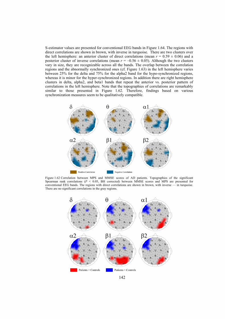
142

S-estimator values are presented for conventional EEG bands in Figure 1.64. The regions with direct correlations are shown in brown, with inverse in turquoise. There are two clusters over the left hemisphere: an anterior cluster of direct correlations (mean r = 0.59 ± 0.06) and a posterior cluster of inverse correlations (mean r = –0.56 ± 0.05). Although the two clusters vary in size, they are recognizable across all the bands. The overlap between the correlation regions and the abnormally synchronized ones (cf. Figure 1.63) in the left hemisphere varies between 25% for the delta and 75% for the alpha2 band for the hypo-synchronized regions, whereas it is minor for the hyper-synchronized regions. In addition there are right hemisphere clusters in delta, alpha2, and beta1 bands that repeat the anterior vs. posterior pattern of correlations in the left hemisphere. Note that the topographies of correlations are remarkably similar to those presented in Figure 1.62. Therefore, findings based on various synchronization measures seem to be qualitatively compatible.

Figure 1.62 Correlation between MPS and MMSE scores of AD patients. Topographies of the significant Spearman rank correlations (P < 0.05, BH corrected) between MMSE scores and MPS are presented for conventional EEG bands. The regions with direct correlations are shown in brown, with inverse — in turquoise. There are no significant correlations in the gray regions.

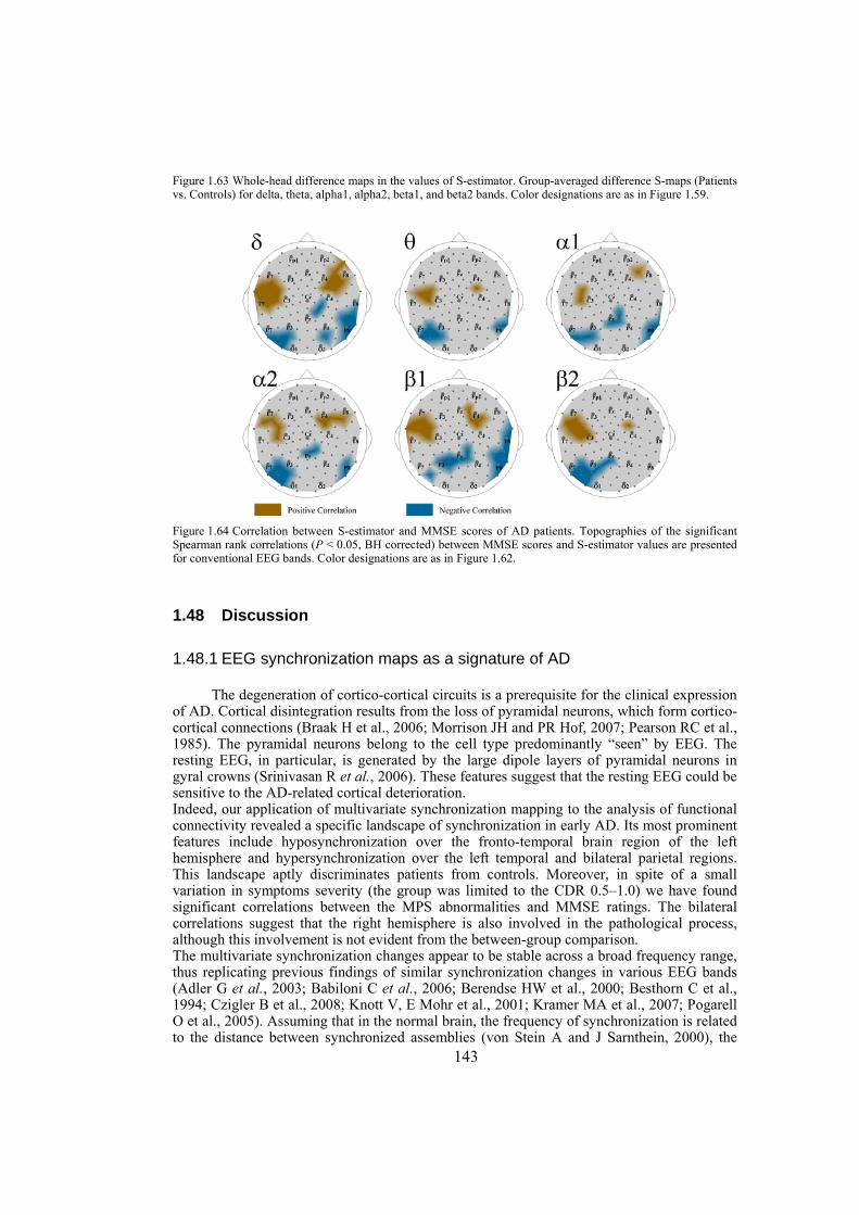
143

Figure 1.63 Whole-head difference maps in the values of S-estimator. Group-averaged difference S-maps (Patients vs. Controls) for delta, theta, alpha1, alpha2, beta1, and beta2 bands. Color designations are as in Figure 1.59.

Figure 1.64 Correlation between S-estimator and MMSE scores of AD patients. Topographies of the significant Spearman rank correlations (P < 0.05, BH corrected) between MMSE scores and S-estimator values are presented for conventional EEG bands. Color designations are as in Figure 1.62.

1.48 Discussion

1.48.1 EEG synchronization maps as a signature of AD

The degeneration of cortico-cortical circuits is a prerequisite for the clinical expression of AD. Cortical disintegration results from the loss of pyramidal neurons, which form cortico-cortical connections (Braak H et al., 2006; Morrison JH and PR Hof, 2007; Pearson RC et al., 1985). The pyramidal neurons belong to the cell type predominantly “seen” by EEG. The resting EEG, in particular, is generated by the large dipole layers of pyramidal neurons in gyral crowns (Srinivasan R et al., 2006). These features suggest that the resting EEG could be sensitive to the AD-related cortical deterioration. Indeed, our application of multivariate synchronization mapping to the analysis of functional connectivity revealed a specific landscape of synchronization in early AD. Its most prominent features include hyposynchronization over the fronto-temporal brain region of the left hemisphere and hypersynchronization over the left temporal and bilateral parietal regions. This landscape aptly discriminates patients from controls. Moreover, in spite of a small variation in symptoms severity (the group was limited to the CDR 0.5–1.0) we have found significant correlations between the MPS abnormalities and MMSE ratings. The bilateral correlations suggest that the right hemisphere is also involved in the pathological process, although this involvement is not evident from the between-group comparison. The multivariate synchronization changes appear to be stable across a broad frequency range, thus replicating previous findings of similar synchronization changes in various EEG bands (Adler G et al., 2003; Babiloni C et al., 2006; Berendse HW et al., 2000; Besthorn C et al., 1994; Czigler B et al., 2008; Knott V, E Mohr et al., 2001; Kramer MA et al., 2007; Pogarell O et al., 2005). Assuming that in the normal brain, the frequency of synchronization is related to the distance between synchronized assemblies (von Stein A and J Sarnthein, 2000), the

144

frequency-nonspecific alterations in an AD brain seem to be very likely due to the involvement of various-range connections in the pathological process. Importantly, the MPS changes are dissimilar from the EEG power alterations (cf. Figure 1.59 and Figure 1.60), which makes a significant effect of volume conduction unlikely and allows an interpretation in terms of regional synchronization. Because of the low spatial resolution of EEG, we discuss the AD-related changes in synchronization topography in large-scale terms. On this scale, the MPS difference maps characterized by the anteriorly (fronto-temporal) and posteriorly (parieto-temporal) located abnormalities in synchronization are consistent with the topography of gyral athrophy (Giannakopoulos P et al., 1997), of cortical gray matter loss (Thompson et al. 2003), and with the topography of amiloid deposits in AD (Buckner RL et al., 2005). Therefore, such a synchronization landscape presents a more accurate and specific picture than the selective bivariate measurements of synchronization.

The majority of the synchronization measures including multivariate and bivariate methods detect coupling (Carmeli C et al., 2005; Quiroga R et al., 2002). Specifically in the AD domain, a recent comparison of nonlinear synchronization measures with phase synchronization demonstrated their similar performance (Kramer MA et al., 2007). Furthermore, we analyzed EEG synchronization in AD patients not only with MPS as presented above, but also, in parallel, with S-estimator (Carmeli C et al., 2005). The latter determines synchronization from the embedding dimension in a state-space domain based on the theoretical consequence of the cooperative behavior of simultaneous time series — the shrinking of the state-space embedding dimension. The results of our MPS and S-estimator analyses appeared to be similar, as supplementary Figure 1.63 and Figure 1.64 confirm. Therefore, findings based on various synchronization measures seem to be qualitatively compatible. In the AD literature, a consensus exists on the reduction of EEG synchronization, which has been tested in pairs of locations or globally (Adler G et al., 2003; Babiloni C et al., 2006; Berendse HW et al., 2000; Czigler B et al., 2008; Franciotti R et al., 2006; Koenig T et al., 2005; Pijnenburg YA et al., 2004; Stam CJ et al., 2003). Furthermore, in neuroimaging studies, dealing with very low temporal frequencies, long-distance (e.g., fronto-parietal) synchronization was also shown to be decreased (Grady CL et al., 2001; Horwitz B et al., 1995; Wang K et al., 2007). Such changes of functional connectivity are consistent with the demyelination observed in postmortem morphological studies (Bartzokis G et al., 2004) and in in vivo Magnetization Transfer Imaging AD studies (van der Flier WM et al., 2002). The anterior clusters of hypo-synchronized EEG signals from the landscapes of MPS abnormalities described in the present paper are in agreement with frequently reported frontal decoupling (Adler G et al., 2003; Babiloni C et al., 2006; Berendse HW et al., 2000; Besthorn C et al., 1994; Czigler B et al., 2008; Knott V, E Mohr et al., 2001; Pogarell O et al., 2005).

The AD-related increase in synchronization over the left temporal and bilateral parietal and occipital cortices has never been reported in EEG studies (except for low EEG frequencies, e.g., see (Koenig T et al., 2005)). The discrepancy between our findings and those reported in the EEG/MEG literature are likely to be due to the fact that previous studies analyzed the long-distance synchronization, whereas we consider connections within the circle of 10-12 cm in diameter. Notably, an increase in intraregional functional connectivity against a decrease in interregional connectivity was observed with PET and fMRI methods (Grady CL et al., 2001; Horwitz B et al., 1995; Wang K et al., 2007). The last reference is of particular interest for our discussion, since in this paper, the resting-state functional connectivity over the whole-brain was analyzed. These authors found increased correlations between spontaneous fluctuations of BOLD (Blood-Oxygen-level-dependent) signals within prefrontal, parietal, and occipital lobes in AD patients compared to controls. Another reason for the discrepancy can be related to the fact that, according to the MMSE ratings, the symptoms in our patients were milder that in the majority of EEG synchronization studies (cf.

145

(Adler G et al., 2003; Berendse HW et al., 2000; Franciotti R et al., 2006; Pijnenburg YA et al., 2004; Stam CJ et al., 2003)). Therefore, this finding suggests some plastic mechanisms working at an early stage of AD.

1.48.2 Abnormal EEG synchronization and plasticity of cortical circuits in early AD

Such a mechanism can be provided by synaptic plasticity. The scenario that binds the EEG synchronization alterations and synaptic plasticity might be as follows. The death of pyramidal neurons and the loss of synapses in AD are accompanied by plastic processes, including axonal and dendritic sprouting (Adams IM, 1991; Agnati LF et al., 1992; Horwitz B, 1988; Masliah E et al., 2006; Scheff SW and DA Price, 2003). This aberrant sprouting together with a decrease in the number of afferent neurons and with the expansion of the territory occupied by a single axon/dendrite are likely to increase the temporal coordination of input signals to a target cortical area. A more synchronized input would increase the postsynaptic synchronization visible in EEG. Eventually, with the progression of the disease, the pathological cascade overcomes this plastic response and ruins connectivity, which results in the synchronization decrease. Applied to our data, this two-stage scenario suggests that the anterior (fronto-temporal) and posterior associative areas pass the compensatory and further degradation stages at different times and/or vary in the mechanisms/ability to compensate. Indeed, the AD-related annual loss of gray matter in the fronto-temporal cortex reaches 4-5%, whereas in the posterior temporal and parietal cortices it is mostly within 1-2% (Thompson PM et al., 2003). The analysis of the overall gene expression change in AD has shown that the temporal and prefrontal cortices are the most vulnerable brain regions (Haroutunian V et al., 2007). Furthermore, the neurochemical studies of synaptic plasticity provide some evidence of interregional differences. For example, in brain specimens from MCI and AD patients, the loss of synaptic proteins in the frontal cortex is more severe than in the parietal cortex (Reddy PH et al., 2005), and less severe than in the temporal cortex (Counts SE et al., 2006). Plasticity of the synaptic contact zone in AD brains also varies among the inferior temporal, superior parietal, parieto-occipital, and superior frontal cortical regions (Adams IM, 1991). Specifically, this last study revealed that the loss of synapses is accompanied by an increase in the synaptic contact length only in the inferior temporal and superior parietal cortices.

Of particular interest for this discussion is the distribution of neuro-fibrillary tangles (NFT), the number of which strongly correlates with AD progression. The NFT are found predominantly in layers III and V of the neocortex (Giannakopoulos P et al., 1997; Lewis DA et al., 1987; Pearson RC et al., 1985). In general, layer V contains more NFT than layer III; however, in the visual association cortex the NFT are predominantly found in layer III, whereas in the temporal association cortex about two thirds of NFT are in layer V (Lewis DA et al., 1987). Furthermore, the NFT are less frequent in the parietal and occipital cortices than in the temporal cortex, while the frontal cortex displays intermediate densities. The neurons of layers II and III provide feed-forward, association, and callosal connections, whereas feedback connections and those descending to subcortical structures originate in layer V. The interaction of these cortical features with the across-layer and across-region distribution of NFT suggests that feedback and descending connections, especially in the frontal and temporal areas, are at a higher risk in AD than feed-forward connections. Finally, considering that layer V is strongly implicated in cortical synchrony (Connors BW and Y Amitai, 1995), one can assume that the AD-related abnormalities of EEG synchronization would be more advanced in the fronto-temporal than in the parietal areas, an assumption that agrees with the interregional difference reported here.

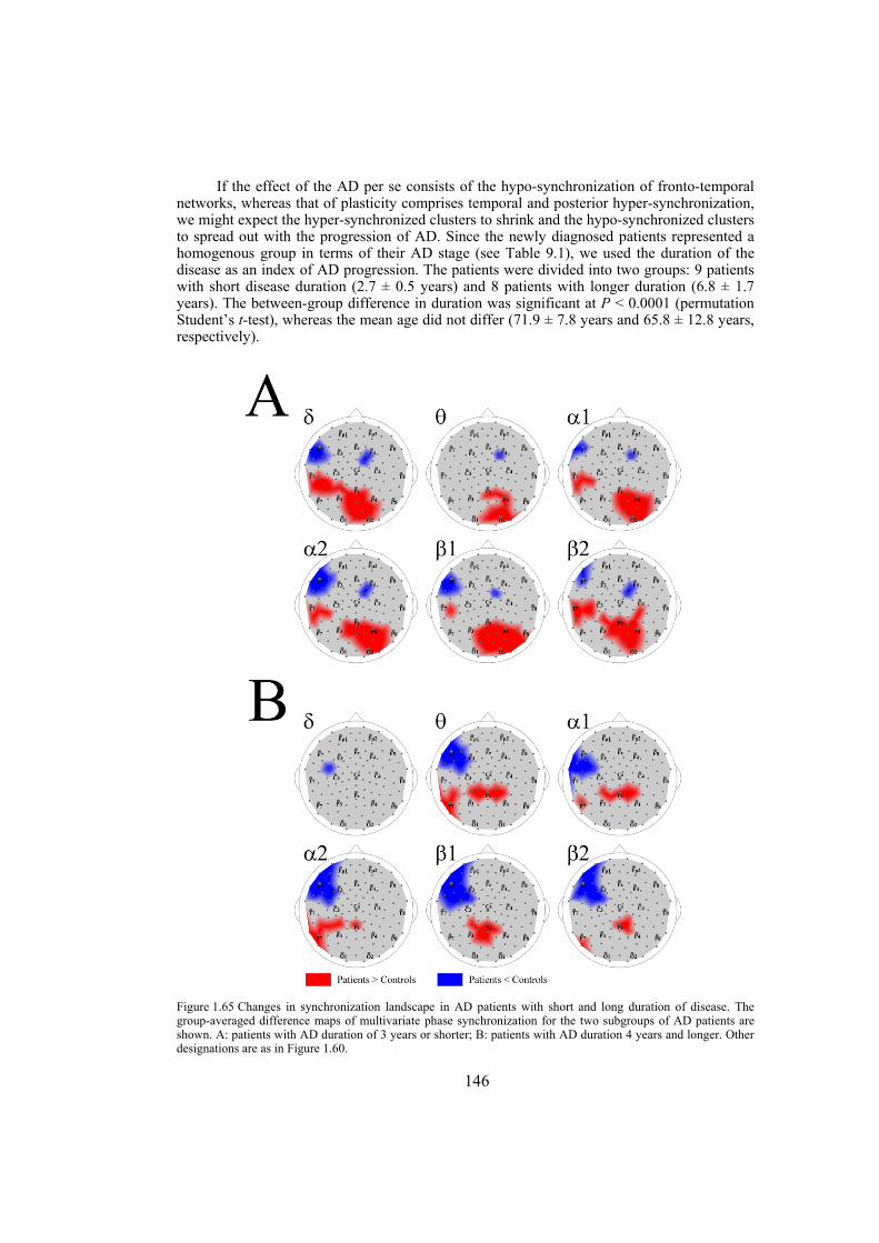
146

If the effect of the AD per se consists of the hypo-synchronization of fronto-temporal networks, whereas that of plasticity comprises temporal and posterior hyper-synchronization, we might expect the hyper-synchronized clusters to shrink and the hypo-synchronized clusters to spread out with the progression of AD. Since the newly diagnosed patients represented a homogenous group in terms of their AD stage (see Table 9.1), we used the duration of the disease as an index of AD progression. The patients were divided into two groups: 9 patients with short disease duration (2.7 ± 0.5 years) and 8 patients with longer duration (6.8 ± 1.7 years). The between-group difference in duration was significant at P < 0.0001 (permutation Student’s t-test), whereas the mean age did not differ (71.9 ± 7.8 years and 65.8 ± 12.8 years, respectively).

Figure 1.65 Changes in synchronization landscape in AD patients with short and long duration of disease. The group-averaged difference maps of multivariate phase synchronization for the two subgroups of AD patients are shown. A: patients with AD duration of 3 years or shorter; B: patients with AD duration 4 years and longer. Other designations are as in Figure 1.60.

147

As Figure 1.65 shows, the MPS difference maps for these groups were characterized by the predicted features. Indeed, in the short-duration group ( Figure 1.65A), there are 90 hyper-synchronized (red) and 27 hypo-synchronized (blue) sensors (summarized across EEG bands), whereas in the long-duration group ( Figure 1.65B), the number of red sensors dramatically reduces to only 36, while the number of blue sensors increases up to 47. Furthermore, by dividing our patients into groups according to their age (8 patients younger than 66 years of age (60.1 ± 6.7), and 9 patients older than 70 years of age (76.9 ± 6.1), we could show that only red (“compensatory”) clusters reduce with age (70 vs. 36), whereas AD-related clusters do not differ between the groups (46 vs. 43, Figure 1.66). The result is not a surprising one, considering that neither stage nor duration of AD (4.9 ± 2.0 years in the younger vs. 4.3 ± 2.8 years in the older patients) differ in these groups, whereas the plastic properties of the brain decrease with age.

However, it is not clear whether the processes that result in EEG synchronization can compensate for cognitive deficits in AD: the inverse correlations between the parieto-temporal MPS and the MMSE scores in our group of patients suggest that the MPS increase is related to more severe symptoms. This might be accounted for by sprouting that leads to the decreased selectivity of connections. The enlarged activation area shown in AD patients with neuroimaging methods ((Wang K et al., 2007) and references therein) probably reflects this effect. Finally, insufficiently selective connections fail to provide real functional compensation. The topography of EEG synchronization in AD seems to be a promising area for further research. Moreover, our hypothesis based on this topography provides specific and testable predictions: i) the AD progression would result in replacing the synchronization increase with its reduction in posterior associative areas; ii) the MCI and mild early-onset AD patients are likely to have relatively wide-spread hyper-synchronized regions, including fronto-temporal ones; and iii) patients with late-onset AD would have less extensive hyper-synchronized regions. Although the last two predictions are supported by our preliminary evidence, additional studies including the analysis of task-related EEG are required to confirm them. The results would be important for the early diagnostics and for the adequate choice of treatment strategies.

1.49 Summary

The results presented in this chapter was indeed the result of combined expertise from advanced nonlinear modeling and signal processing, modern EEG and neuroimaging techniques, and clinical neurology and neuropsychlogy. It should be mentioned that, due to the explosive development of neuroimaging techniques, the “old cheap EEG” is experiencing difficult though exciting times, searching for a new place and role in modern neuroscience. In this sense, our results are of principal interest, as it reports a successful application of a new EEG synchronization mapping strategy to an extremely important area of AD research. We analyze the surface topography of the multivariate phase synchronization (MPS) of multichannel EEG in 17 AD patients compared to 17 age- and education-level- matched control subjects and by applying a combination of global and regional MPS measures to the resting EEG. Our main results included a specific whole-head synchronization landscape, revealed in AD patients for the first time. In early AD, the whole-head mapping revealed a specific landscape of synchronization characterized by a decrease in MPS over the fronto-temporal region and an increase over the temporo-parieto-occipital region predominantly of the left hemisphere. These features manifest themselves through the EEG delta-beta bands and discriminate patients from controls with an accuracy of up to 94%. Moreover, the abnormal MPS in both anterior and posterior clusters were relevant in the clinical context:

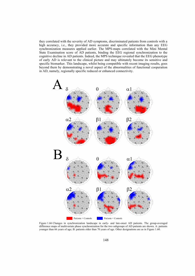
148

they correlated with the severity of AD symptoms, discriminated patients from controls with a high accuracy, i.e., they provided more accurate and specific information than any EEG synchronization measures applied earlier. The MPS-maps correlated with the Mini Mental State Examination score of AD patients, binding the EEG regional synchronization to the cognitive decline in AD patients. Indeed, the MPS technique revealed that the EEG phenotype of early AD is relevant to the clinical picture and may ultimately become its sensitive and specific biomarker. This landscape, whilst being compatible with recent imaging results, goes beyond them by demonstrating a novel aspect of the abnormalities of functional cooperation in AD, namely, regionally specific reduced or enhanced connectivity.

Figure 1.66 Changes in synchronization landscape in early- and late-onset AD patients. The group-averaged difference maps of multivariate phase synchronization for the two subgroups of AD patients are shown. A: patients younger than 66 years of age; B: patients older than 70 years of age. Other designations are as in Figure 1.60.

149

CONCLUSIONS AND OUTLOOK

In this thesis we studied some aspects of synchronization in complex dynamical networks. The study of synchronization phenomenon has various potential applications in many fields of science and technology. It may guide us to better understand the organizing principles of real-world complex networks (such as brain) and/or design artificial networks with high efficiency (such as sensor networks). The thesis is divided into three sections each of which covers an important topic in the field of synchronization of dynamical networks. In this chapter we give the essence of our findings and also some possible future directions of the work.

1.50 Synchronizability of dynamical networks

For the ease by which dynamical systems are synchronized over a network, usually, the term synchronizability is encountered. However, there is no unique interpretation of synchronizability and a particular choice is adopted for each study. Here, we used previously developed methods in the field of dynamical networks for quantifying the synchronizability. Of these are the master-stability-function (Pecora LM and TL Carroll, 1998) and the connection-graph-stability (Belykh VN et al., 2004) methods. The former gives necessary condition for linear (local) stability of the synchronization manifold, whereas the latter gives sufficient condition for global synchronization. We formulized the problem of synchronizability in dynamical networks and gave four possible interpretations for that. We also considered synchronization in weighted dynamical networks. Our main findings could be listed as the following.

• One can interpret the synchronizability in a dynamical network in at least four different ways (Jalili M, A Ajdari Rad et al., 2007): Network N1 is said to be more synchronizable than network N2, (i) if for larger range of parameters, it is possible to synchronize N1 compared to N2. Considering the largest and the second smallest eigenvalues of the Laplacian matrix of the connection graph as λN and λ2, this interpretation of synchronizability is linked to λN /λ2, i.e. the less the eigenratio λN /λ2 the better the synchronizability. (ii) Network N1 is synchronized with less effort

150

compared to N2. This interpretation is related to the second smallest eigenvalue of the Laplacian, so called algebraic connectivity of the graph, i.e. for the same sum of the connection weights, the larger the λ2 the better the synchronizability of the network. (iii) With the same cost, network N1 synchronizes faster than N2. (iv) With the same cost, the degree of phase synchronization, estimated for example by order parameter, is larger in N1 than in N2. This interpretation is useful especially in the situations where complete synchronization can not be defined such as coupled nonidentical dynamical systems.

• In general, the above interpretations of synchronizability do not coincide. In heterogeneous networks such as unweighted scale-free networks, the interpretations (i) and (iv) lie in the same line as the parameters of the network change, whereas interpretation (ii) goes in the opposite direction. In unweighted Watts-Strogatz networks, which show more homogenous degree distribution compared to scale-free networks, these interpretations almost lie in the same line as the network parameter changes.

• Networks with non-uniform diffusive couplings could have better synchronizability than those of with uniform diffusive coupling. One way to assign proper strength for diffusive links is to use of the connection-graph-stability method.

• Networks with optimal synchronizability are neither undirected nor unweighted. Here we proposed an algorithm based on node and edge betweenness centrality measures for enhancing the synchronizability. By considering a particular interpretation of synchronizability we introduced an algorithm for assigning connection weights resulting is a weighted and directed network. Since in some applications it is desired that the network with high synchronizability to be undirected, we proposed another weighting rule for reducing the synchronization cost preserving the network undirected.

• We showed that in networks with high synchronization properties, different interpretations of synchronizability go hand in hand as network parameters change. We used two methods to obtain networks with high synchronizability; weighting the links and making rewiring in the connections links.

There are a number of possible future directions based on the works presented in this thesis. Trying to come up with better weighting algorithms for further enhancing the synchronizability is one of the possible outlooks. We used a very simple rewiring of the connection links to optimize the synchronizability, i.e. optimizing synchronizability without weighting and just by changing the structure of the network. Our proposed intelligent rewiring method dramatically speeded up the previous methods. Another possible future work could be using more sophisticated optimization algorithm for rewiring. Also, optimizing the synchronizability by rewiring preserving the degree distribution can be another interesting extension to our work.

1.51 Synchronization in networks of Hindmarsh-Rose neurons

We investigated the synchronization phenomenon in networks of Hindmarsh-Rose neuron models. It is believed that synchronization plays a role in information binding in the brain; different populations of neurons get into synchrony for processing information. Although it has not proved that weather getting into synchrony causes the process of information in the brain or it is just a consequence of information binding, it is worth to put efforts on studying synchronization in neural networks. The mechanisms of spike-timing-

151

dependent-plasticity are affected by synchronization in gamma frequency bad. Thus, even if synchronization has nothing to do with binding puzzle in the brain, it is important for spike-timing-dependent-plasticity. The main results obtained in this part of the work are listed in the following.

• We considered diffusively coupled Hindmarsh-Rose neurons (with electrical coupling) over Newman-Watts networks and calculated the synchronizing coupling strength using both the numerically solving the network’s differential equations and the master-stability-function method. We showed that the coupling strengths predicted by the master-stability-function are near to the real synchronizing ones. Therefore, for large networks where the numerical simulation is expensive one can simply use the master-stability-function method that needs only computing the eigenvalues of the connection graph.

• The synchronization of Hindmarsh-Rose neurons over a class of clustered networks was investigated. In such networks, the intra-cluster links are dense, whereas the nodes in different clusters are connected sparsely. Our results revealed that in such networks, the synchronization is more influenced by the inter-cluster links than the intra-cluster connections. In other words, to have high synchronizability, the intra-cluster and inter-cluster links should be in balance.

• We also studied complete synchronization in networks of Hindmarsh-Rose neurons with both type of couplings, electrical and chemical. We showed that chemical coupling can play a complementary role to electrical connections to provide the complete synchronization in the network.

• We proposed a minimal network consisting of only five neurons (one thalamic-relay neuron, two pyramidal neurons and two interneurons) with proper electrical and excitatory/inhibitory couplings in between, to produce synchronized gamma oscillations. The frequency of the oscillations could be controlled by the input current injected to the neurons and in particular that of the thalamic-relay neuron.

• Then, large networks of interacting locally synchronized gamma oscillators were studied. The dependence of the spike synchrony to some network parameters such as the probability of intermodular electrical couplings between interneurons, the probability and the strength of intermodular inhibition of interneurons, the probability and the strength of intermodular excitatory connections ascending from pyramidal neurons, parameter mismatch, correlation of thalamic input, and transmission time-delay, was investigated.

The work we did for simulating the interacting locally synchronized gamma oscillations deserves further analysis. Especially the interesting influence of the transmission time-delay in spike synchrony can be investigated in a more general case, for example in a network with a number of pyramidal neurons and interneurons with some random excitatory/inhibitory connection. The optimal transmission time-delay is likely a function of the oscillation frequency of the network.

1.52 EEG synchronization in patients with schizophrenia or Alzheimer’s disease

In this thesis we used two methods for quantifying cooperativeness in the EEG time series: the S-estimator (Carmeli C et al., 2005), a state-space based synchronization estimator, and multivariate phase synchronization. Traditionally, bivariate methods such as coherence

152

analysis have been used for analyzing synchronization phenomenon in EEG data. The major limitation of such methods is that they can not be directly used for multivariate analyses and are usually applied for predetermined region of interest. Thus, using the traditional bivariate methods one can not reveal the topography of synchronization for high density EEG data. We applied the multivariate synchronization measures to two EEG datasets: one from patients experiencing schizophrenia and their matched control subjects and the other one from patients with Alzheimer’s disease and some age-matched healthy control subjects. The important findings are as the following.

• Our new method for parametrization of multichannel EEG, i.e. calculating relative power density maps, revealed specific map of power-changes (changes in mesoscale synchronization values) in schizophrenic patients. Although the global power was decreased in schizophrenia patients, we observed a relative increase of power in the anterior brain regions against the decrease of power over the posterior regions. This peculiar feature discriminated schizophrenia patients from normal control and correlated with the clinical picture of the illness as well as the chronicity. Our finding supports the concept of hypofrontality in schizophrenia and suggests alpha rhythm for further detailed noninvasive research into the neurobiology of schizophrenia.

• By applying the S-estimator technique to the EEG data of schizophrenia patients, we revealed the whole-head synchronization topography. It included bilaterally increased local synchronization over temporal brain regions and decreased synchronization over the postcentral/parietal region neighboring the midline. The observed synchronization-map was almost robust in all of the conventional frequency bands. It also showed a robust pattern in the course of several months. These abnormalities in the local synchronization were linked to the clinical scores of the schizophrenia. These synchronization-maps go beyond the topography limits, demonstrating a novel aspect of the abnormalities of functional cooperation: namely, regionally reduced or enhanced connectivity.

• We applied the multivariate phase synchronization method for detecting any abnormalities in the synchronization topography of resting EEG in patients with early stages of Alzheimer’s disease. Our analysis revealed a specific synchronization landscape characterized by decrease of synchronization over the fronto-temporal area and an increase over the temporo-parieto-occipital region predominantly of the left hemisphere. These features could discriminate the patients from normal controls in the EEG delta-beta bands. They also correlated with the severity of the disease.

Some further analysis on the same data is still under progress. One of the most interesting results we have found is confirming the hypothesis “loss of brain asymmetry” in schizophrenia (Crow TJ et al., 1989). It is known that the schizophrenic brain looses the normal asymmetry. We try to show if this is the case for local synchronization. One of our future works (partly done) is to use multivariate synchronization techniques for revealing the long-distance synchronization-maps. For example, one can divide the sensors into a number of clusters and then try to obtain the cooperativeness between these clusters. Other analysis could be determining the abnormalities in the direction of coupling using the EEG data (this also has been partly done).

153

BIBLIOGRAPHY

Abarbanel HDI, Huerta R, Rabinovich MI (2002) Dynamical model of long-term synaptic plasticity. Proceedings of the National Academy of Science of the United States of America 99: 10132-10137.

Abarbanel HDI, Rulkov NF, Sushchik MM (1996) Generalized synchronization of chaos: the auxiliary system approach. Physical Review E 53: 4528-4535.

Adams IM (1991) Structural plasticity of synapses in Alzheimer's disease. Molecular Neurobiology 5: 411-419.

Adler G, Brassen S, Jajcevic A (2003) EEG coherence in Alzheimer's dementia. Journal of Neural Transmission 110: 1051-1058.

Agnati LF, Benfenati F, Solfrini V, Biagini G, Fuxe K, Guidolin D, Carani C, Zini I (1992) Brain aging and neuronal plasticity. Annals of New York Academy of Sciences 673: 180-186.

Ajdari Rad A, Jalili M, Hasler M (2008) Efficient rewirings for enhancing synchronizability of dynamical networks. Chaos.

Albert R, Barabasi A-L (2002) Statistical mechanics of complex networks. Reviews of Modern Physics 74: 47-97.

Albert R, Jeong H, Barabasi A-L (1999) Diameter of the World Wide Web. Nature 401: 130-131. Allefeld C, Kurths J (2004) An approach to multivariate phase synchronization analysis and its

application to event-related potentials. International Journal of Bifurcation and Chaos 14: 417-426.

Almaas E, Kovacs B, Vicsek T, Oltvai ZN, Barabasi AL (2004) Global organization of metabolic fluxes in the bacterium Escherichia coli. Nature 427: 839-843.

Almendral JA, Dıaz-Guilera A (2007) Dynamical and spectral properties of complex networks. New Journal of Physics 9: 187.

Alper K (1995) Quantitative EEG and evoked potentials in adult psychiatry. In: Advances in Biological Psychiatry (Panksepp J, ed.), pp 65-112. Greenwich: JAI Press.

Alper K, Gunther W, Prichep LS, John ER, Brodie J (1998) Correlation of qEEG with PET in schizophrenia. Neuropsychobiology 38: 50-56.

Alper KR, John ER, Brodie J, Gunther W, Daruwala R, Prichepx LS (2006) Correlation of PET and qEEG in normal subjects. Psychiatry Research 146: 271-282.

Alzheimer A (1907) Über eine eigenartige erkrankung der hirnrinde. Allgemeine Zeitschrift Psychiatrie Psychisch-Gerichtliche Med.

Anderson J, Wible C, McCarley R, Jakab M, Kasai K, Shenton M (2002) An MRI study of temporal lobe abnormalities and negative symptoms in chronic schizophrenia. Schizophrenia Research 58: 123-134.

Anderson WN, Morley TD (1985) Eigenvalues of the Laplacian of a graph. Linear and Multilinear Algebra 18: 141-145.

Andreasen N, Swayze V, O'Leary D, Nopoulos P, Cizadlo T, Harris G, Arndt S, Flaum M (1995) Abnormalities in midline attentional circuitry in schizophrenia: evidence from magnetic resonance and positron emission tomography. European Neuropsychopharmacology 5: 37-41.

Andreasen NC (1997) The role of the thalamus in schizophrenia. Canadian Journal of Psychiatry 42: 27-33.

Andreasen NC, Rezai K, Alliger R, Swayze VW, Flaum M, Kirchner P, Cohen G, O'Leary DS (1992) Hypofrontality in neuroleptic-naive patients and in patients with chronic schizophrenia. Assessment with xenon 133 single-photon emission computed tomography and the Tower of London. Archives of General Psychiatry 49: 943-958.

154

Arieli A, Sterkin A, Grinvald A, Aertsen A (1996) Dynamics of ongoing activity: explanation of the large variability in evoked cortical responses. Science 273: 1868-1871.

Arizmendi F, Zanette DH (2008) Adaptation to synchronization in phase-oscillator networks. Physica A 387: 5631-5638.

Ashwin P, Buescu J, Stewart I (1994) Bubbling of attractors and synchronisation of chaotic oscillators. Physics Letters A 193: 126-139.

Ashwin P, Buescu J, Stewart I (1996) From attractor to chaotic saddle: a tale of transverse instability. Nonlinearity 9: 703-737.

Babiloni C, Ferri R, Binetti G, Cassarino A, Dal Forno G, Ercolani M, Ferreri F, Frisoni GB, Lanuzza B, Miniussi C, Nobili F, Rodriguez G, Rundo F, Stam CJ, Musha T, Vecchio F, Rossini PM (2006) Fronto-parietal coupling of brain rhythms in mild cognitive impairment: a multicentric EEG study. Brain Research Bulletin 69: 63-73.

Barabasi A-L, Albert R (1999) Emergence of scaling in random networks. Science 286: 5009-5012. Barabasi A-L, Oltvai ZN (2004) Network biology: understanding the cell's functional organization.

Nature Reviews Genetics 5: 101-113. Barahona M, Pecora LM (2002) Synchronization in small-world systems. Physical Review Letters 89:

054101. Barbarossa S, Scutari G (2007) Decentralized maximum likelihood estimation for sensor networks

composed of nonlinearly coupled dynamical systems. IEEE Transactions on Signal Processing 55: 3456-3470.

Barta P, Pearlson G, Powers R, Richards S, Tune L (1990) Auditory hallucinations and smaller superior temporal gyral volume in schizophrenia. American Journal of Psychiatry 147: 1457-1462.

Bartzokis G, Altshuler L (2005) Reduced intracortical myelination in schizophrenia. American Journal of Psychiatry 162: 1229-1230.

Bartzokis G, Sultzer D, Lu PH, Nuechterlein KH, Mintz J, Cummings JL (2004) Heterogeneous age-related breakdown of white matter structural integrity: implications for cortical "disconnection" in aging and Alzheimer's disease. Neurobiology of Aging 25: 843-851.

Beasley CL, Chana G, Honavar M, Landau S, Everall IP, Cotter D (2005) Evidence for altered neuronal organisation within the planum temporale in major psychiatric disorders. Schizophrenia Research 73: 69-78.

Begić D, Hotujac L, Jokicć-Begić N (2000) Quantitative EEG in 'positive' and 'negative' schizophrenia. Acta Psychiatrica Scandinavica 101: 307-311.

Begré S, Federspiel A, Kiefer C, Schroth G, Dierks T, Strik WK (2003) Reduced hippocampal anisotropy related to anteriorization of alpha EEG in schizophrenia. Neuroreport 14: 739-742.

Beierlein M, Gibson JR, Connors BW (2000) A network of electrically coupled interneurons drives synchronized inhibition in neocortex. Nature Neuroscience 3: 904-910.

Belykh I, Belykh V, Hasler M (2006) Generalized connection graph method for synchronization in asymmetrical networks. Physica D 224: 42–51.

Belykh I, Belykh V, Hasler M (2006) Synchronization in asymmetrically coupled networks with node balance. Chaos 16: 015102.

Belykh I, de Lange E, Hasler M (2005) Synchronization of bursting neurons: what matters in the network topology. Physical Review Letters 94: 188101.

Belykh I, Hasler M, Laurent M, Nijmeijer H (2005) Synchronization and graph topology. International Journal of Bifurcation and Chaos 15: 3423-3433

Belykh IV, Belykh VN, Hasler M (2004) Blinking model and synchronization in small-world networks with a time-varying coupling. Physica D 195: 188-206.

Belykh VN, Belykh IV, Hasler M (2004) Connection graph stability method for synchronized coupled chaotic systems. Physica D 195: 159-187.

Benjamini Y, Hochberg Y (1995) Controlling the false discovery rate - a practical and powerful approach to multiple testing. Journal of the Royal Statistical Society Series B - Methodological 57: 289-300.

Berendse HW, Verbunt JP, Scheltens P, van Dijk BW, Jonkman EJ (2000) Magnetoencephalographic analysis of cortical activity in Alzheimer's disease: a pilot study. Clinical Neurophysiology 111: 604-612.

155

Besthorn C, Förstl H, Geiger-Kabisch C, Sattel H, Gasser T, Schreiter-Gasser U (1994) EEG coherence in Alzheimer disease. Electroencephalography and Clinical Neurophysiology 90: 242-245.

Bi GQ, Poo MM (2001) Synaptic modification by correlated activity: Hebb's postulate revisited. Annual Review of Neuroscience 24: 139-166.

Bishop CM (2006) Pattern recognition and machine learning. Singapore: Springer. Black JE, Kodish IM, Grossman AW, Klintsova AY, Orlovskaya D, Vostrikov V, Uranova N,

Greenough WT (2004) Pathology of layer V pyramidal neurons in the prefrontal cortex of patients with schizophrenia. American Journal of Psychiatry 161: 742-744.

Bleuler E (1911) Dementia praecox or the group of schizophrenias. New York: International Universities Press.

Boccaletti S, Kurths J, Osipov G, Valladares DL, Zhou CS (2002) The synchronization of chaotic systems. Physics Reports 366: 1-101.

Boccaletti S, Latora V, Moreno Y, Chavez M, Hwang DU (2006) Complex networks: structure and dynamics. Physics Reports 424: 175-308.

Bollobás B (2001) Random graphs. London: Cambridge University Press. Bolwig TG (2008) EEG and psychiatry: time for a resurrection. Acta Psychiatrica Scandinavica 117:

241-243. Boyd S (2006) Convex optimization of graph Laplacian eigenvalues. Proceedings International

Congress of Mathematicians 3: 1311-1319. Braak H, Rüb U, Schultz C, Del Tredici K (2006) Vulnerability of cortical neurons to Alzheimer's and

Parkinson's diseases. Journal of Alzheimer's Disease 9: 35-44. Brandes U (2001) A faster algorithm for betweenness centrality. Journal of Mathematical Sociology

25: 163-177. Broomhead D, King G (1986) Extracting qualitative dynamics from experimental data. Physica D 20:

217–236. Brown R, Kocarev L (2000) A unifying definition of synchronization for dynamical systems. Chaos

10: 344-349. Brown S, Inskip H, Barraclough B (2000) Causes of the excess mortality of schizophrenia. British

Journal of Psychiatry 177: 212-217. Buckner RL, Snyder AZ, Shannon BJ, La Rossa G, Sachs R, Fotenos AF, Sheline YI, Klunk WE,

Mathis CA, Morris JC, Mintun MA (2005) Molecular, structural, and functional characterization of Alzheimer's disease: evidence for a relationship between default activity, amyloid, and memory. Journal of Neuroscience 25: 7709-7717.

Buzsaki G (2006) Rhythms of the brain. New York: Oxford University Press. Buzsaki G, Geisler C, Henze DA, Wang X-J (2004) Interneuron diversity series: circuit complexity and

axon wiring economy of cortical interneurons. Trends in Neurosciences 27: 186-193. Carmeli C (2006) Assessing cooperative behavior in dynamical networks with applications to brain

data. PhD Thesis, Ecole Polytechnique Federal de Lausanne. Carmeli C, Knyazeva M, Innocenti G, De Feo O (2005) Assessment of EEG synchronization based on

state-space analysis. NeuroImage 25: 339-354. Casanova MF, de Zeeuw L, Switala A, Kreczmanski P, Korr H, Ulfig N, Heinsen H, Steinbusch HW,

Schmitz C (2005) Mean cell spacing abnormalities in the neocortex of patients with schizophrenia. Psychiatry Research 133: 1-12.

Celka P, Kilner B (2006) Carmeli's S index assesses motion and muscle artefact reduction in rowers' electrocardiograms. Physiological Measurement 27: 737-755.

Chavez M, Hwang D-U, Amann A, Boccaletti S (2006) Synchronizing weighted complex networks. Chaos 16: 015106.

Chavez M, Hwang D-U, Amann A, Hentschel HGE, Boccaletti S (2005) Synchronization is enhanced in weighted complex networks. Physical Review Letters 94: 218701.

Chen M (2008) Chaos synchronization in complex networks. IEEE Transactions on Circuits and Systems—I: Fundamental theory ad Applications 55: 1335-1346.

Colizza V, Barrat A, Barthelemy M, Valleron AJ, Vespignani A (2007) Modeling the worldwide spread of pandemic influenza: baseline case and containment interventions. PLoS Medicine 4: e13.

156

Colizza V, Barrat A, Barthelemy M, Vespignani A (2006) Prediction and predictability of global epidemics: the role of the airline transportation network. Proceedings of the National Academy of Science of the United States of America 103: 2015-2020.

Comi G, Leocani L (1999) Neurophysiological imaging techniques in dementia. Italian Journal of Neurological Sciences 20: 265-269.

Connors BW, Amitai Y (1995) Function of local circuits in neocortex: Synchrony and laminae. In: The Cortical Neurons (Gutnick MJ, Mody I, eds.): Oxford University Press.

Cotter D, Mackay D, Chana G, Beasley C, Landau S, Everall IP (2002) Reduced neuronal size and glia cell density in area 9 of the dorsolateral prefrontal cortex in subjects with major depressive disorder. Cerebral Cortex 12: 386–394.

Counts SE, Nadeem M, Lad SP, Wuu J, Mufson EJ (2006) Differential expression of synaptic proteins in the frontal and temporal cortex of elderly subjects with mild cognitive impairment. Journal of Neuropathology and Experimental Neurology 65: 592-601.

Crow TJ, Ball J, Bloom SR, Brown R, Bruton CJ, Colter N, Frith CD, Johnstone EC, Owens DG, Roberts GW (1989) Schizophrenia as an anomaly of development of cerebral asymmetry. A postmortem study and a proposal concerning the genetic basis of the disease. Archives of General Psychiatry 46: 1145-1150.

Csibra G, Davis G, Spratling MW, Johnson MH (2000) Gamma oscillations and object processing in the infant brain. Science 290: 1582-1585.

Cutting J (1992) The role of right hemisphere dysfunction in psychiatric disorders. British Journal of Psychiatry 160: 583-588.

Czigler B, Csikós D, Hidasi Z, Gaál ZA, Csibri É, Kiss É, Salacz P, Molnár M (2008) Quantitative EEG in early Alzheimer's disease patients - power spectrum and complexity features. International Journal of Psychophysiology 68: 75-80.

Dayan P, Abbott LF (2001) Theoretical Neuroscience: Computational and Mathematical Modeling of Neural Systems: MIT Press.

De Feo O, Carmeli C (2008) Estimating interdependences in networks of weakly coupled deterministic systems. Physical Review E 77: 026711.

de Haan L, Bakker JM (2004) Overview of neuropathological theories of schizophrenia: from degeneration to progressive developmental disorder. Psychopathology 37: 1-7.

de Lange E (2006) Neuron models of the generic bifurcation type: network analysis and data modeling. PhD Thesis, Ecole Polytechnique Federal de Lausanne.

de Lange E, Kopell N (2008) Fast threshold modulation. Scholarpedia. de Munck JC, Gonçalves SI, Huijboom L, Kuijer JP, Pouwels PJ, Heethaar RM, Lopes da Silva FH

(2007) The hemodynamic response of the alpha rhythm: an EEG/fMRI study. NeuroImage 35: 1142-1151.

DeLisi L, Sakuma M, Ge S, Kushner M (1998) Association of brain structural change with the heterogeneous course of schizophrenia from early childhood through five years subsequent to a first. Psychiatry Research 84: 75-88.

DeLisi L, Szulc K, Bertisch H, Majcher M, Brown K (2006) Understanding structural brain changes in schizophrenia. Dialogues in Clinical NeuroSciences 8: 71-78.

Derogatis L, Lipman R, Covi L (1973) SCL-90: an outpatient psychiatric rating scale - preliminary report. Psychopharmacology Bulletin 9: 13-28.

Destexhe A, Sejnowski TJ (2001) Thalamocortical assemblies: how ion channels, single neurons and large-scale networks organize sleep oscillations Oxford: Oxford University Press.

Dhamala M, Jirsa VK, Ding M (2004) Enhancement of neural synchrony by time delay. Physical Review Letters 92: 074104.

Donetti L, Hurtado PI, Munoz MA (2005) Entangled networks, synchronization, and optimal network topology. Physical Review Letters 95 188701.

Donetti L, Hurtado PI, Munoz MA (2008) Network synchronization: optimal and pessimal scale-free topologies. Journal of Physics A: Mathematical and Theoretical 41: 224008.

Donetti L, Neri F, Munoz MA (2006) Optimal network topologies: expanders, cages, Ramanujan graphs, entangled networks and all that. Journal of Statistical Mechanics: Theory and Experiment: P08007.

157

Dorogovtsev SN, Mendes JFF (2000) Evolution of networks with aging of sites. Physical Review E 62: 1842-1845

Draguhn A, Traub RD, Schmitz D, Jefferys JGR (1998) Electrical coupling underlies high-frequency oscillations in the hippocampus in vitro. Nature 394: 189-192.

Dzakpasu R, Żochowski M (2005) Discriminating differing types of synchrony in neural systems. Physica D 208: 115-122

Engel AK, Fries P, König P, Brechta M, Singer W (1999) Temporal binding, binocular rivalry, and consciousness. Consciousness and Cognition 18: 128-151.

Engel AK, Fries P, Singer W (2001) Dynamic predictions: oscillations and synchrony in top-down processing. Nature Reviews Neuroscience 2: 704-716.

Erdős P, Rényi A (1960) On the evolution of random graphs. Publication of the Mathematical Institute of the Hungarian Academy of Sciences 5: 17-61.

Fallat S, Kirkland S (1998) Extremizing algebraic connectivity subject to graph theoretic constraints. Electronic Journal of Linear Algebra 3: 48-74.

Feige B, Scheffler K, Esposito F, Salle FD, Hennig J, Seifritz E (2005) Cortical and subcortical correlates of electroencephalographic alpha rhythm modulation. Journal of Neurophysiology 93: 2864-2872.

Fell J, Fernández G, Klaver P, Elger CE, Fries P (2003) Is synchronized neuronal gamma activity relevant for selective attention. Brain Research Reviews 42: 265-272.

Fenton GW, Fenwick PB, Dollimore J, Dunn TL, Hirsch SR (1980) EEG spectral analysis in schizophrenia. British Journal of Psychiatry 136: 445-455.

Fernández A, Hornero R, Mayo A, Poza J, Gil-Gregorio P, Ortiz T (2006) MEG spectral profile in Alzheimer's disease and mild cognitive impairment. Clinical Neurophysiology 117: 306-314.

Ferri R, Rundo F, Bruni O, Terzano MG, Stam CJ (2007) Small-world network organization of functional connectivity of EEG slow-wave activity during sleep. Clinical Neurophysiology 118: 449-456.

Fiedler M (1973) Algebraic connectivity of graphs. Czechoslovak Mathematical Journal 23: 298-305. Fischer E, Sauer U (2005) Large-scale in vivo flux analysis shows rigidity and suboptimal performance

of Bacillus subtilis metabolism. Nature Genetics 37: 636-640. Flaum M, Swayze VWn, O'Leary DS, Yuh WT, Ehrhardt JC, Arndt SV, Andreasen NC (1995) Effects

of diagnosis, laterality, and gender on brain morphology in schizophrenia. American Journal of Psychiatry 152: 704-714.

Flor-Henry P, Koles Z (1984) Statistical quantitative EEG studies of depression, mania, schizophrenia and normals. Biological Psychiatry 19: 257-279.

Folstein MF, McHugh P (1975) Mini-Mental state: A practical method for grading the cognitive state of patients for the clinician. Journal of Psychiatric Research 12: 189-198.

Ford J, Mathalon D, Whitfield S, Faustman W, Roth W (2002) Reduced communication between frontal and temporal lobes during talking in schizophrenia. Biological Psychiatry 51: 485-492.

Franciotti R, Iacono D, Della Penna S, Pizzella V, Torquati K, Onofrj M, Romani GL (2006) Cortical rhythms reactivity in AD, LBD and normal subjects: a quantitative MEG study. Neurobiology of Aging 27: 1100-1109.

Freeman LC (1977) Set of measures of centrality based on betweenness. Siociometry 40: 35-41. Fries P, Reynolds JH, Rorie AE, Desimone R (2001) Modulation of oscillatory neuronal

synchronization by selective visual attention. Science 291: 1560-1563. Friston K (1998) The disconnection hypothesis. Schizophrenia Research 30: 115-125. Galarreta M, Hestrin S (1999) A network of fast-spiking cells in the neocortex connected by electrical

synapses. Nature 402: 72-75. Gallagher S (2004) Neurocognitive models of schizophrenia: a neurophenomenological critique.

Psychopathology 37: 8-19. Garcia-Rill E (1997) Disorders of the reticular activating system. Medical Hypotheses 49: 379-387. Garey LJ, Ong WY, Patel TS, Kanani M, Davis A, Mortimer AM, Barnes TRE, Hirscha SR (1998)

Reduced dendritic spine density on cerebral cortical pyramidal neurons in schizophrenia. Journal of Neurology, Neurosurgery and Psychiatry 65: 446-453.

158

Gaser C, Volz H, Kiebel S, Riehemann S, Sauer H (1999) Detecting structural changes in whole brain based on nonlinear deformations - application to schizophrenia research. NeuroImage 10: 107-113.

Gattaz WF, Mayer S, Ziegler P, Platz M, Gasser T (1992) Hypofrontality on topographic EEG in schizophrenia: Correlations with neuropsychological and psychopathological parameters. European Archives of Psychiatry and Clinical Neuroscience 241: 328-332.

Gerschgorin SA (1931) Über die abgrenzung der eigenwerte einer matrix. Izv Akad Nauk USSR Otd Fiz-Mat Nauk 7: 749-754.

Gerstner W, Kempter R, van Hemmen JL, Wagner H (1995) A neuronal learning rule for sub-millisecond temporal coding. Nature 384: 76-78.

Ghosh A, Boyd S (2006) Growing well-connected graphs. In: IEEE Conference on Decision and Control. pp 6605-6611.

Giannakopoulos P, Hof PR, Michel JP, Guimon J, Bouras C (1997) Cerebral cortex pathology in aging and Alzheimer's disease: a quantitative survey of large hospital-based geriatric and psychiatric cohorts. Brain Research Brain Research Reviews 25: 217-245.

Gibbons J, Chakraborti S (2003) Nonparametric statistical inference: CRC Press. Gibson JR, Beierlein M, Connors BW (1999) Two networks of electrically coupled inhibitory neurons

in neocortex. Nature 402: 75-79. Girvan M, Newman MEJ (2002) Community structure in social and biological networks. Proceedings

of the National Academy of Science of the United States of America 99: 7821-7826. Giuliani N, Calhoun V, Pearlson G, Francis A, Buchanan R (2005) Voxel-based morphometry versus

region of interest: a comparison of two methods for analyzing gray matter differences in schizophrenia. Schizophrenia Research 74: 135-147

Glahn DC, Ragland JD, Abramoff A, Barrett J, Laird AR, Bearden CE, Velligan DI (2005) Beyond hypofrontality: a quantitative meta-analysis of functional neuroimaging studies of working memory in schizophrenia. Human Brain Mapping 25: 60-69.

Glantz LA, Gilmore JH, Lieberman JA, Jarskog LF (2006) Apoptotic mechanisms and the synaptic pathology of schizophrenia. Schizophrenia Research 81: 47-63.

Glantz LA, Lewis DA (2000) Decreased dendritic spine density on prefrontal cortical pyramidal neurons in schizophrenia. Archives of General Psychiatry 57: 65-73.

Glass L (2001) Synchronization and rhythmic processes in physiology. Nature 410: 277-284. Gogtay N, Giedd JN, Lusk L, Hayashi KM, Greenstein D, Vaituzis AC, Nugent TFr, Herman DH,

Clasen LS, Toga AW, Rapoport JL, Thompson PM (2004) Dynamic mapping of human cortical development during childhood through early adulthood. Proceedings of the National Academy of Science of the United States of America 101: 8174-8179.

Goldman RI, Stern JM, Engel J, Cohen MS (2002) Simultaneous EEG and fMRI of the alpha rhythm. Neuroreport 13: 2487-2492.

Goldstein JM, Goodman JM, Seidman LJ, Kennedy DN, Makris N, Lee H, Tourville J, Caviness VS, Faraone SV, Tsuang MT (1999) Cortical abnormalities in schizophrenia identified by structural magnetic resonance imaging. Archives of General Psychiatry 56: 537-547.

Goncalves SI, de Munck JC, Pouwels PJ, Schoonhoven R, Kuijer JP, Maurits NM, Hoogduin JM, Van Someren EJ, Heethaar RM, Lopes da Silva FH (2006) Correlating the alpha rhythm to BOLD using simultaneous EEG/fMRI: inter-subject variability. NeuroImage 30: 203-213.

Grady CL, Furey ML, Pietrini P, Horwitz B, Rapoport SI (2001) Altered brain functional connectivity and impaired short-term memory in Alzheimer's disease. Brain 124: 739-756.

Gray CM, Konig P, Engel AK, Singer W (1989) Oscillatory responses in cat visual-cortex exhebit inter-columinar synchronization which reflects global stimulus properties. Nature 338 334-337

Gray CM, Singer W (1989) Stimulus-specific neuronal oscillations in orientation columns of cat visual cortex. Proceedings of the National Academy of Science of the United States of America 86: 1698-1702.

Greenstein D, Lerch J, Shaw P, Clasen L, Giedd J, Gochman P, Rapoport J, Gogtay N (2006) Childhood onset schizophrenia: cortical brain abnormalities as young adults. Journal of Child Psychology and Psychiatry 47: 1003-1012.

159

Grice SJ, Spratling MW, Karmiloff-Smith A, Halit H, Csibra G, de Haan M, Johnson MH (2001) Disordered visual processing and oscillatory brain activity in autism and Williams Syndrome. Neuroreport 12: 2697-2700.

Guan S, Lai C-H, Wei GW (2005) Phase synchronization between two essentially different chaotic systems. Physical Review E 72: 016205.

Guan S, Wang X, Lai Y-C, Lai C-H (2008) Transition to global synchronization in clustered networks. Phycisal Review E 77: 046211.

Guevara R, Velazquez Jl, Nenadovic V, Wennberg R, Senjanovic G, Dominguez LG (2005) Phase synchronization measurements using electroencephalographic recordings: what can we really say about neuronal synchrony? Neuroinformatics 3: 301-314.

Guich SM, Buchsbaum MS, Burgwald L, Wu J, Haier R, Asarnow R, Nuechterlein K, Potkin S (1989) Effect of attention on frontal distribution of delta activity and cerebral metabolic rate in schizophrenia. Schizophrenia Research 2: 439-448.

Guimera R, Danon L, Diaz-Guilera A, Giralt F, Arenas A (2003) Self-similar community structure in a network of human interactions. Physical review E 68: 065103

Gur R, Turetsky B, Cowell P, Finkelman C, Maany V, Grossman R, Arnold S, Bilker W, Gur R (2000) Temporolimbic volume reductions in schizophrenia. Archives of General Psychiatry 57: 769-775.

Gur RC, Gur RE (1995) Hypofrontality in schizophrenia: RIP. Lancet 345: 1383-1384. Haglund M, Ojemann G, Hochman D (1992) Optical imaging of epileptiform and functional activity in

human cerebral cortex. Nature 358: 668-671. Hahn SL (1996) Hilbert transforms in signal processing: Artech House Publishers. Haroutunian V, Katsel P, Schmeidler J (2007) Transcriptional vulnerability of brain regions in

Alzheimer's disease and dementia. Neurobiology of Aging [Epub ahead of print]. Hasler M, Belykh I (2005) Blinking long-range connections increase the functionality of locally

connected networks. IEICE Transactions on Fundamentals E88-A: 2647-2655. Hasler M, Maistrenko YL (1997) An introduction to the synchronization of chaotic systems: coupled

skew tent maps. IEEE Transactions on Circuits and Systems—I: Fundamental theory ad Applications 44: 856-866.

Hastings W (1970) Monte Carlo sampling methods using Markov chains and their applications. Biometrika 57: 97-109.

Hazlett EA, Buchsbaum MS, Kemether E, Bloom R, Platholi J, Brickman AM, Shihabuddin L, Tang C, Byne W (2004) Abnormal glucose metabolism in the mediodorsal nucleus of the thalamus in schizophrenia. American Journal of Psychiatry 161: 305-314.

Heilman K, Gilmore R (1998) Cortical influences in emotion. Journal of Clinical Neurophysiology 15: 409-423.

Higashima M, Takeda T, Kikuchi M, Nagasawa T, Koshino Y (2006) Functional connectivity between hemispheres and schizophrenic symptoms: a longitudinal study of interhemispheric EEG coherence in patients with acute exacerbations of schizophrenia. Clinical EEG and Neuroscience 37: 10-15.

Higgins JJ (2004) Introduction to Modern Nonparametric Statistics. Pacific-Grove, CA: Brooks/Cole-Thomson Learning.

Hill K, Mann L, Laws KR, Stephenson CM, Nimmo-Smith I, McKenna PJ (2004) Hypofrontality in schizophrenia: a meta-analysis of functional imaging studies. Acta Psychiatrica Scandinavica 110: 243-256.

Hindmarsh JL, Rose RM (1984) A model of neuronal bursting using three coupled first order differential equations. Proceedings of the Royal Society of London Series B-Biological Sciences 221: 87-102.

Hodgkin AL, Huxley AF (1952) A quantitative description of membrane current and its application to conduction and excitation in nerve. Journal of Physiology 117: 500–544.

Hoffman R, Buchsbaum M, Escobar M, Makuch R, Nuechterlein K, Guich S (1991) EEG coherence of prefrontal areas in normal and schizophrenic males during perceptual activation. Journal of Neuropsychiatry and Clinical Neurosciences 3: 169-175.

160

Hogan MJ, Swanwick GR, Kaiser J, Rowan M, Lawlor B (2003) Memory-related EEG power and coherence reductions in mild Alzheimer's disease. International Journal of Psychophysiology 49: 147-163.

Honea R, Crow TJ, Passingham D, Mackay CE (2005) Regional deficits in brain volume in schizophrenia: a meta-analysis of voxel-based morphometry studies. American Journal of Psychiatry 162: 2233-2245.

Honey G, Bullmore E, Sharma T (2002) De-coupling of cognitive performance and cerebral functional response during working memory in schizophrenia. Schizophrenia Research 53: 45-56.

Hong H, Choi MY, Kim BJ (2002) Synchronization on small-world networks. Physical Review E 65: 026139.

Hong H, Kim BJ, Choi MY, Park H (2004) Factors that predict better synchronizability on complex networks. Physical Review E 69: 067105.

Horwitz B (1988) Neuroplasticity and the progression of Alzheimer's disease. International Journal of Neuroscience 41: 1-14.

Horwitz B, McIntosh AR, Haxby JV, Furey M, Salerno JA, Schapiro MB, Rapoport SI, Grady CL (1995) Network analysis of PET-mapped visual pathways in Alzheimer type dementia. Neuroreport 6: 2287-2292.

Hoshi Y, Shinba T, Sato C, Doi N (2006) Resting hypofrontality in schizophrenia: A study using near-infrared time-resolved spectroscopy. Schizophrenia Research 84: 411-420.

Huang L, Lai Y-C, Gatenby RA (2008) Optimization of synchronization in complex clustered networks. Chaos 18: 013101.

Huang L, Park K, Lai Y-C, Yang L, Yang K (2006) Abnormal synchronization in complex clustered networks. Physical Review Letters 97: 164101.

Hubl D, Koenig T, Strik W, Federspiel A, Kreis R, Boesch C, Maier S, Schroth G, Lovblad K, Dierks T (2004) Pathways that make voices: white matter changes in auditory hallucinations. Archives of General Psychiatry 61: 658-668.

Hugenii C (1673) Horoloquim oscilatorium. In. Pasissis, France. Hughes SW, Crunelli V (2005) Thalamic mechanisms of EEG alpha rhythms and their pathological

implications. Neuroscientist 11: 357-372. Humphries MD, Gurney K, Prescott TJ (2006) The brainstem reticular formation is a small-world, not

scale-free network. Proceedings of the Royal Society of London Series B-Biological Sciences 273: 503–511.

Huttenlocher P, Dabholkar A (1997) Regional differences in synaptogenesis in human cerebral cortex. Journal of Computational Neuroscience 387: 167-178.

Ingvar DH, Franzen G (1974) Abnormalities of cerebral blood flow distribution in patients with chronic schizophrenia. Acta Psychiatrica Scandinavica 50: 425-462.

Innocenti GM, Ansermet F, Parnas J (2003) Schizophrenia, neurodevelopment and corpus callosum. Molecular Psychiatry 8: 261-274.

Ito T, Chiba T, Ozawa R, Yoshida M, Hattori M, Sakaki Y (2001) A comprehensive two-hybrid analysis to explore the yeast protein interactome. Proceedings of the National Academy of Science of the United States of America 98: 4569-4574.

Izhikevich EM (2004) Which model to use for cortical spiking neurons? IEEE Transactions on Neural Networks 15: 1063-1070.

Jacobsen LK, D’Souza DC, Mencl WE, Pugh KR, Skudlarski P, Krystal JH (2004) Nicotine effects on brain function and functional connectivity in schizophrenia. Biological Psychiatry 55: 850–858.

Jalili M, Ajdari Rad A, Hasler M (2007) Enhancing synchronizability of dynamical networks using the connection graph stability method. International Journal of Circuit Theory and Applications 35: 611-622.

Jalili M, Ajdari Rad A, Hasler M (2008) Enhancing synchronizability of weighted dynamical networks using betweenness centrality. Physical Review E 78: 016105.

Jalili M, Ajdari Rad A, Hasler M (2008) Reducing synchronization cost in weighted dynamical networks using betweenness centrality measures. In: IEEE International Symposium on Circuits and Systems. pp 2522-2525.

161

Jalili M, Lavoie S, Deppen P, Meuli R, Do KQ, Cuenod M, Hasler M, De Feo O, Knyazeva MG (2007) Dysconnection topography in schizophrenia with state-space analysis of EEG. PLoS ONE 2: e1059.

Jarskog LF, Miyamoto S, Lieberman JA (2007) Schizophrenia: new pathological insights and therapies. Annual Review of Medicine 58: 49-61.

Jelic V, Shigeta M, Julina P, Almkvist O, Winblad B, Wahlund L-O (1996) Quantitative electroencephalography power and coherence in Alzheimer's disease and mild cognitive impairment. Dementia and Geriatric Cognitive Disorders 7: 314-323.

Jeong H, Mason SP, Barabási A-L, Oltvai ZN (2001) Lethality and centrality in protein networks. Nature 411: 41-42.

Jeong J (2004) EEG dynamics in patients with Alzheimer's disease. Clinical Neurophysiology 115: 1490-1505.

Jin Y, Potkin SG, Kemp AS, Huerta ST, Alva G, Thai TM, Carreon D, Bunney WEJ (2006) Therapeutic effects of individualized alpha frequency transcranial magnetic stimulation (alpha-TMS) on the negative symptoms of schizophrenia. Schizophrenia Bulletin 32: 556-561.

Kahn EM, Weiner RD, Coppola R, Kudler HS, Schultz K (1993) Spectral and topographic analysis of EEG in schizophrenic patients. Biological Psychiatry 33: 284-290.

Kaiser J, Lutzenberger W (2003) Induced gamma-band activity and human brain function. Neuroscientist 9: 475-484.

Kandel ER (2000) Disorders of thought and volition: schizophrenia. In: Principles of neuroscience (Kandel ER, Schwartz JH, Jessell TM, eds.), pp 1188-1208: McGraw-Hill Companies.

Kantz H, Schreiber T (2004) Nonlinear time series analysis. Cambridge: Cambridge University Press. Karson CN, Coppola R, Morihisa JM, Weinberger DR (1987) Computed electroencephalographic

activity mapping in schizophrenia. The resting state reconsidered. Archives of General Psychiatry 44: 514-517.

Kasai K, Shenton M, Salisbury D, Hirayasu Y, Onitsuka T, Spencer M, Yurgelun-Todd D, Kikinis R, Jolesz F, McCarley R (2003) Progressive decrease of left Heschl gyrus and planum temporale gray matter volume in first-episode schizophrenia: a longitudinal magnetic resonance imaging study. Archives of General Psychiatry 60: 766-775.

Katz S (1983) Assessing self-maintenance: activities of daily living, mobility, and instrumental activities of daily living. Journal of the American Geriatrics Society 31: 721-727.

Kay S, Fiszbein A, Opler L (1987) The positive and negative syndrome scale (PANSS) for schizophrenia. Schizophrenia Bulletin 13: 261-276.

Keil A, Müller MM, Ray WJ, Gruber T, Elbert T (1999) Human gamma band activity and perception of a gestalt. Journal of Neuroscience 19: 7152-7161.

Kleinberg JM (2000) Navigation in a small world. Nature 406: 845. Klemm E, Danos P, Grunwald F, Kasper S, Moller H, Biersack H (1996) Temporal lobe dysfunction

and correlation of regional cerebral blood flow abnormalities with psychopathology in schizophrenia and major depression—a study with single photon emission computed tomography. Psychiatry Research 68: 1-10.

Knott V, Labelle A, Jones B, Mahoney C (2001) Quantitative EEG in schizophrenia and in response to acute and chronic clozapine treatment. Schizophrenia Research 50: 41-53.

Knott V, Mohr E, Mahoney C, Ilivitsky V (2001) Quantitative electroencephalography in Alzheimer's disease: comparison with a control group, population norms and mental status. Journal of Psychiatry and Neurscience 26: 106-116.

Knyazeva M, Kiper D, Vildavski V, Despland P, Maeder-Ingvar M, Innocenti G (1999) Visual stimulus-dependent changes in interhemispheric EEG coherence in humans. Journal of Neurophysiology 82: 3095-3107.

Knyazeva MG, Fornari E, Meuli R, Innocenti G, Maeder P (2006) Imaging of a synchronous neuronal assembly in the human visual brain. NeuroImage 29: 593-604.

Knyazeva MG, Jalili M, Brioschi A, Bourquin I, Fornari E, Hasler M, Meuli R, Maeder P, Ghilka J (2008) Topography of EEG multivariate phase synchronization in early Alzheimer's disease. Neurobiology of Aging.

Knyazeva MG, Jalili M, Meuli R, Hasler M, De Feo O, Do KQ (2008) Alpha rhythm and hypofrontality in schizophrenia. Acta Psychiatrica Scandinavica 118: 188-199.

162

Koeda T, Knyazeva M, Njiokiktjien C, Jonkman E, De Sonneville L, Vildavsky V (1995) The EEG in acallosal children. coherence values in the resting state: left hemisphere compensatory mechanism? Electtroencephalography and Clinical Neurophysiology 95: 397-407.

Koenig T, Prichepb L, Dierksa T, Hubla D, Wahlundd LO, John ER, Jelicd V (2005) Decreased EEG synchronization in Alzheimer’s disease and mild cognitive impairment. Neurobiology of Aging 26: 165-171.

Kopell N, Ermentrout B (2004) Chemical and electrical synapses perform complementary roles in the synchronization of interneuronal networks. Proceedings of the National Academy of Science of the United States of America 101: 15482-15487.

Kopell N, Ermentrout GB, Whittington MA, Traubi RD (2000) Gamma rhythms and beta rhythms have different synchronization properties. Proceedings of the National Academy of Science of the United States of America 97: 1867–1872.

Korniss G, Novotny MA, Guclu H, Toroczkai Z, Rikvold PA (2003) Suppressing roughness of virtual times in parallel discrete-event simulations. Science 299: 677-679.

Kramer MA, Chang FL, Cohen ME, Hudson D, Szeri AJ (2007) Synchronization measures of the scalp electroencephalogram can discriminate healthy from Alzheimer's subjects. International Journal of Neural Systems 17: 61-69.

Kreuz T, Haas JS, Morelli A, Abarbanel HDI, Politi A (2007) Measuring spike train synchrony. Journal of Neuroscience Methods 165: 151-161.

Krishnamurthy V, Faloutsos M, Chrobak M, Lao L, Cui J-H, Percus AG (2005) Reducing large internet topologies for faster simulations. Lecture Notes in Computer Science 3462: 328–341.

Kubicki M, McCarley R, Westin C, Park H, Maier S, Kikinis R, Jolesz F, Shenton M (2007) A review of diffusion tensor imaging studies in schizophrenia. Journal of Psychiatric Research 41: 15-30.

Kucharska-Pietura K (2006) Disordered emotional processing in schizophrenia and one-sided brain damage. Progress in Brain Research 156: 467-479.

Kurths J, Romano MC, Thiel M, Osipov GV, Ivachenkon MV, Kiss I, Hudson JL (2006) Synchronization analysis of coupled noncoherent oscillators. Nonlinear Dynamics 44: 135-149.

Kyle N (1988) Emotions and hemispheric specialization. Psychiatric Clinics of North America 11: 367-381.

Lachaux P, Rodriguez E, Martinerie J, Adam C, Hasboun D, Varela FJ (2000) A quantitative study of gamma-band activity in human intracranial recordings triggered by visual stimuli. European Journal of Neuroscience 12: 2608-2622.

Lago-Fernández LF, Huerta R, Corbacho F, Sigüenza JA (2000) Fast response and temporal coherent oscillations in small-world networks. Physical Review Letters 84: 2758-2761.

Latora V, Marchiori M (2001) Efficient behavior of small-world networks. Physical Review Letters 87 198701.

Laufs H, Holt JL, Elfont R, Krams M, Paul JS, Krakow K, Kleinschmidt A (2006) Where the BOLD signal goes when alpha EEG leaves. NeuroImage 31: 1408-1418.

Laufs H, Kleinschmidt A, Beyerle A, Eger E, Salek-Haddadi A, Preibisch C, Krakow K (2003) EEG-correlated fMRI of human alpha activity. NeuroImage 19: 1463-1476.

Lawton MP, Brody EM (1969) Assessment of older people: self maintaining and instrumental activities of daily living. Gerontologist 9: 179-186.

Lee S-A, Spencer DD, Spencer SS (2000) Intracranial EEG seizure-onset patterns in neocortical epilepsy. Epilepsia 41: 297-307.

Lewis D, Levitt P (2002) Schizophrenia as a disorder of neurodevelopment. Annual Review of Neuroscience 25: 409-432.

Lewis DA, Campbell MJ, Terry RD, Morrison JH (1987) Laminar and regional distributions of neurofibrillary tangles and neuritic plaques in Alzheimer's disease: a quantitative study of visual and auditory cortices. Journal of Neuroscience 7: 1799-1808.

Liddle PF (1987) Schizophrenic syndromes, cognitive performance and neurological dysfunction. Psychological Medicine 17: 49-57.

Lindau M, Jelic V, Johansson SE, Andersen C, Wahlund LO, Almkvist O (2003) Quantitative EEG abnormalities and cognitive dysfunctions in frontotemporal dementia and Alzheimer's disease. Dementia and Geriatric Cognitive Disorders 15: 106-114.

163

Llinás R, Ribary U (1993) Coherent 40-Hz oscillation characterizes dream state in humans. Proceedings of the National Academy of Science of the United States of America 90: 2078-1081.

Locatelli T, Cursi M, Liberati D, Franceschi M, Comi G (1998) EEG coherence in Alzheimer's disease. Electroencephalography and Clinical Neurophysiology 106: 229-237.

Lopes da Silva FH, Vos JE, Mooibroek J, Van Rotterdam A (1980) Relative contributions of intracortical and thalamo-cortical processes in the generation of alpha rhythms, revealed by partial coherence analysis. Electtroencephalography and Clinical Neurophysiology 50: 449-456.

Lorenz EN (1963) Deterministic nonperiodic flow. Journal of the Atmospheric Sciences 20: 130-141. Lusseau D, Schneider K, Boisseau OJ, Haase P, Slooten E, Dawson SM (2003) The bottlenose dolphin

community of doubtful sound features a large proportion of long-lasting associations - can geographic isolation explain this unique trait? Behavioral Ecology and Sociobiology 54: 396-405.

Mann K, Maier W, Franke P, Roschke J, Gansicke M (1997) Intra- and interhemispheric electroencephalogram coherence in siblings discordant for schizophrenia and healthy volunteers. Biological Psychiatry 42: 655-663.

Markram H, Lübke J, Frotscher M, Sakmann B (1997) Regulation of Synaptic Efficacy by Coincidence of Postsynaptic APs and EPSPs. Science 275: 213-215.

Masliah E, Crews L, Hansen L (2006) Synaptic remodeling during aging and in Alzheimer's disease. Journal of Alzheimer's Disease 9: 91-99.

Masuda N, Doiron B (2007) Gamma oscillations of spiking neural populations enhance signal discrimination. PLoS Computational Biology 3: e236.

McCarley R, Wible C, Frumin M, Hirayasu Y, Levitt J, Fischer I, Shenton M (1999) MRI anatomy of schizophrenia. Biological Psychiatry 45: 1099–1119.

McKhann G, Drachman D, Folstein M, Katzman R, Price D, M SE (1984) Clinical diagnosis of Alzheimer's disease: report of the NINCDS-ADRDA Work Group under the auspices of Department of Health and Human Services Task Force on Alzheimer's Disease. Neurology 34: 939-944.

McKhann G, Drachman D, Folstein M, Katzman R, Price D, Stadlan EM (1984) Clinical diagnosis of Alzheimer's disease: report of the NINCDS-ADRDA Work Group under the auspices of Department of Health and Human Services Task Force on Alzheimer's Disease. Neurology 34: 939-944.

Meng NF, Halgren E, Ulbert I, Devinsky O, Doyle W, Mehta A, Wang C, Thesen T, Bromfield E, Madsen JR, Cash SS (2007) Intracolumnar generators of human alpha rhythms. In: Society for Neuroscience Annual Meeting. San Diego, California, USA.

Merrin E, Floyd T (1996) Negative symptoms and EEG alpha in schizophrenia: a replication. Schizophrenia Research 19: 151-161.

Merrin E, Floyd T, Fein G (1989) EEG coherence in unmedicated schizophrenic patients. Biological Psychiatry 25: 60-66.

Micheloyannis S, Pachou E, Stam CJ, Breakspear M, Bitsios P, Vourkas M, Erimaki S, Zervakis M (2006) Small-world networks and disturbed functional connectivity in schizophrenia. Schizophrenia Research 87: 60-66.

Mientus S, Gallinat J, Wuebben Y, Pascual-Marqui RD, Mulert C, Frick K, Dorn H, Herrmann WM, Winterer G (2002) Cortical hypoactivation during resting EEG in schizophrenics but not in depressives and schizotypal subjects as revealed by low resolution electromagnetic tomography (LORETA). Psychiatry Research 116: 95-111.

Milner PM (1974) A model for visual shape recognition. Psychology Review 81: 521-535. Milo R, Itzkovitz S, Kashtan N, Levitt R, Shen-Orr S, Ayzenshtat I, Sheffer M, Alon U (2004)

Superfamilies of evolved and designed networks. Science 303: 1538-1542. Miltner WHR, Braun C, Arnold M, Witte H, Taub E (1999) Coherence of gamma-band EEG activity as

a basis for associative learning. Nature 397: 434-436. Mitchell RL, Crow TJ (2005) Right hemisphere language functions and schizophrenia: the forgotten

hemisphere? Brain 128: 963-978.

164

Mitelman SA, Byne W, Kemether EM, Hazlett EA, Buchsbaum MS (2005) Metabolic disconnection between the mediodorsal nucleus of the thalamus and cortical Brodmann's areas of the left hemisphere in schizophrenia. American Journal of Psychiatry 162: 1733-1735.

Miyauchi T, Endo S, Kajiwara S, Ishii M, Okajima J (1996) Computerized electroencephalogram in untreated schizophrenics: a comparison between disorganized and paranoid types. Psychiatry and Clinical Neuroscience 50: 71-78.

Molina V, Sanz J, Reig S, Martinez R, Sarramea F, Luque R, Benito C, Gispert JD, Pascau J, Desco M (2005) Hypofrontality in men with first-episode psychosis. British Journal of Psychiatry 186: 203-208.

Molina V, Sanz J, Sarramea F, Palomo T (2007) Marked hypofrontality in clozapine-responsive patients. Pharmacopsychiatry 40: 157-162.

Moosmann M, Ritter P, Krastel I, Brink A, Thees S, Blankenburg F, Taskin B, Obrig H, Villringer A (2003) Correlates of alpha rhythm in functional magnetic resonance imaging and near infrared spectroscopy. NeuroImage 20: 145-158.

Morihisa JM, Duffy FH, Wyatt RJ (1983) Brain electrical activity mapping (BEAM) in schizophrenic patients. Archives of General Psychiatry 40: 719-728.

Morris JC (1993) The clinical dementia rating (CDR): current version and scoring rules. Neurology 43: 2412-2414.

Morrison JH, Hof PR (2007) Life and death of neurons in the aging cerebral cortex. International Reviews in Neurobiology 81: 41-57.

Morstyn R, Duffy FH, McCarley RW (1983) Altered topography of EEG spectral content in schizophrenia. Electroencephalography and Clinical Neurophysiology 56: 263-271.

Mosekilde E, Maistrenkon Y, Postnov D (2002) Chaotic syncrhonization: application to living systems Singapore: World Scientific Publishing

Motter AE, Zhou C, Kurths J (2005) Network synchronization, diffusion, and the paradox of heterogeneity. Physical Review E 71: 016116.

Motter AE, Zhou CS, Kurths J (2005) Enhancing complex-network synchronization. Europhysics Letters 69: 334-340.

Nagase Y, Okubo Y, Matsuura M, Kojima T, Toru M (1992) EEG coherence in unmedicated schizophrenic patients: topographical study of predominantly never medicated cases. Biological Psychiatry 32: 1028-1034.

Nestor P, Onitsuka T, Gurrera R, Niznikiewicz M, Frumin M, Shenton M, McCarley R (2007) Dissociable contributions of MRI volume reductions of superior temporal and fusiform gyri to symptoms and neuropsychology in schizophrenia. Schizophrenia Research 91: 103-106.

Neuenschwander S, Singer W (1996) Long-range synchronization of oscillatory light responses in the cat retina and lateral geniculate nucleus. Nature 379: 728-733.

Newman M, Barabasi A-L, Watts DJ (2006) The structure and dynamics of networks: Princeton University Press.

Newman MEJ (2003) The structure and function of complex networks. SIAM Review 45: 167-256. Newman MEJ (2004) Coauthorship networks and patterns of scientific collaboration. Proceedings of

the National Academy of Science of the United States of America 101: 5200–5205. Newman MEJ, Moore C, Watts DJ (2000) Mean-field solution of the small-world network model.

Physical Review Letters 84: 3201-3204. Newman MEJ, Park J (2003) Why social networks are different from other types of networks. Physical

Review E 68: 036122. Newman MEJ, Watts DJ (1999) Renormalization group analysis of the small-world network model.

Physics Letters A 263: 341-346 Niedermeyer E (1997) Alpha rhythms as physiological and abnormal phenomena. International Journal

of Psychophysiology 26: 31-49. Nishikawa T, Motter AE (2006) Maximum performance at minimum cost in network synchronization

Physica D 224: 77-89. Nishikawa T, Motter AE (2006) Synchronization is optimal in nondiagonalizable networks. Physical

Review E 73: 065106. Nishikawa T, Motter AE, Lai Y-C, Hoppensteadt FC (2003) Heterogeneity in oscillator networks: are

smaller worlds easier to synchronize? Physical Review Letters 91: 014101.

165

Norman R, Malla A, Williamson P, Morrison-Stewart S, Helmes E, Cortese L (1997) EEG coherence and syndromes in schizophrenia. British Journal of Psychiatry 170: 411-415.

Nunez P, Srinivasan R (2006) Electric fields of the brain: the neurophysics of EEG. New York: Oxford University Press.

Nunez P, Srinivasan R, Westdorp A, Wijesinghe R, Tucker D, Silberstein R, Cadusch P (1997) EEG coherency I: Statistics, reference electrode, volume conduction, Laplacians, cortical imaging, and interpretation at multiple scales. Electtroencephalography and Clinical Neurophysiology 103: 499-515.

Nunez P, Wingeier B, Silberstein R (2001) Spatial-temporal structures of human alpha rhythms: theory, microcurrent sources, multiscale measurements, and global binding of local networks. Human Brain Mapping 13: 125-164.

Nurnberger JJ, Blehar M, Kaufmann C, York-Cooler C, Simpson S, Harkavy-Friedman J, Severe J, Malaspina D, Reich T (1994) Diagnostic interview for genetic studies. Rationale, unique features, and training. NIMH Genetics Initiative. Archives of General Psychiatry 51: 849-859.

Ohmoto T, Mimura Y, Baba Y, Miyamoto T, Matsumoto Y, Nishimoto A, Matsumoto K (1978) Thalamic control of spontaneous alpha-rhythm and evoked responses. Applied Neurophysiology 41: 188-192.

Oishi N, Mima T, Ishii K, Bushara KO, Hiraoka T, Ueki Y, Fukuyama H, Hallett M (2007) Neural correlates of regional EEG power change. NeuroImage 36: 1301-1312.

Olfati-Saber R, Fax JA, Murray RM (2007) Consensus and cooperation in networked multi-agent systems. Proceedings of the IEEE 95: 215 - 233.

Oshima K, Carmeli C, Hasler M (2006) State change detection using multivariate synchronization measure from physiological signals. In: International Workshop on Nonlinear Circuits and Signal Processing. Hawaii (USA).

Osipov GV, Kurths J, Zhou C (2007) Synchronization in Oscillatory Networks: Springer. Pae CU, Choe BY, Joo RH, Lim HK, Kim TS, Yoo SS, Choi BG, Kim JJ, Lee SJ, Lee C, Paik IH, Lee

CU (2004) Neuronal dysfunction of the frontal lobe in schizophrenia. Neuropsychobiology 50: 211-215.

Pakkenberg B (1987) Post-mortem study of chronic schizophrenic brains. British Journal of Psychiatry 151: 744-752.

Pakkenberg B (1990) Pronounced reduction of nerve cell number in mediodorsal thalamic nucleus and nucleus accumbens in schizophrenics. Archives of General Psychiatry 47: 1023-1028.

Pantev C, Makeig S, Hoke M, Galambos R, Hampson S, Gallen C (1991) Human Auditory Evoked Gamma-Band Magnetic Fields. Proceedings of the National Academy of Science of the United States of America 88: 8996-2000.

Pastor-Satorras R, Vespignani A (2001) Epidemic spreading in scale-free networks. Physical Review Letters 86: 3200-3203

Pearson RC, Esiri MM, Hiorns RW, Wilcock GK, Powell TP (1985) Anatomical correlates of the distribution of the pathological changes in the neocortex in Alzheimer disease. Proceedings of the National Academy of Science of the United States of America 82: 4531-4534.

Pecora LM (1998) Synchronization conditions and desynchronizing patterns in coupled limit-cycle and chaotic systems. Physical Review E 58: 347-160.

Pecora LM, Carroll TL (1990) Synchronization in chaotic systems. Physical Review Letters 64: 821-825.

Pecora LM, Carroll TL (1998) Master stability functions for synchronized coupled systems. Physical Review Letters 80: 2109-2112.

Pell M (2006) Judging emotion and attitudes from prosody following brain damage. Progress in Brain Research 156: 303-317.

Pijnenburg YA, Made Y, van Walsum AM, Knol DL, Scheltens P, Stam CJ (2004) EEG synchronization likelihood in mild cognitive impairment and Alzheimer's disease during a working memory task. Journal of Clinical Neurophysiology 115: 1332-1339.

Pikovsky A, Rosenblum M, Kurths J (2003) Synchronization: a universal concept in nonlinear sciences: Cambridge University Press.

Pikovsky AS, Rosenblum MG, Osipov GV, Kurths J (1997) Phase synchronization of chaotic oscillators by external driving. Physica D 104: 219-238.

166

Pinkofsky H, Struve F, Meyer M, Patrick G, Reeves R (1997) Decreased multi-band posterior interhemispheric coherence with a lipoma on the corpus callosum: a case report of a possible association. Clinical Electroencephalography 23: 155-159.

Pogarell O, Teipel SJ, Juckel G, Gootjes L, Möller T, Bürger K, Leinsinger G, Möller H-J, Hegerl U, Hampel H (2005) EEG coherence reflects regional corpus callosum area in Alzheimer’s disease. Journal of Neurology Neurosurgery and Psychiatry 76: 109-111.

Pogromsky AY, Santoboni G, Nijmeijer H (2003) An ultimate bound on the trajectories of the Lorenz system and its applications. Nonlinearity 16: 1597–1605.

Polis GA (1998) Ecology: stability is woven by complex webs. Nature 395 744-745. Popken GJ, Bunney WE, Potkin SG, Jones EG (2000) Subnucleus-specific loss of neurons in medial

thalamus of schizophrenics. Proceedings of the National Academy of Science of the United States of America 97: 9276-9280.

Potkin S, Alva G, Fleming K, Anand R, Keator D, Carreon D, Doo M, Jin Y, Wu J, Fallon J (2002) A PET study of the pathophysiology of negative symptoms in schizophrenia. American Journal of Psychiatry 159: 227-237.

Puel M, Hugonot-Diener L (1996) Presenting by the GRECO group of the French adaptation of a cognitive assessment scale used in Alzhiemer type dementia. Presse Medicine 22: 1028-1132.

Quiroga R, Kraskov A, Kreuz T, Grassberger P (2002) Performance of different synchronization measures in real data: a case study on electroencephalographic signals. Physical Review E 65: 041903.

Ramasco JJ, Dorogovtsev SN, Pastor-Satorras R (2004) Self-organization of collaboration networks. Physical Review E 70: 036106.

Rapoport J, Giedd J, Blumenthal J, Hamburger S, Jeffries N, Fernandez T, Nicolson R, Bedwell J, Lenane M, Zijdenbos A, Paus T, Evans A (1999) Progressive cortical change during adolescence in childhood-onset schizophrenia: a longitudinal magnetic resonance imaging study. Archives of General Psychiatry 56: 649-654.

Reddy PH, Mani G, Park BS, Jacques J, Murdoch G, Whetsell WJ, Kaye J, Manczak M (2005) Differential loss of synaptic proteins in Alzheimer's disease: implications for synaptic dysfunction. Journal of Alzheimer's Disease 7: 103-117.

Roberts G, Done D, Bruton C, Crow T (1990) A "mock up" of schizophrenia: temporal lobe epilepsy and schizophrenia-like psychosis. Biological Psychiatry 28: 127-143.

Robinson HP (2006) Probing spike-generating dynamics and synaptic integration with conductance injection –synchronization at gammar hythms in the neocortex. Invited talk in Summer Research Institute, School of Computer and Communication Sciences, EPF Lausanne, Switzerland.

Rodriguez E, George N, Lachaux J-P, Martinerie J, Renault B, Varela FJ (2001) Perception's shadow: long-distance synchronization of human brain activity. Nature 397: 430-433.

Rosenblum M, Pikovsky A, Kurths J, Schafer C, Tass PA (2001) Phase synchronization: from theory to data analysis. In: Handbook of Biological Physics (Gielen FMaS, ed.), pp 279-321: Elsevier Science.

Rosenblum MG, Pikovsky AS, Kurths J (1996) Phase synchronization of chaotic oscillators. Physical Review Letters 76: 1804-1807

Rosenblum MG, Pikovsky AS, Kurths J (1997) From phase to lag synchronization in coupled chaotic oscillators. Physical Review Letters 78: 4193-4196.

Ross E, Orbelo D, Cartwright J, Hansel S, Burgard M, Testa J, Buck R (2001) Affective-prosodic deficits in schizophrenia: comparison to patients with brain damage and relation to schizophrenic symptoms. Journal of Neurology, Neurosurgery and Psychiatry 70: 597-604.

Rössler OE (1976) An equation for continuous chaos. Physics Letters A 57: 397-398 Rulkov NF, Sushchik MM, Tsimring LS, Abarbanel HDI (1995) Generalized synchronization of chaos

in directionally coupled chaotic systems. Physical Review E 51: 980-994 Sadato N, Nakamura S, Oohashi T, Nishina E, Fuwamoto Y, Waki A, Yonekura Y (1998) Neural

networks for generation and suppression of alpha rhythm: a PET study. Neuroreport 9: 893-897.

Salek-Haddadi A, Friston KJ, Lemieux L, Fish DR (2003) Studying spontaneous EEG activity with fMRI. Brain Research Brain Research Reviews 43: 110-133.

167

Scaln SG, Reisberg B (1992) Functional Assessment Staging (FAST) in Alzhiemer’s disease: reliability, validity and ordinality. International Psychogeraitrics 4: 55-69.

Scheff SW, Price DA (2003) Synaptic pathology in Alzheimer's disease: a review of ultrastructural studies. Neurobiology of Aging 24: 1029-1046.

Schreckenberger M, Lange-Asschenfeldt C, Lochmann M, Mann K, Siessmeier T, Buchholz HG, Bartenstein P, Grunder G (2004) The thalamus as the generator and modulator of EEG alpha rhythm: a combined PET/EEG study with lorazepam challenge in humans. NeuroImage 22: 637-644.

Scott T, Price T, George M, Brillman J, Rothfus W (1993) Midline cerebral malformations and schizophrenia. Journal of Neuropsychiatry and Clinical Neuroscience 5: 287-293.

Selemon L, Goldman-Rakic P (1999) The reduced neuropil hypothesis: A circuit based model of schizophrenia. Biological Psychiatry 45: 17-25.

Selemon LD, Mrzljak J, Kleinman JE, Herman MM, Goldman-Rakic PS (2003) Regional specificity in the neuropathologic substrates of schizophrenia: a morphometric analysis of Broca's area 44 and area 9. Archives of General Psychiatry 60: 69-77.

Selemon LD, Rajkowska G, Goldman-Rakic PS (1995) Abnormally high neuronal density in the schizophrenia cortex - a morphometric analysis of prefrontal area-9 and occipital area-17. Archives of General Psychiatry 52: 805-818.

Semkovska M, Bédard MA, Stip E (2001) Hypofrontality and negative symptoms in schizophrenia: synthesis of anatomic and neuropsychological knowledge and ecological perspectives. Encephale 27: 405-415.

Shagass C, Roemer RA, Straumanis JJ (1982) Relationships between psychiatric diagnosis and some quantitative EEG variables. Archives of General Psychiatry 39: 1423-1435.

Shaw J, Colter N, Resek G (1983) EEG Coherence, lateral prefrence and schizophrenia. Psychological Medicine 13: 299-306.

Shenton M, Dickey C, Frumin M, McCarley R (2001) A review of MRI findings in schizophrenia. Schizophrenia Research 49: 1-52.

Shenton M, Kinins R, Jolesz F, Pollak S, Lemay M, Wible C, Hokama H, Martin J, Metcalf D, Coleman M, Mccarey R (1992) Abnormalities of the left temporal-lobe and thought-disorder in schizophrenia - a quantitative magnetic-resonance-imaging study. New England Journal of Medicine 327: 604-612.

Singer W (1993) Synchronization of cortical activity and its putative role in information processing and learning. Annual Review of Physiology 55: 349-374.

Singer W (1999) Neuronal synchrony: a versatile code for the definition of relations? Neuron 24: 49-65.

Singer W, Gray CM (1995) Visual feature integration and the temporal correlation hypothesis. Annual Review of Neuroscience 18: 555-586.

Snitz BE, MacDonald A, Cohen JD, Cho RY, Becker T, Carter CS (2005) Lateral and medial hypofrontality in first-episode schizophrenia: functional activity in a medication-naive state and effects of short-term atypical antipsychotic treatment. American Journal of Psychiatry 162: 2322-2329.

Somers D, Kopell N (1993) Rapid synchronization through fast threshold modulation. Biological Cybernetics 68: 393-407.

Sowell E, Peterson B, Thompson P, Welcome S, Henkenius A, Toga A (2003) Mapping cortical change across the human life span. Nature Neuroscience 6: 309-315.

Spencer K, Nestor P, Niznikiewicz M, Salisbury D, Shenton M, McCarley R (2003) Abnormal neural synchrony in schizophrenia. Journal of Neuroscience 23: 7407-7411.

Sponheim SR, Clementz BA, Iacono WG, Beiser M (1994) Resting EEG in first-episode and chronic schizophrenia. Psychophysiology 31: 37-43.

Sponheim SR, Clementz BA, Iacono WG, Beiser M (2000) Clinical and biological concomitants of resting state EEG power abnormalities in schizophrenia. Biological Psychiatry 48: 1088-1097.

Sporns O (2006) Small-world connectivity, motif composition, and complexity of fractal neuronal connections. BioSystems 85: 55–64.

Sporns O, Chialvo DR, Kaiser M, Hilgetag CC (2004) Organization, development and function of complex brain networks. Trends in Cognitive Sciences 8: 418-425.

168

Sporns O, Zwi JD (2004) The small world of the cerebral cortex. Neuroinformatics 2: 145-162. Srinivasan R, Winter W, Nunez P (2006) Source analysis of EEG oscillations using high-resolution

EEG and MEG. Progress in Brain Research 159: 29-42. Stam CJ, Jones BF, Nolte G, Breakspear M, Scheltens P (2006) Small-world networks and functional

connectivity in Alzheimer’s disease. Cerebral Cortex 17: 92-99. Stam CJ, van der Made Y, Pijnenburg YA, Scheltens P (2003) EEG synchronization in mild cognitive

impairment and Alzheimer's disease. Acta Neurologica Scandinavica 108: 90-96. Stam CJ, van Dijk BW (2002) Synchronization likelihood: an unbiased measure of generalized

synchronization in multivariate data sets. Physica D 163: 236-251. Stephan K, Baldeweg T, Friston K (2006) Synaptic plasticity and dysconnection in schizophrenia.

Biological Psychiatry 59: 929-939. Stevens JR, Livermore A (1982) Telemetered EEG in schizophrenia: spectral analysis during abnormal

behaviour episodes. Journal of Neurology, Neurosurgery and Psychiatry 45: 385-395. Strang G (2003) Introduction to linear algebra: Wellesley-Cambridge Press. Strogatz SH (2001) Exploring complex networks. Nature 410: 268-276. Sun J, Boyd S, Xiao L, Diaconis P (2006) The fastest mixing markov process on a graph and a

connection to a maximum variance unfolding problem. SIAM Review 48: 681-699. Suzuki M, Nohara S, Hagino H, Kurokawa K, Yotsutsuji T, Kawasaki Y, Takahashi T, Matsui M,

Watanabe N, Seto H, Kurachi M (2002) Regional changes in brain gray and white matter in patients with schizophrenia demonstrated with voxel-based analysis of MRI. Schizophrenia Research 55: 41-54.

Takahashi T, Suzuki M, Tanino R, Zhou S, Hagino H, Niu L, Kawasaki Y, Seto H, Kurachi M (2007) Volume reduction of the left planum temporale gray matter associated with long duration of untreated psychosis in schizophrenia: A preliminary report. Psychiatry Research—Neuroimaging 154: 209-219.

Tamás G, Buhl EH, Lörincz A, Somogyi P (2000) Proximally targeted GABAergic synapses and gap junctions synchronize cortical interneurons. Nature Neuroscience 3: 366-371.

Tateno T, Harsch A, Robinson HPC (2004) Threshold firing frequency–current relationships of neurons in rat somatosensory cortex: type 1 and type 2 dynamics. Journal of Neurophysiology 92: 2283-2294.

Tauscher J, Fischer P, Neumeister A, Rappelsberger P, Kasper S (1998) Low frontal electroencephalographic coherence in neuroleptic-free schizophrenic patients. Biological Psychiatry 44: 438-447.

Thompson PM, Hayashi KM, de Zubicaray G, Janke AL, Rose SE, Semple J, Herman D, Hong MS, Dittmer SS, Doddrell DM, Toga AW (2003) Dynamics of gray matter loss in Alzheimer's disease. Journal of Neuroscience 23: 994-1005.

Thompson PM, Vidal CN, Giedd JN, Gochman P, Blumenthal J, Nicolson R, Toga AW, Rapoport JL (2001) Mapping adolescent brain change reveals dynamic wave of accelerated gray matter loss in very early-onset schizophrenia. Proceedings of the National Academy of Science of the United States of America 98: 11650-11655.

Timme M, Wolf F, Geisel T (2004) Topological speed limits to network synchronization. Physical Review Letters 92: 074101.

Uhhaas PJ, Singer W (2006) Neural synchrony in brain disorders: relevance for cognitive dysfunctions and pathophysiology. Neuron 52: 155-168.

Uhlhaas PJ, Linden DEJ, Singer W, Haenschel C, Lindner M, Maurer K, Rodriguez E (2006) Dysfunctional long-range coordination of neural activity during Gestalt perception in schizophrenia. Journal of Neuroscience 26: 8168-8175.

Uhlhaas PJ, Singer W (2006) Neural synchrony in brain disorders: relevance for cognitive dysfunctions and pathophysiology. Neuron 52: 155-168.

Uranova N, Vostrikov V, Vikhreva O, Zimina I, Kolomeets N, Orlovskaya D (2007) The role of oligodendrocyte pathology in schizophrenia. International Journal of Neuropsychopharmacology 21: 1-9.

van der Flier WM, van den Heuvel DM, Weverling-Rijnsburger AW, Bollen EL, Westendorp RG, van Buchem MA, Middelkoop HA (2002) Magnetization transfer imaging in normal aging, mild cognitive impairment, and Alzheimer's disease. Annals of Neurology 52: 62-67.

169

Varela F, Lachaux J-P, Rodriguez E, Martinerie J (2001) The brainweb: phase synchronization and large-scale integration. Nature Reviews Neuroscience 2: 229-239.

Velakoulis D, Pantelis C (1996) What have we learned from functional imaging studies in schizophrenia The role of frontal, striatal and temporal areas. Australian and New Zealand Journal of Psychiatry 30: 195-209.

Vidal C, Rapoport J, Hayashi K, Geaga J, Sui Y, McLemore L, Alaghband Y, Giedd J, Gochman P, Blumenthal J, Gogtay N, Nicolson R, Toga A, Thompson P (2006) Dynamically spreading frontal and cingulate deficits mapped in adolescents with schizophrenia. Archives of General Psychiatry 63: 25-34.

Vogeley K, Tepest R, Schneider-Axmann T, Hutte H, Zilles K, Honer WG, Falkai P (2003) Automated image analysis of disturbed cytoarchitecture in Brodmann area 10 in schizophrenia. Schizophrenia Research 62: 133-140.

von der Malsburg C (1999) The what and why of binding: review the modeler’s perspective. Neuron 24: 95-104.

von Stein A, Sarnthein J (2000) Different frequencies for different scales of cortical integration: from local gamma to long range alpha/theta synchronization. International Journal of Psychophysiology 38: 301-313.

Wada Y, Nanbu Y, Jiang Z, Koshino Y, Hashimoto T (1998) Interhemispheric EEG coherence in never-medicated patients with paranoid schizophrenia: analysis at rest and during photic stimulation. Clinical Electroencephalography 29: 170-176.

Wang B, Tang H, Guo C, Xiu Z, Zhou T (2006) Optimization of network structure to random failures. Physica A: Statistical Mechanics and its Applications 368: 607-614.

Wang K, Liang M, Wang L, Tian L, Zhang X, Li K, Jiang T (2007) Altered functional connectivity in early Alzheimer's disease: a resting-state fMRI study. Human Brain Mapping 28: 967-978.

Wang X, Lai Y-C, Lai CH (2007) Enhancing synchronization based on complex gradient networks. Physical Review E 75: 056205.

Wang XF, Chen G (2002) Synchronization in scale-free dynamical networks: robustness and fragility. IEEE Transactions on Circuits and Systems—I: Regular Papers 49: 54-62.

Wang XF, Chen G (2002) Synchronization in small-world dynamical networks. International Journal of Bifurcation and Chaos 12: 187-192.

Ward LM (2003) Synchronous neural oscillations and cognitive processes. Trends in Cognitive Sciences 7: 553-559.

Watts DJ (2003) Six degrees - the science of a connected age. New York: W.W. Norton & Company. Watts DJ (2003) Small worlds: the dynamics of networks between order and randomness: Princeton

University Press. Watts DJ, Strogatz SH (1998) Collective dynamics of ‘small-world’ networks. Nature 393: 440-442. Weinberger D, Berman K (1988) Speculation on the meaning of cerebral metabolic hypofrontality in

schizophrenia. Schizophrenia Bulletin 14: 157-168. Welch P (1967) The use of fast fourier transform for the estimation of power spectra: a method based

on time averaging over short, modified periodograms. IEEE Transactions on Audio Electroacoustics 15: 70-73.

Whittington MA, Traub RD, Jefferys JGR (1995) Synchronized oscillations in interneuron networks driven by metabotropic glutamate receptor activation. Nature 373: 612-615.

Wiesenfeldt M, Parlitz U, Lauterborn W (2001) Mixed state analysis of multivariate time series. International Journal of Bifurcation and Chaos 11: 2217-2226.

Williamson P (1987) Hypofrontality in schizophrenia: a review of the evidence. Canadian Journal of Psychiatry 23: 399-404.

Winterer G, Egan M, Radler T, Hyde T, Coppola R, Weinberger D (2001) An association between reduced interhemispheric EEG coherence in the temporal lobe and genetic risk for schizophrenia. Schizophrenia Research 49: 129-143.

Womelsdorf T, Fries P, Mitra PP, Desimone R (2006) Gamma-band synchronization in visual cortex predicts speed of change detection. Nature 439: 733-736.

Wong AH, Van HH (2003) Schizophrenia: from phenomenology to neurobiology. Neuroscience and Behavioral Physiology 27: 269-306.

170

Woods BT (1998) Is schizophrenia a progressive neurodevelopmental disorder? Toward a unitary pathogenetic mechanism. American Journal of Psychiatry 155: 1661-1670.

Wu CW, Chua L (1996) On a conjecture regarding the synchronization in an array of linearly coupled dynamical systems. IEEE Transactions on Circuits and Systems—I: Fundamental theory ad Applications 43: 161-165.

Wu EQ, Birnbaum HG, Shi L, Ball DE, Kessler RC, Moulis M, Aggarwal J (2005) The economic burden of schizophrenia in the United States in 2002. Journal of Clinical Psychiatry 66: 1122-1129.

Wuebben Y, Winterer G (2001) Hypofrontality - a risk-marker related to schizophrenia? Schizophrenia Research 48: 207-217.

Xu L, Chen Z, Hu K, Stanley HE, Ivanov PC (2006) Spurious detection of phase synchronization in coupled nonlinear oscillators. Physical Review E 73: 065201.

Yeragani V, Cashmere D, Miewald J, Tancer M, Keshavan M (2006) Decreased coherence in higher frequency ranges (beta and gamma) between central and frontal EEG in patients with schizophrenia: a preliminary report. Psychiatry Research 141: 53-60.

Zhigulin VP, Rabinovich MI (2004) An important role of spike timing dependent synaptic plasticity in the formation of synchronized neural ensembles. Neurocomputing 58-60: 373-378.

Zhigulin VP, Rabinovich MI, Huerta R, Abarbanel HDI (2003) Robustness and enhancement of neural synchronization by activity-dependent coupling. Physical Review E 67: 021901.

Zhou C, Motter AE, Kurths J (2006) Universality in the synchronization of weighted random networks. Physical Review Letters 96: 034101.

Zhou C, Zemanova L, Zamora G, Hilgetag CC, Kurths J (2006) Hierarchical organization unveiled by functional connectivity in complex brain networks. Physical Review Letters 97: 238103.

Zhou S, Suzuki M, Takahashi T, Hagino H, Kawasaki Y, Matsui M, Seto H, Kurachi M (2007) Parietal lobe volume deficits in schizophrenia spectrum disorders. Schizophrenia Research 89: 35-48.

171

CIRCUM VITAE

Mahdi JALILI

Laboratory of Nonlinear Systems (LANOS) School of Computer and Communication Sciences Swiss Federal Institute of Technology Lausanne (EPFL) Station 14, CH 1015 Lausanne, Switzerland Tel.: +41-21-6934683 Fax: +41-21-6936700 Email: [email protected] Education PhD candidate in Computer, Communication and Information Sciences – Swiss Federal Institute of Technology Lausanne (EPFL), Lausanne, Switzerland

2004-2008

M.S. in Electrical Engineering – Engineering Faculty, University of Tehran, Tehran, Iran

2001-2004

B.S. in Electrical Engineering – Amirkabir University of Technology, (Tehran Polytechnic), Tehran, Iran

1997-2001

Research Interests Complex dynamical networks Computer and communication networks Social networks Synchronization in complex networks Dynamical system theory Neuroinformatics Publications

Ajdari Rad A, Jalili M, Hasler M (2008) Efficient rewirings for enhancing synchronizability of dynamical networks. Chaos.

Jalili M, Ajdari Rad A, Hasler M (2007) Enhancing synchronizability of dynamical networks using the connection graph stability method. International Journal of Circuit Theory and Applications 35: 611-622.

Jalili M, Ajdari Rad A, Hasler M (2008) Enhancing synchronizability of weighted dynamical networks using betweenness centrality. Physical Review E 78: 016105.

Jalili M, Lavoie S, Deppen P, Meuli R, Do KQ, Cuenod M, Hasler M, De Feo O, Knyazeva MG (2007) Dysconnection topography in schizophrenia with state-space analysis of EEG. PLoS ONE 2: e1059.

172

Knyazeva MG*, Jalili* M, Brioschi A, Bourquin I, Fornari E, Hasler M, Meuli R, Maeder P, Ghika J (2008) Topography of EEG multivariate phase synchronization in early Alzheimer's disease. Neurobiology of Aging (*: joint first author). Knyazeva MG*, Jalili* M, Meuli R, Hasler M, De Feo O, Do KQ (2008) Alpha rhythm and hypofrontality in schizophrenia. Acta Psychiatrica Scandinavica 118: 188-199 (*: joint first author). Conferences

14th World Congress of Psychophysiology (The Olympics of the Brain), St. Petersburg, Russia 8-13 September 2008 (invited symposia paper).

6th FENS forum of European Neuroscience, Geneva, Switzerland, 12-16 July 2008.

IEEE International Symposium in Circuit and Systems (ISCAS2008), Seattle, WA, USA, 18-21 May 2008 (invited paper).

10th Tamagawa-Rieken Brain Dynamics Forum (DBF07), Hakuba, Japan, 5-9 March 2007.

The EPFL-Latsis Symposium 2006: Dynamical principles for neuroscience and intelligent biomimetic devices, EPFL, Lausanne, Switzerland, March 8-10 2006.

International Seminar and Workshop Dynamics on Complex Networks and Applications, Dresden, Germany, 6 February-3 March 2006.

Documents

Synchronization in Dynamical Networks: Synchronizabi … · Dans ces réseaux, la synchronicité est majoritairement influencée par les connexions entre les sous-réseaux. Par des