Embed Size (px)
Citation preview
THÈSE DE DOCTORAT DE L’UNIVERSITÉ PARIS-SUD
SPÉCIALITÉ : INFORMATIQUE
présentée par
Fei JIANG
pour obtenir le grade de
DOCTEUR DE L’UNIVERSITÉ PARIS-SUD
Sujet de la thèse :
Optimisation de la Topologie deGrands Réseaux de Neurones
Soutenue le 16/12/2009, devant le jury composé de :
Mr Hugues Berry Directeur de these ( Chargé de Recherche, INRIA Rhone-Alpes )Mr Guillaume Beslon Rapporteur ( Professeur, INSA-Lyon, Université de Lyon )Mr Abdel Lisser Examinateur ( Professeur, Université ParisSud )Mme Hélène Paugam-Moisy Examinatrice ( Professeur, Université de Lyon )Mr Marc Schoenauer Directeur de these ( Directeur de Recherche, INRIA Saclay )Mr Darrell Whitley Rapporteur ( Professeur, Colorado State University )

Abstract
In this dissertation, we present our study regarding the influence of the topologyon the learning performances of neural networks with complex topologies. Threedifferent neural networks have been investigated : the classical Self-OrganizingMaps (SOM) with complex graph topology, the Echo State Network (ESN) andthe Standard Model Features(SMF). In each case, we begin by comparing theperformances of different topologies for the same task. We then try to optimizethe topology of some neural network in order to improve such performance.
The first part deals with Self-Organizing Maps, and the task is the standardhandwritten digits recognition of the MNIST database. We show that topologyhas a small impact on performance and robustness to neuron failures, at least atlong learning times. Performance may however be increased by almost 10% byartificial evolution of the network topology. In our experimental conditions, theevolved networks are more random than their parents, but display a more broaddegree distribution.
In the second part, we proposes to apply CMA-ES, the state-of-the-art methodin evolutionary continuous parameter optimization, to theevolutionary learning ofthe parameters of an Echo State Network (the Readout weights,of course, but also,Spectral Radius, Slopes of the neurons active function). First, a standard supervi-sed learning problem is used to validate the approach and compare it to the originalone. But the flexibility of evolutionary optimization allowsus to optimize not onlythe outgoing weights but also, or alternatively, other ESN parameters, sometimesleading to improved results. The classical double pole balancing control problemis used to demonstrate the feasibility of evolutionary reinforcement learning ofESN. We show that the evolutionary ESN obtain results that are comparable withthose of the best topology-learning neuro-evolution methods.
Finally, the last part presents our initial research of the SMF - a visual ob-ject recognition model which is inspired by the visual cortex. Two version basedon SMF are applied to the PASCAL Visual multi-Object recognition Challenge(VOC2008). The long term goal is to find the optimal topology ofthe SMF mo-del, but the computation cost is however too expensive to optimize the completetopology directly. So as a first step, we apply an Evolutionary Algorithm to auto-select the features used by the systems. We show that, for theVOC2008 challenge,with only 20% selected feature, the system can perform as well as with all 1000randomly selected feature.

Acknowledgements
I would like to sincerely thank :
My supervisors : Hugues Berry and Marc Schoenauer for their integrity,kindness, sagacity and unremitting efforts in scientific research.
My reviewers and jury : Professor Guillaume Beslon, Professor Abdel Lisser,Professor Hélène Paugam-Moisy and Professor Darrell Whitley for taking timeto review this report and for giving very detailed comments.
My teams leaders, colleges and friends : Oliver Teman, Michele Sebag, OliverTeytaud, Cédric Hartland, Sylvain Gelly, Xiangliang Zhang,Jun Liu etc. for theirhelping and beneficial discussion.
And my parents for their support.

Résumé
Nous sommes maintenant au 21ème siècle, et depuis les années1950, l’Intelli-gence Artificielle est devenue un sujet indépendant d’études au sein des sciencesinformatiques, et son influence sur notre vie quotidienne n’a cessé d’augmenter.
L’intelligence est le résultat de l’évolution via la sélection naturelle. Dans lesannées récentes, l’étude de ce qu’on appelle les mécanismesbio-inspirés, quitentent d’imiter les processus naturels, a soulevé beaucoup d’intérêt en recherche.En particulier, deux de ces volets de recherche ont attiré beaucoup d’attention etdonné naissance à de nombreux travaux.
D’un point de vue macroscopique, la nature a produit un ensemble riche etdiversifié d’espèces, et toutes les espèces ayant survécu sont apparues à la suitede modifications aléatoires lors de la reproduction, et ont été sélectionnées selonle principe naturel de la “survie du plus apte”. Les Algorithmes EvolutionnairesArtificiels (AEs) sont des algorithmes puissants d’optimisation inspirés par cesmécanismes de variations aveugles et sélection naturelle,et ont été appliquésavec succès dans de nombreux problèmes du monde réel [231].
Du point de vue microscopique, la base matérielle de l’intelligence est baséesur des ensembles de neurones, organisés en réseaux à grandeéchelle. Lesréseaux neuronaux artificiels (RNAs) sont des modèles puissants inspirés parleurs homologues biologiques pour le traitement des connaissances et l’analyse dedonnées. Originaire du début des années 50 [182], la recherche dans le domainedes RNAs est encore très active [105, 143, 93, 198].
Au carrefour de ces deux domaines, la recherche utilisant des algorithmesévolutionnaires pour optimiser les réseaux de neurones artificiels est en coursdepuis de nombreuses années [230] : au-delà la “simple” optimisation des poidsd’un réseau avec une topologie fixe, la flexibilité des algorithmes évolutionnairesles a rendus attrayants quand il s’agissait également d’optimiser la topologie desréseaux neuronaux pour une tâche donnée.
Pendant la même période, l’étude des réseaux complexes s’est fortementdéveloppée et a vu émerger de nouvelles sources d’instpiration et orientationsde recherche. Inspiré à la fois par les réseaux naturels (e.g., les réseaux derégulation génétiques, les réseaux d’interaction protéine-protéine, . . . ) et lesréseaux artificiels (e.g., le World Wide Web, les réseaux de connexions des
compagnies aériennes, les réseaux sociaux tels que les réseaux des co-auteurs,. . . ), de nouvelles connaissances ont été acquises dans les topologies de réseaux.Plus particulièrement, les recherches sur les réseaux “petit-monde” [220] et lesréseaux à invariance d’échelle [19] ont apporté un nouveau point de vue pournotre compréhension de la complexité des réseaux.
Le ChapitreContexte de cette thèse passera en revue ces trois domaines derecherche plus en détail, mettant en évidence les différents paradigmes qui ont étéutilisés dans le cadre de cette thèse. Dans ce contexte, le présent travail est centréautour de la relation (éventuellement complexe) entre la topologie d’un réseau deneurones donné et ses performances en tant qu’unité de calcul. Deux approchesseront envisagées et expérimentées dans différents domaines d’application.
Le problème direct consiste en l’étude de la performance d’un type deréseau de neurones, dans un environnement donné, en fonction de sa topologie.Considérant une classe donnée de topologies paramétrées, nous mesurerons soi-gneusement les performances des réseaux en fonction des paramètres controllantla topologie et en dégagerons quelques tendances concernant l’influence de tel outel paramètre de description de la topologie sur le comportement du réseau.
Nous examinerons ensuite leproblème inverse, qui consiste à optimiserla topologie afin de maximiser la performance du réseau de neurones. L’outild’optimisation sera les Algorithmes Evolutionnaires, et l’action sur les topologiesse fera soit au travers de certains paramètres macroscopiques, soit directementen laissant l’AE gérer la topologie lui-même (e.g., en agissant au niveau desconnexions).
Le premier domaine d’application est celui des Cartes de Kohonen [124] (ouSelf-Organizing Maps(SOMs)), détaillé dans leChapitre SOMs. Les SOMs sontprincipalement utilisées pour l’apprentissage non-supervisé, pour lequel la topo-logie ordinaire standard (grille régulière) est la plus utilisée. Cependant, il n’existepas de mesure de performance universellement reconnue permettant de comparerla performance des algorithmes d’apprentissage non-supervisé. Nous avons doncopté pour une mesure de la performance d’une topologie SOM donnée au traversde l’exactitude du classement pour un problème d’apprendissage supervisé, lareconnaissance de chiffres manuscrits de la célèbre base MNIST. Le problème in-verse sera abordé ici en manipulant directement les connexions entre les neurones.
Le deuxième domaine d’application, présenté dans le Chapitre ESNs, estcelui desEcho State Networks[105] qui rentre dans le paradigme récent du“Reservoir Computing”. Les ESNs sont généralement utilisés pour des tâches
ii
de régression, et le problème se ramène alors à un problème d’optimisationquadratique des poids sortants. Par contre, pour autant quenous le sachions, lesESNs n’ont pratiquement pas encore été utilisés pour des tâches d’apprentissagepar renforcement. Nous allons utiliser dans ce cadre un algorithme évolution-naire, le célèbre CMA-ES (Covariance Matrix Adaptation Evolution Strategy)[88, 86], afin de pallier l’absence de gradient pour l’optimisation des poids desortie du réseau. Un effet secondaire de ce choix est que le même algorithmepeut être utilisé pour optimiser simultanément le poids de sortie et quelqueshyper-paramètres définissant la topologie du réservoir. Nous allons ainsi étudierl’influence des différents hyper-paramètres définissant latopologie du réservoirsur une des tâches de référence en apprentissage par renforcement, l’équilibre dudouble pôle.
Enfin, le ChapitreSMFsprésentera une première étude impliquant un modèlede reconnaissance d’objet inspiré par le cortex visuel [198]. En particulier,nous analyserons si, en utilisant seulement un sous-échantillon des nombreusesfonctionnalités conçues par l’algorithme original, nous pouvons améliorer letaux de reconnaissance global, tout en accélérant la phase d’apprentissage. Lesrésultats seront démontrés sur les données du Challenge VOC2008.
Comme d’habitude, le ChapitreConclusion conclura cette thèse et donneraquelques pistes pour de nouvelles recherches. Nous allons maintenant donnerun peu plus de détails sur les trois types de réseaux de neurones que nous avonsétudiés.
Self-Organizing Maps (SOM)
Dans cette partie, nous utilisons les réseaux de Kohonen (ouSOM, SelfOrganizing Maps) pour la reconnaissance des chiffres manuscrits. Les SOMssont des réseaux de neurones dont les relations de voisinageentre neuronessont définis par un réseau complexe, La théorie de la Self-Organizing Map(SOM) a été introduite par Kohonen [122, 123]. Il décrit une projection d’unespace d’entrées de grande dimension sur un espace de sortiede dimensionbien inférieure. Cela rend possible l’utilisation de SOMs pour la visualisationdes données de grandes dimensions [162]. Le but utilisé dansce travail est lareconnaissance / classification de chiffres manuscrits, enutilisant la base dedonnées bien connue MNIST. Le MNIST [130] a un ensemble d’apprentissagede 60 000 exemples, et un ensemble de test de 10 000 exemples. Les chiffres ontété normalisés en fonction de leur taille, centrés dans une taille fixe (28×28), etreprésentés par 28× 28 pixels sur 256 niveaux de gris. Les SOMs seront doncutilisés ici en apprentissage supervisé. Les neurones sontrépartis dans un espace
iii
2D, et à chaque neurone est associé un vecteur de poids de taille 28×28 (wi) quisont initialisés aléatoirement et seront ajustés pendant la phase d’apprentissage.
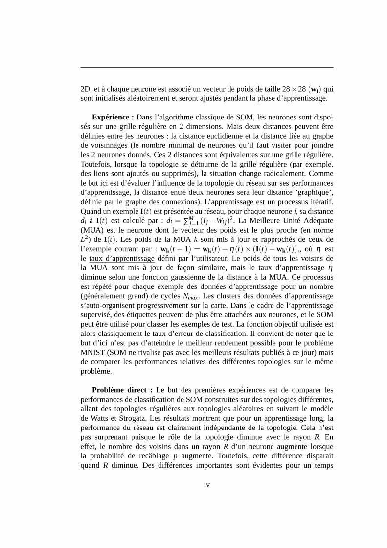
Expérience :Dans l’algorithme classique de SOM, les neurones sont dispo-sés sur une grille régulière en 2 dimensions. Mais deux distances peuvent êtredéfinies entre les neurones : la distance euclidienne et la distance liée au graphede voisinnages (le nombre minimal de neurones qu’il faut visiter pour joindreles 2 neurones donnés. Ces 2 distances sont équivalentes sur une grille régulière.Toutefois, lorsque la topologie se détourne de la grille régulière (par exemple,des liens sont ajoutés ou supprimés), la situation change radicalement. Commele but ici est d’évaluer l’influence de la topologie du réseausur ses performancesd’apprentissage, la distance entre deux neurones sera leurdistance ’graphique’,définie par le graphe des connexions). L’apprentissage est un processus itératif.Quand un exempleI(t) est présentée au réseau, pour chaque neuronei, sa distancedi à I(t) est calculé par :di = ∑M
j=1(I j −Wi j )2. La Meilleure Unité Adéquate
(MUA) est le neurone dont le vecteur des poids est le plus proche (en normeL2) de I(t). Les poids de la MUAk sont mis à jour et rapprochés de ceux del’exemple courant par :wk(t + 1) = wk(t) + η(t)× (I(t) − wk(t)),, où η estle taux d’apprentissage défini par l’utilisateur. Le poids de tous les voisins dela MUA sont mis à jour de façon similaire, mais le taux d’apprentissageηdiminue selon une fonction gaussienne de la distance à la MUA. Ce processusest répété pour chaque exemple des données d’apprentissagepour un nombre(généralement grand) de cyclesNmax. Les clusters des données d’apprentissages’auto-organisent progressivement sur la carte. Dans le cadre de l’apprentissagesupervisé, des étiquettes peuvent de plus être attachées aux neurones, et le SOMpeut être utilisé pour classer les exemples de test. La fonction objectif utilisée estalors classiquement le taux d’erreur de classification. Il convient de noter que lebut d’ici n’est pas d’atteindre le meilleur rendement possible pour le problèmeMNIST (SOM ne rivalise pas avec les meilleurs résultats publiés à ce jour) maisde comparer les performances relatives des différentes topologies sur le mêmeproblème.
Problème direct : Le but des premières expériences est de comparer lesperformances de classification de SOM construites sur des topologies différentes,allant des topologies régulières aux topologies aléatoires en suivant le modèlede Watts et Strogatz. Les résultats montrent que pour un apprentissage long, laperformance du réseau est clairement indépendante de la topologie. Cela n’estpas surprenant puisque le rôle de la topologie diminue avec le rayonR. Eneffet, le nombre des voisins dans un rayonR d’un neurone augmente lorsquela probabilité de recâblagep augmente. Toutefois, cette différence disparaitquandR diminue. Des différences importantes sont évidentes pour un temps
iv
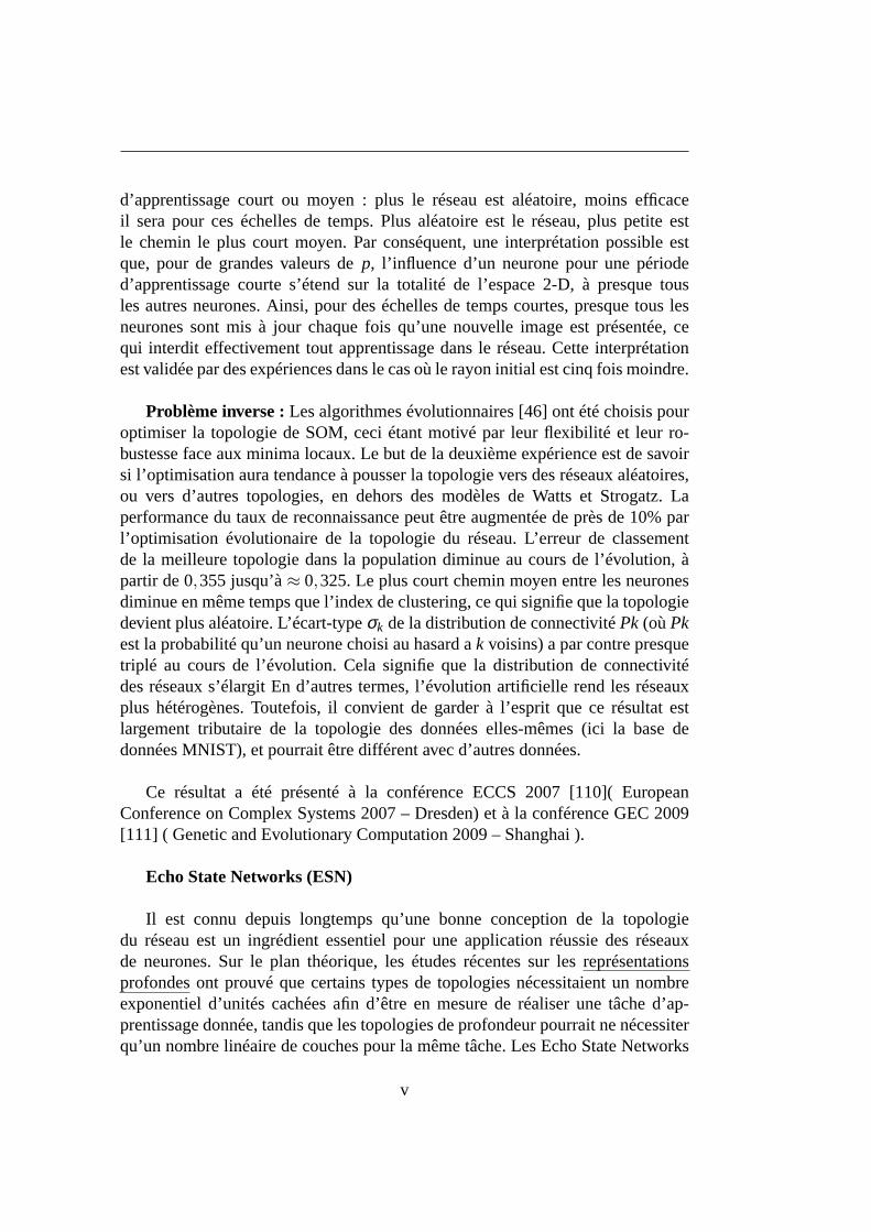
d’apprentissage court ou moyen : plus le réseau est aléatoire, moins efficaceil sera pour ces échelles de temps. Plus aléatoire est le réseau, plus petite estle chemin le plus court moyen. Par conséquent, une interprétation possible estque, pour de grandes valeurs dep, l’influence d’un neurone pour une périoded’apprentissage courte s’étend sur la totalité de l’espace2-D, à presque tousles autres neurones. Ainsi, pour des échelles de temps courtes, presque tous lesneurones sont mis à jour chaque fois qu’une nouvelle image est présentée, cequi interdit effectivement tout apprentissage dans le réseau. Cette interprétationest validée par des expériences dans le cas où le rayon initial est cinq fois moindre.
Problème inverse :Les algorithmes évolutionnaires [46] ont été choisis pouroptimiser la topologie de SOM, ceci étant motivé par leur flexibilité et leur ro-bustesse face aux minima locaux. Le but de la deuxième expérience est de savoirsi l’optimisation aura tendance à pousser la topologie versdes réseaux aléatoires,ou vers d’autres topologies, en dehors des modèles de Watts et Strogatz. Laperformance du taux de reconnaissance peut être augmentée de près de 10% parl’optimisation évolutionaire de la topologie du réseau. L’erreur de classementde la meilleure topologie dans la population diminue au cours de l’évolution, àpartir de 0,355 jusqu’à≈ 0,325. Le plus court chemin moyen entre les neuronesdiminue en même temps que l’index de clustering, ce qui signifie que la topologiedevient plus aléatoire. L’écart-typeσk de la distribution de connectivitéPk (oùPkest la probabilité qu’un neurone choisi au hasard ak voisins) a par contre presquetriplé au cours de l’évolution. Cela signifie que la distribution de connectivitédes réseaux s’élargit En d’autres termes, l’évolution artificielle rend les réseauxplus hétérogènes. Toutefois, il convient de garder à l’esprit que ce résultat estlargement tributaire de la topologie des données elles-mêmes (ici la base dedonnées MNIST), et pourrait être différent avec d’autres données.
Ce résultat a été présenté à la conférence ECCS 2007 [110]( EuropeanConference on Complex Systems 2007 – Dresden) et à la conférence GEC 2009[111] ( Genetic and Evolutionary Computation 2009 – Shanghai).
Echo State Networks (ESN)
Il est connu depuis longtemps qu’une bonne conception de la topologiedu réseau est un ingrédient essentiel pour une application réussie des réseauxde neurones. Sur le plan théorique, les études récentes sur les représentationsprofondes ont prouvé que certains types de topologies nécessitaient un nombreexponentiel d’unités cachées afin d’être en mesure de réaliser une tâche d’ap-prentissage donnée, tandis que les topologies de profondeur pourrait ne nécessiterqu’un nombre linéaire de couches pour la même tâche. Les EchoState Networks
v
[105], qui ont été récemment proposés pour l’apprentissagesupervisé de sériestemporelles, peuvent être considérés comme une approche alternative : au lieude l’optimisation d’une topologie pour une tâche donnée, ilpropose d’utiliserun large réservoir de neurones dont les connexions sont tirées au sort (et àfaible densité). Seuls les poids des connexions sortantes sont à apprendre, ce quitransforme le processus d’apprentissage en un simple un problème d’optimisationquadratique qui est facilement résolu par une méthode baséesur le gradient . . . ,du moins dans le cas de l’apprentissage supervisé.
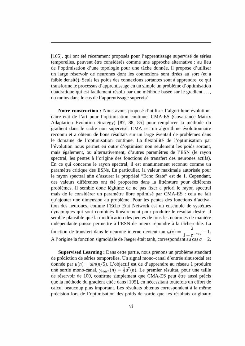
Notre construction : Nous avons proposé d’utiliser l’algorithme évolution-naire état de l’art pour l’optimisation continue, CMA-ES (Covariance MatrixAdaptation Evolution Strategy) [87, 88, 85] pour remplacerla méthode dugradient dans le cadre non supervisé. CMA est un algorithme évolutionnairereconnu et a obtenu de bons résultats sur un large éventail deproblèmes dansle domaine de l’optimisation continue. La flexibilité de l’optimisation parl’évolution nous permet en outre d’optimiser non seulementles poids sortant,mais également, ou alternativement, d’autres paramètres de l’ESN (le rayonspectral, les pentes à l’origine des fonctions de transfertdes neurones actifs).En ce qui concerne le rayon spectral, il est unanimement reconnu comme unparamètre critique des ESNs. En particulier, la valeur maximale autorisée pourle rayon spectral afin d’assurer la propriété “Echo State” est de 1. Cependant,des valeurs différentes ont été proposées dans la littérature pour différentsproblèmes. Il semble donc légitime de ne pas fixer a priori le rayon spectralmais de le considérer un paramètre libre optimisé par CMA-ES :cela ne faitqu’ajouter une dimension au problème. Pour les pentes des fonctions d’activa-tion des neurones, comme l’Echo Etat Network est un ensemblede systèmesdynamiques qui sont combinés linéairement pour produire lerésultat désiré, ilsemble plausible que la modification des pentes de tous les neurones de manièreindépendante puisse permettre à l’ESN de mieux répondre à latâche-cible. La
fonction de transfert dans le neurone interne devient tanha(x) =2
1+e−a∗x − 1.
A l’origine la fonction sigmoïdale de Jaeger était tanh, correspondant au casa= 2.
Supervised Learning :Dans cette partie, nous prenons un problème standardde prédiction de séries temporelles. Un signal mono-canal d’entrée sinusoïdal estdonnée paru(n) = sin(n/5). L’objectif est de d’apprendre au réseau à produireune sortie mono-canal,yteach(n) = 1
2u7(n). Le premier résultat, pour une taillede réservoir de 100, confirme simplement que CMA-ES peut être aussi précisque la méthode du gradient citée dans [105], en nécessitant toutefois un effort decalcul beaucoup plus important. Les résultats obtenus correspondent à la mêmeprécision lors de l’optimisation des poids de sortie que lesrésultats originaux
vi
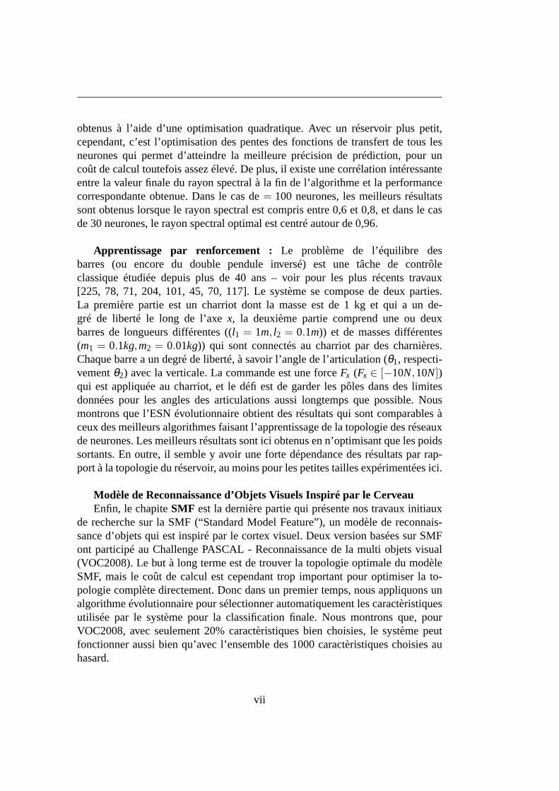
obtenus à l’aide d’une optimisation quadratique. Avec un réservoir plus petit,cependant, c’est l’optimisation des pentes des fonctions de transfert de tous lesneurones qui permet d’atteindre la meilleure précision de prédiction, pour uncoût de calcul toutefois assez élevé. De plus, il existe une corrélation intéressanteentre la valeur finale du rayon spectral à la fin de l’algorithme et la performancecorrespondante obtenue. Dans le cas de= 100 neurones, les meilleurs résultatssont obtenus lorsque le rayon spectral est compris entre 0,6et 0,8, et dans le casde 30 neurones, le rayon spectral optimal est centré autour de 0,96.
Apprentissage par renforcement : Le problème de l’équilibre desbarres (ou encore du double pendule inversé) est une tâche decontrôleclassique étudiée depuis plus de 40 ans – voir pour les plus récents travaux[225, 78, 71, 204, 101, 45, 70, 117]. Le système se compose de deux parties.La première partie est un charriot dont la masse est de 1 kg et qui a un de-gré de liberté le long de l’axex, la deuxième partie comprend une ou deuxbarres de longueurs différentes ((l1 = 1m, l2 = 0.1m)) et de masses différentes(m1 = 0.1kg,m2 = 0.01kg)) qui sont connectés au charriot par des charnières.Chaque barre a un degré de liberté, à savoir l’angle de l’articulation (θ1, respecti-vementθ2) avec la verticale. La commande est une forceFx (Fx ∈ [−10N,10N])qui est appliquée au charriot, et le défi est de garder les pôles dans des limitesdonnées pour les angles des articulations aussi longtemps que possible. Nousmontrons que l’ESN évolutionnaire obtient des résultats qui sont comparables àceux des meilleurs algorithmes faisant l’apprentissage dela topologie des réseauxde neurones. Les meilleurs résultats sont ici obtenus en n’optimisant que les poidssortants. En outre, il semble y avoir une forte dépendance des résultats par rap-port à la topologie du réservoir, au moins pour les petites tailles expérimentées ici.
Modèle de Reconnaissance d’Objets Visuels Inspiré par le CerveauEnfin, le chapiteSMF est la dernière partie qui présente nos travaux initiaux
de recherche sur la SMF (“Standard Model Feature”), un modèle de reconnais-sance d’objets qui est inspiré par le cortex visuel. Deux version basées sur SMFont participé au Challenge PASCAL - Reconnaissance de la multi objets visual(VOC2008). Le but à long terme est de trouver la topologie optimale du modèleSMF, mais le coût de calcul est cependant trop important pouroptimiser la to-pologie complète directement. Donc dans un premier temps, nous appliquons unalgorithme évolutionnaire pour sélectionner automatiquement les caractèristiquesutilisée par le système pour la classification finale. Nous montrons que, pourVOC2008, avec seulement 20% caractèristiques bien choisies, le système peutfonctionner aussi bien qu’avec l’ensemble des 1000 caractèristiques choisies auhasard.
vii
Pour les tâches de reconnaissance immédiate d’objets dans une scène, il a étésuggéré que le cerveau utilise des propriétés d’invariancede l’objet. Le modèleSMF est inspiré par cette remarque. La SMF est fondamentalement un réseau deneurones à propagation directe (“feed-forward”) hiérarchique. Dans ce manuscrit,nous avons utilisé une simplification du modèle de référence[194], donné dans[198], qui se compose de quatre couches de réseaux de neurones non récurrents.Le modèle comporte deux types de neurones : ceux qu’on appelle simples unités,ou S, et les unités complexes, ou C. Les unités S combinent leurs entrées avecune “Bell-Shaped tuning function” pour augmenter la sélectivité. Les unités Ccombinent leurs entrées avec une fonction maximum (MAX) pour augmenterl’invariance. Par conséquent, en réglant les paramètres dusystème, le modèlepeut obtenir un bon équilibre entre la sélectivité et l’invariance.
Dans ce modèle initial, la sortie du réseau est composée de caractéristiquesqui sont passées au travers d’un algorithme de combinaison linéaire pour latâche de classification elle-même, c’est à dire qu’il calcule la confiance deVOC 2008 de chaque image pour chaque classe d’objet. Dans notre étude,nous appliquons une optimisation évolutionnaire utilisant CMA-ES (CovarianceMatrix Adaptation Evolution Strategy [88, 103] pour calculer la confiance deVOC2008 de chaque image pour chaque classe d’objet. Premièrement, nousutilisons CMA-ES afin d’optimiser le poids d’un combinateur linéaire. Commela dimension d’optimisation est au moins aussi grande que 1000, nous testonségalement un algorithme multi-évolutionnaire pour sélectionner de façon op-timale 200 dimensions parmi 1000, avant d’optimiser les 200dimensions choisies.
Nous montrons qu’en sélectionnant 200 caractéristiques optimales le systèmepeut garder presque les mêmes performances dans le défi VOC2008 qu’enutilisant 1000 caractèristiques choisies au hasard, tout en diminuant le coûtcalcul de 2 ordres de grandeur. La robustesse du système semble dépendre descaractéristiques sélectionnées. Même si nos résultats surVOC2008 ne sont pasparmi les meilleurs du challenge, en considérant la simplicité du modèle que nousavons appliqué (nous utilisons seulement la mise en modèle par défaut et il y abeaucoup de paramètres qui peuvent être ajustés), nous estimons qu’il y a encorede la place pour des améliorations significatives. Les futurs travaux de rechercheseraient d’optimiser la topologie des connexions entre lescouches du modèle deSMF, et également d’optimiser les paramètres de réglage quiont effectivementété définis par la recherche bio-inspirée.
viii
Contents
1 Introduction 1
2 Background 52.1 Artificial Neural Networks . . . . . . . . . . . . . . . . . . . . . 5
2.1.1 History . . . . . . . . . . . . . . . . . . . . . . . . . . . 62.1.2 Learning Methods . . . . . . . . . . . . . . . . . . . . . 92.1.3 Network Topology . . . . . . . . . . . . . . . . . . . . . 112.1.4 Recent research . . . . . . . . . . . . . . . . . . . . . . . 12
2.2 Evolutionary Computing . . . . . . . . . . . . . . . . . . . . . . 152.2.1 Key Issues . . . . . . . . . . . . . . . . . . . . . . . . . 162.2.2 Historical Trends . . . . . . . . . . . . . . . . . . . . . . 202.2.3 An Adaptive Evolution Strategy: CMA-ES . . . . . . . . 222.2.4 Applications . . . . . . . . . . . . . . . . . . . . . . . . 26
2.3 Evolving Artificial Neural Network . . . . . . . . . . . . . . . . 282.3.1 Evolving Connection Weights . . . . . . . . . . . . . . . 282.3.2 Evolving Network Topologies . . . . . . . . . . . . . . . 31
2.4 Topology of Complex Networks . . . . . . . . . . . . . . . . . . 432.4.1 Small World Topology . . . . . . . . . . . . . . . . . . . 432.4.2 Scale Free Topology . . . . . . . . . . . . . . . . . . . . 452.4.3 Applications to ANNs . . . . . . . . . . . . . . . . . . . 47
2.5 Research Questions . . . . . . . . . . . . . . . . . . . . . . . . . 47
3 Evolving the Topology of Self-Organizing Map 493.1 Introduction . . . . . . . . . . . . . . . . . . . . . . . . . . . . . 493.2 Topology of Self-Organizing Map . . . . . . . . . . . . . . . . . 49
3.2.1 Kohonen Maps . . . . . . . . . . . . . . . . . . . . . . . 493.2.2 An Example with Color Data . . . . . . . . . . . . . . . . 513.2.3 Quantitative measure of topology preservation in SOM. . 523.2.4 Discussion . . . . . . . . . . . . . . . . . . . . . . . . . 55
3.3 Method and Experiments . . . . . . . . . . . . . . . . . . . . . . 563.3.1 A Simple Experiment with Classical Q H Measure . . . . 56
ix
CONTENTS
3.3.2 Experiments With MNIST database . . . . . . . . . . . . 593.3.3 Learning . . . . . . . . . . . . . . . . . . . . . . . . . . 603.3.4 Distance . . . . . . . . . . . . . . . . . . . . . . . . . . . 623.3.5 Labeling . . . . . . . . . . . . . . . . . . . . . . . . . . 623.3.6 Classifying . . . . . . . . . . . . . . . . . . . . . . . . . 65
3.4 Direct problem . . . . . . . . . . . . . . . . . . . . . . . . . . . 673.4.1 Influence of the radius . . . . . . . . . . . . . . . . . . . 673.4.2 Robustness against noise . . . . . . . . . . . . . . . . . . 69
3.5 Inverse problem . . . . . . . . . . . . . . . . . . . . . . . . . . . 713.5.1 The Algorithm . . . . . . . . . . . . . . . . . . . . . . . 713.5.2 Results . . . . . . . . . . . . . . . . . . . . . . . . . . . 733.5.3 Generalization w.r.t. the Learning Process . . . . . . . .. 73
3.6 Conclusion . . . . . . . . . . . . . . . . . . . . . . . . . . . . . 76
4 Evolutionary Optimization of Echo State Networks 794.1 Introduction . . . . . . . . . . . . . . . . . . . . . . . . . . . . . 794.2 Reservoir Computing Model . . . . . . . . . . . . . . . . . . . . 81
4.2.1 A Chaotic Time Series Prediction by ESN . . . . . . . . . 834.2.2 Researches on RC . . . . . . . . . . . . . . . . . . . . . 834.2.3 Discussion . . . . . . . . . . . . . . . . . . . . . . . . . 86
4.3 Supervised Learning of ESN . . . . . . . . . . . . . . . . . . . . 874.3.1 Jaeger’s Original Settings . . . . . . . . . . . . . . . . . 874.3.2 Which parameters to optimize? . . . . . . . . . . . . . . 894.3.3 The experiments . . . . . . . . . . . . . . . . . . . . . . 904.3.4 Comparative Measures . . . . . . . . . . . . . . . . . . . 914.3.5 Results . . . . . . . . . . . . . . . . . . . . . . . . . . . 914.3.6 Discussion . . . . . . . . . . . . . . . . . . . . . . . . . 95
4.4 Reinforcement Learning of ESN . . . . . . . . . . . . . . . . . . 954.4.1 The Pole-balancing Benchmark . . . . . . . . . . . . . . 954.4.2 Fitness(es) . . . . . . . . . . . . . . . . . . . . . . . . . 994.4.3 Experimental conditions . . . . . . . . . . . . . . . . . . 1004.4.4 Results and Discussion . . . . . . . . . . . . . . . . . . . 101
4.5 ESN vs Developmental Methods . . . . . . . . . . . . . . . . . . 1104.6 Conclusion . . . . . . . . . . . . . . . . . . . . . . . . . . . . . 111
5 Feature Selection in a Cortex-Like Object Recognition Model 1135.1 Cortex-Like Object Recognition . . . . . . . . . . . . . . . . . . 114
5.1.1 Visual Object Recognition in the Cortex . . . . . . . . . . 1145.1.2 Standard Model Features (SMFs) . . . . . . . . . . . . . 1155.1.3 Model Details . . . . . . . . . . . . . . . . . . . . . . . . 1165.1.4 The Perspectives of the Model . . . . . . . . . . . . . . . 121
x
CONTENTS
5.2 PASCAL Visual Object classes Challenge (VOC08) . . . . . . . . 1225.2.1 Classification/Detection Image Sets . . . . . . . . . . . . 1235.2.2 Classification Task . . . . . . . . . . . . . . . . . . . . . 125
5.3 Experiments . . . . . . . . . . . . . . . . . . . . . . . . . . . . . 1285.3.1 Using EC Algorithms with SMF Model . . . . . . . . . . 1285.3.2 Pre-training of SMFs model . . . . . . . . . . . . . . . . 1285.3.3 Linear Combination using CMA-ES . . . . . . . . . . . . 1295.3.4 Multi-Evolutionary Optimization . . . . . . . . . . . . . 1305.3.5 Results . . . . . . . . . . . . . . . . . . . . . . . . . . . 1385.3.6 Result Analysis . . . . . . . . . . . . . . . . . . . . . . . 138
5.4 Conclusion . . . . . . . . . . . . . . . . . . . . . . . . . . . . . 142
6 Conclusion 1456.1 Summary of Results . . . . . . . . . . . . . . . . . . . . . . . . . 145
6.1.1 Evolving SOM Topology . . . . . . . . . . . . . . . . . . 1456.1.2 Evolving Parameters and Hyper-parameters of ESN . . . .1466.1.3 Feature Sub-Sampling in SMF Bio-Inspired Approach . . 147
6.2 Perspectives . . . . . . . . . . . . . . . . . . . . . . . . . . . . . 1486.2.1 Fundamental Issues . . . . . . . . . . . . . . . . . . . . . 1486.2.2 Practical Issues . . . . . . . . . . . . . . . . . . . . . . . 149
xi

CONTENTS
xii
Chapter 1
Introduction
We are now in the 21st century, and since the 1950s, ArtificialIntelligence hasbecome an independent subject of study of Computer Science, and its influenceon our daily life has been ever increasing.
Intelligence is the result of an evolutionary process basedon natural selection.In recent years, studying the so-calledbio-inspired mechanisms, i.e. mechanismsthat try to somehow mimic natural processes, has raised a lotof research interest.In particular, two of these research streams have attractedgreat attention and leadto a large body of work.
From a macroscopic point of view, nature produced a rich and diverse set ofspecies thanks to two principles: blind variations, that created the diversity in thefirst place, and natural selection, that selected some individuals and populationsfor survival according to the natural principle of “survivalof thefittest”. ArtificialEvolutionary Algorithms (EAs) [47, 43] are powerful optimization algorithmsinspired by this natural selection mechanism, and have beensuccessfully appliedin lots of real world problems [231].
From the microscopic point of view, the material basis for intelligence isbased on large-scale ensembles of neurons, organized in networks. ArtificialNeural Networks (ANNs) are a powerful model inspired by their biologicalcounterparts for knowledge processing and analysis. Originated in the early 50s[182], ANN research is still very active [105, 143, 93, 198].
At the crossroad of both research areas, research using Evolutionary Algo-rithm to optimize Artificial Neural Networks has been going on for many years[230]: Beyond the “simple” optimization of the weights of a network with a fixedgiven topology, the flexibility of Evolutionary Algorithmsmade them appealing
1
1. INTRODUCTION
when it came to optimize also the topology of candidate neural networks for agiven task.
During the same period (the last 20 years), the study of complex networkshas brought this area into new research directions and inspiration. Inspired bothby natural networks (e.g. Gene Regulatory Networks, protein-protein interactionnetworks, . . . ) and artificial ones (e.g. the World Wide Web, airline connec-tion networks, social networks such as co-authoring networks, . . . ), new insightshave been gained into network topologies. More particularly, researches on small-world [220] and scale-free [19] networks have produced a newpoint of view forour understanding of network complexity.
Chapter 2 will survey those research areas in more detail, highlighting thedifferent paradigms that have been used for this thesis.
In this context, the present work is centered around the relationship betweenthe (possibly complex) topology of a given Neural Network and its performanceas a computing unit. Two approaches will be considered, and experimentedwith in different application domains. Thedirect problem is the study of theperformance of a given type of neural network, in a given environment, withrespect to its topology. By controlled variation of the topology, within a givenclass of parameterized topologies, and careful measure of the resulting networkperformance, some hints can be gathered regarding the influence of this or thattopology description parameter. We will then consider theinverse problem,i.e. optimize the topology in order to maximize the performance of the neuralnetwork. Evolutionary Algorithms will be the optimizationtool, as they canhandle either continuous optimization, in the case where the topology is describedby some macroscopic description parameters, or directly handle the topologyitself (e.g. through modifications of the connections) to fine-tune the topology.
A first application domain will be that of Self-Organizing Maps (SOMs)[124], detailed in Chapter 3. SOMs are mainly used for unsupervised learning,and the standard regular topology is generally used withoutmuch questioning.However, there is hardly a universally acclaimed performance measure forcomparing the performance of unsupervised learning algorithms. Hence, theperformance of a given SOM topology will be assessed throughthe classificationaccuracy on the well-known MNIST database for digit recognition. The inverseproblem will be addressed here by directly manipulating theconnections betweenneurons.
A second application context, presented in Chapter 4, is thatof Echo StateNetworks [105], the recent paradigm pertaining to the Reservoir Computingfamily. While ESNs are generally used for regression tasks, and the optimization
2
problem then amounts to the quadratic optimization of the outgoing weights,using ESNs for reinforcement learning tasks has hardly beenaddressed inthe literature. We will investigate the influence of different hyper-parametersdefining the reservoir topology on the well-known benchmarktask of balancingthe double-pole. The optimization algorithm for the outputweights will bethe well-known CMA-ES (Covariance Matrix Adaptation Evolution Strategy)[88, 86], as the problem is not quadratic any more. But the goodside of thisdrawback is that the same algorithm can be used to simultaneously optimize theoutput weights and some hyper-parameters defining the topology of the reservoir.
Finally, Chapter 5 will present a first study involving a CortexinspiredVisual Object Recognition model [198]. In particular, we will investigate whetherusing only a sub-sample of the many features designed by the original algorithmcan improve the global recognition rate, while accelerating the learning phase.Results will be demonstrated on the complex VOC2008 challenge.
And as usual, Chapter 6 will conclude this dissertation, summarizing anddiscussing the results, and opening the way for further research.
3

1. INTRODUCTION
4
Chapter 2
Background
This chapter will set up the background for all work to be presented in this disser-tation. First, brief introductions on Artificial Neural Networks (ANNs) and Evo-lutionary Computing (EC) will be given. Then we will focus on Neuro-Evolution,the coupling of both techniques, i.e., the specific EC methods that have been devel-oped for evolving Artificial Neural Networks. Further, recent advances regardingthe Topology of Complex Networks will be surveyed. Finally, in the light of thisstate-of-the-art methods, we will introduce the research questions addressed in thepresent research and their motivations.
2.1 Artificial Neural Networks
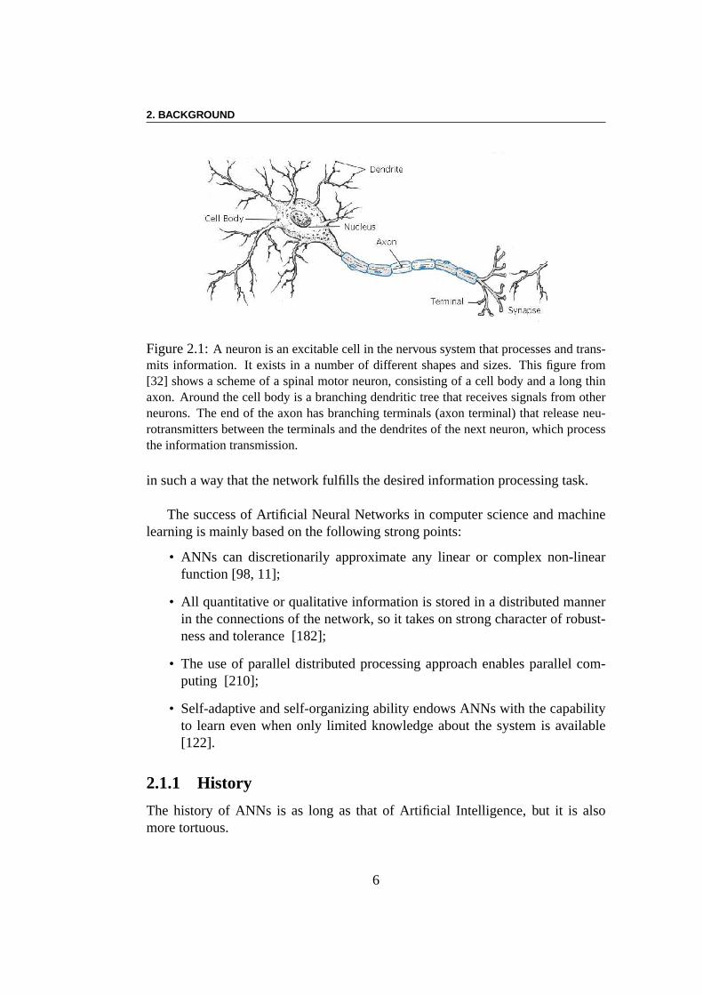
The human brain is a complex biological system composed of a large numberof highly interconnected processing elements (neurons) [137]. It is formed byabout 1011 neurons [104]. Each neuron connects to about 104 other neurons onaverage [155, 30]. Figure 2.1 shows an example of a biological neuron.
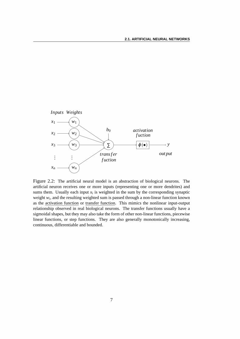
The physiological research about the brain and other biological neuralsystems is the foundation for artificial neural networks (ANNs). The artificialneural model is an abstraction of biological neurons (shownin figure 2.2) , i.e.an interpretation of our understanding of brain operations, applied to build anartificial intelligence system.
Artificial Neural Networks (ANNs) are parallel informationprocessingsystems in which a number of artificial neurons (or units) areinterconnected bysynapses. Usually the output of each unit is a nonlinear function of the sum of itsinputs, weighted by synaptic weights (see figure 2.2). The main idea is then tofind algorithms or heuristics for adjusting the synapses andthe synaptic weights
5
2. BACKGROUND
Figure 2.1:A neuron is an excitable cell in the nervous system that processes and trans-mits information. It exists in a number of different shapes and sizes. This figure from[32] shows a scheme of a spinal motor neuron, consisting of a cell body and a long thinaxon. Around the cell body is a branching dendritic tree that receives signals from otherneurons. The end of the axon has branching terminals (axon terminal) thatrelease neu-rotransmitters between the terminals and the dendrites of the next neuron, which processthe information transmission.
in such a way that the network fulfills the desired information processing task.
The success of Artificial Neural Networks in computer science and machinelearning is mainly based on the following strong points:
• ANNs can discretionarily approximate any linear or complex non-linearfunction [98, 11];
• All quantitative or qualitative information is stored in adistributed mannerin the connections of the network, so it takes on strong character of robust-ness and tolerance [182];
• The use of parallel distributed processing approach enables parallel com-puting [210];
• Self-adaptive and self-organizing ability endows ANNs with the capabilityto learn even when only limited knowledge about the system isavailable[122].
2.1.1 History
The history of ANNs is as long as that of Artificial Intelligence, but it is alsomore tortuous.
6
2.1. ARTIFICIAL NEURAL NETWORKS
∑
w1x1
Inputs Weights
w2x2
w3x3
......
wnxn
b0
trans f erf uction
ϕ(•)
activationf uction
y
out put
Figure 2.2: The artificial neural model is an abstraction of biological neurons. Theartificial neuron receives one or more inputs (representing one or moredendrites) andsums them. Usually each inputxi is weighted in the sum by the corresponding synapticweightwi , and the resulting weighted sum is passed through a non-linear function knownas theactivationfunction or transferfunction. This mimics the nonlinear input-outputrelationship observed in real biological neurons. The transfer functions usually have asigmoidal shapes, but they may also take the form of other non-linear functions, piecewiselinear functions, or step functions. They are also generally monotonically increasing,continuous, differentiable and bounded.
7
2. BACKGROUND
Creation: In 1943, psychologist McCulloch and symbolic logician Pittsbuiltthe first mathematical neuron model [147], known as the MP model. They gavea formal mathematical description: For a given artificial neuron k, let there bem+1 inputs with signalsx0 throughxm and weightswk0 throughwkm. The output
yk of neuronk is: yk = ϕ(
∑mj=0wk jx j
)
, whereϕ is the transfer function.
They proved that a single neuron can perform logic functions, thereby creatingthe era of artificial neural networks. In 1949, the psychologist Hebb proposed aconception that the synaptic contacts could have variable intensities, dependingonly on the activation of the pre- and postsynaptic neurons [91]: “When an axonof cell A is near enough to excite cell B and repeatedly or persistently takes partin firing it, some growth process or metabolic change takes place in one or bothcells such that A’s efficiency, as one of the cells firing B, is increased”.
This so-called Hebb rule of neural network is an underlying basis for the learn-ing algorithm of ANNs. In 1958, Rosenblatt built the Perceptron model [177].The Perceptron is a binary classifier that maps its inputxk (a real-valued vector)to an output valueyk (a single binary value) across the matrix of weights(wi, j :
yk =
{
1 ∑mj=0wk jx j > 0
0 else
The perceptron model is a specifical case of MP model and the Hebb learn-ing algorithm can also be used to tune their connection weights (see section 2.1.2).
The Neural Network Winter: After analyzing the function and the constraintsof artificial neural networks, typically represented by Perceptron, Minsky andco-author published the «Perceptron» book in 1969 [151]. Inthis book theypointed out the limit of the perceptron model. For instance,they reported that nosingle-layer perceptron can solve higher-order classification problems, includingnonlinearly separable problems such as the XOR function. Their argumentsgreatly impacted the study of ANNs. At the same epoch, serialcomputers andartificial intelligence progressed rapidly. These two reasons caused the lack ofthe necessity and urgency to develop new methods for computing. Thereforethe research on ANNs was in depression during more than ten years afterwards.However, some researchers still continued to develop the field and proposed thetheory of self-organizing map (SOMs) [122, 123] in 1972, andestablished astrong mathematical foundation for ANNs [3].
The Return of Spring: Three years after Minsky’s book, Grossberg pub-lished the paper introducing multi-layer networks capableof modeling XOR
8
2.1. ARTIFICIAL NEURAL NETWORKS
functions [74]. But the research on ANNs did not return to Spring until the1980s, helped by the progresses in CPU power. In 1982, physicist Hopfieldproposed what is today known as the Hopfield Neural Network model [96].A Hopfield net is a form of recurrent artificial neural network. Hopfield netsserve as content-addressable memory systems with binary threshold units. Theintroduction of the “calculational energy” determined thestability of the neuralnetwork. They are guaranteed to converge to a local minimum,but convergenceto one of the stored patterns is not guaranteed.
In 1983, Hinton and Sejnowski gave the name of Boltzmann machine toa type of stochastic recurrent neural network [94]. Boltzmann machines canbe seen as the stochastic, generative counterpart of Hopfield nets. They wereone of the first examples of a neural network capable of learning internalrepresentations. They are able to represent, and, given sufficient time, to solvedifficult combinatorial problems. If the connectivity is constrained, the learningcan be made efficient enough to be useful for practical problems. In 1985, thestatistical thermodynamics simulated annealing techniques, which applied in theBoltzmann model, helped to prove that the whole system will eventually convergetoward a global stability point [1]. In 1986, by studying themicrostructureof cognition, Rumelhart and the PDP Research Group proposed the theoryof Parallel Distributed Processing [38]. The famous Back-Propagation (BP)algorithm for multi-layer feedforward ANNs was proposed in1986 too [181].
2.1.2 Learning Methods
One major difference between classical programming techniques and ANNs isthat the later are not strictly speaking programmed, but must be trained beforethey are used. A number of learning methods have been developed over the years,that can be divided into Supervised Learning, Non-supervised Learning and Re-inforcement Learning.
Supervised Learning
In the supervised learning case, the training examples are given together with theexpected outputs or labels (in classification case) called teacher’s dates. By com-paring the margins between the expected dates and ANN’s outputs, the connectionstrengths are adjusted and converge to a stable position. When the environmentchanges after the training, the network is retrained and adapted to the new envi-ronment. The Back-propagation algorithm [181] is a widely used algorithm in
9
2. BACKGROUND
the feedforward multi-layer ANNs. It is a supervised learning method, and is animplementation of theDeltarule.
The Delta rule is a gradient descent learning rule for updating the weightsof the artificial neurons in a single-layer perceptron. For aneuron j, withactivation functiong(x), the delta rule for j ’s ith weight w ji is given by∆w ji = α(t j − y j)g′(h j)xi, whereα is a small constant called learning rate,g(x)is the neuron’s activation function,t j is the target output,h j is the weighted sumof the neuron’s inputs,y j is the actual output, andxi is the ith input. It holdsh j = ∑xiw ji , andy j = g(h j).
The Back-propagation algorithm can be summarized as follows:
1. Present a training sample to the neural network.
2. Compare the resulting output with the desired output for the given input.This is called the error.
3. For each neuron, calculate what the output should have been, and a scalingfactor, how much lower or higher the output must be adjusted to match thedesired output. This is the local error.
4. Adjust the weights of each neuron to lower the local error by applying theDelta rule.
5. Assign "blame" for the local error to neurons at the previous level, back-propagate the local error to the neurons of the previous level accordingto their connection weights with the neurons of current level, adjust theweights by applying the Delta rule too.
6. Repeat from step 3 on the neurons at the previous level, using each "blame"has its error.
In the feed-back ANNs domain, the Reservoir Computing model [105] at-tracted a lot of attention in recent years, in particular forthe Supervised Learningof time series. It will be introduced in detail in chapter 4.
Unsupervised Learning
In the Unsupervised Learning case, there is no expected output associated withthe input, so that, the ANNs is expected to find the correct input-output matchingby using self-organized methods based on its unique networkarchitecture andlearning rules. In the learning process, ANNs continue to accept the learningsamples and auto-organize the data in the pattern of connection weights among
10
2.1. ARTIFICIAL NEURAL NETWORKS
neurons. Self-organizing map [122, 123] network is typically used in this kind oflearning model, to create low dimensional view of high dimensional data.
Reinforcement Learning
In a way, Reinforcement learning can be considered an intermediate between su-pervised and non-supervised learning. In reinforcement learning, the teacher doesnot provide the correct output associated with the input, but a simple reward (orpunishment) when the predicted output is correct (false). This reward can be de-layed. In all robotic experiments where the robot must find its way out of a maze.The system tries to find a policy for maximizing cumulative rewards over thecourse of the problem. Thus, reinforcement learning is particularly well suitedto problems which include a long-term versus short-term reward trade-off. It hasbeen applied successfully to various problems, including robot control (chapter 4),elevator scheduling, telecommunications, backgammon andchess [209, 114].
2.1.3 Network Topology
Based on connection topology, neural network models are traditionally dividedinto feedforward networks andfeedback (orrecurrent) networks. However, recentdevelopments in the so-called complex network field lead to contemplate the useof other classes of topology. We will present these aspects in section 2.4.
Feedforward networks
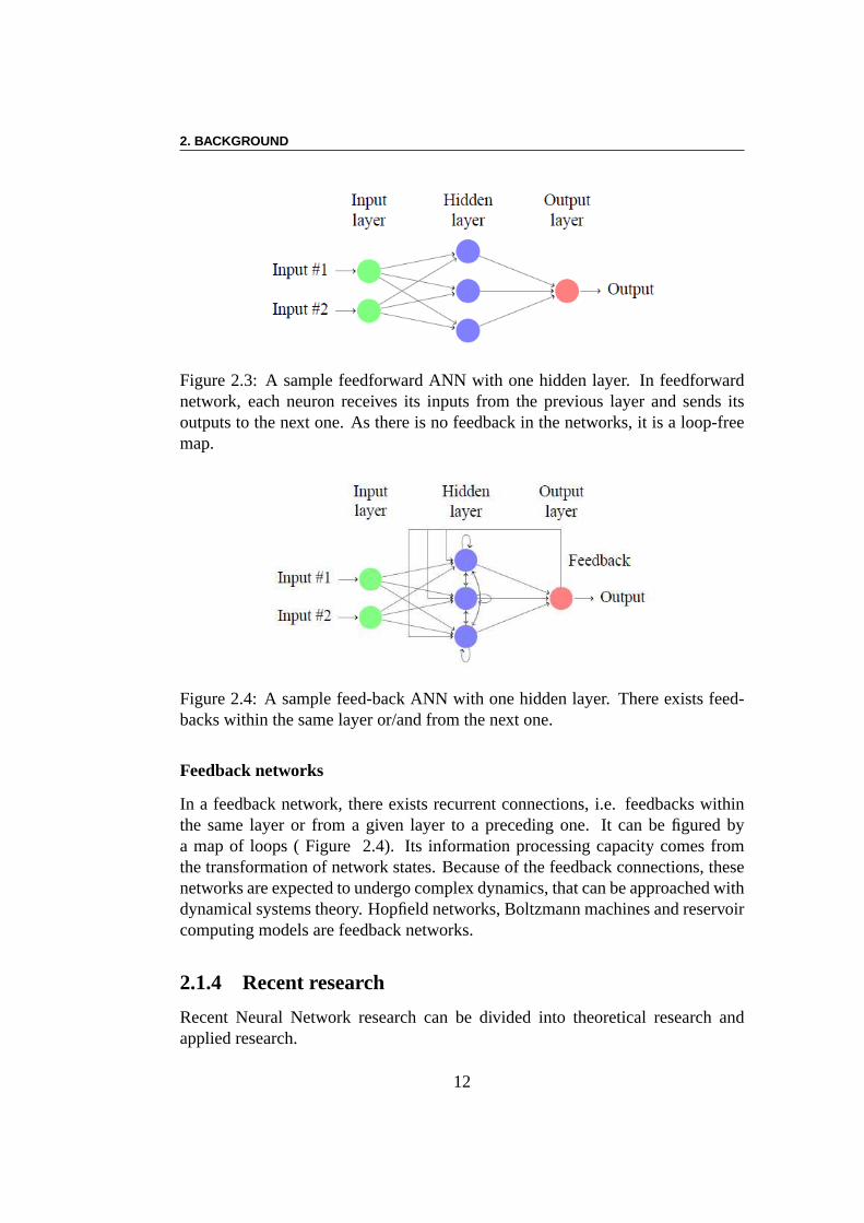
Feedforward networks are structures in which there is no loop in the connectiongraph of the network. A specific case is that oflayered feedforward architectures,where the neurons are organized in layers, and where each neuron takes its inputsfrom the previous layer and sends its output to the next one. Because the con-nection graph is loop-free, there are no feedbacks in the network (Figure 2.3).Consequently, the networks has no real dynamics: information just flows fromone layer to the other. Such a network realizes the projection from the input spaceto the output space, and its information processing capacity comes from a multiplecompound of simple nonlinear functions. This kind of network structure is simpleand easy to implement (compared to networks with loops). Backpropagation is anespecially well-suited supervised learning method for feedforward networks, andeven easier to implement within multi-layer feedforward networks.
11
2. BACKGROUND
Figure 2.3: A sample feedforward ANN with one hidden layer. In feedforwardnetwork, each neuron receives its inputs from the previous layer and sends itsoutputs to the next one. As there is no feedback in the networks, it is a loop-freemap.
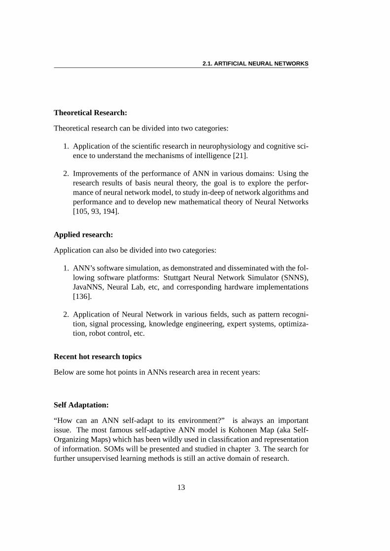
Figure 2.4: A sample feed-back ANN with one hidden layer. There exists feed-backs within the same layer or/and from the next one.
Feedback networks
In a feedback network, there exists recurrent connections,i.e. feedbacks withinthe same layer or from a given layer to a preceding one. It can be figured bya map of loops ( Figure 2.4). Its information processing capacity comes fromthe transformation of network states. Because of the feedback connections, thesenetworks are expected to undergo complex dynamics, that canbe approached withdynamical systems theory. Hopfield networks, Boltzmann machines and reservoircomputing models are feedback networks.
2.1.4 Recent research
Recent Neural Network research can be divided into theoretical research andapplied research.
12
2.1. ARTIFICIAL NEURAL NETWORKS
Theoretical Research:
Theoretical research can be divided into two categories:
1. Application of the scientific research in neurophysiology and cognitive sci-ence to understand the mechanisms of intelligence [21].
2. Improvements of the performance of ANN in various domains: Using theresearch results of basis neural theory, the goal is to explore the perfor-mance of neural network model, to study in-deep of network algorithms andperformance and to develop new mathematical theory of Neural Networks[105, 93, 194].
Applied research:
Application can also be divided into two categories:
1. ANN’s software simulation, as demonstrated and disseminated with the fol-lowing software platforms: Stuttgart Neural Network Simulator (SNNS),JavaNNS, Neural Lab, etc, and corresponding hardware implementations[136].
2. Application of Neural Network in various fields, such as pattern recogni-tion, signal processing, knowledge engineering, expert systems, optimiza-tion, robot control, etc.
Recent hot research topics
Below are some hot points in ANNs research area in recent years:
Self Adaptation:
“How can an ANN self-adapt to its environment?” is always an importantissue. The most famous self-adaptive ANN model is Kohonen Map (aka Self-Organizing Maps) which has been wildly used in classification and representationof information. SOMs will be presented and studied in chapter 3. The search forfurther unsupervised learning methods is still an active domain of research.
13
2. BACKGROUND
Complex Systems Theory:
Since the 1990’s, theoretical studies of Complex System havedeeply changedour view of many fields [192, 232]. “Complex systems are systems where thecollective behavior of their parts entails emergence of properties that can hardly,if not at all, be inferred from properties of the parts. Examples of complexsystems include ant-hills, ants themselves, human economies, climate, nervoussystems, cells and living things, including human beings, as well as modernenergy or telecommunication infrastructures.” – The Complex Systems Society(CSS). ANNs are present in many areas of Complex Systems, and can be seenas one example of complex systems, and recent research [199]shows that theperformance of an ANN can be influenced by its topology, just like what iswell-known in other complex systems (social networks, biological network,internet etc) [28].
Reservoir Computing and Deep Belief Network:
ANNs still suffer from (at least) some crucial issues. The difficulty of learningincreases with the number of neurons (and synapses). Furthermore, learningfeedforward networks is also still very difficult when the network is madeof numerous layers. Finally, there is still no training algorithm for recurrentnetworks. Reservoir computing and Deep Belief Networks are, respectively, twoelements of answer to these issues.
The Reservoir Computing model, proposed independently by Jeager [105](Echo State Networks ) and Maass and colleagues [143] (Liquid State Machines),uses a large recurrent (feedback) network of neurons that are randomly andsparsely connected (the “reservoir”). The weights and topology of this reservoirare not optimized nor adapted and are kept fixed during training. The reservoirneurons are connected to output neurons that are used as a readout of the reservoirstates. The major idea behind reservoir computing is that only outgoing weights(those from the reservoir to the output neurons) are optimized, which amountsin the supervised case to a simple quadratic optimization problem that is easilysolved by any gradient-based method. Hence, reservoir computing can usea large number of neurons and weights (within the reservoir)connected as afeedforward network with rich dynamics, but learning is restricted to the lowernumber of feedforward outgoing weights. The promises of Reservoir Computinghave been fulfilled for several kinds of problems. See chapter 4 for further details.
The Deep Belief Network model was proposed by Hinton in 2006 [93].
14
2.2. EVOLUTIONARY COMPUTING
It has been known for a long time that if the initial weights ofa feedforwardnetwork that has multiple hidden layers are close to a good solution, gradientdescent works well. Conversely, learning is poorly efficientwhenever the initialweight values are far from a good solution. But finding such favorable initialweights is very difficult. In Hinton’s model, each layer is trained just like in asingle-layer network, one after the other and independently from the others. Soa multilayer ANNs is divided into a stack ofRestrictedBoltzmannMachines(RBMs) and each hidden layer of the lower RBMs is the input layer ofthehigher RBM. After this pre-training, the model is unrolled andbackpropagationof error derivatives can be used to fine-tune the ANNs to get good learning results.
The seminal work in Deep Belief Natworks [93] shows that the pre-trainingprocedure works well for a variety of data sets. And inspiredby this model, Jaegerproposed a hierarchical multilayer ESN model in 2007 [107].
Bio-inspired System:
The best current machine vision systems are still not competitive with humanand primate natural vision in visual recognition field, especially for objectsin cluttered and natural scenes of real world, despite decades of hard works[99, 166, 219, 198]. So taking inspiration from real biological systems is animportant method to improve the performance of artificial systems.
Inspired by the biology of visual cortex, Serre and Poggio [198] proposed amodel for invariant visual object recognition in 2007. The model gets the state ofthe art results in a series of visual benchmark tests on complex image data bases,such as CalTech5 [57, 221], CalTech101 [53], MIT-CBCL [92]. More detailsabout this model will be discussed in chapter 5.
2.2 Evolutionary Computing
This section quickly surveys the bases of Evolutionary Computing, adopting themodern point of view popularized by [47, 43], and borrowing most ideas from[188].
Darwin’s evolution theory is based on the two basic principles of naturalselection andblind variations. Natural selection describes how individuals withina given population have better chances to survive and to reproduce if they areadapted to the current environment. Blind variations describes how the geneticmaterial of the parents is randomly modified when transmitted to the children
15
2. BACKGROUND
(even though Darwin had no precise idea about what such genetic material couldbe).
Evolutionary Algorithms (EAs) are stochastic optimization algorithms looselyinspired by this crude view of Darwinian theory. Candidate solutions tothe optimization problem at hand, calledindividuals, are represented by theirchromosome. The target function of the optimization, akafitness, plays the roleof the environment. Within this environment, apopulation, or set of individuals,is first randomly initialized, and the fitness of all individuals is computed. Thispopulation then undergoes a succession ofgenerations. First, the population issubject toparentalselection: some individuals are selected, based on their fitness,in such a way that fitter individuals are more likely to be selected than individ-uals with poor fitness. The selected individuals generateoffspring individuals,thanks to the application ofvariationoperators, bycrossover (orrecombination)operators, that involve 2 or moreparents to generate each offspring, andmutationoperators, where a single parent is randomly modified into anoffspring. The new-born offspring are thenevaluated, i.e., their fitness is computed. Finally, the loopis closed by applyingsurvivalselection, globally to both parents and offspring, inorder to select the starting population for next generation; survival selection stillfavors fitter individuals.
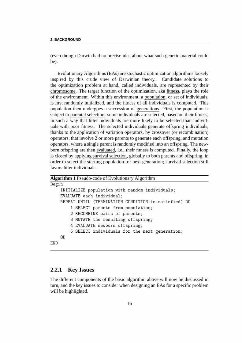
Algorithm 1 Pseudo-code of Evolutionary AlgorithmBegin
INITIALIZE population with random individuals;
EVALUATE each individual;
REPEAT UNTIL (TERMINATION CONDITION is satisfied) DO
1 SELECT parents from population;
2 RECOMBINE pairs of parents;
3 MUTATE the resulting offspring;
4 EVALUATE newborn offspring;
5 SELECT individuals for the next generation;
OD
END
2.2.1 Key Issues
The different components of the basic algorithm above will now be discussed inturn, and the key issues to consider when designing an EAs fora specific problemwill be highlighted.
16
2.2. EVOLUTIONARY COMPUTING
Fitness
How an individual adapts to the environment is measured by its fitness. Improv-ing the fitness function should result in improving the objective function of theoptimization problem at hand. On the other hand, modifying the fitness functionby some linear transformation only impacts the selection steps of the algorithm.Hence we will consider in general that the fitness functionis the original objectivefunction, postponing the discussion about possible transformations to the discus-sion about selection procedures.
A crucial remark about the fitness is that it usually represents most of thecomputational cost of the EA. Indeed, in most real-world situations, selectionand variation are generally very fast operations (though sorting huge populationscan become time consuming when the population size increases) compared to theevaluation, that can involve heavy simulations of possiblynon-linear physical,mechanical, chemical phenomenon. This also explains why the goal of the ECdesigner will be, beyond finding the optimum of the objectivefunction at hand,to minimize the number of fitness function evaluations. And the usual measurefor comparing different EA or EA settings is the number of evaluations needed toreach a predefined optimization goal (e.g., a given fitness value).
Representation
For a given problem, the representation of the candidate solution, or individuals,is crucial. The original optimization problem is posed in a given search space,and solutions must ultimately be given in this space. However, the EC designerfaces two goals that are somehow contradictory. On the one hand, he needs tofind the best possible solution in the original search space;On the other hand,exploration depends on the variation operators, and some structure of the searchspace is mandatory to make the exploration efficient. From this point of view, thechoice of a representation and the design of the variation operators are the twofaces of the same coin, and should be done together.
It is hence often useful to search an auxiliary space, where efficient variationoperators can be designed, rather than the search space of the original optimizationproblem. Still crudely inspired from biology, the originalsearch space is termedphenotypic space1, while the space where variation operators are applied is calledthe genotypic space. The phenotypes (or potential solutions ofthe optimizationproblem at hand) areencoded into the genotypic space, where the actual searchtakes place through the application of the variation operators. The individuals
1or sometimesbehavioralspace as this is where the behavior of the individual is evaluatedwhen the fitness is computed.
17
2. BACKGROUND
referred to in the previous Section 2.2 and in Algorithm 1 aregenotypes, that aredecoded into the corresponding phenotypes for evaluation.
’Natural’ Selection
The two selection steps are the parental selection, that selects which individualsare allowed to reproduce, and the survival selection, that chooses which indi-viduals will survive to the next generation. The main difference between bothselections is that an individual can be selected several times as a parent, while allindividuals are selected at most once for survival, and disappear forever if theyare not selected. However, similar selection procedures can be used in both cases.
Another important remark is that both selection steps only depend on thefitness of the individuals in the population. In that respect, selection isprob-lem independent, and can be viewed as a technical issue when designing anEAs for a specific problem. Many toolboxes exist indeed wherethe EC de-signer can pick the selection method of his choice, without the need to be creative.
Selection procedures can be either deterministic, or stochastic. Determinis-tic selection acts globally on the population, and selects the best (fitness-wise)individuals in the population up to the required number.
Two categories of stochastic selections can be distinguished, whether they arebased on the fitnessvaluesor simply on theranks of the individuals. The mostpopular value-based selection is the so-calledroulettewheel selection [95, 68],where each individual is selected with a probability that isproportional to its fit-ness. Roulette-wheel, like all value-based selection procedures, suffers from beingvery sensitive to the actual distribution of the fitness values: whereas optimizingfor exp( f ) are equivalent optimization problems, the corresponding roulette-wheelselection procedures will produce very different results on both settings, favoringmuch more the best individuals in the latter case: theselectionpressure (the prob-ability to select the best individual divided by the probability to select the averageindividual) is hard to control efficiently. This is why, in spite of many trials to copewith this defect, and in spite of some early theoretical studies on Schema Theorythat are based on proportional selection [95, 68], value-based selection proceduresare hardly used nowadays.
Rank-based selections (including deterministic selection) are insensitive tomonotonous transformations of the fitness function. Many variants have beenproposed, including some roulette-wheel on the ranks of theindividuals, ratherthan on their fitness values (akaranking). However, the most popular selectionprocedure today is thetournament selection: it is a rank-based selection, and theselectionpressure can be easily controlled through a single parameter, the tour-
18
2.2. EVOLUTIONARY COMPUTING
nament sizeT. In order to select one individual, tournament selection first picksup T individuals, and returns the best of thoseT. The selection pressure is pro-portional toT. When selection pressure smaller than 2 are required, a stochasticvariant of the tournament of size 2 is used, where the best of the two uniformlychosen individuals is returned with probabilityt ∈]0.5,1]. The selection pressureis then 2t.
Variation Operators
Variation operators are stochastic transformations defined on the genotype space.One distinguishes two types of variation operators based onthe number of parentsthat are required to generate an offspring.
Crossover: The basic idea of crossover operators is to be able to recombine somegood parts of the parents’ genotypes to possibly generate offspring that have betterfitness than their parents. Crossover involves two (or more [48]) parents, andimplicitly assumes some sort of linearity of the fitness function with respect to(parts of) the genotype.
The debate about the usefulness of crossover has been going on for long:crossover can be seen as just a macro-mutation [113, 4], or even be consideredharmful [61]. Early theoretical work like the Schema Theory[95, 68] only givehints about the way crossover works, though introducing thenotion of Buildingblocks. Indeed, the crossover is only analyzed there by bounding its destructiveeffects. Their extension ofFormaTheory [172, 173] is tentative to also takeinto account the positive effects of crossover, but did not result in more practicalconclusions. More recently, the theory of mixing [211] was revisited in [67] inanother effort to better understand the Building Block Theoryand the effects ofCrossover. In any case, the debate has nowadays cooled down, and the dominantpoint of view is that of pragmatism: if an efficient crossovercan be designed forthe representation at hand, then using crossover does improve the performanceof the EAs (but this is a tautology!). Otherwise, a mutation-only EAs is thebest choice, and many examples of such situations exist, as will be detailed forinstance in Section 2.3.
Mutation : Whereas there can be pros and cons for using crossover operators,there has hardly been any discussion about mutation. Of course, like all very gen-eral statements, this one has its exceptions: Koza’s seminal work on Genetic Pro-gramming [125] did not use mutation, but provided sufficientprovision of Build-ing Blocks by using very large populations; the particular CHCalgorithm usesan exploratory crossover, and hence does not need additional mutation [49]; sameremark applies to the SBX crossover [41]. But almost all practitioners have exper-
19
2. BACKGROUND
imented that in general the lack of mutation largely degrades the efficiency of anyEAs, and early theoretical results [180] as well as more recent ones [6] prove thatthe ergodicity of the mutation operator (i.e., its ability to visit the whole searchspace with positive probability) is mandatory to ensure anyconvergence result ofEAs.
Theprobability of mutation that should be used is related to which variationoperator (crossover or mutation) is considered the major drive of evolution. Whencrossover plays this role, like in traditional GAs, mutation is simply a backgroundoperator ensuring ergodicity, and should be applied sparsely: only a few indi-viduals should be mutated (generally after crossover has been applied). Whenmutation is the main (or the only!) driving force, it should be applied to all in-dividuals. When relevant, the issue of thestrength of mutation is also important,and mutation is generally defined such that ’small’ mutations are more likely than’large’ ones. But the idea of small and large mutations in factrefers to the result-ing modification of the fitness, and relates to the idea ofStrongCausality [174].Such considerations lead to the idea ofadaptive operators, responsible for thegreat successes of Evolution Strategies (see Section 2.2.3below). Unfortunately,such efficient adaptive strategies could not as far as we knowbe generalized toother domains than that of continuous optimization.
Exploration Vs Exploitation
An important concept to keep in mind when designing an Evolutionary Algorithmis theExploitationVs Exploration dilemma. At any time during evolution, thealgorithm must choose whether to look around the best individuals found so far,exploiting the results of previous steps, or whether it should try to explore newregions of the search space that have not yet been searched. Parameter tuningshould permanently take this balance into account. For instance, increasing theselection pressure will undoubtly favor exploitation. On the opposite, increasingthe mutation probability (or the mutation strength) is veryoften the best way toincrease the exploration. The case of crossover is less clear: whereas crossover isan exploration operator at the beginning of evolution, it becomes more and morean exploitation operator as the population diversity decreases.
2.2.2 Historical Trends
The main 3 historical trends of Evolutionary Algorithms were initially proposedin the mid 60s, though several seminal ideas in fact appearedin the late 50s (gath-ered 10 years ago in [60]). Independently, J. Holland in Michigan, I. Rechenbergand H.-P. Schwefel in Germany, and L. Fogel in California proposed to use artifi-cial evolution as a model for problem-solving procedure, publishing thereafter the
20
2.2. EVOLUTIONARY COMPUTING
seminal books that grounded the field into reality.John Holland [95] modeled adaptation in natural systems into what he called
GeneticAlgorithms, and the first PhD student in the field, Ken DeJong,used hisideas for function optimization [42]. Ingo Rechenberg and Hans-Paul Schwefel,two engineers in Berlin, optimized the shape of a nozzle usingwhat was to becomeEvolutionStrategies. Their ideas were generalized later in [174, 191]. Larry Fogeloptimized Finite State Automata to predict time series [63]. The lack of CPUpower of the computer at that time, resulting in the lack of possible real-worldapplications was responsible for what could be called the “EC winter” (see Section2.1.1). In the 80s, however, Holland’s student David Goldberg applied GAs tooptimize a gas pipeline system and found better than state-of-the-art solutions tothis very complex problem. He later published his seminal book [68] “GeneticAlgorithms in Search, Optimization and Machine Learning”,probably the mostcited one in the field. This was the beginning of an extraordinarily revival of thoseideas, and though still considered separate fields, the distinction between the 3branches rapidly started to vanish, thanks to the second generation of pioneerslike Z. Michalewicz [150], T. Bäck [13] and D. Fogel [62].
In the meantime, born as a particular case of application of Genetic Algorithms[37], Genetic Programming was introduced and popularized by John Koza [125]and rapidly became the fourth wheel of theEvolutionaryComputation truck.
As of today, though those four streams should remain mainly as history, theterms are still used to distinguish some specific aspect of particular EAs, andare sometimes referred to as ’dialects’. The following attempts to summarize thecommunities and differences between those dialects.
Genetic Algorithm [95, 68]
Representation: Bit-string representationParental Selection Roulette-wheel (and tournament, later)Survival Selection Generational (or Steady-State)Crossover: 1-point, 2-points, uniform (with given probabilityPc)Mutation: Bit-flip (applied to every bit with probabilitypm )
Evolution strategies [174, 191]
Representation: Real-valued vectorsParental Selection No selectionSurvival Selection (µ
,+ λ ) strategies
Crossover: Intermediate (exchange) or arithmetical (linear combina-tion)
Mutation: (Self-)adaptive Gaussian mutation (see below)
21
2. BACKGROUND
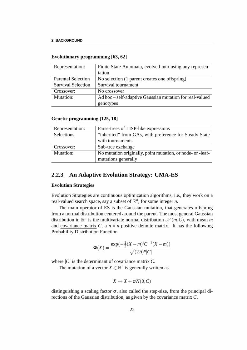
Evolutionary programming [63, 62]
Representation: Finite State Automata, evolved into using any represen-tation
Parental Selection No selection (1 parent creates one offspring)Survival Selection Survival tournamentCrossover: No crossoverMutation: Ad hoc – self-adaptive Gaussian mutation for real-valued
genotypes
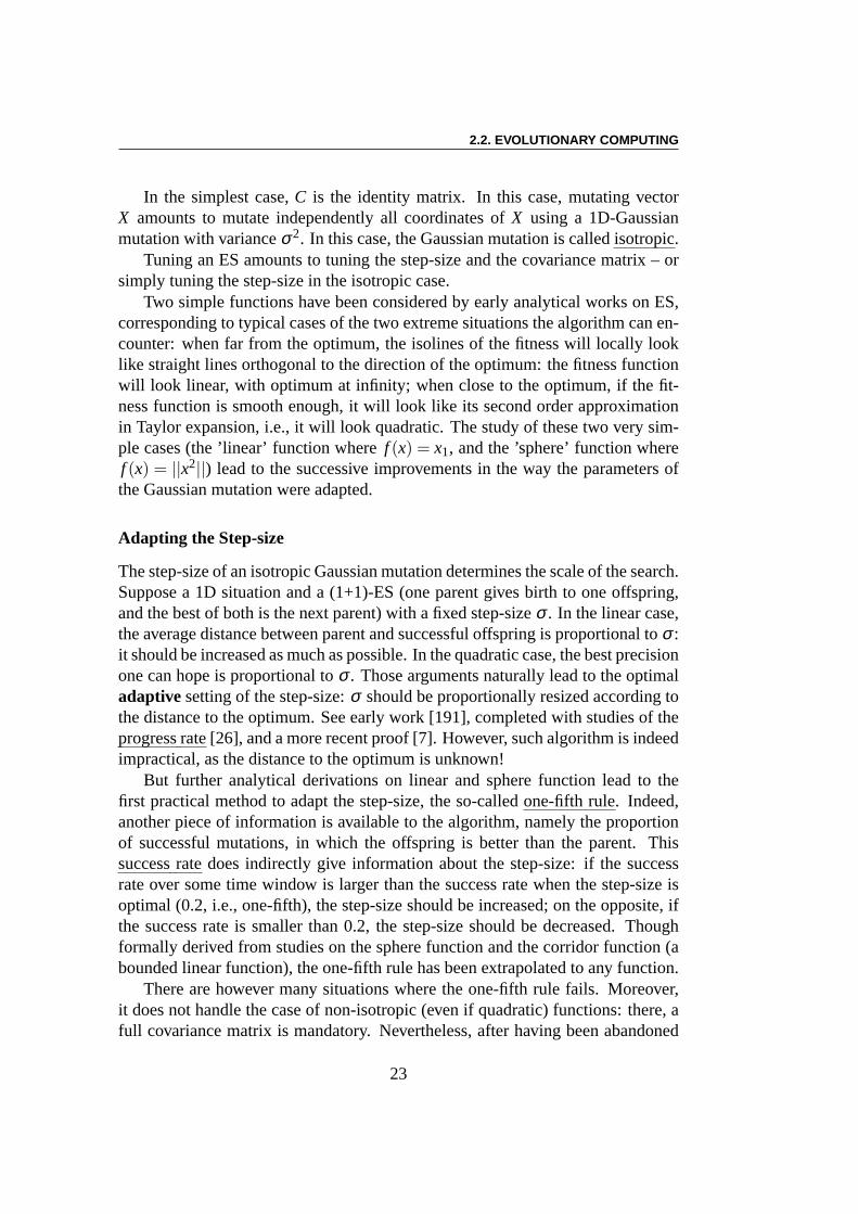
Genetic programming [125, 18]
Representation: Parse-trees of LISP-like expressionsSelections “inherited” from GAs, with preference for Steady State
with tournamentsCrossover: Sub-tree exchangeMutation: No mutation originally, point mutation, or node- or -leaf-
mutations generally
2.2.3 An Adaptive Evolution Strategy: CMA-ES
Evolution Strategies
Evolution Strategies are continuous optimization algorithms, i.e., they work on areal-valued search space, say a subset ofR
n, for some integern.The main operator of ES is the Gaussian mutation, that generates offspring
from a normal distribution centered around the parent. The most general Gaussiandistribution inR
n is the multivariate normal distributionN (m,C), with meanmandcovariancematrix C, a n× n positive definite matrix. It has the followingProbability Distribution Function
Φ(X) =exp(−1
2(X−m)tC−1(X−m))√
(2π)n|C|
where|C| is the determinant of covariance matrixC.The mutation of a vectorX ∈ R
n is generally written as
X → X +σN(0,C)
distinguishing a scaling factorσ , also called thestep-size, from the principal di-rections of the Gaussian distribution, as given by the covariance matrixC.
22
2.2. EVOLUTIONARY COMPUTING
In the simplest case,C is the identity matrix. In this case, mutating vectorX amounts to mutate independently all coordinates ofX using a 1D-Gaussianmutation with varianceσ2. In this case, the Gaussian mutation is calledisotropic.
Tuning an ES amounts to tuning the step-size and the covariance matrix – orsimply tuning the step-size in the isotropic case.
Two simple functions have been considered by early analytical works on ES,corresponding to typical cases of the two extreme situations the algorithm can en-counter: when far from the optimum, the isolines of the fitness will locally looklike straight lines orthogonal to the direction of the optimum: the fitness functionwill look linear, with optimum at infinity; when close to the optimum, if the fit-ness function is smooth enough, it will look like its second order approximationin Taylor expansion, i.e., it will look quadratic. The studyof these two very sim-ple cases (the ’linear’ function wheref (x) = x1, and the ’sphere’ function wheref (x) = ||x2||) lead to the successive improvements in the way the parameters ofthe Gaussian mutation were adapted.
Adapting the Step-size
The step-size of an isotropic Gaussian mutation determinesthe scale of the search.Suppose a 1D situation and a (1+1)-ES (one parent gives birthto one offspring,and the best of both is the next parent) with a fixed step-sizeσ . In the linear case,the average distance between parent and successful offspring is proportional toσ :it should be increased as much as possible. In the quadratic case, the best precisionone can hope is proportional toσ . Those arguments naturally lead to the optimaladaptivesetting of the step-size:σ should be proportionally resized according tothe distance to the optimum. See early work [191], completedwith studies of theprogressrate [26], and a more recent proof [7]. However, such algorithm is indeedimpractical, as the distance to the optimum is unknown!
But further analytical derivations on linear and sphere function lead to thefirst practical method to adapt the step-size, the so-calledone-fifth rule. Indeed,another piece of information is available to the algorithm,namely the proportionof successful mutations, in which the offspring is better than the parent. Thissuccessrate does indirectly give information about the step-size:if the successrate over some time window is larger than the success rate when the step-size isoptimal (0.2, i.e., one-fifth), the step-size should be increased; on the opposite, ifthe success rate is smaller than 0.2, the step-size should bedecreased. Thoughformally derived from studies on the sphere function and thecorridor function (abounded linear function), the one-fifth rule has been extrapolated to any function.
There are however many situations where the one-fifth rule fails. Moreover,it does not handle the case of non-isotropic (even if quadratic) functions: there, afull covariance matrix is mandatory. Nevertheless, after having been abandoned
23
2. BACKGROUND
when Self-Adaptive ES was proposed (see below), the simplicity of the one-fifthrule makes it appealing when simple adaptation rules are needed. It is for instanceused for fast step-size adaptation within the multi-objective CMA-ES algorithm[102].
Self-Adaptive ES
The idea of Self-Adaptive ES (SA-ES) is fairly simple: the parameters of themutation (both the step-size and the covariance matrix) areattached to each in-dividual, and are adapted by mutation, too. Three variants have been proposed:the isotropic case uses a single step-size per individual; thenon-isotropic muta-tion uses a vector ofn “standard deviations”σi (the resulting covariance matrix isequivalent to a diagonal matrixC with σ2
i on the diagonal); and thecorrelated mu-tations attaches a full covariance matrix to each individual. Mutating an individualis then a two-steps process: first, the mutation parameters are themselves mutated;then the design variables are mutated using the new mutationparameters. Detailscan be found in [15, 12].
The rationale for SA-ES are that even though the selection isbased on fitness,an individual with ’poor’ mutation parameters will on average generate offspringthat will be overpassed by offspring of individuals with ’correct’ mutation param-eters, where ’poor’ and ’correct’ refer to the local fitness landscape (for instancethe step-size should be small if the landscape is steep).
SA-ES have often been said to “optimize mutation parametersfor free”through the evolution itself. And indeed, SA-ES have long been the state-of-the-art in parametric optimization [15].
But do SA-ES work as expected? Whereas, it has been experimentally demon-strated for the step-size [13, 27], it is not true for the covariance matrix. Indeed,when replacing the sphere function with a quadratic function (min 1
2XtHX forsome positive definite matrixH), the mutation should progress slower along thedirections of steepest descent of H: the covariance matrix should be proportionalto H−1. And there are some evidences that the covariance matrix that is learnedby thecorrelated SA-ES is not any close from the actual inverse of the Hessian[5].
Back to Adaptation: CMA-ES
Another issue when using SA-ES is the slow adaptation of the mutation parame-ters: even for the simple case of the step-size, if the initial value is not optimal,it takes some time to the algorithm to reach that optimal value and start beingefficient.
24
2.2. EVOLUTIONARY COMPUTING
This observation lead Hansen and Ostermeier to head back to an adaptivemethod for parameter tuning by proposing deterministic schedules to adapt theparameters of the Gaussian mutation. They first addressed the step-size adapta-tion [89], and later that of the full covariance matrix [87].The full CovarianceMatrix Adaptation (CMA-ES) algorithm was detailed after default values for itsparameters had been carefully designed, in [88]. Later, an improvement for theupdate of the covariance matrix was proposed in [86].
The basic ideas in CMA-ES for step-size adaptation is to observe the previousmoves of the algorithm. When successive moves are in collinear directions thestep-size should be increased, in order to allow larger steps – and similarly, whenthe totalpath-length is very short after several iterations, then the step-size shouldbe decreased, as the algorithm is hovering around the optimum.
Regarding the covariance matrix, the idea of the update rule is to increase theprobability in the direction of previous successful moves by adding matrices withthe corresponding eigenvectors to the current covariance matrix.
Following Hansen and Ostermeier [88], in the(µI ,λ )-CMA-ES theλ off-spring of generationg+1 are computed by
xg+1k = 〈x〉(g)
µ +σ (g)B(g)D(g)z(g)k ,k = 1, . . . ,λ ,
B(g)D(g)z(g)k ∼ N (0,C(g))
where
〈x〉(g)µ =
1µ
Σi∈I (g)
selxi(g)
represents the center of mass of the selected individuals ofgenerationg , andi ∈ I (g)
sel is the set of indices of the selected individuals of generation g with |i ∈
I (g)sel | = µ. σ (g) is the global step size.
The random vectorszk areN (O, I) distributed (n -dimensional normally dis-tributed with expectation zero and the identity covariancematrix) and serve togenerate offspring for generationg+1. We can calculate their center of mass as:
〈Z〉(g+1)µ =
1µ
Σi∈I (g)
selzi(g+1)
The covariance matrixC(g) of the random vectorsB(g)D(g)z(g)k is a symmetri-
cal positiven×n -matrix. The improvement equation for the update of the covari-ance matrix proposed in [86] is as follow:
25
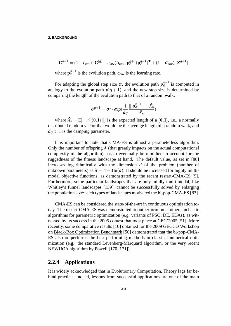
2. BACKGROUND
Cg+1 = (1−ccov) ·C(g) +ccov(αcov·pg+1c (pg+1
c )T +(1−αcov) ·Zg+1)
wherepg+1c is the evolution path,ccov is the learning rate.
For adapting the global step sizeσ , the evolution pathpg+1σ is computed in
analogy to the evolution pathp(g+ 1), and the new step size is determined bycomparing the length of the evolution path to that of a randomwalk:
σg+1 = σg ·exp(1
dσ
‖ pg+1σ ‖ −Xn
Xn)
whereXn = E[‖ N (0, I) ‖] is the expected length of a(0, I), i.e., a normallydistributed random vector that would be the average length of a random walk, anddσ > 1 is the damping parameter.
It is important to note that CMA-ES is almost a parameterless algorithm.Only the number of offspringλ (that greatly impacts on the actual computationalcomplexity of the algorithm) has to eventually be modified toaccount for theruggedness of the fitness landscape at hand. The default value, as set in [88]increases logarithmically with the dimensiond of the problem (number ofunknown parameters) asλ = 4+3ln(d). It should be increased for highly multi-modal objective functions, as demonstrated by the recent restart-CMA-ES [9].Furthermore, some particular landscapes that are only mildly multi-modal, likeWhitley’s funnel landscapes [139], cannot be successfully solved by enlargingthe population size: such types of landscapes motivated thebi-pop-CMA-ES [83].
CMA-ES can be considered the state-of-the-art in continuousoptimization to-day. The restart-CMA-ES was demonstrated to outperform mostother stochasticalgorithms for parametric optimization (e.g. variants of PSO, DE, EDAs), as wit-nessed by its success in the 2005 contest that took place at CEC’2005 [51]. Morerecently, some comparative results [10] obtained for the 2009 GECCO WorkshoponBlack-BoxOptimizationBenchmark [50] demonstrated that the bi-pop-CMA-ES also outperforms the best-performing methods in classical numerical opti-mization (e.g. the standard Levenberg-Marquard algorithm, or the very recentNEWUOA algorithm by Powell [170, 171]).
2.2.4 Applications
It is widely acknowledged that in Evolutionary Computation,Theory lags far be-hind practice. Indeed, lessons from successful applications are one of the main
26
2.2. EVOLUTIONARY COMPUTING
driving forces of EAs research today. Several edited books are devoted to Appli-cations of EAs (see e.g. the recent [231]), and almost every event dedicated toEAs has its own Special Session dedicated to real-world applications.
Application areas can be distinguished according to the type of search spacethey involve.
Regardingcontinuous optimization, Section 2.2.3 has introduced in de-tail the CMA-ES algorithm as the state-of-the-art algorithmfor optimization ofreal-variables. An impressive list of applications of CMA-ES is maintained onN. Hansen’s Web page [84].
Another niche of EAs isMulti-objective optimization . Basically, Multi-Objective Evolutionary Algorithms (MOEAs) are the only algorithms to-date thatcan produce a set of best possible compromise (theParetoset). MOEAs use thesame variation operators than standard EAs, but the Darwinian components aremodified to take into account the multi-valued fitness [40, 35]. Though prominentapplication results have been obtained in the area of multi-objective coutinuousoptimization area (see e.g. [159, 160]), the methods can be used with any searchspace [179, 80].
Combinatorial problems are another area where EAs have proven to be veryefficient. However, as far as benchmark problems are concerned, it is commonlyacknowledged that EAs alone cannot compete with OR methods (see e.g., thepoor results in [16]). However, in the last 15 years, hybrid algorithms, also termedMemeticAlgorithms, coupling traditional OR methods with EAs, haveobtainedthe best-so-far results on a number of such benchmark problems (e.g. from [64]to [149]).
However, for real-world combinatorial problems, “pure” ORheuristics gen-erally don’t directly apply, and OR methods have to take intoaccount problemspecificities. This is where EA flexibility is crucial: some specific EAs, carefullytuned to the problem at hand, have been very successful solving real-world com-binatorial problems, as for instance in the broad area of scheduling [164, 193].
When it comes tomixed search spaces(involving a fixed number of variablesthat can be floating points, integers or discrete), again theflexibility of EAs allowto tailor them to the problem at hand. For instance, constructing variation opera-tors for mixed individuals is straightforward, and can simply be done by applyingto each variable some variation operator defined for its type. Many problem havebeen easily handled that way (see e.g. the optical filter optimization in [14, 145]).Furthermore, some platforms now exist that help the non-EC expert to implementgeneric EAs for a given problem involving different types ofmixed search spaces[36].
Ultimately, the ability of EAs to handle almost any search space can al-low engineers and/or artists to unveil their wildest ideas in Design. Indeed, the
27
2. BACKGROUND
idea ofcomponent-based representationscan boost innovation in structural de-sign [66, 81], architecture [178] as well as in many other areas including art[25, 24]. Furthermore, the recently emerged area ofdevelopmental represen-tations [76, 126] might lead to tremendous applications. The idea isto optimizethe program that builds the solution, rather than the solution itself. The pioneer-ing work of Gruau (see Section 2.3.2) was used to design analog circuits [126] –though exploring a huge search space (a space of programs) implies a heavy com-putational cost. However, it seems that those approaches can bring a breakthroughin Evolutionary Design [201].
2.3 Evolving Artificial Neural Network
This Section surveys existing work that use Evolutionary Computation to opti-mize Neural Networks for a given task (akaNeuro-Evolution), as such contextwill be that of all original works presented in this dissertation. Two types ofapproaches will be considered, whereas only the weights of agiven NN arebeing optimized, or in case the topology of the NN is being optimized as well.An orthogonal classification regards the nature of the task at hand, whethersupervised, reinforcement or unsupervised (see Section 2.1.2). More details canbe found about the early work on Neuro-Evolution in two well-known surveysthat have been written by Schaffer, Whitley, and Eshelman [184] in 1992 and byYao [230] in 1999.
2.3.1 Evolving Connection Weights
In the 80s, great successes of NNs were obtained in the supervised learningframework (see Section 2.1.2) using Back-Propagation (BP) algorithm to op-timize the connections weights [128, 56]. However, the BP algorithm alsoshowed a number of limitations. It demonstrated slow convergence for large-scaleNNs, and too frequent premature convergence to some local minima close tothe starting point, thus missing the global minimum [208, 226]. A workaroundwas to use different initializations, but without much guarantees of convergence.Furthermore, because it requires the differentiability ofthe objective function, BPalgorithm is unable to handle discontinuous neural transfer functions (e.g., theHeaviside function – Unit Step fuction).
On the other hand, in unsupervised or reinforcement learning context, wheredirect gradient information is either unavailable, or costly to obtain, no gradient-based method is available, so even learning the weights of a given NN was con-
28
2.3. EVOLVING ARTIFICIAL NEURAL NETWORK
sidered a difficult task. In that context, because of the lackof a general theory andalso because the optimal output is unknown, the traditionalmanual approacheshave been designed by the experts, e.g. Hopfield networks [96] and AdaptiveResonance Theory (ART) [75]. But such methods have two shortcomings: theirdesign has many degrees of freedom that must be fixed manually; furthermore,they have to be tuned anew for each given task, and the resultshardly generalizefrom one task to another.
Therefore, even though ANNs were considered a good choice for unsuper-vised and reinforcement learning, it seemed that a new approach was requiredto actually perform the optimization of the neural network,starting with theoptimization of the weights of a NNs with a given topology.
At the same period, Evolutionary Algorithms, and more precisely GeneticAlgorithms, started to encounter some success in many areas. Because of theflexibility of Evolutionary Algorithm, and in particular because they do not re-quire derivative information, the initial work of evolvingANNs began at thisstage [152, 226, 39] with the easiest problem, that of optimizing the weights of agiven NN with fixed topology.
The research of what was to become known asNeuro-Evolution hence startedwith optimization of the connection weights of single-layer or multi-layer feed-forward neural networks (aka perceptrons). Starting with the input and outputsizes, the programmer has to manually determine the number of hidden layers,and the number of neurons in each layer. Such topology remains fixed during thewhole learning phase, and the genotype is then simply the vector of all connec-tion weights. Depending on the learning framework, any optimization algorithmcan then be used, as the problem then amounts to standard continuous parameteroptimization.
Early attempts dealt with supervised learning: In 1989, Montana andDavis [152] learned the weights of a simple perceptron for anocean echo de-tection, and achieved better results than the back propagation algorithm; also theother works such as Caudell et al. [34]; Whitley et al. [226]
However, because there didn’t exist any other unanimously recognizedmethod for reinforcement learning tasks, many works in Neuro-Evolution havebeen devoted to such context, from the pioneering work of DeGaris [39] wherethe task was to control some “walking sticks” and Whitley et al. [225] that firstintroduced the pole balancing problems in the EC community (see Section 4.4.1),to handling other classical benchmark problems like lunar lander [176], truckbacker-upper [190], to recent work using standard CMA-ES andsolving thedouble-pole balancing problem using a perceptron with veryfew neurons [101].
Another distinction can be made here whether the weights areencoded as
29
2. BACKGROUND
binary strings or as real numbers. Most of the early works used binary string en-coding, that was considered in the GA community almost as a universal encoding.Hence lots of researchers followed this approach at that time [224, 34, 226, 39].In this method, each connection weight is represented by a binary string of givenlength, and all these strings are concatenated to form the chromosome. Classi-cal GA variation operators can then be applied directly (such as single-point oruniform crossover). Binary representation is also conducive to the realization ofdigital hardware.
However, the precision of the encoding then depends on the string lengththat is chosen to encode each weight, and a compromise has to be made betweenthe precision and the total chromosome length. If the lengthis too short, theconnection weights cannot be optimized with sufficient precision; On the otherhand, when the code length is too large, the optimization process might becometoo slow to converge, degrading the efficiency of the whole process. There arehowever well-known exceptions, such as the work in Evolutionary Roboticsperformed by Floreano and co-authors [59, 158] that repeatedly used coarsebinary encoding (8 bits per weight) to evolve successfully robot controllers forvarious tasks.
Using real encoding (and appropriate variation operators)is a way to over-come this difficulty. Used by Montana and Davis as early as 1989 [152], andfollowed by Whitley et al. [225] for reinforcement learning tasks, it became moreand more popular in the 90s with the growing popularity of Evolution Strategies(see e.g., [176, 190], and more recently [101]). Our work in Chapter 4 builds onthose ideas.
An issue that has been raised about the evolutionary learning of the weightsof a given NN is the “structural/functional mapping” problem [225] (aka “com-peting convention” problem): The mapping from genotype to phenotype is here amany-to-one mapping, because two NNs that only differ by theorder of the hid-den neurons are de facto identical, whereas the corresponding chromosomes willbe completely different. In particular, any crossover operator (and for any repre-sentation of the weights) might be very inefficient. However, in practice, and atleast for not too large populations, it seems that this problem is not an issue, asevolution rapidly chooses one of the possible orderings of the neurons, and hardlyhas to crossover NNs that only differ by a permutation of the hidden neurons [82].
On the other hand, using evolutionary algorithm allows the programmer tooptimize not only the connection weights, but also the parameters of the transferfunctions, sometimes leading to improved results, as advocated in [189]. Thework presented in Chapter 4 is another demonstration of this idea.
30
2.3. EVOLVING ARTIFICIAL NEURAL NETWORK
However, even though multi-layer perceptrons are universal approximators[97], it is well-known that the topology of a NNs is an important issue for large-scape applications. For instance, many man-years of efforthave been devoted tobuilding the topology of the well-known digit recognition NN for the US Post[129, 31]. And again, thanks to their flexibility, EAs are perfect optimizer candi-dates for the task of optimizing the topology of NNs for a given task.
2.3.2 Evolving Network Topologies
Tuning the topology of Neural Networks, even simple feed-forward networks likeperceptrons, has received a lot of attention in the Machine Learning commu-nity. Both bottom-up and top-down approaches have been explored: Cascade-correlation algorithms for instance iteratively add neurons to a very specific archi-tecture [55], while pruning methods start with a very large network and graduallyremove neurons, using from brute force [222] to iterative algorithms [33]. Hence,quite naturally, early works in Neuro-Evolution trying to optimize the topology ofNNs followed similar paths [90, 226, 206]. But here again, theflexibility of EAsrapidly lead researchers to generalize such methods. First, there is no need anymore to work either bottom-up or top-down, as the complete connectivity matrixcan be optimize, adding and removing either neurons or connections, optimizingthe weights either using traditional BP algorithm, in case ofsupervised learning,or within the EAs itself, in case of reinforcement learning –and here again, notonly the weights but any parameter of the transfer function can be optimized [54].Those methods (see [230] for a more complete surveys, as mostof these methodswere published prior to 1999), that use different representations of the topologyto directly manipulate and transform it through the variation operators, are termeddirectrepresentation methods.
However, the poor scaling-up behavior with respect to the size of the problemof direct encoding lead to a change of paradigm, that resulted in the indirectmethods, starting withdevelopmentalmethods, where evolution is concernedwith evolving some program such that, when the program is executed on somepre-definedembryo, the result is a fully operational Neural Network. This ap-proach has been illustrated by the seminal works of Kitano [119] and Gruau [77].However, such developmental approaches have not met their expectations, andrecent trends use other types of indirect representation, going back to biologicalinspiration, and borrowing some basic principles to Gene Regulatory Networksor Protein Interaction Networks to define artificial networks [58, 132, 45, 157].
We will now detail in turn the some recentdirect representation methods, ul-timately focusing on NEAT [204], that is today considered the state-of-the-art forthe evolution of small NNs. Interestingly, NEAT uses an approach very close from
31
2. BACKGROUND
a pure bottom-up approach, in that it keeps adding neurons and connections to aminimal embryo NN.
We will then survey some indirect representations, from theseminal work ofGruau to the recent approaches inspired by biological networks. Through this pre-sentation, we will de facto survey part of the research progress in Neuro-Evolutionin the last decade (i.e. posterior to Yao’s 1999 survey [230]).
Some Direct Representations: from SANE to NEAT
An important issue when using direct representations to evolve both the weightsand the topology of NNs is the following: when the topology ismodified, theperformance of the resulting new topology is generally rather low until theweights have been adjusted to the new topology. Several methods have beenproposed in the recent years in the realm of direct representations for evolvingNNs try to address this issue, beside taking into account thescaling-up issue.
Coevolution MethodsIn 1997 Moriarty and Miikkulainen proposed a co-evolutionary model named
Symbiotic Adaptive Neuro-Evolution (SANE) [154]. The basic idea in SANEis to evolve two populations. The first population is made of neurons, and thesecond population is made of network structures with one hidden layer (akablueprints) pointing to neurons from the first population for the hidden neurons.The blueprints are instantiated, then evaluated on the taskat hand; the neurons areevaluated based on how good are the networks they have participated to.
SANE obtained good results at diverse reinforcement learning tasks: First,because new topologies are using neurons that are proved good with the parenttopologies, preventing too poor performance of offspring;Second, because thealgorithm also implicitly maintains some diversity at the level of the neurons:no neuron can overtake the whole population as networks using mostly copiesof the same neuron are likely to perform poorly. However, SANE proved poorat evolving recurrent NN, probably because in recurrent nets the dynamics ofthe neurons are much more dependent on the other neurons it isconnected to –evolving neurons separately becomes unviable.
In the following years, Miikkulainen and his students modified the SANEmodel into the Enforced Sub-Populations (ESP) model [69]. Like SANE, ESPevolves the topology of NNs with one hidden layer. However, the number ofhidden neurons must be specified, and ESP evolves as many populations ofneurons. Complete Neural Networks are built by randomly choosing one neuronfrom each population, repeatedly until each neuron has beenused on average agiven number of times (e.g. 10). Each neuron is evaluated based on how good
32
2.3. EVOLVING ARTIFICIAL NEURAL NETWORK
on average the networks it has been part of performed. Becausethe clusteringof neurons is explicit (neurons with different sub-tasks belong to differentpopulations), crossover only recombines neurons that are already specialized forthe same sub-task. ESP hence obtained better results than SANE on the samereinforcement tasks. Furthermore, recurrent NN can be evolved with ESP, byincluding the weights of the recurrent connections into thegenotypes of theneurons. However, the main limitation of ESP is that it can only evolve one-layerarchitectures.
Neuroevolution of Augmenting Topologies: NEATBuilding upon SANE and ESP, Miikkulainen and his student Stanley proposed
NEAT (Neuroevolution of Augmenting Topologies) [204, 203], a new direct rep-resentation to evolve any feed-forward or recurrent NN architecture in order toaddress the following issues:
1. How to optimize both the weights and the topology, i.e. explore a hugesearch space efficiently?
2. How can crossover be implemented when structures do not match?
3. How can innovative topologies survive while having initially low fitness?
The original features of NEAT are
• The bottom-up approach to network topology: the optimization processstarts with a minimal NN (one neuron per input, all being connected tothe output neurons), and can only add connections and neurons.
• The representation, that can handle any type of connectivity, while be-ing easily and smoothly evolvable through variation operators. Figure 2.5shows an example of genotype to phenotype mapping (from [204]). TheNode Genes describe the neurons and their role in the network(input, out-put, or hidden), and the Connection Genes describe the connections betweenthe neurons: the input and output neurons, the corresponding weight, an En-abled/Disabled flag, and an important and original feature,the innovationnumber.
• The innovation number stores for each gene the moment it appeared in thehistory of evolution (a global counter is incremented everytime a new geneis created). It allows the crossover operator to answer issue 2 above: whentwo individuals have to be recombined, they are first alignedwith respect toinnovation numbers, and only genes with matching innovation numbers areexchanged. They are genes that are descents of the same initial gene, and
33
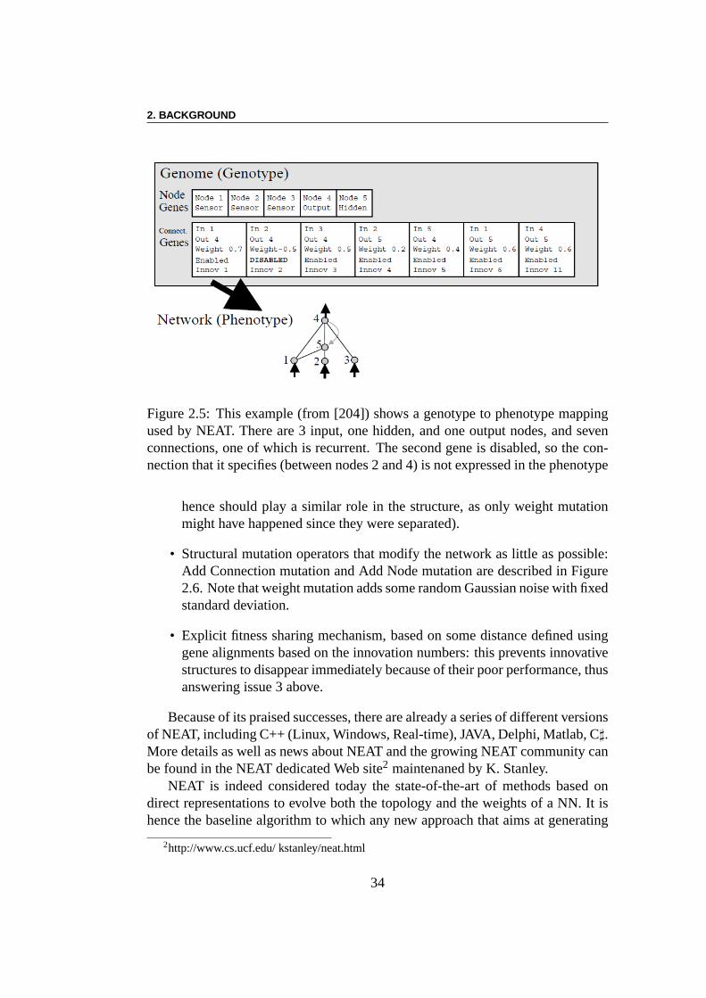
2. BACKGROUND
Figure 2.5: This example (from [204]) shows a genotype to phenotype mappingused by NEAT. There are 3 input, one hidden, and one output nodes, and sevenconnections, one of which is recurrent. The second gene is disabled, so the con-nection that it specifies (between nodes 2 and 4) is not expressed in the phenotype
hence should play a similar role in the structure, as only weight mutationmight have happened since they were separated).
• Structural mutation operators that modify the network as little as possible:Add Connection mutation and Add Node mutation are described in Figure2.6. Note that weight mutation adds some random Gaussian noise with fixedstandard deviation.
• Explicit fitness sharing mechanism, based on some distancedefined usinggene alignments based on the innovation numbers: this prevents innovativestructures to disappear immediately because of their poor performance, thusanswering issue 3 above.
Because of its praised successes, there are already a series of different versionsof NEAT, including C++ (Linux, Windows, Real-time), JAVA, Delphi, Matlab, C♯.More details as well as news about NEAT and the growing NEAT community canbe found in the NEAT dedicated Web site2 maintenaned by K. Stanley.
NEAT is indeed considered today the state-of-the-art of methods based ondirect representations to evolve both the topology and the weights of a NN. It ishence the baseline algorithm to which any new approach that aims at generating
2http://www.cs.ucf.edu/ kstanley/neat.html
34
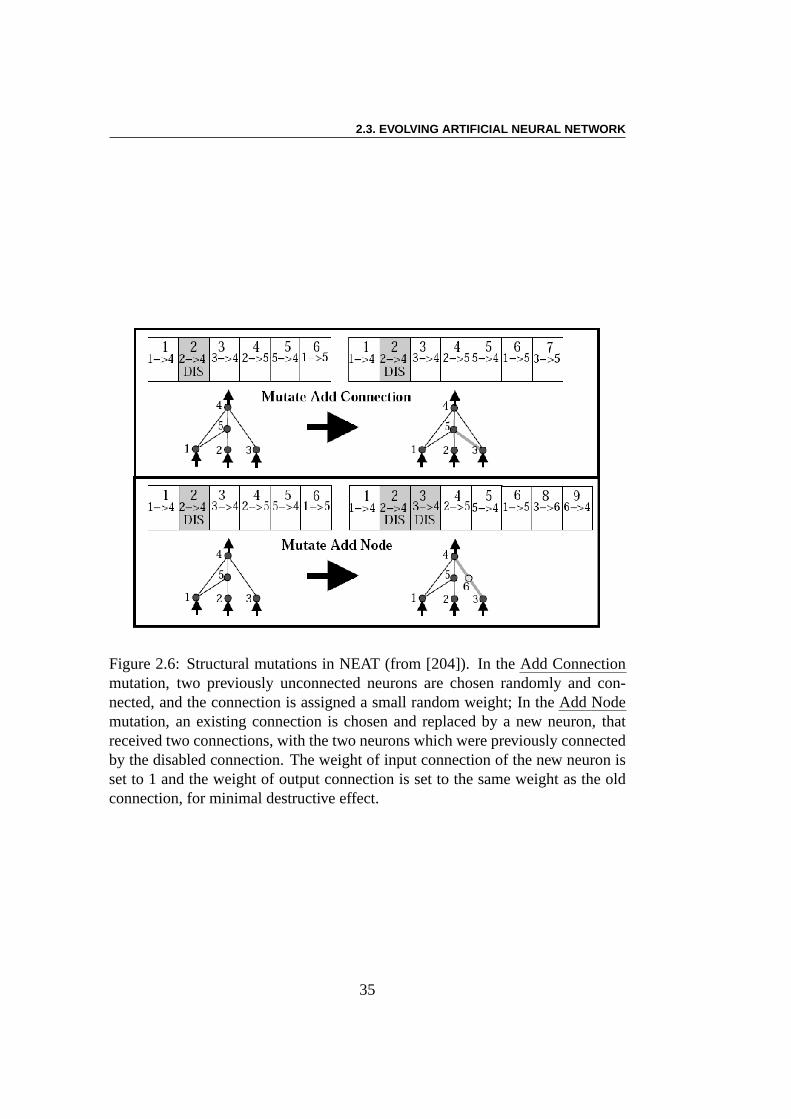
2.3. EVOLVING ARTIFICIAL NEURAL NETWORK
Figure 2.6: Structural mutations in NEAT (from [204]). In the Add Connectionmutation, two previously unconnected neurons are chosen randomly and con-nected, and the connection is assigned a small random weight; In theAdd Nodemutation, an existing connection is chosen and replaced by anew neuron, thatreceived two connections, with the two neurons which were previously connectedby the disabled connection. The weight of input connection of the new neuron isset to 1 and the weight of output connection is set to the same weight as the oldconnection, for minimal destructive effect.
35
2. BACKGROUND
NNs should be compared. However, it also suffers from a severe drawback: ithas a lot of parameters that the user needs to tune, and remains rather difficult tomaster for a completely new task. Furthermore, whereas, when correctly tuned, itcan evolve diverse structures (both feedforward and recurrent) of reasonable size(a few dozens of neurons), it does not scale-up very well - in particular it does notaddress modularity or code-reuse issues, that seem mandatory to tackle large-scaleproblems.
Indirect representations have been proposed in order to address these crucialissues, and next Sections will detail the most popular ones,including one of theearly ones, Hyper-NEAT, a follow-up of NEAT that tries to address the short-comings of NEAT, and some recent representations borrowingideas to biologicalnetworks.
Developmental Representations
There has been several proposal fordevelopmentalrepresentations, i.e. repre-sentations of a program that actually builds the solution tothe problem at handrather than directly evolving the solution itself (such representations are notspecific to Neuro-Evolution, see e.g., [126]). The works by Kitano [119], usingsome grammar-based representation close to L-systems, andGruau [77, 76]using Cellular Encoding, a representation close to the parsetrees of GeneticProgramming have pioneered this research direction. We have chosen to detailthe latter here, as it seems more likely to be generalized to other tasks than theformer. Finally, we will briefly mention the recent HyperNEAT [202], that canbe viewed as a developmental representation even though it is based on differentparadigm than the previous approaches.
Cellular EncodingCellular Encoding is one of the very first instances of developmental represen-
tation. Cellular Encoding is uses a langauge describing local graph transforma-tions, in order to control the division of cells that grow an artificial neural network[77, 76].
In Cellular Encoding, individuals are represented as grammar trees with or-dered branches. The nodes of the grammar tree are labeled with names of programsymbols. The neural network starts with a single ’embryo’ cell, and performs asequential development process by reading the grammar treeand applying theoperation described in the current node of the tree to the current cell it pointsto. Basic operations includeParallelDivision andSequentialDivision of the cell.When a cell meets theEnd instruction, the cell stops its development process andbecomes a neuron. Optimization proceeds on the trees, usingcrossover and mu-tation operators that are very similar to those independently proposed for Genetic
36
2.3. EVOLVING ARTIFICIAL NEURAL NETWORK
Programming [125].Early work with Cellular Encoding addressed only boolean neural networks
[76]. It was later applied to NNs with real valued weights [227, 78]. In 1996,Gruau, Whitley, and Pyeatt solved the double poles balancingwithout velocityproblem with Cellular Encoding [78] (see also Section 4.4.1).
Importantly, Cellular Encoding addressed the scalability issue by adding aRecursion node to the initial representation, allowing to tackle some amount ofmodularity. The proof of concept of increased scalability was made by evolvingsolutions to the multiplexer problem [76]. It was later demonstrated on a real-world problem by Khozabadjian [121] that successfully evolved a controller foran hexapod robot.
However, it seems that the evolvability of Cellular Encodingresulted in acomputationally heavy algorithm, and to the best of our knowledge, it has notbeen used ever since. Note that such very heavy costs were also reported forexperiments using similar ideas borrowing to embryogeniesmade by J. Koza[126].
HyperNEATA completely different approach, that can nevertheless be viewed as some de-
velopmental representation for Neuro-Evolution, is that of Hyper-NEAT [202].Hyper-NEAT builds on NEAT by using the idea of Compositional Pattern Pro-ducing Networks (CPPNs) proposed by Stanley [201] to design patterns with reg-ularities. The goal of Hyper-NEAT is to design large NNs where each neuronis materialized as a point on a 2D grid. The basic idea is then to build (usingNEAT) a top-level Neural Network that will take as input two pairs of coordinates(those of two neurons), and output one real value, that of theweight between bothneurons. Doing so, Hyper-NEAT is able to take into account the geometry of thetarget network (e.g., to design symmetric networks). It also addresses the scala-bility issue, as the optimization is always made on the smallNNs (with 4 inputsand 1 output). For instance, Stanley and co-authors report some success buildinga visual discrimination network containing over eight millions connections [202].
Bio-inspired Indirect representations
Several models of Genetic Regulatory Networks (GRNs) have been proposed asa basis for an indirect representation for Neuro-Evolutoin. They differ in severalways, and actually model only parts of what is known about GRNs. This Sec-tion will quickly detail 3 of them, Analog Genetic Encoding [58, 146], RBF-Gene[131, 132], and finally the so-called Banzhaf model [17, 127] that, though not ap-plied to Neuro-Evolution yet, seem relevant for the perspectives it opens, relativeto the work presented in this dissertation.
37
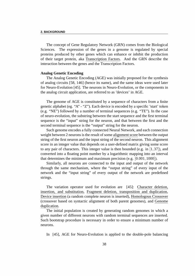
2. BACKGROUND
The concept of Gene Regulatory Network (GRN) comes from the BiologicalSciences. The expression of the genes in a genome is regulated by specialproteins produced by other genes which can enhance or inhibit the productionof their target protein, akaTranscriptionFactors. And the GRN describe theinteraction between the genes and the Transcription Factors.
Analog Genetic EncodingThe Analog Genetic Encoding (AGE) was initially proposed for the synthesis
of analog circuits [58, 146] (hence its name), and the same ideas were used laterfor Neuro-Evolution [45]. The neurons in Neuro-Evolution,or the components inthe analog circuit application, are referred to as ’devices’ in AGE.
The genome of AGE is constituted by a sequence of characters from a finitegenetic alphabet (eg. “A” - “Z”). Each device is encoded by a specific ’start’ token(e.g. “NE”) followed by a number of terminal sequences (e.g.“TE”). In the caseof neuro-evolution, the substring between the start sequence and the first terminalsequence is the “input” string for the neuron, and that between the first and thesecond terminal sequence is the “output” string for the neuron.
Such genome encodes a fully connected Neural Network, and each connectionweight between 2 neurons is the result of somealignmentscore between the outputstring of the first neuron and the input string of the second neuron. This alignmentscore in an integer value that depends on a user-defined matrix giving some scoreto any pair of characters. This integer value is then bounded(e.g. in[1,37]), andconverted into a floating point number by a logarithmic mapping into an intervalthat determines the minimum and maximum precision (e.g.[0.001,1000]).
Similarly, all neurons are connected to the input and outputof the networkthrough the same mechanism, where the “output string” of every input of thenetwork and the “input string” of every output of the networkare predefinedstrings.
The variation operator used for evolution are [45]:Characterdeletion,insertion, and substitution, Fragmentdeletion, transpositionand duplication,Deviceinsertion (a random complete neuron is inserted),HomologousCrossover(crossover based on syntactic alignment of both parent genomes), andGenomeduplication.
The initial population is created by generating random genomes in which agiven number of different neurons with random terminal sequences are inserted.Such bootstrap procedure is necessary in order to ensure a minimum number ofneurons.
In [45], AGE for Neuro-Evolution is applied to the double-pole balancing
38
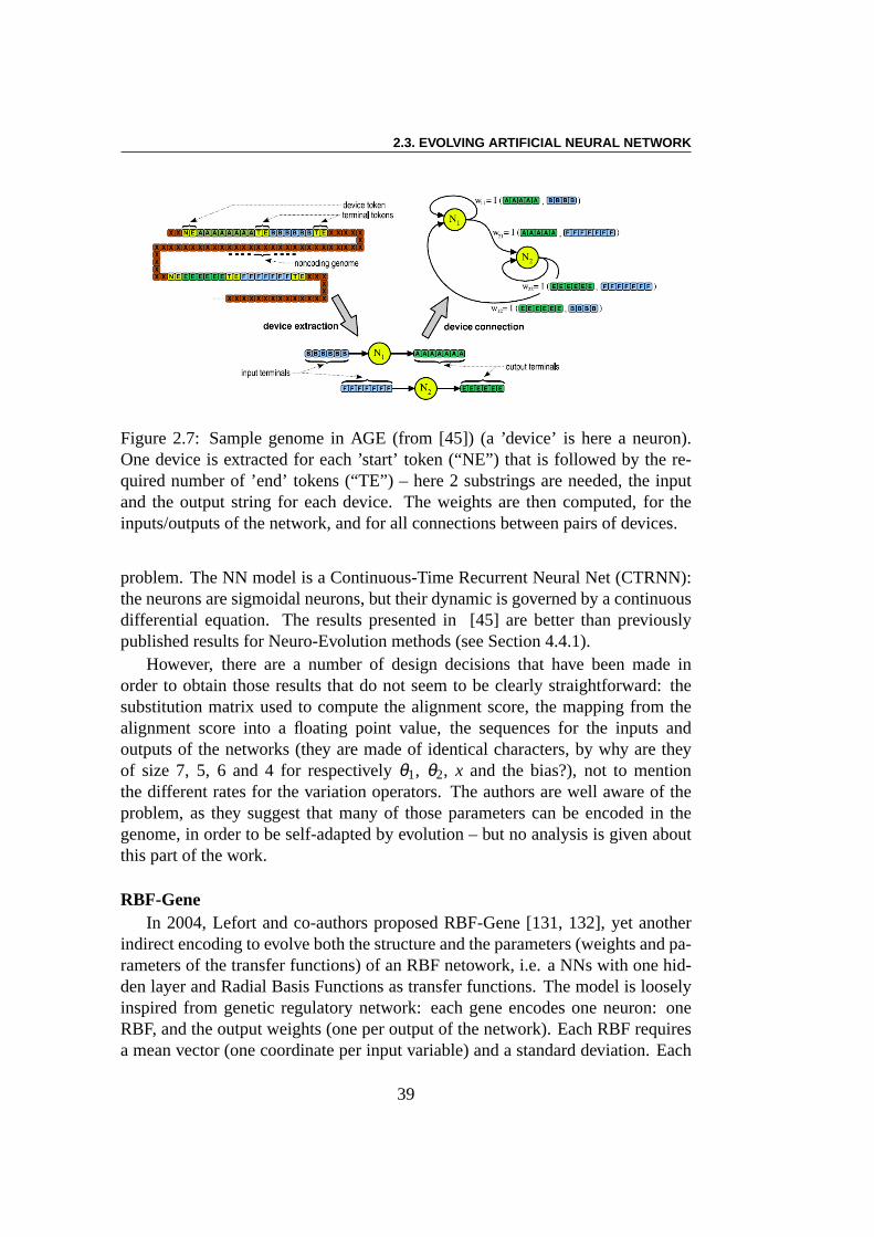
2.3. EVOLVING ARTIFICIAL NEURAL NETWORK
Figure 2.7: Sample genome in AGE (from [45]) (a ’device’ is here a neuron).One device is extracted for each ’start’ token (“NE”) that isfollowed by the re-quired number of ’end’ tokens (“TE”) – here 2 substrings are needed, the inputand the output string for each device. The weights are then computed, for theinputs/outputs of the network, and for all connections between pairs of devices.
problem. The NN model is a Continuous-Time Recurrent Neural Net (CTRNN):the neurons are sigmoidal neurons, but their dynamic is governed by a continuousdifferential equation. The results presented in [45] are better than previouslypublished results for Neuro-Evolution methods (see Section 4.4.1).
However, there are a number of design decisions that have been made inorder to obtain those results that do not seem to be clearly straightforward: thesubstitution matrix used to compute the alignment score, the mapping from thealignment score into a floating point value, the sequences for the inputs andoutputs of the networks (they are made of identical characters, by why are theyof size 7, 5, 6 and 4 for respectivelyθ1, θ2, x and the bias?), not to mentionthe different rates for the variation operators. The authors are well aware of theproblem, as they suggest that many of those parameters can beencoded in thegenome, in order to be self-adapted by evolution – but no analysis is given aboutthis part of the work.
RBF-GeneIn 2004, Lefort and co-authors proposed RBF-Gene [131, 132], yet another
indirect encoding to evolve both the structure and the parameters (weights and pa-rameters of the transfer functions) of an RBF netowork, i.e. a NNs with one hid-den layer and Radial Basis Functions as transfer functions. The model is looselyinspired from genetic regulatory network: each gene encodes one neuron: oneRBF, and the output weights (one per output of the network). Each RBF requiresa mean vector (one coordinate per input variable) and a standard deviation. Each
39
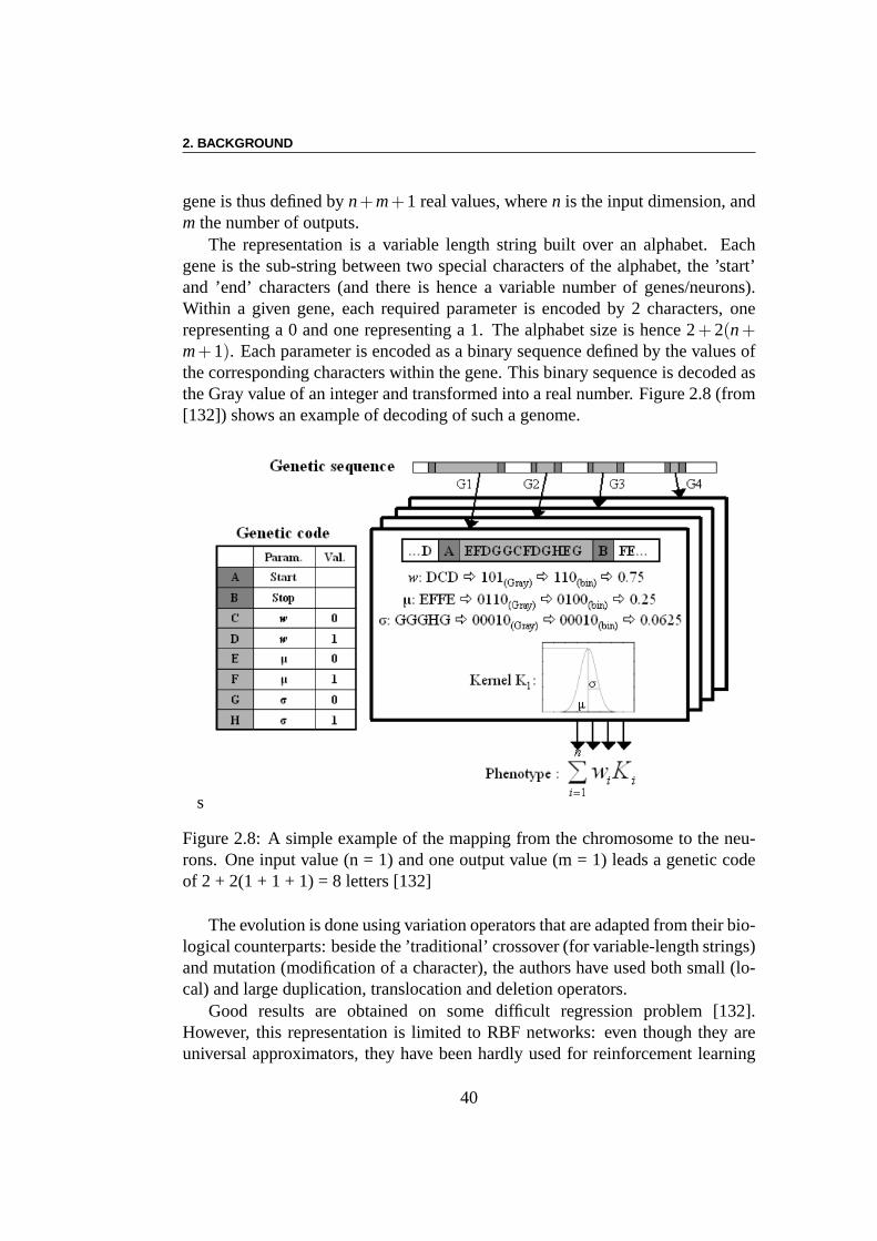
2. BACKGROUND
gene is thus defined byn+m+1 real values, wheren is the input dimension, andm the number of outputs.
The representation is a variable length string built over analphabet. Eachgene is the sub-string between two special characters of thealphabet, the ’start’and ’end’ characters (and there is hence a variable number ofgenes/neurons).Within a given gene, each required parameter is encoded by 2 characters, onerepresenting a 0 and one representing a 1. The alphabet size is hence 2+ 2(n+m+1). Each parameter is encoded as a binary sequence defined by thevalues ofthe corresponding characters within the gene. This binary sequence is decoded asthe Gray value of an integer and transformed into a real number. Figure 2.8 (from[132]) shows an example of decoding of such a genome.
s
Figure 2.8: A simple example of the mapping from the chromosome to the neu-rons. One input value (n = 1) and one output value (m = 1) leads agenetic codeof 2 + 2(1 + 1 + 1) = 8 letters [132]
The evolution is done using variation operators that are adapted from their bio-logical counterparts: beside the ’traditional’ crossover(for variable-length strings)and mutation (modification of a character), the authors haveused both small (lo-cal) and large duplication, translocation and deletion operators.
Good results are obtained on some difficult regression problem [132].However, this representation is limited to RBF networks: eventhough they areuniversal approximators, they have been hardly used for reinforcement learning
40
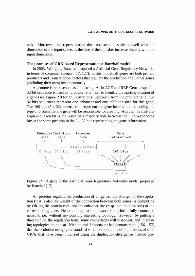
2.3. EVOLVING ARTIFICIAL NEURAL NETWORK
task. Moreover, this representation does not seem to scale up well with thedimension of the input space, as the size of the alphabet increase linearly with theinput dimension.
The promises of GRN-based Representations: Banzhaf modelIn 2003, Wolfgang Banzhaf proposed a Artificial Gene Regulatory Networks
in terms of computer science [17, 127]. In this model, all genes are both proteinproducers and Transcription Factors that regulate the production of all other genes(including their own) instantaneously.
A genome is represented as a bit string. As in AGE and RBF-Gene, aspecific32-bit sequence is used as ’promoter site’, i.e. to identifythe starting location ofa gene (see Figure 2.9 for an illustration). Upstream from the promoter site, two32-bits sequences represent one enhancer and one inhibitorsites for this gene.The 160 bits (5×32) downstream represent the gene information, encoding thetype of protein that the gene will be responsible for creating. A protein is a 32-bitssequence, each bit is the result of a majority vote between the 5 correspondingbits at the same position in the 5×32 bits representing the gene information.
XYZ010 0 01 1 1
32 bits32 bits
Enhancersite
Inhibitorsite
Promotersite
Geneinformation
160 bits32 bits
Protein
32 bits
Figure 2.9: A gene of the Artificial Gene Regulatory Networks model proposedby Banzhaf [17]
All proteins regulate the production of all genes: the strength of the regula-tion (that is also the weight of the connection between both genes) is computingby OR-ing the protein code and the enhancer site (resp. the inhibitor site) of thecorresponding gene. Hence the regulation network is a priori a fully connectednetwork, i.e. without any possibly interesting topology. However, by putting athreshold on the regulation term, some connections will disappear, and interest-ing topologies do appear. Nicolau and Schoenauer has demonstrated [156, 157]that the evolution using quite standard variation operators, of populations of suchGRNs that have been initialized using the duplication-divergence method pro-
41
2. BACKGROUND
posed in the initial model by Banzhaf [17], can be lead toward networks exhibitingvery specific topological statistical properties, such as small-world or scale-freecharacteristics (see next Section 2.4).
Discussion
All representations, whether direct or indirect, that havebeen used for evolvingboth the topology and the weights of NNs are variable length representations.They are all able to generate a variable number of neurons. However, only thebio-inspired representations have non-coding segments.
Regarding the topologies they can generate, though both AGE and RBF-Genecan indeed generate different topologies, those topologies remain within a veryrestricted set, and only differ by the number of genes: AGE creates fully connectedNNs, and RBF-Gene generates 3-layer RBF networks. In that sense,NEAT, and,of course, the developmental methods, can create more diverse types of topologies- and so does the Banzhaf model thanks to the threshold trick that removes manyconnections. Note that it could be possible to apply this trick to AGE too.
Furthermore, only the developmental representations are actually able toscale-up to huge numbers of neurons without requiring a similar increase of therepresentation size. The direct representations clearly need to manipulate (create,tune, connect) each gene one by one: this can be an advantage when only a smallnetwork is needed, but will not be sufficient for large networks. On the other hand,the GRN-inspired representations, though they need to express all genes of thenetwork, can be considered as intermediate with respect to the scaling-up issue:because they use global variation operators like duplication, they can succeedin generating networks of moderate size, up to a few hundredsneurons [156, 157].
Regarding the evolution of the weights, in AGE and in the Banzhaf model, theweights are based on some distance between labels/affinity sites, while in directrepresentations, and in RBF-Gene, they are directly encoded as binary strings. Theconsequence of the indirect encoding of the former methods is that by modifyingone of the labels/sites, all weights issued from one neuron are modified at once,strengthening those connecting a certain type of neurons, and weakening others.A direct encoding of the weights requires, for the same result, that several weightsare modified in the same direction, a very unlikely event. Whether one approach oranother is best for evolution is however unclear: being ableto modify all weightsof a given neuron in a single mutation can indeed help for the coarse adjustmentof the NNs, as witnessed by the improvements brought by adding the coefficientof the sigmoid function to the genome even when only optimizing the weights[189, 54]; On the other hand, fine-tuning a Neural Network often goes through
42
2.4. TOPOLOGY OF COMPLEX NETWORKS
fine-tuning its weights independently.In developmental representations, the causality for the evolution of the
weights is less clear: in Cellular Encoding and other grammar-based representa-tions, the weights have to be described directly, but will beused whenever somecode re-use happens in the morphogenetic process. In Hyper-NEAT, the weightsare the result of the application of the top-level neural net, a complex process noteasily related to the variation operators acting over this network.
In summary, there is of course no method that clearly outperforms all others.Simple approaches, i.e. evolving the weights of a robust topology (e.g. multi-layerperceptron) with a robust optimizer (e.g. CMA-ES) are clearly sufficient for manyproblems (e.g. as witnessed by Igel’s results on the pole-balancing problem [101]– see also Section 4.4.1). But the influence of given characteristics of the topologylike statistical measures that have recently been proposedfor complex networks,has not been systematically studied – and this is part of whathas motivated thepresent work (see also Section 2.5).
2.4 Topology of Complex Networks
Up to recent years, the major types of studied network topology were totally ran-dom networks and regular networks. Since the end of the 1990’s, several real lifenetworks have started to be known with enough precision so asto analyze themin quantified details. The results were that real life networks have actually severalproperties that exclude them from the regular or totally random classes. The so-called complex networks field has mainly been created as a response to this issue.In the last decade, complex network topologies, e.g. small-world or scale-free,have attracted a great amount of interests (for a review, see[28]). In this sectionwe briefly introduce some basic concepts.
2.4.1 Small World Topology
The small-world phenomenon originates from social networkstudies. Accordingto this theory, each person can be seen as a node of a graph, andconnected witha large number of paths with the others. The connections between nodes meanthat the peoples know each other. The hypothesis is that eachperson needsonly a few intermediaries (an average of 6) to establish a link with anybody elsein the world. It is an issue of sociology, mathematics and computer science.The hypothesis is suggested by the social psychologist Milgram [141] for anexperiment in the 1960’s: “Track the shortest path of the social network inUnited States”. He asked each participant to send a letter toa “target person”
43
2. BACKGROUND
who lives beside Boston, and each participant can only transmit the letter toanother person he or she knows. Milgram found that on averagea completechain passed through 6 persons only (note that this statistics is biased by the factthat the large number of unsuccessful trials, ie broken chains, was not factored in.)
Similarly, in 2007, Microsoft researchers Leskovec and Horvitz [133]filtered the MSN messages of a single month of the year 2006. Using 30 billioncommunication messages between 180 million users in this month, they foundthat any user can be connected with anyone else among the 180 million usersthrough an average of 6.6 people. Up to 87% of users can be connected within aconnection trough 7 people.
In 1998, Watts and Strogatz [220] gave a formal model of such asmall-worldnetwork. According to this famous algorithm, small-world networks are inter-mediate topologies between regular and random ones (see figure 2.10). Theirproperties are most often quantified by two key parameters [207]: the clusteringcoefficient (< C >) and mean-shortest path (λ ). The clustering coefficientquantifies the extent to which the neighbors of a given network node (i.e. thenodes to which it is connected) are, on average, interconnected together. It reflectsthe network capacities of local information transmission.The graph distancebetween two nodes of the network is the smallest number of links one has totravel to go from one node to the other. TheMSPis the average graph distance ofthe network and indicates the capacities of long distance information transmission.
Figure 2.10 illustrates an example of small-world network formation ac-cording to Watts and Strogatz. Starting from a regular network (a ring in thefigure, where each node is connected to its four nearest neighbors), one re-wireseach link with (uniform) probabilityp. A regular network (p = 0) has a highclustering coefficient but itsMSP is long. At the other extreme, totally randomnetworks, obtained withp = 1, display a small clustering coefficient but a shortMSP. For small-to-intermediate values ofp (for instancep ∈ [0.004,0.100]for rings with 1000 nodes and 10 links per node [220]), the obtained networkspreserve a high clustering coefficient while theirMSP is already small (Figure2.11). Such networks have optimal information transmission capacities, both atthe local and global scales [120] and are called small-worldnetworks. Many“real-world” networks, either technological (the Internet, electric power grids),social (collaboration networks) or biological (neural networks, protein or genenetworks), have been found to display such a small-world topology [28].
44
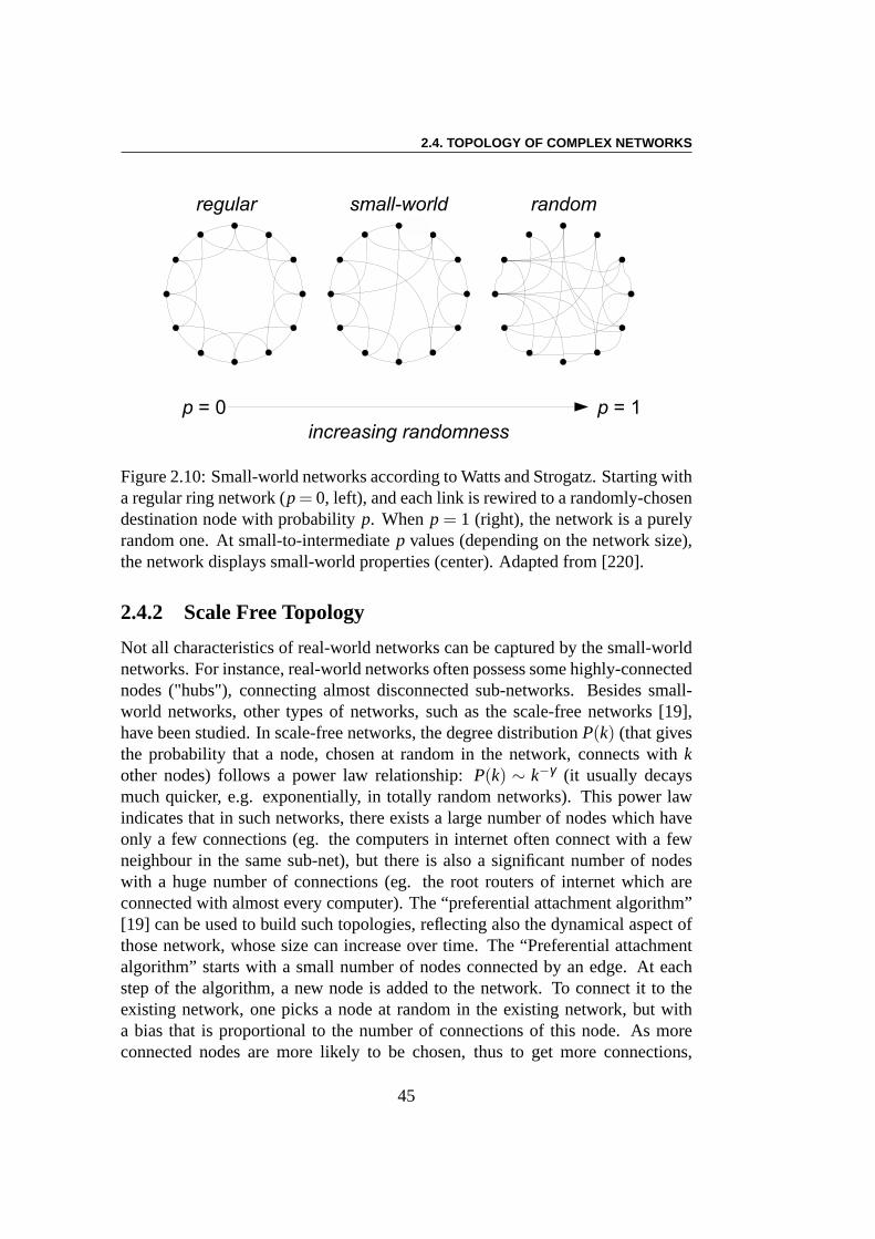
2.4. TOPOLOGY OF COMPLEX NETWORKS
Figure 2.10: Small-world networks according to Watts and Strogatz. Starting witha regular ring network (p= 0, left), and each link is rewired to a randomly-chosendestination node with probabilityp. Whenp = 1 (right), the network is a purelyrandom one. At small-to-intermediatep values (depending on the network size),the network displays small-world properties (center). Adapted from [220].
2.4.2 Scale Free Topology
Not all characteristics of real-world networks can be captured by the small-worldnetworks. For instance, real-world networks often possesssome highly-connectednodes ("hubs"), connecting almost disconnected sub-networks. Besides small-world networks, other types of networks, such as the scale-free networks [19],have been studied. In scale-free networks, the degree distributionP(k) (that givesthe probability that a node, chosen at random in the network,connects withkother nodes) follows a power law relationship:P(k) ∼ k−γ (it usually decaysmuch quicker, e.g. exponentially, in totally random networks). This power lawindicates that in such networks, there exists a large numberof nodes which haveonly a few connections (eg. the computers in internet often connect with a fewneighbour in the same sub-net), but there is also a significant number of nodeswith a huge number of connections (eg. the root routers of internet which areconnected with almost every computer). The “preferential attachment algorithm”[19] can be used to build such topologies, reflecting also thedynamical aspect ofthose network, whose size can increase over time. The “Preferential attachmentalgorithm” starts with a small number of nodes connected by an edge. At eachstep of the algorithm, a new node is added to the network. To connect it to theexisting network, one picks a node at random in the existing network, but witha bias that is proportional to the number of connections of this node. As moreconnected nodes are more likely to be chosen, thus to get moreconnections,
45
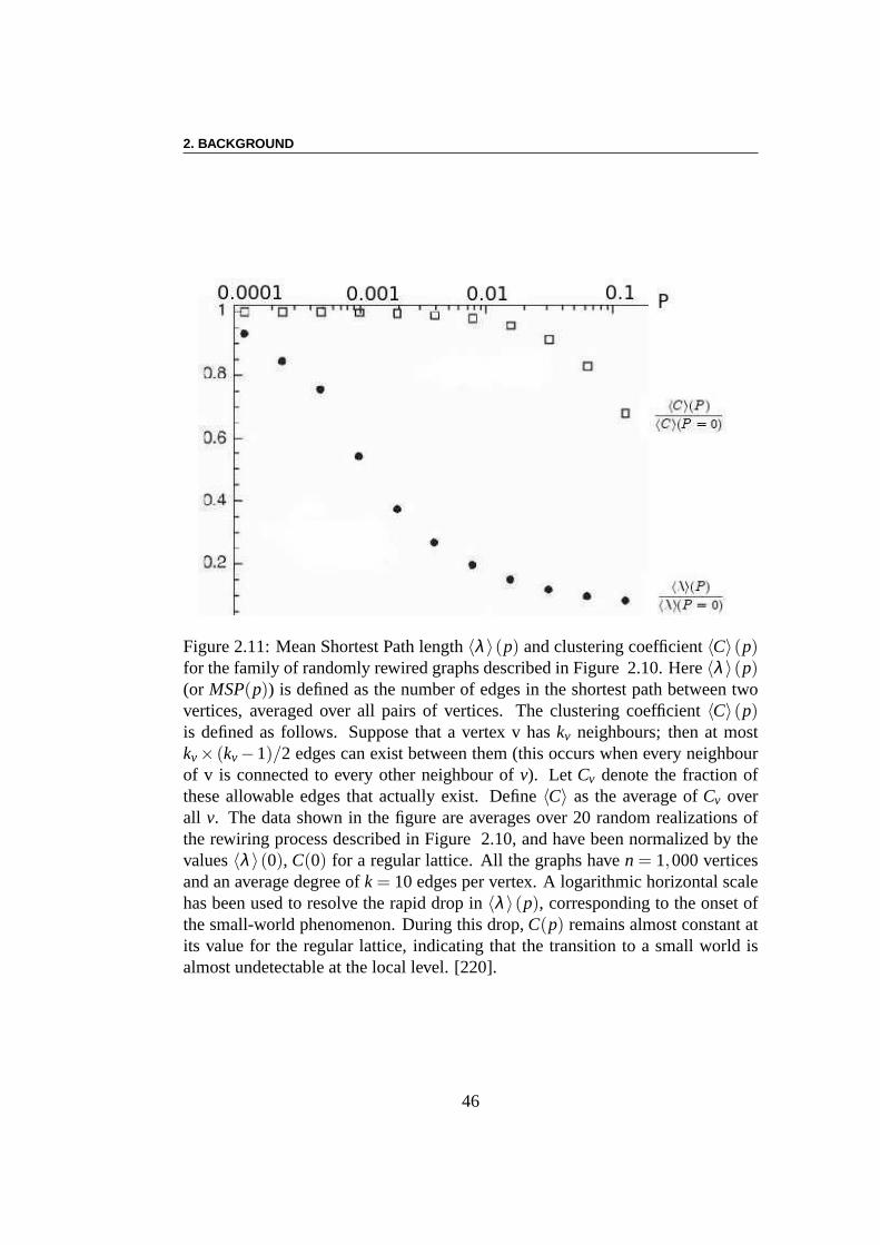
2. BACKGROUND
Figure 2.11: Mean Shortest Path length〈λ 〉(p) and clustering coefficient〈C〉(p)for the family of randomly rewired graphs described in Figure 2.10. Here〈λ 〉(p)(or MSP(p)) is defined as the number of edges in the shortest path betweentwovertices, averaged over all pairs of vertices. The clustering coefficient〈C〉(p)is defined as follows. Suppose that a vertex v haskv neighbours; then at mostkv× (kv−1)/2 edges can exist between them (this occurs when every neighbourof v is connected to every other neighbour ofv). Let Cv denote the fraction ofthese allowable edges that actually exist. Define〈C〉 as the average ofCv overall v. The data shown in the figure are averages over 20 random realizations ofthe rewiring process described in Figure 2.10, and have beennormalized by thevalues〈λ 〉(0), C(0) for a regular lattice. All the graphs haven = 1,000 verticesand an average degree ofk = 10 edges per vertex. A logarithmic horizontal scalehas been used to resolve the rapid drop in〈λ 〉(p), corresponding to the onset ofthe small-world phenomenon. During this drop,C(p) remains almost constant atits value for the regular lattice, indicating that the transition to a small world isalmost undetectable at the local level. [220].
46
2.5. RESEARCH QUESTIONS
this method reflects a "richer get richer" principle. With this method, thecreated network shows aP(k) ∼ k−γ connection distribution. Many “real-world”networks fall into this category (the Internet, airplane routes, metabolic networks,social collaboration networks...) [28].
2.4.3 Applications to ANNs
Importantly, the connectivity structure of such complex networks (i.e. their topol-ogy) is a crucial determinant of their information transferproperties [28]. Hence,the computation made by complex neural networks, i.e. neural networks withcomplex connectivity structure, could as well be dependenton their topology.For instance, recent studies have shown that introducing a small-world topologyin a multilayer perceptron increases its performance [199,29]. However, otherstudies have inspected the performance of Hopfield [118, 153, 148, 205] or Echostate networks [44] with small-world or scale-free topologies and reported morecontrasted results.
2.5 Research Questions
As noted above, the connectivity structure of complex networks (i.e. theirtopology) is a crucial determinant of information transferin large networks(internet, social networks, metabolic networks...). For instance, information,virus or epidemic spreading in Small-world or Scale-free networks is muchmore efficient/faster than in comparable random or regular networks. Othercrucial properties of these systems are topology-controlled, such as tolerance tofaults/defects (robustness), vaccination or the existence of critical thresholds forepidemic spreading [28].
Several studies have applied such complex networks tools toneural networks.Here again, several functional properties of neural networks seem to depend onthe network (complex) topology. For instance, a recent study has shown thatintroducing a Small-world topology in a monolayer perceptron increases thelearning rate of the network [199].
Symmetrically, evolutionary algorithms are commonly usedto modify thetopology of neural networks so as to optimize ANNs performance. But, inmost cases, the studied topologies are quite simple and the number of connec-tions/neurons is low. Furthermore, the evolutionary mechanisms used in most of
47
2. BACKGROUND
these studies do not modify the topology in an intensive manner.
Hence, the optimization of large neural networks through artificial evolutionhas hardly been studied. However the optimization of complex topologies inrelated systems has recently begun to be inspected. For instance, Tomassiniand collaborators [142] have used evolutionary algorithmsto optimize thetopology of 1D-cellular automata networks (majority problem) and reported thattheir optimal topologies were systematically close to Small-world ones. Morerecently, Oikonomou & Cluzel [161] have optimized the topology of booleannetworks and found that the evolution of networks with random topology wasvery different, even quantitatively, from networks with Scale-free topology.
Here, we hope to study the interaction between the topology of large neuralnetworks and their learning capacities. Our approach tackles both the direct andinverse problem:
Direct problem: Given a network with a fixed topology, we study how thenetwork learns to perform its target task through local (backpropagation, Hebb’srules) or global (artificial evolution) rules. An importantaspect of this part ofthe study is that the quantification of the network efficiencycan be defined onthe basis of its pure performance, but it may also be based on its robustness tofailures, noise, or attacks.
Inverse problem: Given a set of local learning rules and a given evolutionaryoptimization algorithm acting on the network topology (and, possibly, on theglobal parameters of the local rules themselves), we want tostudy what kindof topology the networks evolves to. In other words, we want to know if thereexists such a thing as an optimal topology, for given local learning rules and agiven task to perform. An interesting part of this study willbe to compare theobtained topologies with real biological neural networks.Here again, networkoptimization can concern the pure performance of the network, but, alternatively,it may as well concern its robustness to noise or defects.
48
Chapter 3
Evolving the Topology ofSelf-Organizing Map
3.1 Introduction
In this chapter, we use classical Self-Organizing Maps (SOMs) to classify hand-written digits. But unlike classical SOMs where the neuron neighborhood rela-tionships are defined using a simple topology (e.g. regular square or hexagonallattices), we define neighborhood relationships using complex networks. We re-ferred to this kind of ANNs “complex ANNs”. We show that the topology ofneural network has small impact on the performance and robustness of neuronfailures, especially in the case of long learning times. However, the performanceof recognition rate can be increased (by almost 10%) by evolutionary optimiza-tion of the network topology. In our experimental setting, the evolved networksare more random than their parents, whereas they have a more heterogeneous de-gree distribution.
3.2 Topology of Self-Organizing Map
3.2.1 Kohonen Maps
The theory of Self-Organizing Map (SOM) was first proposed asan ArtificialNeural Networks (ANNs) by Kohonen [122, 123]. It is therefore also calledKohonen Maps [124]. The current version of the SOM bibliography containsaround 8000 entries [116, 162].
The Self-Organizing Map usually describes a mapping from a higher dimen-sional input space to a lower dimensional map space. This makes SOM able to be
49
3. EVOLVING THE TOPOLOGY OF SELF-ORGANIZING MAP
used for visualizing high-dimensional data by low-dimensional views. For exam-ple SOM has been widely applied for feature extraction [144,216].
Self-Organizing Map consists of components called nodes orneurons. Eachneuron is associated with a weight vector of the same dimension as the inputdata vectors (high-dimension) and with a location (low-dimension) in the 2Dmap space. Classically, SOM neurons are linked to each other by hexagonal- orsquare-lattice connections, which defines the neighborhood of the neurons. Whenan example from data space is presented, the neuron who has the closest weightvector to the example is firstly found, then the weights of theneuron itself and ofall its neighbors’ are adjusted by the training process as follow:
Training a SOM is a competitive learning process. When a training exam-ple I(t) is presented to the network, for each neuroni, its distancedi to I(t) iscomputed by:
di =M
∑j=1
(I j −wi j )2
wherewi j stands for componentj of the weight vector of neuroni, wi andI j is thej-th component ofI . The correspondingBestMatchingUnit (BMU) is the neuronwhose weight vector is the closest (inL2-norm) toI(t). The weight of the BMUkare updated by:
wk(t +1) = wk(t)+η(t)× (I(t)−wk(t)),
whereη is a user-definedlearningrate. The weights of all BMU neighbors areupdated similarly. In the simplest form, the learning rateη is 1 for all neuronsclose enough to BMU and 0 for others. However, Gaussian decay is a morecommon choice: the learning rateη decays according to a Gaussian law withrespect to the distance to the BMU. The variance of the Gaussian law is alsocalled theradius of the neighborhood. Regardless of the functional form, theradius always decreases with time. At the beginning when theneighborhood isbroad, the self-organizing takes place on the global scale.When the neighborhoodshrinks to only a couple of neurons, the weights are converging to local estimates.
This process is repeated for each input data example for a (usually large)number of cyclesNmax. The patterns in the input data set is self-organized on themap. If these patterns can be labeled, the labels can be attached to the associatedneurons.
50
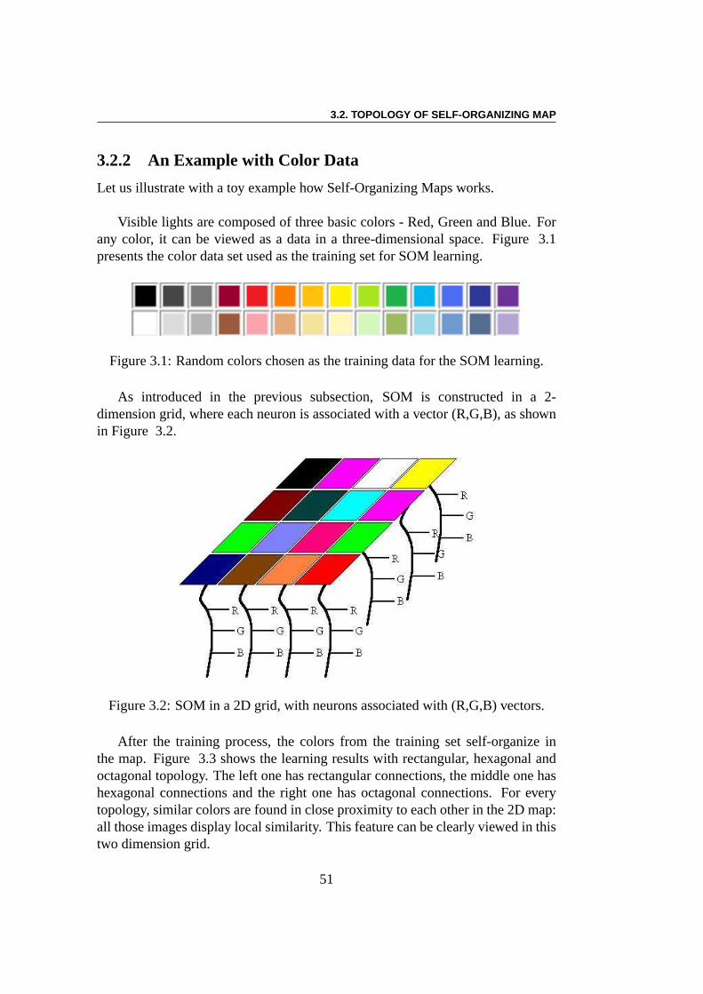
3.2. TOPOLOGY OF SELF-ORGANIZING MAP
3.2.2 An Example with Color Data
Let us illustrate with a toy example how Self-Organizing Maps works.
Visible lights are composed of three basic colors - Red, Greenand Blue. Forany color, it can be viewed as a data in a three-dimensional space. Figure 3.1presents the color data set used as the training set for SOM learning.
Figure 3.1: Random colors chosen as the training data for the SOM learning.
As introduced in the previous subsection, SOM is constructed in a 2-dimension grid, where each neuron is associated with a vector (R,G,B), as shownin Figure 3.2.
Figure 3.2: SOM in a 2D grid, with neurons associated with (R,G,B) vectors.
After the training process, the colors from the training setself-organize inthe map. Figure 3.3 shows the learning results with rectangular, hexagonal andoctagonal topology. The left one has rectangular connections, the middle one hashexagonal connections and the right one has octagonal connections. For everytopology, similar colors are found in close proximity to each other in the 2D map:all those images display local similarity. This feature canbe clearly viewed in thistwo dimension grid.
51
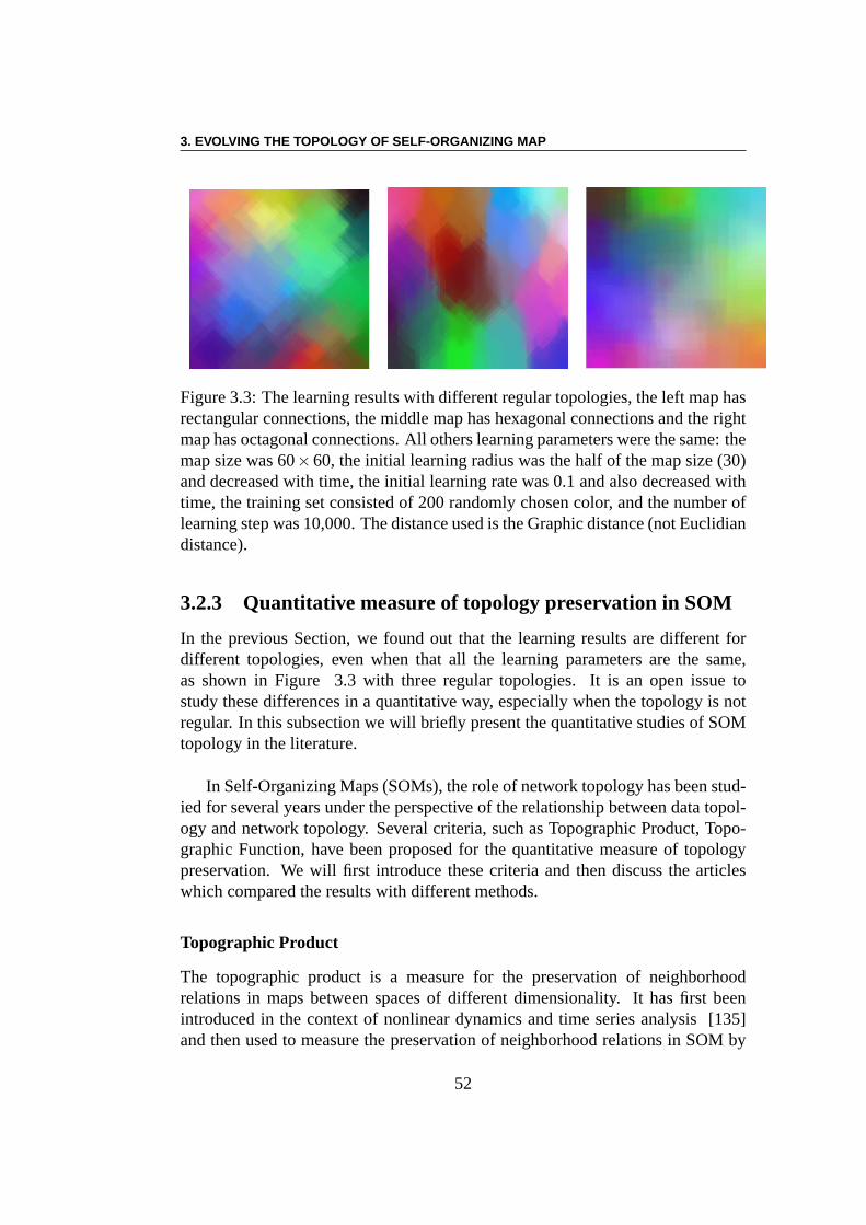
3. EVOLVING THE TOPOLOGY OF SELF-ORGANIZING MAP
Figure 3.3: The learning results with different regular topologies, the left map hasrectangular connections, the middle map has hexagonal connections and the rightmap has octagonal connections. All others learning parameters were the same: themap size was 60×60, the initial learning radius was the half of the map size (30)and decreased with time, the initial learning rate was 0.1 and also decreased withtime, the training set consisted of 200 randomly chosen color, and the number oflearning step was 10,000. The distance used is the Graphic distance (not Euclidiandistance).
3.2.3 Quantitative measure of topology preservation in SOM
In the previous Section, we found out that the learning results are different fordifferent topologies, even when that all the learning parameters are the same,as shown in Figure 3.3 with three regular topologies. It is anopen issue tostudy these differences in a quantitative way, especially when the topology is notregular. In this subsection we will briefly present the quantitative studies of SOMtopology in the literature.
In Self-Organizing Maps (SOMs), the role of network topology has been stud-ied for several years under the perspective of the relationship between data topol-ogy and network topology. Several criteria, such as Topographic Product, Topo-graphic Function, have been proposed for the quantitative measure of topologypreservation. We will first introduce these criteria and then discuss the articleswhich compared the results with different methods.
Topographic Product
The topographic product is a measure for the preservation ofneighborhoodrelations in maps between spaces of different dimensionality. It has first beenintroduced in the context of nonlinear dynamics and time series analysis [135]and then used to measure the preservation of neighborhood relations in SOM by
52
3.2. TOPOLOGY OF SELF-ORGANIZING MAP
Bauer and Pawelzik in 1992 [20]. The topographic product is a quantificationmethod which compares the distance between neuroni and itskth nearest neuronin both input space and output space. For computing the topographic product,Q1(i, j) is the distance between pointi in the output space and itskth nearestneighborj in the output space, divided by the distance between pointi in the inputspace and itskth nearest neighborj in the input space.Q2(i, j) gives analogousinformation wherei and j are both points in the output space. In Ref. [20],Bauer proposed several ways to combineQ1(i, j) and Q2(i, j) to produce asingle numberP, the “Topographic Product” which can define the quality of thepreservation of neighborhood.
The method has been tested in [20] by a simple experiment where a 2-D spaceis embedded into 1, 2 and 3 dimensions spaces, and a more complex example ofthe speech recognition. The result is quantitative, but theprocess is hugely time-consuming.
Topographic Function
The topographic function has been introduced by Villmann etal in 1995 [217].The notion of “ Voronoi polyhedron” was applied to determinethe receptive fieldof each neuron. Each neuron defines a Voronoi cell, that consists of all pointscloser to this neuron than to any other. The segments of the Voronoi diagram areall the points that are equidistant to the two nearest neurons. The Voronoi nodesare the points that are equidistant to three (or more) neurons. The main idea isto observe the neighborhood relations between receptive fields in input space. Ifonly the nearest lattice neighbors of a neuroni have receptive fields which areadjacent to the receptive field of neuroni, the SOM is considered doing a perfectpreservation. The authors have also given a method to determine the adjacency oftwo receptive fields.
Q, H and QH measures
Polani introduced several quantitative measures of SOM quality, such as the en-ergy function measures and Hebbian measures [167] and the Q and QH mea-sures [168]. He also compared the results among these measures by testing 6different topologies (linear, hexagonal, square, crocodile, cubic and tree). We willbriefly present these works below.
The Q measure: Q is themeanquantizationerror between a large set ofpoints from the input space and its discrete approximation in the output space. Itis a rather canonical quantity measure. For calculating Q, alarge set of pointsx1...xq ∈ R of the input space are chosen randomly according to the probability
53
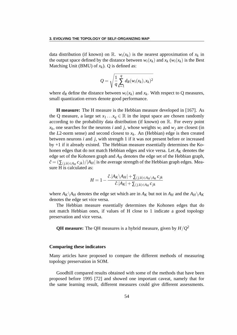
3. EVOLVING THE TOPOLOGY OF SELF-ORGANIZING MAP
data distribution (if known) onR. wi(xk) is the nearest approximation ofxk inthe output space defined by the distance betweenwi(xk) andxk (wi(xk) is the BestMatching Unit (BMU) ofxk). Q is defined as:
Q =
√
1q
q
∑k=1
dR(wi(xk),xk)2
wheredR define the distance betweenwi(xk) andxk. With respect to Q measures,small quantization errors denote good performance.
H measure: The H measure is the Hebbian measure developed in [167]. Asthe Q measure, a large setx1 . . .xq ∈ R in the input space are chosen randomlyaccording to the probability data distribution (if known) on R. For every pointxk, one searches for the neuronsi and j, whose weightswi andw j are closest (intheL2-norm sense) and second closest toxk. An (Hebbian) edge is then createdbetween neuronsi and j, with strength 1 if it was not present before or increasedby +1 if it already existed. The Hebbian measure essentiallydetermines the Ko-honen edges that do not match Hebbian edges and vice versa. Let AK denotes theedge set of the Kohonen graph andAH denotes the edge set of the Hebbian graph,c= (∑( j,k)∈AH
c jk)/|AH | is the average strength of the Hebbian graph edges. Mea-sure H is calculated as:
H = 1−c.|AK\AH |+∑( j,k)∈AH\AK
c jk
c.|AK|+∑( j,k)∈AHc jk
whereAK\AH denotes the edge set which are inAK but not inAH and theAH\AK
denotes the edge set vice versa.The Hebbian measure essentially determines the Kohonen edges that do
not match Hebbian ones, if values of H close to 1 indicate a good topologypreservation and vice versa.
QH measure: The QH measures is a hybrid measure, given byH/Q2
Comparing these indicators
Many articles have proposed to compare the different methods of measuringtopology preservation in SOM.
Goodhill compared results obtained with some of the methodsthat have beenproposed before 1995 [72] and showed one important caveat, namely that forthe same learning result, different measures could give different assessments.
54
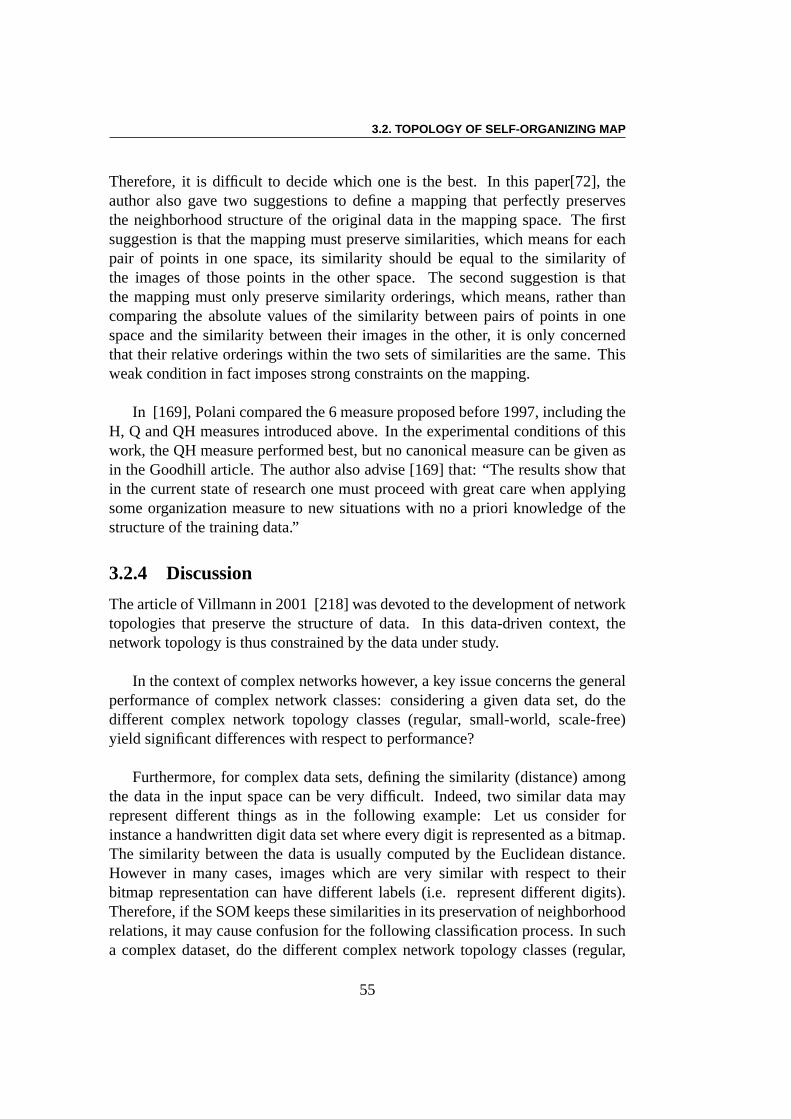
3.2. TOPOLOGY OF SELF-ORGANIZING MAP
Therefore, it is difficult to decide which one is the best. In this paper[72], theauthor also gave two suggestions to define a mapping that perfectly preservesthe neighborhood structure of the original data in the mapping space. The firstsuggestion is that the mapping must preserve similarities,which means for eachpair of points in one space, its similarity should be equal tothe similarity ofthe images of those points in the other space. The second suggestion is thatthe mapping must only preserve similarity orderings, whichmeans, rather thancomparing the absolute values of the similarity between pairs of points in onespace and the similarity between their images in the other, it is only concernedthat their relative orderings within the two sets of similarities are the same. Thisweak condition in fact imposes strong constraints on the mapping.
In [169], Polani compared the 6 measure proposed before 1997, including theH, Q and QH measures introduced above. In the experimental conditions of thiswork, the QH measure performed best, but no canonical measure can be given asin the Goodhill article. The author also advise [169] that: “The results show thatin the current state of research one must proceed with great care when applyingsome organization measure to new situations with no a prioriknowledge of thestructure of the training data.”
3.2.4 Discussion
The article of Villmann in 2001 [218] was devoted to the development of networktopologies that preserve the structure of data. In this data-driven context, thenetwork topology is thus constrained by the data under study.
In the context of complex networks however, a key issue concerns the generalperformance of complex network classes: considering a given data set, do thedifferent complex network topology classes (regular, small-world, scale-free)yield significant differences with respect to performance?
Furthermore, for complex data sets, defining the similarity(distance) amongthe data in the input space can be very difficult. Indeed, two similar data mayrepresent different things as in the following example: Letus consider forinstance a handwritten digit data set where every digit is represented as a bitmap.The similarity between the data is usually computed by the Euclidean distance.However in many cases, images which are very similar with respect to theirbitmap representation can have different labels (i.e. represent different digits).Therefore, if the SOM keeps these similarities in its preservation of neighborhoodrelations, it may cause confusion for the following classification process. In sucha complex dataset, do the different complex network topology classes (regular,
55
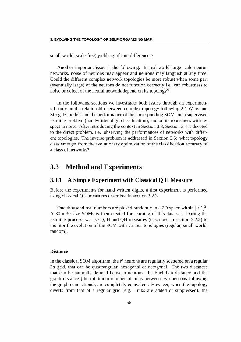
3. EVOLVING THE TOPOLOGY OF SELF-ORGANIZING MAP
small-world, scale-free) yield significant differences?
Another important issue is the following. In real-world large-scale neuronnetworks, noise of neurons may appear and neurons may languish at any time.Could the different complex network topologies be more robust when some part(eventually large) of the neurons do not function correctlyi.e. can robustness tonoise or defect of the neural network depend on its topology?
In the following sections we investigate both issues through an experimen-tal study on the relationship between complex topology following 2D-Watts andStrogatz models and the performance of the corresponding SOMs on a supervisedlearning problem (handwritten digit classification), and on its robustness with re-spect to noise. After introducing the context in Section 3.3, Section 3.4 is devotedto thedirect problem, i.e. observing the performances of networks with differ-ent topologies. Theinverseproblem is addressed in Section 3.5: what topologyclass emerges from the evolutionary optimization of the classification accuracy ofa class of networks?
3.3 Method and Experiments
3.3.1 A Simple Experiment with Classical Q H Measure
Before the experiments for hand written digits, a first experiment is performedusing classical Q H measures described in section 3.2.3.
One thousand real numbers are picked randomly in a 2D space within [0,1]2.A 30× 30 size SOMs is then created for learning of this data set. During thelearning process, we use Q, H and QH measures (described in section 3.2.3) tomonitor the evolution of the SOM with various topologies (regular, small-world,random).
Distance
In the classical SOM algorithm, theN neurons are regularly scattered on a regular2d grid, that can be quadrangular, hexagonal or octogonal. Thetwo distancesthat can be naturally defined between neurons, the Euclidiandistance and thegraph distance (the minimum number of hops between two neurons followingthe graph connections), are completely equivalent. However, when the topologydiverts from that of a regular grid (e.g. links are added or suppressed), the
56
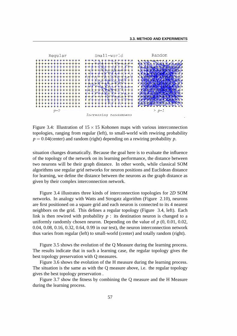
3.3. METHOD AND EXPERIMENTS
Figure 3.4: Illustration of 15× 15 Kohonen maps with various interconnectiontopologies, ranging from regular (left), to small-world with rewiring probabilityp = 0.04(center) and random (right) depending on a rewiring probability p.
situation changes dramatically. Because the goal here is to evaluate the influenceof the topology of the network on its learning performance, the distance betweentwo neurons will be their graph distance. In other words, while classical SOMalgorithms use regular grid networks for neuron positions and Euclidean distancefor learning, we define the distance between the neurons as the graph distance asgiven by their complex interconnection network.
Figure 3.4 illustrates three kinds of interconnection topologies for 2D SOMnetworks. In analogy with Watts and Strogatz algorithm (Figure 2.10), neuronsare first positioned on a square grid and each neuron is connected to its 4 nearestneighbors on the grid. This defines a regular topology (Figure 3.4, left). Eachlink is then rewired with probabilityp : its destination neuron is changed to auniformly randomly chosen neuron. Depending on the value ofp (0, 0.01, 0.02,0.04, 0.08, 0.16, 0.32, 0.64, 0.99 in our test), the neuron interconnection networkthus varies from regular (left) to small-world (center) andtotally random (right).
Figure 3.5 shows the evolution of the Q Measure during the learning process.The results indicate that in such a learning case, the regular topology gives thebest topology preservation with Q measures.
Figure 3.6 shows the evolution of the H measure during the learning process.The situation is the same as with the Q measure above, i.e. theregular topologygives the best topology preservation .
Figure 3.7 show the fitness by combining the Q measure and the HMeasureduring the learning process.
57
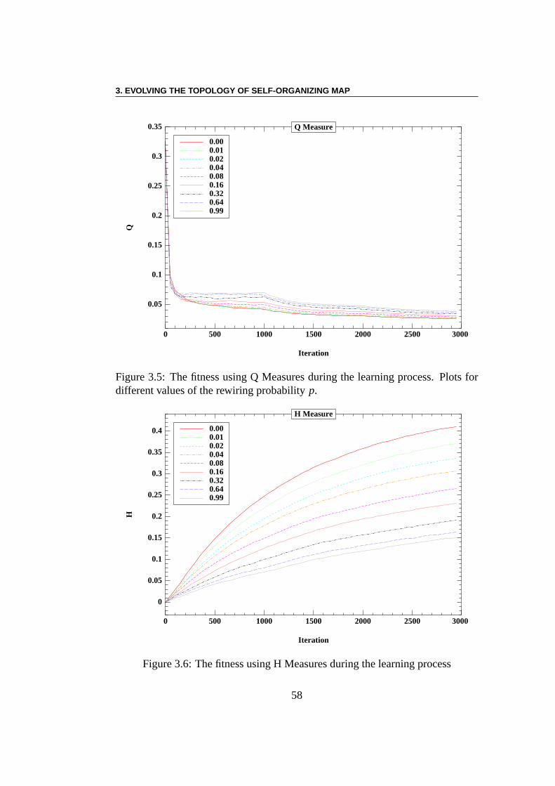
3. EVOLVING THE TOPOLOGY OF SELF-ORGANIZING MAP
Iteration
Q
0 1000 2000 3000500 1500 2500
0.1
0.2
0.3
0.05
0.15
0.25
0.35
0.000.010.020.040.080.160.320.640.99
Q Measure
Figure 3.5: The fitness using Q Measures during the learning process. Plots fordifferent values of the rewiring probabilityp.
Iteration
H
0 1000 2000 3000500 1500 2500
0
0.1
0.2
0.3
0.4
0.05
0.15
0.25
0.35
0.000.010.020.040.080.160.320.640.99
H Measure
Figure 3.6: The fitness using H Measures during the learning process
58
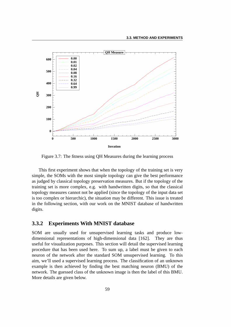
3.3. METHOD AND EXPERIMENTS
Iteration
QH
0 1000 2000 3000500 1500 2500
0
100
200
300
400
500
600 0.000.010.020.040.080.160.320.640.99
QH Measure
Figure 3.7: The fitness using QH Measures during the learningprocess
This first experiment shows that when the topology of the training set is verysimple, the SOMs with the most simple topology can give the best performanceas judged by classical topology preservation measures. But if the topology of thetraining set is more complex, e.g. with handwritten digits,so that the classicaltopology measures cannot not be applied (since the topologyof the input data setis too complex or hierarchic), the situation may be different. This issue is treatedin the following section, with our work on the MNIST databaseof handwrittendigits.
3.3.2 Experiments With MNIST database
SOM are usually used for unsupervised learning tasks and produce low-dimensional representations of high-dimensional data [162]. They are thususeful for visualization purposes. This section will detail the supervised learningprocedure that has been used here. To sum up, a label must be given to eachneuron of the network after the standard SOM unsupervised learning. To thisaim, we’ll used a supervised learning process. The classification of an unknownexample is then achieved by finding the best matching neuron (BMU) of thenetwork. The guessed class of the unknown image is then the label of this BMU.More details are given below.
59
3. EVOLVING THE TOPOLOGY OF SELF-ORGANIZING MAP
The task considered here is the recognition/classificationof handwrittendigits, using the well-known MNIST database: The MNIST database of hand-written digits [130] has a training set of 60,000 examples, and a test set of 10,000examples. It is a subset of a larger set available from NIST. The digits have beensize-normalized and centered in a fixed-size (28× 28) image. SOM will hencebe used here with partly supervised learning, in order to give an unambiguousperformance measure and estimate the corresponding topology/performancerelation. It should be noted that the goal here is not to reachthe best possibleperformance for the MNIST problem (and indeed SOM cannot compete withbest-to-date published results) but to compare the relative performances ofdifferent topologies on the same problem [130].
Each digit in the data base is described by aM = 28× 28 matrix of pixels(integer gray level in [0,255]). TheN neurons of the SOM are scattered on a 2dspace. Each neuroni has an associatedM-dimensional weight vectorwi that isinitialized randomly and will be adjusted while learning the training set. Thedifferent phases of the learning process go as follows.
3.3.3 Learning
This phase is the classical unsupervised SOM learning process which has beenintroduced before (section 3.2.1). It classically go through the following steps:
1. Randomly initialize the weight vectors of all neurons
2. Randomly fetch an input image from the training set
3. For each node in the map
(a) Use Euclidean distance formula to find similarity between the inputimage and the neuron’s weight vector item Track the BMU, i.e.,thenode that produces the smallest distance
4. Update the BMU and the neurons in the neighborhood of the BMU bypulling them closer to the input vector
5. Incrementt and repeat from 2 whilet < Nmax
In the present work, the total number of learning stepsNmax was varied between104 and 106, and the radius is decreased along learning iterations (seee.g. Figure
60
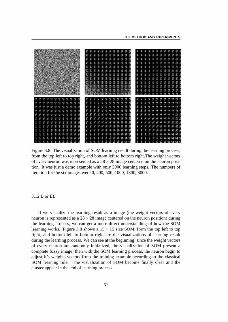
3.3. METHOD AND EXPERIMENTS
Figure 3.8: The visualization of SOM learning result duringthe learning process,from the top left to top right, and bottom left to bottom right.The weight vectorsof every neuron was represented as a 28×28 image centered on the neuron posi-tion. It was just a demo example with only 3000 learning steps. The numbers ofiteration for the six images were 0, 200, 500, 1000, 1800, 3000.
3.12 B or E).
If we visualize the learning result as a image (the weight vectors of everyneuron is represented as a 28×28 image centered on the neuron position) duringthe learning process, we can get a more direct understandingof how the SOMlearning works. Figure 3.8 shows a 15× 15 size SOM, form the top left to topright, and bottom left to bottom right are the visualizations of learning resultduring the learning process. We can see at the beginning, since the weight vectorsof every neuron are randomly initialized, the visualization of SOM present acomplete fuzzy image; then with the SOM learning process, the neuron begin toadjust it’s weights vectors from the training example according to the classicalSOM learning rule. The visualization of SOM become finally clear and thecluster appear in the end of learning process.
61
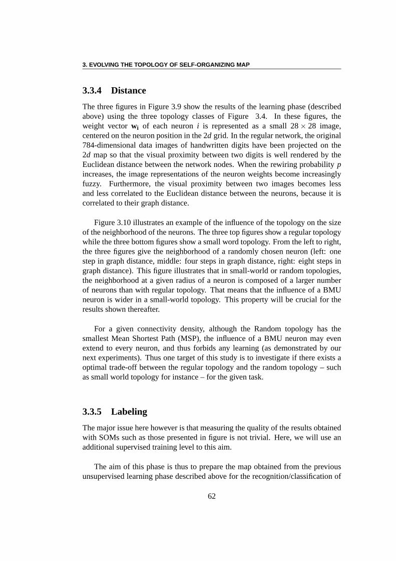
3. EVOLVING THE TOPOLOGY OF SELF-ORGANIZING MAP
3.3.4 Distance
The three figures in Figure 3.9 show the results of the learning phase (describedabove) using the three topology classes of Figure 3.4. In these figures, theweight vectorwi of each neuroni is represented as a small 28× 28 image,centered on the neuron position in the 2d grid. In the regular network, the original784-dimensional data images of handwritten digits have been projected on the2d map so that the visual proximity between two digits is well rendered by theEuclidean distance between the network nodes. When the rewiring probabilitypincreases, the image representations of the neuron weightsbecome increasinglyfuzzy. Furthermore, the visual proximity between two images becomes lessand less correlated to the Euclidean distance between the neurons, because it iscorrelated to their graph distance.
Figure 3.10 illustrates an example of the influence of the topology on the sizeof the neighborhood of the neurons. The three top figures showa regular topologywhile the three bottom figures show a small word topology. From the left to right,the three figures give the neighborhood of a randomly chosen neuron (left: onestep in graph distance, middle: four steps in graph distance, right: eight steps ingraph distance). This figure illustrates that in small-world or random topologies,the neighborhood at a given radius of a neuron is composed of alarger numberof neurons than with regular topology. That means that the influence of a BMUneuron is wider in a small-world topology. This property will be crucial for theresults shown thereafter.
For a given connectivity density, although the Random topology has thesmallest Mean Shortest Path (MSP), the influence of a BMU neuron may evenextend to every neuron, and thus forbids any learning (as demonstrated by ournext experiments). Thus one target of this study is to investigate if there exists aoptimal trade-off between the regular topology and the random topology – suchas small world topology for instance – for the given task.
3.3.5 Labeling
The major issue here however is that measuring the quality ofthe results obtainedwith SOMs such as those presented in figure is not trivial. Here, we will use anadditional supervised training level to this aim.
The aim of this phase is thus to prepare the map obtained from the previousunsupervised learning phase described above for the recognition/classification of
62
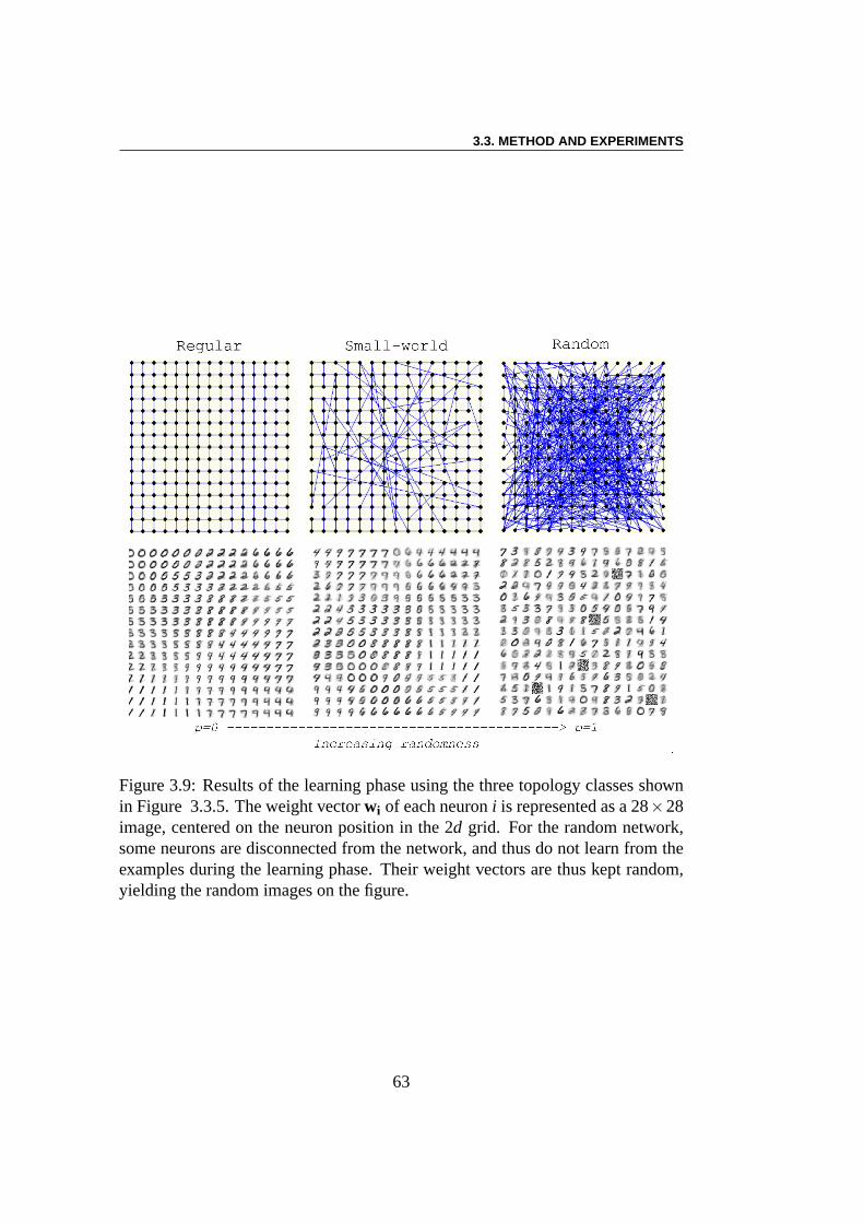
3.3. METHOD AND EXPERIMENTS
Figure 3.9: Results of the learning phase using the three topology classes shownin Figure 3.3.5. The weight vectorwi of each neuroni is represented as a 28×28image, centered on the neuron position in the 2d grid. For the random network,some neurons are disconnected from the network, and thus do not learn from theexamples during the learning phase. Their weight vectors are thus kept random,yielding the random images on the figure.
63
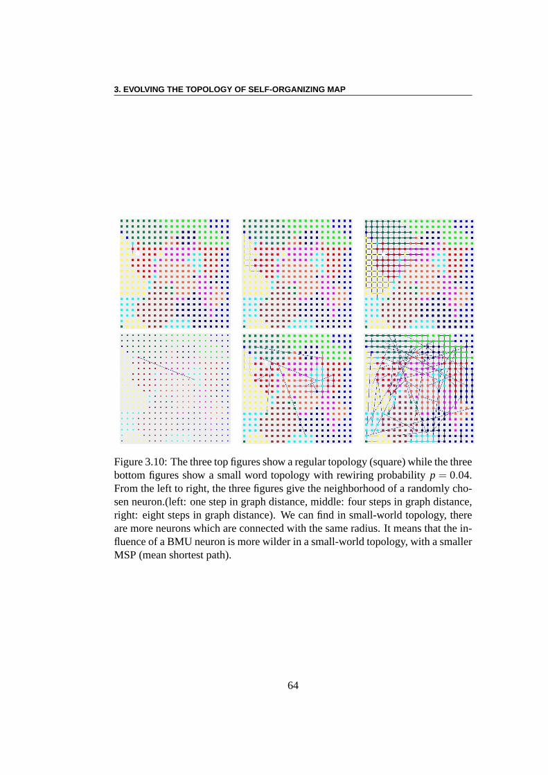
3. EVOLVING THE TOPOLOGY OF SELF-ORGANIZING MAP
Figure 3.10: The three top figures show a regular topology (square) while the threebottom figures show a small word topology with rewiring probability p = 0.04.From the left to right, the three figures give the neighborhood of a randomly cho-sen neuron.(left: one step in graph distance, middle: four steps in graph distance,right: eight steps in graph distance). We can find in small-world topology, thereare more neurons which are connected with the same radius. Itmeans that the in-fluence of a BMU neuron is more wilder in a small-world topology, with a smallerMSP (mean shortest path).
64
3.3. METHOD AND EXPERIMENTS
handwritten digits, i.e., to be able to classify unknown examples. The label ofeach neuron is assigned in the following way. Firstly, the BMUof each exampleof the training set is computed (see Section 3.3.3). Secondly, for each neuronof the network, a probability vector is computed, describing the different votesof each class for this neuron as BMU. For example, if neuroni is the BMU of20 (labeled) examples, out of which 16 are labeled “1” and 4 labeled “7”, theprobabilities attached to this neuron are computed aspi(1) = 16
20, andpi(7) = 420
(andpi(l) = 0 for other values ofl ). Thebasiclabel for the neuron is then definedas the class with higher probability, e.g. “1” in the preceding example. Neuronsthat never were BMUs are given the basic label of the class fromwhich they areat shortest distance inL2 norm (this case only concerns a very small number ofneurons and does not impact the classification accuracy).
Figure 3.11 illustrates an example of the influence of the topology. In thethree figures, the different color indicates the different labels of the neurons. Theleft figure is a SOM with regular topology, the middle one has asmall-worldtopology with low rewiring probability (p = 0.02, close to regular topology) andthe right figure has a topology with high rewiring probability (p = 0.32 which isno longer small-world by the definition, but close to random topology). We cansee that in the regular topology, the neurons with same labelare close to eachother and the clusterings can be clearly identified. But in theright figure, thedifferent clusterings are mixed with others.
3.3.6 Classifying
Using either the whole probability vector, or the basic label, two strategies forclassifying unknown examples can be designed. In both cases, the test example ispresented to the network, then the distance between the example and each neuronis computed, and finally theN nearest neurons from the examples are recorded(N is a user-defined parameter).
Majority by numbers : The class given to the unknown example is thebasic label most often encountered among theN nearest neurons. Preliminaryexperiments (for maps of 3,600 neurons) withN ranging from 1 to 500 showedthat the best performances are obtained forN = 1.
Majority by probability : Here, the probability vectorpi attached to eachneuroni is used to compute the probability that the test image belongs to classk(k∈ [0,9]) using the following equation:
65
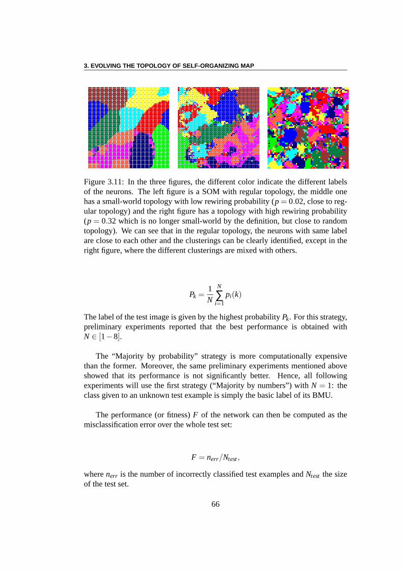
3. EVOLVING THE TOPOLOGY OF SELF-ORGANIZING MAP
Figure 3.11: In the three figures, the different color indicate the different labelsof the neurons. The left figure is a SOM with regular topology,the middle onehas a small-world topology with low rewiring probability (p = 0.02, close to reg-ular topology) and the right figure has a topology with high rewiring probability(p = 0.32 which is no longer small-world by the definition, but closeto randomtopology). We can see that in the regular topology, the neurons with same labelare close to each other and the clusterings can be clearly identified, except in theright figure, where the different clusterings are mixed withothers.
Pk =1N
N
∑i=1
pi(k)
The label of the test image is given by the highest probability Pk. For this strategy,preliminary experiments reported that the best performance is obtained withN ∈ [1−8].
The “Majority by probability” strategy is more computationally expensivethan the former. Moreover, the same preliminary experiments mentioned aboveshowed that its performance is not significantly better. Hence, all followingexperiments will use the first strategy (“Majority by numbers”) with N = 1: theclass given to an unknown test example is simply the basic label of its BMU.
The performance (or fitness)F of the network can then be computed as themisclassification error over the whole test set:
F = nerr/Ntest,
wherenerr is the number of incorrectly classified test examples andNtest the sizeof the test set.
66
3.4. DIRECT PROBLEM
3.4 Direct problem
The goal of the first experiments is to compare the classification performanceof SOM built on different topologies, namely ranging from regular to randomtopologies according to the Watts and Strogatz model (see Figure 2.10).
Figure 3.12-A shows plots of the evolution of the classification performanceFduring the (unsupervised) learning phase for networks of 1024 (32×32 )neuronswith regular (rewiring probabilityp= 0, bottom curve) to small-world (intermedi-ate curves) to fully random (p = 1, top curve) topologies. The initial learning rateis η(0) = 0.008 (adjusted after a few preliminary runs) and the total number oflearning steps is 106. The radius of each neuron (i.e. the variance of the learningrate) was varied as shown in figure 3.12-B. The full MNIST database was usedfor those experiments, i.e. the size of training set is 60000and the size of test setis 10000.
3.4.1 Influence of the radius
First of all, Figure 3.12-A shows that, at long learning times, the networkperformance is clearly independent on the topology. This isnot surprising sincethe role of the topology decreases with the radiusR. Indeed, the number ofneighbors within a radiusR of a given neuron increases when the rewiring prob-ability p increases. However, this difference decays asR decreases. Importantdifferences are however obvious at short to intermediate learning times: the morerandom, the less efficient the network at this time scale. This remark deservesfurther analysis. Indeed, the performance of these random networks evolvesin a piecewise constant fashion. Comparing this evolution tothe simultaneousdecrease of the neighborhood radius (Figure 3.12-B) uncovers that performanceplateaus are synchronized to radius plateaus.The more random the network, the lower its Mean Shortest Path. Hence, apossible interpretation is that, for highp values, the influence of a given neuronat short learning times extends over the entire 2d space, to almost every otherneuron. Thus, at short time scales, almost all neurons are updated each time anew image is presented, which actually forbids any learningin the network. Thisinterpretation is supported by Figure 3.13-D, where the initial radius is five timessmaller than in Figure 3.12-A, everything else being equal.Here, the differencesin short time behaviors observed above have vanished.
67
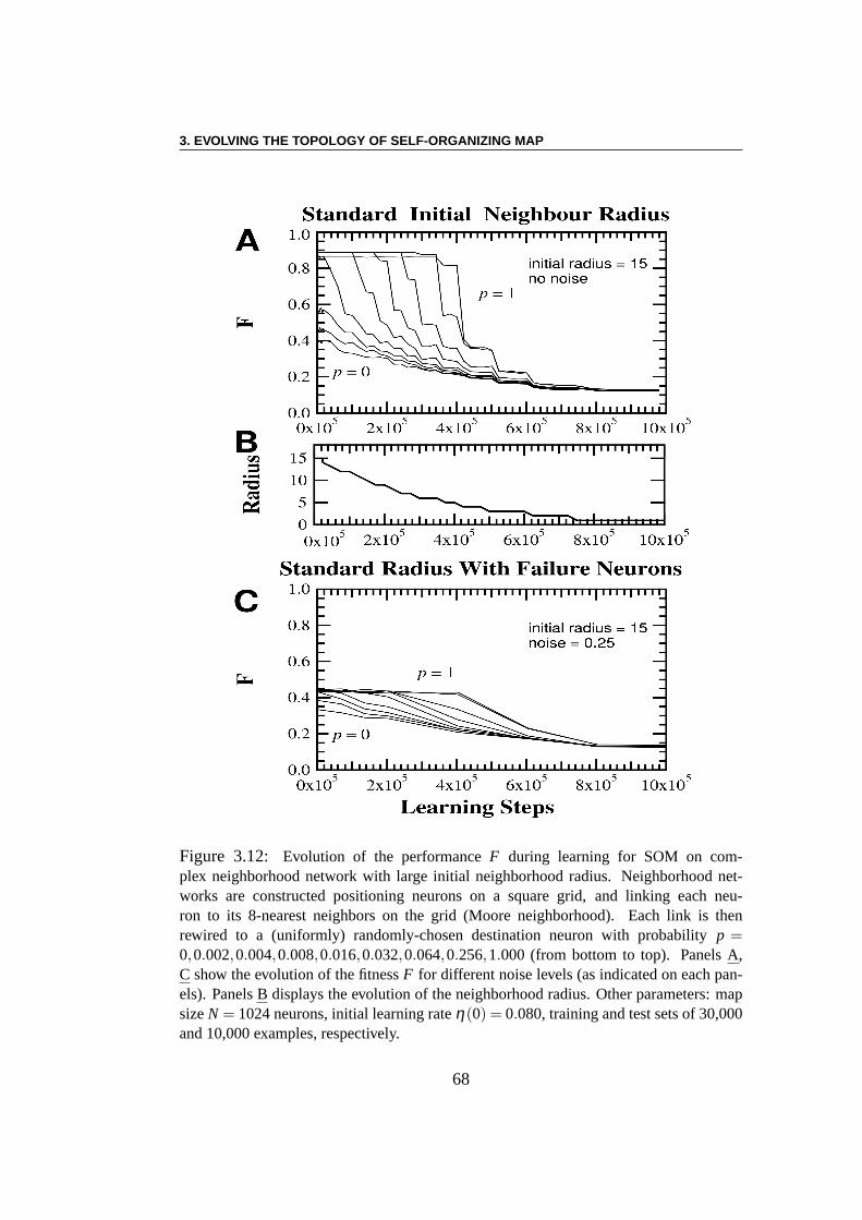
3. EVOLVING THE TOPOLOGY OF SELF-ORGANIZING MAP
Figure 3.12: Evolution of the performanceF during learning for SOM on com-plex neighborhood network with large initial neighborhood radius. Neighborhood net-works are constructed positioning neurons on a square grid, and linkingeach neu-ron to its 8-nearest neighbors on the grid (Moore neighborhood). Eachlink is thenrewired to a (uniformly) randomly-chosen destination neuron with probabilityp =0,0.002,0.004,0.008,0.016,0.032,0.064,0.256,1.000 (from bottom to top). PanelsA,C show the evolution of the fitnessF for different noise levels (as indicated on each pan-els). PanelsB displays the evolution of the neighborhood radius. Other parameters: mapsizeN = 1024 neurons, initial learning rateη(0) = 0.080, training and test sets of 30,000and 10,000 examples, respectively.
68
3.4. DIRECT PROBLEM
3.4.2 Robustness against noise
Unlike most of computer-simulated ones, real-world networks (including neuralnetworks), involving a large number of computing units/neurons, will be subject tonoise and defects. In particular, we were interested in studying now noise affectingthe topology, and its impact on the computing performances of the network (here,its classification performance). Noise is modeled here by deactivating a fractionν of the neurons at each learning step (the list of theNν deactivated neurons ischosen uniformly for each learning step). All neurons are however consideredactive for the evaluation phase (Section 3.3.6).
Figure 3.12-C shows the performance of the same networks during learningwith ν = 0.25 noise level (i.e. 25% of the neurons are insensitive to learning, ateach step) and the same large initial radius as in Figure 3.12-A. The differencesbetween both figures can be explained by looking again at the radius. Clearly,because the deactivated neurons are protected from update,the effect of largeradius that is described above is strongly attenuated. In other words, the presenceof noise (here random node failures) actuallyimproves the performance of thesecomplex random networks at short learning times. That this effect is effectivelyrelated to large radius sizes is confirmed by inspection of Figure 3.13C, whichshows that with small initial radius, this ’beneficial’ effect of noise is not observed(compare with Figure 3.13D).
Another result from Figure 3.12 is that the effects of noise are restricted toshort-to-average learning times and almost disappear withlong learning times,where the performances of all networks are similar (whatever the topologyrandomness or initial radius). Hence, for long learning times, the SOM are robustto neuron failure rates as high as 25%, and this robustness does not seem todepend on their neighborhood topology.
Finally, Figure 3.14 shows the effects of network size on itsperformance. Eachpoint is averaged over 11 independent runs. While large SOM (N > 2,000) per-form better with regular neighborhood networks, the situation is just the oppositewith small (N < 200) SOM, where random networks perform better than regularones. Small-world topologies are intermediate (not shown). Note however thateven for the extreme sizes, the difference of fitness betweenregular and randomtopologies, though statistically significant (see caption), remains minute.
69
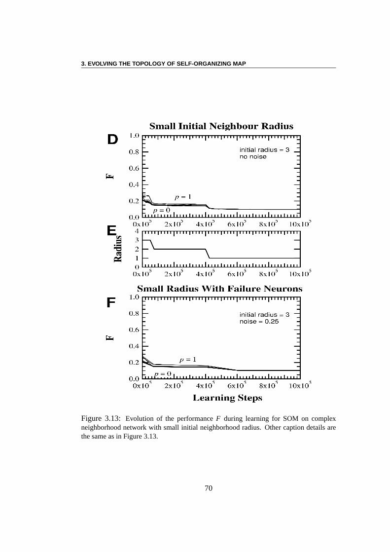
3. EVOLVING THE TOPOLOGY OF SELF-ORGANIZING MAP
Figure 3.13: Evolution of the performanceF during learning for SOM on complexneighborhood network with small initial neighborhood radius. Other captiondetails arethe same as in Figure 3.13.
70
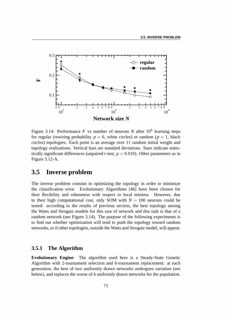
3.5. INVERSE PROBLEM
0.3
0.2
0.1
F
8 9
102
2 3 4 5 6 7 8 9
103
2 3 4 5 6 7 8 9
104
Network size N
*
*
* * *
regular random
Figure 3.14: PerformanceF vs number of neuronsN after 106 learning stepsfor regular (rewiring probabilityp = 0, white circles) or random (p = 1, blackcircles) topologies. Each point is an average over 11 randominitial weight andtopology realizations. Vertical bars are standard deviations. Stars indicate statis-tically significant differences (unpairedt-test,p < 0.010). Other parameters as inFigure 3.12-A.
3.5 Inverse problem
The inverse problem consists in optimizing the topology in order to minimizethe classification error. Evolutionary Algorithms [46] have been chosen fortheir flexibility and robustness with respect to local minima. However, dueto their high computational cost, only SOM withN = 100 neurons could betested: according to the results of previous section, the best topology amongthe Watts and Strogatz models for this size of network and this task is that of arandom network (see Figure 3.14). The purpose of the following experiments isto find out whether optimization will tend to push the topology toward randomnetworks, or if other topologies, outside the Watts and Strogatz model, will appear.
3.5.1 The Algorithm
Evolutionary Engine: The algorithm used here is a Steady-State GeneticAlgorithm with 2-tournament selection and 6-tournament replacement: at eachgeneration, the best of two uniformly drawn networks undergoes variation (seebelow), and replaces the worse of 6 uniformly drawn networksfor the population.
71
3. EVOLVING THE TOPOLOGY OF SELF-ORGANIZING MAP
The initial population is composed of 100 different small-world networks (initialwith rewiring probabilityp = 0.050).
Variation operators: Evolutionary algorithms typically use two types ofvariation operators: crossover, involving two or more parents to generate oneoffspring, and mutation, that uses a single parent to createan offspring. However,because no meaningful crossover operator could be designedhere since wewant to have the total number of connections fix during the optimization, onlymutation was used (no crossover operator is better than a poor crossover operator).
The mutation consists in random rewiring ofC% of uniformly chosen links.C decreases exponentially during evolution (C(g) = 30(102.6)−g/gmax wheregis the generation number andgmax is the total number of generations). Here,gmax = 200,000. In these conditions,C(g) decreases from 102 rewired links intotal (g = 0) down to 1 single rewiring (g = gmax).
Fitness: The fitness is computed as the average misclassification error F (seeSection 3.3.6) over 5 learning phases, starting from 5 different initial weights.
Each network contains 10× 10 neurons, each neuron having 8 neighbors(Moore neighborhood). The initial learning rate is set toη(0) = 0.35 for afast learning. However, in order to further decrease the computational time, thelearning algorithm is run during only 10000 learning steps (see discussion below),using only 2000 examples from the training set, and the fitness is computed using5000 examples from the test set.
This algorithm is summarized below :
• Initialize K networks: rewire 5% of a regular network (8 links per neuronwith its neighbors, 342 global)
• ForM "generations":
1. Draw uniformly 2 networks, select the best one (N )
2. N′ = mutation(N) (rewireC% of its links)
3. Computen times fitness(N′), get the mean
4. Draw uniformly 6 networks, replace the worst by the mutated off-springN′
72
3.5. INVERSE PROBLEM
3.5.2 Results
As already mentioned, considering the small size of the SOM involved, one mayexpect random networks to perform slightly better than regular ones (Figure 3.14).The main statistics of the best networks obtained during 9 evolution runs areplotted Figure 3.15.
The first remark from Figure 3.14-A is that indeed, the classification errorof the best topology in the population decreases along evolution, from 0.355 to≈ 0.325, i.e. a> 9% improvement.
But the most interesting results can be seen when looking at the character-istics of the best topologies that have emerged during evolution: Figure 3.15-Bshows an important decrease of the Mean Shortest Path, whileFigure 3.15-Cdemonstrates a clear collapse (more than fourfold reduction) of the ClusteringIndex. In other words, the topology evolves towards more randomness – as couldbe expected from Figure 3.14.
Interestingly, there is another important change in the topology along evo-lution, concerning the network connectivity distribution. Indeed, the standarddeviationσk of the connectivity distributionP(k) (whereP(k) is the probabilitythat a neuron chosen at random hask neighbors) almost triples during evolution(Figure 3.15D). This means that the connectivity distribution of the networksbroadens (becomes less sharply peaked). In other words, artificial evolutionyields more heterogeneous networks. However, it should be kept in mind that thisresult is highly dependent on the topology of the data themselves (here MNISTdatabase), and could be different with other data. Future works will be necessaryto investigate this interesting question.
3.5.3 Generalization w.r.t. the Learning Process
During the evolution process, the networks at each generation were trainedduring 10,000 learning steps mainly for computational cost reasons. But how dothe evolved networks perform with learning protocols of different lengths (e.g.one million steps)? In order to investigate this generalization ability, the 6 bestnetworks from the initialization phase and the 6 best networks obtained afterevolution were trained during respectively 10,000 (Figure 3.16) and one million(Figure 3.17) learning steps. Note that the results obtained with 10,000 learningsteps are not a simple zoom-in of the results obtained with one million learningsteps, because the radiusR decays at different rates in these two cases (as shown
73
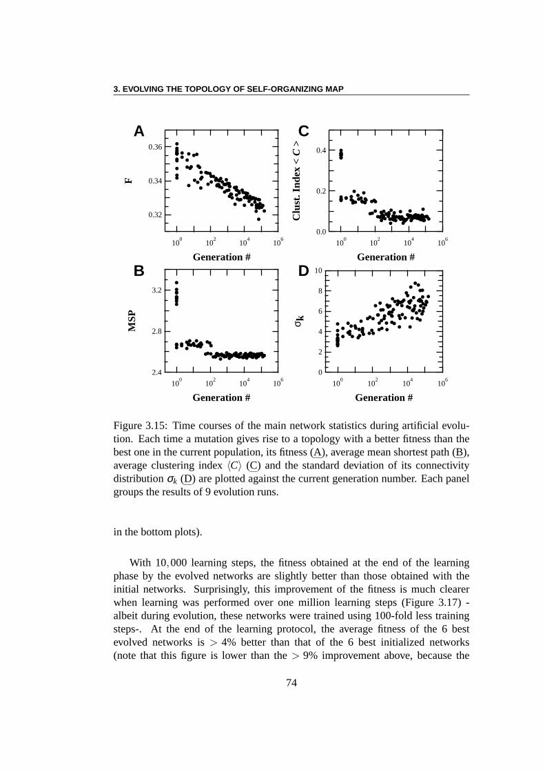
3. EVOLVING THE TOPOLOGY OF SELF-ORGANIZING MAP
0.36
0.34
0.32
F
100 10
2 104 10
6
Generation #
0.4
0.2
0.0
Clu
st. I
ndex
< C
>
100 10
2 104 10
6
Generation #
3.2
2.8
2.4
MS
P
100 10
2 104 10
6
Generation #
10
8
6
4
2
0
σ k
100 10
2 104 10
6
Generation #
A
B D
C
Figure 3.15: Time courses of the main network statistics during artificial evolu-tion. Each time a mutation gives rise to a topology with a better fitness than thebest one in the current population, its fitness (A), average mean shortest path (B),average clustering index〈C〉 (C) and the standard deviation of its connectivitydistributionσk (D) are plotted against the current generation number. Each panelgroups the results of 9 evolution runs.
in the bottom plots).
With 10,000 learning steps, the fitness obtained at the end of the learningphase by the evolved networks are slightly better than thoseobtained with theinitial networks. Surprisingly, this improvement of the fitness is much clearerwhen learning was performed over one million learning steps(Figure 3.17) -albeit during evolution, these networks were trained using100-fold less trainingsteps-. At the end of the learning protocol, the average fitness of the 6 bestevolved networks is> 4% better than that of the 6 best initialized networks(note that this figure is lower than the> 9% improvement above, because the
74
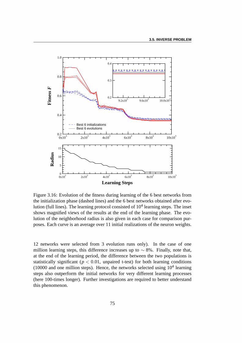
3.5. INVERSE PROBLEM
1.0
0.8
0.6
0.4
0.2
Fitn
ess F
10x103
8x10³
6x10³
4x10³
2x10³
0x103
Best 6 initializations Best 6 evolutions
0.4
0.3
0.210.0x10
39.6x10
39.2x10
3
15
10
5
0
Rad
ius
10x103
8x10³
6x10³
4x10³
2x10³
0x103
Learning Steps
Figure 3.16: Evolution of the fitness during learning of the 6best networks fromthe initialization phase (dashed lines) and the 6 best networks obtained after evo-lution (full lines). The learning protocol consisted of 104 learning steps. The insetshows magnified views of the results at the end of the learningphase. The evo-lution of the neighborhood radius is also given in each case for comparison pur-poses. Each curve is an average over 11 initial realizationsof the neuron weights.
12 networks were selected from 3 evolution runs only). In thecase of onemillion learning steps, this difference increases up to∼ 8%. Finally, note that,at the end of the learning period, the difference between thetwo populations isstatistically significant (p < 0.01, unpaired t-test) for both learning conditions(10000 and one million steps). Hence, the networks selectedusing 104 learningsteps also outperform the initial networks for very different learning processes(here 100-times longer). Further investigations are required to better understandthis phenomenon.
75
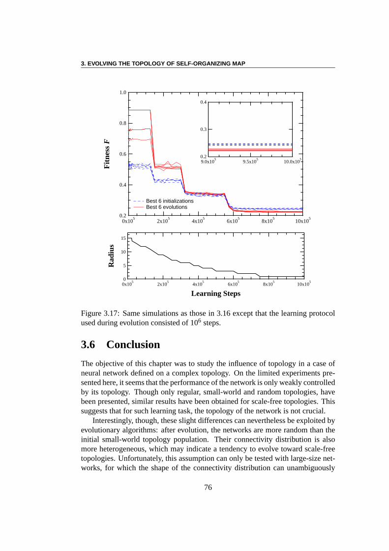
3. EVOLVING THE TOPOLOGY OF SELF-ORGANIZING MAP
1.0
0.8
0.6
0.4
0.2
Fitn
ess F
10x105
8x10⁵
6x10⁵
4x10⁵
2x10⁵
0x105
Best 6 initializations Best 6 evolutions
0.4
0.3
0.210.0x10
59.5x10
59.0x10
5
15
10
5
0
Rad
ius
10x105
8x10⁵
6x10⁵
4x10⁵
2x10⁵
0x105
Learning Steps
Figure 3.17: Same simulations as those in 3.16 except that the learning protocolused during evolution consisted of 106 steps.
3.6 Conclusion
The objective of this chapter was to study the influence of topology in a case ofneural network defined on a complex topology. On the limited experiments pre-sented here, it seems that the performance of the network is only weakly controlledby its topology. Though only regular, small-world and random topologies, havebeen presented, similar results have been obtained for scale-free topologies. Thissuggests that for such learning task, the topology of the network is not crucial.
Interestingly, though, these slight differences can nevertheless be exploited byevolutionary algorithms: after evolution, the networks are more random than theinitial small-world topology population. Their connectivity distribution is alsomore heterogeneous, which may indicate a tendency to evolvetoward scale-freetopologies. Unfortunately, this assumption can only be tested with large-size net-works, for which the shape of the connectivity distributioncan unambiguously
76

3.6. CONCLUSION
be determined, but whose artificial evolution, for computation cost reasons, couldnot be carried out.
77

3. EVOLVING THE TOPOLOGY OF SELF-ORGANIZING MAP
78
Chapter 4
Evolutionary Optimization of EchoState Networks
A possible alternative to fine topology tuning for Neural Network (NN) opti-mization is to use Echo State Networks (ESNs), recurrent NNsbuilt upon a largereservoir of sparsely randomly connected neurons. The promises of ESNs havebeen fulfilled for supervised learning tasks. But reinforcement learning tasks,such as control problems, require more flexible optimization methods – such asEvolutionary Algorithms.
This chapter proposes to apply CMA-ES, the state-of-the-artmethod inevolutionary continuous parameter optimization, to the evolutionary learning ofsome ESN parameters (see Section 2.2.3). First, a standard supervised learningproblem is used to validate the approach and compare it to thestandard quadraticapproach. Further, thanks their flexibility, evolutionaryoptimization allow oneto optimize not only the standard outgoing weights, but also, or alternatively,some other internal parameters of the ESN, sometimes leading to improvedresults, as will be demonstrated here. The classical doublepole balancing controlproblem (Section 4.4.1) is then used to demonstrate the feasibility of evolutionaryreinforcement ESN learning. Note that special care must be taken when usingCMA-ES for this specific problem, in order to lead the evolutionary ESN to-ward results that are comparable with those of the best topology-learning methods.
4.1 Introduction
It has long been known to Neural Networks practitioners thata good design of thetopology of the network was an essential ingredient to a successful application
79
4. EVOLUTIONARY OPTIMIZATION OF ECHO STATE NETWORKS
of Neural Networks, for a given learning task. In the framework of supervisedlearning, the famous US Postal application [129, 31] demonstrated the need tocarefully craft the topology for the problem at hand (see also Section 2.3.2). Onthe theoretical side, the recent studies ondeeprepresentations, as developed in[22] for instance, proved that indeed, some types of topologies (e.g. shallowone-layer perceptrons) require an exponential number of hidden units w.r.t. theinput dimension, in order to be able to achieve a given learning task, while deeptopologies might require as few as a linear number of layers for the same task.The critical issue then becomes that of learning the appropriate weights, andspecific methods have to be used, as the standard backpropagation algorithmbecomes inefficient [23].
Echo State Networks [105], that was recently proposed for supervised learn-ing of time series, can be seen as an alternative approach: instead of optimizing atopology for a given task, it proposes to use a largereservoir of neurons that arerandomly (and sparsely) connected. Only the weights of the outgoing connectionsare to be learned, transforming the learning process into a simple a quadraticoptimization problem that is easily solved by any gradient-based method . . . atleast in the supervised learning case.
The situation changes dramatically when addressing reinforcement learningtasks, such as control tasks: no example of input-output of the network areavailable, and hence the learning problem can no longer be set as a quadraticproblem. Even some tricks like BackPropagation Through Time[223] don’tdirectly apply to recurrent neural network learning.
Evolutionary Computation provides a possible solution for such situations, aslong as some fitness for the sought controller is available
This chapter addresses the following issues: are Evolutionary Algorithms(EAs) a viable method to train Echo State Networks in general, and for rein-forcement learning tasks in particular – and how does it compare to the quadraticlearning in the supervised context? Furthermore, are Echo State Networks analternative to topology learning in the framework of ControlProblem? Finally,as the flexibility of Evolutionary Algorithms allows them tolearn to adjust morethan just the weights of the outgoing connections of the ESN,does this improvethe leaning power of ESNs?
This chapter will start by introducing in Section 4.2 the Echo State Networksand the standard supervised learning of their outgoing weights. To address thefirst research issue listed above, the same experimental setting as the originalsupervised learning of time series proposed in Jaeger’s seminal paper [105] will
80
4.2. RESERVOIR COMPUTING MODEL
be used in Section 4.3, and different reservoir sizes will beexperimented with.But because EAs don’t require gradient information, using anEA in lieu ofa gradient method will offer more flexibility for ESN learning, allowing us tooptimize more than just the outgoing weights of the network,also optimizingthe spectral radius of the ESN, or the slope of the sigmoid at the origin for eachneuron.
Moreover, Evolutionary Learning opens up the field of reinforcement learningto ESNs, that is optimizing the characteristics of the network when no directinput-output examples are available, but only some possibly delayed reward, as isthe case in control problems.
In the reinforcement context, many works advocating different methods toevolve a complete neural network (i.e. both topology and weights) have dealtwith the double pole balancing problem, as presented in Section 4.4.1, providinga basis for comparison without the burden of re-doing all experiments. The samecontrol problem will be used in Section 4.4, the results of ESN evolutionary learn-ing will be compared to those of the literature. Moreover, asin the supervisedcase, experiments will involve the optimization of different parameters of theESN. Section 4.5 will further discuss the results in line with the developmentaland generative approaches it was compared to. Finally, Section 4.6 will sum upthe chapter and sketch directions for on-going and further researches.
4.2 Reservoir Computing Model
The paradigm underlying what is today known as Reservoir Computing (RC)made Recurrent NNs accessible for practical applications asnever before,and outperformed classical fully trained RNNs in many tasks [138]. EchoState Networks (ESN) have been proposed by Jaeger in 2001 [105] with theobjective of endowing a neural network with rich dynamics behavioral patternswhile keeping learning complexity at a low level. An ESN is a discrete time,continuous state, recurrent neural network using a sigmoidal activation functionfor all neurons. A typical ESN is shown in figure 4.1: the inputlayer is totallyconnected to the hidden layer; the hidden layer, and possibly the input layer,are totally connected to the output layer. Moreover, thoughconsidered notessential, the output layer can be connected backward to thehidden layer. Inthis setup, the hidden layer, orreservoir, is randomly generated:N neurons arerandomly connected up to a user-defined density of connectionsδ . The weightsof those connections are randomly set uniformly in[−1,1], and are scaled so
81
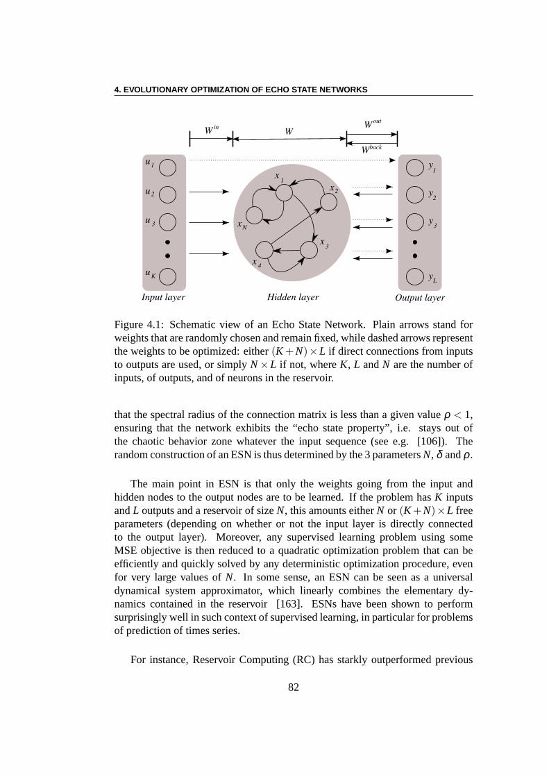
4. EVOLUTIONARY OPTIMIZATION OF ECHO STATE NETWORKS
Figure 4.1: Schematic view of an Echo State Network. Plain arrows stand forweights that are randomly chosen and remain fixed, while dashed arrows representthe weights to be optimized: either(K +N)×L if direct connections from inputsto outputs are used, or simplyN×L if not, whereK, L andN are the number ofinputs, of outputs, and of neurons in the reservoir.
that the spectral radius of the connection matrix is less than a given valueρ < 1,ensuring that the network exhibits the “echo state property”, i.e. stays out ofthe chaotic behavior zone whatever the input sequence (see e.g. [106]). Therandom construction of an ESN is thus determined by the 3 parametersN, δ andρ.
The main point in ESN is that only the weights going from the input andhidden nodes to the output nodes are to be learned. If the problem hasK inputsandL outputs and a reservoir of sizeN, this amounts eitherN or (K +N)×L freeparameters (depending on whether or not the input layer is directly connectedto the output layer). Moreover, any supervised learning problem using someMSE objective is then reduced to a quadratic optimization problem that can beefficiently and quickly solved by any deterministic optimization procedure, evenfor very large values ofN. In some sense, an ESN can be seen as a universaldynamical system approximator, which linearly combines the elementary dy-namics contained in the reservoir [163]. ESNs have been shown to performsurprisingly well in such context of supervised learning, in particular for problemsof prediction of times series.
For instance, Reservoir Computing (RC) has starkly outperformed previous
82
4.2. RESERVOIR COMPUTING MODEL
methods of nonlinear system identification, prediction andclassification, in pre-dicting chaotic dynamics (three orders of magnitude improved accuracy [108]),nonlinear wireless channel equalization (two orders of magnitude improvement[108]), the Japanese Vowel benchmark (zero test error rate,previous best: 1.8%[109]), financial forecasting (winner of the internationalforecasting competitionNN31), and in isolated spoken digits recognition (improvement of word error rateon benchmark from 0.6% for the previous best system to 0.2% [215]).
We will first introduce the state of arts work of ESN in supervised learningarea.
4.2.1 A Chaotic Time Series Prediction by ESN
The first great success of ESN has been done with the Mackey-Glass system, apopular chaotic dynamic system that is defined by a single nonlinear time delayordinary differential equation :
dydt
= αyτ
1+yτ β − γy, γ,α,β > 0,
whereα,γ,τ,β are real numbers, andyτ represents the value of the variabley attime (t − τ). Depending on the values of the parameters, this equation displaysa range of periodic and chaotic dynamics. In the chaotic systems modelingcommunity the parameters are often set toα = 0.2,γ = 0.1,β = 10. Whenτ > 16.8, the system is a chaotic attractor. Depending on the value of τ, thesystem varies form a mildly chaotic attractor (τ = 17, used normally) to a morechaotic behavior (τ = 30). Figure 4.2 shows 600 consecutive time steps obtainedwith τ = 17 andτ = 30
The task here is to create a system which can reproduce the given chaoticattractor as precisely as possible in a predefined number of iterations.
ESNs show excellent results in Jaeger’s first technique report [105] with 400units and state of art results with 1,000 units were also presented [108].
4.2.2 Researches on RC
Since the first report of Jaeger in 2001, Reservoir Computing (RC)attracted a lotof research interest. RC methods have indeed been successfulwhen applied toseveral benchmarks, often outperforming classical fully trained RNNs. And aswith all RC methods these good results were obtained with purely random (i.e.
1http://www.neural-forecasting-competition.com/NN3/index.htm
83
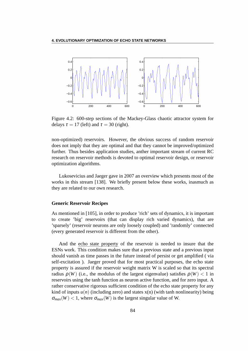
4. EVOLUTIONARY OPTIMIZATION OF ECHO STATE NETWORKS
0 200 400 600
−0.6
−0.4
−0.2
0
0.2
0.4
0 200 400 600
−0.6
−0.4
−0.2
0
0.2
0.4
Figure 4.2: 600-step sections of the Mackey-Glass chaotic attractor system fordelaysτ = 17 (left) andτ = 30 (right).
non-optimized) reservoirs. However, the obvious success of random reservoirdoes not imply that they are optimal and that they cannot be improved/optimizedfurther. Thus besides application studies, anther important stream of current RCresearch on reservoir methods is devoted to optimal reservoir design, or reservoiroptimization algorithms.
Lukosevicius and Jaeger gave in 2007 an overview which presents most of theworks in this stream [138]. We briefly present below these works, inasmuch asthey are related to our own research.
Generic Reservoir Recipes
As mentioned in [105], in order to produce ’rich’ sets of dynamics, it is importantto create ’big’ reservoirs (that can display rich varied dynamics), that are’sparsely’ (reservoir neurons are only loosely coupled) and ’randomly’ connected(every generated reservoir is different from the other).
And the echo stateproperty of the reservoir is needed to insure that theESNs work. This condition makes sure that a previous state and a previous inputshould vanish as time passes in the future instead of persistor get amplified ( viaself-excitation ). Jaeger proved that for most practical purposes, the echo stateproperty is assured if the reservoir weight matrix W is scaled so that its spectralradiusρ(W) (i.e., the modulus of the largest eigenvalue) satisfiesρ(W) < 1 inreservoirs using the tanh function as neuron active function, and for zero input. Arather conservative rigorous sufficient condition of the echo state property for anykind of inputsu(n) (including zero) and states x(n) (with tanh nonlinearity) beingσmax(W) < 1, whereσmax(W) is the largest singular value of W.
84

4.2. RESERVOIR COMPUTING MODEL
But this condition only ensures that the ESNs will not self-excite. The optimalvalue ofρ(W) should be set depending on the amount of memory and nonlinearitythat the given task requires, and varies with the task. Jaeger gives a rule statingthatρ(W) should be close to 1 for tasks that require long memory and accordinglysmaller for the tasks where a too long memory might in fact be harmful [105].
Small-world, scale-free and biologically-inspired connection topologies weretested and compared with sparsely randomly connected ones,but no significantdifferences were presented among there different topologies using the measureand the experiment methods of the article [134].
For a conventional ESNs, one of the shortcoming is that the activations arestill coupled strongly even though the reservoirs are sparse. That makes ESNspoor performers when dealing with different time scales simultaneously. In [229],the reservoir was divided into partially decoupled sub-reservoirs, introducinginhibitory connections among all the sub-reservoirs. Thissystem was shown tosuccessfully resolve the multi-time scale problem at hand.Note moreover thatother related works combine outputs from several separate reservoirs and will bediscussed in the following section.
In conventional ESN, the activation function of the neuronsis usually a Sig-moidal function, but others types of functions were also used for different pro-poses. For example, in Evolino [187] a Long Short-Term Memory type of RNNSwere used to preserve memory for long periods of time. Jaeger[105] also sug-gested a version of a leaky integrator ESNs (LI-ESNs) which uses a leaky inte-grator active function. This version is in fact a discretized version of a continuousdifferential equation for a leaky integrator neuron that reads :
x(n) = (1−α∆t)x(n−1)+∆t f (Winu(n)+Wx(n−1))
Whenα = 1 and∆t = 1, one recovers the classical (non leaky) simple ESN.The parametersα and∆t control the ’speed’ of the reservoir dynamics. Smallvalues ofα and∆t result in reservoirs that react slowly to the input. By changingthese parameters it is possible to shift the effective interval of frequencies inwhich the reservoir is working.
Readouts from the reservoirs
In conventional ESN, the readout always has a single layer. The optimization is alinear mapping form the reservoirs statesx(n) to target outputytarget(n) and thereexists for this aim many linear regression algorithms that are very fast, even for
85
4. EVOLUTIONARY OPTIMIZATION OF ECHO STATE NETWORKS
a very large number of time stepsn to forecast, as the objective is simply here tominimize the quadratic error between theWoutx(n) and theytarget(n).
Recently, however, some multilayer perceptrons (MLPs), trained by errorbackpropagation, are beginning to be used as readouts. Theoretically they aremore powerful than a singer layer, but in practice, trainingby error backpropaga-tion is much more difficult than linear regression with a single layer.
Another approach that has been proposed consists in combining severalreadouts by averaging the outputs coming from several instances of ESNs (e.g.,to refine the prediction of chaotic time series [108]). Thereis also an ESN-basedpredictive classifier [200] which is reported to be much morerobust to noise thana standard Hidden Markov Model for the task of spoken word recognition, byusing a set of competitively trained predictors for each class of the training set,and then applying dynamic programming to find the optimal sequence of the aopoutput of these predictors.
Finally, though the reservoirs may have thousands of units,they usually havea single layer. It was suggested that for complex demanding tasks the adaptationof a single reservoir might not be enough and a hierarchical architecture of ESNsmight be needed. Jaeger himself [107] proposed a first approach to this problem,but this research is still in its infancy.
4.2.3 Discussion
In our opinion, at least three aspects need further investigation in the context orReservoir Computing in general, and ESN in particular.
Gradient Descent or Evolutionary Computing
As discussed in previous section, gradient decent algorithms have been usedto optimize the readout layer in the supervised learning field. The idea ofEvolutionary Learning for Echo State Networks amounts to replacing the gradientdescent that is used to optimize the outgoing weights in Jaeger’s approachby an Evolutionary Algorithm (EA). This makes it possible toapply ESN inReinforcement Learning field. A first mandatory step in that direction is tovalidate this approach on a supervised learning task, comparing the results withthose of the standard gradient method. This will be done in Section 4.3. Then areinforcement learning task will be experimented with in Section 4.4
86
4.3. SUPERVISED LEARNING OF ESN
The Evolutionary Algorithm that has been chosen for the optimization here isthe Covariance Matrix Adaptation Evolution Strategy, aka CMA-ES [87, 88, 85],which has been introduced in detail in 2.2.3. As already discussed, the onlyparameter of CMA-ES that needs to be set by the user is the number of offspringλ , depending on the possible ruggedness of the fitness landscape at hand. Thedefault value, as set in [88], increases logarithmically with the dimensiondof the problem (number of unknown parameters), asλ = 4+ 3ln(d). In thesupervised case of Section 4.3, involving problems of dimensions 30, 60 and 100,the corresponding values ofλ are respectively 12, 15, and 17.
Auto Parameters Turning
In many ESN applications, the ESN parameters were chosen or fine tuned by hand(most often through trial-and-error) and have fixed values.Jaeger [105] states thatρ(W) should be close to 1 for tasks that require long memory and accordinglysmaller for the tasks where a too long memory might in fact be harmful. But theoptimalρ(W) is still unknown. One side effect of the Evolutionary Optimizationof ESN weights is that we will also here use EC to determine theoptimalρ(W).
Transfer Function
In conventional ESNs, the transfer function of all neurons is usually a Sigmoidfunction (or, equivalently, the tanhfunction) with fixed slope. But because we areusing EC, and do not need any more we are also able to optimize the slopes ofevery neuron. And this gives another point of entry into ESN optimization. So inour study, we will also test this aspect on a supervised learning problem and on areinforcement learning case study.
4.3 Supervised Learning of ESN
In order to validate the Evolutionary approach to ESN learning, a first experimentreproduces one of Jaeger’s initial setting [105], but usingan EvolutionaryAlgorithm in lieu of some gradient-based quadratic optimization procedure. Theproblem is that of a time series prediction.
4.3.1 Jaeger’s Original Settings
In this toy example, a single-channel sinusoidal input is given byu(n) = sin(n/5).The target is to train the network to produce a single-channel output,
87
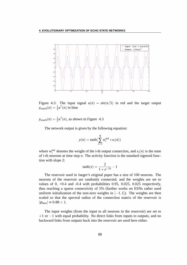
4. EVOLUTIONARY OPTIMIZATION OF ECHO STATE NETWORKS
0 50 100 150 200 250 300−1
−0.8
−0.6
−0.4
−0.2
0
0.2
0.4
0.6
0.8
1
n
Input: u(n) = sin(n/5)
Output: 1/2u(n)7
Figure 4.3: The input signalu(n) = sin(n/5) in red and the target outputyteach(n) = 1
2u7(n) in blue
yteach(n) = 12u7(n), as shown in Figure 4.3
The network output is given by the following equation:
y(n) = tanh(N
∑i=1
wouti ∗xi(n))
wherewouti denotes the weight of the i-th output connection, andxi(n) is the state
of i-th neurone at time stepn. The activity function is the standard sigmoid func-tion with slope 2:
tanh(x) =2
1+e−2x −1
The reservoir used in Jaeger’s original paper has a size of 100 neurons. Theneurons of the reservoir are randomly connected, and the weights are set tovalues of 0, +0.4 and -0.4 with probabilities 0.95, 0.025, 0.025 respectively,thus reaching a sparse connectivity of 5% (further works on ESNs rather useduniform initialization of the non-zero weights in[−1,1]). The weights are thenscaled so that the spectral radius of the connection matrix of the reservoir is|ρmax| ≈ 0.88< 1.
The input weights (from the input to all neurons in the reservoir) are set to+1 or−1 with equal probability. No direct links from inputs to outputs, and nobackward links from outputs back into the reservoir are usedhere either.
88
4.3. SUPERVISED LEARNING OF ESN
As in Jaeger’s work, the fitness to be minimized is the Mean Square Errorof the network. The bootstrapping is done the following way:the states of allneurons in the reservoir is initialized to zero; the networkis then run for 100 timesteps without measuring the error; finally, the MSE is computed on the next 200time steps as
MSEtrain =1
200
300
∑n=101
(y(n)−arctanh(yteach(n)))2
4.3.2 Which parameters to optimize?
In Jaeger’s original paper, only the output weights were optimized, leadingto a quadratic optimization problem of dimensionN, the size of the reser-voir. The optimization was done using a gradient method (more precisely,the Fit function from Mathematica©). The reported result is a training errormsetrain ≈ 3.3∗ 10−15. When the trained network was tested on test data, thereported test error ismsetest ≈ 3.7∗10−15.
However, as already mentioned, whereas gradient method canonly solvereliably convex problems, CMA-ES can reliably find good global quasi-optima ofnon-convex problems, leading to different other option to choose which parame-ters to optimize, as already demonstrated beneficial in the case of feed-forward orsmall recurrent NNs [189, 54].
The Spectral Radius
In particular, a critical parameter in ESN tuning seems to bethe maximal valueallowed for the spectral radius. To ensure “echo state” property, this radius mustbe smaller than 1, but different values have been proposed inthe literature fordifferent problems. Hence it seems a good idea to use the spectral radius asa free parameter, to be optimized by CMA-ES: it only adds one dimension tothe problem. The procedure goes as follows: when a set of parameters is to beevaluated, the weights of the recurrent connection inside the reservoir are firstscaled so that the spectral radius of the connection matrix takes the value of theadditional optimized parameter, the same way it was done during the initializationof the reservoir itself. Then the response of the ESN is computed as usual, usingthe scaled weights.
89
4. EVOLUTIONARY OPTIMIZATION OF ECHO STATE NETWORKS
The Sigmoid Slopes
Because an Echo State Network is a set of dynamical systems that are linearlycombined to generate the desired output, it seems plausiblethat modifying theslopes of all neurons independently might allow the ESN to better fit the target.
The transfer function of in internal neuron becomes tanha(x) =2
1+e−ax − 1.
Jaeger’s original sigmoidal function was tanh, corresponding to the casea = 2.
However, if both the output weights and the sigmoid slopes are optimized, thedimension of the optimization problem is doubled. Hence, a first experiment wasto optimize the slopes alone (and the problem still has as dimension the numberof neurons in the reservoir), before running the complete experiment, optimizingboth the slopes and the output weights.
4.3.3 The experiments
Four variants of evolutionary optimization of an ESN have been compared:the standard optimization of the output weights, denotedStd in the following,which hasN unknown parameters,N being the reservoir size; the optimizationof the output weights plus the spectral radius, denotedRho, of dimensionN +1;the optimization of the sigmoidal slopes denotedSlopes, of dimensionN; andthe optimization of both the output weights and the slopes, denotedFull, ofdimension 2∗N.
Two reservoir sizes have also been chosen:N = 100 as in Jaeger’s originalpaper, that then provides a basis for comparison, andN = 30, that allows moresystematic comparison, in particular regarding theFull variant, as no meaningfulbetter results could be obtained using that variant in the caseN = 100.
However, because of the small reservoir size, the average connectivity wasincreased, to ensure that each neuron has the same average number of connectionsthan in theN = 100 case, leading to setting the weights to values of 0, +0.4and -0.4 with probabilities 0.864, 0.068, 0.068 respectively. The same maximalspectral radius of|ρmax| ≈ 0.88< 1 was used for both reservoir sizes (except fortheRho variants of course).
90
4.3. SUPERVISED LEARNING OF ESN
4.3.4 Comparative Measures
One surprising issue in Jaeger’s original paper is that there is no statisticalanalysis whatsoever: indeed, even if the optimization problem is quadratic, andhas a unique global solution that the gradient method will reliably find, thenetwork itself is randomly built, and different networks might have differentoptimal value for the MSE fitness.
In any case, because CMA-ES, like all EAs, is a stochastic optimizationprocedure, no strong conclusion can be drawn without doing athorough statisticalanalysis of the performances. Hence 15 different networks have been used, andfor each network, 5 runs of CMA-ES were launched with different random seeds(and hence starting points).
A first global performance measure is given by the now standard SP1 measure,an estimator for the success performance used in [85] and analyzed in [8]: it isdefined as the number of evaluations needed to reach a given fitness level, dividedby the proportion of runs that did reach that fitness value, and hence can beviewed as the computational effort that is required to reacha given performancelevel.
Moreover, the variability over the reservoir topology willalso be assessed, bystudying in detail the different results obtained by the 5 runs for each of the 15networks.
4.3.5 Results
Figures 4.4 and 4.5 show the SP1 plots for reservoirs of 100 and 30 neurons,respectively, and all evolution variants, except theFull method that could notbe applied for the reservoir size of 100. The first result, fora reservoir size of100, simply confirms that CMA-ES can be as precise as the gradient methodreported in [105], though undoubtedly requiring a much greater computationaleffort: indeed, a factor of 7 to 10 in the computational cost between CMA-ESand BFGS was reported in [88] for quadratic functions ... whenusing numericalderivation – whereas the analytical gradient is available here. In a few cases,though, CMA-ES was able to find better solution than our local gradient-basedmethod, that was stopped by precision thresholds.
However, the two other plots on Figure 4.4 are rather disappointing, asincreasing the search space didn’t allow to improve the precisions: neither the
91
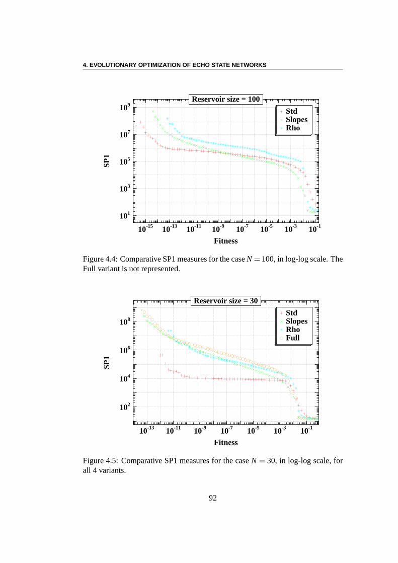
4. EVOLUTIONARY OPTIMIZATION OF ECHO STATE NETWORKS
Fitness
SP
1
-1510 -1310 -1110 -910 -710 -510 -310 -110
110
310
510
710
910 Std SlopesRho
Reservoir size = 100
Figure 4.4: Comparative SP1 measures for the caseN = 100, in log-log scale. TheFull variant is not represented.
Fitness
SP
1
-1310 -1110 -910 -710 -510 -310 -110
210
410
610
810Std SlopesRho Full
Reservoir size = 30
Figure 4.5: Comparative SP1 measures for the caseN = 30, in log-log scale, forall 4 variants.
92
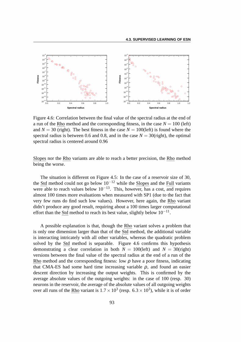
4.3. SUPERVISED LEARNING OF ESN
10-14
10-13
10-12
10-11
10-10
10-9
10-8
10-7
10-6
10-5
10-4
10-3
Fit
nes
s
1.00.80.60.40.20.0
Spectral radius
10-12
10-11
10-10
10-9
10-8
10-7
10-6
10-5
10-4
10-3
10-2
Fit
nes
s
1.21.00.80.60.40.20.0
Spectral radius
Figure 4.6: Correlation between the final value of the spectral radius at the end ofa run of theRho method and the corresponding fitness, in the caseN = 100 (left)andN = 30 (right). The best fitness in the caseN = 100(left) is found where thespectral radius is between 0.6 and 0.8, and in the caseN = 30(right), the optimalspectral radius is centered around 0.96
Slopes nor theRho variants are able to reach a better precision, theRho methodbeing the worse.
The situation is different on Figure 4.5: In the case of a reservoir size of 30,theStd method could not go below 10−12 while theSlopes and theFull variantswere able to reach values below 10−13. This, however, has a cost, and requiresalmost 100 times more evaluations when measured with SP1 (due to the fact thatvery few runs do find such low values). However, here again, the Rho variantdidn’t produce any good result, requiring about a 100 times larger computationaleffort than theStd method to reach its best value, slightly below 10−11.
A possible explanation is that, though theRho variant solves a problem thatis only one dimension larger than that of theStd method, the additional variableis interacting intricately with all other variables, whereas the quadratic problemsolved by theStd method is separable. Figure 4.6 confirms this hypothesisdemonstrating a clear correlation in bothN = 100(left) and N = 30(right)versions between the final value of the spectral radius at theend of a run of theRho method and the corresponding fitness: lowρ have a poor fitness, indicatingthat CMA-ES had some hard time increasing variableρ, and found an easierdescent direction by increasing the output weights. This isconfirmed by theaverage absolute values of the outgoing weights: in the caseof 100 (resp. 30)neurons in the reservoir, the average of the absolute valuesof all outgoing weightsover all runs of theRho variant is 1.7×10³ (resp. 6.3×10³), while it is of order
93
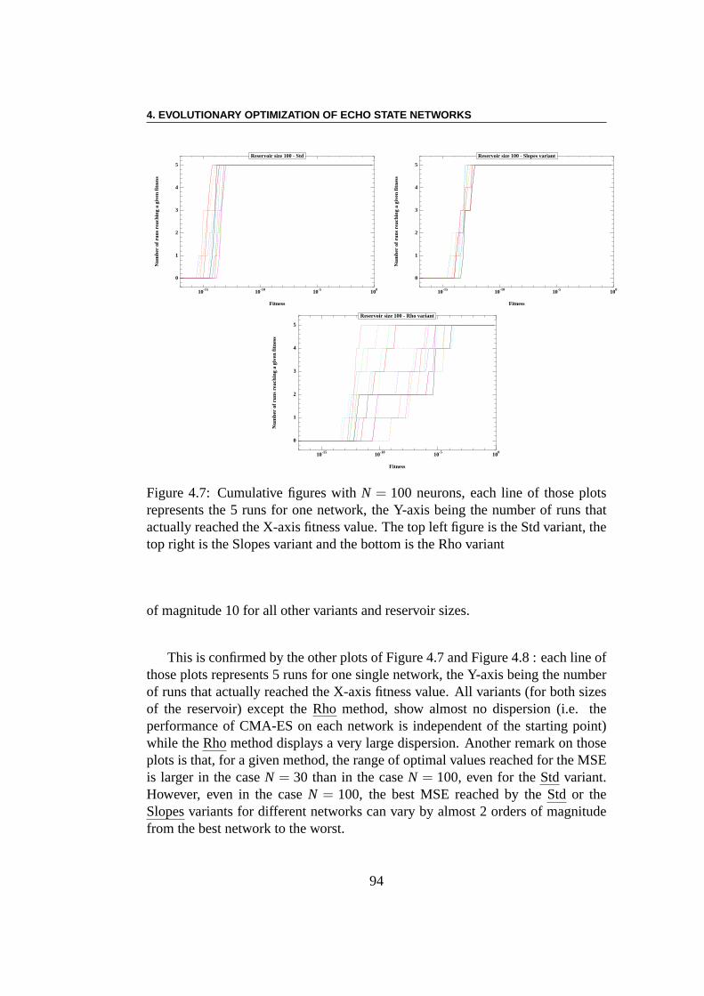
4. EVOLUTIONARY OPTIMIZATION OF ECHO STATE NETWORKS
Fitness
Num
ber
of r
uns
reac
hing
a g
iven
fitn
ess
-1510 -1010 -510 010
0
1
2
3
4
5
Reservoir size 100 - Std
Fitness
Num
ber
of r
uns
reac
hing
a g
iven
fitn
ess
-1510 -1010 -510 010
0
1
2
3
4
5
Reservoir size 100 - Slopes variant
Fitness
Num
ber
of r
uns
reac
hing
a g
iven
fitn
ess
-1510 -1010 -510 010
0
1
2
3
4
5
Reservoir size 100 - Rho variant
Figure 4.7: Cumulative figures withN = 100 neurons, each line of those plotsrepresents the 5 runs for one network, the Y-axis being the number of runs thatactually reached the X-axis fitness value. The top left figureis the Std variant, thetop right is the Slopes variant and the bottom is the Rho variant
of magnitude 10 for all other variants and reservoir sizes.
This is confirmed by the other plots of Figure 4.7 and Figure 4.8 : each line ofthose plots represents 5 runs for one single network, the Y-axis being the numberof runs that actually reached the X-axis fitness value. All variants (for both sizesof the reservoir) except theRho method, show almost no dispersion (i.e. theperformance of CMA-ES on each network is independent of the starting point)while theRho method displays a very large dispersion. Another remark on thoseplots is that, for a given method, the range of optimal valuesreached for the MSEis larger in the caseN = 30 than in the caseN = 100, even for theStd variant.However, even in the caseN = 100, the best MSE reached by theStd or theSlopes variants for different networks can vary by almost 2 orders of magnitudefrom the best network to the worst.
94
4.4. REINFORCEMENT LEARNING OF ESN
4.3.6 Discussion
The result show that:, for such a simple time series problem,the size of ESNis a crucial parameter for getting a better learning precision. When the size ofESN is large enough (as withN = 100), the dynamical states within the ESN arealready rich enough for solving the problem, and theStd version can obtain thebest results. But whenN is small (e.g.,N = 30), it is more important to create richdynamic states by varying the spectral radius (Rho variant) or the slopes (Slopesvariant). A largeN may be not a problem for such supervised time series problem,but as will be detailed in next section, it will be in the case of reinforcementlearning, when the simulation is very costly.
Another conclusion for this section is the interesting correlation between thefinal Rho value and the fitness. We also need to mention that in the caseN = 100,theρ used byStd version is taken from Jaeger’s suggestion, and in that point it isalready an optimized value. For choosing an optimalρ for a specific task, Jaegermade a generic suggestion: if we need short memory in a dynamic environment,theρ should be small, and vice versa. The optimalρ is often chosen by trial anderror. In our experiments, the optimalρ in Rho version forN = 100 is very closedto theρ value which is chosen by Jaeger. This suggests that EAs are a possiblemethod for choosing the optimalρ for a given task.
4.4 Reinforcement Learning of ESN
4.4.1 The Pole-balancing Benchmark
This Section introduces the Pole-balancing problem and briefly recalls compara-tive results that have been obtained by different Neuro-Evolution techniques in therecent years, for getting a more detailed comparison between the Neuro-Evolutiontechniques surveyed in section 2.3.2, and also for preparing the experiments onevolving ESN for reinforcement learning.
The pole-balancing problem (aka inverted pendulum) is a classical controltask that has been used as a benchmark for reinforcement learning for more than40 years [183, 2, 225, 78, 71, 204, 101, 45, 70, 117]. In the early research, therewas only one pole connected. The car position (x), car speed ( ˙x), the joint angle(θ1) and the joint angle speed (θ1) are normalized and become the inputs of thecontrollers. However, at the end of last century, this problem finally proved to berather easy to solve. So in order to increase the difficulty, the speed informationof car and pole were removed from the inputs. This did not add much to thedifficulty, and people thus turned to the double pole problem, adding a secondpole with different length to the system. In this case the twopoles have to be
95
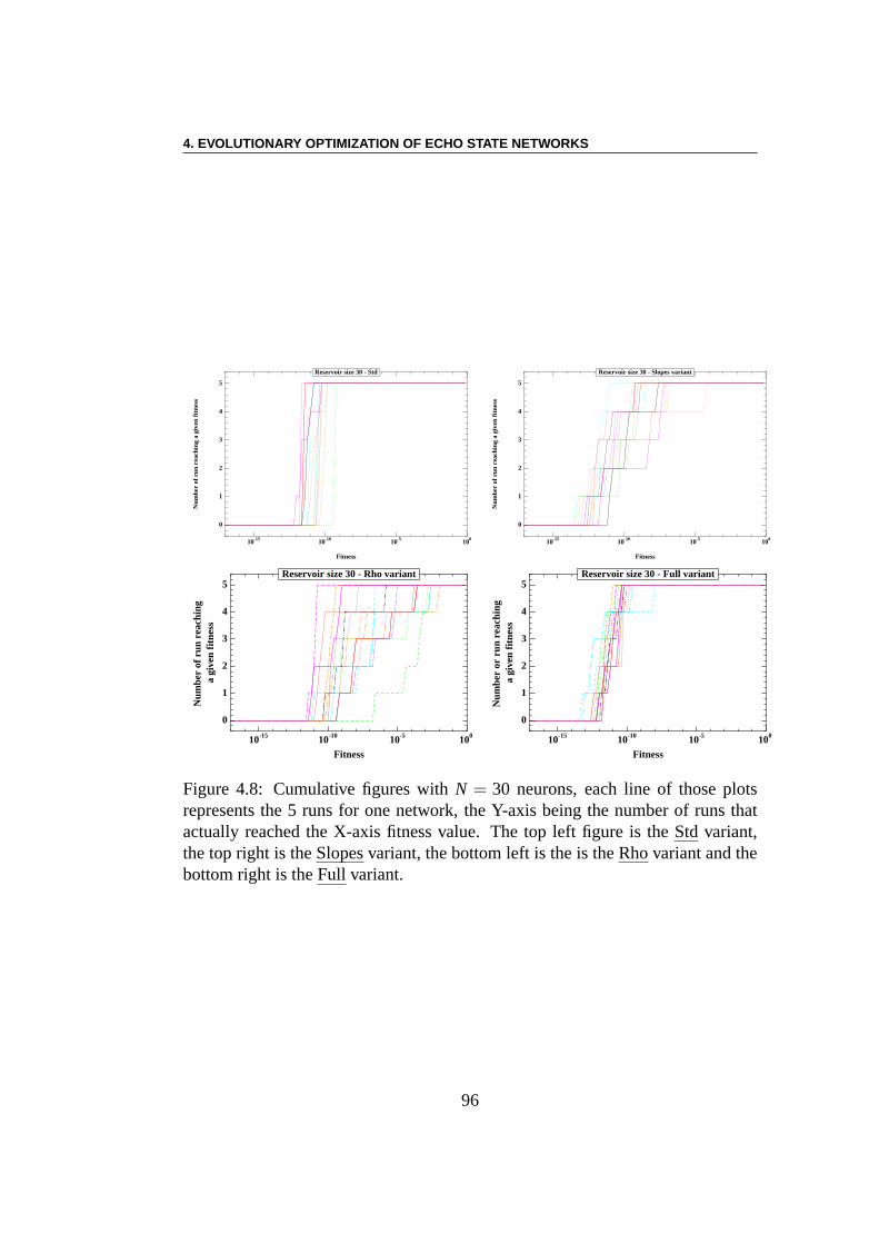
4. EVOLUTIONARY OPTIMIZATION OF ECHO STATE NETWORKS
Fitness
Num
ber
of r
un r
each
ing
a gi
ven
fitne
ss
-1510 -1010 -510 010
0
1
2
3
4
5
Reservoir size 30 - Std
Fitness
Num
ber
of r
un r
each
ing
a gi
ven
fitne
ss
-1510 -1010 -510 010
0
1
2
3
4
5
Reservoir size 30 - Slopes variant
Fitness
Num
ber
of r
un r
each
ing
a gi
ven
fitne
ss
-1510 -1010 -510 010
0
1
2
3
4
5Reservoir size 30 - Rho variant
Fitness
Num
ber
or r
un r
each
ing
a gi
ven
fitne
ss
-1510 -1010 -510 010
0
1
2
3
4
5Reservoir size 30 - Full variant
Figure 4.8: Cumulative figures withN = 30 neurons, each line of those plotsrepresents the 5 runs for one network, the Y-axis being the number of runs thatactually reached the X-axis fitness value. The top left figureis theStd variant,the top right is theSlopes variant, the bottom left is the is theRho variant and thebottom right is theFull variant.
96
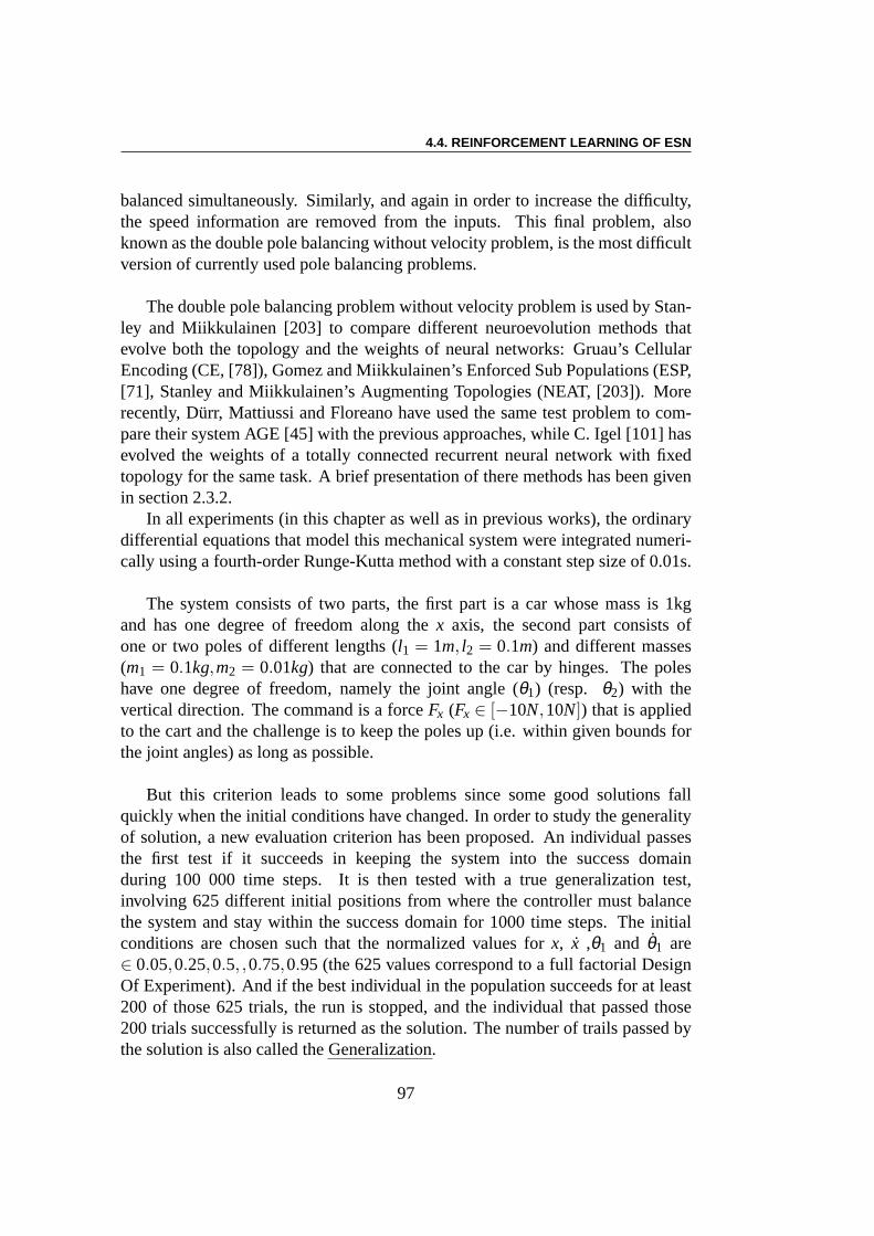
4.4. REINFORCEMENT LEARNING OF ESN
balanced simultaneously. Similarly, and again in order to increase the difficulty,the speed information are removed from the inputs. This finalproblem, alsoknown as the double pole balancing without velocity problem, is the most difficultversion of currently used pole balancing problems.
The double pole balancing problem without velocity problemis used by Stan-ley and Miikkulainen [203] to compare different neuroevolution methods thatevolve both the topology and the weights of neural networks:Gruau’s CellularEncoding (CE, [78]), Gomez and Miikkulainen’s Enforced Sub Populations (ESP,[71], Stanley and Miikkulainen’s Augmenting Topologies (NEAT, [203]). Morerecently, Dürr, Mattiussi and Floreano have used the same test problem to com-pare their system AGE [45] with the previous approaches, while C. Igel [101] hasevolved the weights of a totally connected recurrent neuralnetwork with fixedtopology for the same task. A brief presentation of there methods has been givenin section 2.3.2.
In all experiments (in this chapter as well as in previous works), the ordinarydifferential equations that model this mechanical system were integrated numeri-cally using a fourth-order Runge-Kutta method with a constant step size of 0.01s.
The system consists of two parts, the first part is a car whose mass is 1kgand has one degree of freedom along thex axis, the second part consists ofone or two poles of different lengths (l1 = 1m, l2 = 0.1m) and different masses(m1 = 0.1kg,m2 = 0.01kg) that are connected to the car by hinges. The poleshave one degree of freedom, namely the joint angle (θ1) (resp. θ2) with thevertical direction. The command is a forceFx (Fx ∈ [−10N,10N]) that is appliedto the cart and the challenge is to keep the poles up (i.e. within given bounds forthe joint angles) as long as possible.
But this criterion leads to some problems since some good solutions fallquickly when the initial conditions have changed. In order to study the generalityof solution, a new evaluation criterion has been proposed. An individual passesthe first test if it succeeds in keeping the system into the success domainduring 100 000 time steps. It is then tested with a true generalization test,involving 625 different initial positions from where the controller must balancethe system and stay within the success domain for 1000 time steps. The initialconditions are chosen such that the normalized values forx, x ,θ1 and θ1 are∈ 0.05,0.25,0.5, ,0.75,0.95 (the 625 values correspond to a full factorial DesignOf Experiment). And if the best individual in the populationsucceeds for at least200 of those 625 trials, the run is stopped, and the individual that passed those200 trials successfully is returned as the solution. The number of trails passed bythe solution is also called theGeneralization.
97
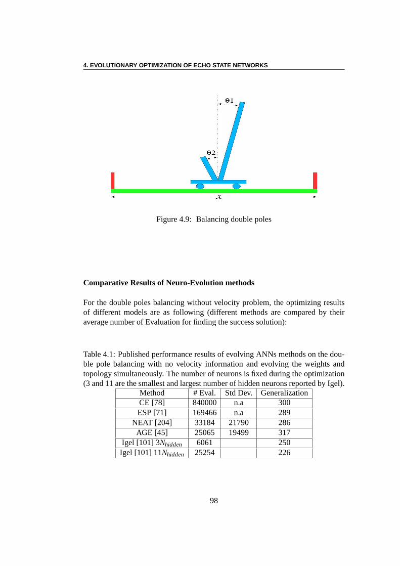
4. EVOLUTIONARY OPTIMIZATION OF ECHO STATE NETWORKS
Figure 4.9: Balancing double poles
Comparative Results of Neuro-Evolution methods
For the double poles balancing without velocity problem, the optimizing resultsof different models are as following (different methods arecompared by theiraverage number of Evaluation for finding the success solution):
Table 4.1: Published performance results of evolving ANNs methods on the dou-ble pole balancing with no velocity information and evolving the weights andtopology simultaneously. The number of neurons is fixed during the optimization(3 and 11 are the smallest and largest number of hidden neurons reported by Igel).
Method # Eval. Std Dev. GeneralizationCE [78] 840000 n.a 300ESP [71] 169466 n.a 289
NEAT [204] 33184 21790 286AGE [45] 25065 19499 317
Igel [101] 3Nhidden 6061 250Igel [101] 11Nhidden 25254 226
98
4.4. REINFORCEMENT LEARNING OF ESN
4.4.2 Fitness(es)
The idea of the fitness function in the double pole experiment, as in all controlproblems, is that an individual that maximizes the fitness should have verygood generalization capabilities. However, standard fitness in such situationsusually average the performance of the controller over manytrials from differentstarting positions, an extremely costly procedure. In order to avoid such heavycomputational cost, many, if not all, previous works in the evolutionary literatureaddressing the double pole balancing problem [78, 71, 204, 101, 45] have useda simplified fitness where the controller performance only depends on its abilityto maintain the poles up during a single trial. Only the best individual in thepopulation (for this fitness) is then evaluated through generalization tests.
However, though this simplified fitness does save a lot of computationalresources, we agree with [45] that it is a poor fitness with respect to the overallgoal of the optimization, in that it is not clear that individuals maximizing thisfitness will perform any good when it comes to generalizationtests. We willhence propose another fitness that additionally captures the generalization abilityof the controller.
We will now in turn introduce both fitnesses.
The “Cheap“ Fitness Function
A single trial is run for every individual in the population,starting from the samestate (θ1(0) = 4.5o, θ1(0) = θ2(0) = θ2(0) = x(0) = x(0) = 0). The simulationis continued until either the system leaves the success domain x∈ [−2.4m,2.4m]andθ1,θ2 ∈ [−36o,36o], or a maximum of 1000 time steps is reached.
The fitness functionFcheapis then a sum of two components:
Fcheap= 0.1t
1000+0.9 fstable, with
fstable=
0 if t < 1000.75
∑ti=t−100(|x
i|+ |xi|+ |θ i1|+ |θ i
1|)otherwise
wheret denotes the number of time steps the system remains inside the successdomain.
99
4. EVOLUTIONARY OPTIMIZATION OF ECHO STATE NETWORKS
The Generalization Fitness
In preliminary tests, we found that some controllers can obtain a very high fitnesswithout ever passing the second test, while some controllers passed all 200 gen-eralization tests with a rather lowFcheap. Hence we have also used a fitness thattakes into account all 3 tests describe above. Of course, itscomputation involvesall 3 tests, including the stabilization during 100,000 times steps, and the 625trials from different starting positions. The fitness valueis then given by
Fnew= Fcheap+#Iter
100,000+30
#Success625
(4.1)
where #Iter is the number of iterations among the 100,000 where the system ismaintained in the success domain, and #Successis the number of generalizationtrials that the controller passes. The value 30 was chosen bytrial and error.Note that the latter means that individuals that are successful on more than625/30≈ 21 generalization runs will have a high fitness now.
4.4.3 Experimental conditions
The size of the reservoir was fixed here to 20 neurons: initialexperimentsindicated that larger reservoirs did not improve the results – an assumption thatwill be revisited in Section 4.5.
To study the variability with respect to the reservoir topology, as in Section4.3, 20 different reservoirs were generated, and 11 independent runs of CMA-ESwere made for each reservoir.
Each reservoir was initialized as described in section 4.3.1, except for thefixed weights: here, the 10% non-zero weights of the reservoir as well as thein-coming weights were randomly initialized in[−1,1].
At the beginning of each run, the activity of all neurons in the reservoir waszeroed, and the network was run for 20 iterations (the numberof neurons) beforethe control actually began and the fitness started to accumulate.
As mentioned in Section 2.2.3, CMA-ES is almost a parameterless algorithm.Only the population size (in fact, number of offspringλ ) is to be tuned [88].Hence, after some preliminary experiments that seemingly demonstrated that alarge population was needed, a first series of experiments was run, withλ = 256,and weird results were obtained (described below in section4.4.4). A second
100
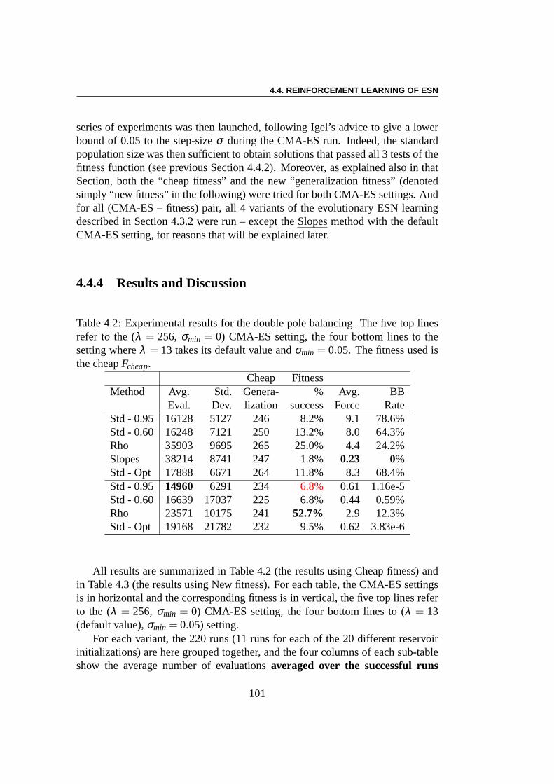
4.4. REINFORCEMENT LEARNING OF ESN
series of experiments was then launched, following Igel’s advice to give a lowerbound of 0.05 to the step-sizeσ during the CMA-ES run. Indeed, the standardpopulation size was then sufficient to obtain solutions thatpassed all 3 tests of thefitness function (see previous Section 4.4.2). Moreover, asexplained also in thatSection, both the “cheap fitness” and the new “generalization fitness” (denotedsimply “new fitness” in the following) were tried for both CMA-ES settings. Andfor all (CMA-ES – fitness) pair, all 4 variants of the evolutionary ESN learningdescribed in Section 4.3.2 were run – except theSlopes method with the defaultCMA-ES setting, for reasons that will be explained later.
4.4.4 Results and Discussion
Table 4.2: Experimental results for the double pole balancing. The five top linesrefer to the (λ = 256, σmin = 0) CMA-ES setting, the four bottom lines to thesetting whereλ = 13 takes its default value andσmin = 0.05. The fitness used isthe cheapFcheap.
Cheap FitnessMethod Avg. Std. Genera- % Avg. BB
Eval. Dev. lization success Force RateStd - 0.95 16128 5127 246 8.2% 9.1 78.6%Std - 0.60 16248 7121 250 13.2% 8.0 64.3%Rho 35903 9695 265 25.0% 4.4 24.2%Slopes 38214 8741 247 1.8% 0.23 0%Std - Opt 17888 6671 264 11.8% 8.3 68.4%Std - 0.95 14960 6291 234 6.8% 0.61 1.16e-5Std - 0.60 16639 17037 225 6.8% 0.44 0.59%Rho 23571 10175 241 52.7% 2.9 12.3%Std - Opt 19168 21782 232 9.5% 0.62 3.83e-6
All results are summarized in Table 4.2 (the results using Cheap fitness) andin Table 4.3 (the results using New fitness). For each table, the CMA-ES settingsis in horizontal and the corresponding fitness is in vertical, the five top lines referto the (λ = 256, σmin = 0) CMA-ES setting, the four bottom lines to (λ = 13(default value),σmin = 0.05) setting.
For each variant, the 220 runs (11 runs for each of the 20 different reservoirinitializations) are here grouped together, and the four columns of each sub-tableshow the average number of evaluationsaveraged over the successful runs
101

4. EVOLUTIONARY OPTIMIZATION OF ECHO STATE NETWORKS
Table 4.3: Experimental results as same as in Table 4.2 except the fitness used isthe new oneFnew. The five top lines refer to the (λ = 256, σmin = 0) CMA-ESsetting, the four bottom lines to the setting whereλ = 13 takes its default valueandσmin = 0.05
New FitnessMethod Avg. Std. Genera- % Avg. BB
Eval. Dev. lization success Force RateStd - 0.95 27770 12522 234 44.5% 9.1 78.6%Std - 0.60 27152 14696 236 62.7% 9.1 82.1%Rho 35275 7481 233 99.5% 7.0 40.6%Slopes 51712 13672 208 19.1% 2.0 0.18%Std - Opt 26683 15395 243 64.5% 9.283.6%Std - 0.95 16303 11511 209 82.3% 2.4 5.7%Std - 0.60 16886 11073 211 87.3% 2.0 5.0%Rho 19796 6770 224 91.4% 3.4 11.0%Std - Opt 15965 11813 208 86.8% 2.0 4.3%
Table 4.4: Experimental resultsStandard Fitness
Method Success % BB RateStd 8.2% 78.6%Rho 25.0% 24.2%Slopes 1.8% 0%Std 6.8% 1.16e-5Rho 52.7% 12.3%
Table 4.5: Experimental resultsNew Fitness
Method Success % BB RateStd 44.5% 78.6%Rho 99.5% 40.6%Slopes 19.1% 0.18%Std 82.3% 5.7%Rho 91.4% 11.0%
102
4.4. REINFORCEMENT LEARNING OF ESN
(columnAvg Eval.), its standard deviation (Std Dev.), the number of tests (outof 625) passed during the third generalization test (Generalization), and, mostimportantly, the percentage of success (% success), i.e. of runs where the bestindividual did pass the 3 generalization tests. The other 2 columns will be detailedlater.
First of all, it should be noted that only Table 4.2 (CheapFitness) can becompared to the published results of Table 4.4.1, because the experiments in thesecond column didn’t use the same fitness.
The first striking result is the poor performance of the largepopulation sizewith no bound onσ (first 5 lines of results of Table 4.2): only a small fractionof all runs did pass the 3 generalization tests, from 25% for the Rho method toas little as 1.8% for theSlopes method. Since the Avg. Eval. is only averagedover the successful runs and because of the poor success rate, compared to otherpublished results (Table 4.4.1), this result is very disappointing. If we compare toother algorithms, the SP1 need to be computed to make a fair comparison. In thesimplest way the SP1 can be cursorily computed asSP1 = Avg.Eval./success%.(we need to notice that it is just a cursorily one because for the unsuccessfulruns, their evaluation number could be more or less than the average evaluationsnumber of success runs.). With this equation the best resultis from the Std-0.60version whose SP1 is 16248/0.132 = 123090, it is almost 4 times larger bycomparing with NEAT.
Things get a little better for the second CMA-ES setting with alowerthreshold onσ (4 last lines of the Table), at least when looking at the performanceof theRho variant: more than half of the runs succeeded, with an average cost of23571 evaluations, which amounts to an SP1 value of about 45300. This is stillworse than NEAT and AGE, but within the same order of magnitude.
However, those weak success rates are to be related with the statement in [45]that “each run has to be restarted 10 times on average to find a solution”. But onthe other hand, NEAT [203], and Igel [101] at a very low cost, consistently founda solution that passed all tests.
As expected, the results really improve when using the new fitness, that takesinto account the generalization ability of the network: with the first CMA-ESsetting, theRho variant almost always find a solution (except for one run out of220), and theStd and theSlopes variants improve a lot over their results with thecheap fitness.
103
4. EVOLUTIONARY OPTIMIZATION OF ECHO STATE NETWORKS
More importantly, using both the new fitness and a lower boundfor σ allowsall variants to reach performances at the level of those of NEAT, AGE, or thetotally recurrent network with 9 neurons or more – though of course those resultscannot really be compared, as they were obtained using a different fitness. Indeed,the SP1 values forStd-0.60,Std-0.95, andRho variants respectively are 19342,19808 and 21658, even though slightly moreRho runs fail to find a solution.
Controller Behaviors In order to try to understand those striking differences, thebehavior of each controller was analyzed – and the results are summarized in thelast 2 columns of each sub-table: columnAvg. Force gives the average (over the100000 times-steps of test 2 and the successful trials of 1000 time steps out ofthe 625 generalization test 3) of the absolute value of the force to be applied tothe cart, (in Newton, in[0,10]); the last column,BB rate gives the percentage oftime steps where the controller gave a ”Bang-Bang“ command, i.e. a force whoseabsolute value is higher than 9 N.
It now clearly appears that all successful controllers thatlearned without alower bound onσ exhibit a behavior that is very close to a complete bang-bangcontrol – and this is even more so with the new fitness. On the other hand, theRho variant manages to find intermediate behaviors, while thefew successfulruns of theSlopes variant can balance the double pole and pass all testswhilespending an incredibly low energy (the average force is close to 0, which meansthe car is almost motionless during the simulation!). Note,however, that the newfitness, because it favors generalization more than decrease of movement (as doesthe cheap fitness alone), allows theRho andSlopes methods to find many moresolutions passing the generalization tests, but the corresponding controllers needlarger forces and are “closer from bang-bang”.
When there is a lower bound onσ , however, no method whatsoever finds anybang-bang solution. Moreover, theStd method in fact exhibits controllers usingsmaller forces (on average) than theRho method. Note that theSlopes variantwas not tried (yet) for this setting.
Interestingly, the average squared weights reaches valuesas high as 1011 forthe results of bothStd variants with the new fitness and CMA-ES unboundedσ ,and as low as 69 and even 7 for theSlopes andRho variants respectively in thesame conditions. But averaging here hides the most interesting phenomenon: ascan be seen on Figure 4.10, that shows the average histogramsof forces values:the Std variants are clearly bang-bang, theSlopes method demonstrates a verysmooth behavior with all forces around 0, and surprisingly,the Rho methodshows both modes, indicating that it found both kinds of solutions.
104
4.4. REINFORCEMENT LEARNING OF ESN
Those findings give some hints about the actual fitness landscapes, and mighthelp to explain the results.
Fitness landscapesFrom the above study on the weights of the solutions, itseems that bang-bang solutions are frequent, deep and wide local optima w.r.t.the output weights: indeed, they correspond to regions of the search space withvery high values of all weights, giving saturated output neurons, and smallmodifications of those weights are not likely to move the search away fromsuch local optimum. This explains why CMA-ES, without a lowerbound onσ , prematurely converges into one of those wells. Adding a lower bound onσ prevents a too early stagnation, and favors exploration, thus allowing thealgorithm to find better optima for the fitness at hand . . . and in the long run,smooth optimizers are better optima than bang-bang commands.
The situation is different for theSlopes variant, that cannot reach any of thebang-bang commands, because its output weights are fixed (with low values).Hence it can only find smooth controllers, but its degrees of freedoms are toolimited to make this search efficient. The most interesting case is that of theRhomethod: it seems that adding this additional variable givesthe algorithm sufficientflexibility to be able to discover both kinds of solutions (see Figure 4.10), thusfavoring exploration increases its chances to find smooth controls. In some sense,even with a smallσ , modifying ρ might be enough to find a shortcut toward asmooth solution later in the run than by modifying all weights individually.
Spectral Radius It has always been advocated by ESN pioneers that the upperbound on the spectral radius was an important feature for successful ESN use,and the results for bothStd variants with different spectral radius seem to confirmthis. In Table 4.2 of the version with Cheap fitness, if we don’tset the low boundfor σ , the success rate of Std-0.60 is better than the success rateof Std-0.95.(13.2 % vs 8.2 %) while in Table 4.3 when the new fitness is used,the successrate of Std-0.60 is also better than the success rate of Std-0.95. (62.7 % vs 44.5 %).
However, the most remarkable fact here is that for all settings (CMA-EStuning and fitness), theRho variant, that explicitly optimizes the Spectral Radius,almost always gives the best results. This is surprising when comparing tothe situation in the supervised context (Section 4.3.5), where theRho variantperformed the worst of all.
Further experiments were run, using theStd variant but fixing the SpectralRadius to the final value found by theRho method (see the lines ”Std – Opt“ in
105
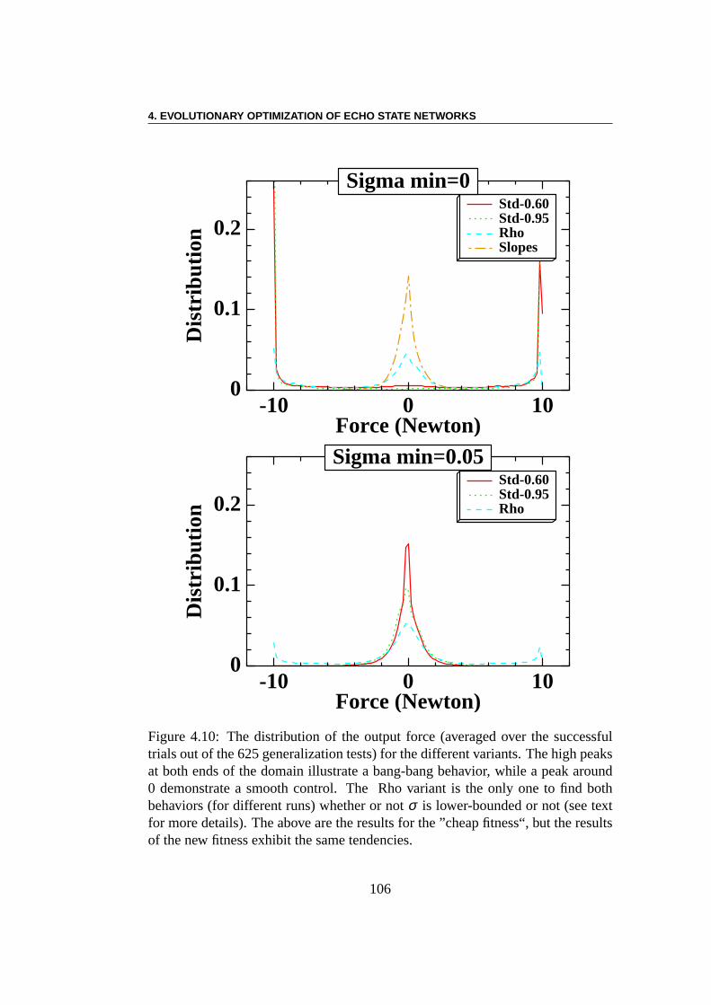
4. EVOLUTIONARY OPTIMIZATION OF ECHO STATE NETWORKS
Force (Newton)
Dis
trib
utio
n
-10 0 100
0.1
0.2Std-0.60Std-0.95Rho Slopes
Sigma min=0
Force (Newton)
Dis
trib
utio
n
-10 0 100
0.1
0.2Std-0.60Std-0.95Rho
Sigma min=0.05
Figure 4.10: The distribution of the output force (averagedover the successfultrials out of the 625 generalization tests) for the different variants. The high peaksat both ends of the domain illustrate a bang-bang behavior, while a peak around0 demonstrate a smooth control. The Rho variant is the only oneto find bothbehaviors (for different runs) whether or notσ is lower-bounded or not (see textfor more details). The above are the results for the ”cheap fitness“, but the resultsof the new fitness exhibit the same tendencies.
106

4.4. REINFORCEMENT LEARNING OF ESN
Table 4.2). Though it generally slightly improves the results over an arbitraryvalue like 0.6 or 0.95, it does not allow to reach the same level of performancethan theRho method itself. The important feature is thatρ can be modifiedduring the optimization, and not the final value it reaches.
Figure 4.11 show the finalρ value for the success runs of fourRho versions,the top two figures are the result with the cheap fitness, the left one withλ = 256andσmin= 0.0 and the right one withλ = 13 andσmin= 0.05, each color representan ESN. In this case there are not many runs can find the successsolutions, butwith σmin = 0.05 the results is already much better.
The bottom two figures are the result with the New fitness, the left one withλ = 256 andσmin = 0.0 and the right one withλ = 13 andσmin = 0.05, we canfind clearly that there are much more success runs than with the cheap fitness.This result may indicate that in our test, each randomly created ESN (with someconstraints) has the ability to solve the double-pole balancing without velocityproblem, if given enough information.
This result is proved by the following test: if evolution (using the new fitness)is continued after the first network has passed the 200-testsof test3: all resultingnetworks are able to successfully solve more than 500 out of the 625 test cases,with a peak at 555 for one network. This is a good advantage about the Rhovariant, which seems to be able to provide controllers that generalize very well.Unfortunately, the other published results do not provide results of this kind, ex-cept for one sentence in [45] that mentions that one network successfully solved525 test cases.
Finally, Figure 4.12 shows the finalρ and the number of evaluation of thebestRho version, whereλ = 13 andσmin = 0.05 by using New fitness. Eachcolor represent a ESN, the dot is the average of the optimalρ and the numberof evaluation, the bars is the range of the different runs. One can see that eachnetwork has its specific optimal value forρ, and that each network does behavedifferently (the range of optimalρ, the range of number of evaluation, etc.) eventhough all the learning parameters are identical. This suggest that the topology ofESN might have an important role for such a learning task, at least when the sizeof ESN is small.
CMA-ES settings It has been said (Section 2.2.3) that CMA-ES was almost aparameterless algorithm. However, the experiments presented above are anotherexample of the dangers of black-box use of any algorithm: because of thecharacteristics of the fitness landscape, the best results were obtained whenusing CMA-ES in a very atypical way, favoring exploration andforbidding
107
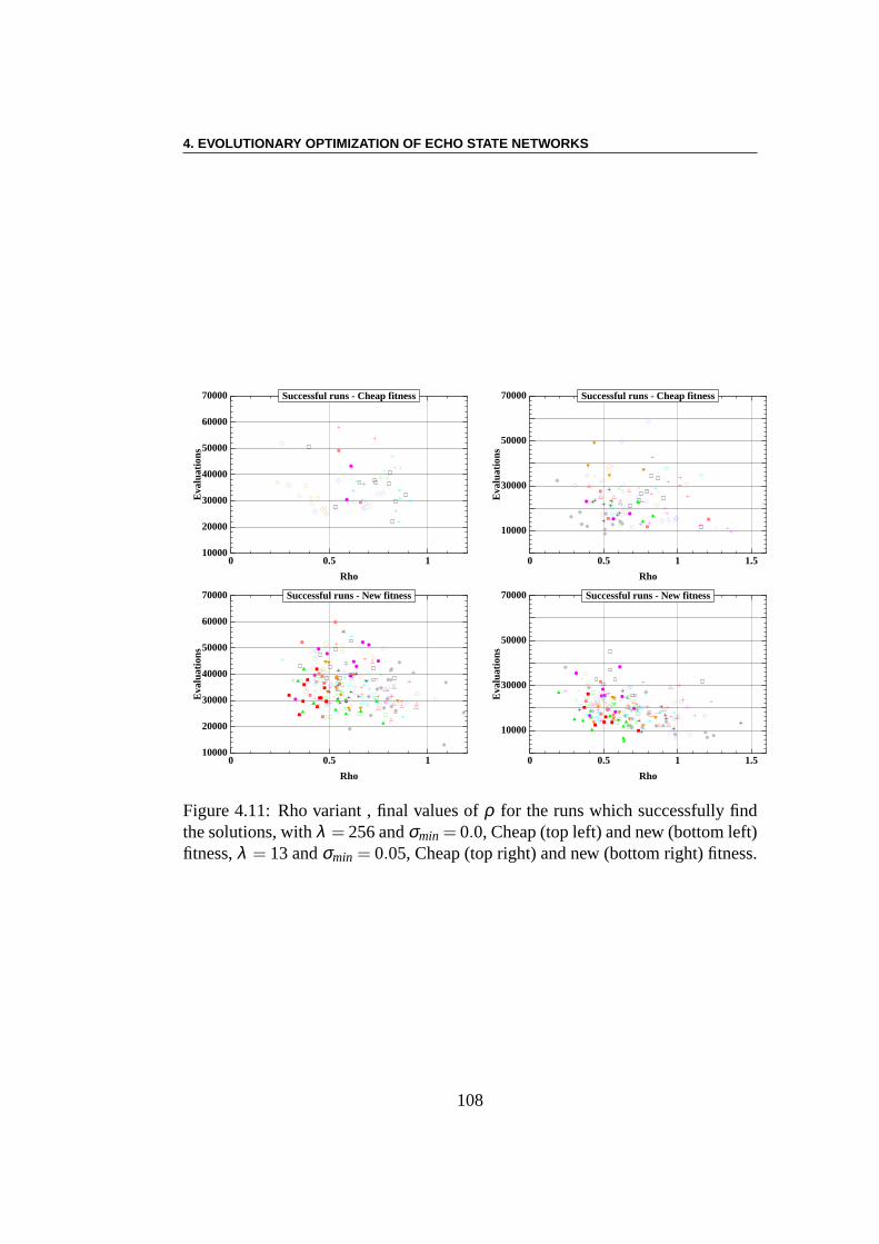
4. EVOLUTIONARY OPTIMIZATION OF ECHO STATE NETWORKS
Rho
Eva
luat
ions
0 10.510000
20000
30000
40000
50000
60000
70000 Successful runs - Cheap fitness
Rho
Eva
luat
ions
0 10.5 1.5
10000
30000
50000
70000 Successful runs - Cheap fitness
Rho
Eva
luat
ions
0 10.510000
20000
30000
40000
50000
60000
70000 Successful runs - New fitness
Rho
Eva
luat
ions
0 10.5 1.5
10000
30000
50000
70000 Successful runs - New fitness
Figure 4.11: Rho variant , final values ofρ for the runs which successfully findthe solutions, withλ = 256 andσmin = 0.0, Cheap (top left) and new (bottom left)fitness,λ = 13 andσmin = 0.05, Cheap (top right) and new (bottom right) fitness.
108
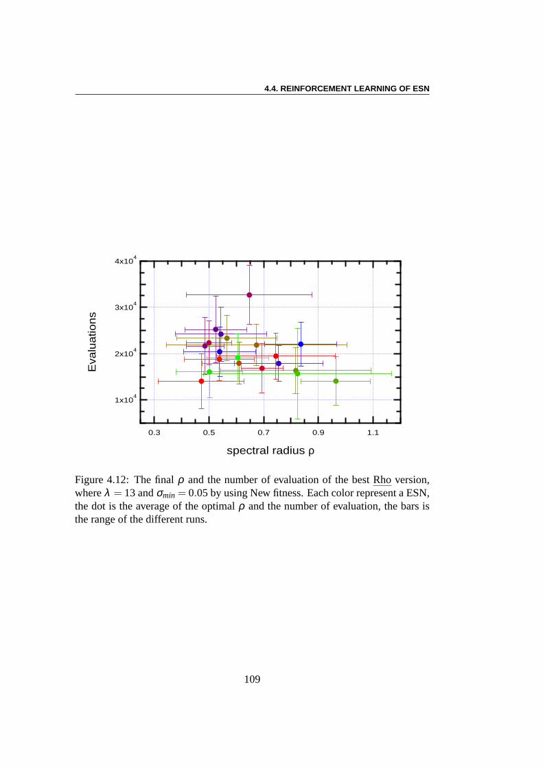
4.4. REINFORCEMENT LEARNING OF ESN
4x10⁴
3x10⁴
2x10⁴
1x10⁴
Eva
lua
tion
s
1.10.90.70.50.3
spectral radius ρ
Figure 4.12: The finalρ and the number of evaluation of the bestRho version,whereλ = 13 andσmin = 0.05 by using New fitness. Each color represent a ESN,the dot is the average of the optimalρ and the number of evaluation, the bars isthe range of the different runs.
109
4. EVOLUTIONARY OPTIMIZATION OF ECHO STATE NETWORKS
exploitation by keepingσ far from 0. But this relates to the fitness design, not tothe optimization algorithm used.
Reservoir topologiesThe influence of the initialization of the topology of thereservoir is clear: for instance, among the 55 runs that passed all tests for theRho variant with CMA-ES first setting (25% of the 220 runs), 40 were obtainedfrom 4 reservoirs out of 20, and 10 reservoirs could not generate a single successduring the 11 runs that were launched. Together with the differences noted inthe supervised learning context (though their statisticalsignificance could not bemeasured due to the too small number of experiments), this makes a clear picturethat the topology of the reservoir matters. Why, and how to take advantage of thisfact, is the object of further work.
4.5 ESN vs Developmental Methods
Quite different results could be observed on the double poleproblem for different(random) settings of the connections (i.e. the non-zero weights), for the samevalue of the density of connection. The question is now open:whereas reservoircomputing has been proposed as a possible alternative to finetuning of thetopology of Neural Networks, it might be the case that tuningthe topology of thereservoir allows to obtain more efficient ESNs. Further workwill address thisresearch question, and two main directions can be imagined.
The network can be built using classes of topologies (e.g. small world,scale free, . . . ); identifying classes of network that are efficient for a giventype of problem (i.e. such that randomly built networks fromthis class have avery high probability to solve the problem at hand) would indeed relieve theprogrammer from the task of optimizing the topology, restricting the search spaceto a parameter space, where CMA-ES proved to be an efficient tool.
It might be the case, however, that for reservoir computing,problem-specifictopology tuning is nevertheless required anew for each problem. The maindifficulty will then be to design efficient techniques for tuning the topology oflarge networks, as most existing methods do not really scaleup to hundredsof neurons or more. Some hints have been recently given with Hyper-NEAT[201] on the one hand, and with the different approaches based on GeneticRegulatory Networks, starting with AGE [45], though other GRNapproaches canbe envisioned, too (see [156, 157] and the discussion in Section 2.3.2).
110
4.6. CONCLUSION
But the benefit of using such approaches still remains to be uncovered, and inparticular special care will need to be paid to comparing reservoir approaches withthe straightforward fully connected recurrent network approach: as witnessedby Igel’results for the double pole balancing problem [101], the latter, thanks toCMA-ES, is able to solve quite a large class of control problems that were atsome point thought to be difficult.
4.6 Conclusion
This chapter has demonstrated the feasibility of evolutionary learning of EchoState Networks. Moreover, the flexibility of EAs opens new paths for optimizingnot just the outgoing weights of the ESN.
In a supervised context, the results on a standard time series predictionproblem reach the same precision when optimizing the outputweights than theoriginal results obtained using quadratic optimization, and other optimization failto improve this precision. With a smaller reservoir, however, optimizing also theslopes of the transfer functions of all neurons allows us to reach better predictionaccuracy, at a high computational cost, though.
For reinforcement tasks, the good news is that the Evolutionary Learning ofESNs works. Moreover, optimizing more than just the outgoing weights doesimprove the results. Furthermore, there seems to be a high dependency of theresults on the topology of the reservoir, at least for the small sizes experimentedwith here.
Hence, the results presented here do not satisfactorily answer the questionof where ESNs stand between the two extremes of neuroevolution today: onthe one hand, the evolutionary optimization of the weights of a fully recurrentneural network (as proposed in [101]), with which evolutionary learning ofESNs shares the ease of implementation (a straightforward application of thenow state-of-the-art CMA-ES for parameter tuning); and on the other hand,the carefully crafted developmental systems that evolve the topology of highlyefficient NNs for a given task [204, 45]. Further experimentsusing more reliabletest problems, and using larger reservoir sizes, are neededto definitely addressthis issue.
Indeed, a side take-home lesson from this chapter regards the usefulness ofthe double pole balancing problem as a benchmark for evolutionary control in
111
4. EVOLUTIONARY OPTIMIZATION OF ECHO STATE NETWORKS
general: the answer is clearly negative for us now (but had been claimed by othersbefore), at least with the kind of fitness used up to now to tackle the problem.The lack or correlation between that fitness and the generalization tests that thesystem is asked to pass to be declared successful introducesa too high randompart in the evaluation of the results, as there is no promise that the good fitnesswill lead to the good generalization, and also as they are many ways to minimizethe fitness, leading to unpredictable generalization properties.
112
Chapter 5
Feature Selection in a Cortex-LikeObject Recognition Model
In this chapter, we will introduce our work regarding a visual object recognitionmodel which is inspired by the biology of visual cortex. Thismodel, originallyproposed by T. Serre and T. Poggio [198], is basically a feed-forward hierarchicalneural network that alternates between template matching stages and maximumpooling operations. The long term goal for us is to study the relationship betweenthe model’s topology and performance. But for the reason of high computationcost, the first step will be the question of how to decrease thecomputational costwhile preserving the system performance, using a multi-evolutionary algorithmand applying the result in the framework of a PASCAL visual multi-objectrecognition challenge [140] (VOC2008).
In this model, the network output consists of standard features that are passedto a linear combination algorithm for the final classification task itself. The coef-ficients of this linear combination will be obtained by evolutionary optimization,using CMA-ES (Covariance Matrix Adaptation Evolution Strategy) [87, 88, 103]detailed in Section 2.2.3.
The results show that optimizing the selection of 200 optimal features among1000 randomly chosen ones, we are able to maintain the performance of the sys-tem on the VOC2008 challenge, while decreasing the computational cost by 2orders of magnitude. Even if our results in VOC2008 are not very strong from theperspective of their performance on the classification tasks at hand, consideringthe simplicity of the model being applied shows that there still is a large room forprogress in the future: we simply used the default model settings, and there arelots of parameters that could be adjusted.
113
5. FEATURE SELECTION IN A CORTEX-LIKE OBJECT RECOGNITION MODEL
5.1 Cortex-Like Object Recognition
Complex visual object recognition is an important domain in computer science,in both theory and practice. However, in spite of decades of hard work, thebest machine vision systems are still not competitive with humans and pri-mates [99, 166, 219, 198]. Therefore building a bio-inspired computer visionsystem is an attractive research direction.
Serre and Poggio proposed a cortex-like feed-forward model[194, 195] whichwas directly inspired by the image processing mechanisms ofcortex and showedexcellent results in a series of image classification tasks [196, 198]. In this section,we will briefly present their model.
5.1.1 Visual Object Recognition in the Cortex
The primary regions for the treatment of visual informationby the cortexof primates (regionsV1 and V2) are located in the occipital lobe, in therearmost part of the skull [115]. Visual information is thentransmittedto higher-level treatment regions through two distinct (albeit partly con-nected) neural routes : the ventral and dorsal streams. The dorsal stream(V1 → V2 → MT → posterior parietal cortex), sometimes called the “wherepathway” is associated with object location in space and motion, while the ventralstream (V1→V2→V4→ inferior temporal cortex), sometimes called the “whatpathway” is associated with form recognition and object representation. Beinginterested here in object recognition/classification tasks, we will emphasis thelatter.
As a first approximation, basic processing of information inthe ventral streamis feedforward, at least for the first stages of visual processing. This hypothesisis supported by the short time spans required for a selectiveresponse to appearin the inferior temporal (IT) cortex cells [165]. Indeed, asemphasized in [100]:“Through a variety of recognition tasks, the activity of small neuronal populationsin monkey IT contains surprisingly accurate and robust information just over veryshort time intervals (as small as 12.5 ms) and only about 100 ms after stimulusonset”.
The ability to learn and categorize scenes as well as the objects within is anessential and important functionality of human. In this framework, the immediaterecognition task consists in recognizing an object within ascene in a very shorttime delay. For this task in particular, it has been suggested that the ventral streammay have invariance properties for the object to be recognized, which means
114
5.1. CORTEX-LIKE OBJECT RECOGNITION
that if the same object is located at different positions in space, or zoomed in orout within the scene, the system is still able to recognize it. The processing isprobably based on a rapid and parallel detection of disjunctive sets of unboundfeatures of the target category [212, 228] : an object is firstcharacterized by aset of line segments that compose it; the process then detects each line segmentin parallel; the object is then recognized through the distribution in space of thedetected line segments. More recently, a psychophysical experiment [52] foundthat during immediate recognition processing, spatial information on the locationof the objects may be absent, which would mean that the dorsalstream is notimplicated in such immediate recognition tasks. Moreover that means the humanobservers may correctly detect a target object in a rapid sequence of images, butnot be able to recover even its approximate location [52].
Another fundamental property of the ventral pathway is thatneuron tuningbecomes increasingly complex along the feedforward path. Neuronal tuning des-ignates the fact that any given neuron responds preferentially to a subset of stimuliwithin its receptive field. In the primary visual areas, neurons have simple tuning.For example, a neuron in V1 may fire to any vertical stimulus inits receptive field.In the higher visual areas, neurons have more complex tuning. For example, inthe inferior temporal cortex (IT), a neuron may fire only whena certain objectappears in its receptive field.
Based on these research results, Riesenhuber, Serre and Poggio elaborateda theory of the feedforward path of object recognition in cortex, that accountsfor the first 100-200 milliseconds of processing in the ventral stream of primatevisual cortex [175, 194]. Riesenhuber and Poggio proposed the model in 1999and showed that it is able to duplicate the tuning propertiesof neurons in severalvisual cortical areas [175]. This first model’s performancewas only evaluated onsimple artificial stimuli without real world image degradations such as changein illumination, clutter, etc. Hence, Serre and Poggio extended the model in2005 and obtained successful results on a variety of large-scale real-worldobject recognition databases with performances that compare favorably withstate-of-the-art systems, whether bio-inspired and not [194]. We will present thismodel in the following section.
5.1.2 Standard Model Features (SMFs)
The model itself attempts to summarize – in a quantitative way – a core of well-accepted facts about the ventral stream in the visual cortex:
1. Visual processing is hierarchical, and aims at building invariance to position
115
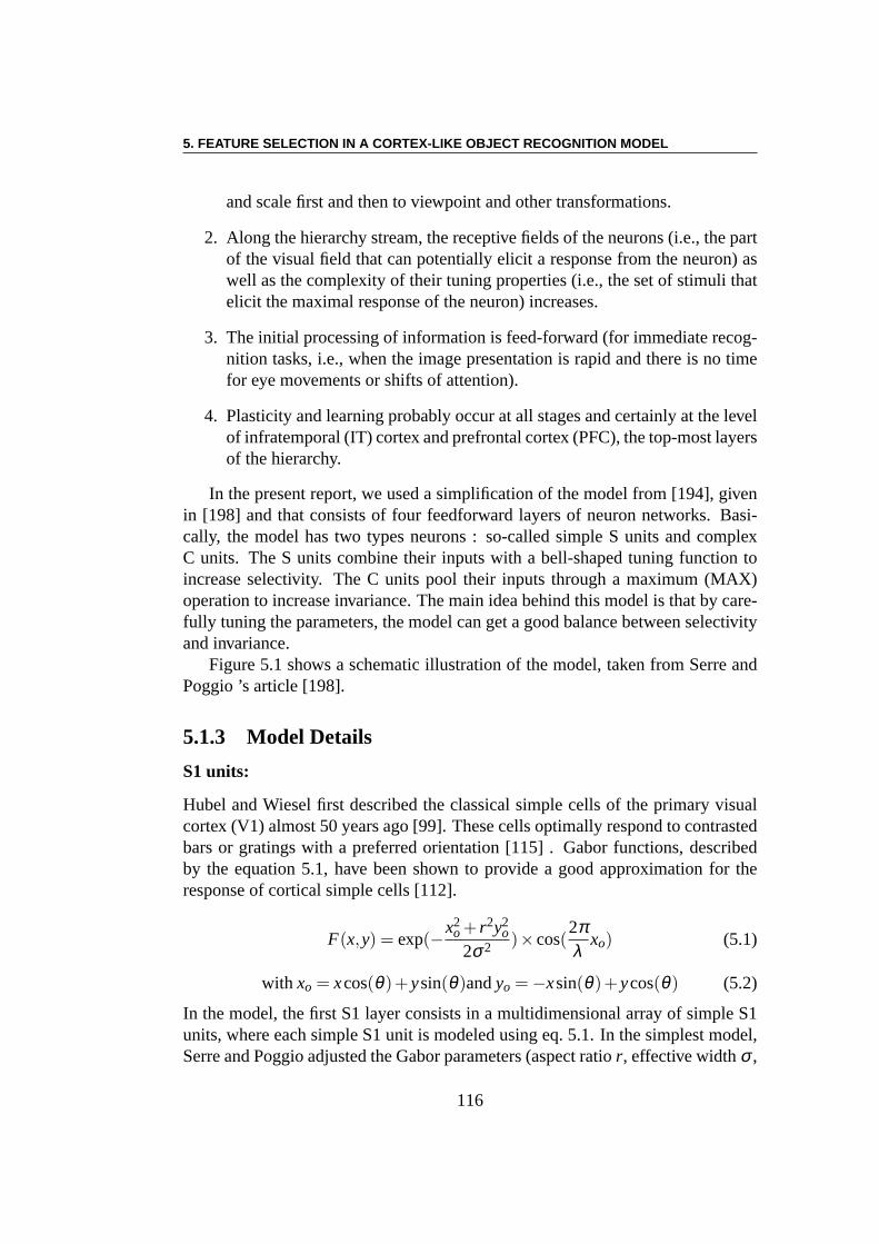
5. FEATURE SELECTION IN A CORTEX-LIKE OBJECT RECOGNITION MODEL
and scale first and then to viewpoint and other transformations.
2. Along the hierarchy stream, the receptive fields of the neurons (i.e., the partof the visual field that can potentially elicit a response from the neuron) aswell as the complexity of their tuning properties (i.e., theset of stimuli thatelicit the maximal response of the neuron) increases.
3. The initial processing of information is feed-forward (for immediate recog-nition tasks, i.e., when the image presentation is rapid andthere is no timefor eye movements or shifts of attention).
4. Plasticity and learning probably occur at all stages and certainly at the levelof infratemporal (IT) cortex and prefrontal cortex (PFC), the top-most layersof the hierarchy.
In the present report, we used a simplification of the model from [194], givenin [198] and that consists of four feedforward layers of neuron networks. Basi-cally, the model has two types neurons : so-called simple S units and complexC units. The S units combine their inputs with a bell-shaped tuning function toincrease selectivity. The C units pool their inputs througha maximum (MAX)operation to increase invariance. The main idea behind thismodel is that by care-fully tuning the parameters, the model can get a good balancebetween selectivityand invariance.
Figure 5.1 shows a schematic illustration of the model, taken from Serre andPoggio ’s article [198].
5.1.3 Model Details
S1 units:
Hubel and Wiesel first described the classical simple cells of the primary visualcortex (V1) almost 50 years ago [99]. These cells optimally respond to contrastedbars or gratings with a preferred orientation [115] . Gabor functions, describedby the equation 5.1, have been shown to provide a good approximation for theresponse of cortical simple cells [112].
F(x,y) = exp(−x2
o + r2y2o
2σ2 )×cos(2πλ
xo) (5.1)
with xo = xcos(θ)+ysin(θ)andyo = −xsin(θ)+ycos(θ) (5.2)
In the model, the first S1 layer consists in a multidimensional array of simple S1units, where each simple S1 unit is modeled using eq. 5.1. In the simplest model,Serre and Poggio adjusted the Gabor parameters (aspect ratio r, effective widthσ ,
116
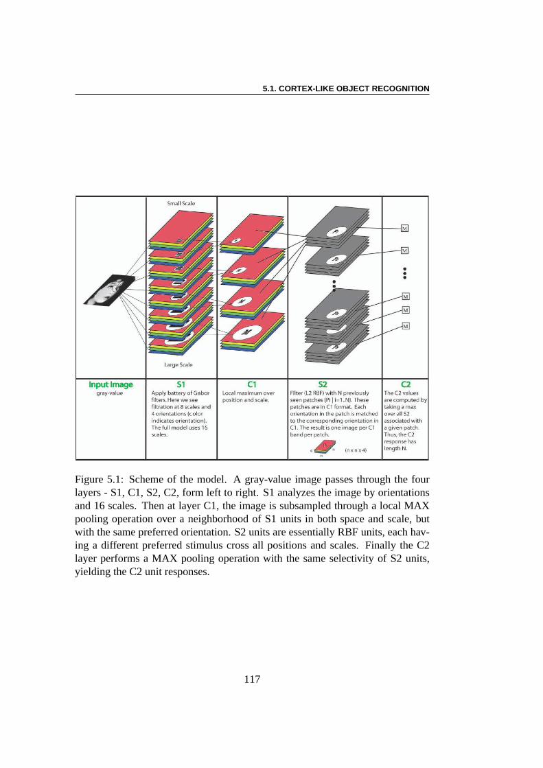
5.1. CORTEX-LIKE OBJECT RECOGNITION
Figure 5.1: Scheme of the model. A gray-value image passes through the fourlayers - S1, C1, S2, C2, form left to right. S1 analyzes the imageby orientationsand 16 scales. Then at layer C1, the image is subsampled through a local MAXpooling operation over a neighborhood of S1 units in both space and scale, butwith the same preferred orientation. S2 units are essentially RBF units, each hav-ing a different preferred stimulus cross all positions and scales. Finally the C2layer performs a MAX pooling operation with the same selectivity of S2 units,yielding the C2 unit responses.
117
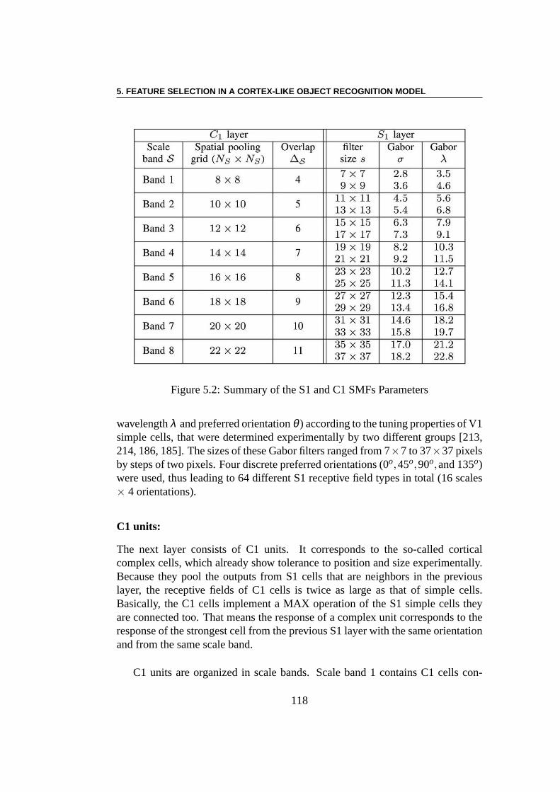
5. FEATURE SELECTION IN A CORTEX-LIKE OBJECT RECOGNITION MODEL
Figure 5.2: Summary of the S1 and C1 SMFs Parameters
wavelengthλ and preferred orientationθ ) according to the tuning properties of V1simple cells, that were determined experimentally by two different groups [213,214, 186, 185]. The sizes of these Gabor filters ranged from 7×7 to 37×37 pixelsby steps of two pixels. Four discrete preferred orientations (0o,45o,90o,and 135o)were used, thus leading to 64 different S1 receptive field types in total (16 scales× 4 orientations).
C1 units:
The next layer consists of C1 units. It corresponds to the so-called corticalcomplex cells, which already show tolerance to position andsize experimentally.Because they pool the outputs from S1 cells that are neighborsin the previouslayer, the receptive fields of C1 cells is twice as large as thatof simple cells.Basically, the C1 cells implement a MAX operation of the S1 simple cells theyare connected too. That means the response of a complex unit corresponds to theresponse of the strongest cell from the previous S1 layer with the same orientationand from the same scale band.
C1 units are organized in scale bands. Scale band 1 contains C1 cells con-
118
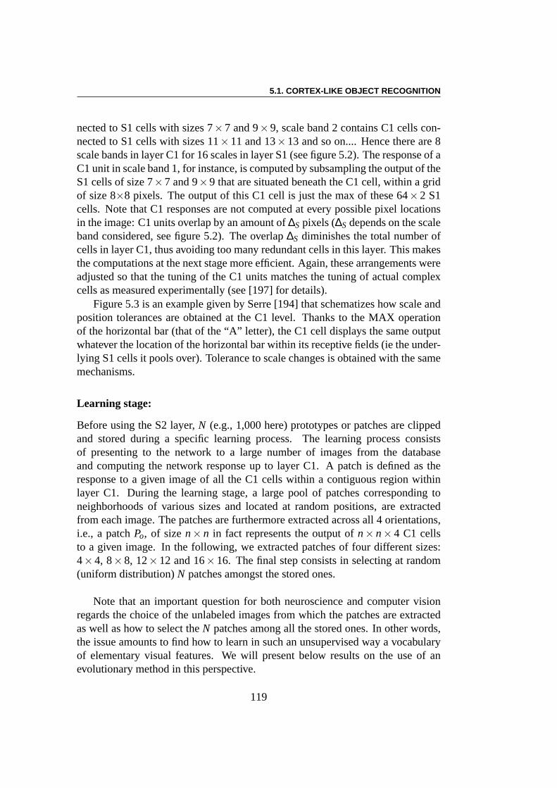
5.1. CORTEX-LIKE OBJECT RECOGNITION
nected to S1 cells with sizes 7×7 and 9×9, scale band 2 contains C1 cells con-nected to S1 cells with sizes 11×11 and 13×13 and so on.... Hence there are 8scale bands in layer C1 for 16 scales in layer S1 (see figure 5.2). The response of aC1 unit in scale band 1, for instance, is computed by subsampling the output of theS1 cells of size 7×7 and 9×9 that are situated beneath the C1 cell, within a gridof size 8×8 pixels. The output of this C1 cell is just the max of these 64×2 S1cells. Note that C1 responses are not computed at every possible pixel locationsin the image: C1 units overlap by an amount of∆S pixels (∆S depends on the scaleband considered, see figure 5.2). The overlap∆S diminishes the total number ofcells in layer C1, thus avoiding too many redundant cells in this layer. This makesthe computations at the next stage more efficient. Again, these arrangements wereadjusted so that the tuning of the C1 units matches the tuning of actual complexcells as measured experimentally (see [197] for details).
Figure 5.3 is an example given by Serre [194] that schematizes how scale andposition tolerances are obtained at the C1 level. Thanks to the MAX operationof the horizontal bar (that of the “A” letter), the C1 cell displays the same outputwhatever the location of the horizontal bar within its receptive fields (ie the under-lying S1 cells it pools over). Tolerance to scale changes is obtained with the samemechanisms.
Learning stage:
Before using the S2 layer,N (e.g., 1,000 here) prototypes or patches are clippedand stored during a specific learning process. The learning process consistsof presenting to the network to a large number of images from the databaseand computing the network response up to layer C1. A patch is defined as theresponse to a given image of all the C1 cells within a contiguous region withinlayer C1. During the learning stage, a large pool of patches corresponding toneighborhoods of various sizes and located at random positions, are extractedfrom each image. The patches are furthermore extracted across all 4 orientations,i.e., a patchPo, of sizen× n in fact represents the output ofn× n× 4 C1 cellsto a given image. In the following, we extracted patches of four different sizes:4×4, 8×8, 12×12 and 16×16. The final step consists in selecting at random(uniform distribution)N patches amongst the stored ones.
Note that an important question for both neuroscience and computer visionregards the choice of the unlabeled images from which the patches are extractedas well as how to select theN patches among all the stored ones. In other words,the issue amounts to find how to learn in such an unsupervised way a vocabularyof elementary visual features. We will present below results on the use of anevolutionary method in this perspective.
119
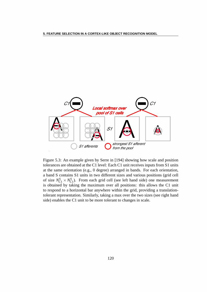
5. FEATURE SELECTION IN A CORTEX-LIKE OBJECT RECOGNITION MODEL
Figure 5.3: An example given by Serre in [194] showing how scale and positiontolerances are obtained at the C1 level: Each C1 unit receives inputs from S1 unitsat the same orientation (e.g., 0 degree) arranged in bands. For each orientation,a band S contains S1 units in two different sizes and various positions (grid cellof size NS
C1 ×NSC1). From each grid cell (see left hand side) one measurement
is obtained by taking the maximum over all positions: this allows the C1 unitto respond to a horizontal bar anywhere within the grid, providing a translation-tolerant representation. Similarly, taking a max over the two sizes (see right handside) enables the C1 unit to be more tolerant to changes in scale.
120

5.1. CORTEX-LIKE OBJECT RECOGNITION
S2 units:
Each cell in layer S2 computes the Euclidean distance between one of the selectedpatchPi and the response of Layer C1 to a new (unknown) image. To this aim,the response of S2 cell layer consists of a Gaussian Radial Basis Function (RBF)φ(x) = exp
(
−‖x−Pi‖2)
, wherePi is the real-valued vector Patchi and x theresponse of layer C1 to the current image.
Each S2 cell pools over afferent C1 units from a local spatial neighborhoodacross all four orientations. Layer S2 thus contains 8×N maps, each representingthe response of one of the 8 scale bands of Layer C1 compared to one patchPi outof theN selected ones.
C2 units:
The final layer, layer C2, computes the global maximum of the all S2 units overall scales and positions. As explained above, one S2 map measures the matchbetween a selected prototypePi and the input image at every position for a givenscale band. One C2 units only keeps the maximal value of the S2 maps across allscale bands for a given patchPi. The final system output for a new image is thusaN-dimensional vector, whereN is to the number of patches extracted during thelearning stage. Note that one C2 unit expresses the maximum ofa S2 map overthe whole image, which implies that its response is not dependent on the objectlocation within the image.
The Classification Stage:
Hence every new image passes the feedforward system and yields a N-valuevector in the output of layer C2, whose elements are calledStandardModelFeatures (SMFs). The SMFs are then further passed to a simplelinear classifier(SVM or boosting in the original article). This part of the learning is a simplesupervised learning, since all the labels are given for the training set, and thefitness to be optimized is just the misclassification rate.
5.1.4 The Perspectives of the Model
Serre et al. [198] list three major perspective directions that could be followed tofurther improve the performance of their architecture :
• Addition of extra layers (e.g., S3, C3, S4, etc.)
• Applying a standard feature selection technique.
121
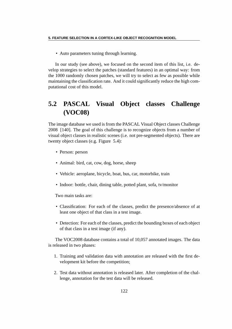
5. FEATURE SELECTION IN A CORTEX-LIKE OBJECT RECOGNITION MODEL
• Auto parameters tuning through learning.
In our study (see above), we focused on the second item of thislist, i.e. de-velop strategies to select the patches (standard features)in an optimal way: fromthe 1000 randomly chosen patches, we will try to select as fewas possible whilemaintaining the classification rate. And it could significantly reduce the high com-putational cost of this model.
5.2 PASCAL Visual Object classes Challenge(VOC08)
The image database we used is from the PASCAL Visual Object classes Challenge2008 [140]. The goal of this challenge is to recognize objects from a number ofvisual object classes in realistic scenes (i.e. not pre-segmented objects). There aretwenty object classes (e.g. Figure 5.4):
• Person: person
• Animal: bird, cat, cow, dog, horse, sheep
• Vehicle: aeroplane, bicycle, boat, bus, car, motorbike, train
• Indoor: bottle, chair, dining table, potted plant, sofa, tv/monitor
Two main tasks are:
• Classification: For each of the classes, predict the presence/absence of atleast one object of that class in a test image.
• Detection: For each of the classes, predict the bounding boxes of each objectof that class in a test image (if any).
The VOC2008 database contains a total of 10,057 annotated images. The datais released in two phases:
1. Training and validation data with annotation are released with the first de-velopment kit before the competition;
2. Test data without annotation is released later. After completion of the chal-lenge, annotation for the test data will be released.
122
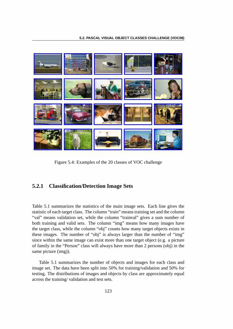
5.2. PASCAL VISUAL OBJECT CLASSES CHALLENGE (VOC08)
Figure 5.4: Examples of the 20 classes of VOC challenge
5.2.1 Classification/Detection Image Sets
Table 5.1 summarizes the statistics of the main image sets. Each line gives thestatistic of each target class. The column “train” means training set and the column“val” means validation set, while the column “trainval” gives a sum number ofboth training and valid sets. The column “img” means how manyimages havethe target class, while the column “obj” counts how many target objects exists inthese images. The number of “obj” is always larger than the number of “img”since within the same image can exist more than one target object (e.g. a pictureof family in the “Person” class will always have more than 2 persons (obj) in thesame picture (img)).
Table 5.1 summarizes the number of objects and images for each class andimage set. The data have been split into 50% for training/validation and 50% fortesting. The distributions of images and objects by class are approximately equalacross the training/ validation and test sets.
123

5. FEATURE SELECTION IN A CORTEX-LIKE OBJECT RECOGNITION MODEL
Table 5.1: Statistics of the main image sets. Object statistics list only the “non-diffcult” objects used in the evaluation.
train val trainvalimg obj img obj img obj
Aeroplane 119 159 117 157 236 316Bicycle 92 133 100 136 192 269
Bird 166 239 139 237 305 476Boat 111 170 96 166 207 336
Bottle 129 229 114 228 243 457Bus 48 61 52 68 100 129Car 243 426 223 414 466 840Cat 159 186 169 192 328 378
Chair 177 313 174 310 351 623Cow 37 61 37 69 74 130
Diningtable 53 55 52 55 105 110Dog 186 238 202 239 388 477
Horse 96 139 102 146 198 285Motorbike 102 137 102 135 204 272
Person 947 1996 1055 2172 2002 4168Pottedplant 85 178 95 183 180 361
Sheep 32 67 32 78 64 145Sofa 69 74 65 77 134 151
Train 78 83 73 83 151 166Tvmonitor 107 138 108 136 215 274
Total 2113 5082 2227 5281 4340 10363
124
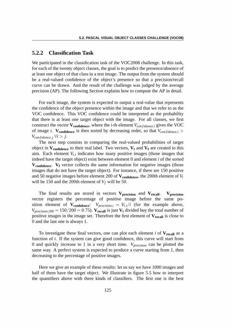
5.2. PASCAL VISUAL OBJECT CLASSES CHALLENGE (VOC08)
5.2.2 Classification Task
We participated in the classification task of the VOC2008 challenge. In this task,for each of the twenty object classes, the goal is to predict the presence/absence ofat least one object of that class in a test image. The output from the system shouldbe a real-valued confidence of the object’s presence so that aprecision/recallcurve can be drawn. And the result of the challenge was judgedby the averageprecision (AP). The following Section explains how to compute the AP in detail.
For each image, the system is expected to output a real-valuethat representsthe confidence of the object presence within the image and that we refer to as theVOC confidence. This VOC confidence could be interpreted as the probabilitythat there is at least one target object with the image. For all classes, we firstconstruct the vectorVconfidence, where thei-th elementVcon f idence,i gives the VOCof imagei. Vconfidence is then sorted by decreasing order, so thatVcon f idence,i >Vcon f idence, j ∀i > j.
The next step consists in comparing the real-valued probabilities of targetobject inVconfidenceto their real label. Two vectors,Vt andVf are created to thisaim. Each elementVt,i indicates how many positive images (those images thatindeed have the target object) exist between element 0 and elementi of the sortedVconfidence. Vf vector collects the same information for negative images (thoseimages that do not have the target object). For instance, if there are 150 positiveand 50 negative images before element 200 ofVconfidence, the 200th element ofVt
will be 150 and the 200th element ofVf will be 50.
The final results are stored in vectorsVprecision and Vrecall. Vprecisionvector registers the percentage of positive image before the same po-sition element of Vconfidence: Vprecision,i = Vt,i/i (for the example above,Vprecision,200= 150/200= 0.75). Vrecall is justVt divided buy the total number ofpositive images in the image set. Therefore the first elementof Vrecall is close to0 and the last one is always 1.
To investigate these final vectors, one can plot each elementi of Vrecall as afunction of i. If the system can give good confidence, this curve will startfrom0 and quickly increase to 1 in a very short time.Vprecision can be plotted thesame way. A perfect system is expected to produce a curve starting from 1, thendecreasing to the percentage of positive images.
Here we give an example of these results: let us say we have 1000 images andhalf of them have the target object. We illustrate in figure 5.5 how to interpretthe quantifiers above with three kinds of classifiers. The first one is the best
125
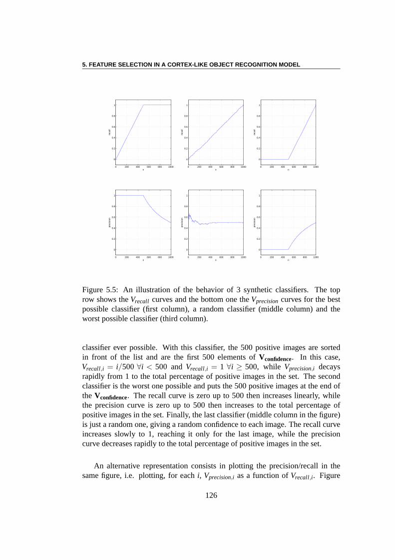
5. FEATURE SELECTION IN A CORTEX-LIKE OBJECT RECOGNITION MODEL
0 200 400 600 800 1000
0
0.2
0.4
0.6
0.8
1
n
reca
ll
0 200 400 600 800 1000
0
0.2
0.4
0.6
0.8
1
n
reca
ll
0 200 400 600 800 1000
0
0.2
0.4
0.6
0.8
1
n
reca
ll0 200 400 600 800 1000
0
0.2
0.4
0.6
0.8
1
n
prec
isio
n
0 200 400 600 800 1000
0
0.2
0.4
0.6
0.8
1
n
prec
isio
n
0 200 400 600 800 1000
0
0.2
0.4
0.6
0.8
1
n
prec
isio
n
Figure 5.5: An illustration of the behavior of 3 synthetic classifiers. The toprow shows theVrecall curves and the bottom one theVprecision curves for the bestpossible classifier (first column), a random classifier (middle column) and theworst possible classifier (third column).
classifier ever possible. With this classifier, the 500 positive images are sortedin front of the list and are the first 500 elements ofVconfidence. In this case,Vrecall,i = i/500 ∀i < 500 andVrecall,i = 1 ∀i ≥ 500, while Vprecision,i decaysrapidly from 1 to the total percentage of positive images in the set. The secondclassifier is the worst one possible and puts the 500 positiveimages at the end ofthe Vconfidence. The recall curve is zero up to 500 then increases linearly, whilethe precision curve is zero up to 500 then increases to the total percentage ofpositive images in the set. Finally, the last classifier (middle column in the figure)is just a random one, giving a random confidence to each image.The recall curveincreases slowly to 1, reaching it only for the last image, while the precisioncurve decreases rapidly to the total percentage of positiveimages in the set.
An alternative representation consists in plotting the precision/recall in thesame figure, i.e. plotting, for eachi, Vprecision,i as a function ofVrecall,i. Figure
126
5.2. PASCAL VISUAL OBJECT CLASSES CHALLENGE (VOC08)
0 0.2 0.4 0.6 0.8 10
0.2
0.4
0.6
0.8
1
recall
prec
isio
n
0 0.2 0.4 0.6 0.8 10
0.2
0.4
0.6
0.8
1
recall
prec
isio
n0 0.2 0.4 0.6 0.8 1
0
0.2
0.4
0.6
0.8
1
recall
prec
isio
n
Figure 5.6: Precision/recall curve, the x-axis is the recall values and the y-axisis the corresponding precision value, the left is from best classifier, the middle isfrom the random classifier and the right is from the worst classifier
5.6 shows the result for the three cases illustrated above. The average preci-sion (AP) is then computed from these precision/recall curves. In practice, therange of recall is divided into 11 sub-parts :{0}, [0.1,1.0], [0.2,1.0], ... [0.9,1.0]and 1.0. The AP is the average of the largest precision value in eachsub-parts:AP= 1
11 ∑10i=0max(precision∈ recall([ i
10,1])). The AP fitness is also called VOCfitness in this chapter.
For the three synthetic classifiers illustrated above, the AP fitness is :APbest=1.0, APrandom= 0.5234 andAPworst = 0.5.
An example code for computing the precision/recall and AP measure is pro-vided in the development kit [140].
Note that, in the system developed by Poggio and collaborators, the final clas-sification stage results in a simple binary response : the input image is guessedto contain (output = 0) or not to contain (ouput=1) one objectbelonging to theimage class under study (car, plane...). In our case however, the above mentioneddefinition of fitness is based on a real-valued confidence indicator and not a bi-nary answer, e.g. whether the target is guessed to exists in the image scene or not.We thus first use an Evolutionary Algorithm to optimize a linear classifier thatproduces the VOC confidence for every images, then compute the AP (averageprecision) of the training set and validation set. For this optimization step, thefitness is simply the AP, to be maximized: the EA seeks to optimize the coeffi-cient of the final linear classifier so as to maximize the AP. A second layer willbe added on top of this EA, trying to select the patches in an optimal manner. Asecond evolutionary algorithm will wrap the system described above, resulting inamulti-evolutionary algorithm.
127
5. FEATURE SELECTION IN A CORTEX-LIKE OBJECT RECOGNITION MODEL
5.3 Experiments
5.3.1 Using EC Algorithms with SMF Model
As explained in the previous section, instead of giving an unambiguousYes orNo answer for the question whether there exists a target object in the test image,the VOC challenge requests an intermediate fitness (the VOC confidence) for theprobability that the target object exists in the image, in order to be able to sortthe ensemble of images and compute the final fitness (AP). Thiskind of fitnessis useful for real-world applications (e.g. image search engines), but it cannotbe directly applied to the conventional SMFs model with SVM classifier. Sincethe relationship between the VOC confidence and the AP fitnessis nonlinear,and almost no prime knowledge about the relationships between them can beused directly, Evolutionary Algorithms seems to be a good choice for this kindof problem. The EC algorithm here is used to optimize a monolayer linearcombinator to create VOC confidence for each image, and the final fitness usedby EA is the AP fitness.
Therefore in our study, we apply evolutionary optimizationusing CMA-ES(see Section 2.2.3) to optimize the VOC confidence for all object classes. In afirst step, we will use CMA-ES to optimize the weights of a linear combination(Section 5.3.3). But because there are 1000 features gathered from the randomchoice of patches in layer C1, and in order to try to reduce the complexity of theoverall algorithm, we will also implement a multi-level Evolutionary Algorithm(Multi-Evolutionary algorithm for short) to optimally select a small subset (200here) of those 1000 features while preserving the recognition accuracy. This willbe presented in Section 5.3.4
5.3.2 Pre-training of SMFs model
We will first briefly present the pre-training process for theSMFs model beforeapplying our optimization approach.
Because the VOCdevkit is released in Matlab code and the demo programreleased by Serre is also in Matlab code, we build our own program in Matlab onthe basis of the Serre’s version1 and keep the original parameters settings. Thepre-training process is as follows:
• First, all training and validation images have to be normalized to a gray
1The author gratefully acknowledges Thomas Serre, McGovernInstitute for Brain Research,MIT, for kindly providing the Matlab code of his program
128
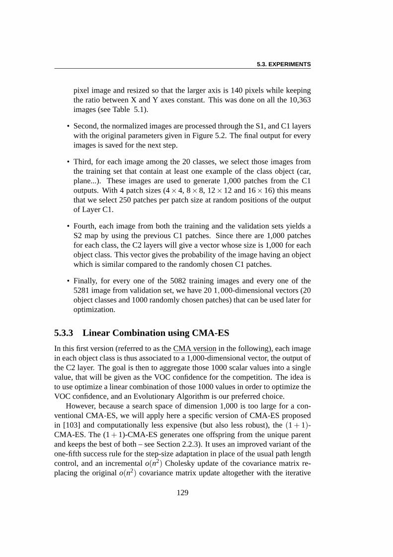
5.3. EXPERIMENTS
pixel image and resized so that the larger axis is 140 pixels while keepingthe ratio between X and Y axes constant. This was done on all the 10,363images (see Table 5.1).
• Second, the normalized images are processed through the S1, and C1 layerswith the original parameters given in Figure 5.2. The final output for everyimages is saved for the next step.
• Third, for each image among the 20 classes, we select those images fromthe training set that contain at least one example of the class object (car,plane...). These images are used to generate 1,000 patches from the C1outputs. With 4 patch sizes (4×4, 8×8, 12×12 and 16×16) this meansthat we select 250 patches per patch size at random positionsof the outputof Layer C1.
• Fourth, each image from both the training and the validation sets yields aS2 map by using the previous C1 patches. Since there are 1,000 patchesfor each class, the C2 layers will give a vector whose size is 1,000 for eachobject class. This vector gives the probability of the imagehaving an objectwhich is similar compared to the randomly chosen C1 patches.
• Finally, for every one of the 5082 training images and everyone of the5281 image from validation set, we have 20 1,000-dimensional vectors (20object classes and 1000 randomly chosen patches) that can beused later foroptimization.
5.3.3 Linear Combination using CMA-ES
In this first version (referred to as theCMA version in the following), each imagein each object class is thus associated to a 1,000-dimensional vector, the output ofthe C2 layer. The goal is then to aggregate those 1000 scalar values into a singlevalue, that will be given as the VOC confidence for the competition. The idea isto use optimize a linear combination of those 1000 values in order to optimize theVOC confidence, and an Evolutionary Algorithm is our preferred choice.
However, because a search space of dimension 1,000 is too large for a con-ventional CMA-ES, we will apply here a specific version of CMA-ES proposedin [103] and computationally less expensive (but also less robust), the(1+ 1)-CMA-ES. The (1+ 1)-CMA-ES generates one offspring from the unique parentand keeps the best of both – see Section 2.2.3). It uses an improved variant of theone-fifth success rule for the step-size adaptation in placeof the usual path lengthcontrol, and an incrementalo(n2) Cholesky update of the covariance matrix re-placing the originalo(n2) covariance matrix update altogether with the iterative
129
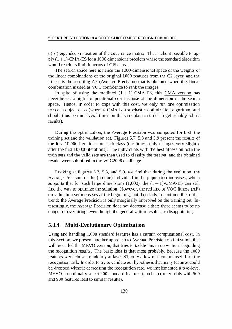
5. FEATURE SELECTION IN A CORTEX-LIKE OBJECT RECOGNITION MODEL
o(n3) eigendecomposition of the covariance matrix. That make it possible to ap-ply (1+1)-CMA-ES for a 1000 dimensions problem where the standard algorithmwould reach its limit in terms of CPU cost.
The search space here is hence the 1000-dimensional space ofthe weights ofthe linear combinations of the original 1000 features from the C2 layer, and thefitness is the resulting AP (Average Precision) that is obtained when this linearcombination is used as VOC confidence to rank the images.
In spite of using the modified(1 + 1)-CMA-ES, this CMA version hasnevertheless a high computational cost because of the dimension of the searchspace. Hence, in order to cope with this cost, we only run one optimizationfor each object class (whereas CMA is a stochastic optimization algorithm, andshould thus be ran several times on the same data in order to get reliably robustresults).
During the optimization, the Average Precision was computed for both thetraining set and the validation set. Figures 5.7, 5.8 and 5.9present the results ofthe first 10,000 iterations for each class (the fitness only changes very slightlyafter the first 10,000 iterations). The individuals with thebest fitness on both thetrain sets and the valid sets are then used to classify the test set, and the obtainedresults were submitted to the VOC2008 challenge.
Looking at Figures 5.7, 5.8, and 5.9, we find that during the evolution, theAverage Precision of the (unique) individual in the population increases, whichsupports that for such large dimensions (1,000), the(1+ 1)-CMA-ES can stillfind the way to optimize the solution. However, the red line ofVOC fitness (AP)on validation set increases at the beginning, but then failsto continue this initialtrend: the Average Precision is only marginally improved onthe training set. In-terestingly, the Average Precision does not decrease either: there seems to be nodanger of overfitting, even though the generalization results are disappointing.
5.3.4 Multi-Evolutionary Optimization
Using and handling 1,000 standard features has a certain computational cost. Inthis Section, we present another approach to Average Precision optimization, thatwill be called theMEVO version, that tries to tackle this issue without degradingthe recognition results. The basic idea is that most probably, because the 1000features were chosen randomly at layer S1, only a few of them are useful for therecognition task. In order to try to validate our hypothesisthat many features couldbe dropped without decreasing the recognition rate, we implemented a two-levelMEVO, to optimally select 200 standard features (patches) (other trials with 500and 900 features lead to similar results).
130
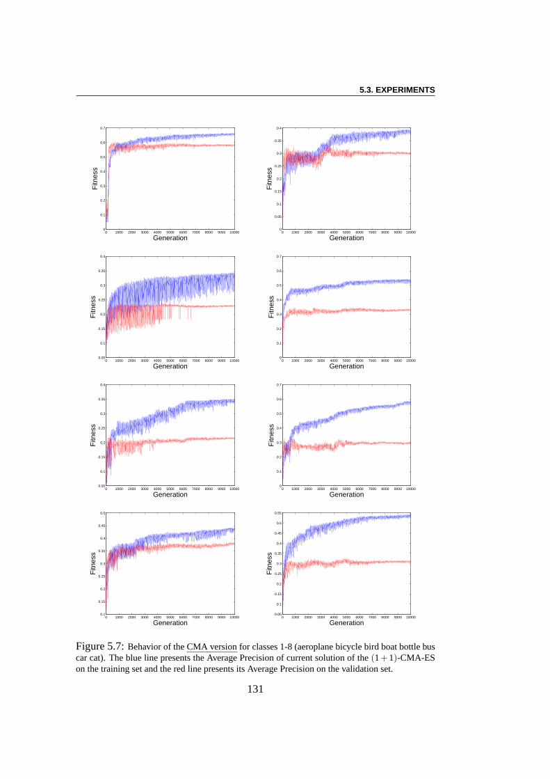
5.3. EXPERIMENTS
0 1000 2000 3000 4000 5000 6000 7000 8000 9000 100000
0.1
0.2
0.3
0.4
0.5
0.6
0.7
Generation
Fitn
ess
0 1000 2000 3000 4000 5000 6000 7000 8000 9000 100000
0.05
0.1
0.15
0.2
0.25
0.3
0.35
0.4
Generation
Fitn
ess
0 1000 2000 3000 4000 5000 6000 7000 8000 9000 100000.05
0.1
0.15
0.2
0.25
0.3
0.35
0.4
Generation
Fitn
ess
0 1000 2000 3000 4000 5000 6000 7000 8000 9000 100000
0.1
0.2
0.3
0.4
0.5
0.6
0.7
Generation
Fitn
ess
0 1000 2000 3000 4000 5000 6000 7000 8000 9000 100000.05
0.1
0.15
0.2
0.25
0.3
0.35
0.4
Generation
Fitn
ess
0 1000 2000 3000 4000 5000 6000 7000 8000 9000 100000
0.1
0.2
0.3
0.4
0.5
0.6
0.7
Generation
Fitn
ess
0 1000 2000 3000 4000 5000 6000 7000 8000 9000 100000.1
0.15
0.2
0.25
0.3
0.35
0.4
0.45
0.5
Generation
Fitn
ess
0 1000 2000 3000 4000 5000 6000 7000 8000 9000 100000.05
0.1
0.15
0.2
0.25
0.3
0.35
0.4
0.45
0.5
0.55
Generation
Fitn
ess
Figure 5.7:Behavior of theCMA version for classes 1-8 (aeroplane bicycle bird boat bottlebuscar cat). The blue line presents the Average Precision of current solution of the(1+1)-CMA-ESon the training set and the red line presents its Average Precision on the validation set.
131
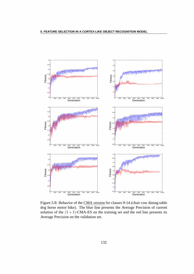
5. FEATURE SELECTION IN A CORTEX-LIKE OBJECT RECOGNITION MODEL
0 1000 2000 3000 4000 5000 6000 7000 8000 9000 100000.1
0.15
0.2
0.25
0.3
0.35
0.4
0.45
0.5
Generation
Fitn
ess
0 1000 2000 3000 4000 5000 6000 7000 8000 9000 100000
0.1
0.2
0.3
0.4
0.5
0.6
0.7
Generation
Fitn
ess
0 1000 2000 3000 4000 5000 6000 7000 8000 9000 100000
0.05
0.1
0.15
0.2
0.25
0.3
0.35
0.4
Generation
Fitn
ess
0 1000 2000 3000 4000 5000 6000 7000 8000 9000 100000.05
0.1
0.15
0.2
0.25
0.3
0.35
0.4
Generation
Fitn
ess
0 1000 2000 3000 4000 5000 6000 7000 8000 9000 100000
0.05
0.1
0.15
0.2
0.25
0.3
0.35
Generation
Fitn
ess
0 1000 2000 3000 4000 5000 6000 7000 8000 9000 100000.05
0.1
0.15
0.2
0.25
0.3
0.35
0.4
0.45
0.5
Generation
Fitn
ess
Figure 5.8: Behavior of theCMA version for classes 9-14 (chair cow dining-tabledog horse motor bike). The blue line presents the Average Precision of currentsolution of the(1+ 1)-CMA-ES on the training set and the red line presents itsAverage Precision on the validation set.
132
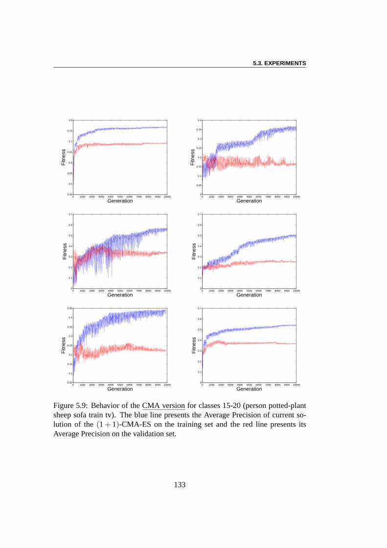
5.3. EXPERIMENTS
0 1000 2000 3000 4000 5000 6000 7000 8000 9000 100000.45
0.5
0.55
0.6
0.65
0.7
0.75
0.8
Generation
Fitn
ess
0 1000 2000 3000 4000 5000 6000 7000 8000 9000 100000
0.05
0.1
0.15
0.2
0.25
0.3
0.35
0.4
Generation
Fitn
ess
0 1000 2000 3000 4000 5000 6000 7000 8000 9000 100000
0.1
0.2
0.3
0.4
0.5
0.6
0.7
Generation
Fitn
ess
0 1000 2000 3000 4000 5000 6000 7000 8000 9000 100000
0.1
0.2
0.3
0.4
0.5
0.6
0.7
Generation
Fitn
ess
0 1000 2000 3000 4000 5000 6000 7000 8000 9000 100000.05
0.1
0.15
0.2
0.25
0.3
0.35
0.4
0.45
Generation
Fitn
ess
0 1000 2000 3000 4000 5000 6000 7000 8000 9000 100000
0.1
0.2
0.3
0.4
0.5
0.6
0.7
Generation
Fitn
ess
Figure 5.9: Behavior of theCMA version for classes 15-20 (person potted-plantsheep sofa train tv). The blue line presents the Average Precision of current so-lution of the (1+ 1)-CMA-ES on the training set and the red line presents itsAverage Precision on the validation set.
133
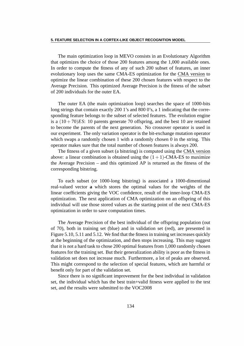
5. FEATURE SELECTION IN A CORTEX-LIKE OBJECT RECOGNITION MODEL
The main optimization loop in MEVO consists in an Evolutionary Algorithmthat optimizes the choice of those 200 features among the 1,000 available ones.In order to compute the fitness of any of such 200 subset of features, an innerevolutionary loop uses the same CMA-ES optimization for theCMA version tooptimize the linear combination of these 200 chosen features with respect to theAverage Precision. This optimized Average Precision is thefitness of the subsetof 200 individuals for the outer EA.
The outer EA (the main optimization loop) searches the spaceof 1000-bitslong strings that contain exactly 200 1’s and 800 0’s, a 1 indicating that the corre-sponding feature belongs to the subset of selected features. The evolution engineis a (10+ 70)ES: 10 parents generate 70 offspring, and the best 10 are retainedto become the parents of the next generation. No crossover operator is used inour experiment. The only variation operator is the bit-exchange mutation operatorwhich swaps a randomly chosen 1 with a randomly chosen 0 in thestring. Thisoperator makes sure that the total number of chosen featuresis always 200.
The fitness of a given subset (a bitstring) is computed using theCMA versionabove: a linear combination is obtained using the(1+1)-CMA-ES to maximizethe Average Precision – and this optimized AP is returned as the fitness of thecorresponding bitstring.
To each subset (or 1000-long bitstring) is associated a 1000-dimentionalreal-valued vectora which stores the optimal values for the weights of thelinear coefficients giving the VOC confidence, result of the inner-loop CMA-ESoptimization. The next application of CMA optimization on anoffspring of thisindividual will use those stored values as the starting point of the next CMA-ESoptimization in order to save computation times.
The Average Precision of the best individual of the offspring population (outof 70), both in training set (blue) and in validation set (red), are presented inFigure 5.10, 5.11 and 5.12. We find that the fitness in trainingset increases quicklyat the beginning of the optimization, and then stops increasing. This may suggestthat it is not a hard task to chose 200 optimal features from 1,000 randomly chosenfeatures for the training set. But their generalization ability is poor as the fitness invalidation set does not increase much. Furthermore, a lot ofpeaks are observed.This might correspond to the selection of special features,which are harmful orbenefit only for part of the validation set.
Since there is no significant improvement for the best individual in validationset, the individual which has the best train+valid fitness were applied to the testset, and the results were submitted to the VOC2008
134
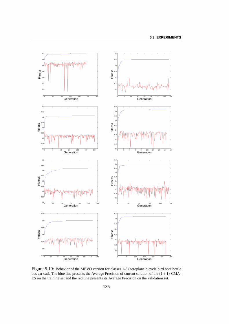
5.3. EXPERIMENTS
0 50 100 150 200 250 3000
0.1
0.2
0.3
0.4
0.5
0.6
0.7
Generation
Fitn
ess
0 20 40 60 80 100 120 140 160
0.2
0.25
0.3
0.35
0.4
0.45
0.5
Generation
Fitn
ess
0 50 100 150 200 250 3000.1
0.15
0.2
0.25
0.3
0.35
0.4
0.45
0.5
Generation
Fitn
ess
0 20 40 60 80 100 120 140 160 1800.2
0.25
0.3
0.35
0.4
0.45
0.5
0.55
0.6
0.65
Generation
Fitn
ess
0 50 100 150 200 250 3000.1
0.15
0.2
0.25
0.3
0.35
0.4
0.45
0.5
Generation
Fitn
ess
0 50 100 150 200 250
0.2
0.25
0.3
0.35
0.4
0.45
0.5
0.55
0.6
0.65
Generation
Fitn
ess
0 20 40 60 80 100 120 140 1600.25
0.3
0.35
0.4
0.45
0.5
0.55
Generation
Fitn
ess
0 50 100 150 200 250 300
0.2
0.25
0.3
0.35
0.4
0.45
0.5
0.55
Generation
Fitn
ess
Figure 5.10:Behavior of theMEVO version for classes 1-8 (aeroplane bicycle bird boat bottlebus car cat). The blue line presents the Average Precision ofcurrent solution of the(1+1)-CMA-ES on the training set and the red line presents its Average Precision on the validation set.
135
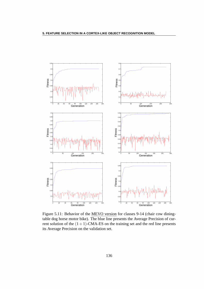
5. FEATURE SELECTION IN A CORTEX-LIKE OBJECT RECOGNITION MODEL
0 20 40 60 80 100 120 140 160 1800.2
0.25
0.3
0.35
0.4
0.45
0.5
0.55
Generation
Fitn
ess
0 50 100 150 200 2500.1
0.2
0.3
0.4
0.5
0.6
0.7
0.8
Generation
Fitn
ess
0 50 100 150 200 2500.1
0.15
0.2
0.25
0.3
0.35
0.4
0.45
0.5
0.55
0.6
Generation
Fitn
ess
0 50 100 150 200 250 3000.2
0.22
0.24
0.26
0.28
0.3
0.32
0.34
0.36
0.38
Generation
Fitn
ess
0 20 40 60 80 100 120 140 160
0.2
0.25
0.3
0.35
0.4
0.45
0.5
Generation
Fitn
ess
0 20 40 60 80 100 120 140 160 1800.2
0.25
0.3
0.35
0.4
0.45
0.5
0.55
Generation
Fitn
ess
Figure 5.11: Behavior of theMEVO version for classes 9-14 (chair cow dining-table dog horse motor bike). The blue line presents the Average Precision of cur-rent solution of the(1+1)-CMA-ES on the training set and the red line presentsits Average Precision on the validation set.
136
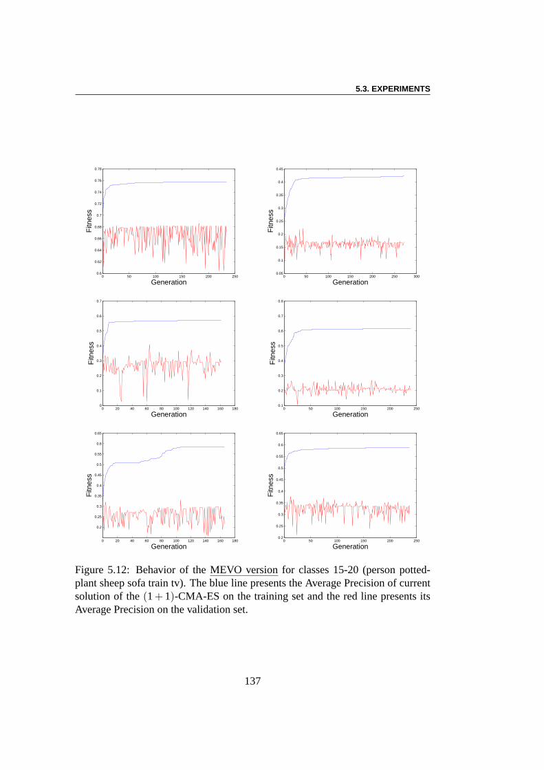
5.3. EXPERIMENTS
0 50 100 150 200 2500.6
0.62
0.64
0.66
0.68
0.7
0.72
0.74
0.76
0.78
Generation
Fitn
ess
0 50 100 150 200 250 3000.05
0.1
0.15
0.2
0.25
0.3
0.35
0.4
0.45
Generation
Fitn
ess
0 20 40 60 80 100 120 140 160 1800
0.1
0.2
0.3
0.4
0.5
0.6
0.7
Generation
Fitn
ess
0 50 100 150 200 2500.1
0.2
0.3
0.4
0.5
0.6
0.7
0.8
Generation
Fitn
ess
0 20 40 60 80 100 120 140 160 180
0.2
0.25
0.3
0.35
0.4
0.45
0.5
0.55
0.6
0.65
Generation
Fitn
ess
0 50 100 150 200 2500.2
0.25
0.3
0.35
0.4
0.45
0.5
0.55
0.6
0.65
Generation
Fitn
ess
Figure 5.12: Behavior of theMEVO version for classes 15-20 (person potted-plant sheep sofa train tv). The blue line presents the Average Precision of currentsolution of the(1+ 1)-CMA-ES on the training set and the red line presents itsAverage Precision on the validation set.
137
5. FEATURE SELECTION IN A CORTEX-LIKE OBJECT RECOGNITION MODEL
We will give the final test results and then compare these two methods in thenext section.
5.3.5 Results
Table 5.2 shows the final results for the 18 different participants’ algorithms thatparticipated to the VOC 2008 challenge (our two own methods are indicated withbold faces). We immediately note that our two methods do clearly not competewith the best methods for each class. Nevertheless, our results are comparable tothose of several other methods participating in the challenge. Furthermore, onemust keep in mind that all the other methods (even among thosethat show worseresults than ours) are developed by research groups with a long-lasting expertisein computer image analysis. We only leveraged the self-training properties ofthe original neural network-based method and almost parameter-free evolutionarystrategies, to reach, with no a priori expertise on computervision, a similar levelof performance than several of these groups. We think that this is an encouragingindication of the promises of this research direction. Moreover we think that ourmethods still offers a wide room for improvement. To this aim, let us first proceedin the following to a deeper analysis of our results.
5.3.6 Result Analysis
In Table 5.3, we summarize the VOC fitness results of theCMA version and theMEVO versions of our approaches, with separate comparison of theresults on thetraining set, the validation set, and the test set. We also list the corresponding bestfitness results among all participants of VOC 2008.
In Figures 5.13 and 5.14, we further give similar information with histogramsof the performance of CMA and MEVO, comparing their fitness on the trainingset (deep blue), validation set (sky blue), and test set (yellow) to the best VOC2008 fitness (brownish red).
From these tables and figures, we find that the results of MEVO on the train-ing set are statistically better than that of CMA. On the otherhand, comparing theresults obtained on the validation set and on the test set, nostatistical differencecan be seen any more, but most of the time, the MEVO version seems to general-ize better than the CMA version (with some noteworthy exceptions like the cowclass!) : using only 200 features allows to slightly overfit the training set, with-out degrading too much the generalization results, even improving them on manyclasses.
However, when compared with the best VOC08 results, our test result lookmuch worse. Furthermore, for several object classes, our results on the trainingset are better than the best VOC08 results (e.g. CMA version forclasses 5, 6, 10,
138
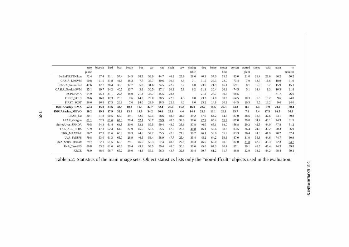
5.3.EX
PE
RIM
EN
TS
aero bicycle bird boat bottle bus car cat chair cow dining doghorse motor person potted sheep sofa train tv
plane table bike plant monitor
BerlinFIRSTNikon 72.4 37.4 51.1 57.4 24.5 38.5 53.9 44.7 46.2 25.6 28.6 40.3 57.0 53.5 83.0 21.0 21.4 28.6 66.2 50.2
CASIA_LinSVM 50.8 21.5 31.8 41.8 18.3 7.7 35.7 40.6 30.6 4.9 7.1 31.5 29.3 22.0 73.4 7.9 13.7 11.6 18.9 31.0
CASIA_NeuralNet 47.6 12.7 28.4 35.3 12.7 5.8 31.6 34.5 22.7 3.7 6.0 23.6 21.9 16.1 69.1 8.1 5.0 8.7 15.9 15.1
CASIA_NonLinSVM 35.1 19.7 24.2 40.5 13.7 3.8 30.5 37.1 30.2 5.8 6.2 31.1 20.4 26.3 74.5 5.1 14.4 9.3 10.3 21.8
ECPLIAMA 54.9 25.3 31.1 29.8 18.9 21.4 33.7 25.5 28.4 - - 21.2 27.7 30.5 68.5 - - - 31.7 26.6
FIRST_SC1C 36.6 16.8 17.3 26.9 7.6 14.0 29.0 28.5 22.9 4.3 8.023.2 14.8 30.3 64.5 10.3 5.5 13.2 9.6 24.0
FIRST_SCST 36.6 16.8 17.3 26.9 7.6 14.0 29.0 28.5 22.9 4.3 8.023.2 14.8 30.3 64.5 10.3 5.5 13.2 9.6 24.0
INRIASaclay_CMA 52.4 15.0 23.6 33.9 10.2 10.3 32.7 32.4 26.4 13.2 16.0 22.2 18.5 27.3 64.8 8.6 4.4 7.9 20.0 30.4
INRIASaclay_MEVO 50.2 19.5 17.9 32.1 13.0 14.9 34.2 30.6 23.1 4.4 14.8 21.0 13.1 26.1 65.7 7.6 7.4 17.5 16.5 30.6
LEAR_flat 80.1 51.8 60.5 66.9 29.1 52.0 57.4 58.6 48.7 31.0 39.2 47.6 64.2 64.6 87.0 28.6 33.3 42.6 73.1 59.8
LEAR_shotgun 81.1 52.9 61.6 67.8 29.4 52.1 58.7 59.9 48.5 32.0 38.6 47.9 65.4 65.2 87.0 29.0 34.4 43.1 74.3 61.5
SurreyUvA_SRKDA 79.5 54.3 61.4 64.8 30.0 52.1 59.5 59.4 48.9 33.6 37.8 46.0 66.1 64.0 86.8 29.2 42.3 44.0 77.8 61.2
TKK_ALL_SFBS 77.9 47.3 52.4 61.0 27.9 45.5 53.5 55.5 47.6 26.8 40.8 46.1 58.6 58.3 83.5 26.4 24.3 39.2 70.3 56.9
TKK_MAXVAL 76.7 47.3 51.6 60.8 28.3 44.6 54.2 55.5 47.8 21.2 39.2 46.1 58.8 55.9 83.3 26.4 24.3 41.9 70.2 52.4
UvA_FullSFS 79.8 53.0 61.3 65.7 28.9 46.5 58.4 58.9 47.7 25.435.4 45.2 64.2 59.6 87.0 31.0 35.3 44.6 74.7 60.9
UvA_Soft5ColorSift 79.7 52.1 61.5 65.5 29.1 46.5 58.3 57.4 48.2 27.9 38.3 46.6 66.0 60.6 87.0 31.8 42.2 45.3 72.3 64.7
UvA_TreeSFS 80.8 53.2 61.6 65.6 29.4 49.9 58.5 59.4 48.0 30.1 39.6 45.0 67.360.4 87.1 30.1 41.5 45.4 74.3 59.8
XRCE 78.9 48.0 58.7 65.2 29.0 44.8 56.1 56.3 43.7 32.8 30.4 39.7 61.2 61.7 86.8 22.9 34.2 44.2 68.4 59.1
Table 5.2: Statistics of the main image sets. Object statistics lists only the “non-diffcult” objects used in the evaluation.
139
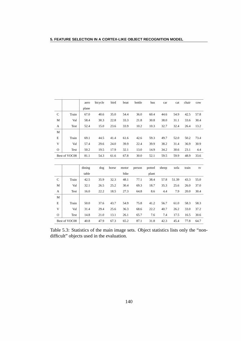
5. FEATURE SELECTION IN A CORTEX-LIKE OBJECT RECOGNITION MODEL
aero bicycle bird boat bottle bus car cat chair cow
plane
C Train 67.0 40.6 35.0 54.4 36.0 60.4 44.6 54.9 42.5 57.8
M Val 58.4 30.3 22.8 33.3 21.8 30.8 38.0 31.1 33.6 30.4
A Test 52.4 15.0 23.6 33.9 10.2 10.3 32.7 32.4 26.4 13.2
M
E Train 69.1 44.5 41.4 61.6 42.6 59.3 49.7 52.0 50.2 73.4
V Val 57.4 29.6 24.0 39.9 22.4 39.9 38.2 31.4 36.9 30.9
O Test 50.2 19.5 17.9 32.1 13.0 14.9 34.2 30.6 23.1 4.4
Best of VOC08 81.1 54.3 61.6 67.8 30.0 52.1 59.5 59.9 48.9 33.6
dining dog horse motor person potted sheep sofa train tv
table bike plant
C Train 42.5 35.9 32.3 48.1 77.1 38.4 57.8 51.39 43.3 55.0
M Val 32.1 26.5 25.2 30.4 69.3 18.7 35.3 25.6 26.0 37.0
A Test 16.0 22.2 18.5 27.3 64.8 8.6 4.4 7.9 20.0 30.4
M
E Train 50.0 37.6 43.7 54.9 75.8 41.2 56.7 61.0 58.3 58.3
V Val 31.4 29.4 25.6 36.3 68.6 22.2 40.7 26.2 33.0 37.2
O Test 14.8 21.0 13.1 26.1 65.7 7.6 7.4 17.5 16.5 30.6
Best of VOC08 40.8 47.9 67.3 65.2 87.1 31.8 42.3 45.4 77.8 64.7
Table 5.3: Statistics of the main image sets. Object statistics lists only the “non-difficult” objects used in the evaluation.
140
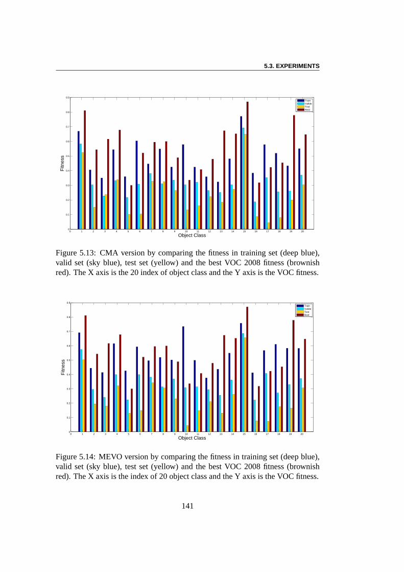
5.3. EXPERIMENTS
0 1 2 3 4 5 6 7 8 9 10 11 12 13 14 15 16 17 18 19 200
0.1
0.2
0.3
0.4
0.5
0.6
0.7
0.8
0.9
Object Class
Fitn
ess
TrainValideTestBest
Figure 5.13: CMA version by comparing the fitness in training set (deep blue),valid set (sky blue), test set (yellow) and the best VOC 2008 fitness (brownishred). The X axis is the 20 index of object class and the Y axis isthe VOC fitness.
0 1 2 3 4 5 6 7 8 9 10 11 12 13 14 15 16 17 18 19 200
0.1
0.2
0.3
0.4
0.5
0.6
0.7
0.8
0.9
Object Class
Fitn
ess
TrainValideTestBest
Figure 5.14: MEVO version by comparing the fitness in training set (deep blue),valid set (sky blue), test set (yellow) and the best VOC 2008 fitness (brownishred). The X axis is the index of 20 object class and the Y axis isthe VOC fitness.
141
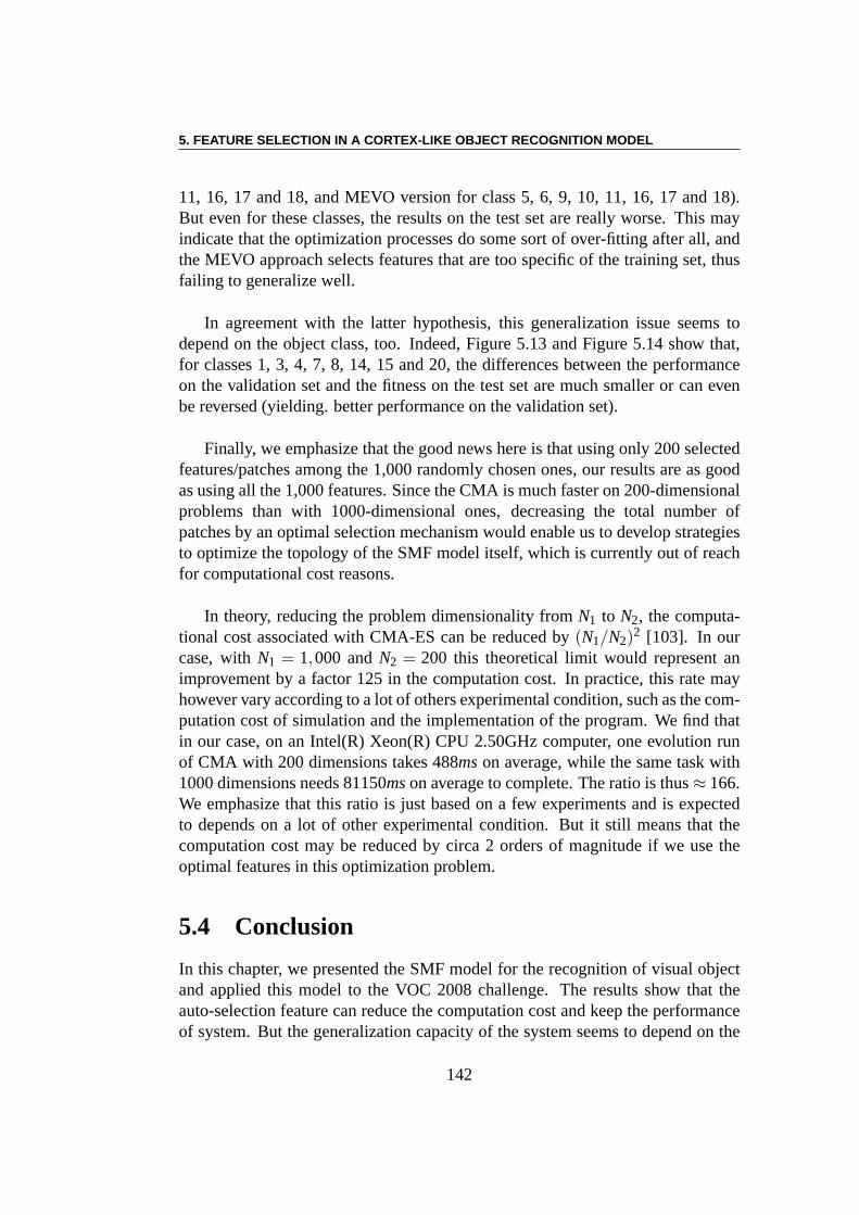
5. FEATURE SELECTION IN A CORTEX-LIKE OBJECT RECOGNITION MODEL
11, 16, 17 and 18, and MEVO version for class 5, 6, 9, 10, 11, 16,17 and 18).But even for these classes, the results on the test set are really worse. This mayindicate that the optimization processes do some sort of over-fitting after all, andthe MEVO approach selects features that are too specific of the training set, thusfailing to generalize well.
In agreement with the latter hypothesis, this generalization issue seems todepend on the object class, too. Indeed, Figure 5.13 and Figure 5.14 show that,for classes 1, 3, 4, 7, 8, 14, 15 and 20, the differences between the performanceon the validation set and the fitness on the test set are much smaller or can evenbe reversed (yielding. better performance on the validation set).
Finally, we emphasize that the good news here is that using only 200 selectedfeatures/patches among the 1,000 randomly chosen ones, ourresults are as goodas using all the 1,000 features. Since the CMA is much faster on200-dimensionalproblems than with 1000-dimensional ones, decreasing the total number ofpatches by an optimal selection mechanism would enable us todevelop strategiesto optimize the topology of the SMF model itself, which is currently out of reachfor computational cost reasons.
In theory, reducing the problem dimensionality fromN1 to N2, the computa-tional cost associated with CMA-ES can be reduced by(N1/N2)
2 [103]. In ourcase, withN1 = 1,000 andN2 = 200 this theoretical limit would represent animprovement by a factor 125 in the computation cost. In practice, this rate mayhowever vary according to a lot of others experimental condition, such as the com-putation cost of simulation and the implementation of the program. We find thatin our case, on an Intel(R) Xeon(R) CPU 2.50GHz computer, one evolution runof CMA with 200 dimensions takes 488mson average, while the same task with1000 dimensions needs 81150mson average to complete. The ratio is thus≈ 166.We emphasize that this ratio is just based on a few experiments and is expectedto depends on a lot of other experimental condition. But it still means that thecomputation cost may be reduced by circa 2 orders of magnitude if we use theoptimal features in this optimization problem.
5.4 Conclusion
In this chapter, we presented the SMF model for the recognition of visual objectand applied this model to the VOC 2008 challenge. The resultsshow that theauto-selection feature can reduce the computation cost andkeep the performanceof system. But the generalization capacity of the system seems to depend on the
142

5.4. CONCLUSION
feature selected. Future work will try to optimize the topology of the connec-tions between the layers of the SMF model, and to optimize theparameters whosevalues in the current work were taken without modification from ref. [198].
143

5. FEATURE SELECTION IN A CORTEX-LIKE OBJECT RECOGNITION MODEL
144
Chapter 6
Conclusion
This dissertation has introduced our study of three different artificial neuralnetworks models: Self-Organizing Map (SOM, Chapter 3), EchoStates Network(ESN, Chapter 4) and Standard Model Features (SMF, Chapter 5).We will nowsummarize our findings, and sketch some directions for further research.
6.1 Summary of Results
6.1.1 Evolving SOM Topology
The first part of our work, Chapter 3, directly addressed issueof the influenceof the topology on Self-Organizing Maps. The task we considered for SOM net-works was the classification of handwritten digits. A modification of the originalSOM practice was to change the neighborhood relationship from Euclidian dis-tance to graph distance for weight updates, so that topologymodification resultedin modified dynamics.
In a first step, we empirically explored the influence of small-world-like topol-ogy modification of the standard regular SOM topology on the performance forthe task at hand. The small-world topology is created by rewiring the connec-tions of a regular SOM network with a probabilityρ. By varying the rewiringprobability, we tracked the performance of different topologies in the handwrittendigits recognition task and found out that, in this class of topologies, topologyhas a small impact on the performance. Furthermore, it does not seem to influ-ence the robustness to neuron failures, at least for long learning times. This resultmay indicate that the performance of the network is only weakly controlled by itstopology, at least for such learning tasks.
We then addressed the inverse problem, and evolved SOM topologies of the
145
6. CONCLUSION
same class with the goal of maximizing the performance on thehandwritten dig-its recognition. The evolutionary algorithm used a direct representation of thenetwork topology, where mutation directly manipulates theconnections. Unfor-tunately, because of the high computation cost of such evolutions, we could onlyapply such evolutionary algorithm to find the optimal topology of a small net-work (100 neurons). At the end of optimization, however, theperformance ofthe best network is improved by almost 10%. All evolved networks are ’morerandom’ than the initial small-world topology population,and display a more het-erogeneous degree distribution, which may indicate a tendency to evolve towardscale-free topologies. Unfortunately, in order to confirm this tendency with lessambiguity, larger networks should be considered.
6.1.2 Evolving Parameters and Hyper-parameters of ESN
Reservoir Computing is an alternative to the fine tuning of NNs topology for eachtask, and has recently received a lot of attention. The original idea of Echo StateNetworks, as proposed by Jaeger, is to rely on random sparse connections within avery large network and to simply combine them linearly. The topology is governedby some hyper-parameters, and only the out-going weights are optimized, leadingto a quadratic optimization problem in the supervised learning case. The questionremains about how to tune those hyper-parameters for a giventask - and whetherthe ESN approach can be efficient in other contexts, e.g., some reinforcementlearning tasks.
In Chapter 4, we demonstrated the ability of CMA-ES, the state-of-the-artmethod in evolutionary continuous parameter optimization, to efficiently optimizeESN parameters and hyper-parameters for both the standard supervised learningcontext already used in previous studies and for the double-pole balancing,a typical reinforcement learning task. Indeed, the flexibility of Evolutionaryoptimization allowed us to optimize not only the outgoing weights but also, otherESN parameters (the Readout, Spectral Radius, Slopes of the neurons activefunction).
The combination of ESN and CMA-ES was first tested on a standardtimeseries prediction problem, and validated against the quadratic optimizationapproach. With the standard parameter setting of an ESN with100 neurons, theresults show that CMA-ES can reach the same precision when optimizing theoutput weights than the original results obtained using quadratic optimization.With a smaller reservoir, surprisingly, optimizing only the slopes of the transferfunctions of all neurons allowed us to reach even a better prediction accuracy,though at a higher computational cost.
146
6.1. SUMMARY OF RESULTS
In the context of the double-pole balancing, the results of CMA-ES applied toESN optimization are compared to those of the best topology-learning methodsin neuro-evolution. For such a reinforcement learning task, the good news is thatEvolutionary Learning of ESN does work: our results are at the level of the bestpublished results of neuro-evolution methods. Moreover, optimizing more thanjust the outgoing weights does improve the results. Furthermore, there seems tobe a high dependency of the results on the topology of the reservoir, at least forthe small sizes experimented with here.
6.1.3 Feature Sub-Sampling in SMF Bio-Inspired Approach
The issue of the topology of the information processing workflow has receivedmany inspirations that are strongly influenced by the study of actual biologicalprocesses, when sufficient information has been gathered bybiologists. This isthe case for the biology of visual cortex, and Chapter 5 has concentrated of abio-inspired model of the visual cortex proposed for objectdetection by Serreand Poggio. Here, the topology is specifically designed to match the recentlyresearches of the biological process. However, several degrees of freedom remainin the proposed topology, leaving room for improvement.
We applied the Standard Model Features of Serre and Poggio tothe PASCALVisual multi-Object recognition Challenge (VOC2008), and concentrated on thepossible selection of some of the random features that are used in the model, in anattempt to decrease its huge computational complexity.
First, a specific variant of the CMA-ES algorithm was used to optimize thefinal layer of the model: because of the non-linearity of the VOC confidence,the measure of quality proposed within the PASCAL Challenge, the problem ofoptimizing even a linear combination of the 1000 features for this specific criterioncould hardly be solved by traditional methods. Then, a higher-level evolutionaryalgorithm was used to select a small fractions of those random features whilemaintaining the same quality of recognition results: the fitness used by this EAwas obtained by running CMA-ES on the corresponding subset offeatures andmeasuring the resulting VOC-confidence.
The results of this Multi-Evolutionary algorithm demonstrated that using onlywith 20% of the original features, the system could obtain the same performancethan with all the features, requiring less computational effort. This result opensthe path for the longer-term goal about this model: optimizealso the topology ofthe SMF model, as this was not possible with the current cost of the method whenusing all features.
147
6. CONCLUSION
6.2 Perspectives
We will here give some hints about possible research directions that emerged fromour work, both at the fundamental and at the practical levels.
6.2.1 Fundamental Issues
One of the main difficulty we faced in Chapter 3 was to find an appropriate fitnessmeasure for the performance of SOMs. Especially, when the input data set has acomplex topology which may not be already clearly understood. How to measurethe approximation between the topology of network and the topology of the dataset is a difficult task. This is why we turned to using SOMs in a classification task,which is not what they have been designed for. A new more specifical quantitativemeasure method is required for unsupervised learning, thatwill allow us to hope-fully evolve optimized SOM topologies, and to maybe confirm that some types ofscale-free topologies are better suited than the regular one, at least in some cases.But it would also help to compare SOMs to other dimension-reduction algorithms.
Regarding our work on the ESN, more research is obviously needed to un-derstand the relationship between the hyper-parameters and the performance ofreservoirs, both from a theoretical and a practical viewpoint. Even the simplequestion of the reservoir size is still open: for what tasks are larger-size reservoirshelpful? On the practical side, we could not even try to solvethe direct problemin reinforcement learning context – i.e., experimental investigate a wide range ofreservoir sizes on the same problem.
The problem of optimizing the reservoir topologies is stillopen, too, andseems to be even more out to reach in terms of computational cost. Several is-sues remain open. We would like to investigate the generative approaches basedon Genetic Regulatory Networks, as discussed at the end of Section 2.3.2. Twoapproaches can be envisioned. The straightforward approach would be to directlyevaluate the evolved topologies on the reinforcement learning problem at hand,with the huge CPU cost this implies. But, if some statistical characteristics of ef-ficient reservoirs have been previously identified, some topologies meeting thoserequirements could first be evolved, without the need for costly simulations, andonly in a second phase the evaluation would be made on the reinforcement learn-ing task. Recent experiments have demonstrated the feasibility of the first phaseof this plan [156, 157], and CPU cost is the only barrier to the second phase (seebelow).
Another possible extension of ESN research, as pointed in [138], regards thesingle-layer architecture of current reservoirs: “Even ifthe reservoirs may havethousands of units, it has still a single layer. It suggests that for demandingly
148
6.2. PERSPECTIVES
complex tasks the adaptation of a single reservoir might notbe enough and ahierarchical architecture of ESNs might be needed.” [138] The possible combi-nation between Reservoir Computing and Deep Network is another appealingfuture research direction . . . that will undoubtedly also require some orders ofmagnitude more CPU resources.
The evolutionary computing vision system presented in Chapter 5, the systemmay benefit from further advances in the biological knowledge of the natural vi-sual system. In the SMF model presented here, the parametersand the topologyof the system were completely hand-designed, and we have only accomplished asmall step in the pruning of the set of random features. But thecomplete topologycould be self-turned by an evolutionary process, especially if we can reduce theCPU cost even more. Evolving the network topology between thelayers, self-turning the system parameters together with self-selection of the C1 feature ishence a promising direction for future research.
Another issue in object recognition research is that of the sample set of images:only raw images are available at the moment, whereas a universal object data basemay be helpful for the future study of the SMF model.
6.2.2 Practical Issues
Balancing the Double Pole
As many published work used this problem as a benchmark, it made sense to keepthe same problem settings and use the same fitness definition to compare one’salgorithms with previous work. However, one important issue concerns the ade-quacy of the classical fitness used up to now to tackle this problem. Consideringthe results presented in Chapter 4, the answer is clearly thatit is not adapted to thegoal (note that such an answer has already been claimed by others before). Indeed,the correlation between the fitness and the generalization tests that the system isdemanded to pass to be declared successful, is possibly deceptive. It introducesa too high random part in the evaluation of the results: indeed, we often foundthat the best individual of the population cannot pass the test of generalization,but other individuals, with lower fitness, could successfully pass the test. An-other inconvenience of the problem is that it doesn’t regardthe control behaviorof the successful solution. From the view of engineering, the solution with lessconsumption of energy is better in practice, as in the Figure4.10 showing thedistribution of the output force. Hence we propose to incorporate the total energyminimization into the fitness – possibly leading to a multi-objective problem.
Another way to go would be to use other benchmarks for reinforcementlearning tasks, from the 2D pole balancing, that seems at themoment still
149

6. CONCLUSION
challenging, to video-game role playing, that could not only be challenging, butcould also attract many good students.
Distributed Computing
In a more general perspective, another issue that we have faced in all our studiesis the computation cost for evolving large neural networks.For example, whenwe evolved the topology of SOM networks (Chapter 3), even though we used aClient-Server approach written in C++ and running on more than20 recent CPUs,the whole evolutionary run tookseveral weeksbefore giving the final results.Similar CPU costs were necessary for the work in other Chapters: One run ofoptimization of ESN could take serval days, which is untractable considering thatseveral different networks have to be tested, each for at least 11 times in order tobe able to draw statistically meaningful conclusions. Thiswas the main limitationregarding the sizes of the networks that were used there.
At the end of the age of Moore’s law, as the speed of single CPU has almoststopped to increase, it seems that the three following technologies may be usefulto construct new ANN simulation frameworks – while requiring new algorithmicdesigns.Multi-thread The tendency of CPU designers is to add more and more coresto the basic commercialized CPUs. But in order to directly benefit from thosearchitectures, multi-threading requires some precautions in terms of memoryaccess to avoid conflicts and/or endless locks.
Message Passing InterfaceMessage Passing Interface (MPI) is a specificationfor an API that allows many computers to communicate with oneanother. It isused in computer clusters and supercomputers, and ultimately can be used onGRIDS. MPI was created by William Gropp, Ewing Lusk and others[73]. Thefamous MOGO computer go program got a speedup of about 25 by using 30computers in parallel with MPI [65]. In [79], the authors give a general guidefor this new technique. For a Evolutionary Algorithms addressing reinforce-ment learning problems, there is always a big computation cost for the fitnesssimulation. Parallel simulation by using MPI with large computational gridsmight useful for such optimization task. However, here again care must be takenabout the algorithm: it is known that increasing the population size of CMA-ESdoes not always result in improving the convergence speed. Specific studies arenecessary to actually take advantage of a huge number of CPUs.
Graphical Processing Units(GPU) have been designed as specialized multi-
150

6.2. PERSPECTIVES
cores SIMD architectures for graphical processes. Nevertheless, they can nowbe programmed with almost general-purpose languages (e.g., CODA® languageby NVIDIA ®) and are hence becoming more and more popular in the EC com-munity, e.g. the Computational Intelligence on Consumer Games and GraphicsHardware (CIGPU) workshop organized in GECCO 20091. Unfortunately, theSIMD architecture requires a complete rewriting of all algorithms. However, theyseem well suited for the simulation of large Neural Networks(the most recentGeforce Gtx 295 has 480 processors) where they could speed upby several ordersof magnitude the simulation time of very large networks.
Ideally, clusters of computers, each being equipped with some highly efficientmulti-core architectures like the GPU could help fulfillingthe research agendathat was set for this work, regarding how the topology oflarge Neural Networksinfluence their computational capacities, and whether it ispossible to optimizetheir topologies to reach breakthrough results.
1http://www.sigevo.org/gecco-2009/workshops.html, http://www.gpgpgpu.com/gecco2009/
151

6. CONCLUSION
152
Bibliography
[1] D. H. Ackley, G. E. Hinton, and T. J. Sejnowski. A learningalgorithm forboltzmann machines.CognitiveScience, 9:147–169, 1985.
[2] C. W. Anderson. Learning to control an inverted pendulum using neuralnetworks.IEEEControlSystemsMagazine, 9(3):31–37, April 1989.
[3] J. A. Anderson. A simple neural network generating an interactive memory.MathematicalBiosciences, 14:197–220, 1972.
[4] P. Angeline. Subtree crossover: Building block engine ormacromutation?In J. Koza, K. Deb, M. Dorigo, D. Fogel, M. Garzon, H. Iba, and R.Riolo,editors,GeneticProgramming1997, pages 9–17. Morgan Kauffman, 1997.
[5] A. Auger. Contributions théoriqueset numériquesÀ l’optimisationcontinueparalgorithmesÉvolutionnaires. PhD thesis, Université Paris 6,December 2004. in French.
[6] A. Auger. Convergence results for (1,λ )-SA-ES using the theory ofϕ-irreducible markov chains.TheoreticalComputerScience, 334(1-3):35–69,2005.
[7] A. Auger, C. L. Bris, and M. Schoenauer. Dimension-independent con-vergence rate for non-isotropic(1,λ )−es. In E. Cantu-Paz et al., editor,Proc.GECCO’2003, pages 512–524. LNCS 2723 and 2724, Springer Ver-lag, 2003.
[8] A. Auger and N. Hansen. Performance evaluation of an advanced localsearch evolutionary algorithm. InProc.CEC’05, 2005.
[9] A. Auger and N. Hansen. A restart cma evolution strategy with increasingpopulation size. InProc.CEC’05, pages 1769–1776. IEEE Press, 2005.
[10] A. Auger, N. Hansen, J. Perez Zerpa, R. Ros, and M. Schoenauer. Ex-perimental Comparisons of Derivative Free Optimization Algorithms. In
153
BIBLIOGRAPHY
Jan Vahrenhold, editor,8th InternationalSymposiumon ExperimentalAlgorithms, LNCS, pages 3–15. Springer Verlag, 2009.
[11] A. D. Back and T. Chen. Universal approximation of multiple nonlinearoperators by neural networks.Neural Comput, 14(11):2561–2566, Nov2002.
[12] T. Bäck. Evolution strategies: an alternative evolutionary algorithm. In J.-M. Alliot et al,, editor,Artificial Evolution,EA’95, number 1063 in LNCS,pages 3–20. Springer Verlag, 1995.
[13] T. Bäck. Evolutionary Algorithms in Theory and Practice. New-York:Oxford University Press, 1995.
[14] T. Bäck and M. Schütz. Evolution strategies for mixed-integer optimizationof optical multilayer systems. In J. R. McDonnell et al., editor,Proc.EP’95.MIT Press, 1995.
[15] T. Bäck and H.-P. Schwefel. An overview of evolutionary algorithms forparameter optimization.EvolutionaryComputation, 1(1):1–23, 1993.
[16] T. Baeck, D. Fogel, and Z. Michalewicz, editors. Handbook ofEvolutionaryComputation. Oxford University Press, 1997.
[17] W. Banzhaf. Artificial regulatory networks and genetic programming.In R. Riolo and B. Worzel, editors,GeneticProgrammingTheory andPractice, pages 43–52. Kluwer Publishers, 2003.
[18] W. Banzhaf, P. Nordin, and R. Keller. Genetic Programming: anIntroduction. dpunkt, Heidelberg, 1998.
[19] A.-L. Barabasi and R. Albert. Emergence of scaling in random networks.Science, 286:509, 1999.
[20] H. Bauer and K. R. Pawelzik. Quantifying the neighborhoodpreservationof self-organizing feature maps.IEEE Transactionson NeuralNetworks,3(4):570–579, July 1992.
[21] M. F. Bear, B. Connors, and M. Paradiso.Neuroscience:Exploring theBrain (Third Edition). Lippincott Williams & Wilkins, February 2006.
[22] Y. Bengio, O. Delalleau, and N. L. Roux. The curse of highlyvariablefunctions for local kernel machines. InNIPS18. MIT Press, 2006.
154
BIBLIOGRAPHY
[23] Y. Bengio, P. Lamblin, D. Popovici, and H. Larochelle. Greedy layer-wisetraining of deep networks. InNIPS19, pages 153–160. MIT Press, 2007.
[24] P. Bentley and D. W. Corne, editors.CreativeEvolutionarySystems. Mor-gan Kaufmann, 2001.
[25] P. J. Bentley, editor.EvolutionaryDesignby Computers. Morgan KaufmanPublishers Inc., 1999.
[26] H.-G. Beyer. The Theory of Evolution Strategies. Natural Computing.Springer Verlag, 2001.
[27] H.-G. Beyer and K. Deb. On the desired behaviors of self-adaptive evolu-tionary algorithms. In M. Schoenauer et al., editor,Proc.PPSNVI, pages59–68. LNCS 1917, Springer Verlag, 2000.
[28] S. Boccaletti, V. Latora, Y. Moreno, M. Chavez, and D. Hwang. Complexnetworks: Structure and dynamics.PhysicsReports, 424:175–308, 2006.
[29] J. Bohland and A. Minai. Efficient associative memory using small-worldarchitecture.Neurocomputing, 38–40:489–496, 2001.
[30] S. A. Braitenberg V. Anatomy of the cortex: Statisticsand geometry.Berlin: Springer, 1991.
[31] C. Burges, J. Ben, J. Denker, Y. LeCun, and C. Nohl. Off line recognitionof handwritten postal words using neural networks.Intl Journalof PatternRecognitionandArtificial Intelligence, 7(4):689–704, 1993.
[32] N. A. Carlson. Foundationsof PhysiologicalPsychology. NeedhamHeights,Massachusetts:Simon & Schuster, 1992.
[33] G. Castellano and A. M. Fanelli. An iterative pruning algorithm for feedfor-ward neural networks.IEEE Transactionson NeuralNetworks, 8(3):519–531, 1997.
[34] T. P. Caudell and C. P. Dolan. Parametric connectivity: Training of con-strained networks using genetic algorithms. In J. D. Schaffer, editor,ICGA,pages 370–374. Morgan Kaufmann, 1989.
[35] C. A. C. Coello, D. A. V. Veldhuizen, and G. B. Lamont.EvolutionaryAlgorithmsfor SolvingMulti-ObjectiveProblems. Kluwer Academic Pub-lishers, 2002.
155
BIBLIOGRAPHY
[36] L. D. Costa and M. Schoenauer. Bringing evolutionary computation toindustrial applications with. In G. Raidl et al., editor,Proc.GECCO’09.ACM Press, 2009.
[37] N. Cramer. A representation for the adaptive generationof simple sequen-tial programs. In L. J. Eshelman, editor,Proceedingsof the6th InternationalConferenceon GeneticAlgorithms, pages 183–187. Morgan Kaufmann,1985.
[38] D. E. Rumelhart and J. L. McClelland, editor.Parallel DistributedProcessing,volume1:Foundations. MIT Press, Cambridge, MA, 1986.
[39] H. de Garis. Genetic programming : building artificial nervous systemsusing genetically programmed neural networks modules. In R.Porter andB. Mooney, editors,Proceedingsof the 7th InternationalConferenceonMachineLearning, pages 132–139. Morgan Kaufmann, 1990.
[40] K. Deb. Multi-Objective OptimizationUsing EvolutionaryAlgorithms.John Wiley, 2001.
[41] K. Deb and R. W. Agrawal. Simulated binary crossover for continuoussearch space.ComplexSystems, 9:115–148, 1995.
[42] K. DeJong.TheAnalysisof theBehaviorof a Classof GeneticAdaptiveSystems. PhD thesis, University of Michigan, Ann Harbor, 1975.DissertationAbstractInternational, 36(10), 5140B. (University MicrofilmsNo 76-9381).
[43] K. DeJong. Evolutionary Computation. A unified Approach. MIT Press,2006.
[44] Z. Deng and Y. Zhang. Complex systems modeling using scale-free highly-clustered echo state network. InIJCNN’06, pages 3128–3135, 2006.
[45] P. Dürr, C. Mattiussi, and D. Floreano. Neuroevolution with Analog Ge-netic Encoding. In Th. Runarsson et al., editor,PPSNIX, pages 671–680.LNCS 4193, Springer Verlag, 2006.
[46] A. Eiben and J. Smith.Introductionto EvolutionaryComputing. SpringerVerlag, 2003.
[47] A. E. Eiben and M. Schoenauer. Evolutionary computing.InformationProcessingLetters, 82(1):1 – 6, 2002.
156
BIBLIOGRAPHY
[48] A. E. Eiben, C. H. M. van Kemenade, and J. N. Kok. Orgy in thecomputer:Multi-parent reproduction in genetic algorithms. InProc.ECAL, pages934–945, 1995.
[49] L. J. Eshelman. The chc adaptive search algorithm: How to have safesearch when engaging in nontraditional genetic recombination. In G. J. E.Rawlins, editor,FOGA, pages 265–283. Morgan Kaufmann, 1990.
[50] G. R. et al., editor.Workshop on Black-Box Optimization Benchmarking at GECCO’09.ACM, 2009.
[51] N. H. et al. Comparison of evolutionary algorithms on a benchmark func-tion set. CEC’05 Special Session, 2005.
[52] K. K. Evans and A. Treisman. Perception of objects in natural scenes: isit really attention free?J Exp PsycholHum PerceptPerform, 31(6):1476–1492, Dec 2005.
[53] L. F., R. Fergus, and P. Perona. Learning generative visual models fromfew training examples: An incremental bayesian approach tested on 101object categories. InProc.Conferenceon ComputerVision and PatternRecognitionWorkshop, pages 178–178, 27–02 June 2004.
[54] A. Fadda and M. Schoenauer. Evolutionary chromatographic law identifi-cation by recurrent neural nets. In J. R. McDonnell, R. G. Reynolds, andD. B. Fogel, editors,Proc.4th Conf.on EvolutionaryProgramming, pages219–235. MIT Press, 1995.
[55] S. Fahlman and C. Libiere. The cascade-correlation learning architec-ture. In D. Touretsky, editor,Advancesin NeuralInformationProcessingSystems2, pages 524–532. Morgan Kaufmann, 1990.
[56] S. S. Fels and G. E. Hinton. Glove-talk: a neural networkinterface betweena data-glove and a speech synthesizer.IEEE TransNeuralNetw, 4(1):2–8,1993.
[57] R. Fergus, P. Perona, and A. Zisserman. Object class recognition byunsupervised scale-invariant learning. InProc. IEEE ComputerSocietyConferenceonComputerVision andPatternRecognition, volume 2, pagesII–264–II–271, 18–20 June 2003.
[58] D. Floreano and C. Mattiussi. Evolution of analog networks using lo-cal string alignment on highly reorganizable genomes. InProc.Conf. onEvolvableHardware,EH’04, 2004.
157
BIBLIOGRAPHY
[59] D. Floreano and F. Mondada. Evolution of homing navigation in a real mo-bile robot. IEEETransactionsonSystems,Man,andCybernetics, 26:396–407, 1994.
[60] D. Fogel.EvolutionaryComputing:TheFossileRecord. IEEE Press, 1998.
[61] D. Fogel and L. Stayton. On the effectiveness of crossover in simulatedevolutionary optimization.BioSystems, 32:171–182, 1994.
[62] D. B. Fogel. Evolutionary computation: toward a new philosophyofmachineintelligence. IEEE Press, New York, 1995.
[63] L. J. Fogel, A. J. Owens, and M. J. Walsh.Artificial IntelligenceThroughsimulatedEvolution. John Wiley and Sons, New York, 1966.
[64] B. Freisleben and P. Merz. New genetic local search operators for the TSP.In H.-M. Voigt et al., editor,Proc.PPSNIV, LNCS 1141, pages 890–899.Springer Verlag, 1996.
[65] S. Gelly, J. B. Hoock, A. Rimmel, O. Teytaud, and Y. Kalemkarian. Theparallelization of monte-carlo planning. InProceedingsof theInternationalConferenceon Informaticsin Control,AutomationandRobotics(ICINCO2008), pages 198–203, 2008.
[66] J. Gero. Adaptive systems in designing: New analogies from genetics anddevelopmental biology. In I. Parmee, editor,AdaptiveComputingin DesignandManufacture, pages 3–12. Springer Verlag, 1998.
[67] D. Goldberg.TheDesignof Innovation:Lessonsfrom andfor CompetentGeneticAlgorithms. Kluwer Academic Publishers, 2002.
[68] D. E. Goldberg.Geneticalgorithmsin search,optimization,andmachinelearning. Addison-Wesley, Reading, MA, 1989.
[69] F. Gomez.RobustNonlinearControl throughNeuroevolution. Tech. rep.ai-tr-03-303, University of Texas at Austin, 2003.
[70] F. Gomez, J. Schmidhuber, and R. Miikkulainen. Efficientnonlinear con-trol through neuroevolution. InProc.EuropeanConferenceon MachineLearning(ECML, 2006.
[71] F. J. Gomez and R. Miikkulainen. Solving non-markovian control taskswith neuro-evolution. InIJCAI, pages 1356–1361, 1999.
158
BIBLIOGRAPHY
[72] G. Goodhill, S. Finch, and T. Sejnowski. Quantifying neighbourhoodpreservation in topographic mappings. Technical report, Institute for Neu-ral Computation Technical Report Series, No. INC-9505, 1995.
[73] E. Gropp, W. Lusk and A. Skjellum. Using MPI: portable parallelprogrammingwith the message-passinginterface. MIT Press In Scien-tific And Engineering Computation Series, Cambridge, MA, USA.307 pp.ISBN 0-262-57104-8, 1994.
[74] S. Grossberg. Contour enhancement, short term memory, and constanciesin reverberating neural networks.Studiesin AppliedMathematics, 52:213–257, September 1973.
[75] S. Grossberg.Competitivelearning:Frominteractiveactivationto adaptiveresonance, pages 213–250. Ablex Publishing Corp., 1988.
[76] F. Gruau. NeuralNetwork SynthesisUsing Cellular EncodingAnd TheGeneticAlgorithm. PhD thesis, Ecole Normale Superieure de Lyon, 1994.L’universite Claude Bernard-lyon I and Of A Diplome De Doctorat and M.Jacques Demongeot and Examinators M. Michel Cosnard and M. JacquesMazoyer and M. Pierre Peretto and M. Darell Whitley.
[77] F. Gruau and D. Whitley. Adding learning to the cellular developmentof neural networks: Evolution and the baldwin effect.EvolutionaryComputation, 1(3):213–233, 1993.
[78] F. Gruau, D. Whitley, and L. Pyeatt. A comparison betweencellular encod-ing and direct encoding for genetic neural networks. In J. K.et al., editor,Proc.GP’96. MIT Press, 28–31 1996.
[79] L. Hablot, O. Glück, J.-C. Mignot, S. Genaud, and P. Vicat-Blanc Primet.Comparison and tuning of MPI implementations in a grid context. ResearchReport RR-6200, INRIA, 2007.
[80] H. Hamda, O. Roudenko, and M. Schoenauer. Multi-objective evolutionarytopological optimum design. In I. Parmee, editor,EvolutionaryDesignandManufacture, pages 121–132. Springer Verlag, 2002.
[81] H. Hamda and M. Schoenauer. Topological optimum designwith evolu-tionary algorithms.Journalof ConvexAnalysis, 9:503–517, 2002.
[82] P. J. B. Hancock. Genetic algorithms and permutation problems: a compar-ison of recombination operators for neural net structure specification. InProc.of the Int’l Workshopon Combinationsof GeneticAlgorithms and
159
BIBLIOGRAPHY
NeuralNetworks(COGANN-92, pages 108–122. IEEE Computer SocietyPress, 1992.
[83] N. Hansen. Benchmarking a BI-Population CMA-ES on the BBOB-2009Function Testbed. In G. R. et al., editor,WorkshopProceedingsatGECCO,pages 2389–2395. ACM, 2009.
[84] N. Hansen. References to cma-es applications, 2009+.
[85] N. Hansen and S. Kern. Evaluating the CMA evolution strategy on multi-modal test functions. In X. Yao et al., editors,PPSNVIII, pages 282–291.LNCS 3242, Springer Verlag, 2004.
[86] N. Hansen, S. D. Müller, and P. Koumoutsakos. Reducing the time com-plexity of the derandomized evolution strategy with covariance matrixadaptation (CMA-ES).EvolutionaryComputation, 11(1):1–18, 2003.
[87] N. Hansen and A. Ostermeier. Adapting arbitrary normalmutation distri-butions in evolutionstrategies: the covariance matrix adaptation. InProc.CEC’96, pages 312–317. IEEE Press, 1996.
[88] N. Hansen and A. Ostermeier. Completely derandomized self-adaptationin evolution strategies.EvolutionaryComputation, 9(2):159–195, 2001.
[89] N. Hansen, A. Ostermeier, and A. Gawelczyk. On the adaptation of arbi-trary normal mutation distributions in evolution strategies: The generatingset adaptation. In L. J. Eshelman, editor,Proc.6th ICGA, pages 57–64.Morgan Kauffman, 1995.
[90] A. Harp, T. Samad, and A. Guha. Towards the genetic synthesis of neuralnetworks. In J. Schaffer, editor,Proc.Third ICGA, pages 360–369. MorganKaufmann, 1989.
[91] D. O. Hebb.TheOrganizationof Behavior:A NeuropsychologicalTheory.Wiley, New York, June 1949.
[92] B. Heisele, T. Serre, M. Pontil, T. Vetter, and T. Poggio.Categorization bylearning and combining object parts. InAdvancesin Neural InformationProcessingSystems14, pages 1239–1245. MIT Press, 2002.
[93] G. E. Hinton, S. Osindero, and Y. Teh. A fast learning algorithm for deepbelief nets.NeuralComput, 18(7):1527–1554, Jul 2006.
160
BIBLIOGRAPHY
[94] G. E. Hinton and T. J. Sejnowski. Optimal perceptual inference. InProceedingsof the IEEE ComputerSociety Conferenceon ComputerVision andPatternRecognition, page 448453, 1983.
[95] J. H. Holland.Adaptationin NaturalandArtifical Systems. University ofMichigan Press, Ann Arbor, MI, 1975.
[96] J. J. Hopfield. Neural networks and physical systems with emergent collec-tive computational abilities. InProc.NationalAcademyof Sciences, pages2554–2558, 1982.
[97] K. Hornik, M. Stinchcombe, and H. White. Multilayer feedforward net-works are universal approximators.Neural Networks, pages 359–366,1989.
[98] K. Hornik, M. Stinchcombe, and H. White. Universal approximation ofan unknown mapping and its derivatives using multilayer feedforward net-works. NeuralNetworks, 3:551–560, 1990.
[99] D. H. Hubel and T. N. Wiesel. Receptive fields, binocular interaction andfunctional architecture in the cat’s visual cortex.J Physiol, 160:106–154,Jan 1962.
[100] C. P. Hung, G. Kreiman, T. Poggio, and J. J. DiCarlo. Fast readout of objectidentity from macaque inferior temporal cortex.Science, 310(5749):863–866, Nov 2005.
[101] C. Igel. Neuroevolution for reinforcement learning using evolution strate-gies. InProc.CEC’03, pages 2588–2595. IEEE Press, 2003.
[102] C. Igel, N. Hansen, and S. Roth. Covariance matrix adaptation for multi-objective optimization.EvolutionaryComputation, 15(1):1–28, 2006.
[103] C. Igel, T. Suttorp, and N. Hansen. A computational efficient covariancematrix update and a (1+1)-cma for evolution strategies. InGECCO’06:Proceedingsof the 8th annualconferenceon Geneticand evolutionarycomputation, pages 453–460, New York, NY, USA, 2006. ACM.
[104] G. Inc., editor.GlencoeHealth2ndEdition. Mission Hills, 1989.
[105] H. Jaeger. The "echo state" approach to analysing and training recurrentneural networks. Technical report, GMD Report 148, GMD - German Na-tional Research Institute for Computer Science, 2001.
161
BIBLIOGRAPHY
[106] H. Jaeger. Tutorial on training recurrent neural networks. Technical report,GMD Report 159, Fraunhofer Institute AIS, 2002.
[107] H. Jaeger. Discovering multiscale dynamical features with hierarchicalecho state networks. Technical report, Technical report 10, School of En-gineering and Science, Jacobs University, 2007.
[108] H. Jaeger and H. Haas. Harnessing nonlinearity: predicting chaotic systemsand saving energy in wireless communication.Science, 304(5667):78–80,Apr 2004.
[109] H. Jaeger, M. Lukosevicius, D. Popovici, and U. Siewert. Optimization andapplications of echo state networks with leaky-integratorneurons.NeuralNetwork, 20(3):335–352, Apr 2007.
[110] F. Jiang, H. Berry, and M. Schoenauer. Optimising the Topology of Com-plex Neural Networks. In J. et al., editor,ECCS07, 2007.
[111] F. Jiang, H. Berry, and M. Schoenauer. The impact of network topology onself-organizing maps. In L. Xu, E. D. Goodman, G. Chen, D. Whitley, andY. Ding, editors,GECSummit, pages 247–254. ACM, 2009.
[112] J. P. Jones and L. A. Palmer. An evaluation of the two-dimensional gaborfilter model of simple receptive fields in cat striate cortex.J Neurophysiol,58(6):1233–1258, Dec 1987.
[113] T. Jones and S. Forrest. Fitness distance correlationas a measure of prob-lem difficulty for genetic algorithms. In L. J. Eshelman, editor,Proceedingsof the6th InternationalConferenceonGeneticAlgorithms, pages 184–192.Morgan Kauffman, 1995.
[114] L. P. Kaelbling, M. L. Littman, and A. W. Moore. Reinforcement learning:A survey. JOURNAL OF ARTIFICIAL INTELLIGENCE RESEARCH,4:237–285, 1996.
[115] E. R. Kandel.Principlesof NeuralScience. McGraw-Hill Education, June2000.
[116] S. Kaski, J. Kangas, and T. Kohonen. Bibliography of self-organizing map(som) papers 1981-1997.NeuralComputingSurveys, 1:1–176, 1998.
[117] Y. Kassahun, J. de Gea, M. Edgington, J. H. Metzen, and F. Kirchner. Ac-celerating neuroevolutionary methods using a kalman filter. In GECCO’08:Proceedingsof the 10th annualconferenceon Geneticand evolutionarycomputation, pages 1397–1404, New York, NY, USA, 2008. ACM.
162
BIBLIOGRAPHY
[118] B. Kim. Performance of networks of artificial neurons: the role of cluster-ing. Phys.Rev.E, 64:045101, 2004.
[119] H. Kitano. Designing neural networks using genetic algorithms with graphgeneration system.ComplexSystems, 4(4):461–476, 1990.
[120] J. M. Kleinberg. Navigation in a small world.Nature, 406(6798), 2000.
[121] J. Kodjabachian and J.-A. Meyer. Evolution and development of modularcontrol architectures for 1-D locomotion in six-legged animats.Connectionscience, 10:211–237, 1998.
[122] T. Kohonen. Correlation matrix memories.IEEE TransactionsonComputers, 21:353–359, 1972.
[123] T. Kohonen. An adaptive associative memory principle. IEEETransactionsonComputers, 4:444–445, April 1974.
[124] T. Kohonen.Self-OrganizationandAssociativeMemory. Springer-Verlag,1989.
[125] J. R. Koza.Geneticprogramming:on the programmingof computersbymeansof naturalselection. MIT Press, Cambridge, MA, 1992.
[126] J. R. Koza and al. GeneticProgrammingIII: Automatic SynthesisofAnalogCircuits. MIT Press, 1999.
[127] P. D. Kuo, W. Banzhaf, and A. Leier. Network topology andthe evolutionof dynamics in an artificial genetic regulatory network model created bywhole genome duplication and divergence.Biosystems, 85(3):177–200,Sep 2006.
[128] K. J. Lang, A. H. Waibel, and G. E. Hinton. A time-delay neural networkarchitecture for isolated word recognition.NeuralNetw., 3(1):23–43, 1990.
[129] Y. LeCun, B. Boser, J. S. Denker, D. Henderson, R. E. Howard,W. Hub-bard, and L. D. Jackel. Handwritten digit recognition with aback-propagation network. In D. Touretzky, editor,NIPS’89. Morgan Kaufmann,1990.
[130] Y. LeCun and C. Cortes. The MNIST database of handwritten digits.http://yann.lecun.com/exdb/mnist/.
163
BIBLIOGRAPHY
[131] V. Lefort, C. Knibbe, G. Beslon, and J. Favrel. A bio-inspired geneticalgorithm with a self-organizing genome: The rbf-gene model. In K. Debet al., editor,Proc.GECCO’04, number 3103 in LNCS, pages 406–407.ACM SIGEVO, Springer Verlag, 2004.
[132] V. Lefort, C. Knibbe, G. Beslon, and J. Favrel. Simultaneaous optimizationof weights and structure of an rbf neural network. In E. Talbiet al., editor,Artificial Evolution’05.Selectedpapers, number 3871 in LNCS. SpringerVerlag, 2005.
[133] J. Leskovec and E. Horvitz. Worldwide buzz: Planetary-scale views on aninstant-messaging network. Technical report, Microsoft Research Techni-cal Report MSR-TR-2006-186, Microsoft Research, 2007.
[134] B. Liebald. Exploration of effects of different network topologies on theesn signal crosscorrelation matrix spectrum. Master’s thesis, Bachelor’sthesis, Jacobs University Bremen, 2004.
[135] W. Liebert, K. Pawelzik, and H. G. Schuster. Optimal embeddings ofchaotic attractors from topological considerations.EPL (EurophysicsLetters), 14(6):521–526, 1991.
[136] B. Linares-Barranco, A. Andreou, G. Indiveri, and T. Shibata. Guest edi-torial - special issue on neural networks hardware implementations. IEEETransactionsonNeuralNetworks, 14(5):976–979, 2003.
[137] F. Lopez-Munoz, J. Boya, and C. Alamo. Neuron theory, thecornerstone ofneuroscience, on the centenary of the nobel prize award to santiago ramuny cajal. BrainResBull, 70(4-6):391–405, Oct 2006.
[138] M. Lukosevicius and H. Jaeger. Overview of reservoir recipes. Technicalreport, Technical Report 11, School of Engineering and Science, JacobsUniversity Bremen, 2007.
[139] M. Lunacek, D. Whitley, and A. Sutton. The impact of global structure onsearch. In G. Rudolph et al., editor,Proc.PPSNX, number 5199 in LNCS,pages 498–507. Springer Verlag, 2008.
[140] E. M., V. G. L., W. C.K.I., W. J., and Z. A. The PASCAL VisualObject Classes Challenge 2008 (VOC2008) Results. http://www.pascal-network.org/challenges/VOC/voc2008/workshop/index.html.
[141] S. M. The small world problem.PsychologyToday2, pages 60–67, 1967.
164
BIBLIOGRAPHY
[142] C. D. M. Tomassini, M. Giacobini. Evolution and dynamics of small-worldcellular automata.ComplexSystems, 15:261–284, 2005.
[143] W. Maass, T. Natschllger, and H. Markram. Real-time computing withoutstable states: a new framework for neural computation basedon perturba-tions. NeuralComput, 14(11):2531–2560, Nov 2002.
[144] J. Mao and A. K. Jain. Artificial neural networks for feature extractionand multivariate data projection.IEEE TransNeuralNetw, 6(2):296–317,1995.
[145] S. Martin, J. Rivory, and M. Schoenauer. Synthesis of optical multi-layersystems using genetic algorithms.AppliedOptics, 34:2267, 1995.
[146] C. Mattiussi. Evolutionary synthesisof analognetworks. PhD thesis,n.3199, EPFL, Lausanne, 2005.
[147] W. S. McCulloch and W. Pitts. A logical calculus of the ideas immanent innervous activity. 1943.Bull MathBiol, 52(1-2):99–115; discussion 73–97,1943.
[148] P. McGraw and M. Menzinger. Topology and computational performanceof attractor neural networks.Phys.Rev.E, 68:047102, 2003.
[149] P. Merz and J. Huhse. An iterated local search approachfor finding prov-ably good solutions for very large tsp instances. In G. Rudolph et al., editor,Proc.PPSNX, number 5199 in LNCS, pages 929–939. Springer Verlag,2009.
[150] Z. Michalewicz. Genetic Algorithms + Data Structures= EvolutionPrograms. Springer Verlag, New-York, 1992-1996. 1st-3rd edition.
[151] M. Minsky and S. Papert.Perceptrons. MIT Press, Cambridge, MA, 1969.
[152] D. J. Montana and L. Davis. Training feedforward neural networks us-ing genetic algorithms. InProceedingsof the 11th InternationalJointConferenceonArtificial Intelligence, page 762–767, San Francisco: Kauf-mann, 1989.
[153] L. G. Morelli, G. Abramson, and M. N. Kuperman. Associative memoryon a small-world neural network.Eur.Phys.J.B, 38:495–500, 2004.
[154] D. E. Moriarty and R. Miikkulainen. Forming neural networks throughefficient and adaptive coevolution.EvolutionaryComputation, 5(4):373–399, 1997.
165
BIBLIOGRAPHY
[155] J. M. Murre and D. P. Sturdy. The connectivity of the brain: multi-levelquantitative analysis.Biol Cybern, 73(6):529–545, Nov 1995.
[156] M. Nicolau and M. Schoenauer. Evolving Scale-Free Topologies usinga Gene Regulatory Network Model. InIEEE Congresson EvolutionaryComputation, pages 3748–3755. IEEE Press, 2008.
[157] M. Nicolau and M. Schoenauer. Evolving Specific Network Statisti-cal Properties using a Gene Regulatory Network Model. InEuropeanConferenceonComplexSystems’08, 2008.
[158] S. Nolfi and D. Floreano.EvolutionaryRobotics. MIT Press, 2000.
[159] S. Obayashi. Pareto genetic algorithm for aerodynamic design usingthe Navier-Stokes equations. In D. Quadraglia, J. Périaux,C. Poloni,and G. Winter, editors,GeneticAlgorithms and Evolution StrategiesinEngineeringandComputerSciences, pages 245–266. John Wiley, 1997.
[160] S. Obayashi. Pareto solutions of multipoint design ofsupersonic wingsusing evolutionary algorithms. In I. Parmee, editor,AdaptiveComputingin DesignandManufactureV, pages 3–15. Springer-Verlag, 2002.
[161] P. Oikonomou and P. Cluzel. Effects of topology on network evolution.NatPhys, 2(8):532–536, 2006.
[162] M. Oja, S. Kaski, and T. Kohonen. Bibliography of self-organizing map(som) papers: 1998-2001 addendum.NeuralComputingSurveys, 1:1–176,2002.
[163] M. Ozturk, D. Xu, and J. Principe. Analysis and Design of Echo StateNetworks.NeuralComputation, 19(1):111–138, 2007.
[164] B. Paechter, R. Rankin, A. Cumming, and T. C. Fogarty. Timetabling theclasses of an entire university with an evolutionary algorithm. In T. B. et al.,editor,Proc.PPSNV, LNCS 1498. Springer Verlag, 1998.
[165] D. I. Perrett, J. K. Hietanen, M. W. Oram, and P. J. Benson. Organizationand functions of cells responsive to faces in the temporal cortex. PhilosTransR SocLond B Biol Sci, 335(1273):23–30, Jan 1992.
[166] D. I. Perrett and M. W. Oram. Neurophysiology of shape processing.ImageVision Comput., 11(6):317–333, 1993.
[167] D. Polani. On the choice of organization measures for self-organizing fea-ture maps. Technical report, Technical report, 1995.
166
BIBLIOGRAPHY
[168] D. Polani. Fitness functions for the optimization of self-organizing maps.In T. Bäck, editor,Proceedingsof theSeventhInternationalConferenceonGeneticAlgorithms (ICGA97), San Francisco, CA, 1997. Morgan Kauf-mann.
[169] D. Polani and J. Gutenberg. Organization measures forself-organizingmaps. InProceedingsof WSOM’97,Workshopon Self-OrganizingMaps,Espoo,Finland,June4-6, pages 280–285. Helsinki University of Technol-ogy, Neural Networks Research Centre, Espoo, Finland, 1997.
[170] M. J. D. Powell.TheNEWUOA softwarefor unconstrainedoptimizationwithout derivatives, pages 255–297. Number 83 in Large-Scale NonlinearOptimization. Springer Verlag, 2006.
[171] M. J. D. Powell. Developments of newuoa for minimization without deriva-tives. IMA Journalof NumericalAnalysis, 2008.
[172] N. J. Radcliffe. Equivalence class analysis of geneticalgorithms.ComplexSystems, 5:183–20, 1991.
[173] N. J. Radcliffe and P. D. Surry. Fitness variance of formae and perfor-mance prediction. In L. D. Whitley and M. D. Vose, editors,Foundationsof GeneticAlgorithms3, pages 51–72. Morgan Kaufmann, 1995.
[174] I. Rechenberg.Evolutionsstrategie:OptimierungtechnischerSystemenachPrinzipienderbiologischenEvolution. frommann-holzbog, Stuttgart, 1973.German.
[175] M. Riesenhuber and T. Poggio. Hierarchical models of object recognitionin cortex.Natureneuroscience, 2(11):1019–1025, November 1999.
[176] E. Ronald and M. Schoenauer. Genetic lunar lander : an experiment inaccurate neuro-control. In Y. Davidor, H.-P. Schwefel, andR. Manner,editors,Proc.PPSNIII, pages 452–461. Springer-Verlag, LNCS 866, 1994.
[177] F. ROSENBLATT. The perceptron: a probabilistic model for informationstorage and organization in the brain.PsycholRev, 65(6):386–408, Nov1958.
[178] M. Rosenman. Evolutionary case-based design. In C. Fonlupt et al., editor,Artificial Evolution’99, pages 53–72. Springer Verlag, LNCS 1829, 1999.
[179] O. Roudenko, T. Bosio, R. Fontana, and M. Schoenauer. Optmization of carfront crash members. InArtificial Evolution’01, pages 202–214. SpringerVerlag, LNCS 2310, 2002.
167
BIBLIOGRAPHY
[180] G. Rudolph. Convergence of non-elitist strategies. In Z. Michalewicz, J. D.Schaffer, H.-P. Schwefel, D. B. Fogel, and H. Kitano, editors, Proceedingsof theFirst IEEE InternationalConferenceon EvolutionaryComputation,pages 63–66. IEEE Press, 1994.
[181] D. E. Rumelhart, G. E. Hinton, and R. J. Williams.Learning InternalRepresentationsby ErrorPropagation. MIT Press, 1986.
[182] D. E. Rumelhart and J. L. Mcclelland.ParallelDistributedProcessing:Explorationsin the Microstructureof Cognition : Foundations(ParallelDistributedProcessing). MIT Press, August 1986.
[183] Schaffer and Cannon. n the control of unstable mechanincal systems. InInAutomaticandRemoteControl III: Proceedingsof theThird CongressoftheInternationalFederationof AutomaticControl, 1966.
[184] J. D. Schaffer, D. Whitley, and L. J. Eshelman. Combinations of geneticalgorithms and neural networks: a survey of the state of the art. In Proc.COGANN-92Combinationsof GeneticAlgorithmsandNeuralNetworksInternationalWorkshopon, pages 1–37, 6 June 1992.
[185] P. H. Schiller, B. L. Finlay, and S. F. Volman. Quantitative studies of single-cell properties in monkey striate cortex. ii. orientation specificity and oculardominance.JNeurophysiol, 39(6):1320–1333, Nov 1976.
[186] P. H. Schiller, B. L. Finlay, and S. F. Volman. Quantitative studies ofsingle-cell properties in monkey striate cortex. iii. spatial frequency. JNeurophysiol, 39(6):1334–1351, Nov 1976.
[187] J. Schmidhuber, D. Wierstra, M. Gagliolo, and F. Gomez. Training recur-rent networks by evolino.NeuralComput, 19(3):757–779, Mar 2007.
[188] M. Schoenauer. Evolutionary computation: Basic algorithms. Notes fromMaster Course at University Paris-Sud.
[189] M. Schoenauer and E. Ronald. Genetic extension of neural net training:transfer functions and renormalisation coefficients. In J.-M. Alliot et al.,editor,First ConferenceonArtifical Evolution. Cepadues, 1994.
[190] M. Schoenauer and E. Ronald. Neuro-genetic truck backer-upper con-troller. In Proc.1st Intl Conf. on EvolutionaryComputation. IEEE Press,1994.
[191] H.-P. Schwefel.Numericaloptimizationof Computermodels. John Wiley& Sons, Ltd., Chichester, 1981.
168
BIBLIOGRAPHY
[192] Science Magazine.ComplexSystems, volume 284, No 5411 ofSpecialIssue. Science, 2 April 1999.
[193] Y. Semet and M. Schoenauer. On the benefits of inoculation, an example intrain scheduling. InGECCO06, pages 1761–1768. ACM Press, 2006.
[194] T. Serre, M. Kouh, C. Cadieu, U. Knoblich, G. Kreiman, andT. Poggio. Atheory of object recognition: computations and circuits inthe feedforwardpath of the ventral stream in primate visual cortex. InAI Memo2005-036/ CBCL Memo259,MIT, 2005.
[195] T. Serre, G. Kreiman, M. Kouh, C. Cadieu, U. Knoblich, andT. Poggio.A quantitative theory of immediate visual recognition.Prog Brain Res,165:33–56, 2007.
[196] T. Serre, A. Oliva, and T. Poggio. A feedforward architecture accounts forrapid categorization.ProcNatl AcadSci U S A, 104(15):6424–6429, Apr2007.
[197] T. Serre and M. Riesenhuber. Realistic modeling of simple and complexcell tuning in the hmax model, and implications for invariant object recog-nition in cortex. Technical report, Massachusetts Institute of Technology,July 2004.
[198] T. Serre, L. Wolf, S. Bileschi, M. Riesenhuber, and T. Poggio. Robustobject recognition with cortex-like mechanisms.IEEE TransPatternAnalMachIntell, 29(3):411–426, Mar 2007.
[199] D. Simard, L. Nadeau, and H. Kroger. Fastest learning in small-worldneural networks.Phys.Lett. A, 336:8–15, 2005.
[200] M. D. Skowronski and J. G. Harris. Automatic speech recognition using apredictive echo state network classifier.NeuralNetw, 20(3):414–423, Apr2007.
[201] K. Stanley. Compositional Pattern Producing Networks: A Novel Ab-straction of Development.GeneticProgrammingandEvolvableMachines,8(2):131–162, 2007.
[202] K. O. Stanley, D. B. D’Ambrosio, and J. Gauci. A hypercube-based encod-ing for evolving large-scale neural networks.Artificial Life, Jan 2009.
[203] K. O. Stanley and R. Miikkulainen. Efficient reinforcement learningthrough evolving neural network topologies. In W. B. Langdonet al., editor,Proc.GECCO’02, pages 569–577. Morgan Kaufmann, 2002.
169
BIBLIOGRAPHY
[204] K. O. Stanley and R. Miikkulainen. Evolving neural networks throughaugmenting topologies.EvolutionaryComputation, 10(2):99–127, 2002.
[205] D. Stauffer, A. Aharony, L. da Fontoura Costa, and J. Adler. EfficientHopfield pattern recognition on a scale-free NN.Eur. Phys.J. B, 32:395–399, 2003.
[206] S. W. Stepniewski and A. J. Keane. Pruning back-propagation neural net-works using modern stochastic optimization techniques.NeuralComputingandApplications, 5:76–98, 1997.
[207] S. H. Strogatz. Exploring complex networks.Nature, 410(6825):268–276,2001.
[208] R. S. Sutton. Two problems with backpropagation and other steepest-descent learning procedures for networks. InProc.8th Annual Conf. ofCognitiveScienceSociety, pages 823–831, 1986.
[209] R. S. Sutton and A. G. Barto.ReinforcementLearning: An Introduction.MIT Press, 1998.
[210] Y. Takefuji. Neuralnetworkparallelcomputing. Kluwer Academic Pub-lishers, Norwell, MA, USA, 1992.
[211] D. Thierens. Dimensional analysis of allel-mixing revisited. In H.-M.Voigt, W. Ebeling, I. Rechenberg, and H.-P. Schwefel, editors,Proc.PPSNIV, pages 255–265. Springer Verlag, 1996.
[212] A. M. Treisman and G. Gelade. A feature-integration theory of attention.CognPsychol, 12(1):97–136, Jan 1980.
[213] R. L. D. Valois, D. G. Albrecht, and L. G. Thorell. Spatial frequency selec-tivity of cells in macaque visual cortex.Vision Res, 22(5):545–559, 1982.
[214] R. L. D. Valois, E. W. Yund, and N. Hepler. The orientation and directionselectivity of cells in macaque visual cortex.Vision Res, 22(5):531–544,1982.
[215] D. Verstraeten, B. Schrauwen, and D. Stroobandt. Reservoir-based tech-niques for speech recognition. InProc.InternationalJointConferenceonNeuralNetworksIJCNN ’06, pages 1050–1053, 16–21 July 2006.
[216] J. Vesanto. Som-based data visualization methods.Intelligent DataAnalysis, 3:111–126, 1999.
170
BIBLIOGRAPHY
[217] T. Villmann, R. Der, and T. Martinetz. A new quantitative measure of topol-ogy preservation in kohonen’s feature maps. InProc.IEEE InternationalConferenceon NeuralNetworksIEEE World Congresson ComputationalIntelligence, volume 2, pages 645–648, 27 June–2 July 1994.
[218] T. Villmann and E. Merenyi. Extensions and modifications of the kohonen-som and applications in remote sensing image analysis. In U.Seiffert andL. Jain, editors,Self-OrganizingMaps:RecentAdvancesandApplications,pages 121–145. Springer-Verlag, 2001.
[219] G. Wallis and E. T. Rolls. A model of invariant object recognition in thevisual system.Prog.Neurobiol, 51:167–194, 1996.
[220] D. Watts and S. H. Strogatz. Collective dynamics of ’small-world’ net-works. Nature, 393:440–442, 1998.
[221] M. Weber, M. Welling, and P. Perona. Unsupervised learning of modelsfor recognition. InProc.1stEuropeanConf.on ComputerVision, volume1042 ofLNCS, pages 18–32. Springer Verlag, 2000.
[222] S. Weigenda, D. E. Rumelhart, and B. A. Huberman. Generalization byweight-elimination with application to foreasting. InAdvancesin NeuralInformationProcessingSystems3, pages 875–882, 1991.
[223] P. J. Werbos. Backpropagation through time: what it does and how to do it.Proceedingsof theIEEE, 78(10):1550–1560, Oct. 1990.
[224] D. Whitley. The GENITOR algorithm and selective pressure: Why rank-Based allocation of reproductive trials is best.InternationalConferenceonGeneticAlgorithms’89, pages 116–121, 1989.
[225] D. Whitley, S. Dominic, R. Das, and C. W. Anderson. Geneticreinforce-ment learning for neurocontrol problems.Mach.Learn., 13(2-3):259–284,1993.
[226] D. Whitley, T. Starkweather, and C. Bogart. Genetic algorithms and neuralnetworks: optimizing connections and connectivity.ParallelComputing,14(3):347–361, August 1990.
[227] L. D. Whitley, F. Gruau, and L. D. Pyeatt. Cellular encoding applied toneurocontrol. In L. J. Eshelman, editor,ICGA, pages 460–469. MorganKaufmann, 1995.
[228] J. M. Wolfe and S. C. Bennett. Preattentive object files: shapeless bundlesof basic features.Vision Res, 37(1):25–43, Jan 1997.
171
BIBLIOGRAPHY
[229] Y. Xue, L. Yang, and S. Haykin. Decoupled echo state networks with lateralinhibition. NeuralNetw, 20(3):365–376, Apr 2007.
[230] X. Yao. Evolving artificial neural networks.Proceedingsof the IEEE,87(9):1423–1447, Sept. 1999.
[231] T. Yu, L. Davis, C. Baydar, and R. Roy, editors.EvolutionaryComputationin Practice. Number 88 in Studies in Computational Intelligence. SpringerVerlag, 2008.
[232] K. Ziemelis, editor.Complexsystems, volume 410, No 6825. Nature In-sight, Nature Insight, 8 March 2001.
172