Embed Size (px)
Citation preview
UNIVERSITE PARIS I
PANTHEON-SORBONNE
CENTRE D’ECONOMIE DE
LA SORBONNE
******************************************************************************************
UNIVERSITE CADI AYYAD
FACULTE DES SCIENCES
SEMLALIA-MARRAKECH
THESE
pour obtenir le garde de
DOCTEUR ES-SCIENCES
SPECIALITE MATHEMATIQUES APPLIQUEES
presentee et soutenue publiquement par
Khalifa ES-SEBAIY
25 avril 2009 a Marrakech
sous le titre
CONTRIBUTIONS TO THE STUDY OF LEVY PROCESSES AND
FRACTIONAL PROCESSES VIA THE MALLIAVIN CALCULUS AND
APPLICATIONS IN STATISTICS.
Directeurs de these
M. Youssef OUKNINE, Professeur a l’Universite Cadi Ayyad, Marrakech, Maroc
M. Ciprian TUDOR, Maıtre de Conferences a l’Universite Paris I, Paris, France
Jury
Rapporteurs : M. Mohamed ERRAOUI, Professeur a l’Universite Cadi Ayyad, Maroc
M. Ivan NOURDIN, Maıtre de Conferences a l’Universite Paris VI, France
M. Josep Llus SOLE, Professeur a l’Universite Autonome de Barcelone, Espagne
Examinateurs : M. M’hamed EDDAHBI, Professeur a l’Universite Cadi Ayyad, Maroc
Mme. Annie MILLET, Professeur a l’Universite Paris I, France
M. Youssef OUKNINE, Professeur a l’Universite Cadi Ayyad, Maroc
M. Ciprian TUDOR, Maıtre de Conferences a l’Universite Paris I, France
Remerciements
Je voudrais tout d’abord remercier Youssef Ouknine, mon directeur de these qui est a l’originede ce travail. C’est un honneur pour moi d’avoir travaille avec lui et je ne peux qu’admirer sontalent. Je lui suis infiniment reconnaissant, non seulement parce qu’il a accepte de me prendreen these, mais aussi parce qu’il a partage ses idees avec moi. Il a dirige ma these avec beaucoupde patience et il a dedie beaucoup de temps a mon travail en etant toujours tres disponible eten venant me chercher tres souvent pour que l’on discute, ce qui m’a enormement encourage.
Mes plus profonds remerciements s’adressent egalement a mon co-directeur de these CiprianTudor, qui m’a accueilli des mon premier stage en 2006 au Centre d’Economie de La Sorbonne,Equipe (Samos), de l’Universite Paris 1. Il m’a propose des sujets de recherche passionnantset a toujours ete disponible et pret a donner une reponse ou un conseil eclaire. Je tiens a direque j’admire non seulement ses connaissances scientifiques mais aussi ses qualites humaines. Sesencouragements m’ont permis d’aboutir a ce travail dont je lui serais toujours reconnaissant.
Mes remerciements s’adressent a Madame Annie Millet, Professeur a l’Universite Paris 1,pour avoir accepte de presider mon jury de these.
Je tiens a exprimer ma reconnaissance a Josep Lluıs Sole Clivilles pour avoir accepte derapporter ma these malgre son emploi du temps charge. Je lui suis reconnaissant pour la lecturetres attentive du manuscrit et pour ses nombreuses remarques.
Un grand merci a Ivan Nourdin d’avoir accepte de rapporter ma these et de faire partie duJury. Par ses questions et remarques constructives, il m’a ete d’une aide precieuse et m’a permisd’ameliorer de maniere significative certaines parties de mon manuscrit.
Je remercie egalement Mohamed Erraoui qui a eu l’amabilite d’analyser mon travail, derediger un rapport sur ma these, ainsi que d’accepter de faire partie du jury.
Je suis egalement tres reconnaissant envers M’hamed Eddahbi pour avoir accepte de participerau jury.
Au cours de cette these, j’ai partage mon temps entre le Laboratoire Ibn al-Banna deMathematique et Application (LIBMA) de l’Universite Cadi Ayyad et le Centre d’Economiede La Sorbonne, Equipe (Samos), de l’Universite Paris 1. Je remercie donc l’ensemble des mem-bres de LIBMA pour leur gentillesse et leur soutien. Je pense egalement a tous ceux qui ont etemes collegues de bureau, notamment a Raby, Rachid, Lahcen, Yassine, Abdelali....Nous avonseu des echanges mathematiques tres interessants et je pense motivants pour chacun de nous. Jeremercie toute l’equipe SAMOS de m’avoir bien accueilli. Merci notamment a Annie, Marie,
1

2
Jean-Marc, Olivier.... Au sein de cette equipe, j’ai eu l’occasion de rencontrer des personnes quim’ont soutenu et que j’ai la chance de pouvoir considerer comme mes amis aujourd’hui : Omaret Mohamed.
Je remercie vivement mes amis Mustapha et Adnane qui m’ont aide enormement pendantmon sejour en France.
Pour finir, je voudrais remercier ma famille et plus particulierement mes parents pour m’avoirsoutenu et aide jusque la.
Travail effectue dans le cadre d’une convention de cotutelle entre l’Universite Paris1 et l’Universite Cadi Ayyad
Resume
Cette these se decompose en six chapitres plus ou moins distincts. Cependant, tous font appel aucalcul de Malliavin, aux notions de processus gaussien et processus de Levy, et a leur utilisationen statistique. Chacune des trois parties a fait l’objet de deux articles.Dans la premiere partie, nous etablissons les theoremes d’Ito et de Tanaka pour le mouvementbrownien bifractionnaire multidimensionnel. Ensuite nous etudions l’existence de la densited’occupation pour certains processus en relation avec le mouvement brownien fractionnaire.Dans la deuxieme partie, nous analysons, dans un premier temps, le comportement asympto-tique de la variation cubique pour le processus de Rosenblatt. Dans un deuxieme temps, nousconstruisons d’une part des estimateurs efficace pour la derive de mouvement brownien fraction-naire et d’autre part des estimateurs biaises de type James-Stein qui dominent, sous le riqsuequadratique usuel, l’estimateur du maximum de vraisemblance.La derniere partie presente deux travaux. Dans le premier, nous utilisons une approche menanta un calcul de Malliavin pour les processus de Levy, qui a ete developpee recemment par Sole etal. [106], et nous etudions des processus anticipes de type integrale d’Ito-Skorohod (au sens de[111]) sur l’espace de Levy. Dans le deuxieme, nous etudions le lien entre les processus stableset les processus auto-similaires, a travers des processus qui sont infiniment divisibles en temps.
3
Abstract
In the first part, we establish Ito’s and Tanaka’s formulas for the multidimensional bifractionalBrownian motion. We study the existence of an occupation density for certain processes relatedto fractional Brownian motion.In the second part, we study the cubic variation of Rosenblatt process. We consider the problemof efficient estimation for the drift of fractional Brownian motion . We also construct supereffi-cient James-Stein type estimators which dominate, under the usual quadratic risk, the naturalmaximum likelihood estimator.In the last part, we study Skorohod integral processes on Levy spaces and we prove an equiv-alence between this class of processes and the class of Ito-Skorohod process. We give a linkbetween stable proceses and selfsimilaire processes through stochastic processes which are in-finitely divisible with respect to time .
4
Contents
Remerciements 1
Resume 3
Abstract 4
Introduction et principaux resultats 8Calcul de Malliavin sur un espace gaussien . . . . . . . . . . . . . . . . . . . . . . . . . 9Mouvement brownien fractionnaire . . . . . . . . . . . . . . . . . . . . . . . . . . . . . 12Mouvement brownien bifractionnaire . . . . . . . . . . . . . . . . . . . . . . . . . . . . 13
Chapitre 1 : Formules d’Ito et Tanaka pour le mBbif multidimensionnel . . . . . 15Chapitre 2 : Densite d’occupation pour certains processus en relation avec le
mouvement brownien fractionnaire . . . . . . . . . . . . . . . . . . . . . . 17Processus de Rosenblatt . . . . . . . . . . . . . . . . . . . . . . . . . . . . . . . . . . . 18
Chapitre 3 : Theoreme non-central limite pour la variation cubique d’une classedes processus stochastiques autosimilaire . . . . . . . . . . . . . . . . . . . 20
Chapitre 4 : Estimation de la derive de mouvement brownien fractionnaire . . . 21Calcul de Malliavin sur l’espace canonique de Levy, la proche de Sole et al. [106] . . . 23
Chapitre 5 : Processus integral d’Ito-Skorohod sur l’espace canonique de Levy . 26Chapitre 6 : Classe des processus qui sont infiniment divisible en temps . . . . . 28
I MALLIAVIN CALCULUS AND LOCAL TIME ON GAUSSIAN SPACE
30
1 Multidimensional bifractional Brownian motion: Ito and Tanaka formulas 321.1 Introduction . . . . . . . . . . . . . . . . . . . . . . . . . . . . . . . . . . . . . . . 321.2 Preliminaries: Deterministic spaces associated and Malliavin calculus . . . . . . . 331.3 Tanaka formula for unidimensional bifractional Brownian motion . . . . . . . . . 361.4 Tanaka formula for multidimensional bifractional Brownian motion . . . . . . . . 44
5
6
2 Occupation densities for certain processes related to fractional Brownian mo-tion 542.1 Introduction . . . . . . . . . . . . . . . . . . . . . . . . . . . . . . . . . . . . . . . 542.2 Preliminaries . . . . . . . . . . . . . . . . . . . . . . . . . . . . . . . . . . . . . . 552.3 Occupation density for Gaussian processes with random drift . . . . . . . . . . . 582.4 Occupation density for Skorohod integrals with respect to the fractional Brownian
motion . . . . . . . . . . . . . . . . . . . . . . . . . . . . . . . . . . . . . . . . . . 60
II LIMIT THEOREMS FOR ROSENBLATT PROCESS AND STEIN
ESTIMATION ON GAUSSIAN SPACE 67
3 Non-central limit theorem for the cubic variation of a class of selfsimilarstochastic processes 693.1 Introduction . . . . . . . . . . . . . . . . . . . . . . . . . . . . . . . . . . . . . . . 693.2 Preliminaries . . . . . . . . . . . . . . . . . . . . . . . . . . . . . . . . . . . . . . 71
3.2.1 Multiple stochastic integrals . . . . . . . . . . . . . . . . . . . . . . . . . . 713.2.2 The Rosenblatt process . . . . . . . . . . . . . . . . . . . . . . . . . . . . 72
3.3 Renormalization of the cubic variation . . . . . . . . . . . . . . . . . . . . . . . . 733.3.1 Estimation of the mean square . . . . . . . . . . . . . . . . . . . . . . . . 733.3.2 Non-convergence to a Gaussian limit . . . . . . . . . . . . . . . . . . . . . 82
3.4 The non-central limit theorem for the cubic variation of the Rosenblatt process . 84
4 Estimation of the drift of fractional Brownian motion 904.1 Introduction . . . . . . . . . . . . . . . . . . . . . . . . . . . . . . . . . . . . . . . 904.2 Preliminaries . . . . . . . . . . . . . . . . . . . . . . . . . . . . . . . . . . . . . . 924.3 The maximum likelihood estimator and Cramer-Rao type bound . . . . . . . . . 934.4 Superefficient James-Stein type estimators . . . . . . . . . . . . . . . . . . . . . . 96
III CONTRIBUTIONS TO THE STUDY OF LEVY PROCESSES 99
5 Levy processes and Ito-Skorohod integrals 1015.1 Introduction . . . . . . . . . . . . . . . . . . . . . . . . . . . . . . . . . . . . . . . 1015.2 Preliminaries . . . . . . . . . . . . . . . . . . . . . . . . . . . . . . . . . . . . . . 1025.3 Generalized Clark-Ocone formula . . . . . . . . . . . . . . . . . . . . . . . . . . . 1045.4 Ito-Skorohod integral calculus . . . . . . . . . . . . . . . . . . . . . . . . . . . . . 106
6 How rich is the class of processes which are infinitely divisible with respectto time? 1106.1 Introduction . . . . . . . . . . . . . . . . . . . . . . . . . . . . . . . . . . . . . . . 1106.2 Preliminaries . . . . . . . . . . . . . . . . . . . . . . . . . . . . . . . . . . . . . . 111
7
6.3 Stable IDT processes . . . . . . . . . . . . . . . . . . . . . . . . . . . . . . . . . . 1126.3.1 Strictly stable IDT processes . . . . . . . . . . . . . . . . . . . . . . . . . 1136.3.2 Strictly semi-stable IDT processes . . . . . . . . . . . . . . . . . . . . . . 1146.3.3 Subordination through an IDT process . . . . . . . . . . . . . . . . . . . . 117
6.4 Multiparameter IDT processes . . . . . . . . . . . . . . . . . . . . . . . . . . . . 118
Bibliographie 123
Introduction et principaux resultats
Au cours de cette introduction, nous presenterons les themes etudies et mettrons en valeur lesresultats principaux.
L’objet de cette these est une contribution, via le calcul stochastique (le calcul de Malliavinen premier lieu), a l’etude de certains processus stochastiques, gaussiens ou non-gaussiens, liesau mouvement brownien fractionnaire et aux processus de Levy. Nous avons divise le presentmanuscrit en trois parties, chacune ayant deux chapitres. D’abord, nous etudions une classede processus gaussiens, ayant la propriete de quasi-helice au sens de Kahane ([58], [59]) et quine sont pas necessairement des processus de Volterra, en particulier le mouvement brownienbifractionnaire (mBbif). Deuxiemement, nous nous interessons a l’analyse du comportementasymptotique de la variation cubique pour le processus de Rosenblatt et, troisiemement, al’etude des processus de type Ito-Skorohod sur un espace de Levy. Enfin, nous etudions, a l’aidede processus qui sont infiniment divisibles en temps, le lien entre les processus stables et lesprocessus auto-similaires.
Les diverses approches d’analyse stochastique, pour etudier des processus qui ne sont pasforcement des semimartingales, peuvent etre divisees en deux principales categories : celles quireposent sur les proprietes trajectorielles (par exemple, la theorie des trajectoires rugueuses [100]et le calcul stochastique par regularisation [102]) et celles qui utilisent le calcul de Malliavin viale caractere gaussien. Dans cette these, nous nous interessons principalement a la deuxiemeapproche.
Le calcul de Malliavin, aussi connu sous le nom de ”calcul stochastique des variations”, est uncalcul differentiel sur un espace de dimension infinie, l’espace de Wiener C (
[0, 1],Rd). Introduit
par Paul Malliavin [67] en 1976, il fut concu a l’origine pour etudier la regularite des densitesdes solutions des equations differentielles stochastiques. Le premier fait marquant de ce calculest qu’il a permis de fournir une preuve probabiliste du celebre theoreme d’Hormander, donnantune condition d’hypoellipticite pour les operateurs aux derivees partielles. Dans les annees quiont suivi, de nombreux probabilistes ont travaille sur ce sujet et la theorie a ete principalementdeveloppee soit dans le cadre de l’analyse sur l’espace de Wiener, soit dans le cadre du bruitblanc. Plusieurs applications en calcul stochastique sont apparues. Il existe plusieurs ouvragesde reference sur le sujet, parmi lesquels aux de D. Nualart [81], D. Bell [9], D. Ocone [88], B.Øksendal [90].
L’application du calcul de Malliavin en finance date du debut des annees 90. En 1991 Karatzas
8
9
et Ocone montrerent comment le calcul de Malliavin peut etre utilise pour calculer des porte-feuilles de couverture en marche complet [89]. Depuis, le calcul de Malliavin a suscite un interetcroissant et beaucoup d’autres applications en finance ont ete revelees.
Plus recemment, le calcul de Malliavin est aussi devenu un outil puissant pour developper lecalcul stochastique pour des processus gaussiens qui ne sont pas necessairement des semimartin-gales (voir, par exemple, Watanabe [116], Nualart [81], Malliavin [68] et Kruk et al. [61]), enparticulier pour les processus de Volterra, generalisation du mouvement brownien fractionnaire,et definis par (voir, [28]):
Bt =
∫ t
0K(t, s)dWs, t ∈ [0, T ]
(1)
ou K est un noyau deterministe et W un mouvement brownien standard. Les processus deVolterra, avec leurs nombreuses proprietes interessantes, constituent un domaine d’etude enplein developpement actuellement.
Comme le calcul de Malliavin joue un role important dans nos travaux, nous allons maintenanten rappeler les principaux resultats.
Calcul de Malliavin sur un espace gaussien
Considerons un espace de probabilite (Ω,F , P ) sur lequel est defini un processus gaussien centre(Bt, t ∈ [0, T ]), et ou F est la tribu engendree par B.Notons E la classe des fonctions simples sur l’intervalle [0, T ]. Soit H l’espace de Hilbert definicomme la fermeture de E relativement au produit scalaire
⟨1[0,t], 1[0,s]
⟩H = R(t, s).
L’application 1[0,t] −→ Bt peut-etre etendue en une isometrie entreH et l’espace gaussien associeau processus B. Introduisons maintenant des proprietes fondamentales du calcul de Malliavinrelativement au processus gaussien B, qui seront utilisees de maniere recurrente au cours de cetravail.
Operateur de derivation. Notons C∞b (Rn,R) la classe des fonctions f : Rn −→ R infini-
ment derivables et telles que f et toutes ses derivees partielles sont bornees. Notons S la classedes fonctionnelles cylindriques de la forme
F = f (B(ϕ1), . . . , B(ϕn)) (2)
ou n ≥ 1, f ∈ C∞b (Rn,R) et ϕ1, . . . , ϕn ∈ H.
L’operateur de derivation, au sens de Malliavin, d’une fonctionnelle F de la forme (2) est alorsl’application D : S −→ L2 (Ω;H) definie par
DF =n∑
i=1
∂f
∂xi(B(ϕ1), . . . , B(ϕn))ϕi.
10
Soient k ≥ 1 et p ≥ 1. On note Dk,p l’espace de Sobolev defini comme la fermeture de S parrapport a la norme
‖F‖pk,p = E(|F |p) +
k∑
j=1
‖DjF‖pLp(Ω;H⊗j)
,
ou Dj est l’operateur de derivation iteree de D.Operateur de Skorohod. L’operateur de Skorohod,(ou operateur de divergence), note δ,
est l’adjoint de l’operateur D, defini grace a la dualite
E(Fδ(u)) = E (〈DF, u〉H) ; u ∈ L2(Ω;H), F ∈ D1,2. (3)
Le domaine de δ, note Dom(δ), est l’ensemble des u ∈ L2 (Ω;H) tel que
E(〈DF, u〉H) ≤ C√
E(F 2),
pour tout F ∈ D1,2, ou C est une constante pouvant dependre de u. Par la suite, l’integrale deSkorohod δ(u) sera aussi notee par
δ(u) =∫ T
0usδBs.
Formule d’integration par parties. Soient F ∈ D1,2 et u ∈ Dom(δ). Supposons que leselements aleatoires Fu et Fδ(u)− 〈DF, u〉H sont de carre integrable. Alors
δ(Fu) = Fδ(u)− 〈DF, u〉H.
Soit (un) une suite de Dom(δ), qui converge vers u dans L2(Ω;H). Supposons que δ(un) convergedans L1(Ω) vers une variable aleatoire de carre integrable G. Alors, on obtient
u ∈ Dom(δ) et δ(u) = G.
Formule de commutation. Soient F ∈ D1,2 et u ∈ Dom(δ) tels que Fδ(u) est de carreintegrable. Alors Fu ∈ Dom(δ) et
δ(Fu) = Fδ(u)− 〈DF, u〉H .
Integrales stochastiques multiples. Supposons maintenant que B est un mouvementbrownien, alors H = L2([0, T ]). On introduit l’ensemble Sn sur lequel on va definir l’integralemultiple par rapport au mouvement brownien B.Sn designe l’ensemble des fonctions simples a n variables de la forme
f =n∑
i1,...,im=1
ci1...im1Ai1×...×Aim
ou ci1...im = 0 si deux indices ik et il sont egaux et ou les ensembles boreliens Ai ∈ B([0, T ]) sontdisjoints deux a deux. Pour une telle fonction f on definit
In(f) =n∑
i1,...,im=1
ci1...imB(Ai1) . . . B(Aim)
11
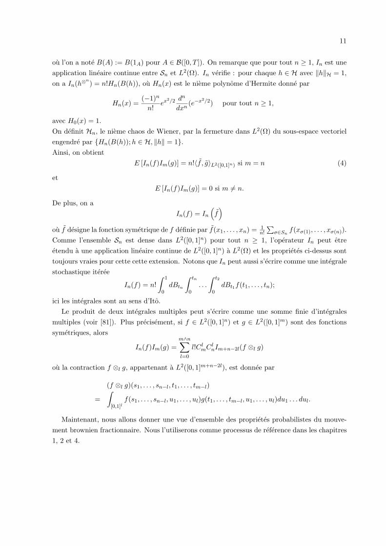
ou l’on a note B(A) := B(1A) pour A ∈ B([0, T ]). On remarque que pour tout n ≥ 1, In est uneapplication lineaire continue entre Sn et L2(Ω). In verifie : pour chaque h ∈ H avec ‖h‖H = 1,on a In(h⊗n
) = n!Hn(B(h)), ou Hn(x) est le nieme polynome d’Hermite donne par
Hn(x) =(−1)n
n!ex2/2 dn
dxn(e−x2/2) pour tout n ≥ 1,
avec H0(x) = 1.On definit Hn, le nieme chaos de Wiener, par la fermeture dans L2(Ω) du sous-espace vectorielengendre par Hn(B(h));h ∈ H, ‖h‖ = 1.Ainsi, on obtient
E [In(f)Im(g)] = n!〈f , g〉L2([0,1]n) si m = n (4)
etE [In(f)Im(g)] = 0 si m 6= n.
De plus, on aIn(f) = In
(f)
ou f designe la fonction symetrique de f definie par f(x1, . . . , xn) = 1n!
∑σ∈Sn
f(xσ(1), . . . , xσ(n)).Comme l’ensemble Sn est dense dans L2([0, 1]n) pour tout n ≥ 1, l’operateur In peut etreetendu a une application lineaire continue de L2([0, 1]n) a L2(Ω) et les proprietes ci-dessus sonttoujours vraies pour cette cette extension. Notons que In peut aussi s’ecrire comme une integralestochastique iteree
In(f) = n!∫ 1
0dBtn
∫ tn
0. . .
∫ t2
0dBt1f(t1, . . . , tn);
ici les integrales sont au sens d’Ito.Le produit de deux integrales multiples peut s’ecrire comme une somme finie d’integrales
multiples (voir [81]). Plus precisement, si f ∈ L2([0, 1]n) et g ∈ L2([0, 1]m) sont des fonctionssymetriques, alors
In(f)Im(g) =m∧n∑
l=0
l!C lmC l
nIm+n−2l(f ⊗l g)
ou la contraction f ⊗l g, appartenant a L2([0, 1]m+n−2l), est donnee par
(f ⊗l g)(s1, . . . , sn−l, t1, . . . , tm−l)
=∫
[0,1]lf(s1, . . . , sn−l, u1, . . . , ul)g(t1, . . . , tm−l, u1, . . . , ul)du1 . . . dul.
Maintenant, nous allons donner une vue d’ensemble des proprietes probabilistes du mouve-ment brownien fractionnaire. Nous l’utiliserons comme processus de reference dans les chapitres1, 2 et 4.
12
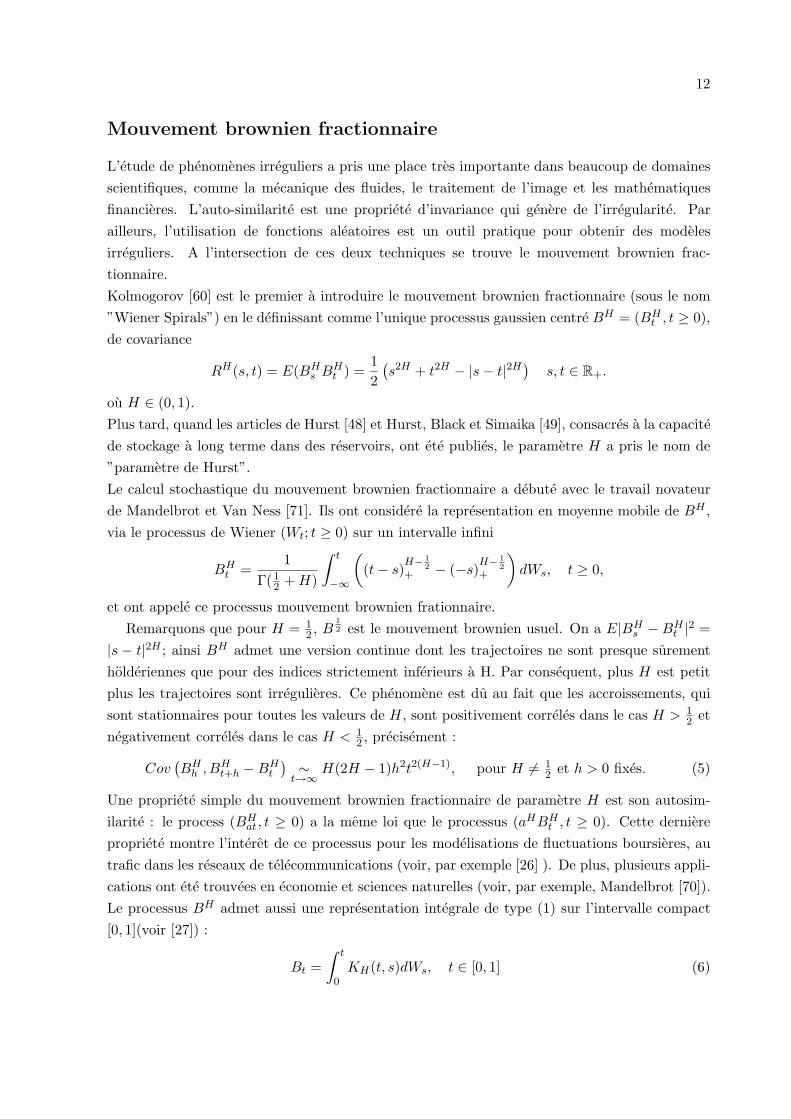
Mouvement brownien fractionnaire
L’etude de phenomenes irreguliers a pris une place tres importante dans beaucoup de domainesscientifiques, comme la mecanique des fluides, le traitement de l’image et les mathematiquesfinancieres. L’auto-similarite est une propriete d’invariance qui genere de l’irregularite. Parailleurs, l’utilisation de fonctions aleatoires est un outil pratique pour obtenir des modelesirreguliers. A l’intersection de ces deux techniques se trouve le mouvement brownien frac-tionnaire.Kolmogorov [60] est le premier a introduire le mouvement brownien fractionnaire (sous le nom”Wiener Spirals”) en le definissant comme l’unique processus gaussien centre BH = (BH
t , t ≥ 0),de covariance
RH(s, t) = E(BHs BH
t ) =12
(s2H + t2H − |s− t|2H
)s, t ∈ R+.
ou H ∈ (0, 1).Plus tard, quand les articles de Hurst [48] et Hurst, Black et Simaika [49], consacres a la capacitede stockage a long terme dans des reservoirs, ont ete publies, le parametre H a pris le nom de”parametre de Hurst”.Le calcul stochastique du mouvement brownien fractionnaire a debute avec le travail novateurde Mandelbrot et Van Ness [71]. Ils ont considere la representation en moyenne mobile de BH ,via le processus de Wiener (Wt; t ≥ 0) sur un intervalle infini
BHt =
1Γ(1
2 + H)
∫ t
−∞
((t− s)
H− 12
+ − (−s)H− 1
2+
)dWs, t ≥ 0,
et ont appele ce processus mouvement brownien frationnaire.Remarquons que pour H = 1
2 , B12 est le mouvement brownien usuel. On a E|BH
s − BHt |2 =
|s − t|2H ; ainsi BH admet une version continue dont les trajectoires ne sont presque surementholderiennes que pour des indices strictement inferieurs a H. Par consequent, plus H est petitplus les trajectoires sont irregulieres. Ce phenomene est du au fait que les accroissements, quisont stationnaires pour toutes les valeurs de H, sont positivement correles dans le cas H > 1
2 etnegativement correles dans le cas H < 1
2 , precisement :
Cov(BH
h , BHt+h −BH
t
) ∼t→∞ H(2H − 1)h2t2(H−1), pour H 6= 1
2 et h > 0 fixes. (5)
Une propriete simple du mouvement brownien fractionnaire de parametre H est son autosim-ilarite : le process (BH
at , t ≥ 0) a la meme loi que le processus (aHBHt , t ≥ 0). Cette derniere
propriete montre l’interet de ce processus pour les modelisations de fluctuations boursieres, autrafic dans les reseaux de telecommunications (voir, par exemple [26] ). De plus, plusieurs appli-cations ont ete trouvees en economie et sciences naturelles (voir, par exemple, Mandelbrot [70]).Le processus BH admet aussi une representation integrale de type (1) sur l’intervalle compact[0, 1](voir [27]) :
Bt =∫ t
0KH(t, s)dWs, t ∈ [0, 1] (6)
13
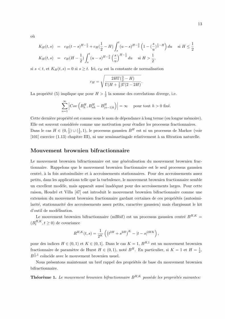
ou
KH(t, s) = cH(t− s)H− 12 + cH(
12−H)
∫ t
s(u− s)H− 3
2
(1− (
s
u)
12−H
)du si H ≤ 1
2
KH(t, s) = cH(H − 12)∫ t
s(u− s)H− 3
2
( s
u
)H− 12du si H >
12,
si s < t, et KH(t, s) = 0 si s ≥ t. Ici, cH est la constante de normalisation
cH =
√2HΓ(3
2 −H)Γ(H + 1
2)Γ(2− 2H).
La propriete (5) implique que pour H > 12 la somme des correlations diverge, i.e.
∞∑
n=1
∣∣∣Cov(BH
h , BHnh −BH
(n−1)h
)∣∣∣ = ∞ pour tout h > 0 fixe.
Cette derniere propriete est connue sous le nom de dependance a long terme (ou longue memoire).Elle est souvent consideree comme une motivation pour etudier les processus fractionnaires.Dans le cas H ∈ (0, 1
2) ∪ (12 , 1), le processus gaussien BH est ni un processus de Markov (voir
[101] exercice (1.13) chapitre III), ni une semimartingale relativement a sa filtration naturelle.
Mouvement brownien bifractionnaire
Le mouvement brownien bifractionnaire est une generalisation du mouvement brownien frac-tionnaire. Rappelons que le mouvement brownien fractionnaire est le seul processus gaussiencentre, a la fois autosimilaire et a accroissements stationnaires. Pour des accroissements assezpetits, dans les applications telle que la turbulence, le mouvement brownien fractionnaire sembleun excellent modele, mais apparaıt aussi inadequat pour des accroissements larges. Pour cetteraison, Houdre et Villa [47] ont introduit le mouvement brownien bifractionnaire comme uneextension du mouvement brownien fractionnaire gardant certaines de ces proprietes (autosimi-larite, stationnarite des accroissements assez petits, caractere gaussien) mais elargissant le kitd’outil de modelisation.
Le mouvement brownien bifractionnaire (mBbif) est un processus gaussien centre BH,K =(BH,K
t , t ≥ 0) de covariance
RH,K(t, s) =1
2K
((t2H + s2H
)K − |t− s|2HK)
,
pour des indices H ∈ (0, 1) et K ∈ (0, 1]. Dans le cas K = 1, BH,1 est un mouvement brownienfractionnaire de parametre de Hurst H ∈ (0, 1), note BH . En particulier, si K = 1 et H = 1
2 ,B
12,1 coıncide avec le mouvement brownien usuel.Nous presentons maintenant un bref rappel des proprietes de base du mouvement brownien
bifractionnaire.
Theoreme 1. Le mouvement brownien bifractionnaire BH,K possede les proprietes suivantes:
14
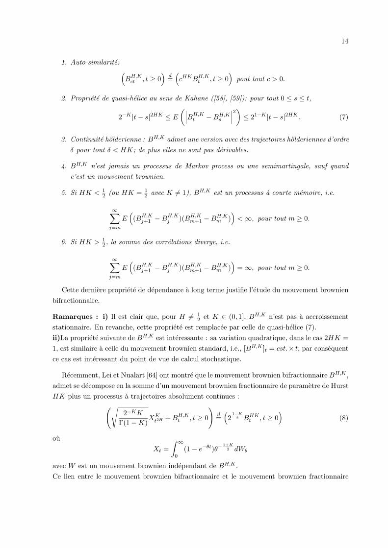
1. Auto-similarite:(BH,K
ct , t ≥ 0)
d=(cHKBH,K
t , t ≥ 0)
pout tout c > 0.
2. Propriete de quasi-helice au sens de Kahane ([58], [59]): pour tout 0 ≤ s ≤ t,
2−K |t− s|2HK ≤ E
(∣∣∣BH,Kt −BH,K
s
∣∣∣2)≤ 21−K |t− s|2HK . (7)
3. Continuite holderienne : BH,K admet une version avec des trajectoires holderiennes d’ordreδ pour tout δ < HK; de plus elles ne sont pas derivables.
4. BH,K n’est jamais un processus de Markov process ou une semimartingale, sauf quandc’est un mouvement brownien.
5. Si HK < 12 (ou HK = 1
2 avec K 6= 1), BH,K est un processus a courte memoire, i.e.
∞∑
j=m
E((BH,K
j+1 −BH,Kj )(BH,K
m+1 −BH,Km )
)< ∞, pour tout m ≥ 0.
6. Si HK > 12 , la somme des correlations diverge, i.e.
∞∑
j=m
E((BH,K
j+1 −BH,Kj )(BH,K
m+1 −BH,Km )
)= ∞, pour tout m ≥ 0.
Cette derniere propriete de dependance a long terme justifie l’etude du mouvement brownienbifractionnaire.
Ramarques : i) Il est clair que, pour H 6= 12 et K ∈ (0, 1], BH,K n’est pas a accroissement
stationnaire. En revanche, cette propriete est remplacee par celle de quasi-helice (7).ii)La propriete suivante de BH,K est interessante : sa variation quadratique, dans le cas 2HK =1, est similaire a celle du mouvement brownien standard, i.e., [BH,K ]t = cst.× t; par consequentce cas est interessant du point de vue de calcul stochastique.
Recemment, Lei et Nualart [64] ont montre que le mouvement brownien bifractionnaire BH,K ,admet se decompose en la somme d’un mouvement brownien fractionnaire de parametre de HurstHK plus un processus a trajectoires absolument continues :
(√2−KK
Γ(1−K)XK
t2H + BH,Kt , t ≥ 0
)d=
(2
1−K2 BHK
t , t ≥ 0)
(8)
ouXt =
∫ ∞
0(1− e−θt)θ−
1+K2 dWθ
avec W est un mouvement brownien independant de BH,K .Ce lien entre le mouvement brownien bifractionnaire et le mouvement brownien fractionnaire
15
conduit, en utilisant les resultats sur le mouvement brownien fractionnaire, a une meilleurecomprehension et a des preuves simplifiees de quelques proprietes du mouvement brownienbifractionnaire qui ont ete obtenues dans la litterature.
Chapitre 1 : Formules d’Ito et de Tanaka pour le mBbif multidimensionnel
Il est bien connu que les formules d’Ito et de Tanaka sont un outil puissant de l’analyse stochas-tique a cause de leur vaste domaine d’application. Ainsi, recemment, plusieurs chercheurs ontetudie des extensions des formules classiques d’Ito et de Tanaka aux processus de type (1) (voir,par exemple, [24] and [1] ) ainsi qu’aux processus multidimensionnels comme le mouvementbrownien multidimensionnel [114] et le mouvement brownien fractionnaire multidimensionnel[115].
Le chapitre 1 de cette these est constitue de la publication [39] en collaboration avec C.Tudor. Cette publication propose une extension des formules d’Ito et de Tanaka au mouvementbrownien bifrationnaire unidimensionnel et multidimentionnel.
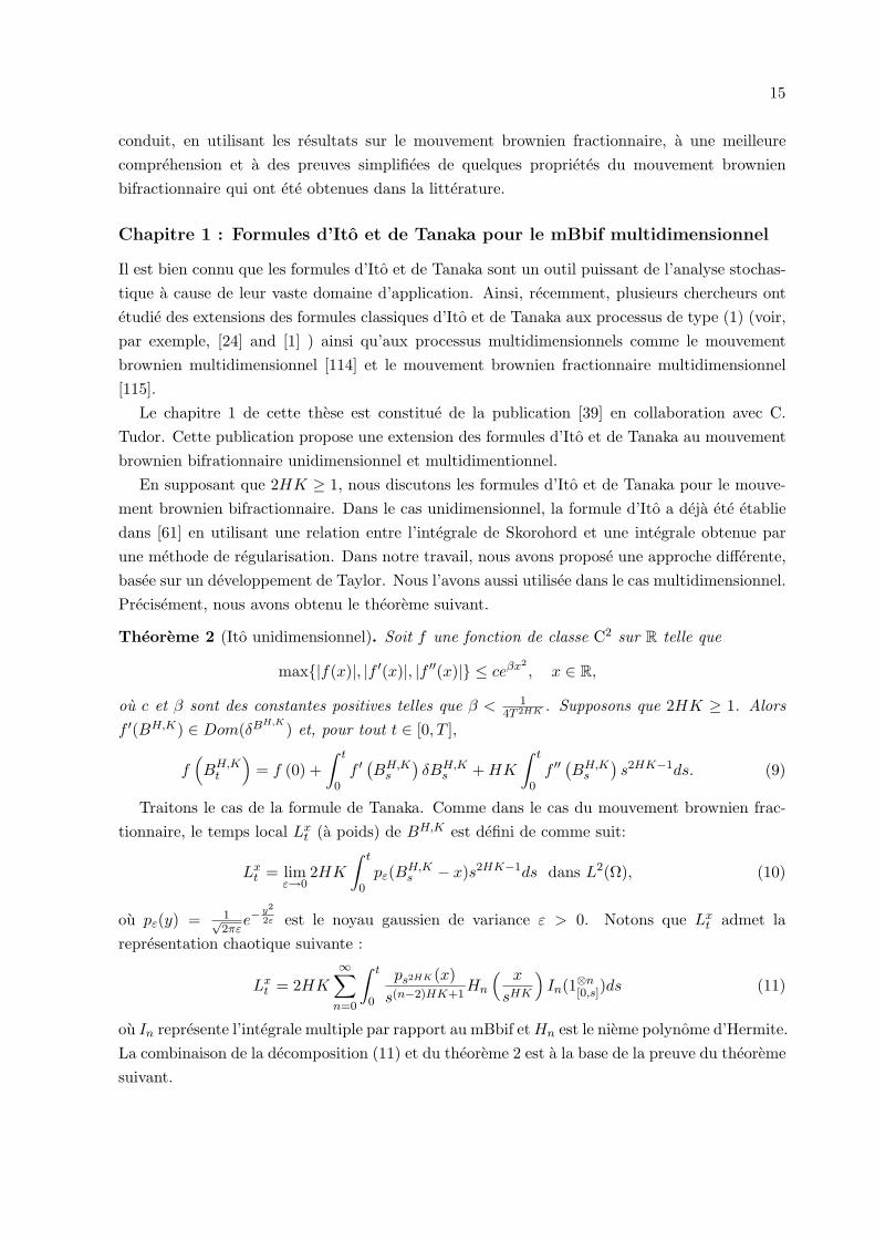
En supposant que 2HK ≥ 1, nous discutons les formules d’Ito et de Tanaka pour le mouve-ment brownien bifractionnaire. Dans le cas unidimensionnel, la formule d’Ito a deja ete etabliedans [61] en utilisant une relation entre l’integrale de Skorohord et une integrale obtenue parune methode de regularisation. Dans notre travail, nous avons propose une approche differente,basee sur un developpement de Taylor. Nous l’avons aussi utilisee dans le cas multidimensionnel.Precisement, nous avons obtenu le theoreme suivant.
Theoreme 2 (Ito unidimensionnel). Soit f une fonction de classe C2 sur R telle que
max|f(x)|, |f ′(x)|, |f ′′(x)| ≤ ceβx2, x ∈ R,
ou c et β sont des constantes positives telles que β < 14T 2HK . Supposons que 2HK ≥ 1. Alors
f ′(BH,K) ∈ Dom(δBH,K) et, pour tout t ∈ [0, T ],
f(BH,K
t
)= f (0) +
∫ t
0f ′
(BH,K
s
)δBH,K
s + HK
∫ t
0f ′′
(BH,K
s
)s2HK−1ds. (9)
Traitons le cas de la formule de Tanaka. Comme dans le cas du mouvement brownien frac-tionnaire, le temps local Lx
t (a poids) de BH,K est defini de comme suit:
Lxt = lim
ε→02HK
∫ t
0pε(BH,K
s − x)s2HK−1ds dans L2(Ω), (10)
ou pε(y) = 1√2πε
e−y2
2ε est le noyau gaussien de variance ε > 0. Notons que Lxt admet la
representation chaotique suivante :
Lxt = 2HK
∞∑
n=0
∫ t
0
ps2HK (x)s(n−2)HK+1
Hn
( x
sHK
)In(1⊗n
[0,s])ds (11)
ou In represente l’integrale multiple par rapport au mBbif et Hn est le nieme polynome d’Hermite.La combinaison de la decomposition (11) et du theoreme 2 est a la base de la preuve du theoremesuivant.
16
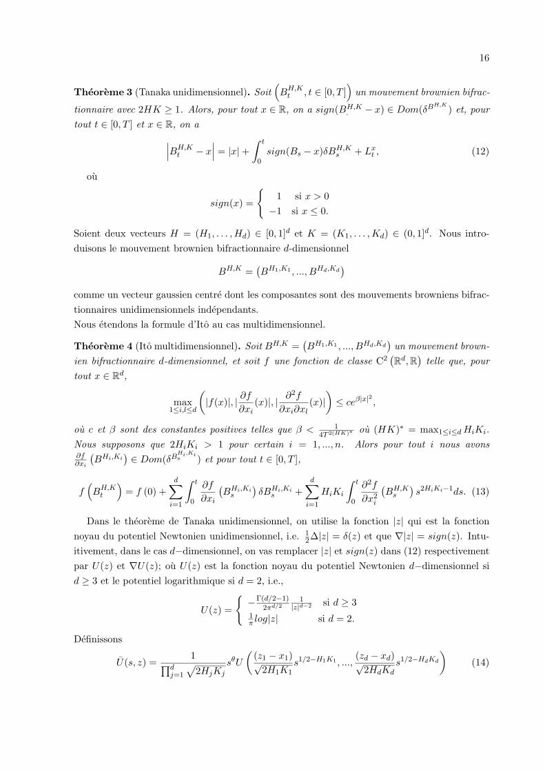
Theoreme 3 (Tanaka unidimensionnel). Soit(BH,K
t , t ∈ [0, T ])
un mouvement brownien bifrac-
tionnaire avec 2HK ≥ 1. Alors, pour tout x ∈ R, on a sign(BH,K. − x) ∈ Dom(δBH,K
) et, pourtout t ∈ [0, T ] et x ∈ R, on a
∣∣∣BH,Kt − x
∣∣∣ = |x|+∫ t
0sign(Bs − x)δBH,K
s + Lxt , (12)
ou
sign(x) =
1 si x > 0
−1 si x ≤ 0.
Soient deux vecteurs H = (H1, . . . , Hd) ∈ [0, 1]d et K = (K1, . . . , Kd) ∈ (0, 1]d. Nous intro-duisons le mouvement brownien bifractionnaire d-dimensionnel
BH,K =(BH1,K1 , ..., BHd,Kd
)
comme un vecteur gaussien centre dont les composantes sont des mouvements browniens bifrac-tionnaires unidimensionnels independants.Nous etendons la formule d’Ito au cas multidimensionnel.
Theoreme 4 (Ito multidimensionnel). Soit BH,K =(BH1,K1 , ..., BHd,Kd
)un mouvement brown-
ien bifractionnaire d-dimensionnel, et soit f une fonction de classe C2(Rd,R
)telle que, pour
tout x ∈ Rd,
max1≤i,l≤d
(|f(x)|, | ∂f
∂xi(x)|, | ∂2f
∂xi∂xl(x)|
)≤ ceβ|x|2 ,
ou c et β sont des constantes positives telles que β < 14T 2(HK)∗ ou (HK)∗ = max1≤i≤d HiKi.
Nous supposons que 2HiKi > 1 pour certain i = 1, ..., n. Alors pour tout i nous avons∂f∂xi
(BHi,Ki
) ∈ Dom(δBHi,Kis ) et pour tout t ∈ [0, T ],
f(BH,K
t
)= f (0) +
d∑
i=1
∫ t
0
∂f
∂xi
(BHi,Ki
s
)δBHi,Ki
s +d∑
i=1
HiKi
∫ t
0
∂2f
∂x2i
(BH,K
s
)s2HiKi−1ds. (13)
Dans le theoreme de Tanaka unidimensionnel, on utilise la fonction |z| qui est la fonctionnoyau du potentiel Newtonien unidimensionnel, i.e. 1
2∆|z| = δ(z) et que ∇|z| = sign(z). Intu-itivement, dans le cas d−dimensionnel, on vas remplacer |z| et sign(z) dans (12) respectivementpar U(z) et ∇U(z); ou U(z) est la fonction noyau du potentiel Newtonien d−dimensionnel sid ≥ 3 et le potentiel logarithmique si d = 2, i.e.,
U(z) =
−Γ(d/2−1)
2πd/21
|z|d−2 si d ≥ 31π log|z| si d = 2.
Definissons
U(s, z) =1∏d
j=1
√2HjKj
sθU
((z1 − x1)√
2H1K1s1/2−H1K1 , ...,
(zd − xd)√2HdKd
s1/2−HdKd
)(14)
17
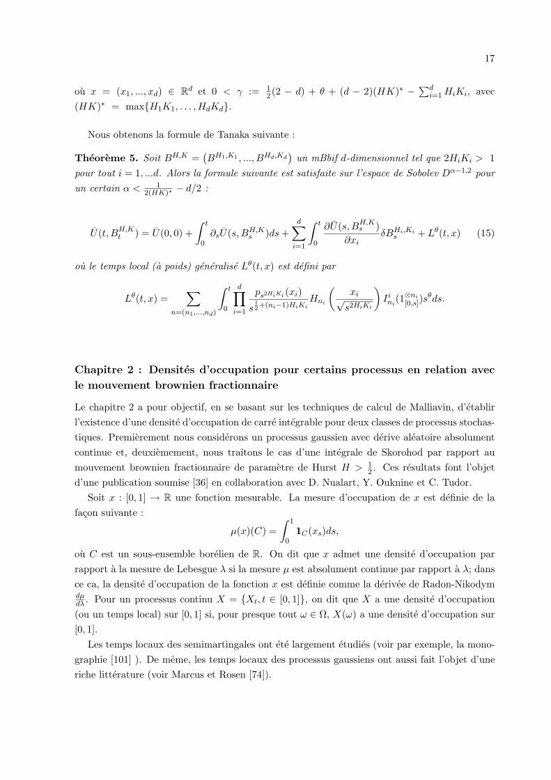
ou x = (x1, ..., xd) ∈ Rd et 0 < γ := 12(2 − d) + θ + (d − 2)(HK)∗ − ∑d
i=1 HiKi, avec(HK)∗ = maxH1K1, . . . , HdKd.
Nous obtenons la formule de Tanaka suivante :
Theoreme 5. Soit BH,K =(BH1,K1 , ..., BHd,Kd
)un mBbif d-dimensionnel tel que 2HiKi > 1
pour tout i = 1, ...d. Alors la formule suivante est satisfaite sur l’espace de Sobolev Dα−1,2 pourun certain α < 1
2(HK)∗ − d/2 :
U(t, BH,Kt ) = U(0, 0) +
∫ t
0∂sU(s,BH,K
s )ds +d∑
i=1
∫ t
0
∂U(s,BH,Ks )
∂xiδBHi,Ki
s + Lθ(t, x) (15)
ou le temps local (a poids) generalise Lθ(t, x) est defini par
Lθ(t, x) =∑
n=(n1,...,nd)
∫ t
0
d∏
i=1
ps2HiKi (xi)
s12+(ni−1)HiKi
Hni
(xi√
s2HiKi
)Iini
(1⊗ni
[0,s])sθds.
Chapitre 2 : Densites d’occupation pour certains processus en relation avec
le mouvement brownien fractionnaire
Le chapitre 2 a pour objectif, en se basant sur les techniques de calcul de Malliavin, d’etablirl’existence d’une densite d’occupation de carre integrable pour deux classes de processus stochas-tiques. Premierement nous considerons un processus gaussien avec derive aleatoire absolumentcontinue et, deuxiemement, nous traıtons le cas d’une integrale de Skorohod par rapport aumouvement brownien fractionnaire de parametre de Hurst H > 1
2 . Ces resultats font l’objetd’une publication soumise [36] en collaboration avec D. Nualart, Y. Ouknine et C. Tudor.
Soit x : [0, 1] → R une fonction mesurable. La mesure d’occupation de x est definie de lafacon suivante :
µ(x)(C) =∫ 1
01C(xs)ds,
ou C est un sous-ensemble borelien de R. On dit que x admet une densite d’occupation parrapport a la mesure de Lebesgue λ si la mesure µ est absolument continue par rapport a λ; dansce ca, la densite d’occupation de la fonction x est definie comme la derivee de Radon-Nikodymdµdλ . Pour un processus continu X = Xt, t ∈ [0, 1], on dit que X a une densite d’occupation(ou un temps local) sur [0, 1] si, pour presque tout ω ∈ Ω, X(ω) a une densite d’occupation sur[0, 1].
Les temps locaux des semimartingales ont ete largement etudies (voir par exemple, la mono-graphie [101] ). De meme, les temps locaux des processus gaussiens ont aussi fait l’objet d’uneriche litterature (voir Marcus et Rosen [74]).
18
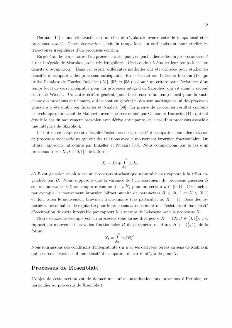
Berman [14] a montre l’existence d’un effet de regularite inverse entre le temps local et leprocessus associe. Cette observation a fait du temps local un outil puissant pour etudier lestrajectoires irregulieres d’un processus continu.
En general, les trajectoires d’un processus anticipant, en particulier celles du processus associea une integrale de Skorohod, sont tres irregulieres. Ceci conduit a etudier leur temps local (oudensite d’occupation). Dans cet esprit, differentes methodes ont ete utilisees pour etudier lesdensites d’occupation des processus anticipants. En se basant sur l’idee de Berman [13] quiutilise l’analyse de Fourier, Imkeller ([51], [52] et [53]) a donne un critere pour l’existence d’untemps local de carre integrable pour un processus integral de Skorohod qui vit dans le secondchaos de Wiener. Un autre critere general, pour l’existence d’un temps local pour la vasteclasse des processus anticipants, qui ne sont en general ni des semimartingales, ni des processusgaussiens a ete etabli par Imkeller et Nualart [50]. La preuve de ce dernier resultat combineles techniques du calcul de Malliavin avec le critere donne par Geman et Horowitz [44], qui ontetudie le cas du mouvement brownien avec derive anticipante, et le cas d’un processus associe aune integrale de Skorohod.
Le but de ce chapitre est d’etablir l’existence de la densite d’occupation pour deux classesde processus stochastiques qui ont des relations avec le mouvement brownien fractionnaire. Onutilise l’approche introduite par Imkeller et Nualart [50]. Nous commencons par le cas d’unprocessus X = Xt, t ∈ [0, 1] de la forme
Xt = Bt +∫ t
0usds,
ou B est gaussien et ou u est un processus stochastique mesurable par rapport a la tribu en-gendree par B. Nous supposons que la variance de l’accroissement du processus gaussien B
sur un intervalle [s, t] se comporte comme |t − s|2ρ, pour un certain ρ ∈ (0, 1). Ceci inclut,par exemple, le mouvement brownien bifractionnaire de parametres H ∈ (0, 1) et K ∈ (0, 1]et donc aussi le mouvement brownien fractionnaire (cas particulier ou K = 1). Sous des hy-potheses raisonnables de regularite pour le processus u, nous montrons l’existence d’une densited’occupation de carre integrable par rapport a la mesure de Lebesgue pour le processus X.
Notre deuxieme exemple est un processus sous forme divergence X = Xt, t ∈ [0, 1], parrapport au mouvement brownien fractionnaire B de parametre de Hurst H ∈ (1
2 , 1), de laforme :
Xt =∫ t
0usδB
Hs .
Nous fournissons des conditions d’integrabilite sur u et ses derivees iterees au sens de Malliavinqui assurent l’existence d’une densite d’occupation de carre integrable pour X.
Processus de Rosenblatt
L’objet de cette section est de donner une breve introduction aux processus d’Hermite, enparticulier au processus de Rosenblatt.
19
Considerons une suite stationnaire centree reduite gaussienne (Xn)n≥1 c’est-a-dire que EX1 =0 et EX2
1 = 1.Soit G une fonction reelle qui verifie EG(X1) = 0 et E(G(X1))2 < ∞. Alors G admet un
developpement d’Hermite dans l’espace L2(R, 1√2π
e−x2
2 dx), qui est de la forme
G(x) =+∞∑
j=1
ajHj(x), ou aj = E (G(X1)Hj(X1)) .
Notons par r(n) la fonction de covariance de (Xn)n≥1 et par k le rang de Hermite de G, i.e.k = minj; aj 6= 0. Supposons que
r(n) := E(X1Xn) = n2H−2
k L(n), et H ∈ (12, 1)
ou L est une fonction a variation lente a l’infini, i.e. L est bornee sur les intervalles finis et pourtout t > 0
L(tx)L(x)
−→ 1, quand x −→ +∞.
Le processus d’Hermite est apparu pour la premiere fois dans le theoreme non-central limitesuivant, prouve par Taqqu [108] (voir aussi Dobrushin et Major [32]). Le processus
1nH
[nt]∑
j=1
G(Xj)
converge (au sens des lois fini-dimensionnelles) lorsque n −→∞ vers le processus
Zk,Ht = C(H, k)
∫
Rk
∫ t
0
(Πk
i=1(s− yi)−( 1
2+ 1−H
k)
+
)dsdWy1 . . . dWyk
ou x+ = max(x, 0) et (Wt; t ∈ [0, T ]) est un mouvement brownien.
Definition. Le processus Zk,H =(Zk,H
t ; t ∈ [0, T ])
est appele processus d’Hermite d’ordre k etde parametre H. Pour k = 1, on retrouve le mouvement brownien fractionnaire, et pour k = 2,il s’agit du processus de Rosenblatt.
Le processus d’Hermite Zk,H verifie les proprietes suivantes:
1. Zk,H est un processus centre tel que V ar(Zk,H1 ) = 1.
2. Ses accroissements sont stationnaires.
3. La fonction de covariance de Zk,H est donnee par
Cov(Zk,Ht , Zk,H
s ) =12
(|t|2H + |s|2H − |t− s|2H), t, s ∈ [0, T ];
par consequent
E∣∣∣Zk,H
t − Zk,Hs
∣∣∣2
= |t− s|2H .
20
4. Si k ≥ 2, alors Zk,H est non-gaussien; le processus de Hermite Zk,H d’ordre k vit dans lechaos de Wiener d’ordre k de W .
5. Zk,H admet une version continue dont les trajectoires sont presque surement holderiennespour tous les indices strictement inferieurs a H. Grace au theoreme de continuite de Kol-mogorov, c’est une consequence de la propriete 3 et de l’equivalence des normes Lp dansun chaos d’orde fixe.
6. Zk,H a une longue memoire (dependance a long terme). Plus precisement, sa fonction decovariance Cov(Zk,H
1 , Zk,Hn+1 − Zk,H
n ) se comporte comme n2H−2 a l’infini.
Exceptee la propriete 6 concernant le caractere gaussien, nous remarquons que les proprietes 1a 5 du processus d’Hermite Zk,H sont similaires a celles du mouvement brownien fractionnairede parametre de Hurst H > 1
2 .Tudor a etabli dans [111] qu’un processus de Hermite Zk,H d’ordre k ≥ 1 peut etre represente, enloi, comme une integrale multiple iteree par rapport au processus de Wiener usuel. Ce resultatfait l’objet de la proposition suivante.
Proposition 1. Fixons k ≥ 1 et H > 12 . Le processus de Hermite Zk,H d’ordre k et de parametre
H a la meme loi que le processus
d(H)∫ t
0. . .
∫ t
0dWy1 . . . dWyk
∫ t
y1∨y2...∨yk
∂KH′
∂u(u, y1) . . .
∂KH′
∂u(u, yk)du; t ∈ [0, T ] (16)
ou (Wt, t ∈ [0, T ]) est un mouvement brownien,
H ′ := 1 +H − 1
k; d(H) :=
1H + 1
(2(2H − 1)
H
) 12
,
et KH′le noyau standard defini dans (6).
Recemment, la representation (16) a ete utilisee par plusieurs auteurs pour developper l’analysestochastique pour les processus d’Hermite (voir [111], [79], [75], [112], [18], [22]).
Chapitre 3 : Theoreme non-central limite pour la variation cubique d’une
classe des processus stochastiques autosimilaire
Nous nous interessons, dans ce chapitre, au comportement asymptotique, quand N −→ ∞, dela variation cubique du processus de Rosenblatt Z(H) definie par
V 3,N (Z(H)) =1N
N−1∑
i=0
(Z
(H)i+1N
− Z(H)iN
)3
E
(Z
(H)i+1N
− Z(H)iN
)3 − 1
.
Pour les processus autosimilaires (en particulier le processus de Rosenblatt), l’etude deleurs variations constitue un outil fondamental pour construire des estimateurs du parametre
21
d’autosimilarite. Les processus autosimilaires sont des modeles convenables a la modelisation denombreux phenomenes, ou la longue memoire est un facteur important. Cela inclu le trafic in-ternet (cf. [117]), l’hydrologie (cf. [76]) et l’economie (cf. [69], [118]). La tache de modelisationla plus importante est ensuite d’estimer le parametre d’autosimilarite, parce qu’il caracterisetoute l’importance des proprietes de dependance a long terme du processus.Il existe une connection directe entre le comportement des variations et la convergence d’unestimateur statistique pour l’indice d’autosimilarite (voir [23], [112]).Le cas de la variation quadratique du processus de Rosenblatt (Z(H)
t )t∈[0,1] d’indice H > 12 , avec
un horizon de temps fini [0, 1], a ete etudie par Tudor et Viens dans [112].Dans le cas d’un mouvement brownien fractionnaire BH , la non-normalite de la variation quadra-tique lorsque H ∈ (3
4 , 1) peut etre evitee en utilisant soit les ”longer filters” (c’est a dire onremplace les accroissements BH
i+1N
− BHiN
par BHi+1N
− 2BHiN
+ BHi−1N
), soit des variations d’ordregrand. Dans notre travail, nous avons considere le deuxieme choix : nous remplacons la varia-tion quadratique par la variation cubique. Dans le cas de BH , ceci n’a pas de sens puisque letroisieme moment d’une variable aleatoire gaussienne est nul. Pour etudier la variation cubiquedu processus Z(H), nous avons utiliser la decomposition chaotique de Wiener pour la statistiqueV 3,N (Z(H)) et nous l’avons decomposee en plusieurs termes qui appartiennent aux chaos d’ordre2, 4 et 6. En normalisant par N1−H , nous avons montre que E
(N1−HV 3,N (Z(H))
)2converge
vers une constante C(H) quand N −→∞. Ensuite, pour etudier la loi limite nous avons utilisele critere suivant:
Theoreme 6 (Nualart-Ortiz−Latorre). Fixons n ≥ 2. Soit (Fk, k ≥ 1), Fk = In(fk) une suitede variables aleatoires dans le neme chaos de Wiener telle que EF 2
k −→ 1 lorsque k −→ ∞.Alors
(Fk)k≥0 converge en loi vers une loi normal N (0, 1).
⇐⇒‖DFk‖2
H −→ n dans L2(Ω) quand k −→∞.
Comme dans [112], [22], le terme dominant note TN de la decomposition de V 3,N (Z(H)) estcelui qui vit dans le deuxieme chaos et qui doit etre normalise par N1−H pour avoir une limitenon triviale. Nous avons etabli que ‖N1−HDTN‖2
H −→ c > 2 dans L2(Ω) quand N −→ ∞. Cequi implique que la loi limite de N1−HV 3,N (Z(H)) est non-normale. De plus et comme dans lecas de la variation quadratique nous avons obtenu la meme limite qui est, a une constante pres,une variable aleatoire de Rosenblatt d’indice H. Ce resultat fait l’objet d’une publication [41]soumise en collaboration avec C. Tudor.
Chapitre 4 : Estimation de la derive de mouvement brownien fractionnaire
Soit BH =(
BH,1t , ..., BH,d
t
); t ∈ [0, T ]
un mouvement brownien fractionnaire (mbf) d-dimensionnel
de parametre H ∈ (0, 1), defini sur un espace de probabilite (Ω,F , P ). Pour chaque i = 1, . . . , n,
22
(F it )t∈[0,T ] denote la filtration engendree par
(BH,i
)t∈[0,T ]
.Soit M un sous espace de l’espace de Cameron-Martin defini par
M =
ϕ : [0, T ] → Rd; ϕit =
∫ t
0ϕi
sds avec ϕi ∈ L2([0, T ])
et ϕi ∈ IH+ 1
2
0+
(L2([0, T ])
), i = 1, ..., d
ou IH+ 1
2
0+ est l’integral fractionnaire a gauche de Riemann-Liouville d’ordre (H + 12).
Soit θ =(θ1
t , . . . , θdt ); t ∈ [0, T ]
une fonction de M . Alors, en appliquant le theoreme de
Girsanov (voir [84]), il existe une mesure de probabilite Pθ absolument continue par rapport aP sous laquelle le processus BH defini par
BHt = BH
t − θt, t ∈ [0, T ]
est un mbf centre de parametre H. Autrement dit, sous la probabilite Pθ, le processus BH estun mbf de derive θ.
Nous nous considerons dans ce chapitre le probleme de l’estimation de la derive θ de BH
sous la probabilite Pθ, dans le cas ou H < 1/2. Nous etudions l’estimation de θ sous le risquequadratique usuel, qui est defini pour tout estimateur δ = (δ1
t , . . . , δdt ), t ∈ [0, T ] de θ par
R(θ, δ) = Eθ
[∫ T
0||δt − θt||2dt
]
ou Eθ est l’esperance relativement a la probabilite Pθ.Un estimateur δ de θ est dit sans biais si, pour tout t ∈ [0, T ]
Eθ(δit) = θi
t, i = 1, . . . , d
et il est adapte si, pour chaque i = 1, . . . , d, δi est adapte a(F i
t
)t∈[0,T ]
.Recemment, Privault et Reveillac dans [96] ont construit, dans un cadre infini dimensionnel,
des estimateurs sans biais de la derive (θt)t∈[0,T ] pour une martingale gaussienne (Xt)t∈[0,T ] devariation quadratique σ2
t dt, ou σ ∈ L2([0, T ], dt) est fonction non nulle. Precisement, ils ontmontre que θ = (Xt)t∈[0,T ] est un estimateur efficace de (θt)t∈[0,T ]. D’autre part, a l’aide decalcul de Malliavin, ils ont construit des estimateurs suroptimaux de la derive d’un processusgaussien de la forme:
Xt :=∫ t
0K(t, s)dWs, t ∈ [0, T ],
ou (Wt)t∈[0,T ] est un mouvement brownien et K(., .) est noyau deterministe. Ces estimateurssont biaises de la forme Xt + Dt log F , ou F est un surharmonique variable aleatoire et D laderivee au sens de Malliavin.
Dans ce chapitre, nous utilisons des techniques basees sur le theoreme tout d’abord de Gir-sanov du mbf et le calcul fractionnaire pour etablir que θ = BHest un estimateur efficace de θ
23
sous la probabilite Pθ de risque
R(θ, BH) = Eθ
[∫ T
0‖BH
t − θt‖2dt
]=
T 2H+1
2H + 1d.
De plus, nous nous montrons que θ = BH est un estimateur de maximum de vraisemblance deθ.
D’autre part, nous nous construisons une classe des estimateurs biaises suroptimaux de typeJames-Stein de la forme:
δ(BH)t =(
1− at2H
(r(‖BH
t ‖2)‖BH
t ‖2
))BH
t , t ∈ [0, T ].
Nous nous donnons des conditions suffisantes sur la fonction r et sur la constante a pour queδ(BH) domine BH sous le risque quadratique usuel i.e.
R (θ, δ
(BH
))< R (
θ,BH)
for all θ ∈ M.
Ce chapitre fait l’objet d’une publication [37] en collaboration avec I. Ouassou et Y. Ouknine.
Calcul de Malliavin sur l’espace canonique de Levy : l’approche
de Sole et al. [106]
Sur l’espace de Poisson et d’une facon generale, deux approches du calcul de variations ontete introduites : l’approche variationnelle (voir par exemple Bichteler et al. [15] et Carlen etPardoux [21]), et l’approche chaotique (voir par exemple Nualart et Vives [85] et Leon et Tudor[65]). Depuis ces dernieres annees, la theorie du calcul de Malliavin a ete etendue dans un cadreplus general a l’espace de Levy par plusieurs approches, avec pour motivations des applicationsen finance (voir par exemple Løkka [66] , Di Nunno et al. [31] et Sole et al. [106]).
Un processus de Levy est un processus stochastique a accroissements independants et sta-tionnaires. Si (Xt, t ≥ 0) est un processus de Levy, alors Xt − Xs avec t ≥ s est independantde l’histoire du processus avant le temps s et sa loi ne depend pas de t ou s separement, maisseulement de t− s.Nous considerons un processus de Levy X = (Xt, 0 ≤ t ≤ 1) defini sur un espace de proba-bilite
(Ω, (FX
t )0≤t≤1, P), ou (FX
t )0≤t≤1 est la filtration engendree par X. Alors, il existe untriplet (γ, σ2, ν): ou γ ∈ R, σ ≥ 0 et une mesure ν(dz) sur R appelee mesure de Levy tels queν(0) = 0,
∫R 1 ∧ x2ν(dx) < ∞ et
E (exp(itX1)) = exp
iγt− 12σt2 +
∫
R
(eitx − 1− itx1|x|≤1
)ν(dx)
, ∀t ∈ R.
Dans tout ce chapitre nous supposons que∫R x2ν(dx) < ∞.
Il est bien connu que le processus X admet une representation de Levy-Ito :
Xt = γt + σWt +∫ ∫
(0,t]×|x|>1xN(ds, dx) + lim
ε↓0
∫ ∫
(0,t]×ε<|x|≤1xN(ds, dx)
24
ou W est un mouvement brownien standard, N est la mesure des sauts de X definie pour toutborelien E ∈ B([0, 1]× R− 0) par :
N(E) = #t : (t, ∆Xt) ∈ E,
ou ∆Xt = Xt −Xt− , # denote le cardinal et N est la mesure des sauts compensee :
N(dt, dx) = N(dt, dx)− dtν(dx).
Suivant l’approche d’Ito [55], X peut etre etendu a une mesure aleatoire sur ([0, 1]×R, B([0, 1]×R)):
M(E) = σ
∫
s∈[0,1]:(s,0)∈EdWs + lim
n→∞
∫ ∫
(s,x)∈E: 1n
<|x|<nxN(ds, dx)
pour tout E ∈ B([0, 1]× R) tel que µ(E) < ∞, ou µ est une mesure σ−finie sur [0, 1]× R:
µ(E) = σ2
∫
s∈[0,1]:(s,0)∈Eds +
∫ ∫
E−s∈[0,1]:(s,0)∈E×0x2dsν(dx).
M est appelee mesure a valeur martingale de type (2, µ). Le second moment existe toujours etpeut s’exprimer en fonction de la mesure µ (voir Applebaum [3] ). De plus M est une mesurealeatoire independante centree:
E (M(E1)M(E2)) = µ(E1 ∩ E2)
pour tout E1, E2 ∈ B([0, 1]× R) tels que µ(E1) < ∞ et µ(E2) < ∞.Utilisant la mesure aleatoire M , comme sur l’espace de Wiener [81], on peut construire l’integralemultiple In(f) par rapport au processus de Levy comme une isometrie entre L2(Ω) et l’espaceL2
n = L2 (([0, 1]× R)n, B(([0, 1]× R)n), µ⊗n). En effet, on debute en considerant le cas elementaire:
f = 1E1×...×En
ou E1, . . . , En ∈ B([0, 1]× R) sont disjoints deux a deux et µ(Ei) < ∞ pour tout i. On definitalors In(f) = M(E1) . . . M(En). Ensuite, on prolonge In(f) a tout L2
n par linearite et continuite.On obtient ainsi la propriete de representation chaotique suivante :
L2(Ω, FX , P ) = ⊕∞n=0In(L2n).
Par consequence, toute variable aleatoire F ∈ L2(Ω, FX , P ), peut etre representee sous la forme
F = E(F ) +∞∑
n=1
In(fn)
ou fn ∈ L2n. A ce stade, et comme dans les cas brownien et poissonien, on peut introduire un
calcul de Malliavin pour les processus de Levy. Si
∞∑
n=0
nn!‖fn‖2L2
n< ∞
25
alors la derivee de Malliavin de F est introduite par
(z, w) ∈ ([0, 1]× R)× Ω DF−→ DzF (w) =∞∑
n=1
nIn−1(fn(z, .)).
Le domaine de l’operateur de derivation D est defini par:
D1,2 =
F =
∞∑
n=0
In(fn) :∞∑
n=0
nn!‖fn‖2L2
n< ∞
.
Notons par Dk,2, k ≥ 1, le domaine de la kieme derivee iteree D(k), qui est un espace deHilbert muni du produit scalaire
〈F,G〉 = E(FG) +k∑
j=1
E
∫
([0,1]×R)j
D(j)z FD(j)
z Gµ(dz).
Maintenant, on peut definir l’operateur adjoint de D, note δ et appele operateur de divergenceou integrale de Skorohod. Soit u ∈ H = L2
([0, 1]× R× Ω, B([0, 1]× R)⊗ FX
T , µ⊗ P). Alors,
pour tout z ∈ [0, 1]× R, u(z) admet la representation suivante
u(z) =∞∑
n=0
In(fn(z, .)), (17)
ou on a fn ∈ L2(([0, 1]× R)n+1, µ⊗n+1) et fn est symetrique en ses n dernieres variables. Si
∞∑
n=0
(n + 1)!‖fn‖2n+1 < ∞
ou fn est la symetrisation de fn, dans ce cas, l’integrale de Skorohod δ(u) de u est definie par
δ(u) =∞∑
n=0
In+1(fn).
Le domaine de δ est l’ensemble des processus de type (17) satisfaisants
∞∑
n=0
(n + 1)!‖fn‖2n+1 < ∞.
En outre, on obtient la formule d’integration par parties
E(Fδ(u)) = E
∫ ∫
[0,1]×RDzFu(z)µ(dz), F ∈ D1,2.
Nous utiliserons les notations suivantes
δ(u) =∫ 1
0
∫
RuzδM(dz) =
∫ 1
0
∫
Rus,xδM(ds, dx).
Dans le cas ou le processus u est adapte, Sole et al. [106] ont montre que l’integrale de Skorohodcoıncide avec l’integrale semimartingale dirige par M introduit dans [3].
26
Pour k ≥ 1, notons par Lk,2 l’espace L2(([0, 1]×R;Dk,2), µ). En particulier, on peut montrerque l’espace L1,2 coıncide avec l’ensemble des u de type (17) tel que
∞∑
n=0
(n + 1)!‖fn‖2n+1 < ∞.
On a aussi Lk,2 ⊂ Dom(δ) pour k ≥ 1 et, pour tout u, v ∈ L1,2,
E(δ(u)δ(v)) = E
∫ ∫
[0,1]×Ru(z)v(z)µ(dz) + E
∫ ∫
([0,1]×R)2Dzu(z′)Dz′v(z)µ(dz)µ(dz′).
En particulier
E(δ(u))2 = E
∫ ∫
[0,1]×Ru(z)2µ(dz) + E
∫ ∫
([0,1]×R)2Dzu(z′)Dz′u(z)µ(dz)µ(dz′).
La relation de commutation entre l’operateur de derivation et l’operateur de divergence estcomme suit. Soit u ∈ L1,2 tel que Dzu ∈ Dom(δ). Alors δ(u) ∈ D1,2 et
Dzδ(u) = u(z) + δ(Dz(u)), z ∈ [0, 1]× R.
Chapitre 5 : Processus integral d’Ito-Skorohod sur l’espace canonique de Levy
Le chapitre 5 de cette these porte sur l’etude des processus integraux d’Ito-Skorohod (au sens de[111]) sur l’espace canonique de Levy. L’etude du lien entre l’integrale de Skorohod et l’integraled’Ito a ete presentee par Tudor [111] sur l’espace de Wiener et par Peccati et Tudor [93] surl’espace de Poisson. Cette etude admet des applications en finance (voir Tudor [110]). Enutilisant la nouvelle approche du calcul de Malliavin pour les processus de Levy introduite dans[106], nous avons pu generaliser ce type d’integrale de Ito-Skorohod aux processus de Levy.
L’objectif de ce chapitre est d’utiliser le calcul de Malliavin sur l’espace canonique de Levy,developpe par Sole et al. [106], pour etudier la relation entre des processus anticipes de typeintegrale de Skorohod et des processus de type integrale d’ Ito-Skorohod (dans le sens de [111]et [93] ).
Comme dans le cas brownien, nous avons etabli les proprietes suivantes:
1. Soit f ∈ L2s(([0, 1]× R)n, µ⊗n
) et A ∈ B([0, 1]). Alors
E(In(f)/FX
A
)= In(f1⊗
n
(A×R))
ou FXA = σ(Xt −Xs : s, t ∈ A).
2. Supposons que F ∈ D1,2 et A ∈ B([0, 1]). Alors l’esperance conditionnelle E(F/FXA )
appartient a D1,2 et pour tout z ∈ [0, 1]× R
DzE(F/FX
A
)= E
(DzF/FX
A
)1A×R(z).
Par consequent, nous obtenons la formule de Clark-Ocone correspondante.
27
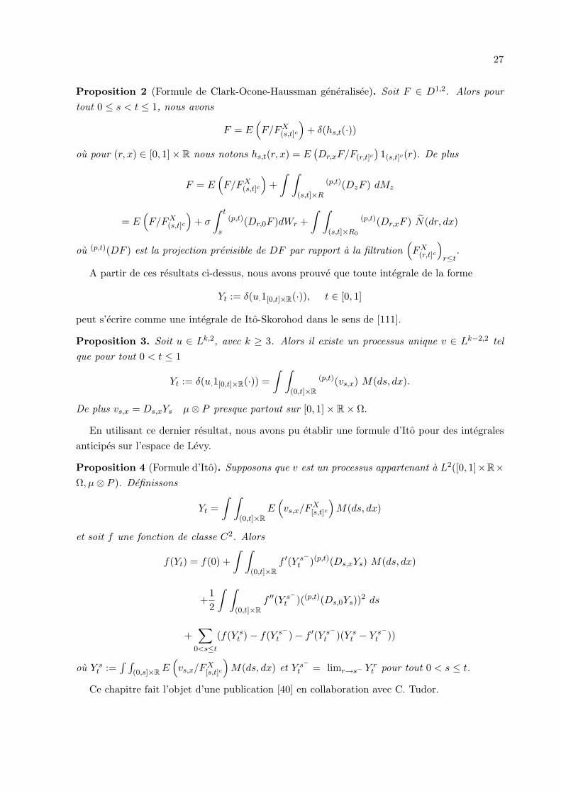
Proposition 2 (Formule de Clark-Ocone-Haussman generalisee). Soit F ∈ D1,2. Alors pourtout 0 ≤ s < t ≤ 1, nous avons
F = E(F/FX
(s,t]c
)+ δ(hs,t(·))
ou pour (r, x) ∈ [0, 1]× R nous notons hs,t(r, x) = E(Dr,xF/F(r,t]c
)1(s,t]c(r). De plus
F = E(F/FX
(s,t]c
)+
∫ ∫
(s,t]×R
(p,t)(DzF ) dMz
= E(F/FX
(s,t]c
)+ σ
∫ t
s
(p,t)(Dr,0F )dWr +∫ ∫
(s,t]×R0
(p,t)(Dr,xF ) N(dr, dx)
ou (p,t)(DF ) est la projection previsible de DF par rapport a la filtration(FX
(r,t]c
)r≤t
.
A partir de ces resultats ci-dessus, nous avons prouve que toute integrale de la forme
Yt := δ(u.1[0,t]×R(·)), t ∈ [0, 1]
peut s’ecrire comme une integrale de Ito-Skorohod dans le sens de [111].
Proposition 3. Soit u ∈ Lk,2, avec k ≥ 3. Alors il existe un processus unique v ∈ Lk−2,2 telque pour tout 0 < t ≤ 1
Yt := δ(u.1[0,t]×R(·)) =∫ ∫
(0,t]×R(p,t)(vs,x) M(ds, dx).
De plus vs,x = Ds,xYs µ⊗ P presque partout sur [0, 1]× R× Ω.
En utilisant ce dernier resultat, nous avons pu etablir une formule d’Ito pour des integralesanticipes sur l’espace de Levy.
Proposition 4 (Formule d’Ito). Supposons que v est un processus appartenant a L2([0, 1]×R×Ω, µ⊗ P ). Definissons
Yt =∫ ∫
(0,t]×RE
(vs,x/FX
[s,t]c
)M(ds, dx)
et soit f une fonction de classe C2. Alors
f(Yt) = f(0) +∫ ∫
(0,t]×Rf ′(Y s−
t )(p,t)(Ds,xYs) M(ds, dx)
+12
∫ ∫
(0,t]×Rf ′′(Y s−
t )((p,t)(Ds,0Ys))2 ds
+∑
0<s≤t
(f(Y st )− f(Y s−
t )− f ′(Y s−t )(Y s
t − Y s−t ))
ou Y st :=
∫ ∫(0,s]×RE
(vs,x/FX
[s,t]c
)M(ds, dx) et Y s−
t = limr→s− Y rt pour tout 0 < s ≤ t.
Ce chapitre fait l’objet d’une publication [40] en collaboration avec C. Tudor.
28
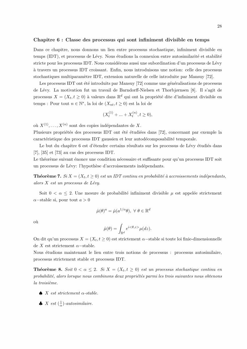
Chapitre 6 : Classe des processus qui sont infiniment divisible en temps
Dans ce chapitre, nous donnons un lien entre processus stochastique, infiniment divisible entemps (IDT), et processus de Levy. Nous etudions la connexion entre autosimilarite et stabilitestricte pour les processus IDT. Nous considerons aussi une subordination d’un processus de Levya travers un processus IDT croissant. Enfin, nous introduisons une notion: celle des processusstochastiques multiparametre IDT, extension naturelle de celle introduite par Mansuy [72].
Les processus IDT ont ete introduits par Mansuy [72] comme une generalisations de processusde Levy. La motivation fut un travail de Barndorff-Nielsen et Thorbjørnsen [8]. Il s’agit deprocessus X = (Xt, t ≥ 0) a valeurs dans Rd qui ont la propriete dite d’infiniment divisible entemps : Pour tout n ∈ N∗, la loi de (Xnt, t ≥ 0) est la loi de
(X(1)t + ... + X
(n)t , t ≥ 0),
ou X(1), . . . , X(n) sont des copies independantes de X.Plusieurs proprietes des processus IDT ont ete etudiees dans [72], concernant par exemple lacaracteristique des processus IDT gaussien et leur autodecomposabilite temporale.
Le but du chapitre 6 est d’etendre certains resultats sur les processus de Levy etudies dans[7], [35] et [73] au cas des processus IDT.Le theoreme suivant enonce une condition necessaire et suffisante pour qu’un processus IDT soitun processus de Levy: l’hypothese d’accroissements independants.
Theoreme 7. Si X = (Xt, t ≥ 0) est un IDT continu en probabilite a accroissements independants,alors X est un processus de Levy.
Soit 0 < α ≤ 2. Une mesure de probabilite infiniment divisible µ est appelee strictementα−stable si, pour tout a > 0
µ(θ)a = µ(a1/αθ), ∀ θ ∈ Rd
ouµ(θ) =
∫
Rd
ei<θ,z>µ(dz).
On dit qu’un processus X = (Xt, t ≥ 0) est strictement α−stable si toute loi finie-dimensionnellede X est strictement α−stable.Nous etudions maintenant le lien entre trois notions de processus : processus autosimilaire,processus strictement stable et processus IDT.
Theoreme 8. Soit 0 < α ≤ 2. Si X = (Xt, t ≥ 0) est un processus stochastique continu enprobabilite, alors lorsque nous combinons deux proprietes parmi les trois suivantes nous obtenonsla troisieme.
♠ X est strictement α-stable.
♣ X est ( 1α)-autosimilaire.
29
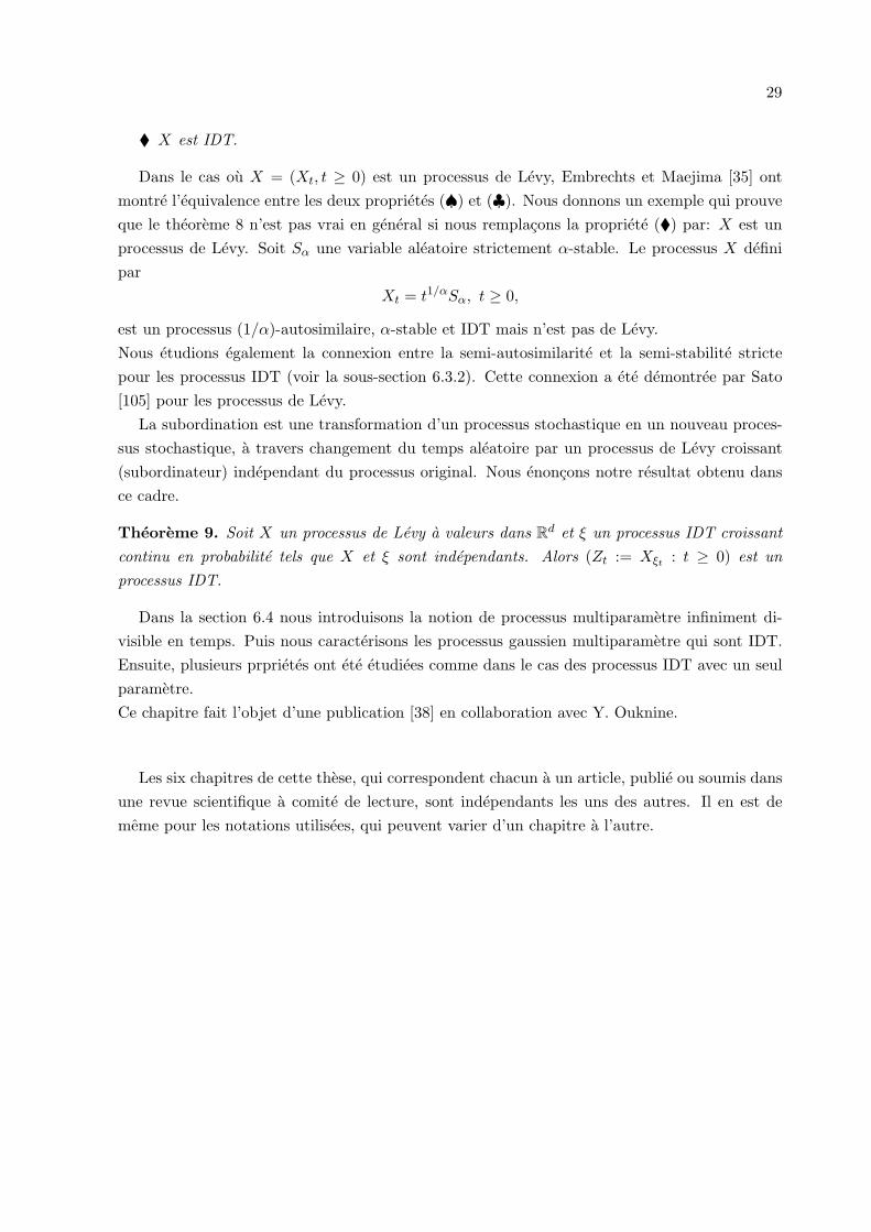
¨ X est IDT.
Dans le cas ou X = (Xt, t ≥ 0) est un processus de Levy, Embrechts et Maejima [35] ontmontre l’equivalence entre les deux proprietes (♠) et (♣). Nous donnons un exemple qui prouveque le theoreme 8 n’est pas vrai en general si nous remplacons la propriete (¨) par: X est unprocessus de Levy. Soit Sα une variable aleatoire strictement α-stable. Le processus X definipar
Xt = t1/αSα, t ≥ 0,
est un processus (1/α)-autosimilaire, α-stable et IDT mais n’est pas de Levy.Nous etudions egalement la connexion entre la semi-autosimilarite et la semi-stabilite strictepour les processus IDT (voir la sous-section 6.3.2). Cette connexion a ete demontree par Sato[105] pour les processus de Levy.
La subordination est une transformation d’un processus stochastique en un nouveau proces-sus stochastique, a travers changement du temps aleatoire par un processus de Levy croissant(subordinateur) independant du processus original. Nous enoncons notre resultat obtenu dansce cadre.
Theoreme 9. Soit X un processus de Levy a valeurs dans Rd et ξ un processus IDT croissantcontinu en probabilite tels que X et ξ sont independants. Alors (Zt := Xξt : t ≥ 0) est unprocessus IDT.
Dans la section 6.4 nous introduisons la notion de processus multiparametre infiniment di-visible en temps. Puis nous caracterisons les processus gaussien multiparametre qui sont IDT.Ensuite, plusieurs prprietes ont ete etudiees comme dans le cas des processus IDT avec un seulparametre.Ce chapitre fait l’objet d’une publication [38] en collaboration avec Y. Ouknine.
Les six chapitres de cette these, qui correspondent chacun a un article, publie ou soumis dansune revue scientifique a comite de lecture, sont independants les uns des autres. Il en est dememe pour les notations utilisees, qui peuvent varier d’un chapitre a l’autre.
Part I
MALLIAVIN CALCULUS AND
LOCAL TIME ON GAUSSIAN
SPACE
30

31
Chapter 1
Multidimensional bifractional
Brownian motion: Ito and Tanaka
formulas
Using the Malliavin calculus with respect to Gaussian processes and the multiple stochasticintegrals we derive Ito’s and Tanaka’s formulas for the d-dimensional bifractional Brownianmotion.
1.1 Introduction
The stochastic calculus with respect to the fractional Brownian motion (fBm) has now a longhistory. Since the nineties, many authors used different approaches to develop a stochasticintegration theory with respect to this process. We refer, among of course many others, to [1],[27], [33] or [46]. The reason for this tremendous interest in the stochastic analysis of the fBmcomes from its large amount of applications in practical phenomena such as telecommunications,hydrology or economics.
Nevertheless, even fBm has its limits in modeling certain phenomena. Therefore, severalauthors introduced recently some generalizations of the fBm which are supposed to fit betterin concrete situations. For example, we mention the multifractional Brownian motion (see e.g.[4]), the subfractional Brownian motion (see e.g. [16]) or the multiscale fractional Brownianmotion (see [5]).
Here our main interest consists in the study of the bifractional Brownian motion (bifBm).The bifBm has been introduced by Houdre and Villa in [47] and a stochastic analysis for it canbe found in [103]. Other papers treated different aspects of this stochastic process, like samplepaths properties, extension of the parameters or statistical applications (see [17], [12], [113] or[25]). Recall that the bifBm BH,K is a centered Gaussian process, starting from zero, withcovariance function
RH,K(t, s) := R(t, s) =1
2K
((t2H + s2H
)K − |t− s|2HK)
(1.1)
32
Section 1.2. Preliminaries: Deterministic spaces associated and Malliavin calculus 33
where the parameters H, K are such that H ∈ (0, 1) and K ∈ (0, 1]. In the case K = 1 weretrieve the fractional Brownian motion while the case K = 1 and H = 1
2 corresponds to thestandard Brownian motion.
The process BH,K is HK-selfsimilar but it has no stationary increments. It has Holdercontinuous paths of order δ < HK and its paths are not differentiable. An interesting propertyof it is the fact that its quadratic variation in the case 2HK = 1 is similar to that of the standardBrownian motion, i.e. [BH,K ]t = cst. × t and therefore especially this case (2HK = 1) is veryinteresting from the stochastic calculus point of view.
In this paper, our purpose is to study multidimensional bifractional Brownian motion and toprove Ito and Tanaka formulas. We start with the one dimensional bifBm and we first derive Itoand Tanaka formulas for it when 2HK ≥ 1. We mention that the Ito formula has been alreadyproved by [61] but here we propose an alternative proof based on the Taylor expansion whichappears to be also useful in the multidimensional settings. The Tanaka formula is obtained fromthe Ito formula by a limit argument and it involves the so-called weighted local time extendingthe result in [24]. In the multidimensional case we first derive an Ito formula for 2HK > 1and we extend it to Tanaka by following an idea by Uemura [114], [115]; that is, since |x| istwice the kernel of the one-dimensional Newtonian potential, i.e. 1
2∆|x| is equal to the deltaDirac function δ(x), we will chose the function U(z), z ∈ Rd which is twice of the kernel ofd-dimensional Newtonian (or logarithmic if d = 2) potential to replace |x| in the d-dimensionalcase. See the last section for the definition of the function U . Our method is based on theWiener-Ito chaotic expansion into multiple stochastic integrals following ideas from [54] or [34].The multidimensional Tanaka formula also involves a generalized local time. We note that theterms appearing in our Tanaka formula when d ≥ 2 are not random variables and they areunderstood as distributions in the Watanabe spaces.
1.2 Preliminaries: Deterministic spaces associated and Malli-
avin calculus
Let(BH,K
t , t ∈ [0, T ])
be a bifractional Brownian motion on the probability space (Ω,F , P ).Being a Gaussian process, it is possible to construct a stochastic calculus of variations with
respect to BH,K . We refer to [1], [81] for a complete description of stochastic calculus withrespect to Gaussian processes. Here we recall only the basic elements of this theory.
The basic ingredient is the canonical Hilbert space H associated to the bifractional Brownianmotion. This space is defined as the completion of the linear space E generated by the indicatorfunctions 1[0,t], t ∈ [0, T ] with respect to the inner product
〈1[0,t], 1[0,s]〉H = R(t, s).
The application ϕ ∈ E → BH,K(ϕ) is an isometry from E to the Gaussian space generated byBH,K and it can be extended to H.
Section 1.2. Preliminaries: Deterministic spaces associated and Malliavin calculus 34
Let us denote by S the set of smooth functionals of the form
F = f(BH,K(ϕ1), . . . , BH,K(ϕn))
where f ∈ C∞b (Rn) and ϕi ∈ H. The Malliavin derivative of a functional F as above is given by
DBH,KF =
n∑
i=1
∂f
∂xi(BH,K(ϕ1), . . . , BH,K(ϕn))ϕi
and this operator can be extended to the closure Dm,2 (m ≥ 1) of S with respect to the norm
‖F‖2m,2 := E |F |2 + E‖DBH,K
F‖2H + . . . + E‖DBH,K ,mF‖2
H⊗m
where H⊗m denotes the m fold symmetric tensor product and the mth derivative DBH,K ,m isdefined by iteration.
The divergence integral δBH,Kis the adjoint operator of DBH,K
. Concretely, a random variableu ∈ L2(Ω;H) belongs to the domain of the divergence operator (Dom(δBH,K
)) if
E∣∣∣〈DBH,K
F, u〉H∣∣∣ ≤ c‖F‖L2(Ω)
for every F ∈ S. In this case δBH,K(u) is given by the duality relationship
E(FδBH,K(u)) = E〈DBH,K
F, u〉H
for any F ∈ D1,2. It holds that
EδBH,K(u)2 = E‖u‖2
H + E〈DBH,Ku, (DBH,K
u)∗〉H⊗H (1.2)
where (DBH,Ku)∗ is the adjoint of DBH,K
u in the Hilbert space H⊗H.
Sometimes working with the space H is not convenient; once, because this space may containalso distributions (as, e.g. in the case K = 1, see [95]) and twice, because the norm in thisspace is not always tractable. We will use the subspace |H| of H which is defined as the set ofmeasurable function f on [0, T ] with
‖f‖2|H| :=
∫ T
0
∫ T
0|f(u)| |f(v)|
∣∣∣∣∂2R
∂u∂v(u, v)
∣∣∣∣ dudv < ∞. (1.3)
It follows actually from [61] that the space |H| is a Banach space for the norm ‖ · ‖|H| and it isincluded in H. In fact,
L2([0, T ]) ⊂ |H| ⊂ H.
andEδBH,K
(u)2 ≤ E‖u‖2|H| + E‖DBH,K
u‖2|H|⊗|H| (1.4)
where, if ϕ : [0, T ]2 → R
‖ϕ‖2|H|⊗|H| =
∫
[0,T ]4|ϕ(u, v)| ∣∣ϕ(u′, v′)
∣∣∣∣∣∣
∂2R
∂u∂u′(u, u′)
∂2R
∂v∂v′(v, v′)
∣∣∣∣ dudvdu′dv′. (1.5)
Section 1.2. Preliminaries: Deterministic spaces associated and Malliavin calculus 35
We will use the following formulas of the Malliavin calculus: the integration by parts
FδBH,K(u) = δBH,K
(Fu) + 〈DBH,KF, u〉H (1.6)
for any u ∈ Dom(δBH,K), F ∈ D1,2 such that Fu ∈ L2(Ω;H); and the chain rule
DBH,Kϕ(F ) =
n∑
i=1
∂iϕ(F )DBH,KF i
if ϕ : Rn → R is continuously differentiable with bounded partial derivatives and F = (F 1, . . . , Fm)is a random vector with components in D1,2.
By the duality between DBH,Kand δBH,K
we obtain the following result for the convergence ofdivergence integrals: if un ∈ Dom(δBH,K
) for every n, un →n→∞ u in L2(Ω;H) and δBH,K
(un) →n→∞
G ∈ L2(Ω) in L1(Ω) then
u ∈ Dom(δBH,K) and δBH,K
(u) = G. (1.7)
It is also possible to introduce multiple integrals In(fn), f ∈ H⊗n with respect to BH,K . Let
F =∑
n≥0
In(fn) (1.8)
where for every n ≥ 0, fn ∈ H⊗n are symmetric functions. Let L be the Ornstein-Uhlenbeckoperator
LF = −∑
n≥0
nIn(fn)
if F is given by (1.8).For p > 1 and α ∈ R we introduce the Sobolev-Watanabe space Dα,p as the closure of the set
of polynomial random variables with respect to the norm
‖F‖α,p = ‖(I − L)α2 ‖Lp(Ω)
where I represents the identity. In this way, a random variable F as in (1.8) belongs to Dα,2 ifand only if ∑
n≥0
(1 + n)α‖In(fn)‖2L2(Ω) < ∞.
Note that the Malliavin derivative operator acts on multiple integral as follows
DBH,K
t F =∞∑
n=1
nIn−1(fn(·, t)), t ∈ [0, T ].
The operator DBH,Kis continuous from Dα−1,p into Dα,p (H) . The adjoint of DBH,K
is denotedby δBH,K
and is called the divergence (or Skorohod) integral. It is a continuous operator from
Section 1.3. Tanaka formula for unidimensional bifractional Brownian motion 36
Dα,p (H) into Dα,p. For adapted integrands, the divergence integral coincides to the classical Itointegral. We will use the notation
δBH,K(u) =
∫ T
0usδB
H,Ks .
Recall that if u is a stochastic process having the chaotic decomposition
us =∑
n≥0
In(fn(·, s))
where fn(·, s) ∈ H⊗n for every s, and it is symmetric in the first n variables, then its Skorohodintegral is given by ∫ T
0usdBH,K
s =∑
n≥0
In+1(fn)
where fn denotes the symmetrization of fn with respect to all n + 1 variables.
1.3 Tanaka formula for unidimensional bifractional Brownian
motion
This paragraph is consecrated to the proof of Ito formula and Tanaka formula for the one-dimensional bifractional Brownian motion with 2HK ≥ 1. Note that the Ito formula has beenalready proved in [61]; here we propose a different approach based on the Taylor expansionwhich will be also used in the multidimensional settings.
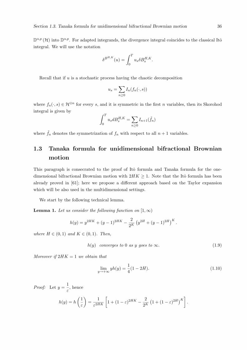
We start by the following technical lemma.
Lemma 1. Let us consider the following function on [1,∞)
h(y) = y2HK + (y − 1)2HK − 22K
(y2H + (y − 1)2H
)K.
where H ∈ (0, 1) and K ∈ (0, 1). Then,
h(y) converges to 0 as y goes to ∞. (1.9)
Moreover if 2HK = 1 we obtain that
limy→+∞ yh(y) =
14(1− 2H). (1.10)
Proof: Let y =1ε, hence
h(y) = h
(1ε
)=
1ε2HK
[1 + (1− ε)2HK − 2
2K
(1 + (1− ε)2H
)K]
.
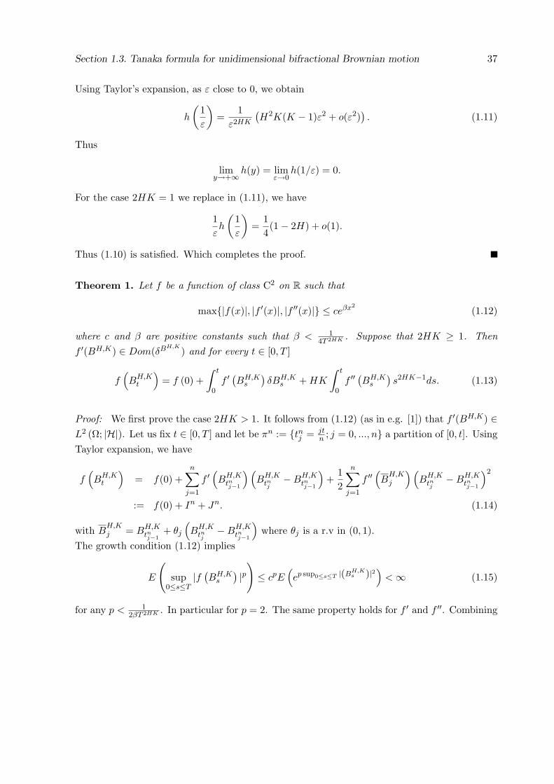
Section 1.3. Tanaka formula for unidimensional bifractional Brownian motion 37
Using Taylor’s expansion, as ε close to 0, we obtain
h
(1ε
)=
1ε2HK
(H2K(K − 1)ε2 + o(ε2)
). (1.11)
Thus
limy→+∞h(y) = lim
ε→0h(1/ε) = 0.
For the case 2HK = 1 we replace in (1.11), we have
1εh
(1ε
)=
14(1− 2H) + o(1).
Thus (1.10) is satisfied. Which completes the proof.
Theorem 1. Let f be a function of class C2 on R such that
max|f(x)|, |f ′(x)|, |f ′′(x)| ≤ ceβx2(1.12)
where c and β are positive constants such that β < 14T 2HK . Suppose that 2HK ≥ 1. Then
f ′(BH,K) ∈ Dom(δBH,K) and for every t ∈ [0, T ]
f(BH,K
t
)= f (0) +
∫ t
0f ′
(BH,K
s
)δBH,K
s + HK
∫ t
0f ′′
(BH,K
s
)s2HK−1ds. (1.13)
Proof: We first prove the case 2HK > 1. It follows from (1.12) (as in e.g. [1]) that f ′(BH,K) ∈L2 (Ω; |H|). Let us fix t ∈ [0, T ] and let be πn := tnj = jt
n ; j = 0, ..., n a partition of [0, t]. UsingTaylor expansion, we have
f(BH,K
t
)= f(0) +
n∑
j=1
f ′(BH,K
tnj−1
)(BH,K
tnj−BH,K
tnj−1
)+
12
n∑
j=1
f ′′(B
H,Kj
)(BH,K
tnj−BH,K
tnj−1
)2
:= f(0) + In + Jn. (1.14)
with BH,Kj = BH,K
tnj−1+ θj
(BH,K
tnj−BH,K
tnj−1
)where θj is a r.v in (0, 1).
The growth condition (1.12) implies
E
(sup
0≤s≤T|f (
BH,Ks
) |p)≤ cpE
(ep sup0≤s≤T |(BH,K
s )|2)
< ∞ (1.15)
for any p < 12βT 2HK . In particular for p = 2. The same property holds for f ′ and f ′′. Combining
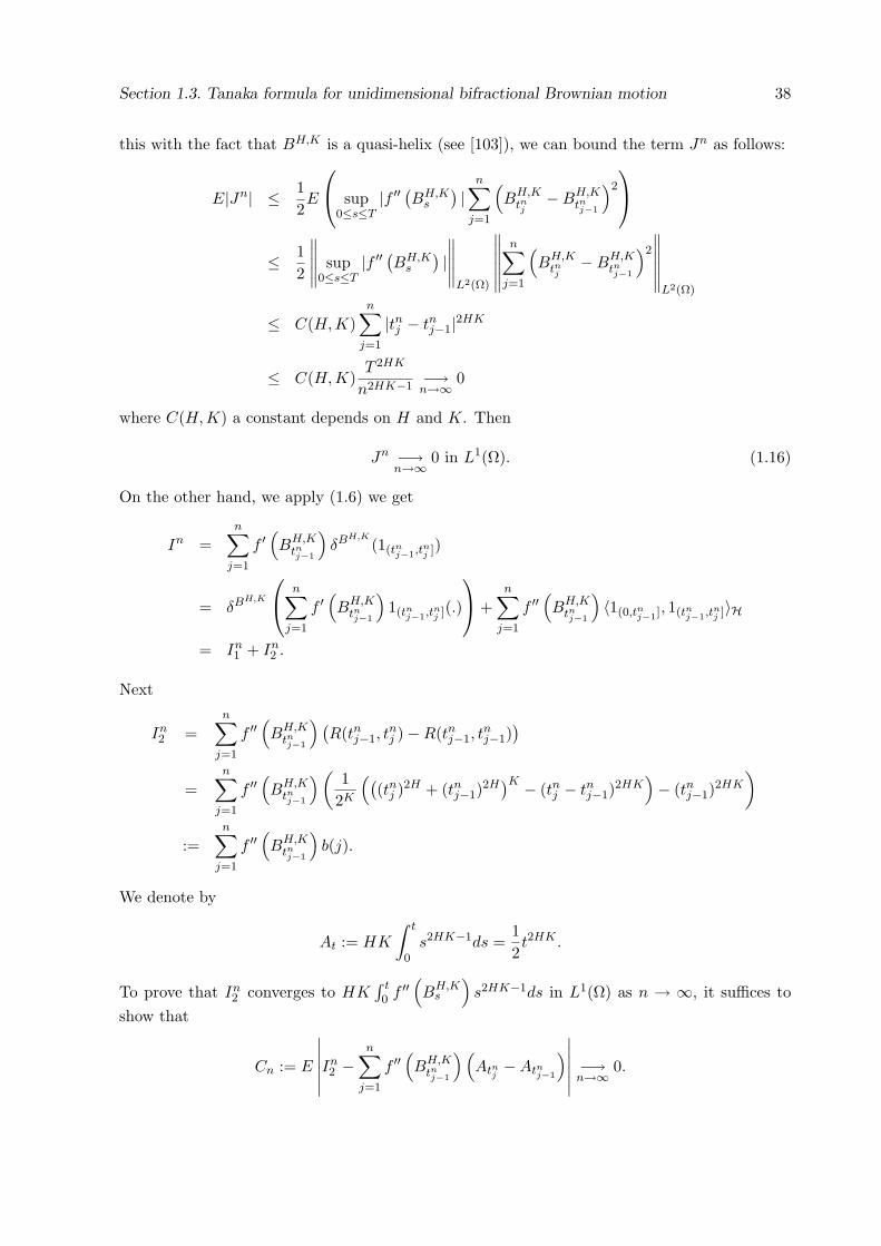
Section 1.3. Tanaka formula for unidimensional bifractional Brownian motion 38
this with the fact that BH,K is a quasi-helix (see [103]), we can bound the term Jn as follows:
E|Jn| ≤ 12E
sup
0≤s≤T|f ′′ (BH,K
s
) |n∑
j=1
(BH,K
tnj−BH,K
tnj−1
)2
≤ 12
∥∥∥∥∥ sup0≤s≤T
|f ′′ (BH,Ks
) |∥∥∥∥∥
L2(Ω)
∥∥∥∥∥∥
n∑
j=1
(BH,K
tnj−BH,K
tnj−1
)2
∥∥∥∥∥∥L2(Ω)
≤ C(H, K)n∑
j=1
|tnj − tnj−1|2HK
≤ C(H, K)T 2HK
n2HK−1−→n→∞ 0
where C(H,K) a constant depends on H and K. Then
Jn −→n→∞ 0 in L1(Ω). (1.16)
On the other hand, we apply (1.6) we get
In =n∑
j=1
f ′(BH,K
tnj−1
)δBH,K
(1(tnj−1,tnj ])
= δBH,K
n∑
j=1
f ′(BH,K
tnj−1
)1(tnj−1,tnj ](.)
+
n∑
j=1
f ′′(BH,K
tnj−1
)〈1(0,tnj−1], 1(tnj−1,tnj ]〉H
= In1 + In
2 .
Next
In2 =
n∑
j=1
f ′′(BH,K
tnj−1
) (R(tnj−1, t
nj )−R(tnj−1, t
nj−1)
)
=n∑
j=1
f ′′(BH,K
tnj−1
)(1
2K
(((tnj )2H + (tnj−1)
2H)K − (tnj − tnj−1)
2HK)− (tnj−1)
2HK
)
:=n∑
j=1
f ′′(BH,K
tnj−1
)b(j).
We denote by
At := HK
∫ t
0s2HK−1ds =
12t2HK .
To prove that In2 converges to HK
∫ t0 f ′′
(BH,K
s
)s2HK−1ds in L1(Ω) as n → ∞, it suffices to
show that
Cn := E
∣∣∣∣∣∣In2 −
n∑
j=1
f ′′(BH,K
tnj−1
)(Atnj
−Atnj−1
)∣∣∣∣∣∣−→n→∞ 0.
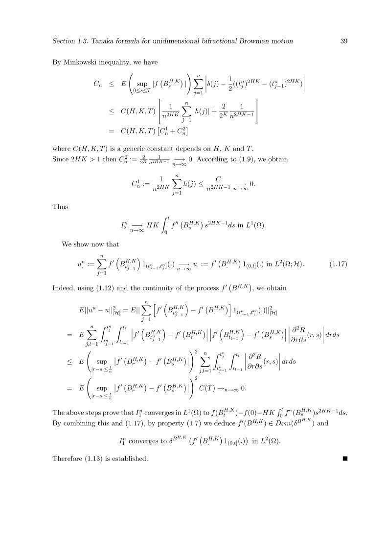
Section 1.3. Tanaka formula for unidimensional bifractional Brownian motion 39
By Minkowski inequality, we have
Cn ≤ E
(sup
0≤s≤T|f (
BH,Ks
) |)
n∑
j=1
∣∣∣∣b(j)−12((tnj )2HK − (tnj−1)
2HK)∣∣∣∣
≤ C(H,K, T )
1
n2HK
n∑
j=1
|h(j)|+ 22K
1n2HK−1
= C(H,K, T )[C1
n + C2n
]
where C(H,K, T ) is a generic constant depends on H, K and T .Since 2HK > 1 then C2
n := 22K
1n2HK−1 −→
n→∞ 0. According to (1.9), we obtain
C1n :=
1n2HK
n∑
j=1
h(j) ≤ C
n2HK−1−→n→∞ 0.
Thus
In2 −→
n→∞ HK
∫ t
0f ′′
(BH,K
s
)s2HK−1ds in L1(Ω).
We show now that
un. :=
n∑
j=1
f ′(BH,K
tnj−1
)1(tnj−1,tnj ](.) −→
n→∞ u. := f ′(BH,K
.
)1(0,t](.) in L2(Ω;H). (1.17)
Indeed, using (1.12) and the continuity of the process f ′(BH,K
), we obtain
E||un − u||2|H| = E||n∑
j=1
[f ′
(BH,K
tnj−1
)− f ′
(BH,K
.
)]1(tnj−1,tnj ](.)||2|H|
= En∑
j,l=1
∫ tnj
tnj−1
∫ tl
tl−1
∣∣∣f ′(BH,K
tnj−1
)− f ′
(BH,K
r
)∣∣∣∣∣∣f ′
(BH,K
tl−1
)− f ′
(BH,K
s
)∣∣∣∣∣∣∣∂2R
∂r∂s(r, s)
∣∣∣∣ drds
≤ E
(sup
|r−s|≤ tn
∣∣f ′ (BH,Kr
)− f ′(BH,K
s
)∣∣)2 n∑
j,l=1
∫ tnj
tnj−1
∫ tl
tl−1
∣∣∣∣∂2R
∂r∂s(r, s)
∣∣∣∣ drds
= E
(sup
|r−s|≤ tn
∣∣f ′ (BH,Kr
)− f ′(BH,K
s
)∣∣)2
C(T ) →n→∞ 0.
The above steps prove that In1 converges in L1(Ω) to f(BH,K
t )−f(0)−HK∫ t0 f”(BH,K
s )s2HK−1ds.By combining this and (1.17), by property (1.7) we deduce f ′(BH,K) ∈ Dom(δBH,K
) and
In1 converges to δBH,K (
f ′(BH,K
.
)1(0,t](.)
)in L2(Ω).
Therefore (1.13) is established.
Section 1.3. Tanaka formula for unidimensional bifractional Brownian motion 40
The proof of the case 2HK = 1 is based on a preliminary result concerning the quadraticvariation of the bifractional Brownian motion. It was proved in [103] using the stochastic calculusvia regularization.
Lemma 2. Suppose that 2HK = 1, then
V nt :=
n∑
j=1
(BH,K
tnj−BH,K
tnj−1
)2−→n→∞
12k−1
t in L2(Ω).
Proof: A straightforward calculation shows that,
EV nt =
t
n
n∑
j=1
h(j) +t
2k−1−→n→∞
t
2k−1.
To obtain the conclusion it suffices to show that
limn→∞E(V n
t )2 = (t
2k−1)2.
In fact we have,
E(V nt )2 =
n∑
i,j=1
E((BH,K
tni−BH,K
tni−1)(BH,K
tnj−BH,K
tnj−1))2
Denote by
µn(i, j) = E((BH,K
tni−BH,K
tni−1)(BH,K
tnj−BH,K
tnj−1))2
It follows by linear regression that
µn(i, j) = E
(N2
1
∣∣∣∣θn(i, j)N1 +√
δn(i, j)− (θn(i, j))2N2
∣∣∣∣2)
where N1 and N2 two independent normal random variables,
θn(i, j) := E((BH,K
tni−BH,K
tni−1)(BH,K
tnj−BH,K
tnj−1))
=t
2Kn
[(i2H + j2H)K − 2|j − i| − (i2H + (j − 1)2H)K + |j − i− 1|
−((i− 1)2H + j2H)K + |j − i + 1|+ ((i− 1)2H + (j − 1)2H)K]
and
δn(i, j) := E(BH,K
tni−BH,K
tni−1
)2E
(BH,K
tnj−BH,K
tnj−1
)2.
Hence
µn(i, j) = 2(θn(i, j))2 + δn(i, j).
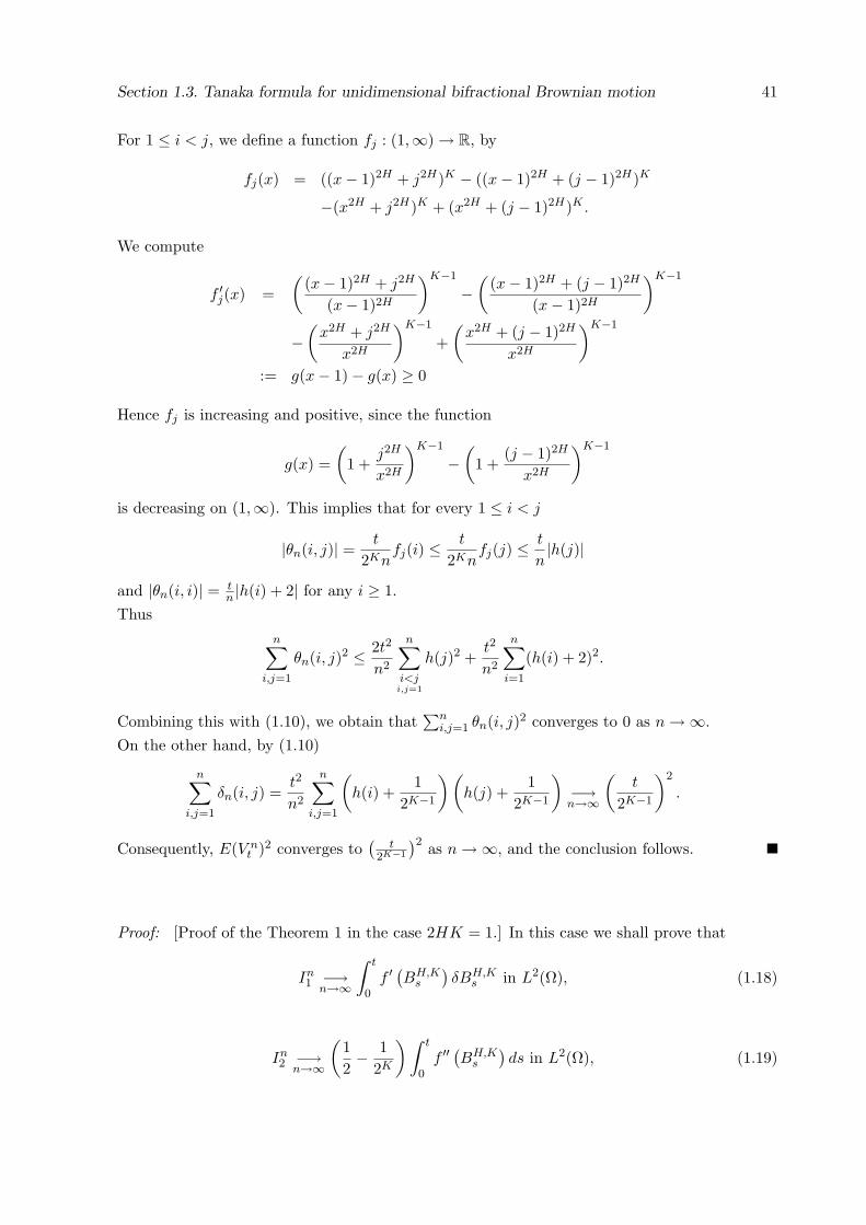
Section 1.3. Tanaka formula for unidimensional bifractional Brownian motion 41
For 1 ≤ i < j, we define a function fj : (1,∞) → R, by
fj(x) = ((x− 1)2H + j2H)K − ((x− 1)2H + (j − 1)2H)K
−(x2H + j2H)K + (x2H + (j − 1)2H)K .
We compute
f ′j(x) =(
(x− 1)2H + j2H
(x− 1)2H
)K−1
−(
(x− 1)2H + (j − 1)2H
(x− 1)2H
)K−1
−(
x2H + j2H
x2H
)K−1
+(
x2H + (j − 1)2H
x2H
)K−1
:= g(x− 1)− g(x) ≥ 0
Hence fj is increasing and positive, since the function
g(x) =(
1 +j2H
x2H
)K−1
−(
1 +(j − 1)2H
x2H
)K−1
is decreasing on (1,∞). This implies that for every 1 ≤ i < j
|θn(i, j)| = t
2Knfj(i) ≤ t
2Knfj(j) ≤ t
n|h(j)|
and |θn(i, i)| = tn |h(i) + 2| for any i ≥ 1.
Thusn∑
i,j=1
θn(i, j)2 ≤ 2t2
n2
n∑
i<ji,j=1
h(j)2 +t2
n2
n∑
i=1
(h(i) + 2)2.
Combining this with (1.10), we obtain that∑n
i,j=1 θn(i, j)2 converges to 0 as n →∞.
On the other hand, by (1.10)
n∑
i,j=1
δn(i, j) =t2
n2
n∑
i,j=1
(h(i) +
12K−1
)(h(j) +
12K−1
)−→n→∞
(t
2K−1
)2
.
Consequently, E(V nt )2 converges to
(t
2K−1
)2 as n →∞, and the conclusion follows.
Proof: [Proof of the Theorem 1 in the case 2HK = 1.] In this case we shall prove that
In1 −→
n→∞
∫ t
0f ′
(BH,K
s
)δBH,K
s in L2(Ω), (1.18)
In2 −→
n→∞
(12− 1
2K
)∫ t
0f ′′
(BH,K
s
)ds in L2(Ω), (1.19)
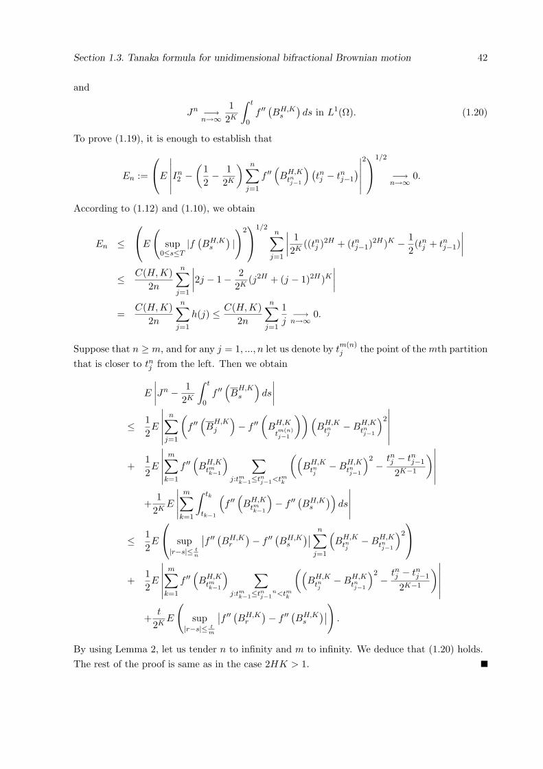
Section 1.3. Tanaka formula for unidimensional bifractional Brownian motion 42
and
Jn −→n→∞
12K
∫ t
0f ′′
(BH,K
s
)ds in L1(Ω). (1.20)
To prove (1.19), it is enough to establish that
En :=
E
∣∣∣∣∣∣In2 −
(12− 1
2K
) n∑
j=1
f ′′(BH,K
tnj−1
) (tnj − tnj−1
)∣∣∣∣∣∣
2
1/2
−→n→∞ 0.
According to (1.12) and (1.10), we obtain
En ≤E
(sup
0≤s≤T|f (
BH,Ks
) |)2
1/2n∑
j=1
∣∣∣∣1
2K((tnj )2H + (tnj−1)
2H)K − 12(tnj + tnj−1)
∣∣∣∣
≤ C(H, K)2n
n∑
j=1
∣∣∣∣2j − 1− 22K
(j2H + (j − 1)2H)K
∣∣∣∣
=C(H, K)
2n
n∑
j=1
h(j) ≤ C(H,K)2n
n∑
j=1
1j−→n→∞ 0.
Suppose that n ≥ m, and for any j = 1, ..., n let us denote by tm(n)j the point of the mth partition
that is closer to tnj from the left. Then we obtain
E
∣∣∣∣Jn − 12K
∫ t
0f ′′
(B
H,Ks
)ds
∣∣∣∣
≤ 12E
∣∣∣∣∣∣
n∑
j=1
(f ′′
(B
H,Kj
)− f ′′
(BH,K
tm(n)j−1
))(BH,K
tnj−BH,K
tnj−1
)2
∣∣∣∣∣∣
+12E
∣∣∣∣∣∣
m∑
k=1
f ′′(BH,K
tmk−1
) ∑
j:tmk−1≤tnj−1<tmk
((BH,K
tnj−BH,K
tnj−1
)2− tnj − tnj−1
2K−1
)∣∣∣∣∣∣
+1
2KE
∣∣∣∣∣m∑
k=1
∫ tk
tk−1
(f ′′
(BH,K
tmk−1
)− f ′′
(BH,K
s
))ds
∣∣∣∣∣
≤ 12E
sup|r−s|≤ t
n
∣∣f ′′ (BH,Kr
)− f ′′(BH,K
s
)∣∣n∑
j=1
(BH,K
tnj−BH,K
tnj−1
)2
+12E
∣∣∣∣∣∣
m∑
k=1
f ′′(BH,K
tmk−1
) ∑
j:tmk−1≤tnj−1n<tmk
((BH,K
tnj−BH,K
tnj−1
)2− tnj − tnj−1
2K−1
)∣∣∣∣∣∣
+t
2KE
(sup
|r−s|≤ tm
∣∣f ′′ (BH,Kr
)− f ′′(BH,K
s
)∣∣)
.
By using Lemma 2, let us tender n to infinity and m to infinity. We deduce that (1.20) holds.The rest of the proof is same as in the case 2HK > 1.
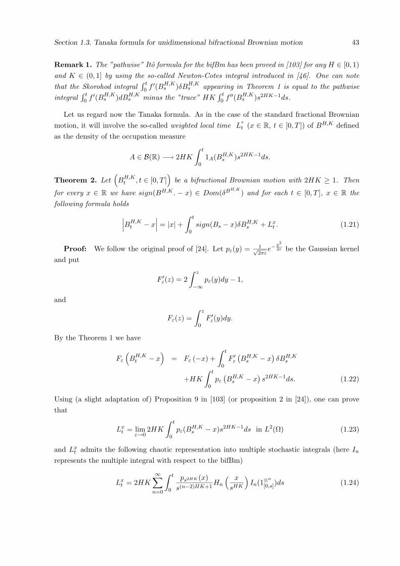
Section 1.3. Tanaka formula for unidimensional bifractional Brownian motion 43
Remark 1. The ”pathwise” Ito formula for the bifBm has been proved in [103] for any H ∈ [0, 1)and K ∈ (0, 1] by using the so-called Newton-Cotes integral introduced in [46]. One can notethat the Skorohod integral
∫ t0 f ′(BH,K
s )δBH,Ks appearing in Theorem 1 is equal to the pathwise
integral∫ t0 f ′(BH,K
s )dBH,Ks minus the ”trace” HK
∫ t0 f ′′(BH,K
s )s2HK−1ds.
Let us regard now the Tanaka formula. As in the case of the standard fractional Brownianmotion, it will involve the so-called weighted local time L
x
t (x ∈ R, t ∈ [0, T ]) of BH,K definedas the density of the occupation measure
A ∈ B(R) −→ 2HK
∫ t
01A(BH,K
s )s2HK−1ds.
Theorem 2. Let(BH,K
t , t ∈ [0, T ])
be a bifractional Brownian motion with 2HK ≥ 1. Then
for every x ∈ R we have sign(BH,K . − x) ∈ Dom(δBH,K) and for each t ∈ [0, T ], x ∈ R the
following formula holds
∣∣∣BH,Kt − x
∣∣∣ = |x|+∫ t
0sign(Bs − x)δBH,K
s + Lxt . (1.21)
Proof: We follow the original proof of [24]. Let pε(y) = 1√2πε
e−y2
2ε be the Gaussian kerneland put
F ′ε(z) = 2
∫ z
−∞pε(y)dy − 1,
and
Fε(z) =∫ z
0F ′
ε(y)dy.
By the Theorem 1 we have
Fε
(BH,K
t − x)
= Fε (−x) +∫ t
0F ′
ε
(BH,K
s − x)δBH,K
s
+HK
∫ t
0pε
(BH,K
s − x)s2HK−1ds. (1.22)
Using (a slight adaptation of) Proposition 9 in [103] (or proposition 2 in [24]), one can provethat
Lxt = lim
ε→02HK
∫ t
0pε(BH,K
s − x)s2HK−1ds in L2(Ω) (1.23)
and Lxt admits the following chaotic representation into multiple stochastic integrals (here In
represents the multiple integral with respect to the bifBm)
Lxt = 2HK
∞∑
n=0
∫ t
0
ps2HK (x)s(n−2)HK+1
Hn
( x
sHK
)In(1⊗
n
[0,s])ds (1.24)
Section 1.4. Tanaka formula for multidimensional bifractional Brownian motion 44
where Hn is the nth Hermite polynomial defined as
Hn(x) =(−1)n
n!ex2/2 dn
dxn(e−x2/2) for every n ≥ 1.
We have Fε(x) → |x| as ε → 0 and since Fε(x) ≤ |x|, then by Lebesgue’s dominated convergencetheorem we obtain that Fε(B
H,Kt − x) converges to |BH,K
t − x| in L2(Ω) as ε → 0.On the other hand, since 0 ≤ F ′
ε(x) ≤ 1 and F ′ε(x) → sign(x) as ε goes to 0 the Lebesgue’s
dominated convergence theorem in L2(Ω×[0, T ]2; P⊗∣∣∣ ∂2R∂u∂v (u, v)
∣∣∣ dudv) implies that F ′ε
(BH,K
. − x)
converges to sign(BH,K
. − x)
in L2(Ω;H) as ε goes to 0 because
E‖F ′ε
(BH,K
. − x)− sign
(BH,K
. − x) ‖2
|H|
= E
∫ T
0
∫ T
0
∣∣F ′ε
(BH,K
u − x)− sign
(BH,K
u − x)∣∣ ∣∣F ′
ε
(BH,K
v − x)− sign
(BH,K
v − x)∣∣
×∣∣∣∣
∂2R
∂u∂v(u, v)
∣∣∣∣ dudv.
Consequently, from the above convergences and (1.7), we deduce as in the proof of Theorem 1that sign
(BH,K − x
) ∈ Dom(δBH,K) for every x and
∫ t
0F ′
ε
(BH,K
s − x)δBH,K
s −→ε→0
∫ t
0sign
(BH,K
s − x)δBH,K
s in L2(Ω).
Then the conclusion follows.
1.4 Tanaka formula for multidimensional bifractional Brownian
motion
Given two vectors H = (H1, . . . ,Hd) ∈ [0, 1]d and K = (K1, . . . , Kd) ∈ (0, 1]d, we introduce thed-dimensional bifractional Brownian motion
BH,K =(BH1,K1 , ..., BHd,Kd
)
as a centered Gaussian vector whose component are independent one-dimensional bifractionalBrownian motions.
We extend the Ito formula to the multidensional case.
Theorem 3. Let BH,K =(BH1,K1 , ..., BHd,Kd
)be a d-dimensional bifractional Brownian mo-
tion, and let f be a function of class C2(Rd,R
)such that for every x ∈ Rd
dmaxi,l=1
(|f(x)|, | ∂f
∂xi(x)|, | ∂2f
∂xi∂xl(x)|
)≤ ceβ|x|2 , (1.25)
where c and β are positive constants such that β < 14T 2(HK)∗ where (HK)∗ = maxd
i=1 H iKi.We assume that 2HiKi > 1 for any i = 1, ...n. Then for every i we have ∂f
∂xi
(BHi,Ki
) ∈Dom(δB
Hi,Kis ) and for every t ∈ [0, T ]
f(BH,K
t
)= f (0) +
d∑
i=1
∫ t
0
∂f
∂xi
(BHi,Ki
s
)δBHi,Ki
s +d∑
i=1
HiKi
∫ t
0
∂2f
∂x2i
(BH,K
s
)s2HiKi−1ds.(1.26)
Section 1.4. Tanaka formula for multidimensional bifractional Brownian motion 45
Proof: Let us fix t > 0 and a partition tnj = jtn ; j = 0, ..., n of [0, t]. As in above, the condition
(1.25) implies that
E
(sup
0≤s≤T|f (
BH,Ks
) |2)≤ c2E
(e2 sup0≤s≤T |(BH,K
s )|2)
< ∞. (1.27)
The same property holds for any ∂f∂xi
and ∂2f∂xi∂xl
with i, l = 1, ..., d. Using Taylor expansion, wehave
f(BH,K
t
)= f(0) +
n∑
j=1
d∑
i=1
∂f
∂xi
(BH,K
tnj−1
)(BHi,Ki
tnj−BHi,Ki
tnj−1
)
+12
n∑
j=1
d∑
i,l=1
∂2f
∂xi∂xl
(B
H,Kj
)(BHi,Ki
tnj−BHi,Ki
tnj−1
)(BHl,Kl
tnj−BHl,Kl
tnj−1
)
:= f(0) + In + Jn
where BH,Kj = BH,K
tnj−1+ θj
(BH,K
tnj−BH,K
tnj−1
), and θj is a random variable in (0, 1).
We show that Jn converges to 0 in L1(Ω) as n → ∞. Applying Holder inequality and theproperty (1.27), we have
E|Jn| ≤ C(H, K)n∑
j=1
d∑
i,l=1
(E
(BHi,Ki
tnj−BHi,Ki
tnj−1
)2)1/2 (
E(BHl,Kl
tnj−BHl,Kl
tnj−1
)2)1/2
≤ C(H, K)d∑
i,l=1
T 2(HK)∗
nHiKi+HlKl−1−→n→∞ 0
(Note that if 2HiKi = 1 for some i then the above sum does not converge to zero). Accordingto (1.6), we get
In =n∑
j=1
d∑
i=1
∂f
∂xi
(BH,K
tnj−1
)(δBHi,Ki (1(tnj−1,tnj ])
)
=d∑
i=1
δBHi,Ki
n∑
j=1
∂f
∂xi
(BH,K
tnj−1
)1(tnj−1,tnj ](.)
+n∑
j=1
∂2f
∂x2i
(BH,K
tnj−1
)〈1(0,tnj−1], 1(tnj−1,tnj ]〉H
=d∑
i=1
[In,i1 + In,i
2
].
As the similar way in the above theorem, we obtain that for every i = 1, ..., d
In,i2 −→
n→∞ HiKi
∫ t
0
∂2f
∂x2i
(BH,K
s
)s2HiKi−1ds in L2(Ω).
Section 1.4. Tanaka formula for multidimensional bifractional Brownian motion 46
We show that for every i ∈ 1, ..., d
In,i1 −→
n→∞
∫ t
0
∂f
∂xi
(BH,K
s
)δBHi,Ki
s in L2(Ω).
We set
un,is =
n∑
j=1
∂f
∂xi
(BH,K
tj−1
)1(tj−1,tj ](s)−
∂f
∂xi
(BH,K
s
)1(0,t](s).
By inequality (1.4), we have
E(δBHi,Ki (un,i)
)2≤ E‖un,i‖2
|Hi| + E‖Dun,i‖2|Hi|⊗|Hi|
where Hi is the Hilbert space associated to BHi,Ki and Ri its covariance function.For every r, s ≤ t
Drun,is =
n∑
j=1
∂2f
∂x2i
(BH,K
tj−1
)1(0,tj−1](r)1(tj−1,tj ](s)−
∂2f
∂x2i
(BH,Ks )1(0,s](r)
we remark that Drun,is and un,i
s converge to zero as n −→ ∞ for any r, s ≤ t. Using (1.12), theLebesgue dominated convergence theorem and the expression of the norm
∣∣Hi∣∣⊗ ∣∣Hi
∣∣ we obtainthat
δBHi,Ki (un,i) −→n→∞ 0 in L2(Ω).
The proof is thus complete.
One can easily generalize the above theorem to the case when the function f depends ontime.
Theorem 4. Let f ∈ C1,2([0, T ]× Rd,R
)and BH,K =
(BH1,K1 , ..., BHd,Kd
)be a d-dimensional
bifBm with 2HiKi > 1 for any i = 1, ..., n. Assume that the function f(t, ·) satisfies (1.12)uniformly in t. Then for every i one has ∂f
∂xi
(·, BH,K
·)∈ Dom(δBHi,Ki ) and for every t
f(t, BH,K
t
)= f (0, 0) +
∫ t
0
∂f
∂s(s, BH,K
s )ds +d∑
i=1
∫ t
0
∂f
∂xi
(s,BH,K
s
)δBHi,Ki
s
+d∑
i=1
HiKi
∫ t
0
∂2f
∂x2i
(s,BH,K
s
)s2HiKi−1ds. (1.28)
We consider twice of the kernel of the d−dimensional Newtonian potential
U(z) =
−Γ(d/2−1)
2πd/21
|z|d−2 if d ≥ 31π log|z| if d = 2.
Section 1.4. Tanaka formula for multidimensional bifractional Brownian motion 47
Set
U(s, z) =1∏d
j=1
√2HjKj
sθU
((z1 − x1)√
2H1K1s1/2−H1K1 , ...,
(zd − xd)√2HdKd
s1/2−HdKd
)(1.29)
where x = (x1, ..., xd) ∈ Rd and 0 < γ := 12(2 − d) + θ + (d − 2)(HK)∗ − ∑d
i=1 HiKi with(HK)∗ = maxH1K1, . . . , HdKd.
We shall prove the following Tanaka formula. It will involve a multidimensional weightedlocal time which is an extension of the one-dimensional local time given by (1.24). Note for anydimension d ≥ 2 the local time is not a random variable anymore and it is a distribution in theWatanabe’s sense.
Theorem 5. Let U as above and let BH,K =(BH1,K1 , ..., BHd,Kd
)be a d-dimensional bifBm
with 2HiKi > 1 for any i = 1, ...d. Then the following formula holds in the Watanabe spaceDα−1
2 for any α < 12(HK)∗ − d/2.
U(t, BH,Kt ) = U(0, 0) +
∫ t
0∂sU(s,BH,K
s )ds +d∑
i=1
∫ t
0
∂U(s,BH,Ks )
∂xiδBHi,Ki
s + Lθ(t, x) (1.30)
where the generalized weighted local time Lθ(t, x) is defined as
Lθ(t, x) =∑
n=(n1,...,nd)
∫ t
0
d∏
i=1
ps2HiKi (xi)
s12+(ni−1)HiKi
Hni
(xi√
s2HiKi
)Iini
(1⊗ni
[0,s])sθds.
Proof: We regularize the function U by standard convolution. Put Uε = pdε ∗ U , with pd
ε isthe Gaussian kernel on Rd given by
pdε(x) =
d∏
i=1
pε(xi) =d∏
i=1
1√2πε
e−x2
2ε , ∀x = (x1, ..., xd) ∈ Rd.
Using the above Ito formula we have
Uε
(t, BH,K
t
)= Uε (0, 0) +
∫ t
0
∂Uε
∂s
(s, BH,K
s
)ds +
d∑
i=1
∫ t
0
∂Uε
∂xi
(s, BH,K
s
)δBHi,Ki
s
+d∑
i=1
HiKi
∫ t
0
∂2Uε
∂x2i
(s,BH,K
s
)s2HiKi−1ds.
= Uε (0, 0) + Iε1(t) + Iε
2(t).
On the other hand, if V (z) = U(a1z1, ..., adzd) and Vε = pdε ∗ V we have
12
d∑
i=1
1a2
i
∂2Vε
∂z2i
(z) = pdε(a1z1, ..., adzd).
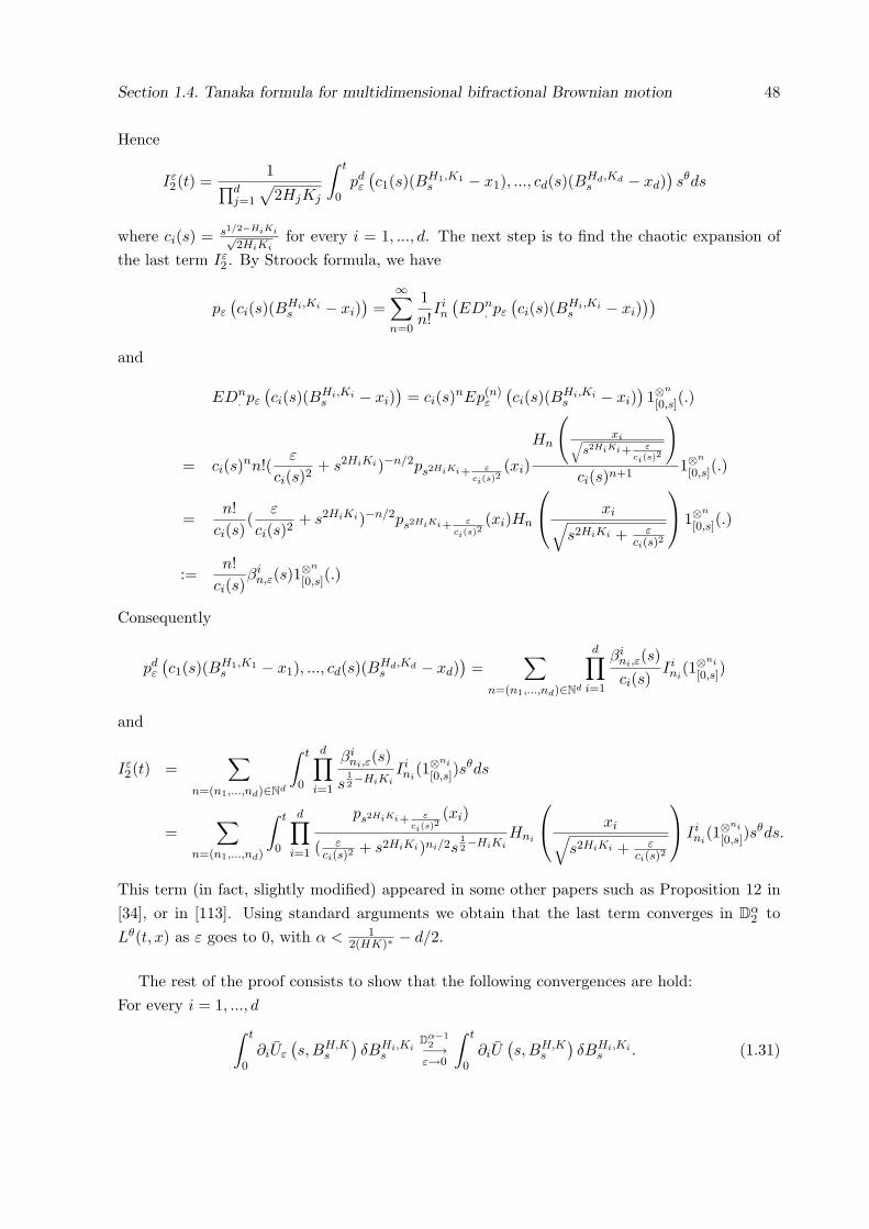
Section 1.4. Tanaka formula for multidimensional bifractional Brownian motion 48
Hence
Iε2(t) =
1∏dj=1
√2HjKj
∫ t
0pd
ε
(c1(s)(BH1,K1
s − x1), ..., cd(s)(BHd,Kds − xd)
)sθds
where ci(s) = s1/2−HiKi√2HiKi
for every i = 1, ..., d. The next step is to find the chaotic expansion ofthe last term Iε
2 . By Stroock formula, we have
pε
(ci(s)(BHi,Ki
s − xi))
=∞∑
n=0
1n!
Iin
(EDn
. pε
(ci(s)(BHi,Ki
s − xi)))
and
EDn. pε
(ci(s)(BHi,Ki
s − xi))
= ci(s)nEp(n)ε
(ci(s)(BHi,Ki
s − xi))1⊗
n
[0,s](.)
= ci(s)nn!(ε
ci(s)2+ s2HiKi)−n/2ps2HiKi+ ε
ci(s)2(xi)
Hn
(xi√
s2HiKi+ εci(s)
2
)
ci(s)n+11⊗
n
[0,s](.)
=n!
ci(s)(
ε
ci(s)2+ s2HiKi)−n/2ps2HiKi+ ε
ci(s)2(xi)Hn
xi√
s2HiKi + εci(s)2
1⊗
n
[0,s](.)
:=n!
ci(s)βi
n,ε(s)1⊗n
[0,s](.)
Consequently
pdε
(c1(s)(BH1,K1
s − x1), ..., cd(s)(BHd,Kds − xd)
)=
∑
n=(n1,...,nd)∈Nd
d∏
i=1
βini,ε(s)ci(s)
Iini
(1⊗ni
[0,s])
and
Iε2(t) =
∑
n=(n1,...,nd)∈Nd
∫ t
0
d∏
i=1
βini,ε(s)
s12−HiKi
Iini
(1⊗ni
[0,s])sθds
=∑
n=(n1,...,nd)
∫ t
0
d∏
i=1
ps2HiKi+ εci(s)
2(xi)
( εci(s)2
+ s2HiKi)ni/2s12−HiKi
Hni
xi√
s2HiKi + εci(s)2
Ii
ni(1⊗
ni
[0,s])sθds.
This term (in fact, slightly modified) appeared in some other papers such as Proposition 12 in[34], or in [113]. Using standard arguments we obtain that the last term converges in Dα
2 toLθ(t, x) as ε goes to 0, with α < 1
2(HK)∗ − d/2.
The rest of the proof consists to show that the following convergences are hold:For every i = 1, ..., d
∫ t
0∂iUε
(s,BH,K
s
)δBHi,Ki
s
Dα−12−→
ε→0
∫ t
0∂iU
(s,BH,K
s
)δBHi,Ki
s . (1.31)
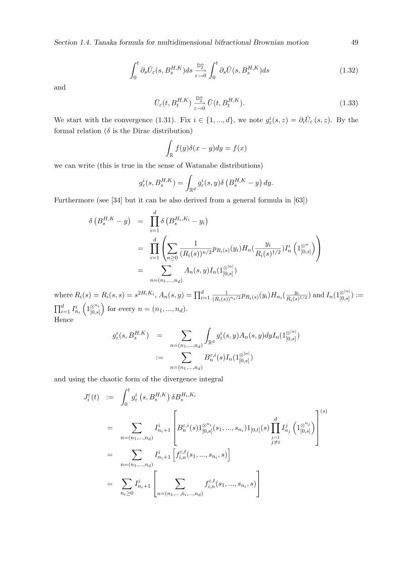
Section 1.4. Tanaka formula for multidimensional bifractional Brownian motion 49
∫ t
0∂sUε(s,BH,K
s )dsDα
2−→ε→0
∫ t
0∂sU(s,BH,K
s )ds (1.32)
and
Uε(t, BH,Kt )
Dα2−→
ε→0U(t, BH,K
t ). (1.33)
We start with the convergence (1.31). Fix i ∈ 1, ..., d, we note giε(s, z) = ∂iUε (s, z). By the
formal relation (δ is the Dirac distribution)∫
Rf(y)δ(x− y)dy = f(x)
we can write (this is true in the sense of Watanabe distributions)
giε(s,B
H,Ks ) =
∫
Rd
giε(s, y)δ
(BH,K
s − y)dy.
Furthermore (see [34] but it can be also derived from a general formula in [63])
δ(BH,K
s − y)
=d∏
i=1
δ(BHi,Ki
s − yi
)
=d∏
i=1
∑
n≥0
1(Ri(s))n/2
pRi(s)(yi)Hn(yi
Ri(s)1/2)Ii
n
(1⊗
n
[0,s]
)
=∑
n=(n1,...,nd)
An(s, y)In(1⊗|n|
[0,s] )
where Ri(s) = Ri(s, s) = s2HiKi , An(s, y) =∏d
i=11
(Ri(s))ni/2 pRi(s)(yi)Hni(yi
Ri(s)1/2 ) and In(1⊗|n|
[0,s] ) :=∏d
i=1 Iini
(1⊗
ni
[0,s]
)for every n = (n1, ..., nd).
Hence
giε(s,B
H,Ks ) =
∑
n=(n1,...,nd)
∫
Rd
giε(s, y)An(s, y)dyIn(1⊗
|n|[0,s] )
:=∑
n=(n1,...,nd)
Bε,in (s)In(1⊗
|n|[0,s] )
and using the chaotic form of the divergence integral
Jεi (t) :=
∫ t
0giε
(s,BH,K
s
)δBHi,Ki
s
=∑
n=(n1,...,nd)
Iini+1
Bε,i
n (s)1⊗ni
[0,s](s1, ..., sni)1[0,t](s)d∏
j=1
j 6=i
Ijnj
(1⊗
nj
[0,s]
)
(s)
=∑
n=(n1,...,nd)
Iini+1
[fε,t
i,n(s1, ..., sni , s)]
=∑
ni≥0
Iini+1
∑
n=(n1,...,ni,...,nd)
fε,ti,n(s1, ..., sni , s)
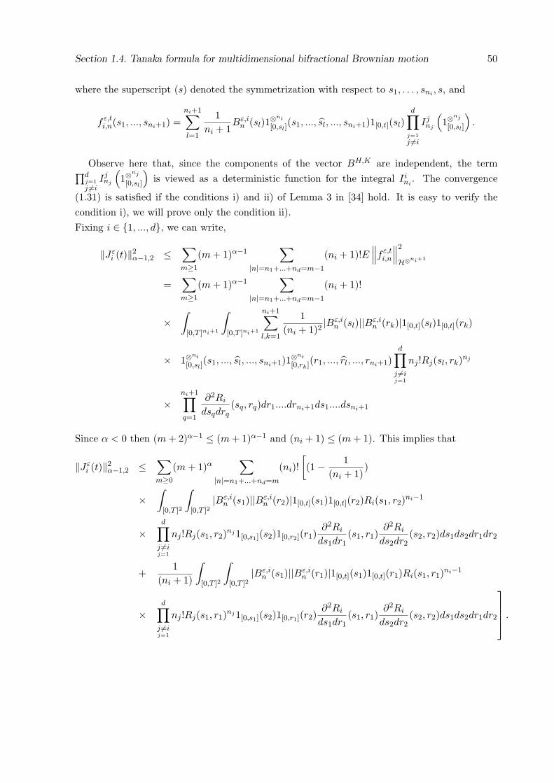
Section 1.4. Tanaka formula for multidimensional bifractional Brownian motion 50
where the superscript (s) denoted the symmetrization with respect to s1, . . . , sni , s, and
fε,ti,n(s1, ..., sni+1) =
ni+1∑
l=1
1ni + 1
Bε,in (sl)1⊗
ni
[0,sl](s1, ..., sl, ..., sni+1)1[0,t](sl)
d∏j=1
j 6=i
Ijnj
(1⊗
nj
[0,sl]
).
Observe here that, since the components of the vector BH,K are independent, the term∏dj=1
j 6=iIjnj
(1⊗
nj
[0,sl]
)is viewed as a deterministic function for the integral Ii
ni. The convergence
(1.31) is satisfied if the conditions i) and ii) of Lemma 3 in [34] hold. It is easy to verify thecondition i), we will prove only the condition ii).Fixing i ∈ 1, ..., d, we can write,
‖Jεi (t)‖2
α−1,2 ≤∑
m≥1
(m + 1)α−1∑
|n|=n1+...+nd=m−1
(ni + 1)!E∥∥∥f ε,t
i,n
∥∥∥2
H⊗ni+1
=∑
m≥1
(m + 1)α−1∑
|n|=n1+...+nd=m−1
(ni + 1)!
×∫
[0,T ]ni+1
∫
[0,T ]ni+1
ni+1∑
l,k=1
1(ni + 1)2
|Bε,in (sl)||Bε,i
n (rk)|1[0,t](sl)1[0,t](rk)
× 1⊗ni
[0,sl](s1, ..., sl, ..., sni+1)1⊗
ni
[0,rk](r1, ..., rl, ..., rni+1)d∏
j 6=ij=1
nj !Rj(sl, rk)nj
×ni+1∏
q=1
∂2Ri
dsqdrq(sq, rq)dr1....drni+1ds1....dsni+1
Since α < 0 then (m + 2)α−1 ≤ (m + 1)α−1 and (ni + 1) ≤ (m + 1). This implies that
‖Jεi (t)‖2
α−1,2 ≤∑
m≥0
(m + 1)α∑
|n|=n1+...+nd=m
(ni)![(1− 1
(ni + 1))
×∫
[0,T ]2
∫
[0,T ]2|Bε,i
n (s1)||Bε,in (r2)|1[0,t](s1)1[0,t](r2)Ri(s1, r2)ni−1
×d∏
j 6=ij=1
nj !Rj(s1, r2)nj1[0,s1](s2)1[0,r2](r1)∂2Ri
ds1dr1(s1, r1)
∂2Ri
ds2dr2(s2, r2)ds1ds2dr1dr2
+1
(ni + 1)
∫
[0,T ]2
∫
[0,T ]2|Bε,i
n (s1)||Bε,in (r1)|1[0,t](s1)1[0,t](r1)Ri(s1, r1)ni−1
×d∏
j 6=ij=1
nj !Rj(s1, r1)nj1[0,s1](s2)1[0,r1](r2)∂2Ri
ds1dr1(s1, r1)
∂2Ri
ds2dr2(s2, r2)ds1ds2dr1dr2
.
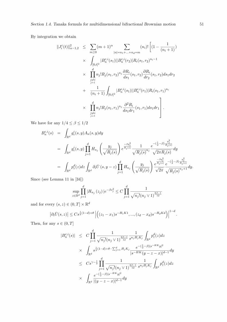
Section 1.4. Tanaka formula for multidimensional bifractional Brownian motion 51
By integration we obtain
‖Jεi (t)‖2
α−1,2 ≤∑
m≥0
(m + 1)α∑
|n|=n1+...+nd=m
(ni)![(1− 1
(ni + 1))
×∫
[0,t]2|Bε,i
n (s1)||Bε,in (r2)|Ri(s1, r2)ni−1
×d∏
j 6=ij=1
nj !Rj(s1, r2)nj∂Ri
ds1(s1, r2)
∂Ri
dr2(s1, r2)ds1dr2
+1
(ni + 1)
∫
[0,t]2|Bε,i
n (s1)||Bε,in (r1)|Ri(s1, r1)ni
×d∏
j 6=ij=1
nj !Rj(s1, r1)nj∂2Ri
ds1dr1(s1, r1)ds1dr1
.
We have for any 1/4 ≤ β ≤ 1/2
Bε,in (s) =
∫
Rd
giε(s, y)An(s, y)dy
=∫
Rd
giε(s, y)
d∏
j=1
Hnj
(yj√Rj(s)
)e
−βy2j
Rj(s)1√
Rj(s)nj
e−( 1
2−β)
y2j
Rj(s)
√2πRj(s)
dy
=∫
Rd
pdε(z)dz
∫
Rd
∂iU (s, y − z)d∏
j=1
Hnj
(yj√Rj(s)
)e
−βy2j
Rj(s)
√2π
e−( 1
2−β)
y2j
Rj(s)
√Rj(s)
nj+1 dy.
Since (see Lemma 11 in [34])
supz∈Rd
d∏
j=1
|Hnj (zj) |e−βz2j ≤ C
d∏
j=1
1√
nj !(nj ∨ 1)8β−1
12
and for every (s, z) ∈ (0, T ]× Rd
∣∣∂iU(s, z)∣∣ ≤ Cs
12(1−d)+θ
∣∣∣((z1 − x1)s−H1K1, ..., (zd − xd)s−HdKd
)∣∣∣1−d
.
Then, for any s ∈ (0, T ]
|Bε,in (s)| ≤ C
d∏
j=1
1√
nj !(nj ∨ 1)8β−1
12
1snjHjKj
∫
Rd
pdε(z)dz
×∫
Rd
s12(1−d)+θ−∑d
j=1 HjKje−( 1
2−β)|s−HKy|2
|s−HK(y − z − x)|d−1dy
≤ Csγ− 12
d∏
j=1
1√
nj !(nj ∨ 1)8β−1
12
1snjHjKj
∫
Rd
pdε(z)dz
×∫
Rd
e−( 12−β)|s−HKy|2
|(y − z − x)|d−1dy
Section 1.4. Tanaka formula for multidimensional bifractional Brownian motion 52
where s−HKy := (s−H1K1y1, ..., s−HdKdyd)§.
Let η a positive constant such that, for every s ∈ (0, T ], j ∈ 1, . . . , d we have s−2HjKj > η.
Combining this with for any a, b ∈ R, a2 ≥ 12(a− b)2 − b2, we obtain
∫
Rd
pdε(z)dz
∫
Rd
e−( 12−β)|s−HKy|2
|(y − z − x)|d−1dy ≤
∫
Rd
pdε(z)dz
∫
Rd
e−η( 12−β)|y|2
|(y − z − x)|d−1dy
≤∫
Rd
pdε(z)eη( 1
2−β)|z+x|2dz
∫
Rd
e−η2( 12−β)|y−(z+x)|2
|(y − (z + x))|d−1dy
≤ Ce2η( 12−β)|x|2
∫
Rd
pdε(z)e2η( 1
2−β)|z|2dz
≤ Ce2η( 12−β)|x|2
∫
Rd
e−|v|22
√2π
de2η( 1
2−β)ε|v|2dv
≤ Ce2η( 12−β)|x|2
∫
Rd
e−β|v|2√
2πd
dv < ∞
since 2ηε ≤ 1 when ε is close to 0.Thus
|Bε,in (s)| ≤ Csγ− 1
2
d∏
j=1
1√
nj !(nj ∨ 1)8β−1
12
1snjHjKj
where C is a constant depending only on d, H, K, T, x and β.On the other hand, there exist a constant C(H, K) positive, such that for every i = 1, . . . , d
∣∣∣∣∂Ri
dr(r, s)
∂Ri
ds(r, s)
∣∣∣∣ ≤ C(H, K)(rs)2HiKi−1,
∣∣∣∣∂2Ri
drds(r, s)
∣∣∣∣ ≤ C(H, K)(rs)HiKi−1
and ∣∣∣∣Ri(r, s)(rs)HiKi
∣∣∣∣ ≤ C(H, K).
It follows by anterior inequalities that
‖Jεi (t)‖2
α−1,2 ≤ C∑
m≥0
(1 + m)α∑
|n|=n1+...+nd=m
d∏
j=1
1
(nj ∨ 1)8β−1
6
×∫
[0,t]2
Ri(r, s)ni−1
(rs)(ni−1)HiKi(rs)γ− 3
2+HiKi
d∏
j=1j 6=i
Rj(r, s)nj
(rs)njHjKjdrds.
We use the selfsimilarity of the covariance kernel R(r, s) = R(1, sr )r2HK and the change of
Section 1.4. Tanaka formula for multidimensional bifractional Brownian motion 53
variables r/s = z in the integral respect to dz to obtain
‖Jεi (t)‖2
α−1,2 ≤ C∑
m≥0
(1 + m)α∑
|n|=n1+...+nd=m
d∏
j=1
1
(nj ∨ 1)8β−1
6
×∫ t
0r2(γ−1+HiKi)dr
∫ 1
0(z)γ− 3
2+HiKi
(Ri(1, z)zHiKi
)ni−1 d∏
j=1j 6=i
(Rj(1, z)zHjKj
)nj
dz.
Since for each i ∈ 1, . . . , d, γ − 32 + HiKi > −1, 2(γ − 1 + HiKi) > −1 and from Lemma 12
and the proof of the Proposition 12 in [34], we obtain that
‖Jεi (t)‖2
α−1,2 ≤ C∑
m≥0
(1 + m)αm− 1
2(HK)∗∑
|n|=n1+...+nd=m
d∏
j=1
1
(nj ∨ 1)8β−1
6
≤ C∑
m≥0
(1 + m)α(m)−1
2(HK)∗−1+d(1− 8β−16
)
is finite if and only if α < 12(HK)∗ − d
2 .On the other hand, for every (s, z) ∈ (0, T ]× Rd we have
∣∣∂sU(s, z)∣∣ ≤ Cs
−d2
+θ∣∣∣((z1 − x1)s−H1K1, ..., (zd − xd)s−HdKd
)∣∣∣2−d
.
and
∣∣U(s, z)∣∣ ≤ Cs
12(2−d)+θ
∣∣∣((z1 − x1)s−H1K1, ..., (zd − xd)s−HdKd
)∣∣∣2−d
and this inequalities imply as in [115] the convergences (1.32) and (1.33) in Dα2 .
Chapter 2
Occupation densities for certain
processes related to fractional
Brownian motion
In this paper we establish the existence of a square integrable occupation density for two classesof stochastic processes. First we consider a Gaussian process with an absolutely continuousrandom drift, and secondly we handle the case of a (Skorohod) integral with respect to thefractional Brownian motion with Hurst parameter H > 1
2 . The proof of these results usesa general criterion for the existence of a square integrable local time, which is based on thetechniques of Malliavin calculus.
2.1 Introduction
Local times for semimartingales have been widely studied. See for example the monograph [101]and the references therein. On the other hand, local times of Gaussian processes have also beenthe object of a rich probabilistic literature; see for example the recent book [74] by Marcusand Rosen. A general criterion for the existence of a local time for a wide class of anticipatingprocesses, which are not semimartingales nor Gaussian processes, was established by Imkellerand Nualart in [50]. The proof of this result combines the techniques of Malliavin calculus withthe criterion given by Geman and Horowitz in [44]. This criterion was applied in [50] to theBrownian motion with an anticipating drift, and to indefinite Skorohod integral processes.
The aim of this paper is to establish the existence of the occupation density for two classes ofstochastic processes related to the fractional Brownian motion, using the approach introducedin [50]. First we consider a Gaussian process B = Bt, t ∈ [0, 1] with an absolutely continuousrandom drift
Xt = Bt +∫ t
0usds,
where u is a stochastic process measurable with respect to the σ-field generated by B. We assumethat the variance of the increment of the Gaussian process B on an interval [s, t] behaves as
54
Section 2.2. Preliminaries 55
|t− s|2ρ, for some ρ ∈ (0, 1). This includes, for instance, the bifractional Brownian motion withparameters H ∈ (0, 1) and K ∈ (0, 1] and the fractional Brownian motion in the particular caseK = 1. Under reasonable regularity hypotheses imposed to the process u we prove the existenceof a square integrable occupation density with respect to the Lebesgue measure for the processX.
Our second example is the indefinite divergence (Skorohod) integral X = Xt, t ∈ [0, 1] withrespect to the fractional Brownian motion with Hurst parameter H ∈ (1
2 , 1), that is
Xt =∫ t
0usδB
Hs .
We provide integrability conditions on the integrand u and its iterated derivatives in the senseof Malliavin calculus in order to deduce the existence of a square integrable occupation densityfor X.
We organize our paper as follows. Section 2 contains some preliminaries on the Malliavincalculus with respect to Gaussian processes. In Section 3 we prove the existence of the occupationdensities for perturbed Gaussian processes and in Section 4 we treat the case of indefinitedivergence integral processes with respect to the fractional Brownian motion.
2.2 Preliminaries
Let Bt, t ∈ [0, 1] be a centered Gaussian process with covariance function
R(t, s) := E(BtBs),
defined in a complete probability space (Ω,F , P ). We assume that the σ-field F is generatedby B. By H we denote the canonical Hilbert space associated to B defined as the closure ofthe linear space generated by the indicator functions 1[0,t], t ∈ [0, 1] with respect to the innerproduct
〈1[0,t],1[0,s]〉H = R(t, s), s, t ∈ [0, 1].
The mapping 1[0,t] → Xt can be extended to an isometry between H and the first Gaussianchaos generated by B. We denote by B(ϕ) the image of an element ϕ ∈ H by this isometry.
We will first introduce some elements of the Malliavin calculus associated with B. Werefer to [81] for a detailed account of these notions. For a smooth random variable F =f (B(ϕ1), . . . , B(ϕn)), with ϕi ∈ H and f ∈ C∞
b (Rn) (f and all its partial derivatives arebounded) the derivative of F with respect to B is defined by
DF =n∑
j=1
∂f
∂xj(B(ϕ1), . . . , B(ϕn))ϕj .
For any integer k ≥ 1 and any real number p ≥ 1 we denote by Dk,p the Sobolev space definedas the closure of the space of smooth random variables with respect to the norm
‖F‖pk,p = E(|F |p) +
k∑
j=1
‖DjF‖pLp(Ω;H⊗j)
,
Section 2.2. Preliminaries 56
where Dj denotes the iterated derivative operator of D. Similarly, for a given Hilbert space V
we can define Sobolev spaces of V -valued random variables Dk,p(V ).The following lemma (see Lemma 1.2.3 in [81]) is a useful tool in proving that a given random
variable belongs to the Sobolev space D1,p, where p > 1.
Lemma 3. Let (Fn)n≥1 be a sequence of random variables converging in Lp, p > 1, to F .Suppose that supn E
(‖DFn‖pH
)< ∞. Then, F belongs to D1,p.
Consider the adjoint δ of D in L2. Its domain is the class of elements u ∈ L2(Ω;H) such that
E(〈DF, u〉H) ≤ C‖F‖1,2,
for any F ∈ D1,2, and δ (u) is the unique element of L2(Ω) given by
E(δ(u)F ) = E(〈DF, u〉H)
for any F ∈ D1,2. We will make use of the notation δ(u) =∫ 10 usδBs, although, in general, the
trajectories of u are not real-valued functions. It is well-known that D1,2(H) is included in thedomain of δ. Note that E(δ(u)) = 0 and the variance of δ(u) is given by
E(δ(u)2) = E(‖u‖2H) + E(〈Du, (Du)∗〉H⊗H), (2.1)
if u ∈ D1,2(H), where (Du)∗ is the adjoint of Du in the Hilbert space H⊗H. Meyer’s inequalitytells us that
E(|δ(u)p|) ≤ Cp
(E(‖u‖p
H) + E(‖Du‖pH⊗H)
), (2.2)
for any p > 1. We will make use of the property
δ(Fu) = Fδ(u)− 〈DF, u〉H. (2.3)
if F ∈ D1,2, u ∈ Dom(δ) and the random elements Fu and Fδ(u) − 〈DF, u〉H are squareintegrable. We also need the commutativity relationship between D and δ
Dδ(u) = u +∫ 1
0DusδBs, (2.4)
if u ∈ D1,2(H) and the H-valued process Dus, s ∈ [0, 1] belongs to the domain of δ.Throughout this paper we will assume that the centered Gaussian process B = Bt, t ∈ [0, 1]
satisfiesC1|t− s|2ρ ≤ E(|Bt −Bs|2) ≤ C2|t− s|2ρ, (2.5)
for some ρ ∈ (0, 1) with C1, C2 two positive constants not depending on t, s. It will follow fromthe Kolmogorov criterium that B admits a Holder continuous version of order δ for any δ < ρ.
Throughout this paper we will denote by C a generic constant that may be different fromline to line.
Section 2.2. Preliminaries 57
Example 1. The bifractional Brownian motion (see, for instance [47]), denoted by BH,K , isdefined as a centered Gaussian process with covariance
R(t, s) =1
2K
((t2H + s2H
)K − |t− s|2HK)
, (2.6)
where H ∈ (0, 1) and K ∈ (0, 1]. When K = 1, then we have a standard fractional Brownianmotion denoted by BH . It has been proven in [47] that for all s ≤ t,
2−K |t− s|2HK ≤ E
(∣∣∣BH,Kt −BH,K
s
∣∣∣2)≤ 21−K |t− s|2HK . (2.7)
So, relation (2.5) holds with ρ = HK. A stochastic analysis for this process can be found in [61]and a study of its occupation density has been done in [39], [113].
For a measurable function x : [0, 1] → R we define the occupation measure
µ(x)(C) =∫ 1
01C(xs)ds,
where C is a Borel subset of R and we will say that x has an occupation density with respectto the Lebesgue measure λ if the measure µ is absolutely continuous with respect to λ. Theoccupation density of the function x will be the Radon-Nikodym derivative dµ
dλ . For a continuousprocess Xt, t ∈ [0, 1] we will say that X has an occupation density on [0, 1] if for almost allω ∈ Ω, X(ω) has an occupation density on [0, 1].
We will use the following criterion for the existence of occupation densities (see [50]). SetT = (s, t) ∈ [0, 1]2 : s < t.Theorem 6. Let Xt, t ∈ [0, 1] be a continuous stochastic process such that Xt ∈ D2,2 for everyt ∈ [0, 1]. Suppose that there exists a sequence of bounded random variables Fn, n ≥ 1 with⋃
nFn 6= 0 = Ω a.s. and Fn ∈ D1,1 for every n ≥ 1, two sequences αn > 0, δn > 0, a measurablebounded function γ : [0, 1] → R, such that γD(Xt −Xs) ∈ H, γ⊗2D2(Xt −Xs) ∈ H ⊗H for all0 ≤ s < t ≤ 1, γDFn ∈ H for all n ≥ 1 and a constant θ > 0, such that:
a) For every n ≥ 1, |t− s| ≤ δn, and on Fn 6= 0 we have
〈γD(Xt −Xs),1(s,t]〉H > αn|t− s|θ, a.s.. (2.8)
b) For every n ≥ 1 ∫
TE(〈γDFn,1(s,t]〉H)|t− s|−θdtds < ∞. (2.9)
c) For every n ≥ 1∫
TE
(∣∣∣Fn
⟨γ⊗2DD(Xt −Xs),1⊗2
(s,t]
⟩H⊗2
∣∣∣)|t− s|−2θdsdt < ∞. (2.10)
Then the process Xt, t ∈ [0, 1] admits a square integrable occupation density on [0, 1].
Remark 2. The original result has been stated in [50] with θ = 1 in the case of the standardBrownian motion. On the other hand, by applying Proposition 2.3 and Theorem 2.1 in [50] itfollows easily that this criterion can be stated for any θ > 0.
Section 2.3. Occupation density for Gaussian processes with random drift 58
2.3 Occupation density for Gaussian processes with random drift
We study in this part the existence of the occupation density for Gaussian processes perturbedby an absolute continuous random drift. The main result of this section is the following.
Theorem 7. Let Bt, t ∈ [0, 1] be a centered Gaussian process satisfying (2.5). Consider theprocess Xt, t ∈ [0, 1] given by
Xt = Bt +∫ t
0usds,
and suppose that the process u satisfies the following conditions:
i) u ∈ D2,2(L2([0, 1])).
ii) E
((∫ 10
∥∥D2ut
∥∥p
H⊗H dt)λ
p
)< ∞, for some λ > 1 and p > 1
1−ρ .
Then, the process X has a square integrable occupation density on the interval [0, 1].
Proof: We are going to apply Theorem 6. Notice first that Xt ∈ D2,2 for all t ∈ [0, 1] due toCondition i). Let us first prove Condition a) in Theorem 6. We assume that γ = 1. For any0 ≤ s < t ≤ 1, applying the derivative operator to the increment Xt −Xs yields
D(Xt −Xs) = 1(s,t] +∫ t
sDurdr.
As a consequence, using (2.5) we can write
⟨D(Xt −Xs),1(s,t]
⟩H =
⟨1(s,t],1(s,t]
⟩H +
⟨∫ t
sDurdr,1(s,t]
⟩
H
= E(|Bt −Bs|2) +⟨∫ t
sDurdr,1(s,t]
⟩
H
≥ C1(t− s)2ρ −∣∣∣∣⟨∫ t
sDurdr,1[s,t]
⟩
H
∣∣∣∣ . (2.1)
Applying again (2.5) and Holder’s inequality yields∣∣∣∣⟨∫ t
sDurdr,1[s,t]
⟩
H
∣∣∣∣ ≤∥∥∥∥∫ t
sDurdr
∥∥∥∥H
∥∥1[s,t]
∥∥H
≤√
C2(t− s)1−1p+ρ
(∫ 1
0‖Dur‖p
H dr
) 1p
. (2.2)
Fix a natural number n ≥ 2, and choose a function ϕn(x), which is infinitely differentiable withcompact support, such that ϕn(x) = 1 if |x| ≤ n−1, and ϕn(x) = 0, if |x| ≥ n. Set Fn = ϕn(G),where
G =(∫ 1
0‖Dur‖p
H dr
) 1p
.
Section 2.3. Occupation density for Gaussian processes with random drift 59
The sequence of random variables Fn satisfies⋃
nFn 6= 0 = Ω, because for each n ≥ 2, theset Fn 6= 0 is included in G ≤ n. We claim that for each n, the random variable Fn belongsto D1,λ. In fact, by duality we can write
G = suph∈Bq
∫ 1
0〈Dur, hr〉H dr,
where Bq is the unit ball in the Banach space h ∈ Lq([0, 1];H), and 1p + 1
q = 1. Let DN , N ≥ 1be an increasing sequence of finite subsets of Bq, whose union is dense in Bq. Set
GN = suph∈DN
∫ 1
0〈Dur, hr〉H dr.
Clearly, ϕn(GN ) converges to Fn, as N tends to infinity, in Lλ. On the other hand, for each N ,the random variable GN belongs to D1,2, because it is a supremum of a finite number of randomvariables in D1,2, and the supremum is a Lipschitz function. Finally, from Lemma 3, it sufficesto show that the norms ‖D (ϕn(GN ))‖H are uniformly bounded in Lλ(Ω), which follows fromCondition ii):
‖D (ϕn(GN ))‖H =∥∥ϕ′n(GN )DGN
∥∥H ≤
∥∥ϕ′n∥∥∞ sup
h∈DN
∥∥∥∥∫ 1
0
⟨D2ur, hr
⟩H dr
∥∥∥∥H
≤ ∥∥ϕ′n∥∥∞ sup
h∈DN
supv∈H
‖v‖H≤1
∣∣∣∣∫ 1
0
⟨D2ur, v ⊗ hr
⟩H⊗2 dr
∣∣∣∣
≤ ∥∥ϕ′n∥∥∞
(∫ 1
0
∥∥D2ur
∥∥p
H⊗2 dr
) 1p
∈ Lλ(Ω).
Choose the constants αn = C12 , and δn =
(C1
2n√
C2
) pp−1−pρ . Then, from (2.1) and (2.2), on the
set Fn 6= 0 ⊂ G ≤ n, assuming |t− s| ≤ δn, and taking into account that 1− 1p − ρ > 0, we
get
⟨D(Xt −Xs),1(s,t]
⟩H ≥ C1(t− s)2ρ − n
√C2(t− s)1−
1p+ρ
= (t− s)2ρ[C1 − n
√C2(t− s)1−
1p−ρ
]
≥ αn(t− s)2ρ,
and property a) of Theorem 6 holds with θ = 2ρ .Condition b) follows immediately from (2.5):
∫
T
E(∣∣∣
⟨DFn,1(s,t]
⟩H
∣∣∣)
|t− s|2ρdsdt ≤
√C2
∫
T
E (‖DFn‖H)|t− s|ρ dsdt < ∞,
Section 2.4. Occupation density for Skorohod integrals with respect to the fractional Brownian motion60
Finally, Condition c) can also be checked:
∫
T
E(∣∣∣Fn
⟨D2(Xt −Xs),1⊗2
([s,t]
⟩H⊗2
∣∣∣)
|t− s|4ρdsdt
≤ ‖ϕn‖∞∫
T
E(∥∥D2(Xt −Xs)
∥∥H⊗2
) ∥∥∥1⊗2
(s,t]
∥∥∥H⊗2
|t− s|4ρdsdt
= ‖ϕn‖∞∫
T
E(∥∥D2(Xt −Xs)
∥∥H⊗2
)E(Bt −Bs)2
|t− s|4ρdsdt
≤ C2 ‖ϕn‖∞∫
T
E(∥∥D2(Xt −Xs)
∥∥H⊗2
)
|t− s|2ρdsdt < ∞,
because
E(∥∥D2(Xt −Xs)
∥∥H⊗2
)= E
(∥∥∥∥∫ t
sD2urdr
∥∥∥∥H⊗2
)≤ E
(∫ t
s
∥∥D2ur
∥∥H⊗2 dr
)
≤ (t− s)1−1p E
[(∫ 1
0
∥∥D2ur
∥∥p
H⊗2 dr
) 1p
],
and 1− 1p − 2ρ > −1, taking into account that p > 1
2(1−ρ) .
Remark 3. These conditions are intrinsic and they do not depend on the structure of the Hilbertspace H. In the case of the Brownian motion, this result is slightly weaker than Theorem 3.1 in[50], because we require here a little more integrability.
2.4 Occupation density for Skorohod integrals with respect to
the fractional Brownian motion
We study here the existence of occupation densities for indefinite divergence integrals withrespect to the fractional Brownian motion. Consider a process of the form Xt =
∫ t0 usδB
Hs ,
t ∈ [0, 1], where B is fractional Brownian motion with Hurst parameter H ∈ (12 , 1
), and u is an
element of D1,2(H) ⊂ Dom(δ).We know that the covariance of the fractional Brownian motion with Hurst parameter H > 1
2
can be written as
E(BHt BH
s ) =∫ t
0
∫ s
0φ(α, β)dαdβ, (2.1)
where φ(α, β) = H(2H − 1)|α− β|2H−2. For any 0 ≤ s < t ≤ 1, and α ∈ [0, 1] we set
fs,t(α) :=∫ t
sφ(α, β)dβ. (2.2)
We also know (see e.g. [81]) that the canonical Hilbert space associated to BH satisfies:
L2 ([0, 1]) ⊂ L1H ([0, 1]) ⊂ H, (2.3)
Section 2.4. Occupation density for Skorohod integrals with respect to the fractional Brownian motion61
and the scalar product in H is given by
〈f, g〉H =∫ 1
0
∫ 1
0f(s)g(t)φ(s, t)dsdt, (2.4)
if f, g ∈ L1H ([0, 1]).
The following is the main result of this section.
Theorem 8. Consider the stochastic process Xt =∫ t0 usδB
Hs , where the integrand u satisfies
the following conditions for some q > 2 and p > 2qH(q−2) :
1) u ∈ D3,2(L2([0, 1])).
2)∫ 10
∫ 10 [E(|Dtus|p) + E(‖ |DtDus| ‖p
H) + E(‖ ∣∣DtD2us
∣∣ ‖pH⊗H)]dsdt < ∞.
3)∫ 10 E
(|ut|−
pp−1
(q+1))
dt < ∞.
Then the process Xt, t ∈ [0, 1] admits a square integrable occupation density on [0, 1].
Proof: We will apply again Theorem 6. Condition 1) implies that Xt ∈ D2,2 for all t ∈ [0, 1].On the other hand, from Theorem 7.8 in [61] (or also by a slightly modification of Theorem 5 in[2]) we obtain the continuity of the paths of the process X. Note that from Lemma 2.2 in [50]corroborated with Hypothesis 3) we obtain the existence of a function γ : [0, 1] → −1, 1 suchthat γtut = |ut| for almost all t and ω. Note that the fact that the function γ is bounded and thehypothesis u ∈ D3,2(L2([0, 1])) and H > 1
2 imply γD(Xt −Xs) ∈ H, γ⊗2D2(Xt −Xs) ∈ H ⊗Hfor all 0 ≤ s < t ≤ 1. We are going to show conditions a), b) and c) of Theorem 6.
Proof of condition a): Fix 0 ≤ s < t ≤ 1. From (2.4) we obtain
D(Xt −Xs) = u1(s,t] +∫ t
sDurδB
Hr ,
and we can write
〈γD(Xt −Xs), 1(s,t]〉H = 〈|u|1(s,t],1(s,t]〉H + 〈∫ t
sDurδB
Hr , γ1(s,t]〉H. (2.5)
We need a lower bound for the first summand in the above expression and an upper bound forthe absolute value of the second summand. Using (2.4) the first summand can be written as
〈|u|1(s,t],1(s,t]〉H =∫ t
s
∫ t
s|uα|φ(α, β)dαdβ =
∫ t
s|uα|fs,t(α)dα.
From the identity
E(|BHt −BH
s |2) =∫ t
sfs,t(α)dα
=∫ t
s(|uα|fs,t(α))
qq+1 (|uα|fs,t(α))−
qq+1 fs,t(α)dα,
Section 2.4. Occupation density for Skorohod integrals with respect to the fractional Brownian motion62
and applying Holder’s inequality with orders q+1q and q + 1, we obtain
(t− s)2H ≤(∫ t
s|uα|fs,t(α)dα
) qq+1
(∫ t
s|uα|−qfs,t(α)dα
) 1q+1
. (2.6)
Notice that the function fs,t(α) is bounded
fs,t(α) ≤ f0,1(α) = H(2H − 1)∫ 1
0|α− β|2H−2dβ = H
(α2H−1 + (1− α)2H−1
) ≤ 2H.
Hence, from (2.6) we get∫ t
s|uα|fs,t(α)dα ≥ C|t− s|
2H(q+1)q Z
− 1q
q , (2.7)
where Zq =∫ 10 |uα|−qdα.
On the other hand, for the second summand in the right-hand side of (2.5) we can write,using (2.4) and Holder’s inequality.
∣∣∣∣⟨
γ
∫ t
sDurδB
Hr ,1(s,t]
⟩
H
∣∣∣∣ =∣∣∣∣∫ t
s
∫ 1
0
(∫ t
sDαurδB
Hr
)γ(β)φ(α, β)dαdβ
∣∣∣∣
≤∫ 1
0
∣∣∣∣∫ t
sDαurδB
Hr
∣∣∣∣ fs,t(α)dα
≤(∫ 1
0fs,t(α)
pp−1 dα
) p−1p
×(∫ 1
0
∣∣∣∣∫ t
sDαurδB
Hr
∣∣∣∣p
dα
) 1p
. (2.8)
We claim that (∫ 1
0fs,t(α)
pp−1 dα
) p−1p
≤ C|t− s|η, (2.9)
for some η < 2H − 1p . In fact. the right-hand side of (2.9) can be written as
(∫ 1
0fs,t(α)
pp−1 dα
) p−1p
= cH
∥∥∥∥∫ t
s| · −β|2H−2dβ
∥∥∥∥L
pp−1 ([0,1])
≤ cH
∥∥1[s,t] ∗ | · |2H−21[−1,1]
∥∥L
pp−1 (R)
, (2.10)
where cH = H(2H − 1). Young’s inequality with exponents a and b in (1,∞) such that 1a + 1
b =2− 1
p yields
∥∥1[s,t] ∗ | · |2H−21[−1,1]
∥∥L
pp−1 (R)
≤ ∥∥1[s,t]
∥∥La(R)
∥∥| · |2H−21[−1,1]
∥∥Lb(R)
. (2.11)
Choosing b < 12−2H and letting η = 1
a < 2H − 1p we obtain (2.9).
Section 2.4. Occupation density for Skorohod integrals with respect to the fractional Brownian motion63
On the other hand, applying Lemma II.2.4 in [62] (see Nikol’skiı [78], and Garsia-Rodemich-Rumsey [43]) with exponents p and m > 0, and to the continuous function us =
∫ s0 DαurδB
Hr ,
yields ∣∣∣∣∫ t
sDαurδB
Hr
∣∣∣∣p
≤ N |t− s|m∫ 1
0
∫ 1
0
∣∣∫ yx DαurδB
Hr
∣∣p|x− y|m+2
dxdy,
for some constant N > 0. As a consequence
(∫ 1
0
∣∣∣∣∫ t
sDαurδB
Hr
∣∣∣∣p
dα
) 1p
≤ N1p |t− s|mp Y
1p
m,p, (2.12)
where
Ym,p =∫ 1
0
∫ 1
0
∫ 1
0
∣∣∫ yx DαurδB
Hr
∣∣p|x− y|m+2
dxdydα.
Substituting (2.9) and (2.12) into (2.8) yields∣∣∣∣⟨
γ
∫ t
sDurδB
Hr ,1(s,t]
⟩
H
∣∣∣∣ ≤ C|t− s|η+mp Y
1p
m,p, (2.13)
and from (2.7), (2.13) and (2.5) we get
〈γD(Xt −Xs),1(s,t]〉H ≥ C
(|t− s|
2H(q+1)q Z
− 1q
q − |t− s|η+mp Y
1p
m,p
)
= C|t− s|2H+ 2Hq
(Z− 1
qq − |t− s|δY
1p
m,p
), (2.14)
where δ = η + mp − 2H − 2H
q . If we assume that
m > 1 +2Hp
q, (2.15)
then we can choose η < 2H − 1p in such a way that the exponent δ is positive.
We construct now the sequence Fn, n ≥ 1. Fix a natural number n ≥ 2, and choose afunction ϕn(x), which is infinitely differentiable with compact support, such that ϕn(x) = 1 if|x| ≤ n − 1, and ϕn(x) = 0, if |x| ≥ n. Set Fn = ϕn (G ), where G = Zq + Ym,p. Then, from(2.14) and choosing the constants αn = 1
2n1/q and δn = 1
2n1p +1
q, it follows that Condition a) of
Theorem 6 holds with θ = 2H + 2Hq .
It only remains to show that the random variables Fn are in the space D1,1. This will givethat γDFn ∈ H for every n. We can approximate Zq and Ym,p by the sequences
ZNq =
∫ 1
0
(u2
s +1N
)− q2
ds,
and
Y Nm,p =
∫ 1
0
∫ 1
0
∫ 1
0
∣∣∫ yx DαurδB
Hr
∣∣p|x− y|m+2 + 1
N
dxdydα.
Clearly, ϕn(ZNq + Y N
m,p) converges to Fn, as N tends to infinity, almost surely and in L1. Thus,to show that Fn belongs to D1,1 it suffices to prove that the derivatives D
(ϕn(ZN
q + Y Nm,p)
)
Section 2.4. Occupation density for Skorohod integrals with respect to the fractional Brownian motion64
converge in L1(Ω;H) as N tends to infinity. The random variables ZNq and Y N
m,p belong to D1,1
and we can write
DZNq = −q
∫ 1
0
(u2
s +1N
)− q2−1
usDusds,
and
DY Nm,p = p
∫ 1
0
∫ 1
0
∫ 1
0
|ξx,y,α|p−1 sign(ξx,y,α)Dξx,y,α
|x− y|m+2 + 1N
dxdydα,
where ξx,y,α =∫ xy DαurδBr. As a consequence, D
(ϕn(ZN
q + Y Nm,p)
)converges pointwise as N
tends to infinity toϕ′n(Zq + Ym,p) [DZq + DYm,p] ,
where
DZq = (−q)∫ 1
0|us|−q−1sign(us)Dusds,
and
DYm,p = p
∫ 1
0
∫ 1
0
∫ 1
0|ξx,y,α|p−1 sign(ξx,y,α)Dξx,y,α|x− y|−m−2dxdydα,
Then, suffices to show that the random variables ‖DZq‖H and ‖DYm,p‖H are integrable on theset G ≤ n. By Holder’s inequality
E(‖DZq‖H
) ≤ q
(∫ 1
0E
(|us|−
pp−1
(q+1))
ds
)1− 1p
(∫ 1
0E
(‖Dus‖pH
)ds
) 1p
.
The first factor in the right-hand side is finite by Condition 3), and the second factor is alsofinite by Condition 2), the continuous embedding of L
1H ([0, 1]) into H (see (2.3), and the fact
that pH ≥ 1. On the other hand,
‖DYm,p‖H ≤ p
∫ 1
0
∫ 1
0
∫ 1
0|ξx,y,α|p−1 ‖Dξx,y,α‖H|x− y|−m−2dxdydα
≤ p(Ym,p)p−1
p
(∫ 1
0
∫ 1
0
∫ 1
0‖Dξx,y,α‖p
H|x− y|−m−2dxdydα
)1/p
.
Then, on the set G ≤ n, the factor (Ym,p)p−1
p is bounded and it suffices to show that therandom variable
Y =∫ 1
0
∫ 1
0
∫ 1
0‖Dξx,y,α‖p
H|x− y|−m−2dxdydα
has a finite expectation. Since, for any 0 ≤ y < x ≤ 1
Dξx,y,α = 1[y,x]Dαu +∫ x
yDDαusδB
Hs ,
we have
Y ≤ C
(∫ 1
0
∫ 1
0
∫ 1
0‖1[y,x]Dαu‖p
H|x− y|−m−2dxdydα
+∫ 1
0
∫ 1
0
∫ 1
0‖
∫ x
yDDαusδB
Hs ‖p
H|x− y|−m−2dxdydα
)
:= C(Y1 + Y2).
Section 2.4. Occupation density for Skorohod integrals with respect to the fractional Brownian motion65
¿From the continuous embedding of L1H ([0, 1]) into H, we obtain
Y1 ≤ C
∫ 1
0
∫ 1
0
∫ 1
0‖1[y,x]Dαu‖p
L1/H([0,1])|x− y|−m−2dxdydα
≤ C|x− y|pH−1
∫ 1
0
∫ 1
0
∫ 1
0
∫ x
y|Dαur|p |x− y|−m−2drdxdydα.
Hence, E(Y1) < ∞, by Fubini’s theorem, Proposition 3.1 in [50] and Condition 2), provided
m < pH − 1. (2.16)
On the other hand, using the estimate (2.2), and again the continuous embedding of L1H ([0, 1])
into H yields
E
(‖
∫ x
yDDαusδB
Hs ‖p
H
)≤ C E
(∥∥DαDu·1[y,x](·)∥∥p
H⊗2 +∥∥DαD2u·1[y,x](·)
∥∥p
H⊗3
)
≤ C E(∥∥|DαDu·|1[y,x](·)
∥∥p
L1/H([0,1];H)
+∥∥∣∣DαD2u·
∣∣1[y,x](·)∥∥p
L1/H([0,1];H⊗2)
)
≤ C|x− y|pH−1
(∫ x
yE
(‖|DαDur|‖pH
)dr
+∫ x
yE
(∥∥∣∣DαD2ur
∣∣∥∥p
H⊗2
)dr
).
As before we obtain E(Y2) < ∞ by Fubini’s theorem and Condition 2), provided (2.16) holds.Notice that condition p > 2q
H(q−2) implies that we can choose an m such that (2.15) and (2.16)hold.
Proof of Condition b): Define An = G ≤ n. Then, Condition b) in Theorem 6 follows from∫
TE(〈γDFn,1(s,t]〉H)|t− s|−θdtds ≤ C
∫
TE(1An
∣∣〈γDG,1(s,t]〉H∣∣)|t− s|−θdtds
≤ CE (1An‖DG‖H)∫
T|t− s|H−θdsdt < ∞,
since E (1An‖DG‖H) < ∞ and θ −H = H + 2Hq < 1.
Proof of Condition c): We have
DαDβ(Xt −Xs) = 1(s,t](β)Dαuβ + 1(s,t](α)Dβuα +∫ t
sDαDβurδB
Hr .
Hence,⟨γ⊗2D2(Xt −Xs),1⊗2
(s,t]
⟩H⊗2
=⟨γ⊗21(s,t](β)Dαuβ,1⊗2
(s,t]
⟩H⊗2
+⟨γ⊗21(s,t](α)Dβuα,1⊗2
(s,t]
⟩H⊗2
+⟨
γ⊗2
∫ t
sDαDβurδB
Hr ,1⊗2
(s,t]
⟩
H⊗2
:= J1(s, t) + J2(s, t) + J3(s, t).
Section 2.4. Occupation density for Skorohod integrals with respect to the fractional Brownian motion66
For i = 1, 2, 3, we set
Ai = E
(Fn
∫
T|t− s|−2θ |Ji(s, t)| dsdt
).
Let us compute first
A1 ≤ C
∫
T
∫
T|t− s|2H−2θE
(‖|Dαuβ|1(s,t](β)‖H⊗2
)dsdt
= C
∫
T
∫
T|t− s|2H−2θ
(∫ t
s
∫ t
sϕ(β, y)dβdy
) 12
dsdt,
where
ϕ(β, y) =∫ 1
0
∫ 1
0E (|Dαuβ||Dxuy|) φ(α, x)φ(β, y)dαdx.
By Fubini’s theorem A1 < ∞, because 2H − 2θ > −2, which is equivalent to q > H, and∫ 1
0
∫ 1
0ϕ(β, y)dβdy ≤ E
(‖|Du|‖2
H⊗2
)
and this is finite because of the inclusion of L2([0, 1]) in H. In the same way we can show thatA2 < ∞. Finally,
A3 = E
(Fn
∫
T
∫
T|t− s|−2θ
∣∣∣∣⟨
γ⊗2
∫ t
sDαDβurδB
Hr ,1⊗2
(s,t]
⟩
H⊗2
∣∣∣∣ dsdt
)
≤ C
∫
T
∫
T|t− s|2H−2θE
(∥∥∥∥∫ t
sDDurδB
Hr
∥∥∥∥H⊗2
)dsdt,
and we conclude as before by using, for example, the bound (2.2) for the norm of the Skorohodintegral and Condition 2).
Remark 4. If the process u is bounded below, then we can choose any q, and the condition onp is just p > 2
H .
Part II
LIMIT THEOREMS FOR
ROSENBLATT PROCESS AND
STEIN ESTIMATION ON
GAUSSIAN SPACE
67

68
Chapter 3
Non-central limit theorem for the
cubic variation of a class of
selfsimilar stochastic processes
By using multiple Wiener-Ito stochastic integrals, we study the cubic variation of a class ofselfsimilar stochastic processes with stationary increments (the Rosenblatt process with selfsim-ilarity order H ∈ (
12 , 1
)). This study is motivated by statistical purposes. We prove that this
renormalized cubic variation satisfies a non-central limit theorem and its limit is (in the L2(Ω)sense) still the Rosenblatt process.
3.1 Introduction
The self-similarity property for a stochastic process means that scaling of time is equivalent toan appropriate scaling of space. That is, a process (Yt)t≥0 is selfsimilar of order H > 0 if for allc > 0 the processes (Yct)t≥0 and (cHYt)t≥0 have the same finite dimensional distributions. Theselfsimilar processes are of interest for various applications, such as economics, internet traffic ofhydrology. The fractional Brownian motion (fBm) is the usual candidate to model phenomenain which the selfsimilarity property can be observed from the empirical data. Recall that thefractional Brownian motion is a centered Gaussian process with covariance function RH(t, s) =12(t2H + s2H − |t − s|2H). The parameter H ∈ (0, 1) characterizes almost all the importantproperties of the process. The fBm can be also defined as the only centered Gaussian processwhich is selfsimilar with stationary increments. In some models the gaussianity assumptioncould be not plausible and in this case one needs to use a different selfsimilar process withstationary increments to model the phenomena. Natural candidates are the Hermite processes:these stochastic processes appear as limits in the so-called Non-Central Limit Theorem (see [20],[32], [108], [45]). In contrast with the classical Central Limit Theorem, the non-central limittheorem deals with sequences of dependent random variable whose renomalized sum convergesin some situations to a non gaussian distribution. For a complete exposition of limit theorems
69
Section 3.1. Introduction 70
in probability theory, we refer to [56] or [98]. Except the Gaussian character, these Hermiteprocesses have the same property as the fBm with Hurst parameter H > 1
2 : selfsimilarity,stationarity of increments, Holder continuous path, long -range dependence. While the fractionalBrownian motion can be expressed as a Wiener integral with respect to the standard Wienerprocess, the Hermite process of order q ≥ 2 is a q iterated integral of a deterministic functionwith q variables with respect to the Brownian motion. The Rosenblatt process is obtained inthe particular case q = 2. It will be properly defined in Section 2. This processes have beenrecently studied by several authors (see [18], [22], [80], [75], [79], [111], [112]).
The Hurst parameter H characterizes all the important properties of a Hermite process, asseen above. Therefore, estimating H properly is of the utmost importance. Several statisticshave been introduced to this end, such as wavelets, k-variations, variograms, maximum likelihoodestimators, or spectral methods. Information on these various approaches can be found in thebook of Beran [6].
One of the most popular methods to estimate the selfsimilarity order for stochastic process isbased on the study of their variations. The p-variation of a process (Xt)t∈[0,1] is defined as thelimit of the sequence (sometimes the absolute value of the increment is used in the definition)
V p,N (X) =1N
N−1∑
i=0
(X i+1
N−X i
N
)p
E(X i+1
N−X i
N
)p − 1
. (3.1)
There exists a direct connection between the behavior of the variations and the convergenceof an estimator for the selfsimilarity order based of these variation (see [23], [112]); basicallyif there renormalized variation satisfies a central limit theorem then the estimator satisfies acentral limit theorem and this fact is very useful for statistical aspects.
In a recent paper ([112]) the quadratic variation of the Rosenblatt process (Z(H)t )t∈[0,1] with
selfsimilarity order H ∈ (12 , 1) has been studied. The following facts happen: the normalized
sequence N1−HV 2,N (Z(H)) satisfies a non-central limit theorem, it converges in L2 to the Rosen-blatt random variable Z
(H)1 . From this, we can construct an estimator for H whose behavior
is still non-normal. This situation is somehow not good for statistical applications because onealways prefers the estimators which are asymptotically normal. To have normal estimators weneed to define some adjusted variations (as in [112]).
In the fractional Brownian motion case the well-known non-normality of the quadratic vari-ation when H ∈ (3
4 , 1) can be avoided by using ”longer filters” (that means, replacing theincrements X i+1
N−X i
Nby X i+1
N− 2X i
N+ X i−1
N) or higher order variations (choosing a bigger
p). In this work we will consider the second choice (the first choice will be treated in a separatepaper): we replace the quadratic variation by the cubic variation for the Rosenblatt processes tosee what happens and if it is possible to find a Gaussian distribution as law of the renormalizedcubic variation. In the fractional Brownian motion case, this has no sense because the thirdmoment of a centered Gaussian random variable is zero. In this paper we therefore study thecubic variation for this process. We use the Wiener chaos expansion for the statistics V 3,N (Z(H))
Section 3.2. Preliminaries 71
and we will decompose it in several terms in the Wiener chaoses of ordres 2, 4 and 6. As in othercases ([112], [22]) the second chaos term is dominant and it has to be renormalized by N1−H tohave a non-trivial limit. We note that the rate of convergence N1−H is the same as for quadraticvariation, so there no gain for the speed and moreover the limit is again, modulo a constant, aRosenblatt random variable with index H (only the constant is changing). This property hasbeen called in [22] the reproduction property of the Rosenblatt process because its variationsgenerates again Rosenblatt random variable as limits. We conjecture that the same propertyholds true for the p-power variations.
The organization of our paper is as follows. Section 2 contains the presentation of thebasic tools that we will need throughout the paper: multiple Wiener-Ito integrals and theirbasic properties, the definition of the Rosenblatt process and its characteristics. In Section 3we estimate the mean square of the cubic variation of the Rosenblatt process and we give itsnormalization and finally in Section 4 we prove a non-central limit theorem for the renormalizedcubic variation.
3.2 Preliminaries
3.2.1 Multiple stochastic integrals
In this paragraph we describe the basic elements of calculus on Wiener chaos. Let (Wt)t∈[0,1] bea classical Wiener process on a standard Wiener space (Ω,F ,P). If f ∈ L2([0, 1]n) with n ≥ 1integer, we introduce the multiple Wiener-Ito integral of f with respect to W . We refer to [81]for a detailed exposition of the construction and the properties of multiple Wiener-Ito integrals.
Let f ∈ Sm be an elementary functions with m variables that can be written as
f =∑
i1,...,im
ci1,...im1Ai1×...×Aim
where the coefficients satisfy ci1,...im = 0 if two indices ik and il are equal and the sets Ai ∈B([0, 1]) are disjoints. For a such step function f we define
Im(f) =∑
i1,...,im
ci1,...imW (Ai1) . . . W (Aim)
where we put W ([a, b]) = Wb −Wa. It can be seen that the application In constructed abovefrom S to L2(Ω) is is linear and the following properties hold:
E [In(f)Im(g)] = n!〈f, g〉L2([0,1]n) if m = n (3.2)
andE [In(f)Im(g)] = 0 if m 6= n.
It also holds thatIn(f) = In
(f)
Section 3.2. Preliminaries 72
where f denotes the symmetrization of f defined by f(x1, . . . , xn) = 1n!
∑σ∈Sn
f(xσ(1), . . . , xσ(n)).Since the set Sn is dense in L2([0, 1]n) for every n ≥ 1 the mapping In can be extended to a
linear and continuous operator from L2([0, 1]n) to L2(Ω) and the above properties hold true forthis extension. Note also that In can be viewed as an iterated stochastic integral
In(f) = n!∫ 1
0dWtn
∫ tn
0. . .
∫ t2
0f(t1, . . . , tn)dWt1 ;
here the integrals are of Ito type; this formula is easy to show for elementary f ’s, and followsfor general f ∈ L2([0, 1]n) by a density argument.
The product for two multiple integrals can be expanded into a sum of multiple integrals (see[81]): if f ∈ L2([0, 1]n) and g ∈ L2([0, 1]m) are symmetric functions, then it holds that
In(f)Im(g) =m∧n∑
l=0
l!C lmC l
nIm+n−2l(f ⊗l g) (3.3)
where the contraction f ⊗l g belongs to L2([0, 1]m+n−2l) for l = 0, 1, . . . , m∧n and it is given by
(f ⊗l g)(s1, . . . , sn−l, t1, . . . , tm−l)
=∫
[0,1]lf(s1, . . . , sn−l, u1, . . . , ul)g(t1, . . . , tm−l, u1, . . . , ul)du1 . . . dul. (3.4)
When l = 0, we will denote, throughout this paper, by f ⊗ g := f ⊗0 g.
3.2.2 The Rosenblatt process
The Rosenblatt process (Z(H)(t))t∈[0,1] appears as a limit in the so-called Non Central LimitTheorem (see [32], [108], [45]). It is not a Gaussian process and can be defined through itsrepresentation as double iterated integral with respect to a standard Wiener process (see [111]).More precisely, the Rosenblatt process with self-similarity order H ∈ (1
2 , 1) is defined by
Z(H)t :=
∫ t
0
∫ t
0Lt(y1, y2)dWy1dWy2 (3.5)
where (Wt, t ∈ [0, 1]) is a Brownian motion,
LHt (y1, y2) := Lt(y1, y2) = d(H)1[0,t](y1)1[0,t](y2)
∫ t
y1∨y2
∂KH′
∂u(u, y1)
∂KH′
∂u(u, y2)du, (3.6)
with
H ′ :=H + 1
2and d(H) :=
1H + 1
(H
2(2H − 1)
)− 12
and with KH the standard kernel defined in (3.7) appearing in the Wiener integral representationof the fBm (for t > s and H > 1
2)
KH(t, s) := cHs12−H
∫ t
s(u− s)H− 3
2 uH− 12 du (3.7)
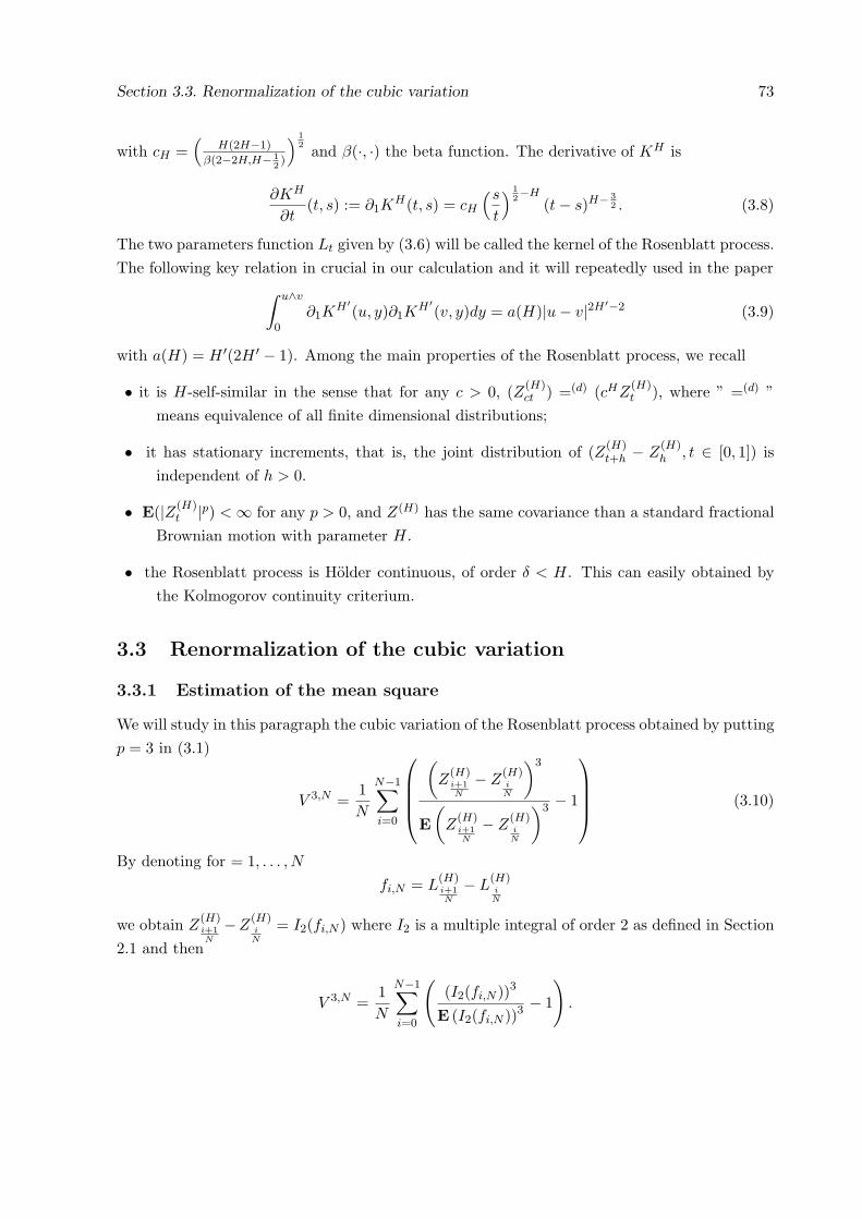
Section 3.3. Renormalization of the cubic variation 73
with cH =(
H(2H−1)
β(2−2H,H− 12)
) 12 and β(·, ·) the beta function. The derivative of KH is
∂KH
∂t(t, s) := ∂1K
H(t, s) = cH
(s
t
) 12−H
(t− s)H− 32 . (3.8)
The two parameters function Lt given by (3.6) will be called the kernel of the Rosenblatt process.The following key relation in crucial in our calculation and it will repeatedly used in the paper
∫ u∧v
0∂1K
H′(u, y)∂1K
H′(v, y)dy = a(H)|u− v|2H′−2 (3.9)
with a(H) = H ′(2H ′ − 1). Among the main properties of the Rosenblatt process, we recall
• it is H-self-similar in the sense that for any c > 0, (Z(H)ct ) =(d) (cHZ
(H)t ), where ” =(d) ”
means equivalence of all finite dimensional distributions;
• it has stationary increments, that is, the joint distribution of (Z(H)t+h − Z
(H)h , t ∈ [0, 1]) is
independent of h > 0.
• E(|Z(H)t |p) < ∞ for any p > 0, and Z(H) has the same covariance than a standard fractional
Brownian motion with parameter H.
• the Rosenblatt process is Holder continuous, of order δ < H. This can easily obtained bythe Kolmogorov continuity criterium.
3.3 Renormalization of the cubic variation
3.3.1 Estimation of the mean square
We will study in this paragraph the cubic variation of the Rosenblatt process obtained by puttingp = 3 in (3.1)
V 3,N =1N
N−1∑
i=0
(Z
(H)i+1N
− Z(H)iN
)3
E(
Z(H)i+1N
− Z(H)iN
)3 − 1
(3.10)
By denoting for = 1, . . . , Nfi,N = L
(H)i+1N
− L(H)iN
we obtain Z(H)i+1N
−Z(H)iN
= I2(fi,N ) where I2 is a multiple integral of order 2 as defined in Section2.1 and then
V 3,N =1N
N−1∑
i=0
((I2(fi,N ))3
E (I2(fi,N ))3− 1
).
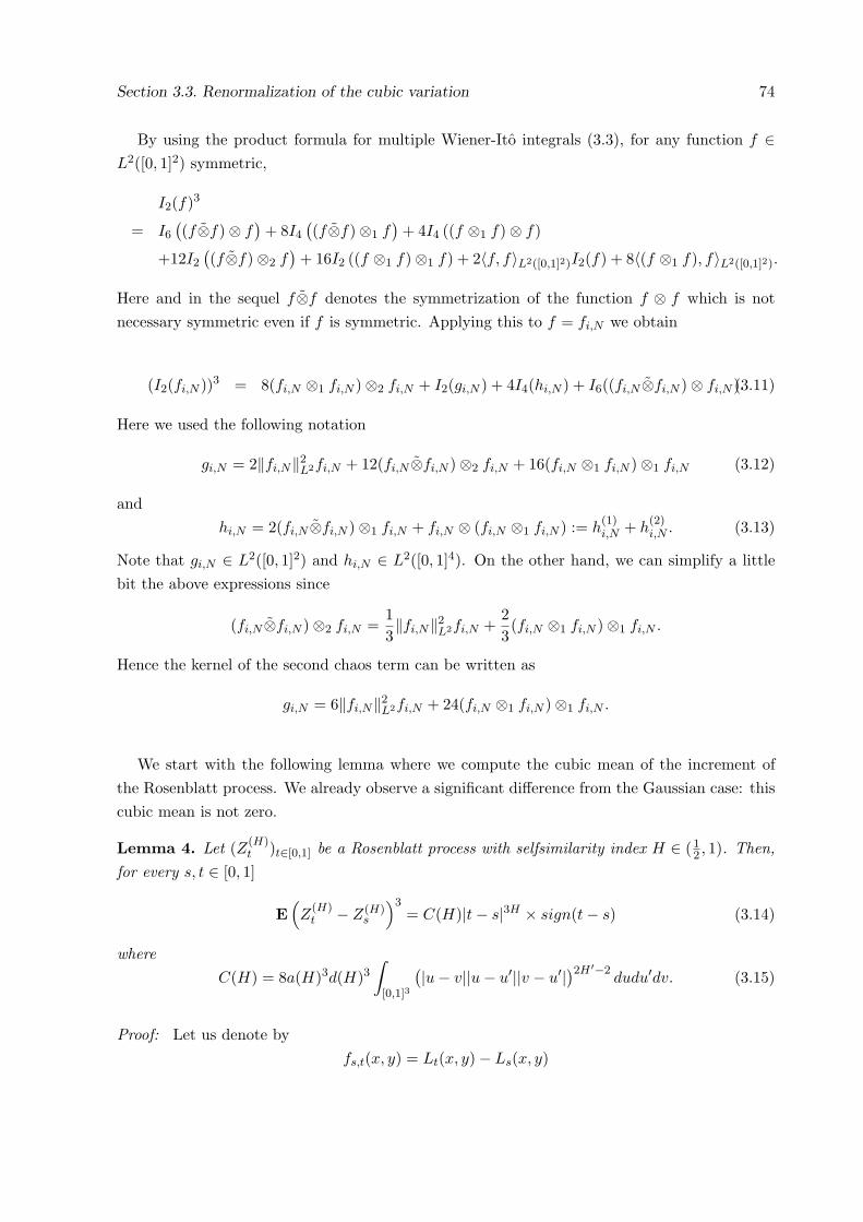
Section 3.3. Renormalization of the cubic variation 74
By using the product formula for multiple Wiener-Ito integrals (3.3), for any function f ∈L2([0, 1]2) symmetric,
I2(f)3
= I6
((f⊗f)⊗ f
)+ 8I4
((f⊗f)⊗1 f
)+ 4I4 ((f ⊗1 f)⊗ f)
+12I2
((f⊗f)⊗2 f
)+ 16I2 ((f ⊗1 f)⊗1 f) + 2〈f, f〉L2([0,1]2)I2(f) + 8〈(f ⊗1 f), f〉L2([0,1]2).
Here and in the sequel f⊗f denotes the symmetrization of the function f ⊗ f which is notnecessary symmetric even if f is symmetric. Applying this to f = fi,N we obtain
(I2(fi,N ))3 = 8(fi,N ⊗1 fi,N )⊗2 fi,N + I2(gi,N ) + 4I4(hi,N ) + I6((fi,N ⊗fi,N )⊗ fi,N ).(3.11)
Here we used the following notation
gi,N = 2‖fi,N‖2L2fi,N + 12(fi,N ⊗fi,N )⊗2 fi,N + 16(fi,N ⊗1 fi,N )⊗1 fi,N (3.12)
andhi,N = 2(fi,N ⊗fi,N )⊗1 fi,N + fi,N ⊗ (fi,N ⊗1 fi,N ) := h
(1)i,N + h
(2)i,N . (3.13)
Note that gi,N ∈ L2([0, 1]2) and hi,N ∈ L2([0, 1]4). On the other hand, we can simplify a littlebit the above expressions since
(fi,N ⊗fi,N )⊗2 fi,N =13‖fi,N‖2
L2fi,N +23(fi,N ⊗1 fi,N )⊗1 fi,N .
Hence the kernel of the second chaos term can be written as
gi,N = 6‖fi,N‖2L2fi,N + 24(fi,N ⊗1 fi,N )⊗1 fi,N .
We start with the following lemma where we compute the cubic mean of the increment ofthe Rosenblatt process. We already observe a significant difference from the Gaussian case: thiscubic mean is not zero.
Lemma 4. Let (Z(H)t )t∈[0,1] be a Rosenblatt process with selfsimilarity index H ∈ (1
2 , 1). Then,for every s, t ∈ [0, 1]
E(Z
(H)t − Z(H)
s
)3= C(H)|t− s|3H × sign(t− s) (3.14)
whereC(H) = 8a(H)3d(H)3
∫
[0,1]3
(|u− v||u− u′||v − u′|)2H′−2dudu′dv. (3.15)
Proof: Let us denote byfs,t(x, y) = Lt(x, y)− Ls(x, y)
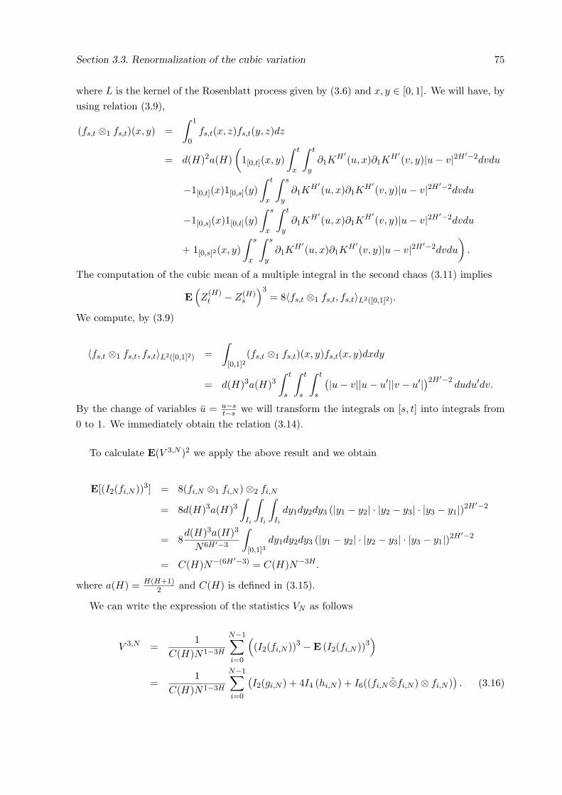
Section 3.3. Renormalization of the cubic variation 75
where L is the kernel of the Rosenblatt process given by (3.6) and x, y ∈ [0, 1]. We will have, byusing relation (3.9),
(fs,t ⊗1 fs,t)(x, y) =∫ 1
0fs,t(x, z)fs,t(y, z)dz
= d(H)2a(H)(
1[0,t](x, y)∫ t
x
∫ t
y∂1K
H′(u, x)∂1K
H′(v, y)|u− v|2H′−2dvdu
−1[0,t](x)1[0,s](y)∫ t
x
∫ s
y∂1K
H′(u, x)∂1K
H′(v, y)|u− v|2H′−2dvdu
−1[0,s](x)1[0,t](y)∫ s
x
∫ t
y∂1K
H′(u, x)∂1K
H′(v, y)|u− v|2H′−2dvdu
+ 1[0,s]2(x, y)∫ s
x
∫ s
y∂1K
H′(u, x)∂1K
H′(v, y)|u− v|2H′−2dvdu
).
The computation of the cubic mean of a multiple integral in the second chaos (3.11) implies
E(Z
(H)t − Z(H)
s
)3= 8〈fs,t ⊗1 fs,t, fs,t〉L2([0,1]2).
We compute, by (3.9)
〈fs,t ⊗1 fs,t, fs,t〉L2([0,1]2) =∫
[0,1]2(fs,t ⊗1 fs,t)(x, y)fs,t(x, y)dxdy
= d(H)3a(H)3∫ t
s
∫ t
s
∫ t
s
(|u− v||u− u′||v − u′|)2H′−2dudu′dv.
By the change of variables u = u−st−s we will transform the integrals on [s, t] into integrals from
0 to 1. We immediately obtain the relation (3.14).
To calculate E(V 3,N )2 we apply the above result and we obtain
E[(I2(fi,N ))3] = 8(fi,N ⊗1 fi,N )⊗2 fi,N
= 8d(H)3a(H)3∫
Ii
∫
Ii
∫
Ii
dy1dy2dy3 (|y1 − y2| · |y2 − y3| · |y3 − y1|)2H′−2
= 8d(H)3a(H)3
N6H′−3
∫
[0,1]3dy1dy2dy3 (|y1 − y2| · |y2 − y3| · |y3 − y1|)2H′−2
= C(H)N−(6H′−3) = C(H)N−3H .
where a(H) = H(H+1)2 and C(H) is defined in (3.15).
We can write the expression of the statistics VN as follows
V 3,N =1
C(H)N1−3H
N−1∑
i=0
((I2(fi,N ))3 −E (I2(fi,N ))3
)
=1
C(H)N1−3H
N−1∑
i=0
(I2(gi,N ) + 4I4 (hi,N ) + I6((fi,N ⊗fi,N )⊗ fi,N )
). (3.16)
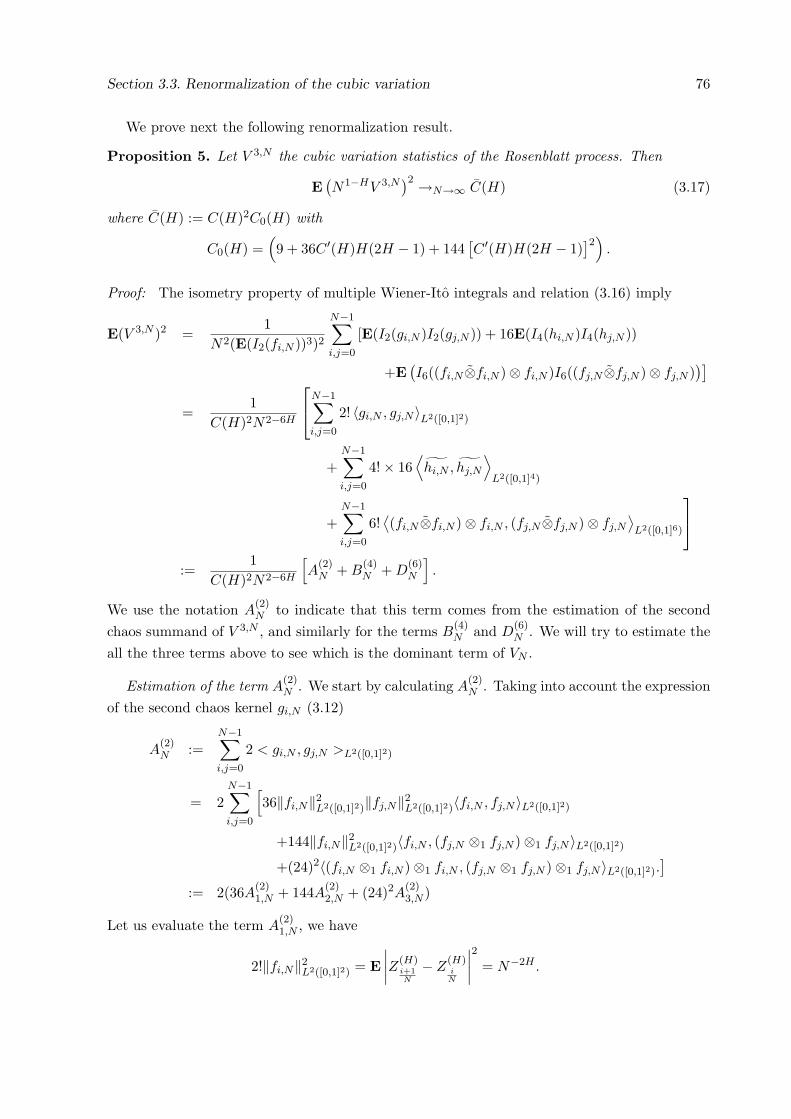
Section 3.3. Renormalization of the cubic variation 76
We prove next the following renormalization result.
Proposition 5. Let V 3,N the cubic variation statistics of the Rosenblatt process. Then
E(N1−HV 3,N
)2 →N→∞ C(H) (3.17)
where C(H) := C(H)2C0(H) with
C0(H) =(9 + 36C ′(H)H(2H − 1) + 144
[C ′(H)H(2H − 1)
]2)
.
Proof: The isometry property of multiple Wiener-Ito integrals and relation (3.16) imply
E(V 3,N )2 =1
N2(E(I2(fi,N ))3)2
N−1∑
i,j=0
[E(I2(gi,N )I2(gj,N )) + 16E(I4(hi,N )I4(hj,N ))
+E(I6((fi,N ⊗fi,N )⊗ fi,N )I6((fj,N ⊗fj,N )⊗ fj,N )
)]
=1
C(H)2N2−6H
N−1∑
i,j=0
2! 〈gi,N , gj,N 〉L2([0,1]2)
+N−1∑
i,j=0
4!× 16⟨hi,N , hj,N
⟩L2([0,1]4)
+N−1∑
i,j=0
6!⟨(fi,N ⊗fi,N )⊗ fi,N , (fj,N ⊗fj,N )⊗ fj,N
⟩L2([0,1]6)
:=1
C(H)2N2−6H
[A
(2)N + B
(4)N + D
(6)N
].
We use the notation A(2)N to indicate that this term comes from the estimation of the second
chaos summand of V 3,N , and similarly for the terms B(4)N and D
(6)N . We will try to estimate the
all the three terms above to see which is the dominant term of VN .
Estimation of the term A(2)N . We start by calculating A
(2)N . Taking into account the expression
of the second chaos kernel gi,N (3.12)
A(2)N :=
N−1∑
i,j=0
2 < gi,N , gj,N >L2([0,1]2)
= 2N−1∑
i,j=0
[36‖fi,N‖2
L2([0,1]2)‖fj,N‖2L2([0,1]2)〈fi,N , fj,N 〉L2([0,1]2)
+144‖fi,N‖2L2([0,1]2)〈fi,N , (fj,N ⊗1 fj,N )⊗1 fj,N 〉L2([0,1]2)
+(24)2〈(fi,N ⊗1 fi,N )⊗1 fi,N , (fj,N ⊗1 fj,N )⊗1 fj,N 〉L2([0,1]2).]
:= 2(36A(2)1,N + 144A(2)
2,N + (24)2A(2)3,N )
Let us evaluate the term A(2)1,N , we have
2!‖fi,N‖2L2([0,1]2) = E
∣∣∣∣Z(H)i+1N
− Z(H)iN
∣∣∣∣2
= N−2H .
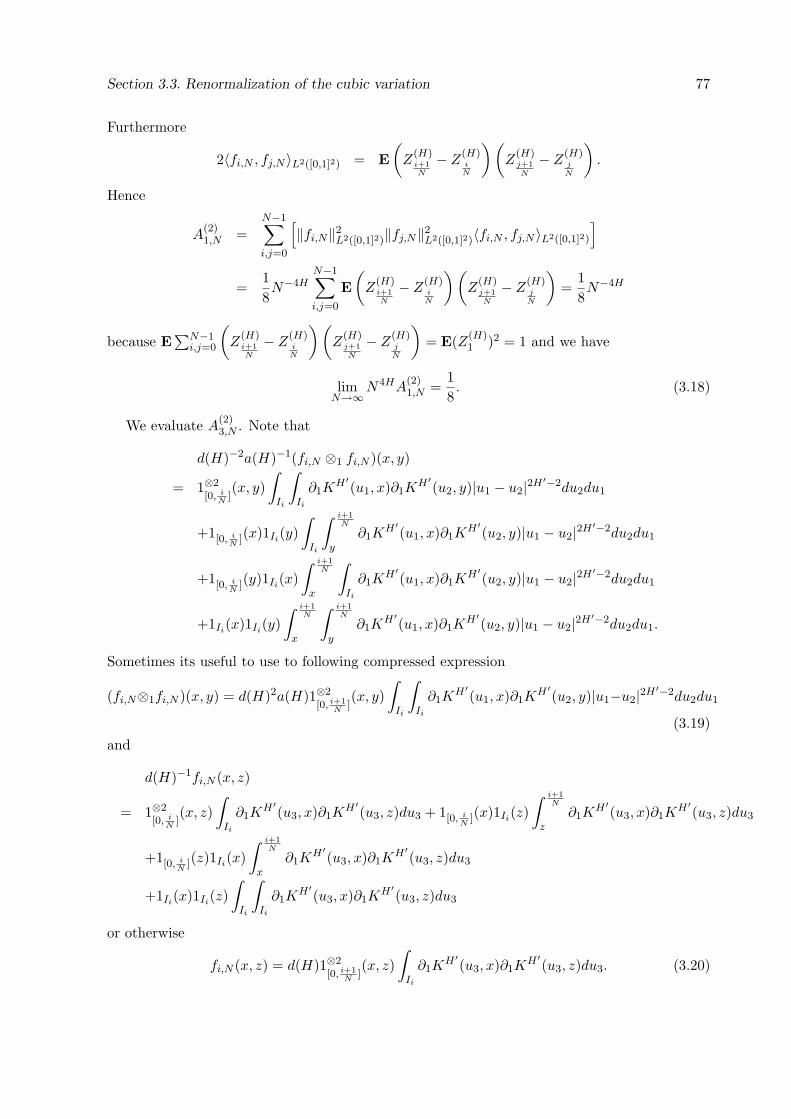
Section 3.3. Renormalization of the cubic variation 77
Furthermore
2〈fi,N , fj,N 〉L2([0,1]2) = E(
Z(H)i+1N
− Z(H)iN
)(Z
(H)j+1N
− Z(H)jN
).
Hence
A(2)1,N =
N−1∑
i,j=0
[‖fi,N‖2
L2([0,1]2)‖fj,N‖2L2([0,1]2)〈fi,N , fj,N 〉L2([0,1]2)
]
=18N−4H
N−1∑
i,j=0
E(
Z(H)i+1N
− Z(H)iN
)(Z
(H)j+1N
− Z(H)jN
)=
18N−4H
because E∑N−1
i,j=0
(Z
(H)i+1N
− Z(H)iN
)(Z
(H)j+1N
− Z(H)jN
)= E(Z(H)
1 )2 = 1 and we have
limN→∞
N4HA(2)1,N =
18. (3.18)
We evaluate A(2)3,N . Note that
d(H)−2a(H)−1(fi,N ⊗1 fi,N )(x, y)
= 1⊗2[0, i
N](x, y)
∫
Ii
∫
Ii
∂1KH′
(u1, x)∂1KH′
(u2, y)|u1 − u2|2H′−2du2du1
+1[0, iN
](x)1Ii(y)∫
Ii
∫ i+1N
y∂1K
H′(u1, x)∂1K
H′(u2, y)|u1 − u2|2H′−2du2du1
+1[0, iN
](y)1Ii(x)∫ i+1
N
x
∫
Ii
∂1KH′
(u1, x)∂1KH′
(u2, y)|u1 − u2|2H′−2du2du1
+1Ii(x)1Ii(y)∫ i+1
N
x
∫ i+1N
y∂1K
H′(u1, x)∂1K
H′(u2, y)|u1 − u2|2H′−2du2du1.
Sometimes its useful to use to following compressed expression
(fi,N⊗1fi,N )(x, y) = d(H)2a(H)1⊗2[0, i+1
N](x, y)
∫
Ii
∫
Ii
∂1KH′
(u1, x)∂1KH′
(u2, y)|u1−u2|2H′−2du2du1
(3.19)and
d(H)−1fi,N (x, z)
= 1⊗2[0, i
N](x, z)
∫
Ii
∂1KH′
(u3, x)∂1KH′
(u3, z)du3 + 1[0, iN
](x)1Ii(z)∫ i+1
N
z∂1K
H′(u3, x)∂1K
H′(u3, z)du3
+1[0, iN
](z)1Ii(x)∫ i+1
N
x∂1K
H′(u3, x)∂1K
H′(u3, z)du3
+1Ii(x)1Ii(z)∫
Ii
∫
Ii
∂1KH′
(u3, x)∂1KH′
(u3, z)du3
or otherwise
fi,N (x, z) = d(H)1⊗2[0, i+1
N](x, z)
∫
Ii
∂1KH′
(u3, x)∂1KH′
(u3, z)du3. (3.20)
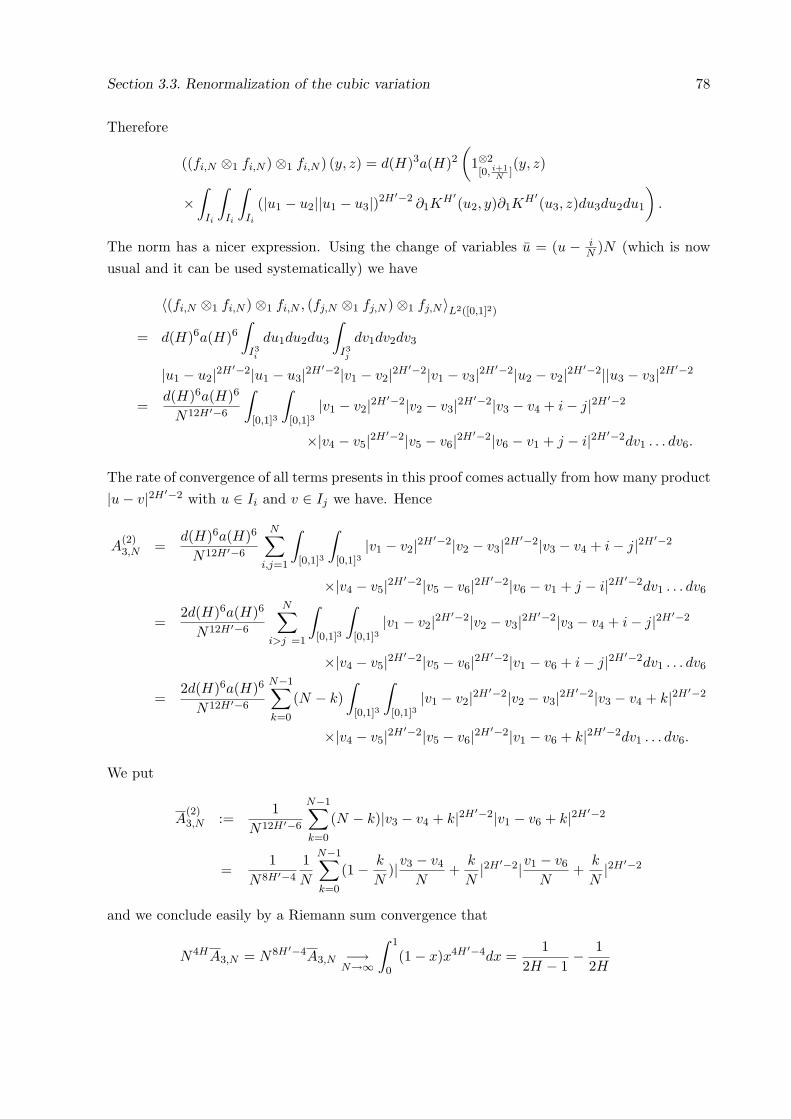
Section 3.3. Renormalization of the cubic variation 78
Therefore
((fi,N ⊗1 fi,N )⊗1 fi,N ) (y, z) = d(H)3a(H)2(
1⊗2[0, i+1
N](y, z)
×∫
Ii
∫
Ii
∫
Ii
(|u1 − u2||u1 − u3|)2H′−2 ∂1KH′
(u2, y)∂1KH′
(u3, z)du3du2du1
).
The norm has a nicer expression. Using the change of variables u = (u − iN )N (which is now
usual and it can be used systematically) we have
〈(fi,N ⊗1 fi,N )⊗1 fi,N , (fj,N ⊗1 fj,N )⊗1 fj,N 〉L2([0,1]2)
= d(H)6a(H)6∫
I3i
du1du2du3
∫
I3j
dv1dv2dv3
|u1 − u2|2H′−2|u1 − u3|2H′−2|v1 − v2|2H′−2|v1 − v3|2H′−2|u2 − v2|2H′−2||u3 − v3|2H′−2
=d(H)6a(H)6
N12H′−6
∫
[0,1]3
∫
[0,1]3|v1 − v2|2H′−2|v2 − v3|2H′−2|v3 − v4 + i− j|2H′−2
×|v4 − v5|2H′−2|v5 − v6|2H′−2|v6 − v1 + j − i|2H′−2dv1 . . . dv6.
The rate of convergence of all terms presents in this proof comes actually from how many product|u− v|2H′−2 with u ∈ Ii and v ∈ Ij we have. Hence
A(2)3,N =
d(H)6a(H)6
N12H′−6
N∑
i,j=1
∫
[0,1]3
∫
[0,1]3|v1 − v2|2H′−2|v2 − v3|2H′−2|v3 − v4 + i− j|2H′−2
×|v4 − v5|2H′−2|v5 − v6|2H′−2|v6 − v1 + j − i|2H′−2dv1 . . . dv6
=2d(H)6a(H)6
N12H′−6
N∑
i>j =1
∫
[0,1]3
∫
[0,1]3|v1 − v2|2H′−2|v2 − v3|2H′−2|v3 − v4 + i− j|2H′−2
×|v4 − v5|2H′−2|v5 − v6|2H′−2|v1 − v6 + i− j|2H′−2dv1 . . . dv6
=2d(H)6a(H)6
N12H′−6
N−1∑
k=0
(N − k)∫
[0,1]3
∫
[0,1]3|v1 − v2|2H′−2|v2 − v3|2H′−2|v3 − v4 + k|2H′−2
×|v4 − v5|2H′−2|v5 − v6|2H′−2|v1 − v6 + k|2H′−2dv1 . . . dv6.
We put
A(2)3,N :=
1N12H′−6
N−1∑
k=0
(N − k)|v3 − v4 + k|2H′−2|v1 − v6 + k|2H′−2
=1
N8H′−4
1N
N−1∑
k=0
(1− k
N)|v3 − v4
N+
k
N|2H′−2|v1 − v6
N+
k
N|2H′−2
and we conclude easily by a Riemann sum convergence that
N4HA3,N = N8H′−4A3,N −→N→∞
∫ 1
0(1− x)x4H′−4dx =
12H − 1
− 12H
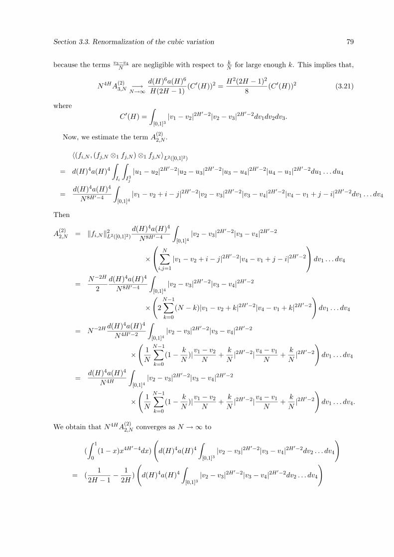
Section 3.3. Renormalization of the cubic variation 79
because the terms v3−v4N are negligible with respect to k
N for large enough k. This implies that,
N4HA(2)3,N −→
N→∞d(H)6a(H)6
H(2H − 1)(C ′(H))2 =
H2(2H − 1)2
8(C ′(H))2 (3.21)
whereC ′(H) =
∫
[0,1]3|v1 − v2|2H′−2|v2 − v3|2H′−2dv1dv2dv3.
Now, we estimate the term A(2)2,N .
〈(fi,N , (fj,N ⊗1 fj,N )⊗1 fj,N 〉L2([0,1]2)
= d(H)4a(H)4∫
Ii
∫
I3j
|u1 − u2|2H′−2|u2 − u3|2H′−2|u3 − u4|2H′−2|u4 − u1|2H′−2du1 . . . du4
=d(H)4a(H)4
N8H′−4
∫
[0,1]4|v1 − v2 + i− j|2H′−2|v2 − v3|2H′−2|v3 − v4|2H′−2|v4 − v1 + j − i|2H′−2dv1 . . . dv4
Then
A(2)2,N = ‖fi,N‖2
L2([0,1]2)
d(H)4a(H)4
N8H′−4
∫
[0,1]4|v2 − v3|2H′−2|v3 − v4|2H′−2
×
N∑
i,j=1
|v1 − v2 + i− j|2H′−2|v4 − v1 + j − i|2H′−2
dv1 . . . dv4
=N−2H
2d(H)4a(H)4
N8H′−4
∫
[0,1]4|v2 − v3|2H′−2|v3 − v4|2H′−2
×(
2N−1∑
k=0
(N − k)|v1 − v2 + k|2H′−2|v4 − v1 + k|2H′−2
)dv1 . . . dv4
= N−2H d(H)4a(H)4
N4H′−2
∫
[0,1]4|v2 − v3|2H′−2|v3 − v4|2H′−2
×(
1N
N−1∑
k=0
(1− k
N)|v1 − v2
N+
k
N|2H′−2|v4 − v1
N+
k
N|2H′−2
)dv1 . . . dv4
=d(H)4a(H)4
N4H
∫
[0,1]4|v2 − v3|2H′−2|v3 − v4|2H′−2
×(
1N
N−1∑
k=0
(1− k
N)|v1 − v2
N+
k
N|2H′−2|v4 − v1
N+
k
N|2H′−2
)dv1 . . . dv4.
We obtain that N4HA(2)2,N converges as N →∞ to
(∫ 1
0(1− x)x4H′−4dx)
(d(H)4a(H)4
∫
[0,1]3|v2 − v3|2H′−2|v3 − v4|2H′−2dv2 . . . dv4
)
= (1
2H − 1− 1
2H)
(d(H)4a(H)4
∫
[0,1]3|v2 − v3|2H′−2|v3 − v4|2H′−2dv2 . . . dv4
)
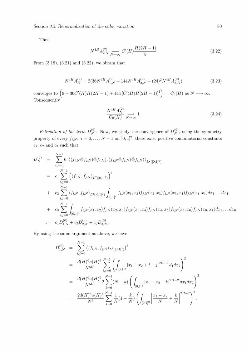
Section 3.3. Renormalization of the cubic variation 80
Thus
N4HA(2)2,N −→
N→∞C ′(H)
H(2H − 1)8
(3.22)
From (3.18), (3.21) and (3.22), we obtain that
N4HA(2)N = 2(36N4HA
(2)1,N + 144N4HA
(2)2,N + (24)2N4HA
(2)3,N ) (3.23)
converges to(9 + 36C ′(H)H(2H − 1) + 144 [C ′(H)H(2H − 1)]2
):= C0(H) as N −→∞.
Consequently
N4HA(2)N
C0(H)−→
N→∞1. (3.24)
Estimation of the term D(6)N . Now, we study the convergence of D
(6)N , using the symmetry
property of every fi,N , i = 0, . . . , N − 1 on [0, 1]2, there exist positive combinatorial constantsc1, c2 and c3 such that
D(6)N =
N−1∑
i,j=0
6!⟨(fi,N ⊗fj,N )⊗fj,N ), (fj,N ⊗fi,N )⊗fi,N )
⟩L2([0,1]6)
= c1
N−1∑
i,j=0
(〈fi,N , fj,N 〉L2([0,1]2)
)3
+ c2
N−1∑
i,j=0
〈fi,N , fj,N 〉L2([0,1]2)
∫
[0,1]4fi,N (x1, x2)fj,N (x2, x3)fi,N (x3, x4)fj,N (x4, x1)dx1 . . . dx4
+ c3
N−1∑
i,j=0
∫
[0,1]6fi,N (x1, x2)fj,N (x2, x3)fi,N (x3, x4)fj,N (x4, x5)fi,N (x5, x6)fj,N (x6, x1)dx1 . . . dx6
:= c1D(6)1,N + c2D
(6)2,N + c3D
(6)3,N .
By using the same argument as above, we have
D(6)1,N =
N−1∑
i,j=0
(〈fi,N , fj,N 〉L2([0,1]2)
)3
=d(H)6a(H)6
N6H
N−1∑
i,j=0
(∫
[0,1]2|x1 − x2 + i− j|2H−2 d1dx2
)3
=d(H)6a(H)6
N6H2
N−1∑
k=0
(N − k)
(∫
[0,1]2|x1 − x2 + k|2H−2 dx1dx2
)3
=2d(H)6a(H)6
N4
N−1∑
k=0
1N
(1− k
N)
(∫
[0,1]2
∣∣∣∣x1 − x2
N+
k
N
∣∣∣∣2H−2
)3
.
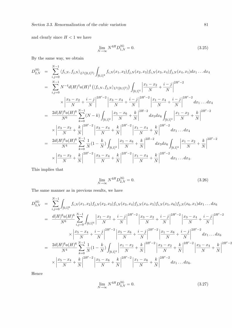
Section 3.3. Renormalization of the cubic variation 81
and clearly since H < 1 we have
limN→∞
N4HD(6)1,N = 0. (3.25)
By the same way, we obtain
D(6)2,N =
N−1∑
i,j=0
〈fi,N , fj,N 〉L2([0,1]2)
∫
[0,1]4fi,N (x1, x2)fj,N (x2, x3)fi,N (x3, x4)fj,N (x4, x1)dx1 . . . dx4
=N−1∑
i,j=0
N−4d(H)4a(H)4(〈fi,N , fj,N 〉L2([0,1]2)
) ∫
[0,1]4
∣∣∣∣x1 − x2
N+
i− j
N
∣∣∣∣2H′−2
×∣∣∣∣x3 − x2
N+
i− j
N
∣∣∣∣2H′−2 ∣∣∣∣
x3 − x4
N+
i− j
N
∣∣∣∣2H′−2 ∣∣∣∣
x1 − x4
N+
i− j
N
∣∣∣∣2H′−2
dx1 . . . dx4
=2d(H)6a(H)6
N6
N−1∑
k=0
(N − k)∫
[0,1]2
∣∣∣∣x5 − x6
N+
k
N
∣∣∣∣2H−2
dx5dx6
∫
[0,1]4
∣∣∣∣x1 − x2
N+
k
N
∣∣∣∣2H′−2
×∣∣∣∣x3 − x2
N+
k
N
∣∣∣∣2H′−2 ∣∣∣∣
x3 − x4
N+
k
N
∣∣∣∣2H′−2 ∣∣∣∣
x1 − x4
N+
k
N
∣∣∣∣2H′−2
dx1 . . . dx4
=2d(H)6a(H)6
N4
N−1∑
k=0
1N
(1− k
N)∫
[0,1]2
∣∣∣∣x5 − x6
N+
k
N
∣∣∣∣2H−2
dx5dx6
∫
[0,1]4
∣∣∣∣x1 − x2
N+
k
N
∣∣∣∣2H′−2
×∣∣∣∣x3 − x2
N+
k
N
∣∣∣∣2H′−2 ∣∣∣∣
x3 − x4
N+
k
N
∣∣∣∣2H′−2 ∣∣∣∣
x1 − x4
N+
k
N
∣∣∣∣2H′−2
dx1 . . . dx4.
This implies that
limN→∞
N4HD(6)2,N = 0. (3.26)
The same manner as in previous results, we have
D(6)3,N =
N−1∑
i,j=0
∫
[0,1]6fi,N (x1, x2)fj,N (x2, x3)fi,N (x3, x4)fj,N (x4, x5)fi,N (x5, x6)fj,N (x6, x1)dx1 . . . dx6
=d(H)6a(H)6
N6
N−1∑
i,j=0
∫
[0,1]6
∣∣∣∣x1 − x2
N+
i− j
N
∣∣∣∣2H′−2 ∣∣∣∣
x3 − x2
N+
i− j
N
∣∣∣∣2H′−2 ∣∣∣∣
x3 − x4
N+
i− j
N
∣∣∣∣2H′−2
×∣∣∣∣x5 − x4
N+
i− j
N
∣∣∣∣2H′−2 ∣∣∣∣
x5 − x6
N+
i− j
N
∣∣∣∣2H′−2 ∣∣∣∣
x1 − x6
N+
i− j
N
∣∣∣∣2H′−2
dx1 . . . dx6
=2d(H)6a(H)6
N4
N−1∑
k=0
1N
(1− k
N)∫
[0,1]4
∣∣∣∣x1 − x2
N+
k
N
∣∣∣∣2H′−2 ∣∣∣∣
x3 − x2
N+
k
N
∣∣∣∣2H′−2 ∣∣∣∣
x3 − x4
N+
k
N
∣∣∣∣2H′−2
×∣∣∣∣x5 − x4
N+
k
N
∣∣∣∣2H′−2 ∣∣∣∣
x5 − x6
N+
k
N
∣∣∣∣2H′−2 ∣∣∣∣
x1 − x6
N+
k
N
∣∣∣∣2H′−2
dx1 . . . dx6.
Hence
limN→∞
N4HD(6)3,N = 0. (3.27)
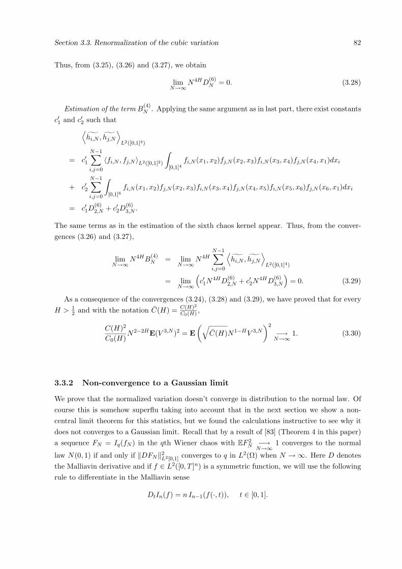
Section 3.3. Renormalization of the cubic variation 82
Thus, from (3.25), (3.26) and (3.27), we obtain
limN→∞
N4HD(6)N = 0. (3.28)
Estimation of the term B(4)N . Applying the same argument as in last part, there exist constants
c′1 and c′2 such that⟨hi,N , hj,N
⟩L2([0,1]4)
= c′1N−1∑
i,j=0
〈fi,N , fj,N 〉L2([0,1]2)
∫
[0,1]4fi,N (x1, x2)fj,N (x2, x3)fi,N (x3, x4)fj,N (x4, x1)dxi
+ c′2N−1∑
i,j=0
∫
[0,1]6fi,N (x1, x2)fj,N (x2, x3)fi,N (x3, x4)fj,N (x4, x5)fi,N (x5, x6)fj,N (x6, x1)dxi
= c′1D(6)2,N + c′2D
(6)3,N .
The same terms as in the estimation of the sixth chaos kernel appear. Thus, from the conver-gences (3.26) and (3.27),
limN→∞
N4HB(4)N = lim
N→∞N4H
N−1∑
i,j=0
⟨hi,N , hj,N
⟩L2([0,1]4)
= limN→∞
(c′1N
4HD(6)2,N + c′2N
4HD(6)3,N
)= 0. (3.29)
As a consequence of the convergences (3.24), (3.28) and (3.29), we have proved that for everyH > 1
2 and with the notation C(H) = C(H)2
C0(H) ,
C(H)2
C0(H)N2−2HE(V 3,N )2 = E
(√C(H)N1−HV 3,N
)2
−→N→∞
1. (3.30)
3.3.2 Non-convergence to a Gaussian limit
We prove that the normalized variation doesn’t converge in distribution to the normal law. Ofcourse this is somehow superflu taking into account that in the next section we show a non-central limit theorem for this statistics, but we found the calculations instructive to see why itdoes not converges to a Gaussian limit. Recall that by a result of [83] (Theorem 4 in this paper)a sequence FN = Iq(fN ) in the qth Wiener chaos with EF 2
N −→N→∞
1 converges to the normal
law N(0, 1) if and only if ‖DFN‖2L2[0,1] converges to q in L2(Ω) when N →∞. Here D denotes
the Malliavin derivative and if f ∈ L2([0, T ]n) is a symmetric function, we will use the followingrule to differentiate in the Malliavin sense
DtIn(f) = n In−1(f(·, t)), t ∈ [0, 1].
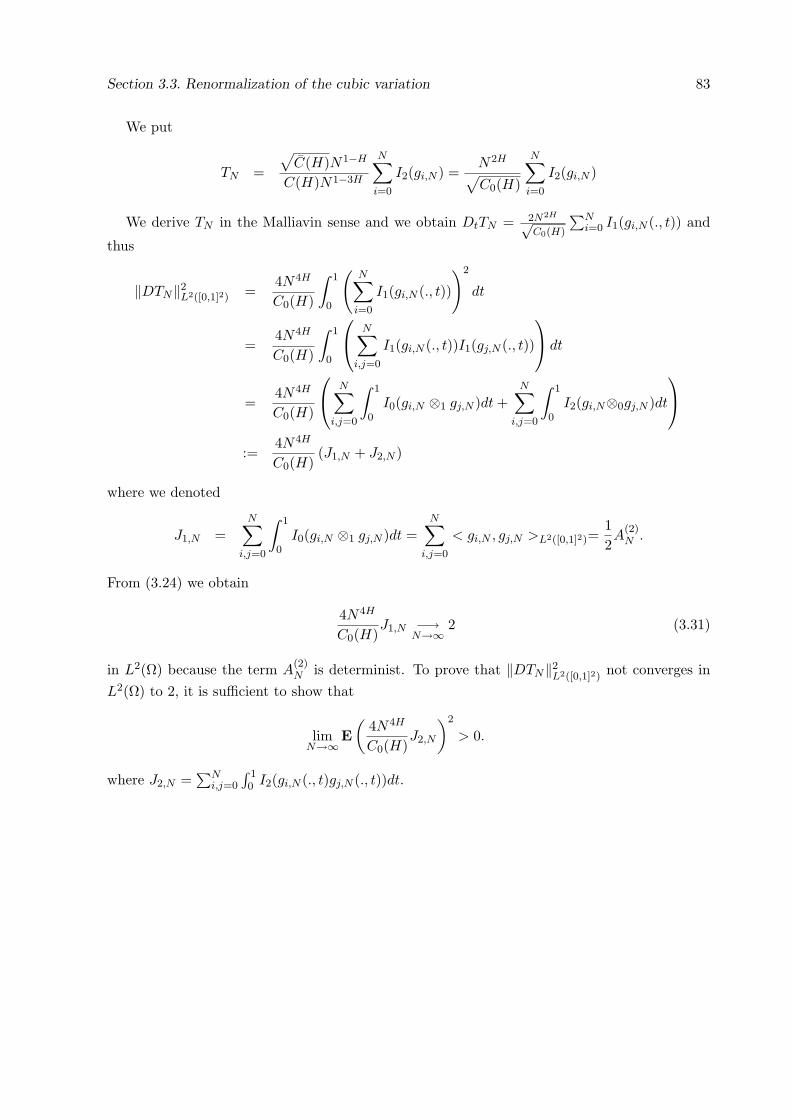
Section 3.3. Renormalization of the cubic variation 83
We put
TN =
√C(H)N1−H
C(H)N1−3H
N∑
i=0
I2(gi,N ) =N2H
√C0(H)
N∑
i=0
I2(gi,N )
We derive TN in the Malliavin sense and we obtain DtTN = 2N2H√C0(H)
∑Ni=0 I1(gi,N (., t)) and
thus
‖DTN‖2L2([0,1]2) =
4N4H
C0(H)
∫ 1
0
(N∑
i=0
I1(gi,N (., t))
)2
dt
=4N4H
C0(H)
∫ 1
0
N∑
i,j=0
I1(gi,N (., t))I1(gj,N (., t))
dt
=4N4H
C0(H)
N∑
i,j=0
∫ 1
0I0(gi,N ⊗1 gj,N )dt +
N∑
i,j=0
∫ 1
0I2(gi,N⊗0gj,N )dt
:=4N4H
C0(H)(J1,N + J2,N )
where we denoted
J1,N =N∑
i,j=0
∫ 1
0I0(gi,N ⊗1 gj,N )dt =
N∑
i,j=0
< gi,N , gj,N >L2([0,1]2)=12A
(2)N .
From (3.24) we obtain
4N4H
C0(H)J1,N −→
N→∞2 (3.31)
in L2(Ω) because the term A(2)N is determinist. To prove that ‖DTN‖2
L2([0,1]2) not converges inL2(Ω) to 2, it is sufficient to show that
limN→∞
E(
4N4H
C0(H)J2,N
)2
> 0.
where J2,N =∑N
i,j=0
∫ 10 I2(gi,N (., t)gj,N (., t))dt.
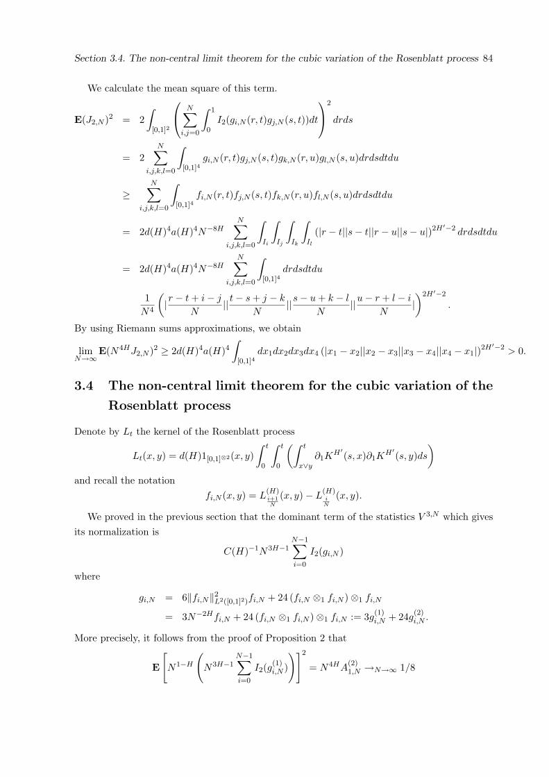
Section 3.4. The non-central limit theorem for the cubic variation of the Rosenblatt process 84
We calculate the mean square of this term.
E(J2,N )2 = 2∫
[0,1]2
N∑
i,j=0
∫ 1
0I2(gi,N (r, t)gj,N (s, t))dt
2
drds
= 2N∑
i,j,k,l=0
∫
[0,1]4gi,N (r, t)gj,N (s, t)gk,N (r, u)gl,N (s, u)drdsdtdu
≥N∑
i,j,k,l=0
∫
[0,1]4fi,N (r, t)fj,N (s, t)fk,N (r, u)fl,N (s, u)drdsdtdu
= 2d(H)4a(H)4N−8HN∑
i,j,k,l=0
∫
Ii
∫
Ij
∫
Ik
∫
Il
(|r − t||s− t||r − u||s− u|)2H′−2 drdsdtdu
= 2d(H)4a(H)4N−8HN∑
i,j,k,l=0
∫
[0,1]4drdsdtdu
1N4
(|r − t + i− j
N|| t− s + j − k
N||s− u + k − l
N||u− r + l − i
N|)2H′−2
.
By using Riemann sums approximations, we obtain
limN→∞
E(N4HJ2,N )2 ≥ 2d(H)4a(H)4∫
[0,1]4dx1dx2dx3dx4 (|x1 − x2||x2 − x3||x3 − x4||x4 − x1|)2H′−2 > 0.
3.4 The non-central limit theorem for the cubic variation of the
Rosenblatt process
Denote by Lt the kernel of the Rosenblatt process
Lt(x, y) = d(H)1[0,1]⊗2(x, y)∫ t
0
∫ t
0
(∫ t
x∨y∂1K
H′(s, x)∂1K
H′(s, y)ds
)
and recall the notationfi,N (x, y) = L
(H)i+1N
(x, y)− L(H)iN
(x, y).
We proved in the previous section that the dominant term of the statistics V 3,N which givesits normalization is
C(H)−1N3H−1N−1∑
i=0
I2(gi,N )
where
gi,N = 6‖fi,N‖2L2([0,1]2)fi,N + 24 (fi,N ⊗1 fi,N )⊗1 fi,N
= 3N−2Hfi,N + 24 (fi,N ⊗1 fi,N )⊗1 fi,N := 3g(1)i,N + 24g(2)
i,N .
More precisely, it follows from the proof of Proposition 2 that
E
[N1−H
(N3H−1
N−1∑
i=0
I2(g(1)i,N )
)]2
= N4HA(2)1,N →N→∞ 1/8
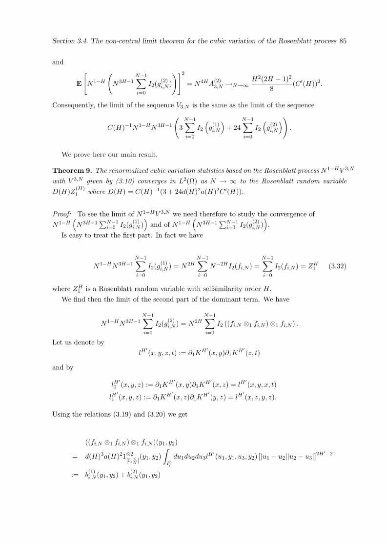
Section 3.4. The non-central limit theorem for the cubic variation of the Rosenblatt process 85
and
E
[N1−H
(N3H−1
N−1∑
i=0
I2(g(2)i,N )
)]2
= N4HA(2)3,N →N→∞
H2(2H − 1)2
8(C ′(H))2.
Consequently, the limit of the sequence V3,N is the same as the limit of the sequence
C(H)−1N1−HN3H−1
(3
N−1∑
i=0
I2
(g(1)i,N
)+ 24
N−1∑
i=0
I2
(g(2)i,N
)).
We prove here our main result.
Theorem 9. The renormalized cubic variation statistics based on the Rosenblatt process N1−HV 3,N
with V 3,N given by (3.10) converges in L2(Ω) as N → ∞ to the Rosenblatt random variableD(H)Z(H)
1 where D(H) = C(H)−1(3 + 24d(H)2a(H)2C ′(H)).
Proof: To see the limit of N1−HV 3,N we need therefore to study the convergence ofN1−H
(N3H−1
∑N−1i=0 I2(g
(1)i,N )
)and of N1−H
(N3H−1
∑N−1i=0 I2(g
(2)i,N )
).
Is easy to treat the first part. In fact we have
N1−HN3H−1N−1∑
i=0
I2(g(1)i,N ) = N2H
N−1∑
i=0
N−2HI2(fi,N ) =N−1∑
i=0
I2(fi,N ) = ZH1 (3.32)
where ZH1 is a Rosenblatt random variable with selfsimilarity order H.
We find then the limit of the second part of the dominant term. We have
N1−HN3H−1N−1∑
i=0
I2(g(2)i,N ) = N2H
N−1∑
i=0
I2 ((fi,N ⊗1 fi,N )⊗1 fi,N ) .
Let us denote bylH
′(x, y, z, t) := ∂1K
H′(x, y)∂1K
H′(z, t)
and by
lH′
0 (x, y, z) := ∂1KH′
(x, y)∂1KH′
(x, z) = lH′(x, y, x, t)
lH′
1 (x, y, z) := ∂1KH′
(x, z)∂1KH′
(y, z) = lH′(x, z, y, z).
Using the relations (3.19) and (3.20) we get
((fi,N ⊗1 fi,N )⊗1 fi,N )(y1, y2)
= d(H)3a(H)21⊗2[0, i
N](y1, y2)
∫
I3i
du1du2du3lH′
(u1, y1, u3, y2) [|u1 − u2||u2 − u3|]2H′−2
:= b(1)i,N (y1, y2) + b
(2)i,N (y1, y2)
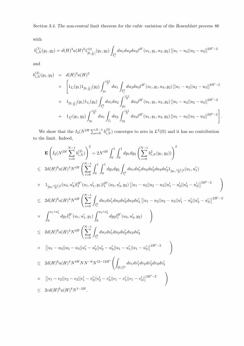
Section 3.4. The non-central limit theorem for the cubic variation of the Rosenblatt process 86
with
b(1)i,N (y1, y2) = d(H)3a(H)21⊗2
[0, iN
](y1, y2)
∫
I3i
du1du2du3lH′
(u1, y1, u3, y2) [|u1 − u2||u2 − u3|]2H′−2
and
b(2)i,N (y1, y2) = d(H)3a(H)2
×[1Ii(y1)1[0, i
N](y2)
∫ i+1N
y1
du1
∫
I2i
du2du3lH′
(u1, y1, u3, y2) [|u1 − u2||u2 − u3|]2H′−2
+ 1[0, iN
](y1)1Ii(y2)∫
I2i
du1du2
∫ i+1N
y2
du3lH′
(u1, y1, u3, y2) [|u1 − u2||u2 − u3|]2H′−2
+ 1I2i(y1, y2)
∫ i+1N
y1
du1
∫
Ii
du2
∫ i+1N
y2
du3lH′
(u1, y1, u3, y2) [|u1 − u2||u2 − u3|]2H′−2
].
We show that the I2(N2H∑N−1
i=0 b(2)i,N ) converges to zero in L2(Ω) and it has no contribution
to the limit. Indeed,
E
(I2(N2H
N−1∑
i=0
b(2)i,N )
)2
= 2N4H
∫ 1
0
∫ 1
0dy1dy2
(N−1∑
i=0
b2i,N (y1, y2))
)2
≤ 2d(H)6a(H)4N4H
(N−1∑
i=0
∫ 1
0
∫ 1
0dy1dy2
∫
I6i
du1du′1du2du′2du3du′31[y1, i+1N
]2(u1, u′1)
× 1[y2, i+1N
]2(u3, u′3)l
H′1 (u1, u
′1, y1)lH
′1 (u3, u
′3, y2)
[|u1 − u2||u2 − u3||u′1 − u′2||u′2 − u′3|]2H′−2
)
≤ 2d(H)6a(H)4N4H
(N−1∑
i=0
∫
I6i
du1du′1du2du′2du3du′3[|u1 − u2||u2 − u3||u′1 − u′2||u′2 − u′3|
]2H′−2
×∫ u1∧u′1
0dy1l
H′1 (u1, u
′1, y1)
∫ u3∧u′3
0dy2l
H′1 (u3, u
′3, y2)
)
≤ 2d(H)6a(H)4N4H
(N−1∑
i=0
∫
I6i
du1du′1du2du′2du3du′3
× [|u1 − u2||u2 − u3||u′1 − u′2||u′2 − u′3||u1 − u′1||u1 − u′3|]2H′−2
)
≤ 2d(H)6a(H)4N4HNN−6N12−12H′(∫
[0,1]6dv1dv′1dv2dv′2dv3dv′3
× [|v1 − v2||v2 − v3||v′1 − v′2||v′2 − v′3||v1 − v′1||v1 − v′3|]2H′−2
)
≤ 2cd(H)6a(H)4N1−2H .
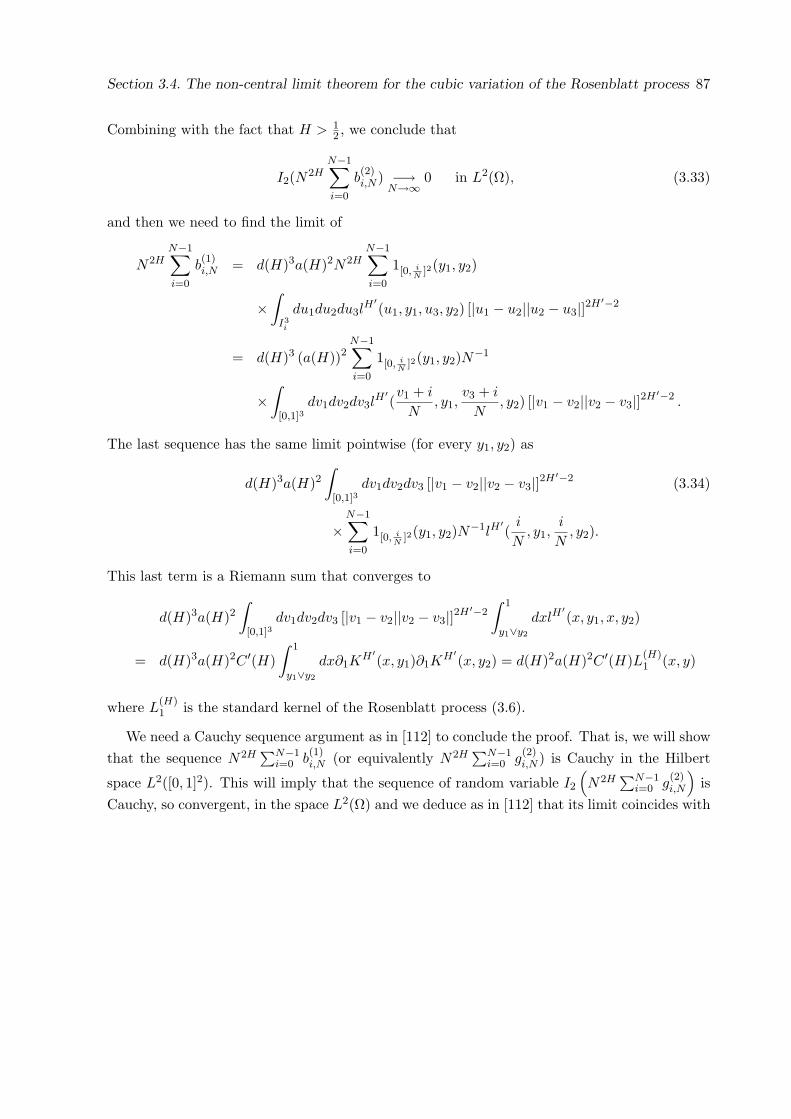
Section 3.4. The non-central limit theorem for the cubic variation of the Rosenblatt process 87
Combining with the fact that H > 12 , we conclude that
I2(N2HN−1∑
i=0
b(2)i,N ) −→
N→∞0 in L2(Ω), (3.33)
and then we need to find the limit of
N2HN−1∑
i=0
b(1)i,N = d(H)3a(H)2N2H
N−1∑
i=0
1[0, iN
]2(y1, y2)
×∫
I3i
du1du2du3lH′
(u1, y1, u3, y2) [|u1 − u2||u2 − u3|]2H′−2
= d(H)3 (a(H))2N−1∑
i=0
1[0, iN
]2(y1, y2)N−1
×∫
[0,1]3dv1dv2dv3l
H′(v1 + i
N, y1,
v3 + i
N, y2) [|v1 − v2||v2 − v3|]2H′−2 .
The last sequence has the same limit pointwise (for every y1, y2) as
d(H)3a(H)2∫
[0,1]3dv1dv2dv3 [|v1 − v2||v2 − v3|]2H′−2 (3.34)
×N−1∑
i=0
1[0, iN
]2(y1, y2)N−1lH′(
i
N, y1,
i
N, y2).
This last term is a Riemann sum that converges to
d(H)3a(H)2∫
[0,1]3dv1dv2dv3 [|v1 − v2||v2 − v3|]2H′−2
∫ 1
y1∨y2
dxlH′(x, y1, x, y2)
= d(H)3a(H)2C ′(H)∫ 1
y1∨y2
dx∂1KH′
(x, y1)∂1KH′
(x, y2) = d(H)2a(H)2C ′(H)L(H)1 (x, y)
where L(H)1 is the standard kernel of the Rosenblatt process (3.6).
We need a Cauchy sequence argument as in [112] to conclude the proof. That is, we will showthat the sequence N2H
∑N−1i=0 b
(1)i,N (or equivalently N2H
∑N−1i=0 g
(2)i,N ) is Cauchy in the Hilbert
space L2([0, 1]2). This will imply that the sequence of random variable I2
(N2H
∑N−1i=0 g
(2)i,N
)is
Cauchy, so convergent, in the space L2(Ω) and we deduce as in [112] that its limit coincides with
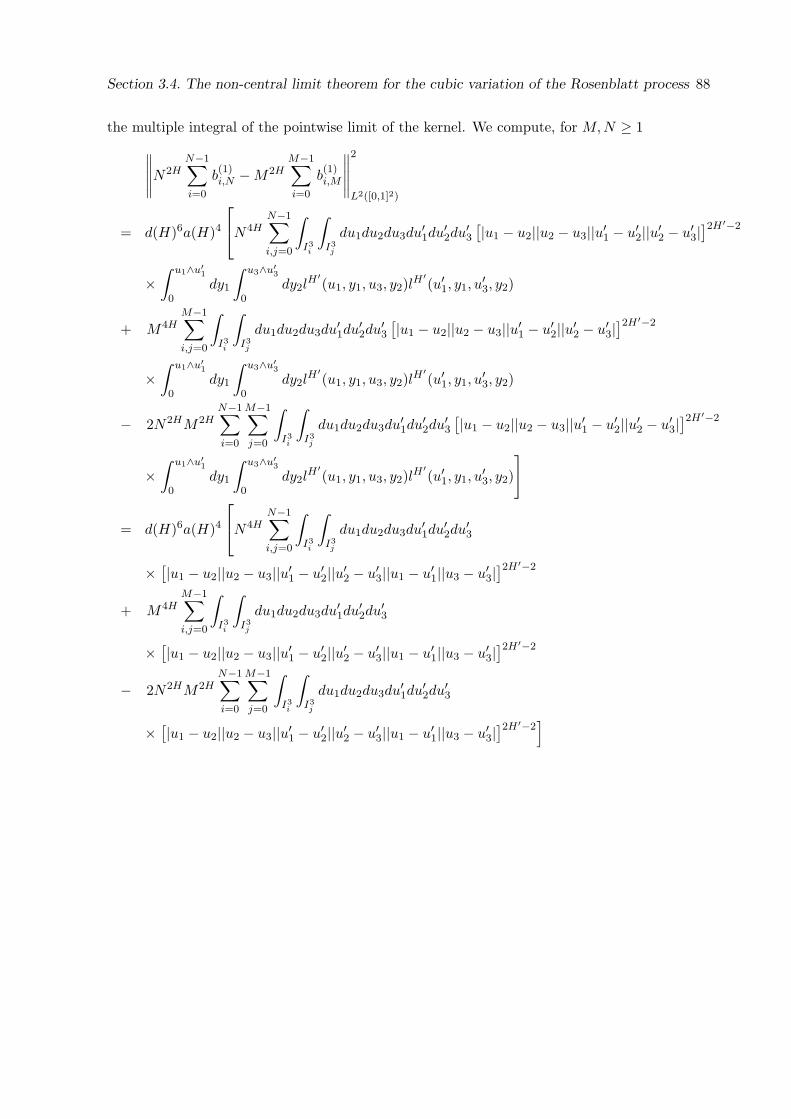
Section 3.4. The non-central limit theorem for the cubic variation of the Rosenblatt process 88
the multiple integral of the pointwise limit of the kernel. We compute, for M, N ≥ 1
∥∥∥∥∥N2HN−1∑
i=0
b(1)i,N −M2H
M−1∑
i=0
b(1)i,M
∥∥∥∥∥
2
L2([0,1]2)
= d(H)6a(H)4
N4H
N−1∑
i,j=0
∫
I3i
∫
I3j
du1du2du3du′1du′2du′3[|u1 − u2||u2 − u3||u′1 − u′2||u′2 − u′3|
]2H′−2
×∫ u1∧u′1
0dy1
∫ u3∧u′3
0dy2l
H′(u1, y1, u3, y2)lH
′(u′1, y1, u
′3, y2)
+ M4HM−1∑
i,j=0
∫
I3i
∫
I3j
du1du2du3du′1du′2du′3[|u1 − u2||u2 − u3||u′1 − u′2||u′2 − u′3|
]2H′−2
×∫ u1∧u′1
0dy1
∫ u3∧u′3
0dy2l
H′(u1, y1, u3, y2)lH
′(u′1, y1, u
′3, y2)
− 2N2HM2HN−1∑
i=0
M−1∑
j=0
∫
I3i
∫
I3j
du1du2du3du′1du′2du′3[|u1 − u2||u2 − u3||u′1 − u′2||u′2 − u′3|
]2H′−2
×∫ u1∧u′1
0dy1
∫ u3∧u′3
0dy2l
H′(u1, y1, u3, y2)lH
′(u′1, y1, u
′3, y2)
]
= d(H)6a(H)4
N4H
N−1∑
i,j=0
∫
I3i
∫
I3j
du1du2du3du′1du′2du′3
× [|u1 − u2||u2 − u3||u′1 − u′2||u′2 − u′3||u1 − u′1||u3 − u′3|]2H′−2
+ M4HM−1∑
i,j=0
∫
I3i
∫
I3j
du1du2du3du′1du′2du′3
× [|u1 − u2||u2 − u3||u′1 − u′2||u′2 − u′3||u1 − u′1||u3 − u′3|]2H′−2
− 2N2HM2HN−1∑
i=0
M−1∑
j=0
∫
I3i
∫
I3j
du1du2du3du′1du′2du′3
× [|u1 − u2||u2 − u3||u′1 − u′2||u′2 − u′3||u1 − u′1||u3 − u′3|]2H′−2
]
Section 3.4. The non-central limit theorem for the cubic variation of the Rosenblatt process 89
and this equal to
d(H)6a(H)4
N−2H
N−1∑
i,j=0
∫
[0,1]6du1du2du3du′1du′2du′3
× [|v1 − v2||v2 − v3||v′1 − v′2||v′2 − v′3||v1 − v′1 + i− j||v3 − v′3 + i− j|]2H′−2
+ M−2HM−1∑
i,j=0
∫
[0,1]6du1du2du3du′1du′2du′3
× [|v1 − v2||v2 − v3||v′1 − v′2||v′2 − v′3||v1 − v′1 + i− j||v3 − v′3 + i− j|]2H′−2
− 2N−1M−1N−1∑
i=0
M−1∑
j=0
∫
[0,1]6du1du2du3du′1du′2du′3
×[|v1 − v2||v2 − v3||v′1 − v′2||v′2 − v′3||
v1
N− v′1
M+
i
N− j
M||v3
N− v′3
M+
i
N− j
M|]2H′−2
]
The same way as in above this las term when N −→∞ and N −→∞ converges to
d(H)6a(H)4[2
∫ 1
0(1− x)x2H−2dx + 2
∫ 1
0(1− x)x2H−2dy + 2
∫ 1
0
∫ 1
0|x− y|2H−2dxdy
]
=1
H(2H − 1)+
1H(2H − 1)
− 2H(2H − 1)
= 0.
We obtained that N2H∑N−1
i=0 b(1)i,N , N ≥ 0 is a Cauchy sequence and this completes the proof.
Chapter 4
Estimation of the drift of fractional
Brownian motion
We consider the problem of efficient estimation for the drift of fractional Brownian motionBH :=
(BH
t
)t∈[0,T ]
with hurst parameter H less than 12 . We also construct superefficient James-
Stein type estimators which dominate, under the usual quadratic risk, the natural maximumlikelihood estimator.
4.1 Introduction
Fix H ∈ (0, 1) and T > 0. Let BH =
(BH,1t , ..., BH,d
t ); t ∈ [0, T ]
be a d-dimensional fractional
Brownian motion (fBm) defined on the probability space (Ω,F , P ). That is, BH is a zeromean Gaussian vector whose components are independent one-dimensional fractional Brownianmotions with Hurst parameter H ∈ (0, 1), i.e., for every i = 1, ..., d BH,i is a Gaussian processand covariance function given by
E(BH,is BH,i
t ) =12
(s2H + t2H − |t− s|2H
), s, t ∈ [0, T ].
For each i = 1, . . . , d,(F i
t
)t∈[0,T ]
denotes the filtration generated by(BH,i
t
)t∈[0,T ]
.
The fBm was first introduced by Kolmogorov [60] and studied by Mandelbrot and Van Ness in[71]. Notice that if H = 1
2 , the process B12 is a standard Brownian motion. However, for H 6= 1
2 ,the fBm is neither a Markov process, nor a semi-martingale.
Let M be a subspace of the Cameron-Martin space defined by
M =
ϕ : [0, T ] → Rd; ϕit =
∫ t
0ϕi
sds with ϕi ∈ L2([0, T ])
and ϕi ∈ IH+ 1
2
0+
(L2([0, T ])
), i = 1, ..., d
.
Let θ =(θ1
t , . . . , θdt ); t ∈ [0, T ]
be a function belonging to M . Then, Applying Girsanov
theorem (see Theorem 2 in [84]), there exist a probability measure absolutely continuous withrespect to P under which the process BH defined by
90
Section 4.1. Introduction 91
BHt = BH
t − θt, t ∈ [0, T ] (4.1)
is a fBm with Hurst parameter H and mean zero. In this case, we say that, under the probabilityPθ, the process BH is a fBm with drift θ.
We consider in this paper the problem of estimating the drift θ of BH under the probabilityPθ, with hurst parameter H < 1/2. We wish to estimate θ under the usual quadratic risk, thatis defined for any estimator δ of θ by
R(θ, δ) = Eθ
[∫ T
0||δt − θt||2dt
]
where Eθ is the expectation with respect to a probability Pθ.Let X = (X1, . . . , Xd) be a normal vector with mean θ = (θ1, . . . , θd) ∈ Rd and identity
covariance matrix σ2Id. The usual maximum likelihood estimator of θ is X itself. Moreover, itis efficient in the sense that the Cramer-Rao bound over all unbiased estimators is attained byX. That is
σ2d = E[‖X − θ‖2
d
]= inf
ξ∈SE
[‖ξ − θ‖2d
],
where S is the class of unbiased estimators of θ and ‖.‖d denotes the Euclidean norm on Rd.Stein [107] constructed biased superefficient estimators of θ of the form
δa,b(X) =(
1− b
a + ||X||2)
X
for a sufficiently small and b sufficiently large when d ≥ 3. James and Stein [57] sharpened laterthis result and presented an explicit class of biased superefficient estimators of the form
(1− a
||X||2d
)X, for 0 < a < 2(d− 2).
Recently, an infinite-dimensional extension of this result has been given by Privault andReveillac in [96]. The authors constructed unbiased estimators of the drift (θt)t∈[0,T ] of a con-tinuous Gaussian martingale (Xt)t∈[0,T ] with quadratic variation σ2
t dt, where σ ∈ L2([0, T ], dt)is an a.e. non-vanishing function. More precisely, they proved that θ = (Xt)t∈[0,T ] is an ef-ficient estimator of (θt)t∈[0,T ]. On the other hand, using Malliavin calculus, they constructedsuperefficient estimators for the drift of a Gaussian processe of the form:
Xt :=∫ t
0K(t, s)dWs, t ∈ [0, T ],
where (Wt)t∈[0,T ] is a standard Brownian motion and K(., .) is a deterministic kernel. Theseestimators are biased and of the form Xt+Dt log F , where F is a positive superharmonic randomvariable and D is the Malliavin derivative.
In Section 3, we prove, using technic based on the fractional calculus and Girsanov theorem,that θ = BH is an efficient estimator of θ under the probability Pθ with risk
R(θ, BH) = Eθ
[∫ T
0‖BH
t − θt‖2dt
]=
T 2H+1
2H + 1d.
Section 4.2. Preliminaries 92
Moreover, we will establish that θ = BH is a maximum likelihood estimator of θ.In Section 4, we construct a class of biased estimators of James-Stein type of the form
δ(BH)t =(
1− at2H
(r(‖BH
t ‖2)‖BH
t ‖2
))BH
t , t ∈ [0, T ].
We give sufficient conditions on the function r and on the constant a in order that δ(BH)dominates BH under the usual quadratic risk i.e.
R (θ, δ
(BH
))< R (
θ,BH)
for all θ ∈ M. (4.2)
4.2 Preliminaries
This section contains the elements from fractional calculus that we will need in the paper.The fractional Brownian motion BH has the following stochastic integral representation (see forinstance, [1], [82])
BH,it =
∫ t
0KH(t, s)dW i
s , i = 1, ..., d; t ∈ [0, T ] (4.3)
where W = (W 1, ..., W d) denotes the d-dimensional Brownian motion and the kernel KH(t, s)is equal to
cH(t− s)H− 12 + cH(
12−H)
∫ t
s(u− s)H− 3
2
(1− (
s
u)
12−H
)du if H ≤ 1
2
cH(H − 12)∫ t
s(u− s)H− 3
2
( s
u
)H− 12du if H >
12,
if s < t and KH(t, s) = 0 if s ≥ t. Here cH is the normalizing constant
cH =
√2HΓ(3
2 −H)Γ(H + 1
2)Γ(2− 2H)
where Γ is the Euler function.We recall some basic definitions and results on classical fractional calculus which we will need.General information about fractional calculus can be found in [97].The left fractional Riemann-Liouville integral of f ∈ L1((a, b)) of order α > 0 on (a, b) is givenat almost all x ∈ (a, b) by
Iαa+f(x) =
1Γ(α)
∫ x
a(x− y)α−1f(y)dy.
If f ∈ Iαa+(Lp(a, b)) with 0 < α < 1 and p > 1 then the left-sided Riemann-Liouville derivative
of f of order α defined by
Dαa+f(x) =
1Γ(1− α)
(f(x)
(x− a)α+ α
∫ x
a
f(x)− f(y)(x− y)α+1
dy
)
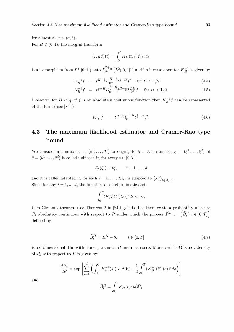
Section 4.3. The maximum likelihood estimator and Cramer-Rao type bound 93
for almost all x ∈ (a, b).For H ∈ (0, 1), the integral transform
(KHf)(t) =∫ t
0KH(t, s)f(s)ds
is a isomorphism from L2([0, 1]) onto IH+ 1
2
0+
(L2([0, 1])
)and its inverse operator K−1
H is given by
K−1H f = tH−
12 D
H− 12
0+ t12−Hf ′ for H > 1/2, (4.4)
K−1H f = t
12−HD
12−H
0+ tH−12 D2H
0+ f for H < 1/2. (4.5)
Moreover, for H < 12 , if f is an absolutely continuous function then K−1
H f can be representedof the form ( see [84] )
K−1H f = tH−
12 I
12−H
0+ t12−Hf ′. (4.6)
4.3 The maximum likelihood estimator and Cramer-Rao type
bound
We consider a function θ =(θ1, . . . , θd
)belonging to M . An estimator ξ = (ξ1, . . . , ξd) of
θ = (θ1, . . . , θd) is called unbiased if, for every t ∈ [0, T ]
Eθ(ξit) = θi
t, i = 1, . . . , d
and it is called adapted if, for each i = 1, . . . , d, ξi is adapted to(F i
t
)t∈[0,T ]
.Since for any i = 1, ..., d, the function θi is deterministic and
∫ T
0(K−1
H (θi)(s))2ds < ∞,
then Girsanov theorem (see Theorem 2 in [84]), yields that there exists a probability measurePθ absolutely continuous with respect to P under which the process BH :=
(BH
t ; t ∈ [0, T ])
defined by
BHt = BH
t − θt, t ∈ [0, T ] (4.7)
is a d-dimensional fBm with Hurst parameter H and mean zero. Moreover the Girsanov densityof Pθ with respect to P is given by:
dPθ
dP= exp
[d∑
i=1
(∫ T
0K−1
H (θi)(s)dW is −
12
∫ T
0(K−1
H (θi)(s))2ds
)]
and
BHt =
∫ t
0KH(t, s)dWs
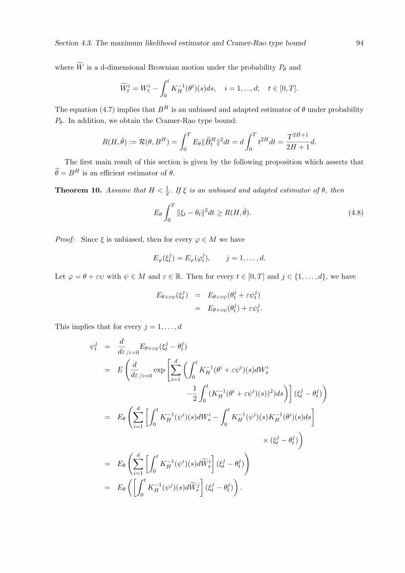
Section 4.3. The maximum likelihood estimator and Cramer-Rao type bound 94
where W is a d-dimensional Brownian motion under the probability Pθ and
W it = W i
t −∫ t
0K−1
H (θi)(s)ds, i = 1, ..., d; t ∈ [0, T ].
The equation (4.7) implies that BH is an unbiased and adapted estimator of θ under probabilityPθ. In addition, we obtain the Cramer-Rao type bound:
R(H, θ) := R(θ, BH) =∫ T
0Eθ‖BH
t ‖2dt = d
∫ T
0t2Hdt =
T 2H+1
2H + 1d.
The first main result of this section is given by the following proposition which asserts thatθ = BH is an efficient estimator of θ.
Theorem 10. Assume that H < 12 . If ξ is an unbiased and adapted estimator of θ, then
Eθ
∫ T
0‖ξt − θt‖2dt ≥ R(H, θ). (4.8)
Proof: Since ξ is unbiased, then for every ϕ ∈ M we have
Eϕ(ξjt ) = Eϕ(ϕj
t ), j = 1, . . . , d.
Let ϕ = θ + εψ with ψ ∈ M and ε ∈ R. Then for every t ∈ [0, T ] and j ∈ 1, . . . , d, we have
Eθ+εψ(ξjt ) = Eθ+εψ(θj
t + εψjt )
= Eθ+εψ(θjt ) + εψj
t .
This implies that for every j = 1, . . . , d
ψjt =
d
dε/ε=0Eθ+εψ(ξj
t − θjt )
= E
(d
dε/ε=0exp
[d∑
i=1
(∫ t
0K−1
H (θi + εψi)(s)dW is
−12
∫ t
0(K−1
H (θi + εψi)(s))2)ds
)](ξj
t − θjt )
)
= Eθ
(d∑
i=1
[∫ t
0K−1
H (ψi)(s)dW is −
∫ t
0K−1
H (ψi)(s)K−1H (θi)(s)ds
]
× (ξjt − θj
t ))
= Eθ
(d∑
i=1
[∫ t
0K−1
H (ψi)(s)dW is
](ξj
t − θjt )
)
= Eθ
([∫ t
0K−1
H (ψj)(s)dW js
](ξj
t − θjt )
).
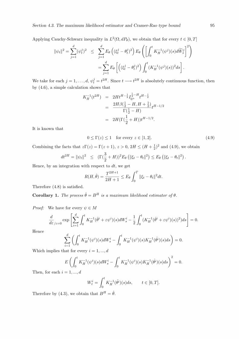
Section 4.3. The maximum likelihood estimator and Cramer-Rao type bound 95
Applying Cauchy-Schwarz inequality in L2(Ω, dPθ), we obtain that for every t ∈ [0, T ]
‖ψt‖2 =d∑
j=1
(ψjt )
2 ≤d∑
j=1
Eθ
((ξj
t − θjt )
2)
Eθ
([∫ t
0K−1
H (ψj)(s)dW js
]2)
=d∑
j=1
Eθ
[((ξj
t − θjt )
2)∫ t
0(K−1
H (ψj)(s))2ds
].
We take for each j = 1, . . . , d, ψjt = t2H . Since t −→ t2H is absolutely continuous function, then
by (4.6), a simple calculation shows that
K−1H (t2H) = 2HtH−
12 I
12−H
0+ tH−12
=2Hβ(1
2 −H, H + 12)
Γ(12 −H)
tH−1/2
= 2H(Γ(12
+ H))tH−1/2.
It is known that
0 ≤ Γ(z) ≤ 1 for every z ∈ [1, 2]. (4.9)
Combining the facts that zΓ(z) = Γ(z + 1), z > 0, 2H ≤ (H + 12)2 and (4.9), we obtain
dt2H = ‖ψt‖2 ≤ (Γ(32
+ H))2Eθ
(‖ξt − θt‖2) ≤ Eθ
(‖ξt − θt‖2).
Hence, by an integration with respect to dt, we get
R(H, θ) =T 2H+1
2H + 1≤ Eθ
∫ T
0‖ξt − θt‖2dt.
Therefore (4.8) is satisfied.
Corollary 1. The process θ = BH is a maximum likelihood estimator of θ.
Proof: We have for every ψ ∈ M
d
dε/ε=0exp
[d∑
i=1
∫ t
0K−1
H (θi + εψi)(s)dW is −
12
∫ t
0(K−1
H (θi + εψi)(s))2)ds
]= 0.
Henced∑
i=1
(∫ t
0K−1
H (ψi)(s)dW is −
∫ t
0K−1
H (ψi)(s)K−1H (θi)(s)ds
)= 0.
Which implies that for every i = 1, ..., d
E
(∫ t
0K−1
H (ψi)(s)dW is −
∫ t
0K−1
H (ψi)(s)K−1H (θi)(s)ds
)2
= 0.
Then, for each i = 1, ..., d
W it =
∫ t
0K−1
H (θi)(s)ds, t ∈ [0, T ].
Therefore by (4.3), we obtain that BH = θ.
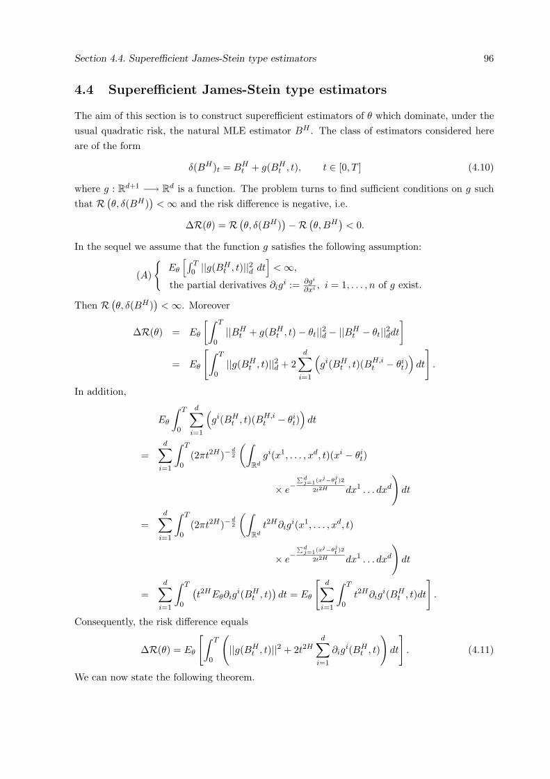
Section 4.4. Superefficient James-Stein type estimators 96
4.4 Superefficient James-Stein type estimators
The aim of this section is to construct superefficient estimators of θ which dominate, under theusual quadratic risk, the natural MLE estimator BH . The class of estimators considered hereare of the form
δ(BH)t = BHt + g(BH
t , t), t ∈ [0, T ] (4.10)
where g : Rd+1 −→ Rd is a function. The problem turns to find sufficient conditions on g suchthat R (
θ, δ(BH))
< ∞ and the risk difference is negative, i.e.
∆R(θ) = R (θ, δ(BH)
)−R (θ,BH
)< 0.
In the sequel we assume that the function g satisfies the following assumption:
(A)
Eθ
[∫ T0 ||g(BH
t , t)||2d dt]
< ∞,
the partial derivatives ∂igi := ∂gi
∂xi , i = 1, . . . , n of g exist.
Then R (θ, δ(BH)
)< ∞. Moreover
∆R(θ) = Eθ
[∫ T
0||BH
t + g(BHt , t)− θt||2d − ||BH
t − θt||2ddt
]
= Eθ
[∫ T
0||g(BH
t , t)||2d + 2d∑
i=1
(gi(BH
t , t)(BH,it − θi
t))
dt
].
In addition,
Eθ
∫ T
0
d∑
i=1
(gi(BH
t , t)(BH,it − θi
t))
dt
=d∑
i=1
∫ T
0(2πt2H)−
d2
(∫
Rd
gi(x1, . . . , xd, t)(xi − θit)
× e−
∑dj=1(xj−θ
jt )2
2t2H dx1 . . . dxd
)dt
=d∑
i=1
∫ T
0(2πt2H)−
d2
(∫
Rd
t2H∂igi(x1, . . . , xd, t)
× e−
∑dj=1(xj−θ
jt )2
2t2H dx1 . . . dxd
)dt
=d∑
i=1
∫ T
0
(t2HEθ∂ig
i(BHt , t)
)dt = Eθ
[d∑
i=1
∫ T
0t2H∂ig
i(BHt , t)dt
].
Consequently, the risk difference equals
∆R(θ) = Eθ
[∫ T
0
(||g(BH
t , t)||2 + 2t2Hd∑
i=1
∂igi(BH
t , t)
)dt
]. (4.11)
We can now state the following theorem.
Section 4.4. Superefficient James-Stein type estimators 97
Theorem 11. Let g : Rd+1 −→ Rd be a function satisfying (A). A sufficient conditions forthe estimator
(BH
t + g(BHt , t)
)t∈[0,T ]
to dominate BH under the usual quadratic risk which isequivalent that
Eθ
[∫ T
0
(||g(BH
t , t)||2 + 2t2Hd∑
i=1
∂igi(BH
t , t)
)dt
]< 0.
As an application, take g of the form
g(x, t) = at2H r(‖x‖2
)
‖x‖2x, (4.12)
where a is a constant strictly positive and r : R+ → R+ is bounded derivable function.The next lemma give a sufficient condition for g in (4.12) to satisfies the assumption (A).
Lemma 5. If d ≥ 3 and H < 12 then
E
[∫ T
0
1‖BH
t ‖2dt
]< ∞. (4.13)
Proof: Firstly the integral given by (4.13) is well defined, because
(dt× P )((t, w);BH
t (w) = 0)
= 0
where (dt× P ) is the product measure.Using the change of variable and d ≥ 3 we see that
E
∫ T
0
1‖BH
t ‖2dt =
∫ T
0
dt
t2H
∫
Rd
e−‖y‖2
2√2π‖y‖2
dy ≤ C
∫ T
0
1t2H
dt,
where C is a constant depending only on d. Furthermore, since H < 12 then (4.13) holds.
Theorem 12. Assume that d ≥ 3. If the function r, the constant a and the parameter H satisfy:
i) 0 ≤ r(.) ≤ 1
ii) r(·) is differentiable and increasing
iii) 0 < a ≤ 2(d− 2) and H < 1/2,
then the estimator
δ(BH) = BHt − at2H r
(‖BHt ‖2
)
‖BHt ‖2
BHt , t ∈ [0, T ].
dominates BH .
Section 4.4. Superefficient James-Stein type estimators 98
Proof: It suffices to prove that ∆R(θ) < 0. From (4.11) and the hypothesis i) and ii) we canwrite
∆R(θ) = aEθ
[∫ T
0t4H
(ar2(‖BH
t ‖2)‖BH
t ‖2− 2(d− 2)
r(‖BHt ‖2)
‖BHt ‖2
− 4r′(‖BHt ‖2)
)dt
]
≤ a [a− 2(d− 2)]Eθ
[a
∫ T
0t4H r(‖BH
t ‖2)‖BH
t ‖2
].
Combining this fact with the assumption iii) yields that the risk difference is negative. Whichproves the desired result.
For r = 1, we obtain a James-Stein type estimator:
Corollary 2. Let d ≥ 3, 0 < H < 12 and 0 < a ≤ 2(d− 2). Then the estimator
(1− at2H
‖BHt ‖2
)BH
t , t ∈ [0, T ]
dominates BH .
Part III
CONTRIBUTIONS TO THE
STUDY OF LEVY PROCESSES
99

100
Chapter 5
Levy processes and Ito-Skorohod
integrals
We study Skorohod integral processes on Levy spaces and we prove an equivalence between thisclass of processes and the class of Ito-Skorohod process (in the sense of [109]).
5.1 Introduction
We study in this work anticipating integrals with respect to a Levy process. The anticipatingintegral on the Wiener space, known in general as the Skorohod integral (and sometimes as theHitsuda integral) constitutes an extension of the standard Ito integral to non-adapted integrands.It is nothing else than the classical Ito integral if the integrand is adapted. The Skorohod integralhas been extended to the Poisson process and next it has been defined with respect to a normalmartingale (see [29]) due to the Fock space structure generates by such processes. Recently, ananticipating calculus of Malliavin-type has been defined on Levy spaces again by using somemultiple stochastic integral with respect to a Levy process which have been in essence definedin the old paper by K. Ito (see [55]). We refer to [30], [31] or [106] for Malliavin calculus onLevy spaces and possible applications to mathematical finance.
The purpose of this paper is to understand the relation between anticipating Skorohod integralprocesses and Ito-Skorohod integral process (in the sense of [109] or [93]) in the Levy case. Werecall that the results in [109] and [93] show that on Wiener and Poisson spaces the class ofSkorohod integral process with regular integrals coincides with the class of some Ito-Skorohodintegrals that have similarities to the classical Ito integrals for semimartingales. The fact thatthe driven processes have independent increments plays an crucial role. Therefore, it is expectedto obtain the same type of results for Levy processes. We prove here such an equivalent betweenSkorohod and Ito-Skorohod integrals by using a recent Malliavin calculus for Levy processes.
Section 2 contains some preliminaries on Levy processes and Malliavin-Skorohod calculus forthem. In Section 3 we prove a generalized Clark-Ocone formula that we will use in Section 4to prove the correspondence between Skorohod and Ito-Skorohod integrals and to develop an
101
Section 5.2. Preliminaries 102
Ito-type calculus for anticipating integrals on Levy spaces.
5.2 Preliminaries
In this section we introduce the basic properties of Malliavin calculus for Levy processes usedin this paper. For more details the reader is referred to [106].
In this paper we deal with a cadlag Levy process X = (Xt)0≤t≤1 defined on a certain completeprobability space
(Ω, (FX
t )0≤t≤1, P), with the time horizon T = [0, 1], and equipped with its
generating triplet (γ, σ2, ν) where γ ∈ R, σ ≥ 0 and ν(dz) is the Levy measure on R which, werecall, is such that ν(0) = 0 and
∫
R1 ∧ x2ν(dx) < ∞
Throughout the paper, we suppose that∫R x2ν(dx) < ∞, and we use the notation and termi-
nologies of [3], [106]. By N we will denote the jump measure of X:
N(E) = #t : (t, ∆Xt) ∈ E,
for E ∈ B(T × R0) , where R0 = R − 0, ∆Xt = Xt −Xt− , and # denotes the cardinal. Wewill note N the compensated jump measure:
N(dt, dx) = N(dt, dx)− dtν(dx).
The process X admits a Levy-Ito representation
Xt = γt + σWt +∫ ∫
(0,t]×|x|>1xN(ds, dx) + lim
ε↓0
∫ ∫
(0,t]×ε<|x|≤1xN(ds, dx)
where W is a standard Brownian motion.Define
µ(E) = σ2
∫
E(0)ds +
∫ ∫
E−E(0)×0x2dsν(dx).
Ito [55] proved that X can be extended to a martingale-valued measure M of type (2, µ) on(T ×R, B(T × R)) : For any E ∈ B(T × R) with µ(E) < ∞
M(E) = σ
∫
E(0)dWs + lim
n→∞
∫ ∫
(s,x)∈E: 1n
<|x|<nxN(ds, dx).
where E(0) = s ∈ T : (s, 0) ∈ E.Furthermore, M is a centered independent random measure such that
E (M(E1)M(E2)) = µ(E1 ∩ E2)
for any E1, E2 ∈ B(T × R) with µ(E1) < ∞ and µ(E2) < ∞.
Section 5.2. Preliminaries 103
Using the random measure M one can construct multiple stochastic integrals driven by aLevy process as an isometry between L2(Ω) and the space L2 ((T ×R)n, B((T ×R)n), µ⊗n).Indeed, one can use the same steps as on the Wiener space: first, consider a simple function f
of the formf = 1E1×...×En
where E1, . . . , En ∈ B(T × R) are pathwise disjoint and µ(Ei) < ∞ for every i. For such afunction, define In(f) = M(E1) . . .M(En) and then the operator In can be extended by linearityand continuity to an isometry between L2(Ω) and the space L2 ((T × R)n, B((T × R)n), µ⊗n).
An interesting fact is that, as in the Brownian and Poissonian cases, M enjoys the chaoticrepresentation property (see [106]), i.e. every F ∈ L2(Ω, FX , P ) = L2(Ω), can be written as anorthogonal sum of multiple stochastic integrals
F = E(F ) +∞∑
n=1
In(fn)
where the convergence holds L2(Ω) and fn ∈ L2s ((T × R)n, B((T × R)n), µ⊗n) (the last space is
the space of symmetric and square integrable functions on (T × R)n with respect to µ⊗n).At this point we can introduce a Malliavin calculus with respect to the Levy process X by
using this Fock space-type structure. If
∞∑
n=0
nn!‖fn‖2n < ∞ (5.1)
(here ‖fn‖n denotes the norm in the space L2 ((T ×R)n, B((T ×R)n), µ⊗n)) then the Malliavinderivative of F is introduced as an annihilation operator (see for example [85])
DzF =∞∑
n=1
nIn−1(fn(z, .)), z ∈ T × R.
The domain of the operator D is denoted by D1,2. It is exactly the set of random variablesverifying (5.1). We denote by Dk,2, k ≥ 1 the domain of the kth iterated derivative D(k), whichis a Hilbert space with respect the scalar product
〈F, G〉 = E(FG) +k∑
j=1
E
∫
(T×R)j
D(j)z FD(j)
z Gµ(dz).
We introduce now the Skorohod integral with respect to X as a creation operator. Letu ∈ H = L2
(T ×R× Ω, B(T × R)⊗ FX
T , µ⊗ P), then, for every z ∈ T × R, u(z) admit the
following representation
u(z) =∞∑
n=0
In(fn(z, .)).
Here we have fn ∈ L2((T × R)n+1, µ⊗n+1) and fn is symmetric in the last n variables. If
Section 5.3. Generalized Clark-Ocone formula 104
∞∑
n=0
(n + 1)!‖fn‖2n+1 < ∞ (5.2)
(fn represents the symmetrization of fn in all its n + 1 variables) then the Skorohod integralδ(u) of u with respect to X is introduced by
δ(u) =∞∑
n=0
In+1(fn).
The domain of δ is the set of processes satisfying (5.2) and we have the duality relationship
E(Fδ(u)) = E
∫ ∫
T×RDzFu(z)µ(dz), F ∈ D1,2.
We will use the notation
δ(u) =∫ 1
0
∫
RuzδM(dz) =
∫ 1
0
∫
Rus,xδM(ds, dx).
Remark 5. It has been proved in [106] that if the integrand is predictable then the Skorohodintegral coincides with the standard semi-martingale integral introduced in [3].
For k ≥ 1, we denote by Lk,2 the set L2((T × R;Dk,2), µ). In particular one can prove thatL1,2 is given by the set of u in the above chaotic form such that (5.2) satisfied.We also have Lk,2 ⊂ Domδ for k ≥ 1 and and for every u, v ∈ L1,2
E(δ(u)δ(v)) = E
∫ ∫
T×Ru(z)v(z)µ(dz) + E
∫ ∫
(T×R)2Dzu(z′)Dz′v(z)µ(dz)µ(dz′).
In particular
E(δ(u))2 = E
∫ ∫
T×Ru(z)2µ(dz) + E
∫ ∫
(T×R)2Dzu(z′)Dz′u(z)µ(dz)µ(dz′).
The commutativity relationship between the derivative operator and Skorohod integral is givenby: let u ∈ L1,2 such that Dzu ∈ Dom(δ), then δ(u) ∈ D1,2 and
Dzδ(u) = u(z) + δ(Dz(u)), z ∈ T ×R.
5.3 Generalized Clark-Ocone formula
We start this section by proving some properties of the multiple integrals In(f) and how itbehaves if it is conditioned by a σ-algebra. If A ∈ B(T ) we will denote by FX
A the σ-algebragenerated by the increments of the process X on the set A
FXA = σ(Xt −Xs : s, t ∈ A).
Section 5.3. Generalized Clark-Ocone formula 105
Proposition 6. Let f ∈ L2s((T × R)n, µ⊗n
) and A ∈ B(T ). Then
E(In(f)/FX
A
)= In(f1⊗
n
(A×R)).
Proof: By density and linearity argument, it is enough to consider f = 1E1×...×En , whereE1, ..., En are pairwise disjoint set of B (T ×R) and µ(Ei) < ∞ for every i = 1, ..., n. In thiscase we have
E(In(f)/FX
A
)= E
(M(E1)....M(En)/FX
A
)
= E
(n∏
i=1
(M(Ei ∩ (A× R)) + M(Ei ∩ (Ac × R))) /FXA
)
=n∏
i=1
M(Ei ∩ (A× R)) = In(f1⊗n
(A×R)).
And an immediate consequence, we have
Corollary 3. Suppose that F ∈ D1,2 and A ∈ B(T ). Then the conditional expectation E(F/FXA )
belongs to D1,2 and for every z ∈ T × R
DzE(F/FX
A
)= E
(DzF/FX
A
)1A×R(z).
Proof: let F have the form∑
n≥0 In(fn) with fn ∈ L2s ((T × R)n, B((T × R)n), µ⊗n). Then, by
Proposition 8,
DzE(F/FX
A
)= Dz
∑
n≥0
In
(fn1⊗n
A×R)
=∑
n≥1
nIn−1
(fn(·, z)1⊗(n−1)
A×R)
1A×R(z)
and it remains to observe that E(DzF/FX
A
)=
∑n≥1 nIn−1
(fn(·, z)1⊗(n−1)
A×R).
At this point we can state the following version of Clark-Ocone formula on Levy space. Thisextends a results in [106].
Proposition 7 (Generalized Clark-Ocone formula). Let F be a random variable in D1,2. Then,for every 0 ≤ s < t ≤ 1, we have
F = E(F/FX
(s,t]c
)+ δ(hs,t(·))
where for (r, x) ∈ T ×R we denoted by hs,t(r, x) = E(Dr,xF/F(r,t]c
)1(s,t]c(r).Moreover
F = E(F/FX
(s,t]c
)+
∫ ∫
(s,t]×R(p,t)(DzF ) dMz
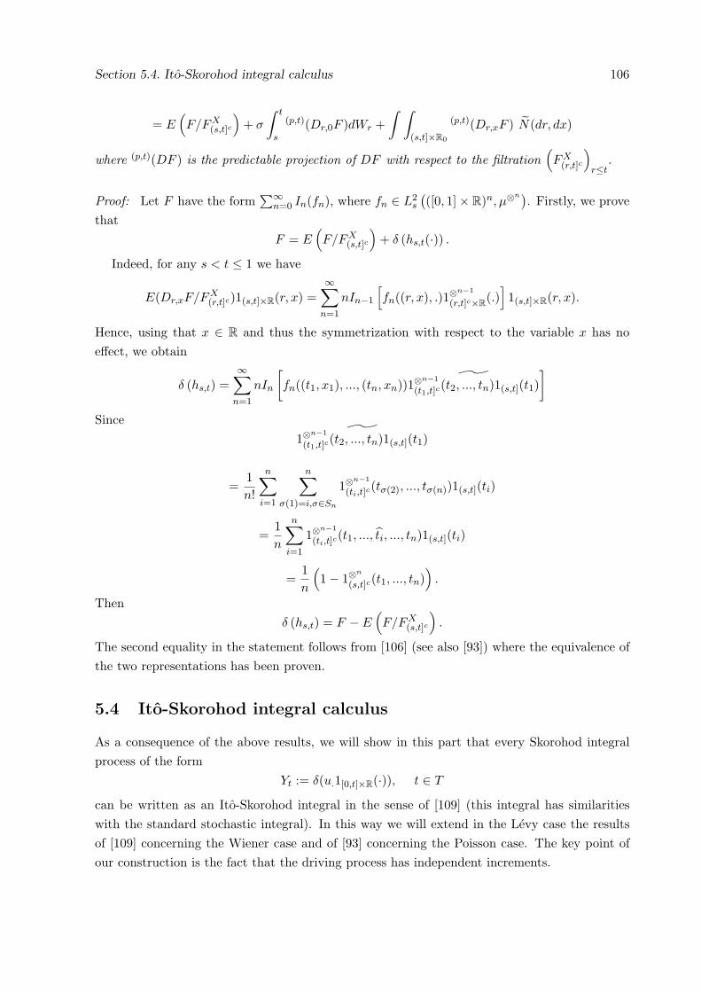
Section 5.4. Ito-Skorohod integral calculus 106
= E(F/FX
(s,t]c
)+ σ
∫ t
s
(p,t)(Dr,0F )dWr +∫ ∫
(s,t]×R0
(p,t)(Dr,xF ) N(dr, dx)
where (p,t)(DF ) is the predictable projection of DF with respect to the filtration(FX
(r,t]c
)r≤t
.
Proof: Let F have the form∑∞
n=0 In(fn), where fn ∈ L2s
(([0, 1]× R)n, µ⊗n)
. Firstly, we provethat
F = E(F/FX
(s,t]c
)+ δ (hs,t(·)) .
Indeed, for any s < t ≤ 1 we have
E(Dr,xF/FX(r,t]c)1(s,t]×R(r, x) =
∞∑
n=1
nIn−1
[fn((r, x), .)1⊗
n−1
(r,t]c×R(.)]1(s,t]×R(r, x).
Hence, using that x ∈ R and thus the symmetrization with respect to the variable x has noeffect, we obtain
δ (hs,t) =∞∑
n=1
nIn
[fn((t1, x1), ..., (tn, xn)) ˜1⊗
n−1
(t1,t]c(t2, ..., tn)1(s,t](t1)]
Since˜1⊗
n−1
(t1,t]c(t2, ..., tn)1(s,t](t1)
=1n!
n∑
i=1
n∑
σ(1)=i,σ∈Sn
1⊗n−1
(ti,t]c(tσ(2), ..., tσ(n))1(s,t](ti)
=1n
n∑
i=1
1⊗n−1
(ti,t]c(t1, ..., ti, ..., tn)1(s,t](ti)
=1n
(1− 1⊗
n
(s,t]c(t1, ..., tn))
.
Thenδ (hs,t) = F − E
(F/FX
(s,t]c
).
The second equality in the statement follows from [106] (see also [93]) where the equivalence ofthe two representations has been proven.
5.4 Ito-Skorohod integral calculus
As a consequence of the above results, we will show in this part that every Skorohod integralprocess of the form
Yt := δ(u.1[0,t]×R(·)), t ∈ T
can be written as an Ito-Skorohod integral in the sense of [109] (this integral has similaritieswith the standard stochastic integral). In this way we will extend in the Levy case the resultsof [109] concerning the Wiener case and of [93] concerning the Poisson case. The key point ofour construction is the fact that the driving process has independent increments.
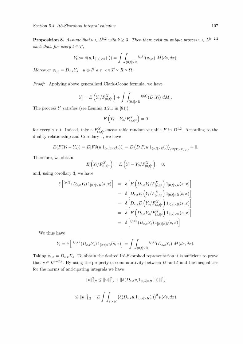
Section 5.4. Ito-Skorohod integral calculus 107
Proposition 8. Assume that u ∈ Lk,2 with k ≥ 3. Then there exist an unique process v ∈ Lk−2,2
such that, for every t ∈ T ,
Yt := δ(u.1[0,t]×R(·)) =∫ ∫
(0,t]×R(p,t)(vs,x) M(ds, dx).
Moreover vs,x = Ds,xYs µ⊗ P a.e. on T ×R× Ω.
Proof: Applying above generalized Clark-Ocone formula, we have
Yt = E(Yt/FX
(0,t]c
)+
∫ ∫
(0,t]×R(p,t)(DzYt) dMz.
The process Y satisfies (see Lemma 3.2.1 in [81])
E(Yt − Ys/FX
(s,t]c
)= 0
for every s < t. Indeed, take a FX(s,t]c-measurable random variable F in D1,2. According to the
duality relationship and Corollary 1, we have
E(F (Yt − Ys)) = E[Fδ(u.1(s,t]×R(.))] = E⟨D.F, u.1(s,t]×R(.)
⟩L2(T×R, µ)
= 0.
Therefore, we obtainE
(Yt/FX
(0,t]c
)= E
(Yt − Y0/FX
(0,t]c
)= 0,
and, using corollary 3, we have
δ[(p,t) (Ds,xYt) 1[0,t]×R(s, x)
]= δ
[E
(Ds,xYt/FX
(s,t]c
)1[0,t]×R(s, x)
]
= δ[Ds,xE
(Yt/FX
(s,t]c
)1[0,t]×R(s, x)
]
= δ[Ds,xE
(Ys/FX
(s,t]c
)1[0,t]×R(s, x)
]
= δ[E
(Ds,xYs/FX
(s,t]c
)1[0,t]×R(s, x)
]
= δ[(p,t) (Ds,xYs) 1[0,t]×R(s, x)
]
We thus have
Yt = δ[
(p,t) (Ds,xYs) 1[0,t]×R(s, x)]
=∫ ∫
(0,t]×R(p,t)(Ds,xYs) M(ds, dx).
Taking vs,x = Ds,xXs. To obtain the desired Ito-Skorohod representation it is sufficient to provethat v ∈ Lk−2,2. By using the property of commutativity between D and δ and the inequalitiesfor the norms of anticipating integrals we have
‖v‖21,2 ≤ ‖u‖2
1,2 + ‖δ(Ds,xu.1[0,s]×R(.))‖21,2
≤ ‖u‖21,2 + E
∫ ∫
T×R
(δ(Ds,xu.1[0,s]×R(.)
)2µ(ds, dx)
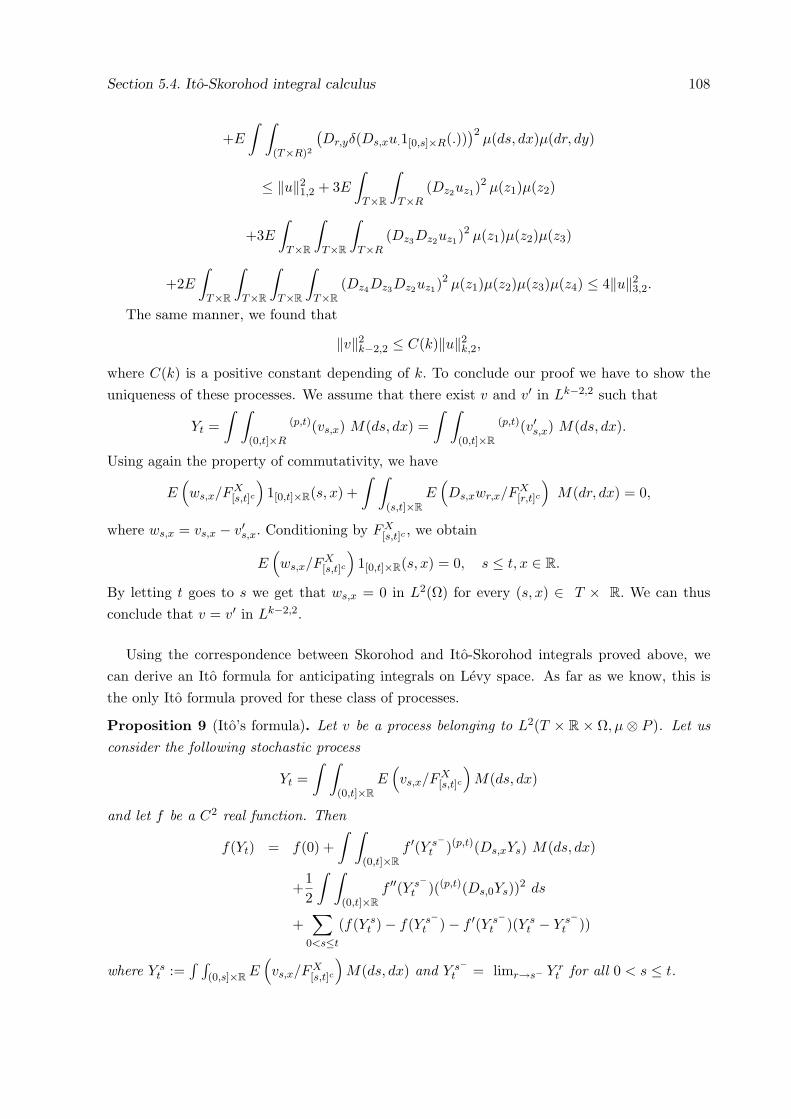
Section 5.4. Ito-Skorohod integral calculus 108
+E
∫ ∫
(T×R)2
(Dr,yδ(Ds,xu.1[0,s]×R(.))
)2µ(ds, dx)µ(dr, dy)
≤ ‖u‖21,2 + 3E
∫
T×R
∫
T×R(Dz2uz1)
2 µ(z1)µ(z2)
+3E
∫
T×R
∫
T×R
∫
T×R(Dz3Dz2uz1)
2 µ(z1)µ(z2)µ(z3)
+2E∫
T×R
∫
T×R
∫
T×R
∫
T×R(Dz4Dz3Dz2uz1)
2 µ(z1)µ(z2)µ(z3)µ(z4) ≤ 4‖u‖23,2.
The same manner, we found that
‖v‖2k−2,2 ≤ C(k)‖u‖2
k,2,
where C(k) is a positive constant depending of k. To conclude our proof we have to show theuniqueness of these processes. We assume that there exist v and v′ in Lk−2,2 such that
Yt =∫ ∫
(0,t]×R
(p,t)(vs,x) M(ds, dx) =∫ ∫
(0,t]×R(p,t)(v′s,x) M(ds, dx).
Using again the property of commutativity, we have
E(ws,x/FX
[s,t]c
)1[0,t]×R(s, x) +
∫ ∫
(s,t]×RE
(Ds,xwr,x/FX
[r,t]c
)M(dr, dx) = 0,
where ws,x = vs,x − v′s,x. Conditioning by FX[s,t]c , we obtain
E(ws,x/FX
[s,t]c
)1[0,t]×R(s, x) = 0, s ≤ t, x ∈ R.
By letting t goes to s we get that ws,x = 0 in L2(Ω) for every (s, x) ∈ T × R. We can thusconclude that v = v′ in Lk−2,2.
Using the correspondence between Skorohod and Ito-Skorohod integrals proved above, wecan derive an Ito formula for anticipating integrals on Levy space. As far as we know, this isthe only Ito formula proved for these class of processes.
Proposition 9 (Ito’s formula). Let v be a process belonging to L2(T × R × Ω, µ ⊗ P ). Let usconsider the following stochastic process
Yt =∫ ∫
(0,t]×RE
(vs,x/FX
[s,t]c
)M(ds, dx)
and let f be a C2 real function. Then
f(Yt) = f(0) +∫ ∫
(0,t]×Rf ′(Y s−
t )(p,t)(Ds,xYs) M(ds, dx)
+12
∫ ∫
(0,t]×Rf ′′(Y s−
t )((p,t)(Ds,0Ys))2 ds
+∑
0<s≤t
(f(Y st )− f(Y s−
t )− f ′(Y s−t )(Y s
t − Y s−t ))
where Y st :=
∫ ∫(0,s]×RE
(vs,x/FX
[s,t]c
)M(ds, dx) and Y s−
t = limr→s− Y rt for all 0 < s ≤ t.
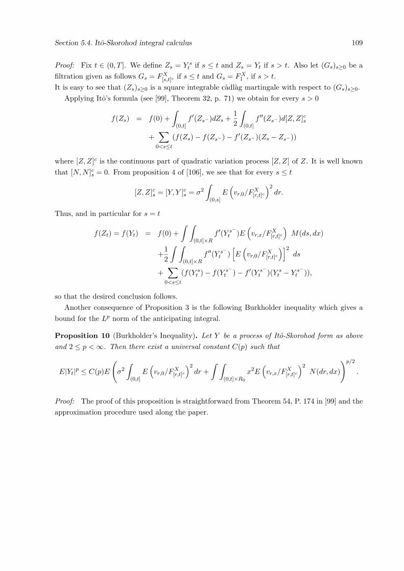
Section 5.4. Ito-Skorohod integral calculus 109
Proof: Fix t ∈ (0, T ]. We define Zs = Y st if s ≤ t and Zs = Yt if s > t. Also let (Gs)s≥0 be a
filtration given as follows Gs = FX[s,t]c if s ≤ t and Gs = FX
1 , if s > t.
It is easy to see that (Zs)s≥0 is a square integrable cadlag martingale with respect to (Gs)s≥0.Applying Ito’s formula (see [99], Theorem 32, p. 71) we obtain for every s > 0
f(Zs) = f(0) +∫
(0,t]f ′(Zs−)dZs +
12
∫
(0,t]f ′′(Zs−)d[Z,Z]cs
+∑
0<s≤t
(f(Zs)− f(Zs−)− f ′(Zs−)(Zs − Zs−))
where [Z,Z]c is the continuous part of quadratic variation process [Z,Z] of Z. It is well knownthat [N, N ]cs = 0. From proposition 4 of [106], we see that for every s ≤ t
[Z,Z]cs = [Y, Y ]cs = σ2
∫
(0,s]E
(vr,0/FX
[r,t]c
)2dr.
Thus, and in particular for s = t
f(Zt) = f(Yt) = f(0) +∫ ∫
(0,t]×Rf ′(Y s−
t )E(vr,x/FX
[r,t]c
)M(ds, dx)
+12
∫ ∫
(0,t]×Rf ′′(Y s−
t )[E
(vr,0/FX
[r,t]c
)]2ds
+∑
0<s≤t
(f(Y st )− f(Y s−
t )− f ′(Y s−t )(Y s
t − Y s−t )),
so that the desired conclusion follows.Another consequence of Proposition 3 is the following Burkholder inequality which gives a
bound for the Lp norm of the anticipating integral.
Proposition 10 (Burkholder’s Inequality). Let Y be a process of Ito-Skorohod form as aboveand 2 ≤ p < ∞. Then there exist a universal constant C(p) such that
E|Yt|p ≤ C(p)E
(σ2
∫
(0,t]E
(vr,0/FX
[r,t]c
)2dr +
∫ ∫
(0,t]×R0
x2E(vr,x/FX
[r,t]c
)2N(dr, dx)
)p/2
.
Proof: The proof of this proposition is straightforward from Theorem 54, P. 174 in [99] and theapproximation procedure used along the paper.
Chapter 6
How rich is the class of processes
which are infinitely divisible with
respect to time?
We give a link between stochastic processes which are infinitely divisible with respect to time(IDT) and Levy processes. We investigate the connection between the selfsimilarity and thestrict stability for IDT processes. We also consider a subordination of a Levy process by anincreasing IDT process. We introduce a notion of multiparameter IDT stochastic processes,extending the one studied by Mansuy [72]. The main example of this kind of processes is theLevy sheet.
6.1 Introduction
An Rd−valued stochastic process X = (Xt, t ≥ 0) is said to be IDT if, for every n ∈ N, we have
(Xnt, t ≥ 0) d= (X(1)t + ... + X
(n)t , t ≥ 0), (6.1)
where (X(1), t ≥ 0), ..., (X(n), t ≥ 0) are independent copies of X and d= denotes equality in allfinite-dimensional distributions. The notion of IDT processes has been introduced by Mansuy[72] as a generalization of Levy processes. Various properties of IDT processes have been alreadyinvestigated in [72], related for instance to their temporal self-decomposability and the charac-terization of IDT Gaussian processes. Regarded as a contribution to this expending topic, it isthe purpose of this paper to extend some results on Levy processes studied in [7], [35] and [73] tothe case of IDT processes. In particular, we shall prove that IDT processes are more tractablethan Levy processes, since they could be obtained by combining the selfsimilarity and strictstability. Such a result is not true in general for Levy processes. Moreover, we will prove that anecessary and sufficient condition for an IDT process to be a Levy process is the hypothesis ofindependence increments. Actually, this last condition can be circumvented when dealing withIDT processes. So it turns out that the class of IDT processes is very rich.
110
Section 6.2. Preliminaries 111
The paper is organized as follows. Section 2 contains some preliminaries on stable processesand selfsimilar processes. Section 3 establishes, for IDT processes, the connection between theselfsimilar (semi-selfsimilar, resp.) processes and the strictly stable (strictly semi-stable, resp.)processes. Namely, strictly stable (strictly semi-stable, resp.) IDT process is a simple exam-ple of selfsimilar (semi-selfsimilar, resp.) process. As a byproduct, we consider the so-calledLamperti transformation for strictly semi-stable IDT processes to give a generalized semi-stableOrnstein-Uhlenbeck process (see Definition 3.4).
Time-changed Levy processes where the chronometers are more general than subordinatorsarise now in many fields of application, see for instance [7] and the reference therein. We shallprove (Theorem 3.6) the inheritance of IDT under time change when base processes are Levyprocesses.
In section 4 we shall introduce a notion of multiparameter IDT processes and we give severalexamples of this kind of processes, one of them is the Levy sheet. Contrary to the one-parametercase, we will prove that multiparameter Levy processes are not IDT in our sense. As in theone-parameter case [72], we characterize the multiparameter IDT Gaussian processes. Moreover,we define multiparameter temporal selfdecomposable processes similar to those introduced byBarndorff-Nielsen, Maejima and Sato [7] and we prove that multiparameter IDT processes aretemporal selfdecomposable.
6.2 Preliminaries
In this section we recall some definitions that are needed in the sequel. For more details thereader is referred to Sato [105].
An Rd−valued random variable X is called degenerate if it is a constant almost surely. AnRd−valued process (Xt, t ≥ 0) is called trivial if Xt is degenerate for every t.
Let 0 < α ≤ 2. An infinitely divisible probability measure µ on Rd is called α−stable if, forany a > 0, there is γa ∈ Rd such that
µ(θ)a :=(∫
Rd
ei<θ,z>µ(dz))a
= µ(a1/αθ)ei<θ,γa>, ∀ θ ∈ Rd. (6.2)
It is called strictly α−stable if, for any a > 0,
µ(θ)a = µ(a1/αθ), ∀ θ ∈ Rd. (6.3)
It is called α−semi-stable if, for some a > 0 with a 6= 1, there is γa ∈ Rd satisfying (6.2). It iscalled strictly α−semi-stable if, there is some a > 0 with a 6= 1 satisfying (6.3).
Let (Xt, t ≥ 0) be a Levy (IDT, resp.) process on Rd. It is called a α-stable, strictly α-stable,semi α-stable, or strictly α-semi-stable Levy (IDT, resp.) process if every finite-dimensionaldistribution of X is, respectively, α-stable, strictly α-stable, semi α-stable, or strictly α-semi-stable.
Section 6.3. Stable IDT processes 112
Let H > 0. A stochastic process (Xt, t ≥ 0) on Rd is called H-selfsimilar if, for any a > 0,
(Xat, t ≥ 0) d= (aHXt, t ≥ 0). (6.4)
It is called wide-sense H-selfsimilar if, for any a > 0, there is a function c(t) from R+ to Rd suchthat
(Xat, t ≥ 0) d= (aHXt + c(t), t ≥ 0). (6.5)
It is called H-semi-selfsimilar if there is some a > 0 with a 6= 1 satisfying (6.4). It is calledwide-sense H-semi-selfsimilar if, for some a > 0 with a 6= 1, there is a function c(t) satisfying(6.5).
6.3 Stable IDT processes
The goal of this section is to generalize some properties of Levy process to the case of IDTprocess. We first establish rather a link between IDT process and Levy process than betweenIDT process and selfsimilar process.
Theorem 13. If X = (Xt, t ≥ 0) is an IDT, stochastically continuous process with independentincrements, then X is a Levy process.
Proof: It suffices to prove that X has stationary increments. Using the IDT property (6.1), weobtain
EeiθXk =(EeiθX1
)k, for any k ∈ N. (6.6)
In a similar way (6.6) can be obtained when k is a rational time. It follows now from thestochastic continuity of X that
EeiθXt =(EeiθX1
)t, for any t ∈ R+.
Therefore, for any 0 ≤ s < t, we have
EeiθXt−s =(EeiθX1
)t−s=
EeiθXt
EeiθXs= Eeiθ(Xt−Xs),
where the last equality follows from the independence of increments. Since for IDT processesX0 = 0 almost surely, then X has stationary increments, which completes the proof.
Remark 6. If (Xt, t ≥ 0) is a centered Gaussian process satisfying the assumptions of theprevious proposition, then X is Brownian motion up to a multiplicative constant, that is has thecovariance function c(s, t) = E(XtXs) = (s ∧ t) c(1, 1). In particular, for Gaussian processes,one can replace the assumption of independence of increments by stationarity of increments.
Section 6.3. Stable IDT processes 113
Indeed, let s < t, since X is an IDT centered Gaussian process, then it is 1/2-selfsimilar (see[72]), hence
E exp (i(Xt −Xs)) = exp(−1
2[(t + s)EX2
1 − 2E(XtXs)])
. (6.7)
On the other hand, we have
E exp (i(Xt −Xs)) = (E exp(iX1))t−s = exp
(−1
2(t− s)E(X1)2
). (6.8)
It follows from (6.7) and (6.8) that E(XtXs) = sE(X1)2 for s < t.
Proposition 11. Let 0 < α ≤ 2. A nontrivial, strictly α-stable and (1/α)-selfsimilar process(Xt, t ≥ 0) is an IDT process.
Proof: Since X is strictly α-stable, we have
(n(1/α)Xt, t ≥ 0
)d=
(n∑
i=1
X(i)t , t ≥ 0
), ∀ n ∈ N∗,
where X(1), ..., X(n) are independent copies of X. On the other hand, it follows from the self-similarity of X that
(Xnt, t ≥ 0) d=(n(1/α)Xt, t ≥ 0
),
which implies X is an IDT process.
6.3.1 Strictly stable IDT processes
In the case of a Levy process (Xt, t ≥ 0), Theorem 1.4.2 in [35] prove that L(X1) is stable if andonly if (Xt, t ≥ 0) is selfsimilar. We can generalize this result as follows.
Theorem 14. Let (Xt, t ≥ 0) be a nontrivial, stochastically continuous and IDT process. Then(Xt, t ≥ 0) is strictly α-stable if and only if it is ( 1
α)-selfsimilar.
Proof: First, assume that (Xt, t ≥ 0) is ( 1α)-selfsimilar. Using the IDT property, we obtain
(n( 1
α)Xt, t ≥ 0
)d= (Xnt, t ≥ 0) d=
(n∑
i=1
X(i)t , t ≥ 0
), for any n ∈ N∗,
where X(1), ..., X(n) are independent copies of X. Thus X is strictly α-stable.Conversely, suppose that (Xt, t ≥ 0) is strictly α-stable. Since X is an IDT process, we have
(Xnt, t ≥ 0) d= (n∑
i=1
X(i)t , t ≥ 0) d=
(n
1α Xt, t ≥ 0
), for any n ∈ N∗,
and also (X t
n, t ≥ 0
)d=
((1n
)1α Xt, t ≥ 0
).
Section 6.3. Stable IDT processes 114
Hence, for any m ∈ N, n ∈ N∗, we have that(X(m
nt), t ≥ 0
)d=
((m/n)
1α Xt, t ≥ 0
).
Combining this last fact with the stochastic continuity of X, we obtain that X is ( 1α)-selfsimilar.
The proof is now complete.Next, we will give an example of an IDT process which is not a Levy process and satisfies
the above theorem.
Example 2. Let Sα be a strictly α-stable random variable. The process X defined by
Xt = t1/αSα, t ≥ 0,
is an (1/α)-selfsimilar and IDT process.
Corollary 4. If α = 2 or 0 < α < 1, then all 1α -selfsimilar IDT process with stationary
increments is an α-stable Levy processes.
The proof of this corollary is straightforward from Theorem 7.5.4 in [104] and Theorem 14 above.
Corollary 5 (Sub-stable processes). Let 0 < α < 2, α < β ≤ 2 and (Yt, t ≥ 0) be a symmetricβ-stable IDT process. Let ξ be a (α/β)-stable positive random variable independent of Y . Theprocess (Xt, t ≥ 0), defined by
Xt = ξ1β Yt,
is ( 1β )-selfsimilar, symmetric α-stable.
Proof: The 1/β-self similarity follows from Theorem 14 while the symmetric α-stability can beproved by using classical arguments on sub-stable processes (see Example 3.6.3 in [35]). Detailsare left to the reader.
6.3.2 Strictly semi-stable IDT processes
The following result gives the connection between semi-selfsimilarity and strict semi-stability forIDT processes. The case of Levy processes appears in [[105], Theorem 4.1].
Theorem 15. Let (Xt, t ≥ 0) be an Rd-valued IDT, stochastically continuous process. Then1) (Xt, t ≥ 0) is semi-stable if it is wide-sense semi-selfsimilar.2) (Xt, t ≥ 0) is semi-selfsimilar if and only if it is strictly semi-stable.
Proof: 1) Suppose X is wide-sense H-semi-selfsimilar. Then for some a ∈ (0, 1)∪ (1,∞), thereexists a nonrandom function c : [0,∞) → Rd, such that
(Xat, t ≥ 0) d= (aHXt + c(t), t ≥ 0).
Section 6.3. Stable IDT processes 115
Therefore, and by using IDT property, for all t1, t2, ..., tm ∈ R+ and all (θ1, ...θm) ∈ Rd×m, wehave
(Eei
∑mk=1〈θk,Xtk〉
)a=
(Eei
∑mk=1〈θk,Xatk〉
)
=(Eei
∑mk=1〈θk,aHXtk〉
)(ei
∑mk=1〈θk,c(tk)〉
).
It remains to show that (Xt1 , ..., Xtm) is infinitely divisible, which follows from the IDT property.Thus (Xt, t ≥ 0) is 1/H-semi-stable.2) Assume that (Xt, t ≥ 0) is strictly α-semi-stable. Then, for some a ∈ (0, 1)∪ (1,∞), we have
(Eei〈θ,a1/α(Xt1 ,...,Xtm )〉) =
(Eei〈θ,(Xt1 ,...,Xtm )〉)a
=(Eei〈θ,(Xat1 ,...,Xatm )〉) ,
where the last equality follows from the IDT property. Hence (Xt, t ≥ 0) is 1/α-semi-selfsimilar.The converse can be proved in a similar way.
Is a wide-sense H-selfsimilar in fact H-selfsimilar, if it is H-semi-selfsimilar? The answer isknown in the case of a stable Levy process, see [73]. We can also answer this question in thecase of a stable IDT process.
Proposition 12. Let (Xt, t ≥ 0) be an Rd-valued, nontrivial and stochastically continuous α-stable IDT process. If it is strictly α-semi-stable, then it is strictly α-stable.
Proof: Assume that (Xt, t ≥ 0) is strictly α-semi-stable. Then, for some a > 1,
(Xat, t ≥ 0) d= (a1/αXt, t ≥ 0). (6.9)
Fix t1, ..., tm ∈ R+ and b1, ..., bm ∈ R. Then there exists a finite measure Γ on the unit sphereS of Rd×m, a vector µ in Rd×m and a symmetric nonnegative-definite matrix A, such that thecharacteristic function of X := (Xt1 , ..., Xtm) has the following form
Eei<θ,X>
=
e−∫
S |<θ,s>|α(1−isign(<θ,s>) tan(πα/2))Γ(ds)+i<θ,µ> if α 6= 1, 2
e−∫
S |<θ,s>|(1+i 2π
sign(<θ,s>) ln |<θ,s>|)Γ(ds)+i<θ,µ> if α = 1
e− 12<Aθ,θ>+i<θ,µ> if α = 2.
The pair (Γ, µ) is unique, and
sign(x) =
1 if x > 00 if x = 0−1 if x < 0.
Using the IDT property and (6.9), we have
Section 6.3. Stable IDT processes 116
(Eei<θ,X>
)a= Eei<θ,(Xat1 ,...,Xatm )> = Eei<a
1α θ,X>, ∀ θ ∈ Rd×m. (6.10)
First, if α 6= 1, then according to (6.10) we have aµ = a1α µ. This implies that µ = 0. Thus, X
is strictly α-stable.Let us now assume that α = 1. Then
∫
S< θ, s > ln | < θ, s > |Γ(ds) =
∫
S< θ, s > ln | < aθ, s > |Γ(ds).
Consequently ∫
Sln(a) < θ, s > Γ(ds) = 0, ∀θ ∈ Rd.
This means that∫S skΓ(ds) = 0 for k = 1, 2, ..., d. Which is exactly the condition for the strictly
1−stability of X. Then every finite-dimensional distribution of (Xt, t ≥ 0) is strictly α-stable.The proof is completed.
Applying the Lamperti transformation to semi-stable IDT processes, we derive a new classof periodically stationary processes. Recall that a stochastic process (Yt, t ∈ R) is said to beperiodically stationary with period p (> 0) if
(Yt+p, t ∈ R) d= (Yt, t ∈ R).
Definition 1. Let 0 < α ≤ 2 and (Xt, t ≥ 0) be a strictly α-semi-stable IDT and stochasticallycontinuous process. We define a periodically stationary process (Yt, t ∈ R) by
Yt = e−t/αXet .
We call this process a generalized α-semi-stable Ornstein-Uhlenbeck process.
Proposition 13. A generalized α-semi-stable Ornstein-Uhlenbeck process (Yt, t ∈ R) is strictlyα-semi-stable.
Proof: From Theorem 15, point 2) we obtain
(Xat, t ≥ 0) d= (a1/αXt, t ≥ 0), for some a ∈ (0, 1) ∪ (1,∞). (6.11)
Combining the IDT property and (6.11), we have that for any θ = (θ1, ...., θm), θk ∈ Rd, k =1, ...,m and (t1, ..., tm) ∈ Rm,
(Eei〈θ,(Yt1 ,...,Ytm )〉)a
=(Eei〈θ,(e−t1/αX
aet1 ,...,e−tm/αXaetm )〉)
=(Eei〈θ,(a1/αe−t1/αX
et1 ,...,a1/αe−tm/αXetm )〉)
=(Eei〈a1/αθ,(Yt1 ,...,Ytm )〉) .
Thus (Yt1 , ..., Ytm) is strictly α-semi-stable for any (t1, ..., tm) ∈ Rm. The proof is completed.
Section 6.3. Stable IDT processes 117
6.3.3 Subordination through an IDT process
Subordination is a transformation of a stochastic process to a new stochastic process throughrandom time change by an increasing Levy process (subordinator) independent of the originalprocess. The aim of this paragraph is to investigate the case where the chronometer is anincreasing IDT process .
Definition 2. A real-valued stochastic process ξ = ξt, t ≥ 0 with ξ0 = 0 a.s. is called achronometer if it is increasing and stochastically continuous.
The following result is inheritance of IDT under time change when initial processes are Levyprocesses.
Theorem 16. Let X be a Levy process on Rd and ξ is an IDT chronometer such that X and ξ
are independent. Then (Zt := Xξt : t ≥ 0) is an IDT process.
Proof: Let ξ(j), j = 1, ..., n be independent copies of ξ. Since X is independent of ξ, then forevery n ≥ 1, θ = (θ1, ..., θm) ∈ (Rd)m, we have
J(n, θ) := E expm∑
k=1
i⟨θk, Xξntk
⟩ = E
(E exp
m∑
k=1
i 〈θk, Xsk〉
)
sk=ξntk, k=1,...,m
.
By using the IDT property, we obtain
J(n, θ) = E
(E exp
m∑
k=1
i 〈θk, Xsk〉
)
sk=∑n
j=1 ξ(j)tk
, k=1,...,m
.
According to the change of variables ck = θk + ... + θn and t0 = 0, and the independence ofincrements of X, we have
J(n, θ) = E
(E exp
m∑
k=1
i⟨ck, Xsk
−Xsk−1
⟩)
sk=∑n
j=1 ξjtk
, k=1,...,m
= E
(m∏
k=1
E expi ⟨ck, Xsk
−Xsk−1
⟩)
sk=∑n
j=1 ξ(j)tk
, k=1,...,m
.
Now, it follows from the stationarity of the increments of X and the independence of the ξ(j),j = 1, ..., n, that
J(n, θ) = E
m∏
k=1
n∏
j=1
E expi⟨ck, Xrj
k
⟩
rjk=ξ
(j)tk−ξ
(j)tk−1
, k=1,...,m, j=1,...,n
= E
n∏
j=1
E expm∑
k=1
i⟨θk, Xrj
k
⟩
rjk=ξ
(j)tk
, k=1,...,m, j=1,...,n
Section 6.4. Multiparameter IDT processes 118
=
E
(E exp
m∑
k=1
i 〈θk, Xrk〉
)
rk=ξtk, k=1,...,m
n
=
(E exp
m∑
k=1
i⟨θk, Xξtk
⟩)n
.
This completes the proof.Similarly, one can prove the following result.
Proposition 14. LetXs : s ∈ RN
+
be an RN
+ -parameter Levy process on Rd and let ξt : t ≥ 0be a N-dimensional subordinator in the sense of being a N-dimensional IDT process ξt =(
ξ1t , ..., ξN
t
)>that is increasing in each coordinate with the superscript > denoting the trans-
pose, and ξt independent of(X(s) : s ∈ RN
+
). Define the subordinated process by composition
as followsYt = Xξt , t ≥ 0.
Then (Yt : t ≥ 0) is an IDT process on Rd.
6.4 Multiparameter IDT processes
In this section we introduce the notion of multiparameter infinitely divisible with respect to time(IDT) process. A typical example of this processes is the Levy sheet.
Definition 3. An Rd-valued stochastic process (Xt, t ∈ RN+ ) is said to be IDT if for any n =
(n1, ..., nN ) ∈ (N∗)N ,
(X(n.t), t ∈ RN
+
) d=
∏Nk=1 nk∑
i=1
X(i)t , t ∈ RN
+
;
where X(1), ..., X(∏N
k=1 nk) are independent copies of X and (n.t) := (n1t1, ..., nN tN ).
In the following we give some examples of multiparameter IDT processes.
Example 3. 1) Let ξ be a strictly α-stable random variable. The process defined by(Xt = (t1/α
1 t1/α2 ....t
1/αN )ξ, t ∈ RN
+
),
is an IDT process.
2) If X is an IDT process and µ a measure on RN+ such that
X(µ)t =
∫
RN+
X(s.t) µ(ds), t ∈ RN+
is well defined, then X(µ) is an IDT process.
Section 6.4. Multiparameter IDT processes 119
3) Let (Xt, t ≥ 0) be an IDT process. Then the multiparameter process defined by
Yt = Xt1t2...tN , for any t = (t1, ..., tN ) ∈ RN+ ,
is IDT.
In order to show that any Levy sheet process is IDT, we give firstly the definition of such aprocess.
Definition 4. Let (Xt, t ∈ R2+) be a family of random variables on Rd. We write Xs1,s2 instead
of Xs when s = (s1, s2)>. For s = (s1, s2)> and u = (u1, u2)> in R2+ with s1 ≤ u1 and s2 ≤ u2,
call B = (s1, u1]× (s2, u2] a rectangle in R2+ and set
X(B) = Xu1,u2 −Xs1,u2 −Xu1,s2 + Xs1,s2 .
If B1, ..., Bn are disjoint rectangles in R2+ and B = ∪n
j=1Bj, then set X(B) =∑n
j=1 X(Bj).The stochastic process (Xt, t ∈ R2
+) is called a Levy sheet if
(a) If n ≥ 2 and B1, ..., Bn are disjoint rectangles, then X(B1), ..., X(Bn) are independent.
(b) If B is a rectangle and s ∈ R2+, then X(B) d= X(B + s).
(c) Xs1,0 = X0,s2 = 0 a.s. for s1, s2 ∈ R2+.
(d) Xt → Xs in probability as |t− s| → 0 in R2+.
Proposition 15. Let (Xt, t ∈ R2+) be a Levy sheet process on Rd. Then it is IDT.
Proof: Let n,m ∈ N, θ = (θ1, ..., θp) ∈ Rd×p, 0 = s0 ≤ s1 < ... < sp and 0 = t0, t1, ..., tp ∈ R+,let σ be a permutation such that tσ(1) ≤ ... ≤ tσ(p) and σ(0) = 0. We consider disjoint rectangles(Bl
k = (nsk−1, nsk]× (mtσ(l−1),mtσ(l)]), k = 1, ..., p, l = 1, ..., p. Using Levy sheet properties
(see [94]), there exist a matrix(clk
)0≤k,l≤p
, clk ∈ Rd such that
Eei∑p
j=1
⟨θj ,X(nsj,mtj)
⟩= Eei
∑pj=1〈θj ,X((0,nsj ]×(0,mtj ])〉 = Eei
∑0≤k,l≤p〈cl
k,X(Blk)〉.
=∏
0≤k,l≤p
Eei〈clk,X(Bl
k)〉
=∏
0≤k,l≤p
(Eei〈cl
k,X1,1〉)λ(Blk)
= I, say,
where λ is the Lebesgue measure. Since λ(Blk) = n ×mλ
((sk−1, sk]× (tσ(l), tσ(l−1)]
), then we
have
I =
∏
0≤k,l≤p
(Eei〈cl
k,X1,1〉)λ((sk−1,sk]×(tσ(l),tσ(l−1)])
n×m
=
∏
0≤k,l≤p
(Eei〈cl
k,X((sk−1,sk]×(tσ(l),tσ(l−1)])〉)
n×m
=(Eei
∑pj=1〈θj ,X((0,sj ]×(0,tj ])〉
)n×m
Section 6.4. Multiparameter IDT processes 120
This completes the proof.
Remark 7. If (Xt, t ∈ RN+ ) is an Rd-valued stochastically continuous IDT process, then
Xt = 0 a.s for any t ∈ RN+ , with inf
i=1,...,Nti = 0.
Indeed, for any n ≥ 1, u ∈ Rd and t = (t1, ..., tj−1, 0, tj+1, ...tN ), by IDT property we have
E exp (i〈u,Xt〉) = E exp(i〈u,X(t1,...,tj−1,n×0,tj+1,...,tN )〉
)= [E exp (i〈u,Xt〉)]n .
Moreover the characteristic function of Xt is non vanishing (because the laws of this variable isinfinitely divisible), then
EeiuXt = 1, for all u ∈ Rd.
Thus, L(Xt) = δ0, where δ0 is the distribution concentrated at 0 and L(X) denotes the law ofX.
According to Mansuy [72], Proposition 1.1, any one-parameter Levy process is IDT. Thefollowing result shows that such a result does not hold in the multiparameter case. We refer toPedersen and Sato [[94], Definition 2.1] for the definition and properties of RN
+ -parameter Levyprocesses in law.
Proposition 16. Let N ≥ 2. If (Xt, t ∈ RN+ ) is an RN
+ -parameter Levy processes in lawsatisfying the IDT property, then Xt = 0 a.s, ∀t ∈ RN
+ .
Proof: Let X be such a process. Then, by Remark 7, we have
Eei〈u,Xt〉 =N∏
k=1
Eei〈u,X(0,...,0,tk,0,...,0)〉 = 1, for any t ∈ RN+ , u ∈ Rd.
This proves that L(Xt) = δ0, ∀t ∈ RN+ .
In the following we show that for any stochastically continuous IDT process X there exists aLevy sheet that has the same one-dimensional marginals than X.
Proposition 17. Let(Xt, t ∈ R2
+
)be a stochastically continuous IDT process. Then there exists
a Levy sheet process (Zt, t ∈ R2+) such that
Xtd= Zt, for any t ∈ R2
+.
Proof: First we note that the laws of finite dimensional marginals of an multiparameter IDTprocess X are infinitely divisible. In particular, the law of X1,1 is infinitely divisible. Then thereexists a Levy sheet (Zt, t ∈ R2
+) with X1,1d= Z1,1. It follows that if Zt, t ∈ R2
+ is a Levy sheetthen L(Xt) is infinitely divisible and
E[ei〈z,Xt1,t2〉
]=
(E
[ei〈z,X1,1〉
])t1t2for any t1, t2 ∈ R+.
HenceXt
d= Zt, for any t ∈ R2+.
Section 6.4. Multiparameter IDT processes 121
Definition 5. An stochastic process(Yt, t ∈ RN
)is said to be strictly stationary if, for every
a ∈ RN
(Ya+t, t ∈ RN
) d=(Yt, t ∈ RN
).
For the characterization of IDT Gaussian multiparameter processes, we will need the follow-ing:
Lemma 6. Let(Yt, t ∈ RN
)be a strictly stationary process, and fix H = (h1, ..., hN ) ∈ (R∗+)N .
Define(Xt, t ∈ RN
+
)by
Xt = th11 ...thN
N Y(log(t1),...,log(tN )), t ∈ (R+)N ; X0 = 0.
Then(Xt, t ∈ RN
+
)is H-selfsimilar in the following sense
(X(a.t), t ∈ (R+)N
) d=(ah1
1 ...ahNN Xt, t ∈ (R+)N
)for any a ∈ (R∗+)N .
Conversely, if(Xt, t ∈ (R+)N
)is H-selfsimilar process, then its Lamperti transform
(Yt := e−
∑Nk=1 hktkX(et1 ,...,etN ), t ∈ RN
),
is strictly stationary.
Proof: Assume that(Yt, t ∈ RN
)is strictly stationary. Then, for any a = (a1, ..., aN ) ∈ (R∗+)N ,
we have(X(a.t), t ∈ RN
+
)=
((a1t1)h1 ...(aN tN )hN Y(log(a1)+log(t1),...,log(aN )+log(tN )), t ∈ RN
+
)
d=((a1t1)h1 ...(aN tN )hN Y(log(t1),...,log(tN )), t ∈ RN
+
)
=(ah1
1 ...ahNN Xt, t ∈ RN
+
).
Hence,(Xt, t ∈ RN
+
)is H-selfsimilar. Conversely, since
(Xt, t ∈ RN
)is H-selfsimilar, for any
b = (b1, ..., bN ) ∈ R+N we have
(Y(t+b), t ∈ RN
)=
(e−
∑Nk=1 hk(tk+bk)X(et1+b1 ,...,etN +bN ), t ∈ RN
)
d=(e−
∑Nk=1 hktkX(et1 ,...,etN ), t ∈ RN
)=
(Yt, t ∈ RN
).
Thus,(Yt, t ∈ RN
)is strictly stationary.
Proposition 18. Let (Xt, t ∈ RN+ ) be a stochastically continuous, and centered Gaussian process.
Then the following properties are equivalent:i) (Xt, t ∈ RN
+ ) is an IDT process.ii) The covariance function c(s, t) := E(XsXt), (s, t) ∈ RN
+ × RN+ , satisfies
c(α.s, α.t) = α1...αNc(s, t), for any α ∈ (R∗+)N .
iii) The process (Xt, t ∈ RN+ ) is (1
2 , ..., 12)-selfsimilar.
iv)(Yy := e−
∑Nk=1 hkykX(ey1 ,...,eyN ), y ∈ RN
)is strictly stationary.
Section 6.4. Multiparameter IDT processes 122
Proof: i) ⇔ ii). We have that (Xt, t ∈ RN+ ) is IDT if and only if, for any n = (n1, ..., nN ) ∈
NN , s, t ∈ RN+
c(n.s, n.t) = n1...nNc(s, t),
and also, for any q = (q1, ..., qN ) ∈ QN+ , s, t ∈ RN
+
c(q.s, q.t) = q1...qNc(s, t).
Moreover, since X is stochastically continuous, its covariance function is continuous. Hence,using the density of Q+ in R+, we obtain the result.ii) ⇔ iii). Since a centered Gaussian process is characterized by its covariance function, weobtain the result easily.iii) ⇔ iv). It is a direct application of Lemma 6 for H = (1/2, ..., 1/2).
Example 4. Let (Bt, t ∈ RN+ ) be a Brownian sheet, i.e. a centered, real-valued Gaussian
random field with covariance function E (B(t)B(s)) =∏N
i=1 si∧ ti. Since its covariance functionsatisfies the point ii) of Proposition 18, then (Bt, t ∈ RN
+ ) is an IDT process.
We will define the multiparameter temporally selfdecomposable processes which extend theone introduced in [7] and relate this notion with the IDT processes.
Definition 6. An Rd-valued stochastic process X = (Xt, t ∈ RN+ ) is temporally selfdecomposable
if, for every c ∈ (0, 1)N , there exist two independent processes X(c) = (X(c)t , t ∈ RN
+ ), andU (c) = (U (c)
t , t ∈ RN+ ) on Rd, such that
Xd= X(c) + U (c),
where X(c) d= (X(c.t), t ∈ RN+ ) and U c is called the c-residual of X.
For every m ≥ 2, we say that X is temporally selfdecomposable of order m if, it is temporallyselfdecomposable and if any c ∈ (0, 1)N , the c-residual process of X is temporally selfdecomposableof order (m−1). When X is temporally selfdecomposable of order m for all m, we call it infinitelytemporally selfdecomposable.
Proposition 19. An Rd-valued stochastically continuous IDT process is infinitely temporallyselfdecomposable.
Proof: By stochastic continuity and IDT property, we have, for any (t1, ..., tm) ∈ (RN+ )m, ξ ∈ Rm
and c = (c1, ..., cN ) ∈ (0, 1)N
Ee∑m
j=1 i〈ξj ,Xtj 〉 =
(Ee
∑mj=1 i
⟨ξj ,X
(c1t1j
,...,cN tNj
)
⟩)1/∏N
k=1 ck
=(Ee
∑mj=1 i〈ξj ,Xc.tj 〉
)Ee
∑mj=1 i
⟨ξj ,X
(c1( 1∏Nk=1
ck−1)t1
j,...,cN ( 1∏N
k=1ck−1)tN
j)
⟩ .
123
Therefore (Xt, t ∈ RN+ ) is temporally selfdecomposable and
(Xt, t ∈ RN+ ) d= (Xc.t + U c
t , t ∈ RN+ ),
where U c is independent of (Xc.t, t ∈ RN+ ) and
(U ct , t ∈ RN
+ ) d= (X(c1( 1∏Nk=1
ck−1)t1,...,cN ( 1∏N
k=1ck−1)tN ), t ∈ RN
+ ). (6.12)
It follows from (6.12) that U c is stochastically continuous and IDT. The same steps as aboveapplied to U c proves that U c is temporally selfdecomposable and its residuel process is stochasti-cally continuous and IDT. Using the same arguments, we conclude that X is infinitely temporallyselfdecomposable.
Bibliography
[1] E. Alos, O. Mazet and D. Nualart (2001). Stochastic calculus with respect to Gaussian pro-cesses. Annals of Probability, 29, pag. 766-801.
[2] A. Alos, and D. Nualart (2002). Stochastic integration with respect to the fractional Brownianmotion. Stochastics and Stochastics Reports 75 129-152.
[3] D. Applebaum (2004). Levy processes and stochastic and stochastic calculs. Cambridge Uni-versity Press, Cambridge.
[4] A. Ayache and J. Levy-Vehel (1999). Generalized multifractional Brownian motion. Fractals:theory and applications in engeneering, pag. 17-32. bibitemBNLOP
[5] J.M. Bardet and P. Bertrand (2007). Identification of the multiscale fractional Brownianmotion with biomechanical applications. Journal of Time Series Analysis, Vol. 28, Issue 1,pag. 1-52.
[6] J. Beran (1994). Statistics for Long-Memory Processes. Chapman and Hall.
[7] O.E. Barndorff-Nielsen, M. Meajima, and K. Sato (2005). Infinite divisibility for stochasticprocesses and time change, to appear in Journal of Theoretical Probability.
[8] O.E. Barndorff-Nielsen and S. Thorbjørnsen (2002). Levy laws in free probability. Proc. NatlAcad. Sci. 99, 16568-16575.
[9] D. Bell. (1987).The Malliavin Calculus. serie Pitman Monographs and Surveys in Pure andApplied Math., numero 34, Longman and Wiley.
[10] S. Belly, L. Decreusefond (1997). Multi-dimensional fractional Brownian Motion and someApplications to Queueing Theory. In Fractals in Engineering, C. Tricot, J. Levy-Vehel, Eds.170-185.
[11] F. E. Benth, G. Di Nunno, A. Lokka, B. Oksendal, F. Proske (2003). Explicit representationsof the minimal variance portfolio in markets driven by Levy processes. Mathematical Finance,13, pag. 55-72.
[12] A. Begyn (2005). Quadratic variations along irregular subdivisions for Gaussian processes.Electronic Journal of Probability. Volume: 10, pag. 691-717.
124
125
[13] S. M. Berman (1969). Local times and sample function properties of stationary Gaussianprocesses. Trans. Amer. Math. Soc. 137 277-300.
[14] S. M. Berman (1972). Gaussian sample functions: uniform dimension and Holder conditionsnowhere, Nagoya Math. J. 46, 63-86.
[15] K. Bichteler, J.-B. Gravereaux, and J. Jacod (1987). Malliavin calculus for processes withjumps. Gordon and Breach Science Publishers.
[16] T. Bojdecki, L.G. Gorostiza and A. Talarczyk (2004). Sub-fractional Brownian motion andits relation to occupation times. Stat. Prob. Lett. 69, 405-419.
[17] T. Bojdecki, L. Gorostiza and A. Talarczyk (2006). Some extension of fractional Brownianmotion and sigfractional Brownian motion related to particle system. Preprint.
[18] J.-C. Breton and I. Nourdin (2008). Error bounds on the non-normal approximation of Her-mite power variations of fractional Brownian motion. Electronic Communications in Proba-bility. 13, 482-493.
[19] A.C. Brandwein, W.E. Strawderman (1991). Generalizations of James-Stein estimatorsunder spherical symmetry, Ann. Statist. 19, 1639-1650.
[20] P. Breuer and P. Major (1983). Central limit theorems for nonlinear functionals of Gaussianfields. J. Multivariate Analysis, 13 (3), 425-441.
[21] E.A. Carlen and E. Pardoux (1990). Differential calculus and integration by parts on Poissonspace. Stochastics, Algebra and Analysis in Classical and Quantum Dynamics (Marseille,1988). Math. Appl. 59, 63-73.
[22] A. Chronopoulou, C.A. Tudor and F. Viens (2008). Self-similarity parameter estimationand reproduction property for non-Gaussian Hermite processes. Preprint.
[23] J.F. Coeurjolly (2001). Estimating the parameters of a fractional Brownian motion by dis-crte variations of its sample paths. Statistical Inference for Stochastic Processes, 4, 199-227.
[24] L. Coutin, D. Nualart and C.A. Tudor (2001). The Tanaka formula for the fractionalBrownia motion. Stochastic Proc. Applic., 94(2), pag. 301-315.
[25] Z. Chen (2007). Polar sets and polar functions of bifractional Brownian sheets. Preprint.
[26] R. Coelho and L. Decreusfond (1995). Video correlated traffic models for broadband com-munications networks. In Proceeding of the ITC seminar on teletraffic management.
[27] L. Decreusefond and A.S. Ustunel (1998). Stochastic analysis of the fractional Brownianmotion. Potential Analysis, 10, pag. 177-214.
126
[28] L. Decreusefond (2005). Stochastic Integration with respect to Volterra processes. Ann. Inst.H. Poincare Probab. Statist. 41 , no. 2, 123-149
[29] C. Dellacherie, B. Maisonneuve, P.A. Meyer (1992). Probabilites et Potentiel, ChapitresXVII a XXIV. Hermann.
[30] G. Di Nunno, B. Oksendal, F. Proske (2004). White Noise Analysis for Levy processes.Journal of Functional Analysis 206 , 109-148.
[31] G. Di Nunno, T. Meyer-Brandis, B. Oksendal and F. Proske (2005). Malliavin calculus andanticipative Ito formulae for Levy processes. Infin. Dimens. Anal. Quantum Probab. Relat.Top. 8 (2), 235-258.
[32] R.L. Dobrushin and P. Major (1979). Non-central limit theorems for non-linear functionalsof Gaussian fields. Z. Wahrscheinlichkeitstheorie verw. Gebiete, 50, 27-52.
[33] T. Duncan, Y. Z. Hu and B. Pasik-Duncan (2000). Stochastic Calculus for FractionalBrownian Motion I. Theory. SIAM J. Control Optim., 38 (2), pag. 582-612.
[34] M. Eddahbi, R. Lacayo, J.L. Sole, C. A. Tudor and J. Vives (2005), Regularity of local timefor th d-dimensional fractional Brownian motion with N-parameters. Stoch. Anal. Appl, 23,383-400.
[35] P. Embrechts and M. Maejima (2002). Selfsimilar processes. Princeton University Press,Princeton, New York.
[36] K. Es-Sebaiy, D. Nualart, Y. Ouknine and C.A. Tudor (2008). Occupation densities forcertain processes related to fractional Brownian motion. Submitted.
[37] K. Es-Sebaiy, I. Ouassou and Y. Ouknine (2008). SEstimation of the drift of fractionalBrownian motion. To appear in Statistics and Probability Letters.
[38] K. Es-Sebaiy, Y. Ouknine (2007). How rich is the class of processes which are infinitelydivisible with respect to time?, Statistics and Probability Letters. 78 (2008) 537-547.
[39] K. Es-Sebaiy and C. Tudor (2007). Multidimensional bifractional Brownian motion: Itoand Tanaka’s formulas. Stochastics and Dynamics 3 365-388.
[40] K. Es-Sebaiy, C. Tudor (2007). Levy processes and Ito-Skorohod integrals, Proceedings ofinternational conference on Skorokhod space, 17-23 June, 2007, Kyiv, Ukraine.
[41] K. Es-Sebaiy and C. Tudor (2008). Non-central limit theorem for the cubic variation of aclass of selfsimilar stochastic processes. Submitted.
[42] D. Fourdrinier, I. Ouassou and W. E. Strawderman (2003). Estimation of a parametervector when some components are restricted. Journal of Multivariate Analysis Volume 86,Number 1, pp. 14-27.
127
[43] A. M. Garsia, E. Rodemich and H. Rumsey (1970/1971). A real variable lemma and thecontinuity of paths of some Gaussian processes. Indiana Univ. Math. J. 20 565–578.
[44] D. Geman and J. Horowitz (1980). Occupation densities. Ann. Probab. 8 1-67.
[45] L. Giraitis and D. Surgailis (1985). CLT and other limit theorems for non-linear functionalsof Gaussian processes. Z. Wahrsch. verw. Gebiete 70, 191-212.
[46] M. Gradinaru, I. Nourdin, F. Russo and P. Vallois (2003). m-order integrals and generalizedIto’s formula; the case of a fractional Brownian motion with any Hurst parameter. Annalesde l’Institut Henri Poincare, 41(4), 781-806.
[47] C. Houdre and J. Villa (2003). An example of infinite dimensional quasi-helix. Contempo-rary Mathematics, Amer. Math. Soc., 336, pag. 195-201.
[48] H.E. Hurst (1951). Long-term storage capacity in reservoirs. Trans. Amer Soc. Civil. Eng.,116, 400-410
[49] H.E. Hurst, R.P Black and Y.M Simaika (1965). Long Term Storage in Reservoirs. AnExperimental Study. Constable, London.
[50] P. Imkeller and D. Nualart. (1994). Integration by parts on Wiener Space and the Existenceof Occupation Densities. Ann. Probab. 22 469–493.
[51] P. Imkeller (1992). Occupation densities for stochastic integral processes in the secondWiener chaos. Probab. Theory Related Fields. 91, 1-24.
[52] P. Imkeller (1991). On the existence of occupation densities of stochastic integral pro-cesses via operator theory. In Seminar on Stochastic Processes 1990 (E. Cinlar, ed.) ProgressProbab. 24, 207-240. Birkhauser, Boston.
[53] P. Imkeller (1993). Existence and continuity of occupation densities of stochastic integralprocesses. Ann. Probab. 21, 1050-1072.
[54] P. Imkeller and F. Weisz (1994). The asymptotic behaviour of local times and occupationintegrals of the N-parameter Wiener process in Rd. Probability Theory and Related Fields98(1), pag. 47-75.
[55] K. Ito (1956). Spectral type of the shift transformation of differential processes with station-ary increments.Trans. Am. Math. Soc., 81, pag. 252-263.
[56] J. Jacod and A.N. Shiryaev (2003). Limit theorems for stochastic processes. Second edition.Grundlehren der Mathematischen Wissenschaften [Fundamental Principles of MathematicalSciences], 288, Springer.
[57] W. James, C. Stein (1961). Estimation with quadratic loss, Proceedings of the FourthBerkeley Symposium on Mathematical Statistics and Probability, vol. 1,361-379.
128
[58] J. P. Kahane (1981). Helices at quasi-helices. Adv. Math. 7B , 417-433.
[59] J. P. Kahane (1985). Some random series of functions. Cambridge University Press.
[60] A. N. Kolmogorov (1940). The Wiener spiral and some other intereting curves in Hilbertspace. Dokl. Akad. Nauk SSSR, 26, 115-118.
[61] I. Kruk, F. Russo and C. A. Tudor (2007). Wiener integrals, Malliavin calculus and covari-ance structure measure. J. Funct. Anal. 249 92-142.
[62] N. V. Krylov (1995). Introduction to the Theory of Diffusion Processes. American Mathe-matical Society.
[63] H.H. Kuo (1996). White Noise Distribution Theory. CRC Press.
[64] P. Lei and D. Nualart (2008). A decomposition of the bifractional Brownian motion andsome applications. Statistics and Probability Letters, to appear.
[65] J.A. Leon and C. Tudor (1998). A chaos approach to the anticipating calculus for thePoisson process. Stochastics Stochastics Rep. 62(3-4), 217-250.
[66] A. Løkka (2004). Martingale representation of functionals of Levy processes. StochasticAnal. Appl. 22(4), 867-892.
[67] P. Malliavin (Kyoto, 1976) Stochastic calculus of variations and hypoelliptic operators. Proc.Int. Symp. on Stochastic Differential Equations Wiley, New York, 195-263.
[68] P. Malliavin (1997). Stochastic analysis. Springer Verlag.
[69] B.B. Mandelbrot (1963). The variation of certain speculative prices. Journal of BusinessXXXVI, 392-417.
[70] B.B. Mandelbrot (1982). The fractal geometry of nature, San Francisco: W.H. Freeman
[71] B. B. Mandelbrot and J. W. Van Ness (1968). Fractional Brownian motions, fractionalnoises and applications. SIAM Review 10(4), 422-437.
[72] R. Mansuy (2005) On processes which are infinitely divisible with respect to time,arXiv:math/0504408.
[73] M. Meajima and K. Sato (1999). Semi-selfsimilar processes, J. Theoret. Probab. 12, 347-373.
[74] M. Marcus and J. Rosen (2006). Markov Processes, Gaussian processes and local times.Cambridge University Press.
[75] M. Maejima and C.A. Tudor (2007). Wiener integrals and a Non-Central Limit Theoremfor Hermite processes, Stochastic Analysis and Applications, 25 (5), 1043-1056.
129
[76] A.I. McLeod and K.W. Kipel (1978).Preservation of the rescaled adjusted range: a reaasse-ment of the Hurst exponent. Water Resourc. Res., 14 (3), 491-508.
[77] J. Memin, Y. Mishura and E. Valkeila (2001) Inequalities for the moments of Wiener inte-grals with respect to a fractional Brownian motion. Statist. Probab. Lett. 51 197-206.
[78] S. M. Nikol’skiı (1969). Approximation of functions of several variables and imbedding the-orems, “Nauka”, Moscow; Gundlehren Math. Wiss., vol. 205, Springer-Verlag, Berlin, 1975.
[79] I. Nourdin, D. Nualart and C.A Tudor (2007). Central and Non-Central Limit Theoremsfor weighted power variations of the fractional Brownian motion. Preprint.
[80] I. Nourdin, G. Peccati and A. Reveillac (2008). Multivariate normal approximation usingStein’s method and Malliavin calculus. Preprint.
[81] D. Nualart (2006). The Malliavin calculus and related topics. Springer Verlag. Second Edi-tion.
[82] D. Nualart (2003). Stochastic calculus with respect to the fractional Brownian motion andapplications. Contemp. Math. 336, 3-39.
[83] D. Nualart and S. Ortiz-Latorre (2008). Central limit theorems for multiple stochasticintegrals and Malliavin calculus. Stochastic Processes and their Applications, 118, 614-628.
[84] D. Nualart and Y. Ouknine (2002). Regularization of differential equations by fractionalnoise. Stochastic Proc. Appl. 102, 103-116.
[85] D. Nualart, J. Vives (1990). Anticipative calculus for the Poisson space based on the Fockspace. Seminaire de Probabilites XXIV, LNM 1426, edited by Springer, pag. 154-165.
[86] G. Di Nunno, B. Oksendal, F. Proske (2004). White Noise Analysis for Levy processes.Journal of Functional Analysis, 206, pag. 109-148.
[87] G. Di Nunno, Th. Meyer-Brandis, B. Oksendal, F. Proske (2004). Malliavin calculus andanticipative Ito formulae for Levy processes. Preprint series in Pure Mathematics, Universityof Oslo.
[88] D. Ocone (1987). A guide to the stochastic calculus of variations. in ¿ Stochastic Analy-sis and Related Topics À, Lecture Notes in Math. 1316, editeurs H. KOERZLIOGLU, S.USTUNEL., pages 1-79.
[89] D. Ocone, I. Karatzas (1991). A generalized representation formula with application tooptimal portfolios. in ¿ Stochastics and Stochastic Reports À, volume 34, pages 187-220.
130
[90] B. Øksendal (1996). An Introduction to Malliavin Calculus with Applications to Economics.in ¿ Lecture Notes from a course given 1996 at the Norwegian School of Economics andBusiness Administration (NHH) À, September, 1996, NHH Preprint Series.
[91] B. Øksendal, F. Proske (2004). White Noise of Poisson random measure. Potential Analysis,21, pag. 375-403.
[92] I. Ouassou and W.E. Strawderman (2002). Estimation of a parameter vector restricted toa cone Statistics and Probability Letters, Volume 56, Number 2, pp. 121-129
[93] G. Peccati, C.A. Tudor (2007). Anticipating integrals and martingales on the Poisson space.Random Operators and Stochastic Equations. Random Operators and Stochastic Equations.Volume 15, Issue 4, Pages 327-352.
[94] J. Pedersen and K. Sato (2004). Semigroups and processes with parameter in a cone,Abstract and Applied analysis: pp. 499-513.
[95] V. Pipiras and M. Taqqu (2001). Integration questions related to the fractional Brownianmotion. Probability Theory and Related Fields, 118, 2, pag. 251 - 281.
[96] N. Privault and A. Reveillac (2007). Stein estimation for the drift of Gausian processesusing the Malliavin calculus. The Annals of Statistics, to appear.
[97] S. G. Samko, A. A. Kilbas and O. I. Mariachev (1993). Fractional integrals and derivatives.Gordon and Breach Science.
[98] Yu. V. Prokhorov and V. Statulevicius, eds. (2006). Limit Theorems In Probability Theory.Springer.
[99] Ph. Protter (1992). Stochastic integration and differential equations: a new approach,Springer.
[100] Z. Qian and T. Lyons (2002). System control and rough paths. Clarendon Press, Oxford.
[101] Revuz, D. and Yor, M. (1994). Continuous martingales and Brownian motion. SpringerVerlag.
[102] F. Russo and P. Vallois (1993). Forward backward and symmetric stochastic integration.Prob. Theory Rel. Fields, 97, pag. 403-421.
[103] F. Russo and C. A. Tudor (2006). On the bifractional Brownian motion. Stochastic Pro-cess. Appl. 5, 830-856.
[104] G. Samorodnitsky and M. Taqqu (1994). Stable Non-Gaussian random variables. Chapmanand Hall, London.
131
[105] K. Sato (1999). Levy processes and Infinitely Divisible Distributions, Cambridge Univ.Press, Cambridge.
[106] J. L. Sole, F. Utzet, J. Vives (2007). Canonical Levy process and Malliavin calculus.Stochastic Processes and their Applications, 117, pag. 165-187.
[107] C. Stein(1956). Inadmissibility of the usual estimator for the mean vector of a multivariatenormal distribution, Proceedings of the Third Berkeley Symposium Mathmatical on Statisticsand Probability, vol. 1, 197-206.
[108] M. Taqqu (1975). Weak convergence to the fractional Brownian motion and to the Rosen-blatt process. Z. Wahrscheinlichkeitstheorie verw. Gebiete, 31, 287-302.
[109] C.A. Tudor (2004). Martingale type stochastic calculus for anticipating integral processes.Bernoulli, 10, pag. 313-325.
[110] C.A. Tudor (2004). Ito-Skorohod stochastic equations and applications to finance. Journalof Applied Mathematics and Stochastic Analysis, 4, pag. 359-369.
[111] C.A. Tudor (2008). Analysis of the Rosenblatt process. ESAIM Probability and Statistics,12, 230-257.
[112] C.A. Tudor and F. Viens (2007). Variations and estimators for the selfsimilarity orderthrough Malliavin calculus. To appear in Annals of Probability
[113] Y. Xiao and C.A. Tudor (2007). Sample paths properties of the bifractional Brownianmotion. Bernoulli 13(4) 1023-1053.
[114] H. Uemura (2004). Tanaka formula for Multidimensional Brownian motion. J. of Theo-retical Probability, 17(2),pag. 347-366.
[115] H. Uemura (2008). On the Weighted Local Time and the Tanaka Formula for the Multidi-mensional Fractional Brownian Motion. Stochastic Analysis and Applications, 26: 136-168.
[116] S. Watanabe (1994). Lecture on stochastic differential equations and Malliavin calculus,Tata institute of fundamental research, Springer-Verlag.
[117] W. Willinger, M. Taqqu, W.E. Leland and D.V. Wilson (1995).Selfsimilarity in high speedpacket traffic: analysis and modelisation of ethernet traffic measurements. Statist. Sci. 10,67-85.
[118] W. Willinger, M. Taqqu and V. Teverovsky (1999). Long range dependence and stockreturns. Finance and Stochastics, 3, 1-13.


![Mod©lisation statique et dynamique des poutres en [ ] - Code_Aster](https://img.pdfslide.fr/doc/110x75/620631908c2f7b1730054b88/modlisation-statique-et-dynamique-des-poutres-en-codeaster.jpg)