Embed Size (px)
Citation preview
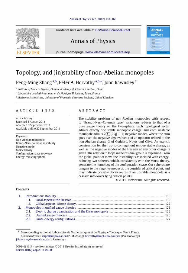
Annals of Physics 327 (2012) 118–165
Contents lists available at SciVerse ScienceDirect
Annals of Physics
journal homepage: www.elsevier.com/locate/aop
Topology, and (in)stability of non-Abelian monopolesPeng-Ming Zhang a,b, Peter A. Horvathy a,b,∗, John Rawnsley c
a Institute of Modern Physics, Chinese Academy of Sciences, Lanzhou, Chinab Laboratoire de Mathématiques et de Physique Théorique, Tours, Francec Mathematics Institute, University of Warwick, Coventry, England, United Kingdom
a r t i c l e i n f o
Article history:Received 5 August 2011Accepted 1 September 2011Available online 22 September 2011
Keywords:Non-Abelian monopoleBrand–Neri–Coleman instabilityNegative modeMorse theoryConfiguration space topologyEnergy-reducing sphere
a b s t r a c t
The stability problem of non-Abelian monopoles with respectto ‘‘Brandt–Neri–Coleman type’’ variations reduces to that of apure gauge theory on the two-sphere. Each topological sectoradmits exactly one stable monopole charge, and each unstablemonopole admits 2
(2|q| − 1) negative modes, where the sum
goes over the negative eigenvalues q of an operator related to thenon-Abelian charge Q of Goddard, Nuyts and Olive. An explicitconstruction for the [up-to-conjugation] unique stable charge, aswell as the negative modes of the Hessian at any other charge isgiven. The relation to loops in the residual group is explained. Fromthe global point of view, the instability is associated with energy-reducing two-spheres, which, consistently with the Morse theory,generate the homology of the configuration space. Our spheres aretangent to the negative modes at the considered critical point, andmay indicate possible decay routes of an unstable monopole as acascade into lower lying critical points.
© 2011 Elsevier Inc. All rights reserved.
Contents
1. Introduction: stability.................................................................................................................................... 1191.1. Local aspects: the Hessian................................................................................................................. 1191.2. Global aspects: Morse theory............................................................................................................ 122
2. Monopoles in unified gauge theories ........................................................................................................... 1232.1. Electric charge quantization and the Dirac monopole .................................................................... 1232.2. Unified gauge theories....................................................................................................................... 1262.3. Finite-energy configurations............................................................................................................. 127
∗ Corresponding author at: Laboratoire de Mathématiques et de Physique Théorique, Tours, France.E-mail addresses: [email protected] (P.-M. Zhang), [email protected] (P.A. Horvathy),
[email protected] (J. Rawnsley).
0003-4916/$ – see front matter© 2011 Elsevier Inc. All rights reserved.doi:10.1016/j.aop.2011.09.003
P.-M. Zhang et al. / Annals of Physics 327 (2012) 118–165 119
3. Lie algebra structure and Lie group topology............................................................................................... 1304. Finite energy solutions: the GNO charge...................................................................................................... 1385. Stability analysis ............................................................................................................................................ 141
5.1. Reduction from R3 to S2 .................................................................................................................... 1415.2. Negative modes.................................................................................................................................. 1455.3. Supersymmetric interpretation of the negative modes .................................................................. 147
6. The geometric picture: YM on S2 .................................................................................................................. 1477. Loops ............................................................................................................................................................... 1518. Global aspects................................................................................................................................................. 153
8.1. Configuration space topology and energy-reducing two-spheres ................................................. 1548.2. Energy-reducing two-spheres .......................................................................................................... 1548.3. Examples ............................................................................................................................................ 156
9. Conclusion ...................................................................................................................................................... 162Acknowledgements........................................................................................................................................ 163References....................................................................................................................................................... 164
1. Introduction: stability
Magnetic monopoles arise as exact solutions of spontaneously broken Yang–Mills–Higgstheory [1–5], see Section 2 for an outline. It has been pointed out by Brandt and Neri [6] andemphasized by Coleman [3], however, that most such solutions are unstable when the residual gaugegroup H is non-Abelian.
This review, which heavily draws on previous work of two of us with late O’Raifeartaigh, [7,8],is devoted to the study of various aspects of ‘‘Brandt–Neri–Coleman’’ monopole instability. Furtherrelated contributions can be found in [9–11].
1.1. Local aspects: the Hessian
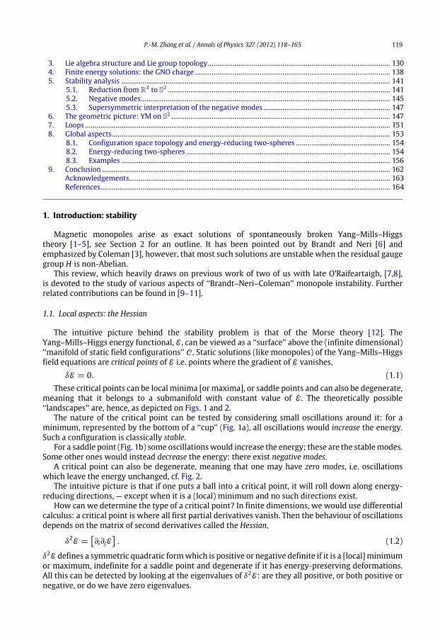
The intuitive picture behind the stability problem is that of the Morse theory [12]. TheYang–Mills–Higgs energy functional, E , can be viewed as a ‘‘surface’’ above the (infinite dimensional)‘‘manifold of static field configurations’’ C. Static solutions (like monopoles) of the Yang–Mills–Higgsfield equations are critical points of E i.e. points where the gradient of E vanishes,
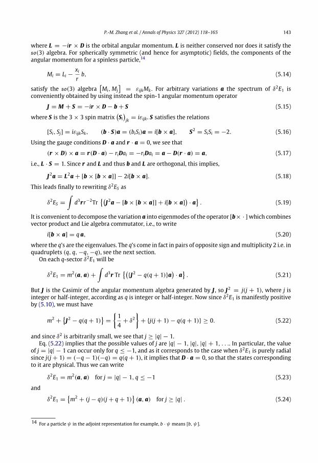
δE = 0. (1.1)These critical points can be local minima [or maxima], or saddle points and can also be degenerate,
meaning that it belongs to a submanifold with constant value of E . The theoretically possible‘‘landscapes’’ are, hence, as depicted on Figs. 1 and 2.
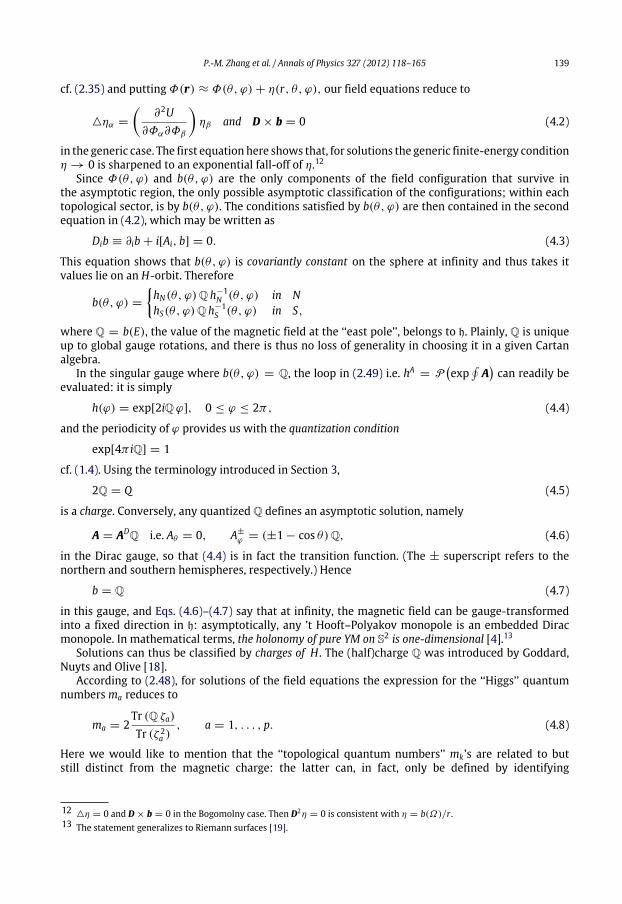
The nature of the critical point can be tested by considering small oscillations around it: for aminimum, represented by the bottom of a ‘‘cup’’ (Fig. 1a), all oscillations would increase the energy.Such a configuration is classically stable.
For a saddle point (Fig. 1b) some oscillationswould increase the energy; these are the stablemodes.Some other ones would instead decrease the energy: there exist negative modes.
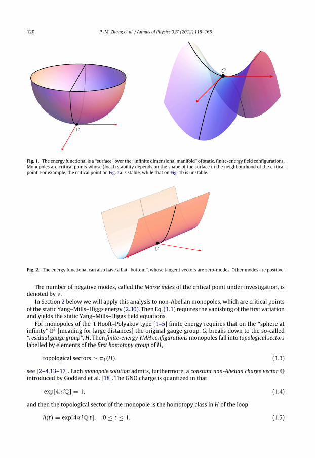
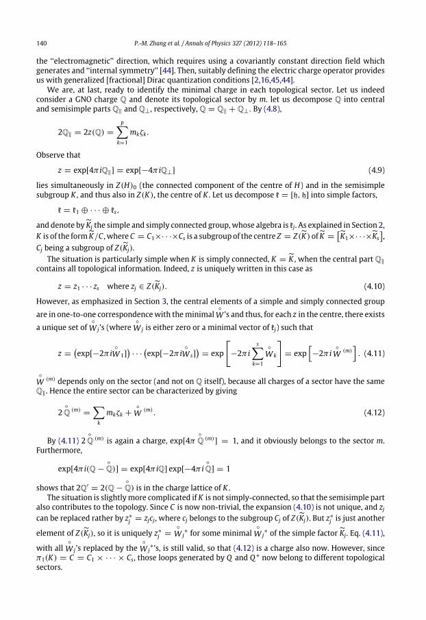
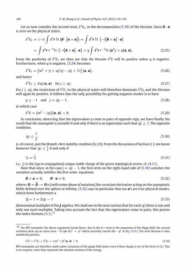
A critical point can also be degenerate, meaning that one may have zero modes, i.e. oscillationswhich leave the energy unchanged, cf. Fig. 2.
The intuitive picture is that if one puts a ball into a critical point, it will roll down along energy-reducing directions, — except when it is a (local) minimum and no such directions exist.
How can we determine the type of a critical point? In finite dimensions, we would use differentialcalculus: a critical point is where all first partial derivatives vanish. Then the behaviour of oscillationsdepends on the matrix of second derivatives called the Hessian,
δ2E =∂i∂jE
. (1.2)
δ2E defines a symmetric quadratic formwhich is positive or negative definite if it is a [local]minimumor maximum, indefinite for a saddle point and degenerate if it has energy-preserving deformations.All this can be detected by looking at the eigenvalues of δ2E : are they all positive, or both positive ornegative, or do we have zero eigenvalues.
120 P.-M. Zhang et al. / Annals of Physics 327 (2012) 118–165
Fig. 1. The energy functional is a ‘‘surface’’ over the ‘‘infinite dimensionalmanifold’’ of static, finite-energy field configurations.Monopoles are critical points whose (local) stability depends on the shape of the surface in the neighbourhood of the criticalpoint. For example, the critical point on Fig. 1a is stable, while that on Fig. 1b is unstable.
Fig. 2. The energy functional can also have a flat ‘‘bottom’’, whose tangent vectors are zero-modes. Other modes are positive.
The number of negative modes, called the Morse index of the critical point under investigation, isdenoted by ν.
In Section 2 below we will apply this analysis to non-Abelian monopoles, which are critical pointsof the static Yang–Mills–Higgs energy (2.30). Then Eq. (1.1) requires the vanishing of the first variationand yields the static Yang–Mills–Higgs field equations.
For monopoles of the ’t Hooft–Polyakov type [1–5] finite energy requires that on the ‘‘sphere atinfinity’’ S2 [meaning for large distances] the original gauge group, G, breaks down to the so-called‘‘residual gauge group’’,H . Then finite-energy YMH configurationsmonopoles fall into topological sectorslabelled by elements of the first homotopy group of H ,
topological sectors ∼ π1(H), (1.3)
see [2–4,13–17]. Each monopole solution admits, furthermore, a constant non-Abelian charge vector Qintroduced by Goddard et al. [18]. The GNO charge is quantized in that
exp[4π iQ] = 1, (1.4)
and then the topological sector of the monopole is the homotopy class in H of the loop
h(t) = exp[4π iQ t], 0 ≤ t ≤ 1. (1.5)
P.-M. Zhang et al. / Annals of Physics 327 (2012) 118–165 121
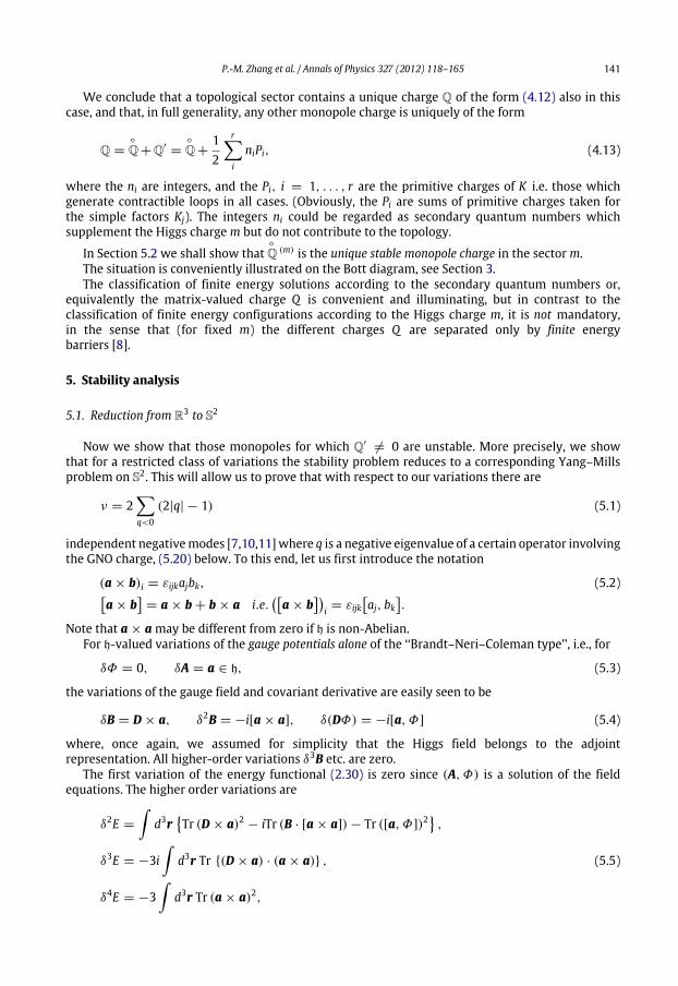
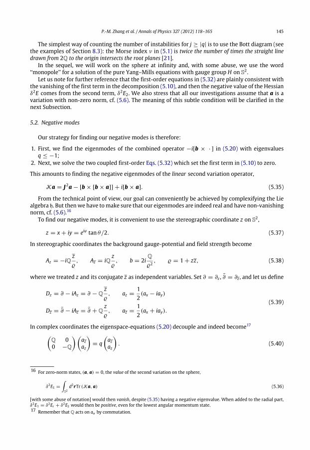
Fig. 3. An elastic string wound around a sphere is in unstable equilibrium and shrinks to a point if it is perturbed.
Then the clue is that for certain type of variations referred to as of the ‘‘Brandt–Neri type’’, thestability problem reduces to that of a pure Yang–Mills theory on the sphere at infinity with group H .1Then the problem boils down to studying the GNO charge, Q. Below we show indeed.
Theorem (Goddard–Olive–Coleman [9,3]). For a ’t Hooft–Polyakov monopole each topological sector
contains exactly one stable charge
Q.
The proof will be deduced from the formula which counts the number of negative modes,
ν = 2q
(2|q| − 1) , (1.6)
where the (half-integer) q are the eigenvalues of definite sign of the GNO charge Q [10,7,8,11]. Itfollows that a monopole is stable if its only eigenvalues are 0 or ±1/2 [6,9,3]. All other monopolescorrespond to saddle points, cf. Fig. 1b.
The number of instabilities, (1.6), is conveniently counted by the so-called Bott diagram [21], seeSection 5.2.
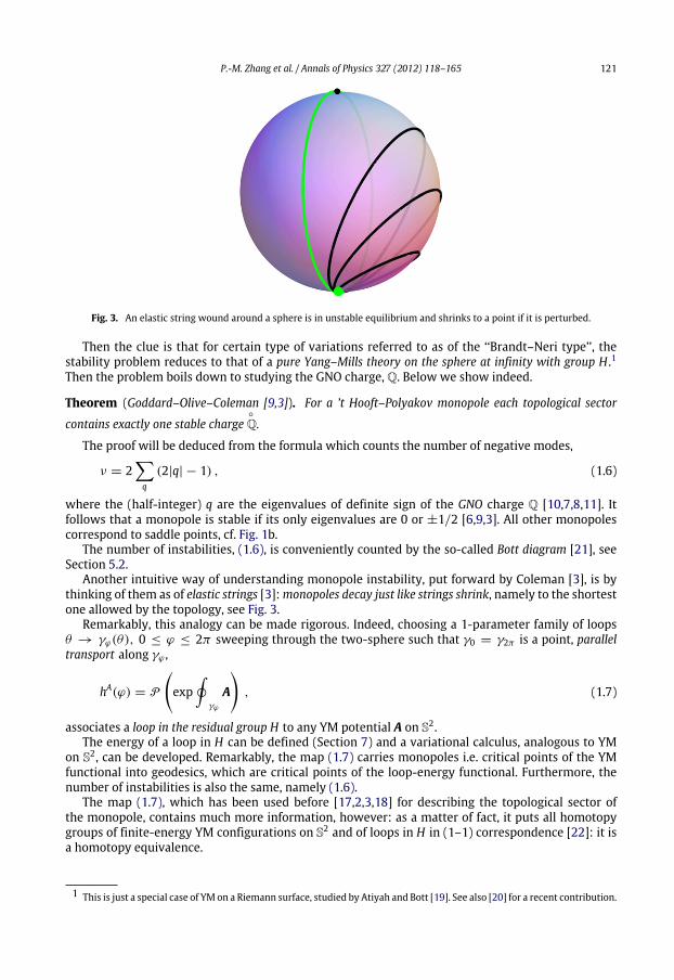
Another intuitive way of understanding monopole instability, put forward by Coleman [3], is bythinking of them as of elastic strings [3]:monopoles decay just like strings shrink, namely to the shortestone allowed by the topology, see Fig. 3.
Remarkably, this analogy can be made rigorous. Indeed, choosing a 1-parameter family of loopsθ → γϕ(θ), 0 ≤ ϕ ≤ 2π sweeping through the two-sphere such that γ0 = γ2π is a point, paralleltransport along γϕ ,
hA(ϕ) = P
exp
γϕ
A
, (1.7)
associates a loop in the residual group H to any YM potential A on S2.The energy of a loop in H can be defined (Section 7) and a variational calculus, analogous to YM
on S2, can be developed. Remarkably, the map (1.7) carries monopoles i.e. critical points of the YMfunctional into geodesics, which are critical points of the loop-energy functional. Furthermore, thenumber of instabilities is also the same, namely (1.6).
The map (1.7), which has been used before [17,2,3,18] for describing the topological sector ofthe monopole, contains much more information, however: as a matter of fact, it puts all homotopygroups of finite-energy YM configurations on S2 and of loops in H in (1–1) correspondence [22]: it isa homotopy equivalence.
1 This is just a special case of YM on a Riemann surface, studied by Atiyah and Bott [19]. See also [20] for a recent contribution.
122 P.-M. Zhang et al. / Annals of Physics 327 (2012) 118–165
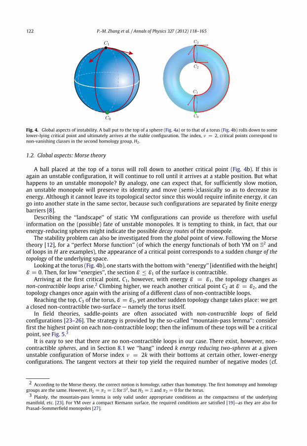
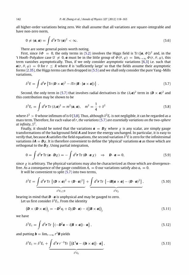
Fig. 4. Global aspects of instability. A ball put to the top of a sphere (Fig. 4a) or to that of a torus (Fig. 4b) rolls down to somelower-lying critical point and ultimately arrives at the stable configuration. The index, ν = 2, critical points correspond tonon-vanishing classes in the second homology group, H2 .
1.2. Global aspects: Morse theory
A ball placed at the top of a torus will roll down to another critical point (Fig. 4b). If this isagain an unstable configuration, it will continue to roll until it arrives at a stable position. But whathappens to an unstable monopole? By analogy, one can expect that, for sufficiently slow motion,an unstable monopole will preserve its identity and move (semi-)classically so as to decrease itsenergy. Although it cannot leave its topological sector since this would require infinite energy, it cango into another state in the same sector, because such configurations are separated by finite energybarriers [8].
Describing the ‘‘landscape’’ of static YM configurations can provide us therefore with usefulinformation on the (possible) fate of unstable monopoles. It is tempting to think, in fact, that ourenergy-reducing spheres might indicate the possible decay routes of the monopole.
The stability problem can also be investigated from the global point of view. Following the Morsetheory [12], for a ‘‘perfect Morse function’’ (of which the energy functionals of both YM on S2 andof loops in H are examples), the appearance of a critical point corresponds to a sudden change of thetopology of the underlying space.
Looking at the torus (Fig. 4b), one starts with the bottomwith ‘‘energy’’ [identifiedwith the height]E = 0. Then, for low ‘‘energies’’, the section E ≤ E1 of the surface is contractible.
Arriving at the first critical point, C1, however, with energy E = E1, the topology changes asnon-contractible loops arise.2 Climbing higher, we reach another critical point C2 at E = E2, and thetopology changes once again with the arising of a different class of non-contractible loops.
Reaching the top, C3 of the torus, E = E3, yet another sudden topology change takes place: we geta closed non-contractible two-surface — namely the torus itself.
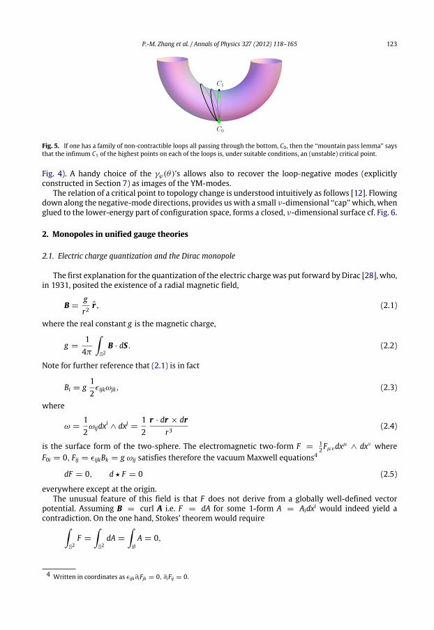
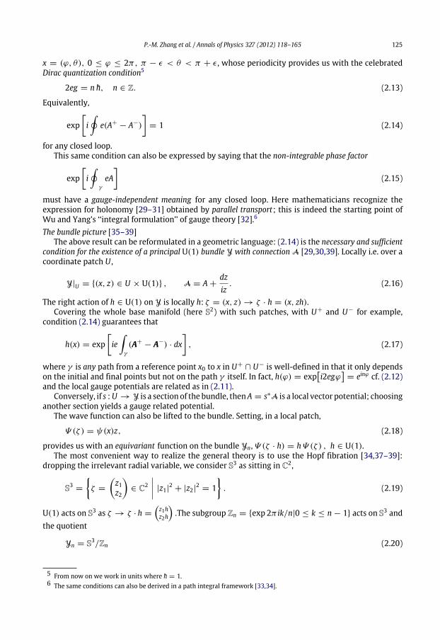
In field theories, saddle-points are often associated with non-contractible loops of fieldconfigurations [23–26]. The strategy is provided by the so-called ‘‘mountain-pass lemma’’: considerfirst the highest point on each non-contractible loop; then the infimum of these tops will be a criticalpoint, see Fig. 5.3
It is easy to see that there are no non-contractible loops in our case. There exist, however, non-contractible spheres, and in Section 8.1 we ‘‘hang’’ indeed k energy reducing two-spheres at a givenunstable configuration of Morse index ν = 2k with their bottoms at certain other, lower-energyconfigurations. The tangent vectors at their top yield the required number of negative modes (cf.
2 According to the Morse theory, the correct notion is homology, rather than homotopy. The first homotopy and homologygroups are the same. However, H2 = π2 = Z for S2 , but H2 = Z and π2 = 0 for the torus.3 Plainly, the mountain-pass lemma is only valid under appropriate conditions as the compactness of the underlying
manifold, etc. [23]. For YM over a compact Riemann surface, the required conditions are satisfied [19]—as they are also forPrasad–Sommerfield monopoles [27].
P.-M. Zhang et al. / Annals of Physics 327 (2012) 118–165 123
Fig. 5. If one has a family of non-contractible loops all passing through the bottom, C0 , then the ‘‘mountain pass lemma’’ saysthat the infimum C1 of the highest points on each of the loops is, under suitable conditions, an (unstable) critical point.
Fig. 4). A handy choice of the γϕ(θ)’s allows also to recover the loop-negative modes (explicitlyconstructed in Section 7) as images of the YM-modes.
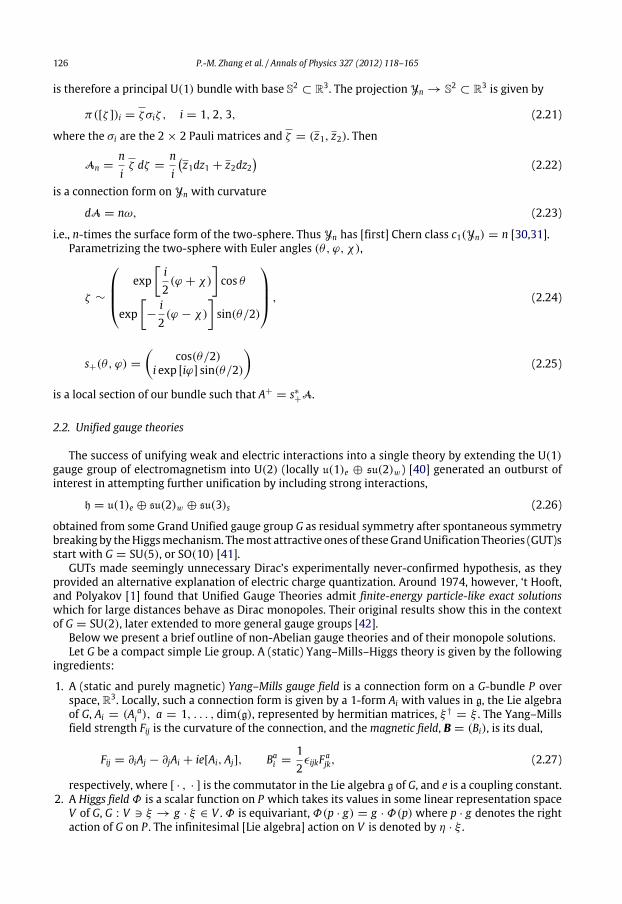
The relation of a critical point to topology change is understood intuitively as follows [12]. Flowingdown along the negative-mode directions, provides uswith a small ν-dimensional ‘‘cap’’ which, whenglued to the lower-energy part of configuration space, forms a closed, ν-dimensional surface cf. Fig. 6.
2. Monopoles in unified gauge theories
2.1. Electric charge quantization and the Dirac monopole
The first explanation for the quantization of the electric chargewas put forward by Dirac [28], who,in 1931, posited the existence of a radial magnetic field,
B =gr2
r, (2.1)
where the real constant g is the magnetic charge,
g =14π
S2
B · dS. (2.2)
Note for further reference that (2.1) is in fact
Bi = g12ϵijkωjk, (2.3)
where
ω =12ωijdxi ∧ dxj =
12
r · dr × drr3
(2.4)
is the surface form of the two-sphere. The electromagnetic two-form F = 12Fµνdx
µ∧ dxν where
F0i = 0, Fij = ϵijkBk = g ωij satisfies therefore the vacuumMaxwell equations4
dF = 0, d ⋆ F = 0 (2.5)
everywhere except at the origin.The unusual feature of this field is that F does not derive from a globally well-defined vector
potential. Assuming B = curl A i.e. F = dA for some 1-form A = Aidxi would indeed yield acontradiction. On the one hand, Stokes’ theorem would require
S2F =
S2
dA =∅
A = 0,
4 Written in coordinates as ϵijk∂iFjk = 0, ∂iFij = 0.
124 P.-M. Zhang et al. / Annals of Physics 327 (2012) 118–165
Fig. 6. Flowing down from a critical point of Morse index ν along the negative-mode directions yields a ν-dimensional ‘‘cap’’which, when glued to the lower-energy part of the configuration space, forms a closed ν-dimensional surface which generatesa non-trivial homology class in Hν .
since the closed two-surface S2 has no boundary. Direct evaluation yields, however,S2
F = 4πg = 0,
a contradiction.The clue of Dirac has been that this fact has no physical consequence provided the electric and
magnetic charges, e and g , satisfy a suitable quantization condition.At the purely classical level, the vector potential plays no role. It does play a role at the quantum
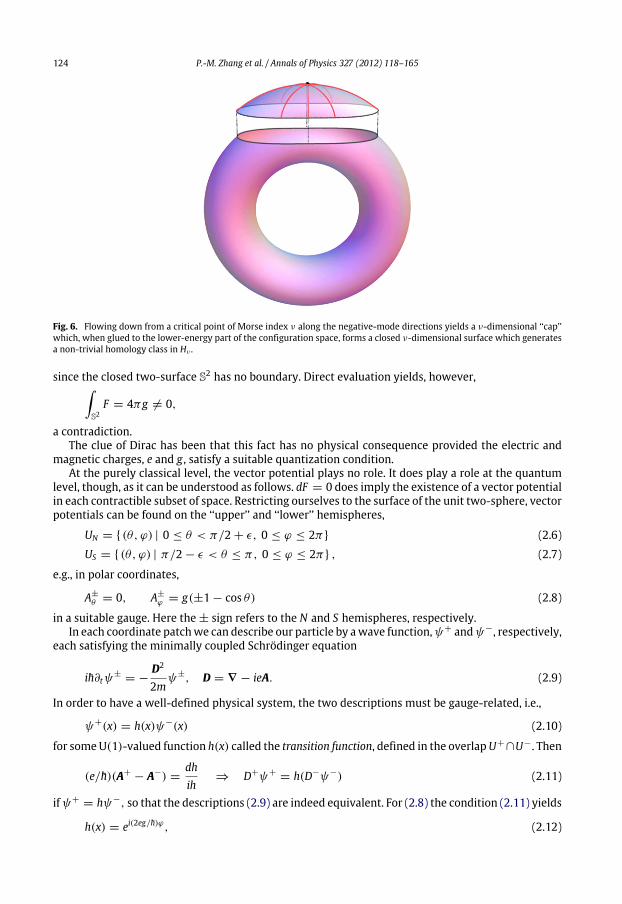
level, though, as it can be understood as follows. dF = 0 does imply the existence of a vector potentialin each contractible subset of space. Restricting ourselves to the surface of the unit two-sphere, vectorpotentials can be found on the ‘‘upper’’ and ‘‘lower’’ hemispheres,
UN = (θ, ϕ) | 0 ≤ θ < π/2+ ϵ, 0 ≤ ϕ ≤ 2π (2.6)
US = (θ, ϕ) | π/2− ϵ < θ ≤ π, 0 ≤ ϕ ≤ 2π , (2.7)
e.g., in polar coordinates,
A±θ = 0, A±ϕ = g(±1− cos θ) (2.8)
in a suitable gauge. Here the± sign refers to the N and S hemispheres, respectively.In each coordinate patchwe can describe our particle by awave function,ψ+ andψ−, respectively,
each satisfying the minimally coupled Schrödinger equation
ih∂tψ± = −D2
2mψ±, D = ∇ − ieA. (2.9)
In order to have a well-defined physical system, the two descriptions must be gauge-related, i.e.,
ψ+(x) = h(x)ψ−(x) (2.10)
for someU(1)-valued function h(x) called the transition function, defined in the overlapU+∩U−. Then
(e/h)(A+ − A−) =dhih
⇒ D+ψ+ = h(D−ψ−) (2.11)
ifψ+ = hψ−, so that the descriptions (2.9) are indeed equivalent. For (2.8) the condition (2.11) yields
h(x) = ei(2eg/h)ϕ, (2.12)
P.-M. Zhang et al. / Annals of Physics 327 (2012) 118–165 125
x = (ϕ, θ), 0 ≤ ϕ ≤ 2π, π − ϵ < θ < π + ϵ, whose periodicity provides us with the celebratedDirac quantization condition5
2eg = n h, n ∈ Z. (2.13)
Equivalently,
expi
e(A+ − A−)= 1 (2.14)
for any closed loop.This same condition can also be expressed by saying that the non-integrable phase factor
expi
γ
eA
(2.15)
must have a gauge-independent meaning for any closed loop. Here mathematicians recognize theexpression for holonomy [29–31] obtained by parallel transport; this is indeed the starting point ofWu and Yang’s ‘‘integral formulation’’ of gauge theory [32].6
The bundle picture [35–39]The above result can be reformulated in a geometric language: (2.14) is the necessary and sufficient
condition for the existence of a principal U(1) bundle Y with connection A [29,30,39]. Locally i.e. over acoordinate patch U ,
Y|U = (x, z) ∈ U × U(1) , A = A+dziz. (2.16)
The right action of h ∈ U(1) on Y is locally h: ζ = (x, z)→ ζ · h = (x, zh).Covering the whole base manifold (here S2) with such patches, with U+ and U− for example,
condition (2.14) guarantees that
h(x) = expieγ
(A+ − A−) · dx, (2.17)
where γ is any path from a reference point x0 to x in U+ ∩ U− is well-defined in that it only dependson the initial and final points but not on the path γ itself. In fact, h(ϕ) = exp
i2egϕ
= einϕ cf. (2.12)
and the local gauge potentials are related as in (2.11).Conversely, if s :U → Y is a section of the bundle, thenA = s∗A is a local vector potential; choosing
another section yields a gauge related potential.The wave function can also be lifted to the bundle. Setting, in a local patch,
Ψ (ζ ) = ψ(x)z, (2.18)
provides us with an equivariant function on the bundle Yn, Ψ (ζ · h) = hΨ (ζ ) , h ∈ U(1).The most convenient way to realize the general theory is to use the Hopf fibration [34,37–39]:
dropping the irrelevant radial variable, we consider S3 as sitting in C2,
S3=
ζ =
z1z2
∈ C2
|z1|2 + |z2|2 = 1. (2.19)
U(1) acts on S3 as ζ → ζ · h =z1hz2h
.The subgroup Zn = exp 2π ik/n|0 ≤ k ≤ n− 1 acts on S3 and
the quotient
Yn = S3/Zn (2.20)
5 From now on we work in units where h = 1.6 The same conditions can also be derived in a path integral framework [33,34].
126 P.-M. Zhang et al. / Annals of Physics 327 (2012) 118–165
is therefore a principal U(1) bundle with base S2⊂ R3. The projection Yn → S2
⊂ R3 is given by
π([ζ ])i = ζσiζ , i = 1, 2, 3, (2.21)
where the σi are the 2× 2 Pauli matrices and ζ = (z1, z2). Then
An =niζ dζ =
ni
z1dz1 + z2dz2
(2.22)
is a connection form on Yn with curvature
dA = nω, (2.23)
i.e., n-times the surface form of the two-sphere. Thus Yn has [first] Chern class c1(Yn) = n [30,31].Parametrizing the two-sphere with Euler angles (θ, ϕ, χ),
ζ ∼
expi2(ϕ + χ)
cos θ
exp−
i2(ϕ − χ)
sin(θ/2)
, (2.24)
s+(θ, ϕ) =
cos(θ/2)i exp [iϕ] sin(θ/2)
(2.25)
is a local section of our bundle such that A+ = s∗+A.
2.2. Unified gauge theories
The success of unifying weak and electric interactions into a single theory by extending the U(1)gauge group of electromagnetism into U(2) (locally u(1)e ⊕ su(2)w) [40] generated an outburst ofinterest in attempting further unification by including strong interactions,
h = u(1)e ⊕ su(2)w ⊕ su(3)s (2.26)
obtained from some Grand Unified gauge group G as residual symmetry after spontaneous symmetrybreaking by theHiggsmechanism. Themost attractive ones of theseGrandUnification Theories (GUT)sstart with G = SU(5), or SO(10) [41].
GUTs made seemingly unnecessary Dirac’s experimentally never-confirmed hypothesis, as theyprovided an alternative explanation of electric charge quantization. Around 1974, however, ‘t Hooft,and Polyakov [1] found that Unified Gauge Theories admit finite-energy particle-like exact solutionswhich for large distances behave as Dirac monopoles. Their original results show this in the contextof G = SU(2), later extended to more general gauge groups [42].
Below we present a brief outline of non-Abelian gauge theories and of their monopole solutions.Let G be a compact simple Lie group. A (static) Yang–Mills–Higgs theory is given by the following
ingredients:
1. A (static and purely magnetic) Yang–Mills gauge field is a connection form on a G-bundle P overspace, R3. Locally, such a connection form is given by a 1-form Ai with values in g, the Lie algebraof G, Ai = (A a
i ), a = 1, . . . , dim(g), represented by hermitian matrices, ξ Ď = ξ . The Yang–Millsfield strength Fij is the curvature of the connection, and themagnetic field, B = (Bi), is its dual,
Fij = ∂iAj − ∂jAi + ie[Ai, Aj], Bai =
12ϵijkF a
jk, (2.27)
respectively, where [ · , · ] is the commutator in the Lie algebra g of G, and e is a coupling constant.2. A Higgs fieldΦ is a scalar function on P which takes its values in some linear representation space
V of G, G : V ∋ ξ → g · ξ ∈ V .Φ is equivariant,Φ(p · g) = g ·Φ(p)where p · g denotes the rightaction of G on P . The infinitesimal [Lie algebra] action on V is denoted by η · ξ .
P.-M. Zhang et al. / Annals of Physics 327 (2012) 118–165 127
A frequent choice is V = g the Lie algebra, and then the actions are the adjoint ones,
Adg(ξ) = g−1ξg and adη(ξ) = −i[η, ξ ], (2.28)
respectively. In what follows, we shall mostly consider the adjoint case, V = g, when Φ =(Φa), a = 1, . . . , dim g.
3. A Higgs potential U is a non-negative invariant function on V , U ≥ 0, U(g · Φ) = U(Φ). Then theabsolute minima of U(Φ) lie in some orbitO ≃ G ·Φ0 of G. This assumption that G acts transitivelymeans the orbit is identified with O ≃ G/H where H is the stability subgroup ofΦ0, H ·Φ0 = Φ0.In the physical context H will be referred to as the residual group.
In the simplest case G = SU(2), the most frequent choice is
U(Φ) =λ
4
1− ∥Φ∥2
2(2.29)
where, for an adjoint Higgs, ∥Φ∥2 = Tr (Φ2) = ΦaΦa.
A (static and purely magnetic) finite-energy Yang–Mills–Higgs configuration is such that the energy,
E =
R3
12Tr (B2)+
12Tr (DΦ)2 + U(Φ)
d3r (2.30)
is finite. HereDiΦ = ∂iΦ + ie[Ai,Φ] (2.31)
is the covariant derivative where, for simplicity, we restricted ourselves to an adjoint Higgs field.The energy (2.30) is invariant w.r.t. gauge transformations,
Aj → gAjg−1 −ieg∂jg−1, Φ → g · Φ = gΦg−1, (2.32)
which imply that B→ gBg−1, DΦ → g · DΦ .Monopoles arise as finite-energy solutions of the associated variational Yang–Mills–Higgs
equations [1–4]. Restricting ourselves, for notational simplicity, to the adjoint case, the field equationsread
D× B = ie[DΦ,Φ], (2.33)
D2Φ =δUδΦ. (2.34)
2.3. Finite-energy configurations
In this subsection we shall not require that the fields satisfy the field equations, but only that theybe of finite energy, i.e., such that the integral in (2.30) converges. One reason for this is to emphasizethat themost important spontaneous symmetry breakdown, namely that of theHiggs potential, comesfrom the finite energy and not from the field equations.
We shall consider the three terms in (2.30) in turn. It will be convenient to use the radial gauger · A = 0.Pure gauge term Tr B2
For sufficiently smooth gauge fields the finite energy condition imposed by this term is, with someabuse of notation,
A(r)→A(θ, ϕ)
r, B(r)→
b(θ, ϕ)r2
=b(θ, ϕ)
r2r, (2.35)
where θ, ϕ denote the polar angles.7 Note that (2.35) only involves the gauge field.
7 A = (Aai ) is a Lie algebra valued vector potential with a and i Lie algebra and resp. space indices. Similarly, B = (Ba
i ) andb = (bai ) are Lie algebra valued vectors. The last equality in (2.35) decomposes the Lie algebra valued asymptotic magnetic fieldb into a Lie algebra-valued scalar b(θ, ϕ)/r2 times the radial direction r = r/r[4].
128 P.-M. Zhang et al. / Annals of Physics 327 (2012) 118–165
Higgs potential U(Φ)The finite energy condition for this term is r2 U(Φ) ∼ 0 as r →∞. A necessary condition for this
is that U → 0. But U ≥ 0 is assumed to be a Higgs potential i.e. one whose minima lie on some non-trivial group orbit G/H , where H is an appropriate subgroup of G, called the ‘‘residual gauge group’’.
At large distances the Higgs field takes therefore its values in the orbit G/H and may only dependnon-trivially on the polar angles: Φ(r, θ, ϕ)→ Φ(θ, ϕ) as r →∞ (again with some abuse of nota-tion). Then the asymptotic values ofΦ define a map of ‘‘the two-sphere at infinity’’ S2
∞parametrized
with the polar angles (θ, ϕ) into the orbit G/H ,
Φ : S2∞→ G/H. (2.36)
The asymptotic values of the Higgs field define thus a homotopy class in π2(G/H). Since this classcannot be changed by smooth deformations, the ‘‘manifold’’ of finite-energy configurations splits intotopological sectors, labelled by π2(G/H) [2–4,13–16].
As
π2(G/H) ≃ π1(H) (2.37)
for any [simply connected] Lie groupG, the topological sectors can be labelled also by classes inπ1(H);the first homotopy group of the residual group. Indeed, on the upper and respectively on the lowerhemispheres N and S of S2,
Φ(θ, ϕ) =
gN(θ, ϕ)Φ(E) in NgS(θ, ϕ)Φ(E) in S,
where (the ‘‘east pole’’) E is an arbitrary point in the overlap.
h(ϕ) = g−1N (ϕ)gS(ϕ) (2.38)
where ϕ is the polar angle on the equator of S2 is a loop in H which represents the topological sector.(2.38) is contractible in G [3,2].
For any compact and connected Lie group H , π1(H) is Abelian so has a free part and a torsion part
π1(H) = Zp⊕ T,
where p is the dimension of the centre of h and T is a finite Abelian group [16], see Section 3 below.In fact, T is isomorphic to π1(K)where K is the compact and semisimple subgroup of H generated byk = [h, h].
The free partZp provides uswith p integer ‘‘quantum’’ numbersm1, . . . ,mp. They can be calculatedas surface integrals as follows. To the asymptotic physical Higgs field Φ in any representation and toeach vector ζ from the centre of the Lie algebra h, we can associate an auxiliary adjoint ‘‘Higgs’’ fieldΨ defined by
Ψζ (θ, ϕ) = g(θ, ϕ) ζ g−1(θ, ϕ), (2.39)
where g(θ, ϕ) is any of those ‘‘lifts’’ in (2.38). Although the lifts in (2.38) are ambiguous, ghworks alsoif g does so, provided h belongs to H , Ψ (θ, ϕ) is well-defined, because ζ belongs to the centre of h.The projection of the charge lattice ΓQ into the centre is a p-dimensional lattice there, generated overthe integers by p vectors ζ1, . . . , ζp,
ζ =
pi=1
niζi, ni ∈ Z. (2.40)
Note that the ζa are not in general charges themselves, nor are they normalized.The above construction associates then an adjoint ‘‘Higgs’’ field Ψa to each generator ζa, and the
quantum numbersma are calculated according to [13,16]
ma =1
4π |ζa|3
S2
BaΨa,
∂θΨa, ∂ϕΨa
dϕ ∧ dθ, a = 1, . . . , p, (2.41)
P.-M. Zhang et al. / Annals of Physics 327 (2012) 118–165 129
where Ψa is the auxiliary Higgs field (2.39) for ζ = ζa, Ba is a multiple (αa, αa)B/2 of the Killing formB of G and αa is a simple root determined by ζa.
The mathematical content of this theorem is that the free part of π2(O) has the same rank as thedimension of the second de Rham cohomology,
π2(O)⊗ R ≃ H2(O)⊗ R ≃ H2dR(O), (2.42)
which is in turn generated by the pull-backs to the orbitO ≃ (G/H) of the canonical symplectic formsof the coadjoint orbits of the basis vectors ζk [14–16].
For a matrix group, B can be replaced by the trace, for example, for G = SU(n)we have
B(η, ζ ) = 2n Tr(ηζ ) and (αk, αk) = 2 (2.43)
for all simple root αk. The charge (2.41) is in fact the same as
ma =1
2π |ζa|
S2Ψ ∗a Ωa, (2.44)
where Ωa is the canonical symplectic form of the coadjoint orbit Oa = Ad∗G ζa identified with anadjoint orbit using (αa, αa)B/2. T, the finite part of π1(H), has no similar expression.
The physically most relevant case is when T = 0 and the sectors are described by a single integerquantum number m. This happens when the Lie algebra h of H has a 1-dimensional centre generatedby a single vector ζ and the semisimple subgroup K is simply connected.
Another case of [mostly pedagogical] interest [3] is H = SO(3), for which p = 0 and T = Z2.The homotopy classification is not merely convenient, but is mandatory in that the classes are
separated by infinite energy barriers [8].Note that since not only U → 0 but r3U → 0 one has [8],
Φ(r)→ Φ(θ, ϕ)+ η(r, θ, ϕ), (2.45)
where rη(r, θ, ϕ)→ 0 as r →∞.8We stress that monopole topology only depends on the Higgs field and not on the gauge field
[13,16].The cross-term (DΦ)2
This final term involves both Φ and A and it hence provides the connection between the[asymptotic] Higgs field Φ(θ, ϕ) and the gauge field b(θ, ϕ) and thus puts a topological constrainton the gauge field. This constraint may be expressed as a quantization condition as follows: the finiteenergy condition is easily seen to be r2(DΦ)2 → 0 and thusΦ is covariantly constant on S2
∞,
DiΦ ≡ ∂iΦ + iAi · Φ = 0 (2.47)
[and hence also DiΨ ≡ ∂iΨ + i[Ai,Φ] = 0] where, with some abuse of notations, we switched tofields and covariant derivative on the sphere at infinity involving their asymptotic values.
Then the topological quantum numbersma can be expressed as [16]
ma =1
2π |ζ |
S2
dS Tr (Ψab), a = 1, . . . , p. (2.48)
Eq. (2.48) shows that in general it is not the gauge field B itself, but only its projection onto thecentre that is quantized. Note that the quantization of
Tr (Ψab) is again mandatory, since the value
of Tr (ΨaB) cannot be changed without violating at least one of the finite-energy conditions r2V → 0or r3(DΦ)2 → 0 and thus passing through an infinite energy barrier.
8 A notable exception to this observation is the Bogomolny–Prasad–Sommerfield (BPS) limit of vanishing potential, U = 0,for which the Bogomolny condition B = DΦ implies [27] that
Φ(r)→ Φ(θ, ϕ)+b(θ, ϕ)
r+ O(1/r2) as r →∞. (2.46)
130 P.-M. Zhang et al. / Annals of Physics 327 (2012) 118–165
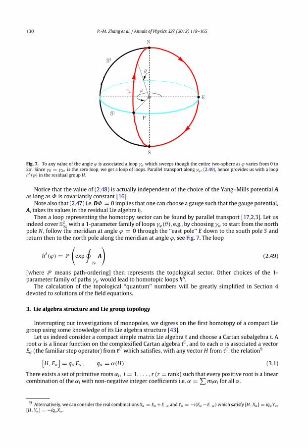
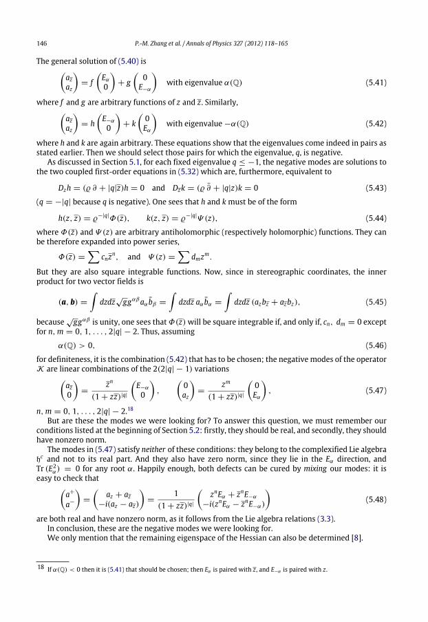
Fig. 7. To any value of the angle ϕ is associated a loop γϕ which sweeps though the entire two-sphere as ϕ varies from 0 to2π . Since γ0 = γ2π is the zero loop, we get a loop of loops. Parallel transport along γϕ , (2.49), hence provides us with a loophA(ϕ) in the residual group H .
Notice that the value of (2.48) is actually independent of the choice of the Yang–Mills potential Aas long asΦ is covariantly constant [16].
Note also that (2.47) i.e.DΦ = 0 implies that one can choose a gauge such that the gauge potential,A, takes its values in the residual Lie algebra h.
Then a loop representing the homotopy sector can be found by parallel transport [17,2,3]. Let usindeed cover S2
∞with a 1-parameter family of loops γϕ(θ), e.g., by choosing γϕ to start from the north
pole N , follow the meridian at angle ϕ = 0 through the ‘‘east pole’’ E down to the south pole S andreturn then to the north pole along the meridian at angle ϕ, see Fig. 7. The loop
hA(ϕ) = P
exp
γϕ
A
(2.49)
[where P means path-ordering] then represents the topological sector. Other choices of the 1-parameter family of paths γϕ would lead to homotopic loops hA.
The calculation of the topological ‘‘quantum’’ numbers will be greatly simplified in Section 4devoted to solutions of the field equations.
3. Lie algebra structure and Lie group topology
Interrupting our investigations of monopoles, we digress on the first homotopy of a compact Liegroup using some knowledge of its Lie algebra structure [43].
Let us indeed consider a compact simple matrix Lie algebra k and choose a Cartan subalgebra t. Aroot α is a linear function on the complexified Cartan algebra tC, and to each α is associated a vectorEα (the familiar step operator) from kC which satisfies, with any vector H from tC, the relation9
H, Eα= qα Eα , qα = α(H). (3.1)
There exists a set of primitive roots αi, i = 1, . . . , r (r = rank) such that every positive root is a linearcombination of the αi with non-negative integer coefficients i.e. α =
miαi for all α.
9 Alternatively, we can consider the real combinations Xα = Eα+E−α and Yα = −i(Eα−E−α)which satisfy [H, Xα] = iqαYα ,[H, Yα] = −iqαXα .
P.-M. Zhang et al. / Annals of Physics 327 (2012) 118–165 131
If α is a root, let us define the vector Hα in tC by
α(X) = Tr (HαX). (3.2)
With suitable normalization we have
(Eα)Ď = E−α Tr (Eα, E−α) = 1, [Eα, E−α] = Hα . (3.3)
For each root α, Hα and the E±α ’s form therefore [complexified] so(3)c subalgebras of k.Lattice of primitive charges, ΓP
The primitive charges Pi are defined by
Pi =2Hi
Tr (H2i )
where Hi = Hαi . (3.4)
The primitive charges form a natural (non-orthogonal) basis for the Cartan algebra and by adding theEα ’s we get a basis for the Lie algebra kC. The integer combinations
i niPi of the primitive charges
form an r-dimensional lattice ΓP sitting in the Cartan algebra.Co-weight lattice, ΓW
Let us introduce next another basis for the Cartan algebra with elements Wi dual to the primitiveroots,
αi(Wj) = Tr (HiWj) = δij, i, j = 1, . . . , r. (3.5)
Comparing (3.5) with the conventional definition [22] of primitiveweights, for which there is an extrafactor (αi, αi)/2 in front of the δij, one sees that the Wi’s are just re-scaled weights. They are calledco-weights [9] and it is evident that they can be normalized so as to coincide with the conventionalweights (by choosing (αi, αi) = 2) for all groups whose roots are all of the same length, i.e. all groupsexcept Sp(2r), SO(2r + 1), G2 and F4.
The integer combinations
miWi form another lattice we denote by ΓW .Since α(Pi) is always an integer, theW -lattice actually contains the primitive-charge lattice,
ΓP ⊂ ΓW . (3.6)
The root planes of k are those vectors X in the Cartan algebra for which α(X) is an integer, i.e., thosevectors which have integer eigenvalues in the adjoint representation. The root planes intersect in thepoints of theW -lattice.
Let us stress that the weights and primitive charges only depend on the Lie algebra, and not on itsglobal group structure. Now we define a third lattice, which does depend on the global structure.Charge lattice, ΓQ
Denote by K the (unique) compact, simple, and simply connected Lie group generated by k. Anyother group K whose Lie algebra is k is then of the form K = K/C , where C is a subgroup of Z = Z(K),the centre ofK . Z is finite and Abelian, so C is always discrete. SinceK is simply connected, C is justπ1(K), the first homotopy group of K .
The primitive charges satisfy the quantization conditionexp2π iPi = 1 (exponential inK ) and thusalso in any representation of K i.e. in any other group K with the same Lie algebra. For any set ni,i = 1, . . . , r of integers,
exp2π it
niPi
, 0 ≤ t ≤ 1, (3.7)
(exponential in K ) is hence a contractible loop in all representations. Since any loop is homotopic toone of the form exp 2π itP, 0 ≤ t ≤ 1 where P is a constant vector in k, we conclude that the latticeΓP consists of the generators of contractible loops.
More generally, let us fix a group K (i.e., a representation ofK ) and define a general charge Q to bean element of the Cartan algebra such that
exp[2π iQ ] = 1 in K , (3.8)
132 P.-M. Zhang et al. / Annals of Physics 327 (2012) 118–165
so that exp[2π itQ ], 0 ≤ t ≤ 1, is a loop, and any loop is homotopic to one of this form, as saidabove.10
ThoseQ ’s satisfying the quantization condition (3.8) [with ‘‘exp’’meant inK ] form the charge latticedenoted by ΓQ . It depends on the global structure, but it always contains ΓP , the lattice of contractibleloops.ΓP andΓQ are actually the same for the covering groupK .More generally, two loops exp[2π itQ1]
and exp[2π itQ2] are homotopic if and only if Q1 − Q2 belongs to ΓP , so that π1(K) is the quotient ofthe lattices ΓQ and ΓP .
On the other hand, the charge lattice ΓQ is contained in the W -lattice ΓW , because for any root αand charge Q ,
1 =exp[2π iEα]
exp[2π iQ ]
exp[−2π iEα]
= exp
2π i
e2π iEαQe−2π iEα
= e2π iα(Q ) exp[2π iEα] = e2π iα(Q ),
and hence α(Q ) is an integer.The three lattices introduced above satisfy therefore the relation
ΓP ⊂ ΓQ ⊂ ΓW . (3.9)
In general,exp[2π iWj] is not unity in the fundamental representation ofK . It is however unity in theadjoint representation.exp[2π iWj] = zj (3.10)
belongs therefore to the centre ofK . Hence the two latticesΓP andΓW coincide for the adjoint group.11On the other hand, the correspondence W ∼ z can be made one-to-one by restricting the W ’s
to those ones,
W ’s (say), for which the geodesicsexp[2π i W t] (0 ≤ t ≤ 1) are geodesics of minimallength from1 to z i.e. forwhich TrW 2 isminimal for each z ∈ Z . (Since theweightsW are all of different
lengths and are unique up to conjugation, the
W for each z ∈ Z will be unique up to conjugation). Suchco-weights
W are calledminimal vectors orminimal co-weights [9], and a simple intuitive way to findthem (indeed an alternative way to introduce them) is as follows.
In terms of roots α, the 0,±1 property (which will be crucial for the stability investigation [6,3,9])may be expressed by saying that for any positive root α,
α(
W ) = 0,±1. (3.11)
If one considers in particular the expansion of the highest root θ in terms of the primitive roots αi,θ =
hiαi, hi ≥ 1, and applies (3.11), one sees that αi(
W ) can be non-zero for only one primitive
root,
αi (say), and that the coefficient
hi of
αi must be unity [9,7]. This result provides us with a simple,practical method of identifying the
W ’s in terms of primitive weights, namely as the duals to thoseprimitive roots for which the coefficient in the expansion of θ is unity [9,7].
The W -lattice containing the charge lattice, together with the root planes, form the Bottdiagram [21] of K . Those vectors satisfying the ‘‘minimality’’ or ‘‘stability’’ condition (3.11) either liein the centre or belong to the root plane which is the closest to the centre.
Magnetic monopoles belong to topological classes, described by the first homotopy group of theresidual symmetry group, H . Now for any compact and connected Lie group H , π1(H) is of the form
π1(H) = Zp⊕ T, (3.12)
10 Warning: by historical reasons, there is a slight discrepancy between the mathematical formalism adopted here and thephysical one in Section 4: a ‘‘GNO charge’’, Q, is the half of ‘‘charge’’ noted Q in this section, 2Q = Q . This comes from the 2πresp. 4π between the definitions (3.8) and (1.4).11 Note that the correspondence Wj ∼ zj is one-to-one only for SU(N) since for the other groups there are rW ’s but less thanr elements in the centre.
P.-M. Zhang et al. / Annals of Physics 327 (2012) 118–165 133
where p is the dimension of the centre Z ofH andT is a finite Abelian group [16]. In fact,T is isomorphicto π1(K), where K is the compact and semisimple subgroup ofH generated by k = [h, h]. The free partZp provides us with p integer ‘‘quantum’’ numbersm1, . . . ,mp.
On the other hand, (twice) the ‘‘GNO charge’’ of a monopole mentioned in the previous section isa ‘‘charge’’ in the sense defined here, and belongs therefore to the charge lattice ΓQ .
The projections of the charge lattice ΓQ into the centre is a p-dimensional lattice there, generatedover the integers by p vectors Ψ1, . . .Ψp. The simplest and physically most relevant case is when thehomotopy group π1(H) is described by a single integer quantum number m. This happens when theLie algebra h of H has a 1-dimensional centre generated by a single vector Ψ and the semisimplesubgroup K is simply connected.
Now the fundamental statement in Refs. [3,9] says
Theorem (Goddard–Olive–Coleman). For any compact Lie group H, each topological sector contains an
[up to conjugation] unique stable charge
Q .
Curiously, Coleman [3], stated this theorem generally, but only proved it for H = SO(3), whichappears spurious. Incredibly, his proof already contains the germ of the general proof [7,8], though.The strategy is to reduce the problem to the adjoint group by factoring out the centre; this leaves uswith the semisimple part alone, k. Now any semisimple Lie algebra can be decomposed into a sum ofsimple Lie algebras, k = k1 + · · · + ks, and the minimal charge – which, for a simple adjoint group, isthe same as a minimal co-weight – can be checked by inspection using the list of simple Lie algebras,see e.g. [43].
The examples below may help to understand the general theory outlined above.
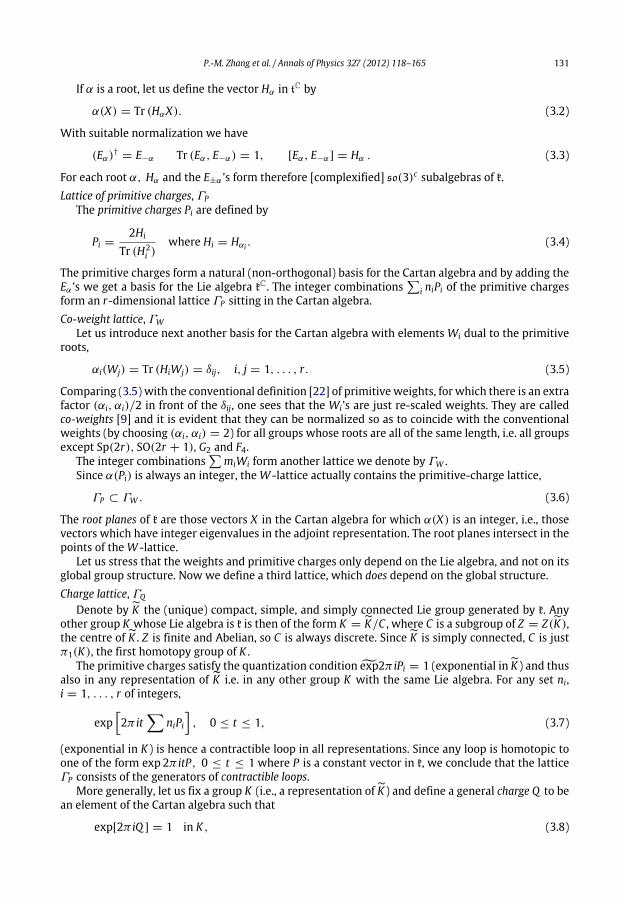
Example 1: H = SO(3)The simplest non-trivial example is when the residual Lie algebra is h = su(2) ≃ so(3), see Fig. 8.
Then the residual gauge group can be either H = SU(2)which is simply connected and has therefore
trivial topology. The unique minimal charge is the vacuum,
Q = 0.Non-trivial topology can, however, be obtained by changing the global structure by factoring out
the centre, Z ≃ Z2, yielding H = SO(3). Then we have two topological sectors, labelled bym = 0 andm = 1.
In detail, the Cartan algebra of su(2) consists of traceless diagonal matrices generated by σ3. Theonly positive root α is the difference of the diagonal entries,
Hα = σ3 =1 00 −1
, E+ = σ+ =
0 10 0
, E− = σ− =
0 01 0
, (3.13)
generate the complexified Lie algebra su(2)c . The unique minimal co-weight is
W =12σ3 =
12
1 00 −1
. (3.14)
The root lattice consists of integer multiples of
W . The unique primitive charge is
P = 2
W = σ3. (3.15)
The centre of SU(2) is Z ≃ Z2 = 12,−12 and the adjoint group, SO(3) ≃ SU(2)/Z2, has twotopological sectors, represented by the curves in SU(2)
γ0(t) = exp[2π iσ3t] and γ1(t) = exp[π iσ3t], (3.16)
0 ≤ t ≤ 1, respectively. Note that while γ0 is a loop in SU(2), γ1 is only ‘‘half of a loop’’, as it endsin−12. Factoring out the centre, both curves project to loops in SO(3); γ0 projects into a contractibleone, but γ1 represents the non-trivial class [1]. Conversely, when lifted to SU(2), all contractible in
134 P.-M. Zhang et al. / Annals of Physics 327 (2012) 118–165
Fig. 8. The Bott diagram of SO(3) ≃ SU(2)/Z2 , the adjoint group of SU(2). The minimal co-weight
W =
W 1 is now a charge,
so that ΓW = ΓQ . π1(SO(2)) ≃ Z2 ,
W 0 = 0 and
W are the minimal charges of the two topological sectors.
SO(3) loops end at 12 and the lifts of loops in the non-trivial class end at −12. The stable charges ofthe respective sectors are
Q (0)= 0 and
Q (1)=
W =12σ3. (3.17)
Then any charge is
Q =
Q (m)+ nP =
nσ3 trivial sector12+ n
σ3, nontrivial sector (3.18)
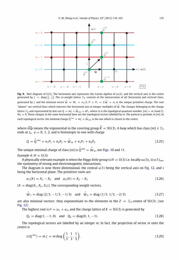
where n is some integer.Example 2: H = U(2)
Another simple case of considerable interest is that of when the little group H of the Higgs fieldis H = U(2). The Lie algebra is decomposed into centre plus the semisimple part, h = u(1) ⊕ su(2),which is indeed used to describe electroweak interactions.
The Cartan algebra consists of diagonal matrices (combinations of σ3 and of the unit matrix 12).In fact, H ∈ t, E± and the primitive weight
W =
W 1 are as in (3.13). The only primitive vector,
W 1,
is also a minimal one. In fact, exp 2π i
W 1 = −12. P1 = 2
W 1 = σ3 generates the charge lattice ofK = SU(2)which is also the topological zero-sector of U(2). The topological sectors are labelled by asingle integerm, defined by projecting onto the centre,
Q∥ = m diag12,12
≡ m ζ . (3.19)
Note that ζ = diag(1/2, 1/2) generates the centre, see Fig. 9. Note that only 2ζ is a charge,exp[4π iζ ] = 1. The [up to conjugation] unique minimal charge of the sectorm is (see Fig. 9)
Q (m)= mζ +
W [m] =diag (k, k) for m = 2kdiag (k+ 1, k) for m = 2k+ 1 (3.20)
where [m] is mmodulo 2 and
W 0 = 0 by convention. Any other charge of Sectorm is
Q (m)=
Q (m)+ nP1 =
Q (m)+ nσ3 =
Q (m)+ diag(n,−n). (3.21)
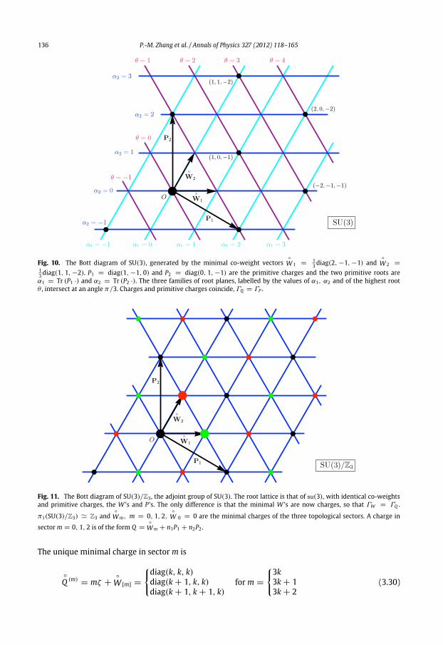
Example 3: SU(3)/Z3SU(3) = K is simply connected; its centre is Z3, with elements
z0 = diag1, 1, 1
, z1 = diag
e4π i/3, e−2π i/3, e−2π i/3
,
z2 = diage2π i/3, e2π i/3, e−4π i/3
.
(3.22)
The co-weights are now charges, so that
ΓW = ΓQ . (3.23)
The adjoint group of SU(3) = K is SU(3)/Z has therefore three homotopy classes labelled by thezm, m = 1, 2, 3 Each of such loop is homotopic to one of the formexp [2π iQt] 0 ≤ t ≤ 1,exp [2π iQ ] = zm, (3.24)
P.-M. Zhang et al. / Annals of Physics 327 (2012) 118–165 135
Fig. 9. Bott diagram of U(2). The horizontal axis represents the Cartan algebra of su(2), and the vertical axis is the centregenerated by ζ = diag
12 ,
12
. The co-weight lattice ΓW consists of the intersections of all (horizontal and vertical) lines,
generated by ζ and the minimal vector
W ≡ W1 = σ3/2. P = P1 = 2
W = σ3 is the unique primitive charge. The root
‘‘planes’’ are vertical lines which intersect the horizontal axis at integer multiples of
W . The charges belonging to the charge
lattice ΓQ and represented by dots are Q = mζ +
W [m] + nP1 , wherem is the topological quantum number, [m] = m (mod 2),W0 = 0. Those charges in the same horizontal lines are the topological sectors labelled by m. The pattern is periodic in [m]. In
each topological sector, the minimal charge
Q (m)= mζ +
W [m] is the one which is closest to the centre.
whereexp means the exponential in the covering groupK = SU(3). A loop which has class [m] ∈ Z3ends at za, a = 0, 1, 2, and is homotopic to one with charge
Q =
Q (m)+ n1P1 + n2P2 =
Wm + n1P1 + n2P2. (3.25)
The unique minimal charge of class [m] is
Q [m] =
Wm, see Figs. 10 and 11.
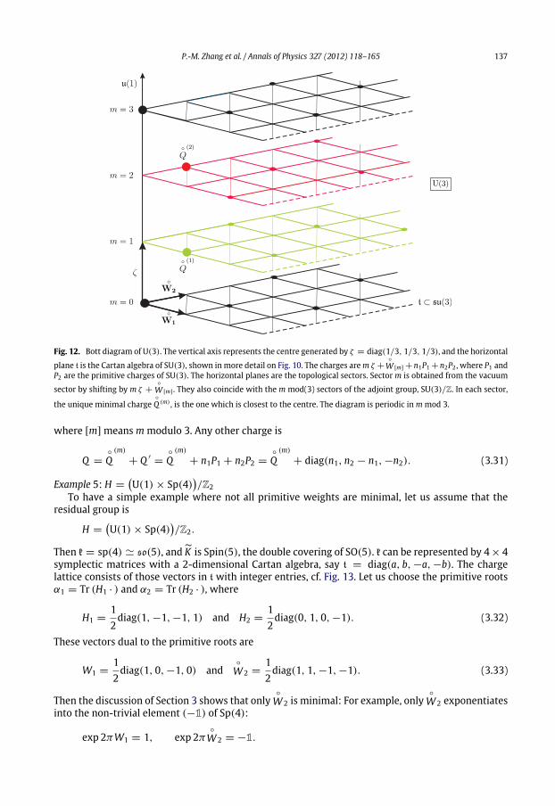
Example 4: H = U(3)A physically relevant example iswhen theHiggs little group isH = U(3) i.e. locally su(3)c⊕u(1)em,
the symmetry of strong and electromagnetic interactions.The diagram is now three-dimensional, the central u(1) being the vertical axis on Fig. 12, and t
being the horizontal plane. The primitive roots are
α1(X) = X1 − X2 and α2(X) = X2 − X3 (3.26)
(X = diag(X1, X2, X3)). The corresponding weight vectors,
W 1 = diag (2/3,−1/3,−1/3) and
W 2 = diag (1/3, 1/3,−2/3) (3.27)
are also minimal vectors: they exponentiate to the elements in the Z = Z3-centre of SU(3). (seeFig. 12)
The highest root is θ = α1 + α2, and the charge lattice of K = SU(3) is generated by
Q1 = diag(1,−1, 0) and Q2 = diag(0, 1,−1). (3.28)
The topological sectors are labelled by an integer m. In fact, the projection of sector m onto thecentre is
z(Q (m)) = m ζ = m diag13,13,13
. (3.29)
136 P.-M. Zhang et al. / Annals of Physics 327 (2012) 118–165
Fig. 10. The Bott diagram of SU(3), generated by the minimal co-weight vectors
W 1 =13 diag(2,−1,−1) and
W 2 =13 diag(1, 1,−2). P1 = diag(1,−1, 0) and P2 = diag(0, 1,−1) are the primitive charges and the two primitive roots areα1 = Tr (P1 ·) and α2 = Tr (P2 ·). The three families of root planes, labelled by the values of α1, α2 and of the highest rootθ , intersect at an angle π/3. Charges and primitive charges coincide, ΓQ = ΓP .
Fig. 11. The Bott diagram of SU(3)/Z3 , the adjoint group of SU(3). The root lattice is that of su(3), with identical co-weightsand primitive charges, the W ’s and P ’s. The only difference is that the minimal W ’s are now charges, so that ΓW = ΓQ .
π1(SU(3)/Z3) ≃ Z3 and
Wm, m = 0, 1, 2,
W 0 = 0 are the minimal charges of the three topological sectors. A charge in
sectorm = 0, 1, 2 is of the form Q =
Wm + n1P1 + n2P2 .
The unique minimal charge in sectorm is
Q (m)= mζ +
W [m] =
diag(k, k, k)diag(k+ 1, k, k)diag(k+ 1, k+ 1, k)
for m =
3k3k+ 13k+ 2
(3.30)
P.-M. Zhang et al. / Annals of Physics 327 (2012) 118–165 137
Fig. 12. Bott diagram of U(3). The vertical axis represents the centre generated by ζ = diag(1/3, 1/3, 1/3), and the horizontal
plane t is the Cartan algebra of SU(3), shown in more detail on Fig. 10. The charges arem ζ +
W [m]+n1P1+n2P2 , where P1 andP2 are the primitive charges of SU(3). The horizontal planes are the topological sectors. Sector m is obtained from the vacuum
sector by shifting by m ζ +
W [m] . They also coincide with the m mod(3) sectors of the adjoint group, SU(3)/Z. In each sector,
the unique minimal charge
Q (m) , is the one which is closest to the centre. The diagram is periodic inmmod 3.
where [m]means m modulo 3. Any other charge is
Q =
Q(m)+ Q ′ =
Q(m)+ n1P1 + n2P2 =
Q(m)+ diag(n1, n2 − n1,−n2). (3.31)
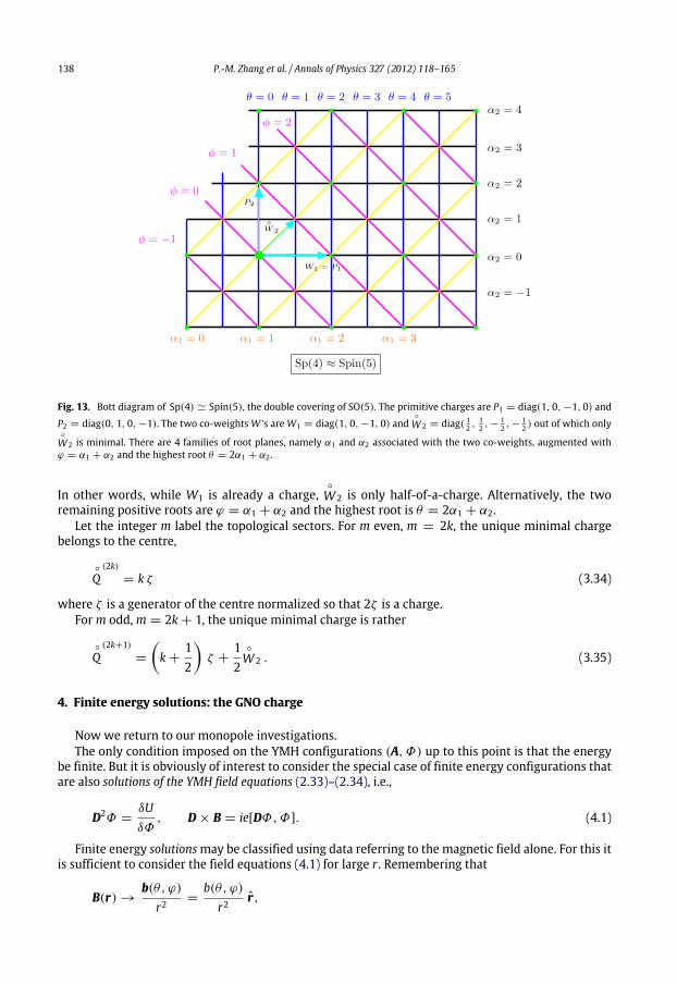
Example 5: H =U(1)× Sp(4)
/Z2
To have a simple example where not all primitive weights are minimal, let us assume that theresidual group is
H =U(1)× Sp(4)
/Z2.
Then k = sp(4) ≃ so(5), andK is Spin(5), the double covering of SO(5). k can be represented by 4× 4symplectic matrices with a 2-dimensional Cartan algebra, say t = diag(a, b,−a,−b). The chargelattice consists of those vectors in t with integer entries, cf. Fig. 13. Let us choose the primitive rootsα1 = Tr (H1 · ) and α2 = Tr (H2 · ), where
H1 =12diag(1,−1,−1, 1) and H2 =
12diag(0, 1, 0,−1). (3.32)
These vectors dual to the primitive roots are
W1 =12diag(1, 0,−1, 0) and
W 2 =12diag(1, 1,−1,−1). (3.33)
Then the discussion of Section 3 shows that only
W 2 is minimal: For example, only
W 2 exponentiatesinto the non-trivial element (−1) of Sp(4):
exp 2πW1 = 1, exp 2π
W 2 = −1.
138 P.-M. Zhang et al. / Annals of Physics 327 (2012) 118–165
Fig. 13. Bott diagram of Sp(4) ≃ Spin(5), the double covering of SO(5). The primitive charges are P1 = diag(1, 0,−1, 0) and
P2 = diag(0, 1, 0,−1). The two co-weightsW ’s areW1 = diag(1, 0,−1, 0) and
W 2 = diag( 12 ,12 ,−
12 ,−
12 ) out of which only
W 2 is minimal. There are 4 families of root planes, namely α1 and α2 associated with the two co-weights, augmented withϕ = α1 + α2 and the highest root θ = 2α1 + α2 .
In other words, while W1 is already a charge,
W 2 is only half-of-a-charge. Alternatively, the tworemaining positive roots are ϕ = α1 + α2 and the highest root is θ = 2α1 + α2.
Let the integer m label the topological sectors. For m even, m = 2k, the unique minimal chargebelongs to the centre,
Q(2k)= k ζ (3.34)
where ζ is a generator of the centre normalized so that 2ζ is a charge.For m odd, m = 2k+ 1, the unique minimal charge is rather
Q(2k+1)
=
k+
12
ζ +
12
W 2 . (3.35)
4. Finite energy solutions: the GNO charge
Now we return to our monopole investigations.The only condition imposed on the YMH configurations (A,Φ) up to this point is that the energy
be finite. But it is obviously of interest to consider the special case of finite energy configurations thatare also solutions of the YMH field equations (2.33)–(2.34), i.e.,
D2Φ =δUδΦ, D× B = ie[DΦ,Φ]. (4.1)
Finite energy solutionsmay be classified using data referring to the magnetic field alone. For this itis sufficient to consider the field equations (4.1) for large r . Remembering that
B(r)→b(θ, ϕ)
r2=
b(θ, ϕ)r2
r,
P.-M. Zhang et al. / Annals of Physics 327 (2012) 118–165 139
cf. (2.35) and puttingΦ(r) ≈ Φ(θ, ϕ)+ η(r, θ, ϕ), our field equations reduce to
ηα =
∂2U
∂Φα∂Φβ
ηβ and D× b = 0 (4.2)
in the generic case. The first equation here shows that, for solutions the generic finite-energy conditionη→ 0 is sharpened to an exponential fall-off of η.12
Since Φ(θ, ϕ) and b(θ, ϕ) are the only components of the field configuration that survive inthe asymptotic region, the only possible asymptotic classification of the configurations; within eachtopological sector, is by b(θ, ϕ). The conditions satisfied by b(θ, ϕ) are then contained in the secondequation in (4.2), which may be written as
Dib ≡ ∂ib+ i[Ai, b] = 0. (4.3)
This equation shows that b(θ, ϕ) is covariantly constant on the sphere at infinity and thus takes itvalues lie on an H-orbit. Therefore
b(θ, ϕ) =hN(θ, ϕ)Q h−1N (θ, ϕ) in NhS(θ, ϕ)Q h−1S (θ, ϕ) in S,
where Q = b(E), the value of the magnetic field at the ‘‘east pole’’, belongs to h. Plainly, Q is uniqueup to global gauge rotations, and there is thus no loss of generality in choosing it in a given Cartanalgebra.
In the singular gauge where b(θ, ϕ) = Q, the loop in (2.49) i.e. hA= P
exp
Acan readily be
evaluated: it is simply
h(ϕ) = exp[2iQϕ], 0 ≤ ϕ ≤ 2π, (4.4)
and the periodicity of ϕ provides us with the quantization condition
exp[4π iQ] = 1
cf. (1.4). Using the terminology introduced in Section 3,
2Q = Q (4.5)
is a charge. Conversely, any quantized Q defines an asymptotic solution, namely
A = ADQ i.e. Aθ = 0, A±ϕ = (±1− cos θ)Q, (4.6)
in the Dirac gauge, so that (4.4) is in fact the transition function. (The ± superscript refers to thenorthern and southern hemispheres, respectively.) Hence
b = Q (4.7)
in this gauge, and Eqs. (4.6)–(4.7) say that at infinity, the magnetic field can be gauge-transformedinto a fixed direction in h: asymptotically, any ’t Hooft–Polyakov monopole is an embedded Diracmonopole. In mathematical terms, the holonomy of pure YM on S2 is one-dimensional [4].13
Solutions can thus be classified by charges of H . The (half)charge Q was introduced by Goddard,Nuyts and Olive [18].
According to (2.48), for solutions of the field equations the expression for the ‘‘Higgs’’ quantumnumbersma reduces to
ma = 2Tr (Q ζa)Tr (ζ 2
a ), a = 1, . . . , p. (4.8)
Here we would like to mention that the ‘‘topological quantum numbers’’ mk’s are related to butstill distinct from the magnetic charge: the latter can, in fact, only be defined by identifying
12η = 0 and D× b = 0 in the Bogomolny case. Then D2η = 0 is consistent with η = b(Ω)/r .
13 The statement generalizes to Riemann surfaces [19].
140 P.-M. Zhang et al. / Annals of Physics 327 (2012) 118–165
the ‘‘electromagnetic’’ direction, which requires using a covariantly constant direction field whichgenerates and ‘‘internal symmetry’’ [44]. Then, suitably defining the electric charge operator providesus with generalized [fractional] Dirac quantization conditions [2,16,45,44].
We are, at last, ready to identify the minimal charge in each topological sector. Let us indeedconsider a GNO charge Q and denote its topological sector by m. let us decompose Q into centraland semisimple parts Q∥ and Q⊥, respectively, Q = Q∥ + Q⊥. By (4.8),
2Q∥ = 2z(Q) =p
k=1
mkζk.
Observe that
z = exp[4π iQ∥] = exp[−4π iQ⊥] (4.9)
lies simultaneously in Z(H)0 (the connected component of the centre of H) and in the semisimplesubgroup K , and thus also in Z(K), the centre of K . Let us decompose k = [h, h] into simple factors,
k = k1 ⊕ · · · ⊕ ks,
and denote byKj the simple and simply connected group,whose algebra is kj. As explained in Section 2,K is of the formK/C , whereC = C1×· · ·×Cs is a subgroupof the centre Z = Z(K)ofK = K1×· · ·×Ks
,
Cj being a subgroup of Z(Kj).The situation is particularly simple when K is simply connected, K = K , when the central part Q∥
contains all topological information. Indeed, z is uniquely written in this case as
z = z1 · · · zs where zj ∈ Z(Kj). (4.10)
However, as emphasized in Section 3, the central elements of a simple and simply connected groupare in one-to-one correspondencewith theminimal
W ’s and thus, for each z in the centre, there existsa unique set of
W j’s (where
W j is either zero or a minimal vector of kj) such that
z =exp[−2π i
W 1]· · ·exp[−2π i
W s]= exp
−2π i
sk=1
W k
= exp
−2π i
W (m). (4.11)
W (m) depends only on the sector (and not on Q itself), because all charges of a sector have the sameQ∥. Hence the entire sector can be characterized by giving
2
Q (m)=
k
mkζk +
W (m). (4.12)
By (4.11) 2
Q (m) is again a charge, exp[4π
Q (m)] = 1, and it obviously belongs to the sector m.
Furthermore,
exp[4π i(Q−
Q)] = exp[4π iQ] exp[−4π i
Q] = 1
shows that 2Q′ = 2(Q−
Q) is in the charge lattice of K .The situation is slightlymore complicated if K is not simply-connected, so that the semisimple part
also contributes to the topology. Since C is now non-trivial, the expansion (4.10) is not unique, and zjcan be replaced rather by z∗j = zjcj, where cj belongs to the subgroup Cj of Z(Kj). But z∗j is just another
element of Z(Kj), so it is uniquely z∗j =
W j∗ for some minimal
W j∗ of the simple factorKj. Eq. (4.11),
with all
W j’s replaced by the
W j∗’s, is still valid, so that (4.12) is a charge also now. However, since
π1(K) = C = C1 × · · · × Cs, those loops generated by Q and Q ∗ now belong to different topologicalsectors.
P.-M. Zhang et al. / Annals of Physics 327 (2012) 118–165 141
We conclude that a topological sector contains a unique charge Q of the form (4.12) also in thiscase, and that, in full generality, any other monopole charge is uniquely of the form
Q =
Q+Q′ =
Q+12
ri
niPi, (4.13)
where the ni are integers, and the Pi, i = 1, . . . , r are the primitive charges of K i.e. those whichgenerate contractible loops in all cases. (Obviously, the Pi are sums of primitive charges taken forthe simple factors Kj). The integers ni could be regarded as secondary quantum numbers whichsupplement the Higgs chargem but do not contribute to the topology.
In Section 5.2 we shall show that
Q (m) is the unique stable monopole charge in the sectorm.The situation is conveniently illustrated on the Bott diagram, see Section 3.The classification of finite energy solutions according to the secondary quantum numbers or,
equivalently the matrix-valued charge Q is convenient and illuminating, but in contrast to theclassification of finite energy configurations according to the Higgs charge m, it is not mandatory,in the sense that (for fixed m) the different charges Q are separated only by finite energybarriers [8].
5. Stability analysis
5.1. Reduction from R3 to S2
Now we show that those monopoles for which Q′ = 0 are unstable. More precisely, we showthat for a restricted class of variations the stability problem reduces to a corresponding Yang–Millsproblem on S2. This will allow us to prove that with respect to our variations there are
ν = 2q<0
(2|q| − 1) (5.1)
independent negativemodes [7,10,11]where q is a negative eigenvalue of a certain operator involvingthe GNO charge, (5.20) below. To this end, let us first introduce the notation
(a× b)i = εijkajbk, (5.2)a× b
= a× b+ b× a i.e.
a× b
i = εijk
aj, bk
.
Note that a× a may be different from zero if h is non-Abelian.For h-valued variations of the gauge potentials alone of the ‘‘Brandt–Neri–Coleman type’’, i.e., for
δΦ = 0, δA = a ∈ h, (5.3)
the variations of the gauge field and covariant derivative are easily seen to be
δB = D× a, δ2B = −i[a× a], δ(DΦ) = −i[a,Φ] (5.4)
where, once again, we assumed for simplicity that the Higgs field belongs to the adjointrepresentation. All higher-order variations δ3B etc. are zero.
The first variation of the energy functional (2.30) is zero since (A,Φ) is a solution of the fieldequations. The higher order variations are
δ2E =
d3rTr (D× a)2 − iTr (B · [a× a])− Tr ([a,Φ])2
,
δ3E = −3i
d3r Tr (D× a) · (a× a) ,
δ4E = −3
d3r Tr (a× a)2,
(5.5)
142 P.-M. Zhang et al. / Annals of Physics 327 (2012) 118–165
all higher-order variations being zero. We shall assume that all variations are square-integrable andhave non-zero norm,
0 = (a, a) =
d3r Tr (a)2 <∞. (5.6)
There are some general points worth noting.First, since δΦ = 0, the only terms in (5.2) involves the Higgs field is Tr ([a,Φ])2 and, in the
’t Hooft–Polyakov case U = 0, a must be in the little group of Φ(θ, ϕ) = limr→∞Φ(r, θ, ϕ), thisterm vanishes asymptotically. Thus, if we only consider asymptotic variations [6,3] i.e. such thata(r, θ, ϕ) = 0 for r ≤ R where R is ‘sufficiently large’ so that the fields assume their asymptoticforms (2.35), theHiggs terms can then dropped in (5.5) andwe shall only consider the pure Yang–Millsvariations,
δ2E =
d3rTr (D× a)2 − iTr (B · [a× a])
. (5.7)
Second, the only term in (5.7) that involves radial derivatives is the (∂ra)2 term in (D × a)2 andthis contribution may be shown to be
δ2Er =
d3r Tr (∂ra)2 = m2(a, a), m2=
14+ δ2 (5.8)
where δ2 > 0whose infimum of is 0 [3,8]. Thus, although δ2Er is not negligible, it can be regarded as amass term. Therefore, for each value of r , the variations (5.7) are essentially variations on the two-sphereat infinity, S2.
Finally, it should be noted that the variations a = Dχ where χ is any scalar, are simply gaugetransformations of the background field A and leave the energy unchanged. In particular, it is easy toverify that, becauseA satisfies the field equations, the second variation δ2E is zero for the infinitesimalvariations δA = Dχ . It is therefore convenient to define the ‘physical’ variations a as those which areorthogonal to the Dχ . Using partial integration,
0 =
d3r Tr (a · Dχ) = −
d3r Tr (D · aχ) ⇒ D · a = 0, (5.9)
since χ is arbitrary. The physical variations may also be characterized as those which are divergence-free. As a consequence of the gauge condition Ar = 0 our variations satisfy also ar = 0.
It will be convenient to split (5.7) into two terms,
δ2E =
d3r Tr(D× a)2 + (D · a)2
δ2E1≥0
+
d3r Tr
−iB[a× a] − (D · a)2
δ2E2
, (5.10)
bearing in mind that D · a is unphysical and may be gauged to zero.Let us first consider δ2E1. From the identity
D× (D× a)j = −D
2aj + Dj(D · a)− i[B× a]
j (5.11)
we have
δ2E1 =
d3r Tr(−D2a− i[B× a]) · a
, (5.12)
and putting b = limr→∞ r2B yields
δ2E1 = δ2Er +
d3r r−2Tr
L2a− i[b× a]· a
δ2ES
, (5.13)
P.-M. Zhang et al. / Annals of Physics 327 (2012) 118–165 143
where L = −ir × D is the orbital angular momentum. L is neither conserved nor does it satisfy theso(3) algebra. For spherically symmetric (and hence for asymptotic) fields, the components of theangular momentum for a spinless particle,14
Mi = Li −xirb, (5.14)
satisfy the so(3) algebraMi,Mj
= εijkMk. For arbitrary variations a the spectrum of δ2E1 is
conveniently obtained by using instead the spin-1 angular momentum operator
J = M + S = −ir × D− b+ S (5.15)
where S is the 3× 3 spin matrixSijk = iεijk. S satisfies the relations
[Si, Sj] = iεijkSk, (b · S)a = (biSi)a = i[b× a], S2= SiSi = −2. (5.16)
Using the gauge conditions D · a and r · a = 0, we see that
(r × D)× a = r(D · a)− riDai = −riDai = a− D(r · a) = a, (5.17)
i.e., L · S = 1. Since r and L and thus b and L are orthogonal, this implies,
J2a = L2a+ [b× [b× a]] − 2i[b× a]. (5.18)
This leads finally to rewriting δ2ES as
δ2ES =
d3rr−2Tr
J2a− [b× [b× a]] + i[b× a]· a. (5.19)
It is convenient to decompose the variation a into eigenmodes of the operator [b× · ]which combinesvector product and Lie algebra commutator, i.e., to write
i[b× a] = q a, (5.20)
where the q’s are the eigenvalues. The q’s come in fact in pairs of opposite sign andmultiplicity 2 i.e. inquadruplets (q, q,−q,−q), see the next section.
On each q-sector δ2E1 will be
δ2E1 = m2(a, a)+
d3r TrJ2 − q(q+ 1)a
· a. (5.21)
But J is the Casimir of the angular momentum algebra generated by J , so J2 = j(j + 1), where j isinteger or half-integer, according as q is integer or half-integer. Now since δ2E1 is manifestly positiveby (5.10), we must have
m2+J2 − q(q+ 1)
=
14+ δ2
+ j(j+ 1)− q(q+ 1) ≥ 0. (5.22)
and since δ2 is arbitrarily small, we see that j ≥ |q| − 1.Eq. (5.22) implies that the possible values of j are |q| − 1, |q|, |q| + 1, . . .. In particular, the value
of j = |q| − 1 can occur only for q ≤ −1, and as it corresponds to the case when δ2E1 is purely radialsince j(j+ 1) = (−q− 1)(−q) = q(q+ 1), it implies that D · a = 0, so that the states correspondingto it are physical. Thus we can write
δ2E1 = m2(a, a) for j = |q| − 1, q ≤ −1 (5.23)
and
δ2E1 =m2+ (j− q)(j+ q+ 1)
(a, a) for j ≥ |q| . (5.24)
14 For a particle ψ in the adjoint representation for example, b · ψ means [b, ψ].
144 P.-M. Zhang et al. / Annals of Physics 327 (2012) 118–165
Let us now consider the second term, δ2E2, in the decomposition (5.10) of the Hessian. Since D · ais zero on the physical states,
δ2E2 = (−i)
d3r TrB ·a× a
=
d3r Tr
−iB× a
· a
=
d3r r−2Tr
−ib× a
· a= q
d3r r−2Tr
a2= q
a, a
. (5.25)
From the positivity of δ2E1 we then see that the Hessian δ2E will be positive unless q is negative.Furthermore, when q is negative, (5.24) becomes
δ2E1 =m2+ (j+ |q|)(j− |q| + 1)
a, a
, (5.26)
and hence
δ2E1 ≥ 2|q|(a, a) for j ≥ |q|. (5.27)
For j ≥ |q|, the restriction of δ2E1 to the physical states will therefore dominate δ2E2 and the Hessianwill again be positive. It follows that the only possibility for getting negative modes is to have
q ≤ −1 and j = |q| − 1, (5.28)
in which case
δ2E =m2− |q|
a, a
< 0. (5.29)
In conclusion, observing that the eigenvalues q come in pairs of opposite sign, we have finally theresult that themonopole is unstable if and only if there is an eigenvalue such that |q| ≥ 1. The oppositecondition,
|q| ≤12, (5.30)
is, of course, just the Brandt–Neri stability condition [6,3,9]. From the discussion of Section 2.3.we knowhowever that |q| ≤ 1
2 if and only if
Q =
Q (5.31)
i.e., Q is the [up to conjugation] unique stable charge of the given topological sector, cf. (4.11).Note that since, in the case j = |q| − 1, the first term on the right-hand side of (5.10) vanishes the
variation actually satisfies the first-order equations
D× a = 0, D · a = 0, (5.32)
where rD =D→ D is [with some abuse of notation] the covariant derivative acting on the asymptoticfields defined over the sphere at infinity. (5.32) says in particular that our a’s are true physical modes,which form furthermore a
2j+ 1 = 2|q| − 1 (5.33)
dimensionalmultiplet of the J algebra.We shall see in the next section that for each |q| there is one andonly one such multiplet. Taking into account the fact that the eigenvalues come in pairs, this provesthe index formula (5.1).15
15 For BPS monopoles the above arguments break down: due to the b/r term in the expansion of the Higgs field, the secondvariation picks up an extra term −Tr ([a, b])2 = q2 which precisely cancels the −q2 in Eq. (5.21). The total Hessian is thusmanifestly positive,
δ2E = δ2E1 + δ2E2 = ((m2+ J2)a, a) > 0. (5.34)
BPS monopoles are therefore stable under variations of the gauge field alone, even if their charge is not of the form (4.12). Thisis no surprise, since they represent the absolute minima of the energy.
P.-M. Zhang et al. / Annals of Physics 327 (2012) 118–165 145
The simplest way of counting the number of instabilities for j ≥ |q| is to use the Bott diagram (seethe examples of Section 8.3): the Morse index ν in (5.1) is twice the number of times the straight linedrawn from 2Q to the origin intersects the root planes [21].
In the sequel, we will work on the sphere at infinity and, with some abuse, we use the word‘‘monopole’’ for a solution of the pure Yang–Mills equations with gauge group H on S2.
Let us note for further reference that the first-order equations in (5.32) are plainly consistent withthe vanishing of the first term in the decomposition (5.10), and then the negative value of the Hessianδ2E comes from the second term, δ2E2. We also stress that all our investigations assume that a is avariation with non-zero norm, cf. (5.6). The meaning of this subtle condition will be clarified in thenext Subsection.
5.2. Negative modes
Our strategy for finding our negative modes is therefore:
1. First, we find the eigenmodes of the combined operator −i[b × · ] in (5.20) with eigenvaluesq ≤ −1;
2. Next, we solve the two coupled first-order Eqs. (5.32) which set the first term in (5.10) to zero.
This amounts to finding the negative eigenmodes of the linear second variation operator,
Ka = J2a− [b× [b× a]] + i[b× a]. (5.35)
From the technical point of view, our goal can conveniently be achieved by complexifying the Liealgebra h. But thenwe have tomake sure that our eigenmodes are indeed real and have non-vanishingnorm, cf. (5.6).16
To find our negative modes, it is convenient to use the stereographic coordinate z on S2,
z = x+ iy = eiϕ tan θ/2. (5.37)
In stereographic coordinates the background gauge-potential and field strength become
Az = −iQzϱ, Az = iQ
zϱ, b = 2i
Qϱ2, ϱ = 1+ zz, (5.38)
where we treated z and its conjugate z as independent variables. Set ∂ = ∂z , ∂ = ∂z , and let us define
Dz = ∂ − iAz = ∂ − Qzϱ, az =
12(ax − iay)
Dz = ∂ − iAz = ∂ + Qzϱ, az =
12(ax + iay).
(5.39)
In complex coordinates the eigenspace-equations (5.20) decouple and indeed become17Q 00 −Q
azaz
= q
azaz
. (5.40)
16 For zero-norm states, (a, a) = 0, the value of the second variation on the sphere,
δ2ES =
S2d2rTr (Ka, a) (5.36)
[with some abuse of notation] would then vanish, despite (5.35) having a negative eigenvalue. When added to the radial part,δ2E1 = δ2Er + δ2ES would then be positive, even for the lowest angular momentum state.17 Remember that Q acts on aα by commutation.
146 P.-M. Zhang et al. / Annals of Physics 327 (2012) 118–165
The general solution of (5.40) isazaz
= f
Eα0
+ g
0
E−α
with eigenvalue α(Q) (5.41)
where f and g are arbitrary functions of z and z. Similarly,azaz
= h
E−α0
+ k
0Eα
with eigenvalue−α(Q) (5.42)
where h and k are again arbitrary. These equations show that the eigenvalues come indeed in pairs asstated earlier. Then we should select those pairs for which the eigenvalue, q, is negative.
As discussed in Section 5.1, for each fixed eigenvalue q ≤ −1, the negative modes are solutions tothe two coupled first-order equations in (5.32) which are, furthermore, equivalent to
Dzh = (ϱ ∂ + |q|z)h = 0 and Dzk = (ϱ ∂ + |q|z)k = 0 (5.43)
(q = −|q| because q is negative). One sees that h and k must be of the form
h(z, z) = ϱ−|q|Φ(z), k(z, z) = ϱ−|q|Ψ (z), (5.44)
where Φ(z) and Ψ (z) are arbitrary antiholomorphic (respectively holomorphic) functions. They canbe therefore expanded into power series,
Φ(z) =
cnzn, and Ψ (z) =
dmzm.
But they are also square integrable functions. Now, since in stereographic coordinates, the innerproduct for two vector fields is
(a, b) =
dzdz√ggαβaα bβ =
dzdz aα bα =
dzdz (azbz + azbz), (5.45)
because√ggαβ is unity, one sees thatΦ(z)will be square integrable if, and only if, cn, dm = 0 except
for n,m = 0, 1, . . . , 2|q| − 2. Thus, assuming
α(Q) > 0, (5.46)
for definiteness, it is the combination (5.42) that has to be chosen; the negative modes of the operatorK are linear combinations of the 2(2|q| − 1) variations
az0
=
zn
(1+ zz)|q|
E−α0
,
0az
=
zm
(1+ zz)|q|
0Eα
, (5.47)
n,m = 0, 1, . . . , 2|q| − 2.18But are these the modes we were looking for? To answer this question, we must remember our
conditions listed at the beginning of Section 5.2: firstly, they should be real, and secondly, they shouldhave nonzero norm.
Themodes in (5.47) satisfy neither of these conditions: they belong to the complexified Lie algebrahc and not to its real part. And they also have zero norm, since they lie in the Eα direction, andTr (E2
α) = 0 for any root α. Happily enough, both defects can be cured by mixing our modes: it iseasy to check that
a+
a−
=
az + az−i(az − az)
=
1(1+ zz)|q|
znEα + znE−α−i(znEα − znE−α)
(5.48)
are both real and have nonzero norm, as it follows from the Lie algebra relations (3.3).In conclusion, these are the negative modes we were looking for.We only mention that the remaining eigenspace of the Hessian can also be determined [8].
18 If α(Q) < 0 then it is (5.41) that should be chosen; then Eα is paired with z, and E−α is paired with z.
P.-M. Zhang et al. / Annals of Physics 327 (2012) 118–165 147
5.3. Supersymmetric interpretation of the negative modes
Weconclude this section bymentioning that theMorse [instability] index 2|q|−1 is also theWittenindex for supersymmetry and the Atiyah–Singer index for the Dirac operator. Indeed, let us considerthe part of δ2ES of the Hessian, which played a central role in Section 5.1. From Eq. (5.13) one maywrite, after some transformations,
δ2ES =
r2dr K , K =
dzdz ϱ2Tr (Ψ , (HΨ )Ď),H = −12
Q+,Q−
, (5.49)
where
Q+ =
0 Dz0 0
, Q− =
0 0Dz 0
, Ψ =
azaz
. (5.50)
The multiplicity ν of the ground state, the latter being a square integrable solution of
Q+Ψ =
Dzaz0
= 0, Q−Ψ =
0
Dzaz
= 0, (5.51)
is called theWitten index. But these are just the negative-mode equations (5.43). The result ν = 2|q|−1is consistent with that found in Ref. [46] for supersymmetric QM on the sphere. Observe that thesupersymmetric Hamiltonian H can also be written as
H = −12D 2 where D = Dzσ+ + Dzσ− =
0 DzDz 0
(5.52)
is a Dirac-type operator, and the negative modes are exactly those satisfying
D Ψ = 0. (5.53)
The number of solutions of (5.53) is the Atiyah–Singer (AS) index.19 The result 2|q| − 1 is obtainedby the same calculation as the one in Atiyah and Bott [19], which is valid for an arbitrary Riemannsurface. See also [20].
It is worthmentioning that supersymmetry is a useful tool to describe both the fluctuations arounda self-dual (BPS) monopole [47], as well as the scattering of BPS monopoles [48].
6. The geometric picture: YM on S2
The aim of this section is to present an alternative approach [7] devised for more geometrically-minded readers and close to the spirit of Atiyah and Bott’s generalization to Riemann surfaces [19].To make this section self-contained, we present full (and somewhat redundant) proofs.
Consider indeed pure YM theory of the two-sphere at infinity with gauge group H . Geometrically,the YM potential is a connection 1-form still denoted by A on a principal H-bundle P over S2
≡ S2∞.
The YM action is
A =
S2
Tr (F ∧ ⋆F), (6.1)
where F = DA is the curvature 2-form, and ⋆ is the Hodge duality operator on S2. The associated fieldequation reads
D⋆F = 0. (6.2)
Now we can state again the geometric form of the GNO theorem,
19 Since a is a 2-vector, the instability index is the AS index for vectors.
148 P.-M. Zhang et al. / Annals of Physics 327 (2012) 118–165
Theorem (GNO [18]). In a suitable gauge the general solution of the Yang–Mills equations (6.2) is
F = iQω, (6.3)
where ω is the canonical surface form of the two-sphere and Q is a constant vector in the Lie algebra h,quantized as in (1.4),
exp[4π iQ] = 1. (6.4)
Proof. Our clue is that the YM equations (6.2) can indeed be written as
D ⋆ F = 0 (6.5)
since the adjoint operator D⋆ is −⋆D⋆ on the two-sphere. The field strength F = 12Fµνdx
µ∧ dxν is a
two-form on S2 and therefore
F = b(θ, ϕ) ω (6.6)
for some h-valued function [zero-form] b = b(θ, ϕ) on the sphere. Then the Hodge dual of F is pre-cisely b,
⋆ F = b(θ, ϕ), (6.7)
because the dual of the canonical surface form of the sphere is ⋆ω = 1, as it can be verified writing ωeither in polar or complex coordinates,
ω =12sin θ dθ ∧ dϕ =
1i
dz ∧ dz(1+ zz)2
, (6.8)
respectively. Then (6.5) requires that b is covariantly constant (4.3)—and this is precisely the equationwe solved in Section 4. Firstly, there exists, as explained before, a (singular) gauge transformation gsuch that
g−1bg = iQ. (6.9)
Let A be a gauge potential for F . Then we note that A′ = g−1Ag + g−1dg takes its values in k, thestabilizer of Q in h. Let us decompose A′ into components parallel and perpendicular to Q,
A′ = α iQ+ β,
where α and β are 1-forms (α real). Now we prove that α is a Dirac monopole potential and β can begauged away. The curvature of A′ is in fact
dA′ −i2[A′ ∧ A′] = (dα)iQ+ dβ −
i2[(αiQ+ β) ∧ (αiQ+ β)].
But it is also g−1Fg = ω iQ. Comparing the two expressions allows us to infer that
ω = dα, dβ −i2[β ∧ β] = 0. (6.10)
β is hence flat and can therefore be gauged away by a suitable k-valued transformation k,β = −dkk−1,where k = [h, h]. Then putting h = gk,
h−1Ah+ h−1dh = k−1A′k+ k−1dk = αiQ+ k−1βk+ k−1dk = αiQ.
The first relation in (6.10) also proves that α is in fact the gauge potential of a Dirac monopole in theDirac gauge,
α = (±1− cos θ)dϕ, (6.11)
P.-M. Zhang et al. / Annals of Physics 327 (2012) 118–165 149
where the± signs refer to the N/S hemispheres. The gauge potentials are consistently defined there-fore when the transition function
h(ϕ) = exp[2π iQϕ] (6.12)
is well-defined, i.e., when Q is quantized as in (1.4).Now we construct the non-Abelian YM bundle P from the Abelian bundle Y ≡ Y1 on S2 whose
Chern class is c(Y) = 1. The latter describes a Dirac monopole of unit strength and is given by theHopf fibration S3
→ S2. Now
χ(eit) = exp[4π iQt]
is a homomorphism of U(1) into H allowing us to form the associated bundle, Y×χ H . In fact, Y×χ His isomorphic to our YM bundle P .
Conversely, the H-bundle with its YM connection can be reduced to the U(1) bundle Y.Having proved the GNO theorem, we turn to the stability problem. Our investigations follow the
same lines as in Section 5, the main difference being that instead of vectors we use rather differentialforms and a more geometric language. The stability properties of the YM solution are determined bythe Hessian, which is now
12δ2A(a, a) =
S2
TrD⋆Da+ ⋆
⋆F , a
, a, (6.13)
where the variation a is an adP-valued 1-form on S2 i.e. a section of Ω1(S2; ad P ). Those a’s of the
form a = Dχ are infinitesimal gauge transformations and are therefore zero modes for (6.1). Varia-tions which are orthogonal to gauge transformations satisfy hence
D ⋆ a = 0. (6.14)
These are the physical modes cf. (5.9). The Hessian (6.13) can be completed by adding
DD⋆a = −D ⋆ D ⋆ a = 0 (6.15)
to the integrand, which combines with the first term to yield the gauge covariant Laplacian
A = D⋆D+ DD⋆. (6.16)
The Hessian is therefore
12δ2A(a, a) =
S2
TrA a+ F(a), a
, F(a) = ⋆
⋆F , a
. (6.17)
Our strategy, analogous to the one we followed in Section 5.2, will then be to show that the only wayof producing a negative mode is by diagonalizing the second term, F , and annihilating the first termin (6.17).
To this end we note that the square of Hodge star operator ∗ on the two-sphere is minus the iden-tity, ∗2 = −1; its eigenvalues are therefore±i. The space of [complex] 1-forms on S2,Ω , decomposesaccording to the eigenvalues of the Hodge star,
Ω = Ω(1,0)⊕Ω(0,1), ∗Ω(1,0)
= −iΩ(1,0), ∗Ω(0,1)= iΩ(0,1). (6.18)
The decomposition hC= tC⊕
α hα of the complexified Lie algebrawhere hα denotes the root spaces
generated by the Eα ’s implies the analogous decomposition
ad P C= P0 ⊕
α
Pα (6.19)
where P0 = Y×χ t and Pα = Y×χ hα . Both P0 and Pα are holomorphic line bundles. P0 is trivial,c(P0) = 0 and Pα has Chern class c(Pα) = 2α(Q).
150 P.-M. Zhang et al. / Annals of Physics 327 (2012) 118–165
By (6.19) the sections of ad P C⊗Ω are obtained from those of
(P0 ⊗Ω)⊕α
Pα ⊗Ω
(1,0)⊕Pα ⊗Ω
(0,1). (6.20)
The sections of each of these bundles are eigenspaces of
F(a) = ⋆⋆F , a
with eigenvalues 0,−α(Q), α(Q), (6.21)
respectively. On the other hand, the covariant Laplacian preserves the decomposition (6.20); onPα ⊗ Ω it reduces in fact to the covariant Laplacian of a Dirac monopole of strength α(Q). This isa positive operator,∆A ≥ 0, whose first non-zero eigenvalue is 2|α(Q )| [8].
Let us now consider a root α such that α(Q) > 0. Then the only way of getting a negative mode isby having a section a of Pα ⊗Ω
(1,0) for which
A a = 0. (6.22)
By (6.14) this is the same as Da = 0. Splitting a and D as
a = a′ + a′′, D = D′ + D′′ (6.23)
according to the eigenvalues of ⋆, the conditions for getting a negative mode reduce to
D′′a′ = 0. (6.24)
Now, according to a theorem of Koszul andMalgrange, a complex vector bundle with connection overS2 has a unique holomorphic structurewhose holomorphic sections are exactly the solutions of (6.24).We conclude that the negative modes are the holomorphic sections of ad P ⊗Ω(1,0).
It is sufficient to consider the terms in (6.19) separately.The Chern class of a tensor product is the sum of the Chern classes, andΩ(1,0) has Chern class (−2).
Thus
c(P0 ⊗Ω(1,0)) = −2 (6.25)
and P0 ⊗Ω(1,0) has no holomorphic sections. On the other hand,
c(Pα ⊗Ω(1,0)) = 2α(Q)− 2 = nα. (6.26)
Then the Riemann–Roch theorem tells us that a line bundle with positive Chern class nα ≥ 0 admits
nα + 1 = 2α(Q)− 1 (6.27)
holomorphic sections. Summing over all roots provides us therefore with the Morse index formula(5.1).
The negative modes are conveniently found in terms of complex coordinates (5.37) i.e., z =eiϕ tan(θ/2) on the northern hemisphere. Then
⋆ (dz) = −idz, ⋆(dz) = idz (6.28)
shows that a holomorphic section is of the form a(z, z)dz, where
∂za+n2
z1+ zz
a = 0. (6.29)
The solution is
a =f (z)
(1+ zz)n/2, (6.30)
where f (z) is an arbitrary holomorphic function.Similarly, on the southern hemisphere
w = e−iϕ cot(θ/2) =1z
(6.31)
P.-M. Zhang et al. / Annals of Physics 327 (2012) 118–165 151
is a complex coordinate, and the solutions of Eqs. (6.14) and (6.24) is
g(w)(1+ ww)n/2
(6.32)
where g(w) is holomorphic inw.For Chern class n the transition function is einϕ = (z/z)n/2. Expanding f (z) and g(w) as
f (z) =
i
aiz i and g(w) = −
j
bjwj,
consistency requires1
(1+ zz)n/2
i
aiz idz =
zz
n/2 −1(1+ ww)n/2
j
aiwi
dw.
It follows that f (z) and g(w) can only be polynomials of degree at most n − 2, and ai = bn−2−i.Returning to the original problem, we see that the root α contributes 2α(Q) − 1 negative modes,namely
aα ≡ a(k)α =zk
(1+ zz)nα/2dz Eα, 0 ≤ k ≤ 2α(Q)− 2 = nα. (6.33)
Similarly, we also have for the root−α
a−α ≡ a(k)−α =zk
(1+ zz)nα/2dz E−α, 0 ≤ k ≤ 2α(Q)− 2 = nα. (6.34)
Thus we have re-derived, once again, the negative modes (5.47) as holomorphic and anti-holomorphic sections of line bundles over the two-sphere with Chern class 2|q| − 2.20
In Section 5.2 these samemodeswere obtainedusing angularmomentum. This is not a coincidence,since the holomorphic sections of line bundles are precisely the carrier spaces of representations ofthe rotation group SU(2).
7. Loops
Nowwe deepen and elaborate the intuitive remark of Coleman [3] about the analogy of monopolesand elastic strings.
Let us considerΩ = Ω(H), the space of loops in a compact Lie group H which start and end at theidentity element of H . The energy of a loop γ (t), 0 ≤ t ≤ 1 is given by
L(γ ) =14π
1
0Trγ−1
dγdt
2
dt. (7.1)
A variation of γ (t) is a 2-parameter map α(s, t) into H such that α(0, t) = γ (t). We fix the endpoints, α(s, 0) = γ (0) and α(s, 1) = γ (1) for all s. For each fixed t , ∂α/∂s at s = 0 is then a vectorfield X(t) along γ (t), X(0) = X(1) = 0. Ω can be viewed then as an infinite dimensional manifoldwhose tangent space at a ‘‘point’’ γ (i.e., a loop γ (t), 0 ≤ t ≤ 1) is a vector field X(t) along γ (t),which vanishes at the end points. Since the Lie algebra h of H can be identified with the left-invariantvector fields on H , it is convenient to consider η(t) = γ−1(t)X(t) which is a loop in the Lie algebra h
s.t. η(0) = η(1) = 0. This is true in particular for ζ (t) = γ−1(t) dγdt .21
20 Note that the (−2) comes from the fact that our variations are differential 1-forms rather than merely functions.21 It is worth pointing out that the Morse index reappears in the Maslov correction of the propagator, see [49].
152 P.-M. Zhang et al. / Annals of Physics 327 (2012) 118–165
The first variation of the loop-energy functional (7.1) is
δL(η) = −12π
Trdζdtη(t)
dt. (7.2)
The critical points of the energy satisfy therefore dζ/dt = 0 and are, hence,
h(t) = exp4π iQt
, 0 ≤ t ≤ 1,Q ∈ h (7.3)
i.e. closed geodesics in H which start and end at the identity element. To be so, Q must be quantized asin (1.4), exp 4π iQ = 1. The energy of such a geodesic is obviously L(h) = 4πTr (Q2).
The stability properties are determined by the Hessian. After partial integration, this is found to be
12δ2L(η, η) = −
14π
Tr
d2ηdt2+ 4π i
Q,
dηdt
η
dt. (7.4)
The spectrum of the Hessian is obtained hence by solving
d2ηdt2+ 4π i
Q,
dηdt
= λη, η(0) = η(1) = 0. (7.5)
Taking η parallel to the step operators E±α , (7.5) reduces to the scalar equations
d2ηdt2± 4π iq
dηdt= −λη, η(0) = η(1) = 0, (7.6)
where q = qα = α(Q), and whose solutions yield
η kα (t) = e∓2π iqt
eiπ(k+1)t − e−iπ(k+1)t
E±α, λ = −π24q2 − (k+ 1)2
, (7.7)
where k ≥ 0 is an integer. (For k = −1, we would get η = 0, and for (−k− 2)we would get (−η kα )).
λ is negative if 0 ≤ k ≤ 2|q| − 2, providing us with 2(2|qα| − 1) negative modes. The total number ofnegativemodes is therefore the same as for amonopolewith non-Abelian chargeQ, cf. (5.1) [19,10,11].
Unlike for ‘‘monopoles’’ [i.e. YM on S2], loops admit zero modes. For k+ 1 = 2|q|we get in fact
η(t) = ±1− e−4π i|q|t
E±α, (7.8)
while for |k| ≥ 2|q| (7.7) yields positive modes.If |q| ≤ 1 i.e. q = 0 or ±1, there are no negative modes: the geodesic is stable. The results of
Section 4 imply therefore that in each homotopy sector there is a unique stable geodesic.Loops in H can be related to YM on S2. Indeed, the map (2.49) i.e.
hA(ϕ) = P
exp
γϕ
A
(7.9)
associates a loop hA(ϕ) to each YM field A on S2 [3,18,2].For a generic connection the notation (7.9) is merely symbolical. It can be calculated, however,
explicitly if A is Abelian. In particular, if it is a solution to the Yang–Mills equations on S2, when it isjust the geodesic (7.3).
We conclude that
• The map (7.9) carries the critical points of the YM functional into critical points of the loop-energyfunctional;• the number of negative YMmodes is the same as the number of negative loop-modes;• The energies of critical points are also the same, namely
A = L = 4πTr (Q2). (7.10)
P.-M. Zhang et al. / Annals of Physics 327 (2012) 118–165 153
The differential of the map (7.9) carries a YM variation a into a loop-variation ηA(ϕ) i.e. a loop inthe Lie algebra h. Explicitly, let us consider
g(θ, ϕ) = P
exp
θ
0
γϕ
A
. (7.11)
where our notation means integration along the curve γϕ . A YM variation a goes then into
ηA(ϕ) = −
g−1(θ, ϕ)aθ
γϕ(θ)
g(θ, ϕ)dθ . (7.12)
Remarkably,ηA(ϕ)depends on the choice of the loopsγϕ(θ) and evenof the stating point. For example,with the choice of Section 2.3, the image of the YM negative mode a(k) is
ηA(t) = Ck(1− e−2π ikt), (7.13)
where the numerical factor Ck is,
Ck=
π
0(sin θ/2)k(cos θ/2)2|q|−2−kdθ =
Γ k+1
2
Γ
2|q|−k−1
2
Γ
2|q|+1
2
. (7.14)
(7.13) is similar to, but still different from the loop-eigenmodes (7.7). If we choose however γϕ(θ) tobe the loop which starts from the south pole, goes to the north pole along the meridian at ϕ/2, andreturns to the south pole along the meridian at−ϕ/2, we do obtain (7.7).
The map (7.9) YM→ loops is not one-to-one. One possible inverse of it is given as
Aθ = 0, Aϕ =
14(1− cos θ) h−1
dhdϕ
−14(1+ cos θ)
dhdϕ
h−1inNS. (7.15)
8. Global aspects
Where can an unstablemonopole go? It cannot leave its homotopy sector, since this would requireinfinite energy. But it can go into another configuration in the same sector, because any two suchconfigurations are separated only by finite energy [8].
Yang–Mills–Higgs theory on R3 has the same topology as YM on S2. The true configuration spaceC of this latter is furthermore the space A of all YM potentials modulo gauge transformations,
C ≃ A/H where H =Maps S2
→ H, (8.1)
and the path components of C are just the topological sectors:
π0(C) ≃ π2(G/H) ≃ π1(H). (8.2)
When studying the topology of C, we can also use loops. Themap (7.9) (widely used for describingthe topological sectors [3,18,2,8]), is in fact a homotopy equivalence between YM on S2 and Ω =Ω(H)/H , the loop-space of H modulo global gauge rotation [22].22 This correspondence explains alsowhy we could count the negative YMmodes using the diagram introduced by Bott [21] for loops.
For this reason, we shall consider, in what follows, loops in the residual gauge group H and YM onthe sphere at infinity as the same theory and use the word ‘‘monopole’’ for a critical point of each ofthe theories.
22 One has to divide out by H because a gauge-transformation changes the non-integrable phase factor by a global gaugerotation.
154 P.-M. Zhang et al. / Annals of Physics 327 (2012) 118–165
8.1. Configuration space topology and energy-reducing two-spheres
As we mentioned already, saddle-point solutions in field theories are often associated to non-contractible loops [23–26]. There are no non-contractible loops in our case,
π1(C) ≃ π1(Ω) ≃ π2(H) = 0. (8.3)
There are, however, non-contractible two-spheres:
π2(A/H) ≃ π1(H) ≃ π3(H). (8.4)
But for any compact H , π3(H) is the direct sum of the π3’s of the simple factors Kj, j = 1, . . . , s. Onthe other hand, for any compact, simple Lie group, π3 ≃ Z. Note that SO(4) is not simple and its π3 isZ⊕ Z.
The role of our spheres is explained by theMorse theory [12]: a critical point of index ν of a ‘‘perfectMorse function’’ is in fact associated to a class inHν , the ν-dimensional homology group. TheHurewiczisomorphism [31] tells however that, for simply connected manifolds, π2 is isomorphic to H2, thesecond homology group. The Künneth formula [31] shows furthermore that the direct product of the(ν/2) two-spheres has a non-trivial class in Hν .
8.2. Energy-reducing two-spheres
Belowwe associate an energy-reducing two-spherewhich interpolates between a given (unstable)monopole and some other, lower-energymonopole to each intersection of the line 0←→ Q with theroot plane. The tangent vectors to these spheres are furthermore negative modes for the Hessian.
Let us first consider a geodesic exp[4π iQt], 0 ≤ t ≤ 1 in H rather than a monopole. Rememberthat the step operators
E±α and Hα = [Eα, E−α] (8.5)
close into an o(3) subalgebra of k ⊂ h. Denote by Gα the generated subgroup of K ⊂ H . Our two-spheres are associated to these Gα ’s.
Observe first that, for each root α,
Sα =g−1Pαg, g ∈ Gα
, (8.6)
is a two-sphere in the Lie algebra k ⊂ h, where
Pα =2Hα
Tr (H2α)
(8.7)
is the primitive charge associated to the root α, cf. (3.4).If ξ is an arbitrary vector from Sα ,
exp[π iξ ] = exp[π i g−1Pαg] = g−1exp[π iPα]
g = ±1, (8.8)
with the sign depending on Gα being SU(2) or SO(3), because
exp2π iPα
= 1. (8.9)
Our now clue is to define, for ξ ∈ Sα ,
h kξ (t) = eπ it(k+1)ξ e2π it(2Q−(k+1)Pα/2), (8.10)
0 ≤ t ≤ 1. Remarkably,
eπ i(k+1)ξ e2π i(2Q−(k+1)Pα/2) = (±1)k+1e4π iQ
(e−π iPα )k+1 = (±1)2(k+1) = 1, (8.11)
using thatQ and Pα commute since both of thembelongs to the Cartan algebra, and thatQ is quantized.It follows from (8.11) that, for each ξ from Sα and integer k, is a loop in H . Eq. (8.10) provides ustherefore with a two-sphere of loops in H , parametrized by ξ ∈ S2. Note that
R = 2Q−12(k+ 1)Pα, (8.12)
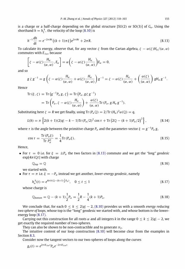
P.-M. Zhang et al. / Annals of Physics 327 (2012) 118–165 155
is a charge or a half-charge depending on the global structure [SU(2) or SO(3)] of Gα . Using theshorthand h = h k
ξ , the velocity of the loop (8.10) is
h−1dhdt= e−2π iRt
(k+ 1)πξ
e2π iRt + 2πR. (8.13)
To calculate its energy, observe that, for any vector ζ from the Cartan algebra, ζ − α(ζ )Hα/(α, α)commutes with E±α , because
ζ − α(ζ )Hα(α, α)
, Eα
= α
ζ − α(ζ )
Hα(α, α)
Eα = 0,
and so
g ζ g−1 = gζ − α(ζ )
Hα(α, α)
+ α(ζ )Hα(α, α)
g−1 = ζ − α(ζ )
Hα(α, α)
+
α(ζ )
(α, α)
gHα g−1.
Hence
Tr (ξ , ζ ) = Trg−1Pα g, ζ
= Tr
Pα, gζ g−1)
= TrPα, ζ − α(ζ )
Hα(α, α)
+α(ζ )
(α, α)Tr (Pα, g Hα g−1).
Substituting here ζ = Rwe get finally, using Tr (PαQ) = 2/Tr (Hα)2α(Q) = q,
L(h) = π2(k+ 1)(2|q| − k− 1)Tr (Pα/2)2 cos τ + Tr
2Q− (k+ 1)Pα/2
2, (8.14)
where τ is the angle between the primitive charge Pα and the parameter-vector ξ = g−1Pα g ,
cos τ =Tr (Pαξ)Tr P2
α
=14Tr (Pαξ). (8.15)
Hence,
• For τ = 0 i.e. for ξ = ±Pα the two factors in (8.13) commute and we get the ‘‘long’’ geodesicexp[4π iQt]with charge
Qtop = Q (8.16)
we started with.• For τ = π i.e. ξ = −Pα instead we get another, lower-energy geodesic, namely
h kα (t) = e4π it(Q−(k+1)
12 Pα), 0 ≤ t ≤ 1 (8.17)
whose charge is
Qbottom = Q− (k+ 1)12Pα =
12R−
14(k+ 1)Pα. (8.18)
We conclude that, for each 0 ≤ k ≤ 2|q| − 2, (8.10) provides us with a smooth energy reducingtwo sphere of loops, whose top is the ‘‘long’’ geodesic we started with, and whose bottom is the lower-energy loop (8.17).
Carrying out this construction for all roots α and all integers k in the range 0 ≤ k ≤ 2|q| − 2, weget exactly the required number of two-spheres.
They can also be shown to be non-contractible and to generate π2.The intuitive content of our loop construction (8.10) will become clear from the examples in
Section 8.3.Consider now the tangent vectors to our two-spheres of loops along the curves
gs(t) = e2π iE±α sPαe−2π iE±α s
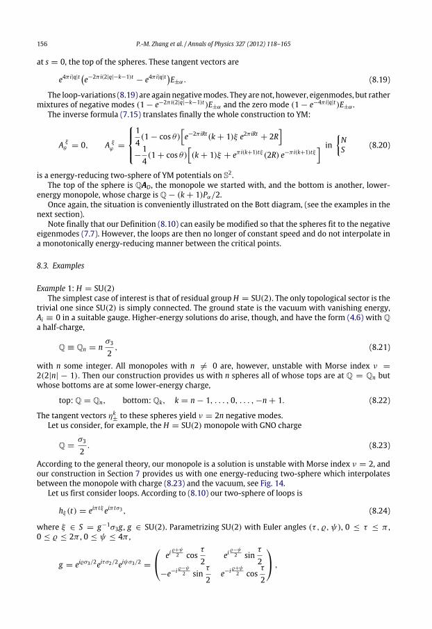
156 P.-M. Zhang et al. / Annals of Physics 327 (2012) 118–165
at s = 0, the top of the spheres. These tangent vectors are
e4π i|q|te−2π i(2|q|−k−1)t − e4π i|q|t
E±α. (8.19)
The loop-variations (8.19) are again negativemodes. They are not, however, eigenmodes, but rathermixtures of negative modes (1− e−2π i(2|q|−k−1)t)E±α and the zero mode (1− e−4π i|q|t)E±α .
The inverse formula (7.15) translates finally the whole construction to YM:
A ξθ = 0, A ξ
ϕ =
14(1− cos θ)
e−2π iRt(k+ 1)ξ e2π iRt + 2R
−
14(1+ cos θ)
(k+ 1)ξ + eπ i(k+1)tξ (2R) e−π i(k+1)tξ
inNS (8.20)
is a energy-reducing two-sphere of YM potentials on S2.The top of the sphere is QAD, the monopole we started with, and the bottom is another, lower-
energy monopole, whose charge is Q− (k+ 1)Pα/2.Once again, the situation is conveniently illustrated on the Bott diagram, (see the examples in the
next section).Note finally that our Definition (8.10) can easily be modified so that the spheres fit to the negative
eigenmodes (7.7). However, the loops are then no longer of constant speed and do not interpolate ina monotonically energy-reducing manner between the critical points.
8.3. Examples
Example 1: H = SU(2)The simplest case of interest is that of residual group H = SU(2). The only topological sector is the
trivial one since SU(2) is simply connected. The ground state is the vacuum with vanishing energy,Ai ≡ 0 in a suitable gauge. Higher-energy solutions do arise, though, and have the form (4.6) with Qa half-charge,
Q ≡ Qn = nσ3
2, (8.21)
with n some integer. All monopoles with n = 0 are, however, unstable with Morse index ν =2(2|n| − 1). Then our construction provides us with n spheres all of whose tops are at Q = Qn butwhose bottoms are at some lower-energy charge,
top: Q = Qn, bottom: Qk, k = n− 1, . . . , 0, . . . ,−n+ 1. (8.22)
The tangent vectors ηk±to these spheres yield ν = 2n negative modes.
Let us consider, for example, the H = SU(2)monopole with GNO charge
Q =σ3
2. (8.23)
According to the general theory, our monopole is a solution is unstable with Morse index ν = 2, andour construction in Section 7 provides us with one energy-reducing two-sphere which interpolatesbetween the monopole with charge (8.23) and the vacuum, see Fig. 14.
Let us first consider loops. According to (8.10) our two-sphere of loops is
hξ (t) = eiπ tξ eiπ tσ3 , (8.24)
where ξ ∈ S = g−1σ3g , g ∈ SU(2). Parametrizing SU(2) with Euler angles (τ , ϱ, ψ), 0 ≤ τ ≤ π ,0 ≤ ϱ ≤ 2π , 0 ≤ ψ ≤ 4π ,
g = eiϱσ3/2eiτσ2/2eiψσ3/2 =
eiϱ+ψ2 cos
τ
2eiϱ−ψ2 sin
τ
2−e−i
ϱ−ψ2 sin
τ
2e−i
ϱ+ψ2 cos
τ
2
,
P.-M. Zhang et al. / Annals of Physics 327 (2012) 118–165 157
Fig. 14. The GNO charge Q = σ3/2 supports an unstable solution of the SU(2) YM theory over the two-sphere. Its ν = 2negative modes are recovered as the tangents to the energy-reducing two-sphere whose top is Q = σ3/2 and whose bottomis the vacuum. The vertical axis is the Cartan algebra of su(2).
yields the parametrization with polar angles (τ , ψ) of the ξ -sphere,
ξ =
cos τ e−iψ sin τeiψ sin θ − cos τ
∈ su(2).
Then
eiπ tξ =cosπ t + i sinπ t cos τ ie−iψ sinπ t sin τieiψ sinπ t sin τ cosπ t − i sinπ t cos τ
,
eiπ tσ3 =eiπ t 00 e−iπ t
(8.25)
so that our sphere of loops (8.24) reads
hξ (t) =(cosπ t + i sinπ t cos τ) eiπ t ie−i(ψ+π t) sinπ t sin τ
iei(ψ+π t) sinπ t sin τ (cosπ t − i sinπ t cos τ) e−iπ t
. (8.26)
Calculating the speed of our loops,
h−1∂th = iπ
1+ cos τ e−i(ψ+2π t) sin τei(ψ+2π t) sin τ −1− cos τ
, (8.27)
[h ≡ hξ ] allows us to infer that the energy of the loopwith parameter ξ is simply the height function onthe unit ξ -sphere,
L(τ ,ψ) = π(1+ cos τ). (8.28)
This result is also consistent with (8.14). The intuitive picture is that of Fig. 14 with the ‘‘sphere’’meaning now SU(2) ≈ S3.
In YM terms, (8.20) yields in turn the two-sphere of YM configurations reads
A ξθ = 0, A ξ
ϕ =14(1− cos θ)
(1+ cos τ)σ3 − sin τ(e−i(ϱ+ϕ)σ+ + ei(ϱ+ϕ)σ−)
=
14(1− cos θ)
(1+ cos τ)σ3 − sin τ
cos(ϱ + ϕ)σ1 + sin(ϱ + ϕ)σ2
(8.29)
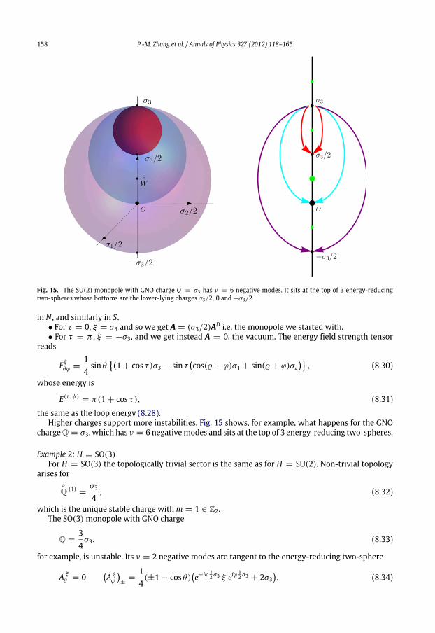
158 P.-M. Zhang et al. / Annals of Physics 327 (2012) 118–165
Fig. 15. The SU(2) monopole with GNO charge Q = σ3 has ν = 6 negative modes. It sits at the top of 3 energy-reducingtwo-spheres whose bottoms are the lower-lying charges σ3/2, 0 and−σ3/2.
in N , and similarly in S.• For τ = 0, ξ = σ3 and so we get A = (σ3/2)AD i.e. the monopole we started with.• For τ = π , ξ = −σ3, and we get instead A = 0, the vacuum. The energy field strength tensor
reads
F ξθϕ =14sin θ
(1+ cos τ)σ3 − sin τ
cos(ϱ + ϕ)σ1 + sin(ϱ + ϕ)σ2
, (8.30)
whose energy is
E(τ ,ψ) = π(1+ cos τ), (8.31)
the same as the loop energy (8.28).Higher charges support more instabilities. Fig. 15 shows, for example, what happens for the GNO
chargeQ = σ3, which has ν = 6 negativemodes and sits at the top of 3 energy-reducing two-spheres.
Example 2: H = SO(3)For H = SO(3) the topologically trivial sector is the same as for H = SU(2). Non-trivial topology
arises for
Q (1)=σ3
4, (8.32)
which is the unique stable charge withm = 1 ∈ Z2.The SO(3)monopole with GNO charge
Q =34σ3, (8.33)
for example, is unstable. Its ν = 2 negative modes are tangent to the energy-reducing two-sphere
A ξθ = 0
A ξϕ
±=
14(±1− cos θ)
e−iϕ
12 σ3 ξ eiϕ
12 σ3 + 2σ3
, (8.34)
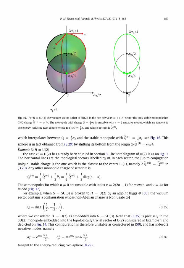
P.-M. Zhang et al. / Annals of Physics 327 (2012) 118–165 159
Fig. 16. For H = SO(3) the vacuum sector is that of SU(2). In the non-trivialm = 1 ∈ Z2 sector the only stable monopole has
GNO charge
Q (1)= σ3/4. The monopole with charge Q = 3
4σ3 is unstable with ν = 2 negative modes, which are tangent to
the energy-reducing two-sphere whose top is Q = 34σ3 and whose bottom is
Q (1) .
which interpolates between Q = 34σ3 and the stable monopole with
Q (1)=
14σ3, see Fig. 16. This
sphere is in fact obtained from (8.29) by shifting its bottom from the origin to
Q (1)= σ3/4.
Example 3: H = U(2)The case H = U(2) has already been studied in Section 3. The Bott diagram of U(2) is as on Fig. 9.
The horizontal lines are the topological sectors labelled by m. In each sector, the [up to conjugation
unique] stable charge is the one which is the closest to the central u(1), namely 2
Q (m)=
Q (m) in(3.20). Any other monopole charge of sectorm is
Q(m)=
12
Q (m)+
n2P1 =
12
Q (m)+
12diag(n,−n).
Those monopoles for which n = 0 are unstable with index ν = 2(2n− 1) form even, and ν = 4n form odd (Fig. 17).
For example, when G = SU(3) is broken to H = U(2) by an adjoint Higgs Φ [50], the vacuumsector contains a configuration whose non-Abelian charge is [conjugate to]
Q = diag12,−
12, 0, (8.35)
where we considered H = U(2) as embedded into G = SU(3). Note that (8.35) is precisely in theSU(2)monopole embedded into the topologically trivial sector of U(2) considered in Example 1 anddepicted on Fig. 14. This configuration is therefore unstable as conjectured in [50], and has indeed 2negative modes, namely
a±θ = e∓iϕσ±
2, a±ϕ = ∓e
∓iϕ sin θσ±
2(8.36)
tangent to the energy-reducing two-sphere (8.29).
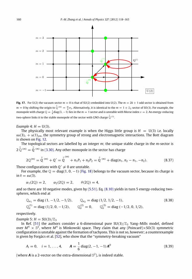
160 P.-M. Zhang et al. / Annals of Physics 327 (2012) 118–165
Fig. 17. For U(2) the vacuum sector m = 0 is that of SU(2) embedded into U(2). The m = 2k+ 1 odd sector is obtained from
m = 0 by shifting the origin to
Q (m)=
m4 σ3 . Alternatively, it is identical to the m = 1 ∈ Z2 sector of SO(3). For example, the
monopole with charge Q = 14 diag(3,−1) lies in them = 1 sector and is unstable withMorse index ν = 2. An energy-reducing
two-sphere links it to the stable monopole of the sector with GNO charge
Q (1) .
Example 4: H = U(3).The physically most relevant example is when the Higgs little group is H = U(3) i.e. locally
su(3)c + u(1)em, the symmetry group of strong and electromagnetic interactions. The Bott diagramis shown on Fig. 12.
The topological sectors are labelled by an integer m; the unique stable charge in the m-sector is
2
Q (m)=
Q (m) in (3.30). Any other monopole in the sector has charge
2Q(m)=
Q (m)+ Q ′ =
Q(m)+ n1P1 + n2P2 =
Q (m)+ diag(n1, n2 − n1,−n2). (8.37)
Those configurations with Q ′ = 0 are unstable.For example, the Q = diag(1, 0,−1) (Fig. 18) belongs to the vacuum sector, because its charge is
in k = su(3).
α1(2Q) = 2, α2(2Q) = 2, θ(2Q) = 4,
and so there are 10 negative modes, given by (5.51). Eq. (8.10) yields in turn 5 energy-reducing two-spheres, which end at
Qα1 = diag (1,−1/2,−1/2), Qα2 = diag (1/2, 1/2,−1), (8.38)
Q(1)θ = diag (1/2, 0,−1/2), Q(2)
θ = 0, Q(3)θ = diag (−1/2, 0, 1/2),
respectively.Example 5: H = SU(3)/Z3
In Ref. [51] the authors consider a 6-dimensional pure SU(3)/Z3 Yang–Mills model, definedover M4
× S2, where M4 is Minkowski space. They claim that any (Poincaré)×SO(3) symmetricconfiguration is unstable against the formation of tachyons. This is not so, however; a counterexampleis given by Forgács et al. [52], who show that the ‘‘symmetry-breaking vacuum’’
Ai = 0, i = 1, . . . , 4, A =16diag(2,−1,−1)AD (8.39)
(where A is a 2-vector on the extra-dimensional S2), is indeed stable.
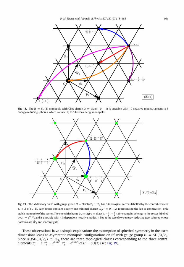
P.-M. Zhang et al. / Annals of Physics 327 (2012) 118–165 161
Fig. 18. The H = SU(3) monopole with GNO charge Q = diag(1, 0,−1) is unstable with 10 negative modes, tangent to 5energy-reducing spheres, which connect Q to 5 lower-energy monopoles.
Fig. 19. The YM theory on S2 with gauge group H = SU(3)/Z3 ≃ Z3 has 3 topological sectors labelled by the central element
za ∈ Z of SU(3). Each sector contains exactly one minimal charge
W j , j = 0, 1, 2, representing the [up to conjugation] only
stable monopole of the sector. The one with charge 2Q = 2
W 2 = diag(1,− 12 ,−
12 ), for example, belongs to the sector labelled
by z1 = e4π i/3 , and is unstable with 4 independent negativemodes. It lies at the top of two energy-reducing two-spheres whose
bottoms are
W 1 and its conjugate.
These observations have a simple explanation: the assumption of spherical symmetry in the extradimensions leads to asymptotic monopole configurations on S2 with gauge group H = SU(3)/Z3.Since π1(SU(3)/Z3) ≃ Z3, there are three topological classes corresponding to the three centralelements z∗0 = 1, z∗1 = e2π i/3, z∗2 = e4π i/3 of H = SU(3) (see Fig. 19).
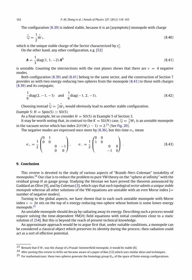
162 P.-M. Zhang et al. / Annals of Physics 327 (2012) 118–165
The configuration (8.39) is indeed stable, because it is an [asymptotic] monopole with charge
Q =12
W 1, (8.40)
which is the unique stable charge of the Sector characterized by z∗2 .On the other hand, any other configuration, e.g. [52]
A =13diag(1, 1,−2)AD (8.41)
is unstable. Counting the intersections with the root planes shows that there are ν = 4 negativemodes.
Both configuration (8.39) and (8.41) belong to the same sector, and the construction of Section 7provides us with two energy-reducing two-spheres from the monopole (8.41) to those with charges(8.39) and its conjugate,
16diag(2,−1,−1) and
16diag(−1, 2,−1). (8.42)
Choosing instead
Q = 12
W 2 would obviously lead to another stable configuration.Example 5: H = Spin(5) ≃ SO(5)
As a final example, let us consider H = SO(5) in Example 5 of Section 3.It may be worth noting that, in contrast to the K = SU(N) case, Q = 1
2W1 is an unstablemonopolein the vacuum sector which has index 2(θ(W1)− 1) = 2.23 (See Fig. 20).
The negative modes are expressed once more by (8.36), but this time σ± mean
σ+ =12
0 10 0
0 −10 0
, σ− =12
0 01 0
0 0−1 0
. (8.43)
9. Conclusion
This review is devoted to the study of various aspects of ‘‘Brandt–Neri–Coleman’’ instability ofmonopoles.24 Our clue is to reduce the problem to pure YM theory on the ‘‘sphere at infinity’’ with theresidual group H as gauge group. Studying the Hessian we have proved the theorem announced byGoddard an Olive [9], and by Coleman [3], which says that each topological sector admits a unique stablemonopole whereas all other solutions of the YM equations are unstable with an even Morse index [=number of negative modes].
Turning to the global aspects, we have shown that to each such unstable monopole with Morseindex ν = 2n sits on the top of n energy-reducing two-sphere whose bottom is some lower-energymonopole.25
An unstablemonopole should decay by radiating away its energy. Describing such a process wouldrequire solving the time-dependent YM(H) field equations with initial conditions close to a staticsolution cf. [54]. But this is beyond the reach of present technical knowledge.
An approximate approach would be to argue first that, under suitable conditions, a monopole canbe considered a classical object which preserves its identity during the process; then radiation couldact as a sort of effective potential.
23 Remark that ifW1 was the charge of a Prasad–Sommerfield monopole, it would be stable [8].24 After posting this review to ArXiv we became aware of a paper of Bais [53] which uses similar ideas and techniques.25 For mathematicians: these two-spheres generate the homology group H2n of the space of finite-energy configurations.
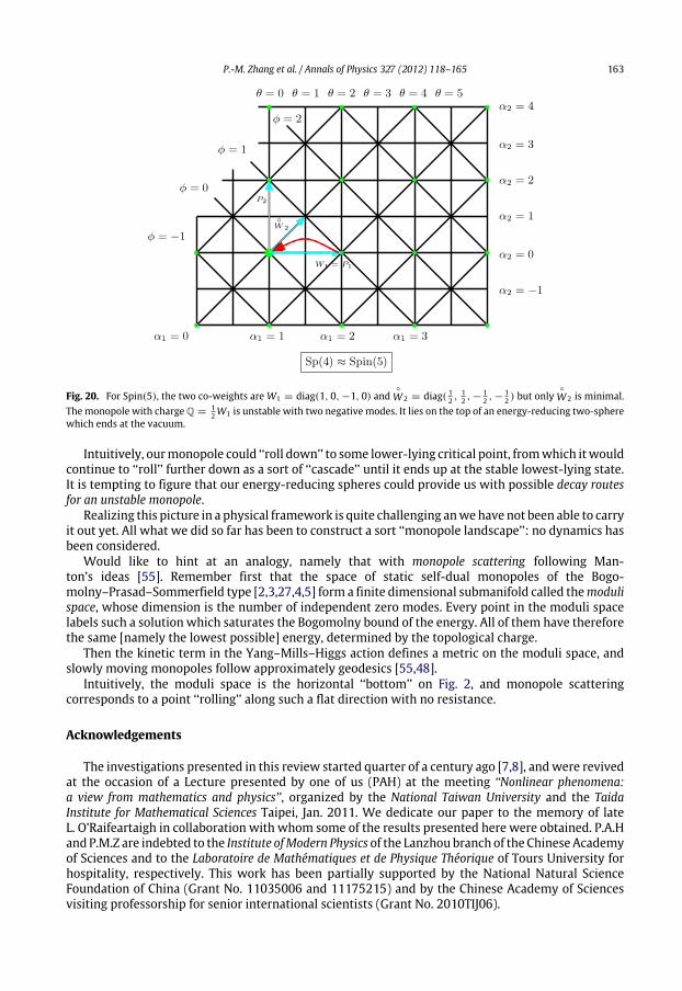
P.-M. Zhang et al. / Annals of Physics 327 (2012) 118–165 163
Fig. 20. For Spin(5), the two co-weights are W1 = diag(1, 0,−1, 0) and
W 2 = diag( 12 ,12 ,−
12 ,−
12 ) but only
W 2 is minimal.The monopole with charge Q = 1
2W1 is unstable with two negative modes. It lies on the top of an energy-reducing two-spherewhich ends at the vacuum.
Intuitively, ourmonopole could ‘‘roll down’’ to some lower-lying critical point, fromwhich itwouldcontinue to ‘‘roll’’ further down as a sort of ‘‘cascade’’ until it ends up at the stable lowest-lying state.It is tempting to figure that our energy-reducing spheres could provide us with possible decay routesfor an unstable monopole.
Realizing this picture in a physical framework is quite challenging anwehave not been able to carryit out yet. All what we did so far has been to construct a sort ‘‘monopole landscape’’: no dynamics hasbeen considered.
Would like to hint at an analogy, namely that with monopole scattering following Man-ton’s ideas [55]. Remember first that the space of static self-dual monopoles of the Bogo-molny–Prasad–Sommerfield type [2,3,27,4,5] form a finite dimensional submanifold called themodulispace, whose dimension is the number of independent zero modes. Every point in the moduli spacelabels such a solution which saturates the Bogomolny bound of the energy. All of them have thereforethe same [namely the lowest possible] energy, determined by the topological charge.
Then the kinetic term in the Yang–Mills–Higgs action defines a metric on the moduli space, andslowly moving monopoles follow approximately geodesics [55,48].
Intuitively, the moduli space is the horizontal ‘‘bottom’’ on Fig. 2, and monopole scatteringcorresponds to a point ‘‘rolling’’ along such a flat direction with no resistance.
Acknowledgements
The investigations presented in this review started quarter of a century ago [7,8], andwere revivedat the occasion of a Lecture presented by one of us (PAH) at the meeting ‘‘Nonlinear phenomena:a view from mathematics and physics’’, organized by the National Taiwan University and the TaidaInstitute for Mathematical Sciences Taipei, Jan. 2011. We dedicate our paper to the memory of lateL. O’Raifeartaigh in collaboration with whom some of the results presented here were obtained. P.A.Hand P.M.Z are indebted to the Institute ofModern Physics of the Lanzhou branch of the Chinese Academyof Sciences and to the Laboratoire de Mathématiques et de Physique Théorique of Tours University forhospitality, respectively. This work has been partially supported by the National Natural ScienceFoundation of China (Grant No. 11035006 and 11175215) and by the Chinese Academy of Sciencesvisiting professorship for senior international scientists (Grant No. 2010TIJ06).
164 P.-M. Zhang et al. / Annals of Physics 327 (2012) 118–165
References
[1] G. ’t Hooft, Nuclear Phys. B 79 (1974) 276;A.M. Polyakov, JETP Lett. 20 (1974) 194.
[2] P. Goddard, D. Olive, Rep. Prog. Phys. 41 (1978) 1357.[3] S. Coleman, in: A. Zichichi (Ed.), The Unity of Fundamental Interactions, Plenum, New York, 1983; Aspects of symmetries,
in: Selected Erice Lectures, Cambridge UP, 1885.[4] P.A. Horváthy, Introduction to Monopoles, in: Monographs and Textbooks in Physical Science. Lecture Notes, vol. 6,
Bibliopolis, Naples, Italy, 1988.[5] K. Konishi, Lect. Notes Phys. 737 (2008) 471. arXiv:hep-th/0702102.[6] R.A. Brandt, F. Neri, Nuclear Phys. B 161 (1979) 253.[7] P.A. Horváthy, J.H. Rawnsley, Proceedings of the International Conference onDifferential GeometricMethods in Theoretical
Physics. Clausthal’1986, World Scientific, Singapore, 1986, p. 108;P.A. Horváthy, in: Z. Horváth, L. Palla, A. Patkós. (Eds.), Proc. Non-perturbativeMethods in QFT,World Scientific, Singapore,1987, p. 39.
[8] P.A. Horváthy, L. O’Raifeartaigh, J.H. Rawnsley, Int. J. Mod. Phys. A 3 (1988) 665. Available as arXiv:0909.2523 [hep-th].[9] P. Goddard, D.I. Olive, Nuclear Phys. B. 191 (1981) 528.
[10] Th. Friedrich, L. Habermann, Comm. Math. Phys. 100 (1985) 231.[11] W. Nahm, K. Uhlenbeck, The equivalence of quantized gauge fields on S2 and the quantummechanics of a particle moving
on the group manifold, Unpublished notes, Chicago 1988.[12] J. Milnor, Morse Theory, in: Ann. Math. Studies, vol. 51, Princeton University Press, New Jersey, 1963;
R. Bott, Bull. Amer. Math. Soc. 7 (3) (1982) 331.[13] J. Arafune, P.G.O. Freund, C.J. Goebel, J. Math. Phys. 16 (1975) 433.[14] A.S. Schwarz, Nuclear Phys. B 112 (1976) 358.[15] C.H. Taubes, Comm. Math. Phys. 81 (1981) 299.[16] P.A. Horváthy, J.H. Rawnsley, Comm. Math. Phys. 96 (1984) 497; Comm. Math. Phys. 99 (1985) 517;
P.A. Horvathy, J.H. Rawnsley, J. Phys. A 20 (1987) 747. In a rather peculiar way, the same topological charge arises fornon-topological ‘‘Jackiw-Pi’’ vortex solutions, see P.A. Horváthy, Lett. Math. Phys. 49 (1999) 67.
[17] E. Lubkin, Ann. Phys. 23 (1963) 233.[18] P. Goddard, J. Nuyts, D. Olive, Nuclear Phys. B 125 (1977) 1.[19] M.F. Atiyah, R. Bott, Philos. Trans. R. Soc. Lond. Ser. A 308 (1983) 523.[20] J.M. Speight, The ground state energy of a charged particle on a Riemann surface, arxiv.org/abs/1012.3337 [hep-th].[21] R. Bott, Representation Theory of Lie Groups, in: Atiyah (Ed.), Proc. Oxford’77, Cambridge University Press, 1979, p. 63.[22] I. Singer, Phys. Scr. 24 (1984) 817.[23] N.S. Manton, Phys. Rev. D 28 (1983) 2019.[24] C. Taubes, Comm. Math. Phys. 91 (1983) 235.[25] P. Forgács, Z. Horváth, Phys. Lett. B 138 (1984) 397.[26] L.M. Sibner, J. Talvacchia, Comm. Math. Phys. 162 (1994) 333.[27] E.B. Bogomolny, Sov. J. Nucl. Phys. 24 (1976) 449;
M.K. Prasad, C.M. Sommerfield, Phys. Rev. Lett. 35 (1975) 760.[28] P.A.M. Dirac, Proc. R. Soc. Lond. A 133 (1931) 60.[29] N. Steenrod, Topology of Fibre Bundles, Princeton Univ. Press, 1951.[30] S. Kobayashi, K. Nomizu, Foundations of Differential Geometry, vol. I, Interscience, NY, 1963; vol. II, Interscience, NY, 1969.[31] R. Bott, L. Tu, Differential Forms in Algebraic Topology, Springer, Verlag, New York, Heidelberg, Berlin, 1982.[32] T.T. Wu, C.N. Yang, Phys. Rev. D 12 (1975) 3845.[33] T.T. Wu, C.N. Yang, Phys. Rev. D 14 (1976) 437.[34] P.A. Horváthy, Proc. Int. Coll. on Diff. Geom. Meths. in Math. Phys., Aix-en Provence’79, in: Souriau (Ed.), Springer Lecture
Notes in Math., vol. 836, 1980, p. 67.[35] J. Sniatycki, J. Math. Phys. 15 (1974) 619.[36] W. Greub, H.R. Petry, J. Math. Phys. 16 (1975) 1347.[37] A. Trautman, Int. J. Theor. Phys. 16 (1977) 561.[38] P.A. Horváthy, Int. J. Theor. Phys. 20 (1981) 697.[39] A. Trautman, Stony Brook Lectures, in: Monographs and Textbooks in Physical Sciences, Bibliopolis, Napoli, 1984.[40] A. Salam, Weak and electromagnetic interactions, in: Proceedings of 8th Nobel Symposium, Lerum, Sweden, 19–25 May
1968, Alqvist and Wicksell, Stockholm, 1968, pp. 367–377.[41] H. Georgi, S.L. Glashow, Phys. Rev. Lett. 32 (1974) 438.[42] Z. Horváth, L. Palla, Phys. Lett. B 69 (1977) 197; Nuclear Phys. B 116 (1976) 500;
C.P. Dokos, T.N. Tomaras, Phys. Rev. D 21 (1980) 2940.[43] J.E. Humphreys, Introduction to Lie Algebras and Representation Theory, Springer Verlag, Berlin, 1972.[44] P.A. Horváthy, J.H. Rawnsley, Phys. Rev. D 32 (1985) 968.[45] P. Goddard, D.I. Olive, Nuclear Phys. B 191 (1981) 511.[46] M. Spiegelglas, Phys. Lett. B 166 (1986) 160.[47] L. Fehér, P.A. Horváthy, L. O’Raifeartaigh, Int. J. Mod. Phys. A 4 (1989) 5277.[48] E.J. Weinberg, P. Yi, Phys. Rep. 438 (2007) 65. arXiv:hep-th/0609055;
E.J. de Vries, B.J. Schroers, Nuclear Phys. B 815 (2009) 368. arXiv:0811.2155 [hep-th].[49] P.A. Horváthy, Int. J. Theor. Phys. 18 (1979) 245; Cent. Eur. J. Phys. 9 (2011) 1. quant-ph/0702236.[50] E. Corrigan, D. Olive, D.B. Fairlie, J. Nuyts, Nuclear Phys. B 106 (1976) 475.[51] S. Randjbar-Daemi, A. Salam, J. Strathdee, Phys. Lett. B 124 (1983) 345.[52] P. Forgács, Z. Horváth, L. Palla, Phys. Lett. B 147 (1984) 311.[53] F.A. Bais, To be or not to be?Magneticmonopoles in non-Abelian gauge theories, in: ’t Hooft, G. (Ed.): 50 years of Yang–Mills
Theory, pp. 271–307 [hep-th/0407197 ].
P.-M. Zhang et al. / Annals of Physics 327 (2012) 118–165 165
[54] H. Guo, E.J. Weinberg, Phys. Rev. D 77 (2008) 105026. arXiv:0803.0736 [hep-th].[55] N.S. Manton, Phys. Lett. B 110 (1982) 54; Phys. Lett. B 154 (1985) 397; Phys. Lett. B157 (1985) 475;
M.F. Atiyah, N.J. Hitchin, Phil. Trans. R. Soc. Lond. A 315 (1985) 459;M.F. Atiyah, N.J. Hitchin, Phys. Lett. A 107 (1985) 21;M.F. Atiyah, N.J. Hitchin, The Geometry and Dynamics of Magnetic Monopoles. M. B. Porter Lectures, USA, Univ. Press,Princeton, 1988.


![- [S.l.] : [s.n.], 1985 CCBAEbdace81a-afd9...1 Boletín de novedades bibliográficas en CCBAE Biblioteca Archivo General de Indias Diciembre 2019 1. Aguila, Yves Monopoles d'etat](https://img.pdfslide.fr/doc/110x75/5f72edc215fe8051f118e312/-sl-sn-1985-ccbae-bdace81a-afd9-1-boletn-de-novedades-bibliogrficas.jpg)

![Ingénieur de RechercheDéveloppement de la plateforme TTK · Ingénieur de Recherche Développement de la plateforme TTK Julien Tierny Fig. 1. TTK (the “Topology ToolKit” [38])](https://img.pdfslide.fr/doc/110x75/5f346a361811470af41b20a8/ingnieur-de-recherchedveloppement-de-la-plateforme-ttk-ingnieur-de-recherche.jpg)