Embed Size (px)
Citation preview
HAL Id: tel-00116961https://tel.archives-ouvertes.fr/tel-00116961
Submitted on 29 Nov 2006
HAL is a multi-disciplinary open accessarchive for the deposit and dissemination of sci-entific research documents, whether they are pub-lished or not. The documents may come fromteaching and research institutions in France orabroad, or from public or private research centers.
L’archive ouverte pluridisciplinaire HAL, estdestinée au dépôt et à la diffusion de documentsscientifiques de niveau recherche, publiés ou non,émanant des établissements d’enseignement et derecherche français ou étrangers, des laboratoirespublics ou privés.
Trois essais sur la croissance, la pauvreté et lespropriétés cycliques de la politique budgétaire
Oumar Diallo
To cite this version:Oumar Diallo. Trois essais sur la croissance, la pauvreté et les propriétés cycliques de la politiquebudgétaire. Humanities and Social Sciences. Université d’Auvergne - Clermont-Ferrand I, 2006.English. <tel-00116961>
Université d’Auvergne Faculté des Sciences Economiques de Gestion
Ecole Doctorale des Sciences Economiques et de Gestion Centre d’Etudes et de Recherches sur le Développement International (CERDI)
Année 2006
THESE NOUVEAU REGIME Présentée et soutenue publiquement
Pour l’obtention du titre de Docteur ès Sciences Economiques
par
Oumar Diallo
Septembre 2006
Titre : TROIS ESSAIS SUR LA CROISSANCE, LA PAUVRETE ET LES PROPRIETES CYCLIQUES
DE LA POLITIQUE BUDGETAIRE
Directeurs de thèse : Jean-Louis Arcand et Jean-Louis Combes
JURY :
Directeurs Jean-Louis Arcand, Professeur à l’Université d’Auvergne, CERDI
Jean-Louis Combes, Professeur à l’Université d’Auvergne, CERDI
Rapporteurs Olivier Cadot, Professeur à l’Université de Lausanne
Christian Morrisson, Professeur à l’Université de Paris I
Suffragants Patrick Guillaumont, Professeur à l’Université d’Auvergne, CERDI
Jean-François Brun, Maître de Conférences à l’Université d’Auvergne, CERDI
tel-0
0116
961,
ver
sion
1 -
29 N
ov 2
006
1
A Mariam, Mamadou, Adama, Oumar Jr. et à toute la génération montante de ma famille.
tel-0
0116
961,
ver
sion
1 -
29 N
ov 2
006
2
Le CERDI n’entend donner aucune approbation ou improbation aux opinions émises dans cette thèse. Ces opinions doivent être considérées comme propes à leur auteur.
tel-0
0116
961,
ver
sion
1 -
29 N
ov 2
006
REMERCIEMENTS
3
REMERCIEMENTS
Mener une thèse à son terme est généralement perçu comme le fruit d’un travail et
d’effort personnels mais le soutien de nombreuses personnes y est déterminant, et je tiens à
remercier ici ces personnes.
Mes remerciements s’adressent, en tout premier lieu, à Monsieurs les Professeurs
Jean-Louis Arcand et Jean-Louis Combes qui ont accepté de me guider tout au long de cette
aventure. Leur disponibilité, leurs encouragements, leurs vastes connaissances théoriques et
parfaite maîtrise d’outils quantitatifs, et la pertinence de leurs points de vue me furent d’une
grande utilité.
Je suis également infiniment reconnaissant à Monsieur le Professeur Patrick
Guillaumont pour son soutien constant et l’intérêt qu’il a toujours manifesté pour mes
travaux de recherche. Je lui rends ici un vibrant hommage pour avoir su créer au CERDI un
environnement propice à l’éclosion de talents.
Je remercie sincèrement Monsieurs les Professeurs Olivier Cadot et Christian
Morrisson qui, en dépit de leur emploi du temps très serré, m’ont fait l’honneur d’être
rapporteurs dans mon jury. Je suis aussi redevable à l’ensemble des personnes qui ont suivi
ma présentation au séminaire des doctorants, notamment Madame le Professeur Sylviane
Guillaumont-Jeanneney et Monsieur Jules-Armand Tapsoba, pour la pertinence de leurs
commentaires et leurs suggestions constructives.
La préparation de la thèse a nécessité de fréquents déplacements sur Clermont-
Ferrand et de nombreuses démarches consulaires. Ceci n’aurait été possible sans la
promptitude et la disponibilité de Monsieur Patrick Doger, à qui je dis merci. Je ne peux
évidemment oublier Martine Bouchut, Marie-Michèle Ceysson, Solange Debas et Jacqueline
Reynard pour leur disponibilité et leur professionnalisme.
tel-0
0116
961,
ver
sion
1 -
29 N
ov 2
006
REMERCIEMENTS
4
Ce projet aurait été hardi voir impossible n’eut été l’existence d’un environnement
social agréable. J’ai une pensée particulière à toute ma famille, au vrai sens africain du terme,
et singulièrement à mon père et à ma mère pour leur soutien et leurs encouragements. Je leur
suis infiniment reconnaissant de m’avoir inculqué le sens de l’humilité, l’esprit de
dépassement, une foi inébranlable, et une ténacité inaccessible au découragement : caractères
qui m’ont permis de mener ma thèse de doctorat à son terme.
Mes remerciements vont également à mes frères Papa, Oumar Djoboula, Macky, Sid
et Amadou NJ, mon oncle Ousmane, mon(a) neveu(ièce) Doura/Sandrine et leurs familles
respectives pour avoir su créer un cadre familial agréable. Je voudrais également renouveler
mon admiration à mon épouse, Aissatou L., pour son soutien et sa compréhension durant
cette épreuve que fut la préparation de la thèse.
Dans les instants d’incertitude, le soutien, les encouragements et l’amitié de collègues
et de mentors ont été déterminants. Je voudrais témoigner ici ma reconnaissance à
Abdoulaye et Sata Seck, Emmanuel Goued-Njayick, Ruth Engo, Diaretou Gaye, Brian Ngo,
Emmanuel Akpa, Carl Gray, Edouard Nsimba, Pingfan Hong et Ana Cortez.
Le contenu de cette thèse a bénéficié des commentaires et suggestions d’amis et
certains membres de l’équipe du CERDI. Je voudrais exprimer ma gratitude à Sid, Boubou,
Roland, Djoulassi Oloufade, Jean-François Brun, Fanon, Leonard et Janvier pour les
discussions constructives, à Bachir et Harry pour l’aide qu’ils m’ont apportée dans la
construction d’une de mes bases de données.
J’ai bénéficié également du soutien moral de personnes avec lesquelles j’ai noué de
solides amitiés à la faveur de mon passage au CERDI. Je rends ici hommage à Boubou,
Ahmed, Gaëlle, Armand Gala et Marie-Cécile. Enfin, mes sincères remerciements vont à
Yaya Seydou, Djoulassi Oloufade et Mamadou Dian pour leur totale disponibilité et la
précieuse aide qu’ils m’ont apportées et qui m’ont permis de déposer la thèse dans un délai
raisonnable.
tel-0
0116
961,
ver
sion
1 -
29 N
ov 2
006
TABLE OF CONTENTS
5
TABLE OF CONTENTS
GENERAL INTRODUCTION………………………………………………….9 CHAPTER I: PUBLIC SPENDING AND REAL EXCHANGE RATE INSTABILITIES AND GROWTH IN AFRICA: EVIDENCE FROM PANEL DATA……………………………………………………………………………………21 I-INTRODUCTION........................................................................................................................22 II-DATA: AFRICA VERSUS OTHER DEVELOPING REGIONS ....................................24
2.1 Instability Measurement .........................................................................................................24 2.2 Comparison Africa vs. other developing regions ...............................................................27 2.3 The case of Botswana.............................................................................................................30
III- THEORETICAL CONSIDERATIONS...............................................................................31 3.1 Solow Model ............................................................................................................................31 3.2 Criticisms..................................................................................................................................33 3.3 The role of economic policies: importance of stability ....................................................35
3.3.1 Public spending instability and growth ........................................................................36 3.3.2 Real exchange rate instability and growth....................................................................38
IV-ECONOMETRIC METHODOLOGY..................................................................................40 4.1 Ineffective OLS .......................................................................................................................41 4.2 Instrumental Variable Estimator of Anderson and Hsiao (1982)....................................42 4.3 First-Differenced Generalised Method-of-Moments Estimator (GMM) and System Generalised Method-of-Moments Estimator (SYS-GMM) ....................................................43
V-EMPIRICAL RESULTS..............................................................................................................44 5.1 Validity of The Solow Model and its augmented version .................................................45 5.2 Core Model ..............................................................................................................................48
5.2.1 The potential channels from public spending instability to poor economic growth.....................................................................................................................................................52 5.2.2 The potential channels from real exchange rate instability to poor economic growth.........................................................................................................................................57
VI- CONCLUSION..........................................................................................................................62 APPENDIX I-1: VARIABLES AND SOURCES.......................................................................65 APPENDIX I-2: SAMPLE..............................................................................................................66 APPENDIX I-3 STRUCTURAL, INSTITUTIONAL, AND POLICY FACTORS DETERMINING GROWTH ........................................................................................................67 APPENDIX I-4: PANEL UNIT ROOT TESTS ........................................................................70 APPENDIX I-5: INCLUSION OF POLICY FACTORS.........................................................74
tel-0
0116
961,
ver
sion
1 -
29 N
ov 2
006
TABLE OF CONTENTS
6
CHAPTER II: POVERTY AND REAL EXCHANGE RATE: EVIDENCE FROM PANEL DATA………………………………………………………….78 I- INTRODUCTION.......................................................................................................................79 II- OVERVIEW.................................................................................................................................81 III- SIMPLE DEPENDENT ECONOMY MODEL................................................................83 IV- REAL EXCHANGE RATE, ABSORPTION, AND POVERTY ...................................87
4.1 Indirect effects.........................................................................................................................87 4.1.1 Real exchange rate, absorption, and growth................................................................87 4.1.2 Growth and poverty........................................................................................................88
4.2 Direct effects............................................................................................................................89 4.2.1 The direct impact of the reduction of absorption ......................................................89 4.2.2 The direct impact of real exchange rate on poverty...................................................90
4.3 Third set of factors .................................................................................................................93 4.3.1 Inequality ..........................................................................................................................93 4.3.2 The quality of institutions ..............................................................................................95
V-THEORETICAL FRAMEWORK AND THE ECONOMETRIC METHODOLOGY..............................................................................................................................................................96 5.1 Theoretical Framework ..........................................................................................................96 5.2 Econometric Methodology....................................................................................................98
VI- DATA ISSUES AND ECONOMETRIC RESULTS........................................................100 6.1 Description of the variables and their sources..................................................................100
6.1.1 Poverty ............................................................................................................................101 6.1.2 Key explanatory variables of interest..........................................................................102
6.2 Main Empirical Results ........................................................................................................108 6.2.1 The results of the estimation of the basic model......................................................108 6.2.2 The results of the estimation of the core model.......................................................110 6.2.3 Additional controls........................................................................................................114 6.2.4 Asymmetric effects........................................................................................................119
VII- CONCLUSION......................................................................................................................122 APPENDIX II-1: SOURCES AND COMMENTS..................................................................125 APPENDIX II-2: SAMPLES ........................................................................................................127 APPENDIX II-3 : DEFINITION ET INDICATEURS DE PAUVRETE.........................128
CHAPTER III: IS FISCAL POLICY BECOMING COUNTERCYCLICAL IN AFRICA ?……………………………………………………………………153 I-INTRODUCTION......................................................................................................................155 II- COUNTERCYCLICAL FISCAL POLICIES AND LONG TERM GROWTH..........158 III-DETERMINANTS OF PROCYCLICAL FISCAL POLICY ..........................................161 IV-DEMOCRATIC INSTITUTIONS AND CYCLICAL PROPERTIES OF FISCAL POLICY ............................................................................................................................................163
4.1 Democratic institutions conducive to procyclical fiscal policies....................................163 4.2 Democratic institutions conducive to countercyclical fiscal policies.............................165 4.3 Theoretical Model .................................................................................................................167
tel-0
0116
961,
ver
sion
1 -
29 N
ov 2
006
TABLE OF CONTENTS
7
V- COUNTRY EXPERIENCES .................................................................................................169 5.1 Botswana ................................................................................................................................169 5.2 Nigeria.....................................................................................................................................171
VI -DATA ISSUES AND EMPIRICAL STRATEGY.............................................................173 6.1 Data .........................................................................................................................................173
6.1.1 Dependent variable .......................................................................................................173 6.1.2 Explanatory variables....................................................................................................176 6.1.3 Control variables............................................................................................................178
6.2 Empirical Strategy .................................................................................................................179 VII-RESULTS..................................................................................................................................180
7.1 Terms-of-trade shock, democratic institutions and fiscal policy stance .......................181 7.1.1 Fiscal policy stance captured through government expenditure ............................181 7.1.2 Fiscal policy stance captured through government current expenditure ..............184
7.2 The residual approach ..........................................................................................................185 7.3 Transmission channels and other covariates.....................................................................189
VIII-CONCLUSION......................................................................................................................194 APPENDIX III-1: DEFINITION OF VARIABLES AND SOURCES..............................196 APPENDIX III-2: SAMPLES ......................................................................................................197
GENERAL CONCLUSION…………………………………………………..198 REFERENCES................................................................................................................................207
tel-0
0116
961,
ver
sion
1 -
29 N
ov 2
006
TABLES AND FIGURES
8
TABLES AND FIGURES CHAPTER I: PUBLIC SPENDING AND REAL EXCHANGE RATE INSTABILITIES AND GROWTH IN AFRICA: EVIDENCE FROM PANEL DATA Table 1: Panel unit root test based on Levin, Lin, and Chu (2002) approach ..........................25 Table 2: Panel unit root test based on Im, Pesaran, and Shin (2003) approach .......................26 Table 3: Panel unit root test based on Fisher-Augmented Dicker Fuller approach ................26 Table 4: The median of some key indicators in Sub-Saharan Africa and in other Developing Countries .............................................................................................................................................28 Table 5: Comparison of the median of some key indicators in Sub-Saharan Africa and in other Developing Countries in 1994-1997 and 1974-1993..........................................................29 Table 6: SYS-GMM Estimates of Solow Model............................................................................46 Table 7: SYS-GMM Estimates of the Model of Growth and Instabilities of Real Exchange Rate and Public Spending .................................................................................................................49 Table 8: SYS-GMM Estimates of the Model of Growth and Instabilities of Real Exchange Rate and Public Spending based on 8-year sub periods ...............................................................51 Table 9: SYS-GMM Estimates of the Model of Growth, with a focus on potential ratchet effects...................................................................................................................................................53 Table 10: SYS-GMM Estimates of the Model of Growth and Instabilities of Real Exchange Rate and Public Spending .................................................................................................................54 Table 11: SYS-GMM Estimates of the Determinants of Real Investment ...............................56 Table 12: SYS-GMM Estimates of the Model of Growth, with a focus on potential asymmetric effects..............................................................................................................................58 Table 13: SYS-GMM Estimates of the Model of Growth, with a focus on potential inertia effects...................................................................................................................................................59
CHAPTER II: POVERTY AND REAL EXCHANGE RATE: EVIDENCE FROM PANEL DATA Figure 1: Dynamics in a dependent economy model....................................................................86 Table 1: Macroeconomic policies and poverty trend....................................................................82 Table 2: The incomes of the poor and real exchange rate .........................................................109 Table 3: The incomes of the poor, real exchange rate, institutions, and inequality ...............111 Table 4: The incomes of the poor, real exchange rate, institutions, and inequality ...............113 Table 5: The incomes of the poor, real exchange rate, institutions, inequality, and other covariates...........................................................................................................................................117 Table 6: The incomes of the poor, real exchange rate, institutions, inequality, and other covariates...........................................................................................................................................118 Table 7: The incomes of the poor and real exchange rate asymmetric effects .......................120 Table 8: The incomes of the poor and real exchange rate asymmetric effects .......................121
tel-0
0116
961,
ver
sion
1 -
29 N
ov 2
006
TABLES AND FIGURES
9
CHAPTER III: IS FISCAL POLICY BECOMING COUNTERCYCLICAL IN AFRICA ? Table 1: Fiscal Indicators: Theoretical Correlations with the Business Cycle.........................174 Table 2: Correlation Matrix between Civil Liberties and Political Rights Indexes...............177 Table 3: Determinants of the cyclicality of Government Expenditure....................................183 Table 4: Determinants of the cyclicality of Government Current Expenditure.....................185 Table 5: Determinants of the cyclicality of Government Expenditure....................................187 Table 6: Determinants of the cyclicality of Government Current Expenditure.....................189 Table 7: Democratic Institution indexes and two key characteristics of democratic systems............................................................................................................................................................191 Table 8: Determinants of the cyclicality of Public Spending, additional covariates considered............................................................................................................................................................192
tel-0
0116
961,
ver
sion
1 -
29 N
ov 2
006
GENERAL INTRODUCTION
10
GENERAL INTRODUCTION
tel-0
0116
961,
ver
sion
1 -
29 N
ov 2
006
GENERAL INTRODUCTION
11
GENERAL INTRODUCTION
Africa1’s GDP growth varies considerably across time but appears to be generally
poor. The region’s growth performance is disappointing in absolute terms, and is even
gloomier when set against that of other developing regions. Economic growth was so
weak in the continent that Africa’s per capita GDP was lower in 1997 than 30 years
before. The decline was even stronger in some countries, where per-capita output fell by
more than 50 percent (World Bank, 2000). As a result of this poor growth, the average
income2 in Africa in 1997 stands at just a third of that of South Asia3, making the region
the poorest in the world (World Bank, 2000). Similarly, the big income divide between
African countries and developed countries continues to widen as the latter group of
countries has grown steadily, albeit at a moderate pace, over the past three decades
(United Nations, 2006). Africa’s poor performance is perhaps an important part of
Bourguignon and Morrisson (2002)’s finding that attributes growing disparities in
welfare between the world’s citizens more to differences in inequality between countries
than inequality within countries.
In addition to this dismal economic performance, the continent lags behind in
terms of human development. Africa’s social indicators do not compare favourably with
those of other regions despite some improvements recorded in the continent. For instance,
life expectancy in Africa stood at only 52 years in 1997 compared to an average of 65
1 Africa means Sub-Saharan Africa in the rest of the dissertation. 2 The figure used is the per capita GNI measured through the Atlas Method. 3 Many African countries were wealthier than their South Asian counterparts in the 1960s.
tel-0
0116
961,
ver
sion
1 -
29 N
ov 2
006
GENERAL INTRODUCTION
12
years in the developing world and 77 years in the Organisation for Economic Co-
operation and Development (OECD) countries. This reflects, in part, high infant and
maternity mortalities in Africa as well as the toll taken on lives in the region by the
HIV/AIDS epidemic. Ninety African out a thousand die before reaching 5 years
compared to 77 in South Asia and 6 per 1 000 in the OECD countries. High maternal
mortality is also pervasive in the continent: of the 12 countries in the world with rates
above 1 000 deaths per 100 000 live births in 1997, 10 were located in Africa. Similar
patterns emerge also in the area of education. Africa saw its gross primary enrolment
rates stagnate at 74 percent from 1982 to 1997 while South Asia managed to increase its
rates from 77 percent to more than 100 percent throughout the same period (World Bank,
2001). As far as the HIV/AIDS prevalence is concerned, Sub-Saharan Africa is home to
over 70 percent of the total world HIV-positive population. And, such countries as
Botswana, Zimbabwe, and Zambia have HIV seroprevalence rates above 20 percent
while South Africa has the fastest growing epidemic of HIV in the world, with 10% of its
population, or 4 million people, are infected, placing it first in the world in number of
infected individuals (United Nations, 2000).
The above trends clearly show that African countries are increasingly diverging
compared to other developing countries with respect to economic and social
development. The United Nations (2006) finds growing income inequality among
countries, in general, to be worrisome for three reasons. First, countries that have better
“endowments” are more likely to enjoy preferential access to capital markets, which
make them more immune against commodity market disturbances. The underlying reason
tel-0
0116
961,
ver
sion
1 -
29 N
ov 2
006
GENERAL INTRODUCTION
13
for such phenomena is to be found in the “inequitable” world markets. For instance,
investment tends to be concentrated in countries with favorable endowments in terms of
wealth and institutions. Second, economic might and political clout tend to move hand-
in-hand. In other terms, the rules governing global markets may not always reflect the
interests of the poorest nations mainly because these countries tend to have difficulties
making their voice heard during the negotiation processes preceding the adoption of those
rules. Third, growing global divergences can impair economic growth and hamper the
ability of poorer countries to fully take advantage of opportunities unleashed by
globalization. Lackluster growth limits poverty reduction efforts. And, in some instances,
this has proved to be a leading factor to civil conflicts, regional tensions, and social
instability (Collier, 2006: Murshed, 2006)
Generating high and sustained economic growth and more generally fostering
economic and social development in Africa is arguably the most important challenge in
global development. Accordingly, Africa has been at the centre of major development-
related initiatives launched by the international community in recent years. The United
Nations Millennium Development Goals (MDGs), drawn from the Millennium
Declaration, set quantitative targets for eradicating poverty and related human
deprivations worldwide and places a particular emphasis on Africa. Similarly, the
Monterrey Consensus, which highlights the mutual responsibility of developed countries
and developing countries in achieving the MDGs, also gives due consideration to the
special needs of the region. The philosophy of mutual commitment and accountability is
an essential element of the content and process of the New Partnership for Africa's
tel-0
0116
961,
ver
sion
1 -
29 N
ov 2
006
GENERAL INTRODUCTION
14
Development (NEPAD). NEPAD is an African-inspired plan for the development of the
continent. It was designed to tackle current challenges facing Africa, including issues
such as peace, security, good governance, political and corporate governance, thus
creating an enabling environment for private investment, both domestic and foreign, and
economic and social development. NEPAD was formally approved by the Organisation
of African Unity (OAU) and subsequently endorsed by the Group of Eight4 (G8) and the
United Nations General Assembly, as the main strategic framework to address the
challenges facing Africa. At the heart of this plan is the concept of partnerships, which
emphasises mutual commitments and obligations by African countries and the
international community. On the one hand, African governments are expected to adopt
measures aimed at ensuring greater accountability to their citizens and efficient and
effective use of their resources. On the other hand, the international community must do
their part to ensure increased and effective aid, more debt relief, and fairer trade rules.
Calling for mutual commitment and accountability of developed and developing
nations in addressing poverty and other development challenges is an implicit recognition
of the role played by both endogenous and exogenous factors in shaping the development
paths of many developing countries, especially those in Africa. This view reflects also
some of the findings of the growth literature on Africa. In fact, many explanations have
been offered to account for Africa’s dismal growth performance. They can be
summarised into three main interrelated arguments.
4 The Group of Eight (G8) consists of Canada, France, Germany, Italy, Japan, Russia, the United Kingdom, and the United States.
tel-0
0116
961,
ver
sion
1 -
29 N
ov 2
006
GENERAL INTRODUCTION
15
The first places a great importance on deep-rooted structural constraints in
explaining Africa’s poor performance. Those constraints are typically associated with
climate and geography, and beyond the control of African policymakers. Sachs and
Warner (1997), for instance, link the disappointing growth performance of the region to
its tropical location, its position in global markets, and its resources.
The second emphasises institutional factors. Some, such as Easterly and Levine
(1997), attribute Africa’s slow growth to ethnic fragmentation. Others, such as Acemoglu
et al. (2001), point to the lack of institutions that enforce the rule of law and promote
investment as the main explanation of poor growth performance of African economies.
They suggest that these institutions were shaped by colonisation strategies, which in turn
were guided by the feasibility of settlement or in other words by geography. There are
few settlements in countries that have inauspicious climate and high mortality rates.
Accordingly, institutions that were developed in these countries tend to promote
extractive states, with little enforcement of property rights and few checks and balances.
More importantly, these institutions endured after independence, and African countries
are some cases in point.
The third argument lies on policy mistakes. Africa’s economic crisis is explained
by poor public policies, including the lack of openness and macroeconomic instability
(high inflation, unsustainable fiscal and current deficits, and real exchange rate
misalignments). This view has dominated the economic thinking and served as the basis
for policy prescription for the continent since the 1980s. Most of the policies that have
tel-0
0116
961,
ver
sion
1 -
29 N
ov 2
006
GENERAL INTRODUCTION
16
been prescribed and implemented are grounded in the dependent economy model or
“Australian model”, in which clearing internal and external imbalances requires an
increase of the relative price of tradable to nontradable goods, defined as the depreciation
of real exchange rate, and a reduction in domestic absorption. One persuasive strand of
this literature explores the effects of policy instabilities on economic growth. For
instance, Guillaumont et al. (1999) uncover a negative relationship between economic
growth and investment and real exchange rate instabilities and presents evidence that
these policy-related instabilities are ignited by exogenous shocks or “primary
instabilities” such as terms of trade instability, political disturbances, and climate shock.
Chapter I will build on the aforementioned work. But, it differs from it in two respects.
Firstly, it concentrates in real exchange rate and public spending, the two key variables in
the dependent economy model. Secondly, the analysis and conclusions in this chapter are
based on dynamic panel data rather than the commonly use of cross-country data. While
acknowledging the critical role played by institutional and structural factors in Africa’s
poor performance, Chapter I will explore how instabilities in public spending and real
exchange rate have constrained economic growth in Africa. Chapter I will then
investigate the transmission channels through which these relationships operate.
The impact of policies, largely inspired by the dependent economy model, on
poverty has been the subject of a lot of controversy. Some, such as Ali (1998), find
successful macroeconomic reforms implemented in African countries to have increased
poverty. Others, such Demery and Squire (1996), disagree and show that improved
macroeconomic environment moves, to a large extent, hand-in-hand with poverty
tel-0
0116
961,
ver
sion
1 -
29 N
ov 2
006
GENERAL INTRODUCTION
17
reduction. Chapter II will explore the relationship between economic policies and poverty
by using again the dependent economy model as the main theoretical framework.
Accordingly, it will focus on two variables: the real exchange rate and the absorption,
more on the first than the second, and explores the links between these two variables and
poverty. In line with the vast empirical literature on poverty reduction, Chapter II will
highlight economic growth as the major indirect channel through which economic
policies, captured through real exchange and absorption, influence poverty. However, it
will underscore direct channels that are at work as well. In fact, the reduction of the
absorption generally achieved by tightening public spending can be detrimental to the
poor if the cuts in government expenditures target social programmes and other transfers
and subsidies to the poor. Moreover, by assuming that the tradable sector is labour
intensive and that the main asset at the disposal of the poor is their workforce, any
depreciation of real exchange rate may result in the increase of returns to labour and thus
improve the poor’s well-being. But, this relationship critically depends on a third set of
factors, which include the income distribution and the quality of institutions. The level of
income inequality may determine the extent to which the poor benefit from the
depreciation of the real exchange rate. Higher price of tradable relative to nontradable
goods increases the profitability of the tradable sector. The poor may reap this
opportunity only if they have full access to production factors, including capital. In the
presence of credit market imperfections as it is the case in most developing countries,
access to production factors is based upon the ownership of collateral, which the poor
lack if the distribution of income is skewed. Equally important is the quality of
institutions. Efficient institutions could not only facilitate the transmission of price
tel-0
0116
961,
ver
sion
1 -
29 N
ov 2
006
GENERAL INTRODUCTION
18
signals to the poor but also help them respond to these signals. In sum, the additional
argument put forward is that real exchange rate depreciation favours the poor, provided
that income is fairly distributed and institutions are sound.
One common structural weakness of many African economies is their great
vulnerability to terms-of-trade shocks, which heavily influence economic cycles and the
cyclical properties of economic policies. During boom periods, many countries
implemented very expansionary fiscal and monetary policies that led to real exchange
appreciation and increasing fiscal and external imbalances. At the other hand of the
spectrum, bust times forced many of these countries to adopt tight monetary policies and
indiscriminate fiscal adjustments. Such policies, which are obviously procyclical, might
result in important losses in many valuable social and infrastructural projects, impairing
the accumulation of both physical and human capital as well as productivity and thus not
only leading to short-term protracted recession but also lessening the potential for long-
term growth. However, institutions can play an essential role in shaping policy responses
to exogenous shocks, therefore contributing to mitigating the adverse effects of
exogenous shocks on economic activity. Many African countries have embarked, since
the early 1990s, in bolder political reforms, which coincide with a wave of economic
reforms. These countries experienced significant political transformations, moving from
one-party systems to multipartite regimes. In line with the literature that links policy
choices to political regimes, Chapter III will explore the implications of such changes on
the cyclical properties of fiscal policy. In particular, the main question that will be raised
in that chapter is whether democratic institutions have been conducive to more
tel-0
0116
961,
ver
sion
1 -
29 N
ov 2
006
GENERAL INTRODUCTION
19
countercyclical fiscal policies in the region. Additionally, Chapter III will look at the two
dimensions of democratic systems, electoral competition and checks and balances, and
will attempt to uncover the channel that explains why democracies can smooth business
cycles better than autocracies.
tel-0
0116
961,
ver
sion
1 -
29 N
ov 2
006

20
tel-0
0116
961,
ver
sion
1 -
29 N
ov 2
006
Chapter I: PUBLIC SPENDING AND REAL EXCHANGE RATE INSTABILITIES AND GROWTH IN AFRICA: EVIDENCE FROM PANEL DATA
21
CHAPTER I:
PUBLIC SPENDING AND REAL EXCHANGE RATE
INSTABILITIES AND GROWTH IN AFRICA: EVIDENCE FROM PANEL DATA5
5 A condensed version of this chapter is forthcoming in the United Nations’ Department of Economic and
Social Affairs Working Paper Series. We would like to thank Jean-Louis Arcand, Jean-Louis Combes, Pingfan Hong, Jules Tapsoba, and one anonymous referee for helpful discussions and pertinent comments on an earlier draft, along with the participants at the “Seminaire des Doctorants” organised by CERDI and held in Clermont-Ferrand in April 2006.
tel-0
0116
961,
ver
sion
1 -
29 N
ov 2
006
Chapter I: PUBLIC SPENDING AND REAL EXCHANGE RATE INSTABILITIES AND GROWTH IN AFRICA: EVIDENCE FROM PANEL DATA
22
I-INTRODUCTION
African economic performance has been very uneven over time and across
countries but appeared to be generally disappointing. GDP growth was relatively robust
until the 1973 oil shock, averaging 5.2 per cent during 1966-73. Growth then decelerated
significantly, with an annual average rate of 1.6 percent during 1974-93. Finally, growth
recovered from 1994 to 1997, averaging 4.1 per cent during this period. These regional
patterns are very much similar to country level record on growth. Indeed, the vast
majority of countries in the continent have experienced many short-lived growth
episodes, which seem to be closely associated with positive exogenous shocks such as
terms of trade improvements, large capital inflows, and favourable weather conditions.
Boom periods have been characterised by accommodative fiscal and monetary
policies in many countries. Booms often resulted in relatively higher government
spending and exchange rate overvaluation. Prolonged unfavourable times, on the other
hand, forced countries to adjust by tightening monetary and fiscal policies, and
depreciating real exchange rate. This alternation of boom and bust cycles triggered severe
instabilities in public spending and real exchange rate6, which, in turn, have hampered
capital accumulation, productivity, and consequently economic growth. There are two
schools of thoughts in the literature that offer explanations for the poor economic
performance of African countries. The first emphasises deep-rooted institutional and
structural constraints in explaining Africa’s poor performance. Those constraints are
6 Heavily inspired by the conclusions of the dependent economy model, policy makers in developing countries tend to focus on the level of absorption and the real exchange rate.
tel-0
0116
961,
ver
sion
1 -
29 N
ov 2
006
Chapter I: PUBLIC SPENDING AND REAL EXCHANGE RATE INSTABILITIES AND GROWTH IN AFRICA: EVIDENCE FROM PANEL DATA
23
typically geographical, demographical, political, and social in nature. The second stresses
inadequate policies, including the lack of openness and macroeconomic instability (high
inflation, unsustainable fiscal and current deficits, and real exchange misalignments) as
the key driving forces behind slow growth in Africa. Some of the extensions of this
strand of literature highlight the potential impact of policy instabilities on economic
growth7. For instance, seminal work by Guillaumont et al. (1999) uncovers a negative
relationship between economic growth and investment and real exchange rate instabilities
and presents evidence that these policy-related instabilities8 are ignited by exogenous
shocks or “primary instabilities” such as terms of trade instability, political disturbances,
and climate shock. While this chapter builds on Guillaumont et al, it differs from them in
two respects. Firstly, it focuses on real exchange rate and public spending, the two key
variables of the dependent economy model. Secondly, the analysis and conclusions in this
chapter rely on dynamic panel data rather than the commonly use of cross-country data.
While acknowledging the critical role played by institutional and structural factors in
Africa’s poor performance9, this chapter assesses how instabilities in public spending and
real exchange rate played a determinant role in the dismal performance of African
economies.
The chapter is organised as follows. Section 2 sets the context by providing an
overview of descriptive statistics comparing African countries to other developing
7 The work of Ramey and Ramey (1995), Hnatkovska and Loayza (2003), which focuses mostly on output volatility, can be considered as part of this literature too. 8 Real exchange rate can not entirely be considered as policy variable because it could be influenced by exogenous factors. 9 To some extent, the delimitation policy versus structural and institutional factors can be considered as artificial because of the intertwining between these two set of factors. Further discussion on this issue is presented in annex I-3
tel-0
0116
961,
ver
sion
1 -
29 N
ov 2
006
Chapter I: PUBLIC SPENDING AND REAL EXCHANGE RATE INSTABILITIES AND GROWTH IN AFRICA: EVIDENCE FROM PANEL DATA
24
countries. The variables of interest in this analysis are average growth rate, real
investment rate and instabilities in real exchange rate and government spending. Section
3 presents the models that are used in the discussion, notably the neoclassical growth
model and the endogenous growth framework. The latter helps capture dynamics such as
the role of policies. Section 4 reviews the existing econometric methodologies and
identifies the best suited approach for the estimation strategy. Section 5 presents the
empirical results. Section 6 concludes with policy implications based on the results of the
empirical work.
II-DATA: AFRICA VERSUS OTHER DEVELOPING REGIONS
2.1 Instability Measurement
Before presenting the descriptive statistical analysis, it is important to specify the
measurement of instability in operation in the chapter. Following (Combes et al., 1999),
we start with the following equation:
titiiiiti XctbaX ,1,, ε+++= − (1)
where Xi,t is the variable of interest in country i and in period t . This equation suggests
that variables can potentially have two components: stationary (ai) and non-stationary (bit
+ ciXi,t-1 ). The non-stationary component could display a deterministic or/and a stochastic
trends. Instability is then captured by the square of the error term (εi,t)2 . This implies that
the standard deviation captures accurately instability when the series are stationary
around a constant.
tel-0
0116
961,
ver
sion
1 -
29 N
ov 2
006
Chapter I: PUBLIC SPENDING AND REAL EXCHANGE RATE INSTABILITIES AND GROWTH IN AFRICA: EVIDENCE FROM PANEL DATA
25
Recent developments in panel data econometrics facilitate panel-based unit root
tests. There are two set of panel unit root tests. The first set assumes that the unit root
process is the same across cross-sections, meaning that ci is the same across individuals
or countries (ci =c ). In contrast, the second category of tests assumes different unit root
processes, implying that the constant varies across individuals or countries. Levin, Lin,
and Chu (2002) test is part of the first category of tests while the Im, Peseran and Shin
(2003) test and the Fisher-type tests (Maddala and Wu, 1999: Choi, 2001), which use the
Augmented Dicker-Fuller (ADF) approach, belong to the latter.
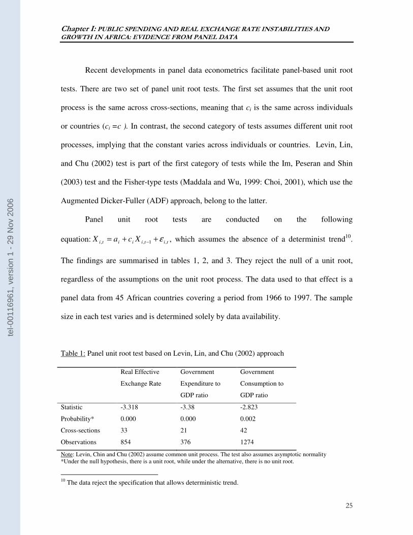
Panel unit root tests are conducted on the following
equation: titiiiti XcaX ,1,, ε++= − , which assumes the absence of a determinist trend10.
The findings are summarised in tables 1, 2, and 3. They reject the null of a unit root,
regardless of the assumptions on the unit root process. The data used to that effect is a
panel data from 45 African countries covering a period from 1966 to 1997. The sample
size in each test varies and is determined solely by data availability.
Table 1: Panel unit root test based on Levin, Lin, and Chu (2002) approach
Real Effective
Exchange Rate
Government
Expenditure to
GDP ratio
Government
Consumption to
GDP ratio
Statistic -3.318 -3.38 -2.823
Probability* 0.000 0.000 0.002
Cross-sections 33 21 42
Observations 854 376 1274
Note: Levin, Chin and Chu (2002) assume common unit process. The test also assumes asymptotic normality *Under the null hypothesis, there is a unit root, while under the alternative, there is no unit root.
10 The data reject the specification that allows deterministic trend.
tel-0
0116
961,
ver
sion
1 -
29 N
ov 2
006
Chapter I: PUBLIC SPENDING AND REAL EXCHANGE RATE INSTABILITIES AND GROWTH IN AFRICA: EVIDENCE FROM PANEL DATA
26
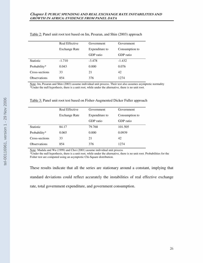
Table 2: Panel unit root test based on Im, Pesaran, and Shin (2003) approach
Real Effective
Exchange Rate
Government
Expenditure to
GDP ratio
Government
Consumption to
GDP ratio
Statistic -1.710 -3.478 -1.432
Probability* 0.043 0.000 0.076
Cross-sections 33 21 42
Observations 854 376 1274
Note: Im, Pesaran and Shin (2003) assume individual unit process. Their test also assumes asymptotic normality *Under the null hypothesis, there is a unit root, while under the alternative, there is no unit root.
Table 3: Panel unit root test based on Fisher-Augmented Dicker Fuller approach
Real Effective
Exchange Rate
Government
Expenditure to
GDP ratio
Government
Consumption to
GDP ratio
Statistic 84.17 79.768 101.505
Probability* 0.065 0.000 0.0939
Cross-sections 33 21 42
Observations 854 376 1274
Note: Madala and Wu (1999) and Choi (2001) assume individual unit process *Under the null hypothesis, there is a unit root, while under the alternative, there is no unit root. Probabilities for the Fisher test are computed using an asymptotic Chi-Square distribution.
These results indicate that all the series are stationary around a constant, implying that
standard deviations could reflect accurately the instabilities of real effective exchange
rate, total government expenditure, and government consumption.
tel-0
0116
961,
ver
sion
1 -
29 N
ov 2
006
Chapter I: PUBLIC SPENDING AND REAL EXCHANGE RATE INSTABILITIES AND GROWTH IN AFRICA: EVIDENCE FROM PANEL DATA
27
2.2 Comparison Africa vs. other developing regions
The comparison of the African and non-African data on the variables used in the
study yields interesting preliminary lessons. While these preliminary findings might be
very arbitrary, they nonetheless provide useful guidance regarding the structure of the
theoretical model as well as the empirical investigation.
The comparison is based on a sample that covers 147 countries, including 45 Sub-
Saharan African countries. The period under consideration spans three decades, from
1966 to 1997. This data set is structured as a panel with observations for each country
consisting of four-year averages or standard deviations. Indicators of instability are
captured by standard deviations while level indicators are represented by four-year
averages. Each country has eight observations: 1966-1969, 1970-1973, 1974-1977, 1978-
1981, 1982-1985, 1986-1989, 1990-1993 and 1994-1997. The panel is, however, not
balanced because some observations are missing for a number of countries.
Africa is compared to other regions, using the median11. A Wilcoxon/Mann-
Whitney test12 is used to that effect.
11 The use of median rather than the mean is justified on practical grounds. Most of the observations are geometric averages and standard deviations. This means that the “mean comparison” has to be based on the mean of geometric average or standard deviations, which is very hard to interpret. 12 The Wilcoxon Mann-Whitney test is viewed as one of the most powerful non-parametric tests. It tests the null hypothesis that two samples have identical distribution functions against the alternative hypothesis that the two distribution functions differ with respect to the median. Its main advantage lies on the fact it does not require the differences between two populations to have a normal distribution.
tel-0
0116
961,
ver
sion
1 -
29 N
ov 2
006
Chapter I: PUBLIC SPENDING AND REAL EXCHANGE RATE INSTABILITIES AND GROWTH IN AFRICA: EVIDENCE FROM PANEL DATA
28
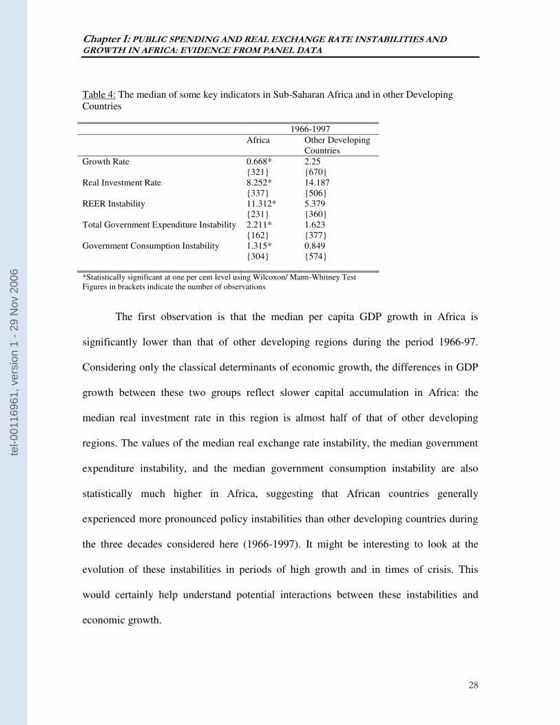
Table 4: The median of some key indicators in Sub-Saharan Africa and in other Developing Countries
1966-1997
Africa Other Developing Countries
Growth Rate 0.668* {321}
2.25 {670}
Real Investment Rate 8.252* {337}
14.187 {506}
REER Instability 11.312* {231}
5.379 {360}
Total Government Expenditure Instability 2.211* {162}
1.623 {377}
Government Consumption Instability 1.315* {304}
0.849 {574}
*Statistically significant at one per cent level using Wilcoxon/ Mann-Whitney Test Figures in brackets indicate the number of observations
The first observation is that the median per capita GDP growth in Africa is
significantly lower than that of other developing regions during the period 1966-97.
Considering only the classical determinants of economic growth, the differences in GDP
growth between these two groups reflect slower capital accumulation in Africa: the
median real investment rate in this region is almost half of that of other developing
regions. The values of the median real exchange rate instability, the median government
expenditure instability, and the median government consumption instability are also
statistically much higher in Africa, suggesting that African countries generally
experienced more pronounced policy instabilities than other developing countries during
the three decades considered here (1966-1997). It might be interesting to look at the
evolution of these instabilities in periods of high growth and in times of crisis. This
would certainly help understand potential interactions between these instabilities and
economic growth.
tel-0
0116
961,
ver
sion
1 -
29 N
ov 2
006
Chapter I: PUBLIC SPENDING AND REAL EXCHANGE RATE INSTABILITIES AND GROWTH IN AFRICA: EVIDENCE FROM PANEL DATA
29
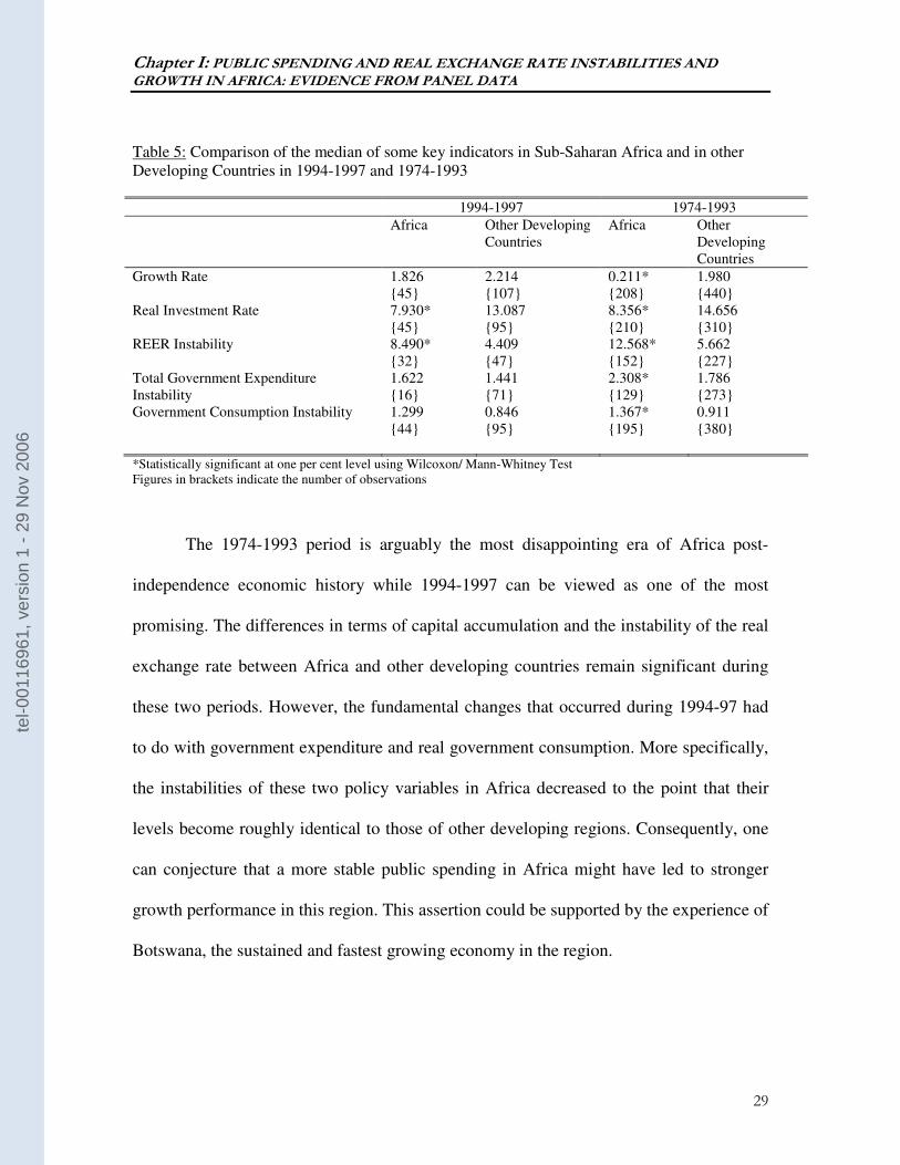
Table 5: Comparison of the median of some key indicators in Sub-Saharan Africa and in other Developing Countries in 1994-1997 and 1974-1993
1994-1997 1974-1993
Africa Other Developing Countries
Africa Other Developing Countries
Growth Rate 1.826 {45}
2.214 {107}
0.211* {208}
1.980 {440}
Real Investment Rate 7.930* {45}
13.087 {95}
8.356* {210}
14.656 {310}
REER Instability 8.490* {32}
4.409 {47}
12.568* {152}
5.662 {227}
Total Government Expenditure Instability
1.622 {16}
1.441 {71}
2.308* {129}
1.786 {273}
Government Consumption Instability 1.299 {44}
0.846 {95}
1.367* {195}
0.911 {380}
*Statistically significant at one per cent level using Wilcoxon/ Mann-Whitney Test Figures in brackets indicate the number of observations
The 1974-1993 period is arguably the most disappointing era of Africa post-
independence economic history while 1994-1997 can be viewed as one of the most
promising. The differences in terms of capital accumulation and the instability of the real
exchange rate between Africa and other developing countries remain significant during
these two periods. However, the fundamental changes that occurred during 1994-97 had
to do with government expenditure and real government consumption. More specifically,
the instabilities of these two policy variables in Africa decreased to the point that their
levels become roughly identical to those of other developing regions. Consequently, one
can conjecture that a more stable public spending in Africa might have led to stronger
growth performance in this region. This assertion could be supported by the experience of
Botswana, the sustained and fastest growing economy in the region.
tel-0
0116
961,
ver
sion
1 -
29 N
ov 2
006
Chapter I: PUBLIC SPENDING AND REAL EXCHANGE RATE INSTABILITIES AND GROWTH IN AFRICA: EVIDENCE FROM PANEL DATA
30
2.3 The case of Botswana
Botswana is viewed in the literature as the greatest success stories in Africa both
in terms of economic growth and human development13. Botswana’s real GDP per capita
grew annually by 6.4 percent from 1966 to 1997. Its record in human development was
equally remarkable before the HIV infection took a heavy toll on some of the
achievements, especially the improvement in life expectancy.
In stark contrast to other African oil and non-oil commodity producing countries,
Botswana is virtually the only country in the continent to have successfully achieved
sustained economic growth. Part of this success is attributable to the use of counter-
cyclical fiscal policies to manage booms and slumps in the mining sector, particularly the
diamond industry, and the effective management of its real exchange rate.
One of the greatest successes of the fiscal policy in Botswana was to achieve
public expenditure smoothing while at the same time allowing sustainable increases in
public spending. The fiscal policy strategy broadly consisted in running substantial
budget surpluses and building impressive international reserves in periods of high
diamond prices. Those reserves were drawn in when the diamond market was weak, thus
avoiding any drastic cut in expenditures during bust times. The general goal of such
strategy was to ensure some stability in public spending. It is worth noting that the
predictability of government spending was made possible thanks to National
Development Plans. These plans set targets for public expenditures which are in line with
expected government revenues and the absorption capacity of the economy.
13 Some of the achievements in human development have recently been reversed by of HIV/AIDS pandemic.
tel-0
0116
961,
ver
sion
1 -
29 N
ov 2
006
Chapter I: PUBLIC SPENDING AND REAL EXCHANGE RATE INSTABILITIES AND GROWTH IN AFRICA: EVIDENCE FROM PANEL DATA
31
Botswana also places a major emphasis on the management of the exchange rate
so as to avoid real appreciation14. Booms usually bring excessive foreign exchange. If
these flows are not properly sterilised, which it very often the case, they lead to an
appreciation of the real exchange rate and undermine the competitiveness of the tradable
sector. In light of this, Botswana managed to prevent its currency from appreciating,
allowing therefore other tradable goods, outside the mining sector, to maintain
competitiveness in world markets. Additionally, this policy implicitly helped Botswana
pursue a relatively successful diversification of its economy.
III- THEORETICAL CONSIDERATIONS
3.1 Solow Model
This chapter uses the Mankiw, Romer and Weil (1992)’s version of the Solow
model as the main framework to investigate the determinants of growth. This model is
based on a Cobb-Douglas production function with Harrod-neutral, i.e. labour-
augmenting, technological progress. It is summarised by an approximation of the growth
rate around steady-state, which takes the following form:
++
−−+++
−−
+−−−=− ptAsdpnyeyy 000 lnln
1)ln(
1ln)1(lnln
βα
α
βα
βαγ
(2)
14 There is great deal of evidence associating high instability of real exchange rate with exchange rate appreciation. Conversely, relatively stable real exchange rate would equate with the absence of an appreciation of real exchange rate.
tel-0
0116
961,
ver
sion
1 -
29 N
ov 2
006
Chapter I: PUBLIC SPENDING AND REAL EXCHANGE RATE INSTABILITIES AND GROWTH IN AFRICA: EVIDENCE FROM PANEL DATA
32
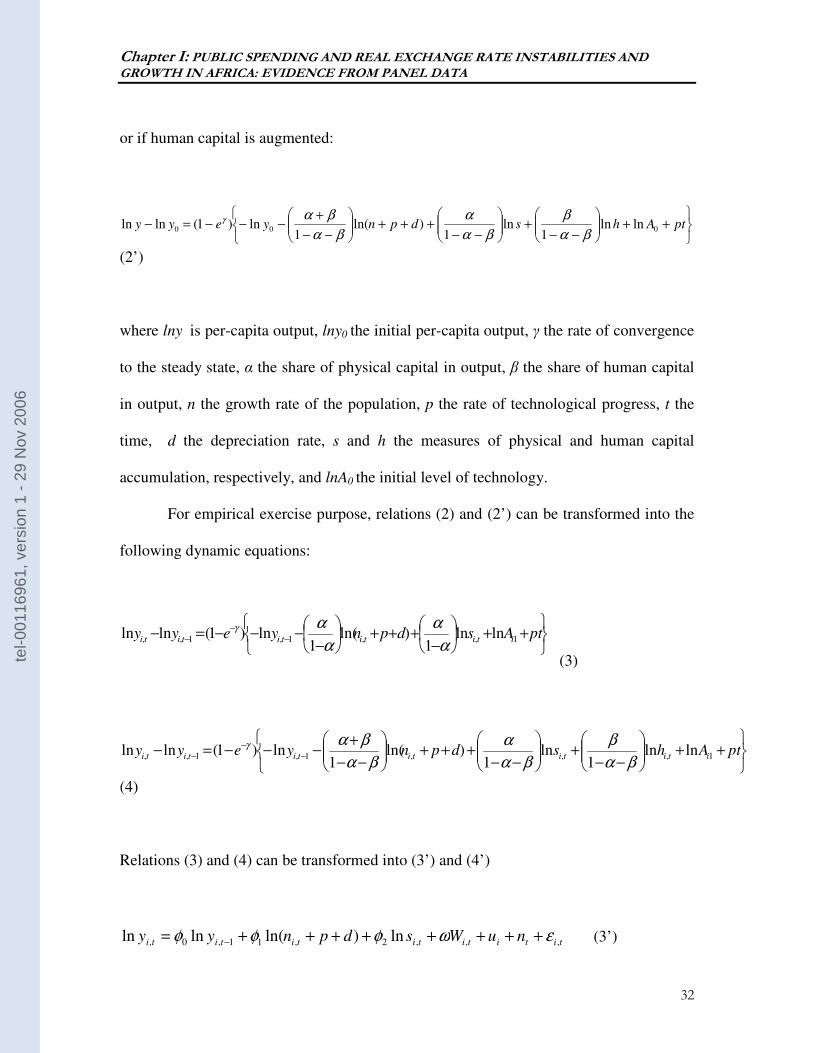
or if human capital is augmented:
++
−−+
−−+++
−−
+−−−=− ptAhsdpnyeyy 000 lnln
1ln
1)ln(
1ln)1(lnln
βα
β
βα
α
βα
βαγ
(2’)
where lny is per-capita output, lny0 the initial per-capita output, γ the rate of convergence
to the steady state, α the share of physical capital in output, β the share of human capital
in output, n the growth rate of the population, p the rate of technological progress, t the
time, d the depreciation rate, s and h the measures of physical and human capital
accumulation, respectively, and lnA0 the initial level of technology.
For empirical exercise purpose, relations (2) and (2’) can be transformed into the
following dynamic equations:
(3)
++
−−+
−−+++
−−
+−−−=− −
−− ptAhsdpnyeyy ititititititi 1,,,1,1,, lnln
1ln
1)ln(
1ln)1(lnln
βα
β
βα
α
βα
βαγ
(4)
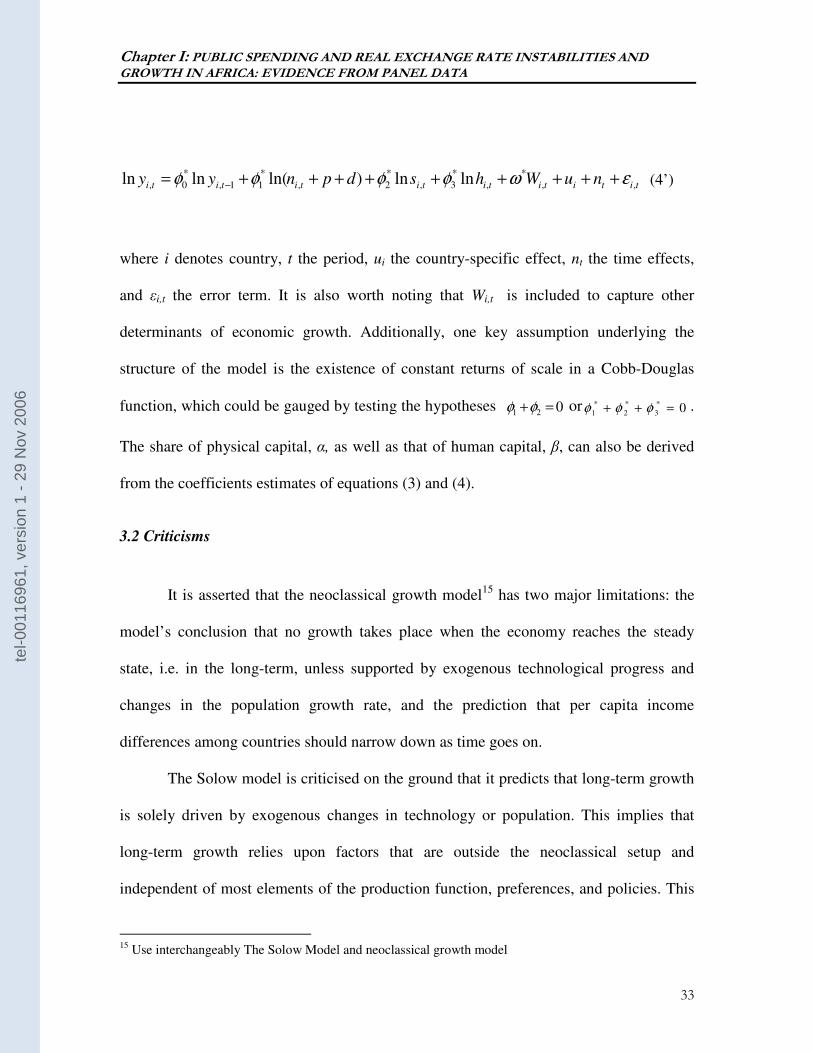
Relations (3) and (4) can be transformed into (3’) and (4’)
tititititititi nuWsdpnyy ,,,2,11,0, ln)ln(lnln εωφφφ ++++++++= − (3’)
++
−
+++
−
−−−=− −−
− ptAsdpnyeyy itititititi 1,,1,1,, lnln1
)ln(1
ln)1(lnlnα
α
α
αγ
tel-0
0116
961,
ver
sion
1 -
29 N
ov 2
006
Chapter I: PUBLIC SPENDING AND REAL EXCHANGE RATE INSTABILITIES AND GROWTH IN AFRICA: EVIDENCE FROM PANEL DATA
33
titititititititi nuWhsdpnyy ,,
*
,
*
3,
*
2,
*
11,
*
0, lnln)ln(lnln εωφφφφ +++++++++= − (4’)
where i denotes country, t the period, ui the country-specific effect, nt the time effects,
and εi,t the error term. It is also worth noting that Wi,t is included to capture other
determinants of economic growth. Additionally, one key assumption underlying the
structure of the model is the existence of constant returns of scale in a Cobb-Douglas
function, which could be gauged by testing the hypotheses 021 =+φφ or 0*
3
*
2
*
1 =++ φφφ .
The share of physical capital, α, as well as that of human capital, β, can also be derived
from the coefficients estimates of equations (3) and (4).
3.2 Criticisms
It is asserted that the neoclassical growth model15 has two major limitations: the
model’s conclusion that no growth takes place when the economy reaches the steady
state, i.e. in the long-term, unless supported by exogenous technological progress and
changes in the population growth rate, and the prediction that per capita income
differences among countries should narrow down as time goes on.
The Solow model is criticised on the ground that it predicts that long-term growth
is solely driven by exogenous changes in technology or population. This implies that
long-term growth relies upon factors that are outside the neoclassical setup and
independent of most elements of the production function, preferences, and policies. This
15 Use interchangeably The Solow Model and neoclassical growth model
tel-0
0116
961,
ver
sion
1 -
29 N
ov 2
006
Chapter I: PUBLIC SPENDING AND REAL EXCHANGE RATE INSTABILITIES AND GROWTH IN AFRICA: EVIDENCE FROM PANEL DATA
34
conclusion contrasts sharply with recent history that is replete with examples of countries
that have been successful in maintaining strong per-capita growth rates over long periods
of time. More importantly, growth experience, in the fastest growing economies, has
proved to be systematically associated with some of the aspects of production function
and economic policies. Robust growth rates have been very often associated with high
capital accumulation and sound economic policies.
The second strand of criticisms has to do with the issue of convergence. The neo-
classical model, which predicts higher growths in poor countries than in rich countries,
turns out to be, in some instances, inadequate in explaining the magnitude and persistence
of income gap between low-income countries and high-income countries. The issue of
growth divergence among countries is well illustrated by the findings of Bourguignon
and Morrisson (2002) and Milanovic (2005) that suggest that 70 percent of income
inequality among world citizens is originated from differences in incomes among
countries while only 30 percent is explained by income disparities within countries.
Endogenous models have emerged especially as viable alternatives to explain
steady-state growth. Romer, Lucas, Robelo, for instance, built models in which long term
growth can be sustained endogenously at rates that may be tributary to policy choices,
preferences, and technologies. Endogenous growth models are very often classified into
two major groups: AK models and R&D models (Jones, 1995). AK growth models such
as those of Romer (1986, 1987), Lucas (1988) and Robelo (1991) posit that physical and
human capital accumulation can generate sustained economic growth, even in the
absence of exogenous technological progress and population growth. The R&D-style
tel-0
0116
961,
ver
sion
1 -
29 N
ov 2
006
Chapter I: PUBLIC SPENDING AND REAL EXCHANGE RATE INSTABILITIES AND GROWTH IN AFRICA: EVIDENCE FROM PANEL DATA
35
growth models of Romer (1990) and Aghion and Howitt (1992) highlight technological
progress as the means to perpetuate growth at the steady-state. In these models,
technological change is driven by the activities of economic agents in perpetual quest of
innovation.
In some of the AK-styled growth models, especially those involving positive
externalities, private returns to investment differ from social returns to investment. This
implies that an entirely market-based solution leads to sub-optimal solutions both in
terms of growth and capital accumulation. These models therefore implicitly recognised
the role of government intervention in eliminating distortions and ensuring ongoing per-
capita growth. The beneficial impact of government intervention is also acknowledged
when public services are considered as an input to private production16 (Aschauer, 1988:
Barro, 1990). Public spending, therefore, matters for growth.
3.3 The role of economic policies: importance of stability
A close look at the patterns of government expenditures in most African countries
suggests a procyclical nature. Commodity price booms and/or large capital inflows
encourage many countries to initiate large expenditure programs. These programs are cut
back in periods of lower prices and more often in times when external capital flows dry
up17. Public spending, therefore, tends to be very volatile. Similarly, real exchange rate
tends to follow the same patterns as public spending. Substantial inflows of export
16 Evidence from some developed countries rejects this view. Cadot et al. (2002) find a little economic return of infrastructure spending, once they account for pork barrel. 17 Some categories of public programs, say public consumption, initiated during boom times tend to be sustained even when bust times follow.
tel-0
0116
961,
ver
sion
1 -
29 N
ov 2
006
Chapter I: PUBLIC SPENDING AND REAL EXCHANGE RATE INSTABILITIES AND GROWTH IN AFRICA: EVIDENCE FROM PANEL DATA
36
earnings generated by rising commodity prices or/and large foreign capital inflows result
in the appreciation of the real exchange rate18. This is followed by serious internal and
external imbalances, which are addressed by depreciating the real exchange rate. This
clearly suggests some swings in the real exchange rate as well. Public spending and real
exchange rate instabilities have the potential to hamper economic growth. In fact, they
have a detrimental impact on capital (human and physical) accumulation while at the
same time undermining the total factor productivity: the efficiency with which capital and
labour are combined.
3.3.1 Public spending instability and growth
Public spending instability might incur both direct and indirect costs for economic
growth. Public spending instability may influence economic growth “directly” through
the efficiency channel or/and “indirectly” through its effect on the accumulation of
factors of production, namely capital.
3.3.1.1. The productivity channel
Two lines of arguments are typically put forth to justify a potential negative
impact of public spending instability on productivity. On the one hand, intense
fluctuations in government spending give rise to erratic provision of public services, such
18 If the appreciation of the real exchange rate endures for some time, it leads to a Dutch disease phenomenon: a contraction of the non-commodity economy.
tel-0
0116
961,
ver
sion
1 -
29 N
ov 2
006
Chapter I: PUBLIC SPENDING AND REAL EXCHANGE RATE INSTABILITIES AND GROWTH IN AFRICA: EVIDENCE FROM PANEL DATA
37
as infrastructure facilities, which leads to weak productivity (Calderòn and Servén, 2003).
On the other hand, public spending instability, which is very often associated with boom-
bust cycles, produces ratchet effects on public spending, notably on public consumption
(Guillaumont, 2006)19. Ratchet effects eventually result in an upward trend in public
spending in the long run. If one assumes a heavy fiscal reliance on monetary financing,
higher government spending leads to high and volatile inflation, the blurring of market
signals, and ultimately a misallocation of resources and weak productivity.
3.3.1.2 The factor accumulation channel
As mentioned earlier, public sector expands very often in boom periods. The
expansion turns out not be to be sustainable, especially in bad times or/and when external
financing dries up. Public spending is then cut in bust periods. This fiscal adjustment is
achieved mainly through the reduction of some categories of public investment, such as
investment in infrastructural facilities, or some specific current expenditures, including
maintenance expenditures, which are complementary to private investment. Such policies
affect private investment and constraint economic growth as earlier suggested in the
endogenous growth model. Moreover, cuts in public spending often lead to protracted
recession, which can have long-lasting effects. For instance Ocampo (2002) indicates that
firms, in situation of prolonged recession, may experience irreversible losses of material
and immaterial assets, which include, among others, the social capital built as well as the
19 Public wages and other current expenditures increase significantly in good times and do not adjust or partially adjust in bad times.
tel-0
0116
961,
ver
sion
1 -
29 N
ov 2
006
Chapter I: PUBLIC SPENDING AND REAL EXCHANGE RATE INSTABILITIES AND GROWTH IN AFRICA: EVIDENCE FROM PANEL DATA
38
institutional and technological settings built within the firms. He also alludes to the
irreparable damages caused by recessions to human capital: “the human capital of the
unemployed or the underemployed may be permanently lost; and the children may leave
school and never return”.
Finally, public spending instability may represent an important source of real
exchange instability, which in turn could constraint growth through direct and indirect
channels (Ghura and Greenes, 1993: Soderling, 2002).
3.3.2 Real exchange rate instability and growth
Again, we identify two sorts of mediating channels from real exchange rate
instability to disappointing economic growth: the “direct” or total productivity channel
and the “indirect” channels through the impact on factor accumulation.
3.3.2.1 The productivity channel
The alternation of real exchange appreciations and depreciations can modify the
structure of the economy and generate enduring effects on productivity and economic
growth. The “Dutch Disease” analysis captures very well these dynamics (Corden, 1982:
Corden and Neary, 1984 : Gylafason et al., 1999). The analysis considers three sectors,
namely a booming export sector, a lagging export sector (or traditional export sector),
and a nontradable sector. A natural resource boom results in the increase of export
earnings and higher domestic spending. If some of the windfalls are spent on nontradable
goods, which is very often the case, higher domestic demand drives up the relative price
tel-0
0116
961,
ver
sion
1 -
29 N
ov 2
006
Chapter I: PUBLIC SPENDING AND REAL EXCHANGE RATE INSTABILITIES AND GROWTH IN AFRICA: EVIDENCE FROM PANEL DATA
39
of nontradables and leads to real exchange rate appreciation20. The appreciation of the
real exchange rate undermines the competitiveness of the country’s exports and causes
the contraction of the traditional export sector. This effect is termed “the spending
effect”. In addition to this effect, a resource movement effect also takes place, with
labour and capital moving from the traditional export sector to the nontradable sector, to
meet the rise in domestic demand, and to the booming export sector. In sum, booms21 can
potentially bring about important changes in the structure of economies where they occur.
Some sectors, such as the manufacturing sector, with significant productivity spillovers to
the rest of the economy, might face severe contractions, which could eventually lead to
their disappearance. Real exchange rate appreciation might generate “inertia effects” in
the sense that the end of booms and subsequent deprecations in real exchange rate may
turn not to be sufficient for the recovery of the manufactory sector. Given potential
positive externalities of the manufacturing sector, a persistent decline of this sector
lowers productivity and long term growth.
Apart from its sector-specific effects on growth, real exchange rate instability can
be detrimental to productivity in the economy in general. Real exchange rate fluctuations
distort market signals and lead to an ineffective and inefficient allocation of investment.
This argument has been largely supported in the literature (Aizenmann and Marion, 1999:
Ghura and Greennes, 1993: Guillaumont, 1999: Serven, 1997).
20 This basically reflects instances where exchange rate is fixed. If exchange rate is flexible, nominal appreciation could be the main cause of real exchange rate appreciation. 21 The analysis was initially formulated in the context of natural resource boom but could also well describe situations of impressive aid flows (Rajan and Subramanian, 2005).
tel-0
0116
961,
ver
sion
1 -
29 N
ov 2
006
Chapter I: PUBLIC SPENDING AND REAL EXCHANGE RATE INSTABILITIES AND GROWTH IN AFRICA: EVIDENCE FROM PANEL DATA
40
3.3.2.2 The factor accumulation channel
The instability of real exchange rate can also impact negatively the level of
investment because of the uncertainty it creates (Guillaumont et al., 1999). Uncertainty
may well be perceived by economic agents as a loss of credibility in government policies,
which can ultimately diminish the expected return on private investment and therefore
depress growth. Additionally, it is generally argued that under conditions of uncertainty,
risk-adverse economic agents predict greater instability in expected returns, and may cut
back in their investments, while risk-neutral agents may adopt a “wait and see” attitude in
terms of investment strategy (Azam et al., 2002). In any case, the outcome of greater
uncertainty is a fall in investment rates and lower growth.
IV-ECONOMETRIC METHODOLOGY
The empirical growth literature has until recently relied, to a large degree, on
Ordinary Least Squares, henceforth OLS, to investigate the determinants of economic
expansion. This technique has been severely criticised on the ground that it does not
properly address the problems of measurement error, omitted variables, and endogeneity,
which are common to growth regressions.
tel-0
0116
961,
ver
sion
1 -
29 N
ov 2
006
Chapter I: PUBLIC SPENDING AND REAL EXCHANGE RATE INSTABILITIES AND GROWTH IN AFRICA: EVIDENCE FROM PANEL DATA
41
4.1 Ineffective OLS
To make easy the discussion on how ineffective is OLS in the presence of those
problems, we rewrite equation (4) and (4’) as tiitititi uZyy ,,1,0, lnln εξφ +++= − (5)
where Zi,t represents the vector of all the explanatory variables of economic growth,
except the natural logarithm of initial per capita income, and ξ the associated vector of
coefficients. The issue of measurement error can be illustrated by the following: assume
that *
,tiy and *
,tiZ capture yi,t and Zi,t, with tiw , and tin , their respective measurement errors:
tititi nyy ,,
*
, lnln += (6)
tititi wZZ ,,
*
, += (7)
Combining (5) (6) and (7) yields
tiitititi uZyy ,
*
,
*
1,0
*
, lnln ψξφ +++= − with tititititi wnn ,1,0,,, ξφεψ −−+= − (8)
One of the key assumptions underlying the use of OLS technique is the absence of
correlation between the regressors, *
,tiZ and *
1, −tiy , and the disturbance tiiu ,ψ+ . That
hypothesis does not hold as:
[ ] 0))(( ,1,0,,,, ≠−−+++ − titititiititi wnnuwZE ξφε more specifically because 0)( 2
, ≠tiwE (9)
[ ] 0))((ln ,1,0,,,, ≠−−+++ − titititiititi wnnunyE ξφε because 0)( 2
, ≠tinE (10)
Further, the omission of some pertinent explanatory variables can also make OLS
estimates biased and inconsistent. In fact, omitted variable, for instance time-invariant
tel-0
0116
961,
ver
sion
1 -
29 N
ov 2
006
Chapter I: PUBLIC SPENDING AND REAL EXCHANGE RATE INSTABILITIES AND GROWTH IN AFRICA: EVIDENCE FROM PANEL DATA
42
country-specific characteristics such as the initial level of technology, will be absorbed
by the disturbance tiiu ,ψ+ in equation (5), making therefore [ ] 0)(( ,, ≠+ tiiti wuZE .
Finally, the endogeneity of some of the regressors leads to results that are very
similar to those reported in the case of omitted variable. For instance, 1, −tiy is
mechanically correlated with isε in (5) for ts < , [ ] 0))(( 1, ≠− istiyE ε , violating therefore
the assumption that all the explanatory variables are exogenous.
4.2 Instrumental Variable Estimator of Anderson and Hsiao (1982)
One way of addressing both the endogeneity and omitted variable is to use the
methodology suggested by Anderson and Hsiao (1982). This consists in eliminating
country-specific effects, iu , by time differencing equation (5):
)()()(ln)(ln ,,1,0, titititi Zyy εξφ ∆+∆+∆=∆ − (11)
By construction, )(ln 1, −∆ tiy becomes correlated with )( ,tiε∆ , thus indicating the need to
instrument suspected endogenous variables. Assuming no serial correlation in ti ,ε ,
2,ln −tiy is not correlated with )( ,tiε∆ and can serve as instrument for 1,(ln −∆ tiy ). The
Anderson and Hsiao’s instrumental methodology guarantees therefore consistent
estimates.
tel-0
0116
961,
ver
sion
1 -
29 N
ov 2
006
Chapter I: PUBLIC SPENDING AND REAL EXCHANGE RATE INSTABILITIES AND GROWTH IN AFRICA: EVIDENCE FROM PANEL DATA
43
4.3 First-Differenced Generalised Method-of-Moments Estimator (GMM) and System
Generalised Method-of-Moments Estimator (SYS-GMM)
Even though Anderson Hsiao’s instrumental variable estimator provides
consistent estimates, it is not efficient because additional lagged values of the dependent
variable, lnyi,t-3 , lnyi,t-4 , lnyi,t-4…lnyi,t-k and Zi,t-1, Zi,t-2…Zi,t-k 22are also good instruments
under the assumption of no further serial correlation in ti ,ε .
0)(ln ,, =∆− tiptiyE ε for p=2, 3,..., (T-1) (12)
0)( ,, =∆− tirtiZE ε for r=1, 2, 3,…, (T-1) (13)
On that basis, Arrelano and Bond (1991) suggest a Generalised Method of
Moments Estimator (GMM), well-known by “first-differenced GMM estimator” that
combines the suggested instruments efficiently. However, Blundell and Bond (1998)
demonstrate that first-differenced GMM have poor finite sample properties, especially
when lagged levels of the variables are not strongly correlated with subsequent first-
differences. Bond et al. (2001) indicate that this is likely to be the case when the series
are close to a random walk or when variance of the country-specific effects, ni , rises
relative to the variance of error term isε .
In order to address the problem associated with persistent panel data, Blundell and
Bond (1998) develop a system GMM estimator that is based on a simultaneous system of
two equations, which are equations (5) and (11). Lagged levels of lnyi,t and Zi,t serve as
instruments for the differenced equation (11) while their lagged first-differences are the
instruments for the equation in level (5):
22 Assuming that some of regressors in Zi,t are endogenous.
tel-0
0116
961,
ver
sion
1 -
29 N
ov 2
006
Chapter I: PUBLIC SPENDING AND REAL EXCHANGE RATE INSTABILITIES AND GROWTH IN AFRICA: EVIDENCE FROM PANEL DATA
44
0)ln( ,, =∆ − tiptiyE ε and 0)( ,, =∆ − tirtiZE ε for p and r=2,…, (T-1) (14)
0)(ln ,, =∆− tiptiyE ε and 0)(ln ,, =∆− tirtiZE ε for p and r=2,…, (T-1) (15)
The validity of the system GMM as a consistent estimator can be ascertained by
showing that the error term is not serially correlated, and the instruments used are the
adequate ones. The first condition is gauged by Arrelano and Bond (1991) test for
autocorrelation, which determines whether the first-differenced error term has second-
order. The second condition is verified by a test of over-identifying restrictions, which
could be either the Sargan (1958) test or Hansen (1982) test.
V-EMPIRICAL RESULTS
The sample used in the empirical analysis includes 45 African countries but the
sample size in each regression varies and is determined solely by data availability. The
period covered is from 1966 to 1997. This data set is structured as a panel with
observations for each country consisting of four-year averages, standard deviations or
data in levels provided quadrennially. Real exchange rate and public spending
instabilities are captured by standard deviations estimated on a four year period. The
investment to GDP ratio is built by taking four-year non-overlapping averages. Real per
capita GDP is obtained quadrennially, starting from 1966 and ending in 1997. Each
country has eight observations: 1966-1969, 1970-1973, 1974-1977, 1978-1981, 1982-
1985, 1986-1989, 1990-1993 and 1994-1997. The panel is, however, not balanced
because some observations are missing for a number of countries.
tel-0
0116
961,
ver
sion
1 -
29 N
ov 2
006
Chapter I: PUBLIC SPENDING AND REAL EXCHANGE RATE INSTABILITIES AND GROWTH IN AFRICA: EVIDENCE FROM PANEL DATA
45
5.1 Validity of the Solow Model and its augmented version
Regressions (2) and (3) report the results of the estimation of the Solow Model
and its augmented version. Just as primary education enrolment rate captures human
capital accumulation in regression (2), so does secondary school enrolment rate in
regression23 (3).
23 We couldn’t use Barro and Lee (2000)’s average years of schooling because these data are provided quinquennially, starting in 1960,…and ending in 1990. We would have ended up with a very small sample. More importantly, the formulation that is adopted in this chapter uses the rate of accumulation rather the level of human of capital. See Mankiw et al. (1992) pp. 417-418. Furthermore, Pritchett (1996) argues that school enrolments reflect human capital stock only if constant over time.
tel-0
0116
961,
ver
sion
1 -
29 N
ov 2
006
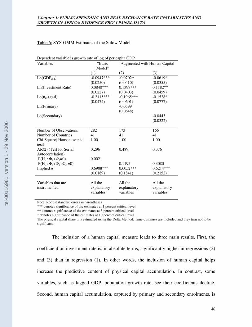
Chapter I: PUBLIC SPENDING AND REAL EXCHANGE RATE INSTABILITIES AND GROWTH IN AFRICA: EVIDENCE FROM PANEL DATA
46
Table 6: SYS-GMM Estimates of the Solow Model
Dependent variable is growth rate of log of per capita GDP
Variables “Basic Model”
Augmented with Human Capital
(1) (2) (3)
Ln(GDPit-1) -0.0947*** (0.0250)
-0.0702* (0.0410)
-0.0619* (0.0355)
Ln(Investment Rate) 0.0840*** (0.0227)
0.1397*** (0.0403)
0.1182** (0.0459)
Ln(ni,t+g+d) -0.2115*** (0.0474)
-0.1965*** (0.0601)
-0.1528* (0.0777)
Ln(Primary) -0.0599 (0.0648)
Ln(Secondary) -0.0443 (0.0322)
Number of Observations 282 173 166 Number of Countries 41 41 41 Chi-Square( Hansen over-id test)
1.00 1.00 1.00
AR(2) (Test for Serial Autocorrelation)
0.296 0.489 0.376
P(H0 : Φ1+Φ2=0) 0.0021 P(H0 : Φ1+Φ2+Φ3 =0) 0.1195 0.3080 Implied α 0.6908***
(0.0189) 0.6052*** (0.1841)
0.6214*** (0.2152)
Variables that are instrumented
All the explanatory variables
All the explanatory variables
All the explanatory variables
Note: Robust standard errors in parentheses *** denotes significance of the estimates at 1 percent critical level ** denotes significance of the estimates at 5 percent critical level * denotes significance of the estimates at 10 percent critical level The physical capital share α is estimated using the Delta Method. Time dummies are included and they turn not to be significant.
The inclusion of a human capital measure leads to three main results. First, the
coefficient on investment rate is, in absolute terms, significantly higher in regressions (2)
and (3) than in regression (1). In other words, the inclusion of human capital helps
increase the predictive content of physical capital accumulation. In contrast, some
variables, such as lagged GDP, population growth rate, see their coefficients decline.
Second, human capital accumulation, captured by primary and secondary enrolments, is
tel-0
0116
961,
ver
sion
1 -
29 N
ov 2
006
Chapter I: PUBLIC SPENDING AND REAL EXCHANGE RATE INSTABILITIES AND GROWTH IN AFRICA: EVIDENCE FROM PANEL DATA
47
negatively associated with per capita growth, albeit not significantly. This finding does
not mean that human capital accumulation is irrelevant for economic growth. Numerous
studies found similar result. Pritchett (1996) suggests three explanations. First, the initial
human capital might have initially been so poor that any improvement in subsequent
periods resulted in a scant improvement in skills and productivity. Second, marginal
returns to education might have dropped as a result of the combination of increased
supply of educated labour and a virtually unchanged demand for educated labour. Finally,
the institutional setup might have been so deleterious that human capital accumulation
did not lead to per-capita growth. In addition to these explanations, the lack of
significance could also be qualified by measurement problems. Arcand and d’Hombres
(2005) challenge the use of school enrolment indicators as the rate of human capital
accumulation, arguing that school enrolments in period t do not capture the flux of
investment in human capital for the same period.
We test the validity of the Solow Model and its augmented version24 by checking
if the sum of the coefficients on investment, population growth rate and on human capital
(if necessary) is equal to 0. In addition, we estimate the magnitude of the share of
physical capital in total output and compare it to the widely accepted values25. The results
are reported in the bottom of Table 6. They generally reject both the Solow Model and its
augmented version. The Solow Model is rejected on two accounts. First, the sum of the
coefficients on investment and population growth rate turns to be significantly different
from 0 at the 5 percent level in the regression. Second, the implied share of physical
24 It is a test on the existence of constant returns of scale in a Cobb-Douglas function. 25 The number that comes up in the literature is 1/3 (Mankiw et al., 1992 ).
tel-0
0116
961,
ver
sion
1 -
29 N
ov 2
006
Chapter I: PUBLIC SPENDING AND REAL EXCHANGE RATE INSTABILITIES AND GROWTH IN AFRICA: EVIDENCE FROM PANEL DATA
48
capital is equal to 0.6908, which is well above the usual one-third found in the literature.
On the other hand, the validity of the Solow Model augmented with human capital can be
challenged because the estimated share of physical capital in total output varies from
0.6052 to 0.6214, which again is relatively higher than the norms.
5.2 Core Model
We turn to the issue of interest of this chapter by investigating the potential
impact of policy- related instabilities on economic growth. Public spending and real
exchange rate instabilities are therefore added to the Augmented Solow construct26. To
ensure that the analysis is robust, we use two measures of public spending, especially
government consumption and total government expenditure27.
27 We try to go further in the breakdown in an attempt to identify current and capital expenditures but could not get enough observations to be used in the empirical investigation.
tel-0
0116
961,
ver
sion
1 -
29 N
ov 2
006
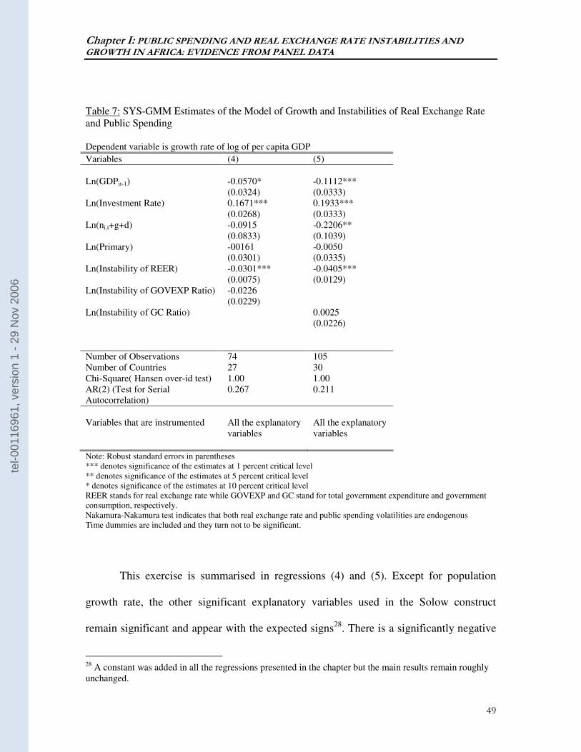
Chapter I: PUBLIC SPENDING AND REAL EXCHANGE RATE INSTABILITIES AND GROWTH IN AFRICA: EVIDENCE FROM PANEL DATA
49
Table 7: SYS-GMM Estimates of the Model of Growth and Instabilities of Real Exchange Rate and Public Spending Dependent variable is growth rate of log of per capita GDP
Variables (4) (5)
Ln(GDPit-1) -0.0570*
(0.0324) -0.1112*** (0.0333)
Ln(Investment Rate) 0.1671*** (0.0268)
0.1933*** (0.0333)
Ln(ni,t+g+d) -0.0915 (0.0833)
-0.2206** (0.1039)
Ln(Primary) -00161 (0.0301)
-0.0050 (0.0335)
Ln(Instability of REER) -0.0301*** (0.0075)
-0.0405*** (0.0129)
Ln(Instability of GOVEXP Ratio) -0.0226 (0.0229)
Ln(Instability of GC Ratio) 0.0025 (0.0226)
Number of Observations 74 105 Number of Countries 27 30 Chi-Square( Hansen over-id test) 1.00 1.00 AR(2) (Test for Serial Autocorrelation)
0.267 0.211
Variables that are instrumented All the explanatory
variables All the explanatory variables
Note: Robust standard errors in parentheses *** denotes significance of the estimates at 1 percent critical level ** denotes significance of the estimates at 5 percent critical level * denotes significance of the estimates at 10 percent critical level REER stands for real exchange rate while GOVEXP and GC stand for total government expenditure and government consumption, respectively. Nakamura-Nakamura test indicates that both real exchange rate and public spending volatilities are endogenous Time dummies are included and they turn not to be significant.
This exercise is summarised in regressions (4) and (5). Except for population
growth rate, the other significant explanatory variables used in the Solow construct
remain significant and appear with the expected signs28. There is a significantly negative
28 A constant was added in all the regressions presented in the chapter but the main results remain roughly unchanged.
tel-0
0116
961,
ver
sion
1 -
29 N
ov 2
006
Chapter I: PUBLIC SPENDING AND REAL EXCHANGE RATE INSTABILITIES AND GROWTH IN AFRICA: EVIDENCE FROM PANEL DATA
50
coefficient on initial GDP and a robust positive coefficient on investment. Population
growth rate displays a negative coefficient, which turns to be statistically robust in
regression (5) and not in regression (4). Human capital, captured by primary education,
remains statistically insignificant. In addition to be broadly consistent with previous
findings, the results support the prediction that real exchange rate instability exerts a
direct negative impact on growth while at the same time indicating a lack of a direct
statistically strong effect of public spending instability on economic growth.
tel-0
0116
961,
ver
sion
1 -
29 N
ov 2
006
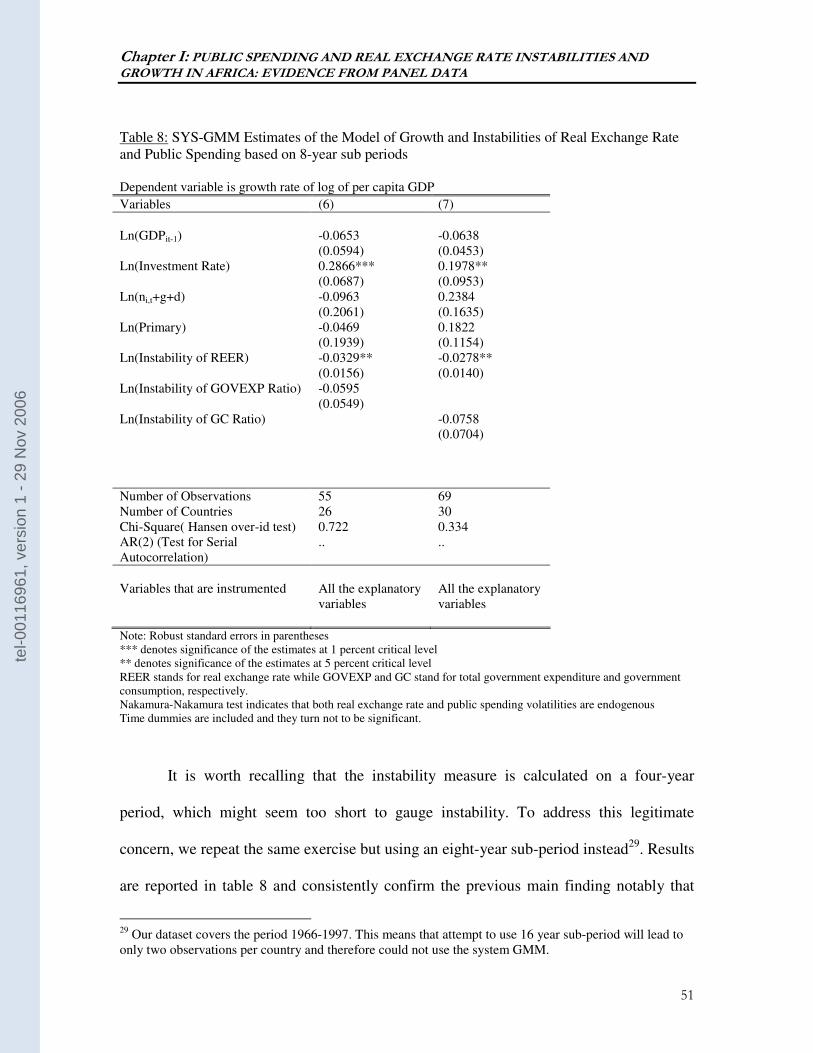
Chapter I: PUBLIC SPENDING AND REAL EXCHANGE RATE INSTABILITIES AND GROWTH IN AFRICA: EVIDENCE FROM PANEL DATA
51
Table 8: SYS-GMM Estimates of the Model of Growth and Instabilities of Real Exchange Rate and Public Spending based on 8-year sub periods Dependent variable is growth rate of log of per capita GDP
Variables (6) (7)
Ln(GDPit-1) -0.0653
(0.0594) -0.0638 (0.0453)
Ln(Investment Rate) 0.2866*** (0.0687)
0.1978** (0.0953)
Ln(ni,t+g+d) -0.0963 (0.2061)
0.2384 (0.1635)
Ln(Primary) -0.0469 (0.1939)
0.1822 (0.1154)
Ln(Instability of REER) -0.0329** (0.0156)
-0.0278** (0.0140)
Ln(Instability of GOVEXP Ratio) -0.0595 (0.0549)
Ln(Instability of GC Ratio) -0.0758 (0.0704)
Number of Observations 55 69 Number of Countries 26 30 Chi-Square( Hansen over-id test) 0.722 0.334 AR(2) (Test for Serial Autocorrelation)
.. ..
Variables that are instrumented All the explanatory
variables All the explanatory variables
Note: Robust standard errors in parentheses *** denotes significance of the estimates at 1 percent critical level ** denotes significance of the estimates at 5 percent critical level REER stands for real exchange rate while GOVEXP and GC stand for total government expenditure and government consumption, respectively. Nakamura-Nakamura test indicates that both real exchange rate and public spending volatilities are endogenous Time dummies are included and they turn not to be significant.
It is worth recalling that the instability measure is calculated on a four-year
period, which might seem too short to gauge instability. To address this legitimate
concern, we repeat the same exercise but using an eight-year sub-period instead29. Results
are reported in table 8 and consistently confirm the previous main finding notably that
29 Our dataset covers the period 1966-1997. This means that attempt to use 16 year sub-period will lead to only two observations per country and therefore could not use the system GMM.
tel-0
0116
961,
ver
sion
1 -
29 N
ov 2
006
Chapter I: PUBLIC SPENDING AND REAL EXCHANGE RATE INSTABILITIES AND GROWTH IN AFRICA: EVIDENCE FROM PANEL DATA
52
among the two instabilities previously identified only real exchange rate instability seems
to influence directly growth. The magnitude of the coefficients associated with real
exchange rate instability turns, however, to be more modest, ranging from -0.0278 to -
0.0329, compared from -0.0301 to -0.0405 previously found.
These results warrant two comments. On the one hand, the direct negative impact
of real exchange rate instability on growth implies that real exchange rate instability
influences negatively total factor productivity or suggests that the productivity channel is
at work30. On the other hand, insignificant coefficient on public spending instability
means that either such variation does not operate through the total factor productivity
channel or it unfolds through other factors that have not been accounted for in the
regressions. This leads us to investigate the mediating channels though which
government spending instability potentially hampers economic growth.
5.2.1 The potential channels from public spending instability to poor
economic growth
5.2.1.1 The productivity channel
In line with the ratchet effect argument developed in the theoretical construct, we
introduce the level of public spending in the core regression. The purpose of such an
exercise is to see if public spending instability leads to higher public spending, which in
30In a growth regression, the significance of additional variable, to the traditional important control variables such as investment rate, lagged per capita GDP and human capital, can be interpreted as some influence of total factor productivity.
tel-0
0116
961,
ver
sion
1 -
29 N
ov 2
006
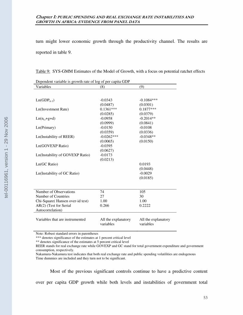
Chapter I: PUBLIC SPENDING AND REAL EXCHANGE RATE INSTABILITIES AND GROWTH IN AFRICA: EVIDENCE FROM PANEL DATA
53
turn might lower economic growth through the productivity channel. The results are
reported in table 9.
Table 9: SYS-GMM Estimates of the Model of Growth, with a focus on potential ratchet effects
Dependent variable is growth rate of log of per capita GDP
Variables (8) (9)
Ln(GDPit-1) -0.0343 (0.0487)
-0.1084*** (0.0301)
Ln(Investment Rate) 0.1361*** (0.0285)
0.1877*** (0.0379)
Ln(ni,t+g+d) -0.0958 (0.0999)
-0.2014** (0.0841)
Ln(Primary) -0.0150 (0.0359)
-0.0108 (0.0336)
Ln(Instability of REER) -0.0262*** (0.0065)
-0.0348** (0.0150)
Ln(GOVEXP Ratio) -0.0395 (0.0627)
Ln(Instability of GOVEXP Ratio) -0.0173 (0.0213)
Ln(GC Ratio) 0.0193 (0.0448)
Ln(Instability of GC Ratio) -0.0029 (0.0185)
Number of Observations 74 105 Number of Countries 27 30 Chi-Square( Hansen over-id test) 1.00 1.00 AR(2) (Test for Serial Autocorrelation)
0.266 0.2222
Variables that are instrumented All the explanatory
variables All the explanatory variables
Note: Robust standard errors in parentheses *** denotes significance of the estimates at 1 percent critical level ** denotes significance of the estimates at 5 percent critical level REER stands for real exchange rate while GOVEXP and GC stand for total government expenditure and government consumption, respectively. Nakamura-Nakamura test indicates that both real exchange rate and public spending volatilities are endogenous Time dummies are included and they turn not to be significant.
Most of the previous significant controls continue to have a predictive content
over per capita GDP growth while both levels and instabilities of government total
tel-0
0116
961,
ver
sion
1 -
29 N
ov 2
006
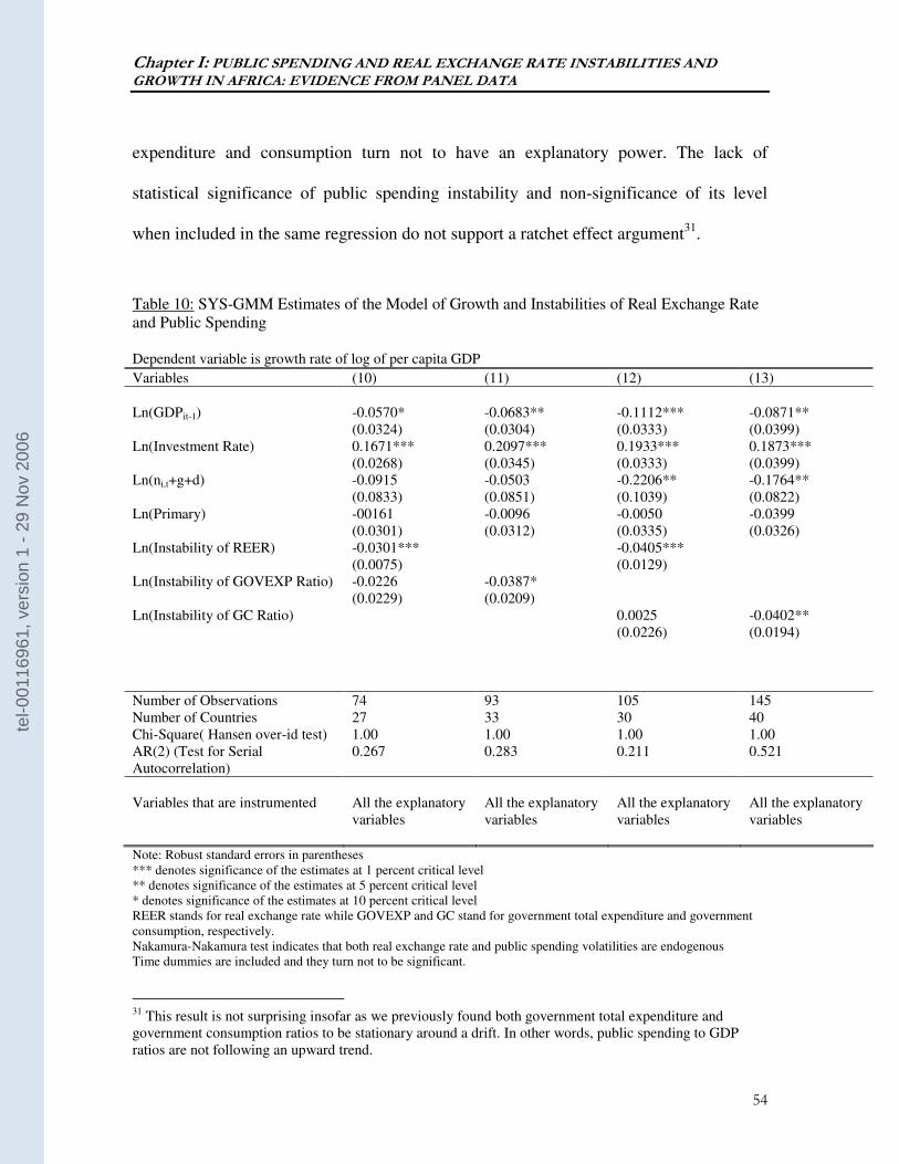
Chapter I: PUBLIC SPENDING AND REAL EXCHANGE RATE INSTABILITIES AND GROWTH IN AFRICA: EVIDENCE FROM PANEL DATA
54
expenditure and consumption turn not to have an explanatory power. The lack of
statistical significance of public spending instability and non-significance of its level
when included in the same regression do not support a ratchet effect argument31.
Table 10: SYS-GMM Estimates of the Model of Growth and Instabilities of Real Exchange Rate and Public Spending Dependent variable is growth rate of log of per capita GDP
Variables (10) (11) (12) (13)
Ln(GDPit-1) -0.0570*
(0.0324) -0.0683** (0.0304)
-0.1112*** (0.0333)
-0.0871** (0.0399)
Ln(Investment Rate) 0.1671*** (0.0268)
0.2097*** (0.0345)
0.1933*** (0.0333)
0.1873*** (0.0399)
Ln(ni,t+g+d) -0.0915 (0.0833)
-0.0503 (0.0851)
-0.2206** (0.1039)
-0.1764** (0.0822)
Ln(Primary) -00161 (0.0301)
-0.0096 (0.0312)
-0.0050 (0.0335)
-0.0399 (0.0326)
Ln(Instability of REER) -0.0301*** (0.0075)
-0.0405*** (0.0129)
Ln(Instability of GOVEXP Ratio) -0.0226 (0.0229)
-0.0387* (0.0209)
Ln(Instability of GC Ratio) 0.0025 (0.0226)
-0.0402** (0.0194)
Number of Observations 74 93 105 145 Number of Countries 27 33 30 40 Chi-Square( Hansen over-id test) 1.00 1.00 1.00 1.00 AR(2) (Test for Serial Autocorrelation)
0.267 0.283 0.211 0.521
Variables that are instrumented All the explanatory
variables All the explanatory variables
All the explanatory variables
All the explanatory variables
Note: Robust standard errors in parentheses *** denotes significance of the estimates at 1 percent critical level ** denotes significance of the estimates at 5 percent critical level * denotes significance of the estimates at 10 percent critical level REER stands for real exchange rate while GOVEXP and GC stand for government total expenditure and government consumption, respectively. Nakamura-Nakamura test indicates that both real exchange rate and public spending volatilities are endogenous Time dummies are included and they turn not to be significant.
31 This result is not surprising insofar as we previously found both government total expenditure and government consumption ratios to be stationary around a drift. In other words, public spending to GDP ratios are not following an upward trend.
tel-0
0116
961,
ver
sion
1 -
29 N
ov 2
006
Chapter I: PUBLIC SPENDING AND REAL EXCHANGE RATE INSTABILITIES AND GROWTH IN AFRICA: EVIDENCE FROM PANEL DATA
55
We explore another potential productivity channel, that is, the channel via real
exchange rate instability. Strong evidence from the literature supports the view that
fluctuations in public spending explain real exchange rate instability and real exchange
rate appreciation (Ghura and Greenes, 1993: Soderling, 2002). The most straightforward
approach to uncover this channel is to compare two set of regressions: one that includes
both public spending and real exchange rate instabilities and the other that accounts for
public spending only. Results are presented in Table 10. Public spending, either captured
by government total expenditure or government consumption, turns negative and
significant when real exchange rate fluctuations are not factored in (regressions 11 and
13). However, the same variables appear statistically insignificant once real exchange
rate instability is included in regressions 10 and 12. These results lend a strong support to
the contention that government spending fluctuations amplify real exchange rate
instability, which in turn depresses total factor productivity and ultimately economic
expansion.
5.2.1.2 The factor accumulation channel
A more systematic way to explore a potential investment channel is to look at the
determinants of investment. We therefore regress real investment rate on all the
explanatory variables of the core growth regression and a new control, namely, the
lagged investment rate. Table 11 presents results that do not support any evidence of an
tel-0
0116
961,
ver
sion
1 -
29 N
ov 2
006
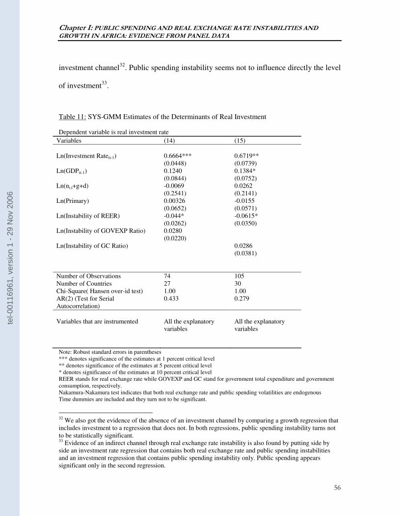
Chapter I: PUBLIC SPENDING AND REAL EXCHANGE RATE INSTABILITIES AND GROWTH IN AFRICA: EVIDENCE FROM PANEL DATA
56
investment channel32. Public spending instability seems not to influence directly the level
of investment33.
Table 11: SYS-GMM Estimates of the Determinants of Real Investment Dependent variable is real investment rate
Variables (14) (15)
Ln(Investment Rateit-1) 0.6664***
(0.0448) 0.6719** (0.0739)
Ln(GDPit-1) 0.1240 (0.0844)
0.1384* (0.0752)
Ln(ni,t+g+d) -0.0069 (0.2541)
0.0262 (0.2141)
Ln(Primary) 0.00326 (0.0652)
-0.0155 (0.0571)
Ln(Instability of REER) -0.044* (0.0262)
-0.0615* (0.0350)
Ln(Instability of GOVEXP Ratio) 0.0280 (0.0220)
Ln(Instability of GC Ratio) 0.0286 (0.0381)
Number of Observations 74 105 Number of Countries 27 30 Chi-Square( Hansen over-id test) 1.00 1.00 AR(2) (Test for Serial Autocorrelation)
0.433 0.279
Variables that are instrumented All the explanatory
variables All the explanatory variables
Note: Robust standard errors in parentheses *** denotes significance of the estimates at 1 percent critical level ** denotes significance of the estimates at 5 percent critical level * denotes significance of the estimates at 10 percent critical level REER stands for real exchange rate while GOVEXP and GC stand for government total expenditure and government consumption, respectively. Nakamura-Nakamura test indicates that both real exchange rate and public spending volatilities are endogenous Time dummies are included and they turn not to be significant.
32 We also got the evidence of the absence of an investment channel by comparing a growth regression that includes investment to a regression that does not. In both regressions, public spending instability turns not to be statistically significant. 33 Evidence of an indirect channel through real exchange rate instability is also found by putting side by side an investment rate regression that contains both real exchange rate and public spending instabilities and an investment regression that contains public spending instability only. Public spending appears significant only in the second regression.
tel-0
0116
961,
ver
sion
1 -
29 N
ov 2
006
Chapter I: PUBLIC SPENDING AND REAL EXCHANGE RATE INSTABILITIES AND GROWTH IN AFRICA: EVIDENCE FROM PANEL DATA
57
5.2.2 The potential channels from real exchange rate instability to poor
economic growth
5.2.2.1 The productivity channel
Results from Table 7 clearly indicate a direct negative impact of real exchange
rate fluctuations on growth. As mentioned before, this “direct effect” indicates that real
exchange instability has a negative impact on growth and that impact is felt through
meagre total productivity factor growth. The finding is quite close and broadly consistent
with what was uncovered by Aizenman and Marion (1999), Ghura and Greenes (1993),
Guillaumont et al. (1999) and Serven (1997).
tel-0
0116
961,
ver
sion
1 -
29 N
ov 2
006
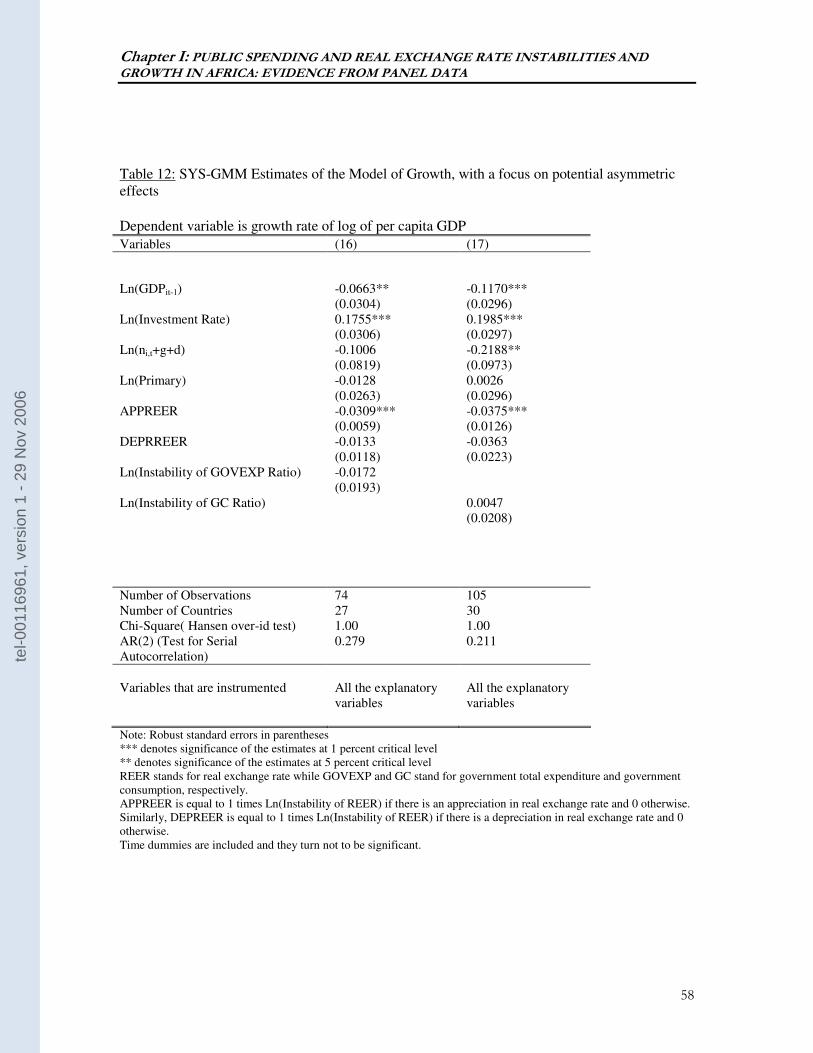
Chapter I: PUBLIC SPENDING AND REAL EXCHANGE RATE INSTABILITIES AND GROWTH IN AFRICA: EVIDENCE FROM PANEL DATA
58
Table 12: SYS-GMM Estimates of the Model of Growth, with a focus on potential asymmetric effects
Dependent variable is growth rate of log of per capita GDP
Variables (16) (17)
Ln(GDPit-1) -0.0663** (0.0304)
-0.1170*** (0.0296)
Ln(Investment Rate) 0.1755*** (0.0306)
0.1985*** (0.0297)
Ln(ni,t+g+d) -0.1006 (0.0819)
-0.2188** (0.0973)
Ln(Primary) -0.0128 (0.0263)
0.0026 (0.0296)
APPREER -0.0309*** (0.0059)
-0.0375*** (0.0126)
DEPRREER -0.0133 (0.0118)
-0.0363 (0.0223)
Ln(Instability of GOVEXP Ratio) -0.0172 (0.0193)
Ln(Instability of GC Ratio) 0.0047 (0.0208)
Number of Observations 74 105 Number of Countries 27 30 Chi-Square( Hansen over-id test) 1.00 1.00 AR(2) (Test for Serial Autocorrelation)
0.279 0.211
Variables that are instrumented All the explanatory
variables All the explanatory variables
Note: Robust standard errors in parentheses *** denotes significance of the estimates at 1 percent critical level ** denotes significance of the estimates at 5 percent critical level REER stands for real exchange rate while GOVEXP and GC stand for government total expenditure and government consumption, respectively. APPREER is equal to 1 times Ln(Instability of REER) if there is an appreciation in real exchange rate and 0 otherwise. Similarly, DEPREER is equal to 1 times Ln(Instability of REER) if there is a depreciation in real exchange rate and 0 otherwise. Time dummies are included and they turn not to be significant.
tel-0
0116
961,
ver
sion
1 -
29 N
ov 2
006
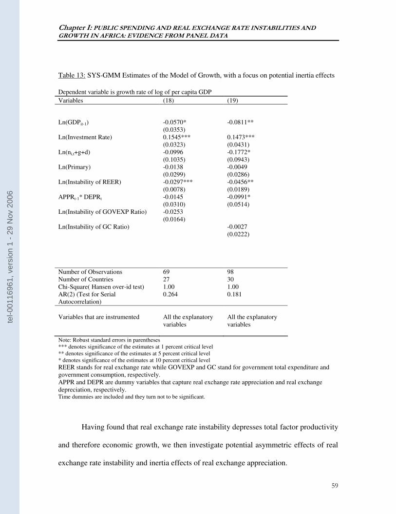
Chapter I: PUBLIC SPENDING AND REAL EXCHANGE RATE INSTABILITIES AND GROWTH IN AFRICA: EVIDENCE FROM PANEL DATA
59
Table 13: SYS-GMM Estimates of the Model of Growth, with a focus on potential inertia effects
Dependent variable is growth rate of log of per capita GDP
Variables (18) (19)
Ln(GDPit-1) -0.0570* (0.0353)
-0.0811**
Ln(Investment Rate) 0.1545*** (0.0323)
0.1473*** (0.0431)
Ln(ni,t+g+d) -0.0996 (0.1035)
-0.1772* (0.0943)
Ln(Primary) -0.0138 (0.0299)
-0.0049 (0.0286)
Ln(Instability of REER) -0.0297*** (0.0078)
-0.0456** (0.0189)
APPRt-1* DEPRt -0.0145 (0.0310)
-0.0991* (0.0514)
Ln(Instability of GOVEXP Ratio) -0.0253 (0.0164)
Ln(Instability of GC Ratio) -0.0027 (0.0222)
Number of Observations 69 98 Number of Countries 27 30 Chi-Square( Hansen over-id test) 1.00 1.00 AR(2) (Test for Serial Autocorrelation)
0.264 0.181
Variables that are instrumented All the explanatory
variables All the explanatory variables
Note: Robust standard errors in parentheses *** denotes significance of the estimates at 1 percent critical level ** denotes significance of the estimates at 5 percent critical level * denotes significance of the estimates at 10 percent critical level
REER stands for real exchange rate while GOVEXP and GC stand for government total expenditure and government consumption, respectively. APPR and DEPR are dummy variables that capture real exchange rate appreciation and real exchange depreciation, respectively. Time dummies are included and they turn not to be significant.
Having found that real exchange rate instability depresses total factor productivity
and therefore economic growth, we then investigate potential asymmetric effects of real
exchange rate instability and inertia effects of real exchange appreciation.
tel-0
0116
961,
ver
sion
1 -
29 N
ov 2
006
Chapter I: PUBLIC SPENDING AND REAL EXCHANGE RATE INSTABILITIES AND GROWTH IN AFRICA: EVIDENCE FROM PANEL DATA
60
a. Asymmetric effects of real exchange instability
Referring to real exchange instability implies accounting for both real exchange
rate appreciation and real exchange rate depreciation. Therefore, it will be interesting to
find out which of these two components of real exchange instability drives the result.
This exercise amounts to exploring potential asymmetric effects. We introduce a
multiplicative variable APPREER and DEPREER in the core regressions to account for
these effects. APPREER is a multiplicative variable equal to 1 times real exchange rate
instability if there is an appreciation in real exchange rate and 0 otherwise. Similarly,
DEPREER is equal to 1 times real exchange rate instability if there is depreciation in real
exchange rate and 0 otherwise. Table 12 summarises the results. These results indicate
that among the newly included variables only APPREER turns to have a significant
predictive content over per-capita growth, which suggest that the detrimental effect of
real exchange rate instability on growth is mostly driven by real exchange rate
appreciation.
b. Inertia effects of real exchange rate appreciation
In line with the theoretical argument developed in section 3.3, we explore further
potential inertia effects of real exchange rate appreciation on total productivity factor and
growth. We introduce a multiplicative variable APPRt-1*DEPRt in the core regressions.
That variable is a combination of the lagged of a dummy variable APPR, which captures
real exchange rate appreciation, and a dummy variable DEPR, which stands for real
tel-0
0116
961,
ver
sion
1 -
29 N
ov 2
006
Chapter I: PUBLIC SPENDING AND REAL EXCHANGE RATE INSTABILITIES AND GROWTH IN AFRICA: EVIDENCE FROM PANEL DATA
61
exchange depreciation. The idea being captured here is that initial real exchange rate
appreciation has an enduring impact in subsequent period even if that subsequent period
is characterised by real exchange depreciation. Results are reported in table 13. The
multiplicative variable APPRt-1*DEPRt turns with the expected sign both in regressions
18 and 19. However, the coefficient on this multiplicative variable is statistically
significant only in regression 19. These results tend to support partially the contention
that real exchange rate appreciation exerts an enduring impact on per capita growth.
5.2.2.2 The factor accumulation channel
The regressions presented in table 11 show a significant negative relationship
between real exchange rate instability and investment, suggesting real exchange rate
instability also affects growth in a significant and negative way through the investment
channel. This result is in line with what was found by Guillaumont et al. (1999).
To recap, instabilities of public spending and real exchange rate exert detrimental
impact on growth through a variety of channels. On the one hand, the effects of real
exchange rate instability work through both meagre total factor productivity and lower
investment. One the other, government spending instability seems to have indirect effects
only. It amplifies real exchange rate instability, which in turn depresses total productivity
factor and investment.
tel-0
0116
961,
ver
sion
1 -
29 N
ov 2
006
Chapter I: PUBLIC SPENDING AND REAL EXCHANGE RATE INSTABILITIES AND GROWTH IN AFRICA: EVIDENCE FROM PANEL DATA
62
VI- CONCLUSION
Recent economic research on Africa has extensively explored possible reasons for
the continent’s dismal growth performance. This debate has been dominated by two lines
of argument: those who attribute Africa’s poor performance to poor policies and those
who explain it by structural and institutional impediments. That classification might be
very simplistic because omitting the view that indicates that both factors are interrelated.
While acknowledging the critical role played by institutional and structural factors in
Africa’s poor performance, this chapter revisits the policy argument along the lines of the
arguments developed by Guillaumont et al. (1999) and explores the role played by policy
instabilities. However, the approach adopted in this chapter differs from earlier work in
two perspectives. First, it relies entirely on the key variables underscored in the
dependent economy model, namely the real exchange rate and the absorption. Second,
the analysis is based on dynamic panel data instead of cross-country data. Using the
system GMM, the most appropriate econometric technique for our model, we find only
real exchange instability to have a direct significant effect on economic growth. The
combination of a statistical significance of real exchange instabilities and the non-
significance of public spending instability, when incorporated in the same regression,
indicates that both are not two distinct factors regarding their impact on per capita
growth. Public spending instability has a significant positive predictive content over real
exchange rate instability, which in turn hampers growth both through investment and
productivity channels. Also, real exchange rate instability has asymmetric effects on
economic growth as the relationship between these two variables is driven by real
tel-0
0116
961,
ver
sion
1 -
29 N
ov 2
006
Chapter I: PUBLIC SPENDING AND REAL EXCHANGE RATE INSTABILITIES AND GROWTH IN AFRICA: EVIDENCE FROM PANEL DATA
63
exchange rate appreciation. Finally, partial evidence supports the view that real exchange
rate appreciation contributes to the decline of sectors with important positive
externalities, thereby leading to persistent productivity losses and weak economic growth.
Overall, we interpret the above findings as suggesting that the stability of public spending
and real exchange rate are keys to Africa’s long-term economic growth.
Having said that, the question arises as to how to achieve those objectives.
Avoiding large swings in public spending requires having some control over government
revenue sources, both internal and external. In many African countries, with a narrow
production basis, domestic revenues are closely synchronized with developments in
commodity markets. The long-term solution for government revenue and expenditure
instability is to broaden the revenue base through economic diversification. However,
achieving a stability of government domestic revenues in the short-run may be facilitated
by the adoption of the use of contingent financial instruments and some institutional
arrangements, such as the establishment of a stabilisation fund. The use of contingent
financial instruments, such as futures, swaps, and options, has the potential to transfer
commodity price instability to international markets and guarantee more stable public
revenue and expenditure. However, the use of such instruments critically depends on the
existence of a sophisticated domestic financial sector, which does not exist in many
African countries. Contrary to the contingent financial tools, stabilisation seems to be a
feasible solution34. The stabilisation fund serves as a buffer mechanism whereby some
part of windfall revenues are transferred from the budget to the stabilisation fund during
34 Transparency and fiscal restraint are just as important in ensuring the well-functioning of a stabilisation fund.
tel-0
0116
961,
ver
sion
1 -
29 N
ov 2
006
Chapter I: PUBLIC SPENDING AND REAL EXCHANGE RATE INSTABILITIES AND GROWTH IN AFRICA: EVIDENCE FROM PANEL DATA
64
times of increasing commodity prices and the other way round when prices are declining,
ensuring therefore the stability of public spending. The other source of uncertainty for
government revenue is the flows of resources coming from abroad and financing
government deficit. Most African countries rely on aid flows in that respect, which means
a more predictable aid, could also be beneficial. Having a more stable public spending
could take care of an important source of real exchange rate instability.
In a context of renewed interest on the nexus between poverty and economic
policies, it might be interesting to use again the dependent economy framework to
explore this issue. And, this will be the objective of Chapter II.
tel-0
0116
961,
ver
sion
1 -
29 N
ov 2
006
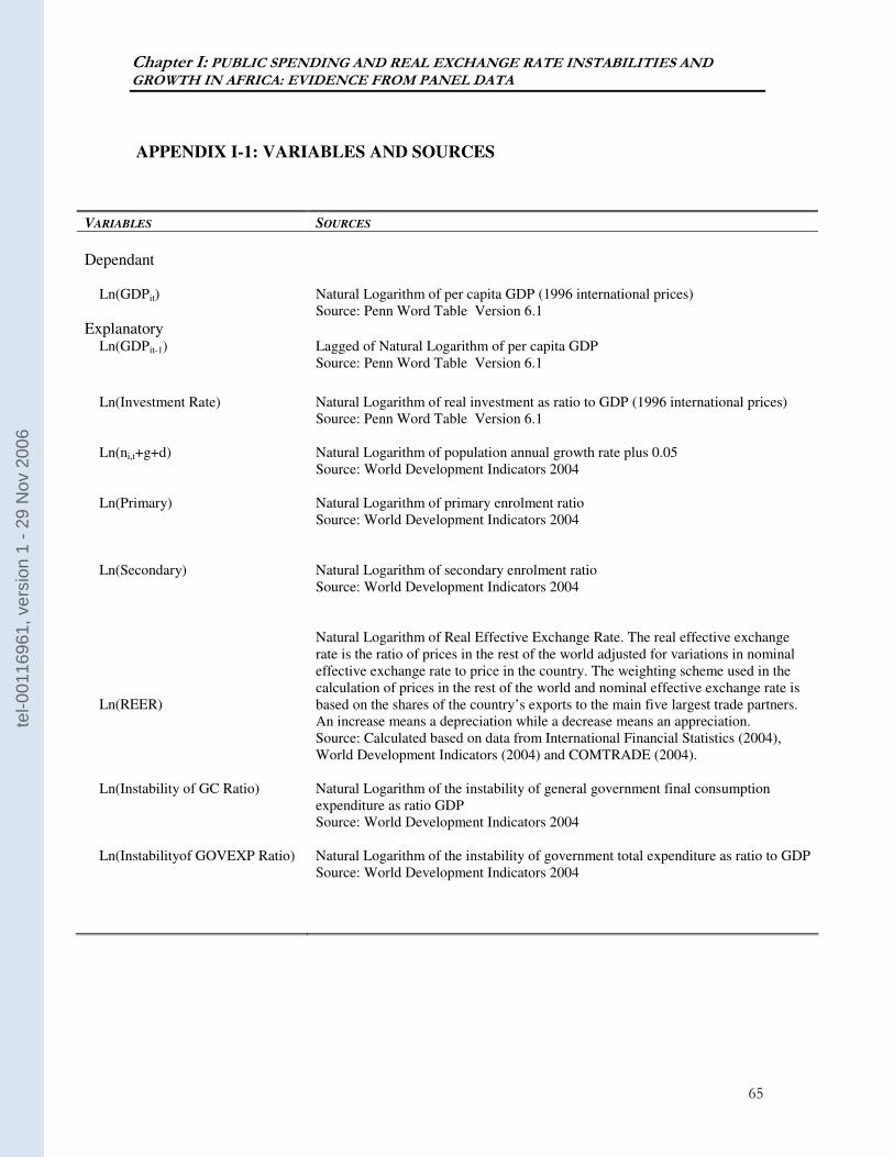
Chapter I: PUBLIC SPENDING AND REAL EXCHANGE RATE INSTABILITIES AND GROWTH IN AFRICA: EVIDENCE FROM PANEL DATA
65
APPENDIX I-1: VARIABLES AND SOURCES
VARIABLES SOURCES
Dependant Ln(GDPit)
Natural Logarithm of per capita GDP (1996 international prices) Source: Penn Word Table Version 6.1
Explanatory Ln(GDPit-1)
Lagged of Natural Logarithm of per capita GDP Source: Penn Word Table Version 6.1
Ln(Investment Rate)
Natural Logarithm of real investment as ratio to GDP (1996 international prices) Source: Penn Word Table Version 6.1
Ln(ni,t+g+d)
Natural Logarithm of population annual growth rate plus 0.05 Source: World Development Indicators 2004
Ln(Primary)
Natural Logarithm of primary enrolment ratio Source: World Development Indicators 2004
Ln(Secondary)
Natural Logarithm of secondary enrolment ratio Source: World Development Indicators 2004
Ln(REER)
Natural Logarithm of Real Effective Exchange Rate. The real effective exchange rate is the ratio of prices in the rest of the world adjusted for variations in nominal effective exchange rate to price in the country. The weighting scheme used in the calculation of prices in the rest of the world and nominal effective exchange rate is based on the shares of the country’s exports to the main five largest trade partners. An increase means a depreciation while a decrease means an appreciation. Source: Calculated based on data from International Financial Statistics (2004), World Development Indicators (2004) and COMTRADE (2004).
Ln(Instability of GC Ratio)
Natural Logarithm of the instability of general government final consumption expenditure as ratio GDP Source: World Development Indicators 2004
Ln(Instabilityof GOVEXP Ratio)
Natural Logarithm of the instability of government total expenditure as ratio to GDP Source: World Development Indicators 2004
tel-0
0116
961,
ver
sion
1 -
29 N
ov 2
006
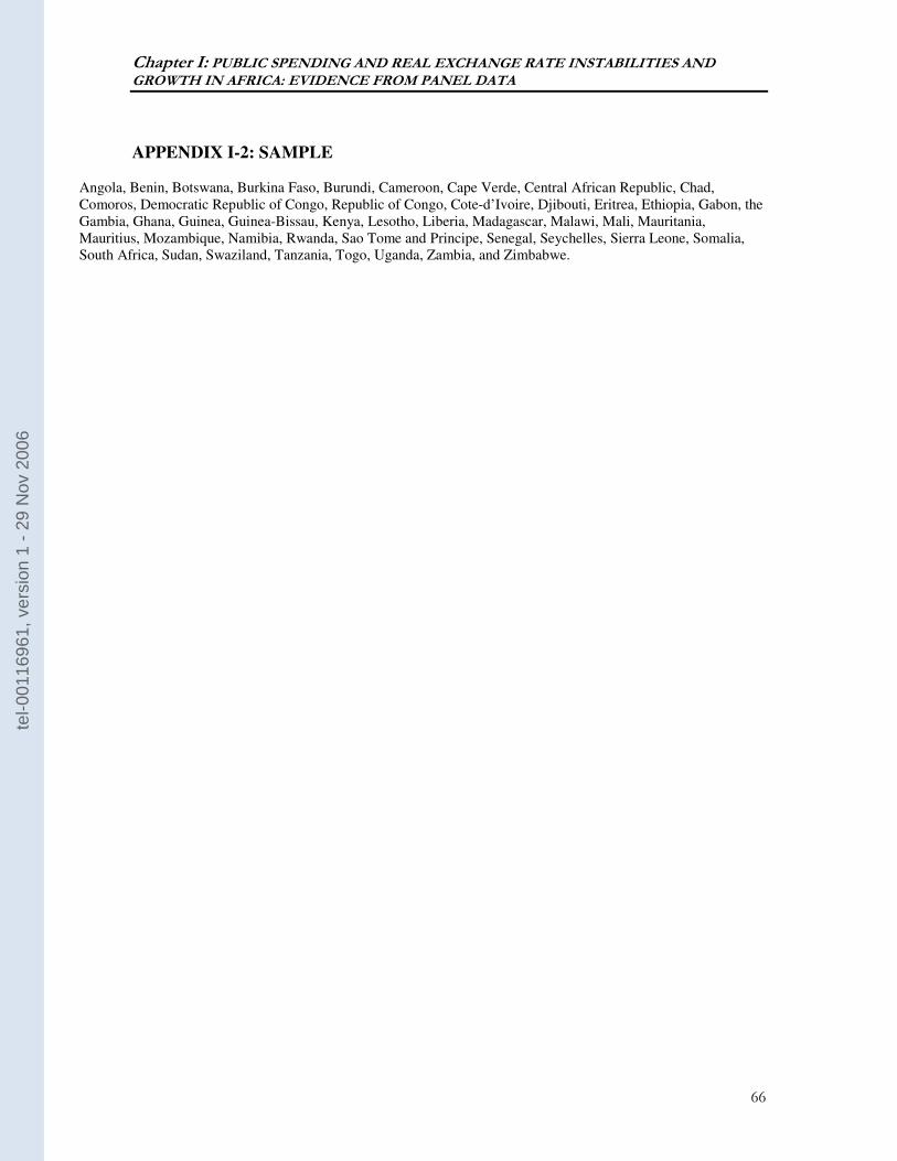
Chapter I: PUBLIC SPENDING AND REAL EXCHANGE RATE INSTABILITIES AND GROWTH IN AFRICA: EVIDENCE FROM PANEL DATA
66
APPENDIX I-2: SAMPLE
Angola, Benin, Botswana, Burkina Faso, Burundi, Cameroon, Cape Verde, Central African Republic, Chad, Comoros, Democratic Republic of Congo, Republic of Congo, Cote-d’Ivoire, Djibouti, Eritrea, Ethiopia, Gabon, the Gambia, Ghana, Guinea, Guinea-Bissau, Kenya, Lesotho, Liberia, Madagascar, Malawi, Mali, Mauritania, Mauritius, Mozambique, Namibia, Rwanda, Sao Tome and Principe, Senegal, Seychelles, Sierra Leone, Somalia, South Africa, Sudan, Swaziland, Tanzania, Togo, Uganda, Zambia, and Zimbabwe.
tel-0
0116
961,
ver
sion
1 -
29 N
ov 2
006
Chapter I: PUBLIC SPENDING AND REAL EXCHANGE RATE INSTABILITIES AND GROWTH IN AFRICA: EVIDENCE FROM PANEL DATA
67
APPENDIX I-3 STRUCTURAL, INSTITUTIONAL, AND POLICY FACTORS
DETERMINING GROWTH
Easterly and Levine (2002) provide a comprehensive and succinct account of the debate
on policy versus structural and institutional determinants of economic growth. They highlight
three main hypotheses, which are the geography/endowment, the institution, and the policy
arguments.
Geography/endowment
The geography/endowment hypothesis asserts that environment exerts a significant
influence on the quality and quantity of production factors such as labour and land and therefore
contributes to determining the level of output and income. Environment also determines
technological progress and impacts the pace of economic growth. In particular, locating in the
tropics is seen as a handicap to higher labour productivity because of the proliferation of human
infectious diseases in this environment (Bloom and Sachs, 1998). Other view holds that tropical
climate dampens labour productivity as few fully involve in productive activities when hot and
wet (Landes, 1998). Similarly, geographical location determines the quality of land. Bloom and
Sachs (1998) and Sachs (2001) attribute the poorness of Africa’s soil to ecological factors
inherent to the location in the tropics. Finally, environment could also drive technological
development as well as efficiency. Diamond (1997) indicates that germs and crops influence the
technical progress of societies in the long-term. He argues that people living in Europe developed
some resistance to certain diseases they contracted from their farm animals. More importantly,
the use of draft animals helps Eurasia to gain a technological lead over other continents, say
Africa, where tsetse flies severely limit the expansion of cattle. Other particular geographical
circumstances such as landlockness could constraint the accessibility of producers to large
economic market, limit economies of scale gains, and therefore lead to meagre production
efficiency (Sachs and Warner, 1998; 1997).
Institutions
The institution argument asserts that environment shapes institutions which, in turn,
influence policies and therefore economic development path. Easterly and Levine (2002) identify
tel-0
0116
961,
ver
sion
1 -
29 N
ov 2
006
Chapter I: PUBLIC SPENDING AND REAL EXCHANGE RATE INSTABILITIES AND GROWTH IN AFRICA: EVIDENCE FROM PANEL DATA
68
three aspects of environment, namely the location in the tropics, the proliferation of germs, and
the type of crops grown, as some of the factors that determine the nature and the quality of
institutions. The argument on “tropics” holds that countries that are located in the tropics are
likely to develop poor institutions while those that are remote from the tropics tend to display
relatively sound institutions (Hall and Jones, 1999). This argument is based on the assumption
that Western Europeans have a historical lead over others in terms of good institutions. This
implies that other regions where Western Europeans settle, meaning regions with similar climate,
are likely to have relatively sound institutions.
European settlement and their historical advance in terms of the quality of institutions are
also at the heart of the argument based on “germs”. Acemoglu et al. (2001) relate current
institutions in developing countries to the past colonisation strategies of Europeans. They argue
that Europeans were very much inclined to settle in countries where mortality among potential
settlers is low. Europeans settlers develop institutions similar to those of their home country.
These institutions largely promote property rights and establish checks and balances mechanisms,
and Australia, New Zealand, Canada and the United States are some cases in point. In contrary
when environment is hostile, with a proliferation of germs and high mortality, European did not
settle in large numbers. They instead encouraged the emergence of “extractive institutions”, with
little regard to property right protection and few institutional safeguards against government
abuses. Acemoglu et al. (2001) claimed that this description fits well the situation of African
countries. Perhaps more important in their argument is the persistence of institutions that were
shaped during the colonisation process. These institutions tend to endure even after independence.
Finally, the argument on “crops” was developed by Sokoloff and Engerman (2000).
Although European settlement is central to this argument, the two pillars of the “crops” view are
factor endowments and the resulting crops. The comparison of development paths in the
Americas provides an interesting case to illustrate this argument. Latin America strong
comparative advantage in land and its wide use of slave and indigenous people made producing
commodities such as sugar cane, rice, silver efficient. These commodities were produced in a
system of large-scale agriculture and mining, which was controlled by a plantation and mining
elite, allowing therefore substantial economies of scale. The elite subsequently manage to control
power by promoting institutions that restrict political participation and economic opportunities for
the majority. These institutions persist even when countries stop specializing in activities that
display large economies of scale. Similarly, Isham et al. (2006) show that countries that rely on
plantations crops such as sugar display worse institutions compared to countries that specialize in
tel-0
0116
961,
ver
sion
1 -
29 N
ov 2
006
Chapter I: PUBLIC SPENDING AND REAL EXCHANGE RATE INSTABILITIES AND GROWTH IN AFRICA: EVIDENCE FROM PANEL DATA
69
the production of grains (rice and wheat). Turning to the success of North America countries such
as Canada and the United States, Engerman and Sokoloff recall that “these economies35 were not
endowed with substantial populations of natives able to provide labour, nor with climates and
soils that gave them a comparative advantage in the production of crops characterized by major
economies of using slave labour.” These endowments explain the widespread of small family
farms that produced grains and the relatively equal income distribution during this period. The
development of a middle class went hand-in-hand with the development of institutions that
promote economic and social advancement.
Policy View
The policy argument holds that environment-related hindrances are not a fatality and can
be largely alleviated by sound microeconomic as well as macroeconomic policies. The aim of
promoting good microeconomic policies is to remove price distortions and allow an efficient
allocation of goods and factors and substantial productivity gains. Microeconomic policies are
often termed as “structural policies”. They mainly include trade reforms, which consisted of
reduction in protection, and deregulation of markets36. Good macroeconomic policies very often
defined in terms of economic policy outcomes. They refer, among other things, to low inflation
rates, positive real interest rates, competitive real exchange rates, low fiscal and current account
deficits, if not surpluses of those balances (Fisher, 1993: Ghura and Hadjimichael, 1996:
Catamitsis et al., 1999).
35 The focus was on North East of the United States and not its southern states 36 These are some of policies promoted by Bretton Woods Institutions, specially the World Bank.
tel-0
0116
961,
ver
sion
1 -
29 N
ov 2
006
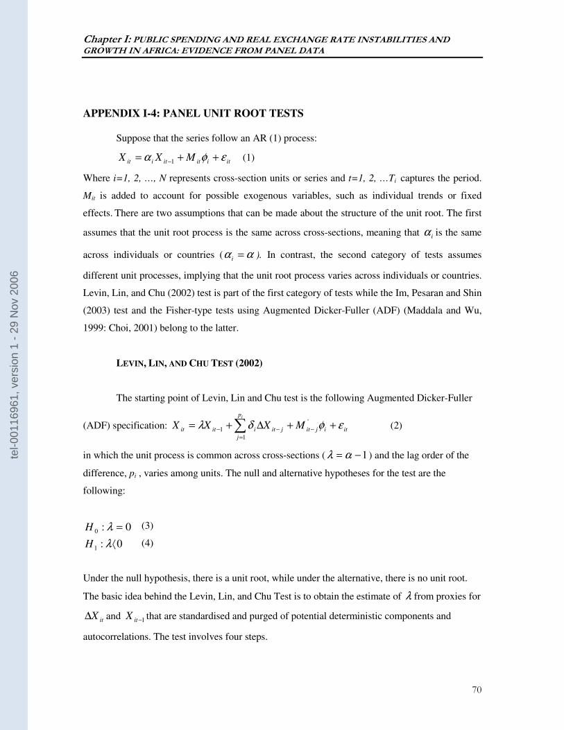
Chapter I: PUBLIC SPENDING AND REAL EXCHANGE RATE INSTABILITIES AND GROWTH IN AFRICA: EVIDENCE FROM PANEL DATA
70
APPENDIX I-4: PANEL UNIT ROOT TESTS
Suppose that the series follow an AR (1) process:
itiititiit MXX εφα ++= −1 (1)
Where i=1, 2, …, N represents cross-section units or series and t=1, 2, …Ti captures the period.
Mit is added to account for possible exogenous variables, such as individual trends or fixed
effects. There are two assumptions that can be made about the structure of the unit root. The first
assumes that the unit root process is the same across cross-sections, meaning that iα is the same
across individuals or countries ( αα =i ). In contrast, the second category of tests assumes
different unit processes, implying that the unit root process varies across individuals or countries.
Levin, Lin, and Chu (2002) test is part of the first category of tests while the Im, Pesaran and Shin
(2003) test and the Fisher-type tests using Augmented Dicker-Fuller (ADF) (Maddala and Wu,
1999: Choi, 2001) belong to the latter.
LEVIN, LIN, AND CHU TEST (2002)
The starting point of Levin, Lin and Chu test is the following Augmented Dicker-Fuller
(ADF) specification: itijit
p
j
jitiitit MXXXi
εφδλ ++∆+= −=
−− ∑ '
1
1 (2)
in which the unit process is common across cross-sections ( 1−= αλ ) and the lag order of the
difference, pi , varies among units. The null and alternative hypotheses for the test are the
following:
(3)
(4)
Under the null hypothesis, there is a unit root, while under the alternative, there is no unit root.
The basic idea behind the Levin, Lin, and Chu Test is to obtain the estimate of λ from proxies for
itX∆ and 1−itX that are standardised and purged of potential deterministic components and
autocorrelations. The test involves four steps.
0:
0:
1
0
⟨
=
λ
λ
H
H
tel-0
0116
961,
ver
sion
1 -
29 N
ov 2
006
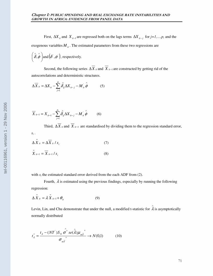
Chapter I: PUBLIC SPENDING AND REAL EXCHANGE RATE INSTABILITIES AND GROWTH IN AFRICA: EVIDENCE FROM PANEL DATA
71
First, itX∆ and 1−itX are regressed both on the lags terms jitX −∆ for j=1,…,pi and the
exogenous variables itM . The estimated parameters from these two regressions are
∧∧
φδ , and ( )'' ,φδ , respectively.
Second, the following series itX∆ and 1−itX are constructed by getting rid of the
autocorrelations and deterministic structures.
∧
−=
∧
−∆−∆=∆ ∑ φδ '
1
itjit
p
j
ijitit MXXXi
(5)
∧
−=
∧
−− −∆−= ∑ φδ '
1
11 itjit
p
j
ijitit MXXXi
(6)
Third, itX∆ and 1−itX are standardised by dividing them to the regression standard error,
si .
iitit sXX /∆=∆≈
(7)
iitit sXX /11 −−
≈
= (8)
with si the estimated standard error derived from the each ADF from (2).
Fourth, λ is estimated using the previous findings, especially by running the following
regression:
ititit XX θλ +=∆ −
≈≈
1 (9)
Levin, Lin, and Chu demonstrate that under the null, a modified t-statistic for ∧
λ is asymptotically
normally distributed
)1,0()()(
*
**'
*N
seSNTtt
Tm
TmN→
−=
∧∧
σ
µλσλ
λ (10)
tel-0
0116
961,
ver
sion
1 -
29 N
ov 2
006
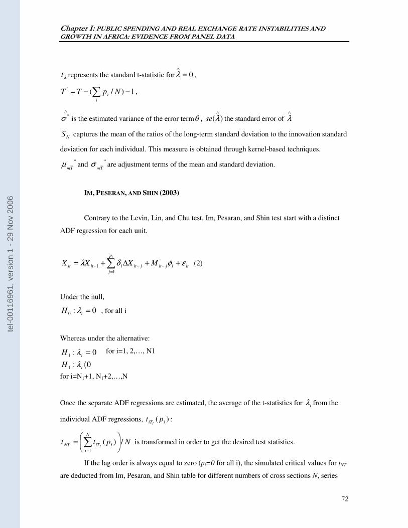
Chapter I: PUBLIC SPENDING AND REAL EXCHANGE RATE INSTABILITIES AND GROWTH IN AFRICA: EVIDENCE FROM PANEL DATA
72
λt represents the standard t-statistic for 0=∧
λ ,
1)/(' −−= ∑ NpTTi
i ,
∧*σ is the estimated variance of the error termθ , )(
∧
λse the standard error of ∧
λ
NS captures the mean of the ratios of the long-term standard deviation to the innovation standard
deviation for each individual. This measure is obtained through kernel-based techniques.
*
Tmµ and
*
Tmσ are adjustment terms of the mean and standard deviation.
IM, PESERAN, AND SHIN (2003)
Contrary to the Levin, Lin, and Chu test, Im, Pesaran, and Shin test start with a distinct
ADF regression for each unit.
itijit
p
j
jitiitit MXXXi
εφδλ ++∆+= −=
−− ∑ '
1
1 (2)
Under the null,
0:0 =iH λ , for all i
Whereas under the alternative:
for i=1, 2,…, N1
for i=N1+1, N1+2,…,N
Once the separate ADF regressions are estimated, the average of the t-statistics for iλ from the
individual ADF regressions, )( iiT ptI
:
NpttN
i
iiTNT I/)(
1
= ∑
=
is transformed in order to get the desired test statistics.
If the lag order is always equal to zero (pi=0 for all i), the simulated critical values for tNT
are deducted from Im, Pesaran, and Shin table for different numbers of cross sections N, series
0:
0:
1
1
⟨
=
i
i
H
H
λ
λ
tel-0
0116
961,
ver
sion
1 -
29 N
ov 2
006
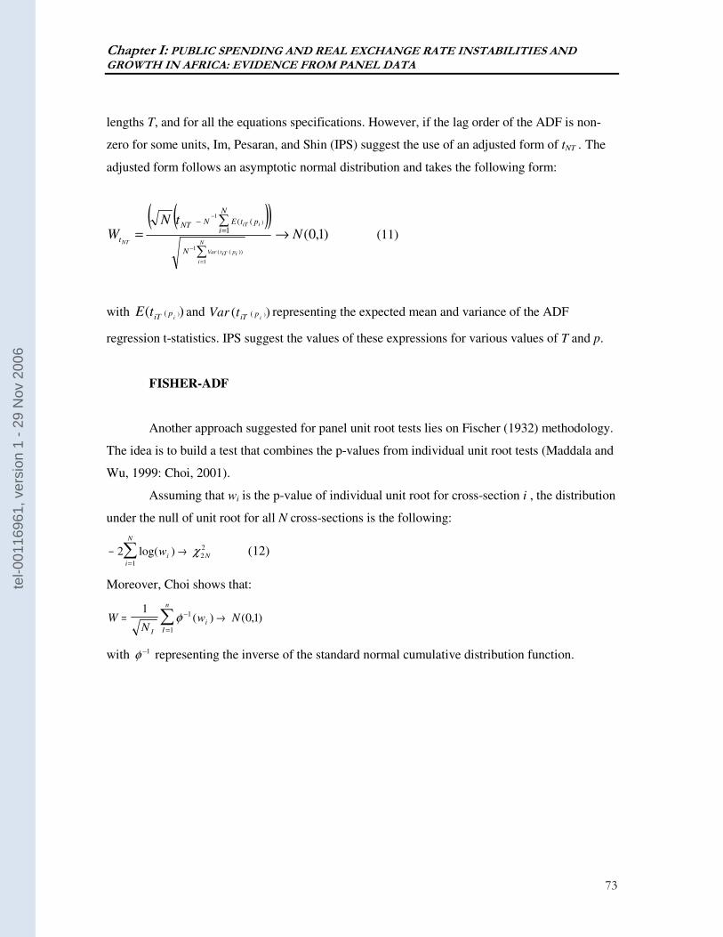
Chapter I: PUBLIC SPENDING AND REAL EXCHANGE RATE INSTABILITIES AND GROWTH IN AFRICA: EVIDENCE FROM PANEL DATA
73
lengths T, and for all the equations specifications. However, if the lag order of the ADF is non-
zero for some units, Im, Pesaran, and Shin (IPS) suggest the use of an adjusted form of tNT . The
adjusted form follows an asymptotic normal distribution and takes the following form:
( )( )∑
∑=
=
−
−
=−
N
i
ipiTtVar
iiT
NT
N
N
iptENNT
t
tNW
1
))((1
)1
1((
)1,0(N→ (11)
with )( )(i
piTtE and )( )(i
piTtVar representing the expected mean and variance of the ADF
regression t-statistics. IPS suggest the values of these expressions for various values of T and p.
FISHER-ADF
Another approach suggested for panel unit root tests lies on Fischer (1932) methodology.
The idea is to build a test that combines the p-values from individual unit root tests (Maddala and
Wu, 1999: Choi, 2001).
Assuming that wi is the p-value of individual unit root for cross-section i , the distribution
under the null of unit root for all N cross-sections is the following:
− →=
∑2 22
1
log( )wi Ni
N
χ (12)
Moreover, Choi shows that:
WN
w NI I
n
i= →−
=
∑1
0 11
1
φ ( ) ( , )
with φ −1 representing the inverse of the standard normal cumulative distribution function.
tel-0
0116
961,
ver
sion
1 -
29 N
ov 2
006
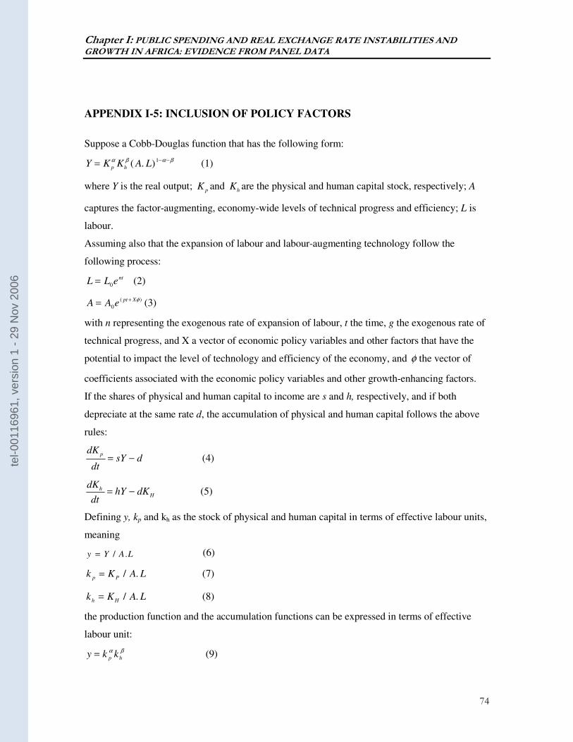
Chapter I: PUBLIC SPENDING AND REAL EXCHANGE RATE INSTABILITIES AND GROWTH IN AFRICA: EVIDENCE FROM PANEL DATA
74
APPENDIX I-5: INCLUSION OF POLICY FACTORS
Suppose a Cobb-Douglas function that has the following form:
Y K K A Lp h
= − −α β α β( . )1 (1)
where Y is the real output; Kpand K
hare the physical and human capital stock, respectively; A
captures the factor-augmenting, economy-wide levels of technical progress and efficiency; L is
labour.
Assuming also that the expansion of labour and labour-augmenting technology follow the
following process:
L L ent= 0 (2)
A A ept X= +
0
( )φ (3)
with n representing the exogenous rate of expansion of labour, t the time, g the exogenous rate of
technical progress, and X a vector of economic policy variables and other factors that have the
potential to impact the level of technology and efficiency of the economy, and φ the vector of
coefficients associated with the economic policy variables and other growth-enhancing factors.
If the shares of physical and human capital to income are s and h, respectively, and if both
depreciate at the same rate d, the accumulation of physical and human capital follows the above
rules:
dK
dtsY d
p= − (4)
dK
dthY dKh
H= − (5)
Defining y, kp and kh as the stock of physical and human capital in terms of effective labour units,
meaning
LAYy ./= (6)
k K A Lp P
= / . (7)
k K A Lh H
= / . (8)
the production function and the accumulation functions can be expressed in terms of effective
labour unit:
y k kp h
= α β (9)
tel-0
0116
961,
ver
sion
1 -
29 N
ov 2
006
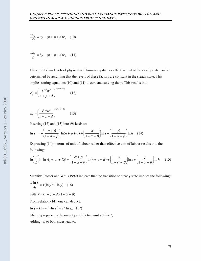
Chapter I: PUBLIC SPENDING AND REAL EXCHANGE RATE INSTABILITIES AND GROWTH IN AFRICA: EVIDENCE FROM PANEL DATA
75
dk
dtsy n p d k
p
p= − + +( ) (10)
dk
dthy n p d kh
h= − + +( ) (11)
The equilibrium levels of physical and human capital per effective unit at the steady state can be
determined by assuming that the levels of these factors are constant in the steady state. This
implies setting equations (10) and (11) to zero and solving them. This results into:
ks h
n p dp
*
( )
=+ +
−− −
11/ 1β β α β
(12)
ks h
n p dh
*
( )
=+ +
−− −
11/ 1α α α β
(13)
Inserting (12) and (13) into (9) leads to:
ln ln( ) ln ln*y n p d s h= −
+
− −
+ + +
− −
+
− −
α β
α β
α
α β
β
α β1 1 1 (14)
Expressing (14) in terms of unit of labour rather than effective unit of labour results into the
following:
ln ln ln( ) ln lnY
LA pt X n p d s h
= + + −
+
− −
+ + +
− −
+
− −
0
1 1 1φ
α β
α β
α
α β
β
α β (15)
Mankiw, Romer and Weil (1992) indicate that the transition to steady state implies the following:
d y
dty y
ln(ln * ln )= −γ (16)
with γ α β= + + − −( )( )n p d 1
From relation (14), one can deduct:
ln ( ) ln ln*y e y e y
t t= − +1 0
γ γ (17)
where y0 represents the output per effective unit at time to
Adding -yo to both sides lead to:
tel-0
0116
961,
ver
sion
1 -
29 N
ov 2
006
Chapter I: PUBLIC SPENDING AND REAL EXCHANGE RATE INSTABILITIES AND GROWTH IN AFRICA: EVIDENCE FROM PANEL DATA
76
+++
−−+
−−+++
−−
+−−−=− θ
βα
β
βα
α
βα
βαγ XptAhsdpnyeyy T
000 lnln1
ln1
)ln(1
ln)1(lnln
(18), with T representing the period under consideration.
tel-0
0116
961,
ver
sion
1 -
29 N
ov 2
006

77
tel-0
0116
961,
ver
sion
1 -
29 N
ov 2
006
Chapter II: POVERTY AND REAL EXCHANGE RATE: EVIDENCE FROM PANEL DATA
78
CHAPTER II:
POVERTY AND REAL EXCHANGE RATE: EVIDENCE FROM PANEL DATA37
37 A condensed version of this chapter is forthcoming in the Journal of African Development, September 2006. We would like to thank Jean-Louis Arcand and Jean-Louis Combes and two anonymous referees of the Journal of African Development for helpful discussions and pertinent comments on an earlier draft. We would also like to thank Roland Kpodar for sharing his program on Bootstraping and Tsangarides Charambolos for sharing his database.
tel-0
0116
961,
ver
sion
1 -
29 N
ov 2
006
Chapter II: POVERTY AND REAL EXCHANGE RATE: EVIDENCE FROM PANEL DATA
79
I- INTRODUCTION
Frequent exogenous shocks, including volatility of terms of trade and resource
flows, and capricious weather conditions, have taken a heavy toll on the internal and
external balances of many developing countries. As a result, some of these countries have
adopted economic policies largely inspired by structural adjustment programs. The
theoretical foundations of these policies are rooted in the dependent economy model or
“Australian model”, in which clearing internal and external imbalances requires an
increase of the relative price of tradable to nontradable goods, defined as the depreciation
of real exchange rate, and a reduction in domestic absorption. Policies aimed at reducing
fiscal deficits and privatising state owned enterprises are therefore supposed to contain
domestic absorption while measures gearing toward promoting trade, such as slashing
tariffs on exports, are expected to lead to the depreciation of real exchange rate. The
analysis of the impact of these economic policies on real incomes, or poverty, has
received a special attention in the literature38.
This chapter investigates the influence of the intermediate indicators of economic
policies, namely real exchange rate and absorption, on poverty. This differs from some of
the approaches generally used in the literature. Dollar and Kraay (2002), Ghura et al.
(2002), for instance, explore the relationship between policy outcome indicators, such as
inflation, trade openness, and fiscal deficits, and the incomes of the poor. The idea of
reverting to intermediate policy indicators rather than policy outcome indicators has two
38 Bourguignon et al. (1991) look into the impact of adjustment policies on the distribution of income based on some case studies. They also bring into the analysis issues of trade-off between efficiency and equity as well as political feasibility of such policies.
tel-0
0116
961,
ver
sion
1 -
29 N
ov 2
006
Chapter II: POVERTY AND REAL EXCHANGE RATE: EVIDENCE FROM PANEL DATA
80
advantages. First, it makes the model specification less cumbersome as the analysis relies
on fewer factors. Second, the method helps in effectively addressing model uncertainty
concerns and the parsimonious choice of macroeconomic policy-related variables
because the approach is based on a theoretical model. The relationship between the
intermediate policy variables and poverty come into play through indirect and direct
channels. In line with the vast empirical literature on poverty reduction (Foster and
Szekely, 2001: Dollar and Kraay, 2002: Ghura et al., 2002), economic growth is
considered as the major indirect channel through which economic policies, real exchange
and absorption, public spending in this chapter, influence poverty. In this chapter, direct
channels are highlighted as well.
The rest of the chapter proceeds as follows. Section II provides an overview of the
nexus between economic policies and poverty in the context of Sub-Saharan Africa,
where the challenge of alleviating poverty is of particular importance. Section III presents
the dependent economy model. Section IV provides the conceptual background by
reviewing the indirect and direct channels through which real exchange rate and public
spending affect the incomes of the poor. This analysis will be complemented by a close
look at the role of a third set of factors that determine the direct relationship between real
exchange rate and poverty. Section V presents the theoretical framework and the
econometric methodology. Section VI discusses the choice of variables and data and
presents the econometric results. Section VII concludes.
tel-0
0116
961,
ver
sion
1 -
29 N
ov 2
006
Chapter II: POVERTY AND REAL EXCHANGE RATE: EVIDENCE FROM PANEL DATA
81
II- OVERVIEW
The World Bank and the International Monetary Fund sponsored structural
adjustments programs have often been criticised for their detrimental effects on the
poorest segments of the society. Some, like Ali (1998), find successful macroeconomic
reforms to be associated with increasing poverty by using IFAD data. On the other hand,
others, like Demery and Squire (1996), reject the claim and show that improved
macroeconomic environment is largely condusive to poverty reduction.
These two views can be illustrated in table 1, which summarises a study carried
out by Christiansen et al. (2002). The information combines macroeconomic policy score
and information on poverty headcount39 and is based on poverty country case studies. It
has the advantage of using data that are comparable over time.
39 Poverty headcount is the share of the national population whose incomes are below the official threshold (or thresholds) set by the national governement.
tel-0
0116
961,
ver
sion
1 -
29 N
ov 2
006
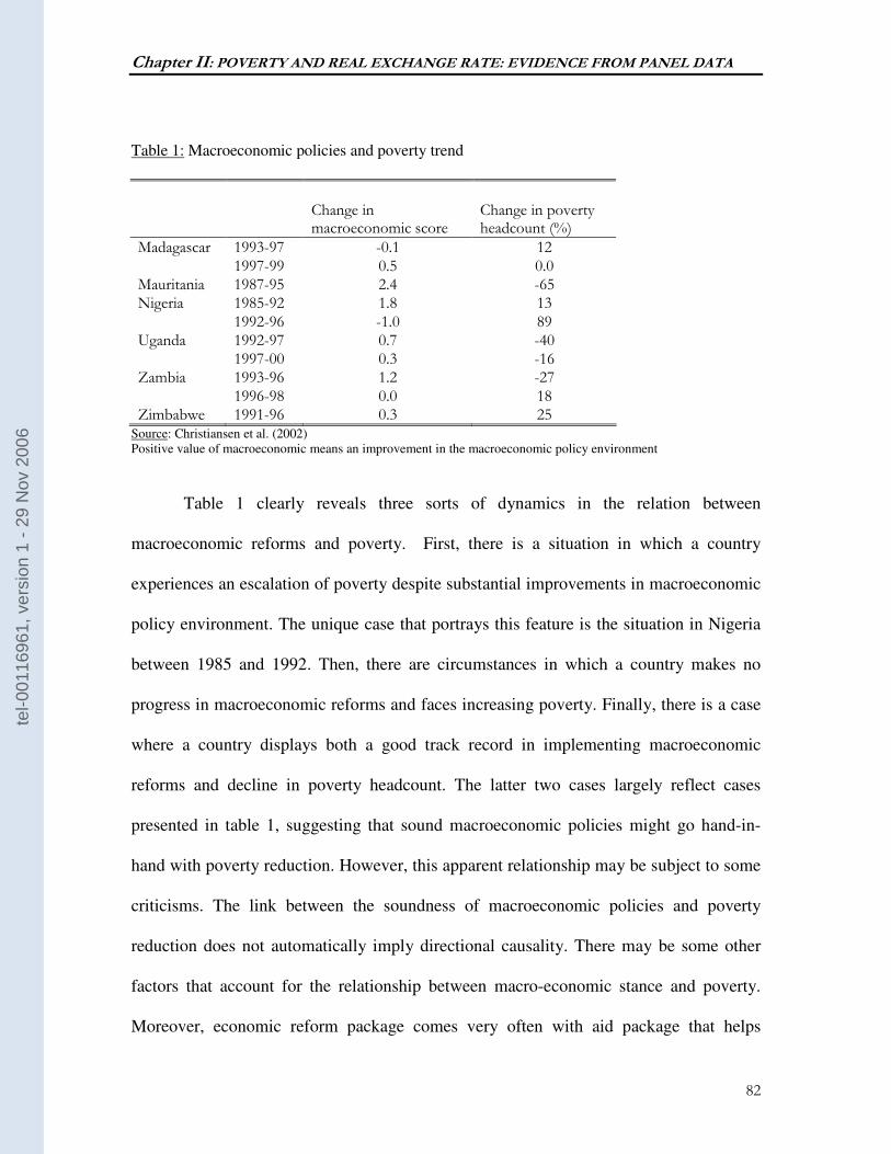
Chapter II: POVERTY AND REAL EXCHANGE RATE: EVIDENCE FROM PANEL DATA
82
Table 1: Macroeconomic policies and poverty trend
Change in macroeconomic score
Change in poverty headcount (%)
Madagascar 1993-97 -0.1 12 1997-99 0.5 0.0 Mauritania 1987-95 2.4 -65 Nigeria 1985-92 1.8 13 1992-96 -1.0 89 Uganda 1992-97 0.7 -40 1997-00 0.3 -16 Zambia 1993-96 1.2 -27 1996-98 0.0 18 Zimbabwe 1991-96 0.3 25
Source: Christiansen et al. (2002) Positive value of macroeconomic means an improvement in the macroeconomic policy environment
Table 1 clearly reveals three sorts of dynamics in the relation between
macroeconomic reforms and poverty. First, there is a situation in which a country
experiences an escalation of poverty despite substantial improvements in macroeconomic
policy environment. The unique case that portrays this feature is the situation in Nigeria
between 1985 and 1992. Then, there are circumstances in which a country makes no
progress in macroeconomic reforms and faces increasing poverty. Finally, there is a case
where a country displays both a good track record in implementing macroeconomic
reforms and decline in poverty headcount. The latter two cases largely reflect cases
presented in table 1, suggesting that sound macroeconomic policies might go hand-in-
hand with poverty reduction. However, this apparent relationship may be subject to some
criticisms. The link between the soundness of macroeconomic policies and poverty
reduction does not automatically imply directional causality. There may be some other
factors that account for the relationship between macro-economic stance and poverty.
Moreover, economic reform package comes very often with aid package that helps
tel-0
0116
961,
ver
sion
1 -
29 N
ov 2
006
Chapter II: POVERTY AND REAL EXCHANGE RATE: EVIDENCE FROM PANEL DATA
83
dampen the effects of negative exogenous shocks. Thus, one acceptable approach is to
consider rigorous counterfactual scenarios rather than an ex-ante/ex-post comparison.
General equilibrium models generally provide suitable environment for such simulations
as shown by Bourguignon et al. (1991). Finally, the extent to which poverty headcount
captures poverty and the way the macroeconomic score40 is built may be questionable41.
We will present in the next section the dependent economy model, which is the
theoretical basis for policies that have been implemented in many developing countries.
The model will help find alternative indicators to be considered in the discussion on
economic policies and poverty.
III- SIMPLE DEPENDENT ECONOMY MODEL
The failure of traditional economic models, Keynesian and Monetarian models, to
capture the reality of the developing world gave a prominent role to the dependent
economy model. This model has provided the theoretical background for policies
designed to reduce internal and external imbalances in many developing countries.
The dependent economy model was initially developed in the area of international
trade theory (Salter, 1959: Swan, 1960) and subsequently found numerous applications in
development economics because of its ability to capture dynamics in small open
economies, especially developing economies. The model is built on the assumption that
the country is price-taker, meaning that the country market power is not significant to
40 The index is composed of three components: fiscal, monetary and exchange rate policy. The weights of each component are derived from international cross section regressions. 41 The weighting scheme used to compute the macroeconomic score might sound very arbitrary.
tel-0
0116
961,
ver
sion
1 -
29 N
ov 2
006
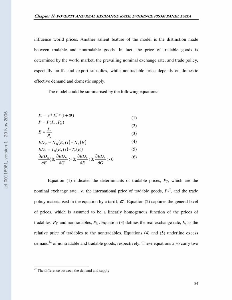
Chapter II: POVERTY AND REAL EXCHANGE RATE: EVIDENCE FROM PANEL DATA
84
influence world prices. Another salient feature of the model is the distinction made
between tradable and nontradable goods. In fact, the price of tradable goods is
determined by the world market, the prevailing nominal exchange rate, and trade policy,
especially tariffs and export subsidies, while nontradable price depends on domestic
effective demand and domestic supply.
The model could be summarised by the following equations:
(1)
(2)
(3)
(4)
(5)
(6)
Equation (1) indicates the determinants of tradable prices, PT, which are the
nominal exchange rate , e, the international price of tradable goods, PT*, and the trade
policy materialised in the equation by a tariff, ϖ . Equation (2) captures the general level
of prices, which is assumed to be a linearly homogenous function of the prices of
tradables, PT, and nontradables, PN . Equation (3) defines the real exchange rate, E, as the
relative price of tradables to the nontradables. Equations (4) and (5) underline excess
demand42 of nontradable and tradable goods, respectively. These equations also carry two
42 The difference between the demand and supply
( ) ( )( ) ( )
0;0;0;0
,
,
),(
)1(** *
>∂
∂⟨
∂
∂>
∂
∂⟩
∂
∂
−=
−=
=
=
+=
G
ED
E
ED
G
ED
E
ED
ETGETED
ENGENED
P
PE
PPPP
PeP
TTNN
SDT
SDN
N
T
NT
TT ϖ
tel-0
0116
961,
ver
sion
1 -
29 N
ov 2
006
Chapter II: POVERTY AND REAL EXCHANGE RATE: EVIDENCE FROM PANEL DATA
85
public policy variables: the public spending G43 and the real exchange rate, E. Equation
(4) suggests that any appreciation of the real exchange rate results in the decline of the
excess demand of nontradables as they become relatively expensive. On the other hand,
an increase in public spending leads to higher excess of the demand for nontradables.
Equation (5) shows that an appreciation of real exchange rate, both by boosting the
demand and restraining the supply of tradables, increases the excess demand of this
particular good. The same equation suggests that an increase in government expenditure
or an augmentation in absorption widens the excess demand for tradable goods.
Equations (4) and (5) could be used to set the conditions for internal and external
equilibriums, which require excess demands for nontradables and tradables to be equal to
zero. In the dimension (E,G) internal equilibrium is represented by a curve with a
negative slope, (NN). This reflects the idea that a real exchange appreciation is essential
in restoring equilibrium in the nontradable market when public spending increases. In
other words, an increase in absorption, which is identical to an increase in public
spending, triggers an excess in the demand of nontradables. The relative price of
nontradables must go up for this imbalance to be cleared, meaning that the real exchange
rate must appreciate. The external equilibrium is captured by an increasing curve (TT),
suggesting that, if public spending increases, so does the absorption, relative price of
tradables must rise in order to eliminate the external imbalance. The simultaneous
internal and external equilibriums are achieved in point A.
43 We ignore the public spending on nontradable goods for simplicity purposes
tel-0
0116
961,
ver
sion
1 -
29 N
ov 2
006
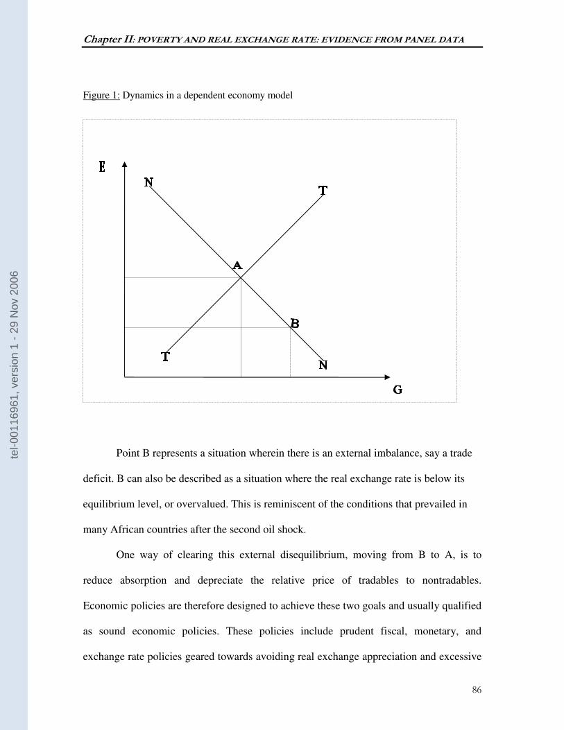
Chapter II: POVERTY AND REAL EXCHANGE RATE: EVIDENCE FROM PANEL DATA
86
Figure 1: Dynamics in a dependent economy model
Point B represents a situation wherein there is an external imbalance, say a trade
deficit. B can also be described as a situation where the real exchange rate is below its
equilibrium level, or overvalued. This is reminiscent of the conditions that prevailed in
many African countries after the second oil shock.
One way of clearing this external disequilibrium, moving from B to A, is to
reduce absorption and depreciate the relative price of tradables to nontradables.
Economic policies are therefore designed to achieve these two goals and usually qualified
as sound economic policies. These policies include prudent fiscal, monetary, and
exchange rate policies geared towards avoiding real exchange appreciation and excessive
tel-0
0116
961,
ver
sion
1 -
29 N
ov 2
006
Chapter II: POVERTY AND REAL EXCHANGE RATE: EVIDENCE FROM PANEL DATA
87
absorption. Clearly, economic policies in the dependent economy model framework tend
to primarily impact the real exchange rate and absorption. Consequently, analysing the
effects of sound economic policies on poverty amounts to assessing the impact of real
exchange rate and absorption on poverty. The chapter identifies direct and indirect
channels through which real exchange rate and absorption influence poverty.
IV- REAL EXCHANGE RATE, ABSORPTION, AND POVERTY
4.1 Indirect effects
Economic growth remains one of the key indirect channels through which
absorption and real exchange rate affect poverty. In fact, sound macroeconomic policies,
reflected in the dependent economy model by appropriate real exchange rate and
absorption, are generally considered to be conducive to strong economic growth (Fischer,
1993), and strong economic growth , which is itself believed to yield poverty reduction
(Foster and Szekely, 2001: Dollar and Kraay, 2002: Ghura et al., 2002).
4.1.1 Real exchange rate, absorption, and growth
Many growth studies support the contention that misalignments of real exchange
rate adversely affect economic performance (Cottani et al., 1990: Ghura and Grennes,
1993). There are two explanations behind this pattern. First, as a relative price of tradable
to nontradable goods, real exchange rate determines, to a large extent, the degree of
competitiveness of the export sector, a key growth engine in many small developing
tel-0
0116
961,
ver
sion
1 -
29 N
ov 2
006
Chapter II: POVERTY AND REAL EXCHANGE RATE: EVIDENCE FROM PANEL DATA
88
countries. Second, an inappropriate real exchange rate gives rise to speculation against
the domestic currency. This creates a destabilising effect on domestic financial markets,
leading therefore to lower investment and growth.
The relationship between the reduction in absorption and economic growth is
rather ambiguous. A case in point is the experience of many developing countries that
implemented fiscal adjustment policies. Those countries adopted stringent fiscal
measures, including deep cuts in public investment spending and severe cuts in transfers,
in order to achieve sustainable fiscal balances. The purpose of such policies is to send a
signal to the private sector about governments’ commitment and ability to efficiently run
their economies and contributes to higher private investment and economic growth.
However, some of the measures may seriously undermine economic growth prospects.
This is particularly true if the cuts relate to public-sector spending in infrastructural
facilities and in the area of human capital, and law and order, which tend to strongly
crowd in private investment and therefore highly beneficial to economic growth
(Aschauer, 1989: Erenburg, 1993: Serven and Solimano, 1993: Oshikoya, 1994: Serven,
1996).
4.1.2 Growth and poverty
Although there is no fully developed theoretical framework on the relationship
between economic growth and poverty, numerous empirical studies provide conclusive
evidence about the positive association between income growth and income measures of
poverty. Using panel data, Dollar and Kraay (2002) found that a one percent increase of
per capita income results in one percent rise of the average incomes of the poorest fifth of
tel-0
0116
961,
ver
sion
1 -
29 N
ov 2
006
Chapter II: POVERTY AND REAL EXCHANGE RATE: EVIDENCE FROM PANEL DATA
89
society. Timer (1997), Ghura et al. (2002), Foster and Szekely (2002) applied different
approaches to the same data, and found that the incomes of the poorest 20 per cent
increase less than proportional with those of the non-poor. The positive impact of
economic growth on poverty is also confirmed by various individual country studies
(Lipton and Ravallion, 1995: Ravallion and Datt, 1996).
4.2 Direct effects
4.2.1 The direct impact of the reduction of absorption
The reduction of the absorption is often achieved by cutting public spending,
namely by freezing the nominal bill wage or/and downsizing the public sector or/and
reducing substantially subsidies and other currents transfers. These measures increase
directly poverty, particularly in a context where there are few work opportunities for the
poor in the private sector.
However, the relationship between absorption, especially public expenditure, and
poverty could be also positive for three reasons. First, cuts in public spending may reduce
the government tendency to revert to monetary financing as means of funding fiscal
deficits, thereby contribute to lowering inflation. The poor may therefore benefit from
low inflationary pressures as clearly demonstrated by Easterly and Fischer (2001).
Second, a growing body of evidence shows that the structure of public expenditures in
social sectors in many developing countries, especially in Africa, tends to favour the
tel-0
0116
961,
ver
sion
1 -
29 N
ov 2
006
Chapter II: POVERTY AND REAL EXCHANGE RATE: EVIDENCE FROM PANEL DATA
90
richest at the expense of the poorest (Castro-Leal et al., 1999). For instance, the share of
public subsidy to the poorest 20 percent of the population in the health sector varies from
4 percent in Guinea to 17 percent in Tanzania while the share received by the richest 20
percent ranges from 48 percent in Guinea to 17 percent in South Africa. In the education
sector, the poorest 20 percent capture only 5 and 14 percent of public spending in
education respectively in Guinea and Tanzania whereas the 20 percent richest receive 44
percent and 21 percent of public spending in Guinea and Ghana. In such circumstances,
reduction in public spending may have little impact on the poor. Third, this is all the more
true if cuts in public expenditures are accompanied by changes affecting the intra and
inter allocation of public spending, with more public resources channelled towards social
sectors and/or compartments of these sectors extensively used by the poor. For instance, a
shift in social spending toward the delivery of basic public services, including basic
education and health care that are mostly consumed by the poor, can lead to poverty
reduction. Clearly, the direction of the relationship between poverty and absorption is
ambiguous.
4.2.2 The direct impact of real exchange rate on poverty
The Stolper-Samuelson (1941) theorem provides a strong foundation for a
potential positive impact of real exchange rate depreciation on poverty. In fact, if one
assumes that the tradable sector is labour-intensive, as suggested in many studies (Dorosh
and Sahn, 2000: Agenor, 2004), and a perfect mobility of labour across sectors,
especially between tradable and nontradable sectors, any increase of the relative price of
tel-0
0116
961,
ver
sion
1 -
29 N
ov 2
006
Chapter II: POVERTY AND REAL EXCHANGE RATE: EVIDENCE FROM PANEL DATA
91
tradable goods would lead to higher returns for labour: the most abundant factor at the
disposal of the poor.
However, real exchange rate depreciation can potentially give rise to offsetting
effects that could mitigate partially, or even completely, the benefits the poor get from
stronger relative price of tradables. These effects are mainly three. First, higher tradable
price, if achieved by nominal depreciation, raises the domestic costs of imported goods
and therefore the cost of living of the poor. This negative income effect might seriously
dampen the relative price effect if imported goods represent a substantial share in the
consumption basket of the poor. Except for the urban poor, this impact tends to be
marginal for rural poor, who make up the majority of the poor in most developing
countries. Second, when production and resources switch in favour of the tradable sector
as a result of real exchange appreciation, the demand for labour and wages in the
nontradable sector declines, depressing therefore revenues in that sector. Since most
urban poor tend to be nontradable good producers, the consequence will be increasing
urban poverty. But, this effect is likely to be mitigated by the reduction in rural poverty if
most of the poor live in rural areas. Third, the other offsetting effect comes from the
potential contraction impact of a nominal depreciation. A real depreciation gained
through a nominal depreciation can lead to higher cost of capital and intermediate inputs,
such as oil, that are generally imported in developing countries (Lora and Oliveria, 1998).
Real exchange rate depreciation generates therefore a negative supply-side shock that can
take a toll on output and employment, both in the tradable and nontradable sectors. As a
result poverty may rise. Again, this effect could be very limited in situations where
production techniques are highly labour intensive and allow a high degree of substitution
tel-0
0116
961,
ver
sion
1 -
29 N
ov 2
006
Chapter II: POVERTY AND REAL EXCHANGE RATE: EVIDENCE FROM PANEL DATA
92
between production factors, namely capital and labour. Such production techniques are
likely to reflect those of commodities and some manufacturing goods44 , the mainstay of
many developing countries’ exports.
4.1.2.1 Unskilled and skilled labour
The structure of the labour market could be much more complex than what was
previously assumed, with the coexistence of skilled and unskilled labour. One can assume
that the poor constitute the bulk of unskilled workers because they are more likely than
other segments of the society to lack education and marketable skills. In this framework,
the outcomes of real exchange depreciation remain again favourable to the poor provided
that the two types of labour are mobile and the tradable sector is low-skill-intensive.
These results fit well with the experience of some East Asian countries that experienced
significant real exchange depreciation and poverty reduction in the 1960s and 1970s.
Wood (1994, 1997), for instance, shows that the demand for unskilled labour and wages
for this type of labour soared in the Republic of Korea, Taiwan, and Singapore after these
countries liberalise their trade and increase the relative price of their tradable goods.
Elsewhere, in Latin America particularly, empirical evidence is mixed, with real
exchange depreciation leading to an apparent change in the structure of labour demand in
favour of skilled workers and higher overall unemployment and poverty in most countries
(Berry, 1998: Hanson and Harrison, 1999). The apparent combination of real exchange
rate depreciation and rising poverty stirs controversy about the Latin America’s
44 Textiles and apparels are cases in point
tel-0
0116
961,
ver
sion
1 -
29 N
ov 2
006
Chapter II: POVERTY AND REAL EXCHANGE RATE: EVIDENCE FROM PANEL DATA
93
comparative advantage. Given the region’s impressive endowment in natural resources
and its relatively higher human capital endowment compared to other developing regions,
Spilimbergo et al. (1999) and Wood (1997) suggest that Latin America’s comparative
advantage might not be in low-skill-intensive production.
In any event, even by assuming that labour, especially unskilled labour, is the
most abundant factor and a perfect mobility of this production factor among sectors, one
can suspect the relationship between real exchange rate and the incomes of the poor to be
influenced by a third set of factors, which include the quality of institutions and the
distribution of productive assets.
4.3 Third set of factors
4.3.1 Inequality
The debate on inequality, growth, and poverty has recently regained momentum.
A vast literature tends to point towards a potential deleterious impact of inequality on
growth (Persson and Tabellini, 1991: Alesina and Perotti, 1993: Alesina and Rodrik,
1994: Keefer and Knack, 2000)45. Similar conclusions are also found on the relationship
between inequality and poverty, with inequality leading to the appearance of poverty
traps. The issue of access to production factors is widely referred as the key explanation
for such relationships.
45 This view contrasts with the classical approach that suggests that the marginal propensity to save of the rich is higher than that of the poor, meaning that high initial inequality results in higher aggregate savings, capital accumulation and growth (Kaldor, 1957: Bourguignon, 1981).
tel-0
0116
961,
ver
sion
1 -
29 N
ov 2
006
Chapter II: POVERTY AND REAL EXCHANGE RATE: EVIDENCE FROM PANEL DATA
94
The access to productive assets is essential in determining the responses to
incentives, particularly the increased relative price of tradables to nontradables. In fact,
expanding activities in the tradable sector, as a result of a favourable real exchange rate,
requires additional capital, which has to be mobilised through credit. But the access to
credit, in a context of financial market imperfections, critically depends on collateral,
which lenders demand in exchange of any loan they grant. For this reason, only
borrowers with reasonable assets are able to respond to price incentives and engage in
productive activities. Consequently, only few reap the income opportunities created by
adequate real exchange rate when inequality runs high.
Inequality could also determine the direction and the scope of the effects of real
exchange rate on poverty through its impact on human capital accumulation. Inequality
adversely affects the process of acquiring skills in two ways. First, credit market
imperfections and the demand for collateral can constraint not only the access of the poor
to capital but also to education, especially if the funding of education depends on loans.
Acquisition of skills becomes therefore easy only for a very few when inequality is high.
Second, inequality may influence the process of human capital accumulation even if there
is no credit constraint. This is the case if the quality of the educational system is a local
good (Durlauf, 1994: Fernandez and Rogerson, 1998). In this situation, agents are sorted
in groups that are separated according to human capital or wealth status. The segregation
can even be reinforced by the establishment of political measures, including zoning
restrictions or voluntary contribution to school financing (Deininger and Olinto, 2000).
Consequently, disparities in skills widens over time, with the poor likely to be the most
affected. Since the level of skills may be one of the determinants as for how agents
tel-0
0116
961,
ver
sion
1 -
29 N
ov 2
006
Chapter II: POVERTY AND REAL EXCHANGE RATE: EVIDENCE FROM PANEL DATA
95
effectively take advantage of opportunities, the poor are unlikely to gain the benefits
arising from real exchange rate depreciation.
It can therefore be assumed that a fair distribution of wealth plays a positive
catalytic role in the relationship between real exchange rate and poverty while a more
unequal one dampens the supposedly positive effects of real exchange depreciation on the
incomes of the poor.
4.3.2 The quality of institutions
It is broadly agreed that institutions play a critical role in the process of economic
development. In particular, institutions that promote economic freedom, ensure a good
provision of public goods, and enforce contracts are regarded as determinant in creating
an enabling environment for economic activities, thus leading to economic expansion
(Rodrik, 1999: Parente and Prescott, 1999: Acemoglu et al., 2001: Acemoglu and
Robinson, 2003). Such institutions also determine the effectiveness of the poor’s
response to any economic incentive, especially to changes in real exchange rate.
The impact of institutions on the relationship between real exchange rate and
poverty will be illustrated by three pieces of evidence. First, the lack of access to capital
is regarded as one of the constraints facing the poor in their endeavours to boost their
incomes. It has been already mentioned in the chapter that access to credit, when capital
markets are imperfect, depends upon collateral provided by borrowers. The ownership of
that collateral can be severely constrained if property rights are not well defined and
tel-0
0116
961,
ver
sion
1 -
29 N
ov 2
006
Chapter II: POVERTY AND REAL EXCHANGE RATE: EVIDENCE FROM PANEL DATA
96
protected. The implication is that the poor can hardly get loans in the absence of a clear
definition and protection of property rights. As a result the poor are unlikely to expand
their activities in the tradable sector when there is real exchange rate depreciation.
Second, even if property rights are protected, the lack of adequate provision of
public goods can dampen the response of the poor to any improvement of the relative
price of tradable to nontradable goods. For instance, the quality and density of the road
system, namely rural roads, determines to what extent the poor are connected to markets
and therefore their ability to exploit growth-promoting opportunities. Consequently, the
lower the provision of the public goods is, the weaker is the positive impact of a
favourable real exchange rate on poverty.
Third, the enforcement of contracts is also likely to influence the extent to which
the poor react to economic incentives created by the change in real exchange rate. The
reason for this is that enforcing contract reduces the risk of default between agents and
creates a more auspicious environment for investment. In this context, the poor are
therefore more likely to gain from new opportunities created by real exchange
depreciation.
V-THEORETICAL FRAMEWORK AND THE ECONOMETRIC
METHODOLOGY
5.1 Theoretical Framework
Following Dollar and Kraay (2002)’s approach, the relationship between the
economic policies and poverty is formulated as follows:
tel-0
0116
961,
ver
sion
1 -
29 N
ov 2
006
Chapter II: POVERTY AND REAL EXCHANGE RATE: EVIDENCE FROM PANEL DATA
97
tiititititititititi XEGEIEYP ,
'
,5,,4,,3,2,10, ** νηδδδδδδ +++++++= (7)
where the i subscripts refers to country and t indexes years. Variable tiP , is supposed to
capture poverty. Since there are few observations for alternative indicators of poverty, we
revert to the logarithm of per capita income of the poor to measure poverty46. tiY , denotes
the logarithm of per-capita income. tiI , represents the quality of institutions, tiE , is the
real exchange rate, and Gi,t corresponds to the Gini coefficient. '
,tiX is a vector of control
variables. The error component is decomposed into a time invariant element iη and a time
variant component ti,ν . δ0 is the constant. δ1 captures the impact of economic growth on
poverty but also reflects the indirect effects of other right-hand-side variables on the
incomes of the poor. δ3 measures the interactive effect of real exchange rate and the
quality of institutions while 4δ captures the interaction between real exchange rate and
income inequality. These interactions are key elements in determining the direction and
the scope of the effects of economic policies on poverty. δ3 is expected to be positive,
which implies that any combination of real exchange rate depreciation and sounder
institutions results into the increase of the incomes of the poor. Conversely, any
depreciation of real exchange rate that takes place in the context of weaker institutions is
associated with disappointing outcomes for the poor. In line with the theoretical
framework, we expect 4δ to be negative. This means that real exchange depreciation
would be beneficial for the poor if there is a fairly equal income distribution. On the other
hand, increasing the relative price of tradable to nontradable would not serve the cause of
46 Alternative poverty indicators are presented in Appendix II.3
tel-0
0116
961,
ver
sion
1 -
29 N
ov 2
006
Chapter II: POVERTY AND REAL EXCHANGE RATE: EVIDENCE FROM PANEL DATA
98
poverty alleviation if income distribution is acutely skewed. Finally, the coefficient
vector δ5 also capture potential direct effects that other control variables may have on
poverty. These right-hand-side variables include other policy as well as structural
variables.
5.2 Econometric Methodology
tiititititititititi XEGEIEYP ,
'
,5,,4,,3,2,10, ** νηδδδδδδ +++++++= (7’)
The first temptation is to use Ordinary Least Squares (OLS) as an estimation
approach. This method, in the particular case of this study, has a number of shortcomings.
First, some of the right-hand-side variables, especially per capita income, Yi,t, are likely to
be endogenous. In fact, various studies on income distribution and growth point to a
reverse causation from per capita income of the poorest to average income (Barro, 1999:
Perotti, 1996). Then, one should not rule out possible omission of explanatory variables
that are correlated with other right-hand-side variables of the equation. Moreover, not
accounting for unobserved country-specific effects is likely to lead to biased results.
Finally, over or under-reporting can be an important problem associated to the poverty
measure and other control variables. It is well known that measurement error of the
dependent variable does not generate biased coefficients47 when the error is not correlated
with other right-hand-side variables. This seems unlikely to be the case for the poverty
measure. For instance, in many developing countries, rural households may be difficult to
reach by survey teams, leading to the underestimation of poverty. The same is true in
47 Even though coefficients are not biased their standard errors are.
tel-0
0116
961,
ver
sion
1 -
29 N
ov 2
006
Chapter II: POVERTY AND REAL EXCHANGE RATE: EVIDENCE FROM PANEL DATA
99
situation where education attainment of the population is low or in a context in which
income inequality is high. Measurement error in poverty can clearly be influenced by the
education attainment of the population, which constitutes some of the regressors of the
equation to be estimated. Using OLS in a context of likely combination of omitted
explanatory variables, measurement error, and endogeneity of some explanatory variables
leads to inconsistent estimates.
Following the procedure developed by Anderson and Hsiao (1982), one possible
solution is to revert to the Method of Instrumental Variables (IV), which is a first-
differenced 48version of equation 7’:
)()()*()*()()( ,
'
,5,,4,,3,2,1, tititititititititi XEGEIEYP νδδδδδ ∆+∆+∆+∆++∆=∆ (8)
This procedure eliminates not only country-specific effects but also all other time-
invariant variables. It also helps control for endogeneity and even address the
inconsistency problem associated with measurement errors (Greene, 1998) if the chosen
instrumental variables are not correlated with measurement errors. In line with standard
arguments on the instrumental variables, the lagged differenced-endogenous variables (or
lagged endogenous variables) are used as instruments. But Arellano and Bond (1991)
argue that if such procedure is adequate therefore further lagged variables are good
instruments as well. On that basis, they develop a Generalised Method of Moments
Estimator (GMM), well-known by “first-differenced GMM estimator” that combines the
suggested instruments in an efficient way. However, Blundell and Bond (1998)
demonstrate that first-differenced GMM have poor finite sample properties, especially
48 First-differencing may exacerbate measurement error
tel-0
0116
961,
ver
sion
1 -
29 N
ov 2
006
Chapter II: POVERTY AND REAL EXCHANGE RATE: EVIDENCE FROM PANEL DATA
100
when lagged levels of the variables are not strongly correlated with subsequent first-
differences. Bond et al. (2001) indicate that this is likely the case when the series are
close to a random walk or when the variance of the country-specific effects iη rises
relative to the variance of error term isε .
In order to address the problem associated with persistent panel data, Blundell and
Bond(1998) develop a system GMM estimator that is based on a simultaneous system of
two equations, which are equations (7’) and (8). Lagged variables serve as instruments
for the differenced equation (8) while their lagged first-differences are the instruments for
the equation in level (7’).
The validity of the system GMM as a consistent estimator can be ascertained by
showing that the error term is not serially correlated and the instruments used are the
adequate ones. The first condition is gauged by Arrelano and Bond (1991) test for
autocorrelation, which determines whether the first-differenced error term has a second-
order. The second condition is verified by a test of over-identifying restrictions, which
could be either the Sargan (1958) test or Hansen (1982) Test.
VI- DATA ISSUES AND ECONOMETRIC RESULTS
6.1 Description of the variables and their sources
The chapter relies to a great extent on Dollar and Kraay’s dataset, which was also
used in other studies including Ghura et al. (2002). This dataset is complemented by
several sources. The World Development Indicators (WDI) (2004) provides data on
tel-0
0116
961,
ver
sion
1 -
29 N
ov 2
006
Chapter II: POVERTY AND REAL EXCHANGE RATE: EVIDENCE FROM PANEL DATA
101
government total expenditure, GE. Data from International Financial Statistics (IFS)
(2004), COMTRADE (2004) and WDI (2004) are used to compute Real Effective
Exchange Rate, REER. Polity V Database is the source for the indicators of political
institutions. The dataset used in this chapter refers to an unbalanced panel of 86
developed and developing countries, including 13 Sub-Saharan African countries,
observed from 1962 to 1999.
6.1.1 Poverty
Among the several available measures of the welfare of the poor, the chapter
sticks to the one presented in Dollar and Kraay’s database, which defines the poor as the
poorest 20 per cent of the population. Thus, the empirical investigation uses per capita
income of the poorest quintile as dependent variable. This decision is almost driven by
data availability concern and criticisms that alternative measures are subject to. In fact, it
is extremely difficult to come up with a number of observations for alternative measures
of poverty that is equal or higher 248, which is the number of observations available in
our dataset. More importantly, Dollar and Kraay (2002) suggest that the use of three other
measures of poverty may be misleading. In particular, the recourse to the average
incomes below a particular poverty line, as an indicator of poverty, is intricate to interpret
especially when the distribution of income is very sharp in the vicinity of the poverty
line. In this particular case, any economic growth that is not accompanied with a change
in distribution will elevate a substantial share of the population from just below to just
above the poverty line and consequently bring about a decline of the income of those
tel-0
0116
961,
ver
sion
1 -
29 N
ov 2
006
Chapter II: POVERTY AND REAL EXCHANGE RATE: EVIDENCE FROM PANEL DATA
102
below the poverty line. This outcome completely distorts the exact picture, which is the
improvement of the welfare of the poor. Similar apprehensions also hold when using
other measures that give higher weight to the poorest of the population.
Dollar and Kraay (2002) indicate that data on the average income of the poorest
quintile comes from two sources. The first source, household surveys, is by far the most
important reliable one. The second is generated from data on Gini coefficient. This
method is applied only for countries that have Gini coefficient data but lack figures on
the poorest quintile. The technique consists in extrapolating the income of 20 per cent
poorest of the society by assuming that the distribution of income is lognormal
(Aitchinson and Brown, 1966: Johnson et al., 1994).
6.1.2 Key explanatory variables of interest
Per capita income: The chapter relies on the real per capita GDP at purchasing power
parity available in Dollar and Kraay dataset as indicator for average income. This dataset
builds on the Summers-Heston Penn World Tables Version, which is extended forward
through 1997.
Real Exchange Rate: As a relative price, the real exchange rate plays a key role in the
analysis of dynamics that open economies go through. In the simple model described
previously, real exchange rate moves to achieve internal and external balance, i.e., the
equilibrium in the supply and demand of nontradable as well as tradable goods. However,
tel-0
0116
961,
ver
sion
1 -
29 N
ov 2
006
Chapter II: POVERTY AND REAL EXCHANGE RATE: EVIDENCE FROM PANEL DATA
103
one major problem associated with the concept of real exchange rate is how to align
measurement to the theoretical definition.
In practice, there is no price index for tradable and nontradables as such. Instead,
there are only few aggregate price indexes, which include the consumer price index
(CPI), the wholesale price index (WPI) and the producer price index (PPI), and some
price deflators, among other things, the personal expenditure (PCE) deflator, the Implicit
Deflator of GDP. Most of these indicators are difficult to find in many countries or
cannot be compared from one country to another. For these reasons, the majority of
economists turn to the CPI, which is the most readily available indicator. In so doing, the
real exchange rate is understood as real effective exchange rate, which is defined as the
product of nominal exchange rate, expressed in units of the domestic currency per unit of
the foreign currency, and the ratio of the price level abroad to domestic price. This
measurement seems to be different to the theoretical definition of real exchange rate in
the chapter, which refers to the relative price of tradable to nontradable goods. In reality,
it captures in some way the ratio of tradable price to that of nontradable.
This assertion can be best illustrated by using the following decomposition.
Suppose that the aggregate price level, both at home and abroad, comprises tradable and
nontradable components:
(9)
(10)
where TP denotes the log price of tradable at home, NP denotes the log price of
nontradable at home, and β represents the share of tradable goods in the economy. The
***** )1(
)1(
NT
NT
PPP
PPP
ββ
ββ
−+=
−+=
tel-0
0116
961,
ver
sion
1 -
29 N
ov 2
006
Chapter II: POVERTY AND REAL EXCHANGE RATE: EVIDENCE FROM PANEL DATA
104
same definitions apply to (10), expect that the * denotes for the foreign country. Let’s
define now real exchange rate with respect to overall prices, Z,
(11)
where e denotes the log exchange rate defined in units of home currency per unit of
foreign. The combination of the three relations leads to the following:
)()()( ****
NTNTTT PPPPPPeZ −−−++−≡ ββ (12)
Equation (12) shows therefore that the common measurement of real exchange rate, Z,
captures three elements: (i) the relative price of tradables, (ii) the relative price of
tradables to nontradables in the home country, which by the way is the definition adopted
in the dependent economy framework, and (iii) the relative price of tradable to
nontradable abroad. It can be noted that, all other things equal, that a change in NT PP − ,
brings about a change in Z . So, the measurement of real effective exchange rate may
reflect to some extent the theoretical definition of the concept.
Inequality: In the absence of significant number of observations for other indicators of
wealth/asset inequality49, the chapter chooses the data income distribution available in
Dollar and Kraay’s dataset. This database has four distinct sources. The most important
one is the UN-WIDER World Income Inequality Database. The three others come from
Deininger and Squire (1996), Chen and Ravallion (2000), and Lundberg and Squire
(2000).
49 We strive to get the Gini’s land index of concentration but could not get enough observations to be used in a regression.
*PePZ ++−≡
tel-0
0116
961,
ver
sion
1 -
29 N
ov 2
006
Chapter II: POVERTY AND REAL EXCHANGE RATE: EVIDENCE FROM PANEL DATA
105
Institutions: Recent literature suggests that the quality of institutions matters for
economic growth (Acemoglu et al., 2001: Acemoglu and Robinson, 2003). Well
functioning institutions refer to an environment where the rule of law is enforced,
effective government and civil society entities exist, and policies and legal framework
have not been controlled by vested interests. Ideally, ICRG50 index should have been the
appropriate indicator to capture what is understood as institutions in the context of this
chapter. Unfortunately, we could not get series for this indicator and finally have to
content myself with indicators of political institutions, supplied by Polity V Database and
Freedom House. These indictors include Democracy index, DEMO, Civil Liberties Index,
ICL, and Political Rights Index, IPR. Higher values of these indexes indicate better
institutions. There are theoretical underpinnings behind using political institutions
indexes as indicators of good institutions. It has been widely shown in the literature that
democratic institutions are likely to be associated with strong legal structure and security
of property, which are some of the features emphasized in the definition of institutions
(Clague et al., 1997: Gradstein, M. 2005).
Educational attainment: Economic literature has clearly established the importance of
human capital as a key determinant of economic growth and poverty reduction.
Education attainment, for instance, has been proven to be effective in increasing both
productivity and wages in agriculture and informal sector, sectors where most of the poor
operate. This chapter uses measures of education status, namely primary and secondary
50 International Country Risk Guide index is based on underlying numerical evaluations with respect to the expropriation risk, corruption, the rule of law and government repudiation of contracts.
tel-0
0116
961,
ver
sion
1 -
29 N
ov 2
006
Chapter II: POVERTY AND REAL EXCHANGE RATE: EVIDENCE FROM PANEL DATA
106
attainments, as indicators of human capital development. The data are extirpated from
Dollar and Kraay dataset.
6.1.3 Other regressors
Indicators for government spending: The absorption in the model is captured by public
expenditure indicators. We revert to the government total expenditure to GDP ratio,
which is retrieved from Word Development Indicators (2004).
Openness: Measuring openness constitutes a tricky exercise as the literature has so often
pointed out (Rodriguez and Rodrik, 1999). It is worth noting that one of the widely-used
indicators for openness is the ratio of trade (exports, imports, or both) to GDP. However,
such measure seems to reflect much more the outcome than the stance of the trade policy,
prompting Sachs and Warner to develop an alternative indicator of openness. Their index
is composed of five indicators, which capture various policy variables that influence the
degree of openness of a country. A country is considered as open if none of the following
conditions is met: i) an existence of a socialist economic system, ii) a state monopoly on
major exports, iii) an average tariff rates higher or equal to 40 per cent, iv) non tariff
barriers covering 40 per cent or more of trade; and iii) a black market premium on
exchange rate higher than 20 per cent. Conversely, if one or more of these conditions are
fulfilled, the economy is defined as closed. The Sachs and Warner index is therefore a
binary variable, implying that an economy could be either open or closed with no
possibility to be in-between. This binary representation contrasts verily with the essence
tel-0
0116
961,
ver
sion
1 -
29 N
ov 2
006
Chapter II: POVERTY AND REAL EXCHANGE RATE: EVIDENCE FROM PANEL DATA
107
of openness, which itself implies gradual differences between countries an over time. The
ideal index should have been a continuous rather than a binary variable. The Sachs and
Warner Index is subject to other criticisms. One is the arbitrary choice of the index
components and the thresholds associated with them. Another weakness is the nature of
components. Rodriguez and Rodrik (1999) point out that only two of the five indicators,
namely the tariff and the coverage of quantitative import restrictions, really capture the
orientation of trade policy. The other three measures, the classification as a socialist
economy, the black market premium on exchange rate, and the state monopoly for major
exports, should be considered as purely institutional indicators.
The notion of “observed openness” and “revealed openness” developed by
Combes et al. (1999), Guillaumont and Guillaumont (1988), and Guillaumont (1985,
1989, 1994) constitutes an attempt to address some of the shortcomings of using trade to
GDP ratio as the indicator for openness. Their core argument is that the magnitude of
trade depends on structural factors, such as the size of the country, its natural
endowments and location, as well as policies that are pursued. For that reason, actual
trade figures, captured by the trade to GDP ratio, reflect partially the degree of openness
to trade, therefore are qualified as an indicator of “observed openness”. In other words;
“observed openness” has two components: one that is driven by the structural
determinants of trade and another explained by trade policies. The latter is called
“revealed openness” and captures efforts made by countries to open to trade. “Revealed
openness” is thus conceived as the difference between “observed openness” and the
amount of trade caused by structural factors. Due to some obvious advantages of the
“revealed openness” indicator, we revert to a very similar indicator which was built by
tel-0
0116
961,
ver
sion
1 -
29 N
ov 2
006
Chapter II: POVERTY AND REAL EXCHANGE RATE: EVIDENCE FROM PANEL DATA
108
Ghura et al. (2002). This indicator was calculated by regressing trade volumes on
geographical determinants. Then, the residuals of that regression, OPENADJAV, are
extracted and considered as reflecting trade policy. Openness to trade indicator is
therefore provided by Ghura et al. (2002) dataset.
Agricultural productivity: The agricultural labour productivity, AGRPRODAV, is
introduced to capture the idea that a stronger growth in agriculture relative to the rest of
the economy is beneficial to the poor. Following Dollar and Kraay (2002), the current
price share of agriculture in GDP divided by share of workforce in agriculture is used as
indicator for agricultural productivity.
6.2 Main Empirical Results
6.2.1 The results of the estimation of the basic model
The first step is to estimate a basic equation, in which the key variable of interest,
the real exchange rate, is introduced in addition to per capita GDP and school enrolment
as explanatory variables. We also consider two measures for school enrolment, namely
primary and secondary enrolments, to make sure that the results are robust. The same
approach will be followed in the rest of the empirical investigation.
tel-0
0116
961,
ver
sion
1 -
29 N
ov 2
006
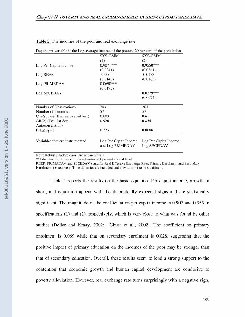
Chapter II: POVERTY AND REAL EXCHANGE RATE: EVIDENCE FROM PANEL DATA
109
Table 2: The incomes of the poor and real exchange rate Dependent variable is the Log average income of the poorest 20 per cent of the population
SYS-GMM SYS-GMM (1) (2)
Log Per Capita Income 0.9071*** (0.0341)
0.9550*** (0.0361)
Log REER -0.0065 (0.0148)
-0.0133 (0.0165)
Log PRIMEDAV 0.0690*** (0.0172)
Log SECEDAV 0.0279*** (0.0074)
Number of Observations 203 203 Number of Countries 57 57 Chi-Square( Hansen over-id test) 0.603 0.61 AR(2) (Test for Serial Autocorrelation)
0.920 0.854
P(H0: 10 =δ ) 0.223 0.0086
Variables that are instrumented Log Per Capita Income
and Log PRIMEDAV Log Per Capita Income, Log SECEDAV
Note: Robust standard errors are in parenthesis *** denotes significance of the estimates at 1 percent critical level REER, PRIMADAV and SECEDAV stand for Real Effective Exchange Rate, Primary Enrolment and Secondary Enrolment, respectively. Time dummies are included and they turn not to be significant.
Table 2 reports the results on the basic equation. Per capita income, growth in
short, and education appear with the theoretically expected signs and are statistically
significant. The magnitude of the coefficient on per capita income is 0.907 and 0.955 in
specifications (1) and (2), respectively, which is very close to what was found by other
studies (Dollar and Kraay, 2002; Ghura et al., 2002). The coefficient on primary
enrolment is 0.069 while that on secondary enrolment is 0.028, suggesting that the
positive impact of primary education on the incomes of the poor may be stronger than
that of secondary education. Overall, these results seem to lend a strong support to the
contention that economic growth and human capital development are conducive to
poverty alleviation. However, real exchange rate turns surprisingly with a negative sign,
tel-0
0116
961,
ver
sion
1 -
29 N
ov 2
006
Chapter II: POVERTY AND REAL EXCHANGE RATE: EVIDENCE FROM PANEL DATA
110
albeit statistically insignificant in all the specifications. The insignificance of real
exchange rate may be due to two reasons. First, the channels through which real
exchange rate influences poverty might have not been properly captured. More
specifically, as indicated in the theoretical framework, the level of inequality and the
quality of institutions may determine the extent to which real exchange rate influences
poverty. Second, regressions based on the basic equation might have left out other
important variables. If those variables happen to be correlated with other right-hand-side
variables, the estimates may turn biased. It is therefore important to expand the
specification to account for other key factors.
6.2.2 The results of the estimation of the core model
The next move is to estimate the core specification of our model, which includes
as main right-hand-side variables average income, a human capital indicator, real
exchange rate and the interactions between real exchange rate and the quality of
institutions and between real exchange rate and inequality. To check the robustness of the
econometric results, we use three measures of political institutions: democratic
institutions index, DEMO, civil liberties index, ICL, and political rights index, IPR, in
columns (4), (5) and (6), respectively.
tel-0
0116
961,
ver
sion
1 -
29 N
ov 2
006
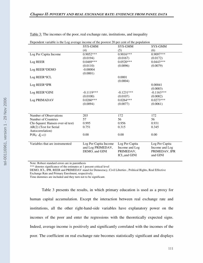
Chapter II: POVERTY AND REAL EXCHANGE RATE: EVIDENCE FROM PANEL DATA
111
Table 3: The incomes of the poor, real exchange rate, institutions, and inequality Dependent variable is the Log average income of the poorest 20 per cent of the population
SYS-GMM SYS-GMM SYS-GMM (4) (5) (6)
Log Per Capita Income 0.9052*** (0.0194)
0.9016*** (0.0167)
0.9097*** (0.0172)
Log REER 0.0469*** (0.0110)
0.0520*** (0.0096)
0.0443*** (0.0079)
Log REER*DEMO -0.00004 (0.0001)
Log REER*ICL 0.0001 (0.0004)
Log REER*IPR 0.00041 (0.0003)
Log REER*GINI -0.1119*** (0.0100)
-0.1231*** (0.0107)
-0.1163*** (0.0082)
Log PRIMADAV 0.0260*** (0.0094)
0.0264*** (0.0077)
0.0273*** (0.0061)
Number of Observations 203 172 172 Number of Countries 57 56 56 Chi-Square( Hansen over-id test) 0.995 0.956 0.931 AR(2) (Test for Serial Autocorrelation)
0.751 0.315 0.345
P(H0: 10 =δ ) 0.00 0.00 0.00
Variables that are instrumented Log Per Capita Income and Log PRIMEDAV, DEMO, and GINI
Log Per Capita Income and Log PRIMEDAV, ICL,and GINI
Log Per Capita Income and Log PRIMEDAV, IPR and GINI
Note: Robust standard errors are in parenthesis *** denotes significance of the estimates at 1 percent critical level DEMO, ICL, IPR, REER and PRIMEDAV stand for Democracy, Civil Liberties , Political Rights, Real Effective Exchange Rate and Primary Enrolment, respectively. Time dummies are included and they turn not to be significant.
Table 3 presents the results, in which primary education is used as a proxy for
human capital accumulation. Except the interaction between real exchange rate and
institutions, all the other right-hand-side variables have explanatory power on the
incomes of the poor and enter the regressions with the theoretically expected signs.
Indeed, average income is positively and significantly correlated with the incomes of the
poor. The coefficient on real exchange rate becomes statistically significant and displays
tel-0
0116
961,
ver
sion
1 -
29 N
ov 2
006
Chapter II: POVERTY AND REAL EXCHANGE RATE: EVIDENCE FROM PANEL DATA
112
a positive sign, which indicates that real depreciation in exchange rate is potentially
beneficial to the poor. More importantly, the interaction between real exchange rate and
the Gini coefficient turns to be significantly negative, meaning that inequality has the
potential to reduce the positive contribution of real exchange rate depreciation to poverty
alleviation. However, the interaction between real exchange rate and all the indicators
measuring institutions turns not to exert a statistically significant influence on poverty.
This finding does not necessary imply that the quality of institutions does not matter. It
could suggest that measures based on political institutions might not be entirely
appropriate in gauging the quality of institutions. In line with previous findings, we find
primary enrolment to have a positive and significant effect on the incomes of the poor.
tel-0
0116
961,
ver
sion
1 -
29 N
ov 2
006
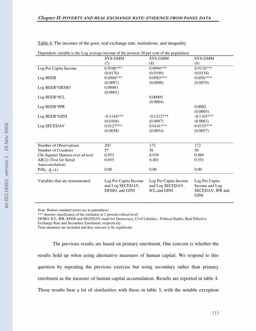
Chapter II: POVERTY AND REAL EXCHANGE RATE: EVIDENCE FROM PANEL DATA
113
Table 4: The incomes of the poor, real exchange rate, institutions, and inequality Dependent variable is the Log average income of the poorest 20 per cent of the population
SYS-GMM SYS-GMM SYS-GMM (7) (8) (9)
Log Per Capita Income 0.9106*** (0.0176)
0.8994*** (0.0199)
0.9116*** (0.0154)
Log REER 0.0504*** (0.0097)
0.0583*** (0.0098)
0.0501*** (0.0079)
Log REER*DEMO 0.00001 (0.0001)
Log REER*ICL 0.00005 (0.0004)
Log REER*IPR 0.0002 (0.0003)
Log REER*GINI -0.1144*** (0.0104)
-0.1212*** (0.0097)
-0.1165*** (0.0063)
Log SECEDAV 0.0127*** (0.0038)
0.0141*** (0.0054)
0.0155*** (0.0057)
Number of Observations 203 172 172 Number of Countries 57 56 56 Chi-Square( Hansen over-id test) 0.933 0.939 0.989 AR(2) (Test for Serial Autocorrelation)
0.655 0.401 0.551
P(H0: 10 =δ ) 0.00 0.00 0.00
Variables that are instrumented Log Per Capita Income
and Log SECEDAV, DEMO, and GINI
Log Per Capita Income and Log SECEDAV, ICL,and GINI
Log Per Capita Income and Log SECEDAV, IPR and GINI
Note: Robust standard errors are in parenthesis *** denotes significance of the estimates at 1 percent critical level DEMO, ICL, IPR, REER and SECEDAV stand for Democracy, Civil Liberties , Political Rights, Real Effective Exchange Rate and Secondary Enrolment, respectively. Time dummies are included and they turn not to be significant.
The previous results are based on primary enrolment. One concern is whether the
results hold up when using alternative measures of human capital. We respond to this
question by repeating the previous exercise but using secondary rather than primary
enrolment as the measure of human capital accumulation. Results are reported in table 4.
Those results bear a lot of similarities with those in table 3, with the notable exception
tel-0
0116
961,
ver
sion
1 -
29 N
ov 2
006
Chapter II: POVERTY AND REAL EXCHANGE RATE: EVIDENCE FROM PANEL DATA
114
that the coefficient on secondary enrolment is significantly lower than that on primary
education. In any event, these results are preliminary because there are some structural
and policy variables that have not yet been accounted for.
6.2.3 Additional controls
The second concern that has consistently been raised in the chapter is the issue of
omitted variables. We therefore consider in tables 5 and 6 potential controls that might
have been left out in our core specification. These controls include trade openness,
agricultural productivity, public spending variables, three variables that are frequently
used as right-side-variables in the regressions on poverty. Accounting for the labour
productivity in agricultural sector, AGRPRODAV, is a way to capture the impact of a
sectoral distribution of growth on poverty. The poor are likely to live in rural areas and
derive their livehood from the agriculture sector. As a result, they stand to benefit more
than the rest of the population from a strong performance of that sector. The economic
literature is replete with examples of countries where a vibrant productivity in
agricultural sector is associated with better outcomes for the poor (Ravallion and Datt,
1996). The idea of considering an indicator of openness in the empirical investigation is
justified by the desire to take into account the burning issue of trade liberalization and
poverty. Following Ghura et al. (2002), we use as indictor of openness the residuals of
trade volumes purged of the geographical determinants, OPENADJAV51. Both openness
and productivity in agriculture appear not to have statistically significant effects on
51 The trade openness indicator is a residual, which implies that its standard error is biased. We use bootstrap method to obtain an unbaiased estimate of the standard error but the results turn to be roughly identical.
tel-0
0116
961,
ver
sion
1 -
29 N
ov 2
006
Chapter II: POVERTY AND REAL EXCHANGE RATE: EVIDENCE FROM PANEL DATA
115
poverty. The purpose of adding an indicator for public spending is to include in the
empirical analysis the second main policy variable of the dependent economy model: the
absorption. In this regard, the government expenditure to GDP ratio appears to be an
ideal candidate.
Results from table 5 and 6 clearly reinforce the previous findings. All additional
controls turn to be statistically insignificant, expect in column 10 of table 5 where the
coefficient on openness turns to be positive and significant. The lack of a statistically
significant effect of openness, agricultural productivity and public spending on the
incomes of the poor does not imply that these factors are irrelevant for poverty
alleviation. It rather suggests that those factors affect the poorest 20 per cent of the
society the same way as they impact the rest of the population. In other terms, it indicates
that the main channel through openness, agricultural productivity, and public spending
influence the poor is through their impact on the average income or the growth of per -
capita income
The coefficient on average income, which is the elasticity of the income of the
poorest 20 percent of the population with respect to average income, is statistically
significant and appears with the expected sign. Its magnitude varies from 0.9016 to
0.9246 and the test on growth-poverty elasticity indicates that its value is statistically
different to 1. The positive and significant coefficient on per capita income confirms
various studies findings (Foster and Szekely, 2001: Dollar and Kraay, 2002: Ghura et al.,
2002) that fostering economic growth is an important avenue for poverty reduction.
Putting this finding in the African context, one could affirm that the lacklustre economic
tel-0
0116
961,
ver
sion
1 -
29 N
ov 2
006
Chapter II: POVERTY AND REAL EXCHANGE RATE: EVIDENCE FROM PANEL DATA
116
growth in the continent has been the driving force behind the relatively poor performance
of the region in terms of poverty reduction in recent years.
Real exchange rate continues to display a statistically significant impact on
poverty. The same is also true for the interaction between real exchange rate and
inequality and the human capital development indicator. Both tables 5 and 6 show that
the interaction between income distribution, captured through Gini coefficient, and real
exchange rate appears with a negative coefficient, with significance obtained at the 1
percent level. Once again, this indicates that a skewed income distribution can undermine
the positive impact of an appropriate real exchange rate on the incomes of the poor. The
most important change that occurs when including additional controls is that the
coefficient on the interaction between real exchange rate and some of institution
variables, especially civil liberties and political rights indicators, turns significant and
appears with a positive sign. Even though entering the regression with the expected sign,
the interaction between real exchange rate and democracy index, DEMO, remains
statistically insignificant. Overall, the results on institution variables tend to support the
claim that the quality of institutions amplifies the positive impact of real exchange rate
depreciation on poverty alleviation. Turning to human capital indicators, we again find
both secondary and primary enrolments to be positively related to the income of the
poorest fifth of the population in all specifications.
tel-0
0116
961,
ver
sion
1 -
29 N
ov 2
006
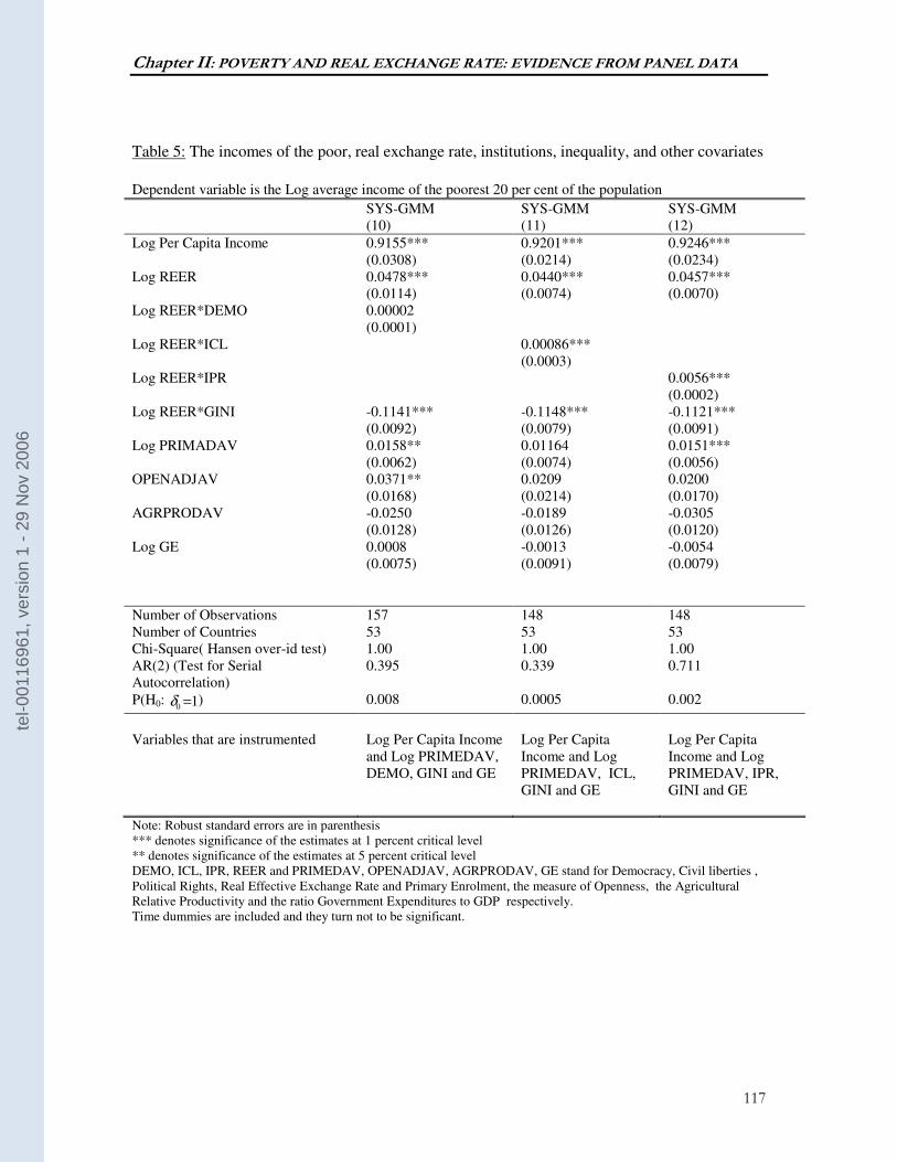
Chapter II: POVERTY AND REAL EXCHANGE RATE: EVIDENCE FROM PANEL DATA
117
Table 5: The incomes of the poor, real exchange rate, institutions, inequality, and other covariates
Dependent variable is the Log average income of the poorest 20 per cent of the population
SYS-GMM SYS-GMM SYS-GMM (10) (11) (12)
Log Per Capita Income 0.9155*** (0.0308)
0.9201*** (0.0214)
0.9246*** (0.0234)
Log REER 0.0478*** (0.0114)
0.0440*** (0.0074)
0.0457*** (0.0070)
Log REER*DEMO 0.00002 (0.0001)
Log REER*ICL 0.00086*** (0.0003)
Log REER*IPR 0.0056*** (0.0002)
Log REER*GINI -0.1141*** (0.0092)
-0.1148*** (0.0079)
-0.1121*** (0.0091)
Log PRIMADAV 0.0158** (0.0062)
0.01164 (0.0074)
0.0151*** (0.0056)
OPENADJAV 0.0371** (0.0168)
0.0209 (0.0214)
0.0200 (0.0170)
AGRPRODAV -0.0250 (0.0128)
-0.0189 (0.0126)
-0.0305 (0.0120)
Log GE 0.0008 (0.0075)
-0.0013 (0.0091)
-0.0054 (0.0079)
Number of Observations 157 148 148 Number of Countries 53 53 53 Chi-Square( Hansen over-id test) 1.00 1.00 1.00 AR(2) (Test for Serial Autocorrelation)
0.395 0.339 0.711
P(H0: 10 =δ ) 0.008 0.0005 0.002
Variables that are instrumented Log Per Capita Income
and Log PRIMEDAV, DEMO, GINI and GE
Log Per Capita Income and Log PRIMEDAV, ICL, GINI and GE
Log Per Capita Income and Log PRIMEDAV, IPR, GINI and GE
Note: Robust standard errors are in parenthesis *** denotes significance of the estimates at 1 percent critical level ** denotes significance of the estimates at 5 percent critical level DEMO, ICL, IPR, REER and PRIMEDAV, OPENADJAV, AGRPRODAV, GE stand for Democracy, Civil liberties , Political Rights, Real Effective Exchange Rate and Primary Enrolment, the measure of Openness, the Agricultural Relative Productivity and the ratio Government Expenditures to GDP respectively. Time dummies are included and they turn not to be significant.
tel-0
0116
961,
ver
sion
1 -
29 N
ov 2
006
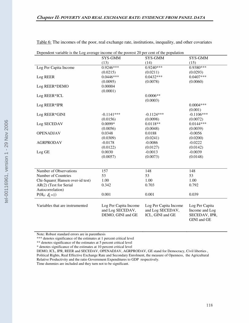
Chapter II: POVERTY AND REAL EXCHANGE RATE: EVIDENCE FROM PANEL DATA
118
Table 6: The incomes of the poor, real exchange rate, institutions, inequality, and other covariates
Dependent variable is the Log average income of the poorest 20 per cent of the population
SYS-GMM SYS-GMM SYS-GMM (13) (14) (15)
Log Per Capita Income 0.9246*** (0.0215)
0.9240*** (0.0211)
0.9380*** (0.0293)
Log REER 0.0446*** (0.0095)
0.0432*** (0.0078)
0.0407*** (0.0060)
Log REER*DEMO 0.00004 (0.0001)
Log REER*ICL 0.0006** (0.0003)
Log REER*IPR 0.0004*** (0.001)
Log REER*GINI -0.1141*** (0.0156)
-0.1124*** (0.0098)
-0.1106*** (0.0072)
Log SECEDAV 0.0099* (0.0056)
0.0118** (0.0048)
0.0144*** (0.0039)
OPENADJAV 0.0348 (0.0309)
0.0188 (0.0241)
-0.0056 (0.0200)
AGRPRODAV -0.0178 (0.0122)
-0.0086 (0.0127)
-0.0222 (0.0142)
Log GE 0.0030 (0.0057)
-0.0013 (0.0073)
-0.0039 (0.0148)
Number of Observations 157 148 148 Number of Countries 53 53 53 Chi-Square( Hansen over-id test) 1.00 1.00 1.00 AR(2) (Test for Serial Autocorrelation)
0.342 0.703 0.792
P(H0: 10 =δ ) 0.001 0.001 0.039
Variables that are instrumented Log Per Capita Income
and Log SECEDAV, DEMO, GINI and GE
Log Per Capita Income and Log SECEDAV, ICL, GINI and GE
Log Per Capita Income and Log SECEDAV, IPR, GINI and GE
Note: Robust standard errors are in parenthesis *** denotes significance of the estimates at 1 percent critical level ** denotes significance of the estimates at 5 percent critical level * denotes significance of the estimates at 10 percent critical level DEMO, ICL, IPR, REER and SECEDAV, OPENADJAV, AGRPRODAV, GE stand for Democracy, Civil liberties , Political Rights, Real Effective Exchange Rate and Secondary Enrolment, the measure of Openness, the Agricultural Relative Productivity and the ratio Government Expenditures to GDP respectively. Time dummies are included and they turn not to be significant.
tel-0
0116
961,
ver
sion
1 -
29 N
ov 2
006
Chapter II: POVERTY AND REAL EXCHANGE RATE: EVIDENCE FROM PANEL DATA
119
6.2.4 Asymmetric effects
One of the concerns about the results in tables 5 and 6 is whether the real
exchange-poverty correlation is either driven by episodes of real exchange rate
depreciation and decline in poverty or episodes of real exchange appreciation and
increasing poverty. We address this concern by extending the analysis so as to account
for potential asymmetric effects of real exchange rate on poverty. Following Agénor
(2002), we introduce two dummy variables. The first is labelled PASY and is equal to 1
times REER when there is depreciation in real exchange rate and 0 otherwise. The second
is called NASY, which gets the value 1 times REER when there is real appreciation in
exchange rate and 0 otherwise.
tel-0
0116
961,
ver
sion
1 -
29 N
ov 2
006
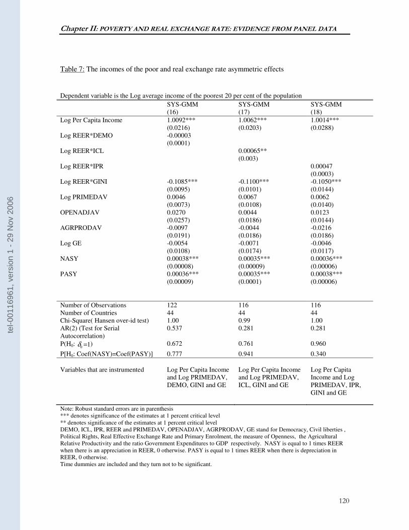
Chapter II: POVERTY AND REAL EXCHANGE RATE: EVIDENCE FROM PANEL DATA
120
Table 7: The incomes of the poor and real exchange rate asymmetric effects
Dependent variable is the Log average income of the poorest 20 per cent of the population
SYS-GMM SYS-GMM SYS-GMM (16) (17) (18)
Log Per Capita Income 1.0092*** (0.0216)
1.0062*** (0.0203)
1.0014*** (0.0288)
Log REER*DEMO -0.00003 (0.0001)
Log REER*ICL 0.00065** (0.003)
Log REER*IPR 0.00047 (0.0003)
Log REER*GINI -0.1085*** (0.0095)
-0.1100*** (0.0101)
-0.1050*** (0.0144)
Log PRIMEDAV 0.0046 (0.0073)
0.0067 (0.0108)
0.0062 (0.0140)
OPENADJAV 0.0270 (0.0257)
0.0044 (0.0186)
0.0123 (0.0144)
AGRPRODAV -0.0097 (0.0191)
-0.0044 (0.0186)
-0.0216 (0.0186)
Log GE -0.0054 (0.0108)
-0.0071 (0.0174)
-0.0046 (0.0117)
NASY 0.00038*** (0.00008)
0.00035*** (0.00009)
0.00036*** (0.00006)
PASY 0.00036*** (0.00009)
0.00035*** (0.0001)
0.00038*** (0.00006)
Number of Observations 122 116 116 Number of Countries 44 44 44 Chi-Square( Hansen over-id test) 1.00 0.99 1.00 AR(2) (Test for Serial Autocorrelation)
0.537 0.281 0.281
P(H0: 10 =δ ) 0.672 0.761 0.960
P[H0: Coef(NASY)=Coef(PASY)] 0.777 0.941 0.340
Variables that are instrumented Log Per Capita Income
and Log PRIMEDAV, DEMO, GINI and GE
Log Per Capita Income and Log PRIMEDAV, ICL, GINI and GE
Log Per Capita Income and Log PRIMEDAV, IPR, GINI and GE
Note: Robust standard errors are in parenthesis *** denotes significance of the estimates at 1 percent critical level ** denotes significance of the estimates at 1 percent critical level DEMO, ICL, IPR, REER and PRIMEDAV, OPENADJAV, AGRPRODAV, GE stand for Democracy, Civil liberties , Political Rights, Real Effective Exchange Rate and Primary Enrolment, the measure of Openness, the Agricultural Relative Productivity and the ratio Government Expenditures to GDP respectively. NASY is equal to 1 times REER when there is an appreciation in REER, 0 otherwise. PASY is equal to 1 times REER when there is depreciation in REER, 0 otherwise. Time dummies are included and they turn not to be significant.
tel-0
0116
961,
ver
sion
1 -
29 N
ov 2
006
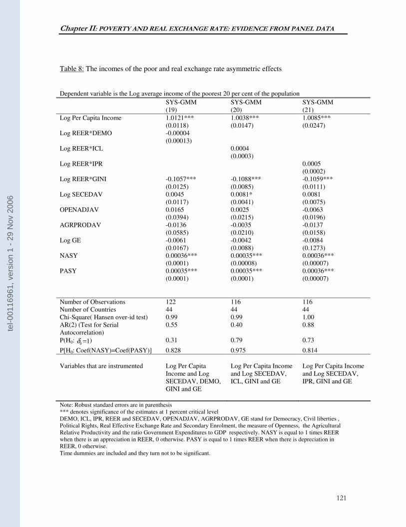
Chapter II: POVERTY AND REAL EXCHANGE RATE: EVIDENCE FROM PANEL DATA
121
Table 8: The incomes of the poor and real exchange rate asymmetric effects
Dependent variable is the Log average income of the poorest 20 per cent of the population
SYS-GMM SYS-GMM SYS-GMM (19) (20) (21)
Log Per Capita Income 1.0121*** (0.0118)
1.0038*** (0.0147)
1.0085*** (0.0247)
Log REER*DEMO -0.00004 (0.00013)
Log REER*ICL 0.0004 (0.0003)
Log REER*IPR 0.0005 (0.0002)
Log REER*GINI -0.1057*** (0.0125)
-0.1088*** (0.0085)
-0.1059*** (0.0111)
Log SECEDAV 0.0045 (0.0117)
0.0081* (0.0041)
0.0081 (0.0075)
OPENADJAV 0.0165 (0.0394)
0.0025 (0.0215)
-0.0063 (0.0196)
AGRPRODAV -0.0136 (0.0585)
-0.0035 (0.0210)
-0.0137 (0.0158)
Log GE -0.0061 (0.0167)
-0.0042 (0.0088)
-0.0084 (0.1273)
NASY 0.00036*** (0.0001)
0.00035*** (0.00008)
0.00036*** (0.00007)
PASY 0.00035*** (0.0001)
0.00035*** (0.0001)
0.00036*** (0.00007)
Number of Observations 122 116 116 Number of Countries 44 44 44 Chi-Square( Hansen over-id test) 0.99 0.99 1.00 AR(2) (Test for Serial Autocorrelation)
0.55 0.40 0.88
P(H0: 10 =δ ) 0.31 0.79 0.73
P[H0: Coef(NASY)=Coef(PASY)] 0.828 0.975 0.814
Variables that are instrumented Log Per Capita
Income and Log SECEDAV, DEMO, GINI and GE
Log Per Capita Income and Log SECEDAV, ICL, GINI and GE
Log Per Capita Income and Log SECEDAV, IPR, GINI and GE
Note: Robust standard errors are in parenthesis *** denotes significance of the estimates at 1 percent critical level DEMO, ICL, IPR, REER and SECEDAV, OPENADJAV, AGRPRODAV, GE stand for Democracy, Civil liberties , Political Rights, Real Effective Exchange Rate and Secondary Enrolment, the measure of Openness, the Agricultural Relative Productivity and the ratio Government Expenditures to GDP respectively. NASY is equal to 1 times REER when there is an appreciation in REER, 0 otherwise. PASY is equal to 1 times REER when there is depreciation in REER, 0 otherwise. Time dummies are included and they turn not to be significant.
tel-0
0116
961,
ver
sion
1 -
29 N
ov 2
006
Chapter II: POVERTY AND REAL EXCHANGE RATE: EVIDENCE FROM PANEL DATA
122
Table 7 reports the results wherein primary enrolment is used as the measure of
human capital development whereas Table 8 contains the results of estimates that revert
to secondary enrolment as the measure of education. The results in both tables tilt
towards the same conclusions. The more important one is that the coefficients on PASY
and NASY are significant and statistically indistinguishable, which implies that there is no
asymmetric effect of real exchange rate on the incomes of the poor. As far as the other
explanatory variables are concerned, results largely confirm previous findings.
Especially, per capita income, or economic growth, continues to be strongly correlated
with poverty as suggested by significant higher poverty-growth elasticity, which in both
tables is not statistically different to 1. The coefficient on the interaction between
inequality and real exchange rate also remains statistically significant while those on
openness, agricultural productivity and government expenditure are insignificant at
conventional significance levels.
VII- CONCLUSION
Facing both external and internal imbalances, several developing countries have
implemented some economic reforms over the past two decades. The dependent economy
model shows that these policies have two pillars: the reduction of absorption, obtained to
a large degree through fiscal adjustment, and the depreciation of real exchange rate. The
approach used in this chapter consists in assessing the impact of economic policies on
poverty through these two instruments, with more emphasis on real exchange rate.
tel-0
0116
961,
ver
sion
1 -
29 N
ov 2
006
Chapter II: POVERTY AND REAL EXCHANGE RATE: EVIDENCE FROM PANEL DATA
123
The main point in the theoretical framework is that the depreciation of real
exchange rate is conducive to poverty reduction provided that there are good institutions
and a fairly equal distribution of income. The empirical investigation strongly supports
the view that high inequality, proxied by income distribution, impedes the potential
positive effect of real exchange rate depreciation on poverty. It also largely backs the
contention that the potential positive impact of real exchange rate depreciation on the
poor is much stronger when institutions are sound.
Some additional controls are added in the analysis to account for other factors that
might have been missed in the analysis. Education appears to be critical for poverty
reduction. On the other hand, trade openness, agricultural productivity and public
spending are found not to be statistically associated with the incomes of the poor. The
lack of significant coefficients associated with these variables does not mean a complete
absence of relationships between these indicators and poverty but rather indicates that
trade openness, agricultural productivity and public spending come into play indirectly
because of their potential impact on economic growth.
Overall, the main policy implication of our findings is that real exchange
depreciation could be a powerful tool for poverty reduction if complemented by other
policies. Those policies include facilitating the access of the poor to production factors
and improving the quality of institutions.
The improvement of institutions, especially political, may have an important
bearing on the design of economic policies. In view of the major political reforms that
took place in many African countries, it will be worth exploring the implications of such
tel-0
0116
961,
ver
sion
1 -
29 N
ov 2
006
Chapter II: POVERTY AND REAL EXCHANGE RATE: EVIDENCE FROM PANEL DATA
124
changes on economic policy stances in the continent. This is, in part, what Chapter III is
going to pursue.
tel-0
0116
961,
ver
sion
1 -
29 N
ov 2
006
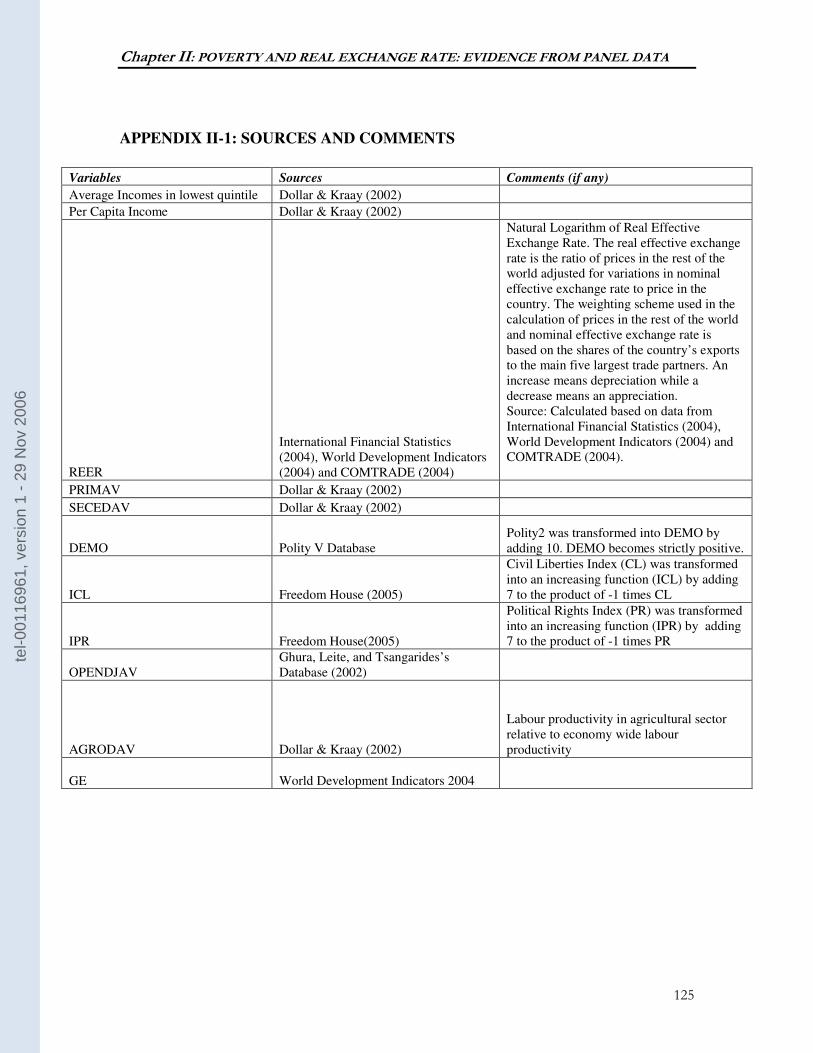
Chapter II: POVERTY AND REAL EXCHANGE RATE: EVIDENCE FROM PANEL DATA
125
APPENDIX II-1: SOURCES AND COMMENTS
Variables Sources Comments (if any)
Average Incomes in lowest quintile Dollar & Kraay (2002)
Per Capita Income Dollar & Kraay (2002)
REER
International Financial Statistics (2004), World Development Indicators (2004) and COMTRADE (2004)
Natural Logarithm of Real Effective Exchange Rate. The real effective exchange rate is the ratio of prices in the rest of the world adjusted for variations in nominal effective exchange rate to price in the country. The weighting scheme used in the calculation of prices in the rest of the world and nominal effective exchange rate is based on the shares of the country’s exports to the main five largest trade partners. An increase means depreciation while a decrease means an appreciation. Source: Calculated based on data from International Financial Statistics (2004), World Development Indicators (2004) and COMTRADE (2004).
PRIMAV Dollar & Kraay (2002)
SECEDAV Dollar & Kraay (2002)
DEMO Polity V Database Polity2 was transformed into DEMO by adding 10. DEMO becomes strictly positive.
ICL Freedom House (2005)
Civil Liberties Index (CL) was transformed into an increasing function (ICL) by adding 7 to the product of -1 times CL
IPR Freedom House(2005)
Political Rights Index (PR) was transformed into an increasing function (IPR) by adding 7 to the product of -1 times PR
OPENDJAV Ghura, Leite, and Tsangarides’s Database (2002)
AGRODAV Dollar & Kraay (2002)
Labour productivity in agricultural sector relative to economy wide labour productivity
GE World Development Indicators 2004
tel-0
0116
961,
ver
sion
1 -
29 N
ov 2
006
Chapter II: POVERTY AND REAL EXCHANGE RATE: EVIDENCE FROM PANEL DATA
126
tel-0
0116
961,
ver
sion
1 -
29 N
ov 2
006
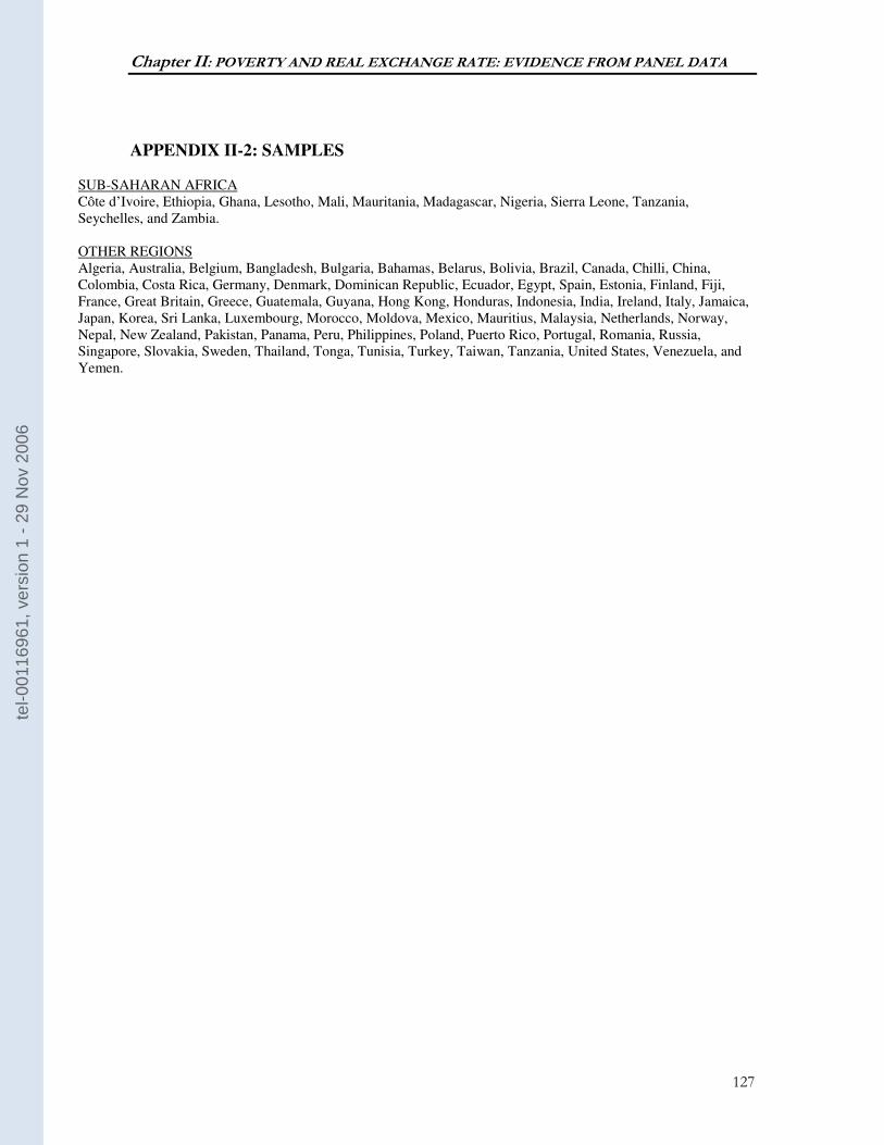
Chapter II: POVERTY AND REAL EXCHANGE RATE: EVIDENCE FROM PANEL DATA
127
APPENDIX II-2: SAMPLES
SUB-SAHARAN AFRICA Côte d’Ivoire, Ethiopia, Ghana, Lesotho, Mali, Mauritania, Madagascar, Nigeria, Sierra Leone, Tanzania, Seychelles, and Zambia. OTHER REGIONS Algeria, Australia, Belgium, Bangladesh, Bulgaria, Bahamas, Belarus, Bolivia, Brazil, Canada, Chilli, China, Colombia, Costa Rica, Germany, Denmark, Dominican Republic, Ecuador, Egypt, Spain, Estonia, Finland, Fiji, France, Great Britain, Greece, Guatemala, Guyana, Hong Kong, Honduras, Indonesia, India, Ireland, Italy, Jamaica, Japan, Korea, Sri Lanka, Luxembourg, Morocco, Moldova, Mexico, Mauritius, Malaysia, Netherlands, Norway, Nepal, New Zealand, Pakistan, Panama, Peru, Philippines, Poland, Puerto Rico, Portugal, Romania, Russia, Singapore, Slovakia, Sweden, Thailand, Tonga, Tunisia, Turkey, Taiwan, Tanzania, United States, Venezuela, and Yemen.
tel-0
0116
961,
ver
sion
1 -
29 N
ov 2
006
Chapter II: POVERTY AND REAL EXCHANGE RATE: EVIDENCE FROM PANEL DATA
128
APPENDIX II-3 : DEFINITION ET INDICATEURS DE PAUVRETE
La pauvreté est l’état dans lequel le bien-être d’une personne ou d’un groupe de
personnes est en deçà du niveau perçu comme étant le minimum raisonnable selon les critères
d’une société donnée (Ravallion, 1995). Cette définition soulève trois questions. La première
porte sur la façon dont on évalue le « bien-être » ou précisément les concepts ou les approches qui
permettent de saisir le « bien-être ». La seconde a trait à l’identification du seuil à partir duquel
une personne est considérée comme étant pauvre. La troisième concerne la façon dont il faut
synthétiser les informations en un indicateur agrégé de pauvreté. La première question soulevée
relève de l’identification des approches permettant de capter le bien-être, et sera traitée dans la
première section de cette annexe. Les deux dernières questions touchent à l’élaboration des
indicateurs de pauvreté et seront analysées dans la deuxième section.
I. APPROCHES
De nombreuses méthodes conceptuelles existent pour mesurer le bien-être d’un individu.
Ces méthodes diffèrent non seulement selon le nombre de facteurs retenus pour évaluer le bien-
être mais aussi selon l’importance qu’attache l’analyste à la manière dont l’individu juge lui-
même son bien-être.
1.1 Approche matérielle et non-matérielle
Certaines méthodes ne captent que le côté matériel autrement dit « le bien-être
économique », et ainsi définissent la pauvreté comme étant la rareté de ressources et de biens
(Bey, 1999), entravant la satisfaction de besoins essentiels comme la nutrition, l’habillement, et le
logement. Cette définition met en lumière deux aspects importants de la pauvreté « matérielle »,
à savoir le faible revenu et la non-satisfaction des nécessités de base. La prise en compte de la
deuxième dimension, c’est-à-dire les besoins fondamentaux, répond aux interrogations soulevées
sur la pertinence de l’approche en termes de revenu dans l’évaluation de la pauvreté. Au nombre
tel-0
0116
961,
ver
sion
1 -
29 N
ov 2
006
Chapter II: POVERTY AND REAL EXCHANGE RATE: EVIDENCE FROM PANEL DATA
129
des limites d’une telle approche figurent la difficulté à évaluer les revenus non-monétaires
(autoconsommation en particulier) dans les pays pauvres, la difficulté à mesurer les flux
d’entraide, et la non-prise en compte des externalités générées par l’Etat, à travers la fourniture de
biens publics, et les industries, par le truchement de leurs effets sur l’environnement. Bref, les
approches fondées exclusivement sur le revenu n’accordent pas d’importance aux biens qui ne
passent pas par le marché et qui ont un impact sur le niveau de vie des individus, et contribuent
ainsi à biaiser vers le haut ou le bas le niveau de pauvreté. Pour cette raison, elles sont complétées
par d’autres concepts qui mettent en exergue la satisfaction de nécessités de base.
Les besoins fondamentaux recouvrent non seulement ce qui est requis à un ménage au
titre de sa consommation individuelle (alimentation, logement, habillement) mais également ce
dont la collectivité ne peut se passer (approvisionnement en eau potable, services d’éducation, de
santé et d’hygiène) (Destremau et Salama, 2002). Ces besoins fondamentaux ont la particularité
d’être considérés comme universels et identiques, c’est-à-dire indépendants des cultures et
civilisations, du temps et de l’espace. Cependant, ils constituent des besoins physiques et
psychiques qui peuvent être satisfaits selon des modalités économiques extrêmement variées. Une
autre particularité des besoins fondamentaux est qu’elle possède deux attributs. Le premier est
qu’ils peuvent être quantifiables ou mesurables. Le second attribut est que leur satisfaction est
productive en ce qu’elle rehausse le niveau de productivité des hommes.
L’approche des besoins fondamentaux tire ses fondements d’une vision humaniste qui va
au-delà de l’économie et qui met l’accent sur la morale et le développement de l’Homme sur tous
les angles. Elle a connu un grand écho à partir des années 1950. Pour des fins descriptives et
normatives, l’approche se ramena à celle de minimum vital. Certains comme François Perroux
(1952) parlait de « coûts de l’homme » qui englobent la nourriture, la santé, et l’éducation.
L’approche des besoins fondamentaux attira davantage l’attention de la communauté
internationale à partir de la moitié des années 1970 avec la Conférence mondiale tripartite sur
l’emploi, la répartition du revenu, le progrès social, et la division internationale du travail. Suite à
cette conférence, elle devient l’épine dorsale d’un nouveau type de stratégies pour la promotion
du développement dans le Tiers Monde.
La rareté de ressources et d’actifs compromet la possibilité de se couvrir contre le risque,
donc le concept de pauvreté recouvre également la notion de vulnérabilité face aux chocs. La
notion de vulnérabilité a la même signification que celle exposée par Guillaumont et Combes
(2000), à savoir le risque pour les pauvres d’être défavorablement touchés par des chocs exogènes
tel-0
0116
961,
ver
sion
1 -
29 N
ov 2
006
Chapter II: POVERTY AND REAL EXCHANGE RATE: EVIDENCE FROM PANEL DATA
130
sur lesquels ils n’ont pas un contrôle direct. Il est possible de distinguer trois éléments de la
vulnérabilité : l’importance du choc, le degré d’exposition aux chocs, et la résilience ou capacité à
réagir aux chocs (Combes et Guillaumont, 2002 ; Guillaumont, 1999).
Dercon (2001) analyse la relation entre pauvreté et vulnérabilité, et propose un schéma
conceptuel distinguant trois niveaux de risques. Le premier niveau de risques survient lorsque les
ménages dotés d’actifs comme le travail, le capital physique, le capital humain, et le capital social
s’engagent dans des activités génératrices de revenus. Ce type de risques peut être lié aux
contraintes d’information, et de fonctionnement des marchés et des autres institutions. Le
deuxième groupe de risques peut porter directement sur les actifs, entre autres les risques de
destruction imputables à l’environnement et aux conflits armés, et à l’érosion du capital humain.
Les risques liés aux actifs peuvent, également, découler du non-respect des droits de propriété. Le
troisième groupe de risques survient au cours du processus de passage des revenus vers
l’accroissement des capacités, et comporte des risques pouvant être liés aux politiques publiques
adoptées et à l’accès aux biens publics. En somme, cette typologie de risques montre que la
vulnérabilité est une dimension importante dans la dynamique de production et de création de
revenus et ainsi de la pauvreté matérielle, mais souligne également qu’elle peut en être la cause.
L’adoption de comportements réducteurs de risque peut être la source de moindres revenus et
donc limite les possibilités de réduction de la pauvreté.
D’autres, par contre, intègrent dans la définition de la pauvreté d’autres aspects plus
abstraits du bien-être, à savoir l’absence ou le manque de potentialités ou de capacités
(capabilities). Le manque ou l’absence de ces éléments entravent l’acquisition d’un capital
physique minimale requis pour s’épanouir dans une société donnée.
Le concept de capacités a été développé par Sen (1985a), qui se démarque des approches
axées sur les besoins fondamentaux et opte pour une démarche mettant l’accent sur la justice
sociale, l’équité, et les inégalités. Aussi, définit-il la pauvreté dans un cadre qui prend en compte
non seulement les facteurs économiques mais également les dimensions légales, politiques, et
sociales. La base de son analyse sur les capacités part d’une réflexion sur les famines. Celle-ci
l’amène à deux conclusions majeures. Premièrement, il rejette la possession de biens matériels, y
compris ceux jugés essentiels, comme élément permettant d’apprécier le bien-être des personnes.
Deuxièmement, il met en cause les approches agrégées pour cerner la problématique des famines,
des inégalités et de la pauvreté.
tel-0
0116
961,
ver
sion
1 -
29 N
ov 2
006
Chapter II: POVERTY AND REAL EXCHANGE RATE: EVIDENCE FROM PANEL DATA
131
En effet, Sen démontre que la disponibilité d’un bien à un endroit donné n’est que
faiblement corrélée (par l’autoproduction, la création d’emplois, le système des prix et la
constitution de réserves publiques) à l’aptitude qu’ont certains groupes d’y avoir accès.
Autrement dit, c’est l’incapacité à se procurer les biens et non la pénurie, qui explique les
famines. Cette incapacité découle de facteurs légaux, ou semi-légaux, et économiques.
Partant de ce constat, la pauvreté se définirait non pas comme un manque vis-à-vis des
besoins fondamentaux en divers biens, mais en termes de défaut de réalisation de certains
fonctionnements de base et de l’acquisition des capacités correspondantes. L’approche des
capacités est ainsi une approche qualitative qui embrasse à la fois l’avoir matériel mais porte
également une grande attention aux valeurs de réalisation et de liberté, les fonctionnements
représentant une façon de mener son existence, et les capacités incarnant les diverses opportunités
qui se présentent à une personne et parmi lesquelles elle opère un choix. Il découle que ni le
revenu, ni l’utilité ne peut capter le bien-être dans l’approche en termes de capacités. La pauvreté
ne peut pas être définie par rapport à la faiblesse du revenu et de l’utilité mais plutôt par rapport à
l'inadaptation des moyens économiques au regard de l’aptitude des individus à les transformer en
capacités de fonctionner, et ceci dans un contexte social, économique et culturel spécifique.
La combinaison de la rareté de ressources et d’opportunités limite le choix des pauvres et
leur capacité à être entendu et à contrôler les situations dont dépendent leur sort (powerless and
voiceless) (Narayan et al., 2000). Donc la pauvreté peut-être synonyme d’exclusion sociale, de
détresse psychologique, et de manque de choix et d’action.
1.2. Les approches « utilitariste » et « non utilitariste »
1.2.1 Exposé
L’approche utilitariste fonde les comparaisons du bien-être exclusivement sur les
préférences des individus et tire une grande partie de ses fondements théoriques de la théorie
microéconomique moderne. Au cœur de l’approche se trouve la notion de classement des
préférences pour les biens, qui peut être captée par une « fonction d’utilité ». La valeur de cette
dernière est supposée résumer le bien-être d’un individu. Les utilités constituent alors la base des
préférences sociales, y compris des comparaisons de la pauvreté. Des doutes sont émis quant à la
pertinence des jugements personnels de bien-être, et deux raisons sont couramment évoquées. La
première est que les individus peuvent être mal informés. La seconde repose sur le phénomène de
tel-0
0116
961,
ver
sion
1 -
29 N
ov 2
006
Chapter II: POVERTY AND REAL EXCHANGE RATE: EVIDENCE FROM PANEL DATA
132
« dissonance cognitive » (Akerlof, 1982) dans lequel les choix effectués par l’individu peuvent
s’avérer économiquement irrationnels même en présence d’information parfaite.
En supposant qu’il soit possible de comparer les utilités de différents individus (utilités
cardinales), des fonctions de bien-être social, qui ne sont que l’agrégation d’utilités individuelles,
peuvent être construites. Cependant, le concept de fonction de bien-être social est incompatible
avec la théorie purement ordinaliste des préférences en raison entre autres de la non-transitivité
des choix sociaux, et ne permet pas ainsi d’établir des comparaisons logiques de pauvreté ou de
former tout autre jugement pertinent sur le bien-être social.
En effet, en définissant les préférences sociales à partir des préférences individuelles et en
choisissant la règle de la majorité comme étant la base de définition d’une fonction de bien-être
social, le Paradoxe de Condorcet nous apprend que le concept de bien-être social ne révèle pas, de
façon cohérente, ce qui est préféré socialement. En effet, il est possible qu’une alternative A soit
préférée à une alternative B, que B soit préférée à C, mais par contre que C soit préférée à A,
violant ainsi le principe de transitivité des choix.
Le Théorème d’Impossibilité d’Arrow, qui est une version générale du paradoxe de
Condorcet, élimine la possibilité d’existence d’une fonction de bien-être social. Arrow établit un
certain nombre d’hypothèses sur ce que doit être une fonction de bien-être, et démontre qu’il
n’existe aucun mécanisme, permettant le passage des préférences individuelles aux préférences
sociales et qui ne violerait pas les hypothèses de départ. Une des hypothèses est l’absence de
dictature, qui suppose qu’une fonction de bien-être social ne se résume pas à la fonction d’utilité
d’une personne. Une autre hypothèse est l’indépendance des choix « independence of irrelevant
alternatives » qui postule que si une fonction de bien-être social amène à conclure qu’une
alternative A est préférée à une alternative B, tout changement de préférences qui n’affecte pas
l’ordre de préférence entre A et B établit par les individus ne modifie nullement les préférences
sociales pour A et B. Une autre hypothèse établit le principe de transitivité de la fonction de bien-
être social, à savoir que si A est préféré à B, et B préféré à C, alors A est préféré à C.
L’approche non utilitariste se distingue par la référence faite à certaines aptitudes
élémentaires à satisfaire ses besoins fondamentaux, comme la possibilité de se nourrir et de se
vêtir de manière adéquate. Sen (1980, 1985b, 1987) marque sa préférence pour l’approche non-
utilitaire en s’appuyant sur une argumentation différente, abandonnant à la fois l’utilité comme
étalon de mesure du bien-être et les formules non utilitaires axées sur les besoins. Sen (1987)
tel-0
0116
961,
ver
sion
1 -
29 N
ov 2
006
Chapter II: POVERTY AND REAL EXCHANGE RATE: EVIDENCE FROM PANEL DATA
133
rappelle que « la valeur du niveau de vie a tout à voir avec la vie, non pas avec la possession de
biens ». La pauvreté est ainsi perçue comme une privation de la faculté qu’ont les individus à
fonctionner. L’analyse de la pauvreté revient pour Sen à cerner ce que sont ces facultés dans des
sociétés spécifiques et à identifier les personnes qui ne peuvent pas les acquérir.
Par ailleurs, Sen, tout en admettant la pertinence d’une considération de l’efficacité,
propre aux utilitaristes, remet en cause les arguments en faveur d’un maintien des inégalités, et
conteste l’idée selon laquelle toute réduction des inégalités est antithétique à l’amélioration de
l’efficience d’une économie et au principe de maximisation des utilités.
La critique des modèles non utilitaires tient au fait que l’identification des formes
spécifiques de privation de biens ainsi que l’importance qui leur sont accordées relèvent du
champ de l’analyste, soulevant ainsi des critiques relatives au caractère arbitraire de l’approche.
1.2.2 Points communs et divergences
La théorie donne rarement des recommandations pratiques quant à la façon de mesurer
les niveaux de vie. Aussi, constate-t-on l’usage de nombreuses procédures d’estimation du bien-
être par chaque approche. Néanmoins, ce qui semble ressortir des deux approches est le choix
porté sur la consommation de biens et services comme facteur déterminant du bien-être.
L’approche utilitaire génère des indicateurs reposant sur les biens et services consommés
par un ménage et sur les caractéristiques dudit ménage ; ce qui restreint la notion « d’utilité » au
seul « bien-être économique » et amène à ignorer les autres aspects de l’utilité qui ne sont pas
quantifiables comme les biens non marchands et les éléments non matériels de la condition
humaine comme la liberté. L’indicateur qui découle de l’approche utilitariste est le total des
dépenses de consommation en biens et services, normalisé de sorte à prendre en compte les
différences de prix et les caractéristiques des ménages. Les approches non utilitaires et celles
fondées sur les facultés mettent en avant l’aptitude à se procurer des biens comme élément
explicatif du bien-être et retiennent aussi la consommation comme indicateur.
Quoiqu’ayant systématiquement recours aux données sur la consommation, l’usage qui
en est faite diffère d’une approche à une autre. Primo, les utilitaristes fondent leur analyse du
bien-être sur les dépenses totales tandis que les non-utilitaristes ne s’intéressent qu’à certains
types de privation de biens à l’instar du logement, de la nutrition ou de l’habillement. Secundo,
dans l’approche utilitaire les méthodes d’agrégation des biens et services consommés sont
clairement explicitées. Les prix du marché servent à évaluer les préférences. Par contre les
tel-0
0116
961,
ver
sion
1 -
29 N
ov 2
006
Chapter II: POVERTY AND REAL EXCHANGE RATE: EVIDENCE FROM PANEL DATA
134
approches non utilitaires ne donnent aucune indication sur la façon dont il faudrait agréger les
principaux déterminants du bien-être. Tierco, des divergences subsistent quant à l’estimation de la
valeur des services publics consommés et sur l’importance accordée aux caractéristiques de
l’individu qui, rappelons le, peuvent influencer les aptitudes des individus sans pour autant agir
sur les préférences.
II-INDICATEURS DE PAUVRETE
Deux catégories d’indicateurs seront présentées, celles reposant sur des mesures
monétaires et celles intégrant d’autres dimensions de la pauvreté autres que le revenu.
2.1 Les indicateurs de pauvreté monétaire
Le processus de construction d’indicateurs de pauvreté monétaire exige qu’on réponde à
trois questions : la première a trait au choix du type de données, la seconde porte sur le choix de
l’unité de référence et de la façon dont on tient compte de son hétérogénéité, et la troisième est
relative au seuil qui permet de définir qui est pauvre et qui ne l’est pas.
2.1.1 L’unité d’observation et l’ajustement pour les économies d’échelle
Les enquêtes budget-consommation prennent généralement le ménage comme unité de
référence et d’analyse. Ce dernier n’ayant pas toujours la même composition, il y a lieu de
prendre en compte la dimension taille du ménage dans la mesure du bien-être matériel. En effet,
une personne qui vit dans un ménage de cinq personnes ayant une consommation totale de 10 000
CFA par mois est manifestement moins nantie qu’une personne issue d’un ménage d’un individu
enregistrant une consommation totale de 10 000 CFA. Une façon d’intégrer la dimension taille
dans l’analyse peut consister à raisonner en termes de consommation par tête, ce qui peut paraître
simpliste pour deux raisons. Premièrement, certains types de biens peuvent être consommés par
tout le ménage d’où l’existence d’économies d’échelle. Deuxièmement, l’âge influe sur le niveau
de la consommation. On peut s’attendre à ce que la consommation d’un adolescent soit moins
importante que celle d’un adulte en activité. La notion d’échelle équivalente est généralement
utilisée et permet de capter tant la structure d’âge que la taille du ménage. La notion d’échelle
tel-0
0116
961,
ver
sion
1 -
29 N
ov 2
006
Chapter II: POVERTY AND REAL EXCHANGE RATE: EVIDENCE FROM PANEL DATA
135
équivalente se mesure à travers deux méthodes : une dite de deux paramètres et l’autre dit d’un
seul paramètre. Elles se formulent de la façon suivante :
Echelle équivalente = (adultes + α*enfants)θ
Echelle équivalente = (Taille du ménage)θ
Par enfants, on entend le nombre de personnes âgées de moins de 15 ans ; α et θ sont des
paramètres tels que : 0 ≤ α ≤ 1 et 0 ≤ θ ≤ 1 ; θ capte les économies d’échelle , plus il est élevé
plus les économies d’échelle sont importantes ; α saisit le poids de la consommation des enfants.
Cependant, il n’existe aucune technique d’estimation consensuelle de θ : l’ampleur des
économies d’échelle (Deaton, Paxon 1996, Deaton 1997). De nombreuses méthodes sont
utilisées, chacune ayant des limites. Les méthodes utilisées diffèrent selon les pays, posant du
coup un problème de comparabilité.
2.1.2 Choix du type de données
La mesure monétaire de la pauvreté requiert des données sur le revenu ou sur les
dépenses. La seconde alternative est préférée à la première pour trois raisons: i) pour des raisons
liées aux chocs intermittents, les revenus des ménages, dans bon nombre de pays en
développement, subissent une évolution erratique qui peut ne pas refléter rigoureusement celle de
la richesse des ménages; par contre la consommation fluctue moins en raison du fait qu’elle est
lissée dans le temps; ii) l’épargne est perçue comme une consommation différée et par conséquent
affecte les niveaux de bien-être ; iii) les données sur la consommation sont plus fiables que celles
sur le revenu parce que les ménages les divulguent plus facilement. En effet, les ménages ont
tendance à sous-estimer le niveau de leurs revenus par volonté d’échapper à la fiscalité ou pour
des raisons culturelles.
2.1.3 Seuils de pauvreté
Définir une personne comme étant pauvre suppose l’existence d’un repère, qui peut être
un seuil ou un indice, sur lequel repose le classement. Les seuils sont formulés le plus souvent
dans l’espace de la consommation, et deux concepts reviennent souvent : la notion de « pauvreté
relative » et celle de « pauvreté absolue ». Ravallion (1995) définit le seuil de pauvreté absolue
tel-0
0116
961,
ver
sion
1 -
29 N
ov 2
006
Chapter II: POVERTY AND REAL EXCHANGE RATE: EVIDENCE FROM PANEL DATA
136
comme étant « le seuil constant en termes de niveaux de vie, et unique sur l’ensemble du
domaine dans lequel les comparaisons de la pauvreté sont effectuées ». Un seuil de pauvreté
relative, par contre, consiste à choisir une fraction donnée des dépenses moyennes par habitant ou
par ménage comme repère.
La détermination du seuil de pauvreté absolue commence par la détermination du panier
de biens permettant d’obtenir l’énergie nutritive requise pour survivre. Cependant, force est de
reconnaître qu’il existe plusieurs paniers d’aliments pouvant assurer l’énergie nutritive
recherchée. L’efficience voudrait qu’on choisisse la combinaison d’aliments qui minimise le coût
du nombre de calories nécessaires à la survie, à des prix donnés, et qui répond aux habitudes
alimentaires d’une population donnée. Dès que ces biens sont identifiés, on leur trouve une
équivalence monétaire en utilisant un système de prix qui reflète la structure du panier de
consommation. Le montant ainsi trouvé est appelé la ligne d’indigence qu’on peut élargir au
ménage en appliquant des coefficients de réduction pour les membres de la famille au-delà ou en
deçà d’un certain âge. On parlera de pauvreté extrême pour qualifier les personnes (ou les
ménages) ayant des revenus en dessous de la ligne d’indigence.
Cependant, la relation entre la consommation d’énergie nutritive et des dépenses de
consommation diffère d’un secteur à un autre, d’une période à une autre, et d’une région à une
autre. Cette relation peut être tributaire des goûts, des prix relatifs, de l’existence de biens publics,
et de la richesse. Par exemple, les ménages les plus nantis auront tendance à acheter des calories
plus onéreuses. Pour toutes ces raisons, la méthode décrite ci-dessus dite de l’énergie nutritive
génère des seuils de pauvreté différents selon les sous-groupes, et ne permet pas ainsi d’établir un
profil de pauvreté cohérent.
Le passage de la ligne d’indigence à la ligne de pauvreté nécessite la prise en compte des
dépenses de logement, d’habillement et de transport qui se fait en appliquant à la ligne
d’indigence un multiplicateur dit d’Engel. Afin de faciliter des comparaisons internationales, la
ligne de pauvreté est convertie en utilisant des taux de change en termes de parité de pouvoir
d’achat (PPA). Ceux-ci sont préférés aux taux de change du marché parce que prenant en compte
les différences de prix relatifs entre pays. Le seuil couramment retenu comme seuil de pauvreté
absolue est celle de la Banque Mondiale qui se base sur le critère 1$ ou 2$ (PPA) par jour et par
personne. Il est très souvent utilisé à des fins de comparaisons internationales de pauvreté.
Indépendamment de leurs besoins absolus, les ménages peuvent se sentir pauvres lorsque
leur niveau de vie est en dessous de celui des autres membres de la société. La notion de pauvreté
relative capte, dès lors, cette situation. La ligne de pauvreté relative définit la pauvreté par rapport
tel-0
0116
961,
ver
sion
1 -
29 N
ov 2
006
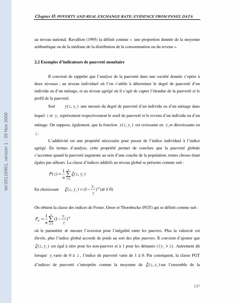
Chapter II: POVERTY AND REAL EXCHANGE RATE: EVIDENCE FROM PANEL DATA
137
au niveau national. Ravallion (1995) la définit comme « une proportion donnée de la moyenne
arithmétique ou de la médiane de la distribution de la consommation ou du revenu ».
2.2 Exemples d’indicateurs de pauvreté monétaire
Il convient de rappeler que l’analyse de la pauvreté dans une société donnée s’opère à
deux niveaux ; au niveau individuel où l’on s’attèle à déterminer le degré de pauvreté d’un
individu ou d’un ménage, et au niveau agrégé où il s’agit de capter l’étendue de la pauvreté et le
profil de la pauvreté.
Soit ),( iyzy une mesure du degré de pauvreté d’un individu ou d’un ménage dans
lequel z et iy représentent respectivement le seuil de pauvreté et le revenu d’un individu ou d’un
ménage. On suppose, également, que la fonction ),( iyzy est croissante en iy et décroissante en
z .
L’additivité est une propriété nécessaire pour passer de l’indice individuel à l’indice
agrégé. En termes d’analyse, cette propriété permet de conclure que la pauvreté globale
s’accentue quand la pauvreté augmente au sein d’une couche de la population, toutes choses étant
égales par ailleurs. La classe d’indices additifs au niveau global se présente comme suit :
),(1
)(1
∑=
=q
i
iyzn
zP ξ
En choisissant )0()1(),( ≥−= αξ α
z
yyz i
i
On obtient la classe des indices de Foster, Greer et Thornbecke (FGT) qui se définit comme suit :
αα )1(
1
1
∑=
−=q
n
i
z
y
nP
où le paramètre α mesure l’aversion pour l’inégalité entre les pauvres. Plus la valeurα est
élevée, plus l’indice global accorde de poids au sort des plus pauvres. Il convient d’ajouter que
),( iyzξ est égal à zéro pour les non-pauvres et à 1 pour les démunis ( )( zy i > . Autrement dit
lorsque iy varie de 0 à z , l’indice de pauvreté varie de 1 à 0. Par conséquent, la classe FGT
d’indices de pauvreté s’interprète comme la moyenne de ),( iyzξ sur l’ensemble de la
tel-0
0116
961,
ver
sion
1 -
29 N
ov 2
006
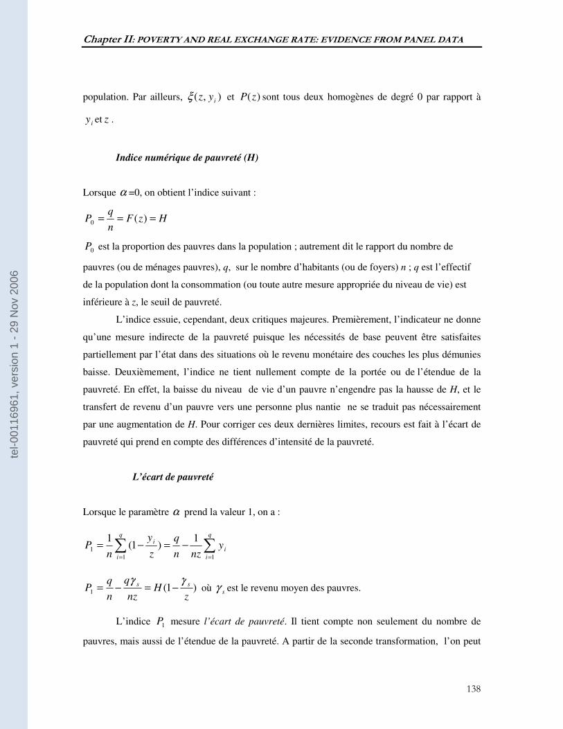
Chapter II: POVERTY AND REAL EXCHANGE RATE: EVIDENCE FROM PANEL DATA
138
population. Par ailleurs, ),( iyzξ et )(zP sont tous deux homogènes de degré 0 par rapport à
iy et z .
Indice numérique de pauvreté (H)
Lorsque α =0, on obtient l’indice suivant :
HzFn
qP === )(0
0P est la proportion des pauvres dans la population ; autrement dit le rapport du nombre de
pauvres (ou de ménages pauvres), q, sur le nombre d’habitants (ou de foyers) n ; q est l’effectif
de la population dont la consommation (ou toute autre mesure appropriée du niveau de vie) est
inférieure à z, le seuil de pauvreté.
L’indice essuie, cependant, deux critiques majeures. Premièrement, l’indicateur ne donne
qu’une mesure indirecte de la pauvreté puisque les nécessités de base peuvent être satisfaites
partiellement par l’état dans des situations où le revenu monétaire des couches les plus démunies
baisse. Deuxièmement, l’indice ne tient nullement compte de la portée ou de l’étendue de la
pauvreté. En effet, la baisse du niveau de vie d’un pauvre n’engendre pas la hausse de H, et le
transfert de revenu d’un pauvre vers une personne plus nantie ne se traduit pas nécessairement
par une augmentation de H. Pour corriger ces deux dernières limites, recours est fait à l’écart de
pauvreté qui prend en compte des différences d’intensité de la pauvreté.
L’écart de pauvreté
Lorsque le paramètre α prend la valeur 1, on a :
∑∑==
−=−=q
i
i
q
i
i ynzn
q
z
y
nP
11
1
1)1(
1
)1(1z
Hnz
q
n
qP ss γγ
−=−= où sγ est le revenu moyen des pauvres.
L’indice 1P mesure l’écart de pauvreté. Il tient compte non seulement du nombre de
pauvres, mais aussi de l’étendue de la pauvreté. A partir de la seconde transformation, l’on peut
tel-0
0116
961,
ver
sion
1 -
29 N
ov 2
006
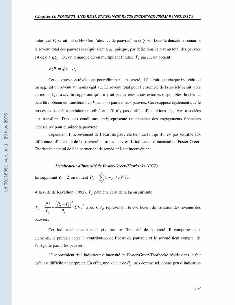
Chapter II: POVERTY AND REAL EXCHANGE RATE: EVIDENCE FROM PANEL DATA
139
noter que 1P serait nul si H=0 (en l’absence de pauvres) ou si sγ =z. Dans le deuxième scénario,
le revenu total des pauvres est équivalent à qz, puisque, par définition, le revenu total des pauvres
est égal à sqγ . Or, on remarque qu’en multipliant l’indice 1P par nz, on obtient :
[ ]szqnzP µ−=1
Cette expression révèle que pour éliminer la pauvreté, il faudrait que chaque individu ou
ménage ait un revenu au moins égal à z. Le revenu total pour l’ensemble de la société serait alors
au moins égal à nz. En supposant qu’il n’y ait pas de ressources externes disponibles, le résultat
peut être obtenu en transférant 1nzP des non-pauvres aux pauvres. Ceci suppose également que le
processus peut être parfaitement ciblé et qu’il n’y pas d’effets d’incitations négatives associées
aux transferts. Dans ces conditions, 1nzP représente un plancher des engagements financiers
nécessaires pour éliminer la pauvreté.
Cependant, l’inconvénient de l’écart de pauvreté tient au fait qu’il n’est pas sensible aux
différences d’intensité de la pauvreté entre les pauvres. L’indicateur d’intensité de Foster-Greer-
Thorbecke et celui de Sen permettent de remédier à cet inconvénient.
L’indicateur d’intensité de Foster-Greer-Thorbecke (FGT)
En supposant 2=α on obtient nzyP i
q
i
/)/1( 2
1
2 ∑=
−=
A la suite de Ravallion (1992), 2P peut être écrit de la façon suivante :
( ) 2
2
0
10
0
2
12 PCV
P
PP
P
PP
−+= avec PCV représentant le coefficient de variation des revenus des
pauvres.
Cet indicateur encore noté 2H mesure l’intensité de pauvreté. Il comporte deux
éléments, le premier capte la contribution de l’écart de pauvreté et le second tient compte de
l’inégalité parmi les pauvres.
L’inconvénient de l’indicateur d’intensité de Foster-Greer-Thorbecke réside dans le fait
qu’il est difficile à interpréter. En effet, une valeur de 2P , pris comme tel, donne peu d’indication
tel-0
0116
961,
ver
sion
1 -
29 N
ov 2
006
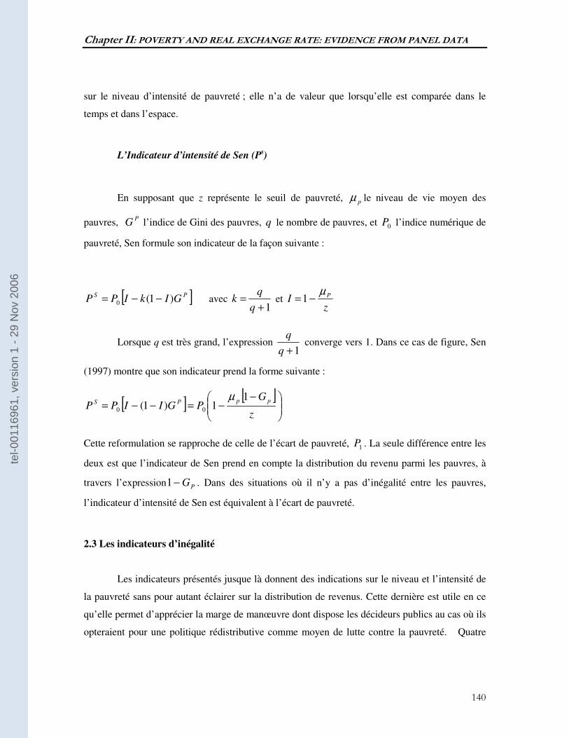
Chapter II: POVERTY AND REAL EXCHANGE RATE: EVIDENCE FROM PANEL DATA
140
sur le niveau d’intensité de pauvreté ; elle n’a de valeur que lorsqu’elle est comparée dans le
temps et dans l’espace.
L’Indicateur d’intensité de Sen (Ps)
En supposant que z représente le seuil de pauvreté, pµ le niveau de vie moyen des
pauvres, P
G l’indice de Gini des pauvres, q le nombre de pauvres, et 0P l’indice numérique de
pauvreté, Sen formule son indicateur de la façon suivante :
[ ]PSGIkIPP )1(0 −−= avec
1+=
q
qk et
zI Pµ
−=1
Lorsque q est très grand, l’expression 1+q
q converge vers 1. Dans ce cas de figure, Sen
(1997) montre que son indicateur prend la forme suivante :
[ ] [ ]
−−=−−=
z
GPGIIPP
ppPS1
1)1( 00
µ
Cette reformulation se rapproche de celle de l’écart de pauvreté, 1P . La seule différence entre les
deux est que l’indicateur de Sen prend en compte la distribution du revenu parmi les pauvres, à
travers l’expression PG−1 . Dans des situations où il n’y a pas d’inégalité entre les pauvres,
l’indicateur d’intensité de Sen est équivalent à l’écart de pauvreté.
2.3 Les indicateurs d’inégalité
Les indicateurs présentés jusque là donnent des indications sur le niveau et l’intensité de
la pauvreté sans pour autant éclairer sur la distribution de revenus. Cette dernière est utile en ce
qu’elle permet d’apprécier la marge de manœuvre dont dispose les décideurs publics au cas où ils
opteraient pour une politique rédistributive comme moyen de lutte contre la pauvreté. Quatre
tel-0
0116
961,
ver
sion
1 -
29 N
ov 2
006
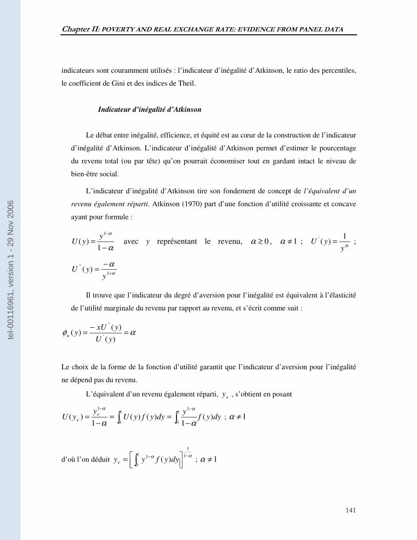
Chapter II: POVERTY AND REAL EXCHANGE RATE: EVIDENCE FROM PANEL DATA
141
indicateurs sont couramment utilisés : l’indicateur d’inégalité d’Atkinson, le ratio des percentiles,
le coefficient de Gini et des indices de Theil.
Indicateur d’inégalité d’Atkinson
Le débat entre inégalité, efficience, et équité est au cœur de la construction de l’indicateur
d’inégalité d’Atkinson. L’indicateur d’inégalité d’Atkinson permet d’estimer le pourcentage
du revenu total (ou par tête) qu’on pourrait économiser tout en gardant intact le niveau de
bien-être social.
L’indicateur d’inégalité d’Atkinson tire son fondement de concept de l’équivalent d’un
revenu également réparti. Atkinson (1970) part d’une fonction d’utilité croissante et concave
ayant pour formule :
α
α
−=
−
1)(
1y
yU avec y représentant le revenu, 0≥α , 1≠α ; α
yyU
1)(' = ;
α
α+
−=
1
'' )(y
yU
Il trouve que l’indicateur du degré d’aversion pour l’inégalité est équivalent à l’élasticité
de l’utilité marginale du revenu par rapport au revenu, et s’écrit comme suit :
αφ =−
=)(
)()(
'
''
yU
yxUyu
Le choix de la forme de la fonction d’utilité garantit que l’indicateur d’aversion pour l’inégalité
ne dépend pas du revenu.
L’équivalent d’un revenu également réparti, ey , s’obtient en posant
dyyfy
dyyfyUy
yUz z
e
e )(1
)()(1
)(0 0
11
∫ ∫ −==
−=
−−
αα
αα
; 1≠α
d’où l’on déduit αα −−
= ∫
1
1
0
1 )( dyyfyyz
e ; 1≠α
tel-0
0116
961,
ver
sion
1 -
29 N
ov 2
006
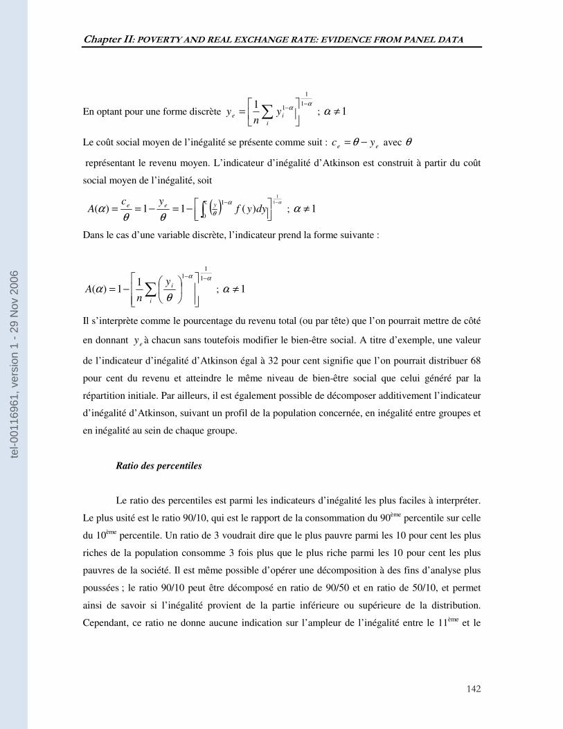
Chapter II: POVERTY AND REAL EXCHANGE RATE: EVIDENCE FROM PANEL DATA
142
En optant pour une forme discrète α
α−
−
= ∑
1
1
11
i
ie yn
y ; 1≠α
Le coût social moyen de l’inégalité se présente comme suit : ee yc −= θ avec θ
représentant le revenu moyen. L’indicateur d’inégalité d’Atkinson est construit à partir du coût
social moyen de l’inégalité, soit
( ) αα
θθθα
−
−=−== ∫
− 1
1
0
1
)(11)(z
yee dyyfyc
A ; 1≠α
Dans le cas d’une variable discrète, l’indicateur prend la forme suivante :
αα
θα
−−
−= ∑
1
11
11)(
i
iy
nA ; 1≠α
Il s’interprète comme le pourcentage du revenu total (ou par tête) que l’on pourrait mettre de côté
en donnant ey à chacun sans toutefois modifier le bien-être social. A titre d’exemple, une valeur
de l’indicateur d’inégalité d’Atkinson égal à 32 pour cent signifie que l’on pourrait distribuer 68
pour cent du revenu et atteindre le même niveau de bien-être social que celui généré par la
répartition initiale. Par ailleurs, il est également possible de décomposer additivement l’indicateur
d’inégalité d’Atkinson, suivant un profil de la population concernée, en inégalité entre groupes et
en inégalité au sein de chaque groupe.
Ratio des percentiles
Le ratio des percentiles est parmi les indicateurs d’inégalité les plus faciles à interpréter.
Le plus usité est le ratio 90/10, qui est le rapport de la consommation du 90ème percentile sur celle
du 10ème percentile. Un ratio de 3 voudrait dire que le plus pauvre parmi les 10 pour cent les plus
riches de la population consomme 3 fois plus que le plus riche parmi les 10 pour cent les plus
pauvres de la société. Il est même possible d’opérer une décomposition à des fins d’analyse plus
poussées ; le ratio 90/10 peut être décomposé en ratio de 90/50 et en ratio de 50/10, et permet
ainsi de savoir si l’inégalité provient de la partie inférieure ou supérieure de la distribution.
Cependant, ce ratio ne donne aucune indication sur l’ampleur de l’inégalité entre le 11ème et le
tel-0
0116
961,
ver
sion
1 -
29 N
ov 2
006
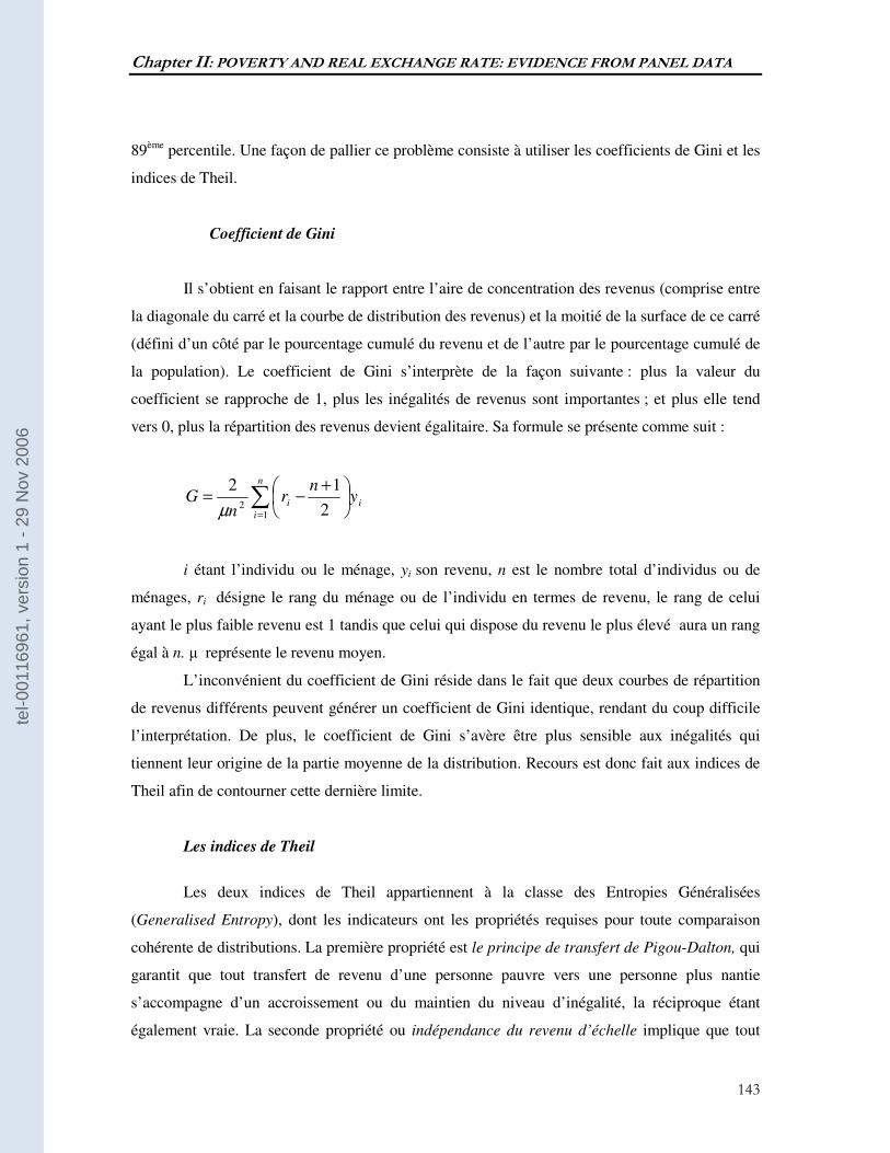
Chapter II: POVERTY AND REAL EXCHANGE RATE: EVIDENCE FROM PANEL DATA
143
89ème percentile. Une façon de pallier ce problème consiste à utiliser les coefficients de Gini et les
indices de Theil.
Coefficient de Gini
Il s’obtient en faisant le rapport entre l’aire de concentration des revenus (comprise entre
la diagonale du carré et la courbe de distribution des revenus) et la moitié de la surface de ce carré
(défini d’un côté par le pourcentage cumulé du revenu et de l’autre par le pourcentage cumulé de
la population). Le coefficient de Gini s’interprète de la façon suivante : plus la valeur du
coefficient se rapproche de 1, plus les inégalités de revenus sont importantes ; et plus elle tend
vers 0, plus la répartition des revenus devient égalitaire. Sa formule se présente comme suit :
i
n
i
i yn
rn
G ∑=
+−=
12 2
12
µ
i étant l’individu ou le ménage, yi son revenu, n est le nombre total d’individus ou de
ménages, ri désigne le rang du ménage ou de l’individu en termes de revenu, le rang de celui
ayant le plus faible revenu est 1 tandis que celui qui dispose du revenu le plus élevé aura un rang
égal à n. µ représente le revenu moyen.
L’inconvénient du coefficient de Gini réside dans le fait que deux courbes de répartition
de revenus différents peuvent générer un coefficient de Gini identique, rendant du coup difficile
l’interprétation. De plus, le coefficient de Gini s’avère être plus sensible aux inégalités qui
tiennent leur origine de la partie moyenne de la distribution. Recours est donc fait aux indices de
Theil afin de contourner cette dernière limite.
Les indices de Theil
Les deux indices de Theil appartiennent à la classe des Entropies Généralisées
(Generalised Entropy), dont les indicateurs ont les propriétés requises pour toute comparaison
cohérente de distributions. La première propriété est le principe de transfert de Pigou-Dalton, qui
garantit que tout transfert de revenu d’une personne pauvre vers une personne plus nantie
s’accompagne d’un accroissement ou du maintien du niveau d’inégalité, la réciproque étant
également vraie. La seconde propriété ou indépendance du revenu d’échelle implique que tout
tel-0
0116
961,
ver
sion
1 -
29 N
ov 2
006
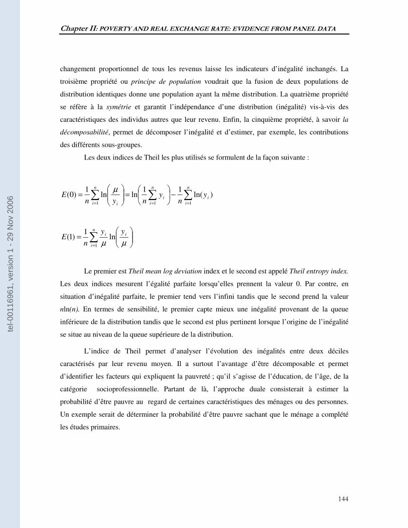
Chapter II: POVERTY AND REAL EXCHANGE RATE: EVIDENCE FROM PANEL DATA
144
changement proportionnel de tous les revenus laisse les indicateurs d’inégalité inchangés. La
troisième propriété ou principe de population voudrait que la fusion de deux populations de
distribution identiques donne une population ayant la même distribution. La quatrième propriété
se réfère à la symétrie et garantit l’indépendance d’une distribution (inégalité) vis-à-vis des
caractéristiques des individus autres que leur revenu. Enfin, la cinquième propriété, à savoir la
décomposabilité, permet de décomposer l’inégalité et d’estimer, par exemple, les contributions
des différents sous-groupes.
Les deux indices de Theil les plus utilisés se formulent de la façon suivante :
)ln(11
lnln1
)0(111
∑∑∑===
−
=
=
n
i
i
n
i
i
n
i i
yn
ynyn
Eµ
= ∑
= µµi
n
i
i yy
nE ln
1)1(
1
Le premier est Theil mean log deviation index et le second est appelé Theil entropy index.
Les deux indices mesurent l’égalité parfaite lorsqu’elles prennent la valeur 0. Par contre, en
situation d’inégalité parfaite, le premier tend vers l’infini tandis que le second prend la valeur
nln(n). En termes de sensibilité, le premier capte mieux une inégalité provenant de la queue
inférieure de la distribution tandis que le second est plus pertinent lorsque l’origine de l’inégalité
se situe au niveau de la queue supérieure de la distribution.
L’indice de Theil permet d’analyser l’évolution des inégalités entre deux déciles
caractérisés par leur revenu moyen. Il a surtout l’avantage d’être décomposable et permet
d’identifier les facteurs qui expliquent la pauvreté ; qu’il s’agisse de l’éducation, de l’âge, de la
catégorie socioprofessionnelle. Partant de là, l’approche duale consisterait à estimer la
probabilité d’être pauvre au regard de certaines caractéristiques des ménages ou des personnes.
Un exemple serait de déterminer la probabilité d’être pauvre sachant que le ménage a complété
les études primaires.
tel-0
0116
961,
ver
sion
1 -
29 N
ov 2
006
Chapter II: POVERTY AND REAL EXCHANGE RATE: EVIDENCE FROM PANEL DATA
145
2.4 Les indicateurs captant les conditions de vie
Pour pallier les insuffisances des indicateurs décrites ci-dessous, le PNUD a construit un
certain nombre d’indicateurs qui reposent sur le critère de revenu. Ces indicateurs intègrent
diverses dimensions de la pauvreté et partent d’une théorisation de la production/reproduction de
la pauvreté qui prennent en compte tous les contours de la vie économique, sociale et politique
des pauvres, ainsi que les questions identitaires, de statut et de représentations. Cependant,
l'élaboration des indicateurs de développement humain pose de nombreux problèmes
méthodologiques. Ces problèmes tiennent tant à la multiplicité des dimensions qu’à la difficulté
de les quantifier52.
Construit à partir de 1990, l’indice du développement humain (IDH) mesure les progrès
accomplis en matière d’accès aux besoins de base. A partir de 1995 ont été ajouté à la liste deux
indicateurs, à savoir l’indicateur sexospécifique du développement humain (ISDH) et l’indicateur
de participation féminine (IPF), qui prennent en compte la dimension genre dans la mesure du
développement humain. Enfin, l’indicateur de pauvreté humaine (IPH) remplace, depuis 1997,
l’indice de pénurie des capacités (ICP), créé un an plutôt. Contrairement à l’indice de
développement, axé uniquement sur les besoins de base, l’IPH essaie de capter les autres formes
de privation, entre autres l’accès problématique aux ressources publiques et privées. Tous ces
indicateurs se basent sur le principe du développement humain.
Le concept du développement humain
Le concept de développement humain fut son apparition à l’occasion de la publication du
premier rapport sur le développement humain en 1990. Cet évènement intervenait dans un
contexte où les programmes d’ajustement structurels et de stabilisation macroéconomique mises
en place dans bon nombre de pays n’avaient pas abouti au résultat escompté, à savoir le retour de
la croissance économique. Pis, les réformes portant sur le secteur public, le taux de change, le
commerce, et la politique de prix des produits agricoles ont largement occulté la dimension
humaine du développent. Partant de ce constat, les rapports sur le développement humain se
proposent d’aider à recentrer le concept de développement autour de l’homme ; autrement dit que
le développement soit conçu comme « étant celui de l’homme » (PNUD,1991).
52 La plupart des dimensions sont, par nature, qualitatives.
tel-0
0116
961,
ver
sion
1 -
29 N
ov 2
006
Chapter II: POVERTY AND REAL EXCHANGE RATE: EVIDENCE FROM PANEL DATA
146
Le développement humain, tel que définit par le PNUD, est le processus qui consiste à
élargir les choix des individus et le niveau de leur bien-être, et ce en augmentant leurs capabilités
(capabilities). Trois capabilités sont considérées comme fondamentales au développement
humain : celle garantissant une vie longue et saine, celle permettant d’accéder au stock de savoir
accumulé, et celle facilitant l’accès suffisant aux ressources indispensables à une vie descente.
L’élargissement de ces facultés doit être équitable, productive, soutenable et doit s’effectuer dans
des conditions garantissant la participation de tous les acteurs. Le développement humain
consisterait ainsi à accroître les capabilités des personnes à mener une vie descente à travers
l’accroissement des revenus et l’amélioration des autres composantes du niveau de vie entre
autres l’espérance de vie, la santé, l’éducation, le savoir et le contrôle de son propre destin
(Anand et Sen, 1994 ; Griffin et Knight, 1989).
Le concept de développement humain englobe tant les aspects matériels que non-
matériels. Ces derniers incluent la liberté dans le choix du travail et du mode de vie, l’accès à un
environnement physique harmonieux, la liberté de mouvement et d’expression, l’absence de
persécution et d’arrestation arbitraire, la libération de l’oppression, de la violence et de
d’exploitation, la liberté de cultes, et la participation aux activités de société civile (Steeten,
1999).
Il existe quatre composantes principales du paradigme du développement humain : la
productivité, l’équité, la soutenabilité et la responsabilisation (empowerment). Accroître les
capabilités implique rehausser la productivité des agents économiques de sorte à les rendre agents
actifs de la croissance. Ceci passe par leur participation au processus de création de richesse et
d’emplois. En ce qui concerne l’équité, les agents économiques doivent avoir les mêmes
chances ; pour ce faire toutes les entraves d’ordre économique, politique et social doivent être
levées de sorte à permettre à tous les agents économiques de bénéficier des mêmes opportunités.
La soutenabilité sous-tend que les considérations liées à l’équité ne doivent pas seulement se
limiter aux générations présentes mais aussi aux générations futures ; ce qui implique que toutes
les formes de capital (physique, environnemental et humain) doivent être régénérées. La
responsabilisation suppose que les hommes et femmes participent activement à la conception et
l’exécution des décisions touchant à leurs destinées.
Le concept de développement humain diffère sous plusieurs angles des approches
conventionnelles basées sur la croissance économique, le développement du capital humain, et la
satisfaction des besoins primaires. En effet, en partant de l’hypothèse que la croissance bénéficie
à toute la société, les approches orientées sur la croissance économique font de la maximisation
tel-0
0116
961,
ver
sion
1 -
29 N
ov 2
006
Chapter II: POVERTY AND REAL EXCHANGE RATE: EVIDENCE FROM PANEL DATA
147
de la croissance économique le seul objectif. En revanche, les approches du développement
humain, axées sur une perspective beaucoup plus large, posent la croissance économique comme
condition nécessaire mais pas suffisante de l’amélioration du bien-être. La croissance devient, dès
lors, un moyen d’accélérer le développement humain et non une fin en soi. Le développement
humain met concomitamment ensemble production, distribution, et expansion des capabilités tout
en ayant un regard sur les choix que les personnes peuvent faire dans le but d’améliorer leurs
niveaux de vie.
Une dernière caractéristique du concept de développement humain est l’importance
de la complémentarité entre les dépenses touchant aux capacités humaines. Une illustration est
donnée par Griffin et McKinley (1992) qui montrent que les dépenses de santé primaire ont une
répercussion directe sur l’état de santé des pauvres. Cette amélioration de la santé accroît, par
ricochet, l’efficience du processus de transformation des aliments en calories, et donc renforce les
gains des programmes de nutrition infantile et maternelle. Des progrès en matière de nutrition
rehaussent la capacité d’apprentissage des enfants et ainsi améliorent les rendements scolaires.
L’indicateur de développement humain (IDH)
L’indicateur de développement humain est un indice composite qui a été construit pour
refléter les aspects fondamentaux du développement humain. Il capte les éléments fondamentaux
que les personnes doivent disposer pour s’intégrer à la société et y apporter leur contribution.
Aussi, permet-il de mesurer les résultats atteints en matière de satisfaction des besoins primaires,
entre autres la connaissance, la longévité, et l’accès à une vie décente. L’indicateur du
développement humain est la moyenne arithmétique de trois éléments : la santé/longévité, captée
par l’espérance de vie à la naissance ; le niveau d’éducation mesuré par une combinaison du taux
scolarisation aux trois niveaux et du taux d’alphabétisation, et le niveau de vie capté par le PIB en
termes réels, exprimé en dollars pondérés des parités de pouvoir d’achat (PNUD, 1995 et 1999).
La technique de construction de l’IDH a évolué dans le temps, prenant en compte les
nombreuses critiques formulées à son encontre. Les modifications intervenues permettent de
mesurer les progrès réalisés et non plus les probabilités de souffrir de dénuement. Elles sont aussi
tel-0
0116
961,
ver
sion
1 -
29 N
ov 2
006
Chapter II: POVERTY AND REAL EXCHANGE RATE: EVIDENCE FROM PANEL DATA
148
de nature à corriger les biais53, engendrés par les méthodes permettant de passer des indicateurs
de pauvreté aux indices.
La version originelle de l’IDH partait des indicateurs partiels de manque. L’espérance de
vie à la naissance traduit le manque par rapport à un maximum établi par la moyenne des
longévités les plus élevés. En 1994-1995, les extrema ont été établis de manière normative
(minimum à 25 ans et maximum à 85 ans) de sorte à éviter que les pays développés ne constituent
un horizon mobile pour les pays pauvres.
L’indicateur, saisissant le manque de savoir, était au départ le taux d’alphabétisation,
avec un maximum à 100 %. Cet indicateur cède le pas, à partir de 1991, à une combinaison de la
moyenne de durée de la scolarité et du taux d’alphabétisation. La pondération assignée au premier
est un tiers tandis que le second occupe les deux tiers restants. En 1995, l’indicateur mesurant le
manque en termes de savoir fut modifié, et la moyenne de la durée de la scolarisation substituée
par le taux de scolarisation aux trois niveaux.
La variable choisie, pour capter le niveau de vie dans la version de 1990, était le
logarithme du PIB par habitant en termes réels, affecté d’une pondération nulle au-dessus d’une
valeur correspondant au seuil de pauvreté des neuf pays les plus riches. Pour tenir compte de
l’utilité marginale décroissante des niveaux élevés de revenus, et du principe selon lequel un
niveau respectable n’exige pas de revenus illimités, le PNUD eut recours à la formule d’Atkinson
pour corriger les niveaux de revenus. Cette technique permet de comprimer les plus hauts
revenus dans le calcul de l’IDH. Elle consiste notamment à faire augmenter progressivement la
valeur de l’élasticité de l’utilité marginale du revenu par rapport au développement humain à
mesure que le revenu augmente54. La formule d’Atkinson se présente comme suit :
ε
ε−
−= 1
1
1)( yyZ avec 10 ≤≤ ε
)(yZ est l’utilité dérivée du revenu, y le revenu, et ε l’élasticité de l’utilité marginale du revenu
par rapport au développement humain.
Soit *y le seuil de pauvreté moyen de 17 pays industrialisés. Si ε =1, le revenu n’a
aucune contribution au développement humain. Si ε =0, W(y)=y et il en ressort qu’il n’y a pas de
53 Le biais est en faveur des pays à revenu élevé. 54 Chaque tranche est exprimée en multiple du seuil de pauvreté moyen de 17 pays industrialisés
tel-0
0116
961,
ver
sion
1 -
29 N
ov 2
006
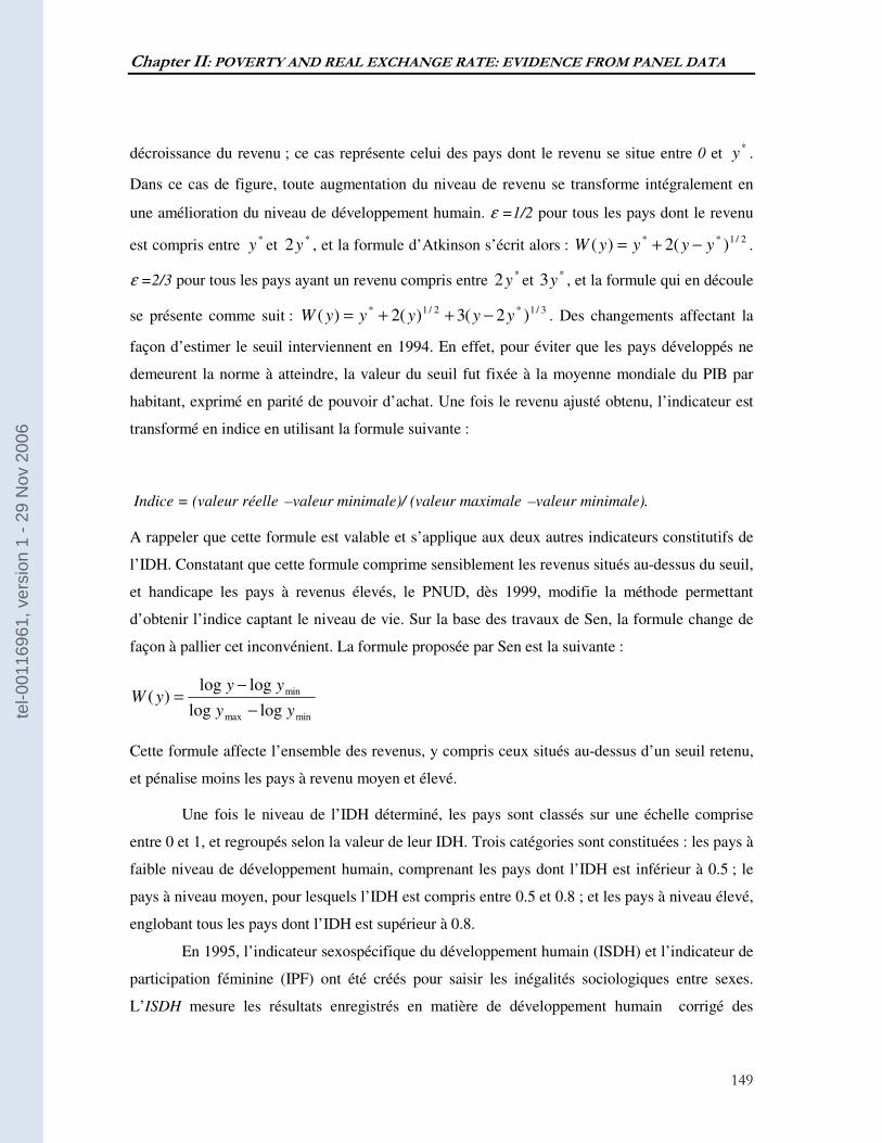
Chapter II: POVERTY AND REAL EXCHANGE RATE: EVIDENCE FROM PANEL DATA
149
décroissance du revenu ; ce cas représente celui des pays dont le revenu se situe entre 0 et *y .
Dans ce cas de figure, toute augmentation du niveau de revenu se transforme intégralement en
une amélioration du niveau de développement humain. ε =1/2 pour tous les pays dont le revenu
est compris entre *y et
*2y , et la formule d’Atkinson s’écrit alors : 2/1** )(2)( yyyyW −+= .
ε =2/3 pour tous les pays ayant un revenu compris entre *2y et
*3y , et la formule qui en découle
se présente comme suit : 3/1*2/1* )2(3)(2)( yyyyyW −++= . Des changements affectant la
façon d’estimer le seuil interviennent en 1994. En effet, pour éviter que les pays développés ne
demeurent la norme à atteindre, la valeur du seuil fut fixée à la moyenne mondiale du PIB par
habitant, exprimé en parité de pouvoir d’achat. Une fois le revenu ajusté obtenu, l’indicateur est
transformé en indice en utilisant la formule suivante :
Indice = (valeur réelle –valeur minimale)/ (valeur maximale –valeur minimale).
A rappeler que cette formule est valable et s’applique aux deux autres indicateurs constitutifs de
l’IDH. Constatant que cette formule comprime sensiblement les revenus situés au-dessus du seuil,
et handicape les pays à revenus élevés, le PNUD, dès 1999, modifie la méthode permettant
d’obtenir l’indice captant le niveau de vie. Sur la base des travaux de Sen, la formule change de
façon à pallier cet inconvénient. La formule proposée par Sen est la suivante :
minmax
min
loglog
loglog)(
yy
yyyW
−
−=
Cette formule affecte l’ensemble des revenus, y compris ceux situés au-dessus d’un seuil retenu,
et pénalise moins les pays à revenu moyen et élevé.
Une fois le niveau de l’IDH déterminé, les pays sont classés sur une échelle comprise
entre 0 et 1, et regroupés selon la valeur de leur IDH. Trois catégories sont constituées : les pays à
faible niveau de développement humain, comprenant les pays dont l’IDH est inférieur à 0.5 ; le
pays à niveau moyen, pour lesquels l’IDH est compris entre 0.5 et 0.8 ; et les pays à niveau élevé,
englobant tous les pays dont l’IDH est supérieur à 0.8.
En 1995, l’indicateur sexospécifique du développement humain (ISDH) et l’indicateur de
participation féminine (IPF) ont été créés pour saisir les inégalités sociologiques entre sexes.
L’ISDH mesure les résultats enregistrés en matière de développement humain corrigé des
tel-0
0116
961,
ver
sion
1 -
29 N
ov 2
006
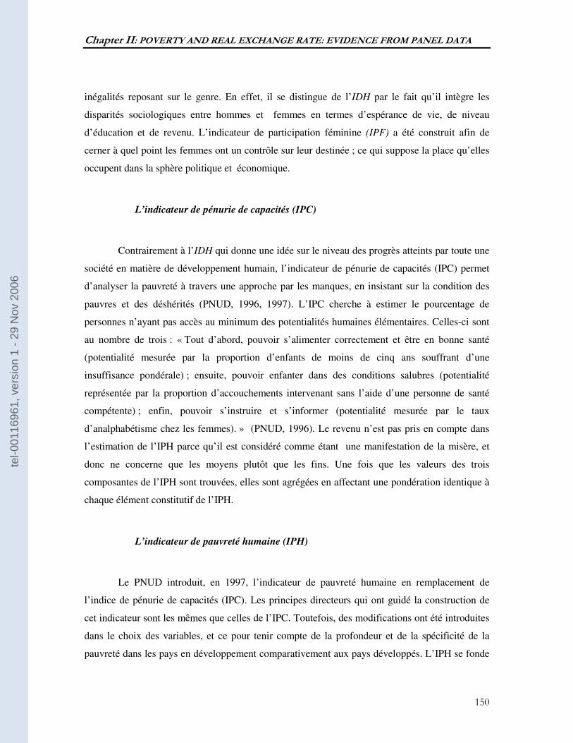
Chapter II: POVERTY AND REAL EXCHANGE RATE: EVIDENCE FROM PANEL DATA
150
inégalités reposant sur le genre. En effet, il se distingue de l’IDH par le fait qu’il intègre les
disparités sociologiques entre hommes et femmes en termes d’espérance de vie, de niveau
d’éducation et de revenu. L’indicateur de participation féminine (IPF) a été construit afin de
cerner à quel point les femmes ont un contrôle sur leur destinée ; ce qui suppose la place qu’elles
occupent dans la sphère politique et économique.
L’indicateur de pénurie de capacités (IPC)
Contrairement à l’IDH qui donne une idée sur le niveau des progrès atteints par toute une
société en matière de développement humain, l’indicateur de pénurie de capacités (IPC) permet
d’analyser la pauvreté à travers une approche par les manques, en insistant sur la condition des
pauvres et des déshérités (PNUD, 1996, 1997). L’IPC cherche à estimer le pourcentage de
personnes n’ayant pas accès au minimum des potentialités humaines élémentaires. Celles-ci sont
au nombre de trois : « Tout d’abord, pouvoir s’alimenter correctement et être en bonne santé
(potentialité mesurée par la proportion d’enfants de moins de cinq ans souffrant d’une
insuffisance pondérale) ; ensuite, pouvoir enfanter dans des conditions salubres (potentialité
représentée par la proportion d’accouchements intervenant sans l’aide d’une personne de santé
compétente) ; enfin, pouvoir s’instruire et s’informer (potentialité mesurée par le taux
d’analphabétisme chez les femmes). » (PNUD, 1996). Le revenu n’est pas pris en compte dans
l’estimation de l’IPH parce qu’il est considéré comme étant une manifestation de la misère, et
donc ne concerne que les moyens plutôt que les fins. Une fois que les valeurs des trois
composantes de l’IPH sont trouvées, elles sont agrégées en affectant une pondération identique à
chaque élément constitutif de l’IPH.
L’indicateur de pauvreté humaine (IPH)
Le PNUD introduit, en 1997, l’indicateur de pauvreté humaine en remplacement de
l’indice de pénurie de capacités (IPC). Les principes directeurs qui ont guidé la construction de
cet indicateur sont les mêmes que celles de l’IPC. Toutefois, des modifications ont été introduites
dans le choix des variables, et ce pour tenir compte de la profondeur et de la spécificité de la
pauvreté dans les pays en développement comparativement aux pays développés. L’IPH se fonde
tel-0
0116
961,
ver
sion
1 -
29 N
ov 2
006
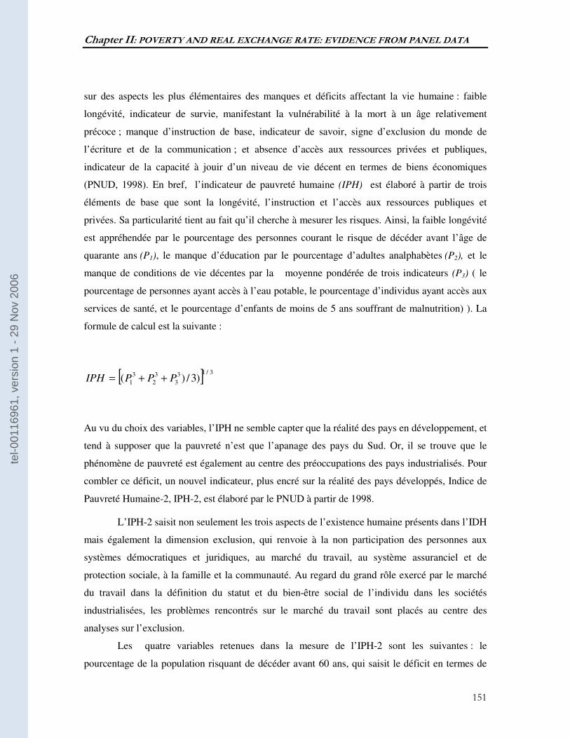
Chapter II: POVERTY AND REAL EXCHANGE RATE: EVIDENCE FROM PANEL DATA
151
sur des aspects les plus élémentaires des manques et déficits affectant la vie humaine : faible
longévité, indicateur de survie, manifestant la vulnérabilité à la mort à un âge relativement
précoce ; manque d’instruction de base, indicateur de savoir, signe d’exclusion du monde de
l’écriture et de la communication ; et absence d’accès aux ressources privées et publiques,
indicateur de la capacité à jouir d’un niveau de vie décent en termes de biens économiques
(PNUD, 1998). En bref, l’indicateur de pauvreté humaine (IPH) est élaboré à partir de trois
éléments de base que sont la longévité, l’instruction et l’accès aux ressources publiques et
privées. Sa particularité tient au fait qu’il cherche à mesurer les risques. Ainsi, la faible longévité
est appréhendée par le pourcentage des personnes courant le risque de décéder avant l’âge de
quarante ans (P1), le manque d’éducation par le pourcentage d’adultes analphabètes (P2), et le
manque de conditions de vie décentes par la moyenne pondérée de trois indicateurs (P3) ( le
pourcentage de personnes ayant accès à l’eau potable, le pourcentage d’individus ayant accès aux
services de santé, et le pourcentage d’enfants de moins de 5 ans souffrant de malnutrition) ). La
formule de calcul est la suivante :
[ ] 3/13
3
3
2
3
1 )3/)( PPPIPH ++=
Au vu du choix des variables, l’IPH ne semble capter que la réalité des pays en développement, et
tend à supposer que la pauvreté n’est que l’apanage des pays du Sud. Or, il se trouve que le
phénomène de pauvreté est également au centre des préoccupations des pays industrialisés. Pour
combler ce déficit, un nouvel indicateur, plus encré sur la réalité des pays développés, Indice de
Pauvreté Humaine-2, IPH-2, est élaboré par le PNUD à partir de 1998.
L’IPH-2 saisit non seulement les trois aspects de l’existence humaine présents dans l’IDH
mais également la dimension exclusion, qui renvoie à la non participation des personnes aux
systèmes démocratiques et juridiques, au marché du travail, au système assuranciel et de
protection sociale, à la famille et la communauté. Au regard du grand rôle exercé par le marché
du travail dans la définition du statut et du bien-être social de l’individu dans les sociétés
industrialisées, les problèmes rencontrés sur le marché du travail sont placés au centre des
analyses sur l’exclusion.
Les quatre variables retenues dans la mesure de l’IPH-2 sont les suivantes : le
pourcentage de la population risquant de décéder avant 60 ans, qui saisit le déficit en termes de
tel-0
0116
961,
ver
sion
1 -
29 N
ov 2
006
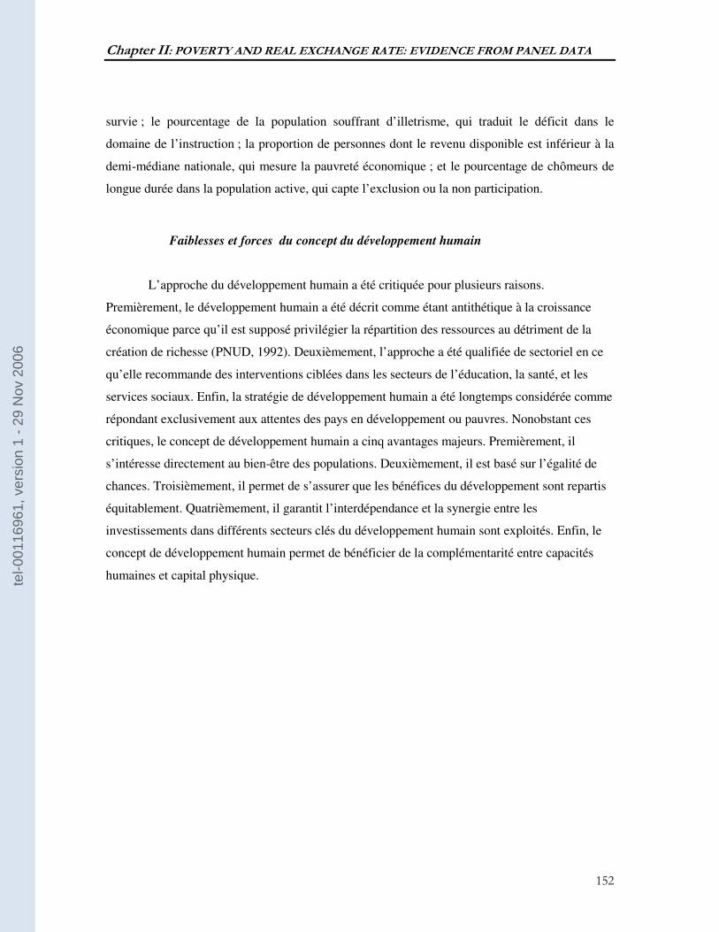
Chapter II: POVERTY AND REAL EXCHANGE RATE: EVIDENCE FROM PANEL DATA
152
survie ; le pourcentage de la population souffrant d’illetrisme, qui traduit le déficit dans le
domaine de l’instruction ; la proportion de personnes dont le revenu disponible est inférieur à la
demi-médiane nationale, qui mesure la pauvreté économique ; et le pourcentage de chômeurs de
longue durée dans la population active, qui capte l’exclusion ou la non participation.
Faiblesses et forces du concept du développement humain
L’approche du développement humain a été critiquée pour plusieurs raisons.
Premièrement, le développement humain a été décrit comme étant antithétique à la croissance
économique parce qu’il est supposé privilégier la répartition des ressources au détriment de la
création de richesse (PNUD, 1992). Deuxièmement, l’approche a été qualifiée de sectoriel en ce
qu’elle recommande des interventions ciblées dans les secteurs de l’éducation, la santé, et les
services sociaux. Enfin, la stratégie de développement humain a été longtemps considérée comme
répondant exclusivement aux attentes des pays en développement ou pauvres. Nonobstant ces
critiques, le concept de développement humain a cinq avantages majeurs. Premièrement, il
s’intéresse directement au bien-être des populations. Deuxièmement, il est basé sur l’égalité de
chances. Troisièmement, il permet de s’assurer que les bénéfices du développement sont repartis
équitablement. Quatrièmement, il garantit l’interdépendance et la synergie entre les
investissements dans différents secteurs clés du développement humain sont exploités. Enfin, le
concept de développement humain permet de bénéficier de la complémentarité entre capacités
humaines et capital physique. tel-0
0116
961,
ver
sion
1 -
29 N
ov 2
006

153
tel-0
0116
961,
ver
sion
1 -
29 N
ov 2
006
Chapter III: IS FISCAL POLICY BECOMING COUNTERCYCLICAL IN AFRICA?
154
CHAPTER III:
IS FISCAL POLICY BECOMING COUNTERCYCLICAL IN AFRICA55?
55 We would like to thank Jean-Louis Arcand and Jean-Louis Combes for helpful discussions and pertinent comments on an earlier draft. We would also like to thank Roland Kpodar for sharing his program on Bootstraping.
tel-0
0116
961,
ver
sion
1 -
29 N
ov 2
006
Chapter III: IS FISCAL POLICY BECOMING COUNTERCYCLICAL IN AFRICA?
155
I-INTRODUCTION
The adoption of multipartism and the systematic use of elections as means of
selecting rulers were the key political developments in virtually all Sub-Saharan African
countries during the 1990s. While some analysts viewed this development as opening a
new area for improved economic performance, others were more pessimistic, fearing that
democratic reforms would result in political instability and poor economic outcomes. The
issue of the impact of democratisation is still a matter of debate, with each camp
supporting its claim with some anecdotal examples. Even though the discussion on
democracy among economists primarily focuses on potential correlation between
democratic reforms and economic outcome such as growth, a growing number of papers
explore economic policy changes that may be associated with democratic institutions.
One area that is frequently explored is the effect of political regimes on government
spending or social spending policies. Person and Tabellini (2004) analyse the impact of
electoral rules and political regimes on the size of government spending in a large
number of democracies. Stasavage (2003) investigates whether the move to a more
democratic system has been associated with larger spending in primary education in
African countries. Similar discussion also takes place in the context of other developing
regions. Brown and Hunter (1999) and Kaufman and Segura-Ubiergo (2001) examine the
impact of democratic reforms on public spending in Latin America.
This chapter follows the aforementioned central thesis, which is the effect of
political reforms on public policies. However, the thrust of the chapter departs slightly
from the mentioned studies and focuses on the impact of democratic reforms on the
tel-0
0116
961,
ver
sion
1 -
29 N
ov 2
006
Chapter III: IS FISCAL POLICY BECOMING COUNTERCYCLICAL IN AFRICA?
156
cyclical properties of fiscal policy. More specifically, we ask whether the increase in
political pluralism in many African countries in recent years has resulted in the adoption
of more countercyclical fiscal policies. This question is of particular importance for at
least one reason. The post-independence experience was characterised by the
predominance of authoritarian regimes, riddled with patronage and interest groups whose
continued loyalty was preserved by implicit and explicit government transfers. Such
environment was, in part, condusive to stop-go policies, resulting in boom-bust cycles.
On the one hand, positive shocks, such as an improvement in terms of trade, increased the
pressure, especially from entrenched constituencies, for higher spending. Public spending
therefore spiralled out of control during good times. On the other hand, negative shocks
forced, though not instantly, countries to embrace fiscal consolidation. Against this
background, the move towards political pluralism is expected to unleash more political
competition. The likelihood of retaining office becomes closely related to the ability of
rulers to pursue policies that increase the well-being of the median voter. If one assumes
that countercyclical fiscal policies are welfare-enhancing, it is likely that governments
favour such fiscal polices, which smooth out fluctuations in output and boost, or at least
preserve, the well being of the majority.
The circumstances described above are those that prevail in a properly working
democracy system. But it is not often the case in the majority of newly democratised
African nations. One condition underlying the functioning of a well established
democracy is the existence of objective information to the typical voter. This condition is
unmet when voter loyalty to ethnic communities is strong. In such case, political
competition does not always produce rulers that are keen of delivering national public
tel-0
0116
961,
ver
sion
1 -
29 N
ov 2
006
Chapter III: IS FISCAL POLICY BECOMING COUNTERCYCLICAL IN AFRICA?
157
goods. Beyond the mechanisms guiding the selection of rulers, another important feature
of a properly working democracy is the mechanisms that limit how power is used, which
are often called “checks and balances”. This dimension of democracy is the most difficult
element to build as it takes time to introduce effective restraints on power. The foregoing
arguments suggest caution in hastily drawing optimistic views about the impact of
democracy on the cyclicality of fiscal policy. However, this does not imply that
democracy is largely ineffective in Africa because political pluralism and freedom are
essential values in their own rights. Moreover, even a scant improvement in civil liberties
and political rights represents an institutional change, and it is worth exploring the
implications of such change in the conduct of economic policies in general or more
particularly on fiscal policy.
The chapter is divided into six sections. Section II reviews some of the theoretical
support for the positive relationship between countercyclical fiscal policies and growth.
Section III presents a brief literature review of the determinants of procyclical fiscal
policy. Section IV highlights the ambiguous relationship between democratic institutions
and countercyclical fiscal policies, thus providing the theoretical foundation for our
analysis. Section V presents two country cases to illustrate our theoretical construct.
Section V discusses data issues and the empirical strategy. Section VII confronts the
implications of the theoretical framework with the data and comments the results. Finally,
section VIII concludes.
tel-0
0116
961,
ver
sion
1 -
29 N
ov 2
006
Chapter III: IS FISCAL POLICY BECOMING COUNTERCYCLICAL IN AFRICA?
158
II- COUNTERCYCLICAL FISCAL POLICIES AND LONG TERM GROWTH
Apart from being volatile, public spending tends to be procyclical in Sub-Saharan
Africa. It increases during booms and experiences severe cuts in bad times. This
procyclical nature of government spending is costly as it dampens economic growth and
increases poverty. Why do procyclical fiscal policies hamper long term growth?
Endogenous growth models, especially those suggested by Aghion (1992) and
Aghion et al. (2006), provide an interesting and compelling explanation of how
countercyclical fiscal policy could positively affect long-term growth56. Aghion et al.
(2006) argue that a recession is considered, in the Schumpeterian tradition, as a cleansing
mechanism, whereby inefficient firms are eliminated and surviving firms experience deep
restructuring. Such restructuring involves reallocating resources, innovating, and
branching out to new markets. This process requires new investments, say, in the form of
investment in R&D. If firms have full access to credit, the restructuring process goes
smoothly, with firms investing in R&D and innovating. Ultimately, productivity growth
is increased and long-term growth fostered. However, if firms evolve in an environment
where credit is rationed, the restructuring process is impaired and protracted recession
follows. For instance, if firms can only borrow an amount proportional to their current
earnings, their borrowing capacity shrinks significantly with recession. Firms cut back on
R&D expenditures and other necessary investments and may not be able to initiate the
necessary restructuring activities. The degree of innovation slows down, and productivity
56 Similarly, in the pure Keynesian tradition, increasing public spending during recession helps to stabilize the cycle and ensure a full employment. Tax smoothing (Barro, 1979: Lucas and Stockey, 1983) and public spending smoothing motives (permanent income theory) explain the conduct of counter-cyclical fiscal policy, with countries running deficits during recessions and surpluses during good times.
tel-0
0116
961,
ver
sion
1 -
29 N
ov 2
006
Chapter III: IS FISCAL POLICY BECOMING COUNTERCYCLICAL IN AFRICA?
159
growth and long-term growth are reduced. The policy implication is that countercyclical
fiscal policy can help achieve a seamless adjustment process and secures long-term
growth in a financially constrained economy. In other words, government can increase
public spending or reduce tax in order to boost the demand for firms’ products and
improve their growth prospects. These measures can also consist of providing direct
incentives to firms through subsidies and other transfers to firms.
The R&D expenditure dynamics within firms is one of the main arguments put
forward to justify a potential positive impact of countercyclical fiscal policy on long-term
growth. The argument fits very well situations that prevail in developed countries and
some of the more advanced developing countries, where R&D expenditure represents an
important source of innovation. But such an explanation might not fully capture the
specificities of other developing countries, especially Sub-Saharan African countries. In
these countries, R&D expenditure tend be marginal, and innovation is very often brought
about through imported capital goods, which require skilled labour in order to be used
effectively and efficiently. This means that countercyclical fiscal policy may affect long-
term growth in the poorest countries if for instance it can impact the human capital and
the ability to import in these countries. It follows that human capital and real exchange
channels are plausible chains of causation from countercyclical fiscal policy to stronger
long-term growth.
A great deal of evidence suggests that crises can have long-lasting effects on
human capital accumulation and economic growth (Lustig, 1998; Ocampo, 2002). This is
primarily the outcomes of both household and government reactions in times of crises.
During economic downturns, some households are forced to pull their children out of
tel-0
0116
961,
ver
sion
1 -
29 N
ov 2
006
Chapter III: IS FISCAL POLICY BECOMING COUNTERCYCLICAL IN AFRICA?
160
schools. Long-term human capital is then eroded, and the long-run overall performance
of the economy weakened. Similarly, governments facing mounting fiscal deficits during
bust times cut in social spending, notably in education expenditure. These policies lead to
setbacks in education enrolments and contribute to lowering long-term human capital and
potential growth. The situation of African countries in the 1980s illustrates very well this
point. One way of avoiding such an adverse development is to pursue a countercyclical
fiscal policy. This implies increasing public spending, especially in social sectors, during
bad times so as to avoid irreversible losses in human capital and sustain long-term
growth. The argument is very much similar to the economic rationale for publicly funded
safety nets.
The second mediating channel from countercyclical fiscal policy to higher output
operates through real exchange rate. The reason is that developments in real exchange
rate can determine export competitiveness, export earnings, and therefore the capacity to
import, especially of countries that have limited access to international capital markets.
More specifically, real exchange rate appreciates as a result of the accommodative fiscal
policies that are adopted during boom times. This phenomenon is commonly dubbed as
“Dutch Disease”. The real appreciation of exchange rate exerts a negative impact on
export receipts and undermines countries’ ability to import goods, especially capital
goods that represent an important source of innovation and productivity improvement.
Apart from the import channel, real exchange rate appreciation is accompanied by
a structural transformation that can have an enduring impact on growth. The real
appreciation of exchange rate caused by rising export prices has two opposite effects on
the tradable sector. First, tradable industries that benefit from high prices, such as
tel-0
0116
961,
ver
sion
1 -
29 N
ov 2
006
Chapter III: IS FISCAL POLICY BECOMING COUNTERCYCLICAL IN AFRICA?
161
commodity producers, expand significantly. Second, other tradable industries, including
the manufacturing, that produce goods for which prices decline or experience modest
gains, contract. The contraction may be so severe as to cripple these industries and
making the situation irreversible even when booms end and real exchange rate
depreciates. Since the manufacturing industry generates positive externalities or
productivity advantages57, over other sectors, such as those that produce commodities, a
persistent decline of this industry impairs long-term growth. Again, fiscal policy can help
prevent these negative outcomes by addressing the primary cause of real exchange rate
appreciation. Implementing countercyclical fiscal policy during booms times, meaning
pursing tight fiscal stance limits the overvaluation of real exchange rate and contributes
to long-term productivity improvement and growth. If countercyclical policy is growth-
enhancing, why have many developing countries persistently pursued procyclical fiscal
policies?
III-DETERMINANTS OF PROCYCLICAL FISCAL POLICY
Understanding the factors underlying fiscal procyclicality has been a subject
largely explored in the literature. However, this intense research generally tends to
concentrate on developed or emerging countries and gives little space to Sub-Saharan
African countries.
Many factors have been put forward to explain fiscal procyclicality in developing
countries. Tornell and Lane (1999) link fiscal procyclicality to distributional conflicts
57 These positive externalities and productivity advantages are diffused through learning by doing
tel-0
0116
961,
ver
sion
1 -
29 N
ov 2
006
Chapter III: IS FISCAL POLICY BECOMING COUNTERCYCLICAL IN AFRICA?
162
over government resources. They argue that struggle among government entities
(ministries, provinces) for public resources gives rise to a “voracity effect”, whereby
expenditures outpace windfalls. Likewise, Talvi and Végh (2000) argue that it is optimal
for policymakers to run negligible primary surpluses during booms by boosting
government spending and cutting tax rates. In contrast, Gavin and Perotti (1997) attribute
the procyclicality of government spending in developing countries to the credit
constraints these countries face. These constraints reduce their ability to borrow during
recessions or busts thereby forcing them to adjust through cuts in public spending and/or
increase in taxes.
Both factors, i.e. distributional conflict and credit constraints, come into play in
determining the fiscal policy stance in many African countries. Because of the
narrowness of their export structures as well as their domestic economic activities, those
countries are likely to suffer much more from exogenous shocks than other developing
countries. In other words, African countries are more prone to distributional conflicts
than other developing countries. In addition to their vulnerability to exogenous shocks,
most of the countries in the region have a limited or no access to international capital
markets. However, these two constraints do not necessary imply that fiscal policy in the
region is doomed to experience procyclicality. Democratic institutions can be conducive
to both procyclical and countercyclical fiscal policies.
tel-0
0116
961,
ver
sion
1 -
29 N
ov 2
006
Chapter III: IS FISCAL POLICY BECOMING COUNTERCYCLICAL IN AFRICA?
163
IV-DEMOCRATIC INSTITUTIONS AND CYCLICAL PROPERTIES OF
FISCAL POLICY
4.1 Democratic institutions conducive to procyclical fiscal policies
There are some reasons to believe that the advent of democracy might exacerbate
the procyclicality of fiscal stance. That view is supported by the political business
cycle58 argument, especially the opportunistic version of that argument, and the argument
based on corruption. Opportunistic political business cycle theory posits that incumbents
facing competitive elections engage in economic policy manipulation to induce economic
expansions prior to elections, therefore increasing their chances to get re-elected
(Nordhaus, 1975: Lindbeck, 1976: Tufte, 1978). The manipulation of economic policy
tools consists in pursing expansionary monetary and fiscal policies before elections and
adopting contractionary polices after elections. This situation is said to be particularly
acute in new democracies as, for example, the newly democratised African states. At
least two main factors explain the widespread of politically motivated policies in newly
democratised countries (Block et al., 2003: Brender and Drazen, 2004). First, during
transitions from dictatorships to democracies, authoritarian leaders tend to have enough
leeway to distort economic policies in their favour. Initial competitive elections provide
them with the opportunity to discourage entry by future challengers. Showering
constituents with public spending increases around election time, for instance, boosts the
58 The political business cycle theory has two versions. The first is termed “rational partisan cycle” and emphasizes the importance of ideology as the driving force behind the cycle generated before election. The second is dubbed as “opportunistic business cycle” and highlights the opportunistic behaviour of all incumbents independently of ideology or partisanship (Hibbs, 1977: Alesina et al., 1997). Evidence suggests that opportunistic business cycle is more common in Africa (Ka and van de Walle, 1994).
tel-0
0116
961,
ver
sion
1 -
29 N
ov 2
006
Chapter III: IS FISCAL POLICY BECOMING COUNTERCYCLICAL IN AFRICA?
164
incumbents’ credentials and public support before the opposition has any say on the
design and conduct of economic policies. Such behaviours are made easier by the lack of
significant institutional constraints, such as a free press or independent legislatures,
which reduce the degree of discretion for incumbents to manipulate macroeconomic
policies. Second, some deficiencies are inherent to transitions from dictatorships to
democracies. Constituents generally lack information about candidates and are not very
much knowledgeable about the functioning of a democracy, thus providing incumbents
with further incentives to engage in politically motivated policy interventions. However,
it is worth noting that falling into political budget cycles is not purely identical to
conducting procyclical policies. For instance, conducting expansionary fiscal or monetary
policies prior to elections does not always mean that governments impart a procyclical
bias to policies. It is only true when the economy is booming before the elections.
Similarly, pursuing contractionary fiscal or monetary policies after elections amounts to
conducting procyclical policies only if economies experience recessions after elections.
The second argument that is put forward in explaining procyclical policies, and in
particular procyclical fiscal policy, in nascent democracy lies on corruption (Alesina and
Tabelleni, 2005). Numerous accounts point to widespread corruption in some of the
African countries characterised by authoritarian regimes (Ake, 1990). That feature
persists during the transitions from authoritarian rule to democracies.
The “corruption” argument rests on the premise that constituents do not trust
corrupt governments when it comes to managing additional resources. The public tends
to believe that any additional government revenue will be siphoned off through
distributing favours to special groups close to the government or the increase of the
tel-0
0116
961,
ver
sion
1 -
29 N
ov 2
006
Chapter III: IS FISCAL POLICY BECOMING COUNTERCYCLICAL IN AFRICA?
165
consumption of government officials. Thus, in line of the “starve the Leviathan”
argument the constituents demand increases in public spending, transfers or public
investment, whenever the economy experiences a positive shock. This is one way for
constituencies to hold governments accountable. Such demand forces governments to
pursue a procyclical fiscal stance during good times. Alesina and Tabelleni (2005)
illustrate this using a principal-agent framework wherein constituents represent the
principal and the government the agent.
4.2 Democratic institutions conducive to countercyclical fiscal policies
Democratic institutions can mitigate credit constraints and the “voracity effect”,
the two main causes of procyclical fiscal policy. Democratic systems per se can not
address credit constraints but they have the potential to cure the leading factor of
procyclical fiscal stance: rising government spending during expansions. Access to
international capital markets is closely linked to the business cycle, with capital flows
pouring during good times and drying up during recessions. This means that the issue of
access to international capital markets often cited in the literature is of relevance only
when crisis erupts. In different circumstances, i.e. during booms, countries enjoy large
capital inflows, and the challenge during those times is to follow prudent fiscal polices,
such as putting aside windfalls. These policies would ultimately gives more room of
maneuver for expansionary fiscal stance during recessions. However, the political
acceptance of cautious fiscal policies during expansions may be hard to sell, notably in
African countries. Poor infrastructure, widespread poverty, low levels of human
tel-0
0116
961,
ver
sion
1 -
29 N
ov 2
006
Chapter III: IS FISCAL POLICY BECOMING COUNTERCYCLICAL IN AFRICA?
166
development, and the pressing need to address these problems places pressure on
government expenditure. Public pressure for more public spending during good times
could be lessen if governments are enough persuasive and “trusted”. These two qualities
may critically depend on their legitimacy and to the extent to which they are accountable
to the people: the electorate. Legitimacy may be gained through political competition,
notably free and fair elections, while accountability may be guaranteed by what we
previously call “checks and balances” institutions, which are restraints on the executive
branch. Interestingly, political competition and checks and balances are two important
aspects of a properly working democracy. Consequently, one may expect democracy to
facilitate governments’ plan to follow responsible fiscal policy during good times and set
a stage for an expansionary fiscal stance during recessions.
Distributional conflicts can also be mitigated by what Rodrik (1999) refers to as
“institutions of conflict management”, and these institutions include “democratic
institutions, an independent and effective judiciary, an honest and non-corrupt
bureaucracy, and institutionalized modes of social insurance”. In sum, if democratic
institutions carry transparency and accountability values, they are likely to put a restraint
on a fierce competition for public resources during good times and open avenue for a
more relaxed fiscal policy during bad times.
The argument advanced in this chapter is therefore that the democratic nature of
political institutions matters for the cyclical stance of fiscal policy. Countries with
sufficient checks and balances on the executive power are in a better position to conduct
countercyclical fiscal policy than countries with weak institutions.
tel-0
0116
961,
ver
sion
1 -
29 N
ov 2
006
Chapter III: IS FISCAL POLICY BECOMING COUNTERCYCLICAL IN AFRICA?
167
4.3 Theoretical Model
Even though the chapter entirely concentrates on fiscal policy, the empirical
model is a slight modified version of the standard Taylor rule’s monetary model, without
inflation deviation term. Following Calderòn et al. (2004), our baseline model
specification is as follows:
tiitititititititititi unIyyyygggg ,,
*
,,4
*
,,3
*
1,1,21
*
,, )()()()( ++−+−+−+=− −− λλλλ (1)
where i and t represent the country and the period, respectively; )( *
,, titi gg − is the
difference between actual government spending and its long-run value;
)( *
1,1, −− − titi gg denotes the deviation of lagged government spending from its long-term
trend; )( *
,, titi yy − represents the output-gap, meaning the deviation of real GDP from its
long-term trend; Ii,t captures the quality of political institutions; ni denotes the unobserved
country-specific effects and ui,t is the error term. The additional point that is being
brought in the discussion is that the quality of political institutions might help attenuate
the potential detrimental effect of shocks on the soundness of policies.
Since the deviation of real GDP from its long-term trend is assumed to be
capturing exogenous shocks African countries are confronted with, we replace the
expression )( *
,, titi yy − by the term Si,t, with Si,t representing the exogenous shocks. This
formulation builds on the argument that shocks, such as terms of trade volatility, impact
negatively the design and implementation of sound economic policy (Guillaumont et al.,
2003). Substituting )( *
,, titi yy − by Si,t leads to the following structural equation:
tiitititititititi unISSgggg ,,,4,3
*
1,1,21
*
,, *)()( ++++−+=− −− λλλλ (2)
tel-0
0116
961,
ver
sion
1 -
29 N
ov 2
006
Chapter III: IS FISCAL POLICY BECOMING COUNTERCYCLICAL IN AFRICA?
168
λ2 captures inertia effect and is expected to display a positive sign but smaller than 1. The
coefficient on shocks, λ3, is also expected to carry a positive sign while that on the
interaction term, λ4, is supposed to be negative. The joint statistical significance of λ3 and
λ4 may indicate the existence of a trade-off mechanism, with two opposite forces in
action. First, the occurrence of a positive (negative) shock induces governments to favour
an expansionary (contractionary) fiscal policy stance. Second, the same positive
(negative) shock, in the presence of sound political institutions, induces a countercyclical
fiscal response: a relaxed (tight) fiscal stance in the presence of negative (positive) shock.
The theoretical framework developed below entirely concentrates on the concept
of democracy, therefore ignoring the two attributes of democracy we refer to in the
discussion: electoral competition and checks and balances. These two formal dimensions
of democracy can be integrated in the analysis and replace the democratic institution
variable, and the model specification becomes:
tiitititititititititi unRBSCESSgggg ,,,5,,4,3
*
1,1,21
*
,, **)()( +++++−+=− −− λλλλλ (3)
where CEi,t and RBi,t are the measures of competitive elections and the restraints on the
executive branch, respectively. If electoral competition is the key channel through which
democratic institutions exert their influence on fiscal policy stance, λ4 will appear with a
statistically significant negative sign while λ5 will be statistically insignificant. On the
contrary, if the main mediating channel is through checks and balances, the interaction
between exogenous shock and restraints on the executive branch, Si,t*RBi,t, will enter the
regression negative and significant while the coefficient on the interaction between
exogenous shock and political competition, Si,t*CEi,t, will be insignificant.
tel-0
0116
961,
ver
sion
1 -
29 N
ov 2
006
Chapter III: IS FISCAL POLICY BECOMING COUNTERCYCLICAL IN AFRICA?
169
V- COUNTRY EXPERIENCES
A brief country-specific analysis is conducted to show how democratic
institutions can potentially affect fiscal policy stance. The analysis will also reveal the
transmission channels supporting the relationship between fiscal policy stance and
democracy. The exercise will be a selective analysis of only two African countries:
Botswana and Nigeria. Botswana is considered as the brightest spot in the continent in
terms of avoiding procyclical fiscal policies while Nigeria constitutes in many views the
typical example of how poor institutions can give rise to procyclical fiscal policies.
5.1 Botswana
Apart from being the most well-known economic success story in Africa,
Botswana is perhaps, with Mauritius, one of the most politically stable and democratic
nations in the continent. Since gaining independence in 1966, Botswana has organised
multipartite elections every five years, which all have been won by the ruling Botswana
Democratic Party (Tsie, 1996). Even though views differ on whether Botswana is a
genuine democracy, with competitive elections, a vast majority of analysts agree that the
country has an independent judiciary system and a relatively free press and has actively
pursued a broad based participation approach in designing public policies.
The Botswanan legal system functions effectively. The constitution of the country
provides for an independence of the judiciary system from the executive and the
legislative branches, and this provision is largely abode by. Also, standards of conduct in
civil, commercial, and political life are high. Corruption or misuses of position cases,
tel-0
0116
961,
ver
sion
1 -
29 N
ov 2
006
Chapter III: IS FISCAL POLICY BECOMING COUNTERCYCLICAL IN AFRICA?
170
though rare, are prosecuted by the independent Directorate for Corruption and Economic
Crime. As a result, Botswana compares favourably to other developing countries in terms
of the quality of the judiciary system. The country ranked 11th worldwide according to
the World Economic Forum, Global Technology Report 2003-2004.
The press is relatively free. Even though that there is only one daily newspaper,
which is state-owned, there are many weekly newspapers that are free to take a critical
stance about the government and inquire about allegations of public mismanagement.
The third important feature of Botswanan institutions is the degree of
participation of a broad-section of the society in the formulation of policies. Such
participation limits the degree of discretion of the elites to manipulate policies in their
favour.
The aforementioned features contribute to constraining the power of the executive
branch, thus limiting rent seeking behaviours and corruption. The foundations of some of
these elements of constraints on the executive are grounded in the Botswana’s pre-
colonial institutions, which were not altered by the British colonisation (Acemoglu et al.,
2003). The institution that is often cited as having contributed to fostering the culture of
openness to criticism is the Kgotla. Acemoglu et al. (2003) argue that “the Kgotla was an
assembly of adult males in which issues of public interest were discussed. Both wards
and the whole society itself had kgotlas. Even though they were supposed to be advisory
they seem to have been and effective way for commoners to criticize the King. They also
were the venue where the king heard court cases and law was dispensed”.
The effective constraints on the executive ensure transparency and accountability
in managing mineral booms. The country resisted to spending effects of the diamond
tel-0
0116
961,
ver
sion
1 -
29 N
ov 2
006
Chapter III: IS FISCAL POLICY BECOMING COUNTERCYCLICAL IN AFRICA?
171
booms. Instead, any excess revenue from the mining sector was set aside, in the form of
foreign exchange reserves, and drew in years when revenues were low, like in the earlier
1980s and 1990s. Thus, Botswana was able to smooth public spending relative to public
revenue.
5.2 Nigeria
In contrast to Botswana, Nigeria’s economic performance has been startlingly
poor. The country has grown poorer since mid 1970s, leaving its per capita GDP in 2005
among the 20 lowest in the world. The country experienced high political instability, with
a succession of many civilian and military regimes. Eifert et al. (2003) classify Nigerian
military regimes as predatory autocracies and suggest that power in such systems “is not
based on broad public support or economic performance; rather, military power and the
support of a narrow elite are the basis for authority… state power faces few constraints.”
The lack of legitimacy and constraints on the executive creates a lot of pressure on public
spending during oil booms. Significant shares of oil windfalls were squandered through
inefficient public investment (Sala-i-Martin and Subramanian, 2003) or implicit transfers
to specific groups. One of these implicit transfers consists in selling to specific agents
foreign exchange at an official rate that is below the market price (Azam, 1999). This
amounts to allocating implicit subsidies to these agents. Since the increases in
government expenditure were not sustainable, the country was forced to undertake fiscal
adjustment during bad times. Fiscal policy tends therefore to be highly procyclical.
One interesting aspect of Nigeria case is that civilian rule has dominated the
country from 1960 to 1966, from 1979 to 1983, from 1998-2003 and since 2003. These
tel-0
0116
961,
ver
sion
1 -
29 N
ov 2
006
Chapter III: IS FISCAL POLICY BECOMING COUNTERCYCLICAL IN AFRICA?
172
periods were all marked by intense political pluralism and multipartite elections, but the
only period where some effective restraints were introduced is the period after 2003,
which corresponds to the second term of President Obasanjo. Institutions have been
established during this period to improve the standards of conduct in political and
economic life, thus restraining government officials from plundering oil windfalls. Two
independent commissions are at the forefront of Nigeria’s fight against corruption. First
is the Economic and Financial Crimes commission. Its main role is to investigate
allegations of economic and financial crimes and bring charges against people involved
in these crimes. The second, which complements the first, is the Independent Corrupt
Practices Commission. It main duty is to receive complaints and prosecute alleged
financial and economic criminals. Other tasks assigned to the commission include
education and enlightenment of the public about bribery, corruption, and other related
offences. The commission is also in charge of assessing and suggesting an overhaul of
the activities of public bodies that may encourage corruption.
This period is perhaps the first successful attempt to conduct prudent fiscal
management and accumulating savings during boom times. The country has been able to
build-up impressive foreign reserves and even to repay ahead of schedule its foreign debt.
One this account, one can conjecture that the attribute of democracy that matters the most
for the ability of a country to conduct countercyclical or neutral fiscal policy is the
existence of checks and balances institutions rather than electoral competition.
tel-0
0116
961,
ver
sion
1 -
29 N
ov 2
006
Chapter III: IS FISCAL POLICY BECOMING COUNTERCYCLICAL IN AFRICA?
173
VI -DATA ISSUES AND EMPIRICAL STRATEGY
6.1 Data
The dataset used for the empirical investigation consists of annual observations
(1989-2002) for 47 African countries. This gives a panel dataset, which allows us to
exploit both time-series for each country and cross-country differences. The panel is not
balanced because of some missing observations. The reason that we decide to start from
1989 is qualified by the fact that this year roughly corresponds to the beginning of
democratic reforms on the continent. Prior to 1989, virtually all countries were ruled by
one-party regimes.
6.1.1 Dependent variable
The dependent variable of the model is the cyclical behaviour of fiscal policy.
What remains unclear is the indicator that should be used to estimate the cyclicality of
fiscal policy.
Which indicators to use for fiscal policy?
The analysis of the cyclical properties of fiscal policy requires a clear
understanding of the concept of “policy cyclicality”. The most widely prevailing view in
the literature is that policy cyclicality is seen through outcomes, such as fiscal balance,
tax revenues, rather than through policy instruments, such as government spending and
tel-0
0116
961,
ver
sion
1 -
29 N
ov 2
006
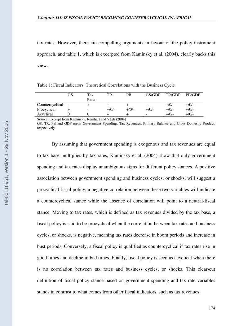
Chapter III: IS FISCAL POLICY BECOMING COUNTERCYCLICAL IN AFRICA?
174
tax rates. However, there are compelling arguments in favour of the policy instrument
approach, and table 1, which is excerpted from Kaminsky et al. (2004), clearly backs this
view.
Table 1: Fiscal Indicators: Theoretical Correlations with the Business Cycle
GS Tax Rates
TR PB GS/GDP TR/GDP PB/GDP
Countercyclical - + + + - +/0/- +/0/- Procyclical + - +/0/- +/0/- +/0/- +/0/- +/0/- Acyclical 0 0 + + - +/0/- +/0/-
Source: Excerpt from Kaminsky, Reinhart and Végh (2004) GS, TR, PB and GDP mean Government Spending, Tax Revenues, Primary Balance and Gross Domestic Product, respectively
By assuming that government spending is exogenous and tax revenues are equal
to tax base multiplies by tax rates, Kaminsky et al. (2004) show that only government
spending and tax rates display unambiguous signs for different policy stances. A positive
association between government spending and business cycles, or shocks, will suggest a
procyclical fiscal policy; a negative correlation between these two variables will indicate
a countercyclical stance while the absence of correlation will point to a neutral-fiscal
stance. Moving to tax rates, which is defined as tax revenues divided by the tax base, a
fiscal policy is said to be procyclical when the correlation between tax rates and business
cycles, or shocks, is negative, meaning tax rates decrease in boom periods and increase in
bust periods. Conversely, a fiscal policy is qualified as countercyclical if tax rates rise in
good times and decline in bad times. Finally, fiscal policy is seen as acyclical when there
is no correlation between tax rates and business cycles, or shocks. This clear-cut
definition of fiscal policy stance based on government spending and tax rate variables
stands in contrast to what comes from other fiscal indicators, such as tax revenues.
tel-0
0116
961,
ver
sion
1 -
29 N
ov 2
006
Chapter III: IS FISCAL POLICY BECOMING COUNTERCYCLICAL IN AFRICA?
175
We will illustrate this by focusing on one fiscal indicator reported in table 1,
namely tax revenues. A countercyclical fiscal policy in terms of tax revenues means that
these revenues rise in good times and drop in bad periods, suggesting therefore a positive
correlation between business cycle, or shocks, and tax revenues. What is confusing is that
the very same patterns might indicate the pursuit of a neutral fiscal stance. Indeed, a
positive (negative) shock could give rise to increased (decreased) tax revenues, via the
widening (shrinking) of the tax base, even if tax rates are kept constant59. Moreover, the
positive association between tax revenues and business cycles can be an indication of a
procyclical fiscal policy as well. Higher tax revenues in good times can go hand-in-hand
with lower tax rates, provided that tax base increases substantially. Conversely, lower tax
revenues in bad times can be accompanied with rising tax rates, which aim at offsetting
the shrinkage in tax base.
Because of the ambiguous cyclical behaviour of primary balance, government
revenues, and other variables presented in table 1, we will base our analysis on
government spending60 indicators, which provide a clear-cut measure of fiscal stance.
Government spending will be captured through the government total expenditure and the
government current expenditure. These two variables will be denominated in constant
terms.
Once we decide to define the cyclicality of fiscal policy in terms of public
spending, a question arises as how to measure cyclicality. We favour the approach that
59 This is very much similar to the automatic fiscal stability argument. 60 Even though tax rates fits into the group of indicators that give an unambiguous measure of fiscal stance, it is dropped because of data availability concern.
tel-0
0116
961,
ver
sion
1 -
29 N
ov 2
006
Chapter III: IS FISCAL POLICY BECOMING COUNTERCYCLICAL IN AFRICA?
176
consists in using the deviation of fiscal spending from its corresponding country
average61.
6.1.2 Explanatory variables
Turning to one of the key explanatory variables, the exogenous shock, Si,t , we
focus on terms of trade shock, which we believe is one of the most important shocks in
the context of African countries.62 Gauging the shock requires splitting terms of trade into
a trend component and a volatility component and then uses the volatility component as
the measurement of cyclicality. Two approaches are used. Firstly, we resort to the
Hodrick-Prescott (H-P) filter, which generates a smooth trend and stationary deviations63.
The deviation of terms of trade from its H-P- filtered trend will then capture the shock64.
Secondly, we turn to the approach suggested by Combes et al. (1999) for robustness
check. That approach assumes a broad specification, with series having the following
structure:
titiiiiti XctbaX ,1,, ε+++= −
61 It has been shown in Chap I that public spending series are stationary around a drift. 62 Ideally we should have added a variable that capture climate hazard. Agricultural sector output seems to be the ideal candidate but turns empirically not to be significant. 63 Following the frequency rule of power of Rvan and Uhlig (2002), we put the value of the smoothness parameter at 100. 64 The Hodrick-Prescott (HP) filter tool has been criticized on many grounds. Some of criticisms point to the arbitrary choice of the smoothness parameter. Additionally, it is shown the HP filter does not handle effectively structural breaks. Another weakness highlighted in the literature is the instability of the HP filter in the beginning and end of the sample because of its symmetric two-sided structure. Though the HP filter meets numerous criticisms, it is still commonly used because alternative tools are far from being perfect too. For instance, the Band-Pass (BP) filter designed by Baxter and King (1995) defines a cycle period between 6 and 32 quarters, which could be considered as arbitrary. Moreover, the BP filter has end-point instability problem too.
tel-0
0116
961,
ver
sion
1 -
29 N
ov 2
006
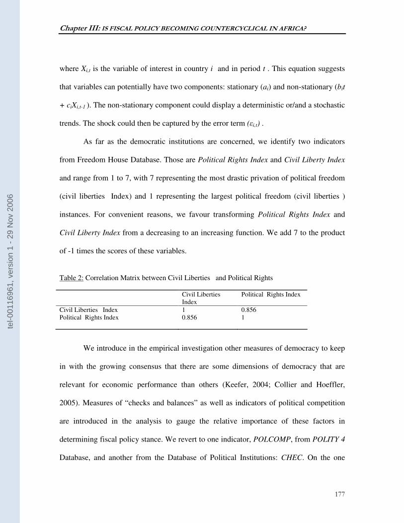
Chapter III: IS FISCAL POLICY BECOMING COUNTERCYCLICAL IN AFRICA?
177
where Xi,t is the variable of interest in country i and in period t . This equation suggests
that variables can potentially have two components: stationary (ai) and non-stationary (bit
+ ciXi,t-1 ). The non-stationary component could display a deterministic or/and a stochastic
trends. The shock could then be captured by the error term (εi,t) .
As far as the democratic institutions are concerned, we identify two indicators
from Freedom House Database. Those are Political Rights Index and Civil Liberty Index
and range from 1 to 7, with 7 representing the most drastic privation of political freedom
(civil liberties Index) and 1 representing the largest political freedom (civil liberties )
instances. For convenient reasons, we favour transforming Political Rights Index and
Civil Liberty Index from a decreasing to an increasing function. We add 7 to the product
of -1 times the scores of these variables.
Table 2: Correlation Matrix between Civil Liberties and Political Rights
Civil Liberties Index
Political Rights Index
Civil Liberties Index 1 0.856 Political Rights Index 0.856 1
We introduce in the empirical investigation other measures of democracy to keep
in with the growing consensus that there are some dimensions of democracy that are
relevant for economic performance than others (Keefer, 2004; Collier and Hoeffler,
2005). Measures of “checks and balances” as well as indicators of political competition
are introduced in the analysis to gauge the relative importance of these factors in
determining fiscal policy stance. We revert to one indicator, POLCOMP, from POLITY 4
Database, and another from the Database of Political Institutions: CHEC. On the one
tel-0
0116
961,
ver
sion
1 -
29 N
ov 2
006
Chapter III: IS FISCAL POLICY BECOMING COUNTERCYCLICAL IN AFRICA?
178
hand, POLCOMP measures the competitiveness of executive recruitment and is meant to
capture the degree of electoral competition. Its value ranges from 1 to 7, with higher
numbers indicating stronger competition. On the other hand, CHEC measures how many
political actors can blockpropose the legislation, therefore capturing the intensity of the
constraints that the executive faces. This variable is expected to measure “checks and
balances”. The highest value of this variable is also 7 while the lowest is 1. Higher score
corresponds to more constraints on the executive and consequently lower independence
of the executive.
6.1.3 Control variables
We add a small set of variables to control for the impact of political business
cycle, demographic factors, and openness, on fiscal stance. As argued before, politically
motivated fiscal policy can be pursued before elections, contributing to expansionary
stance during these times. We introduce presidential electoral dummy65 to capture this
dynamic. The demographic argument posits that a high dependency ratio demands
governments to commit more public resources to satisfy the growing needs of the
population. The demographic view is captured through the dependency ratio, which is the
ratio of people younger than 15 and older than 64 to those age between 15 and 64 years.
Finally, the rationale behind including trade shares as a control is to gauge the openness
65 The data on elections is compiled from CIA-World Factbook and Wikipedia, the free encyclopedia.
tel-0
0116
961,
ver
sion
1 -
29 N
ov 2
006
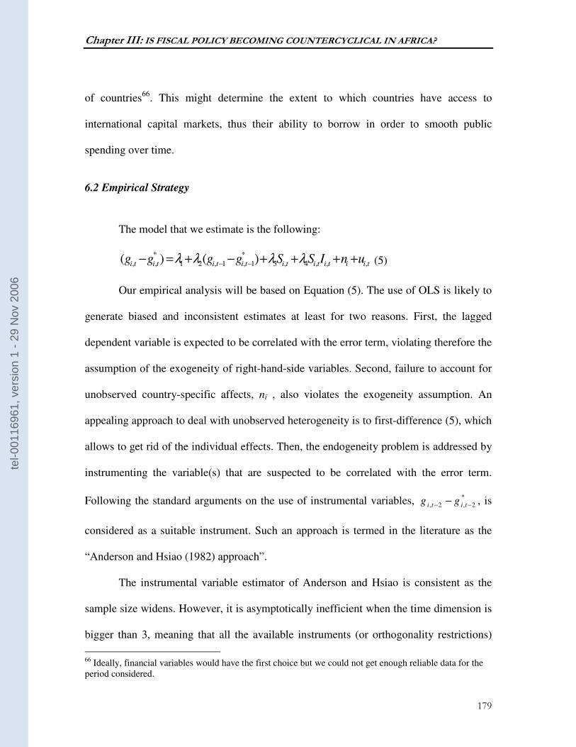
Chapter III: IS FISCAL POLICY BECOMING COUNTERCYCLICAL IN AFRICA?
179
of countries66. This might determine the extent to which countries have access to
international capital markets, thus their ability to borrow in order to smooth public
spending over time.
6.2 Empirical Strategy
The model that we estimate is the following:
tiitititititititi unISSgggg ,,,4,3
*
1,1,21
*
,, )()( ++++−+=− −− λλλλ (5)
Our empirical analysis will be based on Equation (5). The use of OLS is likely to
generate biased and inconsistent estimates at least for two reasons. First, the lagged
dependent variable is expected to be correlated with the error term, violating therefore the
assumption of the exogeneity of right-hand-side variables. Second, failure to account for
unobserved country-specific affects, ni , also violates the exogeneity assumption. An
appealing approach to deal with unobserved heterogeneity is to first-difference (5), which
allows to get rid of the individual effects. Then, the endogeneity problem is addressed by
instrumenting the variable(s) that are suspected to be correlated with the error term.
Following the standard arguments on the use of instrumental variables, *
2,2, −− − titi gg , is
considered as a suitable instrument. Such an approach is termed in the literature as the
“Anderson and Hsiao (1982) approach”.
The instrumental variable estimator of Anderson and Hsiao is consistent as the
sample size widens. However, it is asymptotically inefficient when the time dimension is
bigger than 3, meaning that all the available instruments (or orthogonality restrictions)
66 Ideally, financial variables would have the first choice but we could not get enough reliable data for the period considered.
tel-0
0116
961,
ver
sion
1 -
29 N
ov 2
006
Chapter III: IS FISCAL POLICY BECOMING COUNTERCYCLICAL IN AFRICA?
180
are not used. Arrelano and Bond (1991) propose a remedy for that problem by developing
a Generalised Method-of-Moments Estimator (GMM) that uses all the orthogonality
restrictions. All possible lags of the dependent variable from at least two periods earlier
and eventually lags of other right-hand side variables are used as instruments. However,
Blundell and Bond (1998) demonstrate that first-differenced GMM have poor finite
sample properties. Bond et al. (2001) indicate that this is the case when the series are
close to a random walk or when variance of the country-specific effects ni rises relative to
the variance of error term.
In order to address the problem associated with persistent panel data, Blundell and
Bond(1998) develop a system GMM estimator that is based on a simultaneous system of
two equations, which are the equation in level and that in difference. Lagged variables
serve as instruments for the differenced equation while their lagged first-differences are
the instruments for the equation in level.
The validity of the instruments is established by using an over-identification test.
This could be either the Sargan (1958) test of overidentifying restrictions or the Hansen
(1982) J-test, both testing whether the instruments are orthogonal to the error terms. This
should be complemented by a test on the no residual serial autocorrelation.
VII-RESULTS
The results of the implementation of our empirical construct are presented in this
section. We consider terms of trade volatility as the measurement of exogenous shock
because of the prominence of this factor in the debate on export performance, GDP
tel-0
0116
961,
ver
sion
1 -
29 N
ov 2
006
Chapter III: IS FISCAL POLICY BECOMING COUNTERCYCLICAL IN AFRICA?
181
growth, and fiscal policy in the context of African countries (Deaton, 1999). The
rationale is that the export basis of many African countries tends to be concentrated in a
few major primary commodities, making exports, government revenues, and expenditures
in these countries highly dependent to developments in commodity markets. We then
check the robustness of our results to alternative indicators or measurement of democratic
institutions and fiscal stance. Finally, we identify the critical aspect(s) of democracy that
are of relevance for conducting countercyclical fiscal policies.
7.1 Terms-of-trade shock, democratic institutions, and fiscal policy stance
7.1.1 Fiscal policy stance captured through government expenditure
Column 1 in Table 3 reports the relation between the cyclicality of government
expenditure, terms-of-trade shock, and democratic institutions. Democratic institutions
are measured by the Civil Liberties Index, ICL, which is derived from Freedom House
(2005). Fiscal stance is captured by the deviation of government expenditure from
country average normalised to country average. Terms-of-trade shock is derived from the
H-P cyclical component of terms of trade normalised to the filtered-trend, and weighted
by trade shares67 (Guillaumont et al., 1999, Combes and Saadi-Sedik, 2006). In line with
the model developed below, we introduce lagged fiscal stance to account for possible
persistent effects of previous fiscal policies. All the coefficients in this regression turn to
67 The idea is to capture the degree of exposure of countries to terms-of-trade shocks. The more open the countries are the more they are exposed to terms-of-trade shocks.
tel-0
0116
961,
ver
sion
1 -
29 N
ov 2
006
Chapter III: IS FISCAL POLICY BECOMING COUNTERCYCLICAL IN AFRICA?
182
have the theoretically expected signs and are statistically significant at conventional
levels. The coefficient on lagged fiscal policy cyclicality is positive, indicating the
existence of some degree of persistence in fiscal policy stance. The jointly positive
coefficient on terms-of-trade shock and negative coefficient on the interaction between
terms-of-trade shock and democracy is consistent with the trade-off concept developed in
the theoretical model. An exogenous shock is conducive to the adoption of procyclical
fiscal policy, but this outcome can potentially be alleviated and even reversed in the
presence of sound democratic institutions. Since some of the variables may be very
volatile, a question then arises as what is the relative magnitude of the effects of the
significant explanatory variables. We respond to this question by reverting to the concept
of “standardised beta coefficients” outlined by Isham et al. (2006). These coefficients are
the product of the coefficient on the variable of interest and the standard deviation of that
variable, divided by the standard deviation of the dependent variable. Results on these
coefficients are reported in column (1’). Interestingly, they suggest higher persistency of
fiscal policy, but more importantly they indicate the effect of the interaction of terms-of-
trade shock and democratic institutions may be as strong as the impact of the terms of
trade alone, meaning that democratic institutions could completely offset the negative
effect of terms-of-trade on the ability of government to pursue countercyclical fiscal
policies.
tel-0
0116
961,
ver
sion
1 -
29 N
ov 2
006
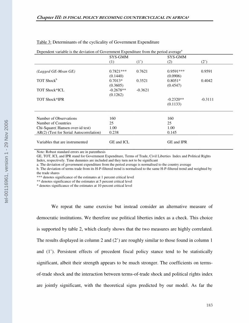
Chapter III: IS FISCAL POLICY BECOMING COUNTERCYCLICAL IN AFRICA?
183
Table 3: Determinants of the cyclicality of Government Expenditure Dependent variable is the deviation of Government Expenditure from the period averagea
SYS-GMM SYS-GMM (1) (1’) (2) (2’)
(Lagged GE-Mean GE) 0.7821***
(0.1440) 0.7621 0.9591***
(0.0906) 0.9591
TOT Shockb 0.7013* (0.3605)
0.3521 0.8051* (0.4547)
0.4042
TOT Shock*ICL -0.2678** (0.1262)
-0.3621
TOT Shock*IPR -0.2320** (0.1133)
-0.3111
Number of Observations 160 160 Number of Countries 25 25 Chi-Square( Hansen over-id test) 1.00 1.00 AR(2) (Test for Serial Autocorrelation) 0.238 0.145
Variables that are instrumented GE and ICL GE and IPR
Note: Robust standard errors are in parenthesis GE, TOT, ICL and IPR stand for Government Expenditure, Terms of Trade, Civil Liberties Index and Political Rights Index, respectively. Time dummies are included and they turn not to be significant a. The deviation of government expenditure from the period average is normalised to the country average b. The deviation of terms trade from its H-P-filtered trend is normalised to the same H-P-filtered trend and weighted by the trade shares *** denotes significance of the estimates at 1 percent critical level ** denotes significance of the estimates at 5 percent critical level * denotes significance of the estimates at 10 percent critical level
We repeat the same exercise but instead consider an alternative measure of
democratic institutions. We therefore use political liberties index as a check. This choice
is supported by table 2, which clearly shows that the two measures are highly correlated.
The results displayed in column 2 and (2’) are roughly similar to those found in column 1
and (1’). Persistent effects of precedent fiscal policy stance tend to be statistically
significant, albeit their strength appears to be much stronger. The coefficients on terms-
of-trade shock and the interaction between terms-of-trade shock and political rights index
are jointly significant, with the theoretical signs predicted by our model. As far the
tel-0
0116
961,
ver
sion
1 -
29 N
ov 2
006
Chapter III: IS FISCAL POLICY BECOMING COUNTERCYCLICAL IN AFRICA?
184
relative magnitude of the effects of the right-hand-side variables is concerned, we find the
interaction between terms-of-trade shock and political rights index to be more modest and
to offset only partially the procyclical bias of terms-of-trade shock.
7.1.2 Fiscal policy stance captured through government current expenditure
One concern with our results in table 3 is that they may depend on the choice of
the measure for the dependent variable. To shed some light on this issue, we estimate the
same model as in table 3, but with other measures of public spending: current
expenditure68. Results are then summarised in table 4. They lend strong support to the
argument that democratic institutions are conducive to the adoption of countercyclical
fiscal policies.
68 In addition to current expenditure, we try with current expenditure minus interest payments but the results turn to be roughly identical.
tel-0
0116
961,
ver
sion
1 -
29 N
ov 2
006
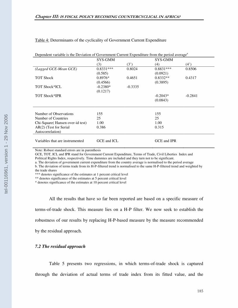
Chapter III: IS FISCAL POLICY BECOMING COUNTERCYCLICAL IN AFRICA?
185
Table 4: Determinants of the cyclicality of Government Current Expenditure
Dependent variable is the Deviation of Government Current Expenditure from the period averagea
SYS-GMM SYS-GMM (3) (3’) (4) (4’)
(Lagged GCE-Mean GCE) 0.8331*** (0.585)
0.8024 0.8831*** (0.0921)
0.8506
TOT Shock 0.8976* (0.4566)
0.4651 0.8332** (0.3895)
0.4317
TOT Shock*ICL -0.2380* (0.1217)
-0.3335
TOT Shock*IPR -0.2043* (0.0843)
-0.2841
Number of Observations 155 155 Number of Countries 25 25 Chi-Square( Hansen over-id test) 1.00 1.00 AR(2) (Test for Serial Autocorrelation)
0.386 0.315
Variables that are instrumented GCE and ICL GCE and IPR
Note: Robust standard errors are in parenthesis GCE, TOT, ICL and IPR stand for Government Current Expenditure, Terms of Trade, Civil Liberties Index and Political Rights Index, respectively. Time dummies are included and they turn not to be significant. a. The deviation of government current expenditure from the country average is normalised to the period average b. The deviation of terms trade from its H-P-filtered trend is normalised to the same H-P-filtered trend and weighted by the trade shares *** denotes significance of the estimates at 1 percent critical level ** denotes significance of the estimates at 5 percent critical level * denotes significance of the estimates at 10 percent critical level
All the results that have so far been reported are based on a specific measure of
terms-of-trade shock. This measure lies on a H-P filter. We now seek to establish the
robustness of our results by replacing H-P-based measure by the measure recommended
by the residual approach.
7.2 The residual approach
Table 5 presents two regressions, in which terms-of-trade shock is captured
through the deviation of actual terms of trade index from its fitted value, and the
tel-0
0116
961,
ver
sion
1 -
29 N
ov 2
006
Chapter III: IS FISCAL POLICY BECOMING COUNTERCYCLICAL IN AFRICA?
186
dependent variable in these regressions is the deviation of government total expenditure
from country average. The indicator of terms-of-trade shock is an estimated variable.
Therefore, its standard error is likely to be biased. We correct this bias by using the
method of bootstrapping, which is a commonly used method of resampling (Wooldridge,
2002). The general idea is to consider the observed sample as the population and, at each
iteration, draw from this sample a sub-sample that is used to estimate coefficients on
terms-of-trade shock and on the interaction between terms-of-trade shock and political
institution variables. Several iterations69 are run and the estimated coefficients are used to
compute the real values of the standard errors.
The results reported in column 5 are satisfactory as all the coefficients on
explanatory variables appear with the theoretically expected signs. Lagged fiscal stance
has significant and high explanatory power on current fiscal policy, suggesting persistent
effects. Column 5 also indicates that terms-of-trade shock potentially introduces a
procyclical bias to fiscal policy, as shown by the positive coefficient on terms-of-trade
volatility. Finally, the interaction between terms-of-trade shock and institutions,
measured by civil liberties index, ICL, appears with a significant negative coefficient,
confirming the offsetting impact of democratic institutions. It is worth noting that both
the absolute and relative magnitude of the coefficient on the interaction between terms-
of-trade shock and institutions is lower than what was previously found. Overall, these
results are in line with those found earlier. The next move is to see if the results hold up
when using an alternative measure for institutions. Column 6 reports the results based on
the use of political rights index, IPR, as the measure of the quality of political institutions.
69 We run 1 000 iterations in this exercise.
tel-0
0116
961,
ver
sion
1 -
29 N
ov 2
006
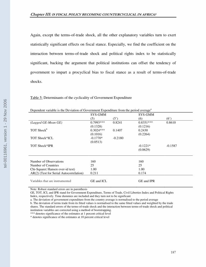
Chapter III: IS FISCAL POLICY BECOMING COUNTERCYCLICAL IN AFRICA?
187
Again, except the terms-of-trade shock, all the other explanatory variables turn to exert
statistically significant effects on fiscal stance. Especially, we find the coefficient on the
interaction between terms-of-trade shock and political rights index to be statistically
significant, backing the argument that political institutions can offset the tendency of
government to impart a procyclical bias to fiscal stance as a result of terms-of-trade
shocks.
Table 5: Determinants of the cyclicality of Government Expenditure
Dependent variable is the Deviation of Government Expenditure from the period averagea
SYS-GMM SYS-GMM (5) (5’) (6) (6’)
(Lagged GE-Mean GE) 0.7993*** (0.1328)
0.8241 0.8351*** (0.1216)
0.8610
TOT Shockb 0.3024*** (0.1016)
0.1407 0.2430 (0.2264)
TOT Shock*ICL -0.1770* (0.0513)
-0.2180
TOT Shock*IPR -0.1221* (0.0629)
-0.1587
Number of Observations 160 160 Number of Countries 25 25 Chi-Square( Hansen over-id test) 1.00 1.00 AR(2) (Test for Serial Autocorrelation) 0.211 0.174
Variables that are instrumented GE and ICL GE and IPR
Note: Robust standard errors are in parenthesis GE, TOT, ICL and IPR stand for Government Expenditure, Terms of Trade, Civil Liberties Index and Political Rights Index, respectively. Time dummies are included and they turn not to be significant a. The deviation of government expenditure from the country average is normalised to the period average b. The deviation of terms trade from its fitted values is normalised to the same fitted values and weighted by the trade shares. The standard errors of the terms-of-trade shock and the interaction between terms-of-trade shock and political institution variables are corrected using a method of bootstrapping. *** denotes significance of the estimates at 1 percent critical level * denotes significance of the estimates at 10 percent critical level
tel-0
0116
961,
ver
sion
1 -
29 N
ov 2
006
Chapter III: IS FISCAL POLICY BECOMING COUNTERCYCLICAL IN AFRICA?
188
We again conduct robustness check by using an alternative measure of fiscal
stance, which is based on government current expenditure rather than government total
expenditure70. Results are reported in table 6. They are very much similar to those found
earlier. Except the terms-of-trade shock, all the key variables of interest appear with the
theoretically expected signs and are statistically significant at conventional levels. We
find, for instance, the coefficient on lagged discretionary fiscal policy measure to be
positive and slightly bigger than what was uncovered in previous findings, confirming the
presence of a persistence effect of previous discretionary fiscal policy. The coefficients
on terms-of-trade shock and on the interaction between terms-of-trade shock and political
institutions are robust and exhibit the right signs, implying again that economies that
exhibit sound political institutions are prone to conduct countercyclical fiscal policies
when facing terms-of-trade shocks.
70 In addition to current expenditure, we try with current expenditure minus interest payments but the results turn to be roughly identical.
tel-0
0116
961,
ver
sion
1 -
29 N
ov 2
006
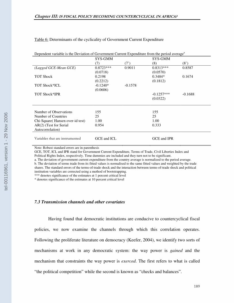
Chapter III: IS FISCAL POLICY BECOMING COUNTERCYCLICAL IN AFRICA?
189
Table 6: Determinants of the cyclicality of Government Current Expenditure
Dependent variable is the Deviation of Government Current Expenditure from the period averagea
SYS-GMM SYS-GMM (7) (7’) (8) (8’)
(Lagged GCE-Mean GCE) 0.8723*** (0.0718)
0.9011 0.8313*** (0.0570)
0.8587
TOT Shock 0.2198 (0.2212)
0.3484* (0.1812)
0.1674
TOT Shock*ICL -0.1240* (0.0606)
-0.1578
TOT Shock*IPR -0.1257*** (0.0322)
-0.1688
Number of Observations 155 155 Number of Countries 25 25 Chi-Square( Hansen over-id test) 1.00 1.00 AR(2) (Test for Serial Autocorrelation)
0.954 0.333
Variables that are instrumented GCE and ICL GCE and IPR
Note: Robust standard errors are in parenthesis GCE, TOT, ICL and IPR stand for Government Current Expenditure, Terms of Trade, Civil Liberties Index and Political Rights Index, respectively. Time dummies are included and they turn not to be significant. a. The deviation of government current expenditure from the country average is normalized to the period average. b. The deviation of terms trade from its fitted values is normalised to the same fitted values and weighted by the trade shares. The standard errors of the terms-of-trade shock and the interaction between terms-of-trade shock and political institution variables are corrected using a method of bootstrapping. *** denotes significance of the estimates at 1 percent critical level * denotes significance of the estimates at 10 percent critical level
7.3 Transmission channels and other covariates
Having found that democratic institutions are conducive to countercyclical fiscal
policies, we now examine the channels through which this correlation operates.
Following the proliferate literature on democracy (Keefer, 2004), we identify two sorts of
mechanisms at work in any democratic system: the way power is gained and the
mechanism that constraints the way power is exerced. The first refers to what is called
“the political competition” while the second is known as “checks and balances”.
tel-0
0116
961,
ver
sion
1 -
29 N
ov 2
006
Chapter III: IS FISCAL POLICY BECOMING COUNTERCYCLICAL IN AFRICA?
190
To gauge the relative importance of these two dimensions in the measurement of
the quality of democratic institutions, we regress civil liberties index, ICL, and political
rights index, IPR, on political competition, POLCOMP, and checks and balances, CHEC,
and the results are recorded in columns 9 and 10, respectively. All the coefficients in
those regressions are found to be robustly significant. In particular, coefficients on
POLCOMP and CHEC display positive signs and are statistically significant at one
percent, supporting the argument that political competition and checks and balances
constitute some important aspects of democratic regimes. We also find the coefficients on
political competition to be much higher than those on checks and balances, suggesting
that a higher consideration is given to political competition in designing the indicators of
democratic institutions. In sum, we find the competitiveness of elections and restraints on
the executive branch to be two important dimensions of democratic regimes.
tel-0
0116
961,
ver
sion
1 -
29 N
ov 2
006
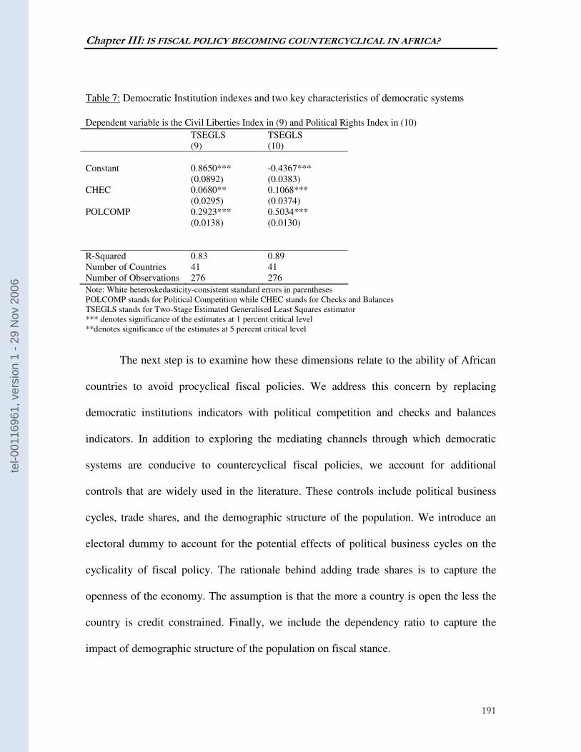
Chapter III: IS FISCAL POLICY BECOMING COUNTERCYCLICAL IN AFRICA?
191
Table 7: Democratic Institution indexes and two key characteristics of democratic systems
Dependent variable is the Civil Liberties Index in (9) and Political Rights Index in (10)
TSEGLS TSEGLS (9) (10)
Constant 0.8650***
(0.0892) -0.4367*** (0.0383)
CHEC 0.0680** (0.0295)
0.1068*** (0.0374)
POLCOMP 0.2923*** (0.0138)
0.5034*** (0.0130)
R-Squared 0.83 0.89 Number of Countries 41 41 Number of Observations 276 276
Note: White heteroskedasticity-consistent standard errors in parentheses POLCOMP stands for Political Competition while CHEC stands for Checks and Balances TSEGLS stands for Two-Stage Estimated Generalised Least Squares estimator *** denotes significance of the estimates at 1 percent critical level **denotes significance of the estimates at 5 percent critical level
The next step is to examine how these dimensions relate to the ability of African
countries to avoid procyclical fiscal policies. We address this concern by replacing
democratic institutions indicators with political competition and checks and balances
indicators. In addition to exploring the mediating channels through which democratic
systems are conducive to countercyclical fiscal policies, we account for additional
controls that are widely used in the literature. These controls include political business
cycles, trade shares, and the demographic structure of the population. We introduce an
electoral dummy to account for the potential effects of political business cycles on the
cyclicality of fiscal policy. The rationale behind adding trade shares is to capture the
openness of the economy. The assumption is that the more a country is open the less the
country is credit constrained. Finally, we include the dependency ratio to capture the
impact of demographic structure of the population on fiscal stance.
tel-0
0116
961,
ver
sion
1 -
29 N
ov 2
006
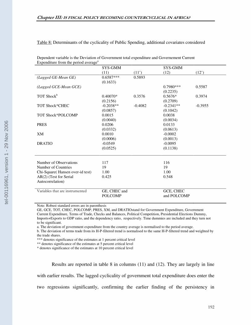
Chapter III: IS FISCAL POLICY BECOMING COUNTERCYCLICAL IN AFRICA?
192
Table 8: Determinants of the cyclicality of Public Spending, additional covariates considered
Dependent variable is the Deviation of Government total expenditure and Governement Current Expenditure from the period averagea
SYS-GMM SYS-GMM (11) (11’) (12) (12’)
(Lagged GE-Mean GE) 0.6587*** (0.1633)
0.5893
(Lagged GCE-Mean GCE) 0.7980*** (0.2235)
0.5587
TOT Shockb 0.40070* (0.2156)
0.3576 0.5676* (0.2709)
0.3974
TOT Shock*CHEC -0.2038** (0.0857)
-0.4082 -0.2341** (0.1042)
-0.3955
TOT Shock*POLCOMP 0.0015 (0.0040)
0.0038 (0.0034)
PRES 0.0206 (0.0332)
0.0133 (0.0613)
XM 0.0010 (0.0006)
-0.0002 (0.0013)
DRATIO -0.0549 (0.0525)
-0.0095 (0.1138)
Number of Observations 117 116 Number of Countries 19 19 Chi-Square( Hansen over-id test) 1.00 1.00 AR(2) (Test for Serial Autocorrelation)
0.425 0.548
Variables that are instrumented GE, CHEC and
POLCOMP GCE, CHEC
and POLCOMP
Note: Robust standard errors are in parenthesis GE, GCE, TOT, CHEC, POLCOMP, PRES, XM, and DRATIOstand for Government Expenditure, Government Current Expenditure, Terms of Trade, Checks and Balances, Political Competition, Presidential Elections Dummy, Imports+Exports to GDP ratio, and the dependency ratio, respectively. Time dummies are included and they turn not to be significant. a. The deviation of government expenditure from the country average is normalised to the period average. b. The deviation of terms trade from its H-P-filtered trend is normalised to the same H-P-filtered trend and weighted by the trade shares. *** denotes significance of the estimates at 1 percent critical level ** denotes significance of the estimates at 5 percent critical level * denotes significance of the estimates at 10 percent critical level
Results are reported in table 8 in columns (11) and (12). They are largely in line
with earlier results. The lagged cyclicality of government total expenditure does enter the
two regressions significantly, confirming the earlier finding of the persistency in
tel-0
0116
961,
ver
sion
1 -
29 N
ov 2
006
Chapter III: IS FISCAL POLICY BECOMING COUNTERCYCLICAL IN AFRICA?
193
cyclicality. Other interesting finding is that the coefficient on terms-of-trade shock is
statistically significant at conventional levels and turns with the right sign (positive sign).
As mentioned before this result suggests that a positive (negative) exogenous shock,
irrespective of the quality of political institutions, gives rise to expansionary
(contractionary) fiscal stance.
Moving to the two features of democratic systems, we find the interaction
between terms-of-trade shock and checks and balances indicator, TOT Shock*CHEC, to
have a statistically significant negative impact on the cyclicality of public spending,
suggesting that constraints on the executive branch have the potential to make fiscal
policy countercyclical in the presence of exogenous shocks. On the other hand, the
coefficient on the interaction between terms-of-trade shock and political competition
indicator, TOT Shock*POLCOMP, is not statistically significant. This result might
indicate that political competition alone does not set conditions for fiscal policies to be
countercyclical. These results therefore lend strong support to the argument that
democratic institutions are prone to conduct countercyclical not because of the electoral
competition they brought about but because of the effective restraints they put on rulers.
Turning to other controls, we find all to be statistically insignificant. Political
business cycle, the degree of openness, and the demographic structure of the population
do not impact directly the cyclicality of fiscal policy. The non-significance of the
coefficient on the electoral dummy may indicate that political business cycles may be
neutralised in the presence of effective constraints of the executive. Assuming that the
trade shares capture the degree of openness, the lack of significance of the coefficient on
trade shares may illustrate the imperfection of the international capital markets
tel-0
0116
961,
ver
sion
1 -
29 N
ov 2
006
Chapter III: IS FISCAL POLICY BECOMING COUNTERCYCLICAL IN AFRICA?
194
(Kaminsky et al., 2004). In other terms, even open economies can not borrow during bad
times to smooth public spending.
Overall, the main argument holds up even when one includes additional controls.
Democratic institutions facilitate the adoption of countercyclical fiscal policies mainly
because of the effective constraints these institutions place on the executive.
VIII-CONCLUSION
The vast majority of African countries went through bold political transformations
in the earlier 1990s, especially moving from one-party rule to increased political
pluralism. The period that predates the democratisation era was characterised by a broad
wave of authoritarian rule, procyclical economic policies, including fiscal and monetary,
and poor economic growth. These three events have been proven to be closely related.
For that reason, a move towards greater democracy in many African countries
legitimately raises hopes among many analysts for an improved economic management
and stronger and sustained economic growth. The goal of this chapter was therefore to
test whether democratic reforms in the context of African countries have the potential to
make fiscal policy more countercyclical. If this is the case, what are the channels through
which this correlation operates?
The empirical analysis is based on panel data of 47 African countries over the
1989-2002 period, and the estimation technique used is the system Generalised Method-
of-Moments Estimator System (SYS-GMM). We found measures of government
spending cyclicality to be negatively and strongly correlated with the interaction between
tel-0
0116
961,
ver
sion
1 -
29 N
ov 2
006
Chapter III: IS FISCAL POLICY BECOMING COUNTERCYCLICAL IN AFRICA?
195
democratic institution indicators (political rights index and civil liberties index) and
terms-of-trade shock. This result is consistent with the prediction of our model, which is
that sound democratic institutions are conducive to countercyclical policies. Moving to
the channels through which fiscal policy matters for fiscal policy, we focused on two
critical aspects of democratic institutions, which are electoral competition and checks and
balances. These two dimensions of democratic systems are found to be strongly related to
the two measures of democratic institutions (political rights index and civil liberties
index). Among the two dimensions of a democratic system, electoral competition,
however, seems to have the highest weight in the construction of indicators of democratic
institutions.
Even though more weight is given to political competition in the compilation of
democratic institutions indexes, we found this dimension of democracy to be uncorrelated
to fiscal policy stance. On the contrary, we found formal institutions that impose
restraints on the executive branch to be the key factor that explain why democracies can
smooth business cycles better than autocracies.
tel-0
0116
961,
ver
sion
1 -
29 N
ov 2
006
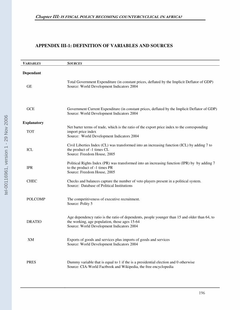
Chapter III: IS FISCAL POLICY BECOMING COUNTERCYCLICAL IN AFRICA?
196
APPENDIX III-1: DEFINITION OF VARIABLES AND SOURCES
VARIABLES SOURCES
Dependant
GE GCE
Total Government Expenditure (in constant prices, deflated by the Implicit Deflator of GDP) Source: World Development Indicators 2004 Government Current Expenditure (in constant prices, deflated by the Implicit Deflator of GDP) Source: World Development Indicators 2004
Explanatory
TOT
Net barter terms of trade, which is the ratio of the export price index to the corresponding import price index Source: World Development Indicators 2004
ICL
Civil Liberties Index (CL) was transformed into an increasing function (ICL) by adding 7 to the product of -1 times CL Source: Freedom House, 2005
IPR
Political Rights Index (PR) was transformed into an increasing function (IPR) by by adding 7 to the product of -1 times PR Source: Freedom House, 2005
CHEC
Checks and balances capture the number of veto players present in a political system. Source: Database of Political Institutions
POLCOMP
The competitiveness of executive recruitment. Source: Polity 5
DRATIO
Age dependency ratio is the ratio of dependents, people younger than 15 and older than 64, to the working, age population, those ages 15-64 Source: World Development Indicators 2004
XM
Exports of goods and services plus imports of goods and services Source: World Development Indicators 2004
PRES
Dummy variable that is equal to 1 if the is a presidential election and 0 otherwise Source: CIA-World Factbook and Wikipedia, the free encyclopedia
tel-0
0116
961,
ver
sion
1 -
29 N
ov 2
006
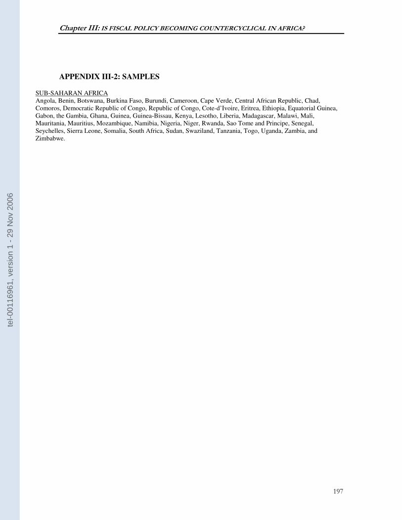
Chapter III: IS FISCAL POLICY BECOMING COUNTERCYCLICAL IN AFRICA?
197
APPENDIX III-2: SAMPLES SUB-SAHARAN AFRICA Angola, Benin, Botswana, Burkina Faso, Burundi, Cameroon, Cape Verde, Central African Republic, Chad, Comoros, Democratic Republic of Congo, Republic of Congo, Cote-d’Ivoire, Eritrea, Ethiopia, Equatorial Guinea, Gabon, the Gambia, Ghana, Guinea, Guinea-Bissau, Kenya, Lesotho, Liberia, Madagascar, Malawi, Mali, Mauritania, Mauritius, Mozambique, Namibia, Nigeria, Niger, Rwanda, Sao Tome and Principe, Senegal, Seychelles, Sierra Leone, Somalia, South Africa, Sudan, Swaziland, Tanzania, Togo, Uganda, Zambia, and Zimbabwe.
tel-0
0116
961,
ver
sion
1 -
29 N
ov 2
006

198
tel-0
0116
961,
ver
sion
1 -
29 N
ov 2
006
GENERAL CONCLUSION
199
GENERAL CONCLUSION
tel-0
0116
961,
ver
sion
1 -
29 N
ov 2
006
GENERAL CONCLUSION
200
GENERAL CONCLUSION
Despite the recent growth resumption in Sub-Saharan Africa, the region continues
to harbour the majority of the world’s poorest nations. Per-capita income is still below
the level achieved before the 1973 oil shock. The distribution of incomes and assets is
largely skewed, and Africa is considered the second highest unequal region in the world
(United Nations, 2006). The poor growth record and high inequality conspire to increase
poverty. Africa is home to a growing share of the world’s absolute poor.
However, there are some positive developments. There is an increasing number of
countries that have made headway in pursuing economic and political reforms, which
both are believed to be conducive to strong economic growth. Most of the economic
reforms that have been implemented are rooted in the dependent economy model. Real
exchange rate and absorption, captured by public spending, are therefore the two
variables targeted by policy-makers. Chapter I revisits the policy argument along the
lines of the arguments developed by Guillaumont et al. (1999) and looks into the role
played by policy instabilities in the poor growth performance of African countries.
However, the approach adopted in Chapter I differs from earlier work in two
perspectives. First, it relies entirely on the key variables underscored in the dependent
economy model, namely the real exchange rate and public spending. Second, the analysis
is based on dynamic panel data instead of the commonly use of cross-country data. The
empirical investigation shows that only real exchange instability has a direct significant
influence on economic growth. The combination of a statistical significance of real
tel-0
0116
961,
ver
sion
1 -
29 N
ov 2
006
GENERAL CONCLUSION
201
exchange instability and the non-significance of public spending instability, when
incorporated in the same regression, indicates that both are not two distinct factors
regarding their impact on per capita growth. Public spending instability has a significant
positive predictive power over real exchange rate instability, which in turn hampers
growth both through investment and productivity channels. Also, real exchange rate
instability has asymmetric effects on economic growth as the relationship between these
two variables is driven by real exchange rate appreciation. Finally, partial evidence
supports the view that real exchange rate appreciation contributes to the decline of sectors
with important positive externalities, thereby leading to persistent productivity losses and
weak economic growth. Overall, we interpret these findings as suggesting that the
stability of public spending and real exchange rate are keys to Africa’s long-term
economic growth. Reducing large fluctuations in public spending requires gaining some
control over both internal and external sources of government revenues. In many African
countries, with a narrow production basis, domestic revenues are closely linked to
developments in commodity markets. The long-term solution for government revenue
and expenditure instability is to broaden the revenue base through economic
diversification. However, achieving stability of government domestic revenues in the
short-run may be facilitated by the adoption of contingent financial instruments and some
institutional arrangements, such as the establishment of a stabilisation fund. The use of
contingent financial instruments, such as futures, swaps, and options, has the potential to
transfer commodity price instability to international markets and guarantee more stable
public revenue and expenditure. However, the shortcoming of this scheme is that it
requires a sophisticated domestic financial sector, or at least capacity in trading
tel-0
0116
961,
ver
sion
1 -
29 N
ov 2
006
GENERAL CONCLUSION
202
commodity-backed financial instruments. Such institutional structures do not yet exist in
many African countries. Contrary to the contingent financial tools, stabilisation seems to
be a feasible solution. The stabilisation fund serves as a buffer mechanism whereby part
of windfall revenues are transferred from the budget to the stabilisation fund during times
of increasing commodity prices and the other way around when prices are declining,
ensuring therefore a stability of public spending. The other source of uncertainty for
government revenue is the flow of resources from abroad that finance government deficit.
Most African countries rely on aid flows in that respect, which means a more predictable
aid could also be beneficial. Having more stable public spending could take care of an
important source of real exchange rate instability.
The dependent economy model also serves as the main theoretical framework to
investigate the controversial nexus between economic policies and poverty in chapter II.
The approach used in that chapter consists in assessing the impact of economic policies
on poverty through real exchange rate and public spending, with more emphasis on real
exchange rate. The main argument put forward in the theoretical framework is that the
depreciation of real exchange rate is conducive to poverty reduction provided that there
are good institutions and a fairly equal income distribution.
The empirical investigation strongly supports the view that high inequality,
proxied by income Gini coefficient, impedes the potential positive effect of real exchange
rate depreciation on the poor incomes. It also largely backs the contention that the
potential positive impact of real exchange rate depreciation on the poor is much stronger
tel-0
0116
961,
ver
sion
1 -
29 N
ov 2
006
GENERAL CONCLUSION
203
when institutions are sound. In addition, it appears that there is no asymmetric effect of
real exchange rate on the incomes of the poor. These findings hold when adding
additional covariates. Additional controls are added to the analysis to account for other
factors that might have been missed. Among these variables, education appears to be
critical for poverty reduction. On the other hand, trade openness, agricultural
productivity, and public spending are found not to be statistically associated with the
incomes of the poor. The lack of significant coefficients associated with these variables
does not mean a complete absence of relationships between these indicators and poverty
but rather indicates that trade openness, agricultural productivity, and public spending
come into play indirectly because of their potential impact on economic growth. The
main lesson that can be drawn from these findings is that policies favouring the
depreciation of real exchange rate could be a powerful tool for poverty reduction,
provided they are complemented by reforms that facilitate the access of the poor to
production factors and improve the quality of institutions.
The quality of institutions, notably political institutions, is at the core of the issues
raised in Chapter III. The vast majority of African countries went through bold political
transformations in the early 1990s, especially moving from one-party rule to increased
political pluralism. This development raised hopes because the period that predates this
wave of democratisation was characterised by authoritarian rule, procyclical economic
policies, including fiscal and monetary, and poor economic growth, which all three have
been proven to be closely related. Chapter III attempts to test whether democratic
reforms, in the context of African countries, have the potential to make fiscal policy more
tel-0
0116
961,
ver
sion
1 -
29 N
ov 2
006
GENERAL CONCLUSION
204
countercyclical. In addition, it tries to uncover the channels, through which this
correlation operates, if there is any association between democratic changes and
countercyclical policy.
Assuming that terms-of-trade shock captures the deviation of output from its
long-term level, the empirical analysis suggests that the cyclicality of government
spending is negatively and strongly associated with the interaction between democratic
institution indicators (political rights index and civil liberties index) and terms-of-trade
shock. This result is consistent with the main argument developed in the chapter, namely
that sound democratic institutions are conducive to countercyclical policies. As far as the
transmission channels are concerned, we focused on two critical dimensions of
democratic institutions, which include electoral competition and the checks and balances.
These two dimensions of democratic systems are found to be strongly related to the two
measures of democratic institutions (political rights index and civil liberties index).
Among the two dimensions of a democratic system, electoral competition, however, has
implicitly the highest weight in the construction of indicators of democratic institutions.
Even though more weight is given to political competition in the compilation of
democratic institutions indexes, we find this dimension of democracy not be condusive to
countercyclical fiscal policies. On the contrary, we find formal institutions that impose
restraints on the executive branch to be the key factor explaining why democracies can
smooth business cycles better than autocracies. The policy implication is that the recent
wave of democratisation constitutes a positive development because it provides countries
with the opportunity to avoid procyclical policy. Competitive elections are important.
tel-0
0116
961,
ver
sion
1 -
29 N
ov 2
006
GENERAL CONCLUSION
205
But, taken alone, they do not guarantee changes in the cyclical properties of fiscal policy.
Promoting and accelerating the introduction of domestic effective restraints on the
executive branch, which prove to be more sustainable than foreign-led constraints, would
probably increase the likelihood of adopting countercyclical fiscal policies.
Overall, the conclusive findings of the empirical investigation conducted in all the
three chapters should not obscure the importance of dealing effectively with variable
definition problems. All the empirical results in Chapter I are based on a definition of
poverty that relies on the fifth poorest quintile. Future research would gain from
considering alternative measures of poverty as there has been significant progress in
collecting household surveys in recent years. Also in the same chapter, we revert to
political institution variables as proxies for institutions because we could not get time-
varying indicators of institutions such as those generated by ICRG71. Again, addressing
such a shortcoming would be of great interest. The same also holds true for the indicator
for inequality since we use income Gini coefficient instead of an indicator that captures
the distribution of assets.
In addition to variable definition problems, some substantive questions require
further exploration. Chapter II finds a strong evidence for a positive relationship between
real exchange rate and public spending stability and growth. The experience of African
countries suggests that stable real exchange rate and public spending are exceptions
71 International Country Risk Guide index is based on underlying numerical evaluations with respect to the expropriation risk, corruption, the rule of law, and government repudiation of contracts.
tel-0
0116
961,
ver
sion
1 -
29 N
ov 2
006
GENERAL CONCLUSION
206
rather than the rules. Then, the question of what motives push governments to pursue
such policies may require further investigation. Finally, Chapter III substantiates the view
that a move toward democratic systems is favourable to countercyclical fiscal policy,
especially if checks and balances are in place. This analysis is arguably general because it
does not account for the variety of electoral rules and forms of governments. In other
words, the view might be seen as falling under the trap of “One size fits all”. Perhaps one
of the greatest payoffs for future research on the relationship between the cyclical
properties of fiscal policies and democracy is likely to be obtained by considering the
wide range of political systems across democracies.
tel-0
0116
961,
ver
sion
1 -
29 N
ov 2
006
REFERENCES
207
REFERENCES Acemoglu, D and S. Johnson (2003) “Unbundling Institutions” NBER Working Paper
No. 9934
Acemoglu, D., J. Robinson and S. Johnson (2001) “The Colonial Origins of Comparative
Development: An Empirical Investigation” American Economic Review, Vol.91,
pp.1396-1401
Acemuglu, D., J. Robinson, and S. Johnson (2003) “An African Success Story:
Botswana” in Search of Prosperity: Analytical Narrative on Economic Growth, edited by
Dani Rodrik, Princeton University Press
Agénor, Pierre-Richard (2004) “Macroeconomic Adjustment and the Poor: Analytical
Issues and Cross-Country Evidence” Journal of Economic Surveys, Vol.18, pp.351-408
Aghion P. and P. Howitt (1992) “A Model of Growth through Creative Destruction”
Econometrica, Vol. 60, pp.323-51
Aitchinson, J and J.A.C. Brown (1966) The Lognormal Distribution, Cambridge:
Cambridge University Press.
Ake, C. (1990) The Case for Democracy: African Governance in the 1990s, Atlanta, Ga.
: Carter Center
Akerlof, George and William T. Dickens (1982) “The Economic Consequences of
Cognitive Dissonance” American Economic Review, Vol.72, pp.307-19
Alesina, A., N. Roubini, and G. Cohen (1997) Political Cycles and the Macroeconomy.
Cambridge MA: MIT Press.
tel-0
0116
961,
ver
sion
1 -
29 N
ov 2
006
REFERENCES
208
Alesina, A., S. Olzer, N. Roubini, and P. Swagel (1996) “Political Instability and
Economic Growth” Journal of Economic Growth, Vol.1, pp. 189-213
Alesina, Alberto and Roberto, Perotti (1996) “Income Distribution, Political Instability,
and Investment” European Economic Review, Vol. 40, pp.1203-25
Alesina, Alberto, and Dani, Rodrik (1994) “Distributive Politics and Economic Growth”
Quartely Journal of Economics, Vol.109, pp.465-90
Alesina, Alberto, and Guido, Tabellini (2005) “Why is Fiscal Policy Often Procyclical?”
NBER Working Paper, No. 11600
Ali, A.A.G. (1998) “Structural adjustment in sub-Saharan Africa: 1985-1995” in
T.Mkandawire and C.C.Soludo (eds.) African perspectives on structural adjustement
Vol.2, International Development Research Centre, Ottawa, O.N. Canada
Anand, Sudhir and Amartya Sen (1994) “Sustainable Human Development: Concepts
and Measurement” Occasional Paper 1, Human Development Report Office
Anderson, T. and Hsiao, C. (1982) “Formulation and Estimation of Dynamic Models
using Panel Data” Journal of Econometrics, Vol.18, pp.67-82
Arcand, Jean-Louis and Béatrice d'Hombres (2005) “Explaining the Negative Coefficient
Associated with Human Capital in Augmented Solow Growth Regressions”
Macroeconomics 0510010, Economics Working Paper Archive EconWPA
Arellano, Manuel and Steven Bond (1991) “Some Tests of Specification for Panel Data:
Monte Carlo Evidence and Application to Employment Equations” Review of Economic
Studies, Vol.58, 277-97
tel-0
0116
961,
ver
sion
1 -
29 N
ov 2
006
REFERENCES
209
Aschauer, David A. (1989) “Is Public Expenditure Productive?” Journal of Monetary
Economics, Vol. 23, pp. 177-200.
Atkinson, A.B (1970) “On the measurement of inequality” Journal of Economic Theory,
Vol. 2, pp. 244--263.
Azam, Jean-Paul (1999) “Dollars for Sale: Exchange Rate Policy and Inflation in Africa”
World Development, Vol.27, pp.1843-1859
Azam, Jean-Paul, Fosu, Augustin and Ndung’u, Njuguna S. (2002) “Explaining Slow
Growth in Africa” African Development Review, Vol. 14, pp. 177-220
Barro, Robert J. (1999) “Inequality, Growth, and Investment” NBER Working Papers,
No.7038
Barro, Robert J. “Government Spending in a Simple Model of Endogenous Growth
Model” Journal of Political Economy, Vol.98, pp.103-25
Barro, Robert J. and Jong-Wha Lee (2000) “International Data on Educational
Attainment: Updates and Implications” (CID Working Paper No. 42, April 2000) -
HUMAN CAPITAL UPDATED FILES,http://www.cid.harvard.edu/ciddata/ciddata.html
Baxter, Marianne, and Robert, King (1999) “Measuring Business Cycles: Approximate
Band-Pass Filters For Economic Time Series” The Review of Economics and Statistics,
Vol. 81, pp.575-93
Berry, Albert (1998) Poverty, Economic Reform, and Income Distribution in Latin
America, London: Lynne Rienner
tel-0
0116
961,
ver
sion
1 -
29 N
ov 2
006
REFERENCES
210
Bey, M. (1999) “ Recherches sur la pauvreté : état des lieux. Contribution à la définition
d’une problématique” Tiers Monde, n °180, Paris
Blattman, Christopher, Jason Hwang, and Jeffrey G. Williamson (2004) “ The Impact of
the Terms of Trade on Economic Development in the Periphery, 1870-1939: Volatility
and Secular Change ” NBER Working Paper, No.10600
Block, Steven A., Ferree, Karen E., and Singh, S. (2003) “Multiparty Competition,
Founding Elections and Political Business Cycles in Africa” Journal of African
Economies, Vol. 12, No. 3, pp.444-468
Bloom, David E. and Jeffrey Sachs (1998) “Geography, Demography, and Economic
Growth in Africa” Brookings Papers on Economic Activity, Vol.2, pp.207-295
Blundell, R. and S. Bond (1998) “Initial Conditions and Moment Restrictions in Dynamic
Panel Data Models” Journal of Econometrics, Vol.87, pp.114-43
Bourguignon, François (1981) “Pareto Superiority of Unegalitarian Equilibrium in
Stiglitz’s Model of Wealth Distribution with Convex Saving Function” Econometrica,
Vol.47, pp.403-27
Bourguignon, François, Jaime, de Melo, and Chritsian, Morrisson (1991) “Poverty and
Income Distribution during Adjustment” Policy Research Working Papers, The World
Bank, Washington, D.C.
Bourguignon, François and Christian, Morrisson (2002) “Inequality among World
Citizens: 1820-1992” American Economic Review, Vol.92, pp.727-44
Brender, A., and Drazen, A. (2004) “Political Budget Cycles in New versus Established
Democracies” NBER Working Paper Series, No. 10539
tel-0
0116
961,
ver
sion
1 -
29 N
ov 2
006
REFERENCES
211
Brown, David and Wenger Hunter (1999) “Democracy and Social Spending in Latin
America” American Political Science Review, Vol.93, pp.779-790
Calamitsis, E.A., A. Basu and G. Dhaneshwar (1999) “Adjustment and Growth in Sub-
Saharan Africa” IMF Working Papers, Vol.99/51, International Monetary Fund
Calderón, C., L. Servén (2003) “Latin America’s infrastructure in the era of
macroeconomic crises” In “The Limits of Stabilisation: Infrastructure, Public Deficits,
and Growth in Latin America” (W. Easterly and L. Servén, eds), Palo Alto, California,
and Washington, D.C.: Stanford University Press and World Bank, pp.21-94
Calderón, César, Roberto Duncan and Klaus Schmidt-Hebbel (2004) “Institutions and
Cyclical Properties of Macroeconomic Policies” Central Bank of Chile Working Papers,
No.285
Castro-Leal, Florencia Dayton, Julia Demery, Lionel Mehra, Kalpana (1999) “Public
Spending in Africa: Do the Poor Benefit?” The World Bank Research Observer, Vol.14,
pp.49-72
Chen, Shaohua and Martin, Ravallion (2000) “How Did the World’s Poorest Fare in the
1990s?” Manuscript, the World Bank
Choi, I. (2001), “Unite Root Tests for Panel Data” Journal of International Money and
Finance, Vol. 20, pp.249-272
Clague, Christopher, Philip Keefer, Stephen Knack, and Mancur Olson (1996). “Property
and Contract Rights in Autocracies and Democracies," Journal of Economic Growth
Vol.1(2): 243-276
tel-0
0116
961,
ver
sion
1 -
29 N
ov 2
006
REFERENCES
212
Collier, Paul (2006) “Economic Causes of Civil Conflict and Their Implications for
Policy” mimeo, Department of Economics, Oxford University, April 2006
Collier, Paul and Anke Hoeffler (2005), “Democracy and Resource Rents”, Global
Poverty Research Group Working Paper Series, No.016
Combes J-L. and P. Guillaumont (2002). “Commodity Price Volatility, Vulnerability and
Development” Development Policy Review, Vol. 29, pp.25-39
Combes, J.L, P. Guillaumont, S. Guillaumont Jeanneney and P. Motel Combes (1999)
“Ouverture sur l’extérieur et instabilité des taux de croissance" Etudes et Documents,
CERDI, CNRS, Université d’Auvergne.
Combes, Jean-Louis, and Tahsin, Saadi-Sedik (2006) “How Does Trade Openness
Influence Budget Deficits in Developing Countries?” IMF Working Paper, WP/06/3
Corden, W. M. (1984) “Booming Sector and Dutch Disease Economics: Survey and
Consolidation” Oxford Economic Papers, Vol. 36, pp. 359-380
Corden, W. M. and J.P. Neary (1982) “Booming Sector and De-Industrialisation in a
Small Open Economy” The Economic Journal, Vol. 92, pp. 825-848
Cottani, Joaquin, Domingo Cavallo, and Shahbaz Khan (1990) “RER behavior and
economic performance in LDCs” Economic Development and Cultural Change, Vol. 39,
pp.61-76
Dani Rodrik (2000) “Institutions for High-Quality Growth: What They Are and How to
Acquire Them” Studies in Comparative International Development, Vol. 35, No.3
tel-0
0116
961,
ver
sion
1 -
29 N
ov 2
006
REFERENCES
213
Deaton Angus, and Christina Paxon (1996) “Economies of Scale, Household Size, and
the Demand for Food” Research Program in Development Studies, Princeton University,
Princeton, N.J. Processed.
Deaton, Angus (1997) The Analysis of Household Surveys: Microeconometric Approach
to Development Policy, Baltimore: Johns Hopkins University Press
Deininger, Klaus and Lyn Squire (1996) “A New Data Set Measuring Income Inequality”
The World Bank Economic Review, Vol.10, pp.565-591
Deininger, Klaus and Pedro Olinto (2000) “Asset Distribution, Inequality, and Growth”
Policy Research Working Paper Series, No. 2375, The World Bank, Washington, D.C.
Demery, Lionel and Lyn Squire (1996) “Macroeconomic adjustement and poverty in
Africa: an emerging picture” World Bank Research Observer, Vol.11, pp.39-59
Demery, Lionel, Luc Christiansen, and Stefano Paternostro (2002) “Growth, Distribution
and Poverty in Africa: Messages from the 1990s”, mimeo, World Bank, Washington D.C
Dercon, Stefan (2001) “Assessing Vulnerability” Paper prepared for the Department for
International Development (DfID), London
Destremau, Blandine et Pierre Salama (2002) Mesures et démesure de la pauvreté,
Presses Universitaires de France, Paris
Diamond, Jared (1997) Guns, germs, and steel: the fate of human societies. .W. W.
Norton (New York)
Dollar, David and A. Kraay (2002) “Growth is Good for the Poor” Journal of Economic
Growth, Vol.7, pp. 195-225
tel-0
0116
961,
ver
sion
1 -
29 N
ov 2
006
REFERENCES
214
Dorosh, Paul A., and David E. Sahn (2000) “A General Equilibrium Analysis of the
Effect of Macroeconomic Adjustment on Poverty in Africa” Journal of Policy Modeling,
Vol.22, pp. 753-76
Durlauf, Steven N. (1994) “Spillovers, Stratification, and Inequality”, European
Economic Review, Vol.38, pp.836-45
Easterly, William and Ross Levine (1997) “Africa’s growth tragedy: policies and ethnic
divisions" Quarterly Journal of Economics, Vol.112, pp.1203-50
Easterly, William and Ross Levine (2003) “Tropics, Germs, and Crops: How
Endowments Influence Economic Development" Journal of Monetary Economics,
Vol.50, pp.3-39
Eifert, Benn, Alan Gelb, and Nils Borje Tallroth (2003) “Managing Oil Wealth” Finance
and Development, Vol.40, No.1
Erenburg Sharon J. (1993) "The Real Effects of Public Investment on Private Investment:
A Rational Expectations Model" Applied Economics, Vol.25, pp. 831-837.
Fernàndez, Raquel and R. Rogerson (1998) “Public education and income distribution: a
dynamic quantitative evaluation of education-finance reform” American Economic
Review, vol.88, pp.813-33
Fisher, Stanley (1993) “The role of macroeconomic factors in growth” Journal of
Monetary Economics, Vol. 32, pp. 485-512
Foster, J.E and M. Szekely (2001) “Is Economic Growth Good for the Poor? Tracking
Low Incomes Using General Means” paper presented at the United Nations University
tel-0
0116
961,
ver
sion
1 -
29 N
ov 2
006
REFERENCES
215
World Institute for Development Economic Research Conference on Growth and
Poverty, Helsinki, May 25-26
Gavin, Michael and Roberto Perotti (1997) “Fiscal Policy in Latin America” in Ben
Bernanke and Julio Rotemberg eds., NBER Macroeconomics Annual, Cambridge: The
MIT Press, pp.11-61
Ghura, D. and M.T. Hadjimichael (1996) “Growth in sub-Saharan Africa” IMF Staff
Papers, Vol.22, pp.605-34
Ghura, Dhaneshwar, Leite, Carlos A., and Charalambos Tsangarides (2002) “Is Growth
Enough? Macroeconomic Policy and Poverty Reduction”, IMF Working Paper, No.
02/118
Ghura, Dhaneshwar and Thomas Grennes (1993) “The RER and macroeconomic
performance in Sub-Saharan Africa” Journal of Development Economics, Vol.42, P. 155-
174.
Gradstein, M. (2005) “Democracy, Property Rights, Redistribution and Economic
Growth” CEPR Discussion Paper no. 5130. London, Centre for Economic Policy
Research. http://www.cepr.org/pubs/dps/DP5130.asp
Greene, William H. (1998) Econometric Analysis, Third Edition, Prentice-Hall
International, Inc
Griffin, Keith and John Knight (1989) “Human Development in the 1980s and Beyond”,
Special number, Journal of Development Planning, Vol.19
Griffin, Keith and Terry McKinley (1992) “Towards a human development strategy”,
Occasional Paper 6, Human Development Report Office
tel-0
0116
961,
ver
sion
1 -
29 N
ov 2
006
REFERENCES
216
Guillaumont P. (1985) “Protectionnisme, substitution à l’importation et développement
tourné vers l’extérieur: quelques équivoques illustrées par le cas des pays africains de la
Zone Franc”, in M. Lassudrie-Duchêne et J.L. Reiffers, Le Protectionnisme, Economica
Guillaumont P. (1989) “Stratégie de développement et ouverture sur l’extérieur ” Revue
Africaine de Développement, Banque Africaine de Développement, Vol.1, pp.40-57
Guillaumont P. (1994) “ Politique d’ouverture et croissance économique : les effets de la
croissance et de l’instabilité des exportations ” Revue d’Economie du Développement,
No1, pp.91-114
Guillaumont, P. (1999) “On the Economic Vulnerability of Low Income Countries”
mimeo, CERDI-CNRS, Université d’Auvergne, France.
Guillaumont, P. (2006) “Macro vulnerability in low income countries and aid responses”,
World Bank Economic Review, Forthcoming
Guillaumont P. et S. Guillaumont Jeanneney (1988) Stratégies de développement
comparées, Zone Franc et hors Zone Franc, Paris, Economica
Guillaumont P., S.Guillaumont S. and F. Brun (1999) “How Instability Lowers African
Growth” Journal of African Economies, Vol. 8, pp.87-107
Guillaumont, P., Guillaumont Jeanneney, S, Jacquet, P, Chauvet, L., and Savoye, B
(2003) “Attenuating through aid the vulnerability to price shocks” World Bank Annual
Bank Conference on Development Economics (ABCDE) Europe, Paris.
tel-0
0116
961,
ver
sion
1 -
29 N
ov 2
006
REFERENCES
217
Gylfason, Thorvaldur, T.T. Herbertsson, G. Zoega (1999) “A mixed Blessing: Natural
Resources and Economic Growth” Macroeconomic Dynamics, Cambridge University
Press, Vol. 3, pp. 204-25.
Hall, Robert and Charles L. Jones (1999) “Why Some Countries Produce So Much More
Output per Worker than Others?” Quarterly Journal of Economics, Vol.114, pp.83-116
Hansen, L.P. (1982) “Large Sample Properties of Generalised Method of Moment
Estimators” Econometrica, Vol.50, 1029-54
Hanson, Gordon, and Ann Harrison (1999) “Trade, Technology and Wage Inequality”
Industrial and Labor Relations Review, Vol.52, pp.271-88
Hibbs, D. (1977) “Political Parties and Macroeconomic Policy” American Political
Science Review, Vol.71, pp.467-87
Hnatkovska, Viktoria, and Norman Loayza (2003) “Volatility and Growth” World Bank
Working Paper Series, WPS3184, Washington, D.C
Hoeffler, Anke (2002) “Openness, Investment and Growth” Journal of African
Economies, Vol. 10, pp.470-497
Hoeffler, Anke (2000) “The Augmented Solow Model and the African Growth Debate”
CDI Working Paper, No.36
Im, K. S., Pesaran, M. H., and Shin, Y. (2003) “Testing for Unit Roots in Heterogeneous
Panels” Journal of Econometrics, Vol. 115, pp. 53-74
Isham, J, G. Busby, L. Pritchett, and M. Woolcock (2006) World Bank Economic Review,
Forthcoming
tel-0
0116
961,
ver
sion
1 -
29 N
ov 2
006
REFERENCES
218
Johnston, N, s. Kotz, and N. Balakrishnan (1994) Continuous Univariate Distributions
(Second Edition, Volume 2). New York: Wiley
Jones, Charles I (1995) “R&D-Based Models of Economic Growth” Journal of Political
Economy, Vol.103, pp. 759-84
Ka, S. and N. van de Walle (1994) “Senegal: Stalled Reform in a Dominant Party
system” in S. Haggard and S. Webb (eds), Voting for Reform, New York: Oxford
University Press.
Kaldor, N. (1957) “A Model of Economic Growth” Economic Journal, Vol. 67, pp.591-
624
Kaminsky, Graciela, Carmen Reinhart, and Carlos Vègh (2004) “ When It Rains, It
Pours: procyclical Capital Flows and Macroeconomic Policies” in Mark Gertler and
Kenneth Rogoff (eds) NBER Macroeconomic Annual 2004, Cambridge, MA: MIT Press.
Kaufman, Robert R. and Alex Segura-Ubiergo (2001) “Globalization, Domestic Politics,
and Social Spending in Latin America” World Politics, Vol.53, pp.553-587
Keefer, Philip (2004) “All democracies are not the same: Identifying whether institutions
matter for growth” presented at the 2005 Allied Social Science Associations Annual
Meeting January 7-9, 2005, Philadelphia, PA
Knack, S. and P. Keefer (1995) “Institutions and Economic Performance: Cross-Country
Tests Using Alternative Institutional Measures” Economics and Politics, Vol.7, pp. 207-
27
tel-0
0116
961,
ver
sion
1 -
29 N
ov 2
006
REFERENCES
219
Knack, S and P. Keefer (2000) “Polarization, Politics and Property Rights: Links
Between Inequality and Growth” Policy Research Working Paper, No.2418, World Bank.
Kormendi, R.C. and P.C. Meguire P.C. (1985) “Macroeconomic Determinants of
Growth: Cross-Country Evidence” Journal of Monetary Economics, Vol.16, pp.141-163
Landes, David S. (1998) The Wealth and Poverty of Nations: Why Some Are So Rich and
Others So Poor. W. W. Norton (New York)
Levin, A., Lin, C. F., and Chu, C. (2002) “Unit Root Tests in Panel Data: Asymptotic and
Finite-Sample Properties” Journal of Econometrics, Vol. 108, pp.1-24
Lindbeck, A.(1976) “ Stabilisation policies in open economics with endogenous
politicians” The American Economic Review Papers and Proceedings, pp.1-19
Lipton, Michael and M. Ravallion (1995). “Poverty and policy". In "Handbook of
development economics" (J. Behrman and T.N. Srinivasan, ed.), vol. 3. Amsterdam:
North Holland.
Lora, Eduardo, and Mauricio Oliveira (1998) “Macro Policy and Employment Problems
in Latin America” Inter-American Bank, Office of the Chief Economist. Working Paper
372
Lucas, Robert E., Jr.(1988) “On the Mechanics of Economic Development” Journal of
Monetary Economics, Vol.22, pp.3-42
Lundberg, Mattias and Lyn Squire (2000) “The Simultaneous Evolution of Growth and
Inequality” Manuscript, The World Bank
tel-0
0116
961,
ver
sion
1 -
29 N
ov 2
006
REFERENCES
220
Madala, G.S and S. Wu (1999) “A Comparative Study of Unit Root Tests with panel
Data and a New Simple Test” Oxford Bulletin of Economics and Statistics, Vol. 61, pp.
631-652
Mankiw, N., G. Romer, and D.N.Weil (1992) “A Contribution to the Empirics of
Economic Growth” The Quarterly Journal of Economics, Vol.107, pp.407-437
Milanovic, Branko (2005) Worlds Apart: Measuring International and Global Inequality,
Princeton, New Jersey: Princeton University Press
Murshed, S. Mansoob (2006) “Turning swords to ploughshares and little acorns to tall
trees: the conflict-growth nexus and the poverty of nations” Background Paper prepared
for the World Economic and Social Survey 2006
Narayan, Deepa, Raj Patel, Kai Schafft, Anne Rademacher, and Sarah Koch-Schulte
(2000) Voices of the Poor: Can Anyone Hear Us? New York, N.Y.: Published for the
World Bank, Oxford University Press
Newey, W. and K. West (1987) “Hypothesis Testing with Efficient Method of Moments
Estimation” International Economic Review, Vol.28, pp.777-87
Nordhaus, W. (1975) “The political Business Cycle” The Review of Economic Studies,
Vol.42, pp.169-190
Ocampo, José Antonio (2002) “Rethinking the development agenda” Cambridge Journal
of Economics Vol.26, pp.393-407
Oshikoya, Temitope W. (1994) “Macroeconomic Determinants of Domestic Private
Investment in Africa: An Empirical Analysis” Economic Development and Cultural
Change, Vol.42, pp.573-96
tel-0
0116
961,
ver
sion
1 -
29 N
ov 2
006
REFERENCES
221
Parente, Stephen L. and Edward C. Prescott (1999) “Monopoly Rights: A Barrier to
Riches” American Economic Review, Vol.89, pp1216-33
Perroti, Roberto (1996) “Growth, Income Distribution and Democracy: What the Data
Say” Journal of Economic Growth, Vol.1, pp.149-87
Perroux, François (1952) "Note sur les coûts de l’homme" Economie Appliquée, Vol. 5,
pp.139-50
Persson, Torsten, and Guido Tabellini (1991) “Is inequality harmful for growth? Theory and evidence” NBER Working Paper, No. 3599
Pritchett, L. (1996) “Where Has All the Education Gone?” Policy Research Working
Paper, No.1581, Washington DC: World Bank.
Rajan, Raghuram and Arvind Subramanian (2005) “What Undermines Aid’s Impact on
Growth?” IMF Working Paper, WP/05/126, Washington D.C
Ramey, G. and V. Ramey “Cross Country Evidence on the Link Between Volatility and
Growth”, The American Economic Review, Vol.5, pp.1138-51
Ravallion, Martin (1995) " Comparaisons de la Pauvreté: Concepts et méthodes" Living
Standards Measurement Study, Working Paper No. 122F, World Bank, Washington, D.C.
Ravallion, Martin and G. Datt (1996) “How Important to India’s Poor Is the Sector
Composition of Economic Growth” World Bank Economic Review, Vol.10, pp.1-25
Robelo, Sergio. (1991) “Long-Run Policy Analysis and Long-Run Growth” Journal of
Political Economy, Vol.99, pp.500-21
tel-0
0116
961,
ver
sion
1 -
29 N
ov 2
006
REFERENCES
222
Rodriguez, Francisco and Dani Rodrik (1999) "Trade Policy and Economic Growth: A
Skeptic's Guide to Cross-National Evidence" NBER Working Paper, No. W7081
Rodrik, D., A. Subramanian, and F. Trebbi (2002) “Institutions Rule: The Primacy of
Institutions over Geography and Integration in Economic Development” NBER Working
Paper, No. 9305 (Cambridge: National Bureau of Economic Research).
Rodrik, Dani (1999) “Where Did All the Growth Go? External Shocks, Social Conflict,
and Growth Collapses” Journal of Economic Growth, Vol.4, pp.385-412
Romer, Paul M (1986) “Increasing Returns and Long-Run Growth” Journal of Political
Economy, Vol.94, pp.1002-37
Romer, Paul M (1990) “Endogenous Technical Change” Journal of Political Economy,
Vol.98, pp.71-103
Romer, Paul M. (1987) “Growth Based on Increasing Returns Due to Specialization”
American Economic Review, Vol.77, pp.56-62
Sachs, J.D and Andrew M. Warner (1997) “Sources of slow Growth in African
Economies” Journal of African Economies, Vol.6, pp.335-376
Sachs, J.D and Andrew M. Warner (1997) “Sources of slow Growth in African
Economies” Journal of African Economies, Vol.6, pp.335-376
Sachs, J.D. (2001) “The Curse of natural resources” European Economic Review, Vol.45,
pp.827-838
Sachs, J.D. (2001) “Tropical Underdevelopment” NBER Working Paper, No. 8119,
Cambridge Mass.
tel-0
0116
961,
ver
sion
1 -
29 N
ov 2
006
REFERENCES
223
Sala-i-Martin, Xavier and Arvind, Subramanian (2003) “Addressing the Natural
Resource Curse: An illustration from Nigeria” IMF Working Paper, No.139
Salter, W.E.G (1959) "Internal and External Balance: The role of price and expenditure
effects" Economic Record, Vol. 35, p.226-38.
Sargan, John (1958) “The Estimation of Economic Relationships Using Instrumental
Variables” Econometrica, Vol. 26, pp.393-415
Sen, Amartya (1980) “The Welfare Basis of Real Income Comparisons: A reply” Journal
of Economic Literature, Vol.18, pp.1547-52
Sen, Amartya (1985a) Commodities and Capabilities, Amsterdam, North-Holland.
Sen, Amartya (1985b) “A Sociological Approach to the Measurement of Poverty: A
Reply to Professor Peter Townsend” Oxford Economic Papers, New Series, Vol. 37,
pp.669-676
Sen, Amartya K. (1987) On Ethics and Economics, Oxford, Basil Blackwell.
Servén, Luis, and Solimano, Andrés (1993) Striving for Growth after Adjustment: The
Role of Capital Formation. Washington, D.C. : World Bank
Soderling, Ludvig (2002) “Escaping the Curse of Oil? The Case of Gabon” IMF Working
Paper, WP/02/93, Washington, D.C
Sokoloff, K. and S. Engerman (2000) “Institutions, Factor Endowments, and Paths of
Development in the New World” The Journal of Economic Perspectives, Vol. 14, No. 14,
pp. 217-232
tel-0
0116
961,
ver
sion
1 -
29 N
ov 2
006
REFERENCES
224
Spilimbergo, Antonio, Juan Luis Londono, and Miguel Székely (1999) “Income
Distribution, Factor Endowments, and Trade Openess” Journal of Development
Economics, Vol.59, pp.77-101
Stasavage, David (2003) “Democracy and Education Spending: Has Africa’s Move to
Multiparty Elections Made a Difference for Policy?” Dicussion Paper No.DEDPS/37
Stolper, Wolfang and Paul A. Samuelson (1941) “Protection and Real Wages” Review of
Economic Studies, Vol.9, pp.56-73
Swan, T.W. (1960) "Economic Control in a Dependent Economy" Economic Record,
Vol. 36, pp.51-66.
Talvi, Ernesto and Carlos Vègh (2000) “Tax Base Variability and procyclical Fiscal
Policy” NBER Working Paper, No.7499
Tornell, Aaron and Philip Lane (1999) “Voracity and Growth” American Economic
Review, Vol. 89, pp.22-46
Tsie B (1996) “The Political Context of Botswana’s Development Performance” Journal
of Southern African Studies, Vol. 22, No 4, pp. 599-616.
Tufte, E. (1978) Political Control of the Economy, Princeton University Press, Princeton
UNDP (1991) Human Development Report 1998. Oxford University Press, New York,
United States, and Oxford, United Kingdom
UNDP (1992) Human Development Report 1992. Oxford University Press, New York,
United States, and Oxford, United Kingdom
tel-0
0116
961,
ver
sion
1 -
29 N
ov 2
006
REFERENCES
225
UNDP (1995) Human Development Report 1995. Oxford University Press, New York,
United States, and Oxford, United Kingdom
UNDP (1997) Human Development Report 1997. Oxford University Press, New York,
United States, and Oxford, United Kingdom
UNDP (1998) Human Development Report 1998. Oxford University Press, New York,
United States, and Oxford, United Kingdom
UNDP (1999) Human Development Report 1999. Oxford University Press, New York,
United States, and Oxford, United Kingdom
United Nations (2000) Report on the Global HIV/AIDS Epidemic
United Nations (2006) Diverging Growth and Development, World Economic and Social
Survey, WESS, New York.
Wood, Adrian (1997) “Openness and Wage Inequality in Developing Countries: The
Latin America Challenge to East Asian Conventional Wisdom” World Bank Economic
Review, Vol.11, pp.33-57
Wooldridge, Jeffrey (2002) Econometric Analysis of Cross Section and Panel Data,
Cambridge, MA: MIT Press
World Bank (2000) Can Africa Claim the 21st Century? Washington D.C.
World Bank (2001) Attacking Poverty: Opportunity, Empowerment, and Security.
Washington, D.C.: Oxford University Press for the World Bank.
tel-0
0116
961,
ver
sion
1 -
29 N
ov 2
006

tel-0
0116
961,
ver
sion
1 -
29 N
ov 2
006
Résumé
Cette thèse est un recueil de trois essais, chacun correspondant à un chapitre. Le premier chapitre procède à l’analyse des causes de la faible croissance de l’Afrique en s’appuyant sur l’argument dit « des politiques ». C’est ainsi qu’il convoque la littérature mettant l’accent sur le rôle de l’instabilité des politiques et utilise le modèle de l’économie dépendante comme fondement théorique. Le chapitre explore les effets potentiels de l’instabilité des dépenses publiques et du taux de change réel sur la dynamique de croissance ainsi que les canaux de transmission à travers lesquels ces effets prennent corps. Les résultats de l’analyse empirique révèlent que l’instabilité des dépenses publiques exacerbe l’instabilité du taux de change réel, qui, en retour, exerce un effet négatif tant sur l’investissement que sur la productivité globale des facteurs. Par ailleurs, l’analyse empirique indique, en partie, que l’appréciation du taux de change réel contribue au déclin des secteurs à forte externalités positives, contribuant ainsi à des pertes continues de productivité et à une croissance économique atone. Ces résultats impliquent que la stabilité des dépenses publiques et du taux de change réel est cruciale pour la croissance économique à long-terme du continent. Le second chapitre s’intéresse à la problématique politiques économiques et pauvreté et s’appuie, également, sur le modèle de l’économie dépendante. Le chapitre part des dépenses publiques et, dans une large mesure, du taux de change réel et explore les liens entre ces deux variables et la pauvreté. L’analyse empirique, reposant sur un échantillon de pays africains et non-africains, montre que la dépréciation du taux de change réel favorise les pauvres, à condition que les inégalités de revenus ne soient pas criardes et que les institutions fonctionnent adéquatement. Il découle de ces résultats empiriques que la dépréciation du taux de change réel peut être un puissant outil au service de la réduction de la pauvreté si elle est complémentée par d’autres politiques. Ces politiques comprennent entre autres : faciliter l’accès des pauvres aux facteurs de production et améliorer la qualité des institutions. S’inscrivant dans la droite ligne de la littérature liant les choix de politiques aux régimes politiques, le troisième et dernier chapitre porte un regard sur les implications du processus de démocratisation enclenché en Afrique sur les propriétés cycliques de la politique budgétaire. La principale question à laquelle essaie de répondre ce chapitre est de savoir si les institutions démocratiques ont facilité l’adoption de politiques budgétaires contra-cycliques sur le continent. L’analyse empirique y répond en montrant une corrélation positive entre institutions démocratiques et politiques budgétaires contra-cycliques. De plus, et ce point est sans doute le plus important, les institutions formelles ayant pour vocation de contrebalancer le poids de l’exécutif s’avèrent être le principal facteur qui explique pourquoi les démocraties lissent mieux les cycles économiques que les autocraties. Numéros de Classification JEL : C23, E32, E6, I3, F41, O4, O55, P16 Mots Clés: Modèles avec des données de panels, Fluctuations/Cycles Economiques, Formulation de Politique Macroéconomique, Pauvreté, Macroéconomie en Economie Ouverte, Croissance Economique, Afrique, Economie Politique.
Executive Summary
This thesis is a collection of three essays, each corresponding to a chapter. The first chapter investigates the causes of Africa’s poor growth performance along the line of the policy argument. It therefore focuses on the strand of literature that highlights the role of policy instability and uses the dependent economy model as the main theoretical framework. It explores the potential effects of real exchange rate and public spending instabilities on growth dynamics as well as the transmission channels through which these effects unfold. Results from the empirical analysis indicate that public spending instability increases real exchange rate instability, which in turn exerts a negative impact on both investment and total factor productivity. In addition, the empirical investigation suggests partially that real exchange rate appreciation contributes to the decline of sectors with important positive externalities, thereby leading to persistent productivity losses and weak economic growth. These results can be interpreted as indicating that the stability of public spending and real exchange rate are keys to the region’s long-term economic growth.
The second chapter explores the relationships between economies policies and poverty, using again the dependent economy model as the main theoretical construct. Accordingly, it focuses on public spending and real exchange rate, with more emphasis on real exchange rate, and explores the links between these two variables and poverty. The empirical analysis, which is based on a sample of African and non-African countries, shows that real exchange rate depreciation favours the poor, provided that income is fairly distributed and institutions are sound. The main policy implication of this finding is that real exchange rate depreciation could be a powerful tool for poverty reduction if complemented by other policies. Such policies include facilitating the access of the poor to production factors and improving the quality of institutions.
In line with the literature that links policy choices to political regimes, the third and last chapter looks into the implications of the democratisation process in Africa on the cyclical properties of fiscal policy in the continent. In particular, the main question that is investigated is whether democratic institutions have been conducive to more countercyclical fiscal policies in the region. The empirical investigation uncovers a positive association between democratic institutions and countercyclical fiscal policies. More importantly, formal institutions that impose restraints on the executive branch are found to be the key factor that explains why democracies can smooth business cycles better than autocracies. JEL Classification Numbers: C23, E32, E6, I3, F41, O4, O55, P16 Keywords: Models with Panel Data, Business Fluctuations/Cycles, Macroeconomic Policy Formation, Poverty, Open Economy Macroeconomics, Economic Growth, Africa, Political Economy.
tel-0
0116
961,
ver
sion
1 -
29 N
ov 2
006