Tuesday, March 2, 2010 1 - irit.fr · -> Sylvie -> Thèse dans l’équipe -> Chargée de recherche LCPC Nantes ... le fond -> pas de POI -> mesure pas signiﬁcative ... 68 17 22

1Tuesday, March 2, 2010

Complémentarité des détecteurs de points d’intérêt

Guillaume GALES

Alain CROUZIL

Sylvie CHAMBON


-> « Bonjour, le travail que je vais vous présenter aujourd’hui est une variante d’un travail que nous avons présenté en janvier dernier à RFIA et qui sera présenté à VISAPP à Angers prochainement.-> Ces travaux sont encadrés par Alain Crouzil et Sylvie Chambon ... »-> Sylvie -> Thèse dans l’équipe -> Chargée de recherche LCPC NantesÉvaluation complémentarité des détecteurs de POI très utilisés en VO

Problématique

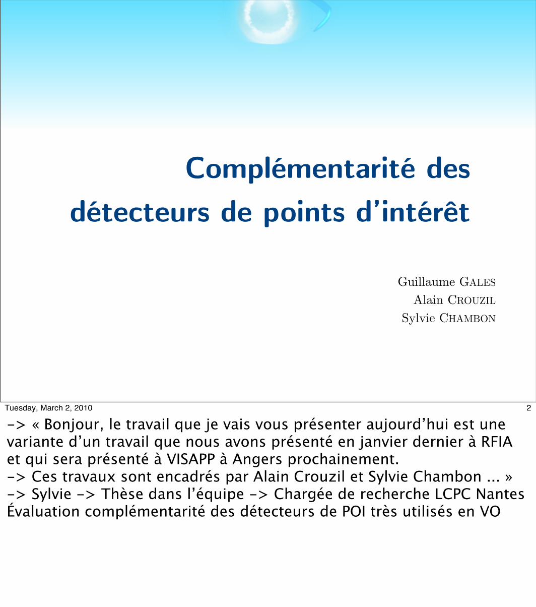
• Point d’intérêt : point particulier de l’image qui a une caractéristique intéressante pour une application donnée

• Applications : mise en correspondance stéréoscopique, estimation de la matrice fondamentale, suivi, indexation

3


-> POI -> définition-> Utilisés dans différentes applications -> MENC -> appariements sans ambiguité -> non situés dans les zones homogènes-> Donc dans ce cas -> pts qui se distinguent de leurs voisins -> Exemple POI de la boîte (sur les lettres)

Problématique

• De nombreux détecteurs ont été proposés• Sont-ils complémentaires ?

4


-> les détecteurs de POI sont nombreux-> on se pose la question : sont-ils complémentaires ? (peu d’études détaillées)

Plan de la présentation

• Détection de points d’intérêt• Mesures proposées• Résultats• Conclusion

5


Points d’intérêt

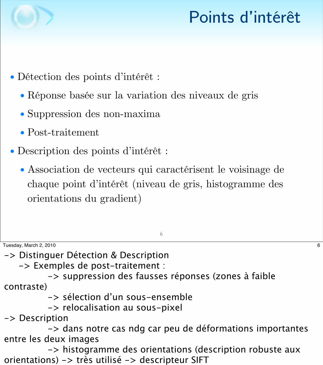
• Détection des points d’intérêt :• Réponse basée sur la variation des niveaux de gris• Suppression des non-maxima• Post-traitement

• Description des points d’intérêt :• Association de vecteurs qui caractérisent le voisinage de

chaque point d’intérêt (niveau de gris, histogramme des orientations du gradient)

6


-> Distinguer Détection & Description -> Exemples de post-traitement : -> suppression des fausses réponses (zones à faible contraste) -> sélection d’un sous-ensemble -> relocalisation au sous-pixel-> Description -> dans notre cas ndg car peu de déformations importantes entre les deux images -> histogramme des orientations (description robuste aux orientations) -> très utilisé -> descripteur SIFT-> Dans cette étude -> c’est la Détection qui nous intéresse


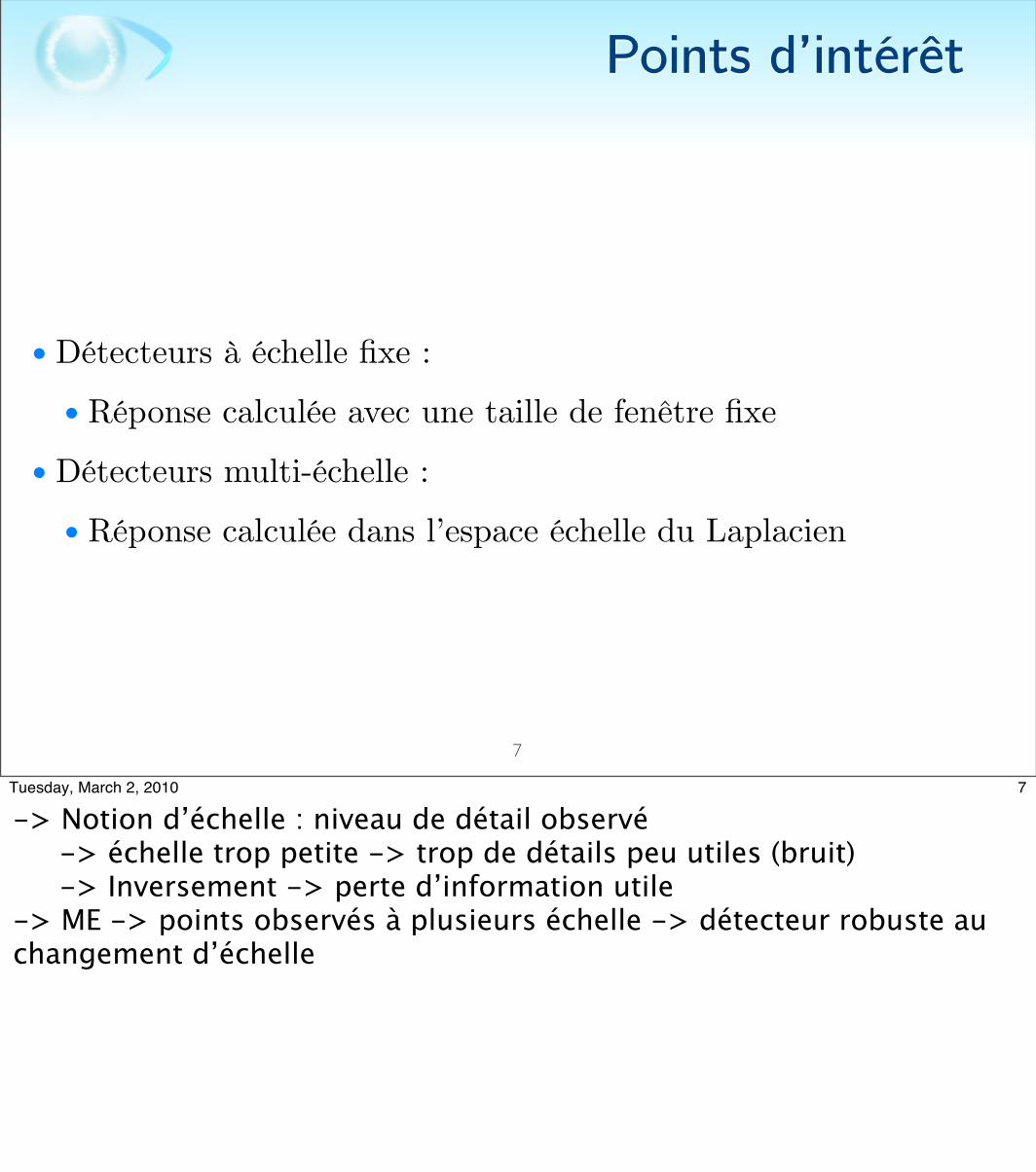
• Détecteurs à échelle fixe :• Réponse calculée avec une taille de fenêtre fixe

• Détecteurs multi-échelle :• Réponse calculée dans l’espace échelle du Laplacien

7


-> Notion d’échelle : niveau de détail observé -> échelle trop petite -> trop de détails peu utiles (bruit) -> Inversement -> perte d’information utile-> ME -> points observés à plusieurs échelle -> détecteur robuste au changement d’échelle


• Détecteurs à échelle fixe :• MORAVEC (MO), HARRIS (HA), KITCHEN-ROSENFELD (KR),

BEAUDET (BE), SUSAN (SU), FAST (FA)• Détecteurs multi-échelle :• SIFT (SI), HARRIS-LAPLACE (HAL), HESSIAN-LAPLACE

(HEL), SURF (SU), KADIR (KA)

8


-> voir article


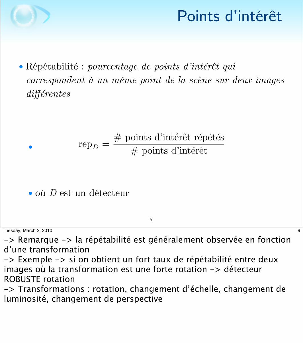
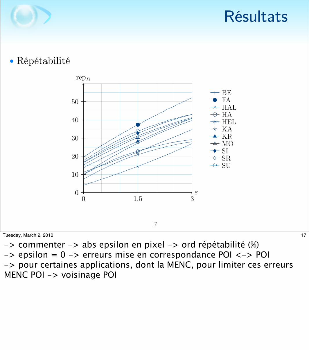
• Répétabilité : pourcentage de points d’intérêt qui correspondent à un même point de la scène sur deux images différentes

•

• où D est un détecteur

9

repD =# points d’interet repetes

# points d’interet


-> Remarque -> la répétabilité est généralement observée en fonction d’une transformation-> Exemple -> si on obtient un fort taux de répétabilité entre deux images où la transformation est une forte rotation -> détecteur ROBUSTE rotation-> Transformations : rotation, changement d’échelle, changement de luminosité, changement de perspective


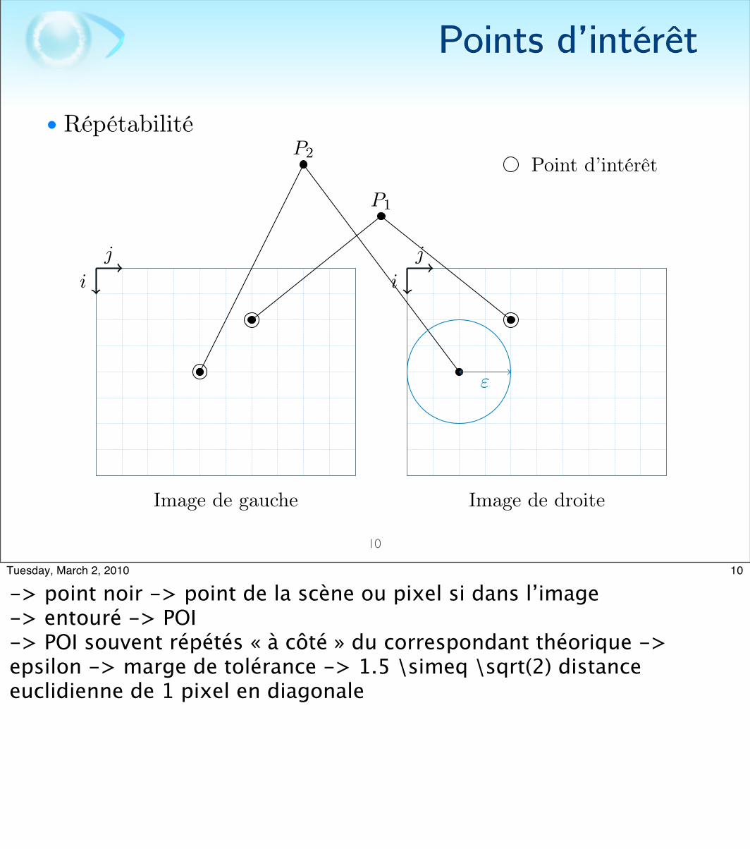
• Répétabilité

10

1

ε

repD

0 1.5 30

10

20

30

40

50BEFAHALHAHELKAKRMOSISRSU

Figure 1: Répétabilités.

i i

j j

P1

P2

ε

Image de gauche Image de droite

Point d’intérêt

Figure 2: Schéma répétabilité.

1


-> point noir -> point de la scène ou pixel si dans l’image-> entouré -> POI-> POI souvent répétés « à côté » du correspondant théorique -> epsilon -> marge de tolérance -> 1.5 \simeq \sqrt(2) distance euclidienne de 1 pixel en diagonale

Mesures proposées

• Répartition spatiale par régions• Complémentarité• Mesure d’apport• Gain de répétabilité• Gain de répartition

11


-> 1) répartition spatiale -> motivation -> menc dense -> précision d’estimation d’une homographie qui lie deux images -> éviter les concentrations sur une zones peu utiles-> 2) plusieurs mesures pour caractériser la complémentarité

Mesures proposées

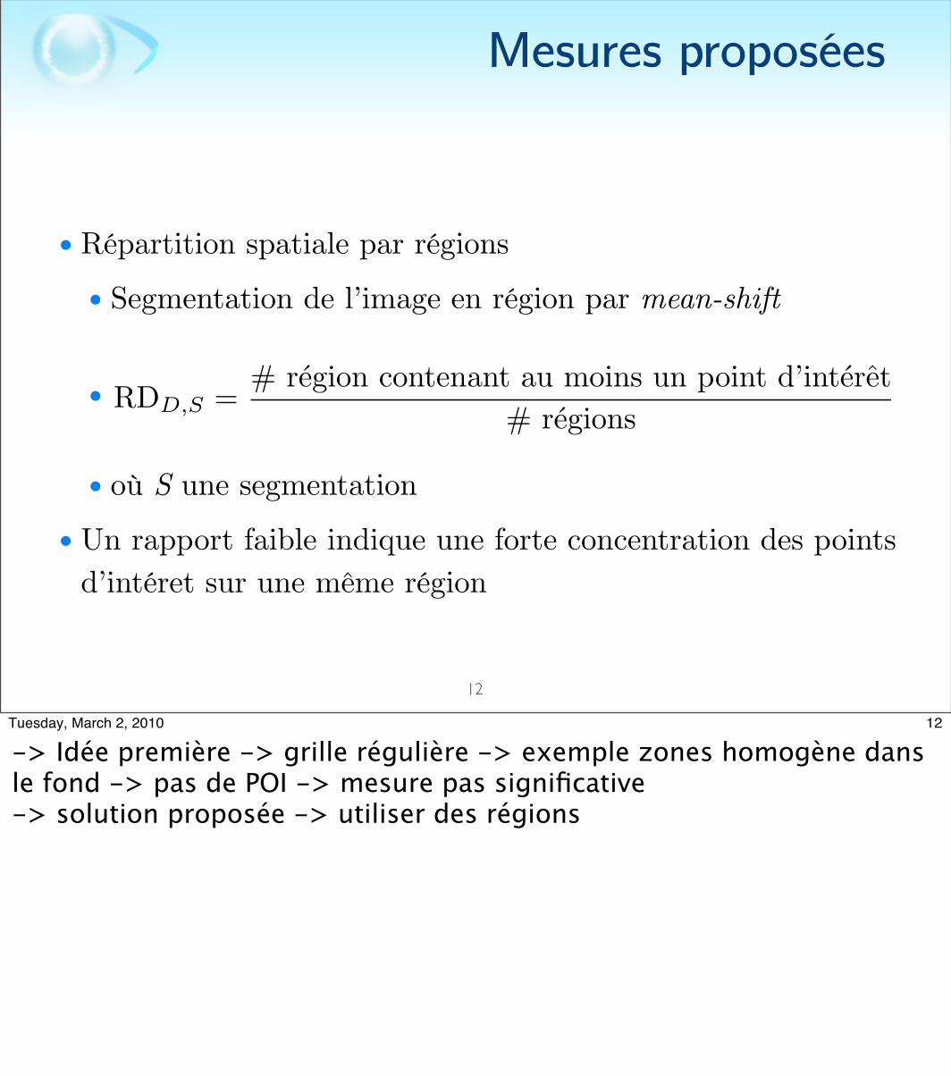
• Répartition spatiale par régions• Segmentation de l’image en région par mean-shift

•

• où S une segmentation• Un rapport faible indique une forte concentration des points

d’intéret sur une même région

12

RDD,S =# region contenant au moins un point d’interet

# regions


-> Idée première -> grille régulière -> exemple zones homogène dans le fond -> pas de POI -> mesure pas significative-> solution proposée -> utiliser des régions

Mesures proposées

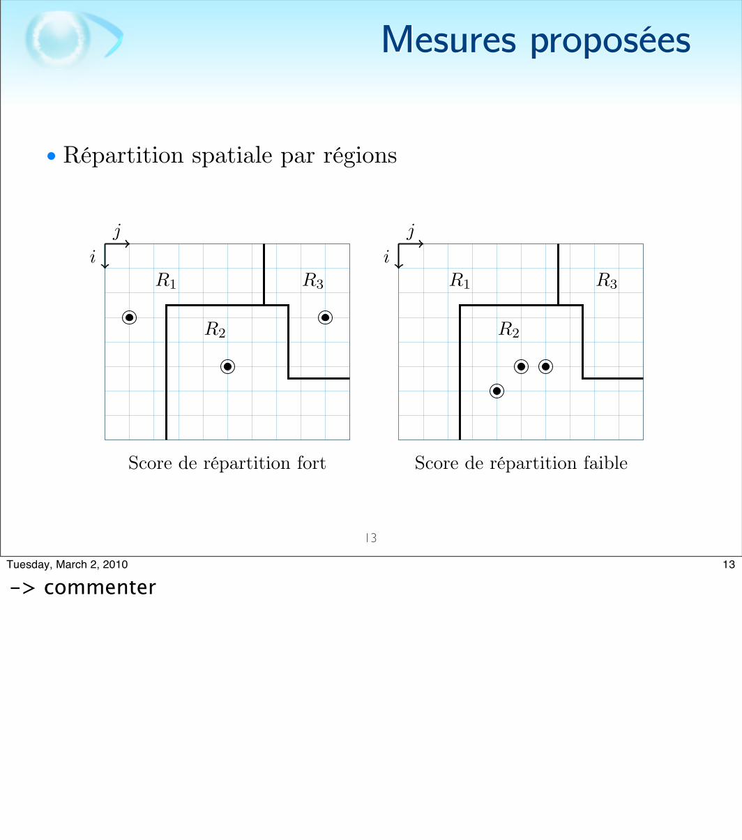
• Répartition spatiale par régions

13

2

i i

j j

Score de répartition fort Score de répartition faible

R1

R2

R3 R1

R2

R3

Figure 3: Distribution

2


-> commenter

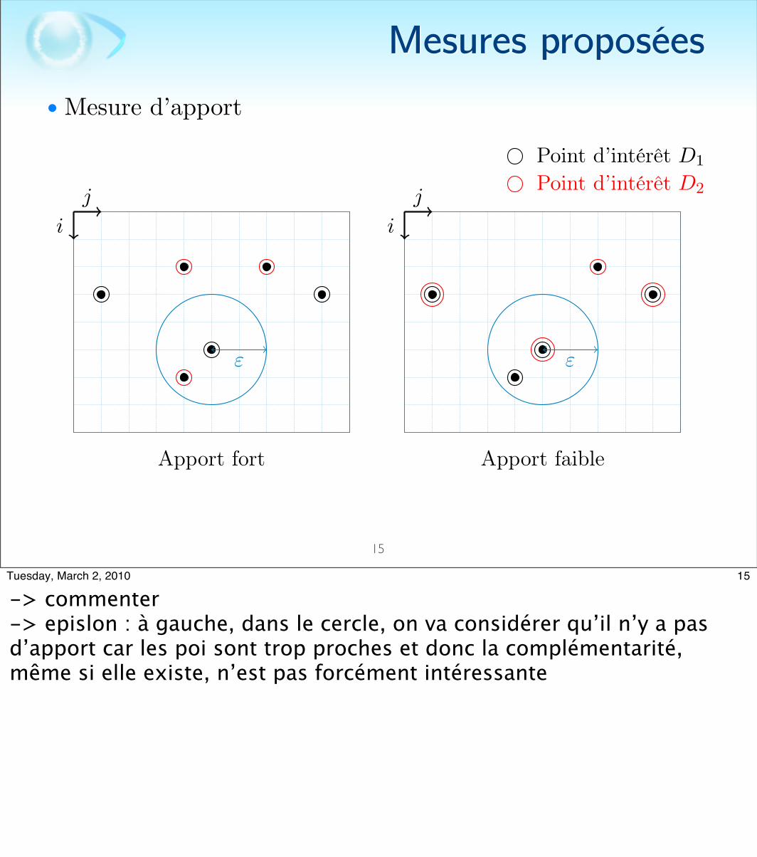
• Mesure d’apport

•

•

• où est l’ensemble des points d’intérêt retournés par le détecteur D

Mesures proposées

14

ApportD2|D1=

card {PD2}− card {PD1 ∩ PD1}card {PD1}

PD

Apport(D1, D2) = Apport(D2, D1)= min(ApportD2|D1

,ApportD1|D2)


-> Apport -> Calcul des POI de D1 -> Mesure du pourcentage de nouveaux POI apportés par D2-> non symétrique -> valeur représentative d’un couple de détecteur -> on prend le min


Mesures proposées

15

2

i i

j j

Score de répartition fort Score de répartition faible

R1

R2

R3 R1

R2

R3

Figure 3: Distribution

i i

j j

ε ε

Apport fort Apport faible

Point d’intérêt D1

Point d’intérêt D2

Figure 4: Apport

2


-> commenter -> epislon : à gauche, dans le cercle, on va considérer qu’il n’y a pas d’apport car les poi sont trop proches et donc la complémentarité, même si elle existe, n’est pas forcément intéressante

Mesures proposées

• Gain de répétabilité•

• Gain de répartition•

16

gainrepD1&D2= repD1&D2

−max�repD1

, repD2

�

gainRDD1&D2 ,S = RDD1&D2,S −max (RDD1,S ,RDD2,S)


-> gain (ou perte) de l’union de 2 ensembles de POI issus en terme de performances : répétabilité & répartition

Résultats

• Répétabilité

17

1

ε

repD

0 1.5 30

10

20

30

40

50BEFAHALHAHELKAKRMOSISRSU

Figure 1: Répétabilités.

1


-> commenter -> abs epsilon en pixel -> ord répétabilité (%)-> epsilon = 0 -> erreurs mise en correspondance POI <-> POI-> pour certaines applications, dont la MENC, pour limiter ces erreurs MENC POI -> voisinage POI

Résultats

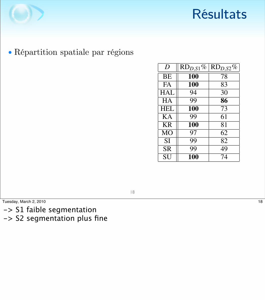
• Répartition spatiale par régions

18

Table 1: Mean cardinalities (Card.), mean of the distribu-tion measures in depth discontinuity (DA), and mean of theregion based distribution measure (RD) with segmentationS1 ans S2. For each column the best result is shown in bold.

D Card. DA% RDD,S1% RDD,S2%BE 967 28 100 78FA 2243 27 100 83

HAL 293 35 94 30HA 989 25 99 86

HEL 1252 32 100 73KA 638 29 99 61KR 1153 31 100 81MO 845 27 97 62SI 1662 29 99 82SR 303 31 99 49SU 922 29 100 74

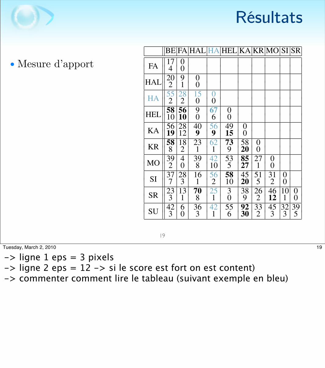
Table 2: Contribution measures taking into account all thefeature points. For each couple of detectors D1&D2, weshow contributionD2|D1 . ε = 3 on the first row and ε = 12on the second row. To find out which detector is the mostcomplementary with HA and ε = 3, for instance, look at theHA row and column (here in blue). It shows that it is HEL.For each detector and each ε value, the best result appearsin bold.

BE FA HAL HA HEL KA KR MO SI SR

FA 17 04 0

HAL 20 9 02 1 0

HA 55 28 15 02 2 0 0

HEL 58 56 9 67 010 10 0 6 0

KA 56 28 40 56 49 019 12 9 9 15 0

KR 58 18 23 62 73 58 08 2 1 1 9 20 0

MO 39 4 39 42 53 85 27 02 0 8 10 5 27 1 0

SI 37 28 16 56 58 45 51 31 07 3 1 2 10 20 5 2 0

SR 23 13 70 25 3 38 26 46 10 03 1 8 1 0 9 2 12 1 0

SU 42 6 36 42 55 92 33 45 32 393 0 3 1 6 30 2 3 3 5

in table 2 (the measures are computed over all the fea-tures points) and in table 3 (the measures are com-puted over the repeated feature points). According tothese results, the most complementary detectors areKA+SU, KA+MO and KR+HEL. By reading thesetables, we can see for instance that by taking the unionHA+SI, we add in the worst case 67% of new repeatedfeature points within a distance of ε = 3 pixels of eachother and 2% of new repeated feature points within adistance of ε = 12 (i.e. at least 12 pixels farther thanthe already computed feature points).

Table 3: Contribution measures taking into account the re-peated feature points (see table 2 for notations).


FA 18 06 0

HAL 19 7 02 1 0

HA 52 30 12 03 3 0 0

HEL 61 51 8 75 013 12 1 6 0

KA 34 19 71 33 32 017 14 11 7 16 0

KR 68 17 22 60 72 42 09 2 1 1 11 22 0

MO 46 5 36 44 55 82 35 02 0 10 0 6 31 1 0

SI 42 27 15 67 63 29 53 34 08 4 1 2 13 21 6 2 0

SR 21 9 85 20 3 64 24 42 8 03 1 12 1 0 11 2 13 1 0

SU 42 5 43 36 47 85 35 62 29 413 1 3 1 7 37 2 3 3 5

Table 4: Repeatability gain. For each couple of detectorsD1&D2, we show gainrepD1&D2

(ε = 3). To determine whichdetector is the most complementary in terms of repeatabilitywith HA, for instance, look at the HA row and column (herein blue), it shows that it is HEL. For each detector, the bestresult appears in bold.

BE FA HAL HA HEL KA KR MO SI SRFA 1.55 0

HAL 0.75 -0.36 0HA 3.77 0.32 -0.36 0HEL 4.48 2.12 0.36 4.20 0KA -0.17 -1.69 -0.39 -0.38 2.03 0KR 4.71 0.22 0.90 3.88 5.75 1.81 0MO 3.78 -0.69 -0.62 3.11 4.47 -1.34 2.83 0SI 3.57 1.19 0.76 3.40 2.37 0.82 4.98 3.00 0SR 1.01 0.38 0.09 0.66 -2.06 1.48 1.70 0.82 -0.19 0SU 3.53 -1.21 1.65 2.24 5.00 2.60 3.50 2.23 2.46 2.63

Repeatability gain The results are shown in ta-ble 4. They show which detectors are the most com-plementary in terms of repeatability. First, it showsthe good complementarity of the following detectorsKR+HEL, HEL+SU and KR+SI. Second, it showswhich detector to use in combination to another in or-der to improve the repeatability. The best repeatabil-ity was given by FA, see § 5.1. Therefore, adding thefeature points from the detector HEL can improve by2.12% the repeatability of FA.

Distribution gain The segmentation S2 is used inour experimentation, see § 5.2. The results are shownin table 5. They show which detectors are the mostcomplementary in terms of region based distribu-tion. First, it shows the good complementarity of the



HAL 293 35 94 30HA 989 25 99 86




FA 17 04 0

HAL 20 9 02 1 0

HA 55 28 15 02 2 0 0

HEL 58 56 9 67 010 10 0 6 0

KA 56 28 40 56 49 019 12 9 9 15 0

KR 58 18 23 62 73 58 08 2 1 1 9 20 0

MO 39 4 39 42 53 85 27 02 0 8 10 5 27 1 0

SI 37 28 16 56 58 45 51 31 07 3 1 2 10 20 5 2 0

SR 23 13 70 25 3 38 26 46 10 03 1 8 1 0 9 2 12 1 0

SU 42 6 36 42 55 92 33 45 32 393 0 3 1 6 30 2 3 3 5




FA 18 06 0

HAL 19 7 02 1 0

HA 52 30 12 03 3 0 0

HEL 61 51 8 75 013 12 1 6 0

KA 34 19 71 33 32 017 14 11 7 16 0

KR 68 17 22 60 72 42 09 2 1 1 11 22 0

MO 46 5 36 44 55 82 35 02 0 10 0 6 31 1 0

SI 42 27 15 67 63 29 53 34 08 4 1 2 13 21 6 2 0

SR 21 9 85 20 3 64 24 42 8 03 1 12 1 0 11 2 13 1 0

SU 42 5 43 36 47 85 35 62 29 413 1 3 1 7 37 2 3 3 5








-> S1 faible segmentation-> S2 segmentation plus fine

Résultats


19



HAL 293 35 94 30HA 989 25 99 86




FA 17 04 0

HAL 20 9 02 1 0

HA 55 28 15 02 2 0 0

HEL 58 56 9 67 010 10 0 6 0

KA 56 28 40 56 49 019 12 9 9 15 0

KR 58 18 23 62 73 58 08 2 1 1 9 20 0

MO 39 4 39 42 53 85 27 02 0 8 10 5 27 1 0

SI 37 28 16 56 58 45 51 31 07 3 1 2 10 20 5 2 0

SR 23 13 70 25 3 38 26 46 10 03 1 8 1 0 9 2 12 1 0

SU 42 6 36 42 55 92 33 45 32 393 0 3 1 6 30 2 3 3 5




FA 18 06 0

HAL 19 7 02 1 0

HA 52 30 12 03 3 0 0

HEL 61 51 8 75 013 12 1 6 0

KA 34 19 71 33 32 017 14 11 7 16 0

KR 68 17 22 60 72 42 09 2 1 1 11 22 0

MO 46 5 36 44 55 82 35 02 0 10 0 6 31 1 0

SI 42 27 15 67 63 29 53 34 08 4 1 2 13 21 6 2 0

SR 21 9 85 20 3 64 24 42 8 03 1 12 1 0 11 2 13 1 0

SU 42 5 43 36 47 85 35 62 29 413 1 3 1 7 37 2 3 3 5








-> ligne 1 eps = 3 pixels-> ligne 2 eps = 12 -> si le score est fort on est content)-> commenter comment lire le tableau (suivant exemple en bleu)

Résultats

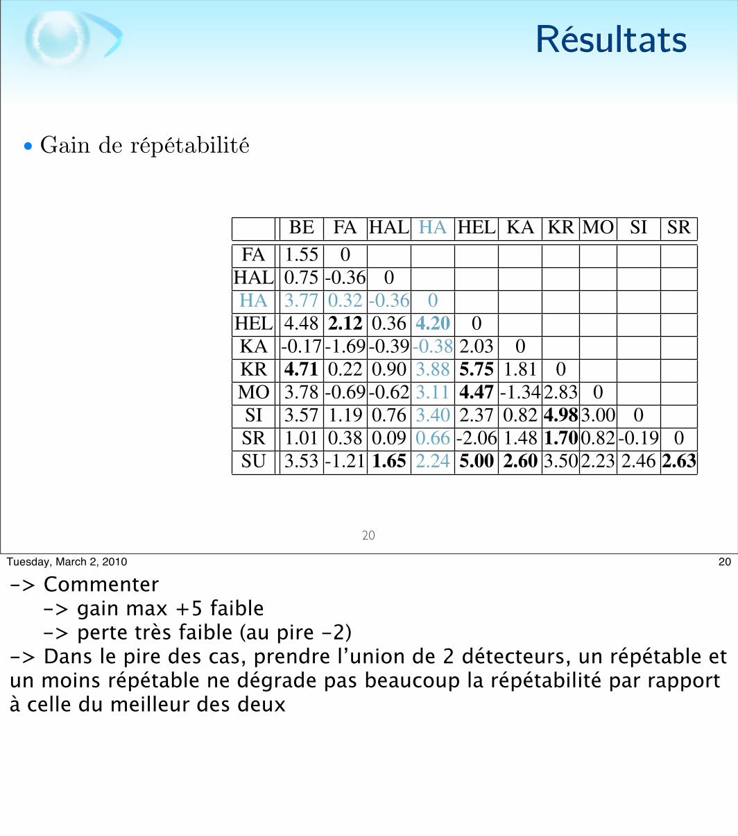
• Gain de répétabilité

20



HAL 293 35 94 30HA 989 25 99 86




FA 17 04 0

HAL 20 9 02 1 0

HA 55 28 15 02 2 0 0

HEL 58 56 9 67 010 10 0 6 0

KA 56 28 40 56 49 019 12 9 9 15 0

KR 58 18 23 62 73 58 08 2 1 1 9 20 0

MO 39 4 39 42 53 85 27 02 0 8 10 5 27 1 0

SI 37 28 16 56 58 45 51 31 07 3 1 2 10 20 5 2 0

SR 23 13 70 25 3 38 26 46 10 03 1 8 1 0 9 2 12 1 0

SU 42 6 36 42 55 92 33 45 32 393 0 3 1 6 30 2 3 3 5




FA 18 06 0

HAL 19 7 02 1 0

HA 52 30 12 03 3 0 0

HEL 61 51 8 75 013 12 1 6 0

KA 34 19 71 33 32 017 14 11 7 16 0

KR 68 17 22 60 72 42 09 2 1 1 11 22 0

MO 46 5 36 44 55 82 35 02 0 10 0 6 31 1 0

SI 42 27 15 67 63 29 53 34 08 4 1 2 13 21 6 2 0

SR 21 9 85 20 3 64 24 42 8 03 1 12 1 0 11 2 13 1 0

SU 42 5 43 36 47 85 35 62 29 413 1 3 1 7 37 2 3 3 5








-> Commenter -> gain max +5 faible -> perte très faible (au pire -2)-> Dans le pire des cas, prendre l’union de 2 détecteurs, un répétable et un moins répétable ne dégrade pas beaucoup la répétabilité par rapport à celle du meilleur des deux

Résultats

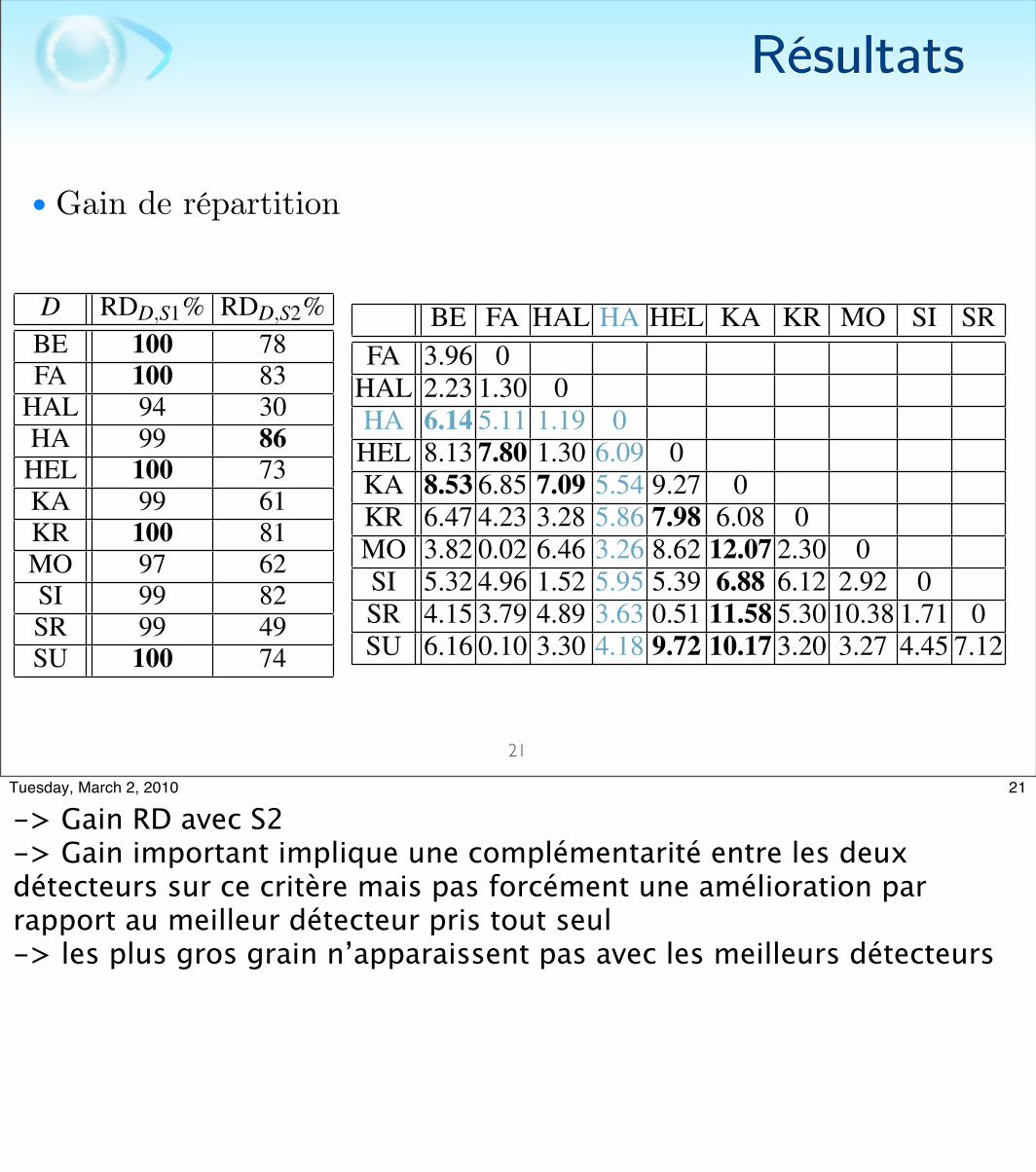
• Gain de répartition

21

Table 5: Distribution gain. For each couple of detectorsD1&D2, we show gainRDD1&D2 ,S2

(ε = 3) (see 4 for an exam-ple of how to read the table).


HAL 2.23 1.30 0HA 6.14 5.11 1.19 0

HEL 8.13 7.80 1.30 6.09 0KA 8.53 6.85 7.09 5.54 9.27 0KR 6.47 4.23 3.28 5.86 7.98 6.08 0MO 3.82 0.02 6.46 3.26 8.62 12.07 2.30 0SI 5.32 4.96 1.52 5.95 5.39 6.88 6.12 2.92 0SR 4.15 3.79 4.89 3.63 0.51 11.58 5.30 10.38 1.71 0SU 6.16 0.10 3.30 4.18 9.72 10.17 3.20 3.27 4.45 7.12

Table 6: This table summarizes the most complementarydetectors to Harris, FAST and SIFT in terms of contribution(Cont.) (ε = 3) (results are similar whether all the featurepoints or only the repeated points are taken into account),repeatability (R) and region based distribution (RDS2).

D Cont. R RDD1&D2,S2HA HEL HEL BEFA HEL HEL HELSI HEL KR KA

following detectors KA+MO, KA+SU and KA+SR.Second, it shows which detector to use in combina-tion to another in order to improve the spatial distri-bution. The best region based distribution was givenby HA, see § 5.2. By reading table 5, we can seethat adding the feature points from the detector BEcan improve the distribution by 6.14% which gives ascore of 86+6.14=92.14% for the union HA+BE.

Analysis These results can be read in two ways: (i)for each detector they give which detector is the mostcomplementary in terms of contribution, repeatabilityand spatial distribution ; (ii) they give the most com-plementary detectors between them. The best com-promises between repeatability and distribution aregiven by: Harris, FAST and SIFT. Table 6 summa-rizes the most complementary detectors to the detec-tors in terms of contribution, repeatability and region-wise distribution. The most complementary detectorsbetween them are Kadir and SUSAN, Kitchen andRosenfeld and Hessian-Laplace, Moravec and Kadiri.e. they return the most distinct sets of feature points.

6 CONCLUSION

We proposed an evaluation and a comparison ofeleven well-known feature point detectors based onnew criteria used to characterize spatial distribution

and complementarity. This study aims to be helpfulfor any applications that need feature points well dis-tributed in the image. It also helps to select the mostcomplementary detectors in terms of region based dis-tribution. This work will be extended on larger trans-formations between the images.

REFERENCES

Bay, H., Ess, A., Tuytelaars, T., and Gool, L. V. (2006).SURF: Speeded up robust features. CVIU, pages 346–359.

Beaudet, P. R. (1978). Rotationally invariant image opera-tors. In ICPR, pages 579–583, Kyoto, Japan.

Gil, A., Martinez, O., Ballesta, M., and Reinoso, O. (2009).A comparative evaluation of interest point detectorsand local descriptors for visual SLAM. MVA.

Harris, C. and Stephens, M. (1988). A combined cornerand edge detector. In Alvey Vision Conference, pages147–151, Manchester, United-Kingdom.

Hartley, R. I. and Zisserman, A. (2004). Multiple View Ge-ometry in Computer Vision. Cambridge UniversityPress, ISBN: 0521540518, second edition.

Kadir, T., Zisserman, A., and Brady, M. (2004). An affineinvariant salient region detector. In ECCV, pages 404–416, Prague, Czech Republic.

Kitchen, L. and Rosenfeld, A. (1982). Gray level cornerdetection. PRL, 1(2):95–102.

Lhuillier, M. and Quan, L. (2002). Match propagationfor image-based modeling and rendering. PAMI,24(8):1140–1146.

Lowe, D. G. (1999). Object recognition from local scale-invariant features. In ICCV, volume 2, pages 1150–1157, Kerkyra, Greece.

Mikolajczyk, K., Leibe, B., and Schiele, B. (2005). Localfeatures for object classe recognition. In ICCV, vol-ume 2, pages 1792–1799, Beijing, China.

Mikolajczyk, K. and Schmid, C. (2004). Scale & affineinvariant interest point detectors. IJCV, 60(1):63–86.

Moravec, H. P. (1977). Toward automatic visual obstacleavoidance. In IJCAI, volume 2, pages 584–584, Mas-sachusetts, USA.

Noble, J. A. (1988). Finding corners. IVC, 6(2):121–128.Rosten, E. and Drummond, T. (2006). Machine learning

for high-speed corner detection. In ECCV, volume 1,pages 430–443, Graz, Austria.

Schmid, C., Mohr, R., and Bauckhage, C. (2000). Evalua-tion of interest point detectors. IJCV, 37(2):151–172.

Shi, J. and Tomasi, C. (1994). Good features to track. InCVPR, pages 593–600, Seattle, USA.

Smith, S. M. and Brady, J. M. (1997). Susan – a new ap-proach to low level image processing. IJCV, 23(1):45–78.



HAL 293 35 94 30HA 989 25 99 86




FA 17 04 0

HAL 20 9 02 1 0

HA 55 28 15 02 2 0 0

HEL 58 56 9 67 010 10 0 6 0

KA 56 28 40 56 49 019 12 9 9 15 0

KR 58 18 23 62 73 58 08 2 1 1 9 20 0

MO 39 4 39 42 53 85 27 02 0 8 10 5 27 1 0

SI 37 28 16 56 58 45 51 31 07 3 1 2 10 20 5 2 0

SR 23 13 70 25 3 38 26 46 10 03 1 8 1 0 9 2 12 1 0

SU 42 6 36 42 55 92 33 45 32 393 0 3 1 6 30 2 3 3 5




FA 18 06 0

HAL 19 7 02 1 0

HA 52 30 12 03 3 0 0

HEL 61 51 8 75 013 12 1 6 0

KA 34 19 71 33 32 017 14 11 7 16 0

KR 68 17 22 60 72 42 09 2 1 1 11 22 0

MO 46 5 36 44 55 82 35 02 0 10 0 6 31 1 0

SI 42 27 15 67 63 29 53 34 08 4 1 2 13 21 6 2 0

SR 21 9 85 20 3 64 24 42 8 03 1 12 1 0 11 2 13 1 0

SU 42 5 43 36 47 85 35 62 29 413 1 3 1 7 37 2 3 3 5









HAL 293 35 94 30HA 989 25 99 86




FA 17 04 0

HAL 20 9 02 1 0

HA 55 28 15 02 2 0 0

HEL 58 56 9 67 010 10 0 6 0

KA 56 28 40 56 49 019 12 9 9 15 0

KR 58 18 23 62 73 58 08 2 1 1 9 20 0

MO 39 4 39 42 53 85 27 02 0 8 10 5 27 1 0

SI 37 28 16 56 58 45 51 31 07 3 1 2 10 20 5 2 0

SR 23 13 70 25 3 38 26 46 10 03 1 8 1 0 9 2 12 1 0

SU 42 6 36 42 55 92 33 45 32 393 0 3 1 6 30 2 3 3 5




FA 18 06 0

HAL 19 7 02 1 0

HA 52 30 12 03 3 0 0

HEL 61 51 8 75 013 12 1 6 0

KA 34 19 71 33 32 017 14 11 7 16 0

KR 68 17 22 60 72 42 09 2 1 1 11 22 0

MO 46 5 36 44 55 82 35 02 0 10 0 6 31 1 0

SI 42 27 15 67 63 29 53 34 08 4 1 2 13 21 6 2 0

SR 21 9 85 20 3 64 24 42 8 03 1 12 1 0 11 2 13 1 0

SU 42 5 43 36 47 85 35 62 29 413 1 3 1 7 37 2 3 3 5








-> Gain RD avec S2-> Gain important implique une complémentarité entre les deux détecteurs sur ce critère mais pas forcément une amélioration par rapport au meilleur détecteur pris tout seul-> les plus gros grain n’apparaissent pas avec les meilleurs détecteurs

Résultats

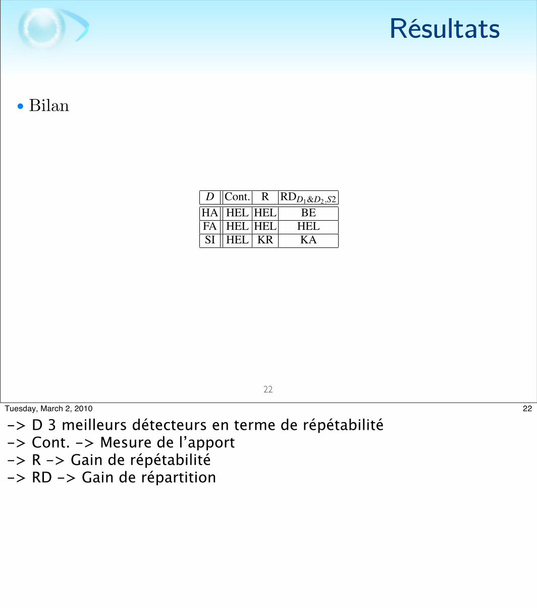
• Bilan

22

Table 5: Distribution gain. For each couple of detectorsD1&D2, we show gainRDD1&D2 ,S2

(ε = 3) (see 4 for an exam-ple of how to read the table).


HAL 2.23 1.30 0HA 6.14 5.11 1.19 0

HEL 8.13 7.80 1.30 6.09 0KA 8.53 6.85 7.09 5.54 9.27 0KR 6.47 4.23 3.28 5.86 7.98 6.08 0MO 3.82 0.02 6.46 3.26 8.62 12.07 2.30 0SI 5.32 4.96 1.52 5.95 5.39 6.88 6.12 2.92 0SR 4.15 3.79 4.89 3.63 0.51 11.58 5.30 10.38 1.71 0SU 6.16 0.10 3.30 4.18 9.72 10.17 3.20 3.27 4.45 7.12

Table 6: This table summarizes the most complementarydetectors to Harris, FAST and SIFT in terms of contribution(Cont.) (ε = 3) (results are similar whether all the featurepoints or only the repeated points are taken into account),repeatability (R) and region based distribution (RDS2).

D Cont. R RDD1&D2,S2HA HEL HEL BEFA HEL HEL HELSI HEL KR KA

following detectors KA+MO, KA+SU and KA+SR.Second, it shows which detector to use in combina-tion to another in order to improve the spatial distri-bution. The best region based distribution was givenby HA, see § 5.2. By reading table 5, we can seethat adding the feature points from the detector BEcan improve the distribution by 6.14% which gives ascore of 86+6.14=92.14% for the union HA+BE.

Analysis These results can be read in two ways: (i)for each detector they give which detector is the mostcomplementary in terms of contribution, repeatabilityand spatial distribution ; (ii) they give the most com-plementary detectors between them. The best com-promises between repeatability and distribution aregiven by: Harris, FAST and SIFT. Table 6 summa-rizes the most complementary detectors to the detec-tors in terms of contribution, repeatability and region-wise distribution. The most complementary detectorsbetween them are Kadir and SUSAN, Kitchen andRosenfeld and Hessian-Laplace, Moravec and Kadiri.e. they return the most distinct sets of feature points.

6 CONCLUSION

We proposed an evaluation and a comparison ofeleven well-known feature point detectors based onnew criteria used to characterize spatial distribution

and complementarity. This study aims to be helpfulfor any applications that need feature points well dis-tributed in the image. It also helps to select the mostcomplementary detectors in terms of region based dis-tribution. This work will be extended on larger trans-formations between the images.

REFERENCES

Bay, H., Ess, A., Tuytelaars, T., and Gool, L. V. (2006).SURF: Speeded up robust features. CVIU, pages 346–359.

Beaudet, P. R. (1978). Rotationally invariant image opera-tors. In ICPR, pages 579–583, Kyoto, Japan.

Gil, A., Martinez, O., Ballesta, M., and Reinoso, O. (2009).A comparative evaluation of interest point detectorsand local descriptors for visual SLAM. MVA.

Harris, C. and Stephens, M. (1988). A combined cornerand edge detector. In Alvey Vision Conference, pages147–151, Manchester, United-Kingdom.

Hartley, R. I. and Zisserman, A. (2004). Multiple View Ge-ometry in Computer Vision. Cambridge UniversityPress, ISBN: 0521540518, second edition.

Kadir, T., Zisserman, A., and Brady, M. (2004). An affineinvariant salient region detector. In ECCV, pages 404–416, Prague, Czech Republic.

Kitchen, L. and Rosenfeld, A. (1982). Gray level cornerdetection. PRL, 1(2):95–102.

Lhuillier, M. and Quan, L. (2002). Match propagationfor image-based modeling and rendering. PAMI,24(8):1140–1146.

Lowe, D. G. (1999). Object recognition from local scale-invariant features. In ICCV, volume 2, pages 1150–1157, Kerkyra, Greece.

Mikolajczyk, K., Leibe, B., and Schiele, B. (2005). Localfeatures for object classe recognition. In ICCV, vol-ume 2, pages 1792–1799, Beijing, China.

Mikolajczyk, K. and Schmid, C. (2004). Scale & affineinvariant interest point detectors. IJCV, 60(1):63–86.

Moravec, H. P. (1977). Toward automatic visual obstacleavoidance. In IJCAI, volume 2, pages 584–584, Mas-sachusetts, USA.

Noble, J. A. (1988). Finding corners. IVC, 6(2):121–128.Rosten, E. and Drummond, T. (2006). Machine learning

for high-speed corner detection. In ECCV, volume 1,pages 430–443, Graz, Austria.

Schmid, C., Mohr, R., and Bauckhage, C. (2000). Evalua-tion of interest point detectors. IJCV, 37(2):151–172.

Shi, J. and Tomasi, C. (1994). Good features to track. InCVPR, pages 593–600, Seattle, USA.

Smith, S. M. and Brady, J. M. (1997). Susan – a new ap-proach to low level image processing. IJCV, 23(1):45–78.


-> D 3 meilleurs détecteurs en terme de répétabilité-> Cont. -> Mesure de l’apport-> R -> Gain de répétabilité-> RD -> Gain de répartition

Conclusion

• Évaluation et comparaison de 11 détecteurs de points d’intérêt suivant des nouveaux critères caractérisant la complémentarité

• Extension à une évaluation avec des transformations plus importante entre les deux images

23


-> En conclusion comment répondre à la question : « Il vaut mieux utiliser quoi avec quoi ? »-> Tout dépend du critère qui va être le plus important selon l’application-> Exemple mise en correspondance de germes pour des algorithmes de mise en correspondance de pixel par propagation -> Répartition -> meilleure répartition HA+BE

Documents

Tuesday, March 2, 2010 1 - irit.fr · -> Sylvie -> Thèse dans l’équipe -> Chargée de recherche LCPC Nantes ... le fond -> pas de POI -> mesure pas signiﬁcative ... 68 17 22