Embed Size (px)
Citation preview
UNIVERSITE DES ANTILLES ET DE LA GUYANE
Faculté des sciences exactes et naturelles
École doctorale pluridisciplinaireThèse pour le doctorat en physiologie et biologie des organismes,
populations, interactions
Mélaine Aubry-Kientz
Quelle sera la réponse des forêts tropicales humides àl'augmentation des températures et aux changements de
pluviométrie ?Modéliser la dynamique forestière pour identi�er les processus
sensibles en Guyane Française.
Sous la direction de Bruno Hérault et de Vivien Rossi
Soutenue le 04 décembre 2014 à Kourou
N : 2014AGUY0802
Jury :Avner Bar-Hen, Professeur à l'Université Paris-DescartesBenoît Courbaud, Ingénieur-chercheur à l'IRSTEARaphael Pelissier, Directeur de recherche à l'IRDBruno Hérault, Cadre scienti�que au CIRAD

Remerciements
"Qu'importe où nous allons, honnêtement. Je ne le cache pas. De moinsen moins. Qu'importe ce qu'il y a au bout. [...] Je m'en �che ! Ce qui resteraest une certaine qualité d'amitié, architecturée par l'estime. Et brodée desquelques rires, des quelques éclats de courage ou de génie qu'on aura su s'of-frir les uns aux autres. Pour tout ça, les �lles et les gars, je vous dis merci.Merci." Alain Damasio, La horde du contrevent.
Je remercie mon directeur de thèse, Bruno Hérault, pour son encadrementgénial, pour la con�ance qu'il m'a accordée, pour ses conseils avisés, et poursa patience inébranlable. Ainsi que mon codirecteur Vivien Rossi, pour sesexplications limpides, pour sa disponibilité malgré les kilomètres, pour sonsoutien constant. Je n'aurai pu espérer meilleur encadrement.
Je remercie le CIRAD et le Labex CEBA (ref ANR-10-LABX-0025) pourma bourse de thèse, ainsi que le projet Climfor (Fondation pour la Recherchesur la Biodiversité) et le projet Guyasim (European structural funding, PO-feder) pour le soutien �nancier.
Je remercie les membres de mon comité de thèse, qui n'ont jamais étéavares de bons conseils, pour leur disponibilité lors de mes comités, Gré-goire Vincent, Sylvie Gourlet-Fleury, Jean-Jacque Boreux, Frédérique Mor-tier, Guillaume Cornu. De plus, je remercie Guillaume pour la rapidité àlaquelle il a toujours répondu à mes mails de détresse et pour la qualité deses réponses, ainsi que Jean-Jacques et Fred pour leur accueil à Megève etArlon.
Je remercie énormément mes rapporteurs Benoît Courbaud et PierreCouteron, d'avoir pris le temps de relire avec attention mon travail, pourleurs commentaires constructifs et enrichissants.
Je remercie Avner Ben-Har pour son intérêt pour mon travail, pour sesencouragements et pour avoir accepté d'être examinateur lors de ma soute-nance. Je remercie aussi Raphaël Pelissier pour avoir accepté d'être exami-nateur.
Je remercie tous les membres de l'UMR Ecofog et tout particulièrementEric Marcon et Marc Giberneau, pour ces trois superbes années passées danscette unité.
Pour leur accueil dans le monde de la thèse, leur soutien, leurs nom-breux conseils et leur amitié, je remercie Fabien et Quentin. Je remercie tousmes collègues de ce qui fût le laboratoire de modélisation, Alana, Gustave,Marianne, Anaïs.
i

Je remercie ceux qui m'ont fait adorer ma dernière année de thèse, Ro-main et Hélène, les stagiaires dont je n'aurai osé rêver, pour leur travailpassionné, leur amitié et leur soutien infaillible pendant la dernière lignedroite.
Je remercie ceux qui ont pris le temps de discuter avec moi pendant cestrois années, pour leurs avis toujours éclairés, entre autre Christopher Ba-raloto, Bruno Ferry, Olivier Bruno, Stéphane Guitet, Damien Bonal, JimmyLe Bec.
Je remercie bien sûr de tout c÷ur tous les thésards et collègues de l'UMR,Axel, Elodie, Youven, Camille, Aurélie, Audrey, Olivier, Stan, Alex, Sté-phane, Heidy, Jean-Chris, Mélanie, Louise, Julien, Kara, Pascal, Claire, Clé-ment, Benoit, Valérie, Stéphanie, Jocelyn, Jean-Yves, Patrick, Bruno, Hélène,Julie, Romain, Jacques, Christophe, Caroline, Émeline, Arnaud, Guillaume.
Je remercie ceux qui récoltent les données que j'ai utilisé pendant mathèse, ceux qui tous les ans réalisent les inventaires à Paracou, pour leurtravail tout à la fois gigantesque et minutieux, Frits Kwasie, Lindon Yansen,Martinus Koese, Michel Baisie Onoefé Ngwete, Petrus Naisso, et RichardSante.
Je remercie ceux qui m'ont emmené avec eux sur le terrain, grâce à quij'ai pu mieux appréhender la forêt tropicale.
Je remercie les étudiants avec lesquels j'ai eu la chance de travailler, pourleur incroyable enthousiasme, Elias, Carmen, Malou, Sylvène et Mathilde.
Je remercie tous mes amis, qui de près ou de loin, n'ont jamais cessé dem'encourager, notamment pendant les derniers mois.
Je remercie les Coyotes, et tout particulièrement Sophie, pour tout ceque j'ai appris avec elles, pour leurs généreux encouragements, et pour lesheures passées sur l'eau qui m'ont vidé la tête lorsque j'en avais besoin.
Je remercie la canaille et I am d'avoir rythmé les longues et laborieusespériodes d'écriture. Je remercie Alain Damasio et Andreï Kourkov de m'enavoir extrait quotidiennement.
Je remercie, bien sûr, ceux qui ont pris grand soin de moi ces dernierstemps, Marie-Mélina et tout particulièrement Pierre pour son extraordinairesoutien de tous les instants.
En�n, je remercie ceux qui me soutiennent depuis toujours, mon in-croyable famille, et tout particulièrement mon père, ma mère, et mon frère.
ii
Résumé
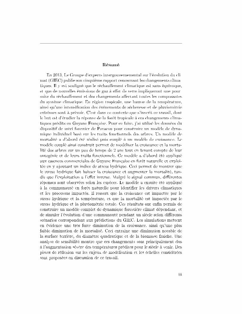
En 2013, Le Groupe d'experts intergouvernemental sur l'évolution du cli-mat (GIEC) publie son cinquième rapport concernant les changements clima-tiques. Il y est souligné que le réchau�ement climatique est sans équivoque,et que de nouvelles émissions de gaz à e�et de serre impliqueront une pour-suite du réchau�ement et des changements a�ectant toutes les composantesdu système climatique. En région tropicale, une hausse de la température,ainsi qu'une intensi�cation des événements de sécheresse et de pluviométrieextrêmes sont à prévoir. C'est dans ce contexte que s'inscrit ce travail, dontle but est d'étudier la réponse de la forêt tropicale à ces changements clima-tiques prédits en Guyane Française. Pour ce faire, j'ai utilisé les données dudispositif de suivi forestier de Paracou pour construire un modèle de dyna-mique individuel basé sur les traits fonctionnels des arbres. Un modèle demortalité a d'abord été réalisé puis couplé à un modèle de croissance. Lemodèle couplé ainsi construit permet de modéliser la croissance et la morta-lité des arbres sur un pas de temps de 2 ans tout en tenant compte de leurontogénie et de leurs traits fonctionnels. Ce modèle a d'abord été appliquéaux essences commerciales de Guyane Française en forêt naturelle et exploi-tée en y ajoutant un indice de stress hydrique. Ceci permet de montrer quele stress hydrique fait baisser la croissance et augmenter la mortalité, tan-dis que l'exploitation a l'e�et inverse. Malgré le signal commun, di�érentesréponses sont observées selon les espèces. Le modèle a ensuite été appliquéà la communauté en forêt naturelle pour identi�er les drivers climatiqueset les processus impactés. Il ressort que la croissance est impactée par lestress hydrique et la température, et que la mortalité est impactée par lestress hydrique et la pluviométrie totale. Ces résultats ont en�n permis deconstruire un modèle complet de dynamique forestière climat dépendant, etde simuler l'évolution d'une communauté pendant un siècle selon di�érentsscénarios correspondant aux prédictions du GIEC. Les simulations mettenten évidence une très forte diminution de la croissance, ainsi qu'une plusfaible diminution de la mortalité. Ceci entraine une diminution notable dela surface terrière, du diamètre quadratique et de la biomasse fraiche. Uneanalyse de sensibilité montre que ces changements sont principalement dusà l'augmentation sévère des températures prédites pour le siècle à venir. Despistes de ré�exion sur les enjeux de modélisation et les échelles considéréessont proposées en discussion de ce travail.
iii
TABLE DES MATIÈRES
Introduction générale 11 Les forêts tropicales . . . . . . . . . . . . . . . . . . . . . . . 1
1.1 Carbone et biodiversité . . . . . . . . . . . . . . . . . 11.2 Diversité spéci�que et fonctionnelle en forêt tropicale . 31.3 La dynamique forestière . . . . . . . . . . . . . . . . . 4
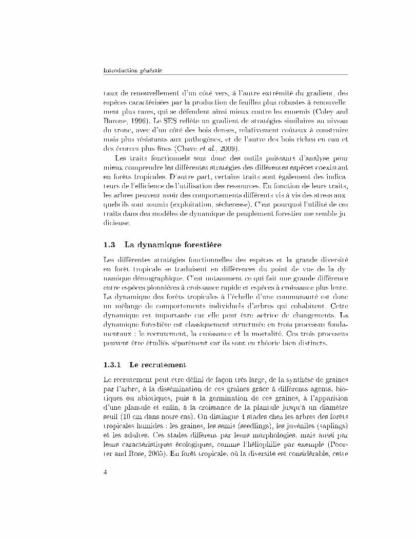
1.3.1 Le recrutement . . . . . . . . . . . . . . . . . 41.3.2 La croissance . . . . . . . . . . . . . . . . . . 51.3.3 La mortalité . . . . . . . . . . . . . . . . . . 51.3.4 La compétition pour les ressources . . . . . . 6
1.4 Plus particulièrement en Guyane Française . . . . . . 71.4.1 L'environnement physique . . . . . . . . . . . 81.4.2 L'environnement biologique . . . . . . . . . . 91.4.3 La population . . . . . . . . . . . . . . . . . 91.4.4 Le climat . . . . . . . . . . . . . . . . . . . . 9
1.5 Le site de Paracou . . . . . . . . . . . . . . . . . . . . 121.5.1 Le site expérimental . . . . . . . . . . . . . . 121.5.2 Les données disponibles . . . . . . . . . . . . 121.5.3 L'identi�cation taxonomique . . . . . . . . . 12
2 Les changements climatiques . . . . . . . . . . . . . . . . . . 142.1 Les changements globaux . . . . . . . . . . . . . . . . 142.2 Les modèles du GIEC . . . . . . . . . . . . . . . . . . 172.3 Les climats futurs en forêts tropicales . . . . . . . . . 182.4 E�ets attendus des changements climatiques sur la fo-
rêt tropicale . . . . . . . . . . . . . . . . . . . . . . . . 22
iv

TABLE DES MATIÈRES
2.4.1 A l'échelle de l'arbre . . . . . . . . . . . . . . 222.4.2 A l'échelle de la forêt . . . . . . . . . . . . . 24
3 La modélisation . . . . . . . . . . . . . . . . . . . . . . . . . . 253.1 Les modèles de dynamique forestière . . . . . . . . . . 25
3.1.1 Stand models . . . . . . . . . . . . . . . . . . 253.1.2 Tree models . . . . . . . . . . . . . . . . . . . 26
3.2 Les enjeux de modélisation en forêts tropicales . . . . 273.2.1 L'approche groupes fonctionnels . . . . . . . 293.2.2 L'approche traits fonctionnels . . . . . . . . . 29
3.3 Les enjeux actuels . . . . . . . . . . . . . . . . . . . . 303.4 L'inférence bayésienne . . . . . . . . . . . . . . . . . . 30
4 Plan . . . . . . . . . . . . . . . . . . . . . . . . . . . . . . . . 31
1 Toward trait-based mortality models for tropical forests 421 Abstract . . . . . . . . . . . . . . . . . . . . . . . . . . . . . . 442 Introduction . . . . . . . . . . . . . . . . . . . . . . . . . . . . 443 Materials and Methods . . . . . . . . . . . . . . . . . . . . . . 47
3.1 Data collection . . . . . . . . . . . . . . . . . . . . . . 473.2 Addressing uncertainties in botanical determination . 49
3.2.1 Attributing trait values to trees of species wi-thout known trait values or to trees determi-ned at genus/family levels : Cases (i) and (ii) 50
3.2.2 Attributing trait values to trees having onlyvernacular names : Case (iii) . . . . . . . . . 51
3.3 Modelling tree mortality . . . . . . . . . . . . . . . . . 533.4 Model validation . . . . . . . . . . . . . . . . . . . . . 53
4 Results . . . . . . . . . . . . . . . . . . . . . . . . . . . . . . . 545 Discussion . . . . . . . . . . . . . . . . . . . . . . . . . . . . . 57
5.1 Functional Traits . . . . . . . . . . . . . . . . . . . . . 595.2 Toward new community models of population dynamics ? 605.3 Conclusion . . . . . . . . . . . . . . . . . . . . . . . . 61
1.A Mortality model equation . . . . . . . . . . . . . . . . . . . . 701.B Algorithms . . . . . . . . . . . . . . . . . . . . . . . . . . . . 71
1.B.1 Algorithms for sampling traits value for undeterminedtrees . . . . . . . . . . . . . . . . . . . . . . . . . . . . 71
1.B.2 Algorithm for estimating parameters in a classical logitmodel . . . . . . . . . . . . . . . . . . . . . . . . . . . 72
1.B.3 Algorithm for estimating parameters in a logit modelwith random covariates . . . . . . . . . . . . . . . . . 73
v

TABLE DES MATIÈRES
1.B.4 Algorithm for estimating parameters and selecting co-variates in a logit model with random covariates . . . 74
2 Tree vigour is a key component of tropical forest dynamics 771 Abstract . . . . . . . . . . . . . . . . . . . . . . . . . . . . . . 792 Introduction . . . . . . . . . . . . . . . . . . . . . . . . . . . . 793 Materials and methods . . . . . . . . . . . . . . . . . . . . . . 82
3.1 Data . . . . . . . . . . . . . . . . . . . . . . . . . . . . 823.2 Growth and mortality models . . . . . . . . . . . . . . 833.3 Vigour quanti�cation . . . . . . . . . . . . . . . . . . . 843.4 Coupling growth and mortality . . . . . . . . . . . . . 843.5 Estimation and selection . . . . . . . . . . . . . . . . . 85
4 Results . . . . . . . . . . . . . . . . . . . . . . . . . . . . . . . 864.1 Quanti�cation of vigour . . . . . . . . . . . . . . . . . 864.2 Tree vigour and mortality . . . . . . . . . . . . . . . . 864.3 Model coupling . . . . . . . . . . . . . . . . . . . . . . 86
5 Discussion . . . . . . . . . . . . . . . . . . . . . . . . . . . . . 875.1 Quantifying tree vigour . . . . . . . . . . . . . . . . . 875.2 Improvement of the mortality model . . . . . . . . . . 905.3 Coupling tree growth and mortality . . . . . . . . . . . 92
6 Conclusion . . . . . . . . . . . . . . . . . . . . . . . . . . . . . 922.A Vigour estimator . . . . . . . . . . . . . . . . . . . . . . . . . 1002.B R codes . . . . . . . . . . . . . . . . . . . . . . . . . . . . . . 101
3 Vulnerability of commercial tree species to water stress inFrench Guiana 1111 Abstract . . . . . . . . . . . . . . . . . . . . . . . . . . . . . . 1132 Introduction . . . . . . . . . . . . . . . . . . . . . . . . . . . . 1133 Materials and Methods . . . . . . . . . . . . . . . . . . . . . . 117
3.1 Study site . . . . . . . . . . . . . . . . . . . . . . . . . 1173.2 Data . . . . . . . . . . . . . . . . . . . . . . . . . . . . 1173.3 Model . . . . . . . . . . . . . . . . . . . . . . . . . . . 1173.4 Inference and Selection Method . . . . . . . . . . . . . 1193.5 Quanti�cation of the impacts of water stress on growth
and mortality . . . . . . . . . . . . . . . . . . . . . . . 1203.5.1 Impact on growth . . . . . . . . . . . . . . . 1203.5.2 Impact on mortality . . . . . . . . . . . . . . 120
4 Results . . . . . . . . . . . . . . . . . . . . . . . . . . . . . . . 1214.1 Variable selection . . . . . . . . . . . . . . . . . . . . . 121
vi

TABLE DES MATIÈRES
4.2 Response to the combined e�ects of logging and waterstress . . . . . . . . . . . . . . . . . . . . . . . . . . . 1214.2.1 Growth . . . . . . . . . . . . . . . . . . . . . 1214.2.2 Mortality . . . . . . . . . . . . . . . . . . . . 123
4.3 Response pro�les observed . . . . . . . . . . . . . . . . 1265 Discussion . . . . . . . . . . . . . . . . . . . . . . . . . . . . . 128
5.1 Exploitation impacts . . . . . . . . . . . . . . . . . . . 1285.2 Water stress impacts . . . . . . . . . . . . . . . . . . . 1295.3 From tree vulnerability to timber logging strategy . . 129
6 Conclusion and Prospects . . . . . . . . . . . . . . . . . . . . 1303.A Simulations of growth . . . . . . . . . . . . . . . . . . . . . . 1383.B Simulations of mortality . . . . . . . . . . . . . . . . . . . . . 140
4 Identifying climatic drivers of tropical forest dynamics usinga growth-mortality model 1421 Abstract . . . . . . . . . . . . . . . . . . . . . . . . . . . . . . 1442 Introduction . . . . . . . . . . . . . . . . . . . . . . . . . . . . 1443 Materials and Methods . . . . . . . . . . . . . . . . . . . . . . 146
3.1 Data Collection . . . . . . . . . . . . . . . . . . . . . . 1463.1.1 Tree dynamic . . . . . . . . . . . . . . . . . . 1473.1.2 Functional traits . . . . . . . . . . . . . . . . 1473.1.3 Climate . . . . . . . . . . . . . . . . . . . . . 147
3.2 Model . . . . . . . . . . . . . . . . . . . . . . . . . . . 1493.3 Variable selection . . . . . . . . . . . . . . . . . . . . . 1503.4 Model inference . . . . . . . . . . . . . . . . . . . . . . 1513.5 Functional trait and forest dynamic responses . . . . . 151
4 Results . . . . . . . . . . . . . . . . . . . . . . . . . . . . . . . 1534.1 Variable selection . . . . . . . . . . . . . . . . . . . . . 153
4.1.1 PCA . . . . . . . . . . . . . . . . . . . . . . . 1534.1.2 Univariate analyses . . . . . . . . . . . . . . 1544.1.3 Variable selection . . . . . . . . . . . . . . . 154
4.2 Full model inference . . . . . . . . . . . . . . . . . . . 1554.3 Functional variability of responses . . . . . . . . . . . 155
5 Discussion . . . . . . . . . . . . . . . . . . . . . . . . . . . . . 1565.1 Water stress . . . . . . . . . . . . . . . . . . . . . . . . 1595.2 Water saturation . . . . . . . . . . . . . . . . . . . . . 1595.3 Temperature . . . . . . . . . . . . . . . . . . . . . . . 160
6 Conclusions . . . . . . . . . . . . . . . . . . . . . . . . . . . . 1614.A Total likelihood of the growth-mortality model . . . . . . . . 1684.B Growth and mortality simulations for Oxandra an Hevea . . . 168
vii

TABLE DES MATIÈRES
5 Will tropical forests face slow down with ongoing climatechanges ? 1701 Abstract . . . . . . . . . . . . . . . . . . . . . . . . . . . . . . 1722 Introduction . . . . . . . . . . . . . . . . . . . . . . . . . . . . 1723 Materials and methods . . . . . . . . . . . . . . . . . . . . . . 174
3.1 Data . . . . . . . . . . . . . . . . . . . . . . . . . . . . 1743.2 Climate change scenarios . . . . . . . . . . . . . . . . 1743.3 Simulator . . . . . . . . . . . . . . . . . . . . . . . . . 1763.4 The vigour term . . . . . . . . . . . . . . . . . . . . . 1783.5 Outputs . . . . . . . . . . . . . . . . . . . . . . . . . . 1793.6 Sensitivity analysis . . . . . . . . . . . . . . . . . . . . 179
4 Results . . . . . . . . . . . . . . . . . . . . . . . . . . . . . . . 1794.1 Climate change scenarios . . . . . . . . . . . . . . . . 1794.2 Sensitivity analysis . . . . . . . . . . . . . . . . . . . . 180
5 Discussion . . . . . . . . . . . . . . . . . . . . . . . . . . . . . 1805.A Adaptation of the joined growth-mortality model to simulator
SELVA . . . . . . . . . . . . . . . . . . . . . . . . . . . . . . . 1905.B Parameters of the simulator SELVA . . . . . . . . . . . . . . . 191
Discussion et perspectives : Quelles échelles pour répondreà quelles questions ? 1921 De la photosynthèse aux changements climatiques . . . . . . . 192
1.1 Du minuscule au gigantesque . . . . . . . . . . . . . . 1921.2 De la seconde au millénaire . . . . . . . . . . . . . . . 192
2 Modéliser la diversité . . . . . . . . . . . . . . . . . . . . . . . 1932.1 Peut-on tout modéliser ? . . . . . . . . . . . . . . . . . 1932.2 Doit-on tout modéliser ? . . . . . . . . . . . . . . . . . 1942.3 Quelles hypothèses pour répondre à quelles questions ? 195
3 Modéliser la complexité . . . . . . . . . . . . . . . . . . . . . 1953.1 Les propriétés émergentes . . . . . . . . . . . . . . . . 1963.2 L'e�et individuel . . . . . . . . . . . . . . . . . . . . . 1963.3 Comment concilier complexité et diversité ? . . . . . . 197
4 Modéliser pour simuler . . . . . . . . . . . . . . . . . . . . . . 198
viii
INTRODUCTION GÉNÉRALE
1 Les forêts tropicales
Les forêts tropicales recouvrent environ 17 millions de km2 sur trois conti-nents, en Amérique latine, en Afrique et en Asie (Roy et al., 2001). Ces forêtssont au centre d'intérêts majeurs, notamment car elles contiennent un stockde 471±93 Pg de carbone, soit 55% du carbone présent dans la forêt surTerre (Pan et al., 2011).
1.1 Carbone et biodiversité
A l'heure actuelle, la forêt amazonienne est encore souvent considérée parle grand public comme le poumon de la planète. Elles jouent le rôle d'unpuits de carbone (Phillips, 1998; Nemani et al., 2003; Baker et al., 2004;Lewis et al., 2004; Ichii et al., 2005) mais ce rôle est controversé et notrecompréhension du rôle de la forêt tropicale dans le cycle du carbone restepartielle. Certes, les forêts tropicales participent activement au stockage ducarbone terrestre (Pan et al., 2011), mais ce stock est dynamique : du car-bone est absorbé par les végétaux lors de la photosynthèse, et du carboneest rejeté dans l'atmosphère via la respiration de la biomasse vivante et ladécomposition de la biomasse morte. Les incertitudes restent grandes quantà l'estimation des �ux de carbone en forêts tropicales (Phillips and Lewis,2013), les données disponibles ne permettent ni de trancher dé�nitivementsur la question ni d'estimer avec précision les changements de stock (Phillipsand Lewis, 2013). Une erreur, telle qu'une détection de tendance à courtterme ne re�étant pas le processus à plus long terme, peut être vite com-
1
Introduction générale
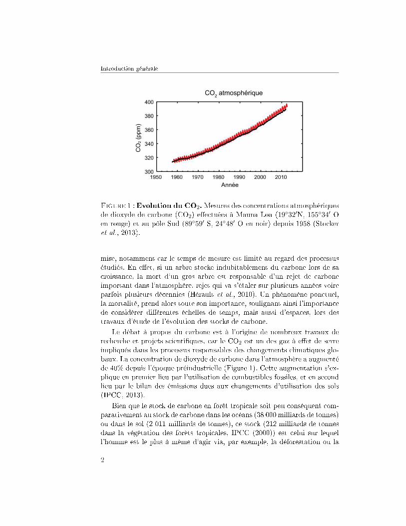
Figure 1 : Evolution du CO2.Mesures des concentrations atmosphériquesde dioxyde de carbone (CO2) e�ectuées à Mauna Loa (19◦32′N, 155◦34′ Oen rouge) et au pôle Sud (89◦59′ S, 24◦48′ O en noir) depuis 1958 (Stockeret al., 2013).
mise, notamment car le temps de mesure est limité au regard des processusétudiés. En e�et, si un arbre stocke indubitablement du carbone lors de sacroissance, la mort d'un gros arbre est responsable d'un rejet de carboneimportant dans l'atmosphère, rejet qui va s'étaler sur plusieurs années voireparfois plusieurs décennies (Hérault et al., 2010). Un phénomène ponctuel,la mortalité, prend alors toute son importance, soulignant ainsi l'importancede considérer di�érentes échelles de temps, mais aussi d'espaces, lors destravaux d'étude de l'évolution des stocks de carbone.
Le débat à propos du carbone est à l'origine de nombreux travaux derecherche et projets scienti�ques, car le CO2 est un des gaz à e�et de serreimpliqués dans les processus responsables des changements climatiques glo-baux. La concentration de dioxyde de carbone dans l'atmosphère a augmentéde 40% depuis l'époque préindustrielle (Figure 1). Cette augmentation s'ex-plique en premier lieu par l'utilisation de combustibles fossiles, et en secondlieu par le bilan des émissions dues aux changements d'utilisation des sols(IPCC, 2013).
Bien que le stock de carbone en forêt tropicale soit peu conséquent com-parativement au stock de carbone dans les océans (38 000 milliards de tonnes)ou dans le sol (2 011 milliards de tonnes), ce stock (212 milliards de tonnesdans la végétation des forêts tropicales, IPCC (2000)) est celui sur lequell'homme est le plus à même d'agir via, par exemple, la déforestation ou la
2
1. LES FORÊTS TROPICALES
mise en oeuvre de politiques de protection. En outre, les �ux de carbonepeuvent changer sous l'impulsion des changements climatiques, et participerainsi à ces changements, créant des e�ets de feedback qui sont di�ciles àprévoir et à quanti�er.
1.2 Diversité spéci�que et fonctionnelle en forêt tropicale
La forêt tropicale n'est pas uniquement un stock de carbone, mais aussi unréservoir de biodiversité. Avec entre 50 et 70 % des espèces vivantes en mi-lieux terrestres sur seulement 7 % des terres émergées, les forêts tropicalespeuvent être considérées comme une formidable machine à créer et mainte-nir de la biodiversité. Cette diversité, notamment des espèces d'arbres, esttelle que les écologues cherche à comprendre comment ces espèces coexistent(Chesson, 2000; Hubbell, 2001; Webb et al., 2002; Wright, 2002).
Les espèces ont souvent été regroupées de façon à distinguer par exempleles espèces pionnières des espèces à croissance lente (Favrichon, 1998). Cesregroupements peuvent parfois se baser sur (i) des distances phylogénétiquesqui permettent de regrouper les espèces par genre ou par famille ou (ii) surla distance fonctionnelle entre espèces, distance qui n'était pas facilementquanti�able avant la récolte systématique d'un grand nombre de traits fonc-tionnels. Ces traits fonctionnels peuvent être relatifs au bois, à la feuille, ouà l'architecture de l'arbre, et sont autant d'indicateurs des stratégies d'allo-cation des ressources des di�érentes espèces. Un e�ort collectif important aété fourni, ces dernières années, par la communauté scienti�que pour créerdes bases de données de traits (Baraloto et al., 2010a,b; Chave et al., 2009;Wright et al., 2004) selon des protocoles standardisés (Cornelissen et al.,2003).
Ces bases de données de traits fonctionnels ont permis d'étudier la va-riabilité inter- et intra-spéci�que des traits et de tester l'existence d'éven-tuels compromis fonctionnels. Ces études montrent que des axes orthogonauxpeuvent être créés, chaque axe pouvant être décrit par un certain nombrede traits, et représentant un gradient continu de stratégies écologiques. Dif-férents axes ont donc été mis en avant, d'abord par Westoby et al. (2002),qui identi�e des traits relatifs aux feuilles, à la tige, et à la structure géné-rale de l'arbre. La portée mondiale de l'axe relatif aux feuilles a été miseen avant par Wright et al. (2004) (LES : leaf economics spectrum). Plusrécemment un axe relatif au bois a été identi�é (Chave et al., 2009) (SES :stem economics spectrum). Ces deux axes sont orthogonaux chez les arbrestropicaux (Baraloto et al., 2010b). Le LES re�ète un gradient d'investisse-ment des ressources partant d'espèces ayant une production de feuilles à fort
3
Introduction générale
taux de renouvellement d'un côté vers, à l'autre extrémité du gradient, desespèces caractérisées par la production de feuilles plus robustes à renouvelle-ment plus rares, qui se défendent ainsi mieux contre les ennemis (Coley andBarone, 1996). Le SES re�ète un gradient de stratégies similaires au niveaudu tronc, avec d'un côté des bois denses, relativement coûteux à construiremais plus résistants aux pathogènes, et de l'autre des bois riches en eau etdes écorces plus �nes (Chave et al., 2009).
Les traits fonctionnels sont donc des outils puissants d'analyse pourmieux comprendre les di�érentes stratégies des di�érentes espèces coexistanten forêts tropicales. D'autre part, certains traits sont également des indica-teurs de l'e�cience de l'utilisation des ressources. En fonction de leurs traits,les arbres peuvent avoir des comportements di�érents vis à vis des stress aux-quels ils sont soumis (exploitation, sécheresse). C'est pourquoi l'utilité de cestraits dans des modèles de dynamique de peuplement forestier me semble ju-dicieuse.
1.3 La dynamique forestière
Les di�érentes stratégies fonctionnelles des espèces et la grande diversitéen forêt tropicale se traduisent en di�érences du point de vue de la dy-namique démographique. C'est notamment ce qui fait une grande di�érenceentre espèces pionnières à croissance rapide et espèces à croissance plus lente.La dynamique des forêts tropicales à l'échelle d'une communauté est doncun mélange de comportements individuels d'arbres qui cohabitent. Cettedynamique est importante car elle peut être actrice de changements. Ladynamique forestière est classiquement structurée en trois processus fonda-mentaux : le recrutement, la croissance et la mortalité. Ces trois processuspeuvent être étudiés séparément car ils sont en théorie bien distincts.
1.3.1 Le recrutement
Le recrutement peut être dé�ni de façon très large, de la synthèse de grainespar l'arbre, à la dissémination de ces graines grâce à di�érents agents, bio-tiques ou abiotiques, puis à la germination de ces graines, à l'apparitiond'une plantule et en�n, à la croissance de la plantule jusqu'à un diamètreseuil (10 cm dans notre cas). On distingue 4 stades chez les arbres des forêtstropicales humides : les graines, les semis (seedlings), les juvéniles (saplings)et les adultes. Ces stades di�érent par leurs morphologies, mais aussi parleurs caractéristiques écologiques, comme l'héliophilie par exemple (Poor-ter and Rose, 2005). En forêt tropicale, où la diversité est considérable, cette
4
1. LES FORÊTS TROPICALES
variabilité additionnelle ne permet pas de connaitre avec précision le compor-tement de chaque stade de chaque espèce. En l'absence de perturbation, denombreux modélisateurs préfèrent souvent considérer le recrutement commeun processus aléatoire respectant les proportions des di�érentes espèces pré-sentes (Moravie et al., 1997).
1.3.2 La croissance
La croissance peut être de deux types, la croissance primaire concerne lataille tandis que la croissance secondaire concerne le diamètre. Il est di�-cile de mesurer la taille d'un arbre en forêt, et les forestiers s'intéressent engénéral à la croissance en diamètre. Des modèles d'allométrie permettentéventuellement de passer du diamètre à la taille (Molto et al., 2014), mêmesi ces modèles fournissent des prédictions entachées de grandes incertitudes(Molto et al., 2013). La croissance en diamètre est, par conséquent, un sujetrelativement bien traité dans la littérature des forêts tropicales humides, etceci notamment grâce aux dispositifs de suivi forestier comme Paracou enGuyane française, La Selva au Costa Rica, ou BCI au Panama (Barro Colo-rado Island). Ce type de dispositif permet de suivre la croissance d'arbres dedi�érentes espèces sur plusieurs dizaines d'hectares et de façon régulière dansle temps sur plusieurs décennies. La croissance secondaire peut être mise enrelation avec di�érents traits fonctionnels, et ainsi être associée à di�érentesstratégies écologiques. Deux comportements extrêmes se distinguent avec,d'une part, les arbres pionniers dont la croissance est rapide, le bois peudense, et le cycle de vie court. Ces espèces sont héliophiles et le Cécropia enest un représentant emblématique en Guyane Française. Un grand nombred'individus de cette espèce se retrouve dans les trouées ou au bord des routes.Cette espèce est donc souvent observée en forêt secondaire. A l'ombre de cesespèces pionnières, d'autres espèces peuvent se développer et croitre de façonplus lente. Ces espèces sont souvent caractérisées par des bois plus denses.La croissance peut aussi considérablement varier entre les individus d'unemême espèce. Cette variabilité intra-spéci�que peut être liées à des facteursenvironnementaux exogènes (climat, lumière...), biotiques exogènes (compé-tition, prédation, facilitation...) et endogènes (génétique). En�n, les arbresgrandissent à des vitesses di�érentes en fonction de leur stade ontogénique(Hérault et al., 2011), ce qui ajoute une variabilité intra-individuelle.
1.3.3 La mortalité
La mortalité est un processus plus di�cile à observer que la croissance etses causes sont, de fait, moins comprises. La mortalité peut être de plusieurs
5
Introduction générale
types : sur pied, ou par chablis primaire ou secondaire. La mortalité est unprocessus ponctuel, observable uniquement lors de suivis réguliers dans letemps. Pourtant les processus impliqués dans la mortalité peuvent être longsde plusieurs décennies. La complexité du processus de mortalité provientégalement de notre incapacité à détecter précisément l'occurrence du phé-nomène. Un arbre peut être pris pour mort une année, puis vivant l'annéesuivante, le processus peut en e�et toucher une partie de l'arbre uniquement.La mortalité est très importante, car elle peut être à l'origine d'un chabliset d'une trouée, qui ouvrira la canopée pour laisser les rayons du soleil at-teindre le sous-bois. C'est suite à la mort des arbres que d'autres plus jeunesprennent la place libre, la mortalité est donc le moteur à part entière de ladynamique.
La probabilité de mourir n'est pas la même en fonction du stade ontogé-nique de l'arbre. Les arbres très jeunes ont des taux de mortalité élevés, dus àla très forte compétition régnant parmi les jeunes plantules. Les petits arbressont en e�et soumis à une forte pression de sélection, et seul un petit nombred'entre eux parviendront à une taille adulte. Le taux de mortalité est aussiplus élevé pour les vieux arbres, ceci est dû à la sénescence. Comme c'est lecas pour la croissance, d'autres facteurs entrent en jeux. Les arbres peuventêtre soumis à di�érentes contraintes (herbivorie, événements climatiques ex-trêmes...) et ne pas se remettre des dégâts causés. Une faiblesse causée parune sécheresse pourra, par exemple, être fatale à un arbre des années plustard, lors d'une seconde sécheresse moins importante (Dobbertin, 2005).
1.3.4 La compétition pour les ressources
Il est di�cile de décrire la dynamique forestière sans faire intervenir la no-tion de compétition. Il s'agit de la compétition pour les ressources, à savoirla lumière, l'eau et les nutriments et ions nécessaires à la croissance et aumaintien de l'arbre. L'idée de compétition est omniprésente et a une longuetradition en écologie dès que plusieurs organismes sont en présence (Lotka,1925; Volterra, 1926; Gause, 1932; Tilman, 1981), elle est intimement liéeà l'idée de la sélection, qui ne conserve, à long terme, que les individus quiont les meilleures valeurs sélectives. En forêt, les arbres sont soumis à uneforte compétition pour la lumière, qui les fera grandir le plus vite et le plushaut possible, et à une compétition pour l'eau, qui les obligera à former unsystème racinaire adapté.
Pour quanti�er cette compétition pour la ressource, de nombreux in-dices de compétition ont été créés. Les indices indépendants de la distanceprennent en compte le nombre de voisins et/ou leurs tailles (Gourlet-Fleury,
6
1. LES FORÊTS TROPICALES
1998; Stoll and Newbery, 2005). Les indices dépendants de la distance ajoutentà cela la distance entre les arbres (Canham et al., 2004; Uriarte et al., 2010;Thorpe et al., 2010). Plus rares, certains indices se basent sur les diagrammesde Voronoi, pour lesquels la disponibilité de la ressource est dépendante del'agencement spatial des voisins. Les diagrammes de Voronoi permettent departitionner la surface étudiée en autant de polygones que d'arbres, chaquepolygone représente alors un espace disponible pour l'arbre et l'aire du po-lygone est utilisée comme indice de compétition pour l'arbre associé (Aakalaet al., 2013). Certains indices dépendent aussi de la taille de l'arbre consi-déré. Par exemple, le nombre total d'arbres qui se trouvent au voisinagede l'arbre d'intérêt et qui sont plus gros que ce dernier. Dans un modèlede croissance dépendant du diamètre, de tels indices sont di�cilement uti-lisables, car ils sont directement liés au diamètre de l'arbre, et covarient defaçon évidente avec ce diamètre. Ils sont donc à proscrire pour inclure dela compétition dans un modèle de croissance, pour ne pas avoir de confu-sion d'e�ets entre ontogénie et compétition. En forêt tempérée, les relationsinter-spéci�ques de compétition sont parfois très bien décrites et peuventêtre correctement, c'est à dire une à une, prise en compte dans la construc-tion des indices de compétition, ce qui rend l'indice encore plus puissant.En forêt tropicale, il est compliqué d'envisager une telle complexité, au vudu nombre d'espèces. En forêts exploitées, les gradients liés à la compéti-tion sont importants, l'intensité d'exploitation étant très hétérogène dansl'espace, ce qui justi�e l'utilisation de ces indices de compétition. En forêtnaturelle, ces gradients existent aussi grâce aux chablis naturels. Ceci dit,très peu d'individus sont �nalement en situation de faible compétition sibien que les gradients de compétition ne semblent pas expliquer une partimportante de la variabilité de la croissance observée (Gaspard, 2014). Il estdi�cile de trouver un estimateur de compétition sans inclure dans cet es-timateur les e�ets à expliquer. Par exemple, une fois que la variance liée àl'ontogénie est correctement prise en compte, la variance résiduelle expliquéepar la compétition est �nalement très faible. La compétition n'est donc pastraitée dans ce manuscrit et n'a pas été inclue dans les modèles utilisés. Tou-tefois il faut garder en tête que celle-ci s'avérerait nécessaire pour étendrenos modèles à des forêts exploitées, ce dont il sera question dans le chapitre4.
1.4 Plus particulièrement en Guyane Française
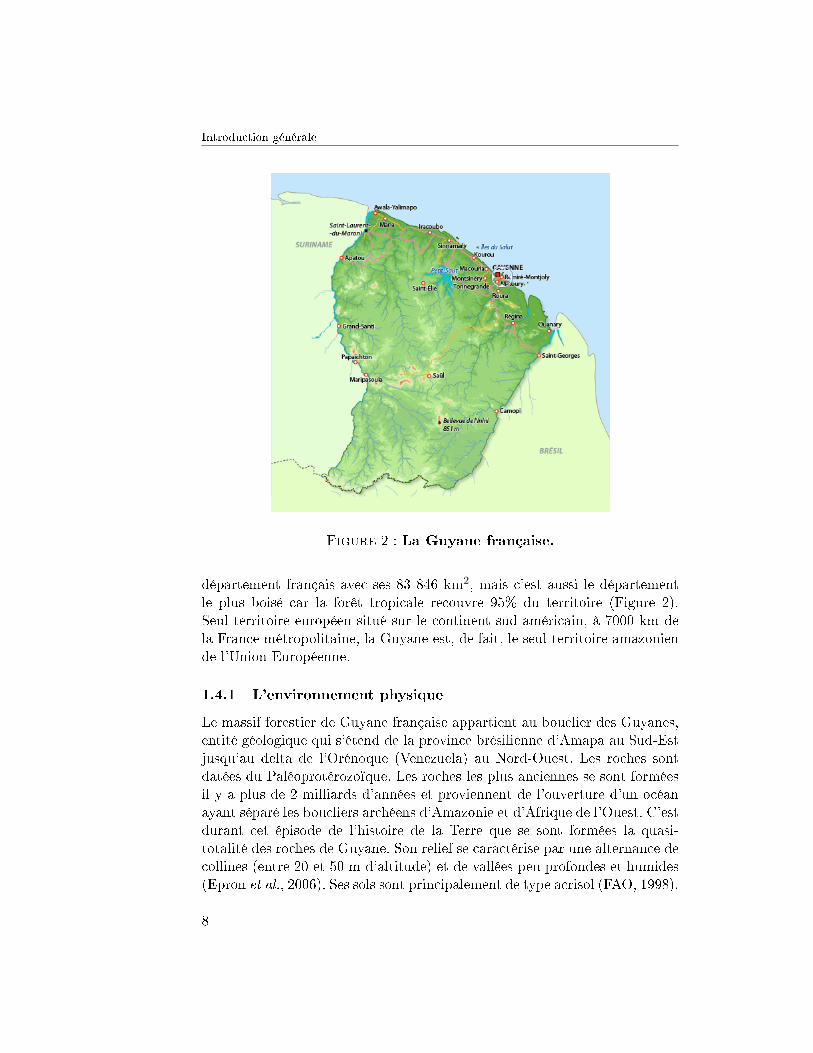
La Guyane française est située entre le Suriname à l'Ouest, le Brésil au Sud-Ouest, et l'océan Atlantique au Nord. La Guyane française est le plus grand
7
Introduction générale
Figure 2 : La Guyane française.
département français avec ses 83 846 km2, mais c'est aussi le départementle plus boisé car la forêt tropicale recouvre 95% du territoire (Figure 2).Seul territoire européen situé sur le continent sud-américain, à 7000 km dela France métropolitaine, la Guyane est, de fait, le seul territoire amazoniende l'Union Européenne.
1.4.1 L'environnement physique
Le massif forestier de Guyane française appartient au bouclier des Guyanes,entité géologique qui s'étend de la province brésilienne d'Amapa au Sud-Estjusqu'au delta de l'Orénoque (Venezuela) au Nord-Ouest. Les roches sontdatées du Paléoprotérozoïque. Les roches les plus anciennes se sont forméesil y a plus de 2 milliards d'années et proviennent de l'ouverture d'un océanayant séparé les boucliers archéens d'Amazonie et d'Afrique de l'Ouest. C'estdurant cet épisode de l'histoire de la Terre que se sont formées la quasi-totalité des roches de Guyane. Son relief se caractérise par une alternance decollines (entre 20 et 50 m d'altitude) et de vallées peu profondes et humides(Epron et al., 2006). Ses sols sont principalement de type acrisol (FAO, 1998).
8

1. LES FORÊTS TROPICALES
1.4.2 L'environnement biologique
En Guyane française, la forêt est équatoriale sempervirente ombrophile deplaine. La biodiversité rencontrée en Guyane est considérable. Plus de 7000espèces végétales (champignons exclus) sont recensées dont 5600 de plantessupérieures incluant 1500 espèces d'arbres. Plus de 9 espèces végétales sur10 sont des espèces forestières. La faune est également très riche. A titred'exemple, si la France métropolitaine recense 77 espèces de poissons d'eaudouce, quasiment 500 sont répertoriées en Guyane. Qui plus est, un tiers deces poissons sont, à l'heure actuelle, endémiques de Guyane. A ce jour, 190espèces de mammifères, 740 d'oiseaux, 160 de reptiles, 110 d'amphibiens sontrelativement bien connus alors qu'on estime à 400 000 le nombre d'espècesd'invertébrés peuplant les forêts guyanaises (de Noter, 2008). Une grandepartie de cette biodiversité a pu se maintenir en Guyane grâce à une densitéde population extrêmement faible à l'intérieur des terres.
1.4.3 La population
La population guyanaise estimée en 2013 était de 250 109 hab, ce qui fait dela Guyane un département de très faible densité démographique. Mais cettedensité est en forte augmentation et les prédictions pour 2030 sont de 425000 hab (INSEE, 2013). Cette augmentation provient d'une démographietrès dynamique et d'une forte immigration des pays voisins. L'exploitationforestière en Guyane française est réglementée et réduite au domaine fores-tier permanent, ce qui fait de la forêt un espace relativement protégé. Maisd'ici 2030, la demande en bois de construction augmentera fortement, ainsi,probablement, que la demande en bois énergie pour suppléer au barrage dePetit-Saut.
1.4.4 Le climat
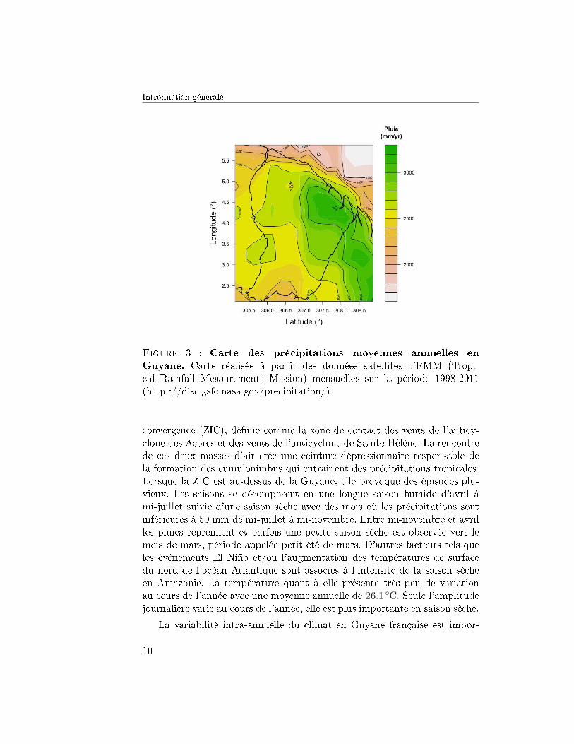
La Guyane, "terre d'eaux abondantes" en Arawak, porte bien son nom.Comme c'est souvent le cas en climat tropical, le climat est plus in�uencépar le régime des pluies que par les variations saisonnières de températures.Les précipitations moyennes sont comprises entre 2000 et 4000 mm par anet montrent une très grande variabilité spatiale et temporelle (Figures 3,5 et 4). Il existe un fort gradient de précipitations d'ouest en est avec desprécipitations annuelles parfois supérieures à 4000 mm à l'est et des préci-pitations annuelles proches de 1500 mm pour certaines stations à l'ouest dudépartement. La variabilité saisonnière des précipitations est importante enGuyane. Ces variations sont dues au déplacement de la zone intertropicale de
9
Introduction générale
Figure 3 : Carte des précipitations moyennes annuelles enGuyane. Carte réalisée à partir des données satellites TRMM (Tropi-cal Rainfall Measurements Mission) mensuelles sur la période 1998-2011(http ://disc.gsfc.nasa.gov/precipitation/).
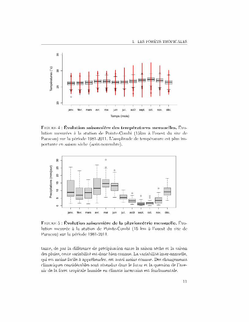
convergence (ZIC), dé�nie comme la zone de contact des vents de l'anticy-clone des Açores et des vents de l'anticyclone de Sainte-Hélène. La rencontrede ces deux masses d'air crée une ceinture dépressionnaire responsable dela formation des cumulonimbus qui entrainent des précipitations tropicales.Lorsque la ZIC est au-dessus de la Guyane, elle provoque des épisodes plu-vieux. Les saisons se décomposent en une longue saison humide d'avril àmi-juillet suivie d'une saison sèche avec des mois où les précipitations sontinférieures à 50 mm de mi-juillet à mi-novembre. Entre mi-novembre et avrilles pluies reprennent et parfois une petite saison sèche est observée vers lemois de mars, période appelée petit été de mars. D'autres facteurs tels queles événements El Niño et/ou l'augmentation des températures de surfacedu nord de l'océan Atlantique sont associés à l'intensité de la saison sècheen Amazonie. La température quant à elle présente très peu de variationau cours de l'année avec une moyenne annuelle de 26.1 ◦C. Seule l'amplitudejournalière varie au cours de l'année, elle est plus importante en saison sèche.
La variabilité intra-annuelle du climat en Guyane française est impor-
10
1. LES FORÊTS TROPICALES
Figure 4 : Évolution saisonnière des températures mensuelles. Évo-lution mesurées à la station de Pointe-Combi (15km à l'ouest du site deParacou) sur la période 1981-2011. L'amplitude de température est plus im-portante en saison sèche (août-novembre).
Figure 5 : Évolution saisonnière de la pluviométrie mensuelle. Évo-lution mesurée à la station de Pointe-Combi (15 km à l'ouest du site deParacou) sur la période 1981-2011.
tante, de par la di�érence de précipitation entre la saison sèche et la saisondes pluies, cette variabilité est donc bien connue. La variabilité inter-annuelle,qui est moins facile à appréhender, est aussi moins connue. Des changementsclimatiques considérables sont attendus dans le futur et la question de l'ave-nir de la forêt tropicale humide en climats incertains est fondamentale.
11
Introduction générale
1.5 Le site de Paracou
1.5.1 Le site expérimental
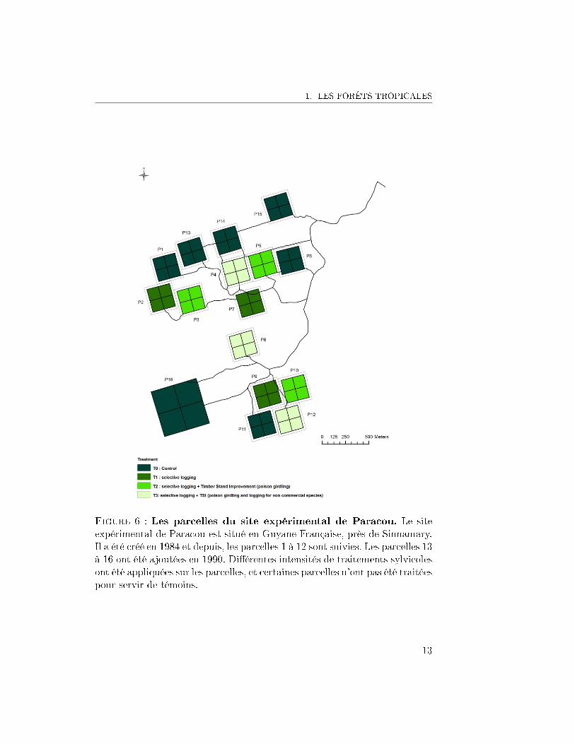
Le site expérimental de Paracou est installé sur la commune de Sinnamarydepuis 1984, il est constitué de 15 parcelles de 6.25 hectares chacune et d'uneparcelle de 25 hectares (Figure 6). Certaines de ces parcelles ont été soumisesà des traitements d'exploitation forestière, il existe trois traitements di�é-rents, correspondant à une exploitation plus ou moins intense. Les autresparcelles ont été laissées en contrôle pour servir de témoins (parcelles 1,6,11,Figure 6). Les parcelles 13,14,15 et 16 ont été ajoutées au dispositif en 1990.Le site était initialement conçu pour étudier l'impact de l'exploitation fores-tière, et répondre à des questions de sylviculture. Cette problématique initiales'est peu à peu diversi�ée, et aujourd'hui le site de Paracou est utilisé pourétudier la dynamique des écosystèmes forestiers guyanais en général. La forêtdu site de Paracou comprend plus de 700 espèces d'arbres de DBH supérieurà 10cm. Les familles dominantes sont les Fabaceae, les Chrysobalanaceae, lesLecythidaceae et les Sapotaceae.
1.5.2 Les données disponibles
Chaque année, pendant la saison sèche (à partir du mois de juillet), l'inven-taire des parcelles 1 à 15 du site de Paracou a lieu. Pendant cet inventaire,tous les arbres dont le diamètre à 1.30m (DBH : diameter at breast height)est supérieur à 10cm sont mesurés, avec une précision de 0.5cm. Les arbresrecrutés, qui n'étaient pas dans l'inventaire l'année précédente, sont ajou-tés avec leurs coordonnées, les arbres morts sont notés morts, et le type demort est relevé (sur pied, chablis primaire ou secondaire). Lorsqu'un arbrea de trop gros contreforts ou un tronc de forme particulière, la mesure dudiamètre est rehaussée, ou estimée. Cet inventaire annuel permet donc desuivre la dynamique individuelle des arbres depuis l'installation du site en1984 ou depuis 1990 pour les parcelles les plus récentes.
Le travail réalisé sur le site de Paracou et les données qu'il génère sont àl'origine de nombreuses études qui ont permis et permettent encore de mieuxcomprendre l'écosystème forestier guyanais, c'est un travail titanesque qu'ilconvient de saluer et d'apprécier à sa juste valeur.
1.5.3 L'identi�cation taxonomique
L'identi�cation taxonomique de tous les arbres des parcelles témoins du sitede Paracou est �nalisée depuis 2012. Avant cette date, les arbres étaient
12
1. LES FORÊTS TROPICALES
Figure 6 : Les parcelles du site expérimental de Paracou. Le siteexpérimental de Paracou est situé en Guyane Française, près de Sinnamary.Il a été créé en 1984 et depuis, les parcelles 1 à 12 sont suivies. Les parcelles 13à 16 ont été ajoutées en 1990. Di�érentes intensités de traitements sylvicolesont été appliquées sur les parcelles, et certaines parcelles n'ont pas été traitéespour servir de témoins.
13
Introduction générale
identi�és grâce à leurs noms vernaculaires. Des numéros étaient associés àces noms vernaculaires et chaque arbre était associé à un numéro lors de sonrecrutement, c'est-à-dire son entrée dans la base de donnée. Or, ces nomsvernaculaires n'ont pas une grande précision taxonomique, certains nomsvernaculaires correspondent à plusieurs espèces, et les correspondances sontparfois beaucoup moins claires qu'attendues. Il a donc été décidé d'identi�ertous les arbres de Paracou, grâce à l'expertise de botanistes, avec l'aide del'herbier de Cayenne lorsque c'était nécessaire.
2 Les changements climatiques
Le 21/09/2014, la marche mondiale pour le climat a mobilisé des centainesde milliers de personnes dans plus de 2500 endroits du globe. A Cayenne, enGuyane Française, seule une cinquantaine de personnes ont dé�lé. Pourtantcette région du monde ne sera pas épargnée par les changements prévus parle groupe d'experts intergouvernemental sur l'évolution du climat (GIEC).
2.1 Les changements globaux
Les changements climatiques sont au c÷ur de plusieurs milliers de publica-tions chaque année. Leurs impacts sur les écosystèmes sont une des préoc-cupations au c÷ur des débats. Les climatosceptiques sont de plus en plusrares, et les rapports fournis par le GIEC sont maintenant reconnus commeune base de travaux extrêmement �able.
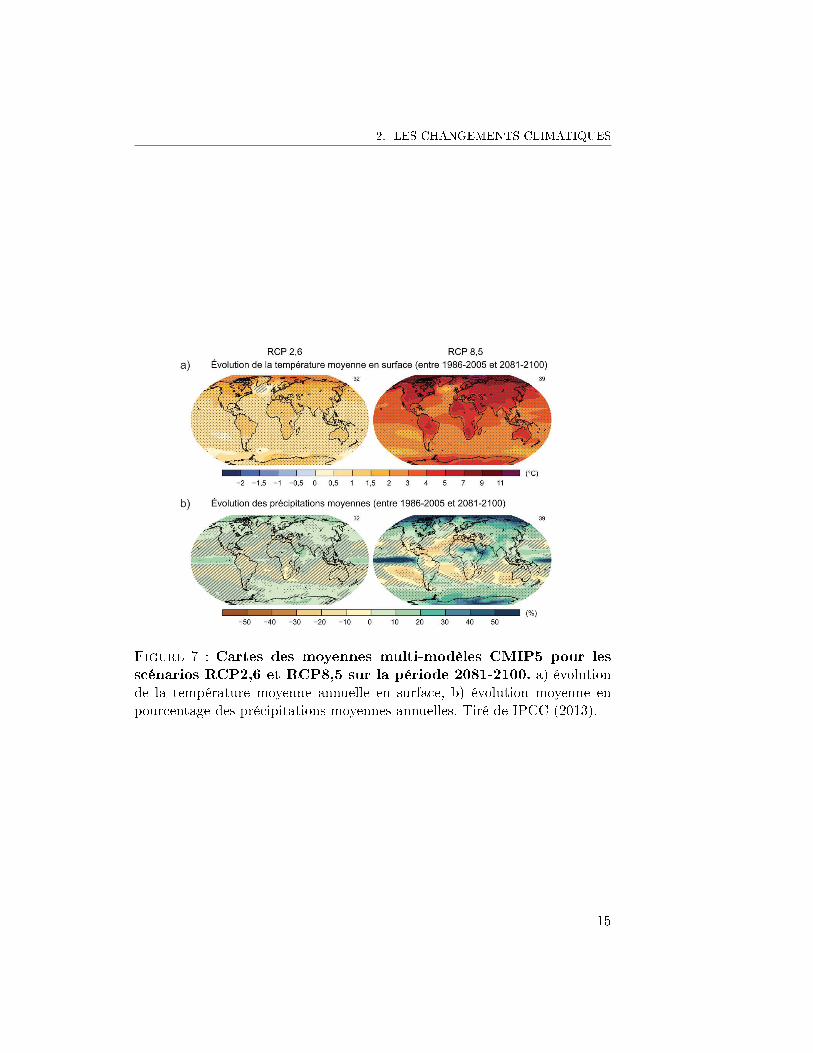
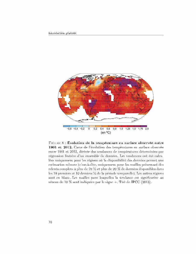
Le GIEC a été créé en 1988 sous l'impulsion de l'organisation météoro-logique mondiale (OMM) et du Programme des Nations Unies pour l'Envi-ronnement (PNUE). L'une des principales activités du GIEC consiste à pro-céder, à intervalles réguliers, à une évaluation de l'état des connaissances re-latives au changement climatique. Dans le rapport du GIEC intitulé "Chan-gements climatiques 2013, les éléments scienti�ques", et comme le montre laFigure 8, le GIEC souligne que le réchau�ement du système climatique estsans équivoque et que, depuis les années 1950, beaucoup de changements ob-servés sont sans précédent depuis des décennies voire des millénaires (IPCC,2013). L'atmosphère et l'océan se sont réchau�és, les couvertures de neige etde glace ont diminué, le niveau des mers s'est élevé et les concentrations desgaz à e�et de serre ont augmenté.
Pour tirer ses conclusions sur les futurs climats probables, le GIEC uti-lise des scénarios dits RCP (Representative Concentration Pathway) plus oumoins optimistes. Ces scénarios permettent d'envisager le futur en fonctiondes décisions prises et des émissions de gaz à e�et de serre, tels que le CO2.
14
2. LES CHANGEMENTS CLIMATIQUES
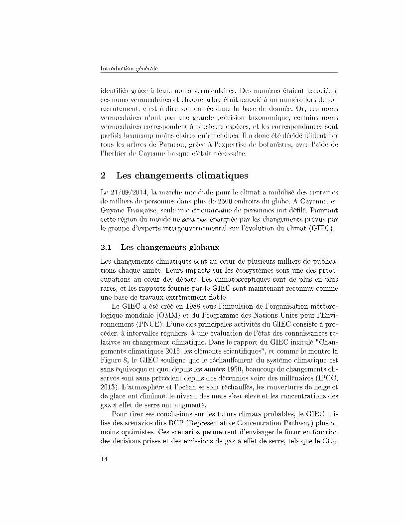
Figure 7 : Cartes des moyennes multi-modèles CMIP5 pour lesscénarios RCP2,6 et RCP8,5 sur la période 2081-2100. a) évolutionde la température moyenne annuelle en surface, b) évolution moyenne enpourcentage des précipitations moyennes annuelles. Tiré de IPCC (2013).
15
Introduction générale
Figure 8 : Évolution de la température en surface observée entre1901 et 2012. Carte de l'évolution des températures en surface observéeentre 1901 et 2012, dérivée des tendances de températures déterminées parrégression linéaire d'un ensemble de données. Les tendances ont été calcu-lées uniquement pour les régions où la disponibilité des données permet uneestimation robuste (c'est-à-dire, uniquement pour les mailles présentant desrelevés complets à plus de 70 % et plus de 20 % de données disponibles dansles 10 premiers et 10 derniers % de la période temporelle). Les autres régionssont en blanc. Les mailles pour lesquelles la tendance est signi�cative auniveau de 10 % sont indiquées par le signe +. Tiré de IPCC (2013).
16
2. LES CHANGEMENTS CLIMATIQUES
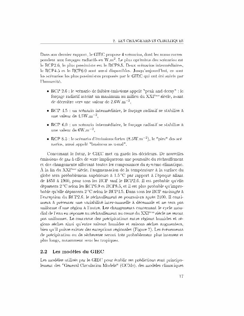
Dans son dernier rapport, le GIEC propose 4 scénarios, dont les noms corres-pondent aux forçages radiatifs en W.m2. Le plus optimiste des scénarios estle RCP2.6, le plus pessimiste est le RCP8.5. Deux scénarios intermédiaires,le RCP4.5 et le RCP6.0 sont aussi disponibles. Jusqu'aujourd'hui, ce sontles scénarios les plus pessimistes proposés par le GIEC qui ont été suivis parl'humanité.
• RCP 2.6 : le scénario de faibles émissions appelé "peak and decay" : leforçage radiatif atteint un maximum au milieu du XXIème siècle, avantde décroitre vers une valeur de 2.6W.m−2,
• RCP 4.5 : un scénario intermédiaire, le forçage radiatif se stabilise àune valeur de 4.5W.m−2,
• RCP 6.0 : un scénario intermédiaire, le forçage radiatif se stabilise àune valeur de 6W.m−2,
• RCP 8.5 : le scénario d'émissions fortes (8.5W.m−2), le "pire" des scé-narios, aussi appelé "business as usual".
Concernant le futur, le GIEC met en garde les décideurs. De nouvellesémissions de gaz à e�et de serre impliqueront une poursuite du réchau�ementet des changements a�ectant toutes les composantes du système climatique.À la �n du XXIème siècle, l'augmentation de la température à la surface duglobe sera probablement supérieure à 1.5 ◦C par rapport à l'époque allantde 1850 à 1900, pour tous les RCP sauf le RCP2.6. Il est probable qu'elledépassera 2 ◦C selon les RCP6.0 et RCP8.5, et il est plus probable qu'impro-bable qu'elle dépassera 2 ◦C selon le RCP4.5. Dans tous les RCP envisagés àl'exception du RCP2.6, le réchau�ement se poursuivra après 2100. Il conti-nuera à présenter une variabilité inter-annuelle à décennale et ne sera pasuniforme d'une région à l'autre. Les changements concernant le cycle mon-dial de l'eau en réponse au réchau�ement au cours du XXIème siècle ne serontpas uniformes. Le contraste des précipitations entre régions humides et ré-gions sèches ainsi qu'entre saisons humides et saisons sèches augmentera,bien qu'il puisse exister des exceptions régionales (Figure 7). Les événementsde précipitation ou de sécheresse seront très probablement plus intenses etplus longs, notamment sous les tropiques.
2.2 Les modèles du GIEC
Les modèles utilisés par le GIEC pour établir ses prédictions sont principa-lement des "General Circulation Models" (GCMs), des modèles climatiques
17
Introduction générale
basés sur la combinaison de modèles biogéochimiques, géographiques et deperturbations climatiques, et qui permettent de modéliser les di�érents �uxsur la surface terrestre ainsi que l'impact des changements climatiques surla végétation et sur les cycles de carbone et d'eau associés. Leur utilisationn'est pas aisée, et les sorties des modèles ne sont pas présentées de façon àpouvoir être directement utilisées pour étudier l'impact des changements cli-matiques sur d'autres systèmes dynamiques (Jones et al., 2009). Les sortiesdes GCMs doivent être réduites pour obtenir des données journalières à unendroit donné de la planète. Di�érentes méthodes existent pour réduire lesdonnées, les méthodes les plus grossières sont en général aussi les plus mau-vaises, tandis que des méthodes plus précises auront de meilleurs résultatsmais nécessiteront des données additionnelles pour permettre de calibrer lessorties des modèles.
Di�érents outils sont actuellement développés pour réaliser des descentesd'échelles. C'est le cas de MarkSim, ce logiciel permet de simuler des donnéesà partir de 17 modèles pour les années 2010 à 2095, et il est mis à dispositionsur internet (gisweb.ciat.cgiar.org/MarkSimGCM/). Le logiciel MarkSim estcalibré grâce aux données climatiques de plus de 10 000 stations météorolo-giques dans le monde. D'autre part, une descente d'échelle a été réalisée pourla France (métropole, mais aussi DOM-TOM) pour le modèle Arpege-V4.6de Météo-France (non disponible dans MarkSim), qui est disponible en lignesur la plateforme DRIAS (http ://www.drias-climat.fr/). Cet outil permetentre autres d'avoir des prédictions précises pour la Guyane (Figures 9 et10). Ces descentes d'échelles sont d'un grand intérêt car (i) elles permettentd'utiliser des données précises et de les intégrer dans des modèles pour lesappliquer à des processus climat-dépendants et (ii) la mise à disposition deces données spatiales permet à tout un chacun de se faire une idée des cli-mats attendus dans une région d'intérêts, et de mieux prendre consciencedes changements climatiques en cours.
2.3 Les climats futurs en forêts tropicales
D'après le dernier rapport du GIEC (IPCC, 2013), des augmentations destempératures moyennes saisonnières et annuelles importantes sont prévues.Les épisodes de précipitations extrêmes deviendront très probablement plusintenses et fréquents sur les continents des moyennes latitudes et dans lesrégions tropicales humides d'ici la �n de ce siècle, en lien avec l'augmentationde la température moyenne en surface. Les modèles utilisés pour construireles prédictions du GIEC sont nombreux et issus de laboratoires di�érents, ré-partis partout dans le monde. A l'échelle amazonienne, un consensus semble
18
2. LES CHANGEMENTS CLIMATIQUES
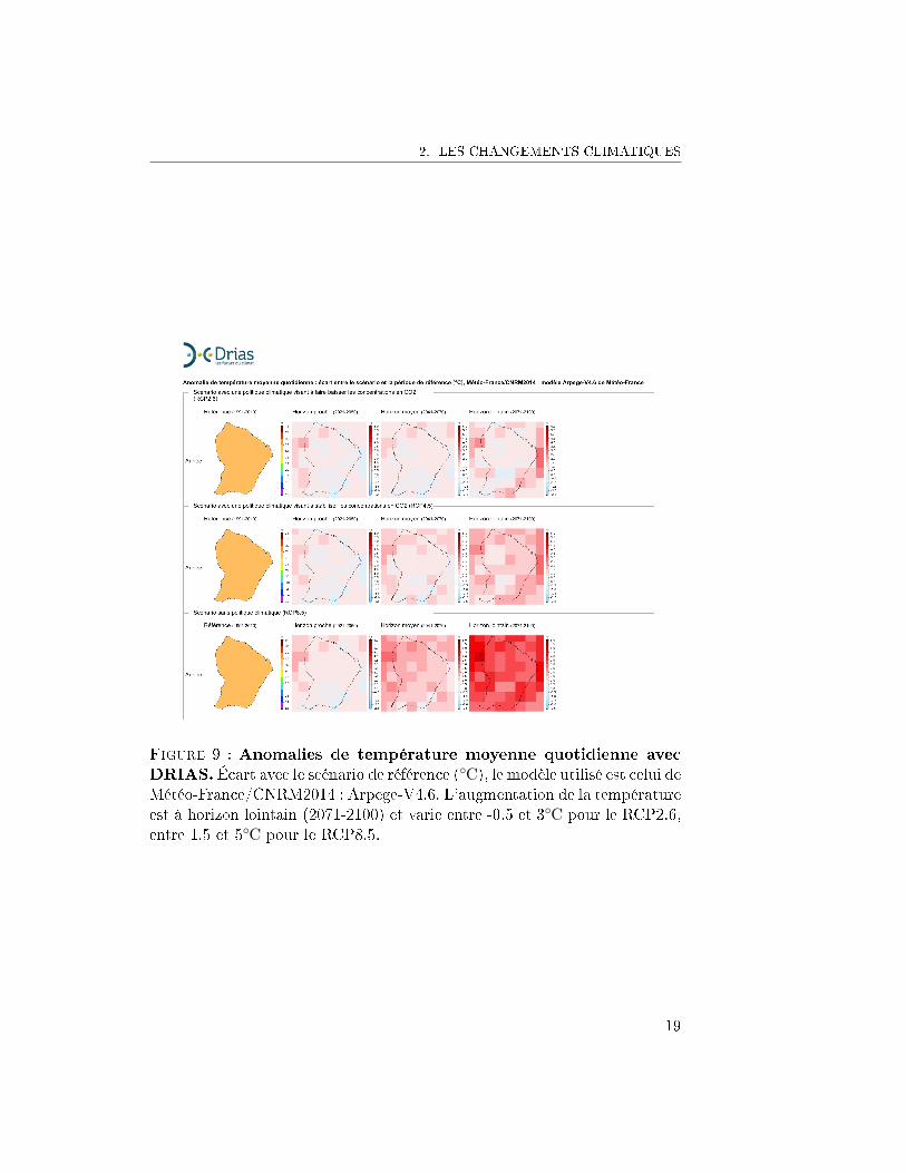
Figure 9 : Anomalies de température moyenne quotidienne avecDRIAS. Écart avec le scénario de référence (◦C), le modèle utilisé est celui deMétéo-France/CNRM2014 : Arpege-V4.6. L'augmentation de la températureest à horizon lointain (2071-2100) et varie entre -0.5 et 3◦C pour le RCP2.6,entre 1.5 et 5◦C pour le RCP8.5.
19
Introduction générale
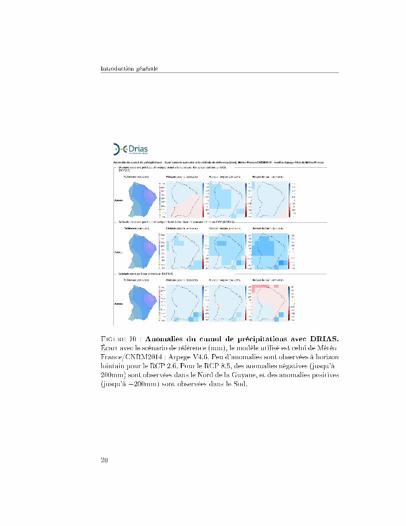
Figure 10 : Anomalies du cumul de précipitations avec DRIAS.Écart avec le scénario de référence (mm), le modèle utilisé est celui de Météo-France/CNRM2014 : Arpege-V4.6. Peu d'anomalies sont observées à horizonlointain pour le RCP 2.6. Pour le RCP 8.5, des anomalies négatives (jusqu'à -200mm) sont observées dans le Nord de la Guyane, et des anomalies positives(jusqu'à +200mm) sont observées dans le Sud.
20
2. LES CHANGEMENTS CLIMATIQUES
émerger des modèles du rapport IPCC AR5 et suggère un renforcement (endurée et en intensité) des saisons sèches (Joetzjer et al., 2013). Toutefois, ilest à noter que les di�érents modèles ont des sorties di�érentes et que l'uniqueconsensus qu'il est possible d'établir est bien cette prolongation de la saisonsèche, particulièrement dans la partie Est du bassin Amazonien. De tous lesmodèles utilisés, seul celui de l'IPSL (ipsl-sm5a-lr) prévoit une diminutionde la longueur de la saison sèche, tandis que 6 modèles (CCCMA, CNRM,MOHC, MPI, MRI et NCAR) prévoient une augmentation signi�cative dela longueur de la saison sèche (Joetzjer et al., 2013).
Les variations de température à la surface de l'océan Paci�que , princi-palement causées par le phénomène El Niño-Southern Oscillation (ENSO),jouent un rôle important dans le renforcement de la saison sèche. En e�et,les événements El Niño sont responsables de climats plus chauds et plussecs pour le bassin amazonien (Malhi et al., 2008; Li et al., 2006). De plus,une augmentation des gradients des température à la surface de l'océan (seasurface temperature SST) du Nord-Ouest de l'Atlantique est prévue par lesGCMs. Ceci peut déplacer la ZIC et modi�er les gradients pluviométriquesà l'échelle intra-annuelle mais aussi modi�er le système de circulation descellules de Hadley, ce qui impliquerait un renforcement des saisons sèchessur une échelle de temps plus longue (Christensen et al., 2007). Les modèlesutilisés par l'IPCC 5AR ne sont pas capables de bien modéliser ces change-ments de longueur de saisons sèches (Fu et al., 2013), ce qui laisse présagerdes augmentations plus drastiques que celles qui sont annoncées.
Le logiciel MarkSim m'a permis de construire un jeu de données clima-tique pour le site de Paracou. Les modèles disponibles ne sont pas les mêmesque dans Joetzjer et al. (2013), et je me suis demandée si le même consensusest observable. En e�ectuant 99 itérations de MarkSim pour chacun des 17modèles disponibles, l'augmentation de la période sèche n'est pas si consen-suelle, que ce soit en regardant le nombre de jours ou le nombre de mois.Aucune conclusion ne peut être tirée concernant l'évolution du régime plu-viométrique. Par contre, l'augmentation de la température est unanime pourtous les modèles et pour tous les scénarios. Il faut garder en tête qu'il esttoujours plus di�cile d'avoir con�ance en une prédiction très spatialisée quede dégager des tendances communes, à l'échelle du bassin amazonien.
Sous la plateforme DRIAS, une forte augmentation de la température estobservée, notamment pour le scénario 8.5 (Figure 9). L'évolution de la pluvio-métrie est moins marquée, avec toutefois une diminution de la pluviométrieprévue pour le scénario 8.5 dans le Nord-Ouest de la Guyane (Figure 10), orcette région est déjà la région qui reçoit le moins d'eau (< 2000mm). Le seuild'évapotranspiration nécessaire en forêt tropicale humide est de 1500mm
21
Introduction générale
(Roche, 1982), ce qui signi�e qu'au minimum 1500mm doivent entrer dansle système. Si la pluviométrie diminue trop et �nit par être inférieure à cece seuil, le fonctionnement des forêts tropicales humides sera profondémentbouleversé.
2.4 E�ets attendus des changements climatiques sur la forêttropicale
Le régime pluviométrique et la température en forêt tropicale amazoniennerisquent d'être modi�és. Ces changements impacteront-ils la dynamique fo-restière dans ces forêts, et si oui, comment ? Pour comprendre cela, il fautcommencer par comprendre les relations qui existent entre le climat et lefonctionnement écophysiologique de l'arbre, mais il faut aussi comprendrecomment ces relations se retranscrivent à l'échelle de la dynamique de lacommunauté, ce changement d'échelle est important car il convient de cor-rectement prendre en compte la diversité de comportements individuels.
2.4.1 A l'échelle de l'arbre
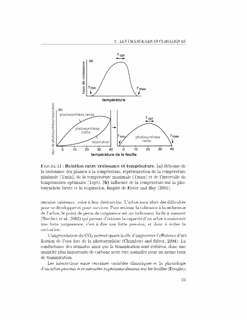
La hausse de la température a un e�et non linéaire sur le fonctionnementde l'arbre. La température joue un rôle dans les réactions chimiques ; uneaugmentation de la température peut causer une augmentation de la vitessedes réactions, notamment de la photosynthèse. Toutefois, si la températureaugmente trop, la structure tertiaire des enzymes responsables des réactionspeut être endommagée (Fitter and Hay, 2001). Les réactions enzymatiques sefont alors plus di�cilement, voire plus du tout. La combinaison de ces deuxprincipes conduit à la Figure 11, où la croissance est représentée en fonctionde la température. Cette courbe prend la forme d'une cloche. En fonctionde la température actuelle, une augmentation de la température peut avoirun impact positif sur la croissance. Ou bien, si la température est élevée,comme cela semble être le cas en forêt tropicale (Clark et al., 2003), uneaugmentation de la température aura un impact négatif sur la croissance.
L'augmentation de la longueur et de l'intensité des saisons sèches prévuesur la bassin amazonien aura probablement aussi des conséquences à l'échelleindividuelle. Lorsqu'un arbre manque d'eau, la pression au niveau de sesracines diminue, la di�érence de pression nécessaire pour la montée de la sèvedans le xylème diminue alors elle aussi, ce qui peut ralentir cette montée, etavec elle tout le métabolisme de l'arbre. Si la sécheresse continue, la pressiontrop faible sera cause de cavitation, des bulles d'air se formeront dans lesvaisseaux, ce qui peut conduire à l'embolisme, au mauvais fonctionnement de
22
2. LES CHANGEMENTS CLIMATIQUES
Figure 11 : Relation entre croissance et température. (a) Réponse dela croissance des plantes à la température, représentation de la températureminimale (Tmin), de la température maximale (Tmax) et de l'intervalle detempératures optimales (Topt). (b) In�uence de la température sur la pho-tosynthèse brute et la respiration. Inspiré de Fitter and Hay (2001).
certains vaisseaux, voire à leur destruction. L'arbre aura alors des di�cultéspour se développer et pour survivre. Pour estimer la tolérance à la sécheressede l'arbre, le point de perte de turgesence est un indicateur facile à mesurer(Bartlett et al., 2012) qui permet d'estimer la capacité d'un arbre à maintenirune forte turgescence, c'est-à-dire une forte pression, et donc à éviter lacavitation.
L'augmentation du CO2 permet quant-à-elle d'augmenter l'e�cience d'uti-lisation de l'eau lors de la photosynthèse (Chambers and Silver, 2004). Laconductance des stomates ainsi que la transpiration sont réduites, donc unequantité plus importante de carbone peut être assimilée pour un même tauxde transpiration.
Les interactions entre certaines variables climatiques et la physiologied'un arbre peuvent être mesurées expérimentalement sur les feuilles (Doughty,
23
Introduction générale
2011), ou sur un arbre (Wullschleger et al., 1998). Toutefois, pour passer àl'échelle de la forêt, les extrapolations ne sont pas forcément simples.
2.4.2 A l'échelle de la forêt
De façon générale, bien que les processus qui agissent au niveau de la feuillesoient assez bien connus, les réactions de la forêt tropicale aux changementsclimatiques à l'échelle de la communauté restent inconnues.
Concernant la température, les conséquences d'une augmentation de tem-pérature à l'échelle de la communauté sont inconnues. En e�et, les tempé-ratures en forêt tropicales sont relativement peu variables, et aucune expé-rience de réchau�ement n'a été réalisée pour simuler le réchau�ement desprochaines décennies.
Pour étudier l'e�et de la sécheresse sur la forêt, les études se sont baséessur la dynamique forestière observée suite aux sécheresses importantes de2005 et de 2010 (Phillips et al., 2009; Lewis et al., 2011). Ces travaux ontmontré que la disponibilité en eau avait un e�et important sur la dynamiqueforestière, en augmentant notamment le taux de mortalité annuel. De façongénérale, la sécheresse augmente la vulnérabilité des plantes (McDowell et al.,2008; Allen et al., 2010; Choat et al., 2012). D'autre part, il a été possible demettre en place des expériences d'exclusion en recouvrant la forêt pour em-pêcher la pluie de venir irriguer le sol (da Costa et al., 2010; Nepstad et al.,2007; Brando et al., 2008). Ces expériences appelées TFE (throughfall exclu-sion) ont permis de mettre en évidence, une fois encore, une augmentation dela mortalité, notamment de la mortalité des gros arbres. Toutefois, ces expé-riences ne re�ètent pas vraiment l'évolution continue vers un potentiel climatfutur, mais un changement drastique et brutal de la disponibilité en eau. Lesmodèles inter-annuels actuels de dynamique forestière ne permettent pas en-core de prédire de façon correcte les conséquences des sécheresses futures(McDowell et al., 2013). A l'échelle saisonnière toutefois, la disponibilité eneau est le déterminant majeur de la dynamique de la forêt tropicale (Wagneret al., 2012, 2014).
Tout comme la température, l'e�et de la concentration de CO2 sur la dy-namique est controversé. L'augmentation du CO2 a été mise en relation avecune augmentation du recrutement et de la croissance en Amazonie (Lewiset al., 2004), mais il a été argumenté que la hausse de la concentration du CO2
ne pouvait avoir impacté aussi rapidement la croissance (Chambers and Sil-ver, 2004), dont l'augmentation doit être plutôt causée par d'autres facteursenvironnementaux dont les e�ets sont plus instantanés, comme l'irradianceou encore des perturbations environnementales anciennes (Chambers and
24
3. LA MODÉLISATION
Silver, 2004). L'augmentation des concentrations de CO2 atmosphérique estlinéaire dans le temps, il est donc di�cile de bien di�érencier les e�ets dusà cette augmentation de CO2 d'e�ets purement temporels liés à l'évolutionde la forêt dans le temps.
3 La modélisation
Pour mieux comprendre la dynamique des arbres en forêt tropicale, ainsi queles impacts que peuvent avoir les changements climatiques sur cette dyna-mique, la modélisation est un outil incontournable. La modélisation permeten e�et de schématiser des systèmes complexes, en ne gardant que les proces-sus sur lesquels porte l'étude. De par l'incessante croissance des capacités denos ordinateurs, la modélisation est devenue une discipline à part entière etdes méthodes de modélisation ont vu le jour, qui ne sont plus limitées par lestemps de calcul ou la place en mémoire. Dans cette thèse, je cherche à mo-déliser la dynamique de la forêt tropicale à Paracou, et plus particulièrementles e�ets des variations climatiques inter-annuelles sur cette dynamique. Laconstruction et l'utilisation d'un tel modèle me permettent (i) de mettre aupoint une méthodologie transposable dans d'autres sites d'études, (ii) si lesréponses sont su�samment génériques, d'établir les grandes lignes de scéna-rios possibles pour l'évolution de la dynamique des forêts tropicales.
3.1 Les modèles de dynamique forestière
Les trois processus de recrutement, croissance et mortalité peuvent être mo-délisés séparément ou conjointement. Les modèles de croissance sont les plusnombreux, car la croissance est souvent liée à la productivité de la forêt etau stockage du carbone, ce qui intéresse particulièrement les exploitants etdi�érents acteurs de la gestion forestière.
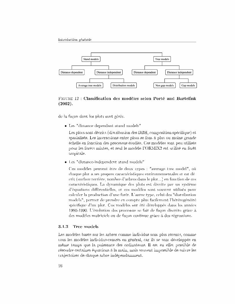
Di�érentes classi�cations ont été proposées en fonction de l'architecturedes modèles proposés. Ces di�érentes classi�cations font référence à di�é-rentes classes de modèles, Porté en propose une en 2002 que je vais briève-ment décrire ici (Figure 12). Il faut garder en tête que d'autres classi�cationsexistent et que cette présentation me permettra essentiellement de passer enrevue les di�érents modèles existants.
3.1.1 Stand models
Dans les stand models, la forêt est représentée comme une mosaïque de sous-forêts (plots). Cette classe de modèles se divise en deux groupes, en fonction
25
Introduction générale
Figure 12 : Classi�cation des modèles selon Porté and Bartelink(2002).
de la façon dont les plots sont gérés.
• Les "distance-dependant stand models"
Les plots sont décrits (distribution des DBH, composition spéci�que) etspatialisés. Les interactions entre plots se font à plus ou moins grandeéchelle en fonction des processus étudiés. Ces modèles sont peu utiliséspour les forêts mixtes, et seul le modèle FORMIX2 est utilisé en forêttropicale.
• Les "distance-independent stand models"
Ces modèles peuvent être de deux types : "average tree model", oùchaque plot a ses propres caractéristiques environnementales et est dé-crit (surface terrière, nombre d'arbres dans le plot...) en fonction de cescaractéristiques. La dynamique des plots est décrite par un systèmed'équations di�érentielles, et ces modèles sont souvent utilisés pourcalculer la production d'une forêt. L'autre type, celui des "distributionmodels", permet de prendre en compte plus facilement l'hétérogénéitéspéci�que d'un plot. Ces modèles ont été développés dans les années1980-1990. L'évolution des processus se fait de façon discrète grâce àdes modèles matriciels ou de façon continue grâce à des régressions.
3.1.2 Tree models
Les modèles basés sur les arbres comme individus sont plus récents, commetous les modèles individus-centrés en général, car ils se sont développés enmême temps que la puissance des ordinateurs. Il est en e�et possible derésoudre certaines équations à la main, mais souvent impossible de suivre lestrajectoires de chaque arbre indépendamment.
26
3. LA MODÉLISATION
On distingue encore di�érentes sortes de modèles, en fonction de la ges-tion ou non de l'espace :
• les "distance-dependent tree models"
On modélise chaque arbre individuellement, en prenant en compte saplace dans l'espace. La plupart des modèles ne se contentent pas dereprésenter la croissance, mais aussi souvent la mortalité, et parfois lerecrutement, et se basent sur des régressions multivariées pour calcu-ler la croissance individuelle. Plus rarement, ils utilisent une approcheplus mécaniste et fonctionnelle basée sur la production primaire et se-condaire. La prise en compte de la distance entre les arbres permetd'inclure des indices de compétition comme prédicteurs dans les ré-gressions.
• les "distance independent tree models"
Certains modèles ne prennent pas en compte la position de l'arbre,ceux-ci sont pour la plupart des gap-models. Les gap-models s'inspirentde JABOWA, développé par Botkin et al. (1972), les gap sont des mor-ceaux de forêt de taille variable et caractérisés par une liste d'individus.Ces gaps ont des conditions environnementales homogènes et la dyna-mique de chaque arbre à l'intérieur de chaque gap est calculée de façonindividuelle. Les gap models calculent le recrutement, la croissance etla mortalité, en prenant en compte la quantité de lumière disponiblepour chaque arbre dans chaque gap, qui est l'un des paramètres lesplus importants intervenant dans ce type de modèle. Les "distance in-dependant tree models" qui ne sont pas des gap models sont plutôtrares, et se basent sur des fonctions empiriques.
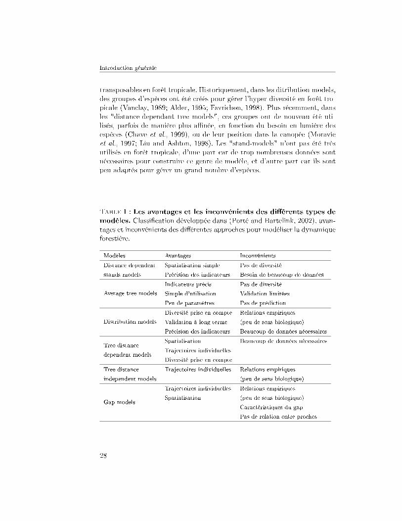
Le Tableau 1 permet de synthétiser les avantages et inconvénient liés à laconstruction et à l'utilisation des di�érents modèles.
3.2 Les enjeux de modélisation en forêts tropicales
La plupart des forêts mondiales sont constituées de plusieurs espèces d'arbresqui cohabitent, et sont appelées "mixed forests". Tous les modèles de dyna-mique présentés précédemment ne sont pas forcément adaptés (Porté andBartelink, 2002). En forêt tropicale, le nombre très important d'espèces rendimpossible la paramétrisation de modèles spéci�ques à chaque espèce. Desstratégies doivent donc être mises en place pour prendre cette diversité encompte tout en la synthétisant. Ainsi, parmi les classes de modèles présen-tées plus tôt, certaines très utilisées en climat tempéré peuvent s'avérer peu
27
Introduction générale
transposables en forêt tropicale. Historiquement, dans les ditribution-models,des groupes d'espèces ont été créés pour gérer l'hyper-diversité en forêt tro-picale (Vanclay, 1989; Alder, 1995; Favrichon, 1998). Plus récemment, dansles "distance-dependant tree models", ces groupes ont de nouveau été uti-lisés, parfois de manière plus a�née, en fonction du besoin en lumière desespèces (Chave et al., 1999), ou de leur position dans la canopée (Moravieet al., 1997; Liu and Ashton, 1998). Les "stand-models" n'ont pas été trèsutilisés en forêt tropicale, d'une part car de trop nombreuses données sontnécessaires pour construire ce genre de modèle, et d'autre part car ils sontpeu adaptés pour gérer un grand nombre d'espèces.
Table 1 : Les avantages et les inconvénients des di�érents types demodèles. Classi�cation développée dans (Porté and Bartelink, 2002), avan-tages et inconvénients des di�érentes approches pour modéliser la dynamiqueforestière.
Modèles Avantages Inconvénients
Distance dependent Spatialisation simple Pas de diversité
stands models Précision des indicateurs Besoin de beaucoup de données
Average tree models
Indicateurs précis Pas de diversité
Simple d'utilisation Validation limitées
Peu de paramètres Pas de prédiction
Distribution models
Diversité prise en compte Relations empiriques
Validation à long terme (peu de sens biologique)
Précision des indicateurs Beaucoup de données nécessaires
Tree distanceSpatialisation Beaucoup de données nécessaires
dependent modelsTrajectoires individuelles
Diversité prise en compte
Tree distance Trajectoires individuelles Relations empiriques
independent models (peu de sens biologique)
Gap models
Trajectoires individuelles Relations empiriques
Spatialisation (peu de sens biologique)
Caractéristiques du gap
Pas de relation entre proches
28
3. LA MODÉLISATION
3.2.1 L'approche groupes fonctionnels
Des groupes d'espèces ont couramment été créés pour gérer le grand nombred'espèces en forêts tropicales. Les critères de groupement di�èrent en fonc-tion des objectifs à atteindre, ces critères sont par exemple souvent relatifsà la place de l'arbre dans la canopée (Chave et al., 1999), qui est considéréecomme un indicateur de la lumière disponible pour l'arbre. Le rapproche-ment des espèces en groupes fonctionnels est un outil qui peut aussi êtreutilisé pour étudier la coexistence des espèces et la redondance des fonctionsécologiques de ces espèces.
Les groupes peuvent également être créés en s'appuyant directement surles processus étudiés, ce qui demande une méthodologie appropriée (Oue-draogo et al., 2013). Les groupes sont alors formés pendant le processusde modélisation et n'ont pas forcément de signi�cation biologique. Certainsalgorithmes peuvent notamment chercher le nombre de groupes le plus ap-proprié, ce qui résout la question épineuse du nombre de groupes (Mortieret al., 2013). Les méthodes développées sont alors des méthodes d'optimisa-tion combinatoires, et des heuristiques doivent être utilisées (Picard et al.,2002).
In �ne, l'idée des groupes fonctionnels est de rassembler les espèces partype de comportements. Ces groupes permettent donc de prendre toute lavariabilité des stratégies observées, d'un comportement extrême à l'autre.Toutefois, ces groupes peuvent sembler arti�ciels, les limites arbitraires et lechoix du nombre de groupes subjectif d'autant qu'il n'y a pas de consensussur les critères de regroupement importants.
3.2.2 L'approche traits fonctionnels
L'approche par les traits fonctionnels permet de mieux prendre en compte lecontinuum entre les di�érentes stratégies. En e�et, bien que di�érents com-portements soient observés en forêt tropicale, la création de groupes biendistincts est parfois arti�cielle. Les traits fonctionnels sont considérés commedes proxys des di�érentes stratégies sur les di�érents axes de variations pos-sibles : le leaf economics spectrum, le wood economics spectrum et le life-history spectrum. Un nombre restreint de traits qui ont un rôle prépondérantdans les stratégies de recrutement/croissance/mortalité peuvent être choisiscomme variables à inclure dans les di�érents modèles pour les di�érents pro-cessus démographiques. Cette approche permet de chercher, d'une part, unsignal commun à tous les arbres, et d'autre part de prendre en compte lavariabilité de chaque espèce, sans avoir à gérer un trop grand nombre de
29
Introduction générale
paramètres. De plus, contrairement à des groupes qui peuvent paraitre arti-�ciels et vides de fondements biologiques, les traits fonctionnels permettentde baser nos modèles sur des hypothèses éco-physiologiques.
Contrairement à l'approche par groupes, l'utilisation des traits fonction-nels n'est pas adaptée pour prendre facilement en compte les comporte-ments extrêmes. De plus, les traits fonctionnels disponibles sont des traitsdits "soft" qui ne sont que des indicateurs des traits "hard". Les traits "hard"sont mécaniquement plus liés aux performances des arbres, mais sont di�-ciles à mesurer, ce qui limite fortement leur utilisation.
3.3 Les enjeux actuels
Actuellement, des modèles basés sur les traits fonctionnels permettent deprendre en compte l'immense diversité présente en forêt tropicale. Ceci per-met de manipuler cette diversité avec un nombre restreint de paramètres etde construire des modèles de dynamique individu-centrés. De plus, les don-nées climatiques disponibles permettent d'inclure des variables climatiquesdans ces modèles, il devient dès lors indispensable de construire des simula-teurs qui permettent d'explorer les di�érents scénarios possibles, en utilisantles prédictions issues de modèles climatiques. Ces prédictions permettent dese faire une meilleure idée de la façon dont la forêt tropicale peut répondre àl'augmentation des températures et aux changements de régimes pluviomé-triques.
3.4 L'inférence bayésienne
Les modèles utilisés au cours de la thèse ont été calibrés par des méthodesbayésiennes. Ces méthodes permettent l'inférence de modèles intégrant del'information a priori dans une structure hiérarchique. C'est le cas de laméthode développée dans le premier chapitre pour attribuer des traits fonc-tionnels à tous les arbres du jeux de données. L'expertise des forestiers surla correspondance entre noms vernaculaires et noms scienti�ques correspondà une connaissance a priori. Tout au long de la thèse, l'incertitude taxono-mique est prise en compte grâce aux distribution a posteriori obtenues dans lepremier chapitre. Les méthodes bayésiennes sont très souples et permettentd'inférer des modèles complexes, tout en propageant bien les incertitudes.C'est notamment ce qui a permis de calibrer un modèle de croissance et demortalité conjointement dans cette thèse.
30
4. PLAN
4 Plan
Dans cette thèse, j'apporterai des éléments de réponse et de ré�exion sur laréaction des forêts tropicales aux changements climatiques. Le document estarticulé en cinq chapitres, qui prennent la forme d'articles publiés, soumis,ou en phase �nale de rédaction.
• Dans le premier chapitre, je présenterai une méthode de gestion del'incertitude taxonomique, qui permet d'attribuer des traits fonction-nels à tous les arbres d'une communauté quel que soit leur niveaud'identi�cation taxonomique, et qui sera utilisée dans la suite de montravail. Cette méthode a permis de prendre en compte l'ensemble desarbres morts avant que leur identi�cation botanique ne soit faite pourconstruire un modèle de mortalité à l'échelle de la communauté.
• Dans le second chapitre, ce modèle de mortalité est couplé avec unmodèle de croissance. Le couplage fait intervenir la vigueur individuelledes arbres. Pour estimer cette vigueur, la croissance observée sur leterrain est comparée à la croissance prévue par le modèle de croissance.La vigueur ainsi estimée est un très bon prédicteur de la probabilité demourir, les arbres qui grandissent plus que prévu ont une probabilitéplus faible de mourir.
• Dans le troisième chapitre, je présenterai les résultats obtenus lorsquece modèle joint est paramétré spéci�quement pour les espèces com-merciales de Guyane française. Deux variables sont ajoutées dans lesmodèles pour tenir compte de l'intensité d'exploitation et du stress hy-drique. Ces modèles permettent d'observer un gradient de réponses austress hydrique chez les essences commerciales. L'exploitation a ten-dance à diminuer la compétition et ainsi à augmenter la croissance etdiminuer la mortalité, tandis que le stress hydrique a l'e�et inverse.Malgré cette réponse commune, des pro�ls de susceptibilité di�érentssont observés pour chaque essence commerciale, ce qui permet d'identi-�er des essences particulièrement sensibles, et d'autres plus résistantes.
• Dans le quatrième chapitre, je présenterai l'introduction de variablesclimatiques dans le modèle joint à l'échelle de la communauté, en forêtnaturelle. Ce chapitre met en évidence l'impact du stress hydrique, dela température, et de la saturation du sol en eau. Le stress hydriquea un impact négatif sur la croissance et la mortalité, la températurea un impact négatif sur la croissance, et la saturation du sol en eauaugmente la taux de mortalité.
31

Introduction générale
• Dans le cinquième et dernier chapitre, le modèle climat dépendant estimplémenté dans le simulateur de forêt SELVA, et di�érents scénariosclimatiques correspondant aux simulations du GIEC sont testés pourle siècle prochain sur la communauté d'arbres actuelle de Paracou. Lessorties montrent que les hausses de température à venir peuvent êtreresponsables d'un ralentissement de la croissance et d'une diminutionsubstantielle de la surface terrière, du diamètre quadratique et de labiomasse.
Des pistes de ré�exion sur les enjeux de modélisation et les échelles considé-rées sont proposées en discussion de ce travail.
32
BIBLIOGRAPHIE
Aakala, T., Fraver, S., D'Amato, A. W., and Palik, B. J. (2013). In�uence ofcompetition and age on tree growth in structurally complex old-growthforests in northern Minnesota, USA. Forest Ecology and Management,308:128�135.
Alder, D. (1995). Growth modelling for mixed tropical forests. TropicalForestry Papers (United Kingdom).
Allen, C. D., Macalady, A. K., Chenchouni, H., Bachelet, D., McDowell, N.,Vennetier, M., Kitzberger, T., Rigling, A., Breshears, D. D., Hogg, E.T. H., Gonzalez, P., Fensham, R., Zhang, Z., Castro, J., Demidova, N.,Lim, J.-H. H., Allard, G., Running, S. W., Semerci, A., and Cobb, N.(2010). A global overview of drought and heat-induced tree mortalityreveals emerging climate change risks for forests. Forest Ecology andManagement, 259(4):660�684.
Baker, T. R., Phillips, O. L., Malhi, Y., Almeida, S., Arroyo, L., Di Fiore, A.,Erwin, T., Higuchi, N., Killeen, T. J., Laurance, S. G., Laurance, W. F.,Lewis, S. L., Monteagudo, A., Neill, D. a., Vargas, P. N. n., Pitman, N.C. a., Silva, J. N. M., and Martínez, R. V. (2004). Increasing biomass inAmazonian forest plots. Philosophical transactions of the Royal Societyof London. Series B, Biological sciences, 359(1443):353�65.
Baraloto, C., Paine, C. E. T., Patiño, S., Bonal, D., Hérault, B., and Chave,J. (2010a). Functional trait variation and sampling strategies in species-rich plant communities. Functional Ecology, 24(1):208�216.
33
BIBLIOGRAPHIE
Baraloto, C., Paine, C. E. T., Poorter, L., Beauchene, J., Bonal, D., Dome-nach, A. M., Hérault, B., Patino, S., Roggy, J. C., and Chave, J. (2010b).Decoupled leaf and stem economics in rain forest trees. Ecology Letters,13(11):1338�1347.
Bartlett, M. K., Sco�oni, C., and Sack, L. (2012). The determinants ofleaf turgor loss point and prediction of drought tolerance of species andbiomes : a global meta-analysis. Ecology letters, 15(5):393�405.
Botkin, D. B., Janak, J. F., and Wallis, J. R. (1972). Some ecological conse-quences of a computer model of forest growth. Journal of Ecology, pages849�872.
Brando, P. M., Nepstad, D. C., Davidson, E. a., Trumbore, S. E., Ray, D., andCamargo, P. (2008). Drought e�ects on littefall, wood production andbelowground carbon cycling in an Amazon Forest : result of a throughfallreduction experiment. Philosophical Transactions of the Royal Society,363(1498):1839�1848.
Canham, C. D., LePage, P. T., and Coates, K. D. (2004). A neighborhoodanalysis of canopy tree competition : e�ects of shading versus crowding.Canadian Journal of Forest Research, 34(4):778�787.
Chambers, J. Q. and Silver, W. L. (2004). Some aspects of ecophysiologicaland biogeochemical responses of tropical forests to atmospheric change.Philosophical transactions of the Royal Society of London. Series B,Biological sciences, 359(1443):463�76.
Chave, J., Condense, E., and Merisiers, O. (1999). Study of structural ,successional and spatial patterns in tropical rain forests using TROLL ,a spatially explicit forest model. Ecological Modelling, 124(2-3):233�254.
Chave, J. J., Coomes, D., Jansen, S., Lewis, S. L., Swenson, N. G., andZanne, A. E. (2009). Towards a worldwide wood economics spectrum.Ecology letters, 12(4):351�66.
Chesson, P. (2000). Mechanisms of maintenance of species diversity. Annualreview of Ecology and Systematics, pages 343�366.
Choat, B., Jansen, S., Brodribb, T. J., Cochard, H., Delzon, S., Bhaskar, R.,Bucci, S. J., Feild, T. S., Gleason, S. M., Hacke, U. G., Jacobsen, A. L.,Lens, F., Maherali, H., Martínez-Vilalta, J., Mayr, S., Mencuccini, M.,Mitchell, P. J., Nardini, A., Pittermann, J., Pratt, R. B., Sperry, J. S.,
34
BIBLIOGRAPHIE
Westoby, M., Wright, I. J., and Zanne, A. E. (2012). Global convergencein the vulnerability of forests to drought. Nature, 491(7426):752�5.
Christensen, J. H., Hewitson, B., Busuioc, A., Chen, A., Gao, X., Held, R.,Jones, R., Kolli, R. K., Kwon, W., and Laprise, R. (2007). Regionalclimate projections. Climate Change, 2007 : The Physical Science Ba-sis. Contribution of Working group I to the Fourth Assessment Reportof the Intergovernmental Panel on Climate Change, University Press,Cambridge, Chapter 11, pages 847�940.
Clark, D. A., Piper, S. C., Keeling, C. D., and Clark, D. B. (2003). Tropi-cal rain forest tree growth and atmospheric carbon dynamics linkedto interannual temperature variation during 1984-2000. Proceedingsof the National Academy of Sciences of the United States of America,100(10):5852�7.
Coley, P. D. and Barone, J. a. (1996). Herbivory and Plant Defenses inTropical Forests. Annual Review of Ecology and Systematics, 27(1):305�335.
Cornelissen, J. H. C., Lavorel, S., Garnier, E., Díaz, S., Buchmann, N., Gur-vich, D. E., Reich, P. B., Steege, H. T., Morgan, H. D., Heijden, M. G.a. V. D., Pausas, J. G., and Poorter, H. (2003). A handbook of pro-tocols for standardised and easy measurement of plant functional traitsworldwide. Australian Journal of Botany, 51(4):335.
da Costa, A. C. L., Galbraith, D., Almeida, S., Portela, B. T. T., da Costa,M., Silva Junior, J. a. D. A., Braga, A. P., de Gonçalves, P. H. L.,de Oliveira, A. a. R., Fisher, R., Phillips, O. L., Metcalfe, D. B., Levy, P.,and Meir, P. (2010). E�ect of 7 yr of experimental drought on vegetationdynamics and biomass storage of an eastern Amazonian rainforest. TheNew phytologist, 187(3):579�91.
de Noter, C. (2008). Etat des connaissances, analyse et synthèse biblio-graphique sur la faune de Guyane en vue d�etudier les potentialités dedéveloppement économique et de transfert de technologies. Technicalreport, Rapport pour DRRT Guyane. 59p.
Dobbertin, M. (2005). Tree growth as indicator of tree vitality and of treereaction to environmental stress : a review. European Journal of ForestResearch, 124(4):319�333.
35
BIBLIOGRAPHIE
Doughty, C. E. (2011). An in situ leaf and branch warming experiment inthe Amazon. Biotropica, 43(6):658�665.
Epron, D., Bosc, A., Bonal, D., and Freycon, V. (2006). Spatial variation ofsoil respiration across a topographic gradient in a tropical rain forest inFrench Guiana. Journal of Tropical Ecology, 22:565�574.
FAO (1998). World reference base for soil resources.World Soil ResourcesReport 84.
Favrichon, V. (1998). Modeling the dynamics and species composition of atropical mixed-species uneven-aged natural forest : e�ects of alternativecutting regimes. Forest Science, 44(1):113�124.
Fitter, A. H. and Hay, R. K. (2001). Environmental physiology of plants.Academic press.
Fu, R., Yin, L., Li, W., Arias, P. A., Dickinson, R. E., Huang, L., Chakra-borty, S., Fernandes, K., Liebmann, B., Fisher, R., and Myneni, R. B.(2013). Increased dry-season length over southern Amazonia in recentdecades and its implication for future climate projection. Proceedingsof the National Academy of Sciences of the United States of America,110(45):18110�18115.
Gaspard, R. (2014). A neighborhood analysis of tree growth in a tropicalforest. Master repport, AgroParisTech.
Gause, G. F. (1932). Experimental studies on the struggle for existenceI. Mixed population of two species of yeast. Journal of experimentalbiology, 9(4):389�402.
Gourlet-Fleury, S. (1998). Indices de compétition en forêt dense tropicalehumide : Paracou ( Guyane française ). Annales des sciences forestières,55:623�654.
Hérault, B., Bachelot, B., Poorter, L., Rossi, V., Bongers, F., Chave, J.,Paine, C. E. T., Wagner, F., and Baraloto, C. (2011). Functional traitsshape ontogenetic growth trajectories of rain forest tree species. Journalof Ecology, 99(6):1431�1440.
Hérault, B., Beauchene, J., Muller, F., Wagner, F., Baraloto, C., Blanc, L.,Martin, J.-M., and Beauchêne, J. (2010). Modeling decay rates of deadwood in a neotropical forest. Oecologia, 164(1):243�251.
36
BIBLIOGRAPHIE
Hubbell, S. P. (2001). The Uni�ed Neutral Theory of Biodoversity and Bio-geography. Princeton University Press.
Ichii, K., Hashimoto, H., Nemani, R., and White, M. (2005). Modeling theinterannual variability and trends in gross and net primary productivityof tropical forests from 1982 to 1999. Global and Planetary Change,48(4):274�286.
INSEE, A.-G. (2013). Projections de population à l'horizon 2040 Plus d'undemi-million de Guyanais. Technical report.
IPCC (2000). Land Use, Land-Use Change and Forestry. Cambridge Uni-versity Press.
IPCC (2013). Climate change 2013 : the scienti�c basis. contribution of wor-king group 1 to the fourth assessment report of the intergovernmentalpanel on climate change. Cambridge University Press.
Joetzjer, E., Douville, H., Delire, C., and Ciais, P. (2013). Present-day andfuture Amazonian precipitation in global climate models : CMIP5 versusCMIP3. Climate Dynamics, 41(11-12):2921�2936.
Jones, P. G., Thornton, P. K., and Heinke, J. (2009). Generating characte-ristic daily weather data using downscaled climate model data from theIPCC ' s Fourth Assessment. Technical report.
Lewis, S. L., Brando, P. M., Phillips, O. L., van der Heijden, G. M. F., andNepstad, D. (2011). The 2010 Amazon drought. Science (New York,N.Y.), 331(6017):554.
Lewis, S. L., Phillips, O. L., Baker, T. R., Lloyd, J., Malhi, Y., Almeida, S.,Higuchi, N., Laurance, W. F., Neill, D. a., Silva, J. N. M., Terborgh,J., Lezama, a. T., Martínez, R. V., Brown, S., Chave, J., Kuebler, C.,Vargas, P. N. n., and Vinceti, B. (2004). Concerted changes in tropicalforest structure and dynamics : evidence from 50 South American long-term plots. Philosophical transactions of the Royal Society of London.Series B, Biological sciences, 359(1443):421�36.
Li, W., Fu, R., and Dickinson, R. E. (2006). Rainfall and its seasonality overthe Amazon in the 21st century as assessed by the coupled models forthe IPCC AR4. Journal of Geophysical Research : Atmospheres (1984�2012), 111(D2).
37
BIBLIOGRAPHIE
Liu, J. and Ashton, P. S. (1998). FORMOSAIC : an individual-based spa-tially explicit model for simulating forest dynamics in landscape mosaics.Ecological Modelling, 106(2-3):177�200.
Lotka, A. J. (1925). Elements of Physical Biology. Williams and WilkinsCompany.
Malhi, Y., Roberts, J. T., Betts, R. a., Killeen, T. J., Li, W., and Nobre,C. a. (2008). Climate change, deforestation, and the fate of the Amazon.Science (New York, N.Y.), 319(5860):169�72.
McDowell, N., Pockman, W. T., Allen, C. D., Breshears, D. D., Cobb, N.,Kolb, T., Plaut, J., Sperry, J., West, A., Williams, D. G., and Ye-pez, E. A. (2008). Mechanisms of plant survival and mortality duringdrought : why do some plants survive while others succumb to drought ?New Phytologist, 178:719�739.
McDowell, N. G., Fisher, R. A., Xu, C., Domec, J. C., Hölttä, T., Mackay,D. S., Sperry, J. S., Boutz, A., Dickman, L., Gehres, N., Limousin, J. M.,Macalady, A., Martìnez-Vilalta, J., Mencuccini, M., Pault, J. A., Ogée,J., Pangle, R. E., Rasse, D. P., Ryan, M. G., Sevanto, S., Waring, R. H.,Williams, A. P., Yepez, E. A., and Pockman, W. T. (2013). Evaluatingtheories of drought-induced vegetation mortality using a multimodel �experiment framework. pages 304�321.
Molto, Q., Hérault, B., Boreux, J.-J., Daullet, M., Rousteau, a., and Rossi, V.(2014). Predicting tree heights for biomass estimates in tropical forests� a test from French Guiana. Biogeosciences, 11(12):3121�3130.
Molto, Q., Rossi, V., and Blanc, L. (2013). Error propagation in biomassestimation in tropical forests. Methods in Ecology and Evolution, 4(2):175�183.
Moravie, M.-a., Pascal, J.-P., and Auger, P. (1997). Investigating canopyregeneration processes through individual-based spatial models : appli-cation to a tropical rain forest. Ecological Modelling, 104(2-3):241�260.
Mortier, F., Rossi, V., Guillot, G., Gourlet-Fleury, S., and Picard, N. (2013).Population dynamics of species-rich ecosystems : the mixture of matrixpopulation models approach. Methods in Ecology and Evolution, 4:316�326.
38
BIBLIOGRAPHIE
Nemani, R. R., Keeling, C. D., Hashimoto, H., Jolly, W. M., Piper, S. C.,J., T. C., Myneni, R. B., and Running, S. W. (2003). Global terrestrialnet primamry production from 1982 to 1999. Science, 300:1560�1563.
Nepstad, D. C., Tohver, I. M., Ray, D., Moutinho, P., and Cardinot, G.(2007). Mortality of large trees and lianas following experimentaldrought in an Amazon forest. Ecology, 88(9):2259�69.
Ouedraogo, D.-Y., Mortier, F., Gourlet-Fleury, S., Freycon, V., and Picard,N. (2013). Slow-growing species cope best with drought : evidence fromlong-term measurements in a tropical semi-deciduous moist forest ofCentral Africa. Journal of Ecology, 101(6):1459�1470.
Pan, Y., Birdsey, R. a., Fang, J., Houghton, R., Kauppi, P. E., Kurz, W. a.,Phillips, O. L., Shvidenko, A., Lewis, S. L., Canadell, J. G., Ciais, P.,Jackson, R. B., Pacala, S. W., McGuire, a. D., Piao, S., Rautiainen, A.,Sitch, S., and Hayes, D. (2011). A large and persistent carbon sink inthe world's forests. Science, 333(6045):988�93.
Phillips, O. L. (1998). Changes in the Carbon Balance of Tropical Forests :Evidence from Long-Term Plots. Science, 282(5388):439�442.
Phillips, O. L., Aragão, L. E., Lewis, S. L., Fisher, J. B., Lloyd, J., López-González, G., Malhi, Y., Monteagudo, A., Peacock, J., Quesada, C. A.,et al. (2009). Drought sensitivity of the amazon rainforest. Science,323(5919):1344�1347.
Phillips, O. L. and Lewis, S. L. (2013). Evaluating the tropical forest carbonsink. Global change biology, pages 2039�2041.
Picard, N., Gourlet-Fleury, S., and Sist, P. (2002). Using processdependentgroups of species to model the dynamics of a tropical rain-forest. Mo-delling Forest Systems (Eds. A. Amaro, D. Reed & P. Soares). CABInternational Publishing, Wallingford, 237â��248. Proceedings of theIUFRO 4.01 and 4.11 Conference, Instituto Superior de Gestão andInstituto Superior de Agronomia, Sesimbra, Portugal, 2-5.
Poorter, L. and Rose, S. (2005). Light-dependent changes in the relationshipbetween seed mass and seedling traits : a meta-analysis for rain foresttree species. Oecologia, 142(3):378�387.
Porté, A. and Bartelink, H. H. (2002). Modelling mixed forest growth : areview of models for forest management. Ecological Modelling, 150(1-2):141�188.
39

BIBLIOGRAPHIE
Roche, M.-A. (1982). Evapotranspiration réelle de la forêt amazonienne enGuyane. Cah. ORSTROM, sér. Hydrol., 19(1):37�44.
Roy, J., Mooney, H. A., and Saugier, B. (2001). Terrestrial global productivity.Academic Press.
Stocker, T., Qin, D., Plattner, G., Tignor, M., Allen, S., Boschung, J., Nauels,A., Xia, Y., Bex, B., and Midgley, B. (2013). IPCC, 2013 : climatechange 2013 : the physical science basis. Contribution of working groupI to the �fth assessment report of the intergovernmental panel on climatechange. Cambridge University Press.
Stoll, P. and Newbery, D. M. (2005). Evidence of species-speci�c neighbo-rhood e�ects in the dipterocarpaceae of a bornean rain forest. Ecology,86(11):3048�3062.
Thorpe, H., Astrup, R., Trowbridge, a., and Coates, K. (2010). Competitionand tree crowns : A neighborhood analysis of three boreal tree species.Forest Ecology and Management, 259(8):1586�1596.
Tilman, D. (1981). Resource competition and community structure. Mono-graphs in population biology, 17:1�296.
Uriarte, M., Swenson, N. G., Chazdon, R. L., Comita, L. S., John Kress,W., Erickson, D., Forero-Montaña, J., Zimmerman, J. K., and Thomp-son, J. (2010). Trait similarity, shared ancestry and the structure ofneighbourhood interactions in a subtropical wet forest : implications forcommunity assembly. Ecology letters, 13(12):1503�14.
Vanclay, J. (1989). A growth model for north Queensland rainforests. ForestEcology and Management, 27(3-4):245�271.
Volterra, V. (1926). Fluctuations in the abundance of a species consideredmathematically. Nature, 118:558�560.
Wagner, F., Rossi, V., Baraloto, Christopher andBonal, D., Stahl, C., andHérault, B. (2014). Are commonly measured functional traits involvedin tropical tree responses to climate ? International Journal of Ecology,2014:1�10.
Wagner, F., Rossi, V., Stahl, C., Bonal, D., and Hérault, B. (2012). Wateravailability is the main climate driver of neotropical tree growth. PlosOne, 7(4):e34074.
40

BIBLIOGRAPHIE
Webb, C. O., Ackerly, D. D., McPeek, M. A., and Donoghue, M. J. (2002).Phylogenies and community ecology. Annual review of ecology and sys-tematics, pages 475�505.
Westoby, M., Falster, D. S., Moles, A. T., Vesk, P. A., and Wright, I. J.(2002). Plant ecological strategies : Some leading dimensions of variationbetween species. Annual Review of Ecology and Systematics, 33:125�159.
Wright, I. J., Reich, P. B., Westoby, M., Ackerly, D. D., Baruch, Z., Bongers,F., Cavender-Bares, J., Chapin, T., Cornelissen, J. H. C., Diemer, M.,Flexas, J., Garnier, E., Groom, P. K., Gulias, J., Hikosaka, K., Lamont,B. B., Lee, T., Lee, W., Lusk, C., Midgley, J. J., Navas, M. L., Niinemets,U., Oleksyn, J., Osada, N., Poorter, H., Poot, P., Prior, L., Pyankov,V. I., Roumet, C., Thomas, S. C., Tjoelker, M. G., Veneklaas, E. J.,and Villar, R. (2004). The worldwide leaf economics spectrum. Nature,428(6985):821�827.
Wright, S. J. (2002). Plant diversity in tropical forests : a review of mecha-nisms of species coexistence. Oecologia, 130:1�14.
Wullschleger, S. D., Meinzer, F. C., and Vertessy, R. A. (1998). A review ofwhole-plant water use studies in trees. Tree physiology, 18:499�512.
41
CHAPITRE 1
TOWARD TRAIT-BASED MORTALITY MODELS FORTROPICAL FORESTS
Mélaine Aubry-Kientz1,∗
Bruno Hérault1,2
Charles Ayotte-Trépanier2
Christopher Baraloto3
Vivien Rossi2
1 Université des Antilles et de la Guyane, UMR `Ecologie des Forêts de Guya-ne', Kourou, France.2 CIRAD, UMR `Ecologie des Forêts de Guyane', Kourou, France.3 INRA, UMR `Ecologie des Forêts de Guyane', Kourou, France.∗ E-mail : [email protected]
42
La mortalité est un processus moteur de la dynamique forestière. Lesarbres qui meurent laissent leurs places à de nouveaux arbres, plus jeunes,parfois d'espèces di�érentes, et qui formeront la forêt quelques années plustard. Lors de la mort de gros arbres, des trouées de plusieurs dizaines de m2
se forment, où pourront pousser des espèces héliophiles qui ne pouvaient sedévelopper dans l'ombre du sous-bois. Mais la mortalité est aussi un proces-sus complexe. Bien que ce soit un processus binaire et ponctuel, il faut parfoisconnaitre l'histoire de vie d'un arbre dans sa totalité pour comprendre lescauses de sa mort et parfois, elles restent inconnues.
Dans ce premier chapitre, nous proposons une méthode de modélisationde la mortalité des arbres en forêt tropicale qui fait intervenir les traitsfonctionnels et le stade ontogénique de l'arbre pour calculer une probabilitéindividuelle de mourir. Nous nous plongeons dans les méthodes bayésiennesqui permettent d'inférer des modèles tout en tenant compte des incertitudessur les prédicteurs. Ceci nous permet notamment d'attribuer des traits fonc-tionnels aux arbres qui sont morts sans avoir été identi�és.
Ce premier chapitre nous permet donc de modéliser le processus fonda-mental de la mortalité en forêt tropicale, à l'échelle de la communauté, touten tenant compte des caractéristiques de chaque individu.
43

Chapitre 1. Toward trait-based mortality models for tropical forests
1 Abstract
• Tree mortality in tropical forests is a complex ecological process forwhich modelling approaches need to be improved to better understand,and then predict, the evolution of tree mortality in response to globalchange. The mortality model introduced here computes an individualprobability of dying for each tree in a community.
• The mortality model uses the ontogenetic stage of the tree becauseyoungest and oldest trees are more likely to die. Functional traits areintegrated as proxies of the ecological strategies of the trees to permitgeneralization among all species in the community. Data used to para-metrize the model were collected at Paracou study site, a tropical rainforest in French Guiana, where 20,408 trees have been censused for 18years.
• A Bayesian framework was used to select useful covariates and to es-timate the model parameters. This framework was developed to dealwith sources of uncertainty, including the complexity of the mortalityprocess itself and the �eld data, especially historical data for whichtaxonomic determinations were uncertain. Uncertainty about the func-tional traits was also considered, to maximize the information theycontain.
• Four functional traits were strong predictors of tree mortality : wooddensity, maximum height, laminar toughness and stem and branchorientation, which together distinguished the light-demanding, fast-growing trees from slow-growing trees with lower mortality rates.
• Our modelling approach formalizes a complex ecological problem ando�ers a relevant mathematical framework for tropical ecologists to pro-cess similar uncertain data at the community level.
2 Introduction
The dynamics of tree populations in tropical rain forests is a complex ecolo-gical process, involving biotic and abiotic interactions between diverse treespecies and their environment. Three demographic processes are motors oftree dynamics : recruitment, growth and mortality. Tree recruitment is oftende�ned as recruitment above a minimum DBH (diameter at breast height)
44
2. INTRODUCTION
(Alder and Silva, 2000). Recruitment depends, on the one hand, on spe-cies characteristics related to regeneration (seed mass, dispersal ability . . . )(Moles and Westoby, 2004; Baraloto et al., 2005; Baraloto and Forget, 2007;Poorter and Rose, 2005) and, on the other, on diverse environmental va-riables such as competition for light (Gourlet-Fleury et al., 2005) or soilfertility (Ferry et al., 2010). Tree growth �rst depends on the species' ownlife-history strategy (Gourlet-Fleury, 1999), from fast-growing pioneer spe-cies to light-wooded understorey species (Wright et al., 2010). In addition,tree growth is mediated by climate (Wagner et al., 2012), environment (light,soil moisture) and competition (Uriarte et al., 2004) drivers (Poorter, 1999).Mortality is the least-documented process for diverse reasons. Standing deathmay occur due to intrinsic senescence (Carey et al., 1994) or extrinsic agentssuch as drought or natural enemies. Trees may fall (alone or together) ordie standing but may also be broken by wind, rain, or by other falling trees,sometimes causing cascading treefall events (Jansen et al., 2008). Finally,dominant modes of death may di�er in di�erent regions (Chao et al., 2009).As a result, tree mortality is a complex phenomenon that hampers the de-velopment of robust and predictive forest dynamics models on a large scale.
Mortality is a punctual phenomenon and, moreover, uncommon (rarelyexceeding 2 or 3% y−1 in tropical rain forests all over the world (Carey et al.,1994; Condit et al., 1995)). Like any phenomenon of this kind, di�culty in ob-serving the event renders problematic the understanding of its determinantsand, ultimately, its modelling. In this context, mortality modelling has oftenfocused on mortality rates and contrasted these rates between DBH (diame-ter at breast height) classes (Bohlman and Pacala, 2012; Condit et al., 2004)or between species groups (Alder and Silva, 2000). However, recent studiessuggest that mortality rates are very hard to accurately estimate (Wagneret al., 2010), their value being particularly sensitive to the time betweenforest censuses (Sheil and May, 1996; Lewis et al., 2004). For example, aninaccurate modelling of mortality processes prevents accurate simulation ofthe spatial variations in above-ground biomass (Delbart et al., 2010). Analternative strategy is to model the probability of dying at the individualtree level (Phillips et al., 2004), taking species' ecological strategies into ac-count, in addition to local environmental factors a�ecting each individual.Such models take advantage of individual tree characteristics, such as pasttree growth, neighbouring basal area or current DBH (Phillips et al., 2004;Gourlet-Fleury et al., 2005), and of the local environment, including competi-tion, climatic variables or soil characteristics. To date, the ecological strategyof each species and the individual vigour of each tree has not been integratedin these approaches. As a starting point, we can suppose that each species
45
Chapitre 1. Toward trait-based mortality models for tropical forests
has its own ecological strategy, resulting in a unique determinism of the mor-tality behavior of each species. But the parameterization of such mortalitymodels in mega-diverse communities such as tropical forests poses severalproblems. First, assuming that it is technically feasible, what interpretationis ecologically meaningful without making the e�ort to link these behavioursto their biological determinism, i.e. to their functional traits ? A second pro-blem is model surparameterization. Indeed, if one wishes to estimate as manymodel parameters as species, the amount of data to be acquired to obtainrobust species estimators is prohibitive. A promising way to solve these twoproblems simultaneously is to integrate the tree ecological strategy into mor-tality models through the explicit inclusion of functional traits in the modelcore, a goal recently achieved for growth models of tropical trees (Héraultet al., 2011; Rüger et al., 2012). A central goal of ecology is to understandhow variation in the biological properties, i.e. functional traits, of species re-lates to di�erences in population dynamics, which, in turn, shape the spatialdistribution and temporal �uctuation of communities (McGill et al., 2006).Among community ecologists, a consensus is emerging on the existence ofdi�erent orthogonal axes related to the characteristics of the leaves, wood,seeds and life-history (Westoby, 1998; Baraloto et al., 2010b). The leaf econo-mics spectrum opposes inexpensive, short-lived leaves with rapid returns oninvestments to long-lived leaves with delayed payback times (Wright et al.,2004). Wood density is emerging as a core plant functional trait for woodyspecies (Chave et al., 2009), because it is related to stem construction costs,biomechanics and hydraulic constraints. Seed mass, although not directlyrelated to rates of population dynamics, is an important indicator of thelife-history strategy of species, with fast-growing species tending to havesmall seeds that are easily dispersed (Moles and Westoby, 2004). Given thatlarge trait databases on tropical trees are now emerging (Chave et al., 2009;Baraloto et al., 2010a), demonstrating the ability of functional traits to ac-curately predict mortality behaviour could have important implications fordeveloping robust mortality models in tropical forests. The paper has threeobjectives :
• to present a new community mortality model based on functional traits,
• to present an original statistical method used to select the variablesand to parameterize the model in a Bayesian framework
• to highlight how species functional traits shape individual tree morta-lity.
46

3. MATERIALS AND METHODS
3 Materials and Methods
3.1 Data collection
The study was conducted using data from the Paracou experimental site(5◦18′N,52◦55′W), a lowland tropical rain forest near Sinnamary, in FrenchGuiana. The forest is typical of Guianan rain forests, with dominant tree fa-milies including Fabaceae, Chrysobalanaceae, Lecythidaceae and Sapotaceae,and with more than 500 woody species attaining 10 cm DBH found at thesite. Mean annual precipitation averages 2980 mm (30-y period) with a longdry season from mid-August to mid-November and a short dry season inMarch (Wagner et al., 2011). Soils are mostly acrisols, limited in depth bya transformed loamy saprolite (≤ 1 m deep), which has a low permeabilityand leads to lateral drainage during heavy rains (Ferry et al., 2010).
Two data sets are used in the study. The �rst data set is an inventory ofall trees >10 cm DBH in 6 natural forest plots of 6.25 ha. Forest inventorieswere conducted since 1991. Censuses of mortality, recruitment and diametergrowth have been conducted every year until 1995 and every 2 years the-reafter. We used mortality inventories between 1992 and 2010. The wholedata set contained 20,408 individual trees, among which 17,450 were alivein 2010. For each tree in each year, we know the location, DBH, vernacularname and status (dead or alive). The vernacular name is the name used by lo-cal treespotters. Botanical determination of the trees was completed in 2012,following extensive inventories with voucher collection and determination atregional and international herbaria. Hence, a large part of the trees that diedduring the period studied (1992-2010) have no botanical determination, butonly a vernacular name.
The second data set is a collection of 15 functional traits of 335 Guianantree species that occur at the Paracou site. Traits are related to leaf econo-mics, stem economics and life history (see Table 1.1) and are extracted froma large database (Baraloto et al., 2010a,b; Hérault et al., 2010b, 2011).
47
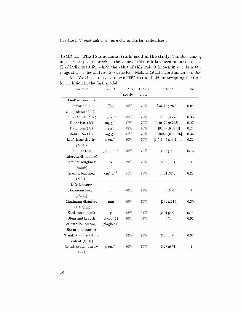
Chapitre 1. Toward trait-based mortality models for tropical forests
Table 1.1 : The 15 functional traits used in the study. Variable names,units, % of species for which the value of this trait is known in our data set,% of individuals for which the value of this trait is known in our data set,range of the value and results of the Kuo-Mallick (KM) algorithm for variableselection. We chose to use a value of 90% as threshold for accepting the traitfor inclusion in the �nal model.
Variable Units known known Range KM
species indiv.
Leaf economics
Foliar δ13C 0/00 75% 79% [-36.13 ;-26.2] 0.044
composition (δ13C)
Foliar C : N (CN) cg g−1 75% 79% [10.8 ;46.7] 0.38
Foliar Km (K) mg g−1 47% 70% [0.00122 ;0.223] 0.47
Foliar Nm (N) cg g−1 75% 79% [0.108 ;0.0451] 0.25
Foliar Pm (P ) mg g−1 47% 70% [0.00029 ;0.00216] 0.34
Leaf tissue density g cm−3 80% 79% [1.6 10-5 ;1.4 10-4] 0.31
(LTD)
Laminar total µg mm−2 80% 79% [20.8 ;149] 0.13
chlorophyll (chloro)
Laminar toughness N 79% 79% [0.22 ;11.4] 1
(tough)
Speci�c leaf area cm2 g−1 81% 79% [4.01 ;37.6] 0.28
(SLA)
Life history
Maximum height m 66% 77% [8 ;56] 1
(Hmax)
Maximum diameter mm 69% 79% [132 ;1110] 0.29
(DBHmax)
Seed mass (seed) g 42% 64% [0.01 ;20] 0.14
Stem and branch ortho (1) 46% 64% 0/1 0.91
orientation (ortho) plagio (0)
Stem economics
Trunk wood moisture 72% 75% [0.26 ;1.8] 0.37
content (WM)
Trunk xylem density g cm−3 80% 79% [0.28 ;0.91] 1
(WD)
48

3. MATERIALS AND METHODS
3.2 Addressing uncertainties in botanical determination
The traits data set is complete for 51% of individuals, and our goal was toattribute functional traits to all trees in the database. This is not feasibledirectly for three cases :
• (i) the tree species is known but some trait values of the species arenot available ;
• (ii) the tree species is not determined at the species level, but only atthe family or genus level ;
• (iii) the tree is dead before being identi�ed and only its vernacularname is available.
The trees falling in this third case cannot be excluded because they represent85% of dead trees.
An intuitive approach is to use a weighted mean of the traits for themissing data. But this approach has some disadvantages. First, some traitsare qualitative ; attributing a mean value to these traits is not feasible. Mostimportantly, it could be dangerous to use mean traits. As shown in Figure1.1, using means instead of the true values may create an arti�cial signalin the process we want to model. For instance, if trees of species A andB are well determined but trees of species C and D are not and share thesame vernacular name. Using a standard `mean-trait' approach, the meantrait value will be associated with individuals of species C and D, and afalse signal may be detected. A �nal reason for using our method is theuncertainty. If mean traits are used, their values will not be permitted tovary. Then, it will be impossible to propagate the inherent uncertainty of thetrait values when observing the uncertainty of the model outputs. Resultsof the covariates selection using weighted means of the traits and using ourmethod are compared in Figure 1.2. These results clearly show that usinga weighted mean approach would have led to a false trait-based mortalitymodel.
We addressed the cases (i) and (ii) with one relationship model and thecase (iii) with a second relationship model (Figure 1.3). We describe belowthese relationship models for a single trait T , but the same relationshipmodels were used independently for all traits.
The starting point was a set of nT species {s1, . . . , snT } for which wehave the associated set of values {t1, . . . , tnT } for the trait T . For any tree ofa species s ∈ {s1, . . . , snT }, the trait value was set to ts. For the other trees,the value of the trait was modelled by a multinomial distribution on the
49
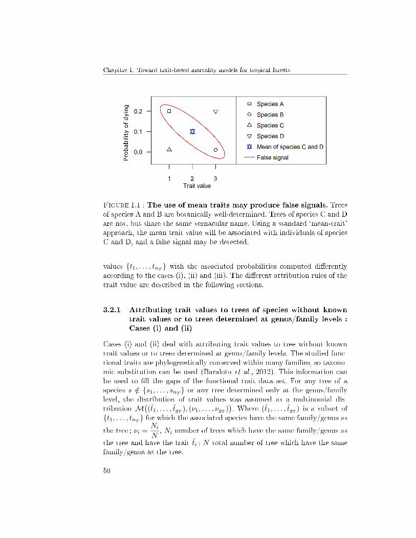
Chapitre 1. Toward trait-based mortality models for tropical forests
Figure 1.1 : The use of mean traits may produce false signals. Treesof species A and B are botanically well-determined. Trees of species C and Dare not, but share the same vernacular name. Using a standard `mean-trait'approach, the mean trait value will be associated with individuals of speciesC and D, and a false signal may be detected.
values {t1, . . . , tnT } with the associated probabilities computed di�erentlyaccording to the cases (i), (ii) and (iii). The di�erent attribution rules of thetrait value are described in the following sections.
3.2.1 Attributing trait values to trees of species without knowntrait values or to trees determined at genus/family levels :Cases (i) and (ii)
Cases (i) and (ii) deal with attributing trait values to tree without knowntrait values or to trees determined at genus/family levels. The studied func-tional traits are phylogenetically conserved within many families, so taxono-mic substitution can be used (Baraloto et al., 2012). This information canbe used to �ll the gaps of the functional trait data set. For any tree of aspecies s /∈ {s1, . . . , snT } or any tree determined only at the genus/familylevel, the distribution of trait values was assumed as a multinomial dis-tribution M
((t1, . . . , tgT ), (ν1, . . . , νgT )
). Where (t1, . . . , tgT ) is a subset of
{t1, . . . , tnT } for which the associated species have the same family/genus as
the tree ; νi =Ni
N, Ni number of trees which have the same family/genus as
the tree and have the trait ti ; N total number of tree which have the samefamily/genus as the tree.
50
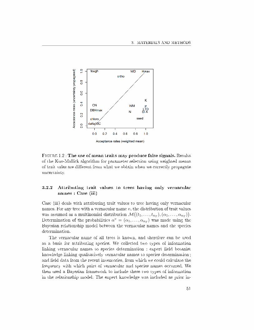
3. MATERIALS AND METHODS
Figure 1.2 :The use of mean traits may produce false signals. Resultsof the Kuo-Mallick algorithm for parameter selection using weighted meansof trait vales are di�erent from what we obtain when we correctly propagateuncertainty.
3.2.2 Attributing trait values to trees having only vernacularnames : Case (iii)
Case (iii) deals with attributing trait values to tree having only vernacularnames. For any tree with a vernacular name v, the distribution of trait valueswas assumed as a multinomial distributionM
((t1, . . . , tnT ), (α1, . . . , αnT )
).
Determination of the probabilities αv = (α1, . . . , αnT ) was made using theBayesian relationship model between the vernacular names and the speciesdetermination.
The vernacular name of all trees is known, and therefore can be usedas a basis for attributing species. We collected two types of informationlinking vernacular names to species determination : expert �eld botanistknowledge linking qualitatively vernacular names to species determination ;and �eld data from the recent inventories, from which we could calculate thefrequency with which pairs of vernacular and species names occurred. Wethen used a Bayesian framework to include these two types of informationin the relationship model. The expert knowledge was included as prior in-
51
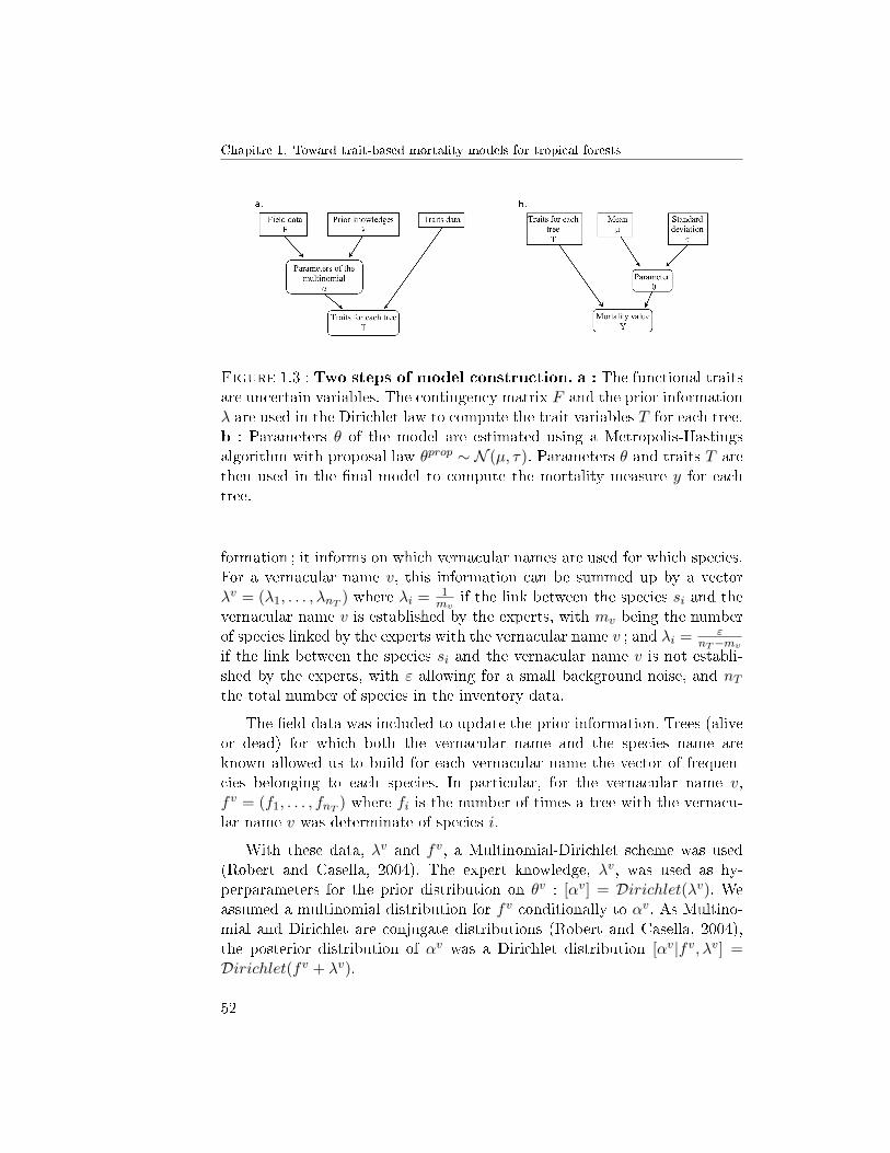
Chapitre 1. Toward trait-based mortality models for tropical forests
Figure 1.3 : Two steps of model construction. a : The functional traitsare uncertain variables. The contingency matrix F and the prior informationλ are used in the Dirichlet law to compute the trait variables T for each tree.b : Parameters θ of the model are estimated using a Metropolis-Hastingsalgorithm with proposal law θprop ∼ N (µ, τ). Parameters θ and traits T arethen used in the �nal model to compute the mortality measure y for eachtree.
formation ; it informs on which vernacular names are used for which species.For a vernacular name v, this information can be summed up by a vectorλv = (λ1, . . . , λnT ) where λi = 1
mvif the link between the species si and the
vernacular name v is established by the experts, with mv being the numberof species linked by the experts with the vernacular name v ; and λi = ε
nT−mvif the link between the species si and the vernacular name v is not establi-shed by the experts, with ε allowing for a small background noise, and nTthe total number of species in the inventory data.
The �eld data was included to update the prior information. Trees (aliveor dead) for which both the vernacular name and the species name areknown allowed us to build for each vernacular name the vector of frequen-cies belonging to each species. In particular, for the vernacular name v,fv = (f1, . . . , fnT ) where fi is the number of times a tree with the vernacu-lar name v was determinate of species i.
With these data, λv and fv, a Multinomial-Dirichlet scheme was used(Robert and Casella, 2004). The expert knowledge, λv, was used as hy-perparameters for the prior distribution on θv : [αv] = Dirichlet(λv). Weassumed a multinomial distribution for fv conditionally to αv. As Multino-mial and Dirichlet are conjugate distributions (Robert and Casella, 2004),the posterior distribution of αv was a Dirichlet distribution [αv|fv, λv] =Dirichlet(fv + λv).
52
3. MATERIALS AND METHODS
3.3 Modelling tree mortality
We modelled tree mortality with a generalized linear model (GLM) using alogit link function (McCullagh and Nelder, 1989). Tree mortality is a binaryvariable equal to 0 if the tree remained alive between 1992 and 2010, elseequal to 1. The probability of dying for each tree is the logit of a linearcombination of a set of covariates : 15 functional trait covariates and 2 on-
togenetic covariates DBHDBHmax
and(
DBH
DBHmax
)2
. DBH is the diameter of
the tree at breast height and DBHmax is computed as the 95the percentileof the observed DBH for each species. The ratio DBH
DBHmaxis then used as a
proxy of the ontogenetic stage of the tree. As it is well-known that the curvelinking mortality probability to ontogenetic stage is U-shaped, we also intro-
duced(
DBH
DBHmax
)2
as a covariate. The originality of the model is that the
trait covariates are uncertain for some trees and certain for the other trees.We used the method proposed by Kuo and Mallick (1998) to select the traitcovariates useful to explain mortality. The method consists in multiplyingeach trait covariate by an indicator. This indicator can be 0 if its covariateis not included in the model or 1 if its covariate is included in the model. Wedeveloped a Gibbs algorithm to attribute either 1 or 0 to the indicators anda Metropolis-Hastings within Gibbs algorithm to estimate the coe�cients ofthe covariates. We included a trait covariate in the �nal model if the expec-tation of its indicator, given by the Kuo-Mallick method, was between 0.9and 1 (Figure 1.4). We chose the threshold 0.9 after considering the histo-gram of the expectations of the trait covariate indicators (Figure 1.4). Oncethe �nal model was de�ned, the coe�cients of the covariates selected wereestimated using the Metropolis-Hastings algorithm. To test the convergenceof the chain, we run several chains from diverse initial values and inspect thechains to verify they all converge on the same value after some iterations.The autocorrelation is computed to ensure the chain is mixing adequately.The autocorrelation must decrease to zero when we increase the lag value.The methodology of model building is shown in Figure 1.3. See Appendicesfor further information.
All of the algorithms and statistical treatments were implemented withR software (R Development Core Team, 2010).
3.4 Model validation
To validate our mortality model, we split our data into a calibration dataset, which contains data between 1992 and 2001, and a validation data set,
53
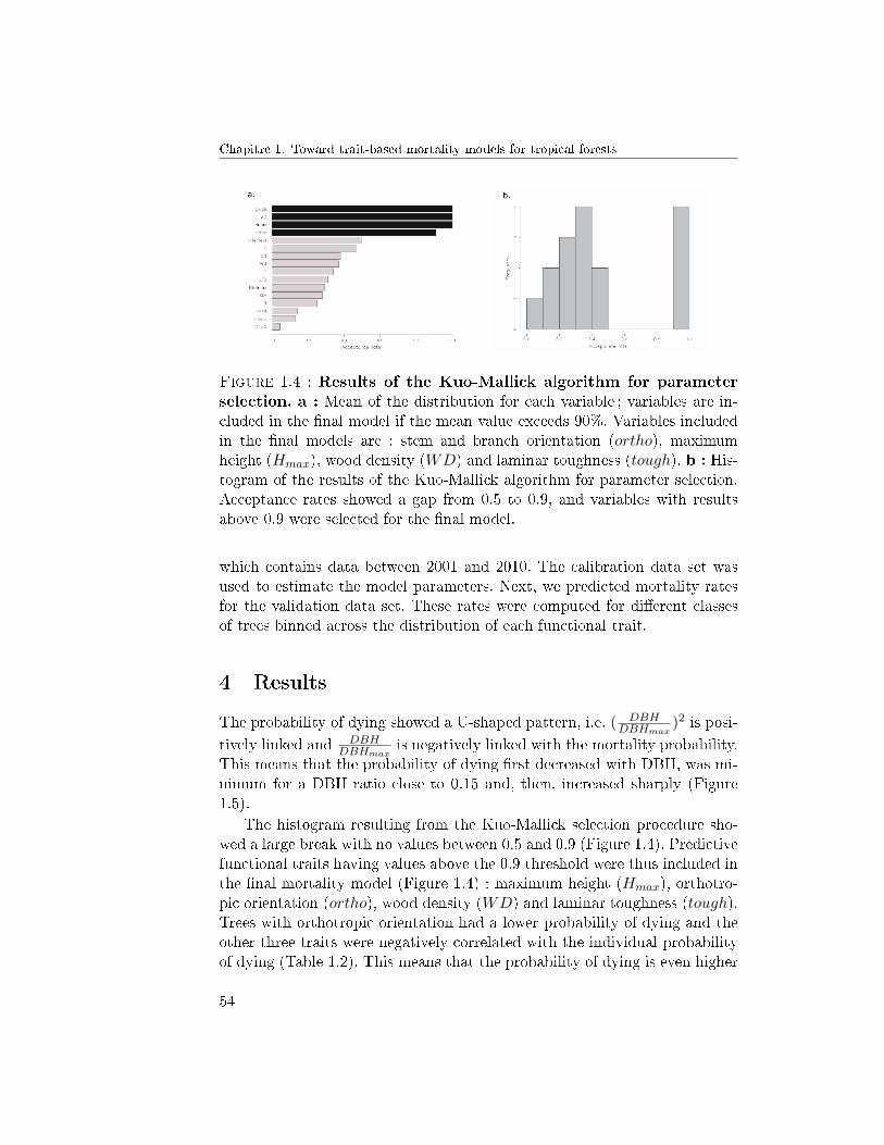
Chapitre 1. Toward trait-based mortality models for tropical forests
Figure 1.4 : Results of the Kuo-Mallick algorithm for parameterselection. a : Mean of the distribution for each variable ; variables are in-cluded in the �nal model if the mean value exceeds 90%. Variables includedin the �nal models are : stem and branch orientation (ortho), maximumheight (Hmax), wood density (WD) and laminar toughness (tough). b : His-togram of the results of the Kuo-Mallick algorithm for parameter selection.Acceptance rates showed a gap from 0.5 to 0.9, and variables with resultsabove 0.9 were selected for the �nal model.
which contains data between 2001 and 2010. The calibration data set wasused to estimate the model parameters. Next, we predicted mortality ratesfor the validation data set. These rates were computed for di�erent classesof trees binned across the distribution of each functional trait.
4 Results
The probability of dying showed a U-shaped pattern, i.e. ( DBHDBHmax
)2 is posi-tively linked and DBH
DBHmaxis negatively linked with the mortality probability.
This means that the probability of dying �rst decreased with DBH, was mi-nimum for a DBH ratio close to 0.15 and, then, increased sharply (Figure1.5).
The histogram resulting from the Kuo-Mallick selection procedure sho-wed a large break with no values between 0.5 and 0.9 (Figure 1.4). Predictivefunctional traits having values above the 0.9 threshold were thus included inthe �nal mortality model (Figure 1.4) : maximum height (Hmax), orthotro-pic orientation (ortho), wood density (WD) and laminar toughness (tough).Trees with orthotropic orientation had a lower probability of dying and theother three traits were negatively correlated with the individual probabilityof dying (Table 1.2). This means that the probability of dying is even higher
54
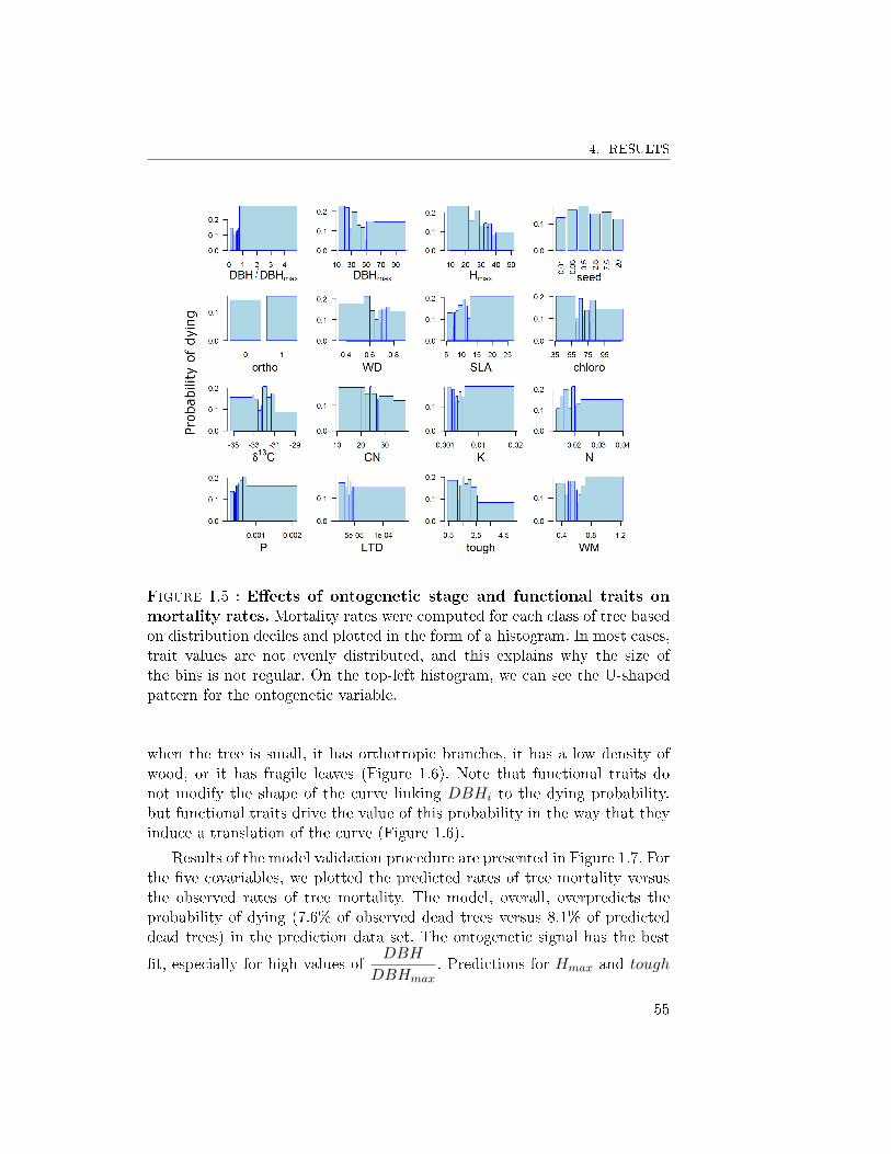
4. RESULTS
Figure 1.5 : E�ects of ontogenetic stage and functional traits onmortality rates. Mortality rates were computed for each class of tree basedon distribution deciles and plotted in the form of a histogram. In most cases,trait values are not evenly distributed, and this explains why the size ofthe bins is not regular. On the top-left histogram, we can see the U-shapedpattern for the ontogenetic variable.
when the tree is small, it has orthotropic branches, it has a low density ofwood, or it has fragile leaves (Figure 1.6). Note that functional traits donot modify the shape of the curve linking DBHi to the dying probability,but functional traits drive the value of this probability in the way that theyinduce a translation of the curve (Figure 1.6).
Results of the model validation procedure are presented in Figure 1.7. Forthe �ve covariables, we plotted the predicted rates of tree mortality versusthe observed rates of tree mortality. The model, overall, overpredicts theprobability of dying (7.6% of observed dead trees versus 8.1% of predicteddead trees) in the prediction data set. The ontogenetic signal has the best
�t, especially for high values ofDBH
DBHmax. Predictions for Hmax and tough
55
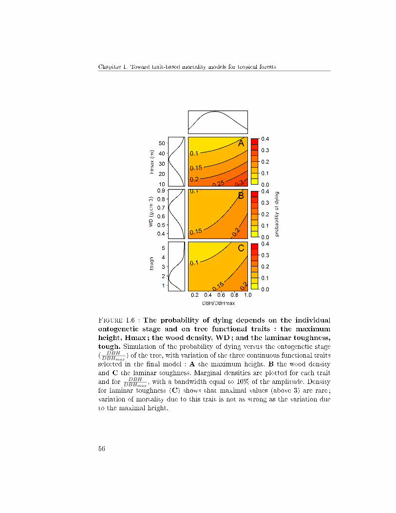
Chapitre 1. Toward trait-based mortality models for tropical forests
Figure 1.6 : The probability of dying depends on the individualontogenetic stage and on tree functional traits : the maximumheight, Hmax ; the wood density, WD ; and the laminar toughness,tough. Simulation of the probability of dying versus the ontogenetic stage( DBHDBHmax
) of the tree, with variation of the three continuous functional traitsselected in the �nal model : A the maximum height, B the wood densityand C the laminar toughness. Marginal densities are plotted for each traitand for DBH
DBHmax, with a bandwidth equal to 10% of the amplitude. Density
for laminar toughness (C) shows that maximal values (above 3) are rare ;variation of mortality due to this trait is not as strong as the variation dueto the maximal height.
56
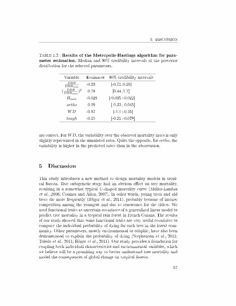
5. DISCUSSION
Table 1.2 : Results of the Metropolis-Hastings algorithm for para-meter estimation. Median and 90% credibility intervals of the posteriordistribution for the selected parameters.
Variable Estimates 90% credibility intervalsDBH
DBHmax-0.23 [-0.71 ;0.26]
( DBHDBHmax
)2 0.78 [0.44 ;1.1]
Hmax -0.028 [-0.035 ;-0.022]
ortho -0.19 [-0.33 ;-0.045]
WD -0.87 [-1.1 ;-0.55]
tough -0.15 [-0.21 ;-0.078]
are correct. ForWD, the variability over the observed mortality rates is onlyslightly represented in the simulated rates. Quite the opposite, for ortho, thevariability is higher in the predicted rates than in the observation.
5 Discussion
This study introduces a new method to design mortality models in tropi-cal forests. Tree ontogenetic stage had an obvious e�ect on tree mortality,resulting in a somewhat typical U-shaped mortality curve (Muller-Landauet al., 2006; Coomes and Allen, 2007). In other words, young trees and oldtrees die more frequently (Rüger et al., 2011), probably because of intensecompetition among the youngest and due to senescence for the oldest. Weused functional traits as uncertain covariates of a generalized linear model topredict tree mortality in a tropical rain forest in French Guiana. The resultsof our study showed that some functional traits are very useful covariates tocompute the individual probability of dying for each tree in the forest com-munity. Other parameters, mostly environmental or edaphic, have also beendemonstrated to explain the probability of dying (Stephenson et al., 2011;Toledo et al., 2011; Rüger et al., 2011). Our study provides a foundation forcoupling both individual characteristics and environmental variables, whichwe believe will be a promising way to better understand tree mortality andmodel the consequences of global change on tropical forests.
57
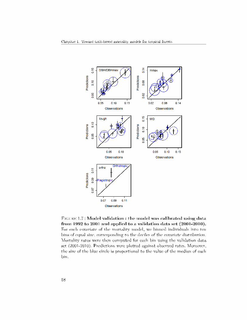
Chapitre 1. Toward trait-based mortality models for tropical forests
Figure 1.7 :Model validation : the model was calibrated using datafrom 1992 to 2001 and applied to a validation data set (2001-2010).For each covariate of the mortality model, we binned individuals into tenbins of equal size, corresponding to the deciles of the covariate distribution.Mortality rates were then computed for each bin using the validation dataset (2001-2010). Predictions were plotted against observed rates. Moreover,the size of the blue circle is proportional to the value of the median of eachbin.
58
5. DISCUSSION
5.1 Functional Traits
We used an original selection procedure to evaluate which tree functionaltraits shape the mortality curves. In doing so, we formally incorporated treefunctional diversity into forest dynamics modelling without the necessity tobuild any functional groups. All in all, only four functional traits were robustpredictors of the mortality probability. Most of the numerous measured traitsrelated to leaf economics (δ13C, K...) were not included in the �nal model,instead traits related to life history or stem economics were largely selected.
First, wood density was expected to be a good predictor of mortalityrates, since Chao et al. (2008); Kraft et al. (2010) reported a robust negativecorrelation between wood density and tree mortality in Amazonian forests.Moreover, King et al. (2006) also highlighted the importance of wood den-sity in the trade-o� between resource acquisition and investment in survival.In a nutshell, trees with low density are light-demanding trees with rapidbole expansion, leading to a higher mortality probability. High wood den-sity is known to shape resistance to water-stress embolism (Jacobsen et al.,2005), mechanical breakage or attack by pathogens (Chave et al., 2009; Zanneet al., 2010). This �nding is in line with Chao's hypothesis that species withhigh mortality rates would create more canopy gaps that, in turn, favor lowwood-density species and vice-versa. This means that the mortality regimein tropical forests may be both a cause and an e�ect of �oristic composition(Chao et al., 2008).
Hmax was predicted to be negatively linked to mortality probability (Fi-gure 1.5), as reported by Wright et al. (2010). We know that Hmax cap-tures a major variation in functional traits found among tropical rain foresttree species, and in combination with light-demand, it provides a rough butstraightforward model to understand niche di�erentiation in tropical forests(Poorter et al., 2006). Hmax is predicted to be small for light-demandingspecies with rapid growth and mortality and large for shade-tolerant specieswith slow growth and mortality (Wright et al., 2010).
Light-demanding tropical trees are characterized by orthotropic stemsand branches, large leaves, and a monolayer leaf arrangement (Poorter et al.,2006). They are known to realize an e�cient height growth through forma-tion of narrow, shallow crowns (Poorter et al., 2006). Species with orthotropicarchitecture are therefore expected to be fast-growing and light demanding(Poorter et al., 2003) and, thus, to have higher mortality rates then plagio-tropic species. Surprisingly, our model parameters suggest that orthotropictrees have lower mortality rates than plagiotropic trees. We believe this isdue to the combined e�ect of wood density and maximum height, that over-
59
Chapitre 1. Toward trait-based mortality models for tropical forests
estimated the e�ect of both traits on mortality. In other words, orthotropicspecies indeed have higher mortality rates than plagiotropic trees, but thetrait model over-predicts this rate for individuals that are small or have alow wood density.
Finally, shade-tolerant plant species have tough leaves because of the highcost of leaf replacement in shade relative to potential carbon gain (Westbrooket al., 2011). Leaf toughness (resistance to fracture per unit fracture area) wasthe only trait from the leaf economic spectrum to be retained in the mortalitymodel. Leaf toughness was a good candidate because, for some tree saplings,Kitajima and Poorter (2010) showed that fracture toughness correlated posi-tively with leaf lifespan and survival. Recently, Westbrook et al. (2011) alsoshowed that mortality rates of individuals 1-10 cm in stem diameter werenegatively correlated with material toughness and lamina density but wereindependent of structural toughness and cell-wall �ber content. We extendthis �nding to adult trees, highlighting the importance of plant-defense traitsin shaping individual tree survival.
5.2 Toward new community models of population dynamics ?
In a context of global change, the long-term response of tropical forests toclimate change cannot be predicted without using forest simulators or Dy-namic Vegetation Models that incorporate both growth and mortality pro-cesses. Although tropical forests are known to have very di�erent dynamicsregimes, it has been shown that past tree growth is an accurate predictor oftree mortality (Chao et al., 2008). The problem with such a result is thatit is di�cult to use past tree growth per se in a predictive model. Indeed,it only postpones the prediction problem, as it restricts one to predictingevents of low growth in the life of a given tree, a goal very hard to achieveacross the forest community for at least two reasons. First, most ecologicalworks have focused on the average growth rates (Wright et al., 2010), as pre-dicting outliers is something extremely complicated in statistical modelling.Second, a tree's death linked to a decline in vigour appears predictable byits growth pattern before mortality, but tree death caused by disturbance,such as wind, is far from predictable (Chao et al., 2008). In this context, wechoose to decouple, at �rst, the growth determinants (Hérault et al., 2011)from the mortality determinants and, then, we hope to �nd the right waysto combine both processes into a single modelling framework.
The community growth model developed in Hérault et al. (2011) is basedon individual growth computed with the functional traits of trees as cova-riates. We used the same strategies to build a mortality model, but in our
60
5. DISCUSSION
study, we also have to deal with uncertainty of the process of death on theone hand, and with incomplete species information on the other. The stra-tegy of using functional traits does add some uncertainty to the model. Themethodology developed in this study handles the uncertainty of the cova-riates, due both to missing information about the functional traits and todi�erent levels of botanical identi�cation. This kind of incomplete informa-tion is common in many tropical forest inventory data sets with high varia-bility in the levels of botanical determination of the trees (Réjou-Mechainet al., 2011).We used the maximum available information about the trees(species, vernacular name, family/genus) to attribute trait values, under theassumption that functional traits are strongly conserved between species ofthe same genus and/or the same vernacular name. Although there is somesupport for this assumption in French Guianan trees (Baraloto et al., 2012),the method necessarily involves a loss of some trait information.
Variable selection in nonlinear models remains a complex issue. In ourstudy, the unconventional uncertainties about trait covariates complicatedthe issue even further. To select the covariates, usual frequentist criteriabased on the penalized likelihood, like AIC, BIC, . . . , were unusable. Baye-sian methods were better adapted because they naturally support di�erentsources of uncertainties in the models. However, using the Bayesian versionsof penalized likelihood criteria, such DIC, AICm, . . . , over all combinationsof the trait covariates would have required too much computation time. The-refore, we developed a Bayesian algorithm that explores all combinations oftrait covariates while calibrating the parameters. There were two possible ap-proaches : Kuo and Mallick (Kuo and Mallick, 1998) or the reversible jump(Richardson and Green, 1997). We chose the Kuo and Mallick approach be-cause it performs better in cases of correlated covariates. Furthermore, itsinterpretation and implementation are more intuitive because the dimensionof the model is not variable, as in the reversible jump approach.
5.3 Conclusion
Our aim in this study was to model tree mortality in a tropical rain forestusing functional traits. Considering �rst the complexity of the mortality pro-cess, and second the uncertainty due to the data, the model needed to bedeveloped with particular attention to the methodology. We used a Bayesianframework, on the one hand to use all data about the tree and functionaltraits at our disposal, and on the other hand, to build the most accuratemodel using this data. This approach can be generalized to many similarstudies about tropical forest dynamics, because more and more data are col-
61
Chapitre 1. Toward trait-based mortality models for tropical forests
lected about tree dynamics, but frameworks are missing to correctly processthis data. Indeed, ecologists are often limited in their research when workingwith data from old inventories. Our method should permit increased use ofdata from old inventories to examine tree mortality. This is particularly in-teresting for conducting meta-analyses, which are generally based on datawith widely varying levels of accuracy.
Tree mortality plays a key-role in the carbon cycle (Rutishauser et al.,2010; Hérault et al., 2010a) and is intimately linked to forest productivity(e.g. Stephenson et al. (2011)). Global changes, and associated increases inthe frequency, duration and/or severity of drought events and heat stress al-ready could have ampli�ed natural tree mortality and potentially will conti-nue to in the future (Phillips et al., 2010; Allen et al., 2010; Condit et al.,1995), altering tropical forest dynamics and other ecosystem services (Cor-lett, 2011; Lewis, 2006; Condit et al., 1996). Based on a long-term forest dataset, in this study, we developed mortality models suitable for species-rich tro-pical forest communities, using functional traits as surrogates for taxon-levelmodels. Methods used in this study allow us to model the tree communityas a continuum, connecting functional traits to the mortality probabilitywithout collapsing species into functional groups.
Acknowledgments
We thank Francesco de Bello and two anonymous reviewers for useful com-ments on previous drafts of the manuscript.
62
BIBLIOGRAPHIE
Alder, D. and Silva, J. N. M. (2000). An empirical cohort model for manage-ment of terra �rme forests in the brazilian amazon. Forest Ecology andManagement, 130(1-3):141�157.
Allen, C. D., Macalady, A. K., Chenchouni, H., Bachelet, D., McDowell,N., Vennetier, M., Kitzberger, T., Rigling, A., Breshears, D. D., Hogg,E. H., Gonzalez, P., Fensham, R., Zhang, Z., Castro, J., Demidova, N.,Lim, J. H., Allard, G., Running, S. W., Semerci, A., and Cobb, N.(2010). A global overview of drought and heat-induced tree mortalityreveals emerging climate change risks for forests. Forest Ecology andManagement, 259(4):660�684.
Altaleb, A. and Robert, C. P. (2001). Analyse bayésienne du modèle logit :algorithme par tranches ou metropolis-hastings ? Revue de statistiqueAppliquée, 49(4):53�70.
Baraloto, C. and Forget, P. M. (2007). Seed size, seedling morphology, andresponse to deep shade and damage in neotropical rain forest trees.American Journal of Botany, 94(6):901�911.
Baraloto, C., Forget, P. M., and Goldberg, D. E. (2005). Seed mass, seedlingsize and neotropical tree seedling establishment. Journal of Ecology,93(6):1156�1166.
Baraloto, C., Hardy, O. J., Paine, C. E. T., Dexter, K. G., Cruaud, C., Dun-ning, L. T., Gonzalez, M. A., Molino, J. F., Sabatier, D., Savolainen, V.,and Chave, J. (2012). Using functional traits and phylogenetic trees to
63
Chapitre 1. Toward trait-based mortality models for tropical forests
examine the assembly of tropical tree communities. Journal of Ecology,100(3):690�701.
Baraloto, C., Paine, C. E. T., Patino, S., Bonal, D., Hérault, B., and Chave,J. (2010a). Functional trait variation and sampling strategies in species-rich plant communities. Functional Ecology, 24(1):208�216.
Baraloto, C., Paine, C. E. T., Poorter, L., Beauchêne, J., Bonal, D., Dome-nach, A. M., Hérault, B., Patino, S., Roggy, J. C., and Chave, J. (2010b).Decoupled leaf and stem economics in rain forest trees. Ecology Letters,13(11):1338�1347.
Bohlman, S. and Pacala, S. (2012). A forest structure model that determinescrown layers and partitions growth and mortality rates for landscape-scale applications of tropical forests. Journal of Ecology, 100(2):508�518.
Carey, E. V., Brown, S., Gillespie, A. J. R., and Lugo, A. E. (1994). Treemortality in mature lowland tropical moist and tropical lower montanemoist forests of Venezuela. Biotropica, 26(3):255�265.
Chao, K. J., Phillips, O. L., Gloor, E., Monteagudo, A., Torres-Lezama, A.,and Martinez, R. V. (2008). Growth and wood density predict treemortality in Amazon forests. Journal of Ecology, 96(2):281�292.
Chao, K. J., Phillips, O. L., Monteagudo, A., Torres-Lezama, A., and Mar-tinez, R. V. (2009). How do trees die ? Mode of death in northernamazonia. Journal of Vegetation Science, 20(2):260�268.
Chave, J., Coomes, D., Jansen, S., Lewis, S. L., Swenson, N. G., and Zanne,A. E. (2009). Towards a worldwide wood economics spectrum. EcologyLetters, 12(4):351�366.
Condit, R., Aguilar, S., Hernandez, A., Perez, R., Lao, S., Angehr, G., Hub-bell, S. P., and Foster, R. B. (2004). Tropical forest dynamics across arainfall gradient and the impact of an El Nino dry season. Journal ofTropical Ecology, 20:51�72.
Condit, R., Hubbell, S. P., and Foster, R. B. (1995). Mortality-rates of 205neotropical tree and shrub species and the impact of a severe drought.Ecological Monographs, 65(4):419�439.
Condit, R., Hubbell, S. P., and Foster, R. B. (1996). Assessing the responseof plant functional types to climatic change in tropical forests. Journalof Vegetation Science, 7(3):405�416.
64
BIBLIOGRAPHIE
Coomes, D. A. and Allen, R. B. (2007). E�ects of size, competition andaltitude on tree growth. Journal of Ecology, 95(5):1084�1097.
Corlett, R. T. (2011). Impacts of warming on tropical lowland rainforests.Trends in Ecology and Evolution, 26(11):606�613.
Delbart, N., Ciais, P., Chave, J., Viovy, N., Malhi, Y., and Le Toan, T. (2010).Mortality as a key driver of the spatial distribution of abovegroundbiomass in Amazonian forest : results from a dynamic vegetation model.Biogeosciences, 7(10):3027�3039.
Ferry, B., Morneau, F., Bontemps, J. D., Blanc, L., and Freycon, V. (2010).Higher treefall rates on slopes and waterlogged soils result in lower standbiomass and productivity in a tropical rain forest. Journal of Ecology,98(1):106�116.
Gourlet-Fleury, S. (1999). Individual-based spatially explicit modelling of fo-rest stands in French Guiana. In Laumonier, Y., King, B., Legg, C., andRenolls, K., editors, Data management and modelling using remote sen-sing and GIS for tropical forest land inventory, pages 473�490, Jakarta,Indonesia.
Gourlet-Fleury, S., Cornu, G., Jesel, S., Dessard, H., Jourget, J. G., Blanc,L., and Picard, N. (2005). Using models to predict recovery and assesstree species vulnerability in logged tropical forests : A case study fromFrench Guiana. Forest Ecology and Management, 209(1-2):69�86.
Hérault, B., Bachelot, B., Poorter, L., Rossi, V., Bongers, F., Chave, J.,Paine, C. E. T., Wagner, F., and Baraloto, C. (2011). Functional traitsshape ontogenetic growth trajectories of rain forest tree species. Journalof Ecology, 99(6):1431�1440.
Hérault, B., Beauchêne, J., Muller, F., Wagner, F., Baraloto, C., Blanc, L.,and Martin, J. M. (2010a). Modeling decay rates of dead wood in aneotropical forest. Oecologia, 164(1):243�251.
Hérault, B., Ouallet, J., Blanc, L., Wagner, F., and Baraloto, C. (2010b).Growth responses of neotropical trees to logging gaps. Journal of AppliedEcology, 47(4):821�831.
Jacobsen, A. L., Ewers, F. W., Pratt, R. B., Paddock, W. A., and Davis,S. D. (2005). Do xylem �bers a�ect vessel cavitation resistance ? PlantPhysiology, 139(1):546�556.
65
Chapitre 1. Toward trait-based mortality models for tropical forests
Jansen, P. A., Van Der Meer, P. J., and Bongers, F. (2008). Spatial conta-giousness of canopy disturbance in tropical rain forest : an individual-tree-based test. Ecology, 89(12):3490�3502.
King, D. A., Davies, S. J., Tan, S., and Noor, N. S. M. (2006). The roleof wood density and stem support costs in the growth and mortality oftropical trees. Journal of Ecology, 94(3):670�680.
Kitajima, K. and Poorter, L. (2010). Tissue-level leaf toughness, but notlamina thickness, predicts sapling leaf lifespan and shade tolerance oftropical tree species. New Phytologist, 186(3):708�721.
Kraft, N. J. B., Metz, M. R., Condit, R. S., and Chave, J. (2010). Therelationship between wood density and mortality in a global tropicalforest data set. New Phytologist, 188(4):1124�1136.
Kuo, L. and Mallick, B. (1998). Variable selection for regression models.Sankhya Ser.B, (60):65�81.
Lewis, S. L. (2006). Tropical forests and the changing earth system.Philosophical Transactions of the Royal Society B-Biological Sciences,361(1465):195�210.
Lewis, S. L., Phillips, O. L., Sheil, D., Vinceti, B., Baker, T. R., Brown, S.,Graham, A. W., Higuchi, N., Hilbert, D. W., Laurance, W. F., Lejoly,J., Malhi, Y., Monteagudo, A., Vargas, P. N., Sonke, B., Supardi, N.,Terborgh, J. W., and Martinez, R. V. (2004). Tropical forest tree mor-tality, recruitment and turnover rates : calculation, interpretation andcomparison when census intervals vary. Journal of Ecology, 92(6):929�944.
McCullagh, P. and Nelder, J. (1989). Generalized linear models. Boca Raton :Chapman and Hall, 2nd edition.
McGill, B. J., Enquist, B. J., Weiher, E., and Westoby, M. (2006). Rebuil-ding community ecology from functional traits. Trends in Ecology andEvolution, 21(4):178�185.
Moles, A. T. and Westoby, M. (2004). Seedling survival and seed size : asynthesis of the literature. Journal of Ecology, 92(3):372�383.
Muller-Landau, H. C., Condit, R. S., Chave, J., Thomas, S. C., Bohlman,S. A., Bunyavejchewin, S., Davies, S., Foster, R., Gunatilleke, S., Gu-natilleke, N., Harms, K. E., Hart, T., Hubbell, S. P., Itoh, A., Kassim,
66
BIBLIOGRAPHIE
A. R., LaFrankie, J. V., Lee, H. S., Losos, E., Jr, M., Ohkubo, T., Suku-mar, R., Sun, I. F., Supardi, N. M. N., Tan, S., Thompson, J., Valencia,R., Munoz, G. V., Wills, C., Yamakura, T., Chuyong, G., Dattaraja,H. S., Esufali, S., Hall, P., Hernandez, C., Kenfack, D., Kiratiprayoon,S., Suresh, H. S., Thomas, D., Vallejo, M. I., and Ashton, P. (2006). Tes-ting metabolic ecology theory for allometric scaling of tree size, growthand mortality in tropical forests. Ecology Letters, 9(5):575�588.
Phillips, O. L., van der Heijden, G., Lewis, S. L., Lopez-Gonzalez, G., Ara-gao, L., Lloyd, J., Malhi, Y., Monteagudo, A., Almeida, S., Davila, E. A.,Amaral, I., Andelman, S., Andrade, A., Arroyo, L., Aymard, G., Baker,T. R., Blanc, L., Bonal, D., de Oliveira, A. C. A., Chao, K. J., Cardozo,N. D., da Costa, L., Feldpausch, T. R., Fisher, J. B., Fyllas, N. M., Frei-tas, M. A., Galbraith, D., Gloor, E., Higuchi, N., Honorio, E., Jimenez,E., Keeling, H., Killeen, T. J., Lovett, J. C., Meir, P., Mendoza, C.,Morel, A., Vargas, P. N., Patino, S., Peh, K. S. H., Cruz, A. P., Prieto,A., Quesada, C. A., Ramirez, F., Ramirez, H., Rudas, A., Salamao, R.,Schwarz, M., Silva, J., Silveira, M., Slik, J. W. F., Sonke, B., Thomas,A. S., Stropp, J., Taplin, J. R. D., Vasquez, R., and Vilanova, E. (2010).Drought-mortality relationships for tropical forests. New Phytologist,187(3):631�646.
Phillips, P. D., de Azevedo, C. P., Degen, B., Thompson, I. S., Silva, J.N. M., and van Gardingen, P. R. (2004). An individual-based spatiallyexplicit simulation model for strategic forest management planning inthe eastern Amazon. Ecological Modelling, 173(4):335�354.
Poorter, L. (1999). Growth responses of 15 rain-forest tree species to a lightgradient : the relative importance of morphological and physiologicaltraits. Functional Ecology, 13(3):396�410.
Poorter, L., Bongers, F., Sterck, F. J., and Woll, H. (2003). Architecture of53 rain forest tree species di�ering in adult stature and shade tolerance.Ecology, 84(3):602�608.
Poorter, L., Bongers, L., and Bongers, F. (2006). Architecture of 54 moist-forest tree species : traits, trade-o�s, and functional groups. Ecology,87(5):1289�1301.
Poorter, L. and Rose, S. (2005). Light-dependent changes in the relationshipbetween seed mass and seedling traits : a meta-analysis for rain foresttree species. Oecologia, 142(3):378�387.
67
Chapitre 1. Toward trait-based mortality models for tropical forests
R Development Core Team (2010). R : a language and environment forstatistical computing. R Foundation for Statistical Computing, Vienna,Austria.
Réjou-Mechain, M., Fayolle, A., Nasi, R., Gourlet-Fleury, S., Doucet, J. L.,Gally, M., Hubert, D., Pasquier, A., and Billand, A. (2011). Detectinglarge-scale diversity patterns in tropical trees : can we trust commercialforest inventories ? Forest Ecology and Management, 261(2):187�194.
Richardson, S. and Green, P. J. (1997). On Bayesian analysis of mixtureswith an unknown number of components. Journal of the Royal StatisticalSociety Series B-Methodological, 59(4):731�758.
Robert, C. P. and Casella, G. (2004). Monte Carlo statistical methods. Sprin-ger, 2nd edition.
Rüger, N., Huth, A., Hubbell, S. P., and Condit, R. (2011). Determinants ofmortality across a tropical lowland rainforest community. Oikos, 120(7):1047�1056.
Rüger, N., Wirth, C., Wright, S. J., and Condit, R. (2012). Functional traitsexplain light and size response of growth rates in tropical tree species.Ecology, 93(12):2626�2636.
Rutishauser, E., Wagner, F., Hérault, B., Nicolini, E. A., and Blanc, L.(2010). Contrasting above-ground biomass balance in a neotropical rainforest. Journal of Vegetation Science, 21(4):672�682.
Sheil, D. and May, R. M. (1996). Mortality and recruitment rate evaluationsin heterogeneous tropical forests. Journal of Ecology, 84(1):91�100.
Stephenson, N. L., van Mantgem, P. J., Bunn, A. G., Bruner, H., Harmon,M. E., O'Connell, K. B., Urban, D. L., and Franklin, J. F. (2011). Causesand implications of the correlation between forest productivity and treemortality rates. Ecological Monographs, 81(4):527�555.
Toledo, J. J., Magnusson, W. E., Castilho, C. V., and Nascimento, H. E. M.(2011). How much variation in tree mortality is predicted by soil andtopography in central amazonia ? Forest Ecology and Management,262(3):331�338.
Uriarte, M., Canham, C. D., Thompson, J., and Zimmerman, J. K. (2004). Aneighborhood analysis of tree growth and survival in a hurricane-driventropical forest. Ecological Monographs, 74(4):591�614.
68
BIBLIOGRAPHIE
Wagner, F., Hérault, B., Stahl, C., Bonal, D., and Rossi, V. (2011). Modelingwater availability for trees in tropical forests. Agricultural and ForestMeteorology, 151(9):1202�1213.
Wagner, F., Rossi, V., Stahl, C., Bonal, D., and Hérault, B. (2012). Wateravailability is the main climate driver of neotropical tree growth. PlosOne, 7(4):e34074.
Wagner, F., Rutishauser, E., Blanc, L., and Hérault, B. (2010). E�ects of plotsize and census interval on descriptors of forest structure and dynamics.Biotropica, 42(6):664�671.
Westbrook, J. W., Kitajima, K., Burleigh, J. G., Kress, W. J., Erickson,D. L., and Wright, S. J. (2011). What makes a leaf tough ? patternsof correlated evolution between leaf toughness traits and demographicrates among 197 shade-tolerant woody species in a neotropical forest.American Naturalist, 177(6):800�811.
Westoby, M. (1998). A leaf-height-seed (lhs) plant ecology strategy scheme.Plant and Soil, 199(2):213�227.
Wright, I. J., Reich, P. B., Westoby, M., Ackerly, D. D., Baruch, Z., Bongers,F., Cavender-Bares, J., Chapin, T., Cornelissen, J. H. C., Diemer, M.,Flexas, J., Garnier, E., Groom, P. K., Gulias, J., Hikosaka, K., Lamont,B. B., Lee, T., Lee, W., Lusk, C., Midgley, J. J., Navas, M. L., Niinemets,U., Oleksyn, J., Osada, N., Poorter, H., Poot, P., Prior, L., Pyankov,V. I., Roumet, C., Thomas, S. C., Tjoelker, M. G., Veneklaas, E. J.,and Villar, R. (2004). The worldwide leaf economics spectrum. Nature,428(6985):821�827.
Wright, S. J., Kitajima, K., Kraft, N. J. B., Reich, P. B., Wright, I. J., Bun-ker, D. E., Condit, R., Dalling, J. W., Davies, S. J., Diaz, S., Engelbrecht,B. M. J., Harms, K. E., Hubbell, S. P., Marks, C. O., Ruiz-Jaen, M. C.,Salvador, C. M., and Zanne, A. E. (2010). Functional traits and thegrowth-mortality trade-o� in tropical trees. Ecology, 91(12):3664�3674.
Zanne, A. E., Westoby, M., Falster, D. S., Ackerly, D. D., Loarie, S. R., Ar-nold, S. E. J., and Coomes, D. A. (2010). Angiosperm wood structure :Global patterns in vessel anatomy and their relation to wood density andpotential conductivity. American Journal of Botany, 97(2):207�215.
69

Chapitre 1. Toward trait-based mortality models for tropical forests
1.A Mortality model equation
Tree mortality is a binary variable yi equal to 0 if tree i is alive, else equalto 1. The mortality model is a generalized linear model, which computes atree-individual probability of dying. The probability of dying pi for tree i iscalculated with a logit function :
pi = logit−1(LCi) =LCi
1 + exp(LCi)
where LCi is a linear combination of the covariates associated with the tree i.The covariates are 15 functional traits of tree i and two ontogenetic variables(
DBHiDBHmax,i
and ( DBHiDBHmax,i
)2), included to estimate the ontogenetic stage of
tree i (Hérault et al., 2011) :
LCi = θ0 + θ1DBHi
DBHmax,i+ θ2
(DBHi
DBHmax,i
)2
+ θ3δ13Ci + θ4CNi + ...
where θ = θ0, θ1, θ2, · · · θm is a vector of parameters to be estimated. Themortality value yi for tree i is then yi ∼ Bern(pi).
70

1.B. ALGORITHMS
1.B Algorithms
1.B.1 Algorithms for sampling traits value for undeterminedtrees
We sampled the trait values using di�erent algorithms, according to the levelof determination of the trees. (i) If the tree species is known but some traitvalues of the species are not attributed, we used the algorithm 1 to samplethe missing trait values.
for each determined tree, with some unattributed trait valuesdo
for each trait T with unattributed value for the tree do- let nT the number of species in the same genus withthe value of trait T attributed : t1, . . . , tnT ;- for i = 1, . . . , nT , let νi = Ni
N with Ni the number oftrees in the genus with the trait value ti and N thenumber of trees in the genus ;- sample t ∼M
((t1, . . . , tnT ), (ν1, . . . , νnT )
), the value
for the trait T for the tree;end
endAlgorithm 1: Multinomial algorithm for sampling traits values -case (i)
For the trees determined at the genus/family level we used the followingalgorithm 2.
for each tree determined at the genus/family level dofor each traits T do
- let nT the number of species in the same genus/familywith the value of trait T attributed : t1, . . . , tnT ;- for i = 1, . . . , nT , let νi = Ni
N with Ni the number oftrees in the genus/family with the trait value ti and Nthe number of trees in the genus ;- sample t ∼M
((t1, . . . , tnT ), (ν1, . . . , νnT )
), the value
for the trait T for the tree;end
endAlgorithm 2: Multinomial algorithm for sampling traits values -case (ii)
71

Chapitre 1. Toward trait-based mortality models for tropical forests
For the trees with only a vernacular name we used the algorithm 3.
for each tree with only a vernacular name dolet v the vernacular name of the tree;for each traits T do
- let nT the number of species with the value of trait Tattributed : t1, . . . , tnT ;- let fv = (f1, . . . , fnT ) the number of trees withvernacular name v which were determined among thesespecies;- let mv the number of species among the nT for whichthe expert con�rmed a link with the vernacular name v;- let λv = (λ1, . . . , λnT ) with
λi =
{1mv
if the link is con�rmedε
nT−mv otherwise;
- sample (α1, . . . , αnT ) ∼ Dir(fv + λv) ;- sample t ∼M
((t1, . . . , tnT ), (α1, . . . , αnT )
), the value
for the trait T for the tree;end
endAlgorithm 3: Multinomial algorithm for sampling traits values -case (iii)
Practically, to implement the algorithm 3 on our case study we usedε = 0.1.
1.B.2 Algorithm for estimating parameters in a classical lo-git model
First, let us assume that the covariates (the 15 functional traits) are com-pletely known for all the trees. The model is :
yi ∼ Bern (logit(θ0 + θ1xi1 + θ2xi2 + · · ·+ θmxim)) .
The likelihood function is :
L(Y |X, θ) =n∏i=1
exp((θ0 + θ1xi1 + ...+ θmxim)yi)
1 + exp(θ0 + θ1xi1 + ...+ θmxim)
where
• Y = y1, y2, ..., yn is the vector of mortality values for all trees,
72

1.B. ALGORITHMS
• X = xi1, xi2, ..., xim is the vector of covariates for tree i (ontogeneticvariables and traits),
• θ = θ1, θ2, ..., θm is the vector of parameters of the model.
The estimation of parameters θ in the Bayesian framework consists inestimating the posterior distribution of the parameters πθ|Y,X . From theBayesian formula we have πθ|Y,X(θ) ∝ L(Y |X, θ)π0
θ(θ) where π0θ is the prior
distribution set by the user on θ. To estimate the posterior distribution πθ|Y,Xwe can use a Monte Carlo Markov Chain algorithm, like Metropolis-Hastings(cf. algorithm 4). Such algorithm only requires a proposal distribution πprop
to sample possible values for θ and this values are kept or not in the chainaccording to their likelihoods.
Initialisation : t = 1, θt ∼ π0θ ;
repeatSample θ∗ ∼ πprop ;Sample u ∼ Unif [0, 1] ;
Compute ρ(θt, θ∗) =L(Y |X, θ∗)π0
θ(θ∗)
L(Y |X, θt)π0θ(θ
t)
πprop(θt)
πprop(θ∗);
if u < ρ(θt, θ∗) thenθt+1 = θ∗
elseθt+1 = θt
endt=t+1
until the chain (θt)t=1,... reaches its stationary state;Algorithm 4: Metropolis-Hastings
1.B.3 Algorithm for estimating parameters in a logit modelwith random covariates
However, in our case study, the covariates are not completely known for allthe trees. In the paper we built models of knowledge for the traits, thus, thecovariates become random for some trees. Let us note πX|i the distributionof the covariate values for the tree i as de�ned by the algorithm describedin the section 1.B.1. For a tree i, for which all traits values are known, πX|iis a Dirac measure on its traits values i.e. sampling from πX|i always returnthe traits values of the tree.
Thanks to the Bayesian framework, we could take the randomness on Xinto account while estimating θ. We must add a Monte-Carlo step into the
73

Chapitre 1. Toward trait-based mortality models for tropical forests
Metropolis-Hastings algorithm. Practically, we run the Metropolis-Algorithmand new values for the covariates are sampled at each iteration (cf. Algorithm5).
Initialisation : t = 1, θt ∼ π0θ ;
repeatSample covariate values for each individual i : Xi ∼ πX,i;Sample θ∗ ∼ πprop ;Sample u ∼ Unif [0, 1] ;
Compute ρ(θt, θ∗) =L(Y |X, θ∗)π0
θ(θ∗)
L(Y |X, θt)π0θ(θ
t)
πprop(θt)
πprop(θ∗);
if u < ρ(θt, θ∗) thenθt+1 = θ∗
elseθt+1 = θt
endt=t+1
until the chain (θt)t=1,... reaches its stationary state;Algorithm 5:Monte Carlo within Metropolis-Hastings for a modelwith random explicative variables
1.B.4 Algorithm for estimating parameters and selecting co-variates in a logit model with random covariates
The last methodological point of the paper was to select useful covariates toexplain the mortality while taking their randomness into account. We useda method proposed by Kuo and Mallick (1998) which consists in adding anindicator for each covariate :
yi ∼ Bern (logit(θ0 + θ1I1xi1 + θ2I2xi2 + · · ·+ θmImxim)) .
These indicators, I1, . . . , Im, are considered as unknown parameters. Thisparameters have to be estimates in addition to θ. We added some steps, inspi-red from Kuo and Mallick (1998), in the algorithm 5 to estimate the posteriordistribution of the indicators while taking into account the randomness ofthe covariates (cf. algorithm (Kuo and Mallick, 1998)). The idea of that me-thod is that if the posterior distribution of the indicator Ij has its mode closeto 1, then the covariate j must be kept in the model, otherwise the covariatej must be discarded.
74
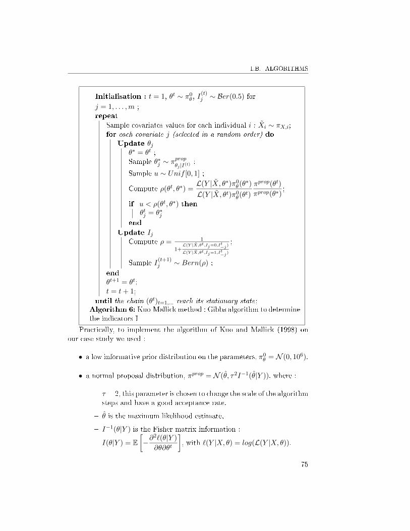
1.B. ALGORITHMS
Initialisation : t = 1, θt ∼ π0θ , I
(t)j ∼ Ber(0.5) for
j = 1, . . . ,m ;repeat
Sample covariates values for each individual i : Xi ∼ πX,i;for each covariate j (selected in a random order) do
Update θjθ∗ = θt ;Sample θ∗j ∼ π
prop
θj |I(t);
Sample u ∼ Unif [0, 1] ;
Compute ρ(θt, θ∗) =L(Y |X, θ∗)π0
θ(θ∗)
L(Y |X, θt)π0θ(θ
t)
πprop(θt)
πprop(θ∗);
if u < ρ(θt, θ∗) thenθtj = θ∗j
endUpdate Ij
Compute ρ = 1
1+L(Y |X,θt,Ij=0,It−j)
L(Y |X,θt,Ij=1,It−j)
;
Sample I(t+1)j ∼ Bern(ρ) ;
endθt+1 = θt;t = t+ 1;
until the chain (θt)t=1,... reach its stationary state;Algorithm 6: Kuo-Mallick method : Gibbs algorithm to determinethe indicators I
Practically, to implement the algorithm of Kuo and Mallick (1998) onour case study we used :
• a low informative prior distribution on the parameters, π0θ = N (0, 106).
• a normal proposal distribution, πprop = N (θ, τ2I−1(θ|Y )), where :
� τ = 2, this parameter is chosen to change the scale of the algorithmsteps and have a good acceptance rate.
� θ is the maximum likelihood estimate,
� I−1(θ|Y ) is the Fisher matrix information :
I(θ|Y ) = E[−∂
2`(θ|Y )
∂θ∂θt
], with `(Y |X, θ) = log(L(Y |X, θ)).
75

Chapitre 1. Toward trait-based mortality models for tropical forests
This proposal distribution was used for a similar problem in one di-mension by A. Altaleb and C. Robert (Altaleb and Robert, 2001).
76
CHAPITRE 2
TREE VIGOUR IS A KEY COMPONENT OFTROPICAL FOREST DYNAMICS
Mélaine Aubry-Kientz1∗
Vivien Rossi 2,3,4
Jean-Jacques Boreux 5
Bruno Hérault 2
1 Université des Antilles et de la Guyane, UMR `Ecologie des Forêts de Guya-ne', Campus agronomique de Kourou, France.2 CIRAD, UMR `Ecologie des Forêts de Guyane', Campus agronomique deKourou, France.3 CIRAD, UPR Bsef, Montpellier, France.4 Université de Yaoundé I, UMMISCO (UMI 209), BP337, Yaoundé, Came-roun.5 Université de Liège.∗ E-mail : [email protected]
77
Chapitre 2. Tree vigour is a key component of tropical forest dynamics
Une fois le processus de mortalité modélisé, je souhaitais l'intégrer dansun simulateur, avec un modèle de croissance et un modèle de recrutement.Mais lorsque j'ai simplement concaténé un modèle de croissance et un modèlede mortalité dans le simulateur SELVA, la dynamique résultante n'était passatisfaisante et ne reproduisait pas ce qui est observé en forêt naturelle. Pourmieux modéliser la dynamique, il faut comprendre comment les processus decroissance et de mortalité s'articulent entre eux. Dans ce deuxième chapitre,il est donc question de coupler les deux processus dans un seul et mêmemodèle, et de prendre en compte l'impact de la croissance sur la mortalité.En e�et, ces deux processus ne sont pas indépendants l'un de l'autre, et unarbre qui pousse vite a une plus faible probabilité de mourir. Pour prendrecette idée en compte dans notre modèle, j'introduis la notion de vigueur.Cette quantité est décrite comme la capacité d'un arbre à pousser plus quece que prédisent ses traits fonctionnels et son stade ontogénique. Lorsquecette vigueur est ajoutée comme prédicteur de la probabilité de mourir, lemodèle de mortalité est sensiblement amélioré. La méthodologie développéedans ce chapitre permet de créer un modèle de croissance et de mortalité pourla communauté, tout en introduisant la vigueur, une composante essentiellede la dynamique en forêt tropicale.
78

1. ABSTRACT
1 Abstract
• Tree vigour is often mentioned when tree mortality is predicated fromtree growth, but it is rarely clearly de�ned. We propose a way to quan-tify tree vigour at the community level, based on the di�erence betweenexpected and observed growth.
• The available methods to join non-linear tree growth and mortalityprocesses are not commonly used by forest ecologists. We develop aninference methodology based on an MCMC approach, allowing us tosample the parameters of the growth and mortality model accordingto their posterior distribution by using the joint model likelihood.
• We apply our framework to a set of data on the 20-year dynamics of aforest in Paracou, French Guiana, taking advantage of functional-traitbased growth and mortality models already developed independently.
• Our results showed that growth and mortality are intimately linkedand that the vigour estimator is the main negative predictor of mor-tality, highlighting that trees growing by more than expected have alower probability of dying. Our joint model methodology is su�cientlygeneric to be used to join two longitudinal and punctual linked pro-cesses and thus may be applied to a wide range of growth and mortalitymodels.
• In the context of global change, at the community level, such jointmodels are urgently needed in tropical forests to analyse, and thenpredict, the e�ects of the ongoing changes on the dynamics of hyper-diverse tropical forests.
2 Introduction
The biological processes responsible for tree mortality involve a combinationof environmental stresses, but early warning signs can be detected by lookingat the behaviour of tree growth (Pedersen, 1998; Dobbertin, 2005). Indeed,it is widely acknowledged that trees exhibiting the highest growth rates havea better chance to stay alive, while trees with lower than expected growthrates are more likely to die before their expected size at maturity (Chao et al.,2008). This phenomenon is often called tree vigour. However, although theconcept of tree vigour is often used, or suggested, it has been rarely preciselyde�ned. Nevertheless, this vigour is a good starting point from which to build
79
Chapitre 2. Tree vigour is a key component of tropical forest dynamics
coupled models of growth and mortality that explicitly take into account thedemographical link between these two processes. Tree population dynamicsresult from three demographic processes : recruitment, growth, and morta-lity. In tropical forests, tree recruitment is a complex ecological process thatin forest simulators is often assumed to be species neutral (Hubbell, 2001)because of its `lottery' nature (Busing and Brokaw, 2002). In contrast, mo-delling individual tree growth in tropical forests is a well-documented task(Gourlet-Fleury, 1999; Hérault et al., 2011), while modelling mortality hasreceived considerable attention in recent years (Aubry-Kientz et al., 2013;Kraft et al., 2010; Rüger et al., 2011). However, once models for these twodemographical processes are developed, coupling them in a single frameworkis a delicate issue that is harder to achieve than a simple concatenation. Thetwo processes are obviously not independent. Few studies have proposed aclear quanti�cation of vigour, which is a concept rather than a measurablequantity. Shigo (2004) proposed a de�nition of tree vigour as `the capacityto resist strain ; a genetic factor, a potential force against any threats tosurvival' and distinguished between vigour and vitality : `the ability to growunder the conditions present'. Most studies have not distinguished betweenthese two views, and tree vigour has been generally related to high survivalor high growth rates. Indeed, on the one hand, this concept may be related totree mortality, as a loss of vigour is expected to imply a higher susceptibilityto stresses (Manion, 1981). On the other hand, vigour may be linked withgrowth, and most studies using the term vigour have described this quantityas the diameter growth rate (Buchman et al., 1983; Rosso and Hansen, 1998).A more complex estimator of vigour based on growth is the stem growth perunit of leaf area, which was used in Waring et al. (1980) as an estimatorof the proportion of carbon allocated to stem wood production. Based ongrowth rates, this kind of vigour estimator may then be linked with mor-tality, and past growth may be included as a predictor in mortality models(Chao et al., 2008; Bigler et al., 2004).
Vigour may be related to the pressure undergone in tree dynamics, suchas competition and environmental stress. Vigour is then sometimes relatedto the cause and not to the consequences (growth). For instance, vigour maybe de�ned as competitive vigour, the quality of how a tree is able to competefor resources, or it may also be used as capability to react to environmentalstresses.One can consider that tree vigour is an individual property that describes thehealth of the tree and its capacity to maintain this healthy state, independentof not only the processes observed (growth, mortality, competition, etc.), butalso the species strategies and the ontogeny. Indeed in tropical forests where
80
2. INTRODUCTION
species diversity is high growth strategies highly di�er between species. Pio-neer species have high growth rates, while many other species grow slowly.A good vigour estimator has to be independent of the species identity, inthe knowledge that an individual having a low growth may e�ectively havevery low vigour if it belongs to a species that normally grows growing fast,but a normal vigour value if it belongs to a slow-growing species. Moreover,growth is highly dependent on the ontogenetic stage. Most species attainedthe maximum growth rate at 60% of their maximum diameter and showedhump-shaped ontogenetic growth trajectories (Hérault et al., 2011). The pro-bability of mortality is also strongly dependent on ontogenetic stages. Youngtrees and old trees die more frequently, because of the intense competitionamong the youngest and senescence of the oldest (Muller-Landau et al., 2006;King et al., 2006). Thus, a good vigour estimator also has to be independentof the ontegenetic stage.
In this paper, we present (i) a quanti�cation of tree individual vigour ; (ii)improvement of a mortality model using this vigour estimator ; and (iii) a wayto bind growth and mortality in a model of tropical tree dynamics using theresults of our investigation of vigour. We then discuss the possibilities thatsuch a methodology o�ers, as well as limitations and possible improvements.
To achieve this goal, we need to build growth and mortality models oftropical trees. A wide range of linear models is used to describe the treegrowth process because linear models are easy to implement and infer usinguser friendly available tools. However, as our knowledge on the growth pro-cess has improved, diverse non-linear models are being developed in order totake into account the size-dependent growth trajectory (Paine et al., 2012).Non-linear growth models have a long history (Hunt, 1982), and it is gene-rally acknowledged that most tropical tree species attain maximal absolutegrowth rates at intermediate sizes (Hérault et al., 2011), leading to a typi-cal hump-backed, growth-diameter relationship. During the early stages oftree growth, the growth curve of the tree size may accelerate rapidly be-cause taller trees have better access to light and a larger photosynthetic area(Sterck et al., 2003), while the growth rates of mature and old trees oftendecline because of (i) resource reallocation towards reproduction (Thomas,1996), (ii) respiration costs of roots and stems becoming too high (Ryan andYoder, 1997), or (iii) trees beginning to senesce. Non-linear models have tobe inferred using likelihood maximization or Bayesian Monte-Carlo Markovchain (MCMC) methods, implying that building a sophisticated non-linearmodel requires more computational e�ort for parametrization (e.g., Rügeret al. (2012)). Paradoxically, while the biological determinants of mortalityseem less well known than those of growth, mortality modelling may be sim-
81
Chapitre 2. Tree vigour is a key component of tropical forest dynamics
pler because it is a binary process that is well captured by logistic models(Brando et al., 2012; Monserud and Sterba, 1999; Ruiz-Benito et al., 2013).Inthis study, we used a community growth model and a community mortalitymodel, both of which use functional traits and ontogenetic stage as predictorsof tree dynamics.
3 Materials and methods
3.1 Data
The study was conducted using data from the Paracou experimental site(5◦18′N,52◦55′W), a lowland tropical rain forest near Sinnamary, FrenchGuiana. The forest is typical of Guianan rain forests, with dominant tree fa-milies including Fabaceae, Chrysobalanaceae, Lecythidaceae, and Sapotaceaeand with more than 500 woody species attaining 10 cm diameter at breastheight (DBH). Mean annual precipitation averages 2980 mm (30-year per-iod), with a long dry season from mid-August to mid-November and a shortdry season in March (Wagner et al., 2011).
Two data sets were used is the study. The �rst data set is a 20-yearinventory of all trees >10 cm DBH in six natural forest plots of 6.25 ha.Censuses of mortality and diameter growth were conducted every 10 years.DBH was calculated from precise measurements of circumferences at 0.5 cm.We excluded individuals with buttresses or other problems that required anincrease in measurement because we were unsure about the height of theinitial points of measurement on these trees. The data set contained 17,151trees. For each tree every 10 years, we know the location, DBH, vernacularname, and status (dead or alive). The vernacular name is the name used bylocal tree spotters. The botanical determination of the trees was completedin 2012, following extensive inventories with voucher collections and deter-mination at regional and international herbaria. Hence, a large number ofthe trees that died during the study period (1991�2011) have no botanicaldetermination, only a vernacular name.
The second data set was a collection of six functional traits of the 335Guianan tree species that occur at the Paracou site (Table 2.1). Traits arerelated to leaf economics, stem economics, and life history and are extractedfrom a large database (Baraloto et al., 2010a,b). Some of these functionaltraits are accurate proxies of growth trajectories (Hérault et al., 2010, 2011)and mortality rates (Aubry-Kientz et al., 2013). The set of data on traitsis not complete for all individuals because all trees were not determined atthe species level, and some trait values were not available for all species.
82
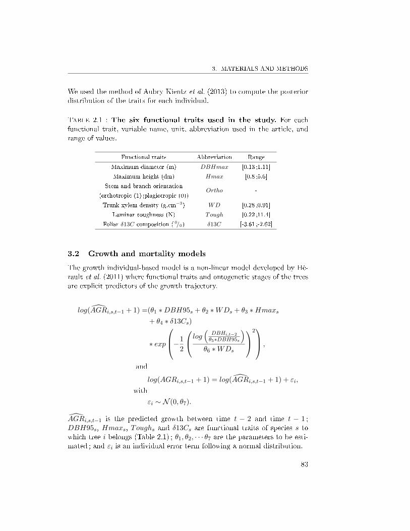
3. MATERIALS AND METHODS
We used the method of Aubry-Kientz et al. (2013) to compute the posteriordistribution of the traits for each individual.
Table 2.1 : The six functional traits used in the study. For eachfunctional trait, variable name, unit, abbreviation used in the article, andrange of values.
Functional traits Abbreviation Range
Maximum diameter (m) DBHmax [0.13 ;1.11]
Maximum height (dm) Hmax [0.8 ;5.6]
Stem and branch orientationOrtho -
(orthotropic (1) ;plagiotropic (0))
Trunk xylem density (g.cm−3) WD [0.28 ;0.91]
Laminar toughness (N) Tough [0.22 ;11.4]
Foliar δ13C composition ( 0/0) δ13C [-3.61 ;-2.62]
3.2 Growth and mortality models
The growth individual-based model is a non-linear model developed by Hé-rault et al. (2011) where functional traits and ontogenetic stages of the treesare explicit predictors of the growth trajectory.
log(AGRi,s,t−1 + 1) =(θ1 ∗DBH95s + θ2 ∗WDs + θ3 ∗Hmaxs+ θ4 ∗ δ13Cs)
∗ exp
−1
2
log(
DBHi,t−2
θ5∗DBH95s
)θ6 ∗WDs
2 ,
and
log(AGRi,s,t−1 + 1) = log(AGRi,s,t−1 + 1) + εi,
with
εi ∼ N (0, θ7).
AGRi,s,t−1 is the predicted growth between time t − 2 and time t − 1 ;DBH95s, Hmaxs, Toughs and δ13Cs are functional traits of species s towhich tree i belongs (Table 2.1) ; θ1, θ2, · · · θ7 are the parameters to be esti-mated ; and εi is an individual error term following a normal distribution.
83

Chapitre 2. Tree vigour is a key component of tropical forest dynamics
The mortality individual-based model was developed by Aubry-Kientzet al. (2013) to compute the individual probability of dying at each timestep. At each time step, a tree i of species s may die with probability pi,s,t.
pi,s,t =logit−1
(β1 ∗
DBHi,s,t−1
DBH95s+ β2 ∗
(DBHi,s,t−1
DBH95s
)2
+ β3 ∗Hmaxs + β4 ∗Orthos + β5 ∗WDs + β6 ∗ Toughs)
DBH95s,Hmaxs, Orthos,WDs, and Toughs are functional traits of speciess to which tree i belongs (Table 2.1) ; β1, β2, · · ·β6 are the parameters to beestimated.
3.3 Vigour quanti�cation
The vigour estimator must be independent from the ontogenetic stage andfrom the species ecological strategies. These two factors are included in thegrowth model. The ontogenetic stage is DBHi,s,t−1
DBH95s, and the functional traits
allow taking into account the speci�c ecological strategies. Thus, we used thegrowth model to compute four possible vigour estimator. Vigour is describedas the di�erence between the computed expected growth and the growth ob-served in the �eld. The four estimators postponed are : AGRi,t − AGRi,t ;AGRi,t
AGRi,t; log
(AGRi,t + 1
AGRi,t + 1
); and
log(AGRi,t + 1)
log(AGRi,t + 1), where AGRi,t is the ob-
served growth between time t − 1 and time t for tree i, and AGRi,t is thepredicted growth between time t − 1 and time t for tree i using a growthmodel.
3.4 Coupling growth and mortality
The growth and mortality processes were linked through tree vigour and areparametrized simultaneously. If tree i stays alive, it grows at a growth rateAGRi,s,t, and its diameter Di,t−1 becomes Di,t. The joint model likelihoodis then
•∏nt=1 f(Di,t|Di,t−1) ∗ (1 − pi,s,t) if tree i stays alive during the length
of the study period,
• pi,s,k∗∏k−1t=1 (f(Di,t|Di,t−1) ∗ (1− pi,s,t)) if tree i dies between time k−1
and time k
84
3. MATERIALS AND METHODS
where
• f(Di,t|Di,t−1) is the probability density for a tree with diameter Di,t−1
at time t − 1 to have a diameter Di,t at time t ; this quantity is usedto compute the vigour estimator
• pi,s,t is the probability of dying between time t − 1 and time t, whichdepends on the vigour estimator, added as a new predictor in the mor-tality model by multiplying the vigour estimator by β0.
The model computes the mortality probability pi,s,t and the predicted growthrate AGRi,s,t. In this study, these two demographical parameters are com-puted using a joint model inspired by the studies of Hérault et al. (2011)and Aubry-Kientz et al. (2013), as described in the previous subsection onthe growth and mortality models. However, this coupling methodology canbe used with all other growth and mortality models.
3.5 Estimation and selection
We implemented a MCMC algorithm to estimate the parameters (Robertand Casella, 2004). A random walk was used as proposal distribution tosample new values of parameters that were or were not selected, using theMetropolis-Hastings ratio. Only standard deviation θ7 was sampled in aninverse-gamma posterior distribution, using a Gibbs sampler. The functio-nal traits used as demographical predictors were uncertain because botanicaldetermination was incomplete for the older censuses, and not all values offunctional traits were available for all species. We used the method deve-loped in Aubry-Kientz et al. (2013) to handle these uncertainties. Becausethe growth and mortality models were created separately, some functionaltraits were independently selected in the two processes. We used the methodproposed by Kuo-Mallick (Kuo and Mallick, 1998) to select the most usefulpredictors in the joint model. The method then was applied to eight predic-tors : Hmax, Ortho,WD, and Tough of the mortality process and DBH95,WD, Hmax, and δ13C of the growth process.
All algorithms and statistical treatments were implemented using R soft-ware (Team, 2013). The R codes developed in this study are available in theAppendix 2.B.
85
Chapitre 2. Tree vigour is a key component of tropical forest dynamics
4 Results
4.1 Quanti�cation of vigour
Distributions of the four investigated vigour estimators are plotted in Figure2.4. The �rst one, AGRi,t− AGRi,t is not symmetric because few trees grewfaster than predicted. The same problem was observed with the second es-
timatorAGRi,t
AGRi,t, but with the additional problem that this estimator had
no value lower than 0. To avoid this long-tailed distribution of vigour, we
introduced a logarithm. The third estimator was log
(AGRi,t + 1
AGRi,t + 1
)and was
more symmetric. This distribution corresponded to the error of the growth
model. The last estimatorlog(AGRi,t + 1)
log(AGRi,t + 1)was highly bimodal and thus less
appropriate. We retained log
(AGRi,t + 1
AGRi,t + 1
).
4.2 Tree vigour and mortality
When vigour was included in the mortality model, the values of parameter β0
were around −0.4 (Table 2.2), implying that a tree with a higher past growththan expected would have a lower probability of dying (Figure 2.1). TheBIC of the mortality model without vigour was 11,215, and with vigour was10,987. The adjusted pseudo-r2 of Mac Fadden without vigour was 0.0288and 0.0492 whit vigour. If we computed the adjusted pseudo-R2 with thereference model set as the model without vigour, we obtained 0.0209.
4.3 Model coupling
Starting from the values of the parameters found in Hérault et al. (2011) andAubry-Kientz et al. (2013), we realized 2000 iterations of the Metropolis-Hastings algorithm. We used a burning of 1000 iterations and a thinning of10 to achieve a satisfying autocorrelation. The histogram resulting from theKuo-Mallick selection procedure showed a large break with no values between0.4 and 0.8 (Figure 2.2). The 0.4 value was the indicator associated withorthotropic orientation (Ortho). Therefore, this predictor was not includedin the �nal coupled model.
86
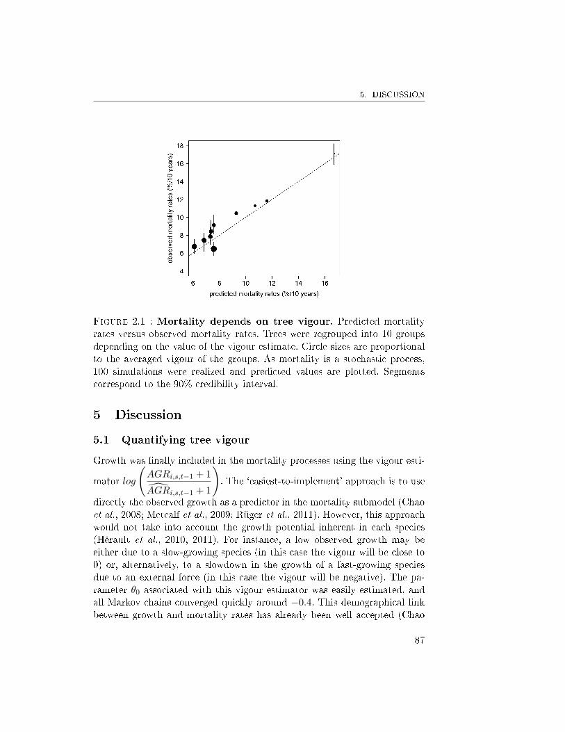
5. DISCUSSION
Figure 2.1 : Mortality depends on tree vigour. Predicted mortalityrates versus observed mortality rates. Trees were regrouped into 10 groupsdepending on the value of the vigour estimate. Circle sizes are proportionalto the averaged vigour of the groups. As mortality is a stochastic process,100 simulations were realized and predicted values are plotted. Segmentscorrespond to the 90% credibility interval.
5 Discussion
5.1 Quantifying tree vigour
Growth was �nally included in the mortality processes using the vigour esti-
mator log
(AGRi,s,t−1 + 1
AGRi,s,t−1 + 1
). The `easiest-to-implement' approach is to use
directly the observed growth as a predictor in the mortality submodel (Chaoet al., 2008; Metcalf et al., 2009; Rüger et al., 2011). However, this approachwould not take into account the growth potential inherent in each species(Hérault et al., 2010, 2011). For instance, a low observed growth may beeither due to a slow-growing species (in this case the vigour will be close to0) or, alternatively, to a slowdown in the growth of a fast-growing speciesdue to an external force (in this case the vigour will be negative). The pa-rameter θ0 associated with this vigour estimator was easily estimated, andall Markov chains converged quickly around −0.4. This demographical linkbetween growth and mortality rates has already been well accepted (Chao
87
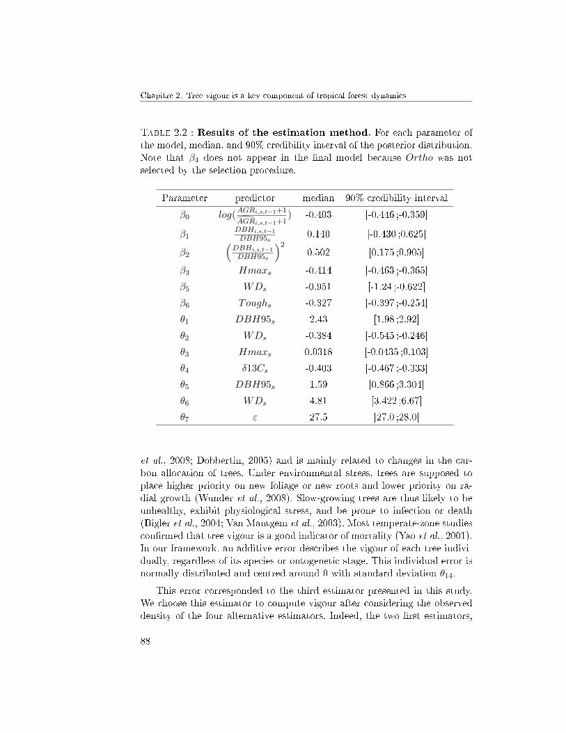
Chapitre 2. Tree vigour is a key component of tropical forest dynamics
Table 2.2 : Results of the estimation method. For each parameter ofthe model, median, and 90% credibility interval of the posterior distribution.Note that β4 does not appear in the �nal model because Ortho was notselected by the selection procedure.
Parameter predictor median 90% credibility interval
β0 log(AGRi,s,t−1+1
AGRi,s,t−1+1) -0.403 [-0.446 ;-0.359]
β1DBHi,s,t−1
DBH95s0.140 [-0.430 ;0.625]
β2
(DBHi,s,t−1
DBH95s
)20.502 [0.175 ;0.905]
β3 Hmaxs -0.414 [-0.463 ;-0.365]
β5 WDs -0.951 [-1.24 ;-0.622]
β6 Toughs -0.327 [-0.397 ;-0.254]
θ1 DBH95s 2.43 [1.98 ;2.92]
θ2 WDs -0.384 [-0.545 ;-0.246]
θ3 Hmaxs 0.0318 [-0.0435 ;0.103]
θ4 δ13Cs -0.403 [-0.467 ;-0.333]
θ5 DBH95s 1.59 [0.866 ;3.304]
θ6 WDs 4.81 [3.422 ;6.67]
θ7 ε 27.5 [27.0 ;28.0]
et al., 2008; Dobbertin, 2005) and is mainly related to changes in the car-bon allocation of trees. Under environmental stress, trees are supposed toplace higher priority on new foliage or new roots and lower priority on ra-dial growth (Wunder et al., 2008). Slow-growing trees are thus likely to beunhealthy, exhibit physiological stress, and be prone to infection or death(Bigler et al., 2004; Van Mantgem et al., 2003). Most temperate-zone studiescon�rmed that tree vigour is a good indicator of mortality (Yao et al., 2001).In our framework, an additive error describes the vigour of each tree indivi-dually, regardless of its species or ontogenetic stage. This individual error isnormally distributed and centred around 0 with standard deviation θ14.
This error corresponded to the third estimator presented in this study.We choose this estimator to compute vigour after considering the observeddensity of the four alternative estimators. Indeed, the two �rst estimators,
88
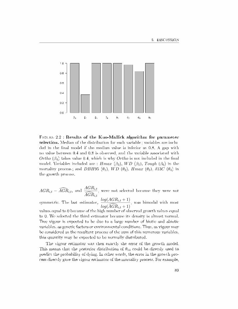
5. DISCUSSION
Figure 2.2 : Results of the Kuo-Mallick algorithm for parameterselection. Median of the distribution for each variable ; variables are inclu-ded in the �nal model if the median value is inferior as 0.8. A gap withno value between 0.4 and 0.8 is observed, and the variable associated withOrtho (β4) takes value 0.4, which is why Ortho is not included in the �nalmodel. Variables included are : Hmax (β3), WD (β5), Tough (β6) in themortality process ; and DBH95 (θ1), WD (θ2), Hmax (θ3), δ13C (θ4) inthe growth process.
AGRi,t − AGRi,t, andAGRi,t
AGRi,t, were not selected because they were not
symmetric. The last estimator,log(AGRi,t + 1)
log(AGRi,t + 1), was bimodal with most
values equal to 0 because of the high number of observed growth values equalto 0. We selected the third estimator because its density is almost normal.Tree vigour is expected to be due to a large number of biotic and abioticvariables, as genetic factors or environmental conditions. Thus, as vigour maybe considered as the resultant process of the sum of this numerous variables,this quantity may be expected to be normally distributed.
The vigour estimator was then exactly the error of the growth model.This means that the posterior distribution of θ14 could be directly used topredict the probability of dying. In other words, the error in the growth pro-cess directly gave the vigour estimator of the mortality process. For example,
89
Chapitre 2. Tree vigour is a key component of tropical forest dynamics
a tree with high value of the vigour estimator deterministically would have ahigher growth rate and a smaller probability of dying. However, this is ques-tionable when we want to use this joint model in a forest simulator. Roughly,there are two possibilities. Either an error is sampled at each time step, oreach individual tree has its own vigour, which does not change throughoutits life. This is an important choice in the simulation, and it is clear thatthe reality may be more nuanced. Even if the vigour of a tree may changeduring its life because of biotic or abiotic factors (Moravie et al., 1999), thereis also increasing forestry evidence of strong observed temporal dependence(Woollons and Norton, 1990). Some studies indicated that the inclusion oftemporal dependence in stochastic dynamic models results in outputs thatare similar to those of deterministic models (Kangas, 1997, 1998), but thetheoretical and ecological basis of the stochastic model is clearly superior tothat of the deterministic model (Fox et al., 2001). A more realist alternativecould thus be to sample a new vigour estimator at each time t, dependingon the vigour estimator at time t − 1, such as in an autoregressive model(Suarez et al., 2004).
5.2 Improvement of the mortality model
Building a vigour estimator and including it in the mortality model allo-wed us to take into account individual variability, which previously was notpossible. The introduction of vigour into the mortality model improved theprediction and highlighted that vigour is a key driver of mortality (Figures2.1, 2.3). The Mac Fadden's adjusted pseudo-R2 can be interpreted as theratio of the estimated information gain when the model is used in comparisonwith the null model in order to estimate the information potentially recove-rable by including all possible explanatory variables (Shtatland et al., 2002).In our case, the R2 was almost double when vigour was included, which im-plies that the goodness-of-�t would be almost double if the vigour estimatorwere included. Thus, past tree growth, independent of ontogeny and speciesecological strategies, was by far the �rst predictor of tree mortality. Redu-ced radial growth is often linked to increased mortality rates (Wunder et al.,2008), but as Dobbertin (2005) asserted, `important for any potential vitalityindicator is the comparison with a suitable reference'. This reference may bethe di�erence or residual of tree growth against mean growth or modelledgrowth (Dobbertin, 2005).
Our de�nition of vigour includes vigour and vitality according to Shigo(2004), where vigour is de�ned as `the capacity to resist strain ; a genetic fac-tor, a potential force against any threats to survival', and vitality is de�ned
90
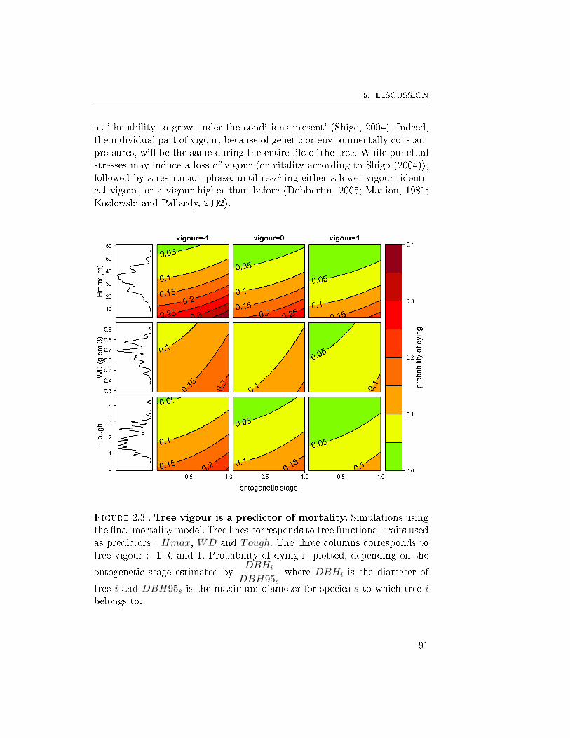
5. DISCUSSION
as `the ability to grow under the conditions present' (Shigo, 2004). Indeed,the individual part of vigour, because of genetic or environmentally constantpressures, will be the same during the entire life of the tree. While punctualstresses may induce a loss of vigour (or vitality according to Shigo (2004)),followed by a restitution phase, until reaching either a lower vigour, identi-cal vigour, or a vigour higher than before (Dobbertin, 2005; Manion, 1981;Kozlowski and Pallardy, 2002).
Figure 2.3 : Tree vigour is a predictor of mortality. Simulations usingthe �nal mortality model. Tree lines corresponds to tree functional traits usedas predictors : Hmax, WD and Tough. The three columns corresponds totree vigour : -1, 0 and 1. Probability of dying is plotted, depending on the
ontogenetic stage estimated byDBHi
DBH95swhere DBHi is the diameter of
tree i and DBH95s is the maximum diameter for species s to which tree ibelongs to.
91
Chapitre 2. Tree vigour is a key component of tropical forest dynamics
5.3 Coupling tree growth and mortality
The available methods of combining non-linear tree growth and mortalityprocesses are not commonly used by forest ecologists. Our inference metho-dology is based on an MCMC approach, which allowed us to sample themodel parameters according to their posterior distribution, using the jointmodel likelihood. This likelihood takes growth and mortality forest dyna-mic processes into account at each step of the algorithm. Hence, growthand mortality parameters are estimated simultaneously until stabilization.The joint model parameters were sampled individually to increase conver-gence speed. When the sampled parameter concerned the mortality processonly, the growth process did not change and only the term of the likelihoodlinked to the growth process (f(Di,t|Di,t−1)) was updated. When the esti-mated parameter concerned the growth process, as the growth process isplugged into the mortality process, all terms of the likelihood were a�ec-ted : f(Di,s,t|Di,s,t−1) and pi,s,t. In practical terms, the parameters involvedin the mortality process converged more easily than parameters involved inthe growth process. Indeed, tree growth is strongly shaped by many addi-tional environmental variables (e.g., topography, light availability, etc.) (Hé-rault et al., 2010) and by local competition (Uriarte et al., 2004) ; however,neither factor was investigated in the present methodological study. Never-theless, our methodology succeeded in binding the two processes, and theselection method allowed keeping only the useful variables as the parametersin the �nal model. Thus, the collinearity of the two processes was managed.
6 Conclusion
In this paper, we present a method of estimating tree vigour and a �exiblemethodology for building a growth�mortality joint model using this vigourestimator. The vigour estimator, based on the di�erence between observedand predicted growth, signi�cantly improved the mortality model. This re-sult con�rmed that the individual behaviour of trees is of great importancein the processes of growth and mortality and therefore should be conside-red in the study of forest dynamics. We successfully applied our conceptualframework to a complex hyperdiverse tropical forest community, taking intoaccount di�erent sources of data uncertainties, and con�rming the link bet-ween growth and mortality in a tropical forest. Our joint model methodologymay be used with a wide range of growth and mortality models. Indeed, theinference process needs only one growth model that computes AGRi,s,t and amortality model that computes pi,s,t. Once computed, these two sets of values
92
6. CONCLUSION
are used to calculate the global likelihood and to estimate posterior distribu-tions. The growth model may be more straightforward (e.g. a linear model)or more complex (e.g. random species e�ects). This joint model approachprovides an interesting framework for including other predicting variablespossibly linked with tree dynamics, such as environmental and climatic va-riables. In the context of climate change, proper methodological frameworksare needed both to model the e�ect of climate variations on the dynamics ofhyperdiverse tropical forest communities (Choat et al., 2012; Feeley et al.,2012; Wagner et al., 2011) and to include these climate-explicit models intoforest simulators in order to test their resilience to future expected changes.
Acknowledgements
Funding came from the Climfor project (Fondation pour la Recherche surla Biodiversité) and from the Guyasim project (European structural fun-ding, PO-feder). The funders had no role in the study design, data collectionand analysis, decision to publish, or preparation of the manuscript. Thiswork also bene�ted from an `Investissement d'Avenir' grant managed by theAgence Nationale de la Recherche (CEBA, ref ANR-10-LABX-0025) andfrom a grant from the Centre de coopération Internationale en RechercheAgronomique pour le Développement.
93
BIBLIOGRAPHIE
Aubry-Kientz, M., Hérault, B., Ayotte-Trépanier, C., Baraloto, C., and Rossi,V. (2013). Toward trait-based mortality models for tropical forests. PloSone, 8(5):e63678.
Baraloto, C., Paine, C. E. T., Patiño, S., Bonal, D., Hérault, B., and Chave,J. (2010a). Functional trait variation and sampling strategies in species-rich plant communities. Functional Ecology, 24(1):208�216.
Baraloto, C., Paine, C. E. T., Poorter, L., Beauchene, J., Bonal, D., Dome-nach, A. M., Hérault, B., Patino, S., Roggy, J. C., and Chave, J. (2010b).Decoupled leaf and stem economics in rain forest trees. Ecology Letters,13(11):1338�1347.
Bigler, C., Gricar, J., Bugmann, H., and Cufar, K. (2004). Growth patternsas indicators of impending tree death in silver �r. Forest Ecology andManagement, 199(2-3):183�190.
Brando, P. M., Nepstad, D. C., Balch, J. K., Bolker, B., Christman, M. C.,Coe, M., and Putz, F. E. (2012). Fire-induced tree mortality in a neo-tropical forest : the roles of bark traits, tree size, wood density and �rebehavior. Global Change Biology, 18(2):630�641.
Buchman, R. G., Pederson, S. P., and Walters, N. R. (1983). A tree survivalmodel with application to species of the Great Lakes region. CanadianJournal of Forest Research-Revue Canadienne De Recherche Forestiere,(13):601�608.
94
BIBLIOGRAPHIE
Busing, R. T. and Brokaw, N. (2002). Tree species diversity in temperate andtropical forest gaps : the role of lottery recruitment. Folia Geobotanica,37(1):33�43.
Chao, K. J., Phillips, O. L., Gloor, E., Monteagudo, A., Torres-Lezama, A.,and Martinez, R. V. (2008). Growth and wood density predict treemortality in Amazon forests. Journal of Ecology, 96(2):281�292.
Choat, B., Jansen, S., Brodribb, T. J., Cochard, H., Delzon, S., Bhaskar, R.,Bucci, S. J., Feild, T. S., Gleason, S. M., Hacke, U. G., Jacobsen, A. L.,Lens, F., Maherali, H., Martínez-Vilalta, J., Mayr, S., Mencuccini, M.,Mitchell, P. J., Nardini, A., Pittermann, J., Pratt, R. B., Sperry, J. S.,Westoby, M., Wright, I. J., and Zanne, A. E. (2012). Global convergencein the vulnerability of forests to drought. Nature, 491(7426):752�5.
Dobbertin, M. (2005). Tree growth as indicator of tree vitality and of treereaction to environmental stress : a review. European Journal of ForestResearch, 124(4):319�333.
Feeley, K. J., Malhi, Y., Zelazowski, P., and Silman, M. R. (2012). Therelative importance of deforestation, precipitation change, and tempe-rature sensitivity in determining the future distributions and diversityof Amazonian plant species. Global Change Biology, 18(8):2636�2647.
Fox, J. C., Ades, P. K., and Bi, H. Q. (2001). Stochastic structure andindividual-tree growth models. Forest Ecology and Management, 154(1-2):261�276.
Gourlet-Fleury, S. (1999). Individual-based spatially explicit modelling offorest stands in French Guiana. In Y., L., King, B., Legg, C., andRenolls, K., editors, Data Management and Modelling Using RemoteSensing and GIS for Tropical Forest Land Inventory, pages 473�490,Jakarta, Indonesia.
Hérault, B., Bachelot, B., Poorter, L., Rossi, V., Bongers, F., Chave, J.,Paine, C. E. T., Wagner, F., and Baraloto, C. (2011). Functional traitsshape ontogenetic growth trajectories of rain forest tree species. Journalof Ecology, 99(6):1431�1440.
Hérault, B., Ouallet, J., Blanc, L., Wagner, F., and Baraloto, C. (2010).Growth responses of neotropical trees to logging gaps. Journal of AppliedEcology, 47(4):821�831.
95

Chapitre 2. Tree vigour is a key component of tropical forest dynamics
Hubbell, S. P. (2001). The Uni�ed Neutral Theory of Biodoversity and Bio-geography. Princeton University Press.
Hunt, R. (1982). Plant growth curves. The functional approach to plantgrowth analysis. University Park Press.
Kangas, A. S. (1997). On the prediction bias and variance in long-termgrowth projections. Forest Ecology and Management, 96(3):207�216.
Kangas, A. S. (1998). Uncertainty in growth and yield projections due toannual variation of diameter growth. Forest Ecology and Management,108(3):223�230.
King, D. A., Davies, S. J., and Noor, N. S. M. (2006). Growth and mortalityare related to adult tree size in a Malaysian mixed dipterocarp forest.Forest Ecology and Management, 223(1-3):152�158.
Kozlowski, T. T. and Pallardy, S. G. (2002). Acclimation and AdaptiveResponses of Woody Plants to Environmental Stresses. The BotanicalReview, 68(2):270�334.
Kraft, N. J. B., Metz, M. R., Condit, R. S., and Chave, J. (2010). Therelationship between wood density and mortality in a global tropicalforest data set. New Phytologist, 188(4):1124�1136.
Kuo, L. and Mallick, B. (1998). Variable selection for regression models.Sankhya Ser.B, (60):65�81.
Manion, P. D. (1981). Tree disease concepts. Prentice-Hall, Engle- woodCli�s, NJ, USA.
Metcalf, C. J. E., McMahon, S. M., and Clark, J. S. (2009). Overcomingdata sparseness and parametric constraints in modeling of tree morta-lity : a new nonparametric Bayesian model. Canadian Journal of ForestResearch, 39(9):1677�1687.
Monserud, R. A. and Sterba, H. (1999). Modeling individual tree mortalityfor Austrian forest species. Forest Ecology and Management, 113(2-3):109�123.
Moravie, M.-a. A., Durand, M., and Houllier, F. (1999). Ecological meaningand predictive ability of social status, vigour and competition indices ina tropical rain forest (India). Forest Ecology and Management, 117:221�240.
96
BIBLIOGRAPHIE
Muller-Landau, H. C., Condit, R. S., Chave, J., Thomas, S. C., Bohlman,S. A., Bunyavejchewin, S., Davies, S., Foster, R., Gunatilleke, S., Gu-natilleke, N., Harms, K. E., Hart, T., Hubbell, S. P., Itoh, A., Kassim,A. R., LaFrankie, J. V., Lee, H. S., Losos, E., Jr, M., Ohkubo, T., Suku-mar, R., Sun, I. F., Supardi, N. M. N., Tan, S., Thompson, J., Valencia,R., Munoz, G. V., Wills, C., Yamakura, T., Chuyong, G., Dattaraja,H. S., Esufali, S., Hall, P., Hernandez, C., Kenfack, D., Kiratiprayoon,S., Suresh, H. S., Thomas, D., Vallejo, M. I., and Ashton, P. (2006). Tes-ting metabolic ecology theory for allometric scaling of tree size, growthand mortality in tropical forests. Ecology Letters, 9(5):575�588.
Paine, C. E. T., Marthews, T. R., Vogt, D. R., Purves, D., Rees, M., Hector,A., and Turnbull, L. A. (2012). How to �t nonlinear plant growth modelsand calculate growth rates : an update for ecologists. Methods in Ecologyand Evolution, 3(2):245�256.
Pedersen, B. S. (1998). The role of stress in the mortality of midwesternoaks as indicated by growth prior to death. Ecology, 79(1):79�93.
Robert, C. P. and Casella, G. (2004). Monte Carlo statistical methods. Sprin-ger, 2 edition.
Rosso, P. and Hansen, E. (1998). Tree vigour and the susceptibility of Dou-glas �r to Armillaria root disease. Eur. J. For. Path., 28:43�52.
Rüger, N., Huth, A., Hubbell, S. P., and Condit, R. (2011). Determinantsof mortality across a tropical lowland rainforest community. Oikos,120(7):1047�1056.
Rüger, N., Wirth, C., Wright, S. J., and Condit, R. (2012). Functional traitsexplain light and size response of growth rates in tropical tree species.Ecology, 93(12):2626�2636.
Ruiz-Benito, P., Lines, E. R., Gómez-Aparicio, L., Zavala, M. A., and Co-omes, D. A. (2013). Patterns and Drivers of Tree Mortality in IberianForests : Climatic E�ects Are Modi�ed by Competition. Plos One,8(2):e56843.
Ryan, M. G. and Yoder, B. J. (1997). Hydraulic limits to tree height andtree growth. BioScience, 47(4):242�253.
Shigo, A. (2004). How Trees Survive. The overst edition.
97
Chapitre 2. Tree vigour is a key component of tropical forest dynamics
Shtatland, E. S., Kleinman, K., and Cain, E. M. (2002). one more timeabout r2 measures of �t in logistic regression. NESUG 15 Proceedings,(M):222�226.
Sterck, F., Martinéz-Ramos, M., Dyer-Leal, G., Rodríguez-Velazquez, J., andPoorter, L. (2003). The consequences of crown traits for the growth andsurvival of tree saplings in a Mexican lowland rainforest. FunctionalEcology, 17(2):194�200.
Suarez, M. L., Ghermandi, L., and Kitzberger, T. (2004). Factors predispo-sing episodic drought-induced tree mortality in Nothofagus - site, cli-matic sensitivity and growth trends. Journal of Ecology, 92(6):954�966.
Team, R. C. (2013). R : A Language and Environment for Statistical Com-puting.
Thomas, S. (1996). Reproductive allometry in Malaysian rain forest trees :Biomechanics versus optimal allocation. Evolutionary Ecology, 10(5):517�530.
Uriarte, M., Canham, C. D., Thompson, J., and Zimmerman, J. K. (2004). Aneighborhood analysis of tree growth and survival in a hurricane-driventropical forest. Ecological Monographs, 74(4):591�614.
Van Mantgem, P. J., Stephenson, N. L., Mutch, L. S., Johnson, V. G., Espe-ranza, A. M., and Parsons, D. J. (2003). Growth rate predicts morta-lity of Abies concolor in both burned and unburned stands. CanadianJournal of Forest Research-Revue Canadienne De Recherche Forestiere,33(6):1029�1038.
Wagner, F., Hérault, B., Stahl, C., Bonal, D., and Rossi, V. (2011). Modelingwater availability for trees in tropical forests. Agricultural and ForestMeteorology, 151(9):1202�1213.
Waring, R. H., Thies, W. G., and Muscato, D. (1980). Stem Growth per Unitof Leaf Area : A Measure of Tree Vigor. Forest Science, 26(1):112�117.
Woollons, R. C. and Norton, D. A. (1990). time-series analyses appliedto sequences of nothofagus growth-ring measurements. New ZealandJournal of Ecology, 13:9�15.
Wunder, J., Brzeziecki, B., Zybura, H., Reineking, B., Bigler, C., and Bug-mann, H. (2008). Growth-mortality relationships as indicators of life-
98

BIBLIOGRAPHIE
history strategies : a comparison of nine tree species in unmanaged Eu-ropean forests. Oikos, 117(6):815�828.
Yao, X. H., Titus, S. J., and MacDonald, S. E. (2001). A generalized logisticmodel of individual tree mortality for aspen, white spruce, and lodge-pole pine in Alberta mixedwood forests. Canadian Journal of ForestResearch-Revue Canadienne De Recherche Forestiere, 31(2):283�291.
99
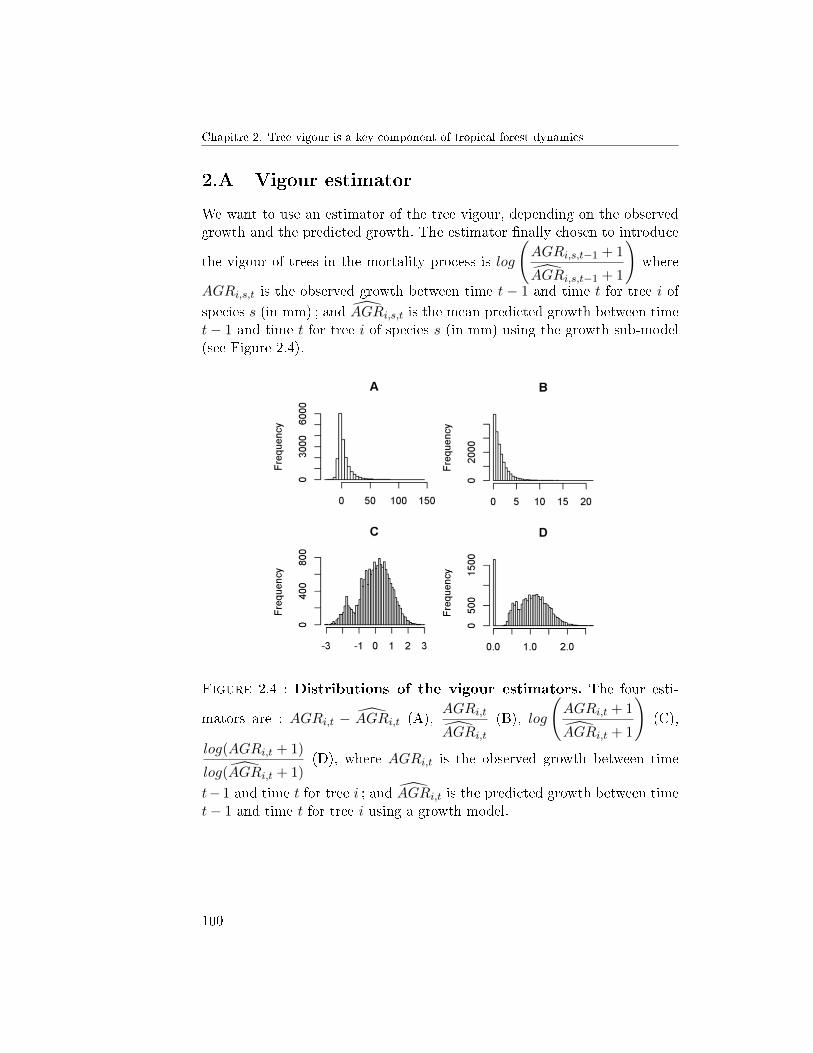
Chapitre 2. Tree vigour is a key component of tropical forest dynamics
2.A Vigour estimator
We want to use an estimator of the tree vigour, depending on the observedgrowth and the predicted growth. The estimator �nally chosen to introduce
the vigour of trees in the mortality process is log
(AGRi,s,t−1 + 1
AGRi,s,t−1 + 1
)where
AGRi,s,t is the observed growth between time t − 1 and time t for tree i ofspecies s (in mm) ; and AGRi,s,t is the mean predicted growth between timet− 1 and time t for tree i of species s (in mm) using the growth sub-model(see Figure 2.4).
Figure 2.4 : Distributions of the vigour estimators. The four esti-
mators are : AGRi,t − AGRi,t (A),AGRi,t
AGRi,t(B), log
(AGRi,t + 1
AGRi,t + 1
)(C),
log(AGRi,t + 1)
log(AGRi,t + 1)(D), where AGRi,t is the observed growth between time
t− 1 and time t for tree i ; and AGRi,t is the predicted growth between timet− 1 and time t for tree i using a growth model.
100
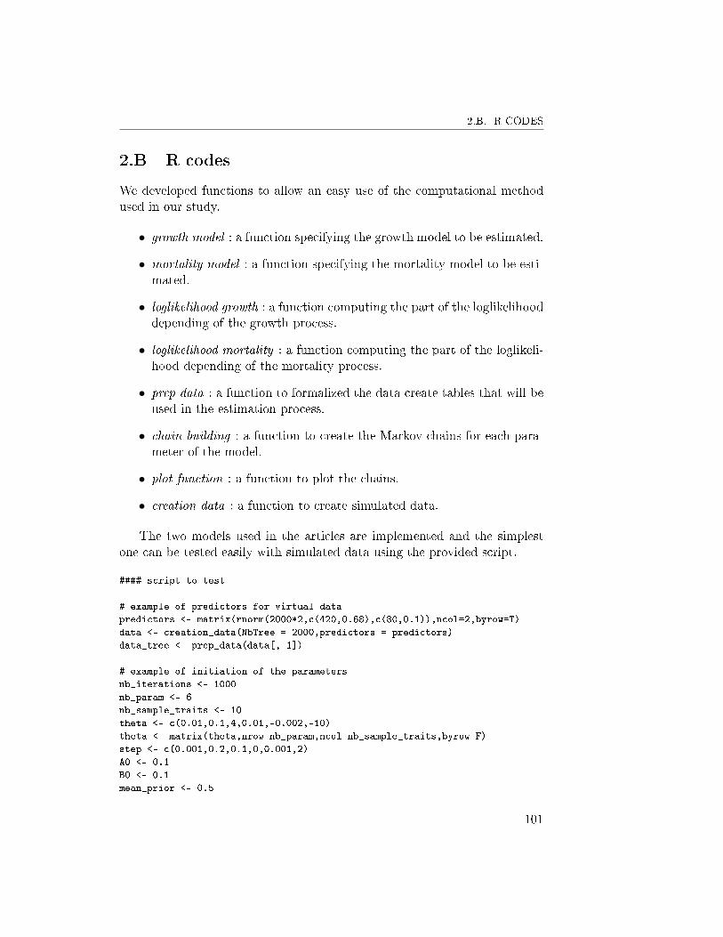
2.B. R CODES
2.B R codes
We developed functions to allow an easy use of the computational methodused in our study.
• growth model : a function specifying the growth model to be estimated.
• mortality model : a function specifying the mortality model to be esti-mated.
• loglikelihood growth : a function computing the part of the loglikelihooddepending of the growth process.
• loglikelihood mortality : a function computing the part of the loglikeli-hood depending of the mortality process.
• prep data : a function to formalized the data create tables that will beused in the estimation process.
• chain building : a function to create the Markov chains for each para-meter of the model.
• plot function : a function to plot the chains.
• creation data : a function to create simulated data.
The two models used in the articles are implemented and the simplestone can be tested easily with simulated data using the provided script.
#### script to test
# example of predictors for virtual data
predictors <- matrix(rnorm(2000*2,c(420,0.68),c(80,0.1)),ncol=2,byrow=T)
data <- creation_data(NbTree = 2000,predictors = predictors)
data_tree <- prep_data(data[,-1])
# example of initiation of the parameters
nb_iterations <- 1000
nb_param <- 6
nb_sample_traits <- 10
theta <- c(0.01,0.1,4,0.01,-0.002,-10)
theta <- matrix(theta,nrow=nb_param,ncol=nb_sample_traits,byrow=F)
step <- c(0.001,0.2,0.1,0,0.001,2)
A0 <- 0.1
B0 <- 0.1
mean_prior <- 0.5
101

Chapitre 2. Tree vigour is a key component of tropical forest dynamics
sd_prior <- 500
model <- 1
id_sigma <- 4
# creation of the MCMC chains
test <- chain_building(model,id_sigma,nb_iterations,nb_param,theta,
nb_sample_traits,step,traits,data_tree,A0,B0,mean_prior,sd_prior)
# plot the results
plot_function(test,burn=0,thin=1)
####
#### functions
growth_model <- function(theta,traits,data_DBH)
{
lAGR_pred <- t(theta[1,] * traits[,,'DBH95']*10 *
exp(-0.5 *
((log( (data_DBH[,2])/(theta[2,]*traits[,,'DBH95']*10) )
/( theta[3,] * traits[,,'WD'] ) )^2)))
return(lAGR_pred)
}
growth_model <- function(theta,traits,data_DBH)
{
lAGR_pred <- t(t(theta[1,] * t(traits[,,'DBH95']/100) +
theta[2,] * t(traits[,,'WD']) + theta[3,] * t(traits[,,'Height']/10) +
theta[4,] * t(traits[,,'Delta13C']/10) ) *
exp( -0.5 * ((log((data_DBH[,2])/t(theta[5,]*t(traits[,,'DBH95']*10)))
/(t(theta[6,]*t(traits[,,'WD']))))^2)))
return(lAGR_pred)
}
mortality_model <- function(theta,rate,traits,data_DBH,nb_sample_traits)
{
logit_p <- t(theta[5,] *
traits[(1:nb_sample_traits),IdTrees,'DBH95']*10 +
theta[6,] * t(rate))
return(logit_p)
}
mortality_model <- function(theta,rate,traits,data_DBH,nb_sample_traits)
{
logit_p <- t(theta[8,] * t(rate)) + t(theta[9,] *
t((data_DBH[,3]/10)/t(traits[(1:nb_sample_traits),IdTrees,'DBH95']))) +
t(theta[10,] *
102
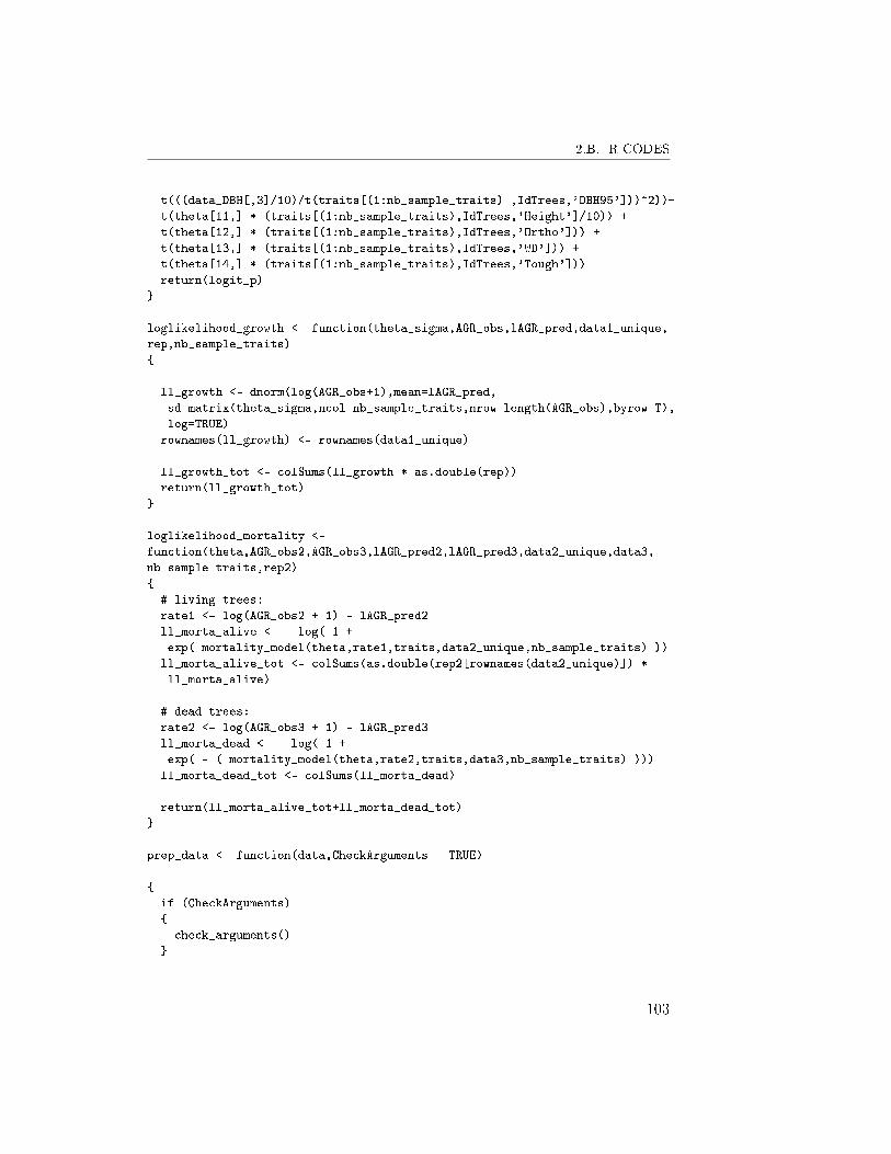
2.B. R CODES
t(((data_DBH[,3]/10)/t(traits[(1:nb_sample_traits) ,IdTrees,'DBH95']))^2))+
t(theta[11,] * (traits[(1:nb_sample_traits),IdTrees,'Height']/10)) +
t(theta[12,] * (traits[(1:nb_sample_traits),IdTrees,'Ortho'])) +
t(theta[13,] * (traits[(1:nb_sample_traits),IdTrees,'WD'])) +
t(theta[14,] * (traits[(1:nb_sample_traits),IdTrees,'Tough']))
return(logit_p)
}
loglikelihood_growth <- function(theta_sigma,AGR_obs,lAGR_pred,data1_unique,
rep,nb_sample_traits)
{
ll_growth <- dnorm(log(AGR_obs+1),mean=lAGR_pred,
sd=matrix(theta_sigma,ncol=nb_sample_traits,nrow=length(AGR_obs),byrow=T),
log=TRUE)
rownames(ll_growth) <- rownames(data1_unique)
ll_growth_tot <- colSums(ll_growth * as.double(rep))
return(ll_growth_tot)
}
loglikelihood_mortality <-
function(theta,AGR_obs2,AGR_obs3,lAGR_pred2,lAGR_pred3,data2_unique,data3,
nb_sample_traits,rep2)
{
# living trees:
rate1 <- log(AGR_obs2 + 1) - lAGR_pred2
ll_morta_alive <- - log( 1 +
exp( mortality_model(theta,rate1,traits,data2_unique,nb_sample_traits) ))
ll_morta_alive_tot <- colSums(as.double(rep2[rownames(data2_unique)]) *
ll_morta_alive)
# dead trees:
rate2 <- log(AGR_obs3 + 1) - lAGR_pred3
ll_morta_dead <- - log( 1 +
exp( - ( mortality_model(theta,rate2,traits,data3,nb_sample_traits) )))
ll_morta_dead_tot <- colSums(ll_morta_dead)
return(ll_morta_alive_tot+ll_morta_dead_tot)
}
prep_data <- function(data,CheckArguments = TRUE)
{
if (CheckArguments)
{
check_arguments()
}
103
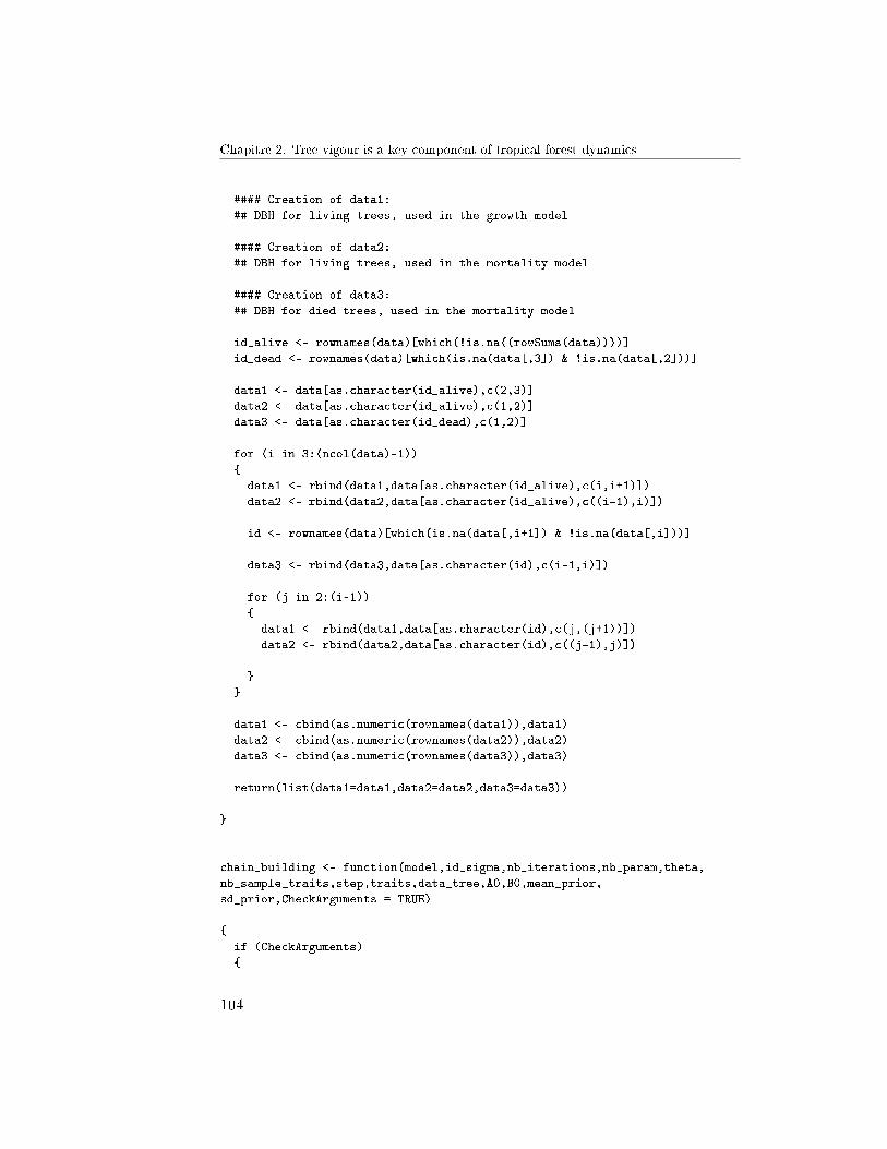
Chapitre 2. Tree vigour is a key component of tropical forest dynamics
#### Creation of data1:
## DBH for living trees, used in the growth model
#### Creation of data2:
## DBH for living trees, used in the mortality model
#### Creation of data3:
## DBH for died trees, used in the mortality model
id_alive <- rownames(data)[which(!is.na((rowSums(data))))]
id_dead <- rownames(data)[which(is.na(data[,3]) & !is.na(data[,2]))]
data1 <- data[as.character(id_alive),c(2,3)]
data2 <- data[as.character(id_alive),c(1,2)]
data3 <- data[as.character(id_dead),c(1,2)]
for (i in 3:(ncol(data)-1))
{
data1 <- rbind(data1,data[as.character(id_alive),c(i,i+1)])
data2 <- rbind(data2,data[as.character(id_alive),c((i-1),i)])
id <- rownames(data)[which(is.na(data[,i+1]) & !is.na(data[,i]))]
data3 <- rbind(data3,data[as.character(id),c(i-1,i)])
for (j in 2:(i-1))
{
data1 <- rbind(data1,data[as.character(id),c(j,(j+1))])
data2 <- rbind(data2,data[as.character(id),c((j-1),j)])
}
}
data1 <- cbind(as.numeric(rownames(data1)),data1)
data2 <- cbind(as.numeric(rownames(data2)),data2)
data3 <- cbind(as.numeric(rownames(data3)),data3)
return(list(data1=data1,data2=data2,data3=data3))
}
chain_building <- function(model,id_sigma,nb_iterations,nb_param,theta,
nb_sample_traits,step,traits,data_tree,A0,B0,mean_prior,
sd_prior,CheckArguments = TRUE)
{
if (CheckArguments)
{
104

2.B. R CODES
check_arguments()
}
source(paste('growth_model_',model,'.R',sep=''))
source(paste('mortality_model_',model,'.R',sep=''))
source('loglikelihood_growth.R')
source('loglikelihood_mortality.R')
data1_unique <- unique(data_tree\$data1)
data2_unique <- unique(data_tree\$data2)
data3 <- data_tree\$data3
names1 <- unique(paste(as.character(data_tree\$data1[,1]),
as.character(data_tree\$data1[,2]),as.character(data_tree\$data1[,3]),sep='_'))
rownames(data1_unique) <- names1
rep <- table(paste(as.character(data_tree\$data1[,1]),
as.character(data_tree\$data1[,2]),as.character(data_tree\$data1[,3]),sep='_'))
names2 <- unique(paste(as.character(data_tree\$data2[,1]),
as.character(data_tree\$data2[,2]),as.character(data_tree\$data2[,3]),sep='_'))
rownames(data2_unique) <- names2
rep2 <- table(paste(as.character(data_tree\$data2[,1]),
as.character(data_tree\$data2[,2]),as.character(data_tree\$data2[,3]),sep='_'))
names3 <- paste(as.character(data3[,1]),as.character(data3[,2]),
as.character(data3[,3]),sep='_')
rownames(data3) <- names3
names2_ok <- names2[which(names2\%in\%names1)]
names3_ok <- names3[which(names3\%in\%names1)]
AGR_obs <- apply(data1_unique[,c(2,3)],1,diff)
AGR_obs[AGR_obs<0] <- 0
AGR_obs2 <- apply(data2_unique[,c(2,3)],1,diff)
AGR_obs2[AGR_obs2<0] <- 0
AGR_obs3 <- apply(data3[,c(2,3)],1,diff)
AGR_obs3[AGR_obs3<0] <- 0
traits1 <- traits[(1:nb_sample_traits),as.character(data1_unique[,1]),]
lAGR_pred <- growth_model(theta,traits1,data1_unique)
rownames(lAGR_pred) <- names1
lAGR_pred2 <- matrix(NA,nrow=nrow(data2_unique),ncol=nb_sample_traits)
rownames(lAGR_pred2) <- names2
lAGR_pred2[names2_ok,] <- lAGR_pred[names2_ok,]
num2 <- which(is.na(lAGR_pred2[,1]))
105
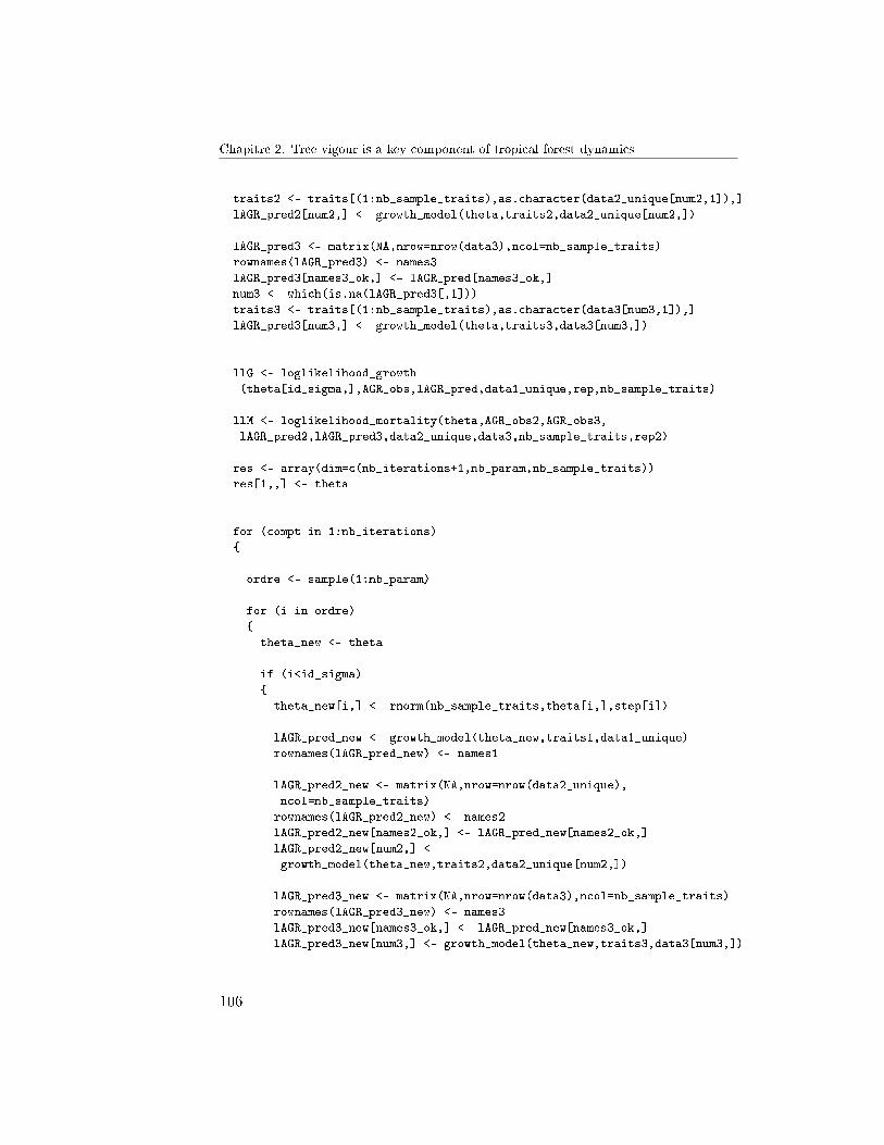
Chapitre 2. Tree vigour is a key component of tropical forest dynamics
traits2 <- traits[(1:nb_sample_traits),as.character(data2_unique[num2,1]),]
lAGR_pred2[num2,] <- growth_model(theta,traits2,data2_unique[num2,])
lAGR_pred3 <- matrix(NA,nrow=nrow(data3),ncol=nb_sample_traits)
rownames(lAGR_pred3) <- names3
lAGR_pred3[names3_ok,] <- lAGR_pred[names3_ok,]
num3 <- which(is.na(lAGR_pred3[,1]))
traits3 <- traits[(1:nb_sample_traits),as.character(data3[num3,1]),]
lAGR_pred3[num3,] <- growth_model(theta,traits3,data3[num3,])
llG <- loglikelihood_growth
(theta[id_sigma,],AGR_obs,lAGR_pred,data1_unique,rep,nb_sample_traits)
llM <- loglikelihood_mortality(theta,AGR_obs2,AGR_obs3,
lAGR_pred2,lAGR_pred3,data2_unique,data3,nb_sample_traits,rep2)
res <- array(dim=c(nb_iterations+1,nb_param,nb_sample_traits))
res[1,,] <- theta
for (compt in 1:nb_iterations)
{
ordre <- sample(1:nb_param)
for (i in ordre)
{
theta_new <- theta
if (i<id_sigma)
{
theta_new[i,] <- rnorm(nb_sample_traits,theta[i,],step[i])
lAGR_pred_new <- growth_model(theta_new,traits1,data1_unique)
rownames(lAGR_pred_new) <- names1
lAGR_pred2_new <- matrix(NA,nrow=nrow(data2_unique),
ncol=nb_sample_traits)
rownames(lAGR_pred2_new) <- names2
lAGR_pred2_new[names2_ok,] <- lAGR_pred_new[names2_ok,]
lAGR_pred2_new[num2,] <-
growth_model(theta_new,traits2,data2_unique[num2,])
lAGR_pred3_new <- matrix(NA,nrow=nrow(data3),ncol=nb_sample_traits)
rownames(lAGR_pred3_new) <- names3
lAGR_pred3_new[names3_ok,] <- lAGR_pred_new[names3_ok,]
lAGR_pred3_new[num3,] <- growth_model(theta_new,traits3,data3[num3,])
106

2.B. R CODES
llG_new <- loglikelihood_growth(theta_new[id_sigma,],
AGR_obs,lAGR_pred_new,data1_unique,rep,nb_sample_traits)
llM_new <- loglikelihood_mortality(theta_new,AGR_obs2,AGR_obs3,
lAGR_pred2_new,lAGR_pred3_new, data2_unique,data3,nb_sample_traits,rep2)
logr <- llM_new + llG_new - llG - llM +
dnorm(theta[i,],theta_new[i,],step[i],log=T) -
dnorm(theta_new[i,],theta[i,],step[i],log=T) +
dnorm(theta_new[i,], mean_prior, sd_prior, log=T) -
dnorm(theta[i,], mean_prior, sd_prior, log=T)
r <- exp(logr)
nb_ok <- which(!is.na(r))
r_ok <- na.omit(r)
accepte <- nb_ok[(runif(length(r_ok),min=0,max=1) < r_ok)]
theta[,accepte] <- theta_new[,accepte]
llG[accepte] <- llG_new[accepte]
llM[accepte] <- llM_new[accepte]
lAGR_pred[,accepte] <- lAGR_pred_new[,accepte]
lAGR_pred2[,accepte] <- lAGR_pred2_new[,accepte]
lAGR_pred3[,accepte] <- lAGR_pred3_new[,accepte]
}
if (i==id_sigma)
{
theta[i,] <- rgamma(nb_sample_traits, A0+nrow(lAGR_pred)/2,
(sum((log(AGR_obs+1)-lAGR_pred)^2))*0.5+B0)
llG <- loglikelihood_growth(theta[id_sigma,],AGR_obs,lAGR_pred,
data1_unique,rep,nb_sample_traits)
}
if (i>id_sigma)
{
theta_new[i,] <- rnorm(nb_sample_traits,theta[i,],step[i])
llG_new <- llG
107

Chapitre 2. Tree vigour is a key component of tropical forest dynamics
llM_new <- loglikelihood_mortality(theta_new,AGR_obs2,AGR_obs3,
lAGR_pred2,lAGR_pred3,data2_unique,data3,nb_sample_traits,rep2)
logr <- llM_new + llG_new - llG - llM +
dnorm(theta[i,],theta_new[i,],step[i],log=T) -
dnorm(theta_new[i,],theta[i,],step[i],log=T) +
dnorm(theta_new[i,], mean_prior, sd_prior, log=T) -
dnorm(theta[i,], mean_prior, sd_prior, log=T)
r <- exp(logr)
nb_ok <- which(!is.na(r))
r_ok <- na.omit(r)
accepte <- nb_ok[(runif(length(r_ok),min=0,max=1) < r_ok)]
theta[,accepte] <- theta_new[,accepte]
llM[accepte] <- llM_new[accepte]
}
}
res[compt+1,,] <- theta
}
return(res)
}
plot_function <- function(result,burn,thin)
{
nb <- dim(result)[2]
l <- dim(result)[1]
nb2 <- dim(result)[3]
r <- nb%%3
r2 <- 1
if (r == 0)
{r2 <- 0}
a <- layout(matrix(c(1:(2*nb),rep(0,2*(3-r))),
108

2.B. R CODES
ncol = 2*((nb\%/\%3)+r2),nrow=3,byrow=T), heights=rep(1,3),
widths = rep(c(1,0.2),((nb\%/\%3)+r2)))
for (i in 1:nb)
{
par(mar=c(2,2,2,0.5))
plot(result[seq(from=burn,to=l,by=thin),i,1],type='l',main=paste('theta',i))
for (j in 2:nb2 )
{
lines(result[seq(from=burn,to=l,by=thin),i,j],col=j)
}
par(mar=c(2,0,2,1))
plot(density(na.omit(result[seq(from=burn,to=l,by=thin),i,1]))\$y,
density(na.omit(result[seq(from=burn,to=l,by=thin),i,1]))\$x,
type='l',yaxt='n',xaxt='n')
for (j in 2:nb2)
{
lines(density(na.omit(result[seq(from=burn,to=l,by=thin),i,j]))\$y,
density(na.omit(result[seq(from=burn,to=l,by=thin),i,j]))\$x,
type='l',col=j)
}
}
}
creation_data <- function(NbTree, NbYears , param, param_sd , predictors)
{
epsilon <- rnorm(NbTree,0, param[4])
DBH <- matrix(rnorm(NbTree,15,0.2))
ID <- 1 : NbTree
names(epsilon) <- ID
rownames(predictors) <- ID
rownames(DBH) <- ID
dat <- DBH
DBH <- cbind(ID,DBH)
# growth function
growth_model <- function(id)
{
lAGR_pred <- rnorm(1,param[1],param_sd[1]) *
predictors[as.character(id),1] *
exp( -0.5 * (( log( (DBH[as.character(id),2])/
(rnorm(1,param[2],param_sd[2]) * predictors[as.character(id),1]) )/
109

Chapitre 2. Tree vigour is a key component of tropical forest dynamics
( rnorm(1,param[3],param_sd[3]) * predictors[as.character(id),2] ) )^2) )
return(lAGR_pred)
}
# mortality function
mortality_model <- function(id)
{
logit_p <- rnorm(1,param[5],param_sd[5]) *
predictors[as.character(id),1] + rnorm(1,param[6],param_sd[6]) * epsilon
return(logit_p)
}
# first year:
LC <- mortality_model(ID)
p_death <- 1/( 1+exp(-LC))
dead <- rbinom(NbTree,1,p_death)
res <- rep(NA,NbTree)
id_alive <- DBH[dead==0,1]
lAGR_pred <- growth_model(id_alive)
lAGR_sim <- lAGR_pred + epsilon[id_alive]
res[dead==0] <- DBH[id_alive,2] + (exp(lAGR_sim)-1)
dat <- cbind(DBH,res)
for (i in 1:(NbYears-2))
{
dead <- rbinom(NbTree,1,p_death)
res <- rep(NA,NbTree)
names(res) <- rownames(dat)
id_alive <- DBH[dead == 0 & !is.na(dat[,i+2]),1]
lAGR_pred <- growth_model(id_alive)
lAGR_sim <- lAGR_pred + epsilon[id_alive]
res[id_alive] <- dat[id_alive,i+2] + (exp(lAGR_sim) - 1)
dat <- cbind(dat,res)
}
dat <- dat[!is.na(dat[,2]),]
return(dat)
}
110
CHAPITRE 3
VULNERABILITY OF COMMERCIAL TREE SPECIESTO WATER STRESS IN FRENCH GUIANA
Hélène Fargeon 1
Bruno Hérault 1
Olivier Brunaux 2
Laurent Descroix 2
Stéphane Guitet 2,3
Vivien Rossi 1,4,5
Mélaine Aubry-Kientz1∗
1 CIRAD, UMR `Ecologie des Forêts de Guyane', Kourou, France.2 ONF, Direction Régionale de Guyane, 97307, Cayenne, France.3 INRA, UMR Amap, TA A51/PS2, 34398 Montpellier Cedex, France.4 CIRAD, UPR B&sef, F-34398 Montpellier, France.5 Université de Yaoundé I, UMMISCO (UMI 209), BP337, Yaoundé, Came-roun.6 Université des Antilles et de la Guyane, UMR `Ecologie des Forêts de Guya-ne', Kourou, France.∗ E-mail : [email protected]
111
Chapitre 3. Vulnerability of commercial tree species to water stress in French Guiana
La méthode de couplage développée dans le chapitre précédent peut êtreutilisée pour répondre à des questions de foresterie. Dans le cadre du staged'Hélène Fargeon, nous avons cherché à appliquer cette méthode pour créerdes modèles de croissance-mortalité pour 14 espèces d'intérêt commercial enGuyane Française. Les modèles intègrent un indice d'intensité d'exploitationet un indice de stress hydrique. En e�et, selon les prédictions du GIEC, lespériodes sèches vont augmenter en intensité et en durée dans les régionstropicales, ce qui augmentera le stress hydrique auquel seront soumises lesforêts. Nos résultats montrent un comportement communs aux di�érentesessences étudiées : le stress hydrique diminue la croissance et augmente lamortalité, tandis que l'exploitation augmente la croissance et diminue lamortalité. Malgré cette réponse commune, des pro�ls de susceptibilité di�é-rents sont observés et permettent d'identi�er des essences particulièrementsensibles et d'autres plus résistantes. Les résultats de cette étude nous inter-pellent sur la nécessité de bien dé�nir le rôle de l'exploitation en terme degestion durable des forêts tropicales humides.
112
1. ABSTRACT
1 Abstract
• Although the rate of global deforestation has decreased slightly in thelast decade, the future of tropical managed forests is threatened byclimate change, a new phenomenon that is the indirect result of hu-man activity. In anticipation of the changes in rainfall patterns andthe increase in frequency of water stress episodes predicted by clima-tic models for intertropical regions, it is essential to study commercialtrees' resilience and vulnerability to water stress by identifying poten-tial interaction e�ects between stress caused by logging and stress dueto a lack of water.
• Focusing on 14 species presenting a potential or acknowledged interestfor the timber industry in the Guiana Shield, a joint model couplinggrowth and mortality processes for each species was parametrized, in-cluding a climatic variable related to water stress and an estimatorof the intensity of logging : the quantity of aboveground biomass lostafter logging. Moreover, we looked for any interaction e�ects betweenthe two predictors.
• For the vast majority of the species, water stress had a negative impacton growth rate, while the impact of logging was positive. The oppositeresults were observed for the mortality process. Some groups may beextrapolated from the combined results of the two processes, generatingtheir vulnerability pro�les and ranking from species apparently quiteresistant to water stress (Balata pomme, Goupi, Gonfolo Rose), evenunder logging pressure, to highly vulnerable species (Kobe).
• In light of our results, the timber industry may want to conduct aconservation strategy of the most vulnerable species, leading to a di-versi�cation of the logged species. Conservation of the already-adaptedspecies may also be considered as the most certain way to protect thetropical forests under future climates. Scientists and foresters have tode�ne the role of silviculture in forest conservation, and the timber in-dustry will necessarily have to adapt to changes expected under futureclimates.
2 Introduction
Half of standing primary tropical forests, up to 400 million hectares, are de-signated by national forest services for timber production (Blaser, 2011). In
113
Chapitre 3. Vulnerability of commercial tree species to water stress in French Guiana
this context, clarifying the role of tree harvesting in forest management isessential. Recently, selective logging has been recognized as one of the lessdisturbing land-use changes (Gibson et al., 2011). As a result, sustainablelogging through reduced-impact rules is often promoted as the best way toboth develop local economy and to preserve large rainforest areas. Howe-ver, this "middle-way" between deforestation and integral conservation ispolitically charged, and sustainability remains poorly de�ned (Putz et al.,2012).
Presently, the extension of production areas is particularly rapid, even inthe most sparsely populated rainforests such as Guiana Shield (Hammond,2005). For example, in Suriname production, areas dropped from 2.5 M to 4.0M ha in the last twenty years and timber production dropped from 200,000 to400,000 m3 in the last three years. In French Guiana, forests areas managedfor production also increased by 2.2 M ha in the last twenty years, but meanannual timber production is still limited to about 75,000 m3, with a verylow logging rate of 1 to 6 trees.ha−1 (Guitet et al., 2012). It is expectedthat the timber demand will increase, as demographic projections forecast adoubling of the Guianan population before 2030. In both countries, timberselection is concentrated on a few species : Dicorynia guianensis (commonname : Angélique) and Qualea rosea (Gongolo rose) constitute 60% of thewood logged in French Guiana and 35% of the wood logged in Suriname.
Numerous studies about the sustainability of logging have been conduc-ted, and even forest management's striving for sustainability appears to bequestioned (Zimmerman and Kormos, 2012). Logging unavoidably causestimber and carbon loss (Asner et al., 2005), and logging impacts on biodi-versity, which are more di�cult to quantify (Clark and Covey, 2012). Concer-ning forest dynamics, forest logging decreases resource competition betweentrees immediately after exploitation and promotes rapid growth of residualtrees (Silva et al., 1995; Dwyer et al., 2010; D'Amato et al., 2011). In Nor-thern French Guiana, an increase from 1.2 mm.years−1 to 2.2 mm.year−1
was observed by Guitet et al. (2009) and Herault et al. (2010) the years fol-lowing logging. This growth increase is still observable more than eight yearsafter logging in 7 neotropical forests sites resumed in Blanc et al. (2009). Atthe same time, the e�ects of logging on tree mortality switches from highmortality rates of damaged trees straight after logging to no impact severalyears after logging (Blanc et al., 2009; Silva et al., 1995).
It is well accepted by the scienti�c community that climate change willhave a serious impact on tropical forests, particularly in the Amazon Basin,resulting in a change in rainfall patterns and, as a result, increased waterstress (GIEC, 2013). A consensus emerged on the lengthening and streng-
114
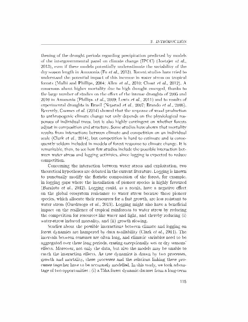
2. INTRODUCTION
thening of the drought periods regarding precipitation predicted by modelsof the intergovernmental panel on climate change (IPCC) (Joetzjer et al.,2013), even if these models potentially underestimate the variability of thedry season length in Amazonia (Fu et al., 2013). Recent studies have tried tounderstand the potential impact of this increase in water stress on tropicalforests (Malhi and Phillips, 2004; Allen et al., 2010; Choat et al., 2012). Aconsensus about higher mortality due to high drought emerged, thanks tothe large number of studies on the e�ect of the intense droughts of 2005 and2010 in Amazonia (Phillips et al., 2009; Lewis et al., 2011) and to results ofexperimental droughts in Brasil (Nepstad et al., 2007; Brando et al., 2008).Recently, Coomes et al. (2014) showed that the response of wood productionto anthropogenic climate change not only depends on the physiological res-ponses of individual trees, but is also highly contingent on whether forestsadjust in composition and structure. Some studies have shown that mortalityresults from interactions between climate and competition on an individualscale (Clark et al., 2014), but competition is hard to estimate and is conse-quently seldom included in models of forest response to climate change. It isremarkable, then, to see how few studies include the possible interaction bet-ween water stress and logging activities, since logging is expected to reducecompetition.
Concerning the interaction between water stress and exploitation, twotheoretical hypotheses are debated in the current literature. Logging is knownto punctually modify the �oristic composition of the forest, for example,in logging gaps where the installation of pioneer species is highly favoured(Baraloto et al., 2012). Logging could, as a result, have a negative e�ecton the global ecosystem resistance to water stress because these pioneerspecies, which allocate their resources for a fast growth, are less resistant towater stress (Ouedraogo et al., 2013). Logging might also have a bene�cialimpact on the resilience of tropical rainforests to water stress by reducingthe competition for resources like water and light, and thereby reducing (i)water-stress induced mortality, and (ii) growth slowing.
Studies about the possible interactions between climate and logging onforest dynamics are hampered by data availability (Clark et al., 2014). Theintervals between censuses are often long, and climatic variables need to beaggregated over these long periods, erasing exceptionally wet or dry seasons'e�ects. Moreover, not only the data, but also the models may be unable tocatch the interaction e�ects. As tree dynamics is drawn by two processes,growth and mortality, these processes and the relations linking these pro-cesses together have to be accurately modelled. In this study, we took advan-tage of two opportunities : (i) a 75ha forest dynamic dataset from a long-term
115
Chapitre 3. Vulnerability of commercial tree species to water stress in French Guiana
Table 3.1 : List of the commercial species taken into account forthe study. The current level of exploitation was calculated as a relativepercentage of the 20 main commercial species logged during the last 25 years.Column 3 indicates the abundance of the species in the study site of Paracou,French Guiana.
Common name Taxonomic identi�cation
Current
Trees in exploitation
Paracou level
(% in volume)
Angélique Dicorynia guianensis 647 41.63%
Balata franc Manilkara bidentata 138 2.28%
Balata pomme Chrysophyllum spp. 205 0.04%
Boco Bocoa prouacensis 1135 0.01%
Carapa Carapa surinamensis 702 0.04%
Gonfolo gris Ruizterania albi�ora 73 1.43%
Gonfolo rose Qualea rosea 669 21.12%
Goupi Goupia glabra 291 1.89%
Grignon franc Sextonia rubra 188 8.94%
Kobe Sterculia spp. 460 <0.0003%
Manil marécage Symphonia spp. 69 <0.0003%
Wacapou Vouacapoua americana 874 1.29%
Wapa Eperua falcata 2628 0.49%
Yayamadou montagne Virola michelii 344 0.26%
logging experiment, where all trees with DBH>10cm were censused every 2yrover a 20yr post-logging period, and (ii) a joint growth-mortality model re-cently developed (chapter 2). Fourteen forest species (see Table 3.1) wereidenti�ed, together with forest managers, as potentially interesting for theGuianan timber industry using criteria including natural abundance, currentlevel of exploitation or future logging potential. We tackled two questions :
• How will these commercial species respond, in terms of demographicalrates, to the increase in water stress induced by climate change ?
• Will logging and water stress interact, making some species more fragilethan others ?
116

3. MATERIALS AND METHODS
3 Materials and Methods
3.1 Study site
The study was conducted using data from the Paracou experimental site(5◦18′N,52◦55′W), a lowland tropical rain forest near Sinnamary, FrenchGuiana. It is typical of Northern Guianan rain forests (Rutishauser et al.,2010; ter Steege et al., 2006), with a high species diversity (more than 500woody species attaining 10 cm Diameter at Breast Height DBH found atthe site) and dominant tree families including Fabaceae, Chrysobalanaceae,Lecythidaceae, Sapotaceae and Burseraceae. Nearly two-thirds of the annual3040 mm of precipitation between mid-March and mid-June, followed by along dry season from mid-August to mid-November (Wagner et al., 2011).Most common soils in Paracou are acrisol, limited in depth by a transformedloamy saprolite (≤ 1 m deep), which has a low permeability and leads tolateral drainage during heavy rains (Ferry et al., 2010).
3.2 Data
Twelve plots of 6.25 ha each were established in 1984 for a complete annualinventory of all trees > 10cm of DBH. These plots underwent 3 di�erent log-ging treatments between October 1986 and May 1987, with 3 plots assignedas controls. An average of 10 trees ≥ 50 cm DBH (treatment 1), 32 trees ≥40 cm DBH (treatment 2) and 40 trees ≥ 40 cm DBH (treatment 3) wereremoved per hectare. Three new additional control plots of 6.25 ha were esta-blished in 1990. Forest inventories have been conducted since 1991. Censusesof mortality, recruitment and diameter growth were conducted every yearuntil 1995 and every 2 years thereafter. DBH was calculated from circumfe-rence measures made to a precision of 0.5 cm. We used data from 1991 to2011. For each tree we know the location, DBH, name and status (dead oralive).
3.3 Model
The joint model used is based on 2 sub-models. The �rst one is a non-linear growth model developed in Hérault et al. (2011) in which the growthtrajectory depends on 3 parameters : Gmax (the maximum growth rate),Dopt (the diameter at maximum growth) and K (the kurtosis of the curvede�ning the shape of the ontogenetic variation in growth rate).
The second one is a mortality model developed by Aubry-Kientz et al.(2013), computing the individual probability of dying at each time step.
117

Chapitre 3. Vulnerability of commercial tree species to water stress in French Guiana
These 2 processes are interdependent, insofar as past tree growth has animpact on the individual probability of dying (Chao et al., 2008; Metcalfet al., 2009), and similar ecological predictors can be simultaneously impliedin the two processes. To address the delicate issue of coupling both processes,we used tree vigour to link growth and mortality. Tree vigour is estimated
with log
(AGRi,t + 1
AGRi,t + 1
), where AGRi,t is the observed absolute growth rate
between time t−1 and time t for individual tree i, and AGRi,t is the predictedabsolute growth rate between time t−1 and time t for individual tree i usingthe growth sub-model. At each time step, an individual tree i may die withprobability pi,t. If tree i stays alive, it grows at a growth rate AGRi,t, andits diameter Di,t−1 becomes Di,t. The joint model likelihood is then :
•∏nt=1 f(Di,t|Di,t−1) ∗ (1 − pi,s,t) if tree i stays alive during the length
of the studied period,
• pi,s,k∗∏k−1t=1 (f(Di,t|Di,t−1) ∗ (1− pi,s,t)) if tree i dies between time k−1
and time k,
where f(Di,t|Di,t−1) is the probability density for a tree with diameter Di,t−1
at time t − 1 to grow to diameter Di,t at time t, and pi,t is the probabilityof dying between time t− 1 and time t. This probability is computed by themodel :
pi,t = logit−1(θ1 ∗ log
(AGRi,t−1 + 1
AGRi,t−1 + 1
)+ θ2 ∗Di,t−1 + θ3 ∗ (Di,t−1)2
+ θ4 ∗Watert + θ5 ∗AGBLi + θ6 ∗Watert ∗AGBLi)
Watert is here a covariate related to the water stress undergone by treesat time t. We chose, as the water stress indicator, an estimator computedusing the relative extractable water index (REW) (Wagner et al., 2011), thatis the area over the REW curve and under the threshold of 0.4 de�ned ascritical by Wagner et al. (2012). To include the logging impact in the model,we quanti�ed it by the above-ground biomass (AGB.ha−1) loss measured, atthe 6.25ha plot level, right after the logging. This value varies from 0 to 225t.ha−1, which is the covariate indicated by AGBLi in the equation. To com-pare, mean AGBL in current harvested blocks in French Guiana is estimatedbetween 20% and 35% that correspond to 70-100 tMS.ha−1 (Guitet et al.,2012). We expect θ2 to be negative and θ3 to be positive in the probability
118
3. MATERIALS AND METHODS
of dying, leading to a U-shape mortality curve. This means that a tree hashigher risks of dying when it is young and small, or large and old, than whenit has an intermediate DBH, a phenomenon that we can explain by intensecompetition among the youngest and by senescence for the oldest (Aubry-Kientz et al., 2013). Growth rates are predicted with the following model,also including a water stress e�ect (Watert), a logging e�ect (AGBLi) andan interaction between those two e�ects :
log(AGRi,t−1 + 1) =(θ1 + θ4 ∗Watert−1 + θ5 ∗AGBLi+ θ6 ∗Watert−1 ∗AGBLi)
∗ exp
−1
2
log(Di,t−2
θ2
)θ3
2
log(AGRi,t−1 + 1) = log(AGRi,t−1 + 1) + ε
with ε ∼ N(0, θ7)
In these equations, θ are all unknown parameters that we will infer. ε isan error term following a normal distribution.
3.4 Inference and Selection Method
A Bayesian Monte-Carlo Markov Chain (MCMC) method was implementedto estimate the parameters (Dellaportas et al., 2002). A random walk wasused as proposal distribution to sample new values of parameters that wereor were not selected, using the ratio of Metropolis-Hastings. The only pa-rameter that was not sampled this way was the standard deviation of thegrowth model θ7, for which an inverse-gamma posterior distribution with aGibbs sampler was used. Since values of vigour change as predicted growthchanges, growth and mortality processes were parametrized simultaneously.The growth model is taken into account through the vigour estimate whenmortality parameters are estimated. All parameters are sampled one by oneat each step, and the global likelihood is computed. Three thousand iterationsof Metropolis-Hastings were done for each parameter. All the algorithmsand statistical treatments were implemented using R software RCoreTeam(2014).
We used the selection method proposed by Kuo and Mallick (1998) todetermine whether it was signi�cant to include an interaction between cli-mate and water stress in the growth model or in the mortality model. The
119
Chapitre 3. Vulnerability of commercial tree species to water stress in French Guiana
method consists of multiplying each interaction term we want to test by anindicator, whose value will be either 1 (term included in the model) or 0(term not included). A Gibbs algorithm was used to attribute either 1 or 0to the indicator, and a Metropolis-Hastings within Gibbs algorithm was usedto estimate the value of the parameters. We decided to include the interac-tion e�ect when the expectation of the indicator given by the Kuo-Mallickmethod was above 0.8.
3.5 Quanti�cation of the impacts of water stress on growthand mortality
The water stress e�ect, represented by the covariate (Watert), has the samerange for all the species. The parametrization of the joint model for eachspecies gives us a value of parameter θ4 multiplying this covariate, but toquantify a standardized (i.e., comparable between species) impact of waterstress on the two processes, further calculations were necessary.
3.5.1 Impact on growth
For the growth process, the water stress is added to other terms in equation(2), so that we weight it with θ1, a parameter related with the maximumgrowth rate of the species. In order to have access to an index of waterstress impact on growth comparable between the species, we considered avalue of water stress of 1 and a value of above-ground biomass loss (AGBL)corresponding to the logging treatment 3, and we calculated :
Impact on growth =θ4 + θ6 ∗AGBL
θ1.
This index describes the proportional decrease of growth rates observed withwater stress. No impact of water stress on the growth of the tree speciesconsidered corresponds to a value of 0. If an interaction between water stressand logging is selected for a species, then θ6 is not null to take this interactioninto account.
3.5.2 Impact on mortality
For the mortality process, the calculations used were more complicated dueto the logit function in equation (1). We calculated a medium basal signalrelating the ontogeny of the tree with the probability of dying and includeda water stress e�ect :
Basal signal = θ2 ∗median(DBH) + θ3 ∗ (median(DBH))2.
120
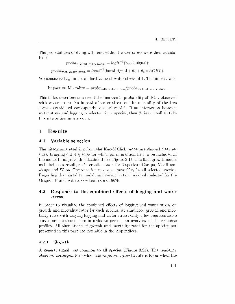
4. RESULTS
The probabilities of dying with and without water stress were then calcula-ted :
probawithout water stress = logit−1(basal signal);
probawith water stress = logit−1(basal signal + θ4 + θ6 ∗AGBL).
We considered again a standard value of water stress of 1. The impact was
Impact on Mortality = probawith water stress/probawithout water stress.
This index describes as a result the increase in probability of dying observedwith water stress. No impact of water stress on the mortality of the treespecies considered corresponds to a value of 1. If an interaction betweenwater stress and logging is selected for a species, then θ6 is not null to takethis interaction into account.
4 Results
4.1 Variable selection
The histograms resulting from the Kuo-Mallick procedure showed clear re-sults, bringing out 4 species for which an interaction had to be included inthe model to improve the likelihood (see Figure 3.1). The �nal growth modelincluded, as a result, an interaction term for 3 species : Carapa, Manil ma-récage and Wapa. The selection rate was above 99% for all selected species.Regarding the mortality model, an interaction term was only selected for theGrignon Franc, with a selection rate of 86%.
4.2 Response to the combined e�ects of logging and waterstress
In order to visualize the combined e�ects of logging and water stress ongrowth and mortality rates for each species, we simulated growth and mor-tality rates with varying logging and water stress. Only a few representativecurves are presented here in order to present an overview of the responsepro�les. All simulations of growth and mortality rates for the species notpresented in this part are available in the Appendices.
4.2.1 Growth
A general signal was common to all species (Figure 3.2a). The tendencyobserved corresponds to what was expected : growth rate is lower when the
121
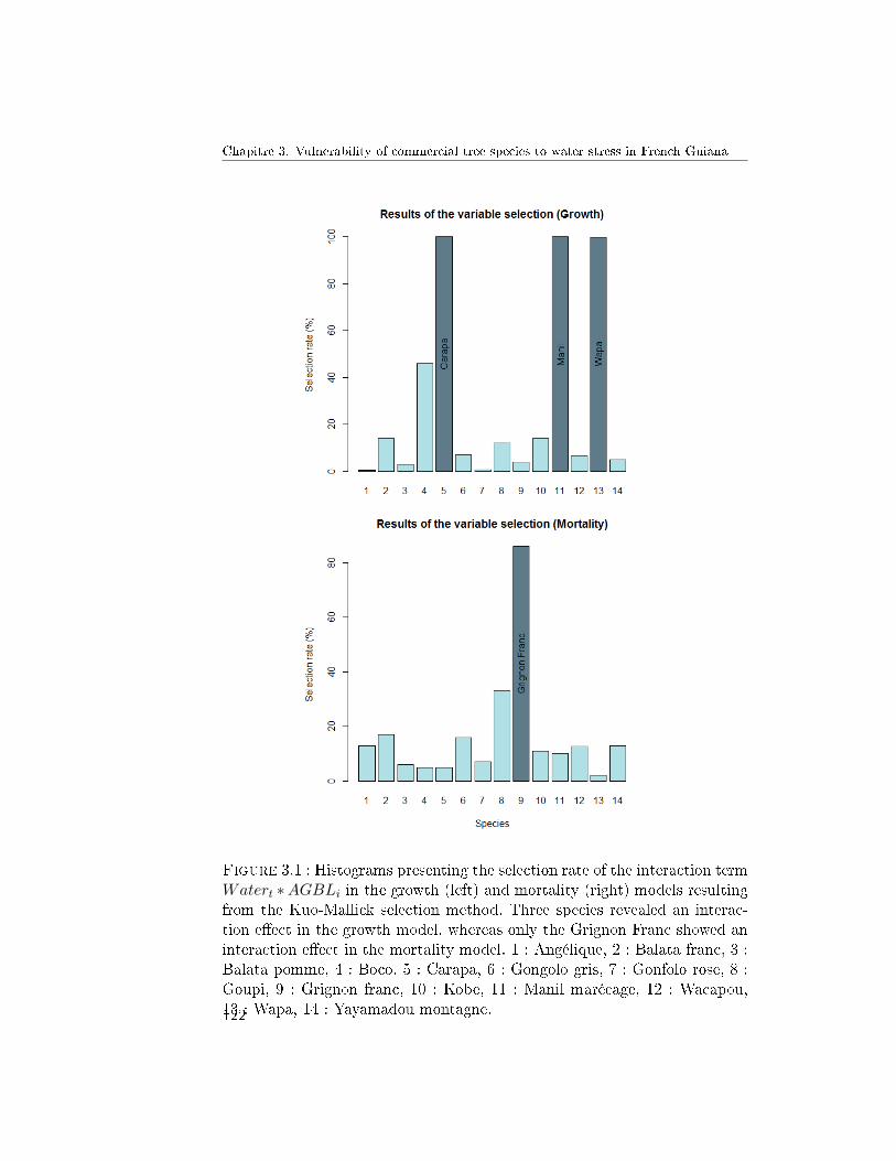
Chapitre 3. Vulnerability of commercial tree species to water stress in French Guiana
Figure 3.1 : Histograms presenting the selection rate of the interaction termWatert ∗AGBLi in the growth (left) and mortality (right) models resultingfrom the Kuo-Mallick selection method. Three species revealed an interac-tion e�ect in the growth model, whereas only the Grignon Franc showed aninteraction e�ect in the mortality model. 1 : Angélique, 2 : Balata franc, 3 :Balata pomme, 4 : Boco, 5 : Carapa, 6 : Gongolo gris, 7 : Gonfolo rose, 8 :Goupi, 9 : Grignon franc, 10 : Kobe, 11 : Manil marécage, 12 : Wacapou,13 : Wapa, 14 : Yayamadou montagne.122

4. RESULTS
tree is exposed to an important water stress, but exploitation has an oppositee�ect insofar as it decreases competition among trees for common resourcessuch as light and water in the soil.
Besides this common pattern, important di�erences between species canbe pointed out. All the species are distributed along a gradient, as illustratedin Figure 3.2. Some of them are well resistant to water stress (like the BalataPomme) and show nearly horizontal isoclines. Other tree species appear morea�ected by the lack of water, though exploitation seems to play an o�settingrole (Angélique). For these species, the isoclines tend to be more vertical.Finally, the Manil marécage illustrates how the interaction between loggingand water stress can twist the curves and lead to a low growth rate whenthe water stress becomes too signi�cant, even with logging.
4.2.2 Mortality
For the probability of dying, no pattern was shared by all the species. Howe-ver, the majority of them (12 species out of 14) showed a common scheme(see Figure 3.3). The tendency observed is again in agreement with whatwas expected : probability of dying is higher when the tree is exposed to animportant water stress, but exploitation has an opposite e�ect by decrea-sing competition, and therefore, exploitation reduces mortality rates. All thespecies sharing this tendency (i.e., all except Grignon Franc and Yayama-dou) are distributed along the same kind of gradient as shown in the sectionlabeled "growth" above ; this gradient is illustrated in Figure 3.3.
Some of them are well resistant to water stress. That is the case forthe Wacapou, whose isoclines are horizontal. Other tree species appear lessresistant to the lack of water, though exploitation could play an o�setting roleto a certain extent. The Boco, as well as a lot of other species like the Goupior the Gonfolo Gris, match this pro�le. Some species have isoclines thattend to be vertical, conveying an impact of water stress on the probability ofdying which may or may not be strong but which is observed with or withoutexploitation. That is the case of the Kobe, but also of the Carapa.
A completely di�erent pro�le was observed for 2 residual species : theYayamadou and the Grignon Franc. The isoclines of the Grignon Franc are alittle confused, likely due to the small number of trees in the database (73 ; seeTable 3.1). The interaction e�ect was di�cult to interpret for the same reason.The pro�le of the Grignon Franc is quite similar to the Yayamadou insofaras we consider that we have a basal mortality rate for standard conditions(high water stress only, intense exploitation only, or a combination of lowwater stress and light exploitation). The combination of high water stress
123
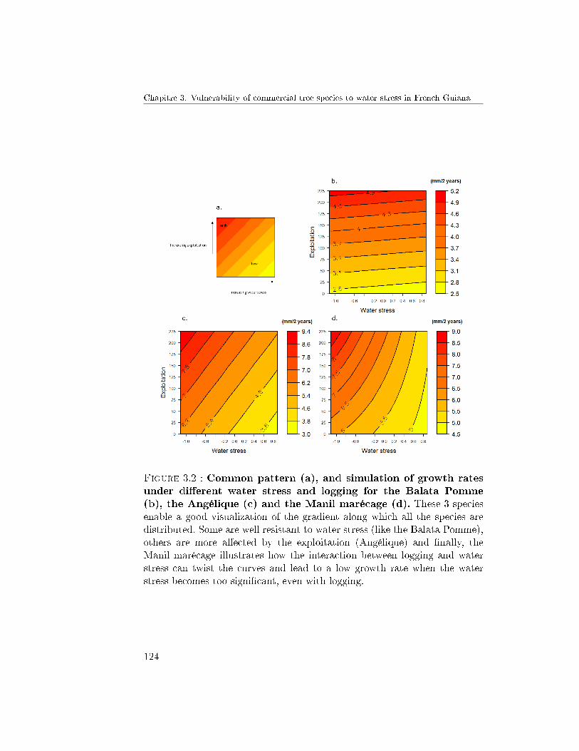
Chapitre 3. Vulnerability of commercial tree species to water stress in French Guiana
Figure 3.2 : Common pattern (a), and simulation of growth ratesunder di�erent water stress and logging for the Balata Pomme(b), the Angélique (c) and the Manil marécage (d). These 3 speciesenable a good visualization of the gradient along which all the species aredistributed. Some are well resistant to water stress (like the Balata Pomme),others are more a�ected by the exploitation (Angélique) and �nally, theManil marécage illustrates how the interaction between logging and waterstress can twist the curves and lead to a low growth rate when the waterstress becomes too signi�cant, even with logging.
124
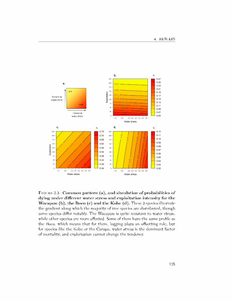
4. RESULTS
Figure 3.3 : Common pattern (a), and simulation of probabilities ofdying under di�erent water stress and exploitation intensity for theWacapou (b), the Boco (c) and the Kobe (d). These 3 species illustratethe gradient along which the majority of tree species are distributed, thoughsome species di�er notably. The Wacapou is quite resistant to water stress,while other species are more a�ected. Some of them have the same pro�le asthe Boco, which means that for them, logging plays an o�setting role, butfor species like the Kobe or the Carapa, water stress is the dominant factorof mortality, and exploitation cannot change the tendency.
125
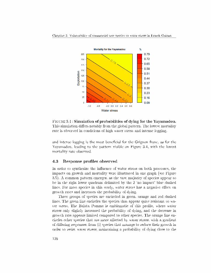
Chapitre 3. Vulnerability of commercial tree species to water stress in French Guiana
Figure 3.4 : Simulation of probabilities of dying for the Yayamadou.This simulation di�ers notably from the global pattern. The lowest mortalityrate is observed in conditions of high water stress and intense logging.
and intense logging is the most bene�cial for the Grignon franc, as for theYayamadou, leading to the pattern visible on Figure 3.4, with the lowestmortality rate observed.
4.3 Response pro�les observed
In order to synthesize the in�uence of water stress on both processes, theimpacts on growth and mortality were illustrated in one graph (see Figure3.5). A common pattern emerges, as the vast majority of species appear tobe in the right lower quadrant delimited by the 2 `no impact' blue dashedlines. For most species in this study, water stress has a negative e�ect ongrowth rates and increases the probability of dying.
Three groups of species are encircled in green, orange and red dashedlines. The green line encircles the species that appear quite resistant to wa-ter stress. The Balata Pomme is emblematic of this pro�le, where waterstress only slightly increased the probability of dying, and the decrease ingrowth rate appears limited compared to other species. The orange line en-circles other species that are more a�ected by water stress, with a gradientof di�ering responses, from (i) species that manage to reduce their growth inorder to resist water stress, maintaining a probability of dying close to the
126
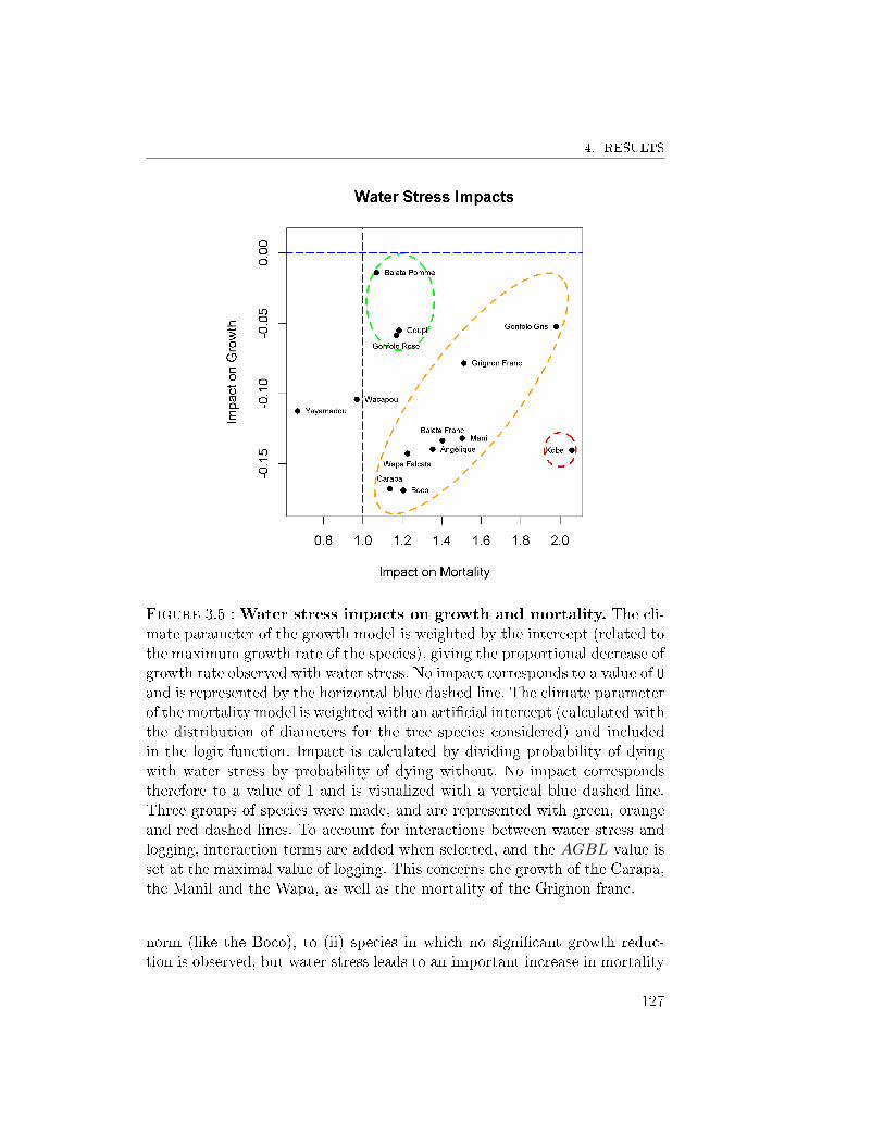
4. RESULTS
Figure 3.5 : Water stress impacts on growth and mortality. The cli-mate parameter of the growth model is weighted by the intercept (related tothe maximum growth rate of the species), giving the proportional decrease ofgrowth rate observed with water stress. No impact corresponds to a value of 0and is represented by the horizontal blue dashed line. The climate parameterof the mortality model is weighted with an arti�cial intercept (calculated withthe distribution of diameters for the tree species considered) and includedin the logit function. Impact is calculated by dividing probability of dyingwith water stress by probability of dying without. No impact correspondstherefore to a value of 1 and is visualized with a vertical blue dashed line.Three groups of species were made, and are represented with green, orangeand red dashed lines. To account for interactions between water stress andlogging, interaction terms are added when selected, and the AGBL value isset at the maximal value of logging. This concerns the growth of the Carapa,the Manil and the Wapa, as well as the mortality of the Grignon franc.
norm (like the Boco), to (ii) species in which no signi�cant growth reduc-tion is observed, but water stress leads to an important increase in mortality
127
Chapitre 3. Vulnerability of commercial tree species to water stress in French Guiana
rates (like the Gonfolo Gris). Finally, the red line encircles a unique species,the Kobe, which appears highly vulnerable to water stress. Its probability ofdying is indeed particularly increasing with water stress and its growth rateis also signi�cantly reduced.
If an interaction is observed, the interaction term is added and the valueof AGBL is set at the maximum value of logging. This is the case for thegrowth of the Carapa, the Manil and the Wapa, and for the mortality ofthe Grignon franc. If the e�ects of water stress are computed without in-teraction for the Carapa, the Manil or the Wapa, the growth reductions arelower, switching these species from the orange susceptible group to the greenresistant group (see Figure 3.5).
5 Discussion
The aim of this study was to quantify the vulnerability of commercial treespecies in French Guiana to a combination of exploitation and water stress.Joint models for growth and mortality were successfully parametrized for14 species ; parameters included climate and logging e�ects. An interactione�ect appeared necessary for several species, con�rming the necessity of in-cluding competition (through logging) and water stress in forest models forthe prediction of managed forests' responses to climate change (Clark et al.,2014). Some common patterns were noticeable in our results. For the vastmajority of species, water stress had a negative impact on growth rates, whilethe impact of logging was positive. The opposite results were observed formortality.
5.1 Exploitation impacts
Logging, by removing mature trees using resources like water, soil nutrientsand light, reduces competition among remaining trees, allowing them to growfaster. Positive e�ects of logging on growth last more than 8 years (Blancet al., 2009) and may be increased by the use of silvicultural treatments(Peña Claros et al., 2008; Guitet et al., 2009). This increased growth is ofparticular importance considering the large live tree carbon increment. Al-though reducing the competition through logging may counterbalance theimpacts of water stress, the e�ects are not strong enough to totally com-pensate for it, and some signi�cant interaction terms showed us that thesee�ects of reduced competition may be partly attenuated in cases of waterstress (see Figures 3.2 and 3.3).
128
5. DISCUSSION
5.2 Water stress impacts
Plant performance under drought is a well-documented phenomenon (Choatet al., 2012; Allen et al., 2010; Phillips et al., 2009). Water stress leads to adrop in soil water potential, resulting in a decrease of the leaf water potentialof the plant. This triggers a reduction in stomatal conductance, enabling theplant to reduce excessive transpiration but also limiting the carbon assimila-tion. In the case of prolonged drought, this reduction in stomatal conductancemay lead to a continued decline of assimilation and thus a noticeable growthreduction. Under extreme drought events, an increased number of xylem ves-sels run the risk of cavitation, because water transported through the xylemis under negative pressure (Choat et al., 2012). The resultant air embolismblocks xylem conduits and reduces the plant's ability to move water from soilto sites of photosynthesis, with vessels becoming completely dysfunctional.A series of events such as loss of plant hydraulic conductivity, stomatal clo-sure and �nally the abscission of leaves, shoots and branches will sometimeslead to plant death (Choat et al., 2012; Markesteijn, 2010). If water becameinsu�cient, the competition for these resource will increase and the mostadapted trees will be favoured ; indeed, it has been shown that drought killsselectively (Phillips et al., 2009). Reducing this competition by logging mayhave di�erent impacts on the water budget available for the remaining trees.
5.3 From tree vulnerability to timber logging strategy
Our results draw our attention to the problem that the timber industry willface in the next century : if some tree species are more vulnerable, or willbecame vulnerable, how should the timber industry react or prepare ?
In view of forest sustainability, some arguments may suggest a conser-vation strategy of the most vulnerable species. As 3 species (Carapa, Manilmarécage and Wapa) are particularly fragile under logging (negative θ6), theexploitation of these species may be avoided. It is then noticeable that theAngélique, the �rst tree species logged in French Guiana, appears quite vul-nerable to climate change. It might be worth trying to encourage the timberindustry to reduce the logging pressure on Angélique, should water stressintensify drastically in the coming decades. This diversi�cation should leadto a preferential exploitation of species like the Balata Pomme, the Goupi orthe Gonfolo Rose, which are more resilient to water stress. It also appearsnecessary to alleviate the pressure on species like the Kobe, the Gonfolo Grisor the Boco, as they were revealed vulnerable to water stress by our study.With minimal logging pressure for the most vulnerable species, we enable the
129

Chapitre 3. Vulnerability of commercial tree species to water stress in French Guiana
conservation of a larger genetic pool, trusting in the adaptative potential ofthese species to drier conditions by natural selection of the most resistant in-dividuals. Moreover, the diversi�cation of logged species has other bene�ts ;Putz et al. (2012) showed that if the same species continue to be harvested,only 35% of the original timber stock will be available for the second cut,compared to 54% if other species are harvested in the same time.
Another strategy could be defended : at similar logging intensities, pro-tecting the vulnerable species highlighted in this study will occur to thedetriment of other better-adapted species. One could argue that the conser-vation of these already-adapted species may be considered the most assuredway to protect the tropical forests under the future climates and to guaran-tee a larger genetic pool of species that are likely to be resistant. Sensitivespecies that are vulnerable to climate changes may be condemned, and theirprotection for some time is, in any case, doomed to failure in the long run.Our results highlight many questions that need to be asked. Indeed, the tro-pical forest and its dynamics are a complex system that may be drasticallyimpacted by climate changes and by logging practices, and consequencesof logging practices have to be considered before action is taken. Scientistsand foresters have to de�ne the role of silviculture in forest conservation.Sustainable logging in the tropics involves many trade-o�s.
6 Conclusion and Prospects
Our results allowed a species-centered interpretation of the in�uence of log-ging and climate on growth and mortality, the fundamental processes of fo-rest dynamics. They enabled to point out some global trends on the responseof the tree species studied for each process : (i) growth rates increase withlogging and decrease with water stress while (ii) probabilities of dying havethe exact opposite pattern. Resistant species were identi�ed, like the Ba-lata Pomme ; on the contrary, the Kobe or the Angélique stood out as morevulnerable. Forest plots are sometimes dominated by one species and popu-lation are rarely homogeneous. This is the case for the Angélique, which isextremely abundant in some areas. Some future studies need to address thispopulation, to study the potential ampli�cation feedbacks e�ects. Indeed,as the Angélique appears vulnerable to water stress, increased mortality ofareas dominated by this species will likely experience a drastic loss of bio-mass and other changes for the remaining trees. As suggested by Coomeset al. (2014), the forests's structure will potentially condition the responseto climate changes. Even if the species studied here are somewhat represen-
130

6. CONCLUSION AND PROSPECTS
tative of commercial species founded in Amazon (ter Steege et al., 2006),studying forests that are under di�erent climatic conditions is urgent.
131
BIBLIOGRAPHIE
Allen, C. D., Macalady, A. K., Chenchouni, H., Bachelet, D., McDowell, N.,Vennetier, M., Kitzberger, T., Rigling, A., Breshears, D. D., Hogg, E.T. H., Gonzalez, P., Fensham, R., Zhang, Z., Castro, J., Demidova, N.,Lim, J.-H. H., Allard, G., Running, S. W., Semerci, A., and Cobb, N.(2010). A global overview of drought and heat-induced tree mortalityreveals emerging climate change risks for forests. Forest Ecology andManagement, 259(4):660�684.
Asner, G. P., Knapp, D. E., Broadbent, E. N., Oliveira, P. J. C., Keller,M., and Silva, J. N. (2005). Selective logging in the Brazilian Amazon.Science (New York, N.Y.), 310(5747):480�2.
Aubry-Kientz, M., Hérault, B., Ayotte-Trépanier, C., Baraloto, C., and Rossi,V. (2013). Toward trait-based mortality models for tropical forests. PloSone, 8(5):e63678.
Baraloto, C., Hérault, B., Paine, C. E. T., Massot, H., Blanc, L., Bonal,D., Molino, J.-F., Nicolini, E. a., and Sabatier, D. (2012). Contrastingtaxonomic and functional responses of a tropical tree community toselective logging. Journal of Applied Ecology, 49(4):861�870.
Blanc, L., Echard, M., Herault, B., Bonal, D., Marcon, E., Chave, J., andBaraloto, C. (2009). Dynamics of aboveground carbon stocks in a se-lectively logged tropical forest. Ecological applications : a publication ofthe Ecological Society of America, 19(6):1397�404.
Blaser, J. (2011). Status of tropical forest management 2011. InternationalTropical Timber Organization.
132
BIBLIOGRAPHIE
Brando, P. M., Nepstad, D. C., Davidson, E. a., Trumbore, S. E., Ray, D., andCamargo, P. (2008). Drought e�ects on littefall, wood production andbelowground carbon cycling in an Amazon Forest : result of a throughfallreduction experiment. Philosophical Transactions of the Royal Society,363(1498):1839�1848.
Chao, K. J., Phillips, O. L., Gloor, E., Monteagudo, A., Torres-Lezama, A.,and Martinez, R. V. (2008). Growth and wood density predict treemortality in Amazon forests. Journal of Ecology, 96(2):281�292.
Choat, B., Jansen, S., Brodribb, T. J., Cochard, H., Delzon, S., Bhaskar, R.,Bucci, S. J., Feild, T. S., Gleason, S. M., Hacke, U. G., Jacobsen, A. L.,Lens, F., Maherali, H., Martínez-Vilalta, J., Mayr, S., Mencuccini, M.,Mitchell, P. J., Nardini, A., Pittermann, J., Pratt, R. B., Sperry, J. S.,Westoby, M., Wright, I. J., and Zanne, A. E. (2012). Global convergencein the vulnerability of forests to drought. Nature, 491(7426):752�5.
Clark, J. a. and Covey, K. R. (2012). Tree species richness and the loggingof natural forests : A meta-analysis. Forest Ecology and Management,276(0):146�153.
Clark, J. S., Bell, D. M., Kwit, M. C., and Zhu, K. (2014). Competition-interaction landscapes for the joint response of forests to climate change.Global Change Biology, 20(6):1979�1991.
Coomes, D. A., Flores, O., Holdaway, R., Jucker, T., Lines, E. R., and Van-derwel, M. C. (2014). Wood production response to climate change willdepend critically on forest composition and structure. Global changebiology, pages 1�14.
D'Amato, A. W., Bradford, J. B., Fraver, S., and Palik, B. J. (2011). Forestmanagement for mitigation and adaptation to climate change : Insightsfrom long-term silviculture experiments. Forest Ecology and Manage-ment, 262(5):803�816.
Dellaportas, P., Forster, J. J., and Ntzoufras, I. (2002). On Bayesian modeland variable selection using MCMC. Statistics and Computing, 12:27�36.
Dwyer, J. M., Fensham, R., and Buckley, Y. M. (2010). Restoration thinningaccelerates structural development and carbon sequestration in an en-dangered Australian ecosystem. Journal of Applied Ecology, 47(3):681�691.
133

Chapitre 3. Vulnerability of commercial tree species to water stress in French Guiana
Ferry, B., Morneau, F., Bontemps, J. D., Blanc, L., and Freycon, V. (2010).Higher treefall rates on slopes and waterlogged soils result in lower standbiomass and productivity in a tropical rain forest. Journal of Ecology,98(1):106�116.
Fu, R., Yin, L., Li, W., Arias, P. A., Dickinson, R. E., Huang, L., Chakra-borty, S., Fernandes, K., Liebmann, B., Fisher, R., and Myneni, R. B.(2013). Increased dry-season length over southern Amazonia in recentdecades and its implication for future climate projection. Proceedingsof the National Academy of Sciences of the United States of America,110(45):18110�18115.
Gibson, L., Lee, T. M., Koh, L. P., Brook, B. W., Gardner, T. a., Barlow,J., Peres, C. a., Bradshaw, C. J. a., Laurance, W. F., Lovejoy, T. E.,and Sodhi, N. S. (2011). Primary forests are irreplaceable for sustainingtropical biodiversity. Nature, 478(7369):378�81.
GIEC (2013). Changements climatiques 2013 Les éléments scienti�ques.GIEC, groupe de travail 1.
Guitet, S., Blanc, L., Trombe, P.-J., and Lehallier, B. (2009). Traitementssylvicoles en forêt tropicale guyanaise : bilan de dix ans d'expérimenta-tions. Bois et forêts des tropiques, 301(3):7�19.
Guitet, S., Pithon, S., Brunaux, O., Jubelin, G., and Gond, V. (2012). Im-pacts of logging on the canopy and the consequences for forest manage-ment in French Guiana. Forest Ecology and Management, 277:124�131.
Hammond, D. S. (2005). Tropical forests of the Guiana shield : ancientforests in a modern world. CABI.
Hérault, B., Bachelot, B., Poorter, L., Rossi, V., Bongers, F., Chave, J.,Paine, C. E. T., Wagner, F., and Baraloto, C. (2011). Functional traitsshape ontogenetic growth trajectories of rain forest tree species. Journalof Ecology, 99(6):1431�1440.
Herault, B., Ouallet, J., Blanc, L., Wagner, F., and Baraloto, C. (2010).Growth responses of neotropical trees to logging gaps. Journal of AppliedEcology, 47(4):821�831.
Joetzjer, E., Douville, H., Delire, C., and Ciais, P. (2013). Present-day andfuture Amazonian precipitation in global climate models : CMIP5 versusCMIP3. Climate Dynamics, 41(11-12):2921�2936.
134
BIBLIOGRAPHIE
Kuo, L. and Mallick, B. (1998). Variable selection for regression models.Sankhya Ser.B, (60):65�81.
Lewis, S. L., Brando, P. M., Phillips, O. L., van der Heijden, G. M. F., andNepstad, D. (2011). The 2010 Amazon drought. Science (New York,N.Y.), 331(6017):554.
Malhi, Y. and Phillips, O. L. (2004). Tropical forests and global atmosphericchange : a synthesis. Philosophical transactions of the Royal Society ofLondon. Series B, Biological sciences, 359(1443):549�55.
Markesteijn, L. (2010). Drought tolerance of tropical tree species ; FunctionalTraits, Trade-o�s and Species Distribution. PhD thesis, WageningenUniversity.
Metcalf, C. J. E., McMahon, S. M., and Clark, J. S. (2009). Overcomingdata sparseness and parametric constraints in modeling of tree morta-lity : a new nonparametric Bayesian model. Canadian Journal of ForestResearch, 39(9):1677�1687.
Nepstad, D. C., Tohver, I. M., Ray, D., Moutinho, P., and Cardinot, G.(2007). Mortality of large trees and lianas following experimentaldrought in an Amazon forest. Ecology, 88(9):2259�69.
Ouedraogo, D.-Y., Mortier, F., Gourlet-Fleury, S., Freycon, V., and Picard,N. (2013). Slow-growing species cope best with drought : evidence fromlong-term measurements in a tropical semi-deciduous moist forest ofCentral Africa. Journal of Ecology, 101(6):1459�1470.
Peña Claros, M., Fredericksen, T., Alarcón, a., Blate, G., Choque, U., Leaño,C., Licona, J., Mostacedo, B., Pariona, W., Villegas, Z., and Putz, F.(2008). Beyond reduced-impact logging : Silvicultural treatments toincrease growth rates of tropical trees. Forest Ecology and Management,256(7):1458�1467.
Phillips, O. L., Aragao, L., Lewis, S. L., Fisher, J. B., Lloyd, J., Lopez-Gonzalez, G., Malhi, Y., Monteagudo, A., Peacock, J., Quesada, C. A.,van der Heijden, G., Almeida, S., Amaral, I., Arroyo, L., Aymard, G.,Baker, T. R., Banki, O., Blanc, L., Bonal, D., Brando, P., Chave, J.,de Oliveira, A. C. A., Cardozo, N. D., Czimczik, C. I., Feldpausch,T. R., Freitas, M. A., Gloor, E., Higuchi, N., Jimenez, E., Lloyd, G.,Meir, P., Mendoza, C., Morel, A., Neill, D. A., Nepstad, D., Patino, S.,Penuela, M. C., Prieto, A., Ramirez, F., Schwarz, M., Silva, J., Silveira,
135
Chapitre 3. Vulnerability of commercial tree species to water stress in French Guiana
M., Thomas, A. S., ter Steege, H., Stropp, J., Vasquez, R., Zelazowski,P., Davila, E. A., Andelman, S., Andrade, A., Chao, K.-j. J., Erwin, T.,Di Fiore, A., Honorio, E., Keeling, H., Killeen, T. J., Laurance, W. F.,Cruz, A. P. n., Pitman, N. C. A., Vargas, P. N. n., Ramirez-Angulo,H., Rudas, A., Salamao, R., Silva, N., Terborgh, J., Torres-Lezama, A.,Aragão, L. E. O. C., López-gonzález, G., Heijden, G. V. D., Bánki, O.,Cristina, A., Oliveira, A. D., Jiménez, E., Patiño, S., Peñuela, M. C.,Ramírez, F., Steege, H., Vásquez, R., Dávila, E. A., Fiore, A. D., C,E. H., Ramírez-angulo, H., and Salamão, R. (2009). Drought sensitivityof the Amazon Rainforest. Science, 323(March):1344�1347.
Putz, F. E., Zuidema, P. a., Synnott, T., Peña Claros, M., Pinard, M. a.,Sheil, D., Vanclay, J. K., Sist, P., Gourlet-Fleury, S., Griscom, B., Pal-mer, J., and Zagt, R. (2012). Sustaining conservation values in selecti-vely logged tropical forests : the attained and the attainable. Conser-vation Letters, 5(4):296�303.
RCoreTeam (2014). R : A Language and Environment for Statistical Com-puting.
Rutishauser, E., Wagner, F., Hérault, B., Nicolini, E. A., and Blanc, L.(2010). Contrasting above-ground biomass balance in a Neotropicalrain forest. Journal of Vegetation Science, 21(4):672�682.
Silva, J. N. M., Carvalhoa, J. O. P. D., Lopes, J. C. A., Almeida, B. F. D.,Costa, D. H. M., Oliveira, L. C., Vanclay, J. K., and Skovsgaard, J. P.(1995). Growth and yield of a tropical rain forest in the Brazilian Ama-zon 13 years after logging. Forest Ecology and Management, 71:267�274.
ter Steege, H., Pitman, N. C. a., Phillips, O. L., Chave, J., Sabatier, D.,Duque, A., Molino, J.-F., Prévost, M.-F., Spichiger, R., Castellanos,H., von Hildebrand, P., and Vásquez, R. (2006). Continental-scale pat-terns of canopy tree composition and function across Amazonia. Nature,443(7110):444�7.
Wagner, F., Hérault, B., Stahl, C., Bonal, D., and Rossi, V. (2011). Modelingwater availability for trees in tropical forests. Agricultural and ForestMeteorology, 151(9):1202�1213.
Wagner, F., Rossi, V., Stahl, C., Bonal, D., and Hérault, B. (2012). WaterAvailability Is the Main Climate Driver of Neotropical Tree Growth.Plos One, 7(4):e34074.
136

BIBLIOGRAPHIE
Zimmerman, B. L. and Kormos, C. F. (2012). Prospects for SustainableLogging in Tropical Forests. BioScience, 62(5):479�487.
137
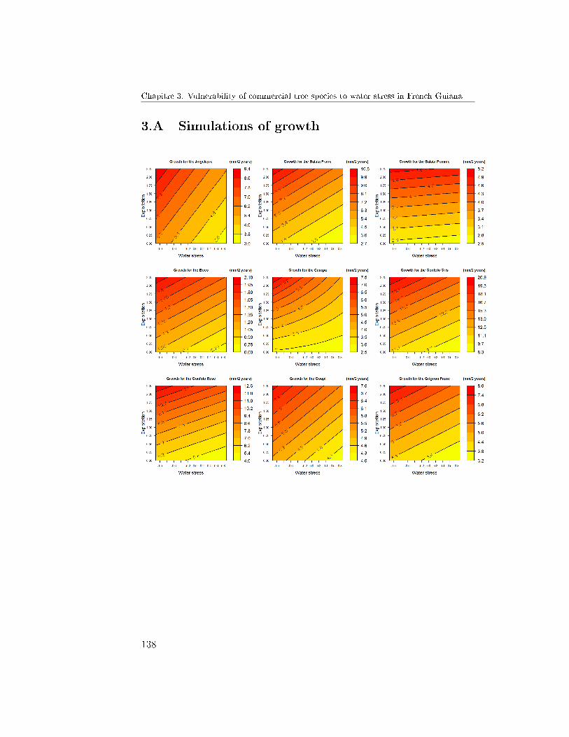
Chapitre 3. Vulnerability of commercial tree species to water stress in French Guiana
3.A Simulations of growth
138
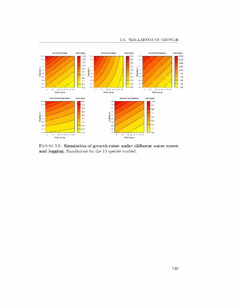
3.A. SIMULATIONS OF GROWTH
Figure 3.6 : Simulation of growth rates under di�erent water stressand logging. Simulations for the 14 species studied.
139
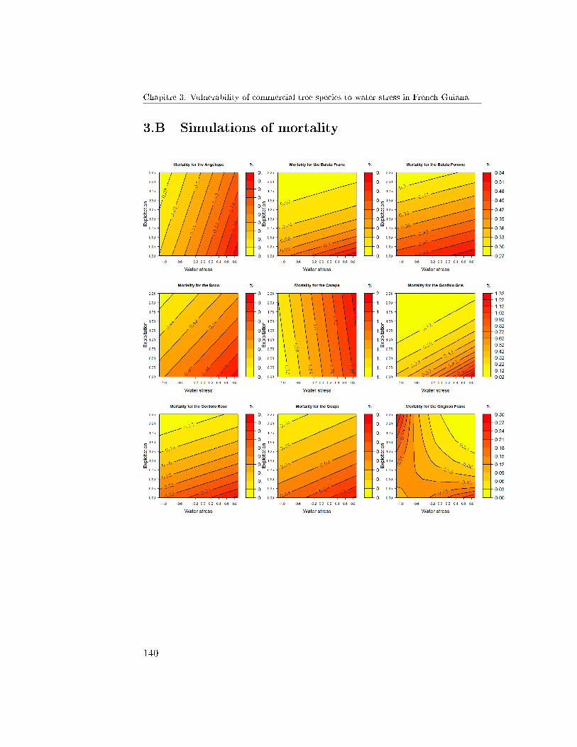
Chapitre 3. Vulnerability of commercial tree species to water stress in French Guiana
3.B Simulations of mortality
140
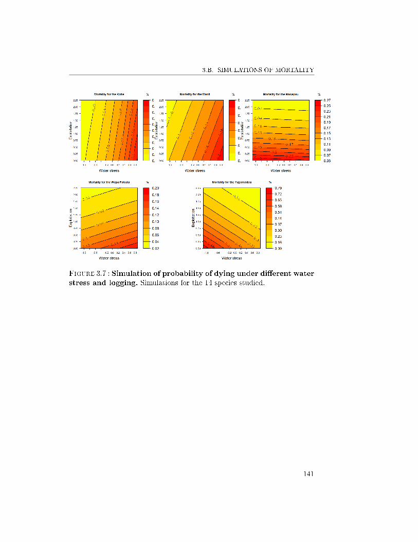
3.B. SIMULATIONS OF MORTALITY
Figure 3.7 : Simulation of probability of dying under di�erent waterstress and logging. Simulations for the 14 species studied.
141
CHAPITRE 4
IDENTIFYING CLIMATIC DRIVERS OF TROPICALFOREST DYNAMICS USING A GROWTH-MORTALITY
MODEL
Mélaine Aubry-Kientz1∗
Vivien Rossi 2,3,4
Fabien Wagner 2,5
Bruno Hérault 2
1 Université des Antilles et de la Guyane, UMR `Ecologie des Forêts de Guya-ne', Campus agronomique de Kourou, France.2 CIRAD, UMR `Ecologie des Forêts de Guyane', Campus agronomique deKourou, France.3 CIRAD, UPR Bsef, Montpellier, France.4 Université de Yaoundé I, UMMISCO (UMI 209), BP337, Yaoundé, Came-roun.5 Remote sensing division, National Institute for Space Research-INPE, SãoJosé dos Campos, SP, Brazil.∗ E-mail : [email protected]
142
Dans le chapitre précédent, l'introduction du climat s'est faite par l'es-timation du stress hydrique. Mais d'autres changements sont prévus parle GIEC, notamment une augmentation marquée de la température. Pourmieux prendre en compte le climat dans notre modèle, les variables clima-tiques qui ont un rôle dans la croissance et/ou la mortalité doivent être atten-tivement sélectionnées. Dans ce chapitre, je cherche à identi�er ces variables.Pour commencer, une analyse multivariée permet de mettre en évidence desaxes relatif à la température, au stress hydrique, et à la saturation du sol eneau. Ensuite, l'ajout des variables climatiques sélectionnées dans le modèlemontre que le stress hydrique a un impact négatif sur la croissance et lamortalité, que la température a un impact négatif sur la croissance, et quela saturation du sol en eau augmente le taux de mortalité. Une interactionentre la densité du bois et le stress hydrique est ajoutée dans le processusde croissance, et montre que les arbres à bois dense sont plus résistants à lasécheresse. De même, une interaction entre le diamètre de l'arbre et le stresshydrique montre que les arbres les plus gros sont aussi les plus sensibles àla sécheresse. Les variables climatiques et les interactions mises en évidencesont ajoutées dans le modèle développé dans le chapitre 2, ce qui permet deconstruire un modèle de croissance et de mortalité climat-explicite pour lacommunauté.
143
Chapitre 4. Identifying climatic drivers of tropical forest dynamics using agrowth-mortality model
1 Abstract
• In the context of climate changes, identifying and then predicting theimpacts of climatic drivers on tropical forest dynamics is becoming amatter of urgency.
• We used a coupled model of tropical tree growth and mortality, calibra-ted with forest dynamic data from the 20-year study site of Paracou,French Guiana, in order to introduce and test a set of climatic variables.
• Three major climatic drivers were identi�ed through the variable selec-tion procedure : drought, water saturation and temperature. Droughtdecreased annual growth and mortality rates, high precipitation increa-sed mortality rates and high temperature decreased growth. Interac-tions between key functional traits, stature and climatic variables wereinvestigated, showing best resistance to drought for trees with highwood density and for trees with small current diameters.
• Our results highlighted strong long-term impacts of climate variableson tropical forest dynamics, suggesting potential deep impacts of cli-mate changes during the next century.
2 Introduction
In French Guianan forests, the intra-annual climate variability is stronglystructured by the occurrence of the dry seasons : a long dry season frommid-August to mid-November, and a short one in March. Such a seasona-lity is typical in many tropical forest areas, and implies various changes ofthe availability of resources, such as water and light, necessary to tree deve-lopment and to forest functioning. The seasonality of tree growth and treemortality is consequently highly studied in tropical forests, with demons-trable success in the past (Wagner et al., 2012; Grogan and Schulze, 2012;Brando et al., 2010). Tree growth is mainly related to water availability,resulting in growth during the wet months and static or even contractedstates during the dry season months (Grogan and Schulze, 2012). The use ofa convenient water availability estimator like the relative extractable water(REW) (Wagner et al., 2011) shows that low levels of REW rather than lackof rainfall per se are the key drivers of the decrease in growth rate, or evenof the stop, at a seasonal time step. (Wagner et al., 2012).
At another time scale, long-term forest dynamic changes may also berelated to exceptional climate events. E�ects of unusual dry periods on tree
144
2. INTRODUCTION
growth and mortality may enlighten us about the long-term processes lin-king water availability and tree dynamics. After the intense 2005 droughtin Amazonia, the forest su�ered an additional mortality, leading to a hugeloss of alive tree biomass (Phillips et al., 2009). A consensus about highermortality due to severe drought events has recently emerged (Choat et al.,2012; Allen et al., 2010). Experimental droughts in Brazil provide results inline with this consensus(Nepstad et al., 2007; da Costa et al., 2010; Brandoet al., 2008).
Besides exceptional events and the intra-annual seasonal rhythmicity,there is a gap in our research knowledge on an inter-annual scale investiga-ting the potential links between inter-annual climate variations and forestdynamics from a long-term perspective. This gap is partly due to the weakmagnitude of variation of the demographic rates when compared to whatis observed from a seasonal point of view or from some spectacular events.This gap is also due to the lack of sites in tropical forests where annual re-gular inventories of tree growth and death are performed and where climaticdata on the same time-scale are available. Convenient tools are needed toprocess these data. A modelling approach may help to tackle these ques-tions (Zuidema et al., 2013) because models can mechanistically link climateconditions, resource acquisition, allocation, and functional plant traits totree growth and survival. Functional traits have been recently used to in-clude functional diversity in models of tree growth (Hérault et al., 2011;Rüger et al., 2012; Wagner et al., 2014) and tree mortality (Aubry-Kientzet al., 2013). Such models need to start from potential underlying physiolo-gical processes, helping to articulate hypotheses that will serve as the basisfor building the models.
Some climatic variables are expected to play a role in forest dynamicsregarding the tree's physiological processes. Water stress due to drought iswell documented (Phillips et al., 2009; Allen et al., 2010). Water insu�ciencyleads generally to higher mortality rates and lower growth (Choat et al.,2012). Water stress needs to be estimated, and diverse estimators may befound in the literature (Wagner et al., 2011; Toledo et al., 2011; Aragãoet al., 2007; Malhi et al., 2009). The length of the dry season seems to bethe simplest estimator. The REW described in the study of Wagner et al.(2011) was computed using the daily rainfall and gave an estimate of thequantity of water available for tree development. This indicator is alreadyrelated to intra-annual forest dynamics in Wagner et al. (2012). Althoughwater availability is expected to reduce growth and increase mortality, theseimpacts have to be investigated on an inter-annual time-scale.
Rain may also be responsible for water saturation, a phenomenon that
145
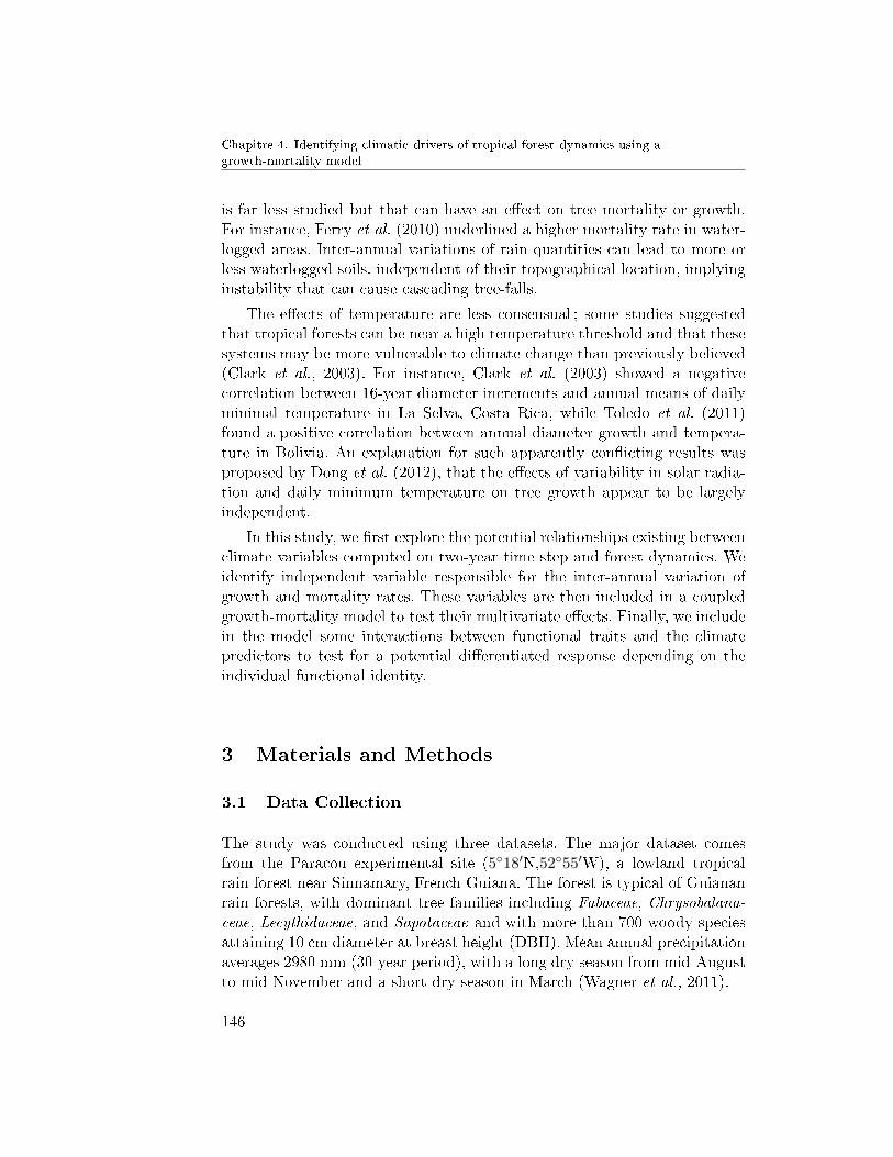
Chapitre 4. Identifying climatic drivers of tropical forest dynamics using agrowth-mortality model
is far less studied but that can have an e�ect on tree mortality or growth.For instance, Ferry et al. (2010) underlined a higher mortality rate in water-logged areas. Inter-annual variations of rain quantities can lead to more orless waterlogged soils, independent of their topographical location, implyinginstability that can cause cascading tree-falls.
The e�ects of temperature are less consensual ; some studies suggestedthat tropical forests can be near a high temperature threshold and that thesesystems may be more vulnerable to climate change than previously believed(Clark et al., 2003). For instance, Clark et al. (2003) showed a negativecorrelation between 16-year diameter increments and annual means of dailyminimal temperature in La Selva, Costa Rica, while Toledo et al. (2011)found a positive correlation between annual diameter growth and tempera-ture in Bolivia. An explanation for such apparently con�icting results wasproposed by Dong et al. (2012), that the e�ects of variability in solar radia-tion and daily minimum temperature on tree growth appear to be largelyindependent.
In this study, we �rst explore the potential relationships existing betweenclimate variables computed on two-year time step and forest dynamics. Weidentify independent variable responsible for the inter-annual variation ofgrowth and mortality rates. These variables are then included in a coupledgrowth-mortality model to test their multivariate e�ects. Finally, we includein the model some interactions between functional traits and the climatepredictors to test for a potential di�erentiated response depending on theindividual functional identity.
3 Materials and Methods
3.1 Data Collection
The study was conducted using three datasets. The major dataset comesfrom the Paracou experimental site (5◦18′N,52◦55′W), a lowland tropicalrain forest near Sinnamary, French Guiana. The forest is typical of Guiananrain forests, with dominant tree families including Fabaceae, Chrysobalana-ceae, Lecythidaceae, and Sapotaceae and with more than 700 woody speciesattaining 10 cm diameter at breast height (DBH). Mean annual precipitationaverages 2980 mm (30-year period), with a long dry season from mid-Augustto mid-November and a short dry season in March (Wagner et al., 2011).
146
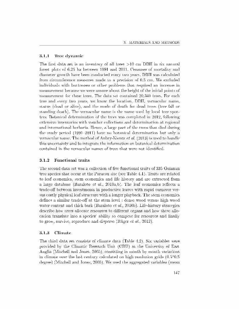
3. MATERIALS AND METHODS
3.1.1 Tree dynamic
The �rst data set is an inventory of all trees >10 cm DBH in six naturalforest plots of 6.25 ha between 1991 and 2011. Censuses of mortality anddiameter growth have been conducted every two years. DBH was calculatedfrom circumference measures made to a precision of 0.5 cm. We excludedindividuals with buttresses or other problems that required an increase inmeasurement because we were unsure about the height of the initial points ofmeasurement for these trees. The data set contained 20,340 trees. For eachtree and every two years, we know the location, DBH, vernacular name,status (dead or alive), and the mode of death for dead trees (tree-fall orstanding death). The vernacular name is the name used by local tree spot-ters. Botanical determination of the trees was completed in 2012, followingextensive inventories with voucher collections and determination at regionaland international herbaria. Hence, a large part of the trees that died duringthe study period (1991�2011) have no botanical determination but only avernacular name. The method of Aubry-Kientz et al. (2013) is used to handlethis uncertainty and to integrate the information on botanical determinationcontained in the vernacular names of trees that were not identi�ed.
3.1.2 Functional traits
The second data set was a collection of �ve functional traits of 335 Guianantree species that occur at the Paracou site (see Table 4.1). Traits are relatedto leaf economics, stem economics and life history and are extracted froma large database (Baraloto et al., 2010a,b). The leaf economics re�ects atrade-o� between investments in productive leaves with rapid turnover ver-sus costly physical leaf structure with a longer playback. The stem economicsde�nes a similar trade-o� at the stem level : dense wood versus high woodwater content and thick bark (Baraloto et al., 2010b). Life-history strategiesdescribe how trees allocate resources to di�erent organs and how these allo-cation translate into a species' ability to compete for resources and �nallyto grow, survive, reproduce and disperse (Rüger et al., 2012).
3.1.3 Climate
The third data set consists of climate data (Table 4.2). Six variables wereprovided by the Climatic Research Unit (CRU) at the University of EastAnglia (Mitchell and Jones, 2005), consisting in month-by-month variationsin climate over the last century calculated on high-resolution grids (0.5*0.5degree) (Mitchell and Jones, 2005). We used the aggregated variables (mean
147
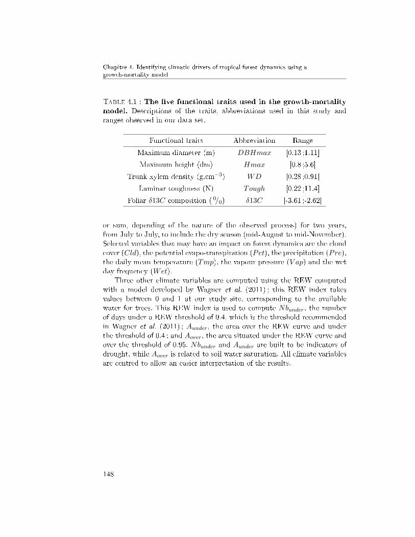
Chapitre 4. Identifying climatic drivers of tropical forest dynamics using agrowth-mortality model
Table 4.1 : The �ve functional traits used in the growth-mortalitymodel. Descriptions of the traits, abbreviations used in this study andranges observed in our data set.
Functional traits Abbreviation Range
Maximum diameter (m) DBHmax [0.13 ;1.11]
Maximum height (dm) Hmax [0.8 ;5.6]
Trunk xylem density (g.cm−3) WD [0.28 ;0.91]
Laminar toughness (N) Tough [0.22 ;11.4]
Foliar δ13C composition ( 0/0) δ13C [-3.61 ;-2.62]
or sum, depending of the nature of the observed process) for two years,from July to July, to include the dry season (mid-August to mid-November).Selected variables that may have an impact on forest dynamics are the cloudcover (Cld), the potential evapo-transpiration (Pet), the precipitation (Pre),the daily mean temperature (Tmp), the vapour pressure (V ap) and the wetday frequency (Wet).
Three other climate variables are computed using the REW computedwith a model developed by Wagner et al. (2011) ; this REW index takesvalues between 0 and 1 at our study site, corresponding to the availablewater for trees. This REW index is used to compute Nbunder, the numberof days under a REW threshold of 0.4, which is the threshold recommendedin Wagner et al. (2011) ; Aunder, the area over the REW curve and underthe threshold of 0.4 ; and Aover, the area situated under the REW curve andover the threshold of 0.95. Nbunder and Aunder are built to be indicators ofdrought, while Aover is related to soil water saturation. All climate variablesare centred to allow an easier interpretation of the results.
148
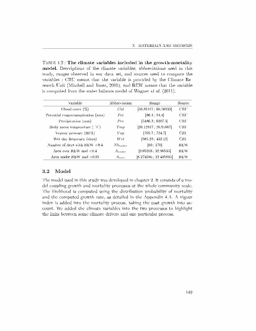
3. MATERIALS AND METHODS
Table 4.2 : The climate variables included in the growth-mortalitymodel. Descriptions of the climate variables, abbreviations used in thisstudy, ranges observed in our data set, and sources used to compute thevariables : CRU means that the variable is provided by the Climate Re-search Unit (Mitchell and Jones, 2005), and REW means that the variableis computed from the water balance model of Wagner et al. (2011).
Variable Abbreviation Range Source
Cloud cover (%) Cld [56.85417 ; 60.70833] CRU
Potential evapotranspiration (mm) Pet [80.4 ; 84.4] CRU
Precipitation (mm) Pre [5486.3 ; 6207.3] CRU
Daily mean temperature (�C) Tmp [26.12917 ; 26.91667] CRU
Vapour pressure (HPA) V ap [705.7 ; 724.7] CRU
Wet day frequency (days) Wet [385.23 ; 432.12] CRU
Number of days with REW <0.4 Nbunder [89 ; 170] REW
Area over REW and <0.4 Aunder [9.05203 ; 32.96535] REW
Area under REW and >0.95 Aover [8.274586 ; 12.485895] REW
3.2 Model
The model used in this study was developed in chapter 2. It consists of a mo-del coupling growth and mortality processes at the whole community scale.The likelihood is computed using the distribution probability of mortalityand the computed growth rate, as detailed in the Appendix 4.A. A vigourindex is added into the mortality process, taking the past growth into ac-count. We added the climate variables into the two processes to highlightthe links between some climate drivers and one particular process.
149
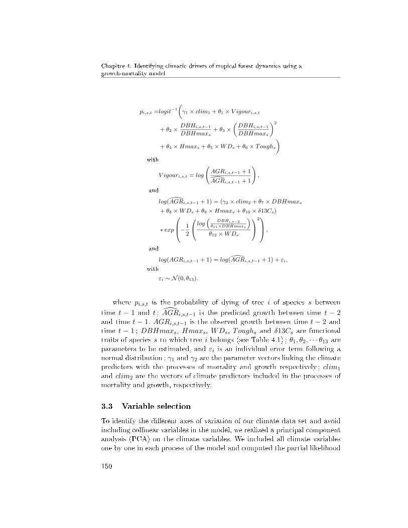
Chapitre 4. Identifying climatic drivers of tropical forest dynamics using agrowth-mortality model
pi,s,t =logit−1
(γ1 × clim1 + θ1 × V igouri,s,t
+ θ2 ×DBHi,s,t−1
DBHmaxs+ θ3 ×
(DBHi,s,t−1
DBHmaxs
)2
+ θ4 ×Hmaxs + θ5 ×WDs + θ6 × Toughs)
with
V igouri,s,t = log
(AGRi,s,t−1 + 1
AGRi,s,t−1 + 1
),
and
log(AGRi,s,t−1 + 1) = (γ2 × clim2 + θ7 ×DBHmaxs+ θ8 ×WDs + θ9 ×Hmaxs + θ10 × δ13Cs)
∗ exp
−1
2
log(
DBHi,t−2
θ11×DBHmaxs
)θ12 ×WDs
2 ,
and
log(AGRi,s,t−1 + 1) = log(AGRi,s,t−1 + 1) + εi,
with
εi ∼ N (0, θ13).
where pi,s,t is the probability of dying of tree i of species s betweentime t − 1 and t ; AGRi,s,t−1 is the predicted growth between time t − 2and time t − 1. AGRi,s,t−1 is the observed growth between time t − 2 andtime t − 1 ; DBHmaxs, Hmaxs, WDs, Toughs and δ13Cs are functionaltraits of species s to which tree i belongs (see Table 4.1) ; θ1, θ2, · · · θ13 areparameters to be estimated, and εi is an individual error term following anormal distribution ; γ1 and γ2 are the parameter vectors linking the climatepredictors with the processes of mortality and growth respectively ; clim1
and clim2 are the vectors of climate predictors included in the processes ofmortality and growth, respectively.
3.3 Variable selection
To identify the di�erent axes of variation of our climate data set and avoidincluding collinear variables in the model, we realized a principal componentanalysis (PCA) on the climate variables. We included all climate variablesone by one in each process of the model and computed the partial likelihood
150
3. MATERIALS AND METHODS
for each sub-model of growth or mortality we obtained. This provides a �rstresult about the importance of each climate variable. Depending on theseresults and on their degree of collinearity from the PCA, we selected someclimate variables and included them in the growth model and in the logitfunction of mortality.
3.4 Model inference
We implemented a MCMC algorithm to estimate the model parameters (Ro-bert and Casella, 2004). A random walk was used as a proposal distributionto sample new values of parameters that were or were not selected, usingthe ratio of Metropolis-Hasting. Only standard deviation was sampled in aninverse-gamma posterior distribution with a Gibbs sampler. All the algo-rithms and statistical treatments were implemented with R software (coreTeam, 2014).
3.5 Functional trait and forest dynamic responses
Wood density and DBH of each individual tree are often expected to playroles in the tree water budget (see Table 4.3). Thus, we included in the modelan interaction between wood density and the drought estimator Aunder, aninteraction between DBH and Aunder, and an interaction between DBH andprecipitation Pre.
The current tree diameter may also in�uence resistance drought eventsor other climatic perturbations (Nepstad et al., 2007; Condit et al., 2004).Two main hypotheses may be tested. First, small, young trees that are notwell established and that do not have deep roots may be more sensitive andmay su�er under stressful water conditions. Second, large, older trees mayfeel water stress because they must maintain their photosynthesis activitiesand carry sap to a higher altitude. We tested these two hypotheses usinginteraction e�ects (see Table 4.3).
Species vary over one order of magnitude in their wood density (WD),ranging from 0.08 to 1.39 g.cm3 (Iida et al., 2012), and the encounteredrange of wood density is particularly large in species-rich tropical rainforests(Chave et al., 2006, 2009). Wood density is a key functional trait becauseof its importance for mechanical stability, defence against herbivores, hy-draulic conductivity, photosynthetic carbon gain and diameter growth ratesof plants (Poorter et al., 2008). High wood density implies thin and shortxylem vessels with small pit-pores, which decrease the risk of embolism andcavitation. Trees with high wood density are then expected to be less sensi-
151
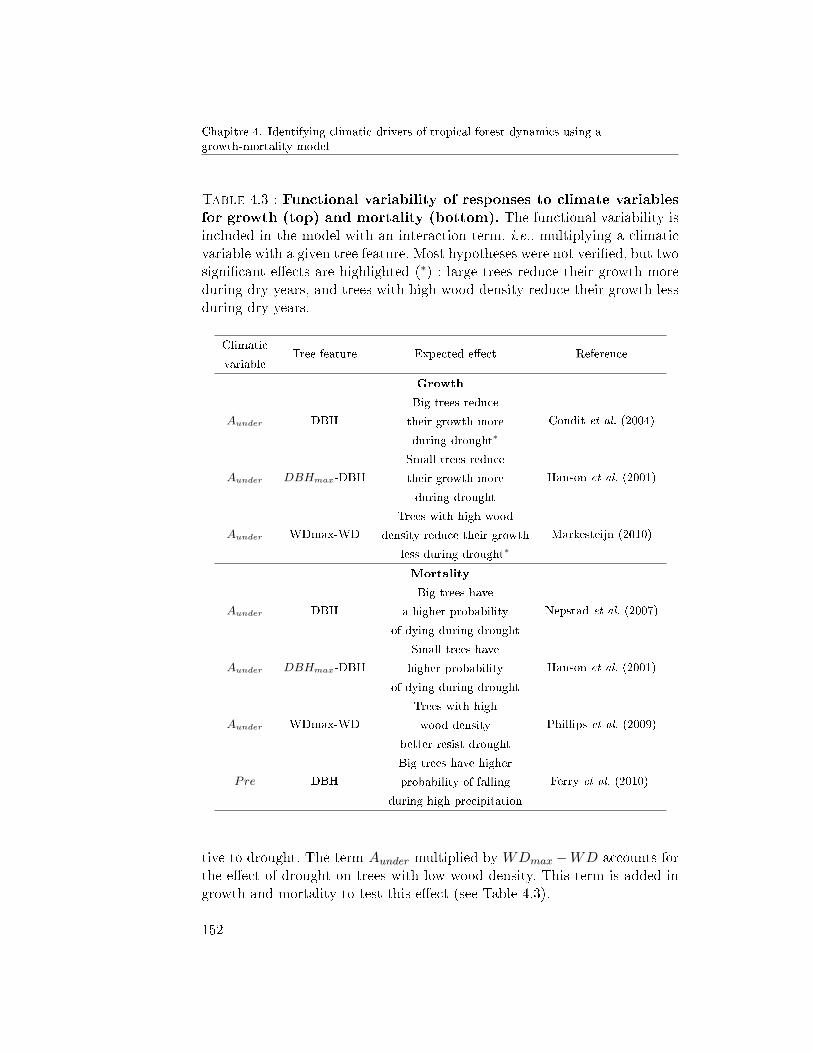
Chapitre 4. Identifying climatic drivers of tropical forest dynamics using agrowth-mortality model
Table 4.3 : Functional variability of responses to climate variablesfor growth (top) and mortality (bottom). The functional variability isincluded in the model with an interaction term, i.e., multiplying a climaticvariable with a given tree feature. Most hypotheses were not veri�ed, but twosigni�cant e�ects are highlighted (∗) : large trees reduce their growth moreduring dry years, and trees with high wood density reduce their growth lessduring dry years.
ClimaticTree feature Expected e�ect Reference
variable
Growth
Aunder DBH
Big trees reduce
Condit et al. (2004)their growth more
during drought∗
Aunder DBHmax-DBH
Small trees reduce
Hanson et al. (2001)their growth more
during drought
Aunder WDmax-WD
Trees with high wood
Markesteijn (2010)density reduce their growth
less during drought∗
Mortality
Aunder DBH
Big trees have
Nepstad et al. (2007)a higher probability
of dying during drought
Aunder DBHmax-DBH
Small trees have
Hanson et al. (2001)higher probability
of dying during drought
Aunder WDmax-WD
Trees with high
Phillips et al. (2009)wood density
better resist drought
Pre DBH
Big trees have higher
Ferry et al. (2010)probability of falling
during high precipitation
tive to drought. The term Aunder multiplied by WDmax −WD accounts forthe e�ect of drought on trees with low wood density. This term is added ingrowth and mortality to test this e�ect (see Table 4.3).
152
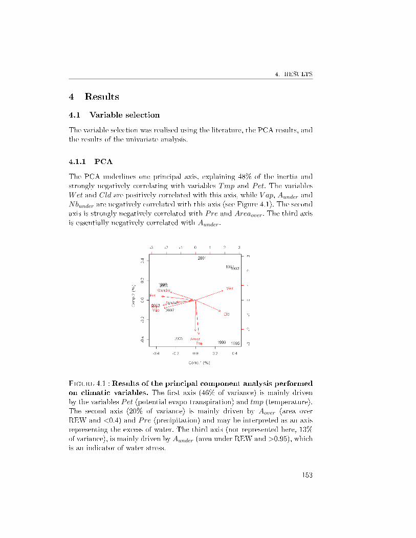
4. RESULTS
4 Results
4.1 Variable selection
The variable selection was realised using the literature, the PCA results, andthe results of the univariate analysis.
4.1.1 PCA
The PCA underlines one principal axis, explaining 48% of the inertia andstrongly negatively correlating with variables Tmp and Pet. The variablesWet and Cld are positively correlated with this axis, while V ap, Aunder andNbunder are negatively correlated with this axis (see Figure 4.1). The secondaxis is strongly negatively correlated with Pre and Areaover. The third axisis essentially negatively correlated with Aunder.
Figure 4.1 : Results of the principal component analysis performedon climatic variables. The �rst axis (46% of variance) is mainly drivenby the variables Pet (potential evapo-transpiration) and tmp (temperature).The second axis (20% of variance) is mainly driven by Aover (area overREW and <0.4) and Pre (precipitation) and may be interpreted as an axisrepresenting the excess of water. The third axis (not represented here, 13%of variance), is mainly driven by Aunder (area under REW and >0.95), whichis an indicator of water stress.
153
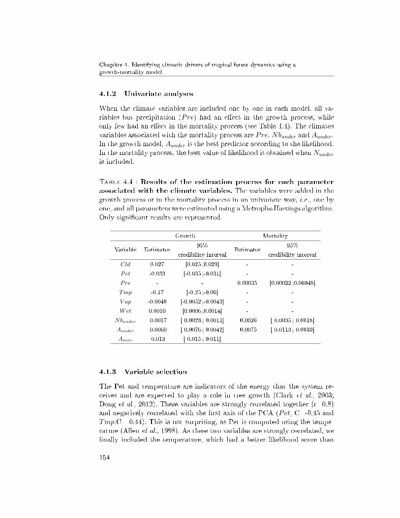
Chapitre 4. Identifying climatic drivers of tropical forest dynamics using agrowth-mortality model
4.1.2 Univariate analyses
When the climate variables are included one by one in each model, all va-riables but precipitation (Pre) had an e�ect in the growth process, whileonly few had an e�ect in the mortality process (see Table 4.4). The climatesvariables associated with the mortality process are Pre, Nbunder and Aunder.In the growth model, Aunder is the best predictor according to the likelihood.In the mortality process, the best value of likelihood is obtained when Nunder
is included.
Table 4.4 : Results of the estimation process for each parameterassociated with the climate variables. The variables were added in thegrowth process or in the mortality process in an univariate way, i.e., one byone, and all parameters were estimated using a Metroplis-Hastings algorithm.Only signi�cant results are represented.
Growth Mortality
Variable Estimator95%
Estimator95%
credibility interval credibility interval
Cld 0.027 [0.025 ;0.029] - -
Pet -0.033 [-0.035 ;-0.031] - -
Pre - - 0.00035 [0.00022 ;0.00048]
Tmp -0.17 [-0.25 ;-0.06] - -
V ap -0.0048 [-0.0052 ;-0.0043] - -
Wet 0.0010 [0.0006 ;0.0014] - -
Nbunder -0.0017 [-0.0023 ;-0.0011] -0.0026 [-0.0035 ;-0.0018]
Aunder -0.0060 [-0.0076 ;-0.0042] -0.0075 [-0.0113 ;-0.0039]
Aover -0.013 [-0.015 ;-0.011] - -
4.1.3 Variable selection
The Pet and temperature are indicators of the energy that the system re-ceives and are expected to play a role in tree growth (Clark et al., 2003;Dong et al., 2012). These variables are strongly correlated together (r=0.8)and negatively correlated with the �rst axis of the PCA (Pet, C=-0.45 andTmp,C=-0.44). This is not surprising, as Pet is computed using the tempe-rature (Allen et al., 1998). As these two variables are strongly correlated, we�nally included the temperature, which had a better likelihood score than
154
4. RESULTS
Pet when it is included in the growth model. Neither Pet nor the tempera-ture had an e�ect if included in the mortality process. The second axis ofthe PCA is related to water saturation and is correlated with Pre (C=-0.68)and Aover (C=-0.61) ; only Aover had an e�ect when included in the growthprocess, but the likelihood is the worst score obtained, which is why we didnot include this variable in the �nal model. Concerning mortality, Pre hadan e�ect and is thus included in both the �nal growth and mortality model.The third axis of the PCA is strongly correlated with the drought estimatorAunder, which is the better climate driver of growth regarding the likelihood.Aunder also had an e�ect on the mortality process, and is �nally included inthe two processes in the �nal model.
4.2 Full model inference
The growth trajectory was adjusted by a size-dependent diameter growthmodel. Parameters linking the maximal growth to the functional traits WD,DBHmax, Hmax and δ13C have have similar values to (Hérault et al.,2011) (see Table 4.5), i.e., maximum growth rates increase with increasingDBHmax, and decreasing WD, Hmax and δ13C. Diameter at maximumgrowth is attained for 0.794*DBHmax. The parameters linking the proba-bility of mortality to Hmax, WD and Tough converged around negativevalues, meaning that the probability of dying is lower when the tree is high,has a high wood density and/or high laminar toughness. The drought es-timator (Aunder) converged to negative values in the growth and mortalityprocesses ; thus growth and mortality computed at our biannual time-scaleare lower when the drought estimator Aunder is higher. The parameter lin-king mortality with precipitation (Pre) is positive. This �nding implies thatmortality rate is higher during two-year time-scale with high precipitation.The parameter linking temperature (tmp) and growth takes negative values ;thus growth values are lower during the warmest periods.
4.3 Functional variability of responses
In the growth process, interaction between WDmax −WD and drought isnegative (Table 4.3), implying that trees with lower WD are more sensitiveto drought and reduce their growth more. Moreover, interactions linking thecurrent diameter and drought are also negative ; thus larger trees are moresensitive to drought and reduce their growth more compared to smaller trees.None of the interaction terms included in the mortality process had an e�ect(Table 4.3).
155
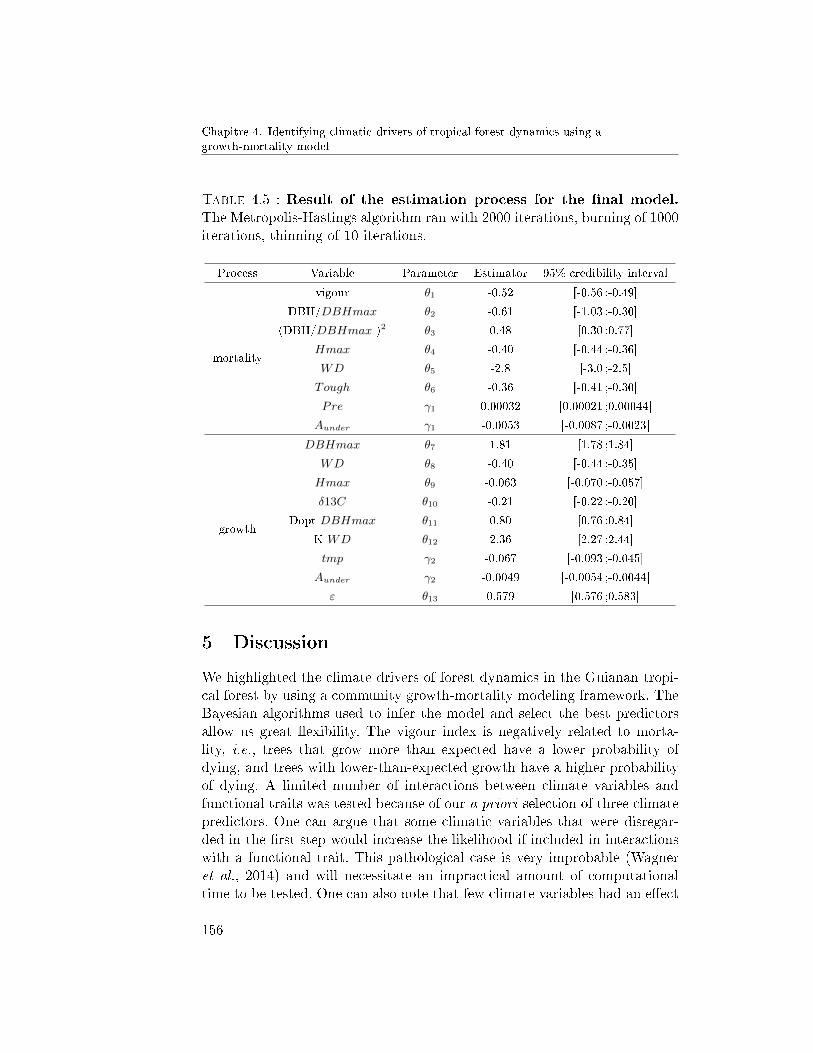
Chapitre 4. Identifying climatic drivers of tropical forest dynamics using agrowth-mortality model
Table 4.5 : Result of the estimation process for the �nal model.The Metropolis-Hastings algorithm ran with 2000 iterations, burning of 1000iterations, thinning of 10 iterations.
Process Variable Parameter Estimator 95% credibility interval
mortality
vigour θ1 -0.52 [-0.56 ;-0.49]
DBH/DBHmax θ2 -0.61 [-1.03 ;-0.30]
(DBH/DBHmax )2 θ3 0.48 [0.30 ;0.77]
Hmax θ4 -0.40 [-0.44 ;-0.36]
WD θ5 -2.8 [-3.0 ;-2.5]
Tough θ6 -0.36 [-0.41 ;-0.30]
Pre γ1 0.00032 [0.00021 ;0.00044]
Aunder γ1 -0.0053 [-0.0087 ;-0.0023]
growth
DBHmax θ7 1.81 [1.78 ;1.84]
WD θ8 -0.40 [-0.44 ;-0.35]
Hmax θ9 -0.063 [-0.070 ;-0.057]
δ13C θ10 -0.21 [-0.22 ;-0.20]
Dopt DBHmax θ11 0.80 [0.76 ;0.84]
K WD θ12 2.36 [2.27 ;2.44]
tmp γ2 -0.067 [-0.093 ;-0.045]
Aunder γ2 -0.0049 [-0.0054 ;-0.0044]
ε θ13 0.579 [0.576 ;0.583]
5 Discussion
We highlighted the climate drivers of forest dynamics in the Guianan tropi-cal forest by using a community growth-mortality modeling framework. TheBayesian algorithms used to infer the model and select the best predictorsallow us great �exibility. The vigour index is negatively related to morta-lity, i.e., trees that grow more than expected have a lower probability ofdying, and trees with lower-than-expected growth have a higher probabilityof dying. A limited number of interactions between climate variables andfunctional traits was tested because of our a priori selection of three climatepredictors. One can argue that some climatic variables that were disregar-ded in the �rst step would increase the likelihood if included in interactionswith a functional trait. This pathological case is very improbable (Wagneret al., 2014) and will necessitate an impractical amount of computationaltime to be tested. One can also note that few climate variables had an e�ect
156
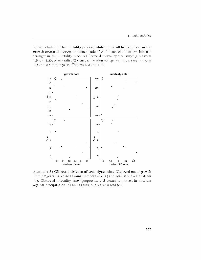
5. DISCUSSION
when included in the mortality process, while almost all had an e�ect in thegrowth process. However, the magnitude of the impact of climate variables isstronger in the mortality process (observed mortality rate varying between1.6 and 2.5% of mortality/2 years, while observed growth rates vary between1.9 and 2.5 mm/2 years, Figures 4.2 and 4.3).
Figure 4.2 : Climatic drivers of tree dynamics. Observed mean growth(mm / 2 years) is plotted against temperature (a) and against the water stress(b). Observed mortality rate (proportion / 2 years) is plotted in abscissaagainst precipitation (c) and against the water stress (d).
157
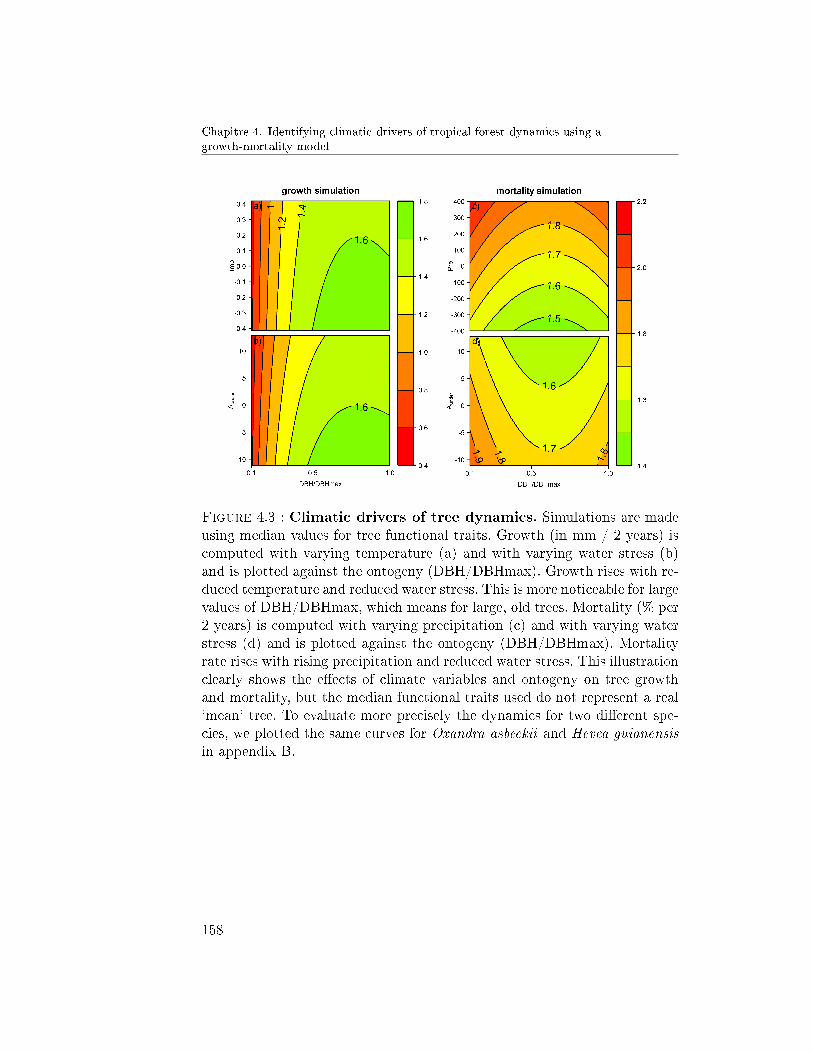
Chapitre 4. Identifying climatic drivers of tropical forest dynamics using agrowth-mortality model
Figure 4.3 : Climatic drivers of tree dynamics. Simulations are madeusing median values for tree functional traits. Growth (in mm / 2 years) iscomputed with varying temperature (a) and with varying water stress (b)and is plotted against the ontogeny (DBH/DBHmax). Growth rises with re-duced temperature and reduced water stress. This is more noticeable for largevalues of DBH/DBHmax, which means for large, old trees. Mortality (% per2 years) is computed with varying precipitation (c) and with varying waterstress (d) and is plotted against the ontogeny (DBH/DBHmax). Mortalityrate rises with rising precipitation and reduced water stress. This illustrationclearly shows the e�ects of climate variables and ontogeny on tree growthand mortality, but the median functional traits used do not represent a real`mean' tree. To evaluate more precisely the dynamics for two di�erent spe-cies, we plotted the same curves for Oxandra asbeckii and Hevea guianensisin appendix B.
158
5. DISCUSSION
5.1 Water stress
The water stress during the dry season, estimated with Aunder, negativelyimpacts the growth and mortality processes. Trees will thus grow less qui-ckly and have a lower probability of dying during two-year periods with themost intense dry seasons. The reduction of growth is expected, and has manyecophysiological causes. Indeed, water is essential for sap �uxes and for pho-tosynthesis e�ciency. The reduction of growth is furthermore linked with thecurrent DBH and the species' wood density (Table 4.3). Big trees are moresensitive to water stress than small trees. This was expected in light of theresults obtained after rainfall exclusion (da Costa et al., 2010). Indeed, main-tenance costs are higher for big trees, making these trees more vulnerable tothe driest periods. Regarding the wood density, species with high values aremore resistant to drought. This is consistent with our hypothesis that highwood density implies thin and short xylem vessels and thus decreases the riskof embolism and cavitation. As the ability of trees to recover from periodsof sustained drought is strongly related to their embolism resistance (Choatet al., 2012), a tree with high wood density will be more able to maintaingrowth during dry years. For similar reasons, we expected a positive impactof Aunder on mortality, as long-time drought may increase mortality rates.Results showed the inverse pattern, but this may be explained by some �eldobservations. After experimental trough-fall exclusions, high mortality rateswere observed in Tapajos and Caxiuaña, and our results seemed to be contra-dictory. The real intensity of the drought during the driest seasons in ourdataset is, by far, less stressful than the 50% rainfall exclusion performed du-ring the experiment (Nepstad, 2002). Moreover, our time-scale of two yearsand our framework prevented us from seeing long-term e�ects induced byrepeated drought events. When plotting tree mode of death against droughtestimator (Aunder), no evidence was observed for a potential trend (Figure4.4), suggesting that standing death is not more frequent during the driestperiods. To conclude, our results con�rmed that the relationship betweendrought and mortality may be challenging to estimate and to link with theirunderlying causes at an inter-annual time scale.
5.2 Water saturation
Water saturation had a strong e�ect on mortality ; mortality rate variedbetween 1.5 and 2% per 2-years with increasing total precipitation. This isconsistent with the hypothesis that trees are more vulnerable when the soilis saturated. When looking at the cause of tree death, about half of tree
159
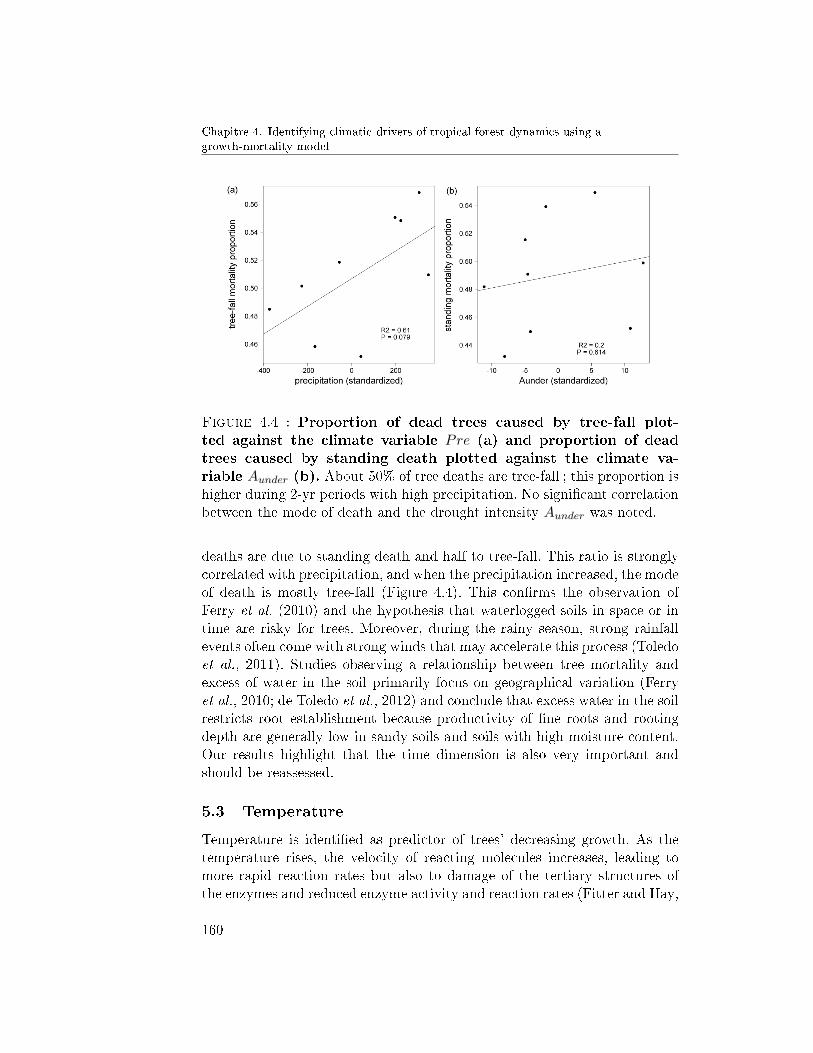
Chapitre 4. Identifying climatic drivers of tropical forest dynamics using agrowth-mortality model
Figure 4.4 : Proportion of dead trees caused by tree-fall plot-ted against the climate variable Pre (a) and proportion of deadtrees caused by standing death plotted against the climate va-riable Aunder (b). About 50% of tree deaths are tree-fall ; this proportion ishigher during 2-yr periods with high precipitation. No signi�cant correlationbetween the mode of death and the drought intensity Aunder was noted.
deaths are due to standing death and half to tree-fall. This ratio is stronglycorrelated with precipitation, and when the precipitation increased, the modeof death is mostly tree-fall (Figure 4.4). This con�rms the observation ofFerry et al. (2010) and the hypothesis that waterlogged soils in space or intime are risky for trees. Moreover, during the rainy season, strong rainfallevents often come with strong winds that may accelerate this process (Toledoet al., 2011). Studies observing a relationship between tree mortality andexcess of water in the soil primarily focus on geographical variation (Ferryet al., 2010; de Toledo et al., 2012) and conclude that excess water in the soilrestricts root establishment because productivity of �ne roots and rootingdepth are generally low in sandy soils and soils with high moisture content.Our results highlight that the time dimension is also very important andshould be reassessed.
5.3 Temperature
Temperature is identi�ed as predictor of trees' decreasing growth. As thetemperature rises, the velocity of reacting molecules increases, leading tomore rapid reaction rates but also to damage of the tertiary structures ofthe enzymes and reduced enzyme activity and reaction rates (Fitter and Hay,
160
6. CONCLUSIONS
2001; Lloyd and Farquhar, 2008). These two processes are responsible for abell-shaped curve of growth response to temperature (Fitter and Hay, 2001).Temperature can a�ect photosynthesis through modulation of the rates ofactivity of photosynthetic enzymes and the electron transport chain, andin a more indirect manner, through leaf-temperatures de�ning the magni-tude of the leaf-to-air vapour pressure di�erence, a key factor in�uencingstomatal conductances (Lloyd and Farquhar, 2008). In tropical forests, astemperatures are already high, rising temperatures may imply lower growth,consistent with results from Clark et al. (2003). This temperature e�ect maybecome the most problematic for forest dynamics, considering the risingtemperatures that are predicted, with a great degree of certainty, by climatemodels for the next century (IPCC, 2013). As no consensus has been reachedyet, additional studies using regular inventories are urgently needed (Reedet al., 2012; Corlett, 2011) to explain the con�icting patterns found in theextant literature (Dong et al., 2012).
6 Conclusions
Our study highlights the complex link between the various components ofthe climate and tropical forest dynamics. Our modelling framework allowsus to study inter-annual variations of climatic variables and identify whichof these climatic variables are the drivers of tree dynamics in the study siteof Paracou, French Guiana. Drought, precipitation and temperature werehighlighted as strong drivers of tree growth and/or mortality. Drought is ex-pected to become longer and stronger in the future ; precipitation is expectedto be drastically reduced, and the temperature will rise drastically during thenext century. Thus, in light of our results, raising awareness of the potentialimpacts of climate changes on tropical forest dynamics is urgent.
Acknowledgements
Funding came from the Climfor Project (Fondation pour la Recherche sur laBiodiversité) and from the Guyasim Project (European structural funding,PO-feder). The funders had no role in study design, data collection and ana-lysis, decision to publish or preparation of the manuscript. This work alsobene�ted from an `Investissement d'Avenir' grant managed by the AgenceNationale de la Recherche (CEBA, ref ANR-10-LABX-0025) and from agrant from the Centre de Coopération Internationale en Recherche Agrono-mique pour le Développement.
161

BIBLIOGRAPHIE
Allen, C. D., Macalady, A. K., Chenchouni, H., Bachelet, D., McDowell, N.,Vennetier, M., Kitzberger, T., Rigling, A., Breshears, D. D., Hogg, E.T. H., Gonzalez, P., Fensham, R., Zhang, Z., Castro, J., Demidova, N.,Lim, J.-H. H., Allard, G., Running, S. W., Semerci, A., and Cobb, N.(2010). A global overview of drought and heat-induced tree mortalityreveals emerging climate change risks for forests. Forest Ecology andManagement, 259(4):660�684.
Allen, R. G., Pereira, L. S., Raes, D., and Smith, M. (1998). Crop evapo-transpiration - Guidelines for computing crop water requirements - FAOIrrigation and drainage paper 56. pages 1�15.
Aragão, L. E. O. C., Malhi, Y., Roman-Cuesta, R. M., Saatchi, S., Anderson,L. O., and Shimabukuro, Y. E. (2007). Spatial patterns and �re responseof recent Amazonian droughts. Geophysical Research Letters, 34(7):L07701.
Aubry-Kientz, M., Hérault, B., Ayotte-Trépanier, C., Baraloto, C., and Rossi,V. (2013). Toward trait-based mortality models for tropical forests. PloSone, 8(5):e63678.
Baraloto, C., Paine, C. E. T., Patiño, S., Bonal, D., Hérault, B., and Chave,J. (2010a). Functional trait variation and sampling strategies in species-rich plant communities. Functional Ecology, 24(1):208�216.
Baraloto, C., Paine, C. E. T., Poorter, L., Beauchene, J., Bonal, D., Dome-nach, A. M., Hérault, B., Patino, S., Roggy, J. C., and Chave, J. (2010b).
162
BIBLIOGRAPHIE
Decoupled leaf and stem economics in rain forest trees. Ecology Letters,13(11):1338�1347.
Brando, P. M., Goetz, S. J., Baccini, A., Nepstad, D. C., Beck, P. S. a., andChristman, M. C. (2010). Seasonal and interannual variability of climateand vegetation indices across the Amazon. Proceedings of the NationalAcademy of Sciences of the United States of America, 107(33):14685�90.
Brando, P. M., Nepstad, D. C., Davidson, E. a., Trumbore, S. E., Ray, D., andCamargo, P. (2008). Drought e�ects on littefall, wood production andbelowground carbon cycling in an Amazon Forest : result of a throughfallreduction experiment. Philosophical Transactions of the Royal Society,363(1498):1839�1848.
Chave, J., Muller-Landau, H. C., Baker, T. R., Easdale, T. a., ter Steege, H.,and Webb, C. O. (2006). Regional and phylogenetic variation of wooddensity across 2456 Neotropical tree species. Ecological applications : apublication of the Ecological Society of America, 16(6):2356�67.
Chave, J. J., Coomes, D., Jansen, S., Lewis, S. L., Swenson, N. G., andZanne, A. E. (2009). Towards a worldwide wood economics spectrum.Ecology letters, 12(4):351�66.
Choat, B., Jansen, S., Brodribb, T. J., Cochard, H., Delzon, S., Bhaskar, R.,Bucci, S. J., Feild, T. S., Gleason, S. M., Hacke, U. G., Jacobsen, A. L.,Lens, F., Maherali, H., Martínez-Vilalta, J., Mayr, S., Mencuccini, M.,Mitchell, P. J., Nardini, A., Pittermann, J., Pratt, R. B., Sperry, J. S.,Westoby, M., Wright, I. J., and Zanne, A. E. (2012). Global convergencein the vulnerability of forests to drought. Nature, 491(7426):752�5.
Clark, D. a., Piper, S. C., Keeling, C. D., and Clark, D. B. (2003). Tropi-cal rain forest tree growth and atmospheric carbon dynamics linkedto interannual temperature variation during 1984-2000. Proceedingsof the National Academy of Sciences of the United States of America,100(10):5852�7.
Condit, R., Aguilar, S., Hernandez, A., Perez, R., Lao, S., Angehr, G., Hub-bell, S. P., and Foster, R. B. (2004). Tropical forest dynamics across arainfall gradient and the impact of an El Nino dry season. Journal ofTropical Ecology, 20:51�72.
core Team, R. (2014). R : A Language and Environment for StatisticalComputing.
163
Chapitre 4. Identifying climatic drivers of tropical forest dynamics using agrowth-mortality model
Corlett, R. T. (2011). Impacts of warming on tropical lowland rainforests.Trends in Ecology and Evolution, 26(11):606�613.
da Costa, A. C. L., Galbraith, D., Almeida, S., Portela, B. T. T., da Costa,M., Silva Junior, J. a. D. A., Braga, A. P., de Gonçalves, P. H. L.,de Oliveira, A. a. R., Fisher, R., Phillips, O. L., Metcalfe, D. B., Levy, P.,and Meir, P. (2010). E�ect of 7 yr of experimental drought on vegetationdynamics and biomass storage of an eastern Amazonian rainforest. TheNew phytologist, 187(3):579�91.
de Toledo, J. J., Magnusson, W. E., Castilho, C. V., and Nascimento, H.E. M. (2012). Tree mode of death in Central Amazonia : E�ects of soiland topography on tree mortality associated with storm disturbances.Forest Ecology and Management, 263:253�261.
Dong, S. X., Davies, S. J., Ashton, P. S., Bunyavejchewin, S., Supardi, M.N. N., Kassim, A. R., Tan, S., and Moorcroft, P. R. (2012). Variability insolar radiation and temperature explains observed patterns and trendsin tree growth rates across four tropical forests. Proceedings. Biologicalsciences / The Royal Society, 279(1744):3923�31.
Ferry, B., Morneau, F., Bontemps, J. D., Blanc, L., and Freycon, V. (2010).Higher treefall rates on slopes and waterlogged soils result in lower standbiomass and productivity in a tropical rain forest. Journal of Ecology,98(1):106�116.
Fitter, A. H. and Hay, R. K. (2001). Environmental physiology of plants.Academic p edition.
Grogan, J. and Schulze, M. (2012). The Impact of Annual and SeasonalRainfall Patterns on Growth and Phenology of Emergent Tree Speciesin Southeastern Amazonia, Brazil. Biotropica, 44(3):331�340.
Hanson, P. J., Todd, D. E., and Amthor, J. S. (2001). A six-year study ofsapling and large-tree growth and mortality responses to natural andinduced variability in precipitation and throughfall. Tree physiology,21(6):345�58.
Hérault, B., Bachelot, B., Poorter, L., Rossi, V., Bongers, F., Chave, J.,Paine, C. E. T., Wagner, F., and Baraloto, C. (2011). Functional traitsshape ontogenetic growth trajectories of rain forest tree species. Journalof Ecology, 99(6):1431�1440.
164
BIBLIOGRAPHIE
Iida, Y., Poorter, L., Sterck, F. J., Kassim, A. R., Kubo, T., Potts, M. D.,and Kohyama, T. S. (2012). Wood density explains architectural dif-ferentiation across 145 co-occurring tropical tree species. FunctionalEcology, 26(1):274�282.
IPCC (2013). Climate change 2013 : the scienti�c basis. contribution of wor-king group 1 to the fourth assessment report of the intergovernmentalpanel on climate change. Cambridge University Press.
Lloyd, J. and Farquhar, G. D. (2008). E�ects of rising temperatures and[CO2] on the physiology of tropical forest trees. Philosophical tran-sactions of the Royal Society of London. Series B, Biological sciences,363(1498):1811�7.
Malhi, Y., Aragão, L. E. O. C., Galbraith, D., Huntingford, C., Fisher, R.,Zelazowski, P., Sitch, S., Mcsweeney, C., and Meir, P. (2009). Exploringthe likelihood and mechanism of a climate-change-induced dieback ofthe Amazon rainforest.
Markesteijn, L. (2010). Drought tolerance of tropical tree species ; FunctionalTraits, Trade-o�s and Species Distribution. PhD thesis, WageningenUniversity.
Mitchell, T. D. and Jones, P. D. (2005). An improved method of construc-ting a database of monthly climate observations and associated high-resolution grids. International Journal of Climatology, 25(6):693�712.
Nepstad, D. C. (2002). The e�ects of partial throughfall exclusion on canopyprocesses, aboveground production, and biogeochemistry of an Amazonforest. Journal of Geophysical Research, 107(D20):8085.
Nepstad, D. C., Tohver, I. M., Ray, D., Moutinho, P., and Cardinot, G.(2007). Mortality of large trees and lianas following experimentaldrought in an Amazon forest. Ecology, 88(9):2259�69.
Phillips, O. L., Aragao, L., Lewis, S. L., Fisher, J. B., Lloyd, J., Lopez-Gonzalez, G., Malhi, Y., Monteagudo, A., Peacock, J., Quesada, C. A.,van der Heijden, G., Almeida, S., Amaral, I., Arroyo, L., Aymard, G.,Baker, T. R., Banki, O., Blanc, L., Bonal, D., Brando, P., Chave, J.,de Oliveira, A. C. A., Cardozo, N. D., Czimczik, C. I., Feldpausch,T. R., Freitas, M. A., Gloor, E., Higuchi, N., Jimenez, E., Lloyd, G.,Meir, P., Mendoza, C., Morel, A., Neill, D. A., Nepstad, D., Patino, S.,Penuela, M. C., Prieto, A., Ramirez, F., Schwarz, M., Silva, J., Silveira,
165
Chapitre 4. Identifying climatic drivers of tropical forest dynamics using agrowth-mortality model
M., Thomas, A. S., ter Steege, H., Stropp, J., Vasquez, R., Zelazowski,P., Davila, E. A., Andelman, S., Andrade, A., Chao, K.-j. J., Erwin, T.,Di Fiore, A., Honorio, E., Keeling, H., Killeen, T. J., Laurance, W. F.,Cruz, A. P. n., Pitman, N. C. A., Vargas, P. N. n., Ramirez-Angulo,H., Rudas, A., Salamao, R., Silva, N., Terborgh, J., Torres-Lezama, A.,Aragão, L. E. O. C., López-gonzález, G., Heijden, G. V. D., Bánki, O.,Cristina, A., Oliveira, A. D., Jiménez, E., Patiño, S., Peñuela, M. C.,Ramírez, F., Steege, H., Vásquez, R., Dávila, E. A., Fiore, A. D., C,E. H., Ramírez-angulo, H., and Salamão, R. (2009). Drought sensitivityof the Amazon Rainforest. Science, 323(March):1344�1347.
Poorter, L., Wright, S. J., Paz, H., Ackerly, D. D., Condit, R., Ibarra-Manríquez, G., Harms, K. E., Licona, J.-C., Martínez-Ramos, M., Ma-zer, S. J., Muller-Landau, H. C., Peña Claros, M., Webb, C. O., andWright, I. J. (2008). Are functional traits good predictors of demogra-phic rates ? Evidence from �ve Neotropical forests. Ecology, 89(7):1908�1920.
Reed, S. C., Wood, T. E., and Cavaleri, M. A. (2012). Tropical forests in awarming world. New Phytologist, 193:27�29.
Robert, C. P. and Casella, G. (2004). Monte Carlo statistical methods. Sprin-ger, 2 edition.
Rüger, N., Wirth, C., Wright, S. J., and Condit, R. (2012). Functional traitsexplain light and size response of growth rates in tropical tree species.Ecology, 93(12):2626�2636.
Toledo, M., Poorter, L., Peña Claros, M., Alarcón, A., Balcázar, J., Leaño,C., Licona, J. C., Llanque, O., Vroomans, V., Zuidema, P. A., and Bon-gers, F. (2011). Climate is a stronger driver of tree and forest growthrates than soil and disturbance. Journal of Ecology, 99(1):254�264.
Wagner, F., Hérault, B., Stahl, C., Bonal, D., and Rossi, V. (2011). Modelingwater availability for trees in tropical forests. Agricultural and ForestMeteorology, 151(9):1202�1213.
Wagner, F., Rossi, V., Baraloto, C., Bonal, D., Stahl, C., and Hérault, B.(2014). Are Commonly Measured Functional Traits Involved in TropicalTree Responses to Climate ? International Journal of Ecology, 2014(i):1�10.
166

BIBLIOGRAPHIE
Wagner, F., Rossi, V., Stahl, C., Bonal, D., and Hérault, B. (2012). WaterAvailability Is the Main Climate Driver of Neotropical Tree Growth.Plos One, 7(4):e34074.
Zuidema, P. a., Baker, P. J., Groenendijk, P., Schippers, P., van der Sleen,P., Vlam, M., and Sterck, F. (2013). Tropical forests and global change :�lling knowledge gaps. Trends in plant science, 18(8):413�9.
167
Chapitre 4. Identifying climatic drivers of tropical forest dynamics using agrowth-mortality model
4.A Total likelihood of the growth-mortality model
Growth and mortality processes were linked through tree vigour and areparametrized simultaneously. If tree i stays alive, it grows at a growth rateAGRi,s,t, and its diameter Di,t−1 becomes Di,t. The joint model likelihoodis then
•∏nt=1 f(Di,t|Di,t−1) ∗ (1 − pi,s,t) if tree i stays alive during the length
of the studied period,
• pi,s,k∗∏k−1t=1 (f(Di,t|Di,t−1) ∗ (1− pi,s,t)) if tree i dies between time k−1
and time k,
where
• f(Di,t|Di,t−1) is the probability density for a tree with diameter Di,t−1
at time t − 1 to have a diameter Di,t at time t ; this quantity is usedto compute the vigour estimator.
• pi,s,t is the probability of dying between time t − 1 and time t, whichdepends on the vigour estimator, added in the model by multiplyingthe vigour estimator by β0.
The model computes a mortality probability pi,s,t and a predicted growthrate AGRi,s,t.
4.B Growth and mortality simulations for Oxandra
an Hevea
Simulations presented in Figure 4.3 are realized using median values for treefunctional traits. These median values do not have any ecological meaning,and the �gure was realized only to show how climatic drivers impact the treegrowth and mortality in reality (Figure 4.2) and in our model (Figure 4.3). Toshow more realistic simulations, the same patterns are plotted for two speciesthat di�er in their ecological strategies in Figure 4.5. The �rst column showsthe simulated dynamics of Oxandra asbeckii, a relatively small tree. Thesecond column shows the simulated dynamics of Hevea guianensis, whichis a canopy tree reaching heights of 50 meters and which has a low wooddensity. These two strongly contrasting species show two di�erent growthand mortality rates, although the e�ects of climatic drivers stay the same.
168
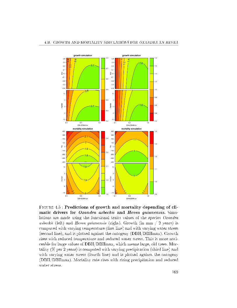
4.B. GROWTH AND MORTALITY SIMULATIONS FOR OXANDRA AN HEVEA
Figure 4.5 : Predictions of growth and mortality depending of cli-matic drivers for Oxandra asbeckii and Hevea guianensis. Simu-lations are made using the functional traits values of the species Oxandraasbeckii (left) and Hevea guianensis (right). Growth (in mm / 2 years) iscomputed with varying temperature (�rst line) and with varying water stress(second line), and is plotted against the ontogeny (DBH/DBHmax). Growthrises with reduced temperature and reduced water stress. This is more noti-ceable for large values of DBH/DBHmax, which means large, old trees. Mor-tality (% per 2 years) is computed with varying precipitation (third line) andwith varying water stress (fourth line) and is plotted against the ontogeny(DBH/DBHmax). Mortality rate rises with rising precipitation and reducedwater stress.
169
CHAPITRE 5
WILL TROPICAL FORESTS FACE SLOW DOWNWITH ONGOING CLIMATE CHANGES?
Mélaine Aubry-Kientz1∗
Vivien Rossi 2,3,4
Guillaume Cornu3
Fabien Wagner 2,5
Bruno Hérault 2
1 Université des Antilles et de la Guyane, UMR `Ecologie des Forêts de Guya-ne', Campus agronomique de Kourou, France.2 CIRAD, UMR `Ecologie des Forêts de Guyane', Campus agronomique deKourou, France.3 CIRAD, UPR Bsef, Montpellier, France.4 Université de Yaoundé I, UMMISCO (UMI 209), BP337, Yaoundé, Came-roun.5 Remote sensing division, National Institute for Space Research-INPE, SãoJosé dos Campos, SP, Brazil.∗ Email : [email protected]
170
Un modèle de croissance et de mortalité climat-dépendant a été construitpour la forêt tropicale de Paracou, et les dernières prédictions climatiques duGIEC pour le siècle prochain sont disponibles. Il ne reste donc plus qu'un pasà faire pour simuler la dynamique de la forêt tropicale de Paracou soumiseaux changements climatiques prévus. C'est ce que je propose de faire dansce dernier chapitre grâce au simulateur SELVA. La communauté d'arbreest simulée et à chaque pas de temps, le recrutement, la croissance et lamortalité sont modélisés. En utilisant des scénarios climatiques basés sur lesprédictions du dernier rapport du GIEC, nous observons une diminution de lacroissance et de la mortalité, accompagnées par une diminution de la surfaceterrière, du diamètre quadratique et de la biomasse de notre communauté.Ces simulations, loin de prédire l'avenir, montrent comment la températurepeut impacter les processus, et donnent des pistes de ré�exions pour mieuxenvisager la réponse des forêts tropicales aux changements climatiques.
171

Chapitre 5. Will tropical forests face slow down with ongoing climate changes ?
1 Abstract
• Climate changes are expected to continue all over the world. Below thetropics, temperatures are expected to rise and dry periods to be stron-ger and longer. As some climate variables were identi�ed as key driversof tropical forest dynamics, the later will likely be deeply impacted.
• To provide some elements of response, we submitted a simulated tro-pical forest community to the climate changes expected over the nextcentury. We used SELVA, an individual-based model calibrated withforest dynamic data from the Paracou study site in French Guiana tosimulate the forest trajectory over the next 100 years. The model is cli-mate dependent, such that temperature, precipitation and water stressare used as predictors of growth and/or mortality rates.
• We ran simulations for the next century using predictions of the IPCC5AR, building three di�erent scenarios corresponding to three relativeconcentration pathways. The basal area, above-ground fresh biomass,quadratic diameter, tree growth and mortality rates were then compu-ted to characterize the resulting forest.
• All processes and resulting structure variables exhibited decreasing va-lues as the scenario became pessimistic. A sensitivity analysis identi�edtemperature as the stronger climate driver of this behaviour, highligh-ting a temperature-driven drop of 40% in average forest growth anda precipitation-driven drop of 30% in mortality rates for the RCP8.5scenario.
• This conclusion is alarming, as temperature rises were predicted by allclimate scenarios of the IPCC 5AR. Our study highlights the potentialslow-down danger that tropical forests will face during the next century.
2 Introduction
In the context of climate changes, more and more e�orts are being made todescribe the climatic drivers of tropical forest dynamics. The identi�cation ofthese drivers is essential to model and predict the implications for the forestdynamics. Water and temperature are currently the two principal drivers ofinterest.
Water comes in a variety of indexes, (i) water availability for trees mostappropriate to estimate drought (Wagner et al., 2011; Malhi et al., 2009) or
172
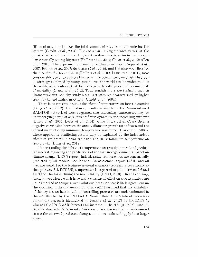
2. INTRODUCTION
(ii) total precipitation, i.e. the total amount of water annually entering thesystem (Condit et al., 2004). The consensus among researchers is that thegreatest e�ect of drought on tropical tree dynamics is a rise in tree morta-lity, especially among big trees (Phillips et al., 2009; Choat et al., 2012; Allenet al., 2010). The experimental troughfall exclusion in Brazil (Nepstad et al.,2007; Brando et al., 2008; da Costa et al., 2010), and the observed e�ects ofthe drought of 2005 and 2010 (Phillips et al., 2009; Lewis et al., 2011), wereconsiderably useful to address this issue. The convergence on a risky hydrau-lic strategy exhibited by many species over the world can be understood asthe result of a trade-o� that balances growth with protection against riskof mortality (Choat et al., 2012). Total precipitations are typically used tocharacterise wet and dry study sites. Wet sites are characterised by highertree growth and higher mortality (Condit et al., 2004).
There is no consensus about the e�ect of temperature on forest dynamics(Dong et al., 2012). For instance, results arising from the Amazon-basedRAINFOR network of plots suggested that increasing temperature may bean underlying cause of accelerating forest dynamics and increasing turnover(Baker et al., 2004; Lewis et al., 2004), while at La Selva, Costa Rica, anegative correlation between the annual diameter growth rate of trees and theannual mean of daily minimum temperature was found (Clark et al., 2003).These apparently con�icting results may be explained by the independente�ects of variability in solar radiation and daily minimum temperature ontree growth (Dong et al., 2012).
Understanding the e�ects of temperature on tree dynamics is of particu-lar interest regarding the predictions of the last intergovernmental panel onclimate change (IPCC) report. Indeed, rising temperatures are consensuallypredicted by all models used for the �fth assessment report (5AR) and allover the world. For the business-as-usual scenarios (representative concentra-tion pathway 8.5, RCP8.5), temperature is expected to gain between 2.6 and4.8 ◦C on the earth during the next century (IPCC, 2013). On the contrary,drought evolutions, which have had a consensual e�ect on tree dynamics, arenot as marked as temperature evolutions because there is little agreement onthe evolution of the dry season. Fu et al. (2013) assumed that the variabilityof the dry season length and its controlling processes are underestimated inthe models used by the IPCC 5AR. Nevertheless, an increase of two weeksfor the dry season is highlighted by Joetzjer et al. (2013) for the RCP8.5 ;whereas the IPCC 5AR forecasts an increase in the strength of climate va-riability due to El Niño events. We clearly lack the scaling up tools neededto use the observed predicted changes on a �ner scale and apply it to largerareas.
173
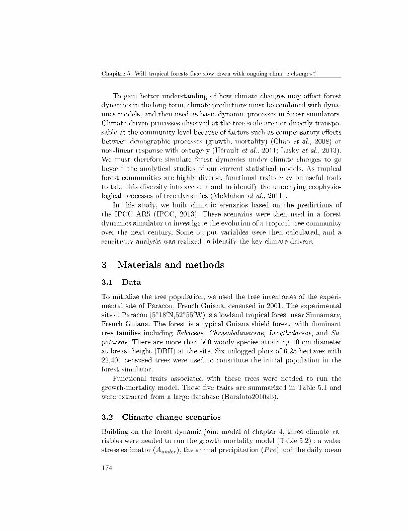
Chapitre 5. Will tropical forests face slow down with ongoing climate changes ?
To gain better understanding of how climate changes may a�ect forestdynamics in the long-term, climate predictions must be combined with dyna-mics models, and then used as basic dynamic processes in forest simulators.Climate-driven processes observed at the tree scale are not directly transpo-sable at the community level because of factors such as compensatory e�ectsbetween demographic processes (growth, mortality) (Chao et al., 2008) ornon-linear response with ontogeny (Hérault et al., 2011; Lasky et al., 2013).We must therefore simulate forest dynamics under climate changes to gobeyond the analytical studies of our current statistical models. As tropicalforest communities are highly diverse, functional traits may be useful toolsto take this diversity into account and to identify the underlying ecophysio-logical processes of tree dynamics (McMahon et al., 2011).
In this study, we built climatic scenarios based on the predictions ofthe IPCC AR5 (IPCC, 2013). These scenarios were then used in a forestdynamics simulator to investigate the evolution of a tropical tree communityover the next century. Some output variables were then calculated, and asensitivity analysis was realized to identify the key climate drivers.
3 Materials and methods
3.1 Data
To initialize the tree population, we used the tree inventories of the experi-mental site of Paracou, French Guiana, censused in 2001. The experimentalsite of Paracou (5◦18′N,52◦55′W) is a lowland tropical forest near Sinnamary,French Guiana. The forest is a typical Guiana shield forest, with dominanttree families including Fabaceae, Chrysobalanaceae, Lecythidaceae, and Sa-potaceae. There are more than 500 woody species attaining 10 cm diameterat breast height (DBH) at the site. Six unlogged plots of 6.25 hectares with22,401 censused trees were used to constitute the initial population in theforest simulator.
Functional traits associated with these trees were needed to run thegrowth-mortality model. These �ve traits are summarized in Table 5.1 andwere extracted from a large database (Baraloto2010ab).
3.2 Climate change scenarios
Building on the forest dynamic joint model of chapter 4, three climate va-riables were needed to run the growth-mortality model (Table 5.2) : a waterstress estimator (Aunder), the annual precipitation (Pre) and the daily mean
174
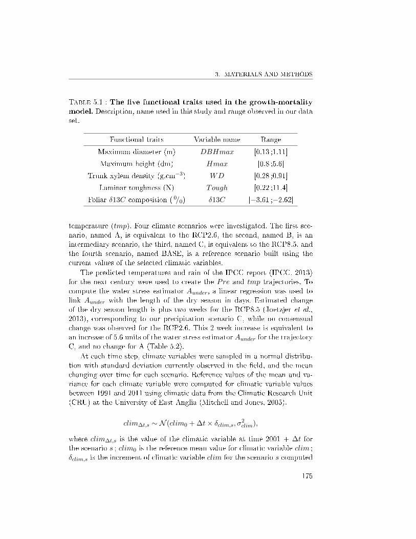
3. MATERIALS AND METHODS
Table 5.1 : The �ve functional traits used in the growth-mortalitymodel. Description, name used in this study and range observed in our dataset.
Functional traits Variable name Range
Maximum diameter (m) DBHmax [0.13 ;1.11]
Maximum height (dm) Hmax [0.8 ;5.6]
Trunk xylem density (g.cm−3) WD [0.28 ;0.91]
Laminar toughness (N) Tough [0.22 ;11.4]
Foliar δ13C composition ( 0/0) δ13C [−3.61 ;−2.62]
temperature (tmp). Four climate scenarios were investigated. The �rst sce-nario, named A, is equivalent to the RCP2.6, the second, named B, is anintermediary scenario, the third, named C, is equivalent to the RCP8.5, andthe fourth scenario, named BASE, is a reference scenario built using thecurrent values of the selected climatic variables.
The predicted temperatures and rain of the IPCC report (IPCC, 2013)for the next century were used to create the Pre and tmp trajectories. Tocompute the water stress estimator Aunder, a linear regression was used tolink Aunder with the length of the dry season in days. Estimated changeof the dry season length is plus two weeks for the RCP8.5 (Joetzjer et al.,2013), corresponding to our precipitation scenario C, while no consensualchange was observed for the RCP2.6. This 2-week increase is equivalent toan increase of 5.6 units of the water stress estimator Aunder for the trajectoryC, and no change for A (Table 5.2).
At each time step, climate variables were sampled in a normal distribu-tion with standard deviation currently observed in the �eld, and the meanchanging over time for each scenario. Reference values of the mean and va-riance for each climate variable were computed for climatic variable valuesbetween 1991 and 2011 using climatic data from the Climatic Research Unit(CRU) at the University of East Anglia (Mitchell and Jones, 2005).
clim∆t,s ∼ N (clim0 + ∆t× δclim,s, σ2clim),
where clim∆t,s is the value of the climatic variable at time 2001 + ∆t forthe scenario s ; clim0 is the reference mean value for climatic variable clim ;δclim,s is the increment of climatic variable clim for the scenario s computed
175
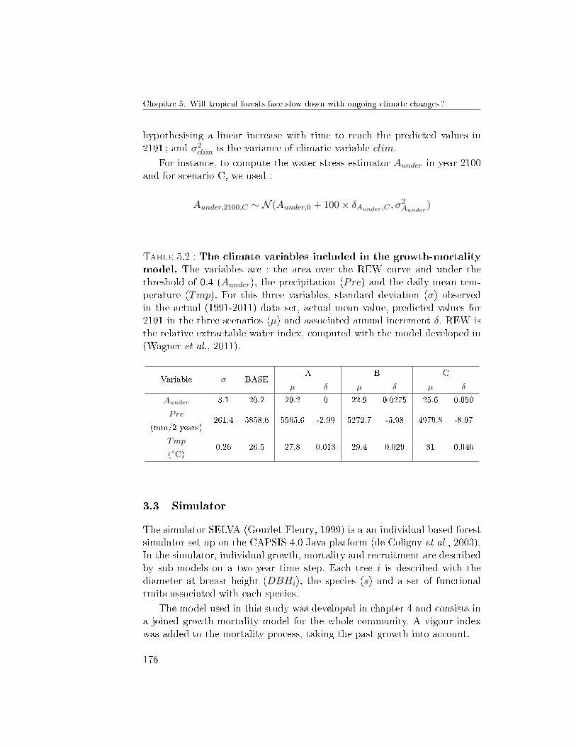
Chapitre 5. Will tropical forests face slow down with ongoing climate changes ?
hypothesising a linear increase with time to reach the predicted values in2101 ; and σ2
clim is the variance of climatic variable clim.
For instance, to compute the water stress estimator Aunder in year 2100and for scenario C, we used :
Aunder,2100,C ∼ N (Aunder,0 + 100× δAunder,C , σ2Aunder
)
Table 5.2 : The climate variables included in the growth-mortalitymodel. The variables are : the area over the REW curve and under thethreshold of 0.4 (Aunder), the precipitation (Pre) and the daily mean tem-perature (Tmp). For this three variables, standard deviation (σ) observedin the actual (1991-2011) data set, actual mean value, predicted values for2101 in the three scenarios (µ) and associated annual increment δ. REW isthe relative extractable water index, computed with the model developed in(Wagner et al., 2011).
Variable σ BASEA B C
µ δ µ δ µ δ
Aunder 8.1 20.2 20.2 0 22.9 0.0275 25.6 0.050
Pre261.4 5858.6 5565.6 -2.99 5272.7 -5.98 4979.8 -8.97
(mm/2 years)
Tmp0.26 26.5 27.8 0.013 29.4 0.029 31 0.046
(◦C)
3.3 Simulator
The simulator SELVA (Gourlet-Fleury, 1999) is a an individual-based forestsimulator set-up on the CAPSIS 4.0 Java platform (de Coligny et al., 2003).In the simulator, individual growth, mortality and recruitment are describedby sub-models on a two-year time step. Each tree i is described with thediameter at breast height (DBHi), the species (s) and a set of functionaltraits associated with each species.
The model used in this study was developed in chapter 4 and consists ina joined growth-mortality model for the whole community. A vigour indexwas added to the mortality process, taking the past growth into account.
176
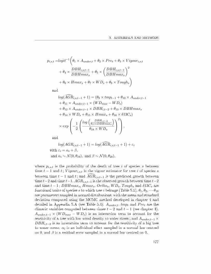
3. MATERIALS AND METHODS
pi,s,t =logit−1
(θ1 ×Aunder,t + θ2 × Pret + θ3 × V igouri,s,t
+ θ4 ×DBHi,s,t−1
DBHmaxs+ θ5 ×
(DBHi,s,t−1
DBHmaxs
)2
+ θ6 ×Hmaxs + θ7 ×WDs + θ8 × Toughs)
and
log(AGRi,s,t−1 + 1) = (θ9 × tmpt−1 + θ10 ×Aunder,t−1
+ θ11 ×Aunder,t−1 × (WDmax −WDs)
+ θ12 ×Aunder,t−1 ×DBHi,t−2 + θ13 ×DBHmaxs+ θ14 ×WDs + θ15 ×Hmaxs + θ16 × δ13Cs)
× exp
−1
2
log(
DBHi,t−2
θ17×DBHmaxs
)θ18 ×WDs
2 ,
and
log(AGRi,s,t−1 + 1) = log(AGRi,s,t−1 + 1) + εi
with εi = αi + β,
and αi ∼ N (0, θ19), and β ∼ N (0, θ20),
where pi,s,t is the probability of the death of tree i of species s betweentime t − 1 and t ; V igouri,s,t is the vigour estimator for tree i of species sbetween time t − 1 and t ; and AGRi,s,t−1 is the predicted growth betweentime t−2 and time t−1. AGRi,s,t−1 is the observed growth between time t−2and time t− 1 ; DBHmaxs, Hmaxs, Orthos, WDs, Toughs and δ13Cs arefunctional traits of species s to which tree i belongs (Table 5.1). θ1, θ2, · · · θ18
are parameters sampled in normal distributions, with the mean and standarddeviation computed using the MCMC method developed in chapter 4 anddetailed in Appendix 5.A (see Table 5.4). Aunder,t, tmpt and Pret are theclimatic variables computed between times t − 2 and t − 1 (see chapter 4).Aunder,t−1 × (WDmax − WDs) is an interaction term to account for thesensitivity of a tree with low wood density to water stress ; and Aunder,t−1×DBHi,t−2 is an interaction term to account for the sensitivity of a big treeto water stress. αi is an individual e�ect sampled in a normal law centredon 0, and β is a residual error sampled in a normal law centred on 0.
177
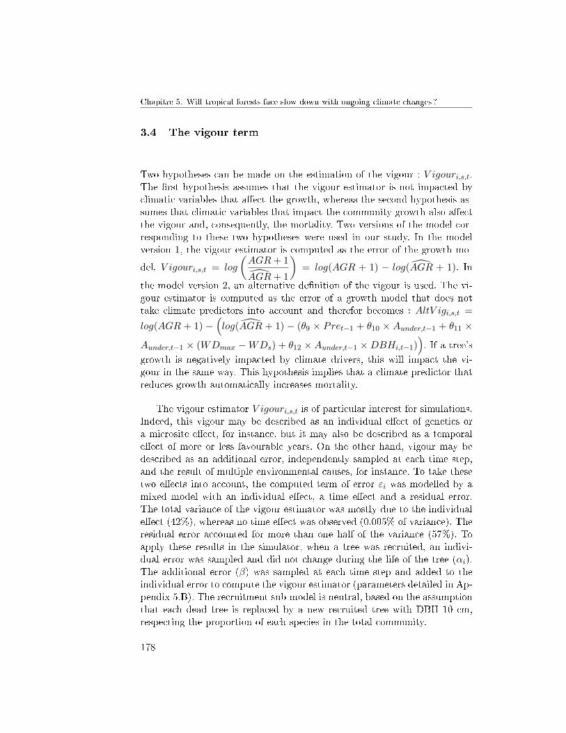
Chapitre 5. Will tropical forests face slow down with ongoing climate changes ?
3.4 The vigour term
Two hypotheses can be made on the estimation of the vigour : V igouri,s,t.The �rst hypothesis assumes that the vigour estimator is not impacted byclimatic variables that a�ect the growth, whereas the second hypothesis as-sumes that climatic variables that impact the community growth also a�ectthe vigour and, consequently, the mortality. Two versions of the model cor-responding to these two hypotheses were used in our study. In the modelversion 1, the vigour estimator is computed as the error of the growth mo-
del, V igouri,s,t = log
(AGR+ 1
AGR+ 1
)= log(AGR + 1) − log(AGR + 1). In
the model version 2, an alternative de�nition of the vigour is used. The vi-gour estimator is computed as the error of a growth model that does nottake climate predictors into account and therefor becomes : AltV igi,s,t =
log(AGR + 1) −(log(AGR + 1) − (θ9 × Pret−1 + θ10 × Aunder,t−1 + θ11 ×
Aunder,t−1 × (WDmax −WDs) + θ12 × Aunder,t−1 ×DBHi,t−1)). If a tree's
growth is negatively impacted by climate drivers, this will impact the vi-gour in the same way. This hypothesis implies that a climate predictor thatreduces growth automatically increases mortality.
The vigour estimator V igouri,s,t is of particular interest for simulations.Indeed, this vigour may be described as an individual e�ect of genetics ora microsite e�ect, for instance, but it may also be described as a temporale�ect of more or less favourable years. On the other hand, vigour may bedescribed as an additional error, independently sampled at each time step,and the result of multiple environmental causes, for instance. To take thesetwo e�ects into account, the computed term of error εi was modelled by amixed model with an individual e�ect, a time e�ect and a residual error.The total variance of the vigour estimator was mostly due to the individuale�ect (42%), whereas no time e�ect was observed (0.005% of variance). Theresidual error accounted for more than one half of the variance (57%). Toapply these results in the simulator, when a tree was recruited, an indivi-dual error was sampled and did not change during the life of the tree (αi).The additional error (β) was sampled at each time step and added to theindividual error to compute the vigour estimator (parameters detailed in Ap-pendix 5.B). The recruitment sub-model is neutral, based on the assumptionthat each dead tree is replaced by a new recruited tree with DBH 10 cm,respecting the proportion of each species in the total community.
178
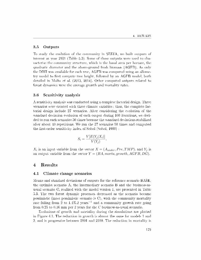
4. RESULTS
3.5 Outputs
To study the evolution of the community in SELVA, we built outputs ofinterest at year 2101 (Table 5.3). Some of these outputs were used to cha-racterise the community structure, which is the basal area per hectare, thequadratic diameter and the above-ground fresh biomass (AGFB). As onlythe DBH was available for each tree, AGFB was computed using an allome-try model to �rst compute tree height, followed by an AGFB model, bothdetailed in Molto et al. (2013, 2014). Other computed outputs related toforest dynamics were the average growth and mortality rates.
3.6 Sensitivity analysis
A sensitivity analysis was conducted using a complete factorial design. Threescenarios were created with three climate variables ; thus, the complete fac-torial design include 27 scenarios. After considering the evolution of thestandard deviation evolution of each output during 100 iterations, we deci-ded to run each scenarios 50 times because the standard deviations stabilizedafter about 40 repetitions. We ran the 27 scenarios 50 times and computedthe �rst-order sensitivity index of Sobol (Sobol, 1990) :
Si =V [E(Yj |Xi)]
V (Yj),
Xi is an input variable from the vector X = (Aunder, P re, TMP ), and Yj isan output variable from the vector Y = (BA,morta, growth,AGFB,DG).
4 Results
4.1 Climate change scenarios
Means and standard deviations of outputs for the reference scenario BASE,the optimist scenario A, the intermediary scenario B and the business-as-usual scenario C, realized with the model version 1, are presented in Table5.3. The two forest dynamic processes decreased as the scenario becamepessimistic (most pessimistic scenario is C), with the community mortalityrate falling from 2 to 1.4%.2 years−1 and a community growth rate goingfrom 0.25 to 0.16 mm per 2 years for the C business-as-usual scenario.
Evolutions of growth and mortality during the simulations are plottedin Figure 4.1. The reduction in growth is almost the same for models 1 and2, and is progressive between 2001 and 2100. The reduction in mortality is
179
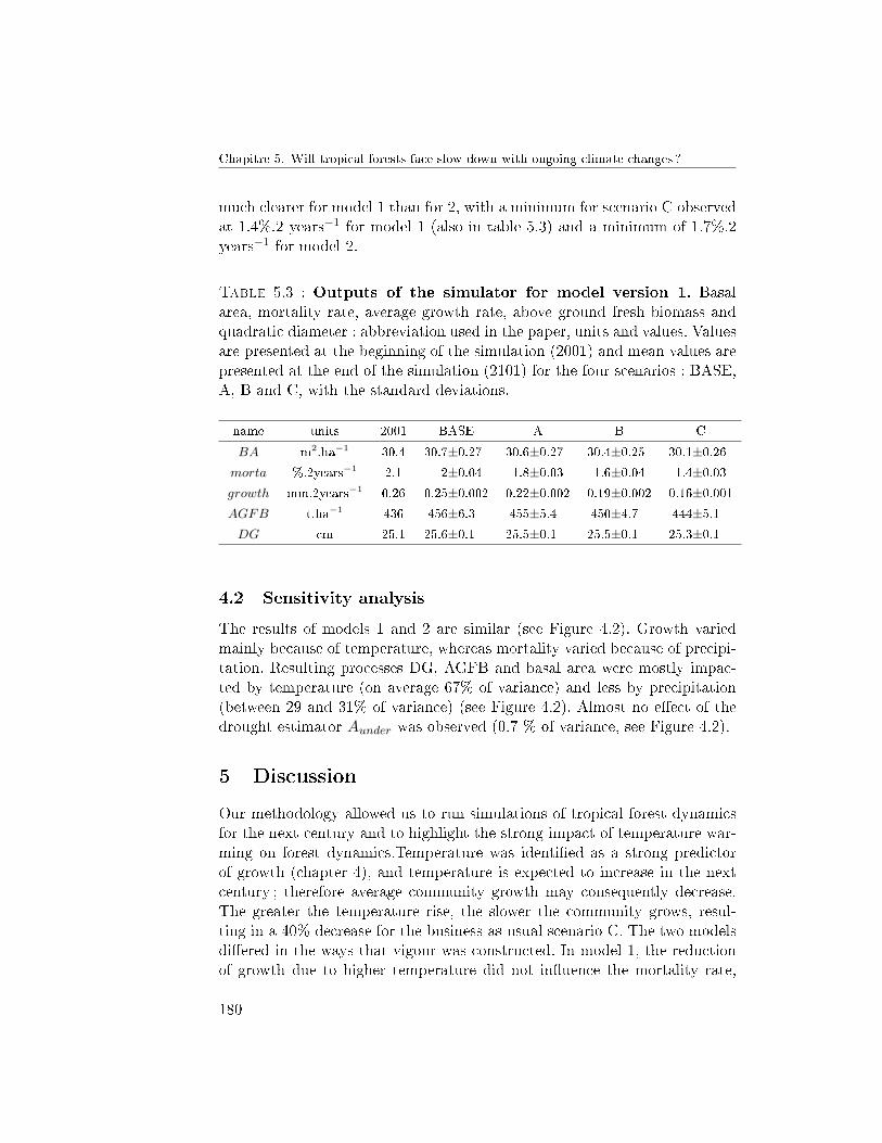
Chapitre 5. Will tropical forests face slow down with ongoing climate changes ?
much clearer for model 1 than for 2, with a minimum for scenario C observedat 1.4%.2 years−1 for model 1 (also in table 5.3) and a minimum of 1.7%.2years−1 for model 2.
Table 5.3 : Outputs of the simulator for model version 1. Basalarea, mortality rate, average growth rate, above ground fresh biomass andquadratic diameter : abbreviation used in the paper, units and values. Valuesare presented at the beginning of the simulation (2001) and mean values arepresented at the end of the simulation (2101) for the four scenarios : BASE,A, B and C, with the standard deviations.
name units 2001 BASE A B C
BA m2.ha−1 30.4 30.7±0.27 30.6±0.27 30.4±0.25 30.1±0.26morta %.2years−1 2.1 2±0.04 1.8±0.03 1.6±0.04 1.4±0.03growth mm.2years−1 0.26 0.25±0.002 0.22±0.002 0.19±0.002 0.16±0.001AGFB t.ha−1 436 456±6.3 455±5.4 450±4.7 444±5.1DG cm 25.1 25.6±0.1 25.5±0.1 25.5±0.1 25.3±0.1
4.2 Sensitivity analysis
The results of models 1 and 2 are similar (see Figure 4.2). Growth variedmainly because of temperature, whereas mortality varied because of precipi-tation. Resulting processes DG, AGFB and basal area were mostly impac-ted by temperature (on average 67% of variance) and less by precipitation(between 29 and 31% of variance) (see Figure 4.2). Almost no e�ect of thedrought estimator Aunder was observed (0.7 % of variance, see Figure 4.2).
5 Discussion
Our methodology allowed us to run simulations of tropical forest dynamicsfor the next century and to highlight the strong impact of temperature war-ming on forest dynamics.Temperature was identi�ed as a strong predictorof growth (chapter 4), and temperature is expected to increase in the nextcentury ; therefore average community growth may consequently decrease.The greater the temperature rise, the slower the community grows, resul-ting in a 40% decrease for the business-as-usual scenario C. The two modelsdi�ered in the ways that vigour was constructed. In model 1, the reductionof growth due to higher temperature did not in�uence the mortality rate,
180
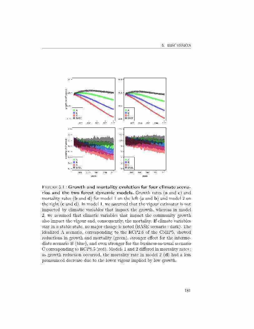
5. DISCUSSION
Figure 5.1 :Growth and mortality evolution for four climate scena-rios and the two forest dynamic models. Growth rates (a and c) andmortality rates (b and d) for model 1 on the left (a and b) and model 2 onthe right (c and d). In model 1, we assumed that the vigour estimator is notimpacted by climatic variables that impact the growth, whereas in model2, we assumed that climatic variables that impact the community growthalso impact the vigour and, consequently, the mortality. If climate variablesstay in a stable state, no major change is noted (BASE scenario : dark). Theidealized A scenario, corresponding to the RCP2.6 of the CMIP5, showedreductions in growth and mortality (green), stronger e�ect for the interme-diate scenario B (blue), and even stronger for the business-as-usual scenarioC corresponding to RCP8.5 (red). Models 1 and 2 di�ered in mortality rates ;as growth reduction occurred, the mortality rate in model 2 (d) had a lesspronounced decrease due to the lower vigour implied by low growth.
181
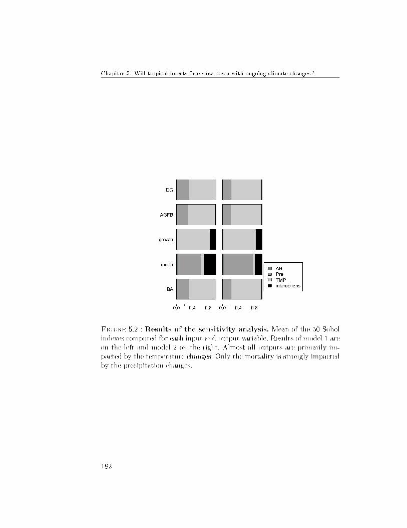
Chapitre 5. Will tropical forests face slow down with ongoing climate changes ?
Figure 5.2 : Results of the sensitivity analysis. Mean of the 50 Sobolindexes computed for each input and output variable. Results of model 1 areon the left and model 2 on the right. Almost all outputs are primarily im-pacted by the temperature changes. Only the mortality is strongly impactedby the precipitation changes.
182
5. DISCUSSION
leading to decreasing mortality rates due to rain diminution. In model 2, thereduction of growth due to higher temperature induced a reduction of vigourand impacted mortality, leading to a less marked decrease in mortality ratesthan in model 1. These two hypothetical forest dynamic behaviours implytwo divergent approaches to mortality and vigour. Model 1 is better adaptedto simulate the actual dynamics observed in our study site in French Guiana,as no evident relation was found between factors such as temperature andmortality in chapter 4. Thus, the rise in temperature impacts the growth butnot the mortality process. This implies a weak vigour-mediated relationshipbetween growth and mortality. If all tree decrease their growth under climatepressures, mortality rates would not be impacted. On the contrary, model 2assumed that climate variables that impact the growth process also impactthe mortality process indirectly. Indeed, the vigour estimator will be lowerdue to a decrease in growth, the mortality will rise as a consequence. Thisimplies that the mortality of the community will change drastically if growthdoes, and that over-mortality may be observed due to climate-induced loss ofgrowth. Such a strong link between growth and mortality is already well do-cumented (Chao et al., 2008), and past growth is often used as a predictor ofmortality (e.g. Rüger et al. (2011)). During experimental throughfall exclu-sion in Brazil, a decrease in growth was observed (Nepstad, 2002), followedby an increase in mortality rates (Nepstad et al., 2007). These experimentalresults are more consistent with model 2 and underlined the probable linksbetween growth and mortality after environmental stress. We ignore howforest dynamics will behave in the next century under the climate pressuresthat will be di�erent from those observed, because the hypotheses we usedto build our models will probably be wrong. The reality will probably fallbetween models 1 and 2, but these two models are useful to explore the pos-sible futures and to measure the impacts of the di�erent hypotheses we putforward to construct our simulations.
The sensitivity analysis points out two climate drivers. Temperature riseis by far the strongest driver of almost all output variability. Precipitationvariability primarily in�uence the mortality rates. However, these resultsmust be considered with caution because the range of variation of clima-tic variables depends on the IPCC 5AR predictions. The relative changes intemperature values in the three climate scenarios are higher than the relativechanges for precipitation and water stress, which is one cause for the resultsobserved in Figure 4.2. Even so, our results underlined the important roleof temperature rises in community dynamics and structure. In our simula-tions, growth is the most impacted process, and this slowing-down dynamicimplies a slight reduction in above-ground fresh biomass, quadratic diameter
183

Chapitre 5. Will tropical forests face slow down with ongoing climate changes ?
and basal area. If, as highlighted by the results from model 2, a higher mor-tality follows the growth reduction, the population will change signi�cantlywith few large old trees and more small trees. This community change willimpact the basal area (from 30.1m2.ha−1 for scenario C with model 1 to26m2.ha−1 for scenario C with model 2) and the above-ground fresh biomass(from 444t.ha−1 for scenario C with model 1 to 369t.ha−1 for scenario Cwith model 2). Temperature is expected to rise of 4.5 ◦C during the nextcentury in French Guiana. Higher temperature can drastically a�ect pho-tosynthesis by causing irreversible damage to leaves (Doughty, 2011) and,currently, no forests in the world exist in areas with mean temperatures of31 ◦C. Concerning precipitation, a noticeable reduction in mortality appearedin our simulations. This is due to the predicted reduction of precipitations.In the model developed in chapter 4, the stronger driver of mortality is pre-cipitation, which positively impacts mortality rates. This is partly due to theincrease in falling trees during the most rainy years (see chapter 4), becausetrees are more vulnerable when the soil is saturated (Ferry et al., 2010).Consequently, the decrease of precipitation predicted for the next centuryimplies consequently a decrease in mortality rates in the simulated commu-nities. But the IPCC AR5 also forecasts an intensi�cation of abundant rainevents in the tropics (IPCC, 2013), that may play the inverse role, increa-sing the mortality. The problem is that such events are not currently wellquanti�ed, and relations between mortality and extreme events are complexto model. In addition to the variability observed between models 1 and 2,this makes mortality a crucial process that is di�cult to model as properlyas is growth.
There are no studies simulating the future of forest dynamics under cli-mate changes with which to compare our results. This kind of combinedapproach may help us identify potential consensual risks for the tropical fo-rests for the next century. If, as expected by Fu et al. (2013), the dry seasonlength is underestimated in the models used by the IPCC, one more chal-lenge for the future will be quantifying this underestimation, which couldadd uncertainty to the inputs of forest simulators. Global models that takeuncertainties into account will be inestimable tools to identify gaps in ourknowledges and to point out useful studies in the future.
184
BIBLIOGRAPHIE
Allen, C. D., Macalady, A. K., Chenchouni, H., Bachelet, D., McDowell, N.,Vennetier, M., Kitzberger, T., Rigling, A., Breshears, D. D., Hogg, E.T. H., Gonzalez, P., Fensham, R., Zhang, Z., Castro, J., Demidova, N.,Lim, J.-H. H., Allard, G., Running, S. W., Semerci, A., and Cobb, N.(2010). A global overview of drought and heat-induced tree mortalityreveals emerging climate change risks for forests. Forest Ecology andManagement, 259(4):660�684.
Baker, T. R., Phillips, O. L., Malhi, Y., Almeida, S., Arroyo, L., Di Fiore, A.,Erwin, T., Higuchi, N., Killeen, T. J., Laurance, S. G., Laurance, W. F.,Lewis, S. L., Monteagudo, A., Neill, D. a., Vargas, P. N. n., Pitman, N.C. a., Silva, J. N. M., and Martínez, R. V. (2004). Increasing biomass inAmazonian forest plots. Philosophical transactions of the Royal Societyof London. Series B, Biological sciences, 359(1443):353�65.
Brando, P. M., Nepstad, D. C., Davidson, E. a., Trumbore, S. E., Ray, D., andCamargo, P. (2008). Drought e�ects on littefall, wood production andbelowground carbon cycling in an Amazon Forest : result of a throughfallreduction experiment. Philosophical Transactions of the Royal Society,363(1498):1839�1848.
Chao, K. J., Phillips, O. L., Gloor, E., Monteagudo, A., Torres-Lezama, A.,and Martinez, R. V. (2008). Growth and wood density predict treemortality in Amazon forests. Journal of Ecology, 96(2):281�292.
Choat, B., Jansen, S., Brodribb, T. J., Cochard, H., Delzon, S., Bhaskar, R.,Bucci, S. J., Feild, T. S., Gleason, S. M., Hacke, U. G., Jacobsen, A. L.,
185
Chapitre 5. Will tropical forests face slow down with ongoing climate changes ?
Lens, F., Maherali, H., Martínez-Vilalta, J., Mayr, S., Mencuccini, M.,Mitchell, P. J., Nardini, A., Pittermann, J., Pratt, R. B., Sperry, J. S.,Westoby, M., Wright, I. J., and Zanne, A. E. (2012). Global convergencein the vulnerability of forests to drought. Nature, 491(7426):752�5.
Clark, D. a., Piper, S. C., Keeling, C. D., and Clark, D. B. (2003). Tropi-cal rain forest tree growth and atmospheric carbon dynamics linkedto interannual temperature variation during 1984-2000. Proceedingsof the National Academy of Sciences of the United States of America,100(10):5852�7.
Condit, R., Aguilar, S., Hernandez, A., Perez, R., Lao, S., Angehr, G., Hub-bell, S. P., and Foster, R. B. (2004). Tropical forest dynamics across arainfall gradient and the impact of an El Nino dry season. Journal ofTropical Ecology, 20:51�72.
da Costa, A. C. L., Galbraith, D., Almeida, S., Portela, B. T. T., da Costa,M., Silva Junior, J. a. D. A., Braga, A. P., de Gonçalves, P. H. L.,de Oliveira, A. a. R., Fisher, R., Phillips, O. L., Metcalfe, D. B., Levy, P.,and Meir, P. (2010). E�ect of 7 yr of experimental drought on vegetationdynamics and biomass storage of an eastern Amazonian rainforest. TheNew Phytologist, 187(3):579�91.
de Coligny, F., Ancelin, P., Cornu, Guillaume Courbaud, B., Dreyfus, P., Go-reaud, F., Gourlet-Fleury, S., Meredieu, C., and Saint-André, L. (2003).CAPSIS : Computer-aided Projection for Strategies in Silviculture :Advantages of modelling Platform. Amaro, A., Reed, D., Soares, P.(Eds.), Modelling Forest Systems. CABI Publishing, Wallingford, UK,pages 319�323.
Dong, S. X., Davies, S. J., Ashton, P. S., Bunyavejchewin, S., Supardi, M.N. N., Kassim, A. R., Tan, S., and Moorcroft, P. R. (2012). Variability insolar radiation and temperature explains observed patterns and trendsin tree growth rates across four tropical forests. Proceedings. Biologicalsciences / The Royal Society, 279(1744):3923�31.
Doughty, C. E. (2011). An In Situ Leaf and Branch Warming Experimentin the Amazon. Biotropica, 43(6):658�665.
Ferry, B., Morneau, F., Bontemps, J. D., Blanc, L., and Freycon, V. (2010).Higher treefall rates on slopes and waterlogged soils result in lower standbiomass and productivity in a tropical rain forest. Journal of Ecology,98(1):106�116.
186
BIBLIOGRAPHIE
Fu, R., Yin, L., Li, W., Arias, P. A., Dickinson, R. E., Huang, L., Chakra-borty, S., Fernandes, K., Liebmann, B., Fisher, R., and Myneni, R. B.(2013). Increased dry-season length over southern Amazonia in recentdecades and its implication for future climate projection. Proceedingsof the National Academy of Sciences of the United States of America,110(45):18110�18115.
Gourlet-Fleury, S. (1999). Individual-based spatially explicit modelling offorest stands in French Guiana. In Y., L., King, B., Legg, C., andRenolls, K., editors, Data Management and Modelling Using RemoteSensing and GIS for Tropical Forest Land Inventory, pages 473�490,Jakarta, Indonesia.
Hérault, B., Bachelot, B., Poorter, L., Rossi, V., Bongers, F., Chave, J.,Paine, C. E. T., Wagner, F., and Baraloto, C. (2011). Functional traitsshape ontogenetic growth trajectories of rain forest tree species. Journalof Ecology, 99(6):1431�1440.
IPCC (2013). Climate change 2013 : the scienti�c basis. contribution of wor-king group 1 to the fourth assessment report of the intergovernmentalpanel on climate change. Cambridge University Press.
Joetzjer, E., Douville, H., Delire, C., and Ciais, P. (2013). Present-day andfuture Amazonian precipitation in global climate models : CMIP5 versusCMIP3. Climate Dynamics, 41(11-12):2921�2936.
Lasky, J. R., Sun, I.-F., Su, S.-H., Chen, Z.-S., and Keitt, T. H. (2013). Trait-mediated e�ects of environmental �ltering on tree community dynamics.Journal of Ecology, 101(3):722�733.
Lewis, S. L., Brando, P. M., Phillips, O. L., van der Heijden, G. M. F., andNepstad, D. (2011). The 2010 Amazon drought. Science (New York,N.Y.), 331(6017):554.
Lewis, S. L., Phillips, O. L., Baker, T. R., Lloyd, J., Malhi, Y., Almeida, S.,Higuchi, N., Laurance, W. F., Neill, D. a., Silva, J. N. M., Terborgh,J., Lezama, a. T., Martínez, R. V., Brown, S., Chave, J., Kuebler, C.,Vargas, P. N. n., and Vinceti, B. (2004). Concerted changes in tropicalforest structure and dynamics : evidence from 50 South American long-term plots. Philosophical transactions of the Royal Society of London.Series B, Biological sciences, 359(1443):421�36.
187
Chapitre 5. Will tropical forests face slow down with ongoing climate changes ?
Malhi, Y., Aragão, L. E. O. C., Galbraith, D., Huntingford, C., Fisher, R.,Zelazowski, P., Sitch, S., Mcsweeney, C., and Meir, P. (2009). Exploringthe likelihood and mechanism of a climate-change-induced dieback ofthe Amazon rainforest.
McMahon, S. M., Harrison, S. P., Armbruster, W. S., Bartlein, P. J., Beale,C. M., Edwards, M. E., Kattge, J., Midgley, G., Morin, X., and Prentice,I. C. (2011). Improving assessment and modelling of climate changeimpacts on global terrestrial biodiversity. Trends in ecology & evolution,26(5):249�59.
Mitchell, T. D. and Jones, P. D. (2005). An improved method of construc-ting a database of monthly climate observations and associated high-resolution grids. International Journal of Climatology, 25(6):693�712.
Molto, Q., Hérault, B., Boreux, J.-J., Daullet, M., Rousteau, a., and Rossi, V.(2014). Predicting tree heights for biomass estimates in tropical forestsâ�� a test from French Guiana. Biogeosciences, 11(12):3121�3130.
Molto, Q., Rossi, V., and Blanc, L. (2013). Error propagation in biomassestimation in tropical forests. Methods in Ecology and Evolution, 4(2):175�183.
Nepstad, D. C. (2002). The e�ects of partial throughfall exclusion on canopyprocesses, aboveground production, and biogeochemistry of an Amazonforest. Journal of Geophysical Research, 107(D20):8085.
Nepstad, D. C., Tohver, I. M., Ray, D., Moutinho, P., and Cardinot, G.(2007). Mortality of large trees and lianas following experimentaldrought in an Amazon forest. Ecology, 88(9):2259�69.
Phillips, O. L., Aragao, L., Lewis, S. L., Fisher, J. B., Lloyd, J., Lopez-Gonzalez, G., Malhi, Y., Monteagudo, A., Peacock, J., Quesada, C. A.,van der Heijden, G., Almeida, S., Amaral, I., Arroyo, L., Aymard, G.,Baker, T. R., Banki, O., Blanc, L., Bonal, D., Brando, P., Chave, J.,de Oliveira, A. C. A., Cardozo, N. D., Czimczik, C. I., Feldpausch,T. R., Freitas, M. A., Gloor, E., Higuchi, N., Jimenez, E., Lloyd, G.,Meir, P., Mendoza, C., Morel, A., Neill, D. A., Nepstad, D., Patino, S.,Penuela, M. C., Prieto, A., Ramirez, F., Schwarz, M., Silva, J., Silveira,M., Thomas, A. S., ter Steege, H., Stropp, J., Vasquez, R., Zelazowski,P., Davila, E. A., Andelman, S., Andrade, A., Chao, K.-j. J., Erwin, T.,Di Fiore, A., Honorio, E., Keeling, H., Killeen, T. J., Laurance, W. F.,
188

BIBLIOGRAPHIE
Cruz, A. P. n., Pitman, N. C. A., Vargas, P. N. n., Ramirez-Angulo,H., Rudas, A., Salamao, R., Silva, N., Terborgh, J., Torres-Lezama, A.,Aragão, L. E. O. C., López-gonzález, G., Heijden, G. V. D., Bánki, O.,Cristina, A., Oliveira, A. D., Jiménez, E., Patiño, S., Peñuela, M. C.,Ramírez, F., Steege, H., Vásquez, R., Dávila, E. A., Fiore, A. D., C,E. H., Ramírez-angulo, H., and Salamão, R. (2009). Drought sensitivityof the Amazon Rainforest. Science, 323(March):1344�1347.
Rüger, N., Huth, A., Hubbell, S. P., and Condit, R. (2011). Determinantsof mortality across a tropical lowland rainforest community. Oikos,120(7):1047�1056.
Sobol, I. M. (1990). Sensitivity estimats for nonlinear mathematical models.Matematicheskoe Modelirovanie, 2:112�118.
Wagner, F., Hérault, B., Stahl, C., Bonal, D., and Rossi, V. (2011). Modelingwater availability for trees in tropical forests. Agricultural and ForestMeteorology, 151(9):1202�1213.
189

Chapitre 5. Will tropical forests face slow down with ongoing climate changes ?
5.A Adaptation of the joined growth-mortality mo-
del to simulator SELVA
Each individual error εi is modelled by a mixed model with an individuale�ect αi and a time e�ect γt :
εi,t ∼ N (αi + γt, β),
where αi ∼ N (0, θα) and γt ∼ N (0, θγ)With this model, the parameter αi accounts for 42% of the variance,
the estimator γ for 0.005% and the residual e�ect accounts for the remai-ning 57%. This is why, in the �nal model, the growth model takes only theindividual e�ect αi into account.
What is more, trees with DBH higher than the maximum DBH observedfor the species multiplied by 1.2 have a probability of dying equal to 1 toavoid trees reaching unrealistic DBH in the simulator.
190
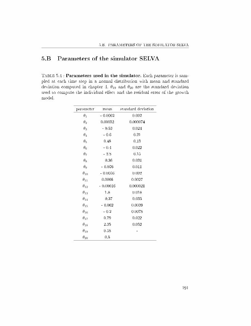
5.B. PARAMETERS OF THE SIMULATOR SELVA
5.B Parameters of the simulator SELVA
Table 5.4 : Parameters used in the simulator. Each parameter is sam-pled at each time step in a normal distribution with mean and standarddeviation computed in chapter 4. θ19 and θ20 are the standard deviationused to compute the individual e�ect and the residual error of the growthmodel.
parameter mean standard deviation
θ1 - 0.0062 0.002
θ2 0.00032 0.000074
θ3 - 0.53 0.024
θ4 - 0.6 0.21
θ5 0.48 0.13
θ6 - 0.4 0.022
θ7 - 2.8 0.15
θ8 - 0.36 0.031
θ9 - 0.076 0.011
θ10 - 0.0056 0.002
θ11 0.0066 0.0027
θ12 - 0.00016 0.000021
θ13 1.8 0.018
θ14 - 0.37 0.033
θ15 - 0.062 0.0039
θ16 - 0.2 0.0078
θ17 0.79 0.022
θ18 2.35 0.052
θ19 0.58 -
θ20 0.5 -
191

DISCUSSION ET PERSPECTIVES : QUELLESÉCHELLES POUR RÉPONDRE À QUELLES
QUESTIONS ?
1 De la photosynthèse aux changements climatiques
1.1 Du minuscule au gigantesque
La photosynthèse s'e�ectue au niveau des feuilles de l'arbre, et impliquedes photons, des molécules, et des enzymes qui ne peuvent être observés àl'÷il nu. C'est grâce à cette photosynthèse que l'arbre pourra se développer,grandir, se reproduire. C'est ce même arbre qui en interaction avec les autresarbres, les autres végétaux et les animaux, formera la forêt tropicale. EnAmazonie, cette forêt recouvre 5,5 millions de km2. On dénombre plus de16 000 espèces d'arbres, avec une canopée atteignant parfois 60 mètres dehauteur. A chaque échelle, des processus sont à l'÷uvre qui sont responsablesdu développement de cet écosystème exceptionnel.
A Paracou, sur 6 parcelles de 6.25 hectares, nous étudions grâce à plus de20 000 individus recensés très régulièrement la dynamique d'une communautéque nous prenons pour représentative du plateau des Guyanes, mais notreéchelle spatiale, centrée sur l'individu, reste située à mi-chemin entre la feuilleet la forêt.
1.2 De la seconde au millénaire
L'étude de la dynamique forestière est une tâche d'autant plus ardue quel'espérance de vie d'un être humain ne dépasse pas le siècle, tandis que les
192
2. MODÉLISER LA DIVERSITÉ
arbres qui peuplent la forêt tropicale Amazonienne atteignent des âges cano-niques de plusieurs centaines voire, exceptionnellement, un millier d'années(Chambers et al., 1998). En s'intéressant à la croissance annuelle d'un arbre,on se positionne à une échelle de temps certes commode pour l'être humain,mais qui peut paraître dérisoire en comparaison de la longévité des arbres.
Les changements climatiques, quant-à-eux, sont des processus de grandeampleur, qui se réalisent à des échelles de temps et d'espace trop importantespour que l'on puisse les percevoir de façon globale. Mais l'heure est aux chan-gements d'échelles, et à mesure que les changements climatiques s'accélèrent,on voit apparaitre des phénomènes concrets à notre échelle, marques inquié-tantes de l'accélération de ces changements.
Lorsque l'on souhaite étudier les impacts des changements climatiquessur la forêt tropicale, on se heurte à la question fondamentale de l'échelle àlaquelle on va se placer. Cette question est d'autant plus importante que lesprocessus des di�érentes échelles ont tous leurs importances, et que l'étudede chaque échelle peut répondre à des questions bien précises. En étudiantla dynamique sur un pas de deux ans pendant 20 ans comme c'est le casdans cette thèse, on se place à une échelle de temps intermédiaire, entre lavariabilité intra-annuelle �ne et rapide et les changements globaux plus lents.
2 Modéliser la diversité
Les modèles utilisés actuellement pour modéliser les changements clima-tiques et leurs potentiels impacts sur la végétation sont principalement desmodèles de dynamique végétation globaux (Dynamic global vegetation mo-del, DGVM), des modèles qui fonctionnent par couches, et qui prennent descomportements moyens en compte. Ces modèles se placent au-dessus desprocessus dynamiques, contrairement à ce qui est fait dans cette thèse, ilspermettent de modéliser à un niveau supérieur, mais sans lien direct avec lefonctionnement individuel des arbres.
2.1 Peut-on tout modéliser ?
"Time to model all life on Earth" (Purves, 2013)
En utilisant de tels modèles, la forêt entière est modélisée, elle est re-présentée par une couche mise en relation avec la couche atmosphère et lacouche sol. Ces modèles permettent donc d'étudier les processus à grandeéchelle et de répondre à des questions globales. Pour passer à ce niveau,l'arbre individuel disparait au pro�t d'une feuille géante, la photosynthèse
193
Discussion et perspectives
devient le processus central, ces modèles se basent donc bien sur des hypo-thèses physiologiques. Mais l'échelle intermédiaire de l'arbre n'apparait pasentre la feuille et la forêt.
Les modèles sont de plus en plus sophistiqués, et on peut raisonnablementse demander si les connaissances actuelles nous permettent de modéliser àdes échelles encore plus grandes et en prenant la plus grande diversité pos-sible en compte. C'est ce que propose Drew Purves en 2013 dans le journalNature (Purves, 2013). Pour lui, nos connaissances sont su�santes pour com-mencer à chercher à répondre à des questions globales, qui prennent tous lesécosystèmes en compte. Or, je pense qu'il faut avoir les ambitions adaptéesà l'échelle à laquelle on se place et je me demande s'il est judicieux de mo-déliser à un niveau élevé sans savoir modéliser à un niveau plus bas. Ainsi,pour beaucoup de modélisateurs en écologie, les processus de chaque niveauinférieur restent omniprésents, et il semble absurde de modéliser au niveaude la communauté lorsque l'on ne sait pas le faire au niveau de l'arbre oude la feuille, on manque alors une étape qui nous permettrait de poser leshypothèses (physiologiques par exemple) qui permettent de construire le mo-dèle de niveau haut. Toutefois, ces restrictions ne me semblent pas toujoursjusti�ées lorsqu'il s'agit de modéliser car c'est bien par essence qu'un modèlecaricature la réalité.
2.2 Doit-on tout modéliser ?
-"Essentially, all models are wrong, but some are useful." George EP Box
-"All models are right, most are useless." Thaddeus Tarpey
Bien que la perspective de tout modéliser soit scienti�quement alléchante,on peut douter de l'e�cacité d'une telle approche. En e�et, si l'on en croit lestravaux de Dirk Helbing et de son équipe (Helbing et al., 2012), une nouvelleaire sociale pourrait voir le jour si l'on réussissait à modéliser l'intégralité desprocessus sociaux en jeux. Cette vision des choses me parait bien utopiste sil'on garde en tête que la modélisation peut nous apprendre des choses commeoutil de prédiction, mais qu'elle n'impacte évidemment pas directement lesprocessus. Comprendre un processus est une chose, savoir avec certitudecomment il répondra à une contrainte en est une autre, et pouvoir créer ouéviter cette contrainte en est encore une autre.
194
3. MODÉLISER LA COMPLEXITÉ
2.3 Quelles hypothèses pour répondre à quelles questions ?
Dans le cadre de cette thèse, la modélisation est utilisée comme outil, pourapporter un élément de réponse aux questions qui taraudent la communautéscienti�que à propos de l'impact des changements climatiques sur la dyna-mique de la forêt tropicale. Pour apporter cette pierre à l'édi�ce, on a vuqu'il nous a été nécessaire de poser un certain nombre d'hypothèses. Ces hy-pothèses sont lourdes de sens, mais ce sont elles qui permettent de construireun modèle.
Ainsi, un arbre est représenté par un DBH, des traits fonctionnels et unstade ontogénique. Son environnement, notamment le sol ou la compétition,ne sont pas pris en compte dans mes modèles. De plus, tous les arbres sontsoumis au même modèle de croissance et de mortalité, ce qui lisse fortementle signal et empêche certains comportements exceptionnels potentiellementimportants. On peut se demander quelles sont les conséquences de telleshypothèses sur notre habilité à répondre à des questions d'écologie. Dansnotre cas, la communauté entière est représentée, avec les traits fonctionnelsqui permettent de prendre en compte la diversité sans devoir créer de groupesarti�ciels. Mais les comportements extrêmes sont laissés pour compte, quece soit par exemple le comportement des très gros arbres ou la croissanceparticulièrement rapide de certains individus.
3 Modéliser la complexité
Si notre approche permet de modéliser la diversité en forêt tropicale, ellegomme par endroit sa complexité. Les comportements extrêmes sont lesmoins bien représentés, bien que l'on sache qu'ils sont d'une grande im-portance. Les très gros arbres, les événements rares, les comportements mar-ginaux sont autant de sources de potentiels changements brutaux de dyna-mique, ce que l'on appelle des black swan (Taleb, 2010). La croissance parexemple, est très faible dans la forêt étudiée à Paracou, ce qui nous conduità prédire des taux de croissance très faibles. Pourtant on sait que certainsindividus, parfois indépendamment de leur espèce, peuvent croitre de fa-çon inattendue. La vigueur, introduite dans le troisième chapitre, permet demieux prendre en compte cette variabilité résiduelle sur les processus. Tou-tefois, la façon dont la vigueur est prise en compte dans les modèles peutchanger drastiquement les résultats comme le montre le chapitre 5, encoreune fois ceci dépend des hypothèses qui ont été formulées.
195
Discussion et perspectives
3.1 Les propriétés émergentes
Les hypothèses que l'on fait ont un impact fort sur les résultats observés,et on peut voir apparaitre des propriétés émergentes qui n'avaient pas étéinitialement prévues. C'est parfois le cas d'e�et de seuil ou de rétroaction.Dans notre cas, nous ne voyons pas de tels e�ets se manifester. Toutefois,on peut prendre conscience de l'importance de nos hypothèses en constatantles di�érents résultats. Le calcul de la vigueur prend toute son importancelorsque l'on regarde son e�et sur des simulations de 100 ans. S'il n'y a pasd'e�et lors de l'inférence des paramètres, il y en a par contre un lors de lasimulation de la communauté. Si l'e�et de la sécheresse sur la croissance serépercute sur la mortalité, alors on observe une diminution plus faible de lamortalité. Toutefois, si la sécheresse devait avoir un e�et sur la mortalité, ons'attend à ce que notre modèle l'ai pris en compte. La forêt telle qu'on l'ob-serve n'est probablement ni tout l'un ni tout l'autre. En e�et, si l'on chercheà comprendre ce que de telles hypothèses impliquent, écologiquement par-lant, on voit alors deux types de caricatures possibles. La mortalité peutêtre vue comme un processus relativement stable, qui épure la forêt de sesarbres les moins bons. A chaque pas de temps, un certain nombre d'arbresva donc mourir et pour déterminer lesquels mourront, on peut regarder lestade ontogénique, l'environnement, ou d'autres facteurs. D'une autre façon,la mortalité peut être perçue comme un processus sans borne, qui va sim-plement supprimer les arbres les moins vaillants sous une contrainte donnée,quitte à voir disparaitre la moitié de la forêt si la contrainte est forte. Laréalité est bien sûr di�érente, puisque le processus de mortalité est complexe,et reste pour le moment relativement constant, autour de 1% par an sur lesite de Paracou. Toutefois, ces deux visions extrêmes et caricaturales nouspermettent de mieux nous interroger sur les scénarios possibles concernantla mortalité en forêt tropicale.
3.2 L'e�et individuel
L'introduction de la vigueur pose la question d'un e�et individuel. De tels ef-fets sont amplement étudiés en écologie, grâce à l'essor des modèles mixtes etleur facilité d'utilisation. L'ajout d'e�ets aléatoires, que ce soit spéci�ques,ou individuels, permet de prendre ce genre de variabilité en compte et dedé�nir à quel niveau chaque e�et intervient. Toutefois, si ces modèles sonttrès informatifs, on peut se demander quel est leur pouvoir de prédiction. Sila variabilité individuelle des réponses de dynamique aux changements cli-matiques apparait importante, quelle doit être la conclusion pour prédire la
196
3. MODÉLISER LA COMPLEXITÉ
réponse de la forêt ? On peut décider de modéliser dans son ensemble, commeje l'ai fait, mais en se concentrant plus sur la structuration de la variance ré-siduelle par cet e�et individuel. Compte tenu de la distribution non normaledes DBH et des processus complexes qui interviennent au niveau individuel,une telle approche nous permettrait potentiellement d'observer l'émergencede propriétés non observées durant cette thèse. C'est ce qui est recherché lorsde la construction de modèle individus-centrés. Les propriétés émergentes,qui sont parfois surprenantes, permettent de comprendre l'apparition de phé-nomènes à l'échelle globale qui n'était pourtant pas implémentés à l'échelleindividuelle. C'est notamment ce qui permet de modéliser les mouvementsdes étourneaux sans avoir à implémenter les formes parfois complexes qui enrésultent. Dans le cas de la dynamique des arbres en forêt tropicale, il estdi�cile de �xer le niveau auquel les processus doivent être modélisés pourrépondre le mieux à notre question. Contrairement à un étourneau, un arbrerestera toute sa vie au même endroit, il est donc crucial de s'intéresser à l'en-vironnement proche. De même, de nombreuses interactions peuvent entreren jeux, car la diversité animale et végétale en forêt tropicale est grande, cequi a amené les nombreuses espèces à créer un grand nombre de mécanismesde coexistence. Ces processus, aux aussi, peuvent entrer en compte lors dechangements climatiques. Il est donc justi�é de vouloir s'intéresser à l'indi-vidu, et de modéliser à un niveau bas. Mais cette approche, gourmande entemps et en énergie se pose à l'encontre des modèles DVGM dont il a étéquestion plus haut. En e�et, une propriété émergente, par dé�nition, doitêtre irréductible. C'est-à-dire qu'elle ne peut pas être déduite des niveauxplus bas à partir desquels elle émerge. Dans cette thèse, aucune propriétéémergente n'a été observée. Si la descente d'échelle impliquée par la priseen compte d'un e�et individuel fort n'entraine pas l'apparition de propriétésémergentes, on peut raisonnablement se demander si elle a un intérêt.
3.3 Comment concilier complexité et diversité ?
Il existe donc deux approches, l'une à un niveau bas, centrée sur l'arbre in-dividuel, et l'autre à un niveau haut, centrée sur les processus. De nombreuxmodèles se situent bien sûr entre ces deux extrêmes. Si l'on se rappelle laclassi�cation des modèles proposée par Porté and Bartelink (2002) décriteen introduction, on se souviendra que les deux grandes classes de modèlessont les stand models, basé sur des morceaux de forêt considérés comme ho-mogènes, et les tree models basés sur des arbres modélisés individuellement.Cette structuration prend tout son sens lorsque l'on sait que ces deux niveauxcorrespondent à deux approches bien di�érentes, et servent à répondre à des
197
Discussion et perspectives
questions di�érentes. En e�et, après avoir proposé une classi�cation, Portépropose une étude comparative des modèles pour savoir quels modèles sontadaptés pour quelles questions. La première question qui nécessite de telsmodèles concerne la sylviculture, et s'intéresse à la croissance et à la produc-tion. Un autre objectif est celui de comprendre la dynamique et la successionen tenant compte des perturbations et de la structure de la communauté. Lesmodèles utilisés pour une question ne le sont pas forcément pour l'autre, etPorté met en valeur la nécessité de s'intéresser à l'échelle la plus pertinenteen fonction de la question que l'on se pose.
Zuidema et al. (2013) nous propose d'identi�er les trous de connaissanceaux di�érentes échelles auxquelles on peut considérer la forêt (Figure 5.3).Il met en évidence un manque au niveau du passage de la feuille à l'arbre.Il conseille aux scienti�ques de s'intéresser à l'arbre au lieu de se placer àl'échelle de la feuille ou de la communauté, de s'intéresser aux e�ets surle long terme (il entend par là, plutôt dizaine d'années voire siècle), et decomprendre les mécanismes, plutôt que de se baser sur des études empiriques.La plupart des lacunes soulevées concernent l'arbre et la population, ce quinous pousse à penser que les échelles intermédiaires sont celles sur lesquelleson se doit de travailler pour combler ces lacunes.
4 Modéliser pour simuler
"Trying to predict the future is a mugs' game. But increasingly it's a gamewe all have to play because the world is changing so fast and we need to havesome sort of idea of what the future's actually going to be like because we aregoing to have to live there, probably next week." (Adams, 2002)
Notre objectif dans cette thèse était de simuler une communauté d'arbres,en s'intéressant aux signaux communs, aux réponses aux variables clima-tiques, et en mettant des stratégies en évidence. Pour ce faire, nous avonsdonc posé des hypothèses, nous nous sommes placés au niveau de l'arbreindividuel, mais tout en cherchant à retrouver le signal observé à l'échellede la communauté. Des signaux communs ont été observés, entre les traitsfonctionnels et la dynamique, puis entre les variables climatiques et la dyna-mique, en incluant les interactions potentielles entre les traits et les variablesclimatiques. Une telle approche nous a permis de simuler l'évolution d'unecommunauté pendant un siècle, et d'observer les évolutions qui apparaissentau sein de cette communauté. L'outil développé dans cette thèse nous ap-porte donc des éléments de réponses, et nous permet d'apporter notre pierre
198
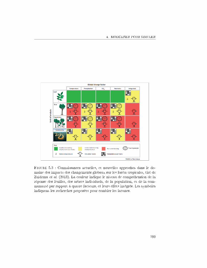
4. MODÉLISER POUR SIMULER
Figure 5.3 : Connaissances actuelles, et nouvelles approches dans le do-maine des impacts des changements globaux sur les forêts tropicales, tiré deZuidema et al. (2013). La couleur indique le niveau de compréhension de laréponse des feuilles, des arbres individuels, de la population, et de la com-munauté par rapport à quatre facteurs, et leurs e�ets intégrés. Les symbolesindiquent les recherches proposées pour combler les lacunes.
199
Discussion et perspectives
à l'édi�ce.Les échelles auxquelles on s'intéresse sont d'une grande importance, en
plus de l'échelle spatiale qui permet de passer de la feuille à la forêt, l'échelletemporelle ne doit pas être perdue de vue. En e�et, il est particulièrementdi�cile d'appréhender des processus qui se réalisent à des échelles de tempstrès supérieures à la nôtre. De fait, on ne sent pas la température évoluerau jour le jour en Guyane, et il n'est donc pas intuitif de s'y intéresser. Leschangements climatiques et la dynamique forestière sont des processus lents,et notre propre perception du temps nous empêche parfois d'étudier conve-nablement de tels processus.
"Prediction is very di�cult, especially if it's about the future." Niels Bohr
Si les changements climatiques suivent les prédictions les plus pessimistesde l'IPCC, alors la température à la surface du globe va conséquemmentaugmenter d'ici quelques décennies. Les hypothèses qui nous ont permis deconstruire nos modèles seront alors probablement fausses. Les processus quenous avons considérés linéaires sur nos intervalles peuvent ne pas l'être surdes intervalles plus grands. Les variables qui n'ont pas été sélectionnées dansle chapitre 4 car elles n'ont actuellement pas d'impact sur la dynamiquepeuvent devenir cruciales. Les e�ets de seuils ou des hystérésis peuvent ap-paraitre. L'étude des systèmes complexes nous permet de mieux comprendreces e�ets, et dans certains cas de les modéliser. Mais il ne faut pas perdrede vue qu'il est très di�cile de trouver quelque chose quand on ne le cherchepas, et de s'imaginer le futur alors que celui-ci n'a pas encore eu lieu.
200

BIBLIOGRAPHIE
Adams, D. (2002). The salmon of doubt : hitchhicking the galaxy one lasttime. UK : William Heinemann Ltd., US : Pocket Books.
Chambers, J. Q., Higuchi, N., and Schimel, J. P. (1998). Ancient trees inAmazonia. Nature, 391:135�136.
Helbing, D., Bishop, S., Conte, R., Lukowicz, P., and McCarthy, J. B. (2012).FuturICT : Participatory computing to understand and manage ourcomplex world in a more sustainable and resilient way. The EuropeanPhysical Journal Special Topics, 214:11�39.
Porté, A. and Bartelink, H. H. (2002). Modelling mixed forest growth : areview of models for forest management. Ecological Modelling, 150(1-2):141�188.
Purves, D. (2013). Time to model all life on Earth. Nature, 493:7�9.
Taleb, N. N. (2010). The Black Swan : : The Impact of the Highly ImprobableFragility. Random House LLC.
Zuidema, P. a., Baker, P. J., Groenendijk, P., Schippers, P., van der Sleen,P., Vlam, M., and Sterck, F. (2013). Tropical forests and global change :�lling knowledge gaps. Trends in plant science, 18(8):413�9.
201