Embed Size (px)
Citation preview


COMPOSITION, DISTRIBUTION SPATIALE ET STRUCTURE TROPHIQUE DE
LA COMMUNAUTÉ ZOOPLANCTONIQUE DANS LE GOLFE SAN JORGE EN
PATAGONIE ARGENTINE
Mémoire présentée
dans le cadre du programme de maîtrise en océanographie
en vue de l’obtention du grade de maître ès sciences
PAR
© ELOÍSA MARIANA GIMÉNEZ
[Février 2018]

ii
Composition du jury :
Jean-Claude Brêthes, président du jury, UQAR/ISMER, Rimouski
Gesche Winkler, directeur de recherche, UQAR/ISMER, Rimouski
Gustavo Ferreyra, codirecteur de recherche, UQAR/ISMER, Rimouski
Mónica Hoffmeyer, codirecteur de recherche, IADO/CONICET, Bahía Blanca
Stephane Plourde, examinateur externe, Institut Maurice-Lamontagne, Mont Joli
Dépôt initial le 14 août 2017 Dépôt final le 19 février 2018

iv
UNIVERSITÉ DU QUÉBEC À RIMOUSKI
Service de la bibliothèque
Avertissement
La diffusion de ce mémoire ou de cette thèse se fait dans le respect des droits de son auteur,
qui a signé le formulaire « Autorisation de reproduire et de diffuser un rapport, un
mémoire ou une thèse ». En signant ce formulaire, l’auteur concède à l’Université du
Québec à Rimouski une licence non exclusive d’utilisation et de publication de la totalité
ou d’une partie importante de son travail de recherche pour des fins pédagogiques et non
commerciales. Plus précisément, l’auteur autorise l’Université du Québec à Rimouski à
reproduire, diffuser, prêter, distribuer ou vendre des copies de son travail de recherche à des
fins non commerciales sur quelque support que ce soit, y compris l’Internet. Cette licence
et cette autorisation n’entraînent pas une renonciation de la part de l’auteur à ses droits
moraux ni à ses droits de propriété intellectuelle. Sauf entente contraire, l’auteur conserve
la liberté de diffuser et de commercialiser ou non ce travail dont il possède un exemplaire.

vi
[Libres son quienes crean, no
quienes copian, y libres son quienes
piensan, no quienes obedecen.
Enseñar, es enseñar a dudar (Eduardo
Galeano)]

viii
REMERCIEMENTS
C'est dans un état de gratitude immense que j'offre mes remerciements aux personnes
qui m'ont soutenue et accompagnée tout au long de ce processus d'études jusqu'à
l'aboutissement complet de mon mémoire de maîtrise que je présente ici avec grande fierté.
Merci tout d'abord à tous ceux et celles avec qui j'ai eu le plaisir de travailler et qui m'ont
accompagnée avec loyauté, confiance, sincérité et générosité. Vous avez été une grande
source d'inspiration et de réconfort et cela m'a permis d'aller au bout de cet
accomplissement, de ce voyage académique, avec motivation et détermination.
Je tiens à remercier chaleureusement ma directrice, Gesche Winkler, et mes
codirecteurs, Gustavo Ferreyra et Mónica Hoffmeyer. Vos grandes qualités humaines,
comme votre compréhension, votre humour exceptionnel et si nécessaire, vos précieux
conseils et votre foi en moi, m'ont apporté une guidance extraordinaire à chaque étape de ce
cheminement. Merci, Gesche, pour les suggestions pertinentes, ta transparence et
l'encadrement considérable que tu m'as offert. Merci aussi pour le partage de tes
connaissances, pour l'amour que tu portes à ce métier et que tu as si bien su me faire voir et
me transmettre. Je veux aussi souligner le support constant et remarquable de Gus qui, à
travers les conseils éclairants, m'a apporté un franc soutien moral, me guidant avec une
constance impeccable, tant dans la sphère académique que dans les autres aspects de la vie.
Merci de m’avoir fait don de ta confiance en me proposant ce projet. Puis, merci Irene
Schloss, « tía Ire », qui a joué des rôles multiples lors des dernières années ; ta présence et
ton investissement ont été primordiaux.
Je tiens également à remercier Jean-Claude Brêthes d’avoir accepté d’être président
du jury. Je remercie également tous les membres du jury d’avoir accepté de lire ce travail,
spécialement à Stéphane Plourde de s'être intéressé à cette étude sur le golfe San Jorge.
x
C’est en tant que récipiendaire d’une bourse de maitrise ainsi qu’une formation
approfondie en français du programme BEC.AR que je tiens à remercier le gouvernement
argentin pour son soutien financier.
Un merci plus que spécial à mes parents, Graciela et Ricardo. Sans eux, bien
évidemment, je ne serais pas allée aussi loin dans la vie. Ils ont su mettre les conditions, par
leurs encouragements et la confiance qu'ils me portent, pour que je puisse aller au bout de
mes projets, même si cela impliquait de quitter famille et amis(es) pour aller vivre et étudier
au Canada pendant deux ans. Merci maman d'avoir autant insisté (et presque obligé) à
suivre des cours de langue française quand j'étais à l’école : voilà les fruits que tu récoltes
de ton initiative. Puis, à mes frères Julián et Facundo, merci de m'avoir soutenue
à différents moments de ce voyage intellectuel et émotionnel. À mes grand-mères : merci
pour vos sages conseils et pour votre appui transcendantal. À ma petite nièce Julita pour le
bonheur qu’elle me donne. À ma chère tante Marta, merci beaucoup de tes corrections et de
ton soutien continu.
Ensuite, immanquablement, je souhaite remercier toute la communauté de l’ISMER
(quel endroit formidable !). Merci aux autorités et à tout le personnel de soutien : Ariane
Plourde, Karine Lemarchand, Martine Belzile (un grand merci en couleurs à toi pour ta
patience et ton humour si délicieux et apprécié chaque jour). Brigitte Dubé, Marielle
Lepage et Nancy Lavernage ; merci de votre bienveillance constante. Merci aux techniciens
et un merci tout spécial à Mathieu Babin pour les analyses des isotopes stables. Un gros
merci à « mi amiga » Valérie Massé-Beaulne pour les analyses des isotopes stables de la
matière organique particulaire et pour son aide et sa bonne volonté continuelle. Pour les
formations et les aspects plus techniques pratiques, je tiens à remercier Pascal Rioux,
Pascal Guillot, Dominique Lavallee, James Caveen, Nathalie Gauthier et Gilles Desmeules
(merci pour ta bonne humeur chronique). Merci à tous les professeurs exemplaires des
cours que j’ai suivis. Parmi eux, j’aimerais spécialement remercier Alain Caron pour ses
conseils-statistiques. Merci aux copains NEMO ; vous êtes un groupe extraordinaire ! On a
bien su s'amuser, rire et se supporter mutuellement. Cela a permis d'intégrer un peu de
xi
douceur et de folie à travers tout ce processus de travail ardu tant dans les cours qu'au
laboratoire. Merci aux collègues des laboratoires du zooplancton et benthos pour les heures,
les aides et les musiques partagées.
Merci aussi au service des bourses de l’UQAR de m’avoir permis de suivre la
formation de taxonomie du zooplancton à l’INIDEP (Institut National de Recherche et de
Développement de la Pêche), Argentine. Je remercie au regroupement Québec Océan
d'avoir rendu possible ma participation à l’assemblée générale annuelle de Québec-Océan
(2015 et 2016).
Merci à l’Université de Buenos Aires (la UBA) qui m'a permis la réalisation de ma
formation universitaire grâce à laquelle j’ai pu poursuivre mes études jusqu'au
couronnement d'une maitrise. Je tiens à remercier aussi les chercheurs, les professeurs
(spécialement à Martin Ehrlich), les collègues et les amis(es) de cette université pour les
cours, les formations, les travaux de terrain et les heures d’étude partagés.
J’aimerais remercier le laboratoire du zooplancton de l’INIDEP (Carla Derisio,
Brenda Temperoni, Georgina Cepeda et María Delia Viñas) qui m’ont facilité l’énorme
tâche de l’identification dans un environnement de travail formidable.
Comment pourrais-je oublier de souligner le beau et très nécessaire travail de mes
professeures de français?! Nathalie, Claudie et Odile (plus qu’une professeure : une amie,
une « matante Odile ») : franchement merci! Sans votre aide, ce mémoire n’aurait pas été
possible, bien certainement.
Un gros merci aux colocs (Gigi, Léo, Kev, Jérem, Marie, Cam et Fred) pour cette
expérience de vie commune très agréable, pleine de bonheur, de sourires, de blagues
insolites et désopilantes, d'accompagnement, de confidences et tellement plus encore. Votre
épaulement et votre compréhension ont été un baume de douceur pour moi lors des derniers
mois « full folle » de rédaction! Merci aussi à toi "Lavie" !
xii
Geneviève, moi et les « papillons », nous te remercions énormément pour ton support
et tes encouragements continuels et de manière inconditionnelle. Phylou ; un énorme merci
à toi aussi. Tu as été un pilier dans plein de mémorables moments lors de mon
cheminement sur le sol québécois.
Finalement, un gros merci à la bande de l'Argentine et « latina » de Rimouski,
notamment Ari, Juli, Mai et Xime, merci pour tout : aide, soutien et compagnie. Quelle
belle équipe on a formée ! Jesi, Nacho et Licho, merci pour votre bonheur contagieux, pour
vos conseils, vos sourires et votre présence extraordinaire. Mari et Santi : ¡gracias por todo!
Tomi (p.p.) merci pour ta présence, malgré la distance, et ta patience : je t’aime ! Adri,
compañera de aventuras. Te adoro latinamente !

xiii
AVANT-PROPOS
Ce projet de recherche sur la structure de la communauté zooplanctonique dans le
golfe San Jorge s’insère dans le cadre du Projet MARES (MArine ecosystem health of the
San Jorge Gulf : Present status and RESilience capacity) qui fait partie d’un programme
plus vaste intitulé PROMESse (Programme multidisciplinaire de recherche en
océanographie pour l'étude de l'écosystème et de la géologie marine du golfe San Jorge et
de la côte des provinces de Chubut et de Santa Cruz). Ce projet multidisciplinaire vise à
établir une ligne de base sur les connaissances de l’écosystème marin et de la géologie dans
le golfe San Jorge en Patagonie argentine, qui représente une région de grand intérêt
économique et par conséquent très exposée aux impacts d’origine anthropique. D’ici
l’importance d’approfondir ces connaissances afin de développer une exploitation durable
de ressources naturelles telles que la pêche et l´exploitation des hydrocarbures extracôtiers.
PROMESse est le résultat d’un accord binational entre le ministère de la Science et de la
Technologie, la Province du Chubut et le Conseil national de la recherche du côté argentin,
et l’Université du Québec à Rimouski / l’Institut des sciences de la mer (UQAR/ISMER) de
la part du Canada, dans lequel différentes institutions des deux pays ont aussi participé.
Dans ce contexte, j’ai obtenu une bourse du programme BEC.AR du gouvernement
argentin pour poursuivre mes études de maîtrise en océanographie à l’UQAR/ISMER. Pour
la présentation écrite de mon devis de recherche j’ai eu une reconnaissance comme
troisième meilleur devis écrit, donné par le Comité des programmes en océanographie de
l’ISMER. Je voudrais également souligner l’aide financière reçue du Service aux Étudiants
de l’UQAR pour faire une formation de courte durée en taxonomie du zooplancton de
l’Océan Atlantique sud à l’Institut National de Recherche et de Développement de la Pêche
(INIDEP) en Argentine. Cette expérience m’a permis de rendre possible la tâche de
l’identification des espèces zooplanctoniques du golfe San Jorge, de confirmer avec
certitude la détermination des différents stades de vie des espèces les plus importantes,
xv
ainsi que de faire des échanges afin d’élargir les collaborations futures avec des chercheurs
d’Argentine. Je voudrais souligner aussi l’aide financière du regroupement Québec Océan
pour leur soutien à ma participation à l’assemblée générale annuelle de Québec-Océan
(2015 et 2016) ainsi que le financement des analyses d’isotopes stables par le programme
CRSNG découverte de G. Winkler.
Les résultats de ce projet ont été présentés dans les évènements scientifiques
suivants :
Giménez, E., «Zooplankton community composition, distribution and trophic
structure in the San Jorge Gulf during austral summer». Conference. Mars 2017. Workshop
on the PROMESSe project: results and opportunities. Rimouski, Québec.
Giménez, E., Winkler, G., Ferreyra, G., « Biodiversité, structure spatial et trophique
de la communauté zooplanctonique dans le Golfe San Jorge en Patagonie argentine ».
Affiche. Novembre 2016. Assemblée Générale Annuelle Québec Océan, Rimouski,
Québec.
Bravo. G., Flores Melo, X., Giménez, E., Kaminsky, J., Klotz, P., Nocera, A.,
Latorre, M., « Naviguons dans le golfe San Jorge, Patagonie Argentine ». Kiosque avec des
affiches et de l’information audiovisuel. Mars 2016. Colloque La nature dans tous ses
états, UQAR, Rimouski, Québec.
Giménez, E., Winkler, G., Ferreyra, G., Hoffmeyer, M., « Structure de la
communauté et distribution spatiale du zooplancton dans le Golfe San Jorge et dans la zone
du talus continental en Patagonie argentine ». Affiche. Novembre 2015. Assemblée
Générale Annuelle Québec Océan, Québec, Québec.
Les principaux résultats de recherche seront publiés dans le journal scientifique
Oceanography avec l’ensemble des résultats du PROMESse.

xvi
RÉSUMÉ
L’hétérogénéité dans la composition et dans la distribution spatiale du zooplancton,
liées aux conditions environnementales, influence sa biodiversité et par conséquent
complexifie la dynamique trophique dans la communauté. Le but central de cette recherche
est de caractériser la composition, la distribution spatiale et la structure trophique au niveau
du zooplancton dans le golfe San Jorge (GSJ, 45º - 47º S, océan Atlantique Sud-Ouest)
pendant la période d’été austral. Les objectifs spécifiques étaient premièrement d’identifier
la structure des masses d’eau dans le GSJ et de décrire la composition, l’abondance, la
biomasse et les assemblages des espèces présentes, ainsi que d’explorer leurs relations avec
des conditions environnementales. Deuxièmement, il s’agissait de décrire la structure du
réseau trophique zooplanctonique du GSJ, d’identifier les sources de carbone et d’évaluer
le régime alimentaire des taxons dominants qui le composent. L’échantillonnage
correspondait à une grille de 14 stations couvrant la plupart du GSJ, réalisé en février 2014
à bord du N/R Coriolis II. Les hypothèses essayées étaient : 1) trois assemblages
zooplanctoniques sont présents dans le GSJ, reliés à trois zones hydrographiques supposées
distinctes (le nord, le centre et le sud) et 2) les différences environnementales dans ces trois
zones supposées sont reflétées dans la variabilité de la structure trophique du GSJ.
Cependant, l'analyse des informations recueillies sur la température, la chlorophylle a et la
stratification de la colonne d’eau ont permis d’identifier deux zones : le nord-centre
(stratifié) et le sud (température de surface plus froide, non stratifié) du GSJ. En
coïncidence, nous avons trouvé deux assemblages différents de zooplancton dans ces deux
masses d’eau distinctes. Il existe une distribution et composition hétérogène liée à
l’environnement. Les valeurs des isotopes stables du carbone (13
C) et de l’azote (15
N) ont
permis de définir trois principales guildes trophiques : les herbivores, les omnivores et les
carnivores. Un enrichissement en 13
C dans l’axe nord - sud a également été observé dans
la majorité des composants du réseau trophique. Cette nette variabilité a été identifiée par la
première fois dans la région. Les résultats obtenus grâce à ce mémoire de maîtrise
permettront une meilleure compréhension du fonctionnement écosystémique global du GSJ
en relation avec les conditions environnementales.
Mots clés : zooplancton, golfe San Jorge, plateau continental argentin, distribution
spatiale, assemblages, conditions environnementales, structure trophique, isotopes stables.

xviii
ABSTRACT
Zooplankton plays a major role in marine ecosystems and food webs. Zooplankton
community dynamics are complex due to spatial heterogeneity and diversity in species
composition, which are influenced by environmental conditions. The goal of this study was
to characterize the composition, spatial distribution and trophic structure of zooplankton in
the San Jorge Gulf (SJG, 45° - 47° S, Southwestern Atlantic Ocean) during the austral
summer. The specific objectives were the following. First, to characterize the structure of
water masses in the SJG and to describe the composition, abundance, biomass and
zooplankton assemblages in relation to environmental conditions. Second, to describe the
structure of the zooplankton food web of the SJG, to identify its carbon sources, and to
determine trophic levels of zooplankton taxa. Sampling was performed on a grid of 14
stations throughout the SJG during February 2014, on board the R/V Coriolis II. The
hypotheses were: 1) three zooplankton assemblages are present in the SJG, according to
three different putative hydrographic zones (North, Center and South) and 2) environmental
differences in the three expected zones correlate to the variability of the trophic structure of
the SJG. The temperature, chlorophyll a and stratification of the water column
distinguished only two zones: a North/Center stratified zone, and the Southern zone,
unstratified and with colder surface temperature. Two different assemblages of zooplankton
were found in these two zones that differ in their environmental conditions. The stable
isotopes of carbon (13
C) and nitrogen (15
N) allowed the definition of three main trophic
guilds: the herbivores, the omnivores and the carnivores. A general enrichment in 13
C
observed from the Northern to the Southern zones in most food web components might
reflect different sources of carbon. The results of this master´s thesis offer new perspectives
on the composition, distribution, dynamics and structure of the zooplankton food web that
contributes towards a better understanding of the ecosystem functioning in the SJG and
how it relates to environmental conditions.
Key words: zooplankton, San Jorge Gulf, Argentine continental shelf, spatial distribution,
assemblages, environmental conditions, trophic structure, stable isotopes.

xx
TABLE DES MATIÈRES
REMERCIEMENTS .............................................................................................................. ix
AVANT-PROPOS ............................................................................................................... xiv
RÉSUMÉ ........................................................................................................................... xvii
ABSTRACT ......................................................................................................................... xix
TABLE DES MATIÈRES ................................................................................................... xxi
LISTE DES TABLEAUX ................................................................................................ xxiii
LISTE DES FIGURES ...................................................................................................... xxvi
LISTE DES ABRÉVIATIONS, DES SIGLES ET DES ACRONYMES ......................... xxix
INTRODUCTION GÉNÉRALE ............................................................................................ 1
CHAPITRE 1 Zooplankton community composition, spatial distribution and trophic
structure in the San Jorge Gulf (45°-47°S, SW atlantic ocean) ............................................ 10
RÉSUMÉ .............................................................................................................................. 10
ABSTRACT ........................................................................................................................... 12
1.1 INTRODUCTION .......................................................................................................... 14
1.2 MATERIALS AND METHODS ........................................................................................ 19
1.2.1 Study area ........................................................................................................... 19
1.2.2 Sample collection ............................................................................................... 20
1.2.2.1 Environmental parameters ................................................................................. 21
1.2.2.2 Zooplankton sampling and identification .......................................................... 22
1.2.3 Stable isotopes analyses ..................................................................................... 24
1.2.3.1 Samples processing ............................................................................................ 24
1.2.3.2 Trophic level ...................................................................................................... 25
xxii
1.2.4 Data analyses ..................................................................................................... 26
1.2.4.1 Univariate analyses ............................................................................................ 26
1.2.4.2 Multivariate analyses ......................................................................................... 27
1.3 RESULTS .................................................................................................................... 28
1.3.1 Environmental parameters ................................................................................. 28
1.3.2 Zooplankton community structure .................................................................... 32
1.3.3 Zooplankton food web structure ........................................................................ 39
1.4 DISCUSSION ............................................................................................................... 45
1.4.1 Environmental conditions .................................................................................. 45
1.4.2 Zooplankton community structure and spatial distribution ............................... 46
1.4.3 Zooplankton community with respect to environmental conditions ................. 47
1.4.4 Zooplankton abundance, biomass and composition .......................................... 48
1.4.5 Zooplankton food web structure ........................................................................ 51
CONCLUSION GÉNÉRALE .............................................................................................. 59
RÉFÉRENCES BIBLIOGRAPHIQUES ............................................................................. 71
ANNEXES .............................................................................................................................. I
LISTE DES TABLEAUX
Table 1: Station description and environmental data (mean surface and bottom temperature,
chlorophyll a (Chl a) and Brunt-Väissälä frequency (VAIS)) recorded during summer in
the San Jorge Gulf. N = North; C = Center; S = South; SD= standard deviation…….……29
Table 2: PCA ordination of environmental variables that defined differences in water
properties among the various zones of the San Jorge Gulf. Entries are eigenvalues of the
correlation matrix between the normalized environmental values and the PC1 and PC2.
Environmental parameters contributing most to axis placement and consequent ordination
are in bold………………………………………………………………………….…..…...32
Table 3: Analysis of similarity (ANOSIM) showing pairwise comparisons performed to test
for significant differences in water masses properties of zones of San Jorge Gulf during
austral summer. Global R = 0.281, p = 0.021……………………………………………...32
Table 4: Means and (ranges) of depth-integrated abundance (ind. m-2
) and biomass (mg m-
2) of most important zooplankton taxa within the Northern, Central and Southern
assemblages of the San Jorge Gulf. Individuals were collected with a 243 µm mesh size in
February 2014. ―Copepodite‖ represents developmental stages of Ctenocalanus vanus,
Paracalanus parvus and Clausocalanus brevipes, SD: standard
deviation……………………………………………………………………………………35
Table 5: Analysis of similarity (ANOSIM) showing pairwise comparisons performed to test
for significant differences in zooplankton assemblages of three geographic zones of San
Jorge Gulf during austral summer. Global R = 0.569, p = 0.002…………………………..37
Table 6: Similarity percentages (SIMPER) analysis showing major zooplankton
contributors to the average similarity within and to the average dissimilarity between both
assemblages (North/Center and South) in the San Jorge Gulf during summer. Copepodites
stages correspond to species Ctenocalanus vanus, Clausocalanus brevipes and Paracalanus
parvus………………………………………………………………………………………39
Table 7: Spearman rank correlation of environmental parameters and zooplankton
assemblages in the San Jorge Gulf (BIOENV analysis)…………………………..….……40
xxiv
Table 8: Mean ± standard error of δ15
N and δ13
C of major components of zooplankton
community of the San Jorge Gulf in the North, the Center and the South. From 1 to 4
replicates per zone were available. n = number of replicates. Copepodites = development
stages of Ctenocalanus vanus, Clausocalanus brevipes, Drepanopus forcipatus and
Paracalanus parvus. POM = particulate organic matter…………………………………..43

xxv
LISTE DES FIGURES
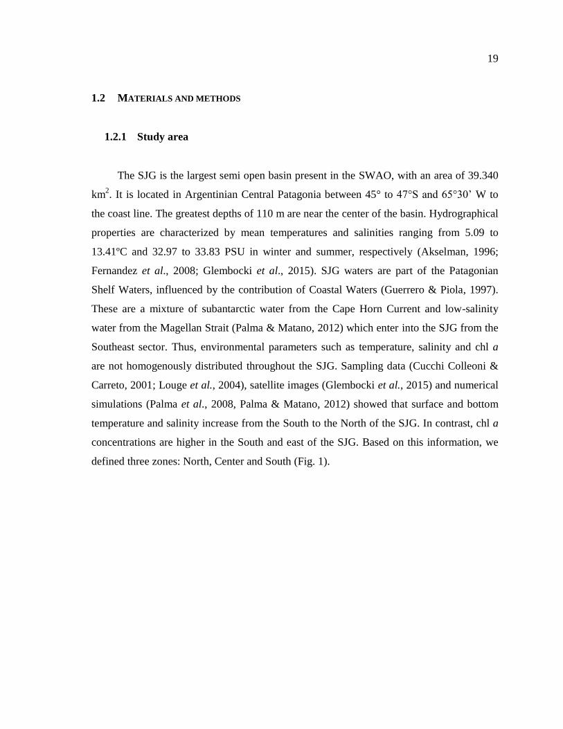
Figure 1: Three a priori defined hydrographic zones, Northern, Central and Southern, of
the San Jorge Gulf according to according to Cucchi Colleoni and Carreto (2001), Louge et
al.(2004), Palma and Matano (2012) and Glembocki et al. (2015)………………………. 20
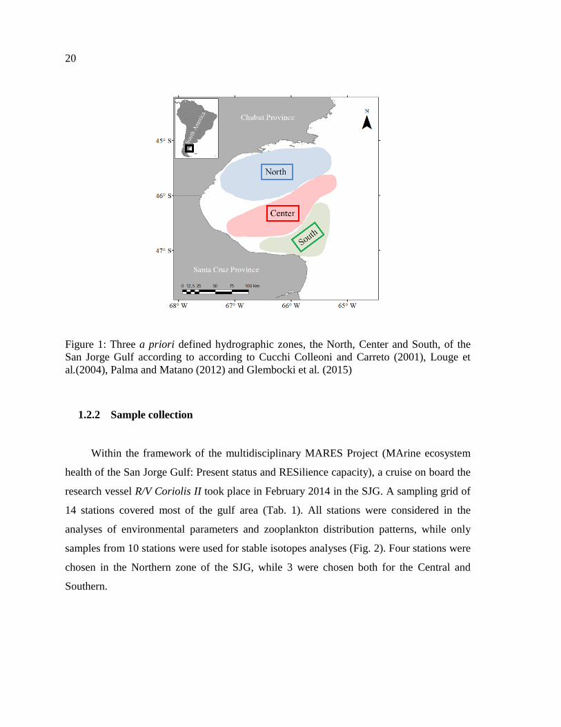
Figure 2: Zooplankton stations sampled in the San Jorge Gulf in February 2014 on board
the R/V Coriolis II. Black circles represent stations where samples of environmental
parameters and zooplankton (243 µm mesh size) were collected. Red dots indicate stations
where stable isotopes analyses were performed. X indicates stations where no zooplankton
samples were available. Bathymetry was adapted from Chart H-365 from the National
Hydrographic Survey of Argentina ...................................................................................... 21
Figure 3: Density (Sigma-T, kg m-3
) and Brunt-Väisälä frequency (VAIS; sec-1
) profiles
representative for stations located at the a) Northern (G06), b) Central (G09) and c)
Southern (G11) zones of the San Jorge Gulf during austral summer 2014 .......................... 30
Figure 4: Principal Components Analysis (PCA) showing the ordination space of the
correlations of environmental variables (surface and bottom temperature, integrated
chlorophyll a and stratification) with the first two axes (PC1 and PC2). C = Central zone;
N = Northern zone; S = Southern zone. Tsur = surface temperature, Tbott = bottom
temperature, Chl a = chlorophyll integrated over the water column ................................... 31
Figure 5: Relative contribution of major taxa in the SJG of zooplankton community. Cvan:
Ctenocalanus vanus; Cop: copepodites of C. vanus, Clausocalanus brevipes, Drepanopus
focripatus and Paracalanus parvus; Dfor: D. forcipatus; Ppar: P. parvus; Aton: Acartia
tonsa; Cal: Calanidae family (Calanus australis and Calanoides carinatus); Oiko:
Oikopleura sp.; Others: other zooplankton taxonomic groups ............................................ 33
Figure 6: Total abundance (ind. m-2
) (a) and total biomass (mg m-2
) (b) for zooplankton
community in 3 putative geographic zones of San Jorge Gulf during austral summer.
Medians, first (25%) and third (75%) quartiles are represented .......................................... 35
xxvii
Figure 7: The zooplankton assemblages of 14 stations of the San Jorge Gulf divided into 3
geographic zones, North (N), Center (C) and South (S) shown by non-metric
multidimensional scaling (nMDS) ........................................................................................ 36
Figure 8: Abundance (ind. m-2
) (a) and biomass (mg DW m-2
) (b) of zooplankton
community in 14 stations of San Jorge Gulf during austral summer. « Copepodite »
represents copepodites stages of C. vanus, C. brevipes and P. parvus. Northern zone: G04,
G05, G06, G07, G15 and G16; Central zone: G01, G09, G14, SF14; Southern zone: G10,
G11, G12, G13 ...................................................................................................................... 37
Figure 9: Pielou´s evenness and Shannon-Wiener biodiversity indices for the
Northern/Central zone (N-C) and the Southern-one (S) of the San Jorge Gulf during austral
summer. Error bars represent standard errors ....................................................................... 39
Figure 10: Surface and bottom 13
C (a, b) and 15
N values (c, d) of particulate organic
matter for Northern (N), Central (C) and Southern (S) zones of the San Jorge Gulf.
Different letters indicate significant differences in isotopic ratios of carbon and nitrogen
among zones. Error bars show standard errors ..................................................................... 40
Figure 11: Biplots of stable isotope signatures (13
C and15
N) of the main components of
the zooplankton community in the Northern, Central and Southern zones of the San Jorge
Gulf during austral summer. Error bars indicates +/- standard errors. The 13
C on the x-
axis reflect potential carbon sources, while the 15
N values in the y-axis shows the taxa
trophic position. POM: particulate organic matter; Copepodite: development stages of
Ctenocalanus vanus, Clausocalanus brevipes, Paracalanus parvus and Drepanopus
forcipatus; Euph: euphausiids ............................................................................................... 43
Figure 12: Mean trophic levels (TLs) for copepods (a) and euphausiids (b) in the San Jorge
Gulf. Different letters indicate significant differences in mean TLs among zones. Error bars
represent standard errors ....................................................................................................... 44
Figure 13: Mean trophic levels of copepods, chaetognaths and appendicularians for the
three zones (Northern, Central and Southern) of San Jorge Gulf. Sagit= Sagitta sp.; Aton=
Acartia tonsa; Ppar= Paracalanus parvus; Cop= Copepodites of Ctenocalanus vanus,
Clausocalanus brevipes, Drepanopus forcipatus and Paracalanus parvus; Cvan=
Ctenocalanus vanus; Ohel= Oithona helgolandica; Oiko= Oikopleura sp. ......................... 45

xxviii
LISTE DES ABRÉVIATIONS, DES SIGLES ET DES ACRONYMES
Français
GSJ golfe San Jorge
N/R Navire de recherche
MOP matière organique particulaire
13
C signature isotopiques du carbone
15
N signature isotopique de l’azote
chl a chlorophylle a
p.s. poids sec
Anglais
SJG San Jorge Gulf
SWAO Southwestern Atlantic Ocean
POM Particulate organic matter
C Carbon
N Nitrogen
13
C Carbon isotopic signature
15
N Nitrogen isotopic signature
xxx
R/V Research vessel
FW Food web
chl a Chlorophyll a
TL Trophic level
ANOVA Analysis of variance
df Degrees of freedom
nMDS Non metric multidimensional scaling
PCA Principal components analysis

xxxi

1
INTRODUCTION GÉNÉRALE
Le zooplancton et la biodiversité
Le zooplancton habite l’ensemble de la colonne d’eau et possède une faible capacité
de nage, si l’on compare avec les courants océaniques. Par conséquent, ses mouvements
verticaux et sa distribution spatiale horizontale sont considérablement affectés par deux
causes principales : d’une part, il est affecté par la dérive des courants et, d’autre part, sa
distribution spatiale dépend de la capacité de survivre et de se reproduire dans les endroits
où il dérive (Mackas et Beaugrand, 2010). Le zooplancton comprend une large gamme
autant taxonomique que de tailles (Lenz, 2000). En outre, si l’on considère le cycle
biologique des animaux marins, on distinguera l’holozooplancton et le merozooplancton
(Márquez et al., 2009). Le premier inclut des organismes planctoniques durant toute leur
vie, tandis que le deuxième correspond à des organismes qui passent une partie de leur vie
dans la colonne d’eau avant de changer vers une phase nectonique (ex. : les larves des
poissons) ou benthique (ex. : les larves des crustacés décapodes ou des bryozoaires). En
outre, parmi les organismes zooplanctoniques on retrouve des modèles de développement
différents : le développement direct, comme par exemple les chaetognathes, et le
développement indirect, avec une grande variété des formes de larves, tel que les
copépodes qui possèdent 11 stades de développement (6 larves nauplii et 5 stades
copepodites) avant devenir des copépodes adultes (Hulseman, 1991). La classification du
plancton établie par Sieburth et al. (1978) est actuellement acceptée pour classifier le
zooplancton considérant des classes de taille, selon les catégories suivantes : le
nanozooplancton (2 – 20 µm ; flagellées hétérotrophes), le microzooplancton (20 – 200
µm ; ciliés, flagellées et des œufs et des premiers stades du développement des crustacés
planctoniques), le mesozooplancton (200 µm – 0,2 cm ; copépodes, cladocères,
cténophores, appendiculaires, chaetognathes de petite taille, larves de crustacés et des œufs
2
et certains larves de poissons), le macrozooplancton ( 2 – 20 cm ; méduses, chaetognathes
de grande taille, mysidacés, amphipodes, salpes et euphausides), et dernièrement le
megazooplancton ( 20 cm – 2 m ; principalement des méduses de grande taille). Ce
mémoire s’intéresse principalement au mesozooplancton et, en second lieu, à certaines
composantes du macrozooplancton. Les copépodes sont considérés comme le groupe du
mesozooplancton le plus abondant dans le milieu pélagique en termes d’abondance et de
biomasse ainsi que les plus importants producteurs secondaires, suivis des appendiculaires
qui ont des taux de croissance élevées par rapport aux copépodes et qui peuvent contribuer
de façon importante à la biomasse totale du plancton (Kiørboe, 1997 ; Hopcroft et Roff,
1998). Tel que mentionné précédemment, le zooplancton est un groupe possédant une
biodiversité élevée. Ceci reste un terme très vaste, si l´on considère étant plus que la
richesse spécifique, c’est-à-dire, le nombre des espèces ou de taxons présents dans une
région (Clarke et Warwick, 2001). Ainsi, la biodiversité intègre aussi d’autres dimensions
telles que la diversité génétique, la diversité des écosystèmes, le nombre des niveaux
trophiques présents ou la variété des cycles de vie (Harper et Hawksworth, 1995).
Distribution spatiale du zooplancton
La distribution du zooplancton dans le milieu pélagique est loin d’être homogène.
Elle varie dans l’espace et dans le temps à différentes échelles. Cette distribution
hétérogène, qui n’est ni aléatoire ni uniforme, est devenue un sujet d’intérêt important
autant sur le plan théorique que sur le plan de la stratégie d’échantillonnage.
L’hétérogénéité spatiale des conditions environnementales génère des variations dans la
diversité des organismes, aussi comme dans les processus écologiques et biologiques à
différentes échelles dans l’espace et le temps (Legendre et Fortin, 1989). Il faut tenir en
compte qu’il n’y a pas qu’un seul facteur qui détermine la distribution hétérogène du
zooplancton. C’est un ensemble de facteurs divers opérant à différentes échelles. À
l’échelle locale, les processus biologiques (ex. : interactions trophiques et disponibilité de la
nourriture) exercent une influence dominante. À grande échelle, il a été remarqué que ce
3
sont les conditions environnementales et les processus abiotiques qui influencent d’une
façon plus marquée la distribution spatiale du zooplancton (Pinel-Alloul et Pont, 1991).
La relation entre les masses d’eau et les assemblages zooplanctoniques a été
documentée dans différents environnements par plusieurs auteurs (Ward et al., 2007 ;
Brugnano et al., 2010), qui constatent que l’hétérogénéité des conditions
environnementales des masses d’eau a une influence marquée sur la composition et sur la
distribution spatiale des communautés zooplanctoniques. Ces assemblages étaient corrélés
avec la température, la salinité (Smooth et Hopcroft, 2016) et la stratification de la colonne
d’eau (Lee et al., 2005). Notamment, sur le plateau continental argentin, ces conditions
environnementales ont été liées à des assemblages zooplanctoniques divers (Marrari et al.,
2004 ; Sabatini et al., 2016). Dans un système de fronts au nord du plateau continental
patagonique, premièrement la température et deuxièmement la stratification étaient
inversement corrélées avec les abondances des copépodes et des appendiculaires. De plus,
la chlorophylle a a été le principal facteur déterminant la composition et la répartition de la
communauté de mesozooplancton (Spinelli, 2013). Il faut noter que le zooplancton
représente la source d’alimentation primaire accessible aux autres invertébrés aquatiques
des niveaux trophiques supérieurs et aux poissons (Ivanovic et Brunetti, 1994 ; Baier et
Purcell, 1997). De ce fait, la distribution du zooplancton exerce une influence importante
pour les zones de reproduction et de nurserie des populations de ces organismes (Spinelli et
al., 2012).
Le zooplancton et son importance dans le milieu pélagique
Le zooplancton occupe une position clé dans le milieu marin en créant un lien entre
les producteurs primaires et les consommateurs secondaires à travers du transfert du
carbone fixé par le phytoplancton (Cushing, 1984 ; Kiørboe, 1989). Le zooplancton joue
également un rôle central dans la structuration des réseaux alimentaires pélagiques. La
limitation des ressources (contrôle « bottom-up »), et la mortalité par prédation (« contrôle
4
top-down »), déterminent la dynamique et les processus au sein des communautés
planctoniques (Kiørboe, 1997). En général, le zooplancton consomme le phytoplancton
ainsi que la composante microbienne. La perception de l’écologie trophique du plancton
marin a considérablement changé depuis les trois dernières décennies. Il est devenu évident
que les réseaux trophiques pélagiques sont moins simples que l’on pensait, car ils incluent
un nombre plus élevé de niveaux trophiques par rapport à ce que l’on avait cru auparavant
(Pomeroy et Wiebe, 1988). Ce concept sur la dynamique planctonique reconnait que les
microorganismes phototrophes et hétérotrophes jouent un rôle substantiel et parfois
dominant dans le cycle de la matière en milieu pélagique. Ce concept révéle qu’une grande
fraction de la production primaire n’est pas consommée directement par les herbivores,
mais qu’elle est plutôt acheminée à travers la matière organique morte avant qu’elle ne
devienne disponible, par production bactérienne, pour des organismes phagotrophes
(Fenchel, 1988). Par la suite, l’image classique des chaînes trophiques planctoniques reste
essentiellement correcte, mais cette description est incomplète. La boucle microbienne
décrite par Azam et al. (1983) a élargi la vision écologique des relations trophiques au
milieu pélagique. Dans l’ancienne image classique, la reminéralisation est en partie due au
zooplancton et la vision des relations trophiques reste linéaire. La production de matière
organique dans la mer dépend du phytoplancton, principalement des diatomées et des
dinoflagellés, qui sont consommés par le zooplancton. Ces organismes servent de
nourriture pour les poissons planctivores et pour d’autres composantes du necton. Cette
manière de coupler étroitement la production primaire et la production des poissons dans
les écosystèmes marins est une vision très simple et très réduite du réseau alimentaire
pélagique et des interactions trophiques (Lacroix et Danger, 2008). Cette vision a été
remplacée lorsque la boucle microbienne et lorsque la grande diversité du zooplancton par
rapport la forme et la fonction ont été reconnues (Fenchel, 1988). L’eau de mer contient des
détritus en suspension qui incluent la matière organique particulaire (MOP). Il s’agit, entre
autres, d’un ensemble de cellules bactériennes et phytoplanctoniques vivantes, de maisons
d’appendiculaires, des pelotes fécales, des restes d’organismes zooplanctoniques et d’autres
composantes organiques non vivantes (Alldredge, 1976 ; Dong et al., 2010). Certains
5
organismes tels que les petits copépodes semblent se nourrir de la MOP. Ils sont alors
considérés comme détritivores (Turner, 2004). De cette manière, les régimes alimentaires et
les guildes trophiques dans les communautés de zooplancton sont variés. Certains taxons
peuvent se nourrir en tant que brouteurs de phytoplancton et sont donc herbivores. D’autres
taxons sont carnivores, tels que les chaetognathes, certains copépodes et les larves nauplii
du grand copépode Calanus spp., prédateurs d’une grande variété des proies (Turner,
2004 ; Sato et al., 2011). D’autres groupes sont considérés comme omnivores (ex. : le
copépode Acartia sp.), qui sont brouteurs de phytoplancton, des cyanobactéries et des
protistes hétérotrophes (Turner et al., 1998). Ils agissent aussi comme détritivores et
carnivores, en s’alimentant de proies appartenant aux niveaux trophiques adjacents et
inférieurs (Coat, 2009). Par exemple, les euphausiacés ont également été signalés comme
omnivores car ils se nourrissent du phytoplancton, des dinoflagellées et d'autres sources
alimentaires (Price et al., 1988 ; Schmidt et al., 2006). En conséquence, le zooplancton peut
limiter les populations des ciliés et des flagellés dans le cas de pénurie de phytoplancton
(Atkinson, 1996). Dans ce cas, une très grande variété de sources de nourriture peut
favoriser certaines populations. Par exemple, le petit cyclopoïde Oithona sp. a été signalé
comme brouteur de diatomées, de ciliés, de bactérioplancton et d’autres composantes de la
boucle microbienne. Il a été également signalé comme carnivore et coprophage, en utilisant
les pelotes fécales des herbivores comme source de nourriture (González et Smetacek, 1994
; Castellani et al., 2005 ; Iversen et Poulsen, 2007). Par conséquent, l’omnivorie dans les
organismes planctoniques, y compris les espèces de la boucle microbienne dans les études
des réseaux trophiques planctoniques, est en train d’améliorer la compréhension du
recyclage de la matière organique des agrégats incluant le détritus et les pelotes fécales
ainsi que le transfert des nutriments aux niveaux trophiques supérieurs (Lacroix et Danger,
2008 ; Pond et Ward, 2011). Le zooplancton se compose donc d’organismes phagotrophes
et selon leurs préférences alimentaires, ils peuvent être herbivores, détritivores, omnivores
et carnivores (Lenz, 2000). La diversité des modes d’alimentation présentes au sein du
zooplancton a fait de ces organismes un groupe d’étude remarquable des réseaux trophiques
dans les milieux pélagiques.
6
Un autre aspect important du zooplancton dans les écosystèmes marins est leur rôle
dans le transfert de matière organique vers les niveaux trophiques supérieurs, tels que les
poissons. Sur le plateau continental argentin, la distribution et la variabilité du zooplancton
a des effets sur les zones de reproduction et de nurserie des poissons et crustacés. Parmi
eux, des espèces d’intérêt commercial, telles que décrites pour Merluccius hubbsi (de
Ciechomski et Sánchez, 1983, Sabatini et al., 2004), Macruronus magellanicus (Sabatini et
al., 2004) et Engraulis anchoita (Viñas et Ramírez 1996 ; Viñas et al., 2002, Spinelli,
2013). Le recrutement larvaire des premiers stades de développement dépend de la
disponibilité d'une nourriture suffisante et adaptée au moment de la première phase
d'alimentation des larves (Cushing, 1972). Par conséquent, à l’intérêt écologique qu’il
suscite il faut ajouter l’importance dans le domaine économique, faisant du zooplancton
une composante du milieu pélagique d’intérêt prioritaire pour la recherche.
L’étude de la structure trophique du zooplancton : l’utilité des analyses avec
isotopes stables
La plupart des connaissances sur les régimes alimentaires dans les communautés
zooplanctoniques et leur écologie trophique est basée sur des techniques traditionnelles
telles que les contenus stomacaux, intestinaux, les analyses des pelotes fécales, les mesures
de taux d’ingestion, de sélectivité alimentaire et d’autres expériences d’alimentation
réalisées en laboratoire (Bautista et Harris, 1992; Abe et al., 2016). Les deux premières
analyses fournissent une image instantanée sur les sources alimentaires récemment
consommées in situ. Toutefois, les études de ce type demandent une grande précision de
manipulation et demeurent difficiles à réaliser dans le cas du zooplancton le plus petit (˂
800 µm). Ces dernières années, les analyses des acides gras comme marqueurs organiques
naturels et des isotopes stables, notamment celui du carbone (
C) et de l’azote (
N), ont
été reconnues comme un outil puissant pour l’étude de la structure trophique et des régimes
alimentaires dans les réseaux trophiques pélagiques, étant utilisées à l’échelle mondiale
7
dans des écosystèmes d’eau douce (Jones et al., 1999) et marins (DeNiro et Epstein, 1981 ;
Fry, 1988 ; Kattner et al., 2003 ; Verschoor et al., 2005). Les analyses des isotopes stables
ont plusieurs avantages : les données sont précises et le coût est raisonnable. Les
échantillons sont faciles à préparer et sont faciles à transporter et à stocker pour une longue
période de temps (Verschoor et al., 2005, Smyntek et al., 2007). Cependant, il existe encore
un manque de standardisation méthodologique, ce qui oblige à prendre des précautions lors
des comparaisons entre les études. Les recherches utilisant cette méthodologie ont été
effectuées dans tous les océans (Hobson et al., 2002 ; Rosas Luis et Loor Andrade, 2015) et
en particulier dans l’océan Atlantique sud se sont principalement penchés sur les
composantes supérieures des réseaux trophiques marins (Galván et al., 2009) ou des
réseaux trophiques benthiques (Andrade et al., 2016). Cependant, peu d’attention a été
porté sur les réseaux trophiques planctoniques marins dans la région (Wada et al., 1987 ;
Rau et al., 1991).
Le site d’étude
Le golfe San Jorge (GSJ) est un bassin océanique ouvert sur l’océan Atlantique Sud
situé entre 45-47 S, 63°30’O et la ligne de rivage, entre cap Dos Bahías et cap Tres Puntas,
couvrant une surface d’environ 39300 km2. Il a une extension d’environ 240 km de long à
son embouchure. Les côtes du GSJ sont partagées par les provinces du Chubut et Santa
Cruz. La profondeur maximale est de 110 m, et se trouve dans la zone centrale du GSJ,
bien délimitée par l’isobathe de 90 m. Dans le secteur nord, le golfe présente un seuil de
250 km de long avec des profondeurs autour de 80-95 m (Akselman, 1996). On décrit deux
zones de fronts dans le golfe : un front thermique au nord, bien développé pendant le
printemps et l’été, où la colonne d’eau devient stratifiée et un front de marée thermo-haline
au sud (Glembocki et al., 2015). Ces zones de fronts ont été associées à une productivité
primaire élevée, selon des observations in situ (Akselman, 1996 ; Cucchi Colleoni et
Carreto, 2001) et des données d’images satellites (Glembocki et al., 2015). Les eaux du
GSJ font partie des eaux du plateau continental argentin qui sont modifiés par la
8
contribution des eaux côtières de salinité faible coulant du détroit de Magellan (connue
comme « La Plume de Magellan »), près de la côte de la province de Santa Cruz, où son
flux est séparé dans deux branches principales. L’une entre dans le golfe à l’extrême sud-
est et a une remarquable influence sur la région tout au long de l’année. L’autre branche
s’éloigne de la côte (Bianchi et al., 1982 ; Fernández et al., 2005). Les résultats des
modèles numériques hydrodynamiques de la circulation moyenne montrent la présence de
deux gyres présentant des directions opposées dans le GSJ : l’un au nord qui tourne dans le
sens horaire, tandis qu’au sud la circulation est plus intense et dans l’autre sens (Tonini et
al., 2006). Il n’y a aucune rivière avec embouchure dans le golfe et les précipitations sont
rares, avec une moyenne annuelle de 233 mm à Comodoro Rivadavia. Cette ville est la plus
importante à proximité du GSJ, possédant un port de pêche commerciale d’envergure. De
plus, il est exposé aux risques environnementaux liés au développement urbain-industriel, à
l’exploitation terrestre de pétrole (Commendatore et al., 2000), au forage en mer et à
l’intense activité du transport de pétrole (Yorio, 2009 ; Góngora et al., 2012). Le bassin
pétrolier du GSJ est le plus grand et le plus productif en Argentine (Sylwan, 2001). En
outre, le GSJ a des aires de frai et nurserie pour des nombreuses espèces de poissons et de
crustacés. Le golfe possède une intense activité de pêche, ciblée sur la crevette (Pleoticus
muelleri), le merlu argentin (Merluccius hubbsi), l’anchois (Engraulis anchoita) et le crabe
royal (Lithodes santolla) parmi d’autres espèces d’intérêt commercial (de Ciechomski et
Sánchez 1983 ; Sánchez et Prenski, 1996 ; Viñas et Ramírez 1996 ; Sabatini et al., 2004 ;
Góngora et al., 2012). Enfin, le GSJ présente des domaines de grande valeur pour la
conservation des environnements marins. Le plus remarquable est l’aire marine protégée
qui se trouve le long de la côte nord-est du golfe, le « Parc Marin Patagonia Austral », très
importante pour la reproduction et l’alimentation de nombreuses espèces de poissons,
d’oiseaux et de mammifères marins (Yorio, 2001 ; 2009).
9
Objectifs de recherche
Étant donné l’importance du zooplancton autant du point de vue écologique
qu’économique, le présent projet de maîtrise a pour but de caractériser la composition, la
distribution spatiale et la structure trophique du zooplancton dans le GSJ pendant l’été
australe. Pour cela, les objectifs spécifiques sont : 1) d’identifier la structure des masses
d’eau dans le GSJ et de décrire la composition, l’abondance, la biomasse et les assemblages
des espèces composant le zooplancton en relation avec des conditions environnementales et
2) de décrire la structure du réseau trophique zooplanctonique, d’identifier les sources de
carbone et de déterminer les niveaux trophiques des taxons qui le composent. L’analyse
isotopique du carbone (13
C) et de l’azote (15
N) de la matière organique particulaire et des
composantes de la communauté zooplanctonique permettra la caractérisation des sources de
carbone et l’estimation des niveaux trophiques zooplanctoniques présents dans le GSJ. La
partie centrale de ce mémoire de maîtrise est présenté dans un chapitre rédigé en anglais
sous forme d’article scientifique.
CHAPITRE 1
ZOOPLANKTON COMMUNITY COMPOSITION, SPATIAL DISTRIBUTION
AND TROPHIC STRUCTURE IN THE SAN JORGE GULF (45°-47°S, SW
ATLANTIC OCEAN)
RÉSUMÉ
La composition, la distribution spatiale liée aux conditions environnementales et la
structure du réseau trophique de la communauté zooplanctonique dans le golfe San Jorge
(GSJ, 45°-47° S, Atlantique Sud-Ouest) ont été étudiées dans le cadre d’une mission
océanographique en en février 2014, durant l’été austral. L’échantillonnage a été effectué à
l’aide d’un filet à 243 µm de maille et il a compris 14 stations réparties sur l’ensemble du
GSJ. L’abondance moyenne et la biomasse du zooplancton ont varié de 55356 à 425469
ind. m-2
et de 492 à 4454 mg p.s. m-3
, respectivement. La communauté zooplanctonique
était composée de 30 taxons, avec les copépodes représentant 83% de la densité totale. La
structure de la communauté a été fortement liée à la température de surface et à la
stratification de la colonne d’eau. La température, la chlorophylle a et la stratification de la
colonne d’eau ont permis d’identifier deux zones : le nord/centre (bien stratifié) et le sud
(température de surface plus froide, non stratifié) du GSJ. On a trouvé deux assemblages
différents de zooplancton dans ces deux masses d’eau distinctes. Le nord/centre a été
fortement dominée par les copépodes calanoides Ctenocalanus vanus, les stades de
développement copépodites de C. vanus, Clausocalanus brevipes et Paracalanus parvus,
les appendiculaires et le copépode cyclopoide Oithona helgolandica. La zone sud a été
caractérisée par P. parvus, les copépodites de C. vanus, C. brevipes et P. parvus, Acartia
tonsa et Drepanopus forcipatus. Les analyses des isotopes stables du carbone (13
C) et de
l’azote (15
N) ont permis d’évaluer la structure trophique de la communauté du zooplancton
dans la zone nord, centrale et sud du GSJ. La matière organique particulaire de surface et de
11
fond a été enrichie en 13
C du nord au sud. Les valeurs appauvries dans le nord peuvent
s’expliquer par des matériels terrigènes introduits dans le golfe par les vents forts de
l’ouest. De grandes variations ont été trouvées dans les valeurs de 13
C des taxons dans
chaque zone et parmi les zones. La large gamme des valeurs (-16.8 ± 1.5 13
C to -30.6 ±
3.4 13
C) reflète une vaste diversité de sources alimentaires parmi les différents taxons. Une
forte tendance à l’enrichissement en 13
C du nord au sud a également été observée dans la
majorité des composants du réseau trophique. L’espace trophique étroit enregistré dans le
réseau sud suggère des stratégies d’alimentation similaires parmi les taxons. Les
chaetognathes ont occupé la position trophique la plus haute au nord et au centre, tandis
que, dans le sud, sa position était occupée par A. tonsa. Les appendiculaires ont montré les
niveaux trophiques les plus bas : deux et trois au nord et au centre, respectivement. Une
augmentation des valeurs des niveaux trophiques a été observée du nord au sud pour les
appendiculaires, les copépodes, les euphausiides et les chaetognathes. Les résultats obtenus
grâce à cette étude ont ouvert de nouvelles perspectives et contribueront à mieux connaître
la composition, la distribution, la dynamique et la structure trophique du zooplancton dans
le GSJ en relation avec les conditions environnementales.
Mots clés : zooplancton, distribution spatiale, masses d’eau, assemblages, isotopes
stables, réseau trophique, écosystème marin, golfe San Jorge, plateau continental argentin.
12
ABSTRACT
This study analyses the zooplankton community structure, its spatial pattern relative
to environmental conditions and the food web structure in the San Jorge Gulf (SJG, 45°-
47°S, Southwestern Atlantic Ocean). Sampling was conducted during February of 2014
using a zooplankton net of 243µm mesh size, along 14 stations distributed over the entire
SJG. Mean zooplankton density and biomass throughout the SJG ranged from 55356 to
425469 ind. m-2
and 492 to 4454 mg DW m-2
, respectively. The sampled zooplankton
community was composed of 30 taxa with copepods accounting for 83% of the total
density. Community structure was strongly related to surface temperature and stratification
of the water column. The temperature, chlorophyll a and stratification of the water column
permitted to distinguish two water-mass zones, each characterized by distinct zooplankton
assemblages: a stratified one comprising the North/Center of the SJG, and another one, in
the South, unstratified and with colder surface temperatures. The North/Central zone was
dominated by the adult of the calanoid copepods Ctenocalanus vanus, copepodites stages of
C. vanus, Clausocalanus brevipes and Paracalanus parvus, appendicularians and the
cyclopoid copepod Oithona helgolandica. The Southern zone was characterized by the
dominance of the calanoid copepods P. parvus, copepodites stages of C. vanus, C. brevipes
and P. parvus, Acartia tonsa and Drepanopus forcipatus. Stable isotope analyses of carbon
(13
C) and nitrogen (15
N) were performed to assess the zooplankton community trophic
structure, along three zones (North, Central and South) chosen a priori for this study of the
SJG. Surface and bottom particulate organic matter was enriched in 13
C from North to
South. Depleted values in the North may be explained by terrigenous inputs derived from
strong westerly winds. Large variations were found in 13
C values of zooplankton taxa
within each zone and among zones. The broad range of values obtained (-16.8 ± 1.5 13
C to
-30.6 ± 3.4 13
C) reflected a wide diversity of food sources among the taxa. A strong
enrichment in 13
C from North to South was observed in the majority of the food web
components. The narrow trophic space observed in the Southern food web suggests,
however, similar feeding strategies among the taxa in that zone. Chaetognaths occupied the
13
highest trophic position in the North and in the Center, while in the South its position was
occupied by A. tonsa. Appendicularians showed the lowest trophic levels of two and three
in the North and in the Center, respectively. An increase in the values of trophic levels was
observed from the North to the South for appendicularians, copepods, euphausiids, and
chaetognaths. The results of this study opened new perspectives and contribute to a better
understanding of the composition, distribution, dynamics and trophic structure of the SJG
zooplankton in relation to environmental conditions.
Key words: zooplankton, spatial distribution patterns, water masses, assemblages,
stable isotope analyses, food web, marine ecosystem, San Jorge gulf, Argentine continental
shelf.
14
1.1 INTRODUCTION
Zooplankton plays a major role in the productivity and the functioning of marine
ecosystems since they occupy a key position in the pelagic community, transferring the
energy from primary producers up in the food web (FW), influencing nutrient dynamics
(Cushing, 1984; Kiørboe, 1989; Legendre & Rassoulzadegan, 1995) and favoring the
biological carbon pump (Longhurst & Harrison, 1989). Marine zooplankton is composed of
a large diversity of taxonomic groups. Among them, planktonic crustaceans, such as
copepods and euphausiids, represent the most abundant groups, contributing to secondary
production in most of the marine environments, including the Southwestern Atlantic Ocean
(SWAO; Boltovskoy, 1981; Voronina, 1998, Ward et al., 2007; Marquez et al., 2009;
Thompson et al., 2013). Biodiversity of zooplankton comprises not only species variety,
but also diversity in functional groups, which are relevant to understand the functioning of
marine ecosystems influencing processes and interactions (Duffy & Stachowicz, 2006). On
the other hand, zooplankton represents a source of organic carbon in terms of exoskeletal
material and fecal pellets, which sink passively or is actively transported by diel vertical
migrations from the euphotic zone into deeper waters, contributing to the CO2 biological
pump (Longhurst & Harrison, 1989; Lavaniegos & Cadena-Ramírez, 2012). Furthermore,
zooplankton is a source of carbon which can be transferred through trophic interactions to
upper levels in the community. Hence, distribution of these organisms has an impact on
spawning and nursery areas of fish populations, in particular commercially exploited fishes
on the Argentine continental shelf, such as Merluccius hubbsi (de Ciechomski & Sánchez,
1983; Sabatini et al., 2004) and Engraulis anchoita (Viñas & Ramírez, 1996; Viñas et al.,
2002; Spinelli, 2013).
Heterogeneity in environmental properties of water masses usually controls
zooplankton community composition, structure and distribution. For example, in the Arctic
Ocean during summer and autumn, zooplankton community structure was correlated with
15
temperature and salinity averaged over the upper mixed layer (Smooth & Hopcroft, 2016).
In the Central Irish Sea, during summer, species composition variations were directly
related to the stratification of the water column (Lee et al., 2005). On the Argentinian
continental shelf (SWAO) and in particular on the Patagonian shelf, distinct abiotic (e.g.,
temperature, salinity, stratification of the water column) and biotic (e.g., chlorophyll a -chl
a-) oceanographic conditions were associated with different zooplankton assemblages and
distribution (Marrari et al., 2004; Spinelli et al., 2012; Spinelli, 2013; Sabatini et al. 2016).
In frontal systems of the Patagonian shelf, temperature and stratification in summer were
inversely correlated with copepods and appendicularians abundances (Spinelli et al., 2012;
Spinelli, 2013). In addition, high chl a concentration at one side of the front were related to
high abundances of calanoid and cyclopoid copepods (Temperoni et al., 2014; Temperoni,
2015).
Differences in water mass properties were found to have an influence not only in
zooplankton distribution patterns, but also in the trophic structure of the entire plankton
community. In terms of nutrients and resources availability (Kiørboe, 1993; De Ruiter et
al., 2005), this translates into a variety of potential food sources for zooplankton (Andrade
et al., 2016). In particular, in the SWAO those differences were reflected in the trophic
structure of the plankton community during summer. High and low chl a concentrations (as
a proxy of phytoplankton) were related to high contribution of herbivorous or omnivorous
zooplankton, respectively. Furthermore, spatial fluctuations of zooplankton feeding forms
in different regions of the SWAO were evidenced by dissimilar values of trophic levels
(TLs) within the zooplankton community (Thompson et al., 2013). The variability in
zooplankton distribution also has a strong influence in the higher TLs of FW that feed on it,
like fish larvae (Hunter, 1981) and juveniles of fish species (Padovani et al., 2012;
Temperoni & Viñas, 2013).
Trophic structure is one of the most fundamental characteristic of marine
environments since it provides a way to understand energy and matter flows in the
ecosystem and trophic linkages among organisms. Trophic interactions within the FW may
16
influence the persistence and the dynamics of zooplankton populations through resources
availability and predation pressure (De Ruiter et al., 2005). Considering that zooplankton is
responsible for channeling a large fraction of the primary production to higher TLs, it is
important to improve the knowledge of energy pathways in the FW.
The marine planktonic FWs are more complex and dynamic as previously thought
(Pomeroy & Wiebe, 1988). The recognition of the enormous diversity of zooplankton with
respect to form and function (Fenchel, 1988) and the discovery of the microbial loop
(Azam et al., 1983) expanded the vision of the marine FW. Feeding habits and trophic
groups within zooplankton communities are diverse (Duffy & Stachowicz, 2006).
Particulate organic matter (POM) is a bulk of living components such as bacteria,
phytoplankton cells, and nonliving organic matter as appendicularians houses, other
remains of zooplankters, fecal pellets and other detrital organic matter (Alldredge, 1976;
Dong et al., 2010). Some zooplanktonic organisms, such as small copepods, appear to feed
on it as detritivores (Turner, 2004). Some other taxa can feed as grazers of phytoplankton
as herbivores. Carnivores, such as chaetognaths and some species of copepods, feed as
predators upon heterotrophic protists and on a large variety of preys (Turner, 2004; Sato et
al., 2011). Other groups feed as omnivores (e.g., the ubiquitous copepod Acartia spp.),
grazing on phytoplankton and cyanobacteria as well as upon heterotrophic protists (Turner
et al., 1998). Euphausiids are omnivorous, feeding on phytoplankton as well as on another
food sources (Price et al., 1988). The small cyclopoid Oithona sp. has been reported
worldwide to graze upon diatoms, as well as upon bacterioplankton, ciliates and other
autotrophic nanoplankton, and to be able to feed carnivorously and coprophagously on
calanoid and euphausid faecal material (González & Smetacek, 1994; Castellani et al.,
2005; Iversen & Poulsen, 2007). Thus, a very wide variety of food sources can sustain
populations. Consequently, research on the omnivory within communities, including the
organisms of the microbial loop, will increase our understanding of organic matter, detrital
aggregates and fecal material recycling and of nutrient transfer to higher TLs (Lacroix &
Danger, 2008; Pond & Ward, 2011). The diversity in feeding forms present in zooplankton
communities makes it an interesting study group in FW of marine environments.
17
Food availability exerts a bottom-up control on the size of populations (Antacli et al.,
2014). Knowledge on the zooplankton community and its trophic structure of the San Jorge
Gulf (SJG, 45°-47°S, SWAO) is crucial to improve estimates of food availability for many
invertebrate and vertebrate species of economic interest to fisheries such as Illex
argentinus, Pleoticus muelleri, Merluccius hubbsi and Engraulis anchoita, which partially
or strictly depend on zooplankton as a food source (Viñas & Ramírez, 1996; Sabatini,
2004; Vinuesa, 2005). The entire SJG represents a nursery area for several fish species,
while the Northern and Southern mouth regions are spawning areas for the Argentine hake
(Merluccius hubbsi), which varies its food source along the ontogeny. Larvae and juveniles
of M. hubbsi feed strictly on zooplankton preys. Larvae prefer, for example, copepod
nauplii and copepodites and adult copepods (Paracalanus parvus, Oithona spp., Acartia
tonsa and Clausocalanidae). When juveniles, they switch their diet to euphausiids
(Euphausia spp.), amphipods (Themisto gaudichaudii), mysids and other
macrozooplankton (Sabatini, 2004; Sánchez, 2009; Temperoni, 2015). It is an area of great
interest not only for commercial fishing, but also for conservation of marine mammals and
seabirds (Bertolotti et al., 1996; Yorio, 2009). Besides, the SJG includes highly diverse
coastal and marine environments and is an area of importance in terms of biodiversity and
productivity (Roux & Fernández, 1997; Góngora et al., 2012). At the same time, the SJG
basin represents the highest cumulative hydrocarbon production in Argentina
(Commendatore et al., 2000; Sylwan, 2001).
In the last three decades, carbon (C) and nitrogen (N) stable-isotopes ratios have
become suitable tools to describe FW structure since organisms are enriched in heavier
isotopes relative to their diet (Fry, 2006). Besides, terrestrial origin POM has a lower C
isotopic signature than marine-one (Peterson et al., 1994). Thus, it is possible to describe
and compare food sources. Furthermore, stable N isotopes are used to determine the TLs of
organisms (Minagawa & Wada, 1984). Hence, isotopic signatures of individuals provide
integrated information about their feeding habits and about the trophic structure of the
entire community as well. In the present study, we used stable isotope analyses to gain
18
insights into the trophic structure of the zooplankton community of the SJG during
summer.
Over the past 30 years, a series of studies on zooplankton community composition
and distribution patterns were carried out mostly in the North, South and on the outer shelf
of SJG (Pérez Seijas et al., 1987; Santos & Ramirez, 1991; Fernández Aráoz 1994; Sabatini
& Colombo, 2001; Antacli et al., 2014; Temperoni et al., 2014). Despite the strong
heterogeneity of hydrographic features (Cucchi Colleoni & Carreto, 2001; Glembocki et
al., 2015) and the fish nursery function of the SJG (Viñas et al., 1992), which may have an
impact on zooplankton community composition and distribution, none of the studies on
zooplankton distribution patterns or FW structure has covered the entire SJG.
In this framework, the aim of this study was twofold. First, to characterize the
zooplankton community structure and its spatial distribution across the entire SJG in
relation to environmental parameters such as temperature, stratification of the water column
and chl a. We tested the hypothesis that three zooplankton assemblages are present in the
SJG during summer, according to three putative distinct hydrographic zones: the North, the
Center and the South of the SJG. These zones were defined a priori according to
differences in water masses properties reported in previous studies in the gulf. Second, to
compare mesozooplankton FW structure of the three distinct zones and to estimate the
trophic positions of the main taxa. We hypothesized that environmental differences in the 3
putative zones of SJG might reflect variability in the trophic structure.
19
1.2 MATERIALS AND METHODS
1.2.1 Study area
The SJG is the largest semi open basin present in the SWAO, with an area of 39.340
km2. It is located in Argentinian Central Patagonia between 45° to 47°S and 65°30’ W to
the coast line. The greatest depths of 110 m are near the center of the basin. Hydrographical
properties are characterized by mean temperatures and salinities ranging from 5.09 to
13.41ºC and 32.97 to 33.83 PSU in winter and summer, respectively (Akselman, 1996;
Fernandez et al., 2008; Glembocki et al., 2015). SJG waters are part of the Patagonian
Shelf Waters, influenced by the contribution of Coastal Waters (Guerrero & Piola, 1997).
These are a mixture of subantarctic water from the Cape Horn Current and low-salinity
water from the Magellan Strait (Palma & Matano, 2012) which enter into the SJG from the
Southeast sector. Thus, environmental parameters such as temperature, salinity and chl a
are not homogenously distributed throughout the SJG. Sampling data (Cucchi Colleoni &
Carreto, 2001; Louge et al., 2004), satellite images (Glembocki et al., 2015) and numerical
simulations (Palma et al., 2008, Palma & Matano, 2012) showed that surface and bottom
temperature and salinity increase from the South to the North of the SJG. In contrast, chl a
concentrations are higher in the South and east of the SJG. Based on this information, we
defined three zones: North, Center and South (Fig. 1).
20
Figure 1: Three a priori defined hydrographic zones, the North, Center and South, of the
San Jorge Gulf according to according to Cucchi Colleoni and Carreto (2001), Louge et
al.(2004), Palma and Matano (2012) and Glembocki et al. (2015)
1.2.2 Sample collection
Within the framework of the multidisciplinary MARES Project (MArine ecosystem
health of the San Jorge Gulf: Present status and RESilience capacity), a cruise on board the
research vessel R/V Coriolis II took place in February 2014 in the SJG. A sampling grid of
14 stations covered most of the gulf area (Tab. 1). All stations were considered in the
analyses of environmental parameters and zooplankton distribution patterns, while only
samples from 10 stations were used for stable isotopes analyses (Fig. 2). Four stations were
chosen in the Northern zone of the SJG, while 3 were chosen both for the Central and
Southern.
21
Figure 2: Zooplankton stations sampled in the San Jorge Gulf in February 2014 on board
the R/V Coriolis II. Black circles represent stations where samples of environmental
parameters and zooplankton (243 µm mesh size) were collected. Red dots indicate stations
where stable isotopes analyses were performed. X indicates stations where no zooplankton
samples were available. Bathymetry was adapted from Chart H-365 from the National
Hydrographic Survey of Argentina
1.2.2.1 Environmental parameters
Data of the water column were collected at all stations. Temperature (°C), salinity
(PSU) and depth (m) were measured with a CTD Sea-Bird SBE 911 plus. Chl a (g L-1
)
was measured with a sensor WetLabs ECO. These probes were installed in a rosette with
12L Niskin bottles. Chl a profiles were calibrated with laboratory measurements of chl a
measurements from discrete water samples taken at four depths (surface, chl a maximum,
below the pycnocline and at 10 m from the bottom) according to the fluorometric technique
(Parsons et al., 1984). Depth-integrated chl a biomass (mg m-2
) was obtained for each
22
station following the trapezoidal rule. The Brunt-Väissälä frequency (VAIS, hertz) was
used to characterize water column stability, as a proxy of the degree of stratification at each
station. It was also used to determine the depth of the mixed layer, to calculate the
temperature average for the upper and the bottom layers of the water column. Maximum
values of VAIS matched with the pycnocline (Mann & Lazier, 2013). Density (kg m-3
) was
derived from temperature and salinity values, based on the equation of state for seawater
(EOS-80, Fofonoff & Millard, 1983).
POM above (surface) and below (bottom) the pycnocline was analyzed. Two to four
water samples were taken at each station (two replicates per sample) depending on their
depth and their degree of stratification. Seawater samples were filtered on board through 21
mm diameter Whatman GF/F filters (nominal pore size 0.7m) pre-combusted for 5 hours
at 450°C. Filters were individually wrapped in pre-combusted aluminum foils. On board,
samples were frozen and stored at -80°C.
1.2.2.2 Zooplankton sampling and identification
Vertical zooplankton tows of the entire water column were carried out with a Jacknet
(strobe in the net opening, 1 m diameter, 243 m mesh size), independently of the time of
day. Towing speed was 40 m min-1
from 3m above the bottom (95-35 m, depending on
each station’s maximum depth) to the surface. A 15 kg weight was attached to the net
frame to depress the sampler. A known fraction of each sample was preserved on board in a
4% buffered formaldehyde seawater solution for zooplankton identification, while the other
fraction was stored at -80°C for stable isotopes analyses.
In the laboratory, each sample was homogenized and splitted using a Motoda splitter.
Splits ranged from 1/2 to 1/8, depending on the total abundance within each sample.
Afterwards, separate subsamples of variable volume (20-60 ml) were obtained from the
smallest split with a Stempel Pipette. A minimum of 400 organisms of the dominant taxa
23
were counted to obtain a representative abundance. Zooplankton was identified under
©Leica MZ12.5 binocular microscope at a magnification of 1000 x. A ©Wild Heer-Brugg
digital camera was also used to confirm the taxonomy. Organisms were identified to the
lowest taxonomical level possible (species level in case of adult copepods and euphausiids,
while appendicularians and chaetognaths were identified to genus level and copepodite
stages to family level). Identification was based on the following references: Heron &
Bowman (1971), Ramírez (1971), Boltovskoy (1975), Boltovskoy (1981), Hulsemann
(1991), Mazzocchi et al. (1995), Guglielmo et al. (1997), Ramírez & Sabatini (2000),
Sabatini et al. (2007) and Cepeda et al. (2016), as well as online sources such as
http://copepodes.obs-banyuls.fr/, http://www.marinespecies.org/ and http://species-
identification.org. Taxonomy of most of the samples was carried out in Gesche Winkler’s
zooplankton laboratory (ISMER-UQAR, Rimouski, Canada). The analyses of some
samples were carried out in the National Institute for Fisheries Research and Development
(INIDEP, Mar del Plata, Argentine), where regional experts gave their advice with
problematic species and copepodites stages. Density (ind. m-3
) and depth-integrated
abundances (ind. m-2
) were calculated for each taxon considering each sampling depth. To
calculate biomass expressed in dry weight (DW) for all important taxa, individuals were
dried at 60°C for 48 hours and then weighed on a microbalance (precision 0.001 mg). The
number of animals used per weighing varied according to the individual size of different
taxa (4 animals for amphipods up to 220 for euphausiid eggs). Integrated water-column
biomass (mg m-2
) at each station has been estimated by multiplying taxa densities with
individual DW (mg DW ind.-1
) and sampling depth.
24
1.2.3 Stable isotopes analyses
1.2.3.1 Samples processing
In the laboratory, zooplankton samples were thawed in filtered sea water and sorted
to the lowest taxon level possible. Individuals were separated under a stereomicroscope in
recipients containing ice to keep them cool. Three to four replicates were carried out in
each zone, one station being one replicate within each zone. The number of individuals per
replicate varied between 1 (e.g., amphipods) and 220 (e.g., euphausiids eggs). In the case of
adults of the squat lobster (Munida gregaria, the only non-zooplankton species considered
in our analyses) a part of the abdominal muscle was extracted. Samples were rinsed three
times with distilled water to remove salt that could alter the following weighting process.
Afterwards, they were dried at 60°C for 48 h and then ground to a fine powder. Depending
on the quantity of individuals present in the sample and on the size of animals, between
0.15 mg (e.g., copepods) and 1.30 mg (e.g., euphausiids and amphipods) were weighed on
a microbalance (precision 0.001 mg) then put into pre-weighed tin capsules. Stable isotopes
were analyzed for a total of 22 zooplankton taxa. For POM sample processing, filters (21
mm diameter) were dried in aluminum foils at 60°C for 48 h and then encapsulated.
Zooplankton and POM samples were posteriorly analyzed by continuous flow isotope
ratio mass spectrometry in the Institut de Sciences de la Mer à Rimouski (ISMER).
Samples were combusted in a Costech 4010 elemental analyzer coupled to a Thermo
Deltaplus xp isotope ratio mass spectrometer (IRMS), to obtain isotopic ratios of carbon
(δ13
C) and nitrogen (δ15
N). For zooplankton, averages of taxa 13
C and 15
N values were
determined per zone for almost all taxa, excluding those where only one data point was
available. Finally, mean values of surface and bottom POM were calculated for each zone.
δ13
C and δ15
N are expressed in δ-notation with units of particles per thousand (‰).
It is a ratio of the amounts of heavy and light isotopes in the sample. Increases in ratios
25
denote increases in the amount of heavy isotopes (Peterson & Fry, 1987). The following
equation was used for the calculations:
δ X(‰) = ((Rs/Rst) -1) x 1000,
where X is 13
C or 15
N, s: sample, st: standard and R is the corresponding ratio 13
C/12
C,
15N/
14N.
Calibration standards used for 13
C and 15
N were caffeine (Sigma Aldrich),
Nannochloropsis sp. (in house culture) and Mueller Hinton Broth (Fisher Scientific).
Reference material used as analytical control was Sorghum flour (B2159) and sediment of
High Organic Content (B2151), both from Elemental MicroAnalysis. Measurement errors
due to the analyses were 0.4 ‰ and 0.2 ‰ for δ13
C and δ15
N, respectively.
1.2.3.2 Trophic level
The ratio of stable isotopes of nitrogen (δ15
N) is used to determine the trophic
position of taxa because each consumer is enriched relative to its diet (Minagawa & Wada,
1984). Estimates of the trophic shift (discrimination factor: Δn) for consumers are quite
variable depending on the sort of organisms considered (Post, 2002; Mc Cutchan et al.,
2003; Persic et al., 2004; Rodríguez Graña et al., 2008). In this study, we adopted a Δn of 2
‰ (Chew et al., 2012). In contrast, the ratio of carbon isotopes (δ13
C) changes little from
the resource to the consumer (1‰), so that it can be used to determine the source of
carbon for a consumer (Peterson & Fry, 1987). The stable isotopes spaces covered by the
zooplankton community were visualized by isotopes biplots (δ13
C vs. δ15
N) in each putative
zone of the SJG. Furthermore, TLs were determined for all zooplankton taxa in each zone
using the equation from Post (2002):
26
TL = + (δ15
Nconsumer - δ15
Nbase)/n,
where TL: trophic level; trophic position of the item used to estimate δ15
Nbase,
δ15
Nconsumer is the direct measure from the taxa of interest and n is the enrichment in δ15
N
per TL, which in this study is 2‰ (McCutchan et al., 2003; Chew et al., 2012). Surface
POM was used as a baseline (Koppelmann et al., 2009; Favier, 2013)
1.2.4 Data analyses
1.2.4.1 Univariate analyses
The three putative geographic zones, North, Center and South, of SJG were compared on
the basis of the total zooplankton abundance, biomass and biodiversity indexes (Pielou’s
evenness, J’, and Shannon-Wiener diversity index, H´). These indices were calculated for
each station and then averaged to obtain zonal averages. First, Shapiro-Wilk and Levene´s
tests were performed to examine if the assumptions of normality of residuals and
homogeneity of variances were met. As assumptions were not fulfilled, the Kruskal-Wallis
non-parametric test was carried out to evaluate differences in total abundance of
zooplankton between zones. The post-hoc Dunn´s Method was performed as Pairwise
Multiple Comparisons Procedure. One-way Analysis of Variance (ANOVA) was
accomplished to test differences in total biomass among zones.
Differences among the three zones of δ13
C and TL of zooplankton taxa and POM
present in all stations were also tested using one-way ANOVAs. The post-hoc Tukey test
was used when ANOVAs were significant. In case that ANOVA´s test assumptions were
not accomplished, a Kruskal-Wallis test was performed. All statistical tests were performed
27
at a significance level set to 5%. Analyses were performed using statistical softwares
InfoStat/E 2008 version and SigmaStat 4.0.
1.2.4.2 Multivariate analyses
Environmental data were pre-treated by normalization of all variables as they had no
comparable units or scales. Besides, the Brunt-Väissälä frequency data were pre-treated by
log-transformation. All multivariate analyses of environmental data were performed using
Euclidean distances. One-way crossed analyses of similarity (ANOSIM) were used to test
whether the three putative zones of the SJG, chosen a priori, differed significantly in their
hydrographic features. A global R value was obtained, considering groups as highly
separated if R > 0.75, overlapped if R > 0.5 and poorly separated if R < 0.25 (Clarke &
Gorley, 2006). Pairwise comparisons tests allowed determining where differences laid.
Moreover, environmental variables were analyzed by Principal Components Analysis
(PCA). Representative variables were selected a priori under the assumption that
temperature, chl a and stratification of the water column are key factors controlling
zooplankton communities.
Spatial patterns of the zooplankton community were also analyzed by multivariate
analyses. Abundance data were square-root transformed, allowing weighing down the
importance of highly abundant species and increasing the influence of less abundant
species in the similarity calculations (Clarke & Warwick, 1994). Community similarity at
each station was assessed using the Bray-Curtis similarity index (Bray & Curtis, 1957).
Species assemblages were analyzed considering only those species or taxa that contributed
at least for 2% of the total abundance at each station. A non-metric multi-dimensional
scaling (nMDS) visualized similarities of all samples in a low dimensional space (2D). The
stress (s) value indicated how faithfully the 2D ordination plots represented the high-
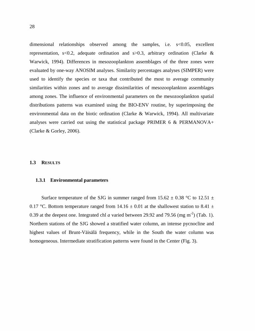
28
dimensional relationships observed among the samples, i.e. s<0.05, excellent
representation, s<0.2, adequate ordination and s>0.3, arbitrary ordination (Clarke &
Warwick, 1994). Differences in mesozooplankton assemblages of the three zones were
evaluated by one-way ANOSIM analyses. Similarity percentages analyses (SIMPER) were
used to identify the species or taxa that contributed the most to average community
similarities within zones and to average dissimilarities of mesozooplankton assemblages
among zones. The influence of environmental parameters on the mesozooplankton spatial
distributions patterns was examined using the BIO-ENV routine, by superimposing the
environmental data on the biotic ordination (Clarke & Warwick, 1994). All multivariate
analyses were carried out using the statistical package PRIMER 6 & PERMANOVA+
(Clarke & Gorley, 2006).
1.3 RESULTS
1.3.1 Environmental parameters
Surface temperature of the SJG in summer ranged from 15.62 ± 0.38 °C to 12.51 ±
0.17 °C. Bottom temperature ranged from 14.16 ± 0.01 at the shallowest station to 8.41 ±
0.39 at the deepest one. Integrated chl a varied between 29.92 and 79.56 (mg m-2
) (Tab. 1).
Northern stations of the SJG showed a stratified water column, an intense pycnocline and
highest values of Brunt-Väisälä frequency, while in the South the water column was
homogeneous. Intermediate stratification patterns were found in the Center (Fig. 3).
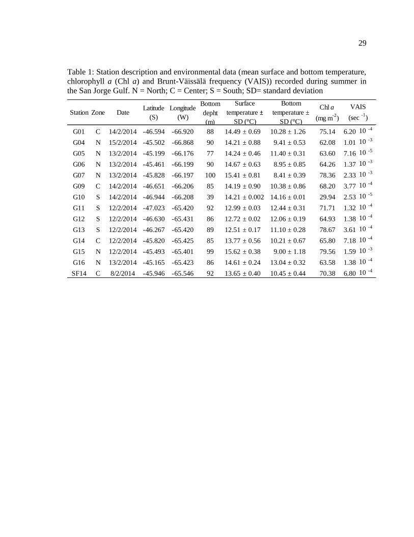
29
Table 1: Station description and environmental data (mean surface and bottom temperature,
chlorophyll a (Chl a) and Brunt-Väissälä frequency (VAIS)) recorded during summer in
the San Jorge Gulf. N = North; C = Center; S = South; SD= standard deviation
Station Zone DateLatitude
(S)
Longitude
(W)
Bottom
depht
(m)
Chl a
(mg m-2
)
G01 C 14/2/2014 -46.594 -66.920 88 14.49 ± 0.69 10.28 ± 1.26 75.14 6.20 10 -4
G04 N 15/2/2014 -45.502 -66.868 90 14.21 ± 0.88 9.41 ± 0.53 62.08 1.01 10 -3
G05 N 13/2/2014 -45.199 -66.176 77 14.24 ± 0.46 11.40 ± 0.31 63.60 7.16 10 -5
G06 N 13/2/2014 -45.461 -66.199 90 14.67 ± 0.63 8.95 ± 0.85 64.26 1.37 10 -3
G07 N 13/2/2014 -45.828 -66.197 100 15.41 ± 0.81 8.41 ± 0.39 78.36 2.33 10 -3
G09 C 14/2/2014 -46.651 -66.206 85 14.19 ± 0.90 10.38 ± 0.86 68.20 3.77 10 -4
G10 S 14/2/2014 -46.944 -66.208 39 14.21 ± 0.002 14.16 ± 0.01 29.94 2.53 10 -5
G11 S 12/2/2014 -47.023 -65.420 92 12.99 ± 0.03 12.44 ± 0.31 71.71 1.32 10 -4
G12 S 12/2/2014 -46.630 -65.431 86 12.72 ± 0.02 12.06 ± 0.19 64.93 1.38 10 -4
G13 S 12/2/2014 -46.267 -65.420 89 12.51 ± 0.17 11.10 ± 0.28 78.67 3.61 10 -4
G14 C 12/2/2014 -45.820 -65.425 85 13.77 ± 0.56 10.21 ± 0.67 65.80 7.18 10 -4
G15 N 12/2/2014 -45.493 -65.401 99 15.62 ± 0.38 9.00 ± 1.18 79.56 1.59 10 -3
G16 N 13/2/2014 -45.165 -65.423 86 14.61 ± 0.24 13.04 ± 0.32 63.58 1.38 10 -4
SF14 C 8/2/2014 -45.946 -65.546 92 13.65 ± 0.40 10.45 ± 0.44 70.38 6.80 10 -4
Surface
temperature ±
SD (°C)
Bottom
temperature ±
SD (°C)
VAIS
(sec -1
)
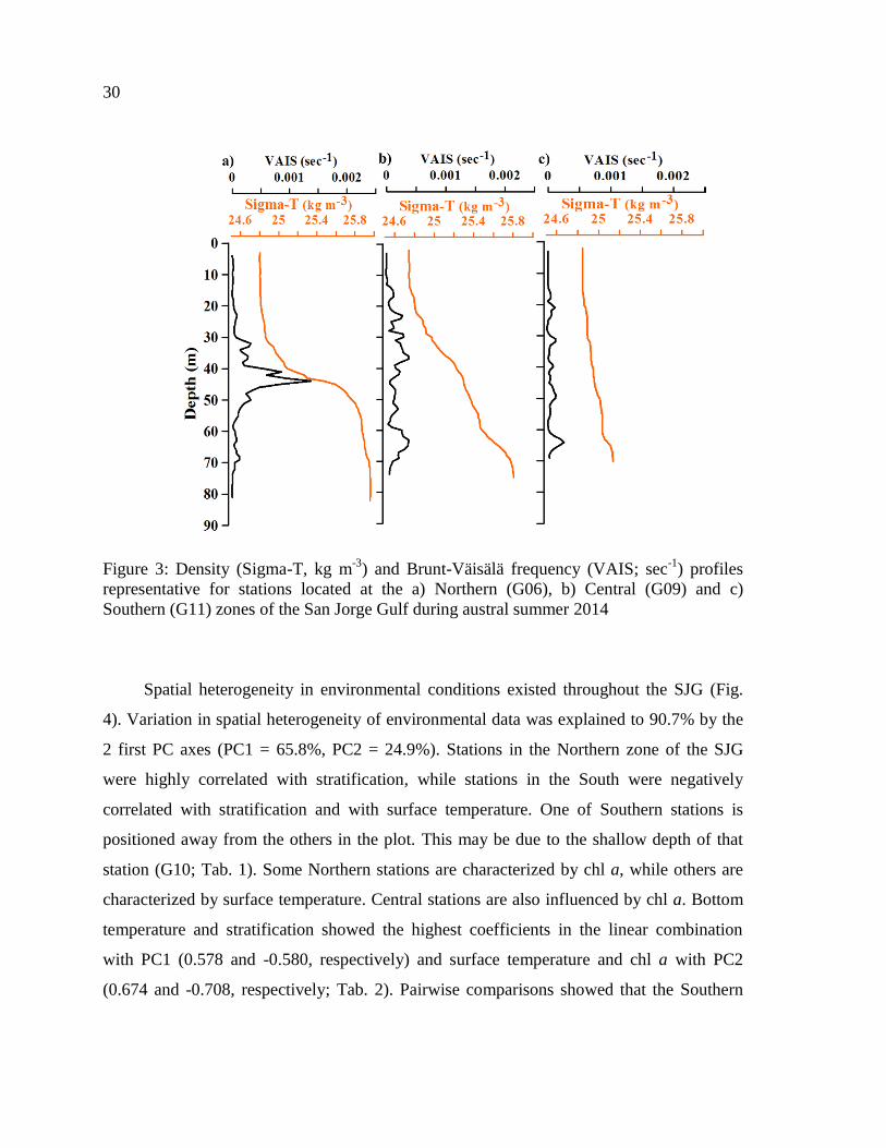
30
Figure 3: Density (Sigma-T, kg m-3
) and Brunt-Väisälä frequency (VAIS; sec-1
) profiles
representative for stations located at the a) Northern (G06), b) Central (G09) and c)
Southern (G11) zones of the San Jorge Gulf during austral summer 2014
Spatial heterogeneity in environmental conditions existed throughout the SJG (Fig.
4). Variation in spatial heterogeneity of environmental data was explained to 90.7% by the
2 first PC axes (PC1 = 65.8%, PC2 = 24.9%). Stations in the Northern zone of the SJG
were highly correlated with stratification, while stations in the South were negatively
correlated with stratification and with surface temperature. One of Southern stations is
positioned away from the others in the plot. This may be due to the shallow depth of that
station (G10; Tab. 1). Some Northern stations are characterized by chl a, while others are
characterized by surface temperature. Central stations are also influenced by chl a. Bottom
temperature and stratification showed the highest coefficients in the linear combination
with PC1 (0.578 and -0.580, respectively) and surface temperature and chl a with PC2
(0.674 and -0.708, respectively; Tab. 2). Pairwise comparisons showed that the Southern
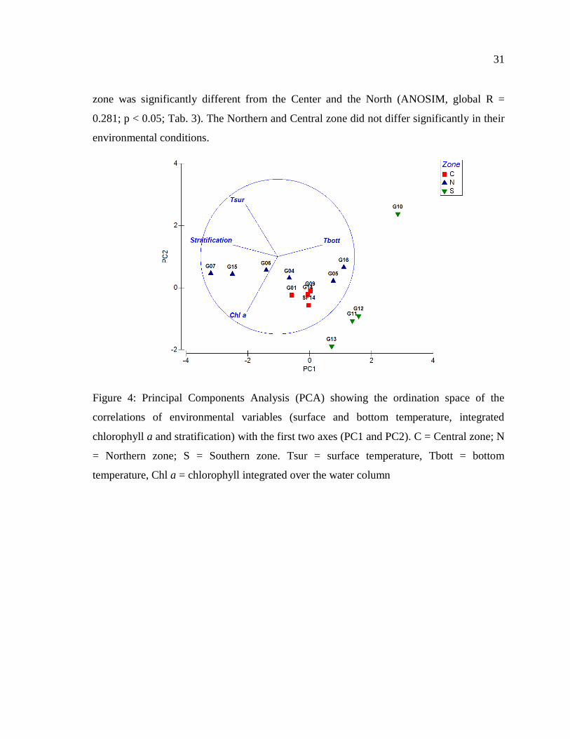
31
zone was significantly different from the Center and the North (ANOSIM, global R =
0.281; p < 0.05; Tab. 3). The Northern and Central zone did not differ significantly in their
environmental conditions.
Figure 4: Principal Components Analysis (PCA) showing the ordination space of the
correlations of environmental variables (surface and bottom temperature, integrated
chlorophyll a and stratification) with the first two axes (PC1 and PC2). C = Central zone; N
= Northern zone; S = Southern zone. Tsur = surface temperature, Tbott = bottom
temperature, Chl a = chlorophyll integrated over the water column
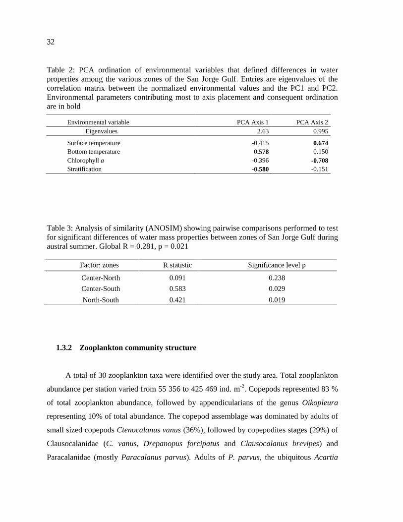
32
Table 2: PCA ordination of environmental variables that defined differences in water
properties among the various zones of the San Jorge Gulf. Entries are eigenvalues of the
correlation matrix between the normalized environmental values and the PC1 and PC2.
Environmental parameters contributing most to axis placement and consequent ordination
are in bold
Environmental variable PCA Axis 1 PCA Axis 2
Eigenvalues 2.63 0.995
Surface temperature -0.415 0.674
Bottom temperature 0.578 0.150
Chlorophyll a -0.396 -0.708
Stratification -0.580 -0.151
Table 3: Analysis of similarity (ANOSIM) showing pairwise comparisons performed to test
for significant differences of water mass properties between zones of San Jorge Gulf during
austral summer. Global R = 0.281, p = 0.021
1.3.2 Zooplankton community structure
A total of 30 zooplankton taxa were identified over the study area. Total zooplankton
abundance per station varied from 55 356 to 425 469 ind. m-2
. Copepods represented 83 %
of total zooplankton abundance, followed by appendicularians of the genus Oikopleura
representing 10% of total abundance. The copepod assemblage was dominated by adults of
small sized copepods Ctenocalanus vanus (36%), followed by copepodites stages (29%) of
Clausocalanidae (C. vanus, Drepanopus forcipatus and Clausocalanus brevipes) and
Paracalanidae (mostly Paracalanus parvus). Adults of P. parvus, the ubiquitous Acartia
Factor: zones R statistic Significance level p
Center-North 0.091 0.238
Center-South 0.583 0.029
North-South 0.421 0.019
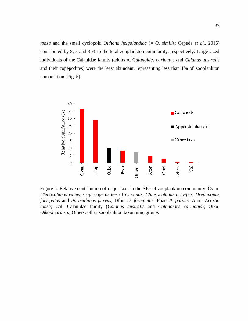
33
tonsa and the small cyclopoid Oithona helgolandica (= O. similis; Cepeda et al., 2016)
contributed by 8, 5 and 3 % to the total zooplankton community, respectively. Large sized
individuals of the Calanidae family (adults of Calanoides carinatus and Calanus australis
and their copepodites) were the least abundant, representing less than 1% of zooplankton
composition (Fig. 5).
Figure 5: Relative contribution of major taxa in the SJG of zooplankton community. Cvan:
Ctenocalanus vanus; Cop: copepodites of C. vanus, Clausocalanus brevipes, Drepanopus
focripatus and Paracalanus parvus; Dfor: D. forcipatus; Ppar: P. parvus; Aton: Acartia
tonsa; Cal: Calanidae family (Calanus australis and Calanoides carinatus); Oiko:
Oikopleura sp.; Others: other zooplankton taxonomic groups
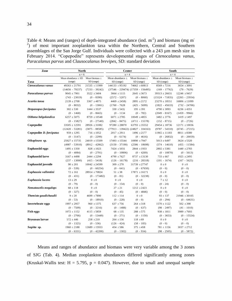
34
Table 4: Means and (ranges) of depth-integrated abundance (ind. m-2
) and biomass (mg m-
2) of most important zooplankton taxa within the Northern, Central and Southern
assemblages of the San Jorge Gulf. Individuals were collected with a 243 µm mesh size in
February 2014. ―Copepodite‖ represents developmental stages of Ctenocalanus vanus,
Paracalanus parvus and Clausocalanus brevipes, SD: standard deviation
Zone
Taxa
Ctenocalanus vanus 49263 ± 21791 21535 ± 11999 144133 ± 95192 74662 ± 60813 8569 ± 7216 3654 ± 3091
(14656 - 79237) (7233 - 39242) (37546 - 229474) (17359 - 156495) (169 - 17762) (79 - 7629)
Paracalanus parvus 9045 ± 7901 3522 ± 3404 3664 ± 1115 2645 ± 3673 39313 ± 26631 12246 ± 9457
(743 - 23019) (0 - 8390) (2572 - 5207) (0 - 8060) (15524 - 71835) (2265 - 23934)
Acartia tonsa 2139 ± 2708 3367 ± 4875 4469 ± 2458) 2895 ± 2172 23270 ± 18551 16806 ± 11099
(0 - 8032) (0 - 13061) (1760 - 7628 (425 - 5699) (1822 - 45633) (732 - 24706)
Drepanopus forcipatus 302 ± 530 1444 ± 3537 330 ± 543) 195 ± 391 4790 ± 3093 6236 ± 4351
(0 - 1468) (0 - 8665) (0 - 1134 (0 - 782) (2049 - 8167) (1459 - 9966)
Oithona helgolandica 6257 ± 5075 8759 ± 10548 6071 ± 2785 10049 ± 4855 3482 ± 3776 1419 ± 1497
(0 - 15827) (0 - 27540) (2842 - 8475) (4711 - 15578) (152 - 8715) (0 - 2726)
Copepodite 33505 ± 12591 28926 ± 31082 97280 ± 28870 63793 ± 35552 29454 ± 18736 12171 ± 10036
(12420 - 53281) (5875 - 88585) (77913 - 139422) (24827 - 104163) (9787 - 54310) (6745 - 27215)
Copepodite D. forcipatus 959 ± 1295 716 ± 1052 2017 ± 2911 1496 ± 2177 11965 ± 11183 8811 ± 8380
(0 - 3147) (0 - 2299) (0 - 6174) (0 - 4616) (0 - 26832) (0 - 20059)
Oikopleura sp. 25927 ± 15735 24019 ± 15509 17493 ± 15544 10890 ± 7947 5013 ± 6497 3624 ± 5320
(4987 - 53910) (8912 - 42862) (3150 - 37190) (2586 - 18698) (574 - 14610) (455 - 11584)
Euphausiid eggs 1495 ± 1350 828 ± 1023 7424 ± 5031 2844 ± 1933 2802 ± 5381 1440 ± 2783
(0 - 4084) (0 - 2791) (0 - 10806) (0 - 4269) (0 - 10870) (0 - 5613)
Euphausiid larve 3167 ± 4498 2444 ± 2294 4790 ± 7627 8737 ± 13130 733 ± 667 1925 ± 2495
(237 - 13000) (415 - 5418) (126 - 16178) (216 - 28318) (101 - 1674) (167 - 5625)
Euphausiid juvenile 90 ± 201 10042 ± 24599 309 ± 270 31739 ± 27747 0 ± 0 0 ± 0
(0 - 539) (0 - 60254) (0 - 641) (0 - 67650) (0 - 0) (0 - 0)
Euphausia vallentini 72 ± 161 28914 ± 70824 51 ± 38 17871 ± 16171 0 ± 0 0 ± 0
(0 - 431) (0 - 173482) (0 - 81) (0 - 32238) (0 - 0) (0 - 0)
Euphausia lucens 13 ± 29 0 ± 0 0 ± 0 0 ± 0 7 ± 12 0 ± 0
(0 - 79) (0 - 0) (0 - 154) (0 - 0) (0 - 24) (0 - 0)
Nematoscelis megalops 68 ± 118 0 ± 0 27 ± 21 1212 ± 2423 0 ± 0 0 ± 0
(0 - 327) (0 - 0) (0 - 45) (0 - 4846) (0 - 0) (0 - 0)
Themisto gaudichaudii 9 ± 20 4699 ± 7890 112 ± 114 0 ± 0 93 ± 137 21946 ± 30105
(0 - 53) (0 - 18910) (0 - 228) (0 - 0) (0 - 294) (0 - 64631)
Invertebrate eggs 1997 ± 2957 960 ± 1375 637 ± 756 264 ± 318 1570 ± 1122 502 ± 398
(0 - 7509) (0 - 3216) (0 - 1488) (0 - 637) (98 - 2497) (41 - 1010)
Fish eggs 1072 ± 1152 4115 ± 5859 68 ± 135 288 ± 575 938 ± 1811 3989 ± 7693
(0 - 2766) (0 - 12449) (0 - 271) (0 - 1150) (0 - 3653) (0 - 15524)
Bryozoan larvae 572 ± 446 258 ± 210 264 ± 156 118 ± 69 0 ± 0 0 ± 0
(0 - 1325) (0 - 536) (126 - 424) (58 - 183) (0 - 0) (0 - 0)
Sagitta sp. 1960 ± 2188 12689 ± 15933 454 ± 586 375 ± 458 781 ± 1156 3037 ± 2712
(0 - 6331) (0 - 42200) (0 - 1302) (0 - 934) (98 - 2505) (0 - 5872)
Mean biomass ±
SD (range)
North Center South
n = 6 n = 4 n = 4
Mean abundance ± SD
(range)
Mean biomass ±
SD (range)
Mean abundance ±
SD (range)
Mean biomass ±
SD (range)
Mean abundance ±
SD (range)
Means and ranges of abundance and biomass were very variable among the 3 zones
of SJG (Tab. 4). Median zooplankton abundances differed significantly among zones
(Kruskal-Wallis test: H = 5.795, p = 0.047). However, due to small and unequal sample
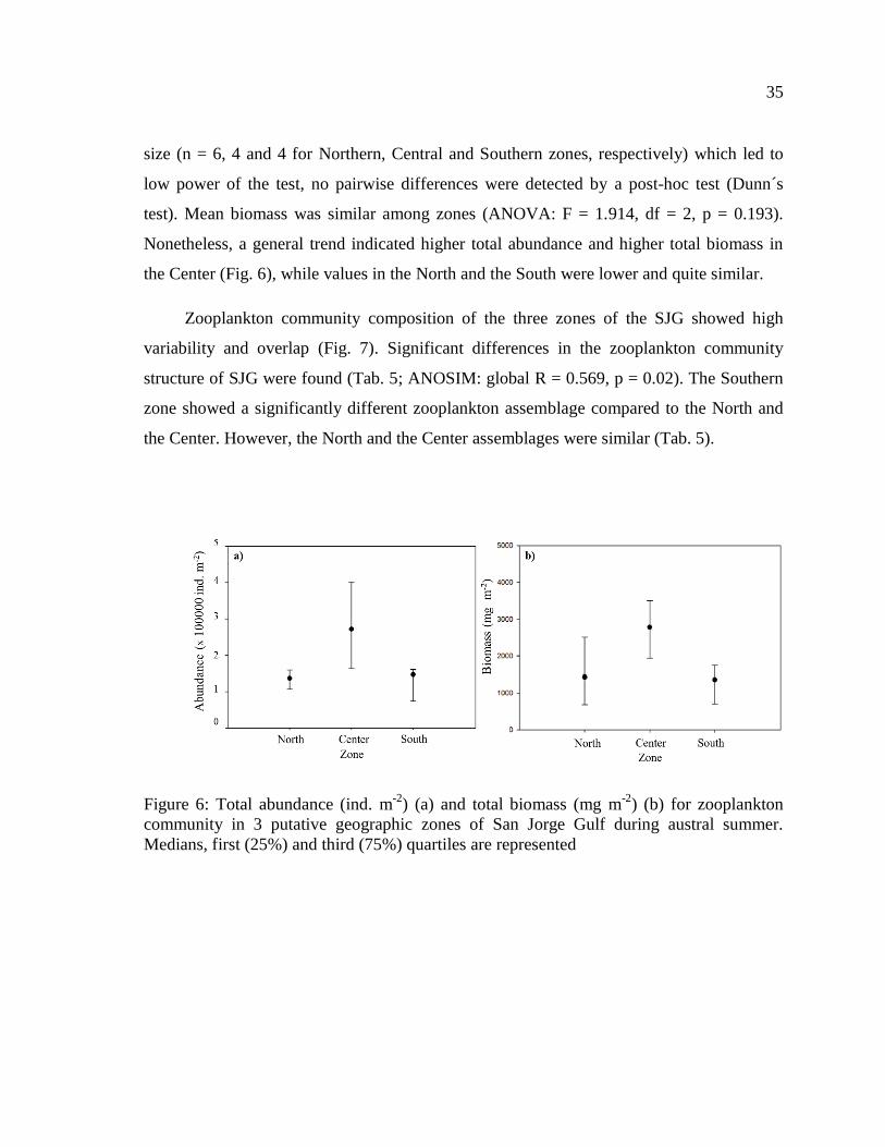
35
size (n = 6, 4 and 4 for Northern, Central and Southern zones, respectively) which led to
low power of the test, no pairwise differences were detected by a post-hoc test (Dunn´s
test). Mean biomass was similar among zones (ANOVA: F = 1.914, df = 2, p = 0.193).
Nonetheless, a general trend indicated higher total abundance and higher total biomass in
the Center (Fig. 6), while values in the North and the South were lower and quite similar.
Zooplankton community composition of the three zones of the SJG showed high
variability and overlap (Fig. 7). Significant differences in the zooplankton community
structure of SJG were found (Tab. 5; ANOSIM: global R = 0.569, p = 0.02). The Southern
zone showed a significantly different zooplankton assemblage compared to the North and
the Center. However, the North and the Center assemblages were similar (Tab. 5).
Figure 6: Total abundance (ind. m-2
) (a) and total biomass (mg m-2
) (b) for zooplankton
community in 3 putative geographic zones of San Jorge Gulf during austral summer.
Medians, first (25%) and third (75%) quartiles are represented
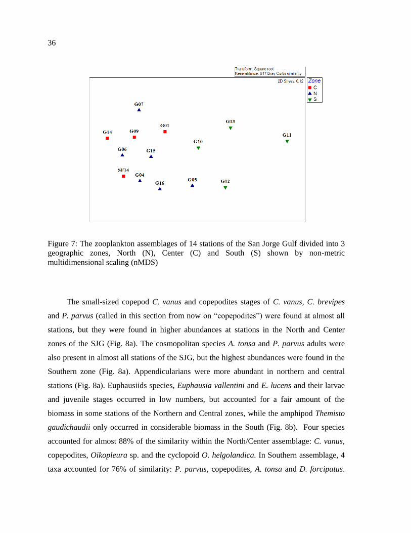
36
Figure 7: The zooplankton assemblages of 14 stations of the San Jorge Gulf divided into 3
geographic zones, North (N), Center (C) and South (S) shown by non-metric
multidimensional scaling (nMDS)
The small-sized copepod C. vanus and copepodites stages of C. vanus, C. brevipes
and P. parvus (called in this section from now on ―copepodites‖) were found at almost all
stations, but they were found in higher abundances at stations in the North and Center
zones of the SJG (Fig. 8a). The cosmopolitan species A. tonsa and P. parvus adults were
also present in almost all stations of the SJG, but the highest abundances were found in the
Southern zone (Fig. 8a). Appendicularians were more abundant in northern and central
stations (Fig. 8a). Euphausiids species, Euphausia vallentini and E. lucens and their larvae
and juvenile stages occurred in low numbers, but accounted for a fair amount of the
biomass in some stations of the Northern and Central zones, while the amphipod Themisto
gaudichaudii only occurred in considerable biomass in the South (Fig. 8b). Four species
accounted for almost 88% of the similarity within the North/Center assemblage: C. vanus,
copepodites, Oikopleura sp. and the cyclopoid O. helgolandica. In Southern assemblage, 4
taxa accounted for 76% of similarity: P. parvus, copepodites, A. tonsa and D. forcipatus.
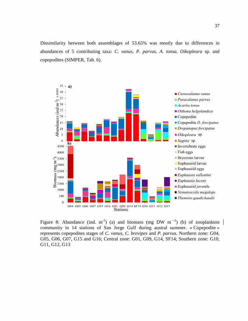
37
Dissimilarity between both assemblages of 53.65% was mostly due to differences in
abundances of 5 contributing taxa: C. vanus, P. parvus, A. tonsa, Oikopleura sp. and
copepodites (SIMPER, Tab. 6).
Figure 8: Abundance (ind. m-2
) (a) and biomass (mg DW m -2
) (b) of zooplankton
community in 14 stations of San Jorge Gulf during austral summer. « Copepodite »
represents copepodites stages of C. vanus, C. brevipes and P. parvus. Northern zone: G04,
G05, G06, G07, G15 and G16; Central zone: G01, G09, G14, SF14; Southern zone: G10,
G11, G12, G13
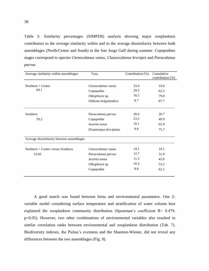
38
Table 5: Similarity percentages (SIMPER) analysis showing major zooplankton
contributors to the average similarity within and to the average dissimilarity between both
assemblages (North/Center and South) in the San Jorge Gulf during summer. Copepodites
stages correspond to species Ctenocalanus vanus, Clausocalanus brevipes and Paracalanus
parvus
Average similarity within assemblages Taxa Contribution (%) Cumulative
contribution (%)
Northern + Center Ctenocalanus vanus
33.0 33.0
64.1 Copepodite 29.5 62.5
Oikopleura sp. 16.5 79.0
Oithona helgolandica 8.7 87.7
Southern Paracalanus parvus
26.6 26.7
59.2 Copepodite 23.2 49.9
Acartia tonsa 16.1 65.9
Drepanopus forcipatus 9.8 75.7
Average dissimilarity between assemblages
Northern + Center versus Southern Ctenocalanus vanus
19.1
19.1
53.65 Paracalanus parvus 12.7 31.9
Acartia tonsa 11.2 43.0
Oikopleura sp. 10.2 53.2
Copepodite 8.8 62.1
A good match was found between biota and environmental parameters. One 2-
variable model considering surface temperature and stratification of water column best
explained the zooplankton community distribution (Spearman’s coefficient R= 0.479,
p<0.05). However, two other combinations of environmental variables also resulted in
similar correlation ranks between environmental and zooplankton distribution (Tab. 7).
Biodiversity indexes, the Pielou’s evenness and the Shannon-Wiener, did not reveal any
differences between the two assemblages (Fig. 9).
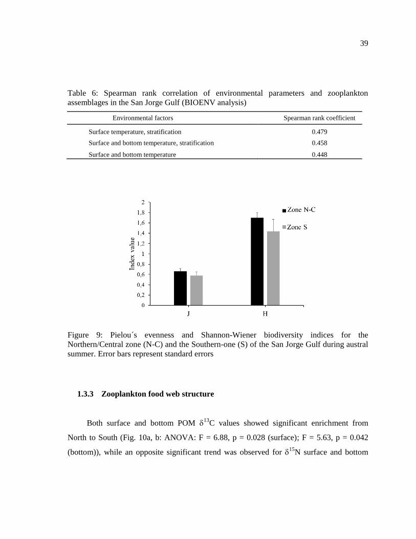
39
Table 6: Spearman rank correlation of environmental parameters and zooplankton
assemblages in the San Jorge Gulf (BIOENV analysis)
Environmental factors Spearman rank coefficient
Surface temperature, stratification 0.479
Surface and bottom temperature, stratification 0.458
Surface and bottom temperature 0.448
Figure 9: Pielou´s evenness and Shannon-Wiener biodiversity indices for the
Northern/Central zone (N-C) and the Southern-one (S) of the San Jorge Gulf during austral
summer. Error bars represent standard errors
1.3.3 Zooplankton food web structure
Both surface and bottom POM 13
C values showed significant enrichment from
North to South (Fig. 10a, b: ANOVA: F = 6.88, p = 0.028 (surface); F = 5.63, p = 0.042
(bottom)), while an opposite significant trend was observed for 15
N surface and bottom
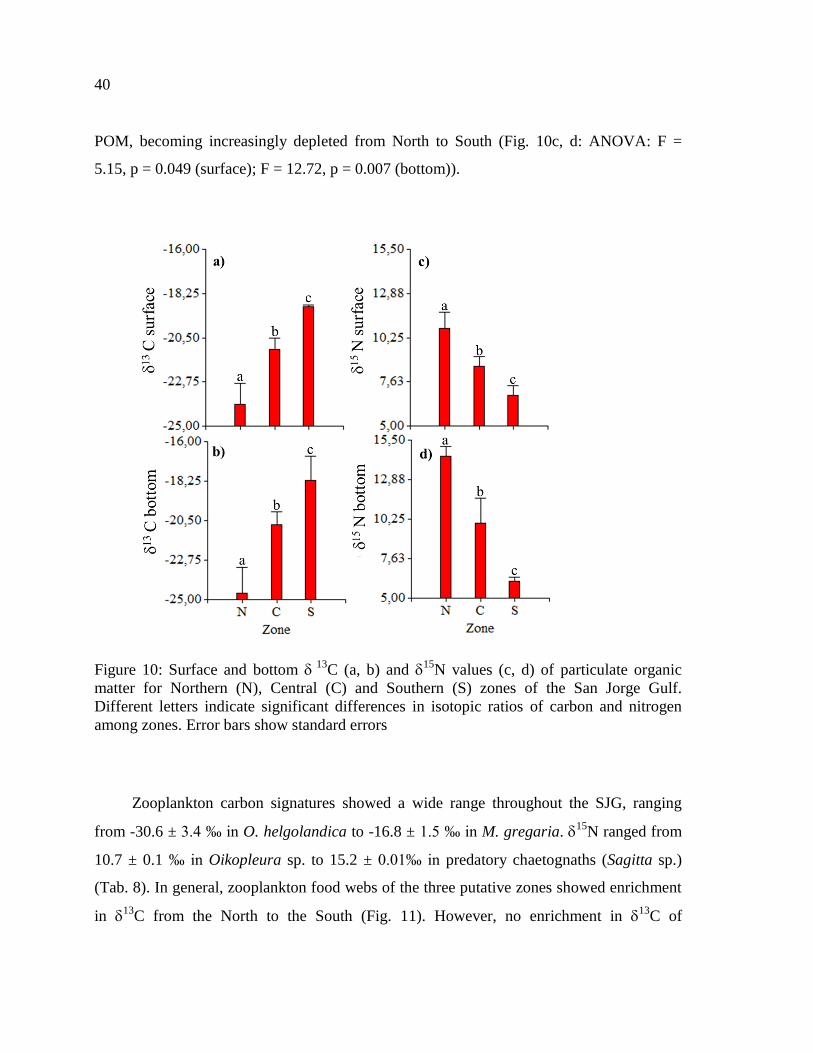
40
POM, becoming increasingly depleted from North to South (Fig. 10c, d: ANOVA: F =
5.15, p = 0.049 (surface); F = 12.72, p = 0.007 (bottom)).
Figure 10: Surface and bottom 13
C (a, b) and 15
N values (c, d) of particulate organic
matter for Northern (N), Central (C) and Southern (S) zones of the San Jorge Gulf.
Different letters indicate significant differences in isotopic ratios of carbon and nitrogen
among zones. Error bars show standard errors
Zooplankton carbon signatures showed a wide range throughout the SJG, ranging
from -30.6 ± 3.4 ‰ in O. helgolandica to -16.8 ± 1.5 ‰ in M. gregaria. 15
N ranged from
10.7 ± 0.1 ‰ in Oikopleura sp. to 15.2 ± 0.01‰ in predatory chaetognaths (Sagitta sp.)
(Tab. 8). In general, zooplankton food webs of the three putative zones showed enrichment
in 13
C from the North to the South (Fig. 11). However, no enrichment in 13
C of
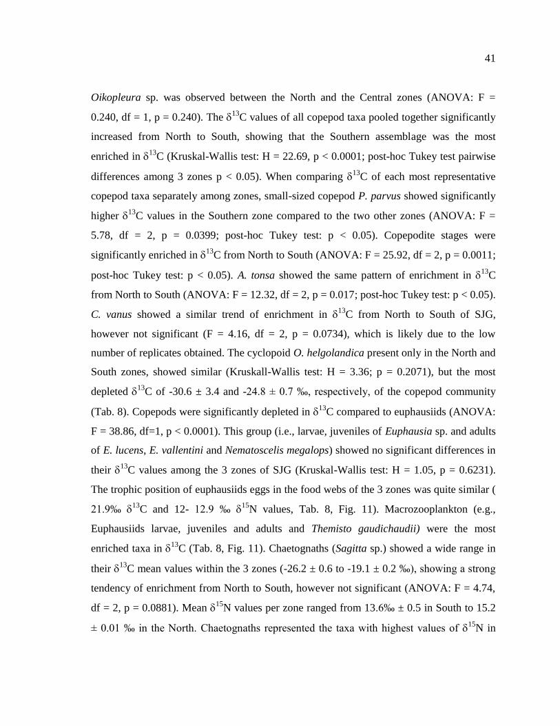
41
Oikopleura sp. was observed between the North and the Central zones (ANOVA: F =
0.240, df = 1, p = 0.240). The 13
C values of all copepod taxa pooled together significantly
increased from North to South, showing that the Southern assemblage was the most
enriched in 13
C (Kruskal-Wallis test: H = 22.69, p < 0.0001; post-hoc Tukey test pairwise
differences among 3 zones p < 0.05). When comparing 13
C of each most representative
copepod taxa separately among zones, small-sized copepod P. parvus showed significantly
higher 13
C values in the Southern zone compared to the two other zones (ANOVA: F =
5.78, df = 2, p = 0.0399; post-hoc Tukey test: p < 0.05). Copepodite stages were
significantly enriched in 13
C from North to South (ANOVA: F = 25.92, df = 2, p = 0.0011;
post-hoc Tukey test: p < 0.05). A. tonsa showed the same pattern of enrichment in 13
C
from North to South (ANOVA: F = 12.32, df = 2, p = 0.017; post-hoc Tukey test: p < 0.05).
C. vanus showed a similar trend of enrichment in 13
C from North to South of SJG,
however not significant (F = 4.16, df = 2, p = 0.0734), which is likely due to the low
number of replicates obtained. The cyclopoid O. helgolandica present only in the North and
South zones, showed similar (Kruskall-Wallis test: H = 3.36; p = 0.2071), but the most
depleted 13
C of -30.6 ± 3.4 and -24.8 ± 0.7 ‰, respectively, of the copepod community
(Tab. 8). Copepods were significantly depleted in 13
C compared to euphausiids (ANOVA:
F = 38.86, df=1, p < 0.0001). This group (i.e., larvae, juveniles of Euphausia sp. and adults
of E. lucens, E. vallentini and Nematoscelis megalops) showed no significant differences in
their 13
C values among the 3 zones of SJG (Kruskal-Wallis test: H = 1.05, p = 0.6231).
The trophic position of euphausiids eggs in the food webs of the 3 zones was quite similar (
21.9‰ 13
C and 12- 12.9 ‰ 15
N values, Tab. 8, Fig. 11). Macrozooplankton (e.g.,
Euphausiids larvae, juveniles and adults and Themisto gaudichaudii) were the most
enriched taxa in 13
C (Tab. 8, Fig. 11). Chaetognaths (Sagitta sp.) showed a wide range in
their 13
C mean values within the 3 zones (-26.2 ± 0.6 to -19.1 ± 0.2 ‰), showing a strong
tendency of enrichment from North to South, however not significant (ANOVA: F = 4.74,
df = 2, p = 0.0881). Mean 15
N values per zone ranged from 13.6‰ ± 0.5 in South to 15.2
± 0.01 ‰ in the North. Chaetognaths represented the taxa with highest values of 15
N in
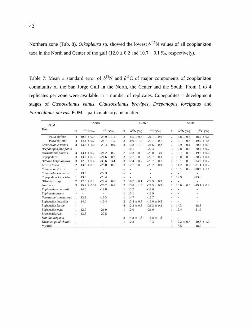
42
Northern zone (Tab. 8). Oikopleura sp. showed the lowest 15
N values of all zooplankton
taxa in the North and Center of the gulf (12.0 ± 0.2 and 10.7 ± 0.1 ‰, respectively).
Table 7: Mean ± standard error of δ15
N and δ13
C of major components of zooplankton
community of the San Jorge Gulf in the North, the Center and the South. From 1 to 4
replicates per zone were available. n = number of replicates. Copepodites = development
stages of Ctenocalanus vanus, Clausocalanus brevipes, Drepanopus forcipatus and
Paracalanus parvus. POM = particulate organic matter
POM
Taxan n n
POM surface 4 10.8 ± 0.9 -23.9 ± 1.1 3 8.5 ± 0.6 -21.1 ± 0.6 2 6.8 ± 0.6 -18.9 ± 0.1
POM bottom 4 14.4 ± 0.7 -24.7 ± 1.5 3 10.0 ± 1.7 -20.7 ± 0.7 2 6.1 ± 0.3 -19.9 ± 1.4
Ctenocalanus vanus 4 13.8 ± 1.0 -23.4 ± 0.9 3 13.8 ± 1.0 -21.6 ± 0.2 2 12.9 ± 0.4 -20.8 ± 0.9
Drepanopus forcipatus - - - - 14.1 -22.4 3 12.8 ± 0.2 -20.7 ± 0.7
Paracalanus parvus 4 13.4 ± 0.2 -24.2 ± 0.5 2 12.3 ± 0.9 -25.0 ± 3.0 3 13.7 ± 0.8 -19.8 ± 0.6
Copepodites 3 13.2 ± 0.3 -24.6 0.7 3 12.7 ± 0.5 -22.7 ± 0.3 3 13.0 ± 0.5 -20.7 ± 0.4
Oithona helgolandica 3 12.5 ± 0.4 -30.6 ± 3.4 3 12.4 ± 0.7 -23.7 ± 0.7 2 13.1 ± 0.6 -24.8 ± 0.7
Acartia tonsa 2 13.8 ± 0.9 -26.0 ± 0.5 3 12.7 ± 0.5 -23.2 ± 0.9 3 14.2 ± 0.7 -21.1 ± 0.2
Calanus australis - - - - - - 2 13.1 ± 0.7 -20.3 ± 1.1
Calanoides carinatus 1 13.3 -22.3 - - - - - -
Copepodites Calanidae 1 13.0 -23.4 - - - 1 12.9 -23.6
Oikopleura sp. 2 12.0 ± 0.2 -24.4 ± 0.6 2 10.7 ± 0.1 -22.9 ± 0.2 - - -
Sagitta sp. 3 15.2 ± 0.01 -26.2 ± 0.6 2 13.8 ± 1.8 -21.5 ± 0.9 2 13.6 ± 0.5 -19.1 ± 0.2
Euphausia valentinii 1 14.0 -19.8 1 12.7 -19.6 - - -
Euphausia lucens - - - 1 13.1 -18.9 - - -
Nematoscelis megalops 1 13.8 -19.3 1 14.7 -19.7 - - -
Euphausiids juveniles 1 14.0 -19.4 2 13.4 ± 0.5 -19.0 ± 0.5 - - -
Euphausiids larvae - - - 4 12.3 ± 0.3 -21.2 ± 0.2 1 14.3 -18.6
Euphausiids eggs 1 12.9 -21.9 1 12.0 -21.9 1 12.4 -21.9
Bryozoan larvae 1 13.5 -22.5 - - - - - -
Munida gregaria - - - 2 14.2 ± 1.8 -16.8 ± 1.5 - - -
Themisto gaudichaudii - - - 1 12.8 -19.3 3 12.2 ± 0.7 -20.8 ± 1.0
Mysidae - - - - - - 1 13.5 -18.0
North Center South
δ15
N (‰) δ13
C (‰) δ15
N (‰) δ13
C (‰) δ15
N (‰) δ13
C (‰)
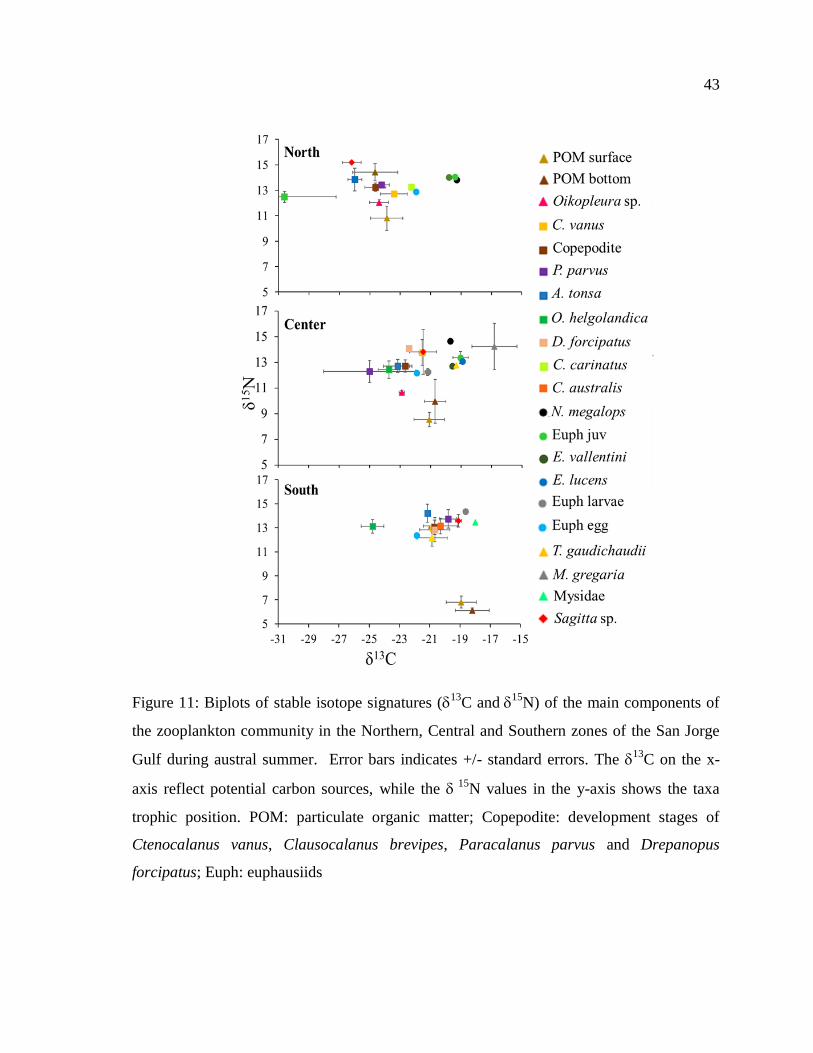
43
Figure 11: Biplots of stable isotope signatures (13
C and15
N) of the main components of
the zooplankton community in the Northern, Central and Southern zones of the San Jorge
Gulf during austral summer. Error bars indicates +/- standard errors. The 13
C on the x-
axis reflect potential carbon sources, while the 15
N values in the y-axis shows the taxa
trophic position. POM: particulate organic matter; Copepodite: development stages of
Ctenocalanus vanus, Clausocalanus brevipes, Paracalanus parvus and Drepanopus
forcipatus; Euph: euphausiids
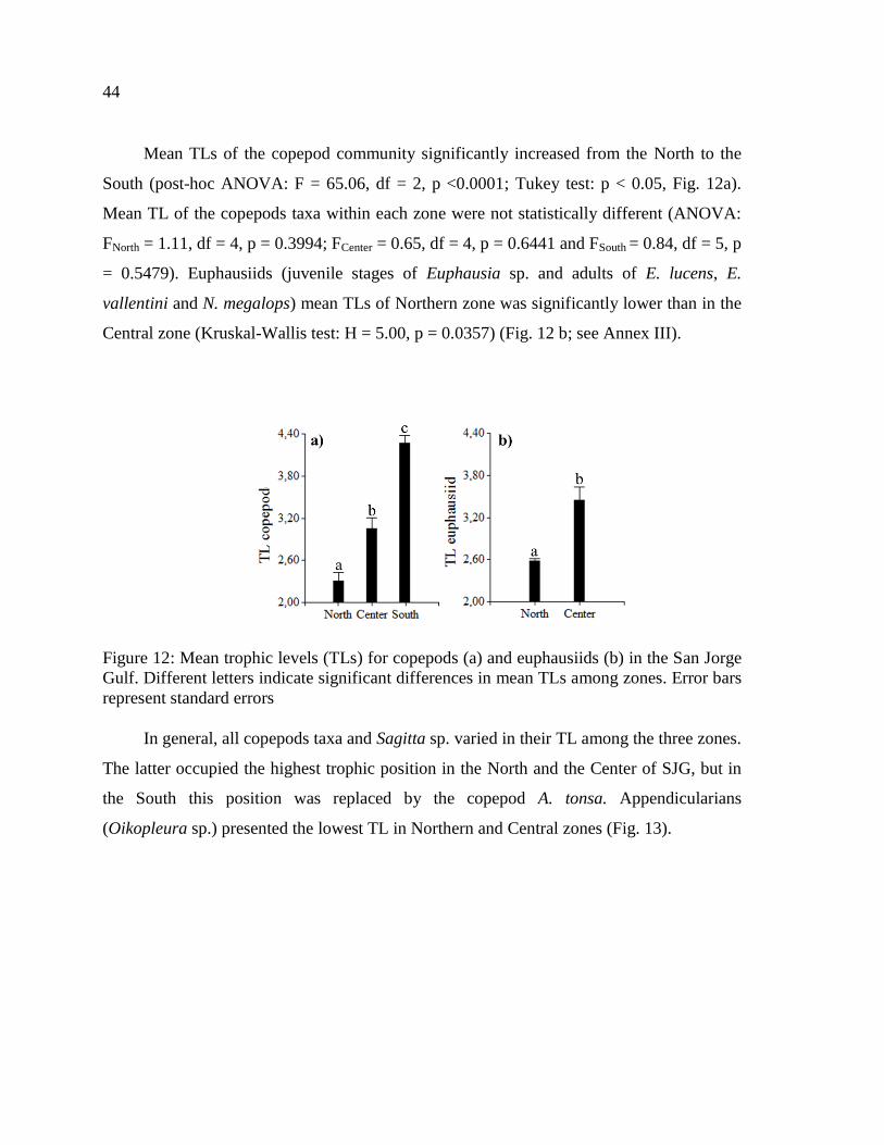
44
Mean TLs of the copepod community significantly increased from the North to the
South (post-hoc ANOVA: F = 65.06, df = 2, p <0.0001; Tukey test: p < 0.05, Fig. 12a).
Mean TL of the copepods taxa within each zone were not statistically different (ANOVA:
FNorth = 1.11, df = 4, p = 0.3994; FCenter = 0.65, df = 4, p = 0.6441 and FSouth = 0.84, df = 5, p
= 0.5479). Euphausiids (juvenile stages of Euphausia sp. and adults of E. lucens, E.
vallentini and N. megalops) mean TLs of Northern zone was significantly lower than in the
Central zone (Kruskal-Wallis test: H = 5.00, p = 0.0357) (Fig. 12 b; see Annex III).
Figure 12: Mean trophic levels (TLs) for copepods (a) and euphausiids (b) in the San Jorge
Gulf. Different letters indicate significant differences in mean TLs among zones. Error bars
represent standard errors
In general, all copepods taxa and Sagitta sp. varied in their TL among the three zones.
The latter occupied the highest trophic position in the North and the Center of SJG, but in
the South this position was replaced by the copepod A. tonsa. Appendicularians
(Oikopleura sp.) presented the lowest TL in Northern and Central zones (Fig. 13).
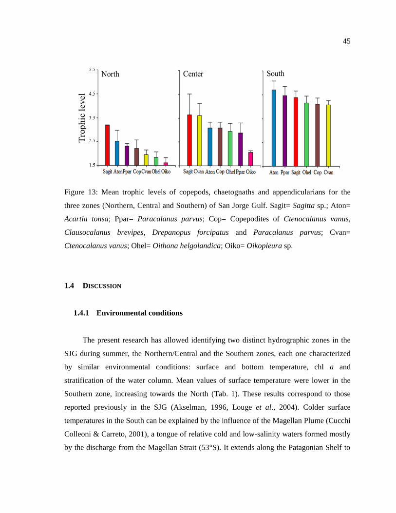
45
Figure 13: Mean trophic levels of copepods, chaetognaths and appendicularians for the
three zones (Northern, Central and Southern) of San Jorge Gulf. Sagit= Sagitta sp.; Aton=
Acartia tonsa; Ppar= Paracalanus parvus; Cop= Copepodites of Ctenocalanus vanus,
Clausocalanus brevipes, Drepanopus forcipatus and Paracalanus parvus; Cvan=
Ctenocalanus vanus; Ohel= Oithona helgolandica; Oiko= Oikopleura sp.
1.4 DISCUSSION
1.4.1 Environmental conditions
The present research has allowed identifying two distinct hydrographic zones in the
SJG during summer, the Northern/Central and the Southern zones, each one characterized
by similar environmental conditions: surface and bottom temperature, chl a and
stratification of the water column. Mean values of surface temperature were lower in the
Southern zone, increasing towards the North (Tab. 1). These results correspond to those
reported previously in the SJG (Akselman, 1996, Louge et al., 2004). Colder surface
temperatures in the South can be explained by the influence of the Magellan Plume (Cucchi
Colleoni & Carreto, 2001), a tongue of relative cold and low-salinity waters formed mostly
by the discharge from the Magellan Strait (53°S). It extends along the Patagonian Shelf to
46
42°S, from the surface to the bottom of the water column, and it detaches off the coast at
the South of the SJG (Palma & Matano, 2012). In our study, we did not take into account
salinity since its values were similar throughout the SJG. The plume is vertically
homogeneous, which is consistent with the lack of stratification found in the South in the
present study. Similarly, a well-mixed vertical pattern was revealed by the Simpson-Hunter
parameter in the Southeastern sector of the SJG (e.g., Palma et al., 2004; Glembocki et al.,
2015). However, stratification increased from South to North, as depicted by the Brunt-
Väisäla frequency. Most stations of the North of SJG were stratified, presenting a pycnoline
between 30-50 m (Fig. 3). This is consistent with stratification patterns found by Louge et
al. (2004) and by Paparazzo et al. (2017). In the North of the SJG only coastal stations
(G05 and G16, Fig. 2) near the Marine Park (i.e., also reported by Yorio, 2001; 2009) were
not stratified. These mixed waters could result from the interaction between coastal
topography, wind stress and tidal energy (Tonini et al., 2006). One station of the SJG
located in the South zone (G10, 39 m depth, Tab. 1, Fig. 4) deviated from the pattern
observed in the other Southern stations, since it shows higher surface and bottom
temperatures, which might be explained by its shallow depth. Furthermore, it presents the
most unstratified water column of all southern stations (i.e., the lowest VAIS values).
Integrated chl a distribution patterns in the SJG were similar to the ones described in
Cucchi Colleoni & Carreto (2001), showing higher values in the South-east, central-east
and in some northern stations.
1.4.2 Zooplankton community structure and spatial distribution
The results of the present study provided detailed information on the composition,
spatial distribution, abundance and biomass in the entire SJG during summer. No
differences in Shannon-Wiener diversity and Pielou´s evenness indexes were identified
throughout the SJG (Tab. 6, Fig. 8). However, including species composition and
abundance into the similarity index (Bray-Curtis) revealed finer resolution of the
47
zooplankton diversity and assemblages. Distinct spatial patterns of the zooplankton
community over the entire SJG were observed (Tab. 5, Fig. 7). Two clearly distinctive
zooplankton assemblages, spatially segregated, were revealed: one in the North/Center and
the other in the South, coinciding with the two zones of distinct water masses mentioned
above. These assemblages were determined taking into account all copepods species, their
developmental stages and other zooplankton taxa. The species composition in terms of
abundances differed significantly between those assemblages (Tab. 6). The small-sized
copepods P. parvus, A. tonsa and D. forcipatus were characteristic in Southern assemblage,
while C. vanus, appendicularians (Oikopleura) and O. helgolandica defined the
North/Center assemblage. Former studies lacked this resolution as they compared density
patterns of the copepod group and not the species (Pérez Seijas et al., 1987).
1.4.3 Zooplankton community with respect to environmental conditions
A good match between the environmental factors and zooplankton composition and
abundance data was found. Surface temperature and stratification explained 48% of the
variance in the zooplankton composition in terms of abundance throughout the entire SJG
(Tab. 7). The association between water mass properties and zooplankton assemblages was
previously documented in the Argentine continental shelf, where a positive relationship
between the presence of stratified waters and some copepod species abundances was shown
(Sabatini et al., 2000; Marrari et al., 2004; Derisio, 2012; Temperoni, 2015). Stratification
of water column is often associated to the occurrence of frontal areas, which are
oceanographic structures well known as highly productive where phytoplankton
accumulates (Acha et al., 2004). As frontal systems are common in the SJG (Glembocki et
al., 2015) it was not surprising to find stratified and mixed water masses. The upper layer
of any stratified water column allows for the growth and retention of phytoplankton when
light and nutrients are available. This biomass accumulation supports to the development of
zooplankton and other components of the ecosystem (Alemany et al., 2014 and references
48
therein). Besides, food availability and temperature were described as the main factors in
the SJG regulating the development and growth of copepods (Fernández Aráoz, 1994).
Chl a was used in our study as a proxy of phytoplankton biomass, since it is major
food source for herbivorous zooplankton. No direct relationships between chl a and
zooplankton abundance and distribution were measured since this variable was not chosen
in the BIOENV procedure (Tab. 7). However, differences in species composition of the
phytoplankton community throughout the gulf were reported by Latorre (2017) in samples
collected during the same cruise of our study. Within the microplankton size class,
mixotrophic dinoflagellates dominated the Northern zone, whereas heterotrophic and pico-
cyanobacteria dominated the Central zone. Besides, diatoms and dinoflagellates were the
main micro-autotrophs observed in the Southern zone. Finally, ciliates were uniformly
distributed throughout the gulf.
1.4.4 Zooplankton abundance, biomass and composition
Mean zooplankton abundance in the entire SJG was 2 345 ± 1 373 ind. m-3
(see
Annex I), value three times lower than that-one reported in Viñas et al. (1992) just for
mesozooplankton in early summer. Nonetheless, that estimate showed a large standard
deviation due to wide dispersal in mean values per sample. Besides, differences with our
results could be because samples were taken with a smaller mesh size (150µm instead of
243µm in the present study) and most of the stations were situated outside the SJG.
In our study, small-sized copepods (Ctenocalanus vanus, Paracalanus parvus,
Drepanopus forcipatus, Acartia tonsa, Oithona helgolandica and copepodites) were the
most relevant components of the SJG zooplankton community, representing 83% of total
abundances. Similar findings were previously reported in other sectors of the Argentine
continental shelf (Sabatini et al., 2001; Sabatini et al., 2004; Fernández Severini &
Hoffmeyer, 2005; Antacli et al., 2014; Derisio, 2012; Spinelli et al., 2012) and specifically
49
in the SJG (Pérez Seijas et al., 1987). Temperoni (2015) found in some outer Northern and
inner Southern coastal stations of the SJG that copepods represented more than 90% of the
community in terms of abundance, dominated by copepodites of the order Calanoida and
adults of D. forcipatus, C. vanus and Centropages brachiatus. C. brachiatus, a common
coastal species with continuous reproduction throughout the year (Gonzalez & Marín,
1998; Hidalgo & Escribano, 2007) was not present in any of our samples. Its absence in the
coastal stations might be explained by patchiness in their spatial distribution (Levin, 1992).
In contrast to the present study, Viñas et al. (1992) reported that O. helgolandica dominated
the SJG, which is most likely due to sampling. These authors used a smaller mesh size,
which is more appropriate for sampling small-sized cyclopoids and copepodites. Thus,
comparisons should be done with caution not only because of differences between net mesh
sizes but also because of differences in sampling effort. In January 1985, highest copepod
densities (>1400 ind. m-3
) were found in the Southern stations (Pérez Seijas et al., 1987),
whereas in the present study no significant differences in zooplankton abundances among
the three zones were found. Pérez Seijas et al. (1987) reported pre-adults of euphausiids
(i.e., furcilia larvae and juveniles) as the second abundant group in the SJG in summer,
showing highest abundances (65 - 145 ind. m-3
) in the Central-Southern region. In our
study, euphausiids group peak densities corresponded to larvae and juveniles (167 ind. m-3
and 10 ind. m-3
) and were found in stations of the North and the Center of the gulf,
respectively. However, this macrozooplankton group was under sampled due to the vertical
towing. Appendicularians were the second most abundant taxon in the SJG (Fig. 5).
Highest abundances were found in the North and Center of the SJG (Fig. 8, Tab. 4). In
many pelagic environments, these organisms represent one of the most important secondary
producers along with copepods. High appendicularians growth rates may compensate for a
low biomass in their contribution to a significant secondary production (Hopcroft & Roff,
1998).
Mean zooplankton biomass throughout the 14 stations sampled in the SJG was 23 ±
14 mg DW m-3
, which represented only half of the biomass found by Viñas et al. (1992)
and almost one order of magnitude less than zooplankton biomass reported by Pérez Seijas
50
et al. (1987) in the mouth of the SJG in summer (see Annex I). Those discrepancies might
be due to differences in timing of the field sampling in the season and to underestimation of
macrozooplankton biomass in our study, as mentioned above. Meroplanktonic larvae were
almost absent in the samples, excepting for bryozoan larvae (Tab. 4). Polychaete and
decapods larvae and barnacle nauplii were very rarely observed (data not shown) because
the time of sampling did not exactly coincide with the breeding season of these benthic
invertebrates.
Highest abundances and biomass were observed in the Central zone of the SJG (Fig.
6; 8), particularly in the two stations (G14 and SF14) at the mouth of the SJG (5 006 and 4
440 ind. m-3
, respectively; see Annex I, Fig. 2). According to the literature, the opposite
might have been expected, this is higher abundances in Southern and Northern zones
associated to frontal areas (Palma et al., 2004; Glembocki et al., 2015; Temperoni, 2015)
which are known as highly productive. However, high-resolution modelling results
describe circulation patterns in the SJG, a clockwise gyre in the North and a
counterclockwise gyre in the South (Tonini et al., 2006). Taking this into account, high
zooplankton abundances observed in stations located in the Central zone of the mouth of
the gulf could be due to mechanisms of aggregation and passive accumulation by the effect
of those gyres and currents. Evidence of zooplankton retention zones due to physical
processes were described by several studies worldwide. Mackas et al. (2005) found that, in
the North Pacific, various zooplankton and ichtyoplankton taxa had maximal abundances at
the margin of eddies, coinciding with fast anticyclonic currents and sea-surface elevation
gradients. Furthermore, wind stress also contributes to lateral and horizontal exchange of
water, affecting drift trajectories of organisms (Molinero et al., 2008). These points still
remain hypothetical for the explanation and comprehension of zooplankton distribution and
aggregation patterns, as the time scale, the spacing and number of our stations were not
adequate to resolve such mesoscale features. Future studies should consider a finer spatial
scale to elucidate the impact of the SJG two-circulation cells on zooplankton retention.
51
1.4.5 Zooplankton food web structure
This field study presents the first description of the zooplankton food web (FW) of
the entire SJG using stable carbon (C) and nitrogen (N) isotopes, including POM as the
primary food source as well as the most relevant zooplankton community components.
Bottom and surface POM (bPOM and sPOM, respectively) isotopic ratios of C (13
C)
varied within the SJG, showing enrichment in 13
C from North to South (Fig. 10),
suggesting distinct sources of carbon in the three zones. POM with dominant contribution
of terrestrial-derived plants matter and soil material has a strongly negative 13
C signal
(Martineau et al., 2004). C3 terrestrial plants are depleted in 13
C (- 27 ‰; Fry & Sherr,
1989). The land mass in the North of SJG consists of a dark-colored type of soil, Mollisols,
with high organic matter content (Coronato et al., 2008; Duran et al., 2011). As the SJG
does not have significant freshwater contribution, terrestrial input (i.e., plant material from
land) is mostly imported into the gulf by the strong westerly winds in the region. Thus,
terrestrial organic matter was likely dominant contributor to the bulk POM in the North of
SJG and might have caused the depletion of 13
C observed in such zone. Furthermore,
POM in the North and particularly the bPOM showed the most depleted 13
C bPOM
values, whereas nitrogen isotopic ratios (15
N) where the most enriched compared to the
Center and Southern zones (Fig 10c, d). This might be due to a high decomposition of
organic matter and detritus, which becomes more depleted in 13
C and enriched in 15
N
during the process (Thornton & McManus, 1994). Furthermore, the presence of sea birds
colonies in the Northern coast of the SJG (Yorio, 2009) and the subsequent inputs of guano
might influence the isotopic ratios (Hawke & Clark, 2010). It is expected to find a gradient
from enriched POM 15
N values in areas of large input of guano to less input (Wainright et
al., 1998). Alternatively, the position of 13
C sPOM and bPOM in the trophic space
throughout the SJG could be due to the differential contribution of algae to the bulk POM
(Gearing et al., 1984; Peterson et al., 1985), which would mean increasingly phytoplankton
contributions from North to South in the present study. In contrast, detritus and terrestrial
52
components seemed to be higher in the Northern region, as suggested by depleted 13
C and
enriched 15
N, as mentioned above, potentially related to high abundances of
appendicularians in that zone. Appendicularians discarded mucus houses constitute a
substratum for the aggregation of small particles and are used as feeding and resting sites
for microorganisms (Alldredge, 1976). They also contribute to the formation of aggregates
of ―marine snow‖ (Alldredge & Silver, 1988), which sink and could have influenced bPOM
isotopic signatures. This hypothesis is supported by VPR (Video Plankton Recorder)
images obtained and analyzed during the cruise, which showed the presence of abundant
marine snow in the images (unpublished data).
Phytoplankton studies in several ecosystems have linked diatom dominance to high
algal and POC δ13
C content (Gearing et al., 1984). Latorre (2017) analyzed the microbial
community composition in the SJG from the same cruise of the present study,
aforementioned. Differences in the contribution of bacterial and algal groups in the three
regions of the SJG were observed. In the entire Southern zone, particularly, diatoms and
dinoflagellates dominated the micro-autotroph community, with the main diatom carbon
contribution (0.17 – 25.70 µg l-1
) at one station (G13) of that zone. Diatoms were absent in
the Center and North of the gulf, except at one station (G05) in the latter zone where low
abundance of diatoms were observed. These differences in algal distribution between the
three zones might also be responsible for the differences found in POM stable isotopes
signature, showing a general enrichment in 13
C when diatoms were present. These results
reinforce the idea that diatoms are likely an important food source into the Southern zone at
the time of this study.
The wide range of 13
C values found throughout the zooplankton community in the
three zones of the SJG (Tab. 8; Fig 11) with a general enrichment from the North to the
South might reflect different sources of carbon, as previously mentioned. Relatively
enriched 13
C signatures close to -18.1 ‰ 13
C of the zooplankton might indicate the use of
carbon originated from diatoms (Fry & Wainright, 1991, Riera & Richard, 1997). In the
present study, euphausiids and mysids with signatures of approximately -19 ‰ 13
C were
53
the closest to algal signatures. However, their high 15
N signatures contrasted with a strictly
algal (mostly diatom) diet interpretation. The copepod community showed more depleted
13
C signatures, suggesting a more omnivorous feeding behavior, which is also supported
by the TL > 2 found in the Center and Southern zones. This remains an uncertainty since
we lack information about the link between algae and the zooplankton. Considering this
viewpoint, the mostly carnivorous TLs of around 4 suggested a high contribution of
microzooplankton in the Southern zone.
During the last three decades, it became evident that marine planktonic food webs are
more complex and dynamic as formerly thought (Pomeroy & Wiebe, 1988). The discovery
of the microbial loop (Azam et al., 1983) expanded the vision of marine food webs.
Zooplankton not only feed on phytoplankton, but also on heterotrophic protists, linking
microbial loop with the classic pelagic food chain (Pomeroy, 1974, Porter, 1996; Turner,
2004). Bacterial production as part of the microbial loop coupled to the classic food chain
exerts a positive bottom-up control as supplemental food source (Porter, 1996). Since POM
is a mixture of bacteria, phytoplankton, small microzooplankton and detritus (Fry, 1988;
Lee et al., 2004), a major problem to date in studies of plankton FW has been the
separation of algae from other microbes and detritus, to obtain the proper phytoplankton
13
C and 15
N values (Jones et al., 1999). The present study is not an exception as
phytoplankton was not isolated from the bulk POM, and thus the autotrophic food base of
the SJG could not be accurately characterized. A mixture of potential autotrophic C
sources, bacteria, microzooplankton and detritus might thus be considered for interpreting
isotope values of POM (Fry & Sherr, 1989). Furthermore, carbon signatures for bacteria in
a salt marsh were found to be similar or more depleted than plankton (Peterson et al.,
1980). The relevance of microbial production to the zooplankton FW could be evidenced
by including bacteria in future sampling protocoles (Fry & Sherr, 1989). In addition,
isolating algae in order to have its own isotopic signatures would add significant
information to understand the functioning of the whole plankton FW structure of the SJG.
54
Zooplankton 13
C for the different taxa identified in the SJG ranged from - 16.8‰ in
the squat lobster in the Center zone to - 30.6 ‰ in O. helgolandica in the North, spanning
the values documented in previous investigations for Southern Ocean invertebrates (Rau et
al., 1991 and references therein). Copepods (C. vanus, D. forcipatus, P. parvus, A.tonsa, O.
helgolandica, C. australis, C. carinatus and copepodites stages) were depleted in 13
C
compared to euphausiids (E. lucens, E. valentinii, N. megalops, juveniles of Euphausia sp.
and larves -nauplii, metanauplii, calyptopis and furcilia-) within the three zones of SJG
(Fig. 11). That indicates that both groups were using different food sources. No evidence in
stable isotopic signatures could be found in the present study showing that small planktonic
copepods played a major role as herbivores as found by Turner & Granéli (1992) and
Smetacek et al., (2004), as all signatures suggested an omnivorous feeding mode in the
three zones. This supports the increasing evidence that some species (e.g., A. tonsa, O.
helgolandica and P. parvus) are important components of the microbial loop while feeding
as predators upon heterotrophic flagellates and ciliates, that in turn are bacterivorous and
phytoplanktivorous (Turner, 2004 and references therein). Mostly, copepod nauplii can
feed directly on bacterioplankton as documented in Turner et al. (1998) for cyanobacteria.
Thus, bacterivory may increase the efficiency of the microbial loop, if micro and
mesozooplankton bacterial-feeders are directly consumed by ichtyoplankton or other upper-
level consumers (Turner & Tester, 1992). A. tonsa showed intermediate 13
C values. This
species has been considered as omnivorous, feeding on diatoms, dinoflagellates and other
autotroph and heterotroph protists, as well as eggs and larval stages of co-specifics and
other copepods. (Londsdale et al., 1979; Turner, 1984 and references therein). This species
might show this feeding behavior in the SJG, taking into account its high TL observed in
the three zones of the SJG (Fig. 13).
Other taxa and species of copepods showed intermediate 13
C values in the entire
SJG, which could reflect various food sources as they are feeding as omnivores, eating a
variety of autotrophic and heterotrophic protozoan and metazoan food sources (Turner
2004). The narrow trophic space occupied by copepods in the Southern zone implies that
55
there is considerable dietary overlap among all those small crustaceans, whereas in the
Northern zone their signatures differed considerably, suggesting a certain degree of
differentiation in the diets assimilated. Trophic niche differentiation through selective
feeding might be a strategy to minimize competition among species of the same taxonomic
group (Turner, 1991). Other copepods appear to feed both as carnivores upon metazoan or
as detritivores upon organic aggregates and detritus, as suggested for cyclopoids of the
genus Oithona, which were reported as detritivores (Lampitt & Gamble, 1982) as well as
they showed all types of different feeding strategies (Turner, 1984; Turner & Granéli, 1992;
González & Smetacek, 1994). The depleted 13
C values found in the present study in the
three zones for O. helgolandica, also for P. parvus in the Central zone, suggest that they
might be feeding as detritivores.
Euphausiids adults 13
C values for E. vallentini, E. lucens and N. megalops
throughout the SJG ranged from - 19.3 to - 18.9 ‰ (Tab. 8, Fig. 11). The enrichment in
13
C for euphausiids in the SJG suggests an herbivore feeding behavior, since euphausiids
show a signature similar to that reported for phytoplankton in temperate seas (Fry & Sherr,
1989). Krill is morphologically adapted to phytoplankton consumption, which has been
supported by several gut content studies (e.g., in E. vallentini, Hamame & Antezana, 2010).
It has been repeatedly demonstrated that 15
N increases as the trophic distance from
the base of the FW increases (Mingawa & Wada, 1984; Fry, 1988). Thus, 15
N values are
good indicators for trophic positions within a region, when the same FW base-line values
are considered. To describe and compare the trophic structure of taxa among different
regions, TLs were calculated from 15
N results and are discussed in detail below. In
general, our 15
N values are much more enriched in 15
N compared to those reported in the
Southern Ocean (Rau et al., 1991 and references therein; Jia et al., 2016). 15
N throughout
the SJG ranged from 10.7 ‰ in appendicularians in the Central zone to 15.2 ‰ in
chaetognaths (Sagitta sp.) in the Northern zone (Tab. 8). A narrow range in zooplankton
community 15
N values was found for the Northern, Center and Southern zones of 3.2 ‰, 4
‰ and 2.1 ‰, respectively. This might be interpreted as a reflection of dietary differences
56
within zones as well as differential feeding strategies among species. However, wider
values of 15
N (8.5‰) were reported in other studies (e.g., Rau et al., 1991, in the Weddell
Sea in late summer) reflecting more diverse trophic roles in the entire community. These
results also depend strongly on how many species of the community have been analyzed.
Appendicularians (Oikopleura sp.) presented the most depleted 15
N values in the
Northern and Center zones (Tab. 8, Fig. 11), close to POM values, consistent with their
filter feeding habit. Appendicularians feed on phytoplankton and are capable of efficiently
utilizing pico- and nanoplankton and even colloidal material (Capitanio & Esnal, 1998;
Hopcroft et al., 1998). They are considered as an energetic food source for higher TLs (e.g.,
anchovy adults or several pelagic larval fishes, Spinelli et al., 2012). Discarded mucus
houses could be an important food source because they are enriched with small particles
removed from the water, however not ingested by the appendicularian, and they also house
a rich community of microorganisms (Capitanio et al., 2005). Appendicularians showed the
lowest mean TL of all zooplankton taxa. In contrast, chaetognaths were the most enriched
in 15
N in the North (15.2 ‰), and enriched values in the Center and in the South (13.8 and
13.6 ‰, respectively; Tab. 8). They presented the highest TL in the North and in the Center
(Fig. 13; see Annex III), suggesting a carnivorous diet, confirming their documented role as
predators (Baier & Purcell, 1997; Giesecke & González, 2004). They are known to feed on
a variety of zooplankton prey such as appendicularians, cladocerans, decapods and
cirripede larvae, small polychaetes, fish eggs and larvae as well as being cannibalistic (Sato
et al., 2011). They were mainly reported as predators of copepods, playing an important
role on copepods population regulation because they influence their abundance, removing a
significant fraction of the standing stock of these small crustaceans (Alvarez-Cadena, 1993;
Giesecke & González, 2004). Chaetognaths might share their prey with larval fish (Baier &
Purcell 1997), which makes them not only important in marine ecosystems as predators, but
also as competitors (Hunter, 1981). However, the role of chaetognaths as dominant and
exclusive predators should be revisited. Casanova et al. (2012) found that Sagitta sp. can
feed on dissolved and POM filtering detritus, bacteria and protozoans. Furthermore, Grigor
et al. (2015) reported in the Svalbard archipelago (Arctic Ocean) the presence of green
57
detritus in Parasagitta elegans guts and high levels of a fatty acid marker of
dinoflagellates, which may suggest omnivory or detritivory. Those feeding behaviors might
explain the unexpected depleted 15
N values and low TL of chaetognaths found in the study
in the Southern zone of SJG in accordance to depleted and similar 13
C values to that of
POM in both zones.
The adult euphausiids species analyzed (E. lucens, E. vallentini and N. megalops) did
not differ in their 15
N in the North (Tab. 8). Euphausia sp. juveniles and adults of
Euphausia occupied the same trophic space in the North and in the Center zones (Fig. 11),
which contrasts with the results obtained by Rau et al. (1991), who found that 15
N
increased with increasing size of individuals. The mean TL of euphausiids was higher in
the Center than in the North (Fig. 11; Fig. 12b; see Annex III), which might indicate an
omnivorous feeding behavior within this zone, alternatively to herbivory proposed above.
Omnivory was previously observed in Euphausia sp., feeding carnivorously on a wide
range of prey (e.g., Artemia sp., nauplii, copepods and its own furcilia) and on
phytoplankton (Price et al., 1998). The highest TL values for the entire zooplankton
community were found in the South (Fig. 13, see Annex III). This is due to depleted 15
N
values of the bulk POM measured in that zone, as discussed above. Thus, the TL estimates
should be considered as relative values for the FW of SJG during summer rather than as
absolute values and are to be interpreted with great caution, since sPOM values taken as
base-line were significantly different in each zone. As previously described, the
contribution of autotrophs in the bulk POM might have increased from the Northern to the
Southern zone. The second parameter increasing the TL is a relatively small discrimination
factor used in the present study of ∆n = 2‰, which was chosen according to Chew et al.
(2012) for primary consumers. Stable isotopes reveal the variability in trophic positions and
the overlapping of trophic spaces among species. Care has to be applied when comparing
individuals of different environments and ecosystems. Natural variation of isotopic values
of primary producers and consumers should be considered, since C and N fixation rates
might be higher in middle latitudes (Rosas Luis & Loor Andrade, 2015). One assumption
58
of the stable isotopes technique is that there is a constant isotopic composition of C
produced by phytoplankton. However, according to environmental conditions of growth,
variable isotopic signals have been found in both field and laboratory studies (Gearing et
al., 1984 and references therein).
In conclusion, large differences in 13
C and 15
N were observed in the SJG, within
the Northern, the Central and the Southern zones and among the zooplankton taxa studied.
Isotopic variability at the base of the FW and the large range of 13
C throughout the SJG
suggest different carbon sources among zones and among taxa within zones. Particularly in
the North of SJG, zooplankton presented higher variance in 13
C, indicating less trophic
overlap among different taxa compared to the two other zones. Especially in the Southern
zone, trophic position of the zooplankton suggested high trophic overlap among consumers.
There is a general trend of enrichment of 13
C from North to South. Such geographic
isotopic gradient has not been previously reported in the region. This showed that most of
the various taxa might not be moving through the entire SJG, but are confined to a region
and incorporated a specific isotopic signature, which could vary from one zone to the other.
Differences in isotopic composition imply differences in trophic structure of zooplankton
community in the three zones of SJG. Those zones showed variability (North/Center and
South) in their water mass properties, as discussed in the section 1.6.1. A general pattern
was observed in the North and the Center of the gulf, with appendicularians at the bottom,
copepods in the middle and chaetognaths at the top of the zooplankton FW. The present
study represents a relevant contribution providing information on the trophic structure of
zooplankton FW in the SJG. Future isotopic inter-seasonal measurements in the SJG,
including bacterioplankton, microzooplankton and upper TL consumer signatures, may
prove useful in elucidating the food sources of zooplankton and providing substantial
information on their feeding behavior.
59
CONCLUSION GÉNÉRALE
Cette recherche s´insère dans le cadre d’un projet plus vaste nommé MARES
(MArine ecosystem health of the San Jorge Gulf : Present status and RESilience capacity),
qui représente une importante contribution à la connaissance de l’écosystème du golfe San
Jorge (GSJ). Ce projet multidisciplinaire a permis d’établir des liens entre certains
compartiments clés de l’écosystème, tel que la communauté microbienne (Latorre, 2017), le
métabolisme de la communauté microbienne et les flux de carbone (Massé-Beaulne, 2017),
le phytoplancton en relation avec un front des marées au sud du GSJ (Flores Melo, 2017),
la communauté benthique (Kaminsky, 2017), l’effet des hydrocarbures sur le système
planctonique (Klotz, 2017) et les effets des processus biologiques et physiques qui
influencent les flux verticaux des particules biogéniques (Nocera, 2017). Notamment,
l’importance de mon projet de recherche réside en appliquant une approche holistique de la
communauté zooplanctonique, en considérant sa composition, biodiversité, distribution
spatiale en relation avec les conditions hydrologiques ainsi que la structure du réseau
trophique et les niveaux trophiques de ses composants.
Structure de la communauté zooplanctonique et distribution spatiale en relation avec
les conditions environnementales
Le premier objectif de ce projet de recherche était d’identifier la structure des masses
d’eau et de décrire la composition, l’abondance, la biomasse et les assemblages d’espèces
composant le zooplancton en relation avec des conditions environnementales dans le GSJ
pendant l´été austral. Le zooplancton se distribue d’une façon hétérogène dans le GSJ.
Deux assemblages zooplanctoniques ont été trouvés : l’un dans la zone nord/centrale et
l’autre dans la zone sud. Ces assemblages coïncident avec les deux zones identifiées dans
toute l’extension du golfe selon les paramètres environnementaux étudiés (température,
chlorophylle a - chl a- et stratification de la colonne d´eau). Ces résultats viennent infirmer
l’hypothèse de départ qui stipulait que trois assemblages zooplanctoniques seraient présents
60
dans le GSJ, selon trois zones hydrographiques distinctes définies a priori : le nord, le
centre et le sud. Les valeurs moyennes de température de surface ont été plus faibles dans la
zone sud, augmentant vers le nord. Cela peut s’expliquer par l’influence de la Plume de
Magellan (Palma et Matano, 2012), une langue des eaux relativement froides et de faible
salinité, formée principalement par le déversement des eaux du détroit de Magellan (53° S).
Cependant, l’influence de la salinité sur le zooplancton dans le GSJ dans cette étude a été
ignorée compte tenu de sa faible variabilité entre les stations. La Plume de Magellan, la
bathymétrie et les marées au sud du GSJ pourraient expliquer aussi la présence d’une
colonne d’eau non stratifiée, avec un fort mélange vertical, dans le sud. Le niveau de
stratification augmente vers le nord, à l’exception des deux stations côtières du nord
influencées par la topographie.
Les indices d’équitabilité de Pielou et de biodiversité de Shannon-Wiener calculés
pour les trois zones du GSJ n’ont pas montré des différences significatives. Par contre,
l’indice multivarié de dissimilarité de Bray-Curtis, a détecté la présence d’assemblages
différents. Ces résultats opposés suggèrent que le choix des indices peut affecter
l’interprétation des résultats (Drouin, 2006). À l’intérieur des zones, chaque assemblage
zooplanctonique a été caractérise par une différente composition taxonomique. D’un côté,
les copépodes Paracalanus parvus, Acartia tonsa et Drepanopus forcipatus, ont été les plus
représentatifs de l’assemblage du sud. De l’autre côté, Ctenocalanus vanus, les
appendiculaires du genre Oikopleura et le cyclopoide Oithona helgolandica ont été les
groupes qui ont contribué le plus à l’assemblage du nord/centre du golfe. Sur un plan
général, les résultats issus de cette recherche montrent que les facteurs environnementaux
les plus influents sur la distribution du zooplancton sont la température de surface et la
stratification de la colonne d’eau.
La communauté a été dominée par les copépodes de petite taille (0.6 – 1.5 cm)
C.vanus, P. parvus, D. forcipatus, A. tonsa, O. helgolandica et copépodites) qui ont
représenté le 83% de l’abondance totale dans le GSJ. Ces résultats coïncident avec ceux
rapportés par d’autres auteurs dans la même région (ex. : Pérez Seijas et al., 1987 ;
61
Temperoni, 2015). L’appendiculaire Oikopleura sp. a été le deuxième taxon le plus
abondant dans le GSJ, comme il était prévu, car il représente une des plus importants
producteurs secondaires en milieu pélagique (Hopcroft et Roff, 1995). La quasi-absence
des composantes méroplanctoniques chez le zooplancton pourrait être due à la période
d’échantillonnage, qui ne coïncide exactement pas avec la saison de reproduction des
invertébrés benthiques, ainsi que le type de filet utilisé et la méthode de récolte des
échantillons. La biomasse moyenne du zooplancton dans tout le GSJ a été 23 ± 14 mg p.s.
m-3
. Enfin, on a trouvé dans cette étude une tendance montrant des valeurs d’abondance et
de biomasse plus élevées dans la zone centrale du GSJ, malgré le fait que nous avons
attendu de trouver les valeurs les plus élevées dans les zones nord et sud qui sont associées
aux fronts de marée (Palma et al., 2004 ; Glembocki, 2015). La cause pouvant expliquer ce
résultat est la présence de deux tourbillons dans le GSJ : l’un qui tourne dans le sens horaire
dans le nord (anti-cyclonique), et l’autre en sens inverse dans le sud (cyclonique) (Tonini et
al., 2006).
Les patrons généraux vus précédemment dans cette étude ont été comparés aux
résultats des études effectuées précédemment dans le GSJ (Pérez Seijas et al., 1987 ; Viñas
et al., 1992 ; Fernández Aráoz, 1994 ; Temperoni, 2015). Cependant, cela devrait se faire
avec prudence, dès qu’il existe certaines restrictions, comme par exemple : différents plans
d’échantillonnage, type et taille des mailles des filets, stratégies de traits (verticaux,
obliques et horizontaux), points des prélèvements, saison d´échantillonnage et la variabilité
physique interannuelle. Les procédures utilisés dans cette étude ont permis une bonne
représentation des formes flottantes comme des œufs ainsi que des organismes à faible
capacité de déplacement (et par conséquent d’échappement à la capture par filet) comme
les copépodes, les appendiculaires et autres composants du mesozooplancton. Au contraire,
il pourrait sous-estimer l’abondance et la biomasse des organismes avec déplacement
rapide tels que les euphausiacés, les amphipodes, les chaetognathes et autres composantes
du macrozooplancton. En général, ces taxons sont moins nombreux par rapport ceux de
plus petite taille. En conséquence, un plus grand volume d’eau filtré est nécessaire pour
62
assurer des valeurs d’abondance représentatives (Boltovskoy, 1981 ; Pérez Seijas et al.,
1987).
Les résultats obtenus grâce à cette étude sont expliqués à partir d’un modèle de
régulation bottom-up, où les ressources, les interactions entre les différents composants de
la communauté et les conditions physiques sont les principaux facteurs régulant
l’abondance, la structure et la distribution du zooplancton (Ward et al., 2013). Le contrôle
top-down, tel que la prédation des niveaux trophiques supérieurs, comme les larves des
poissons, n’a pas été étudié lors de cette recherche, ce qui représente une des limitations de
celle-ci.
Perspectives sur l’étude de la composition, la distribution et la structure de la
communauté zooplanctonique dans le GSJ
Cette étude ouvre des nouvelles perspectives afin d’élargir les connaissances de
l’écosystème du GSJ en général, et les caractéristiques de la communauté zooplanctonique
en particulier. L’étude de l’influence de la dynamique et de la vitesse des courants est une
suggestion de recherche pertinente quand on cherche à expliquer la variation du
zooplancton à l’échelle spatiale horizontale et temporelle dans une même saison ainsi que
tout au long de l’année. La grille d’échantillonnage de cette étude a couvert une bonne
partie de la surface du GSJ, ce qui a permis de faire une bonne description de la
communauté zooplanctonique. Cependant, les stations étaient séparées par ~40 km. Nous
suggérons d’approfondir les études futures avec un plan d’échantillonnage plus intensif, en
multipliant le nombre de stations pour accroître la couverture dans la collecte de données.
Cela pourrait donner une meilleure interprétation sur la distribution spatiale du zooplancton
dans le GSJ en incluant les espèces moins fréquentes. Une résolution d’échantillonnage
plus élevée pourrait également donner plus d’informations sur le stock permanent réel de la
biomasse du zooplancton.
63
Cette recherche a été réalisée durant une semaine en été, ce qui nous donne une image
instantanée de l’état de la communauté zooplanctonique du GSJ. Nous suggérons
d’effectuer des échantillonnages systématiques en augmentant la résolution des données
temporelles. L’étude de la variabilité saisonnière et interannuelle est centrale pour décrire
les processus écologiques tels que la succession et le développement communautaire du
zooplancton (Levin, 1992). Cela a été montré par Sabatini et al. (2016) sur le plateau
continental du sud de Patagonie, où les différences saisonnières dans les abondances du
zooplancton ont été documentées, présentant les abondances maximales (2.6 x 10⁶
ind. m-2
)
à la fin de l’été.
Les recherches futures devraient également se concentrer sur la répartition verticale
de la communauté zooplanctonique du GSJ afin d’accroître la connaissance de sa
distribution spatiale non seulement horizontalement, mais verticalement et de son
comportement migratoire verticale. De plus, des bouteilles de prélèvement et des filets avec
une taille de maille plus petite (ex. : 30, 63, 150 µm) devraient être utilisés pour couvrir une
plus large gamme de la communauté zooplanctonique, y compris le microzooplancton, les
autres petites espèces de mesozooplancton ainsi que les œufs, les larves et les stades
juvéniles des copépodes et autres taxons composants du macrozooplancton. Ceci
permettrait de vérifier si le GSJ représente une zone de nurserie pour les espèces de plus
grande mobilité, comme les euphausiacés et les amphipodes, dans les régions extérieures et
adjacentes au golfe.
Dernièrement, pour des études futures dans le GSJ, des traits horizontaux ou obliques
devraient être menés afin d’éviter de négliger et pour représenter pleinement l’abondance et
la distribution du macrozooplancton. Cela va permettre une meilleure compréhension par
rapport à la structure de l’ensemble de la communauté. Ce groupe a été sous-estimé dans
cette recherche dû au petit volume d’eau filtré lors des traits verticaux fond-surface
effectués. En outre, la fuite passive ou active des organismes à travers les mailles du filet
est une source importante d’erreur qui persiste comme un biais de sous-estimation. La
précision des estimations de l’abondance et la biomasse du macrozooplancton, donc,
64
pourrait être amélioré avec un plus grand nombre d’échantillons, en augmentant la vitesse
de trait, le volume d’eau filtré et en effectuant des traits de nuit (Clutter et Anraku, 1968 ;
Vanucci, 1968 ; Wiebe et al., 1982).
Structure du réseau trophique du zooplancton
Le deuxième objectif de ce travail de recherche était d’étudier la structure trophique
de la communauté zooplanctonique dans le GSJ pendant l’été austral, en utilisant la
méthode des isotopes stables. Les résultats obtenus dans cette étude ont permis de faire une
bonne description de la structure trophique. Pour cela, trois zones du GSJ (nord, central et
sud) et ses réseaux trophiques ont été analysés et comparés. Des grandes différences des
valeurs des isotopes stables du carbone (13
C) et de l’azote (15
N) ont été observées dans la
matière organique particulaire (MOP) et les composants de la communauté
zooplanctonique en comparant les trois zones et parmi les taxons analysés. L’hétérogénéité
isotopique de ressources utilisées par le zooplancton peut-être la cause de la variabilité
isotopique trouvée. La MOP du fond et de surface a montré des signatures isotopiques
variables entre les trois zones du GSJ, avec des valeurs de 13
C plus enrichies et des valeurs
de 15
N plus appauvries en suivant l’axe du nord au sud (Fig. 10). Cela révèle que les
sources de la MOP sont différentes dans les trois zones. Notamment, dans le nord du GSJ,
ils ont été trouvés les valeurs de 13
C de la MOP les plus appauvris du golfe. La MOP
provenant principalement de matériel terrigène ont des valeurs de 13
C très basses (ex. :
plantes C3 dérivées du sol, 13
C = -27 ‰ ; Martineau et al., 2004 ; Fry et Sherr, 1989). Les
sols dans la partie nord du GSJ possèdent de fortes teneurs en matière organique (Coronato
et al., 2008). Alors, les valeurs appauvries en 13
C trouvées dans le nord peuvent être
expliquées par le transport de particules riches en matière organique transportées par les
vents forts et persistants de l’ouest, car il n’y a pas de contribution fluviale significative
dans le GSJ.
65
Étant donné que la MOP est composée de phytoplancton, de détritus, de bactéries et
de microzooplancton (Riley, 1971 ; Fry, 1988 ; Lee et al., 2004), un problème pas
négligeable dans les études des réseaux trophiques planctoniques a été la séparation des
algues des détritus et d’autres microorganismes afin d’obtenir les valeurs isotopiques
appropriées pour le phytoplancton (Jones et al., 1999). Comme dans presque toutes les
études de ce genre, nous n’avons pas isolé le phytoplancton du reste de la MOP. De cette
façon, tout en supposant que le phytoplancton est le principal contributeur à la MOP, une
erreur peut être introduite dans les études. Compte tenu qu’une vaste gamme de particules
présentes dans l’eau a été filtrée ensemble, les contributions de différentes sources
alimentaires à 13
C et 15
N sont reflétées dans les mesures isotopiques de la MOP. La
variation isotopique entre la MOP et le phytoplancton a été documentée dans certaines
études des réseaux trophiques (ex. : Fry, 1988). La difficulté d’interprétation des résultats et
la comparaison avec d’autres études de ce genre en raison de cet effet devraient être prises
en compte.
Un patron général dans la structure du réseau trophique a été démontré, où les
appendiculaires se trouvent au bas, les copépodes au milieu et les chaetognathes au sommet
dans le nord et le centre du GSJ. Au sud, cette structure change et ces organismes montrent
une diminution de leur NT. Cela peut être expliqué par le comportement alimentaire
herbivore ou détritivore de ces animaux dans cette zone-ci, qui a été déjà rapporté par
Grigor et al. (2015) dans l’Océan Arctique. Les vers sagittaires ont été signalés
principalement comme prédateurs d’une vaste variété de zooplancton et des larves de
poissons (Baier et Purcell, 1997) jouant un rôle important dans la dynamique des
populations zooplanctoniques, surtout des copépodes (Alvarez-Cadena, 1993), en
influençant leur abondance et éliminant une fraction significative de leur stock permanent
(Giesecke et González, 2004). Les résultats de cette étude suggèrent que le rôle des
chaetognathes comme prédateurs dominants devrait être revu dans l’équilibre écologique
global de l’océan. Leur capacité à assimiler la matière organique particulaire pourrait
expliquer la réussite des vers sagittaires en abondance et biomasse et le manque de relation
66
entre eux et la disponibilité des proies, observées dans certains environnements (Casanova
et al., 2012).
Concernant les copépodes, les signatures isotopiques ont varié dans l’ensemble du
GSJ. Dans le nord, leurs signatures diffèrent considérablement et présentent une large
gamme des valeurs de 13
C, ce qui suggère une certaine différentiation du régime
alimentaire assimilé. La différentiation au sein des niches trophiques par l’alimentation
sélective pourrait être une stratégie pour diminuer la compétition entre les espèces du même
groupe taxonomique (Turner, 1991). D’un autre côté, l’espace trophique étroit occupé par
les copépodes dans la zone sud implique qu’il existe un chevauchement considérable sur le
régime alimentaire entre ces petits crustacés.
La large gamme des valeurs de 13
C trouvées dans toute la communauté
zooplanctonique dans les trois zones du GSJ (Tab. 8 ; Fig. 11) reflète différentes sources de
carbone. Il a été observé un changement d’un réseau trophique plus appauvri en 13
C dans
le nord vers un réseau trophique plus enrichi dans le sud. Un tel gradient isotopique
géographique n’a pas été signalé précédemment dans la région. L’utilisation des diverses
sources de carbone montre tout d’abord que la plupart des différents taxons ne se
déplaceraient pas dans l’ensemble du GSJ, mais se limiteraient à une zone particulière et y
intégraient une signature isotopique spécifique, qui peut varier d’une zone à l’autre. Afin
d’élucider ces points, des études portant sur l’influence des courants sur la répartition du
zooplancton pourraient être particulièrement utiles. Il faut cependant faire attention lorsque
nous comparons des individus d’écosystèmes et d’environnements différents. Il devrait être
considéré la variation naturelle des signatures isotopiques des producteurs primaires et
secondaires, car les taux d’assimilation et de fixation de C et N pourraient être différents
d’une région à l’autre, surtout plus élevés dans les latitudes moyennes (Rosas Luis et Loor
Andrade, 2015). Il faut aussi tenir en compte des temps d’intégration (c’est-à-dire, le
turnover métabolique du carbone structural) des individus. Par exemple, les études de
laboratoire à 25°C dans les post-larves de crevettes brunes ont atteint un équilibre
isotopique avec leur alimentation en 8 – 23 jours (Fry et Arnold, 1982). Frazer et al. (1997)
67
a travaillé avec des larves de krill en simulant les températures hivernales et il a fallu 10
jours aux larves pour approcher la composition isotopique de leur nouvelle source
alimentaire. Ainsi, les taux de turnover métabolique lents du C en hiver pourraient limiter
l’utilité des isotopes stables dans les études trophiques pendant cette saison, en raison du
fait que de longes périodes d’échantillonnage seraient nécessaires pour détecter les
changements dans le régime alimentaire. Par contre, pendant les mois non-hivernaux, ces
changements se manifestent rapidement dans la composition isotopique du zooplancton,
étant une bonne représentation de l’état présent de la structure trophique, pendant l’été et le
printemps. Une supposition de la technique des isotopes stables est qu’il existe une
composition isotopique relativement constante du C produite par le phytoplancton.
Néanmoins, des signaux isotopiques variables ont été trouvés selon les conditions
environnementales de croissance dans des études de terrain et de laboratoire (Gearing et al.,
1984). Les écarts par rapport à cette supposition peuvent conduire à une large variabilité
isotopique dans les systèmes avec une source de C majeur.
Les valeurs de 15
N mesurées chez le zooplancton dans le GSJ (Tab. 8 ; Fig. 11) ont
permis de définir trois principales guildes trophiques : les détritivores/herbivores (ex. :
appendiculaires) ; les omnivores (ex. : les stades de développement des copépodes) et les
carnivores (ex : des espèces de copépodes tels que Acartia sp. dans les trois zones et les
chaetognathes dans le nord et le centre, comme cela a été souligné précédemment).
L’alimentation omnivore, définie par Thompson et al., (2007) comme la capacité des
organismes consommateurs à se nourrir des sources de matière organique de différents
niveaux trophiques, contribue au partitionnement des niches trophiques et à une moindre
compétition entre les espèces d’un même groupe trophique. Le nombre important de
niveaux trophiques trouvés au nord et au centre par rapport au sud du golfe (Fig. 12, 13)
révèle une plus grande diversité des niches trophiques, et la capacité des différents taxons à
utiliser plusieurs sources d’alimentation.
Les résultats de cette étude de terrain appuient l’utilisation des isotopes stables de
carbone et d’azote comme indicateur trophique dans le GSJ. Cette méthode a démontré
68
dans de nombreuses études son utilité comme moyen efficace pour étudier l’alimentation
du zooplancton et résoudre ainsi la structure et relations trophiques dans tous les
environnements aquatiques, à la fois dans les études de terrain et expérimentales (Corbisier
et al., 2004 ; Verschoor et al., 2005 ; Jia et al., 2016). Les études des relations et de la
structure trophique ont été généralement fondées sur des conclusions de différentes
approches méthodologiques, comme par exemple des observations des taux d’alimentation
(Kiørboe, 1989) et l’analyse des contenus stomacaux (Beaudouin, 1973 ; Hopkins et al.,
1993). Cette dernière a été l’une des méthodes les plus anciennes et souvent utilisée pour
déduire les relations trophiques dans les écosystèmes aquatiques. Cependant, chez les
organismes plus petits (˂ 800µm) les études de ce genre sont délicates et nécessitent une
grande habileté de manipulation. Cette technique n’est donc pas un outil très puissant pour
le plancton appartenant à des communautés situées à la base du réseau trophique. Les
techniques biochimiques telles que l’analyse des isotopes stables et des acides gras
(Gautier, 2015) développées plus récemment ont permis l’élucidation des habitudes
alimentaires des composantes plus petits du zooplancton ainsi que des niveaux trophiques
inférieurs et microorganismes, en évitant une simplification et en permettant une
description plus précise et représentative de la structure trophique du zooplancton.
Perspectives sur l’étude de la structure trophique dans le GSJ
Il aurait été intéressant dans cette étude de disposer de données de 13
C et 15
N du
bactérioplancton, du phytoplancton et du microzooplancton isolés afin d’élucider les
sources du C, les régimes alimentaires et les relations trophiques d’une façon plus précise.
De plus, il est essentiel de discerner l’importance de diverses sources de MOP. Nous
aurions alors pu résoudre certaines incertitudes, comme par exemple, quel est exactement
l’élément que le zooplancton consomme au sud du golfe, discuté dans la section
précédente. La découverte de la boucle microbienne (Azam et al., 1983) a élargi la vision
des réseaux trophiques marins. Il est devenu évident que les réseaux trophiques
planctoniques marins sont plus complexes et dynamiques que l’on pensait autrefois. Il a été
69
signalé que des métazoaires peuvent se nourrir directement du détritus. En conséquence, les
métazoaires et les bactéries peuvent à un degré considérable partager des ressources
communes (partition de niche). Les microorganismes, conjointement avec les métazoaires,
sont importants pour la stabilité des communautés planctoniques à travers leurs rôles en
tant que minéralisateurs rapides de la matière organique (Pomeroy et Wiebe, 1988). Le
zooplancton ne se nourrit pas seulement du phytoplancton, mais aussi des protistes
hétérotrophes, reliant la boucle microbienne à la chaîne pélagique classique (Pomeroy,
1974, Porter, 1996 ; Turner, 2004). La production bactérienne dans le cadre de la boucle
microbienne couplée à la chaîne alimentaire classique exerce un contrôle bottom-up positif
comme source alimentaire complémentaire (Porter, 1996). La bactériophagie peut
augmenter l’efficacité de la boucle microbienne, si les organismes micro et
mesozooplanctoniques qui se nourrissent des bactéries sont directement consommées par
l’ichtyoplancton, par exemple, ou d’autres consommateurs des niveaux trophiques
supérieurs (Turner et Tester, 1992).
De futurs travaux pourraient aussi inclure des mesures isotopiques inter-saisonnières,
qui permettront de détecter la variabilité temporelle dans le régime alimentaire de la
communauté du zooplancton. Il a été démontré que les valeurs de 13
C et 15
N du
phytoplancton et du zooplancton ont augmenté au cours de la floraison du printemps, en
soutenant que plusieurs facteurs, comme par exemple la température, ont peut-être
contribue à la variabilité isotopique observée avec le temps pendant tout le cycle de
production du printemps (Goering et al., 1990). Notamment, le 13
C du phytoplancton a
varié avec le stade du cycle de production. Il est donc nécessaire de procéder à des
échantillonnages temporels systématiques pour suivre toute la dynamique du réseau
trophique du plancton dans le GSJ.
Finalement, l’utilisation des analyses des contenus stomacaux et des acides gras
seraient aussi des bonnes approches complémentaires pour étudier les relations trophiques
et la structure des réseaux trophiques du milieu pélagique, chacune ayant des points forts et
des inconvénients (Schmidt et al., 2006, López Ibarra, 2009). Une combinaison de ces deux
70
méthodes couplées aux analyses des isotopes stables serait un outil puissant pour ajouter
des informations importantes dans la structure trophique du zooplancton dans le GSJ. En
synthèse, cette partie de la recherche représente une contribution pertinente fournissant des
informations sur la structure du réseau trophique du zooplancton dans le GSJ, ce que va
permettre de mieux comprendre le fonctionnement écosystémique global dans cet
environnement.
71
RÉFÉRENCES BIBLIOGRAPHIQUES
Abe, Y., Miyamoto, H., Saito, R., Matsuno, K., Yamaguchi, A., & Imai, I. (2016).
Comparative ecology of three dominant pelagic chaetognaths (Eukrohnia hamata,
Parasagitta elegans, Pseudosagitta scrippsae) in the Oyashio region during the
spring phytoplankton bloom. Regional Studies in Marine Science, 8, 122-132.
Acha, E. M., Mianzan, H. W., Guerrero, R. A., Favero, M., & Bava, J. (2004). Marine
fronts at the continental shelves of austral South America: physical and ecological
processes. Journal of Marine systems, 44(1-2), 83-105.
Akselman, R. (1996). Estudios ecológicos en el Golfo San Jorge y adyacencias (Atlántico
sudoccidental). Distribución, abundancia y variación estacional del fitoplancton en
relación a factores físico-químicos y la dinámica hidrológica. PhD thesis, Universidad
de Buenos Aires, Argentina, 234 pp.
Alemany, D., Acha, E. M., & Iribarne, O. O. (2014). Marine fronts are important fishing
areas for demersal species at the Argentine Sea (Southwest Atlantic Ocean). Journal
of sea research, 87, 56-67.
Alldredge, A. L. (1976). Discarded appendicularian houses as sources of food, surface
habitats, and particulate organic matter in planktonic environments. Limnol.
Oceanogr, 21(1), 14-23.
Alldredge, A. L., & Silver, M. W. (1988). Characteristics, dynamics and significance of
marine snow. Progress in oceanography, 20(1), 41-82.
Alvarez-Cadena, J. N. (1993). Feeding of the chaetognath Sagitta elegans
Verrill. Estuarine, Coastal and Shelf Science, 36(2), 195-206.
Andrade, C., Ríos, C., Gerdes, D., & Brey, T. (2016). Trophic structure of shallow-water
benthic communities in the sub-Antarctic Strait of Magellan. Polar Biology, 39(12),
2281-2297.
Antacli, J. C., Sabatini, M. E., Silva, R. I., Hernández, D. R., Jaureguizar, A. J., &
Akselman, R. (2014). Feeding and reproductive activity of the copepods Drepanopus
forcipatus and Calanus australis during late summer on the Southern patagonian
shelf (Argentina, 47°-55° S). Brazilian Journal of Oceanography, 62(4), 295-314.
72
Atkinson, A. (1996). Subantarctic copepods in an oceanic, low chlorophyll environment:
ciliate predation, food selectivity and impact on prey populations. Marine Ecology
Progress Series, 130, 85-96.
Azam, F., Fenchel, T., Field, J. G., Gray, J. S., Meyer-Reil, L. A., & Thingstad, F. (1983).
The ecological role of water-column microbes in the sea. Marine Ecology Progress
Series, 257-263.
Baier, C. T., & Purcell, J. E. (1997). Trophic interactions of chaetognaths, larval fish, and
zooplankton in the South Atlantic Bight. Marine Ecology Progress Series, 43-53.
Bautista, B., & Harris, R. P. (1992). Copepod gut contents, ingestion rates and grazing
impact on phytoplankton in relation to size structure of zooplankton and
phytoplankton during a spring bloom. Marine Ecology Progress Series, 41-50.
Beaudouin, J. (1973). Etude préliminaire du zooplancton du Detroit de Davis. Relations
trophiques entre zooplancton et poissons. Revue des Travaux de l'Institut des Pêches
Maritimes, 37(1), 69-76.
Bertolotti, M. I., Brunetti, N. E., Carreto, J. I., Prenski, L. B., & Sanchez, R. P. (1996).
Influence of shelf-break fronts on shellfish and fish stocks off Argentina. [Influencia
del frente de talud en moluscos y stocks de peces de Argentina]. ICES. CM, 41.
Bianchi, A., Massonneau, M., & Olivera, R. M. (1982). Análisis estadístico de las
características TS del sector austral de la plataforma continental argentina. Acta
Oceanográfica Argentina, 3.
Boltovskoy, D. (1975). Some biometrical, ecological, morphological and distributional
aspects of Chaetognata. Hydrobiologia, 46(4), 515-534.
Boltovskoy, D. (1981). Atlas del zooplancton del Atlántico Sudoccidental y métodos de
trabajo con el zooplancton marino. Publicaciones especiales INIDEP, Mar del Plata,
936 pp.
Bray, J.R., Curtis, J.T., (1957). An ordination of the upland forest communities of Southern
Wisconsin. Ecological Monogaphs. 27, 325-349.
Brugnano, C., Bergamasco, A., Granata, A., Guglielmo, L., & Zagami, G. (2010). Spatial
distribution and community structure of copepods in a central Mediterranean key
region (Egadi Islands—Sicily Channel). Journal of Marine Systems, 81(4), 312-322.
Capitanio, F. L., & Esnal, G. B. (1998). Vertical distribution of maturity stages of
Oikopleura dioica (Tunicata, Appendicularia) in the frontal system off Valdés
Peninsula, Argentina. Bulletin of Marine Science, 63(3), 531-539.
73
Capitanio, F. L., Pájaro, M., & Esnal, G. B. (2005). Appendicularians: an important food
supply for the Argentine anchovy Engraulis anchoita in coastal waters. Journal of
Applied Ichthyology, 21(5), 414-419.
Casanova, J. P., Barthelemy, R., Duvert, M., & Faure, E. (2012). Chaetognaths feed
primarily on dissolved and fine particulate organic matter, not on prey: implications
for marine food webs. Hypotheses in the Life Sciences, 2(1), 20-29.
Castellani, C., Irigoien, X., Harris, R. P., & Lampitt, R. S. (2005). Feeding and egg
production of Oithona similis in the North Atlantic. Marine Ecology Progress Series,
288, 173-182.
Cepeda, G. D., Sabatini, M. E., Scioscia, C. L., Ramírez, F. C., & Viñas, M. D. (2016). On
the uncertainty beneath the name Oithona similis Claus, 1866 (Copepoda,
Cyclopoida). ZooKeys, (552), 1.
Chew, L. L., Chong, V. C., Tanaka, K., & Sasekumar, A. (2012). Phytoplankton fuel the
energy flow from zooplankton to small nekton in turbid mangrove waters. Marine
Ecology Progress Series, 469, 7-24.
Clarke, K.R. & Warwick, R.M., (1994). Change in marine communities: an approach to
statistical analysis and interpretation. Natural Environment Research Council,
Plymouth, 144 pp.
Clarke, K. R., & Warwick, R. M. (2001). A further biodiversity index applicable to species
lists: variation in taxonomic distinctness. Marine Ecology Progress Series, 216, 265-
278.
Clarke, K.R. & Gorley, R.N. 2006. « PRIMER V6: User Manual/Tutorial ». Plymouth:
Primer-E Ltd.
Clutter, R. I., & Anraku, M. (1968). Avoidance of samplers. In: Zooplankton sampling,
UNESCO (4): 57-76.
Coat, S. (2009). Identification du réseau trophique de rivière et étude de sa contamination
par les pesticides organochlorés (chlordécone et β-HCH) en Guadeloupe. PhD thesis,
Université des Antilles et de la Guyane, 209 pp.
Commendatore, M. G., Esteves, J. L., & Colombo, J. C. (2000). Hydrocarbons in coastal
sediments of Patagonia, Argentina: levels and probable sources. Marine Pollution
Bulletin, 40(11), 989-998.
Corbisier, T. N., Petti, M. A., Skowronski, R. S., & Brito, T. A. (2004). Trophic
relationships in the nearshore zone of Martel Inlet (King George Island, Antarctica):
δ13C stable-isotope analysis. Polar Biology, 27(2), 75-82.
74
Coronato, A. M., Coronato, F., Mazzoni, E., & Vázquez, M. (2008). The physical
geography of Patagonia and Tierra del Fuego. Developments in Quaternary
Sciences, 11, 13-55.
Cucchi Colleoni, D., & Carreto, J. I. (2001). Variación estacional de la biomasa
fitoplanctónica en el Golfo San Jorge. Resultados de las campañas de investigación
OB-01/00. OB-03/00, OB-07/00, OB-10/00 y OB-12/00. Technical report INIDEP.
DNI-INIDEP, 49: 30 pp.
Cushing, D. H. (1972). The production cycle and the numbers of marine fish. Conservation
and productivity of natural waters, 29, 213-232.
Cushing, D. H. (1984). The gadoid outburst in the North Sea. Journal du Conseil, 41(2),
159-166.
De Ciechomski, J. D., & Sánchez, R. P. (1983). Relationship between ichthyoplankton
abundance and associated zooplankton biomass in the shelf waters off
Argentina. Biological Oceanography, 3(1), 77-101.
DeNiro, M. J., & Epstein, S. (1981). Influence of diet on the distribution of nitrogen
isotopes in animals. Geochimica et Cosmochimica Acta, 45(3), 341-351.
Derisio, C. (2012). El rol del frente de mareas de Península Valdés en el control de la
comunidad zooplanctónica.[The role of the Península Valdés tidal front in the control
of zooplankton community]. PhD thesis, Universidad Nacional de Mar del Plata.
Facultad de Ciencias Exactas y Naturales, 134 pp.
De Ruiter, P. C., Wolters, V., & Moore, J. C. (2005). Dynamic food webs. In Dynamic food
webs: multispecies assemblages, ecosystem development and environmental change
(Vol. 3) (De Ruiter, P. C., Wolters, V., & Moore, J. C., eds), Academic Press, pp. 3-
9.
Dong, H. P., Wang, D. Z., Dai, M., & Hong, H. S. (2010). Characterization of particulate
organic matter in the water column of the South China Sea using a shotgun proteomic
approach. Limnology and Oceanography, 55(4), 1565-1578.
Drouin, A. (2006). Comparaison des communautés d'invertébrés entre des lacs avec et sans
omble de fontaine (Salvelinus fontinalis). Master's thesis, University of Quebec in
Chicoutimi, Quebec, 95 pp.
Duffy, J. E., & Stachowicz, J. J. (2006). Why biodiversity is important to oceanography:
potential roles of genetic, species, and trophic diversity in pelagic ecosystem
processes. Marine Ecology Progress Series, 311, 179-189.
75
Durán, A., Morrás, H., Studdert, G., & Liu, X. (2011). Distribution, properties, land use
and management of Mollisols in South America. Chinese Geographical Science,
21(5), 511.
Favier, J.-B., (2013). Détermination de la niche écologique du complexe
d’espèces Eurytemora affinis dans la zone de transition estuarienne du Saint-Laurent.
Master's thesis, University of Quebec in Rimouski, Quebec, 124 pp.
Fenchel, T. (1988). Marine plankton food chains. Annual Review of Ecology and
Systematics, 19(1), 19-38.
Fernández Aráoz, N. C. (1994). Estudios sobre la biomasa de Copepoda (Crustacea) con
especial énfasis en Calanoida del Atlántico Sudoccidental. PhD thesis, Universidad
Nacional de Mar del Plata. Facultad de Ciencias Exactas y Naturales, 202 pp.
Fernández-Severini, M. D., & Hoffmeyer, M. S. (2005). Mesozooplankton assemblages in
two bays in the Beagle Channel (Argentina) during January, 2001. Scientia
Marina, 69(S2), 27-37.
Fernández, M., Carreto, J. I., Mora, J., & Roux, A. (2005). Physico-chemical
characterization of the benthic environment of the Golfo San Jorge,
Argentina. Journal of the Marine Biological Association of the United
Kingdom, 85(6), 1317-1328.
Fernández, M., Mora, J., Roux, A., Colleoni, D. A. C., & Gasparoni, J. C. (2008). New
contribution on spatial and seasonal variability of environmental conditions of the
Golfo San Jorge benthic system, Argentina. Journal of the Marine Biological
Association of the UK, 88(02), 227-236.
Flores Melo, E. X. (2017). Réponse du phytoplancton au cycle de marée vive-eau/morte-
eau, dans en front de marée au sud du golfe San Jorge, Patagonie argentine. Master's
thesis, University of Quebec in Rimouski, Quebec (accepted).
Fofonoff, N. P., & Millard, R. C. (1983). Algorithms for computation of fundamental
properties of seawater. Unesco Technical Papers in Marine Science, 44: 53.
Frazer, T. K., Ross, R. M., Quetin, L. B., & Montoya, J. P. (1997). Turnover of carbon and
nitrogen during growth of larval krill, Euphausia superba Dana: a stable isotope
approach. Journal of Experimental Marine Biology and Ecology, 212(2), 259-275.
Fry, B., & Arnold, C. (1982). Rapid 13 C/12 C turnover during growth of brown shrimp
(Penaeus aztecus). Oecologia, 54(2), 200-204.
Fry, B. (1988). Food web structure on Georges Bank from stable C, N, and S isotopic
compositions. Limnology and Oceanography, 33(5), 1182-1190.
76
Fry, B., & Sherr, E. B. (1989). δ13
C measurements as indicators of carbon flow in marine
and freshwater ecosystems. In Stable Isotopes in Ecological Research , Springer New
York, 196-229.
Fry, B., & Wainright, S. C. (1991). Diatom sources of 13 C-rich carbon in marine food
webs. Marine Ecology Progress Series, 149-157.
Galván, D. E., Botto, F., Parma, A. M., Bandieri, L., Mohamed, N., & Iribarne, O. O.
(2009). Food partitioning and spatial subsidy in shelter‐ limited fishes inhabiting
patchy reefs of Patagonia. Journal of Fish Biology, 75(10), 2585-2605.
Gautier, F. (2015). Fonctionnement des réseaux trophiques des herbiers à Thalassia
testudinum en Guadeloupe (Petites Antilles): apports des isotopes stables et des
acides gras. Doctoral dissertation, Antilles, 202 pp.
Gearing, J. N., Gearing, P. J., Rudnick, D. T., Requejo, A. G., & Hutchins, M. J. (1984).
Isotopic variability of organic carbon in a phytoplankton-based, temperate
estuary. Geochimica et Cosmochimica Acta, 48(5), 1089-1098.
Giesecke, R., & González, H. E. (2004). Feeding of Sagitta enflata and vertical distribution
of chaetognaths in relation to low oxygen concentrations. Journal of Plankton
Research, 26(4), 475-486.
Glembocki, N. G., Williams, G. N., Góngora, M. E., Gagliardini, D. A. & Orensanz, J. M.
L. (2015). Synoptic oceanography of San Jorge Gulf (Argentina): A template for
Patagonian red shrimp (Pleoticus muelleri) spatial dynamics. Journal of Sea
Research, 95, 22-35.
Goering, J., Alexander, V., & Haubenstock, N. (1990). Seasonal variability of stable carbon
and nitrogen isotope ratios of organisms in a North Pacific bay. Estuarine, Coastal
and Shelf Science, 30(3), 239-260.
Góngora, M. E., González-Zevallos, D., Pettovello, A., & Mendía, L. (2012).
Caracterización de las principales pesquerías del Golfo San Jorge Patagonia,
Argentina. Latin American Journal of Aquatic research, 40(1), 1-11.
González, H. E., & Smetacek, V. (1994). The possible role of the cyclopoid copepod
Oithona in retarding vertical flux of zooplankton faecal material. Marine Ecology
Progress Series, 113(3), 233-246.
Gonzalez, A., & Marin, V. H. (1998). Distribution and life cycle of Calanus chilensis and
Centropages brachiatus (Copepoda) in Chilean coastal waters: a GIS
approach. Marine Ecology Progress Series, 165, 109-117.
77
Grigor, J. J., Marais, A. E., Falk-Petersen, S., & Varpe, Ø. (2015). Polar night ecology of a
pelagic predator, the chaetognath Parasagitta elegans. Polar Biology, 38(1), 87-98.
Guerrero, R. A. & Piola, A. R. (1997) ―Masas de agua de la Plataforma Continental
Argentina‖. In: El Mar Argentino y sus recursos pesqueros; Tomo 1: Antecedentes
históricos de las exploraciones en el mar y características ambientales, Edition: Mayo
1997, Chapter: Tomo 1, Publisher: Instituto Nacional de Investigación y Desarrollo
Pesquero (INIDEP), Editors: Enrique E Boschi, 107-118.
Guglielmo, L., Antezana, T., Crescenti, N. & Granata, A. (1997). Atlas of Marine
Zooplankton, Straits of Magellan: Amphipods, mysids, euphausiids, ostracods,
chaetognaths. L. Guglielmo & A. Ianora (eds) Springer-Verlag, Berlin, 279 pp.
Hamame, M., & Antezana, T. (2010). Vertical diel migration and feeding of Euphausia
vallentini within Southern Chilean fjords. Deep Sea Research Part II: Topical Studies
in Oceanography, 57(7), 642-651.
Harper, J. L., & Hawksworth, D. L. (1994). Biodiversity: measurement and
estimation. Phisophical Transactions of the Royal Society of London, 345, 5-12.
Hawke, D. J., & Clark, J. M. (2010). Isotopic signatures (13C/12C; 15N/14N) of blue
penguin burrow soil invertebrates: carbon sources and trophic relationships. New
Zealand Journal of Zoology, 37(4), 313-321.
Heron, G. A., & Bowman, T. E. (1971). Postnaupliar developmental stages of the copepod
crustaceans Clausocalanus laticeps, C. brevipes, and Ctenocalanus citer (Calanoida:
Pseudocalanidae). Biology of the Antarctic Seas IV, 141-165.
Hidalgo, P., & Escribano, R. (2007). Coupling of life cycles of the copepods Calanus
chilensis and Centropages brachiatus to upwelling induced variability in the Central-
Southern region of Chile. Progress in Oceanography, 75(3), 501-517.
Hobson, K. A., Fisk, A., Karnovsky, N., Holst, M., Gagnon, J. M., & Fortier, M. (2002). A
stable isotope (δ 13 C, δ 15 N) model for the North Water food web: implications for
evaluating trophodynamics and the flow of energy and contaminants. Deep Sea
Research Part II: Topical Studies in Oceanography, 49(22), 5131-5150.
Hopcroft, R. R., & Roff, J. C. (1995). Zooplankton growth rates: extraordinary production
by the larvacean Oikopleura dioica in tropical waters. Journal of Plankton
Research, 17(2), 205-220.
Hopcroft, R. R., & Roff, J. C. (1998). Production of tropical larvaceans in Kingston
Harbour, Jamaica: are we ignoring an important secondary producer? Journal of
Plankton Research, 20(3), 557-569.
78
Hopcroft, R. R., Roff, J. C., & Bouman, H. A. (1998). Zooplankton growth rates: the
larvaceans Appendicularia, Fritillaria and Oikopleura in tropical waters. Journal of
Plankton Research, 20(3), 539-555.
Hopkins, T. L., Lancraft, T. M., Torres, J. J., & Donnelly, J. (1993). Community structure
and trophic ecology of zooplankton in the Scotia Sea marginal ice zone in winter
(1988). Deep Sea Research Part I: Oceanographic Research Papers, 40(1), 81-105.
Hunter, J. R. (1981). Feeding Ecology and Predation of Marine Fish Larvae. R. Lasker
(ed), 1, 34-77.
Hulsemann, K. (1991). The copepodid stages of Drepanopus forcipatus Giesbrecht, with
notes on the genus and a comparison with other members of the family
Clausocalanidae (Copepoda Calanoida). Helgoländer Meeresuntersuchungen, 45(1),
199.
Ivanovic, M. L., & Brunetti, N. E. (1994). Food and feeding of Illex argentinus. Antarctic
Science, 6(2), 185-193.
Iversen, M., & Poulsen, L. K. (2007). Coprohexy, coprophagy, and coprochaly in the
copepods Calanus helgolandicus, Pseudocalanus elongatus, and Oithona similis.
Marine Ecology Progress Series, 350, 79-89.
Jia, Z., Swadling, K. M., Meiners, K. M., Kawaguchi, S., & Virtue, P. (2016). The
zooplankton food web under East Antarctic pack ice–a stable isotope study. Deep Sea
Research Part II: Topical Studies in Oceanography, 131, 189-202.
Jones, R. I., Grey, J., Sleep, D., & Arvola, L. (1999). Stable isotope analysis of zooplankton
carbon nutrition in humic lakes. Oikos, 97-104.
Kaminski, J. (2017). Analyses spatiales de la biodiversité benthique du golfe San Jorge,
Argentine. Master's thesis, University of Quebec in Rimouski, Quebec (accepted).
Kattner, G., Albers, C., Graeve, M., & Schnack-Schiel, S. B. (2003). Fatty acid and alcohol
composition of the small polar copepods, Oithona and Oncaea: indication on feeding
modes. Polar Biology, 26(10), 666-671.
Kiørboe, T. (1989). Phytoplankton growth rate and nitrogen content: Implications for
feeding and fecundity in a herbivorous copepod. Marine Ecology Progress Series.
Oldendorf, 55(2), 229-234.
Kiørboe, T. (1993). Turbulence, phytoplankton cell size, and the structure of pelagic food
webs. Advances in Marine Biology, 29, 1-72.
79
Kiørboe, T. (1997). Population regulation and role of mesozooplankton in shaping marine
pelagic food webs. Hydrobiologia, 363(1-3), 13-27.
Klotz, P. (2017). Dynamique du plancton dans le golfe de San Jorge, Argentine :
modélisation et simulation des réponses face aux perturbations. Master's thesis,
University of Quebec in Rimouski, Quebec (accepted).
Koppelmann, R., Böttger-Schnack, R., Möbius, J., & Weikert, H. (2009). Trophic
relationships of zooplankton in the eastern Mediterranean based on stable isotope
measurements. Journal of Plankton Research, 31(6), 669-686.
Lacroix, G., & Danger, M. (2008). Des réseaux trophiques au fonctionnement des
écosystèmes lacustres : vers une intégration de l’hétérogénéité et de la complexité.
Revue des sciences de l'eau:/Journal of Water Science, 21(2), 155-172.
Lampitt, R. S., & Gamble, J. C. (1982). Diet and respiration of the small planktonic marine
copepod Oithona nana. Marine Biology, 66(2), 185-190.
Latorre, M. P. (2017). Contrôle environnemental de la structure et de la distribution de la
communauté microbienne dans le Golfe de San Jorge, Argentine. Master's thesis,
University of Quebec in Rimouski, Quebec (accepted).
Lavaniegos, B. & Cadena-Ramírez, J. (2012). Aporte del zooplancton migrante al flujo
vertical de carbono frente a Baja California. In book: Estado actual del conocimiento
del ciclo del carbono y sus interacciones en México: síntesis a 2011, Chapter: 2.8,
Publisher: Instituto Nacional de Ecología/Programa Mexicano del Carbono, México,
D.F., Editors: Paz F., Cuevas R.M., 514-519.
Lee, C., Wakeham, S., & Arnosti, C. (2004). Particulate organic matter in the sea: the
composition conundrum. AMBIO: A Journal of the Human Environment, 33(8), 565-
575.
Lee, O., Nash, R. D. M., & Danilowicz, B. S. (2005). Small-scale spatio-temporal
variability in ichthyoplankton and zooplankton distribution in relation to a tidal-mixing
front in the Irish Sea. ICES Journal of Marine Science, 62(6), 1021-1036.
Legendre, P., & Fortin, M. J. (1989). Spatial pattern and ecological
analysis. Vegetatio, 80(2), 107-138.
Legendre, L., & Rassoulzadegan, F. (1995). Plankton and nutrient dynamics in marine
waters. Ophelia, 41(1), 153-172.
Lenz, J. (2000). In: Ices Zooplanton Methodology Manual, Academic Press, London, p. 1 –
32.
80
Levin, S. A. (1992). The problem of pattern and scale in ecology: the Robert H. MacArthur
award lecture. Ecology, 73(6), 1943-1967.
Lonsdale, D. J., Heinle, D. R., & Siegfried, C. (1979). Carnivorous feeding behavior of the
adult calanoid copepod Acartia tonsa Dana. Journal of Experimental Marine Biology
and Ecology, 36(3), 235-248.
Longhurst, A. R., & Harrison, W. G. (1989). The biological pump: profiles of plankton
production and consumption in the upper ocean. Progress in Oceanography, 22(1),
47-123.
López Ibarra, G. A. (2009). Estructura trófica de los copépodos pelágicos en el Océano
Pacífico Oriental Tropical . Doctoral dissertation. Instituto Politécnico Nacional.
Centro Interdisciplinario de Ciencias Marinas, 92pp.
Louge, E. B., Reta, R. A. Ú. L., Santos, B. A., & Hernandez, D. R. (2004). Variaciones
interanuales (1995-2000) de la temperatura y la salinidad registradas en los meses de
enero en el Golfo San Jorge y aguas adyacentes (43 S-47 S). Revista de
Invesigación.y Desarrollo. Pesquero, 16, 27-42.
Mackas, D. L., Tsurumi, M., Galbraith, M. D., & Yelland, D. R. (2005). Zooplankton
distribution and dynamics in a North Pacific Eddy of coastal origin: II. Mechanisms
of eddy colonization by and retention of offshore species. Deep Sea Research Part II:
Topical Studies in Oceanography, 52(7), 1011-1035.
Mackas, D. L., & Beaugrand, G. (2010). Comparisons of zooplankton time series. Journal
of Marine Systems, 79(3), 286-304.
Mackas, D. L., Tsurumi, M., Galbraith, M. D., & Yelland, D. R. (2005). Zooplankton
distribution and dynamics in a North Pacific Eddy of coastal origin: II. Mechanisms
of eddy colonization by and retention of offshore species. Deep Sea Research Part II:
Topical Studies in Oceanography, 52(7), 1011-1035.
Mann, K. H., & Lazier, J. R. (2013). Dynamics of marine ecosystems: biological-physical
interactions in the oceans. John Wiley & Sons.
Márquez, B., Díaz-Ramos, J., Troccoli, L., Marín, B., & Varela, R. (2009). Densidad,
biomasa y composición del zooplancton, en el estrato superficial de la cuenca de
Cariaco, Venezuela. Revista de Biología Marina y Oceanografía, 44(3), 737-749.
Marrari, M., Viñas, M. D., Martos, P., & Hernández, D. (2004). Spatial patterns of
mesozooplankton distribution in the Southwestern Atlantic Ocean (34–41 S) during
austral spring: relationship with the hydrographic conditions. ICES Journal of Marine
Science, 61(4), 667-679.
81
Martineau, C., Vincent, W. F., Frenette, J. J., & Dodson, J. J. (2004). Primary consumers
and particulate organic matter: isotopic evidence of strong selectivity in the estuarine
transition zone. Limnology and Oceanography, 49(5), 1679-1686.
Massé-Beaulne V. (2017). Métabolisme de la communauté microbienne et flux de carbone
à court terme dans le golfe San Jorge, Patagonie (Argentine). Master's thesis,
University of Quebec in Rimouski, Quebec, 92 pp.
Mazzocchi, M. G., G. Zagami, A. Ianora, L. Guglielmo, N. Crescenti & J. Hure (1995).
Atlas of marine zooplankton, Straits of Magellan: Copepods. In: Guglielmo, L. &
Ianora, A. (eds.). Springer-Verlag, Berlin, 279 pp.
McCutchan, J. H., Lewis, W. M., Kendall, C., & McGrath, C. C. (2003). Variation in
trophic shift for stable isotope ratios of carbon, nitrogen, and sulfur. Oikos, 102(2),
378-390.
Minagawa, M., & Wada, E. (1984). Stepwise enrichment of 15 N along food chains: further
evidence and the relation between δ 15 N and animal age. Geochimica et
cosmochimica acta, 48(5), 1135-1140.
Molinero, J. C., Ibanez, F., Souissi, S., Bosc, E., & Nival, P. (2008). Surface patterns of
zooplankton spatial variability detected by high frequency sampling in the NW
Mediterranean. Role of density fronts. Journal of Marine Systems, 69(3), 271-282.
Nocera, A. C. (2017) Modelling of biological and physical processes influencing biogenic
sinking particles in the San Jorge Gulf, Patagonia, Argentina. Master's thesis,
University of Quebec in Rimouski, Quebec, pp 96 (accepted).
Padovani, L. N., Viñas, M. D., Sánchez, F., & Mianzan, H. (2012). Amphipod-supported
food web: Themisto gaudichaudii, a key food resource for fishes in the Southern
Patagonian Shelf. Journal of Sea Research, 67(1), 85-90.
Palma, E. D., & Matano, R. P. (2012). A numerical study of the Magellan Plume. Journal
of Geophysical Research: Oceans, 117(C5).
Palma, E. D., Matano, R. P., & Piola, A. R. (2004). A numerical study of the Southwestern
Atlantic Shelf circulation: Barotropic response to tidal and wind forcing. Journal of
Geophysical Research: Oceans, 109(C8).
Palma, E. D., Matano, R. P., & Piola, A. R. (2008). A numerical study of the Southwestern
Atlantic Shelf circulation: Stratified ocean response to local and offshore forcing.
Journal of Geophysical Research: Oceans, 113(C11).
Paparazzo, F. E., Williams, G. N., Pisoni, J. P., Solís, M., Esteves, J. L., & Varela, D. E.
(2017). Linking phytoplankton nitrogen uptake, macronutrients and chlorophyll-a in
82
SW Atlantic waters: The case of the Gulf of San Jorge, Argentina. Journal of Marine
Systems, 172, 43-50.
Parsons, T.R., Maita, Y. & Lalli, C.M. (1984). A manual of chemical and biological
methods for seawater analysis. Pergamon Press, 173 pp.
Pérez Seijas, G.M., Ramírez, F.C. & Viñas, M.D. (1987). Variaciones de la abundancia
numérica y biomasa del zooplancton de red en el golfo San Jorge (Año 1985). Rev.
Invest. Des. Pesq., 7: 5 - 20.
Persic, A., Roche, H., & Ramade, F. (2004). Stable carbon and nitrogen isotope
quantitative structural assessment of dominant species from the Vaccarès Lagoon
trophic web (Camargue Biosphere Reserve, France). Estuarine, Coastal and Shelf
Science, 60(2), 261-272.
Peterson, B. J., & Fry, B. (1987). Stable isotopes in ecosystem studies. Annual Review of
Ecology and Systematics, 18(1), 293-320.
Peterson, B. J., Howarth, R. W., Lipschultz, F., & Ashendorf, D. (1980). Salt marsh
detritus: an alternative interpretation of stable carbon isotope ratios and the fate of
Spartina alterniflora. Oikos, 173-177.
Peterson, B., Fry, B., Hullar, M., Saupe, S., & Wright, R. (1994). The distribution and
stable carbon isotopic composition of dissolved organic carbon in estuaries. Estuaries
and Coasts, 17(1), 111-121.
Pinel-Alloul, B., & Pont, D. (1991). Spatial distribution patterns in freshwater
macrozooplankton: variation with scale. Canadian Journal of Zoology, 69(6), 1557-
1570.
Pomeroy, L. R. (1974). The ocean's food web, a changing paradigm. Bioscience, 24(9),
499-504.
Pomeroy, L. R., & Wiebe, W. J. (1988). Energetics of microbial food webs. Hydrobiologia,
159(1), 7-18.
Pond, D. W., & Ward, P. (2011). Importance of diatoms for Oithona in Antarctic waters.
Journal of Plankton Research, 33(1), 105-118.
Porter, K. 1996. Integrating the microbial loop and the classic grazer food chain into a
realistic planktonic food web. In: Polis G, Winemiller KO (eds.). Food webs:
integration of patterns and dynamics. Chapman and Hall, 51-59.
Post, D. M. (2002). Using stable isotopes to estimate trophic position: models, methods,
and assumptions. Ecology, 83(3), 703-718.
83
Price, H. J., Boyd, K. R., & Boyd, C. M. (1988). Omnivorous feeding behavior of the
Antarctic krill Euphausia superba. Marine Biology, 97(1), 67-77.
Ramírez, F. C. (1971). Eufáusidos de algunos sectores del Atlántico
Sudoccidental.[Euphausiids from some sectors of the Southwest Atlantic ocean.].
Physis, 30(81), 385-405.
Ramírez, F. C., & Sabatini, M. E. (2000). The occurrence of Calanidae species in waters off
Argentina. Hydrobiologia, 439(1-3), 21-42.
Rau, G. H., Hopkins, T. L., & Torres, J. J. (1991). N-15/N-14 and C-13/C-12 in Weddell
Sea Invertebrates: Implications for Feeding Diversity. Marine Ecology Progress
Series, 77(1), 1-6.
Riera, P., & Richard, P. (1997). Temporal variation of 13
C in particulate organic matter
and oyster Crassostrea gigas in Marennes-Oléron Bay (France): effect of freshwater
inflow. Marine Ecology Progress Series, 147, 105-115.
Riley, G. A. (1971). Particulate organic matter in sea water. Advances in Marine Biology, 8,
1-118.
Rodríguez-Graña, L., Calliari, D., Conde, D., Sellanes, J., & Urrutia, R. (2008). Food web
of a SW Atlantic shallow coastal lagoon: spatial environmental variability does not
impose substantial changes in the trophic structure. Marine Ecology Progress
Series, 362, 69-83.
Rosas Luis, R. & Loor Andrade, P. (2015). Isotopos estables de nitrógeno y carbono para
entender la ecología trófica de los organismos marinos. Boletín de la Asociación
Argentina de Malacología, 4(2):19-22.
Roux A. & Fernández, M. (1997). Caracterización de los fondos de pesca del langostino
patagónico Pleoticus muelleri en el golfo San Jorge y litoral de la provincia de
Chubut, Argentina. Technical report INIDEP, Nº 13, 28 pp.
Sabatini, M. (2004). Características ambientales, reproducción y alimentación de la merluza
(Merluccius hubbsi) y la anchoíta (Engraulis anchoita) en su habitatreproductivo
patagónico. Síntesis y perspectivas. Revista de Invesigación y. Desarrollo Pesquero,
16: 15-25.
Sabatini, M. E., & Colombo, G. L. A. (2001). Seasonal pattern of zooplankton biomass in
the Argentinian shelf off Southern Patagonia (45º-55º S). Scientia Marina, 65(1), 21-
31.
84
Sabatini, M. E., Ramírez, F. C., & Martos, P. (2000). Distribution pattern and population
structure of Calanus australis Brodsky, 1959 over the Southern Patagonian Shelf off
Argentina in summer. ICES Journal of Marine Science, 57(6), 1856-1866.
Sabatini, M., Giménez, J., & Rocco, V. (2001). Características del zooplancton del área
costera de la plataforma patagónica austral (Argentina). Boletín. Instituto Español de
Oceanografía, 17 : 245-254.
Sabatini, M., Reta, R., & Matano, R. (2004). Circulation and zooplankton biomass
distribution over the Southern Patagonian shelf during late summer. Continental Shelf
Research, 24(12), 1359-1373.
Sabatini, M., Ramírez, F., & Bradford-Grieve, J. (2007). Redescription of Calanoides
carinatus (Krøyer)(Copepoda: Calanoida: Calanidae) with a discussion on the status
of related species. Invertebrate Systematics, 21(4), 341-364.
Sabatini, M. E., Reta, R., Lutz, V. A., Segura, V., & Daponte, C. (2016). Influence of
oceanographic features on the spatial and seasonal patterns of mesozooplankton in
the Southern Patagonian shelf (Argentina, SW Atlantic). Journal of Marine
Systems, 157, 20-38.
Sánchez, F. (2009). Alimentación de la merluza (Merluccius hubbsi) en el Golfo San Jorge
y aguas adyacentes. Technical report INIDEP, Nº 75, 21 pp.
Sánchez, F., & Prenski, L. B. (1996). Ecología trófica de peces demersales en el Golfo San
Jorge. Revista de Investigación y Desarrollo pesquero, 10, 57-71.
Santos, B. A., & Ramírez, F. C. (1991). Variación estacional de las asociaciones de
copépodos en una transecta de la plataforma Argentina. Boletim du Insituto
Oceanografico, S Paulo, 39(1), 71-86.
Sato, N. E., Hernández, D., & Viñas, M. D. (2011). Hábitos alimentarios de Sagitta
friderici Ritter-Záhony en las aguas costeras de la provincia de Buenos Aires,
Argentina. Bulletin of Marine and Coastal Research. 40(1), 59-74.
Schmidt, K., Atkinson, A., Petzke, K. J., Voss, M., & Pond, D. W. (2006). Protozoans as a
food source for Antarctic krill, Euphausia superba: Complementary insights from
stomach content, fatty acids, and stable isotopes. Limnology and
Oceanography, 51(5), 2409-2427.
Sieburth, J. M., Smetacek, V., & Lenz, J. (1978). Pelagic ecosystem structure:
heterotrophic compartments of the plankton and their relationship to plankton size
fractions. Limnology and Oceanography, 23(6), 1256-1263.
85
Smetacek, V., Assmy, P., & Henjes, J. (2004). The role of grazing in structuring Southern
Ocean pelagic ecosystems and biogeochemical cycles. Antarctic Science, 16(04),
541-558.
Smoot, C. A., & Hopcroft, R. R. (2016). Cross-shelf gradients of epipelagic zooplankton
communities of the Beaufort Sea and the influence of localized hydrographic
features. Journal of Plankton Research, 39(1), 65-78.
Smyntek, P. M., Teece, M. A., Schulz, K. L., & Thackeray, S. J. (2007). A standard
protocol for stable isotope analysis of zooplankton in aquatic food web research using
mass balance correction models. Limnology and Oceanography, 52(5), 2135-2146.
Spinelli, M. L., Pájaro, M., Martos, P., Esnal, G. B., Sabatini, M., & Capitanio, F. L.
(2012). Potential zooplankton preys (Copepoda and Appendicularia) for Engraulis
anchoita in relation to early larval and spawning distributions in the Patagonian
frontal system (SW Atlantic Ocean). Scientia Marina, 76(1), 39-47.
Spinelli, M. L. (2013). Ecología del mesozooplancton (Appendicularia y Copepoda) en
aguas costeras Norpatagónicas (42-46 S): ciclo anual y relaciones tróficas .PhD
thesis, Universidad de Buenos Aires. Facultad de Ciencias Exactas y Naturales, 165
pp.
Sylwan, C. A. (2001). Geology of the Golfo San Jorge Basin, Argentina. Geología de la
Cuenca del Golfo San Jorge, Argentina. Journal of Iberian Geology, 27, 123-158.
Temperoni, B. (2015). Análisis de la alimentación de larvas y juveniles del ―stock‖
patagónico de la merluza común (Merluccius hubbsi) en relación con la composición
taxonómica, abundancia y calidad nutricional del zooplancton. PhD thesis,
Universidad Nacional de Mar del Plata. Facultad de Ciencias Exactas y Naturales,
198 pp.
Temperoni, B., & Viñas, M. D. (2013). Food and feeding of Argentine hake (Merluccius
hubbsi) larvae in the Patagonian nursery ground. Fisheries Research, 148, 47-55.
Temperoni, B., Viñas, M. D., Martos, P., & Marrari, M. (2014). Spatial patterns of copepod
biodiversity in relation to a tidal front system in the main spawning and nursery area
of the Argentine hake Merluccius hubbsi. Journal of Marine Systems, 139, 433-445.
Thompson, R. M., Hemberg, M., Starzomski, B. M., & Shurin, J. B. (2007). Trophic levels
and trophic tangles: the prevalence of omnivory in real food webs. Ecology, 88(3),
612-617.
Thompson, G. A., Dinofrio, E. O., & Alder, V. A. (2013). Structure, abundance and
biomass size spectra of copepods and other zooplankton communities in upper waters
86
of the Southwestern Atlantic Ocean during summer. Journal of Plankton Research,
35(3), 610-629.
Thornton, S. F., & McManus, J. (1994). Application of organic carbon and nitrogen stable
isotope and C/N ratios as source indicators of organic matter provenance in estuarine
systems: evidence from the Tay Estuary, Scotland. Estuarine, Coastal and Shelf
Science, 38(3), 219-233.
Tonini, M., Palma, E. D., & Rivas, A. (2006). Modelo de alta resolución de los Golfos
Patagónicos. Mecánica Computacional, 25, 1441-1460.
Turner, J.T. (1984). The feeding ecology of some zooplankters that are important prey of
larval fish. NOAA. Technical report NMFS, 7, 1-28.
Turner, J. T. (1991). Zooplankton feeding ecology: Do co-occurring copepods compete for
the same food? Reviews in Aquatic Sciences, 5, 101-195.
Turner, J. T. (2004). The importance of small planktonic copepods and their roles in
pelagic marine food webs. Zoological Studies, 43(2), 255-266.
Turner, J. T., & Granéli, E. (1992). Zooplankton feeding ecology: grazing during enclosure
studies of phytoplankton blooms from the west coast of Sweden. Journal of
Experimental Marine Biology and Ecology, 157(1), 19-31.
Turner, J. T., & Tester, P. A. (1992). Zooplankton feeding ecology: bacterivory by
metazoan microzooplankton. Journal of Experimental Marine Biology and
Ecology, 160(2), 149-167.
Turner, J. T., Hopcroft, R. R., Lincoln, J. A., Huestis, C. S., & Tester, P. A. (1998).
Zooplankton feeding ecology: grazing by marine copepods and cladocerans upon
phytoplankton and cyanobacteria from Kingston Harbour, Jamaica. Marine
Ecology, 19(3), 195-208.
Vanucci, M. (1968). Loss of organisms through the meshes. In: Zooplankton sampling,
UNESCO, (5): 77-86.
Verschoor, A. M., Boonstra, H., & Meijer, T. (2005). Application of stable isotope tracers
to studies of zooplankton feeding, using the rotifer Brachionus calyciflorus as an
example. Hydrobiologia, 546(1), 535-549.
Vinuesa, J. H. (2005). Distribución de crustáceos decápodos y estomatópodos del golfo San
Jorge, Argentina. Revista de Biología Marina y Oceanografía, 40(1), 7-21.
Viñas, M. D., & Ramírez, F. C. (1996). Gut analysis of first-feeding anchovy larvae from
Patagonian spawning area in relation to food availability.[Análisis de conductos
87
digestivos de larvas de anchoíta de primera alimentación en las áreas de desove
patagónica en relación con la disponibilidad de alimento]. Archive of Fishery and
Marine Research, 43(3), 231-256.
Viñas, M. D., Ramírez, F. C., Santos, B. A., & Pérez Seijas, G. M. (1992). Zooplankton
distributed in the Northpatagonian nursery and spawning ground of the hake
(Merluccius hubbsi). [Zooplancton distribuído en el área de desove y de crianza
norpatagónica de la merluza (Merluccius hubbsi)]. Frente Marítimo, 11, 105-113.
Viñas, M. D., Negri, R. M., Ramírez, F. C., & Hernández, D. (2002). Zooplankton
assemblages and hydrography in the spawning area of anchovy (Engraulis anchoita)
off Rio de la Plata estuary (Argentina–Uruguay). Marine and Freshwater
Research, 53(6), 1031-1043.
Voronina, N. M. (1998). Comparative abundance and distribution of major filter-feeders in
the Antarctic pelagic zone. Journal of Marine Systems, 17(1), 375-390.
Wada, E., Terazaki, M., Kabaya, Y., & Nemoto, T. (1987). 15
N and 13
C abundances in the
Antartic Ocean with emphasis on the biogeochemical structure of the food web. Deep
Sea Research Part A. Oceanographic Research Papers, 34(5-6), 829-841.
Wainright, S. C., Haney, J. C., Kerr, C., Golovkin, A. N., & Flint, M. V. (1998). Utilization
of nitrogen derived from seabird guano by terrestrial and marine plants at St. Paul,
Pribilof Islands, Bering Sea, Alaska. Marine Biology, 131(1), 63-71.
Ward, P., Whitehouse, M., Shreeve, R., Thorpe, S., Atkinson, A., Korb, R., ... & Young, E.
(2007). Plankton community structure South and west of South Georgia (Southern
Ocean): Links with production and physical forcing. Deep Sea Research Part I:
Oceanographic Research Papers, 54(11), 1871-1889.
Ward, B. A., Dutkiewicz, S., & Follows, M. J. (2013). Modelling spatial and temporal
patterns in size-structured marine plankton communities: top–down and bottom–up
controls. Journal of Plankton Research, 36(1), 31-47.
Wiebe, P. H., Boyd, S. H., Davis, B. M., & Cox, J. L. (1982). Avoidance of towed nets by
the euphausiid Nematoscelis megalops. Fisheries Bulletin, 80(1), 75-91.
Yorio, P. (2001). Antecedentes para la creación de una nueva área marina protegida en la
Provincia de Chubut: el norte del golfo San Jorge. Technical report, Centro Nacional
Patagónico, Puerto Madryn (Argentina), 27 pp.
Yorio, P. (2009). Marine protected areas, spatial scales, and governance: implications for
the conservation of breeding seabirds. Conservation Letters, 2(4), 171-178.

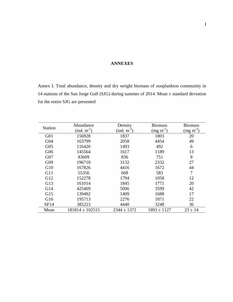
I
ANNEXES
Annex I. Total abundance, density and dry weight biomass of zooplankton community in
14 stations of the San Jorge Gulf (SJG) during summer of 2014. Mean ± standard deviation
for the entire SJG are presented
Station Abundance
(ind. m-2
)
Density
(ind. m-3
)
Biomass
(mg m-2
)
Biomass
(mg m-3
)
G01 156928 1837 1803 20
G04 163799 2058 4454 49
G05 116420 1493 492 6
G06 145564 1617 1189 13
G07 83609 836 751 8
G09 196718 3132 2332 27
G10 167826 4416 1672 44
G11 55356 668 583 7
G12 152278 1794 1058 12
G13 161014 1845 1771 20
G14 425469 5006 3599 42
G15 139492 1409 1688 17
G16 195713 2276 1871 22
SF14 385223 4440 3248 36
Mean 181814 ± 102515 2344 ± 1372 1893 ± 1127 23 ± 14
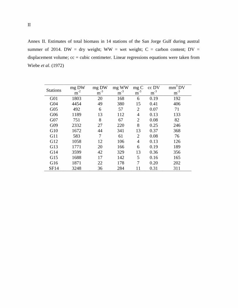
II
Annex II. Estimates of total biomass in 14 stations of the San Jorge Gulf during austral
summer of 2014. DW = dry weight; WW = wet weight; C = carbon content; DV =
displacement volume; cc = cubic centimeter. Linear regressions equations were taken from
Wiebe et al. (1972)
Stations mg DW
m-2
mg DW
m-3
mg WW
m-3
mg C
m-3
cc DV
m-3
mm3
DV
m-3
G01 1803 20 168 6 0.19 192
G04 4454 49 380 15 0.41 406
G05 492 6 57 2 0.07 71
G06 1189 13 112 4 0.13 133
G07 751 8 67 2 0.08 82
G09 2332 27 220 8 0.25 246
G10 1672 44 341 13 0.37 368
G11 583 7 61 2 0.08 76
G12 1058 12 106 4 0.13 126
G13 1771 20 166 6 0.19 189
G14 3599 42 329 13 0.36 356
G15 1688 17 142 5 0.16 165
G16 1871 22 178 7 0.20 202
SF14 3248 36 284 11 0.31 311
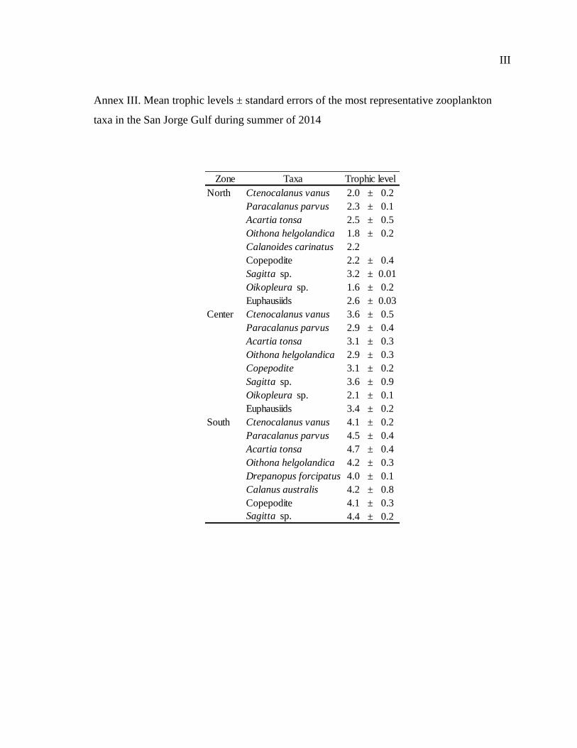
III
Annex III. Mean trophic levels ± standard errors of the most representative zooplankton
taxa in the San Jorge Gulf during summer of 2014
Zone Taxa
North Ctenocalanus vanus 2.0 ± 0.2
Paracalanus parvus 2.3 ± 0.1
Acartia tonsa 2.5 ± 0.5
Oithona helgolandica 1.8 ± 0.2
Calanoides carinatus 2.2
Copepodite 2.2 ± 0.4
Sagitta sp. 3.2 ± 0.01
Oikopleura sp. 1.6 ± 0.2
Euphausiids 2.6 ± 0.03
Center Ctenocalanus vanus 3.6 ± 0.5
Paracalanus parvus 2.9 ± 0.4
Acartia tonsa 3.1 ± 0.3
Oithona helgolandica 2.9 ± 0.3
Copepodite 3.1 ± 0.2
Sagitta sp. 3.6 ± 0.9
Oikopleura sp. 2.1 ± 0.1
Euphausiids 3.4 ± 0.2
South Ctenocalanus vanus 4.1 ± 0.2
Paracalanus parvus 4.5 ± 0.4
Acartia tonsa 4.7 ± 0.4
Oithona helgolandica 4.2 ± 0.3
Drepanopus forcipatus 4.0 ± 0.1
Calanus australis 4.2 ± 0.8
Copepodite 4.1 ± 0.3
Sagitta sp. 4.4 ± 0.2
Trophic level