Embed Size (px)
Citation preview
UNIVERSITÉ DU QUEBEC
MÉMOIRE PRÉSENTÉ À
L'UNIVERSITÉ DU QUÉBEC À CHICOUTIMI
COMME EXIGENCE PARTIELLE
DE LA MAÎTRISE EN INGÉNIERIE
par
SHAHRIAR VARKIANI
APPLICATION DES RESEAUX NEURONAUX FLOUS A
L'IDENTIFICATION ET LA PROTECTION D'UN
TRANSFORMATEUR TRIPHASÉ
Avril 1998

bibliothèquePaul-Emile-Bouletj
UIUQAC
Mise en garde/Advice
Afin de rendre accessible au plusgrand nombre le résultat destravaux de recherche menés par sesétudiants gradués et dans l'esprit desrègles qui régissent le dépôt et ladiffusion des mémoires et thèsesproduits dans cette Institution,l'Université du Québec àChicoutimi (UQAC) est fière derendre accessible une versioncomplète et gratuite de cette �uvre.
Motivated by a desire to make theresults of its graduate students'research accessible to all, and inaccordance with the rulesgoverning the acceptation anddiffusion of dissertations andtheses in this Institution, theUniversité du Québec àChicoutimi (UQAC) is proud tomake a complete version of thiswork available at no cost to thereader.
L'auteur conserve néanmoins lapropriété du droit d'auteur quiprotège ce mémoire ou cette thèse.Ni le mémoire ou la thèse ni desextraits substantiels de ceux-ci nepeuvent être imprimés ou autrementreproduits sans son autorisation.
The author retains ownership of thecopyright of this dissertation orthesis. Neither the dissertation orthesis, nor substantial extracts fromit, may be printed or otherwisereproduced without the author'spermission.

Do tkoâe wko kai/e filled mu life witk loue
/r/u wife, fr/akin; mu dau^kter, -S^kadi; mu motker, J^kakbano r /azemi;
and mu motker-in-law, Lratemek Dsalantari
Jrn lot/in^ memory of mu fatker, ^Jéli ^éô
Contents
List of Figures vii
List of Tables JC
Résumé xi
Abstract xiii
Acknowledgements xv
Chapter 1 : Introduction 1
1.1 Background 2
1.2 Motivation and Objective 5
1.3 Methodology 7
1.4 Survey of the Thesis 8
Chapter 2 : Review of the Literature 9
2.1 Introduction 10
2.2 Harmonic Restraint Approach 11
2.3 Artificial Neural Networks Approach 15
2.4 Fuzzy Logic Approach 18
m
Chapter 3 : Fundamental Theories 26
3.1 Introduction 27
SECTION ONE. 29
3.1.1 What are Artificial Neural Networks? 29
3.1.2 Model of an Artificial Neuron 31
3.1.3 Types of Activation Functions 33
3.1.4 Learning 35
3.1.4.1 Back-Propagation Learning 37
SECTION TWO 41
3.2.1 What is Fuzzy Logic? 41
3.2.2 Basic Notions of Fuzzy Logic 42
3.2.2.1 Fuzzy Set 42
3.2.2.2 Linguistic Variable 44
3.2.2.3 Membership Function 44
3.2.3 Operations on Fuzzy Sets 45
3.2.3.1 Complement 45
3.2.3.2 Intersection or Triangular Norms 46
3.2.3.3 Union Triangular Co-Norms 47
3.2.4 Notion of Linguistic Rule 49
3.2.5 General Structure of Fuzzy Systems 49
IV
3.2.5.1 Procedure of Fuzzy Reasoning 51
3.2.5.2 Type of Fuzzy Reasoning 53
3.2.5.3 Defuzzification Strategies 55
SECTION THREE. 58
3.3.1 What are Neuro-Fuzzy Systems ? 58
3.3.2 Background of Neuro-Fuzzy Systems 58
3.3.3 Neural Fuzzy Inference Systems 61
3.3.3.1 Knowledge Structure and Linguistic Variables 61
3.3.3.2 Network Architecture 63
3.3.3.3 Learning Algorithm 67
Chapter 4 : Neuro-Fuzzy Models 69
4.1 Introduction 70
4.2 Identification 71
4.3 Structure of the Neuro-Fuzzy System 74
4.4 Learning Algorithm 80
4.5 Training Data 83
4.6 Pre-processing 88
4.7 Training of the Model 94
Chapter 5 : Validation 97
5.1 Introduction 98
5.2 Verification of the Direct and Indirect Models 99
5.3 Validation of the Direct and Indirect Models 106
5.3.1 Description of the Validation Data Files 106
5.3.2 Internal Fault at the Secondary Side of the Power Transformer 108
5.3.3 Internal Fault at the Primary Side of the Power Transformer 117
Chapter 6 : Conclusion and Further Works 130
References 135
VI
List of Figures
Figure 2.1 : A simplified block diagram of the Fuzzy Logic Relay (FLR) for powertransformers. 22
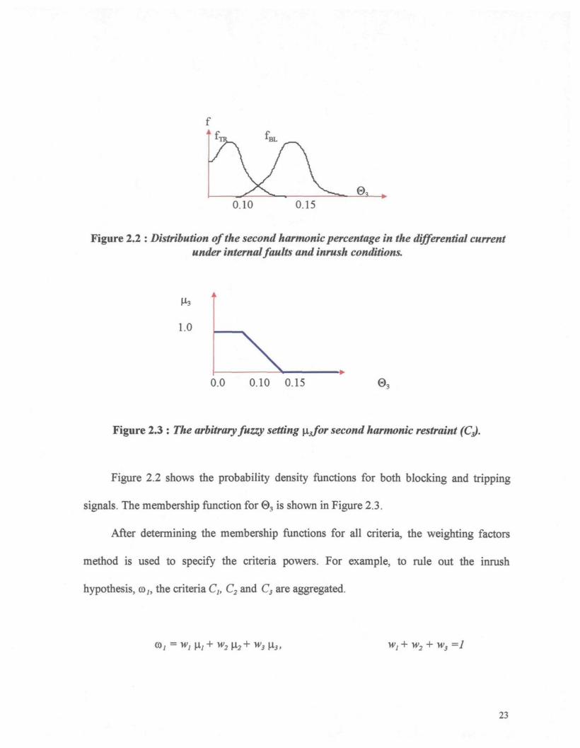
Figure 2.2 : Distribution of the second harmonic percentage in the differential current
under internal faults and inrush conditions. 23
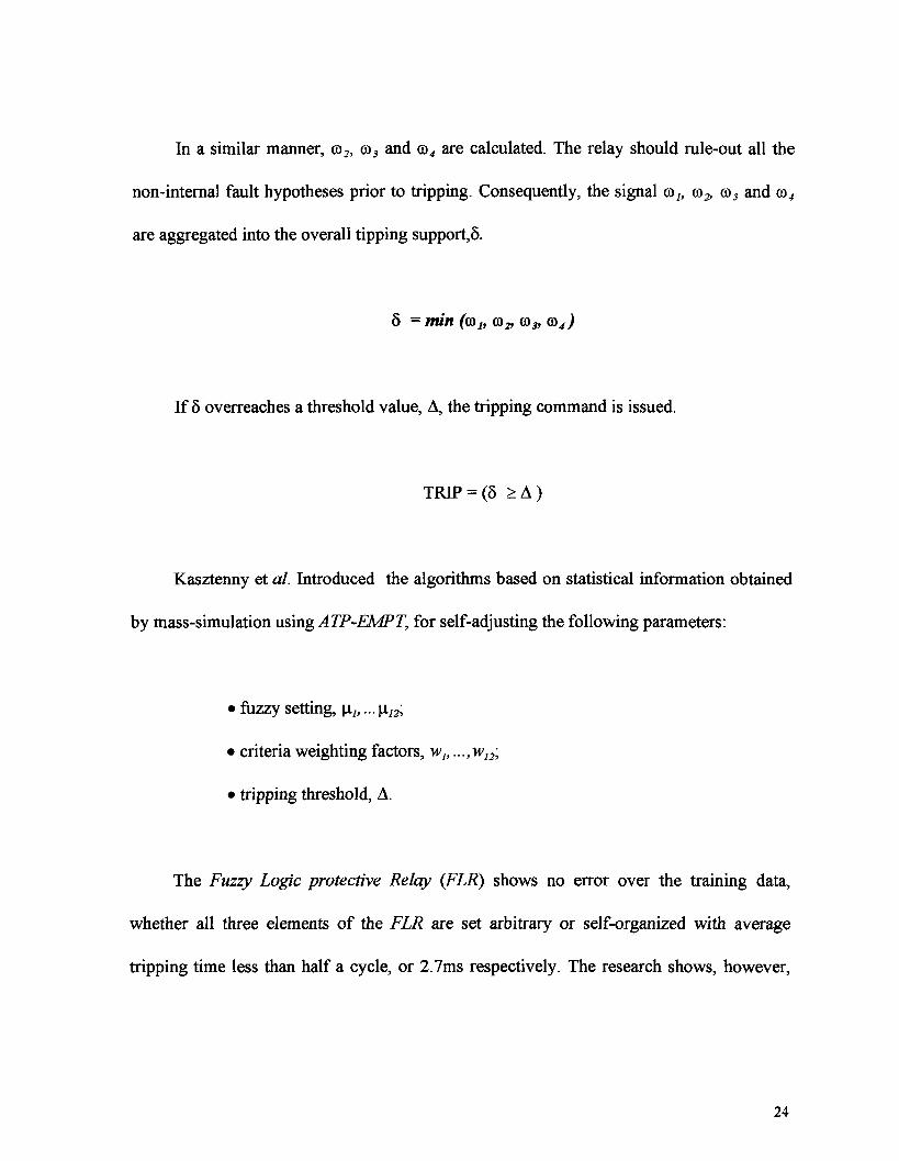
Figure 2.3 : The arbitrary fuzzy setting \i3for second harmonic restraint (CJ 23
Figure 3.1 : Multiple-Input Neuron. 32
Figure 3.2 : Different shapes of member ship functions: monotonie, triangular, trapezoidaland bell-shaped 44
Figure 3.3 : Graphical representation of operations with fuzzy set; (a) Triangular norm
(min operator); (b) Triangular co-norm (max operator) 48
Figure 3.4 : Fuzzy Inference System 50
Figure 3.5 : General structure of the fuzzy system 53
Figure 3.6 : Four types of reasoning in fuzzy inference systems. 55
Figure 3.7 : Neuro-fuzzy systems integrate fuzzy logic and neural networks. 59
Figure 3.8 : Fuzzy if-then rules and fuzzy reasoning mechanisms. 62
Figure 3.9 : (a) type-3 fuzzy reasoning; (b) equivalent ANFIS (type-3 ANFIS) 64
Figure 4.1 : Basic scheme of the parallel identification model using neuro-fuzzy systems.72
Figure 4.2 : Basic scheme of the series-parallel identification model using neuro-fuzzysystems 73
vu
Figure 4.3 : Direct Model 75
Figure 4.4 : Indirect Model 76
Figure 4.5 : Various methods of partition the input space : (a) grid partition; (b) tree
partition, (c) scatter partition 77
Figure 4.6 : (a) fuzzy reasoning; (b) Equivalent ANFIS 80
Figure 4.7 : Train 1, an example of training data. 84
Figure 4.8 : Train2, an example of training data. 85
Figure 4.9 : TrainS, an example of training data. 85
Figure 4.10 : Train4, an example of training data. 86
Figure 4.11 : Primary and secondary voltages. 87
Figure 4.12 : Training Algorithm 96
Figure 5.1 : Prediction of the secondary current by the direct model. 100Figure 5.2 : This figure consists of three subplots; Top : Error of the direct model; Middle
: Difference error of the direct model; Bottom : Secondary current of thetransformer 101
Figure 5.3 : Prediction of the primary current by the indirect model. 102
Figure 5.4 : This figure consists of three subplots; Top; Error of the indirect model;Middle : Difference error of the indirect model; Bottom : Primary current ofthe transformer 103
Figure 5.5 : Hybrid method, which is the combination of intelligent relay and over currentrelay signals. 104
Figure 5.6 : Direct model, validation file T3121211 Ill
Figure 5.7 : Indirect model, validation file T3121211 112
Figure 5.8 : Comparison of the direct model output with the secondary current of thepower transformer, validation file T3121211 113
Vlll
Figure 5.9 : Direct model, validation file T3121214. 114
Figure 5.10 : Indirect model, validation file T3121214 115
Figure 5.11 : Comparison of the indirect model output with the primary current of the
power transformer, validation file T3121214. 116
Figure 5.12 : Direct model, validation file T3111211 119
Figure 5.13 : Indirect model, validation file T3U1211 120
Figure 5.14 : Comparison of the direct model output with the secondary current of the
power transformer, validation file T3111211 121
Figure 5.15 -. Direct model, validation file T3111233 122
Figure 5.16 : Indirect model, validation file T3111233 124
Figure 5.17 : Direct model, validation file T2111233 126
Figure 5.18 : Indirect model, validation file T2111233 127
Figure 5.19 : Direct model, validation file 5111242 128
Figure 5.20 : Indirect model, validation file 5111242 129
IX
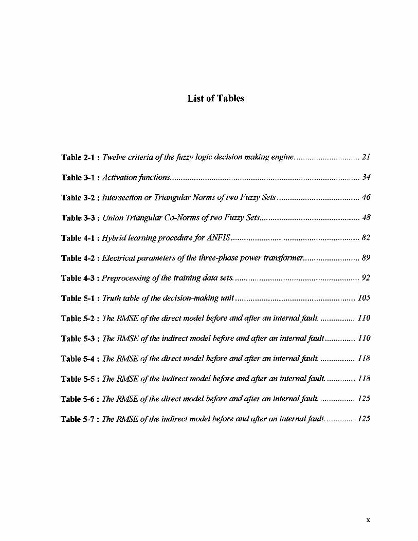
List of Tables
Table 2-1 : Twelve criteria of the fuzzy logic decision making engine 21
Table 3-1 : Activation functions 34
Table 3-2 : Intersection or Triangular Norms of two Fuzzy Sets 46
Table 3-3 : Union Triangular Co-Norms of two Fuzzy Sets 48
Table 4-1 : Hybrid learning procedure for ANFIS 82
Table 4-2 : Electrical parameters of the three-phase power transformer. 89
Table 4-3 : Preprocessing of the training data sets. 92
Table 5-1 : Truth table of the decision-making unit 105
Table 5-2 : The RMSE of the direct model before and after an internal fault. 110
Table 5-3 : The RMSE of the indirect model before and after an internal fault 110
Table 5-4 : The RMSE of the direct model before and after an internal fault. 118
Table 5-5 : The RMSE of the indirect model before and after an internal fault. 118
Table 5-6 : The RMSE of the direct model before and after an internal fault. 125
Table 5-7 : The RMSE of the indirect model before and after an internal fault. 125

Résumé
Récemment, des systèmes avancés de reconnaissance et de prise de décision
incorporant des éléments de logique floue et de réseaux de neurones artificiels ont été
appliqués avec succès à l'identification, la commande et la protection des réseaux
électriques. Le principal objectif de cette thèse consiste à explorer la capacité de systèmes
neuro-flous, qui sont une combinaison des systèmes à réseaux de neurones et à logique
floue, pour l'identification d'un transformateur triphasé, en vue de développer un modèle
non-linéaire permettant de mieux protéger le transformateur contre les défauts internes.
Deux modèles, l'un direct et l'autre indirect, sont développés afin de prédire les
courants secondaires en fonction des courants primaires et réciproquement. Un algorithme
hybride d'apprentissage est utilisé pour entraîner les modèles. Celui-ci procède en deux
étapes; premièrement, dans la passe en sens direct (des entrées vers les sorties) il impose
des paramètres des prémisses et emploie l'estimateur aux moindres carrés pour ajuster les
paramètres des conclusions. Ensuite, procédant en sens rétrograde (des sorties vers les
entrées), il fixe les paramètres des conclusions et emploie un algorithme du gradient pour
ajuster les paramètres des prémisses, de manière à minimiser l'erreur total des modèles.
Plusieurs fichiers de données d'apprentissage sont utilisés, afin de refléter toutes les
conditions d'exploitation possibles: nominales, surcharges permanentes et transitoires,
XI

défauts externes et courants d'appel lors de la mise sous tension. Cependant, ces fichiers
d'apprentissage n'incluent aucune donnée de défaut interne.
Au terme de l'apprentissage, plusieurs nouveaux fichiers de données sont utilisés
pour valider les modèles neuro-flous. On peut ainsi vérifier leur généralisation sur des
données qu'ils n'ont pas vues durant leur entraînement. Au total, les modèles neuro-flous
démontrent une bonne aptitude à prédire le comportement d'un transformateur de
puissance de façon précise sous des conditions nominales, avec des erreurs de modèle
direct et indirect relativement faibles. Cependant, ces erreurs augmentent substantiellement
lors d'un défaut interne, ce qui permet de déterminer rapidement l'occurrence d'un tel
défaut.
Xll
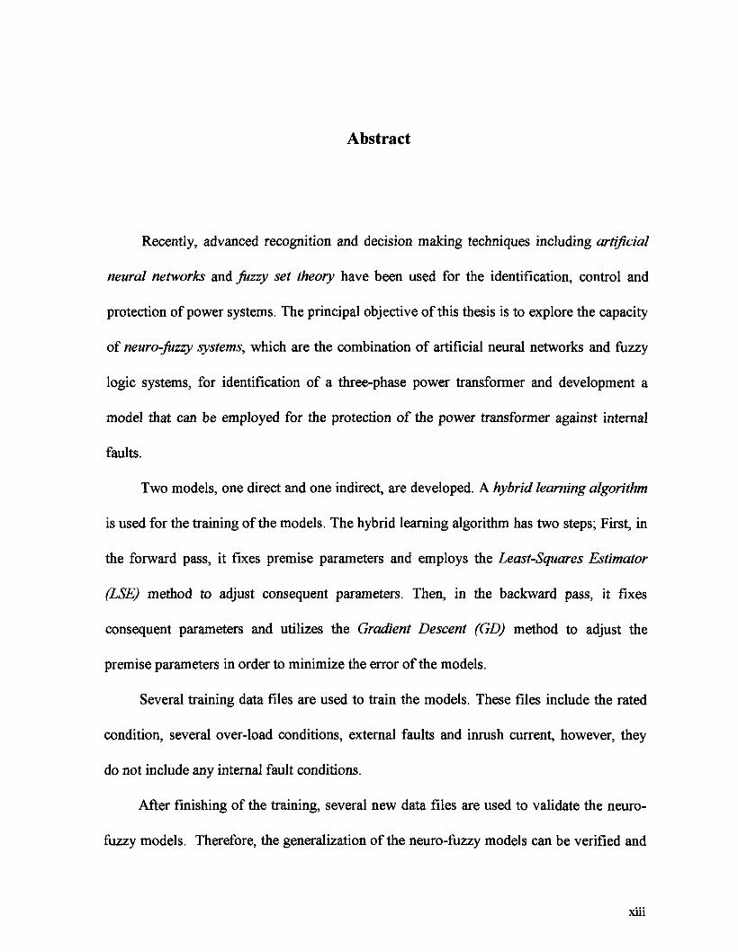
Abstract
Recently, advanced recognition and decision making techniques including artificial
neural networks and fuzzy set theory have been used for the identification, control and
protection of power systems. The principal objective of this thesis is to explore the capacity
of neuro-fuzzy systems, which are the combination of artificial neural networks and fuzzy
logic systems, for identification of a three-phase power transformer and development a
model that can be employed for the protection of the power transformer against internal
faults.
Two models, one direct and one indirect, are developed. A hybrid learning algorithm
is used for the training of the models. The hybrid learning algorithm has two steps; First, in
the forward pass, it fixes premise parameters and employs the Least-Squares Estimator
(LSE) method to adjust consequent parameters. Then, in the backward pass, it fixes
consequent parameters and utilizes the Gradient Descent (GD) method to adjust the
premise parameters in order to minimize the error of the models.
Several training data files are used to train the models. These files include the rated
condition, several over-load conditions, external faults and inrush current, however, they
do not include any internal fault conditions.
After finishing of the training, several new data files are used to validate the neuro-
fuzzy models. Therefore, the generalization of the neuro-fuzzy models can be verified and
Xll l

tested by the unseen data files. The neuro-fuzzy models show that they can predict
precisely the behavior of the power transformer under rated conditions. The amplitude of
the errors of the direct and indirect models are small. However, these errors increase in
amplitude when an internal fault occurs in the power transformer, allowing for rapid
detection.
XIV

Acknowledgements
I take this opportunity to express my thanks to all who have helped me, either for
technical or moral support, to finish this thesis.
First of all, I would like to thank my director, Professor Masoud Farzaneh, for his
support and supervision for the entire work of my M.Sc. thesis. I would like to
acknowledge my co-director, Dr. Innocent Kamwa at Institut de recherche d'Hydro-
Québec (IREQ), for his support and guidance and also for his helpful advice and
discussions. I am grateful to Dr. Jean Rouat, Professor at the University of Quebec in
Chicoutimi, who helped me develop my knowledge and skills in artificial neural networks.
I would also like to express my appreciation to the entire staff of the GRIEA, in
particular Sylvain Desgagnés, for their help and excellent working atmosphere. I wish to
thank Chantale Dumas, secretary of Applied Sciences Department, for her help and
assistance during my studies at UQAC.
Last, but by no means least, my heartfelt thanks go to my dear wife, Mahin, for her
support, advice, patience and love.
XV

Chapter 1
Introduction
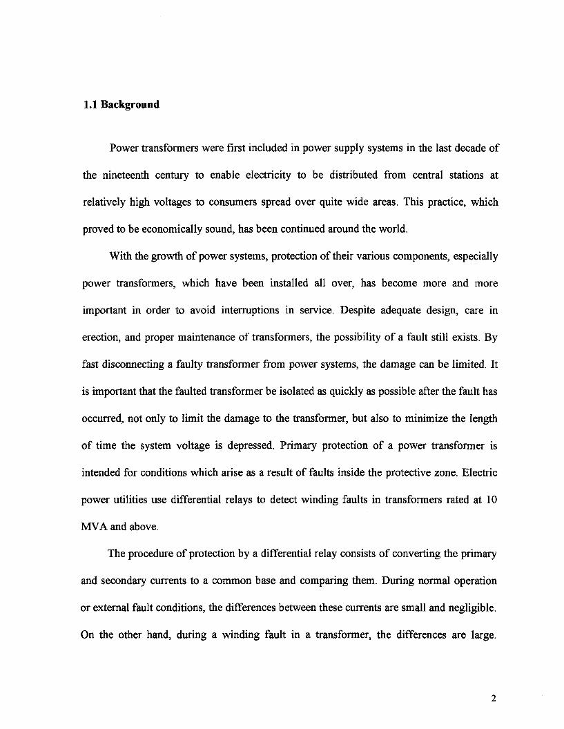
1.1 Background
Power transformers were first included in power supply systems in the last decade of
the nineteenth century to enable electricity to be distributed from central stations at
relatively high voltages to consumers spread over quite wide areas. This practice, which
proved to be economically sound, has been continued around the world.
With the growth of power systems, protection of their various components, especially
power transformers, which have been installed all over, has become more and more
important in order to avoid interruptions in service. Despite adequate design, care in
erection, and proper maintenance of transformers, the possibility of a fault still exists. By
fast disconnecting a faulty transformer from power systems, the damage can be limited. It
is important that the faulted transformer be isolated as quickly as possible after the fault has
occurred, not only to limit the damage to the transformer, but also to minimize the length
of time the system voltage is depressed. Primary protection of a power transformer is
intended for conditions which arise as a result of faults inside the protective zone. Electric
power utilities use differential relays to detect winding faults in transformers rated at 10
MVA and above.
The procedure of protection by a differential relay consists of converting the primary
and secondary currents to a common base and comparing them. During normal operation
or external fault conditions, the differences between these currents are small and negligible.
On the other hand, during a winding fault in a transformer, the differences are large.
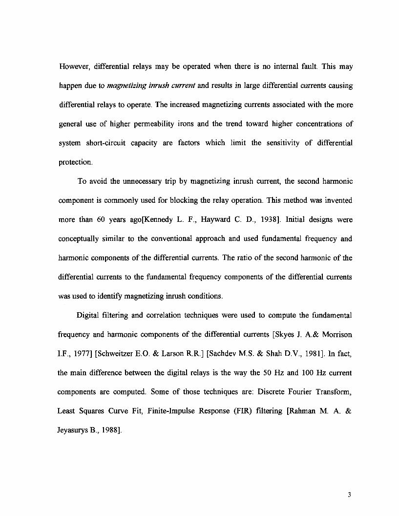
However, differential relays may be operated when there is no internal fault. This may
happen due to magnetizing inrush current and results in large differential currents causing
differential relays to operate. The increased magnetizing currents associated with the more
general use of higher permeability irons and the trend toward higher concentrations of
system short-circuit capacity are factors which limit the sensitivity of differential
protection.
To avoid the unnecessary trip by magnetizing inrush current, the second harmonic
component is commonly used for blocking the relay operation. This method was invented
more than 60 years ago[Kennedy L. F., Hayward C. D., 1938]. Initial designs were
conceptually similar to the conventional approach and used fundamental frequency and
harmonic components of the differential currents. The ratio of the second harmonic of the
differential currents to the fundamental frequency components of the differential currents
was used to identify magnetizing inrush conditions.
Digital filtering and correlation techniques were used to compute the fundamental
frequency and harmonic components of the differential currents [Skyes J. A.& Morrison
I.F., 1977] [Schweitzer E.O. & Larson R.R.] [Sachdev M.S. & Shah D.V., 1981]. In fact,
the main difference between the digital relays is the way the 50 Hz and 100 Hz current
components are computed. Some of those techniques are: Discrete Fourier Transform,
Least Squares Curve Fit, Finite-Impulse Response (FIR) filtering [Rahman M. A. &
Jeyasurys B., 1988].
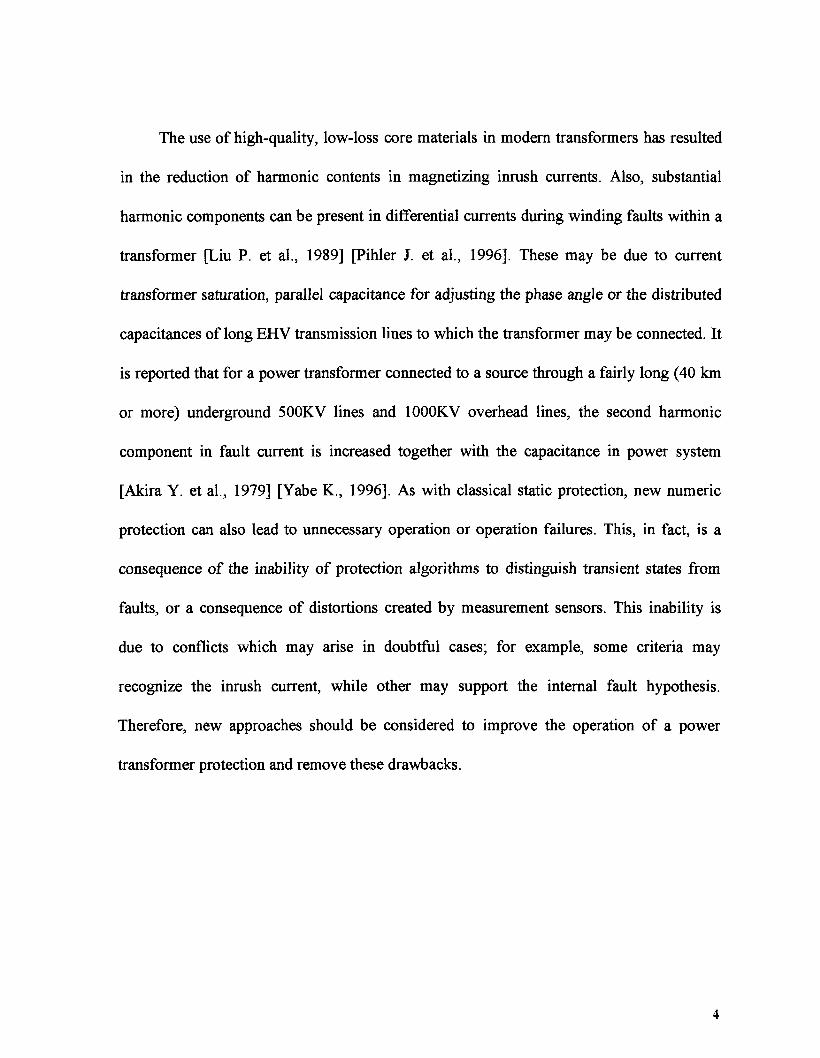
The use of high-quality, low-loss core materials in modern transformers has resulted
in the reduction of harmonic contents in magnetizing inrush currents. Also, substantial
harmonic components can be present in differential currents during winding faults within a
transformer [Liu P. et al., 1989] [Pihler J. et al., 1996]. These may be due to current
transformer saturation, parallel capacitance for adjusting the phase angle or the distributed
capacitances of long EHV transmission lines to which the transformer may be connected. It
is reported that for a power transformer connected to a source through a fairly long (40 km
or more) underground 500KV lines and 1000KV overhead lines, the second harmonic
component in fault current is increased together with the capacitance in power system
[Akira Y. et al., 1979] [Yabe K., 1996]. As with classical static protection, new numeric
protection can also lead to unnecessary operation or operation failures. This, in fact, is a
consequence of the inability of protection algorithms to distinguish transient states from
faults, or a consequence of distortions created by measurement sensors. This inability is
due to conflicts which may arise in doubtful cases; for example, some criteria may
recognize the inrush current, while other may support the internal fault hypothesis.
Therefore, new approaches should be considered to improve the operation of a power
transformer protection and remove these drawbacks.
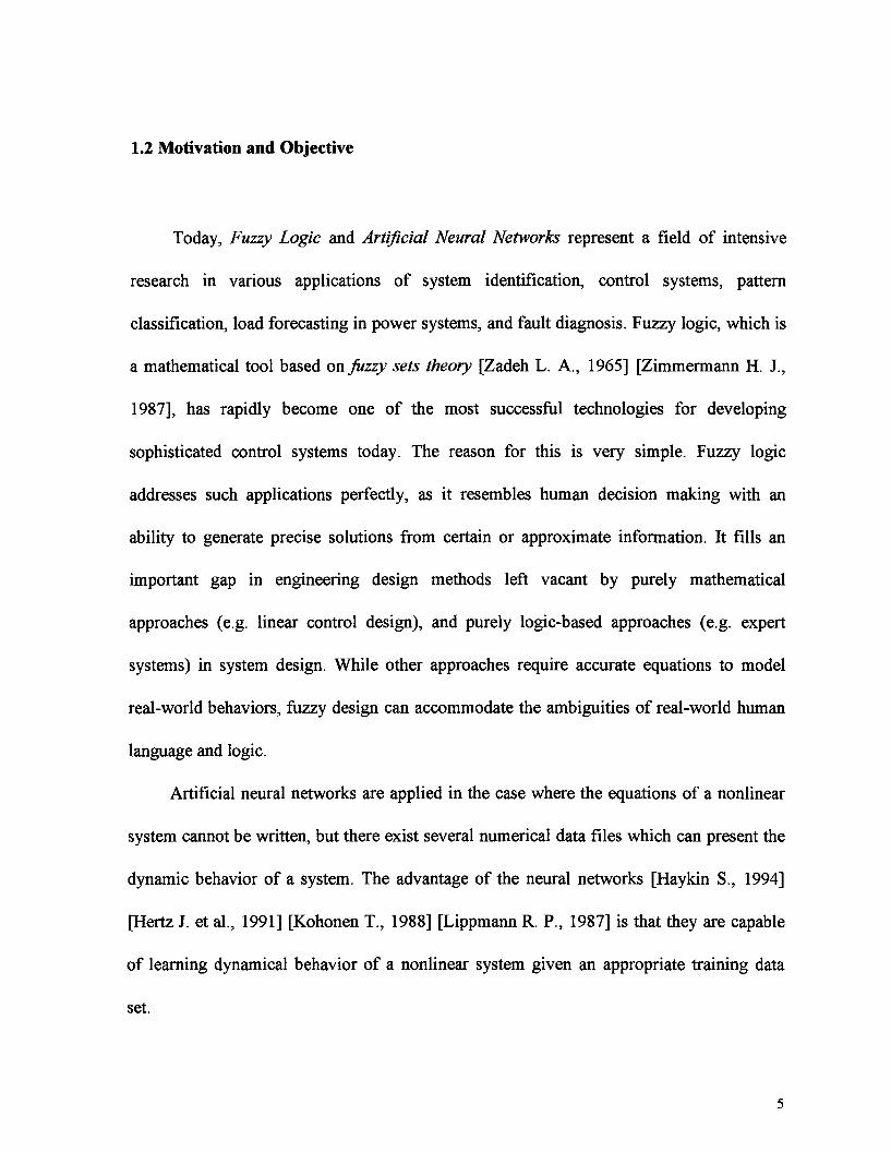
1.2 Motivation and Objective
Today, Fuzzy Logic and Artificial Neural Networks represent a field of intensive
research in various applications of system identification, control systems, pattern
classification, load forecasting in power systems, and fault diagnosis. Fuzzy logic, which is
a mathematical tool based on fuzzy sets theory [Zadeh L. A., 1965] [Zimmermann H. J.,
1987], has rapidly become one of the most successful technologies for developing
sophisticated control systems today. The reason for this is very simple. Fuzzy logic
addresses such applications perfectly, as it resembles human decision making with an
ability to generate precise solutions from certain or approximate information. It fills an
important gap in engineering design methods left vacant by purely mathematical
approaches (e.g. linear control design), and purely logic-based approaches (e.g. expert
systems) in system design. While other approaches require accurate equations to model
real-world behaviors, fuzzy design can accommodate the ambiguities of real-world human
language and logic.
Artificial neural networks are applied in the case where the equations of a nonlinear
system cannot be written, but there exist several numerical data files which can present the
dynamic behavior of a system. The advantage of the neural networks [Haykin S., 1994]
[Hertz J. et al., 1991] [Kohonen T., 1988] [Lippmann R. P., 1987] is that they are capable
of learning dynamical behavior of a nonlinear system given an appropriate training data
set.
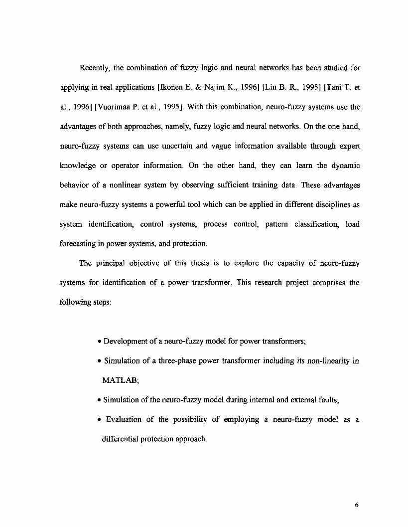
Recently, the combination of fuzzy logic and neural networks has been studied for
applying in real applications [Ikonen E. & Najim K., 1996] [Lin B. R., 1995] [Tani T. et
al., 1996] [Vuorimaa P. et al., 1995]. With this combination, neuro-fuzzy systems use the
advantages of both approaches, namely, fuzzy logic and neural networks. On the one hand,
neuro-fuzzy systems can use uncertain and vague information available through expert
knowledge or operator information. On the other hand, they can learn the dynamic
behavior of a nonlinear system by observing sufficient training data. These advantages
make neuro-fuzzy systems a powerful tool which can be applied in different disciplines as
system identification, control systems, process control, pattern classification, load
forecasting in power systems, and protection.
The principal objective of this thesis is to explore the capacity of neuro-fuzzy
systems for identification of a power transformer. This research project comprises the
following steps:
� Development of a neuro-fuzzy model for power transformers;
� Simulation of a three-phase power transformer including its non-linearity in
MATLAB;
� Simulation of the neuro-fuzzy model during internal and external faults;
� Evaluation of the possibility of employing a neuro-fuzzy model as a
differential protection approach.
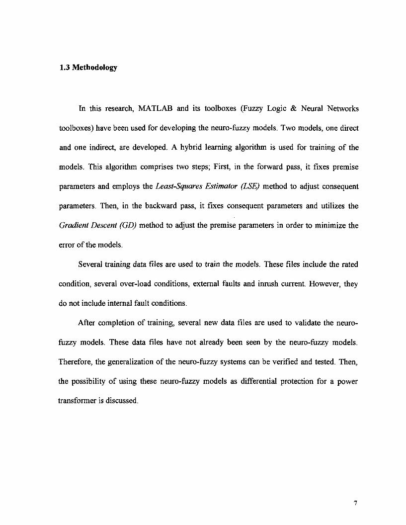
1.3 Methodology
In this research, MATLAB and its toolboxes (Fuzzy Logic & Neural Networks
toolboxes) have been used for developing the neuro-fuzzy models. Two models, one direct
and one indirect, are developed. A hybrid learning algorithm is used for training of the
models. This algorithm comprises two steps; First, in the forward pass, it fixes premise
parameters and employs the Least-Squares Estimator (LSE) method to adjust consequent
parameters. Then, in the backward pass, it fixes consequent parameters and utilizes the
Gradient Descent (GD) method to adjust the premise parameters in order to minimize the
error of the models.
Several training data files are used to train the models. These files include the rated
condition, several over-load conditions, external faults and inrush current. However, they
do not include internal fault conditions.
After completion of training, several new data files are used to validate the neuro-
fuzzy models. These data files have not already been seen by the neuro-fuzzy models.
Therefore, the generalization of the neuro-fuzzy systems can be verified and tested. Then,
the possibility of using these neuro-fuzzy models as differential protection for a power
transformer is discussed.
1.4 Survey of the Thesis
There are a total of six chapters in this thesis. In chapter 1, a synopsis of relevant
problems, the objective and methodology of this work have already been presented and
analyzed.
In chapter 2, a review of previous research in this field, is presented. Chapter 3
consists of three sections: In the first section, the concept of Artificial Neural Networks
(ANN) and their learning abilities are explained. In the section that follows, the Fuzzy Logic
(FL) concept is presented. Then, fuzzy sets, fuzzy relations, and approximate reasoning are
introduced. Finally, in the last section, the synergism of fusing fuzzy logic and artificial
neural networks techniques into an integrated system called Neuro-Fuzzy System (NFS) is
introduced. Then, hybrid learning algorithm, in order to minimize the error of neuro-fuzzy
systems, is explained.
In chapter 4, two models, one direct and one indirect, are developed for a three-phase
power transformer. The structure and architecture of the models, and the learning
procedure are explained in greater detail. The validation of the models and the possibility
of using this approach as a protection method for three-phase power transformers are
presented in chapter 5. Finally, in chapter 6, the impact of this work is summarized,
improvements are suggested, and further research is recommended.

Chapter 2
Review of the Literature
2.1 Introduction
Identification theory is a vast subject of considerable interest to the power industry.
Due to increasingly complex power systems, the need to quickly and accurately identify the
important characteristics of power system components is aprimary concern. The ability to
adequately represent the important dynamics of a system, over a wide bandwidth, is of
paramount importance for all identification schemes.
Any control action or protection design for a power system will only be as good as
the model it is based on. The model may be obtained either analytically, where the model is
derived from basic equations and the parameters are assumed, or experimentally, using
direct measurements. In practice, however, it is very difficult, and sometimes, impossible
to develop an analytic model for a nonlinear dynamic system.
A power transformer is an essential component of a power system. Power
transformers may be subject to various types of faults. Proper design and setting of a
differential relay for power transformers are recognized as challenging problems for
protection engineers. In the case of a power transformer, detection of a differential current
does not provide a clear distinction between internal faults and other conditions. Biased
differential characteristics combined with 2nd and 5th harmonic restraints constitute a
classical approach to the problem. Searching for better relay sensitivity, selectivity and
speed of operation, initial designs conceptually similar to the conventional technique have
10
shifted to new recognition methods in the areas of both signal estimation and decision
making.
More recently, advanced recognition and decision making techniques, including
artificial neural networks and fuzzy set theory, have been used for the identification,
control, and protection of power systems.
During this research, several papers and theses have been studied as bibliography.
While it is not possible to review all of them in this chapter, some of the most important
are reviewed. In the first two sections, different digital power transformer protection
algorithms based on the harmonics restraint approach are reviewed. Then, in the next two
sections, application of artificial neural networks for recognition of inrush current, and
improvement of power transformer protection are discussed. The last paper presents a new
approach for protection of power transformers based on fuzzy logic.
2.2 Harmonic Restraint Approach
Rahman M. A., Jeyasurya B.,'A State-Of-Art Review of Transformer Protection Algorithms",
IEEE Transaction on Power Delivery, vol. 3, no. 2, April 1988.
This paper reviews different algorithms for digital differential protection power
transformers. The following algorithms are briefly explained in their mathematical aspects:
11
� Fourier Analysis Approach;
� Rectangular Transform Approach;
� Algorithm based on Walsh Function;
� Haar Function Approach;
� Finite Impulse Response Approach (FIR);
� Least-Squares Curve Fitting Algorithm.
The ultimate purpose in all of the above mentioned algorithms is to determine the
peak of the fundamental and harmonic content of the differential current as each new
sample is taken. Since the inrush current has a higher percentage of harmonics than internal
fault, this information is used to determine whether there is an inrush current condition or
an internal fault. The authors use frequency response, which is a measure of the filtering
characteristic of the algorithms. Each algorithm may be considered as four digital filtering
computations, two for the fundamental frequency and two for the second harmonic. The
frequency responses of the algorithms show that these algorithms are able to effectively
extract components of the fundamental and second harmonic frequencies of the differential
current from sample data. A three-phase transformer model is used to simulate the inrush
current and internal faults. Since the restraining signal is well above the operating signal,
the performance of all the algorithms for inrush current is good and there is not any
possibility for malfunction . For internal faults, the restraining signal is higher immediately
after inception of the internal fault. However, after about 15 ms, the operating signal is
12
higher than the restraining signal, and a trip signal is issued. The authors compare the
computational requirements and time for all the algorithms. It shows that Least-Square
Curve Fitting, Rectangular Transform, Fourier Analysis and Finite Impulse Response
algorithms can do the computations in less than 40% of the sampling interval and excess
time can be used for data acquisition, relay logic, and monitoring.
Grcar B., Dolinar D.. "Integrated Digital Power Transformer Protection", lEEEProc. Gener.
Transm. Distrib., 141(4), pp. 323-328, July 1994.
Dolinar D,, Pihler J., Grcar B., "Dynamic Model of a Three-Phase Power Transformer", IEEE/PES
Winter Meeting, Columbus USA, February 1993.
The authors propose an integrated digital three-phase power transformer protection.
It consists of a percentage differential relay with harmonic restraint at inrush and over-
excitation conditions, an over-current relay with instantaneous and time-lag operation, a
sensitive relay for selective operation at high impedance ground faults, and a fault recorder.
The proposed integrated protection concept is developed on the basis of a nonlinear
mathematical transformer model which includes nonlinear effects of saturation, hysteresis
and eddy currents. In this paper, a complete hardware and software structure of an
integrated transformer protection is given. The integrated protection algorithm is
implemented on a high-performance digital processor DSP32C connected to a standard PC
and a peripheral input-output unit. There are two program modules. The first program is
13
executed on PC to ensure an equidistant sampling interval and the transfer of sampled
signals into the signal processor. The second program is executed on signal processor to
execute the protection algorithm. The sampled currents are transformed on a common base
by means of signal preprocessing. The transformation matrix T is used to obtain the
differential and through currents. The transformation matrices T are predefined for
different connection groups and stored in the memory as a configuration parameter. The
differential and through currents for connection Yd5 are
id(k) = Tip(k) - is(k)
= 0.5[Tip(k)-is(k)]
The determination of the fundamental, second and fifth harmonic components in
differential, through and ground currents are done by the least-squares curve-fitting
technique. The inrush and over-excitation conditions are detected on the basis of the
percentage of the second and fifth harmonics in the differential current respectively. The
slop of the percentage differential characteristic is changed based on the through current.
Laboratory results and field testing indicate that the performance of the integrated digital
relay is superior to that of existing static relays. Despite numerous laboratory and field
tests, false operations or operation failures never occurred. The maximal operation time is
approximately 25 ms. In addition, the algorithm has enough robustness in relation to the
system frequency.
14
2.3 Artificial Neural Networks Approach
Perez L. G., Flechsig A. J., Meador J. L.; Obradovic Z.,"Training an Artificial Neural Network to
Discriminate between Magnetizing and Internal Faults", IEEE/PES Winter Meeting, Columbus,
OH, January 31 - February 5, 1993.
The authors devise a method for discriminating between inrush current and internal
fault, based on a Feed-Forward Neural Network (FFNN) . To compromise between speed
and accuracy, different architectures are selected. However, the network has one neuron in
its output layer. There are 3 networks with 3 layers (12+2+1, 6+2+1 & 4+2+1) and 3
networks with only 2 layers (12+1, 6+1 & 4+1). The sigmoid transfer junction is chosen
for each neuron. The network is trained with the well-known back-propagation algorithm.
The training data consists of two files. The first file represents the inrush currents, which
are obtained by measuring on a small 50 VA, 120/240 V power transformer in the
laboratory. The measured data represent an acceptable range of inrush current shapes. The
desired output of FFNN for this group is considered as zero. The second training file
consists of internal fault cases, which are produced by EMTP. The desired response of
FFNN for this case is considered as one. After completing the training procedure, the
neurons transfer functions are changed to hard-limit. This change increases the FFNN
computation speed considerably, since it takes less computation time to implement a hard
limit than a sigmoid transfer function. The results of simulation show that only four
15
architectures of the AW (12+2+1, 6+2+1, 12+1 & 6+1) show good performance and the
others (4+2+1 & 4+1) show poor performance. While, the time necessary to detect inrush
current is longer than by Fourier analysis, but the authors believe that this protection
method is more secure as regards false trips. In this research, only the inrush current cases
are considered and more work should be done in order to test the model with other non-
internal fault hypotheses (as external faults mixed with saturation of the CTs).
Pihler J., Grcar B., Dolinar D.," Improved Operation of Power Transformer Protection using
Artificial Neural Network ", IEEE/PES Summer Meeting, Denver, Colorado, July 28 - August
1,1996.
The authors propose a way for using intelligent concepts to recognize the inrush
current and restore the secondary current of CTs, which are partially or totally saturated, in
order to improve the operation of a digital power transformer protection. They explain that
digital relays with harmonic restraint are not reliable in all cases, and that in several cases
the relays are caused to operate incorrectly. They propose to use an artificial neural
network to recognize the inrush currents. It comprises 3 layers (6 + 4 + 1 ) and uses the
back-propagation algorithm as learning rule. The Sigmoid Junction is considered as the
transfer function for all the neurons. There are 137 training vectors which contain different
inrush conditions, fault currents, and stationary transformer state currents. The desired
output for the inrush conditions equals 1, and zero for the fault conditions. After
16
completion of the training, the network responses to all 137 training vectors correctly. The
network incorrectly recognized only 2% of the unseen inrush patterns and 8% of other
patterns. To restore the current of the saturated CT, another artificial neural network is
used. It comprises 3 layers (20 + 3 + 1). Inputs are twenty samples of the secondary
currents (one instantaneous and 19 previously). The target vector is the value of the
primary current at the instant of observation. After training the network, it is tested with
unseen patterns and the restored current differs from the target at amplitude values about
10%. They propose a critérium to select either the secondary currents obtained directly
from the secondary side of the CTs or the restored currents from ANN. In protection
algorithm, there are two branches for detecting inrush current. The first branch determines
the inrush by computing the ratio of the second harmonic to fundamental. The second
branch ascertains inrush by artificial neural network for all three differential currents
simultaneously. In case of discrepancy, the artificial neural network has a higher priority.
The proposed digital differential power transformer protection, including the artificial
neural network, is tested on 30 KVA and 50 MVA transformers. The proposed protection
algorithm has a reliable response and the following advantages:
� reliable establishment of inrush even in cases when inrush current contains less
than 16% of the second harmonic component (inrush current detection is based
on recognizing its wave shape);
� increasing the operating speed at inrush with a simultaneous or slightly delayed
short circuit;
17
� improving the reliability in case of faults where a second harmonic component is
present, even though the transformer has not been switched-on;
� reliable operation of protection at partially saturated current transformers.
2.4 Fuzzy Logic Approach
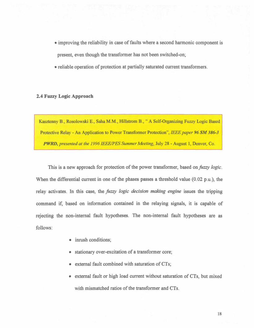
Kasztenny B., Rosolowski E., SahaM.M., Hillstrom B., " A Self-Organizing Fuzzy Logic Based
Protective Relay - An Application to Power Transformer Protection", IEEE paper 96 SM 386-3
PWRD, presented at the 1996IEEE/PES Summer Meeting, July 28 - August 1, Denver, Co.
This is a new approach for protection of the power transformer, based on fuzzy logic.
When the differential current in one of the phases passes a threshold value (0.02 pu) , the
relay activates. In this case, the juzzy logic decision making engine issues the tripping
command if, based on information contained in the relaying signals, it is capable of
rejecting the non-internal fault hypotheses. The non-internal fault hypotheses are as
follows:
� inrush conditions;
� stationary over-excitation of a transformer core;
� external fault combined with saturation of CTs;
� external fault or high load current without saturation of CTs, but mixed
with mismatched ratios of the transformer and CTs.
18

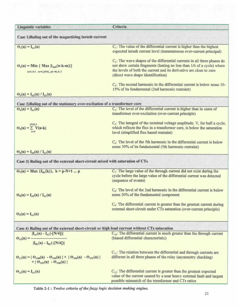
To recognize these non-internal fault hypotheses, the authors establish 12 criteria (3
for each hypothesis) in linguistic forms so that a Fuzzy Inference System (FIS) can be used
to decide whether there is an internal fault hypothesis or a non-internal fault hypothesis.
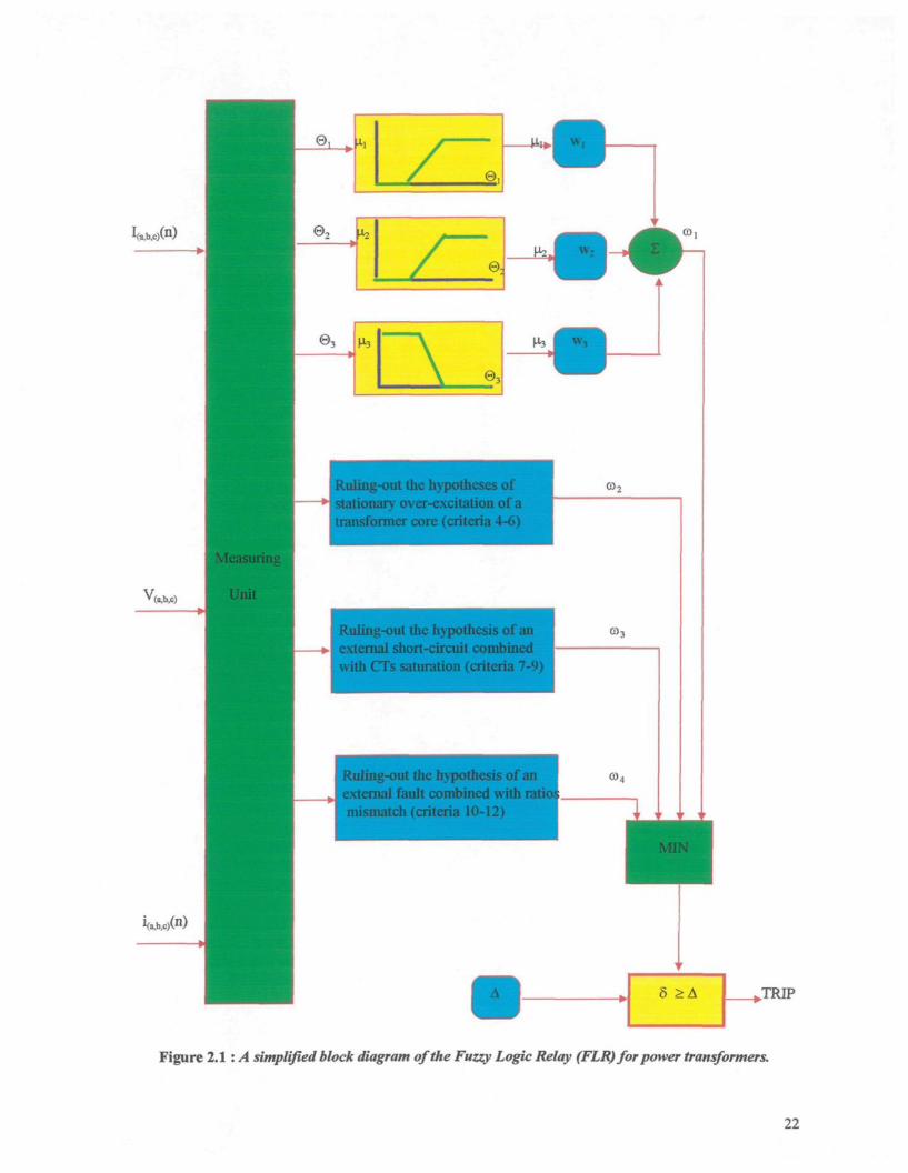
The 12 criteria are listed in Table 2.1, and a schematic diagram of the system is shown in
Figure 2.1.
To obtain the membership function for each signal, 150 simulations are performed
employing ATP-EMPT. These simulations are presented in the following cases:
a) transformer energizing cases (16%);
b) stationary over-excitation cases, including over-voltages and frequency
reduction (7%);
c) external faults with and without saturation of CTs (24%);
d) internal faults including terminal, inter-winding, and turn-to-turn faults
(53%).
A three-phase, two-winding, 5.86 MW, 140/10.52 kV, Yd-connected, five-leg core
type power transformer is modeled by the digital ATP-based model. The sampling rate is
assumed to be 20 samples per cycle (1 kHz). The differential and through currents are
measured by measuring units which are based on Finite impulse Response (FIR) full-cycle
orthogonal filters designed using the least square method with perfect separation between
1st, 2nd and 5th harmonics.
19

To determine the parameters of the membership functions, the probability density
functions for internal and non-internal fault cases are determined. In the overlapping
region, the decision making is vague and uncertain. Therefore, a linguistic variable is
defined. For example, as is shown in Figure 2.2, the membership jnnction has three distinct
regions for the third criteria (C3):
� @3< 0.10 : There is absolutely an internal fault, and there is no magnetizing
inrush current;
� 03 > 0.15 : There is certainly a magnetizing inrush current, and internal
hypothesis is completely rejected;
� 0.10 < 03 <0.15 : This is a fuzzy region and both cases can occur. The
function for this region has been obtained by a self-adjusting algorithm.
20
Linguistic variables Criteria
Case l)Ruling out of the magnetizing inrush current
e,(n) =
e2(n) = Min { Max |iAph(n-k-m)|>iD=0-[N/6],ph=R,S,T
©3(n) =
j : The value of the differential current is higher than the highestexpected inrush current level (instantaneous over-current principal)
Cj: The wave shapes of the differential currents in all three phases donot show certain fragments (lasting no less than 1/6 of a cycle) wherethe levels of both the current and its derivative are close to zero(direct wave shape identification)
C3: The second harmonic in the differential current is below some 10-15% of its fundamental (2nd harmonic restraint)
Case 2)Ruliitg out of the stationary over-excitation of a transformer core
= Z V(n-k)
C4: The level of the differential current is higher than in cases oftransformer over-excitation (over-current principle)
C3: The integral of the terminal voltage amplitude, V, for half a cycle,which reflects the flux in a transformer core, is below the saturationlevel (simplified flux based restraint)
CÉ: The level of the 5th harmonic in the differential current is belowsome 30% of its fundamental (5th harmonic restraint)
Case 3) Ruling out of the external short-circuit mixed with saturation of CTs
= Max {IM(k)}, k = p-N+1... p C7 : The large value of the through current did not exist during thecycle before the large value of the differential current was detected(sequence of events)
Cs: The level of the 2nd harmonic hi the differential current is belowsome 20% of the fundamental component
C9: The differential current is greater than the greatest current duringexternal short-circuit under CTs saturation (over-current principle)
Case 4) Ruling oat of the external short-circuit or high load current without CTs saturation
|@]0T(n) - e 1 0 R ( n ) |
C10: The differential current is much greater than the through current(biased differential characteristic)
Ci i : The relation between the differential and through currents are- ©1Oi(n) | different hi all three phases of the relay (asymmetry checking)
C12: The differential current is greater than the greatest expectedvalue of the current caused by a near heavy external fault and largestpossible mismatch of the transformer and CTs ratios
Table 2-1 : Twelve criteria of the fuzzy logic decision making engine.21
ing-out the hypothesesstationary over-excitation of atransformer core (criteria 4-6)
Ruling-out the hypothesis of anexternal short-circuit combined
ith CTs saturation (criteria 7-
ng-oiit the hypothesis oxtemal fault combined witr
ismatch (criteria 10-12)
TRIP
Figure 2.1 : A simplified block diagram of the Fuzzy Logic Relay (FLR) for power transformers.
22
0.10 0.15
Figure 2.2 : Distribution of the second harmonie percentage in the differential currentunder internal faults and inrush conditions.
1.0
0.0 0.10 0.15
Figure 2.3 : The arbitrary fuzzy setting \ijfor second harmonic restraint
Figure 2.2 shows the probability density functions for both blocking and tripping
signals. The membership function for @3 is shown in Figure 2.3.
After determining the membership functions for all criteria, the weighting factors
method is used to specify the criteria powers. For example, to rule out the inrush
hypothesis, ©;, the criteria Ch C2 and Q are aggregated.
3 =1
In a similar manner, &2, &3 and ®4 are calculated. The relay should rule-out all the
non-internal fault hypotheses prior to tripping. Consequently, the signal co7) &2, &3 and G>4
are aggregated into the overall tipping support,5.
5 = nun (iooj, co2, <o3, &4)
If ô overreaches a threshold value, A, the tripping command is issued.
TRIP = (Ô > A )
Kasztenny et al. Introduced the algorithms based on statistical information obtained
by mass-simulation using ATP-EMPT, for self-adjusting the following parameters:
� fuzzy setting, \i,,...[i12;
� criteria weighting factors, wlt ...,w12;
� tripping threshold, A.
The Fuzzy Logic protective Relay (FLR) shows no error over the training data,
whether all three elements of the FLR are set arbitrary or self-organized with average
tripping time less than half a cycle, or 2.7ms respectively. The research shows, however,
24

that the FLR is not robust enough against unseen cases and it trips falsely in 4% of non-
internal cases.
To Improve the FLR and stabilize the relay, Kasztenny et a/. Suggested the following
approaches:
� re-learn the tripping threshold using the entire data-base;
� artificially increase the tripping threshold so that the relay is stable;
� apply an extra delay in tripping.
The provided examples show a good stability and selectivity and the robustness of
the relay is approved.
25

Chapter 3
Fundamental Theories
3.1 Introduction
Over the last 10 years, several advanced techniques for modeling and controlling
processes have entered electrical, chemical, petroleum, and manufacturing plants. These
techniques include Artificial Neural Networks (ANN) and Fuzzy Logic.
Artificial neural networks are based on a novel approach to modeling. While other
modeling techniques, such as linear regression, may suffice for simple problems, neural
networks are good at solving complex problems. The key strength of neural networks is
that they are excellent at modeling extremely difficult, complex problems, offering a
powerful predictive capability to engineering. The key drawback is that they require large
amounts of data. The three major neural network applications are :
1. Prediction;
2. Control;
3. Fault diagnosis.
Fuzzy logic is attracting a great deal of attention in the industrial world, and among
scientists and researchers. It has emerged as a profitable tool in control systems and
complex industrial processes, as well as for diagnosis systems and other expert systems. It
is important to realize that fuzzy logic is a superset of conventional (Boolean) logic that has
been extended to handle the concept of partial truth (truth values between "completely
27

truth" and "completely false"). As its name suggests, it is the logic underlying modes of
reasoning which are approximate rather than exact. The importance of fuzzy logic derives
from the fact that most modes of human reasoning, and especially common sense
reasoning, are approximate in nature.
This chapter consists of three sections. In the first section, the concept of artificial
neural networks and their learning abilities are explained. Then, their architectures and
back-propagation learning algorithm are briefly introduced. Fuzzy logic is presented in the
second section, and its structure and approximate reasoning are introduced. The synergism
of fusing fuzzy logic and neural networks techniques into an integrated system called
neuro-fuzzy system is discussed in the last section. Then, parameters adjustment algorithm,
in order to minimize the error of the system, is explained. Finally, ANFIS, Adaptive Neuro-
Fuzzy Inference System [Jang J.-S. R., Gulley N., 1995],[ Jang J.-S. R, 1993], is
introduced.
28

SECTION ONE
3.1.1 What are Artificial Neural Networks?
It has been a goal of science and engineering to develop intelligent machines for
many decades. Scientists want to know what is the difference between a computer and a
human brain, and how they can mimic the brain. To answer these questions, many people
in different disciplines, including psychology, mathematics, neuroscience, physics,
engineering, computer science, philosophy, biology, and linguistics, have been working for
many years, and the research will continue for several years to come.
Anyone knows that the brain is more powerful and faster than a digital computer in
some aspects. Consider, for example, human vision, which is an information-processing
task. It is the function of the visual system to provide a representation of the environment
around us and, more importantly, to supply the information we need to interact with the
environment. To be specific, the brain routinely accomplishes perceptual recognition tasks
(e.g., recognizing a familiar face embedded in an unfamiliar scene) is something of the
order of 100-200 ms, whereas tasks of much lesser complexity will take days on a huge
conventional computer.
The brain has many other features that would be desirable in artificial neural
networks:
29

� It is robust and fault tolerant. Nerve cells in the brain die every day
without significantly affecting its performance.
� It is flexible. It can easily adjust to a new environment by learning. It does
not have to be programmed in Pascal, Fortran or C.
� It can deal with information that is fuzzy, probabilistic, noisy, or
inconsistent.
� It is highly parallel. It is worth remarking that the typical cycle time of
neurons is a few milliseconds, which is about a million times slower than
their silicon counterparts, semiconductor gates. Nevertheless, the brain can
do very fast processing for tasks like vision, motor-control, and decision on
the basis of incomplete and noisy data, tasks that are far beyond the
capacity of a supercomputer. This is obviously possible only because
billions of neurons operate simultaneously.
� It is small, compact, and dissipates very little power.
� It has an enormous efficient structure. Specifically, the energetic efficiency
of the brain is approximately 10"16 joules (J) per operation per second,
whereas the corresponding value for the best computers in use today is
about 10"6 joules per operation per second.
Artificial neural networks (ANN) are mathematical models of the human brain with
the hope that the model can learn by itself through what we usually refer to as experience.
30
3.1.2 Model of an Artificial Neuron
The first model of an artificial neuron was proposed in 1943 by McCulloch and Pitts
[McCulloch W. & Pitts W., 1943]. Although it is a very simple computation unit, it is the
basic element of artificial neural networks. Figure 3.1.1 shows the model of a neuron. Each
neuron may have several inputs. There is a set of synapses, or connecting links, between
inputs and neuron. The input signals are multiplied by their weights or strengths before
summing them. Specifically, a signal Xj connected to neuron k is multiplied by the synaptic
weight WQ. The first subscript refers to the neuron in question, and the second, to the input
end of the synapse to which the weight refers. The weight w^ is positive if the associated
synapse is excitatory, it is negative if the synapse in inhibitory.
An adder is used for summing the input signals, weighted by the respective synapses
of the neuron. The adder output n, often referred as the net input, goes into a transfer
function f which produces the scalar neuron output a. This transfer function is usually
referred to as an activation function or a squashing function . The activation function limits
the amplitude of the output of a neuron to some finite value. Typically, the normalized
amplitude range of the output of a neuron is written as the closed unit interval [0,1] or
alternatively [-1,1].
In mathematical form, we may describe the kth neuron by writing the following pair
of equations:
31
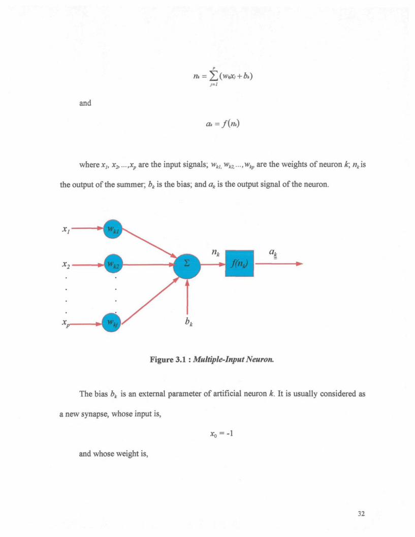
3=1
and
at = /(«*)
where x,, X2,...,xp are the input signals; wkJi wk2,...,w^ are the weights of neuron t, nki&
the output of the summer; bk is the bias; and ak is the output signal of the neuron.
a,
Figure 3.1 : Multiple-Input Neuron.
The bias bk is an external parameter of artificial neuron k. It is usually considered as
a new synapse, whose input is,
xo = -\
and whose weight is,
32
Note that w and b are both adjustable scalar parameters of the neurons. Typically, the
transfer function is chosen by the designer and then the parameters w and b will be adjusted
by some learning rule so that the neuron input/output relationship meets some specific goal.
3.1.3 Types of Activation Functions
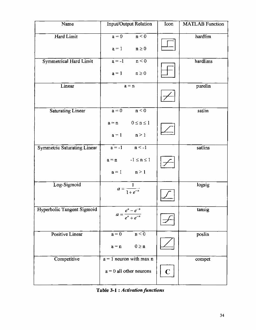
The activation function which defines the output of a neuron in terms of its net input
n, may be a linear or a nonlinear function of n. A particular transfer function is chosen to
satisfy some specification of the problem that the neuron is attempting to solve. Most of the
activation functions which are commonly used in artificial neural networks are illustrated
in Table 3.1.1.
33
Name
Hard Limit
Symmetrical Hard Limit
Linear
Saturating Linear
Symmetric Saturating Linear
Log-Sigmoid
Hyperbolic Tangent Sigmoid
Positive Linear
Competitive
Input/Output Relation
a=0 n<0
a=1 n>0
a = -l n<0
a= 1 n>0
a = n
a=0 n<0
a - n 0 < n < l
a = l n > l
a = -l n< - l
a = n - l < n < l
a = l n>1
1
e" - en
a ~ e" + e~"
a=0 n<0
a = n 0 >n
a = 1 neuron with max n
a = 0 all other neurons
Icon
JZ
zF
JL
/
c
MATLAB Function
hardlim
hardlims
purelin
satlin
satlins
logsig
tansig
poslin
compet
Table 3-1 : Activation functions
34
3.1.4 Learning
When an architecture is selected for a neural network, one may ask;" How do we
choose the connection weights and biases so that the network can do a specific task? "
We can teach the network to perform the desired task by iterative adjustments of the
weights and biases. This is one of the most interesting features of artificial neural networks;
it is the ability to learn from a set of inputs/outputs, or sometimes only a set of inputs, that
represents the behavior of a system or process in question. Learning is an adaptive process
that adjusts the weights and biases of neural networks in order to minimize a cost function.
Learning in the context of neural networks is defined as follows [Haykin S., 1994]:
Learning is a process by which the free parameters of a neural network are
adapted through a continuing process of stimulation by the environment in
which the network is embedded. The type of learning is determined by the
manner in which the parameter changes take place.
The neural networks have this advantage that it is not necessary to specify every
detail of a calculation and find the equations which can express the behavior of the system
or process. Instead, one simply has to compile a training set of representative examples.
This means that we can hope to treat problems where appropriate rules are very hard to
know it in advance. It may also save a lot of tedious and expensive software design and
35

programming even when we do have explicit rules. If there are no (or they are too difficult
to find) explicit rules, or the optimum algorithm for a particular problem, neural networks
are a powerful tool for the task.
There are many interesting methods for training a neural network to do a specific
task. In all of them, the main purpose is to adjust parameters of neural networks in order to
minimize a cost function. They fall into two broad categories: supervised learning and
unsupervised learning.
1. Supervised Learning : In supervised learning, the learning rule is provided with a
set of examples (the training set) of proper network behavior:
{xud,},{x2,d2}, ,{xq,dq},
where xq is an input to the network and dq is the corresponding target output. As
the inputs are applied to the network, the network outputs are compared to the
target outputs. The learning rule is then used to adjust the weights and biases of
the network in order to move the network outputs closer to the target outputs.
2. Unsupervised Learning : In unsupervised learning, the weights and biases are
modified in response to network inputs only. There are no target outputs available.
Most of these algorithms perform some kind of clustering operation. They learn to
categorize the input patterns into a finite number of classes. This is especially
useful in such applications as vector quantization.
36
One of the powerful supervised learning techniques is the back-propagation
algorithm.
3.1.4.1 Back-Propagation Learning
With introduction of back-propagation algorithm, many researchers and scientists
have become interested in this algorithm and have used it for training multi-layer feed-
forward neural networks. A multi-layer feed-forward neural network consists of several
layers.
The first layer is called input layer and receives inputs from environment and feeds
forward through layers. The last layer is the output layer, since its outputs are interesting
for us and they are the final outputs of neural network. There are often one or more layers
in between, which are called hidden layers since they do not have any communication with
the environment.
The basic idea is that if the network gives the wrong answer, the weights are
corrected so that the error is lessened and, as a result, future responses of the network are
more likely to be correct.
Back-propagation networks are composed of a number of interconnected layers; It
means that each layer is fully connected to the layers below and above. It typically starts
out with random weights and biases. When the network is given an input, the updating of
activation values propagates forward from the input layer through each hidden layer, to the
37

output layer. The output layer then provides the response of the network. After completion
of the feed forward pass, the learning mechanism starts with the output layer and
propagates backward through each internal unit to the input layer. That is why it is called
back-propagation algorithm. It overcomes the limitations of the perceptron, (perceptrons
can only classify patterns that are linearly separable), because it can adopt two or more
layers of weights, and each hidden layer acts as a layer of feature detectors. The power of
back-propagation lies in its ability to train hidden layers and thereby escape the restricted
capabilities of single layer networks.
The back-propagation learning rule can be used to adjust the weights and biases of a
network in order to minimize the sum-squared error of the network. This is done by
continually changing the values of the network weights and biases in the direction of
steepest descent with respect to error. Suppose that in a multi-layer feed-forward neural
network, neuron j lies in a layer to the right of neuron / , and neuron k lies in a layer to the
right of neuron j when neuron y is in a hidden layer. Then the back-propagation algorithm
can be expressed in mathematical form as follows:
off) =^<Wj
E(t) = Vi S <
dwJt)
38

By using the chain rule, the partial derivative can be expressed in terms of two
factors, one expressing the rate of change of error with respect to the output ap and the
other expressing the rate of change of the output of the neuron y with respect to the input to
the same neuron. Finally, the correction AwJt(t) applied to Wj,{t) is expressed by:
where
jj = weight correction;
TÏ = learning rate parameter;
5/0 = local gradient;
a{(t) - input signal of neuron j .
For calculating of 5/0, two cases are distinguished:
�If neuron j is an output node, 5/0 equals the product of the derivative of
/(w/0) and the error signal eft), both of which are associated with neuron/
ô/0=/'(«/0) * eft)
39

�If neuron j is a hidden node, Sj(O equals the product of the associated
derivative of fipft)) and the weighted sum of the Ô's computed for the
neurons in the next hidden or output layer that are connected to neuron j .
40
SECTION TWO
3.2.1 What is Fuzzy Logic ?
Humans, when making decisions, tend to work with vague or imprecise concepts
which can often be expressed linguistically. Prof. Lotfi A. Zadeh proposed an approach for
modeling of this decision making process [Zadeh, 1965], and is based on the theory of
approximate reasoning which enables certain classes of linguistic statement to be treated
mathematically. First, investigations by Prof. Zadeh concerned how to use mathematical
tools to represent human language and knowledge [Zadeh, 1973]. He was the first who
introduced the terms of fuzzy rules and linguistic variables in control theory. In a paper
[Zadeh, 1972], he claims that fuzzy algorithms underlie much of human thinking. We use
them both consciously and unconsciously when we talk, park a car, recognize patterns.
This use is more intuitive and qualitative than systematic and quantitative. Moreover,
Zadeh believes that the modern control theory must become less preoccupied with
mathematical rigor and precision, and more concerned with the development of qualitative
or approximate solutions to pressing real world problems. In short, he proposed that all
problems in which the data, the objectives and the constraints are too complex, or too ill-
defined to admit a precise mathematical analysis, have to be treated by approximate (fuzzy)
solutions. This new approach is receiving more and more attention, not only in research,
but also in industrial applications.
41
Fuzzy controllers were developed to imitate the performance of human expert
operators by encoding their knowledge in the form of linguistic rules [Mamdani, 1975].
They provide a complementary alternative to the conventional analytical control
methodology. Some authors argue that fuzzy controllers are suitable where a precise
mathematical model of the process being controlled is not available [Kickert W. J. M. &
Mamdani E. H., 1978] [Li Y. F.& Lau C. C, 1988].
3.2.2 Basic Notions of Fuzzy Logic
In this part, fundamental terms and concepts of fuzzy logic are briefly defined.
3.2.2.1 Fuzzy Set
A general definition of a set can be stated as follows [Kaufmann, 1988]:
"A set is a collection of objects distinct and perfectly specified "
A subset is a subgroup of a set. For example, let A to be a finite referential set:
A = {a, b, c,d, e,f)
We can form a crisp subset of A, for example:
B={b,d,f}
42

In the classical set theory, one element can either belong to a set, or not. This
property can be represented by a degree of membership. This concept is basic in the
classical set theory. However, the main concept of fuzzy theory is a notion of fuzzy set.
Fuzzy set is an extension of crisp set. Zadeh gave the following definition [Zadeh, 1965]:
A fuzzy set is a class of objects with a continuum of grades ojmembership. Such a set
is characterized by a membership (characteristic) junction which assigns to each object a
grade of membership ranging between zero and one.
After him, many authors found different ways of denoting fuzzy sets. Zimmermann
[Zimmerman, 1990] writes:
A fuzzy set is denoted by an ordered set of pairs, the jirst element of which denotes
the element (x) and the second (\xB (x)) the degree of membership:
B={(x,[iB(x))\ xeX}
where uB takes values in the interval [0, / ] .
Fuzzy sets can be regarded as a generalization of the concept of the classical (crisp)
sets whose membership function only requires two values {0,1}. However, it should be
mentioned that a classical set always has a unique membership function, whereas every
fuzzy set has an infinite number of membership functions that can represent it [Bezdek,
1993].
43
3.2.2.2 Linguistic Variable
Fuzzy sets can be used to represent linguistic variables. Linguistic variables are the
process states and control variables in a fuzzy controller. Their values are defined in
linguistic terms. They can be words or sentences in a natural language. For example, for
the linguistic variable "height ", a set of terms can be defined:
H (height) = {tall, medium, short}.
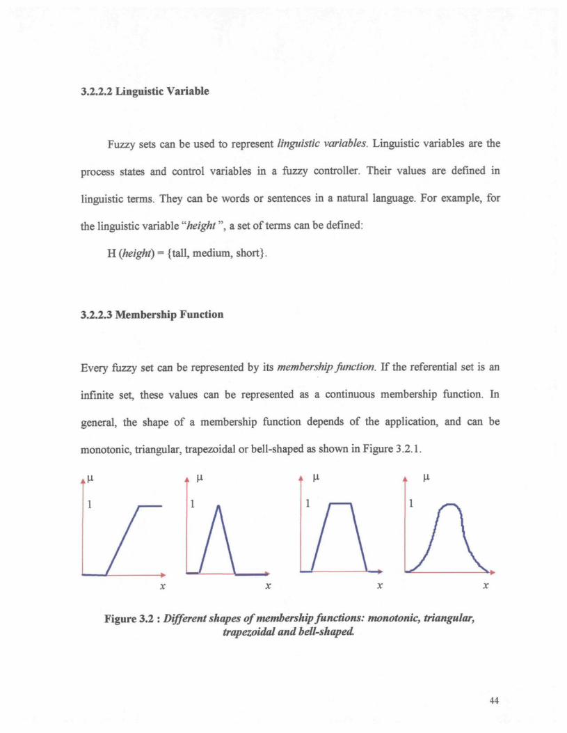
3.2.2.3 Membership Function
Every fuzzy set can be represented by its membership fonction. If the referential set is an
infinite set, these values can be represented as a continuous membership function. In
general, the shape of a membership function depends of the application, and can be
monotonie, triangular, trapezoidal or bell-shaped as shown in Figure 3.2.1.
Figure 3.2 : Different shapes of membership functions: monotonie, triangular,trapezoidal and bell-shaped.
44
3.2.3 Operations on Fuzzy Sets
As operations are defined on classical sets, similar operations are defined on fuzzy
sets. However, due to the fact that membership values are no longer restricted to {0,1}, and
can have any value in the interval [0,1], these operators cannot be uniquely defined. Fuzzy
set theory offers a vast range of operations that do not exist in the classical theory [Zadeh,
1965].
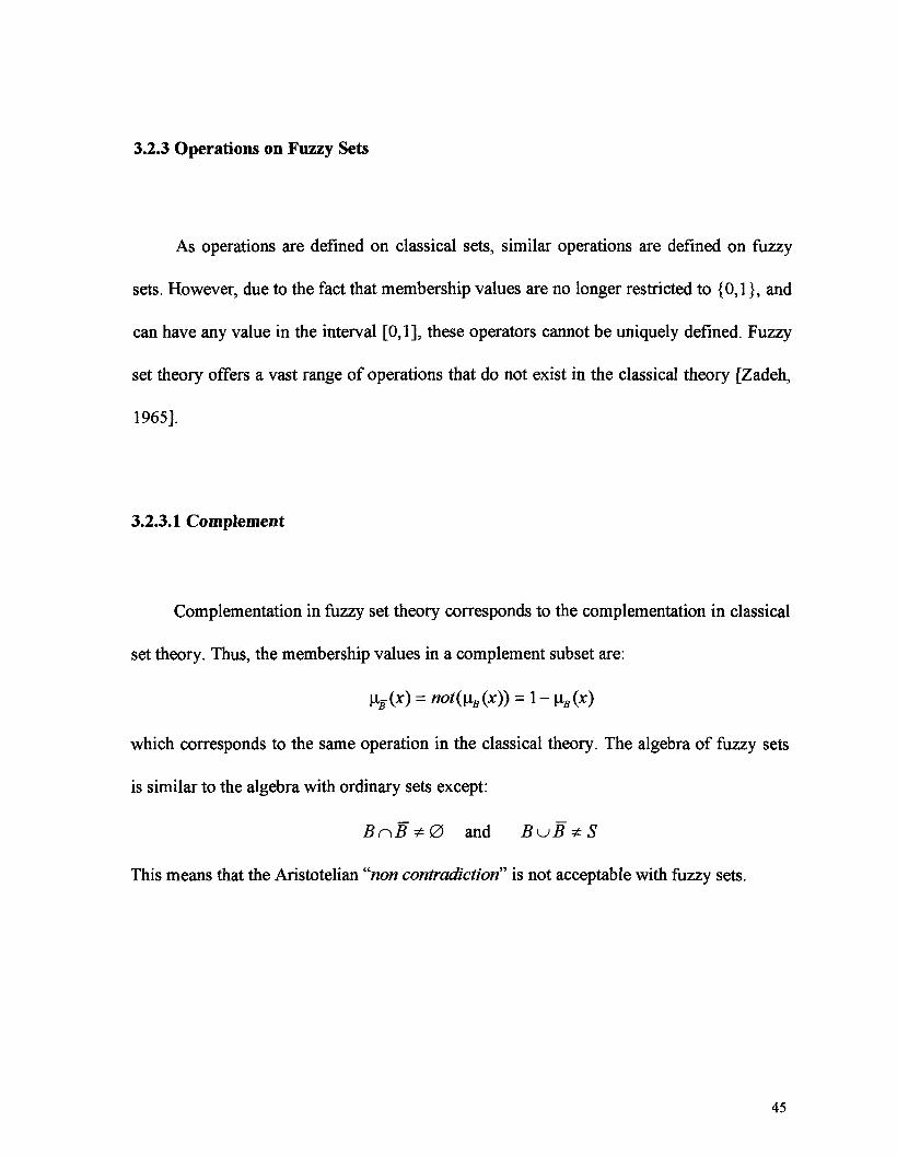
3.2.3.1 Complement
Complementation in fuzzy set theory corresponds to the complementation in classical
set theory. Thus, the membership values in a complement subset are:
hr (*) = not(iiB(x)) = 1 - \xB(x)
which corresponds to the same operation in the classical theory. The algebra of fuzzy sets
is similar to the algebra with ordinary sets except:
Br^B*0 and BVJB*S
This means that the Aristotelian "non contradiction" is not acceptable with fuzzy sets.
45
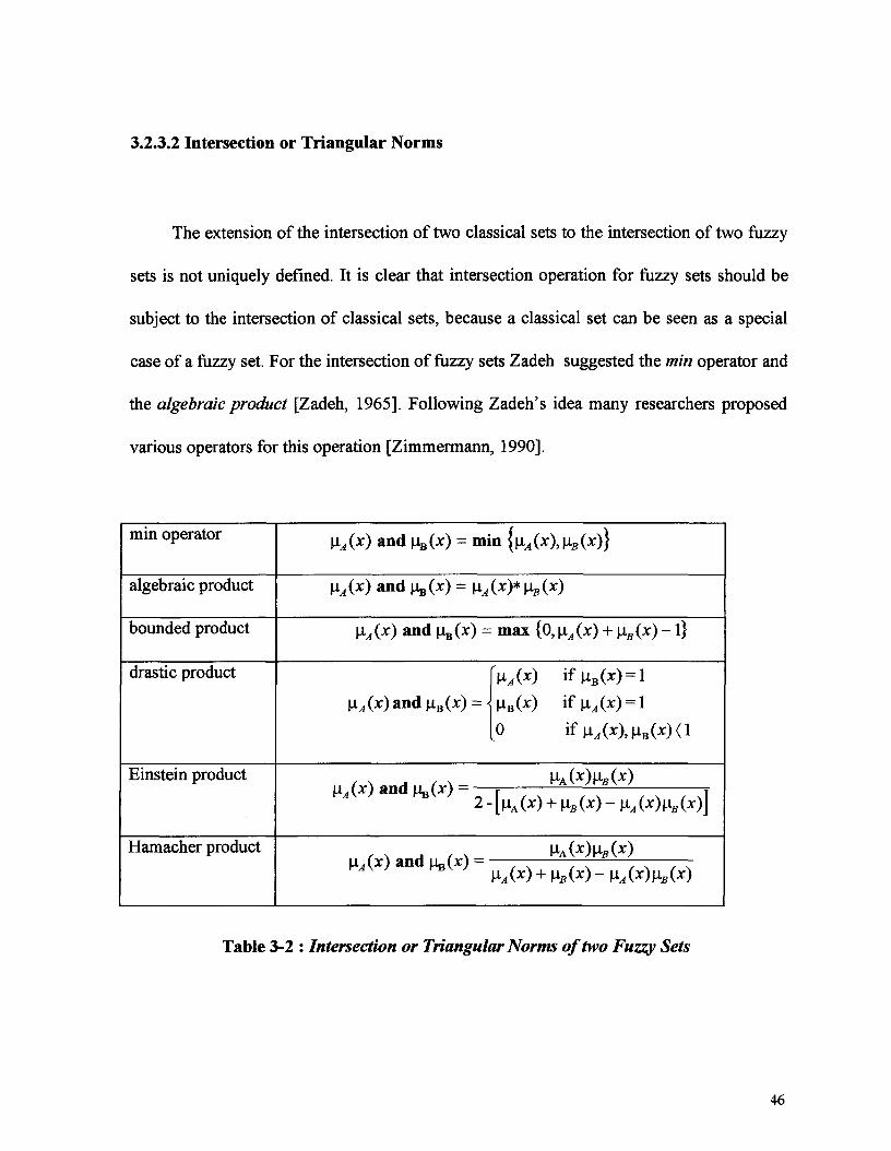
3.2.3.2 Intersection or Triangular Norms
The extension of the intersection of two classical sets to the intersection of two fuzzy
sets is not uniquely defined. It is clear that intersection operation for fuzzy sets should be
subject to the intersection of classical sets, because a classical set can be seen as a special
case of a fuzzy set. For the intersection of fuzzy sets Zadeh suggested the min operator and
the algebraic product [Zadeh, 1965]. Following Zadeh's idea many researchers proposed
various operators for this operation [Zimmermann, 1990].
min operator
algebraic product
bounded product
drastic product
Einstein product
Harnacher product
u^(x) and MBO) = min {[iA(x),[iB(x)}
\iA(x) and UB(X) = u^(x)*Ug(x)
\LA(X) and MB(X) = max (0,u^(x) + nB(x) -1}
\iA(x)andiLB(x) = -
0 if^(x),nB(x)<l
U J ( X ) <H1Q U D ( X ) r i2-[HA(X) + MX)-MX)M B (* ) ]
\iA(x) and \ivix) -\iA(x)\xB(x)
VA(X) + VB(X)~ M*(*)MB(*)
Table 3-2 : Intersection or Triangular Norms of two Fuzzy Sets
46
Let A and B be two fuzzy sets in U, the universe of discourse, with membership
functions \iA and \xB respectively. The most important intersection operators are listed in
Table 3.2.1.
All these operators belong to the so-called triangular norms (T-norms). Functions T
define a general class of intersection operators for fuzzy sets and can be parametric or non-
parametric.
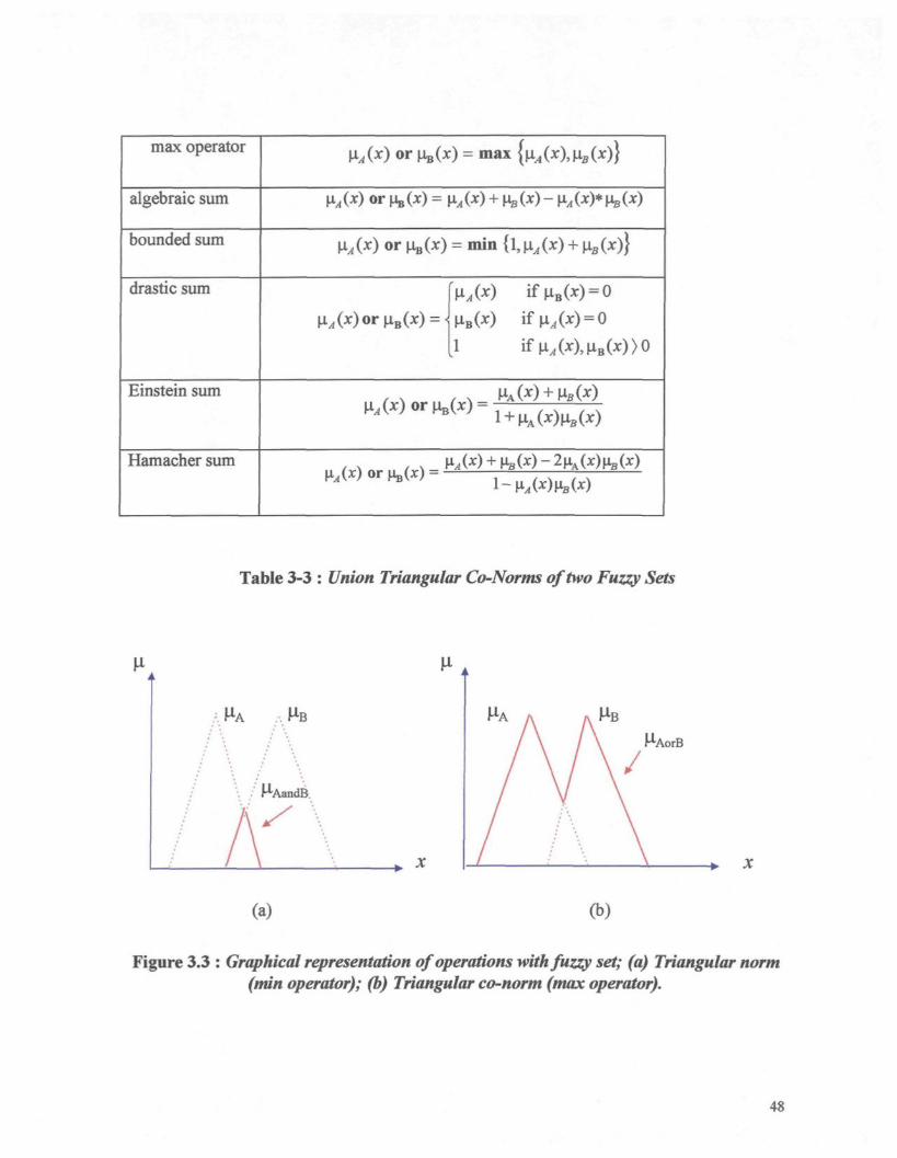
3.2.3.3 Union Triangular Co-Norms
For the union of two fuzzy sets, there is a class of operators named triangular
co-norms (T-conorms or S-norms). The most used union operators in the literature are
listed in Table 3.2.2.
Suppose that we define two fuzzy sets by their membership functions \xA and \iB
which have triangular membership functions (dotted lines on Figure 3.2.2.a). The
application of T-norm (in this example, the operator is miri) gives the fuzzy set "A and B"
which is represented by its membership function iAandB(x) (solid line on Figure 3.2.2.a).
The application of T-conorm (here max operator) on these fuzzy sets gives the fuzzy set
represented with solid line as shown in Figure 3.2.2.b.
47
max operator
algebraic sum
bounded sum
drastic sum
Einstein sum
Harnacher sum
HA(x) or mO) = max {MVI(*),M*)}
Ma(*) <W MB<*) ^ Rj(*> + MB(*) - M« 0 0 * MB (*)
\iA(x) or B(x) = min {l,^(x) +^(x)}
u.^(x)oru-B0:) = <V^x) ifM*) = 0^B(x) ifji^(x) = O
1 if^(x),^B(x))0
, v ^ W + feWW l + A(x)^(x)
OO + hrW-^OOM*)
Table 3-3 : Union Triangular Co-Norms of two Fuzzy Sets
, MB
M-AandB,
MAorB
(a) (b)
Figure 3.3 : Graphical representation of operations with fuzzy set; (a) Triangular norm(min operator); (b) Triangular co-norm (max operator).
48
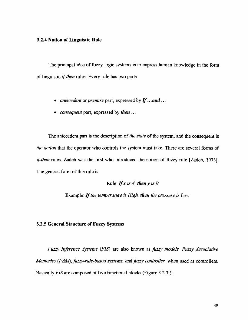
3.2.4 Notion of Linguistic Rule
The principal idea of fuzzy logic systems is to express human knowledge in the form
of linguistic if-then rules. Every rule has two parts:
� antecedent or premise part, expressed by If... and...
� consequent part, expressed by then ...
The antecedent part is the description of the state of the system, and the consequent is
the action that the operator who controls the system must take. There are several forms of
if-then rules. Zadeh was the first who introduced the notion of fuzzy rule [Zadeh, 1973].
The general form of this rule is:
Rule: Ifx is A, then y is B.
Example: If the temperature is High, then the pressure is Low
3.2.5 General Structure of Fuzzy Systems
Fuzzy Inference Systems (FIS) are also known as fuzzy models, Fuzzy Associative
Memories (FAM), fuzzy-rule-based systems, and fuzzy controller, when used as controllers.
Basically FIS are composed of five functional blocks (Figure 3.2.3.):
49

1. Rule base: containing a number of fuzzy if-then rules;
2. Database: defines the membership functions of the fuzzy sets and their
parameters used in the fuzzy rules. Usually, the rule base and the database are
jointly referred to as the knowledge base,
3. Decision-making unit: performs the inference operations on the rules;
4. Fuzzification interface: transforms the crisp inputs into a degree of match with
linguistic variables
5. Defuzzification interface: transforms the fuzzy results into a crisp output
Input
(crisp)fuzzification
interface
(fuzzy)
Knowledge base
data base rule base
decision-making unit
defuzzificationinterface
: Output
(crisp)
{fuzzy)
Figure 3.4 : Fuzzy Inference System
50
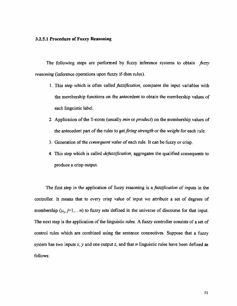
3.2.5.1 Procedure of Fuzzy Reasoning
The following steps are performed by fuzzy inference systems to obtain fuzzy
reasoning (inference operations upon fuzzy if-then rules).
1. This step which is often called fuzzification, compares the input variables with
the membership functions on the antecedent to obtain the membership values of
each linguistic label.
2. Application of the T-norm (usually min or product) on the membership values of
the antecedent part of the rules to get firing strength or the weight for each rule.
3. Generation of the consequent value of each rule. It can be fuzzy or crisp.
4. This step which is called defuzzification, aggregates the qualified consequents to
produce a crisp output.
The first step in the application of fuzzy reasoning is a fuzzification of inputs in the
controller. It means that to every crisp value of input we attribute a set of degrees of
membership (\ii,j=l,...ri) to fuzzy sets defined in the universe of discourse for that input.
The next step is the application of the linguistic rules. A fuzzy controller consists of a set of
control rules which are combined using the sentence connectives. Suppose that a fuzzy
system has two inputs x, y and one output z, and that n linguistic rules have been defined as
follows:
51
If x is A, and y is B, then z is C,
If x is A2 and y is B2 then z is C2
Ifx is 4n and y is #� f/ren z is Cn
where x, y and z are linguistic variables representing the process state variables and the
control variable; Ah B{ and C{ (/' = 1,...«) are fuzzy sets defined in the universe of discourse
for x, y and z respectively.
In mathematical sense, activation of the rules is the application of T-norm [Lee,
1990], in order to get a firing strength for every rule. Usually, it means that the operator
min or product is applied on membership values. It is denoted here by wt:
Consequently, the firing strengths are combined using the compositional operator,
which expresses the sentence connective, and the consequent value (fuzzy or crisp) is
generated.
Finally, defuzzification is performed in order to get crisp output. Figure 3.2.4. shows
the fuzzy system.
52
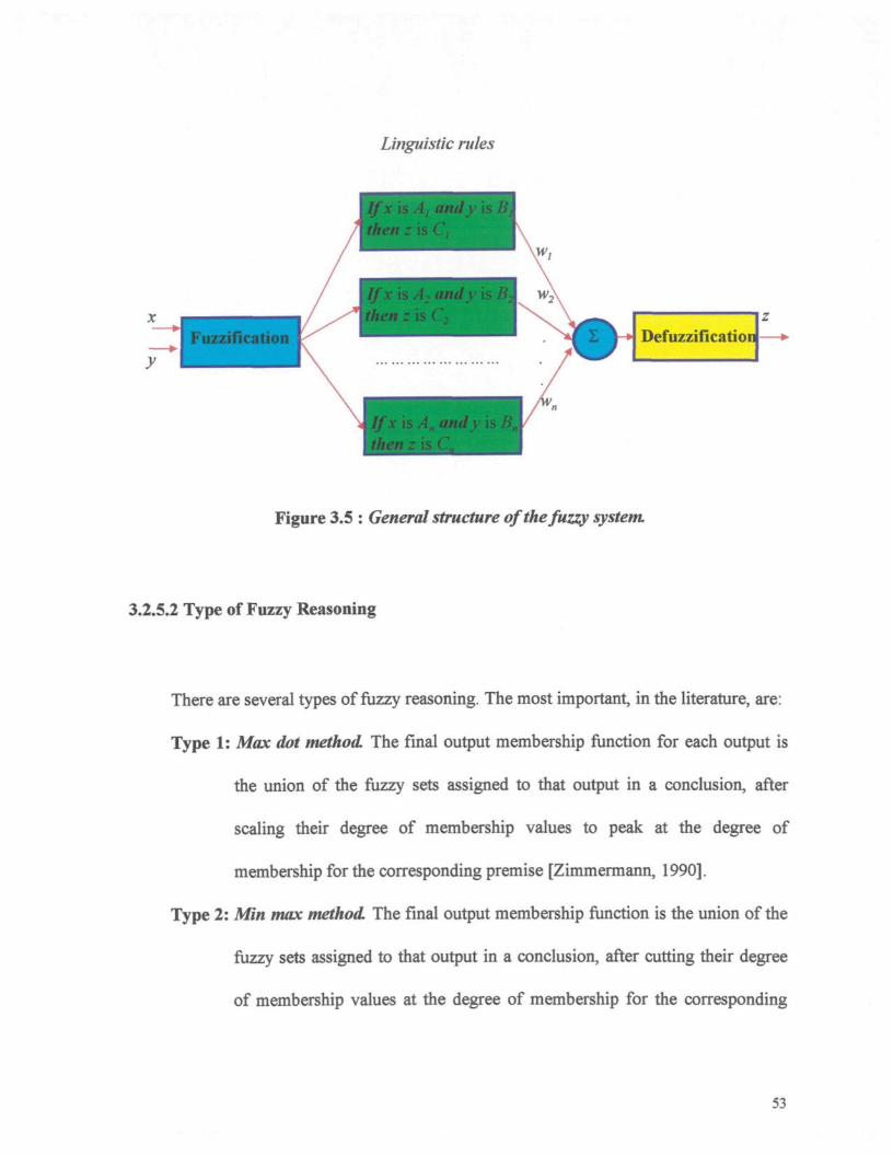
Linguistic rules
Defuzzification
If x is An and y'hen z is Cn
Figure 3.5 : General structure of the fuzzy system.
3.2,5.2 Type of Fuzzy Reasoning
There are several types of fuzzy reasoning. The most important, in the literature, are:
Type 1: Max dot method. The final output membership function for each output is
the union of the fuzzy sets assigned to that output in a conclusion, after
scaling their degree of membership values to peak at the degree of
membership for the corresponding premise [Zimmermann, 1990],
Type 2: Min max method The final output membership function is the union of the
fuzzy sets assigned to that output in a conclusion, after cutting their degree
of membership values at the degree of membership for the corresponding
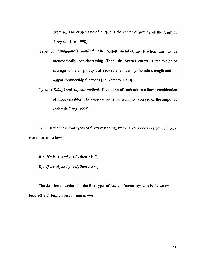
premise. The crisp value of output is the center of gravity of the resulting
fuzzy set [Lee, 1990].
Type 3: Tsukamoto's method The output membership function has to be
monotonically non-decreasing. Then, the overall output is the weighted
average of the crisp output of each rule induced by the rule strength and the
output membership functions [Tsukamoto, 1979].
Type 4: Takagi and Sugeno method. The output of each rule is a linear combination
of input variables. The crisp output is the weighted average of the output of
each rule [Jang, 1993].
To illustrate these four types of fuzzy reasoning, we will consider a system with only
two rules, as follows;
R^ If x is Aj and y is Bt then z is C,
R2: If x is A2 and y is B2 then z is C2
The decision procedure for the four types of fuzzy inference systems is shown on
Figure 3.2.5. Fuzzy operator and is min.
54
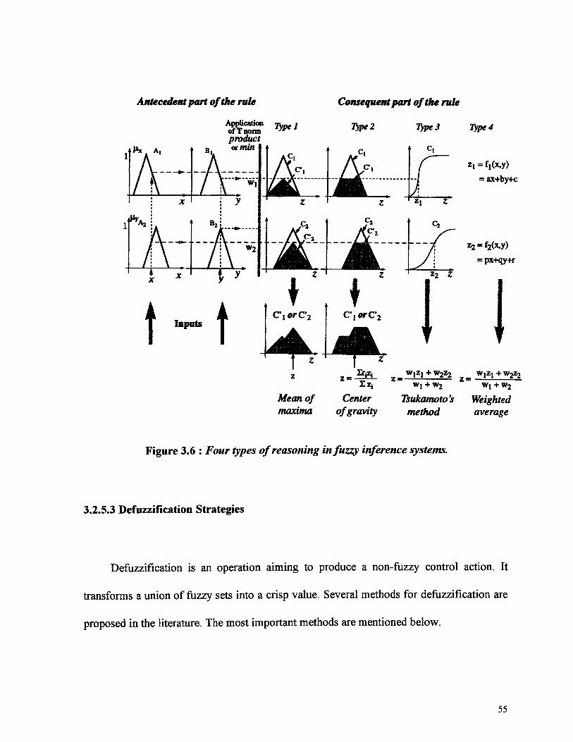
Antecedent part of the rule
Applicationof T normproduct
Consequent part of the rule
Type* Vfpe3 Type4
= f,(x,y)= ax+by+c
= px+qy+r
Mean of Center Tsukamoto's Weightedmaxima of gravity method average
Figure 3.6 : Four types of reasoning in fuzzy inference systems.
3.2.5.3 Defuzzification Strategies
Defuzzification is an operation aiming to produce a non-fuzzy control action. It
transforms a union of fuzzy sets into a crisp value. Several methods for defuzzification are
proposed in the literature. The most important methods are mentioned below.
55
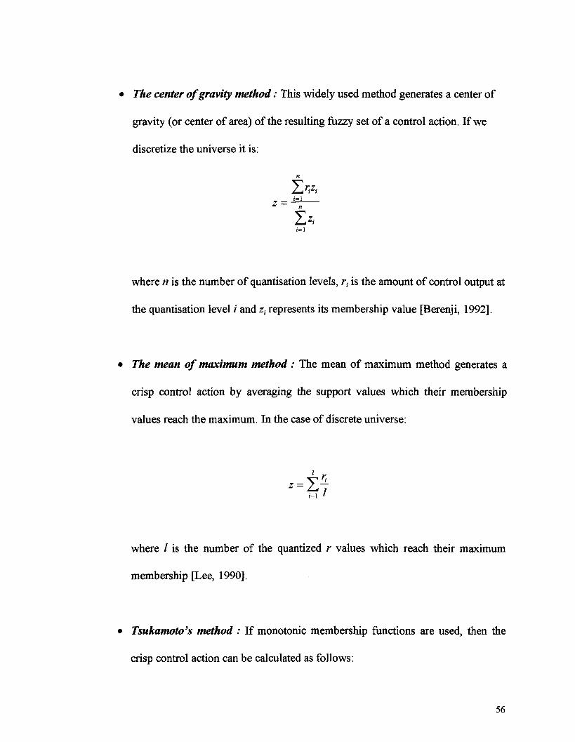
The center of gravity method : This widely used method generates a center of
gravity (or center of area) of the resulting fuzzy set of a control action. If we
discretize the universe it is:
where n is the number of quantisation levels, r, is the amount of control output at
the quantisation level / and zt represents its membership value [Berenji, 1992].
The mean of maximum method : The mean of maximum method generates a
crisp control action by averaging the support values which their membership
values reach the maximum. In the case of discrete universe:
z � 7 �
where / is the number of the quantized r values which reach their maximum
membership [Lee, 1990].
Tsukamoto's method : If monotonie membership functions are used, then the
crisp control action can be calculated as follows:
56

r -Z - n
V
� The weighted average method : This method is used when the fuzzy control rules are
the functions of their inputs [Takagi, 1983] as shown in the Figure 3.2.5 for type 4. In
general, the consequent part of the rule is:
If w, is the firing strength of the ith rule, then the crisp value is given by:
where n is the number of firing rules.
57
SECTION THREE
3.3.1 What are Neuro-Fuzzy Systems ?
In the design of a conventional fuzzy system, the user must tune by trial-and-error the
membership functions of fuzzy sets defined in the input and output universes of discourse.
This drawback is eliminated with neuro-fuzzy systems [Jang J.-S. R. & Sun C. T., 1995]
[Wang L. X., 1994] which combine the advantages of neural networks and fuzzy systems.
By employing supervised learning methods, it is now possible to optimize both the
antecedent and consequent parts of a linguistic rule-base fuzzy system.
This section introduces neuro-fuzzy systems which combine the properties of neural
networks and fuzzy systems. First, the background and the taxonomy of neuro-fuzzy
systems are presented. After, the interest is focused on knowledge structure, network
architecture and learning algorithm.
3.3.2 Background of Neuro-Fuzzy Systems
In the previous sections, neural networks and fuzzy logic systems were presented. It
was noted that neural networks have two main benefits. First, they are capable of learning
non-linear mapping of numerical data. Second, they perform parallel computation.
However, the operation of neural networks have also many weaknesses. For example, in
58
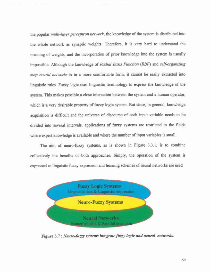
the popular multi-layer perceptron network, the knowledge of the system is distributed into
the whole network as synaptic weights. Therefore, it is very hard to understand the
meaning of weights, and the incorporation of prior knowledge into the system is usually
impossible. Although the knowledge of Radial Basis Function (RBF) and self-organizing
map neural networks is in a more comfortable form, it cannot be easily extracted into
linguistic rules. Fuzzy logic uses linguistic terminology to express the knowledge of the
system. This makes possible a close interaction between the system and a human operator,
which is a very desirable property of fuzzy logic system. But since, in general, knowledge
acquisition is difficult and the universe of discourse of each input variable needs to be
divided into several intervals, applications of fuzzy systems are restricted to the fields
where expert knowledge is available and where the number of input variables is small.
The aim of neuro-fuzzy systems, as is shown in Figure 3.3.1, is to combine
collectively the benefits of both approaches. Simply, the operation of the system is
expressed as linguistic fuzzy expression and learning schemes of neural networks are used
iizzy Logic SystemsLinguistic data & Linguistic expression
Neuro-Fuzzy Systems
Neural Networksmerical data & Parallel operatic
Figure 3.7 : Neuro-fuzzy systems integrate fuzzy logic and neural networks.
59
to train the system. In addition, neuro-fuzzy systems allow incorporation of both numerical
and linguistic data into the system. The neuro-fuzzy system is also capable of extracting
fuzzy knowledge from numerical data, which is an important property [Abe & Lan, 1995].
The neuro-fuzzy systems can be divided into two main groups:
1. Neural fuzzy inference systems
2. Fuzzy neural networks
The origin idea of neural fuzzy inference systems is to incorporate neural concepts,
such as learning and parallelism, into fuzzy logic inference systems (fuzzy controllers, in
the context of control applications). Neural fuzzy inference systems realize fuzzy inference
[Berenji, 1992] [Halgamuga & denser, 1994] [Jang, 1993]. The architecture of the
systems are parallel, and they exploit the same learning algorithms, as used with neural
networks.
In fuzzy neural networks [Gupta & Rao, 1994] [Pal & Mitra, 1992] [Pedrycz, 1992],
the fuzzy ideas are incorporated into neural networks. Lee and Lee [Lee & Lee, 1975] are
the first who worked on neuro-fuzzy systems, especially on fuzzy neural networks. Their
approach replaced the weighted sum of the McCulloch-Pitts neuron by a corresponding
fuzzy operation. The operation of their neuro-fuzzy system was exactly the same as the
McCulloch-Pitts neural network. Unfortunately, they did not provide any training rule for
the network.
60
In this research, we are interested in neural fuzzy inference systems, which will be
described in greater detail below. Then, a specific type of neuro-fuzzy systems called
ANFIS, will be introduced.
3.3.3 Neural Fuzzy Inference Systems
The basic idea in neural fuzzy inference systems is to incorporate parallel architecture
and learning capability to fuzzy inference systems. These systems are implemented as
multi-layer networks [Jang, 1993], and they were trained using a hybrid learning algorithm
which consists of the gradient descent and least squares estimate methods. Moreover, close
functional similarities between fuzzy inference systems and RBF networks were also
noticed [Jang, 1993] [Nie & Linkens, 1993] [Wang & Mendel, 1992]. In the following
sections, knowledge structures and learning schemes of neural fuzzy inference systems are
presented.
3.3.3.1 Knowledge Structure and Linguistic Variables
Fuzzy rules are the fundamental part of the knowledge base in a fuzzy inference
system. These rules define behavior of a system or process. In practice, there are three
typical forms of fuzzy rules used in neuro-fuzzy systems.
61
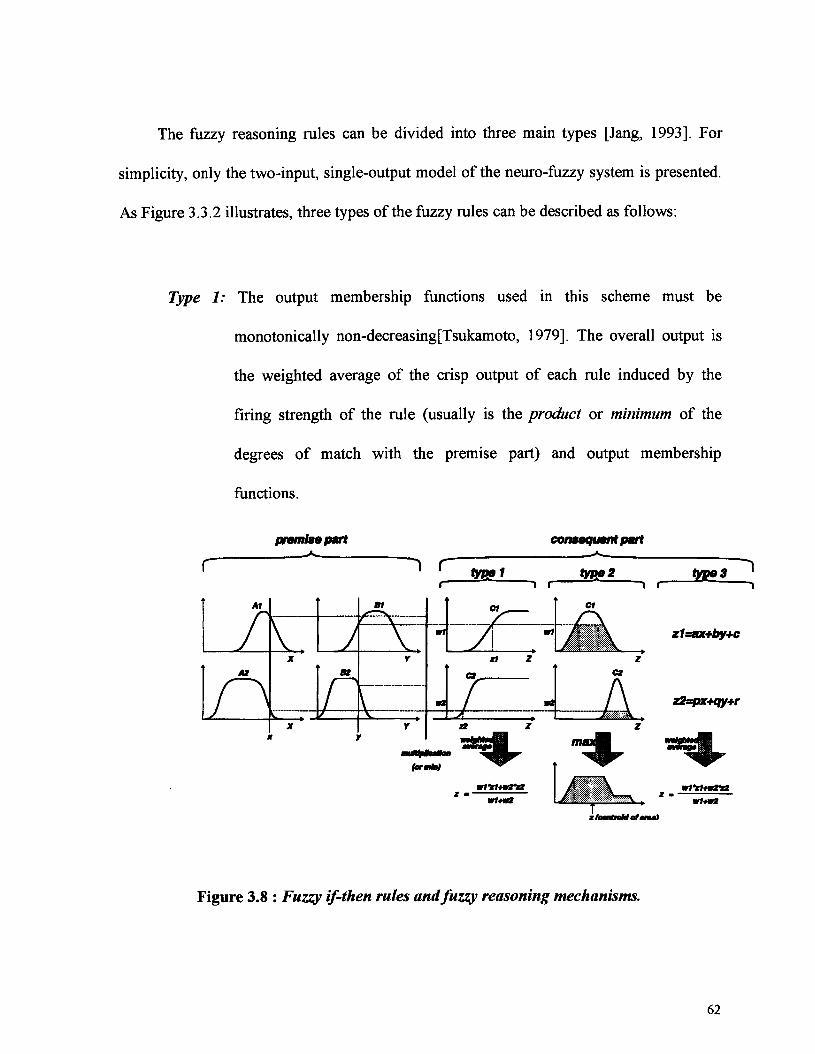
The fuzzy reasoning rules can be divided into three main types [Jang, 1993]. For
simplicity, only the two-input, single-output model of the neuro-fuzzy system is presented.
As Figure 3.3.2 illustrates, three types of the fuzzy rules can be described as follows:
Type 1: The output membership functions used in this scheme must be
monotonically non-decreasing[Tsukamoto, 1979]. The overall output is
the weighted average of the crisp output of each rule induced by the
firing strength of the rule (usually is the product or minimum of the
degrees of match with the premise part) and output membership
functions.
premise part consequent part
typei type 2 types
CI
=ax+by+c
z2=px+qy+r
Figure 3.8 : Fuzzy if-then rules and fuzzy reasoning mechanisms.
62
Type 2: The overall fuzzy output is derived by applying "max" operation to the
qualified fuzzy outputs (each of which is equal to the minimum of firing
strength and the output membership function of each rule). Various
schemes have been proposed to choose the final crisp output based on the
overall fuzzy output; some of them are center of area, bisector of area,
mean of maxima, maximum criterion, etc. [Lee (1), 1990] [Lee (2), 1990].
Type 3: Takagi and Sugeno's fuzzy if-then rules are used [Takagi & Sugeno,1983,
1985]. The output of each rule is a linear combination of input variables
plus a constant term, and the final output is the weighted average of the
output of each rule.
3.3.3.2 Network Architecture
The fuzzy logic inference system can be considered as a five-layer artificial neural
network, as shown in Figure 3.3.3. This type of architecture is the most popular among
neural fuzzy inference systems. Since we have used ANFIS, which stands for Adaptive-
Network-based Fuzzy Inference System, in this research, the architecture of ANFIS is
explained. For simplicity, the fuzzy inference system which has only two inputs x and y
and one output z is considered. It should be noted that the third type of fuzzy rule is used.
In addition, suppose that the rule base comprises only two fuzzy rules of Takagi and
Sugeno's type:
63
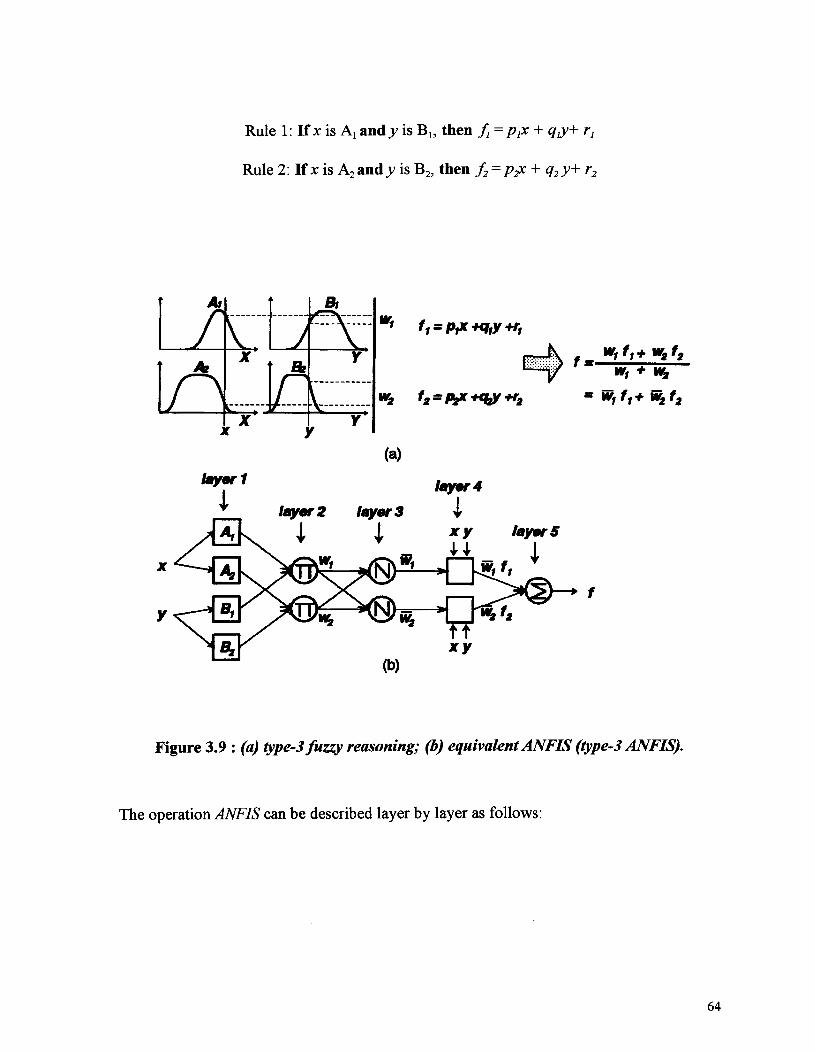
Rule 1: If x is A, and^ is Bl5 then / , = p,x + q,y+ rt
Rule 2: If x is A2andy is B2, then f2 = Pi£ + q2y+ r2
Bi
layer 1(a)
layer 2 layer 31 i
Iayw4
xy layer 5
i
Figure 3.9 : (a) type-3 fuzzy reasoning; (b) equivalent ANFIS (type-3 ANFIS).
The operation ANFIS can be described layer by layer as follows:
64
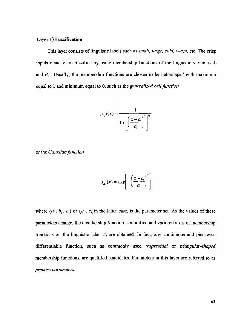
Layer 1) Fuzzification
This layer consists of linguistic labels such as small, large, cold, warm, etc. The crisp
inputs x and y are fuzzified by using membership functions of the linguistic variables A,
and Bt . Usually, the membership functions are chosen to be bell-shaped with maximum
equal to 1 and minimum equal to 0, such as the generalized bell function
»"(*) =
1 + x-c;
a;
or the Gaussian function
(x) = exp x-c:
a.
where {a,, bt, c,} or {a,, c;}in the latter case, is the parameter set. As the values of these
parameters change, the membership function is modified and various forms of membership
functions on the linguistic label At are obtained. In fact, any continuous and piecewise
differentiable function, such as commonly used trapezoidal or triangular-shaped
membership functions, are qualified candidates. Parameters in this layer are referred to as
premise parameters.
65
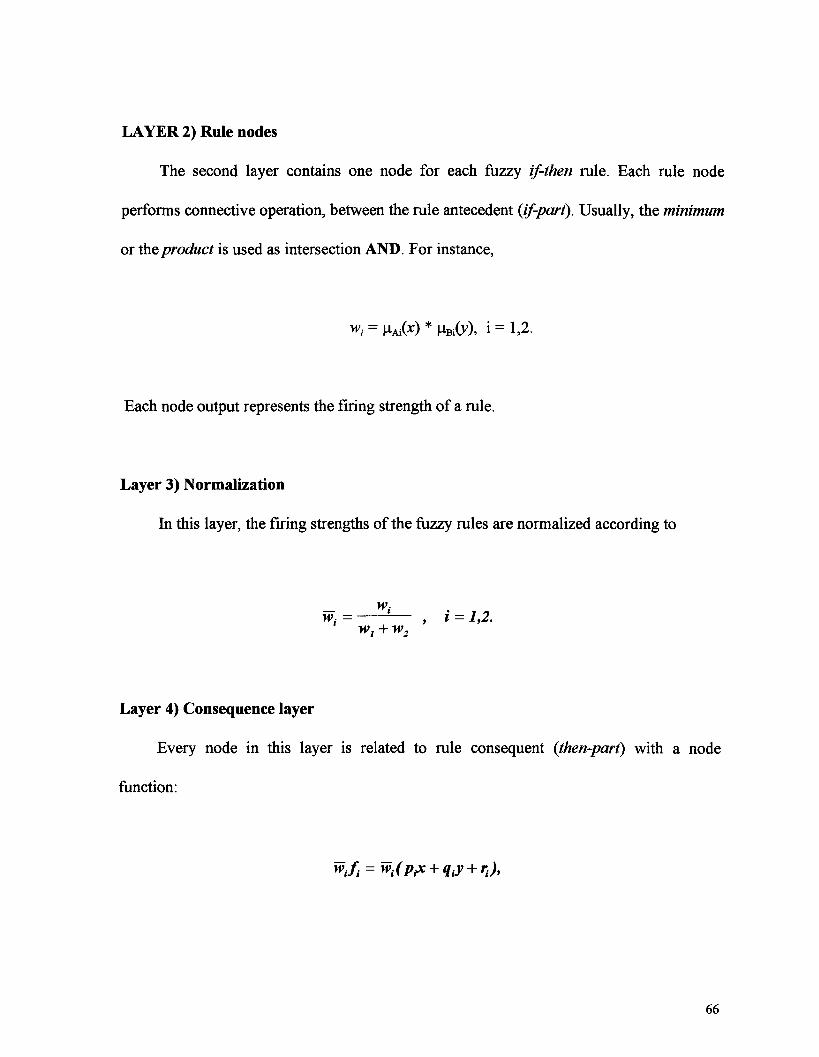
LAYER 2) Rule nodes
The second layer contains one node for each fuzzy if-then rule. Each rule node
performs connective operation, between the rule antecedent {if-part). Usually, the minimum
or the product is used as intersection AND. For instance,
w* = \ijjx) * MKGO» i = 1,2.
Each node output represents the firing strength of a rule.
Layer 3) Normalization
In this layer, the firing strengths of the fuzzy rules are normalized according to
w.
Layer 4) Consequence layer
Every node in this layer is related to rule consequent (then-part) with a node
function:
66
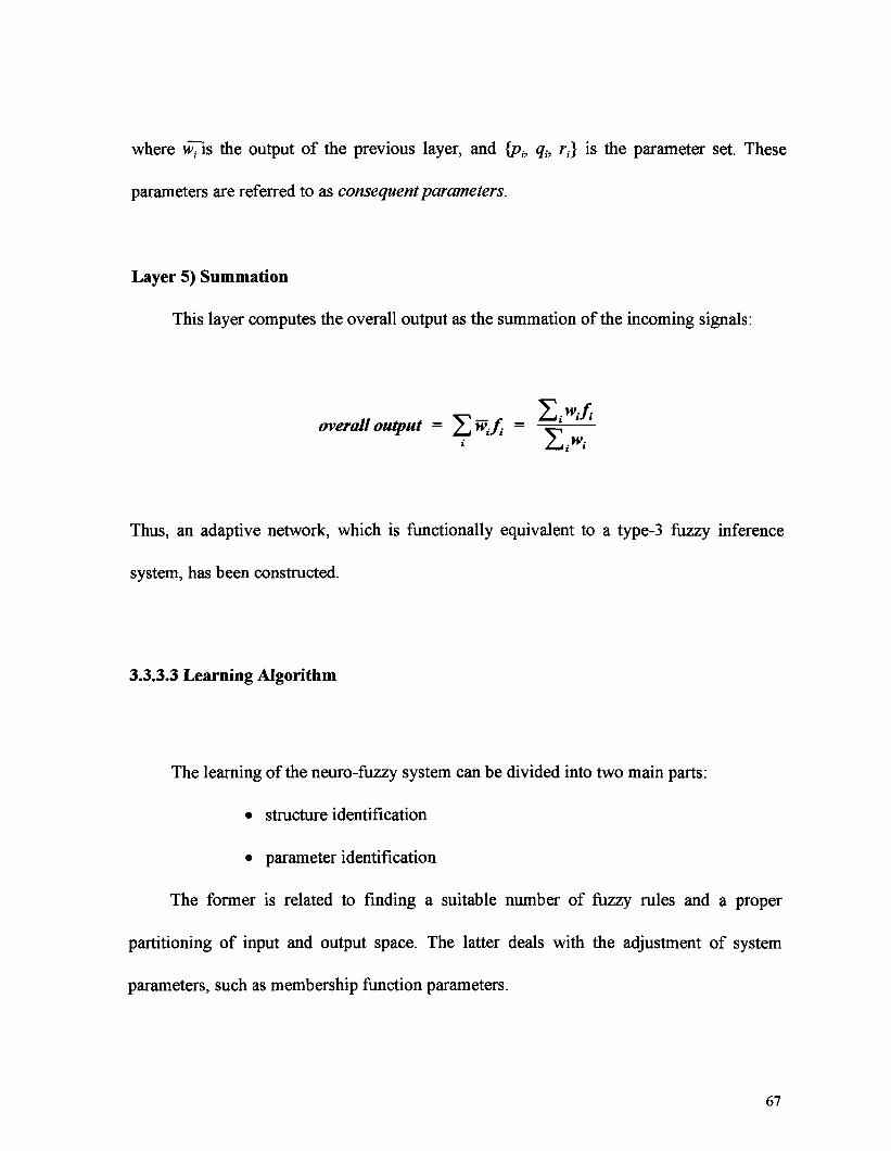
where w, is the output of the previous layer, and {pfo qh r,} is the parameter set. These
parameters are referred to as consequent parameters.
Layer 5) Summation
This layer computes the overall output as the summation of the incoming signals:
overall output = ^ / * = ^
Thus, an adaptive network, which is functionally equivalent to a type-3 fuzzy inference
system, has been constructed.
3.3.3.3 Learning Algorithm
The learning of the neuro-fuzzy system can be divided into two main parts:
� structure identification
� parameter identification
The former is related to finding a suitable number of fuzzy rules and a proper
partitioning of input and output space. The latter deals with the adjustment of system
parameters, such as membership function parameters.
67

There are several learning algorithms for neuro-fuzzy systems. Jang [Jang, 1993]
proposed a learning scheme, called hybrid learning algorithm, which is a combination of
the least-squares estimate (LSE) and the gradient descent for tuning the ANFIS
architecture. The system is initialized with a number of membership functions and a fixed
rule base. The learning scheme consists of two separate passes. In the forward pass, input
signals go forward until they reach to the output layer, and the consequent parameters are
identified by the LSE. In the backward pass, the error rates propagate backward and the
premise parameters are updated by the gradient descent.
68

Chapter 4
Neuro-Fuzzy Models
4.1 Introduction
In this chapter, two neuro-fuzzy models for a non-linear three-phase power
transformer are developed. First, their structures and architectures are explained. After
determination of the architecture, the models should be trained by a set of inputs/outputs.
To acquire the dynamic behavior of a system, a set of inputs/outputs which includes
sufficient dynamic behavior of a system should be presented to the neuro-fuzzy models.
This set of inputs/outputs data is called training data. The generalization of the dynamic
behavior of a system depends on the training data. This means that by increasing the
amount of information in the training data files, a neuro-fuzzy system learns more about a
process, or system under consideration, and it can better generalize the dynamic behavior
of a system.
As shown by Narendra and Parthasarathy [Narendra & parthasarathy, 1990], there are
two schemes for identification of a system:
� Parallel model
� Series-parallel model
Since the series-parallel model converges faster and it is more accurate, in practice, this
model is employed.
70
After determining the architecture of the models, a training algorithm should be
selected to train the neuro-fuzzy models. An epoch number, which is the number of passes
through all of the training input and target vectors, and an error goal should be chosen. The
training process stops if the designated epoch number is reached or the error goal is
achieved, whichever comes first.
4.2 Identification
Identification consists of setting up a suitably parameterized identification model and
adjusting the parameters of the model to minimize a cost function based on the error
between the plant and the identification model outputs. However, as shown in what
follows, suitable precautions have to be taken to ensure that the procedure results in
convergence of the identified model parameters to their desired values. In general, there are
two identification models as follows:
1. Parallel Identification Model
Suppose that we want to identify the discrete nonlinear system
y(k + l) = f(y(k),...,y(k-n + iy,x(k),-Mk-m + \)) (4-1)
where x and y are the input and output, respectively, n and m are positive integers, and/is
an unknown function. In parallel identification model, the output of the identification
71
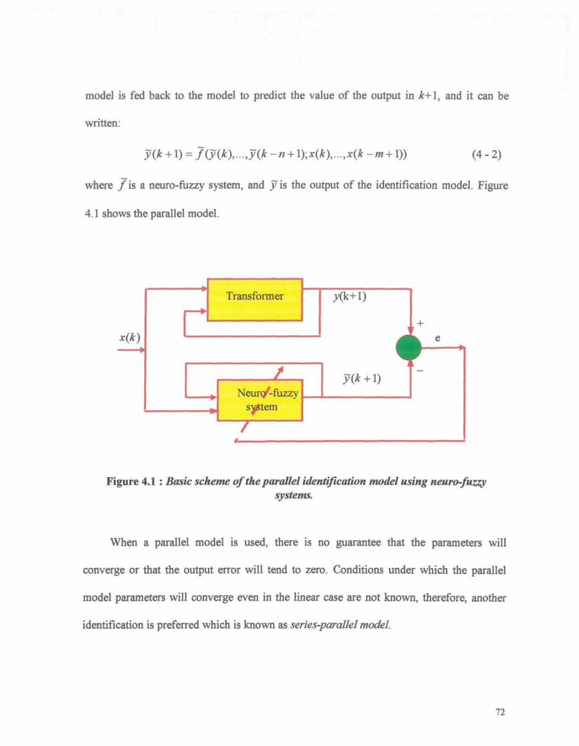
model is fed back to the model to predict the value of the output in A+l, and it can be
written:
(4-2)
where / is a neuro-fuzzy system, and y is the output of the identification model. Figure
4.1 shows the parallel model.
x(k)
r�ITransformer
/Neur</-fuzzy
J4y(k +1)
Figure 4.1 : Basic scheme of the parallel identification model using neuro-fuzzysystems.
When a parallel model is used, there is no guarantee that the parameters will
converge or that the output error will tend to zero. Conditions under which the parallel
model parameters will converge even in the linear case are not known, therefore, another
identification is preferred which is known as series-parallel model.
72
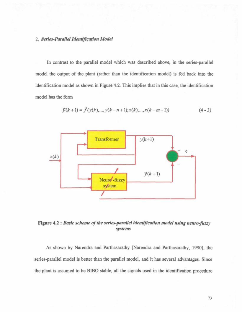
2. Series-Parallel Identification Model
In contrast to the parallel model which was described above, in the series-parallel
model the output of the plant (rather than the identification model) is fed back into the
identification model as shown in Figure 4.2. This implies that in this case, the identification
model has the form
)) (4 - 3)
x{k)
11� �
Transformer
/
Neurw-fuzzys^tem
Xk+1) 1
y(k +1)
Figure 4.2 : Basic scheme of the series-parallel identification model using neuro-fuzzysystems
As shown by Narendra and Parthasarathy [Narendra and Parthasarathy, 1990], the
series-parallel model is better than the parallel model, and it has several advantages. Since
the plant is assumed to be BIBO stable, all the signals used in the identification procedure
73
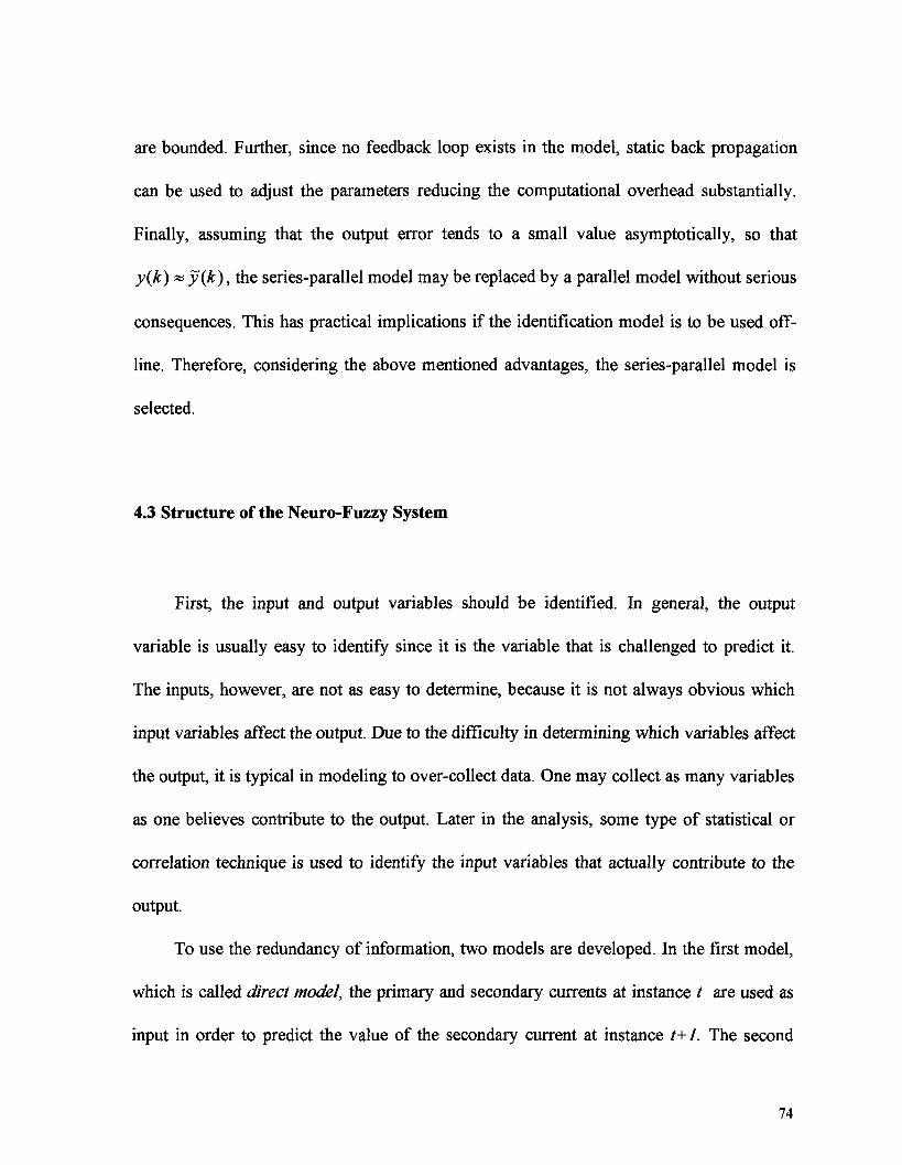
are bounded. Further, since no feedback loop exists in the model, static back propagation
can be used to adjust the parameters reducing the computational overhead substantially.
Finally, assuming that the output error tends to a small value asymptotically, so that
y(k) « y(k), the series-parallel model may be replaced by a parallel model without serious
consequences. This has practical implications if the identification model is to be used off-
line. Therefore, considering the above mentioned advantages, the series-parallel model is
selected.
4.3 Structure of the Neuro-Fuzzy System
First, the input and output variables should be identified. In general, the output
variable is usually easy to identify since it is the variable that is challenged to predict it.
The inputs, however, are not as easy to determine, because it is not always obvious which
input variables affect the output. Due to the difficulty in determining which variables affect
the output, it is typical in modeling to over-collect data. One may collect as many variables
as one believes contribute to the output. Later in the analysis, some type of statistical or
correlation technique is used to identify the input variables that actually contribute to the
output.
To use the redundancy of information, two models are developed. In the first model,
which is called direct model, the primary and secondary currents at instance / are used as
input in order to predict the value of the secondary current at instance t+1. The second
74
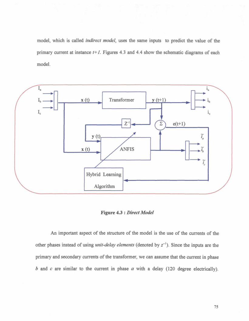
model, which is called indirect model, uses the same inputs to predict the value of the
primary current at instance /+/. Figures 4.3 and 4.4 show the schematic diagrams of each
model.
Hybrid Learning
Algorithm
Figure 4.3 : Direct Model
An important aspect of the structure of the model is the use of the currents of the
other phases instead of using unit-delay elements (denoted by z"1). Since the inputs are the
primary and secondary currents of the transformer, we can assume that the current in phase
b and c are similar to the current in phase a with a delay (120 degree electrically).
75
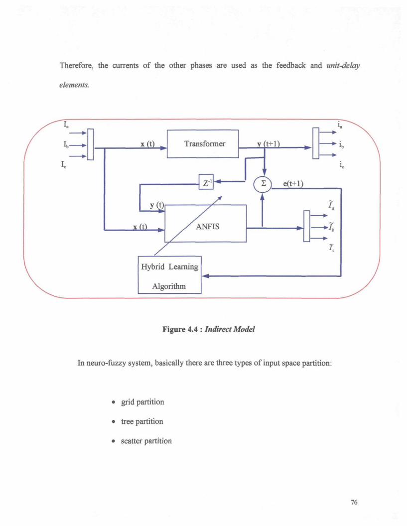
Therefore, the currents of the other phases are used as the feedback and unit-delay
elements.
Hybrid Learning
Algorithm
Figure 4.4 : Indirect Model
In neuro-fuzzy system, basically there are three types of input space partition:
grid partition
tree partition
� scatter partition
76

( a ) ( b ) ( c )
Figure 4.5 : Various methods of partition the input space : (a) grid partition; (b) treepartition, (c) scatter partition.
As it is shown in Figure 4.5 (a), grid partition consists of all possible combinations of
membership functions of all inputs. This leads to an exponential explosion even when the
number of inputs is moderately large. For instance, for a system with 10 inputs, each with
two membership functions, the grid partition leads to 1024 (2 A 10) rules, which is
prohibitively large for any practical learning methods. This situation, where the number of
fuzzy rules in a grid partition increases exponentially with the number of input variables, is
called curse of dimensionality.
Figure 4.5 (b) shows a typical tree partition, in which each region can be uniquely
specified along a corresponding decision tree. The tree partition relieves the problem of an
exponential increase in the number of rules. However, more membership functions for each
input are needed to define these fuzzy regions, and these membership functions do not
usually bear clear linguistic meanings such as small, big and so on.
77
Scatter partition uses a clustering algorithm to determine different clusters in the
whole input space which determine regions of possible occurrence of the input vectors.
This method which is shown in Figure 4.5 ( c ), can limit the number of rules to a
reasonable amount.
Grid partition is supported in MATLAB. Therefore, this method is used for
partitioning of the whole input space. To avoid the curse of dimensionality problem, only 2
membership functions for each input are considered.
There are several types of membership functions. In MATLAB, eleven types of
membership functions are provided. The only condition a membership function must really
satisfy is that it must vary between 0 and 1. A triangular membership function is selected
because it is a simple membership function and the calculation is done faster. On the other
hand, in contrast to a, generalized Bell-shape membership function, which is saturated near
its center, a triangular membership function does not suffer this pitfall. This is an
important consideration because when the currents increase, and there is a short-circuit or
over-load, the generalized Bell-shape membership function does not let the model follow
the variation of currents in saturation regions. However, there is not any saturation region
for the Triangular membership function.
It should be noted that grid partition and the triangular membership function
are used only for the premise of the if-then rules, while the Sugeno fuzzy model ( also
called TSK fuzzy model ) is used for the consequences of the if-then rules. The Sugeno fuzzy
model has several advantages and it can be more expressive than the Mamdani fuzzy model.
78
Because it is a more compact and computationally efficient representation than the
Mamdani fuzzy model, the Sugeno fuzzy model lends itself to adaptive techniques. The
advantages of the Sugeno fuzzy model are as follows [Jang & Gulley, 1995]:
� Computational efficiency
� Works well with linear techniques
� Works well with optimization and adaptive techniques
� Guaranteed continuity of the output surface
� Better suited to mathematical analysis
A typical fuzzy rule in a Sugeno fuzzy model has the form
ifx is A and y is B then z =f(z, y)
where A and B are fuzzy sets in the antecedent, while z =f(x ,y)isa crisp function in the
consequent. A first-order polynomial is used instead o f / ( x ,y ), which is called a first-
order Sugeno fuzzy model. Therefore, the parameters of the consequent are linear
parameters which can be adjusted by the Least Square Method (LSM), which will be
explained in the next section.
79
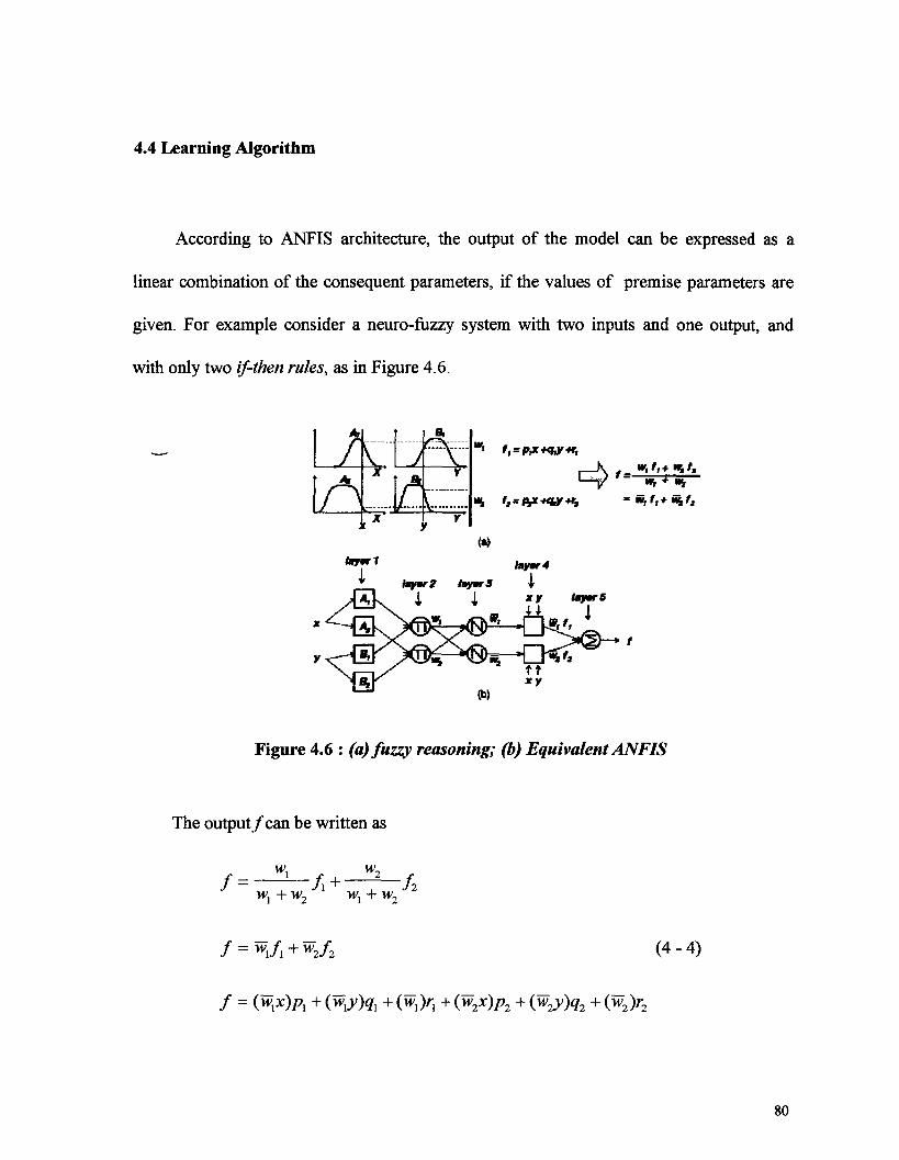
4.4 Learning Algorithm
According to ANFIS architecture, the output of the model can be expressed as a
linear combination of the consequent parameters, if the values of premise parameters are
given. For example consider a neuro-fuzzy system with two inputs and one output, and
with only two if-then rules, as in Figure 4.6.
Figure 4.6 : (a) fuzzy reasoning; (b) Equivalent ANFIS
The output/can be written as
V1
= wjx+w2f2
f = (^x)p{ + (wxy)qx
(4-4)
(w2x)p2 + {w2y)q2 + (w2)r2
80

which is linear in the consequent parameters {p\,qx, rup2, q2, r2}. Now, given the values of
premise parameters, we can apply P training data to the system and obtain a matrix
equation:
A® = B (4 -5)
where 0 is an unknown vector whose elements are consequent parameters. This equation
represents the standard linear least-squares problem and the best solution for 0, which
minimize || 40 - B\\2 ,is the least-squares estimator (LSE) 0*:
(4-6)
where AT is the transpose of A and (ATA)~lAT is the pseudo-inverse of A if ATA is non-
singular.
After the values of consequent parameters are identified, the gradient descent method
can be used to adjust the values of premise parameters in order to minimize the error of the
model. The error signal for each training data entry is defined by,
e(n) = d(n)-y(n) (4-7)
where n represents the nth training data entry. The overall error measure is,
{n) (4-8)
i
and with using of the chain rule, the correction value for each premise parameters can be
calculated:
81
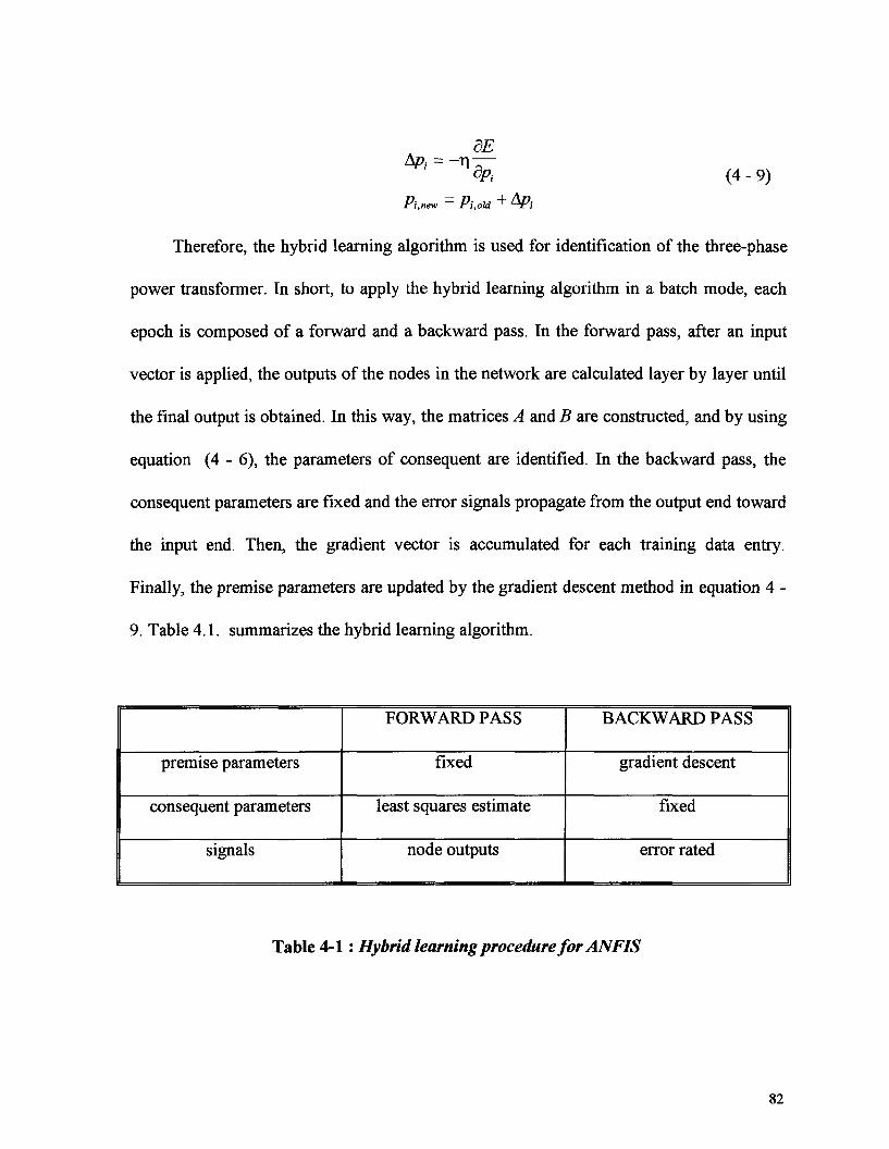
(4-9)
Therefore, the hybrid learning algorithm is used for identification of the three-phase
power transformer. In short, to apply the hybrid learning algorithm in a batch mode, each
epoch is composed of a forward and a backward pass. In the forward pass, after an input
vector is applied, the outputs of the nodes in the network are calculated layer by layer until
the final output is obtained. In this way, the matrices A and B are constructed, and by using
equation (4 - 6), the parameters of consequent are identified. In the backward pass, the
consequent parameters are fixed and the error signals propagate from the output end toward
the input end. Then, the gradient vector is accumulated for each training data entry.
Finally, the premise parameters are updated by the gradient descent method in equation 4 -
9. Table 4.1. summarizes the hybrid learning algorithm.
premise parameters
consequent parameters
signals
FORWARD PASS
fixed
least squares estimate
node outputs
BACKWARD PASS
gradient descent
fixed
error rated
Table 4-1 : Hybridlearning procedure for ANFIS
82

4.5 Training Data
As mentioned above, training data should include rated conditions of a three-phase
power transformer in addition to dynamic transients of the transformer. Since neuro-fuzzy
systems are self-learning systems, that is they learn the behavior of systems by observing
different values of inputs/outputs, a well-prepared training data plays a significant role in
the validation and generalization of a model. In other words, the key point to remember is
to have enough data that are well-distributed in the process operating range. A neuro-fuzzy
system is only as good as the data with which it was trained.
After determining the structure of the neuro-fuzzy system, the training data should be
applied to train the system. There are four training data files. Each file contains 3840
sampling data of primary and secondary currents, applied voltages and load voltages. They
also include the sampling times. Figures 4.7, 4.8, 4.9, and 4.10 show the training data files.
It should be noted that a resistive load is connected to the secondary side of the
transformer. Therefore, the secondary currents and secondary voltages have similar
waveforms.
83
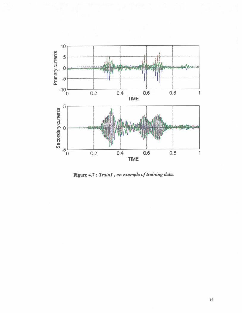
0
in
cIo
03
S8
CO-5
0
0.2
0.2
0.4 0.6TIME
0.8
^ * � � "WHS
r
mffi1 1
fDrUMa] Ï] l i TiSnWV >
E;l j � j fir
p i 1i i
0.4 0.6TIME
0.8
Figure 4.7 : Trainl, an example of training data.
84
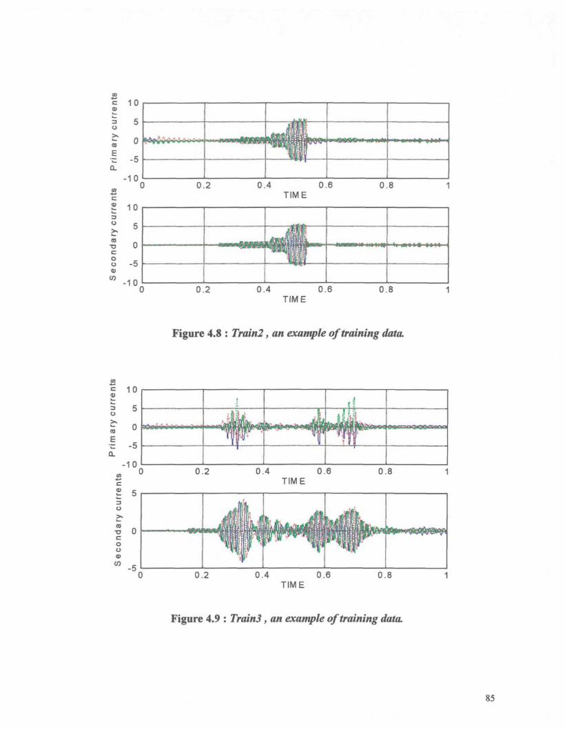
J5ctuh.
3O
CO
E
3C
CO
o
0.2 0.4 0.6TIME
0.8
Figure 4.8 : Train!, an example of training data.
TIME
Figure 4.9 : TrainJ, an example of training data.
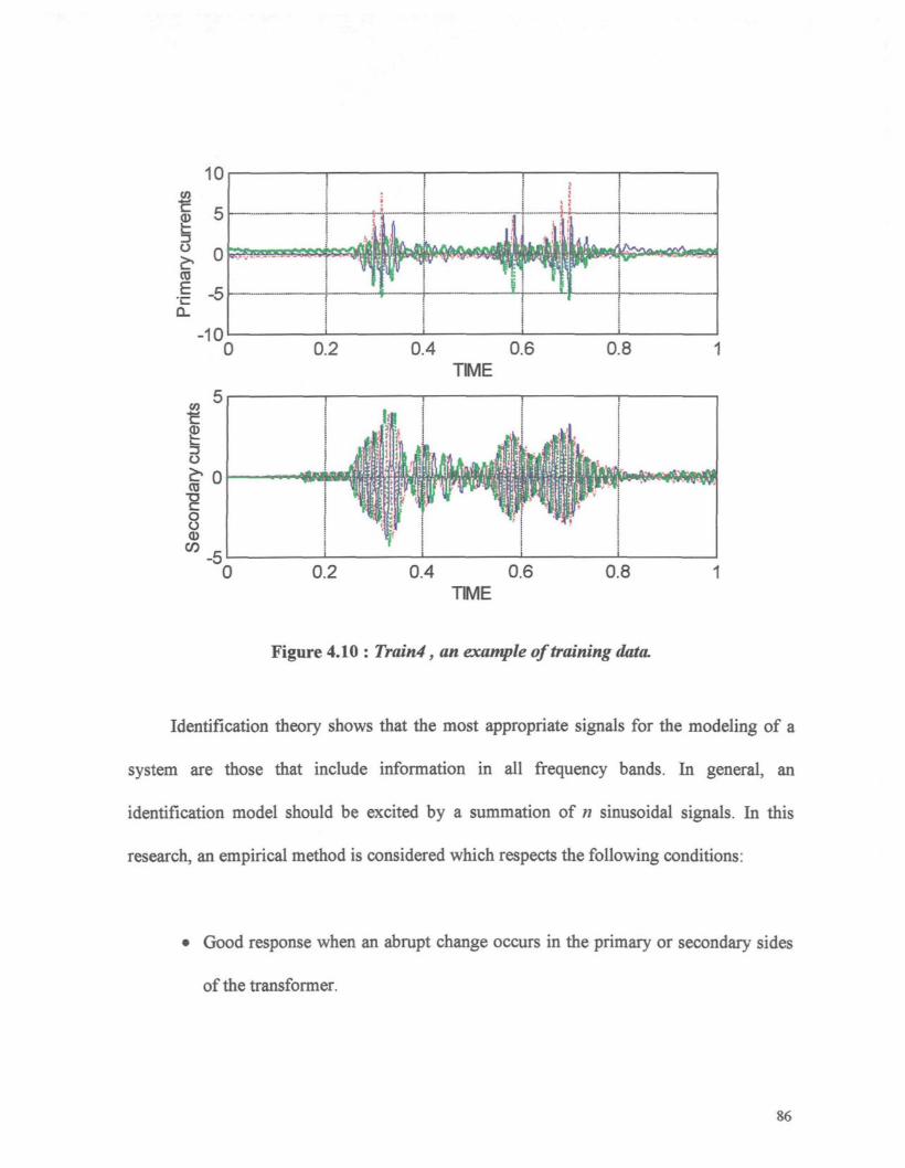
l3 il
i
1i!i
! !
ii i 1
0 0.2 0.4 0.6 0.8TIME
Figure 4.10 : Train4, an example of training data.
Identification theory shows that the most appropriate signals for the modeling of a
system are those that include information in all frequency bands. In general, an
identification model should be excited by a summation of n sinusoidal signals. In this
research, an empirical method is considered which respects the following conditions:
Good response when an abrupt change occurs in the primary or secondary sides
of the transformer.
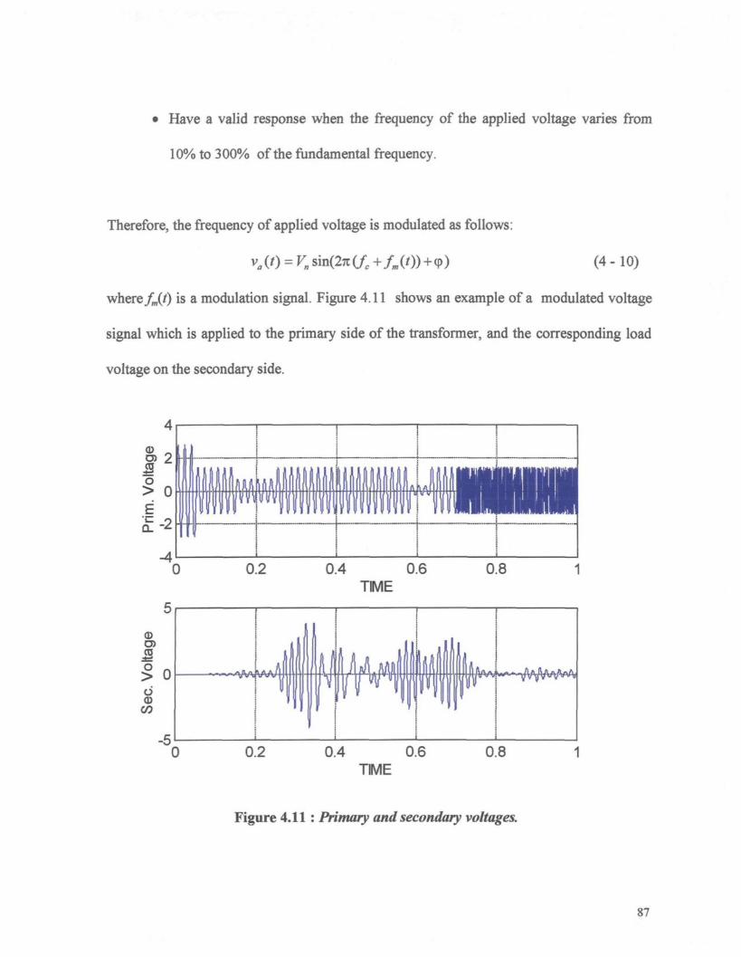
Have a valid response when the frequency of the applied voltage varies from
10% to 300% of the fundamental frequency.
Therefore, the frequency of applied voltage is modulated as follows:
(4-10)
where fjt) is a modulation signal. Figure 4.11 shows an example of a modulated voltage
signal which is applied to the primary side of the transformer, and the corresponding load
voltage on the secondary side.
0
0
0.4 0.6TIME
0.8
0.4 0.6TIME
0.8
Figure 4.11 : Primary and secondary voltages.
In order to have a proper excitation of the neuro-fuzzy system, different values of
modulation frequencies randomly distributed between 6 Hz to 200 Hz, several values of
applied voltage, and different load conditions are considered. The amplitude of the applied
voltage varies from 0.5 p.u. to 2.8 p.u., and the load conditions are varied in the range of
0.01 p.u. to 10 p.u. (from open circuit to short circuit). Figures 4.7, 4.8, 4.9, and 4.10 show
the training data files. It can be noted that the transformer is excited in different modes,
from completely saturated and extreme short circuit conditions to its rated conditions.
4.6 Pre-processing
Pre-processing, which may take the form of a linear transformation of the input data,
or sometimes a more complicated method, has a significant role in determining the
performance of the final system. Although neural networks and neuro-fuzzy systems can
perform essentially arbitrary non-linear mapping from the raw input data directly onto the
required final output values, in practice, such an approach will generally give poor results
for several reasons. For instance, in a chemical plant, two of the inputs might represent a
temperature and a pressure respectively. Depending on the units in which each of these is
measured, and their typical values, they may have values which differ by several orders of
magnitude. Furthermore, the typical sizes of the inputs may not reflect their relative
importance in determining the required outputs. On the other hand, we may have very large
and very small values for data. Therefore, in the gradient descent method, the gradient
88
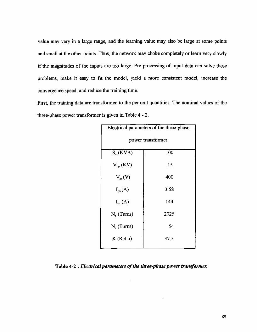
value may vary in a large range, and the learning value may also be large at some points
and small at the other points. Thus, the network may choke completely or learn very slowly
if the magnitudes of the inputs are too large. Pre-processing of input data can solve these
problems, make it easy to fit the model, yield a more consistent model, increase the
convergence speed, and reduce the training time.
First, the training data are transformed to the per unit quantities. The nominal values of the
three-phase power transformer is given in Table 4 - 2 .
Electrical parameters of the three-phase
power
Sn (KVA)
Vpn (KV)
V.(V)
Ipn(A)
Isn (A)
Np (Turns)
Ns (Turns)
K (Ratio)
transformer
100
15
400
3.58
144
2025
54
37.5
Table 4-2 : Electrical parameters of the three-phase power transformer.
89
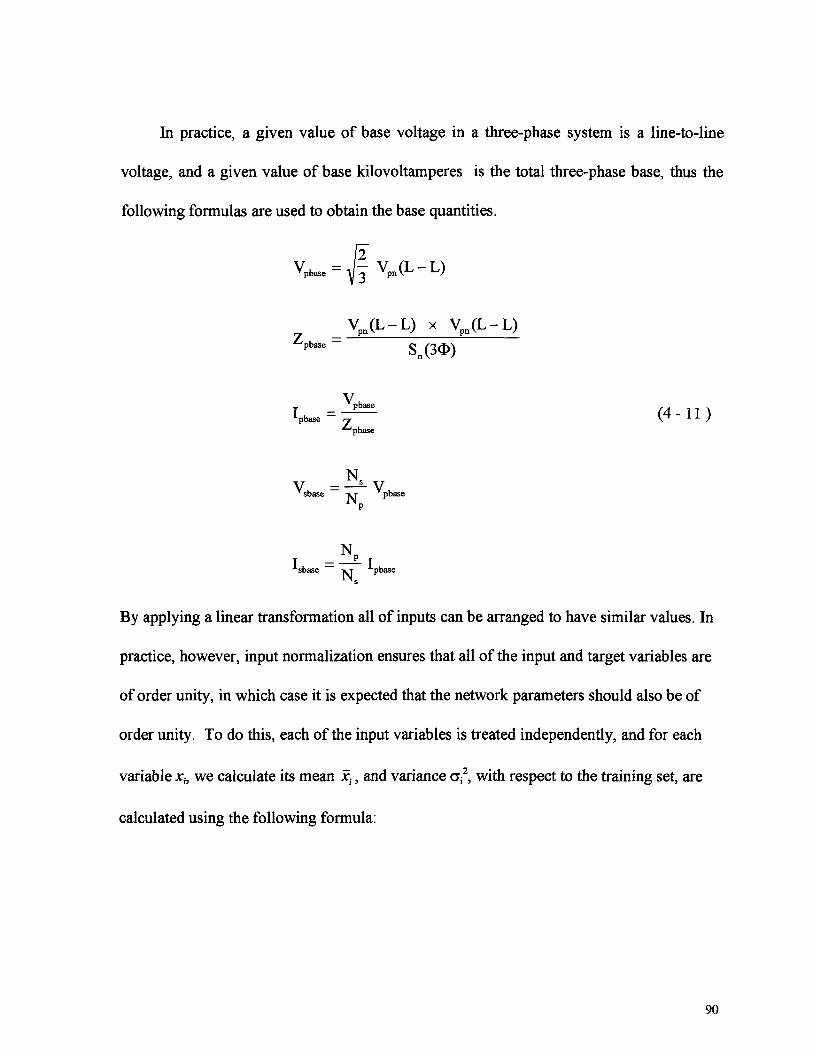
In practice, a given value of base voltage in a three-phase system is a line-to-line
voltage, and a given value of base kilovoltamperes is the total three-phase base, thus the
following formulas are used to obtain the base quantities.
3= J - Vpn(L-L)
VfL-L) x Vm(L-L)pn \ J pn '
J pbase
I p b a s e ^ ^ ( 4 - H )
V = �- Vsbase -VT pbase
AT P ^ e
By applying a linear transformation all of inputs can be arranged to have similar values. In
practice, however, input normalization ensures that all of the input and target variables are
of order unity, in which case it is expected that the network parameters should also be of
order unity. To do this, each of the input variables is treated independently, and for each
variable xh we calculate its mean xt, and variance o;2, with respect to the training set, are
calculated using the following formula:
90
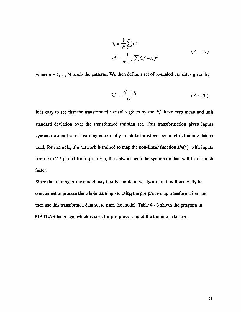
( 4 - 1 2 )2 �Yôc"-x)2
where n = 1,..., N labels the patterns. We then define a set of re-scaled variables given by
x" - x,( 4 - 1 3 )
It is easy to see that the transformed variables given by the x" have zero mean and unit
standard deviation over the transformed training set. This transformation gives inputs
symmetric about zero. Learning is normally much faster when a symmetric training data is
used, for example, if a network is trained to map the non-linear function sin(x) with inputs
from 0 to 2 * pi and from -pi to +pi, the network with the symmetric data will learn much
faster.
Since the training of the model may involve an iterative algorithm, it will generally be
convenient to process the whole training set using the pre-processing transformation, and
then use this transformed data set to train the model. Table 4 - 3 shows the program in
MATLAB language, which is used for pre-processing of the training data sets.
91
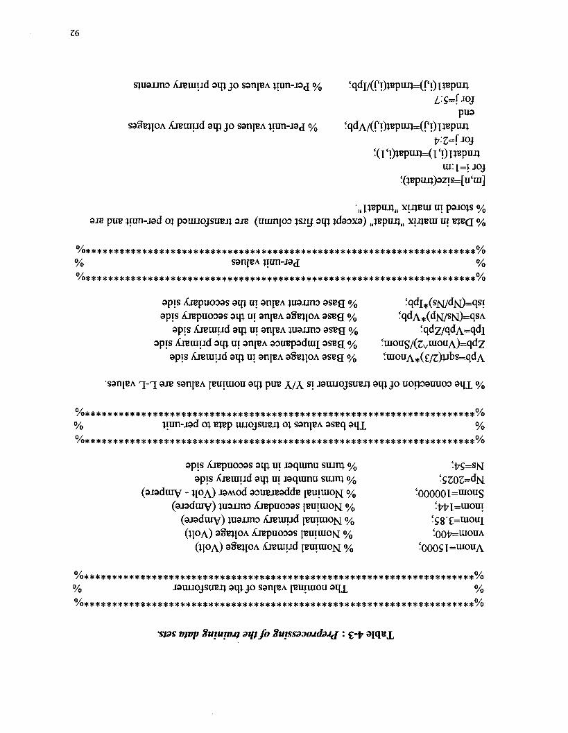
À\reuiud
puaAjBuiud aip jo sati{B A jxun-j9£ % ! qdA/( PO^P^^C PO l TBpufl-
!( i 'i);tjpim=( i 'i
èl XUJBUI UI p9JOJS o/opire jmn-j9d 01 pauuojsireji 9JB (uumioo ISJIJ 9ip jdaoxg) .jBpiuj,, XUJBUI ui
0/ 0/
% sanjBA i m n - j g d o/o
%*********************************************************************%
apis Aiepuiapis À\repuc
apis AJBI
apis AjBuiudapis AJBU
ooas aip ui>oas aip uiuud aqj uiaqj ui anp
jud aui ui
o/o 'qdi,is(sj«N[/dM)=qsi
-q 9JB san BA JBUIUIOU avfl. pue x/A Sl. JauuqjsuBJi ^m j o uoipauuoo 9i[x %
%****** * * * * * * * * * * * * * * * * * * * * * * * * * * * * * * * * * * * * * * * * * * * * * * * * * * * * * * * * * * * * * * *%% jiun-jgd o; Bjep UXIOJSUBJI OI sanjBA 9SBq gqx %%*********************************************************************%
apis AjBpuooas aip ui jaquinu sujtn % -K=SNapis Ajeuiud aqj ui jaquinu sujnj %
(ajaduiy - 1\OA) -is vod gouBJBadde(ajadiuv) luauno ÀJBpuoogs
jugjjno Ajeuiud
%
%
%
�00000 l=uiousït7t7l=UiOUI
!Ç8£=UJOUI
% * * * * * * * * * * * * * * * * * * * * * * * * * * * * * * * * * * * * * * * * * * * * * * * * * * * * * * * * * * * * * * * * * * * * * %
% jauiIOJSUBJJ9l[JJOS9n|BA|BUlUIOU9qx %%*********************************************************************%
Suwwjf 3tii fo Sui

endforj=8:10trndatl (i j)=trndat(ij)/vsb; % Per-unit values of the secondary voltages
endforj=ll:13trndatl (ij)=trndat(ij)/isb; % Per-unit values of the secondary currents
endend
0^*********************************************************************0^
% Normalization of the data %0/^*********************************************************************0^
% In this step, the data is normalized so that a zero mean and a standard deviation equal to% one are achieved.
[m,n]=size(trndatl );datmean=mean(trndatl); % Mean calculation for all variablesdatstd=std(trndatl); % Standard deviation calculation for all variablesfor i=l:mtrndat2(i, l)=trndatl(i, 1);forj=2:ntrndat2(ij)=(trndatl(i,j)-datmean(j))/datstd(j); % Normalized data
endend
93

4.7 Training of the Model
After determination of the structure of the neuro-fuzzy model and preprocessing of
training data, a learning scheme should be developed. In practice, there are two schemes of
learning:
� off-line learning or batch learning
� on-line learning or pattern learning
In off-line learning the update action takes place only after each epoch or sweep. On
the other hand, in on-line learning the parameters are updated immediately after each
input/output pair has been presented. However, it is possible to combine these two learning
modes and update the parameters after k training data entries have been presented, where k
is between 1 and maximum number of input-output pairs in training data file.
Kamwa and Grondin [ Kamwa & Grondin, Nov. 1996] proposed an interesting scheme.
Although they used the scheme for training an artificial neural network, it is very effective
and useful for training a neuro-fuzzy system. Using this scheme for training a neuro-fuzzy
system decreases the amount of the required calculations. Therefore, it makes the process
of training faster and it converges rapidly. For example, as it has been explained, to update
the consequent parameters (see section 4.4. LEARNING ALGORITHM), by presenting each
input-output pair to the model, a row of the matrices A and B are constructed. Then A'1
94
should be calculated. If the number of input-output pairs is small, it can be calculated
rapidly, however, for a large matrix, calculating A'1 takes a long time.
Figure 4.12 shows a learning scheme employed for training the neuro-fuzzy system.
First, the structure of the neuro-fuzzy model with initial values of the parameters should be
determined. In MATLAB, genfisl determines the initial values of the parameters. Then the
first training file is presented, and the parameters of the model are adjusted so that to
minimize the total error of the system. These parameters values are considered as the initial
values for the second training data file, and the second training file is presented to train the
system and adjust the parameters to have a better and more precise model. This process is
continued for all the training files in the first loop, and then the loop is repeated N times.
Finally, the validation of the model should be checked with a training file which has not
been presented to the model. If the model is not very precise or not acceptable, the final
model should be considered as the initial model and all the steps should be repeated with
the new initial values. If the model is still not accurate, the structure of the neuro-fuzzy
model should be modified, its complexity increased, and the process restarted from zero.
95
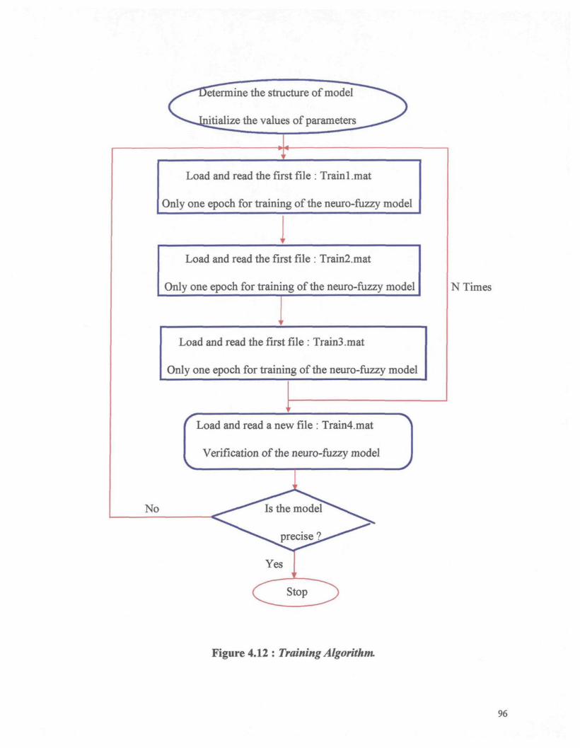
etermine the structure of model
itialize the values of parameters
Load and read the first file : Trainl.mat
Only one epoch for training of the neuro-fuzzy model
Load and read the first file : Train2,mat
Only one epoch for training of the neuro-fuzzy model
Load and read the first file : Train3.mat
Only one epoch for training of the neuro-fuzzy model
Load and read a new file : Train4.mat
Verification of the neuro-fuzzy model
No Is the model
precise^
(^ Stop ^)
N Times
Figure 4.12 : Training Algorithm.
96

Chapter 5
Validation
5.1 Introduction
When the training of the direct and indirect models have been completed, the
accuracy and rigidity of the system should be examined to determine how well it works.
These tests should be done in two steps:
�Verification;
�Validation.
In the verification process, the direct and indirect models encounter the training data that
have been used during the training procedure. The models response to the data which have
already seen. Therefore, if the parameters have been adjusted properly, the direct and
indirect models should predict the actual outputs precisely, and the errors are few and of
small amplitude. In this case, the models contain the dynamic characteristics of the
transformer.
Validation plays an important role since it can determine the generalization of a model. In
other words, we want to investigate the behavior of the neuro-fuzzy system when it
encounters input data that has not been seen before. If the direct and indirect models can
predict the behavior of the transformer with few errors , it means that they can generalize
the behavior of the power transformer very well. On the other hand, if they encounters
input data which contain information about abnormal conditions (like internal faults), the
98
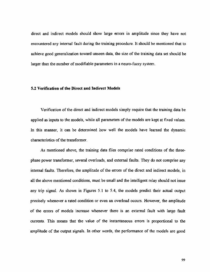
direct and indirect models should show large errors in amplitude since they have not
encountered any internal fault during the training procedure. It should be mentioned that to
achieve good generalization toward unseen data, the size of the training data set should be
larger than the number of modifiable parameters in a neuro-fuzzy system.
5.2 Verification of the Direct and Indirect Models
Verification of the direct and indirect models simply require that the training data be
applied as inputs to the models, while all parameters of the models are kept at fixed values.
In this manner, it can be determined how well the models have learned the dynamic
characteristics of the transformer.
As mentioned above, the training data files comprise rated conditions of the three-
phase power transformer, several overloads, and external faults. They do not comprise any
internal faults. Therefore, the amplitude of the errors of the direct and indirect models, in
all the above mentioned conditions, must be small and the intelligent relay should not issue
any trip signal. As shown in Figures 5.1 to 5.4, the models predict their actual output
precisely whenever a rated condition or even an overload occurs. However, the amplitude
of the errors of models increase whenever there is an external fault with large fault
currents. This means that the value of the instantaneous errors is proportional to the
amplitude of the output signals. In other words, the performance of the models are good
99
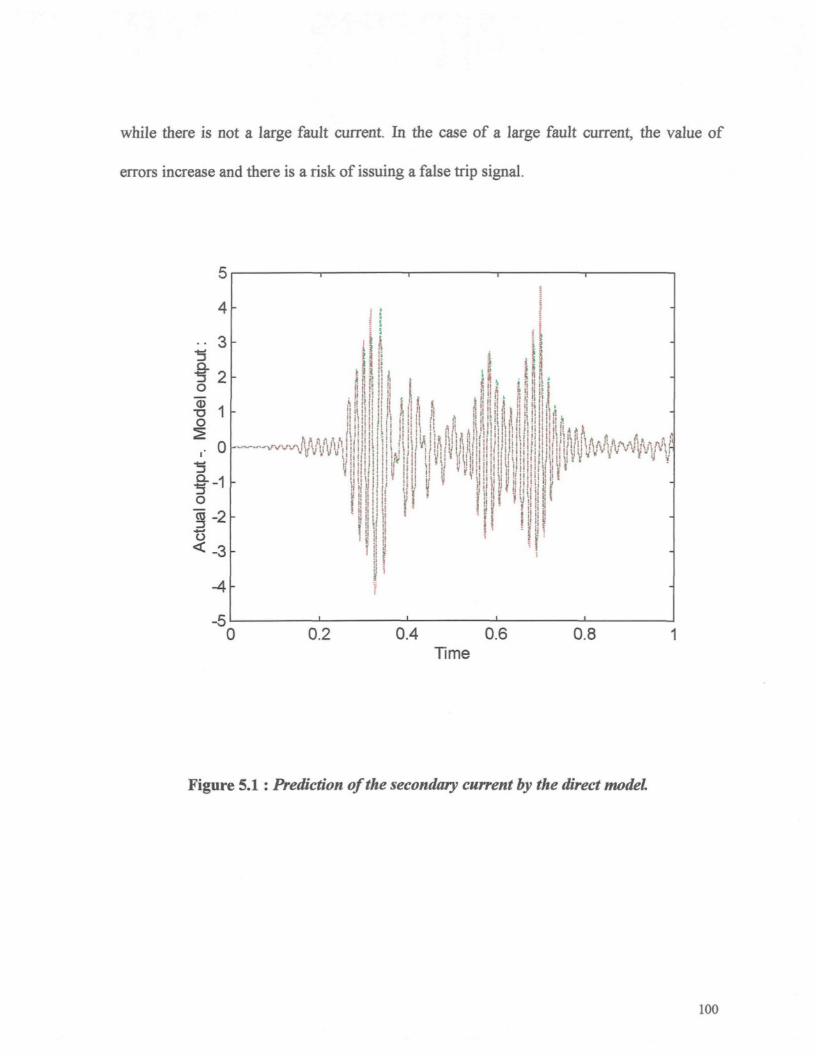
while there is not a large fault current. In the case of a large fault current, the value of
errors increase and there is a risk of issuing a false trip signal.
0 0.4 0.6 0.8Time
Figure 5.1 : Prediction of the secondary current by the direct model
100
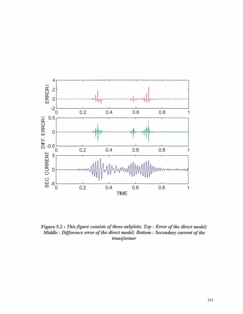
0 0.2 0.4 0.6TIME
0.8
Figure 5.2 : This figure consists of three subplots; Top : Error of the direct model;Middle : Difference error of the direct model; Bottom : Secondary current of the
transformer
101
a
a
3CD
Actual output -. Model output�k ta O M Oî
oto
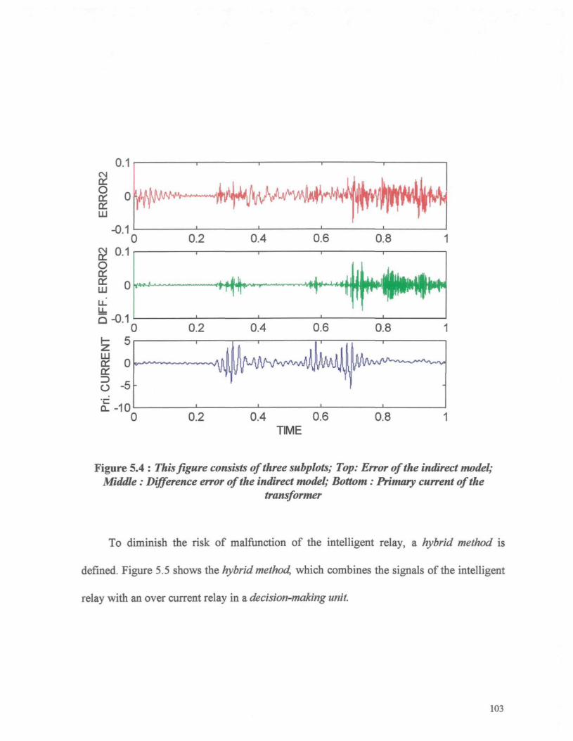
Q.-100.2 0.4 0.6
TIME0.8
Figure 5.4 : This figure consists of three subplots; Top: Error of the indirect model;Middle : Difference error of the indirect model; Bottom : Primary current of the
transformer
To diminish the risk of malfunction of the intelligent relay, a hybrid method is
defined. Figure 5.5 shows the hybrid method, which combines the signals of the intelligent
relay with an over current relay in a decision-making unit.
103
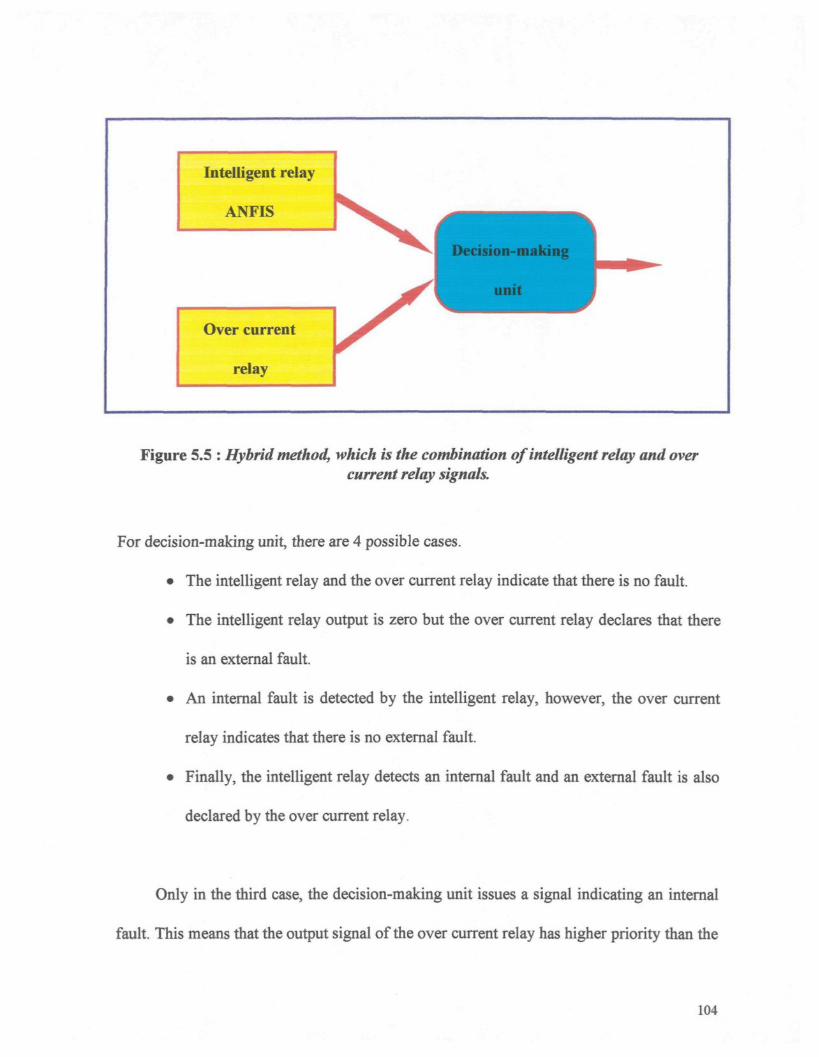
Intelligent relay
ANFIS
Over current
relay
Decision-making [ _
J ^ \ Unit
Figure 5.5 : Hybrid method, which is the combination of intelligent relay and overcurrent relay signals.
For decision-making unit, there are 4 possible cases.
� The intelligent relay and the over current relay indicate that there is no fault.
� The intelligent relay output is zero but the over current relay declares that there
is an external fault.
� An internal fault is detected by the intelligent relay, however, the over current
relay indicates that there is no external fault.
� Finally, the intelligent relay detects an internal fault and an external fault is also
declared by the over current relay.
Only in the third case, the decision-making unit issues a signal indicating an internal
fault. This means that the output signal of the over current relay has higher priority than the
104

intelligent relay. Therefore, when both relays are activated, the decision-making unit does
not issue any signal indicating an internal fault. It is clear that in the first two cases, the
intelligent relay does not detect any internal fault. Therefore, the decision-making unit does
not declare an internal fault.
Table 5.1 shows the truth table of the decision-making unit. The hybrid method
configuration shows that when the training data files are applied to verify the direct and
indirect models, an internal fault is not detected, and the amplitude of the errors of the
models are generally small.
Intelligent relay
0
0
1
1
Over current relay
0
1
0
1
Decision-making unit
0
0
1
0
Table 5-1 : Truth table of the decision-making unit
105
5.3 Validation of the Direct and Indirect Models
In the validation procedure, new data files, which are called validation files, are used
to verify the generalization of a neural network or a neuro-fuzzy system. The validation
files consist of data and information that have not been seen by the neural networks or the
neuro-fuzzy systems. Therefore, they are completely new information for them. By
applying the validation files, the behavior and the errors of the direct and indirect models
are observed. If they can predict the behavior of the transformer under rated conditions,
and theirs output errors remain small, the models can be accepted as a good predictor of the
behavior of the transformer under rated condition. When an internal fault occurs, the
amplitude of the errors should increase. Since the direct and indirect models have not been
trained with data files, which consist of any internal fault, and they cannot predict the
behavior of the power transformer under internal fault conditions, the predicted values are
not very precise and the amplitude of the errors increase considerably. The trip signal is
issued when the errors increase above a threshold value.
5.3.1 Description of the Validation Data Files
According to practical standards in protection engineering, a complete and exhaustive
simulation should be carried out to determine the limitation of the performance of the
neuro-fuzzy system, which is considered as an intelligent relay.
106

In the validation data files, several parameters are varied to have an exhaustive set of
simulations. These parameters are explained as follows:
� Initial phase angle: changing the initial phase of the applied voltage to the
primary side of the transformer. Four different values are selected for the initial
phase of the applied voltage, which can change the shape of inrush currents and
the amount of the second harmonic. Therefore, we can investigate the behavior
of the system for different values of inrush currents. These four values are zero,
pi/4 , pi/2 and pi.
� winding : internal fault is simulated on the primary or secondary windings.
� Phase : internal fault is simulated on different phases. Therefore, three possible
cases exist.
� Load : different loads are selected before and after internal faults. The load
variations consist in open and short-circuits. These load values are
I. open-circuit;
II. 10% of the nominal load;
III. 50% of the nominal load;
IV. nominal load;
V. 200% of the nominal load;
VI. 400% of the nominal load;
VII. 800% of the nominal load (short-circuit).
107

Fault amplitude : different percentages of windings are short-circuited to simulate
different levels of internal fault. These values are as follows:
i. 0% of the winding is short-circuited (healthy winding).
ii. 3% of the winding is short-circuited.
iii. 10% of the winding is short-circuited.
iv. 15% of the winding is short-circuited.
v. 40% of the winding is short-circuited.
vi. 75% of the winding is short-circuited.
vii.95% of the winding is short-circuited.
5.3.2 Internal Fault at the Secondary Side of the Power Transformer
The validation files that include internal faults in the secondary of the transformer
have the following configuration:
� internal fault of 15% in the secondary side which occurs at 400ms, including the
following perturbations in the network:
a) temporary short-circuit and over-voltage in the primary side
b) variable load
c) different initial phase angle for the applied voltage
108

The validation files are T3121211, T3121214, T3121244 and T3121264. Figures 5.6 to
5.11 show the result of the validation only for the first two validation files. However, the
RMSE (Root Mean Squared Error) values are calculated for all of them. As mentioned
earlier, these files contain an internal fault with 15% of the secondary winding short-
circuited in phase a. The internal faults occur at 400ms and they have different initial phase
angles and load values.
As it is shown in these figures, the errors of the direct and indirect models increase in
amplitude, after occurrence of an internal fault. Tables 5.2 and 5.3 show the values of
RMSE of the direct and indirect models respectively, when these validation files are
applied. They illustrate that RMSE before the occurrence of an internal fault is very small,
while it increases after the occurrence of an internal fault in the secondary side.
109
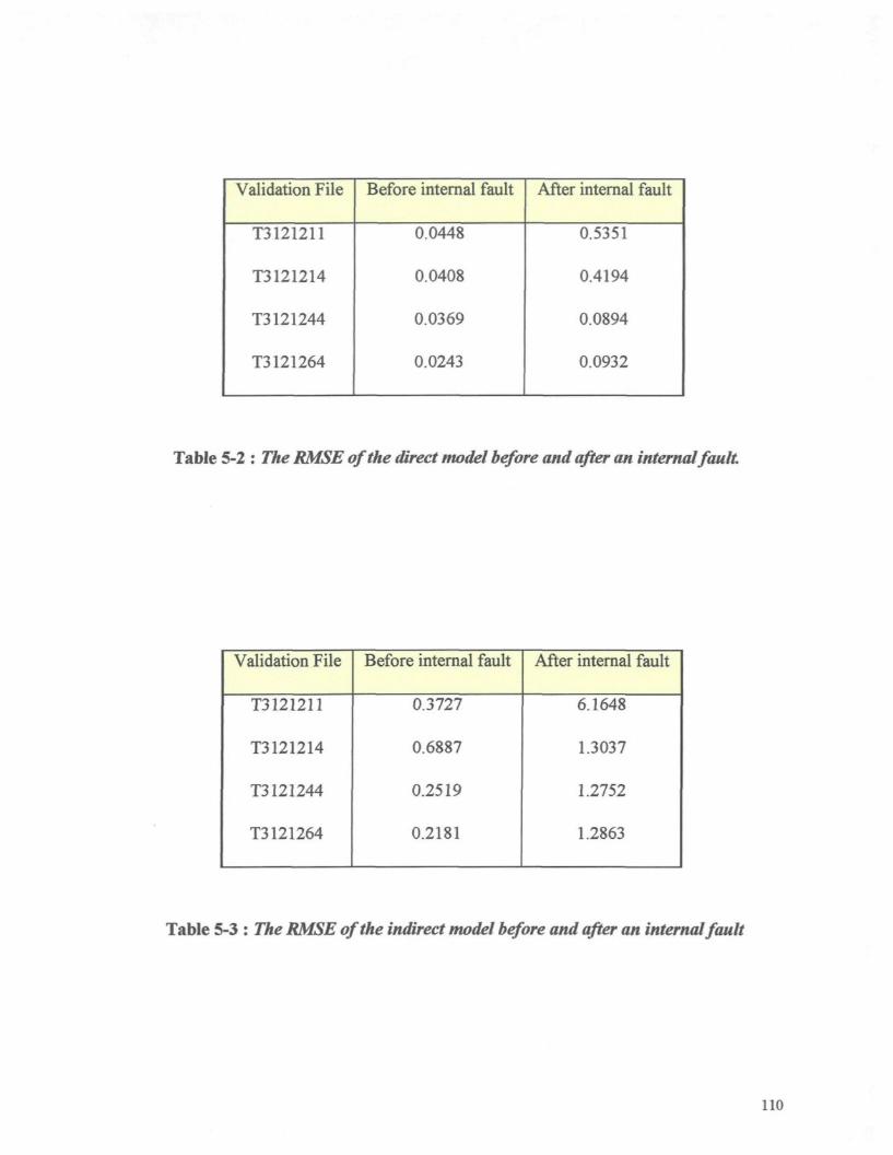
Validation File
T3I21211
T3121214
T3121244
T3121264
Before internal fault
0.0448
0.0408
0.0369
0.0243
After internal fault
0.5351
0.4194
0.0894
0.0932
Table 5-2 : The RMSE of the direct model before and after an internal fault
Validation File
T3121211
T3121214
T3121244
T3121264
Before internal fault
0.3727
0.6887
0.2519
0.2181
After internal fault
6.1648
1.3037
1.2752
1.2863
Table 5-3 : The RMSE of the indirect model before and after an internal fault
110
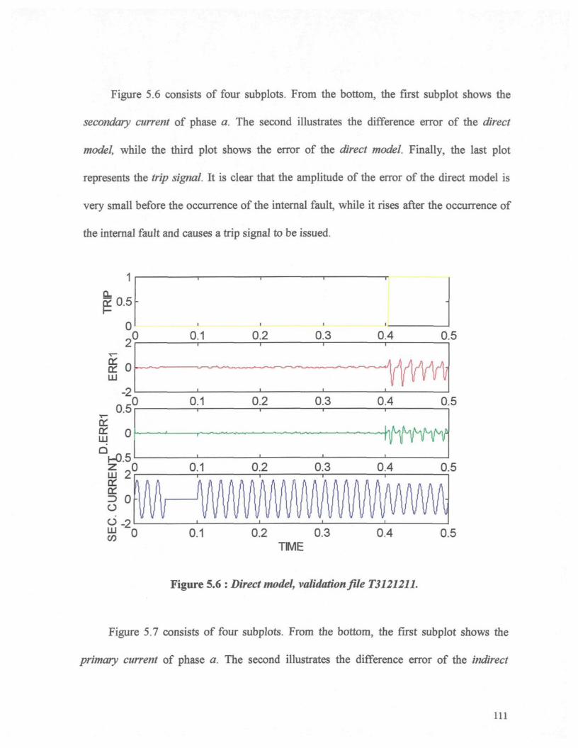
Figure 5.6 consists of four subplots. From the bottom, the first subplot shows the
secondary current of phase a. The second illustrates the difference error of the direct
model, while the third plot shows the error of the direct model. Finally, the last plot
represents the trip signal. It is clear that the amplitude of the error of the direct model is
very small before the occurrence of the internal fault, while it rises after the occurrence of
the internal fault and causes a trip signal to be issued.
0.2 0.3TIME
0.4 0.5
Figure 5.6 : Direct model, validation file T312121L
Figure 5.7 consists of four subplots. From the bottom, the first subplot shows the
primary current of phase a. The second illustrates the difference error of the indirect
111
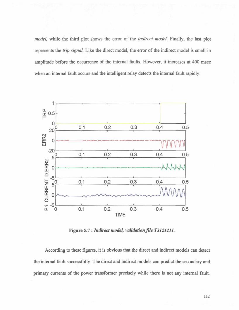
model, while the third plot shows the error of the indirect model Finally, the last plot
represents the trip signal. Like the direct model, the error of the indirect model is small in
amplitude before the occurrence of the internal faults. However, it increases at 400 msec
when an internal fault occurs and the intelligent relay detects the internal fault rapidly.
fPI
o
£ 0 0.2 0.3TIME
0.4 0.5
Figure 5.7 : Indirect model, validation file T312121L
According to these figures, it is obvious that the direct and indirect models can detect
the internal fault successfully. The direct and indirect models can predict the secondary and
primary currents of the power transformer precisely while there is not any internal fault.
112
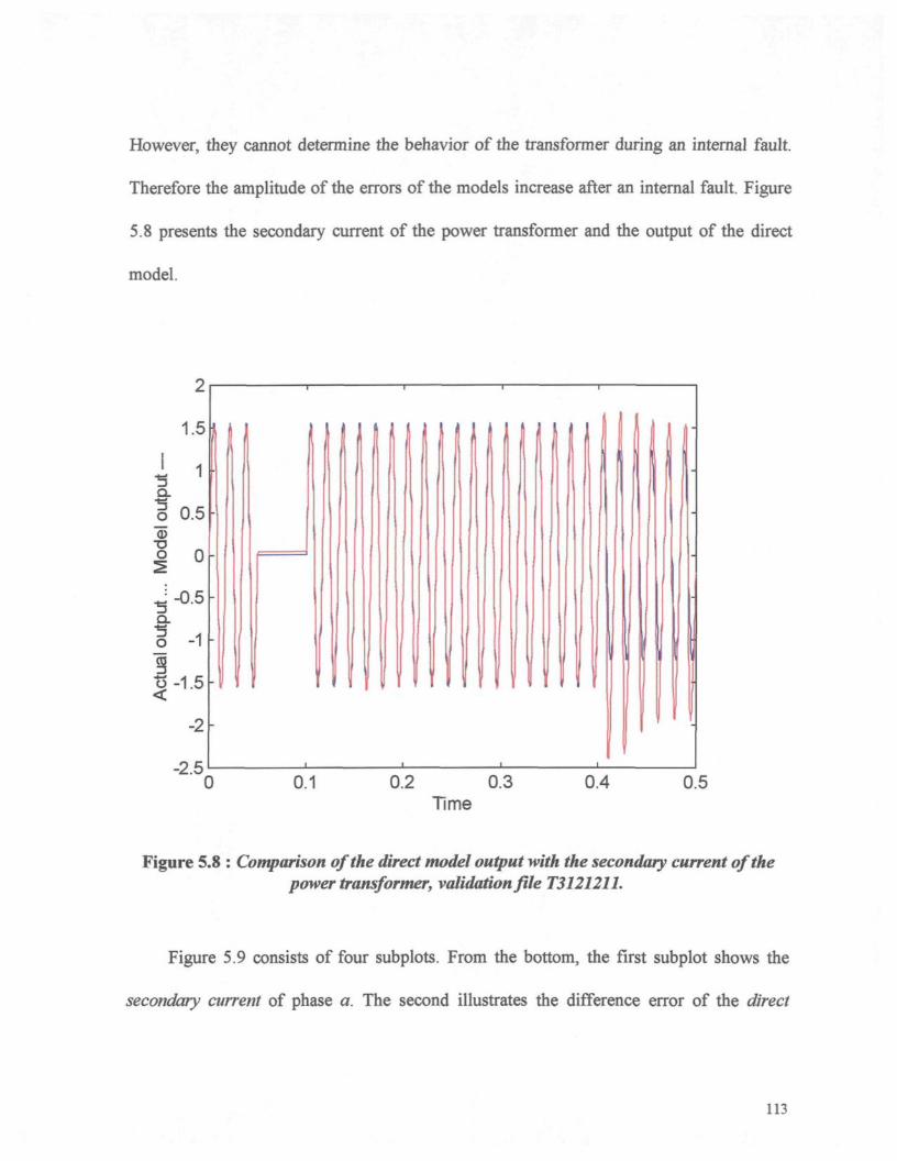
However, they cannot determine the behavior of the transformer during an internal fault.
Therefore the amplitude of the errors of the models increase after an internal fault. Figure
5.8 presents the secondary current of the power transformer and the output of the direct
model.
0.2 0.3Time
0.4 0.5
Figure 5.8 : Comparison of the direct model output with the secondary current of thepower transformer, validation file T312121L
Figure 5.9 consists of four subplots. From the bottom, the first subplot shows the
secondary current of phase a. The second illustrates the difference error of the direct
113
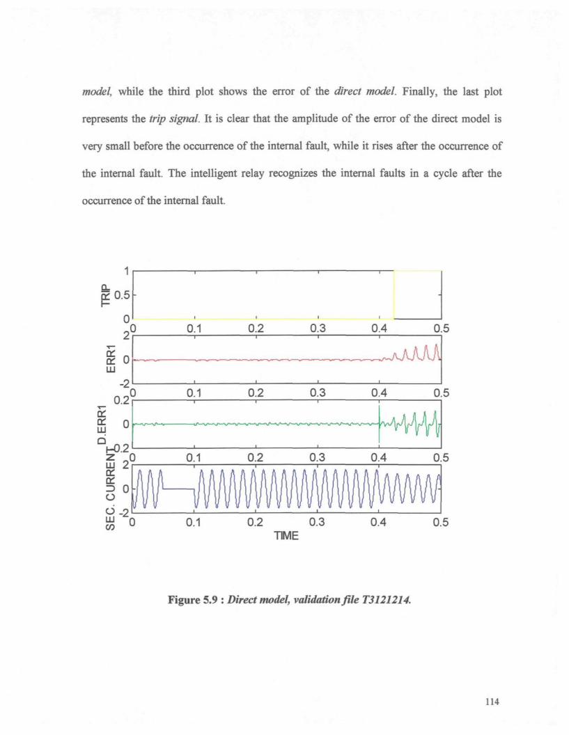
model, while the third plot shows the error of the direct model Finally, the last plot
represents the trip signal It is clear that the amplitude of the error of the direct model is
very small before the occurrence of the internal fault, while it rises after the occurrence of
the internal fault. The intelligent relay recognizes the internal faults in a cycle after the
occurrence of the internal fault.
o<> - 2UJ Q 0.1 0.2 0.3
TIME0.5
Figure 5.9 : Direct model, validation file T3121214.
114
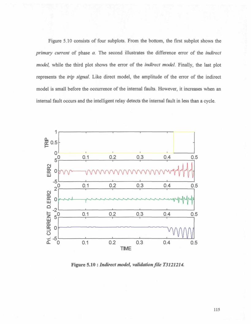
Figure 5.10 consists of four subplots. From the bottom, the first subplot shows the
primary current of phase a. The second illustrates the difference error of the indirect
model, while the third plot shows the error of the indirect model Finally, the last plot
represents the trip signal. Like direct model, the amplitude of the error of the indirect
model is small before the occurrence of the internal faults. However, it increases when an
internal fault occurs and the intelligent relay detects the internal fault in less than a cycle.
d5a. 0 0.2 0.3
TIME
Figure 5.10 : Indirect model, validation file T3121214.
0.5
115
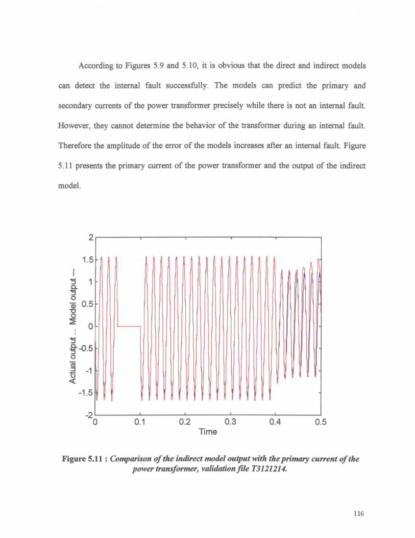
According to Figures 5.9 and 5.10, it is obvious that the direct and indirect models
can detect the internal fault successfully. The models can predict the primary and
secondary currents of the power transformer precisely while there is not an internal fault.
However, they cannot determine the behavior of the transformer during an internal fault.
Therefore the amplitude of the error of the models increases after an internal fault. Figure
5.11 presents the primary current of the power transformer and the output of the indirect
model.
2
1.5
3
oâ 0.5o
§�-0.5o
TÏ-1
-1.5
-20.2 0.3
Time0.4 0.5
Figure 5.11 : Comparison of the indirect model output with the primary current of thepower transformer, validation file T3121214.
116

5.3.3 Internal Fault at the Primary Side of the Power Transformer
There are several validation files which contain internal faults in the primary side of
the transformer. These validation files have the following configurations:
� different values of internal faults in the primary side of the transformer exist.
These values are 15%, 10% and 3% of the primary winding in phase a are short-
circuit.
� different load values, from open-circuit to short circuit, are considered.
� different initial phase angles for the applied voltage to the transformer are
selected. These values are zero, TC/4, nl2 ,and % degree.
The validation files are T3111211, T3111233, T3111243 and T3111244. Figure 5.12 to
5.16 show the results of the validation only for the first two validation files. However, the
RMSE (Root Mean Squared Error) values are calculated for all of them. These files
contain internal faults with 15% of the primary winding short-circuited in phase a. The
internal fault occurs at 200 msec and they have different initial phase angles and load
values.
As it is shown in these figures, the errors of the direct and indirect mode
117
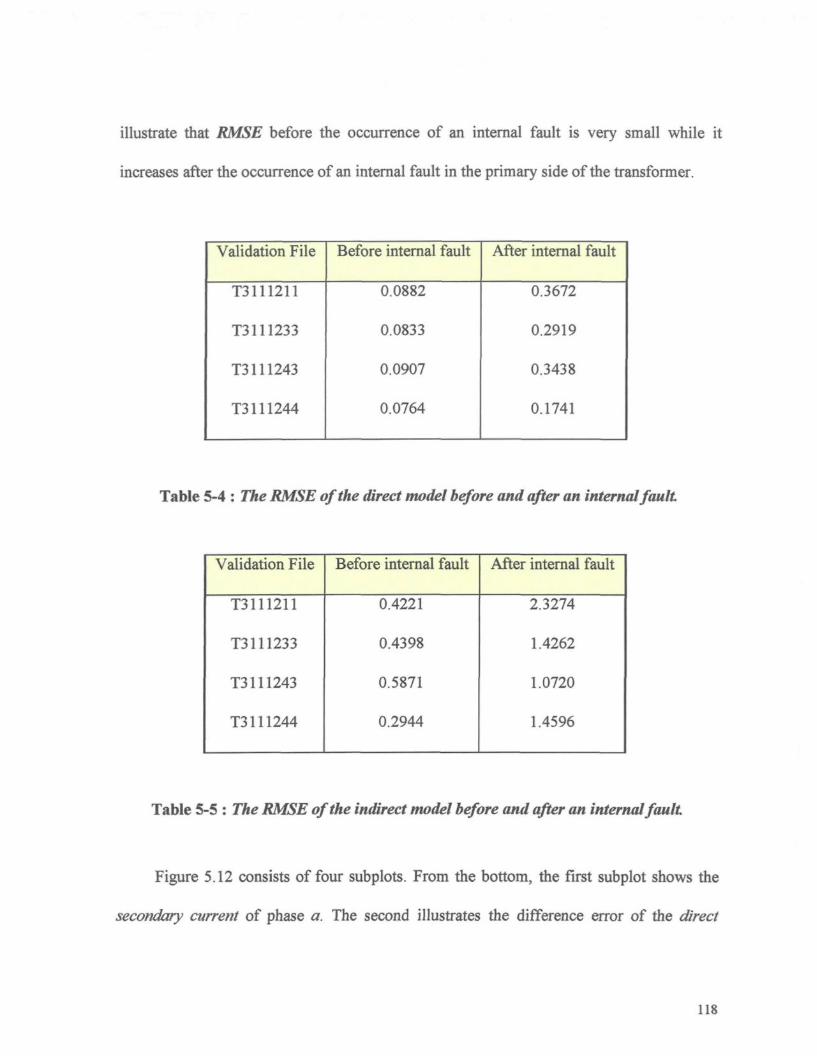
illustrate that RMSE before the occurrence of an internal fault is very small while it
increases after the occurrence of an internal fault in the primary side of the transformer.
Validation File
T3111211
T3111233
T3111243
T3111244
Before internal fault
0.0882
0.0833
0.0907
0.0764
After internal fault
0.3672
0.2919
0.3438
0.1741
Table 5-4 : The RMSE of the direct model before and after an internal fault
Validation File
T3111211
T3111233
T3111243
T3111244
Before internal fault
0.4221
0.4398
0.5871
0.2944
After internal fault
2.3274
1.4262
1.0720
1.4596
Table 5-5 : The RMSE of the indirect model before and after an internal fault
Figure 5.12 consiste of four subplots. From the bottom, the first subplot shows the
secondary current of phase a. The second illustrates the difference error of the direct
118
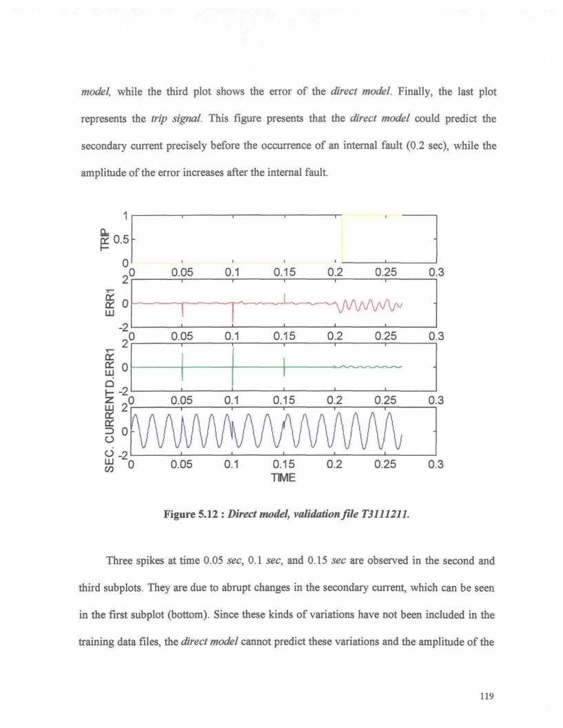
model, while the third plot shows the error of the direct model. Finally, the last plot
represents the trip signal. This figure presents that the direct model could predict the
secondary current precisely before the occurrence of an internal fault (0.2 sec), while the
amplitude of the error increases after the internal fault.
1
èo.5-1 1 1 1
-
0.05 0.1 0.15 0.2 0.25 0.3
0.05 0.1 0.15 0.2 0.25 0.3
DC
85°Ê-2
0.05 0.1 0.15 0.2 0.25 0.3
Figure 5.12 : Direct model, validation file T31112U.
Three spikes at time 0.05 sec, 0.1 sec, and 0.15 sec are observed in the second and
third subplots. They are due to abrupt changes in the secondary current, which can be seen
in the first subplot (bottom). Since these kinds of variations have not been included in the
training data files, the direct model cannot predict these variations and the amplitude of the
119
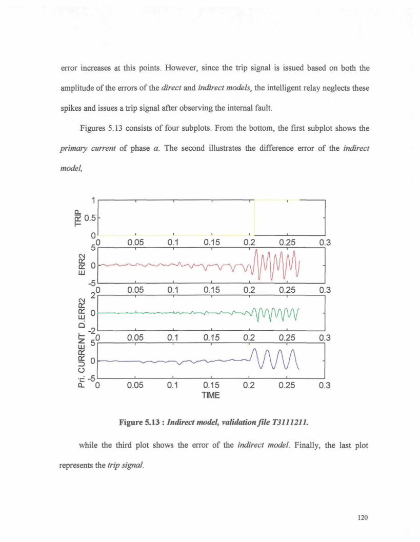
error increases at this points. However, since the trip signal is issued based on both the
amplitude of the errors of the direct and indirect models, the intelligent relay neglects these
spikes and issues a trip signal after observing the internal fault.
Figures 5.13 consists of four subplots. From the bottom, the first subplot shows the
primary current of phase a. The second illustrates the difference error of the indirect
model,
û. 0
0.05 0.1 0.15 0.2 0.25 0.3
0.05 0.1 0.15 0.2TIME
0.25 0.3
Figure 5.13 : Indirect model, validation file T311121L
while the third plot shows the error of the indirect model. Finally, the last plot
represents the trip signal
120
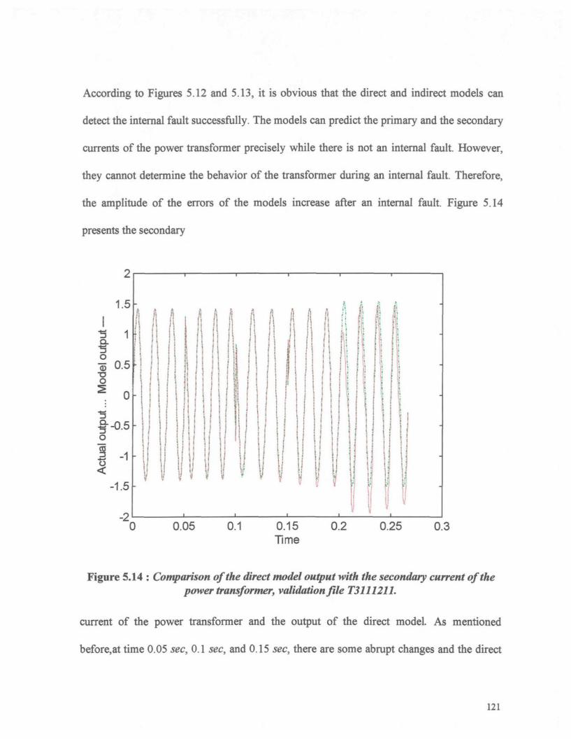
According to Figures 5.12 and 5.13, it is obvious that the direct and indirect models can
detect the internal fault successfully. The models can predict the primary and the secondary
currents of the power transformer precisely while there is not an internal fault. However,
they cannot determine the behavior of the transformer during an internal fault. Therefore,
the amplitude of the errors of the models increase after an internal fault. Figure 5.14
presents the secondary
to©�oo
"5Q_�3o
So
1.5
0.5
0
-0.5
-1
-1.5
-2
\i j
0
ji ii ii ;I
I k
i i
; :
i !i! If
I !
y y y|
V
! i 11
i
ily
J
M i! i1 j
[j
II= i
;
|
0.05 0.1 0.15Time
0.2 0.25 0.3
Figure 5.14 : Comparison of the direct model output with the secondary current of thepower transformer, validation file T3111211.
current of the power transformer and the output of the direct model. As mentioned
before,at time 0.05 sec, 0.1 sec, and 0.15 sec, there are some abrupt changes and the direct
121
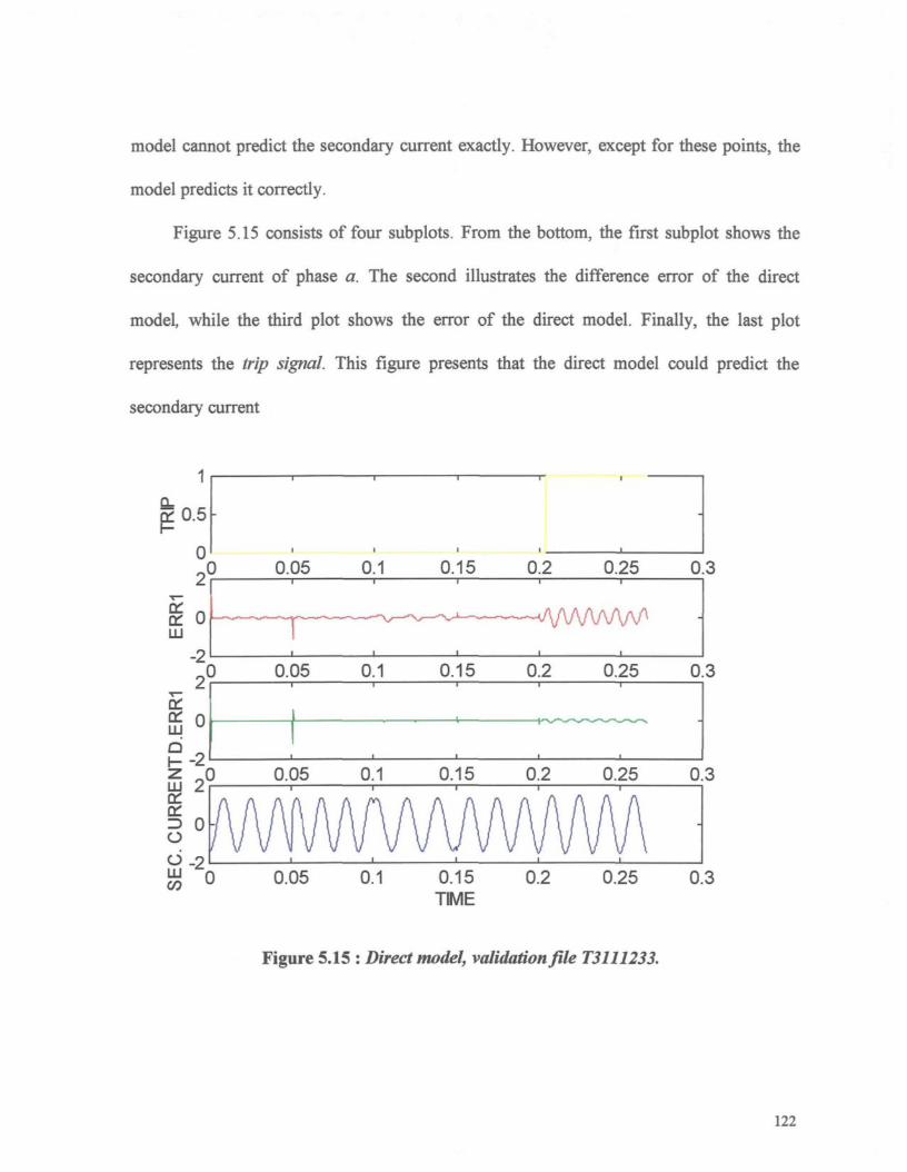
model cannot predict the secondary current exactly. However, except for these points, the
model predicts it correctly.
Figure 5.15 consists of four subplots. From the bottom, the first subplot shows the
secondary current of phase a. The second illustrates the difference error of the direct
model, while the third plot shows the error of the direct model. Finally, the last plot
represents the trip signal This figure presents that the direct model could predict the
secondary current
1
0.5
0 1 1 t 1
0.05 0.1 0.15 0.2 0.25 0.3
0.05 0.1 0.15 0.2 0.25 0.3
0.15 0.2 0.25 0.3
Figure 5.15 : Direct model, validation file T3111233.
122

precisely before the occurrence of an internal fault (0.2 sec), while the amplitude of the
error increases after the internal fault. Two spikes at time 0.0 sec, and 0.05 sec are
observed in the second and third subplots. They are due to abrupt changes in the secondary
current which can be seen in the first subplot (from bottom). Since these kinds of variations
have not been included in the training data files, the direct model cannot predict these
variations and the error increases in amplitude at these points. However, since the trip
signal is issued based on the amplitude of the errors of the direct and indirect models, the
intelligent relay neglects these spikes and issues a trip signal after observing the internal
fault.
Figures 5.16 consists of four subplots. From the bottom, the first subplot shows the
primary current of phase a. The second illustrates the difference error of the indirect
model, while the third plot shows the error of the indirect model. Finally, the last plot
represents the trip signal.
Finally, there are some validation files which include internal faults in the primary
side of the transformer with 10% or 3% of the primary winding short-circuited in phase a.
The validation files are T2111214, T2111233, T5111214 and T5111262. Figure 5.17
to 5.20 show the results of applying the second and the third validation files. However, the
RMSE {Root Mean Squared Error) values are calculated for all of them. The internal fault
occurs at 50 msec and they have different initial phase angles and load values.
As is shown in these Figures, the error of the direct and indirect models increase in
amplitude after occurrence of an internal fault for the first two validation files which 10%
123
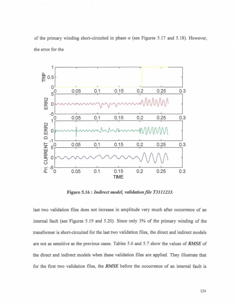
of the primary winding short-circuited in phase a (see Figures 5.17 and 5.18). However,
the error for the
0.05 0.1 0.15 0.2 0.25 0.3
! ^ ' A r N ' ' V N ~ r v v ' v v ^
0.15 0.2 0.25 0.3
Q- 0
Figure 5.16 : Indirect model, validation file T3111233.
last two validation files does not increase in amplitude very much after occurrence of an
internal fault (see Figures 5.19 and 5.20). Since only 3% of the primary winding of the
transformer is short-circuited for the last two validation files, the direct and indirect models
are not as sensitive as the previous cases. Tables 5.6 and 5,7 show the values of RMSE of
the direct and indirect models when these validation files are applied. They illustrate that
for the first two validation files, the RMSE before the occurrence of an internal fault is
124

very small while it increases after the occurrence of an internal fault in the primary side of
the transformer. In contrast, for the last two validation files, the amplitude of the errors do
not change very much after the occurrence of an internal fault. This indicates that the
models are not sensitive enough for a small internal fault and they cannot recognize and
detect them precisely.
Validation File
T2111214
T2111233
T5111242
T5111262
Before internal fault
0.0290
0.0997
0.0758
0.0419
After internal fault
0.2130
0.2880
0.0821
0.0286
Table 5-6 : The RMSE of the direct model before and after an internal fault
Validation File
T2111214
T2111233
T5111242
T5111262
Before internal fault
0.1398
0.2283
0.3077
0.2483
After internal fault
1.7103
1.3546
0.2893
0.2347
Table 5-7 : The RMSE of the indirect model before and after an internal fault
125
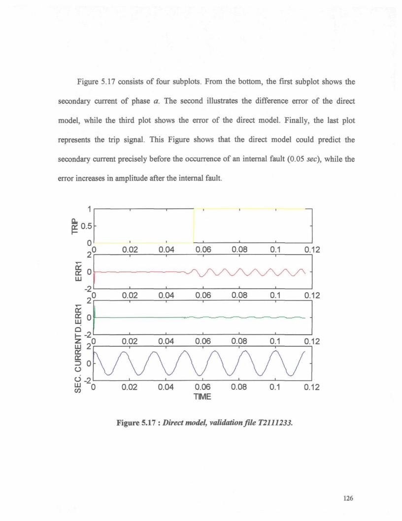
Figure 5.17 consists of four subplots. From the bottom, the first subplot shows the
secondary current of phase a. The second illustrates the difference error of the direct
model, while the third plot shows the error of the direct model. Finally, the last plot
represents the trip signal. This Figure shows that the direct model could predict the
secondary current precisely before the occurrence of an internal fault (0.05 sec), while the
error increases in amplitude after the internal fault.
1
Ê°1 1 t 1 1
P-20
0.02 0.04 0.06 0.08 0.1
0.02 0.04 0.06 0.08 0.1
0.02 0.04 0.06 0.08 0.1
Figure 5.17 : Direct model, validation file T2111233.
0.12
0.12
0.12
0.02 0.04 0.06 0.08 0.1
126
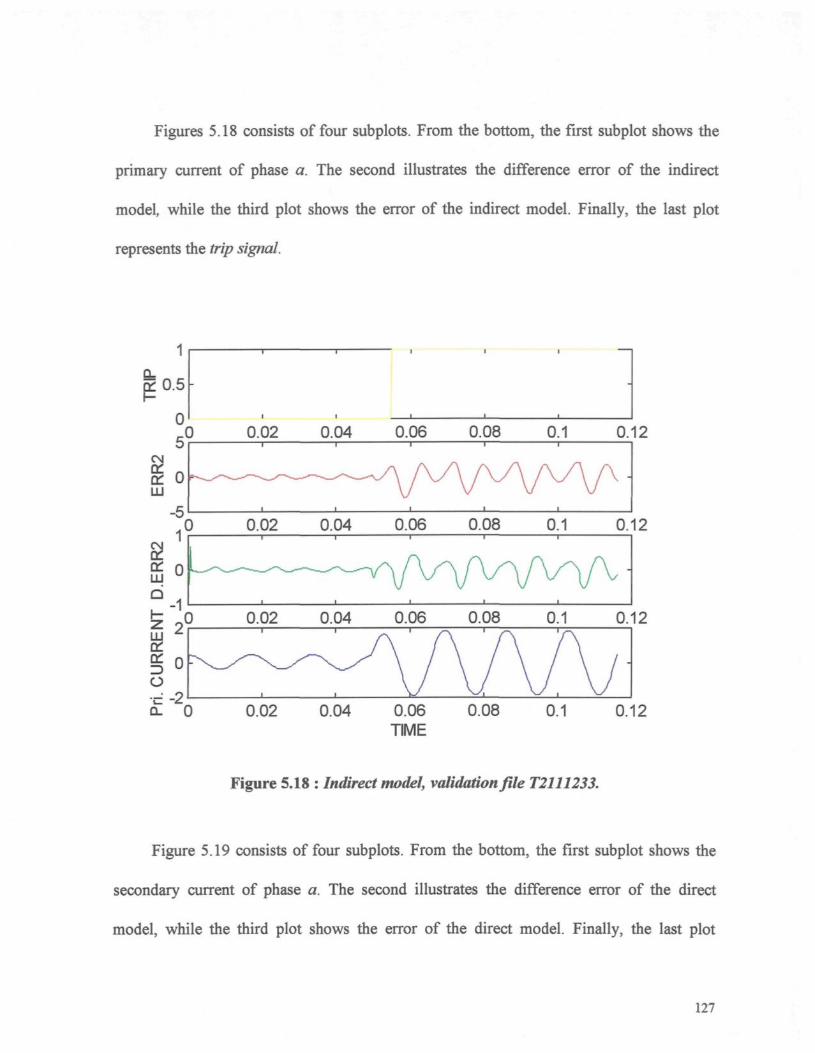
Figures 5.18 consists of four subplots. From the bottom, the first subplot shows the
primary current of phase a. The second illustrates the difference error of the indirect
model, while the third plot shows the error of the indirect model. Finally, the last plot
represents the trip signal.
1
E0.5 -
1 ' J
.0 0.02 0.04 0.06 0.08 0.1
0.02 0.04 0.06 0.08 0.1
0.12
0.12
0.02 0.04 0.06 0.08 0.1
0.02 0.04 0.06 0.08 0.1û- 0
Figure 5.18 : Indirect model, validation file T2111233.
Figure 5.19 consists of four subplots. From the bottom, the first subplot shows the
secondary current of phase a. The second illustrates the difference error of the direct
model, while the third plot shows the error of the direct model. Finally, the last plot
127
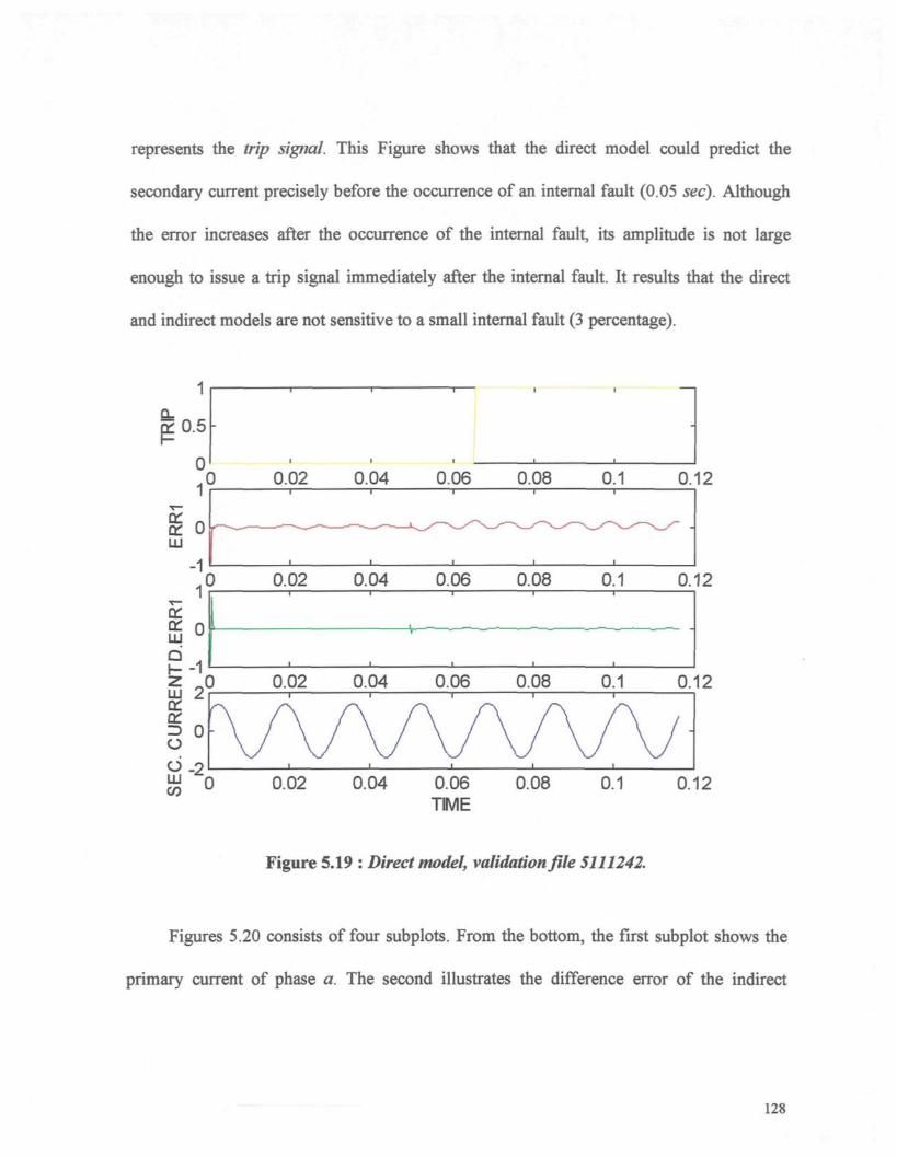
represents the trip signal. This Figure shows that the direct model could predict the
secondary current precisely before the occurrence of an internal fault (0.05 sec). Although
the error increases after the occurrence of the internal fault, its amplitude is not large
enough to issue a trip signal immediately after the internal fault. It results that the direct
and indirect models are not sensitive to a small internal fault (3 percentage).
1
cÉo.51 1 1
-
,0
aia:LLJQ
0.02 0.04 0,06 0.08 0.1 0.12
0.02 0.04 0.06 0.08 0.1 0.12
0.02 0.04 0,06 0.08 0.1 0.12
0.02 0.04 0.06 0.08 0.1
Figure 5.19 : Direct model, validation file 5111242.
Figures 5.20 consists of four subplots. From the bottom, the first subplot shows the
primary current of phase a. The second illustrates the difference error of the indirect
128
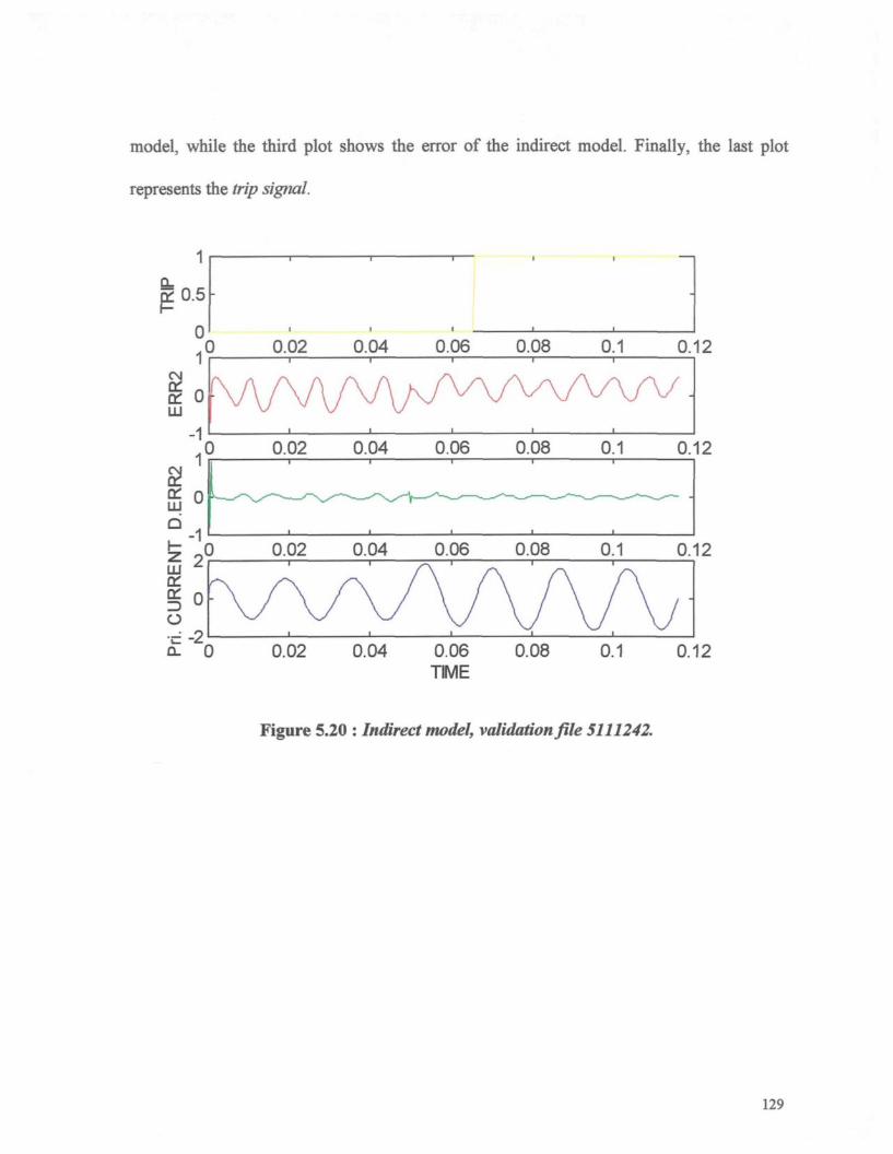
model, while the third plot shows the error of the indirect model. Finally, the last plot
represents the trip signal.
1
S 0.5
H
0I 1
0 0.02 0.04 0,06 0.08 0.1 0.12
0 0.02 0.04 0.06 0.08 0.1 0.12
t
JRR
Ei.
CI
2(
0
n
) 0.02 0.04
A /0.06
vy
0.08
vy
0.1
v A0.
vy0 0.02 0.04 0.06 0.08 0.1 0.12
TIME
Figure 5.20 : Indirect model, validation file 5111242.
129

Chapter 6
Conclusion and Further Works
The work presented in this thesis was undertaken to identify a three-phase nonlinear
power transformer by neuro-fuzzy systems, and to employ this identification system as a
model-based protective relay for the power transformer. Standard identification and control
systems deal with systems that can be represented by a set of differential equations. In
practice, most of the systems cannot be defined by mathematical equations. Therefore, new
approaches like fuzzy logic are employed to identify a system by a set of input/output data.
While other approaches require accurate equations to model real-world behaviors, fuzzy
design can accommodate the ambiguities of real-world human language and logic.
However, there are some very important drawbacks:
� No standard methods exist for transforming human knowledge or experience
into the rule base and database of a fuzzy inference system;
� There is a need for effective methods for tuning the membership function so as
to minimize the output error measure;
� Computing time could be long, because of the complex operations such as
fuzzification and particularly defuzzification.
Neuro-fuzzy systems, which combine the properties of neural networks and fuzzy
logic systems, are a new branch of system identification. It is concerned with the
construction of a fuzzy inference system that can predict and hopefully explain the
behavior of an unknown system described by a set of sample data. The aim of neuro-fuzzy
131
systems is to combine collectively the benefits of both approaches. Simply, the operation of
the system is expressed as linguistic fuzzy expressions, and learning schemes of neural
networks are used to train the system. In addition, neuro-fuzzy systems allow incorporation
of both numerical and linguistic data. The neuro-fuzzy system is also capable of extracting
fuzzy knowledge from numerical data. The main advantages of neuro-fuzzy systems are:
� No need to represent the system by a set of mathematical equations;
� It is possible to implement expert knowledge and experience using comprehensible
linguistic rules;
� It is possible to identify nonlinear systems.
In this research, two neuro-fuzzy models, one direct and one indirect, are developed.
The models were trained by the hybrid learning algorithm which comprises the Least-
Squares Estimator (LSE) and Gradient Descent (GD) methods. Several training files
(including the rated conditions of the power transformer, over load conditions, and external
faults) were employed during the training procedure.
Several unseen data files were applied to the models in order to verify the validation
and the generalization of the models. These data files included the rated conditions and
different types of internal faults. The validation procedure showed that the direct and
indirect models could identify the power transformer accurately during rated conditions
and the amplitude of their errors were small and negligible. However, the errors increased
132
considerably as soon as an internal fault occurred. Therefore, the errors of both models
were used to detect the internal faults. They detected all the internal faults immediately
(except the 3% internal faults in the primary side of the power transformer). Although they
could not detect the 3% internal faults in the primary side of the transformer immediately,
the internal faults were detected after one cycle. This showed that neuro-fuzzy systems can
be employed as an identification and protection system for a power transformer.
A typical modeling problem includes structure determination and parameter
identification. The structure determination problem, which deals with the partition style,
the number of membership function for each input, and the number of fuzzy if-then rules,
and so on, is now an active research topic in the field. As it was explained in chapter 4, the
grid partition was employed. This partition style causes problems , usually referred to as
the curse of dimentionality, in the case of a moderately large number of inputs. It is
suggested to employ another partition style like the tree partition, the scatter partition,
CART (classification and regression tree), and various clustering algorithms to avoid this
problem. This can also decrease the training time.
The identification of the parameters determines a feasible set of parameters under the
given structure. Though the parameter identification problems can be speeded up by
introducing the least-squares estimator into the learning cycle, the gradient descent method
still slows down the training process and the training time could be prohibitively long for a
complicated task like identification of a nonlinear power transformer. Therefore, the need
133

to search for better learning algorithms in order to speed up the training process is very
important.
Detecting an internal fault can be considered as a clustering problem. In this work,
the internal faults were detected based on the amplitude of the errors of both the direct and
indirect models. In other words, if the amplitude of the errors are larger than a threshold
value, a trip signal is issued. Otherwise, it declares that there is no internal fault. However,
determining the threshold value is a time consuming procedure. Therefore, the errors can
be clustered into two groups. Integrating the fuzzy clustering, which is a data clustering
technique where each data point belongs to a cluster to a degree specified by a membership
grade, into the models can improve and automate the fault diagnosis process.
134

References
References
1) Abe S., Lan M.-S., "Fuzzy Rules Extraction Directly from Numerical Data for Function
Approximation", IEEE Transaction On Systems, Man, and Cybernetics, Vol. 25, No. 1,
January 1995.
2) Akira Y., Hiroshi S., Terunobu M. and Yasuo A., "Transformer Protection Relaying
Equipment" HITACI Comments, vol. 61, no. 11, November 1979.
3) Berenji H. R., "Fuzzy logic Controllers" in An Introduction to Fuzzy Logic Applications
in Intelligent Systems, R. R, Yager and L.A. Zadeh, Eds., Kluwer academic publishers,
pp. 69-96, 1992.
4) Brownlee W. R. et al., "Relay Protection of Power Transformers", AIEE Transaction,
vol. 66, pp.911-915, AIEE summer general meeting, Montreal, Quebec, Canada, June 9-
13, 1947.
5) Dolinar D., Pihler J., Grcar B., "Dynamic Model of a Three-Phase Power Transformer",
IEEE/PES Winter Meeting, Columbus USA, February 1993.
136
6) Grcar B., Dolinar D., "Integrated Digital Power Transformer Protection", IEEE Proc.
Gener. Transm. Distrib., 141(4), pp. 323-328, July 1994.
7) Gupta M. M., Rao D. H., "On the principales of fuzzy neural networks", Fuzzy Sets and
Systems, vol. 61, pp. 1-18, 1994.
8) Halgamuge S.K., Glesner M., "Neural networks in designing fuzzy systems for real
world applications", Int. J. Fuzzy Sets and Systems, 1994.
9) Haykin S., "Neural Networks, A Comprehensive Foundation", IEEE Computer Society
Press, Macmillan College Publishing Company, Inc., 1994.
10)Hayward C. D., "HarmonicCurrentRestrained Relays for Transformer Differential
Protection", AIEE Transaction, vol. 60, pp. 377-382, 1941.
ll)Hertz J. Krogh A., Palmer R. G., "Introduction to The Theory of Neural Computing",
Addison-Wesley, New-York, 1991.
12)Horowitz S. H., " Protective Relaying for Power Systems", IEEE Press, The Institute of
Electrical and Electronics Engineers, Inc., New York, pp. 271-175, 1980.
137
13)Ikonen E. & Najim K., "Fuzzy neural networks and application to the FBC process",
IEEProc. Control Theory Applications, vol. 143, no. 3., May 1996.
14)Jang J.-S. R.,"ANFIS: adaptive -network-based fuzzy inference system", IEEE
Tranaction Syst., Man, Cybern., vol. 23, no. 3, pp. 665-685, 1993.
15)Jang J.-S. R., Sun C. T., "Neuro-Fuzzy Modeling and Control", The Proceeding of the
IEEE, March 1995.
16)Jang J.-S. R, Gulley N , "Fuzzy Logic TOOLBOX, For Use with MATLAB", Chapter
2, pp. 53-58, TheMathWorks, Inc., January 1995.
17)Kamwa I., Grondin R.,"Réseaux de Neurones en Commande et Protection, Protection
différentielle neuro-floue", Institut de recherche d'Hydro-Québec, Novembre 1996.
18)Kasztenny B., Rosolowski E., Saha M.M., Hillstrom B., " A Self-Organizing Fuzzy
Logic Based Protective Relay - An Application to Power Transformer Protection",
IEEE paper 96 SM 386-3 PWRD, presented at the 1996 IEEE/PES Summer Meeting,
July 28 - August 1, Denver, Co.
138
19)Kaufmann A., "Le paramétrage des moteurs d'inférence", Hermes, 1988.
20)Kennedy L. F., Hayward CD . , "Harmonic-Current-Restrained Relays for Differential
Protection", AIEE Transactions, vol.57, pp. 262-271, May 1938.
21)Kickert W. J. M., Mamdani E. H., "Analysis of a Fuzzy Logic Controller", Fuzzy Sets
and Systems 7,North Holland Publishing Company, pp. 29-44, 1978.
22)Kohonen T., "An Introduction to Neural Computing", Neural Networks, vol. 1, pp. 3-
16, 1988.
23)Lee C. C.,"Fuzzy logic in control systems: fuzzy logic controller-part 1", IEEE
Transaction On Systems, Man, and Cybernetics, vol. 20, no. 2, pp. 404-418, 1990
24)Lee C. C,"Fuzzy logic in control systems: fuzzy logic controller-part 2", IEEE
Transaction On Systems, Man, and Cybernetics, vol. 20, no. 2, pp. 419-435, 1990
25)Lee S.C., Lee E. T., "Fuzzy neural networks "Mathematical Biosciences, vol. 23, pp.
151-177, 1975.
139
26)Li Y. F., Lau C. C, "Development of Fuzzy Algorithms for Servo Systems", IEEE
International Conferences on Robotics and Automation, Philadelphia, Pennsylvania,
April 1988.
27)Lin B. R.,"Power converter control based on neural and fuzzy methods", Electric
Power Systems Research, 35, pp. 193-206, 1995.
28)Lippmann R. P., "An Introduction to Computing with Neural Nets", IEEE ASSP
Magazine, pp. 4-22, April 1987.
29)Liu P., Malik O. P., Chen D. and Hope G.S., "Study of Non-Operation for Internal
Faults of SecondHarmonic Restraint Differential Protection of Power Transformers",
Transaction of the Engineering and Operating Division of the Canadian Electrical
Association, vol. 28, part 3, pp. 1-23, 1989.
30)Mamdani E. H., Assilian S., "An Experiment in Linguistic Synthesis With a fuzzy
Logic Controller", Int. Journal of Man-Machine Studies, vol. 7, no. 1, pp. 1-13, 1975.
31)McCulloch W., Pitts W., "A logical calculus of the ideas immanent in nervous activity",
Bulletin of Mathematical Biophysics, vol. 5, pp. 115-133, 1943.
140
32)Narendra K. S., Parthasarathy K., "Identification and Control of Dynamical Systems
Using Neural Networks", IEEE Transaction On Neural networks, vol. 1, no. 1, pp. 4-27,
March 1990.
33)Nie J., Linkens D. A., "Learning control using fuzzified self-organizing radial basis
function network", IEEE Transaction On Fuzzy Systems, vol. 1, no. 4, pp. 280-287,
1993.
34)Pal S. K., Mitra S., "Multilayer perceptron, fuzzy set, and classification", IEEE
Transaction On Neural Networks, vol. 3, pp. 683-697, 1992
35)Pedrycz W., "Fuzzy neural networks with reference neurons as pattern classifiers",
IEEE Transaction On Neural Networks, vol. 3, no. 5, pp. 770-775, 1992.
36)Perez L. G., Flechsig A. J., Meador J. L., Obradovic Z.,"Training an Artificial Neural
Network to Discriminate between Magnetizing and Internal Faults", IEEE/PES Winter
Meeting, Columbus, OH, January 31 - February 5, 1993.
37)Pihler J., Grcar B., Dolinar D.," Improved Operation of Power Transformer Protection
using Artificial Neural Network ", IEEE / PES Summer Meeting, Denver, Colorado,
July 28-August 1,1996.
141
38)Rahman M. A. & Jeyasurys B.,"A state-of-the-art review of transformer protection
algorithms", IEEE Transactions on Power Delivery, vol.3, no.2, pp. 534-544, April
1988.
39)Sachdev M.S. & Shah D.V., "Transformer Differential and Restricted Earth Fault
Protection Using a Digital Processor", Transactions of the Engineering and Operating
Division of the Canadian Electrical Association, vol. 2, part 4, pp. 1-11, March 1981.
40)Schweitzer E.O. & Larson R.R, "An Efficient Inrush Detection Algorithm for Digital
Computer Relay Protection of Transformers", IEEE PES Summer Meeting, Paper no. 77
510-1, Mexico City.
41)Skyes J. A.& Morrison I.F.,"A Proposed Method of Harmonic Restraint Differential
Protection of Transformers By Digital Computer" IEEE Transactions on Power
Apparatus and Systems, vol. PAS-91, pp. 1266-1272, May/June 1977.
42)Takagi T., Sugeno M., "Derivation of fuzzy control rules from human operator's
control actions", Proc. Of the IFAC Symp. On Fuzzy Information, knowledge
Representation and decision Analysis, pp. 55-60, July 1983
142
43)Takagi T., Sugeno M., "Fuzzy identification of systems and its applications to modeling
and control ", IEEE Transaction On Systems, Man, and Cybernetics, vol. 15, no. 1, pp.
116-132, 1985
44)Tani T., Murakoshi S., and Umano M.,"Neuro-Fuzzy Hybrid Control System of Tank
Level in Petroleum Plant", IEEE Transactions on Fuzzy Systems, vol. 4, no. 3, August
1996.
45)Tsukamoto Y., "An approach to fuzzy reasoning method", In Madan M. Gupta,
Rammohan K. Ragade, and Ronald R. Yager, editors, Advances in Fuzzy Set Theory and
Applications, pp. 137-149, North-Holland, Amsterdam, 1979.
46)Vuorimaa P., Jukarainen T., and Kàrpânoja E., "A Neuro-Fuzzy System for Chemical
Agent Detection", IEEE Transactions on Fuzzy Systems, vol. 3, no. 4, November 1995.
47)Wang L. X., "Adaptive Fuzzy Systems and Control, Design and Stability Analysis",
Prentice-Hall, Inc., 1994.
48)Wang L. X., Mendel J. M., "Fuzzy basis functions, universal approximation, and
orthogonal least-squares learning" IEEE Transaction On Neural Networks, vol. 3, no. 5,
pp. 807-814, 1992.
143
49)Yabe K., "Power Differential Method for Discrimination between Fault and
Magnetizing Inrush Current in Transformers" IEEE/PES Summer Meeting, Denver,
Colorado, July 28- August 1, 1996.
50)ZadehL. A., "Fuzzy Sets", Inform. Control, vol. 8, pp. 338-353, 1965.
51)Zadeh L. A., "A fuzzy-set theoretic interpretation of linguistic hedges", J. Cybem., vol.
2, pp. 4-34, 1972.
52)Zadeh L. A., "Outline of a new approach to the analysis of complex system and
decision processes",/£££ Trans. Syst. Man, Cybern., vol. SMC-3, no. 1, pp. 28-44,
1973.
53)Zimmermann H. J., "Fuzzy sets, Decision Making, and Expert Systems", Kluwer
Academic Publisher, Boston, 1987
54)Zimmermann H. J., "Fuzzy Set Theory - and Its Applications", Kluwer Academic
Publishers, 1990.
144