ORSAYNo D’ORDRE : 8515

UNIVERSITÉ PARIS XIU.F.R. SCIENTIFIQUE D’ORSAY

THÈSE

présentée pour obtenir le grade de

DOCTEUR EN SCIENCESDE L’UNIVERSITÉ PARIS XI ORSAY

SPÉCIALITÉ : MATHÉMATIQUES

par

Marie SAUVÉ

SÉLECTION DE MODÈLES EN RÉGRESSION NONGAUSSIENNE. APPLICATIONS À LA SÉLECTION DEVARIABLES ET AUX TESTS DE SURVIE ACCÉLÉRÉS.

Rapporteurs : Mme Fabienne COMTEM. Gérard GRÉGOIRE

Soutenue le 11 décembre 2006 devant le jury composé de :

Mme Fabienne COMTE RapporteurMme Elisabeth GASSIAT PrésidenteM. Gérard GRÉGOIRE RapporteurMme Sylvie HUET ExaminatriceM. Pascal MASSART Directeur de ThèseM. Jean-Michel POGGI Examinateur

Remerciements

Un grand merci à Pascal avec qui j’ai découvert les statistiques en maîtrise, puis la sélectionde modèles en DEA et en thèse. Chacune de nos discussions a été riche d’enseignements etde plaisir. Merci de m’avoir guidée et motivée, d’avoir été à la fois présent et discret.

Je remercie Fabienne Comte, Elisabeth Gassiat, Gérard Grégoire, Sylvie Huet et Jean-MichelPoggi qui me font l’honneur et le plaisir de participer au jury de cette thèse. Un merci parti-culier à Fabienne Comte et Gérard Grégoire pour avoir rapporté mon travail.

Je tiens à remercier sincèrement Bernard Besançon, mon professeur de math spé, qui m’afait découvrir et aimer les mathématiques. Ses cours passionants m’ont donné les moyens etl’envie de poursuivre.

Je remercie aussi tous mes professeurs d’Orsay et en particulier Alano Ancona, Lucile Bégueri,Raphaël Cerf, Jacques Chaumat, Jean Coursol, Béatrice Laurent et Wendelin Werner pourleurs cours à la fois bien construits et ouverts à la réflexion.

Merci à toute l’équipe de Probabilités et Statistiques pour leur sympathie, leur disponibilitéet leurs coups de pouce en informatique. Merci en particulier à Didier Dacunha-Castelle,Elisabeth Gassiat et Marc Lavielle pour leur soutien.

Merci aux doctorants ou ex-doctorants: Aurélien, Besma, Christine, Gilles, Ismaël B et C,Laurent, Magalie, Marc, Marion, Mina, Nicolas, Sébastien, Sophie et tous les autres pour leurprésence et leur amitié. Merci surtout à Christine pour nos discussions mathématiques etautres, et pour tous ses petits conseils pratiques. Merci aussi à Marc de m’avoir initiée à lafiabilité.

Un grand merci également à Thomas Lafforgue et Luc Abergel pour leur aide, leur soutien etleurs précieux conseils.

Mille mercis à Françoise pour sa présence, son écoute, et sa bonne humeur communicative.Ce fut une chance pour moi de l’avoir eu à mes côtés durant ces années.

A mes parents, mon frère, mes grands-parents et mes beau-parents pour leur soutien et leurfierté. A Guillaume pour tellement.

Résumé

Cette thèse traite de la sélection de modèles en régression non gaussienne. Notre but estd’obtenir des informations sur une fonction s : X → R dont on ne connaît qu’un certainnombre de valeurs perturbées par des bruits non nécessairement gaussiens. Nous adoptonsl’approche non asymptotique de la sélection de modèles par minimisation d’un critère desmoindres carrés pénalisés. Nous considérons une collection de modèles (Sm)m∈Mn . ChaqueSm est une classe de fonctions définies sur X et à valeurs dans R à laquelle nous associonsl’estimateur sm des moindres carrés sur Sm. Nous déterminons des critères pénalisés quipermettent de sélectionner un modèle Sm approximativement optimal au sens où le risque del’estimateur pénalisé sm est comparable à l’infimum des risques des (sm)m∈Mn . Pour chaquepénalité proposée, nous donnons une borne de risque non asymptotique. Nous utilisons lasélection de modèles pour estimer s sans faire d’hypothèses a priori et nous envisageons ladétection de ruptures et la sélection de variables comme des cas particuliers de sélection demodèles.

Dans un premier temps, nous considérons des modèles de fonctions constantes par morceauxassociés à une collection de partitions de X . Nous déterminons un critère des moindres carréspénalisés qui permet de sélectionner une partition dont l’estimateur associé (de type regresso-gramme) vérifie une inégalité de type oracle. La sélection d’un modèle de fonctions constantespar morceaux ne conduit pas en général à une bonne estimation de s, mais permet notammentde détecter les ruptures de s. Nous proposons aussi une méthode non linéaire de sélectionde variables qui repose sur l’application de plusieurs procédures CART et sur la sélectiond’un modèle de fonctions constantes par morceaux. CART permet d’associer à chaque pa-quet de variables une série de modèles de fonctions constantes par morceaux construits surles variables du paquet considéré. Puis nous déterminons un critère pénalisé permettant desélectionner un modèle et le paquet de variables sous-jacent.

Dans un deuxième temps, nous considérons des modèles de fonctions polynomiales parmorceaux, dont les qualités d’approximation sont meilleures. L’objectif est d’estimer s parun polynôme par morceaux dont le degré peut varier d’un morceau à l’autre. Nous détermi-nons un critère pénalisé qui sélectionne une partition de X = [0, 1]p et une série de degrésdont l’estimateur polynomial par morceaux associé vérifie une inégalité de type oracle. Nousappliquons aussi ce résultat pour détecter les ruptures d’un signal affine par morceaux. Cedernier travail est motivé par la détermination d’un intervalle de stress convenable pour lestests accélérés visant à obtenir dans des délais raisonnables des informations sur le temps desurvie de certains composants.

Contents

Introduction 3

1 Histogram selection in non Gaussian regression 191.1 Introduction . . . . . . . . . . . . . . . . . . . . . . . . . . . . . . . . . . . . . 191.2 The statistical framework . . . . . . . . . . . . . . . . . . . . . . . . . . . . . 22

1.2.1 The random perturbations . . . . . . . . . . . . . . . . . . . . . . . . . 221.2.2 The piecewise constant estimators . . . . . . . . . . . . . . . . . . . . 23

1.3 The main theorem . . . . . . . . . . . . . . . . . . . . . . . . . . . . . . . . . 241.4 A concentration inequality for a χ2 like statistic . . . . . . . . . . . . . . . . . 271.5 Proof of lemma 1.1 . . . . . . . . . . . . . . . . . . . . . . . . . . . . . . . . . 301.6 Proof of the theorem . . . . . . . . . . . . . . . . . . . . . . . . . . . . . . . . 32

2 Variable Selection through CART 372.1 Introduction . . . . . . . . . . . . . . . . . . . . . . . . . . . . . . . . . . . . . 372.2 Preliminaries . . . . . . . . . . . . . . . . . . . . . . . . . . . . . . . . . . . . 40

2.2.1 Overview of CART . . . . . . . . . . . . . . . . . . . . . . . . . . . . . 402.2.2 The context . . . . . . . . . . . . . . . . . . . . . . . . . . . . . . . . . 41

2.3 Regression . . . . . . . . . . . . . . . . . . . . . . . . . . . . . . . . . . . . . . 422.3.1 Variable selection via (M1) and (M2) . . . . . . . . . . . . . . . . . . 422.3.2 Final selection . . . . . . . . . . . . . . . . . . . . . . . . . . . . . . . 45

2.4 Classification . . . . . . . . . . . . . . . . . . . . . . . . . . . . . . . . . . . . 462.4.1 Variable selection via (M1) and (M2) . . . . . . . . . . . . . . . . . . 462.4.2 Final selection . . . . . . . . . . . . . . . . . . . . . . . . . . . . . . . 48

2.5 Simulations . . . . . . . . . . . . . . . . . . . . . . . . . . . . . . . . . . . . . 482.6 Appendix . . . . . . . . . . . . . . . . . . . . . . . . . . . . . . . . . . . . . . 51

2.6.1 Useful lemmas in the regression framework . . . . . . . . . . . . . . . 522.6.2 Useful lemmas in the classification framework . . . . . . . . . . . . . . 53

2.7 Proofs . . . . . . . . . . . . . . . . . . . . . . . . . . . . . . . . . . . . . . . . 562.7.1 Regression . . . . . . . . . . . . . . . . . . . . . . . . . . . . . . . . . . 562.7.2 Classification . . . . . . . . . . . . . . . . . . . . . . . . . . . . . . . . 62

3 Piecewise polynomial estimation of a regression function 673.1 Introduction . . . . . . . . . . . . . . . . . . . . . . . . . . . . . . . . . . . . . 673.2 The statistical framework . . . . . . . . . . . . . . . . . . . . . . . . . . . . . 693.3 The main theorem . . . . . . . . . . . . . . . . . . . . . . . . . . . . . . . . . 713.4 CART extension to piecewise polynomial estimation . . . . . . . . . . . . . . 75

3.4.1 An overview of CART . . . . . . . . . . . . . . . . . . . . . . . . . . . 76

1

3.4.2 CART extension to piecewise polynomial estimation . . . . . . . . . . 773.4.3 Some comments on MARS . . . . . . . . . . . . . . . . . . . . . . . . . 83

3.5 A concentration inequality for a χ2 like statistic . . . . . . . . . . . . . . . . . 853.6 Proof of lemma 3.3 . . . . . . . . . . . . . . . . . . . . . . . . . . . . . . . . . 873.7 Proof of the theorem . . . . . . . . . . . . . . . . . . . . . . . . . . . . . . . . 92

4 Application to Accelerating Life Test 974.1 Introduction . . . . . . . . . . . . . . . . . . . . . . . . . . . . . . . . . . . . . 974.2 The statistical framework . . . . . . . . . . . . . . . . . . . . . . . . . . . . . 1004.3 The main theorem . . . . . . . . . . . . . . . . . . . . . . . . . . . . . . . . . 1014.4 First method . . . . . . . . . . . . . . . . . . . . . . . . . . . . . . . . . . . . 105

4.4.1 Massart’s heuristic . . . . . . . . . . . . . . . . . . . . . . . . . . . . . 1054.4.2 Results obtained on simulated data . . . . . . . . . . . . . . . . . . . . 106

4.5 Second method . . . . . . . . . . . . . . . . . . . . . . . . . . . . . . . . . . . 1094.5.1 A simulation study to determine the constant c. . . . . . . . . . . . . . 1104.5.2 A practical rule to determine λ according to the data. . . . . . . . . . 113

A MARS 117

Bibliography 122

2

Introduction

Notre travail se situe dans le cadre statistique d’un modèle de régression multivariée. Nousétudions le comportement d’une variable réelle Y (appelée variable réponse) en fonction d’uneou plusieurs variables explicatives x1, . . . , xp. Nous notons x le p-uplet (x1, . . . , xp) et Xl’ensemble des valeurs possibles pour x (X = Rp en général). Nous supposons que

Y = s(x1, . . . , xp) + ε (1)

où s : X −→ R est une fonction inconnue qui donne la relation entre x = (x1, . . . , xp) et Y , etoù ε est une perturbation aléatoire d’espérance nulle (conditionnellement à x). ε correspondsoit à des erreurs de mesure, soit à la dépendance de Y vis à vis de quantités autres que(x1, . . . , xp) qui ne sont ni contrôlées ni observées. Notre but est d’obtenir des informationssur s à partir d’un échantillon de n observations (x1

i , . . . , xpi , Yi)1≤i≤n obéissant à la relation

(1). Nous utilisons les données (x1i , . . . , x

pi , Yi)1≤i≤n pour résoudre trois problèmes classiques

en statistique:

• l’estimation de s, qui consiste à approcher la fonction inconnue s par une fonctionmesurable des observations (x1

i , . . . , xpi , Yi)1≤i≤n (une telle fonction est appelée un esti-

mateur et est notée s),

• la sélection de variables, qui consiste à déterminer un petit nombre de variables parmix1, . . . , xp permettant à elles seules de bien expliquer ou prédire la réponse Y ,

• la détection de ruptures, qui consiste à localiser des ruptures dans le comportement dela fonction s.

Dans la suite, nous appelons modèle tout espace vectoriel de fonctions définies sur X et àvaleurs dans R, et nous abordons chacun des trois problèmes cités ci-dessus sous l’angle de lasélection de modèles. Nous adoptons l’approche non asymptotique de la sélection de modèlespar pénalisation développée par Birgé et Massart [3, 4] dans un cadre gaussien très général.Leurs résultats s’appliquent en particulier lorsque que l’on observe n couples (xi, Yi)1≤i≤n véri-fiant (1) avec des xi déterministes et des perturbations aléatoires εi indépendantes, centréeset de même loi gaussienne. Dans notre étude, nous ne supposerons pas que les erreurs sontgaussiennes. Nous supposerons seulement qu’elles ont des moments exponentiels au voisinagede 0.

Dans le premier chapitre, nous considérons des modèles de fonctions constantes par morceaux.Nous déterminons un critère des moindres carrés pénalisés qui permet de sélectionner un mod-èle de fonctions constantes par morceaux dont l’estimateur associé (de type regressogramme)

3

vérifie une inégalité de type oracle. Les modèles de fonctions constantes par morceaux ontl’avantage d’être simples, mais ils sont parfois trop frustes pour permettre une bonne estima-tion de la fonction s. Ils permettent en revanche de détecter des ruptures dans la moyenned’un signal. Le travail d’Emilie Lebarbier [16] sur la détection de ruptures dans la moyenned’un signal gaussien s’appuie sur le résultat de sélection de modèles de Birgé et Massart [3],qu’elle applique à une collection de modèles de fonctions constantes par morceaux. Pour unetelle collection de modèles, nous avons pu relaxer l’hypothèse gaussienne. Il est donc possibled’étendre le travail d’Emilie Lebarbier à un cadre non gaussien. Le résultat de ce chapitrepermet aussi de justifier l’étape d’élagage de l’algorithme CART [7] dans un cadre de régres-sion non gaussienne.

Dans le deuxième chapitre, nous proposons une méthode non linéaire de sélection devariables qui repose sur l’application de plusieurs procédures CART. Nous justifions notreméthode dans un cadre de régression non gaussienne par le biais d’inégalités de type oracle.Le résultat du premier chapitre permet de démontrer ce nouveau résultat. Notre méthode desélection de variables s’applique aussi dans le cadre de la classification binaire, mais dans cecas la démonstration repose sur une inégalité de concentration due à Talagrand.

Le troisième chapitre traite de l’estimation d’une fonction de régression s par un polynômepar morceaux dont le degré peut varier d’un morceau à l’autre. Nous déterminons un critèrepénalisé qui sélectionne une partition de X = [0, 1]p et une série de degrés dont l’estimateurpolynomial par morceaux associé vérifie une inégalité de type oracle. Ce résultat généralisecelui du premier chapitre. Il permet de valider la procédure d’estimation de Comte et Rozen-holc [10] dans un cadre un peu plus général (non nécessairement sous-gaussien) et de mieuxcomprendre l’algorithme MARS de Friedman [12]. Nous proposons aussi une extension del’algorithme CART pour construire un estimateur polynomial par morceaux.

Dans le quatrième chapitre, nous appliquons le résultat sur la sélection d’un modèle poly-nomial par morceaux du chapitre 3 pour détecter les ruptures d’un signal affine par morceaux(ou approché par une fonction affine par morceaux). Nous proposons deux méthodes pourcalibrer les constantes de la pénalité donnée par le théorème du chapitre 3. Ce travail est mo-tivé par la détermination d’un intervalle de stress convenable pour les tests accélérés visantà obtenir dans des délais raisonnables des informations sur le temps de survie de certainscomposants.

Avant de décrire plus précisément les travaux mentionnés ci-dessus, nous présentons laméthode d’estimation par minimisation du contraste des moindres carrés et les principes dela sélection de modèles.

Prédiction et estimation

Dans le cadre de la régression définie par (1), nous appelons prédicteur toute fonction mesurableu : X −→ R. Soit (xi, Yi)1≤i≤n n observations vérifiant (1). s est le meilleur prédicteur au

4

sens où il minimise E[γn(u)], γn étant le contraste des moindres carrés:

γn(u) =1

n

n∑

i=1

(Yi − u(xi))2.

La qualité d’un prédicteur u est alors mesurée par sa perte relative:

l(s, u) = E[γn(u)] − E[γn(s)]

=

∥s− u∥2n si les xi sont déterministes

∥s− u∥2µ si les xi sont des variables aléatoires indépendantes et de même loi µ

où ∥.∥µ est la norme de L2(µ), ∥.∥n est la norme euclidienne de Rn divisée par√

n, et où l’onnote de la même façon une fonction u et le vecteur associé (u(xi))1≤i≤n ∈ Rn.

Remarque 0.1 Lorsque les xi seront considérés aléatoires, nous les noterons Xi au lieu dexi.

s étant inconnue, on veut construire un estimateur s à partir des données qui soit le plusproche possible de s au sens où son risque E[l(s, s)] est le plus petit possible. Une méthodeclassique pour estimer s consiste à minimiser le contraste γn sur un modèle S. L’estimateurainsi obtenu est noté sS et est appelé l’estimateur des moindres carrés associé à S. Lorsqueles points xi sont déterministes, le risque de sS s’écrit:

E(

∥s− sS∥2n)

= infu∈S∥s− u∥2n +

τ2

ndimRn(S) où τ2 = E(ε2i ). (2)

Le premier terme, appelé le terme de biais, représente l’erreur d’approximation du modèleS. Le deuxième terme, appelé le terme de variance, représente l’erreur d’estimation dans lemodèle S. Plus le modèle S est gros, plus on améliore les qualités d’approximation et doncplus le terme de biais est petit, mais plus on commet d’erreurs d’estimation et donc plus leterme de variance est grand. Inversement, plus le modèle S est petit, plus le terme de biaisest grand, mais plus le terme de variance est petit. Pour obtenir un bon estimateur de s,il faut déterminer un modèle S qui fait un bon compromis entre le biais et la variance. Cedernier point est l’objectif de la sélection de modèles.

Sélection de modèles

Nous décrivons ici l’approche non asymptotique de la sélection de modèles par pénalisationdéveloppée par Birgé et Massart [3, 4].

Soit (Sm)m∈Mn une collection de modèles dont le nombre peut dépendre de la taille nde l’échantillon des observations. Nous considérons la collection (sm)m∈Mn des estimateursdes moindres carrés associés aux modèles (Sm)m∈Mn . Le modèle idéal m∗ est celui dontl’estimateur associé sm∗ a le plus petit risque:

m∗ = arg minm∈Mn

E(

∥s− sm∥2n)

.

5

Comme m∗ dépend de s, sm∗ ne peut pas être utilisé comme estimateur de s. Le butde la sélection de modèles est de construire un modèle m à partir des données tel que lerisque de l’estimateur associé sm soit le plus proche possible de l’oracle: E

(

∥s − sm∗∥2n)

=inf

m∈Mn

E(

∥s− sm∥2n)

. Vu l’expression (2) du risque, m doit pour cela faire un bon compromis

entre le biais et la variance. L’idée consiste à sélectionner un modèle m en minimisant uncritère des moindres carrés pénalisés:

crit(m) = γn(sm) + pen(m) (3)

où le terme pen(m) pénalise les gros modèles Sm. L’estimateur sm associé au modèle mainsi choisi est appelé l’estimateur des moindres carrés pénalisés. Le but de l’approche nonasymptotique est de déterminer une pénalité pen(m) telle que l’estimateur des moindres carréspénalisés sm vérifie:

E(

∥s− sm∥2n)

≤ C infm∈Mn

E(

∥s− sm∥2n)

(4)

où C est une constante supérieure à 1 et le plus proche possible de 1. Une telle inégalité estappelée inégalité oracle.

Le premier critère pénalisé de type (3) est du à Mallows [17]. Il est issu de l’heuristiquedécrite ci-après. Notons sm = arg min

u∈Sm

∥s− u∥2n et Dm = dimRn(Sm). D’après la décomposi-

tion du risque en biais-variance (2) et d’après Pythagore, m∗ minimise

m −→ −∥sm∥2n +τ2

nDm (5)

L’heuristique de Mallows consiste à dire qu’en remplaçant ∥sm∥2n dans (5) par un estimateursans biais, on obtient un minimiseur m dont les performances sont proches de l’oracle. CommeE(

∥sm∥2n)

= ∥sm∥2n + τ2

n Dm, ∥sm∥2n − τ2

n Dm est un estimateur sans biais de ∥sm∥2n, et onobtient −∥sm∥2n + 2 τ2

n Dm = −∥Y ∥2n + γn(sm)+ 2 τ2

n Dm. Le critère Cp de Mallows [17] s’écrit:

Cp(m) = γn(sm) + 2τ2

nDm.

Ce critère est un critère pénalisé de type (3) avec pen(m) = 2 τ2

n Dm. Lorsque la varianceτ2 = E(ε2i ) est inconnue, on peut la remplacer par un estimateur.Le critère Cp de Mallows ne donne de bons résultats que si le nombre de modèles de dimensiondonnée n’est pas trop grand. Pour que l’heuristique de Mallows fonctionne, il faudrait que∥sm∥2n soit du même ordre de grandeur que son espérance pour tous les modèles m ∈ Mn

simultanément. Pour obtenir une pénalité qui sélectionne un m proche de m∗ en terme derisque, on ne peut pas se contenter de remplacer ∥sm∥2n par ∥sm∥2n− τ2

n Dm. Il faut étudier lesdéviations de ∥sm∥2n−∥sm∥2n autour de son espérance ( τ2

n Dm), et choisir une pénalité qui lescompense. Les outils essentiels dans la détermination d’une bonne pénalité sont les inégalitésde concentration.

6

Résultats de Birgé et Massart dans un cadre gaussien:

Dans un cadre gaussien, grâce à une inégalité de concentration pour la somme d’un χ2 etd’une gaussienne [4, Appendix,lemma 1], Birgé et Massart ont obtenu une inégalité de typeoracle pour une pénalité de la forme:

pen(m) = Kτ2

n

(

Dm + a√

Dmxm + bxm

)

(6)

où K > 1, a > 2 et b > 2 sont trois constantes, et où (xm)m∈Mn est une famille de poidsvérifiant:

∑

m∈Mn

e−xm ≤ Σ, Σ ∈ R∗+. (7)

La pénalité dépend de la complexité de la collection de modèles (Sm)m∈Mn via les poids(xm)m∈Mn .Lorsque le nombre de modèles de dimension D donnée n’est pas trop gros, plus précisémentlorsque | m ∈Mn; Dm = D | ≤ ΓDr avec Γ ∈ R∗

+ et r ∈ N, alors les poids xm = LDm

vérifient (7) pour tout L > 0, et donc pen(m) = K ′ τ2

n Dm avec K ′ > 1 convient. Le critèreCp de Mallows (qui correspond à K ′ = 2) est alors validé.

Lorsque le nombre de modèles de dimension D est beaucoup plus gros, de l’ordre de(

ND

)

avec N grand, alors il faut prendre des poids plus gros et donc une pénalité plus forte. Danscette situation, Birgé et Massart [4] ont montré que le critère de Mallows peut donner de trèsmauvais résultats.

Résultats dans un cadre non gaussien:

Dans un cadre de régression non gaussienne, la difficulté pour déterminer une bonne pénalitéet obtenir un résultat du type [4, theorem 1] de Birgé et Massart est de contrôler les déviationsdes statistiques χ2

m = ∥εm∥2n où εm = arg minu∈Sm

∥ε − u∥2n. Si E (|εi|p) < +∞ pour un p ≥ 2,

Baraud [1, Corollary 5.1] a montré que pour tout x > 0

P

(

χ2m ≥

τ2

nDm + 2

τ2

n

√

Dmx +τ2

nx

)

≤ C(p)E (|εi|p)τp

Dmx−p/2. (8)

Lorsque | m ∈Mn; Dm = D | ≤ ΓDr, en supposant seulement que les perturbations εiont des moments d’ordre p > 2r + 6, Baraud [1] en a déduit qu’une pénalité de la formepen(m) = K ′ τ2

n Dm avec K ′ > 1 permet encore d’obtenir une inégalité de type oracle.Nous aimerions déterminer, au delà du résultat de Baraud, une pénalité générale (telle que lapénalité (6)) qui permet d’obtenir une inégalité de type oracle quelle que soit la complexitéde la collection de modèles. Pour obtenir son résultat, Baraud a du supposer que les εiont des moments d’ordre p > 2r + 6 où r est le degré du polynôme majorant la complexitéde la collection de modèles. La valeur minimale admissible pour p croît avec le degré rde la complexité. Pour traiter des collections de modèles de complexité exponentielle, noussupposerons que les εi ont des moments exponentiels au voisinage de 0. Cela revient à supposerqu’il existe deux constantes b ≥ 0 et σ > 0 telles que:

pour tout λ ∈ (−1/b, 1/b) log E(

eλεi

)

≤ σ2λ2

2(1− b|λ|) . (9)

7

σ2 est nécessairement supérieur à τ2 = E(ε2i ), mais il peut être choisi aussi proche de τ2 quel’on veut à condition de prendre un plus grand b.

Nous venons de voir que la sélection de modèles permet de déterminer un estimateurdont le risque est petit relativement aux risques des estimateurs associés aux modèles d’unecollection donnée. Elle permet aussi de répondre à des problèmes plus spécifiques comme lasélection de variables ou la détection de ruptures.

Sélection de variables

Etant donnée une liste de variables x1, . . . , xp, le but de la sélection de variables est de déter-miner un petit nombre de variables qui suffisent à elles seules à bien expliquer ou prédire laréponse.

Dans le cadre particulier de la régression linéaire, s(x) =∑p

j=1 αjxj et donc (1) devient:

Y =p∑

j=1

αjxj + ε.

L’estimateur des moindres carrés s(x) =∑p

j=1 αjxj avec α = arg minα

1n

∑ni=1

(

Yi −∑p

j=1 αjxji

)2

est non biaisé mais, lorsque le nombre p de variables est grand, sa variance est grande. Lerisque de s peut être amélioré en diminuant ou en éliminant certains coefficients αj , de façonà réduire le terme de variance quitte à augmenter un peu le terme de biais. En éliminantcertains coefficients (cad en éliminant certaines variables), on gagne aussi en interprétabilité.

Les méthodes Ridge Regression et Lasso (voir [15]) sont des versions pénalisées de la méth-ode des moindres carrés. Pour Ridge Regression, la pénalité est proportionnelle à la normel2 de α = (α1, . . . ,αp). Cette méthode donne des coefficients αj plus petits et un meilleurestimateur s au sens du risque. Pour Lasso, la pénalité est proportionnelle à la norme l1

de α = (α1, . . . ,αp). Lasso réduit certains coefficients et en élimine certains autres. Cetteméthode améliore aussi le risque et permet en plus d’obtenir un estimateur plus simple, quifait intervenir un plus petit nombre de variables. Avec Lasso, on gagne à la fois en terme derisque et en interprétabilité. Malheureusement son coût algorithmique est très élevé.

Un autre moyen de construire un estimateur de risque petit et qui soit facile à interpréterconsiste à déterminer pour chaque K ∈ 0, 1, . . . , p le paquet de K variables qui minimisele critère des moindres carrés. L’algorithme de Furnival et Wilson [13] permet de faire cetterecherche pour p ≤ 40. Il faut ensuite choisir K en estimant par exemple les risques parvalidation croisée (ou grâce à un échantillon test).

Nous pouvons aussi adopter une approche de sélection de modèles, en associant à chaquepaquet M de variables (i.e. M sous-ensemble de x1, . . . , xp) le modèle SM des fonctionslinéaires en les variables de M ainsi que l’estimateur sM des moindres carrés de s sur SM .

8

Nous sélectionnons un paquet M en minimisant un critère pénalisé:

crit(M) = γn(sM ) + pen(M)

avec une pénalité pen(M) qui pénalise les gros paquets de variables, et qui doit être choisiede façon à ce que l’estimateur sM vérifie une inégalité de type oracle. En général, la pénalitépen(M) ne dépend du paquet M que via le nombre de variables qu’il contient: KM = |M |.Nous choisissons donc pour chaque K ∈ 0, 1, . . . , p le paquet de K variables MK qui min-imise le critère des moindres carrés. La pénalité permet de choisir le nombre K tel que lemodèle associé fait un bon compromis entre le biais et la variance.

En associant à chaque paquet de variables M , le modèle SM des fonctions linéaires en lesvariables de M , nous nous somme ramenés au problème de sélection d’un modèle, et nouspouvons donc appliquer les résultats précédents. Si l’on considère uniquement les paquetsde variables de la forme M = x1, . . . , xj, avec 1 ≤ j ≤ p, alors une pénalité de la formepen(M) = K ′ τ2

n |M | convient comme le démontre le résultat de Birgé et Massart [3, 4] dans uncadre gaussien et comme le confirme le résultat de Baraud [1] dans un cadre non gaussien. Si

l’on considère tous les paquets possibles, alors |M ; |M | = K| =

(

pK

)

et Birgé et Massart

[4] montre que la pénalité précédente n’est plus suffisante. Dans ce cas, nous disposons d’unepénalité validée uniquement dans le cadre gaussien.

Les méthodes de sélection de variables discutées ci-dessus sont des méthodes linéairesde sélection de variables dans le sens où elles considèrent des interactions linéaires entre lesvariables explicatives et la réponse. Dans le chapitre 2, nous proposons une méthode nonlinéaire de sélection de variables. Nous adoptons une approche sélection de modèles, mais aulieu d’associer à chaque paquet M de variables le modèle SM des fonctions linéaires en lesvariables de M , nous associons à M des modèles SM de fonctions constantes par morceauxconstruits sur les variables de M .

Les modèles de fonctions constantes par morceaux sont des modèles simples notammentutilisés en détection de ruptures.

détection de ruptures

La détection de ruptures peut elle aussi être abordée par une approche de sélection de modèles(voir le chapitre 2 de la thèse de Lebarbier [16]).

Supposons que s est constante par morceaux ou qu’elle peut être convenablement ap-prochée par une fonction constante par morceaux:

s =∑

J∈M

αJ1IJ

avec M = (J1, . . . , JD) une partition de X . L’objectif est d’estimer cette partition M . Pourcela, nous commençons par définir une collection Mn de partitions de l’espace X . LorsqueX = [0, 1] et xi = i

n pour tout 1 ≤ i ≤ n, la collection Mn naturelle est la collection de

9

toutes les partitions dont les noeuds appartiennent à la grille ( in)1≤i≤n. Puis, nous associons

à chaque partition M ∈Mn, le modèle SM des fonctions constantes par morceaux construitessur la partition M , et sM l’estimateur des moindres carrés de s sur SM . Nous sélectionnonsune partition M en minimisant un critère pénalisé:

crit(M) = γn(sM ) + pen(M)

avec une pénalité pen(M) qui pénalise les partitions ayant un grand nombre de morceaux, etqui doit être choisie de façon à ce que l’estimateur sM vérifie une inégalité de type oracle.

Cette méthode vise à déterminer la partition dont l’estimateur des moindres carrés associéapproche le mieux possible le vrai signal. Elle ne déterminera pas forcément le vrai nombrede ruptures, car, lorsque certaines ruptures sont peu marquées, l’oracle ne correspond pas àla partition tenant compte de toutes les ruptures.

Dans le cas où X = [0, 1] et où Mn est la collection de toutes les partitions dont lesnoeuds appartiennent à la grille (xi = i

n)1≤i≤n, en appliquant le résultat gaussien de sélectionde modèles de Birgé et Massart, Lebarbier a obtenu la pénalité suivante:

pen(M) = τ2 |M |n

(

α logn

|M | + β

)

où τ2 = E(ε2i ), α et β sont deux constantes absolues, et |M | est le nombre de morceaux dela partition M . Nous verrons dans le chapitre 1 qu’une pénalité de forme similaire peut êtreutilisée pour détecter les ruptures dans la moyenne d’un signal non nécessairement gaussien.

Lorsqu’il s’agit de détecter les sauts ou les changements de pente d’un signal affine parmorceaux (ou approché par une fonction affine par morceaux), nous pouvons procéder de lamême manière en associant à chaque partition M ∈Mn, le modèle SM des fonctions affinespar morceaux construites sur la partition M . Cette méthode est appliquée ici dans le chapitre4.

Dans les 4 paragraphes qui suivent, je présente mes travaux.

Sélection d’un modèle de type histogramme en régression non

gaussienne

Dans le premier chapitre, nous considérons des observations (xi, Yi)1≤i≤n vérifiant (1) avecxi ∈ X déterministes et εi des perturbations aléatoires centrées, indépendantes et de même loiayant des moments exponentiels au voisinage de 0. Etant donnée une collection Mn de parti-tions de X , nous associons à chaque partition M ∈Mn le modèle SM des fonctions constantespar morceaux construites sur la partition M et l’estimateur sM obtenu par minimisation ducontraste des moindres carrés sur SM . Les estimateurs (sM )M∈Mn sont des fonctions con-stantes par morceaux appelées regressogrammes. Nous déterminons un critère des moindrescarrés pénalisés qui permet de sélectionner une partition M dont le regressogramme associésM vérifie une inégalité de type oracle. Lorsque X = [0, 1] et que les xi prennent N valeursdistinctes 0 = v0 < v1 < . . . < vN−1 < 1, la collection Mn naturelle est la collection detoutes les partitions dont les noeuds appartiennent à la grille de points (v1, . . . , vN−1). Le

10

nombre de modèles de dimension D donnée est alors(

N − 1D − 1

)

, et le résultat de Baraud [1]

ne s’applique donc pas. Notre résultat donne une forme générale de pénalité permettant detraiter à la fois des collections de complexité polynomiale et des collections plus complexestelles que celle citée ci-dessus. Pour l’obtenir, nous avons construit une nouvelle inégalitéde concentration pour les statistiques χ2

M = ∥εM∥2n où εM = arg minu∈SM

∥ε − u∥2n. Pour des

modèles SM de fonctions constantes par morceaux, nous avons pu construire à la main desinégalités de concentration en utilisant seulement l’inégalité de Bernstein [19, section 2.2.3].En nous plaçant sur un événement Ωδ de grande probabilité, nous avons pu montrer que lesdéviations de χ2

M autour de son espérance sont du même ordre que dans le cas gaussien. Nousavons obtenu (voir section 1.4, lemma 1.1): pour tout x > 0,

P

(

χ2M1IΩδ

≥ σ2

n|M | + 4

σ2

n(1 + bδ)

√

2|M |x + 2σ2

n(1 + bδ)x

)

≤ e−x (10)

où b et σ2 sont définis par (9), et où |M | est le nombre de morceaux de la partition M . Grâce àcette inégalité de concentration, nous montrons (voir section 1.3, theorem 1.1) qu’en prenantune pénalité de la forme

pen(M) = Kσ2

n|M | + κ1

σ2

n

√

|M |xM +

(

κ2σ2

n+

4Rb

n

)

xM

avec des poids (xM )M∈Mn vérifiant (7) on obtient une inégalité de type oracle. La pénalitéobtenue ici est de la même forme que la pénalité (6) obtenue dans le cas gaussien, sauf qu’ellene concerne que des modèles SM de fonctions constantes par morceaux.

Le principal attrait des modèles SM de fonctions constantes par morceaux est leur sim-plicité. Les estimateurs sM associés donnent des informations faciles à interprêter. Le reversde la médaille est qu’ils sont fortement discontinus. Même les meilleurs d’entre eux ne don-nent souvent pas une bonne estimation de s, surtout si s est très régulière. La sélection d’unmodèle de fonctions constantes par morceaux ne permet pas de construire un bon estimateur.Elle permet en revanche de détecter les ruptures de s : X −→ R. Pour X = [0, 1], considéronsà nouveau la collection Mn de toutes les partitions dont les noeuds appartiennent à la grillede valeurs (v1, . . . , vN−1). Les poids xM = |M |

(

a + log N|M |

)

avec a > 1 satisfont l’inégalité

(7) et l’on obtient une pénalité de la forme:

pen(M) = (σ2 + Rb)|M |n

(

α logN

|M | + β

)

Lebarbier [16] a travaillé sur la détection de ruptures d’un signal gaussien. Grâce au résultatde Birgé et Massart, elle obtient la même forme de pénalité avec b = 0. Elle donne ensuiteune méthode de calibration des constantes de la pénalité à partir des données, et obtient uneprocédure qui permet de sélectionner une partition M (et donc de déterminer des ruptures)de manière automatique à partir des données. Le résultat de ce chapitre permet de proposerune procédure de détection de ruptures similaire sans supposer les observations gaussiennes.

Si la détection de ruptures est l’application la plus immédiate de la sélection de modèlesconstants par morceaux, ce n’est pas la seule. Nous utilisons dans le chapitre 2 des modèles

11

de fonctions constantes par morceaux pour déterminer les variables influentes.

Des prédicteurs de type regressogrammes sont construits par le célèbre algorithme CART.La première étape de l’algorithme CART consiste à construire de manière récursive dyadiqueune partition fine de l’espace X . La partition initiale est celle constituée d’une seule région:l’espace X tout entier. A chaque étape, on découpe en deux les régions de la partition exis-tante. Cette construction est naturellement représentée par un arbre de profondeur maximalenoté Tmax et dont les feuilles forment une partition fine de X notée M0. A chaque sous-arbreélagué T de Tmax correspond une partition MT de X construite à partir de M0. On disposealors de la collection de partitions (MT )T≼Tmax , où T ≼ Tmax signifie T sous-arbre élagué deTmax. La deuxième étape de l’algorithme CART consiste à élaguer l’arbre Tmax en minimisant

le critère γn(sMT) +α′ |MT |

n . Or, comme |T ≼ Tmax; |MT | = D| ≤ 1D

(

2(D − 1)D − 1

)

≤ 22D

D , on

peut prendre xM = a|M | avec a > 2 log 2, et d’après notre résultat de sélection de modèles,une pénalité de la forme pen(M) = α(σ2 + Rb) |M |

n permet d’obtenir une inégalité de typeoracle. Notre résultat valide donc la procédure d’élagage de CART dans le cadre d’une ré-gression non gaussienne avec des points xi déterministes.

Sélection de variables au travers de CART

Nous disposons d’un échantillon d’observations L = (X1, Y1), . . . , (Xn, Yn) constitué de ncopies indépendantes d’un couple (X,Y ) où X = (X1, . . . ,Xp) est à valeurs dans Rp et apour loi µ et où Y est à valeurs soit dans R soit dans 0, 1. Nous considérons le cadre dela régression dans lequel Y est à valeurs dans R et le cadre de la classification binaire danslequel Y est à valeurs dans 0, 1. Les variables X1, . . . ,Xp sont les variables explicatives etY est la variable réponse. A l’aide des données, notre but est de déterminer un petit nombrede variables parmis X1, . . . ,Xp qui suffisent à elles seules à bien expliquer ou prédire laréponse Y . Nous proposons ici une méthode de sélection de variables qui utilise l’algorithmeCART [7] et nous adoptons une approche sélection de modèles par pénalisation.

Dans le cadre de la régression, Y est à valeurs dans R et nous appelons prédicteur toutefonction mesurable u : Rp −→ R. La fonction de régression s est définie par:

s(x) = E (Y |X = x) .

s est le meilleur prédicteur au sens des moindres carrés, i.e. s = arg minu:Rp→R

E (γ(u,X, Y )), où

γ(u, x, y) = (y − u(x))2 est le contraste des moindres carrés.Dans le cadre de la classification binaire, Y est à valeurs dans 0, 1 et nous appelons classifieur(ou prédicteur) toute fonction mesurable u : Rp −→ 0, 1. Nous préférons alors noter η lafonction de régression et garder la notation s pour le classifieur de Bayes défini par:

s(x) = 1Iη(x)≥1/2 avec η(x) = E (Y |X = x) .

s est le meilleur classifieur au sens des moindres carrés, i.e. s = arg minu:Rp→0,1

E (γ(u,X, Y )).

Remarquons que, comme Y et les classifieurs u sont à valeurs dans 0, 1, γ(u, x, y) = 1Iy =u(x).

12

Dans les deux cadres, nous voulons déterminer un petit paquet M de variables (i.e. M sous-ensemble de X1, . . . ,Xp) tel que l’on puisse construire à partir de M un prédicteur sM quine dépend que des variables de M et dont le risque quadratique E[l(s, sM )] est petit. l est icila perte quadratique définie par l(s, u) = E (γ(u,X, Y ))− E (γ(s,X, Y )).

Comme nous allons utiliser CART, rappelons que la première étape de CART consiste àconstruire récursivement une partition fine de l’espace des covariables (ici Rp). La partitioninitiale est constituée d’une seule région: l’espace Rp tout entier. A chaque étape, les régionsde la partition existante sont découpées en deux selon un découpage du type "Xj ≤ c" où1 ≤ j ≤ p et c ∈ R. Cette construction est naturellement représentée par un arbre de pro-fondeur maximale noté Tmax et dont les feuilles forment une partition fine de Rp.

Notre procédure est la suivante. Nous commençons par appliquer la première étape deCART à chaque paquet M de variables. Grâce à CART, pour chaque paquet M de variables,nous construisons à l’aide des données et en autorisant uniquement les découpages faisantintervenir les variables du paquet M un arbre maximal T (M)

max . Nous considérons alors pourtout sous-arbre élagué T de T (M)

max (noté T ≼ T (M)max) le modèle SM,T constitué des fonctions

constantes par morceaux définies sur la partition associée aux feuilles de l’arbre T . Nousnotons sM,T l’estimateur des moindres carrés de s sur SM,T . A chaque paquet M de variablesest donc associé une liste de modèles (SM,T )

T≼T(M)max

et une liste d’estimateurs (sM,T )T≼T

(M)max

.Le paquet idéal M∗ est le plus petit paquet tel que:

∃ T ∗ ≼ T (M∗)max : (M∗, T ∗) = arg min

(M,T )E (l(s, sM,T ))

où le minimum est pris parmis tous les couples (M,T ) avec M sous-ensemble de X1, . . . ,Xpet T ≼ T (M)

max. s étant inconnu, M∗ est aussi inconnu. Notre but est de déterminer à l’aide desdonnées un paquet M "proche" de M∗. Nous adoptons l’approche de la sélection de modèlespar pénalisation. Nous estimons (M∗, T ∗) par

(!M,T ) = arg min(M,T )

γn(sM,T ) + pen(M,T )

Le résultat principal de ce chapitre recommande une pénalité de la forme:

pen(M,T ) = α′ |T |n

+ β′|M |n

(

1 + log

(p

|M |

))

.

où |T | est le nombre de feuilles de l’arbre T et |M | est le nombre de variables dans le paquetM . Les propositions 2.3.1 et 2.3.2 dans le cadre de la régression et les propositions 2.4.1et 2.4.2 dans le cadre de la classification justifient cette pénalité par le biais d’inégalités detype oracle. Le premier terme de la pénalité

(

α′ |T |n

)

correspond à la pénalité utilisée dansle critère d’élagage de CART. A M fixé, nos inegalités de type oracle permettent donc dejustifier l’étape d’élagage de CART dans le cadre de la régression non gaussienne et de laclassification binaire. Le deuxième terme de la pénalité pénalise les gros paquets de variables.Nous notons pour tout M

TM = arg minT≼T (M)

max

γn(sM,T ) + α′ |T |n

.

13

L’arbre TM s’obtient par la deuxième étape de CART: l’étape d’élagage. Les modèles (M, TM )servent de modèles de référence. Le paquet M est sélectionné en minimisant γn(sM,TM

) + pen(M, TM ),qui est un critère permettant de faire un compromis entre l’adéquation aux données du modèle(M, TM ) et sa complexité (mesurée par le nombre de feuilles de TM et le nombre de variablesdans M).

Estimation d’une fonction de régression par un polynôme par

morceaux

Dans le troisième chapitre, comme dans le premier, nous avons des observations (xi, Yi)1≤i≤n

vérifiant (1) avec xi ∈ X = [0, 1]p déterministes et Yi ∈ R aléatoires. Chaque Yi correspond àla valeur bruitée d’une fonction inconnue s au point xi. Les bruits, notés εi, sont des variablesaléatoires supposées centrées, indépendantes et de même loi ayant des moments exponentielsau voisinage de 0. Notre but est de construire un estimateur polynomial par morceaux de lafonction s.

Pour cela, nous considérons une collection Mn de couples m = (M, d) avec M une partitionde [0, 1]p et d = (dJ)J∈M ∈ NM . Nous associons à chaque couple m = (M, d) ∈Mn le modèleSm des fonctions polynomiales par morceaux définies sur la partition M et de degré variableinférieur ou égal à dJ sur la région J de M , ainsi que l’estimateur des moindres carrés de s surSm noté sm. Nous disposons alors d’une collection (Sm)m∈Mn de modèles de polynomes parmorceaux et d’une collection (sm)m∈Mn d’estimateurs polynomiaux par morceaux. Puis nousdéterminons un critère des moindres carrés pénalisés qui permet de sélectionner un modèle mdont l’estimateur polynomial par morceaux associé sm vérifie une inégalité de type oracle. Cerésultat généralise celui du chapitre 1 pour des modèles de polynomes par morceaux au lieudes modèles de fonctions constantes par morceaux.

Pour obtenir ce nouveau résultat de sélection de modèles, nous construisons encore uneinégalité de concentration pour les statistiques χ2

m = ∥εm∥2n où εm = arg minu∈Sm

∥ε − u∥2n. Par

rapport à l’inégalité de concentration obtenue dans le cas de modèles de fonctions constantespar morceaux, la difficulté supplémentaire est de contrôler la norme infinie de polynômes enfonction de leur norme l2 discrète relative à la suite de points (xi)1≤i≤n (ou à une sous-suite).Pour comparer ces deux normes (voir section 3.6, lemma 3.5), nous supposons que les points(xi)1≤i≤n sont "bien répartis" dans [0, 1]p. Nous obtenons alors une inégalité de concentrationqui généralise (10) (voir section 3.5, lemma 3.3). Puis nous en déduisons (voir section 3.3,theorem 3.1) qu’une pénalité de la forme

pen(m) = Kσ2

nDm + κ1(d, p)

σ2

n

√

Dmxm + κ2(d, p)σ2 + Rb

nxm (11)

avec p le nombre de variables, d le degré maximal des polynômes, et des poids (xm)m∈Mn

vérifiant (7), permet d’obtenir une inégalité de type oracle. La pénalité (11) a la même formeque la pénalité (6) obtenue dans le cas gaussien, sauf que κ1 et κ2 dépendent ici du nombrep de variables et du degré maximal d des polynômes.

14

Après avoir choisi une collection Mn, il faut en pratique déterminer des poids xm vérifiant(7), préciser le développement de pen(m) et calibrer les constantes inconnues apparaissantdans pen(m) à partir des données. Pour p = 1, ce travail est réalisé par Comte et Rozenholc[10]. Ils obtiennent un algorithme qui détermine automatiquement une partition, une série dedegrés, et construit un estimateur polynomial par morceaux. La forme de la pénalité utiliséedans leur algorithme est validée théoriquement par [2] quand les bruits sont sous-gaussiens.Notre résultat permet de la valider dans un cas plus général.

Dans une deuxième partie de ce chapitre, pour p quelconque, nous proposons une procé-dure d’estimation polynomiale par morceaux basée sur l’algorithme CART. Cette procédureest simple et rapide, mais impose un degré uniforme sur chaque morceau de la partition.

Le célèbre algorithme MARS de Friedman [12] peut lui aussi être interprété comme uneextension de CART à l’estimation polynomiale par morceaux. La différence majeure avecnotre travail est qu’il construit des estimateurs continus même aux noeuds des partitions.Pour cela, il considère des modèles engendrés par des splines, et il sélectionne un modèlepar un critère pénalisé. Malheureusement, notre résultat ne s’applique pas pour des modèlesengendrés par des splines. La pénalité (11) que nous obtenons pour des modèles de polynômespar morceaux a la même forme que la pénalité (6) obtenue par Birgé et Massart [4] dans uncadre gaussien pour des collections de modèles quelconques. Nous pouvons donc supposerque la pénalité (11) donne aussi de bon résultats pour les modèles utilisés par MARS. Enétudiant la complexité de la collection de modèles obtenue à l’issue de la première étape deMARS (i.e. en comptant le nombre de modèles de dimension donnée), nous déterminons despoids vérifiant (7), et en les substituant dans (11) nous obtenons la même forme de pénalité(à un facteur log près) que celle proposée par Friedman.

Application en fiabilité

Dans le dernier chapitre, nous présentons un travail motivé par un problème de fiabilité. Nousnous intéressons aux tests accélérés dont l’objectif est d’obtenir dans des délais raisonnablesdes informations sur le temps de survie de composants ou de systèmes. Ces tests accélérésconsistent à soumettre des composants tests à des niveaux de stress plus élevés que la normale.Puis, grâce à des modèles statistiques physiquement raisonnables, les résultats sont extrapoléspour obtenir des informations sur le temps de survie du même composant dans les conditionsstandards.

L’un des modèles les plus utilisés est le modèle Weibull log-linéaire qui suppose que letemps de survie suit une loi de Weibull de paramètres η et β:

f(t) =β

η

(t

η

)β−1

e− t

η

β

1It>0,

avec β une constante strictement positive et η une fonction log-linéaire des variables de stress:

log η = c0 +p∑

j=1

ajxj .

15

Les variables xj sont des variables de stress ou plus généralement des fonctions connues d’uneou plusieurs variables de stress. Le modèle d’Arrhenius, par exemple, suppose que η est unefonction log-linéaire de la variable 1/T où T est la température.

Nous notons Y le logarithme du temps de survie. Y suit alors une loi des valeurs extrêmesde moyenne µ = log η− γ

β où γ = 0.5772 . . . est la constante d’Euler, et de variance τ2 = 1β2

π2

6 .Nous avons donc

Y = µ + Z,

µ = a0 +p∑

j=1

ajxj , (12)

avec Z une variable qui suit une loi des valeurs extrêmes de moyenne 0 et de variance τ2, et(a0, a1, . . . , ap, τ) des paramètres inconnus.

A l’issu du test, nous obtenons des données (xi, Yi)1≤i≤n, où xi = (x1i , . . . , x

pi ) sont les

valeurs des variables de stress auxquelles le ième composant a été soumis, et où Yi est letemps de survie du ième composant. Rappelons que les valeurs (x1

i , . . . , xpi ) sont plus élevées

que la normale. Grâce à ces données, on construit des estimateurs (a0, a1, . . . , ap, τ) de(a0, a1, . . . , ap, τ). Pour un niveau standard de stress x = (x1, . . . , xp), la moyenne du loga-rithme du temps de survie (µ(x)) est estimée par µ(x) = a0 +

∑pj=1 ajxj.

Cette méthode d’estimation ne donne pas toujours de bons résultats. Ceci peut s’expliquerpar exemple lorsque le composant étudié a plusieurs défauts notés D1,D2, . . ., et lorsqueseul le défaut D1 peut causer une panne dans les conditions standards, les autres défautsn’apparaissant que pour des niveaux de stress hors normes. Dans ce cas, on ne peut pasestimer les paramètres à partir de données obtenues avec des stress trop élevés et interpolerla relation (12) pour des stress standards. Lors d’un test accéléré, il faut augmenter suffisam-ment les niveaux de stress pour obtenir des informations dans des délais raisonnables, mais ilne faut pas dépasser les niveaux au delà desquels des défauts inexistants dans les conditionsstandards se manifestent.

Nous proposons donc de remplacer la relation (12) par une relation linéaire par morceaux:

µ =∑

J∈M

⎧

⎨

⎩a0,J +

p∑

j=1

aj,Jxj

⎫

⎬

⎭1Ix∈J

où M est une partition inconnue de l’ensemble S de toutes les valeurs possibles pour x. Grâceau théorème 3.1 du chapitre 3, nous obtenons un critère des moindres carrés pénalisés quipermet de détecter les ruptures de µ, cad d’estimer la partition M . Pour obtenir des informa-tions sur le temps de survie dans les conditions normales, il ne faudra utiliser que le morceaude la partition M correspondant aux plus petites valeurs de stress.

Nous considérons une collection Mn de partitions de S construites à partir d’une grille(ou quadrillage) de S, et nous sélectionnons une partition M en minimisant un critère desmoindres carrés pénalisé. Grâce au théorème 3.1, nous obtenons la forme de pénalité suivante:

∀ M ∈Mn pen(M) =|M |n

(

α log

(Nn

|M |

)

+ β

)

16

où |M | est le nombre de morceaux de la partition M et Nn est le nombre de morceaux de lagrille initiale. Cette pénalité dépend de deux constantes inconnues α et β. Dans le cas où iln’y a qu’une seule variable x, nous proposons deux méthodes pour calibrer α et β à partir desdonnées. La première méthode est basée sur l’heuristique de Massart (rappelée dans la section4.4.1) et consiste à estimer simultanément α et β à partir des données, en ajustant le contrasteassocié à la "meilleure" partition de K morceaux (γn(µK)) sur −1

2Kn

(

α log(

NnK

)

+ β)

− γpour une suite de K grands. La deuxième méthode consiste à calibrer la constante c = β/αà l’aide de données simulées correspondant à µ = 0 et τ = 1, puis à déterminer la constantemultiplicative α à partir des données d’apprentissage grâce à la règle de Birgé et Massart [4].Les deux méthodes sont évaluées et comparées sur un jeu de données simulées.

17

Dans les quatre chapitres suivants, je présente mes travaux en anglais.

Chapter 1

Histogram selection in non Gaussian

regression

Abstract: We deal with the problem of choosing a piecewise constant estimator of a re-gression function s mapping X into R. We consider a non Gaussian regression frameworkwith deterministic design points, and we adopt the non asymptotic approach of model selec-tion via penalization developed by Birgé and Massart. Given a collection of partitions of X ,with possibly exponential complexity, and the corresponding collection of piecewise constantestimators, we propose a penalized least squares criterion which selects a partition whoseassociated estimator performs approximately as well as the best one, in the sense that itsquadratic risk is close to the infimum of the risks. The risk bound we provide is non asymp-totic.

Keywords: CART, change-points detection, concentration inequalities, model selection, ora-cle inequalities, regression

1.1 Introduction

We consider the fixed design regression framework. We observe n pairs (xi, Yi)1≤i≤n, wherethe xi’s are fixed points belonging to some set X and the Yi’s are real valued random variables.We suppose that:

Yi = s(xi) + εi, 1 ≤ i ≤ n, (1.1)

where s is an unknown function mapping X into R, and (εi)1≤i≤n are centered, independentand identically distributed random perturbations. Our aim is to get informations on s fromthe observations (xi, Yi)1≤i≤n.

In order to get a simple estimator of s, we consider a partition M0 of X with a largenumber of small cells and we minimize the least squares contrast over the class SM0 of piecewiseconstant functions defined on the partition M0. The resulting estimator is denoted by sM0 andis called the least squares estimator over SM0 . SM0 is called the histogram model associatedwith M0. It is a linear space with finite dimension DM0 = |M0|, where |M0| is the number ofcells of the partition M0. Denoting ∥.∥n the Euclidean norm on Rn scaled by a factor n−1/2 anddenoting the same way a function u ∈ RX and the corresponding vector (u(xi))1≤i≤n ∈ Rn,

19

Chapter 1. Histogram selection in non Gaussian regression

the quadratic risk of sM0 , E(

∥s− sM0∥2n)

, is the sum of two terms, respectively called biasand variance:

E(

∥s − sM0∥2n)

= infu∈SM0

∥s − u∥2n +τ2

n|M0| where τ2 = E(ε2i ).

We see in this expression of the risk of sM0 that sM0 behaves poorly when M0 has a too largenumber of cells and that we should rather choose a partition M built from M0 (or equivalentlya histogram model SM ⊂ SM0) which makes a better trade-off between the bias inf

u∈SM

∥s−u∥2n

and the variance τ2

n |M |.

Our estimation procedure is as follows. We consider a collection Mn of partitions of X andthe corresponding collection (SM )M∈Mn of histogram models. Denoting sM the least squaresestimator over the model SM , the best model is the one which minimizes E

(

∥s− sM∥2n)

.Unfortunately this model depends on s. The aim of model selection is to propose a datadriven criterion, whose minimizer among (SM )M∈Mn is an approximately best model. Weselect a model SM by minimizing over Mn a penalized least squares criterion crit(M) =∥Y − sM∥2n + pen(M):

M = arg minM∈Mn

∥Y − sM∥2n + pen(M)

.

The estimator sM is called the penalized least squares estimator. The penalty pen has to bechosen such that the model SM is close to the optimal model, more precisely such that

E(

∥s− sM∥2n

)

≤ C infM∈Mn

E(

∥s− sM∥2n)

. (1.2)

The inequality (1.2) will be referred to as the oracle inequality. It bounds the risk of the pe-nalized least squares estimator by the infimum of the risks on a given model up to a constantC. The main result of this paper determines a penalty pen which leads to an oracle typeinequality.

The proposed penalty has the same form as those obtained by Birgé and Massart [4]in the Gaussian case and those obtained by Baraud, Comte and Viennet [2] in the sub-Gaussian case, for any collections of models (not only for histogram models). In this paper,the (εi)1≤i≤n are only supposed to have exponential moments around 0. We follow the sameideas and techniques as [4, 2]. The main point is to control the statistics χ2

M = ∥εM∥2n whereεM = arg min

u∈SM

∥ε − u∥2n. In the Gaussian case, the nτ2χ2

M ’s are χ2 distributed. But in the

non Gaussian case, it is much more difficult to study the deviations of these statistics aroundtheir expectations. Under an even milder integrability condition on the (εi)1≤i≤n (assumingthat E (|εi|p) < +∞ for some p ≥ 2), Baraud [1] gives a polynomial concentration inequalityfor the χ2

M ’s (see inequality (8) in the introduction). This inequality allows him to prove thatpenalties pen(M) = K ′ τ2

n DM , with K ′ > 1, lead to oracle type inequalities when the numberof models with a given dimension D is a polynomial function of D. In order to deal withbigger collections of models, we need exponential concentration inequalities for the χ2

M ’s. Bywriting χM = sup

u∈BM

< ε, u >n, with BM = u ∈ SM ; ∥u∥n ≤ 1, we can apply Bousquet’s

exponential concentration inequality for a supremum of an empirical process [6]. Unfortu-nately this general result is not sufficient here. Instead of viewing χM as a supremum, we can

20

1.1. Introduction

view χ2M as a χ2 like statistic and write it as a sum of squares. For histogram models, we can

then build adequate exponential concentration inequalities by hand, using only Bernstein’sinequality. This is the reason why we determine a penalty which we prove to lead to an oracleinequality only for histogram models.

Thanks to this penalty, given a collection Mn of partitions, we get an estimator sM whichis simple, easy to interpret and close to the optimal one among the collection of piecewiseconstant estimators (sM )M∈Mn . Unfortunately, since the estimators (sM )M∈Mn are sharplydiscontinuous, even the best one may not provide an accurate estimation of s.

Histogram model selection may not lead to an accurate estimation of the regressionfunction s, but it enables to detect the change-points of s. In the framework (1.1) withX = [0, 1] and xi = i

n , Lebarbier [16, chapter 2] considers the collection Mn of all partitionswith endpoints belonging to the grid (xi)1≤i≤n, and the corresponding collection (SM )M∈Mn

of histogram models. For this collection, |M ∈Mn; |M | = D| =

(

n− 1D − 1

)

, and there-

fore Baraud’s result [1] does not apply to this case. Assuming the perturbations εi to beGaussian, Lebarbier applies the model selection result of Birgé and Massart [3] to the collec-tion (SM )M∈Mn . She gets a penalty defined up to two multiplicative constants. Then sheproposes a method to calibrate them according to the data and therefore gives a procedure toautomatically detect the change-points of a Gaussian signal according to the data. Thanksto our result, we can propose a similar procedure without assuming the perturbations εi tobe Gaussian.

One of the most famous statistical issues is variable selection. In the classical linearregression framework,

Yi =p∑

j=1

βjxji + εi, 1 ≤ i ≤ n,

selecting a small subset of variables V ⊂ x1, . . . , xp which explain "at best" the responseY is equivalent to choosing the "best" model SV of functions linear in xj ∈ V . Insteadof considering linear interaction between

(

x1, . . . , xp)

and Y , we can use histogram models.Sauvé and Tuleau (see chapter 2 or [23]) propose a variable selection procedure based onhistogram model selection.

The CART algorithm (Classification And Regression Trees), proposed by Breiman et al.[7], involves histogram models. Our result allows to validate the pruning step of CART in anon Gaussian regression framework.

The paper is organized as follows. The section 1.2 presents the statistical framework andsome notations. The section 1.3 gives the main result. To get this result, we have to controla χ2 like statistic. The section 1.4 is more technical, it exposes a concentration inequality fora χ2 like statistic and explains why the existing concentration inequality, due to Bousquet, isnot sufficient. Sections 1.5 and 1.6 are devoted to the proofs.

21

Chapter 1. Histogram selection in non Gaussian regression

1.2 The statistical framework

In this paper, we consider the regression framework defined by (1.1) and we look for a bestor approximately best piecewise constant estimator of s. In this section, we precise theintegrability condition that should satisfy the random perturbations (εi)1≤i≤n involved in(1.1), then we define the piecewise constant estimators of s and their risk. We give here somenotations needed in the rest of the paper.

1.2.1 The random perturbations

As noted above in the introduction, we assume that the random perturbations (εi)1≤i≤n havefinite exponential moments around 0. This assumption is equivalent to the existence of twoconstants b ∈ R+ and σ ∈ R∗

+ such that

∀ λ ∈ (−1/b, 1/b) log E(

eλεi

)

≤ σ2λ2

2(1 − b|λ|) (1.3)

σ2 is necessarily greater than E(ε2i ) and can be chosen as close to E(ε2i ) as we want, but atthe price of a larger b.

Remark 1.1 Under assumption (1.3), we have

∀ λ ∈ (−1/2b, 1/2b) log E(

eλεi

)

≤ σ2λ2

but we prefer inequality (1.3) to this last inequality because with the last one we loose a factor2 in the variance term.

Remark 1.2 Thanks to assumption (1.3) and Cramer-Chernoff method (see [19, section2.1]), we can easily get concentration inequalities for any linear combination of the (εi)1≤i≤n.First, since the (εi)1≤i≤n are independent, we get from inequality (1.3) similar inequalities forany linear combination

∑ni=1 αiεi. Denoting ∥α∥∞ = max1≤i≤n |αi| and v = σ2

(∑ni=1 α

2i

)

,

∀ λ ∈(

0,1

b∥α∥∞

)

log E(

eλ ni=1 αiεi

)

≤ vλ2

2(1− b∥α∥∞λ). (1.4)

We denote by ψ(λ) the right term of (1.4) and by h(u) = 1 + u−√

1 + 2u for any u ∈ R∗+.

Then, applying Cramer-Chernoff method, since for any x > 0

sup0<λ< 1

b∥α∥∞

λx− ψ(λ) =v

b2∥α∥2∞h

(b∥α∥∞x

v

)

,

we get for any x > 0:

P

(n∑

i=1

αiεi ≥ x

)

≤ exp

(

− v

b2∥α∥2∞h

(b∥α∥∞x

v

))

.

Finally we deduce the two following inequalities:

22

1.2. The statistical framework

• Since h is inversible with h−1(u) = u +√

2u,

P

(n∑

i=1

αiεi ≥√

2vx + b∥α∥∞x

)

≤ e−x.

• Since h(u) ≥ u2

2(1+u) ,

P

(n∑

i=1

αiεi ≥ x

)

≤ exp

(−x2

2 (v + b∥α∥∞x)

)

.

1.2.2 The piecewise constant estimators

For a given partition M of X , we denote SM the space of piecewise constant functions definedon the partition M and sM the least squares estimator over SM .

sM = arg minu∈SM

γn(u) with γn(u) = ∥Y − u∥2n =1

n

n∑

i=1

(Yi − u(xi))2

where ∥.∥n denotes the Euclidean norm on Rn scaled by a factor n−1/2, Y = (Yi)1≤i≤n, andfor u ∈ RX , the vector (u(xi))1≤i≤n ∈ Rn is denoted by u too. SM is the histogram modelassociated with M and sM is the piecewise constant estimator belonging to SM which playsthe role of benchmark among all the estimators in SM .

Let now calculate the quadratic risk of sM : E(

∥s− sM∥2n)

. To this end, we denote by

sM = arg minu∈SM

∥s− u∥2n,

εM = arg minu∈SM

∥ε− u∥2n where ε = (εi)1≤i≤n,

|M | the number of elements of the partition M .

sM , sM and εM are respectively the orthogonal projections of Y , s and ε on the space SM

according to ∥.∥n. Thanks to Pythagore’s equality, we get that:

E(

∥s− sM∥2n)

= ∥s− sM∥2n + E(

∥εM∥2n)

.

For any element J of the partition M , we denote by |J | = |1 ≤ i ≤ n; xi ∈ J| and by

1IJ : x → 1 if x ∈ J and 0 if x /∈ J . Since(√

n|J |1IJ

)

J∈M

is an orthonormal basis of

(SM , ∥.∥n), we have

∥εM∥2n =∑

J∈M

⟨

ε,

√n

|J |1IJ⟩2

n

=1

n

∑

J∈M

(∑

xi∈J εi)2

|J | . (1.5)

Since (εi)1≤i≤n are centered, independent and identically distributed random variables withE(ε2i ) ≤ σ2, we get that

E(

∥εM∥2n)

= E(ε21)|M |n≤ σ2 |M |

n.

Therefore

E(

∥s − sM∥2n)

= ∥s− sM∥2n + E(ε21)|M |n≤ ∥s− sM∥2n + σ2 |M |

n.

23

Chapter 1. Histogram selection in non Gaussian regression

Remark 1.3 In the following, the statistic ∥εM∥2n is denoted by χ2M . Thanks to the decom-

position (1.5), we can see χ2M as a χ2 like statistic. If the (εi)1≤i≤n were Gaussian variables

with variance τ2, then the variables nτ2χ2

M would be χ2(|M |)-distributed.

1.3 The main theorem

Let M0 a partition of X and Mn a family of partitions of X built from M0, i.e. for anyM ∈Mn and any element J of M , J is the union of elements of M0. In the following the-orem, we assume that the initial partition M0 is not too fine in the sense that the elementsof the partition M0 contain a minimal number of points xi. We measure the fineness of thepartition M0 by the number Nmin = inf

J∈M0

|J | where |J | = |1 ≤ i ≤ n; xi ∈ J|.

The ideal partition M∗ minimizes the quadratic risk E(

∥s− sM∥2n)

over all the partitionsM ∈ Mn. Unfortunately M∗ depends on the unknown regression function s and sM∗ cannot be used as an estimator of s. The purpose of model selection is to propose a datadriven criterion which selects a partition M whose associated piecewise constant estimatorsM performs approximately as well as sM∗ in terms of risks. We select a partition M byminimizing a penalized least squares criterion crit(M) = ∥Y − sM∥2n + pen(M) over Mn:

M = arg minM∈Mn

∥Y − sM∥2n + pen(M)

.

It remains to provide a penalty pen such that the partition M is close to the optimal partition,in the sense that the penalized least squares estiamtor sM satisfies an oracle inequality like(1.2). The following theorem determines a general form of penalty pen which leads to anoracle type inequality for any family of partitions built from a partition M0 not too fine. Wecompare our result to those of Birgé and Massart and those of Baraud, and we study in moredetail two particular families of partitions.

Example 1: We consider X = [0, 1] and a grid on [0, 1] such that there are at leastNmin points xi between two consecutive grid points. For example, we can take the grid(vj)1≤j≤[n/Nmin] with vj = xjNmin . We define M0 as the partition associated with the wholegrid, and M1

n as the family of all partitions of [0, 1] with endpoints belonging to the grid. M1n

corresponds to the collection of partitions used by Lebarbier [16] to detect the change-pointsof a Gaussian signal s : [0, 1] −→ R.

Example 2: We build a partition M0 by splitting recursively X and the obtained subsetsin two different parts as long as each subset contains at least Nmin points xi. A useful rep-resentation of this construction is a tree of maximal depth, called maximal tree and denotedby Tmax. The leaves of Tmax are the elements of the partition M0. Every pruned subtree ofTmax gives a partition of X built from M0. We denote by M2

n this second family of partitions.M2

n corresponds to the family of partitions obtained via the first step of the CART algorithm.

Theorem 1.1 Let b ∈ R+ and σ ∈ R∗+ such that inequality (1.3) holds.

Let M0 a partition of X such that Nmin = infJ∈M0

|J | satisfies Nmin ≥ 12 b2

σ2 log n.

Let Mn a family of partitions of X built from M0 and (xM )M∈Mn a family of weights such

24

1.3. The main theorem

that∑

M∈Mn

e−xM ≤ Σ ∈ R∗+.

Assume ∥s∥∞ ≤ R, with R a positive constant.Let θ ∈ (0, 1) and K > 2− θ two numbers.

Taking a penalty satisfying

pen(M) ≥ Kσ2

n|M | + 8

√2(2− θ)σ

2

n

√

|M |xM +

(

4(2 − θ) +2

θ

)σ2

n+

4Rb

n

xM

we have

E(

∥s− sM∥2n

)

≤ 2

1− θ infM

∥s− sM∥2n + pen(M)

+1

1− θ

8(2 − θ)(

1 +8(2 − θ)

K + θ − 2

)

+4

θ+ 2

σ2

nΣ +

12

1− θRb

nΣ

+C(b,σ2, R)1Ib=0

n(log n)3/2

where C(b,σ2, R) is a positive constant which depends only on b, σ2 and R.

This theorem gives the general form of the penalty function

pen(M) = Kσ2

n|M | +

κ1(θ)σ2

n

√

|M |xM +

(

κ2(θ)σ2

n+

4Rb

n

)

xM

The penalty is the sum of two terms: the first one is proportional to |M |n and the second one

depends on the complexity of the family Mn via the weights (xM )M∈Mn . For θ ∈ (0, 1) andK > 2 − θ, the penalized least squares estimator sM satisfies an oracle type inequality withan additional term tending to 0 like 1/n when n→ +∞.

E(

∥s− sM∥2n

)

≤ C1infM

∥s − sM∥2n + pen(M)

+C2

n

where the constant C1 only depends on θ, whereas C2 depends on s (via R), on the family ofpartitions (via Σ) and on the integrability condition of (εi)1≤i≤n (via σ2 and b).

For the two particular families Mn quoted above, we calculate adequate weights (xM )M∈Mn

and we get a simpler form of penalty. Before studying these two examples, we compare thegeneral result with those of Birgé and Massart [4], those of Baraud, Comte and Viennet [2]and those of Baraud [1].

If b can be taken equal to zero in (1.3), then the variables (εi)1≤i≤n are said to be sub-Gaussian. In this case, we do not need any assumptions neither on Nmin the minimal numberof observations in each element of the partition M0 nor on s the regression function. Andtaking a penalty satisfying

pen(M) ≥ Kσ2

n|M | + 8

√2(2− θ)σ

2

n

√

|M |xM +

(

4(2 − θ) +2

θ

)σ2

nxM

25

Chapter 1. Histogram selection in non Gaussian regression

we have

E(

∥s− sM∥2n

)

≤ 2

1− θ infM

∥s − sM∥2n + pen(M)

+1

1− θ

8(2− θ)(

1 +8(2 − θ)

K + θ − 2

)

+4

θ+ 2

σ2

nΣ

Up to some small differences in the constants (which can be improved by looking more pre-cisely at the proof), this is the result obtained by Birgé and Massart in the Gaussian case.Using the inequality 2

√

|M |xM ≤ |M |+xM , we recover the result obtained by Baraud, Comteand Viennet [2] in the sub-Gaussian case.

Baraud [1] studies the non Gaussian regression framework as defined in (1.1) with a milderintegrability condition on the random perturbations than ours. For a collection of histogrammodels (SM )M∈Mn whose complexity is polynomial, our theorem and those of Baraud bothvalidate penalties pen(M) proportional to |M |/n through an oracle type inequality withan additional term tending to 0 like 1/n when n → +∞. Thanks to Baraud’s result, if|M ∈Mn; |M | = D| ≤ ΓDr for some constants Γ ∈ R∗

+ and r ∈ N, one only needs toassume that the random perturbations have a finite absolute moment of order p > 2r + 6.The minimal admissible value of p increases with the degree r of the polynomial complexity.And, whatever p, having a finite absolute moment of order p seems to be not enough to dealwith collections of exponential complexity. Our assumption on the exponential moments istoo strong when the complexity is polynomial, but it allows us to propose a general form ofpenalty which is still valid when the complexity is exponential.

Let now see which form of penalty is adapted to the two collections of partitions quoted above.The complexity of the two corresponding collections of histogram models is exponential, andtherefore Baraud’s result does not apply to this case.

Example 1: Since∣∣

M ∈M1n; |M | = D

∣∣ =

(

D0 − 1D − 1

)

≤(

eD0D

)D, where D0 − 1 is the

number of grid points, taking xM = |M |(

a + log D0|M |

)

with a > 1 leads to∑

M∈M1n

e−xM ≤(

ea−1 − 1)−1 ∈ R∗

+. We deduce from the above theorem that:taking a penalty

pen(M) =σ2 + Rb

n|M |

(

α log|M0||M | + β

)

with α and β big enough, we have

E(

∥s− sM∥2n

)

≤ C1(α,β)infM

∥s− sM∥2n +σ2 + Rb

n|M |

(

log|M0||M |

+ 1

)

+ C2(α,β)σ2 + Rb

n

+C(b,σ2, R)1Ib=0

n(log n)3/2

Since σ2, b and R are unknown, we consider penalties of the form pen(M) = |M |n

(

α′ log |M0||M | + β′

)

and we determine the right constants α′ and β′ according to the data by using, for example,the same technique as Lebarbier [16]. We get a data driven criterion which selects a close

26

1.4. A concentration inequality for a χ2 like statistic

to optimal partition M . The endpoints of the partition M provide estimators of the changepoints of the signal s.

Example 2: Thanks to Catalan inequality,∣∣

M ∈M2n; |M | = D

∣∣ ≤ 1

D

(

2(D − 1)D − 1

)

≤ 22D

D .

Thus taking xM = a|M | with a > 2 log 2, we get∑

M∈M2n

e−xM ≤ − log(

1− e−(a−2 log 2))

∈ R∗+.

We deduce from the above theorem that:taking a penalty

pen(M) = ασ2 + Rb

n|M |

with α big enough, we have

E(

∥s − sM∥2n

)

≤ C1(α)infM

∥s− sM∥2n +σ2 + Rb

n|M |

+ C2(α)σ2 + Rb

n+ C(b,σ2, R)

1Ib=0

n(log n)3/2

For this second example, we recommend a penalty pen(M) proportional to |M |n . For such a

penalty, the selected model satisfies an oracle inequality with an additional term tending to0 like 1/n when n → +∞. This result validates the CART pruning step which involves apenalized least squares criterion with pen(M) = α′ |M |

n . The last step of CART consists inchoosing the right parameter α′ via cross-validation or test sample.

Remark 1.4 If the points (xi)1≤i≤n of the design are random points (Xi)1≤i≤n, then with thesame approach, working first conditionnally to (Xi)1≤i≤n,we get a similar result. For moredetails see chapter 2 (or equivalently [23]).

1.4 The key to determine an adequate form of penalty: a con-

centration inequality for a χ2 like statistic

This section is more technical. First we give an expression of ∥s − sM∥2n, which allows us

to see that the penalty pen(M) has to compensate the deviation of the statistic denoted byχ2

M , in order that the penalized least squares estimator sM satisfies an oracle type inequality.The square root of this statistic is the supremum of a random process. Then we explain whyBousquet’s concentration inequality for the supremum of a random process is not convenient.And finally, by viewing χ2

M as a χ2 like statistic and by writing it as a sum of squares, lemma1.1 gives a concentration inequality for χ2

M . This concentration inequality is the main pointof the proof of theorem 1.1, the remaining of the proof only consists in technical details.

Let us recall that M = arg minM∈Mn

∥Y − sM∥2n + pen(M)

with the penalty pen to be chosen such that

E(

∥s− sM∥2n

)

≤ C ′ infM

∥s− sM∥2n + σ2 |M |n

.

According to the definition of M , we have

∥s− sM∥2n = −2

⟨

ε, s − sM

⟩

n− pen(M ) + inf

M∈Mn

∥s− sM∥2n + 2 ⟨ε, s − sM⟩n + pen(M)

.

27

Chapter 1. Histogram selection in non Gaussian regression

Since sM = sM + εM ,

⟨ε, s− sM ⟩n = ⟨ε, s− sM ⟩n − ∥εM∥2n and ∥s − sM∥2n = ∥s− sM∥2n + ∥εM∥2n.

Thus

∥s − sM∥2n = 2∥εM∥

2n − 2

⟨

ε, s− sM

⟩

n− pen(M)

+ infM∈Mn

∥s − sM∥2n − ∥εM∥2n + 2 ⟨ε, s − sM⟩n + pen(M)

and

∥s− sM∥2n = ∥s− sM∥

2n + ∥εM∥

2n.

We deduce from these two last equalities that for any θ ∈ (0, 1),

(1− θ)∥s− sM∥2n = (2− θ)∥εM∥

2n − 2

⟨

ε, s− sM

⟩

n− θ∥s− sM∥

2n − pen(M ) (1.6)

+ infM∈Mn

∥s− sM∥2n − ∥εM∥2n + 2 ⟨ε, s − sM⟩n + pen(M)

.

To get an oracle type inequality, the penalty pen(M) has to compensate the deviations of thestatistics

χ2M = ∥εM∥2n and ⟨ε, s− sM ⟩n

for all partitions M ∈Mn simultaneously.Thanks to assumption (1.3) and Cramer-Chernoff method (see remark 1.2), it is easy to obtainthe following concentration inequality for ⟨ε, s − sM⟩n:

for all x > 0 P

(

± < ε, s− sM >n≥σ√n∥s− sM∥n

√2x +

b

n

(

max1≤i≤n

|s(xi)− sM(xi)|)

x

)

≤ e−x.

If ∥s∥∞ ≤ R then

for all x > 0 P

(

± < ε, s − sM >n≥σ√n∥s − sM∥n

√2x +

2Rb

nx

)

≤ e−x. (1.7)

It remains to study the deviation of the statistic χ2M around its expectation. As told in

remark 1.3, if the perturbations (εi)1≤i≤n were Gaussian variables with variance τ2, then thevariables n

τ2χ2M would be χ2(|M |)-distributed. Thus χ2

M would satisfy for any x > 0 thefollowing concentration inequality:

P

(

χ2M ≥

τ2

n|M | + 2

τ2

n

√

|M |x + 2τ2

nx

)

≤ e−x (1.8)

and its square root χM would satisfy

P

(

χM ≥τ√n

√

|M | + τ√n

√2x

)

≤ e−x. (1.9)

Recall that χM = ∥εM∥n where εM is the orthogonal projection of ε = (εi)1≤i≤n on SM (morepecisely on u(xi)1≤i≤n; u ∈ SM). According to Cauchy-Schwarz inequality, we can writeχM as the supremum of a random process:

χM = ∥εM∥n = supu∈SM∥u∥n=1

< ε, u >n=1

nsup

u∈SM∥u∥n=1

n∑

i=1

uiεi. (1.10)

28

1.4. A concentration inequality for a χ2 like statistic

Therefore, if the εi were Gaussian, we could apply the concentration inequality for the supre-mum of a Gaussian process due to Cirel’son, Ibragimov and Sudakov (see [19, chapter 3]).Then we would recover inequality (1.9).

Here, the expression (1.10) is still valid, but the (εi)1≤i≤n are not Gaussian, they are onlysupposed to have exponential moments around 0. Our first idea was to consider expression(1.10) and use Bousquet’s concentration inequality for the supremum of an empirical processinstead of the Gaussian result of Cirel’son, Ibragimov and Sudakov. Thanks to Bousquet’sresult [6], we have for any x > 0 and any γ > 0:

P

(

χM ≥ (1 + γ)E(χM ) +1

n

√2vx +

1

n(2 + γ−1)bcx

)

≤ e−x

where c = supu∈SM∥u∥n=1

∥u∥∞ and the variance term v =∑n

i=1 supu∈SM∥u∥n=1

Var(uiεi) ≤ nc2σ2.

Thus

P

(

χM ≥ (1 + γ)E(χM ) +σ√n

c√

2x +1

n(2 + γ−1)bcx

)

≤ e−x. (1.11)

If we compare inequality (1.9) (which corresponds to the case b = 0 and εi Gaussian) withinequality (1.11), we see that the variance term v is much too large. We should havev = supu

∑ni=1 Var(uiεi) instead of v =

∑ni=1 supu Var(uiεi). With such a refinement, we

would obtain here v ≤ nσ2 instead of v ≤ nc2σ2 and the term σ√nc√

2x in (1.11) would be

replaced by σ√n

√2x.

Remark 1.5 Let see which result we could get with the refinement v = supu

∑ni=1 Var(uiεi) ≤ nσ2.

The supremum in (1.10) is achieved with u = εM∥εM∥n

.

Thus, denoting Ωδ =

∀J ∈M0;∣∣∑

xi∈J εi∣∣ ≤ δσ2|J |

and truncating χM with Ωδ⋂

χM ≥ σ√n

√2x

,

we would get:

P

(

χM1IΩδ≥ (1 + γ)E(χM ) +

σ√n

√2x +

(2 + γ−1)δb√2

σ√n

√x

)

≤ e−x.

As Bousquet’s concentration inequality is not convenient for our problem (and its refinementseems difficult to obtain), we build our own concentration inequality. Instead of consideringexpression (1.10) where χM is written as a supremum, we wiew χ2

M = ∥εM∥2n as a χ2 likestatistic and we write it as a sum of squares (see expression (1.5)). Then we get the followinglemma.

Lemma 1.1 Let b ∈ R+ and σ ∈ R∗+ such that inequality (1.3) holds.

Let M0 a partition of X and denote Nmin = infJ∈M0

|J |.

Let δ > 0 and Ωδ =

∀J ∈M0;∣∣∑

xi∈J εi∣∣ ≤ δσ2|J |

For any partition M built from M0 and for any x > 0

P

(

χ2M1IΩδ

≥ σ2

n|M | + 4

σ2

n(1 + bδ)

√

2|M |x + 2σ2

n(1 + bδ)x

)

≤ e−x

29

Chapter 1. Histogram selection in non Gaussian regression

and

P (Ωcδ) ≤ 2

n

Nminexp

(−δ2σ2Nmin

2(1 + bδ)

)

If b = 0, we do not need to truncate χ2M with Ωδ and for any x > 0

P

(

χ2M ≥

σ2

n|M | + 4

σ2

n

√

2|M |x + 2σ2

nx

)

≤ e−x

In lemma 1.1, the (εi)1≤i≤n are only supposed to have exponential moments around 0. Inthis case, by truncating χ2

M , we get a concentration inequality which differs from inequality(1.8) (corresponding to the Gaussian case) only in the multiplicative constants. The set Ωδ

on which we control the deviations of χ2M is very large. More precisely, if Nmin satisfies

Nmin ≥ 2(k + 1) (1+bδ)δ2σ2 log n for some integer k, then

P (Ωcδ) ≤

1

(k + 1)

δ2σ2

(1 + bδ)

1

nk log n.

In theorem 1.1, we take k = 2 so that P (Ωcδ) = o

(1n2

)

when n→ +∞.

The concentration inequalities of the(

χ2M

)

M∈Mnand (⟨ε, s − sM⟩n)M∈Mn

are the key todetermine the adequate form of penalty. ⟨ε, s− sM ⟩n is centered and the expectation of χ2

M

is upper bounded by σ2

n |M |. The weights (xM )M∈Mn satisfying∑

M∈Mne−xM ≤ Σ ∈ R∗

+

allow to control χ2M and ⟨ε, s− sM ⟩n for all M ∈Mn simultaneously. This is the reason why,

as told in section 1.3, the right penalty pen is the sum of two terms: one proportional to |M |n

(corresponding to E(χ2M )) and a second depending on xM .

Remark 1.6 This lemma is based on Bernstein inequality [19, section 2.2.3]. By truncatingall χ2

M with the set Ωδ, we get concentration inequalities which remain sharp when summingthem over all partitions M ∈Mn. In the context of histogram density estimation, Castellan[8] has to control an other χ2 like statistic. Like here, the main point is to truncate thestatistic. While she concludes by applying a Talagrand inequality to the truncated statistic, weuse Bernstein inequality.

1.5 Proof of lemma 1.1

Let M a partition built from M0 and denote, for any J ∈M ,

ZJ =

(∑

i∈J εi)2

|J | ∧(

δ2σ4|J |)

(ZJ)J∈M are independent random variables, E (ZJ) ≤ E(

ε21)

≤ σ2, and for any k ≥ 2 we have

30

1.5. Proof of lemma 1.1

E(

|ZJ |k)

=1

|J |kE

⎡

⎣

∣∣∣∣∣

∑

i∈J

εi

∣∣∣∣∣∧(

δσ2|J |)

2k⎤

⎦

=1

|J |k

∫ +∞

02kx2k−1P

(∣∣∣∣∣

∑

i∈J

εi

∣∣∣∣∣∧(

δσ2|J |)

≥ x

)

dx

=1

|J |k

∫ δσ2|J |

02kx2k−1P

(∣∣∣∣∣

∑

i∈J

εi

∣∣∣∣∣≥ x

)

dx

We deduce from assumption (1.3) and Cramer-Chernoff method (see remark 1.2) that for anyx > 0

P

(∣∣∣∣∣

∑

i∈J

εi

∣∣∣∣∣≥ x

)

≤ 2 exp

(−x2

2(σ2|J | + bx)

)

Thus

E(

|ZJ |k)

≤ 1

|J |k

∫ δσ2|J |

02kx2k−12 exp

(−x2

2(σ2|J | + bx)

)

dx

≤ 4k

|J |k

∫ +∞

0x2k−1 exp

(−x2

2σ2|J |(1 + bδ)

)

dx

Integrating part by part, we get

E(

|ZJ |k)

≤ k!

2

(

4σ2(1 + bδ))2 (

2σ2(1 + bδ))k−2

Thanks to Bernstein inequality we obtain that for any x > 0

P

(

∑

J∈M

ZJ ≥ σ2|M | + 4σ2(1 + bδ)√

2|M |x + 2σ2(1 + bδ)x

)

≤ e−x

Since 1n

∑

J∈M ZJ = χ2M on the set Ωδ,

P

(

χ2M1IΩδ

≥ σ2

n|M | + 4

σ2

n(1 + bδ)

√

2|M |x + 2σ2

n(1 + bδ)x

)

≤ e−x

Thanks to assumption (1.3), for any J ∈M0, we have

P

(∣∣∣∣∣

∑

i∈J

εi

∣∣∣∣∣≥ δσ2|J |

)

≤ 2 exp

(−δ2σ2|J |2(1 + bδ)

)

≤ 2 exp

(−δ2σ2Nmin

2(1 + bδ)

)

Summing these inequalities over J ∈M0, we get

P (Ωcδ) ≤ 2|M0| exp

(−δ2σ2Nmin

2(1 + bδ)

)

≤ 2n

Nminexp

(−δ2σ2Nmin

2(1 + bδ)

)

31

Chapter 1. Histogram selection in non Gaussian regression

1.6 Proof of the theorem

Let θ ∈ (0, 1) and K > 2− θ.

According to (1.6),

(1− θ)∥s− sM∥2n = ∆M + inf

M∈Mn

RM (1.12)

where

∆M = (2− θ)∥εM∥2n − 2 < ε, s− sM >n −θ∥s− sM∥2n − pen(M)

RM = ∥s− sM∥2n − ∥εM∥2n + 2 < ε, s− sM >n +pen(M)

Let denote Ω =

∀J ∈M0;∣∣∑

i∈J εi∣∣ ≤ σ2

b |J |

Thanks to lemma 1.1,

P (Ωc) ≤ 2n

Nminexp

(−σ2Nmin

4b2

)

and, for any M ∈Mn and any x > 0,

P

(

∥εM∥2n1IΩ ≥σ2

n|M | + 8

σ2

n

√

2|M |x + 4σ2

nx

)

≤ e−x (1.13)

Thanks to (1.7), we have for any M ∈Mn and any x > 0,

P(

− < ε, s− sM >n≥σ√n∥s− sM∥n

√2x +

2Rb

nx)

≤ e−x (1.14)

Setting x = xM + ξ with ξ > 0, and summing all inequalities (1.13) and (1.14) with respectto M ∈Mn, we derive a set Eξ such that:

• P(

Ecξ

)

≤ e−ξ2Σ

• on the set Eξ⋂

Ω, for any M ,

∆M ≤ (2− θ)σ2

n|M | + 8(2− θ)σ

2

n

√

2|M |(xM + ξ) + 4(2 − θ)σ2

n(xM + ξ)

+2σ√n∥s− sM∥n

√

2(xM + ξ) +4Rb

n(xM + ξ)

−θ∥s− sM∥2n − pen(M)

Using the two following inequalities

2 σ√n∥s− sM∥n

√

2(xM + ξ) ≤ θ∥s− sM∥2n + 2θ

σ2

n (xM + ξ),

8(2− θ)σ2

n

√

2|M |(xM + ξ) ≤ 8√

2(2− θ)σ2

n

√

|M |xM + 4√

2(2− θ)σ2

n

(

η|M | + η−1ξ)

32

1.6. Proof of the theorem

with η = 14√

2K+θ−2

2−θ > 0, we deduce that on the set Eξ⋂

Ω, for any M ,

∆M ≤ (2− θ)σ2

n|M | + 8(2− θ)σ

2

n

√

2|M |(xM + ξ)

+

(

4(2− θ) +2

θ

)σ2

n(xM + ξ) +

4Rb

n(xM + ξ)

−pen(M)

≤ Kσ2

n|M | + 8

√2(2− θ)σ

2

n

√

|M |xM +

(

4(2 − θ) +2

θ

)σ2

nxM +

4Rb

nxM

+

4(2 − θ)(

1 +8(2 − θ)

K + θ − 2

)

+2

θ

σ2

nξ +

4Rb

nξ − pen(M)

Taking a penalty pen wich compensates for all the other terms in M , i.e.

pen(M) ≥ Kσ2

n|M | + 8

√2(2− θ)σ

2

n

√

|M |xM +

(

4(2 − θ) +2

θ

)σ2

n+

4Rb

n

xM

we get that, on the set Eξ⋂

Ω,

∆M ≤

4(2− θ)(

1 +8(2− θ)

K + θ − 2

)

+2

θ

σ2

nξ +

4Rb

nξ

In other words, on the set Eξ,

∆M1IΩ ≤

4(2− θ)(

1 +8(2− θ)

K + θ − 2

)

+2

θ

σ2

nξ +

4Rb

nξ

Integrating with respect to ξ,

E(

∆M1IΩ)

≤ 2

4(2− θ)(

1 +8(2− θ)

K + θ − 2

)

+2

θ

σ2

nΣ +

8Rb

nΣ (1.15)

We are going now to control E

(

infM

RM1IΩ

)

.

Thanks to (1.7), for any M and any x > 0

P(

⟨ε, s − sM⟩n ≥σ√n∥s− sM∥n

√2x +

2Rb

nx)

≤ e−x

Thus we derive a set Fξ such that

• P(

F cξ

)

≤ e−ξΣ

• on the set Fξ, for any M ,

< ε, s − sM >n ≤ σ√n∥s− sM∥n

√

2 (xM + ξ) +2Rb

n(xM + ξ)

33

Chapter 1. Histogram selection in non Gaussian regression

It follows from definition of RM that on the set Fξ, for any M ,

RM ≤ ∥s− sM∥2n + 2σ√n∥s− sM∥n

√

2 (xM + ξ) +4Rb

n(xM + ξ) + pen(M)

≤ 2∥s − sM∥2n + 2σ2

n(xM + ξ) +

4Rb

n(xM + ξ) + pen(M)

≤ 2∥s − sM∥2n + 2pen(M) + 2σ2

nξ +

4Rb

nξ

And

E

(

infM

RM1IΩ

)

≤ 2infM

∥s− sM∥2n + pen(M)

(1.16)

+2σ2

nΣ +

4Rb

nΣ

We conclude from (1.12), (1.15) and (1.16) that

(1− θ)E(

∥s − sM∥2n1IΩ

)

≤ 2infM

∥s− sM∥2n + pen(M)

+

8(2 − θ)(

1 +8(2 − θ)

K + θ − 2

)

+4

θ+ 2

σ2

nΣ +

12Rb

nΣ

It remains to control E(

∥s − sM∥2n1IΩc

)

, except if b = 0 in which case it is finished.

E(

∥s− sM∥2n1IΩc

)

= E(

∥s − sM∥2n1IΩc

)

+ E(

∥εM∥2n1IΩc

)

≤ E(

∥s∥2n1IΩc

)

+ E(

∥εM0∥2n1IΩc

)

≤ R2P (Ωc) +√

E (∥εM0∥4n)√

P (Ωc)

By developing ∥εM0∥4n, since E(

ε2i)

≤ σ2 and E(

ε4i)

≤ C(b,σ2)2, we get

E(

∥εM0∥4n)

≤ σ4|M0|2

n2+

C(b,σ2)2|M0|n2Nmin

+3σ4|M0|

n2

≤ σ4

N2min

+C(b,σ2)2

nN2min

+3σ4

nNmin

≤ C ′(b,σ2)2

N2min

and thus

E(

∥s− sM∥2n1IΩc

)

≤ R2P (Ωc) +C ′(b,σ2)

Nmin

√

P (Ωc)

Let us recall that

P (Ωc) ≤ 2n

Nminexp

(−σ2Nmin

4b2

)

For Nmin ≥ 12 b2

σ2 log n,

P (Ωc) ≤ σ2

6b2

1

n2 log n

34

1.6. Proof of the theorem

and

E(

∥s− sM∥2n1IΩc

)

≤ R2σ2

6b2

1

n2 log n+σ3C ′(b,σ2)

12√

6b3

1

n(log n)3/2

≤ C ′′(b,σ2, R)1

n(log n)3/2

Finally we have the following result:Taking a penalty which satisfies for all M ∈Mn

pen(M) ≥ Kσ2

n|M | + 8

√2(2− θ)σ

2

n

√

|M |xM +

(

4(2 − θ) +2

θ

)σ2

n+

4Rb

n

xM

if Nmin ≥ 12 b2

σ2 log n, we have

E(

∥s− sM∥2n

)

≤ 2

1− θ infM

∥s− sM∥2n + pen(M)

+1

1− θ

8(2 − θ)(

1 +8(2 − θ)

K + θ − 2

)

+4

θ+ 2

σ2

nΣ +

12

1− θRb

nΣ

+C ′′(b,σ2, R)1Ib=0

n(log n)3/2

35

Chapter 2

Variable Selection through CART

Ce chapitre présente un travail réalisé en collaboration avec Christine Tuleau [23].

Abstract: This paper deals with variable selection in the regression and binary classificationframeworks. It proposes an automatic and exhaustive procedure which relies on the use ofthe CART algorithm and on model selection via penalization. Thanks to CART, we associateto each subset of variables a family of models which rely only on the variables belonging tothe considered subset. Then, we determine a penalized criterion which selects a model andthe corresponding subset of variables. The proposed penalties lead to oracle type inequalitiesjustifying the performances of the procedure. A simulation study completes the theoreticalresults.

Keywords: binary classification, CART, model selection, penalization, regression, variableselection

2.1 Introduction

This paper deals with variable selection in regression and classification using the CART al-gorithm and the model selection approach. In both regression and classification, we have asample of observations L = (Xi, Yi); 1 ≤ i ≤ n which consists of n independent copies of apair of random variables (X,Y ). X takes its values in Rp with distribution µ and Y belongs toY (Y = R in the regression framework and Y = 0; 1 in the classification one). We denote bys be the regression function or the Bayes classifier according to the considered framework. Wewrite X = (X1, . . . ,Xp) where the p variables Xj , with j ∈ 1, 2, . . . , p, are the explanatoryvariables. We denote by Λ the set of the p explanatory variables, i.e. Λ = X1,X2, . . . ,Xp.The explained variable Y is called the response.

Let us begin this introduction with some basic ideas focusing on the linear regressionmodel:

Y =p∑

j=1

βjXj + ε = Xβ + ε

where X = (X1, . . . ,Xp) is the vector of the p explanatory variables, Y is the response, andε is an unobservable noise.

37

Chapter 2. Variable Selection through CART

The well-known least squares method provides an estimator of β:

β = arg minβ

1

n

n∑

i=1

⎛

⎝Yi −p∑

j=1

βjXji

⎞

⎠

2

whose components β1, . . . , βp are usually almost all non zero. When p is large, the predictors : x = (x1, . . . , xp) →

∑pj=1 βjxj may be difficult to interpret and may not give an accurate

prediction. By eliminating some variables Xj , we can make interpretation easier and improvethe quadratic risk of s.

Ridge Regression and Lasso are penalized versions of the least squares method. RidgeRegression (see Hastie [15]) involves a L2 penalization which produces the shrinkage of βbut does not put any coefficients of β to zero. Ridge Regression gives a predictor s whichis better in terms of risk, but which still involves all the initial variables. Lasso (see Tibshi-rani [24]) adds a L1 penalty term to the least squares criterion. By this way, Lasso shrinkssome coefficients and puts some others to zero. This last method performs variable selection.It improves both prediction accuracy and interpretation. Unfortunately, its implementationneeds quadratic programming techniques.

Penalization is not the only way to perform variable selection. For example, we can citeSubset Selection (see Hastie [15]) which provides, for each k ∈ 1, . . . , p, the best subset ofsize k, i.e. the subset of k variables which gives smallest residual sum of squares. Then, thefinal subset is selected by cross validation. This method is exhaustive, and so it is difficult touse it in practice when p is large. Often, Forward or Backward Stepwise Selection (see Hastie[15]) are preferred since they are computationally efficient methods. But, they perhaps elim-inate useful variables. Since they are not exhaustive methods, they may not reach the globaloptimal model. In the regression framework, there exists an efficient algorithm developpedby Furnival and Wilson [13] which arrises the optimal model, for a moderate number p ofexplanatory variables, without exploring all the models.

At present, the most promising method seems to be the method called Least Angle Re-gression (LARS) due to Efron et al. [11]. Let ν = Xβ. LARS builds an estimate of ν bysuccessive steps. It proceeds by adding, at each step, one covariate to the model, as ForwardSelection. At the begining, ν = ν0 = 0. At the first step, LARS finds the predictor Xj1 mostcorrelated with the response Y and increases ν0 in the direction of Xj1 until another predictorXj2 has much correlation with the current residuals. So, ν0 is replaced by ν1. This step cor-responds to the first step of Forward Selection. But, unlike Forward Selection, LARS is basedon an equiangulary strategy. For example, at the second step, LARS proceeds equiangularybetween Xj1 and Xj2 until another explanatory variable enters. This method is computation-ally efficient and gives good results in practice. However, a complete theoretical elucidationneeds further investigation.

We aim at finding a small number of variables among Λ = X1,X2, . . . ,Xp which enableto explain or predict the response Y . In contrary to the methods described above, we do notconsider linear interactions between X = (X1, . . . ,Xp) and Y . We propose a non linear vari-able selection procedure for both the regression framework and the classification one. From a

38

2.1. Introduction

theoretical point of view, the first step of the procedure consists in applying the CART algo-rithm to all subsets of variables (but in practice we determine before few data-driven subsetsof variables). Then, considering model selection via penalization, we select the subset whichminimizes a penalized criterion. In the regression and classification frameworks, we determinea form of penalty which leads to an oracle type inequality.

Let now describe our procedure in detail. We split the sample of observations L in threesubsamples L1, L2 and L3 with size n1, n2 and n3 respectively. In the following, we considerthe case L1 independent of L2 and the case L1 = L2. We apply the CART algorithm to allsubsets of Λ. More precisely, for any M ∈ P(Λ), we build the maximal tree by the CARTgrowing procedure using the subsample L1. This tree, denoted by T (M)

max, is constructed thanksto the class of admissible splits SpM which involves only the variables of M . For any M ∈ P(Λ)

and any T pruned subtree of T (M)max (which is denoted T ≼ T (M)

max), we consider the space SM,T

of L2Y(Rp, µ) composed of all piecewise constant functions with values in Y and defined on the

partition T associated with the leaves of T . At this stage, we have the collection of models

SM,T , M ∈ P(Λ) and T ≼ TMmax

which depends only on L1. For any (M,T ), we denote by sM,T the L2 least squares estimatorof s over SM,T .

sM,T = arg minu∈SM,T

γn2(u) with γn2(u) =1

n2

∑

(Xi,Yi)∈L2

(Yi − u(Xi))2 .

Then, we select (!M,T ) by minimizing a L2 penalized contrast:

"(M,T ) = arg min(M,T )

γn2(sM,T ) + pen(M,T )

and we denote the corresponding estimator s = s!M,T.

Our purpose is to determine a penalty function pen such that the model "(M,T ) is closeto the optimal one, more precisely such that:

E [l(s, s) |L1] ≤ C inf(M,T )

E [l(s, sM,T ) |L1]

, C close to 1

where l denotes the loss function. The main results of this paper give adequate penaltiesdefined up to two multiplicative constants α and β. Therefore we get a family of estimatorss(α,β) among which the final estimator is chosen using the test sample L3.

The described procedure is of course a theoretical one since, when p is too large, it isimpossible in practice to take into account all the 2p sets of variables. A solution consists indetermining at first few data-driven subsets of variables which are adapted to perform vari-able selection and then applying our procedure to those subsets. As this family of subsets,denoted by P∗, is constructed thanks to the data, the theoretical penalty, determined whenthe procedure involves the 2p sets, is still adapted for the procedure restricted to P∗.

39

Chapter 2. Variable Selection through CART

The paper is organized as follows. After this introduction, the section 2.2 recalls thedifferent steps of the CART algorithm and defines some notations. The sections 2.3 and 2.4present the results obtained in the regression and classification frameworks. In the section 2.5,we apply our procedure to a simulated example and we compare the results of the procedurewhen on the one hand we consider all sets of variables and on the other hand we take intoaccount only a subset determined thanks to the Variable Importance defined by Breiman etal. [7]. Sections 2.6 and 2.7 collect lemmas and proofs.

2.2 Preliminaries

2.2.1 Overview of CART

In the regression and classification frameworks and thanks to a training sample, CART splitsrecursively the observations space X and defines a piecewise constant function on this parti-tion which is called a predictor or a classifier according to the case. CART proceeds in threesteps: the construction of a maximal tree, the construction of nested models by pruning anda final model selection.

The first step consists of the construction of a nested sequence of partitions of the observa-tions space using binary splits. Each split involves only one original explanatory variable andis determined by maximizing a quality criterion. A useful representation of this constructionis a tree of maximal depth, called maximal tree.The principle of the pruning step is to extract, from the maximal tree, a sequence of nestedsubtrees which minimize a penalized criterion. This penalized criterion realizes a tradeoffbetween the goodness of fit and the complexity of the tree or the model.At last, via a test sample or cross validation, a subtree is selected among the preceding se-quence.

The penalized criterion which appears in the pruning step was proposed by Breiman etal. [7]. It is composed of two parts:

• an empirical contrast which quantifies the goodness of fit,

• a penalty proportional to the complexity of the model which is measured by the numberof leaves of the associated tree. So, if T denotes a tree and ST the associated model,i.e. the linear subspace of L2(X ) composed of the piecewise constant functions definedon the leaves of T , the penalty is proportional to |T |, the number of leaves of T .

In the Gaussian or bounded regression, Gey and Nédélec [14] proved some oracle inequal-

ities for the well-known penalty term(

α|T |n

)

. They consider two situations that we used tooin this article:

• (M1): the training sample L is divided in three independent parts L1, L2 and L3 ofsize n1, n2 and n3 respectively. The subsample L1 is used for the construction of themaximal tree, L2 for its pruning and L3 for the final selection;

• (M2): the training sample L is divided only in two independent parts L1 and L3. Thefirst one is both for the construction of the maximal tree and its pruning whereas thesecond one is for the final selection.

40

2.2. Preliminaries

Remark 2.1 The (M1) situation is easier since all the subsamples are independent. But,often it is difficult to split the data in three parts because the number of data is too small.That is why we also consider the more realistic situation (M2).

CART is an algorithm which builds a binary decision tree. A first idea is to performvariable selection by retaining the variables appearing in the tree. This has many drawbackssince on the one hand, the number of selected variables may be too large, and on the otherhand, some really important variables could be hidden by the selected ones.A second approach is based on the Variable Importance (VI) introduced by Breiman et al. [7].This criterion, calculated with respect to a given tree (typically coming from the procedureCART), quantifies the contribution of each variable by awarding it a note between 0 and100. The variable selection consists of keeping the variables whose notes are greater than anarbitrary threshold. But, there is, at present, no way to automatically determine the thresholdand such a method does not allow to suppress highly dependent influent variables.In this paper, we propose another approach which consists of applying CART to each subsetof variables and choosing the set which minimizes an adequate penalized criterion.

2.2.2 The context

The paper deals with two frameworks: the regression and the binary classification. In bothcases, we denote by

s = arg minu:Rp→Y

E [γ(u, (X,Y ))] with γ(u, (x, y)) = (y − u(x))2. (2.1)

s is the best predictor according to the quadratic contrast γ. Since the distribution P isunknown, s is unknown too. Thus, in the regression and classification frameworks, we use(X1, Y1), ..., (Xn, Yn), independent copies of (X,Y ), to construct an estimator of s. The qualityof this one is measured by the loss function l:

l(s, u) = E[γ(u, .)]− E[γ(s, .)]. (2.2)

In the regression case, the expression of s defined in (2.1) is

∀x ∈ Rp, s(x) = E[Y |X = x],

and the loss function l given by (2.2) is the square of the L2(Rp, µ)-distance:

l(s, u) = ∥s− u∥2µ where ∥.∥µ is the L2(Rp, µ)− norm.

In this context, each (Xi, Yi) satisfies

Yi = s(Xi) + εi

where (ε1, ..., εn) is a sample such that E [εi|Xi] = 0. In the following, we assume that thevariables εi have exponential moments around 0 conditionally to Xi.

In the classification case, the Bayes classifier s, given by (2.1), is defined by:

∀x ∈ Rp, s(x) = 1Iη(x)≥1/2 with η(x) = E[Y |X = x].

As Y and the predictors u take their values in 0; 1, we have γ(u, (x, y)) = 1Iu(x)=y andl(s, u) = P(Y = u(X)) − P(Y = s(X)) = E [|s(X)− u(X)||2η(X) − 1|] .

41

Chapter 2. Variable Selection through CART

2.3 Regression

Let us consider the regression framework where the εi are supposed to have exponentialmoments around 0 conditionally to Xi. This assumption is equivalent to the existence of twoconstants σ ∈ R∗

+ and ρ ∈ R+ such that

for any λ ∈ (−1/ρ, 1/ρ) , log E[

eλεi∣∣Xi

]

≤ σ2λ2

2 (1− ρ|λ|) (2.3)

σ2 is necessarly greater than E(ε2i ) and can be chosen as close to E(ε2i ) as we want, but atthe price of a larger ρ.

Remark 2.2 If ρ = 0 in (2.3), the random variables εi are said to be sub-Gaussian condi-tionally to Xi.

In this section, we add a stop-splitting rule in the CART growing procedure. During theconstruction of the maximal trees T (M)

max , M ∈ P(Λ), a node is split only if the two resultingnodes contain at least Nmin observations.

The following subsection gives results on the variable selection for the methods (M1) and(M2). More precisely, we define convenient penalty functions which lead to oracle bounds.The last subsection deals with the final selection by test sample.

2.3.1 Variable selection via (M1) and (M2)

• (M1) case :

Given the collection of models

SM,T , M ∈ P(Λ) and T ≼ T (M)max

built on L1, we use the second subsample L2 to select a model "(M,T ) which is close to theoptimal one. To do this, we minimize a penalized criterion

crit(M,T ) = γn2 (sM,T ) + pen (M,T )

The following proposition gives a penalty function pen for which the risk of the penalizedestimator s = s!M,T

can be compared to the oracle accuracy.

Proposition 2.3.1 Let suppose that ∥s∥∞ ≤ R, with R a positive constant.

Let consider a penalty function of the form: ∀ M ∈ P(Λ) and ∀ T ≼ T (M)max

pen(M,T ) = α(

σ2 + ρR) |T |

n2+ β

(

σ2 + ρR) |M |

n2

(

1 + log

(p

|M |

))

.

If p ≤ log n2, Nmin ≥ 24 ρ2

σ2 log n2, α > α0 and β > β0, then there exists two positive constantsC1 > 2 and C2, which only depend on α and β, such that:

E[

∥s− s∥2n2|L1

]

≤ C1 inf(M,T )

infu∈SM,T

∥s− u∥2µ + pen(M,T )

+ C2(σ2 + ρR)

n2

+C(ρ,σ, R)1Iρ=0

n2(log n2)3/2

42

2.3. Regression

where ∥ . ∥n2 denotes the empirical norm on Xi; (Xi, Yi) ∈ L2 and C(ρ,σ, R) is a constantwhich only depends on ρ, σ and R.

The penalty function is the sum of two terms. The first one is proportional to |T |n2

. Itcorresponds to the penalty proposed by Breiman et al. [7] in their pruning algorithm andvalidated by Gey and Nédélec [14] for the Gaussian regression case. This proposition validatesthe CART pruning penalty in a more general regression framework than the Gaussian one.The second term is proportional to |M |

n2

(

1 + log(

p|M |

))

and is due to the variable selection.It penalizes models that are based on too much explanatory variables.

Thanks to this penalty function, the problem can be divided in two steps:

- First, for every set of variables M , we select a subtree TM of T (M)max by

TM = arg minT≼T

(M)max

γn2(sM,T ) + α(

σ2 + ρR) |T |

n2

.

This means that TM is a tree obtained by the CART pruning procedure using thesubsample L2.

- Then we choose a set M by minimizing a criterion which penalizes the big sets ofvariables:

M = arg minM∈P(Λ)

γn2(sM,TM) + pen(M, TM )

.

Remark 2.3 In practice, since ρ, σ and R are unknown, we consider penalties of the form

pen(M,T ) = α′ |T |n2

+ β′|M |n2

(

1 + log

(p

|M |

))

Remark 2.4 If ρ = 0, the form of the penalty is

pen(M,T ) = ασ2 |T |n2

+ βσ2 |M |n2

(

1 + log

(p

|M |

))

,

the oracle bound is

E[

∥s− s∥2n2|L1

]

≤ C1 inf(M,T )

infu∈SM,T

∥s− u∥2µ + pen(M,T )

+ C2σ2

n2,

and the assumptions on ∥s∥∞, p and Nmin are no longer useful. Moreover, the constants α0

and β0 can be taken as follows:

α0 = 2(1 + 3 log 2) and β0 = 3.

Since σ2 is the single unknown parameter which appears in the penalty, instead of putting itin the constants α′ and β′ as proposed above, we could in practice replace it by an estimator.

The (M1) situation permits to work conditionally to the construction of the maximal treesT (M)

max and to select a model among a deterministic collection. Finding a convenient penalty toselect a model among a deterministic collection is easier, but we may not always have enough

43

Chapter 2. Variable Selection through CART

observations to split the training sample L in three subsamples. This is the reason why westudy now the (M2) situation.

• (M2) case :

In this situation, the same subsample L1 is used to build the collection of models

SM,T , M ∈ P(Λ) and T ≼ T (M)max

and to select one of them.For technical reasons, we introduce the collection of models

SM,T , M ∈ P(Λ) and T ∈Mn1,M

where Mn1,M is the set of trees built on the grid Xi; (Xi, Yi) ∈ L1 with splits on the vari-ables in M . This collection contains the preceding one and only depends on Xi; (Xi, Yi) ∈ L1.We find nearly the same result as in the (M1) situation.

Proposition 2.3.2 Let suppose that ∥s∥∞ ≤ R, with R a positive constant.

Let consider a penalty function of the form: ∀ M ∈ P(Λ) and ∀ T ≼ T (M)max

pen(M,T ) = α

(

σ2

(

1 +ρ4

σ4log2

(n1

p

))

+ ρR

)(

1 + (|M | + 1)

(

1 + log

(n1

|M | + 1

)))|T |n1

+β

(

σ2

(

1 +ρ4

σ4log2

(n1

p

))

+ ρR

)|M |n1

(

1 + log

(p

|M |

))

.

If p ≤ log n1, α > α0 and β > β0, then there exists three positive constants C1 > 2, C2 and Σwhich only depend on α and β, such that:∀ξ > 0, with probability ≥ 1− e−ξΣ− c

n1 log n11Iρ=0,

∥s− s∥2n1≤ C1 inf

(M,T )

infu∈SM,T

∥s− u∥2n1+ pen(M,T )

+C2

n1

((

1 +ρ4

σ4log2

(n1

p

))

σ2 + ρR

)

ξ

where ∥ . ∥n1 denotes the empirical norm on Xi; (Xi, Yi) ∈ L1 and c is a constant whichdepends on ρ and σ.

Like in the (M1) case, for a given |M |, we find a penalty proportional to |T |n1

as proposed byBreiman et al. and validated by Gey and Nédélec in the Gaussian regression framework. Sohere again, we validate the CART pruning penalty in a more general regression framework.Unlike the (M1) case, the multiplicative factor of |T |

n1, in the penalty function, depends on M

and n1. Moreover, in the method (M2), the inequality is obtained only with high probability.

Remark 2.5 If ρ = 0, the form of the penalty is

pen(M,T ) = ασ2

[

1 + (|M | + 1)

(

1 + log

(n1

|M | + 1

))]|T |n1

+ βσ2 |M |n1

(

1 + log

(p

|M |

))

,

44

2.3. Regression

the oracle bound is ∀ ξ > 0, with probability ≥ 1− e−ξΣ,

∥s− s∥2n1≤ C1 inf

(M,T )

infu∈SM,T

∥s− u∥2n1+ pen(M,T )

+ C2σ2

n1ξ

and the assumptions on ∥s∥∞ and p are no longer useful. Moreover, if we look at the proofmore closely, we see that we can take α0 = β0 = 3.

Since the penalized criterion depends on two parameters α and β, we obtain a family ofpredictors s = s!M,T

indexed by α and β, and the associated family of sets of variables M .Now, we choose the final predictor using test sample and we deduce the corresponding set ofselected variables.

2.3.2 Final selection

Now, we have a collection of predictors

G = s(α,β); α > α0 and β > β0

which depends on L1 and L2.

For any M of P (Λ), the set

T ≼ T (M)max

is finite. As P (Λ) is finite too, the cardinal K of Gis finite and

K ≤∑

M∈P(Λ)

KM

where KM is the number of subtrees of T (M)max obtained by the pruning algorithm defined by

Breiman et al. [7]. KM is very smaller than∣∣∣

T ≼ T (M)max

∣∣∣. Given the subsample L3, we

choose the final estimator ˜s by minimizing the empirical contrast γn3 on G.

˜s = arg mins(α,β)∈G

γn3 (s(α,β))

The next result validates this selection.

Proposition 2.3.3

• In the (M1) situation, taking p ≤ log n2 and Nmin ≥ 4σ2+ρRR2 log n2, we have:

for any ξ > 0, with probability ≥ 1− e−ξ − 1Iρ=0R2

2(σ2+ρR)1

n1−log 22

, ∀η ∈ (0, 1),

∥∥s− ˜s

∥∥

2

n3≤ (1 + η−1 − η)

η2inf

s(α,β)∈G∥s− s(α,β)∥2n3

+1

η2

(2

1− ησ2 + 8ρR

)(2 logK + ξ)

n3.

• In the (M2) situation, denoting ϵ(n1) = 21Iρ=0n1 exp(

− 9ρ2 log2 n12(σ2+3ρ2 log n1)

)

, we have:

for any ξ > 0, with probability ≥ 1− e−ξ − ϵ(n1), ∀η ∈ (0, 1),

45

Chapter 2. Variable Selection through CART

∥∥s− ˜s

∥∥

2

n3≤ (1 + η−1 − η)

η2inf

s(α,β)∈G∥s− s(α,β)∥2n3

+1

η2

(2

1− ησ2 + 4ρR + 12ρ2 log n1

)(2 logK + ξ)

n3.

Remark 2.6 If ρ = 0, by integrating with respect to ξ, we get for the two methods (M1) and(M2) that:for any η ∈ (0, 1),

E[∥∥s− ˜s

∥∥

2

n3

∣∣L1, L2

]

≤ 1 + η−1 − ηη2

infs(α,β)∈G

E[

∥s− s(α,β)∥2n3

∣∣L1, L2

]

+2

η2(1− η)σ2

n3(2 logK + 1) .

The conditional risk of the final estimator ˜s with respect to ∥ ∥n3 is controlled by the minimumof the errors made by s(α,β). Thus the test sample selection does not alterate so much theaccuracy of the final estimator. Now we can conclude that theoretically our procedure is valid.

2.4 Classification

This section deals with the binary classification framework. In this context, we know that thebest predictor is the Bayes classifier s defined by:

∀x ∈ Rp, s(x) = 1Iη(x)≥1/2.

A problem appears when η(x) is close to 1/2, because in this case, the choice between thelabel 0 and 1 is difficult. If P(η(x) = 1/2) = 0, then the accuracy of the Bayes classifier isnot really good and the comparison with s is not relevant. For this reason, we consider themargin condition introduced by Tsybakov [25]:

∃h > 0, such that ∀x ∈ Rp, |2η(x) − 1| ≥ h.

2.4.1 Variable selection via (M1) and (M2)

• (M1) case :

In this subsection, we show that for convenient constants α and β, the same form of penaltyfunction as in the regression framework leads to an oracle bound.

Proposition 2.4.1 Let suppose the existence of h > 0 such that:

∀x ∈ Rp, |2η(x) − 1| ≥ h

and consider a penalty function of the form: ∀ M ∈ P(Λ) and ∀ T ≼ T (M)max

pen(M,T ) =α

h

|T |n2

+β

h

|M |n2

(

1 + log

(p

|M |

))

.

46

2.4. Classification

If α > α0 and β > β0, then there exists two positive constants C1 > 1 and C2, which onlydepend on α and β, such that:

E

[

l (s, s) |L1

]

≤ C1 inf(M,T )

l (s, SM,T ) + pen (M,T )

+ C21

n2h

where l(s, SM,T ) = infu∈SM,T

l(s, u).

Like in the regression case, the penalty is the sum of two terms: one proportional to |T |n2

and

another to |M |n2

(

1 + log(

p|M |

))

. For a given value of |M |, this result validates the CARTpruning algorithm in the binary classification framework.

Remark 2.7 Unfortunately, the multiplicative factors of the two terms of the penalty dependon the margin h which is difficult to estimate. Thus in practice, we consider penalties of theform

pen(M,T ) = α′ |T |n2

+ β′|M |n2

(

1 + log

(p

|M |

))

A main difference between regression and classification is that, in the first case, we overesti-mate the expectation of the empirical loss, whereas in classification we control the real risk.

• (M2) case :

Like in the regression case, we manage to extend our result for only one subsample L1. But,while in the (M1) method we work with the expected loss, here we need the expected lossconditionally to Xi, (Xi, Yi) ∈ L1 defined by:

l1(s, u) = P (u(X) = Y |Xi, (Xi, Yi) ∈ L1)− P (s(X) = Y |Xi, (Xi, Yi) ∈ L1) .

Proposition 2.4.2 Let suppose the existence of h > 0 such that:

∀x ∈ Rp, |2η(x) − 1| ≥ h

and consider a penalty function of the form: ∀ M ∈ P(Λ) and ∀ T ≼ T (M)max

pen(M,T ) =α

h

[

1 + (|M | + 1)

(

1 + log

(n1

|M | + 1

))]|T |n1

+β

h

|M |n1

(

1 + log

(p

|M |

))

.

If α > α0 and β > β0, then there exists three positive constants C1 > 2, C2, Σ which onlydepend on α and β, such that, with probability ≥ 1− e−ξΣ2:

l1(s, s) ≤ C1 inf(M,T )

l1 (s, SM,T ) + pen(M,T )

+C2

n1h(1 + ξ)

where l1(s, SM,T ) = infu∈SM,T

l1(s, u).

Like in the regression case, when we consider the (M2) situation instead of the (M1) one, weobtain only an inequality with high probability instead of a result in expectation.

47

Chapter 2. Variable Selection through CART

2.4.2 Final selection

With the same notations as in the subsection 2.3.2, we validate the final selection for the twomethods. The following proposition is expressed for the (M1) method.

Proposition 2.4.3 For any η ∈ (0, 1), we have:

E

[

l(

s, ˜s)

|L1,L2

]

≤ 1 + η

1− ηinf

(α,β)

l (s, s(α,β))

+

(13 + 1

η

)1

1−η

n3hlogK +

2η+ 13+ 1

η

1−η

n3h.

For the (M2) method, we get exactly the same result except that the loss l is replaced by theconditional loss l1.

Unlike the regression case, for the (M1) method in the classification framework, since theresults in expectation of the propositions 2.4.1 and 2.4.3 involve the same expected loss, wecan compare the final estimator ˜s with the entire collection of models:

E

[

l(s, ˜s) |L1,L2

]

≤ C1 inf(M,T )

l(s, SM,T ) + pen(M,T )

+C2

n2h+

C3

n3h

(

1 + logK)

.

2.5 Simulations

In this section, we illustrate by an example the theoretical procedure described in the section2.1, and we compare the results of the theoretical procedure with those obtained when weconsider the procedure restricted to a family P∗ constructed thanks to Breiman’s VariableImportance.

The simulated example, also used by Breiman et al. (see [7, section 8.6, p.237]), is com-posed of p = 10 explanatory variables X1, . . . ,X10 such that:

P(X1 = −1) = P(X1 = 1) = 12

∀i ∈ 2, . . . , 10, P(Xi = −1) = P(Xi = 0) = P(Xi = 1) = 13

and of the explained variable Y given by:

Y = s(X1, . . . ,X10) + ε =

3 + 3X2 + 2X3 + X4 + ε if X1 = 1 ,

−3 + 3X5 + 2X6 + X7 + ε if X1 = −1 .

where the unobservable random variable ε is independent of X1, . . . ,X10 and normally dis-tributed with mean 0 and variance 2.The variables X8, X9 and X10 do not appear in the definition of the explained variable Y ,they can be considered as observable noise.

The table 2.1 contains the Breiman’s Variable Importance. The first row presents theexplanatory variables ordered from the most influential to the less influential, whereas thesecond one contains the Breiman’s Variable Importance Ranking.

48

2.5. Simulations

Variable X1 X2 X5 X3 X6 X4 X7 X8 X9 X10

Rank 1 2 3 5 4 7 6 8 9 10

Table 2.1: Variable Importance Ranking for the considered simulated example.

We note that the Variable Importance Ranking is consistent with the simulated model sincethe two orders coincide. In fact, in the model, the variables X3 and X6 (respectively X4 andX7) have the same effect on the response variable Y .

To make in use our procedure, we consider a training sample L which consists of therealization of 1000 independent copies of the pair of random variables (X,Y ) where X =(X1, . . . ,X10). The first results are related to the behaviour of the set of variables associatedwith the estimator s(α,β). More precisely, for given values of the parameters α and β of thepenalty function, we look at the selected set of variables. Then, the final estimator ˜s and theassociated set of variables are computed.

According to the model definition and the Variable Importance Ranking, the expectedresults are the following ones:

• the size of the selected set should belong to 1, 3, 5, 7, 10. As the variables X2 and X5

(respectively X3 and X6, X4 and X7 or X8, X9 and X10) have the same effect on theresponse variable, the other sizes could not appear, theoretically;

• the set of size k, k ∈ 1, 3, 5, 7, 10, should contain the k most important variables sinceVariable Importance Ranking and model definition coincide;

• the final selected set should be 1, 2, 5, 3, 6, 4, 7.

The behaviour of the set associated with the estimator s(α,β), when we apply the theo-retical procedure, is summarized by the table 2.2. At the intersection of the row β and thecolumn α appears the set of variables associated with s(α,β).

Table 2.2: Sets of variables associated with the estimators s(α,β).

49

Chapter 2. Variable Selection through CART

First, we notice that those results are the expected ones. Then, we see that for a fixedvalue of the parameter α (respectively β), the increasing of β (resp. α) results in the de-creasing of the size of the selected set, as expected. Therefore, this decreasing is related toBreiman’s Variable Importance since the explanatory variables disappear according to theVariable Importance Ranking (see table 2.1). As the expected final set 1, 2, 5, 3, 6, 4, 7 ap-pears in the table 2.2, obviously, the final step of the procedure, whose results are given bythe table 2.3, returns the "good" set.

α β selected set0.3 → 100 1, 2, 3, 4, 5, 6, 7

Table 2.3: Results of the final model selection.

The table 2.3 provides some other informations. At present, we do not know how tochoose the parameters α and β of the penalty function. This is the reason why the theoreticalprocedure includes a final selection by test sample. But, if we are able to determine, thanksto the data, the value of those parameters, this final step would disappear. If we analyse thetable 2.3, we see that the "best" parameter α takes only one value and that β belongs to a“small” range. So, those results lead to the conclusion that a data-driven determination of theparameters α and β of the penalty function may be possible and that further investigationsare needed.

As the theoretical procedure is validated on the simulated example, we consider now amore realistic procedure when the number of explanatory variables is large. It involves asmaller family P∗ of sets of variables. To determine this family, we use an idea introduced byPoggi and Tuleau in [21] which associates Forward Selection and variable importance (VI) andwhose principle is the following one. The sets of P∗ are constructed by invoking and testingthe explanatory variables according to Breiman’s Variable Importance ranking. More pre-cisely, the first set is composed of the most important variable according to VI. To constructthe second one, we consider the two most important variables and we test if the addition ofthe second most important variable has a significant incremental influence on the responsevariable. If the influence is significant, the second set of P∗ is composed of the two mostimportance variables. If not, we drop the second most important variable and we considerthe first and the third most important variables and so on. So, at each step, we add anexplanatory variable to the preceding set which is less important than the preceding ones.

For the simulated example, the corresponding family P∗ is:

P∗ =

1; 1, 2; 1, 2, 5; 1, 2, 5, 6; 1, 2, 5, 6, 3; 1, 2, 5, 6, 3, 7; 1, 2, 5, 6, 3, 7, 4

In this family, the variables X8, X9 and X10 do not appear. This is consistent with the modeldefinition and Breiman’s VI ranking.

The first advantage of this family P∗ is that it involves, at the most p sets of variablesinstead of 2p. The second one is that, if we perform our procedure restricted to the familyP∗, we obtain nearly the same results for the behavior of the set associated with s. The

50

2.6. Appendix

only difference is that, since P∗ does not contain the set of size 10, in the table 2.2, the set1, 2, 3, 4, 5, 6, 7, 8, 9, 10 is replaced by 1, 2, 5, 6, 3, 7, 4.

2.6 Appendix

This section presents some lemmas which are needed in the proofs of the propositions of thesections 2.3 and 2.4. The lemmas 2.1 and 2.2 give the expression of the weights needed inthe model selection procedures for both the regression and the classification frameworks. Theother lemmas are respectively collected in subsection 2.6.1 and subsection 2.6.2 on case theyare used in the regression framework or in the classification framework.

Lemma 2.1 The weights xM,T = a|T | + b|M |(

1 + log(

p|M |

))

, with a > 2 log 2 and b > 1

two absolute constants, satisfy∑

M∈P(Λ)

∑

T≼T (M)max

e−xM,T ≤ Σ(a, b) (2.4)

with Σ(a, b) = − log(

1− e−(a−2 log 2))

e−(b−1)

1−e−(b−1) ∈ R∗+.

Proof 2.1 We are looking for weights xM,T such that the sum

Σ(L1) =∑

M∈P(Λ)

∑

T≼T(M)max

e−xM,T

is lower than an absolute constant.Taking x as a function of the number of variables |M | and of the number of leaves |T |, wehave

Σ(L1) =p∑

k=1

∑

M∈P(Λ)|M|=k

n1∑

D=1

∣∣∣

T ≼ T (M)max ; |T | = D

∣∣∣ e−x(k,D).

Since∣∣∣

T ≼ T (M)max ; |T | = D

∣∣∣ ≤

1

D

(

2(D − 1)D − 1

)

≤ 22D

D,

we get

Σ(L1) ≤p∑

k=1

(ep

k

)k ∑

D≥1

1

De−(x(k,D)−(2 log 2)D).

Taking x(k,D) = aD + bk(

1 + log( p

k

))

with a > 2 log 2 and b > 1 two absolute constants, wehave

Σ(L1) ≤

⎛

⎝∑

k≥1

e−(b−1)k

⎞

⎠

⎛

⎝∑

D≥1

1

De−(a−(2 log 2))D

⎞

⎠ = Σ(a, b).

Thus the weights xM,T = a|T |+b|M |(

1 + log(

p|M |

))

, with a > 2 log 2 and b > 1 two absolute

constants, satisfy (2.4).

51

Chapter 2. Variable Selection through CART

Lemma 2.2 The weights

xM,T =

(

a + (|M | + 1)

(

1 + log

(n1

|M | + 1

)))

|T | + b

(

1 + log

(p

|M |

))

|M |

with a > 0 and b > 1 two absolute constants, satisfy

∑

M∈P(Λ)

∑

T∈Mn1,M

e−xM,T ≤ Σ′(a, b)

with Σ′(a, b) = e−a

1−e−ae−(b−1)

1−e−(b−1) and Mn1,M the set of trees built on the grid Xi; (Xi, Yi) ∈ L1with splits on the variables in M .

Proof 2.2 The proof is quite the same as the preceding one.

2.6.1 Useful lemmas in the regression framework

The lemmas 2.3 and 2.4 are concentration inequalities for a sum of squared random variableswhose Laplace transform are controlled. The lemma 2.3 recalls the concentration inequalityobtained in chapter 1, lemma 1.1. It allows to generalize the model selection result of Birgéand Massart [4] for histogram models without assuming the observations to be Gaussian. Inlemma 2.3, we consider only partitions m of 1, . . . , n constructed from an initial partitionm0 (i.e. for any element J of m, J is the union of elements of m0), whereas in lemma 2.4 weconsider all partitions m of 1, . . . , n.

Lemma 2.3 Let ε1, . . . , εn n independent and identically distributed random variables satis-fying:

E[εi] = 0 and for any λ ∈ (−1/ρ, 1/ρ) , log E[

eλεi

]

≤ σ2λ2

2 (1− ρ|λ|)

Let m0 a partition of 1, . . . , n such that, ∀J ∈ m0, |J | ≥ Nmin.We consider the collection M of all partitions of 1, . . . , n constructed from m0 and thestatistics

χ2m =

∑

J∈m

(∑

i∈J εi)2

|J |, m ∈M

Let δ > 0 and denote Ωδ =

∀J ∈ m0;∣∣∑

i∈J εi∣∣ ≤ δσ2|J |

.Then for any m ∈M and any x > 0,

P(

χ2m1IΩδ

≥ σ2|m| + 4σ2(1 + ρδ)√

2|m|x + 2σ2(1 + ρδ)x)

≤ e−x

and

P (Ωcδ) ≤ 2

n

Nminexp

(−δ2σ2Nmin

2(1 + ρδ)

)

.

Proof 2.3 see chapter 1, lemma 1.1.

52

2.6. Appendix

Lemma 2.4 Let ε1, . . . , εn n independent and identically distributed random variables satis-fying:

E[εi] = 0 and for any λ ∈ (−1/ρ, 1/ρ) , log E[

eλεi

]

≤ σ2λ2

2 (1− ρ|λ|)We consider the collection M of all partitions of 1, . . . , n and the statistics

χ2m =

∑

J∈m

(∑

i∈J εi)2

|J |, m ∈M

Let δ > 0 and denote Ωδ =

∀1 ≤ i ≤ n; |εi| ≤ δσ2

.Then for any m ∈M and any x > 0,

P(

χ2m1IΩδ

≥ σ2|m| + 4σ2(1 + ρδ)√

2|m|x + 2σ2(1 + ρδ)x)

≤ e−x

and

P (Ωcδ) ≤ 2n exp

(−δ2σ2

2(1 + ρδ)

)

.

Proof 2.4 The proof is exactly the same as the preceding one. The only difference is that theset Ωδ is smaller and Nmin = 1.

2.6.2 Useful lemmas in the classification framework

The lemma 2.5 is a concentration inequality due to Talagrand. We give here Bousquet’sversion [5].

Lemma 2.5 (Talagrand) Consider n independent and identically distributed random vari-ables ξ1, . . . , ξn with values in some measurable space Θ. Let F be some countable class ofmeasurable fonctions f : Θ −→ R such that |f − E (f(ξ1))| ≤ b.Let Z = sup

f∈F

∑ni=1 (f(ξi)− E(f(ξi))) and denote by v = n sup

f∈FVar (f(ξ1)).

Then, for any x > 0,

P

(

Z − E(Z) ≥√

2 (v + 2bE(Z)) x +b

3x

)

≤ e−x

and thus

P

(

Z ≥ (1 + ϵ)E(Z) +√

2vx + b

(1

3+ ϵ−1

)

x

)

≤ e−x for any ϵ > 0.

Proof 2.5 see [5].

The lemma 2.6 allows to pass from local maximal inequalities to global ones.

Lemma 2.6 (A maximal inequality for weighted processes) Let (S,d) be some count-able pseudo-metric space and u ∈ S.Let Z be some process indexed by S and assume that sup

v∈B(u,σ)|Z(v)− Z(u)| has finite expecta-

tion for any positive number σ,where B(u,σ) = v ∈ S; d(u, v) ≤ σ.Let Φ be a non negative function on R+ such that:

53

Chapter 2. Variable Selection through CART

1. Φ(x)x is non increasing on R∗

+

2. ∀ σ ≥ σ∗ > 0 E

(

supv∈B(u,σ)

|Z(u)− Z(v)|)

≤ Φ(σ)

Then, for any x ≥ σ∗,

E

(

supv∈S

|Z(u)− Z(v)|d2(u, v) + x2

)

≤ 4

x2Φ(x)

Proof 2.6 see [18, lemma 5.1] or [20, lemma A.5.].

The lemma 2.7 is a maximal inequality for VC-classes and is due to Massart and Nédélec [20].

Lemma 2.7 (A maximal inequality for VC-classes) Let ξ1, . . . , ξn n independent andidentically distributed random variables with values in X and distribution P . Denote Pn

the empirical distribution associated with (ξ1, . . . , ξn) and νn = Pn − P .Let B be some countable VC-class in X with VC-entropy HB = log (|B

⋂

ξ1, ..., ξn; B ∈ B|)and assume that σ > 0 is such that

P (B) ≤ σ2, for every B ∈ B.

LetWB = sup

B∈Bνn(B) or sup

B∈B−νn(B)

Then

E (WB) ≤ 2√

3σ

√

E(HB)

n

provided that σ ≥ 4√

3√

E(HB)n

Proof 2.7 see [20, lemma A.3.].

We use the two inequalities given in lemmas 2.6 and 2.7 to deduce the following lemma, whichis useful in the proof of proposition 2.4.1.

Lemma 2.8 Let (X1, Y1), (X2, Y2), ..., (Xn, Yn) be independent copies of a pair of randomvariables (X,Y ), where X takes its values in X with distribution µ and Y takes its values in0, 1. Denote by P the distribution of (X,Y ), by Pn the empirical distribution associatedwith (X1, Y1), . . . , (Xn, Yn), and by νn = Pn − P .Let S = 1IA, A ∈ A, where A is a VC-class of measurable subsets of X , with VC-dimensionV.Denote by d the L2(X , µ)-distance and, for any u ∈ S,γn(u) = 1

n

∑ni=1 1IYi =u(Xi) − P (Y = u(X)).

Then ∀u ∈ S ∀x ≥ 4√

3√

E(HA)n

E

(

supv∈S

|γn(u)− γn(v)|d2(u, v) + x2

)

≤ 32√

3

x

√

E(HA)

n

54

2.6. Appendix

Proof 2.8 Let u ∈ S.Let A+ =

(x, y) ∈ X × 0, 1; 1Iy =v(x) < 1Iy =u(x); v ∈ S

and A− =

(x, y) ∈ X × 0, 1; 1Iy =v(x) > 1Iy =u(x); v ∈ S

.For any σ > 0, denoting by B(u,σ) = v ∈ S; d(u, v) ≤ σ, we get

E

[

supv∈B(u,σ)

|γn(u)− γn(v)|]

≤ E

⎡

⎢⎣ sup

B∈A+P (B)≤σ2

νn(B)

⎤

⎥⎦+ E

⎡

⎢⎣ sup

B∈A+P (B)≤σ2

− νn(B)

⎤

⎥⎦

+E

⎡

⎢⎣ sup

B∈A−P (B)≤σ2

νn(B)

⎤

⎥⎦+ E

⎡

⎢⎣ sup

B∈A−P (B)≤σ2

− νn(B)

⎤

⎥⎦

A, A+ and A− are VC-classes with respective VC-entropy HA, HA+ and HA− satisfyingHA+

−

≤ HA.

Thus, thanks to lemma 2.7,

E

[

supv∈B(u,σ)

|γn(u)− γn(v)|]

≤ 8√

3σ

√

E(HA)

n

provided that σ ≥ 4√

3√

E(HA)n .

We conclude by applying lemma 2.6.

The following result is a corollary of lemma 2.8 for S the class of all piecewise constantfunctions mapping X into 0, 1 defined on some partition P of X .

Corollary 2.1 Let (X1, Y1), (X2, Y2), ..., (Xn, Yn) be independent copies of a pair of randomvariables (X,Y ), where X takes its values in X with distribution µ and Y takes its values in0, 1.Let S the class of all piecewise constant functions mapping X into 0, 1 defined on somepartition P of X .Denote d the L2(X , µ)-distance and, for any u ∈ S,γn(u) = 1

n

∑ni=1 1IYi =u(Xi) − P (Y = u(X)).

Then ∀u ∈ S ∀x ≥ 4√

3 log 2√

|P|n

E

(

supv∈S

|γn(u)− γn(v)|d2(u, v) + x2

)

≤ 32√

3 log 2

x

√

|P|n

Proof 2.1 S = 1IA, A ∈ A with A the class of all sets obtained by putting together someregions of the partition P. We can thus apply lemma 2.8. It only remains to upper bound HA.The classical upper bound is given by Sauer’s lemma:

HA ≤ V(

1 + log( n

V

))

(2.5)

where V is the VC-dimension of A.Here, A has a VC-dimension V = |P| and satisfy

HA ≤ log(|A|) ≤ |P| log(2) (2.6)

55

Chapter 2. Variable Selection through CART

In this case, inequality (2.5) is too pessimistic.We conclude by applying lemma 2.8 and using inequality (2.6).

Thanks to the lemma 2.9, we see that the Hold-Out is an adaptative selection procedure forclassification.

Lemma 2.9 (Hold-Out) Assume that we observe N +n independent random variables withcommon distribution P depending on some parameter s to be estimated. The first N observa-tions X ′ = (X ′

1, . . . ,X′N ) are used to build some preliminary collection of estimators (sm)m∈M

and we use the remaining observations (X1, . . . ,Xn) to select some estimator sm among thecollection defined before by minimizing the empirical contrast.Suppose that M is finite with cardinal K.If there exists a function w such that:

− w : R+ → R+,

− x→ w(x)

xis non increasing,

− ∀ϵ > 0, supl(s,t)≤ϵ2

V arP [γ(t, .)− γ(s, .)] ≤ w2(ϵ)

Then, for all θ ∈ (0, 1), one has:

(1− θ)E[

l(s, sm)|X ′] ≤ (1 + θ) infm∈M

l(s, sm) + δ2∗

(

2θ + (1 + log K)

(1

3+

1

θ

))

where δ2∗ satisfies to√

nδ2∗ = w(δ∗).

Proof 2.9 see [19, section 8.5, Hold-out for bounded contrasts].

2.7 Proofs

2.7.1 Regression

Proof of the proposition 2.3.1:Let a > 2 log 2, b > 1, θ ∈ (0, 1) and K > 2− θ four constants.Let us denote

sM,T = arg minu∈SM,T

∥s− u∥2n2and εM,T = arg min

u∈SM,T

∥ε− u∥2n2

Following the proof of theorem 2 in [4], we get

(1− θ)∥s− s∥2n2= ∆!M,T

+ inf(M,T )

RM,T (2.7)

where

∆M,T = (2− θ)∥εM,T ∥2n2− 2 < ε, s − sM,T >n2 −θ∥s− sM,T ∥2n2

− pen(M,T )

RM,T = ∥s− sM,T ∥2n2− ∥εM,T ∥2n2

+ 2 < ε, s − sM,T >n2 +pen(M,T )

56

2.7. Proofs

We are going first to control ∆!M,Tby using concentration inequalities of ∥εM,T ∥2n2

and< ε, s − sM,T >n2 .

For any M , we denote

ΩM =

⎧

⎨

⎩∀t ∈ #

T (M)max

∣∣∣∣∣∣

∑

Xi∈t

εi

∣∣∣∣∣∣

≤ σ2

ρ|Xi ∈ t|

⎫

⎬

⎭

Thanks to lemma 2.3, we get that for any (M,T ) and any x > 0

P

(

∥εM,T ∥2n21IΩM

≥ σ2

n2|T | + 8

σ2

n2

√

2|T |x + 4σ2

n2x∣∣∣L1 and Xi; (Xi, Yi) ∈ L2

)

≤ e−x (2.8)

and

P(

ΩcM

∣∣∣L1 and Xi; (Xi, Yi) ∈ L2

)

≤ 2n2

Nminexp

(−σ2Nmin

4ρ2

)

Denoting Ω =⋂

MΩM , we have

P(

Ωc∣∣∣L1 and Xi; (Xi, Yi) ∈ L2

)

≤ 2p+1 n2

Nminexp

(−σ2Nmin

4ρ2

)

Thanks to assumption (2.3) and ∥s∥∞ ≤ R, we easily obtain for any (M,T ) and any x > 0

P(

− < ε, s− sM,T >n2 ≥ σ√

n2∥s − sM,T ∥n2

√2x +

2ρR

n2x∣∣∣L1 and Xi; (Xi, Yi) ∈ L2

)

≤ e−x (2.9)

Setting x = xM,T + ξ with ξ > 0 and the weights xM,T = a|T | + b|M |(

1 + log(

p|M |

))

as

defined in lemma 2.1, and summing all inequalities (2.8) and (2.9) with respect to (M,T ), wederive a set Eξ such that

• P(

Ecξ |L1 and Xi; (Xi, Yi) ∈ L2

)

≤ 2e−ξΣ(a, b)

• on the set Eξ⋂

Ω, for any (M,T ),

∆M,T ≤ (2 − θ)σ2

n2|T | + 8(2− θ)σ

2

n2

√

2|T |(xM,T + ξ) + 4(2 − θ)σ2

n2(xM,T + ξ)

+2σ√

n2∥s − sM,T∥n2

√

2(xM,T + ξ) + 4ρR

n2(xM,T + ξ)

−θ∥s− sM,T∥2n2− pen(M,T )

where Σ(a, b) = − log(

1− e−(a−2 log 2))

e−(b−1)

1−e−(b−1) .

Using the two following inequalities

57

Chapter 2. Variable Selection through CART

2 σ√n2∥s− sM,T∥n2

√

2(xM,T + ξ) ≤ θ∥s− sM,T∥2n2+ 2

θσ2

n2(xM,T + ξ),

2√

|T |(xM,T + ξ) ≤ η|T | + η−1(xM,T + ξ)

with η = K+θ−22−θ

14√

2> 0, we derive that on the set Eξ

⋂

Ω, for any (M,T ),

∆M,T ≤ Kσ2

n2|T | +

[

4(2 − θ)(

1 +8(2− θ)

K + θ − 2

)

+2

θ+ 4

ρ

σ2R

]σ2

n2(xM,T + ξ)− pen(M,T )

Taking a penalty pen(M,T ) which compensates for all the other terms in (M,T ), i.e.

pen(M,T ) ≥ Kσ2

n2|T | +

[

4(2 − θ)(

1 +8(2− θ)

K + θ − 2

)

+2

θ+ 4

ρ

σ2R

]σ2

n2xM,T

(2.10)

we get that, on the set Eξ

∆!M,T1IΩ ≤

[

4(2− θ)(

1 +8(2− θ)

K + θ − 2

)

+2

θ+ 4

ρ

σ2R

]σ2

n2ξ

Integrating with respect to ξ, we derive

E[

∆!M,T1IΩ∣∣∣L1

]

≤ 2

[

4(2 − θ)(

1 +8(2 − θ)

K + θ − 2

)

+2

θ+ 4

ρ

σ2R

]σ2

n2Σ(a, b) (2.11)

We are going now to control E

[

inf(M,T )

RM,T1IΩ∣∣∣L1

]

.

In the same way we deduced (2.9) from assumption (2.3), we get that for any (M,T ) and anyx > 0

P(

< ε, s − sM,T >n2 ≥ σ√

n2∥s− sM,T∥n2

√2x +

2ρR

n2x∣∣∣L1 and Xi; (Xi, Yi) ∈ L2

)

≤ e−x

Thus we derive a set Fξ such that

• P(

F cξ |L1 and Xi; (Xi, Yi) ∈ L2

)

≤ e−ξΣ(a, b)

• on the set Fξ , for any (M,T ),

< ε, s − sM,T >n2 ≤ σ√

n2∥s− sM,T∥n2

√

2 (xM,T + ξ) +2ρR

n2(xM,T + ξ)

It follows from definition of RM,T and inequality (2.10) on the penalty that

E

[

inf(M,T )

RM,T 1IΩ∣∣∣L1

]

≤ 2 inf(M,T )

E[

∥s − sM,T∥2n2

∣∣∣L1

]

+ pen(M,T )

(2.12)

+(

2 + 4ρ

σ2R) σ2

n2Σ(a, b)

58

2.7. Proofs

We conclude from (2.7), (2.11) and (2.12) that

(1− θ)E[

∥s − s∥2n21IΩ∣∣∣L1

]

≤ 2 inf(M,T )

E[

∥s − sM,T ∥2n2

∣∣∣L1

]

+ pen(M,T )

+[

8(2− θ)(

1 + 8(2−θ)K+θ−2

)

+ 4θ + 2 + 12 ρ

σ2 R]

σ2

n2Σ(a, b)

It remains to control E[

∥s− s∥2n21IΩc

∣∣∣L1

]

, except if ρ = 0 in which case it is finished.

After some calculations (see the proof of theorem 1.1 in chapter 1 or in [22] for more details),we get

E[

∥s− s∥2n21IΩc

∣∣∣L1

]

≤ R2P(

Ωc∣∣∣L1

)

+∑

M

√

E[

∥εM,T (M)

max∥4n2

∣∣∣L1

]√

P(

Ωc∣∣∣L1

)

and

E[

∥εM,T (M)

max∥4n2

∣∣∣L1

]

≤ C2(ρ,σ)

N2min

where C(ρ,σ) is a constant which depends only on ρ and σ.Thus we have

E[

∥s − s∥2n21IΩc

∣∣∣L1

]

≤ R2P(

Ωc∣∣∣L1

)

+ 2p C(ρ,σ)

Nmin

√

P(

Ωc∣∣∣L1

)

Let us recall that

P(

Ωc∣∣∣L1

)

≤ 2p+1 n2

Nminexp

(−σ2Nmin

4ρ2

)

For p ≤ log n2 and Nmin ≥ 24ρ2

σ2 log n2,

• 2p

√

P(

Ωcδ

∣∣∣L1

)

≤ σ√12ρ

1n2

√log n2

• P(

Ωcδ

∣∣∣L1

)

≤ σ2

12ρ21

n42 log n2

It follows that

E[

∥s− s∥2n21IΩc

∣∣∣L1

]

≤ C ′(ρ,σ, R)1

n2(log n2)3/2

Finally, we have the following result:Denoting by Υ =

[

4(2− θ)(

1 + 8(2−θ)K+θ−2

)

+ 2θ

]

and taking a penalty which satisfies ∀ M ∈

P(Λ) ∀ T ≼ T (M)max

pen(M,T ) ≥(

(K + aΥ)σ2 + 4aρR) |T |

n2+(

bΥσ2 + 4bρR) |M |

n2

(

1 + log

(p

|M |

))

59

Chapter 2. Variable Selection through CART

if p ≤ log n2 and Nmin ≥ 24ρ2

σ2 log n2, we have

(1− θ)E[

∥s − s∥2n2|L1]

≤ 2 inf(M,T )

infu∈SM,T

∥s− u∥2µ + pen(M,T )

+(

2Υ + 2 + 12ρ

σ2R) σ2

n2Σ(a, b)

+(1− θ)C ′(ρ,σ, R)1

n2(log n2)3/2

We deduce the proposition by taking K = 2, θ → 1, a→ 2 log 2 and b→ 1.

Proof of the proposition 2.3.2:To follow the preceding proof, we have to consider the "deterministic" bigger collection ofmodels:

SM,T ; T ∈Mn1,M and M ∈ P(Λ)

where Mn1,M denote the set of trees built on the grid Xi; (Xi, Yi) ∈ L1 with splits on thevariables in M . By considering this bigger collection of models, we no longer have partitionsbuilt from an initial one. So, we use lemma 2.4 (with δ = 5 ρ

σ2 log(

n1p

)

) instead of lemma 2.3.The steps of the proof are the same as before. The main difference is that, the quantities arenow conditionned by Xi; (Xi, Yi) ∈ L1 instead of L1 and Xi; (Xi, Yi) ∈ L2.

Proof of the proposition 2.3.3:It follows from the definition of ˜s that for any s(α,β) ∈ G

∥∥s− ˜s

∥∥

2

n3≤ ∥s− s(α,β)∥2n3

+ 2⟨

ε, ˜s − s(α,β)⟩

n3(2.13)

Denoting Mα,β,α′,β′ = max |s(α′,β′)(Xi)− s(α,β)(Xi)| ; (Xi, Yi) ∈ L3, and thanks to as-sumption (2.3) we get that for any s(α,β), s(α′,β′) ∈ G and any x > 0

P(

⟨ε, s(α′,β′)− s(α,β)⟩n3≥ σ√

n3∥s(α′,β′)− s(α,β)∥n3

√2x + Mα,β,α′,β′

ρn3

x∣∣∣ L1, L2, Xi, (Xi, Yi) ∈ L3

)

≤ e−x

Setting x = 2 logK+ ξ with ξ > 0, and summing all these inequalities with respect to s(α,β)and s(α′,β′) ∈ G , we derive a set Eξ such that

• P(

Ecξ |L1, L2, and Xi; (Xi, Yi) ∈ L3

)

≤ e−ξ

• on the set Eξ, for any s(α,β) and s(α′,β′) ∈ G

⟨

ε, s(α′,β′)− s(α,β)⟩

n3≤ σ√

n3∥s(α′,β′)− s(α,β)∥n3

√

2(2 logK + ξ)

+Mα,β,α′,β′ρ

n3(2 logK + ξ)

60

2.7. Proofs

It remains to control Mα,β,α′,β′ in the two situations (M1) and (M2) (except if ρ = 0).In the (M1) situation, we consider the set

Ω1 =⋂

M∈P(Λ)

⎧

⎪⎪⎨

⎪⎪⎩

∀t ∈ #T (M)

max

∣∣∣∣∣∣∣∣

∑

(Xi,Yi)∈L2Xi∈t

εi

∣∣∣∣∣∣∣∣

≤ R |i; (Xi, Yi) ∈ L2 and Xi ∈ t|

⎫

⎪⎪⎬

⎪⎪⎭

Thanks to assumption (2.3), we deduce that for any x > 0

P

⎛

⎜⎜⎝

∣∣∣∣∣∣∣∣

∑

(Xi,Yi)∈L2Xi∈t

εi

∣∣∣∣∣∣∣∣

≥ x

∣∣∣∣∣L1 and Xi; (Xi, Yi) ∈ L2

⎞

⎟⎟⎠≤ 2e

−x2

2(σ2|i; (Xi,Yi)∈L2 and Xi∈t|+ρx)

Taking x = R |i; (Xi, Yi) ∈ L2 and Xi ∈ t| and summing all these inequalities, we get that

P(

Ωc1

∣∣∣ L1 and Xi; (Xi, Yi) ∈ L2

)

≤ 2p+1 n1

Nminexp

(−R2Nmin

2(σ2 + ρR)

)

On the set Ω1, as for any (M,T ), ∥sM,T ∥∞ ≤ 2R, we have Mα,β,α′,β′ ≤ 4R.Thus, on the set Ω1

⋂

Eξ, for any s(α,β) ∈ G⟨

ε, ˜s − s(α,β)⟩

n3≤ σ√

n3∥˜s− s(α,β)∥n3

√

2(2 logK + ξ) + 4Rρ

n3(2 logK + ξ)

It follows from (2.13) that, on the set Ω1⋂

Eξ, for any s(α,β) ∈ G and any η ∈ (0; 1)

η2∥∥s− ˜s

∥∥

2

n3≤ (1 + η−1 − η) ∥s− s(α,β)∥2n3

+

(2

1− ησ2 + 8ρR

)(2 logK + ξ)

n3

Taking p ≤ log n2 and Nmin ≥ 4σ2+ρRR2 log n2, we have

P (Ωc1) ≤

R2

2(σ2 + ρR)

1

n1−log 22

Finally, in the (M1) situation, we havefor any ξ > 0, with probability ≥ 1− e−ξ − R2

2(σ2+ρR)1

n1−log 22

, ∀η ∈ (0, 1),

∥∥s− ˜s

∥∥

2

n3≤ (1 + η−1 − η)

η2inf

s(α,β)∈G∥s− s(α,β)∥2n3

+1

η2

(2

1− ησ2 + 8ρR

)(2 logK + ξ)

n3

In the (M2) situation, we consider the set

Ω2 = ∀1 ≤ i ≤ n1 |εi| ≤ 3ρ log n1

Thanks to assumption (2.3), we get that

P(

Ωc2

∣∣∣ Xi; (Xi, Yi) ∈ L1

)

≤ 2n1 exp

(

− 9ρ2 log2 n1

2(σ2 + 3ρ2 log n1)

)

61

Chapter 2. Variable Selection through CART

with ϵ(n1) = 2n1 exp(

− 9ρ2 log2 n12(σ2+3ρ2 log n1)

)

−→n1→+∞

0

On the set Ω2, as for any (M,T ), ∥sM,T ∥∞ ≤ R + 3ρ log n1, we have Mα,β,α′,β′ ≤ 2(R + 3ρ log n1).Thus, on the set Ω2

⋂

Eξ, for any s(α,β) ∈ G⟨

ε, ˜s− s(α,β)⟩

n3≤ σ√

n3∥˜s− s(α,β)∥n3

√

2(2 logK + ξ) + 2(R + 3ρ log n1)ρ

n3(2 logK + ξ)

It follows from (2.13) that, on the set Ω2⋂

Eξ, for any s(α,β) ∈ G and any η ∈ (0; 1)

η2∥∥s− ˜s

∥∥

2

n3≤ (1 + η−1 − η) ∥s− s(α,β)∥2n3

+

(2

1− ησ2 + 4ρ(R + 3ρ log n1)

)(2 logK + ξ)

n3

Finally, in the (M2) situation, we have for any ξ > 0, with probability ≥ 1 − e−ξ − ϵ(n1),∀η ∈ (0, 1),

∥∥s− ˜s

∥∥

2

n3≤ (1 + η−1 − η)

η2inf

s(α,β)∈G∥s− s(α,β)∥2n3

+1

η2

(2

1− ησ2 + 4ρR + 12ρ2 log n1

)(2 logK + ξ)

n3

2.7.2 Classification

We denote by

• P the common distribution of the pairs (Xi, Yi),

• Pn2 the empirical distribution associated with the sample L2,

• νn2 = Pn2 − P .

The contrast γ is defined by γ(u, (x, y)) = (y − u(x))2 = 1Iy =u(x) for all (x, y) ∈ X × 0, 1and all u : X −→ 0, 1. We denote by

• γn2(u) = Pn2(γ(u, .)),

• γn2(u) = νn2(γ(u, .)) = γn2(u)− E[γn2(u)].

The loss function l is defined by l(s, u) = P (γ(u, .))−P (γ(s, .)). We denote by d the L2(X , µ)-distance, where µ is the common distribution of the Xi. Since l(s, u) = E [|s(X)− u(X)||2η(X) − 1|],we have

d2(s, u) ≤ 1

hl(s, u). (2.14)

Proof of the proposition 2.4.1:

Let M ∈ P(Λ), T ≼ T (M)max and sM,T ∈ SM,T .

l(s, s) ≤ l(s, sM,T ) + γn2(sM,T )− γn2(s) + pen(M,T )− pen(!M,T )

62

2.7. Proofs

For any M ′ ∈ P(Λ) and any T ′ ≼ T (M ′)max , we consider some positive number yM ′,T ′ to be

chosen later and we denote:

•wM ′,T ′(u) = (d(s, sM,T ) + d(s, u))2 + y2M ′,T ′ ∀u ∈ SM ′,T ′

•VM ′,T ′ = supu∈SM′,T ′

|γn2(u)− γn2(sM,T )|wM ′,T ′(u)

Then

l(s, s) ≤ l(s, sM,T ) + w!M,T(s)V!M,T

+ pen(M,T )− pen(!M,T ) (2.15)

To control V!M,T, we consider VM ′,T ′ for all possible values of (M ′, T ′), and we upper bound

them simultaneously.Let M ′ ∈ P(Λ) and T ′ ≼ T (M ′)

max .

VM ′,T ′ = supu∈SM′,T ′

∣∣∣∣νn2

(γ(u, .) − γ(sM,T , .)

wM ′,T ′(u)

)∣∣∣∣

For any u ∈ SM ′,T ′ , which is a finite set,∣∣∣∣

γ(u, .) − γ(sM,T , .)

wM ′,T ′(u)

∣∣∣∣≤ 1

yM ′,T ′2

and

V arP

(γ(u, .) − γ(sM,T , .)

wM ′,T ′(u)

)

≤ d2(u, sM,T )(

d2(u, sM,T ) + y2M ′,T ′

)2

≤ 1

4y2M ′,T ′

Thus, by Talagrand’s inequality (lemma 2.5), we get, for any x > 0,

P

(

VM ′,T ′ ≥ 5

2E(VM ′,T ′) +

1

yM ′,T ′

√x

2n2+

2

y2M ′,T ′

x

n2

∣∣∣ L1

)

≤ e−x

Setting x = xM ′,T ′ + ξ with ξ > 0 and the weights xM ′,T ′ = a|T ′| + b|M ′|(

1 + log(

p|M ′|

))

as

defined in lemma 2.1, and summing all the obtained inequalities with respect to (M ′, T ′), wederive a set Ωξ such that

• P(

Ωcξ|L1

)

≤ e−ξΣ(a, b)

• on the set Ωξ, whatever M ′ ∈ P(Λ) and T ′ ≼ T (M ′)max ,

VM ′,T ′ <5

2E(VM ′,T ′) +

1

yM ′,T ′

√

xM ′,T ′ + ξ

2n2+

2

y2M ′,T ′

xM ′,T ′ + ξ

n2(2.16)

63

Chapter 2. Variable Selection through CART

where Σ(a, b) = − log(

1− e−(a−2 log 2))

e−(b−1)

1−e−(b−1) .

It remains to control E[VM ′,T ′ ].We choose uM ′,T ′ such that d(s, uM ′,T ′) = inf

u∈SM′,T ′d(s, u)

E[VM ′,T ′ ] ≤ E

[

supu∈SM′,T ′

(|γn2(u)− γn2(uM ′,T ′)|

wM ′,T ′(u)

)]

︸ ︷︷ ︸

(E1)

+ E

⎡

⎢⎣

|γn2(uM ′,T ′)− γn2(sM,T )|inf

u∈SM′,T ′

wM ′,T ′(u)

⎤

⎥⎦

︸ ︷︷ ︸

(E2)

(2.17)

For any u ∈ SM ′,T ′

wM ′,T ′(u) ≥ 1

4d2(u, uM ′,T ′) + y2

M ′,T ′

Thus, choosing yM ′,T ′ ≥ 2√

3 log 2√

|T ′|n2

, we get from corollary 2.1:

(E1) ≤ 4E

[

supu∈SM′,T′

|γn2(u)− γn2(uM ′,T ′)|d2(u, uM ′,T ′) + 4y2

M ′,T ′

]

≤ 64√

3 log 2

yM ′,T ′

√

|T ′|n2

(2.18)

For any u ∈ SM ′,T ′

wM ′,T ′(u) ≥ 2yM ′,T ′d(sM,T , uM ′,T ′)

Thus,

(E2) ≤

√

V arP[

γ(uM ′,T ′ , .)− γ(sM,T , .)]

2yM ′,T ′d(sM,T , uM ′,T ′)√

n2

≤ 1

2yM ′,T ′√

n2(2.19)

We deduce from inequalities (2.17),(2.18) and (2.19) that:

E[VM ′,T ′ ] ≤ 64√

3 log 2

yM ′,T ′

√

|T ′|n2

+1

2yM ′,T ′√

n2

It follows from the inequality (2.16) and from the control of E[VM ′,T ′ ] that, on the set Ωξ,

whatever M ′ ∈ P(Λ) and T ′ ≼ T (M ′)max ,

VM ′,T ′ ≤ 5

2yM ′,T ′√

n2

(

64√

3 log 2√

|T ′| + 1

2

)

+1

yM ′,T ′

√

xM ′,T ′ + ξ

2n2

+2

y2M ′,T ′

xM ′,T ′ + ξ

n2

64

2.7. Proofs

We choose

yM ′,T ′ =5L√

n2

(

64√

3 log 2√

|T ′| + 1

2

)

+2√

2L

√

xM ′,T ′ + ξ

n2

≥ 2√

3 log 2

√

|T ′|n2

with L > 1 (to be chosen later),so that, on the set Ωξ, whatever M ′ ∈ P(Λ) and T ′ ≼ T (M ′)

max ,

VM ′,T ′ ≤ 1

L(2.20)

It follows from the choice of yM ′,T ′ and from inequality (2.14) that,

w!M,T(s) ≤ 2

h(l(s, sM,T ) + l(s, s)) +

100L2

n2

(

6423 log 2|TM | + 1

4

)

+16L2x!M,T

+ ξ

n2(2.21)

From (2.15), (2.20) and (2.21), we obtain that, on the set Ωξ,

(

1− 2

Lh

)

l (s, s) ≤(

1 +2

Lh

)

l (s, sM,T ) + pen(M,T )

+100.642.3. log 2L|TM |n2

+ 16Lx!M,T

n2− pen(!M,T )

+L (25 + 16ξ)

n2

So, we take a penalty function pen such that :

pen(M,T ) ≥ 100.642.3. log 2L|T |n2

+ 16LxM,T

n2∀ (M,T )

We choose L such that1+ 2

Lh

1− 2Lh

= C, ie L = 2h

C+1C−1

Then, on the set Ωξ,

l (s, s) ≤ C l (s, sM,T ) + pen(M,T ) +(C + 1)2

C − 1(25 + 16ξ)

1

n2h

Integrating this inequality with respect to ξ leads to:

E [l (s, s) |L1] ≤ C l (s, sM,T ) + pen(M,T ) +(C + 1)2

C − 1(25 + 16Σ(a, b))

1

n2h

65

Chapter 2. Variable Selection through CART

Thus,

E [l (s, s) |L1] ≤ C infm∈P(Λ)

infT≼T

(m)max

l (s, SM,T ) + pen(M,T ) +(C + 1)2

C − 1(25 + 16Σ(a, b))

1

n2h

Finally, we have the following result: Let C > 1.If pen(M,T ) > C+1

C−1

(

(215523 + 64a) log 2 |T |n2h + 32b |M |

n2h

(

1 + log(

p|M |

)))

then

E (l(s, s) |L1) ≤ C infM∈P(Λ)

infT≼T (M)

max

l(s, SM,T ) + pen(M,T )

+(C + 1)2

C − 1

(25 + 16Σ(a, b))

n2h

Proof of the proposition 2.4.2:This proof is quite simlilar to the preceding one. We just need to replace wM ′,T ′(u) and VM ′,T ′

by

• w(M ′,T ′),(M,T )(u) = (d(s, sM,T ) + d(s, u))2 + (yM ′,T ′ + yM,T )2

• V(M ′,T ′),(M,T ) = supu∈SM′,T ′

| ¯γn1(u)− ¯γn1(sM,T )|w(M ′,T ′),(M,T )(u)

And like the proof of proposition 2.3.2, we change the conditionnement.

Proof of the proposition 2.4.3:This result is obtained by a direct application of the lemma 2.9 which is given in the subsection2.6.

66

Chapter 3

Piecewise polynomial estimation of a

regression function

Abstract: We deal with the problem of choosing a piecewise polynomial estimator of a regres-sion function s mapping [0, 1]p into R. In a first part of this paper, we consider some collectionof piecewise polynomial models. Each model is defined by a partition M of [0, 1]p and a seriesof degrees d = (dJ)J∈M ∈ NM . We propose a penalized least squares criterion which selectsa model whose associated piecewise polynomial estimator performs approximately as well asthe best one, in the sense that its quadratic risk is close to the infimum of the risks. The riskbound we provide is non asymptotic. In a second part, we apply this result to tree-structuredcollections of partitions, which look like the one constructed in the first step of the CARTalgorithm. And we propose an extension of the CART algorithm to build a piecewise poly-nomial estimator of a regression function.

Keywords: CART, concentration inequalities, MARS, model selection, oracle inequalities,polynomial estimation, regression

3.1 Introduction

We observe n real variables (Yi)1≤i≤n. Each observation Yi corresponds to the value of anunknown function s : [0, 1]p → R at a point xi = (x1

i , . . . , xpi ) ∈ [0, 1]p, plus a random

perturbation εi.

Yi = s(xi) + εi, 1 ≤ i ≤ n, (3.1)

and the variables (εi)1≤i≤n are supposed to be centered, independent and identically distrib-uted (i.i.d.). Our aim is to estimate the regression function s from the observations (Yi)1≤i≤n.

We look for an estimator s of s such that s is close to s in the sense that its quadratic riskis small when the number n of observations is large. Given a model S, i.e. a class of functionsmapping [0, 1]p into R, a classical method of estimating s consists in minimizing the quadraticcontrast (as well called least squares contrast) over the model S. The resulting estimator isdenoted by sS and is called the least squares estimator over the model S. Denoting ∥.∥nthe Euclidean norm on Rn scaled by a factor n−1/2 and denoting the same way a function u

67

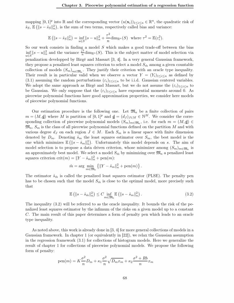
Chapter 3. Piecewise polynomial estimation of a regression function

mapping [0, 1]p into R and the corresponding vector (u(xi))1≤i≤n ∈ Rn, the quadratic risk ofsS, E

(

∥s− sS∥2n)

, is the sum of two terms, respectively called bias and variance:

E(

∥s− sS∥2n)

= infu∈S∥s− u∥2n +

τ2

ndimRn(S) where τ2 = E(ε2i ).

So our work consists in finding a model S which makes a good trade-off between the biasinfu∈S∥s − u∥2n and the variance τ2

n dimRn(S). This is the subject matter of model selection via

penalization developped by Birgé and Massart [3, 4]. In a very general Gaussian framework,they propose a penalized least squares criterion to select a model Sm among a given countablecollection of models (Sm)m∈Mn

. They justify their criterion with an oracle type inequality.Their result is in particular valid when we observe a vector Y = (Yi)1≤i≤n as defined by(3.1) assuming the random perturbations (εi)1≤i≤n to be i.i.d. Gaussian centered variables.We adopt the same approach as Birgé and Massart, but we do not assume the (εi)1≤i≤n tobe Gaussian. We only suppose that the (εi)1≤i≤n have exponential moments around 0. Aspiecewise polynomial functions have good approximation properties, we consider here modelsof piecewise polynomial functions.

Our estimation procedure is the following one. Let Mn be a finite collection of pairsm = (M, d) where M is partition of [0, 1]p and d = (dJ )J∈M ∈ NM . We consider the corre-sponding collection of piecewise polynomial models (Sm)m∈Mn , i.e. for each m = (M, d) ∈Mn, Sm is the class of all piecewise polynomial functions defined on the partition M and withvarious degree dJ on each region J ∈ M . Each Sm is a linear space with finite dimensiondenoted by Dm. Denoting sm the least squares estimator over Sm, the best model is theone which minimizes E

(

∥s− sm∥2n)

. Unfortunately this model depends on s. The aim ofmodel selection is to propose a data driven criterion, whose minimizer among (Sm)m∈Mn isan approximately best model. We select a model Sm by minimizing over Mn a penalized leastsquares criterion crit(m) = ∥Y − sm∥2n + pen(m):

m = arg minm∈Mn

∥Y − sm∥2n + pen(m)

.

The estimator sm is called the penalized least squares estimator (PLSE). The penalty penhas to be chosen such that the model Sm is close to the optimal model, more precisely suchthat

E(

∥s − sm∥2n)

≤ C infm∈Mn

E(

∥s− sm∥2n)

. (3.2)

The inequality (3.2) will be referred to as the oracle inequality. It bounds the risk of the pe-nalized least squares estimator by the infimum of the risks on a given model up to a constantC. The main result of this paper determines a form of penalty pen which leads to an oracletype inequality.

As noted above, this work is already done in [3, 4] for more general collections of models in aGaussian framework. In chapter 1 (or equivalently in [22]), we relax the Gaussian assumptionin the regression framework (3.1) for collections of histogram models. Here we generalize theresult of chapter 1 for collections of piecewise polynomial models. We propose the followingform of penalty:

pen(m) = Kσ2

nDm + κ1

σ2

n

√

Dmxm + κ2σ2 + Rb

nxm

68

3.2. The statistical framework

with weights (xm)m∈Mn satisfying∑

m e−xm ≤ Σ, Σ ∈ R∗+.

In the same regression framework as ours (with an even milder integrability condition on the(εi)1≤i≤n), Baraud [1] validates penalties pen(m) proportional to Dm

n , like those of Mallows’Cp, for "small" collection of models: the number of models with a given dimension D canbe a polynomial function of D but not an exponential function of D. In the Gaussian re-gression framework, in a situation where the number of models with a given dimension D is(

ND

)

, where N is a large parameter (N grows to infinity with n), Birgé and Massart [4] prove

that Mallows’ Cp can lead to terrible results. For "small" collections of piecewise polynomialmodels we recommend a penalty proportional to Dm

n , and for larger collections of models wepropose to add a correction via the weights xm.

After choosing a collection Mn, in practice we have to find adequate weights xm, precisethe development of pen(m), and calibrate the unknown constants involved in pen(m) accord-ing to the data. For p = 1 (i.e. s : [0, 1] −→ R), this work is done in [10] by Comte andRozenholc. They obtain an algorithm which automatically determines a partition, a series ofdegrees, and computes a piecewise polynomial estimator of s. The form of the penalty usedin their algorithm is theoretically validated by [2] when the perturbations are sub-Gaussian.Thanks to our result, it is validated in a more general case.

In a second part of this chapter, we apply our result to tree-structured collections of parti-tions of [0, 1]p associated with uniform degrees d ∈ 0, 1, . . . , dmax. We get a penalty pen(m)which is proportional to the dimension Dm of the linear model Sm. Then we propose anextension of the CART algorithm [7] to build a piecewise polynomial estimator of a regressionfunction s : [0, 1]p −→ R. The procedure selects a partition and a degree which is enforced tobe the same on each subregion of the partition. We give the results obtained on a simulatedtoy example with p = 1, but the same procedure works whatever p.Friedman [12] proposes an other extension of CART called MARS (Multivariate Adaptive Re-gression Splines) which uses splines of order 1 to build a continous estimator of the regressionfunction s. In contrary to MARS, our piecewise polynomial estimator is not enforced to becontinuous at subregion boundaries.

The paper is organized as follows. The section 3.2 presents the statistical framework.We take advantage of this section to define notations needed in the rest of the paper. Thesection 3.3 gives the main result. In section 3.4, we first recall the different steps of the CARTalgorithm. Then we apply the result of section 3.3 to tree-structured collections of partitionsadapted from CART and suitable for piecewise polynomial estimation. And finally we proposean extension of the CART algorithm to build a piecewise polynomial estimator of a regressionfunction. To get the model selection result of section 3.3, like in chapter 1, we have to controla χ2 like statistic. The section 3.5 is more technical, it exposes a concentration inequality forthe χ2 like statistic. Sections 3.6 and 3.7 are devoted to the proofs.

3.2 The statistical framework

In this paper, we consider the regression framework already defined in the introduction by(3.1). We assume that the i.i.d. random perturbations (εi)1≤i≤n have exponential moments

69

Chapter 3. Piecewise polynomial estimation of a regression function

around 0 and that the points (xi)1≤i≤n of the design are “well distributed” in [0, 1]p.

The first assumption can be expressed by the existence of two non negative constants b andσ such that

∀ λ ∈ (−1/b, 1/b) log E(

eλεi

)

≤ σ2λ2

2(1 − b|λ|) (3.3)

σ2 is necessarly greater than E(ε2i ) and can be chosen as close to E(ε2i ) as we want, but atthe price of a larger b. If b = 0 in (3.3) the variables εi are said to be sub-Gaussian.

The second assumption is expressed through the empirical distribution function Fn associatedwith the points (xi)1≤i≤n:

Fn : x = (x1, . . . , xp) −→ 1

n

n∑

i=1

1Ixji≤xj ∀1≤j≤p (3.4)

We assume that Fn is close to the uniform distribution function on [0, 1]p, denoted by F . Wemeasure the distance between Fn and F by ∥Fn − F∥∞ where ∥.∥∞ denotes the sup-norm.

For any d ∈ N, we denote by Rd[x] = Rd[x1, . . . , xp] the space of polynomial functions on[0, 1]p with degree d.For a given m = (M, d) where M is a partition of [0, 1]p and d = (dJ)J∈M is a series of nonnegative integers, we denote

• Sm the space of piecewise polynomial functions defined on the partition M and withvarious degree dJ on each region J ∈M .

Sm =

∑

J∈M

fJ1IJ ; ∀ J ∈M fJ ∈ RdJ[x]

(3.5)

• sm the least squares estimator of s over Sm.

sm = arg minu∈Sm

∥Y − u∥2n

where ∥.∥n denotes the Euclidean norm on Rn scaled by a factor n−1/2 and, for a functionu, the vector (u(xi))1≤i≤n ∈ Rn is denoted u too.

Sm is the piecewise polynomial model associated with m = (M, d). It is a linear space withfinite dimension. We denote by Dm the dimension of Sm, and by Km = |M | the number ofelements of the partition M .

Dm =∑

J∈M

C(dJ , p) where C(dJ , p) = dim RdJ[x1, . . . , xp] =

dJ∑

k=0

(

p + k − 1p− 1

)

=

(

p + dJ

p

)

.

sm is the piecewise polynomial estimator belonging to Sm which plays the role of benchmarkamong all the estimators in Sm.

Denoting sm = arg minu∈Sm

∥s− u∥2n, the quadratic risk of the estimator sm is

E(

∥s− sm∥2n)

= ∥s− sm∥2n + E(ε21)dimRn(Sm)

n≤ ∥s− sm∥2n + σ2 Dm

n

70

3.3. The main theorem

3.3 The main theorem

As told in the introduction, we consider a finite collection Mn of pairs m = (M, d) with Ma partition of [0, 1]p and d = (dJ )J∈M ∈ NM , and the corresponding collection of piecewisepolynomial models (Sm)m∈Mn as defined by (3.5).We select a model Sm by minimizing a penalized criterion crit(m) = ∥Y − sm∥2n + pen(m)over Mn, i.e.

m = arg minm∈Mn

∥Y − sm∥2n + pen(m)

.

It remains to provide a penalty pen such that the model m is close to the optimal model, inthe sense that the PLSE sm satisfies an oracle inequality like (3.2).

For simplicity, let us start with the case p = 1 and the equispaced design xi = in . Then,

the regression function s is a signal mapping [0, 1] into R, and the observations Yi correspondto the values of s at the equispaced points xi = i

n perturbed by noise. We consider here twostandard choices for the collection of models (Sm)m∈Mn :

(R) The collection of piecewise polynomial models built on regular partitions with variousdegree belonging to 0, 1, . . . , d on each subregion. A regular partition is a partitionwhose elements have all the same measure with respect to the Lebesgue measure µ. Wekeep only the regular partitions which have less than Kn =

[n

(log n)2

]

elements (in order

that each subregion contains at least ≃ (log n)2 design points). We denote by Mrn the

family of regular partitions on [0, 1] with size smaller than Kn =[

n(log n)2

]

, and by Mr,dn

the family of pairs m = (M, d) with M ∈Mrn and d = (dJ )J∈M ∈ 0, 1, . . . , dM .

(IR) The classical collection of irregular piecewise polynomial models associated with thecollection M

ir,dn defined below. We consider a sub-series

(

xφ(j)

)

1≤j≤Knof (xi)1≤i≤n such

that: for any 1 ≤ j < Kn, φ(j + 1) − φ(j) ≥ (log n)2. We define Mirn as the family of

all partitions with endpoints belonging to the grid(

xφ(j)

)

1≤j≤Kn. (By taking this new

grid instead of the initial grid(

xi = in

)

1≤i≤n, we ensure that each subregion contains

at least ≃ (log n)2 design points.) Then Mir,dn is the family of pairs m = (M, d) with

M ∈Mirn and d = (dJ)J∈M ∈ 0, 1, . . . , dM .

In the collection of regular partitions Mrn, for any 1 ≤ K ≤ Kn, there is only one partition

with size K. Since the degrees of the polynomials are variable in the set 0, 1, . . . , d, thereis nevertheless a great number of models m ∈M

r,dn .

If we denote by Mrn the collection of all pairs m = (M, d) with M a regular partition of [0, 1]

and d = (dJ )J∈M ∈ NM with no restriction on the degrees dJ , then we have for any D ≥ 1and any 1 ≤ K ≤ D,

|m ∈Mrn; Dm = D and Km = K| =

∣∣∣∣∣∣

⎧

⎨

⎩(d1, . . . , dK) ∈ NK ;

K∑

j=1

(dj + 1) = D

⎫

⎬

⎭

∣∣∣∣∣∣

=

(

D − 1K − 1

)

71

Chapter 3. Piecewise polynomial estimation of a regression function

And,

|m ∈Mrn; Dm = D| =

D∑

K=1

(

D − 1K − 1

)

= 2D−1

There are too many models in order to apply Baraud’s result [1].

Given the collection Mr,dn , the proposition 3.1 gives a form of penalty function which allows

to select a close to optimal model m, in the sense that the penalized least squares estimatorsm satisfies an oracle type inequality. This proposition is a consequence of theorem 3.1.

Proposition 3.1 Let b ∈ R+ and σ ∈ R∗+ such that inequality (3.3) holds. Let R a positive

constant such that ∥s∥∞ ≤ R.

We consider the collection of regular piecewise polynomial models associated with Mr,dn .

Then there exists a universal constant α0 such that for any α ≥ α0:taking

pen(m) ≥ α(d + 1)(σ2 + (d + 1)Rb)Dm

n,

we have

E(

∥s − sm∥2n)

≤ C1(α)infm

∥s− sm∥2n + pen(m)

+C2(α, b,σ2, R, d)

n.

For the collection of regular piecewise polynomial models, the proposition 3.1 recommendspenalties pen(m) proportional to Dm

n .

Since we do not know the constants α0, b, σ2 and R, we consider in practice penalties of theform pen(m) = α′ Dm

n . Then we calibrate the multiplicative factor α′ according to the data,using for example Massart’s heuristic [19, section 8.5.2, paragraph "Some heuristics"] or Birgéand Massart’s rule [4, section 4] (see chapter 4, sections 4.4.1 and 4.5.2).

In contrary to Mrn, in the collection of irregular partitions Mir

n , there are many partitions

with a given size K ∈ 1, . . . ,Kn. More precisely,∣∣

M ∈Mirn ; |M | = K

∣∣ =

(

Kn − 1K − 1

)

.

The proposition 3.2 gives a result similar to proposition 3.1 for the collection Mir,dn whose

complexity is bigger than those of Mr,dn . It is also a consequence of theorem 3.1.

Proposition 3.2 Let b ∈ R+ and σ ∈ R∗+ such that inequality (3.3) holds. Let R a positive

constant such that ∥s∥∞ ≤ R.

We consider the collection of irregular piecewise polynomial models associated with Mir,dn .

Then there exists two universal constants α0 and β0 such that for any α ≥ α0 and any β ≥ β0:taking

pen(m) ≥ (d + 1)(σ2 + (d + 1)Rb)

(

α1

nlog

(

Kn − 1Km − 1

)

+ βDm

n

)

,

we have

E(

∥s− sm∥2n)

≤ C1(α,β)infm

∥s− sm∥2n + pen(m)

+C2(α,β, b,σ2, R, d)

n.

72

3.3. The main theorem

For the collection of irregular piecewise polynomial models, the proposition 3.2 recommendspenalties

pen(m) = α′ 1

nlog

(

Kn − 1Km − 1

)

+ β′Dm

n. (3.6)

We can also choose a more elaborate form of penalty, like those used by Comte and Rozenholc[10]: for any m = (M, d) with Km = |M | = K and d = (dj)1≤j≤K

penCR(m) =1

n

[

c1 log

(

Kn − 1K − 1

)

+ c2(log K)c3 + c4

K∑

j=1

(dj + 1) + c5

K∑

j=1

[log(dj + 1)]c6

]

.

In [10], they theoretically validate this penalty when the perturbations (εi)1≤i≤n are sub-Gaussian thanks to the model selection result of [2]. Proposition 3.2 allows to validate itwhen the (εi)1≤i≤n are only supposed to have exponential moments around 0.

Using the inequality(

Kn − 1K − 1

)

≤(

eKn

K

)K

,

we recover the penalty pen(m) = Dmn

(

α′′ log(

KnKm

)

+ β′′)

proposed by Lebarbier [16] for col-

lection of piecewise constant models defined on irregular partitions (which corresponds hereto d = 0), and used in chapter 4 for collection of piecewise affine models (which correspondsto d = 1). We give in chapter 4 two methods to calibrate the constants α

′′and β

′′. The same

methods could be used to calibrate the constants α′ and β′ in (3.6).

Let us now go back to the more general issue of estimating a function s : [0, 1]p −→ R

when we observe its values (perturbed by noise) at some points (xi)1≤i≤n not necessarily equi-spaced. Thanks to theorem 3.1, we can get results similar to proposition 3.1 and proposition3.2 when s : [0, 1]p −→ R and the design points xi are "well distributed" in [0, 1]p (instead ofs : [0, 1] −→ R and xi = i

n).

For p = 1, in the two preceding propositions, we consider partitions of [0, 1] composed ofsegments containing at least ≃ (log n)2 design points. Now, we consider some collection Mn

of partitions of [0, 1]p composed of hyperrectangle axis oriented regions, which all contain aminimal number of design points.

We consider two types of collection of partitions Mn: "small" collections Mn in which thenumber of partitions with a given size K is bounded by a polynomial function of K, andpossibly bigger collections Mn in which all partitions M are built from an initial partition M0,which is not too fine in the sense that each element of M0 contains a minimal number of designpoints. More precisely, we assume that Mn satisfies one of the two following assumptions:

(A1) there exists Γ ∈ R∗+ and a ∈ N such that: for any K ≥ 1,

|M ∈Mn; |M | = K| ≤ ΓKa,

and then we denote by Nmin = infM∈Mn

infJ∈M

|J | where |J | = |1 ≤ i ≤ n; xi ∈ J|,

73

Chapter 3. Piecewise polynomial estimation of a regression function

(A2) there exists some partition M0 such that: for any M ∈Mn and any element J of M , Jis the union of elements of M0,and then we denote by Nmin = inf

J∈M0

|J | (≤ infM∈Mn

infJ∈M

|J | with equality if M0 ∈Mn).

The assumption (A2) allows to deal with large collections of partitions.

Remark 3.1 The collection Mrn considered in proposition 3.1 satisfies (A1), and the collec-

tion Mirn considered in proposition 3.2 satisfies (A2).

Given a collection Mn of pairs m = (M, d) with M ∈Mn and d = (dJ)J∈M ∈ 0, 1, . . . , dM ,the theorem 3.1 gives a general form of penalty involving weights (xm)m∈Mn , and which leadsto an oracle type inequality.The constants A(d, p), B(2d, p), C(d, p) and C ′′(d, p) only depend on the maximal degree d of

the polynomials and on the number of variables p. C(d, p) =

(

p + dp

)

. A(d, p) and B(2d, p)

are defined in lemma 3.4. C ′′(d, p) = 1 +√

2C(d, p)A(d, p) is defined in remark 3.2. Theconstant κ(a) = 8(2a + 5) if (A1) and 24 if (A2).

Theorem 3.1 Let b ∈ R+ and σ ∈ R∗+ such that inequality (3.3) holds.

Let d ∈ N, and Mn a collection of partitions of [0, 1]p composed of hyperrectangle axis oriented

regions and satisfying assumption (A1) or (A2) with Nmin ≥ κ(a)A(d, p)2 b2

σ2 log n.Assume the points (xi)1≤i≤n to be distributed such that

∥Fn − F∥∞ ≤κ(a)A(d, p)2

2p(4B(2d, p) + 1)

b2

σ2

log n

n.

Let Mn ⊂ m = (M, d); M ∈Mn and d = (dJ)J∈M with dJ ≤ d, and (xm)m∈Mn a familyof weights such that for some Σ ∈ R∗

+∑

m∈Mn

e−xm ≤ Σ. (3.7)

Assume ∥s∥∞ ≤ R, with R a positive constant.Let θ ∈ (0, 1) and K > 2− θ two numbers.Taking a penalty satisfying

pen(m) ≥ Kσ2

nDm + 8

√2(2− θ)C(d, p)

σ2

n

√

Dmxm

+

[(

4(2 − θ)C(d, p) +2

θ

)σ2

n+ 2C ′′(d, p)

Rb

n

]

xm (3.8)

we have

E(

∥s − sm∥2n)

≤ 2

1− θ infm

∥s− sm∥2n + pen(m)

+1

1− θ

[

8(2− θ)C(d, p)

(

1 + 8C(d, p)(2− θ)

K + θ − 2

)

+4

θ+ 2

]σ2

nΣ

+6C ′′(d, p)

1− θRb

nΣ + C(b,σ2, R, d, p)

1Ib=0

n(log n)3/2

where C(b,σ2, R, d, p) is a positive constant which depends only on b, σ2, R, d and p.

74

3.4. CART extension to piecewise polynomial estimation

This theorem gives the general form of the penalty function

pen(m) = Kσ2

nDm +

(

κ1(θ, d, p)σ2

n

√

Dmxm + κ2(θ, d, p)σ2 + Rb

nxm

)

The penalty is the sum of two terms: the first one is proportional to Dmn and the second one

depends on the complexity of the family Mn via the weights (xm)m∈Mn . For θ ∈ (0, 1) andK > 2− θ, the PLSE sm satisfies an oracle type inequality

E(

∥s− sm∥2n)

≤ C1infm

∥s− sm∥2n + pen(m)

+C2

n

where the constant C1 only depends on θ, whereas C2 depends on s (via R), on d the maximaldegree of the polynomials, on p the number of variables, on the family Mn (via Σ) and onthe integrability condition of (εi)1≤i≤n (via σ2 and b).

Given a collection Mn of partitions and a collection Mn of pairs m = (M, d) with M ∈Mn,in order to get a convenient penalty, we have to find weights (xm) satisfying (3.7) and toreplace their expression in (3.8).Let us denote by

C(K) = log |M ∈Mn; |M | = K| .

Then the weights xm = C(Km) + aDm with a > log 2 satisfy inequality (3.7). And applyingtheorem 3.1, we get that for any α ≥ α0 and any β ≥ β0 a penalty satisfying:

pen(m) ≥ C(d, p)(σ2 + A(d, p)Rb)

(

αC(Km)

n+ β

Dm

n

)

leads to an oracle type inequality. This result generalizes propositions 3.1 and 3.2. In practice,we can take

pen(m) = α′ C(Km)

n+ β′

Dm

n

or more elaborate forms.

If we draw a grid in [0, 1]p such that each cell of the grid contains at least Nmin design points,and if Mn is the collection of all partitions obtained by removing some axis of the grid, then

|M ∈Mn; |M | = K| ≤(

Kn

K

)

where Kn is the size of the partition associated with the

complete grid. In this case we can take penalties of the form

pen(m) = α′ 1

nlog

(

Kn

Km

)

+ β′Dm

n.

3.4 CART extension to piecewise polynomial estimation

In this section, we first give an overview of CART in our regression framework. Then, in viewof the form of penalty given by theorem 3.1 for a tree-structured collection of partitions (likethe one built in the first step of CART), we explain how CART can be extended to producea piecewise polynomial estimator.

75

Chapter 3. Piecewise polynomial estimation of a regression function

3.4.1 An overview of CART

CART is an algorithm which builds a piecewise constant estimator of a regression function ora classifier from a training sample L = (xi, Yi)1≤i≤n. We focus here on the regression frame-work with fixed design points as defined in the introduction by (3.1). In order to produce apiecewise constant estimator of s from the points (xi, Yi)1≤i≤n, CART proceeds in three steps.

In the first step, CART builds a fine partition of [0, 1]p by splitting [0, 1]p and the obtainedregions in two hyperrectangle axis oriented subregions as long as they contain a minimalnumber Nmin of design points. Each split is determined by minimizing the empirical leastsquares criterion corresponding to histogram estimation. A useful representation of this re-cursive construction is a tree of maximal depth, denoted by Tmax. This step is thus called theconstruction of a maximal tree.Remark: The leaves of Tmax form a fine partition M0 of [0, 1]p. If T is a pruned subtree ofTmax (i.e. a subtree with same root as Tmax), then the leaves of T form a partition MT of[0, 1]p built from M0. We write T ≼ Tmax if T is a pruned subtree of Tmax. At the end of thisfirst step, we have a collection (MT )T≼Tmax of partitions of [0, 1]p built from M0.

The second step, called pruning step, consists in selecting some pruned subtrees of Tmax

by minimizing a penalized least squares criterion. In this step, we have in mind that theleast squares histogram estimator associated with a too deep tree overfits the training data.This is the reason why Breiman et al propose to select the smallest pruned subtree of Tmax

minimizing the criterion

crit0(T ) = R0(T ) + α|MT |

n,

where R0(T ) is the mean of the residual squares of the least squares histogram estimatorassociated with T . They prove the following result:

Proposition 3.3 There exists

• α0 = 0 < α1 < . . . < αK a finite increasing series of parameters

• T0 = Tmax ≽ T1 ≽ . . . ≽ TK a nested series of pruned subtrees of Tmax with the tree TK

reduced to its root

such that, for any αk ≤ α < αk+1, Tk is the smallest pruned subtree of Tmax minimizing the

criterion crit0(T ) = R0(T ) + α |MT |n .

Remark: At the end of the pruning step, we have K + 1 candidates left. As (T0, T1, . . . , TK)is a nested series of K + 1 different pruned subtrees, there is at most one tree for a givennumber of leaves. And in general, we observe that many sizes are not represented. Thus Kis very smaller than |T ≼ Tmax|. The pruning step reduces the number of subtrees a lot.

In the last step, a final tree T is selected among the nested series (T0, T1, . . . , TK) via testsample or cross validation. As K is small, we are able to calculate an estimation of the riskof every histogram estimator associated with a tree of the nested series. We choose T whichhas a minimal (or nearly minimal) estimated risk and s is estimated by the least squareshistogram estimator associated with T . In the following, this final selection is made via test

76

3.4. CART extension to piecewise polynomial estimation

sample.

As noted above, at the end of the first step of the CART algorithm, we have a collectionMCART

n = (MT )T≼Tmax of partitions built from an initial partition of [0, 1]p. In the classicalCART algorithm, the same training sample L is used to build the maximal tree Tmax and toprune it, and the collection MCART

n depends on L. Like in [14] and in chapter 2 (or [23]), weconsider a slightly modified version of CART, where the first and second steps are respectivelydone with a sample L1 and an other sample L2 independent of L1. This modified version ofCART is easier to study since all steps are done with independent samples. Unfortunately, inpractice, when the number of observations is small, we can not use two different samples inthe two first steps.

3.4.2 CART extension to piecewise polynomial estimation

The first step of CART gives a collection (MT )T≼Tmax of partitions built from an initial one.Tmax is constructed in order that the piecewise constant estimator defined on its leaves best fitthe data. Thus the collection (MT )T≼Tmax is well adapted to piecewise constant estimation.In order to get a collection of partitions adapted to piecewise polynomial estimation, we buildfor each 0 ≤ d ≤ dmax a maximal tree T d

max whose associated piecewise polynomial estimatorwith degree d best fit the data. The construction of T d

max is modelled on those of Tmax. Theonly difference between T d

max and Tmax is that each split of T dmax is determined by minimizing

the empirical least squares criterion corresponding to piecewise polynomial estimation withdegree d instead of histogram estimation. For every d, we consider the partitions (MT )T≼T d

max

and the models of piecewise polynomial functions defined on MT with the same degree don each subregion. These models correspond to pairs m = (MT , d) with d = (d, . . . , d) andT ≼ T d

max. For short, we denote m = (T, d) instead of m = (MT , (d, . . . , d)).We get the collection of models

Mn =dmax⋃

d=0

(T, d); T ≼ T dmax

In order to apply theorem 3.1 to the collection of models Mn, we have to build T dmax with a

sample L1 and then work with a second independent sample L2. In this case, the collectionMn is deterministic conditionally to L1.

Thanks to Catalan inequality,

∣∣∣

T ≼ T dmax; |MT | = K

∣∣∣ ≤

1

K

(

2(K − 1)K − 1

)

≤ 22K

4K,

Thus, taking xm = LDm = L|MT |C(d, p) with L > 2 log 2 for any m = (T, d) ∈Mn, we have

∑

m∈Mn

e−xm ≤dmax∑

d=0

n∑

K=1

22K

4Ke−LKC(d,p) ≤

+∞∑

K=1

22K

4K

e−LK

1− e−LK

≤+∞∑

K=1

(

4e−L)K

3K< +∞

77

Chapter 3. Piecewise polynomial estimation of a regression function

We deduce from theorem 3.1 that taking a penalty

pen(m) = γC(dmax, p)(σ2 + bRA(dmax, p))Dm

n

with γ big enough, we have

E(

∥s− sm∥2n)

≤ C1(γ)infm

∥s − sm∥2n + C(dmax, p)(σ2 + bRA(dmax, p))Dm

n

+C2(γ, b,σ2, R, dmax, p)

n

As we do not know the constants b, σ2 and R, we consider the following form of penalty:

pen(m) = αDm

n

The corresponding penalized criterion is

crit(m) = ∥Y − sm∥2n + αDm

n

In order to find the model m = arg minm∈Mn

crit(m), we proceed in two steps:

- First, for every degree d, we select a subtree Td of T dmax by minimizing among all

T ≼ T dmax the criterion

critd(T ) = Rd(T ) + αC(d, p)|MT |

n

where Rd(T ) = ∥Y − s(T,d)∥2n measures the lack of fit of the piecewise polynomialestimator with degree d associated with T . Rd(T ) is the analogue of R0(T ). Like inthe CART pruning criterion crit0(T ), the additional term is proportional to the numberof leaves of T . Thus we can get the tree Td by the analogue of the CART pruningprocedure for piecewise polynomial estimation with degree d.

- Then we choose a degree d by

d = arg min0≤d≤dmax

Rd(Td) + αC(d, p)|MTd

|n

.

Finally m =(

Td, d)

.

The trees (Td)0≤d≤dmax , the degree d and the model m depend on the parameter α. Thus weshould rather denote them by (Td(α))0≤d≤dmax , d(α) and m(α).

By following the proof of Breiman et al, we get a result similar to proposition 3.3 for the cri-terion critd. We denote by (α0,d,α1,d, . . . ,αKd,d) and (T0,d, T1,d, . . . , TKd,d) the correspondingseries of parameters and subtrees. For any αk,d ≤ α < αk+1,d, Tk,d is the smallest subtreeof T d

max minimizing the criterion critd(T ) = Rd(T ) + αC(d, p) |MT |n . In other words, for any

αk,d ≤ α < αk+1,d, Td(α) = Tk,d. The algorithm which builds these two series is the same as

78

3.4. CART extension to piecewise polynomial estimation

the CART pruning algorithm except that R0 is replaced by Rd.

Then, by putting together all series of parameters (α0,d,α1,d, . . . ,αKd,d), 0 ≤ d ≤ dmax, weget a series α0 = 0 < α1 < . . . < αK with K =

∑dmaxd=0 Kd. For any 1 ≤ i ≤ K, we find Td(αi)

in the set of subtrees T0,d, T1,d, . . . , TKd,d and we calculate

d(αi) = arg min0≤d≤dmax

Rd(Td(αi)) + αiC(d, p)|MTd(αi)

|n

.

At this stage, we have a collection of models

m(αi) = (Td(αi), d(αi)); 1 ≤ i ≤ K

whose

cardinal is smaller than K. (In the following example, K = 46 and we obtain 20 differentmodels.) Some models m(α) may not belong to the set m(αi); 1 ≤ i ≤ K, but we observein practice that it is quite a rare situation, and we believe that we can forget them with no re-gret. (In the following example, only one model m(α) corresponding to large α’s is forgotten.)

We choose the final model among m(αi); 1 ≤ i ≤ K via the test sample L3.

A simulated example:

We simulate n = 1000 variables (Yi)1≤i≤n defined by:

Yi = s(xi) + εi, 1 ≤ i ≤ n,

with (εi)1≤i≤n independent Gumbel variables renormalized such that they have mean 0 andvariance 1, xi = i

n , and s : [0, 1] −→ R

s(x) =

⎧

⎪⎨

⎪⎩

10 if 0 ≤ x ≤ 0.2,

7.5 − 12.5x if 0.2 < x ≤ 0.6,

0 if 0.6 < x ≤ 1.

We build (T dmax)0≤d≤3 the maximal trees corresponding to the degrees 0 ≤ d ≤ 3 by the

analogue of the CART growing procedure using a first sample L1.Then, for each degree d, we compute the series (α0,d,α1,d, . . . ,αKd,d) and (T0,d, T1,d, . . . , TKd,d)via the analogue of the CART pruning procedure using a second sample L2.We denote by α0 = 0 < α1 < . . . < αK the series obtained by concatenating the precedingsseries of parameters. Here we obtain K = 46.

And we calculate d(αi) = arg min0≤d≤3

Rd(Td(αi)) + αiC(d, p)|M

Td(αi)|

n

. We obtain only 20

different models m(αi). (Only one model with degree 0 and 5 subregions is hidden. It corre-spond to m(α) with α ≃ 65.)

The table 3.1 gives the values of αi, d(αi) and |Td(αi)| for 19 ≤ i ≤ 38.Moreover

• for any 1.1420 ≤ α < 1.1607, the selected model m(α) is always the same model withdegree d = 2 associated with a partition with 7 subregions,

• for any 1.1607 ≤ α ≤ 1.6816, the selected model m(α) is always the same model withdegree d = 2 associated with a partition with 6 subregions,

79

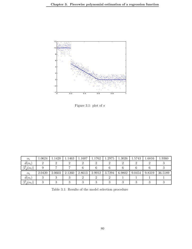
Chapter 3. Piecewise polynomial estimation of a regression function

0 0.2 0.4 0.6 0.8 1−4

−2

0

2

4

6

8

10

12

Figure 3.1: plot of s

αi 1.0624 1.1420 1.1463 1.1607 1.1762 1.2975 1.3026 1.5743 1.6816 1.9360d(αi) 2 2 2 2 2 2 2 2 2 3

|Td(αi)| 9 7 7 6 6 6 6 6 6 3

αi 2.0420 2.0603 2.1260 2.8613 2.9912 3.7294 6.9802 9.0454 9.8319 36.5189d(αi) 3 3 3 2 2 2 1 1 1 1

|Td(αi)| 3 3 3 3 3 3 3 3 3 3

Table 3.1: Results of the model selection procedure

80

3.4. CART extension to piecewise polynomial estimation

0 0.2 0.4 0.6 0.8 10

2

4

6

8

10

12

s

Figure 3.2: plot of s and s

• for any 1.6816 < α < 1.9360, m(α) = m(1.6816) or m(1.9360),

• for any 1.9360 ≤ α ≤ 2.1260, the selected model m(α) is always the same model withdegree d = 3 associated with a partition with 3 subregions, whose limits are 0.2010 and0.5810,

• for any 2.1260 < α < 2.8613, m(α) = m(2.1260) or m(2.8613),

• for any 2.8613 ≤ α ≤ 3.7294, the selected model m(α) is always the same model withdegree d = 2 associated with a partition with 3 subregions, whose limits are 0.2010 and0.5810,

• for any 3.7294 < α < 6.9802, m(α) = m(3.7294) or m(6.9802),

• for any 6.9802 ≤ α ≤ 36.5189 (and even for 6 ≤ α ≤ 50), the selected model m(α) isalways the same model with degree d = 1 associated with a partition with 3 subregions,whose limits are 0.2010 and 0.5340.

Using a test sample L3, we finally select the model with degree 1 and 3 subregions, whoselimits are 0.2010 and 0.5340. The corresponding estimator s is represented on figure 3.2. HisL3−empirical risk is 1.0653. We get the right number of subregions and the selected degree(which is enforced to be the same on each subregion) equals the maximal degree of s.

In practice, when the number of data is not big enough, we can not split the data in 3 samplesL1, L2 and L3. We try the same procedure as before by using the same sample L1 = L2 forthe construction of the maximal trees (T d

max)0≤d≤3 and for their pruning. We get the followingresults.By putting together the series of parameters obtained by pruning all T d

max, we get a series(αi)0≤i≤K with size K = 42. We obtain only 12 different models m(αi) and for any α > 0m(α) belongs to the set m(αi); 1 ≤ i ≤ K.

81

Chapter 3. Piecewise polynomial estimation of a regression function

αi 2.5740 2.5830 2.6721 2.8321 3.0063 3.1198 3.2613 3.3234 3.3651 3.5246d(αi) 0 0 0 0 0 0 0 0 0 0

|Td(αi)| 13 13 13 13 13 13 12 12 12 12

αi 3.5625 4.0520 5.1410 8.0859 8.4452 10.4688 11.0017 12.7039 25.1121 27.8815d(αi) 0 0 0 0 1 1 1 1 1 1

|Td(αi)| 11 10 10 10 3 3 3 3 3 3

Table 3.2: Results of the model selection procedure using a single sample L1 = L2

We write in table 3.2 a part of the series of αi, d(αi) and |Td(αi)|. We see on this tablethat the model with degree 1 and 3 subregions corresponds to larger values of α when themaximal trees (and thus the collection of models Mn) are constructed with the same sampleas well used for the pruning step. When the collection of models Mn is random, the numberof potential models is bigger and the penalty has to be bigger too. From a theoretical pointof view, we have to consider a deterministic collection M0

n which contains Mn. The weights(xm)m∈M0

nand thus the penalty will be larger.

In addition to the informations given in table 3.2, we have:

• for any 2.5740 ≤ α < 3.2613, the selected model m(α) is always the same model withdegree d = 0 associated with a partition with 13 subregions,

• for any 3.2613 ≤ α < 3.5625, the selected model m(α) is always the same model withdegree d = 0 associated with a partition with 12 subregions,

• for any 3.5625 ≤ α < 4.0520, the selected model m(α) is always the same model withdegree d = 0 associated with a partition with 11 subregions,

• for any 4.0520 ≤ α ≤ 8.0859, the selected model m(α) is always the same model withdegree d = 0 associated with a partition with 10 subregions,

• for any 8.0859 < α < 8.4452, m(α) = m(8.0859) or m(8.4452),

• for any 8.4452 ≤ α ≤ 27.8815 (and even for 8.1 ≤ α ≤ 53), the selected model m(α) isalways the same model with degree d = 1 associated with a partition with 3 subregions,whose limits are 0.2010 and 0.5780,

• for larger α, the selected model m(α) correspond to the degree d = 0 and partitions ofsize 4, 3, 2 and 1.

By using a test sample L3, we finally selects the model with degree 1 and 3 subregions, whoselimits are 0.2010 and 0.5780. The corresponding estimator s2 is represented on figure 3.3. HisL3−empirical risk is 1.0569. Thus s2 is a bit better than s. In practice, we can make this laststep of final selection by cross validation instead of test sample.

82

3.4. CART extension to piecewise polynomial estimation

0 0.2 0.4 0.6 0.8 1−2

0

2

4

6

8

10

12

s2

Figure 3.3: plot of s2 and s

3.4.3 Some comments on MARS

The algorithm called MARS (Multivariate Adaptive Regression Splines), proposed by Fried-man [12], as well builds a piecewise polynomial estimator of a regression function. This algo-rithm can be viewed as an other extension of CART, which no longer relies on tree-structuredpartitions (see Appendix). The main difference with our approach is that the estimator ob-tained with MARS is continuous with continuous first derivatives.

The first step of MARS is a forward stepwise procedure which looks like the CART growingprocedure. It produces a large family of tensor product spline basis functions: B1, B2, . . . , BN,with B1 = 1 and

Bi(x) = ΠKik=1

[

si,k

(

xv(i,k) − ti,k)]

+

where si,k = ±, v(i, k) ∈ 1, 2, . . . , p is the number of a variable and ti,k ∈ R is a knot location.

The second step of MARS is a backward stepwise procedure which looks like the CARTpruning procedure. It removes basis functions that no longer contribute sufficiently to theaccuracy of the fit. In the MARS approach, a model Sm is the linear space spanned by asubset m ⊂ B1, B2, . . . , BN which contains B1. The second step of MARS selects a modelm by minimizing the criterion

GCV (m) = ∥Y − sm∥2n(

1− Dm + c|m|n

)−2

where sm is the least squares estimator of s over Sm, Dm = dim(Sm) and |m| is the numberof functions in the set m. Friedman recommends c = 3 in the general case and c = 2 in theadditive case, which corresponds to the case where all basis functions Bi are enforced to have

83

Chapter 3. Piecewise polynomial estimation of a regression function

only Ki = 1 term. When n grows to +∞,(

1− Dm+c|m|n

)−2∼ 1 + 2Dm+c|m|

n . Thus

GCV (m) ≃ ∥Y − sm∥2n + 2∥Y − sm∥2nDm + c|m|

n

≃ ∥Y − sm∥2n + 2τ2 Dm + c|m|n

where τ2 = ∥Y − sm∥2n is viewed as an estimator of the variance τ2. Thus the criterionGCV (m) is close to a penalized least squares criterion with a penalty term

penGCV (m) = 2τ2 Dm + c|m|n

For piecewise polynomial models of the form (3.5), we recommend a penalty

pen(m) = Kσ2

nDm +

(

κ1(θ, d, p)σ2

n

√

Dmxm + κ2(θ, d, p)σ2 + Rb

nxm

)

(3.9)

with xm such that∑

m

e−xm ≤ Σ

Theorem 3.1 is not valid for the models Sm involved in MARS. Since Birgé and Massart [4]recommend the same form of penalty as (3.9) in a Gaussian framework for any countablecollection of models, we believe that a convenient penalty can be obtained here again bychoosing convenient weights and replacing them in expression (3.9).

If there is only one covariable x (i.e. p = 1), then the first step of MARS gives a family ofbasis functions of the form:

F1 = 1, (x− t1)+, (t1 − x)+, . . . , (x− tK)+, (tK − x)+

The linear space spanned by F1 is the space of all piecewise affine functions defined on thepartition with subregion boundaries located at t1, . . . , tK , which are continuous everywhere.We denote by m every subset of F1 which contains the function 1, and by Sm the linear spacespanned by m.

Lemma 3.1 Let G1 = m ⊂ F1; 1 ∈ m.

|m ∈ G1; Dm = N and |m| = N| =

⎧

⎪⎪⎪⎪⎪⎪⎨

⎪⎪⎪⎪⎪⎪⎩

2N−1

(

K

N − 1

)

if N = 1 or 2,

2N−1

(

K

N − 1

)

+ 2N−3(N − 2)

(

K

N − 2

)

if 3 ≤ N ≤ K + 1,

K2K−1 if N = K + 2.

For any 4 ≤ D ≤ K + 2 and any D + 1 ≤ N ≤ 2D − 3,

|m ∈ G1; Dm = D and |m| = N| = 22D−N−3

(

KD − 2

)(

D − 22D −N − 3

)

.

84

3.5. A concentration inequality for a χ2 like statistic

And for any 1 ≤ D ≤ K + 2,

|m ∈ G1; Dm = D| ≤ 3D−1

(

K + 1D − 1

)

.

It follows from lemma 3.1 that we can take xm = 2|m|+Dm log K+2Dm

or xm = Dm

(

2.1 + log K+2Dm

)

.

Thus penalties of the form pen(m) =αDm log K+2

Dm+β|m|

n or pen(m) =αDm log K+2

Dm+β

n are con-venient for the second step of MARS. Up to the factor log K+2

Dm, the proposed penalty pen(m)

has the same form as penGCV (m).

If we consider p variables x = (x1, . . . , xp) and if, during the first step of MARS, B1 is thesingle function admissible for splitting, then the first step of MARS gives a family of basisfunctions of the form:

Fadp = 1, (x1 − t11)+, (t11 − x1)+, . . . , (x1 − t1K1

)+, (t1K1− x1)+,

. . . , (xp − tp1)+, (tp1 − xp)+, . . . , (xp − tpKp)+, (tpKp

− xp)+

and we derive from lemma 3.1 the following lemma:

Lemma 3.2 Let Gadp =

m ⊂ Fadp ; 1 ∈ m

.

|m ∈ Gadp ; Dm = D| ≤

∑

(D1,...,Dp)i Di−(p−1)=D

Πpi=13

Di−1

(

Ki + 1Di − 1

)

≤ 3D−1

(

Dmax − 1D − 1

)

where Dmax = (∑p

i=1 Ki) + p + 1 = dim(Fadp ).

Thus we suggest a penalty of the form pen(m) =αDm log K+2

Dm+β

n .

3.5 The key to determine an adequate form of penalty: a con-

centration inequality for a χ2 like statistic

This section is more technical. First we recall an expression of ∥s − sm∥2n, already used in[4] and in chapter 1, which allows us to see that the penalty pen(m) has to compensate thedeviation of a χ2 like statistic, denoted χ2

m, in order that the PLSE sm satisfies an oracle typeinequality. Then, in lemma 3.3, we give a concentration inequality for χ2

m. This concentra-tion inequality is the main point of the proof of theorem 3.1, the remaining of the proof onlyconsists in technical details.

As noted in (chapter 1, section 1.4), we get from the definition of m that, for any θ ∈ (0, 1),

(1− θ)∥s− sm∥2n = (2− θ)∥εm∥2n − 2 ⟨ε, s− sm⟩n − θ∥s− sm∥2n − pen(m) (3.10)

+ infm∈Mn

∥s − sm∥2n − ∥εm∥2n + 2 ⟨ε, s − sm⟩n + pen(m)

85

Chapter 3. Piecewise polynomial estimation of a regression function

where, for any model m, sm = arg minu∈Sm

∥s− u∥2n and εm = arg minu∈Sm

∥ε− u∥2n.

To get an oracle type inequality, the penalty pen(m) has to compensate, for all modelm = (M, d) ∈Mn simultaneously, the deviations of the statistics

• χ2m = ∥εm∥2n =

∑

J∈M ∥ΠJ,dJε∥2n

where ΠJ,dJdenotes the orthogonal projection of Rn on the space corresponding to

polynomial functions with degree smaller than dJ and support in J .

• ⟨ε, s − sm⟩nThanks to assumption (3.3), it is easy to obtain the following concentration inequality for⟨ε, s − sm⟩n:for any x > 0,

P

(

± < ε, s − sm >n≥σ√n∥s− sm∥n

√2x +

b

n

(

max1≤i≤n

|s(xi)− sm(xi)|)

x

)

≤ e−x.

The main point is the study of the deviations of the χ2 like statistic χ2m around its expecta-

tion. The following lemma gives a concentration inequality for χ2m.

Lemma 3.3 Let b ∈ R+ and σ ∈ R∗+ such that inequality (3.3) holds.

Let d ∈ N, and Mn a collection of partitions of [0, 1]p composed of hyperrectangle axis orientedregions and satisfying assumption (A1) or (A2). We denote by Nmin = inf

M∈Mn

infJ∈M

|J |.

Let δ > 0 and Ωδ =⋂

M∈Mn

∀J ∈M ; ∥ΠJ,dε∥n ≤ δσ2√

|J |n

If the points (xi)1≤i≤n are distributed such that

∥Fn − F∥∞ ≤inf

M∈Mn

infJ∈M

µ(J)

2p+2B(2d, p),

then for any partition M ∈Mn, for any (dJ )J∈M ∈ NM with all dJ ≤ d, and for any x > 0

P

(

χ2m1IΩδ

≥ σ2

nDm + 4C(d, p)

σ2

n(1 + bδC ′(d, p))

√

2Dmx + 2C(d, p)σ2

n(1 + bδC ′(d, p))x

)

≤ e−x

and

P (Ωcδ) ≤

⎧

⎨

⎩

2ΓC(d, p)(

nNmin

)a+1exp

(−δ2σ2Nmin

2C(d,p)(1+bδC′(d,p))

)

if (A1) is satisfyed,

2C(d, p) nNmin

exp(

−δ2σ2Nmin2C(d,p)(1+bδC′(d,p))

)

if (A2) is satisfyed.

If b = 0, we do not need to truncate χ2m with Ωδ and for any x > 0

P

(

χ2m ≥

σ2

nDm + 4C(d, p)

σ2

n

√

2Dmx + 2C(d, p)σ2

nx

)

≤ e−x

The constants A(d, p), B(2d, p), C(d, p) and C ′(d, p) only depend on d and p. A(d, p) and

B(2d, p) are defined in lemma 3.4, C(d, p) = dim Rd[x1, . . . , xp] and C ′(d, p) =√

2C(d,p)A(d, p).

86

3.6. Proof of lemma 3.3

Remark 3.2 Under assumptions of lemma 3.3,

• if Nmin ≥ 2(a + k + 1)C(d, p) (1+bδC′(d,p))δ2σ2 log n,

P (Ωcδ) ≤

Γ

(a + k + 1)

δ2σ2

(1 + bδC ′(d, p))

1

nk log n

with a = 0 and Γ = 1 if assumption (A2) is satisfyed instead of (A1).

• if ∥s∥∞ ≤ R, then, for any model m, max1≤i≤n

|s(xi)− sm(xi)| ≤ RC ′′(d, p)

where C ′′(d, p) = 1 +√

2C(d, p)A(d, p), and thus, for any model m and for any x > 0,

P

(

± < ε, s − sm >n≥σ√n∥s − sm∥n

√2x +

RbC ′′(d, p)

nx

)

≤ e−x (3.11)

3.6 Proof of lemma 3.3

To prove lemma 3.3, we consider for any hyperrectangle axis oriented subregion J ⊂ [0, 1]p andany dJ ∈ N, a family (φ1,J ,φ2,J , . . . ,φDJ ,J) of polynomial functions with support in J and de-gree≤ dJ such that the corresponding vectors ((φ1,J (xi))1≤i≤n, (φ2,J (xi))1≤i≤n, . . . , (φDJ ,J(xi))1≤i≤n)form an orthonormal basis of the linear subspace of Rn corresponding to polynomial functionswith support in J and degree ≤ dJ , according to < ., . >J the Euclidean scalar product ofRn scaled by a factor |J |−1. In other words, the (φk,J)1≤k≤DJ

are polynomial functions withsupport in J and degree ≤ dJ such that:

• 1|J |∑

xi∈J φk,J(xi)φl,J(xi) = 1Ik=l,

• for any polynomial function g with support in J and degree ≤ dJ , the vector g(xi)1≤i≤n

is a linear combination of ((φ1,J(xi))1≤i≤n, (φ2,J(xi))1≤i≤n, . . . , (φDJ ,J(xi))1≤i≤n).

The number of functions DJ depends on (dJ , p) and on the xi ∈ J but is always upperbounded by C(dJ , p).Thanks to the function φk,J , we can write

∥εm∥2n =∑

J∈M

∥ΠJ,dJε∥2n =

∑

J∈M

DJ∑

k=1

< ε,

√n

|J |φk,J >2n .

We need to upper bound the sup-norms supx∈J |φk,J(x)| for any 0 ≤ k ≤ DJ and any region

J by a constant which depends only on (d, p) and not on J nor on the points xi ∈ J .

Let us recall that the Legendre polynomials, denoted by (Lj)j≥0, form an orthogonal basisof(

R[x], L2([−1, 1]))

and satisfy supx∈[−1,1] |Lj(x)| = 1 and∫ 1−1 Lj(x)2dx =

(

j + 12

)−1. Thus(

Pj =√

j + 12Lj

)

j≥0are orthonormal polynomials of

(

R[x], L2([−1, 1]))

and

supx∈[−1,1]

|Pj(x)| =

√

j +1

2.

87

Chapter 3. Piecewise polynomial estimation of a regression function

And therefore for any P ∈ Rd[x],

supx∈[−1,1]

|P (x)| ≤ d + 1√2

(∫ 1

−1P (x)2dx

)1/2

.

The lemma 3.5 and corollary 3.1 state that we have a similar result when we replace Rd[x] byRd[x1, . . . , xp] and the L2([−1, 1]) scalar product by a l2 discret scalar product associated witha set of points xi = (x1

i , . . . , xpi ) "well-distributed" in a hyperrectangle axis oriented region

like [0, 1]p.The lemma 3.4 defines the constants A and B involved in lemma 3.5 and corollary 3.1.

Lemma 3.4 For any g ∈ Cp([0, 1]p), we define

N(g) =

∥∥∥∥

∂pg

∂x1 . . . ∂xp

∥∥∥∥∞

+p∑

k=1

∥∥∥∥

∂p−1g

∂x1 . . . ∂xk−1∂xk+1 . . . ∂xp(, . . . ,, 1,, . . . ,)

∥∥∥∥∞

+ . . . +p∑

j=1

∥∥∥∥

∂g

∂xj(1, . . . , 1,, 1, . . . , 1)

∥∥∥∥∞

+ |g(1, . . . , 1)| .

N is a norm on Cp([0, 1]p).Since Rd[x] = Rd[x1, . . . , xp] ⊂ Cp([0, 1]p) is a linear space with finite dimension, there existstwo positive constants A(d, p) and B(d, p) such that, for any f ∈ Rd[x],

• ∥f∥∞ ≤ A(d, p)√∫

f(x)2dx

• N(f) ≤ B(d, p)∫

|f(x)|dx

A(d, p) and B(d, p) only depend on d and p.

Lemma 3.5 Let (xi)1≤i≤n n points in [0, 1]p. Denote F the uniform distribution function on[0, 1]p and Fn the empirical distribution function associated with (xi)1≤i≤n as defined by (3.4)in section 3.2.If

supx∈[0,1]p

|Fn(x)− F (x)| ≤ 1

2B(2d, p)

then, for any f ∈ Rd[x] = Rd[x1, . . . , xp],

supx∈[0,1]p

|f(x)| ≤√

2A(d, p)

√√√√

1

n

n∑

i=1

f(xi)2

where A(d, p) and B(2d, p) are the two positive constants defined in lemma 3.4.

Corollary 3.1 Let (xi)1≤i≤n n points in [0, 1]p and J an hyperrectangle axis oriented subre-gion of [0, 1]p. Denote |J | = | 1 ≤ i ≤ n; xi ∈ J |, FJ the uniform distribution function onJ , and Fn,J the empirical distribution function associated with the points xi ∈ J .If

supx∈J

|Fn,J(x)− FJ (x)| ≤ 1

2B(2d, p)(3.12)

88

3.6. Proof of lemma 3.3

then, for any f ∈ Rd[x],

supx∈J

|f(x)| ≤√

2A(d, p)

√

1

|J |∑

xi∈J

f(xi)2 (3.13)

where A(d, p) and B(2d, p) are the two positive constants defined in lemma 3.4.

Remark 3.3 What is important in this result is that the constant√

2A(d, p), which appearsin inequality (3.13), does not depend neither on the region J nor on the number |J | of points.In order that assumption (3.12) is satisfied for any hyperrectangle region J ∈ M , M ∈Mn,and for the points xi ∈ J , we suppose that

∥Fn − F∥∞ ≤inf

M∈Mn

infJ∈M

µ(J)

2p+2B(2d, p)

Then, thanks to corollary 3.1, for any hyperrectangle region J ∈ M , M ∈ Mn, and anydj ≤ d, we have:

∀ 1 ≤ k ≤ DJ ∥φk,J∥∞ ≤√

2A(d, p)

Let first prove lemma 3.5. Then we use its corollary to prove lemma 3.3.

Proof of lemma 3.5

Let F the uniform distribution function on [0, 1]p and Fn the empirical distribution functionassociated with (xi)1≤i≤n as defined by (3.4) in section 3.2.For any function f ∈ Cp([0, 1]p), by integrating part by part with respect to each variable xj

the term∫

. . .∫

(Fn(x1, . . . , xp)− x1 . . . xp) ∂pf∂x1...∂xp (x1, . . . , xp)dx1 . . . dxp, we get that:

∫

. . .

∫

f(x1, . . . , xp)dx1 . . . dxp − 1

n

n∑

i=1

f(x1i , . . . , x

pi )

= (−1)p−1∫

. . .

∫

(Fn(x1, . . . , xp)− x1 . . . xp)∂pf

∂x1 . . . ∂xp(x1, . . . , xp)dx1 . . . dxp

+ (−1)p−2p∑

k=1

∫

. . .

∫

(Fn(. . . , 1, . . .)−∏

j =k

xj)∂p−1f

(∂xj)j =k(. . . , 1, . . .)dx1 . . . dxk−1dxk+1 . . . dxp

+ . . .

+p∑

j=1

∫

(Fn(1, . . . , 1, xj , 1, . . . , 1) − xj)∂f

∂xj(1, . . . , 1, xj , 1, . . . , 1)dxj .

Thus∣∣∣∣∣

∫

. . .

∫

f(x1, . . . , xp)dx1 . . . dxp − 1

n

n∑

i=1

f(x1i , . . . , x

pi )

∣∣∣∣∣≤ ∥Fn − F∥∞N(f) (3.14)

where N is the norm on Cp([0, 1]p) defined in lemma 3.4.Let P ∈ Rd[x]. According to (3.14) with f = P 2 and to lemma 3.4, we get that∣∣∣∣∣

∫

P (x)2dx− 1

n

n∑

i=1

P (xi)2

∣∣∣∣∣≤ ∥Fn − F∥∞N(P 2) ≤ 1

2B(2d, p)N(P 2) ≤ 1

2

∫

P (x)2dx

89

Chapter 3. Piecewise polynomial estimation of a regression function

and thus∫

P (x)2dx ≤ 21

n

n∑

i=1

P (xi)2

It follows from lemma 3.4 that

∥P∥∞ ≤√

2A(d, p)

√√√√

1

n

n∑

i=1

P (xi)2

We are now able to prove lemma 3.3.

Proof of lemma 3.3

Let m = (M, d) where M ∈Mn and d = (dJ)J∈M ∈ 0, 1, . . . , dM .Then

χ2m = ∥εm∥2n =

∑

J∈M

∥ΠJ,dJε∥2n.

As, for any J ∈M and any dJ ≤ d,

∥ΠJ,dJε∥2n ≤ ∥ΠJ,dε∥2n

on the set Ωδ,

∥ΠJ,dJε∥n ≤ δσ2

√

|J |n

.

Let denote, for any J ∈M ,

ZJ = ∥ΠJ,dJε∥2n ∧

(

δ2σ4 |J |n

)

(ZJ)J∈M are independent random variables such that:

• on the set Ωδ χ2m =

∑

J∈M ZJ ,

• E (ZJ) ≤ E(

∥ΠJ,dJε∥2n)

= τ2

n DJ ≤ C(dJ , p)σ2

n ,

• and for any k ≥ 2

E(

|ZJ |k)

=

∫ δσ2 |J|n

02kt2k−1P (∥ΠJ,dJ

ε∥n ≥ t) dt (3.15)

In order to upper bound E(

|ZJ |k)

, we first upper bound each P (∥ΠJ,dJε∥n ≥ t). We use the

functions φk,J defined above to decompose ∥ΠJ,dJε∥2n as follows:

∥ΠJ,dJε∥2n =

DJ∑

k=1

< ε,

√n

|J |φk,J >2

n

90

3.6. Proof of lemma 3.3

Then

P (∥ΠJ,dJε∥n ≥ t) = P

(DJ∑

k=1

< ε,

√n

|J |φk,J >2n≥ t2

)

≤DJ∑

j=1

P

(

< ε,

√n

|J |φk,J >2n≥

t2

DJ

)

≤DJ∑

j=1

P

(∣∣∣∣< ε,

√n

|J |φk,J >n

∣∣∣∣≥ t√

DJ

)

(3.16)

Thanks to assumption (3.3), we get that for any 0 < t ≤ δσ2√

|J |n ,

P

(∣∣∣∣< ε,

√n

|J |φk,J >n

∣∣∣∣≥ t√

DJ

)

≤ 2 exp

⎛

⎜⎜⎝

−t2

2DJ

(

σ2

n + bn

√n|J |∥φk,J∥∞ t√

DJ

)

⎞

⎟⎟⎠

≤ 2 exp

⎛

⎝−t2

2DJσ2

n

(

1 + bδ√DJ∥φk,J∥∞

)

⎞

⎠

DJ ≤ C(dJ , p) ≤ C(d, p) and according to corollary 3.1 we get that ∥φk,J∥∞ ≤√

2A(d, p).

Thus, for any 0 < t ≤ δσ2√

|J |n ,

P

(∣∣∣∣< ε,

√n

|J |φk,J >n

∣∣∣∣≥ t√

DJ

)

≤ 2 exp

(

−t2

2C(d, p)σ2

n (1 + bδC ′(d, p))

)

where C ′(d, p) =√

2C(d,p)A(d, p).

It follows from inequality (3.16) that, for any 0 < t ≤ δσ2√

|J |n ,

P (∥ΠJ,dJε∥n ≥ t) ≤ 2C(dJ , p) exp

(

−t2

2C(d, p)σ2

n (1 + bδC ′(d, p))

)

(3.17)

and equality (3.15) gives:

E(

|ZJ |k)

≤∫ +∞

04C(dJ , p)kt2k−1 exp

(

−t2

2C(d, p)σ2

n (1 + bδC ′(d, p))

)

dt

Integrating part by part, and summing with respect to J ∈M , we get

∑

J∈M

E(

|ZJ |k)

≤ k!

2Dm

(

4C(d, p)σ2

n(1 + bδC ′(d, p))

)2(

2C(d, p)σ2

n(1 + bδC ′(d, p))

)k−2

Thanks to Bernstein inequality we obtain that for any x > 0

P

(

∑

J∈M

ZJ ≥σ2

nDm + 4C(d, p)

σ2

n(1 + bδC ′(d, p))

√

2Dmx + 2C(d, p)σ2

n(1 + bδC ′(d, p))x

)

≤ e−x

91

Chapter 3. Piecewise polynomial estimation of a regression function

Since χ2m =

∑

J∈M ZJ on the set Ωδ,

P

(

χ2m1IΩδ

≥ σ2

nDm + 4C(d, p)

σ2

n(1 + bδC ′(d, p))

√

2Dmx + 2C(d, p)σ2

n(1 + bδC ′(d, p))x

)

≤ e−x

It remains to upper bound P(Ωcδ).

Thanks to inequality (3.17), for any J ∈M , M ∈Mn, we have

P

(

∥ΠJ,dε∥n ≥ δσ2

√

|J |n

)

≤ 2C(d, p) exp

(−δ2σ2|J |

2C(d, p)(1 + bδC ′(d, p))

)

≤ 2C(d, p) exp

(−δ2σ2Nmin

2C(d, p)(1 + bδC ′(d, p))

)

If Mn satisfies (A1), then summing these inequalities over J ∈M and over M ∈Mn, we get

P (Ωcδ) ≤ 2ΓC(d, p)

(n

Nmin

)a+1

exp

(−δ2σ2Nmin

2C(d, p)(1 + bδC ′(d, p))

)

.

If Mn satisfies (A2), then Ωδ =

∀J ∈M0; ∥ΠJ,dε∥n ≤ δσ2√

|J |n

and we only need to sum

the preceding inequalities over J ∈M0. We then get

P (Ωcδ) ≤ 2C(d, p)

n

Nminexp

(−δ2σ2Nmin

2C(d, p)(1 + bδC ′(d, p))

)

.

3.7 Proof of the theorem

The proof is exactly the same as the proof of theorem 1.1 in chapter 1. The only differenceis that we use the concentration inequality of lemma 3.3 instead of lemma 1.1, and that weneed again the upper bound of corollary 3.1.For simplicity, we write the proof for the case (A2) where all partitions are built from aninitial one denoted by M0.

Let θ ∈ (0, 1) and K > 2− θ.

According to (3.10),

(1− θ)∥s− sm∥2n = ∆m + infm∈Mn

Rm (3.18)

where

∆m = (2− θ)∥εm∥2n − 2 < ε, s− sm >n −θ∥s− sm∥2n − pen(m)

Rm = ∥s− sm∥2n − ∥εm∥2n + 2 < ε, s − sm >n +pen(m)

Let denote Ω =⋂

M∈Mn

∀J ∈M ; ∥ΠJ,dε∥n ≤ σ2

bC′(d,p)

√

|J |n

=

∀J ∈M0; ∥ΠJ,dε∥n ≤ σ2

bC′(d,p)

√

|J |n

92

3.7. Proof of the theorem

Thanks to lemma 3.3,

P (Ωc) ≤ 2C(d, p)n

Nminexp

(−σ2Nmin

4C(d, p)b2C ′(d, p)2

)

and, for any m ∈Mn and any x > 0,

P

(

∥εm∥2n1IΩ ≥σ2

nDm + 8C(d, p)

σ2

n

√

2Dmx + 4C(d, p)σ2

nx

)

≤ e−x (3.19)

Thanks to inequality (3.11), we have for any m ∈Mn and any x > 0,

P

(

− < ε, s− sm >n≥σ√n∥s− sm∥n

√2x +

RbC ′′(d, p)

nx

)

≤ e−x (3.20)

Setting x = xm + ξ with ξ > 0, and summing all inequalities (3.19) and (3.20) with respectto m ∈Mn, we derive a set Eξ such that:

• P(

Ecξ

)

≤ e−ξ2Σ

• on the set Eξ⋂

Ω, for any m,

∆m ≤ (2− θ)σ2

nDm + 8(2 − θ)C(d, p)

σ2

n

√

2Dm(xm + ξ) + 4(2 − θ)C(d, p)σ2

n(xm + ξ)

+2σ√n∥s− sm∥n

√

2(xm + ξ) +2C ′′(d, p)Rb

n(xm + ξ)

−θ∥s− sm∥2n − pen(m)

Using the two following inequalities2 σ√

n∥s− sm∥n

√

2(xm + ξ) ≤ θ∥s− sm∥2n + 2θ

σ2

n (xm + ξ),

8(2−θ)C(d, p)σ2

n

√

2Dm(xm + ξ) ≤ 8√

2(2−θ)C(d, p)σ2

n

√Dmxm+4

√2(2−θ)C(d, p)σ2

n

(

ηDm + η−1ξ)

with η = 14√

2C(d,p)K+θ−2

2−θ > 0, we deduce that on the set Eξ⋂

Ω, for any m,

∆m ≤ (2− θ)σ2

nDm + 8(2 − θ)C(d, p)

σ2

n

√

2Dm(xm + ξ)

+

(

4(2− θ)C(d, p) +2

θ

)σ2

n(xm + ξ) + 2C ′′(d, p)

Rb

n(xm + ξ)

−pen(m)

≤ Kσ2

nDm + 8

√2(2− θ)C(d, p)

σ2

n

√

Dmxm +

(

4(2− θ)C(d, p) +2

θ

)σ2

nxm + 2C ′′(d, p)

Rb

nxm

+

[

4(2− θ)C(d, p)

(

1 + 8C(d, p)(2− θ)

K + θ − 2

)

+2

θ

]σ2

nξ + 2C ′′(d, p)

Rb

nξ − pen(m)

Taking a penalty pen wich compensates for all the other terms in m, i.e.

pen(m) ≥ Kσ2

nDm+8

√2(2−θ)C(d, p)

σ2

n

√

Dmxm+

[(

4(2 − θ)C(d, p) +2

θ

)σ2

n+ 2C ′′(d)

Rb

n

]

xm

93

Chapter 3. Piecewise polynomial estimation of a regression function

we get that, on the set Eξ⋂

Ω,

∆m ≤[

4(2 − θ)C(d, p)

(

1 + 8C(d, p)(2− θ)

K + θ − 2

)

+2

θ

]σ2

nξ + 2C ′′(d, p)

Rb

nξ

In other words, on the set Eξ,

∆m1IΩ ≤[

4(2− θ)C(d, p)

(

1 + 8C(d, p)(2− θ)

K + θ − 2

)

+2

θ

]σ2

nξ + 2C ′′(d, p)

Rb

nξ

Integrating with respect to ξ,

E (∆m1IΩ) ≤[

8(2− θ)C(d, p)

(

1 + 8C(d, p)(2− θ)

K + θ − 2

)

+4

θ

]σ2

nΣ + 4C ′′(d, p)

Rb

nΣ. (3.21)

We are going now to control E(

infm

Rm1IΩ)

.

Thanks to inequality (3.11), for any m and any x > 0

P(

⟨ε, s − sm⟩n ≥σ√n∥s − sm∥n

√2x +

RbC ′′(d, p)

nx)

≤ e−x

Thus we derive a set Fξ such that

• P(

F cξ

)

≤ e−ξΣ

• on the set Fξ , for any m,

< ε, s − sm >n ≤ σ√n∥s− sm∥n

√

2 (xm + ξ) +RbC ′′(d, p)

n(xm + ξ)

It follows from definition of Rm that on the set Fξ, for any m,

Rm ≤ ∥s− sm∥2n + 2σ√n∥s − sm∥n

√

2 (xm + ξ) + 2C ′′(d, p)Rb

n(xm + ξ) + pen(m)

≤ 2∥s − sm∥2n + 2σ2

n(xm + ξ) + 2C ′′(d, p)

Rb

n(xm + ξ) + pen(m)

≤ 2∥s − sm∥2n + 2pen(m) + 2σ2

nξ + 2C ′′(d, p)

Rb

nξ

And

E(

infm

Rm1IΩ)

≤ 2infm

∥s− sm∥2n + pen(m)

(3.22)

+2σ2

nΣ + 2C ′′(d, p)

Rb

nΣ

We conclude from (3.18), (3.21) and (3.22) that

(1− θ)E(

∥s− sm∥2n1IΩ)

≤ 2infm

∥s − sm∥2n + pen(m)

+

[

8(2 − θ)C(d, p)

(

1 + 8C(d, p)(2− θ)

K + θ − 2

)

+4

θ+ 2

]σ2

nΣ + 6C ′′(d, p)

Rb

nΣ

94

3.7. Proof of the theorem

It remains to control E(

∥s− sm∥2n1IΩc

)

, except if b = 0 in which case it is finished.

E(

∥s− sm∥2n1IΩc

)

= E(

∥s− sm∥2n1IΩc

)

+ E(

∥εm∥2n1IΩc

)

≤ E(

∥s∥2n1IΩc

)

+ E(

∥εm0∥2n1IΩc

)

≤ R2P (Ωc) +√

E (∥εm0∥4n)√

P (Ωc)

where m0 = (M0, d0) and d0 = (d, d, . . . , d).

By developping ∥εm0∥4n =

(∑

J∈M0

∑D0,J

k=1 < ε,√

n|J |φk,J >2

n

)2

and using ∥φk,J∥∞ ≤√

2A(d, p)

(cf corollary 3.1) and |M0| ≤ nNmin

, we get

E(

∥εm0∥4n)

≤ C(d, p, b,σ2)2

N2min

Thus we have

E(

∥s− sm∥2n1IΩc

)

≤ R2P (Ωc) +C(d, p, b,σ2)

Nmin

√

P (Ωc)

Let us recall that

P (Ωc) ≤ 2C(d, p)n

Nminexp

(−σ2Nmin

4C(d, p)b2C ′(d, p)2

)

For Nmin ≥ 12C(d, p)C ′(d, p)2 b2

σ2 log n,

P (Ωc) ≤ σ2

6b2C ′(d, p)21

n2 log n

and

E(

∥s− sm∥2n1IΩc

)

≤ C(b,σ2, R, d, p)1

n(log n)3/2

Finally we have the following result:Taking a penalty which satisfies for all m ∈Mn

pen(m) ≥ Kσ2

nDm+8

√2(2−θ)C(d, p)

σ2

n

√

Dmxm+

[(

4(2 − θ)C(d, p) +2

θ

)σ2

n+ 2C ′′(d, p)

Rb

n

]

xm

we have

E(

∥s − sm∥2n)

≤ 2

1− θ infm

∥s− sm∥2n + pen(m)

+1

1− θ

[

8(2 − θ)C(d, p)

(

1 + 8C(d, p)(2− θ)

K + θ − 2

)

+4

θ+ 2

]σ2

nΣ

+6C ′′(d, p)

1− θRb

nΣ + C(b,σ2, R, d, p)

1Ib=0

n(log n)3/2

!

95

Chapter 4

Application to Accelerating Life Test

Ce chapitre présente un travail réalisé en collaboration avec Marc Lavarde.

Abstract: The Accelerating Life Test log-linear model assumes that some specified percentileof life has a log-linear relationship with the stress. Since this model does not always lead togood results, we consider here piecewise log-linear models associated with a collection Mn ofpartitions of the stress set. We determine a penalized least squares criterion which selects aclose to optimal partition, in the sense that it satisfies an oracle type inequality. The the-oretical result gives a penalty defined up to multiplicative constants. Then we propose twomethods to calibrate the constants according to the data.

Keywords: Accelerating Life Test, model selection, regression, Weibull log-linear model

4.1 Introduction

Accelerating Life Test (ALT) are used in reliability engineering to obtain timely informationon the times-to-failure distributions of components and systems. Rapid change in technology,shorter periods in product development, and higher reliabilities of products, make acceleratedtests even more useful and important in today’s industries. Test units are subjected to higherthan usual levels of stress, such as temperature, voltage, force, humidity, vibration, dust, anduse-rate. Then, the test results are extrapolated from the test conditions to the usual useconditions, via a physically reasonable statistical model.

An ALT model specifies the time-to-failure distribution (for example the lognormal orthe Weibull distribution) and the relationship between the stress variables (for example thetemperature and the voltage) and the parameters of the distribution. Given a time-to-failuredistribution, the log-linear model assumes that some specified percentile of life tq has a log-linear relationship with the stress, i.e.

log tq = c0 +p∑

j=1

ajxj

where the xj are known functions of one or more basic engineering stresses, which are selectedaccording to the failure mechanism. The percentile tq is chosen according to the assumed

97

Chapter 4. Application to Accelerating Life Test

underlying distribution of the life-time. Many well-known and commonly used ALT models,like Arrhenius model and Inverse Power model are special cases of the log-linear model. Thetable 4.1 recalls these classical examples of Life-Stress relationships. In the following, weconsider the Weibull log-linear model.

Model Relationship covariate transformation

Arrhenius tq = AeBT x = 1

TInverse Power tq = 1

KV n x = log V

Combination 1 tq = CeBT

V n x1 = 1T and x2 = log V

Combination 2 tq = AeφT

+ bH x1 = 1

T and x2 = 1H

Table 4.1: Some common Life-Stress relationships.

The Weibull log-linear model is one of the most widely used ALT models in reliabilityengineering. In this model, we consider that the time-to-failure follows a Weibull distributionwith parameters η and β:

f(t) =β

η

(t

η

)β−1

e− t

η

β

1It>0.

The Weibull scale parameter η is the percentile t63.2 and is supposed to be a log-linear functionof the transformed stress variables:

log η = log t63.2 = c0 +p∑

j=1

ajxj

The Weibull shape parameter β is assumed to be constant or at least independent of stresses.

We denote by µ = log η − γβ and by τ = 1

β

√

π2

6 , where γ = 0.5772 . . . is Euler’s constant.Then denoting by Y the logarithm of the life-time, we have:

Y = µ + Z

µ = a0 +p∑

j=1

ajxj (4.1)

where Z is an unobservable random variable with mean 0 and variance τ2, and (a0, a1, . . . , ap, τ)are unknown parameters. βZ−γ is a standard extreme value variable, i.e. βZ−γ ∼ SEV (0, 1)

(it has mean −γ and variance π2

6 ).

Given a model, after the accelerated test, the next step is to fit the test results to the model,i.e. to estimate the model parameters from the test data (xi, Yi)1≤i≤n where xi = (x1

i , . . . , xpi )

are the values of the transformed stress variables to which the ith component is subjectedand Yi is the logarithm of its time-to-failure. Recall that all xi correspond to higher thanusual levels of stress. The estimators (a0, a1, . . . , ap, τ) of (a0, a1, . . . , ap, τ) allow to under-stand the relationship between the stress and the time-to-failure. For a usual level of stressx = (x1, . . . , xp), µ(x) = a0+

∑pj=1 ajxj is an estimator of the mean of the life-time logarithm.

98

4.1. Introduction

In some situations, the classical log-linear models described before lead to bad results.One possible explanation is the following: the component may have several defects denotedby D1,D2, . . .. The defect D1 causes the failure in usual levels of stress. The other defectsare less serious and never cause the failure in usual levels of stress. They only break undervery high levels of stress. So estimating the parameters (a0, a1, . . . , ap, τ) according to testdata with too high levels of stress, and extrapolating the relationship (4.1) for usual levels ofstress, may lead to bad results. During the test, the value of the stress variables have to belarge enough to get timely information, but should not overstep the threshold up to whichthe other defects D2, . . . are detected. Our aim is first to determine the right region of stress,and then to estimate the unknown parameters from the observations corresponding to stressvalues belonging to this region.

The weaknesses of the log-linear model and the possible existence of defects causing failuresonly under over-stress conditions lead us to suggest a piecewise log-linear model. We replacethe relationship (4.1) between µ and the transformed stress variables xj by the following one:

µ =∑

J∈M

⎧

⎨

⎩a0,J +

p∑

j=1

aj,Jxj

⎫

⎬

⎭1Ix∈J

where M is an unknown partition of the transformed stress set S. We consider a collectionMn of partitions of S, and for each M ∈Mn we denote by SM the space of piecewise linearfunctions defined on the partition M . We determine a penalized least squares criterion whichselects a close to optimal partition M . In order to get informations on the time-to-failureunder usual stress levels, we recommend to use only the region J of M which corresponds tothe smallest values of stresses. The other regions are over-stress regions.

In ALT, estimation is usually performed via maximum likelihood method. Unfortunately,for the Weibull model, there exists no analytic solutions to the maximization of the likeli-hood. We can use one of the algorithm implemented to determine the maximum likelihoodestimator or move to the least squares estimator. One of the advantage of the least squarescriterion is that it does not depend on the underlying distribution. In this paper, we use apenalized least squares criterion to detect the change points in the behavior of the logarithmof the life-time. We select a partition M and, at the same time, we estimate the parameters(a0,J , a1,J , . . . , ap,J)J∈M by a least squares method. If the maximum likelihood method ispreferred, after getting the partition M from our penalized least squares criterion, one canremove to the maximum likelihood criterion to estimate (a0,J , a1,J , . . . , ap,J)J∈M .

The main result of this paper is a consequence of theorem 3.1 (chapter 3). It determines apenalized least squares criterion which allows to select a close to optimal partition of the stressset. This penalized criterion does not depend on the underlying distribution of the life-time.We only assume that the random variable Z has exponential moments around 0, which isthe case when the life-time is Weibull distributed. The theoretical result defines a penaltyup to multiplicative constants. In a second part of this paper, we propose two methods tocalibrate the constants according to the data. We explain their heuristics and evaluate theirperformances on simulated data.

99

Chapter 4. Application to Accelerating Life Test

The paper is organized as follows. The section 4.2 presents the statistical framework andsome notations. The section 4.3 gives a simplified version of theorem 3.1 and the form ofpenalty to be used to select a partition M of the stress set. We end this section with someindications to compute M . The sections 4.4 and 4.5 present two methods to calibrate theunknown constants of the penalty.

4.2 The statistical framework

For simplicity, the transformed stress set S will be taken to be [0, 1]p.

We observe n pairs (xi, Yi)1≤i≤n, where

• xi = (x1i , . . . , x

pi ) ∈ [0, 1]p are the p values of the transformed stress variables to which

the ith test unit is subjected,

• Yi is the observed life-time logarithm of the ith test unit.

We assume that

Yi = µ(xi) + Zi

where (Zi)1≤i≤n are independent and identically distributed (i.i.d.) unobservable randomvariables with mean 0, variance τ2 and exponential moments around 0. µ and τ are unknownparameters. µ is a function of the transformed stress variables and τ is a positive constant.

We consider piecewise linear models for the parameter µ. Let Mn some collection of partitionsof S = [0, 1]p. For any partition M ∈ Mn, we denote by SM the space of piecewise linearfunctions defined on M :

SM =

⎧

⎨

⎩x = (x1, . . . , xp)→

∑

J∈M

⎛

⎝a0,J +p∑

j=1

aj,Jxj

⎞

⎠ 1Ix∈J ; aj,J ∈ R

⎫

⎬

⎭(4.2)

SM is the piecewise linear model associated with the partition M . It is a linear space with di-mension DM = (p+1)|M |. We do not assume that µ belongs to one of the models (SM )M∈Mn .The (SM )M∈Mn are only approximations of the reality.

For any partition M ∈Mn, we denote by µM the least squares estimator of µ over SM .

µM = arg minu∈SM

γn(u) where γn(u) = ∥Y − u∥2n

∥.∥n denotes the Euclidean norm on Rn scaled by a factor n−1/2 and, for a function u, thevector (u(xi))1≤i≤n ∈ Rn is denoted u too.µM is the piecewise linear estimator belonging to SM which plays the role of benchmarkamong all the estimators in SM . Denoting µM = arg min

u∈SM

∥µ− u∥2n, the quadratic risk of the

estimator µM is

E(

∥µ− µM∥2n)

= ∥µ− µM∥2n + τ2 dimRn(SM )

n≤ ∥µ− µM∥2n + τ2 (p + 1)|M |

n

100

4.3. The main theorem

The risk E(

∥µ− µM∥2n)

measures the prediction accuracy obtained with the partition M (andmore precisely with the least squares estimator µM ).

As (Zi)1≤i≤n are assumed to have exponential moments around 0, there exists two positiveconstants b and σ such that

∀ λ ∈ (−1/b, 1/b) log E(

eλZi

)

≤ σ2λ2

2(1− b|λ|) (4.3)

σ2 is necessarly greater than τ2 and can be chosen as close to τ2 as we want, but at the priceof a larger b.

In the following lemma, we define two positive constants A(p) and B(p) which only dependon p and which appear in theorem 4.1. Let Lp the space of linear functions on [0, 1]p.

Lp =

⎧

⎨

⎩x = (x1, . . . , xp)→ a0 +

p∑

j=1

ajxj ; (a0, a1, . . . , ap) ∈ Rp

⎫

⎬

⎭

We consider three norms on Lp: the supnorm ∥.∥∞, the L2([0, 1]p)-norm and the norm N1

defined as follows: for any f : (x1, . . . , xp)→ a0 +∑p

j=1 ajxj , N1(f) =∑p

j=0 |aj|.

Lemma 4.1 Since Lp is a linear space with dimension p+1, there exists two positive constantsA(p) and B(p) such that, for any f ∈ Lp,

• ∥f∥∞ ≤ A(p)√∫

f(x)2dx

• 2N1(f) ≤√

B(p)√∫

f(x)2dx

A(p) and B(p) only depend on p.

4.3 The main theorem

Let M0 a partition of S = [0, 1]p composed of hyperrectangle axis oriented regions and Mn afamily of partitions composed of hyperrectangle axis oriented regions built from those of M0,i.e. for any M ∈Mn and any element J of M , J is the union of elements of M0. We considerthe corresponding collection of piecewise linear models (SM )M∈Mn as defined by (4.2). Wedenote by Nmin = inf

J∈M0

|J | where |J | = |1 ≤ i ≤ n; xi ∈ J|. In order to estimate the p + 1

parameters (a0,J , a1,J , . . . , ap,J) for any region J , we need Nmin ≥ p + 1.

The ideal partition M∗ is the one which minimizes the quadratic risk E(

∥µ− µM∥2n)

overall M ∈Mn. It is not necessarily the true partition (when a true partition exists), but thepartition which allows to get the best prediction accuracy. Our aim is not to determine allthe true change points of µ, but to determine stress regions which lead to good predictions.Unfortunately M∗ depends on the unknown function µ, and therefore we have to estimateit. We adopt the non asymptotic approach of model selection via penalization. We select a

101

Chapter 4. Application to Accelerating Life Test

partition M by minimizing a penalized least squares criterion crit(M) = γn(µM ) + pen(M)over Mn:

M = arg minM∈Mn

γn(µM ) + pen(M) .

It remains to provide a penalty pen such that the partition M is close to the optimal partitionM∗, in the sense that the PLSE µM satisfies an oracle inequality like (4). The following theo-rem determines a general form of penalty pen which leads to an oracle type inequality for anyfamily of partitions built from a partition M0 not too fine, assuming the points (xi)1≤i≤n tobe well distributed. This result is a consequence of theorem 3.1 (chapter 3) when the degreeof the polynomials are fixed to be d = 1.

Theorem 4.1 Let b ∈ R+ and σ ∈ R∗+ such that inequality (4.3) holds.

Assume the points (xi)1≤i≤n to be distributed such that

∥Fn − F∥∞ ≤24A(p)2

2p(4B(p) + 1)

b2

σ2

log n

n

where Fn is the empirical distribution function associated with (xi)1≤i≤n, F is the uniformdistribution function on [0, 1]p, and ∥.∥∞ is the sup-norm on [0, 1]p.Let M0 a partition of [0, 1]p composed of hyperrectangle axis oriented regions and assume thatNmin = inf

J∈M0

|J | satisfies

Nmin ≥ 24A(p)2b2

σ2log n

Let Mn a family of partitions of [0, 1]p composed of hyperrectangle axis oriented regions builtfrom those of M0, and (xM )M∈Mn a family of weights such that

∑

M∈Mn

e−xM ≤ Σ ∈ R∗+ (4.4)

Assume ∥µ∥∞ ≤ R, with R a positive constant.Let θ ∈ (0, 1) and K > 2− θ two numbers.Taking a penalty satisfying

pen(M) ≥ K(p + 1)σ2

n|M | + 8

√2(2− θ)(p + 1)

σ2

n

√

(p + 1)|M |xM

+

[(

4(2 − θ)(p + 1) +2

θ

)σ2

n+ 2A′(p)

Rb

n

]

xM (4.5)

we have

E(

∥µ− µM∥2n

)

≤ 2

1− θ infM

∥µ− µM∥2n + pen(M)

+1

1− θ

[

8(2− θ)(p + 1)

(

1 + 8(p + 1)(2− θ)

K + θ − 2

)

+4

θ+ 2

]σ2

nΣ +

6A′(p)

1− θRb

nΣ

+C(b,σ2, R, p)1Ib=0

n(log n)3/2

where C(b,σ2, R, p) is a positive constant which depends only on b, σ2, R, p,and A′(p) = 1 +

√2(p + 1)A(p).

102

4.3. The main theorem

The theorem 4.1 gives the general form of the penalty function

pen(M) = K(p + 1)σ2

n|M | +

(

κ1(θ, p)σ2

n

√

|M |xM + κ2(θ, p)σ2 + Rb

nxM

)

(4.6)

The penalty is the sum of two terms: the first one is proportional to |M |n and the second one

depends on the complexity of the family Mn via the weights (xM )M∈Mn . For θ ∈ (0, 1) andK > 2− θ, the PLSE µM satisfies an oracle type inequality

E(

∥µ− µM∥2n

)

≤ C1infM

∥µ− µM∥2n + pen(M)

+C2

n

where the constant C1 only depends on θ, whereas C2 depends on µ (via R), on p the numberof stress variables, on the family Mn (via Σ) and on the integrability condition of (Zi)1≤i≤n

(via σ2 and b).In order to get an adequate form of penalty, we have to find weights (xM )M∈Mn such thatinequality (4.4) holds, and replace the obtained values in expression (4.6) (or equivalently inthe right term of (4.5)).

A natural way to get a collection Mn of partitions is first to draw a grid on S = [0, 1]p

such that there are at least Nmin points xi in each cell of the grid. Then we take M0 as thepartition of S associated with this grid, and Mn as the collection of all partitions obtainedby removing some axis of the original grid.We choose weights (xM )M∈Mn which depend on M only via KM = |M |, in order to penalizethe same way partitions having the same number of elements. Since

|M ∈Mn; |M | = K| ≤(

Nn

K

)

, where Nn = |M0| ,

the weights xM = |M |(

L + log(

Nn|M |

))

, with L > 1 an absolute constant, satisfy (4.4) with

Σ =(

eL−1 − 1)−1.

Applying theorem 4.1, we finally get that there exists two constants c01(p) and c0

2(p) whichonly depend on p such that for any c1 ≥ c0

1(p) and any c2 ≥ c02(p):

taking

pen(M) ≥ (σ2 + Rb)|M |n

(

c1 log

(Nn

|M |

)

+ c2

)

we have

E(

∥µ− µM∥2n

)

≤ C1(c1, c2)infM

∥µ− µM∥2n + pen(M)

+C2(c1, c2, b,σ2, R, p)

n.

In the following, we focus on the case where the temperature T is the single stress variableand the considered ALT model is the Weibull Arrhenius one (see table 4.1). In this case,the transformed stress variable is x = 1

T and the transformed stress set is S = [ 1Tmax

, 1Tmin

].We consider the grid (vj)1≤j≤Nn with vj = xjNmin in order that there are Nmin points xi

between two consecutive grid points. We define Mn as the collection of all partitions of S

103

Chapter 4. Application to Accelerating Life Test

with endpoints belonging to the grid. According to the preceding result, we can take thefollowing form of penalty:

pen(M) = (σ2 + Rb)|M |n

(

c1 log

(Nn

|M |

)

+ c2

)

. (4.7)

Whatever the underlying distribution, the recommended penalty pen(M) is the sum of

two terms: the first one is proportional to |M |n log

(Nn|M |

)

and the second one is proportional

to |M |n . The right multiplicative factors are unknown. They depend on the parameters of the

ditribution and on unknown absolute constants. In the next section, we propose two methodsto calibrate the multiplicative factors according to the data. Before that, let us explain howto compute the partition M associated with a given penalty pen of the form (4.7).

Since pen(M) depends on M only via KM = |M |, in order to compute

M = arg minM∈Mn

γn(µM ) + pen(M) ,

we proceed in two steps:

• First, we calculate for each 1 ≤ K ≤ Nn the "best" partition MK of size K:

MK = arg minM∈Mn; |M |=K

γn(µM )

The corresponding estimator is

µK = µMK

Its contrast is γn(µK) = min|M |=K

γn(µM ) = minu∈SK

γn(u), where SK =⋃

|M |=KSM .

• Then we determine the "best" size

K = arg min1≤K≤Nn

γn(µK) + pen(K)

We finally get M = MK .

Remark 4.1 For a given K, there are

(

Nn − 1K − 1

)

partitions of size K. Thus the algorithmic

cost to determine MK is O(NKn ). In order to reduce this cost, we compute the (MK)1≤K≤Nn

thanks to the dynamic algorithm described in [16, section 3.3.2]. The total cost of the firststep is then O(N2

n).

Remark 4.2 Since the penalty function pen is only used to select the size K, we measure theperformance of the penalized criterion by comparing the risk of the PLSE to the oracle of themodels (SK)K≥1:

infK

E(

∥µ− µK∥2n)

.

In the simulation studies, we approximate this benchmark by Monte Carlo.

104

4.4. First method

4.4 First method

We consider the following form of penalty:

pen(M) =|M |n

(

α log

(Nn

|M |

)

+ β

)

and we calibrate α and β simultaneously according to the data. The method used in thissection is based on Massart’s heuristic [19, section 8.5.2, paragraph "Some heuristics"]. Thismethod consists in estimating α and β by fitting −γn(µK) on 1

2Kn

(

α log(

NnK

)

+ β)

+ γ for aseries of large K.

4.4.1 Massart’s heuristic

We first recall Mallows’ heuristic. The quality of a model SM is given by the risk of theestimator µM :

E(

∥µ− µM∥2n)

= ∥µ− µM∥2n + E(

∥µM − µM∥2n)

= ∥µ− µM∥2n + σ2 DM

n

where DM is the dimension of the linear model SM . Here DM = 2|M | = 2KM . The bestmodel corresponds to the partition M∗ which minimizes

−∥µM∥2n + σ2 DM

n(4.8)

Mallow’s idea consists in replacing ∥µM∥2n in (4.8) with an unbiased estimator. As

E(

∥µM∥2n)

= ∥µM∥2n + E(

∥µM − µM∥2n)

= ∥µM∥2n + σ2 DM

n,

∥µM∥2n − σ2 DMn is an unbiased estimator of ∥µM∥2n. Mallows’ heuristic is that the minimizer

of

−∥µM∥2n + 2σ2 DM

n

mimics M∗. The corresponding Cp criterion is defined by

Cp(M) = γn(µM ) + 2σ2 DM

n= γn(µM ) + 2E

(

∥µM − µM∥2n)

The weakness of Mallows’ heuristic is that ∥µM∥2n will not necessarly stay of the same orderof magnitude as its expectation for all M simultaneously. This analysis is true only if the num-ber of partitions M ∈Mn with a given dimension is not too large. Thanks to theorem 4.1, if|M ∈Mn;KM = K| ≤ ΓKa, then the PLSE associated with pen(M) = 2σ2 DM

n = 4σ2 |M |n

satisfies an oracle type inequality. For the collection Mn of all partitions of S with endpointsbelonging to a grid of Nn distinct points, theorem 4.1 recommends a stronger form of penalty.In a general Gaussian regression framework, Birgé and Massart [4] prove that for such a bigcollection, Mallows’ Cp criterion can lead to terrible results.

105

Chapter 4. Application to Accelerating Life Test

Since Mallows’ Cp criterion works for small families of models and since we choose penal-ties which depend on M only via KM , in practice for a given collection of models one canbuild a new smaller list of models (SK)K≥1 with SK =

⋃

KM=KSM . Like in section 4.3, we con-

sider µK = µMKand µK = µMK

with MK = arg minM∈Mn; KM=K

γn(µM ). Applying the preceding

heuristic, we get that the right penalty is

pen(K) = 2E(

∥µK − µK∥2n)

Since

• E [γn(µK)] = E [γn(µK)] + E [γn(µK)− γn(µK)] = E [γn(µK)]− E[

∥µK − µK∥2n]

,

• E [γn(µK)] ≃ E [γn(µ)] + E[

∥µ− µK∥2n]

is nearly constant for large values of K,

if γn(µK) is close to its expectation, then for large K

−γn(µK) ≃ 1

2pen(K) + γ

≃ 1

2

K

n

(

α log

(Nn

K

)

+ β

)

+ γ

We estimate α and β thanks to the least squares fit of −γn(µK) on 12

Kn

(

α log(

NnK

)

+ β)

+γ,with Kmin ≤ K ≤ Kmax.

4.4.2 Results obtained on simulated data

We simulate Nsim = 100 realisations of

Yi = µ(xi) + Zi, 1 ≤ i ≤ n (4.9)

with variance τ2 = 1 fixed and the function µ defined as follows:

µ(T ) =

⎧

⎪⎪⎪⎪⎨

⎪⎪⎪⎪⎩

−4 + 3300T if 300 < T ≤ 330

−38411 + 13500

T if 330 < T ≤ 356

−35.2 + 13500T if 356 < T ≤ 370

−40 + 13500T if 370 < T ≤ 400

(4.10)

The plot of µ is given in figure 4.1.

The random variables Zi =√

6π2 (Si + γ) where Si ∼ SEV (0, 1).

We give here the results obtained by fitting −γn(µK) on 12

Kn

(

α log(

NnK

)

+ β)

+ γ and byusing the penalty

pen(M) =|M |n

(

α log

(Nn

|M |

)

+ β

)

.

Since we do not know which values of K should be considered for the least squares fitused to estimate α and β, we apply the method for six different series of values of K with therestriction that the maximal value Kmax has to be smaller than n

2 :

• series 1: 5 ≤ K ≤ 25

106

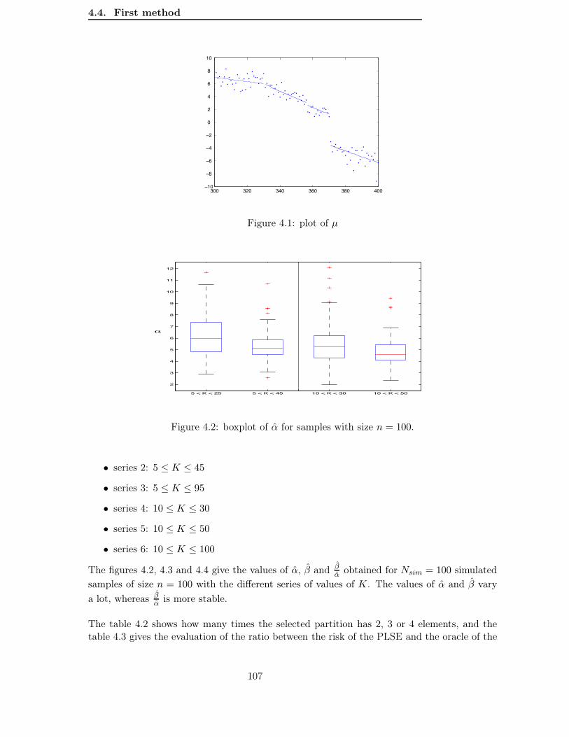
4.4. First method

300 320 340 360 380 400−10

−8

−6

−4

−2

0

2

4

6

8

10

Figure 4.1: plot of µ

5 < K < 25 5 < K < 45 10 < K < 30 10 < K < 50

2

3

4

5

6

7

8

9

10

11

12

α

Figure 4.2: boxplot of α for samples with size n = 100.

• series 2: 5 ≤ K ≤ 45

• series 3: 5 ≤ K ≤ 95

• series 4: 10 ≤ K ≤ 30

• series 5: 10 ≤ K ≤ 50

• series 6: 10 ≤ K ≤ 100

The figures 4.2, 4.3 and 4.4 give the values of α, β and βα obtained for Nsim = 100 simulated

samples of size n = 100 with the different series of values of K. The values of α and β varya lot, whereas β

α is more stable.

The table 4.2 shows how many times the selected partition has 2, 3 or 4 elements, and thetable 4.3 gives the evaluation of the ratio between the risk of the PLSE and the oracle of the

107

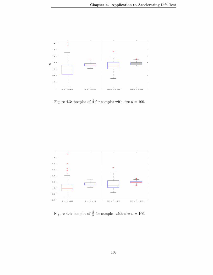
Chapter 4. Application to Accelerating Life Test

5 < K < 25 5 < K < 45 10 < K < 30 10 < K < 50

−2

−1

0

1

2

3

4

β

Figure 4.3: boxplot of β for samples with size n = 100.

5 < K < 25 5 < K < 45 10 < K < 30 10 < K < 50−0.4

−0.2

0

0.2

0.4

0.6

0.8

1

Figure 4.4: boxplot of βα for samples with size n = 100.

108

4.5. Second method

n 50 100 200 4005 ≤ K ≤ 25 23-24-4 25-61-12 4-87-7 0-87-125 ≤ K ≤ 45 18-65-13 2-86-8 0-87-105 ≤ K ≤ 95 0-77-14 0-81-1210 ≤ K ≤ 30 13-30-18 19-62-13 2-80-10 0-86-1010 ≤ K ≤ 50 16-64-12 0-80-11 0-81-910 ≤ K ≤ 100 0-71-15 0-78-12

Table 4.2: Performances of the first method: How many times the selected partition has 2, 3or 4 elements

n 50 100 200 4005 ≤ K ≤ 25 2.29 1.30 1.28 1.315 ≤ K ≤ 45 1.28 1.29 1.345 ≤ K ≤ 95 1.42 1.5110 ≤ K ≤ 30 1.85 1.35 1.37 1.3710 ≤ K ≤ 50 1.34 1.40 1.5810 ≤ K ≤ 100 1.53 1.62

Table 4.3: Performances of the first method: Estimated ratio between the risk of the PLSEand the oracle of the collection (SK)K≥1

collection (SK)K≥1. For samples with size n = 50, we do not get a good result. For sampleswith size n = 100, the length of the series of values of K seems not to be very important,but it seems that we should rather begin with K = 5 rather than K = 10. For samples withsize n = 200 or 400, the series of 21 values of K give better results than the series of 41 and91 values. Like for n = 100, the minimal value of K should be close to the size of the idealpartition M∗ (here K∗ = |M∗| = 3).

The best results are obtained with 5 ≤ K ≤ 25. This means that the series of values of Kused for the fit should not be too large and that the minimal value Kmin should be closeto the size of the ideal partition M∗. The problem is that the number |M∗| is unknown inpractice. The bad result obtained with n = 50 may be explained by the fact that the series5 ≤ K ≤ 25 is large as compared to n = 50. But we can not take smaller series of K becausewe have to estimate 3 parameters α, β and γ.

The main weakness of this method is that we do not know which series of K should be takenfor the fit. Series of 21 values should be preferred to larger series, but in practice we do notknow which minimal value Kmin should be taken.

4.5 Second method

We consider the following form of penalty:

pen(M) = λ|M |n

(

log

(Nn

|M |

)

+ c

)

.

109

Chapter 4. Application to Accelerating Life Test

We determine the right constant c thanks to a study involving simulated extreme value vari-ables (Zi)1≤i≤n with mean 0 and variance 1, and then the multiplicative constant λ is chosenaccording to the data using the practical rule proposed by Birgé and Massart [4, section 4].

Remark 4.3 The form of the penalty does not depend on the underlying distribution of thelife-time, but the constant c is calibrated using simulated extreme value variables (Zi)1≤i≤n.Therefore the obtained c only suits for the Weibull ALT model.

Recall that the theorem 4.1 recommends a penalty

pen(M) = (σ2 + Rb)|M |n

(

c1 log

(Nn

|M |

)

+ c2

)

with c1 and c2 absolute contants. But the theoretical result is not sharp enough to determinethe right constants c1 and c2. The multiplicative constant σ2 + Rb depends on the varianceτ2 and on R = ∥µ∥∞.

In a similar case where the multiplicative constant is the variance τ2 (instead of σ2 +Rb),Lebarbier [16] proposes a method to calibrate the constants c1 and c2 by using a class offunctions µ and simulated data with fixed and known variance τ2. Here we can not apply thesame method since the multiplicative constant depends on ∥µ∥∞. Moreover, we do not trustin the factor σ2 + Rb in the sense that it may rather be σ2 + κRb with κ = 1.

We make a simulation study with µ = 0 and τ2 = 1 both fixed to determine the rightconstant c∗ =

c∗2c∗1

. The simulation study described in the next subsection involves simulated

data corresponding to µ = 0 and τ2 = 1. Since µ = 0, we do not need to know whether theright multiplicative factor is σ2 + Rb or σ2 + 0.5Rb or something else.Then, we consider a penalty of the form pen(M) = λ |M |

n

(

log(

Nn|M |

)

+ c∗)

, and we use the

practical rule proposed by Birgé and Massart [4, section 4] to determine the right constant λaccording to the data.

4.5.1 A simulation study to determine the constant c.

In the first method described in section 4.4, we use Massart’s heuristic to estimate the twoconstants α and β of the penalty according to the data. The problem to use this heuristicin practice is that we do not know from which value of K, E[γn(µK)] is approximately con-stant. Here, we use Massart’s heuristic only to determinate the constant c from simulateddata corresponding to µ = 0 and τ = 1. For such data, E[γn(µK)] = 1 for all K ≥ 1. Thus,we fit −γn(µK) on 1

2Kn

(

α log(

NnK

)

+ β)

+ γ with 1 ≤ K ≤ Kmax. We only have to choose

the maximal value Kmax. Then we take c∗ as the median of c = βα obtained via Nsim = 100

simulated samples with size n.

The figure 4.5 gives the boxplot of the values of c obtained via Nsim = 100 simulated sampleswith n = 50, 100, 200, 400 and Kmax = 15, 25, 50, 100, 200 (Kmax ≤ n

2 ). For some fixed samplesize n, the amplitude of the boxplot of c decreases with Kmax.The table 4.4 gives the median of c as a function of n and Kmax. For some fixed n, the medianof c increases with Kmax. For Kmax

n ≤ 14 , whatever the sample size n, the median of c is close

110

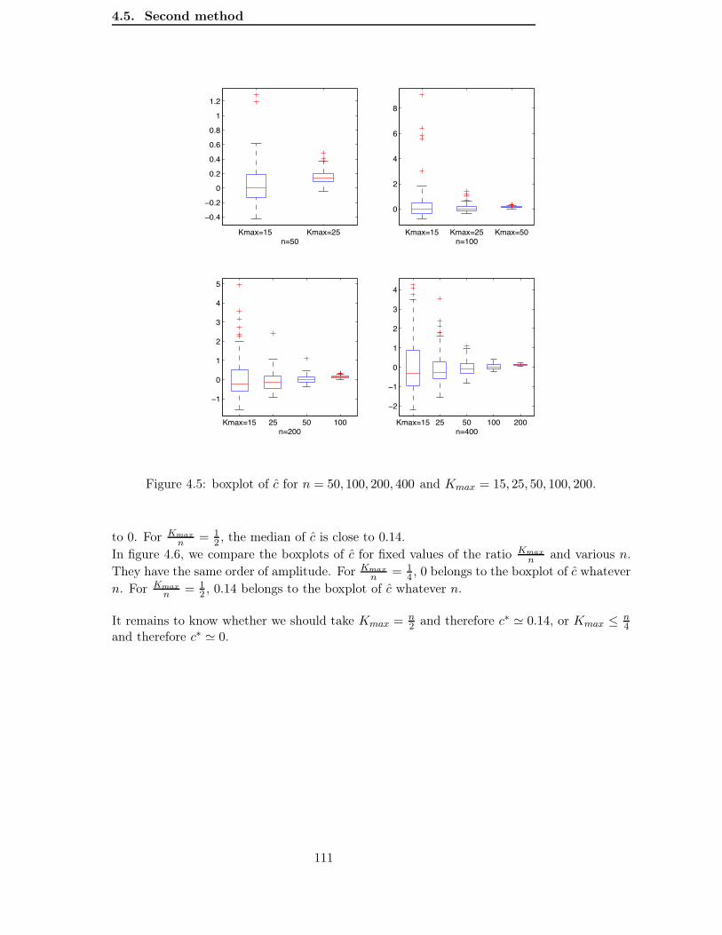
4.5. Second method

Kmax=15 Kmax=25

−0.4

−0.2

0

0.2

0.4

0.6

0.8

1

1.2

n=50Kmax=15 Kmax=25 Kmax=50

0

2

4

6

8

n=100

Kmax=15 25 50 100

−1

0

1

2

3

4

5

n=200Kmax=15 25 50 100 200

−2

−1

0

1

2

3

4

n=400

Figure 4.5: boxplot of c for n = 50, 100, 200, 400 and Kmax = 15, 25, 50, 100, 200.

to 0. For Kmaxn = 1

2 , the median of c is close to 0.14.In figure 4.6, we compare the boxplots of c for fixed values of the ratio Kmax

n and various n.They have the same order of amplitude. For Kmax

n = 14 , 0 belongs to the boxplot of c whatever

n. For Kmaxn = 1

2 , 0.14 belongs to the boxplot of c whatever n.

It remains to know whether we should take Kmax = n2 and therefore c∗ ≃ 0.14, or Kmax ≤ n

4and therefore c∗ ≃ 0.

111

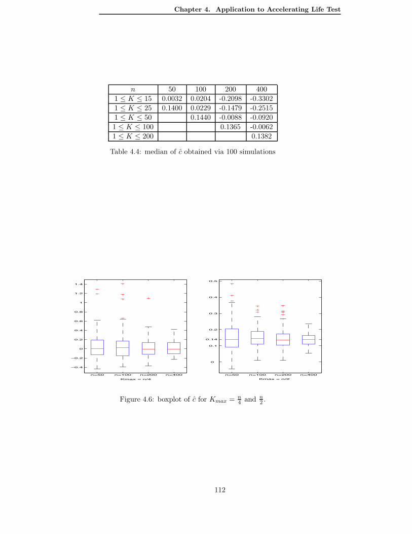
Chapter 4. Application to Accelerating Life Test

n 50 100 200 4001 ≤ K ≤ 15 0.0032 0.0204 -0.2098 -0.33021 ≤ K ≤ 25 0.1400 0.0229 -0.1479 -0.25151 ≤ K ≤ 50 0.1440 -0.0088 -0.09201 ≤ K ≤ 100 0.1365 -0.00621 ≤ K ≤ 200 0.1382

Table 4.4: median of c obtained via 100 simulations

n=50 n=100 n=200 n=400

−0.4

−0.2

0

0.2

0.4

0.6

0.8

1

1.2

1.4

n=50 n=100 n=200 n=400

0

0.1

0.14

0.2

0.3

0.4

0.5

Kmax = n/4 Kmax = n/2

Figure 4.6: boxplot of c for Kmax = n4 and n

2 .

112

4.5. Second method

4.5.2 A practical rule to determine λ according to the data.

In a Gaussian framework, Birgé and Massart [4] show that there exists a minimal penalty ofthe form:

penmin(M) =σ2

nDMA(DM )

with A(D) which depends on |M ∈Mn; DM = D|. More precisely, they prove that

• penalties of the form pen(M) = (1 + η)σ2

n DMA(DM ) with η > 0 lead to oracle typeinequalities,

• if pen(M) ≤ (1 − η)σ2

n DMA(DM ) for some η > 0 and DM sufficiently large, then therisk of the PLSE can be arbitrarly large.

They also show that pen(M) = 2penmin(M) is always a reasonable penalty (non asymptoti-cally) and sometimes an optimal one (asymptotically).In practice, σ2 is unknown and they consider penalties of the form

pen(M) = λDM

nA(DM )

λ = 2σ2 provides a good and sometimes nearly optimal penalty, and all λ < σ2 lead to pro-cedures which tend to choose a model of much too large dimension. Thus they suggest toestimate λ from the data by multiplying by 2 the first value for which the dimension of theselected model jumps to a smaller dimension.

Here the shape of the penalty pen(M) = λ |M |n

(

log(

Nn

|M |

)

+ c∗)

is given by the theory andcompleted by a simulation study. c∗ has been computed via a simulation study in subsection4.5.1. The values of c∗ are given in table 4.4. It remains to decide whether the right c∗ isobtained with Kmax = n

4 or n2 .

We consider

Kλ = arg min1≤K≤Nn

γn(µK) + λK

n

(

log

(Nn

K

)

+ c∗)

and we draw it as a function of λ. Then, we detect the value λmin which corresponds to thelargest jump. And we take λ = 2λmin.

Let (Yi)1≤i≤n a simulated sample with size n = 100 defined by (4.9), (4.10) and Zi =√

6π2 (Si + γ)

where Si ∼ SEV (0, 1). We consider penalties of the form pen(M) = λ |M |n

(

log(

Nn|M |

)

+ c∗)

with c∗ the median of the values of c obtained via the simulation study of section 4.5.1 withn = 100 and 1 ≤ K ≤ 50 , i.e. c∗ = 0.1440. We give in figure 4.7 the graph of Kλ as afunction of λ obtained with the simulated sample and c∗ = 0.1440. In figure 4.7, we see thatλmin = 2.51, λ = 5.02 and the selected number of subregions is 3 (which is the number K∗ ofsubregions of the ideal partition M∗).

In order to evaluate the performances of this second method and compare it to the firstone, we use Nsim = 100 simulated samples and we count how many times the ideal number

113

Chapter 4. Application to Accelerating Life Test

0 2.51 5.02 100

2

5

10

15

20

25

30

35

40

n = 100 and c* = 0.1440

Figure 4.7: Kλ as a function of λ.

n 50 100 200 400c∗ = 0 0-0-0 28-61-9 0-78-13 0-77-14

c∗ = median(cn,Kmax=n/2) 96-3-0 15-62-15 0-76-13 0-77-14

Table 4.5: Performances of the second method: How many times the selected partition has 2,3 or 4 elements

of pieces is chosen. The ideal number is K∗ = 3 when n ≥ 100 and K∗ = 2 when n = 50.The table 4.5 shows how many times the selected partition has 2, 3 or 4 elements. Thanks tothe Nsim = 100 repetitions and a Monte Carlo method, we evaluate the ratio between therisk of the PLSE and the oracle (see table 4.6).

For n ≥ 100, we get similar good results with c∗ = 0 and c∗ ≃ 0.14. For n = 50, we get agood result with c∗ ≃ 0.14, but in this case c∗ = 0 is not sufficient.

Figure 4.8 gives the values of λ obtained for the Nsim = 100 simulated samples of sizen = 100 with c∗ = 0 and 0.1440. This figure allows to understand the closeness of the perfor-mances of the first and second method for n = 100. With the first method and 5 ≤ K ≤ 25, 0

belongs to the boxplot of βα (see figure 4.4) and α takes values close to those of λ when c∗ = 0

(see figures 4.2 and 4.8). The method 1 with 5 ≤ K ≤ 25 and the method 2 with c∗ = 0 givesimilar penalty constants, and therefore similar results.

114

4.5. Second method

n 50 100 200 400c∗ = 0 3.60 1.32 1.42 1.64

c∗ = median(cn,Kmax=n/2) 1.21 1.37 1.46 1.64

Table 4.6: Performances of the second method: Estimated ratio between the risk of the PLSEand the oracle of the collection (SK)K≥1

3

4

5

6

7

8

9

10

11

12

c* = 0 c* = 0.1440

n = 100

Figure 4.8: boxplot of λ obtained with c∗ = 0 and 0.1440.

To sum up,

• For a small sample with size n = 50, the best result is obtained with the second methodand c∗ = 0.14 (which corresponds to Kmax = n

2 ). The ideal size K∗ = 2 is selected 96times among 100 attempts. And the estimated ratio between the risk of the PLSE andthe oracle is 1.21.

• For larger sample sizes n ≥ 100, the second method give similar good results with c∗ = 0and c∗ = 0.14, but the first method with 5 ≤ K ≤ 25 give better results. It seems thatthe minimal value of K (here 5) has to be close to the ideal number of subregions (here 3)and that the length of the series of K has to be moderate. 21 values of K are sufficient.We see on table 4.2 and 4.3 for n ≥ 200, that the series 5 ≤ K ≤ 25 and 10 ≤ K ≤ 30give better results than the longer ones. In order to use the first method, we shouldcomplete it by a procedure which automatically determines the minimal value of K.Without such a procedure, we have to content ourself with the first method, whoseresults are still quite good.

115

Appendix A

MARS

L’algorithme MARS (Multivariate Adaptive Regression Splines) proposé par Friedman [12]construit un estimateur d’une fonction de régression s définie sur un ensemble X ⊂ Rp. Fried-man [12] présente MARS comme une extension des méthodes de régression par constructionrécursive d’une partition (cf CART [7]). Ces méthodes sont notées ici méthodes RPR (Re-cursive Partitioning Regression). Contrairement aux méthodes RPR, MARS construit unestimateur continu (et même de classe C1), et permet d’approcher les fonctions additives ouplus généralement les fonctions qui s’écrivent comme des sommes de termes ne faisant inter-venir qu’un petit nombre de variables.

Commençons par décrire les méthodes RPR. Ces méthodes construisent des estimateurss de la forme:

si x ∈ Rk alors s(x) = ak

où les régions (Rk)1≤k≤K forment une partition de X et les coefficients (ak)1≤k≤K ∈ RK .Elles utilisent les données (xi, Yi)1≤i≤n, où xi = (x1

i , . . . , xpi ) ∈ X et Yi ∈ R, pour choisir la

partition de X et estimer les coefficients.

La création de la partition se fait de manière récursive dyadique. La partition initiale estconstituée d’une seule région: l’ensemble X tout entier. A chaque étape, on découpe en deuxles régions de la partition existante. Les découpages possibles d’une région R en deux régionsfilles Rg et Rd sont les découpages définis comme suit:

Rg =

x = (x1, . . . , xp) ∈ R; xj ≤ t

Rd =

x = (x1, . . . , xp) ∈ R; xj > t

Un découpage est donc défini par une variable xj et une valeur seuil t. Il est choisi de façonà optimiser l’adéquation aux données. On poursuit les découpages jusqu’à obtenir une parti-tion fine constituée d’un grand nombre de régions. Dans CART, on poursuit les découpagesjusqu’à ce que toutes les régions soient pures ou ne contiennent chacune qu’une seule observa-tion. Cette construction est naturellement représentée par un arbre de profondeur maximale.Certaines régions sont ensuite recombinées en supprimant des découpages. Cela revient àélaguer l’arbre maximal pour obtenir un arbre moins profond.La figure A.1 donne un exemple d’arbre ainsi construit.

117

!!

!

xj1, t1

xj2, t2R4

a4!!

!

R1

a1

xj3, t3!

!!

R2

a2R3

a3

Figure A.1: Arbre binaire représentant un estimateur s obtenu par une méthode RPR

Sur l’exemple de la figure A.1, R2 =

x = (x1, . . . , xp) ∈ X ; xj1 ≤ t1, xj2 > t2 et xj3 ≤ t3

,et si x ∈ R2 alors s(x) = a2. Cette représentation géométrique de s facilite la lecture etl’interprétation.

Nous pouvons aussi donner une écriture analytique de s sous forme d’un développementpar rapport à une famille de fonctions de base:

s(x) =K∑

k=1

akBk(x)

Les fonctions de base Bk sont les fonctions indicatrices des régions Rk: Bk(x) = 1IRk(x). Les

coefficients ak sont déterminés de façon à optimiser l’adéquation aux données.Notons γn le contraste des moindres carrés associé à l’échantillon d’observations (xi, Yi)1≤i≤n:

γn(u) =1

n

n∑

i=1

(Yi − u(xi))2 pour u : X → R.

Notons

H+(η) = 1Iη>0

H−(η) = 1Iη≤0

La construction de la partition fine (Rk)1≤k≤Kmax ou de la liste initiale de fonctions (Bk)1≤k≤Kmax

se fait par l’algorithme suivant:

118

Algorithme 1 (1ère étape de la méthode RPR)

B1(x)← 1

For K = 2 to Kmax do: lof∗ ←∞For k = 1 to K − 1 do:

For j = 1 to p do:

For t ∈ xji ; Bk(xi) > 0 do:

u←K−1∑

l=1l=k

alBl(x) + akBk(x)H+(xj − t) + aKBk(x)H−(xj − t)

lof ← mina1,...,aK

γn(u)

if lof < lof∗ then lof∗ ← lof, k∗ ← k, j∗ ← j, t∗ ← t endif

endfor

endfor

endfor

BK(x)← Bk∗(x)H−(xj∗ − t∗)

Bk∗(x)← Bk∗(x)H+(xj∗ − t∗)

endfor

La première ligne de l’algorithme 1 revient à définir la région initiale comme étant l’ensembleX tout entier. La première boucle itère les découpages jusqu’à ce que l’on ait une partitionen Kmax régions. (Rappelons que dans CART, les découpages se poursuivent jusqu’à ce quetoutes les régions soient pures ou ne contiennent chacune qu’une seule observation.) Les 3boucles suivantes déterminent une fonction Bk∗ , une variable xj∗ et une valeur seuil t∗ tellesque le découpage de la région Rk∗ par "xj∗ ≤ t∗" et "xj∗ > t∗" permet la meilleure adéquationaux données. La fonction Bk∗ est alors remplacée par son produit avec H+(xj∗ − t∗), et onajoute la fonction BK(x) = Bk∗(x)H−(xj∗ − t∗).Cet algorithme correspond à la première étape d’une méthode RPR. Il faut ensuite faire uneétape dite d’élagage que nous ne détaillons pas ici (voir CART [7]).

Les fonctions de base construites par les méthodes RPR sont de la forme:

Bk(x) =Nk∏

l=1

Hskl

(

xv(k,l) − tkl

)

où Nk est le nombre de découpages qui ont permis de définir Rk et donc Bk. Pour le lième

découpage, v(k, l) est le numéro de la variable sur laquelle porte le découpage, tkl est la valeurseuil du découpage et skl = ± selon que Rk ⊂ x; xv(k,l) > tkl ou Rk ⊂ x; xv(k,l) ≤ tkl.

Les méthodes RPR ont deux inconvénients:

1. elles produisent des estimateurs fortement discontinus,

2. elles ne permettent pas d’approcher les fonctions additives ou les fonctions dont lesinteractions sont d’ordre petit.

119

La discontinuité vient de l’utilisation des fonctions H±(xj − t) qui sont des splines d’ordre0. En les remplaçant par les splines d’ordre 1: [±(xj − t)]+, on obtient des fonctions de basecontinues puis des estimateurs continus. Avec les splines d’ordre 0: H±(xj − t), les fonc-tions de base Bk sont des produits tensoriels de splines d’ordre 0. Avec les splines d’ordre 1:[±(xj−t)]+, pour que les fonctions de base Bk soient des produits tensoriels de splines d’ordre1, il faudrait que chaque variable xj apparaisse au plus une fois dans le produit définissant Bk.On ne peut malheureusement pas interdire de découper plusieurs fois sur la même variable.Le deuxième inconvénient cité ci-dessus vient du fait que l’on enlève les fonctions faisant in-tervenir un petit nombre de variables et qu’à la sortie de l’algorithme les fonctions Bk fontintervenir beaucoup de variables. En effet, à chaque étape de l’algorithme 1, on remplace unefonction par deux nouvelles fonctions dont le niveau d’interaction est augmenté de 1 (saufsi le découpage se fait sur une variable qui apparaissait déjà). Lors d’un découpage, au lieude remplacer la fonction "mère" par ses deux fonctions "filles", on peut garder la fonction"mère" et simplement ajouter les deux nouvelles fonctions. On perd alors la réprésentationsous forme d’arbre, mais on peut ainsi espérer approcher les fonctions additives et les fonc-tions dont les interactions sont d’ordre petit. En faisant cette deuxième modification, onpeut maintenant imposer que les facteurs d’une même fonction de base fassent intervenir desvariables distinctes.

Friedman propose donc 3 modifications:

1. remplacer H±(x− t) par [±(x− t)]+,

2. lors d’une découpe, ne pas enlever la fonction choisie Bk∗, qui devient donc elligiblecomme ses filles pour les découpes suivantes,

3. imposer que tous les facteurs d’une même fonction de base fassent intervenir des variablesdistinctes.

Avec ces 3 modifications, on obtient la première partie de l’algorithme MARS, notée ci-dessousalgorithme 2.

120

Algorithme 2 (1ère partie de l’algorithme MARS)

B1(x)← 1; K ← 2

While K < Kmax do: lof∗ ←∞For k = 1 to K − 1 do:

For j /∈ v(l, k); 1 ≤ l ≤ Nk do:

For t ∈ xji ; Bk(xi) > 0 do:

u←K−1∑

l=1

alBl(x) + aKBk(x)[(xj − t)]+ + aK+1Bk(x)[−(xj − t)]+

lof ← mina1,...,aK+1

γn(u)

if lof < lof∗ then lof∗ ← lof, k∗ ← k, j∗ ← j, t∗ ← t endif

endfor

endfor

endfor

BK(x)← Bk∗(x)[(xj∗ − t∗)]+

BK+1(x)← Bk∗(x)[−(xj∗ − t∗)]+

K ← K + 2

endfor

La deuxième partie de l’algorithme MARS (notée ici algorithme 3) consiste à éliminer lesfonctions de base qui n’ont pas apporté une amélioration suffisante. Friedman utilise pourcela un critère qui pénalise les modèles associés à un grand nombre de fonctions de base. Al’issue de la première partie de MARS (algorithme 2), on dispose d’une famille de fonctionsde base: F = B1, B2, . . . , BKmax. Nous notons Mn la collection de toutes les sous-famillesde F :

Mn = m = (Bk)k∈N ; N ⊂ 1, 2, . . . ,Kmax ,

et à chaque m = (Bk)k∈N ∈ Mn, nous associons Sm l’espace vectoriel engendré par lesfonctions (Bk)k∈N , et sm l’estimateur des moindres carrés de s sur le modèle Sm. Friedmanpropose le critère suivant:

critF (m) =γn(sm)

(

1− Dm+c|m|n

)2

où Dm est la dimension du modèle Sm, |m| est le cardinal de la famille m et c est une constanteà choisir.A l’aide de ce critère, l’algorithme 3 ci-dessous sélectionne une sous-famille (Bj)j∈J∗ de F .

121

Algorithme 3 (2ème partie de l’algorithme MARS)

J∗ ← 1, 2, . . . ,Kmax; L∗ ← J∗;

lof∗ ← critF ((Bj)j∈J∗)

for K = Kmax to 2 do: b←∞;L← L∗

For k = 2 to K do: I ← L− klof ← critF ((Bi)i∈I)

if lof < b, then b← lof ;L∗ ← I endif

if lof < lof∗, then lof∗ ← lof ;J∗ ← I endif

endfor

endfor

A l’issue de cette deuxième partie, on dispose d’une nouvelle liste (plus petite) de fonctionsde base (Bj)j∈J∗ . Ces fonctions Bj sont des produits de fonctions de la forme b(x|s, t) =[s(x− t)]+. Pour obtenir un estimateur de classe C1, Friedman remplace ces fonctions par:

C(x|s = +, t−, t, t+) =

⎧

⎪⎨

⎪⎩

0 si x ≤ t−

p+(x− t−)2 + r+(x− t−)3 si t− < x < t+

x− t si x ≥ t+

C(x|s = −, t−, t, t+) =

⎧

⎪⎨

⎪⎩

−(x− t) si x ≤ t−

p−(x− t+)2 + r−(x− t+)3 si t− < x < t+

0 si x ≥ t+

où t− < t < t+ et

p+ = (2t+ + t− − 3t)/(t+ − t−)2,

r+ = (2t− t+ − t−)/(t+ − t−)3,

p− = (3t− 2t− − t+)/(t− − t+)2,

r− = (t− + t+ − 2t)/(t− − t+)3.

Les deux valeurs seuil supplémentaires t− et t+ sont placées de façon à réduire les disconti-nuités des dérivées d’ordre 2.Finalement on obtient une famille de fonctions (Bj)j∈J∗ et un estimateur s =

∑

j∈J∗ ajBj declasse C1, où les coefficients aj sont obtenus en minimisant le critère des moindres carrés.

122

Bibliography

[1] Y. Baraud. Model selection for regression on a fixed design. Probability Theory andRelated Fields, 117:467–493, 2000.

[2] Y. Baraud, F. Comte, and G. Viennet. Model Selection for (auto-)regression with de-pendent data. ESAIM Probability and Statistics, 5:33–49, 2001.

[3] L. Birgé and P. Massart. Gaussian model selection. Journal of the European MathematicalSociety, 3(3):203–268, 2001.

[4] L. Birgé and P. Massart. Minimal penalties for Gaussian model selection. To be publishedin Probability Theory and Related Fields, 2005.

[5] O. Bousquet. A Bennett concentration inequality and its application to suprema ofempirical processes. C.R. Math. Acad. Sci. Paris, 334:495–500, 2002.

[6] O. Bousquet. Concentration Inequalities for Sub-Additive Functions Using the EntropyMethod. Stochastic Inequalities and Applications, 56:213–247, 2003.

[7] L. Breiman, J. Friedman, R. Olshen, and C. Stone. Classification And Regression Trees.Chapman et Hall, 1984.

[8] G. Castellan. Modified Akaike’s criterion for histogram density estimation. C.R. Acad.Sci. Paris Sér. I Math., 330(8):729–732, 2000.

[9] G. Castellan. Density estimation via exponential model selection. IEEE Transactions oninformation theory, 49(8):2052–2060, 2003.

[10] F. Comte and Y. Rozenholc. A new algorithm for fixed design regression and denoising.Ann. Inst. Statist. Math., 56(3), 2004.

[11] B. Efron, T. Hastie, I. Johnstone, and R. Tibshirani. Least angle regression. Annals ofStatistics, 32(2):407–499, 2004.

[12] J. Friedman. Multivariate adaptive regression splines. Annals of Statistics, 19:1:141,1991.

[13] G.M. Furnival and R.W. Wilson. Regression by leaps and bounds. Technometrics, 16:499–511, 1974.

[14] S. Gey and E. Nédélec. Model Selection for CART Regression Trees. IEEE Trans. Inf.Theory, 51(2):658–670, 2005.

123

[15] T. Hastie, R. Tibshirani, and J. Friedman. The Elements of Statistical Learning. Springer,2001.

[16] E. Lebarbier. Quelques approches pour la détection de ruptures à horizon fini. PhD thesis,Université Paris XI Orsay, 2002.

[17] C.L. Mallows. Some comments on Cp. Technometrics, 15:661:675, 1973.

[18] P. Massart. Some Applications of Concentration Inequalities to Statistics. Annales de laFaculté des Sciences de Toulouse, 9(2):245–303, 2000.

[19] P. Massart. Notes de Saint-Flour. Lecture Notes to be published, 2003.

[20] P. Massart and E. Nédélec. Risk bounds for statistical learning. Annals of Statistics,34(5), 2006.

[21] J.M. Poggi and C. Tuleau. Classification supervisée en grande dimension. Application àl’agrément de conduite automobile. Preprint Université Paris XI Orsay, 2005.

[22] M. Sauvé. Histogram selection in non gaussian regression. Research Report 5911, INRIA,2006.

[23] M. Sauvé and C. Tuleau. Variable selection through CART. Research Report 5912,INRIA, 2006.

[24] R. Tibshirani. Regression shrinkage and selection via Lasso. Journal of the Royal Sta-tistical Society Series B, 58(1):267–288, 1996.

[25] A.B. Tsybakov. Optimal aggregation of classifiers in statistical learning. Annals ofStatistics, 32(1):135–166, 2004.

124

Résumé. Cette thèse traite de la sélection de modèles en régression non gaussienne.Notre but est d’obtenir des informations sur une fonction s : X → R dont on ne connaît qu’uncertain nombre de valeurs perturbées par des bruits non nécessairement gaussiens. Dans unpremier temps, nous considérons des modèles de fonctions constantes par morceaux associés àune collection de partitions de X . Nous déterminons un critère des moindres carrés pénalisésqui permet de sélectionner une partition dont l’estimateur associé (de type regressogramme)vérifie une inégalité de type oracle. La sélection d’un modèle de fonctions constantes parmorceaux ne conduit pas en général à une bonne estimation de s, mais permet notammentde détecter les ruptures de s. Nous proposons aussi une méthode non linéaire de sélection devariables qui repose sur l’application de plusieurs procédures CART et sur la sélection d’unmodèle de fonctions constantes par morceaux. Dans un deuxième temps, nous considéronsdes modèles de fonctions polynomiales par morceaux, dont les qualités d’approximation sontmeilleures. L’objectif est d’estimer s par un polynôme par morceaux dont le degré peut varierd’un morceau à l’autre. Nous déterminons un critère pénalisé qui sélectionne une partition deX = [0, 1]p et une série de degrés dont l’estimateur polynomial par morceaux associé vérifieune inégalité de type oracle. Nous appliquons aussi ce résultat pour détecter les ruptures d’unsignal affine par morceaux. Ce dernier travail est motivé par la détermination d’un intervallede stress convenable pour les tests de survie accélérés.

Mots-clés. sélection de modèles, sélection de variables, détection de ruptures, estima-tion polynomiale, inégalités de concentration, regression, CART, tests de survie.

Abstract. This thesis deals with model selection in non Gaussian regression. Our aim isto get informations on a function s : X → R given only some values perturbed by noises nonnecessarily Gaussian. In a first part, we consider histogram models (i.e. classes of piecewiseconstant functions) associated with a collection of partitions of X . We determine a penalizedleast squares criterion which selects a partition whose associated estimator satisfies an oracleinequality. Selecting a histogram model does not always lead to an accurate estimation of s,but allows for example to detect the change-points of s. In order to perform variable selection,we also propose a non linear method which relies on the use of CART and on histogram modelselection. In a second part, we consider piecewise polynomial models, whose approximationproperties are better. We aim at estimating s with a piecewise polynomial whose degree canvary from region to region. We determine a penalized criterion which selects a partition ofX = [0, 1]p and a series of degrees whose associated piecewise polynomial estimator satisfiesan oracle inequality. We also apply this result to detect the change points of a piewise affinesignal. The aim of this last work is to provide an adequate stress interval for AcceleratingLife Test.

Keywords. model selection, variable selection, change-points detection, polynomialestimation, concentration inequalities, regression, CART, Accelerating Life Test.