HEADQUARTERS: Brüel & Kjær Sound & Vibration Measurement A/S DK-2850 Nærum · Denmark · Telephone: +45 77 41 20 00 · Fax: +45 45 80 14 05 www.bksv.com · info@bksv.com

Local representatives and service organisations worldwide

www.bksv.comwww.bksv.com

TECHNICAL REVIEW

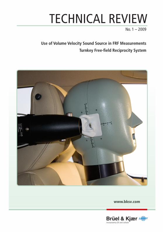
� Use�of�Volume�Velocity�Sound�Source�in�FRF�Measurements

� Turnkey�Free-field�Reciprocity�System

BV

  006

1  –

  11 

   IS

SN  0

007–

2621

No. 1 – 2009

Previously issued numbers ofBrüel & Kjær Technical Review1 – 2008 ISO 16063–11: Primary Vibration Calibration by Laser Interferometry:

Evaluation of Sine Approximation Realised by FFTInfrasound Calibration of Measurement MicrophonesImproved Temperature Specifications for Transducers with Built-in Electronics

1 – 2007 Measurement of Normal Incidence Transmission Loss and Other Acoustical Properties of Materials Placed in a Standing Wave Tube

1 – 2006 Dyn-X Technology: 160 dB in One Input RangeOrder Tracking in Vibro-acoustic Measurements: A Novel ApproachEliminating the Tacho ProbeComparison of Acoustic Holography Methods for Surface Velocity Determination on a Vibrating Panel

1 – 2005 Acoustical Solutions in the Design of a Measurement Microphone for Surface MountingCombined NAH and Beamforming Using the Same ArrayPatch Near-field Acoustical Holography Using a New Statistically Optimal Method

1 – 2004 Beamforming1 – 2002 A New Design Principle for Triaxial Piezoelectric Accelerometers

Use of FE Models in the Optimisation of Accelerometer DesignsSystem for Measurement of Microphone Distortion and Linearity from Medium to Very High Levels

1 – 2001 The Influence of Environmental Conditions on the Pressure Sensitivity of Measurement MicrophonesReduction of Heat Conduction Error in Microphone Pressure Reciprocity CalibrationFrequency Response for Measurement Microphones – a Question of ConfidenceMeasurement of Microphone Random-incidence and Pressure-field Responses and Determination of their Uncertainties

1 – 2000 Non-stationary STSF1 – 1999 Characteristics of the vold-Kalman Order Tracking Filter1 – 1998 Danish Primary Laboratory of Acoustics (DPLA) as Part of the National

Metrology OrganisationPressure Reciprocity Calibration – Instrumentation, Results and UncertaintyMP.EXE, a Calculation Program for Pressure Reciprocity Calibration of Microphones

1 – 1997 A New Design Principle for Triaxial Piezoelectric AccelerometersA Simple QC Test for Knock SensorsTorsional Operational Deflection Shapes (TODS) Measurements

2 – 1996 Non-stationary Signal Analysis using Wavelet Transform, Short-time Fourier Transform and Wigner-Ville Distribution

(Continued on cover page 3)

TechnicalReviewNo. 1 – 2009

Contents

Use of Volume Velocity Sound Sources in the Measurement of Acoustic Frequency Response Functions .............................................................................. 1By Andreas P. Schuhmacher and Gijs Dirks

Turnkey Free-field Reciprocity System for Primary Microphone Calibration... 23By Erling Frederiksen

TRADEMARKS

OmniSource is a trademark of Brüel&Kjær Sound & Vibration Measurement A/S.

Copyright © 2009, Brüel & Kjær Sound & Vibration Measurement A/SAll rights reserved. No part of this publication may be reproduced or distributed in any form, or by any means, without prior written permission of the publishers. For details, contact: Brüel & Kjær Sound & Vibration Measurement A/S, DK-2850 Nærum, Denmark.

Editor: Harry K. Zaveri

Use of Volume Velocity Sound Sources in the Measurement of Acoustic Frequency Response Functions

By Andreas P. Schuhmacher and Gijs Dirks

AbstractIn applications where acoustic radiation from a complicated sound source has tobe modelled, a series of FRFs (Frequency Response Functions) of sound pressure/volume velocity (p/Q) are normally measured. By combining operating acousticsource strengths with the FRFs, the airborne contributions of the modelled soundsources can be determined. In the case of structure-borne noise, a series of FRFs ofsound pressure/force (p/F) are measured. By measuring the operating forces actingon a structure and combining them with these FRFs, the noise contribution at areceiver position can be estimated. To determine the p/Q and p/F FrequencyResponse Functions, the device under test is repeatedly excited in differentpositions using a Volume Velocity Source, whilst there are no other forms ofexcitation.

This paper describes the design of a Volume Velocity Source and verifies its use inthe measurement of p/Q FRFs. Two designs of Volume Velocity Source arepresented, one for low-mid frequencies, and one for mid-high frequencies, bothtaking advantage of the two-microphone technique for estimating volume velocityat the orifice during operation.

RésuméDans le cadre des applications où le rayonnement acoustique diffusé par unesource sonore complexe doit être modélisé, on mesure généralement une série defonctions FRF (fonctions de réponse en fréquence) de la vitesse pressionacoustique/volume (p/Q). En combinant les atouts de la source acoustiqueopérationnelle avec les FRFs, on peut alors déterminer les contributions au bruitaérien des sources sonores modélisées. Une série de fonctions FRF pressionacoustique/force (p/F) sont mesurées pour le bruit propagé par la structure. Enmesurant les forces agissant sur la structure et en les combinant avec ces FRFs, il

1

est possible d'estimer la contribution sonore au point de réception. Pourdéterminer les fonctions de réponse en fréquence p/Q et p/F, l'objet testé subi desexcitations répétées sur différents points de sa structure au moyen d'une sourceomnidirectionnelle Volume Velocity Source, à défaut d'autres formes d'excitation.

La présente communication décrit comment est conçue cette Volume VelocitySource et rapporte les modalités de son utilisation pour des mesures de FRFs p/Q.Deux variantes de cette source sont présentées, une pour les fréquences basses àmoyennes, l'autre pour les fréquences moyennes à hautes, toutes deux intégrant latechnique des deux microphones pour une estimation de la vitesse volumique ensortie en cours d'opérations.

ZusammenfassungBei Anwendungen, bei denen die akustische Strahlung einer kompliziertenSchallquelle modelliert werden muss, wird in der Regel eine Serie vonÜbertragungsfunktionen (FRF) von Schalldruck/Volumengeschwindigkeit (p/Q)gemessen. Durch Kombination der akustischen Betriebs-Quellstärken mit denFRFs lassen sich die Luftschallbeiträge der modellierten Schallquellenbestimmen. Bei Körperschall wird eine Serie von Schalldruck/Kraft-FRFs (p/F)gemessen. Durch Messung der Betriebskräfte, die auf eine Struktur einwirken, undKombination mit diesen FRFs lässt sich der Geräuschbeitrag an einerEmpfängerposition abschätzen. Zur Ermittlung der Übertragungsfunktionen p/Qund p/F wird das zu prüfende Gerät wiederholt in verschiedenen Positionenangeregt, wobei die Anregung ausschließlich durch eineVolumengeschwindigkeitsquelle erfolgt.

Dieser Artikel beschreibt den Aufbau einer Volumengeschwindigkeitsquelle undverifiziert ihre Anwendung bei der Messung von p/Q-FRFs. Es werden zweiBauarten der Volumengeschwindigkeitsquelle vorgestellt: eine für tiefe bismittlere Frequenzen und eine für mittlere bis hohe Frequenzen. Beide profitierenvon der Zweimikrofon-Technik zur Abschätzung der Volumengeschwindigkeit ander Öffnung beim Betrieb.

2

IntroductionTo measure vibro-acoustic (p/F) FRFs in a vehicle, we normally take advantage ofthe reciprocity principle by placing a volume velocity sound source inside thecabin at the receiver position and mounting an accelerometer at the input forcelocation. Acoustic (p/Q) FRFs, on the other hand, can be measured using either adirect or reciprocal approach with a microphone measuring the sound pressure ateither the receiver location or at an assumed acoustic source position. However,for practical reasons, the type of FRFs from engine compartment source to cabinreceiver position are usually measured reciprocally due to the limitation of spacein engine compartments.

A volume velocity source has to meet some specific requirements [1]:

• The source should produce a sufficiently high sound level

• The frequency range covered should be appropriate

• The source should behave as a monopole in the frequency range of interest

• The output volume velocity should be measurable even when the acousticenvironment changes

The acoustic source for this purpose must be powerful and omnidirectional anda signal proportional to the source strength must be available – if the sourcestrength is not available directly. Furthermore, the frequency range covered shouldbe as broad as possible. Most volume velocity sound sources use one microphoneas a reference, assuming that there is a fixed linear relationship between volumevelocity output and reference sound pressure at the microphone. To find thisrelationship, the sound source is operated in an anechoic room and the volumevelocity output can be estimated from a microphone measurement at a knowndistance from the source. A frequency response function between volume velocityand reference sound pressure can then be calculated and stored for use when thesource is used in the real environment. The influence of a changing environmenton this fixed linear relationship will be investigated later in this paper by usingsome real measurements. For sound sources based on a driver (loudspeaker) wherethe sound radiates from the orifice of a flexible hose, the two-microphone methodcan be used to estimate the volume velocity output without first estimating thesound pressure to source strength relationship in the anechoic room. A furtherbenefit of this approach is the ability to determine the output volume velocity inany acoustic environment.

3

Methods to Measure Volume Velocity of a DriverThe following methods can be used:

• Single-microphone Method

• Two-microphone Method

Single-microphone MethodA signal proportional to the volume velocity must be available as the volumevelocity cannot be measured directly. Furthermore, the frequency range coveredshould be as broad as possible. Volume velocity sound sources using onemicrophone as a reference assume there is a fixed linear relationship betweenvolume velocity output and reference sound pressure at the microphone. Thisrelationship, however, is dependent on the impedance loading the sound source,which increases, especially in confined spaces.

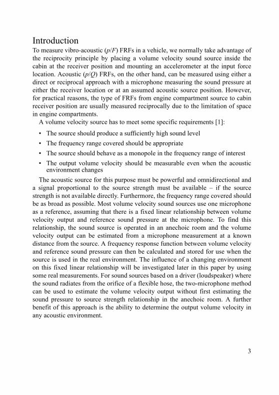
Calibration under anechoic conditions is needed with this method, even thoughthis calibration is not valid for all load impedances.Two-microphone MethodIn an earlier paper [2], the principle behind a particular volume velocity soundsource using two microphones was described in terms of how it was designed. Anomnidirectional sound source (Brüel & Kjær Type 4295), which was already usedfor room acoustic applications, was chosen as ‘the driver’ together with a specialadaptor (Brüel & Kjær Type 4299) that measures the volume velocity output. Apair of phase-matched microphones are used inside the adaptor to estimate thecalibrated volume velocity output spectrum in situ.

Fig. 1 shows the sound source, together with the adaptor, placed inside ananechoic room, and Fig. 2 shows a practical measurement setup where a flexible

Fig. 1. Low-mid frequency sound source(without extension hose)

Fig. 2. Low-mid frequency sound source(with extension hose)

4

hose is mounted between the sound source and the adaptor for ease-of-use duringmeasurements. As the useful frequency range of the driving loudspeaker is 50 Hz– 6 kHz, the output will be sufficient; however, the radiation from the orifice of theadaptor becomes more directional, i.e., less omnidirectional, above 2 – 3 kHz.

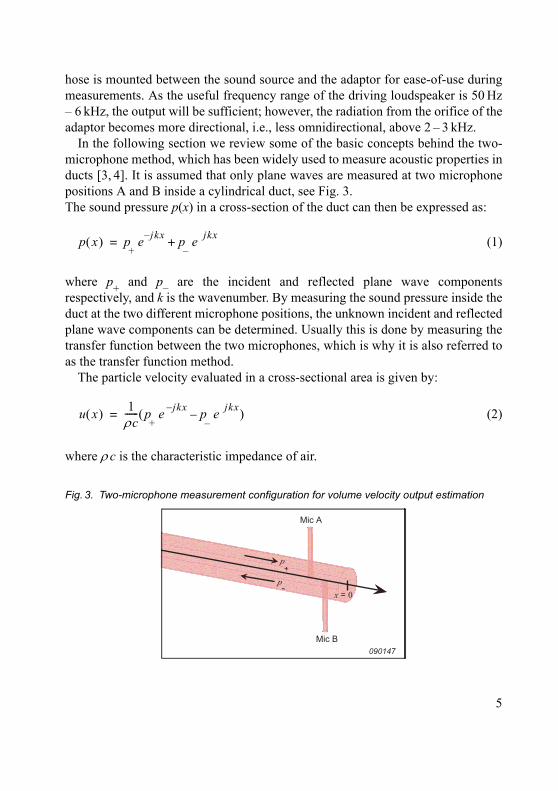
In the following section we review some of the basic concepts behind the two-microphone method, which has been widely used to measure acoustic properties inducts [3, 4]. It is assumed that only plane waves are measured at two microphonepositions A and B inside a cylindrical duct, see Fig. 3.The sound pressure p(x) in a cross-section of the duct can then be expressed as:

(1)

where p+ and p– are the incident and reflected plane wave components

respectively, and k is the wavenumber. By measuring the sound pressure inside theduct at the two different microphone positions, the unknown incident and reflectedplane wave components can be determined. Usually this is done by measuring thetransfer function between the two microphones, which is why it is also referred toas the transfer function method.

The particle velocity evaluated in a cross-sectional area is given by:

(2)

where c is the characteristic impedance of air.

Fig. 3. Two-microphone measurement configuration for volume velocity output estimation

p x p+

e–jkx

p–

ejkx

+=

u x 1c------ p

+e

–jkxp–

ejkx

– =

Mic A

Mic B

x = 0

p

p-

+

090147

5

At the duct opening, x = 0, we have:

(3)

and the output volume velocity signal Q can then be found by multiplication withthe cross-sectional area S of the duct. Higher order modes in the duct opening havezero volume velocity and therefore do not contribute. Finally, the frequencyresponse function p/Q to a response pressure p can be written as:

(4)

Frequency Response Function Measurement with the Two-microphone Volume Velocity MethodThe source to be used for reciprocal FRF measurements must be powerful andomnidirectional, and the frequency range of interest is typically 50 – 8000 Hz.

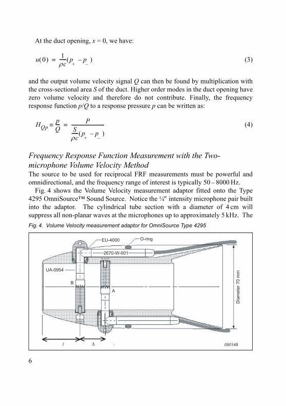
Fig. 4 shows the Volume Velocity measurement adaptor fitted onto the Type4295 OmniSource™ Sound Source. Notice the ¼ intensity microphone pair builtinto the adaptor. The cylindrical tube section with a diameter of 4 cm willsuppress all non-planar waves at the microphones up to approximately 5 kHz. The

Fig. 4. Volume Velocity measurement adaptor for OmniSource Type 4295

u 0 1c------ p

+p–

– =

HQppQ---- P

Sc------ p

+p–

– -----------------------------=

090148

EU-4000 O-ring

2670-W-001

UA-0954

A

B

Dia

met

er 7

0 m

m

ΔΔΔl

6

first higher order mode has a single radial node line and can propagate above5 kHz. But by measuring the pressure on the tube axis, this mode should not bedetected (in principle), as can be seen by the fact that it does not contribute to theoutput Volume Velocity. The first higher order mode, which has non-zero pressureon the axis, can propagate only above 10.4 kHz. At 6 kHz this mode will beattenuated 41 dB over the 3 cm from the opening to the outermost microphone B.Thus, if the two microphones (A and B) could measure the undisturbed pressureexactly on the axis, then only the propagating plane waves would contributesignificantly to the measurement over the frequency range dealt with. In practice,the microphones will disturb the sound field and not measure the pressure exactlyon the axis.

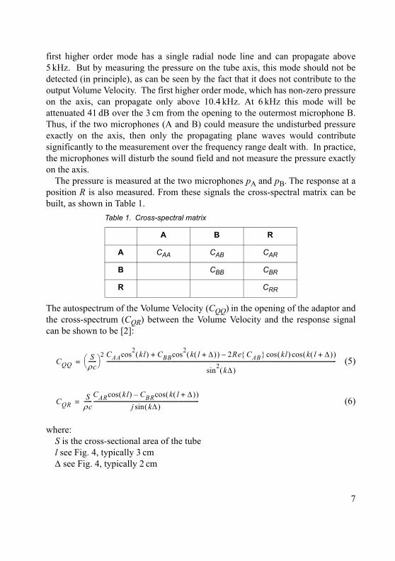
The pressure is measured at the two microphones pA and pB. The response at aposition R is also measured. From these signals the cross-spectral matrix can bebuilt, as shown in Table 1.

The autospectrum of the Volume Velocity (CQQ) in the opening of the adaptor andthe cross-spectrum (CQR) between the Volume Velocity and the response signalcan be shown to be [2]:

(5)

(6)

where:S is the cross-sectional area of the tubel see Fig. 4, typically 3 cmsee Fig. 4, typically 2 cm

Table 1. Cross-spectral matrix

A B R

A CAA CAB CAR

B CBB CBR

R CRR

CQQSc------ 2 CAAcos

2kl CBBcos

2k l + 2Re CAB kl k l + coscos–+

sin2

k ----------------------------------------------------------------------------------------------------------------------------------------------------------------------------=

CQRSc------

CARcos kl CBRcos k l + –

j k sin-------------------------------------------------------------------------------=

7

k wave number (2f/c)is theairdensityc is the propagation speed of sound

Using the two spectra, equations (5) and (6), the FRF HQR between this VolumeVelocity and the response signal can be obtained as:

(7)

Applications for Measuring a Source’s Volume Velocity

IntroductionIn the automotive industry there is a growing need for measurement of acousticalFRFs in connection with transfer path analysis. With advances in electrical andhybrid vehicle development, new paths and sources in the Automotive NVHprocess need to be investigated and evaluated, the main outcome being acousticalsource contribution analysis.

The analysis is used extensively to troubleshoot and to set targets at componentlevel, as well as being used to evaluate the acoustic NVH performance of vehicleswith the help of auralisation tools, such as the NVH Vehicle Simulator Type 8601.

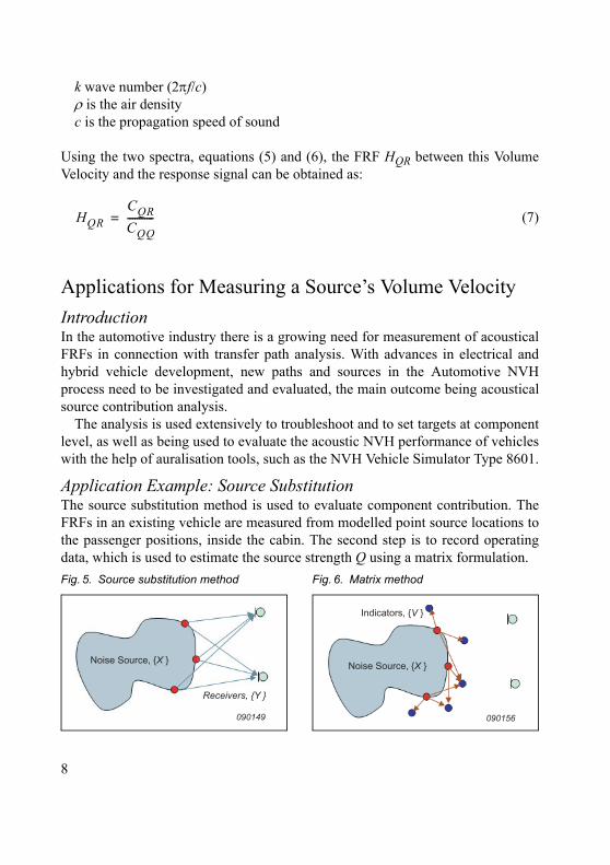
Application Example: Source SubstitutionThe source substitution method is used to evaluate component contribution. TheFRFs in an existing vehicle are measured from modelled point source locations tothe passenger positions, inside the cabin. The second step is to record operatingdata, which is used to estimate the source strength Q using a matrix formulation.

Fig. 5. Source substitution method Fig. 6. Matrix method

HQR

CQR

CQQ-----------=

Receivers, {Y }

Noise Source, {X }

090149

Noise Source, {X }

Indicators, {V }

090156

8

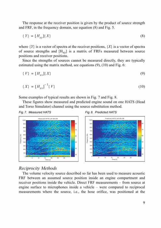
The response at the receiver position is given by the product of source strengthand FRF, in the frequency domain, see equation (8) and Fig. 5.

(8)

where {Y} is a vector of spectra at the receiver positions, {X} is a vector of spectraof source strengths and [Hxy] is a matrix of FRFs measured between sourcepositions and receiver positions.

Since the strengths of sources cannot be measured directly, they are typicallyestimated using the matrix method, see equations (9), (10) and Fig. 6:

(9)

(10)

Some examples of typical results are shown in Fig. 7 and Fig. 8.These figures show measured and predicted engine sound on one HATS (Head

and Torso Simulator) channel using the source substitution method.

Reciprocity MethodsThe volume velocity source described so far has been used to measure acoustic

FRF between an assumed source position inside an engine compartment andreceiver positions inside the vehicle. Direct FRF measurements – from source atengine surface to microphones inside a vehicle – were compared to reciprocalmeasurements where the source, i.e., the hose orifice, was positioned at the

Fig. 7. Measured HATS Fig. 8. Predicted HATS

Y Hxy X =

V Hxv X =

X Hxv – 1V =

Time [s]

Freq

uenc

y [H

z]

Measured HATS Left AB+SB

5 10 15 20 25 300

100

200

300

400

500

600

700

800

900

1000

30

40

50

60

70

80

Time [s]

Freq

uenc

y [H

z]

Predicted HATS Left AB+SB

5 10 15 20 25 300

100

200

300

400

500

600

700

800

900

1000

30

40

50

60

70

80

9

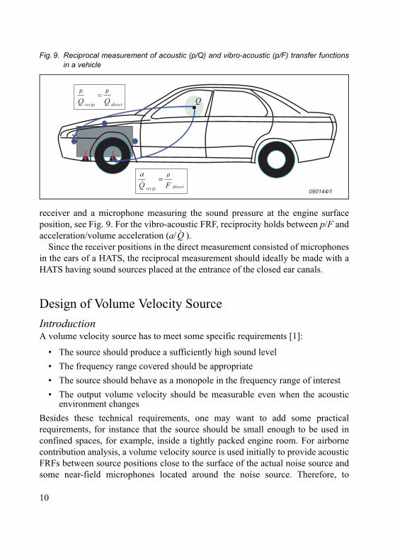
receiver and a microphone measuring the sound pressure at the engine surfaceposition, see Fig. 9. For the vibro-acoustic FRF, reciprocity holds between p/F andacceleration/volume acceleration (a/ ).

Since the receiver positions in the direct measurement consisted of microphonesin the ears of a HATS, the reciprocal measurement should ideally be made with aHATS having sound sources placed at the entrance of the closed ear canals.

Design of Volume Velocity Source

IntroductionA volume velocity source has to meet some specific requirements [1]:

• The source should produce a sufficiently high sound level

• The frequency range covered should be appropriate

• The source should behave as a monopole in the frequency range of interest

• The output volume velocity should be measurable even when the acousticenvironment changes

Besides these technical requirements, one may want to add some practicalrequirements, for instance that the source should be small enough to be used inconfined spaces, for example, inside a tightly packed engine room. For airbornecontribution analysis, a volume velocity source is used initially to provide acousticFRFs between source positions close to the surface of the actual noise source andsome near-field microphones located around the noise source. Therefore, to

Fig. 9. Reciprocal measurement of acoustic (p/Q) and vibro-acoustic (p/F) transfer functionsin a vehicle

directrecip Fp

Qa

=&

Qdirectrecip Qp

Qp

=

090144/1

Q·

10

measure FRFs easily it must be possible to attach the sound source on any surfaceor to position it in the near-field if a reciprocal approach is used. This speaks infavour of using a sound source based on some sort of driver attached to a longflexible hose where the sound is radiated from the hose orifice. The hose end canthen be attached to a surface or placed in air during FRF measurements.

Design of a Low-mid Frequency Volume Velocity Source – Type 4299 Adaptor

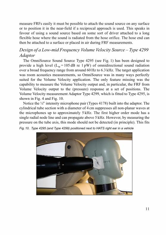
The OmniSource Sound Source Type 4295 (see Fig. 1) has been designed toprovide a high level (Lw = 105 dB re 1 pW) of omnidirectional sound radiationover a broad frequency range from around 60 Hz to 6.3 kHz. The target applicationwas room acoustics measurements, so OmniSource was in many ways perfectlysuited for the Volume Velocity application. The only feature missing was thecapability to measure the Volume Velocity output and, in particular, the FRF fromVolume Velocity output to the (pressure) response at a set of positions. TheVolume Velocity measurement Adaptor Type 4299, which is fitted to Type 4295, isshown in Fig. 4 and Fig. 10.

Notice the ¼ intensity microphone pair (Types 4178) built into the adaptor. Thecylindrical tube section with a diameter of 4 cm suppresses all non-planar waves atthe microphones up to approximately 5 kHz. The first higher order mode has asingle radial node line and can propagate above 5 kHz. However, by measuring thepressure on the tube axis, this mode should not be detected (in principle). This fits

Fig. 10. Type 4295 (and Type 4299) positioned next to HATS right ear in a vehicle

11

with the fact that it does not contribute to the output Volume Velocity. The firsthigher order mode, which has non-zero pressure on the axis, can only propagateabove 10.4 kHz. At 6 kHz, this mode will be attenuated 41 dB over the 3 cm fromthe opening to the outermost microphone (microphone B). So if the twomicrophones (A and B) could measure the undisturbed pressure exactly on theaxis, then only the propagating plane waves would contribute significantly to themeasurement over the considered frequency range. In practice, the microphoneswill disturb the sound field and not measure the pressure exactly on the axis. Soassuming that only plane waves are measured, the plane wave componentspropagating in the two directions can be estimated from the two microphonesignals. These two plane wave components can be extrapolated to the opening ofthe tube, and the Volume Velocity output can be calculated.

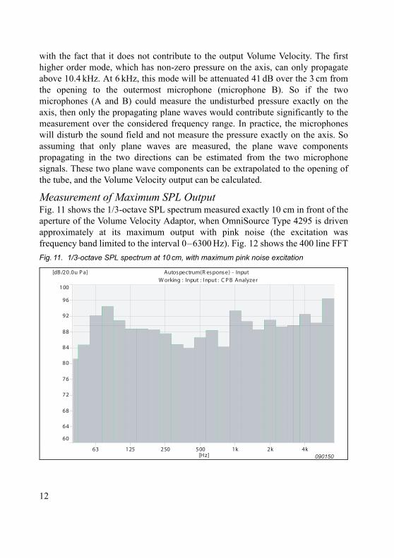
Measurement of Maximum SPL OutputFig. 11 shows the 1/3-octave SPL spectrum measured exactly 10 cm in front of theaperture of the Volume Velocity Adaptor, when OmniSource Type 4295 is drivenapproximately at its maximum output with pink noise (the excitation wasfrequency band limited to the interval 0–6300 Hz). Fig. 12 shows the 400 line FFT

Fig. 11. 1/3-octave SPL spectrum at 10 cm, with maximum pink noise excitation

Autospectrum(R esponse) - InputW orking : Input : Input : C P B Analyzer

63 125 250 500 1k 2k 4k

60

64

68

72

76

80

84

88

92

96

100

[Hz]

[dB /20.0u P a] Autospectrum(R esponse) - InputW orking : Input : Input : C P B Analyzer

63 125 250 500 1k 2k 4k

60

64

68

72

76

80

84

88

92

96

100

[Hz]

[dB /20.0u P a]

090150

12

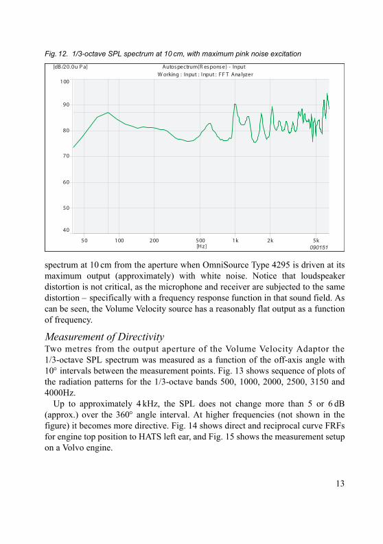
spectrum at 10 cm from the aperture when OmniSource Type 4295 is driven at itsmaximum output (approximately) with white noise. Notice that loudspeakerdistortion is not critical, as the microphone and receiver are subjected to the samedistortion – specifically with a frequency response function in that sound field. Ascan be seen, the Volume Velocity source has a reasonably flat output as a functionof frequency.

Measurement of DirectivityTwo metres from the output aperture of the Volume Velocity Adaptor the1/3-octave SPL spectrum was measured as a function of the off-axis angle with10 intervals between the measurement points. Fig. 13 shows sequence of plots ofthe radiation patterns for the 1/3-octave bands 500, 1000, 2000, 2500, 3150 and4000Hz.

Up to approximately 4 kHz, the SPL does not change more than 5 or 6 dB(approx.) over the 360 angle interval. At higher frequencies (not shown in thefigure) it becomes more directive. Fig. 14 shows direct and reciprocal curve FRFsfor engine top position to HATS left ear, and Fig. 15 shows the measurement setupon a Volvo engine.

Fig. 12. 1/3-octave SPL spectrum at 10 cm, with maximum pink noise excitation

Autospectrum(R esponse) - InputW orking : Input : Input : FF T Analyzer

50 100 200 500 1k 2k 5k

40

50

60

70

80

90

100

[Hz]

[dB /20.0u P a] Autospectrum(R esponse) - InputW orking : Input : Input : FF T Analyzer

50 100 200 500 1k 2k 5k

40

50

60

70

80

90

100

[Hz]

[dB /20.0u P a]

090151

13

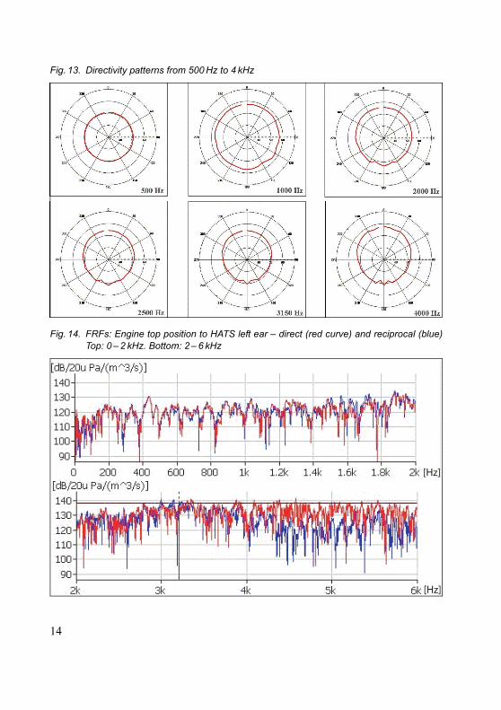
Fig. 13. Directivity patterns from 500 Hz to 4 kHz

Fig. 14. FRFs: Engine top position to HATS left ear – direct (red curve) and reciprocal (blue)Top: 0 – 2 kHz. Bottom: 2 – 6 kHz

[Hz]

[Hz]

14

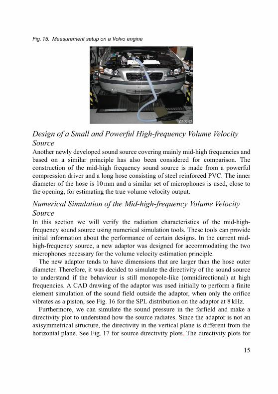
Design of a Small and Powerful High-frequency Volume Velocity SourceAnother newly developed sound source covering mainly mid-high frequencies andbased on a similar principle has also been considered for comparison. Theconstruction of the mid-high frequency sound source is made from a powerfulcompression driver and a long hose consisting of steel reinforced PVC. The innerdiameter of the hose is 10 mm and a similar set of microphones is used, close tothe opening, for estimating the true volume velocity output.

Numerical Simulation of the Mid-high-frequency Volume Velocity SourceIn this section we will verify the radiation characteristics of the mid-high-frequency sound source using numerical simulation tools. These tools can provideinitial information about the performance of certain designs. In the current mid-high-frequency source, a new adaptor was designed for accommodating the twomicrophones necessary for the volume velocity estimation principle.

The new adaptor tends to have dimensions that are larger than the hose outerdiameter. Therefore, it was decided to simulate the directivity of the sound sourceto understand if the behaviour is still monopole-like (omnidirectional) at highfrequencies. A CAD drawing of the adaptor was used initially to perform a finiteelement simulation of the sound field outside the adaptor, when only the orificevibrates as a piston, see Fig. 16 for the SPL distribution on the adaptor at 8 kHz.

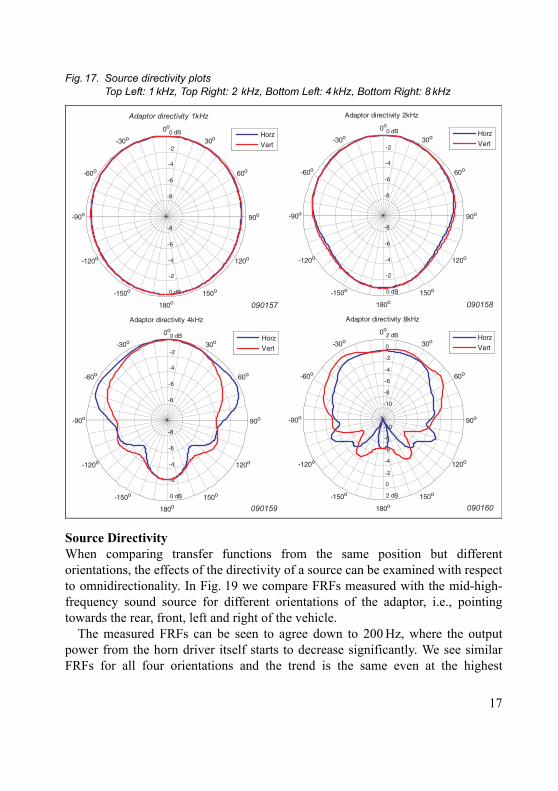
Furthermore, we can simulate the sound pressure in the farfield and make adirectivity plot to understand how the source radiates. Since the adaptor is not anaxisymmetrical structure, the directivity in the vertical plane is different from thehorizontal plane. See Fig. 17 for source directivity plots. The directivity plots for

Fig. 15. Measurement setup on a Volvo engine

15

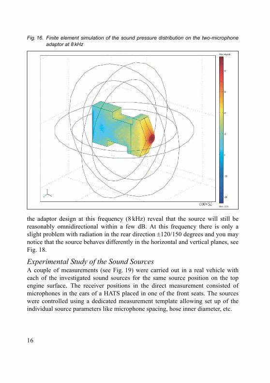
the adaptor design at this frequency (8 kHz) reveal that the source will still bereasonably omnidirectional within a few dB. At this frequency there is only aslight problem with radiation in the rear direction 120/150 degrees and you maynotice that the source behaves differently in the horizontal and vertical planes, seeFig. 18.

Experimental Study of the Sound SourcesA couple of measurements (see Fig. 19) were carried out in a real vehicle witheach of the investigated sound sources for the same source position on the topengine surface. The receiver positions in the direct measurement consisted ofmicrophones in the ears of a HATS placed in one of the front seats. The sourceswere controlled using a dedicated measurement template allowing set up of theindividual source parameters like microphone spacing, hose inner diameter, etc.

Fig. 16. Finite element simulation of the sound pressure distribution on the two-microphoneadaptor at 8 kHz

16

Source DirectivityWhen comparing transfer functions from the same position but differentorientations, the effects of the directivity of a source can be examined with respectto omnidirectionality. In Fig. 19 we compare FRFs measured with the mid-high-frequency sound source for different orientations of the adaptor, i.e., pointingtowards the rear, front, left and right of the vehicle.

The measured FRFs can be seen to agree down to 200 Hz, where the outputpower from the horn driver itself starts to decrease significantly. We see similarFRFs for all four orientations and the trend is the same even at the highest

Fig. 17. Source directivity plotsTop Left: 1 kHz, Top Right: 2 kHz, Bottom Left: 4 kHz, Bottom Right: 8 kHz

-8

-8

-6

-6

-4

-4

-2

-2

0 dB

0 dB

90o

60o

30o

0o

-30o

-60o

-90o

-120o

-150o

180o

150o

120o

Adaptor directivity 1kHz

090157

Horz

Vert

-8

-8

-6

-6

-4

-4

-2

-2

0 dB

0 dB

90o

60o

30o

0o

-30o

-60o

-90o

-120o

-150o

180o

150o

120o

Adaptor directivity 2kHz

090158

Horz

Vert

-8

-8

-6

-6

-4

-4

-2

-2

0 dB

0 dB

90o

60o

30o

0o

-30o

-60o

-90o

-120o

-150o

180o

150o

120o

Adaptor directivity 4kHz

090159

Horz

Vert

-10

-10

-8

-8

-6

-6

-4

-4

-2

-2

0

0

2 dB

2 dB

90o

60o

30o

0o

-30o

-60o

-90o

-120o

-150o

180o

150o

120o

Adaptor directivity 8kHz

Horz

Vert

090160

17

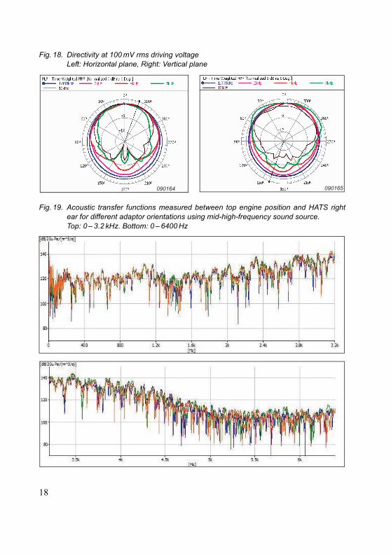
Fig. 18. Directivity at 100 mV rms driving voltageLeft: Horizontal plane, Right: Vertical plane

Fig. 19. Acoustic transfer functions measured between top engine position and HATS rightear for different adaptor orientations using mid-high-frequency sound source. Top: 0 – 3.2 kHz. Bottom: 0 – 6400 Hz

090165090164

18

frequencies shown, i.e., 6.4 kHz. Above this frequency the sound from the orificeof the adaptor becomes more directional as explained earlier, and the effect of thiscan be seen from the lower plot in Fig. 19.

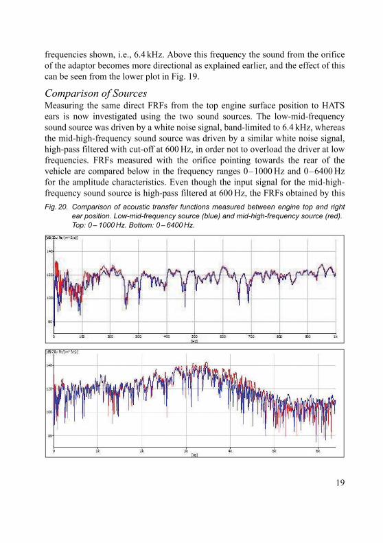
Comparison of SourcesMeasuring the same direct FRFs from the top engine surface position to HATSears is now investigated using the two sound sources. The low-mid-frequencysound source was driven by a white noise signal, band-limited to 6.4 kHz, whereasthe mid-high-frequency sound source was driven by a similar white noise signal,high-pass filtered with cut-off at 600 Hz, in order not to overload the driver at lowfrequencies. FRFs measured with the orifice pointing towards the rear of thevehicle are compared below in the frequency ranges 0–1000 Hz and 0–6400 Hzfor the amplitude characteristics. Even though the input signal for the mid-high-frequency sound source is high-pass filtered at 600 Hz, the FRFs obtained by this

Fig. 20. Comparison of acoustic transfer functions measured between engine top and rightear position. Low-mid-frequency source (blue) and mid-high-frequency source (red). Top: 0 – 1000 Hz. Bottom: 0 – 6400 Hz.

19

source are valid down to 200 Hz, since sufficient sound output is produced by thesource compared to background noise levels. In Fig. 20 it can be seen that themeasured FRFs using the two sound sources agree very well in amplitude from200 Hz up to at least 3 kHz. The lower plot in Fig. 20 shows the amplitude in thefrequency range 0–6400 Hz, where deviations are seen in the range of 10 dB athigh frequencies. This is expected as the high-frequency source is omnidirectionalto a much higher frequency than the low-frequency source and the dimensions ofthe sources (together with their different acoustic centres) play a role at higherfrequencies and this introduces deviations.

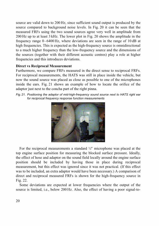
Direct vs Reciprocal MeasurementFurthermore, we compare FRFs measured in the direct sense to reciprocal FRFs.For reciprocal measurements, the HATS was still in place inside the vehicle, butnow the sound source was placed as close as possible to one of the microphonesinside the ears. Fig. 21 shows an example of how to locate the orifice of theadaptor just next to the concha part of the right pinna.

For the reciprocal measurements a standard ½ microphone was placed at thetop engine surface position for measuring the blocked surface pressure. Ideally,the effect of hose and adaptor on the sound field locally around the engine surfaceposition should be included by having those in place during reciprocalmeasurement, but this effect was ignored since it was not practical. (If this effectwas to be included, an extra adaptor would have been necessary.) A comparison ofdirect and reciprocal measured FRFs is shown for the high-frequency source inFig. 22.

Some deviations are expected at lower frequencies where the output of thesource is limited, i.e., below 200 Hz. Also, the effect of having a poor signal-to-

Fig. 21. Positioning the adaptor of mid-high-frequency sound source next to HATS right earfor reciprocal frequency response function measurements

20

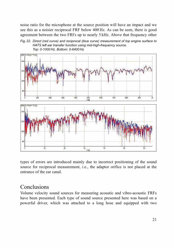
noise ratio for the microphone at the source position will have an impact and wesee this as a noisier reciprocal FRF below 400 Hz. As can be seen, there is goodagreement between the two FRFs up to nearly 5 kHz. Above that frequency other

types of errors are introduced mainly due to incorrect positioning of the soundsource for reciprocal measurement, i.e., the adaptor orifice is not placed at theentrance of the ear canal.

ConclusionsVolume velocity sound sources for measuring acoustic and vibro-acoustic FRFshave been presented. Each type of sound source presented here was based on apowerful driver, which was attached to a long hose and equipped with two

Fig. 22. Direct (red curve) and reciprocal (blue curve) measurement of top engine surface toHATS left ear transfer function using mid-high-frequency source. Top: 0-1000 Hz. Bottom: 0-6400 Hz

21

microphones close to the orifice. They were used to measure the volume velocitysource strength in situ.

FRFs could then easily be estimated. The principle was reviewed and somesources of errors related to current sound sources were pointed out. Acoustic FRFswere measured in a vehicle environment (with some confidence), proving that it ispossible to reciprocally measure the binaural FRFs, by placing the orifice close tothe entrance of the outer ear. In this case, a standard HATS and volume velocitysource can be used to do all the operating and FRF measurements related tosource-path-contribution analysis, including binaural effects. In addition, a soundsource aimed at mid-to-high frequency measurements, making use of the two-microphone method, was investigated and compared to the current low-to-midfrequency sound source.

References[1] F. H. van Tol, J. W. Verheij, “Brite EuRam II: Loudspeaker for Reciprocal

Measurement of Near Field Sound Transfer Functions on Heavy RoadVehicle Engines”, TNO Institute of Applied Physics, Delft, TheNetherlands, 1993.

[2] S. Gade, N. Møller, J. Hald, L. Alkestrup, “The Use of Volume VelocitySource in Transfer Measurements”, Proc. 2004 Int. Conf. on ModalAnalysis Noise and Vibration Engineering (ISMA), Leuven, pp. 2641-2648, 2004.

[3] J. Y. Chung, D. A. Blaser, “Transfer Function Method of Measuring In-duct Acoustic Properties”. I. Theory, J. Acoustical Society of America, Vol.68, No. 3, pp. 907-913, 1980.

[4] H. Bodén, M. Åbom, “Influence of Errors on the Two-microphone Methodfor Measuring Acoustic Properties in Ducts”, Journal of the AcousticalSociety of America, Vol. 79, No. 2, pp. 541-549, 1986.

[5] P. M. Morse, K. U. Ingard, “Theoretical Acoustics”, McGraw-Hill, NewYork, 1968.

[6] A. Schuhmacher, “Practical Measurement of Transfer Functions usingVolume Velocity Sources”, DAGA, 2009.

22

Turnkey Free-field Reciprocity System for Primary Microphone Calibration

Erling Frederiksen

AbstractAlthough most practical measurements are performed under free- or diffuse-fieldconditions, all reference microphone calibrations performed by national metrologyinstitutes are essentially pressure response calibrations. Fortunately, asmeasurement microphones have fixed ratios between the pressure- and free- anddiffuse-field responses, they can be determined simply by adding corrections tothe pressure response. However, to determine the necessary corrections andcalibrate microphones, some institutes need to develop and gain experience withthe use of the free-field calibration technique.

In principle, free-field calibration is simpler than pressure calibration, but inpractice it is more difficult, as one can only obtain very low sound pressures. Asno commercial free-field calibration systems are available, a few institutes havebuilt systems themselves and succeeded in making free-field calibration a routinetask. Even fewer institutes have established a calibration service.

The Danish Technical University (DTU), after several years of research, hasdeveloped a sophisticated free-field reciprocity calibration system, whereBrüel & Kjær has contributed with instruments and technical modifications. Thispaper describes the system, which is now offered by Brüel & Kjær, with softwareand technical support from the university staff.

RésuméMême si, pratiquement, la plupart des mesurages sont réalisés dans des conditionsde champ ou de champ diffus, les étalonnages des microphones de référenceeffectués par les centres métrologiques nationaux sont essentiellement desétalonnages de réponse en pression. Heureusement, comme la relation est fixeentre les réponses en pression et les réponses en champ libre et diffus des

23

microphones de mesure, il suffit pour connaître ces dernières d'ajouter les correctionsidoines aux valeurs de réponse en pression. Toutefois, pour déterminer les correctionsnécessaires et étalonner les microphones, certains laboratoires ont préalablementbesoin d'acquérir une certaine expérience de l'étalonnage en champ libre.

Si, en principe, un étalonnage en champ libre est plus simple qu'un étalonnage enpression, il ne l'est pas dans la pratique car les pressions acoustiques mesurées sonttrès faibles. Comme aucun système d'étalonnage en champ libre n'est disponibledans le commerce, certains centres ont construit leur propre système et réussi à fairede l'étalonnage en champ libre une opération de routine. Un nombre très restreintde centres proposent leurs services sous forme de prestations d'étalonnage.

Au terme de plusieurs années de recherche, le centre de l'Université Technique duDanemark (DTU) a mis au point un système d'étalonnage en champ libre parméthode de réciprocité, auquel Brüel & Kjær a fourni appareillage etmodifications techniques. La présente communication est une description dusystème Brüel & Kjær, avec logiciels et support technique de l'équipe universitaire.

ZusammenfassungObwohl die meisten Messungen in der Praxis unter Freifeld- oderDiffusfeldbedingungen erfolgen, wird bei der Kalibrierung vonBezugsnormalmikrofonen durch nationale Metrologieinstitute hauptsächlich derDruckfrequenzgang kalibriert. Dank der festen Beziehung zwischen demDruckfrequenzgang von Messmikrofonen und den Frequenzgängen in Frei- undDiffusfeld lassen sich letztere ermitteln, indem man zum DruckfrequenzgangKorrekturen addiert. Um jedoch die erforderlichen Korrekturen ermitteln undMikrofone kalibrieren zu können, müssen manche Institute erst eine Freifeld-Kalibriermethode entwickeln und damit Erfahrungen sammeln.

Im Prinzip ist Freifeldkalibrierung einfacher als Druckkalibrierung, doch in derPraxis ist sie schwieriger, da man mit sehr niedrigen Schalldrücken arbeiten muss.Da Freifeldkalibriersysteme nicht kommerziell erhältlich sind, haben einzelneInstitute eigene Systeme gebaut und die Freifeldkalibrierung zur Routineaufgabegemacht. Noch weniger Institute haben einen Kalibrierdienst eingerichtet.

24

Die Dänische Technische Universität (DTU) hat nach mehrjährigerForschungsarbeit ein anspruchsvolles System zur Freifeld-Reziprozitätskalibrierung entwickelt, zu dem Brüel & Kjær mit Geräten undtechnischen Modifikationen beigetragen hat. Dieser Artikel beschreibt dasSystem, das jetzt von Brüel & Kjær angeboten wird, mit Software und technischerUnterstützung durch Mitarbeiter der Universität.

IntroductionThe free-field reciprocity calibration method has been applied for more than half acentury. It is extensively described in literature, and the International StandardIEC 61094–3 [1] describes in detail the principle and influencing parameters.Other IEC standards belonging to the same microphone and calibration series,IEC 61094–1 [2] and IEC 61094–4 [3], describe Laboratory StandardMicrophones and Working Standard Microphones, respectively. The describedmicrophones are all condenser microphones, so they are reciprocal and suited forreciprocity calibration.

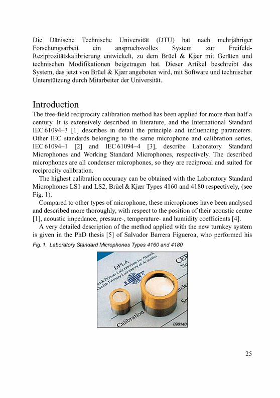
The highest calibration accuracy can be obtained with the Laboratory StandardMicrophones LS1 and LS2, Brüel & Kjær Types 4160 and 4180 respectively, (seeFig. 1).

Compared to other types of microphone, these microphones have been analysedand described more thoroughly, with respect to the position of their acoustic centre[1], acoustic impedance, pressure-, temperature- and humidity coefficients [4].

A very detailed description of the method applied with the new turnkey systemis given in the PhD thesis [5] of Salvador Barrera Figueroa, who performed his

Fig. 1. Laboratory Standard Microphones Types 4160 and 4180

25

study under supervision of Professors Knud Rasmussen (chairman of IEC/TC29)and Finn Jacobsen at the Danish Technical University, Kgs. Lyngby.

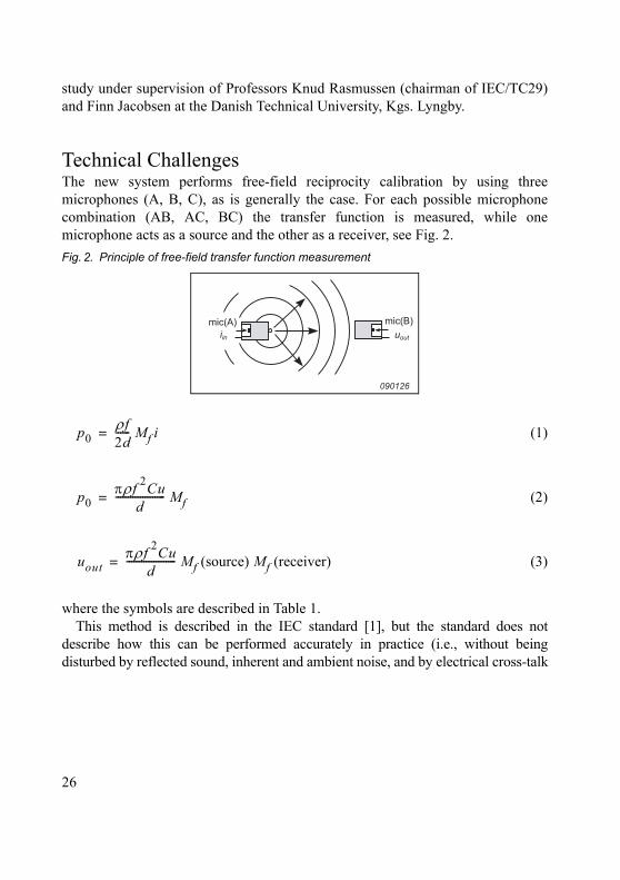
Technical ChallengesThe new system performs free-field reciprocity calibration by using threemicrophones (A, B, C), as is generally the case. For each possible microphonecombination (AB, AC, BC) the transfer function is measured, while onemicrophone acts as a source and the other as a receiver, see Fig. 2.

(1)

(2)

(3)

where the symbols are described in Table 1.This method is described in the IEC standard [1], but the standard does not

describe how this can be performed accurately in practice (i.e., without beingdisturbed by reflected sound, inherent and ambient noise, and by electrical cross-talk

Fig. 2. Principle of free-field transfer function measurement

mic(B)mic(A)uoutiin

090126

p0f2d------ Mf i=

p0f

2Cu

d-------------------- Mf=

uoutf

2Cu

d-------------------- Mf (source) Mf (receiver)=

26

between the source and receiver measurement channels). The technical difficultiesthat are related to the measurement process (which are quite severe) are caused by thefact that the microphones are very weak sound sources. They need to be driven by avoltage that does not exceed 6 V to 8 V to ensure linear and non-distorted operation.

The modulus of the sound pressure produced at a point, remote from a sourcemicrophone, may be calculated by equations (1) and (2), while the output voltageof a receiving microphone, placed at this point, is given by equation (3).Theoutputs of LS1 (Type 4160) and LS2 (Type 4180) microphones, for typicaloperation distances, are calculated and shown in Table 2.

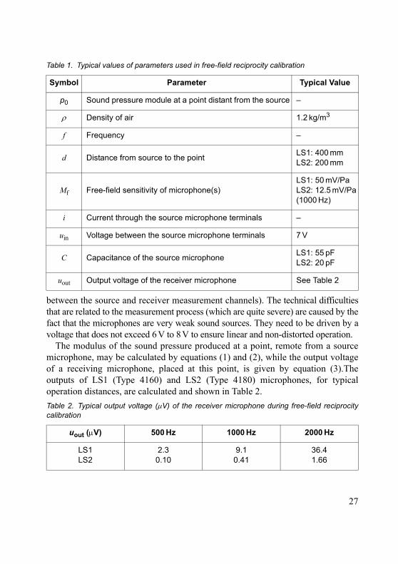
Table 1. Typical values of parameters used in free-field reciprocity calibration

Symbol Parameter Typical Value

p0 Sound pressure module at a point distant from the source –

Density of air 1.2 kg/m3

f Frequency –

d Distance from source to the pointLS1: 400 mmLS2: 200 mm

Mf Free-field sensitivity of microphone(s)LS1: 50 mV/PaLS2: 12.5 mV/Pa(1000 Hz)

i Current through the source microphone terminals –

uin Voltage between the source microphone terminals 7 V

C Capacitance of the source microphoneLS1: 55 pFLS2: 20 pF

uout Output voltage of the receiver microphone See Table 2

Table 2. Typical output voltage (V) of the receiver microphone during free-field reciprocitycalibration

uout (V) 500 Hz 1000 Hz 2000 Hz

LS1LS2

2.30.10

9.10.41

36.41.66

27

As indicated by the numbers in the table, very low voltages have to be measuredwhen calibrating microphones at these frequencies. The voltages are so low atthese frequencies that they are ‘buried’ in noise generated by the system itself andnoise occurring in the ambient surroundings. High sensitivity calibration accuracyrequires high accuracy measurement of the output voltages (0.01 dB – 0.02 dB)and this makes the measurements both difficult and quite time consuming.

This system includes a Brüel & Kjær Multi-analyzer System Type 3560-C andsoftware for an adaptive measurement technique called Steady State Response(SSR). The SSR measurement software records sine-signal packages that aresampled synchronously with the generator signal and averages them until a certainpre-selected accuracy of the averaged signal is achieved. This effective techniquemakes use of the fact that the signals measured synchronously add uparithmetically, while the non-correlated noise adds up more slowly, following thelaw of the root of the squares. Even if this principle is applied, it may take severalminutes to perform a complex (magnitude and phase) measurement at just one ofthe lower frequencies, for example, 800 Hz for LS1 and 3000 Hz for LS2microphones.

Another technical challenge is to keep cross-talk from the transmitter channel tothe receiver channel low, because the receiver channel works with output voltagesthat may be less than 1 V, and the transmitter channel uses 6 to 8 V to drive thesource. As the voltage ratio between the signals is about 107 (140 dB), the cross-talk should ideally be down around 1010 (200 dB), if the result is not to bedisturbed by more than 0.01 dB (approx). However, the influence of thisphenomenon, and sound reflections in the measurement room (which canpotentially be very significant sources of error) are minimised by the signal-processing principle described in the following section.

Principle of CalibrationAccording to the IEC standard [1], the parameters of equation (4) below must bedetermined to obtain the sensitivity product for each of the three microphonecombinations, AB, AC and BC, where A, B and C designate the microphones.After having determined and inserted the parameters, the sensitivities of all threemicrophones are calculated by solving the three equations.

(4)Mf 1, Mf 2, –j2d12

f-----------

U2

i1------ e

v d12 =

28

where:Mf,1, Mf,2 are the sensitivities of microphones ‘1’ and ‘2’d12 is the distance between the acoustic centres of microphones ‘1’ and ‘2’ is the density of airf is the frequencyv is the complex sound propagation coefficientU2 is the output voltage of the receiver microphonei1 is the input current of the source microphone

The system does not, in fact, measure the current of the source microphonedirectly. This is determined by measuring the voltage across a series capacitorplaced close to the source microphone. The transfer impedance (Z12 = U2/i1) can,according to equation (5), be determined by a relatively simple voltage-ratiomeasurement and by an accurate calibration of the capacitance of the seriescapacitor.

(5)

where:Z12 is the transfer impedance of microphones ‘1’ and ‘2’, valid for theparameters of equation (4)U1 is the voltage across the series capacitor of source microphone ‘1’C is the capacitance of series capacitor of the source microphones

The voltage ratio is a function of frequency and must be measured over thefrequency range of interest for the three microphone combinations. In principle,the sets of ratios only need to be measured at one microphone distance, forexample, 400 mm for LS1 and 200 mm for LS2 microphones. At the primary levelof calibration, national metrology institutes (NMIs) aim for an uncertainty that isas low as practically possible. Therefore, it is common to measure at moredistances and obtain correspondingly more sensitive results for comparison,averaging and verification. Normally, two, three or four distances are measured.

Often it is enough to determine the frequency response of a measurementmicrophone with a resolution of 1/12-octave or, in some cases, even 1/3-octave.However, the processing of the voltage ratio results requires that they aremeasured with fixed frequency intervals, typically between 100 Hz and 140 Hz.

Z12

U2

i1------

U2

U1------ –j 2 f C = =

29

The fixed intervals lead to a relative resolution that is low at low frequencies andhigh at high frequencies. This fits well with the response slope of a microphone well,where the slope is generally steeper at high frequencies than at low frequencies.

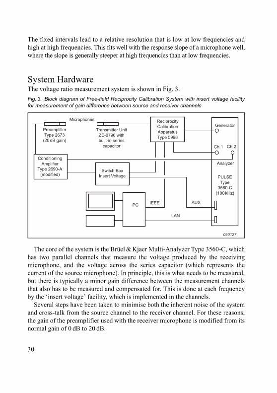
System HardwareThe voltage ratio measurement system is shown in Fig. 3.

The core of the system is the Brüel & Kjaer Multi-Analyzer Type 3560-C, whichhas two parallel channels that measure the voltage produced by the receivingmicrophone, and the voltage across the series capacitor (which represents thecurrent of the source microphone). In principle, this is what needs to be measured,but there is typically a minor gain difference between the measurement channelsthat also has to be measured and compensated for. This is done at each frequencyby the ‘insert voltage’ facility, which is implemented in the channels.

Several steps have been taken to minimise both the inherent noise of the systemand cross-talk from the source channel to the receiver channel. For these reasons,the gain of the preamplifier used with the receiver microphone is modified from itsnormal gain of 0 dB to 20 dB.

Fig. 3. Block diagram of Free-field Reciprocity Calibration System with insert voltage facilityfor measurement of gain difference between source and receiver channels

Microphones

Transmitter UnitZE-0796 withbuilt-in series

capacitor

PreamplifierType 2673

(20 dB gain)

ReciprocityCalibrationApparatusType 5998

Generator

Ch.1

Analyzer

PULSEType

3560-C(100 kHz)

ConditioningAmplifier

Type 2690-A(modified)

Switch BoxInsert Voltage

PC IEEE AUX

LAN

090127

Ch.2

30

Reciprocity Calibration Apparatus Type 5998 is not designed for free-fieldcalibration, but for the less demanding pressure reciprocity calibration. Therefore,even if this instrument has both a transmitter and a receiver channel, only thetransmitter channel is used. To ensure good separation between the systemchannels, i.e., the lowest possible cross-talk, the receiver channel is equipped witha separate conditioning amplifier, Type 2690-A. To increase the immunity of thesystem to low-frequency ambient noise, an additional high-pass filter has beenbuilt into the conditioning amplifier.

System SoftwareThe system includes three dedicated software programs. The first is themeasurement software that sets up the hardware according to preselected inputparameters, automatically controls all measurements, and stores the measurementresults. The second program calculates the sensitivities in accordance withIEC 61094–3 [1]. Knud Rasmussen and Salvador B. Figueroa developed bothprograms during their time with the Technical University of Denmark (DTU) andthe Danish Institute of Fundamental Metrology (DFM). The output of thecalculation program is the complex sensitivities valid at standard conditions. Theresult for each measurement distance result is stored in a separate file. The thirdprogram allows you present the results by loading selected files into standardoffice programs for comparison and for report preparation.

Processing of Measured Voltage RatiosThe series of voltage ratio results to be processed are all measured at multiples of apreselected frequency step, which is typically 120 Hz. The measurementsthemselves typically cover the ranges from about 1000 Hz to 31000 Hz for LS1microphones, and from 3000 Hz to 51000 Hz for LS2 microphones. There arealways three files for each measurement distance and typically two to fourdistances. A sensitivity result will be obtained for each distance. The whole seriesof measurement results are to some degree ‘contaminated’ by disturbing acousticreflections, and these influences need to be removed. To ‘clean up’ the data, thewhole measurement series needs to be extended with additional data down to 0 Hzand up to about 51000 kHz for LS1 and 70000 Hz for LS2.

At low frequencies, the calculation of the additional data for each series is basedon the individual 250 Hz pressure sensitivities of the two applied microphones,

31

and on DTU/DFM experienced data, describing the uniform, low-frequencyresponses of the LS1 and LS2 microphones, Types 4160 and 4180. At highfrequencies, the series is already extended by measuring to frequencies above thenormal operation ranges of the microphones. Further data is calculated byconsidering that the pressure responses ‘roll off’ by 12 dB/octave.

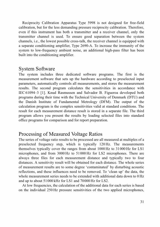
The principle of the signal ‘cleaning’ process is illustrated in Fig. 4.

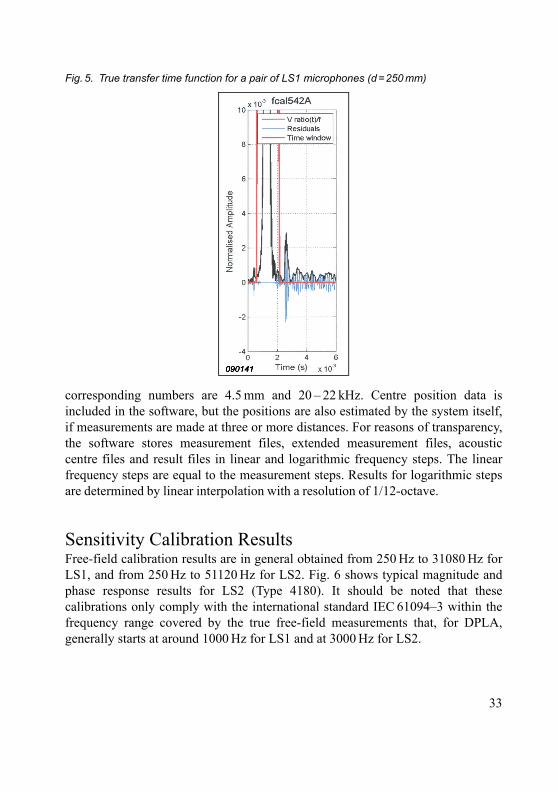
The first step of the procedure is to find the impulse response of the twoacoustically coupled microphones by creating an inverse FFT of the extendedvoltage ratio frequency response (see a true result in Fig. 5).

The response has a clear separation in time between the directly arriving soundand the delayed (and disturbing) sound reflections. The part of the impulse thatbelongs to the reflections is now removed by applying a time window. The resultsare then converted back to the frequency domain by performing FFT, creating thefiltered voltage ratio transfer function, without the influence of reflections.

After ‘cleaning’ the transfer functions, the complex sensitivities of themicrophones are calculated for each measurement distance in accordance withequations (4) and (5). When measurements are made with more than one distance,the average responses can be calculated for both magnitude and phase andpresented as the result of the calibration.

The software used with the system accounts for the position of the acousticcentre of the microphones. The centre position is a function of frequency. For lowfrequencies and for the axial sound incidence, the centre for LS1 microphones isabout 9 mm in front of the diaphragm. As frequency increases, it moves closer tothe diaphragm until it reaches the diaphragm at 8 – 10 kHz. It continues to movepast the diaphragm as frequency increases and is positioned a few millimetresbehind the diaphragm at higher frequencies. For LS2 microphones, the

Fig. 4. Principle of ‘cleaning’ voltage-ratio frequency responses from the influence of soundreflections

Measured ComplexFrequency Response

Frequency0

IFFT0

Time

Reflections

Direct Impulseresponse

Time

Time selectivewindow

FFT

Cleaned ComplexFrequency Response

0Frequency

090128

32

corresponding numbers are 4.5 mm and 20 – 22 kHz. Centre position data isincluded in the software, but the positions are also estimated by the system itself,if measurements are made at three or more distances. For reasons of transparency,the software stores measurement files, extended measurement files, acousticcentre files and result files in linear and logarithmic frequency steps. The linearfrequency steps are equal to the measurement steps. Results for logarithmic stepsare determined by linear interpolation with a resolution of 1/12-octave.

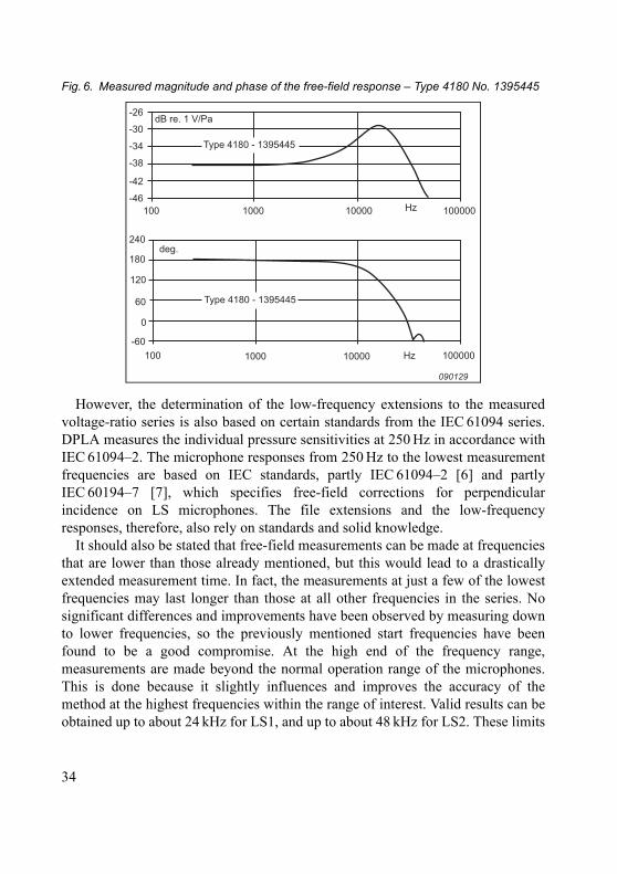
Sensitivity Calibration ResultsFree-field calibration results are in general obtained from 250 Hz to 31080 Hz forLS1, and from 250 Hz to 51120 Hz for LS2. Fig. 6 shows typical magnitude andphase response results for LS2 (Type 4180). It should be noted that thesecalibrations only comply with the international standard IEC 61094–3 within thefrequency range covered by the true free-field measurements that, for DPLA,generally starts at around 1000 Hz for LS1 and at 3000 Hz for LS2.

Fig. 5. True transfer time function for a pair of LS1 microphones (d =250 mm)

33

However, the determination of the low-frequency extensions to the measuredvoltage-ratio series is also based on certain standards from the IEC 61094 series.DPLA measures the individual pressure sensitivities at 250 Hz in accordance withIEC 61094–2. The microphone responses from 250 Hz to the lowest measurementfrequencies are based on IEC standards, partly IEC 61094–2 [6] and partlyIEC 60194–7 [7], which specifies free-field corrections for perpendicularincidence on LS microphones. The file extensions and the low-frequencyresponses, therefore, also rely on standards and solid knowledge.

It should also be stated that free-field measurements can be made at frequenciesthat are lower than those already mentioned, but this would lead to a drasticallyextended measurement time. In fact, the measurements at just a few of the lowestfrequencies may last longer than those at all other frequencies in the series. Nosignificant differences and improvements have been observed by measuring downto lower frequencies, so the previously mentioned start frequencies have beenfound to be a good compromise. At the high end of the frequency range,measurements are made beyond the normal operation range of the microphones.This is done because it slightly influences and improves the accuracy of themethod at the highest frequencies within the range of interest. Valid results can beobtained up to about 24 kHz for LS1, and up to about 48 kHz for LS2. These limits

Fig. 6. Measured magnitude and phase of the free-field response – Type 4180 No. 1395445

100 1000 10000 100000Hz

240

180

120

60

0

-60

100 1000 10000 100000Hz

-26

-30

-34

-38

-42

-46

dB re. 1 V/Pa

deg.

Type 4180 - 1395445

Type 4180 - 1395445

090129

34

are not set by the system, but rather by the microphones, whose frequencyresponses are not smooth beyond the frequencies mentioned.

An LS2 calibration made at one measurement distance will typically take 2hours, while a thorough calibration made at four measurement distances will takea full day. Both calibrations will, of course, result in free-field responses for eachof the three microphones that were included in the process. LS1 calibrationrequires half the time.

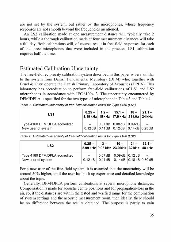
Estimated Calibration UncertaintyThe free-field reciprocity calibration system described in this paper is very similarto the system from Danish Fundamental Metrology (DFM) who, together withBrüel & Kjær, operate the Danish Primary Laboratory of Acoustics (DPLA). Thislaboratory has accreditation to perform free-field calibrations of LS1 and LS2microphones in accordance with IEC 61094–3. The uncertainty encountered byDFM/DPLA is specified for the two types of microphone in Table 3 and Table 4.

For a new user of the free-field system, it is assumed that the uncertainty will bearound 50% higher, until the user has built up experience and detailed knowledgeabout the topic.

Generally, DFM/DPLA perform calibrations at several microphone distances.Compensation is made for acoustic centre positions and for propagation-loss in theair, so, if the distances are within the tested and verified range for the combinationof system settings and the acoustic measurement room, then ideally, there shouldbe no difference between the results obtained. The purpose is partly to gain

Table 3. Estimated uncertainty of free-field calibration result for Type 4160 (LS1)

LS10.25 –

1.19 kHz1.2 –

15 kHz15.1 –

17.9 kHz18 –

21 kHz21.1 – 24 kHz

Type 4160 DFM/DPLA accredited New user of system

–0.12 dB

0.07 dB0.11 dB

0.08 dB0.12 dB

0.09 dB0.14 dB

–0.25 dB

Table 4. Estimated uncertainty of free-field calibration result for Type 4180 (LS2)

LS20.25 –

2.99 kHz3 –

9.98 kHz10 –

23.9 kHz24 –

32 kHz32.1 – 48 kHz

Type 4180 DFM/DPLA accredited New user of system

–0.12 dB

0.07 dB0.11 dB

0.09 dB0.14 dB

0.12 dB0.18 dB

–0.30 dB

35

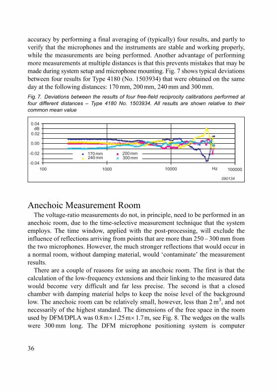
accuracy by performing a final averaging of (typically) four results, and partly toverify that the microphones and the instruments are stable and working properly,while the measurements are being performed. Another advantage of performingmore measurements at multiple distances is that this prevents mistakes that may bemade during system setup and microphone mounting. Fig. 7 shows typical deviationsbetween four results for Type 4180 (No. 1503934) that were obtained on the sameday at the following distances: 170 mm, 200 mm, 240 mm and 300 mm.

Anechoic Measurement RoomThe voltage-ratio measurements do not, in principle, need to be performed in an

anechoic room, due to the time-selective measurement technique that the systememploys. The time window, applied with the post-processing, will exclude theinfluence of reflections arriving from points that are more than 250 – 300 mm fromthe two microphones. However, the much stronger reflections that would occur ina normal room, without damping material, would ‘contaminate’ the measurementresults.

There are a couple of reasons for using an anechoic room. The first is that thecalculation of the low-frequency extensions and their linking to the measured datawould become very difficult and far less precise. The second is that a closedchamber with damping material helps to keep the noise level of the backgroundlow. The anechoic room can be relatively small, however, less than 2 m3, and notnecessarily of the highest standard. The dimensions of the free space in the roomused by DFM/DPLA was 0.8m1.25m1.7m, see Fig. 8. The wedges on the wallswere 300 mm long. The DFM microphone positioning system is computer

Fig. 7. Deviations between the results of four free-field reciprocity calibrations performed atfour different distances – Type 4180 No. 1503934. All results are shown relative to theircommon mean value

0.04

0.02

0.00

-0.02

-0.04100 1000 10000 100000Hz

dB

170 mm240 mm

200 mm300 mm

090134

36

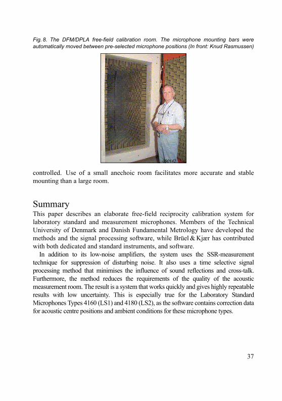
controlled. Use of a small anechoic room facilitates more accurate and stablemounting than a large room.

SummaryThis paper describes an elaborate free-field reciprocity calibration system forlaboratory standard and measurement microphones. Members of the TechnicalUniversity of Denmark and Danish Fundamental Metrology have developed themethods and the signal processing software, while Brüel & Kjær has contributedwith both dedicated and standard instruments, and software.

In addition to its low-noise amplifiers, the system uses the SSR-measurementtechnique for suppression of disturbing noise. It also uses a time selective signalprocessing method that minimises the influence of sound reflections and cross-talk.Furthermore, the method reduces the requirements of the quality of the acousticmeasurement room. The result is a system that works quickly and gives highly repeatableresults with low uncertainty. This is especially true for the Laboratory StandardMicrophones Types 4160 (LS1) and 4180 (LS2), as the software contains correction datafor acoustic centre positions and ambient conditions for these microphone types.

Fig. 8. The DFM/DPLA free-field calibration room. The microphone mounting bars wereautomatically moved between pre-selected microphone positions (In front: Knud Rasmussen)

37

AcknowledgementsThanks to Knud Rasmussen and Salvador B. Figueroa of DFM, Kgs. Lyngby,Denmark, for supplying details about the operation principle and about the resultsobtainable with the method and system described in this paper. The system isbased on their research, method development and on their many years ofexperience with microphone calibration.

References[1] IEC International Standard 61094–3, “Measurement Microphones, Part 3:

Primary Method for Free-field Calibration of Laboratory StandardMicrophones by the Reciprocity Technique”, Int. ElectrotechnicalCommision, Geneva, November 1995.

[2] IEC International Standard 61094–1, “Measurement Microphones, Part 1:Specifications for Laboratory Standard Microphones”, Int.Electrotechnical Commision, Geneva, July 2000.

[3] IEC International Standard 61094–4, “Measurement Microphones, Part 4:Specifications for Working Standard Microphones”, Int. ElectrotechnicalCommision, Geneva, November 1995.

[4] Knud Rasmussen, “The Static Pressure and Temperature Coefficients ofLaboratory Standard Microphones”, Metrologia 36, pp 265–273, 1999.

[5] Salvador B. Figueroa, “New Methods for Transducer Calibration: Free-field Reciprocity Calibration of Condenser Microphones”, PhD Thesis,Ørsted, DTU, Technical University of Denmark, 2003.

[6] IEC International Standard 61094–2, “Measurement Microphones, Part 2:Primary Method for Pressure Calibration of Laboratory Microphones bythe Reciprocity Technique”, Int. Electrotechnical Commision, Geneva,February 2009.

[7] IEC International Standard 61094–7, “Measurement Microphones, Part 7:Values for the Difference Between Free-field and Pressure Sensitivities ofLaboratory Standard Microphones”, Int. Electrotechnical Commision,Geneva, May 2006.

38

1 – 1996 Calibration Uncertainties & Distortion of Microphones.Wide Band Intensity Probe. Accelerometer Mounted Resonance Test

2 – 1995 Order Tracking Analysis1 – 1995 Use of Spatial Transformation of Sound Fields (STSF) Techniques in the

Automative Industry2 – 1994 The use of Impulse Response Function for Modal Parameter Estimation

Complex Modulus and Damping Measurements using Resonant and Non-resonant Methods (Damping Part II)

1 – 1994 Digital Filter Techniques vs. FFT Techniques for Damping Measurements (Damping Part I)

2 – 1990 Optical Filters and their Use with the Type 1302 & Type 1306 Photoacoustic Gas Monitors

1 – 1990 The Brüel & Kjær Photoacoustic Transducer System and its Physical Properties

2 – 1989 STSF — Practical Instrumentation and ApplicationDigital Filter Analysis: Real-time and Non Real-time Performance

1 – 1989 STSF — A Unique Technique for Scan Based Near-Field Acoustic Holography Without Restrictions on Coherence

2 – 1988 Quantifying Draught Risk1 – 1988 Using Experimental Modal Analysis to Simulate Structural Dynamic

ModificationsUse of Operational Deflection Shapes for Noise Control of Discrete Tones

4 – 1987 Windows to FFT Analysis (Part II)Acoustic Calibrator for Intensity Measurement Systems

3 – 1987 Windows to FFT Analysis (Part I)

Special Technical LiteratureBrüel & Kjær publishes a variety of technical literature which can be obtained from your local Brüel & Kjær representative.

The following literature is presently available:

• Catalogues (several languages)• Product Data Sheets (English, German, French, Italian, Spanish)

Furthermore, back copies of the Technical Review can be supplied as listed above. Older issues may be obtained provided they are still in stock.

Previously Issued Numbers ofBrüel & Kjær Technical Review(Continued from cover page 2)

HEADQUARTERS: Brüel & Kjær Sound & Vibration Measurement A/S DK-2850 Nærum · Denmark · Telephone: +45 77 41 20 00 · Fax: +45 45 80 14 05 www.bksv.com · info@bksv.com

Local representatives and service organisations worldwide

www.bksv.comwww.bksv.com

TECHNICAL REVIEW

� Use�of�Volume�Velocity�Sound�Source�in�FRF�Measurements

� Turnkey�Free-field�Reciprocity�System

BV

  006

1  –

  11 

   IS

SN  0

007–

2621

No. 1 – 2009