Embed Size (px)
Citation preview
MPP-2015-178
Quartic AdS Interactions in Higher-Spin Gravityfrom Conformal Field Theory
Xavier Bekaert1, Johanna Erdmenger2, Dmitry Ponomarev3 and Charlotte Sleight4
1 Laboratoire de Mathématiques et Physique ThéoriqueUnité Mixte de Recherche 7350 du CNRS
Fédération de Recherche 2964 Denis PoissonUniversité François Rabelais, Parc de Grandmont, 37200 Tours, France
2, 4 Max-Planck-Institut für Physik (Werner-Heisenberg-Institut)Föhringer Ring 6, D-80805 Munich, Germany
3 Arnold Sommerfeld Center for Theoretical PhysicsLudwig-Maximilians University Munich
Theresienstr. 37, D-80333 Munich, Germany
Abstract
Clarifying the locality properties of higher-spin gravity is a pressing task, but no-toriously difficult due to the absence of a weakly-coupled flat regime. The simplestnon-trivial case where this question can be addressed is the quartic self-interactionof the AdS scalar field present in the higher-spin multiplet. We investigate this issuein the context of the holographic duality between the minimal bosonic higher-spintheory on AdS4 and the free O (N) vector model in three dimensions. In particular,we determine the exact explicit form of the derivative expansion of the bulk scalarquartic vertex. The quartic vertex is obtained from the field theory four-point func-tion of the operator dual to the bulk scalar, by making use of our previous resultsfor the Witten diagrams of higher-spin exchanges. This is facilitated by establishingthe conformal block expansions of both the boundary four-point function and thedual bulk Witten diagram amplitudes. We show that the vertex we find satisfies ageneralised notion of locality.
[email protected]@[email protected]@mpp.mpg.de
arX
iv:1
508.
0429
2v1
[he
p-th
] 1
8 A
ug 2
015
Contents
1 Introduction 3
2 Fixing the cubic action 9
2.1 Fronsdal action and cubic vertices of higher-spin gauge fields on AdS . . . . . . 9
2.2 Fixing the cubic couplings in AdS using holography . . . . . . . . . . . . . . . . 11
3 Four-point Witten diagrams 13
3.1 Exchange diagrams . . . . . . . . . . . . . . . . . . . . . . . . . . . . . . . . . . 13
3.2 Contact diagrams . . . . . . . . . . . . . . . . . . . . . . . . . . . . . . . . . . . 17
4 Scalar singlet four-point function 19
4.1 OPE coefficients of double-trace operators . . . . . . . . . . . . . . . . . . . . . 22
4.2 Contour integral representation . . . . . . . . . . . . . . . . . . . . . . . . . . . 23
5 Uncovering the quartic vertex 25
5.1 Summary: CFT interpretation of Witten diagrams . . . . . . . . . . . . . . . . . 25
5.2 Combining bulk contributions from all channels . . . . . . . . . . . . . . . . . . 27
5.3 Solving for the vertex: Reducing the analysis to a single channel . . . . . . . . . 29
6 Locality 34
7 Summary and Outlook 40
A Notation and conventions 41
A.1 Symmetric tensors in AdS . . . . . . . . . . . . . . . . . . . . . . . . . . . . . . 41
A.2 Symmetric and traceless boundary tensors . . . . . . . . . . . . . . . . . . . . . 41
B AdS harmonic functions 42
C Complete Set of Quartic Vertices 42
D Double Trace Operators 44
D.1 The action of the conformal boost generator . . . . . . . . . . . . . . . . . . . . 44
2
D.2 Imposing that the double-trace operator is primary . . . . . . . . . . . . . . . . 45
D.3 Determining the dependence on the wave operator . . . . . . . . . . . . . . . . . 46
E Computation of OPE coefficients 48
E.1 Three-point function . . . . . . . . . . . . . . . . . . . . . . . . . . . . . . . . . 49
E.1.1 Disconnected part of the 3-point function . . . . . . . . . . . . . . . . . . 49
E.1.2 Connected part of the 3-point function . . . . . . . . . . . . . . . . . . . 50
E.2 Two-point function . . . . . . . . . . . . . . . . . . . . . . . . . . . . . . . . . . 53
E.3 Conformal block coefficient . . . . . . . . . . . . . . . . . . . . . . . . . . . . . . 55
1 Introduction
Despite significant progress in understanding the structure of higher-spin gravity theories dur-ing the last decades, interactions of higher-spin gauge fields are not fully understood. Thestandard approach to address higher-spin interactions is to use the Noether procedure, whichamounts to a perturbative reconstruction of interactions in a way such that they are compatiblewith higher-spin gauge transformations, the latter of which may also be deformed [1]. Thereis a vast literature on cubic interactions, see e.g. [2–26], which in particular gives a completeclassification of local cubic interactions in any dimensions [10]. However, this procedure meetsessential technical difficulties at the quadratic order in a coupling constant, the order at whichone extracts quartic vertices. The first source of complication is that the number of possiblecandidates for a vertex grows considerably with the order of a vertex, even if the spin of theexternal fields is fixed. For example, there is only one cubic vertex for scalar fields that isnon-trivial on the free mass-shell, while the number of independent non-trivial on-free-shellquartic vertices is infinite. As we shall demonstrate, these can be parametrised by two integerparameters taking an infinite set of values. Another issue that complicates the Noether proce-dure for quartic vertices, is that at this order the consistency condition becomes non-linear indeformations. In particular, this implies that the general solution for a quartic vertex cannotbe constructed as a linear combination of quartic vertices involving fields with fixed spins, asis the case for cubic interactions. Instead, such vertices should be considered all together. Oneof the consequences of this analysis is that higher-spin interactions cannot be consistently de-formed to a quartic level unless one includes an infinite tower of fields with unbounded spin.This spectacular property was expected since the formulation of the higher-spin interactionproblem [27] and comes from the structure of the higher-spin algebra, which is to large extentunique [28, 29]. This complicates the problem even further. Quartic vertices in higher-spintheory have been studied in [22, 30–35], and some of these results indicate that local solutionsof the consistency conditions in flat space at this order are problematic.
Let us emphasise that locality of interactions is in essence the main constraint of the Noether
3
procedure. In particular, it has been shown that in relaxing the condition of locality any cubicvertex, consistent till cubic order, can always be completed consistently to all orders [36]. Onthe other hand, as the analysis of cubic vertices indicates [10], the minimal number of derivativesin a consistent vertex grows with the spin of fields forming the vertex. Together with the factthat higher-spin interactions require fields of arbitrarily high spin, this implies that higher-spininteractions are already non-local at the cubic level. In turn, these cubic vertices contributeto the consistency condition for quartic ones. The standard expectation is that non-localitiesshould be present even in quartic interactions of lower-spin fields within higher-spin theories.To summarise, the Noether procedure without locality admits infinitely many solutions, whileenforcing locality does not seem to admit any solutions at all.
In the discussion so far, locality was understood in a strong sense: That is, requiring afinite number of derivatives in the action. A natural way to reconcile locality and the Noetherprocedure for higher-spin interactions could be to extend the definition of locality in such away that it allows terms with infinitely many derivatives in the action. At the same time, thisweaker definition of locality should rule out vertices that give rise to clearly non-local behaviourin the theory. It is reasonable to expect that if the coefficients in the derivative expansions ofvertices decrease fast enough with the number of derivatives, then such a theory is physicallyindistinguishable from a local one even if the number of derivatives in the action is infinite.More precisely, one can call a vertex local if its scattering amplitude is analytic. In this paperwe give some supporting arguments for the extension of this definition to anti-de Sitter (AdS)spacetime. For a recent discussion on the locality of field redefinitions in higher-spin theorysee [37].
Instead of solving the Noether procedure, an alternative approach to the higher-spin in-teraction problem is to use AdS/CFT to extract bulk interactions from the conjectured dualboundary conformal field theory (CFT). A decade ago, it was conjectured [38,39] that unbrokenVasiliev’s higher-spin theory [40–42] is dual to the free O(N) vector model. This duality hasbeen verified at tree level for 3-point Witten diagrams in AdS4 [43–45] (see also [46, 47] for anearly test), and at the level of one-loop vacuum energy [48–51]. Moreover, all n-point func-tions of the free CFT3 have been identified with suitable invariants in Vasiliev’s theory [52–55].Beyond these checks, it remains an open question whether or not it is Vasiliev’s theory in par-ticular that is the bulk higher-spin dual of the O (N) vector model. In any case, one can useholography as a constructive approach to define an interacting higher-spin gravity theory inAdS. Since the dual conformal field theory is free, all boundary correlators are calculable. Byequating these to the associated Witten diagrams in the bulk, in principle one can extract in-teractions of the bulk theory order by order.1 It is the goal of this paper to uncover the quarticvertex involving scalar fields of the bulk higher-spin theory in this manner, and to study itslocality properties.
Although extracting just the quartic self-interaction of the scalar in higher-spin theory1Another approach taken in the literature is to use the holographic RG flow [56] (see also [57]). While the
holographic duality is manifest by construction in these works, the structure of the bulk higher-spin interactionsand their locality properties remain to be clarified. For another approach to studying the latter issue, seee.g. [58].
4
does not fully address the question of quartic higher-spin interactions, the resulting vertex canalready be used to probe such issues as locality in higher-spin theories. It can also be employedto test the higher-spin AdS/CFT conjecture at the more non-trivial level of four-point functions,by checking whether or not the vertex we reconstruct holographically matches the one obtainedfrom Vasiliev’s equations. To do so, what remains is to extract the quartic vertex of scalarfields in Vasiliev’s theory. So far only the cubic interactions have been extracted in explicitform from Vasiliev’s equations [43,44,47,59–61].
Another interesting issue that we would like to address is bulk locality in AdS/CFT ingeneral. While bulk locality above the AdS length scale is to be expected [62–64], locality atdistances much smaller than this scale is more miraculous. Criteria for a CFT to have a localbulk dual at the these scales have been proposed in [62, 65–67]. The higher-spin holographicduality provides a convenient framework in which they can be investigated, for in this case boththe bulk and boundary theories are simple enough to make the necessary objects calculable.
Let us now explain in more detail the approach taken in this paper. We work in the contextof the type A minimal bosonic higher-spin theory on AdS4, whose spectrum consists of a parityeven scalar and an infinite tower of even spin gauge fields. With the appropriate boundaryconditions, this is conjectured to be dual, in the large N limit, to the singlet sector of the freemassless scalar O (N) vector model in three dimensions. The spectrum of single-trace operatorsin the boundary theory consists of the scalar singlet
O = φaφa, (1.1)
of dimension ∆ = d− 2 = 1, and an infinite set of even spin singlet conserved currents
Ji1...is = φa∂(i1 ... ∂ is)φa + ... , s = 2, 4, 6, ... (1.2)
of dimension ∆s = d+ s−2 = s+ 1. The fields φa, where a = 1, 2, ..., N , are the free real scalarfields in the fundamental representation of O(N). Under the duality, each spin-s conservedcurrent (1.2) is dual to a spin-s gauge field ϕµ1...µs in AdS4. The scalar singlet O is dual tothe bulk parity-even scalar, which we denote by ϕ0. The singlet sector also contains multi-trace operators, which are dual to multi-particle states in the bulk. For example, double-traceoperators of the schematic form
O(2)n,i1...is
(x) = n(O (x)
)∂(i1 ...∂ is)O (x) + ... (1.3)
are bi-linear in the single-trace scalar operatorO, with dimension ∆n,s = 2∆+2n+s = 2+2n+s.These are dual to two-particle states of the scalar in AdS, and will be of relevance in the presentwork.
Correlation functions of the singlet operators may be computed holographically via Wittendiagrams involving their dual fields in AdS4. It is this identification of boundary correlationfunctions with bulk Witten diagrams that we use in this paper to probe the nature of quar-tic interactions in higher-spin theory on AdS4: In general, the bulk tree-level computation offour-point functions receives contributions from exchange Witten diagrams mediated by cubic
5
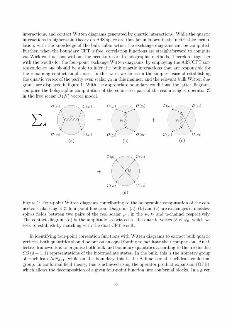
interactions, and contact Witten diagrams generated by quartic interactions. While the quarticinteractions in higher-spin theory on AdS space are thus far unknown in the metric-like formu-lation, with the knowledge of the bulk cubic action the exchange diagrams can be computed.Further, when the boundary CFT is free, correlation functions are straightforward to computevia Wick contractions without the need to resort to holographic methods. Therefore, togetherwith the results for the four-point exchange Witten diagrams, by employing the AdS/CFT cor-respondence one should be able to infer the bulk quartic interactions that are responsible forthe remaining contact amplitudes. In this work we focus on the simplest case of establishingthe quartic vertex of the parity even scalar ϕ0 in this manner, and the relevant bulk Witten dia-grams are displayed in figure 1. With the appropriate boundary conditions, the latter diagramscomprise the holographic computation of the connected part of the scalar singlet operator Oin the free scalar O (N) vector model.
Figure 1: Four-point Witten diagrams contributing to the holographic computation of the con-nected scalar singlet O four-point function. Diagrams (a), (b) and (c) are exchanges of masslessspin-s fields between two pairs of the real scalar ϕ0, in the s-, t- and u-channel respectively.The contact diagram (d) is the amplitude associated to the quartic vertex V of ϕ0, which weseek to establish by matching with the dual CFT result.
In identifying four-point correlation functions with Witten diagrams to extract bulk quarticvertices, both quantities should be put on an equal footing to facilitate their comparison. An ef-fective framework is to organise both bulk and boundary quantities according to the irreducibleSO (d+ 1, 1) representations of the intermediate states. In the bulk, this is the isometry groupof Euclidean AdSd+1, while on the boundary this is the d-dimensional Euclidean conformalgroup. In conformal field theory, this is achieved using the operator product expansion (OPE),which allows the decomposition of a given four-point function into conformal blocks. In a given
6
channel, each conformal block G∆s,s represents the contribution to the four-point function of agiven primary field (+ all of its descendants) present in the OPE, transforming in the spin-sand dimension ∆s representation of the conformal group. For a four-point function of identicalscalars O of dimension ∆, its conformal block expansion can be expressed in the followingcontour-integral form [68] in the direct, i.e. (12)(34), channel
〈O (y1)O (y2)O (y3)O (y4)〉 =1
(y212y
234)
∆
1 +
∑s
∫ ∞−∞
dν fs (ν)Gd2
+iν,s(u, v)
, (1.4)
where u and v are cross-ratios: u =y212y
234
y213y
224, v =
y214y
223
y213y
224, and yij = yi − yj. The function fs (ν)
encodes the contributions of the spin-s operators in the OO OPE: for each spin-s primaryoperator present, fs (ν) contains a pole located at the value of ν where the dimension d
2+ iν of
the conformal block Gd/2+iν,s (u, v) coincides with that of the operator. The residue of fs (ν) atthis pole gives the square of the operator’s OPE coefficient, as in the conventional representationof the conformal block expansion.
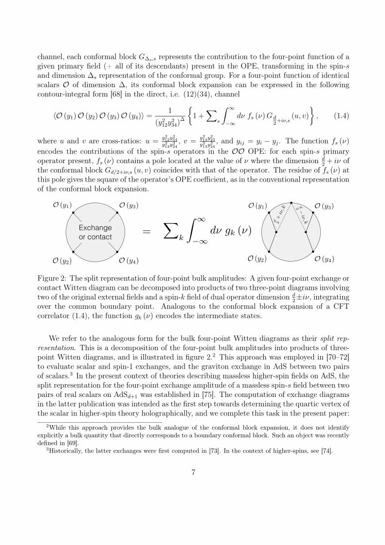
Exchange
or contact
Figure 2: The split representation of four-point bulk amplitudes: A given four-point exchange orcontact Witten diagram can be decomposed into products of two three-point diagrams involvingtwo of the original external fields and a spin-k field of dual operator dimension d
2±iν, integrating
over the common boundary point. Analogous to the conformal block expansion of a CFTcorrelator (1.4), the function gk (ν) encodes the intermediate states.
We refer to the analogous form for the bulk four-point Witten diagrams as their split rep-resentation. This is a decomposition of the four-point bulk amplitudes into products of three-point Witten diagrams, and is illustrated in figure 2.2 This approach was employed in [70–72]to evaluate scalar and spin-1 exchanges, and the graviton exchange in AdS between two pairsof scalars.3 In the present context of theories describing massless higher-spin fields on AdS, thesplit representation for the four-point exchange amplitude of a massless spin-s field between twopairs of real scalars on AdSd+1 was established in [75]. The computation of exchange diagramsin the latter publication was intended as the first step towards determining the quartic vertex ofthe scalar in higher-spin theory holographically, and we complete this task in the present paper:
2While this approach provides the bulk analogue of the conformal block expansion, it does not identifyexplicitly a bulk quantity that directly corresponds to a boundary conformal block. Such an object was recentlydefined in [69].
3Historically, the latter exchanges were first computed in [73]. In the context of higher-spins, see [74].
7
By evaluating the three-point amplitudes in the split representations of the Witten diagrams infigure 1, the latter can be converted into boundary conformal block expansions in the contourintegral form (1.4), allowing for direct comparison with the CFT result.
As explained previously, it is well known that interactions in higher-spin theory are in generalunbounded in their number of derivatives. The quartic vertex of the scalar in higher-spin theoryon AdS therefore takes the general form
V (x) =∑m,s
am,s (ϕ0 (x)∇µ1 ...∇µsϕ0 (x) + ... )m (ϕ0 (x)∇µ1 ...∇µsϕ0 (x) + ... ) , (1.5)
but its properties and behaviour of the coefficients am,s have thus far remained elusive. Using(1.5) as an ansatz to complete the total bulk amplitude in figure 1 for the dual CFT correlator,we determine the coefficients am,s required to be consistent with the holographic duality. Thisrequires two further steps that build upon the previous work [75] on the four-point exchangeamplitudes: the split representation (and subsequent conformal block expansion) of the mostgeneral four-point contact amplitude associated to a quartic vertex of the form (1.5) must bedetermined, as well as the conformal block expansion of the scalar single-trace operator four-point function. The latter is only known in d = 4 CFTs [76] in the literature, whereas forthe former only partial results are known in certain limits [62]. While our choice of using thecontour integral representation (1.4) for conformal block expansions is rather unconventional,it is extremely useful for extracting the coefficients in the quartic ansatz (1.5). This is becauseit reduces the comparison between the bulk and boundary conformal block expansions to amatching of the functions fs (ν) for each spin s.
Before the quartic vertex can be determined holographically in this manner, the explicit cou-plings associated to the cubic vertices appearing in the exchange diagrams need to be uncovered.For the computation of the exchange amplitudes in [75], these couplings were left arbitrary. Wetherefore begin in section 2 by reviewing the free quadratic Fronsdal action in AdSd+1, and itscubic extension to the 0-0-s interactions in the type A minimal bosonic theory. Beyond thelevel of three-point diagrams, these cubic interactions generate exchanges of the massless spin-sfields. In section 2.2 we fix the couplings of the latter interactions holographically in generaldimensions, by matching with corresponding three-point functions in the d-dimensional freeO (N) vector model. In section 3 we move onto the computation of the tree-level four-pointWitten diagrams with four external scalar fields, establishing their split representations andsubsequent conformal block expansions. We begin in section 3.1 by reviewing our previouswork [75] on four-point exchanges of a single massless spin-s field in AdSd+1. We then focus onthe exchanges in AdS4, and establish their conformal block expansions in the contour integralform (1.4). In section 3.2 we derive the analogous expansion for a four-point contact amplitudeassociated to a general quartic vertex (1.5) of the scalar. To do so we introduce a convenientbasis of local quartic vertices, in which any quartic contact interaction of the scalar can beexpanded. By computing the conformal block expansion of the amplitudes associated to thebasis vertices, the result for a general contact diagram follows.
In section 4 we turn to the CFT side of the story, where in general dimensions we deter-mine the contour integral form (1.4) of the conformal block expansion of the scalar single-trace
8
operator four-point function. This requires the knowledge of the OPE coefficients of the op-erators in the scalar singlet OPE, which for the double-trace operators were so far absent inthe literature – with the exception of the d = 4 case derived in [76]. To extend this result togeneral dimensions, we take the direct approach of extracting the OPE coefficients from thecomputation of the two-point functions of the double-trace operators, and their three-pointfunctions with the scalar single-trace operator O. We determine the latter by deriving theexplicit form of double-trace operators O(2)
n,s built from two scalar single-trace operators in ap-pendix D. This result for the double-trace operators completes those already available in theliterature [70, 77–79] for their explicit form.
In section 5 we combine the results for the conformal block expansions of the bulk Wittendiagrams and the dual CFT four-point function derived in the preceding section, to extractthe quartic vertex of the scalar. In particular, we determine a generating function for thecoefficients in its derivative expansion (1.5). In section 6 we then probe the nature of thevertex, studying the amplitude of its four-point Witten diagram in order to quantify its localityproperties. To do this, we draw on the similarity of Mellin amplitudes to flat space amplitudes.We also comment on the role of holography in the locality of interactions in higher-spin theoryduals to CFTs.
2 Fixing the cubic action
We begin by refining the cubic part of the higher-spin action required to study the quarticvertex of the bulk scalar field holographically. In particular, we fix the couplings of the cubicvertices that mediate the spin-s exchanges in figure 1, by comparing with the correspondingthree-point functions in the free conformal scalar O (N) vector model in d-dimensions. Thisalso serves as a simple demonstration of the logic we apply later at the quartic order: Wedetermine interactions in higher-spin theory assuming the validity of the holographic duality,by matching with relevant dual CFT correlation functions. We also take the opportunity tointroduce notation.
2.1 Fronsdal action and cubic vertices of higher-spin gauge fields onAdS
In this paper we work in Euclidean anti-de Sitter space, which we refer to in the sequel as AdS.We label points in the bulk of AdS by xµ with µ = 0, 1, ..., d, while points on the conformalboundary ∂AdS will be denoted by yi with i = 1, ..., d.
The theory we are concerned with is the interacting minimal bosonic higher-spin theory onAdS4, whose spectrum consists of a parity even scalar and an infinite tower of gauge fields ofeven spins s = 2, 4, 6, ....
At the free level, minimal bosonic higher-spin theory is governed by the Frondsal action
9
[27, 80]4
S2 =s!
2
∞∑s=0
∫ √|g| dd+1x ϕs (x, ∂u)
(1− 1
4u2 ∂u · ∂u
)Fs (x, u,∇, ∂u)ϕs (x, u)
∣∣∣u=0
, (2.1)
where Fs(x, u,∇, ∂u) is the Fronsdal operator [78,81]
Fs(x, u,∇, ∂u) = −m2s − u2(∂u · ∂u)− (u · ∇)
((∇ · ∂u)−
1
2(u · ∇)(∂u · ∂u)
), (2.2)
m2s ≡ s2 + s(d− 5)− 2(d− 2),
and ϕs(x, u) is a generating function for the off-shell spin-s Fronsdal field, which is a rank-ssymmetric double-traceless tensor
ϕs(x, u) ≡ 1
s!ϕµ1µ2...µs(x)uµ1uµ2 . . . uµs , (∂u · ∂u)2ϕs(x, u) = 0. (2.3)
In the above, and throughout this paper, we have adopted the use of constant auxiliary vectorsto effectively manage symmetric tensor fields. We use uµ for symmetric tensor fields in thebulk of in AdS, and zi with z2 = 0 for symmetric and traceless boundary fields. Our use of thisformalism is further explained in appendix A.
The quadratic action (2.1) is invariant with respect to the linearised gauge transformations
δ0ϕs(x, u) = (u · ∇)εs−1(x, u), (2.4)
where εs−1(x, u) is a generating function for a rank-(s− 1) symmetric and traceless gaugeparameter
εs−1(x, u) ≡ 1
(s− 1)!εµ1µ2...µs−1(x)uµ1uµ2 . . . uµs−1 , (∂u · ∂u)εs−1(x, u) = 0. (2.5)
To move towards a Lagrangian description of the interacting theory, generally the Noetherprocedure is applied to determine the possible interactions that are consistent with the gaugesymmetries of the theory. For the collection of bulk Witten diagrams we are concerned with infigure 1, the relevant part of the cubic action takes the following form5
S3 = S2 −∞∑s=0
s! gs
∫ √|g| dd+1x ϕs (x, ∂u) Js (x, u) , (2.6)
modulo vertices that vanish on the free mass shell. The gs are the coupling constants of the0-0-s cubic interaction, and Js is a bulk spin-s conserved current bi-linear in ϕ0. It has theform [82]
Js (x, u) =s∑
k=0
(−1)k
k! (s− k)!(u · ∇)s−k ϕ0 (x) (u · ∇)k ϕ0 (x) + Λ u2 (...) , (2.7)
4For the rest of the paper, when expressing tensor contractions through generating functions, setting theauxiliary vector to zero is left implicit.
5I.e. it contains the 0-0-s interactions that mediate the four-point exchange diagrams.
10
where the second term proportional to the cosmological constant Λ is pure trace and vanishesin the flat-space limit, Λ→ 0.6
The Noether approach of determining higher-spin interactions has been successful up tocubic order in the fields, as it has led to the establishment of all consistent cubic vertices.However, beyond this order much less is known in the metric-like formulation. Further, solvingthe Noether procedure at the cubic level is not sufficient to fix the couplings gs of the action(2.6), and thus far their explicit form has not yet been determined.7
The cubic vertex in (2.6) mediates the exchange of higher-spin gauge fields between twopairs of the scalar ϕ0, and is thus required in the computation of the four-point exchangediagrams (a), (b) and (c) in figure 1. Before the quartic interaction of the scalar can be studiedholographically through the contact diagrams (d) in figure 1, it is therefore crucial that thecouplings gs are fixed. In the following section we determine the explicit form of these cubiccouplings as dictated by the holographic duality, through matching the associated three-pointWitten diagrams to the corresponding three-point functions in the free scalar O (N) vectormodel. Moreover, the couplings are established for general field theory dimension d ≥ 3.
2.2 Fixing the cubic couplings in AdS using holography
The goal of this section is to fix the cubic coupling gs associated to the cubic interactions
V(3)s = s! gs
∫AdS
√|g| dd+1x ϕs (x, ∂u) Js (x, u) , (2.8)
according to the duality between the type A minimal bosonic higher-spin theory on AdSd+1
and the free scalar O (N) vector model in d dimensions. This thus fully determines the relevantpart of the cubic action (2.6), which we require to complete the computation of the exchangediagrams in section 3.1.
For the duality with the free scalar vector model, we impose on the parity even scalar ϕ0 thehigher-spin symmetry preserving boundary condition such that it is dual to the scalar single-trace operator O in the free theory, of dimension ∆O = d − 2. Then, since the vertex (2.8)is unique up to terms that vanish on the free mass shell,8 the associated three-point Wittendiagram gives the holographic computation of the following three-point function in the free
6Everywhere else in the paper, we have set Λ = 1.7See however [61] in AdS3 for the λ = 1
2 theory, with the general case in d-dimensions to appear in [83].Note that the λ = 1 theory in AdS3 corresponds to the present case of a CFT dual with a free boson.
8For n-point Witten diagrams involving only contact interactions, all fields involved are on shell and thussuch trivial vertices do not contribute to the amplitude.
11
scalar vector model9
〈O (y1)O (y2)Js (y3, z)〉AdS / CFT
= s! gs
∫AdS
√|g| dd+1x Πd+s−2,s (x, ∂u; y3, z) Js (x, u; y1, y2) ,
(2.9)
where Js is a boundary spin-s conserved current dual to the bulk spin-s gauge field ϕs. Theright-hand-side (RHS) of (2.9) gives the bulk computation of the CFT three-point functionon the left-hand-side (LHS), where Πd+s−2,s is the bulk-to-boundary propagator of a spin-sgauge field [78] and Js (x, u; y1, y2) is the bulk current (2.7), with bulk-to-boundary propagatorsΠd−2,0 (x, y1) and Πd−2,0 (x, y2) for the scalar ϕ0 inserted.10 Recall that z is an auxiliary vectorthat encodes traceless and symmetric boundary fields (see appendix A for details.)
The above three-point Witten diagram was computed in the metric-like formulation in [75](with auxiliary results in [72]), and for convenience in later sections we give the result here for aspin-s bulk-to-boundary propagator Π∆s,s with generic dimension ∆s (i.e. it is not necessarilythe case that ∆s = s+ d− 2 )
gs
∫AdS
√|g| dd+1x s! Π∆s,s (x, ∂u; y3, z) Js (x, u; y1, y2) (2.10)
= gsb (∆s, s)
(y212)
d−2+ s−∆s2 (y2
13)∆s−s
2 (y223)
∆s−s2
(y13 · zy2
13
− y23 · zy2
23
)s,
where
b (∆s, s) =22s− 5
2 Γ(d− 2 + s−∆s
2
)Γ(d2− 1 + ∆s+s−2
2
)Γ(s+∆s
2
)2
πd4 Γ(d2− 1)
Γ(d− 2)Γ(s+ ∆s)
√Γ(∆s − 1)(∆s + s− 1)
Γ(∆s + 1− d
2
) .
(2.11)
In the above, we fixed the normalisation such that the bulk-to-boundary propagators givetwo-point functions of unit norm:
〈Js (y1, z1)Js (y2, z2)〉 =1
(y212)
d+s−2
(z1 · z2 − 2
(z1 · y12) (z2 · y12)
y212
)s, (2.12)
where J0 (y) = O (y) and yij = yi − yj.
The free theory three-point correlation function on the LHS of (2.9) is straightforward todetermine via Wick contractions. With the normalisation (2.12), it is [84]
〈O (y1)O (y2)Js (y3, z)〉 =2s+3
2√s!√N
(d2− 1)s√
(d+ s− 3)s
(y13 · zy2
13
− y23 · zy2
23
)s1
(y212)
d2−1
(y213)
d2−1
(y223)
d2−1,
(2.13)9Throughout this paper, we signify equalities that employ the holographic duality (i.e. those which identify
a purely CFT quantity with its bulk counterpart) byAdS / CFT
= . In other words, such an equality stands for theGubser-Klebanov-Polyakov-Witten prescription.
10We use the notation Π∆,s for the bulk-to-boundary propagators, corresponding to spin-s bulk fields dual toCFT operators of spin-s and dimension ∆.
12
where (a)r = Γ (a+ r) /Γ (a) is the rising Pochhammer symbol.
The holographic duality implies that equation (2.9) identifying the bulk three-point Wittendiagram (2.10) with ∆s = s + d− 2, and the CFT correlator (2.13), holds. This dictates thatthe cubic couplings for the interaction (2.8) have the following explicit form:
gs =2
3d−s−12 π
d−34 Γ
(d−1
2
)√Γ(s+ d
2− 1
2
)√N√s! Γ (d+ s− 3)
. (2.14)
In particular, for d = 3 we have
gs =24− s
2
√N Γ (s)
. (2.15)
This is consistent with the known vanishing of the cubic scalar self coupling in AdS4 [47], whichitself provided a non-trivial check of the duality by comparing with earlier CFT results in [85].
These results for the cubic couplings can now be used to complete the computation [75]of the corresponding exchange Witten diagrams in type A minimal bosonic higher spin theoryon AdSd+1, which we do in the following section. In the latter publication, the 0-0-s cubiccouplings were left arbitrary.
3 Four-point Witten diagrams
3.1 Exchange diagrams
The tree-level amplitude for the exchange of a single massless higher-spin field between two realscalars on an AdS background was originally computed for arbitrary cubic coupling in [75], forgeneral space-time dimension. In particular, the exchanges were decomposed into products ofthree-point amplitudes, which we refer to as their split representation. This is briefly reviewedfor a single spin-s exchange for even s11 before focusing on those in AdS4, where certain usefulfeatures emerge which are not present in the general dimensional case. We further show howthe exchange amplitudes can then be expressed as a conformal block expansion (1.4) on theboundary of AdS. This way of representing the four-point bulk amplitudes will prove significantin determining the bulk quartic vertex of the scalar in higher-spin theory holographically insection 5, as it allows us to effectively compare with the dual CFT.
The exchange of a spin-s gauge field takes place in the s-, t- and u-channels. It is mediatedby the cubic interaction (2.8), whose couplings gs we fixed holographically in section 2.2. Theexchange diagrams are depicted in figures 1. (a), (b) and (c), and in the following we focus on
11For odd spins the exchange is zero, since there are no non-trivial conserved currents of odd spin that arebi-linear in real scalar fields. Indeed, in the present context of the minimal bosonic higher-spin theory, thereare only gauge fields of even spin in the spectrum.
13
the computation of the s-channel exchange amplitude associated to figure 1 (a). Applying theusual recipe for tree-level bulk Witten diagrams, the amplitude takes the form
Aexch.s (y1, y2; y3, y4) (3.1)
= g2s
∫AdS
√|g| dd+1x1
∫AdS
√|g| dd+1x2 Πs (x1, ∂u1 ;x2, ∂u2) Js (x1, u1; y1, y2) Js (x1, u2; y3, y4)
where Πs is the bulk-to-bulk propagator for a massless spin-s field. The t- and u-channelexchanges follow analogously from the s-channel case, and we comment on them briefly towardsthe end of this subsection.
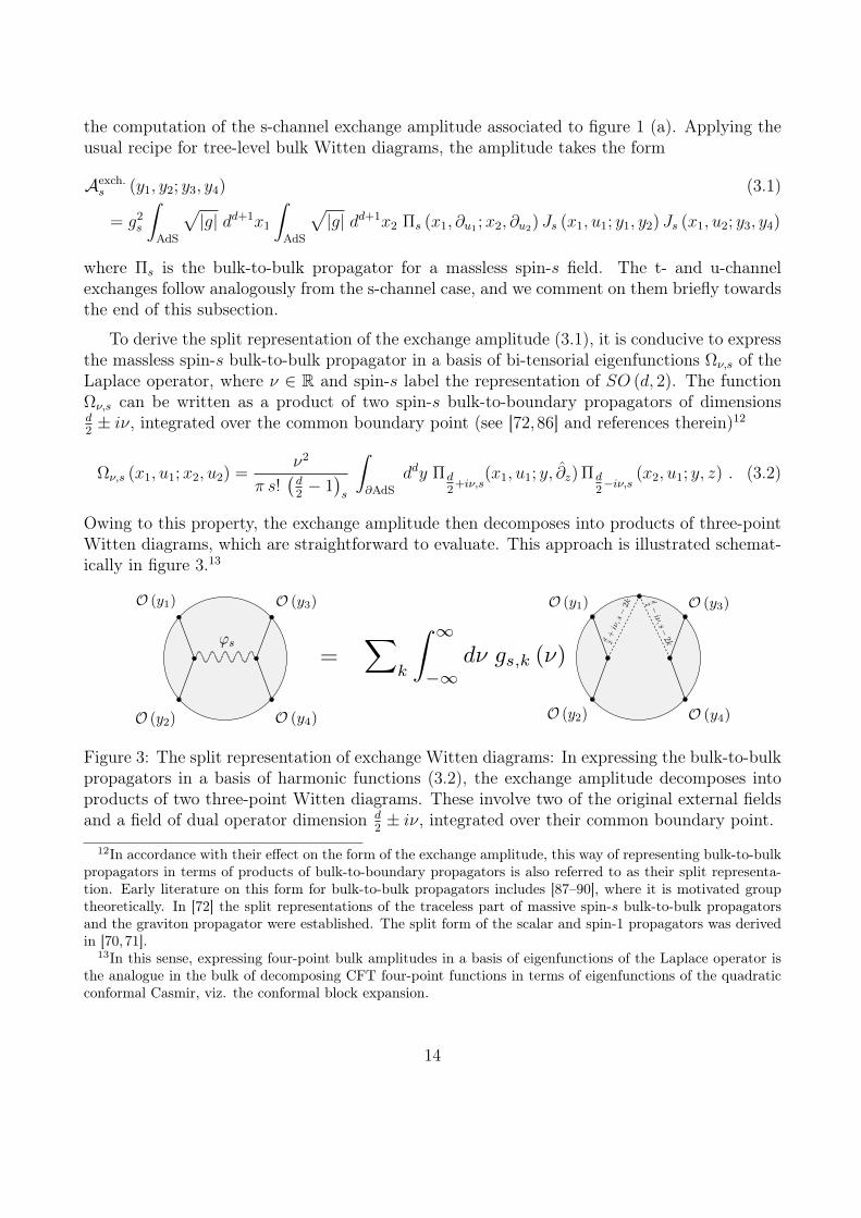
To derive the split representation of the exchange amplitude (3.1), it is conducive to expressthe massless spin-s bulk-to-bulk propagator in a basis of bi-tensorial eigenfunctions Ων,s of theLaplace operator, where ν ∈ R and spin-s label the representation of SO (d, 2). The functionΩν,s can be written as a product of two spin-s bulk-to-boundary propagators of dimensionsd2± iν, integrated over the common boundary point (see [72,86] and references therein)12
Ων,s (x1, u1;x2, u2) =ν2
π s!(d2− 1)s
∫∂AdS
ddy Πd2
+iν,s(x1, u1; y, ∂z) Πd
2−iν,s
(x2, u1; y, z) . (3.2)
Owing to this property, the exchange amplitude then decomposes into products of three-pointWitten diagrams, which are straightforward to evaluate. This approach is illustrated schemat-ically in figure 3.13
Figure 3: The split representation of exchange Witten diagrams: In expressing the bulk-to-bulkpropagators in a basis of harmonic functions (3.2), the exchange amplitude decomposes intoproducts of two three-point Witten diagrams. These involve two of the original external fieldsand a field of dual operator dimension d
2± iν, integrated over their common boundary point.
12In accordance with their effect on the form of the exchange amplitude, this way of representing bulk-to-bulkpropagators in terms of products of bulk-to-boundary propagators is also referred to as their split representa-tion. Early literature on this form for bulk-to-bulk propagators includes [87–90], where it is motivated grouptheoretically. In [72] the split representations of the traceless part of massive spin-s bulk-to-bulk propagatorsand the graviton propagator were established. The split form of the scalar and spin-1 propagators was derivedin [70,71].
13In this sense, expressing four-point bulk amplitudes in a basis of eigenfunctions of the Laplace operator isthe analogue in the bulk of decomposing CFT four-point functions in terms of eigenfunctions of the quadraticconformal Casmir, viz. the conformal block expansion.
14
This method of computing higher-spin four-point exchange amplitudes was taken in [75], forthree different gauges of the spin-s field. For reasons that will become clear shortly, in AdS4 aconvenient gauge to use for the spin-s bulk-to-bulk propagator is the one that makes the tracestructure manifest (see sections 3.5 and 4.3 of [75]). In this gauge, the propagator reads
Πs (x1, u1;x2, u2) =
[ s2 ]∑k=0
∫ ∞−∞
dν gs,k (ν)(u2
1
)k (u2
2
)kΩν,s−2k (x1, u1;x2, u2) , (3.3)
where the (u2)k represent k symmetric products of the background metric. The coefficients gs,k
are given by
gs,0(ν) =1
(d2
+ s− 2)2 + ν2,
gs,k(ν) = −(
12
)k−1
22k+3 k!
(s− 2k + 1)2k
(d2
+ s− 2k)k(d2
+ s− k − 32)k
(d2
+s−2k+iν
2
)k−1
(d2
+s−2k−iν2
)k−1(
d2
+s−2k+1+iν
2
)k
(d2
+s−2k+1−iν2
)k
, k 6= 0.
(3.4)
As opposed to bulk-to-boundary propagators, bulk-to-bulk propagators are not on-shell (i.e.are not traceless and transverse). In the split representation, this fact manifests itself in con-tributions from harmonic functions of lower spin. For the massless spin-s propagator in themanifest trace gauge, these are given by the k > 0 terms in (3.3).
In the above gauge, the s-channel exchange amplitude (3.1) decomposes as
Aexch.s (y1, y2; y3, y4) (3.5)
= g2s
[ s2 ]∑k=0
∫ ∞−∞
dν gs,k (ν)
∫AdS
√|g| dd+1x1
∫AdS
√|g| dd+1x2 s!
2 Ων,s−2k (x1, ∂u1 ;x2, ∂u2)
× (∂u1 · ∂u1)k Js (x1, u1; y1, y2) (∂u2 · ∂u2)k Js (x2, u2; y3, y4) ,
where (∂u · ∂u)k Js denotes the k-th trace of Js. The complete evaluation of (3.5) in generaldimensions is given in [75], but at this point we depart from the general dimensional analysisto focus on the particular case of AdS4.
The suitability of the gauge choice (3.3) to AdS4 becomes apparent when we recall thatthe bulk scalar ϕ0 is conformal in this particular dimension. As a consequence, there is somefreedom which allows us to take the currents Js to be traceless on-shell, i.e. (∂u · ∂u)k Js = 0 fork > 0 when the scalar fields are on their mass shell. This provides a significant simplification,because when the currents are traceless just the k = 0 term in (3.5) contributes. With this
15
choice the exchange amplitude in AdS4 takes the form
Aexch.s (y1, y2; y3, y4) =
∫ ∞−∞
dν1
ν2 +(s− 1
2
)2
ν2
π
∫∂AdS
d3y1
s!(
12
)s
(3.6)
× gs∫
AdS
√|g| d4x1 s! Π3
2+iν,s
(x1, ∂u1 ; y, ∂z)Js (x1, u1; y1, y2)
× gs∫
AdS
√|g| d4x2 s! Π3
2−iν,s
(x2, ∂u2 ; y, z) Js (x2, u2; y3, y4) ,
where we have inserted the representation (3.2) for Ων,s. The amplitude can then be expressedin terms of boundary quantities by using the result (2.10) for the three-point Witten diagrams,with ∆s = 3
2± iν:14
Aexch.s (y1, y2; y3, y4) = g2
s
∫ ∞−∞
dνν2 +
(s+ 1
2
)2
ν2 +(s− 1
2
)2
b(
32
+ iν, s)b(
32− iν, s
)Γ(
12− iν
)Γ(iν + 1
2
)4π4Γ(−iν)Γ(iν)
× 1
s!(
12
)s
∫∂AdS
d3y(y2
20 (y10 · ∂z)− y210 (y20 · ∂z))s
(y212)
2s−2iν+14 (y2
10)2s−2iν+3
4 (y220)
2s−2iν+34
(y240 (y30 · z)− y2
30 (y40 · z))s
(y234)
2s+2iν+14 (y2
30)2s+2iν+3
4 (y240)
2s+2iν+34
,
(3.7)
where here yi0 = yi − y, and the bulk three-point amplitude normalisations b(
32± iν, s
)were
defined by equation (2.11) in section (2.2). Note that the second line is a product of three-pointfunctions of unit norm, integrated over their common boundary point.
To make contact with the dual CFT four-point function, it will be useful to express theamplitude (3.7) in terms of conformal blocks. It is well known that a boundary integral of theform shown in second line of (3.7) can be expressed in terms of conformal blocks correspondingto a given representation of the conformal group and its shadow [72,91]. In our case, the preciserelation is
1
s!(
12
)s
∫∂AdS
d3y(y2
20 (y10 · ∂z)− y210 (y20 · ∂z))s
(y212)
2s−2iν+14 (y2
10)2s−2iν+3
4 (y220)
2s−2iν+34
(y240 (y30 · z)− y2
30 (y40 · z))s
(y234)
2s+2iν+14 (y2
30)2s+2iν+3
4 (y240)
2s+2iν+34
(3.8)
=1
y212y
234
[Kiν,s G 3
2+iν (u, v) + (ν ↔ −ν)
],
where
Kiν,s =π5/22−2(iν+s−1)Γ(−iν)Γ
(s− iν + 1
2
)Γ(s+ iν + 1
2
)Γ(
12− iν
)(2iν + 2s+ 1)Γ
(2s−2iν+3
4
)2Γ(
2s+2iν+14
)2 , (3.9)
14Note that here the normalisation of the spin-s bulk-to-boundary propagator is different to that used in(2.10). It is given by equation (3.53) in [75], and is required to be compatible with the spin-s bulk-to-bulkpropagator (3.3). All normalisations used here are consistent with the canonical normalisation of the kineticterm in the cubic action (2.6).
16
and G3/2+iν,s (u, v) is a direct (i.e. (12)(34)) channel conformal block, of dimension 3/2+ iν andspin-s. The second term with ν ↔ −ν gives the contribution from the shadow representation,whose contribution to the bulk amplitude is identical owing to the integration over ν. Usingthis relationship between the boundary integral in (3.7) and conformal blocks, the s-channelexchange amplitude in AdS4 can be expressed as the following conformal block expansion inthe direct-channel
Aexch.s (y1, y2; y3, y4) =
1
y212y
234
28−s
NΓ (s)2
∫ ∞−∞
dν1
ν2 + (s− 12)2κs(ν)G3
2+iν,s
(u, v) , (3.10)
where we have inserted the explicit expression (2.15) for the cubic coupling gs, and the factor
κs(ν) =2−2iν+2s−3 Γ
(iν + 1
2
)Γ(
2s−2iν+14
)2Γ(
2s+2iν+34
)2
π5/2Γ(iν)(2iν + 2s+ 1)(3.11)
in the integrand will keep appearing when representing various relevant amplitudes as contourintegrals.
This completes the computation of the amplitude for the exchange of a massless spin-s fieldon AdS4 between two pairs of the real scalar ϕ0 in the s-channel, with the result expressed asa conformal block expansion (3.10) in the direct-channel. For the t- and u-channel exchanges(figures 1. (b) and 1. (c)), the process follows much in the same way. In fact, since the externalscalars are not distinct, explicit computation of their amplitudes can be avoided: the t- andu-channel amplitudes can be obtained by permuting the external legs of the s-channel result(3.10). Namely, to acquire the t-channel amplitude one should exchange y2 ↔ y3 in (3.10), andthe result is thus given by
Aexch.s (y1, y3; y2, y4) =
1
y213y
224
28−s
NΓ (s)2
∫ ∞−∞
dν1
ν2 + (s− 12)2κs(ν)G3
2+iν,s
(1u, vu
), (3.12)
which is a (13)(24) crossed-channel expansion. Likewise, for the u-channel we exchange: y2 ↔y4, giving the amplitude Aexch.
s (y1, y4; y2, y3). The latter amplitude is thus a (14)(23) crossed-channel expansion conformal blocks G3/2+iν,s (v, u).
3.2 Contact diagrams
In this section we show how four-point Witten diagrams associated to quartic contact interac-tions of the scalar ϕ0 can be evaluated. In particular, as with the exchange diagrams in theprevious section, we demonstrate how to derive the split representation of the amplitudes, andsubsequently their conformal block expansions in a single channel. The results derived belowfor a contact diagram associated to a general quartic vertex will be instrumental in section 5,where by matching the four-point Witten diagrams with external ϕ0 to the corresponding CFTfour-point function, we determine the quartic vertex of ϕ0 in AdS4.
In general, the computation of a four-point contact Witten diagram associated to an arbi-trary quartic vertex is very involved, owing to the manipulations required of non-commuting
17
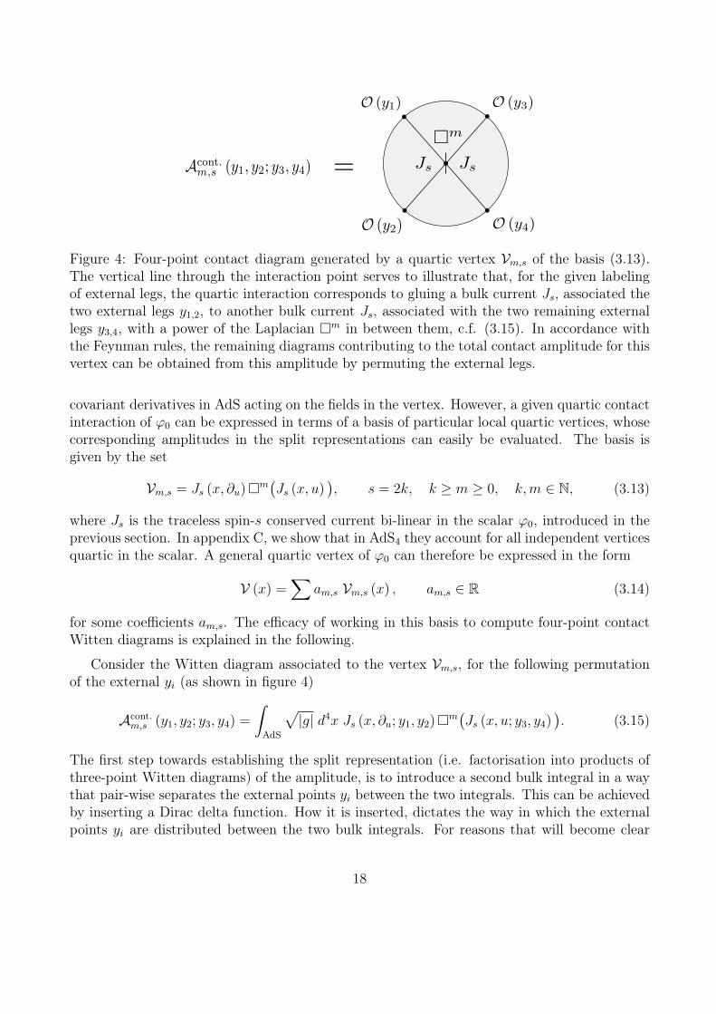
Figure 4: Four-point contact diagram generated by a quartic vertex Vm,s of the basis (3.13).The vertical line through the interaction point serves to illustrate that, for the given labelingof external legs, the quartic interaction corresponds to gluing a bulk current Js, associated thetwo external legs y1,2, to another bulk current Js, associated with the two remaining externallegs y3,4, with a power of the Laplacian m in between them, c.f. (3.15). In accordance withthe Feynman rules, the remaining diagrams contributing to the total contact amplitude for thisvertex can be obtained from this amplitude by permuting the external legs.
covariant derivatives in AdS acting on the fields in the vertex. However, a given quartic contactinteraction of ϕ0 can be expressed in terms of a basis of particular local quartic vertices, whosecorresponding amplitudes in the split representations can easily be evaluated. The basis isgiven by the set
Vm,s = Js (x, ∂u)m(Js (x, u)
), s = 2k, k ≥ m ≥ 0, k,m ∈ N, (3.13)
where Js is the traceless spin-s conserved current bi-linear in the scalar ϕ0, introduced in theprevious section. In appendix C, we show that in AdS4 they account for all independent verticesquartic in the scalar. A general quartic vertex of ϕ0 can therefore be expressed in the form
V (x) =∑
am,s Vm,s (x) , am,s ∈ R (3.14)
for some coefficients am,s. The efficacy of working in this basis to compute four-point contactWitten diagrams is explained in the following.
Consider the Witten diagram associated to the vertex Vm,s, for the following permutationof the external yi (as shown in figure 4)
Acont.m,s (y1, y2; y3, y4) =
∫AdS
√|g| d4x Js (x, ∂u; y1, y2)m
(Js (x, u; y3, y4)
). (3.15)
The first step towards establishing the split representation (i.e. factorisation into products ofthree-point Witten diagrams) of the amplitude, is to introduce a second bulk integral in a waythat pair-wise separates the external points yi between the two integrals. This can be achievedby inserting a Dirac delta function. How it is inserted, dictates the way in which the externalpoints yi are distributed between the two bulk integrals. For reasons that will become clear
18
shortly, for the given permutation of the external points it is most strategic to place the deltafunction such that the pairs (y1, y2) and (y3, y4) are separated. To wit,
Acont.m,s (y1, y2; y3, y4) (3.16)
=
∫AdS
√|g| d4x1 Js (x1, ∂u1 ; y1, y2)
∫AdS
√|g| d4x2
m(Js (x2, ∂u2 ; y3, y4)
)(u1 · u2)s δ4 (x1 − x2) .
The suitability of the basis Vm,s emerges when one inserts the completeness relation (B.4)for the harmonic functions Ων,`. Since the currents Js are conserved and traceless, only theharmonic function with ` = s contributes and one obtains
Acont.m,s (y1, y2; y3, y4) (3.17)
=
∫ ∞−∞
dν
∫AdS
√|g| d4x1 Js (x1, ∂u1 ; y1, y2)
∫AdS
√|g| d4x2
m(Js (x2, ∂u2 ; y3, y4)
)Ων,s (x1, u1;x2, u2)
=
∫ ∞−∞
dν (−1)m(ν2 + s+ 9
4
)m ν2
π
∫∂AdS
d3y1
s!(
12
)s
∫AdS
√|g| d4x1 Js (x1, ∂u1 ; y1, y2) Π3
2+iν,s
(x1, u1; y, ∂z)
×∫
AdS
√|g| d4x2 Js (x2, ∂u2 ; y3, y4) Π3
2−iν,s
(x2, u2; y, z) ,
where in the second equality we used the equation of motion (B.2) for Ων,s, and inserted itsrepresentation (3.2) in terms of spin-s bulk-to-boundary propagators.
The diagram can now easily be evaluated using the known results (2.10) for the three-pointWitten diagrams, just as in the previous section. The resulting conformal block expansion isthe direct channel expansion
Acont.m,s (y1, y2; y3, y4) =
1
y212y
234
∫ ∞−∞
dν (−1)m(ν2 + s+ 9
4
)mκs(ν)G3
2+iν,s
(u, v) , (3.18)
which can be obtained using (3.8), as with the exchange amplitudes in section (3.1).
To complete the full four-point amplitude associated to the vertex Vm,s, in accordance withthe Feynman rules the contact diagrams corresponding to the remaining permutations of theexternal yi have to be taken into account. As for the exchange diagrams in section 3.1, since theexternal scalars are not distinct their amplitudes can be obtained from the result (3.18) withy2 ↔ y3 and y2 ↔ y4, and are given by Acont
m,s (y1, y3; y2, y4) and Acontm,s (y1, y4; y2, y3) respectively.
In the same way as for the exchanges, these amplitudes are also crossed-channel (13)(24) and(14)(23) expansions in terms of conformal blocks: G3/2+iν,s
(1u, vu
)and G3/2+iν,s (v, u), respec-
tively. The total contact amplitude for the vertex Vm,s is thus
Acont.m,s (y1, y2; y3, y4) +Acont.
m,s (y1, y3; y2, y4) +Acont.m,s (y1, y4; y3, y2). (3.19)
4 Scalar singlet four-point function
The four-point Witten diagrams displayed in figure 1 constitute the holographic computationof the connected part of the scalar-singlet four-point function in the free scalar O (N) vector
19
model. With normalisation O = 1√2Nφaφa, this is the O (1/N) part of the full scalar single-trace
operator four-point function [76]
〈O (y1)O (y2)O (y3)O (y4)〉 (4.1)
=1
(y212y
234)
d−2
1 + ud−2 +
(uv
)d−2
+4
N
(ud2−1 +
(uv
) d2−1
+ ud2−1(uv
) d2−1)
,
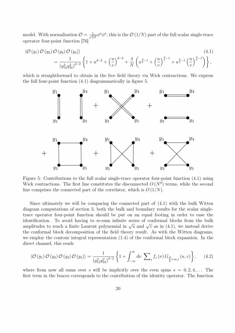
which is straightforward to obtain in the free field theory via Wick contractions. We expressthe full four-point function (4.1) diagrammatically in figure 5.
Figure 5: Contributions to the full scalar single-trace operator four-point function (4.1) usingWick contractions. The first line constitutes the disconnected O (N0) terms, while the secondline comprises the connected part of the correlator, which is O (1/N).
Since ultimately we will be comparing the connected part of (4.1) with the bulk Wittendiagram computations of section 3, both the bulk and boundary results for the scalar single-trace operator four-point function should be put on an equal footing in order to ease theidentification. To avoid having to re-sum infinite series of conformal blocks from the bulkamplitudes to reach a finite Laurent polynomial in
√u and
√v as in (4.1), we instead derive
the conformal block decomposition of the field theory result. As with the Witten diagrams,we employ the contour integral representation (1.4) of the conformal block expansion. In thedirect channel, this reads
〈O (y1)O (y2)O (y3)O (y4)〉 =1
(y212y
234)
d−2
1 +
∫ ∞−∞
dν∑
sfs (ν)Gd
2+iν,s
(u, v)
, (4.2)
where from now all sums over s will be implicitly over the even spins s = 0, 2, 4, . . . Thefirst term in the braces corresponds to the contribution of the identity operator. The function
20
fs (ν) contains poles that ensure only the spin-s operators present in the scalar singlet OPEcontribute, and encodes their OPE coefficients. The goal of this section is to establish thefunction fs (ν). As a first step, we determine those OPE coefficients in the scalar single-traceoperator product expansion (OPE) which are not yet known explicitly:
The OPE of the scalar singlet O takes the schematic form [92–94]
OO ∼ I +∑
scs Js +
∑n,scn,s O(2)
n,s + descendants, (4.3)
where I is the identity operator, cs is the OPE coefficient of the spin-s single-trace conservedcurrent Js and cn,s is the OPE coefficient of the double-trace operator O(2)
n,s. The conservedcurrents Js take the schematic form
Ji1...is = φa∂(i1 ... ∂ is)φa + ..., ∂i1Ji1...is = 0, (4.4)
while the double-trace operators are bi-linear in the single-trace scalar operator O:
O(2)n,i1...is
(x) = n(O (x)
)∂(i1 ...∂ is)O (x) + .... (4.5)
The explicit form for a general double-trace operator built from two scalar single-trace operatorsin conformal field theory is derived in appendix D.
In the direct channel, the explicit conformal block decomposition of (4.1) is thus
〈O (y1)O (y2)O (y3)O (y4)〉 (4.6)
=1
(y212y
234)
d−2
1 +
∑sc2s Gs+d−2,s (u, v) +
∑n,sc2n,s G∆n,s,s (u, v)
,
where ∆n,s = 2(d− 2) + 2n+ s is the dimension of the spin-s double-trace operator O(2)n,s, and
the spin-s conserved current Js has dimension ∆s = s + d − 2. The function fs (ν) of thecorresponding contour integral representation (4.2) can be determined with the knowledge ofthe explicit form of cs and cn,s.
The OPE coefficients cs of the spin-s conserved currents Js are known [76,84], and are givenby
cs =2s+3
2√s!√N
(d2− 1)s√
(d+ s− 3)s. (4.7)
For the double-trace operators O(2)n,s, so far the OPE coefficients have been determined only
for d = 4 in [76]. However, the OPE coefficient of an operator Ok in the OPE of operatorsOi and Oj can be determined with the knowledge of the coefficient of the three-point function〈OiOjOk〉 and the two-point function 〈OkOk〉. In the following section we take this approach tocompute the OPE coefficients cn,s of the double-trace operators in general field theory dimensiond, thus completing the conformal block decomposition (4.6) of the scalar single-trace operatorfour-point function (4.1) in general dimensions.
21
4.1 OPE coefficients of double-trace operators
The aim of this section is to compute the OPE coefficients cn,s of the double-trace operatorsO(2)n,s in the OPE of the scalar singlet O. In a free theory, it is feasible to compute the coefficients
using the relation
cn,s =COOO(2)
n,s√CO(2)
n,s
, (4.8)
where COOO(2)n,s
is the coefficient of the three-point function 〈OOO(2)n,s〉 and CO(2)
n,sis the coefficient
of the two-point function 〈O(2)n,sO(2)
n,s〉 (see below for their explicit forms). The reason for thisis that in a free theory the computation of correlation functions is relatively straightforwardusing Wick contractions, with the knowledge of the explicit form of the operators concerned interms of the fundamental fields.
Using conformal symmetry, it is possible to show that the three- and two-point functionstake the form
〈O (y1)O (y2)O(2)n,s (y3, z)〉 = COOO(2)
n,s
(y212)
n
(y213)
d−2+n(y2
23)d−2+n
(y13 · zy2
13
− y23 · zy2
23
)s, (4.9)
and
〈O(2)n,s (y1, z1)O(2)
n,s (y2, z2)〉 = CO(2)n,s
1
(y212)
∆n,s
(z1 · z2 − 2
(z1 · y12) (z2 · y12)
y212
)s. (4.10)
The coefficients COOO(2)n,s
and CO(2)n,s
can then be determined by comparing with the result ob-tained using Wick contractions. Since the explicit form of the double trace operators (appendixD) is very involved, we were not able to calculate the coefficients explicitly for general n ands. We conjecture their form for any n and s based on the explicit results we could obtain forany n when s = 0, and for any s when n = 0, 1 (see appendix E). This leads to the followingexpression for the double-trace OPE coefficients
c2n,s =
[(−1)s + 1] 2s(d2− 1)2
n(d− 2)2
s+n
s!n!(s+ d
2
)n
(d− 3 + n)n (2d+ 2n+ s− 5)s(
3d2− 4 + n+ s
)n
(4.11)
×
1 + (−1)n4
N
Γ (s)
2sΓ(s2
)(d2− 1)n+
s2(
d−12
)s2
(d− 2)n+
s2
.
Although we were unable to derive the OPE coefficients in full generality, our conjecture abovefor any n and s reproduces the results available in d = 4 [76], and agrees with the coefficientsat N =∞ in general d [79]. These provide two supplementary important checks of its validity.This formula is instrumental in our holographic reconstruction of the quartic self-interaction ofthe scalar field in higher-spin gravity on AdS4, dual to the free vector model CFT3.
22
4.2 Contour integral representation
In this subsection we complete the derivation of the conformal block expansion (4.2) of thescalar single-trace operator four-point function in the form of a contour integral. We use theknowledge of the explicit form (4.7) of the OPE coefficients cs of the single-trace higher-spinconserved currents, and those cn,s of the double-trace operators obtained in the previous section.For concision, we focus on the specific case of interest: d = 3.
Essentially, the task is to find a function fs (ν) which gives precisely the conformal blockexpansion (4.6) when the contour integral over ν in (4.2) is evaluated. Therefore fs (ν) mustcontain poles in ν, within the prescribed contour, where the dimension d
2+ iν of the conformal
blocks matches that of the spin-s operators Js and O(2)n,s in the scalar singlet OPE (4.3).
Since the conformal block G d2
+iν,s (u, v) decays exponentially as Im(ν)→ −∞, we close thecontour in the lower-half plane. Accordingly, fs (ν) must have the following pole structure forthe correct operator spectrum:
1. Spin-s conserved current Js of dimension ∆s = s+ d− 2
→ single pole at ν = −i(s+ d
2− 2).
2. Spin-s double-trace operator O(2)n,s of dimension ∆n,s = 2 (d− 2) + 2n+ s, n = 0, 1, 2, ...
→ single poles at ν = −i(2 (d− 2) + 2n+ s− d
2
).
It will be useful to decompose fs (ν) as
fs (ν) = fJs (ν) + fO(2)s
(ν) , (4.12)
where fJs (ν) and fO(2)s
generate the contributions of Js and the spin-s double-trace operators
O(2)n,s, respectively.
The functions fJs (ν) and fO(2)s
(ν) are not unique, as they can be modified in ways that donot alter the pole structure within the contour, and the corresponding residues. This freedomcan be used to ease comparison with the conformal block expansions of the four-point Wittendiagrams derived in section 3, allowing us to cast the functions into the form
f (ν) = ps (ν) κs(ν) , (4.13)
where ps (ν) is an even function of ν, as is the case for the Witten diagrams (see for examplethe four-point amplitudes (3.10) and (3.18)). We demonstrate how this can be achieved in thefollowing, for the contribution of the double-trace operators.
23
Double-trace operator contribution
To represent the contribution of the double-trace operators, the function fO(2)s
(ν) must bechosen such that ∫ ∞
−∞dν fO(2)
s(ν)Gd
2+iν,s
(u, v) =∞∑n=0
c2n,sG∆n,s,s (u, v) , (4.14)
where we close the contour in the lower-half plane.
As explained above, fO(2)s
(ν) must have poles at ν = −i(2 (d− 2) + 2n+ s− d
2
)for n =
0, 1, 2, ... These poles can be neatly packaged in the gamma function Γ(
4(d−2)+2s−d−2iν4
), which
has poles precisely at those values of ν. The most direct way to find a function which satisfies(4.14), is then to multiply the double-trace conformal block coefficient (4.11) by Γ (−n) anda factor to neutralise the effect of its residue.15. To obtain a function of ν one then simplyreplaces n→ −
(4(d−2)+2s−d−2iν
4
). For d = 3, this direct method gives the following function
fO(2)s
(ν) = pO(2)s
(ν) κs(ν) , (4.15)
with κs given by (3.11) and pO(2)s
by
pO(2)s
(ν) = [1 + (−1)s]π5/225−sΓ
(s+ 3
2
)Γ (s+ 1) Γ
(2s+1−2iν
4
)Γ(
2s+1+2iν4
)Γ(
2s+3−2iν4
)Γ(
2s+3+2iν4
) (4.16)
+1
N[1 + (−1)s]
π326−2sΓ(s+ 3
2
)csc(π4(1 + 2iν)
)csc(π4(2iν − 2s+ 1)
)Γ(s2
+ 1)2
Γ(
3−2iν4
)Γ(
3+2iν4
)Γ(
2s+1−2iν4
)Γ(
2s+1+2iν4
)Γ(
2s+3−2iν4
)Γ(
2s+3+2iν4
) ,where we used the identity Γ (z) Γ (1− z) = π cosec (πz) to make the behaviour of pO(2)
s(ν)
under the transformation ν ↔ −ν manifest. It is then clear that the only terms preventingthe symmetry condition pO(2)
s(−ν) = pO(2)
s(ν) of (4.13) from being satisfied are the cosecant
functions in the numerator of the O (1/N) part. Since the only poles of (4.15) in the lower-halfplane are single poles at ν = −i
(12
+ 2n+ s), the discrepancy can be rectified by evaluating
the cosecant functions at the location of the poles:
csc(π4(1 + 2iν)
)csc(π4(2iν − 2s+ 1)
) ∣∣∣ν=−i(2∆+2n+s−d
2)
=(−1)
s2
√2. (4.17)
The conformal block coefficient function fO(2)s
(ν) = pO(2)s
(ν) κs(ν) with the desired symmetry(4.13) therefore has
pO(2)s
(ν) = [1 + (−1)s]π
32 2s+4Γ
(s+ 3
2
)Γ (s+ 1) Γ
(s+ 1
2+ iν
)Γ(s+ 1
2− iν
) (4.18)
+1
N[1 + (−1)s]
(−1)s2 π
32 2s+4Γ
(s+ 3
2
)Γ(s2
+ 12
)√
2 Γ(s2
+ 1)
Γ (s+ 1) Γ(
34− iν
2
)Γ(
34
+ iν2
)Γ(s+ 1
2+ iν
)Γ(s+ 1
2− iν
) ,15The residue of Γ (z) at z = −n is (−1)n
n! , so in this case the neutralising factor is (−1)nn!
24
where simplifications were also made using the identity: Γ (z) Γ(z + 1
2
)=√π 21−2zΓ (2z).
Higher-spin conserved currents
Just as for the double-trace operators above, one can derive a function fJs (ν) = pJs (ν) κs(ν)that generates the contribution (4.7) of a spin-s conserved current to the conformal blockexpansion (4.6) of the scalar single-trace operator four-point function. The correspondingpJs (ν) that satisfies the symmetry property (4.13) is
pJs (ν) =π 28−s
N
1
ν2 + (s− 12)2
1
Γ(
2s−2iν+14
)2Γ(
2s+2iν+14
)2 . (4.19)
Notice that the factor Γ(
2s−2iν+14
)2 in the denominator cancels that in the numerator of κs (ν).The function fJs (ν) = pJs (ν)κs(ν) therefore only has one pole in the lower-half plane atν = −i (s− 1/2), corresponding to a spin-s conserved current.
5 Uncovering the quartic vertex
5.1 Summary: CFT interpretation of Witten diagrams
Before the scalar quartic vertex in higher-spin theory on AdS4 can be investigated through thecomparison of the CFT3 results in section 4.2 with the four-point bulk amplitudes in section 3,it is instructive to study the latter as objects in conformal field theory. That is, the operatorcontributions in their conformal block expansions.
Exchange Witten diagrams
Let us focus on the s-channel exchange of a massless spin-s field (figure 1. (a)), whose conformalblock expansion (3.10) in the direct channel was derived as a contour integral in section 3.1. Thediscussion for the t- and u-channel exchanges is analogous, and we comment on them brieflytowards the end of this subsection. We take the same prescription for the contour as for theCFT conformal block expansions in section 4.2, closing in the lower-half plane. The four-pointexchange amplitude (3.10), interpreted as a CFT quantity, therefore receives contributions fromthe following operators:
1. Single pole at: ν = −i(s− 1
2
)→ spin-s conserved current Js.
2. Double poles at: ν = −i(2 (d− 2) + 2n+ s− d
2
), n = 0, 1, 2, ...
→ spin-s double-trace operator O(2)n,s with anomalous dimensions.
25
The cubic coupling gs was fixed in section 2.2 according to the OPE coefficient of Js in theoperator product expansion (4.3) (see also equation (2.13)). Therefore, as can be checkedexplicitly from the split representation, the corresponding contribution of Js to the s-channelexchange is identical to that in the direct channel conformal block decomposition of the dualCFT four-point function (4.6). For the double-trace operator contributions the story is clearlynot the same, as indicated by the anomalous dimensions: In a free theory, such as the dual freescalar O (N) vector model, these are not present. The explicit conformal block expansion ofthe s-channel exchange thus takes the form
Aexch.s (y1, y2; y3, y4) =
1
y212y
234
c2s Gs+d−2 , s (u, v) +
∞∑n=0
dexch.n,s G∆n,s+γn,s , s (u, v)
, (5.1)
where the γn,s represent the anomalous dimensions of the double-trace operators O(2)n,s. This
result is consistent with observations in the literature [62, 95] for lower-spin exchanges, thatan exchange Witten diagram does not simply correspond in the CFT to the exchange of theoperator dual to the exchanged bulk field: There are additional contributions from double-trace operators built from the single-trace operators that are dual to the external fields of theexchange Witten diagram.
As explained at the end of section 3.1, the t- and u-channel exchanges have (13)(24) and(14)(23) crossed-channel expansions, which are obtained from the s-channel result by exchang-ing y2 ↔ y3 and y2 ↔ y4 respectively. Consequently, as with the conformal block expansion(5.1) of the s-channel exchange, the contributions from the operator Js in the conformal blockexpansion of these amplitudes coincide with those in the corresponding (13)(24) and (14)(32)crossed channel expansions of the CFT four-point function (4.1).
Before moving onto the analysis of the contact diagrams, let us make a final comment on theoperator contributions to the spin-s exchange. It is important to note that in general it is notthe case that only spin-s representations of the conformal group contribute to the four-pointexchange of a bulk spin-s field. In the present context of higher-spin theory on AdS4, this isonly possible since the conformal scalar present in this dimension allows the conserved currentsin the cubic vertex (2.8) to be traceless. As a consequence, only spin-s conformal blocks appearin the amplitude (5.1). This can be seen from the split representation (3.5) of the exchange ingeneral dimensions, where just the leading (k = 0) term contributes if the current is traceless.In general dimensions the terms for k > 0 would be non-vanishing, because generally the scalaris not conformal. These terms would generate contributions to the amplitude from double-traceoperators of spin lower than s.
Contact Witten diagrams
We now perform the CFT analysis of the contact Witten diagrams considered in section 3.2,which give all possible contact amplitudes for the scalar ϕ0 in AdS4, since they are generatedby quartic vertices belonging to the basis (3.13). A similar analysis can be found in [62], where
26
a complete basis of local quartic interactions was presented and the conformal block expansionsof corresponding four-point contact diagrams were determined in the Regge limit.
The contour integral representation of the contact amplitude (3.18) produced by a genericquartic vertex Vm,s in the basis (3.13), has double poles located at ν = −i
(2 (d− 2) + 2n+ s− d
2
),
n = 0, 1, 2, . . . in the lower-half ν-plane. Its conformal block expansion thus receives contribu-tions only from spin-s double-trace operators with anomalous dimensions,
Acont.m,s (y1, y2; y3, y4) =
1
y212y
234
∞∑n=0
dcont.n,s,m G∆n,s+γn,s , s (u, v) . (5.2)
As with the exchange amplitudes, the conformal block expansions of the remaining contactamplitudes are crossed channel expansions obtained from (5.2) by exchanging y2 ↔ y3 andy2 ↔ y4. They therefore also receive contributions only from double-trace operators in theirrespective channels, with the same coefficients dcont.
n,s,m and anomalous dimensions γn,s.
5.2 Combining bulk contributions from all channels
At the level of four-point functions, holography requires∑sAexch.s (y1, y2; y3, y4) +Aexch.
s (y1, y3; y2, y4) +Aexch.s (y1, y4; y3, y2)
+Acont.(y1, y2; y3, y4) +Acont.(y1, y3; y2, y4) +Acont.(y1, y4; y2, y3) (5.3)AdS / CFT
= 〈O(y1)O(y2)O(y3)O(y4)〉conn.,
where the Acont. are the contributions from quartic contact interaction that we seek, and theRHS is the connected, i.e. O (1/N), part of the scalar single-trace operator four-point function(4.1). The bulk Witten diagrams that comprise the LHS of equation (5.3) are given in figure6.
To extract the quartic vertex V (x) from equation the contact diagrams in (5.3), we makean ansatz of the form
V (x) =∑
m,sam,s Vm,s (x) , am,s ∈ R (5.4)
built from vertices in the basis (3.13), which accounts for all possible independent quarticinteractions of ϕ0 on AdS4. The corresponding four-point contact diagrams (d), (e) and (f)in figure 6 can be evaluated in terms of conformal blocks using the results for the contactamplitudes of the individual basis elements established in section 3.2. For example, for theamplitude of diagram 6. (d)
Acont.(y1, y2; y3, y4) =∑m,s
am,s Acont.m,s (y1, y2; y3, y4), (5.5)
with Acont.m,s (y1, y2; y3, y4) given by (3.18). Combined with the results for the conformal block
expansions of the CFT four-point function (4.2) and the exchange diagrams in section (3.1), one
27
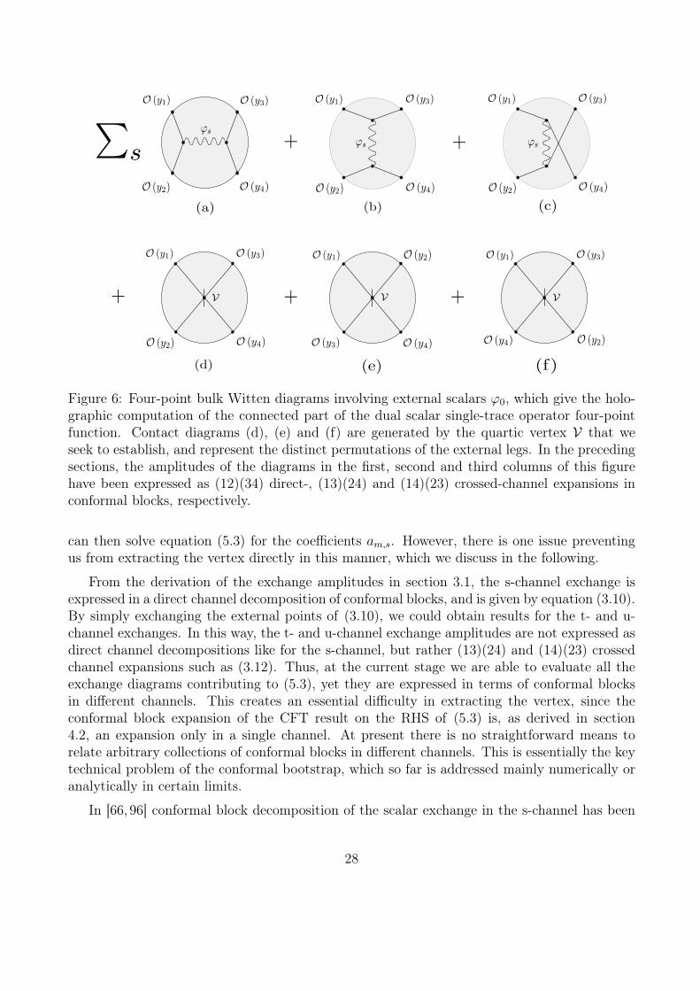
Figure 6: Four-point bulk Witten diagrams involving external scalars ϕ0, which give the holo-graphic computation of the connected part of the dual scalar single-trace operator four-pointfunction. Contact diagrams (d), (e) and (f) are generated by the quartic vertex V that weseek to establish, and represent the distinct permutations of the external legs. In the precedingsections, the amplitudes of the diagrams in the first, second and third columns of this figurehave been expressed as (12)(34) direct-, (13)(24) and (14)(23) crossed-channel expansions inconformal blocks, respectively.
can then solve equation (5.3) for the coefficients am,s. However, there is one issue preventingus from extracting the vertex directly in this manner, which we discuss in the following.
From the derivation of the exchange amplitudes in section 3.1, the s-channel exchange isexpressed in a direct channel decomposition of conformal blocks, and is given by equation (3.10).By simply exchanging the external points of (3.10), we could obtain results for the t- and u-channel exchanges. In this way, the t- and u-channel exchange amplitudes are not expressed asdirect channel decompositions like for the s-channel, but rather (13)(24) and (14)(23) crossedchannel expansions such as (3.12). Thus, at the current stage we are able to evaluate all theexchange diagrams contributing to (5.3), yet they are expressed in terms of conformal blocksin different channels. This creates an essential difficulty in extracting the vertex, since theconformal block expansion of the CFT result on the RHS of (5.3) is, as derived in section4.2, an expansion only in a single channel. At present there is no straightforward means torelate arbitrary collections of conformal blocks in different channels. This is essentially the keytechnical problem of the conformal bootstrap, which so far is addressed mainly numerically oranalytically in certain limits.
In [66, 96] conformal block decomposition of the scalar exchange in the s-channel has been
28
obtained in terms of crossed channel conformal blocks. In principle one can try to generalisethese results to higher spin exchanges, to express them as conformal block expansions in oneand the same channel. However, the split representation of the bulk-to-bulk propagators isnot conducive to deriving a crossed-channel decomposition of a s-channel exchange, since theconstruction naturally delivers s-channel amplitudes as direct channel expansions. Fortunately,as we shall explain in the next subsection, in our case dealing with the conformal block decom-position of the exchanges in different channels can be avoided.
Before explaining how this can be achieved, let us emphasise that the same difficulty alsoappears for the contact Witten diagrams: Consider one of the vertices in the basis (3.13)
Vm,s = Js (ϕ0, ϕ0, ∂u)mJs (ϕ0, ϕ0, u) , (5.6)
where the fact that Js is bilinear in scalar fields ϕ0 is made explicit. According to the Feyn-man rules, the bulk-to-boundary propagators sourced at different boundary points should beattached to the vertex in a Bose-symmetric way. This implies that the vertex (5.6) results notonly in the amplitude
Acont.m,s (y1, y2; y3, y4) (5.7)
≡∫
AdS
√|g|dd+1xJs (Πd−2,0(y1, x),Πd−2,0(y2, x), ∂u)
mJs (Πd−2,0(y3, x),Πd−2,0(y4, x), u) ,
but also in the amplitudes Acont.m,s (y1, y3; y2, y4) and Acont.
m,s (y1, y4; y3, y2). The complete result istherefore
Acont.m,s (y1, y2; y3, y4) +Acont.
m,s (y1, y3; y2, y4) +Acont.m,s (y1, y4; y3, y2). (5.8)
The contact amplitude (5.7) was evaluated explicitly in section 3.2, where it was expressed interms of direct-channel conformal blocks (3.18). By exchanging y2 ↔ y3 and y2 ↔ y4 in thedirect-channel result (3.18) for (5.7), we could obtain the remaining amplitudesAcont.
m,s (y1, y3; y2, y4)and Acont.
m,s (y1, y4; y3, y2) as expansions in terms of (13)(24) and (14)(23) cross-channel confor-mal blocks, respectively. In this way, the total contact amplitude (5.8) is therefore also anexpansion in a mixture of the three channels. To try and express (5.8) as an expansion injust a single channel, in principle one could try and rearrange amplitudes Acont.
m,s (y1, y3; y2, y4)and Acont.
m,s (y1, y4; y3, y2) at the level of the bulk integrand: This would involve taking (5.7) withy2 ↔ y3 and y2 ↔ y4, in attempt to express them as linear combinations of Acont.
m,s (y1, y2; y3, y4)through integrating by parts and using the equations of motion. Their direct channel expan-sions could then be obtained using (3.18). However, this would require the knowledge of theexplicit complete form of traceless conserved currents Js in AdS, as well as cumbersome algebrainvolving covariant derivatives. As with the equivalent issue for exchange diagrams explainedabove, these complicated manipulations can be avoided.
5.3 Solving for the vertex: Reducing the analysis to a single channel
Instead of solving (5.3) for the quartic vertex, which requires us to deal simultaneously withconformal blocks in different channels, since the operators inserted in the four-point function
29
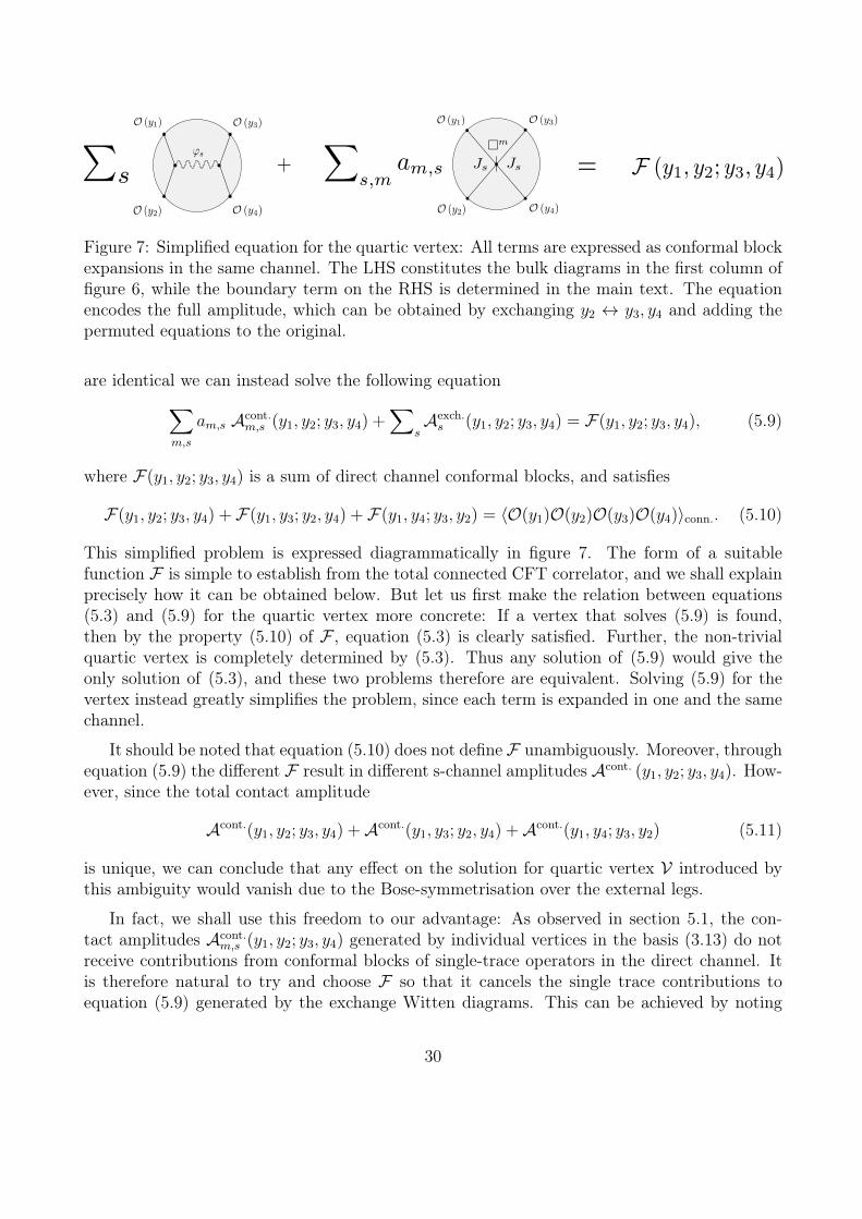
Figure 7: Simplified equation for the quartic vertex: All terms are expressed as conformal blockexpansions in the same channel. The LHS constitutes the bulk diagrams in the first column offigure 6, while the boundary term on the RHS is determined in the main text. The equationencodes the full amplitude, which can be obtained by exchanging y2 ↔ y3, y4 and adding thepermuted equations to the original.
are identical we can instead solve the following equation∑m,s
am,s Acont.m,s (y1, y2; y3, y4) +
∑sAexch.s (y1, y2; y3, y4) = F(y1, y2; y3, y4), (5.9)
where F(y1, y2; y3, y4) is a sum of direct channel conformal blocks, and satisfies
F(y1, y2; y3, y4) + F(y1, y3; y2, y4) + F(y1, y4; y3, y2) = 〈O(y1)O(y2)O(y3)O(y4)〉conn.. (5.10)
This simplified problem is expressed diagrammatically in figure 7. The form of a suitablefunction F is simple to establish from the total connected CFT correlator, and we shall explainprecisely how it can be obtained below. But let us first make the relation between equations(5.3) and (5.9) for the quartic vertex more concrete: If a vertex that solves (5.9) is found,then by the property (5.10) of F , equation (5.3) is clearly satisfied. Further, the non-trivialquartic vertex is completely determined by (5.3). Thus any solution of (5.9) would give theonly solution of (5.3), and these two problems therefore are equivalent. Solving (5.9) for thevertex instead greatly simplifies the problem, since each term is expanded in one and the samechannel.
It should be noted that equation (5.10) does not define F unambiguously. Moreover, throughequation (5.9) the different F result in different s-channel amplitudes Acont. (y1, y2; y3, y4). How-ever, since the total contact amplitude
Acont.(y1, y2; y3, y4) +Acont.(y1, y3; y2, y4) +Acont.(y1, y4; y3, y2) (5.11)
is unique, we can conclude that any effect on the solution for quartic vertex V introduced bythis ambiguity would vanish due to the Bose-symmetrisation over the external legs.
In fact, we shall use this freedom to our advantage: As observed in section 5.1, the con-tact amplitudes Acont.
m,s (y1, y2; y3, y4) generated by individual vertices in the basis (3.13) do notreceive contributions from conformal blocks of single-trace operators in the direct channel. Itis therefore natural to try and choose F so that it cancels the single trace contributions toequation (5.9) generated by the exchange Witten diagrams. This can be achieved by noting
30
that the first two terms of the connected four-point function
〈O (y1)O (y2)O (y3)O (y4)〉conn. =4
N
1
(y212y
234)
d−2
ud2−1 +
(uv
) d2−1
+ ud2−1(uv
) d2−1, (5.12)
contain only single-trace conformal blocks in the direct-channel decomposition
A + B ≡ 4
N
1
(y212y
234)
d−2
ud2−1 +
(uv
) d2−1
=1
(y212y
234)
d−2
∑sc2s Gs+d−2 , s (u, v) , (5.13)
while the remaining term receives contributions only from double-trace conformal blocks
C ≡ 4
N
1
(y212y
234)
d−2
ud2−1(uv
) d2−1
=1
(y212y
234)
d−2
∑n,sc2n,s G∆n,s , s (u, v) , (5.14)
where c2n,s is the O (1/N) part of the double-trace conformal block coefficient (4.11).
Moreover, as noted in section 5.1, the total single-trace contribution to the s-channel ex-change amplitudes in equation (5.9) precisely coincides with A+B. From the ansatz
F = a · (A + B) + c · C,
it is therefore clear that the cancellation of single trace conformal blocks in (5.9) requires a = 1.The value of c can then be fixed by noting that A, B and C transform into each other undery2 ↔ y3 and y2 ↔ y4:16
y2 ↔ y3 : (A,B,C)→ (C,B,A) , (5.15)y2 ↔ y4 : (A,B,C)→ (A,C,B) ,
Then since the total correlator (5.12) is equal to A+B+C, the definition (5.10) demands that2a+ c = 1. Our choice a = 1 therefore requires c = −1.17 The RHS of (5.9) then reads
F(y1, y2; y3, y4) =1
(y212y
234)
d−2
∑sc2s Gs+d−2 , s (u, v)− c2
n,s G∆n,s , s (u, v). (5.16)
In the sequel, taking d = 3 we solve equation (5.9) for the quartic vertex in AdS4 using theform (5.16) above for F(y1, y2; y3, y4).
Solving for the vertex
As explained in section 5.2, we make the following ansatz for the quartic vertex
V =∑
m,sam,s Vm,s, am,s ∈ R (5.17)
16This can straightforwardly be seen from figure 5, where A, B and C are respectively the first, second andthird diagrams on the second line.
17The representation with c = 0 and a = 12 was already derived in [84].
31
Figure 8: In AdS4, the amplitudes of the above Witten diagrams generate only spin-s conformalblocks. To determine the coefficients am,s in the derivative expansion (5.17) of the scalar quarticvertex, we identify them with the spin-s contribution of the term (5.18) in the dual field theoryon the RHS of equation (5.9).
composed of vertices Vm,s from the basis (3.13), whose contribution to equation (5.9) is givenby (5.5).
Extracting the vertex coefficients am,s from equation (5.9) is most straightforward using thecontour integral representation of the conformal block expansion. In this formalism, our choice(5.16) for F in d = 3 takes the form
F(y1, y2; y3, y4) =1
y212y
234
∑s
∫ ∞−∞
dν[pJs (ν)− pO(2)
s(ν)]κs (ν)G3
2+iν,s
(u, v) , (5.18)
where pJs (ν) is given by (4.19) for the contribution of spin-s operators Js in the direct channel,while pO(2)
s(ν) gives the O (1/N) part of the double-trace operator contributions (4.18). The
bulk amplitudes in (5.9) are given by (3.10) and (3.18) in this formalism. Although the functionsps (ν) were originally introduced in a field theory context by equation (4.13), their definitionextends naturally to the bulk amplitudes: For the total sum of the exchange amplitudes in(5.9), we have
pexch.s (ν) =
28−s
NΓ (s)2
1
ν2 + (s− 12)2, (5.19)
to which only the spin-s exchange contributes.18 Likewise, for the contact amplitude of thequartic ansatz,
pcont.s (ν) =
∑mam,s (−1)m
(ν2 + s+ 9
4
)m, (5.20)
since the basis vertices Vm,s also generate only spin-s contributions.
The coefficients am,s for each fixed s can now be determined for every m = 0, 1, 2, ... byequating the total bulk and boundary ps (ν) in equation (5.9). In this way, the am,s are given
18This is because in the specific case of AdS4, spin-s exchanges only generate spin-s conformal blocks.
32
implicitly by∑mam,s (−1)m
(ν2 + s+ 9
4
)m= pJs (ν)− 28−s
NΓ (s)2
1
ν2 + (s− 12)2− pO(2)
s(ν)
=28−s
N
1
ν2 + (s− 12)2
[π
Γ(
2s−2iν+14
)2Γ(
2s+2iν+14
)2 −1
Γ (s)2
]
− 1
N
(−1)s2 π
32 2s+5Γ
(s+ 3
2
)Γ(s2
+ 12
)√
2Γ(s2
+ 1)
Γ (s+ 1) Γ(
34− iν
2
)Γ(
34
+ iν2
)Γ(s+ 1
2+ iν
)Γ(s+ 1
2− iν
) . (5.21)
Then by setting z = −(ν2 + s+ 9
4
), one can establish a generating function:
as(z) ≡∑
mam,s z
m.
This determines the quartic vertex (5.17) of the parity even scalar in the minimal bosonichigher-spin theory on AdS4 dual to the free O(N) vector model in the form
V =∑
s∈2NJs (x, ∂u) as()Js (x, u) , (5.22)
and is one of the main results of this paper. In the next section we examine the properties ofthe vertex, particularly in the context of the locality of interactions in higher-spin theory. Butfirst, let us make the following comments:
The solution (5.22) that we found contains vertices which are not in the basis (3.13) dueto the terms with m > k. The fact that these extra vertices are redundant just means thatit should be possible to express them in terms of vertices with m ≤ k using the freedom ofintegration by parts and the free equations of motion. We used these extra vertices to avoidconversions of conformal blocks between different channels and, eventually, to present the resultin a more concise form.
Since we solve for the coefficients am,s at the level of the integrand of the ν contour integralin (5.21), naïvely it may seem that the vertex is not defined uniquely: One is free to addfunctions of ν that are entire within the contour. In doing so, this would change the form ofam,s and thus the solution for the quartic vertex. However, the addition of such terms does notchange the four-point amplitude and therefore the different vertices obtained in this mannerwould differ only by trivial terms which vanish on-free-shell, e.g. by the terms which can beaccounted for by the redundancy of the representation (5.17) with unbounded m.
Next, let us comment on the presence of anomalous dimensions in the bulk four-pointamplitudes: As observed in section 5.1, the conformal block decompositions of the bulk four-point amplitudes contain contributions from double-trace operators with anomalous dimensions.These manifest themselves in the presence of double poles in the integrands of (3.10) and (3.18)for ν = −i
(2 (d− 2) + 2n+ s− d
2
), n = 0, 1, 2, ..., which are the values of ν that yield double-
trace operator contributions. Owing to the double-poles, evaluating the ν-integral using theCauchy theorem produces not only the “non-anomalous” double-trace conformal blocks G∆n,s,s,
33
but also their derivatives with respect to the dimension (∂/∂∆n,s)G∆n,s,s. These two termstogether indicate that it is not G∆n,s,s that is present in the conformal block decomposition,but rather the conformal block G∆n,s+γn,s,s with an anomalous dimension. Indeed, this can beseen by expanding G∆n,s+γn,s,s as a Taylor series in γn,s,
G∆n,s+γn,s,s = G∆n,s,s + γn,s∂
∂∆n,s
G∆n,s,s +O(1/N2
). (5.23)
The presence of anomalous dimensions is natural in the bulk theory of interacting higher spinfields. But at the same time, the boundary theory is free and the double-trace operators On,sdo not receive any anomalous dimensions. This is consistent with our (4.18) and (4.19) for thecontour integral representation of the CFT four-point function, where the integrands containonly single poles in ν. Thus, the holographic duality between higher spin theories and freeO(N) vector models requires a rather delicate cancelation of anomalous conformal blocks inWitten diagrams. The quartic vertex that we have just found solves (5.3), which implies, inparticular, that this cancellation indeed takes place.
In this respect, the contour integral representation for the conformal block decompositionturned out to be a powerful tool: First of all, it allowed us to solve for a quartic vertexby performing simple algebraic manipulations with the functions ps(ν), instead of solving aninfinite system of linear equations balancing explicit conformal block coefficients of the bulkand boundary results. Moreover, this representation allowed us to treat conformal blocks withanomalous dimensions on the same footing as the non-anomalous ones, simply by controllingthe degree of the pole in ν at the associated point.
As a final comment, general consistency of the higher-spin holographic duality should implythat the vertex we have obtained is consistent with the Noether procedure. Further, to insteadderive the vertex we found via the Noether procedure would involve going to quintic order inthe fields. Indeed, the lowest order in the coupling constant where the quartic vertex for scalarfields contributes to the Noether consistency condition is g3, unlike other quartic vertices forfields of non-zero spin which first appear at the order g2. The reason for this is that the scalarfield does not posses its own undeformed gauge transformation.
6 Locality
Let us now turn to the issue of locality, which we outlined in the introduction. As mentionedthere, while local theories are the standard arena of quantum field theory, locality is a debat-able issue in higher-spin theories and has been the subject of recent investigations [37,61]. Thestandard approach to address the question of higher-spin interactions is to construct them per-turbatively using the Noether procedure [1] (which can be formalised as a BRST cohomologicalproblem [36,97,98]). In this approach, one makes a general ansatz for deformations of both theaction and its gauge transformations and then selects consistent pairs of such deformations bydemanding gauge invariance order by order in a coupling constant. However, at quartic and
34
higher orders in the number of fields this procedure is constraining only if the sought for ver-tices and deformations of gauge transformations are local [36]. Otherwise any cubic interactionvertex consistent until this level, can be made consistent with the gauge symmetry at all higherorders by an appropriate non-local deformation. From this perspective, it seems reasonable tonarrow the search for vertices by focusing attention on local deformations only.
In higher-spin theory, it is crucial to broaden the investigation to field theories which are“quasilocal”19 in the sense that they possess a perturbative expansion (in powers of fields andtheir derivatives) where each individual term in the total Lagrangian is local, though the totalnumber of derivatives may be unbounded in the full series. Indeed, it is a well-establishedfact that higher-spin theory in dimension four and higher requires a spectrum of fields withunbounded spin and, consequently, interactions with an unbounded number of derivatives (sincethe maximal number of derivatives in a cubic vertex grows with the spin). In particular,Vasiliev’s theory [40–42] does contain infinitely many derivatives in its interaction terms. Inorder to resolve this apparent clash with locality, it appears necessary to define a weaker notionof locality that leaves room for vertices with infinitely many derivatives.
To get more intuition on how this generalised locality might be defined, let us for simplicityconcentrate on quartic interactions of scalars in flat space. It is natural to characterise inter-actions by the corresponding S-matrix. It is well-known that local interactions give rise toamplitudes which are polynomial in Mandelstam variables. In turn, amplitudes for exchangediagrams, which are distinct from local quartic interactions, contain poles in Mandelstam vari-ables. So, as a first requirement, one possibility is to demand that amplitudes of local contactinteractions should be free of poles.
A similar conclusion can be drawn by replacing the requirement of the amplitude to bepolynomial by the milder requirement that the coefficients in its Taylor series expansion shoulddecrease fast enough. To be more precise, one possibility is to demand an infinite radius ofconvergence for this Taylor series. In this case the amplitude can be approximated infinitelywell by its Taylor series and for any values of Mandelstam parameters. This means, in turn,that the amplitude is infinitely close to a local one. The requirement for the amplitude tohave an infinite radius of convergence, or in other words, to be an entire function, not onlyexcludes poles, but also branch cuts in the amplitude. According to these arguments, we definea quartic interaction in flat spacetime to be weakly local iff the associated four-point amplitudeis an entire function of Mandelstam variables.20
To extend this definition to AdS space we turn to Mellin amplitudes. This extension isbased on numerous results indicating the similarity of Mellin amplitudes for Witten diagramsin AdS with flat amplitudes in Minkowski space [70, 71, 101]. In particular, it was shownthat vertices with 2n covariant derivatives produce polynomial Mellin amplitudes of degree n
19 This terminology is standard in functional renormalisation group literature (see e.g. [99]), but in higher-spinliterature, the term “perturbatively local” is also sometimes used (see e.g. [100]) and is essentially a synonym.
20A more refined classification could distinguish between “strongly local” (polynomial 4-point amplitude, e.g.sn with n ∈ N) “weakly local” (entire, e.g. exp(−s)), “quasi local” (Taylor series around zero, e.g. 1/(s − s0)with s0 6= 0) and “strongly non-local” (Laurent series around zero, e.g. 1/s) quartic interactions.
35
in Mandelstam variables, exactly as in flat space amplitudes. It was also shown that Mellinamplitudes corresponding to AdS exchange Witten diagrams contain poles. Based on theseresults, and repeating the arguments detailed above for flat space vertices, we will considerthat in AdS spacetime a quartic interaction is weakly local iff the associated four-point Mellinamplitude is an entire function of Mandelstam variables.
As shown in [70], a 4-point conformal correlator does not contain single trace conformalblocks in the conformal block decomposition iff the associated Mellin amplitude is an entirefunction. According to this criterion, polynomial Mellin amplitudes and non-polynomial entireones are in the same class, so it is rather natural to define locality in such a way that thecorresponding bulk vertices fall into the same class as well. This gives yet another argument insupport of the above definition of weak locality.
These definitions can be naturally extended to vertices of any degree in the fields and tofields with spin. For the former the associated amplitudes then depend on a larger numberof Mandelstam (or Mellin) variables, while for the latter one introduces polarisation vectors.Such flat (respectively, AdS) vertices can be considered weakly local if the associated amplitudeis given by an entire function of Mandelstam (respectively, Mellin) variables for any value ofpolarisation vectors.
Flat limit
Our definitions of weak locality in flat or AdS spacetime given above are independent. Inparticular, in the AdS case this definition does not rely on the existence of a flat limit. It cantherefore be applied to higher-spin theories, which are notorious for their lack of a smooth flatlimit. However, since the flat limit was important in the original works establishing the roleof Mellin amplitudes as an AdS counterpart of scattering amplitudes in flat space, to avoidpossible confusions we discuss this limit in more detail in the following.
For a clear flat limit to exist, certain conditions have to be satisfied. In the flat limit,generally we expect to find an action that contains terms with different numbers of derivatives.Therefore, firstly, the theory in AdS should possess two dimensionful parameters (say withthe dimensions of length): the curvature radius R and furthermore an extra parameter l. Theparameter l remains finite in the limit R/l→∞ and is necessary to compensate the dimensionscarried by the partial derivatives. Secondly, the action should not contain positive powers of R,or at least it should be possible to remove such terms by an overall rescaling of the action. Tosatisfy these two conditions, an n-point vertex Vn with a well-defined flat limit should thereforeadmit the following schematic form
Vn = f0(l/R)φ1 . . . φn + f1(l/R)φ1 . . . (l∇) . . . (l∇) . . . φn + . . . , (6.1)
where fi(l/R) are finite at zero, i.e. fi(0) <∞. Its flat limit is then given by
Vn = f0(0)φ1 . . . φn + f1(0)φ1 . . . (l∂) . . . (l∂) . . . φn + . . . . (6.2)
36
In [70] it was shown that the Mellin amplitude M(δij) for the vertex (6.1) reproduces the flatspace amplitude A(pi · pj, l) for the vertex (6.2) in the limit R/l→∞, up to a fixed pre-factor,
limR→∞
M(pi · pjR2, l) ∝ A(pi · pj, l),
where the pi denote momenta of ingoing and outgoing particles.
Higher-spin gravity theories on the other hand do not possess a smooth flat limit. Firstly,the only dimensionful constant in the theory is the curvature radius. This means that ev-ery covariant derivative enters in a dimensionless combination R∇. Moreover, interactions ofhigher-spin fields contain terms with an unbounded number of derivatives, and consequentlywith arbitrarily large powers of R. In this case positive powers of R cannot be removed fromthe action by an overall rescaling, which eventually results in the absence of a smooth flat limit.Let us note, however, that separate cubic vertices do possess a smooth flat space limit sincethey contain a finite number of derivatives. For these vertices, what remains in the flat spacelimit is only the term with the highest number of derivatives [8, 15].
Testing locality of the holographic quartic vertex
We will now apply the definitions introduced in the above to test locality of the quartic vertexwe obtained holographically in section 5, given by (5.22) with coefficients (5.21). One way to dothis would be to evaluate the associated Mellin amplitude explicitly and check whether or not itis an entire function. However, it is instead possible to give a simple argument for the analyticityof the Mellin amplitude by studying the operator contributions to the conformal block expansionof its four-point contact amplitude: In section 5.1, we observed that the exchange diagramscontributing to the bulk computation of the scalar single-trace operator four-point function(4.1) account for the entire contribution from the single-trace operators in the OPE (4.3). Thequartic vertex (5.22) thus only generates contributions from double-trace operators, which, asexplained earlier in this section, implies that the associated Mellin amplitude must be an entirefunction.
An alternative way to conclude the weak locality of the quartic vertex, which is more directand intuitively clear, can be attained by drawing on the similarity of Mellin amplitudes toflat space scattering amplitudes. We establish a flat space analogue of our vertex by simplyreplacing covariant derivatives with flat ones via
R∇ → l∂, (6.3)
and then test its locality based on the definitions we gave for flat space amplitudes in theprevious section. This can be used to investigate the locality of our vertex in AdS, since Mellinamplitudes and flat scattering amplitudes for vertices related by (6.3) differ only by termscontaining subleading powers of the Mandelstam variables. Given that the convergence of theTaylor series depends on the rate of decay of the highest power coefficients, it is natural toexpect that the Mellin amplitude for the original vertex and the flat scattering amplitude forthe vertex obtained by (6.3) are entire (or not) simultaneously. We would like to emphasise
37
that the replacement (6.3) is not related, strictly speaking, to the flat limit and can be appliedeven in the case when the flat limit does not exist.21
For further analysis, it is convenient to split the complete vertex (5.22) into sectors of fixedspin,22
V =∑`
V`, (6.4)
whereV` = J`(x, ∂u)a`()J`(x, u) =
∑m
am,`J`(x, ∂u)mJ`(x, u) . (6.5)
After establishing the flat space analogue of the above vertex via (6.3), to simplify the evaluationof the corresponding flat space four-point amplitude, we replace the traceless conserved currentJ` with the current (C.3). This replacement is valid since the latter current is an improvementof the former, and so differs only by terms which do not contribute to the amplitude.
We first establish the weak locality of the vertex (6.4) in the spin-` sector, by showing thatthe amplitude
A`(s, t, u) = a`(s)(t− u)` =∑m
am,`sm(t− u)` , (6.6)
generated by the flat space analogue of the vertex V` is an entire function in the Mandelstamvariable s. This can be done by demonstrating that a` (ν) is an entire function of ν: Fromstudying its explicit form (5.21), the only pole that could possibly appear is at ν2 = −(`−1/2)2,from denominators of the two terms on the first line. It is straightforward to check that thesepoles cancel. Indeed, this is due to our special choice of the F amplitude (5.16), which wasmade precisely to cancel the single trace contributions on the two sides of (5.9). The associatedflat amplitude (6.6) is therefore an entire function of Mandelstam variable s.
Thus we have shown that in each sector of fixed spin-` the vertex (6.4) is weakly local,since the corresponding flat space amplitudes (6.6) are entire in the Mandelstam variable s.To conclude that the whole vertex is weakly local, it remains to show that the sum
∑`A` has
an infinite radius of convergence in (t − u). This is indeed the case, since the dominant spindependence of a` at large spin ` is 1/Γ2(`), so the series converges for any (t− u) by the ratiotest.
Mellin amplitudes
Let us briefly comment on the use of Mellin amplitudes. So far we only touched upon Mellinamplitudes at the final stage of our work to quantify locality or non-locality of the quartic vertex.For the main part of our computation, we used the more pedestrian approach of the conformalblock decomposition. In solving the same problem entirely in terms of Mellin amplitudes, one
21For instance, there is no reason to expect that the flat analogue of our vertex obtained by (6.3) is consistentwith the Noether procedure in flat spacetime. Of course, if the flat limit would exist, then the vertex in flatspace-time would be consistent with the Noether procedure.
22The spin is denoted ` here in order to distinguish it from the Mandestam variable s.
38
faces the following two problems. The first problem is that Mellin amplitudes for spinningcorrelators involve Mack polynomials [101], which are very complicated. This eventually makescomputations intractable at the present stage. Another problem is that the correlators thatone encounters in free theories do not admit a well-defined Mellin transform. This can beillustrated by considering the term f(u) ≡ ud/2−1 in the correlator (5.12) and applying theMellin transform,
M[f ](z) ≡∫ ∞
0
uz−1f(u)du.
The integral on the RHS diverges for any value of z, and that is why the Mellin transformM[f ]of a power function is ill-defined. Regularisation of the Mellin transform for power functionsremains an open issue. However, a possible way out is that a function τ(z) may exist whoseinverse Mellin transform
M−1[τ ](u) =1
2πi
∫ i∞
−i∞u−zτ(z)dz.
is equal to the power function f(u).
Such an example precisely appeared during our computations. Let us consider
χ(z) ≡ 2−2z
z2 + (s− 1/2)2
Γ(z + 1/2)Γ2(
2s+2z+34
)Γ(z)Γ2
(2s+2z+1
4
)(2z + 2s+ 1)
,
which can be obtained from fJs(ν) = pJs(ν)κs(ν) with pJs(ν) and κs(ν) given by (4.19) and(3.11) respectively by the change of a variable z ≡ iν, and dropping unimportant z independentterms. It has only one pole in the right half-plane located at z = s−1/2. Closing the integrationcontour in the right half-plane and picking a residue at z = s − 1/2, for the inverse Mellintransform of χ(z) we find
1
2πi
∫ i∞
−i∞u−zχ(z)dz ∼ u−s+1/2. (6.7)
In this sense, χ(z) can be viewed as the Mellin transform of the power function u−s+1/2. Weleave further study of this interesting issue for future research.
Locality from CFT
As noted in section 5.1, the exchange diagrams contributing to the bulk computation of thescalar single-trace operator four-point function (4.1) account for the entire contribution fromthe single-trace operators in the OPE (4.3). It is therefore clear that any quartic self interactionof the bulk scalar, to be consistent with the OPE in the dual field theory, can only generatedouble-trace operator contributions. While the four-point amplitude generated by a contactinteraction that is local in the strong sense (that is, with a finite number of derivatives) willalways only yield double-trace contributions to a CFT four-point function, it is not necessarilythe case when such a vertex contains an unbounded number of derivatives. However, thisis guaranteed by the crossing symmetry of the dual CFT, as it places strong constraints on
39
the coefficients in the derivative expansion of the vertex [62], and ensures that it is weaklylocal. It would be interesting to investigate further the power of the OPE and crossing inCFTs admitting a large N expansion in taming non-local bulk interactions: Indeed, it seemsthat when exchange Witten diagrams generate the entire single-trace contribution of their dualCFT correlators (which may well be always the case), these constraints ensure that quarticcontact interactions will always satisfy some notion of locality.
7 Summary and Outlook
In this work we have used holography to shed some light on the elusive nature of quarticinteractions in higher-spin theories on AdS space. In particular, via the identification of Wittendiagrams and CFT correlation functions, we extracted and analysed quartic self-interaction ofthe scalar in type A minimal bosonic higher-spin theory on AdS4. We found that while theinteraction is non-local in the sense that the vertex is unbounded in its number of derivatives, itstill satisfies a weaker notion of locality in that its four-point bulk amplitude behaves similarlyto those of local vertices, and does not exhibit any pathologically non-local behaviour. Theweak locality of our quartic vertex appears to be ensured by the holographic duality, due toOPE and crossing constraints from the dual CFT. This would suggest that the interactions ofhigher-spin gravity theories dual to weakly-coupled CFTs are to some degree local.
Although we focused our study on the simplest example of the scalar self-interaction, weexpect that the techniques employed in this case can be extended to allow for the holographicstudy of quartic vertices involving fields with non-zero spin, as well as higher-order vertices. Itwould also be interesting to develop further the technology of Mellin amplitudes, in order forthem to be applied more effectively in the higher-spin context. This would allow our definitionof weak locality in terms of the analyticity of Mellin amplitudes to be more directly applicable.
We hope that this work will provide a basis for further discussion of locality in higher-spintheories.
Acknowledgements
We thank S. Chester, E. Joung, K. Mkrtchyan, H. Osborn, A. C. Petkou, E. Skvortsov andM. Taronna for useful discussions. We also thank A. L. Fitzpatrick, V. Gonçalves and J. Kaplanfor helpful correspondence.
The research of X.B. was supported by the Russian Science Foundation grant 14-42-00047 inassociation with Lebedev Physical Institute. The work of D.P. was supported by the DFG grantHO 4261/2-1 “Generalized dualities relating gravitational theories in 4-dimensional Anti-de Sit-ter space with 3-dimensional conformal field theories”. The work of J.E. and C.S. was partiallysupported by the European Science Foundation Holograv network (Holographic methods forstrongly coupled systems).
40
A Notation and conventions
A.1 Symmetric tensors in AdS
Symmetric tensors in AdS can be managed in a compact way by encoding them in generatingfunctions. For example, a symmetric rank-r tensor tµ1...µr is represented in this formalism by
tµ1...µr (x)→ t (x, u) =1
r!tµ1...µr (x)uµ1 ...uµr , (A.1)
where we have introduced the constant auxiliary vector uµ. The original tensor can be recoveredby taking derivatives ∂/∂uµ.
In this formalism, tensor operations are replaced by an operator calculus. For example, thecontraction of two rank-r symmetric tensors tµ1...µr and sµ1...µr is implemented via
tµ1...µr (x) sµ1...µr (x) =1
r!t (x, ∂u) s (x, u)
∣∣∣u=0
=1
r!s (x, ∂u) t (x, u)
∣∣∣u=0
. (A.2)
Likewise, the following operations can be represented:
divergence: ∇ · ∂u, symmetrised gradient: u · ∇, trace: ∂u · ∂u. (A.3)
The symmetric metric gµν is denoted simply by u2, and thus terms proportional to u2 are puretrace.
A.2 Symmetric and traceless boundary tensors
On the boundary we work with primary fields represented by symmetric and traceless tensorson d-dimensional flat Euclidean conformal space. Like a symmetric tensor in AdS, a symmetricand traceless boundary tensor ti1...ir (y) can be encoded in a polynomial of a constant auxiliaryboundary vector zi,
ti1...ir (y)→ t (y, z) =1
r!ti1...ir (y) zi1 ...zir , (A.4)
but with the additional requirement that z2 = 0 to enforce tracelessness.
Contractions of symmetric and traceless tensors can be implement by the Thomas-D oper-ator ∂zi
ti1...ir (y) si1...ir (y) =1
r!(d2− 1)r
t(y, ∂z)s (y, z) =1
r!(d2− 1)r
s(y, ∂z)t (y, z) , (A.5)
and [68,102,103]
∂zi =
(d2− 1 + z · ∂
∂z
)∂
∂zi− 1
2zi
∂2
∂z · ∂z. (A.6)
41
B AdS harmonic functions
The AdSd+1 bi-tensorial harmonic functions Ων,` (x1, u1;x2, u2) are spin-` eigenfunctions of theLaplace operator (
1 +(d2
)2+ ν2 + `
)Ων,` (x1, u1;x2, u2) = 0, ν ∈ R, (B.1)
which are traceless and transverse
(∂u1 · ∂u1) Ων,` (x1, u1;x2, u2) = 0, (∇ · ∂u1) Ων,` (x1, u1;x2, u2) = 0. (B.2)
These functions provide a complete basis for symmetric and traceless rank-r bi-tensors inAdSd+1, given by
(w1 · ∇1)` (w2 · ∇2)` Ων,`−r (x1, w1;x2, w2)∣∣ ν ∈ R, ` = 0, 1, ..., r
, (B.3)
with completeness relation
(w1 · w2)r δd+1 (x1 − x2) =r∑`=0
∫ ∞−∞
dν cr,r−`(ν) (w1 · ∇1)r−` (w2 · ∇2)r−` Ων,` (x1, w1;x2, w2) ,
(B.4)
where
cr,`(ν) =2` (r − `+ 1)`
(d2
+ r − `− 12
)`
`! (d+ 2r − 2`− 1)`(d2
+ r − `− iν)`
(d2
+ r − `+ iν)`
. (B.5)
In the above we used constant light-like auxiliary vectors w1,2 to enforce tracelessness.
AdS harmonic bi-tensors have many useful properties, and we only presented those whichwere useful for our purposes here. For more information, the reader can see for example section4.C of [86], and [72,75] for their application in a similar context.
C Complete Set of Quartic Vertices
Here we justify the basis of quartic vertices chosen in (3.13). For our purposes one needs tofind a complete set of quartic vertices which are independent on-free-shell. Moreover, the samevertex can be brought to different forms using integration by parts. All possible relations of thistype should also be taken into account. Counting quartic vertices up to total derivatives andequations of motion is equivalent to counting the associated 4-point amplitudes. For simplicity,the following analysis will be performed in flat space.
Independent flat space 4-point amplitudes have been counted in [62]. They are generatedby monomials of the form
sktkum with integers k ≥ m ≥ 0 , (C.1)
42
where s, t and u are the Mandelstam variables
s = (p1 + p2)2, t = (p1 + p3)2, u = (p2 + p3)2 .
In massless case (pi)2 = 0 and one has
s = 2 p1 · p2 = 2 p3 · p4, t = 2 p1 · p3 = 2 p2 · p4, u = 2 p2 · p3 = 2 p1 · p4 .
Our goal now is to replace the basis (C.1) with an equivalent one, but better suited for ourpurposes. Let us first consider the vertices in position space
m12Jµ1···µ`
(φ(x1), φ(x2)
)Jµ1···µ`
(φ(x3), φ(x4)
), (C.2)
with 12 = (∂x1 + ∂x2)2 and
Jµ1···µ`(φ(x1), φ(x2)
)≡ φ(x1)
←→∂ µ1 · · ·
←→∂ µ`φ(x2) , (C.3)
are the conserved currents of [104], with←→∂ =
←−∂ x1 −
−→∂ x2 . The amplitude in momentum space
associated to the vertex (C.2) reads
(p1 + p2)m [(p1 − p2) · (p3 − p4)]l = sm(t− u)`. (C.4)
For ` = 2k, this amplitude contains a term smtkuk. Up to a Bose symmetry transformation thisreproduces the form of the vertices (C.1). Thus, we conclude that vertices (C.2) with ` = 2kand k ≥ m ≥ 0 generate the basis of quartic vertices.
In order to write compact formulae involving symmetrised multi-indices, in this appendixand in the following ones we will make use of Vasiliev notation e.g. explained in footnote 2of [23].
For our purposes it is more convenient to use not the conserved current J (C.3), but itsimproved traceless version [77]23
Jµ(l)
(φ(x1), φ(x2)
)=
√π Γ (d+ s− 2)
2s+d−3Γ(d−1
2
)Γ(s+ d
2− 1) l∑k=0
ak(∂µ)kφ(x1)(∂µ)l−kφ(x2)− traces,(C.5)
whereak = (−1)k
l!
k!(l − k)!
(δ)l(δ)k(δ)l−k
.
The improvement (C.5) can always be done when the scalar field is conformal. Analogously to(C.2) the flat space amplitude corresponding to a vertex
Vn,` ≡ m12Jµ(`)
(φ(x1), φ(x2)
)Jµ(`)
(φ(x3), φ(x4)
)(C.6)
with ` = 2k generates a term smtkuk. Thus, vertices (C.6) with ` = 2k and k ≥ m ≥ 0 can beused as a basis for quartic interactions.
23Note that the normalisation here is such that it is consistent with the normalisation of (C.3).
43
D Double Trace Operators
In this appendix we construct primary operators bilinear in two scalar primary operators O1
and O2 of dimensions ∆1 and ∆2. We use the convention where the conformal algebra is givenby
[Mij, Pk] = i(ηikPj − ηjkPi), [Mij, Kk] = i(ηikKj − ηjkKi), (D.1)[Mij, D] = 0, [Pi, Kj] = −2(ηijD + iMij), (D.2)[D,Pi] = Pi, [D,Ki] = −Ki. (D.3)
Primary operators O1 and O2 are annihilated by the special conformal generator Ki
KiO1 = 0, KiO2 = 0, (D.4)
and have well-defined scaling dimensions
DO1 = ∆1O1, DO2 = ∆2O2. (D.5)
Our goal is to construct a full set of symmetric higher spin primary operators. It is well knownthat these operators have a schematic form24
[O1O2]n,s = O1∂i(s)nO2 + . . . , (D.6)
where ellipsis denote terms, which are required to make [O1O2]n,s primary. The double traceoperator [O1O2]n,s has spin s and scaling dimension ∆ = ∆1 + ∆2 + 2n+ s.
Our goal here is to specify implicit terms in (D.6). To this end we make the most generalansatz
[O1O2]n,s =∑s1,b1,b2
an,s(s1, s2; b1, b2, b12)∂i(s1)b1∂j(b12)O1∂i(s2)
b2∂j(b12)O2 − traces, (D.7)
and specify an,s from the requirement that [O1O2]n,s is primary. In this sum s = s1 + s2 andn = b1 + b2 + b12, so there are only three independent summations.
D.1 The action of the conformal boost generator
Let us replace derivatives with the momentum operator according to Pi = i∂i and contract freeindices with the auxiliary traceless symmetric tensor V i(s) to ensure that [O1O2]n,s is tracelessand symmetric. A typical term from the sum (D.7) will be denoted as
Tn,s(s1, s2; b1, b2, b12) = V i(s1)j(s2)(ηij)b1(ηij)b12(ηjj)b2Pi(s1+2b1+b12)O1Pj(s2+2b2+b12)O2. (D.8)
24When O1 and O2 are identical operators, O2 = O1 = O, for concision we denote the corresponding double-trace operators by [OO]n,s = O(2)
n,s. This is employed throughout the main text, and in appendix E.
44
Using the conformal algebra, (D.4) and (D.5) one can show that
KjPi(n)O1 = 2n(∆1 + n− 1)ηijPi(n−1)O1 − n(n− 1)ηiiPjPi(n−3)O1. (D.9)
Employing (D.9) we can evaluate that
KjTn,s(s1, s2; b1, b2, b12) = 2[∆1 + s1 + 2b1 + b12 − 1]s1CV (s1 − 1, s2; b1, b2, b12)
+ 2b1[2∆1 + 2b1 − d]C1(s1 + 1, s2; b1 − 1, b2, b12)
− b12(b12 − 1)C1(s1 + 1, s2; b1, b2 + 1, b12 − 2)
− 2s1b12C1(s1, s2 + 1; b1, b2, b12 − 1)
+ 2[∆1 + s1 + 2b1 + b12 − 1]b12C2(s1, s2 + 1; b1, b2, b12 − 1)
+ 2[∆2 + s2 + 2b2 + b12 − 1]s2CV (s1, s2 − 1; b1, b2, b12)
+ 2b2[2∆2 + 2b2 − d]C2(s1, s2 + 1; b1, b2 − 1, b12)
− b12(b12 − 1)C2(s1, s2 + 1; b1 + 1, b2, b12 − 2)
− 2s2b12C2(s1 + 1, s2; b1, b2, b12 − 1)
+ 2[∆2 + s2 + 2b2 + b12 − 1]b12C1(s1 + 1, s2; b1, b2, b12 − 1), (D.10)
where
CV (s1 − 1, s2; b1, b2, b12)
= V ji(s1−1)k(s2)(ηii)b1(ηik)b2(ηkk)b2Pi(s1+2b1+b12−1)O1Pk(s2+2b2+b12)O2,
C1(s1 + 1, s2; b1 − 1, b2, b12)
= V i(s1)k(s2)(ηii)b1−1(ηik)b12(ηkk)b2PjPi(s1+2b1+b12−2)O1Pk(s2+2b2+b12)O2,
C2(s1, s2 + 1; b1, b2, b12 − 1)
= V i(s1)k(s2)(ηii)b1(ηik)b12−1(ηkk)b2Pi(s1+2b1+b12−1)O1PjPk(s2+2b2+b12−1)O2. (D.11)
The only difference of this formula with the one found by [79] is that we do not symmetrisethe index carried by Kj with the remaining ones and for this reason we have more independentstructures on the RHS of (D.10).
D.2 Imposing that the double-trace operator is primary
Having understood how the special conformal generatorKj acts on each term of the ansatz (D.7)we act withKj on the complete expression. Using (D.10), Ki[O1O2]n,s can be expressed in termsof three independent structures CV , C1 and C2 defined in (D.11). Setting the prefactors foreach of these structures to zero we obtain three equations on an,s. The equation correspondingto CV reads
an,s(s1, s2; b1, b2, b12)2[∆1 + s1 + 2b1 + b12 − 1]s1
+ an,s(s1 − 1, s2 + 1; b1, b2, b12)2[∆2 + s2 + 2b2 + b12](s2 + 1) = 0. (D.12)
45
It can be used to fix the dependence of an,s on s1 for fixed b1 and b2
an,s(s1, s2; b1, b2, b12) = (−1)s2s!
s2!s1!
(∆1 + 2b1 + b12 + s1)s2(∆2 + 2b2 + b12)s2
an,s(s, 0; b1, b2, b12). (D.13)
Another equation, which sets the prefactor of C1 to zero reads
an,s(s1, s2; b1, b2, b12)2b1(2∆1 + 2b1 − d)
− an,s(s1, s2; b1 − 1, b2 − 1, b12 + 2)(b12 + 2)(b12 + 1)
− an,s(s1 + 1, s2 − 1; b1 − 1, b2, b12 + 1)2(s1 + 1)(b12 + 1)
+ an,s(s1, s2; b1 − 1, b2, b12 + 1)2(∆2 + s2 + 2b2 + b12)(b12 + 1) = 0. (D.14)
The third term contains an,s(s1 + 1, s2 − 1; b1 − 1, b2, b12 + 1), which can be expressed in termsof an,s(s1, s2; b1 − 1, b2, b12 + 1) by (D.12). This results into
an,s(s1, s2; b1, b2, b12)2b1(2∆1 + 2b1 − d)
− an,s(s1, s2; b1 − 1, b2 − 1, b12 + 2)(b12 + 2)(b12 + 1)
+ an,s(s1, s2; b1 − 1, b2, b12 + 1)2(b12 + 1)(∆2 + s2 + 2b2 + b12)
× ∆1 + s+ 2b1 + b12 − 1
∆1 + s1 + 2b1 + b12 − 1= 0, (D.15)
which relates an,s’s for the same values of arguments s1 and s2 and different values of b1, b2 andb12. This equation together with the one obtained in a similar way for C2, namely,
an,s(s1, s2; b1, b2, b12)2b2(2∆2 + 2b2 − d)
− an,s(s1, s2; b1 − 1, b2 − 1, b12 + 2)(b12 + 2)(b12 + 1)
+ an,s(s1, s2; b1, b2 − 1, b12 + 1)2(b12 + 1)(∆1 + s1 + 2b1 + b12)
× ∆2 + s+ 2b2 + b12 − 1
∆2 + s2 + 2b2 + b12 − 1= 0, (D.16)
defines b-dependence of an,s for fixed s1 and s2.
D.3 Determining the dependence on the wave operator
Now we will solve the recurrence equations (D.15), (D.16) with a boundary condition
an,s(s1, s2; b1, b2, b12) = 0, for b1 < 0 or b2 < 0 or b1 + b2 > n. (D.17)
More precisely, we are going to express the unknown coefficients in terms of an,s(s1, s2; 0, 0, n).For brevity, in the following we will keep only the arguments b1 and b2 of an,s explicit.
First, we consider (D.15) for b2 = 0. Then the second term drops out due to the boundarycondition and the recurrence equation simplifies. It allows to express a(b1, 0) with arbitrary b1
in terms of a(0, 0)
a(b1, 0) = (−1)b1n!
b1!b2!
(∆2 + s2 + n− b1)b1(∆1 + s+ n)b12b1(∆1 + 1− h)b1(∆1 + s1 + n)b1
a(0, 0). (D.18)
46
Then we use (D.16) to specify b2-dependence in the following way. First, we express a(b1, 1)for any b1 in terms of a(b1, 0) and a(b1 − 1, 0), which are known. Then we solve for a(b1, 2) interms of a(b1, 1) and a(b1−1, 1), which have been determined at the previous step. This processcan be continued to define a(b1, b2) for any b2 in terms of a(0, 0). Performing this procedure upto b2 = 3 we conjecture
a(b1, b2) =
(−1
2
)b1+b2 n!
b1!b2!b12!
× (∆1 + s+ n)b1(∆2 + s+ n− b1)b2(∆1 + 1− h)b1(∆2 + 1− h)b2(∆1 + s1 + n)b1−b2(∆2 + s2 + n)b2−b1
×b2∑k=0
b2!
k!(b2 − k)!
(b1 − k + 1)k(∆1 + b1 − h− k + 1)k(∆2 + s+ n− b1)k(∆1 + s+ n+ b1 − k)k
a(0, 0). (D.19)
It can then be checked that (D.19) satisfies (D.15) and (D.16).
The sum appearing in (D.19) can also be rewritten asb2∑k=0
b2!
k!(b2 − k)!
(b1 − k + 1)k(∆1 + b1 − h− k + 1)k(∆2 + s+ n− b1)k(∆1 + s+ n+ b1 − k)k
= 3F2(−b1,−b2,−(∆1 + b1 − h);−(∆1 + s+ n+ b1 − 1),∆2 + s+ n− b1; 1).
Unfortunately, from particular examples one can see that the hypergeometric sum entering herecannot be factorized into a product of Pochhammer symbols.
Let us note that one can solve (D.15), (D.16) differently: first solve for a(0, b2) from (D.16)and then define a(b1, b2) employing (D.15). This leads to
a(b1, b2) =
(−1
2
)b1+b2 n!
b1!b2!b12!
× (∆2 + s+ n)b2(∆1 + s+ n− b2)b1(∆1 + 1− h)b1(∆2 + 1− h)b2(∆1 + s1 + n)b1−b2(∆2 + s2 + n)b2−b1
×b1∑k=0
b1!
k!(b1 − k)!
(b2 − k + 1)k(∆2 + b2 − h− k + 1)k(∆1 + s+ n− b2)k(∆2 + s+ n+ b2 − k)k
a(0, 0). (D.20)
The two expressions (D.19) and (D.20) are not manifestly equal. However, from particularcases one can see that they coincide. For example, from (D.19) one finds
a(1, 1) =n(n− 1)
4
(∆1 + s+ n)(∆2 + s+ n− 1)
(∆1 + 1− h)(∆2 + 1− h)
(1 +
(∆1 + 1− h)
(∆2 + s+ n− 1)(∆1 + s+ n)
),
(D.21)while (D.20) entails
a(1, 1) =n(n− 1)
4
(∆2 + s+ n)(∆1 + s+ n− 1)
(∆1 + 1− h)(∆2 + 1− h)
(1 +
(∆2 + 1− h)
(∆1 + s+ n− 1)(∆2 + s+ n)
).
(D.22)
47
It is not hard to check that (D.21) and (D.22) are equal, despite it is not manifest.
Eventually, combining s- and b-dependences we find as a final result
an,s(s1, s2; b1, b2, b12) =(−1)s2+b1+b2
2b1+b2
s!
s1!s2!
(∆1 + s1 + 2b1 + b12)s2(∆2 + 2b2 + b12)s2
× n!
b1!b2!b12!
(∆1 + s+ n)b1(∆2 + s+ n− b1)b2(∆1 + 1− h)b1(∆2 + 1− h)b2(∆1 + s1 + n)b1−b2(∆2 + s2 + n)b2−b1
×b2∑k=0
b2!
k!(b2 − k)!
(b1 − k + 1)k(∆1 + b1 − h− k + 1)k(∆2 + s+ n− b1)k(∆1 + s+ n+ b1 − k)k
an,s(s, 0; 0, 0, n) , (D.23)
where an,s(s, 0; 0, 0, n) is an arbitrary factor.
E Computation of OPE coefficients
In this Appendix we use the explicit form of double trace operators O(2)n,0 to compute the 3-point
function〈O(x)O(y)O(2)
n,0(z)〉, (E.1)
where the single-trace operator O = : φaφa : is of dimension ∆ = d − 2 and the double-traceoperator O(2)
n,0 is defined by (D.7) and (D.23). By the conformal symmetry the 3-point functionof these operators is fixed to be
〈O(x)O(y)O(2)n,0(z)〉 = COOO(2)
n,0
(|x− y|2
)n(|y − z|2
)∆+n(|x− z|2)∆+n, (E.2)
where COOO(2)n,0
remains to be found. We find COOO(2)n,0
below by explicitly performing Wickcontractions.
To fix the normalisation of O(2)n,0 we compute the 2-point function
〈O(2)n,0(x)O(2)
n,0(y)〉. (E.3)
Again, it is fixed by the conformal symmetry to be
〈O(2)n,0(x)O(2)
n,0(y)〉 =CO(2)
n,0(|x− y|2
)2∆+2n. (E.4)
After having computed both COOO(2)n,0
and CO(2)n,0
we will obtain the coefficient
c2n,0 =
1
4N2
C2
OOO(2)n,0
CO(2)n,0
(E.5)
of the conformal block decomposition of 〈OOOO〉 corresponding to a conformal block withspin zero and dimension 2∆ + 2n.
48
E.1 Three-point function
Performing Wick contractions we find
1
4N2〈O(x)O(y)O(2)
n,0(z)〉
=1
4N2
b1+b2=n∑b1,b2=0
a(b1, b2)〈: φa(x)φa(x) : : φb(y)φb(y) :
: b1∂i(n−b1−b2)φc(z)φc(z)b2∂i(n−b1−b2)φd(z)φd(z) :〉
=
b1+b2=n∑b1,b2=0
a(b1, b2)(b1∂i(n−b1−b2)[D2(x− z)]b2∂i(n−b1−b2)[D
2(y − z)]
+2
Nb1∂i(n−b1−b2)[D(x− z)D(y − z)]b2∂i(n−b1−b2)[D(x− z)D(y − z)]
+ (x↔ y)), (E.6)
whereD(x− y) =
1
|x− y|∆
and all differential operators act on variable z. Here we added 1/4N2 to take into accountthe normalisation of O, as in (E.5). The first line on the RHS of (E.6) and its partner underx↔ y gives the O(1) contribution to cn,0. The remaining terms produce contributions of orderO(1/N).
E.1.1 Disconnected part of the 3-point function
Let us first focus on the order O(1) contribution
b1+b2=n∑b1,b2=0
a(b1, b2)b1∂i(n−b1−b2)[D2(x− z)]b2∂i(n−b1−b2)[D2(y − z)]. (E.7)
The general formula (E.2) requires that the result should contain (|x − y|2)n. The only waythat |x− y|2 can appear from (E.7) is when derivatives acting on D2(x− z) and D2(y− z) arecontracted with each other. Indeed, this produces (x− z) · (y − z), which in turn gives
(z − x) · (z − y) =1
2
[(z − x)2 + (z − y)2 − (x− y)2
]. (E.8)
With this observation it is not hard to see that the only term that produces (|x−y|2)n requiredby (E.2) is the one with b1 = 0 and b2 = 0. From now on we will focus only on terms that are
49
capable to produce (|x− y|2)n. The remaining terms will not be written explicitly. One finds
∂i(n)
(1
|x− z|2∆
)∂i(n)
(1
|y − z|2∆
)= 2n(∆)n
((z − x)i(n)
|x− z|2∆+2n+ . . .
)2n(∆)n
((z − y)i(n)
|y − z|2∆+2n+ . . .
)= [2n(∆)n]2
( ((z − x) · (z − y)
)n|x− z|2∆+2n|y − z|2∆+2n
+ . . .
)
= [2n(∆)n]2(−1
2
)n((x− y)2)
n
((x− z)2)∆+2n ((y − z)2)∆+2n+ . . . . (E.9)
Combining this with its (x ↔ y) partner just doubles the result. So, for the O(1) part of the3-point function we find
1
4N2COOO(2)
n,0= (−2)n2 [(∆)n]2 +O(1/N), (E.10)
where we also set a(0, 0) = 1.
E.1.2 Connected part of the 3-point function
Here we compute the O(1/N) part of the 3-point function (E.6). As previously, we will focusonly on terms with the highest power of (x− z) · (y − z), because this is the only way one canproduce (|x− y|2)n in the numerator. We find that
b1∂i(n−b1−b2)[D(x− z)D(y − z)]b2∂i(n−b1−b2)[D(x− z)D(y − z)]
= 2b1+b2∂i(n−b1−b2)
[∂k(b1) 1
|x− z|∆∂k(b1)
1
|y − z|∆
]∂i(n−b1−b2)
[∂l(b2) 1
|x− z|∆∂l(b2)
1
|y − z|∆
]= 2b1+b2∂i(n−b1−b2)
[[2b1 (∆/2)b1
]2 [(z − x) · (z − y)]b1
|x− z|∆+2b1 |y − z|∆+2b1
]
× ∂i(n−b1−b2)
[[2b2 (∆/2)b2
]2 [(z − x) · (z − y)]b2
|x− z|∆+2b2|y − z|∆+2b2
]+ . . .
= 23(b1+b2)[(∆/2)b1
]2 [(∆/2)b2
]2[(z − x) · (z − y)]b1+b2
× ∂i(n−b1−b2)
(1
|x− z|∆+2b1 |y − z|∆+2b1
)∂i(n−b1−b2)
(1
|x− z|∆+2b2|y − z|∆+2b2
)+ . . . . (E.11)
50
Let us further simplify the last line
B ≡ ∂m(n−b1−b2)
(1
|x− z|∆+2b1 |y − z|∆+2b1
)∂m(n−b1−b2)
(1
|x− z|∆+2b2|y − z|∆+2b2
)=
n−b1−b2∑t=0
(n− b1 − b2)!
t!(n− b1 − b2 − t)!∂m(t) 1
|x− z|∆+2b1∂m(n−b1−b2−t) 1
|y − z|∆+2b1
×n−b1−b2∑r=0
(n− b1 − b2)!
r!(n− b1 − b2 − r)!∂m(n−b1−b2−r)
1
|x− z|∆+2b1∂m(r)
1
|y − z|∆+2b1.
As we are interested only in terms with the highest power of (x− z) · (y− z), from the last linewe should only keep the terms where derivatives acting on |x − z| are contracted with thoseacting on |y − z|. First of all it requires that t = r. So we find
B =
n−b1−b2∑t=0
((n− b1 − b2)!
t!(n− b1 − b2 − t)!
)2
∂m(t) 1
|x− z|∆+2b1∂m(n−b1−b2−t) 1
|y − z|∆+2b1
× ∂m(n−b1−b2−t)1
|x− z|∆+2b1∂m(t)
1
|y − z|∆+2b1+ . . . .
According to our notations, in the last expression all n− b1− b2 derivatives with upper indicesand all n− b1 − b2 derivatives with lower indices are symmetrised before contraction. Keepingonly the terms that produce the highest power of (x− z) · (y − z) we obtain
B =
n−b1−b2∑t=0
(n− b1 − b2)!
t!(n− b1 − b2 − t)!∂m(t) 1
|x− z|∆+2b1∂m(t)
1
|y − z|∆+2b1
×∂r(n−b1−b2−t) 1
|y − z|∆+2b1∂r(n−b1−b2−t)
1
|x− z|∆+2b1+ . . . .
Next we proceed by evaluating the derivatives
B =
n−b1−b2∑t=0
(n− b1 − b2)!
t!(n− b1 − b2 − t)![2t (∆/2 + b1)t
] [2t (∆/2 + b2)t
]×[2n−b1−b2−t (∆/2 + b1)n−b1−b2−t
] [2n−b1−b2−t (∆/2 + b2)n−b1−b2−t
]× [(z − x) · (z − y)]t
|x− z|∆+2b1+2t|y − z|∆+2b2+2t
[(z − x) · (z − y)]n−b1−b2−t
|x− z|∆+2n−2b1−2t|y − z|∆+2n−2b1−2t+ . . .
= 4b12
b12∑t=0
b12!
t!(b12 − t)!(∆/2 + b1)t (∆/2 + b2)t
× (∆/2 + b1)b12−t (∆/2 + b2)b12−t[(z − x) · (z − y)]n
|x− z|2∆+2n|y − z|2∆+2n+ . . . .
51
Replacing (z − x) · (z − y) with (x− y)2 according to (E.8) we find
b1∂m(n−b1−b2)[D(x− z)D(y − z)]b2∂m(n−b1−b2)[D(x− z)D(y − z)]
= (−1)n2−b124b1+b2[(∆/2)b1
]2 [(∆/2)b2
]2 b12∑t=0
4b12b12!
t!(b12 − t)!(∆/2 + b1)t (∆/2 + b2)t
× (∆/2 + b1)b12−t (∆/2 + b2)b12−t[(z − x) · (z − y)]n
|x− z|2∆+2n|y − z|2∆+2n+ . . . . (E.12)
Eq. (E.12) specifies the contribution of a single term with fixed b1 and b2 to the complete3-point function (E.6). Summing over b1 and b2 we encounter the following expression
B ≡ (−1)nb1+b2=n∑b1,b2=0
a(b1, b2)2−b124b1+b2[(∆/2)b1
]2 [(∆/2)b2
]2×
b12∑t=0
4b12b12!
t!(b12 − t)!(∆/2 + b1)t (∆/2 + b2)t (∆/2 + b1)b12−t (∆/2 + b2)b12−t ,
where a(b1, b2) is given by (D.23) for s = 0. Performing this sum with Mathematica for ∆ = d−2and n = 0, 1, 2, 3 we conjecture that
B = 2n (∆)n (∆/2)na(0, 0).
Restoring the 2/N factor from (E.6) and adding the x↔ y piece for the complete O(1/N) partof the 3-point function we find
1
4N2COOO(2)
n,0=
4
NB +O(1) =
4
N2n (∆)n (∆/2)n +O(1), (E.13)
where we set a(0, 0) = 1.
Finally, combining with the O(1) contribution (E.10) we obtain
1
4N2COOO(2)
n,0= 2(−2)n [(∆)n]2 +
4
N2n (∆)n (∆/2)n. (E.14)
52
E.2 Two-point function
In this Section we evaluate the O(1) part of the 2-point function (E.4). This gives
〈O(2)n,0(x)O(2)
n,0(y)〉
= 〈:b1+b2=n∑b1,b2=0
a(b1, b2)b1∂m(n−b1−b2)φa(x)φa(x)b2∂m(n−b1−b2)φb(x)φb(x) :
b′1+b′2=n∑b′1,b′2=0
a(b′1, b′2) : b1∂m(n−b1−b2)φc(y)φc(y)b2∂m(n−b1−b2)φ
d(y)φd(y) :〉
= 8N2
b1+b2=n∑b1,b2=0
b′1+b′2=n∑b′1,b′2=0
a(b1, b2)a(b′1, b′2)b1
x ∂m(b12)x b′1
y ∂n(b′12)y D2(x− y)
×b2x ∂
xm(b12)
b′2y ∂
yn(b′12)D
2(x− y) +O(1/N)
= 8N2
b1+b2=n∑b1,b2=0
b′1+b′2=n∑b′1,b′2=0
a(b1, b2)a(b′1, b′2)∂m(b12+b′12)
x b1+b′1x D2(x− y)
× ∂xm(b12+b′12)b2+b′2x D2(x− y) +O(1/N). (E.15)
Here we supplied differential operators with extra indices x and y, which specify on whichvariable these differential operators act upon. Then we eliminated differential operators actingon y using that x = y and ∂x = −∂y. For brevity, we omit the index x in computationsbelow.
Let us focus on one term with fixed b1, b2, b′1 and b′2. The Laplacians can be evaluated usingthat
nrk = 22n(k/2− n+ 1)n(d/2− n+ k/2)nrk−2n.
We find
C ≡ ∂m(b12+b′12)x b1+b′1
x D2(x− y)∂xm(b12+b′12)b2+b′2x D2(x− y)
= 22(b1+b′1+b2+b′2) (∆)b1+b2(∆ + 1− d/2)b1+b2 (∆)b2+b′2
(∆ + 1− d/2)b2+b′2
× ∂m(b12+b′12)
(1
|x− y|2∆+2b1+2b′1
)∂m(b12+b′12)
(1
|x− y|2∆+2b2+2b′2
). (E.16)
The last contraction is of the form
∂i(n)1
r∆1∂i(n) 1
r∆2.
To evaluate it we use
∂j(n)1
r∆1=
1
r∆1+2n
[n/2]∑m=0
n!(−1)n−m
(n− 2m)!2mm!2n−m(∆1/2)n−mxj(n−2m)(ηjj)
m. (E.17)
53
Next, let us define a function χ that computes the contractions of x’s and η’s
χ(i, k, l) · (r2)l+k−i ≡ xj(l+2k−2i)(ηjj)i(ηjj)kxj(l) =
(r2)l+k−i
(2k + l − 2i+ 1)2i
×i∑
m=0
4i−mi!
m!(i−m)!(k − i+m+ 1)i−m(d/2 + k + l − i)i−m(l − 2m+ 1)2m. (E.18)
The last equality can be obtained, for example, from (D.3) in [75].
Let us introduce another function ψ(∆1,∆2, n)
ψ(∆1,∆2, n) ≡[n/2]∑m=0
n!(−1)n−m
(n− 2m)!2mm!2n−m(∆1/2)n−m
×[n/2]∑k=0
n!(−1)n−k
(n− 2k)!2kk!2n−k(∆2/2)n−kχ(m,n− 2k, k).
It is not hard to see from (E.17) and (E.18) that we introduced ψ(∆1,∆2, n) so that
∂i(n)1
r∆1∂i(n) 1
r∆2= ψ(∆1,∆2, n)
1
r∆1+∆2+2n. (E.19)
In these terms C (E.16) can be rewritten as
C = 22(b1+b′1+b2+b′2) (∆)b1+b2(∆ + 1− d/2)b1+b2 (∆)b2+b′2
(∆ + 1− d/2)b2+b′2
×ψ(2∆ + 2b1 + 2b′1, 2∆ + 2b2 + 2b′2, b12 + b′12)
|x− y|4∆+4n. (E.20)
This formula specifies a contribution to CO(2)n,0
from a single term in (E.15) with fixed b1, b2, b′1and b′2. The complete contribution requires to perform the following summation
C ≡b1+b2=n∑b1,b2=0
b′1+b′2=n∑b′1,b′2=0
a(b1, b2)a(b′1, b′2)ψ(2∆ + 2b1 + 2b′1, 2∆ + 2b2 + 2b′2, b12 + b′12)
×22(b1+b′1+b2+b′2) (∆)b1+b2(∆ + 1− d/2)b1+b2 (∆)b2+b′2
(∆ + 1− d/2)b2+b′2,
where a(b1, b2) is given by (D.23) with s = 0. Evaluating this sum with Mathematica forn = 1, 2, 3, 4 we conjecture that
C = 22nn! [(∆)n]2 (d/2)n(2∆− d/2 + n)n(2∆− d+ 1 + n)n
[(∆− d/2 + 1)n]2,
where a(0, 0) was set to one. Thus, the O(N2) part of the two point function is given by
CO(2)n,0
= 8N2C +O(N). (E.21)
54
E.3 Conformal block coefficient
Let us summarise the results of our computation
COOO(2)n,0
= 8N2A+ 8N2 · 2
NB,
CO(2)n,0
= 8N2C +O(N),
where
A = (−2)n [(∆)n]2 ,
B = 2n (∆)n (∆/2)n,
C = 22nn! [(∆)n]2 (d/2)n(2∆− d/2 + n)n(2∆− d+ 1 + n)n
[(∆− d/2 + 1)n]2.
Having found the 3- and the 2-point functions (E.1), (E.3) we can extract the conformalblock coefficient cn,0 according to (E.5). The O(N) part of CO(2)
n,0, which we did not evaluate
explicitly can be extracted from the requirement that cn,0 contains only terms of orders O(1)and O(1/N). This gives
c2n,0 = 2
A2
C
[1 +
1
N
2BA
]= 2
[(∆)n]2 [(1 + ∆− d/2)n]2
n!(d/2)n(2∆− d/2 + n)n(2∆− d+ 1 + n)n
[1 + (−1)n
2
N
(∆/2)n(∆)n
](E.22)
= 2[(d− 2)n]2
[(d
2− 1)n
]2n!(d/2)n(3d
2− 4 + n)n(d− 3 + n)n
[1 + (−1)n
2
N
(d2− 1)n
(d− 2)n
],
where in the final equality we inserted ∆ = d− 2. This agrees with the result of [76] for d = 4and ∆ = 2, as does the analogous calculation of the OPE coefficients for s fixed and n = 0, 1.For the latter we obtain
c20,s =
[(−1)s + 1] 2s (d− 2)2s
s! (2d+ s− 5)s
1 +4
N
Γ (s)
2sΓ(s2
)(d2− 1)s2(
d−12
)s2
(d− 2) s2
, (E.23)
and
c21,s =
[(−1)s + 1] 2s−2 (d− 2) (d− 2)2s+1
s!(s+ d
2
)(2d+ s− 3)s
(3d2− 3 + s
)1− 4
N
Γ (s)
2sΓ(s2
)(d2− 1)
1+s2(
d−12
)s2
(d− 2)1+
s2
. (E.24)
We have not displayed the lengthy derivation of the above for concision, since they were obtainedin the same way as for the s = 0, fixed n calculation above. Based on the explicit results (E.22),
55
(E.23) and (E.24), a conjecture for the form for general n and s follows quite naturally:
c2n,s =
[(−1)s + 1] 2s(d2− 1)2
n(d− 2)2
s+n
s!n!(s+ d
2
)n
(d− 3 + n)n (2d+ 2n+ s− 5)s(
3d2− 4 + n+ s
)n
(E.25)
×
1 + (−1)n4
N
Γ (s)
2sΓ(s2
)(d2− 1)n+
s2(
d−12
)s2
(d− 2)n+
s2
,
which agrees with the results available in d = 4 [76], and for N =∞ in general dimensions [79].
References
[1] F. A. Berends, G. J. H. Burgers, and H. van Dam, “On the Theoretical Problems inConstructing Interactions Involving Higher Spin Massless Particles,” Nucl. Phys. B260(1985) 295.
[2] A. K. H. Bengtsson, I. Bengtsson, and L. Brink, “Cubic Interaction Terms for ArbitrarySpin,” Nucl. Phys. B227 (1983) 31.
[3] F. A. Berends, G. J. H. Burgers, and H. Van Dam, “On spin three self interactions,” Z.Phys. C24 (1984) 247–254.
[4] E. S. Fradkin and M. A. Vasiliev, “Cubic Interaction in Extended Theories of MasslessHigher Spin Fields,” Nucl. Phys. B291 (1987) 141.
[5] E. S. Fradkin and M. A. Vasiliev, “On the Gravitational Interaction of Massless HigherSpin Fields,” Phys. Lett. B189 (1987) 89–95.
[6] R. R. Metsaev, “Generating function for cubic interaction vertices of higher spin fieldsin any dimension,” Mod. Phys. Lett. A8 (1993) 2413–2426.
[7] R. R. Metsaev, “Cubic interaction vertices of totally symmetric and mixed symmetrymassless representations of the Poincare group in D = 6 space-time,” Phys. Lett. B309(1993) 39–44.
[8] X. Bekaert, N. Boulanger, and S. Cnockaert, “Spin three gauge theory revisited,” JHEP01 (2006) 052, hep-th/0508048.
[9] N. Boulanger, S. Leclercq, and S. Cnockaert, “Parity violating vertices for spin-3 gaugefields,” Phys. Rev. D73 (2006) 065019, hep-th/0509118.
[10] R. R. Metsaev, “Cubic interaction vertices of massive and massless higher spin fields,”Nucl. Phys. B759 (2006) 147–201, hep-th/0512342.
56
[11] N. Boulanger and S. Leclercq, “Consistent couplings between spin-2 and spin-3 masslessfields,” JHEP 11 (2006) 034, hep-th/0609221.
[12] R. R. Metsaev, “Gravitational and higher-derivative interactions of massive spin 5/2field in (A)dS space,” Phys. Rev. D77 (2008) 025032, hep-th/0612279.
[13] A. Fotopoulos and M. Tsulaia, “Gauge Invariant Lagrangians for Free and InteractingHigher Spin Fields. A Review of the BRST formulation,” Int. J. Mod. Phys. A24 (2009)1–60, 0805.1346.
[14] Yu. M. Zinoviev, “On spin 3 interacting with gravity,” Class. Quant. Grav. 26 (2009)035022, 0805.2226.
[15] N. Boulanger, S. Leclercq, and P. Sundell, “On The Uniqueness of Minimal Coupling inHigher-Spin Gauge Theory,” JHEP 08 (2008) 056, 0805.2764.
[16] R. Manvelyan, K. Mkrtchyan, and W. Ruhl, “Off-shell construction of some trilinearhigher spin gauge field interactions,” Nucl. Phys. B826 (2010) 1–17, 0903.0243.
[17] X. Bekaert, N. Boulanger, and S. Leclercq, “Strong obstruction of theBerends-Burgers-van Dam spin-3 vertex,” J. Phys. A43 (2010) 185401, 1002.0289.
[18] R. Manvelyan, K. Mkrtchyan, and W. Ruehl, “Direct Construction of A CubicSelfinteraction for Higher Spin gauge Fields,” Nucl. Phys. B844 (2011) 348–364,1002.1358.
[19] R. Manvelyan, K. Mkrtchyan, and W. Ruhl, “General trilinear interaction for arbitraryeven higher spin gauge fields,” Nucl. Phys. B836 (2010) 204–221, 1003.2877.
[20] A. Sagnotti and M. Taronna, “String Lessons for Higher-Spin Interactions,” Nucl. Phys.B842 (2011) 299–361, 1006.5242.
[21] R. Manvelyan, K. Mkrtchyan, and W. Ruehl, “A Generating function for the cubicinteractions of higher spin fields,” Phys. Lett. B696 (2011) 410–415, 1009.1054.
[22] A. Fotopoulos and M. Tsulaia, “On the Tensionless Limit of String theory, Off - ShellHigher Spin Interaction Vertices and BCFW Recursion Relations,” JHEP 11 (2010)086, 1009.0727.
[23] M. A. Vasiliev, “Cubic Vertices for Symmetric Higher-Spin Gauge Fields in (A)dSd,”Nucl. Phys. B862 (2012) 341–408, 1108.5921.
[24] E. Joung and M. Taronna, “Cubic interactions of massless higher spins in (A)dS:metric-like approach,” Nucl. Phys. B861 (2012) 145–174, 1110.5918.
[25] E. Joung, L. Lopez, and M. Taronna, “On the cubic interactions of massive andpartially-massless higher spins in (A)dS,” JHEP 07 (2012) 041, 1203.6578.
57
[26] N. Boulanger, D. Ponomarev, and E. Skvortsov, “Non-abelian cubic vertices forhigher-spin fields in anti-de Sitter space,” JHEP 1305 (2013) 008, 1211.6979.
[27] C. Fronsdal, “Massless Fields with Integer Spin,” Phys.Rev. D18 (1978) 3624.
[28] E. S. Fradkin and M. A. Vasiliev, “Candidate to the Role of Higher Spin Symmetry,”Annals Phys. 177 (1987) 63.
[29] N. Boulanger, D. Ponomarev, E. Skvortsov, and M. Taronna, “On the uniqueness ofhigher-spin symmetries in AdS and CFT,” Int.J.Mod.Phys. A28 (2013) 1350162,1305.5180.
[30] M. A. Vasiliev, “Dynamics of Massless Higher Spins in the Second Order in Curvatures,”Phys. Lett. B238 (1990) 305–314.
[31] R. R. Metsaev, “Poincare invariant dynamics of massless higher spins: Fourth orderanalysis on mass shell,” Mod. Phys. Lett. A6 (1991) 359–367.
[32] D. Polyakov, “Higher Spins and Open Strings: Quartic Interactions,” Phys. Rev. D83(2011) 046005, 1011.0353.
[33] M. Taronna, “Higher-Spin Interactions: four-point functions and beyond,” JHEP 04(2012) 029, 1107.5843.
[34] P. Dempster and M. Tsulaia, “On the Structure of Quartic Vertices for Massless HigherSpin Fields on Minkowski Background,” Nucl. Phys. B865 (2012) 353–375, 1203.5597.
[35] I. L. Buchbinder and V. A. Krykhtin, “Quartic interaction vertex in the massive integerhigher spin field theory in a constant electromagnetic field,” 1507.03723.
[36] G. Barnich and M. Henneaux, “Consistent couplings between fields with a gaugefreedom and deformations of the master equation,” Phys. Lett. B311 (1993) 123–129,hep-th/9304057.
[37] M. A. Vasiliev, “Star-Product Functions in Higher-Spin Theory and Locality,” JHEP 06(2015) 031, 1502.02271.
[38] E. Sezgin and P. Sundell, “Massless higher spins and holography,” Nucl. Phys. B644(2002) 303–370, hep-th/0205131. [Erratum: Nucl. Phys.B660,403(2003)].
[39] I. R. Klebanov and A. M. Polyakov, “AdS dual of the critical O(N) vector model,” Phys.Lett. B550 (2002) 213–219, hep-th/0210114.
[40] M. A. Vasiliev, “Consistent equation for interacting gauge fields of all spins in(3+1)-dimensions,” Phys.Lett. B243 (1990) 378–382.
[41] M. A. Vasiliev, “More on equations of motion for interacting massless fields of all spinsin (3+1)-dimensions,” Phys.Lett. B285 (1992) 225–234.
58
[42] M. Vasiliev, “Nonlinear equations for symmetric massless higher spin fields in (A)dSd,”Phys.Lett. B567 (2003) 139–151, hep-th/0304049.
[43] S. Giombi and X. Yin, “Higher Spin Gauge Theory and Holography: The Three-PointFunctions,” JHEP 09 (2010) 115, 0912.3462.
[44] S. Giombi and X. Yin, “Higher Spins in AdS and Twistorial Holography,” JHEP 04(2011) 086, 1004.3736.
[45] S. Giombi and X. Yin, “The Higher Spin/Vector Model Duality,” J. Phys. A46 (2013)214003, 1208.4036.
[46] A. C. Petkou, “Evaluating the AdS dual of the critical O(N) vector model,” JHEP 03(2003) 049, hep-th/0302063.
[47] E. Sezgin and P. Sundell, “Holography in 4D (super) higher spin theories and a test viacubic scalar couplings,” JHEP 0507 (2005) 044, hep-th/0305040.
[48] S. Giombi and I. R. Klebanov, “One Loop Tests of Higher Spin AdS/CFT,” JHEP 1312(2013) 068, 1308.2337.
[49] S. Giombi, I. R. Klebanov, and B. R. Safdi, “Higher Spin AdSd+1/CFTd at One Loop,”Phys. Rev. D89 (2014), no. 8, 084004, 1401.0825.
[50] S. Giombi, I. R. Klebanov, and A. A. Tseytlin, “Partition Functions and CasimirEnergies in Higher Spin AdSd+1/CFTd,” Phys. Rev. D90 (2014), no. 2, 024048,1402.5396.
[51] M. Beccaria and A. A. Tseytlin, “Higher spins in AdS5 at one loop: vacuum energy,boundary conformal anomalies and AdS/CFT,” JHEP 11 (2014) 114, 1410.3273.
[52] N. Colombo and P. Sundell, “Higher Spin Gravity Amplitudes From Zero-formCharges,” 1208.3880.
[53] V. E. Didenko and E. D. Skvortsov, “Exact higher-spin symmetry in CFT: allcorrelators in unbroken Vasiliev theory,” JHEP 04 (2013) 158, 1210.7963.
[54] O. Gelfond and M. Vasiliev, “Operator algebra of free conformal currents via twistors,”Nucl.Phys. B876 (2013) 871–917, 1301.3123.
[55] V. Didenko, J. Mei, and E. Skvortsov, “Exact higher-spin symmetry in CFT: freefermion correlators from Vasiliev Theory,” Phys.Rev. D88 (2013) 046011, 1301.4166.
[56] M. R. Douglas, L. Mazzucato, and S. S. Razamat, “Holographic dual of free fieldtheory,” Phys. Rev. D83 (2011) 071701, 1011.4926.
L. A. Pando Zayas and C. Peng, “Toward a Higher-Spin Dual of Interacting FieldTheories,” JHEP 10 (2013) 023, 1303.6641.
59
I. Sachs, “Higher spin versus renormalization group equations,” Phys. Rev. D90 (2014),no. 8, 085003, 1306.6654.
R. G. Leigh, O. Parrikar, and A. B. Weiss, “Holographic geometry of the renormalizationgroup and higher spin symmetries,” Phys. Rev. D89 (2014), no. 10, 106012, 1402.1430.
R. G. Leigh, O. Parrikar, and A. B. Weiss, “Exact renormalization group andhigher-spin holography,” Phys. Rev. D91 (2015), no. 2, 026002, 1407.4574.
E. Mintun and J. Polchinski, “Higher Spin Holography, RG, and the Light Cone,”1411.3151.
[57] R. d. M. Koch, A. Jevicki, J. P. Rodrigues, and J. Yoon, “Canonical Formulation ofO(N) Vector/Higher Spin Correspondence,” J. Phys. A48 (2015), no. 10, 105403,1408.4800.
[58] D. Sarkar and X. Xiao, “Holographic Representation of Higher Spin Gauge Fields,”Phys. Rev. D91 (2015), no. 8, 086004, 1411.4657.
[59] F. Kristiansson and P. Rajan, “Scalar field corrections to AdS4 gravity from higher spingauge theory,” JHEP 04 (2003) 009, hep-th/0303202.
[60] C.-M. Chang and X. Yin, “Higher Spin Gravity with Matter in AdS3 and Its CFTDual,” JHEP 10 (2012) 024, 1106.2580.
[61] P. Kessel, G. L. Gomez, E. Skvortsov, and M. Taronna, “Higher Spins and MatterInteracting in Dimension Three,” 1505.05887.
[62] I. Heemskerk, J. Penedones, J. Polchinski, and J. Sully, “Holography from ConformalField Theory,” JHEP 0910 (2009) 079, 0907.0151.
[63] A. L. Fitzpatrick, J. Kaplan, D. Poland, and D. Simmons-Duffin, “The AnalyticBootstrap and AdS Superhorizon Locality,” JHEP 1312 (2013) 004, 1212.3616.
[64] A. L. Fitzpatrick, J. Kaplan, and M. T. Walters, “Universality of Long-Distance AdSPhysics from the CFT Bootstrap,” JHEP 08 (2014) 145, 1403.6829.
[65] A. L. Fitzpatrick, E. Katz, D. Poland, and D. Simmons-Duffin, “Effective ConformalTheory and the Flat-Space Limit of AdS,” JHEP 07 (2011) 023, 1007.2412.
[66] S. El-Showk and K. Papadodimas, “Emergent Spacetime and Holographic CFTs,” JHEP1210 (2012) 106, 1101.4163.
[67] A. L. Fitzpatrick and J. Kaplan, “AdS Field Theory from Conformal Field Theory,”JHEP 02 (2013) 054, 1208.0337.
[68] V. Dobrev, V. Petkova, S. Petrova, and I. Todorov, “Dynamical Derivation of VacuumOperator Product Expansion in Euclidean Conformal Quantum Field Theory,”Phys.Rev. D13 (1976) 887.
60
[69] E. Hijano, P. Kraus, E. Perlmutter, and R. Snively, “Witten Diagrams Revisited: TheAdS Geometry of Conformal Blocks,” 1508.00501.
[70] J. Penedones, “Writing CFT correlation functions as AdS scattering amplitudes,” JHEP03 (2011) 025, 1011.1485.
[71] M. F. Paulos, “Towards Feynman rules for Mellin amplitudes,” JHEP 10 (2011) 074,1107.1504.
[72] M. S. Costa, V. Gonçalves, and J. Penedones, “Spinning AdS Propagators,” JHEP 1409(2014) 064, 1404.5625.
[73] D. Z. Freedman, S. D. Mathur, A. Matusis, and L. Rastelli, “Comments on 4 pointfunctions in the CFT / AdS correspondence,” Phys.Lett. B452 (1999) 61–68,hep-th/9808006.
G. Chalmers and K. Schalm, “The Large Nc limit of four point functions in N = 4superYang-Mills theory from Anti-de Sitter supergravity,” Nucl.Phys. B554 (1999)215–236, hep-th/9810051.
H. Liu and A. A. Tseytlin, “On four point functions in the CFT / AdS correspondence,”Phys.Rev. D59 (1999) 086002, hep-th/9807097.
E. D’Hoker and D. Z. Freedman, “Gauge boson exchange in AdSd+1,” Nucl.Phys. B544(1999) 612–632, hep-th/9809179.
E. D’Hoker and D. Z. Freedman, “General scalar exchange in AdSd+1,” Nucl.Phys.B550 (1999) 261–288, hep-th/9811257.
G. Chalmers and K. Schalm, “Holographic normal ordering and multiparticle states inthe AdS / CFT correspondence,” Phys.Rev. D61 (2000) 046001, hep-th/9901144.
E. D’Hoker, D. Z. Freedman, S. D. Mathur, A. Matusis, and L. Rastelli, “Gravitonexchange and complete four point functions in the AdS / CFT correspondence,”Nucl.Phys. B562 (1999) 353–394, hep-th/9903196.
[74] D. Francia, J. Mourad, and A. Sagnotti, “Current Exchanges and Unconstrained HigherSpins,” Nucl.Phys. B773 (2007) 203–237, hep-th/0701163.
D. Francia, J. Mourad, and A. Sagnotti, “(A)dS exchanges and partially-massless higherspins,” Nucl.Phys. B804 (2008) 383–420, 0803.3832.
A. Sagnotti, “Higher Spins and Current Exchanges,” PoS CORFU2011 (2011) 106,1002.3388.
[75] X. Bekaert, J. Erdmenger, D. Ponomarev, and C. Sleight, “Towards holographichigher-spin interactions: Four-point functions and higher-spin exchange,” JHEP 1503(2015) 170, 1412.0016.
[76] F. Dolan and H. Osborn, “Conformal four point functions and the operator productexpansion,” Nucl.Phys. B599 (2001) 459–496, hep-th/0011040.
61
[77] D. Anselmi, “Higher spin current multiplets in operator product expansions,”Class.Quant.Grav. 17 (2000) 1383–1400, hep-th/9906167.
[78] A. Mikhailov, “Notes on higher spin symmetries,” hep-th/0201019.
[79] A. L. Fitzpatrick and J. Kaplan, “Unitarity and the Holographic S-Matrix,” JHEP 1210(2012) 032, 1112.4845.
[80] C. Fronsdal, “Singletons and Massless, Integral Spin Fields on de Sitter Space(Elementary Particles in a Curved Space. 7.,” Phys.Rev. D20 (1979) 848–856.
[81] R. Metsaev, “Light cone form of field dynamics in Anti-de Sitter space-time and AdS /CFT correspondence,” Nucl.Phys. B563 (1999) 295–348, hep-th/9906217.
[82] X. Bekaert and E. Meunier, “Higher spin interactions with scalar matter on constantcurvature spacetimes: conserved current and cubic coupling generating functions,”JHEP 1011 (2010) 116, 1007.4384.
[83] P. Kessel, C. Sleight, and M. Taronna. To appear.
[84] D. E. Diaz and H. Dorn, “On the AdS higher spin / O(N) vector model correspondence:Degeneracy of the holographic image,” JHEP 0607 (2006) 022, hep-th/0603084.
[85] A. Petkou, “Conserved currents, consistency relations and operator product expansionsin the conformally invariant O(N) vector model,” Annals Phys. 249 (1996) 180–221,hep-th/9410093.
[86] J. Penedones, “High Energy Scattering in the AdS/CFT Correspondence,” 0712.0802.
[87] C. Fronsdal, “Elementary particles in a curved space. ii,” Phys. Rev. D10 (1974)589–598.
[88] V. K. Dobrev, “Intertwining operator realization of the AdS / CFT correspondence,”Nucl. Phys. B553 (1999) 559–582, hep-th/9812194.
[89] T. Leonhardt, R. Manvelyan, and W. Ruhl, “The Group approach to AdS spacepropagators,” Nucl. Phys. B667 (2003) 413–434, hep-th/0305235.
[90] T. Leonhardt, W. Ruhl, and R. Manvelyan, “The Group approach to AdS spacepropagators: A Fast algorithm,” J. Phys. A37 (2004) 7051, hep-th/0310063.
[91] F. Dolan and H. Osborn, “Conformal Partial Waves: Further Mathematical Results,”1108.6194.
[92] S. Ferrara, R. Gatto, and A. F. Grillo, “Conformal invariance on the light cone andcanonical dimensions,” Nucl. Phys. B34 (1971) 349–366.
[93] S. Ferrara, A. F. Grillo, and R. Gatto, “Manifestly conformal covariant operator-productexpansion,” Lett. Nuovo Cim. 2S2 (1971) 1363–1369. [Lett. Nuovo Cim.2,1363(1971)].
62
[94] S. Ferrara, A. F. Grillo, and R. Gatto, “Manifestly conformal-covariant expansion onthe light cone,” Phys. Rev. D5 (1972) 3102–3108.
[95] H. Liu, “Scattering in anti-de Sitter space and operator product expansion,” Phys.Rev.D60 (1999) 106005, hep-th/9811152.
[96] L. Hoffmann, A. C. Petkou, and W. Ruhl, “A Note on the analyticity of AdS scalarexchange graphs in the crossed channel,” Phys. Lett. B478 (2000) 320–326,hep-th/0002025.
[97] J. Stasheff, “Deformation theory and the Batalin-Vilkovisky master equation,” inDeformation theory and symplectic geometry. Proceedings, Meeting, Ascona,Switzerland, June 16-22, 1996, pp. 271–284. 1997. q-alg/9702012.
[98] M. Henneaux, “Consistent interactions between gauge fields: The Cohomologicalapproach,” Contemp. Math. 219 (1998) 93–110, hep-th/9712226.
[99] O. J. Rosten, “Fundamentals of the Exact Renormalization Group,” Phys. Rept. 511(2012) 177–272, 1003.1366.
[100] X. Bekaert, N. Boulanger, and P. Sundell, “How higher-spin gravity surpasses the spintwo barrier: no-go theorems versus yes-go examples,” Rev. Mod. Phys. 84 (2012)987–1009, 1007.0435.
[101] G. Mack, “D-independent representation of Conformal Field Theories in D dimensionsvia transformation to auxiliary Dual Resonance Models. Scalar amplitudes,” 0907.2407.
[102] T. Y. Thomas, “On conformal geometry,” Proceedings of the National Academy ofSciences of the United States of America 12 (1926), no. 5, pp. 352–359.
[103] M. S. Costa, J. Penedones, D. Poland, and S. Rychkov, “Spinning ConformalCorrelators,” JHEP 1111 (2011) 071, 1107.3554.
[104] F. A. Berends, G. J. H. Burgers, and H. van Dam, “Explicit Construction of ConservedCurrents for Massless Fields of Arbitrary Spin,” Nucl. Phys. B271 (1986) 429.
63