Arthur CHARPENTIER - École d'été EURIA.
mesures de risques et dépendance
Arthur Charpentier
Université de Rennes 1 & École Polytechnique
http://blogperso.univ-rennes1.fr/arthur.charpentier/index.php/
1
Arthur CHARPENTIER - École d'été EURIA.
Overview of the two sessions
Consider a set of risks, denoted by a random vector X = (X1, . . . , Xd)
The interest is an agregation function of those risks g(X), where g : Rd → R, andwe wish to measure the risk of this quantity R(g(X)), for some risk measure R.
• Séance jeudi : Mesures de risques et allocation de capital
• Séance vendredi : Corrélations, copules et dépendance
how to model X?
what about diversication eects?
what is the correlation of risks in X?
can we compare R(g(X)) and R(g(X⊥)) (i.e. under independence)?
what is the contribution of Xi in the overall risk?
2
Arthur CHARPENTIER - École d'été EURIA.
Some possible motivations... in nance
Consider a set of stock prices at time T denoted X = (X1, . . . , Xd) andY = (Y1, . . . , Yd) the ratio of the price at time T divided by the price at time 0,and and let g(X) denote the payo at time T of some nancial derivative,
• e.g. spread derivatives, g(x1, x2) = (x1 − x2 −K)+ based on the spreadbetween two assets, or more generally any extreme spread options, dualspread options, correlation options or ratio spread options,
• e.g. buttery derivatives, g(x) = (a′x−K)+, i.e. call option on a portfolioof d assets,
• e.g. min-max derivatives or rainbow, g(x) = (minx −K)+,g(x) = (maxx −K)+, i.e. call option on the minimum or maximum of dassets,
• e.g. Atlas derivatives, g(x) = (∑i=i+i=i−
Yi −K)+, where the sum is consideredskipping the i− lowest and the d− i+ largest returns, or Himalayaderivatives, g(x) = (
∑i=di=i+
Yi −K)+,
3

Arthur CHARPENTIER - École d'été EURIA.
Some possible motivations... in environmental risks
4
Arthur CHARPENTIER - École d'été EURIA.
Some possible motivations... in credit risk
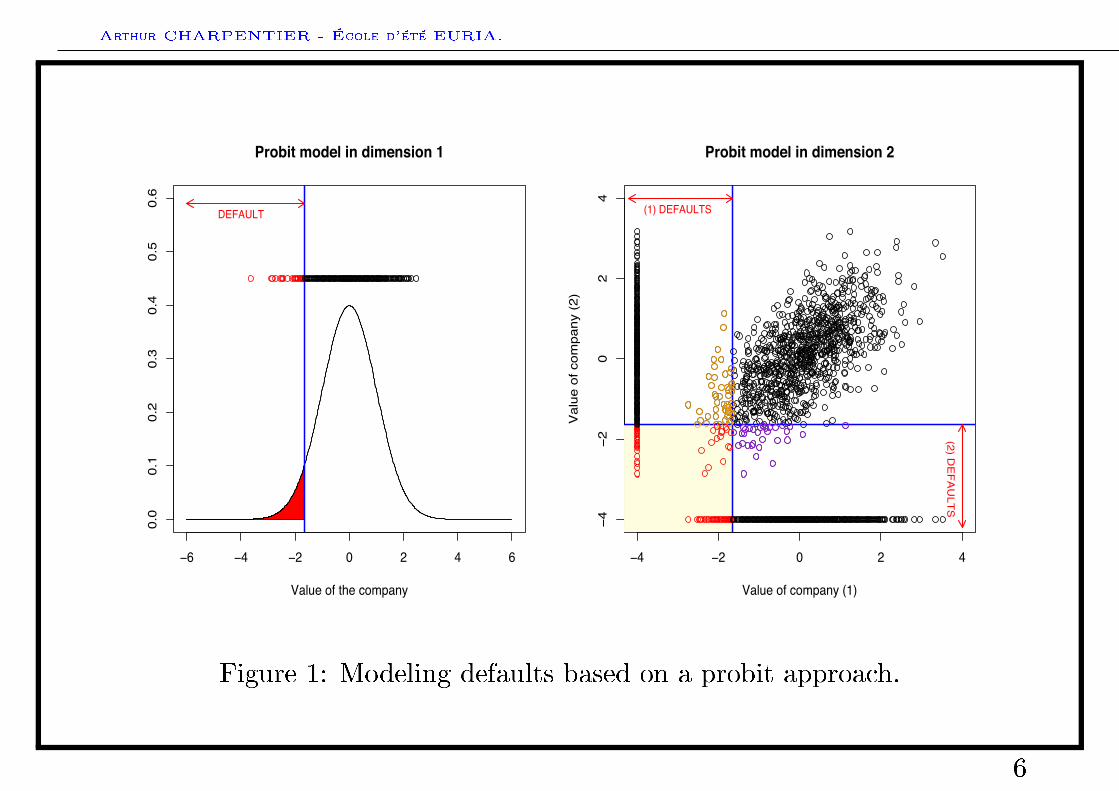
Applications with a high number of risks can also be considered, in credit risk forinstance. Let X = (X1, ..., Xd) denote the vector of indicator variables,indicating if the i-th contract defaulted during a given period of time. If a creditderivative is based on the occurrence of k defaults among d companies, and thus,the pricing is related to the distribution of the number of defaults, N , dened asN = X1 + ...+Xd. Under the assumption of possible contagious risks, thedistribution of N should integrate dependencies.
CreditMetrics in 1995 suggested a Gaussian model for credit changes, based on aprobit approach, Xi = 1(X∗i < ui), where X∗i ∼ N (0, 1).
5
Arthur CHARPENTIER - École d'été EURIA.
!6 !4 !2 0 2 4 6
0.0
0.1
0.2
0.3
0.4
0.5
0.6
Value of the company
Probit model in dimension 1
DEFAULT
!4 !2 0 2 4
!4!2
02
4Value of company (1)
Val
ue o
f com
pany
(2)
(1) DEFAULTS
(2) DE
FA
ULT
SProbit model in dimension 2
Figure 1: Modeling defaults based on a probit approach.
6
Arthur CHARPENTIER - École d'été EURIA.
Some possible motivations... in risk management
Consider a set a risks X = (X1, ..., Xd) (returns in a portfolio, losses per line ofbusiness, positions of nancial desks)
A classical risk measure (as in Markowitz (1959)) is the standard deviation,
σ(Xi) =√V ar(Xi) =
√E((Xi − E(X))2). The risk of the portfolio
S = X1 + . . .+Xd is
σ(S) =√σ(X1)2 + . . .+ σ(Xd)2 + 2
∑i<j
r(Xi, Xj)σ(Xi)σ(Xj).
Risks are now measured using Value-at-Risk (i.e. quantiles), and there is norelationship between q(X1 + . . .+Xd) and q(X1) + . . .+ q(Xd).
7
Arthur CHARPENTIER - École d'été EURIA.
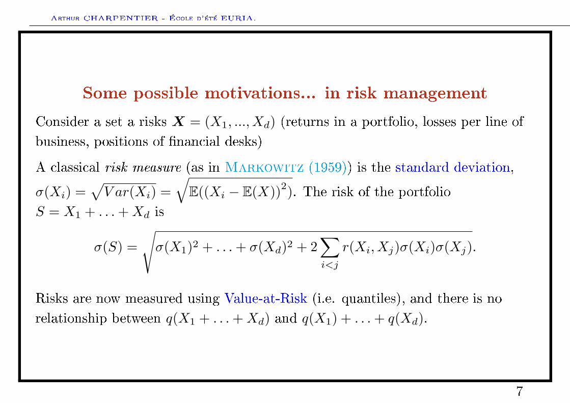
The Dow Jones index, 1896−1935
1900 1910 1920 1930
−0.10
−0.05
0.00
0.05
0.10
0.15
5010
015
020
025
030
035
0
Daily
log re
turn
Leve
l of th
e Dow
Jone
s inde
x
Figure 2: Measuring risks of nancial assets, Dow Jones (1895-1935).
8
Arthur CHARPENTIER - École d'été EURIA.
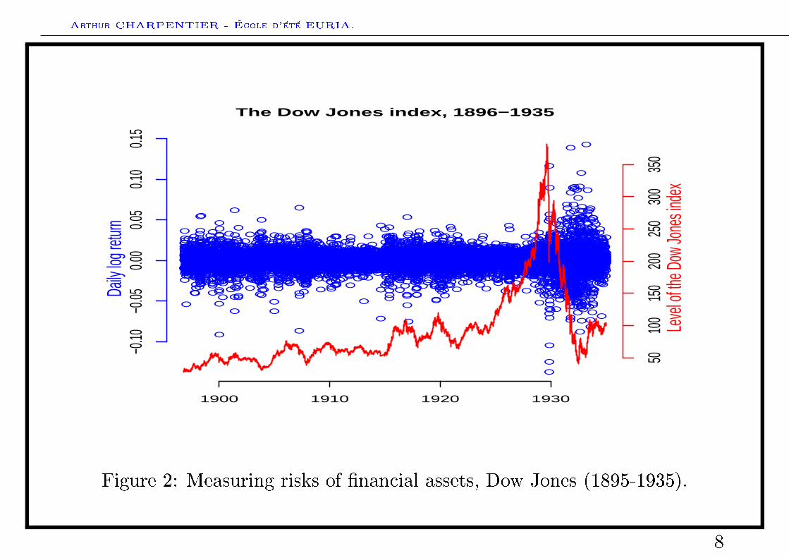
The Nasdaq index, 1971−2007
1970 1980 1990 2000
−0.10
−0.05
0.00
0.05
0.10
010
0020
0030
0040
0050
00
Daily
log re
turn
Leve
l of th
e Nas
daq i
ndex
Figure 3: Measuring risks of nancial assets, Nasdaq (1971-2007).
9
Arthur CHARPENTIER - École d'été EURIA.
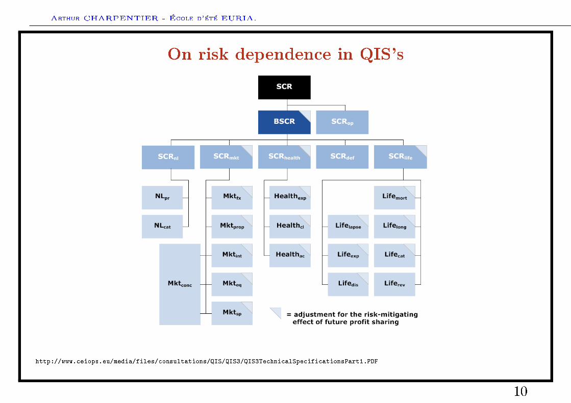
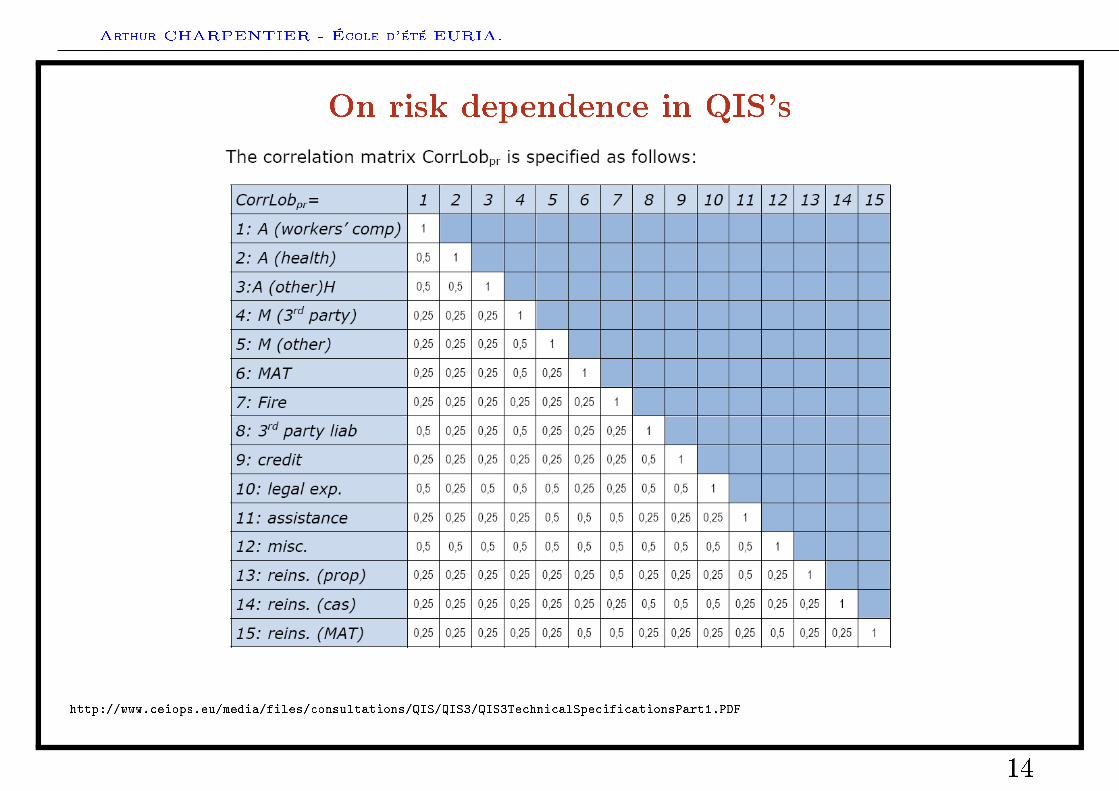
On risk dependence in QIS's
http://www.ceiops.eu/media/files/consultations/QIS/QIS3/QIS3TechnicalSpecificationsPart1.PDF
10
Arthur CHARPENTIER - École d'été EURIA.
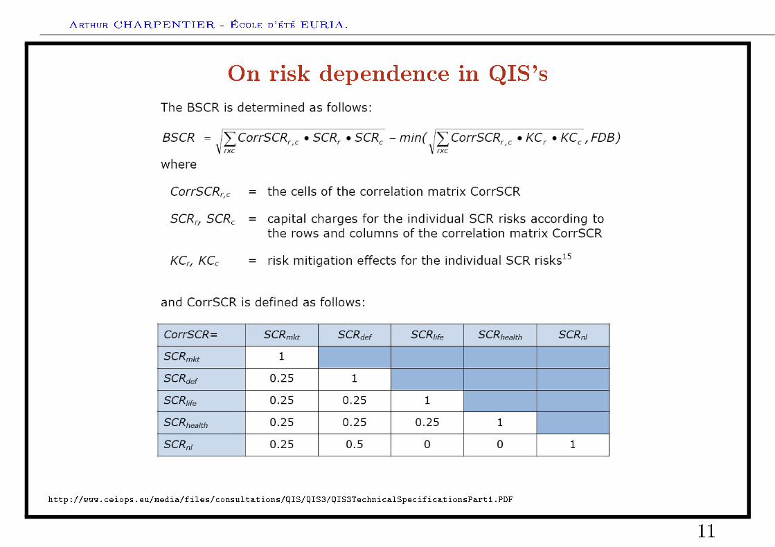
On risk dependence in QIS's
http://www.ceiops.eu/media/files/consultations/QIS/QIS3/QIS3TechnicalSpecificationsPart1.PDF
11
Arthur CHARPENTIER - École d'été EURIA.
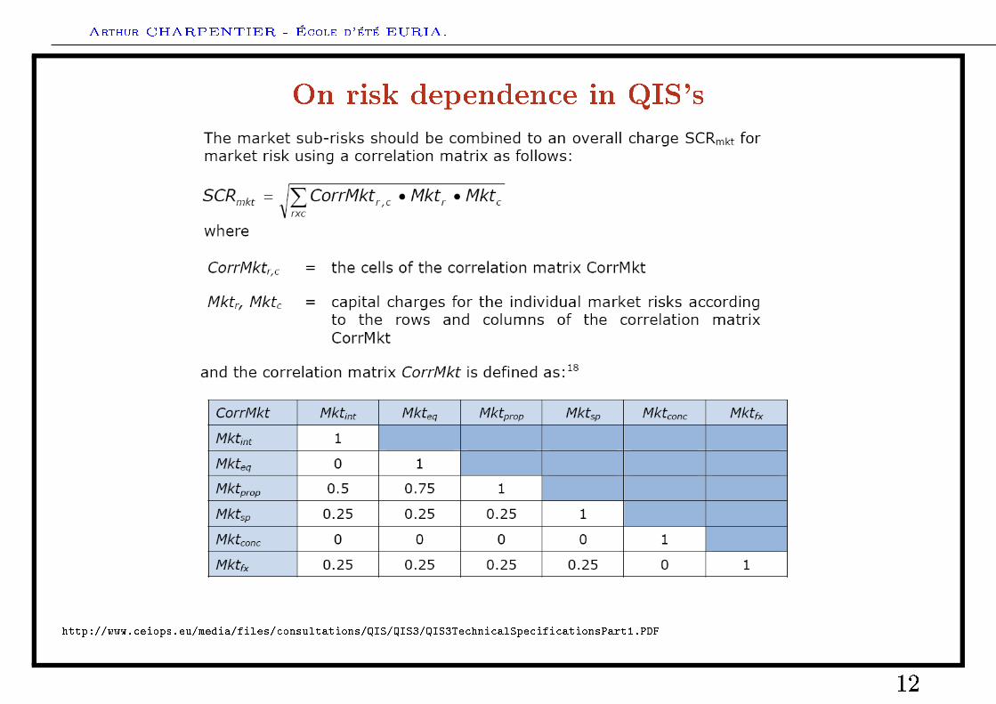
On risk dependence in QIS's
http://www.ceiops.eu/media/files/consultations/QIS/QIS3/QIS3TechnicalSpecificationsPart1.PDF
12
Arthur CHARPENTIER - École d'été EURIA.
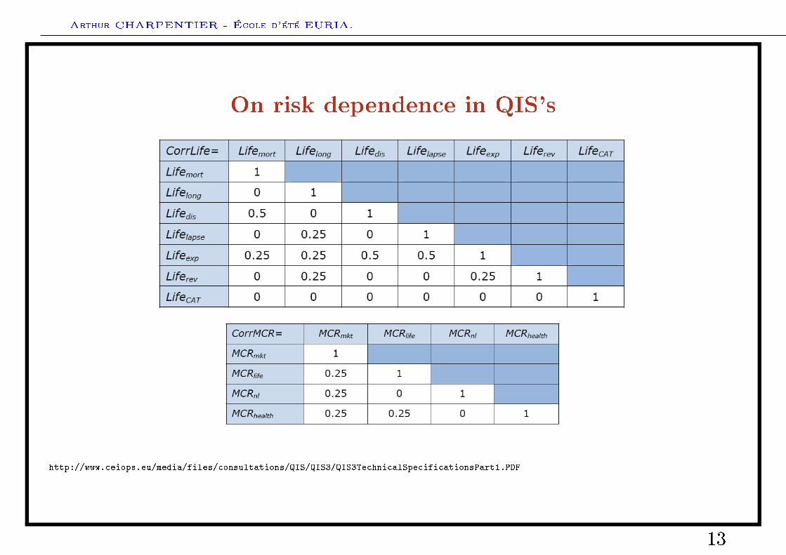
On risk dependence in QIS's
http://www.ceiops.eu/media/files/consultations/QIS/QIS3/QIS3TechnicalSpecificationsPart1.PDF
13
Arthur CHARPENTIER - École d'été EURIA.
On risk dependence in QIS's
http://www.ceiops.eu/media/files/consultations/QIS/QIS3/QIS3TechnicalSpecificationsPart1.PDF
14
Arthur CHARPENTIER - École d'été EURIA.
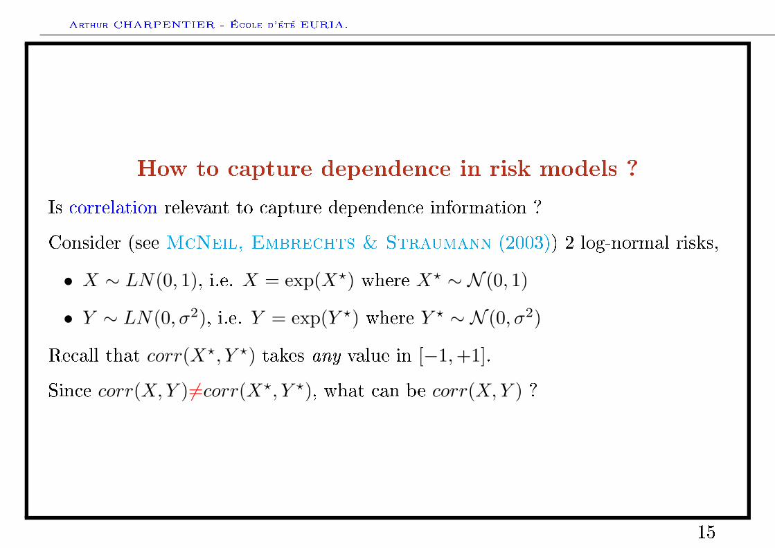
How to capture dependence in risk models ?
Is correlation relevant to capture dependence information ?
Consider (see McNeil, Embrechts & Straumann (2003)) 2 log-normal risks,
• X ∼ LN(0, 1), i.e. X = exp(X?) where X? ∼ N (0, 1)
• Y ∼ LN(0, σ2), i.e. Y = exp(Y ?) where Y ? ∼ N (0, σ2)
Recall that corr(X?, Y ?) takes any value in [−1,+1].
Since corr(X,Y )6=corr(X?, Y ?), what can be corr(X,Y ) ?
15
Arthur CHARPENTIER - École d'été EURIA.
How to capture dependence in risk models ?
0 1 2 3 4 5
−0
.50
.00
.51
.0
Standard deviation, sigma
Co
rre
latio
n
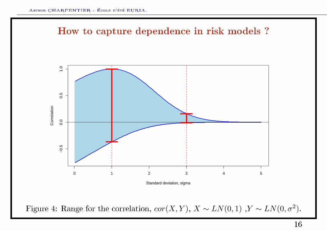
Figure 4: Range for the correlation, cor(X,Y ), X ∼ LN(0, 1) ,Y ∼ LN(0, σ2).
16
Arthur CHARPENTIER - École d'été EURIA.
How to capture dependence in risk models ?
0 1 2 3 4 5
−0
.50
.00
.51
.0
Standard deviation, sigma
Co
rre
latio
n
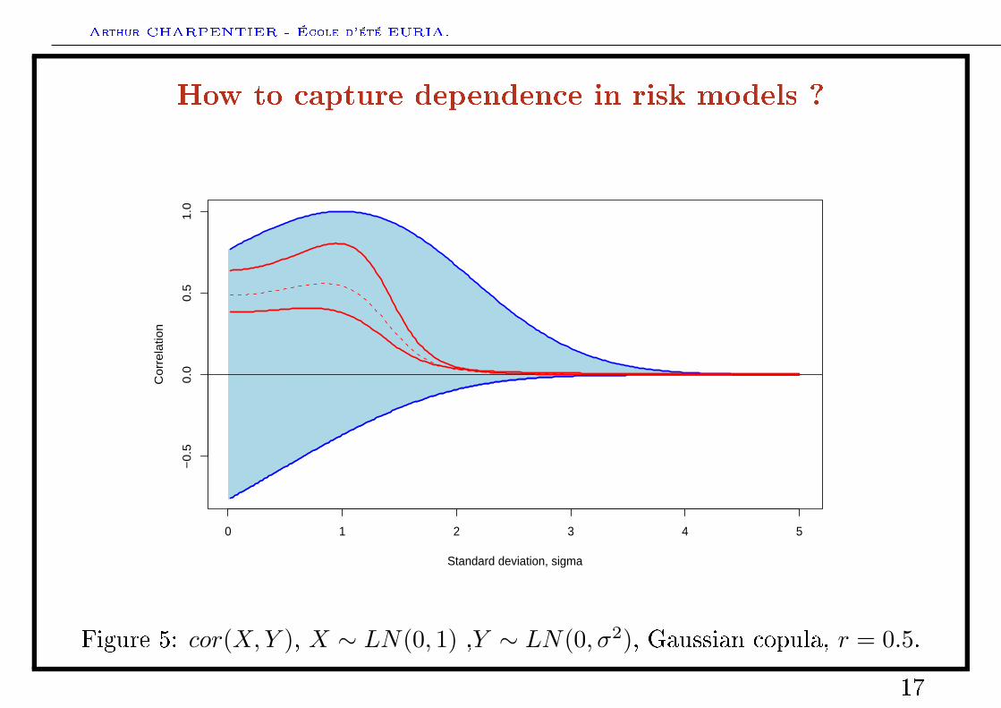
Figure 5: cor(X,Y ), X ∼ LN(0, 1) ,Y ∼ LN(0, σ2), Gaussian copula, r = 0.5.
17

Arthur CHARPENTIER - École d'été EURIA.
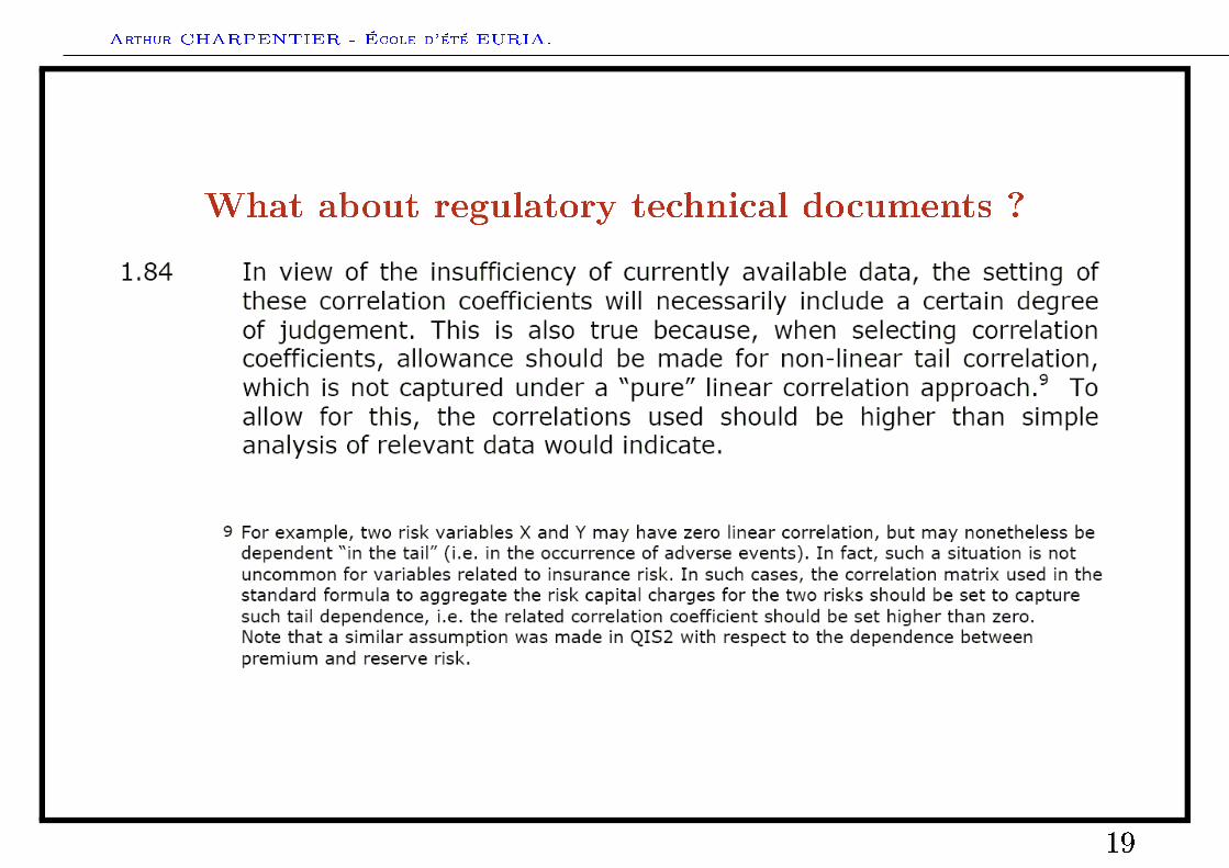
What about regulatory technical documents ?
18
Arthur CHARPENTIER - École d'été EURIA.
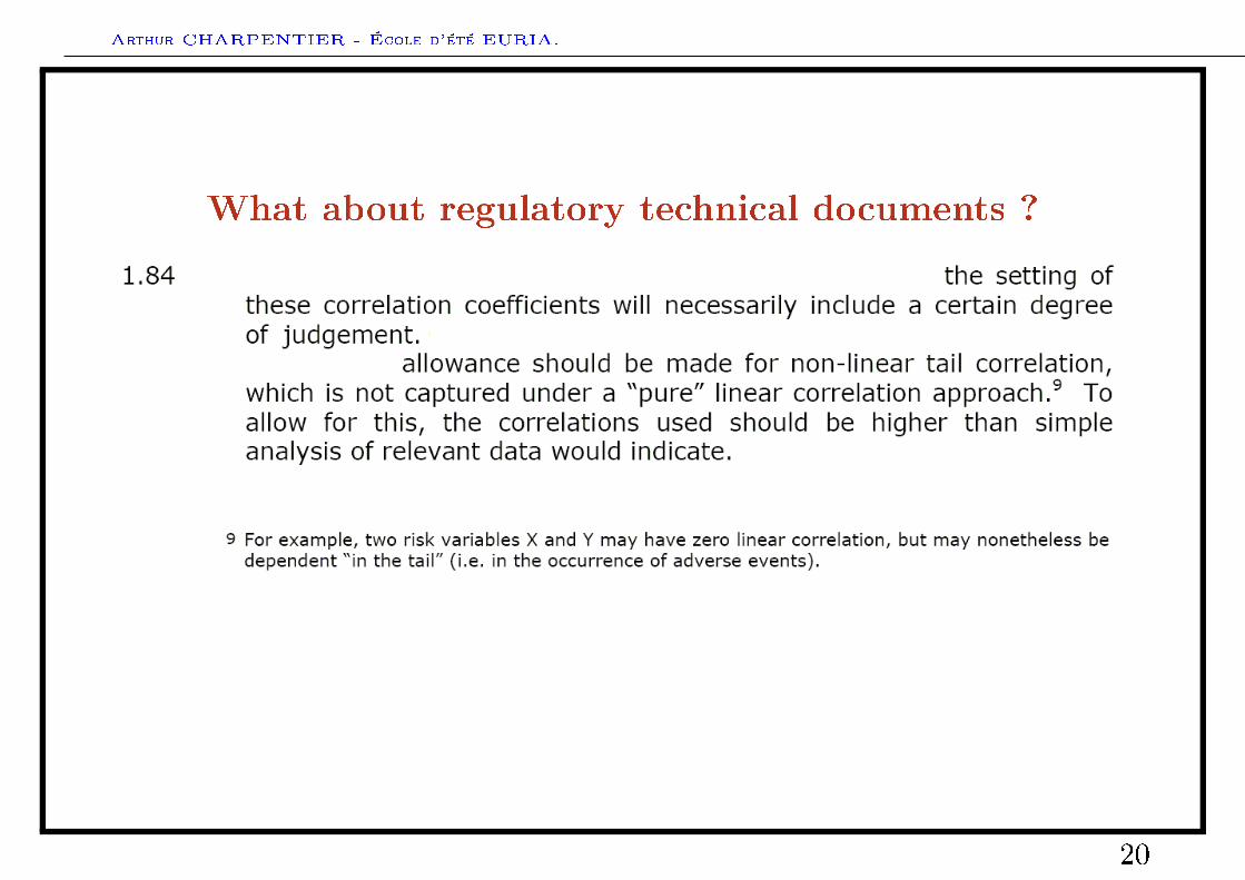
What about regulatory technical documents ?
19
Arthur CHARPENTIER - École d'été EURIA.
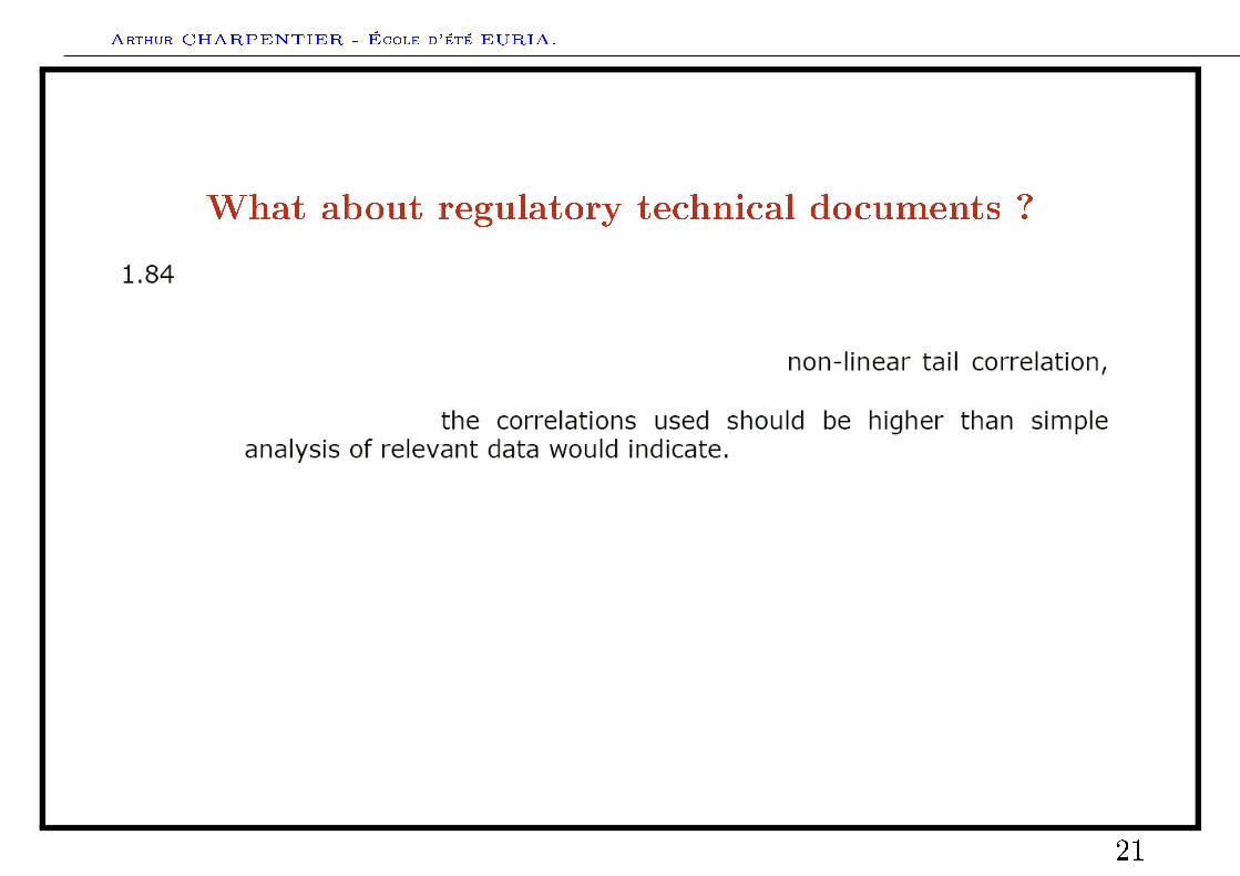
What about regulatory technical documents ?
20
Arthur CHARPENTIER - École d'été EURIA.
What about regulatory technical documents ?
21
Arthur CHARPENTIER - École d'été EURIA.
Agenda
• General introduction
Financial risks
• Market risks
• Credit risk
• Operational risk
Risk measures and capital allocation
• Risk measures: an axiomatic introduction
• Risk measures: convexity and coherence
• Capital allocation: an axiomatic introduction
Risk measures and statistical inference
22
Arthur CHARPENTIER - École d'été EURIA.
Agenda
• General introduction
Financial risks
• Market risks
• Credit risk
• From variance to Value-at-Risk
Risk measures and capital allocation
• Risk measures: an axiomatic introduction
• Risk measures: convexity and coherence
• Capital allocation: an axiomatic introduction
Risk measures and statistical inference
23
Arthur CHARPENTIER - École d'été EURIA.
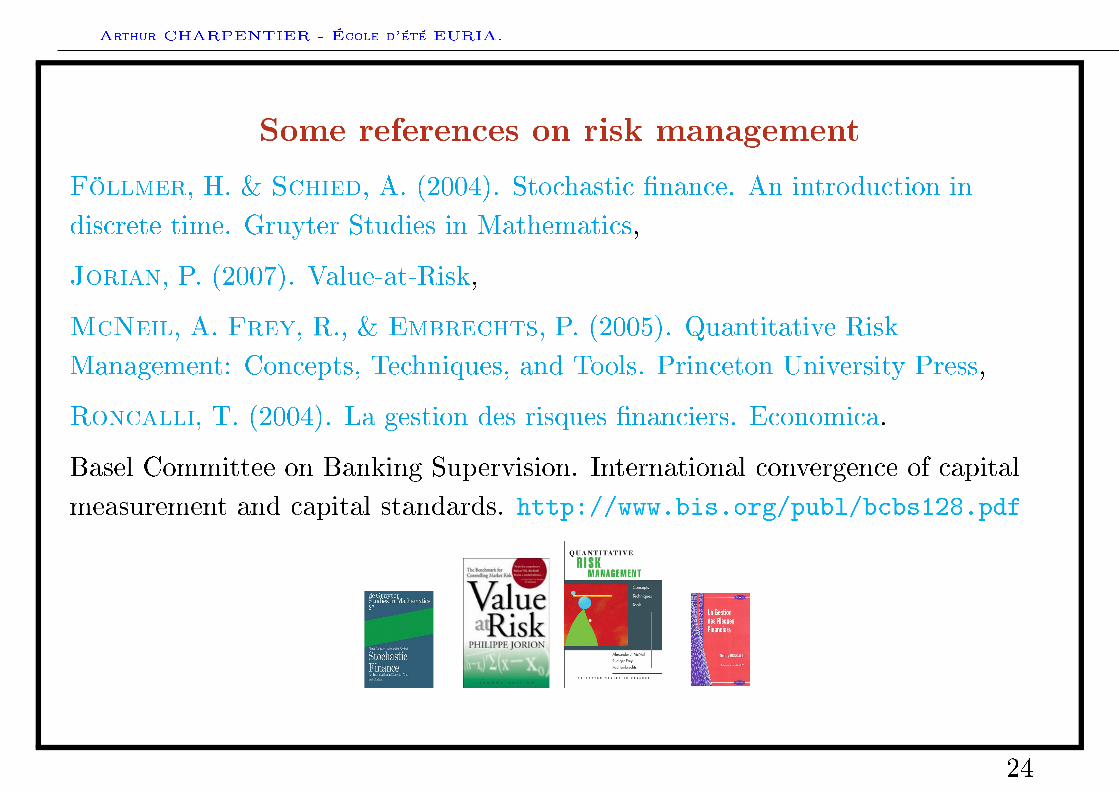
Some references on risk management
Föllmer, H. & Schied, A. (2004). Stochastic nance. An introduction indiscrete time. Gruyter Studies in Mathematics,
Jorian, P. (2007). Value-at-Risk,
McNeil, A. Frey, R., & Embrechts, P. (2005). Quantitative RiskManagement: Concepts, Techniques, and Tools. Princeton University Press,
Roncalli, T. (2004). La gestion des risques nanciers. Economica.
Basel Committee on Banking Supervision. International convergence of capitalmeasurement and capital standards. http://www.bis.org/publ/bcbs128.pdf
24
Arthur CHARPENTIER - École d'été EURIA.
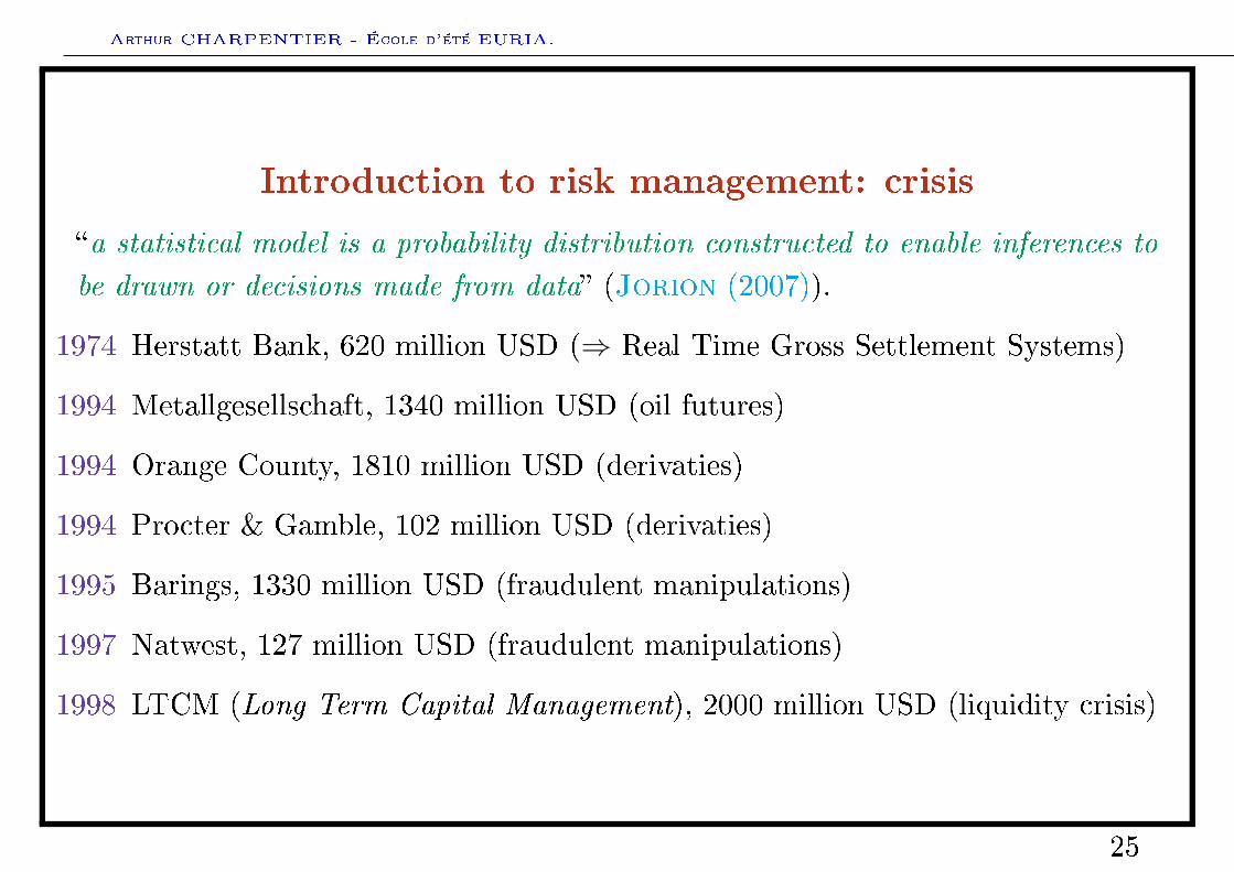
Introduction to risk management: crisis
a statistical model is a probability distribution constructed to enable inferences to
be drawn or decisions made from data (Jorion (2007)).
1974 Herstatt Bank, 620 million USD (⇒ Real Time Gross Settlement Systems)
1994 Metallgesellschaft, 1340 million USD (oil futures)
1994 Orange County, 1810 million USD (derivaties)
1994 Procter & Gamble, 102 million USD (derivaties)
1995 Barings, 1330 million USD (fraudulent manipulations)
1997 Natwest, 127 million USD (fraudulent manipulations)
1998 LTCM (Long Term Capital Management), 2000 million USD (liquidity crisis)
25
Arthur CHARPENTIER - École d'été EURIA.
Distinguishing among risks
• market risk
• interest rate risk
• currency risk
• volatility risk
• credit risk
• default risk
• downgrading risk
• operational risk
• disaster risk
• fraud risk
• technologic risk
• litigation risk
• liquidity risk
• model risk
26
Arthur CHARPENTIER - École d'été EURIA.
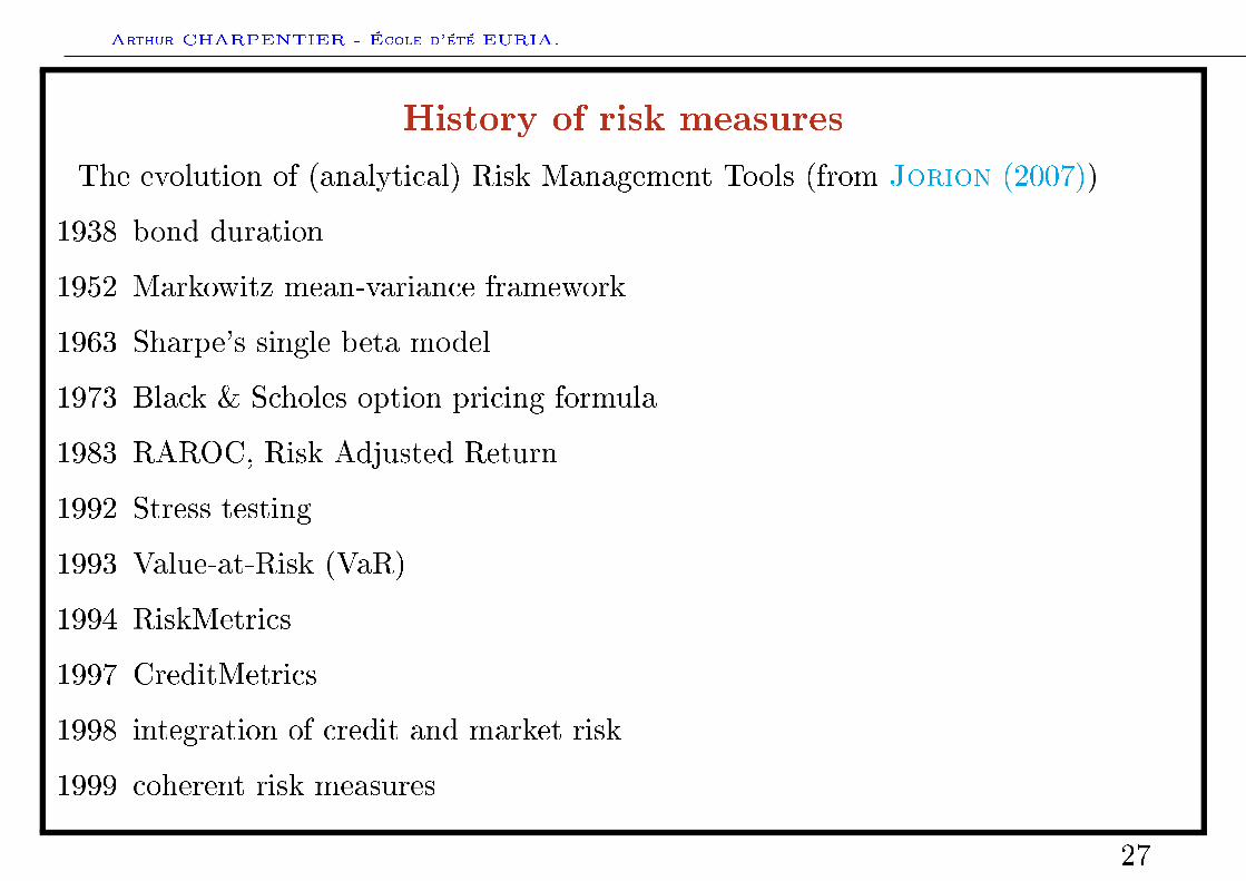
History of risk measures
The evolution of (analytical) Risk Management Tools (from Jorion (2007))
1938 bond duration
1952 Markowitz mean-variance framework
1963 Sharpe's single beta model
1973 Black & Scholes option pricing formula
1983 RAROC, Risk Adjusted Return
1992 Stress testing
1993 Value-at-Risk (VaR)
1994 RiskMetrics
1997 CreditMetrics
1998 integration of credit and market risk
1999 coherent risk measures
27
Arthur CHARPENTIER - École d'été EURIA.
Agenda
• General introduction
Financial risks
• Market risks
• Credit risk
• From variance to Value-at-Risk
Risk measures and capital allocation
• Risk measures: an axiomatic introduction
• Risk measures: convexity and coherence
• Capital allocation: an axiomatic introduction
Risk measures and statistical inference
28
Arthur CHARPENTIER - École d'été EURIA.
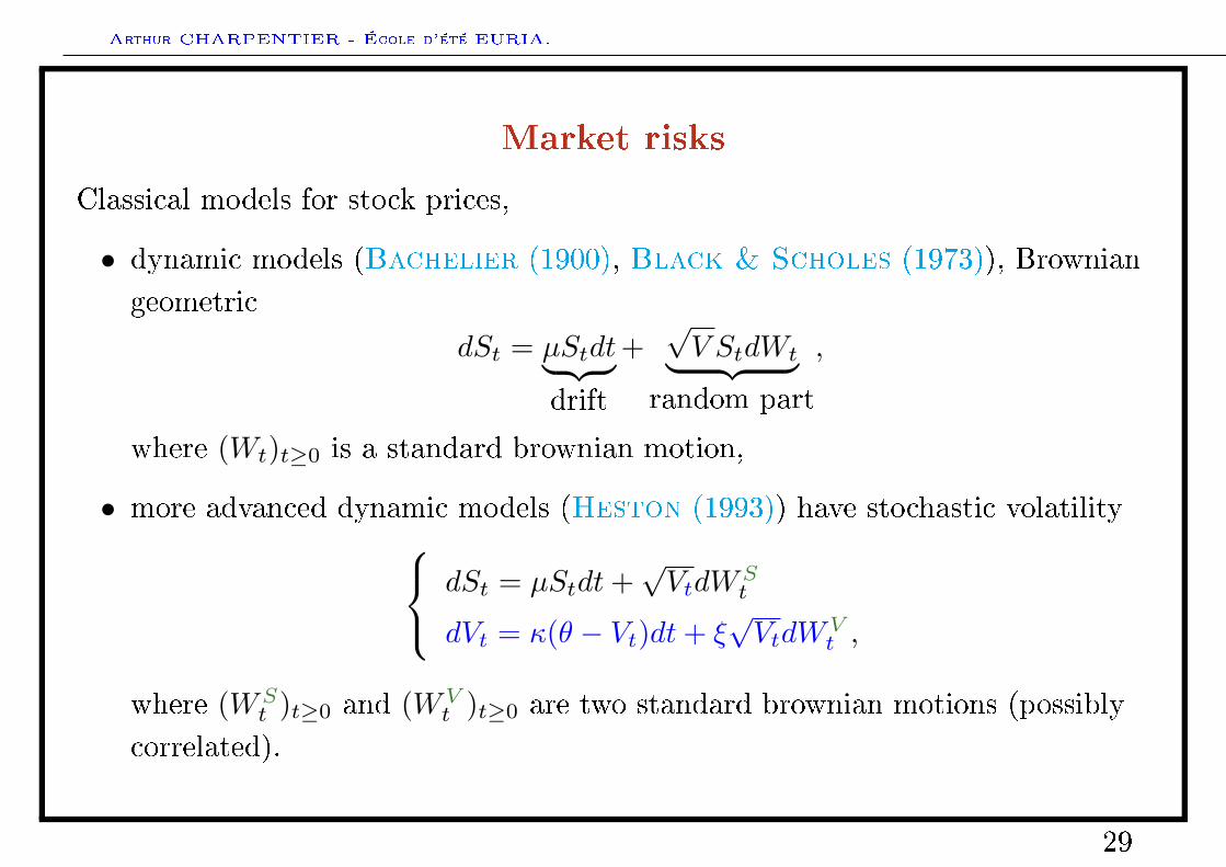
Market risks
Classical models for stock prices,
• dynamic models (Bachelier (1900), Black & Scholes (1973)), Browniangeometric
dSt = µStdt︸ ︷︷ ︸drift
+√V StdWt︸ ︷︷ ︸
random part
,
where (Wt)t≥0 is a standard brownian motion,
• more advanced dynamic models (Heston (1993)) have stochastic volatility dSt = µStdt+√VtdW
St
dVt = κ(θ − Vt)dt+ ξ√VtdW
Vt ,
where (WSt )t≥0 and (WV
t )t≥0 are two standard brownian motions (possiblycorrelated).
29
Arthur CHARPENTIER - École d'été EURIA.
0.0 0.2 0.4 0.6 0.8 1.0
5010
015
020
0Stock price over 1 year, large volatility
Time
0.0 0.2 0.4 0.6 0.8 1.0
5010
015
020
0
Stock price over 1 year, large volatility
Time
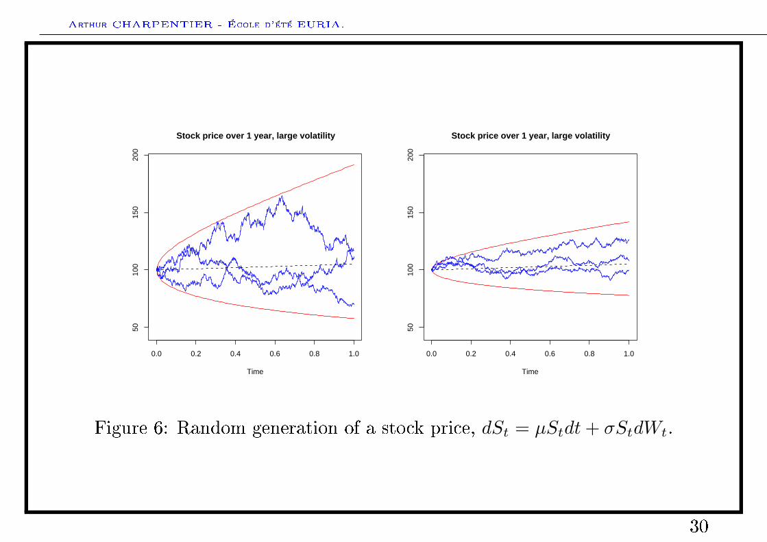
Figure 6: Random generation of a stock price, dSt = µStdt+ σStdWt.
30
Arthur CHARPENTIER - École d'été EURIA.
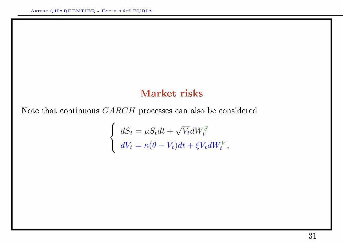
Market risks
Note that continuous GARCH processes can also be considered dSt = µStdt+√VtdW
St
dVt = κ(θ − Vt)dt+ ξVtdWVt ,
31
Arthur CHARPENTIER - École d'été EURIA.
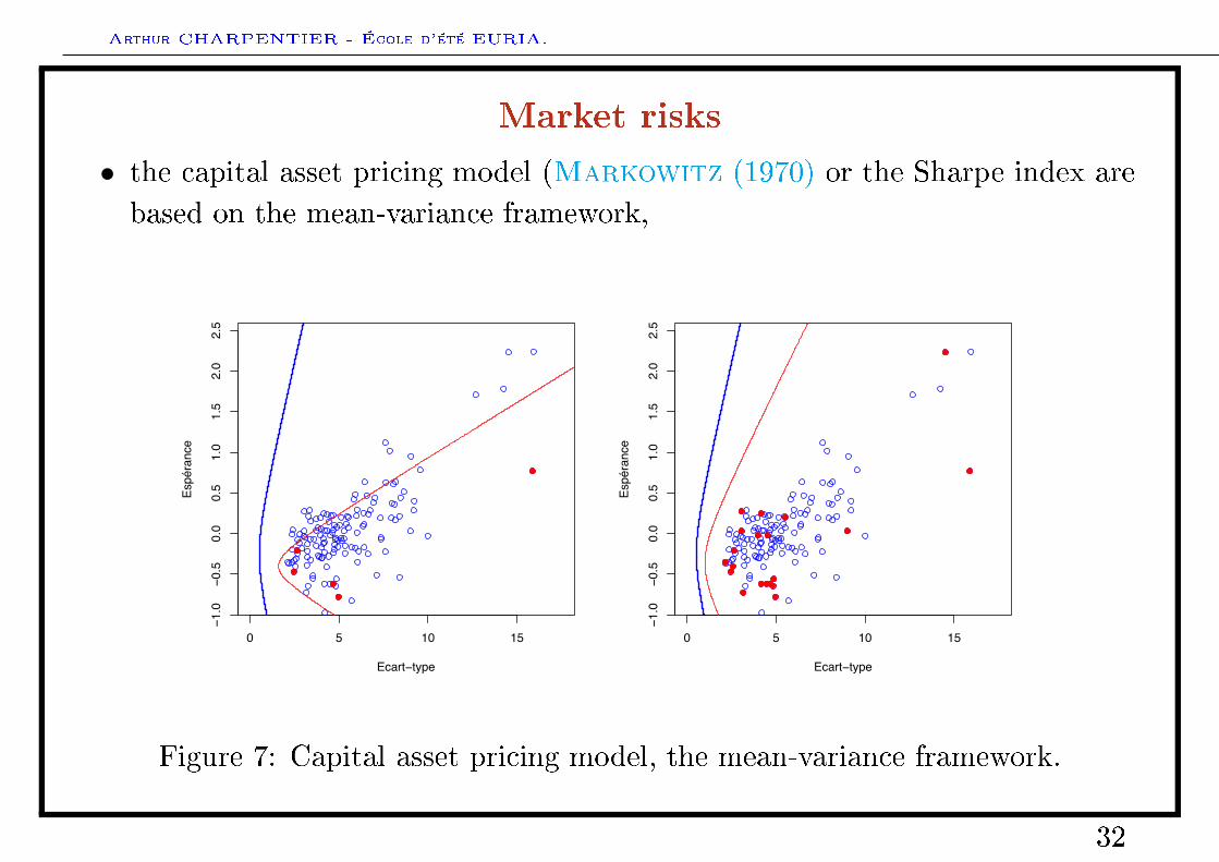
Market risks
• the capital asset pricing model (Markowitz (1970) or the Sharpe index arebased on the mean-variance framework,
0 5 #0 #5
!#.0
!0.5
0.0
0.5
#.0
#.5
%.0
%.5
&ca)t!type
&sp/)ance
0 " #0 #"!#.0
!0."
0.0
0."
#.0
#."
%.0
%."
&ca)t!t+pe
&sp/)ance
Figure 7: Capital asset pricing model, the mean-variance framework.
32
Arthur CHARPENTIER - École d'été EURIA.
How to quantify market risks : volatility
All the information about uncertainty is summarized by the volatiliy - orvariance - parameter.
Note that this is one of the drawback of the use of the Gaussian distribution.
33
Arthur CHARPENTIER - École d'été EURIA.
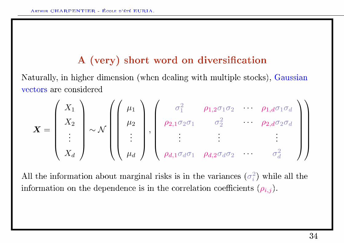
A (very) short word on diversication
Naturally, in higher dimension (when dealing with multiple stocks), Gaussianvectors are considered
X =
X1
X2
...
Xd
∼ N
µ1
µ2
...
µd
,
σ2
1 ρ1,2σ1σ2 · · · ρ1,dσ1σd
ρ2,1σ2σ1 σ22 · · · ρ2,dσ2σd
......
...
ρd,1σdσ1 ρd,2σdσ2 · · · σ2d
All the information about marginal risks is in the variances (σ2
i ) while all theinformation on the dependence is in the correlation coecients (ρi,j).
34
Arthur CHARPENTIER - École d'été EURIA.
On the Gaussian distribution
The Gaussian distribution is very important for many reasons,
• it is a stable distribution, i.e. it appears as a limiting distribution in thecentral limit theorem: for i.i.d. Xi's with nite variance,
√nX − E(X)√
V X
L→ N (0, 1).
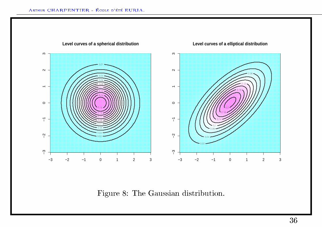
• it is an elliptic distribution, i.e. X = µ+AX0 where A′A = Σ, and whereX0 has a spheric distribution, i.e. f(x0) is a function of x′0x0 (spherical levelcurves),
35
Arthur CHARPENTIER - École d'été EURIA.
−3 −2 −1 0 1 2 3
−3
−2
−1
01
23
Level curves of a spherical distribution
−3 −2 −1 0 1 2 3
−3
−2
−1
01
23
Level curves of a elliptical distribution
Figure 8: The Gaussian distribution.
36
Arthur CHARPENTIER - École d'été EURIA.
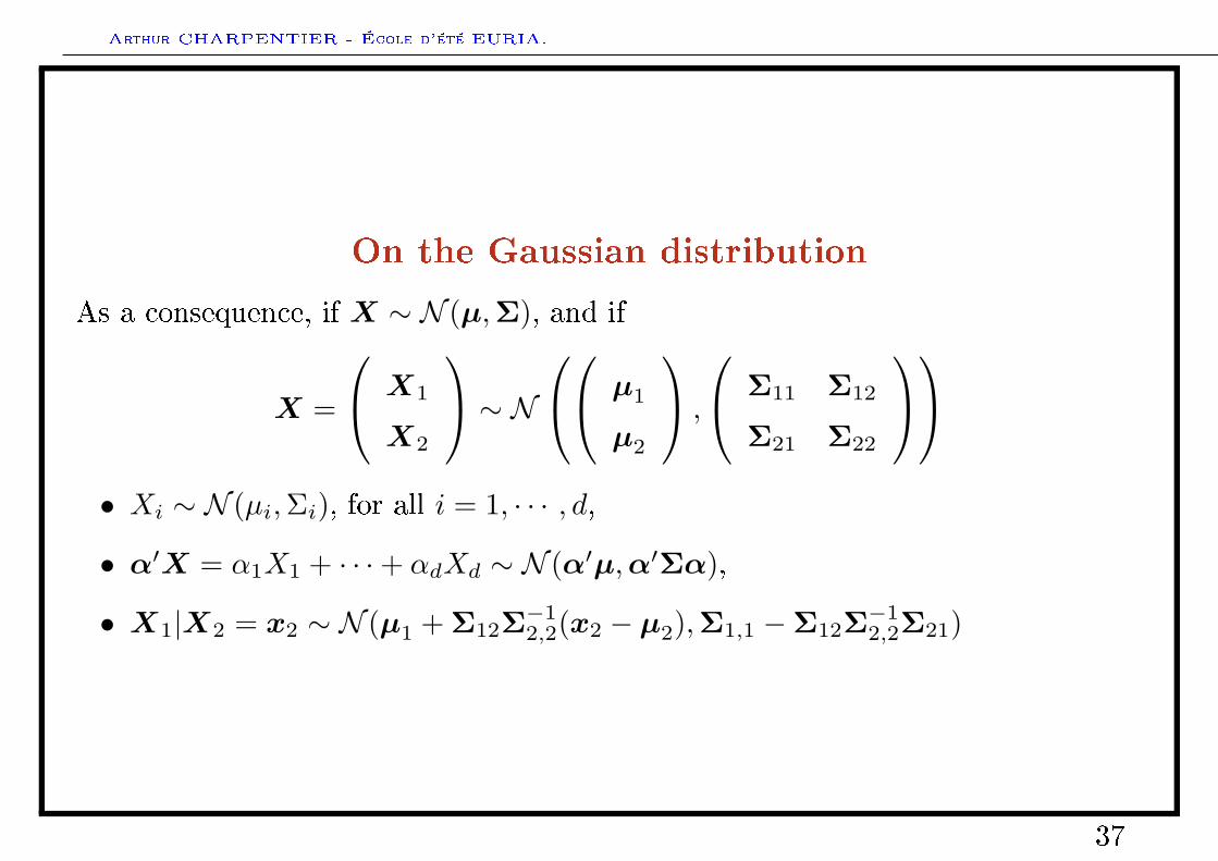
On the Gaussian distribution
As a consequence, if X ∼ N (µ,Σ), and if
X =
X1
X2
∼ N µ1
µ2
,
Σ11 Σ12
Σ21 Σ22
• Xi ∼ N (µi,Σi), for all i = 1, · · · , d,
• α′X = α1X1 + · · ·+ αdXd ∼ N (α′µ,α′Σα),
• X1|X2 = x2 ∼ N (µ1 + Σ12Σ−12,2(x2 − µ2),Σ1,1 −Σ12Σ−1
2,2Σ21)
37
Arthur CHARPENTIER - École d'été EURIA.
−3−2
−10
12
3
−3
−2
−1
0
1
23
0.00
0.05
0.10
0.15
0.20
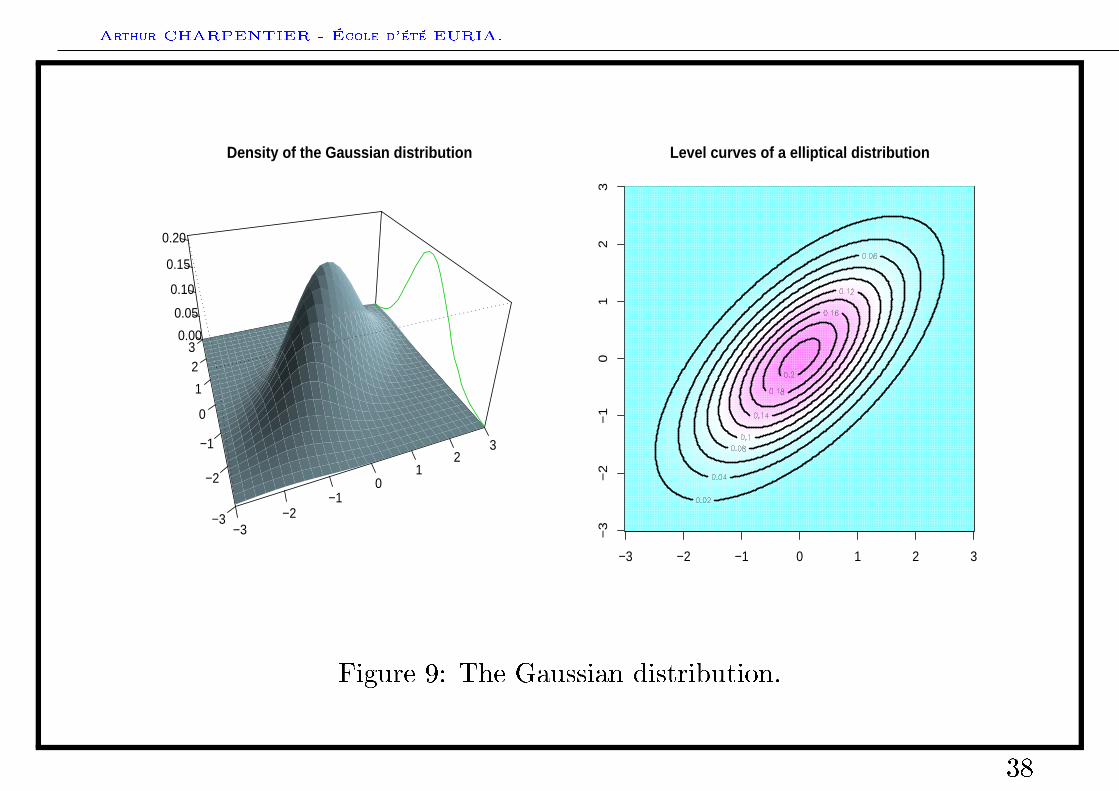
Density of the Gaussian distribution
−3 −2 −1 0 1 2 3
−3
−2
−1
01
23
Level curves of a elliptical distribution
Figure 9: The Gaussian distribution.
38
Arthur CHARPENTIER - École d'été EURIA.
Agenda
• General introduction
Financial risks
• Market risks
• Credit risk
• From variance to Value-at-Risk
Risk measures and capital allocation
• Risk measures: an axiomatic introduction
• Risk measures: convexity and coherence
• Capital allocation: an axiomatic introduction
Risk measures and statistical inference
39
Arthur CHARPENTIER - École d'été EURIA.
Credit risk
Credit risk is the risk that an obligor does not full his payment obligations,either wholly or in part.
For single obligors, one should model
• risk arrival (given a time horizon, it there a default ?)
• risk timing (when does the default occur ?)
• risk magnitude (how high is the loss ?)
and on a portfolio level
• risk correlation (will there be any contagion ?)
Here, loss distributions have low probabilities but high losses (high downside risk,strongly skewed).
Hence, for credit risk, volatiliy has no meaning.
Main problem: no much historical data.
40
Arthur CHARPENTIER - École d'été EURIA.
Classical credit risk models
• credit scoring, logit/probit models to model default occurence
• models for rating transition based on Markov chains
• models for bond prices, intensity based
41
Arthur CHARPENTIER - École d'été EURIA.
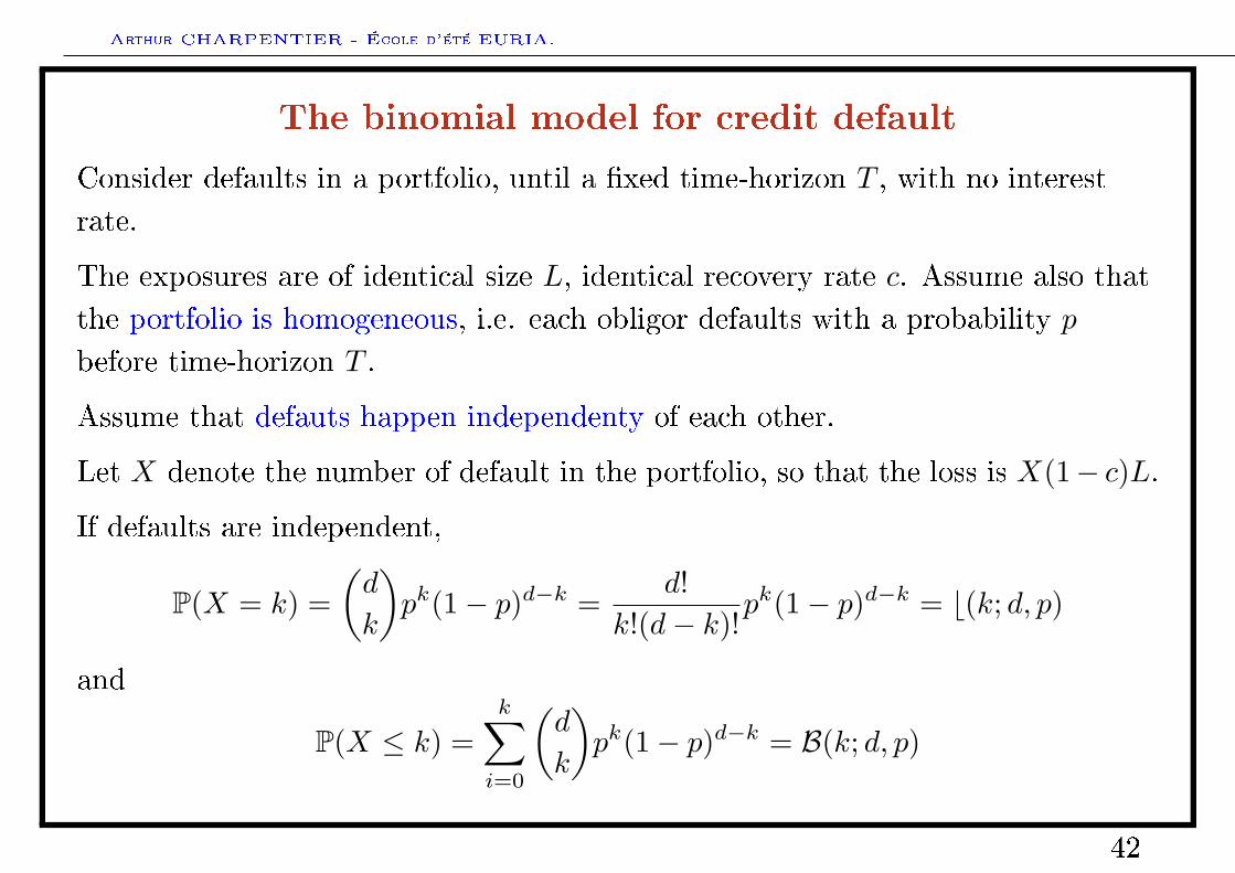
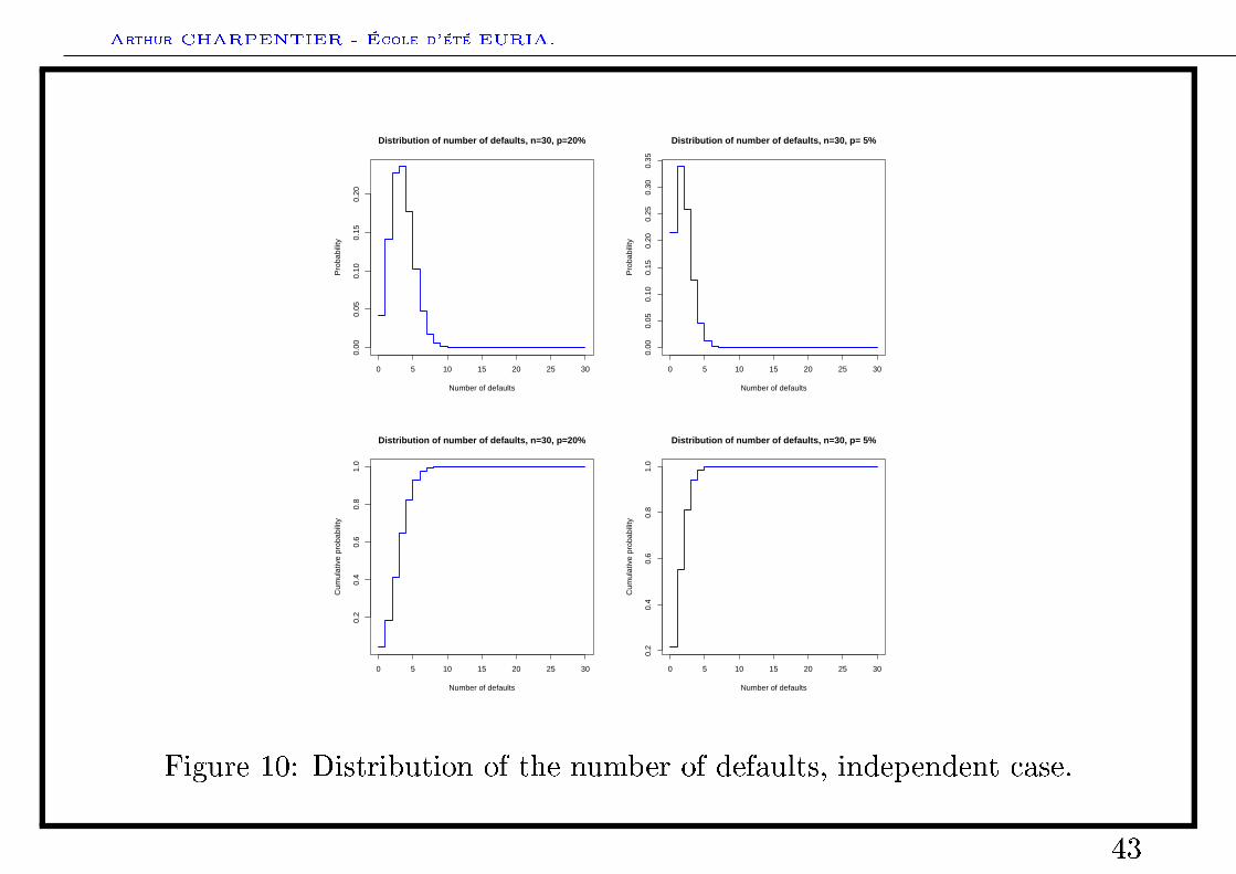
The binomial model for credit default
Consider defaults in a portfolio, until a xed time-horizon T , with no interestrate.
The exposures are of identical size L, identical recovery rate c. Assume also thatthe portfolio is homogeneous, i.e. each obligor defaults with a probability pbefore time-horizon T .
Assume that defauts happen independenty of each other.
Let X denote the number of default in the portfolio, so that the loss is X(1− c)L.
If defaults are independent,
P(X = k) =(d
k
)pk(1− p)d−k =
d!k!(d− k)!
pk(1− p)d−k = b(k; d, p)
and
P(X ≤ k) =k∑i=0
(d
k
)pk(1− p)d−k = B(k; d, p)
42
Arthur CHARPENTIER - École d'été EURIA.
0 5 10 15 20 25 30
0.00
0.05
0.10
0.15
0.20
Distribution of number of defaults, n=30, p=20%
Number of defaults
Pro
babi
lity
0 5 10 15 20 25 30
0.00
0.05
0.10
0.15
0.20
0.25
0.30
0.35
Distribution of number of defaults, n=30, p= 5%
Number of defaults
Pro
babi
lity
0 5 10 15 20 25 30
0.2
0.4
0.6
0.8
1.0
Distribution of number of defaults, n=30, p=20%
Number of defaults
Cum
ulat
ive
prob
abili
ty
0 5 10 15 20 25 30
0.2
0.4
0.6
0.8
1.0
Distribution of number of defaults, n=30, p= 5%
Number of defaults
Cum
ulat
ive
prob
abili
ty
Figure 10: Distribution of the number of defaults, independent case.
43
Arthur CHARPENTIER - École d'été EURIA.
Extending the binomial model for credit default
A simplied rm's value model can be considered, where the default of eachobligor k is triggered by the change of the value Vk(t) of the assets of its rm.
Assume that Vk(T ) is normally distributed, and standardized, i.e.Vk(T ) ∼ N (0, 1). Assume more generally thatV (T ) = (V1(T ), · · · , Vd(T )) ∼ N (0,Σ), i.e. the asset values of dierent obligorsmight be correleted with each other.
Obligor k defaults if its rm's value falls below a barrier Vk(T ) ≤ Bk.
This can be seen as a multivariate probit model.
44
Arthur CHARPENTIER - École d'été EURIA.
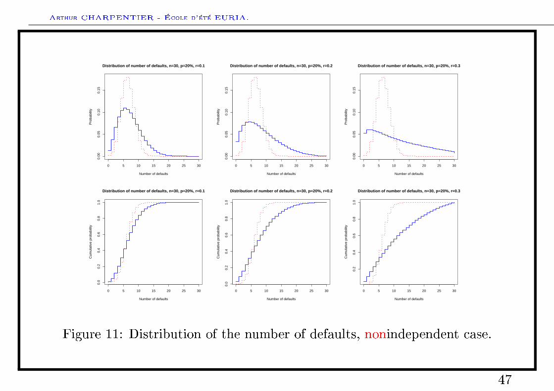
A one-factor model for credit default
Assume that the values of the assets of the obligors are driven by one commonfactor Y , and an idiosyncratic standard normal noise component εk, so that
Vk(T ) =√ρY +
√1− ρεk, k = 1, · · · , d,
where Y and the εk's are independent and N (0, 1) distributed.
This is an exchangeable model: conditional on the realisation of the systematicfactor Y , the rm's values and the defaults rae independent.
Assuming that Bk = B and that the exposure is Lk = 1, then
P(X = k) =∫
P(X = k|Y = y)φ(y)dy,
and conditional on Y = y, the probability to have k defaults is
P(X = k|Y = y) =(d
k
)p(y)k(1− p(y))d−k
45
Arthur CHARPENTIER - École d'été EURIA.
A one-factor model for credit default
where p(y) is the probability that Vi(T ) falls below B, i.e.
p(y) = P(Vi(T ) ≤ B|Y = y) = P
(εi ≤
B −√Y√
1− ρ≤ B
∣∣∣∣∣Y = y
)= Φ
(K −√ρy√
1− ρ
).
Substituting yields
P(X = k) =∫ (
d
k
)[Φ(K −√ρy√
1− ρ
)]k [1− Φ
(K −√ρy√
1− ρ
)]d−kφ(y)dy
46
Arthur CHARPENTIER - École d'été EURIA.
0 5 10 15 20 25 30
0.00
0.05
0.10
0.15
Distribution of number of defaults, n=30, p=20%, r=0.1
Number of defaults
Pro
babi
lity
0 5 10 15 20 25 30
0.00
0.05
0.10
0.15
Distribution of number of defaults, n=30, p=20%, r=0.2
Number of defaults
Pro
babi
lity
0 5 10 15 20 25 30
0.00
0.05
0.10
0.15
Distribution of number of defaults, n=30, p=20%, r=0.3
Number of defaults
Pro
babi
lity
0 5 10 15 20 25 30
0.0
0.2
0.4
0.6
0.8
1.0
Distribution of number of defaults, n=30, p=20%, r=0.1
Number of defaults
Cum
ulat
ive
prob
abili
ty
0 5 10 15 20 25 30
0.0
0.2
0.4
0.6
0.8
1.0
Distribution of number of defaults, n=30, p=20%, r=0.2
Number of defaults
Cum
ulat
ive
prob
abili
ty
0 5 10 15 20 25 30
0.2
0.4
0.6
0.8
1.0
Distribution of number of defaults, n=30, p=20%, r=0.3
Number of defaults
Cum
ulat
ive
prob
abili
ty
Figure 11: Distribution of the number of defaults, nonindependent case.
47
Arthur CHARPENTIER - École d'été EURIA.
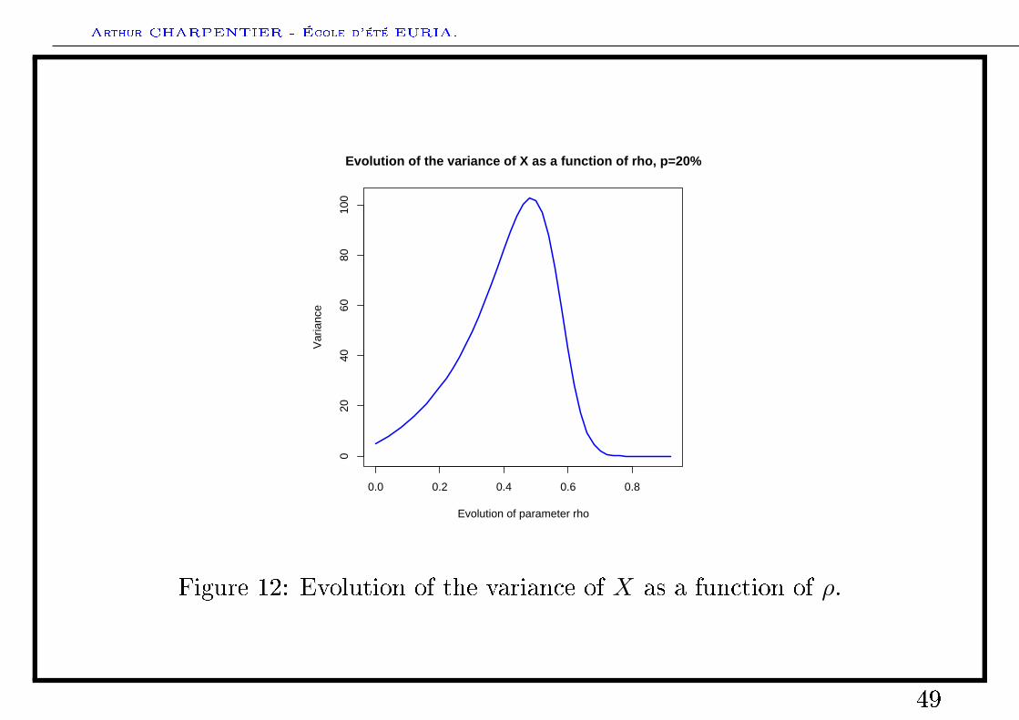
Using variance for credit risk ?
Is variance relevant to measure risk ?
No since it is not a downside risk.
48
Arthur CHARPENTIER - École d'été EURIA.
0.0 0.2 0.4 0.6 0.8
020
4060
8010
0
Evolution of the variance of X as a function of rho, p=20%
Evolution of parameter rho
Var
ianc
e
Figure 12: Evolution of the variance of X as a function of ρ.
49
Arthur CHARPENTIER - École d'été EURIA.
Using variance for credit risk ?
One has to nd a coecient which measures properly downside risk. An idea isto use a quantile
Denition 1. The α-quantile of a distribution FX is qX(α), such that
qX(α) = F−1X (α) where
F−1X (u) = infx, FX(x) ≥ u, where u ∈ (0, 1).
Then F−1X (·) is increasing on (0, 1), continuous from the left, with limits from the
right, and further
F−1X FX(x) ≤ x for any x and FX F−1
X (u) ≥ u for any p.
Remark Almost equivalently, it is possible to dene
F−1X (u) = supx, FX(x) ≤ u, where u ∈ (0, 1).
50
Arthur CHARPENTIER - École d'été EURIA.
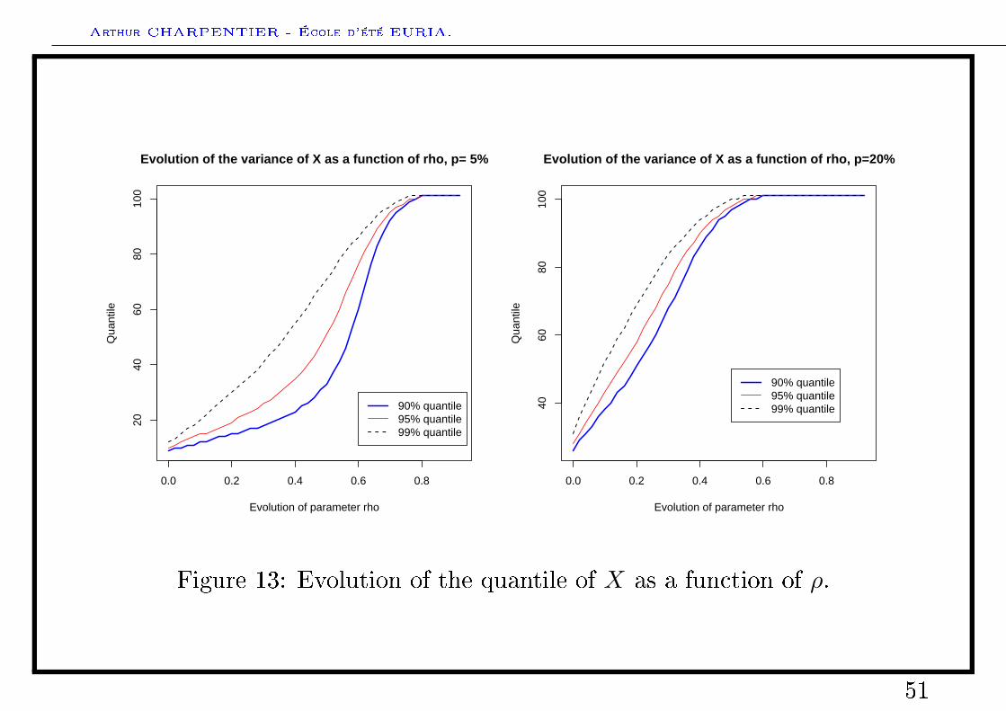
0.0 0.2 0.4 0.6 0.8
2040
6080
100
Evolution of the variance of X as a function of rho, p= 5%
Evolution of parameter rho
Qua
ntile
90% quantile95% quantile99% quantile
0.0 0.2 0.4 0.6 0.8
4060
8010
0
Evolution of the variance of X as a function of rho, p=20%
Evolution of parameter rhoQ
uant
ile
90% quantile95% quantile99% quantile
Figure 13: Evolution of the quantile of X as a function of ρ.
51
Arthur CHARPENTIER - École d'été EURIA.
Agenda
• General introduction
Financial risks
• Market risks
• Credit risk
• From variance to Value-at-Risk
Risk measures and capital allocation
• Risk measures: an axiomatic introduction
• Risk measures: convexity and coherence
• Capital allocation: an axiomatic introduction
Risk measures and statistical inference
52
Arthur CHARPENTIER - École d'été EURIA.
Value-at-Risk
The expression is quite recent and its origin is uncertain: in the 80's, somepapers introduced dollars-at-risk, capital-at-risk, income-at-risk, earning-at-riskand nally value-at-risk
Denomination has been stabilized after the publication of RiskMetrics Technical
Document in 1994, by JPMorgan. Note that the work accomplished byJPMorgan was more a pulic relation campaign than an advanced technical study:VaR is more a practice than a theory.
VaR summarizes the worst loss ever on a target horizon that will not be exceeded
with a given level of condence, i.e. formaly it is a quantile of the projecteddistibution of gains and losses over the target horizon
Till Guldimann (1992) created the term value-at-risk while head of globalresearch at JP Morgan in the late 80's. It appeared in the G30 report (group of
thirty) in July 1993.
53
Arthur CHARPENTIER - École d'été EURIA.
A technical denition for the Value-at-Risk
Denition 2. Let X denote the loss distribution, then
V aR(X,α) = qX(α), for all α ∈ (0, 1).
54
Arthur CHARPENTIER - École d'été EURIA.
The Basel II accord (2004)
June 2004, the Basel Committee nalized the Basel Accords, based on threepillars
• minimum regulatory requierements, i.e. some risk-based capital requirements:set capital charges against credit risk (internal rating based), market risk(internal model approach) and operational risk. the goal is to keep constantthe level of capital in the global banking syste: 8% of risk weighted assets,
• supervisorv review, i.e. expanded role for bank regulartors, to ensure thatbanks operate above the minimum regulatory capital ratios, that banks haveappropriate processes for assessing their risks, and appropriate correctiveactions
• market discipline, i.e. set of disclosure recommendations, encouraging topublish informations about exposures, risk proles, capital cushion...
From the rst pillar, there should be a credit risk charge (CRC), a market riskcharge (MRC) and an operationnal risk charge (ORC), and the bank's total
55
Arthur CHARPENTIER - École d'été EURIA.
capital must exceed the total-risk charge (TRC)
Capital > TRC = CRC + MRC + ORC.
Why using VaR as a risk measure ?
Markowitz (1952) claimed that standard deviation should be an intuitive andappropriate risk measure (leading to the mean-variance trade-o).
The same year, Roy (1952) claimed that the optimal bundle of assets
(investment) for investors who employ the safety rst principle is the portfolio
that minimizes the probability of disaster.
Roy A. D. (1952), Safety rst and the holding of assets, Econometrica, 20,431-449.
Markowitz H. M. (1952), Portfolio selection, Journal of Finance, 7, 77-91.
56
Arthur CHARPENTIER - École d'été EURIA.
Agenda
• General introduction
Financial risks
• Market risks
• Credit risk
• From variance to Value-at-Risk
Risk measures and capital allocation
• Risk measures: an axiomatic introduction
• Risk measures: convexity and coherence
• Capital allocation: an axiomatic introduction
Risk measures and statistical inference
57
Arthur CHARPENTIER - École d'été EURIA.
Introduction the risk measures, and risk perception
S. Clam [...] once said: I dene a coward as someone who will not bet whenyou oer him two-to-one odds and let him choose his side .
With the centuries old St. Petersburg paradox in my mind, I pedantically
corrected him: You mean will not make a suciently small bet (so that thechange in the marginal utility of money will not contaminate his choice)..
Recalling this conversation, a few years ago I oered some lunch colleagues to
bet each $200 to $100 that the side of a coin they specied would not appear at
the rst tom. One distinguished scholar - who lays no claim to advanced
mathematical skills - gave the following answer:
58
Arthur CHARPENTIER - École d'été EURIA.
Introduction the risk measures, and risk perception
I won't bet because I would fell the $100 loss more than the $200 gain. ButI'll take you on if you promise to let me make 100 such bets .
What was behind this interesting answer ? He, and many others, have given
something liko tho following explanation. One toss is not enough to make itreasonably sure that the law of averages will turn out in my favor. But in ahundred tosses of a coin, the law of large numbers will make a dam good bet. Iam, so to speak, virtually sure to come out ahead in such a sequence, and that iswhy I accept the sequence while rejecting the single toss. .
One can check that P(gain > 0) = P(at least 34 odds) ∼ 99.91%.
However, with one toss, the maximal loss is $100 but it becomes $10,000 with100 tosses.
59
Arthur CHARPENTIER - École d'été EURIA.
Notations
Let X be a real valued random variable, interpreted as a (net) loss.
Denition 3. A risk measure is a function R : X → R, interpreted as the capital
necessary.
Example 4. R(X) = supX(ω), ω ∈ Ω, R(X) = supEQ(X),Q ∈ Q where Qis a set of probabilities (called scenarios), R(X) = F−1
X (α) where α ∈ (0, 1) ...etc.
60
Arthur CHARPENTIER - École d'été EURIA.
Risk measures and price of a risk
Pascal, Fermat, Condorcet, Huygens, dAlembert in the XVIIIth centuryproposed to evaluate the produit scalaire des probabilités et des gains,
< p,x >=n∑i=1
pixi = EP(X),
based on the règle des parties.
For Quételet, the expected value was, in the context of insurance, the price thatguarantees a nancial equilibrium.
From this idea, we consider in insurance the pure premium as EP(X). As inCournot (1843), l'espérance mathématique est donc le juste prix des chances(or the fair price mentioned in Feller (1953)).
61
Arthur CHARPENTIER - École d'été EURIA.
What is probability P ?
my dwelling is insured for $ 250,000. My additional premium for earthquake
insurance is $ 768 (per year). My earthquake deductible is $ 43,750... The more I
look to this, the more it seems that my chances of having a covered loss are about
zero. I'm paying $ 768 for this ? (Business Insurance, 2001).
• Estimated annualized proability in Seatle 1/250 = 0.4%,
• Actuarial probability 768/(250, 000− 43, 750) ∼ 0.37%
The probability for an actuary is 0.37% (closed to the actual estimatedprobability), but it is much smaller for anyone else.
62
Arthur CHARPENTIER - École d'été EURIA.
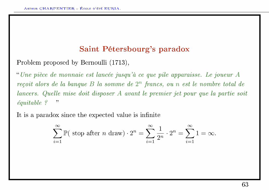
Saint Pétersbourg's paradox
Problem proposed by Bernoulli (1713),
Une pièce de monnaie est lancée jusqu'à ce que pile apparaisse. Le joueur A
reçoit alors de la banque B la somme de 2n francs, ou n est le nombre total de
lancers. Quelle mise doit disposer A avant le premier jet pour que la partie soit
équitable ?
It is a paradox since the expected value is innite
∞∑i=1
P( stop after n draw) · 2n =∞∑i=1
12n· 2n =
∞∑i=1
1 =∞.
63
Arthur CHARPENTIER - École d'été EURIA.
Saint Pétersbourg's paradox
Many answers have been investigated
• the bank does not have innite liabilities, and thus, the player can play onlya nite time (Buffon (1777), Poisson (1837), Borel (1949)),
• the player has a moral utility of money (Cramer(1728), Bernoulli(1738), von Neumann & Morgenstern (1956)) where a concave utilityfunction is considered,
• the player bets using subjective probabilities, were rare events are assumedto be impossible (D'Alembert (1754), Menger (1934), Yaari (1987))
64
Arthur CHARPENTIER - École d'été EURIA.
Risk measures: the expected utility approach
Ru(X) =∫u(x)dP =
∫P(u(X) > x))dx
where u : [0,∞)→ [0,∞) is a utility function.
Example with an exponential utility, u(x) = [1− e−αx]/α,
Ru(X) =1α
log(EP(eαX)
).
65
Arthur CHARPENTIER - École d'été EURIA.
Risk measures: Yarri's dual approach
Rg(X) =∫xdg P =
∫g(P(X > x))dx
where g : [0, 1]→ [0, 1] is a distorted function.
Example if g(x) = I(X ≥ α) Rg(X) = V aR(X,α), and if g(x) = minx/α, 1Rg(X) = TV aR(X,α) (also called expected shortfall),Rg(X) = EP(X|X > V aR(X,α)).
66
Arthur CHARPENTIER - École d'été EURIA.
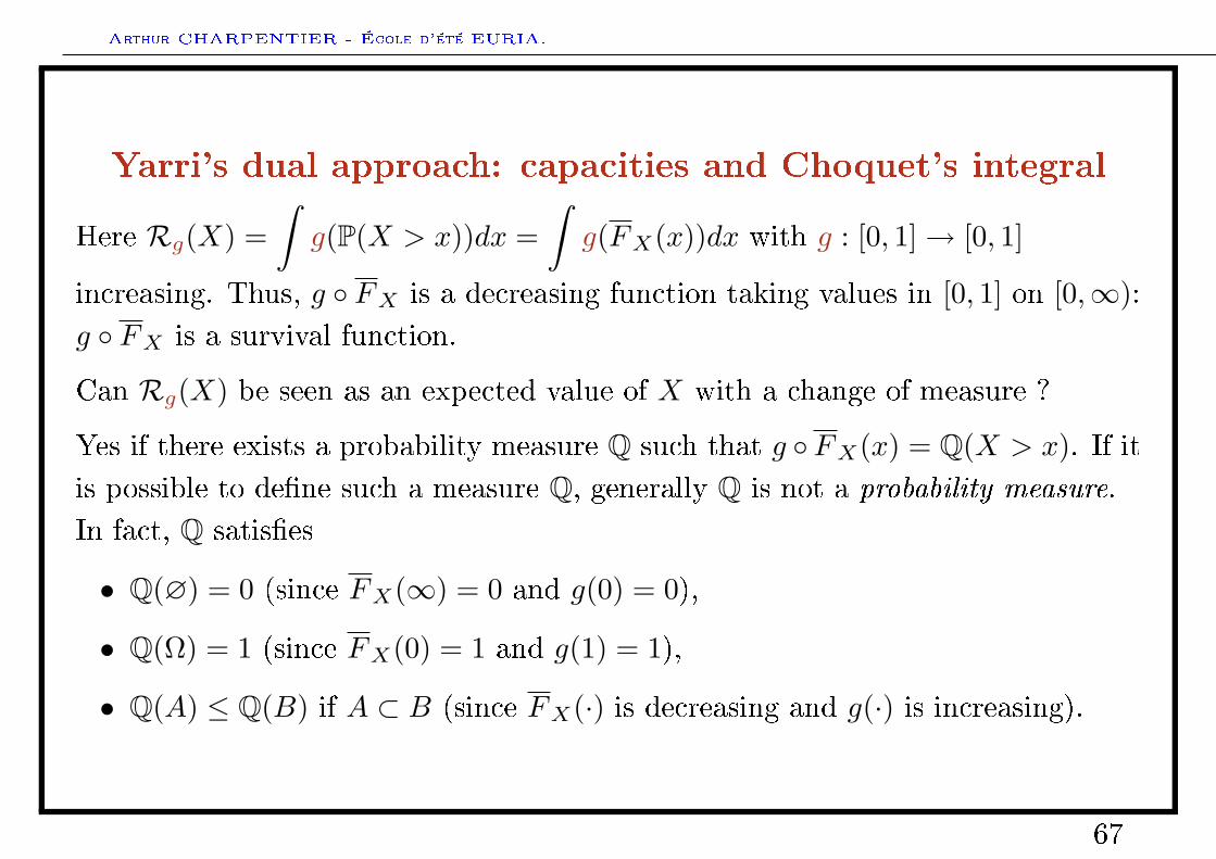
Yarri's dual approach: capacities and Choquet's integral
Here Rg(X) =∫g(P(X > x))dx =
∫g(FX(x))dx with g : [0, 1]→ [0, 1]
increasing. Thus, g FX is a decreasing function taking values in [0, 1] on [0,∞):g FX is a survival function.
Can Rg(X) be seen as an expected value of X with a change of measure ?
Yes if there exists a probability measure Q such that g FX(x) = Q(X > x). If itis possible to dene such a measure Q, generally Q is not a probability measure.In fact, Q satises
• Q(∅) = 0 (since FX(∞) = 0 and g(0) = 0),
• Q(Ω) = 1 (since FX(0) = 1 and g(1) = 1),
• Q(A) ≤ Q(B) if A ⊂ B (since FX(·) is decreasing and g(·) is increasing).
67
Arthur CHARPENTIER - École d'été EURIA.
Yarri's dual approach: capacities and Choquet's integral
Such a measure Q satises only Q(A) ≤ Q(B) if A ⊂ B: Q is a capacity.
With this notation,
Rg(X) =∫xdg P =
∫g(P(X > x))dx =
∫Q(X > x)dx,
but since Q is not a probability measure, Rg(·) is not an expected value: it is theso-called Choquet's integral.
68
Arthur CHARPENTIER - École d'été EURIA.
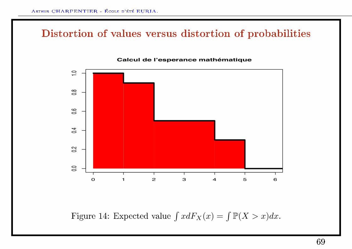
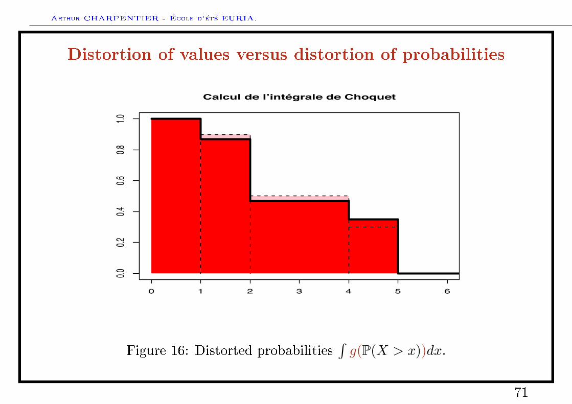
Distortion of values versus distortion of probabilities
0 1 2 3 4 5 6
0.00.2
0.40.6
0.81.0
Calcul de l’esperance mathématique
Figure 14: Expected value∫xdFX(x) =
∫P(X > x)dx.
69
Arthur CHARPENTIER - École d'été EURIA.
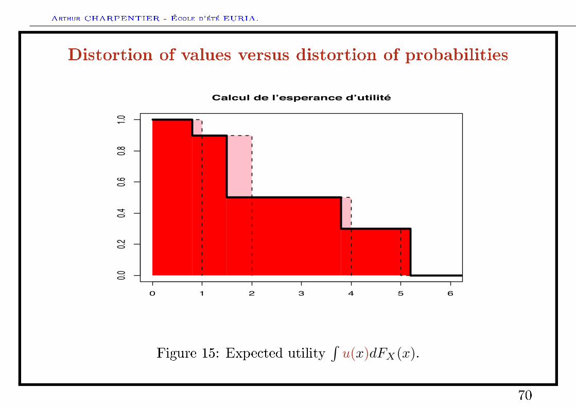
Distortion of values versus distortion of probabilities
0 1 2 3 4 5 6
0.00.2
0.40.6
0.81.0
Calcul de l’esperance d’utilité
Figure 15: Expected utility∫u(x)dFX(x).
70
Arthur CHARPENTIER - École d'été EURIA.
Distortion of values versus distortion of probabilities
0 1 2 3 4 5 6
0.00.2
0.40.6
0.81.0
Calcul de l’intégrale de Choquet
Figure 16: Distorted probabilities∫g(P(X > x))dx.
71
Arthur CHARPENTIER - École d'été EURIA.
Axiomatic approach for risk measures
There are three way to describe risk measure: characterizing natural propertiesthat should satisfy
• the risk measure R(·), e.g. R(·) is subadditive (R(X + Y ) ≤ R(X) +R(Y )),
• induced stochastic ordering , i.e. X Y (Y is more risky than X) if andonly if R(X) ≤ R(Y ) [Economics],
• induced set of acceptable risks A, i.e. X ∈ A (X is is acceptable) if andonly if R(X) ≤ 0 [Financial Mathematics].
72
Arthur CHARPENTIER - École d'été EURIA.
Ordering and comparing risks
Assume that risks are positive random variables.
The higher R(X), the risker X is. Y will be said to be more risky than X will bedenoted X Y .
In Pascal's approach FX(x) = P(X ≤ x)
X Y ⇐⇒ R(X) ≤ R(Y ) where R(X) = EP(X) =∫xdFX(x).
73
Arthur CHARPENTIER - École d'été EURIA.
More dicult to quantify than to compare
Denition 5. is an ordering relationship if it is reexive (FX FX),transitive (if FX FY and FY FZ then FX FZ) and antisymmetric (if
FX FY and FY FX then FX = FY ).
Note that the ordering on the set of distribution functions will be extended to the
set of positive random variables (with X ∼ Y if FX = FY , i.e. XL= Y ).
Denition 6. satises the additivity axiom if for any risks X, Y and Z such
that X Y , then X + Z Y + Z.
It denotes the invariance of perception in case of a common variation. It mightalso be called the linearity axiom.
74
Arthur CHARPENTIER - École d'été EURIA.
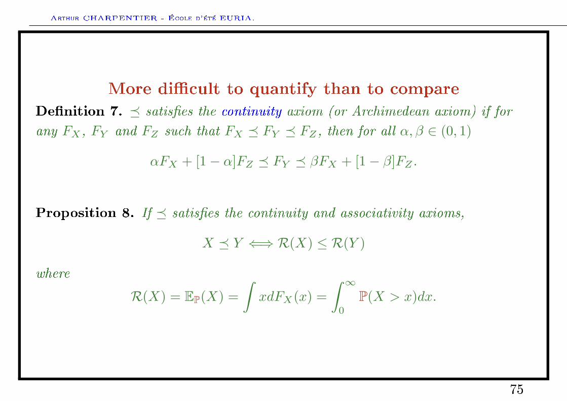
More dicult to quantify than to compare
Denition 7. satises the continuity axiom (or Archimedean axiom) if for
any FX , FY and FZ such that FX FY FZ , then for all α, β ∈ (0, 1)
αFX + [1− α]FZ FY βFX + [1− β]FZ .
Proposition 8. If satises the continuity and associativity axioms,
X Y ⇐⇒ R(X) ≤ R(Y )
where
R(X) = EP(X) =∫xdFX(x) =
∫ ∞0
P(X > x)dx.
75
Arthur CHARPENTIER - École d'été EURIA.
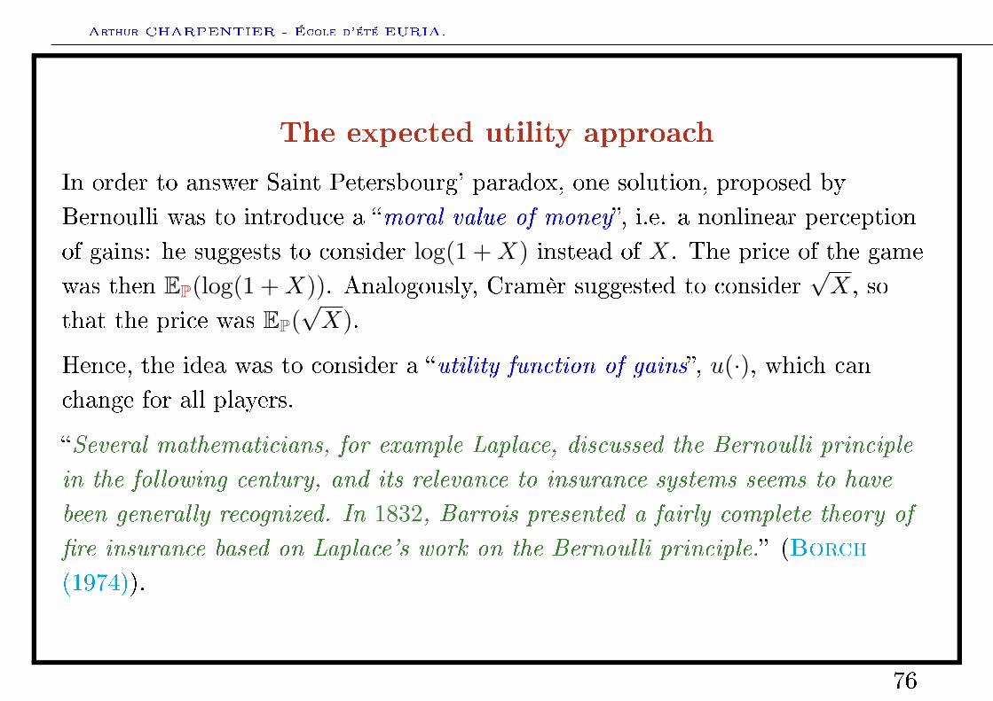
The expected utility approach
In order to answer Saint Petersbourg' paradox, one solution, proposed byBernoulli was to introduce a moral value of money, i.e. a nonlinear perceptionof gains: he suggests to consider log(1 +X) instead of X. The price of the gamewas then EP(log(1 +X)). Analogously, Cramèr suggested to consider
√X, so
that the price was EP(√X).
Hence, the idea was to consider a utility function of gains, u(·), which canchange for all players.
Several mathematicians, for example Laplace, discussed the Bernoulli principle
in the following century, and its relevance to insurance systems seems to have
been generally recognized. In 1832, Barrois presented a fairly complete theory of
re insurance based on Laplace's work on the Bernoulli principle. (Borch(1974)).
76
Arthur CHARPENTIER - École d'été EURIA.
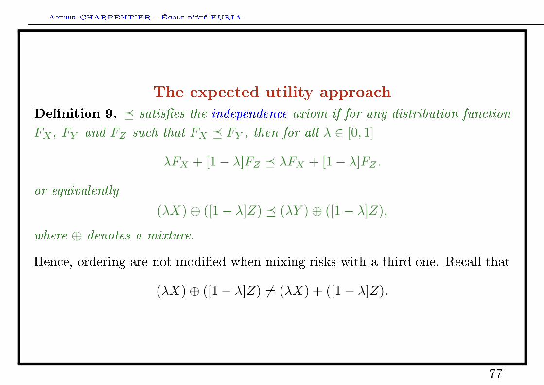
The expected utility approach
Denition 9. satises the independence axiom if for any distribution function
FX , FY and FZ such that FX FY , then for all λ ∈ [0, 1]
λFX + [1− λ]FZ λFX + [1− λ]FZ .
or equivalently
(λX)⊕ ([1− λ]Z) (λY )⊕ ([1− λ]Z),
where ⊕ denotes a mixture.
Hence, ordering are not modied when mixing risks with a third one. Recall that
(λX)⊕ ([1− λ]Z) 6= (λX) + ([1− λ]Z).
77
Arthur CHARPENTIER - École d'été EURIA.
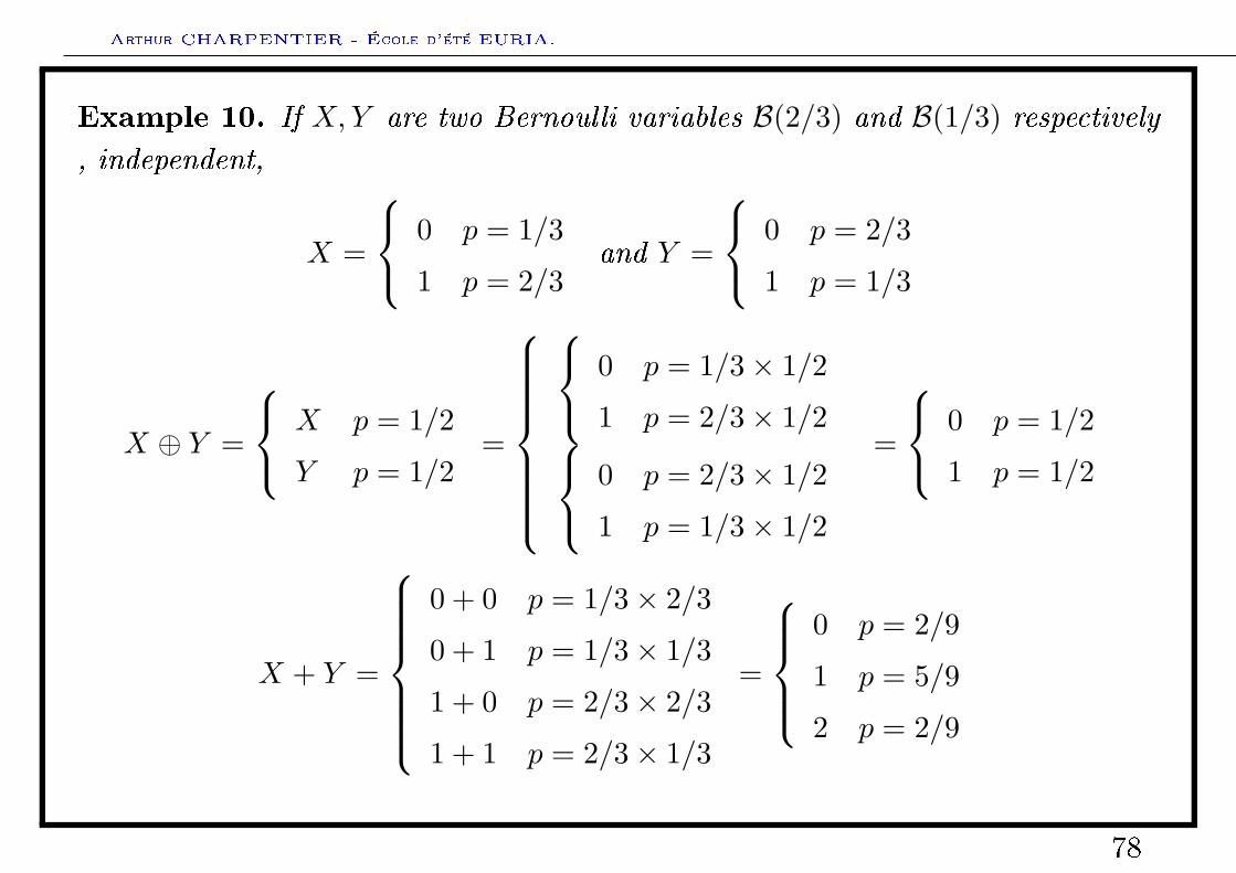
Example 10. If X,Y are two Bernoulli variables B(2/3) and B(1/3) respectively, independent,
X =
0 p = 1/3
1 p = 2/3and Y =
0 p = 2/3
1 p = 1/3
X ⊕ Y =
X p = 1/2
Y p = 1/2=
0 p = 1/3× 1/2
1 p = 2/3× 1/2 0 p = 2/3× 1/2
1 p = 1/3× 1/2
=
0 p = 1/2
1 p = 1/2
X + Y =
0 + 0 p = 1/3× 2/3
0 + 1 p = 1/3× 1/3
1 + 0 p = 2/3× 2/3
1 + 1 p = 2/3× 1/3
=
0 p = 2/9
1 p = 5/9
2 p = 2/9
78
Arthur CHARPENTIER - École d'été EURIA.
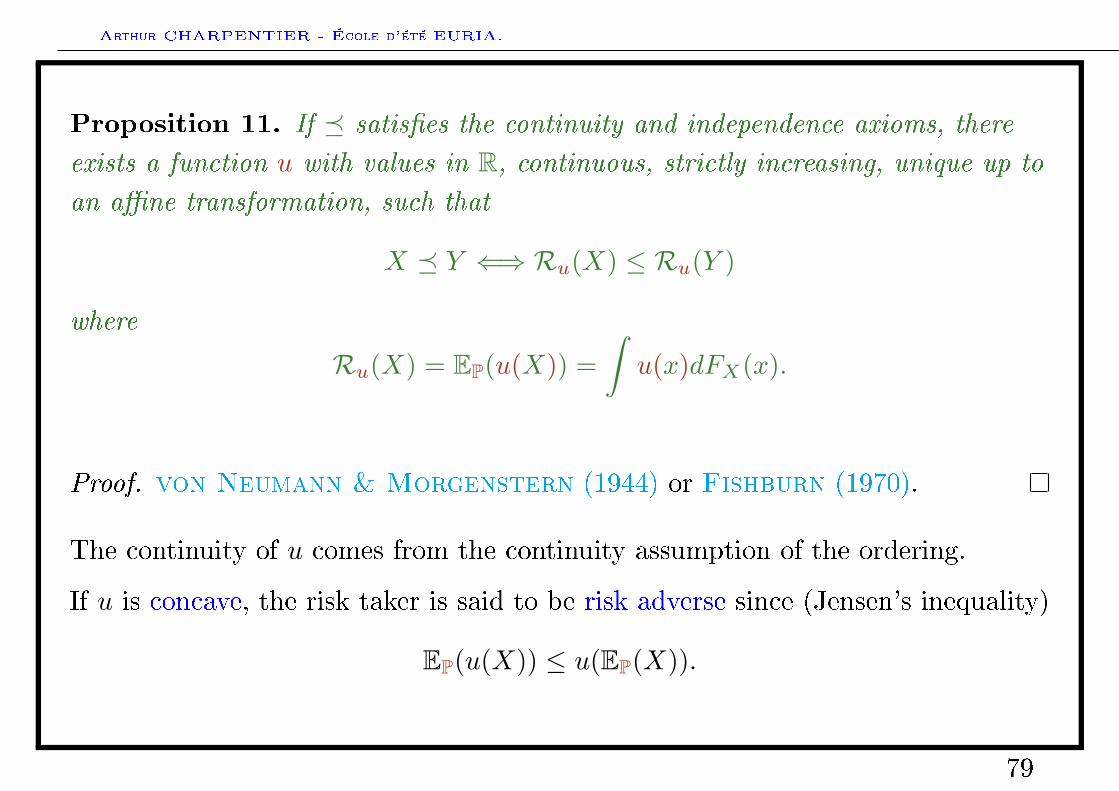
Proposition 11. If satises the continuity and independence axioms, there
exists a function u with values in R, continuous, strictly increasing, unique up to
an ane transformation, such that
X Y ⇐⇒ Ru(X) ≤ Ru(Y )
where
Ru(X) = EP(u(X)) =∫u(x)dFX(x).
Proof. von Neumann & Morgenstern (1944) or Fishburn (1970).
The continuity of u comes from the continuity assumption of the ordering.
If u is concave, the risk taker is said to be risk adverse since (Jensen's inequality)
EP(u(X)) ≤ u(EP(X)).
79
Arthur CHARPENTIER - École d'été EURIA.
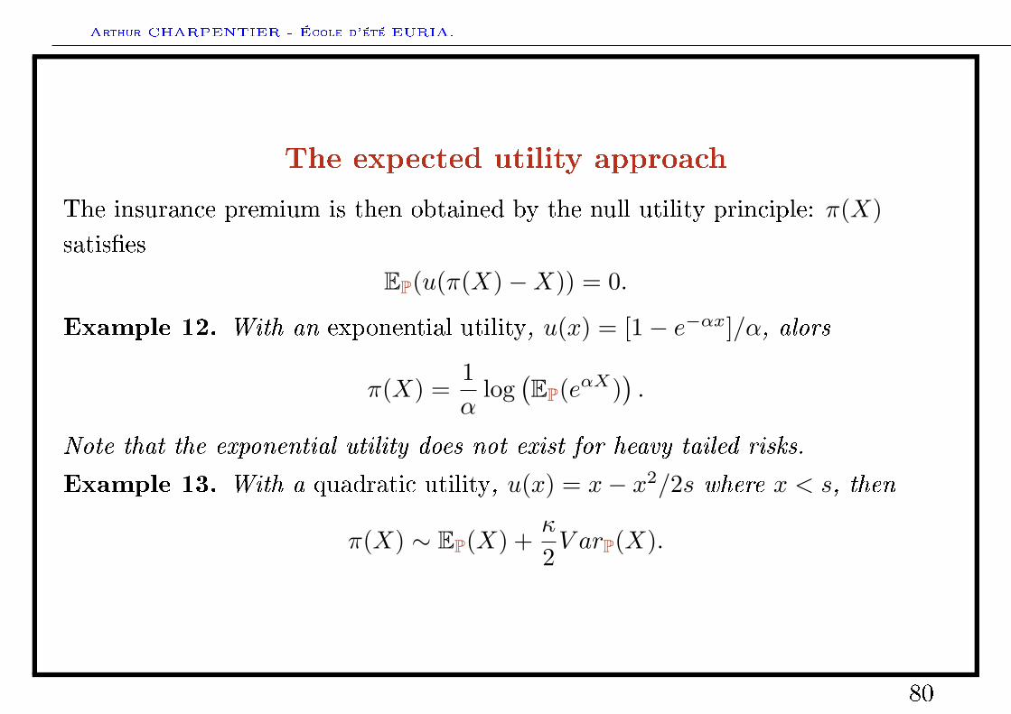
The expected utility approach
The insurance premium is then obtained by the null utility principle: π(X)satises
EP(u(π(X)−X)) = 0.
Example 12. With an exponential utility, u(x) = [1− e−αx]/α, alors
π(X) =1α
log(EP(eαX)
).
Note that the exponential utility does not exist for heavy tailed risks.
Example 13. With a quadratic utility, u(x) = x− x2/2s where x < s, then
π(X) ∼ EP(X) +κ
2V arP(X).
80
Arthur CHARPENTIER - École d'été EURIA.
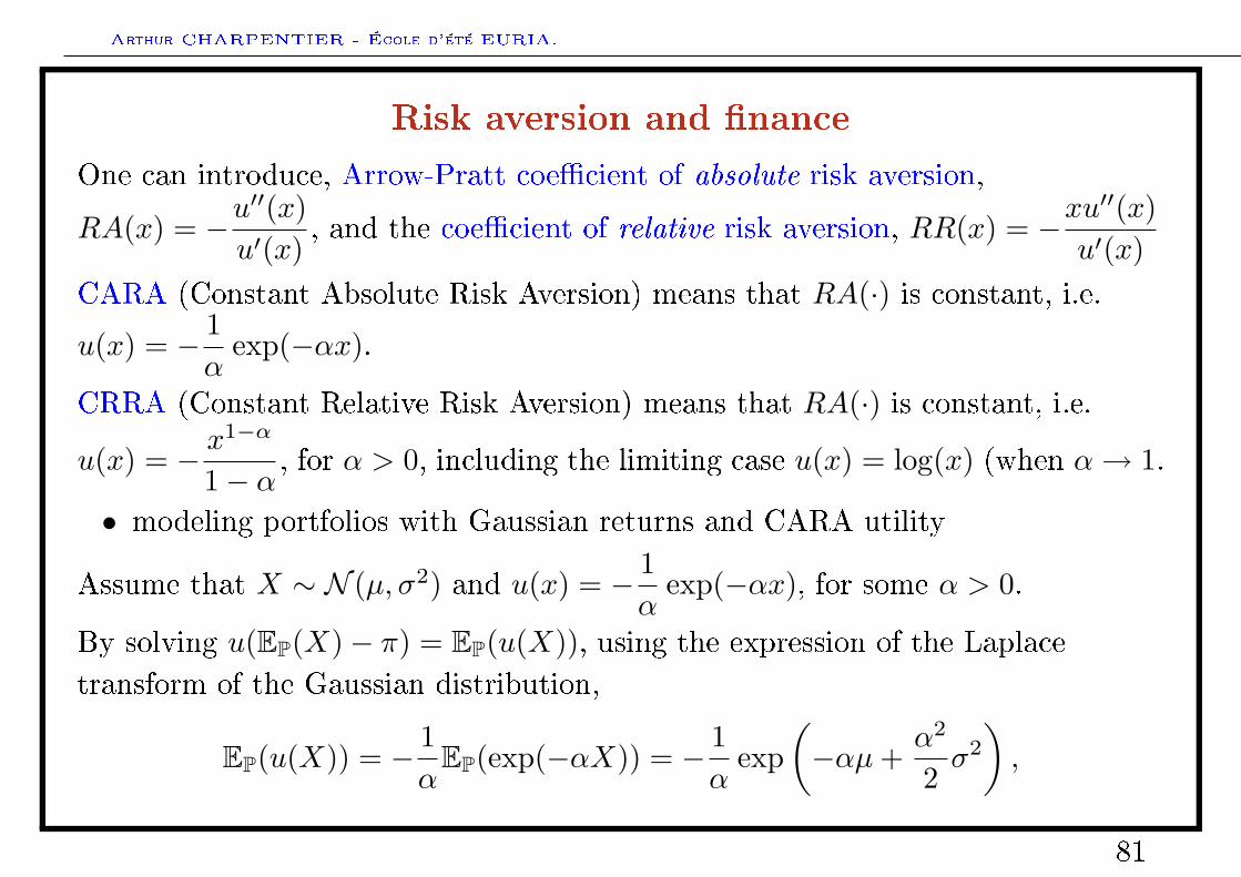
Risk aversion and nance
One can introduce, Arrow-Pratt coecient of absolute risk aversion,
RA(x) = −u′′(x)u′(x)
, and the coecient of relative risk aversion, RR(x) = −xu′′(x)
u′(x)CARA (Constant Absolute Risk Aversion) means that RA(·) is constant, i.e.u(x) = − 1
αexp(−αx).
CRRA (Constant Relative Risk Aversion) means that RA(·) is constant, i.e.
u(x) = − x1−α
1− α, for α > 0, including the limiting case u(x) = log(x) (when α→ 1.
• modeling portfolios with Gaussian returns and CARA utility
Assume that X ∼ N (µ, σ2) and u(x) = − 1α
exp(−αx), for some α > 0.
By solving u(EP(X)− π) = EP(u(X)), using the expression of the Laplacetransform of the Gaussian distribution,
EP(u(X)) = − 1α
EP(exp(−αX)) = − 1α
exp(−αµ+
α2
2σ2
),
81
Arthur CHARPENTIER - École d'été EURIA.
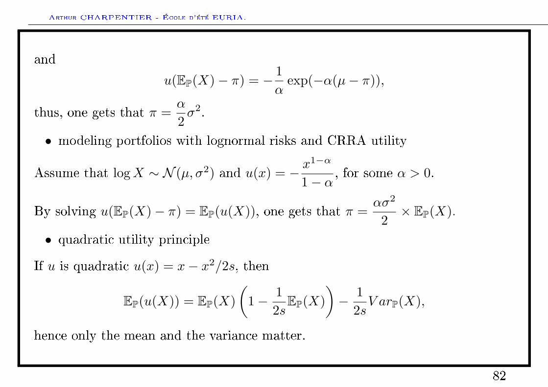
and
u(EP(X)− π) = − 1α
exp(−α(µ− π)),
thus, one gets that π =α
2σ2.
• modeling portfolios with lognormal risks and CRRA utility
Assume that logX ∼ N (µ, σ2) and u(x) = − x1−α
1− α, for some α > 0.
By solving u(EP(X)− π) = EP(u(X)), one gets that π =ασ2
2× EP(X).
• quadratic utility principle
If u is quadratic u(x) = x− x2/2s, then
EP(u(X)) = EP(X)(
1− 12s
EP(X))− 1
2sV arP(X),
hence only the mean and the variance matter.
82
Arthur CHARPENTIER - École d'été EURIA.
Changing probabilities ?
Question: what is probability P ?
Il y a donc une aversion particulière pour l'incertitude liée à l'ignorance. On
préfère avoir un modèle probabiliste que pas de modèle du tout, on préfère évaluer
raisonnablement ses chances de succès, fussent-elles minces, que de n'en avoir
aucune idée. (Ekeland (1991)).
Idée de Ramsey (1931), formalisée par Savage (1972): les individus ne raisonnepas sous P, la probabilité réelle (inconnue), mais sous une probabilité subjectiveQ.
Problème: dicile d'estimer une probabilité d'évènement rare.
Travaux de Selvige (1975): importance des évènements rares aux conséquencesimportantes. Approche psychologique du risque: besoin de comparer à desévènements rares quantiables (taux de mortalité infantile, quinte ush aupocker...).
83
Arthur CHARPENTIER - École d'été EURIA.
Changing probabilities ?
Denition 14. est une relation vériant l'axiome de monotonie si
P(X + ε ≤ Y ) = 1 implique X Y , pour tout ε > 0.
Proposition 15. Si est une relation d'ordre vériant les axiomes de
continuité, d'additivité et de monotonie, alors il existe une probabilité Q telle que
X Y ⇐⇒ RQ(X) ≤ RQ(Y )
où
RQ(X) = EQ(X) =∫ ∞
0
Q(X > x)dx.
84
Arthur CHARPENTIER - École d'été EURIA.
Using subjective probabilities
Considérons un call européen, dont le payo actualisé est e−rT (ST −K)+. Leprix n'est pas EP
(e−rT (ST −K)+
).
Le prix d'un call européen proposant de toucher (ST −K)+ à maturité. Lavalorisation de l'option, à la date d'aujourd'hui est basée sur la notion deportefeuille de réplication: deux portefeuilles orant le même payo à une date Tont nécessairement le même prix aujourd'hui (sinon il serait possible deconstituer une opportunité d'arbitrage).
85
Arthur CHARPENTIER - École d'été EURIA.
Changing probabilities ?
Considérons le modèle de Cox, Ross & Rubinstein (1979), avec un actif sansrisque valant 1 aujourd'hui, et 1 + r dans un an, et un actif risqué valant S0
aujourd'hui, et, dans un an S1, valant soit Su, soit Sd, avec d < 1 + r < u,suivant l'état de la nature. Considérons un call européen donnant le droitd'acheter le sous-jacent à maturité (dans un an) à la valeur K. Le payo dans unan est alors (S1 −K)+. Construisons un portefeuille α+ βS0 permettant derépliquer la valeur de l'option dans un an:
• si le marché monte, le portefeuille vaudra α (1 + r) + βSu, et l'optionCu = (Su−K)+
• si le marché baisse, le portefeuille vaudra α (1 + r) + βSd, et l'optionCd = (Sd−K)+
86
Arthur CHARPENTIER - École d'été EURIA.
Changing probabilities ?
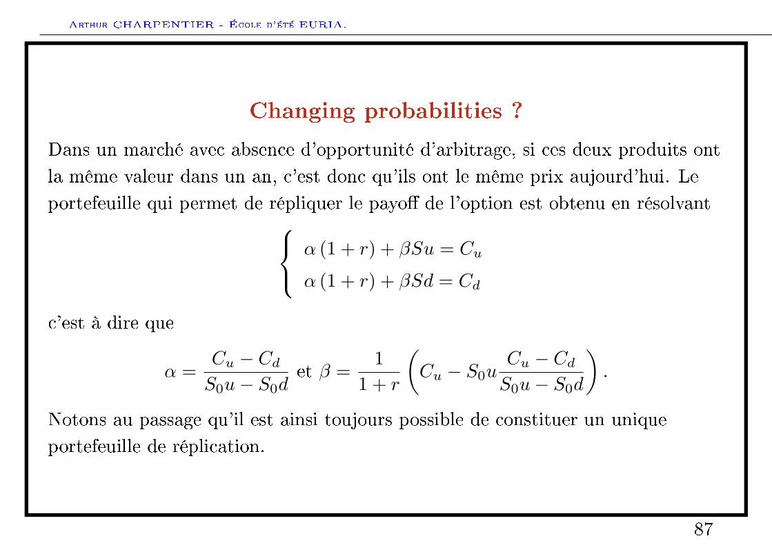
Dans un marché avec absence d'opportunité d'arbitrage, si ces deux produits ontla même valeur dans un an, c'est donc qu'ils ont le même prix aujourd'hui. Leportefeuille qui permet de répliquer le payo de l'option est obtenu en résolvant α (1 + r) + βSu = Cu
α (1 + r) + βSd = Cd
c'est à dire que
α =Cu − CdS0u− S0d
et β =1
1 + r
(Cu − S0u
Cu − CdS0u− S0d
).
Notons au passage qu'il est ainsi toujours possible de constituer un uniqueportefeuille de réplication.
87
Arthur CHARPENTIER - École d'été EURIA.
Changing probabilities ?
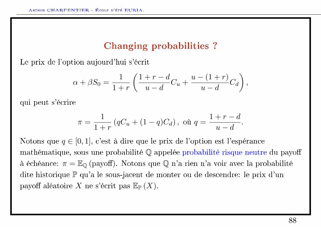
Le prix de l'option aujourd'hui s'écrit
α+ βS0 =1
1 + r
(1 + r − du− d
Cu +u− (1 + r)u− d
Cd
),
qui peut s'écrire
π =1
1 + r(qCu + (1− q)Cd) , où q =
1 + r − du− d
.
Notons que q ∈ [0, 1], c'est à dire que le prix de l'option est l'espérancemathématique, sous une probabilité Q appelée probabilité risque neutre du payoà échéance: π = EQ (payo). Notons que Q n'a rien n'a voir avec la probabilitédite historique P qu'a le sous-jacent de monter ou de descendre: le prix d'unpayo aléatoire X ne s'écrit pas EP (X).
88
Arthur CHARPENTIER - École d'été EURIA.
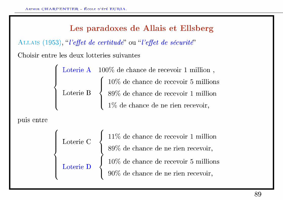
Les paradoxes de Allais et Ellsberg
Allais (1953), l'eet de certitude ou l'eet de sécurité
Choisir entre les deux lotteries suivantesLoterie A 100% de chance de recevoir 1 million ,
Loterie B
10% de chance de recevoir 5 millions
89% de chance de recevoir 1 million
1% de chance de ne rien recevoir,
puis entre Loterie C
11% de chance de recevoir 1 million
89% de chance de ne rien recevoir,
Loterie D
10% de chance de recevoir 5 millions
90% de chance de ne rien recevoir,
89
Arthur CHARPENTIER - École d'été EURIA.
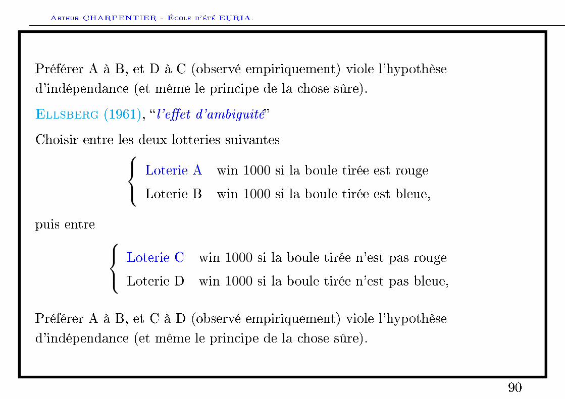
Préférer A à B, et D à C (observé empiriquement) viole l'hypothèsed'indépendance (et même le principe de la chose sûre).
Ellsberg (1961), l'eet d'ambiguité
Choisir entre les deux lotteries suivantes Loterie A win 1000 si la boule tirée est rouge
Loterie B win 1000 si la boule tirée est bleue,
puis entre Loterie C win 1000 si la boule tirée n'est pas rouge
Loterie D win 1000 si la boule tirée n'est pas bleue,
Préférer A à B, et C à D (observé empiriquement) viole l'hypothèsed'indépendance (et même le principe de la chose sûre).
90
Arthur CHARPENTIER - École d'été EURIA.
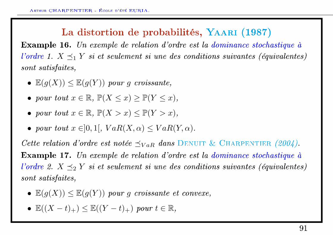
La distortion de probabilités, Yaari (1987)Example 16. Un exemple de relation d'ordre est la dominance stochastique à
l'ordre 1. X 1 Y si et seulement si une des conditions suivantes (équivalentes)
sont satisfaites,
• E(g(X)) ≤ E(g(Y )) pour g croissante,
• pour tout x ∈ R, P(X ≤ x) ≥ P(Y ≤ x),
• pour tout x ∈ R, P(X > x) ≤ P(Y > x),
• pour tout x ∈]0, 1[, V aR(X,α) ≤ V aR(Y, α).
Cette relation d'ordre est notée V aR dans Denuit & Charpentier (2004).
Example 17. Un exemple de relation d'ordre est la dominance stochastique à
l'ordre 2. X 2 Y si et seulement si une des conditions suivantes (équivalentes)
sont satisfaites,
• E(g(X)) ≤ E(g(Y )) pour g croissante et convexe,
• E((X − t)+) ≤ E((Y − t)+) pour t ∈ R,
91
Arthur CHARPENTIER - École d'été EURIA.
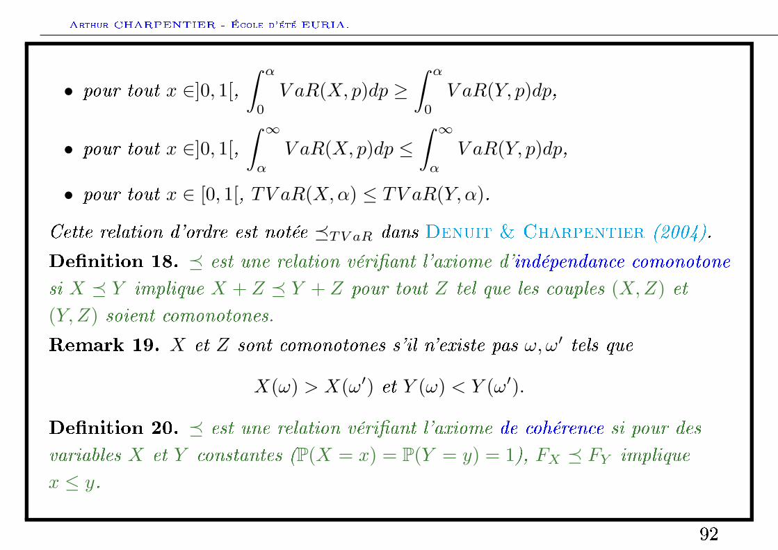
• pour tout x ∈]0, 1[,∫ α
0
V aR(X, p)dp ≥∫ α
0
V aR(Y, p)dp,
• pour tout x ∈]0, 1[,∫ ∞α
V aR(X, p)dp ≤∫ ∞α
V aR(Y, p)dp,
• pour tout x ∈ [0, 1[, TV aR(X,α) ≤ TV aR(Y, α).
Cette relation d'ordre est notée TV aR dans Denuit & Charpentier (2004).
Denition 18. est une relation vériant l'axiome d'indépendance comonotone
si X Y implique X + Z Y + Z pour tout Z tel que les couples (X,Z) et(Y, Z) soient comonotones.
Remark 19. X et Z sont comonotones s'il n'existe pas ω, ω′ tels que
X(ω) > X(ω′) et Y (ω) < Y (ω′).
Denition 20. est une relation vériant l'axiome de cohérence si pour des
variables X et Y constantes (P(X = x) = P(Y = y) = 1), FX FY implique
x ≤ y.
92
Arthur CHARPENTIER - École d'été EURIA.
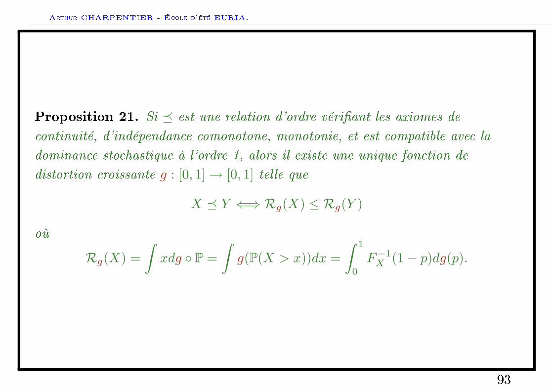
Proposition 21. Si est une relation d'ordre vériant les axiomes de
continuité, d'indépendance comonotone, monotonie, et est compatible avec la
dominance stochastique à l'ordre 1, alors il existe une unique fonction de
distortion croissante g : [0, 1]→ [0, 1] telle que
X Y ⇐⇒ Rg(X) ≤ Rg(Y )
où
Rg(X) =∫xdg P =
∫g(P(X > x))dx =
∫ 1
0
F−1X (1− p)dg(p).
93
Arthur CHARPENTIER - École d'été EURIA.
Agenda
• General introduction
Financial risks
• Market risks
• Credit risk
• From variance to Value-at-Risk
Risk measures and capital allocation
• Risk measures: an axiomatic introduction
• Risk measures: convexity and coherence
• Capital allocation: an axiomatic introduction
Risk measures and statistical inference
94
Arthur CHARPENTIER - École d'été EURIA.
Coherent risk measures and the axiomatic approach
A risk measure is said to be coherent (from Artzner, Delbaen, Eber &
Heath (1999)) if
• R(·) is monotonic, i.e. X ≤ Y implies R(X) ≤ R(Y ),
• R(·) is positively homogeneous, i.e. for any λ ≤ 0, R(λX) = λR(X),
• R(·) is invariant by translation, i.e. for any κ, R(X + κ) = R(X) + κ,
• R(·) is subadditive, i.e. R(X + Y ) ≤ R(X) +R(Y ).
subadditivity can be interpreted as diversication does not increase risk.
Example: the Expected-Shortfall is coherent, the Value-at-Risk is not.
95
Arthur CHARPENTIER - École d'été EURIA.
Value-at-Risk and coherence
Dans le cas d'une loi de Pareto
F (x) = P(X > x) =1
2 + x, x > −1
la VaR est
VaR(Xi, α) =1α− 2.
Alors
P(X1 +X2 > x) =2
4 + x+
2 log[3 + x][4 + x]2
, pour x > −2,
alors
P(X1 +X2 > 2VaR(Xi, α)) = α+α2
2log(
2− αα
)> α.
Aussi
VaR(X1 +X2, α) > VaR(X1, α) + VaR(X2, α) = 2VaR(Xi, α)
96
Arthur CHARPENTIER - École d'été EURIA.
Convex risk measures
A risk measure is said to be convex (from Artzner, Delbaen, Eber & Heath
(1999)) if
• R(·) is monotonic, i.e. X ≤ Y implies R(X) ≤ R(Y ),
• R(·) is invariant by translation, i.e. for any κ, R(X + κ) = R(X) + κ,
• R(·) is convex, i.e. R(λX + (1− λ)Y ) ≤ λR(X) + (1− λ)R(Y ), for anyλ ∈ [0, 1].
Hence, if a convex measure satises the homogeneity condition, it is coherent.
Remark A natural way to dene a convex measure satisfying the small sizecoherent condition is adding a coherent measure a liquidity charge,
Rconvex(X) = Rcoherent(X) + Cliquidity(X).
97
Arthur CHARPENTIER - École d'été EURIA.
Sets of acceptable risksDenition 22. Given a risk measure R, a risk X is acceptable if X ∈ AR where
AR = Y ∈ X such that R(Y ) ≤ 0.
Conversely,Theorem 23. Given a set of acceptable risks A, the associated risk measure is
the smallest capital amont m such that X −m is acceptable, i.e.
RA(X) = infm ∈ R such that X −m ∈ A.
Then RAR(·) = R(·) and ARA = A.Proposition 24. If R is a convex risk measure, then AR is convex. Conversely,
if A is convex, then RA is a convex risk measure.
Proposition 25. If R is a positively homogeneous risk measure, then AR is a
positive cone. Conversely, if A is a positive cone, then RA is a positively
homogeneous risk measure.
Example 26. If R(X) = supX(ω), ω ∈ Ω, then AR = Y, Y ≤ 0. IfR(X) = F−1
X (α) where α ∈ (0, 1), then AR = Y,P(Y ≤ 0) ≥ α.
98
Arthur CHARPENTIER - École d'été EURIA.
Characterizations of coherent risk measures
Proposition 27. If R is a coherent risk measure, then there exists a set of
probability measures Q such that
R(X) = supQ∈QEQ(X).
99
Arthur CHARPENTIER - École d'été EURIA.
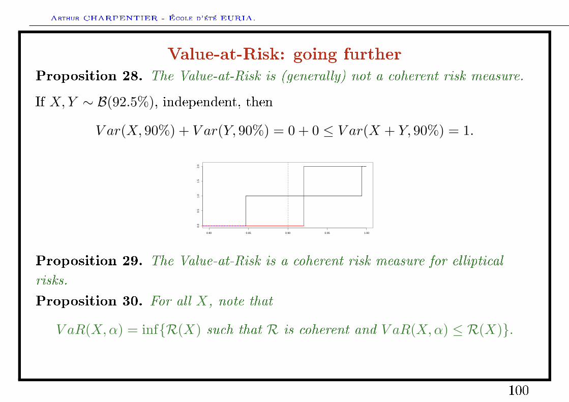
Value-at-Risk: going furtherProposition 28. The Value-at-Risk is (generally) not a coherent risk measure.
If X,Y ∼ B(92.5%), independent, then
V ar(X, 90%) + V ar(Y, 90%) = 0 + 0 ≤ V ar(X + Y, 90%) = 1.
0.80 0.85 0.90 0.95 1.00
0.0
0.5
1.0
1.5
2.0
Proposition 29. The Value-at-Risk is a coherent risk measure for elliptical
risks.
Proposition 30. For all X, note that
V aR(X,α) = infR(X) such that R is coherent and V aR(X,α) ≤ R(X).
100
Arthur CHARPENTIER - École d'été EURIA.
Tail Value-at-Risk (or Expected Shortfall)
Dene
TV aR(X,α) = E(X|X > V aR(X,α)) =1
1− α
∫ 1
α
FX−1(u)du.
In some sense, the TailVaR is the average of worst cases, while V aR was the bestworst case.
Proposition 31. Tail Value-at-Risk is a coherent risk measure.
101
Arthur CHARPENTIER - École d'été EURIA.
Distorted Risk Measures
On pourra noter
R(F,G) =∫ 1
0
F−1(1− u)dG(u)
en faisant une intégration par parties et un changement de variable, on peutmontrer que
R(F,G) =∫ 1
F (0)
G(1− u)dF−1(u) +∫ F (0)
0
[G(1− u)− 1]dF−1(u)
En posant u = F (x), on obtient
R(F,G) =∫ ∞
0
G(F (x))dx−∫ 0
−∞[1−G(F (x))]dx
où
F (x) = 1− F (x) = P(perte > x).
102
Arthur CHARPENTIER - École d'été EURIA.
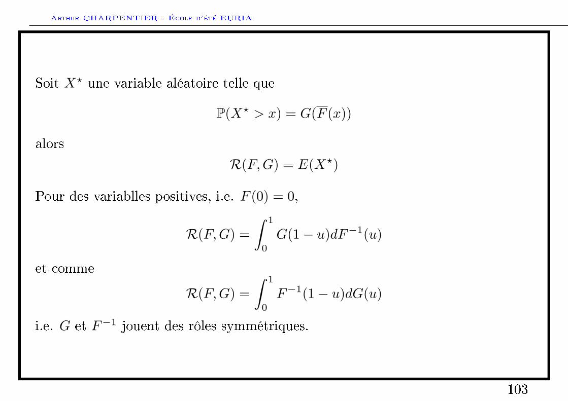
Soit X? une variable aléatoire telle que
P(X? > x) = G(F (x))
alors
R(F,G) = E(X?)
Pour des variablles positives, i.e. F (0) = 0,
R(F,G) =∫ 1
0
G(1− u)dF−1(u)
et comme
R(F,G) =∫ 1
0
F−1(1− u)dG(u)
i.e. G et F−1 jouent des rôles symmétriques.
103
Arthur CHARPENTIER - École d'été EURIA.
Agenda
• General introduction
Financial risks
• Market risks
• Credit risk
• From variance to Value-at-Risk
Risk measures and capital allocation
• Risk measures: an axiomatic introduction
• Risk measures: convexity and coherence
• Capital allocation: an axiomatic introduction
Risk measures and statistical inference
104
Arthur CHARPENTIER - École d'été EURIA.
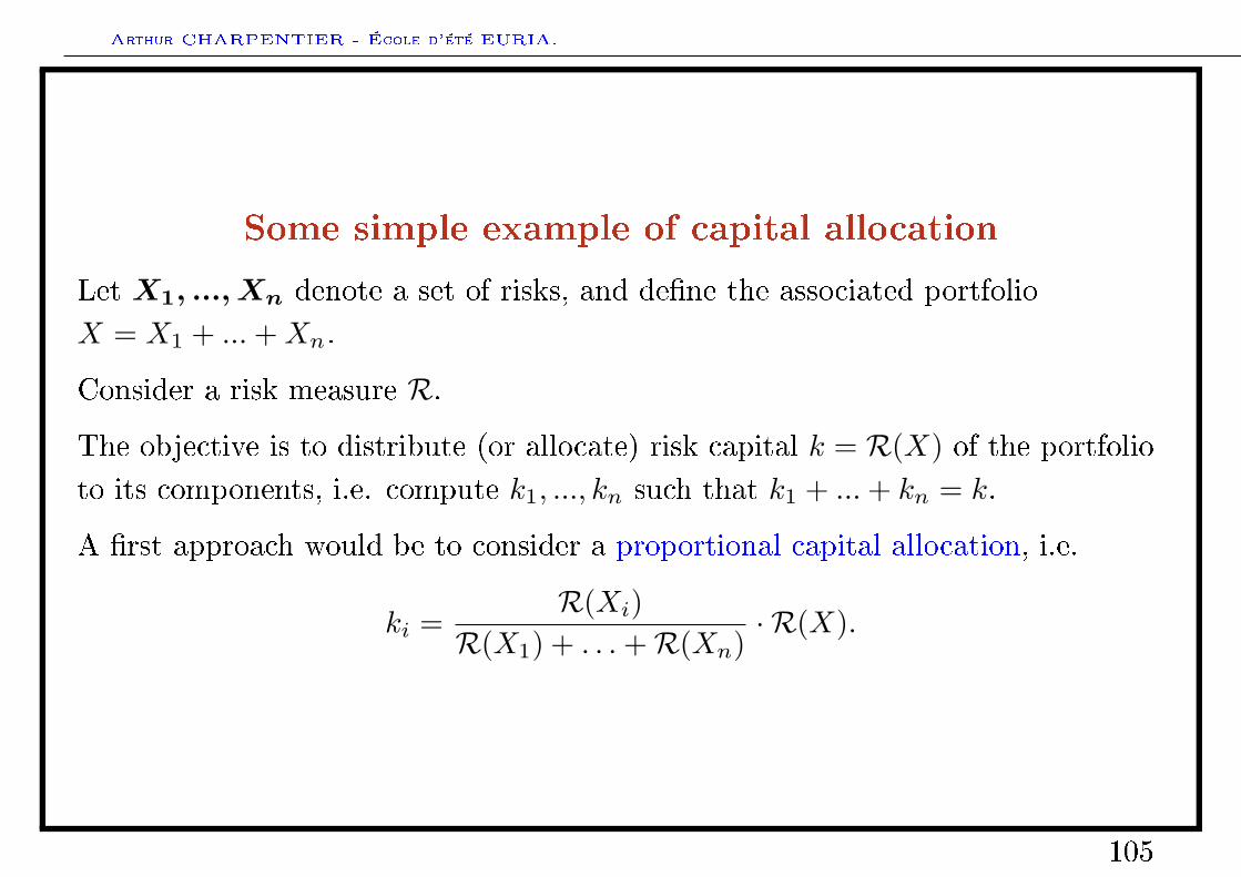
Some simple example of capital allocation
Let X1, ..., Xn denote a set of risks, and dene the associated portfolioX = X1 + ...+Xn.
Consider a risk measure R.
The objective is to distribute (or allocate) risk capital k = R(X) of the portfolioto its components, i.e. compute k1, ..., kn such that k1 + ...+ kn = k.
A rst approach would be to consider a proportional capital allocation, i.e.
ki =R(Xi)
R(X1) + . . .+R(Xn)· R(X).
105
Arthur CHARPENTIER - École d'été EURIA.
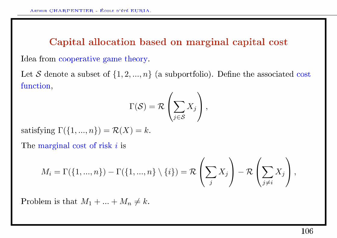
Capital allocation based on marginal capital cost
Idea from cooperative game theory.
Let S denote a subset of 1, 2, ..., n (a subportfolio). Dene the associated costfunction,
Γ(S) = R
∑j∈S
Xj
,
satisfying Γ(1, ..., n) = R(X) = k.
The marginal cost of risk i is
Mi = Γ(1, ..., n)− Γ(1, ..., n \ i) = R
∑j
Xj
−R∑j 6=i
Xj
,
Problem is that M1 + ...+Mn 6= k.
106
Arthur CHARPENTIER - École d'été EURIA.
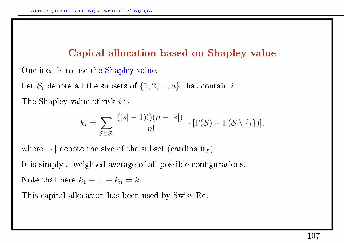
Capital allocation based on Shapley value
One idea is to use the Shapley value.
Let Si denote all the subsets of 1, 2, ..., n that contain i.
The Shapley-value of risk i is
ki =∑S∈Si
(|s| − 1)!)(n− |s|)!n!
· [Γ(S)− Γ(S \ i)],
where | · | denote the size of the subset (cardinality).
It is simply a weighted average of all possible congurations.
Note that here k1 + ...+ kn = k.
This capital allocation has been used by Swiss Re.
107
Arthur CHARPENTIER - École d'été EURIA.
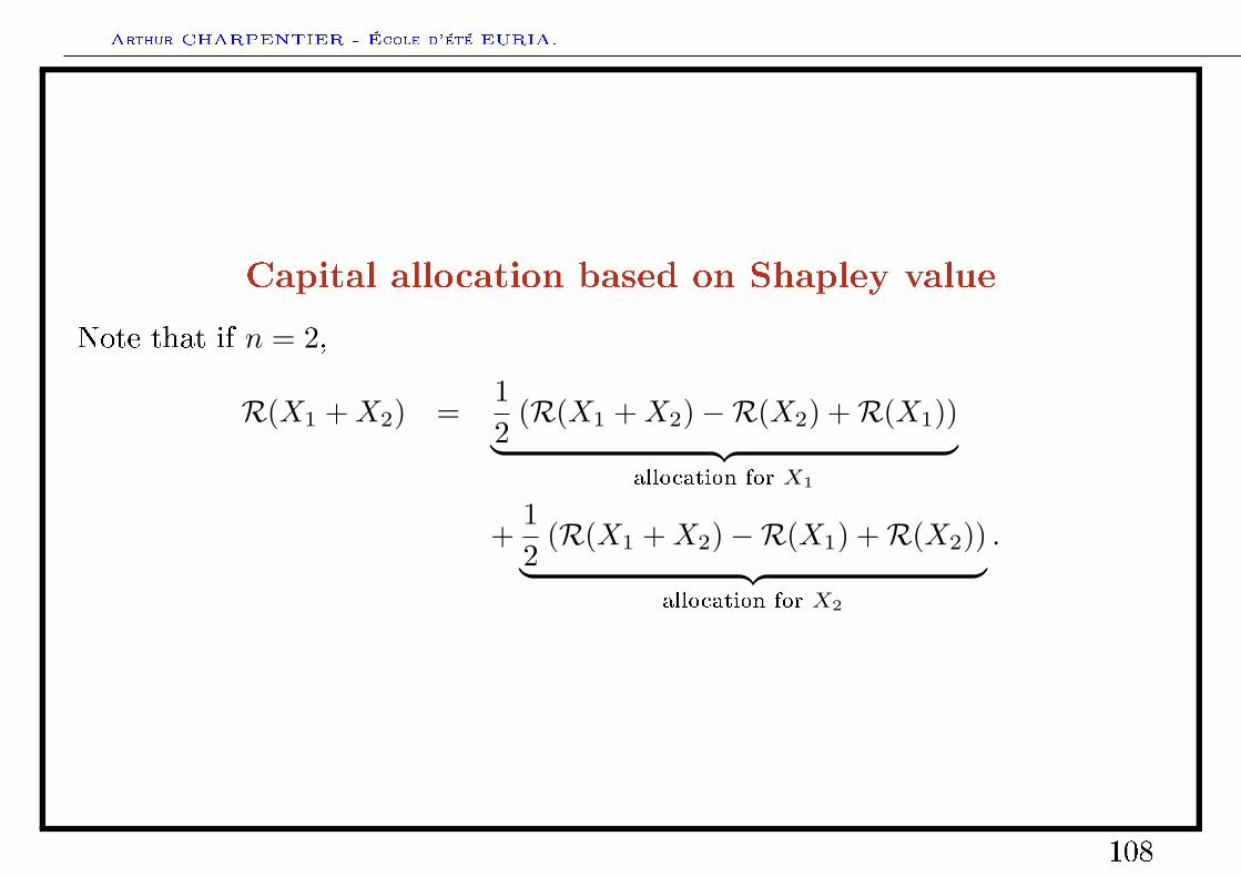
Capital allocation based on Shapley value
Note that if n = 2,
R(X1 +X2) =12
(R(X1 +X2)−R(X2) +R(X1))︸ ︷︷ ︸allocation for X1
+12
(R(X1 +X2)−R(X1) +R(X2))︸ ︷︷ ︸allocation for X2
.
108
Arthur CHARPENTIER - École d'été EURIA.
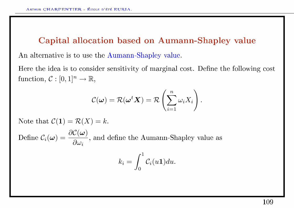
Capital allocation based on Aumann-Shapley value
An alternative is to use the Aumann-Shapley value.
Here the idea is to consider sensitivity of marginal cost. Dene the following costfunction, C : [0, 1]n → R,
C(ω) = R(ωtX) = R
(n∑i=1
ωiXi
).
Note that C(1) = R(X) = k.
Dene Ci(ω) =∂C(ω)∂ωi
, and dene the Aumann-Shapley value as
ki =∫ 1
0
Ci(u1)du.
109
Arthur CHARPENTIER - École d'été EURIA.
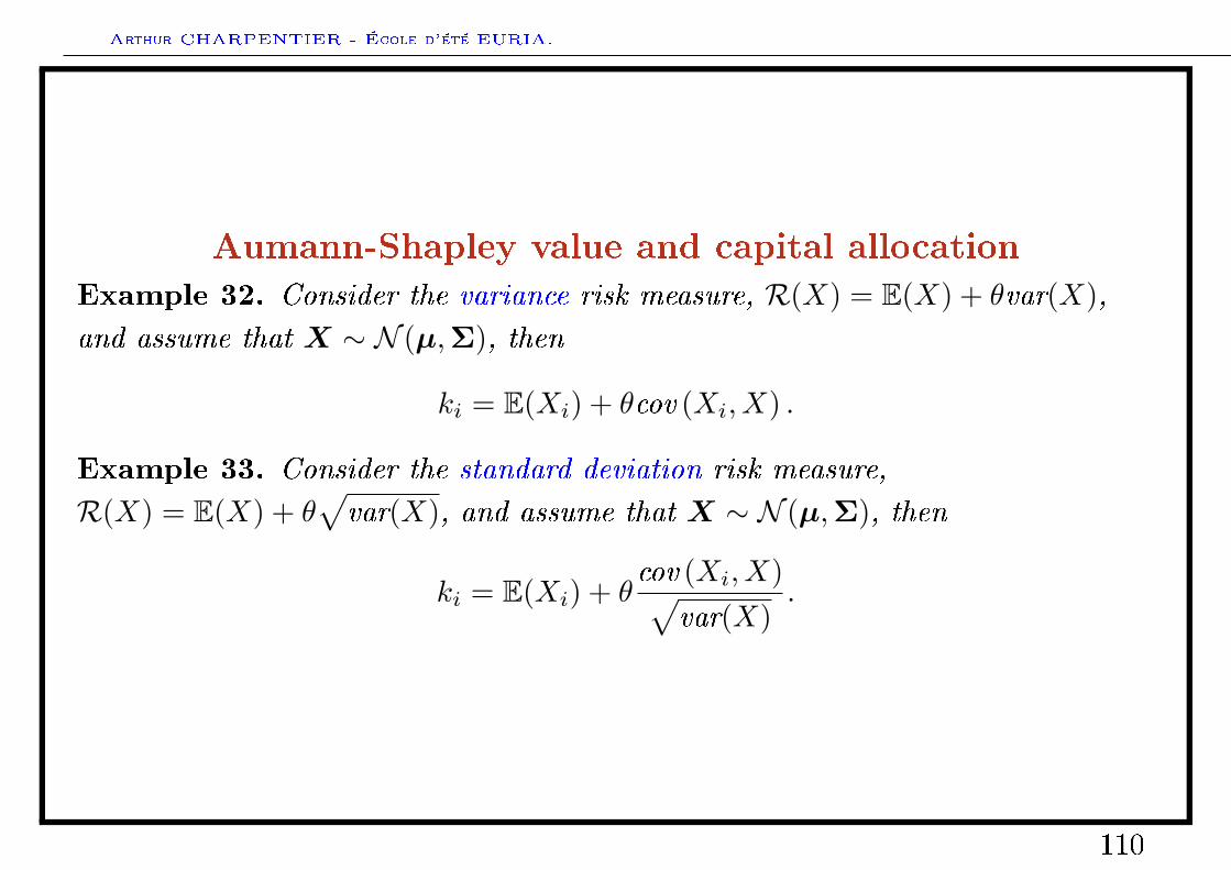
Aumann-Shapley value and capital allocation
Example 32. Consider the variance risk measure, R(X) = E(X) + θvar(X),and assume that X ∼ N (µ,Σ), then
ki = E(Xi) + θcov (Xi, X) .
Example 33. Consider the standard deviation risk measure,
R(X) = E(X) + θ√var(X), and assume that X ∼ N (µ,Σ), then
ki = E(Xi) + θcov (Xi, X)√
var(X).
110

Arthur CHARPENTIER - École d'été EURIA.
Aumann-Shapley value and capital allocation
Assume that R is (positively) homogeneous , then so is C, i.e. C(λω) = λC(ω),and thus Ci(λω)Ci(ω), i.e. the Aumann-Shapley value reduces to marginal costs,
ki =∫ 1
0
Ci(u1)du =∫ 1
0
Ci(1) = Ci(1).
Note that this allocation can also be derived directly using Euler's theorem forhomogeneous functions,
C(ω) = ω1∂C(ω)∂ω1
+ ...+ ωn∂C(ω)∂ωn
.
111
Arthur CHARPENTIER - École d'été EURIA.
Capital allocation using distortion risk measures
If R is a distortion risk measure, R(X) =∫ ∞
0
g(1− Fx)dx.
Writing R as R(X) = EQX(X), where dQX/dP = g(1− FX(X)) then
k = R(X) = EQX(X) and ki = EQX
(Xi).
112
Arthur CHARPENTIER - École d'été EURIA.
Capital allocation and dependence
Since E(XY ) = E(X)E(Y ) + cov(X,Y ), we can write for distortion risk measures
ki = EQX(Xi) = ki = E(Xi · g(1− FX(x))) = E(Xi) + cov(Xi, g(1− FX(X))),
since E(g(1− FX(X))) = 1.
Hence, the capital is maximum if Xi and X are comonotonic, i.e.
ki = E(Xi · g(FX(X))) ≤ E(X+i · g(FX(X+))) = R(X+
i ) = R(Xi).
The allocated capital is always lower than the stand-alone risk, i.e. theallocation belongs to the core (in game theory terms).
Further, one can obtain ki < 0 even if R(Xi) > 0.
113
Arthur CHARPENTIER - École d'été EURIA.
Aumann-Shapley value for TVaR
TVaR is a distortion risk measure, R(X) = E(X|X > F−1X (α)) and thus,
ki = E(Xi|X > F−1X (α)).
Aumann-Shapley value for VaR
VaR is a positively homogenous, and marginal costs works, R(X) = F−1X (α) and
thus,
ki = E(Xi|X = F−1X (α)).
114
Arthur CHARPENTIER - École d'été EURIA.
Capital allocation based on expected utility
Consider for instance exponential risk measures, R(X) =1θ
log E(eθX).
The Aumann-Shapley allocation is then
ki =∫ 1
0
E(XieθuX)
E(eθuX)du = E
(Xi ·
∫ 1
0
eθuX
E(eθuX)
)du
here again, change of measure representation.
Remark 34. If the Xi's are independent, then ki = R(Xi).
115
Arthur CHARPENTIER - École d'été EURIA.
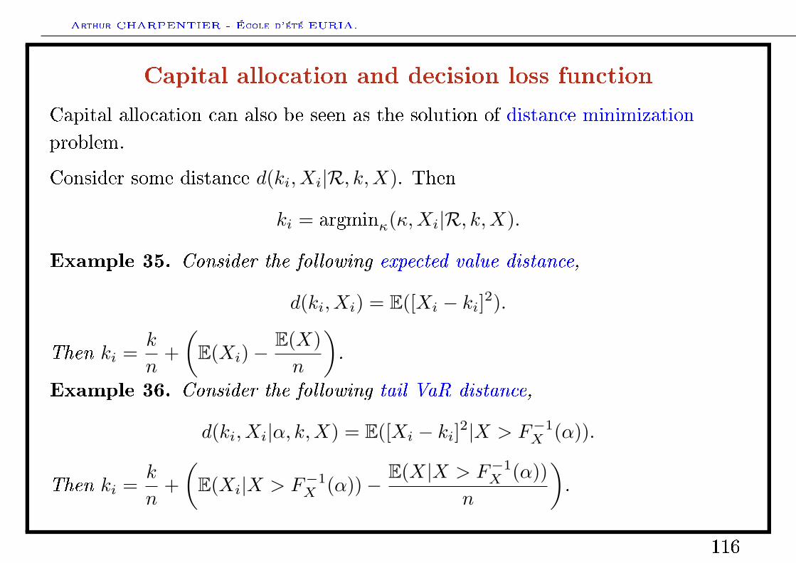
Capital allocation and decision loss function
Capital allocation can also be seen as the solution of distance minimizationproblem.
Consider some distance d(ki, Xi|R, k,X). Then
ki = argminκ(κ,Xi|R, k,X).
Example 35. Consider the following expected value distance,
d(ki, Xi) = E([Xi − ki]2).
Then ki =k
n+(
E(Xi)−E(X)n
).
Example 36. Consider the following tail VaR distance,
d(ki, Xi|α, k,X) = E([Xi − ki]2|X > F−1X (α)).
Then ki =k
n+(
E(Xi|X > F−1X (α))−
E(X|X > F−1X (α))
n
).
116
Arthur CHARPENTIER - École d'été EURIA.
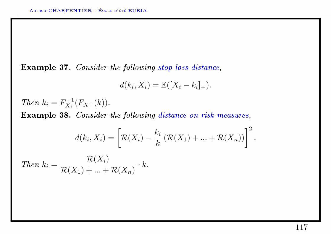
Example 37. Consider the following stop loss distance,
d(ki, Xi) = E([Xi − ki]+).
Then ki = F−1Xi
(FX+(k)).
Example 38. Consider the following distance on risk measures,
d(ki, Xi) =[R(Xi)−
kik
(R(X1) + ...+R(Xn))]2.
Then ki =R(Xi)
R(X1) + ...+R(Xn)· k.
117
Arthur CHARPENTIER - École d'été EURIA.
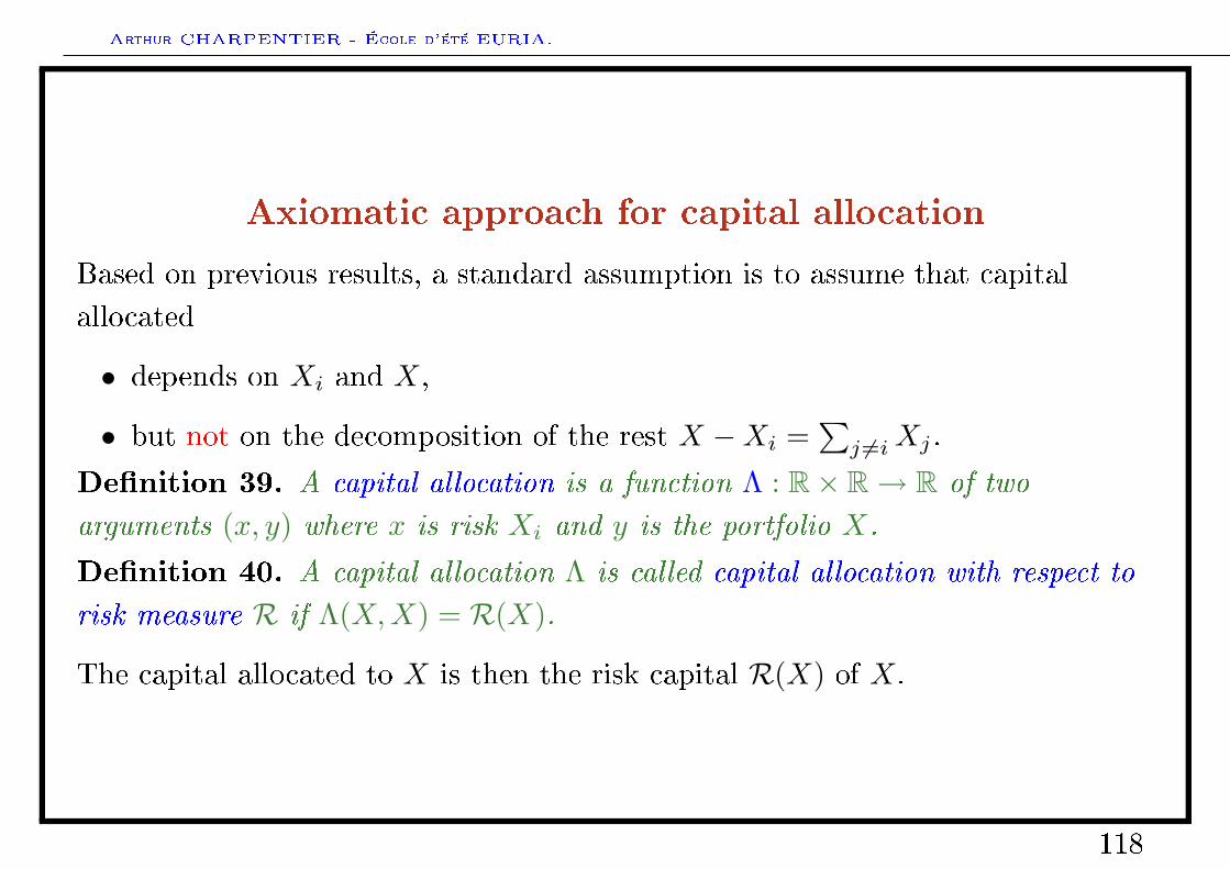
Axiomatic approach for capital allocation
Based on previous results, a standard assumption is to assume that capitalallocated
• depends on Xi and X,
• but not on the decomposition of the rest X −Xi =∑j 6=iXj .
Denition 39. A capital allocation is a function Λ : R× R→ R of two
arguments (x, y) where x is risk Xi and y is the portfolio X.
Denition 40. A capital allocation Λ is called capital allocation with respect to
risk measure R if Λ(X,X) = R(X).
The capital allocated to X is then the risk capital R(X) of X.
118
Arthur CHARPENTIER - École d'été EURIA.
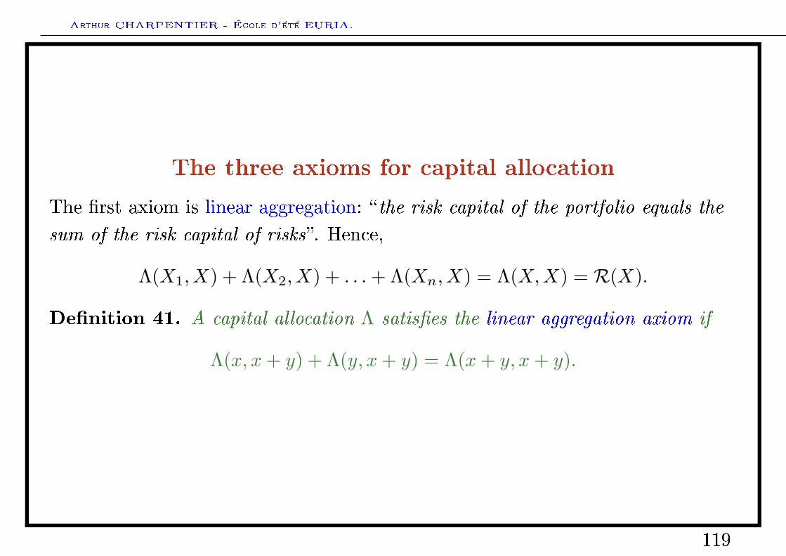
The three axioms for capital allocation
The rst axiom is linear aggregation: the risk capital of the portfolio equals the
sum of the risk capital of risks. Hence,
Λ(X1, X) + Λ(X2, X) + . . .+ Λ(Xn, X) = Λ(X,X) = R(X).
Denition 41. A capital allocation Λ satises the linear aggregation axiom if
Λ(x, x+ y) + Λ(y, x+ y) = Λ(x+ y, x+ y).
119
Arthur CHARPENTIER - École d'été EURIA.
The three axioms for capital allocation
The second axiom is diversication: the risk capital for a component should not
exceed the overall risk capital of the risk considered as a stand-alone portfolio.Hence,
Λ(Xi, X) ≤ Λ(Xi, Xi) for all i = 1, ..., n.
Denition 42. A capital allocation Λ saties the diversication axiom if
Λ(x, y) ≤ Λ(x, x).
120
Arthur CHARPENTIER - École d'été EURIA.
The three axioms for capital allocation
The third axiom is continuity: small changes to the portfolio have a limited
eect on the risk capital . Hence,
Λ(Xi, X + εXi) ∼ Λ(Xi, X) if εissmall.
Denition 43. A capital allocation Λ saties the continuity axiom if
limε→0
Λ(x, y + εy) = Λ(x, y).
121
Arthur CHARPENTIER - École d'été EURIA.
Questions about capital allocation axioms
The existence issue: given a risk measure R, is it possible to derive capitalallocations satisfying those axioms ?
The completeness issue: if the allocation exists, is it unique ? If not, is it possibleto add more axioms ?
The explicit formulation issue: given a risk measure R, is it possible to specifycapital allocation?
122
Arthur CHARPENTIER - École d'été EURIA.
Existence of capital allocation
Recall that a risk measure is
• (positively) homogeneous if R(λX) = λR(X), λ ≥ 0,
• subadditive if R(X + Y ) ≤ R(X) +R(Y ).
If R is a positively homogeneous and subadditive risk measure such that thefollowing functional derivative
limε→0
R(X + εZ)−R(X)ε
exists for every Z, then
Λ(x, y = limε→0
R(y + εx)−R(y)ε
.
123
Arthur CHARPENTIER - École d'été EURIA.
Unicity of capital allocation based on RBased on the three axioms, the risk capital allocation Λ is uniquely determinedas the derivative of the risk measure R at X in direction of risk Xi.
124
Arthur CHARPENTIER - École d'été EURIA.
Examples of capital allocation: standard deviation
For a risk measure based on standard deviation,
R(X) = E(X) + λ ·√var(X),
the derivative can be derived simply as
Λ(X,Y ) = E(X) + λ · cov(X,Y )√var(X)
.
125
Arthur CHARPENTIER - École d'été EURIA.
Examples of capital allocation: expected shortfall
Here also an explicit expression can be derived. If
R(X) =1
1− α
∫ 1
α
VaR(X,u)du =E(X · I(X > VaR(X,α)))
1− α
(continuous random variable), then
Λ(Xi, X) =1
1− α
∫xi · I(X > VaR(X,α))dFXi
(xi).
If P(X = V aR(X,α)) > 0, set β =P(X ≤ V aR(X,α))− α
P(X = V aR(X,α)), then
Λ(Xi, X) =1
1− α
(∫xi · I(X > VaR(X,α))dFXi
(xi) + β
∫xi · I(X = VaR(X,α))dFXi
(xi)·).
126
Arthur CHARPENTIER - École d'été EURIA.
Examples of capital allocation: Value-at-Risk
The VaR is not subadditive, and thus there does not exist a linear, diversifyingcapital allocation with respect to VaR. Nevertheless, the directional derivative
limε→0
V aR(X + εXi, α)− V aR(X,α)ε
might exist for certain portfolios X. This was suggested by Hallerbach (1999),and works well - under continuity assumptions (Tasche (1999) or Gouriéroux,Laurent & Scaillet (2000)).
Alternative is to write V aR(X,α) = E(X) + λ(X) ·√var(X), and to use a
covariance allocation:
if R(X)) = E(X) + λ ·√var(X), then Λ(X,Y ) = E(X) + λ · cov(X,Y )√
var(X).
This technique is very popular in credit risk applications (see Kalkbrener et al.
(2004)).
127
Arthur CHARPENTIER - École d'été EURIA.
And nally a similar idea is to write V aR(X,α) = TV aR(X, a(X)) for some a(·)with values in [0, 1], and to consider capital allocation based on TVaR (seeOverbeck (2000)).
Numerical example based on a simulated portfolio
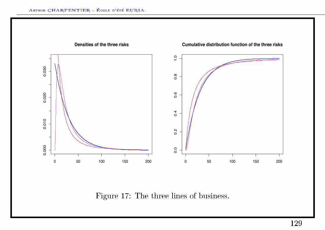
Consider three lines of business, with rather dierent behaviors,
• an exponential distribution X1 ∼ E(0.03), E(X1) ∼ 33,
• a log-normal distribution X2 ∼ LN(3, 1), E(X2) ∼ 33,
• a Pareto distribution X3 ∼ P(2, 30), E(X3) ∼ 33,
Assume further that the three risks are independent.
128
Arthur CHARPENTIER - École d'été EURIA.
0 50 100 150 200
0.000
0.010
0.020
0.030
Densities of the three risks
0 50 100 150 200
0.0
0.2
0.4
0.6
0.8
1.0
Cumulative distribution function of the three risks
Figure 17: The three lines of business.
129
Arthur CHARPENTIER - École d'été EURIA.
risk 1
risk 2
risk 3
Allocation of the pure premium
risk 1risk 2
risk 3
Allocation based on 90%!TVaR
risk 1
risk 2
risk 3
Allocation based on 95%!TVaR
risk 1
risk 2
risk 3
Allocation based on stop!loss distance
risk 1
risk 2
risk 3
Relative (proportional) capital allocation ! VaR 90%
risk 1risk 2
risk 3
Relative (proportional) capital allocation ! VaR 99%
risk 1
risk 2
risk 3
Relative (proportional) capital allocation ! Tail VaR 90%
risk 1
risk 2
risk 3
Relative (proportional) capital allocation ! Tail VaR 99%
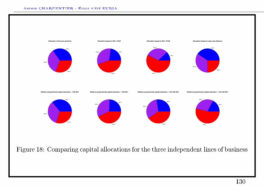
Figure 18: Comparing capital allocations for the three independent lines of business
130
Arthur CHARPENTIER - École d'été EURIA.
Agenda
• General introduction
Financial risks
• Market risks
• Credit risk
• From variance to Value-at-Risk
Risk measures and capital allocation
• Risk measures: an axiomatic introduction
• Risk measures: convexity and coherence
• Capital allocation: an axiomatic introduction
Risk measures and statistical inference
131
Arthur CHARPENTIER - École d'été EURIA.
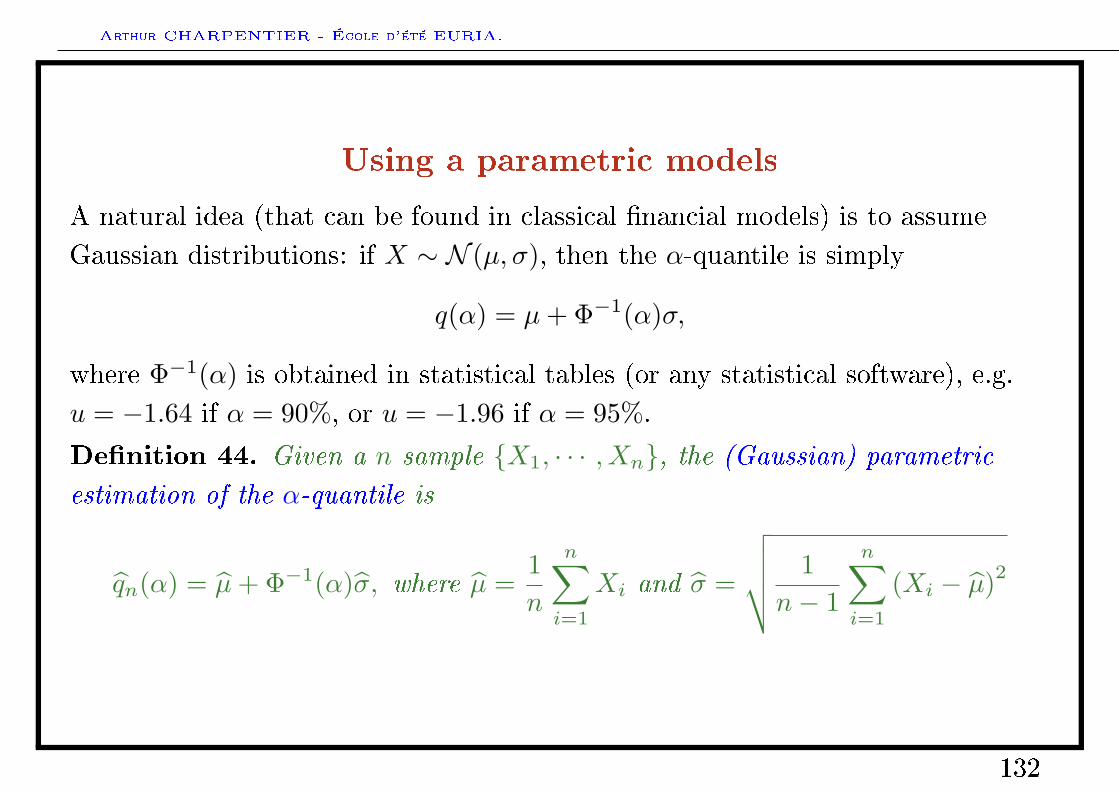
Using a parametric models
A natural idea (that can be found in classical nancial models) is to assumeGaussian distributions: if X ∼ N (µ, σ), then the α-quantile is simply
q(α) = µ+ Φ−1(α)σ,
where Φ−1(α) is obtained in statistical tables (or any statistical software), e.g.u = −1.64 if α = 90%, or u = −1.96 if α = 95%.
Denition 44. Given a n sample X1, · · · , Xn, the (Gaussian) parametric
estimation of the α-quantile is
qn(α) = µ+ Φ−1(α)σ, where µ =1n
n∑i=1
Xi and σ =
√√√√ 1n− 1
n∑i=1
(Xi − µ)2
132
Arthur CHARPENTIER - École d'été EURIA.
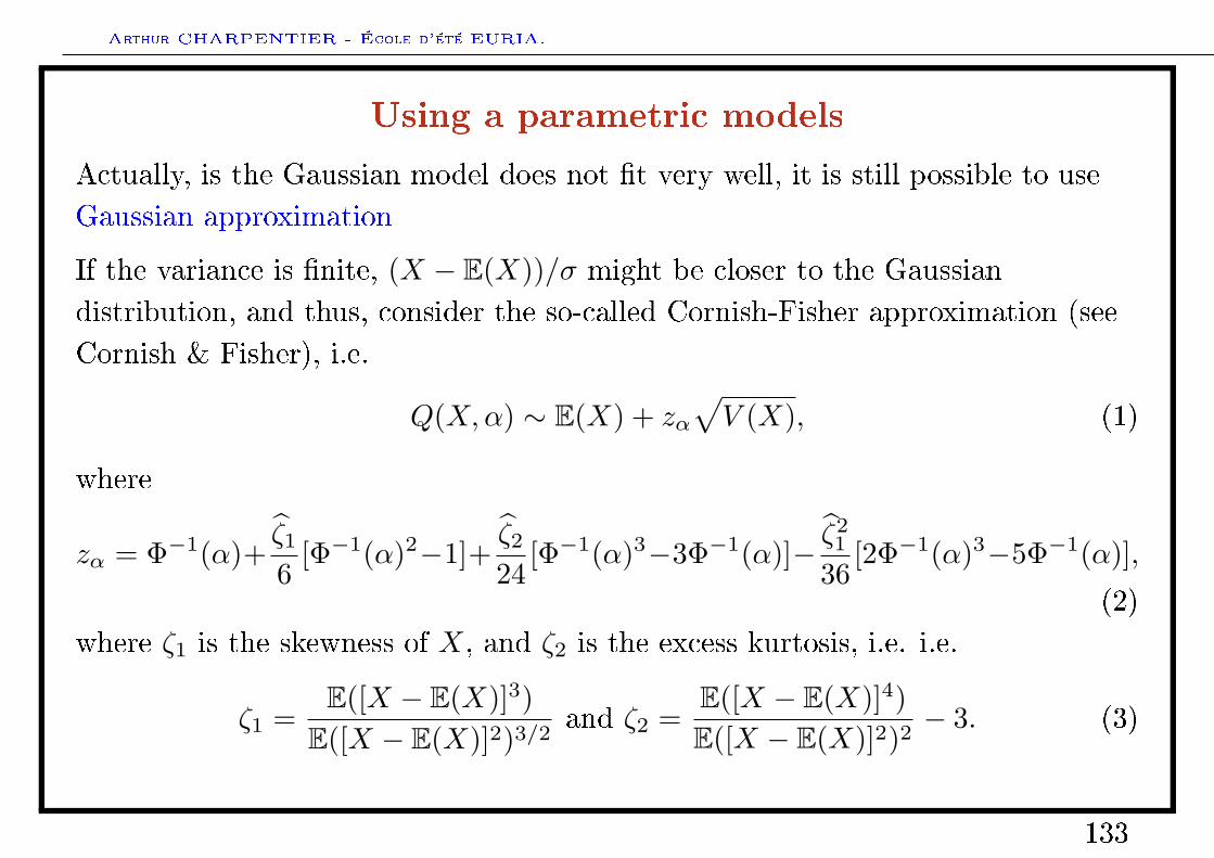
Using a parametric models
Actually, is the Gaussian model does not t very well, it is still possible to useGaussian approximation
If the variance is nite, (X − E(X))/σ might be closer to the Gaussiandistribution, and thus, consider the so-called Cornish-Fisher approximation (seeCornish & Fisher), i.e.
Q(X,α) ∼ E(X) + zα√V (X), (1)
where
zα = Φ−1(α)+ζ16
[Φ−1(α)2−1]+ζ224
[Φ−1(α)3−3Φ−1(α)]− ζ21
36[2Φ−1(α)3−5Φ−1(α)],
(2)where ζ1 is the skewness of X, and ζ2 is the excess kurtosis, i.e. i.e.
ζ1 =E([X − E(X)]3)
E([X − E(X)]2)3/2and ζ2 =
E([X − E(X)]4)E([X − E(X)]2)2
− 3. (3)
133
Arthur CHARPENTIER - École d'été EURIA.
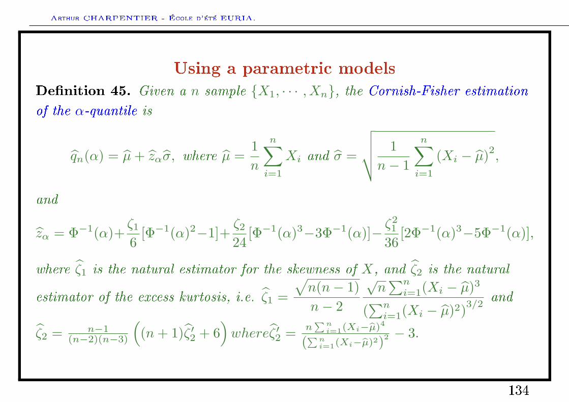
Using a parametric models
Denition 45. Given a n sample X1, · · · , Xn, the Cornish-Fisher estimation
of the α-quantile is
qn(α) = µ+ zασ, where µ =1n
n∑i=1
Xi and σ =
√√√√ 1n− 1
n∑i=1
(Xi − µ)2,
and
zα = Φ−1(α)+ζ16
[Φ−1(α)2−1]+ζ224
[Φ−1(α)3−3Φ−1(α)]− ζ21
36[2Φ−1(α)3−5Φ−1(α)],
where ζ1 is the natural estimator for the skewness of X, and ζ2 is the natural
estimator of the excess kurtosis, i.e. ζ1 =
√n(n− 1)n− 2
√n∑ni=1(Xi − µ)3
(∑ni=1(Xi − µ)2)3/2
and
ζ2 = n−1(n−2)(n−3)
((n+ 1)ζ ′2 + 6
)whereζ ′2 = n
∑ni=1(Xi−µ)4
(∑ni=1(Xi−µ)2)2 − 3.
134
Arthur CHARPENTIER - École d'été EURIA.
Using a parametric models
More generally, if FX ∈ F = Fθ, θ ∈ Θ (assumed to be continuous),qX(α) = F−1
θ (α), and thus, a natural estimator is
qX(α) = F−1
θ(α), (4)
where θ is an estimator of θ (maximum likelihood, moments estimator...).
135
Arthur CHARPENTIER - École d'été EURIA.
Nonparametric statistics: cdf
Soit Fn(x) la fonction de répartition empirique
Fn(x) =1n
n∑i=1
1(X ≤ x)
D'après la loi des grands nombres
Fn(x)→ F (x) si n→∞
de plus la convergence est uniforme (théorème de Glivnko-Cantelli)
supx∈R|Fn(x)− F (x)| → 0 si n→∞
Le théorème central limite garantie aussi que√n[Fn(x)− F (x)] L→ N (0, F (x)[1− F (x)]) si n→∞
136
Arthur CHARPENTIER - École d'été EURIA.
De plus, au sens des distributions,
√n[Fn(x)− F (x)]
d→ BF (x)
où (Bt)t∈[0,1] est un Pont Brownien, i.e.
Bt = Wt − tW1
où (Wt)t≥0 est un mouvement Brownien standard.
137
Arthur CHARPENTIER - École d'été EURIA.
Nonparametric statistics: quantile
La fonction quantile empirique est Qn(·) dénie par F−1n , i.e.
Q−1n (u) = infx ∈ R, Fn(x) ≥ u pour u ∈ (0, 1).
On note (Xi:n) la statistique d'ordre associée à un échantillon (Xi). Onsupposera que F est continue
Q−1n (u) = Xk:n où
k − 1n
< u ≤ k
n.
La convergence uniforme de Fn vers F assure la convergence des quantilesempiriques,
Si F est absolument continue, de densité f , et si f(Q(u)) > 0 pour u ∈ (0, 1),alors
√n[Qn(u)−Q(u)] L→ N
(0,u(1− u)f2(Q(u))
)si n→∞
138
Arthur CHARPENTIER - École d'été EURIA.
Using a nonparametric estimator
For continuous distribution q(α) = F−1X (α), thus, a natural idea would be to
consider q(α) = F−1X (α), for some nonparametric estimation of FX .
Denition 46. The empirical cumulative distribution function FX , based on
sample X1, . . . , Xn is Fn(x) =1n
n∑i=1
1(Xi ≤ x).
Denition 47. The kernel based cumulative distribution function, based on
sample X1, . . . , Xn is
Fn(x) =∫ +∞
−∞
(t− xh
)dFn(t) =
1nh
n∑i=1
∫ x
−∞k
(Xi − th
)dt =
1n
n∑i=1
K
(Xi − xh
)
where K(x) =∫ x
−∞k(t)dt, k being a kernel and h the bandwidth.
139
Arthur CHARPENTIER - École d'été EURIA.
Smoothing nonparametric estimators
Two techniques have been considered to smooth estimation of quantiles, eitherimplicit, or explicit.
• consider a linear combinaison of order statistics,
The classical empirical quantile estimate is simply
Qn (p) = F−1n
(i
n
)= X(i) = X([np]) where [·] denotes the integer part. (5)
The estimator is simple to obtain, but depends only on one observation. Anatural extention will be to use - at least - two observations, if np is not aninteger. The weighted empirical quantile estimate is then dened as
Qn (p) = (1− γ)X([np]) + γX([np]+1) where γ = np− [np] .
140
Arthur CHARPENTIER - École d'été EURIA.
0.0 0.2 0.4 0.6 0.8 1.0
24
68
The quantile function in R
probability level
quan
tile
leve
l
type=1type=3type=5type=7
0.0 0.2 0.4 0.6 0.8 1.0
23
45
67
The quantile function in R
probability levelqu
antil
e le
vel
type=1type=3type=5type=7
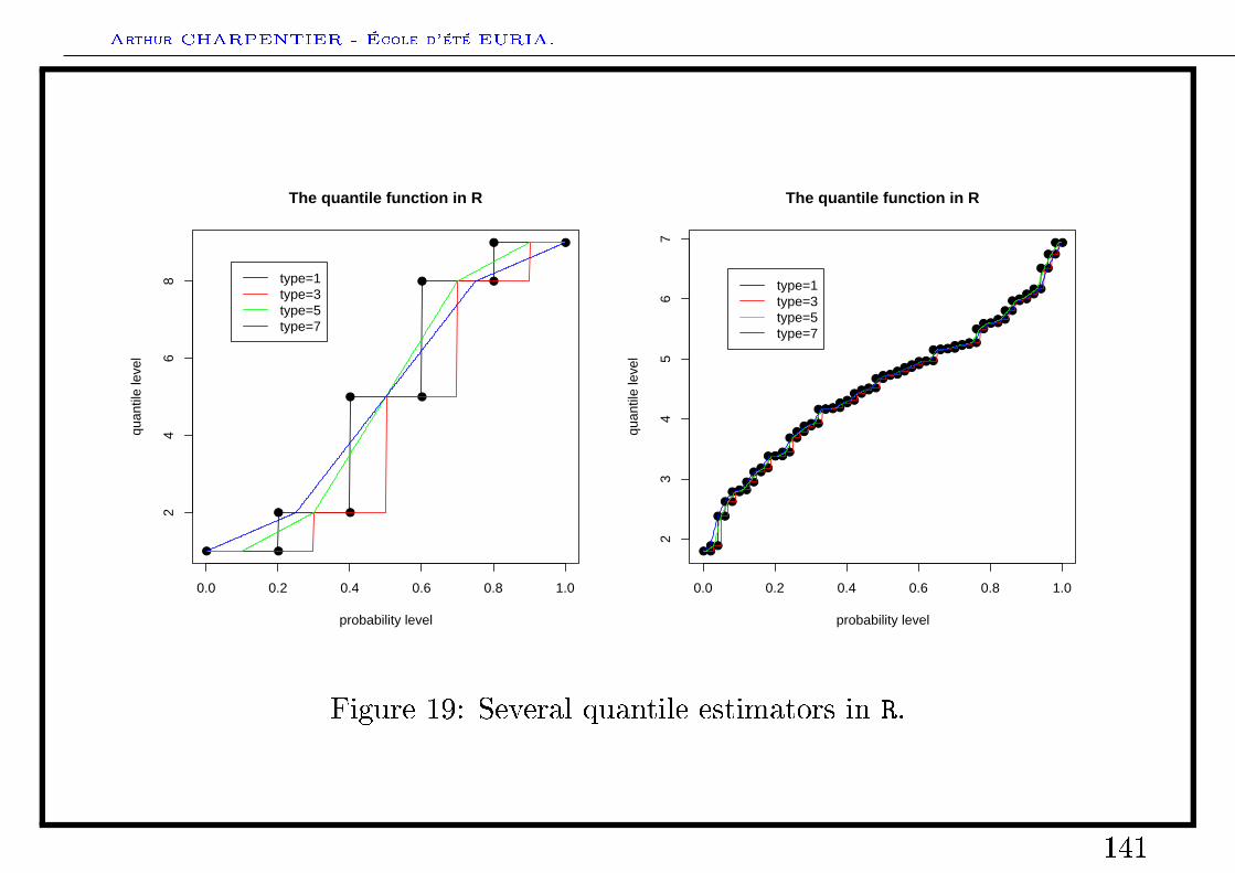
Figure 19: Several quantile estimators in R.
141
Arthur CHARPENTIER - École d'été EURIA.
Smoothing nonparametric estimators
In order to increase eciency, L-statistics can be considered i.e.
Qn (p) =n∑i=1
Wi,n,pXi:n =n∑i=1
Wi,n,pF−1n
(i
n
)=∫ 1
0
F−1n (t) k (p, h, t) dt (6)
where Fn is the empirical distribution function of FX , where k is a kernel and h abandwidth. This expression can be written equivalently
Qn (p) =n∑i=1
[∫ in
(i−1)n
k
(t− ph
)dt
]X(i) =
n∑i=1
[(in − ph
)−
(i−1n − ph
)]X(i)
(7)
where again (x) =∫ x
−∞k (t) dt. The idea is to give more weight to order statistics
X(i) such that i is closed to pn.
142
Arthur CHARPENTIER - École d'été EURIA.
E.g. the so-called Harrell-Davis estimator is dened as
Qn(p) =n∑i=1
[∫ in
(i−1)n
Γ(n+ 1)Γ((n+ 1)p)Γ((n+ 1)q)
y(n+1)p−1(1− y)(n+1)q−1
]Xi:n,
• nd a smooth estimator for FX , and then nd (numerically) the inverse,
The α-quantile is dened as the solution of FX qX(α) = α.
If Fn denotes a continuous estimate of F , then a natural estimate for qX(α) isqn(α) such that Fn qn(α) = α, obtained using e.g. Gauss-Newton algorithm.
143
Arthur CHARPENTIER - École d'été EURIA.
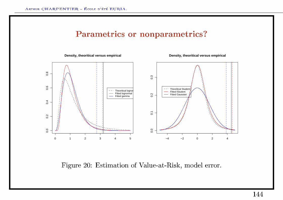
Parametrics or nonparametrics?
0 1 2 3 4 5
0.0
0.2
0.4
0.6
0.8
Density, theoritical versus empirical
Theoritical lognormalFitted lognormalFitted gamma
−4 −2 0 2 4
0.0
0.1
0.2
0.3
Density, theoritical versus empirical
Theoritical StudentFitted lStudentFitted Gaussian
Figure 20: Estimation of Value-at-Risk, model error.
144
Arthur CHARPENTIER - École d'été EURIA.
Using extreme value results, a semi-parametric approach
Quantile estimation based on extreme value results can be seen as semiparametric. Given a n-sample Y1, . . . , Yn, let Y1:n ≤ Y2:n ≤ . . .≤ Yn:n denotesthe associated order statistics. One possible method is to usePickands-Balkema-de Haan theorem. The idea is to assume that for u largeenough, Y − u given Y > u has a Generalized Pareto distribution withparameters ξ and β, which can be estimated using standard maximum likelihoodtechniques. And therefore, if u = Yn−k:n for k large enough, and if ξ>0, denoteby βk and ξk maximum likelihood estimators of the Genralized Paretodistribution of sample Yn−k+1:n − Yn−k:n, ..., Yn:n − Yn−k:n,
Q(Y, α) = Yn−k:n +βk
ξk
((nk
(1− α))−ξk
− 1
)(8)
145
Arthur CHARPENTIER - École d'été EURIA.
Using extreme value results, a semi-parametric approach
An alternative is to use Hill's estimator if ξ > 0,
Q(Y, α) = Yn−k:n
(nk
(1− α))−ξk
, (9)
where ξk =1k
k∑i=1
log Yn+1−i:n − log Yn−k:n (if ξ > 0).
146
Arthur CHARPENTIER - École d'été EURIA.
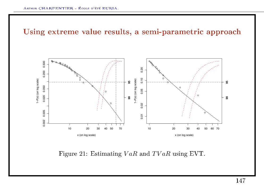
Using extreme value results, a semi-parametric approach
10 20 30 40 50 70
0.00
20.
005
0.02
00.
050
0.20
00.
500
x (on log scale)
1!F(
x) (o
n lo
g sc
ale)
9995
9995
10 20 30 40 50 60 70
0.01
0.02
0.05
0.10
0.20
x (on log scale)1!
F(x)
(on
log
scal
e)
9995
9995
Figure 21: Estimating V aR and TV aR using EVT.
147
Recommended


![Genielog Projet Slides[1]](https://img.pdfslide.fr/doc/110x75/5571fcd0497959916997fb66/genielog-projet-slides1.jpg)