Embed Size (px)
Citation preview
N° d’ordre Année 2012
THESE DE L’UNIVERSITE DE LYON
délivrée par
L’UNIVERSITE CLAUDE BERNARD LYON 1
et préparée en cotutelle avec
L’UNIVERSITE ARAB DE BEYROUTH
ECOLE DOCTORALE
DIPLOME DE DOCTORAT
(arrêté du 7 août 2006 / arrêté du 6 janvier 2005)
soutenue publiquement le 21 Juin 2012
par
M. FARHAT Ayman
TITRE :
Calculs théoriques avec le couplage spin orbitales pour les molécules diatomiques YS, YN, ZrS,
et ZrN
JURY :
M. Abdul-Rahman ALLOUCHE (Examinateur)
M. Florent-Xavier GADEA (Rapporteur)
Mme. Gilberte CHAMBAUD (Rapporteur)
M. Mahmoud KOREK (Codirecteur)
Mme. Monique FRECON (Examinateur) M. Miguel A. L. MARQUES (Codirecteur)

i
© 2012
Ayman K. Farhat
All rights reserved

ii
I would like to dedicate this thesis to my loving parents …

iii
I hereby declare that I am the sole author of this thesis. This is a true copy of the thesis, including any required final revisions, as accepted by my examiners.
iv
Theoretical Calculations with Spin Orbit Effects of the Diatomic Molecules
YS, YN, ZrS, ZrN
Abstract
This dissertation is dedicated to the ab initio study of the electronic structures of the polar
diatomic molecules YN, YS, ZrN, and ZrS. The identification of these molecules in the spectra
of stars as well as the lack in literature on the electronic structures of these molecules motivated
the present study. Theoretical calculations are useful in this respect since they can provide
important data for the properties of the ground and excited electronic states that are not available
from experimental means. In the present work the ab initio calculations were performed at the
complete active space self-consistent field method (CASSCF) followed by multireference single
and double configuration interaction method (MRSDCI). The Davidson correction noted as
(MRSDCI+Q) was then invoked in order to account for unlinked quadruple clusters. The
calculations were performed on two stages in the first spin orbit effects were neglected while in
the second type of calculations spin orbit effects were included by the method of effective core
potentials. All of the calculations were done by using the computational physical chemistry
program MOLPRO and by taking advantage of the graphical user interface Gabedit. In the
present work potential energy curves were constructed and spectroscopic constants computed,
along with permanent electric dipole moments, internal molecular electric fields, and vibrational-
rotational energy structures. We detected in the ZrS molecule several degenerate vibrational
energy levels which can be used to search for possible variations of the fine structure constant α
and the electron to proton mass ratio μ in three S-type stars, named Rand, RCas, and χCyg. A
comparison with experimental and theoretical data for most of the calculated constants
demonstrated a good accuracy for our predictions giving a percentage relative difference that
ranged between 0.1% and 10%. Finally, we expect that the results of the present work should
invoke further experimental investigations for these molecules.
Key Words
Ab initio Calculations, multireference configuration interaction, diatomic molecules, spin orbit effects, spectroscopic constants, fine structure constant, electric dipole moment of the electron.
v
Calculs théoriques avec le couplage spin orbitales pour les molécules diatomiques YS, YN, ZrS, et ZrN
Abstrait
Cette thèse est consacrée à l'étude ab initio des structures électroniques des molécules
diatomiques polaires YN, YS, ZrN, et ZrS. Cette étude est motivé par le manque d’informations
dans la littérature sur la structure électronique de ces molécules, alors qu’elles ont clairement été
identifiées dans le spectre de certaines étoiles. Des calculs théoriques sont ainsi nécessaire puis
qu’ils peuvent fournir d'importantes informations quant aux propriétés des états électroniques
fondamentaux et excités qui ne sont pas accessibles expérimentalement. Dans ce
travail les calculs ab initio ont été effectués par la méthode du champ auto-cohérent de l'espace
actif complet (CASSCF), suivie par l' interaction de configuration multiréférence (MRSDCI).
La correction de Davidson, notée (MRSDCI+ Q), a ensuite été appliquée pour rendre compte
de clusters ou agrégats quadruples non liés. Les calculs ont été effectués selon deux schémas.
Dans le premier les effets spin-orbite ont été négligés alors que dans le second les effets spin-
orbite ont été inclus par la méthode des potentiels de noyau efficaces. Tous les calculs ont été
effectués en utilisant le programme de calcul de chimie physique MOLPRO et en tirant parti de
l’interface graphique Gabedit. Les courbes d'énergie potentielle ont été construites et des
constantes spectroscopiques calculées, ainsi que les moments dipolaires électriques permanent,
les champs électriques moléculaire intenses et les structures énergétiques de vibration-rotation.
Nous avons détecté dans la molécule ZrS plusieurs niveaux vibrationnels dégénérés ceux-ci
peuvent être utilisés pour rechercher les variantes possibles de la constante de structure fine α et
du rapport de masse μ de l’electron par rapport au proton dans trois étoiles de type S, du nom
de Rand, les RCas, et χCyg. La comparaison des données expérimentales et théoriques pour la
plupart des constantes calculées a montré une bonne précision pour nos prédictions avec une
différence relative (en pourcentage) qui varie entre 0,1% et 10%. Ces résultats devraient ainsi
mener à des études expérimentales plus poussées pour ces molécules.
Mots-Cles
Ab initio Calculassions, Multireference configuration interaction, Diatomique molécules, Spin
orbite effets, Spectroscopique constants, Fine structure constant, Electric dipôle moment of the
electron.
Acknowledgments
vi
Acknowledgments
I wish to express my profound sense of gratitude to everyone who made this thesis possible.
Prof. Mahmoud Korek, my thesis supervisor, who guided me through PhD studies. His patience,
generosity and support made this work possible. His constant availability even during his
sabbatical gave me a sense of comfort that helped steer me throughout this endeavor. I profusely
thank him for having spared his time to discuss with me several questions and ideas that evolved
in my mind from time to time and for having initiated and stimulated my research interests.
Prof. Miguel A. L. Marques, my thesis supervisor, for his friendship, encouragement, and
numerous fruitful discussions. His expertise in computational modeling improved my research
skills and prepared me for future challenges. I wish to express my profound sense of gratitude to
him for his continuous support all the way through, which enabled me to successfully complete
this work.
I would like to acknowledge the financial, academic and technical support given by the
University of Claude Bernard - Lyon 1, especially during my stay in France. I also seize this
opportunity to thank Beirut Arab University which gave us the freedom and access to use its
Computational Lab resources.
My special appreciation goes to all the members of the Theoretical and Computational
Spectroscopy Group at the Laboratoire de Physique de la Matière Condensée et Nanostructures,
and special thanks go to Prof. Silvana Botti for her kindness and support. Special thanks also go
to Dr. Saleh abdul-al for the fruitful and technical discussions we had at the beginning of this
research project.
My mom and dad for having an unconditional faith in me, teaching me to “hitch my wagon to a
star”, constantly supporting my decisions and being an endless source of love, a strong safety net
I could always fall back on. My grandparents and brother for being a precious part in my life. My
friends and colleagues whom I shared wonderful times much laughter and many stimulating and
enriching discussions.
Contents
v
Contents
Abstract iv Abstrait v Acknowledgments vi Introduction 1 Chapter 1. Many Body Problems in Atoms and Molecules 7
I. Second Quantization and Many Body Problems 7 II. Ladder Operators in the Simple Harmonic Oscillator 9 III. The Fock Space in Quantum Theory 11 IV. N-particle wave functions 13 V. The Creation and Annihilation Operators in Second Quantization 17
V. 1. Products of Creation and Annihilation Operators 18 VI. Configuration State Functions 19 VII. The Representation of One and Two Electron Operators in Second Quantization 20 VIII. The Molecular Electronic Hamiltonian 22
VIII.1. The Hamiltonian of a Two Body Interaction 23 IX. Spin in Second Quantization 24
IX. 1. Spin Functions 25 IX. 2. Spin Operators 26 IX. 3. Spin Orbit Fine Structure Operator 27
X. The Variation Principle 29 XI. The Underlying Theoretical Basis – The Born Oppenheimer Approximation 31 XII. The Hartree Fock Approximation 32
Contents
vi
XIII. The Roothan-Hall Self Consistent Field Equation 34 XIV. Post Hartree Fock Calculations 35
XIV. 1. Multi Configuration Self Consistent Field Theory MCSCF 36 XIV. 2. Configuration Interaction 37 XIV. 3. Multireference CI Wave Function MRSDCI 39 XIV. 4. Davidson’s Correction 39
XV. Spin Orbit Effects 40 XVI. References 44
Chapter 2. Canonical Function’s Approach for Molecular Vibrations and Rotations 45
I. Canonical Function’s Approach 45 II. The Rotational Schrödinger Equation 47 III. Finding the Pure Vibrational Wavefunction 49 IV. Canonical Formulation for the First Rotational Harmonic 50 V. Numerical Methods 52
V. 1. Calculations of the Canonical Functions α0(r) and β0(r) 52 VI. References 54
Chapter 3. Results and Discussions 55
I. The Computational Approach 55 II. Electronic Structure Calculations 58
III. A. The Structure of Yttrium Nitride YN 58 III. A.1. Preliminary Works on YN 58 III. A.2. Results on YN 59 III. A.3. The Nature of Bonding in YN 72 III.A. 4. The Vibrational Structure of YN 75 III. A. 5. The Permanent Dipole Moment on YN 81 III. A. 6. The Internal Molecular Electric Fields in YN 82
III. B. The Structure of Zirconium Nitride ZrN 84 III. B. 1. Preliminary Works on ZrN 84 III. B. 2. Results on ZrN 85 III. B. 3. The Bonding Nature in ZrN 97 III. B. 4. The Vibrational Structure of ZrN 98 III. B. 5. The Permanent Dipole Moment of ZrN 103 III. B. 6. The Internal Molecular Electric Fields in ZrN 105
III. C. Comparison Between 4d Transition Metal Nitrides MN (M=Y,Zr,Nb,…, Cd) 106
Contents
vii
III. D. The Structure of Zirconium Sulfide ZrS 109 III. D. 1. Preliminary Works on ZrS 109 III. D. 2. Results on ZrS 111 III. D. 3. The Nature of Bonding in ZrS 122 III. D. 4. The Vibrational Structure of ZrS 124 III. D. 5. The Permanent Dipole Moment of ZrS 132 III. D. 6. The Internal Molecular Electric Field in ZrS 134
III. E. The Structure of Yttrium Sulfide YS 135 III. E. 1. Preliminary Works on YS 135 III. E. 2. Results on YS 136 III. E. 3. The Nature of Bonding in YS 141 III. E. 4. The Vibrational Structure of YS 142 III. E. 5. The Permanent Dipole Moment of YS 143 III. E. 6. The Internal Molecular Electric Field in YS 144
III. F. Comparison Between 4d Transition Metal Sulfides MS (M=Y,Zr,Nb,…, Cd) 145 IV. References 149
Chapter 4. Summary and Outlook 154 Résumé et Perspectives (Français) 157 Appendix I. Splitting Figures between Spin Orbit Electronic States 160
Appendix II. Results of Vibrational Calculations 169
Appendix III. Dipole Moment Results 184
Short Curriculum Vitae 187
Introduction
1
Introduction
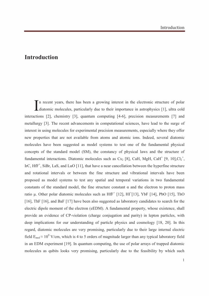
n recent years, there has been a growing interest in the electronic structure of polar
diatomic molecules, particularly due to their importance in astrophysics [1], ultra cold
interactions [2], chemistry [3], quantum computing [4-6], precision measurements [7] and
metallurgy [3]. The recent advancements in computational sciences, have lead to the surge of
interest in using molecules for experimental precision measurements, especially where they offer
new properties that are not available from atoms and atomic ions. Indeed, several diatomic
molecules have been suggested as model systems to test one of the fundamental physical
concepts of the standard model (SM), the constancy of physical laws and the structure of
fundamental interactions. Diatomic molecules such as Cs2 [8], CaH, MgH, CaH+ [9, 10],Cl2+,
IrC, HfF+, SiBr, LaS, and LuO [11], that have a near cancellation between the hyperfine structure
and rotational intervals or between the fine structure and vibrational intervals have been
proposed as model systems to test any spatial and temporal variations in two fundamental
constants of the standard model, the fine structure constant α and the electron to proton mass
ratio μ. Other polar diatomic molecules such as HfF+ [12], HI+[13], YbF [14], PbO [15], ThO
[16], ThF [16], and BaF [17] have been also suggested as laboratory candidates to search for the
electric dipole moment of the electron (eEDM). A fundamental property, whose existence, shall
provide an evidence of CP-violation (charge conjugation and parity) in lepton particles, with
deep implications for our understanding of particle physics and cosmology [18, 20]. In this
regard, diatomic molecules are very promising, particularly due to their large internal electric
field Emol ≈ 109 V/cm, which is 4 to 5 orders of magnitude larger than any typical laboratory field
in an EDM experiment [19]. In quantum computing, the use of polar arrays of trapped diatomic
molecules as qubits looks very promising, particularly due to the feasibility by which such
I
Introduction
2
simple systems may be scaled up to form large networks of coupled qubits [20-33]. Many linear
molecules that have a variety of long lived internal electronic states have been proposed as a
mean to address and manipulate qubit states 1,0 [34]. Another promising new approach for
realizing a quantum computer is based on using the vibrational states of molecules to represent
qubits [35]. In this approach, quantum logic operations are performed to induce the desired
vibrational transitions [36], where by using more vibrational states it may be possible to
represent quantum information units having more than two qubit states (i.e. 0 , 1 , 2 , 3 )
[36]. In spectroscopic studies, the electronic structure of transition metal diatomic molecules
should form a viable tool to test for the abundance of transition metal diatomics in the spectra of
stars [37, 42]. Many transition metal diatomic oxides, sulfides and nitrides have been detected in
the spectra of S and M type stars [43, 44]. Precise spectroscopic data are necessary for a
meaningful search for these molecules in complex stellar spectra. In industrial processes such as
catalysis and organometallic chemistry, Transition metal nitrides are important in the fixation of
nitrogen in industrial, inorganic and biological systems [45, 46]. In high temperature material
applications, within the group of refractory metal nitrides (Ti, Zr, Hf, Nb) titanium and
zirconium nitrides are the most promising hardening additives, which are used for raising the
high-temperature strength of sintered molybdenum and provide high enough ductility parameters
at a temperature up to 2000°C [47]. In ultra-cold interactions the recent experimental
achievements in producing an ultra-cold sample of the heternonuclear diatomic molecule SrF by
researchers at Yale [48] offers a new possibility for producing ultra-cold samples of several
heteronuclear diatomics as the transition metal diatomics of interest in the present work. Such
achievements in ultracold techniques on new molecules are hindered by the lack in the
spectroscopic studies of their electronic structures. In these respects, theoretical investigations
for the spectroscopic properties of heteronuclear diatomic molecules are extremely useful in any
future production of ultracold samples of heteronuclear diatomic molecules. Transition metal
diatomics represent simple metal systems where d electrons participate in the bonding [49].
These molecules provide models for understanding the bonding and reactivity in transition metal
systems [50]. The spectroscopic study of transition metal diatomics is difficult particularly due to
the high density of low-lying electronic states associated with partially occupied d orbitals [51,
52].
Introduction
3
Having seen that the electronic structure of heavy transition metal polar diatomic molecules is an
active area of research with many applications in several areas of science, we decided in the
present work to investigate the electronic structure of the mono-nitrides and mono-sulfides of the
transition metals of group III and IV, Yttrium and Zirconium. Owing to their unfilled 4d shells
the transition metals of group III and IV have a complex electronic structure. Their spectra is less
daunting than other transition metals towards the middle of the periodic table. The metal atom
often has many unpaired electrons that can produce a large number of low-lying electronic states
with high values of spin multiplicity and orbital angular momentum, as well as large spin orbit
interactions. These electronic states may perturb one other, thereby complicating their spectra
and making the experimental analysis very difficult. Theoretical calculations are plagued with
similar problems as it is hard to predict the energy order and properties of the low-lying
electronic states. Electronic correlation effects become important when there are many unpaired
electrons and so these molecules provide a challenge for ab initio calculations. Despite these
difficulties, most of the 4d transition metal monoxides and monocarbides have been well studied
partly due to their importance in astrophysics and as models in understanding the chemical
bonding in simple metal systems. In contrast, little data are available for the corresponding
transition metal nitrides and sulfides (MN, MS).
In this work, we perform ab initio calculations for the electronic structure of the mono-nitrides
and mono-sulfides of Yttrium and Zirconium (YS, YN, ZrN, and ZrS). Relativistic spin orbit
effects were included by the method of effective core potentials (ECP). The potential energy
curves (PEC) for the ground and excited electronic states were constructed as a function of the
internuclear distance R. Then by fitting the calculated potential energy curves in to a polynomial
in R several spectroscopic constants were calculated, such as the transition energy Te relative to
the ground state, the harmonic vibrational frequencies ωe, the equilibrium internuclear distances
Re, and the rotational constants Be and De. Then based on the calculated PECs vibro-rotational
calculations were performed for the vibrational and rotational energy levels of each molecule.
Various physical properties were also computed, such as the permanent electric dipole moment,
and the internal molecular electric field. The bonding nature in each of the investigated
molecules was also analyzed in terms of molecular orbital configurations. A comparison is made
between the calculated values of the present work for the bond distances, vibrational frequencies
Introduction
4
and dipole moments to the remaining series of 4d transition metal mono-nitrides (ZrN, NbN, …,
CdN) and mono-sulfides (ZrS, NbS, …, CdS). The comparison between the different species of
transition metal mono-nitrides (MN) and mono-sulfides (MS) should give an idea on the
variation of molecular properties across the series of 4d transition metals in the periodic table.
Throughout this thesis, we try to validate our theoretical results by comparing the calculated
values of the present work to the experimental and theoretical values in literature. The
comparison between the values of the present work to the experimental and theoretical results
shows a very good agreement. The small percentage relative error, of less than 10% reported in
our calculations for all of the molecular constants, reflects the nearly exact representation of the
true physical system by the wave functions used in our calculations. The extensive results in the
present work on the electronic structures with relativistic spin orbit effects of the molecules YN,
ZrN, YS, and ZrS are presented here for the first time in literature. A preprint for the results of
the present work has been requested by an experimental research group working at Yale under
the supervision of Prof. David Demille.
Introduction
5
References:
1. A. R. Rau., Astronomy-Inspired Atomic and Molecular Physics., Springer, 1 edition (2002). 2. A. Ridinger., Towards Ultracold Polar 6Li40K molecules., Südwestdeutscher Verlag für
Hochschulschriften., (2011). 3. M. A. Duncan., The Binding in Neurtral and Cataionic 3d and 4d Transition Metal Monoxides and
Sulfides., Advances in Metal and Semiconductor Clusters., 5, 347., Elsevier (2001). 4. D. DeMille., Phys. Rev. Lett., 88, 067901 (2002). 5. T. Cheng, A. Brown., J. Chem. Phys., 124, 034111 (2006). 6. L. Bomble, P. Pellegrini, P. Chesquière, M. Desouter-Lecomte., Phys. Rev. A., 82, 062323 (2010). 7. D. DeMille, S. Sainis, J. Sage, T. Bergeman, S. Kotochigova, E. Tiesinga., Phys. Rev. Lett., 100,
043202 (2008). 8. D. DeMille, S. Sainis, J. Sage, T. Bergeman, S. Kotochigova, and E. Tiesinga., Phys. Rev. Lett., 100,
043202 (2008). 9. M. Kajita., Phys. Rev. A., 77, 012511 (2008). 10. M. Kajita and Y. Moriwaki., J. Phys. B., 42, 154022 (2009). 11. V. V. Flambaum and M. G. Kozlov., Phys. Rev. Lett., 99, 150801 (2007). 12. E. R. Meyer, J. L. Bohn, M. P. Deskevich., Phys Rev A., 73, 062108 (2006). 13. T. A. Isaev, A. N. Mosyagin, A. V. Titov., Phys. Rev. Lett., 95, 163004 (2005). 14. M. K. Nayak, R. K. Chaudhuri., Chem. Phys. Lett., 419, 191 (2006). 15. A. N. Petrov, A. V. Titov, T. A. Isaev, N. S. Mosyagin, D. Demille., Phys. Rev. A., 72, 022505
(2005). 16. E. R. Meyer, J. L. Bohn., Phys. Rev. A., 78, 010502 (2008). 17. M.G. Kozlov, A. V. Titov, N. S. Mosyagin, and P. V. Souchko., Phys. Rev. A., 56, R3326 (1997). 18. I. B. Khriplovich, and S. K. Lamoreaux., CP-violation Without Strangeness: Electric Dipole
Moments of Particles, Atoms, and Molecules (Springer, Berlin, 1997). 19. M. Pospelov, and A. Ritz., Ann. Phys., 318, 119 (2005). 20. D. DeMille., Phys. Rev. Lett., 88, 067901 (2002). 21. A. Andre, D. DeMille, J. M. Doyle, M. D. Lukin, S. E. Maxwell, P. Rabl, R. J. Schoelkopf and P.
Zoller., Nature Phys., 2, 636 (2006) 22. S. F. Yelin, K. Kirby and R. Cote., Phys. Rev. A., 74, 050301(R) (2006). 23. L. D. Carr, D. DeMille, R. V. Krems and J. Ye., New J. Phys., 11, 055049 (Focus Issue) (2009). 24. R. V. Krems, W. C. Stwalley and B. Friedrich., Eds. Cold molecules: theory, experiment,
applications., (Taylor and Francis, 2009). 25. B. Friedrich and J. M. Doyle., Chem. Phys. Chem., 10, 604 (2009). 26. S. Kotochigova and E. Tiesinga., Phys. Rev. A., 73, 041405(R) (2006). 27 A. Micheli, G. K. Brennen and P. Zoller., Nature Phys., 2, 341 (2006). 28. E. Charron, P. Milman, A. Keller and O. Atabek., Phys. Rev. A., 75, 033414 (2007); Erratum,. Phys.
Rev. A., 77, 039907 (2008). 29. E. Kuznetsova, R. Cote, K. Kirby and S. F. Yelin., Phys. Rev. A., 78, 012313 (2008). 30. K. K. Ni, S. Ospelkaus, M. H. G. de Miranda, A. Peer, B. Neyenhuis, J. J. Zirbel, S. Kotochigova,
P.S. Julienne, D. S. Jin and J. Ye., Science., 322, 231 (2008).
Introduction
6
31. J. Deiglmayr, A. Grochola, M. Repp, K. Mortlbauer, C. Gluck, J. Lange, O. Dulieu, R.Wester and M. Weidemuller., Phys. Rev. Lett., 101, 133004 (2008).
32. S. F. Yelin, D. DeMille and R. Cote., Quantum information processing with ultracold polar molecules, p. 629 (2009).
33. Q. Wei, S. Kais and Y. Chen., J. Chem. Phys., 132, 121104 (2010). 34. K. Mishima, K. Yamashita., J. Chem. Phys., 367, 63 (2010). 35. C. M. Tesch, L. Kurtz, and R. de Vivie-Riedle., Chem. Phys. Lett., 343, 633 (2001). 36. D. Babikov., J. Chem. Phys., 121, 7577 (2004). 37. H. Machara and Y. Y. Yamashita., Pub. Astron. Soc. Jpn 28, 135–140 Spectrosc., 180, 145 (1996). 38. D. L. Lambert and R. E. S. Clegg., Mon. Not. R. Astron. Soc., 191, 367 (1979). 39. Y. Yerle., Astron. Astrophys., 73, 346 (1979). 40. B. Lindgren and G. Olofsson., Astron. Astrophys., 84, 300 (1980). 41. D. L. Lambert and E. A. Mallia., Mon. Not. R. Astron. Soc., 151, 437 (1971). 42. O. Engvold, H. Wo¨hl and J. W. Brault., Astron. Astrophys. Suppl. Ser. Spectrosc., 42, 209 (1980). 43. J. G. Philips and S. P. Davis., J. Astrophys., 229, 867 (1979). 44. J. Jonsson, S. Wallin, B. Lindgreen., J. Mol. Spectrosc., 192, 198 (1998). 45. G. J. Leigh., Science., 279, 506 (1998). 46. Y. Nishinayashi, S. Iwai, and M. Hidai., Science., 279, 540 (1998). 47. I. O. Ershova, Metalloved. Term. Obrab. Met., No. 2, 26 (2003). 48. E. S. Shuman, J. F. Barry, and D. Demille., Nature., 467, 820 (2010). 49. A. J. Sauval., Astron. Astrophys., 62, 295 (1978). 50. S.R. Langhoff, C.W. Bauschlicher Jr., H. Partridge., J. Chem. Phys., 396, 89 (1988). 51. S.R. Langhoff and C.W. Bauschlicher, Jr. Annu. Rev. Phys.Chem., 39, 181 (1989). 52. M. D. Morse., Chem. Rev., 86, 1049 (1986).
Chapter One. Many Body Problems in Atoms and Molecules
7
Chapter One
Many Body Problems in Atoms and Molecules
omputational physical chemistry is primarily concerned with the properties of single
molecules and with their arrangement in periodic trends, homologous series, functional
groups, and crystals. Theoretical calculations have emerged as an important tool for investigating
a wide range of problems in Molecular Physics, Material Science and Chemistry. Within the
recent development of computational methods and more powerful computers, it has become
possible to solve physical and chemical problems that only a few years ago seemed far beyond
the reach of a rigorous quantum-mechanical treatment.
In this section, we turn our attention to the development of approximations which are more
accurate than the independent particle model and can take account of electron correlation effects.
The Hartree-Fock theory followed by the methods of Complete Active Space Self Consistent
Field (CASSCF) and Multi-reference Configuration Interaction (MRCI) play a pivotal role in the
development of approximate treatments of correlation effects. A key feature of these calculations
is the use of the method of second quantization. We therefore start by introducing the second
quantization formalism in quantum mechanics.
I. Second Quantization and Many Body Problems
Second quantization forms the basis of a very powerful technique for developing a theoretical
description of many-body systems. Many-particle physics is formulated in the second
quantization representation, which is also known by the occupation number representation. In the
second quantization formalism theoretical expressions are written in terms of matrix elements of
C
Chapter One. Many Body Problems in Atoms and Molecules
8
operators in a given basis and are manipulated using the algebra of creation and annihilation
operators.
In this section, we briefly describe the second quantization formalism giving sufficient details for
the application which we describe. First, let us observe that the Schrödinger equation can be
easily written down for an atom or, more particularly, a molecule of arbitrary complexity. The
difficulty is usually said to lie not in writing down the appropriate eigenvalue problem but in the
development of accurate approximations to the solutions of this molecular Schrödinger equation.
However, the Schrödinger equation for a system of arbitrary complexity has another problem
associated with it, namely, it applies to a fixed number of particles. In other words the
Schrödinger equation applies to systems in which the number of particles is conserved. However,
in many physical processes the number of particles is not conserved and particles can be created
or destroyed. Then there arises the need for a new approach in quantum mechanics, namely the
second quantization approach, which allows for the creation and destruction of particles.
Let us digress and turn our attention to the equations of motion in relativistic quantum
mechanics. In particular, if following Dirac we write down the eigen-problem for the hydrogen
atom, we find a very different set of solutions to those found in the non-relativistic (Schrödinger)
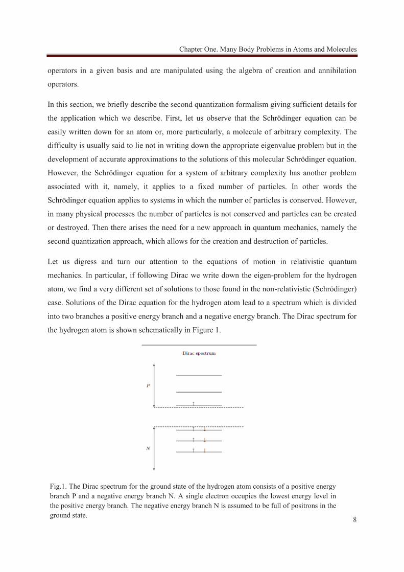
case. Solutions of the Dirac equation for the hydrogen atom lead to a spectrum which is divided
into two branches a positive energy branch and a negative energy branch. The Dirac spectrum for
the hydrogen atom is shown schematically in Figure 1.
Fig.1. The Dirac spectrum for the ground state of the hydrogen atom consists of a positive energy branch P and a negative energy branch N. A single electron occupies the lowest energy level in the positive energy branch. The negative energy branch N is assumed to be full of positrons in the ground state.
Chapter One. Many Body Problems in Atoms and Molecules
9
In the non-relativistic formalism, the ground state of the hydrogen atom consists of a single
electron occupying the lowest energy level in the spectrum. In the relativistic formalism, the
ground state of the hydrogen atom consists of a single electron occupying the lowest energy level
in the positive energy branch of the Dirac spectrum. Dirac famously conjectured that this
electron is prevented from decaying into one of the negative energy states because these states
are themselves filled with electrons. A consequence of this conjecture is that even the simple
hydrogenic atom is an infinity many bodied problem. The electrons filling the negative branch of
the Dirac spectrum are not directly observable. They are positrons. A direct consequence of the
Dirac picture is that the number of electrons in a relativistic system is not conserved. A single
excitation can lead to the formation of an electron-positron pair. In the Dirac picture, it is the
total charge of the system which is conserved. Therefore the use of second quantization is
mandatory in the description of many body problems.
The development of quantum electrodynamics saw the introduction of diagrammatic techniques.
In particular, Feynman [1] in a paper entitled “Space Time approach to Quantum
Electrodynamics”, introduced diagrams which provide not only a pictorial representation of the
microscopic processes but also a precise graphical algebra which is entirely equivalent to other
formulations. It is thus not surprising that second quantization and diagrammatic formulations
emerged as a powerful approach to the quantum many-body problem in non-relativistic quantum
mechanics. Having seen that the second quantization approach to quantum mechanics is
extremely useful in many body problems, we now turn our attention to the mathematical
formalism of second quantization.
II. Ladder Operators in the Simple Harmonic Oscillator
The basic idea behind the second quantization formalism is to rewrite quantum mechanics in
terms of the creation and annihilation operators, which allow for particle creation and
destruction.
It is therefore useful to first review the use of ladder operators in the simple harmonic oscillator.
First we consider the Hamiltonian for the simple harmonic oscillator
.1 12 2 (1)
2 2H p Kx
m
Chapter One. Many Body Problems in Atoms and Molecules
10
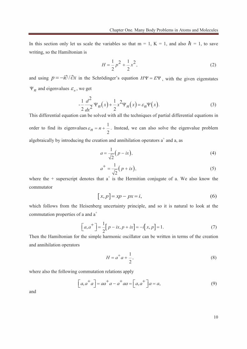
In this section only let us scale the variables so that m = 1, K = 1, and also = 1, to save
writing, so the Hamiltonian is
,1 12 2 (2)2 2
H p x
and using /p i x in the Schrödinger’s equation H E , with the given eigenstates
n and eigenvalues n , we get
.21 1 2 - (3)22 2
dx x x xn n n
dxThis differential equation can be solved with all the techniques of partial differential equations in
order to find its eigenvalues12
nn . Instead, we can also solve the eigenvalue problem
algebraically by introducing the creation and annihilation operators a+ and a, as
,1
(4)21
2
a p ix
a p i , (5) x
where the + superscript denotes that a+ is the Hermitian conjugate of a. We also know the
commutator
, , (6)x p xp px i
which follows from the Heisenberg uncertainty principle, and so it is natural to look at the
commutation properties of a and a+
1 , , , 1. (7)
2a a p ix p ix i x p
Then the Hamiltonian for the simple harmonic oscillator can be written in terms of the creation
and annihilation operators
,1
(8)2
H a a
where also the following commutation relations apply
, , , (9)a a a aa a a aa a a a a
and
Chapter One. Many Body Problems in Atoms and Molecules
11
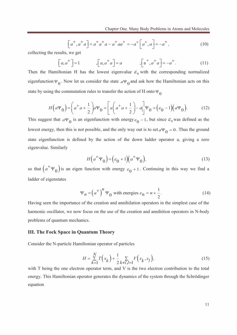
, , , (10)a a a a a a a aa a a a a
collecting the results, we get
.+ , 1 , , , a , (11)a a a a a a a a a
Then the Hamiltonian H has the lowest eigenvalue 0 with the corresponding normalized
eigenfunction 0 . Now let us consider the state 0a and ask how the Hamiltonian acts on this
state by using the commutation rules to transfer the action of H onto 0
1 1 1 . (12)0 0 0 0 02 2
H a a a a a a a a a
This suggest that 0a is an eigenfunction with energy 10 , but since 0 was defined as the
lowest energy, then this is not possible, and the only way out is to set 00a . Thus the ground
state eigenfunction is defined by the action of the down ladder operator a, giving a zero
eigenvalue. Similarly
, 1 (13)0 0 0H a a
so that 0a is an eigen function with energy 10 . Continuing in this way we find a
ladder of eigenstates
.1
with energies (14)n0 2
na nn
Having seen the importance of the creation and annihilation operators in the simplest case of the
harmonic oscillator, we now focus on the use of the creation and annihition operators in N-body
problems of quantum mechanics.
III. The Fock Space in Quantum Theory
Consider the N-particle Hamiltonian operator of particles
,1
, (15)1 , 12
NH T x V x xk k lk k l l
with T being the one electron operator term, and V is the two electron contribution to the total
energy. This Hamiltonian operator generates the dynamics of the system through the Schrödinger
equation

Chapter One. Many Body Problems in Atoms and Molecules
12
. (16)i Htt
H
For systems with a variable number of particles the explicit dependence on the particle number is
inconvenient. Evolution of the quantum system may be represented in a form independent of the
particle number in a Fock space with the operators written in their second quantized forms.
It is usually convenient to express wave functions of many particle systems as linear
combinations of one particle wave function products of the form
, , 1, , .1 1 1 2 2 (17)x x C N x x xn N Nn
Thus, if Ψ is symmetric under an arbitrary exchange xi↔xk, the coefficients C(n1,…,nN) must be
symmetric under the exchange nj↔nk. A set of N particle basis states with well defined
permutation symmetry is the properly symmetrized tensor product
,1
, (18)1 1 2 1!p
N N p NPPN
1 (18),1 2 1!
pN1 2 p NPPN
where the sum runs over the set of all possible permutations P. The weight factor is +1 for
bosons and -1 for an odd permutation of fermions. The inner product of two N-particle states is
,
1 , , ,1 1 1 1 1!
1 ' (19)1 1'!
P QN N Q NQ P PPQN
PN P NQ PPN
11 !1 P Q
N, ,1 PQ P1 1 Q NPQNPP Q
QQ P1 11 QP
N N, ,1
N
where P’=P+Q denotes the permutation resulting from the composition of the permutations P and
Q. Since P and Q are arbitrary permutations, P’ spans the space of all possible permutations as
well. It is easy to see that Eq (19) is nothing but the familiar inner product or Slater determinant
.1 1 1
, , , , (20)1 1
1
N
N N
N N N
1, N, ,1, N N, ,1
111 .
N1
NNNote that the interchange of the coordinates of two electrons corresponds to interchanging two
rows in the Slater determinant which changes the sign of the determinant, thus satisfying the
antisymmetry condition. In addition, having two electrons occupying the same spin orbital
corresponds to having two identical columns in the determinant, which makes it zero, as required
by the Pauli principal. Let us denote by a complete set of orthonormal one particle states,
which satisfy
Chapter One. Many Body Problems in Atoms and Molecules
13
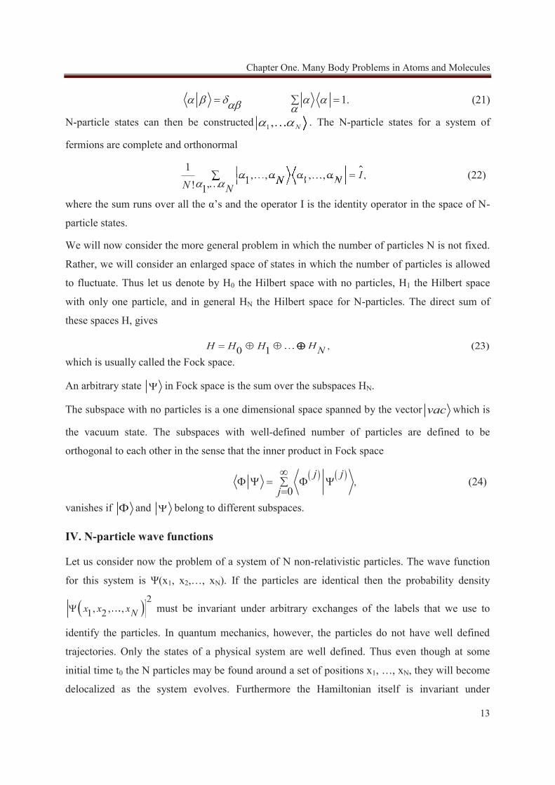
1. (21)
N-particle states can then be constructed 1, NN . The N-particle states for a system of
fermions are complete and orthonormal
,1
, , , , (22)1 1,! 1IN NN N
1, IN, ,1, N , ,11,, N
1,, N
,I
where the sum runs over all the α’s and the operator I is the identity operator in the space of N-
particle states.
We will now consider the more general problem in which the number of particles N is not fixed.
Rather, we will consider an enlarged space of states in which the number of particles is allowed
to fluctuate. Thus let us denote by H0 the Hilbert space with no particles, H1 the Hilbert space
with only one particle, and in general HN the Hilbert space for N-particles. The direct sum of
these spaces H, gives
, (23)0 1H H H HNHNH
which is usually called the Fock space.
An arbitrary state in Fock space is the sum over the subspaces HN.
The subspace with no particles is a one dimensional space spanned by the vector vac which is
the vacuum state. The subspaces with well-defined number of particles are defined to be
orthogonal to each other in the sense that the inner product in Fock space
, (24)0
j jj
vanishes if and belong to different subspaces.
IV. N-particle wave functions
Let us consider now the problem of a system of N non-relativistic particles. The wave function
for this system is Ψ(x1, x2,…, xN). If the particles are identical then the probability density
2, , ,1 2x x xN
2, x, N must be invariant under arbitrary exchanges of the labels that we use to
identify the particles. In quantum mechanics, however, the particles do not have well defined
trajectories. Only the states of a physical system are well defined. Thus even though at some
initial time t0 the N particles may be found around a set of positions x1, …, xN, they will become
delocalized as the system evolves. Furthermore the Hamiltonian itself is invariant under
Chapter One. Many Body Problems in Atoms and Molecules
14
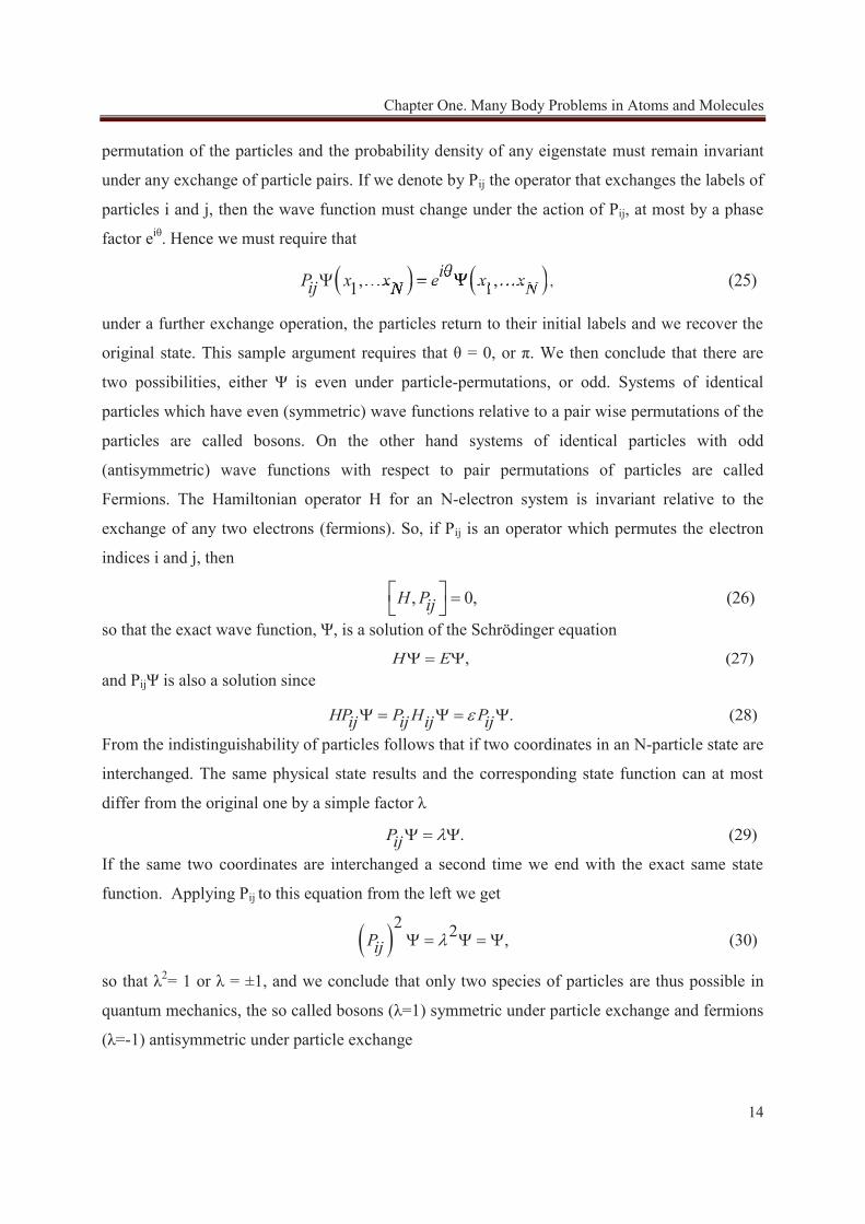
permutation of the particles and the probability density of any eigenstate must remain invariant
under any exchange of particle pairs. If we denote by Pij the operator that exchanges the labels of
particles i and j, then the wave function must change under the action of Pij, at most by a phase
factor eiθ. Hence we must require that
, , , (25)1 1iP x x e x xij N N ,1i x xN,1x x,1iix eieii
under a further exchange operation, the particles return to their initial labels and we recover the
original state. This sample argument requires that θ = 0, or π. We then conclude that there are
two possibilities, either Ψ is even under particle-permutations, or odd. Systems of identical
particles which have even (symmetric) wave functions relative to a pair wise permutations of the
particles are called bosons. On the other hand systems of identical particles with odd
(antisymmetric) wave functions with respect to pair permutations of particles are called
Fermions. The Hamiltonian operator H for an N-electron system is invariant relative to the
exchange of any two electrons (fermions). So, if Pij is an operator which permutes the electron
indices i and j, then
, 0, (26)H Pijso that the exact wave function, Ψ, is a solution of the Schrödinger equation
, (27)H Eand PijΨ is also a solution since
. (28)HP P H Pij ij ij ijFrom the indistinguishability of particles follows that if two coordinates in an N-particle state are
interchanged. The same physical state results and the corresponding state function can at most
differ from the original one by a simple factor λ
. (29)PijIf the same two coordinates are interchanged a second time we end with the exact same state
function. Applying Pij to this equation from the left we get
2 2 , (30)Pij
so that λ2= 1 or λ = ±1, and we conclude that only two species of particles are thus possible in
quantum mechanics, the so called bosons (λ=1) symmetric under particle exchange and fermions
(λ=-1) antisymmetric under particle exchange
Chapter One. Many Body Problems in Atoms and Molecules
15
. (31)Pij
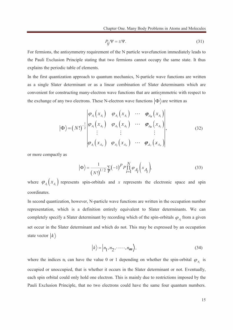
For fermions, the antisymmetry requirement of the N particle wavefunction immediately leads to
the Pauli Exclusion Principle stating that two fermions cannot occupy the same state. It thus
explains the periodic table of elements.
In the first quantization approach to quantum mechanics, N-particle wave functions are written
as a single Slater determinant or as a linear combination of Slater determinants which are
convenient for constructing many-electron wave functions that are antisymmetric with respect to
the exchange of any two electrons. These N-electron wave functions are written as
1 1 2 1 1
1 2 2 2 2
1 2
12 (32) ! ,
N
N
N N N N
A A A A A A
A A A A A A
A A A A A A
x x x
x x xN
x x x
NA xA
A xA ,
NANNxA
or more compactly as
,1/ 21
1 (33)1!
NpP xA Ai i iN
where i iA Ax represents spin-orbitals and x represents the electronic space and spin
coordinates.
In second quantization, however, N-particle wave functions are written in the occupation number
representation, which is a definition entirely equivalent to Slater determinants. We can
completely specify a Slater determinant by recording which of the spin-orbitals iA from a given
set occur in the Slater determinant and which do not. This may be expressed by an occupation
state vector k
, , , , (34)1 2k n n nm ,,n, m
where the indices ni can have the value 0 or 1 depending on whether the spin-orbital iA is
occupied or unoccupied, that is whether it occurs in the Slater determinant or not. Eventually,
each spin orbital could only hold one electron. This is mainly due to restrictions imposed by the
Pauli Exclusion Principle, that no two electrons could have the same four quantum numbers.
Chapter One. Many Body Problems in Atoms and Molecules
16
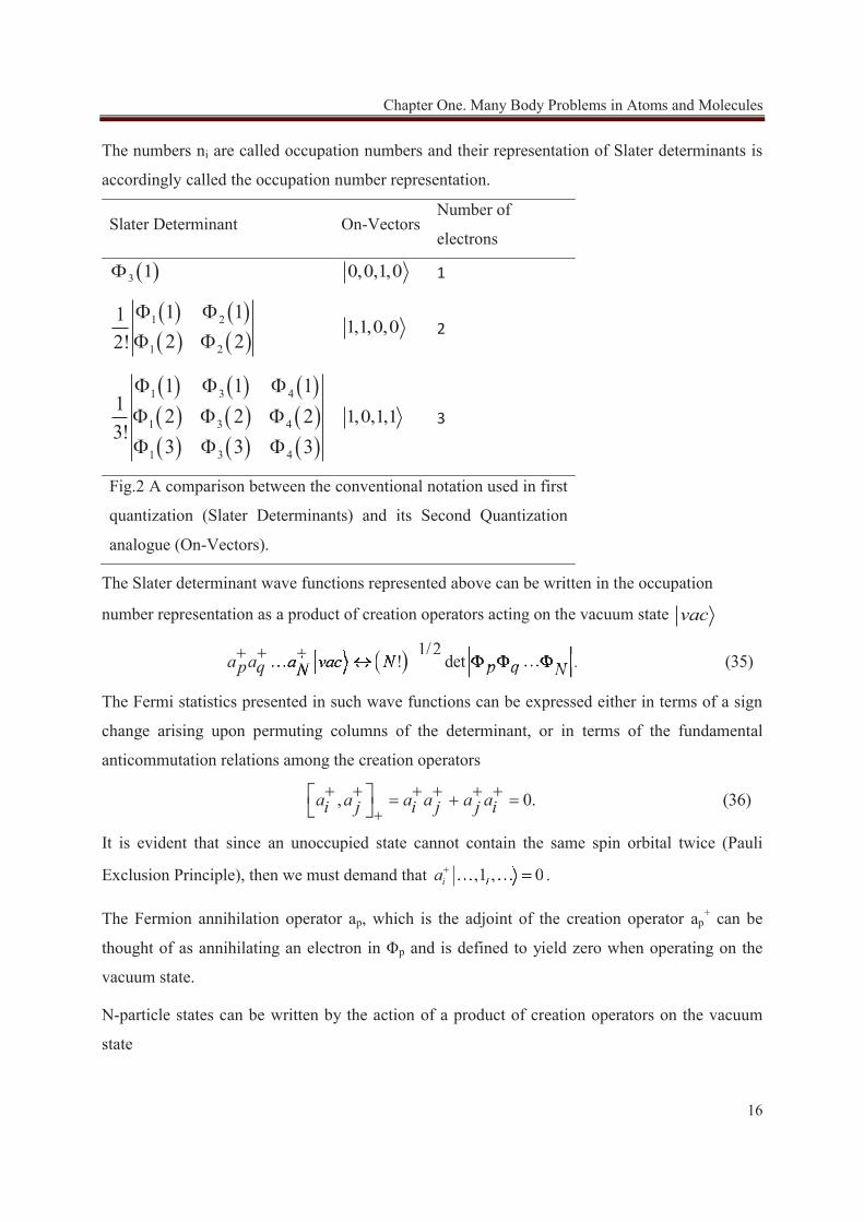
The numbers ni are called occupation numbers and their representation of Slater determinants is
accordingly called the occupation number representation.
Slater Determinant On-Vectors Number of
electrons
3 1 0,0,1,0 1
1 2
1 2
1 112 22!
1,1,0,0 2
1 3 4
1 3 4
1 3 4
1 1 11 2 2 23!
3 3 3 1,0,1,1 3
Fig.2 A comparison between the conventional notation used in first
quantization (Slater Determinants) and its Second Quantization
analogue (On-Vectors).
The Slater determinant wave functions represented above can be written in the occupation
number representation as a product of creation operators acting on the vacuum state vac
.1/2
! det (35)a a a vac Np q p qN N1/2
! det . p q Np qN ! det! det! det
The Fermi statistics presented in such wave functions can be expressed either in terms of a sign
change arising upon permuting columns of the determinant, or in terms of the fundamental
anticommutation relations among the creation operators
, 0. (36)a a a a a ai j i j j i
It is evident that since an unoccupied state cannot contain the same spin orbital twice (Pauli
Exclusion Principle), then we must demand that ,1 , 0i ia ,1 , 0i,1 .
The Fermion annihilation operator ap, which is the adjoint of the creation operator ap+ can be
thought of as annihilating an electron in Φp and is defined to yield zero when operating on the
vacuum state.
N-particle states can be written by the action of a product of creation operators on the vacuum
state

Chapter One. Many Body Problems in Atoms and Molecules
17
. , , 0, 0 (37)1 1 !
aN jn nN j n j
, 0, 0 .1 !
aN j, N j n
Othonormality restrictions must also apply on the ON vectors, in other words, the ON vectors
must also satisfy the following relations
, (38)k ki j ij
with the Kronecker delta ij defined by
.1 when i = j (39)0 when i jij
V. The Creation and Annihilation Operators in Second Quantization
In second quantization, all operators and states can be constructed from a set of elementary
creation and annihilation operators. In this section we introduce these operators and explore their
basic algebraic properties. In general, the effect of the creation and annihilation operators
,i ia a on each spin-orbital, can be summarized by
, ,0 , , , ,1 , ,1 1
, ,1 , , 01
1n j
j
a n n n n nm mi i ii
a n nmi i
n i
0 11n n n n0 1 m, ,n, ,i1,0 , ,0 1,0 , , , ,1, ,1i
,1 , , 01 , , mi,,11
1
(40),
i
and
1 0
0 0, (41)
a ni i ii
ai i
1 01i i01 i
0 0, i0where the phase-factor Γ(n) depends on the number of electrons found before the created or the
annihilated electron: Γ(n) = 1 for an even number of electrons and Γ(n) = -1 for an odd number
of electrons.
Sometimes in quantum mechanics, the need of transformations between position space (x, y, z)
and momentum space (px, py, pz), arises. Then the Fourier transform that changes position space
into momentum space can be written as
. , (42)i p xdp d x x ei p x.dp d x x ed p x
Chapter One. Many Body Problems in Atoms and Molecules
18
and conversely
Then the creation and annihilation operators themselves obey
, ,
, .
. . (44)2
. . 2
dd pi p x i p xda p d xa x e a x a p ed
dd pi p x i p xda p d xa x e a x a p ed
i p x.a p ep
p id d ppd xa x e ad xa x e apd id i p xdd i p x.dd xa x e a xp
dd di p xd pd pp x
i p x.i p x d pd a p eppi p xdd xa x e a xd xa x e a xi p x.dd xa x e a xp
dd di p xp x d pp x (45)
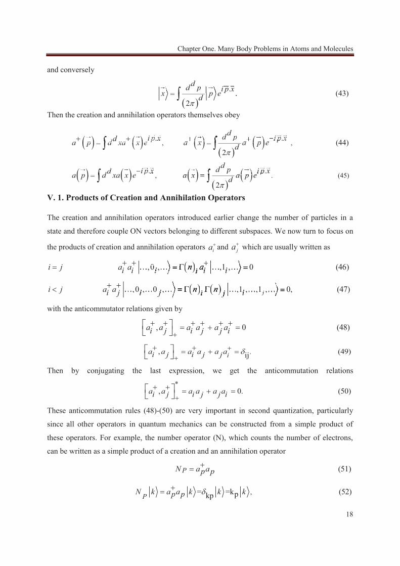
V. 1. Products of Creation and Annihilation Operators
The creation and annihilation operators introduced earlier change the number of particles in a
state and therefore couple ON vectors belonging to different subspaces. We now turn to focus on
the products of creation and annihilation operators ia and ja which are usually written as
,0 , ,1 , 0 (46)i j a a n ai i i i ii ,1 , 0 i i i,1,1,0 , i0 ,1 ,0 ,1,1,0 ,00
,0 , 0 , ,1 , ,1 , 0, (47)ji j a a n ni j i j ii j0 0 1 , ,1 , 0, ji,1i j,0 , 0 ,0,0 , 0 , ,1 , ,1 ,1 10 0 ,1,0 , 0 ,, 0
with the anticommutator relations given by
, 0 (48)a a a a a ai j i j j i
. , (49)ijia a a a a ai j i j j Then by conjugating the last expression, we get the anticommutation relations
* , 0. (50)a a a a a ai j i j j i
These anticommutation rules (48)-(50) are very important in second quantization, particularly
since all other operators in quantum mechanics can be constructed from a simple product of
these operators. For example, the number operator (N), which counts the number of electrons,
can be written as a simple product of a creation and an annihilation operator
(51)PN a ap p
. (43)2
.dd p i p xx p ed
dd pdi p x.p ex p x
, = =k (52)pkpPN k a a k k kp p
Chapter One. Many Body Problems in Atoms and Molecules
19
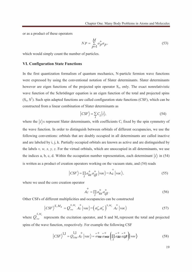
or as a product of these operators
, (53)1
MN a aP p pp
which would simply count the number of particles.
VI. Configuration State Functions
In the first quantization formalism of quantum mechanics, N-particle fermion wave functions
were expressed by using the conventional notation of Slater determinants. Slater determinants
however are eigen functions of the projected spin operator Sz, only. The exact nonrelativistic
wave function of the Schrödinger equation is an eigen function of the total and projected spins
(Sz, S2). Such spin adapted functions are called configuration state functions (CSF), which can be
constructed from a linear combination of Slater determinants as
, (54)CSF C iiiwhere the i s represent Slater determinants, with coefficients Ci fixed by the spin symmetry of
the wave function. In order to distinguish between orbitals of different occupancies, we use the
following conventions: orbitals that are doubly occupied in all determinants are called inactive
and are labeled by i, j, k. Partially occupied orbitals are known as active and are distinguished by
the labels v, w, x, y, z. For the virtual orbitals, which are unoccupied in all determinants, we use
the indices a, b, c, d. Within the occupation number representation, each determinant i in (54)
is written as a product of creation operators working on the vacuum state, and (54) reads
,+
=A (55)cCSF a a vac vaci ii
where we used the core creation operator
. (56) A a ac i iiOther CSFs of different multiplicities and occupancies can be constructed
, ,, = (57)s sS M S M
i ivwS MsCSF A vac A vacc cQ a a
where , sS M
vwQ represents the excitation operator, and S and Ms represent the total and projected
spins of the wave function, respectively. For example the following CSF
1,11,1 (58)CSF Q A vac a a a a vacc v w i ivw i
a a a a vaca a a a vaca a aa a aa aa aaaaaai
Chapter One. Many Body Problems in Atoms and Molecules
20
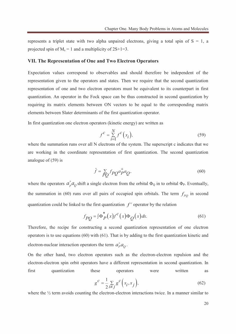
represents a triplet state with two alpha unpaired electrons, giving a total spin of S = 1, a
projected spin of Ms = 1 and a multiplicity of 2S+1=3.
VII. The Representation of One and Two Electron Operators
Expectation values correspond to observables and should therefore be independent of the
representation given to the operators and states. Then we require that the second quantization
representation of one and two electron operators must be equivalent to its counterpart in first
quantization. An operator in the Fock space can be thus constructed in second quantization by
requiring its matrix elements between ON vectors to be equal to the corresponding matrix
elements between Slater determinants of the first quantization operator.
In first quantization one electron operators (kinetic energy) are written as
, (59)1
Nc cf f xiiwhere the summation runs over all N electrons of the system. The superscript c indicates that we
are working in the coordinate representation of first quantization. The second quantization
analogue of (59) is
,ˆ (60)f f a aPPQ QPQ
where the operators p Qa a shift a single electron from the orbital ΦQ in to orbital ΦP. Eventually,
the summation in (60) runs over all pairs of occupied spin orbitals. The term PQf in second
quantization could be linked to the first quantization cf operator by the relation
* . (61)cf x f x x dxPPQ Q
Therefore, the recipe for constructing a second quantization representation of one electron
operators is to use equations (60) with (61). That is by adding to the first quantization kinetic and
electron-nuclear interaction operators the term P Qa a .
On the other hand, two electron operators such as the electron-electron repulsion and the
electron-electron spin orbit operators have a different representation in second quantization. In
first quantization these operators were written as
,1
, (62)2
c cg g x xi ji jwhere the ½ term avoids counting the electron-electron interactions twice. In a manner similar to
Chapter One. Many Body Problems in Atoms and Molecules
21
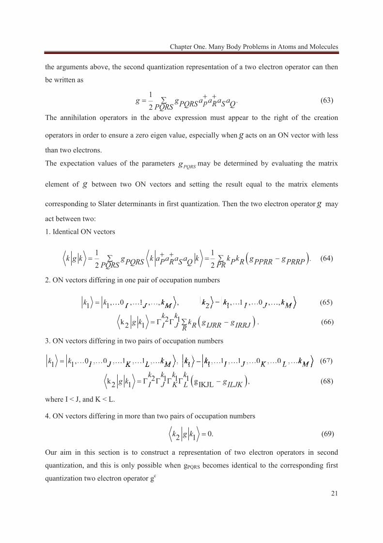
the arguments above, the second quantization representation of a two electron operator can then
be written as
.1
(63)2
g g a a a ap RPQRS S QPQRSThe annihilation operators in the above expression must appear to the right of the creation
operators in order to ensure a zero eigen value, especially when g acts on an ON vector with less
than two electrons.
The expectation values of the parameters PQRSg may be determined by evaluating the matrix
element of g between two ON vectors and setting the result equal to the matrix elements
corresponding to Slater determinants in first quantization. Then the two electron operator g may
act between two:
1. Identical ON vectors
.1 1
(64) 2 2
k g k g k a a a a k k k g gP R P R PPRR PRRPPQRS S Q PRPQRS
2. ON vectors differing in one pair of occupation numbers
, 0 , 1 , , , , 1 , 0 , , (65)1 1 2 1
2 1 k . (66)2 1
k k k k k kI J M I J Mk k
g k k g gI J R IJRR IRRJR
, 00 k k k0 1 1 0I J M I J M, , 0 ,, 0 ,2 1, , , ,, , , , 1 , 0 ,, 0 ,, 1 , , , , , 1 , ,0 10 111
3. ON vectors differing in two pairs of occupation numbers
,
, 0 , 0 , 1 , 1 , , , 1 , 1 , 0 , 0 , (67)1 1 1 1
2 1 1 1 k g (68)IKJL2 1
k k k k k kI J K L M I J K L Mk k k k
g k gI J K L ILJK
, 1 , 1 , 0 , 0 , (671 100 0 1 1 1 1 0 01 1 0 00 I J K L M, 1 , 1 , 0 , 0 ,, 1 , 0 , 0 ,1 1, 0 , , , ,, 0 , , , , 1 , 1 , 0 , 0 ,,, 0 , 1 , 1 , ,,,0 0 1 10 0 1 10 1 10 1 1
where I < J, and K < L.
4. ON vectors differing in more than two pairs of occupation numbers
0. (69)2 1k g k
Our aim in this section is to construct a representation of two electron operators in second
quantization, and this is only possible when gPQRS becomes identical to the corresponding first
quantization two electron operator gc
Chapter One. Many Body Problems in Atoms and Molecules
22
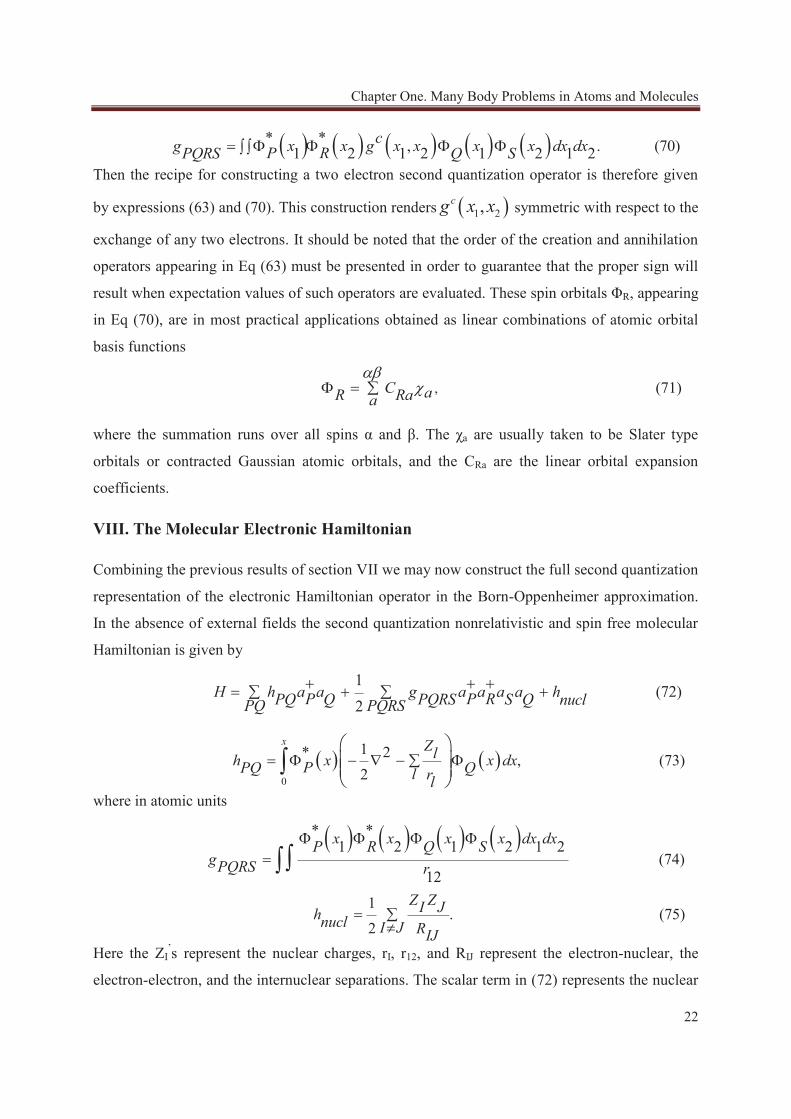
* * , . (70)1 2 1 2 1 2 1 2cg x x g x x x x dx dxP RPQRS Q S
Then the recipe for constructing a two electron second quantization operator is therefore given
by expressions (63) and (70). This construction renders 1 2,cg x x symmetric with respect to the
exchange of any two electrons. It should be noted that the order of the creation and annihilation
operators appearing in Eq (63) must be presented in order to guarantee that the proper sign will
result when expectation values of such operators are evaluated. These spin orbitals ΦR, appearing
in Eq (70), are in most practical applications obtained as linear combinations of atomic orbital
basis functions
, (71)C aR Raa
where the summation runs over all spins α and β. The χa are usually taken to be Slater type
orbitals or contracted Gaussian atomic orbitals, and the CRa are the linear orbital expansion
coefficients.
VIII. The Molecular Electronic Hamiltonian
Combining the previous results of section VII we may now construct the full second quantization
representation of the electronic Hamiltonian operator in the Born-Oppenheimer approximation.
In the absence of external fields the second quantization nonrelativistic and spin free molecular
Hamiltonian is given by
1 (72)
2H h a a g a a a a hP P RPQ Q PQRS S Q nuclPQ PQRS
where in atomic units
* *1 2 1 2 1 2
(74)12
1 .
2
x x x x dx dxP R Q SgPQRS r
Z ZI Jhnucl I J RIJ (75)
Here the ZI’s represent the nuclear charges, rI, r12, and RIJ represent the electron-nuclear, the
electron-electron, and the internuclear separations. The scalar term in (72) represents the nuclear
0
1* 2 , (73)2
x Zlh x x dxPPQ Ql rl
Chapter One. Many Body Problems in Atoms and Molecules
23
repulsion energy and it is simply added to the Hamiltonian and gives the same contribution to the
Hamiltonian as in first quantization.
Acting on the vacuum state the second quantization Hamiltonian (72) produces a linear
combination of the original state with states generated by single ( P Qa a ) and double electron
excitations ( P R S Qa a a a ). With each of these excitations there is an associated amplitude hPQ or
gPQRS, which represents the probability for one and two electron interactions. These probabilities
are best calculated from the spin-orbitals and the one and two electron operators, according to
equations (73) and (74).
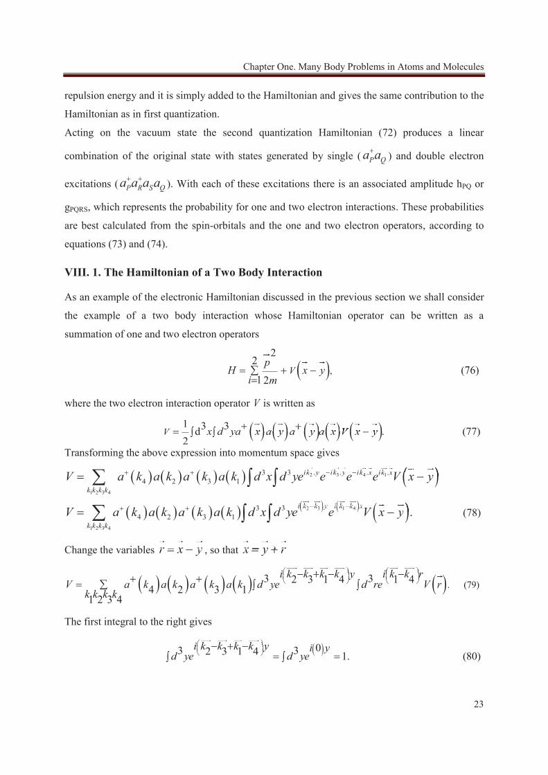
VIII. 1. The Hamiltonian of a Two Body Interaction
As an example of the electronic Hamiltonian discussed in the previous section we shall consider
the example of a two body interaction whose Hamiltonian operator can be written as a
summation of one and two electron operators
,
22
(76)1 2
Vp
H x yi m
2p
x yx
where the two electron interaction operator V is written as
1 3 3 d . (77) 2
V x d ya x a y a y a x V x y
Transforming the above expression into momentum space gives
32 4 1
1 2 3 4
2 3 1 4
1 2 3 4
.. . .3 34 2 3 1
3 34 2 3 1 (78).
ik yik y ik x ik x
k k k k
i k k y i k k x
k k k k
V a k a k a k a k d x d ye e e e V x y
V a k a k a k a k d x d ye e V x y
k x ik xkk y ik Vk y ik x ik xik yk ikk y ikk y
k k y i k k x
x yx
x yx
Change the variables r x yr x yx , so that x y rx ry
. (79)3 32 3 1 4 1 44 2 3 1
1 2 3 4
i k k k k y i k k rV a k a k a k a k d ye d re V r
k k k k
rk k k k i k ki k kk k k k y i k ky i k ky i k ky i k kk k k y i ky iy iy i(79)r
The first integral to the right gives
03 32 3 1 4 1. (80)
i k k k k y i yd ye d ye
yk k k kk k k kk k
Chapter One. Many Body Problems in Atoms and Molecules
24
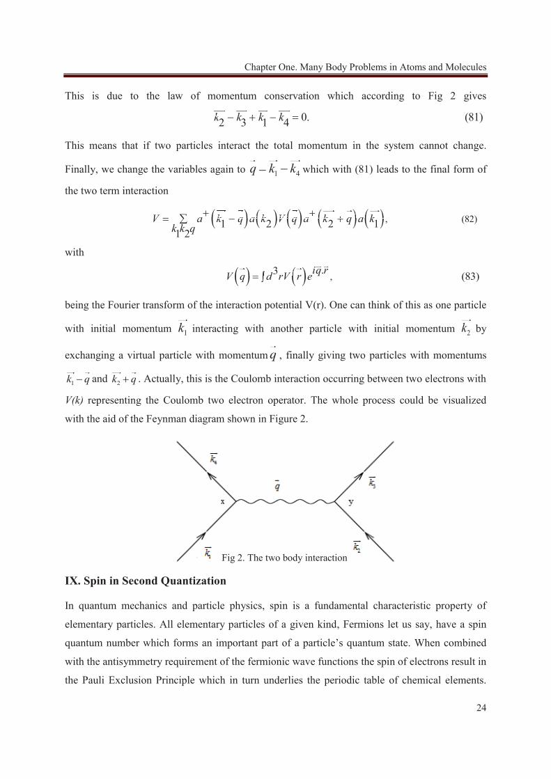
This is due to the law of momentum conservation which according to Fig 2 gives
0. (81)2 3 1 4k k k k 0k k k kk k k
This means that if two particles interact the total momentum in the system cannot change.
Finally, we change the variables again to 1 4q k kq k kk which with (81) leads to the final form of
the two term interaction
, (82)1 2 2 11 2
V a k q a k V q a k q a kk k q
k q a k V q a k q a kk k Vk q a k V q a k
with
,.3 (83)iq rV q d rV r e3 iq r.d rV r e3q q r
being the Fourier transform of the interaction potential V(r). One can think of this as one particle
with initial momentum 1kk interacting with another particle with initial momentum 2kk by
exchanging a virtual particle with momentum qq , finally giving two particles with momentums
1k qk q and 2k qk q . Actually, this is the Coulomb interaction occurring between two electrons with
V(k) representing the Coulomb two electron operator. The whole process could be visualized
with the aid of the Feynman diagram shown in Figure 2.
IX. Spin in Second Quantization
In quantum mechanics and particle physics, spin is a fundamental characteristic property of
elementary particles. All elementary particles of a given kind, Fermions let us say, have a spin
quantum number which forms an important part of a particle’s quantum state. When combined
with the antisymmetry requirement of the fermionic wave functions the spin of electrons result in
the Pauli Exclusion Principle which in turn underlies the periodic table of chemical elements.
Fig 2. The two body interaction
Chapter One. Many Body Problems in Atoms and Molecules
25
Thus the spin of a particle is an important intrinsic degree of freedom. In the formalism of
second quantization presented so far there were no reference to electron spin. In the present
section we develop the theory of second quantization so as to allow for an explicit description of
electron spin.
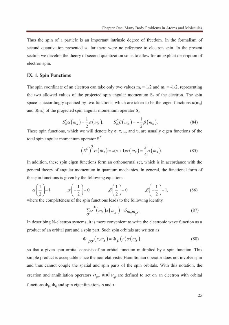
IX. 1. Spin Functions
The spin coordinate of an electron can take only two values ms = 1/2 and ms = -1/2, representing
the two allowed values of the projected spin angular momentum Sz of the electron. The spin
space is accordingly spanned by two functions, which are taken to be the eigen functions α(ms)
and β(ms) of the projected spin angular momentum operator Sz
.1 1
, (84)2 2
c cS m m S m mz s s z s s
These spin functions, which we will denote by σ, τ, μ, and υ, are usually eigen functions of the
total spin angular momentum operator S2
.2 3
( 1) (85)4
cS m s s m ms s s
In addition, these spin eigen functions form an orthonormal set, which is in accordance with the
general theory of angular momentum in quantum mechanics. In general, the functional form of
the spin functions is given by the following equations
1 1 1 1 1 , 0 , 0 , 1, (86)
2 2 2 2where the completeness of the spin functions leads to the following identity
.* (87)' 'm ms m ms s s
In describing N-electron systems, it is more convenient to write the electronic wave function as a
product of an orbital part and a spin part. Such spin orbitals are written as
, , (88)r m r ms p sp so that a given spin orbital consists of an orbital function multiplied by a spin function. This
simple product is acceptable since the nonrelativistic Hamiltonian operator does not involve spin
and thus cannot couple the spatial and spin parts of the spin orbitals. With this notation, the
creation and annihilation operators and p qa a are defined to act on an electron with orbital
functions Φp, Φq and spin eigenfunctions σ and τ.
Chapter One. Many Body Problems in Atoms and Molecules
26
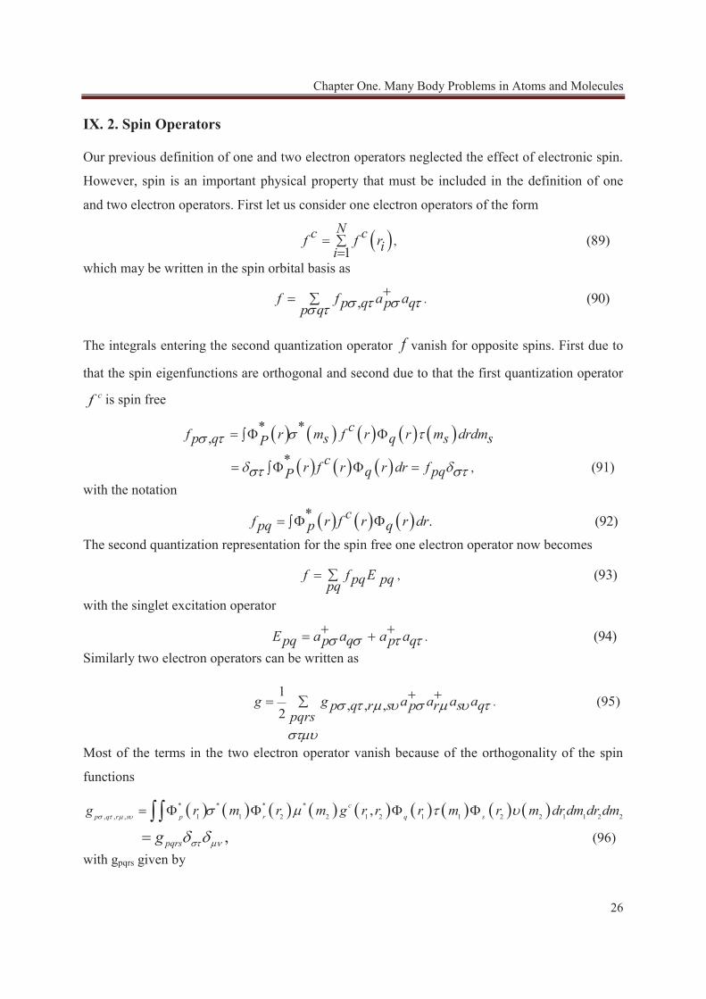
IX. 2. Spin Operators
Our previous definition of one and two electron operators neglected the effect of electronic spin.
However, spin is an important physical property that must be included in the definition of one
and two electron operators. First let us consider one electron operators of the form
, (89)1
Nc cf f riiwhich may be written in the spin orbital basis as
. (90),f f a ap q p qp q
The integrals entering the second quantization operator f vanish for opposite spins. First due to
that the spin eigenfunctions are orthogonal and second due to that the first quantization operator cf is spin free
,
* * ,* (91)
cf r m f r r m drdmp q s q s sPcr f r r dr fq pqP
with the notation
* . (92)cf r f r r drpq p qThe second quantization representation for the spin free one electron operator now becomes
, (93)f f Epq pqpqwith the singlet excitation operator
. (94)E a a a apq p q p qSimilarly two electron operators can be written as
.1
(95), , ,2g g a a a ap q r s p r s q
pqrs
Most of the terms in the two electron operator vanish because of the orthogonality of the spin
functions
* * * *, , , 1 1 2 2 1 2 1 1 2 2 1 1 2 2,
(96 ,
cp q r s p r q s
pqrs
g r m r m g r r r m r m dr dm dr dm
g )with gpqrs given by
Chapter One. Many Body Problems in Atoms and Molecules
27
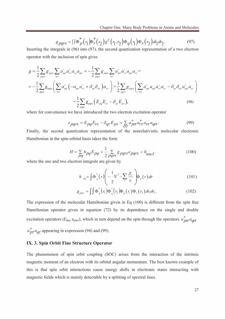
.* * , (97)1 2 1 2 1 2 1 2cg r r g r r r r dr drpqrs p r q s
Inserting the integrals in (96) into (97), the second quantization representation of a two electron
operator with the inclusion of spin gives
where for convenience we have introduced the two electron excitation operator
. (99)e E E E a a a apqrs pq rs qr ps p r s qFinally, the second quantization representation of the nonrelativistic molecular electronic
Hamiltonian in the spin-orbital basis takes the form
,1
(100)2
H h E g e hpq pq pqrs pqrs nuclpq pqrswhere the one and two electron integrals are given by
* 2
* *1 2 1 2 1 2
1 (101)
2
.
lpq qp
l l
pqrs q sp q
Zh r r dr
r
g r r r r dr dr (102)
The expression of the molecular Hamiltonian given in Eq (100) is different from the spin free
Hamiltonian operator given in equation (72) by its dependence on the single and double
excitation operators (Epq, epqrs), which in turn depend on the spin through the operators a ap q
a ap q appearing in expression (94) and (99).
IX. 3. Spin Orbit Fine Structure Operator
The phenomenon of spin orbit coupling (SOC) arises from the interaction of the intrinsic
magnetic moment of an electron with its orbital angular momentum. The best known example of
this is that spin orbit interactions cause energy shifts in electronic states interacting with
magnetic fields which is mainly detectable by a splitting of spectral lines.
pqrspqrs
1 1=
2 2
1 1g =
2 21
= g2
pqrs p r s q pqrs p r q spqrs pqrs
p q r qr s pqrs p q r s qr p spqrs
g g a a a a g a a a a
a a a a g a a a a a a
pqrspqrs
(98) ,pq rs qr psE E E
Chapter One. Many Body Problems in Atoms and Molecules
28
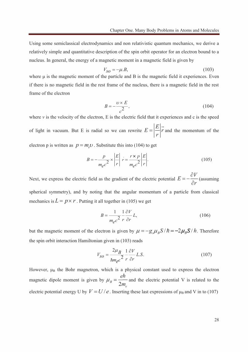
Using some semiclassical electrodynamics and non relativistic quantum mechanics, we derive a
relatively simple and quantitative description of the spin orbit operator for an electron bound to a
nucleus. In general, the energy of a magnetic moment in a magnetic field is given by
. , (103)V Bsowhere μ is the magnetic moment of the particle and B is the magnetic field it experiences. Even
if there is no magnetic field in the rest frame of the nucleus, there is a magnetic field in the rest
frame of the electron
, (104)2E
Bc
where v is the velocity of the electron, E is the electric field that it experiences and c is the speed
of light in vacuum. But E is radial so we can rewrite EE rr
r and the momentum of the
electron p is written as ep m . Substitute this into (104) to get
. (105)2 2rp E r p E
Br rm c m ce e
r pr
Next, we express the electric field as the gradient of the electric potential VEr
(assuming
spherical symmetry), and by noting that the angular momentum of a particle from classical
mechanics is L p r . Putting it all together in (105) we get
1 1 , (106)2
VB L
r rm ce
but the magnetic moment of the electron is given by / 2 /s B Bg S S2 /BS2 B22 . Therefore
the spin orbit interaction Hamiltonian given in (103) reads
2 1 . . (107)2
VBV L Sso r rm ce22 rm ce
However, μB the Bohr magnetron, which is a physical constant used to express the electron
magnetic dipole moment is given by 2B
e
eme
and the electric potential V is related to the
electric potential energy U by /V U e . Inserting these last expressions of μB and V in to (107)
Chapter One. Many Body Problems in Atoms and Molecules
29
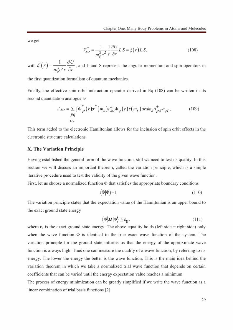
we get1 1
. . , (108)2 2UcV L S r L Sso r rm ce
with 2 2
1
e
Urm c r r
, and L and S represent the angular momentum and spin operators in
the first quantization formalism of quantum mechanics.
Finally, the effective spin orbit interaction operator derived in Eq (108) can be written in its
second quantization analogue as
,* * (109)cV r m V r m drdm a aso p s so q s s p qpq
This term added to the electronic Hamiltonian allows for the inclusion of spin orbit effects in the
electronic structure calculations.
X. The Variation Principle
Having established the general form of the wave function, still we need to test its quality. In this
section we will discuss an important theorem, called the variation principle, which is a simple
iterative procedure used to test the validity of the given wave function.
First, let us choose a normalized function Φ that satisfies the appropriate boundary conditions
=1. (110)=1.
The variation principle states that the expectation value of the Hamiltonian is an upper bound to
the exact ground state energy
, (111)0H , 0H
where ε0 is the exact ground state energy. The above equality holds (left side = right side) only
when the wave function Φ is identical to the true exact wave function of the system. The
variation principle for the ground state informs us that the energy of the approximate wave
function is always high. Thus one can measure the quality of a wave function, by referring to its
energy. The lower the energy the better is the wave function. This is the main idea behind the
variation theorem in which we take a normalized trial wave function that depends on certain
coefficients that can be varied until the energy expectation value reaches a minimum.
The process of energy minimization can be greatly simplified if we write the wave function as a
linear combination of trial basis functions [2]
Chapter One. Many Body Problems in Atoms and Molecules
30
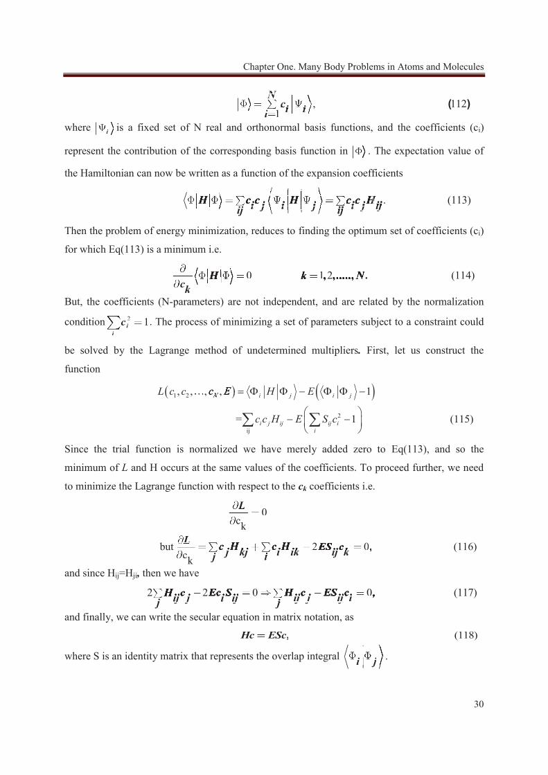
, 1121
( )N
ci ii,
N
ii
Nc
i 1i 1 i ii 1ci ii
where ii is a fixed set of N real and orthonormal basis functions, and the coefficients (ci)
represent the contribution of the corresponding basis function in . The expectation value of
the Hamiltonian can now be written as a function of the expansion coefficients
. (113)H c c H c c Hi j i j i j ijij ij. i j ijij i j i ji j i j i jij i j i j
Then the problem of energy minimization, reduces to finding the optimum set of coefficients (ci)
for which Eq(113) is a minimum i.e.
0 1 2 (114), ,....., .H k Nck
0 , , ,k N0 1 2, ,.....,22ck
But, the coefficients (N-parameters) are not independent, and are related by the normalization
condition 2 1ii
c 2i
i
c 1. The process of minimizing a set of parameters subject to a constraint could
be solved by the Lagrange method of undetermined multipliers. First, let us construct the
function
1 2
2
ij
, , , , 1
= 1 (115)
N i j i j
i j ij ij ii
L c c c E H E
c c H E S c
, N ,, ,,,
Since the trial function is normalized we have merely added zero to Eq(113), and so the
minimum of L and H occurs at the same values of the coefficients. To proceed further, we need
to minimize the Lagrange function with respect to the ck coefficients i.e.
0ck
but 2 0 (116)ck
,
L
L c H c H ES cj kj i ik ij kj i
L 0ck
00
L 0 ,ij kS ci ikj kjc 2j kj i ikcc 2j kjck jjjand since Hij=Hji, then we have
2 2 0 0 (117),H c Ec S H c ES cij j i ij ij j ij ij j0 ,H cij j i i ij j ij ic
j ij j i ijS S2 00i ij ij j ij ic S c S c2 0i ij
and finally, we can write the secular equation in matrix notation, as
(118),Hc ESc ,ESc
where S is an identity matrix that represents the overlap integral i ji j .
Chapter One. Many Body Problems in Atoms and Molecules
31
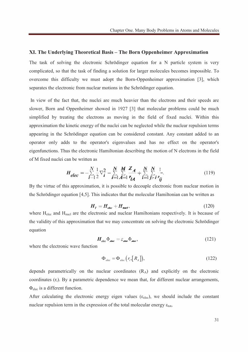
XI. The Underlying Theoretical Basis – The Born Oppenheimer Approximation
The task of solving the electronic Schrödinger equation for a N particle system is very
complicated, so that the task of finding a solution for larger molecules becomes impossible. To
overcome this difficulty we must adopt the Born-Oppenheimer approximation [3], which
separates the electronic from nuclear motions in the Schrödinger equation.
In view of the fact that, the nuclei are much heavier than the electrons and their speeds are
slower, Born and Oppenheimer showed in 1927 [3] that molecular problems could be much
simplified by treating the electrons as moving in the field of fixed nuclei. Within this
approximation the kinetic energy of the nuclei can be neglected while the nuclear repulsion terms
appearing in the Schrödinger equation can be considered constant. Any constant added to an
operator only adds to the operator's eigenvalues and has no effect on the operator's
eigenfunctions. Thus the electronic Hamiltonian describing the motion of N electrons in the field
of M fixed nuclei can be written as
1 12 . (119)21 1 1 1
ZN N M N NAHelec i r ri i A i j iiA ij
1N 1 1 i
1 12N 1 Ai i A1 1 112 1iA i j11i 1 1 11212 1i2 i A i j1 1 11 1i212 1 j
rijrj i
. rrj i
By the virtue of this approximation, it is possible to decouple electronic from nuclear motion in
the Schrödinger equation [4,5]. This indicates that the molecular Hamiltonian can be written as
, (120)T elec nuclH H H , elec nuclH Hll
where Helec and Hnucl are the electronic and nuclear Hamiltonians respectively. It is because of
the validity of this approximation that we may concentrate on solving the electronic Schrödinger
equation
, (121) elec elec elec elecH , elec elec elec
where the electronic wave function
, , (122)elec elec i Ar R
depends parametrically on the nuclear coordinates (RA) and explicitly on the electronic
coordinates (ri). By a parametric dependence we mean that, for different nuclear arrangements,
Φelec is a different function.
After calculating the electronic energy eigen values (εelec), we should include the constant
nuclear repulsion term in the expression of the total molecular energy εtot,
Chapter One. Many Body Problems in Atoms and Molecules
32
1
. (123) M M
A Btot elec
A B A AB
Z ZRelec .
M MA B
AB
Z ZA B
RA B1
M M ZRAARAA R
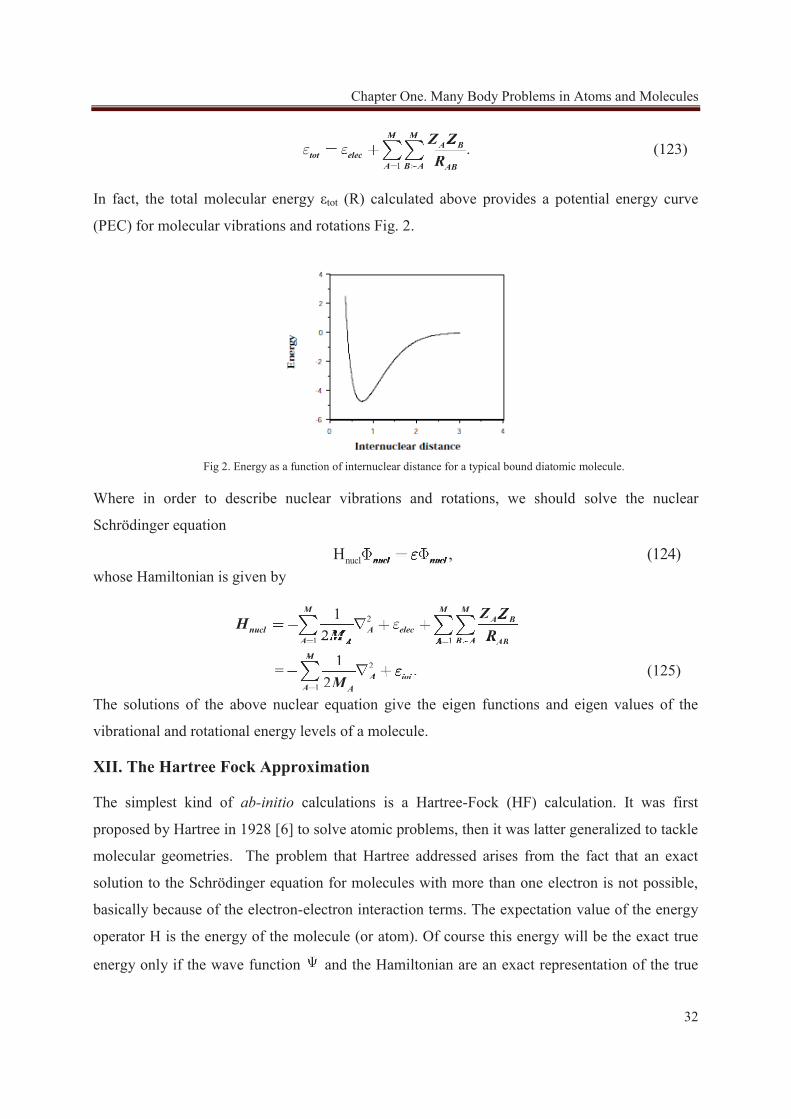
In fact, the total molecular energy εtot (R) calculated above provides a potential energy curve
(PEC) for molecular vibrations and rotations Fig. 2.
Where in order to describe nuclear vibrations and rotations, we should solve the nuclear
Schrödinger equation
nucl H , (124)nucl nucl , nucl nucl
whose Hamiltonian is given by
2
1 1
2
1
1 2
1 = . 2
M M MA B
nucl A elecA A B AA AB
M
A totA A
Z ZH
M R
M
A AB
. tot
M M M1 A B
A
Z ZA B
R21 2 A ABA B1M RA B1 B1
212
M M M1A elec2
ZM RA elec2M R
A AM A1 2M1M
212
M
AM2M
AAA RA AA R
(125)
The solutions of the above nuclear equation give the eigen functions and eigen values of the
vibrational and rotational energy levels of a molecule.
XII. The Hartree Fock Approximation
The simplest kind of ab-initio calculations is a Hartree-Fock (HF) calculation. It was first
proposed by Hartree in 1928 [6] to solve atomic problems, then it was latter generalized to tackle
molecular geometries. The problem that Hartree addressed arises from the fact that an exact
solution to the Schrödinger equation for molecules with more than one electron is not possible,
basically because of the electron-electron interaction terms. The expectation value of the energy
operator H is the energy of the molecule (or atom). Of course this energy will be the exact true
energy only if the wave function and the Hamiltonian are an exact representation of the true
Fig 2. Energy as a function of internuclear distance for a typical bound diatomic molecule.

Chapter One. Many Body Problems in Atoms and Molecules
33
physical system. The variational theorem discussed in the previous section states that the energy
calculated from the equation E H must be greater or equal to the true ground-state
energy of the molecule Eq(111). In practice, any molecular wave function we use is always only
an approximation to the true wave function of the system, therefore the variationally calculated
molecular energy will always be greater than the true energy. In general the Hartree Fock (HF)
method is variational, so the correct energy always lies below any calculated energy by HF
method, then the better the wave function is the lower is the energy.
In the Hartree Fock approximation the electronic wave function is approximated by a single
configuration of spin orbitals (i.e. by a single Slater determinant) and the energy is optimized
with respect to variations of these spin orbitals. In this method the ground state wave function
can then be written as
. 1 2 0 or 0 (126)1N i
Na a a aHF HF iNN 00000000
The optimization of the Hartree Fock wave function must be done to arrive at the optimal
determinant that may be found by solving a set of effective one electron Schrödinger equations
called the Hartree Fock equations and their associated Hamiltonian operator is called the Fock
operator
1 1 2 1 1 , (127)
ncore
j jj
F H J K
with
2
* * *1 1 2 2
1 212
*1 1
1 2
1
1
core
iall l
p p i ii
p ii
ZH
r
r r r rJ dr dr
rr r
K* *
2 21
12
(128)i pr rdr dr
r
In the Fock operator the one-electron part of the true Hamiltonian core
H is retained. The two
electron part iJ is the regular Coulomb repulsion term while the 3rd part iK is called the
exchange term which is a correction to the two Coulomb interaction that arises from the
antisymmetry of the wave function. The Hartree Fock eigenvalue equation is then written as
, (129)f pHF HF
Chapter One. Many Body Problems in Atoms and Molecules
34
with eigen values
.
* *1 1 1 2 22 21 1 1 1 22 1 12
* *1 1 2 2 (130)1 2
12
r r r rZ p p i iKr r dr dr drp pP iK r rK
r r r rp pi i dr dri r
An electron in Φp thus experiences a classical electrostatic Coulomb potential (the 2nd term in the
above equation), generated by the nuclear framework and by the charge distribution of the
remaining electrons, as well as a nonclassical exchange potential (the 3rd term in the above
equation), which corrects the classical repulsion energy for Fermi correlation. The exchange
integral arises from Slater determinant expansion terms that differ only in the exchange of
electrons. It is said to have no simple physical meaning [7] , but we can regard the exchange term
as a kind of correction to the Coulomb integral, reducing its effect. This reduction arises because
particles with opposite spins cannot occupy the same spatial orbital. In other words two electrons
of the same spin avoid each other more than expected in the columbic repulsion.
XIII. The Roothaan-Hall Self Consistent Field Equation
In this section we present the Roothaan-Hall formulation of the Hartree Fock theory, in which
the molecular orbitals (MOs) are expanded in a set of atomic orbitals (AOs) whose expansion
coefficients are used as the variational parameters [7, 8].
In most applications of Hartree Fock theory to molecular systems, the MOs Φp are expanded in a
set of Gaussian type AOs (χμ), with coefficients Cμp
. (131)Cp p
In this case, we are expanding the molecular orbital (MO) Φ in terms of a set of basis functions.
Usually, these basis functions are located on atoms, and thus could be regarded as atomic
orbitals. Therefore, one could write the MOs as a linear combination of atomic orbitals (LCAO),
and the set of basis functions is called a basis set.
Conventionally, there is no upper limit to the size of a basis set and the number of basis functions
m in the expansion can be much bigger than the number n of electron pairs in the molecule [10].
However, only the n occupied orbitals are used to construct the Slater determinant, which
represents the HF wave functions.
Chapter One. Many Body Problems in Atoms and Molecules
35
Now, if we substitute the expansion (131) in to the HF Equation (129) we get
1 11 1
1 1 , (132)m m
a a a sa s a sa ss s
f c f c
where, 1f is the Fock operator for the 1st electron in Ψa.
Then multiply equation (132) by the basis function * 1j from the left and integrate,
* *1 1 1
1 1 1 1 1 1 , (133)
m m
sa j s a sa j ss s
c f c
where by identifying the following terms: *
1
*1 1
1 1
1 1 ,
js j s
js j s
S
f f (134)
we could rewrite equation (133), as
, (135)1 1
m mf c S csa a sajs jss s
mmf c
sS c
mS
1 j1s s1, S csac
1f c js1
SSjsf csas 1S
1Sa 1S
or in matrix notation, as
(136),Fc Sc ,Scwhere c is an m×m matrix (m basis functions) and ε is an m×m diagonal matrix of the orbital
energies.
XIV. Post Hartree Fock Calculations
The Hartree Fock method relies on averages [11], it does not consider the instantaneous
electrostatic interaction between the electrons nor does it take into account the quantum
mechanical effects on electron distributions. This is because the effect of the n-1 electrons on an
electron of interest is treated in an average way. In fact, the HF method overestimates the
electron-electron repulsion and so gives higher electronic energies than the correct ones, even
with the largest basis sets. In brief, we summarize these deficiencies by saying that the HF
method ignores electron correlation [10].
Actually, the HF method allows for some electron correlation, two electrons of the same spin
cannot be in the same place because their spatial and spin coordinates would then be the same
and the Slater determinant (32) representing the molecular wave function would vanish, since a
determinant with two identical rows or columns is zero. This is a consequence of the Pauli
exclusion principal, where in the neighborhood of each electron there would still be a region
Chapter One. Many Body Problems in Atoms and Molecules
36
unfriendly to other electrons of the same spin. This region is called a Fermi hole and the HF
method overestimates the size of a Fermi hole [12].
XIV. 1. Multi Configuration Self Consistent Field Theory MCSCF
The first step in post Hartree Fock quantum mechanical calculations is the Multi Configuration
Self Consistent Field (MCSCF) method, which involves a generalization of the Hartree Fock
wave function to systems dominated by more than one electronic configuration. This model is
useful in describing the electronic structure of bonded molecular systems, and in particular
excited states [13].
In MCSCF theory, the wave function is written as a linear combination of determinants or
configuration state functions CSFs, whose expansion coefficients are optimized simultaneously
with the MOs according to the variational principle. Thus the MCSCF wave functions may be
written as
, (137)C iiiwhere the Cis are the configuration expansion coefficients (normalized to unity). Then the
problem of finding the ground state MCSCF optimum wave function can be obtained by
minimizing the energy with respect to the variational parameters
min . (138)H
EMC
This method allows for a highly flexible description of the electronic system, where both the one
and N-electron functions, MOs and CSFs, may adapt to the physical situation. Usually, the
greatest difficulty faced in setting up an MCSCF calculation is the selection of configuration
space which contributes appreciable to the wave function. Indeed, even for small systems, it is
often impossible to generate an MCSCF configuration space sufficiently flexible to describe the
physical process and yet sufficiently small to be computationally tractable.
The selection of MCSCF configurations is usually not carried out by inspection of the individual
configurations. Instead, whole classes of configurations are simultaneously selected and
classified into three sets:
1. A set of inactive orbitals composed of the lowest energy spin orbitals which are doubly
occupied in all determinants.
Chapter One. Many Body Problems in Atoms and Molecules
37
2. A set of virtual orbitals composed of very high energy spin orbitals which are unoccupied in
all determinants.
3. A set of active orbitals which are energetically intermediate between the inactive and virtual
orbitals.
The active electrons are those that are not in the doubly occupied inactive orbitals, but rather to
which excitations are allowed. The single, double, and triple, etc., excited determinants are those
that arise from all possible ways of distributing the active electrons over all the active orbitals.
This method is known as the complete active space self consistent method CASSCF [13,14].
XIV.2. Configuration Interaction
The configuration interaction (CI) wave function consists of a linear combination of Slater
determinants, the expansion coefficients of which are variationally determined. Owing to the
simple structure of the wave function, the CI method has been extensively and successfully
applied in quantum mechanical calculations [15]. The method is flexible and can give highly
accurate wave functions for small closed and open shell molecular systems with electron
correlation and it may be used to describe complex electronic structure problems such as bond
breakings and excited states. The principle shortcomings of the CI method is that it is difficult to
implement for large molecules because of the rapid growth in the number of configurations
needed to recover a substantial part of the correlation energy for larger systems.
In the treatment of electron correlations it is important to distinguish between static and
dynamical correlations. Static correlation effects are best treated in the complete active space
self-consistent field method CASSCF, by retaining in the CAS reference space the
configurations arising from the distribution of valence electrons in all possible ways among the
active orbitals, while keeping the core orbitals doubly occupied in all configurations. Dynamic
correlations, on the other hand, are subsequently treated by including in the wave function
expansion all configurations generated from the reference space by carrying out excitations up to
a given excitation level.
In the CI method, the wave function is constructed as a linear combination of determinants or
configuration state functions CSFs
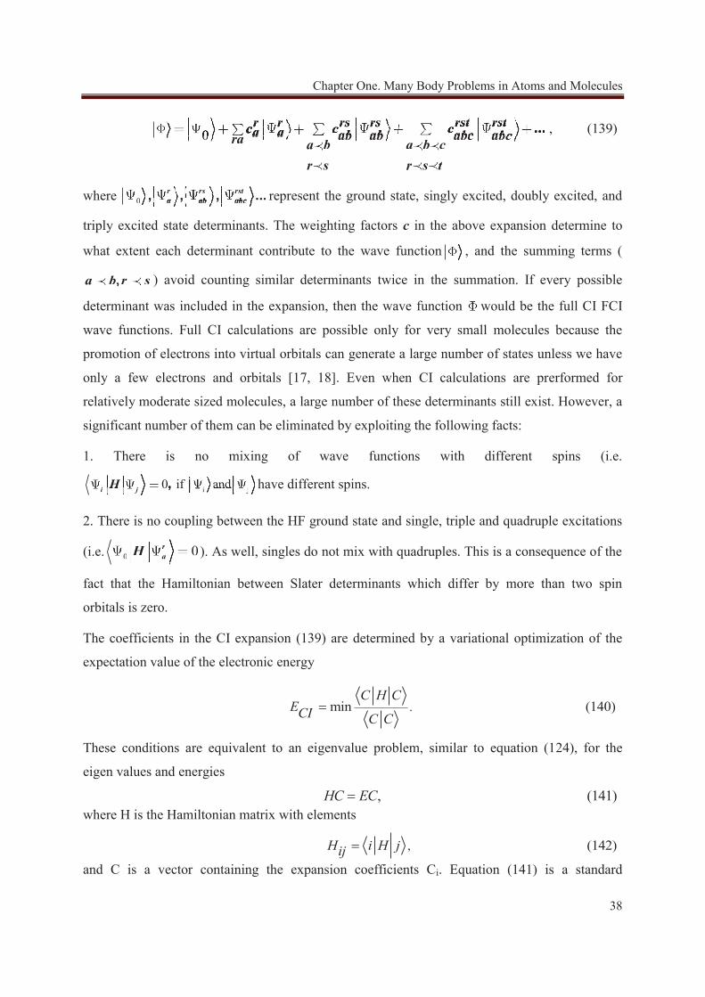
Chapter One. Many Body Problems in Atoms and Molecules
38
, (139)0 ...r r rs rs rst rstc c ca a ab ab abc abcra a b a b cr s r s t
, (0 r bcrar r rs rs rst rsta a bcra a b a b c
abc abb b
ab abab ab abc abb
ab ab
r s r s t
where 0 , , , ...r rs rsta ab abc0 , , , ...,r rs rsta ab abc, ,, , represent the ground state, singly excited, doubly excited, and
triply excited state determinants. The weighting factors c in the above expansion determine to
what extent each determinant contribute to the wave function , and the summing terms (
,a b r s,b r s, ) avoid counting similar determinants twice in the summation. If every possible
determinant was included in the expansion, then the wave function would be the full CI FCI
wave functions. Full CI calculations are possible only for very small molecules because the
promotion of electrons into virtual orbitals can generate a large number of states unless we have
only a few electrons and orbitals [17, 18]. Even when CI calculations are prerformed for
relatively moderate sized molecules, a large number of these determinants still exist. However, a
significant number of them can be eliminated by exploiting the following facts:
1. There is no mixing of wave functions with different spins (i.e.
i j0 if and,i jH i j0 if andi,i jH have different spins.
2. There is no coupling between the HF ground state and single, triple and quadruple excitations
(i.e. 0 0raH0 0raH ). As well, singles do not mix with quadruples. This is a consequence of the
fact that the Hamiltonian between Slater determinants which differ by more than two spin
orbitals is zero.
The coefficients in the CI expansion (139) are determined by a variational optimization of the
expectation value of the electronic energy
. min (140)C H C
ECI C C
These conditions are equivalent to an eigenvalue problem, similar to equation (124), for the
eigen values and energies
, (141)HC ECwhere H is the Hamiltonian matrix with elements
, (142)H i H jijand C is a vector containing the expansion coefficients Ci. Equation (141) is a standard
Chapter One. Many Body Problems in Atoms and Molecules
39
Hermitian eigenvalue problem that is solved by either diagonalizing the Hamiltonian matrix or
by other iterative techniques to extract the eigenvalues and eigenvectors.
Owing to its formal and conceptual simplicity, the CI method has been extensively and
successfully applied in quantum chemistry. However, for even the simplest systems, it is not
possible to carry out full configuration interaction FCI, particularly due to the large number of
determinants included in the expansion. It then becomes necessary to truncate the CI expansion
so that only a small set of the determinants is included. The truncated CI expansion should
preferably recover a large part of the correlation energy and provide a uniform description of the
electronic structure over the whole potential energy surface.
XIV. 3. Multireference CI Wave Function MRSDCI
The Multireference CI (MRCI) wave function is generated by including in the wave function all
configurations arising from the single and double excitations from the reference space, thus
resulting in the multireference singles and doubles configuration interaction (MRSDCI) wave
function
1 , 0,
(143)A ABX XMRSDCI I IJAI A B I J
where, the single and double excitation operators are given in second quantization by
, . (144)0 0 0 0A ABA ABX C a a X C a a a aI IJI A I IJ A B I J
The construction of a multireference CI wave function begins with the generation of a set of
orbitals and a reference space of configurations 0 , which are best generated by the CASSCF
method. The CASSCF method writes the wave function as a linear combination of determinants
or CSFs, whose expansion coefficients are optimized simultaneously with the MOs according to
the variation principle. The fully optimized wave functions in the CASSCF method are then used
as a reference state in the MRSDCI technique, in which single and double excitations are
included.
XIV. 4. Davidson's Correction
Configuration interaction calculations that include single, double, triple, and quadruple
excitations are designated SDTQCI. However, large basis sets involve too many determinants to
be computationally practicable. As the quadruply excited determinants can be important in
Chapter One. Many Body Problems in Atoms and Molecules
40
computing the correlation energy, a simple formula known as the Davidson correction has been
proposed for estimating the contribution of quadruply excited determinants to the correlation
energy [10, 19, 20], this is given by the following relation 20 1 (145)Davidson DCI SCFE c E E
where DCIE is the correlation energy computed in CI calculation using the ground state wave
function 00 and all its double excitations; 0c is the coefficient of 00 for the normalized wave
function. ESCF is the ground state energy obtained in HF-SCF calculations. The Davidson
correction can be computed without additional labor since the c0 is already computed in DCI
calculations. However, in spite of its usefulness for small molecules, the Davidson correction
fails for relatively large molecules [17].
XV. Spin Orbit Effects
The nonrelativistic Schrödinger picture discussed in the previous sections is not complete and
additional terms are needed to account for the intrinsic magnetic moment of the electron (spin).
In atomic and molecular systems, the exact solution of the non-relativistic Schrödinger equation
doesn’t reproduce the real experimental energies. The difference arises from relativistic effects,
which increase with the 4th power of the nuclear charge (Z4) [21]. Relativistic effects can be
neglected in most cases for lighter atoms, but have to be included when dealing with heavy
elements. In non-relativistic quantum mechanics, the velocity of light can be assumed to be
infinite, so that any finite velocity of particles is very small and the mass of the particle can be
approximated by its rest mass. For most measurements on the lighter elements in the periodic
table, non-relativistic quantum mechanics is sufficient, since the velocity of an electron is small
compared to the speed of light. For the heavier elements in the periodic table the picture is
entirely different. As a result for the heavy atoms, the inner electrons attain such high velocities,
comparable to that of light, and non-relativistic quantum mechanics is far from adequate. We can
divide relativistic effects in to several categories such as the mass-velocity correction, Darwin
correction, spin-orbit correction, spin-spin interaction, and Breit interaction [21, 22].
Of all the different kinds of relativistic effects the spin-orbit interaction represented by the Briet-
Pauli Hamiltonian is the most important part [21], which mainly arises from the interaction of the
intrinsic magnetic moment of the electron with the magnetic moment arising from orbital
motions. These effects alter the spectroscopic properties of molecules containing heavy elements
to a considerable extent. Even if a molecule has a closed shell ground state the excited states may
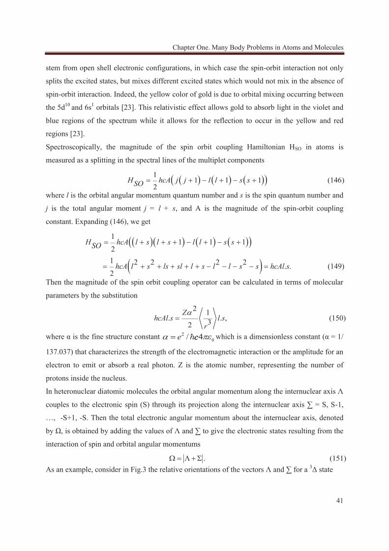
Chapter One. Many Body Problems in Atoms and Molecules
41
stem from open shell electronic configurations, in which case the spin-orbit interaction not only
splits the excited states, but mixes different excited states which would not mix in the absence of
spin-orbit interaction. Indeed, the yellow color of gold is due to orbital mixing occurring between
the 5d10 and 6s1 orbitals [23]. This relativistic effect allows gold to absorb light in the violet and
blue regions of the spectrum while it allows for the reflection to occur in the yellow and red
regions [23].
Spectroscopically, the magnitude of the spin orbit coupling Hamiltonian HSO in atoms is
measured as a splitting in the spectral lines of the multiplet components
1 1 1 1 (146)
2H hcA j j l l s sSO
where l is the orbital angular momentum quantum number and s is the spin quantum number and
j is the total angular moment j = l + s, and A is the magnitude of the spin-orbit coupling
constant. Expanding (146), we get
1 1 1 1
21 2 2 2 2 . . (149)2
H hcA l s l s l l s sSO
hcA l s ls sl l s l l s s hcAl s
Then the magnitude of the spin orbit coupling operator can be calculated in terms of molecular
parameters by the substitution
2 1 . . , (150)32
ZhcAl s l s
rwhere α is the fine structure constant 2
0/ 4e c 044 which is a dimensionless constant (α = 1/
137.037) that characterizes the strength of the electromagnetic interaction or the amplitude for an
electron to emit or absorb a real photon. Z is the atomic number, representing the number of
protons inside the nucleus.
In heteronuclear diatomic molecules the orbital angular momentum along the internuclear axis Λ
couples to the electronic spin (S) through its projection along the internuclear axis ∑ = S, S-1,
…, -S+1, -S. Then the total electronic angular momentum about the internuclear axis, denoted
by Ω, is obtained by adding the values of Λ and ∑ to give the electronic states resulting from the
interaction of spin and orbital angular momentums
. (151)As an example, consider in Fig.3 the relative orientations of the vectors Λ and ∑ for a 3Δ state
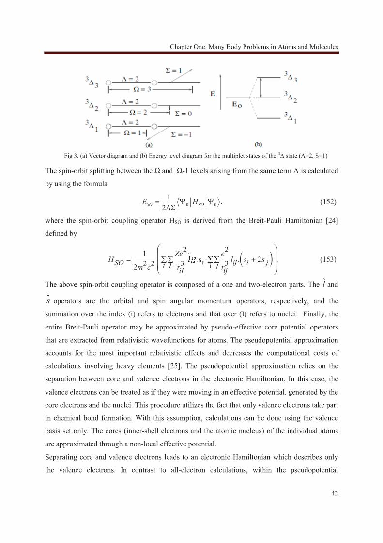
Chapter One. Many Body Problems in Atoms and Molecules
42
The spin-orbit splitting between the Ω and Ω-1 levels arising from the same term Λ is calculated
by using the formula
0 01 , (152)
2SO SOE H
where the spin-orbit coupling operator HSO is derived from the Breit-Pauli Hamiltonian [24]
defined by
.2 21
. - . 2 (153)2 2 3 3i2
Ze eH l s l s siI i ij i jSO i jIm c r rijiI
el --....
The above spin-orbit coupling operator is composed of a one and two-electron parts. The ll and
ss operators are the orbital and spin angular momentum operators, respectively, and the
summation over the index (i) refers to electrons and that over (I) refers to nuclei. Finally, the
entire Breit-Pauli operator may be approximated by pseudo-effective core potential operators
that are extracted from relativistic wavefunctions for atoms. The pseudopotential approximation
accounts for the most important relativistic effects and decreases the computational costs of
calculations involving heavy elements [25]. The pseudopotential approximation relies on the
separation between core and valence electrons in the electronic Hamiltonian. In this case, the
valence electrons can be treated as if they were moving in an effective potential, generated by the
core electrons and the nuclei. This procedure utilizes the fact that only valence electrons take part
in chemical bond formation. With this assumption, calculations can be done using the valence
basis set only. The cores (inner-shell electrons and the atomic nucleus) of the individual atoms
are approximated through a non-local effective potential.
Separating core and valence electrons leads to an electronic Hamiltonian which describes only
the valence electrons. In contrast to all-electron calculations, within the pseudopotential
Fig 3. (a) Vector diagram and (b) Energy level diagram for the multiplet states of the 3Δ state (Λ=2, S=1)
Chapter One. Many Body Problems in Atoms and Molecules
43
procedure only the valence electrons or the electrons (n-1)th shell, are explicitly considered. In
this case the electronic Hamiltonian can be reduced to an atomic valence operator, Hval given by,
2
1 1 1
1 1 , (154)2
v v vN N Nval
i ii i i ij
H V rr
where the indices i and j denote only valence electrons, and the V(ri) operator represents a one-
component, (spin-orbit-averaged) relativistic pseudopotential [26]
2 exp , (155)N
i lk lk ii l ki
ZV r A r Pr
,
where Pl is the projection operator onto the subspace with angular symmetry l
, ,1
. (156)m mm
P Y Y1m
,1
. mY YP , . m m,
In Eq (155) the pseudopotential parameters, the coefficients, Alk and the exponential parameters,
αlk are adjusted to total-valence energies derived from numerical all-electron calculations. The
pseudopotentials for atoms can be used for molecules containing heavy atoms. These potentials
can easily be implemented in quantum mechanical programs. The pseudopotential approximation
is not exact. However, its main advantage is the ease with which relativistic effects can be
included in the calculations. Indeed, a significant reduction of the computational effort can be
achieved by a restriction of the actual spin orbit calculations to the valence electron system and
the implicit inclusion of the influence of the chemically inert atomic cores by means of suitable
parameterized effective core potentials [27].
Chapter One. Many Body Problems in Atoms and Molecules
44
XVI. References: 1. R.P. Feynman., Phys. Rev., 76, 769 (1949). 2. E. Lewars., Computational Chemistry. Introduction to the Theory and Applications of Molecular and Quantum Mechanics., Springer Publications (2003). 3. M. Born and J. R. Oppenheimer., Ann. Physik., 84, 457 (1927). 4. W. Kolos and L. Wolniewicz., J. Chem. Phys., 41, 3663 (1964). 5. B. T. Sutcliffe., Adv. Quantum. Chem., 28, 65 (1997). 6. D. R. Hartree., Proc. Camb. Phill. Soc., 24, 328 (1928). 7. C. C. J. Roothan., Rev. Mod. Phys., 23, 69 (1951). 8. G. G. Hall, Proc. R. Soc. (London)., A205, 541 (1951). 9. A. Szabo and N. S. Ostlund, Modern Quantum Chemistry Introduction to Advanced Electronic Structure Theory., Dover Publications (1989). 10. P. W. Atkins and R. S. Friedman., Molecular Quantum Mechanics: 3rd Ed, Vol 2., Oxford University Press (1996). 11. V. A. Fock., Z. Phys., 15, 126 (1930). 12. C. J. Cramer., Essentials of Computational Chemistry Theories and Models., John Wiley and Sons LTD (2002). 13. P. E. M. Siegbahn., Chem. Phys. Lett., 55, 386 (1978). 14. B. O. Roos., Int. J. Quantum Chem., 14, 175 (1980). 15. T. Helgaker, P. Jorgensen, J. Olsen., Molecular Electronic-Structure Theory., John Wiley and Sons LTD (2000). 16. P. E. M. Siegbahn., in G. H. F. Diercksen and S. Wilson (eds), Methods in Computational Molecular Physics, Reidel., 189 (1983). 17. C. J. Cramer., Essentials of Computational Chemistry Theories and Models., John Wiley and Sons LTD (2002). 18. P.O. Lowdin., Adv. Chem. Phys., 2, 2207 (1959). 19. S. R. Langhoff and E. R. Davidson., Int. J. Quantum Chem., 8, 61 (1974). 20. E. R. Davidson and D. W. Silver., Chem. Phys. Lett., 52, 403 (1977). 21. D. B. Boyd and K. B. Lipkowitz., in Reviews in Computational Chemistry, K. B. Lipkowitz and D. B. Boyd, Eds., Wiley-VCH, New York, Vol. 15 (2000). 22. Bunker, P.R. and Jensen., P. Molecular Symmetry and Spectroscopy, 2nd edition, NRC Research Press Ottawa (1998). 23. Schmidbaur, Hubert, Cronje, Stephanie, Djordjevic, Bratislav, Schuster, Oliver "Understanding gold chemistry through relativity"., Chem. Phys., 311, 151 (2005). 24. D. G. Fedorov, S. Koseki, M.W. Schmidt, M. S. Gordon., Int. Reviews in Physical Chemistry., Vol. 22, No. 3, 551 (2003). 25. R. Boca, P. Pelikan, Coord., Chem. Rev., 229 (1992). 26. D. Andrae, U. Häußermann, M. Dolg, H. Stoll, H. Preuß., Theor. Chim. Acta.,77, 123 (1990). 27. Modern Methods and Algorithms of Quantum Chemistry, Proceedings, Second Edition, J. Grotendorst (Ed.), John von Neumann Institute for Computing, Julich, ¨NIC Series, Vol. 3, 507 (2000).
Chapter Two. Canonical Function’s Approach for Molecular Vibrations and Rotations
45
Chapter Two
Canonical Function’s Approach for Molecular Vibrations
and Rotations
uch attention has recently been focused on the optimal control of quantum systems,
and extensive theoretical works have been performed [1 – 10]. The research on
realizing quantum computers using the molecular internal degrees of freedom (electronic,
vibrational, and rotational) has only begun since the beginning of the century and the proposed
chemical system has been the molecular rovibrational modes of diatomic molecules [11,12-22,
23, 24, 25]. In the present work we explore the vibrational energy structures of the diatomic
molecules YN, YS, ZrN, and ZrS, by solving the vibrational Schrödinger equation within the
canonical functions approach. The theoretical backgrounds of our rovibrational calculations are
listed in this chapter, while the results of these calculations are shown in chapter three of this
thesis.
I. Canonical Function’s Approach
In view of the fact that in a molecule, the nuclei are much heavier than the electrons and their
speeds are slower, Born and Oppenheimer showed in 1927 [26] that molecular problems could
be much simplified by treating the electrons as moving in the field of fixed nuclei. In section XI
of chapter one of this thesis we discussed the theoretical basis of the Born-Oppenheimer
approximation. Within this approximation the kinetic energy of the nuclei is neglected and the
nuclear repulsion energy is considered constant. This allows for decoupling the electronic and
nuclear wavefunctions in the Schrödinger equation.
M
Chapter Two. Canonical Function’s Approach for Molecular Vibrations and Rotations
46
. (1)Total electronic nuclear
The vibrational-rotational wave function of a diatomic molecule is a solution of the radial
Schrödinger equation [27] 2
2 2
2
1 0
2 and =J J+1 , (
vJvJ vJ
r J Jk E V r r
r r
k 2 a2 nd 2)
where v and J represent respectively the vibrational and rotational quantum numbers. μ and
represent the reduced mass and planks constant.
The above equation could be simply written, as [27] '' , (3)x f x x
where 1 , eJ J x r r (re being the equilibrium distance), and
2 . (4)e
f x k E U xx r
However, equation (2) is equivalent to the Volterra integral equation [28]
' '
0
0 0 , (5)x
x x x t f t t dt
in the sense that any solution of equation (5) is a solution to equation (2).
Within the formulation of the canonical function’s approach [29, 30], one considers the
canonical functions α(r) and β(r) defined by ' 0 0 , (6)v v v v vx x x
with '
'
0 1 0 0
0 0 0 1 , (7)
and
10 0
0
where
with x =1 ,
x
i i ii
x A x A x t f t A t dt
A (8)
10 0
0 0
where
with B .
x
i i ii
x B x B x x t f t B t dt
x r r x (9)
Chapter Two. Canonical Function’s Approach for Molecular Vibrations and Rotations
47
Then the initial values of '0 and 0 can be deduced from and x x by using Eq(6)
and by using the following boundary condition [31]
-
0, (10)e
xr
x
one can find ' '0 0
lim , lim . (11)0 0 ex x r
x xx x
II. The Rotational Schrödinger Equation
The vibration-rotation energies of a diatomic molecule are usually written as
2 3 , (12)V V V VE E B D H ,
where, Bv, Dv, Hv, …, represent the rotational constants. One can write [27]
0
0 1 2
,
with , , , and 1 . (13)
nn
n
V V V
E e
e E e B e D J Jandddand
Then the energy factor f x given earlier in equations (3) and (4) could be expanded as [27]
0 , (14) i
in
f x x
0 0where (15-a)
k e U x
1 1 2
0
1 (15-b)
__ __ __ __ __ __ __ __ __ __ __ __
ker x
n for 2 (15-c).
nke i
Now by replacing f x by its value in the function An(r) in equation (8), one finds [32]
0
0
0
10 0
22
0 0 0
1
, (16)
rn n
n nn ir
rn n n
n n nn i ir
A r
A r r t t dt a t
A r r t t a t dt a t
and finally
Chapter Two. Canonical Function’s Approach for Molecular Vibrations and Rotations
48
0 . (17)n
nn
r G r
With the same manner, one obtains
0 . (18)n
nn
r H r
The functions Gn(r) and Hn(r) play the role of the function f x and the canonical functions of
pure vibration [27]
0 0 0 0 and . (19)r G r r H r
Then by taking advantage of the limits in equation (11), and by replacing α(r) and β(r) by their
expressions in equation (17) and (18), we get [27]
'
0 0 / 0 , (20)n
nn
I
where the coefficients In are deduced from the values of the coefficients Gn and Hn at the
boundaries –r and . The vibrational-rotational wavefunctions defined in equation (6) can be
written as
0 0 0
0 0 00 0 0
1 1 1
0 0
0 0 0 , (21)
n n nn n n
n n n
n n nn n n
n n n
x G x I G x
G I G x C x I G x
where from Eq(13), if n=0 then e0 = EV, which indicates that the term with n=0 is a purely
vibrational term. In addition, the first two terms of expression (21) are not related to the
rotational quantum number J, since 0 1, and with n =0 these two terms could be assigned to a
purely vibrational wavefunction 0 x . Accordingly, the vibro-rotational wave function x
given in equation (21) could be refined as
01
. (22)nn
nx x x
The second term of the above equation is a purely rotational function n x , since it depends
directly on . Thus the rotational effect in the vibration-rotation wavefunction x is
separated from the pure vibration wavefunction 0 x [27]. The terms n x in the above
equation are called the rotational harmonics that depend on Cn(x), Gn(x), and In(x).
Chapter Two. Canonical Function’s Approach for Molecular Vibrations and Rotations
49
Finally, by replacing the wave function’s expression of equation (22) in equation (3), we find
01 1
'' ''0 0
1 , (23)n n
n nn n
nn
nr r
which gives [27] ''0 0 0
''1 0 1 1 0
=0 (24-a)
x x x
x x x x x''2 0 2 1 1 2 0
(24-b)
(24-c) __ __ __ __ __ __ __ __ _
x x x x x x x
''n 0
1
_ __ __ __ __ __ __ __ __
. (24-n)n
n m n mm
x x x x x
The first of these equations is called the radial Schrödinger equation of pure vibration for J = 0.
All of the other equations are called the rotational Schrödinger equations for J>0 nuclear
rotations. The rotational Schrödinger equations allow us to successively determine the rotational
harmonics 1 2, , , and nd, and .
III. Finding the Pure Vibrational Wavefunction
The pure vibrational Schrödinger equation was given by
''0 0 0 =0 , (25)x x x
where ε0 represents the energy factor which corresponds to pure vibration. It is obtained by
setting λ = 0 in equation (4). Equation (25) can be written in the integral form [30]
0
'0 0 0 0 0 0 0 0 , (26)
r
r
x r r r r r t t t dt
where the function φ0(r) can be written in the form '
0 0 0 0 0 0 0 . (27)r r r r r
The two canonical functions α(r) and β(r), associated with ε0(r), are given by [29]
0 10 0
0 0
where
with B .
r
i i ii
r B r B r r t t B t dt
r r r (29)
0 10 0
0
where
with r =1,
r
i i ii
r A r A r t t A t dt
A (28)
Chapter Two. Canonical Function’s Approach for Molecular Vibrations and Rotations
50
If we take λ = 0 in equation (21), one can write φ0(r0) = 1 for the wave function. Then by using
the conditions applicable on φ0 at the limits (10), with the relations between φ0, α0, and β0 and by
considering the initial condition of φ’0(r0) given by [27]
0'0 0
00
lim (30)rr
rr
r
with '0 0 0l r , we get
0 0 0 0 . (31)r r l r
In conclusion the calculations for the proper value of pure vibrational energy ε0 and for the pure
vibrational wave function φ0 by using equation 24-a. Then by using the calculated values of ε0
and φ0 in equation 24-b, one can obtain the values of the rotational constant ε1 = Bv and the
rotational harmonic wavefunction φ1. Then by using the values of ε0, ε1, φ0, and φ1 in equation
24-c one can obtain the values of the centrifugal distortion constants ε2 = Dv, with the values of
the 2nd order rotational harmonic φ2. The iterative cycle can be repeated by using equation 24-n
in order to obtain rotational constants as Lv, Hv, …
The remaining part of this chapter is devoted for calculating the rotational harmonics φ1, φ2, …,
φn, described in Ref [27] and whose corresponding eigenvalues are ε1, ε2, …, εn.
IV. Canonical Formulation for the First Rotational Harmonic
Formerly, we found a solution to the vibrational Schrödinger equation (24-a). Now, in this
section we will concentrate on finding a solution to the rotational Schrödinger equation (24-b)
''1 0 1 1 0 . (32)x x x x x
The solution of the above equation is equivalent to the solution of the Voltera integral equation
[27, 33]
0 0
'1 1 0 1 0 0 1 1 0 0 . (33)
r r
r r
r r r r r t t t dt r t t t dt
The solution of the above equation can be greatly simplified by following a procedure similar to
that adopted in section III and by using the canonical functions α and β together with equations
(8) and (9), we get '
1 1 0 0 1 0 0 1 (34)r r r r r r
Chapter Two. Canonical Function’s Approach for Molecular Vibrations and Rotations
51
10
0 1 00
and (35-a)
nn
r
r K r
K r r t t t dt
0
1 1 1 0 10
(35-b)
(35-c)r t
r
K r x t t t t t dt dt
0
1 1 , (35-d)r
n nr
K r r t t K t dt
with the properties below [32]:
(i) for r = r0
0 0 1 0 0
1 0
0
giving 0. (36)nK r K r K r
r0 000
The derivation of the σ1(r)
' '1
0 ( ) , (37)n
nr K r
with0
'1 1
r
n nr
K r t K t dt and
' ' '0 0 1 0 0
'1
0
giving 0. (38)nK r K r K r
r
'0 0'00
For the other higher order derivatives of σ1(r), we find
'' ''1
0 ( ) , (39)n
nr K r
with ''1 1 ,n nK r r K r
and '' '' ''0 1 0 0 0 0nK K K '' 0 0''
n 00
(ii) The rotation harmonics must vanish at the boundaries [27], i.e.
lim 0, 0. (40)e
nxx r
x n
Then the first rotational harmonic φ1(r) written in equation (34), gives '
1 1 0 0 1 , (41)r r r r with the limiting conditions (40)
Chapter Two. Canonical Function’s Approach for Molecular Vibrations and Rotations
52
1'1 0 1
0
lim , (42)e
xx r
rr l
r
to give the rotational wave funciton
1 1 0 1 . (43)r l r r V. Numerical Methods
For a potential function given by U(r), and a vibrational energy value E, the function φ0 is given
by [27]
0 0 0 0 , (44)r r l r
where the functions α0(r) and β0(r) are given by the expression (28) and (29), in terms of the
functions U(r) and E = ε0. The study of these expressions is available independent on the form of
the potential considered. For a numerical potential of type RKR [34, 35] defined by the turning
points and by the polynomial interpolation of the calculated potential energy curves. Once the
formulation of the potential is specified, the calculations can be carried out for the canonical
functions α0(r), β0(r), and the parameters l0 and φ0.
Within a specified interval [ri, ri+1] delimited by the abscissa of two successive points Pi, Pi+1.
The potential function U(r) is written as
n0
1
,
with , 0 - , (45)
Nn
n
i i i
U x x
x r r x r r
and the constants γn are the coefficients determined for the specified numerical potential energy
function.
II.5.1. Calculations of the Canonical Functions α0(r) and β0(r)
The pure vibrational equation, given by equation (24-a) can be written as ''
0 , (46)y x x y x
with 0 0x k e U x . The solution of this equation is written in the form [2]
0 . (47)n
n in
y r c i r r
The functions α0(r) and β0(r) are given by the same function y(r). Then by substituting equation
(47) in to equation (46), we get [27]
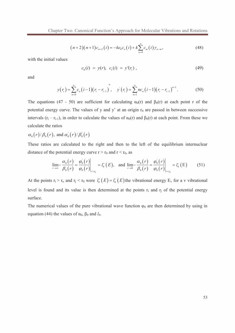
Chapter Two. Canonical Function’s Approach for Molecular Vibrations and Rotations
53
2 00
2 1 , (48)n
n n m n mn
n n c i ke c i k c i
with the initial values
0 1 ( ) ( ), ( ) '( ) , (49)ic i y r c i y r
and
1'1 1
0 1 1 , 1 . (50)
nn
i n i i i n i in n
y r c i r r y r nc i r r
The equations (47 - 50) are sufficient for calculating α0(r) and β0(r) at each point r of the
potential energy curve. The values of y and y’ at an origin r0 are passed in between successive
intervals (ri – ri-1), in order to calculate the values of α0(r) and β0(r) at each point. From these we
calculate the ratios ' '
0 0 0 0/ , and /r r r r
These ratios are calculated to the right and then to the left of the equilibrium internuclear
distance of the potential energy curve r > r0 and r < r0, as
0 0
' '0 0 0 0
0 000 0 0 0
lim , and lim E (51)r r
r r r r
r r r rl E l
r r r r
At the points ri > ro and rj < r0 were 0 0l E l E the vibrational energy Ev for a v vibrational
level is found and its value is then determined at the points ri and rj of the potential energy
surface.
The numerical values of the pure vibrational wave function φ0 are then determined by using in
equation (44) the values of α0, β0 and l0.
Chapter Two. Canonical Function’s Approach for Molecular Vibrations and Rotations
54
VI. References:
1. L. Rees., Proc. Phys. Soc. London., 59, 998 (1947). 2. R. Courant and D. Hilbert., Methods of Mathematical Physics., Wiley, New York (1966). 3. A. P. Pierce, M. A. Dahleh, and H. Rabitz., Phys. Rev., A 37, 4950 (1988). 4. S. Shi and H. Rabitz., J. Chem. Phys., 92, 364 (1992). 5. M. Demiralp and H. Rabitz., Phys. Rev. A., 47, 830 (1993). 6. D. J. Tannor, V. A. Kazakov, and V. Orlov., in Time-Dependent Quantum Molecular Dynamics, edited by J. Broeckhove and L. Lathouwers Plenum,New York, (1992). 7. J. Somloi, V. A. Kazakov, and D. J. Tannor., Chem. Phys., 172, 85 (1993). 8. W. Zhu, J. Botina, H. Rabitz., J. Chem. Phys., 108, 1953 (1997). 9. R. R. Zaari, A. Brown., J. Chem. Phys., 135, 044317 (2011). 10. T. Cheng, A. Brown., J. Chem. Phys., 124, 034111 (2006). 11. R. R. Zaari, A. Brown., J. Chem. Phys., 135, 044317 (2011). 12. J. Vala, Z. Amitay, B. Zhang, S. R. Leone, and R. Kosloff, Phys.Rev. A 66, 062316 (2002). 13. D. Babikov, J. Chem. Phys. 121, 7577 (2004). 14. Y. Ohtsuki, Chem. Phys. Lett. 404, 126 (2005). 15. C. Menzel-Jones and M. Shapiro, Phys. Rev. A 75, 052308 (2007). 16. K. Shioya, K.Mishima, and K. Yamashita, Mol. Phys. 105, 1287 (2007). 17. K. Mishima, K. Tokumo, and K. Yamashita, Chem. Phys. 343, 61 (2008). 18. M. Tsubouchi and T.Momose, Phys. Rev. A 77, 052326 (2008). 19. M. Tsubouchi, A. Khramov, and T. Momose, Phys. Rev. A 77, 023405 (2008). 20. D. Sugny, L. Bomble, T. Ribeyre, O. Dulieu, and M. Desouter-Lecomte, Phys. Rev. A 80, 042325 (2009). 21. K. Mishima and K. Yamashita, Chem. Phys. 367, 63 (2010). 22. R. Zaari and A. Brown, J. Chem. Phys. 132, 014307 (2010). 23. L. Bomble, P. Pellegrini, Pierre Ghesquière, and M. Desouter-Lecomte., Phys. Rev. A., 82, 062323 (2010). 24. S. Sharma, P. Sharma, H. Singh., J. Chem. Sci., 119, 433 (2007). 25. K. Sundermann, M. Motzkus, and R. de Vivie-Riedle., J. Chem. Phys., 110, 1896 (1999). 26. M. Born and J. R. Oppenheimer., Ann. Physik., 84, 457 (1927). 27. M. Korek, International Center for Theoretical Physics (1989). 28. H. Kobeissi and M. Korek., Int. J. Quant. Chem., 22, 23 (1982). 29. H. Kobeissi and M. Alameddine., J. Physique(Paris)., 39, 43 (1978). 30. H. Kobeissi and Y. S. Tergiman., J. Physique., 35, 635 (1974). 31. H. Kobeissi, M. Dagher, M. Korek, and A. Chaalan., J. Comput. Chem., 4, 218 (1983). 32. H. Kobeissi and M. Korek., Int. J. Quant. Chem., 22, 23 (1982). 33. M. Korek and H. Kobeissi., J. Comput. Chem., 13, 1103 (1992). 34. R. Rydberg., Z. Phys., 73, 376 (1931). 35. O. Klein., Z. Phys., 76, 226 (1932).
Chapter Three: Results and Discussion
55
Chapter Three
Results and Discussions
etal-ligand bonding underlies the vast physical and chemical properties that a
material has. The spectroscopic study of heavy polar diatomic molecules is
important in such diverse fields as astrophysics [1], ultracold interactions [2], organometallic
chemistry [3], quantum computing [4-6], precision measurements [7], and metallurgy [3].
The present investigation is devoted to the prediction for the electronic structures of the
transition metal nitrides and sulfides of Yttrium and Zirconium. Our interest in transition
metals has been investigated by the desire to understand the role played by d orbitals in
bonding. The diatomic molecules composed of the transition metals of groups III and IV are
the simplest of the d- block open shell molecules with the valence electronic configuration
[(n-1)d1,2ns2]. In this chapter we list the results of our calculations for the electronic
structures, spectroscopic constants, and vibrational structures of the heavy polar diatomic
molecules YN, ZrN, ZrS and YS. A comparison is made, where available, between the results
of the present work to the experimental and theoretical results in literature. The small relative
difference of less than 10% obtained in the present calculations reflects the accuracy of our
computational approach in representing the true physical systems.
I. The Computational Approach
In the present work ab initio investigations for the lowest lying molecular states of the
molecules YN, ZrN, YS, and ZrS have been performed at the Complete Active Space Self
Consistent Field (CASSCF) method followed by the Multi Reference Single and Double
Excitation Configuration Interaction (MRSDCI) method. The Davidson correction, noted as
MRSDCI+Q was then invoked in order to account for unlinked quadruple clusters. The ab
initio MRSDCI+Q calculations were performed on two stages. In the first, electronic
structure calculations were carried out ignoring the effect of relativistic spin orbit coupling.
M
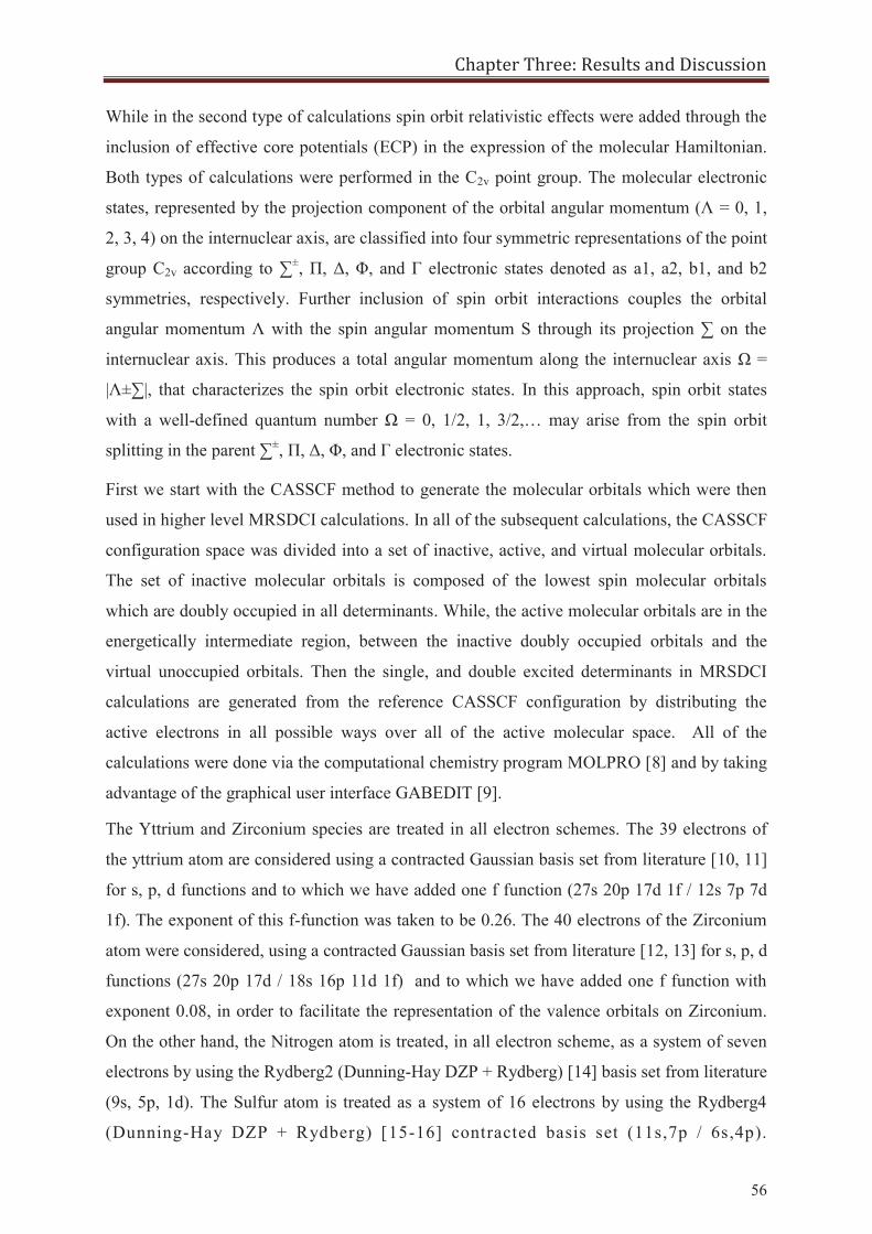
Chapter Three: Results and Discussion
56
While in the second type of calculations spin orbit relativistic effects were added through the
inclusion of effective core potentials (ECP) in the expression of the molecular Hamiltonian.
Both types of calculations were performed in the C2v point group. The molecular electronic
states, represented by the projection component of the orbital angular momentum (Λ = 0, 1,
2, 3, 4) on the internuclear axis, are classified into four symmetric representations of the point
group C2v according to ∑±, Π, Δ, Φ, and Γ electronic states denoted as a1, a2, b1, and b2
symmetries, respectively. Further inclusion of spin orbit interactions couples the orbital
angular momentum Λ with the spin angular momentum S through its projection ∑ on the
internuclear axis. This produces a total angular momentum along the internuclear axis Ω =
|Λ±∑|, that characterizes the spin orbit electronic states. In this approach, spin orbit states
with a well-defined quantum number Ω = 0, 1/2, 1, 3/2,… may arise from the spin orbit
splitting in the parent ∑±, Π, Δ, Φ, and Γ electronic states.
First we start with the CASSCF method to generate the molecular orbitals which were then
used in higher level MRSDCI calculations. In all of the subsequent calculations, the CASSCF
configuration space was divided into a set of inactive, active, and virtual molecular orbitals.
The set of inactive molecular orbitals is composed of the lowest spin molecular orbitals
which are doubly occupied in all determinants. While, the active molecular orbitals are in the
energetically intermediate region, between the inactive doubly occupied orbitals and the
virtual unoccupied orbitals. Then the single, and double excited determinants in MRSDCI
calculations are generated from the reference CASSCF configuration by distributing the
active electrons in all possible ways over all of the active molecular space. All of the
calculations were done via the computational chemistry program MOLPRO [8] and by taking
advantage of the graphical user interface GABEDIT [9].
The Yttrium and Zirconium species are treated in all electron schemes. The 39 electrons of
the yttrium atom are considered using a contracted Gaussian basis set from literature [10, 11]
for s, p, d functions and to which we have added one f function (27s 20p 17d 1f / 12s 7p 7d
1f). The exponent of this f-function was taken to be 0.26. The 40 electrons of the Zirconium
atom were considered, using a contracted Gaussian basis set from literature [12, 13] for s, p, d
functions (27s 20p 17d / 18s 16p 11d 1f) and to which we have added one f function with
exponent 0.08, in order to facilitate the representation of the valence orbitals on Zirconium.
On the other hand, the Nitrogen atom is treated, in all electron scheme, as a system of seven
electrons by using the Rydberg2 (Dunning-Hay DZP + Rydberg) [14] basis set from literature
(9s, 5p, 1d). The Sulfur atom is treated as a system of 16 electrons by using the Rydberg4
(Dunning-Hay DZP + Rydberg) [15-16] contracted basis set (11s,7p / 6s,4p).
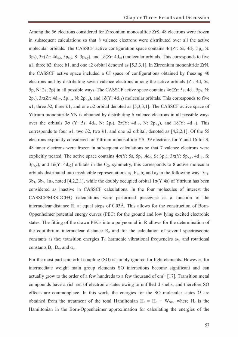
Chapter Three: Results and Discussion
57
Among the 56 electrons considered for Zirconium monosulfide ZrS, 48 electrons were frozen
in subsequent calculations so that 8 valence electrons were distributed over all the active
molecular orbitals. The CASSCF active configuration space contains 4σ(Zr: 5s, 4d0, 5pz, S:
3pz), 3π(Zr: 4d±2, 5px,y, S: 3px,y), and 1δ(Zr: 4d±1) molecular orbitals. This corresponds to five
a1, three b2, three b1, and one a2 orbital denoted as [5,3,3,1]. In Zirconium mononitride ZrN,
the CASSCF active space included a CI space of configurations obtained by freezing 40
electrons and by distributing seven valence electrons among the active orbitals (Zr: 4d, 5s,
5p, N: 2s, 2p) in all possible ways. The CASSCF active space contains 4σ(Zr: 5s, 4d0, 5pz, N:
2pz), 3π(Zr: 4d±2, 5px,y, N: 2px,y), and 1δ(Y: 4d±1) molecular orbitals. This corresponds to five
a1, three b2, three b1, and one a2 orbital denoted as [5,3,3,1]. The CASSCF active space of
Yttrium mononitride YN is obtained by distributing 6 valence electrons in all possible ways
over the orbitals 3σ (Y: 5s, 4d0, N: 2pz), 2π(Y: 4d±2, N: 2px,y), and 1δ(Y: 4d±1). This
corresponds to four a1, two b2, two b1, and one a2 orbital, denoted as [4,2,2,1]. Of the 55
electrons explicitly considered for Yttrium monosulfide YS, 39 electrons for Y and 16 for S,
48 inner electrons were frozen in subsequent calculations so that 7 valence electrons were
explicitly treated. The active space contains 4σ(Y: 5s, 5pz ,4d0, S: 3pz), 3π(Y: 5px,y, 4d±2, S:
3px,y), and 1δ(Y: 4d±2) orbitals in the C2v symmetry, this corresponds to 8 active molecular
orbitals distributed into irreducible representations a1, b1, b2 and a2 in the following way: 5a1,
3b1, 3b2, 1a2, noted [4,2,2,1], while the doubly occupied orbital 1σ(Y:4s) of Yttrium has been
considered as inactive in CASSCF calculations. In the four molecules of interest the
CASSCF/MRSDCI+Q calculations were performed piecewise as a function of the
internuclear distance R, at equal steps of 0.03Å. This allows for the construction of Born-
Oppenheimer potential energy curves (PEC) for the ground and low lying excited electronic
states. The fitting of the drawn PECs into a polynomial in R allows for the determination of
the equilibrium internuclear distance Re and for the calculation of several spectroscopic
constants as the; transition energies Te, harmonic vibrational frequencies ωe, and rotational
constants Be, De, and αe.
For the most part spin orbit coupling (SO) is simply ignored for light elements. However, for
intermediate weight main group elements SO interactions become significant and can
actually grow to the order of a few hundreds to a few thousand of cm-1 [17]. Transition metal
compounds have a rich set of electronic states owing to unfilled d shells, and therefore SO
effects are commonplace. In this work, the energies for the SO molecular states Ω are
obtained from the treatment of the total Hamiltonian Ht = He + WSO, where He is the
Hamiltonian in the Born-Oppenheimer approximation for calculating the energies of the
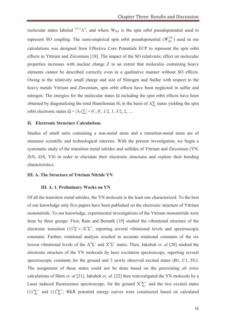
Chapter Three: Results and Discussion
58
molecular states labeled 2s+1Λ±, and where WSO is the spin orbit pseudopotential used to
represent SO coupling. The semi-empirical spin orbit pseudopotential ( PSSOW ) used in our
calculations was designed from Effective Core Potentials ECP to represent the spin orbit
effects in Yttrium and Zirconium [18]. The impact of the SO relativistic effect on molecular
properties increases with nuclear charge Z to an extent that molecules containing heavy
elements cannot be described correctly even in a qualitative manner without SO effects.
Owing to the relatively small charge and size of Nitrogen and Sulfur with respect to the
heavy metals Yttrium and Zirconium, spin orbit effects have been neglected in sulfur and
nitrogen. The energies for the molecular states Ω including the spin orbit effects have been
obtained by diagonalizing the total Hamiltonian Ht in the basis of Λ∑ states yielding the spin
orbit electronic states Ω = |Λ±∑| = 0+, 0-, 1/2, 1, 3/2, 2, …
II. Electronic Structure Calculations
Studies of small units containing a non-metal atom and a transition-metal atom are of
immense scientific and technological interests. With the present investigation, we begin a
systematic study of the transition metal nitrides and sulfides of Yttrium and Zirconium (YN,
ZrN, ZrS, YS) in order to elucidate their electronic structures and explore their bonding
characteristics.
III. A. The Structure of Yttrium Nitride YN
III. A. 1. Preliminary Works on YN
Of all the transition metal nitrides, the YN molecule is the least one characterized. To the best
of our knowledge only five papers have been published on the electronic structure of Yttrium
mononitride. To our knowledge, experimental investigations of the Yttrium mononitride were
done by three groups: First, Ram and Bernath [19] studied the vibrational structure of the
electronic transition (1)1Σ+←X1Σ+, reporting several vibrational levels and spectroscopic
constants. Further, rotational analysis resulted in accurate rotational constants of the six
lowest vibrational levels of the A1Σ+ and X1Σ+ states. Then, Jakubek et. al [20] studied the
electronic structure of the YN molecule by laser excitation spectroscopy, reporting several
spectroscopic constants for the ground and 3 newly observed excited states (B1, C1, D1).
The assignment of these states could not be done based on the preexisting ab initio
calculations of Shim et. al [21]. Jakubek et. al. [22] then reinvestigated the YN molecule by a
Laser induced fluorescence spectroscopy, for the ground X1∑+ and the two excited states
(1)1∑+ and (1)3∑+; RKR potential energy curves were constructed based on calculated
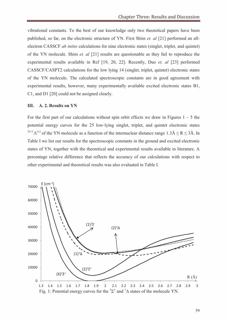
Chapter Three: Results and Discussion
59
vibrational constants. To the best of our knowledge only two theoretical papers have been
published, so far, on the electronic structure of YN. First Shim et. al [21] performed an all-
electron CASSCF ab initio calculations for nine electronic states (singlet, triplet, and quintet)
of the YN molecule. Shim et. al [21] results are questionable as they fail to reproduce the
experimental results available in Ref [19, 20, 22]. Recently, Duo et. al [23] performed
CASSCF/CASPT2 calculations for the low lying 14 (singlet, triplet, quintet) electronic states
of the YN molecule. The calculated spectroscopic constants are in good agreement with
experimental results, however, many experimentally available excited electronic states B1,
C1, and D1 [20] could not be assigned clearly.
III. A. 2. Results on YN
For the first part of our calculations without spin orbit effects we draw in Figures 1 – 5 the
potential energy curves for the 25 low-lying singlet, triplet, and quintet electronic states 2s+1Λ(±) of the YN molecule as a function of the internuclear distance range 1.3Å ≤ R ≤ 3Å. In
Table I we list our results for the spectroscopic constants in the ground and excited electronic
states of YN, together with the theoretical and experimental results available in literature. A
percentage relative difference that reflects the accuracy of our calculations with respect to
other experimental and theoretical results was also evaluated in Table I.
0
10000
20000
30000
40000
50000
60000
70000
1.3 1.4 1.5 1.6 1.7 1.8 1.9 2 2.1 2.2 2.3 2.4 2.5 2.6 2.7 2.8 2.9 3
(X)1Σ+ (2)1Σ+
(1)1Δ
(2)1Δ
(1)1Σ-
E (cm-1)
R (Å)
Fig. 1: Potential energy curves for the 1Σ± and 1Δ states of the molecule YN.
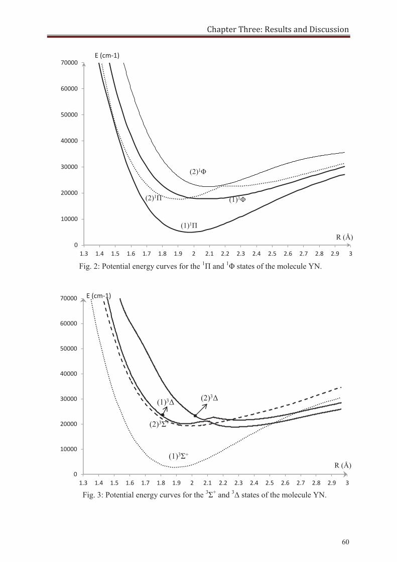
Chapter Three: Results and Discussion
60
0
10000
20000
30000
40000
50000
60000
70000
1.3 1.4 1.5 1.6 1.7 1.8 1.9 2 2.1 2.2 2.3 2.4 2.5 2.6 2.7 2.8 2.9 3
(1)1Π
(2)1Π (1)1Φ
(2)1Φ
E (cm-1)
R (Å)
Fig. 2: Potential energy curves for the 1Π and 1Φ states of the molecule YN.
Fig. 3: Potential energy curves for the 3Σ+ and 3Δ states of the molecule YN.
0
10000
20000
30000
40000
50000
60000
70000
1.3 1.4 1.5 1.6 1.7 1.8 1.9 2 2.1 2.2 2.3 2.4 2.5 2.6 2.7 2.8 2.9 3
(1)3Σ+
(2)3Σ+
(1)3Δ (2)3Δ
E (cm-1)
R (Å)
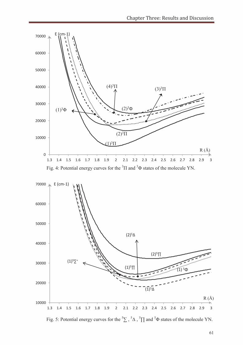
Chapter Three: Results and Discussion
61
0
10000
20000
30000
40000
50000
60000
70000
1.3 1.4 1.5 1.6 1.7 1.8 1.9 2 2.1 2.2 2.3 2.4 2.5 2.6 2.7 2.8 2.9 3
(1)3Π
(1)3Φ
(2)3Π
(2)3Φ
(3)3Π (4)3Π
E (cm-1)
R (Å)
Fig. 4: Potential energy curves for the 3Π and 3Φ states of the molecule YN.
Fig. 5: Potential energy curves for the 5∑ , 5Δ , 5∏ and 5Φ states of the molecule YN.
10000
20000
30000
40000
50000
60000
70000
1.3 1.4 1.5 1.6 1.7 1.8 1.9 2 2.1 2.2 2.3 2.4 2.5 2.6 2.7 2.8 2.9 3
(1)5∆
(1)5∑+
(2)5∆
(1) 5Φ (1)5∏
(2)5∏
E (cm-1)
R (Å)
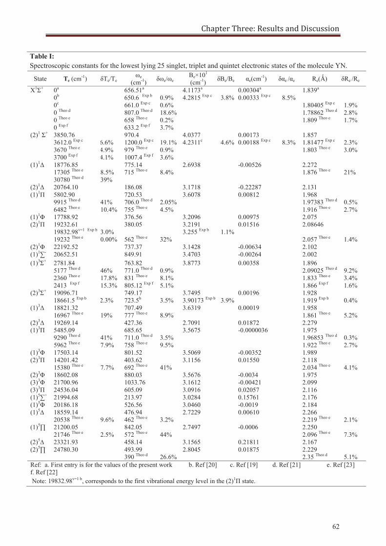
Chapter Three: Results and Discussion
62
Table I: Spectroscopic constants for the lowest lying 25 singlet, triplet and quintet electronic states of the molecule YN.
State Te (cm-1) δTe/Te ωe
(cm-1) δωe/ωe Be×101
(cm-1) δBe/Be αe(cm-1) δαe /αe Re(Ǻ) δRe /Re
X1Σ+ 0a
0b 0c 0 Theo d
0 Theo e
0 Exp f
656.51a
650.6 Exp b
661.0 Exp c
807.0 Theo d
658 Theo e
633.2 Exp f
0.9% 0.6% 18.6% 0.2% 3.7%
4.1173a 4.2815 Exp c
3.8%
0.00304a
0.00333 Exp c 8.5%
1.839a
1.80405 Exp c
1.78862 Theo d
1.809 Theo e
1.9% 2.8% 1.7%
(2)1 Σ+ 3850.76 3612.0 Exp c
3670 Theo e
3700 Exp f
6.6% 4.9% 4.1%
970.4 1200.0 Exp c
979 Theo e
1007.4 Exp f
19.1% 0.9% 3.6%
4.0377 4.2311c
4.6%
0.00173
0.00188 Exp c 8.3%
1.857 1.81477 Exp c
1.803 Theo e
2.3% 3.0%
(1)1Δ 18776.85 17305 Theo e
30780 Theo d
8.5% 39%
775.14 715 Theo e
8.4%
2.6938 -0.00526 2.272 1.876 Theo e
21%
(2)1Δ 20764.10 186.08 3.1718 -0.22287 2.131 (1)1Π
5802.90 9915 Theo d 6482 Theo e
41% 10.4%
720.53 706.0 Theo d
755 Theo e
2.05% 4.5%
3.6078 0.00812 1.968 1.97383 Theo d
1.916 Theo e
0.5% 2.7%
(1)1Φ 17788.92 376.56 3.2096 0.00975 2.075 (2)1Π 19232.61
19832.98v=1 Exp b
19232 Theo e
3.0% 0.00%
380.05 562 Theo e
32%
3.2191 3.255 Exp b
1.1%
0.01516 2.08646 2.057 Theo e
1.4%
(2)1Φ 22192.52 737.37 3.1428 -0.00634 2.102 (1)1∑- 20652.51 849.91 3.4703 -0.00264 2.002 (1)3Σ+ 2781.84
5177 Theo d
2360 Theo e
2413 Exp f
46% 17.8% 15.3%
763.82 771.0 Theo d
831 Theo e
805.12 Exp f
0.9% 8.1% 5.1%
3.8773 0.00358 1.896 2.09025 Theo d
1.833 Theo e
1.866 Exp f
9.2% 3.4% 1.6%
(2)3Σ+
19096.71 18661.5 Exp b
2.3%
749.17 723.5b
3.5%
3.7495 3.90173 Exp b
3.9%
0.00196 1.928 1.919 Exp b
0.4%
(1)3Δ
18821.32 16967 Theo e
19%
707.49 777 Theo e
8.9%
3.6319
0.00019 1.958 1.861 Theo e
5.2%
(2)3Δ 19269.14 427.36 2.7091 0.01872 2.279 (1)3Π 5485.09
9290 Theo d
5962 Theo e
41% 7.9%
685.65
711.0 Theo d
758 Theo e
3.5% 9.5%
3.5675 -0.0000036 1.975 1.96853 Theo d
1.922 Theo e
0.3% 2.7%
(1)3Φ 17503.14 801.52 3.5069 -0.00352 1.989 (2)3Π 14201.42
15380 Theo e 7.7%
403.62 692 Theo e
41%
3.1156 0.01550 2.118 2.034 Theo e
4.1%
(2)3Φ 18602.08 880.03 3.5676 -0.0034 1.975 (3)3Φ 21700.96 1033.76 3.1612 -0.00421 2.099 (3)3Π 24536.04 605.09 3.0916 0.02057 2.116 (1)5∑+ 21994.68 213.97 3.0284 0.15761 2.176 (1)5Φ 20186.18 526.56 3.0460 -0.0019 2.184 (1)5∆ 18559.14
20538 Theo e 9.6%
476.94 462 Theo e
3.2%
2.7229 0.00610 2.266 2.219 Theo e
2.1%
(1)5∏ 21200.05 21746 Theo e
2.5%
842.05 572 Theo e
44%
2.7497 -0.0006 2.250 2.096 Theo e
7.3%
(2)5∆ 23321.93 458.14 3.1565 0.21811 2.167 (2)5∏ 24780.30 493.99
390 Theo d 26.6%
2.8045 0.01875 2.229 2.35 Theo d
5.1%
Ref: a. First entry is for the values of the present work b. Ref [20] c. Ref [19] d. Ref [21] e. Ref [23] f. Ref [22] Note: 19832.98v=1 b, corresponds to the first vibrational energy level in the (2)1Π state.
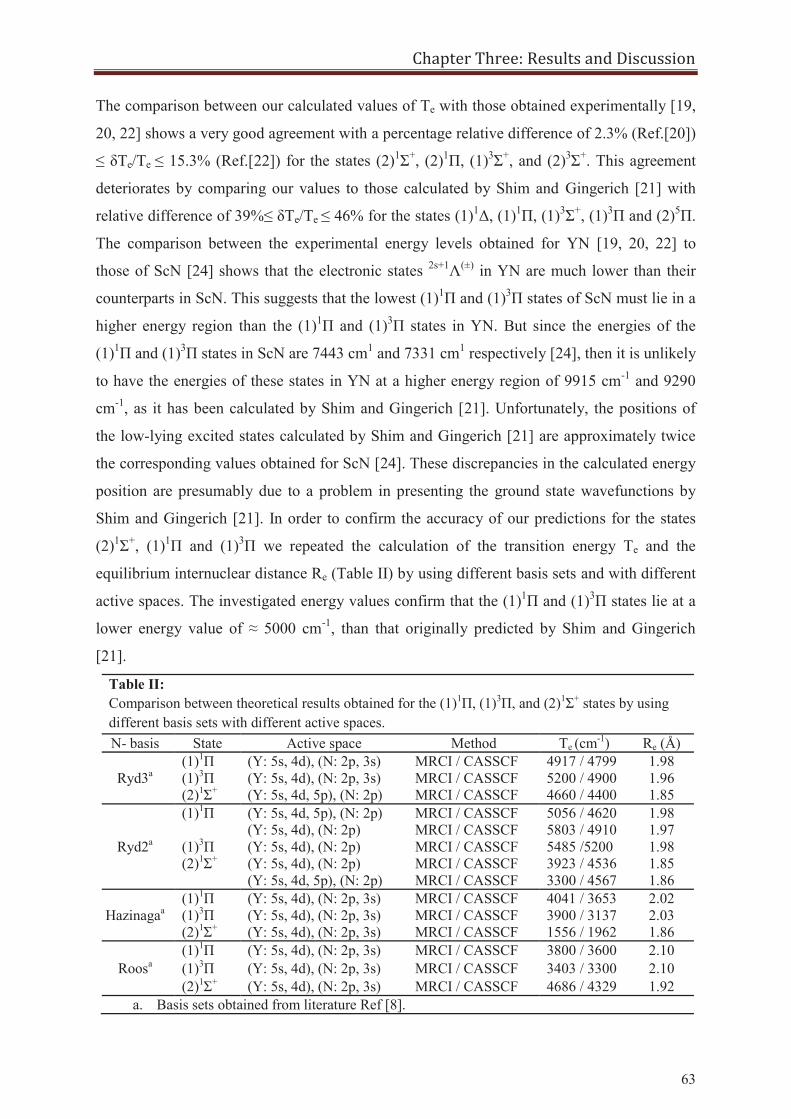
Chapter Three: Results and Discussion
63
The comparison between our calculated values of Te with those obtained experimentally [19,
20, 22] shows a very good agreement with a percentage relative difference of 2.3% (Ref.[20])
≤ δTe/Te ≤ 15.3% (Ref.[22]) for the states (2)1Σ+, (2)1Π, (1)3Σ+, and (2)3Σ+. This agreement
deteriorates by comparing our values to those calculated by Shim and Gingerich [21] with
relative difference of 39%≤ δTe/Te ≤ 46% for the states (1)1Δ, (1)1Π, (1)3Σ+, (1)3Π and (2)5Π.
The comparison between the experimental energy levels obtained for YN [19, 20, 22] to
those of ScN [24] shows that the electronic states 2s+1Λ(±) in YN are much lower than their
counterparts in ScN. This suggests that the lowest (1)1Π and (1)3Π states of ScN must lie in a
higher energy region than the (1)1Π and (1)3Π states in YN. But since the energies of the
(1)1Π and (1)3Π states in ScN are 7443 cm1 and 7331 cm1 respectively [24], then it is unlikely
to have the energies of these states in YN at a higher energy region of 9915 cm-1 and 9290
cm-1, as it has been calculated by Shim and Gingerich [21]. Unfortunately, the positions of
the low-lying excited states calculated by Shim and Gingerich [21] are approximately twice
the corresponding values obtained for ScN [24]. These discrepancies in the calculated energy
position are presumably due to a problem in presenting the ground state wavefunctions by
Shim and Gingerich [21]. In order to confirm the accuracy of our predictions for the states
(2)1Σ+, (1)1Π and (1)3Π we repeated the calculation of the transition energy Te and the
equilibrium internuclear distance Re (Table II) by using different basis sets and with different
active spaces. The investigated energy values confirm that the (1)1Π and (1)3Π states lie at a
lower energy value of ≈ 5000 cm-1, than that originally predicted by Shim and Gingerich
[21].
Table II: Comparison between theoretical results obtained for the (1)1Π, (1)3Π, and (2)1Σ+ states by using different basis sets with different active spaces. N- basis State Active space Method Te (cm-1) Re (Å)
Ryd3a (1)1Π (Y: 5s, 4d), (N: 2p, 3s) MRCI / CASSCF 4917 / 4799 1.98 (1)3Π (Y: 5s, 4d), (N: 2p, 3s) MRCI / CASSCF 5200 / 4900 1.96 (2)1Σ+ (Y: 5s, 4d, 5p), (N: 2p) MRCI / CASSCF 4660 / 4400 1.85
Ryd2a
(1)1Π (Y: 5s, 4d, 5p), (N: 2p) MRCI / CASSCF 5056 / 4620 1.98 (Y: 5s, 4d), (N: 2p) MRCI / CASSCF 5803 / 4910 1.97 (1)3Π (Y: 5s, 4d), (N: 2p) MRCI / CASSCF 5485 /5200 1.98 (2)1Σ+ (Y: 5s, 4d), (N: 2p) MRCI / CASSCF 3923 / 4536 1.85 (Y: 5s, 4d, 5p), (N: 2p) MRCI / CASSCF 3300 / 4567 1.86
Hazinagaa (1)1Π (Y: 5s, 4d), (N: 2p, 3s) MRCI / CASSCF 4041 / 3653 2.02 (1)3Π (Y: 5s, 4d), (N: 2p, 3s) MRCI / CASSCF 3900 / 3137 2.03 (2)1Σ+ (Y: 5s, 4d), (N: 2p, 3s) MRCI / CASSCF 1556 / 1962 1.86
Roosa (1)1Π (Y: 5s, 4d), (N: 2p, 3s) MRCI / CASSCF 3800 / 3600 2.10 (1)3Π (Y: 5s, 4d), (N: 2p, 3s) MRCI / CASSCF 3403 / 3300 2.10 (2)1Σ+ (Y: 5s, 4d), (N: 2p, 3s) MRCI / CASSCF 4686 / 4329 1.92
a. Basis sets obtained from literature Ref [8].
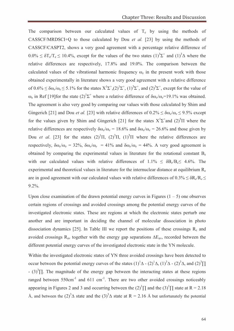
Chapter Three: Results and Discussion
64
The comparison between our calculated values of Te by using the methods of
CASSCF/MRDSCI+Q to those calculated by Dou et al. [23] by using the methods of
CASSCF/CASPT2, shows a very good agreement with a percentage relative difference of
0.0% ≤ δTe/Te ≤ 10.4%, except for the values of the two states (1)3Σ+ and (1)3Δ where the
relative differences are respectively, 17.8% and 19.0%. The comparison between the
calculated values of the vibrational harmonic frequency ωe in the present work with those
obtained experimentally in literature shows a very good agreement with a relative difference
of 0.6% ≤ δωe/ωe ≤ 5.1% for the states X1Σ+,(2)1Σ+, (1)3Σ+, and (2)3Σ+, except for the value of
ωe in Ref [19]for the state (2)1Σ+ where a relative difference of δωe/ωe=19.1% was obtained.
The agreement is also very good by comparing our values with those calculated by Shim and
Gingerich [21] and Dou et al. [23] with relative differences of 0.2% ≤ δωe/ωe ≤ 9.5% except
for the values given by Shim and Gingerich [21] for the states X1Σ+and (2)5Π where the
relative differences are respectively δωe/ωe = 18.6% and δωe/ωe = 26.6% and those given by
Dou et al. [23] for the states (2)1Π, (2)3Π, (1)5Π where the relative differences are
respectively, δωe/ωe = 32%, δωe/ωe = 41% and δωe/ωe = 44%. A very good agreement is
obtained by comparing the experimental values in literature for the rotational constant Be
with our calculated values with relative differences of 1.1% ≤ δBe/Be≤ 4.6%. The
experimental and theoretical values in literature for the internuclear distance at equilibrium Re
are in good agreement with our calculated values with relative differences of 0.3% ≤ δRe/Re ≤
9.2%.
Upon close examination of the drawn potential energy curves in Figures (1 – 5) one observes
certain regions of crossings and avoided crossings among the potential energy curves of the
investigated electronic states. These are regions at which the electronic states perturb one
another and are important in deciding the channel of molecular dissociation in photo
dissociation dynamics [25]. In Table III we report the positions of these crossings Rc and
avoided crossings Rav together with the energy gap separations ∆Eav, recorded between the
different potential energy curves of the investigated electronic state in the YN molecule.
Within the investigated electronic states of YN three avoided crossings have been detected to
occur between the potential energy curves of the states (1)1∆ - (2)1∆, (1)3∆ - (2)3∆, and (2)3∏
- (3)3∏. The magnitude of the energy gap between the interacting states at these regions
ranged between 550cm-1 and 611 cm-1. There are two other avoided crossings noticeably
appearing in Figures 2 and 3 and occurring between the (2)1∏ and the (3)1∏ state at R = 2.18
Å, and between the (2)3∆ state and the (3)3∆ state at R = 2.16 Å but unfortunately the potential
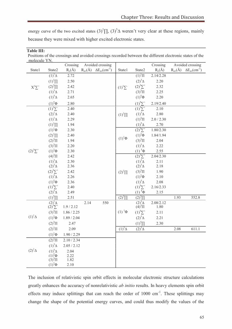
Chapter Three: Results and Discussion
65
energy curve of the two excited states (3)1∏, (3)3∆ weren’t very clear at these regions, mainly
because they were mixed with higher excited electronic states.
The inclusion of relativistic spin orbit effects in molecular electronic structure calculations
greatly enhances the accuracy of nonrelativistic ab initio results. In heavy elements spin orbit
effects may induce splittings that can reach the order of 1000 cm-1. These splittings may
change the shape of the potential energy curves, and could thus modify the values of the
Table III: Positions of the crossings and avoided crossings recorded between the different electronic states of the molecule YN.
Crossing Avoided crossing Crossing Avoided crossing State1 State2 Rc(Ǻ) Rav(Ǻ) ∆Eav(cm-1) State1 State2 Rc(Ǻ) Rav(Ǻ) ∆Eav(cm-1)
X1∑+
(1)1∆ 2.72
(1)1∑-
(1)1Π 2.14/2.28 (1)1∏ 2.50 (2)3∆ 2.20 (2)3∏ 2.42 (2)3∑+ 2.32 (1)3∆ 2.71 (3)3Π 2.25 (1)5∆ 2.65 (1)5Φ 2.20 (1)5Φ 2.80 (1)5∑+ 2.19/2.40
(2)1∑+
(1)1∑- 2.40 (1)1∏
(1)3∑+ 2.10 (2)1∆ 2.40 (1)3∆ 2.80 (1)1∆ 2.29 (1)3Π 2.0 / 2.30 (1)1∏ 1.94 (1)5∆ 2.70 (1)1Φ 2.30
(1)1Φ
(2)3∑+ 1.80/2.30 (2)1∏ 2.40 (1)3Φ 1.84/1.94 (2)3Π 1.94 (3)3Π 2.04 (3)3Π 2.20 (1)5∆ 2.22 (1)3Φ 2.30 (1) 5Φ 2.55 (4)3Π 2.42
(2)1∏
(2)3∑+ 2.04/2.30 (1)3∆ 2.30 (1)3∆ 2.11 (2)3∆ 2.36 (2)3∆ 2.18 (2)3∑+ 2.42 (3)3Π 1.90 (1)5∆ 2.26 (1)3Φ 2.10 (1)5Φ 2.36 (1)5∆ 2.08 (1)5∑+ 2.40 (1)5∑+ 2.16/2.33 (2)5∆ 2.49 (1) 5Φ 2.15 (1)5∏ 2.51 (2)3∏ (2)3∏ 1.93 552.8
(1)1∆
(2)1∆ 2.14 550
(1) 1Φ
(2)3∆ 2.08/2.12 (2)3∑+ 1.9 / 2.12 (4)3Π 1.80 (3)3Π 1.86 / 2.25 (1)5∑+ 2.11 (1)3Φ 1.89 / 2.04 (2)5∆ 2.21 (2)3Π 2.47 (1)5∏ 2.30 (2)1Π 2.09 (1)3∆ (2)3∆ 2.08 611.1 (1)1Φ 1.90 / 2.29
(2)1∆
(2)1Π 2.10 / 2.34 (1)3∆ 2.05 / 2.12 (1)5∆ 2.04 (1)5Φ 2.22 (3)3Π 1.82 (1)3Φ 2.10
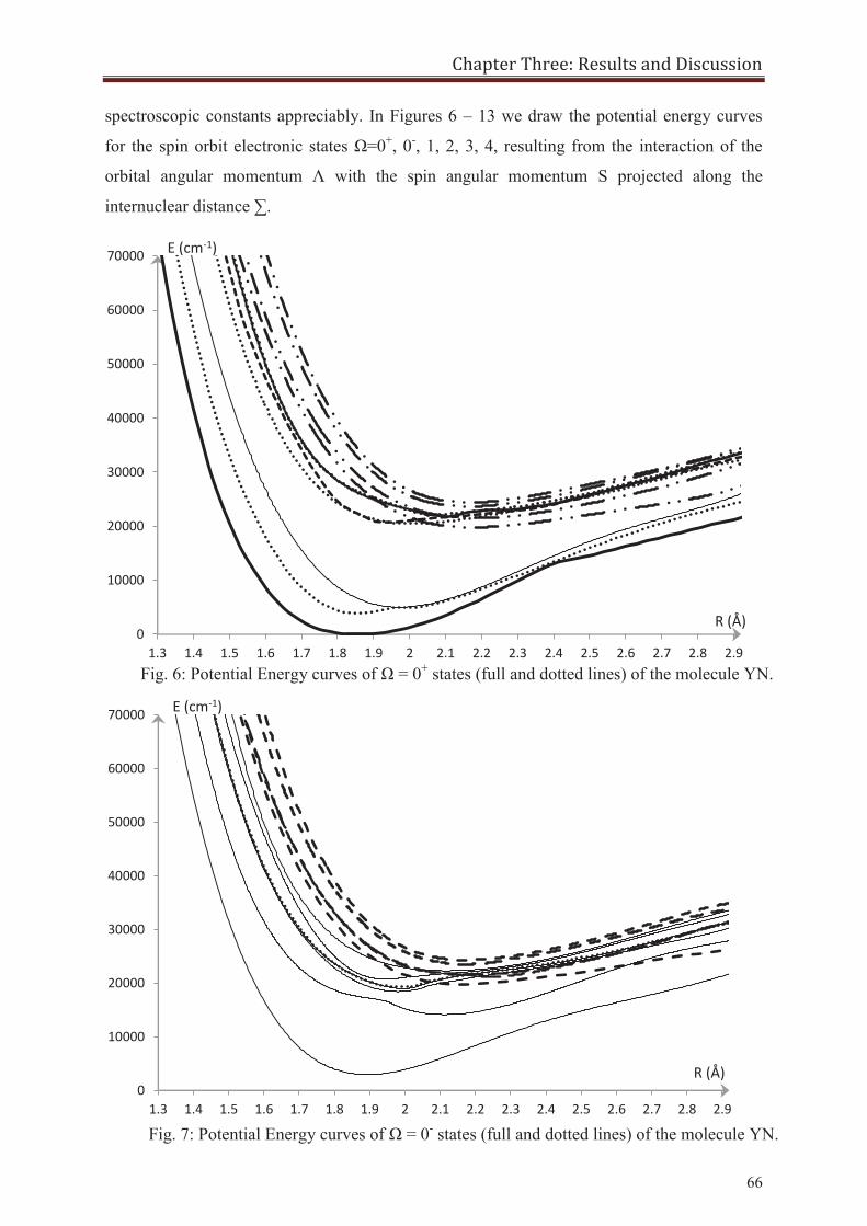
Chapter Three: Results and Discussion
66
spectroscopic constants appreciably. In Figures 6 – 13 we draw the potential energy curves
for the spin orbit electronic states Ω=0+, 0-, 1, 2, 3, 4, resulting from the interaction of the
orbital angular momentum Λ with the spin angular momentum S projected along the
internuclear distance ∑.
Fig. 6: Potential Energy curves of Ω = 0+ states (full and dotted lines) of the molecule YN.
0
10000
20000
30000
40000
50000
60000
70000
1.3 1.4 1.5 1.6 1.7 1.8 1.9 2 2.1 2.2 2.3 2.4 2.5 2.6 2.7 2.8 2.9
E (cm-1)
R (Å)
0
10000
20000
30000
40000
50000
60000
70000
1.3 1.4 1.5 1.6 1.7 1.8 1.9 2 2.1 2.2 2.3 2.4 2.5 2.6 2.7 2.8 2.9
E (cm-1)
R (Å)
Fig. 7: Potential Energy curves of Ω = 0- states (full and dotted lines) of the molecule YN.
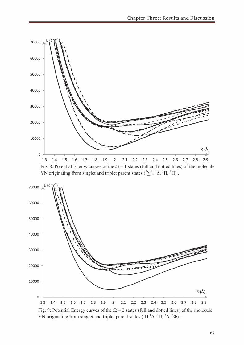
Chapter Three: Results and Discussion
67
0
10000
20000
30000
40000
50000
60000
70000
1.3 1.4 1.5 1.6 1.7 1.8 1.9 2 2.1 2.2 2.3 2.4 2.5 2.6 2.7 2.8 2.9
R (Å)
E (cm-1)
Fig. 8: Potential Energy curves of the Ω = 1 states (full and dotted lines) of the molecule YN originating from singlet and triplet parent states (3∑+, 3Δ, 3Π, 1Π) .
0
10000
20000
30000
40000
50000
60000
70000
1.3 1.4 1.5 1.6 1.7 1.8 1.9 2 2.1 2.2 2.3 2.4 2.5 2.6 2.7 2.8 2.9
E (cm-1)
R (Å)
Fig. 9: Potential Energy curves of the Ω = 2 states (full and dotted lines) of the molecule YN originating from singlet and triplet parent states (1Π,1Δ, 3Π, 3Δ, 3Φ) .
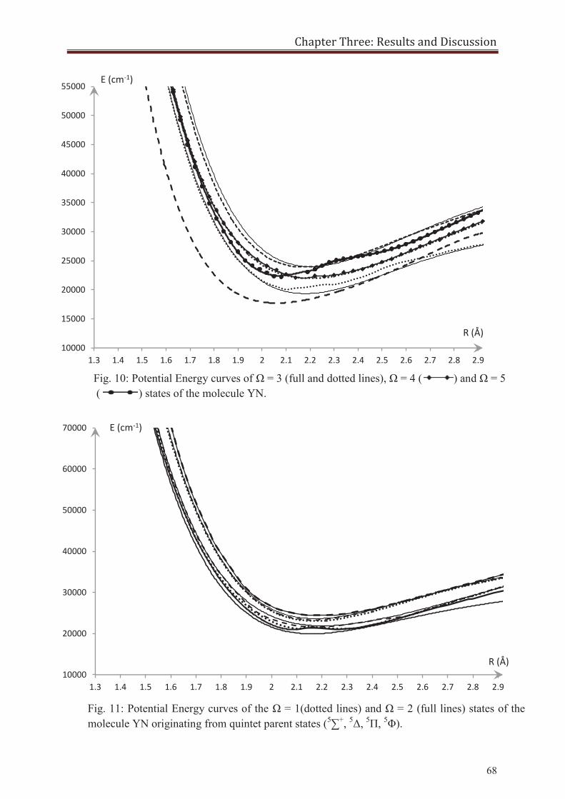
Chapter Three: Results and Discussion
68
10000
20000
30000
40000
50000
60000
70000
1.3 1.4 1.5 1.6 1.7 1.8 1.9 2 2.1 2.2 2.3 2.4 2.5 2.6 2.7 2.8 2.9
E (cm-1)
R (Å)
Fig. 10: Potential Energy curves of Ω = 3 (full and dotted lines), Ω = 4 ( ) and Ω = 5 ( ) states of the molecule YN.
10000
15000
20000
25000
30000
35000
40000
45000
50000
55000
1.3 1.4 1.5 1.6 1.7 1.8 1.9 2 2.1 2.2 2.3 2.4 2.5 2.6 2.7 2.8 2.9
R (Å)
E (cm-1)
Fig. 11: Potential Energy curves of the Ω = 1(dotted lines) and Ω = 2 (full lines) states of the molecule YN originating from quintet parent states (5∑+, 5Δ, 5Π, 5Φ).
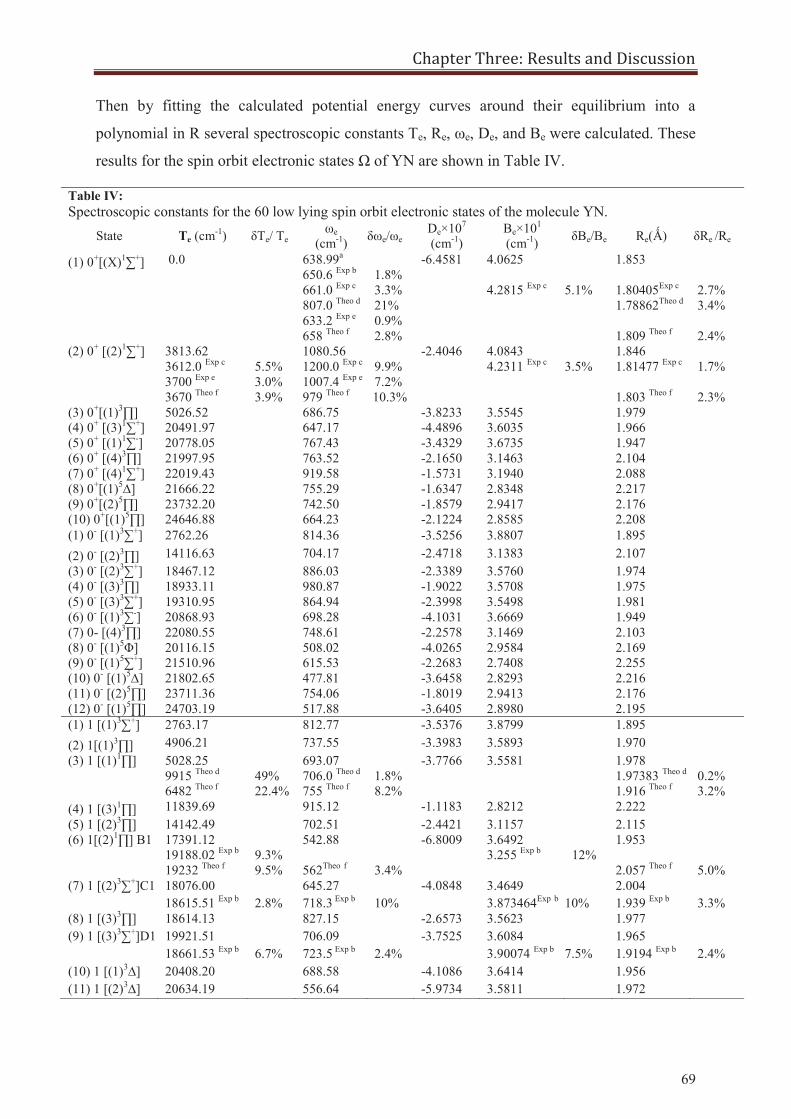
Chapter Three: Results and Discussion
69
Then by fitting the calculated potential energy curves around their equilibrium into a
polynomial in R several spectroscopic constants Te, Re, ωe, De, and Be were calculated. These
results for the spin orbit electronic states Ω of YN are shown in Table IV.
Table IV: Spectroscopic constants for the 60 low lying spin orbit electronic states of the molecule YN.
State Te (cm-1) δTe/ Te ωe
(cm-1) δωe/ωe De×107
(cm-1) Be×101
(cm-1) δBe/Be Re(Ǻ) δRe /Re
(1) 0+[(X)1∑+] 0.0 638.99a 650.6 Exp b
661.0 Exp c
807.0 Theo d
633.2 Exp e
658 Theo f
1.8% 3.3% 21% 0.9% 2.8%
-6.4581 4.0625 4.2815 Exp c
5.1%
1.853 1.80405Exp c
1.78862Theo d
1.809 Theo f
2.7% 3.4% 2.4%
(2) 0+ [(2)1∑+] 3813.62 3612.0 Exp c
3700 Exp e
3670 Theo f
5.5% 3.0% 3.9%
1080.56 1200.0 Exp c
1007.4 Exp e
979 Theo f
9.9% 7.2%
10.3%
-2.4046 4.0843 4.2311 Exp c
3.5%
1.846 1.81477 Exp c
1.803 Theo f
1.7% 2.3%
(3) 0+[(1)3∏] 5026.52 686.75 -3.8233 3.5545 1.979 (4) 0+ [(3)1∑+] 20491.97 647.17 -4.4896 3.6035 1.966 (5) 0+ [(1)1∑-] 20778.05 767.43 -3.4329 3.6735 1.947 (6) 0+ [(4)3∏] 21997.95 763.52 -2.1650 3.1463 2.104 (7) 0+ [(4)1∑+] 22019.43 919.58 -1.5731 3.1940 2.088 (8) 0+[(1)5∆] 21666.22 755.29 -1.6347 2.8348 2.217 (9) 0+[(2)5∏] 23732.20 742.50 -1.8579 2.9417 2.176 (10) 0+[(1)5∏] 24646.88 664.23 -2.1224 2.8585 2.208 (1) 0- [(1)3∑+] 2762.26 814.36 -3.5256 3.8807 1.895 (2) 0- [(2)3∏] 14116.63 704.17 -2.4718 3.1383 2.107 (3) 0- [(2)3∑+] 18467.12 886.03 -2.3389 3.5760 1.974 (4) 0- [(3)3∏] 18933.11 980.87 -1.9022 3.5708 1.975 (5) 0- [(3)3∑+] 19310.95 864.94 -2.3998 3.5498 1.981 (6) 0- [(1)3∑-] 20868.93 698.28 -4.1031 3.6669 1.949 (7) 0- [(4)3∏] 22080.55 748.61 -2.2578 3.1469 2.103 (8) 0- [(1)5Φ] 20116.15 508.02 -4.0265 2.9584 2.169 (9) 0- [(1)5∑+] 21510.96 615.53 -2.2683 2.7408 2.255 (10) 0- [(1)5∆] 21802.65 477.81 -3.6458 2.8293 2.216 (11) 0- [(2)5∏] 23711.36 754.06 -1.8019 2.9413 2.176 (12) 0- [(1)5∏] 24703.19 517.88 -3.6405 2.8980 2.195 (1) 1 [(1)3∑+] 2763.17 812.77 -3.5376 3.8799 1.895 (2) 1[(1)3∏] 4906.21 737.55 -3.3983 3.5893 1.970 (3) 1 [(1)1∏] 5028.25
9915 Theo d
6482 Theo f
49% 22.4%
693.07 706.0 Theo d
755 Theo f
1.8% 8.2%
-3.7766 3.5581 1.978 1.97383 Theo d
1.916 Theo f
0.2% 3.2%
(4) 1 [(3)1∏] 11839.69 915.12 -1.1183 2.8212 2.222 (5) 1 [(2)3∏] 14142.49 702.51 -2.4421 3.1157 2.115 (6) 1[(2)1∏] B1 17391.12
19188.02 Exp b
19232 Theo f
9.3% 9.5%
542.88 562Theo f
3.4%
-6.8009 3.6492 3.255 Exp b
12%
1.953 2.057 Theo f
5.0%
(7) 1 [(2)3∑+]C1 18076.00 18615.51 Exp b
2.8%
645.27 718.3 Exp b
10%
-4.0848 3.4649 3.873464Exp b
10%
2.004 1.939 Exp b
3.3%
(8) 1 [(3)3∏] 18614.13 827.15 -2.6573 3.5623 1.977 (9) 1 [(3)3∑+]D1 19921.51
18661.53 Exp b 6.7%
706.09 723.5 Exp b
2.4%
-3.7525 3.6084 3.90074 Exp b
7.5%
1.965 1.9194 Exp b
2.4%
(10) 1 [(1)3∆] 20408.20 688.58 -4.1086 3.6414 1.956 (11) 1 [(2)3∆] 20634.19 556.64 -5.9734 3.5811 1.972
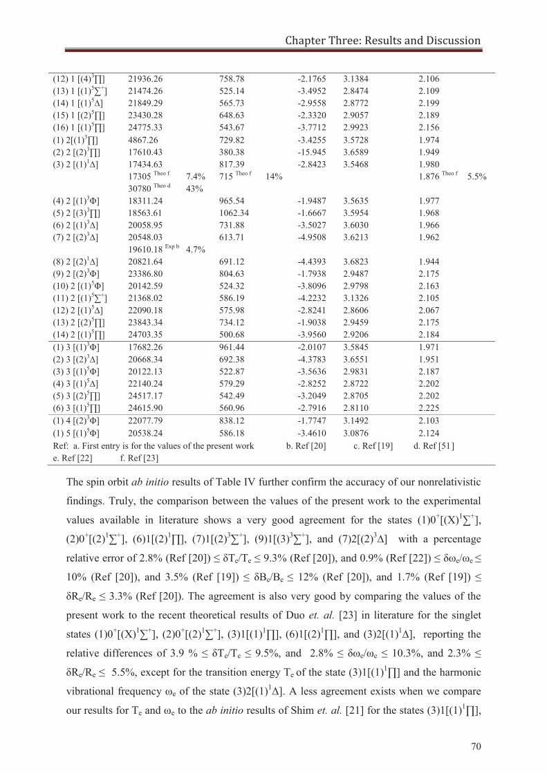
Chapter Three: Results and Discussion
70
The spin orbit ab initio results of Table IV further confirm the accuracy of our nonrelativistic
findings. Truly, the comparison between the values of the present work to the experimental
values available in literature shows a very good agreement for the states (1)0+[(X)1∑+],
(2)0+[(2)1∑+], (6)1[(2)1∏], (7)1[(2)3∑+], (9)1[(3)3∑+], and (7)2[(2)3∆] with a percentage
relative error of 2.8% (Ref [20]) ≤ δTe/Te ≤ 9.3% (Ref [20]), and 0.9% (Ref [22]) ≤ δωe/ωe ≤
10% (Ref [20]), and 3.5% (Ref [19]) ≤ δBe/Be ≤ 12% (Ref [20]), and 1.7% (Ref [19]) ≤
δRe/Re ≤ 3.3% (Ref [20]). The agreement is also very good by comparing the values of the
present work to the recent theoretical results of Duo et. al. [23] in literature for the singlet
states (1)0+[(X)1∑+], (2)0+[(2)1∑+], (3)1[(1)1∏], (6)1[(2)1∏], and (3)2[(1)1∆], reporting the
relative differences of 3.9 % ≤ δTe/Te ≤ 9.5%, and 2.8% ≤ δωe/ωe ≤ 10.3%, and 2.3% ≤
δRe/Re ≤ 5.5%, except for the transition energy Te of the state (3)1[(1)1∏] and the harmonic
vibrational frequency ωe of the state (3)2[(1)1Δ]. A less agreement exists when we compare
our results for Te and ωe to the ab initio results of Shim et. al. [21] for the states (3)1[(1)1∏],
(12) 1 [(4)3∏] 21936.26 758.78 -2.1765 3.1384 2.106 (13) 1 [(1)5∑+] 21474.26 525.14 -3.4952 2.8474 2.109 (14) 1 [(1)5∆] 21849.29 565.73 -2.9558 2.8772 2.199 (15) 1 [(2)5∏] 23430.28 648.63 -2.3320 2.9057 2.189 (16) 1 [(1)5∏] 24775.33 543.67 -3.7712 2.9923 2.156 (1) 2[(1)3∏] 4867.26 729.82 -3.4255 3.5728 1.974 (2) 2 [(2)3∏] 17610.43 380.38 -15.945 3.6589 1.949 (3) 2 [(1)1∆] 17434.63
17305 Theo f
30780 Theo d
7.4% 43%
817.39 715 Theo f
14%
-2.8423 3.5468 1.980 1.876 Theo f
5.5%
(4) 2 [(1)3Φ] 18311.24 965.54 -1.9487 3.5635 1.977 (5) 2 [(3)3∏] 18563.61 1062.34 -1.6667 3.5954 1.968 (6) 2 [(1)3∆] 20058.95 731.88 -3.5027 3.6030 1.966 (7) 2 [(2)3∆] 20548.03
19610.18 Exp b 4.7%
613.71 -4.9508 3.6213 1.962
(8) 2 [(2)1∆] 20821.64 691.12 -4.4393 3.6823 1.944 (9) 2 [(2)3Φ] 23386.80 804.63 -1.7938 2.9487 2.175 (10) 2 [(1)5Φ] 20142.59 524.32 -3.8096 2.9798 2.163 (11) 2 [(1)5∑+] 21368.02 586.19 -4.2232 3.1326 2.105 (12) 2 [(1)5∆] 22090.18 575.98 -2.8241 2.8606 2.067 (13) 2 [(2)5∏] 23843.34 734.12 -1.9038 2.9459 2.175 (14) 2 [(1)5∏] 24703.35 500.68 -3.9560 2.9206 2.184 (1) 3 [(1)3Φ] 17682.26 961.44 -2.0107 3.5845 1.971 (2) 3 [(2)3∆] 20668.34 692.38 -4.3783 3.6551 1.951 (3) 3 [(1)5Φ] 20122.13 522.87 -3.5636 2.9831 2.187 (4) 3 [(1)5∆] 22140.24 579.29 -2.8252 2.8722 2.202 (5) 3 [(2)5∏] 24517.17 542.49 -3.2049 2.8705 2.202 (6) 3 [(1)5∏] 24615.90 560.96 -2.7916 2.8110 2.225 (1) 4 [(2)3Φ] 22077.79 838.12 -1.7747 3.1492 2.103 (1) 5 [(1)5Φ] 20538.24 586.18 -3.4610 3.0876 2.124 Ref: a. First entry is for the values of the present work b. Ref [20] c. Ref [19] d. Ref [51] e. Ref [22] f. Ref [23]
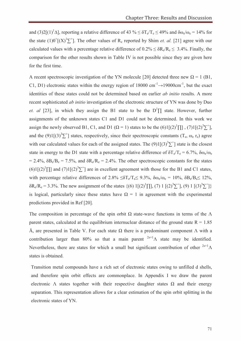
Chapter Three: Results and Discussion
71
and (3)2[(1)1∆], reporting a relative difference of 43 % ≤ δTe/Te ≤ 49% and δωe/ωe = 14% for
the state (1)0+[(X)1∑+]. The other values of Re reported by Shim et. al. [21] agree with our
calculated values with a percentage relative difference of 0.2% ≤ δRe/Re ≤ 3.4%. Finally, the
comparison for the other results shown in Table IV is not possible since they are given here
for the first time.
A recent spectroscopic investigation of the YN molecule [20] detected three new Ω = 1 (B1,
C1, D1) electronic states within the energy region of 18000 cm-1→19000cm-1, but the exact
identities of these states could not be determined based on earlier ab initio results. A more
recent sophisticated ab initio investigation of the electronic structure of YN was done by Duo
et. al [23], in which they assign the B1 state to be the D1∏ state. However, further
assignments of the unknown states C1 and D1 could not be determined. In this work we
assign the newly observed B1, C1, and D1 (Ω = 1) states to be the (6)1[(2)1∏] , (7)1[(2)3∑+],
and the (9)1[(3)3∑+] states, respectively, since their spectroscopic constants (Te, ωe re) agree
with our calculated values for each of the assigned states. The (9)1[(3)3∑+] state is the closest
state in energy to the D1 state with a percentage relative difference of δTe/Te = 6.7%, δωe/ωe
= 2.4%, δBe/Be = 7.5%, and δRe/Re = 2.4%. The other spectroscopic constants for the states
(6)1[(2)1∏] and (7)1[(2)3∑+] are in excellent agreement with those for the B1 and C1 states,
with percentage relative differences of 2.8% ≤δTe/Te≤ 9.3%, δωe/ωe = 10%, δBe/Be≤ 12%,
δRe/Re = 3.3%. The new assignment of the states {(6) 1[(2)1∏], (7) 1 [(2)3∑+], (9) 1 [(3)3∑+]}
is logical, particularly since these states have Ω = 1 in agreement with the experimental
predictions provided in Ref [20].
The composition in percentage of the spin orbit Ω state-wave functions in terms of the Λ
parent states, calculated at the equilibrium internuclear distance of the ground state R = 1.85
Å, are presented in Table V. For each state Ω there is a predominant component Λ with a
contribution larger than 80% so that a main parent 2s+1Λ state may be identified.
Nevertheless, there are states for which a small but significant contribution of other 2s+1Λ
states is obtained.
Transition metal compounds have a rich set of electronic states owing to unfilled d shells,
and therefore spin orbit effects are commonplace. In Appendix I we draw the parent
electronic Λ states together with their respective daughter states Ω and their energy
separation. This representation allows for a clear estimation of the spin orbit splitting in the
electronic states of YN.
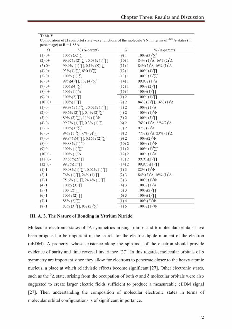
Chapter Three: Results and Discussion
72
III. A. 3. The Nature of Bonding in Yttrium Nitride
Molecular electronic states of 3Δ symmetries arising from σ and δ molecular orbitals have
been proposed to be important in the search for the electric dipole moment of the electron
(eEDM). A property, whose existence along the spin axis of the electron should provide
evidence of parity and time reversal invariance [27]. In this regards, molecular orbitals of σ
symmetry are important since they allow for electrons to penetrate closer to the heavy atomic
nucleus, a place at which relativistic effects become significant [27]. Other electronic states,
such as the 3Δ state, arising from the occupation of both σ and δ molecular orbitals were also
suggested to create larger electric fields sufficient to produce a measureable eEDM signal
[27]. Then understanding the composition of molecular electronic states in terms of
molecular orbital configurations is of significant importance.
Table V: Composition of Ω spin orbit state wave functions of the molecule YN, in terms of 2s+1Λ-states (in percentage) at R = 1.85Å.
Ω % (Λ-parent) Ω % (Λ-parent) (1) 0+ 100% (X)1∑+ (9) 1 100%(3)3∑+ (2) 0+ 99.97% (2)1∑+, 0.03% (1)3∏ (10) 1 84% (1)3∆, 16% (2)3∆ (3) 0+ 99.9% (1)3∏, 0.1% (X)1∑+ (11) 1 84%(2)3∆, 16% (1)3∆ (4) 0+ 93%(3)1∑+, 6%(1)3∑- (12) 1 100% (4)3∏ (5) 0+ 100% (1)1∑- (13) 1 100% (1)5∑+ (6) 0+ 99%(4)3∏, 1% (4)1∑+ (14) 1 99.8% (1)5∆ (7) 0+ 100%(4)1∑+ (15) 1 100% (2)5∏ (8) 0+ 100% (1)5∆ (16) 1 100%(1)5∏ (9) 0+ 100%(2)5∏ (1) 2 100% (1)3∏ (10) 0+ 100%(1)5∏ (2) 2 84% (2)3∏, 16% (1)1∆ (1) 0- 99.98% (1)3∑+, 0.02% (1)3∏ (3) 2 100% (1)1∆ (2) 0- 99.6% (2)3∏, 0.4% (2)3∑+ (4) 2 100% (1)3Φ (3) 0- 89% (2)3∑+, 11% (1)3Φ (5) 2 100% (3)3∏ (4) 0- 99.7% (3)3∏, 0.3% (1)3∑- (6) 2 76% (1)3∆, 22%(2)1∆ (5) 0- 100%(3)3∑+ (7) 2 97% (2)3∆ (6) 0- 94% (1)3∑-, 6% (3)1∑+ (8) 2 77% (2)1∆, 23% (1)3∆ (7) 0- 99.84%(4)3∏, 0.16% (2)3∑+ (9) 2 100%(2)3Φ (8) 0- 99.88% (1)5Φ (10) 2 100% (1)5Φ (9) 0- 100% (1)5∑+ (11) 2 100% (1)5∑+ (10) 0- 100% (1)5∆ (12) 2 100% (1)5∆ (11) 0- 99.88%(2)5∏ (13) 2 99.9%(2)5∏ (12) 0- 99.7%(1)5∏ (14) 2 99.87%(1)5∏ (1) 1 99.98%(1)3∑+, 0.02% (1)3∏ (1) 3 82% (1)3Φ (2) 1 76% (1)3∏, 24% (1)1∏ (2) 3 84%(2)3∆, 16% (1)3∆ (3) 1 75.6% (1)1∏, 24.4% (1)3∏ (3) 3 100% (1)5Φ (4) 1 100% (3)1∏ (4) 3 100% (1)5∆ (5) 1 100 (2)3∏ (5) 3 100%(2)5∏ (6) 1 100% (2)1∏ (6) 3 100%(1)5∏ (7) 1 85% (2)3∑+ (1) 4 100%(2)3Φ (8) 1 83% (3)3∏, 8% (2)3∑+ (1) 5 100% (1)5Φ
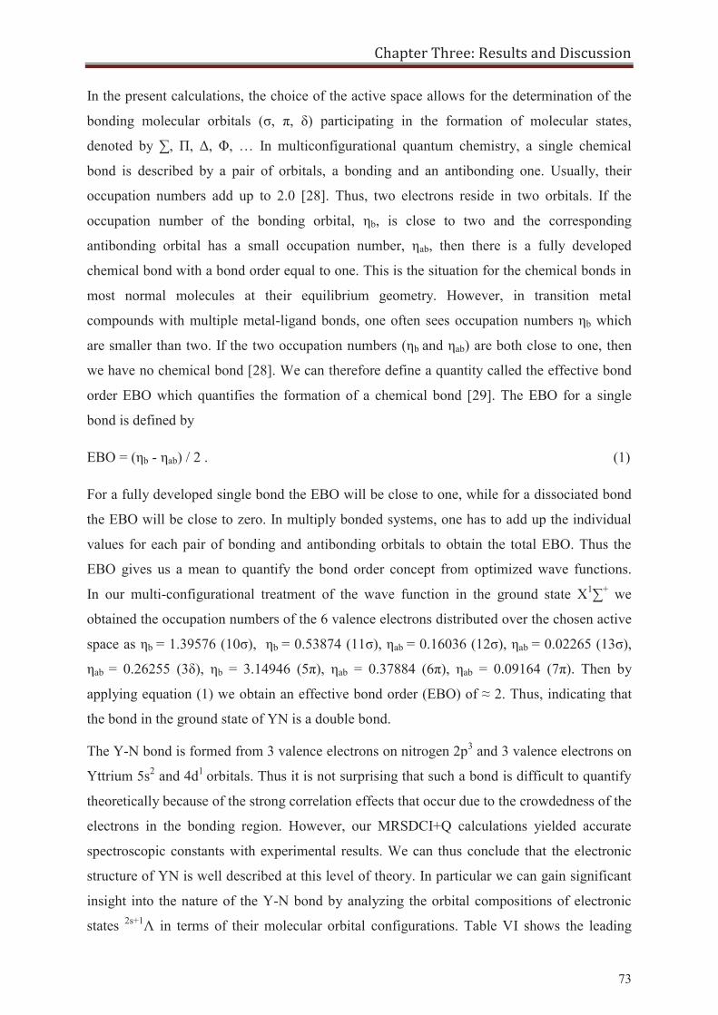
Chapter Three: Results and Discussion
73
In the present calculations, the choice of the active space allows for the determination of the
bonding molecular orbitals (σ, π, δ) participating in the formation of molecular states,
denoted by ∑, Π, Δ, Φ, … In multiconfigurational quantum chemistry, a single chemical
bond is described by a pair of orbitals, a bonding and an antibonding one. Usually, their
occupation numbers add up to 2.0 [28]. Thus, two electrons reside in two orbitals. If the
occupation number of the bonding orbital, ηb, is close to two and the corresponding
antibonding orbital has a small occupation number, ηab, then there is a fully developed
chemical bond with a bond order equal to one. This is the situation for the chemical bonds in
most normal molecules at their equilibrium geometry. However, in transition metal
compounds with multiple metal-ligand bonds, one often sees occupation numbers ηb which
are smaller than two. If the two occupation numbers (ηb and ηab) are both close to one, then
we have no chemical bond [28]. We can therefore define a quantity called the effective bond
order EBO which quantifies the formation of a chemical bond [29]. The EBO for a single
bond is defined by
EBO = (ηb - ηab) / 2 . (1)
For a fully developed single bond the EBO will be close to one, while for a dissociated bond
the EBO will be close to zero. In multiply bonded systems, one has to add up the individual
values for each pair of bonding and antibonding orbitals to obtain the total EBO. Thus the
EBO gives us a mean to quantify the bond order concept from optimized wave functions.
In our multi-configurational treatment of the wave function in the ground state X1∑+ we
obtained the occupation numbers of the 6 valence electrons distributed over the chosen active
space as ηb = 1.39576 (10σ), ηb
= 0.53874 (11σ), ηab = 0.16036 (12σ), ηab = 0.02265 (13σ),
ηab = 0.26255 (3δ), ηb = 3.14946 (5π), ηab = 0.37884 (6π), ηab = 0.09164 (7π). Then by
applying equation (1) we obtain an effective bond order (EBO) of ≈ 2. Thus, indicating that
the bond in the ground state of YN is a double bond.
The Y-N bond is formed from 3 valence electrons on nitrogen 2p3 and 3 valence electrons on
Yttrium 5s2 and 4d1 orbitals. Thus it is not surprising that such a bond is difficult to quantify
theoretically because of the strong correlation effects that occur due to the crowdedness of the
electrons in the bonding region. However, our MRSDCI+Q calculations yielded accurate
spectroscopic constants with experimental results. We can thus conclude that the electronic
structure of YN is well described at this level of theory. In particular we can gain significant
insight into the nature of the Y-N bond by analyzing the orbital compositions of electronic
states 2s+1Λ in terms of their molecular orbital configurations. Table VI shows the leading
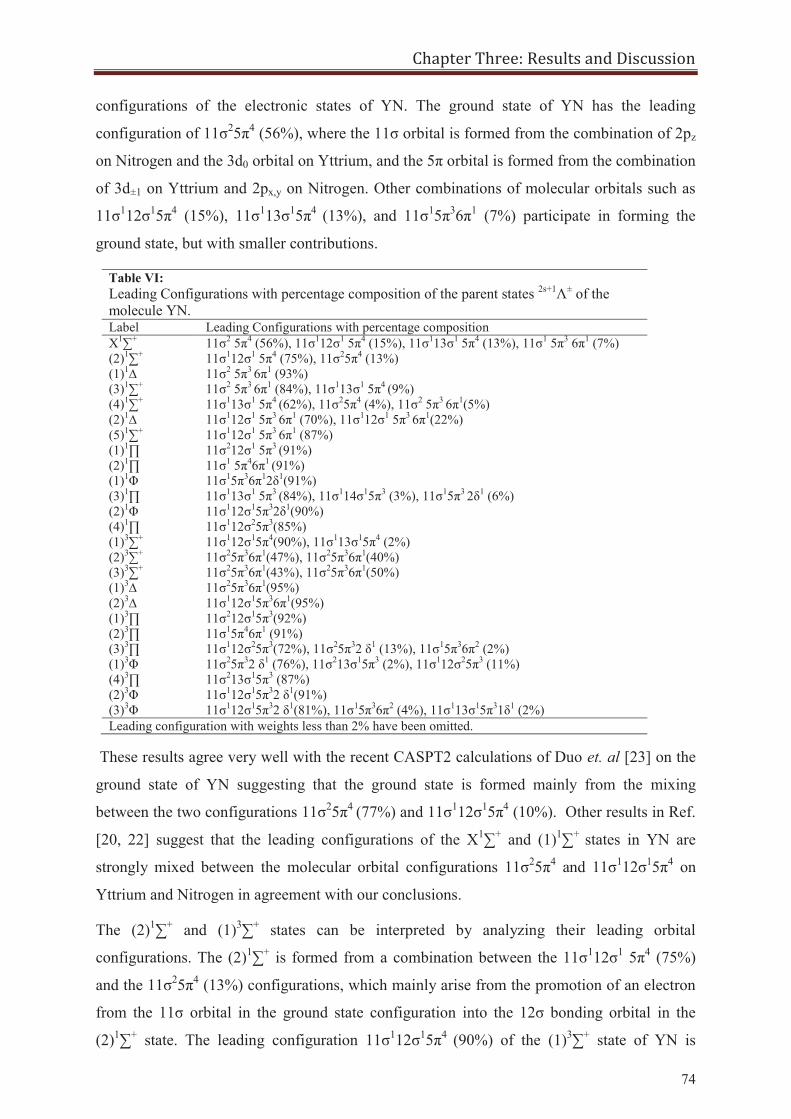
Chapter Three: Results and Discussion
74
configurations of the electronic states of YN. The ground state of YN has the leading
configuration of 11σ25π4 (56%), where the 11σ orbital is formed from the combination of 2pz
on Nitrogen and the 3d0 orbital on Yttrium, and the 5π orbital is formed from the combination
of 3d±1 on Yttrium and 2px,y on Nitrogen. Other combinations of molecular orbitals such as
11σ112σ15π4 (15%), 11σ113σ15π4 (13%), and 11σ15π36π1 (7%) participate in forming the
ground state, but with smaller contributions.
Table VI: Leading Configurations with percentage composition of the parent states 2s+1Λ± of the molecule YN. Label Leading Configurations with percentage composition X1∑+ 11σ2 5π4 (56%), 11σ112σ1 5π4 (15%), 11σ113σ1 5π4 (13%), 11σ1 5π3 6π1 (7%) (2)1∑+ 11σ112σ1 5π4 (75%), 11σ25π4 (13%) (1)1∆ 11σ2 5π3 6π1 (93%) (3)1∑+ 11σ2 5π3 6π1 (84%), 11σ113σ1 5π4 (9%) (4)1∑+ 11σ113σ1 5π4 (62%), 11σ25π4 (4%), 11σ2 5π3 6π1(5%) (2)1∆ 11σ112σ1 5π3 6π1 (70%), 11σ112σ1 5π3 6π1(22%) (5)1∑+ 11σ112σ1 5π3 6π1 (87%) (1)1∏ 11σ212σ1 5π3 (91%) (2)1∏ 11σ1 5π46π1 (91%) (1)1Φ 11σ15π36π12δ1(91%) (3)1∏ 11σ113σ1 5π3 (84%), 11σ114σ15π3 (3%), 11σ15π3 2δ1 (6%) (2)1Φ 11σ112σ15π32δ1(90%) (4)1∏ 11σ112σ25π3(85%) (1)3∑+ 11σ112σ15π4(90%), 11σ113σ15π4 (2%) (2)3∑+ 11σ25π36π1(47%), 11σ25π36π1(40%) (3)3∑+ 11σ25π36π1(43%), 11σ25π36π1(50%) (1)3∆ 11σ25π36π1(95%) (2)3∆ 11σ112σ15π36π1(95%) (1)3∏ 11σ212σ15π3(92%) (2)3∏ 11σ15π46π1 (91%) (3)3∏ 11σ112σ25π3(72%), 11σ25π32 δ1 (13%), 11σ15π36π2 (2%) (1)3Φ 11σ25π32 δ1 (76%), 11σ213σ15π3 (2%), 11σ112σ25π3 (11%) (4)3∏ 11σ213σ15π3 (87%) (2)3Φ 11σ112σ15π32 δ1(91%) (3)3Φ 11σ112σ15π32 δ1(81%), 11σ15π36π2 (4%), 11σ113σ15π31δ1 (2%) Leading configuration with weights less than 2% have been omitted.
These results agree very well with the recent CASPT2 calculations of Duo et. al [23] on the
ground state of YN suggesting that the ground state is formed mainly from the mixing
between the two configurations 11σ25π4 (77%) and 11σ112σ15π4 (10%). Other results in Ref.
[20, 22] suggest that the leading configurations of the X1∑+ and (1)1∑+ states in YN are
strongly mixed between the molecular orbital configurations 11σ25π4 and 11σ112σ15π4 on
Yttrium and Nitrogen in agreement with our conclusions.
The (2)1∑+ and (1)3∑+ states can be interpreted by analyzing their leading orbital
configurations. The (2)1∑+ is formed from a combination between the 11σ112σ1 5π4 (75%)
and the 11σ25π4 (13%) configurations, which mainly arise from the promotion of an electron
from the 11σ orbital in the ground state configuration into the 12σ bonding orbital in the
(2)1∑+ state. The leading configuration 11σ112σ15π4 (90%) of the (1)3∑+ state of YN is
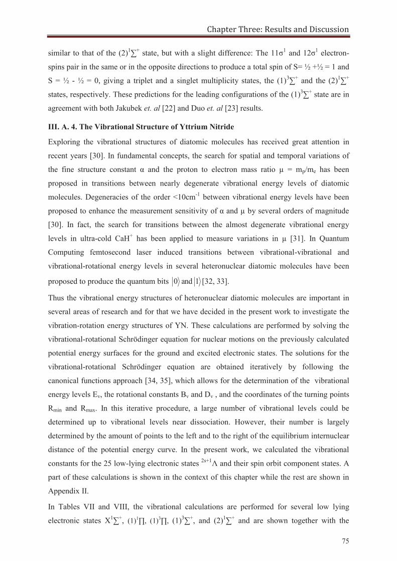
Chapter Three: Results and Discussion
75
similar to that of the (2)1∑+ state, but with a slight difference: The 11σ1 and 12σ1 electron-
spins pair in the same or in the opposite directions to produce a total spin of S= ½ +½ = 1 and
S = ½ - ½ = 0, giving a triplet and a singlet multiplicity states, the (1)3∑+ and the (2)1∑+
states, respectively. These predictions for the leading configurations of the (1)3∑+ state are in
agreement with both Jakubek et. al [22] and Duo et. al [23] results.
III. A. 4. The Vibrational Structure of Yttrium Nitride
Exploring the vibrational structures of diatomic molecules has received great attention in
recent years [30]. In fundamental concepts, the search for spatial and temporal variations of
the fine structure constant α and the proton to electron mass ratio μ = mp/me has been
proposed in transitions between nearly degenerate vibrational energy levels of diatomic
molecules. Degeneracies of the order <10cm-1 between vibrational energy levels have been
proposed to enhance the measurement sensitivity of α and μ by several orders of magnitude
[30]. In fact, the search for transitions between the almost degenerate vibrational energy
levels in ultra-cold CaH+ has been applied to measure variations in μ [31]. In Quantum
Computing femtosecond laser induced transitions between vibrational-vibrational and
vibrational-rotational energy levels in several heteronuclear diatomic molecules have been
proposed to produce the quantum bits 1 and 0 [32, 33].
Thus the vibrational energy structures of heteronuclear diatomic molecules are important in
several areas of research and for that we have decided in the present work to investigate the
vibration-rotation energy structures of YN. These calculations are performed by solving the
vibrational-rotational Schrödinger equation for nuclear motions on the previously calculated
potential energy surfaces for the ground and excited electronic states. The solutions for the
vibrational-rotational Schrödinger equation are obtained iteratively by following the
canonical functions approach [34, 35], which allows for the determination of the vibrational
energy levels Ev, the rotational constants Bv and Dv , and the coordinates of the turning points
Rmin and Rmax. In this iterative procedure, a large number of vibrational levels could be
determined up to vibrational levels near dissociation. However, their number is largely
determined by the amount of points to the left and to the right of the equilibrium internuclear
distance of the potential energy curve. In the present work, we calculated the vibrational
constants for the 25 low-lying electronic states 2s+1Λ and their spin orbit component states. A
part of these calculations is shown in the context of this chapter while the rest are shown in
Appendix II.
In Tables VII and VIII, the vibrational calculations are performed for several low lying
electronic states X1∑+, (1)1∏, (1)3∏, (1)3∑+, and (2)1∑+ and are shown together with the

Chapter Three: Results and Discussion
76
available experimental and theoretical values in literature. All of the vibrational energy levels
Ev were calculated with respect to the zero vibrational energy level of the ground state. The
zero point energy or the difference in energy between the v = 0 vibrational level and the
transition energy at the equilibrium internuclear distance for the ground state is calculated to
be 303.56 cm-1, considered zero in this work.
Table VII: Values of the Eigen-values Ev, the abscissas of the turning point Rmin, Rmax, and the rotational constants Bv for the different vibrational levels of the X1∑+ , (1)1∏, and (1)3∏ states in YN.
X1∑+
v Ev(cm-1) δEv/Ev Rmin(Å) δRmin/Rmin Rmax(Å) δRmax/Rmax Bv×101(cm-1) δBv/Bv 0 0a
0b 1.78a
1.63b
9.2% 1.94a
1.87 Exp b
3.7% 4.021a
4.2666 Exp b 5.7%
1 632.05a 650.64 Exp b
2.8%
1.75 1.64 Exp b
6.7%
1.97 1.93 Exp b
2.1%
3.991 4.23328Exp b
5.7%
2 1286.44 1319 Exp c
2.4%
1.73 1.65 Exp b
4.8%
2.01 1.96 Exp b
2.5%
3.981 4.20739Exp d
5.4%
3 1948.91 1998 Exp c
2.4%
1.71 1.67 Exp b
2.3%
2.04 1.99 Exp b
2.5%
3.962 4.18365Exp d
5.3%
4 2620.94 2688 Exp c
2.5%
1.69 1.69 Exp b
0.0%
2.07 2.02 Exp b
2.4%
3.941 4.16036Exp d
5.2%
5 3294.49 3387 Exp c
2.7%
1.68 1.74 Exp b
3.4%
2.10 2.05 Exp b
2.4%
3.921 4.13793Exp d
5.3%
6 3966.69 4090 Exp c
3.0%
1.66 2.12 3.891
7 4638.30 1.65 2.15 3.872 8 5307.24 1.64 2.17 3.852 9 5975.13 1.63 2.19 3.830
(1)1∏ (1)3∏ v Ev
(cm-1) Rmin
(Å) Rmax
(Å) Bv×101
(cm-1) Dv×107
(cm-1) Ev (cm-1) Rmin(Å) Rmax(Å) Bv×101
(cm-1) Dv×107
(cm-1) 0 5369.55a 1.91a 2.03 a 3.571 3.461 5261.68 1.91 2.03 3.581 3.551 1 6094.86 1.87 2.08 3.572 3.112 5978.32 1.87 2.08 3.572 3.481 2 6837.86 1.84 2.12 3.574 2.884 6694.14 1.84 2.12 3.541 3.781 3 7596.47 1.82 2.14 3.575 2.776 7394.70 1.82 2.16 3.523 3.932 4 8366.24 1.80 2.17 3.566 3.237 8080.03 1.80 2.18 3.494 3.833 5 9129.04 1.78 2.19 3.551 3.228 8756.30 1.79 2.21 3.470 3.804 6 9885.60 1.77 2.21 3.536 3.172 9425.06 1.77 2.24 3.445 4.047 7 10637.42 1.76 2.23 3.522 3.816 10082.35 1.76 2.27 3.416 4.260 8 11371.95 1.75 2.25 3.488 5.164 10727.66 1.75 2.29 3.392 3.921 9 12064.28 1.74 2.28 3.392 1.125 11365.55 1.74 2.32 3.361 4.121 10 12636.82 1.73 2.36 3.187 1.391 11994.53 1.73 2.34 3.342 3.902 11 13124.36 1.72 2.38 3.203 -5.944 12617.49 1.72 2.36 3.323 4.663 12 13693.04 1.72 2.39 3.256 3.941 13226.58 1.72 2.39 3.284 5.194 13 14268.03 1.71 2.42 3.231 2.396 13818.15 1.71 2.41 3.245 4.765 14 14851.77 1.70 2.44 3.230 3.188 14398.37 1.70 2.43 3.226 3.496 15 15437.13 1.69 2.46 3.201 5.483 14977.18 1.70 2.45 3.202 3.941 16 16007.54 1.69 2.48 3.173 2.685 15550.98 1.69 2.48 3.174 5.243 a. First entry is for the values of the present work b.Ref [20] c. Ref [22] d. Ref [19] Note: All vibrational Energy values are measured relative to the zeroth vibrational level whose Ev = 303.56 cm-1 relative to the transition energy at the equilibrium internuclear distance Te for the ground state X1∑+. Exp, correspond to experimental results in literature.
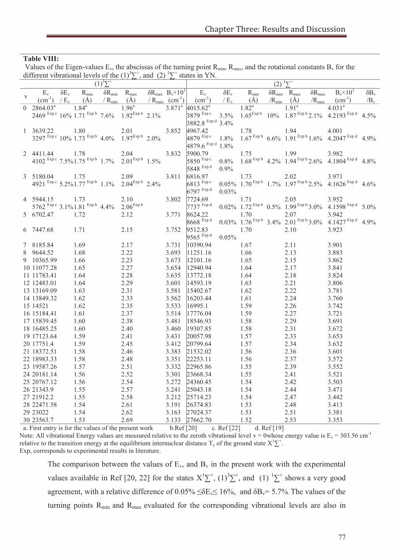
Chapter Three: Results and Discussion
77
The comparison between the values of Ev, and Bv in the present work with the experimental
values available in Ref [20, 22] for the states X1∑+, (1)3∑+, and (1) 1∑+ shows a very good
agreement, with a relative difference of 0.05% ≤δEv≤ 16%, and δBv= 5.7%. The values of the
turning points Rmin and Rmax evaluated for the corresponding vibrational levels are also in
Table VIII: Values of the Eigen-values Ev, the abscissas of the turning point Rmin, Rmax, and the rotational constants Bv for the different vibrational levels of the (1)3∑+, and (2) 1∑+ states in YN.
(1)3∑+ (2) 1∑+
v Ev (cm-1)
δEv / Ev
Rmin (Å)
δRmin / Rmin
Rmax (Å)
δRmax / Rmax
Bv×101
(cm-1) Ev
(cm-1) δEv / Ev
Rmin (Å)
δRmin /Rmin
Rmax (Å)
δRmax /Rmax
Bv×101
(cm-1) δBv /Bv
0 2864.03a
2469 Exp c 16%
1.84a
1.71 Exp b 7.6%
1.96a
1.92Exp b 2.1%
3.871a 4015.62a
3879 Exp c
3882.8 Exp d
3.5% 3.4%
1.82a
1.65Exp b 10%
1.91a 1.87 Exp b
2.1%
4.031a
4.2193 Exp d 4.5%
1 3639.22 3297 Exp c
10%
1.80 1.73 Exp b
4.0%
2.01 1.97Exp b
2.0%
3.852 4967.42 4879 Exp c
4879.6 Exp d
1.8% 1.8%
1.78 1.67 Exp b
6.6%
1.94 1.91 Exp b
1.6%
4.001 4.2047 Exp d
4.9%
2 4411.44 4102 Exp c
7.5%
1.78 1.75 Exp b
1.7%
2.04 2.01Exp b
1.5%
3.832 5900.79 5850 Exp c
5848 Exp d
0.8% 0.9%
1.75 1.68 Exp b
4.2%
1.99 1.94 Exp b
2.6%
3.982 4.1804 Exp d
4.8%
3 5180.04 4921 Exp c
5.2%
1.75 1.77 Exp b
1.1%
2.09 2.04Exp b
2.4%
3.811 6816.97 6813 Exp c
6797 Exp d
0.05% 0.03%
1.73 1.70 Exp b
1.7%
2.02 1.97 Exp b
2.5%
3.971 4.1626 Exp d
4.6%
4 5944.15 5762 Exp c
3.1%
1.73 1.81 Exp b
4.4%
2.10 2.06Exp b
3.802 7724.69 7737 Exp d
0.02%
1.71 1.72 Exp b
0.5%
2.05 1.99 Exp b
3.0%
3.952 4.1598 Exp d
5.0%
5 6702.47 1.72 2.12 3.771 8624.22 8668 Exp d
0.03%
1.70 1.76 Exp b
3.4%
2.07 2.01 Exp b
3.0%
3.942 4.1427 Exp d
4.9%
6 7447.68 1.71 2.15 3.752 9512.83 9565 Exp d
0.05%
1.70 2.10 3.923
7 8185.84 1.69 2.17 3.731 10390.94 1.67 2.11 3.901 8 9644.52 1.68 2.22 3.693 11251.16 1.66 2.13 3.883 9 10365.99 1.66 2.23 3.673 12101.16 1.65 2.15 3.862 10 11077.28 1.65 2.27 3.654 12940.94 1.64 2.17 3.841 11 11783.41 1.64 2.28 3.635 13772.18 1.64 2.18 3.824 12 12483.01 1.64 2.29 3.601 14593.19 1.63 2.21 3.806 13 13169.09 1.63 2.31 3.581 15402.67 1.62 2.22 3.781 14 13849.32 1.62 2.33 3.562 16203.44 1.61 2.24 3.760 15 14521 1.62 2.35 3.533 16995.1 1.59 2.26 3.742 16 15184.41 1.61 2.37 3.514 17776.04 1.59 2.27 3.721 17 15839.45 1.60 2.38 3.481 18546.93 1.58 2.29 3.691 18 16485.25 1.60 2.40 3.460 19307.85 1.58 2.31 3.672 19 17123.64 1.59 2.41 3.431 20057.98 1.57 2.33 3.653 20 17751.4 1.59 2.45 3.412 20799.64 1.57 2.34 3.632 21 18372.51 1.58 2.46 3.383 21532.02 1.56 2.36 3.601 22 18983.33 1.58 2.48 3.351 22253.11 1.56 2.37 3.572 23 19587.26 1.57 2.51 3.332 22965.86 1.55 2.39 3.552 24 20181.14 1.56 2.52 3.301 23668.34 1.55 2.41 3.521 25 20767.12 1.56 2.54 3.272 24360.45 1.54 2.42 3.503 26 21343.9 1.55 2.57 3.241 25043.18 1.54 2.44 3.471 27 21912.2 1.55 2.58 3.212 25714.23 1.54 2.47 3.442 28 22471.58 1.54 2.61 3.191 26374.83 1.53 2.48 3.413 29 23022 1.54 2.62 3.163 27024.37 1.53 2.51 3.381 30 23563.7 1.53 2.69 3.133 27662.70 1.52 2.53 3.353 a. First entry is for the values of the present work b.Ref [20] c. Ref [22] d. Ref [19]
Note: All vibrational Energy values are measured relative to the zeroth vibrational level v = 0whose energy value is Ev = 303.56 cm-1
relative to the transition energy at the equilibrium internuclear distance Te of the ground state X1∑+. Exp, corresponds to experimental results in literature.
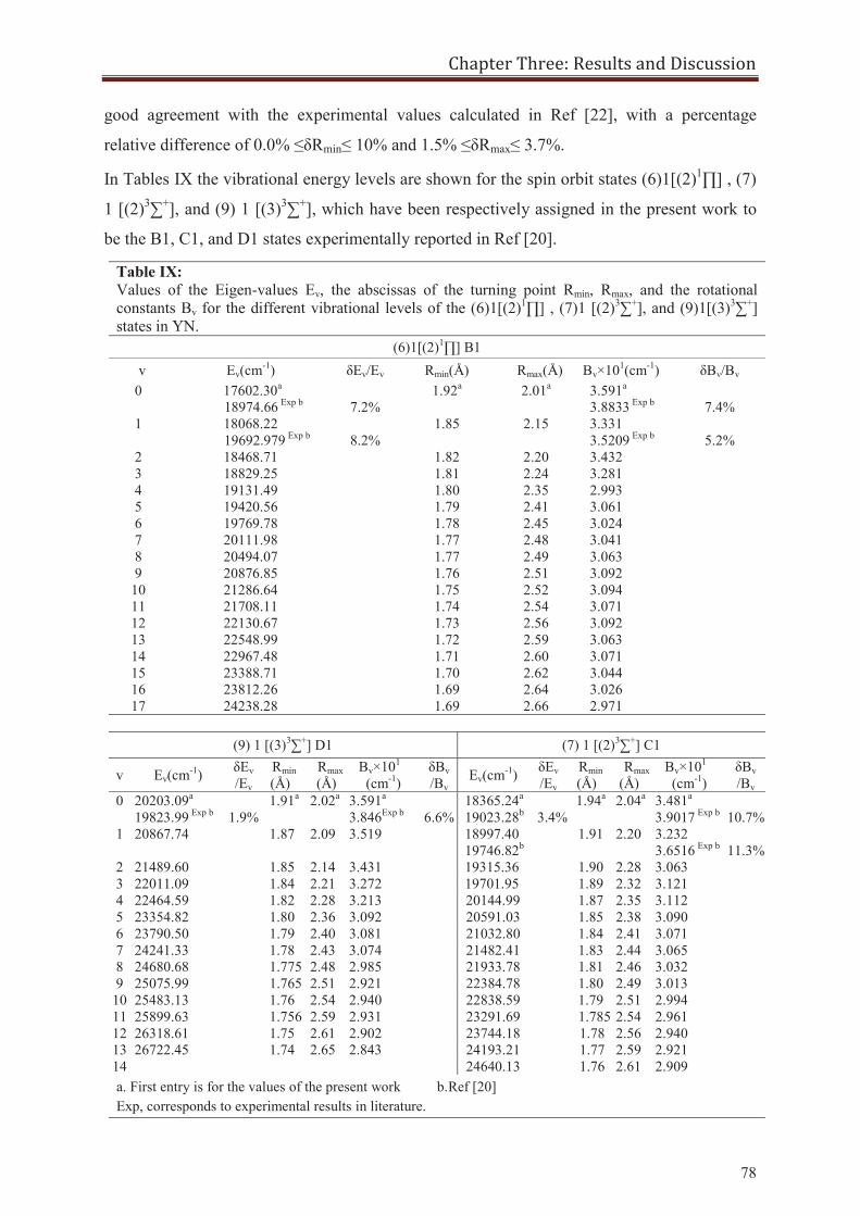
Chapter Three: Results and Discussion
78
good agreement with the experimental values calculated in Ref [22], with a percentage
relative difference of 0.0% ≤δRmin≤ 10% and 1.5% ≤δRmax≤ 3.7%.
In Tables IX the vibrational energy levels are shown for the spin orbit states (6)1[(2)1∏] , (7)
1 [(2)3∑+], and (9) 1 [(3)3∑+], which have been respectively assigned in the present work to
be the B1, C1, and D1 states experimentally reported in Ref [20].
Table IX: Values of the Eigen-values Ev, the abscissas of the turning point Rmin, Rmax, and the rotational constants Bv for the different vibrational levels of the (6)1[(2)1∏] , (7)1 [(2)3∑+], and (9)1[(3)3∑+] states in YN.
(6)1[(2)1∏] B1 v Ev(cm-1) δEv/Ev Rmin(Å) Rmax(Å) Bv×101(cm-1) δBv/Bv
0 17602.30a
18974.66 Exp b
7.2% 1.92a 2.01a 3.591a
3.8833 Exp b
7.4% 1 18068.22
19692.979 Exp b
8.2% 1.85 2.15 3.331
3.5209 Exp b
5.2% 2 18468.71 1.82 2.20 3.432 3 18829.25 1.81 2.24 3.281 4 19131.49 1.80 2.35 2.993 5 19420.56 1.79 2.41 3.061 6 19769.78 1.78 2.45 3.024 7 20111.98 1.77 2.48 3.041 8 20494.07 1.77 2.49 3.063 9 20876.85 1.76 2.51 3.092
10 21286.64 1.75 2.52 3.094 11 21708.11 1.74 2.54 3.071 12 22130.67 1.73 2.56 3.092 13 22548.99 1.72 2.59 3.063 14 22967.48 1.71 2.60 3.071 15 23388.71 1.70 2.62 3.044 16 23812.26 1.69 2.64 3.026 17 24238.28 1.69 2.66 2.971
(9) 1 [(3)3∑+] D1 (7) 1 [(2)3∑+] C1
v Ev(cm-1) δEv /Ev
Rmin (Å)
Rmax (Å)
Bv×101
(cm-1) δBv /Bv
Ev(cm-1) δEv /Ev
Rmin (Å)
Rmax (Å)
Bv×101
(cm-1) δBv /Bv
0 20203.09a
19823.99 Exp b
1.9% 1.91a 2.02a 3.591a
3.846Exp b
6.6% 18365.24a
19023.28b
3.4% 1.94a 2.04a 3.481a
3.9017 Exp b
10.7% 1 20867.74 1.87 2.09 3.519 18997.40
19746.82b 1.91 2.20 3.232
3.6516 Exp b
11.3% 2 21489.60 1.85 2.14 3.431 19315.36 1.90 2.28 3.063 3 22011.09 1.84 2.21 3.272 19701.95 1.89 2.32 3.121 4 22464.59 1.82 2.28 3.213 20144.99 1.87 2.35 3.112 5 23354.82 1.80 2.36 3.092 20591.03 1.85 2.38 3.090 6 23790.50 1.79 2.40 3.081 21032.80 1.84 2.41 3.071 7 24241.33 1.78 2.43 3.074 21482.41 1.83 2.44 3.065 8 24680.68 1.775 2.48 2.985 21933.78 1.81 2.46 3.032 9 25075.99 1.765 2.51 2.921 22384.78 1.80 2.49 3.013
10 25483.13 1.76 2.54 2.940 22838.59 1.79 2.51 2.994 11 25899.63 1.756 2.59 2.931 23291.69 1.785 2.54 2.961 12 26318.61 1.75 2.61 2.902 23744.18 1.78 2.56 2.940 13 26722.45 1.74 2.65 2.843 24193.21 1.77 2.59 2.921 14 24640.13 1.76 2.61 2.909 a. First entry is for the values of the present work b.Ref [20] Exp, corresponds to experimental results in literature.
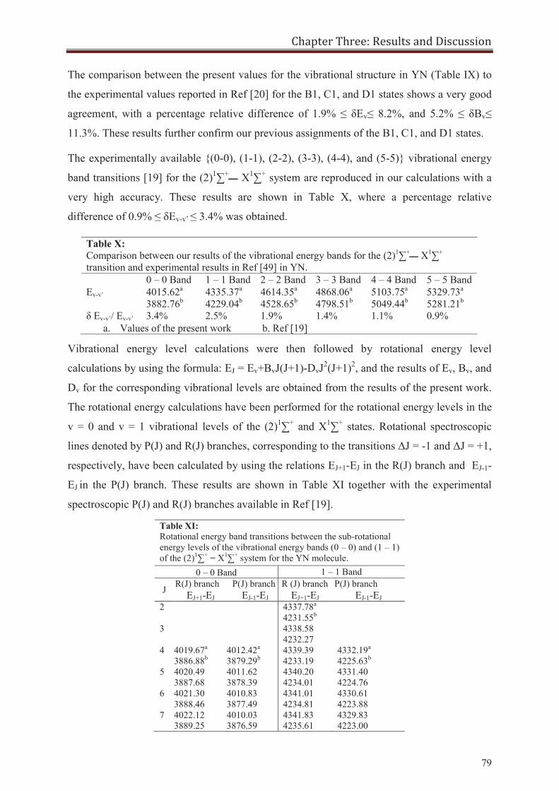
Chapter Three: Results and Discussion
79
The comparison between the present values for the vibrational structure in YN (Table IX) to
the experimental values reported in Ref [20] for the B1, C1, and D1 states shows a very good
agreement, with a percentage relative difference of 1.9% ≤ δEv≤ 8.2%, and 5.2% ≤ δBv≤
11.3%. These results further confirm our previous assignments of the B1, C1, and D1 states.
The experimentally available {(0-0), (1-1), (2-2), (3-3), (4-4), and (5-5)} vibrational energy
band transitions [19] for the (2)1∑+ــــ X1∑+ system are reproduced in our calculations with a
very high accuracy. These results are shown in Table X, where a percentage relative
difference of 0.9% ≤ δEv-v’ ≤ 3.4% was obtained.
Vibrational energy level calculations were then followed by rotational energy level
calculations by using the formula: EJ = Ev+BvJ(J+1)-DvJ2(J+1)2, and the results of Ev, Bv, and
Dv for the corresponding vibrational levels are obtained from the results of the present work.
The rotational energy calculations have been performed for the rotational energy levels in the
v = 0 and v = 1 vibrational levels of the (2)1∑+ and X1∑+ states. Rotational spectroscopic
lines denoted by P(J) and R(J) branches, corresponding to the transitions ΔJ = -1 and ΔJ = +1,
respectively, have been calculated by using the relations EJ+1-EJ in the R(J) branch and EJ-1-
EJ in the P(J) branch. These results are shown in Table XI together with the experimental
spectroscopic P(J) and R(J) branches available in Ref [19].
Table X: Comparison between our results of the vibrational energy bands for the (2)1∑+ــــ X1∑+
transition and experimental results in Ref [49] in YN. 0 – 0 Band 1 – 1 Band 2 – 2 Band 3 – 3 Band 4 – 4 Band 5 – 5 Band Ev-v’ 4015.62a 4335.37a 4614.35a 4868.06a 5103.75a 5329.73a
3882.76b 4229.04b 4528.65b 4798.51b 5049.44b 5281.21b
δ Ev-v’/ Ev-v’ 3.4% 2.5% 1.9% 1.4% 1.1% 0.9% a. Values of the present work b. Ref [19]
Table XI: Rotational energy band transitions between the sub-rotational energy levels of the vibrational energy bands (0 – 0) and (1 – 1) of the (2)1∑+ − X1∑+ system for the YN molecule.
0 – 0 Band 1 – 1 Band
J R(J) branch EJ+1-EJ
P(J) branch EJ-1-EJ
R (J) branch EJ+1-EJ
P(J) branch EJ-1-EJ
2 4337.78a
4231.55b
3 4338.58 4232.27
4 4019.67a
3886.88b 4012.42a
3879.29b 4339.39 4233.19
4332.19a
4225.63b
5 4020.49 3887.68
4011.62 3878.39
4340.20 4234.01
4331.40 4224.76
6 4021.30
3888.46 4010.83 3877.49
4341.01 4234.81
4330.61 4223.88
7 4022.12
3889.25 4010.03 3876.59
4341.83 4235.61
4329.83 4223.00
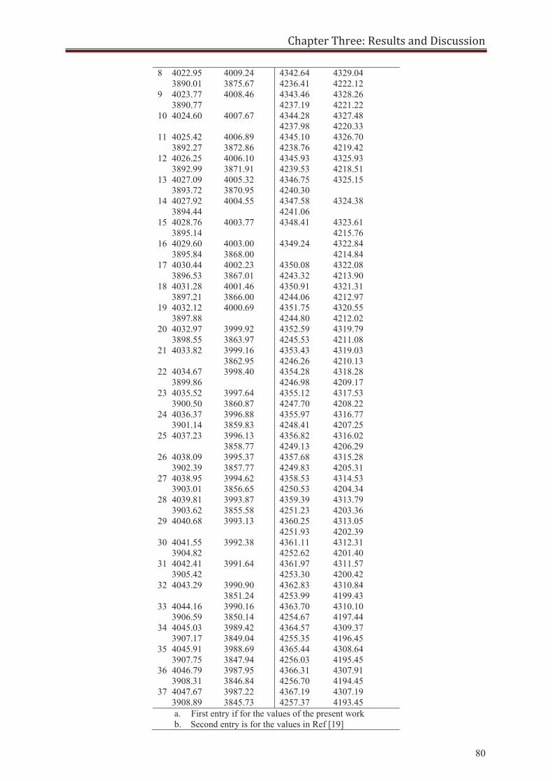
Chapter Three: Results and Discussion
80
8 4022.95 3890.01
4009.24 3875.67
4342.64 4236.41
4329.04 4222.12
9 4023.77 3890.77
4008.46 4343.46 4237.19
4328.26 4221.22
10 4024.60 4007.67 4344.28 4237.98
4327.48 4220.33
11 4025.42 3892.27
4006.89 3872.86
4345.10 4238.76
4326.70 4219.42
12 4026.25 3892.99
4006.10 3871.91
4345.93 4239.53
4325.93 4218.51
13 4027.09
3893.72 4005.32 3870.95
4346.75 4240.30
4325.15
14 4027.92
3894.44 4004.55 4347.58
4241.06 4324.38
15 4028.76
3895.14 4003.77 4348.41 4323.61
4215.76 16 4029.60
3895.84 4003.00 3868.00
4349.24 4322.84 4214.84
17 4030.44
3896.53 4002.23 3867.01
4350.08 4243.32
4322.08 4213.90
18 4031.28
3897.21 4001.46 3866.00
4350.91 4244.06
4321.31 4212.97
19 4032.12
3897.88 4000.69 4351.75
4244.80 4320.55 4212.02
20 4032.97
3898.55 3999.92 3863.97
4352.59 4245.53
4319.79 4211.08
21 4033.82 3999.16 3862.95
4353.43 4246.26
4319.03 4210.13
22 4034.67
3899.86 3998.40 4354.28
4246.98 4318.28 4209.17
23 4035.52
3900.50 3997.64 3860.87
4355.12 4247.70
4317.53 4208.22
24 4036.37
3901.14 3996.88 3859.83
4355.97 4248.41
4316.77 4207.25
25 4037.23 3996.13 3858.77
4356.82 4249.13
4316.02 4206.29
26 4038.09
3902.39 3995.37 3857.77
4357.68 4249.83
4315.28 4205.31
27 4038.95
3903.01 3994.62 3856.65
4358.53 4250.53
4314.53 4204.34
28 4039.81 3903.62
3993.87 3855.58
4359.39 4251.23
4313.79 4203.36
29 4040.68 3993.13 4360.25 4251.93
4313.05 4202.39
30 4041.55
3904.82 3992.38 4361.11
4252.62 4312.31 4201.40
31 4042.41
3905.42 3991.64 4361.97
4253.30 4311.57 4200.42
32 4043.29 3990.90 3851.24
4362.83 4253.99
4310.84 4199.43
33 4044.16
3906.59 3990.16 3850.14
4363.70 4254.67
4310.10 4197.44
34 4045.03
3907.17 3989.42 3849.04
4364.57 4255.35
4309.37 4196.45
35 4045.91
3907.75 3988.69 3847.94
4365.44 4256.03
4308.64 4195.45
36 4046.79
3908.31 3987.95 3846.84
4366.31 4256.70
4307.91 4194.45
37 4047.67
3908.89 3987.22 3845.73
4367.19 4257.37
4307.19 4193.45
a. First entry if for the values of the present work b. Second entry is for the values in Ref [19]
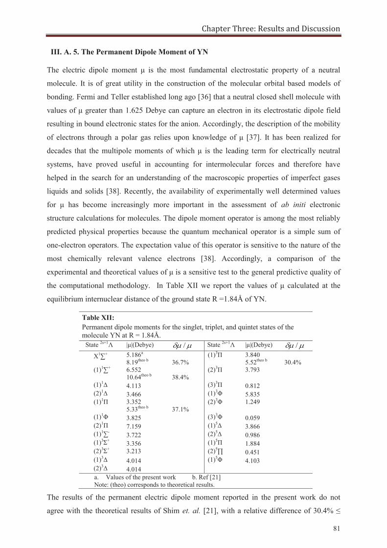
Chapter Three: Results and Discussion
81
III. A. 5. The Permanent Dipole Moment of YN
The electric dipole moment μ is the most fundamental electrostatic property of a neutral
molecule. It is of great utility in the construction of the molecular orbital based models of
bonding. Fermi and Teller established long ago [36] that a neutral closed shell molecule with
values of μ greater than 1.625 Debye can capture an electron in its electrostatic dipole field
resulting in bound electronic states for the anion. Accordingly, the description of the mobility
of electrons through a polar gas relies upon knowledge of μ [37]. It has been realized for
decades that the multipole moments of which μ is the leading term for electrically neutral
systems, have proved useful in accounting for intermolecular forces and therefore have
helped in the search for an understanding of the macroscopic properties of imperfect gases
liquids and solids [38]. Recently, the availability of experimentally well determined values
for μ has become increasingly more important in the assessment of ab initi electronic
structure calculations for molecules. The dipole moment operator is among the most reliably
predicted physical properties because the quantum mechanical operator is a simple sum of
one-electron operators. The expectation value of this operator is sensitive to the nature of the
most chemically relevant valence electrons [38]. Accordingly, a comparison of the
experimental and theoretical values of μ is a sensitive test to the general predictive quality of
the computational methodology. In Table XII we report the values of μ calculated at the
equilibrium internuclear distance of the ground state R =1.84Å of YN.
Table XII: Permanent dipole moments for the singlet, triplet, and quintet states of the molecule YN at R = 1.84Å.
State 2s+1Λ |μ|(Debye) / State 2s+1Λ |μ|(Debye) /
X1∑+ 5.186a 8.19theo b
36.7%
(1)3Π 3.840 5.52theo b
30.4%
(1)1∑+ 6.552 10.64theo b
38.4%
(2)3Π 3.793
(1)1Δ 4.113 (3)3Π 0.812 (2)1Δ 3.466 (1)3Φ 5.835 (1)1Π 3.352
5.33theo b 37.1%
(2)3Φ 1.249
(1)1Φ 3.825 (3)3Φ 0.059 (2)1Π 7.159 (1)5Δ 3.866 (1)1∑- 3.722 (2)5Δ 0.986 (1)3Σ+ 3.356 (1)5Π 1.884 (2)3Σ+ 3.213 (2)5∏ 0.451 (1)3Δ 4.014 (1)5Φ 4.103 (2)3Δ 4.014 a. Values of the present work b. Ref [21] Note: (theo) corresponds to theoretical results.
The results of the permanent electric dipole moment reported in the present work do not
agree with the theoretical results of Shim et. al. [21], with a relative difference of 30.4% ≤
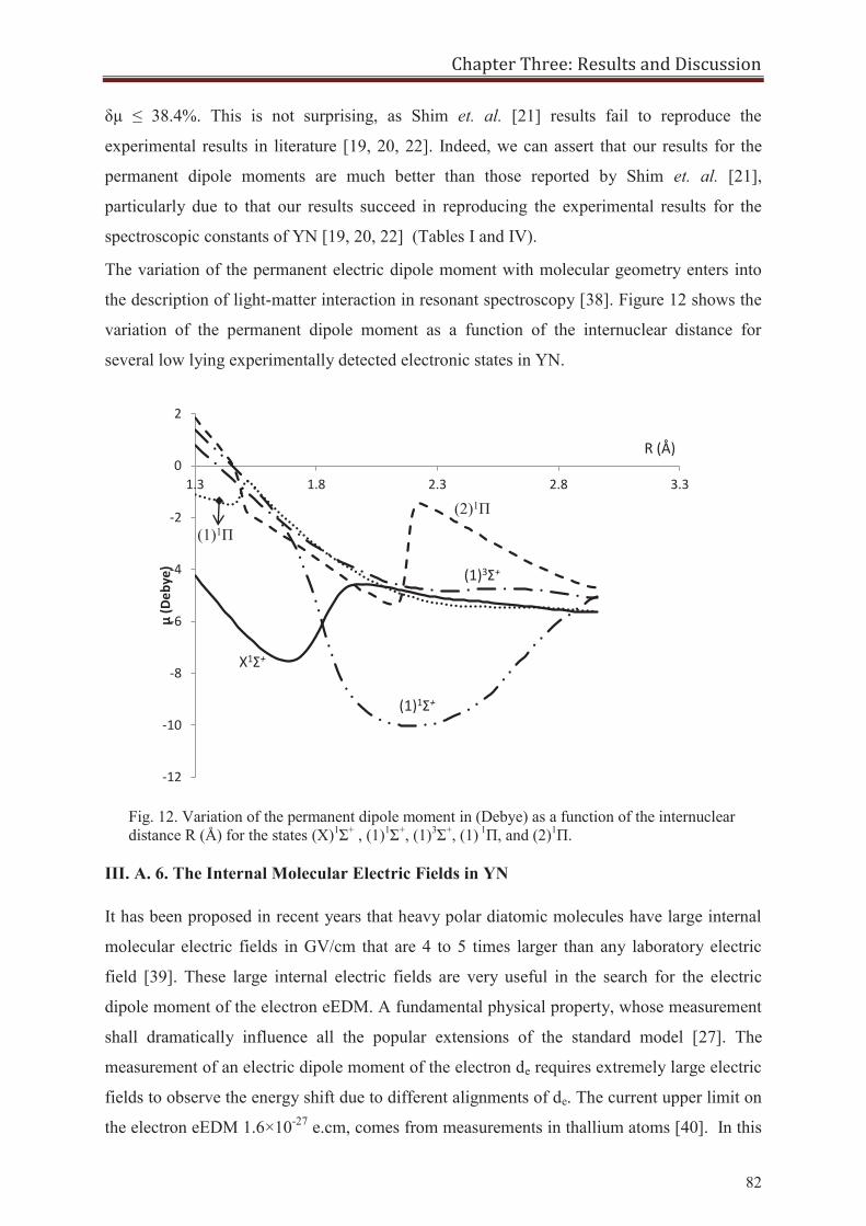
Chapter Three: Results and Discussion
82
δμ ≤ 38.4%. This is not surprising, as Shim et. al. [21] results fail to reproduce the
experimental results in literature [19, 20, 22]. Indeed, we can assert that our results for the
permanent dipole moments are much better than those reported by Shim et. al. [21],
particularly due to that our results succeed in reproducing the experimental results for the
spectroscopic constants of YN [19, 20, 22] (Tables I and IV).
The variation of the permanent electric dipole moment with molecular geometry enters into
the description of light-matter interaction in resonant spectroscopy [38]. Figure 12 shows the
variation of the permanent dipole moment as a function of the internuclear distance for
several low lying experimentally detected electronic states in YN.
III. A. 6. The Internal Molecular Electric Fields in YN
It has been proposed in recent years that heavy polar diatomic molecules have large internal
molecular electric fields in GV/cm that are 4 to 5 times larger than any laboratory electric
field [39]. These large internal electric fields are very useful in the search for the electric
dipole moment of the electron eEDM. A fundamental physical property, whose measurement
shall dramatically influence all the popular extensions of the standard model [27]. The
measurement of an electric dipole moment of the electron de requires extremely large electric
fields to observe the energy shift due to different alignments of de. The current upper limit on
the electron eEDM 1.6×10⁻²⁷ e.cm, comes from measurements in thallium atoms [40]. In this
Fig. 12. Variation of the permanent dipole moment in (Debye) as a function of the internuclear distance R (Å) for the states (X)1Σ+ , (1)1Σ+, (1)3Σ+, (1) 1Π, and (2)1Π.
-12
-10
-8
-6
-4
-2
0
2
1.3 1.8 2.3 2.8 3.3
μ (D
ebye
)
X1Σ+
(1)1Σ+
(2)1Π
(1)3Σ+
(1)1Π
R (Å)
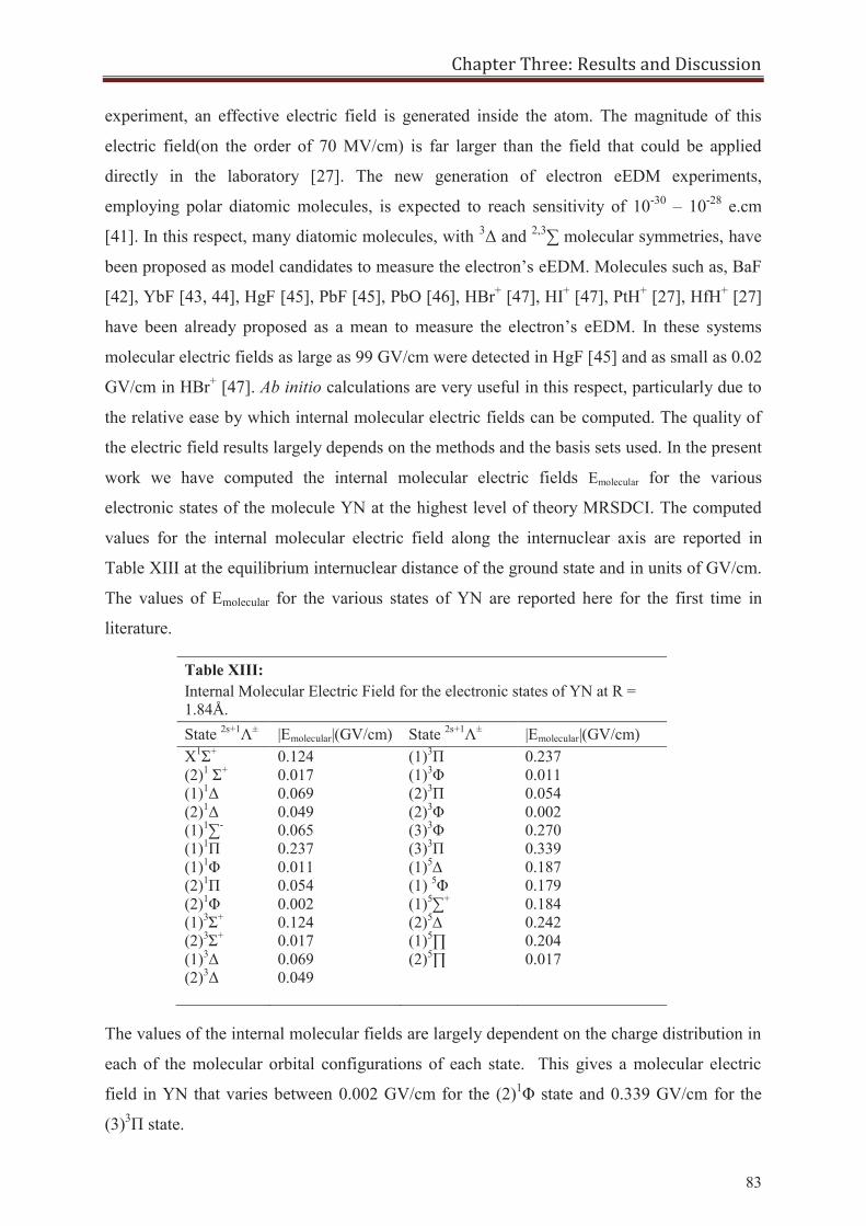
Chapter Three: Results and Discussion
83
experiment, an effective electric field is generated inside the atom. The magnitude of this
electric field(on the order of 70 MV/cm) is far larger than the field that could be applied
directly in the laboratory [27]. The new generation of electron eEDM experiments,
employing polar diatomic molecules, is expected to reach sensitivity of 10-30 – 10-28 e.cm
[41]. In this respect, many diatomic molecules, with 3Δ and 2,3∑ molecular symmetries, have
been proposed as model candidates to measure the electron’s eEDM. Molecules such as, BaF
[42], YbF [43, 44], HgF [45], PbF [45], PbO [46], HBr+ [47], HI+ [47], PtH+ [27], HfH+ [27]
have been already proposed as a mean to measure the electron’s eEDM. In these systems
molecular electric fields as large as 99 GV/cm were detected in HgF [45] and as small as 0.02
GV/cm in HBr+ [47]. Ab initio calculations are very useful in this respect, particularly due to
the relative ease by which internal molecular electric fields can be computed. The quality of
the electric field results largely depends on the methods and the basis sets used. In the present
work we have computed the internal molecular electric fields Emolecular for the various
electronic states of the molecule YN at the highest level of theory MRSDCI. The computed
values for the internal molecular electric field along the internuclear axis are reported in
Table XIII at the equilibrium internuclear distance of the ground state and in units of GV/cm.
The values of Emolecular for the various states of YN are reported here for the first time in
literature.
Table XIII: Internal Molecular Electric Field for the electronic states of YN at R = 1.84Å. State 2s+1Λ± |Emolecular|(GV/cm) State 2s+1Λ± |Emolecular|(GV/cm) X1Σ+ 0.124 (1)3Π 0.237 (2)1 Σ+ 0.017 (1)3Φ 0.011 (1)1Δ 0.069 (2)3Π 0.054 (2)1Δ 0.049 (2)3Φ 0.002 (1)1∑- 0.065 (3)3Φ 0.270 (1)1Π 0.237 (3)3Π 0.339 (1)1Φ 0.011 (1)5∆ 0.187 (2)1Π 0.054 (1) 5Φ 0.179 (2)1Φ 0.002 (1)5∑+ 0.184 (1)3Σ+ 0.124 (2)5∆ 0.242 (2)3Σ+ 0.017 (1)5∏ 0.204 (1)3Δ 0.069 (2)5∏ 0.017 (2)3Δ 0.049
The values of the internal molecular fields are largely dependent on the charge distribution in
each of the molecular orbital configurations of each state. This gives a molecular electric
field in YN that varies between 0.002 GV/cm for the (2)1Φ state and 0.339 GV/cm for the
(3)3Π state.
Chapter Three: Results and Discussion
84
III. B. The Structure of Zirconium Nitride ZrN
III. B. 1. Preliminary Works on ZrN
Zirconium nitride is an interesting and versatile material owing to its low electrical resistivity,
good corrosion resistance, low formation energy, and high mechanical properties [48 - 50].
Typically, ZrN and TiN possessing the best mechanical properties are deposited by physical
vapor deposition to coat medical devices, industrial parts, automotive, aerospace components
and other parts subject to high wear and corrosive environments [51 – 54]. In high
temperature material applications, within the group of refractory metal nitrides Ti, Zr, Hf, and
Nb titanium and zirconium nitrides are the most promising hardening additives, which are
used for raising the high-temperature strength of sintered molybdenum and provide high
enough ductility parameters at a temperature up to 2000°C [55]. Understanding the formation
and nature of the Zirconium-nitrogen bond is thus an active area of research with many
applications in several areas of science. In astrophysics, transition metal atoms are relatively
abundant in cool M- and S-type stars [56]. In fact, diatomic transition metal hydrides and
oxides have been detected in the spectra of stellar atmospheres [57 - 61] and since the nitrides
and oxides often have similar bond energies [62], the nitrides are also of potential
astrophysical importance.
To the best of our knowledge the electronic structures and vibrational spectra of the ZrN
molecule have been topics of research for a considerable period of time [63 – 71]. Bates and
Dunn [63] performed a spectroscopic study for the (0,0) band in the (1)2∏ - X2∑+ and (2)2∑+
- X2∑+ transitions. Recently, Cheung and coworkers [64 – 68] studied the (0,0), (1,1), and
(2,2) vibrational bands of the (1)2∏ - X2∑+ transition for various isotopomers of ZrN 90ZrN, 91ZrN, 92ZrN, 94ZrN, 96ZrN. More recently, Chen et. al. [69] performed a laser spectroscopic
study for the (0,0) vibrational band in the (2)2∑+ - X2∑+ system. These spectroscopic studies
[69] were then followed by ab initio MRCI calculations on the low-lying 5 doublet states and
2 low-lying quartet states. Haiyang et. al. [70] studied the magnetic hyperfine structure of the
X2∑+ state for the isotopomer 91ZrN, recording the laser induced fluorescence spectrum of the
(1)2Π ــ X2∑+ vibrational transition (0 – 0). Gary et. al. [71] performed an infrared
spectroscopic and density functional investigation for the reaction between transition metals,
Ti, Zr, and Hf with nitrogen atoms. They reported the value of the harmonicity constant ωe =
991cm-1 in the ground state of ZrN. Devore et. al. [72] performed an infrared vibrational
spectroscopy of the group IV transition metal gaseous nitrides TiN, ZrN, and HfN. The
ground state in each of the three molecules was detected to be of 2∑ symmetry. Infrared
Chapter Three: Results and Discussion
85
spectroscopic analysis yielded vibrational frequencies and rotational P and R branches in the
ground state of ZrN. A common feature exists between the different experimental studies on
the ZrN molecule. It is the existence of strong severe perturbations in the experimental
spectra. These perturbations could not be resolved easily and resulted in a limited partial
analysis of the obtained spectrum. This is not surprising, as several perturbations have been
also detected in the spectrum of the isoelectronic molecules TiN [73, 74] and ScO [75, 76],
which are similar to ZrN. As the identity of the perturbing states in ZrN could not be
identified, there arises the need for a high quality ab initio investigation for the electronic
structure of the neutral ZrN molecule. Although the atomic structure of Nitrogen is relatively
simple with 4S as its ground electronic state. The electronic structure of Zirconium is more
complicated with 3F as the ground state. These combinations of atomic orbitals on Zr and N
will result in a plenty of molecular states, which could also split due to spin orbit coupling. In
the present work we try to fully explore the electronic structure of the molecule ZrN with the
inclusion of relativistic spin orbit effects. The results of the present calculations yielded
potential energy curves, spectroscopic constant and vibro-rotational energy levels. The
comparison between the values of the present work to the experimental and theoretical results
available in literature shows a very good agreement. This reflects the high accuracy by which
our theoretical calculations are able to represent the bonding in ZrN. Until the work described
here, no extensive theoretical study was available on ZrN.
III. B. 2. Results on ZrN
The potential energy curves for 21 low-lying electronic states 2s+1Λ(±) of the molecule ZrN
have been obtained from MRSDCI +Q calculations performed at 40 internuclear distances
equally distributed between 1.3 Å and 2.5 Å. Figures 13-16 show the potential energy curves
of 12 low-lying doublet and 9 low-lying quartet states. The energy scale of all figures is
relative to the minimum energy of the ground electronic state predicted here to be a X2∑+
state. The spectroscopic constants obtained from all of these curves are given in Table XIV
where Re is the equilibrium internuclear distance, ωe is the harmonic frequencies around the
equilibrium, Te is the transition energy relative to the ground state, Be is the rotational
constant, and De is the centrifugal distortion constant. The ground state of ZrN is a X2∑+ state
resulting from the distribution of 7 valence electrons over the active space of molecular
orbitals 1σ21π42σ1 leading in to an orbital angular momentum Λ = Σλi = 0, with one unpaired
electron (S = ½), giving a doublet multiplicity (2s+1) ground state X2∑+.
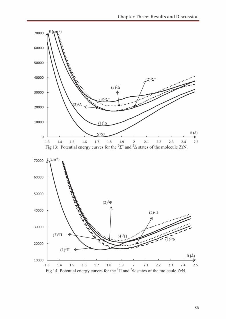
Chapter Three: Results and Discussion
86
0
10000
20000
30000
40000
50000
60000
70000
1.3 1.4 1.5 1.6 1.7 1.8 1.9 2 2.1 2.2 2.3 2.4 2.5
R (Å)
E (cm-1)
X2Σ+
(1)2Δ
(2)2Δ
(2)2Σ+
(3)2Δ
(3)2Σ+
Fig.14: Potential energy curves for the 2Π and 2Φ states of the molecule ZrN.
Fig.13: Potential energy curves for the 2Σ+ and 2Δ states of the molecule ZrN.
10000
20000
30000
40000
50000
60000
70000
1.3 1.4 1.5 1.6 1.7 1.8 1.9 2 2.1 2.2 2.3 2.4 2.5
E (cm-1)
(1)2Π
(2)2Π
(1)2Φ (3)2Π
(2)2Φ
(4)2Π
R (Å)
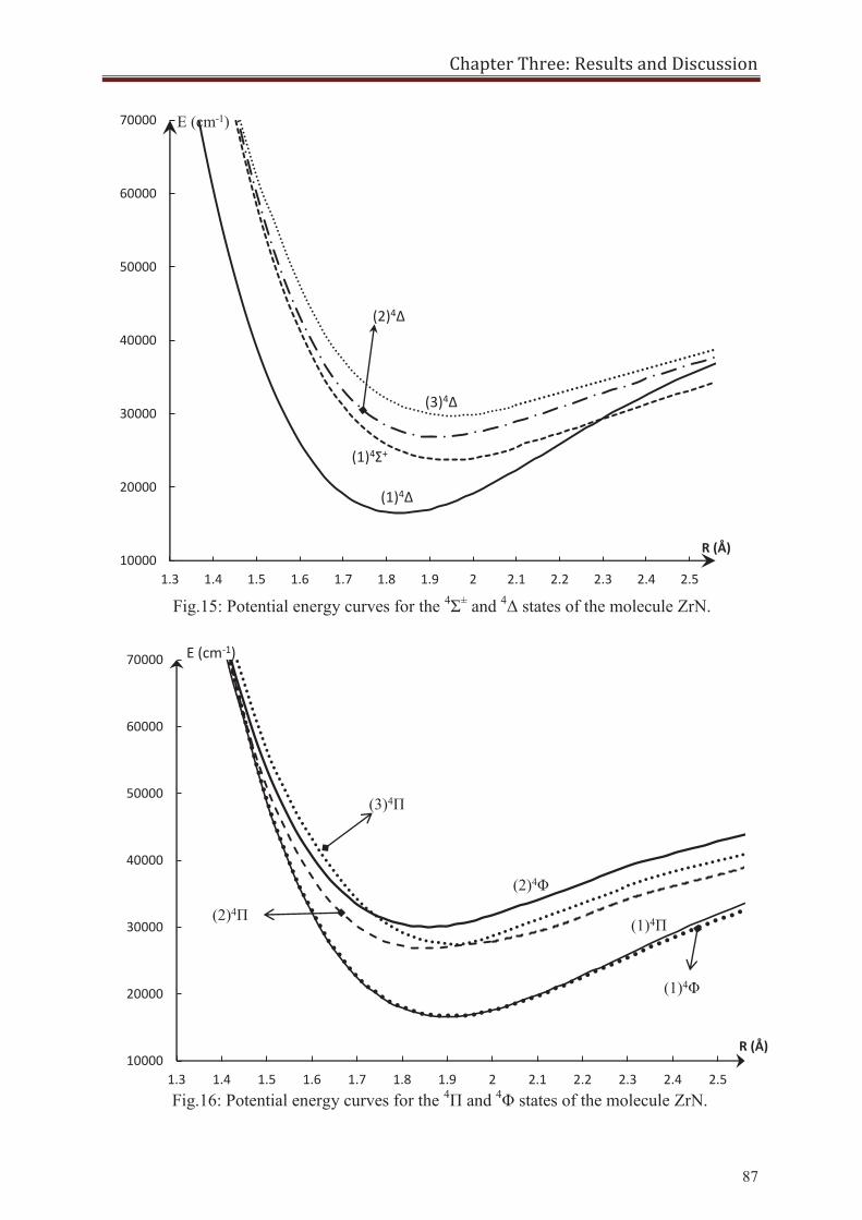
Chapter Three: Results and Discussion
87
10000
20000
30000
40000
50000
60000
70000
1.3 1.4 1.5 1.6 1.7 1.8 1.9 2 2.1 2.2 2.3 2.4 2.5
R (Å)
E (cm-1)
(1)4Δ
(1)4Σ+
(2)4Δ
(3)4Δ
Fig.15: Potential energy curves for the 4Σ± and 4Δ states of the molecule ZrN.
10000
20000
30000
40000
50000
60000
70000
1.3 1.4 1.5 1.6 1.7 1.8 1.9 2 2.1 2.2 2.3 2.4 2.5
R (Å)
E (cm-1)
(1)4Π
(1)4Φ
(2)4Π
(2)4Φ
(3)4Π
Fig.16: Potential energy curves for the 4Π and 4Φ states of the molecule ZrN.
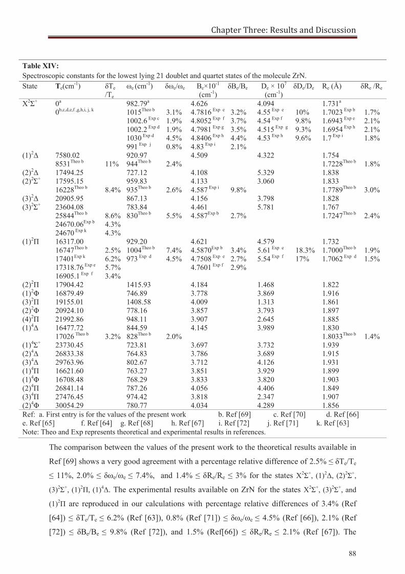
Chapter Three: Results and Discussion
88
The comparison between the values of the present work to the theoretical results available in
Ref [69] shows a very good agreement with a percentage relative difference of 2.5% ≤ δTe/Te
≤ 11%, 2.0% ≤ δωe/ωe ≤ 7.4%, and 1.4% ≤ δRe/Re ≤ 3% for the states X2Σ+, (1)2Δ, (2)2Σ+,
(3)2Σ+, (1)2Π, (1)4Δ. The experimental results available on ZrN for the states X2Σ+, (3)2Σ+, and
(1)2Π are reproduced in our calculations with percentage relative differences of 3.4% (Ref
[64]) ≤ δTe/Te ≤ 6.2% (Ref [63]), 0.8% (Ref [71]) ≤ δωe/ωe ≤ 4.5% (Ref [66]), 2.1% (Ref
[72]) ≤ δBe/Be ≤ 9.8% (Ref [72]), and 1.5% (Ref[66]) ≤ δRe/Re ≤ 2.1% (Ref [67]). The
Table XIV: Spectroscopic constants for the lowest lying 21 doublet and quartet states of the molecule ZrN. State Te(cm-1) δTe
/Te
ωe (cm-1) δωe/ωe Be×10-1
(cm-1) δBe/Be De × 107
(cm-1) δDe/De Re (Å) δRe /Re
X2Σ+ 0a 0b,c,d,e,f ,g,h,i, j, k
982.79a
1015Theo b
1002.6 Exp c 1002.2 Exp d
1030 Exp d
991 Exp j
3.1% 1.9% 1.9% 4.5% 0.8%
4.626 4.7816 Exp e
4.8052 Exp f
4.7981 Exp g
4.8406 Exp h 4.83 Exp i
3.2% 3.7% 3.5% 4.4% 2.1%
4.094 4.55 Exp e
4.54 Exp f
4.515 Exp g
4.53 Exp h
10% 9.8% 9.3% 9.6%
1.731a 1.7023 Exp b 1.6943 Exp e
1.6954 Exp h
1.7 Exp i
1.7% 2.1% 2.1% 1.8%
(1)2Δ 7580.02 8531Theo b
11%
920.97 944Theo b
2.4%
4.509
4.322 1.754 1.7228Theo b
1.8%
(2)2Δ 17494.25 727.12 4.108 5.329 1.838 (2)2Σ+ 17595.15
16228Theo b 8.4%
959.83 935Theo b
2.6%
4.133 4.587 Exp i
9.8%
3.060 1.833 1.7789Theo b
3.0%
(3)2Δ 20905.95 867.13 4.156 3.798 1.828 (3)2Σ+ 23604.08
25844Theo b
24670.06Exp b
24670 Exp k
8.6% 4.3% 4.3%
783.84 830Theo b
5.5%
4.461 4.587Exp b
2.7%
5.781 1.767 1.7247Theo b
2.4%
(1)2Π 16317.00 16747Theo b 17401Exp k
17318.76 Exp e
16905.1 Exp f
2.5% 6.2% 5.7% 3.4%
929.20 1004Theo b
973 Exp d
7.4% 4.5%
4.621 4.5870Exp b
4.7508 Exp e
4.7601 Exp f
3.4% 2.7% 2.9%
4.579 5.61 Exp e 5.54 Exp f
18.3% 17%
1.732 1.7000Theo b
1.7062 Exp d
1.9% 1.5%
(2)2Π 17904.42 1415.93 4.184 1.468 1.822 (1)2Φ 16879.49 746.89 3.778 3.869 1.916 (3)2Π 19155.01 1408.58 4.009 1.313 1.861 (2)2Φ 20924.10 778.16 3.857 3.793 1.897 (4)2Π 21992.86 948.11 3.907 2.645 1.885 (1)4Δ 16477.72
17026 Theo b 3.2%
844.59 828Theo b
2.0%
4.145 3.989 1.830 1.8033Theo b
1.4%
(1)4Σ+ 23730.45 723.81 3.697 3.732 1.939 (2)4Δ 26833.38 764.83 3.786 3.689 1.915 (3)4Δ 29763.96 802.67 3.712 4.126 1.931 (1)4Π 16621.60 763.27 3.851 3.929 1.899 (1)4Φ 16708.48 768.29 3.833 3.820 1.903 (2)4Π 26841.14 787.26 4.056 4.406 1.849 (3)4Π 27476.45 974.42 3.818 2.347 1.907 (2)4Φ 30054.29 780.77 4.034 4.289 1.856 Ref: a. First entry is for the values of the present work b. Ref [69] c. Ref [70] d. Ref [66] e. Ref [65] f. Ref [64] g. Ref [68] h. Ref [67] i. Ref [72] j. Ref [71] k. Ref [63] Note: Theo and Exp represents theoretical and experimental results in references.
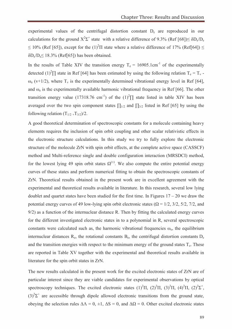
Chapter Three: Results and Discussion
89
experimental values of the centrifugal distortion constant De are reproduced in our
calculations for the ground X2Σ+ state with a relative difference of 9.3% (Ref [68])≤ δDe/De
≤ 10% (Ref [65]), except for the (1)2Π state where a relative difference of 17% (Ref[64]) ≤
δDe/De≤ 18.3% (Ref[65]) has been obtained.
In the results of Table XIV the transition energy Te = 16905.1cm-1 of the experimentally
detected (1)2∏ state in Ref [64] has been estimated by using the following relation Te = Tv -
ωe (v+1/2), where Tv is the experimentally determined vibrational energy level in Ref [64],
and ωe is the experimentally available harmonic vibrational frequency in Ref [66]. The other
transition energy value (17318.76 cm-1) of the (1)2∏ state listed in table XIV has been
averaged over the two spin component states ∏1/2 and ∏3/2 listed in Ref [65] by using the
following relation (T1/2 +T3/2)/2.
A good theoretical determination of spectroscopic constants for a molecule containing heavy
elements requires the inclusion of spin orbit coupling and other scalar relativistic effects in
the electronic structure calculations. In this study we try to fully explore the electronic
structure of the molecule ZrN with spin orbit effects, at the complete active space (CASSCF)
method and Multi-reference single and double configuration interaction (MRSDCI) method,
for the lowest lying 49 spin orbit states Ω(±). We also compute the entire potential energy
curves of these states and perform numerical fitting to obtain the spectroscopic constants of
ZrN. Theoretical results obtained in the present work are in excellent agreement with the
experimental and theoretical results available in literature. In this research, several low lying
doublet and quartet states have been studied for the first time. In Figures 17 – 20 we draw the
potential energy curves of 49 low-lying spin orbit electronic states (Ω = 1/2, 3/2, 5/2, 7/2, and
9/2) as a function of the internuclear distance R. Then by fitting the calculated energy curves
for the different investigated electronic states in to a polynomial in R, several spectroscopic
constants were calculated such as, the harmonic vibrational frequencies ωe, the equilibrium
internuclear distances Re, the rotational constants Be, the centrifugal distortion constants De
and the transition energies with respect to the minimum energy of the ground states Te. These
are reported in Table XV together with the experimental and theoretical results available in
literature for the spin orbit states in ZrN.
The new results calculated in the present work for the excited electronic states of ZrN are of
particular interest since they are viable candidates for experimental observations by optical
spectroscopy techniques. The excited electronic states (1)2Π, (2)2Π, (3)2Π, (4)2Π, (2)2Σ+,
(3)2Σ+ are accessible through dipole allowed electronic transitions from the ground state,
obeying the selection rules ΔΛ = 0, ±1, ΔS = 0, and ΔΩ = 0. Other excited electronic states
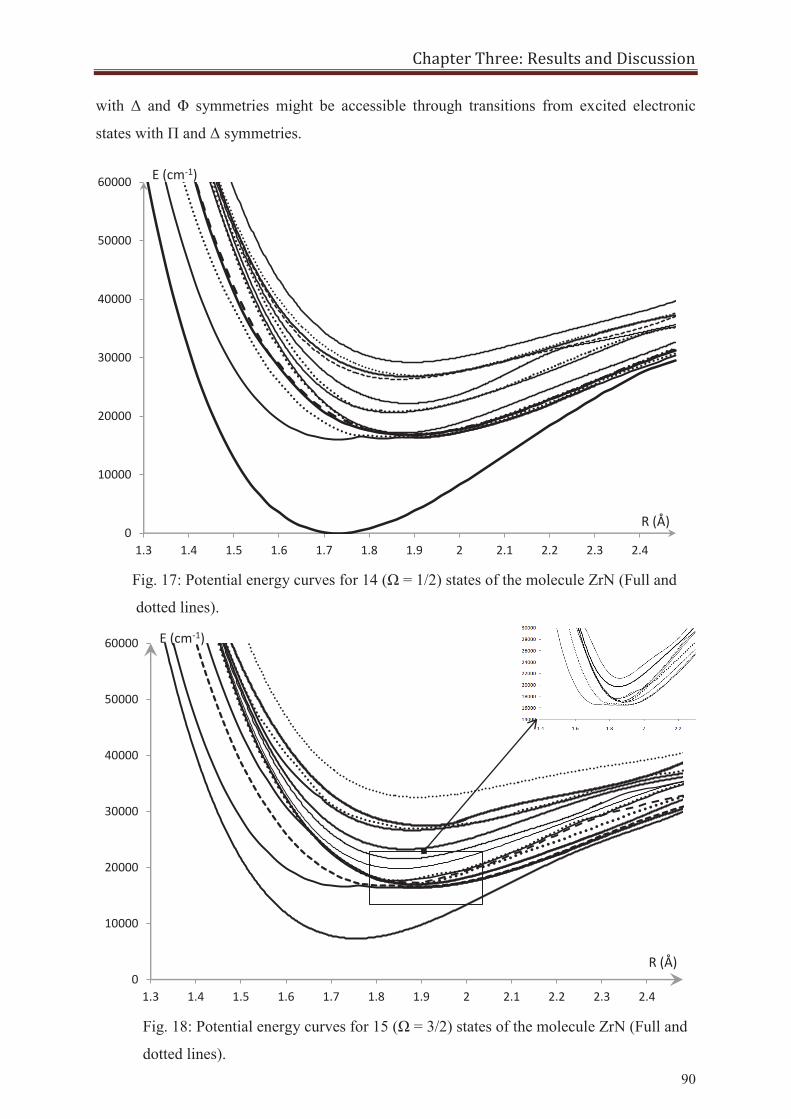
Chapter Three: Results and Discussion
90
with Δ and Φ symmetries might be accessible through transitions from excited electronic
states with Π and Δ symmetries.
0
10000
20000
30000
40000
50000
60000
1.3 1.4 1.5 1.6 1.7 1.8 1.9 2 2.1 2.2 2.3 2.4
R (Å)
E (cm-1)
Fig. 17: Potential energy curves for 14 (Ω = 1/2) states of the molecule ZrN (Full and
dotted lines).
0
10000
20000
30000
40000
50000
60000
1.3 1.4 1.5 1.6 1.7 1.8 1.9 2 2.1 2.2 2.3 2.4
R (Å)
E (cm-1)
Fig. 18: Potential energy curves for 15 (Ω = 3/2) states of the molecule ZrN (Full and
dotted lines).
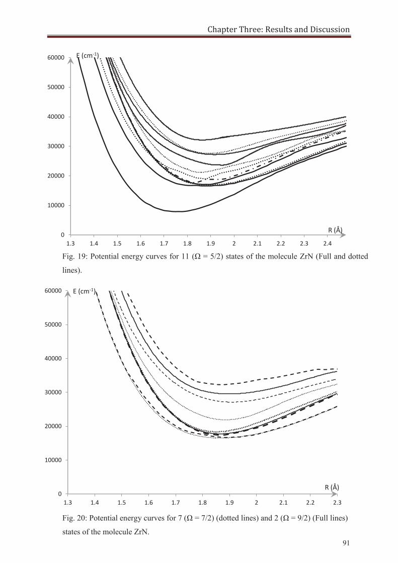
Chapter Three: Results and Discussion
91
0
10000
20000
30000
40000
50000
60000
1.3 1.4 1.5 1.6 1.7 1.8 1.9 2 2.1 2.2 2.3 2.4
R (Å)
E (cm-1)
Fig. 19: Potential energy curves for 11 (Ω = 5/2) states of the molecule ZrN (Full and dotted
lines).
0
10000
20000
30000
40000
50000
60000
1.3 1.4 1.5 1.6 1.7 1.8 1.9 2 2.1 2.2 2.3
E (cm-1)
R (Å)
Fig. 20: Potential energy curves for 7 (Ω = 7/2) (dotted lines) and 2 (Ω = 9/2) (Full lines)
states of the molecule ZrN.
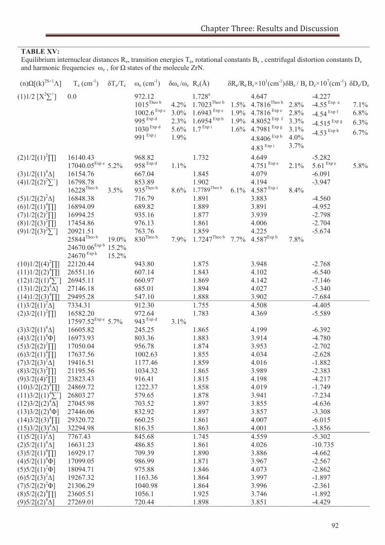
Chapter Three: Results and Discussion
92
TABLE XV: Equilibrium internuclear distances Re, transition energies Te, rotational constants Be , centrifugal distortion constants De and harmonic frequencies ωe , for Ω states of the molecule ZrN.
(n)Ω[(k)2S+1Λ] Te (cm-1) δTe/Te ωe (cm-1) δωe /ωe Re(Å) δRe/Re Be×101(cm-1) δBe / Be De×107(cm-1) δDe/De
(1)1/2 [X2∑+] 0.0 972.12 1015Theo b
1002.6 Exp c
995 Exp d
1030 Exp d
991 Exp j
4.2% 3.0% 2.3% 5.6% 1.9%
1.728a
1.7023Theo b 1.6943 Exp e
1.6954 Exp h
1.7 Exp i
1.5% 1.9% 1.9% 1.6%
4.647 4.7816Theo b
4.7816 Exp e
4.8052 Exp f
4.7981 Exp g
4.8406 Exp h
4.83 Exp i
2.8% 2.8% 3.3% 3.1% 4.0% 3.7%
-4.227 -4.55 Exp e
-4.54 Exp f
-4.515 Exp g
-4.53 Exp h
7.1% 6.8% 6.3% 6.7%
(2)1/2[(1)2∏] 16140.43 17040.05Exp e 5.2%
968.82 958 Exp d
1.1%
1.732 4.649 4.751 Exp e
2.1%
-5.282 5.61 Exp e
5.8%
(3)1/2[(1)4∆] 16154.76 667.04 1.845 4.079 -6.091 (4)1/2[(2)2∑+] 16798.78
16228Theo b 3.5% 853.89 935Theo b
8.6%
1.902 1.7789Theo b
6.1%
4.194 4.587 Exp i
8.4%
-3.947
(5)1/2[(2)2∆] 16848.38 716.79 1.891 3.883 -4.560 (6)1/2[(1)4∏] 16894.09 689.82 1.889 3.891 -4.952 (7)1/2[(2)2∏] 16994.25 935.16 1.877 3.939 -2.798 (8)1/2[(3)2∏] 17454.86 976.13 1.861 4.006 -2.704 (9)1/2[(3)2∑+] 20921.51
25844Theo b
24670.06Exp b
24670 Exp k
19.0% 15.2% 15.2%
763.76 830Theo b
7.9%
1.859 1.7247Theo b
7.7%
4.225 4.587Exp b
7.8%
-5.674
(10)1/2[(4)2∏] 22120.44 943.80 1.875 3.948 -2.768 (11)1/2[(2)4∏] 26551.16 607.14 1.843 4.102 -6.540 (12)1/2[(1)4∑+] 26945.11 660.97 1.869 4.142 -7.146 (13)1/2[(2)4∆] 27146.18 685.01 1.894 4.027 -5.340 (14)1/2[(3)4∏] 29495.28 547.10 1.888 3.902 -7.684 (1)3/2[(1)2∆] 7334.31 912.30 1.755 4.508 -4.405 (2)3/2[(1)2∏] 16582.20
17597.52Exp e 5.7% 972.64 943 Exp d
3.1%
1.783 4.369 -5.589
(3)3/2[(1)4∆] 16605.82 245.25 1.865 4.199 -6.392 (4)3/2[(1)4Φ] 16973.93 803.36 1.883 3.914 -4.780 (5)3/2[(2)2∏] 17050.04 956.78 1.874 3.953 -2.702 (6)3/2[(1)4∏] 17637.56 1002.63 1.855 4.034 -2.628 (7)3/2[(3)2∆] 19416.51 1177.46 1.859 4.016 -1.882 (8)3/2[(3)2∏] 21195.56 1034.32 1.865 3.989 -2.383 (9)3/2[(4)2∏] 23823.43 916.41 1.815 4.198 -4.217 (10)3/2[(2)4∏] 24869.72 1222.37 1.858 4.019 -1.749 (11)3/2[(1)4∑+] 26803.27 579.65 1.878 3.941 -7.234 (12)3/2[(2)4∆] 27045.98 703.52 1.897 3.855 -4.636 (13)3/2[(2)4Φ] 27446.06 832.92 1.897 3.857 -3.308 (14)3/2[(3)4∏] 29320.72 660.25 1.861 4.007 -6.015 (15)3/2[(3)4∆] 32294.98 816.35 1.863 4.001 -3.856 (1)5/2[(1)2∆] 7767.43 845.68 1.745 4.559 -5.302 (2)5/2[(1)4∆] 16631.23 486.85 1.861 4.026 -10.735 (3)5/2[(1)4∏] 16929.17 709.39 1.890 3.886 -4.662 (4)5/2[(1)4Φ] 17099.05 986.99 1.871 3.967 -2.567 (5)5/2[(1)2Φ] 18094.71 975.88 1.846 4.073 -2.862 (6)5/2[(3)2∆] 19267.32 1163.36 1.864 3.997 -1.897 (7)5/2[(2)2Φ] 21306.29 1040.98 1.864 3.996 -2.361 (8)5/2[(2)4∏] 23605.51 1056.1 1.925 3.746 -1.892 (9)5/2[(2)4∆] 27269.01 720.44 1.898 3.851 -4.429
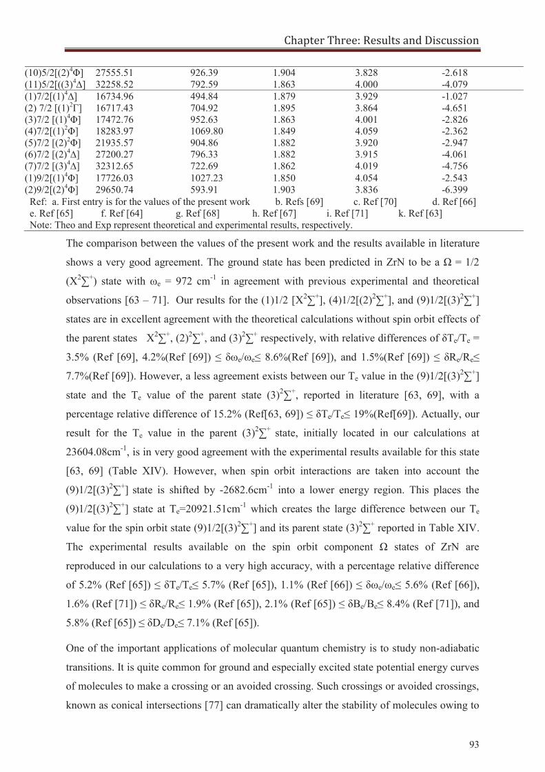
Chapter Three: Results and Discussion
93
(10)5/2[(2)4Φ] 27555.51 926.39 1.904 3.828 -2.618 (11)5/2[((3)4∆] 32258.52 792.59 1.863 4.000 -4.079 (1)7/2[(1)4∆] 16734.96 494.84 1.879 3.929 -1.027 (2) 7/2 [(1)2Г] 16717.43 704.92 1.895 3.864 -4.651 (3)7/2 [(1)4Φ] 17472.76 952.63 1.863 4.001 -2.826 (4)7/2[(1)2Φ] 18283.97 1069.80 1.849 4.059 -2.362 (5)7/2 [(2)2Φ] 21935.57 904.86 1.882 3.920 -2.947 (6)7/2 [(2)4∆] 27200.27 796.33 1.882 3.915 -4.061 (7)7/2 [(3)4∆] 32312.65 722.69 1.862 4.019 -4.756 (1)9/2[(1)4Φ] 17726.03 1027.23 1.850 4.054 -2.543 (2)9/2[(2)4Φ] 29650.74 593.91 1.903 3.836 -6.399 Ref: a. First entry is for the values of the present work b. Refs [69] c. Ref [70] d. Ref [66] e. Ref [65] f. Ref [64] g. Ref [68] h. Ref [67] i. Ref [71] k. Ref [63] Note: Theo and Exp represent theoretical and experimental results, respectively.
The comparison between the values of the present work and the results available in literature
shows a very good agreement. The ground state has been predicted in ZrN to be a Ω = 1/2
(X2∑+) state with ωe = 972 cm-1 in agreement with previous experimental and theoretical
observations [63 – 71]. Our results for the (1)1/2 [X2∑+], (4)1/2[(2)2∑+], and (9)1/2[(3)2∑+]
states are in excellent agreement with the theoretical calculations without spin orbit effects of
the parent states X2∑+, (2)2∑+, and (3)2∑+ respectively, with relative differences of δTe/Te =
3.5% (Ref [69], 4.2%(Ref [69]) ≤ δωe/ωe≤ 8.6%(Ref [69]), and 1.5%(Ref [69]) ≤ δRe/Re≤
7.7%(Ref [69]). However, a less agreement exists between our Te value in the (9)1/2[(3)2∑+]
state and the Te value of the parent state (3)2∑+, reported in literature [63, 69], with a
percentage relative difference of 15.2% (Ref[63, 69]) ≤ δTe/Te≤ 19%(Ref[69]). Actually, our
result for the Te value in the parent (3)2∑+ state, initially located in our calculations at
23604.08cm-1, is in very good agreement with the experimental results available for this state
[63, 69] (Table XIV). However, when spin orbit interactions are taken into account the
(9)1/2[(3)2∑+] state is shifted by -2682.6cm-1 into a lower energy region. This places the
(9)1/2[(3)2∑+] state at Te=20921.51cm-1 which creates the large difference between our Te
value for the spin orbit state (9)1/2[(3)2∑+] and its parent state (3)2∑+ reported in Table XIV.
The experimental results available on the spin orbit component Ω states of ZrN are
reproduced in our calculations to a very high accuracy, with a percentage relative difference
of 5.2% (Ref [65]) ≤ δTe/Te≤ 5.7% (Ref [65]), 1.1% (Ref [66]) ≤ δωe/ωe≤ 5.6% (Ref [66]),
1.6% (Ref [71]) ≤ δRe/Re≤ 1.9% (Ref [65]), 2.1% (Ref [65]) ≤ δBe/Be≤ 8.4% (Ref [71]), and
5.8% (Ref [65]) ≤ δDe/De≤ 7.1% (Ref [65]).
One of the important applications of molecular quantum chemistry is to study non-adiabatic
transitions. It is quite common for ground and especially excited state potential energy curves
of molecules to make a crossing or an avoided crossing. Such crossings or avoided crossings,
known as conical intersections [77] can dramatically alter the stability of molecules owing to
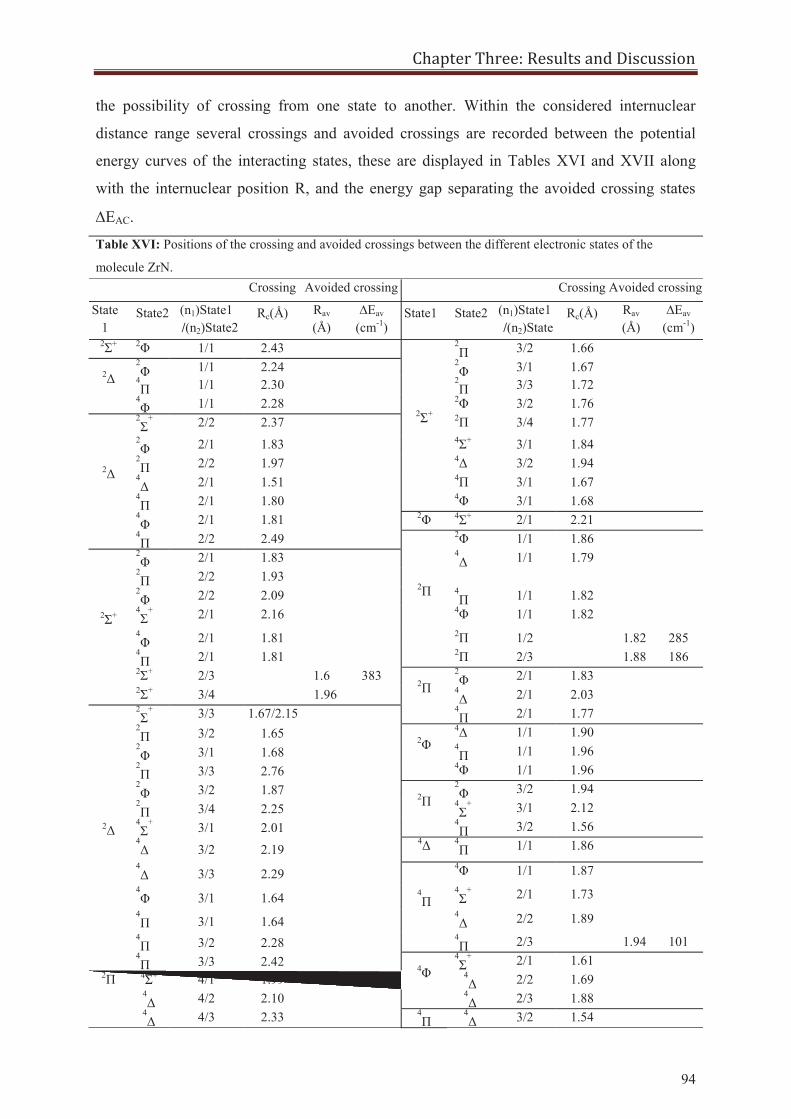
Chapter Three: Results and Discussion
94
the possibility of crossing from one state to another. Within the considered internuclear
distance range several crossings and avoided crossings are recorded between the potential
energy curves of the interacting states, these are displayed in Tables XVI and XVII along
with the internuclear position R, and the energy gap separating the avoided crossing states
EAC.
Table XVI: Positions of the crossing and avoided crossings between the different electronic states of the
molecule ZrN. Crossing Avoided crossing Crossing Avoided crossing
State1
State2 (n1)State1 /(n2)State2
Rc(Å) Rav
(Å) ∆Eav
(cm-1) State1 State2 (n1)State1
/(n2)StateRc(Å) Rav
(Å) ∆Eav
(cm-1) 2Σ+ 2Φ 1/1 2.43
2Σ+
2Π 3/2 1.66
2Δ 2Φ 1/1 2.24 2
Φ 3/1 1.67 4Π 1/1 2.30 2
Π 3/3 1.72 4Φ 1/1 2.28 2Φ 3/2 1.76
2Δ
2Σ
+ 2/2 2.37 2Π 3/4 1.77
2Φ 2/1 1.83 4Σ+ 3/1 1.84
2Π 2/2 1.97 4Δ 3/2 1.94
4Δ 2/1 1.51 4Π 3/1 1.67
4Π 2/1 1.80 4Φ 3/1 1.68
4Φ 2/1 1.81 2Φ 4Σ+ 2/1 2.21
4Π 2/2 2.49
2Π
2Φ 1/1 1.86
2Σ+
2Φ 2/1 1.83 4
Δ 1/1 1.79 2Π 2/2 1.93
2Φ 2/2 2.09 4
Π 1/1 1.82 4Σ
+ 2/1 2.16 4Φ 1/1 1.82
4Φ 2/1 1.81 2Π 1/2 1.82 285
4Π 2/1 1.81 2Π 2/3 1.88 186
2Σ+ 2/3 1.6 383
2Π 2Φ 2/1 1.83
2Σ+ 3/4 1.96 4Δ 2/1 2.03
2Δ
2Σ
+ 3/3 1.67/2.15 4
Π 2/1 1.77 2Π 3/2 1.65
2Φ 4Δ 1/1 1.90
2Φ 3/1 1.68 4
Π 1/1 1.96 2Π 3/3 2.76 4Φ 1/1 1.96
2Φ 3/2 1.87
2Π 2Φ 3/2 1.94
2Π 3/4 2.25 4
Σ+ 3/1 2.12
4Σ
+ 3/1 2.01 4
Π 3/2 1.56 4Δ 3/2 2.19 4Δ 4
Π 1/1 1.86 4Δ 3/3 2.29
4Π
4Φ
1/1 1.87 4Φ 3/1 1.64 4
Σ+ 2/1 1.73
4Π 3/1 1.64 4
Δ 2/2 1.89 4Π 3/2 2.28 4
Π 2/3 1.94 101 4Π 3/3 2.42
4Φ 4Σ
+ 2/1 1.61
2Π 4Σ+ 4/1 1.99 4Δ 2/2 1.69
4Δ 4/2 2.10 4
Δ 2/3 1.88 4Δ 4/3 2.33 4
Π 4Δ 3/2 1.54
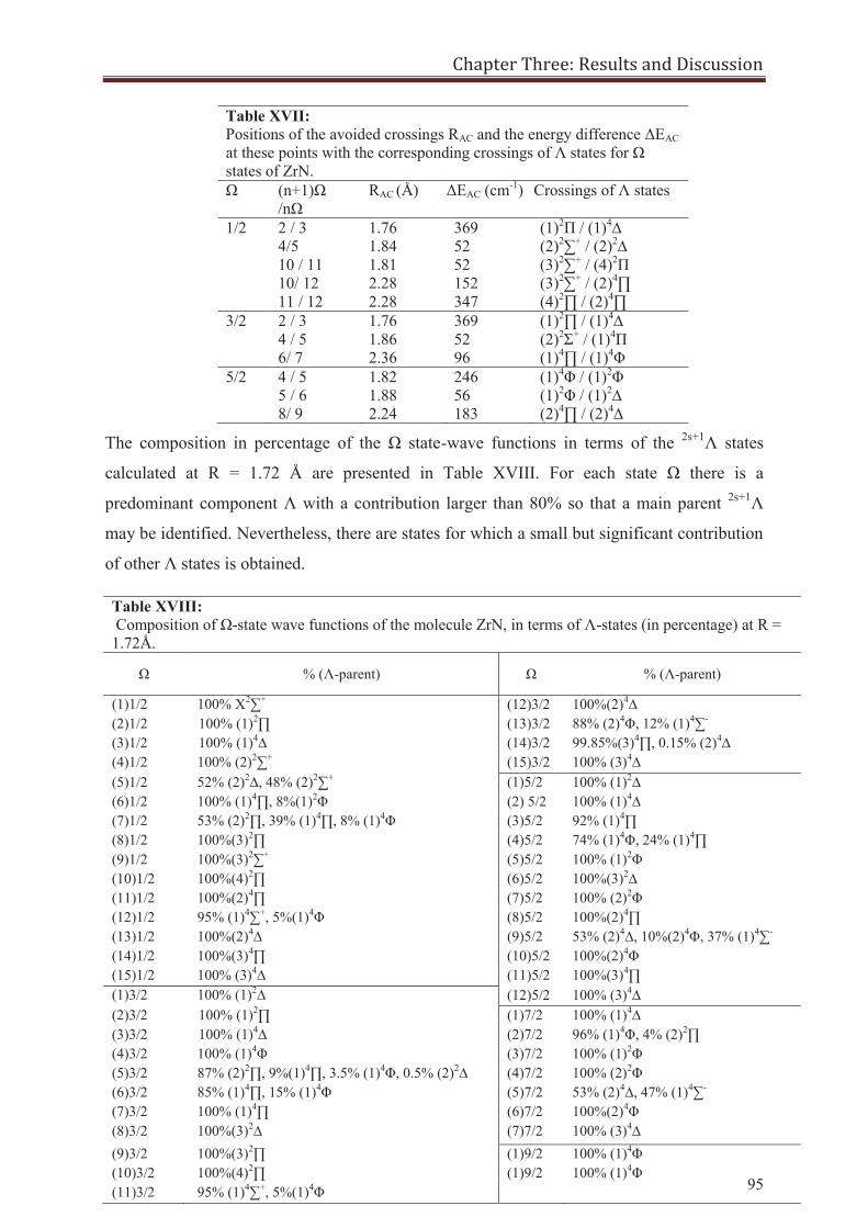
Chapter Three: Results and Discussion
95
Table XVII: Positions of the avoided crossings RAC and the energy difference ΔEAC at these points with the corresponding crossings of Λ states for Ω states of ZrN. Ω (n+1)Ω
/nΩ RAC (Å) ΔEAC (cm-1) Crossings of Λ states
1/2 2 / 3 4/5 10 / 11 10/ 12 11 / 12
1.76 1.84 1.81 2.28 2.28
369 52 52 152 347
(1)2Π / (1)4∆ (2)2∑+ / (2)2∆ (3)2∑+ / (4)2Π (3)2∑+ / (2)4∏ (4)2∏ / (2)4∏
3/2 2 / 3 4 / 5 6/ 7
1.76 1.86 2.36
369 52 96
(1)2∏ / (1)4∆ (2)2Σ+ / (1)4Π (1)4∏ / (1)4Φ
5/2 4 / 5 5 / 6 8/ 9
1.82 1.88 2.24
246 56 183
(1)4Φ / (1)2Φ (1)2Φ / (1)2∆ (2)4∏ / (2)4∆
The composition in percentage of the Ω state-wave functions in terms of the 2s+1Λ states
calculated at R = 1.72 Å are presented in Table XVIII. For each state Ω there is a
predominant component Λ with a contribution larger than 80% so that a main parent 2s+1Λ
may be identified. Nevertheless, there are states for which a small but significant contribution
of other Λ states is obtained.
Table XVIII: Composition of Ω-state wave functions of the molecule ZrN, in terms of Λ-states (in percentage) at R = 1.72Å.
Ω % (Λ-parent) Ω % (Λ-parent)
(1)1/2 100% X2∑+ (12)3/2 100%(2)4∆ (2)1/2 100% (1)2∏ (13)3/2 88% (2)4Φ, 12% (1)4∑- (3)1/2 100% (1)4∆ (14)3/2 99.85%(3)4∏, 0.15% (2)4∆ (4)1/2 100% (2)2∑+ (15)3/2 100% (3)4∆ (5)1/2 52% (2)2∆, 48% (2)2∑+ (1)5/2 100% (1)2∆
(6)1/2 100% (1)4∏, 8%(1)2Φ (2) 5/2 100% (1)4∆ (7)1/2 53% (2)2∏, 39% (1)4∏, 8% (1)4Φ (3)5/2 92% (1)4∏ (8)1/2 100%(3)2∏ (4)5/2 74% (1)4Φ, 24% (1)4∏ (9)1/2 100%(3)2∑+ (5)5/2 100% (1)2Φ (10)1/2 100%(4)2∏ (6)5/2 100%(3)2∆ (11)1/2 100%(2)4∏ (7)5/2 100% (2)2Φ (12)1/2 95% (1)4∑+, 5%(1)4Φ (8)5/2 100%(2)4∏ (13)1/2 100%(2)4∆ (9)5/2 53% (2)4∆, 10%(2)4Φ, 37% (1)4∑- (14)1/2 100%(3)4∏ (10)5/2 100%(2)4Φ (15)1/2 100% (3)4∆ (11)5/2 100%(3)4∏ (1)3/2 100% (1)2∆ (12)5/2 100% (3)4∆ (2)3/2 100% (1)2∏ (1)7/2 100% (1)4∆ (3)3/2 100% (1)4∆ (2)7/2 96% (1)4Φ, 4% (2)2∏ (4)3/2 100% (1)4Φ (3)7/2 100% (1)2Φ (5)3/2 87% (2)2∏, 9%(1)4∏, 3.5% (1)4Φ, 0.5% (2)2∆ (4)7/2 100% (2)2Φ (6)3/2 85% (1)4∏, 15% (1)4Φ (5)7/2 53% (2)4∆, 47% (1)4∑- (7)3/2 100% (1)4∏ (6)7/2 100%(2)4Φ (8)3/2 100%(3)2∆ (7)7/2 100% (3)4∆ (9)3/2 100%(3)2∏ (1)9/2 100% (1)4Φ (10)3/2 100%(4)2∏ (1)9/2 100% (1)4Φ (11)3/2 95% (1)4∑+, 5%(1)4Φ
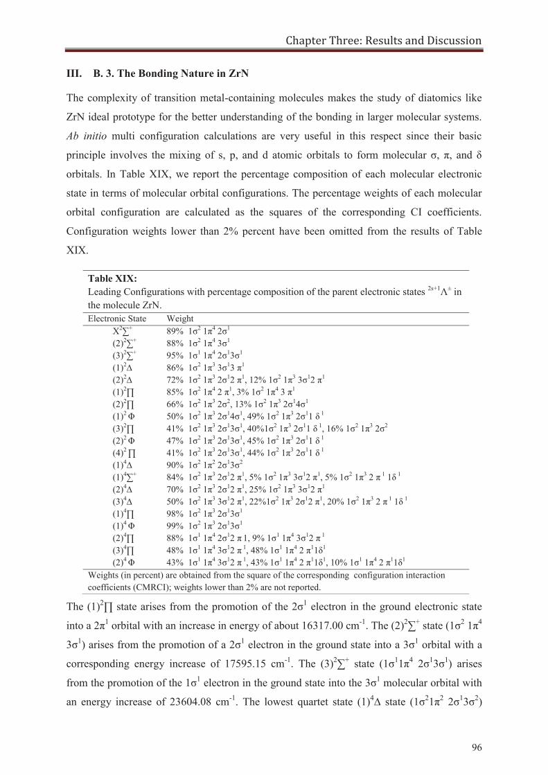
Chapter Three: Results and Discussion
96
III. B. 3. The Bonding Nature in ZrN
The complexity of transition metal-containing molecules makes the study of diatomics like
ZrN ideal prototype for the better understanding of the bonding in larger molecular systems.
Ab initio multi configuration calculations are very useful in this respect since their basic
principle involves the mixing of s, p, and d atomic orbitals to form molecular σ, π, and δ
orbitals. In Table XIX, we report the percentage composition of each molecular electronic
state in terms of molecular orbital configurations. The percentage weights of each molecular
orbital configuration are calculated as the squares of the corresponding CI coefficients.
Configuration weights lower than 2% percent have been omitted from the results of Table
XIX.
The (1)2∏ state arises from the promotion of the 2σ1 electron in the ground electronic state
into a 2π1 orbital with an increase in energy of about 16317.00 cm-1. The (2)2∑+ state (1σ2 1π4
3σ1) arises from the promotion of a 2σ1 electron in the ground state into a 3σ1 orbital with a
corresponding energy increase of 17595.15 cm-1. The (3)2∑+ state (1σ11π4 2σ13σ1) arises
from the promotion of the 1σ1 electron in the ground state into the 3σ1 molecular orbital with
an energy increase of 23604.08 cm-1. The lowest quartet state (1)4∆ state (1σ21π2 2σ13σ2)
Table XIX: Leading Configurations with percentage composition of the parent electronic states 2s+1Λ± in the molecule ZrN. Electronic State Weight
X2∑+ 89% 1σ2 1π4 2σ1 (2)2∑+ 88% 1σ2 1π4 3σ1 (3)2∑+ 95% 1σ1 1π4 2σ13σ1 (1)2∆ 86% 1σ2 1π3 3σ13 π1 (2)2∆ 72% 1σ2 1π3 2σ12 π1, 12% 1σ2 1π3 3σ12 π1 (1)2∏ 85% 1σ2 1π4 2 π1, 3% 1σ2 1π4 3 π1 (2)2∏ 66% 1σ2 1π3 2σ2, 13% 1σ2 1π3 2σ14σ1 (1)2 Φ 50% 1σ2 1π3 2σ14σ1, 49% 1σ2 1π3 2σ11 δ 1 (3)2∏ 41% 1σ2 1π3 2σ13σ1, 40%1σ2 1π3 2σ11 δ 1, 16% 1σ2 1π3 2σ2 (2)2 Φ 47% 1σ2 1π3 2σ13σ1, 45% 1σ2 1π3 2σ11 δ 1 (4)2 ∏ 41% 1σ2 1π3 2σ13σ1, 44% 1σ2 1π3 2σ11 δ 1 (1)4∆ 90% 1σ2 1π2 2σ13σ2 (1)4∑+ 84% 1σ2 1π3 2σ12 π1, 5% 1σ2 1π3 3σ12 π1, 5% 1σ2 1π3 2 π 1 1δ 1 (2)4∆ 70% 1σ2 1π3 2σ12 π1, 25% 1σ2 1π3 3σ12 π1 (3)4∆ 50% 1σ2 1π3 3σ12 π1, 22%1σ2 1π3 2σ12 π1, 20% 1σ2 1π3 2 π 1 1δ 1 (1)4∏ 98% 1σ2 1π3 2σ13σ1 (1)4 Φ 99% 1σ2 1π3 2σ13σ1 (2)4∏ 88% 1σ1 1π4 2σ12 π 1, 9% 1σ1 1π4 3σ12 π 1 (3)4∏ 48% 1σ1 1π4 3σ12 π 1, 48% 1σ1 1π4 2 π11δ1 (2)4 Φ 43% 1σ1 1π4 3σ12 π 1, 43% 1σ1 1π4 2 π11δ1, 10% 1σ1 1π4 2 π11δ1
Weights (in percent) are obtained from the square of the corresponding configuration interaction coefficients (CMRCI); weights lower than 2% are not reported.
Chapter Three: Results and Discussion
97
arises from the promotion of two 1π electrons in the ground state into a 3σ2 orbital with an
energy change of 16477.72cm-1.
In computational quantum chemistry ab initio calculations can be used to analyze the
bonding in simple metal systems. The expansion of molecular orbital wave functions in terms
of atomic orbital basis sets is very useful in understanding the bonding order in the ground
state of small molecules. In the present work, the bonding order in the ground state of the
ZrN molecule is analyzed in terms of the molecular orbital occupation numbers available
from the CASSCF calculations and in the active space of molecular orbitals (4σ3π1δ). The
effective bond order EBO is a quantity that gives the formation of a chemical bond, and was
given in equation (1) of this chapter. In our CASSCF calculations the ground state wave
function in ZrN is obtained by distributing seven valence electrons over the active space of
molecular orbitals 4σ3π1δ. In this treatment we obtained the occupation numbers of the
bonding and anti-bonding orbitals in the following way: ηb (1σ) = 1.61887, ηb (2σ) =
0.69819, ηab (3σ) = 0.37438, ηab (4σ) = 0.11726, ηab (1δ) = 0.38276, , ηb (1π) = 3.33124, ηab
(2π) = 0.39012, ηab (3π) = 0.0872. Now by applying equation (1) for the effective bond order
we obtain an EBO = 2.148 ≈ 2, thus indicating that we have a fully developed double bond in
ZrN.
III. B. 4. The Vibrational Structure of ZrN
In the past few years, the realization of elementary quantum logic gates on molecular systems
have witnessed remarkable experimental achievements [80 – 84]. Due to their rich inner
energy structures, that can be used to encode information, molecules offer a promising
prospect for scalable quantum information processing and have attracted lots of attention.
After the work of Vivie-Riedle and coworkers [85, 86], several groups have explored the
possibility of encoding qubits in rovibrational states of a single diatomic molecule [87 – 97]
or polyatomic molecule [98 – 108] or in two interacting diatomic molecules [109,110]. In
these works, logic gate operations were driven by femtolaser pulses designed by optimal
control theory or genetic algorithms or by using stimulated Raman Adiabatic passage
techniques [111]. In conclusion investigating the vibrational-rotational energy structures of
diatomic molecules is gaining significant importance in diverse research fields as molecular
quantum computing.
In the present work we investigate the vibrational energy levels of the ZrN molecule. First we
solve the time independent radial Schrödinger equation for the vibrational and rotational
motions of the ZrN molecule in the vicinity of the potential energy curves obtained by
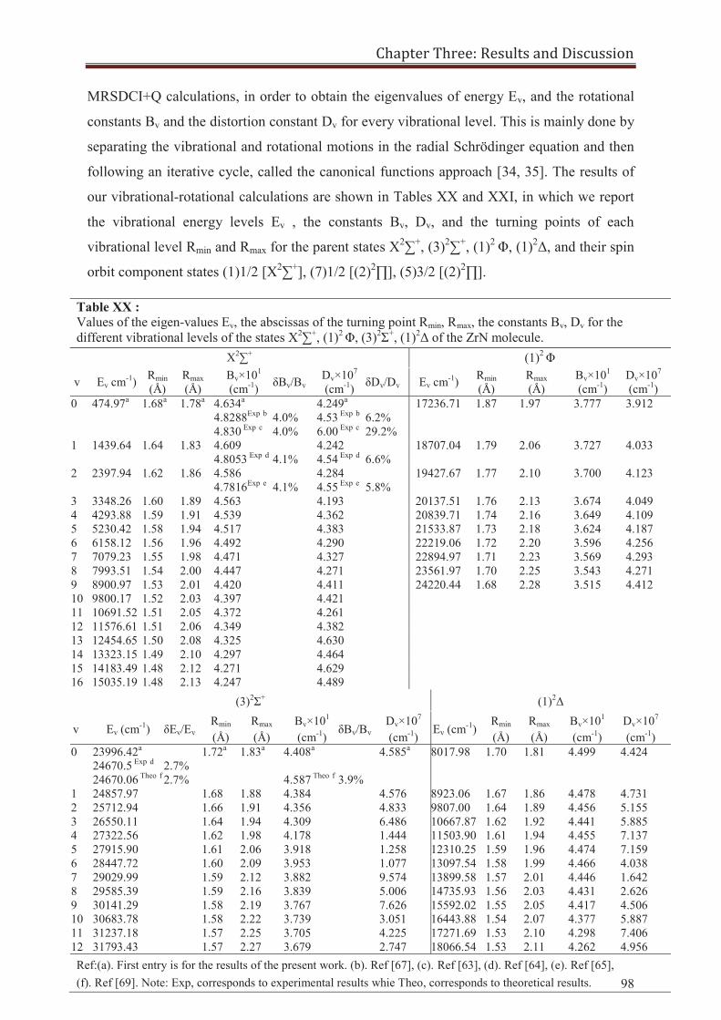
Chapter Three: Results and Discussion
98
MRSDCI+Q calculations, in order to obtain the eigenvalues of energy Ev, and the rotational
constants Bv and the distortion constant Dv for every vibrational level. This is mainly done by
separating the vibrational and rotational motions in the radial Schrödinger equation and then
following an iterative cycle, called the canonical functions approach [34, 35]. The results of
our vibrational-rotational calculations are shown in Tables XX and XXI, in which we report
the vibrational energy levels Ev , the constants Bv, Dv, and the turning points of each
vibrational level Rmin and Rmax for the parent states X2∑+, (3)2∑+, (1)2 Φ, (1)2Δ, and their spin
orbit component states (1)1/2 [X2∑+], (7)1/2 [(2)2∏], (5)3/2 [(2)2∏].
Table XX : Values of the eigen-values Ev, the abscissas of the turning point Rmin, Rmax, the constants Bv, Dv for the different vibrational levels of the states X2∑+, (1)2 Φ, (3)2Σ+, (1)2Δ of the ZrN molecule.
X2∑+ (1)2 Φ
v Ev cm-1) Rmin (Å)
Rmax (Å)
Bv×101
(cm-1) δBv/Bv Dv×107
(cm-1) δDv/Dv Ev cm-1) Rmin (Å)
Rmax (Å)
Bv×101
(cm-1) Dv×107
(cm-1) 0 474.97a 1.68a 1.78a 4.634a
4.8288Exp b
4.830 Exp c
4.0% 4.0%
4.249a
4.53 Exp b
6.00 Exp c
6.2% 29.2%
17236.71 1.87 1.97 3.777 3.912
1 1439.64 1.64 1.83 4.609 4.8053 Exp d
4.1%
4.242 4.54 Exp d
6.6%
18707.04 1.79 2.06 3.727 4.033
2 2397.94 1.62 1.86 4.586 4.7816Exp e
4.1%
4.284 4.55 Exp e
5.8%
19427.67 1.77 2.10 3.700 4.123
3 3348.26 1.60 1.89 4.563 4.193 20137.51 1.76 2.13 3.674 4.049 4 4293.88 1.59 1.91 4.539 4.362 20839.71 1.74 2.16 3.649 4.109 5 5230.42 1.58 1.94 4.517 4.383 21533.87 1.73 2.18 3.624 4.187 6 6158.12 1.56 1.96 4.492 4.290 22219.06 1.72 2.20 3.596 4.256 7 7079.23 1.55 1.98 4.471 4.327 22894.97 1.71 2.23 3.569 4.293 8 7993.51 1.54 2.00 4.447 4.271 23561.97 1.70 2.25 3.543 4.271 9 8900.97 1.53 2.01 4.420 4.411 24220.44 1.68 2.28 3.515 4.412 10 9800.17 1.52 2.03 4.397 4.421 11 10691.52 1.51 2.05 4.372 4.261 12 11576.61 1.51 2.06 4.349 4.382 13 12454.65 1.50 2.08 4.325 4.630 14 13323.15 1.49 2.10 4.297 4.464 15 14183.49 1.48 2.12 4.271 4.629 16 15035.19 1.48 2.13 4.247 4.489
(3)2Σ+ (1)2Δ
v Ev (cm-1) δEv/Ev Rmin
(Å) Rmax
(Å) Bv×101
(cm-1) δBv/Bv Dv×107
(cm-1) Ev (cm-1)
Rmin
(Å) Rmax
(Å) Bv×101
(cm-1) Dv×107
(cm-1) 0 23996.42a
24670.5 Exp d
24670.06 Theo f
2.7% 2.7%
1.72a 1.83a 4.408a
4.587 Theo f
3.9%
4.585a 8017.98 1.70 1.81 4.499 4.424
1 24857.97 1.68 1.88 4.384 4.576 8923.06 1.67 1.86 4.478 4.731 2 25712.94 1.66 1.91 4.356 4.833 9807.00 1.64 1.89 4.456 5.155 3 26550.11 1.64 1.94 4.309 6.486 10667.87 1.62 1.92 4.441 5.885 4 27322.56 1.62 1.98 4.178 1.444 11503.90 1.61 1.94 4.455 7.137 5 27915.90 1.61 2.06 3.918 1.258 12310.25 1.59 1.96 4.474 7.159 6 28447.72 1.60 2.09 3.953 1.077 13097.54 1.58 1.99 4.466 4.038 7 29029.99 1.59 2.12 3.882 9.574 13899.58 1.57 2.01 4.446 1.642 8 29585.39 1.59 2.16 3.839 5.006 14735.93 1.56 2.03 4.431 2.626 9 30141.29 1.58 2.19 3.767 7.626 15592.02 1.55 2.05 4.417 4.506 10 30683.78 1.58 2.22 3.739 3.051 16443.88 1.54 2.07 4.377 5.887 11 31237.18 1.57 2.25 3.705 4.225 17271.69 1.53 2.10 4.298 7.406 12 31793.43 1.57 2.27 3.679 2.747 18066.54 1.53 2.11 4.262 4.956 Ref:(a). First entry is for the results of the present work. (b). Ref [67], (c). Ref [63], (d). Ref [64], (e). Ref [65], (f). Ref [69]. Note: Exp, corresponds to experimental results whie Theo, corresponds to theoretical results.

Chapter Three: Results and Discussion
99
III. B. 5. The Permanent Dipole Moment of ZrN
In an approach to create a quantum computer Demille [113] suggested the use of
heteronuclear diatomic molecules trapped in a 1-dimensional trap array, and controlled by an
electric field gradient that allows the spectroscopic control of molecules. In this system the
qubits are considered to be the electric dipole moments of diatomic molecules, which are in
Table XXI: Values of the eigen-values Ev, the abscissas of the turning point Rmin, Rmax, and the constants Bv, Dv for the different vibrational levels of the states (1)1/2 [X2∑+], (7)1/2 [(2)2∏], (5)3/2 [(2)2∏] of the ZrN molecule.
(1)1/2 [X2∑+] v Ev (cm-1) Rmin
(Å) Rmax (Å) Bv×101 (cm-1) δBv/Bv Dv×107 (cm-1) δDv/Dv
0 475.09a 1.68a 1.78a 4.634a
4.82882 Exp b
4.830 Exp c
4.0% 4.1%
4.244a
4.53 Exp b
6.00 Exp c
6.3% 29.3%
1 1440.37 1.64 1.83 4.609 4.80529 Exp d
4.1%
4.236 4.54 Exp d
6.7%
2 2399.37 1.62 1.86 4.586 4.78164 Exp e
4.1%
4.306 4.55 Exp e
5.3%
3 3349.19 1.60 1.89 4.562 4.202 4 4294.14 1.58 1.91 4.539 4.328 5 5230.98 1.57 1.93 4.517 4.405 6 6158.37 1.56 1.95 4.491 4.269 7 7079.49 1.55 1.97 4.470 4.277 8 7994.44 1.54 1.99 4.446 4.327 9 8901.75 1.53 2.01 4.419 4.386 10 9801.39 1.52 2.03 4.398 4.444 11 10693.29 1.52 2.04 4.374 4.214 12 11579.68 1.51 2.06 4.352 4.270 13 12460.07 1.50 2.08 4.328 4.658 14 13330.08 1.50 2.10 4.296 4.798 15 14188.29 1.49 2.12 4.266 4.811 16 15036.37 1.48 2.13 4.243 4.125 17 15880.28 1.48 2.15 4.223 4.429 18 16716.83 1.47 2.17 4.191 5.313 19 17539.69 1.47 2.18 4.159 4.699 20 18353.78 1.46 2.20 4.135 4.324 21 19161.67 1.46 2.21 4.107 5.157 22 19958.23 1.45 2.23 4.074 5.173 23 20743.58 1.45 2.25 4.045 4.780 24 21520.19 1.44 2.26 4.016 4.983
(7)1/2 [(2)2∏] (5)3/2 [(2)2∏] v Ev (cm-1) Rmin
(Å) Rmax
(Å) Bv×101 (cm-1)
Dv×107 (cm-1)
Ev (cm-1) Rmin
(Å) Rmax
(Å) Bv×101 (cm-1)
Dv×107 (cm-1)
0 17442.50a 1.83a 1.94a 3.918a 2.874a 17512.35 a 1.82a 1.93a 3.936a 2.783a 1 18359.22 1.78 1.98 3.941 3.155 18449.61 1.78 1.97 3.948 3.285 2 19254.73 1.76 2.01 3.909 3.332 19344.99 1.76 2.00 3.915 3.230 3 20125.29 1.74 2.04 3.872 3.879 20218.79 1.74 2.04 3.869 4.213 4 20959.56 1.72 2.07 3.839 5.062 21041.82 1.72 2.07 3.829 4.931 5 21740.06 1.71 2.10 3.793 3.435 21817.58 1.71 2.10 3.794 3.197 6 22515.73 1.70 2.12 3.774 3.948 22596.01 1.70 2.12 3.778 4.169 7 23279.34 1.69 2.15 3.739 5.203 23357.56 1.69 2.15 3.735 5.308 8 24009.28 1.68 2.18 3.681 4.661 24084.98 1.68 2.18 3.687 4.375 9 24721.10 1.67 2.20 3.668 4.284 24797.69 1.67 2.20 3.663 4.283 10 25423.66 1.66 2.22 3.629 4.634 25500.13 1.66 2.22 3.631 4.569 Ref:(a)First entry is for the results of the present work. (b). Ref [67], (c). Ref [63], (d). Ref [64], (e). Ref [65] Exp, corresponds to experimental results in literture.
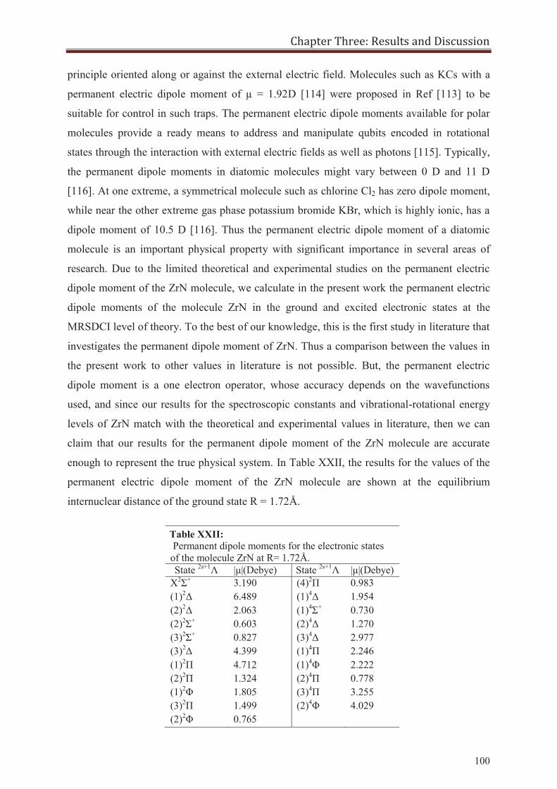
Chapter Three: Results and Discussion
100
principle oriented along or against the external electric field. Molecules such as KCs with a
permanent electric dipole moment of μ = 1.92D [114] were proposed in Ref [113] to be
suitable for control in such traps. The permanent electric dipole moments available for polar
molecules provide a ready means to address and manipulate qubits encoded in rotational
states through the interaction with external electric fields as well as photons [115]. Typically,
the permanent dipole moments in diatomic molecules might vary between 0 D and 11 D
[116]. At one extreme, a symmetrical molecule such as chlorine Cl2 has zero dipole moment,
while near the other extreme gas phase potassium bromide KBr, which is highly ionic, has a
dipole moment of 10.5 D [116]. Thus the permanent electric dipole moment of a diatomic
molecule is an important physical property with significant importance in several areas of
research. Due to the limited theoretical and experimental studies on the permanent electric
dipole moment of the ZrN molecule, we calculate in the present work the permanent electric
dipole moments of the molecule ZrN in the ground and excited electronic states at the
MRSDCI level of theory. To the best of our knowledge, this is the first study in literature that
investigates the permanent dipole moment of ZrN. Thus a comparison between the values in
the present work to other values in literature is not possible. But, the permanent electric
dipole moment is a one electron operator, whose accuracy depends on the wavefunctions
used, and since our results for the spectroscopic constants and vibrational-rotational energy
levels of ZrN match with the theoretical and experimental values in literature, then we can
claim that our results for the permanent dipole moment of the ZrN molecule are accurate
enough to represent the true physical system. In Table XXII, the results for the values of the
permanent electric dipole moment of the ZrN molecule are shown at the equilibrium
internuclear distance of the ground state R = 1.72Å.
Table XXII: Permanent dipole moments for the electronic states of the molecule ZrN at R= 1.72Å. State 2s+1Λ |μ|(Debye) State 2s+1Λ |μ|(Debye)
X2Σ+ 3.190 (4)2Π 0.983 (1)2Δ 6.489 (1)4Δ 1.954 (2)2Δ 2.063 (1)4Σ+ 0.730 (2)2Σ+ 0.603 (2)4Δ 1.270 (3)2Σ+ 0.827 (3)4Δ 2.977 (3)2Δ 4.399 (1)4Π 2.246 (1)2Π 4.712 (1)4Φ 2.222 (2)2Π 1.324 (2)4Π 0.778 (1)2Φ 1.805 (3)4Π 3.255 (3)2Π 1.499 (2)4Φ 4.029 (2)2Φ 0.765
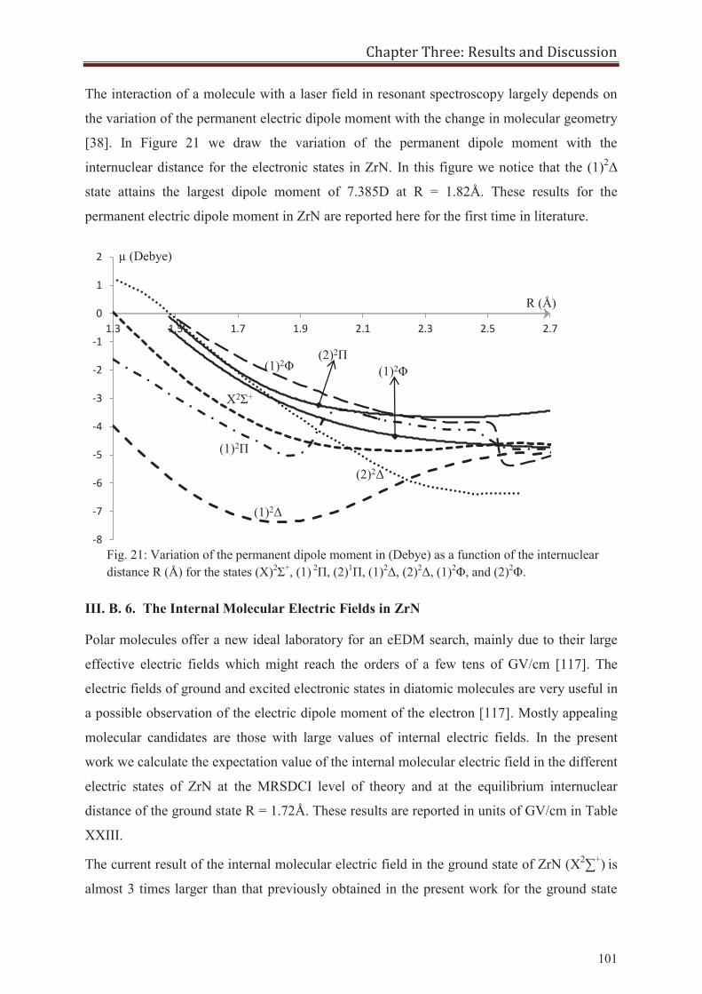
Chapter Three: Results and Discussion
101
The interaction of a molecule with a laser field in resonant spectroscopy largely depends on
the variation of the permanent electric dipole moment with the change in molecular geometry
[38]. In Figure 21 we draw the variation of the permanent dipole moment with the
internuclear distance for the electronic states in ZrN. In this figure we notice that the (1)2Δ
state attains the largest dipole moment of 7.385D at R = 1.82Å. These results for the
permanent electric dipole moment in ZrN are reported here for the first time in literature.
III. B. 6. The Internal Molecular Electric Fields in ZrN
Polar molecules offer a new ideal laboratory for an eEDM search, mainly due to their large
effective electric fields which might reach the orders of a few tens of GV/cm [117]. The
electric fields of ground and excited electronic states in diatomic molecules are very useful in
a possible observation of the electric dipole moment of the electron [117]. Mostly appealing
molecular candidates are those with large values of internal electric fields. In the present
work we calculate the expectation value of the internal molecular electric field in the different
electric states of ZrN at the MRSDCI level of theory and at the equilibrium internuclear
distance of the ground state R = 1.72Å. These results are reported in units of GV/cm in Table
XXIII.
The current result of the internal molecular electric field in the ground state of ZrN (X2∑+) is
almost 3 times larger than that previously obtained in the present work for the ground state
-8
-7
-6
-5
-4
-3
-2
-1
0
1
2
1.3 1.5 1.7 1.9 2.1 2.3 2.5 2.7
X2Σ+
(1)2Δ
(1)2Π
(2)2Δ
(1)2Φ (2)2Π
(1)2Φ
μ (Debye)
R (Å)
Fig. 21: Variation of the permanent dipole moment in (Debye) as a function of the internuclear distance R (Å) for the states (X)2Σ+, (1) 2Π, (2)1Π, (1)2Δ, (2)2Δ, (1)2Φ, and (2)2Φ.
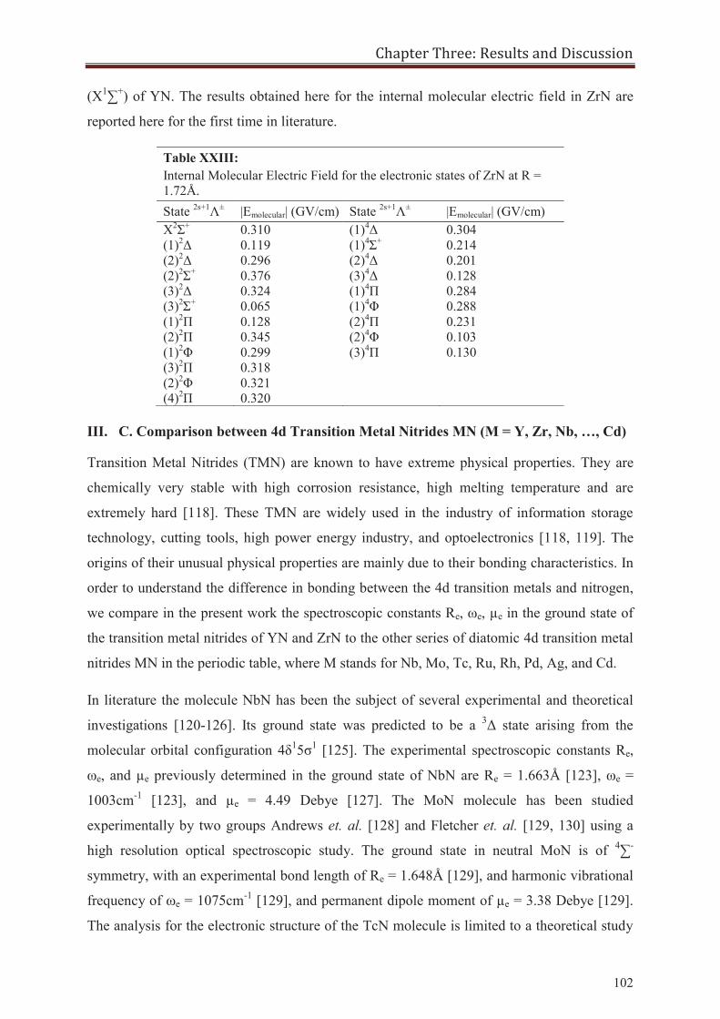
Chapter Three: Results and Discussion
102
(X1∑+) of YN. The results obtained here for the internal molecular electric field in ZrN are
reported here for the first time in literature.
III. C. Comparison between 4d Transition Metal Nitrides MN (M = Y, Zr, Nb, …, Cd)
Transition Metal Nitrides (TMN) are known to have extreme physical properties. They are
chemically very stable with high corrosion resistance, high melting temperature and are
extremely hard [118]. These TMN are widely used in the industry of information storage
technology, cutting tools, high power energy industry, and optoelectronics [118, 119]. The
origins of their unusual physical properties are mainly due to their bonding characteristics. In
order to understand the difference in bonding between the 4d transition metals and nitrogen,
we compare in the present work the spectroscopic constants Re, ωe, μe in the ground state of
the transition metal nitrides of YN and ZrN to the other series of diatomic 4d transition metal
nitrides MN in the periodic table, where M stands for Nb, Mo, Tc, Ru, Rh, Pd, Ag, and Cd.
In literature the molecule NbN has been the subject of several experimental and theoretical
investigations [120-126]. Its ground state was predicted to be a 3Δ state arising from the
molecular orbital configuration 4δ15σ1 [125]. The experimental spectroscopic constants Re,
ωe, and μe previously determined in the ground state of NbN are Re = 1.663Å [123], ωe =
1003cm-1 [123], and μe = 4.49 Debye [127]. The MoN molecule has been studied
experimentally by two groups Andrews et. al. [128] and Fletcher et. al. [129, 130] using a
high resolution optical spectroscopic study. The ground state in neutral MoN is of 4∑-
symmetry, with an experimental bond length of Re = 1.648Å [129], and harmonic vibrational
frequency of ωe = 1075cm-1 [129], and permanent dipole moment of μe = 3.38 Debye [129].
The analysis for the electronic structure of the TcN molecule is limited to a theoretical study
Table XXIII: Internal Molecular Electric Field for the electronic states of ZrN at R = 1.72Å. State 2s+1Λ± |Emolecular| (GV/cm) State 2s+1Λ± |Emolecular| (GV/cm) X2Σ+ 0.310 (1)4Δ 0.304 (1)2Δ 0.119 (1)4Σ+ 0.214 (2)2Δ 0.296 (2)4Δ 0.201 (2)2Σ+ 0.376 (3)4Δ 0.128 (3)2Δ 0.324 (1)4Π 0.284 (3)2Σ+ 0.065 (1)4Φ 0.288 (1)2Π 0.128 (2)4Π 0.231 (2)2Π 0.345 (2)4Φ 0.103 (1)2Φ 0.299 (3)4Π 0.130 (3)2Π 0.318 (2)2Φ 0.321 (4)2Π 0.320
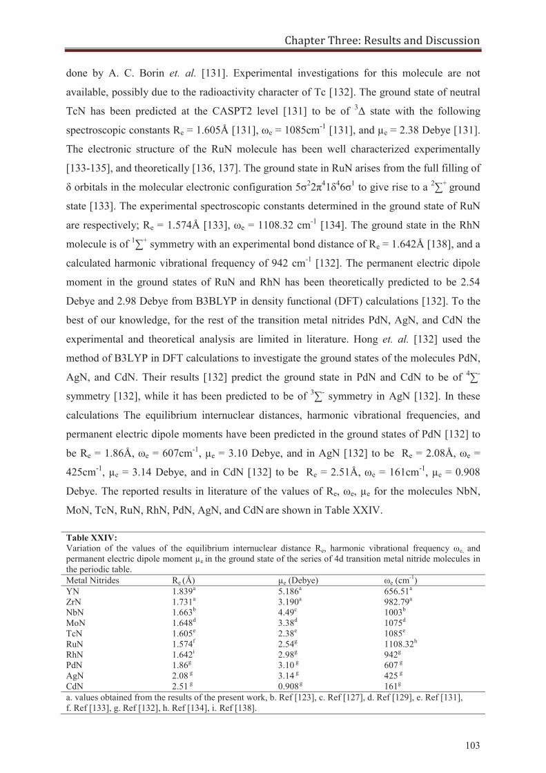
Chapter Three: Results and Discussion
103
done by A. C. Borin et. al. [131]. Experimental investigations for this molecule are not
available, possibly due to the radioactivity character of Tc [132]. The ground state of neutral
TcN has been predicted at the CASPT2 level [131] to be of 3Δ state with the following
spectroscopic constants Re = 1.605Å [131], ωe = 1085cm-1 [131], and μe = 2.38 Debye [131].
The electronic structure of the RuN molecule has been well characterized experimentally
[133-135], and theoretically [136, 137]. The ground state in RuN arises from the full filling of
δ orbitals in the molecular electronic configuration 5σ22π41δ46σ1 to give rise to a 2∑+ ground
state [133]. The experimental spectroscopic constants determined in the ground state of RuN
are respectively; Re = 1.574Å [133], ωe = 1108.32 cm-1 [134]. The ground state in the RhN
molecule is of 1∑+ symmetry with an experimental bond distance of Re = 1.642Å [138], and a
calculated harmonic vibrational frequency of 942 cm-1 [132]. The permanent electric dipole
moment in the ground states of RuN and RhN has been theoretically predicted to be 2.54
Debye and 2.98 Debye from B3BLYP in density functional (DFT) calculations [132]. To the
best of our knowledge, for the rest of the transition metal nitrides PdN, AgN, and CdN the
experimental and theoretical analysis are limited in literature. Hong et. al. [132] used the
method of B3LYP in DFT calculations to investigate the ground states of the molecules PdN,
AgN, and CdN. Their results [132] predict the ground state in PdN and CdN to be of 4∑-
symmetry [132], while it has been predicted to be of 3∑- symmetry in AgN [132]. In these
calculations The equilibrium internuclear distances, harmonic vibrational frequencies, and
permanent electric dipole moments have been predicted in the ground states of PdN [132] to
be Re = 1.86Å, ωe = 607cm-1, μe = 3.10 Debye, and in AgN [132] to be Re = 2.08Å, ωe =
425cm-1, μe = 3.14 Debye, and in CdN [132] to be Re = 2.51Å, ωe = 161cm-1, μe = 0.908
Debye. The reported results in literature of the values of Re, ωe, μe for the molecules NbN,
MoN, TcN, RuN, RhN, PdN, AgN, and CdN are shown in Table XXIV.
Table XXIV: Variation of the values of the equilibrium internuclear distance Re, harmonic vibrational frequency ωe, and permanent electric dipole moment μe in the ground state of the series of 4d transition metal nitride molecules in the periodic table. Metal Nitrides Re (Å) μe (Debye) ωe (cm-1) YN 1.839a 5.186a 656.51a
ZrN 1.731a 3.190a 982.79a
NbN 1.663b 4.49c 1003b
MoN 1.648d 3.38d 1075d
TcN 1.605e 2.38e 1085e
RuN 1.574f 2.54g 1108.32h
RhN 1.642i 2.98g 942g
PdN 1.86g 3.10 g 607 g AgN 2.08 g 3.14 g 425 g CdN 2.51 g 0.908 g 161g a. values obtained from the results of the present work, b. Ref [123], c. Ref [127], d. Ref [129], e. Ref [131], f. Ref [133], g. Ref [132], h. Ref [134], i. Ref [138].
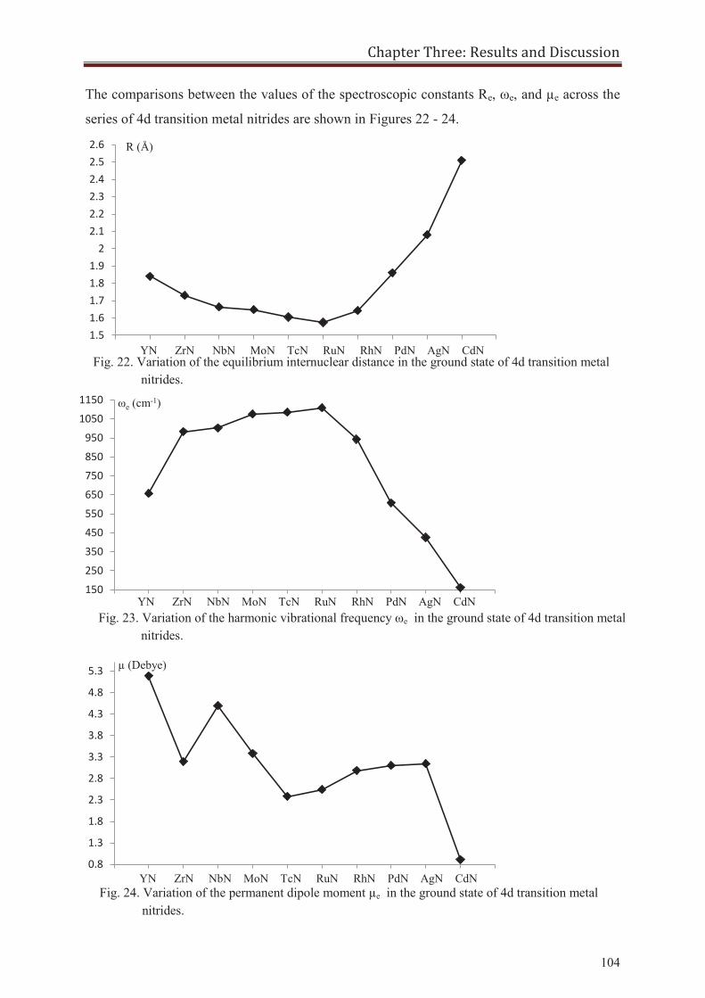
Chapter Three: Results and Discussion
104
The comparisons between the values of the spectroscopic constants Re, ωe, and μe across the
series of 4d transition metal nitrides are shown in Figures 22 - 24.
1.51.61.71.81.9
22.12.22.32.42.52.6 R (Å)
YN ZrN NbN MoN TcN RuN RhN PdN AgN CdN Fig. 22. Variation of the equilibrium internuclear distance in the ground state of 4d transition metal nitrides.
Fig. 23. Variation of the harmonic vibrational frequency ωe in the ground state of 4d transition metal nitrides.
Fig. 24. Variation of the permanent dipole moment μe in the ground state of 4d transition metal nitrides.
0.8
1.3
1.8
2.3
2.8
3.3
3.8
4.3
4.8
5.3 μ (Debye)
YN ZrN NbN MoN TcN RuN RhN PdN AgN CdN
150
250
350
450
550
650
750
850
950
1050
1150 ωe (cm-1)
YN ZrN NbN MoN TcN RuN RhN PdN AgN CdN
Chapter Three: Results and Discussion
105
Across the series of 4d transition metal nitrides from YN to CdN the equilibrium internuclear
distance in the ground state (Fig. 22) decreases from 1.84Å in YN to reach a minimum at
1.574Å in RuN and then increases again to reach a value of 2.51Å in CdN. The shortest bond
length attained in RuN suggests that the bonding in RuN is the strongest among the other 4d
transition metal nitrides. For the harmonic vibrational frequency ωe in the ground state of
each molecule (Fig. 23) it is seen that the value of ωe increases from 656.5cm-1 in YN to
1108.32cm-1 in RuN, and then decreases to reach 161cm-1 in CdN. The polarity in each of the
transition metal nitrides is largely determined by the value of the permanent electric dipole
moment in the ground state of each molecule. The permanent electric dipole moment in Fig
24 is highest in YN, with a value of 5.186 Debye. Its variation across the series of 4d
transition metals is not continuous. Rather, its value decreases from 5.186 Debye in YN to
3.19 Debye in ZrN and then it abruptly increases to reach a value of 4.49 Debye in NbN, to
decrease gradually to a value of 2.38 Debye in TcN. A gradual increase in the dipole moment
value is then observed between TcN and AgN. Across the series of 4d transition metals CdN
has the lowest dipole moment in its ground electronic state, while the mostly polar bond is
that attained in the ground state of YN. The decrease of the dipole moment is an indication
for the decrease of the electronegativity difference between the metal and nitrogen atoms, and
hence a decrease of ionic character across the series of 4d transition metal nitrides.
III. D. The Structure of Zirconium Sulfide ZrS
III. D. 1. Preliminary Works on ZrS
The electronic structure and the nature of the transition metal-sulfur bond is of importance in
such diverse fields as industrial catalysis and biological process [139 - 141]. In Astrophysics
the transition metal monosulphides, including ZrS, may be more abundant than their
corresponding metal monoxides [142] {TiO [143], LaO [144]} and hydrides FeH [145]. In
fact, the ZrS molecule has been reported in cool S-type stars as the carrier of the so-called
Keenan bands [146]. The identification of ZrS bands in the spectra of S stars provides an
opportunity to determine the abundance of sulfur in late-type stars and may give additional
clues to the nuclear processes responsible for their abnormal compositions [147].
Until the work described here, no extensive theoretical study was available on ZrS, except
that performed by Langhoff et. al. [148] on 6 low-lying excited electronic states, and that of
Reddy et. al. [149] on the vibrational band structure of the ground electronic state X1∑+.
Experimentally, the first published spectroscopic study of ZrS was done by Simard et. al
[150] on the (5)1∑+←X1∑+ transition. Jonson and coworkers first studied the (2)3∏←(1)3∆
Chapter Three: Results and Discussion
106
transition [151] via microwave-induced emission spectroscopy, and then the (2)1∏-X1∑+,
(3)1∑+- X1∑+, (5)1∑+- X1∑+ transitions [146] via high resolution emission spectroscopy. In
astrophysics, the first identification of ZrS bands in stars was done by K. Hinkle [147], who
analyzed the spectra obtained between 7400 and 9700 cm-1 of three Mira variable type stars
M and S. The detected bands provide a rare opportunity to measure the sulfur abundance in
the photospheres of late-type stars [147]. Recently, the electronic structures of the states X1∑+
and (1)3∆ in ZrS have received a great attention particularly due to their small energy
separation. Experimentally, S. Beaton and M. Gerry [152] performed a cavity Fourier
transform microwave spectroscopy on the X1∑+ and (1)3∆ bands for five isotopomers of
Zr32S. Theoretically, B. Laing and L. Andrews [153] computed the relative energy separation
of the 1∑+- 3∆ system via density functional theory, but their results contrasts with the
experimental and theoretical results available, as they predict the 3∆ to be the ground state of
ZrS and the relative energy separation of the 1∑+- 3∆ system ranged in their calculations
between 2937cm-1 (B3LYP-calculations) and 8394cm-1 (MP2-calculations). Recently, X. Sun
et. al. [154] reinvestigated the ground state of neutral ZrS by the MP2 method in DFT
calculations, their most extensive results placed the X1∑+ state lower than the (1)3∆ state by
338.75cm-1. Then by repeating the calculations with a larger basis set the (1)3∆ state was
predicted to be 556cm-1 above the ground X1∑+ state. Finally, and in order to understand the
interaction of the ZrS molecule with light, R. Bousquet et. al. [155] studied the dipole
moment of the ZrS molecule in the ground X1∑+ and excited (3)1∑+ states. Their
experimentally measured values of the dipole moments are not in good agreement with the
theoretical results, and thus a more elaborate theoretical ab initio study is required. The
apparent disagreement in literature on the nature of the ground state in the ZrS molecule,
surely warrants a more elaborate theoretical study for the ground and excited electronic states
of this molecule at a high level of theory and with the inclusion of relativistic spin orbit
effects.
In general, transition metal monosulfides have been less well characterized than the
analogous monoxides. The majority of the work to date on these species has been electronic
spectroscopy. However, these molecules often have complicated electronic spectra and thus
provide a challenge to ab initio calculations. In this paper, we try to fully explore the
electronic structure of the ZrS molecule, at the complete active space (CASSCF) method
followed by Multi-reference Single and Double Configuration Interactions (MRSDCI) for the
lowest lying 22 singlet-triplet states and their spin orbit component states.
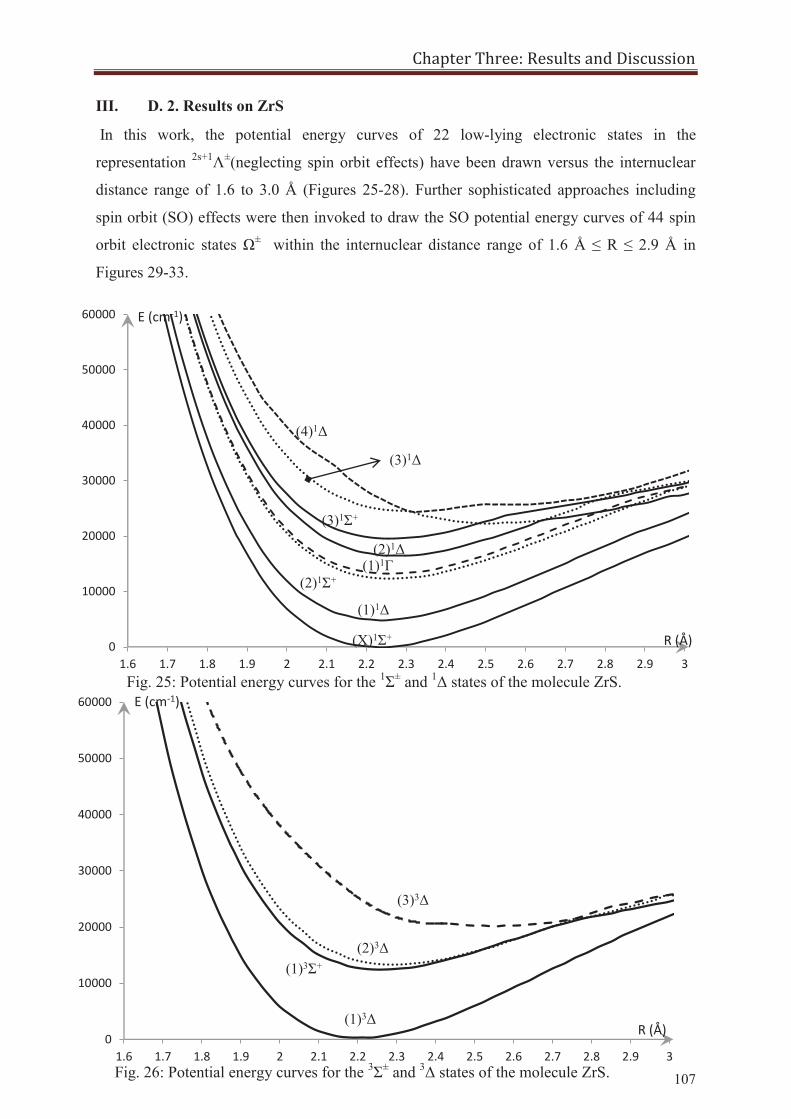
Chapter Three: Results and Discussion
107
III. D. 2. Results on ZrS
In this work, the potential energy curves of 22 low-lying electronic states in the
representation 2s+1Λ±(neglecting spin orbit effects) have been drawn versus the internuclear
distance range of 1.6 to 3.0 Å (Figures 25-28). Further sophisticated approaches including
spin orbit (SO) effects were then invoked to draw the SO potential energy curves of 44 spin
orbit electronic states Ω± within the internuclear distance range of 1.6 Å ≤ R ≤ 2.9 Å in
Figures 29-33.
0
10000
20000
30000
40000
50000
60000
1.6 1.7 1.8 1.9 2 2.1 2.2 2.3 2.4 2.5 2.6 2.7 2.8 2.9 3
(X)1Σ+
(1)1Δ
(2)1Σ+
(1)1Γ
(2)1Δ
(3)1Σ+
(3)1Δ
(4)1Δ
E (cm-1)
R (Å)
Fig. 25: Potential energy curves for the 1Σ± and 1Δ states of the molecule ZrS.
Fig. 26: Potential energy curves for the 3Σ± and 3Δ states of the molecule ZrS.
0
10000
20000
30000
40000
50000
60000
1.6 1.7 1.8 1.9 2 2.1 2.2 2.3 2.4 2.5 2.6 2.7 2.8 2.9 3
R (Å)
E (cm-1)
(1)3Δ
(1)3Σ+
(2)3Δ
(3)3Δ
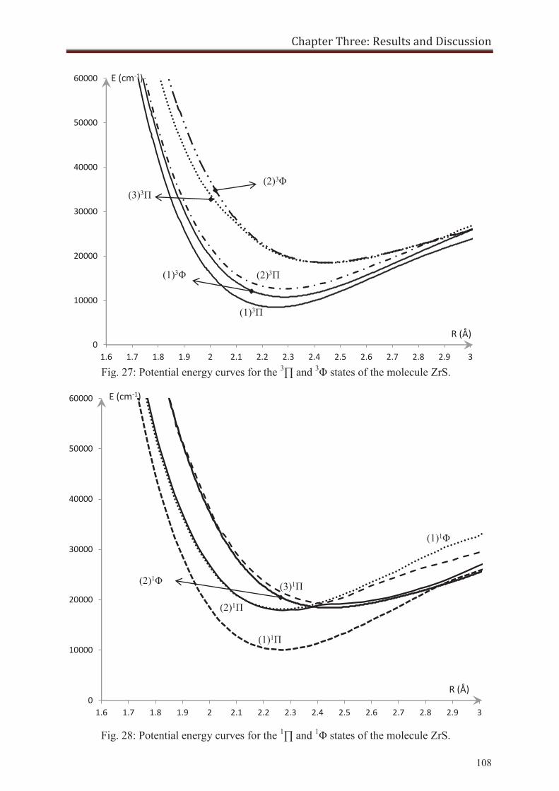
Chapter Three: Results and Discussion
108
0
10000
20000
30000
40000
50000
60000
1.6 1.7 1.8 1.9 2 2.1 2.2 2.3 2.4 2.5 2.6 2.7 2.8 2.9 3
R (Å)
E (cm-1)
(1)3Π
(1)3Φ (2)3Π
(3)3Π (2)3Φ
0
10000
20000
30000
40000
50000
60000
1.6 1.7 1.8 1.9 2 2.1 2.2 2.3 2.4 2.5 2.6 2.7 2.8 2.9 3
E (cm-1)
R (Å)
(1)1Π
(1)1Φ
(2)1Π
(2)1Φ (3)1Π
Fig. 28: Potential energy curves for the 1∏ and 1Φ states of the molecule ZrS.
Fig. 27: Potential energy curves for the 3∏ and 3Φ states of the molecule ZrS.
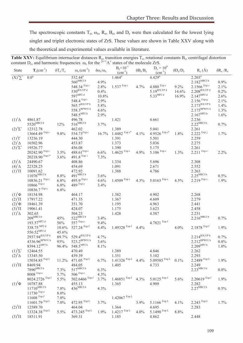
Chapter Three: Results and Discussion
109
The spectroscopic constants Te, ωe, Re, Be, and De were then calculated for the lowest lying
singlet and triplet electronic states of ZrS. These values are shown in Table XXV along with
the theoretical and experimental values available in literature.
Table XXV: Equilibrium internuclear distances Re, transition energies Te, rotational constants Be, centrifugal distortion constant De, and harmonic frequencies ωe for the 2s+1Λ± states of the molecule ZrS.
State Te(cm-1) δTe/Te ωe (cm-1) δωe/ωe Be×10-1
(cm-1) δBe/Be De × 108 (cm-1) δDe/De Re (Å) δRe /Re
(X)1∑+ 0.0a
532.44a
560MRCI b
548.34 Exp c
530B3LYP d
597MP2 d
548.4 Exp i
565.7B3LYP h
558.3BPW91 h
548.5MP2 h
4.9% 2.8% 0.4% 10.8% 2.9% 5.8% 4.6% 2.9%
1.464a
1.537 Exp c
4.7%
4.429a
4.880 Exp c
5.19B3LYP d
5.33MP2 d
9.2% 14.6% 16.9%
2.203a
2.182MRCI b
2.1566 Exp c
2.208B3LYP d
2.147MP2 d
2.156 Exp g
2.173B3LYP h
2.175BPW91 h
2.167MP2 h
0.9% 2.1% 0.2% 2.6% 2.1% 1.4% 1.3% 1.6%
(1)1Δ 4861.87 5520MRCI b
12%
496.78 516MRCI b
3.7%
1.421 4.661 2.236 2.22MRCI b
0.7%
(2)1Σ+ 12312.78 13664.49 Exp c
9.8%
462.02 554.73Exp c
16.7%
1.389 1.4482 Exp c*
4.1%
5.041 4.9526 Exp c*
1.8%
2.261 2.222 Exp j
1.7%
(1)1Г 13236.19 444.30 1.391 5.501 2.259 (2)1Δ 16502.96 453.87 1.373 5.036 2.275 (3)1Σ+ 19526.77
20242.90 Exp c
20218.90 Exp i*
3.5% 3.6%
456.08 488.61Exp c
491.8 Exp i
6.6% 7.3%
1.390 1.4625 Exp c
4.9%
5.175 5.106 Exp c
1.3%
2.261 2.211 Exp c
2.2%
(3)1Δ 24490.67 408.86 1.334 5.696 2.308 (4)1Δ 22328.25 454.69 1.091 2.671 2.552 (1)1Π 10091.62
11076MRCI b
10836.21 Exp c
10866 Exp e
10836.7 Exp e
8.8% 6.8% 6.8% 6.8%
472.92 491MRCI b
495.9 Exp c
489 Exp e
3.6% 4.6% 3.4%
1.388 1.4509 Exp c
4.3%
4.786 5.0163 Exp c
4.5%
2.263 2.25MRCI b
2.219 Exp c
0.5% 1.9%
(1)1Φ 18154.98 464.17 1.382 4.902 2.268 (2)1Π 17917.22 471.35 1.367 4.609 2.279 (2)1Φ 18461.39 351.70 1.195 4.963 2.441 (3)1Π 19061.41 424.07 1.175 3.623 2.458 (1)3∆ 302.65
209MRCI b
193.57MP2 d
338.75 MP2 d
556.52MP2 d
2937.94B3LYP h 4336.96BPW91 h
8394.12MP2 h
45% 56% 10.6% 45.6% 89.7% 93% 96.4%
504.23 522MRCI b
557 Exp e
527.24 Exp f
529.4B3LYP h
523.2BPW91 h
548.5MP2 h
3.4% 9.4% 4.4% 4.7% 3.6% 8.1%
1.428 1.49328 Exp f
4.4%
4.587 4.7821 Exp f
4.0%
2.231 2.216MRCI b
2.1878 Exp f 2.214B3LYP h
2.212BPW91 h
2.209MP2 h
0.7% 1.9% 0.7% 0.8% 1.0%
(1)3Σ+ 12464.55 470.49 1.389 4.846 2.262 (2)3Δ 13345.50
15034.85 Exp L 11.2%
439.39 471.05 Exp L
6.7%
1.351 1.41326 Exp L
4.4%
5.102 5.09585 Exp L
0.1%
2.293 2.2489 Exp L
1.9%
(1)3Π 8469.94 7890MRCI b
8008 Exp e 8024.2726 Exp f
7.3% 5.7% 5.5%
484.05 517MRCI b
506 Exp e
502.6466 Exp f
6.3% 4.3% 3.7%
1.405 1.46851 Exp f
4.3%
4.733 5.0125 Exp f
5.6%
2.249 2.23MRCI b
2.20619 Exp f
0.8% 1.9%
(1)3Φ 10787.88 11710MRCI b
11730 Exp e
11608 Exp f
11601.79 Exp L
7.8% 8.0% 7.0% 7.0%
455.13 436MRCI b
472.95 Exp L
4.3% 3.7%
1.365 1.42067 Exp L
3.9%
4.909 5.1166 Exp L
4.1%
2.282 2.27MRCI b
2.243 Exp L
0.5% 1.7%
(2)3Π 12589.70 13324.38 Exp L
5.5%
464.04 473.245 Exp L
1.9%
1.364 1.4217 Exp L
4.0%
4.695 5.1490 Exp L
8.8%
2.283
(3)3Π 18511.91 369.31 1.185 4.862 2.448
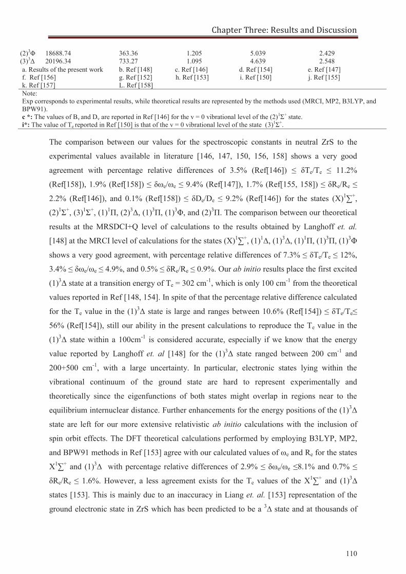
Chapter Three: Results and Discussion
110
(2)3Φ 18688.74 363.36 1.205 5.039 2.429 (3)3Δ 20196.34 733.27 1.095 4.639 2.548 a. Results of the present work b. Ref [148] c. Ref [146] d. Ref [154] e. Ref [147] f. Ref [156] g. Ref [152] h. Ref [153] i. Ref [150] j. Ref [155] k. Ref [157] L. Ref [158] Note: Exp corresponds to experimental results, while theoretical results are represented by the methods used (MRCI, MP2, B3LYP, and BPW91). c *: The values of Bv and Dv are reported in Ref [146] for the v = 0 vibrational level of the (2)1Σ+ state. i*: The value of Te reported in Ref [150] is that of the v = 0 vibrational level of the state (3)1Σ+.
The comparison between our values for the spectroscopic constants in neutral ZrS to the
experimental values available in literature [146, 147, 150, 156, 158] shows a very good
agreement with percentage relative differences of 3.5% (Ref[146]) ≤ δTe/Te ≤ 11.2%
(Ref[158]), 1.9% (Ref[158]) ≤ δωe/ωe ≤ 9.4% (Ref[147]), 1.7% (Ref[155, 158]) ≤ δRe/Re ≤
2.2% (Ref[146]), and 0.1% (Ref[158]) ≤ δDe/De ≤ 9.2% (Ref[146]) for the states (X)1∑+,
(2)1Σ+, (3)1Σ+, (1)1Π, (2)3Δ, (1)3Π, (1)3Φ, and (2)3Π. The comparison between our theoretical
results at the MRSDCI+Q level of calculations to the results obtained by Langhoff et. al.
[148] at the MRCI level of calculations for the states (X)1∑+, (1)1Δ, (1)3Δ, (1)1Π, (1)3Π, (1)3Φ
shows a very good agreement, with percentage relative differences of 7.3% ≤ δTe/Te ≤ 12%,
3.4% ≤ δωe/ωe ≤ 4.9%, and 0.5% ≤ δRe/Re ≤ 0.9%. Our ab initio results place the first excited
(1)3Δ state at a transition energy of Te = 302 cm-1, which is only 100 cm-1 from the theoretical
values reported in Ref [148, 154]. In spite of that the percentage relative difference calculated
for the Te value in the (1)3Δ state is large and ranges between 10.6% (Ref[154]) ≤ δTe/Te≤
56% (Ref[154]), still our ability in the present calculations to reproduce the Te value in the
(1)3Δ state within a 100cm-1 is considered accurate, especially if we know that the energy
value reported by Langhoff et. al [148] for the (1)3Δ state ranged between 200 cm-1 and
200+500 cm-1, with a large uncertainty. In particular, electronic states lying within the
vibrational continuum of the ground state are hard to represent experimentally and
theoretically since the eigenfunctions of both states might overlap in regions near to the
equilibrium internuclear distance. Further enhancements for the energy positions of the (1)3Δ
state are left for our more extensive relativistic ab initio calculations with the inclusion of
spin orbit effects. The DFT theoretical calculations performed by employing B3LYP, MP2,
and BPW91 methods in Ref [153] agree with our calculated values of ωe and Re for the states
X1∑+ and (1)3∆ with percentage relative differences of 2.9% ≤ δωe/ωe ≤8.1% and 0.7% ≤
δRe/Re ≤ 1.6%. However, a less agreement exists for the Te values of the X1∑+ and (1)3∆
states [153]. This is mainly due to an inaccuracy in Liang et. al. [153] representation of the
ground electronic state in ZrS which has been predicted to be a 3∆ state and at thousands of
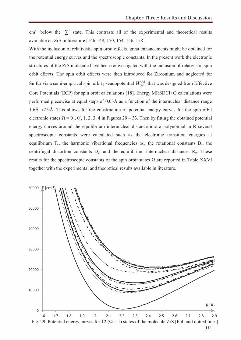
Chapter Three: Results and Discussion
111
cm-1 below the 1∑+ state. This contrasts all of the experimental and theoretical results
available on ZrS in literature [146-148, 150, 154, 156, 158].
With the inclusion of relativistic spin orbit effects, great enhancements might be obtained for
the potential energy curves and the spectroscopic constants. In the present work the electronic
structures of the ZrS molecule have been reinvestigated with the inclusion of relativistic spin
orbit effects. The spin orbit effects were then introduced for Zirconium and neglected for
Sulfur via a semi-empirical spin orbit pseudopotential PSSOW that was designed from Effective
Core Potentials (ECP) for spin orbit calculations [18]. Energy MRSDCI+Q calculations were
performed piecewise at equal steps of 0.03Å as a function of the internuclear distance range
1.6Å→2.9Å. This allows for the construction of potential energy curves for the spin orbit
electronic states Ω = 0+, 0-, 1, 2, 3, 4 in Figures 29 – 33. Then by fitting the obtained potential
energy curves around the equilibrium internuclear distance into a polynomial in R several
spectroscopic constants were calculated such as the electronic transition energies at
equilibrium Te, the harmonic vibrational frequencies ωe, the rotational constants Be, the
centrifugal distortion constants De, and the equilibrium internuclear distances Re. These
results for the spectroscopic constants of the spin orbit states Ω are reported in Table XXVI
together with the experimental and theoretical results available in literature.
Fig. 29. Potential energy curves for 12 (Ω = 1) states of the molecule ZrS [Full and dotted lines].
0
10000
20000
30000
40000
50000
60000
1.6 1.7 1.8 1.9 2 2.1 2.2 2.3 2.4 2.5 2.6 2.7 2.8 2.9
R (Å)
E (cm-1)
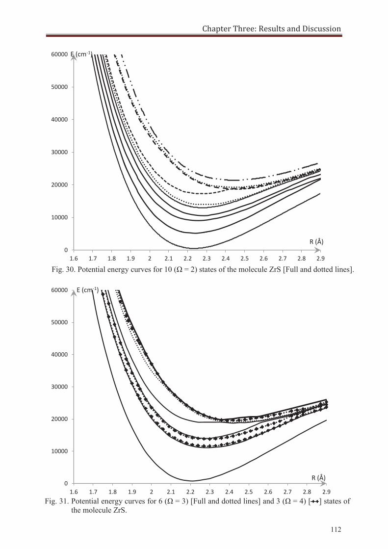
Chapter Three: Results and Discussion
112
Fig. 30. Potential energy curves for 10 (Ω = 2) states of the molecule ZrS [Full and dotted lines].
0
10000
20000
30000
40000
50000
60000
1.6 1.7 1.8 1.9 2 2.1 2.2 2.3 2.4 2.5 2.6 2.7 2.8 2.9
R (Å)
E (cm-1)
0
10000
20000
30000
40000
50000
60000
1.6 1.7 1.8 1.9 2 2.1 2.2 2.3 2.4 2.5 2.6 2.7 2.8 2.9
R (Å)
E (cm-1)
Fig. 31. Potential energy curves for 6 (Ω = 3) [Full and dotted lines] and 3 (Ω = 4) [ ] states of the molecule ZrS.
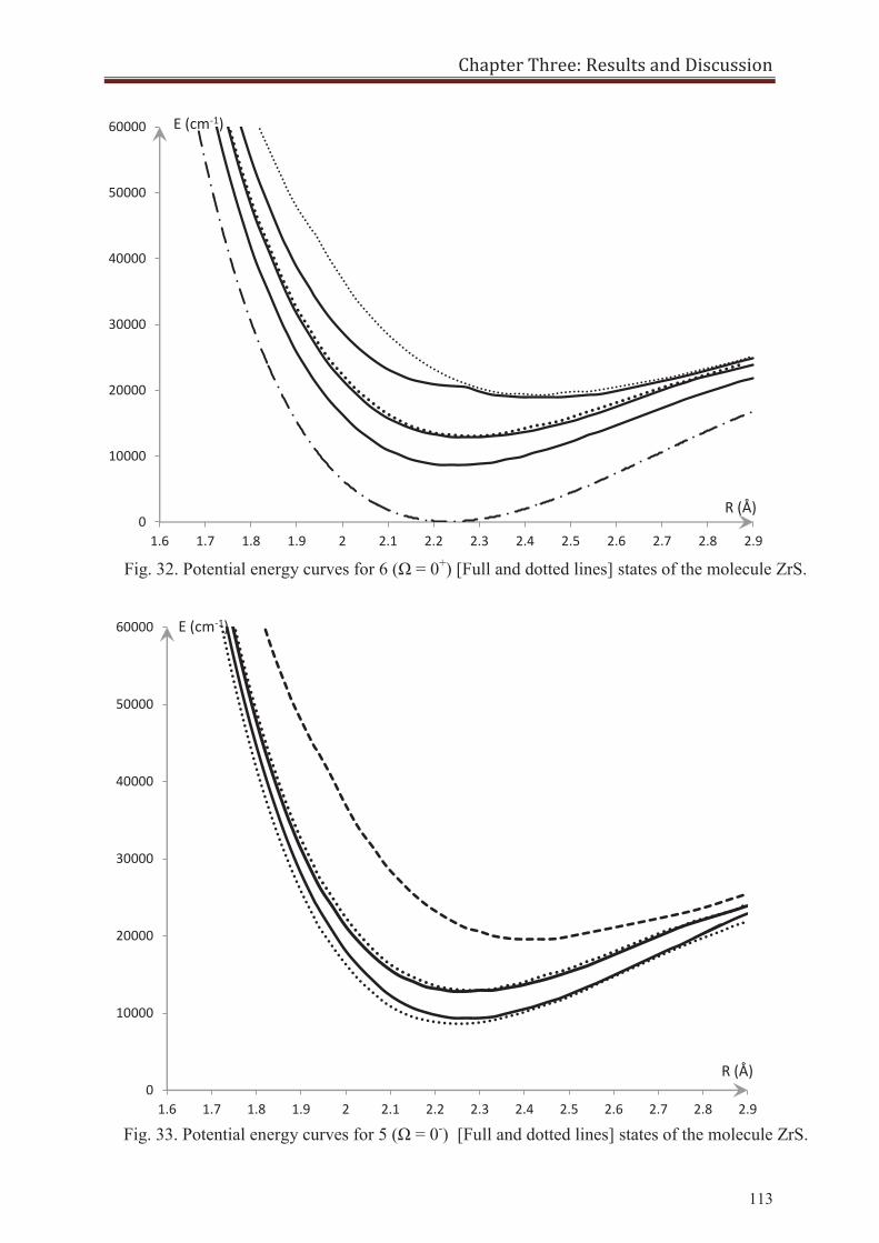
Chapter Three: Results and Discussion
113
0
10000
20000
30000
40000
50000
60000
1.6 1.7 1.8 1.9 2 2.1 2.2 2.3 2.4 2.5 2.6 2.7 2.8 2.9
R (Å)
E (cm-1)
Fig. 32. Potential energy curves for 6 (Ω = 0+) [Full and dotted lines] states of the molecule ZrS.
0
10000
20000
30000
40000
50000
60000
1.6 1.7 1.8 1.9 2 2.1 2.2 2.3 2.4 2.5 2.6 2.7 2.8 2.9
R (Å)
E (cm-1)
Fig. 33. Potential energy curves for 5 (Ω = 0-) [Full and dotted lines] states of the molecule ZrS.
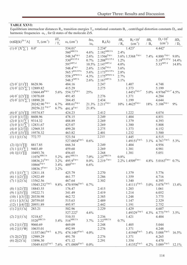
Chapter Three: Results and Discussion
114
TABLE XXVI: Equilibrium internuclear distances Re, transition energies Te, rotational constants Be , centrifugal distortion constants De, and harmonic frequencies ωe , for Ω states of the molecule ZrS.
(n)Ω[(k)2S+1Λ] Te (cm-1) δTe / Te ωe (cm-1) δωe
/ωe Re(Å) δRe
/ Re
Be×101
(cm-1) δBe / Be
De×107
(cm-1) δDe
/ De
(1) 0+ [X1∑+] 0.0a 534.01a 560MRCI b
548.34Exp c
530B3LYP d
597MP2 d
548.4Exp i
565.7B3LYP h
558.3BPW91 h
548.5MP2 h
4.6% 2.6% 0.7% 10.5% 2.6% 5.6% 4.3% 2.6%
2.234a
2.182MRCI b
2.1566Exp c
2.208B3LYP d
2.147MP2 d
2.156Exp g
2.173B3LYP h
2.175BPW91 h
2.167MP2 h
2.4% 3.6% 1.2% 4.0% 3.6% 2.8% 2.7% 3.1%
1.423a
1.5368 Exp c
7.4%
4.442a 4.880 Exp c
5.19B3LYP d
5.33MP2 d
9.0% 14.4% 14.8%
(2) 0+ [(1)3∏ 8628.96 484.16 2.247 1.407 4.748 (3) 0+ [(2)1∑+] 12889.82
13664.49Exp c 5.6% 415.29 554.73Exp c
25%
2.275 1.373 1.4451Exp c*
5.0%
5.199 4.9766Exp c*
4.5%
(4) 0+ [(2)3∏] 13078.69 491.45 2.276 1.371 4.284 (5) 0+ [(3)1∑+] 18890.20
20242.90 Exp c
20256.22 Exp i* 6.7% 6.7%
384.45 488.61Exp c
491.8Exp i
21.3% 21.8%
2.434 2.211Exp c
10%
1.199 1.4625Exp c
18%
4.644 5.106Exp c
9%
(6) 0+ [(3)3∏] 19374.87 424.23 2.412 1.222 4.074 (1) 0- [(1)3∏] 8608.96 478.15 2.249 1.404 4.851 (2) 0- [(1)3∑-] 9314.32 488.89 2.269 1.379 4.393 (3) 0- [(1)3∑+] 12831.67 425.07 2.269 1.380 5.808 (4) 0- [(2)3∏] 12969.35 499.20 2.275 1.373 4.152
(5) 0- [(3)3∏] 19578.32 463.82 2.401 1.232 3.500 (1) 1 [(1)3∆] 772.77 523.54
527.0854Exp L 0.6% 2.215 1.445
1.49151Exp L 3.1%
4.515 4.767 Exp L
5.3%
(2) 1[(1)3∏] 8817.85 666.34 2.249 1.404 4.956 (3) 1 [(1)3∑-] 9403.49 459.60 2.269 1.381 4.981 (4) 1[(1)1∏] 10493.76
11076MRCI b
10836.21Exp c
10866Exp e
10836.7Exp e
5.2% 3.2% 3.4% 3.2%
456.65 491MRCI b
495.9Exp c
489Exp e
7.0% 8.0% 6.6%
2.268 2.25MRCI b
2.219 Exp c
0.8% 2.2%
1.381
1.4509Exp c
4.8%
5.051 5.0163Exp c
0.7%
(5) 1 [(1)3∑+] 12811.18 425.79 2.270 1.379 5.776 (6) 1 [(2)3∏] 12922.49 461.77 2.286 1.359 4.716 (7) 1 [(2)3∆] 13562.56
15043.232 Exp L 9.8% 467.64 470.9596Exp L 0.7%
2.302 1.340 1.41111Exp L
5.0%
4.395 5.078 Exp L
13.4%
(8) 1 [(2)1∏] 18843.55 176.47 2.415 1.203 1.061 (9) 1 [(3)3∏] 19222.71 341.49 2.419 1.214 6.052 (10) 1 [(3)1∏] 20338.98 462.72 2.385 1.248 3.775 (11) 1 [(3)3∆] 20759.05 515.63 2.489 1.147 2.329 (12) 1 [(4)3∏] 20951.89 495.97 2.442 1.191 2.752 (1) 2 [(1)3∆] 283.21 502.96
527.222L 4.6% 2.229 1.429
1.49329 Exp L 4.3%
4.607 4.775 Exp L
3.5%
(2) 2 [(1)1∆] 5218.67 5520MRCI b 5.4%
510.55 516MRCI b 3.7%
2.236 2.22MRCI b
0.7%
1.421 4.404
(3) 2 [(1)3∏] 9060.69 469.09 2.248 1.405 5.044 (4) 2 [(1)3Φ] 10635.01
11357.061Exp L 6.3% 492.99 474.1487Exp L 4.0%
2.276 1.371 1.41948Exp L
3.4%
4.248 5.088 Exp L
16.5%
(3) 2[(2)3∏] 12989.29 491.70 2.276 1.371 4.265 (6) 2[(2)3∆] 13896.30
15049.4155Exp L 7.6% 471.12 471.0809Exp L 0.0%
2.291 1.354 1.41352Exp L
4.2%
4.470 5.089 Exp L
12.1%
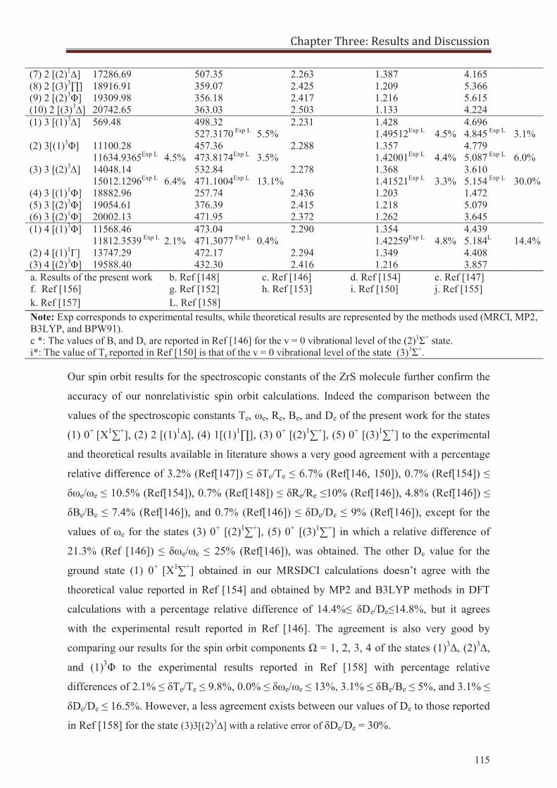
Chapter Three: Results and Discussion
115
(7) 2 [(2)1∆] 17286.69 507.35 2.263 1.387 4.165 (8) 2 [(3)3∏] 18916.91 359.07 2.425 1.209 5.366 (9) 2 [(2)3Φ] 19309.98 356.18 2.417 1.216 5.615 (10) 2 [(3)3∆] 20742.65 363.03 2.503 1.133 4.224 (1) 3 [(1)3∆] 569.48 498.32
527.3170 Exp L 5.5% 2.231 1.428
1.49512Exp L 4.5%
4.696 4.845 Exp L
3.1%
(2) 3[(1)3Φ] 11100.28 11634.9365Exp L 4.5%
457.36 473.8174Exp L 3.5%
2.288 1.357 1.42001Exp L
4.4%
4.779 5.087 Exp L
6.0%
(3) 3 [(2)3∆] 14048.14 15012.1296Exp L 6.4%
532.84 471.1004Exp L 13.1%
2.278 1.368 1.41521Exp L
3.3%
3.610 5.154 Exp L
30.0%
(4) 3 [(1)1Φ] 18882.96 257.74 2.436 1.203 1.472 (5) 3 [(2)3Φ] 19054.61 376.39 2.415 1.218 5.079 (6) 3 [(2)1Φ] 20002.13 471.95 2.372 1.262 3.645 (1) 4 [(1)3Φ] 11568.46
11812.3539 Exp L 2.1% 473.04 471.3077 Exp L 0.4%
2.290 1.354 1.42259Exp L
4.8%
4.439 5.184L
14.4%
(2) 4 [(1)1Γ] 13747.29 472.17 2.294 1.349 4.408 (3) 4 [(2)3Φ] 19588.40 432.30 2.416 1.216 3.857 a. Results of the present work b. Ref [148] c. Ref [146] d. Ref [154] e. Ref [147] f. Ref [156] g. Ref [152] h. Ref [153] i. Ref [150] j. Ref [155] k. Ref [157] L. Ref [158] Note: Exp corresponds to experimental results, while theoretical results are represented by the methods used (MRCI, MP2, B3LYP, and BPW91). c *: The values of Bv and Dv are reported in Ref [146] for the v = 0 vibrational level of the (2)1Σ+ state. i*: The value of Te reported in Ref [150] is that of the v = 0 vibrational level of the state (3)1Σ+.
Our spin orbit results for the spectroscopic constants of the ZrS molecule further confirm the
accuracy of our nonrelativistic spin orbit calculations. Indeed the comparison between the
values of the spectroscopic constants Te, ωe, Re, Be, and De of the present work for the states
(1) 0+ [X1∑+], (2) 2 [(1)1∆], (4) 1[(1)1∏], (3) 0+ [(2)1∑+], (5) 0+ [(3)1∑+] to the experimental
and theoretical results available in literature shows a very good agreement with a percentage
relative difference of 3.2% (Ref[147]) ≤ δTe/Te ≤ 6.7% (Ref[146, 150]), 0.7% (Ref[154]) ≤
δωe/ωe ≤ 10.5% (Ref[154]), 0.7% (Ref[148]) ≤ δRe/Re ≤10% (Ref[146]), 4.8% (Ref[146]) ≤
δBe/Be ≤ 7.4% (Ref[146]), and 0.7% (Ref[146]) ≤ δDe/De ≤ 9% (Ref[146]), except for the
values of ωe for the states (3) 0+ [(2)1∑+], (5) 0+ [(3)1∑+] in which a relative difference of
21.3% (Ref [146]) ≤ δωe/ωe ≤ 25% (Ref[146]), was obtained. The other De value for the
ground state (1) 0+ [X1∑+] obtained in our MRSDCI calculations doesn’t agree with the
theoretical value reported in Ref [154] and obtained by MP2 and B3LYP methods in DFT
calculations with a percentage relative difference of 14.4%≤ δDe/De≤14.8%, but it agrees
with the experimental result reported in Ref [146]. The agreement is also very good by
comparing our results for the spin orbit components Ω = 1, 2, 3, 4 of the states (1)3∆, (2)3∆,
and (1)3Φ to the experimental results reported in Ref [158] with percentage relative
differences of 2.1% ≤ δTe/Te ≤ 9.8%, 0.0% ≤ δωe/ωe ≤ 13%, 3.1% ≤ δBe/Be ≤ 5%, and 3.1% ≤
δDe/De ≤ 16.5%. However, a less agreement exists between our values of De to those reported
in Ref [158] for the state (3)3[(2)3∆] with a relative error of δDe/De = 30%.
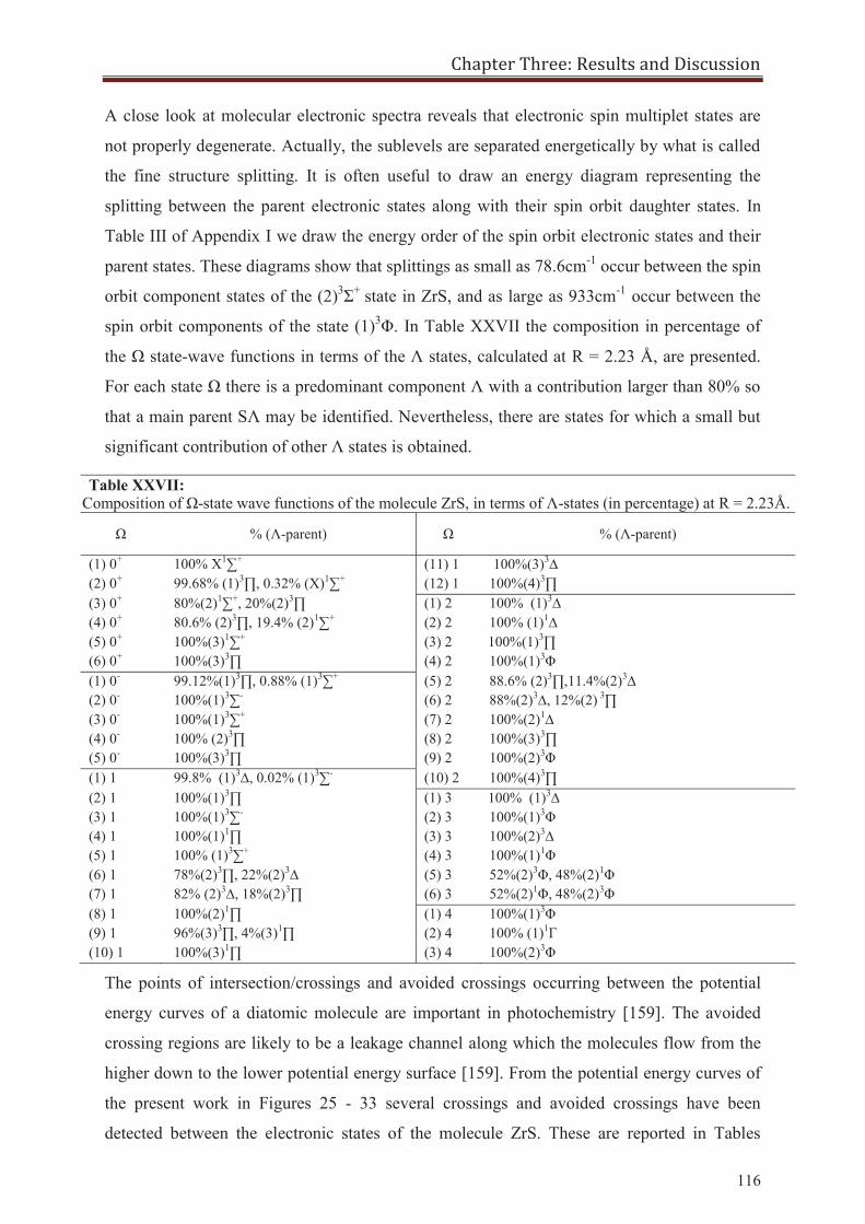
Chapter Three: Results and Discussion
116
A close look at molecular electronic spectra reveals that electronic spin multiplet states are
not properly degenerate. Actually, the sublevels are separated energetically by what is called
the fine structure splitting. It is often useful to draw an energy diagram representing the
splitting between the parent electronic states along with their spin orbit daughter states. In
Table III of Appendix I we draw the energy order of the spin orbit electronic states and their
parent states. These diagrams show that splittings as small as 78.6cm-1 occur between the spin
orbit component states of the (2)3Σ+ state in ZrS, and as large as 933cm-1 occur between the
spin orbit components of the state (1)3Φ. In Table XXVII the composition in percentage of
the Ω state-wave functions in terms of the Λ states, calculated at R = 2.23 Å, are presented.
For each state Ω there is a predominant component Λ with a contribution larger than 80% so
that a main parent SΛ may be identified. Nevertheless, there are states for which a small but
significant contribution of other Λ states is obtained.
The points of intersection/crossings and avoided crossings occurring between the potential
energy curves of a diatomic molecule are important in photochemistry [159]. The avoided
crossing regions are likely to be a leakage channel along which the molecules flow from the
higher down to the lower potential energy surface [159]. From the potential energy curves of
the present work in Figures 25 - 33 several crossings and avoided crossings have been
detected between the electronic states of the molecule ZrS. These are reported in Tables
Table XXVII: Composition of Ω-state wave functions of the molecule ZrS, in terms of Λ-states (in percentage) at R = 2.23Å.
Ω % (Λ-parent) Ω % (Λ-parent)
(1) 0+ 100% X1∑+ (11) 1 100%(3)3∆ (2) 0+ 99.68% (1)3∏, 0.32% (X)1∑+ (12) 1 100%(4)3∏ (3) 0+ 80%(2)1∑+, 20%(2)3∏ (1) 2 100% (1)3∆ (4) 0+ 80.6% (2)3∏, 19.4% (2)1∑+ (2) 2 100% (1)1∆ (5) 0+ 100%(3)1∑+ (3) 2 100%(1)3∏ (6) 0+ 100%(3)3∏ (4) 2 100%(1)3Φ (1) 0- 99.12%(1)3∏, 0.88% (1)3∑+ (5) 2 88.6% (2)3∏,11.4%(2)3∆ (2) 0- 100%(1)3∑- (6) 2 88%(2)3∆, 12%(2) 3∏ (3) 0- 100%(1)3∑+ (7) 2 100%(2)1∆ (4) 0- 100% (2)3∏ (8) 2 100%(3)3∏ (5) 0- 100%(3)3∏ (9) 2 100%(2)3Φ (1) 1 99.8% (1)3∆, 0.02% (1)3∑- (10) 2 100%(4)3∏ (2) 1 100%(1)3∏ (1) 3 100% (1)3∆ (3) 1 100%(1)3∑- (2) 3 100%(1)3Φ (4) 1 100%(1)1∏ (3) 3 100%(2)3∆ (5) 1 100% (1)3∑+ (4) 3 100%(1)1Φ (6) 1 78%(2)3∏, 22%(2)3∆ (5) 3 52%(2)3Φ, 48%(2)1Φ (7) 1 82% (2)3∆, 18%(2)3∏ (6) 3 52%(2)1Φ, 48%(2)3Φ (8) 1 100%(2)1∏ (1) 4 100%(1)3Φ (9) 1 96%(3)3∏, 4%(3)1∏ (2) 4 100% (1)1Γ (10) 1 100%(3)1∏ (3) 4 100%(2)3Φ
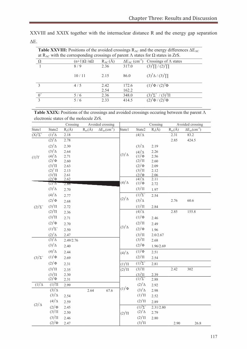
Chapter Three: Results and Discussion
117
XXVIII and XXIX together with the internuclear distance R and the energy gap separation
ΔE.
Table XXVIII: Positions of the avoided crossings RAC and the energy differences ΔEAC at RAC with the corresponding crossings of parent Λ states for Ω states in ZrS. Ω (n+1)Ω /nΩ RAC (Å) ΔEAC (cm-1) Crossings of Λ states 1 8 / 9 2.36 317.0 (3)3∏ / (2)1∏ 10 / 11 2.15 86.0 (3)3∆ / (3)1∏ 3 4 / 5 2.42
2.54 172.6 162.2
(1)1Φ / (2)3Φ
0+ 5 / 6 2.36 348.0 (3)1Σ+ / (3)3Π 3 5 / 6 2.33
414.5 (2)3Φ / (2)1Φ
Table XXIX: Positions of the crossings and avoided crossings occuring between the parent Λ electronic states of the molecule ZrS.
Crossing Avoided crossing Crossing Avoided crossing State1 State2 Rc(Å) Rav(Å) ∆Eav(cm-1) State1 State2 Rc(Å) Rav(Å) ∆Eav(cm-1) (X)1Σ+ (1)3Δ 2.18
(3)1Δ
(4)1Δ 2.31 83.2
(1)1Γ
(2)1Δ 2.78 2.85 424.5 (2)3Δ 2.30 (3)3Δ 2.19 (3)3Δ 2.64 (4)3Δ 2.26 (4)3Δ 2.71 (1)1Φ 2.56 (2)1Φ 2.60 (2)1Π 2.60 (3)1Π 2.63 (2)1Φ 2.09 (2)3 Π 2.13 (3)1Π 2.12 (3)3Π 2.61 (2)3Φ 2.06 (2)3Φ 2.62
(4)1Δ
(4)3Δ 2.11
(2)1Σ+
(2)1Δ 2.86 (1)1Φ 2.72 (3)3Δ 2.70 (3)1Π 1.97
(4)3Δ 2.77 (2)3Δ
(1)3Σ+ 2.54 (2)1Φ 2.68 (3)3Δ 2.76 60.6 (3)1Π 2.72 (1)1Π 2.84 (2)3Π 2.36
(3)3Δ
(4)3Δ 2.85 155.8 (3)3Π 2.71 (1)1Φ 2.46 (2)3Φ 2.70 (2)1Π 2.49 (1)3Σ+ 2.50 (2)1Φ 1.96 (2)3Δ 2.47 (3)1Π 2.0/2.67
(3)1Σ+
(3)1Δ 2.49/2.76 (3)3Π 2.68 (3)3Δ 2.40 (2)3Φ 1.96/2.69
(4)3Δ 2.44 (4)3Δ
(1)1Φ 2.51 (1)1Φ 2.69 (2)1Π 2.54
(2)1Φ 2.31 (1)1Π (1)3Σ+ 2.81 (3)1Π 2.35 (2)1Π
(3)1Π 2.42 302
(3)3Π 2.30 (3)3Π 2.39 (2)3Φ 2.31
(1)3Φ
(1)3Σ+ 2.88 (1)1Δ (1)3Π 2.99 (2)3Δ 2.92
(2)1Δ
(3)1Δ 2.64 67.6 (3)3Δ 2.98 (3)3Δ 2.54 (1)1Π 2.52 (4)3Δ 2.59 (2)1Π 2.89 (2)1Φ 2.45
(2)3Π
(1)3Σ+ 2.31/2.80 (3)1Π 2.50 (2)3Δ 2.79 (3)3Π 2.46 (2)1Π 2.80 (2)3Φ 2.47 (3)3Π 2.90 26.8
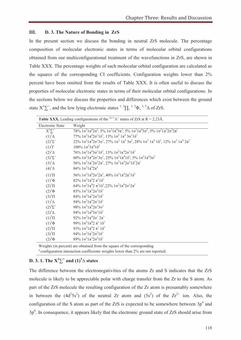
Chapter Three: Results and Discussion
118
III. D. 3. The Nature of Bonding in ZrS
In the present section we discuss the bonding in neutral ZrS molecule. The percentage
composition of molecular electronic states in terms of molecular orbital configurations
obtained from our multiconfigurational treatment of the wavefunctions in ZrS, are shown in
Table XXX. The percentage weights of each molecular orbital configuration are calculated as
the squares of the corresponding CI coefficients. Configuration weights lower than 2%
percent have been omitted from the results of Table XXX. It is often useful to discuss the
properties of molecular electronic states in terms of their molecular orbital configurations. In
the sections below we discuss the properties and differences which exist between the ground
state X1∑+, and the low lying electronic states 1, 3∏, 1, 3Φ, 1, 3∆ of ZrS.
Table XXX. Leading configurations of the 2s+1Λ± states of ZrS at R = 2.23Å. Electronic State Weight
X1∑+ 78% 1σ21π42σ2, 5% 1σ21π43π2, 5% 1σ21π43σ2, 5% 1σ21π32σ22π1 (1)1Δ 77% 1σ21π42σ11δ1, 13% 1σ2 1π4 3σ11δ1 (2)1Σ+ 22% 1σ21π42σ13σ1, 27% 1σ2 1π4 3π2, 28% 1σ2 1π4 1δ2, 12% 1σ2 1π4 2π2 (1)1Г 100% 1σ21π41δ2 (2)1Δ 76% 1σ21π43σ11δ1, 13% 1σ21π42σ11δ1 (3)1Σ+ 60% 1σ21π42σ13σ1, 25% 1σ21π41δ2, 5% 1σ21π43σ2 (3)1Δ 56% 1σ21π32σ22π1, 27% 1σ21π32σ11δ12π1 (4)1Δ 86% 1σ21π42π2
(1)1Π 56% 1σ21π42σ12π1, 40% 1σ21π42π11δ1 (1)1Φ 82% 1σ21π42 π11δ1 (2)1Π 64% 1σ21π42 π11δ1,22% 1σ21π42σ12π1 (2)1Φ 85% 1σ21π32σ21δ1 (3)1Π 84% 1σ21π32σ21δ1 (1)3∆ 94% 1σ21π42σ11δ1 (2)3Σ+ 98% 1σ21π42σ13σ1 (2)3Δ 94% 1σ21π43σ11δ1 (1)3Π 92% 1σ21π42σ1 2π1 (1)3Φ 99% 1σ21π42 π1 1δ1 (2)3Π 93% 1σ21π42 π1 1δ1 (3)3Π 94% 1σ21π32σ21δ1 (2)3Φ 89% 1σ21π32σ21δ1
Weights (in percent) are obtained from the square of the corresponding a configuration interaction coefficients weights lower than 2% are not reported.
D. 3. 1. The X1∑+ and (1)3∆ states
The difference between the electronegativities of the atoms Zr and S indicates that the ZrS
molecule is likely to be appreciable polar with charge transfer from the Zr to the S atom. As
part of the ZrS molecule the resulting configuration of the Zr atom is presumably somewhere
in between the (4d25s2) of the neutral Zr atom and (5s2) of the Zr2+ ion. Also, the
configuration of the S atom as part of the ZrS is expected to be somewhere between 3p4 and
3p6. In consequence, it appears likely that the electronic ground state of ZrS should arise from
Chapter Three: Results and Discussion
119
the valence shell configuration: 1σ21π42σ2 (Table XXXIII). This electronic configuration
(1σ21π42σ2) gives rise to the singlet electronic ground state X1∑+, with orbital angular
momentum Λ = ∑λi = 0. Other configurations arising from the single and double excitation of
electrons from the ground state configuration in to virtual molecular orbitals, forming the
active space of ZrS, may lead to other electronic states 1,3∑, 1,3∏, 1,3∆, 1,3Φ, and 1,3Γ. In ZrS
the electronic energy of the (1)3∆ state is within the vibrational interval of the ground state.
Actually, the potential energy curves of the two states (1)3∆ and X1∑+ state cross at R =
2.15Å. The main difference between the molecular orbital configurations of the two states
(1)3∆ and X1∑+ arises from the promotion of a 2σ1 electron in the ground state in to a 1δ1
orbital, thus giving the (1)3∆ state the following molecular orbital configuration
1σ21π42σ11δ1.
D. 3. 2. The Low-Lying 1, 3∏ and 1, 3∆ states:
The first (1)3∏ and (1)1∏ states, located at 8469.94cm-1 and 10091.62cm-1 above the ground
electronic state are in excellent agreement with the experimental results available in Ref [160,
161, 162]. The electronic configurations of the lowest lying (1)1∏ and (1)3∏ states arise from
the promotion of a 2σ electron on to the virtual molecular orbital 2π1. Thus giving the two
electronic states (1)1∏ and (1)3∏ the leading molecular orbital configurations 56%
1σ21π42σ12π1, 92% 1σ21π42σ1 2π1, respectively. The lowest lying (1)1Δ state 1σ2 1π4 2σ11δ1
arises from the promotion of a metal centered (5s) 2σ1 electron in to the vacant metal (4d±1)
1δ orbital. This places the (1)1Δ state at a transition energy of Te = 4861.87cm-1 relative to the
ground state, in excellent agreement with previous ab initio calculations [139]. The second
(2)3∆ state has a configuration that differs from that of the (1)3∆ state by the promotion of an
electron from the metal (5s) 2σ1 orbital into a vacant (4d0) 3σ1 orbital. This raises the (2)3∆
state in to a higher energy region of 13345 cm-1 above the ground state. Additionally, the
(2)1∑+ state located in our calculations at 12312.78cm-1 arises from a combination of several
orbital configurations 22% 1σ21π42σ13σ1, 27% 1σ2 1π4 3π2, 28% 1σ2 1π4 1δ2, 12% 1σ2 1π4
2π2 without a dominant molecular orbital configuration.
In order to completely describe the bonding in the ground electronic state of the neutral ZrS
molecule, we calculate in the following section the effective bond order EBO, which was
defined earlier in equation (1) of this chapter. A better definition of the effective bond order
can be obtained by considering the occupation numbers of bonding and antibonding natural
orbitals derived from multiconfigurational wave functions. In our CASSCF calculations we
obtained the ground state of ZrS by distributing the 8 valence electrons over the active space
of molecular orbitals. The occupation numbers of bonding molecular orbitals are given by the
Chapter Three: Results and Discussion
120
number ηb and those in the antibonding molecular orbitals are given by ηab. In our CASSCF
treatment of the wavefunctions in ZrS we obtained the occupation numbers of the bonding
and anti-bonding orbitals in the following way: ηb(1σ)= 1.95456, ηb(2σ)= 0.7686, ηab(3σ)=
0.43403, ηab(4σ)= 0.23715, ηab(1δ)= 0.4516, ηb(1π)= 3.54098, ηab(2π)= 0.54062, ηab(3π)=
0.07246. Then by using equation (1), we obtain an effective bond order EBO of 2.26 ≈ 2,
which indicates that the bonding in neutral ZrS is a double bond.
III. D. 4. The Vibrational Structure of ZrS
We suspect in the present section that several vibrational energy levels belonging to the
vibrational spectrum of the ground (1)0+[X1∑+] and first excited states (1)1[(1)3∆],
(1)2[(1)3∆], (1)3[(1)3∆] are degenerate. For this we investigate the vibrational energy
structures of ZrS by solving the vibrational-rotational Schrödinger equation within the
canonical functions approach [34, 35].
The vibrational energy structures of diatomic molecules are important in the search for
possible variations in the fundamental constants of the standard model, the fine structure
constant α and the electron to proton mass ratios μ. In fundamental concepts the fine
structure constant namely called the coupling constant characterizes the strength of the
electromagnetic interaction, or the probability of an electron to capture a photon. Physicists
have pondered for many years whether the fine structure constant is in fact constant and
whether or not its value differs by location and time. The current value of the fine structure
constant 2 /e cc is 1 / 137.035999074 [163, 164] and the current limit on variations in α
obtained from atomic spectra measurements is 15 1/ 2.7 2.6 10 years [165,
166]. Variations in α can be detected by relativistic energy level shifts in atoms and
molecules [167]. If we choose close energy levels which move differently as α varies,
variations in the transitions frequency would correspond to variations in α. An extreme
example of this is in dysprosium. In dysprosium, there are two almost degenerate states with
an energy of 19797.97cm-1. In [168] it was demonstrated that the relative change of the
transition frequency between these two levels in dysprosium is orders of magnitude larger
than the relative change in α [167]. An experiment is currently in progress utilizing this
transition [169]. These measurements can be greatly enhanced by several orders of
magnitude, in transitions occurring between the nearly degenerate fine structure vibrational
energy levels in diatomic molecules. These transitions exist in the microwave frequency
range, on the order of < 20cm-1, and the level widths are generally very small, typically of the
order of ≈ 10-2 Hz [170]. Accurate measurements for variations in α can be done by observing
transitions between nearly degenerate fine structure vibrational energy levels in diatomic
Chapter Three: Results and Discussion
121
molecules. In these regards, searching for the nearly degenerate vibrational levels in diatomic
molecules is important, as it might shed the light on new limits in the search for laboratory
variations of α in certain diatomic molecules. Particularly interesting molecules are those
identified in the spectra of stars, as laboratory tests on these molecules might be extended to
search for variations of α in stars. The molecule of interest in the present work ZrS is
important in this domain since it has been identified as the carrier of the Keenan bands in the
spectra of cool S-type stars [147]. In ZrS, we detected a (1)3Δ state that is only 302cm-1 above
the ground state. We further suspect that near degeneracies of order < 20cm-1 might exist
between the vibrational energy levels of the spin orbit component states (1)0+[(X)1∑+],
(1)1[(1) 3Δ], (1)2[(1) 3Δ], and (1)3[(1) 3Δ]. In search for possible degeneracies between the
vibrational intervals of the ground and low lying electronic states of ZrS, we have decided in
the present work to investigate the vibrational structures of the spin orbit electronic states in
ZrS.
In literature the first identification of the ZrS molecule in the spectra of three Mira variable
stars of type S was done by K. Hinkle et. al. [147] and was based on the identification of the
Δv = -1, 0, 1, and 2 vibrational transitions in the 3Π - 3Δ band system of ZrS. Laboratory
observations for the rotational structure of the ZrS molecule were done by rotational
microwave spectroscopy in Ref [152] for the rotational energy transitions in the vibrational v
= 0, 1, 2 levels of the X1∑+ and (1)3Δ states. Further spectral analysis in Ref [146, 150]
yielded rotational and vibrational energy spectrums in the singlet electronic states of ZrS
{X1∑+, (2)1∑+, (3)1∑+, (1)1Π}. Selected vibrational energy transitions were then observed in
laboratory spectra for the transition (1)3Δ - (1)3Π in Ref [156] and for the transitions (4)3Δ –
(1)3Δ, (2)3Φ - (1)3Δ, (2)1Π – X1∑+, (3)1∑+ - X1∑+ in Ref [151].
The results of our previous ab initio calculations on ZrS place the first (1)3Δ state at a
transition energy of Te = 302cm-1 above the ground state, which is in excellent agreement
with the theoretical values reported in Ref [139, 154]. The ground and first excited states in
ZrS are similar to those in HfF+, which have been suggested as a model system to study the
variations in the fundamental constants α and μ [18]. In this respect, the ZrS molecule is
better than the HfF+ molecule since the [X1∑+]→[(1)3∆] transition occurs at ≈302cm-1 in ZrS,
and at 1633cm-1 in HfF+. Which means, that close degeneracies between vibrational energy
levels of the order < 20cm-1 are more likely to occur in ZrS.
In Tables XXXI, XXXII and XXXIII we report our results for the vibrational energy values
of the states (1)0+[X1∑+], (1)1[(1)3∆], (1)2[(1)3∆], (1)3[(1)3∆], (4)1[(1)1∏] obtained by
solving the vibrational Schrödinger equation within the canonical functions approach.
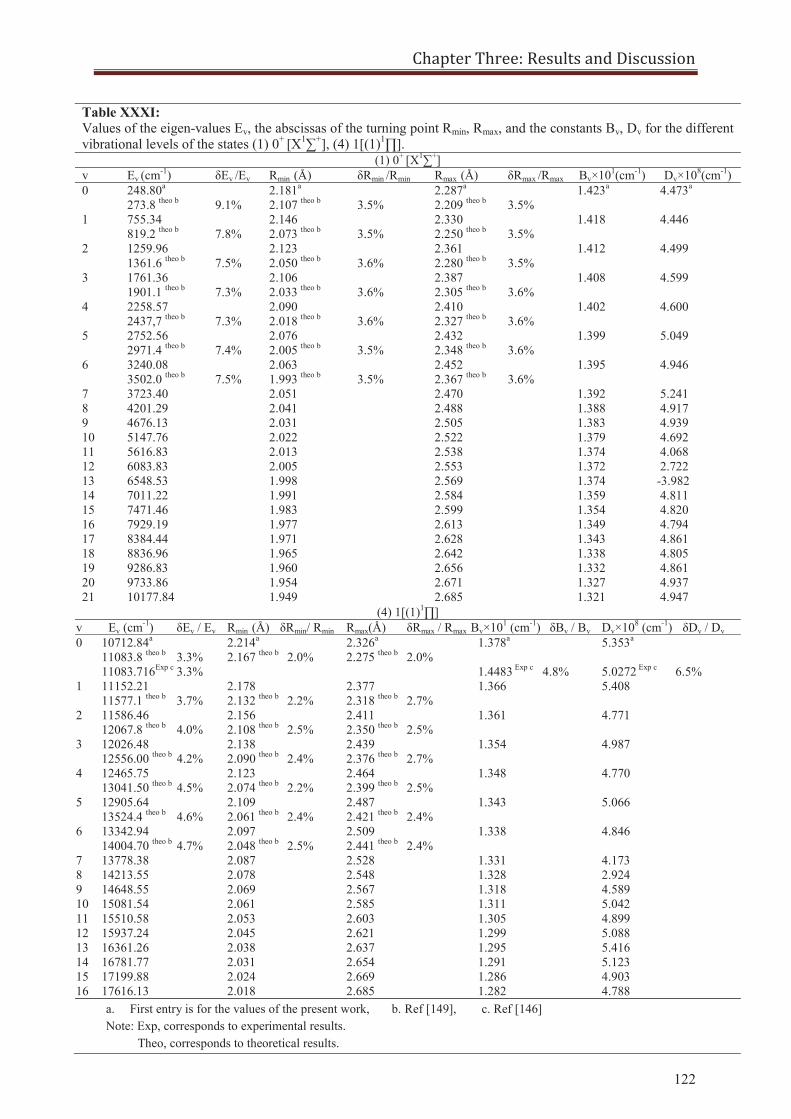
Chapter Three: Results and Discussion
122
Table XXXI: Values of the eigen-values Ev, the abscissas of the turning point Rmin, Rmax, and the constants Bv, Dv for the different vibrational levels of the states (1) 0+ [X1∑+], (4) 1[(1)1∏].
(1) 0+ [X1∑+] v Ev (cm-1) δEv /Ev Rmin
(Å) δRmin /Rmin Rmax (Å) δRmax /Rmax Bv×101(cm-1) Dv×108(cm-1)
0 248.80a
273.8 theo b 9.1%
2.181a
2.107 theo b 3.5%
2.287a
2.209 theo b 3.5%
1.423a 4.473a
1 755.34 819.2 theo b
7.8%
2.146 2.073 theo b
3.5%
2.330 2.250 theo b
3.5%
1.418 4.446
2 1259.96 1361.6 theo b
7.5%
2.123 2.050 theo b
3.6%
2.361 2.280 theo b
3.5%
1.412 4.499
3 1761.36 1901.1 theo b
7.3%
2.106 2.033 theo b
3.6%
2.387 2.305 theo b
3.6%
1.408 4.599
4 2258.57 2437,7 theo b
7.3%
2.090 2.018 theo b
3.6%
2.410 2.327 theo b
3.6%
1.402 4.600
5 2752.56 2971.4 theo b
7.4%
2.076 2.005 theo b
3.5%
2.432 2.348 theo b
3.6%
1.399 5.049
6 3240.08 3502.0 theo b
7.5%
2.063 1.993 theo b
3.5%
2.452 2.367 theo b
3.6%
1.395 4.946
7 3723.40 2.051 2.470 1.392 5.241 8 4201.29 2.041 2.488 1.388 4.917 9 4676.13 2.031 2.505 1.383 4.939 10 5147.76 2.022 2.522 1.379 4.692 11 5616.83 2.013 2.538 1.374 4.068 12 6083.83 2.005 2.553 1.372 2.722 13 6548.53 1.998 2.569 1.374 -3.982 14 7011.22 1.991 2.584 1.359 4.811 15 7471.46 1.983 2.599 1.354 4.820 16 7929.19 1.977 2.613 1.349 4.794 17 8384.44 1.971 2.628 1.343 4.861 18 8836.96 1.965 2.642 1.338 4.805 19 9286.83 1.960 2.656 1.332 4.861 20 9733.86 1.954 2.671 1.327 4.937 21 10177.84 1.949 2.685 1.321 4.947
(4) 1[(1)1∏] v Ev (cm-1) δEv / Ev Rmin
(Å) δRmin/ Rmin Rmax(Å) δRmax / Rmax Bv×101 (cm-1) δBv / Bv Dv×108 (cm-1) δDv / Dv 0 10712.84a
11083.8 theo b
11083.716Exp c 3.3% 3.3%
2.214a
2.167 theo b 2.0%
2.326a
2.275 theo b 2.0%
1.378a
1.4483 Exp c
4.8%
5.353a
5.0272 Exp c
6.5% 1 11152.21
11577.1 theo b 3.7% 2.178 2.132 theo b
2.2%
2.377 2.318 theo b
2.7%
1.366 5.408
2 11586.46 12067.8 theo b 4.0%
2.156 2.108 theo b
2.5%
2.411 2.350 theo b
2.5%
1.361 4.771
3 12026.48 12556.00 theo b 4.2%
2.138 2.090 theo b
2.4%
2.439 2.376 theo b
2.7%
1.354 4.987
4 12465.75 13041.50 theo b 4.5%
2.123 2.074 theo b
2.2%
2.464 2.399 theo b
2.5%
1.348 4.770
5 12905.64 13524.4 theo b 4.6%
2.109 2.061 theo b
2.4%
2.487 2.421 theo b
2.4%
1.343 5.066
6 13342.94 14004.70 theo b 4.7%
2.097 2.048 theo b
2.5%
2.509 2.441 theo b
2.4%
1.338 4.846
7 13778.38 2.087 2.528 1.331 4.173 8 14213.55 2.078 2.548 1.328 2.924 9 14648.55 2.069 2.567 1.318 4.589 10 15081.54 2.061 2.585 1.311 5.042 11 15510.58 2.053 2.603 1.305 4.899 12 15937.24 2.045 2.621 1.299 5.088 13 16361.26 2.038 2.637 1.295 5.416 14 16781.77 2.031 2.654 1.291 5.123 15 17199.88 2.024 2.669 1.286 4.903 16 17616.13 2.018 2.685 1.282 4.788
a. First entry is for the values of the present work, b. Ref [149], c. Ref [146] Note: Exp, corresponds to experimental results. Theo, corresponds to theoretical results.
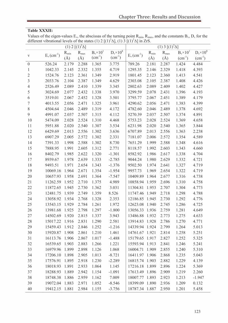
Chapter Three: Results and Discussion
123
Table XXXII: Values of the eigen-values Ev, the abscissas of the turning point Rmin, Rmax, and the constants Bv, Dv for the different vibrational levels of the states (1) 2 [(1)3∆], (1) 3 [(1)3∆] in ZrS.
(1) 2 [(1)3∆] (1) 3 [(1)3∆]
v Ev (cm-1) Rmin
(Å) Rmax
(Å) Bv×101 (cm-1)
Dv×108 (cm-1) Ev (cm-1)
Rmin
(Å) Rmax
(Å) Bv×101 (cm-1)
Dv×108 (cm-1)
0 526.24 2.179 2.288 1.365 3.775 789.26 2.181 2.287 1.424 4.484 1 1042.33 2.145 2.332 1.355 4.719 1295.35 2.146 2.329 1.418 4.393 2 1524.76 2.123 2.361 1.349 2.919 1801.45 2.123 2.360 1.413 4.541 3 2033.76 2.104 2.387 1.349 4.629 2303.08 2.105 2.387 1.408 4.426 4 2526.49 2.089 2.410 1.339 3.345 2802.63 2.089 2.409 1.402 4.427 5 3024.69 2.077 2.432 1.338 3.970 3299.59 2.078 2.431 1.396 4.193 6 3519.01 2.067 2.452 1.328 3.501 3795.77 2.067 2.451 1.389 4.179 7 4013.55 2.056 2.471 1.325 3.961 4290.62 2.056 2.471 1.383 4.399 8 4504.64 2.046 2.489 1.319 4.172 4782.60 2.046 2.489 1.378 4.692 9 4991.07 2.037 2.507 1.315 4.112 5270.39 2.037 2.507 1.374 4.891 10 5474.09 2.028 2.524 1.310 4.468 5753.23 2.028 2.524 1.369 4.658 11 5951.88 2.020 2.540 1.307 3.534 6231.98 2.020 2.540 1.365 3.844 12 6429.69 2.013 2.556 1.302 3.636 6707.89 2.013 2.556 1.363 2.238 13 6907.29 2.005 2.572 1.302 2.331 7181.07 2.006 2.572 1.354 4.589 14 7391.33 1.998 2.588 1.302 8.730 7651.29 1.999 2.588 1.348 4.616 15 7888.95 1.991 2.605 1.312 2.771 8118.57 1.992 2.603 1.343 4.660 16 8402.79 1.985 2.622 1.320 -1.301 8582.92 1.986 2.617 1.338 4.704 17 8939.67 1.978 2.639 1.333 -2.785 9044.24 1.980 2.629 1.332 4.721 18 9493.51 1.971 2.654 1.343 -1.376 9502.50 1.974 2.641 1.327 4.719 19 10069.16 1.964 2.671 1.354 -1.954 9957.73 1.969 2.654 1.322 4.719 20 10657.93 1.958 2.691 1.364 -7.547 10409.89 1.964 2.677 1.316 4.738 21 11262.59 1.952 2.710 1.375 4.989 10858.94 1.959 2.696 1.310 4.758 22 11872.65 1.945 2.730 1.362 3.031 11304.81 1.953 2.707 1.304 4.773 23 12481.75 1.939 2.749 1.359 8.526 11747.46 1.949 2.718 1.298 4.788 24 13058.92 1.934 2.768 1.328 2.353 12186.85 1.945 2.730 1.292 4.776 25 13543.15 1.929 2.784 1.261 1.972 12623.08 1.940 2.745 1.286 4.725 26 13981.68 1.925 2.798 1.297 -1.800 13056.33 1.936 2.759 1.281 4.649 27 14502.69 1.920 2.815 1.337 3.943 13486.88 1.932 2.773 1.275 4.633 28 15017.22 1.916 2.831 1.290 2.581 13914.83 1.928 2.786 1.270 4.771 29 15459.43 1.912 2.846 1.252 -1.216 14339.94 1.924 2.799 1.264 5.013 30 15920.87 1.908 2.861 1.210 1.461 14761.67 1.921 2.814 1.258 5.251 31 16113.76 1.906 2.867 1.017 -1.488 15179.65 1.917 2.827 1.252 5.325 32 16539.65 1.903 2.883 1.266 1.221 15593.94 1.913 2.841 1.246 5.241 33 16979.96 1.899 2.898 1.126 1.068 16004.71 1.909 2.855 1.240 5.310 34 17206.10 1.898 2.905 1.013 -8.721 16411.97 1.906 2.868 1.235 5.043 35 17576.91 1.895 2.918 1.230 -2.289 16815.74 1.903 2.882 1.229 4.139 36 18018.93 1.891 2.933 1.064 1.145 17216.18 1.899 2.896 1.224 5.369 37 18288.93 1.889 2.942 1.154 -1.091 17613.49 1.896 2.909 1.219 2.260 38 18748.38 1.886 2.959 1.162 7.009 18007.77 1.893 2.923 1.213 -1.947 39 19072.04 1.883 2.971 1.052 -8.546 18399.09 1.890 2.936 1.209 0.132 40 19412.15 1.881 2.984 1.155 -3.756 18787.34 1.887 2.950 1.201 5.458
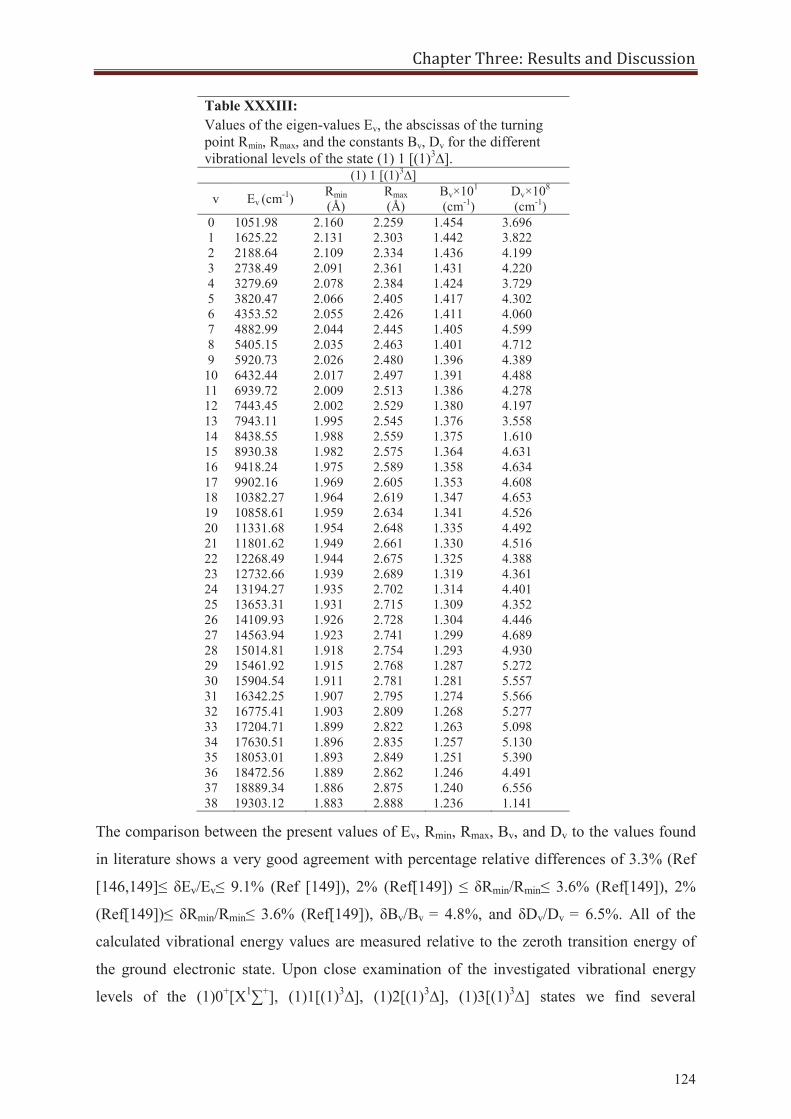
Chapter Three: Results and Discussion
124
Table XXXIII: Values of the eigen-values Ev, the abscissas of the turning point Rmin, Rmax, and the constants Bv, Dv for the different vibrational levels of the state (1) 1 [(1)3∆].
(1) 1 [(1)3∆]
v Ev (cm-1) Rmin (Å)
Rmax (Å)
Bv×101 (cm-1)
Dv×108 (cm-1)
0 1051.98 2.160 2.259 1.454 3.696 1 1625.22 2.131 2.303 1.442 3.822 2 2188.64 2.109 2.334 1.436 4.199 3 2738.49 2.091 2.361 1.431 4.220 4 3279.69 2.078 2.384 1.424 3.729 5 3820.47 2.066 2.405 1.417 4.302 6 4353.52 2.055 2.426 1.411 4.060 7 4882.99 2.044 2.445 1.405 4.599 8 5405.15 2.035 2.463 1.401 4.712 9 5920.73 2.026 2.480 1.396 4.389 10 6432.44 2.017 2.497 1.391 4.488 11 6939.72 2.009 2.513 1.386 4.278 12 7443.45 2.002 2.529 1.380 4.197 13 7943.11 1.995 2.545 1.376 3.558 14 8438.55 1.988 2.559 1.375 1.610 15 8930.38 1.982 2.575 1.364 4.631 16 9418.24 1.975 2.589 1.358 4.634 17 9902.16 1.969 2.605 1.353 4.608 18 10382.27 1.964 2.619 1.347 4.653 19 10858.61 1.959 2.634 1.341 4.526 20 11331.68 1.954 2.648 1.335 4.492 21 11801.62 1.949 2.661 1.330 4.516 22 12268.49 1.944 2.675 1.325 4.388 23 12732.66 1.939 2.689 1.319 4.361 24 13194.27 1.935 2.702 1.314 4.401 25 13653.31 1.931 2.715 1.309 4.352 26 14109.93 1.926 2.728 1.304 4.446 27 14563.94 1.923 2.741 1.299 4.689 28 15014.81 1.918 2.754 1.293 4.930 29 15461.92 1.915 2.768 1.287 5.272 30 15904.54 1.911 2.781 1.281 5.557 31 16342.25 1.907 2.795 1.274 5.566 32 16775.41 1.903 2.809 1.268 5.277 33 17204.71 1.899 2.822 1.263 5.098 34 17630.51 1.896 2.835 1.257 5.130 35 18053.01 1.893 2.849 1.251 5.390 36 18472.56 1.889 2.862 1.246 4.491 37 18889.34 1.886 2.875 1.240 6.556 38 19303.12 1.883 2.888 1.236 1.141
The comparison between the present values of Ev, Rmin, Rmax, Bv, and Dv to the values found
in literature shows a very good agreement with percentage relative differences of 3.3% (Ref
[146,149]≤ δEv/Ev≤ 9.1% (Ref [149]), 2% (Ref[149]) ≤ δRmin/Rmin≤ 3.6% (Ref[149]), 2%
(Ref[149])≤ δRmin/Rmin≤ 3.6% (Ref[149]), δBv/Bv = 4.8%, and δDv/Dv = 6.5%. All of the
calculated vibrational energy values are measured relative to the zeroth transition energy of
the ground electronic state. Upon close examination of the investigated vibrational energy
levels of the (1)0+[X1∑+], (1)1[(1)3∆], (1)2[(1)3∆], (1)3[(1)3∆] states we find several
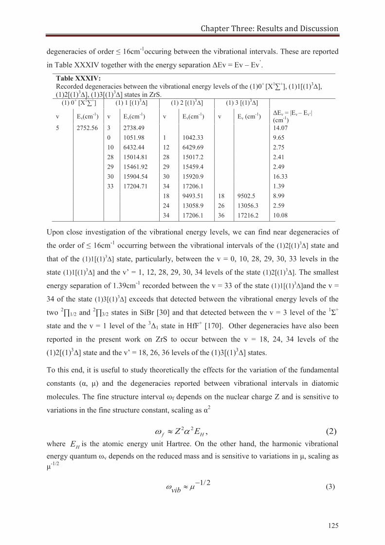
Chapter Three: Results and Discussion
125
degeneracies of order ≤ 16cm-1occuring between the vibrational intervals. These are reported
in Table XXXIV together with the energy separation ΔEv = Ev – Ev’.
Table XXXIV: Recorded degeneracies between the vibrational energy levels of the (1)0+ [X1∑+], (1)1[(1)3∆], (1)2[(1)3∆], (1)3[(1)3∆] states in ZrS.
(1) 0+ [X1∑+] (1) 1 [(1)3∆] (1) 2 [(1)3∆] (1) 3 [(1)3∆]
v Ev(cm-1) v Ev(cm-1) v Ev(cm-1) v Ev (cm-1) ΔEv = |Ev – Ev’| (cm-1)
5 2752.56 3 2738.49 14.07 0 1051.98 1 1042.33 9.65 10 6432.44 12 6429.69 2.75 28 15014.81 28 15017.2 2.41 29 15461.92 29 15459.4 2.49 30 15904.54 30 15920.9 16.33 33 17204.71 34 17206.1 1.39 18 9493.51 18 9502.5 8.99 24 13058.9 26 13056.3 2.59 34 17206.1 36 17216.2 10.08
Upon close investigation of the vibrational energy levels, we can find near degeneracies of
the order of ≤ 16cm-1 occurring between the vibrational intervals of the (1)2[(1)3∆] state and
that of the (1)1[(1)3∆] state, particularly, between the v = 0, 10, 28, 29, 30, 33 levels in the
state (1)1[(1)3∆] and the v’ = 1, 12, 28, 29, 30, 34 levels of the state (1)2[(1)3∆]. The smallest
energy separation of 1.39cm-1 recorded between the v = 33 of the state (1)1[(1)3∆]and the v =
34 of the state (1)3[(1)3∆] exceeds that detected between the vibrational energy levels of the
two 2∏1/2 and 2∏3/2 states in SiBr [30] and that detected between the v = 3 level of the 1Σ+
state and the v = 1 level of the 3Δ1 state in HfF+ [170]. Other degeneracies have also been
reported in the present work on ZrS to occur between the v = 18, 24, 34 levels of the
(1)2[(1)3∆] state and the v’ = 18, 26, 36 levels of the (1)3[(1)3∆] states.
To this end, it is useful to study theoretically the effects for the variation of the fundamental
constants (α, μ) and the degeneracies reported between vibrational intervals in diatomic
molecules. The fine structure interval ωf depends on the nuclear charge Z and is sensitive to
variations in the fine structure constant, scaling as α2
2 2 , (2)f HZ Ewhere HE is the atomic energy unit Hartree. On the other hand, the harmonic vibrational energy quantum ωv depends on the reduced mass and is sensitive to variations in μ, scaling as μ-1/2
1/2 (3)vib
Chapter Three: Results and Discussion
126
Therefore, we obtain an equation for the lines where we can expect approximate cancellation
between the fine structure and vibrational intervals:
1/ 2 0 , 0,1,2, (4)v vf vib
Using equations (2 – 4) we could find the relation between the variation of the transition
frequency ω and the variation in the fundamental constants α and μ
1/ 2.
1 1 2 2 (5)
2 2v
Kf vib
The enhancement factor K = ωf / ω determines the relative frequency shift for a given change
in the fundamental constants. Large values of factor K ≈ 103 - 105 hint at potentially favorable
cases for making experiments, because it is usually preferable to have larger relative shifts
[30]. Because the number of molecules is finite we cannot have ω = 0 exactly. However, a
large number of molecules have ω / ωf <<1 and |K| >> 1 [170]. Moreover, an additional fine
tuning may be achieved by including Ω doublet and hyperfine components. Note that ω is
sensitive to the variation of two most important dimensionless parameters of the Standard
Model. The first parameter α, determines the strength of the electroweak interactions [171].
The second parameter, μ = mp/me, is related to the weak mass scale and strong interaction
scale. The electron mass is proportional to the vacuum expectation value of the Higgs field
which also determines the masses of all fundamental particles [171]. The proton mass is
proportional to another fundamental parameter, the quantum chromodynamics scale ΛQCD
[171]. Therefore, we are speaking about the relative variation of a very important
dimensionless fundamental parameters of the Standard Model.
The near degeneracies detected in Table XXXIV between the vibrational intervals of the
(1)0+[X1∑+], (1)1[(1)3∆], (1)2[(1)3∆], and (1)3[(1)3∆] states can all be used to search for any
variations in the fundamental constants of the Standard Model α and μ, especially those
which can be observed spectroscopically. As an example we shall apply equation (4) on the v
= 0 vibrational level of the (1)1[(1)3∆] state and the v’ = 1 level of the (1)2[(1)3∆] state
2 13 12 1'2 2
0 (6)e ev vT Twhere Te
Ω=2 and TeΩ=1 represent the transition energies at equilibrium of the (1)2[(1)3∆] and
(1)1[(1)3∆] states relative to the zero transition energy of the ground state. The other
constants ωvΩ=1 and ωv’
Ω=2 represent the vibrational harmonic frequencies of the two states
(1)1[(1)3∆] and (1)2[(1)3∆], respectively. Then by using equation (5), and by considering that
the fine structure interval ωf = TeΩ=2-Te
Ω=1 = 489.56cm-1 is the energy splitting occurring
between the v = 1 level in the (1)2[(1)3∆] state and the v = 0 level in the (1)1[(1)3∆] state.
Chapter Three: Results and Discussion
127
With ωv = 523.54cm-1 being the vibrational harmonic frequency of the higher (1)1[(1)3∆]
state, we get
979.12 , = (7)
then by assuming that 1510/ , which is equivalent to the experimental variation of α
from atomic spectra [165, 166], we obtain 12 1 210 2.935 10cm Hz . The estimated
line widths are on the order of 10-2 Hz. This is comparable to the accuracy, which is necessary
to reach sensitivity δα/α ≈10-15 of the best modern laboratory tests [167, 171]. Of course other
vibrational energy level degeneracies listed in Table XXXIV can also be used to measure any
variations in α, their line widths should be comparable to the line width calculated above. The
natural line widths on the order of 10-2 Hz obtained in the present work are identical to the
natural line widths calculated in Ref [171] for the molecules Cs2 and SiBr which were
suggested to be suitable for measuring α variations.
It is natural to search for any changes in α using measurements of the spin orbit splitting
within a specific fine structure multiplet of atoms, and indeed this method has been applied to
quasar atomic spectra by several groups [168, 173-175]. However, while this method is
appealing through its simplicity, it is possible to improve on its efficiency [168]. An order of
magnitude sensitivity gain can be achieved by comparing transition frequencies of heavy
atoms, ions or molecules [173, 176]. Other possibilities for measuring changes in α involve
studying transitions between accidentally degenerate levels in the same atom or molecule
[168]. Of course, there are many more possibilities in molecules where there are vibrational
and rotational structures. The relativistic corrections to the different energy levels are
different and can exceed the very small frequency corresponding to the transition between
degenerate states by many orders of magnitude, i.e., a tiny variation of α can change the
transition frequency significantly [168]. Since α variations have been measured from spectral
analysis of atoms and ions previously identified in quasar spectra, we suggest the inspection
for the spectra of the ZrS molecule in laboratory experiments and in cool S-type stars as a
mean to measure any possible variations of the fine structure constant. The detection of the
ZrS molecule in the spectra of three Mira variable stars, named RAnd, χCyg, and RCas [147],
further enhances this possibility. In fact, the vibrational band systems suggested to be suitable
for measuring α variations in the present work have been previously analyzed in the Kennan
bands of the three Mira variable stars [147]. We suggest the re-inspection of the Kennan
bands in the spectra of the stars RAnd, χCyg, and RCas as a mean to measure possible
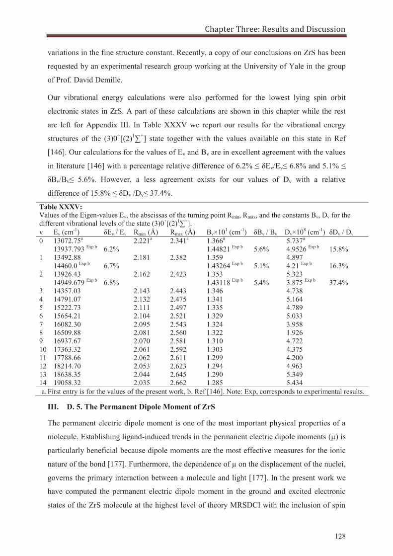
Chapter Three: Results and Discussion
128
variations in the fine structure constant. Recently, a copy of our conclusions on ZrS has been
requested by an experimental research group working at the University of Yale in the group
of Prof. David Demille.
Our vibrational energy calculations were also performed for the lowest lying spin orbit
electronic states in ZrS. A part of these calculations are shown in this chapter while the rest
are left for Appendix III. In Table XXXV we report our results for the vibrational energy
structures of the (3)0+[(2)1∑+] state together with the values available on this state in Ref
[146]. Our calculations for the values of Ev and Bv are in excellent agreement with the values
in literature [146] with a percentage relative difference of 6.2% ≤ δEv/Ev≤ 6.8% and 5.1% ≤
δBv/Bv≤ 5.6%. However, a less agreement exists for our values of Dv with a relative
difference of 15.8% ≤ δDv /Dv≤ 37.4%.
Table XXXV: Values of the Eigen-values Ev, the abscissas of the turning point Rmin, Rmax, and the constants Bv, Dv for the different vibrational levels of the state (3)0+[(2)1∑+]. v Ev (cm-1) δEv / Ev Rmin
(Å) Rmax (Å) Bv×101 (cm-1) δBv / Bv Dv×108 (cm-1) δDv / Dv
0 13072.75a
13937.793 Exp b 6.2%
2.221a 2.341a 1.366a
1.44821 Exp b 5.6%
5.737a
4.9526 Exp b 15.8%
1 13492.88 14460.0 Exp b
6.7%
2.181 2.382 1.359 1.43264 Exp b
5.1%
4.897 4.21 Exp b
16.3%
2 13926.43 14949.679 Exp b
6.8%
2.162 2.423 1.353 1.43118 Exp b
5.4%
5.323 3.875 Exp b
37.4%
3 14357.03 2.143 2.443 1.346 4.738 4 14791.07 2.132 2.475 1.341 5.164 5 15222.73 2.111 2.497 1.335 4.789 6 15654.21 2.104 2.521 1.329 5.033 7 16082.30 2.095 2.543 1.324 3.958 8 16509.88 2.081 2.560 1.322 1.926 9 16937.67 2.070 2.581 1.310 4.722 10 17363.32 2.061 2.592 1.303 4.375 11 17788.66 2.062 2.611 1.299 4.200 12 18214.70 2.053 2.623 1.294 4.963 13 18638.35 2.044 2.645 1.290 5.349 14 19058.32 2.035 2.662 1.285 5.434 a. First entry is for the values of the present work, b. Ref [146]. Note: Exp, corresponds to experimental results.
III. D. 5. The Permanent Dipole Moment of ZrS
The permanent electric dipole moment is one of the most important physical properties of a
molecule. Establishing ligand-induced trends in the permanent electric dipole moments (μ) is
particularly beneficial because dipole moments are the most effective measures for the ionic
nature of the bond [177]. Furthermore, the dependence of μ on the displacement of the nuclei,
governs the primary interaction between a molecule and light [177]. In the present work we
have computed the permanent electric dipole moment in the ground and excited electronic
states of the ZrS molecule at the highest level of theory MRSDCI with the inclusion of spin
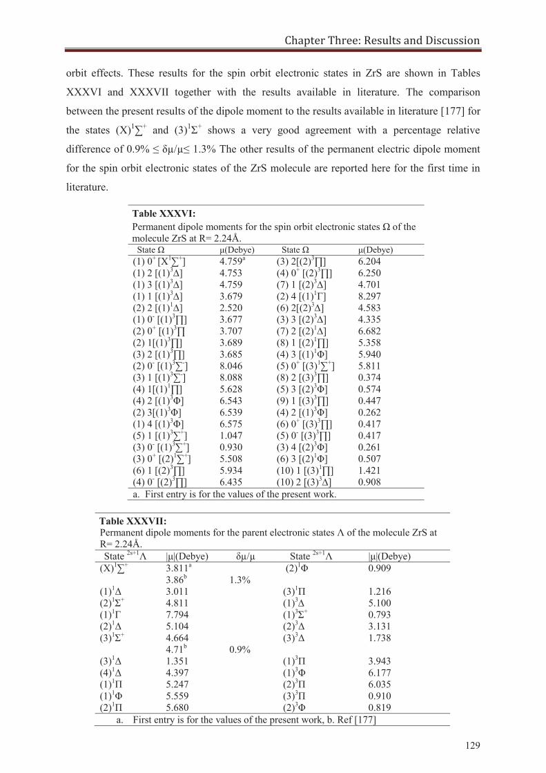
Chapter Three: Results and Discussion
129
orbit effects. These results for the spin orbit electronic states in ZrS are shown in Tables
XXXVI and XXXVII together with the results available in literature. The comparison
between the present results of the dipole moment to the results available in literature [177] for
the states (X)1∑+ and (3)1Σ+ shows a very good agreement with a percentage relative
difference of 0.9% ≤ δμ/μ≤ 1.3% The other results of the permanent electric dipole moment
for the spin orbit electronic states of the ZrS molecule are reported here for the first time in
literature.
Table XXXVI: Permanent dipole moments for the spin orbit electronic states Ω of the molecule ZrS at R= 2.24Å.
State Ω μ(Debye) State Ω μ(Debye) (1) 0+ [X1∑+] 4.759a (3) 2[(2)3∏] 6.204 (1) 2 [(1)3∆] 4.753 (4) 0+ [(2)3∏] 6.250 (1) 3 [(1)3∆] 4.759 (7) 1 [(2)3∆] 4.701 (1) 1 [(1)3∆] 3.679 (2) 4 [(1)1Γ] 8.297 (2) 2 [(1)1∆] 2.520 (6) 2[(2)3∆] 4.583 (1) 0- [(1)3∏] 3.677 (3) 3 [(2)3∆] 4.335 (2) 0+ [(1)3∏ 3.707 (7) 2 [(2)1∆] 6.682 (2) 1[(1)3∏] 3.689 (8) 1 [(2)1∏] 5.358 (3) 2 [(1)3∏] 3.685 (4) 3 [(1)1Φ] 5.940 (2) 0- [(1)3∑-] 8.046 (5) 0+ [(3)1∑+] 5.811 (3) 1 [(1)3∑-] 8.088 (8) 2 [(3)3∏] 0.374 (4) 1[(1)1∏] 5.628 (5) 3 [(2)3Φ] 0.574 (4) 2 [(1)3Φ] 6.543 (9) 1 [(3)3∏] 0.447 (2) 3[(1)3Φ] 6.539 (4) 2 [(1)3Φ] 0.262 (1) 4 [(1)3Φ] 6.575 (6) 0+ [(3)3∏] 0.417 (5) 1 [(1)3∑+] 1.047 (5) 0- [(3)3∏] 0.417 (3) 0- [(1)3∑+] 0.930 (3) 4 [(2)3Φ] 0.261 (3) 0+ [(2)1∑+] 5.508 (6) 3 [(2)1Φ] 0.507 (6) 1 [(2)3∏] 5.934 (10) 1 [(3)1∏] 1.421 (4) 0- [(2)3∏] 6.435 (10) 2 [(3)3∆] 0.908 a. First entry is for the values of the present work.
Table XXXVII: Permanent dipole moments for the parent electronic states Λ of the molecule ZrS at R= 2.24Å. State 2s+1Λ |μ|(Debye) δμ/μ State 2s+1Λ |μ|(Debye)
(X)1∑+ 3.811a
3.86b 1.3%
(2)1Φ 0.909
(1)1Δ 3.011 (3)1Π 1.216 (2)1Σ+ 4.811 (1)3∆ 5.100 (1)1Г 7.794 (1)3Σ+ 0.793 (2)1Δ 5.104 (2)3Δ 3.131 (3)1Σ+ 4.664
4.71b 0.9%
(3)3Δ 1.738
(3)1Δ 1.351 (1)3Π 3.943 (4)1Δ 4.397 (1)3Φ 6.177 (1)1Π 5.247 (2)3Π 6.035 (1)1Φ 5.559 (3)3Π 0.910 (2)1Π 5.680 (2)3Φ 0.819
a. First entry is for the values of the present work, b. Ref [177]
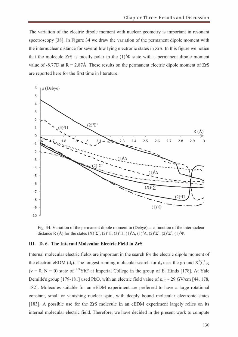
Chapter Three: Results and Discussion
130
The variation of the electric dipole moment with nuclear geometry is important in resonant
spectroscopy [38]. In Figure 34 we draw the variation of the permanent dipole moment with
the internuclear distance for several low lying electronic states in ZrS. In this figure we notice
that the molecule ZrS is mostly polar in the (1)3Φ state with a permanent dipole moment
value of -8.77D at R = 2.87Å. These results on the permanent electric dipole moment of ZrS
are reported here for the first time in literature.
III. D. 6. The Internal Molecular Electric Field in ZrS
Internal molecular electric fields are important in the search for the electric dipole moment of
the electron eEDM (de). The longest running molecular search for de uses the ground X2∑+1/2
(v = 0, N = 0) state of 174YbF at Imperial College in the group of E. Hinds [178]. At Yale
Demille's group [179-181] used PbO, with an electric field value of εeff ~ 29 GV/cm [44, 178,
182]. Molecules suitable for an eEDM experiment are preferred to have a large rotational
constant, small or vanishing nuclear spin, with deeply bound molecular electronic states
[183]. A possible use for the ZrS molecule in an eEDM experiment largely relies on its
internal molecular electric field. Therefore, we have decided in the present work to compute
-10
-9
-8
-7
-6
-5
-4
-3
-2
-1
0
1
2
3
4
5
6
1.6 1.7 1.8 1.9 2 2.1 2.2 2.3 2.4 2.5 2.6 2.7 2.8 2.9 3
(X)1∑
(1)3∆
(1)1Δ
(1)3Φ
(2)3Π
(3)3Π (2)3Σ+
(2)1Σ+
R (Å)
μ (Debye)
Fig. 34. Variation of the permanent dipole moment in (Debye) as a function of the internuclear distance R (Å) for the states (X)1Σ+, (2)3Π, (3)3Π, (1)1Δ, (1)3Δ, (2)1Σ+, (2)3Σ+, (1)3Φ.
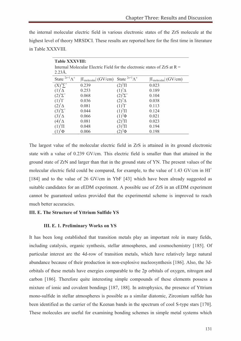
Chapter Three: Results and Discussion
131
the internal molecular electric field in various electronic states of the ZrS molecule at the
highest level of theory MRSDCI. These results are reported here for the first time in literature
in Table XXXVIII.
The largest value of the molecular electric field in ZrS is attained in its ground electronic
state with a value of 0.239 GV/cm. This electric field is smaller than that attained in the
ground state of ZrN and larger than that in the ground state of YN. The present values of the
molecular electric field could be compared, for example, to the value of 1.43 GV/cm in HI+
[184] and to the value of 26 GV/cm in YbF [43] which have been already suggested as
suitable candidates for an eEDM experiment. A possible use of ZrS in an eEDM experiment
cannot be guaranteed unless provided that the experimental scheme is improved to reach
much better accuracies.
III. E. The Structure of Yttrium Sulfide YS
III. E. 1. Preliminary Works on YS
It has been long established that transition metals play an important role in many fields,
including catalysis, organic synthesis, stellar atmospheres, and cosmochemistry [185]. Of
particular interest are the 4d-row of transition metals, which have relatively large natural
abundance because of their production in non-explosive nucleosynthesis [186]. Also, the 3d-
orbitals of these metals have energies comparable to the 2p orbitals of oxygen, nitrogen and
carbon [186]. Therefore quite interesting simple compounds of these elements possess a
mixture of ionic and covalent bondings [187, 188]. In astrophysics, the presence of Yttrium
mono-sulfide in stellar atmospheres is possible as a similar diatomic, Zirconium sulfide has
been identified as the carrier of the Keenan bands in the spectrum of cool S-type stars [170].
These molecules are useful for examining bonding schemes in simple metal systems which
Table XXXVIII: Internal Molecular Electric Field for the electronic states of ZrS at R = 2.23Å. State 2s+1Λ± |Emolecular| (GV/cm) State 2s+1Λ± |Emolecular| (GV/cm) (X)1∑+ 0.239 (2)1Π 0.023 (1)1Δ 0.253 (1)3∆ 0.189 (2)1Σ+ 0.068 (2)3Σ+ 0.104 (1)1Г 0.036 (2)3Δ 0.038 (2)1Δ 0.081 (1)3Г 0.113 (3)1Σ+ 0.044 (1)3Π 0.124 (3)1Δ 0.066 (1)3Φ 0.021 (4)1Δ 0.081 (2)3Π 0.023 (1)1Π 0.048 (3)3Π 0.194 (1)1Φ 0.006 (2)3Φ 0.198
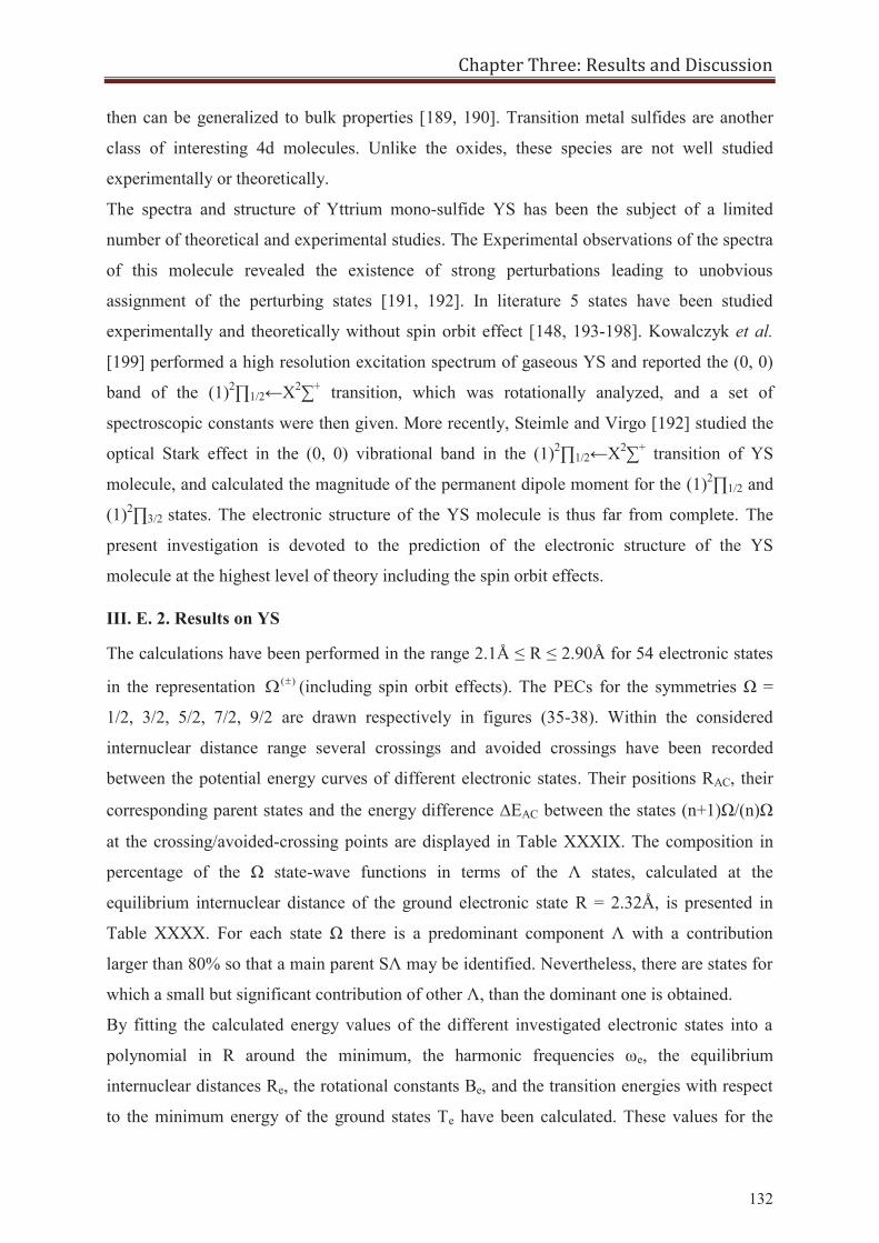
Chapter Three: Results and Discussion
132
then can be generalized to bulk properties [189, 190]. Transition metal sulfides are another
class of interesting 4d molecules. Unlike the oxides, these species are not well studied
experimentally or theoretically.
The spectra and structure of Yttrium mono-sulfide YS has been the subject of a limited
number of theoretical and experimental studies. The Experimental observations of the spectra
of this molecule revealed the existence of strong perturbations leading to unobvious
assignment of the perturbing states [191, 192]. In literature 5 states have been studied
experimentally and theoretically without spin orbit effect [148, 193-198]. Kowalczyk et al.
[199] performed a high resolution excitation spectrum of gaseous YS and reported the (0, 0)
band of the (1)2∏1/2←Χ2∑+ transition, which was rotationally analyzed, and a set of
spectroscopic constants were then given. More recently, Steimle and Virgo [192] studied the
optical Stark effect in the (0, 0) vibrational band in the (1)2∏1/2←Χ2∑+ transition of YS
molecule, and calculated the magnitude of the permanent dipole moment for the (1)2∏1/2 and
(1)2∏3/2 states. The electronic structure of the YS molecule is thus far from complete. The
present investigation is devoted to the prediction of the electronic structure of the YS
molecule at the highest level of theory including the spin orbit effects.
III. E. 2. Results on YS
The calculations have been performed in the range 2.1Å ≤ R ≤ 2.90Å for 54 electronic states
in the representation )( (including spin orbit effects). The PECs for the symmetries Ω =
1/2, 3/2, 5/2, 7/2, 9/2 are drawn respectively in figures (35-38). Within the considered
internuclear distance range several crossings and avoided crossings have been recorded
between the potential energy curves of different electronic states. Their positions RAC, their
corresponding parent states and the energy difference EAC between the states (n+1)Ω/(n)Ω
at the crossing/avoided-crossing points are displayed in Table XXXIX. The composition in
percentage of the Ω state-wave functions in terms of the Λ states, calculated at the
equilibrium internuclear distance of the ground electronic state R = 2.32Å, is presented in
Table XXXX. For each state Ω there is a predominant component Λ with a contribution
larger than 80% so that a main parent SΛ may be identified. Nevertheless, there are states for
which a small but significant contribution of other Λ, than the dominant one is obtained.
By fitting the calculated energy values of the different investigated electronic states into a
polynomial in R around the minimum, the harmonic frequencies ωe, the equilibrium
internuclear distances Re, the rotational constants Be, and the transition energies with respect
to the minimum energy of the ground states Te have been calculated. These values for the
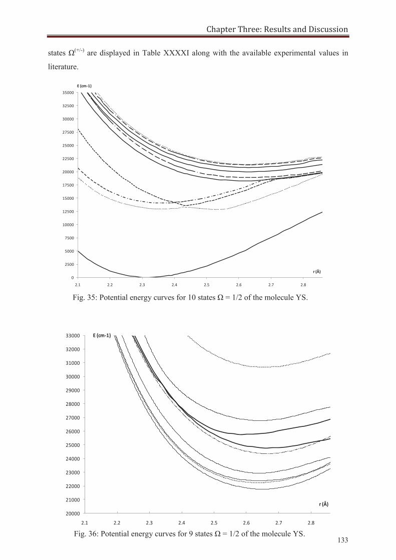
Chapter Three: Results and Discussion
133
states Ω(+/-) are displayed in Table XXXXI along with the available experimental values in
literature.
0
2500
5000
7500
10000
12500
15000
17500
20000
22500
25000
27500
30000
32500
35000
2.1 2.2 2.3 2.4 2.5 2.6 2.7 2.8
E (cm-1)
r (Å)
20000
21000
22000
23000
24000
25000
26000
27000
28000
29000
30000
31000
32000
33000
2.1 2.2 2.3 2.4 2.5 2.6 2.7 2.8
E (cm-1)
r (Å)
Fig. 36: Potential energy curves for 9 states Ω = 1/2 of the molecule YS.
Fig. 35: Potential energy curves for 10 states Ω = 1/2 of the molecule YS.
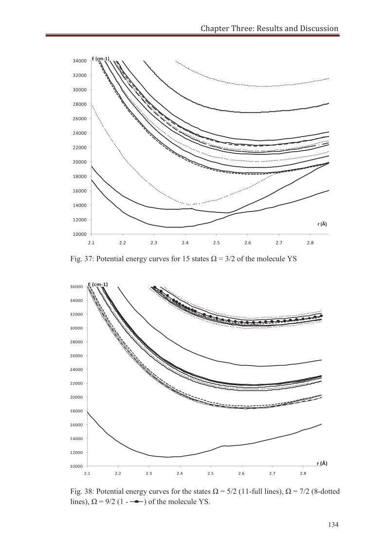
Chapter Three: Results and Discussion
134
Fig. 37: Potential energy curves for 15 states Ω = 3/2 of the molecule YS
10000
12000
14000
16000
18000
20000
22000
24000
26000
28000
30000
32000
34000
36000
2.1 2.2 2.3 2.4 2.5 2.6 2.7 2.8
E (cm-1)
r (Å)
Fig. 38: Potential energy curves for the states Ω = 5/2 (11-full lines), Ω = 7/2 (8-dotted lines), Ω = 9/2 (1 - ) of the molecule YS.
10000
12000
14000
16000
18000
20000
22000
24000
26000
28000
30000
32000
34000
2.1 2.2 2.3 2.4 2.5 2.6 2.7 2.8
E (cm-1)
r (Å)
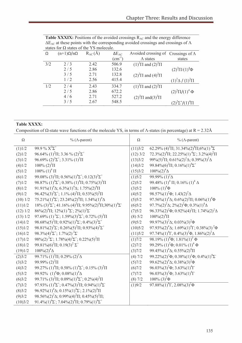
Chapter Three: Results and Discussion
135
Table XXXIX: Positions of the avoided crossings RAC and the energy difference ΔEAC at these points with the corresponding avoided crossings and crossings of Λ states for Ω states of the YS molecule. Ω (n+1)Ω/nΩ RAC (Å) ΔEAC
(cm-1) Avoided crossing of
states Crossings of
states 3/2 2 / 3
2 / 5 3 / 5 1 / 2
2.42 2.86 2.71 2.56
506.9 132.6 132.8 415.4
(1)2 and (2)2
(2)2 and (4)2
(2)2 /(1)4
(1)2 / (1)2
1/2 2 / 4 2 / 5 4 / 6 3 / 5
2.43 2.86 2.71 2.67
334.7 672.2 527.2 548.5
(1)2 and (2)2
(2)2 and(3)2
(2)2 /(1)4
(2)2 +/(1)4
Table XXXX: Composition of Ω-state wave functions of the molecule YS, in terms of Λ-states (in percentage) at R = 2.32Å
Ω % (Λ-parent) Ω % (Λ-parent)
(1)1/2 99.9 % X2Σ+ (11)3/2 62.29% (4)2Π; 31.34%(2)4Π;6%(1) 4Σ (2)1/2 96.64% (1)2Π; 3.36 % (2)2Σ+ (12) 3/2 72.3%(2)4Π; 22.25%(1) 4Σ-; 3.2%(4)2Π (3)1/2 96.69% (2)2Σ+; 3.31% (1)2Π (13)3/2 99%(5)2Π; 0.61%(2)2Δ; 0.39%(3)2Δ (4)1/2 100% (2)2Π (14)3/2 99.84%(6)2Π; 0.16%(1)4Σ+
(5)1/2 100% (1)4 Π (15)3/2 100%(2)4Δ (6)1/2 99.08% (3)2Π; 0.56%(1)4Σ+; 0.12(3)2Σ+ (1)5/2 99.99% (1)2Δ (7)1/2 98.87% (1)4Σ+; 0.38% (1)4Π; 0.75%(3)2Π (2)5/2 99.48% (1)4 Π; 0.16% (1)4 Δ (8)1/2 91.91%(1)4Δ; 6.3%(1)4Δ; 1.75%(2)4Π (3)5/2 100% (1)4Φ (9)1/2 96.42%(3)2Σ+; 1.1% (4)2Π; 0.53%(5)2Π (4)5/2 98.57%(1)2Φ; 1.43(2)2Δ (10) 1/2 75.21%(1)4Σ-; 23.24%(2)4Π; 1.54%(1)4Δ (5)5/2 97.56%(1)4Δ; 0.6%(2)2Π; 0.06%(1)4Φ (11)1/2 18% (3)2Σ+; 41.16% (4)2Π; 9.95%(2)4Π;30%(1)4Σ- (6)5/2 97.7%(2)2Δ; 2%(2)2Φ; 0.3%(1)4Δ (12) 1/2 86%(2)4Π; 12%(1) 4Σ-; 2%(1)2Σ- (7)5/2 96.33%(2)2Φ; 0.92%(4)2Π; 1.74%(2)2Δ (13) 1/2 97.69% (1) 2Σ-; 1.59%(3)2Σ+; 0.72% (5)2Π (8) 5/2 100%(2)4Π (14)1/2 98.68%(5)2Π; 0.92%(1)4Σ-; 0.4%(3)2Σ+ (9)5/2 99.97%(3)2Δ; 0.03%(3)2Φ (15)1/2 98.81%(2)2Σ-; 0.26%(5)2Π; 0.93%(4)2Σ+ (10)5/2 97.93%(2)4Δ; 1.69%(1)4Γ; 0.38%(3) 2Φ (16)1/2 98.3%(4)2Σ+; 1.7%(2) 2Σ- (11)5/2 97.74%(1)4Γ, 0.4%(3)2Φ, 1.86%(2)2Δ (17)1/2 98%(2) 2Σ-; 1.78%(4)2Σ+; 0.22%(5)2Π (1)7/2 98.19% (1)4Φ; 1.81%(1)2 Φ (18)1/2 99.81%(6)2Π; 0.19(3)2 Σ+ (2)7/2 99.29% (1)2Φ; 0.01% (1)4 Φ (19)1/2 100%(2)4Δ (3)7/2 99.45%(1)4Δ; 0.55%(2)4Π (2)3/2 99.71% (1)2Π; 0.29% (2)2Δ (4) 7/2 99.22%(2)2Φ; 0.38%(1)2Φ; 0.4%(1)4Σ- (3)3/2 99.99% (2)2Π (5)7/2 99.62%(2)4Δ; 0.38%(3)2Φ (4)3/2 99.27% (1)4Π; 0.58% (1)4Σ+; 0.15% (3)2Π (6)7/2 96.03%(3)2Φ; 3.63%(1)4Γ (5)3/2 99.92% (1)4Φ; 0.08%(1)4Δ (7)7/2 96.03%(3)2Φ; 3.63%(1)4Γ (6)3/2 99.71% (3)2Π; 0.09%(1)4Σ+; 0.2%(4)2Π (8) 7/2 100% (3)2Φ (7)3/2 97.93% (1)4Σ+; 0.47%(3)2Π; 0.94%(1)4Σ- (1)9/2 97.88%(1)4Γ, 2.08%(3)2Φ (8)3/2 96.92%(1)4Δ; 0.15%(1)4Σ-; 2.1%(2)4Π (9)3/2 98.56%(2)2Δ; 0.99%(4)2Π; 0.45%(5)2Π; (10)3/2 91.4%(1)4Σ-; 7.04%(2)4Π; 0.79%(1)4Σ+
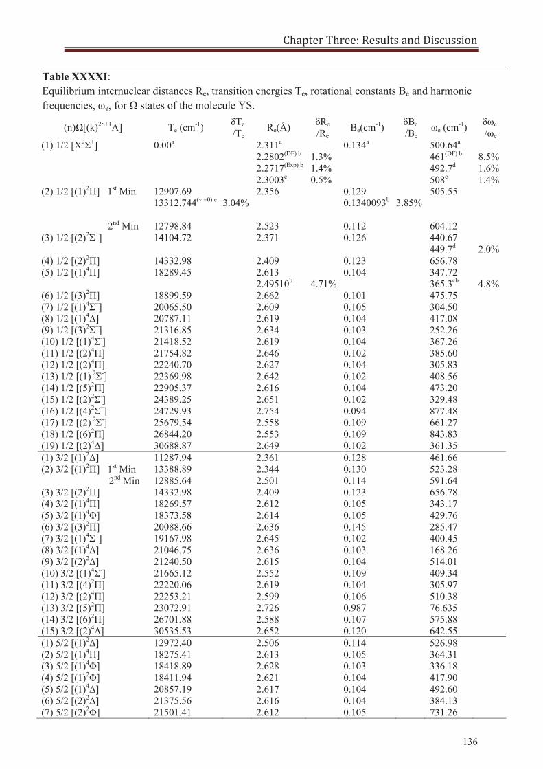
Chapter Three: Results and Discussion
136
Table XXXXI: Equilibrium internuclear distances Re, transition energies Te, rotational constants Be and harmonic frequencies, ωe, for Ω states of the molecule YS.
(n)Ω[(k)2S+1Λ] Te (cm-1) δTe
/Te Re(Å) δRe
/Re Be(cm-1) δBe
/Be ωe (cm-1) δωe
/ωe (1) 1/2 [X2Σ+] 0.00a 2.311a
2.2802(DF) b
2.2717(Exp) b
2.3003c
1.3% 1.4% 0.5%
0.134a 500.64a
461(DF) b
492.7d
508c
8.5% 1.6% 1.4%
(2) 1/2 [(1)2Π] 1st Min
2nd Min
12907.69 13312.744(v =0) e 12798.84
3.04%
2.356 2.523
0.129 0.1340093b
0.112
3.85%
505.55 604.12
(3) 1/2 [(2)2Σ+] 14104.72 2.371 0.126 440.67 449.7d
2.0%
(4) 1/2 [(2)2Π] 14332.98 2.409 0.123 656.78 (5) 1/2 [(1)4Π] 18289.45 2.613
2.49510b 4.71%
0.104 347.72 365.3cb
4.8%
(6) 1/2 [(3)2Π] 18899.59 2.662 0.101 475.75 (7) 1/2 [(1)4Σ+] 20065.50 2.609 0.105 304.50 (8) 1/2 [(1)4Δ] 20787.11 2.619 0.104 417.08 (9) 1/2 [(3)2Σ+] 21316.85 2.634 0.103 252.26 (10) 1/2 [(1)4Σ-] 21418.52 2.619 0.104 367.26 (11) 1/2 [(2)4Π] 21754.82 2.646 0.102 385.60 (12) 1/2 [(2)4Π] 22240.70 2.627 0.104 305.83 (13) 1/2 [(1) 2Σ-] 22369.98 2.642 0.102 408.56 (14) 1/2 [(5)2Π] 22905.37 2.616 0.104 473.20 (15) 1/2 [(2)2Σ-] 24389.25 2.651 0.102 329.48 (16) 1/2 [(4)2Σ+] 24729.93 2.754 0.094 877.48 (17) 1/2 [(2) 2Σ-] 25679.54 2.558 0.109 661.27 (18) 1/2 [(6)2Π] 26844.20 2.553 0.109 843.83 (19) 1/2 [(2)4Δ] 30688.87 2.649 0.102 361.35 (1) 3/2 [(1)2Δ] 11287.94 2.361 0.128 461.66 (2) 3/2 [(1)2Π] 1st Min
2nd Min 13388.89 12885.64
2.344 2.501
0.130 0.114
523.28 591.64
(3) 3/2 [(2)2Π] 14332.98 2.409 0.123 656.78 (4) 3/2 [(1)4Π] 18269.57 2.612 0.105 343.17 (5) 3/2 [(1)4Φ] 18373.58 2.614 0.105 429.76 (6) 3/2 [(3)2Π] 20088.66 2.636 0.145 285.47 (7) 3/2 [(1)4Σ+] 19167.98 2.645 0.102 400.45 (8) 3/2 [(1)4Δ] 21046.75 2.636 0.103 168.26 (9) 3/2 [(2)2Δ] 21240.50 2.615 0.104 514.01 (10) 3/2 [(1)4Σ-] 21665.12 2.552 0.109 409.34 (11) 3/2 [(4)2Π] 22220.06 2.619 0.104 305.97 (12) 3/2 [(2)4Π] 22253.21 2.599 0.106 510.38 (13) 3/2 [(5)2Π] 23072.91 2.726 0.987 76.635 (14) 3/2 [(6)2Π] 26701.88 2.588 0.107 575.88 (15) 3/2 [(2)4Δ] 30535.53 2.652 0.120 642.55 (1) 5/2 [(1)2Δ] 12972.40 2.506 0.114 526.98 (2) 5/2 [(1)4Π] 18275.41 2.613 0.105 364.31 (3) 5/2 [(1)4Φ] 18418.89 2.628 0.103 336.18 (4) 5/2 [(1)2Φ] 18411.94 2.621 0.104 417.90 (5) 5/2 [(1)4Δ] 20857.19 2.617 0.104 492.60 (6) 5/2 [(2)2Δ] 21375.56 2.616 0.104 384.13 (7) 5/2 [(2)2Φ] 21501.41 2.612 0.105 731.26
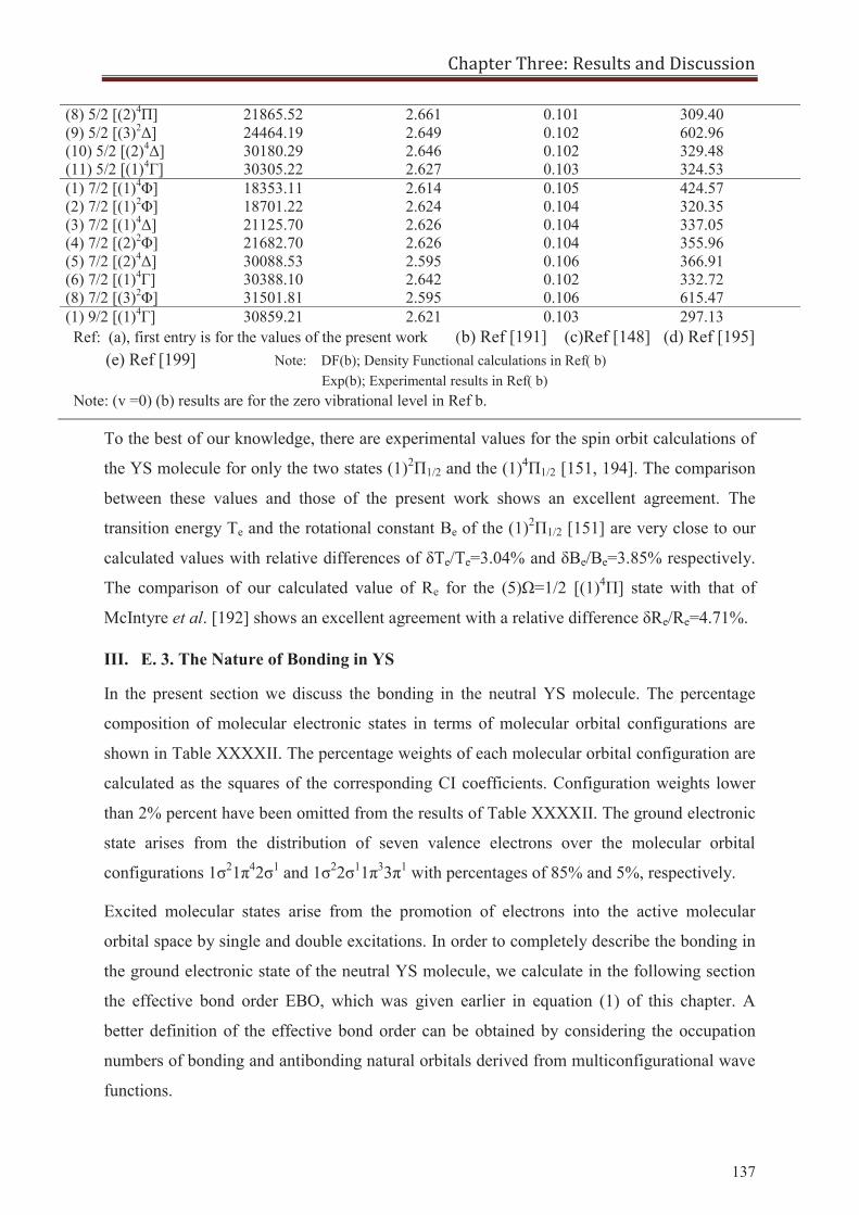
Chapter Three: Results and Discussion
137
To the best of our knowledge, there are experimental values for the spin orbit calculations of
the YS molecule for only the two states (1)2Π1/2 and the (1)4Π1/2 [151, 194]. The comparison
between these values and those of the present work shows an excellent agreement. The
transition energy Te and the rotational constant Be of the (1)2Π1/2 [151] are very close to our
calculated values with relative differences of δTe/Te=3.04% and δBe/Be=3.85% respectively.
The comparison of our calculated value of Re for the (5)Ω=1/2 [(1)4Π] state with that of
McIntyre et al. [192] shows an excellent agreement with a relative difference δRe/Re=4.71%.
III. E. 3. The Nature of Bonding in YS
In the present section we discuss the bonding in the neutral YS molecule. The percentage
composition of molecular electronic states in terms of molecular orbital configurations are
shown in Table XXXXII. The percentage weights of each molecular orbital configuration are
calculated as the squares of the corresponding CI coefficients. Configuration weights lower
than 2% percent have been omitted from the results of Table XXXXII. The ground electronic
state arises from the distribution of seven valence electrons over the molecular orbital
configurations 1σ21π42σ1 and 1σ22σ11π33π1 with percentages of 85% and 5%, respectively.
Excited molecular states arise from the promotion of electrons into the active molecular
orbital space by single and double excitations. In order to completely describe the bonding in
the ground electronic state of the neutral YS molecule, we calculate in the following section
the effective bond order EBO, which was given earlier in equation (1) of this chapter. A
better definition of the effective bond order can be obtained by considering the occupation
numbers of bonding and antibonding natural orbitals derived from multiconfigurational wave
functions.
(8) 5/2 [(2)4Π] 21865.52 2.661 0.101 309.40 (9) 5/2 [(3)2Δ] 24464.19 2.649 0.102 602.96 (10) 5/2 [(2)4Δ] 30180.29 2.646 0.102 329.48 (11) 5/2 [(1)4Γ] 30305.22 2.627 0.103 324.53 (1) 7/2 [(1)4Φ] 18353.11 2.614 0.105 424.57 (2) 7/2 [(1)2Φ] 18701.22 2.624 0.104 320.35 (3) 7/2 [(1)4Δ] 21125.70 2.626 0.104 337.05 (4) 7/2 [(2)2Φ] 21682.70 2.626 0.104 355.96 (5) 7/2 [(2)4Δ] 30088.53 2.595 0.106 366.91 (6) 7/2 [(1)4Γ] 30388.10 2.642 0.102 332.72 (8) 7/2 [(3)2Φ] 31501.81 2.595 0.106 615.47 (1) 9/2 [(1)4Γ] 30859.21 2.621 0.103 297.13 Ref: (a), first entry is for the values of the present work (b) Ref [191] (c)Ref [148] (d) Ref [195]
(e) Ref [199] Note: DF(b); Density Functional calculations in Ref( b) Exp(b); Experimental results in Ref( b) Note: (v =0) (b) results are for the zero vibrational level in Ref b.
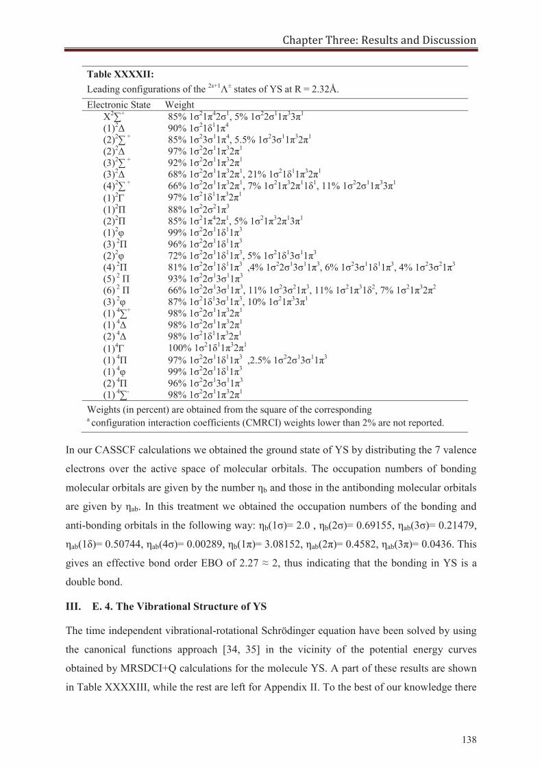
Chapter Three: Results and Discussion
138
Table XXXXII: Leading configurations of the 2s+1Λ± states of YS at R = 2.32Å. Electronic State Weight
X2∑+ 85% 1σ21π42σ1, 5% 1σ22σ11π33π1 (1)2Δ 90% 1σ21δ11π4 (2)2∑ + 85% 1σ23σ11π4, 5.5% 1σ23σ11π32π1 (2)2Δ 97% 1σ22σ11π32π1 (3)2∑ + 92% 1σ22σ11π32π1 (3)2Δ 68% 1σ22σ11π32π1, 21% 1σ21δ11π32π1 (4)2∑ + 66% 1σ22σ11π32π1, 7% 1σ21π32π11δ1, 11% 1σ22σ11π33π1 (1)2 97% 1σ21δ11π32π1 (1)2Π 88% 1σ22σ21π3 (2)2Π 85% 1σ21π42π1, 5% 1σ21π32π13π1 (1)2φ 99% 1σ22σ11δ11π3 (3) 2Π 96% 1σ22σ11δ11π3 (2)2φ 72% 1σ22σ11δ11π3, 5% 1σ21δ13σ11π3 (4) 2Π 81% 1σ22σ11δ11π3 ,4% 1σ22σ13σ11π3, 6% 1σ23σ11δ11π3, 4% 1σ23σ21π3 (5) 2 Π 93% 1σ22σ13σ11π3 (6) 2 Π 66% 1σ22σ13σ11π3, 11% 1σ23σ21π3, 11% 1σ21π31δ2, 7% 1σ21π32π2 (3) 2φ 87% 1σ21δ13σ11π3, 10% 1σ21π33π1 (1) 4∑+ 98% 1σ22σ11π32π1 (1) 4Δ 98% 1σ22σ11π32π1 (2) 4Δ 98% 1σ21δ11π32π1 (1)4 100% 1σ21δ11π32π1 (1) 4Π 97% 1σ22σ11δ11π3 ,2.5% 1σ22σ13σ11π3 (1) 4φ 99% 1σ22σ11δ11π3 (2) 4Π 96% 1σ22σ13σ11π3 (1) 4∑- 98% 1σ22σ11π32π1
Weights (in percent) are obtained from the square of the corresponding a configuration interaction coefficients (CMRCI) weights lower than 2% are not reported.
In our CASSCF calculations we obtained the ground state of YS by distributing the 7 valence
electrons over the active space of molecular orbitals. The occupation numbers of bonding
molecular orbitals are given by the number ηb and those in the antibonding molecular orbitals
are given by ηab. In this treatment we obtained the occupation numbers of the bonding and
anti-bonding orbitals in the following way: ηb(1σ)= 2.0 , ηb(2σ)= 0.69155, ηab(3σ)= 0.21479,
ηab(1δ)= 0.50744, ηab(4σ)= 0.00289, ηb(1π)= 3.08152, ηab(2π)= 0.4582, ηab(3π)= 0.0436. This
gives an effective bond order EBO of 2.27 ≈ 2, thus indicating that the bonding in YS is a
double bond.
III. E. 4. The Vibrational Structure of YS
The time independent vibrational-rotational Schrödinger equation have been solved by using
the canonical functions approach [34, 35] in the vicinity of the potential energy curves
obtained by MRSDCI+Q calculations for the molecule YS. A part of these results are shown
in Table XXXXIII, while the rest are left for Appendix II. To the best of our knowledge there
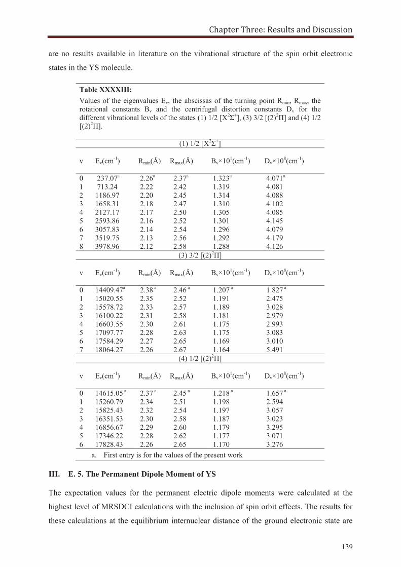
Chapter Three: Results and Discussion
139
are no results available in literature on the vibrational structure of the spin orbit electronic
states in the YS molecule.
Table XXXXIII: Values of the eigenvalues Ev, the abscissas of the turning point Rmin, Rmax, the rotational constants Bv and the centrifugal distortion constants Dv for the different vibrational levels of the states (1) 1/2 [X2Σ+], (3) 3/2 [(2)2Π] and (4) 1/2 [(2)2Π].
(1) 1/2 [X2Σ+]
v Ev(cm-1) Rmin(Å) Rmax(Å) Bv×101(cm-1) Dv×108(cm-1)
0 237.07a 2.26a 2.37a 1.323a 4.071a
1 713.24 2.22 2.42 1.319 4.081 2 1186.97 2.20 2.45 1.314 4.088 3 1658.31 2.18 2.47 1.310 4.102 4 2127.17 2.17 2.50 1.305 4.085 5 2593.86 2.16 2.52 1.301 4.145 6 3057.83 2.14 2.54 1.296 4.079 7 3519.75 2.13 2.56 1.292 4.179 8 3978.96 2.12 2.58 1.288 4.126
(3) 3/2 [(2)2Π]
v Ev(cm-1) Rmin(Å) Rmax(Å) Bv×101(cm-1) Dv×108(cm-1)
0 14409.47a 2.38 a 2.46 a 1.207 a 1.827 a 1 15020.55 2.35 2.52 1.191 2.475 2 15578.72 2.33 2.57 1.189 3.028 3 16100.22 2.31 2.58 1.181 2.979 4 16603.55 2.30 2.61 1.175 2.993 5 17097.77 2.28 2.63 1.175 3.083 6 17584.29 2.27 2.65 1.169 3.010 7 18064.27 2.26 2.67 1.164 5.491
(4) 1/2 [(2)2Π]
v Ev(cm-1) Rmin(Å) Rmax(Å) Bv×101(cm-1) Dv×108(cm-1)
0 14615.05 a 2.37 a 2.45 a 1.218 a 1.657 a 1 15260.79 2.34 2.51 1.198 2.594 2 15825.43 2.32 2.54 1.197 3.057 3 16351.53 2.30 2.58 1.187 3.023 4 16856.67 2.29 2.60 1.179 3.295 5 17346.22 2.28 2.62 1.177 3.071 6 17828.43 2.26 2.65 1.170 3.276
a. First entry is for the values of the present work
III. E. 5. The Permanent Dipole Moment of YS
The expectation values for the permanent electric dipole moments were calculated at the
highest level of MRSDCI calculations with the inclusion of spin orbit effects. The results for
these calculations at the equilibrium internuclear distance of the ground electronic state are
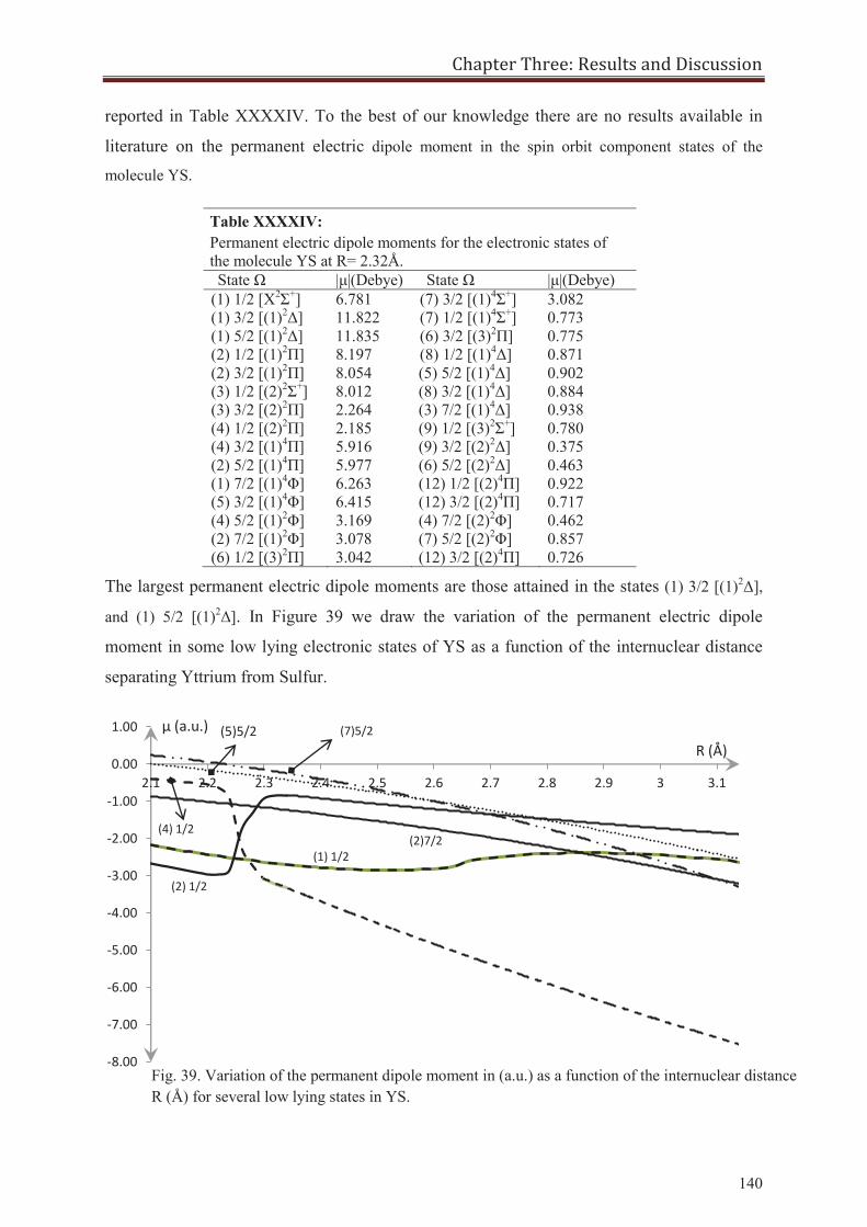
Chapter Three: Results and Discussion
140
reported in Table XXXXIV. To the best of our knowledge there are no results available in
literature on the permanent electric dipole moment in the spin orbit component states of the
molecule YS.
Table XXXXIV: Permanent electric dipole moments for the electronic states of the molecule YS at R= 2.32Å. State Ω |μ|(Debye) State Ω |μ|(Debye)
(1) 1/2 [X2Σ+] 6.781 (7) 3/2 [(1)4Σ+] 3.082 (1) 3/2 [(1)2Δ] 11.822 (7) 1/2 [(1)4Σ+] 0.773 (1) 5/2 [(1)2Δ] 11.835 (6) 3/2 [(3)2Π] 0.775 (2) 1/2 [(1)2Π] 8.197 (8) 1/2 [(1)4Δ] 0.871 (2) 3/2 [(1)2Π] 8.054 (5) 5/2 [(1)4Δ] 0.902 (3) 1/2 [(2)2Σ+] 8.012 (8) 3/2 [(1)4Δ] 0.884 (3) 3/2 [(2)2Π] 2.264 (3) 7/2 [(1)4Δ] 0.938 (4) 1/2 [(2)2Π] 2.185 (9) 1/2 [(3)2Σ+] 0.780 (4) 3/2 [(1)4Π] 5.916 (9) 3/2 [(2)2Δ] 0.375 (2) 5/2 [(1)4Π] 5.977 (6) 5/2 [(2)2Δ] 0.463 (1) 7/2 [(1)4Φ] 6.263 (12) 1/2 [(2)4Π] 0.922 (5) 3/2 [(1)4Φ] 6.415 (12) 3/2 [(2)4Π] 0.717 (4) 5/2 [(1)2Φ] 3.169 (4) 7/2 [(2)2Φ] 0.462 (2) 7/2 [(1)2Φ] 3.078 (7) 5/2 [(2)2Φ] 0.857 (6) 1/2 [(3)2Π] 3.042 (12) 3/2 [(2)4Π] 0.726
The largest permanent electric dipole moments are those attained in the states (1) 3/2 [(1)2Δ],
and (1) 5/2 [(1)2Δ]. In Figure 39 we draw the variation of the permanent electric dipole
moment in some low lying electronic states of YS as a function of the internuclear distance
separating Yttrium from Sulfur.
Fig. 39. Variation of the permanent dipole moment in (a.u.) as a function of the internuclear distance R (Å) for several low lying states in YS.
-8.00
-7.00
-6.00
-5.00
-4.00
-3.00
-2.00
-1.00
0.00
1.00
2.1 2.2 2.3 2.4 2.5 2.6 2.7 2.8 2.9 3 3.1
(2) 1/2
(1) 1/2
(4) 1/2 (2)7/2
(5)5/2 (7)5/2 R (Å)
μ (a.u.)
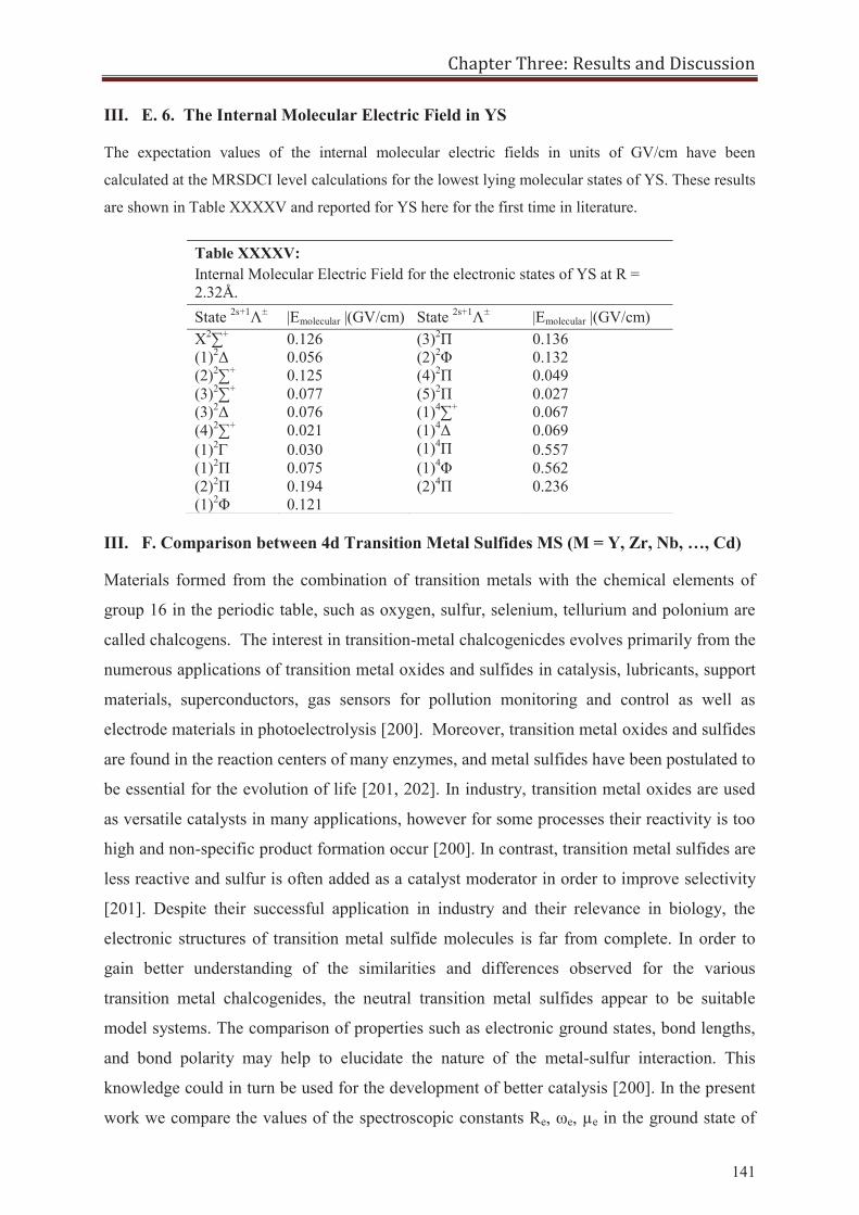
Chapter Three: Results and Discussion
141
III. E. 6. The Internal Molecular Electric Field in YS
The expectation values of the internal molecular electric fields in units of GV/cm have been
calculated at the MRSDCI level calculations for the lowest lying molecular states of YS. These results
are shown in Table XXXXV and reported for YS here for the first time in literature.
III. F. Comparison between 4d Transition Metal Sulfides MS (M = Y, Zr, Nb, …, Cd)
Materials formed from the combination of transition metals with the chemical elements of
group 16 in the periodic table, such as oxygen, sulfur, selenium, tellurium and polonium are
called chalcogens. The interest in transition-metal chalcogenicdes evolves primarily from the
numerous applications of transition metal oxides and sulfides in catalysis, lubricants, support
materials, superconductors, gas sensors for pollution monitoring and control as well as
electrode materials in photoelectrolysis [200]. Moreover, transition metal oxides and sulfides
are found in the reaction centers of many enzymes, and metal sulfides have been postulated to
be essential for the evolution of life [201, 202]. In industry, transition metal oxides are used
as versatile catalysts in many applications, however for some processes their reactivity is too
high and non-specific product formation occur [200]. In contrast, transition metal sulfides are
less reactive and sulfur is often added as a catalyst moderator in order to improve selectivity
[201]. Despite their successful application in industry and their relevance in biology, the
electronic structures of transition metal sulfide molecules is far from complete. In order to
gain better understanding of the similarities and differences observed for the various
transition metal chalcogenides, the neutral transition metal sulfides appear to be suitable
model systems. The comparison of properties such as electronic ground states, bond lengths,
and bond polarity may help to elucidate the nature of the metal-sulfur interaction. This
knowledge could in turn be used for the development of better catalysis [200]. In the present
work we compare the values of the spectroscopic constants Re, ωe, μe in the ground state of
Table XXXXV: Internal Molecular Electric Field for the electronic states of YS at R = 2.32Å. State 2s+1Λ± |Emolecular |(GV/cm) State 2s+1Λ± |Emolecular |(GV/cm) X2∑+ 0.126 (3)2Π 0.136 (1)2Δ 0.056 (2)2Φ 0.132 (2)2∑+ 0.125 (4)2Π 0.049 (3)2∑+ 0.077 (5)2Π 0.027 (3)2Δ 0.076 (1)4∑+ 0.067 (4)2∑+ 0.021 (1)4Δ 0.069 (1)2 0.030 (1)4Π 0.557 (1)2Π 0.075 (1)4Φ 0.562 (2)2Π 0.194 (2)4Π 0.236 (1)2Φ 0.121
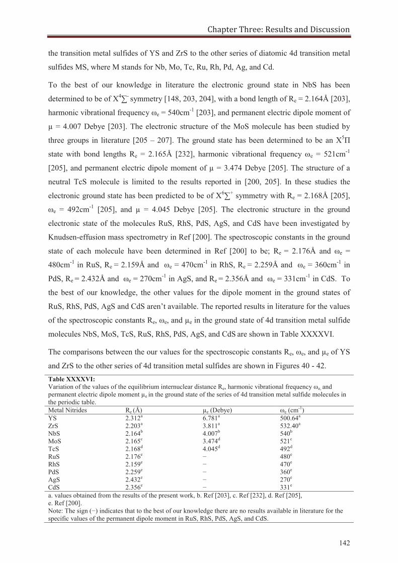
Chapter Three: Results and Discussion
142
the transition metal sulfides of YS and ZrS to the other series of diatomic 4d transition metal
sulfides MS, where M stands for Nb, Mo, Tc, Ru, Rh, Pd, Ag, and Cd.
To the best of our knowledge in literature the electronic ground state in NbS has been
determined to be of X4∑- symmetry [148, 203, 204], with a bond length of Re = 2.164Å [203],
harmonic vibrational frequency ωe = 540cm-1 [203], and permanent electric dipole moment of
μ = 4.007 Debye [203]. The electronic structure of the MoS molecule has been studied by
three groups in literature [205 – 207]. The ground state has been determined to be an X5Π
state with bond lengths Re = 2.165Å [232], harmonic vibrational frequency ωe = 521cm-1
[205], and permanent electric dipole moment of μ = 3.474 Debye [205]. The structure of a
neutral TcS molecule is limited to the results reported in [200, 205]. In these studies the
electronic ground state has been predicted to be of X6∑+ symmetry with Re = 2.168Å [205],
ωe = 492cm-1 [205], and μ = 4.045 Debye [205]. The electronic structure in the ground
electronic state of the molecules RuS, RhS, PdS, AgS, and CdS have been investigated by
Knudsen-effusion mass spectrometry in Ref [200]. The spectroscopic constants in the ground
state of each molecule have been determined in Ref [200] to be; Re = 2.176Å and ωe =
480cm-1 in RuS, Re = 2.159Å and ωe = 470cm-1 in RhS, Re
= 2.259Å and ωe = 360cm-1 in
PdS, Re = 2.432Å and ωe = 270cm-1 in AgS, and Re
= 2.356Å and ωe = 331cm-1 in CdS. To
the best of our knowledge, the other values for the dipole moment in the ground states of
RuS, RhS, PdS, AgS and CdS aren’t available. The reported results in literature for the values
of the spectroscopic constants Re, ωe, and μe in the ground state of 4d transition metal sulfide
molecules NbS, MoS, TcS, RuS, RhS, PdS, AgS, and CdS are shown in Table XXXXVI.
The comparisons between the our values for the spectroscopic constants Re, ωe, and μe of YS
and ZrS to the other series of 4d transition metal sulfides are shown in Figures 40 - 42. Table XXXXVI: Variation of the values of the equilibrium internuclear distance Re, harmonic vibrational frequency ωe, and permanent electric dipole moment μe in the ground state of the series of 4d transition metal sulfide molecules in the periodic table. Metal Nitrides Re (Å) μe (Debye) ωe (cm-1) YS 2.312a 6.781a 500.64a
ZrS 2.203a 3.811a 532.40a
NbS 2.164b 4.007b 540b
MoS 2.165c 3.474d 521c
TcS 2.168d 4.045d 492d
RuS 2.176e − 480e
RhS 2.159e − 470e
PdS 2.259e − 360e AgS 2.432e − 270e CdS 2.356e − 331e a. values obtained from the results of the present work, b. Ref [203], c. Ref [232], d. Ref [205], e. Ref [200]. Note: The sign (−) indicates that to the best of our knowledge there are no results available in literature for the specific values of the permanent dipole moment in RuS, RhS, PdS, AgS, and CdS.
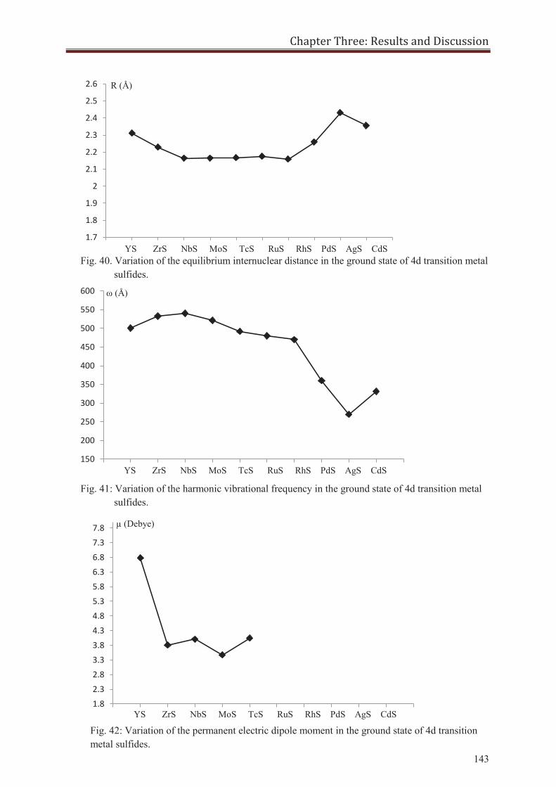
Chapter Three: Results and Discussion
143
Fig. 40. Variation of the equilibrium internuclear distance in the ground state of 4d transition metal sulfides.
Fig. 41: Variation of the harmonic vibrational frequency in the ground state of 4d transition metal sulfides.
Fig. 42: Variation of the permanent electric dipole moment in the ground state of 4d transition metal sulfides.
1.7
1.8
1.9
2
2.1
2.2
2.3
2.4
2.5
2.6 R (Å)
YS ZrS NbS MoS TcS RuS RhS PdS AgS CdS
150
200
250
300
350
400
450
500
550
600 ω (Å)
YS ZrS NbS MoS TcS RuS RhS PdS AgS CdS
1.82.32.83.33.84.34.85.35.86.36.87.37.8 μ (Debye)
YS ZrS NbS MoS TcS RuS RhS PdS AgS CdS
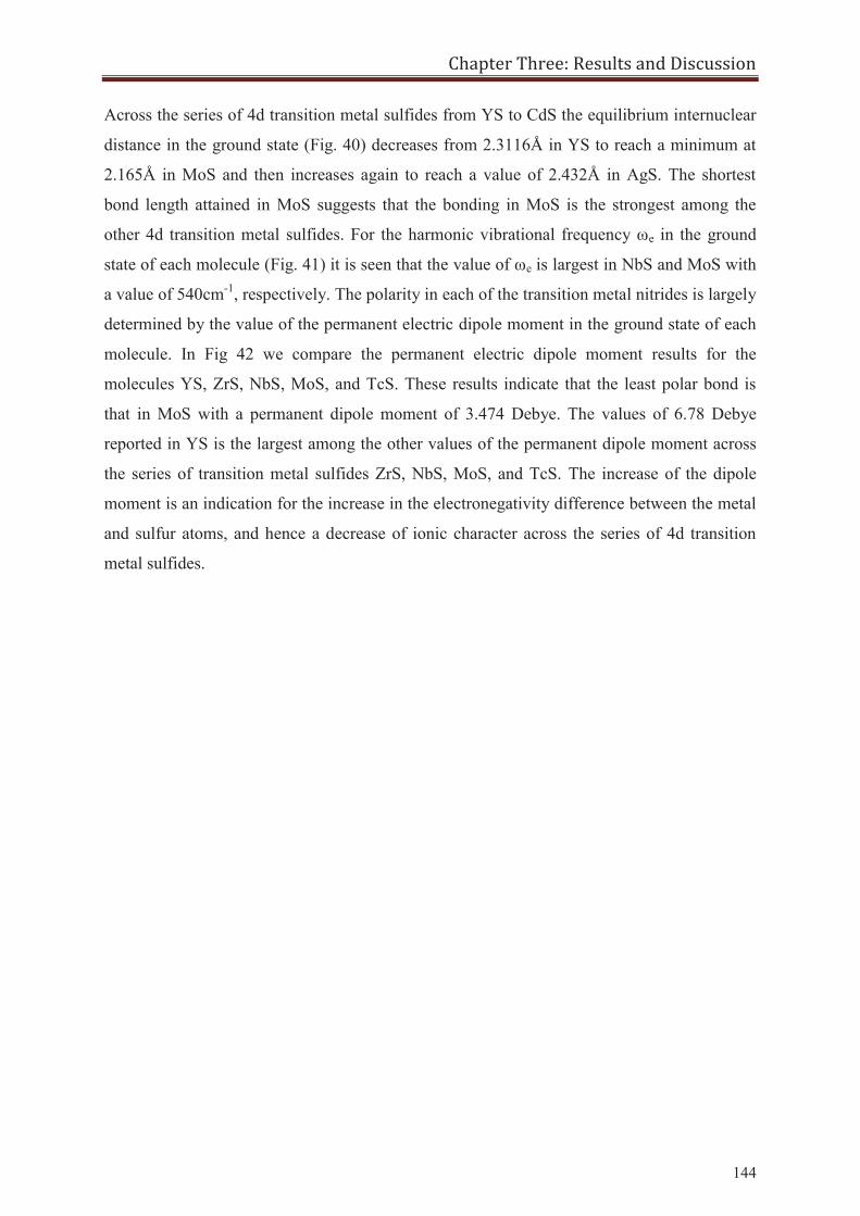
Chapter Three: Results and Discussion
144
Across the series of 4d transition metal sulfides from YS to CdS the equilibrium internuclear
distance in the ground state (Fig. 40) decreases from 2.3116Å in YS to reach a minimum at
2.165Å in MoS and then increases again to reach a value of 2.432Å in AgS. The shortest
bond length attained in MoS suggests that the bonding in MoS is the strongest among the
other 4d transition metal sulfides. For the harmonic vibrational frequency ωe in the ground
state of each molecule (Fig. 41) it is seen that the value of ωe is largest in NbS and MoS with
a value of 540cm-1, respectively. The polarity in each of the transition metal nitrides is largely
determined by the value of the permanent electric dipole moment in the ground state of each
molecule. In Fig 42 we compare the permanent electric dipole moment results for the
molecules YS, ZrS, NbS, MoS, and TcS. These results indicate that the least polar bond is
that in MoS with a permanent dipole moment of 3.474 Debye. The values of 6.78 Debye
reported in YS is the largest among the other values of the permanent dipole moment across
the series of transition metal sulfides ZrS, NbS, MoS, and TcS. The increase of the dipole
moment is an indication for the increase in the electronegativity difference between the metal
and sulfur atoms, and hence a decrease of ionic character across the series of 4d transition
metal sulfides.
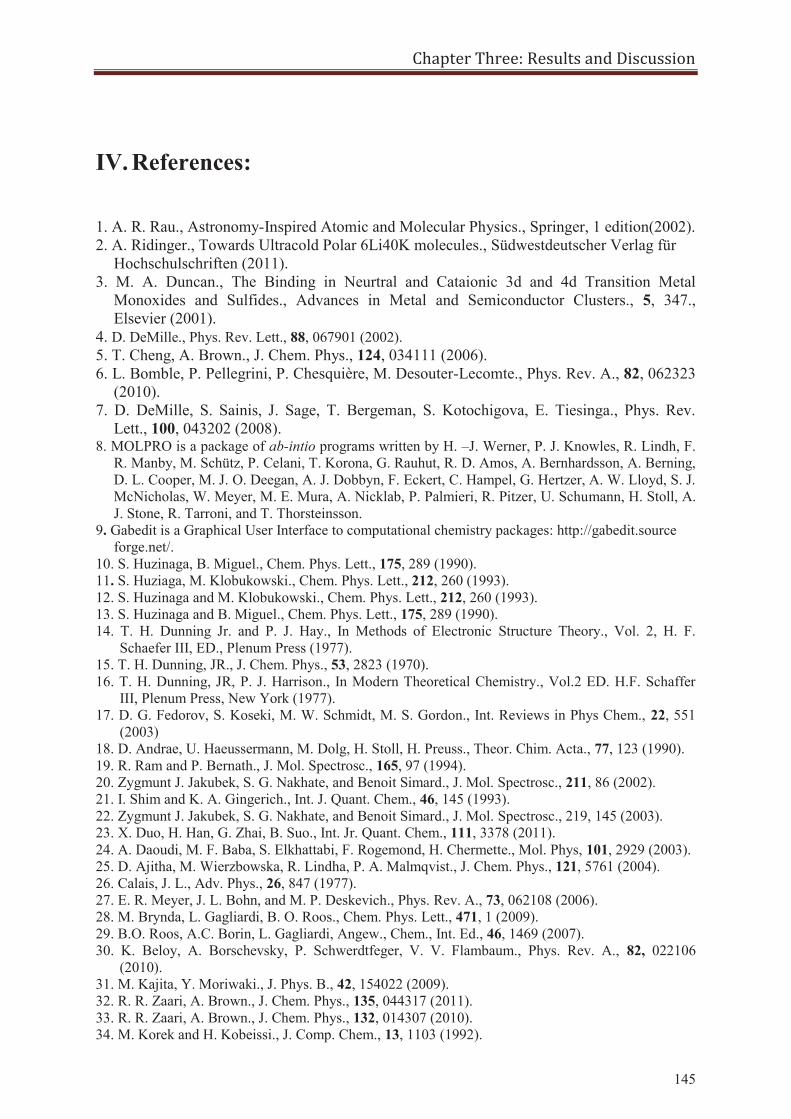
Chapter Three: Results and Discussion
145
IV. References:
1. A. R. Rau., Astronomy-Inspired Atomic and Molecular Physics., Springer, 1 edition(2002). 2. A. Ridinger., Towards Ultracold Polar 6Li40K molecules., Südwestdeutscher Verlag für
Hochschulschriften (2011). 3. M. A. Duncan., The Binding in Neurtral and Cataionic 3d and 4d Transition Metal
Monoxides and Sulfides., Advances in Metal and Semiconductor Clusters., 5, 347., Elsevier (2001).
4. D. DeMille., Phys. Rev. Lett., 88, 067901 (2002). 5. T. Cheng, A. Brown., J. Chem. Phys., 124, 034111 (2006). 6. L. Bomble, P. Pellegrini, P. Chesquière, M. Desouter-Lecomte., Phys. Rev. A., 82, 062323
(2010). 7. D. DeMille, S. Sainis, J. Sage, T. Bergeman, S. Kotochigova, E. Tiesinga., Phys. Rev.
Lett., 100, 043202 (2008). 8. MOLPRO is a package of ab-intio programs written by H. –J. Werner, P. J. Knowles, R. Lindh, F.
R. Manby, M. Schütz, P. Celani, T. Korona, G. Rauhut, R. D. Amos, A. Bernhardsson, A. Berning, D. L. Cooper, M. J. O. Deegan, A. J. Dobbyn, F. Eckert, C. Hampel, G. Hertzer, A. W. Lloyd, S. J. McNicholas, W. Meyer, M. E. Mura, A. Nicklab, P. Palmieri, R. Pitzer, U. Schumann, H. Stoll, A. J. Stone, R. Tarroni, and T. Thorsteinsson.
9. Gabedit is a Graphical User Interface to computational chemistry packages: http://gabedit.source forge.net/.
10. S. Huzinaga, B. Miguel., Chem. Phys. Lett., 175, 289 (1990). 11. S. Huziaga, M. Klobukowski., Chem. Phys. Lett., 212, 260 (1993). 12. S. Huzinaga and M. Klobukowski., Chem. Phys. Lett., 212, 260 (1993). 13. S. Huzinaga and B. Miguel., Chem. Phys. Lett., 175, 289 (1990). 14. T. H. Dunning Jr. and P. J. Hay., In Methods of Electronic Structure Theory., Vol. 2, H. F.
Schaefer III, ED., Plenum Press (1977). 15. T. H. Dunning, JR., J. Chem. Phys., 53, 2823 (1970). 16. T. H. Dunning, JR, P. J. Harrison., In Modern Theoretical Chemistry., Vol.2 ED. H.F. Schaffer
III, Plenum Press, New York (1977). 17. D. G. Fedorov, S. Koseki, M. W. Schmidt, M. S. Gordon., Int. Reviews in Phys Chem., 22, 551
(2003) 18. D. Andrae, U. Haeussermann, M. Dolg, H. Stoll, H. Preuss., Theor. Chim. Acta., 77, 123 (1990). 19. R. Ram and P. Bernath., J. Mol. Spectrosc., 165, 97 (1994). 20. Zygmunt J. Jakubek, S. G. Nakhate, and Benoit Simard., J. Mol. Spectrosc., 211, 86 (2002). 21. I. Shim and K. A. Gingerich., Int. J. Quant. Chem., 46, 145 (1993). 22. Zygmunt J. Jakubek, S. G. Nakhate, and Benoit Simard., J. Mol. Spectrosc., 219, 145 (2003). 23. X. Duo, H. Han, G. Zhai, B. Suo., Int. Jr. Quant. Chem., 111, 3378 (2011). 24. A. Daoudi, M. F. Baba, S. Elkhattabi, F. Rogemond, H. Chermette., Mol. Phys, 101, 2929 (2003). 25. D. Ajitha, M. Wierzbowska, R. Lindha, P. A. Malmqvist., J. Chem. Phys., 121, 5761 (2004). 26. Calais, J. L., Adv. Phys., 26, 847 (1977). 27. E. R. Meyer, J. L. Bohn, and M. P. Deskevich., Phys. Rev. A., 73, 062108 (2006). 28. M. Brynda, L. Gagliardi, B. O. Roos., Chem. Phys. Lett., 471, 1 (2009). 29. B.O. Roos, A.C. Borin, L. Gagliardi, Angew., Chem., Int. Ed., 46, 1469 (2007). 30. K. Beloy, A. Borschevsky, P. Schwerdtfeger, V. V. Flambaum., Phys. Rev. A., 82, 022106
(2010). 31. M. Kajita, Y. Moriwaki., J. Phys. B., 42, 154022 (2009). 32. R. R. Zaari, A. Brown., J. Chem. Phys., 135, 044317 (2011). 33. R. R. Zaari, A. Brown., J. Chem. Phys., 132, 014307 (2010). 34. M. Korek and H. Kobeissi., J. Comp. Chem., 13, 1103 (1992).
Chapter Three: Results and Discussion
146
35. M. Korek., International Center for Theoretical Physics., (1989). 36. E. Fermi, and E. Teller., Phys. Rev., 72, 406 (1947). 37. Th. Klahn, and P. Krebs., J. Chem. Phys., 109, 531 (1998). 38. T. C. Steimle., Int. Rev. Phys. Chem., 19, 455 (2000). 39. M. Pospelov, and A. Ritz., Ann. Phys., 318, 119 (2005). 40. B. C. Regan, E. D. Commins, C. J. Schmidt, and D. DeMille., Phys. Rev. Lett., 88, 071805
(2002). 41. A. N. Petrov, N. S. Mosyagin, T. A. Isaev, A. V. Titov., Phys. Rev. A., 76, 030501 (2007). 42. M. G. Kozlov, A. V. Titov, N. S. Mosyagin, and P. V. Souchko., Phys. Rev. A., 56, R3326 (1997). 43. J. J. Hudson, B. E. Sauer, M. R. Tarbutt, and E. A. Hinds., Phys. Rev. Lett., 89, 023003 (2002). 44. M. G. Kozlov and V. F. Ezhov., Phys. Rev. A., 49, 4502 (1994). 45. Yu. Yu. Dmitriev, Yu. G. Khait, M. G. Kozlov, L. N. Labzovsky, A. O. Mitrushenkov, A. V.
Shtoff, and A. V. Titov., Phys. Lett. A., 167, 280 (1992). 46. D. DeMille, F. Bay, S. Bickman, D. Kawall, D. Krause, S. E. Maxwell, and L. R. Hunter., Phys.
Rev. A., 61, 052507 (2000). 47. B. Ravaine, S. G. Porsev, and A. Derevianko., Phys. Rev. Lett., 94, 013001 (2005). 48. C. S. Chen, C. P. Liu, C. Y. A. Tsao, and H. G. Yang., Scr. Mater., 51, 715 (2004). 49. J. V. Ramana, S. Kumar, C. David, A. K. Ray, and V. S. Raju., Mater. Lett., 43, 73 (2000). 50. C. P. Liu and H. G. Yang., Mater. Chem. Phys., 86, 370 (2004). 51. F. H. Mei, N. Shao, L. Wei, Y. S. Dong, and G. Y. Li., Appl. Phys. Lett., 87, 011906 (2005). 52. M. Hock, E. Schäffer, W. Döll, and G. Kleer., Surf. Coat. Technol., 163, 689 (2003). 53. D. J. Li, M. X. Wang, and J. J. Zhang., Mater. Sci. Eng. A., 423, 116 (2006). 54. C. H. Hsu, M. Li. Chen, and K. L. Lai., Mater. Sci. Eng A., 421, 182 (2006). 55. I. O. Ershova, Metalloved. Term. Obrab. Met., No. 2, 26 (2003). 56. C. Jascheck and M. Jascheck., The Behavior of Chemical Elements in Stars Cambridge University
Press, Cambridge., (1995). 57. H. Machara and Y. Y. Yamashita., Publ. Astron. Soc. Jpn., 28, 135 (1976). 58. D. L. Lambert and R. E. S. Clegg, Mon. Not. R. Astron., Soc. 191, 367 (1980). 59. B. Lindgren and G. Olofsson, Astron. Astrophys., 84, 300 (1980). 60. D. L. Lambert and E. A. Mallia., Mon. Not. R. Astron. Soc., 151, 437 (1971). 61. O. Engvold, H. Wo¨hl, and J. W. Brault., Astron. Astrophys., Suppl. Ser., 42, 209 (1980). 62. R. S. Ram, J, Liévin., P. F. Bernath., Jr. Chem. Phys., 109, 6329 (1998) 63. J.K. Bates, T.M. Dunn., Can. J. Phys., 54, 1216 (1976). 64. C. M.-T. Chan, Haiyang Li, N. S-K. Sze, and A. S-C. Cheung., J. Mol. Spectrosc., 180, 145
(1996). 65. C. M.-T. Chan, Haiyang Li, and A. S-C. Cheung., Chem. Phys. Lett., 269, 49 (1997). 66. H. Jiang, Chensheng Ma, and A. S-C. Cheung., Chem. Phys. Lett., 295, 535 (1998). 67. A.S.-C. Cheung, H. Li, H. Jiang, H. Chen., J. Mol. Spectrosc., 210, 84 (2001). 68. H. Jiang, C. Ma, G.S. –M. Tong, A.S.-C. Cheung., J. Mol. Spectrosc., 480, 277 (1999). 69. H. Chen, Y. Li, D.K. Mok and A. Cheung., J. Mol. Spectrosco., 218, 213 (2003). 70. Haiyang Li, C. M-T. Chan, and A. S-C. Cheung., J. Mol. Spectrosc., 176, 219 (1996). 71. T. C. DeVore, T. N. Gallaher., J. Chem. Phys., 70, 3497 (1978). 72. G. Kushto, P. Souter, G. Chertihin, L. Andrews., J. Chem. Phys., 110, 9020 (1999) 73. T. M. Dunn, L. K. Hanson, and K. A. Rubinson., Can. J. Phys., 48, 1657(1970). 74. C. Athénour, J-L. Féménias, and T. M. Dunn., Can. J. Phys., 60, 109–116 (1982). 75. A. Adams, W. Klemperer, and T. M. Dunn., Can. J. Phys., 46, 2213–2220 (1968). 76. L.Akerlind., Ark. Fys., 22, 41 (1962). 77. Yarkony, D. R., Int. Rev. Phys. Chem., 11, 195 (2001). 78. D. G. Fedorov, S. Koseki, M. W. Schmidt, M. S. Gordon., Int. Reviews in Phys Chem., 22, 551
(2003). 79. S.R. Langhoff and C.W. Bauschlicher., Jr. Annu. Rev. Phys.Chem., 39, 181 (1989). 80. L. Isenhower, E. Urban, X. L. Zhang, A. T. Gill, T. Henage, T. A. Johnson, T. G. Walker, and M.
Saffman., Phys. Rev. Lett., 104, 010503 (2010).
Chapter Three: Results and Discussion
147
81. T.Monz,K.Kim,W. Hansel, M. Riebe, A. S.Villar, P. Schindler,M. Chwalla, M. Hennrich, and R. Blatt., Phys. Rev. Lett., 102, 040501 (2009).
82. L. DiCarlo, J. M. Chow, J. M. Gambetta, Lev. S. Bishop, B. R. Johnson, D. I. Schuster, J. Majer, A. Blais, L. Frunzio, S. M. Girvin, R. J. Schoelkopf., Nature., 460, 240 (2009).
83. A. Politi, J. C. F. Matthews, and J. L. Obrien., Science., 325, 1221 (2009). 84. J. Du, N. Xu, X. Peng, P. Wang, S. Wu, and D. Lu., Phys. Rev.Lett., 104, 030502 (2010). 85. C.M. Tesch, L. Kurtz, andR. deVivie-Riedle., Chem. Phys. Lett., 343, 633 (2001). 86. C.M. Tesch and R. de Vivie-Riedle., Phys. Rev. Lett., 89, 157901 (2002). 87. J. Vala, Z. Amitay, B. Zhang, S. R. Leone, and R. Kosloff., Phys. Rev. A., 66, 062316 (2002). 88. D. Babikov., J. Chem. Phys., 121, 7577 (2004). 89. Y. Ohtsuki., Chem. Phys. Lett., 404, 126 (2005). 90. C. Menzel-Jones and M. Shapiro., Phys. Rev. A., 75, 052308 (2007). 91. K. Shioya, K.Mishima, and K. Yamashita., Mol. Phys., 105, 1287 (2007). 92. K. Mishima, K. Tokumo, and K. Yamashita., Chem. Phys., 343,61 (2008). 93. M. Tsubouchi and T.Momose., Phys. Rev. A., 77, 052326 (2008). 94. M. Tsubouchi, A. Khramov, and T. Momose., Phys. Rev. A., 77,023405 (2008). 95. D. Sugny, L. Bomble, T. Ribeyre, O. Dulieu, and M. Desouter-Lecomte., Phys. Rev. A., 80,
042325 (2009). 96. K. Mishima and K. Yamashita., Chem. Phys., 367, 63 (2010). 97. R. Zaari and A. Brown., J. Chem. Phys., 132, 014307 (2010). 98. C. M. Tesch and R. de Vivie-Riedle., J. Chem. Phys., 121, 12158 (2004). 99. U. Troppmann and R. de Vivie-Riedle., J. Chem. Phys., 122,154105 (2005). 100. B. Korff, U. Troppmann, K. Kompa, and R. de Vivie-Riedle., J. Chem. Phys., 123, 244509
(2005). 101. D. Sugny, C. Kontz, M. Ndong, Y. Justum, G. Dive, and M. Desouter-Lecomte., Phys. Rev. A.,
74, 043419 (2006). 102. D. Sugny, M. Ndong, D. Lauvergnat, Y. Justum, and M. Desouter-Lecomte., J. Photochem.
Photobiol. A., 190, 359 (2007). 103. M. Ndong, D. Lauvergnat, X. Chapuisat, and M. Desouter-Lecomte., J. Chem. Phys., 126,
244505 (2007). 104. D. Weidinger and M. Gruebele., Mol. Phys., 105, 1999 (2007). 105. L. Bomble, D. Lauvergnat, F. Remacle, and M. Desouter-Lecomte., J. Chem. Phys., 128, 064110
(2008). 106. L. Bomble, D. Lauvergnat, F. Remacle, and M. Desouter-Lecomte., Phys. Rev. A., 80, 022332
(2009). 107. L. Bomble, D. Lauvergnat, F. Remacle, and M. Desouter-Lecomte., Phys. Chem. Chem. Phys.,
12, 15628 (2010). 108. M. Schr¨oder and A. Brown., J. Chem. Phys., 131, 034101 (2009). 109. K. Mishima and K. Yamashita., Chem. Phys., 361, 106 (2009). 110. K. Mishima and K. Yamashita., J. Chem. Phys. 130., 034108 (2009). 111.L. Bomble, P. Pellegrini, P. Ghesquiére, and M. Desouter-Lecomte., Phys. Rev. A., 82, 062323
(2010). 112. E. S. Shuman, J. F. Barry, and D. Demille., Nature., 467, 820 (2010). 113. D. DeMille., Phys. Rev. Lett., 88, 067901 (2002). 114. G. Igel-Mann, U. Wedig, P. Fuentealba, and H. Stoll., J. Chem. Phys., 84, 5007 (1986). 115. Q. Wei, S. Kais, B. Friedrich, D. Herschbach., J. Chem. Phys., 135, 154102 (2011). 116. Physical chemistry 2d Edition., G.M. Barrow McGraw Hill., (1966). 117. E. R. Meyer, J. L. Bohn., Phys. Rev. A., 78, 010502 (2008). 118. E. I. Isaev, S. I. Simak and I. A. Abrikosov, R. Ahuja, Yu. Kh. Vekilov, M. I. Katsnelson, A. I.
Lichtenstein, B. Johansson., J. Appl. Phys., 101, 123519 (2007). 119. B. Hong, L. Chen, M. Y. Wang, Z. J. Wu., Mol. Phys., 108, 25 (2010) 120. K.m. Rao, and T. M. Dunn., Nature., 222, 266 (1969). 121. J. –L. Femenias, C. Athenour, and T. M. Dunn., J. Chem. Phys., 63, 2861 (1975). 122. E. A. Pazyuk, E. N. Moskvitina, Y. Y. Kuzyakov., Spectrosc. Lett., 19, 627 (1986). 123. Y. Azuma, A. Barry, M. P. J. Lyne, A. J. Merer, J. O. Schroder, and J. L. Femenias., J. Chem.
Phys., 91, 1 (1989).
Chapter Three: Results and Discussion
148
124. Y. Azuma, A. Barry, G. Huang, M. P. J. Lyne, A. J. Merer, V. I. Srdanov., J. Chem. Phys., 100,4138 (1989).
125. M. F. Zhou, L. Andrews., J. Phys. Chem. A., 102, 9061 (1998). 126. R. S. Ram, and P. F. Bernath., J. Mol. Spectrosc., 201, 267 (2000). 127. D. A. Fletcher, D. Dai, T. C. Steimle, and K. J. Balasubramanian., Chem Phys. 99, 9324 (1993). 128. L. Andres, P. F. Souter, W. D. Bare, and B. Liang., J. Phys. Chem. A., 103, 4649 (1999). 129. D. A. Fletcher, K. Y. Jung, and T. C. Steimle., J. Chem. Phys., 99, 901 (1993). 130. K. Y. Jung, D. A. Fletcher, and T. C. Steimle., J. Mol. Spectrosc., 165, 448 (1994). 131. A. C. Borin, J. P. Gobbo., J. Phy. Chem. A., 113, 12421 (2009). 132. B. Hong, L. Cheng, M. Y. Wang, and Z. J. Wu., Mol. Phys., 108, 25 (2010). 133. R. S. Ram, and P. F. Bernath., J. Mol. Spectrosc., 213, 170 (2002). 134. T. C. Steimlea, and W. Virgo., J. Chem. Phys., 119, 12965 (2003). 135. M. G. Moreno-Armentaa, J. Diaza, A. Martinez-Ruizb, and G. Sotoa., J. Phys. Chem. Solids., 68,
1989 (2007). 136. R. S. Ram, J. Liévin, and P. F. Bernath., J. Chem. Phys., 109, 6329 (1998). 137. A. Citra, and L. Andrews., J. Phys. Chem. A., 104, 1152 (2000). 138. T. M. Ma, J. Gengler, Z. Wang, H. L. Wang, T.C. Steimlea., J. Chem. Phys., 126, 244312
(2007). 139. S. R. Langhoff and C. W. Bauschlicher., The AstroPhysical Journal., 349, 369 (1990). 140. E. I. Stiefel and K. Matsumoto (eds.), Transition Metal Sulfur Chemistry; ACS Symposium
Series 653 (American Chemistry Society, Washington, DC, 1996). 141. M. Hua, C. I. Garcia, and A. DeArdo., J. Metall. Mater. Trans., A, 28, 1769 (1997). 142. J. G. Philips and S. P. Davis., Astrophys., J. 229, 867 (1979). 143. H. Spinrad and R. F. Wing., Annu. Rev. Astron. Astrophys., 7, 249 (1969). 144. P. C. Keenan, Astrophys., J. 107, 420 (1948). 145. H. L. Nordh, B. Lindgren, and R. F. Wing., Astron. Astrophys., 56, 1 (1977). 146. J. Jonsson, S. Wallin, and B. Lindgreen., J. Mol. Spectrosc. 192, 198 (1998). 147. K. Hinkle, D. Lambert, R. Wing., Mon. Not. R. Astr. Soc., 238, 1365 (1989). 148. S.R. Langhoff, C.W. Bauschlicher Jr., H. Partridge., J. Chem. Phys., 2160, 89 (1988). 149. R. R. Reddy, Y. N. Ahammed, B. S. Devi, K. R. Gopal, P. A. Azeem and T. V. Rao., Astro
Physics and Space Science., 281, 729 (2002). 150. B. Simard, S. A. Mitchell, L. M. Hendel, and P. A. Hackett, Faraday Discuss., Chem. Soc. 86,
163 (1988). 151. J. Jonsson, B. Lindgren, and A. G. Taklif., Astron. Astrophys., 246, L67 (1991). 152. S. A. Beaton, and M. C. L. Gerry., J. Chem. Phys., 110, 10715 (1999). 153. B. Liang, L. Andrews., J. Phys. Chem A., 106, 6295 (2002). 154. X. Sun, J. Wang, Z. Wu., J. Clust Sci., 20, 525 (2009). 155. R. R. Bousquet, K. C. Namiki, T. C. Steimle., J. Chem. Phys., 113, 1566 (2000). 156. J. Jonsson, B. Lindgren., J. Mol. Spectr., 169, 30 (1995). 157. D. L. Lambert and R. E. S. Clegg, Mon. Not. R. Astr. Soc., 191, 367 (1980). 158. J. Jonsson., J. Mol. Spectrosc., 169, 18 (1995). 159. W. Th. A. M. van der Lugt and L. J. Oosterhoff., J. Amer. Chem. Soc., 91, 6042 (1969). 160. A. N. Petrov, A. V. Titov, T. A. Isaev, N. S. Mosyagin, D. Demille., Phys. Rev. A., 72, 022505
(2005). 161. M. Pospelov, and A. Ritz., Ann. Phys., 318, 119 (2005). 162. K. Mishima, K. Yamashita., J. Chem. Phys., 367, 63 (2010). 163. "CODATA Value: inverse fine-structure constant". The NIST Reference on Constants, Units,
and Uncertainty. US National Institute of Standards and Technology. June (2011). http://physics.nist.gov/cgi-bin/cuu/Value?alphinv.
164. "CODATA Value: fine-structure constant". The NIST Reference on Constants, Units, and Uncertainty. US National Institute of Standards and Technology. June (2011). http://physics.nist.gov/cgi-bin/cuu/Value?alph.
165. A T Nguyen, D Budker, S K Lamoreaux and J R Torgerson., Phys. Rev. A., 69, 022105. 166. A. Cingӧz, A. Lapierre, A. T. Nguyen, N. Budker, S. K. Lamoreaux, and J. R. Torgerson., Phys.
Rev. Lett., 98, 040801 (2007).
Chapter Three: Results and Discussion
149
167. E. J. Angstmann, V. A. Dzuba, V. V. Flambaum, A. Yu. Nevsky, and S. G. Karshenboim., J. Phys. B: AT. Mol. Opt. Phys., 39, 1937 (2006).
168.V. A. Dzuba, V. V. Flambaum, and J. K. Webb., Phys. Rev. A. 59, 230 (1999). 169. D. Budker., private communication (2005). 170. V. V. Flambaum., Eur. Phys. J. ST., 163, 159 (2008). 171. V. V. Flambaum and M. G. Kozlov., Phys. Rev. Lett., 99, 150801 (2007). 172. T. M. Fortier et. al., Phys. Rev. Lett., 98, 070801 (2007). 173. J. K. Webb, V. V. Flambaum, C. W. Churchill, M. J. Drinkwater, and J. D. Barrow, Phys. Rev.
Lett. 82, 884 (1999). 174. J. K. Webb, M. T. Murphy, V. V. Flambaum, V. A. Dzuba, J. D. Barrow, C. W. Churchill, J. X.
Prochaska, and A. M. Wolfe, Phys. Rev. Lett. 87, 091301 (2001). 175. M. T. Murphy, J. K. Webb, and V. V. Flambaum, Phys. Rev. Lett. 99, 239001 (2007). 176. V. A. Dzuba, V. V. Flambaum, and J. K. Webb, e-print physics/9802029. 177. R. R. Bousquet, K. C. Namiki, T. C. Steimle., J. Chem. Phys., 113, 1566 (2000). 178. J. J. Hudson, B. E. Sauer, M. R. Tarbutt, and E. A. Hinds., Phys. Rev. Lett., 89, 023003 (2002). 179. D. DeMille et. al., Phys. Rev. A., 61, 052507 (2000). 180. L. R. Hunter et. al., Phys. Rev. A., 65, 030501 (2002). 181. D. Kawall, F. Bay, S. Bickman, Y. Jiang and D. DeMille., Phys. Rev. Lett., 92, 133007 (2004). 182. M. G. Kozlov., J. Phys. B., 30, L607 (1997). 183. R. P. Stutz., PhD thesis. Towards Measuring the Electron Electric Dipole Moment Using
Trapped Molecular Ions., http://jila.colorado.edu/bec/CornellGroup/theses/stutz_thesis.pdf (1998).
184. T. A. Isaev, N. S. Mosyagin, A. N. Petrov, and A. V.Titov., Phys. Rev. Lett., 95, 163004 (2005). 185. J. M. Thompsen, L. M. Ziurys., Chem. Phys. Let., 344, 75 (2001). 186. D. Arnett., Supernovae and Nucleosynthesis., Princeton University Press, Princeton (1996). 187. A. J. Merer., Ann. Rev. Phys. Chem., 40, 407 (1989). 188. A. J. Bridgeman, J. Rothery., J. Chem. Soc., Dalton Trans., 211 (2000). 189. C. W. Bauschlicher, P. Maitre., Theor. Chim. Acta., 90, 189 (1995). 190. J. M. Thompsen, L. M. Ziurys., Chem. Phys. Lett., 344, 75 (2001). 191. A. M. James, R. Fournier, B. Simard, M. D. Campbell, Can. J. Chem. 71, 1598 (1993). 192. T. C. Steimle and W. Virgo, J. Mol. Spectrosc. 221, 57 (2003). 193. A. M. James, B. Simard, J. Chem. Phys. 98, 4422 (1993). 194. N. S. McIntyre, K. C. Lin, and W. Weltner, Jr., J. Chem. Phys. 56, 5576 (1972). 195. R. Stringat, B. Fenot, and J.L. Féménias. Can. J. Phys. 57, 300 (1979). 196. Y. Azuma and W. J. Childs, J. Chem. Phys. 93, 8415 (1990). 197. J. M. Andrew, R. Fournier, B. Simard, and M. Campbell, Can. J. Chem. 71, 1598 (1993) 198. M. Korek, A. Farhat, S. Abdul-al., J. Theo. Comp. Chem., 9, 597 (2010). 199. P. Kowalczyk, A.M. James, B. Simard, J. Mol. Spectrosc. 189, 196 (1998). 200. M. A. Duncan., The Binding in Neurtral and Cataionic 3d and 4d Transition Metal Monoxides
and Sulfides., Advances in Metal and Semiconductor Clusters., 5, 347., Elsevier (2001). 201. R. J. P. Williams., Nature., 343, 213 (1990). 202. E. Drobner, H. Huber, G. Wachtershauser, K. O. Stetter., Nature, 346, 742 (1990). 203.O. Launila., J. Mol. Spec., 229, 31 (2005). 204. B. Simard, C. Masoni, P. A. Hackett., J. Chem. Phys., 92, 7003 (1990). 205. S. R. Langhoff, C. W. Bauschlicher, Lars G. M. Pettersson., Chem. Phys., 132, 49 (1989). 206. I. Kretzchmar, A. Fiedler, J. N. Harvey, D. Schroder, and H. Schwarz., J. Phys. Chem. A., 101,
6252 (1997). 207. B. Liang, L. Andrews., J. Phys. Chem. A., 106, 6945 (2002).
Chapter Four. Summary and Outlook
154
Chapter 4
Summary and Outlook
b initio calculations provide us with a tool to describe the electronic structures and
chemical properties of molecules. Computational studies can in general be carried
out in order to find a starting point for laboratory experiments, or to assist in understanding
experimental data. Thus computational studies can explore new properties and guide new
experimental works. Heavy polar diatomic molecules form suitable candidates for computational
investigations, particularly due to their rich inner electronic structures and due to their
importance in several areas of science, as chemistry, astrophysics, ultracold interactions, and
molecular quantum computing. Although, the electronic structures of small diatomic molecules
have been well characterized, still the electronic structures of heavy polar diatomic molecules
containing a transition metal atom of group III and IV is far from complete. The main objective
of this thesis was to fill the gap and study the electronic structures of the transition metal nitrides
and sulfides of Yttrium and Zirconium. In the present work the electronic structures of the
molecules YN, YS, ZrN, and ZrS have been investigated at the multireference single and double
configuration interaction method followed by spin orbit calculations implemented by the method
of effective core potentials. These calculations yielded accurate spectroscopic constants along
with several physical and chemical properties that are within a few percent of the experimental
values. Many other properties have been also computed that weren’t available in literature on the
electronic structures of these molecules. We expect that the results in the present work should
invoke further experimental investigations for this class of molecules. As an example, we found
in the ZrS molecule several degenerate vibrational energy levels which might increase the
A
Chapter Four. Summary and Outlook
155
experimental sensitivity for measurements of small variations in the fine structure constant α in
laboratory experiments and in S-type stars. A preprint for the results of this work has been
requested by an experimental research group working at Yale in the group of Prof. David
Demille.
In chapter 1, we present a brief overview for the theoretical backgrounds of the computational
methods used in the present work. The theoretical backgrounds for the electronic structure
calculations in the Hartree-Fock method, followed by Complete Active Space Calculations and
Multireference Configuration Interaction methods are written within the formalism of second
quantization. A brief discussion for the theoretical background of spin orbit relativistic
interactions in diatomic molecules have been also incorporated within the context of the first
chapter.
In chapter 2, we present the canonical function’s approach for solving the vibrational and
rotational Schrödinger equation in a diatomic molecule. This has allowed us to compute the
vibrational energy structures and rotational constants for the ground and excited electronic states
of each molecule.
In chapter 3, we list the results of our calculations for the electronic structures, with and without
spin orbit effects, of the four diatomic molecules YN, YS, ZrN, and ZrS. Potential energy curves
were constructed and spectroscopic constants were computed. Various other physical properties
were also computed such as the permanent electric dipole moment, internal molecular electric
fields, and bonding characteristics. Ro-vibrational energy calculations were performed by
solving the vibrational-rotational Schrödinger equation in the ground and excited electronic
states of each molecule. With the inclusion of spin orbit effects in the electronic structure
calculations further enhancements in the accuracy of nonrelativistic ab initio results could be
obtained. In the present work a large number of spin orbit electronic states have been studied for
the first time in literature up to 60 states in YN, 49 states in ZrN, 44 states in ZrS, and 54 states
in YS. From these results several other properties and spectroscopic constants were also studied
here for the first time in literature. The accuracy of the calculated constants in the present work
was measured by reporting a percentage relative difference between the present results and the
experimental results, whenever available in literature. For the other values reported here for the
first time in literature no comparison is made. The calculated values of the internal molecular
Chapter Four. Summary and Outlook
156
electric fields in these molecules are reported here for the first time in literature and might help
in clarifying the structures of these molecules in a search for a possible electric dipole moment of
the electron. We detected several degenerate vibrational energy levels in the ground (1)0+[X1∑+]
and first excited electronic states (1)1[(1)3∆], (1)2[(1)3∆], (1)3[(1)3∆] of the ZrS molecule. We
suggest that the reported degeneracies in ZrS, specifically between the vibrational energy levels
of the (1)1[(1)3∆] and (1)2[(1)3∆] states, can be used to enhance the experimental accuracy in
measurements for variations in the fine structure constant α. Finally, in an attempt to observe the
variation of molecular properties across the series of 4d transition metal nitrides and sulfides, we
compare the values in the present work for the equilibrium internuclear distance, permanent
electric dipole moment, and harmonic vibrational frequency for the molecules YN and ZrN to
the other spectroscopic values across series of 4d transition metal nitrides and sulfides: MN and
MS, where M stands for Y, Zr, Nb, Mo, Tc, Ru, Rh, Pd, Ag, Cd.
Résumé et Conclusions (French)
157
Résumé et Perspectives (French)
es calculs ab initio fournissent un outil pour décrire les structures électroniques et les
propriétés chimiques des molécules. Les études théoriques peuvent, en général,
constituer un point de départ pour des expériences de laboratoire, ou encore aider à comprendre
certaines données expérimentales. Ainsi, les études numériques représentent un moyen
d'explorer de nouvelles propriétés et ainsi guider de nouvelles expériences.
Les molécules diatomiques polaires sont des candidats appropriés pour des études numériques en
raison de la richesse de leur structure électronique et de leur importance dans de nombreux
domaines: chimie, astrophysique, interaction à très basses températures ou encore le calcul
quantique moléculaire. Les structures électroniques des petites molécules diatomiques sont à
présent bien connues, cependant les structures électroniques des molécules diatomiques polaires
lourdes contenant un atome de métal de transition des groupes III et IV ne sont "pas
complètement comprises". L'objectif principal de cette thèse est de combler cet écart "en
étudiant" les structures électroniques des nitrures de métaux de transition ainsi que les sulfures
d'yttrium et le zirconium. Dans ce travail, les structures électroniques des molécules lourdes
diatomiques polaires du type YN, YS, ZrN et ZrS ont été étudiées à la configuration
de l'interaction multireference méthode simple et double suivies par des calculs spin-orbite mis
en œuvre par la méthode des potentiels de cœurs effectifs. Ces calculs ont permis d'obtenir des
constantes spectroscopiques précises ainsi que plusieurs propriétés physico-chimiques à quelques
pourcent de leur valeur expérimentale. De nombreuses autres propriétés qui n'étaient pas
L
Résumé et Conclusions (French)
158
disponibles dans la littérature ont également été calculées sur la structure électronique de ces
molécules. Nous nous attendons à ce que les résultats présentés dans cette thèse inspirent de
future études expérimentales pour cette classe de molécules. A titre d'exemple, nous avons
trouvé dans la molécule ZrS plusieurs niveaux d'énergie vibratoire dégénérés, ces niveaux
pourraient augmenter la sensibilité expérimentale pour les mesures de faibles variations dans la
constant de structure fine α et dans les étoiles du type S. De plus, un preprint concernant les
résultats de ce travail a été demandé par le groupe de recherche expérimentale dirigé par le
professeur David Demille de l'Université de Yale.
Dans le chapitre 1 nous présentons un bref aperçu du cadre théorique des méthodes de calcul
utilisées dans le travail actuel. Le cadre théorique pour le calcul de la structure électronique avec
la méthode d'Hartree-Fock, suivi par les méthodes de calcul de l'espace actif et de l'interaction en
configuration multiréférence est celui du formalisme de la seconde quantification. Une brève
discussion sur la théorie de l'interaction spin-orbite pour les molécules diatomiques relativistes a
également été intégrée dans le premier chapitre.
Dans le chapitre 2, nous présentons l'utilisation de la fonction canonique pour la résolution de
l'équation de Schrödinger pour les modes de vibration et de rotation d'une molécule diatomique.
Cela nous a permis de calculer les énergies vibrationnelles des structures et les constantes de
rotation pour l'état fondamental et les états électroniques excités de chaque molécule.
Dans le chapitre 3, nous présentons les résultats de nos calculs pour les structures électroniques,
avec et sans effet spin-orbite, de quatre molécules diatomiques YN, YS, ZrN et ZrS. Les courbes
d'énergie potentielle ont été tracées et les constantes spectroscopiques calculées. D'autres
propriétés physiques ont été calculées comme le moment dipolaire permanent, le champ
électrique moléculaire interne et les caractéristiques de liaison. Les calculs d'énergie ro-
vibrationnelle ont été effectués en résolvant l'équation de Schrödinger de rotation et de vibration
pour l'état fondamental et les états excités de chaque molécule. Avec la prise en compte des
effets spin-orbite dans les calculs de structure électronique, on a pu obtenir de nouvelles
améliorations sur l'exactitude des résultats non relativistes et ab initio. De nombreux états
électroniques de spin-orbite ont été étudiés pour la première fois dans la littérature lors du travail
actuel jusqu'à 60 états pour YN, 49 états pour ZrN, 44 états pour ZrS et 54 états pour YS. A
partir de ces résultats plusieurs autres propriétés et constantes spectroscopiques ont été étudiées
Résumé et Conclusions (French)
159
pour la première fois dans la littérature. La précision des constantes calculées dans le travail
actuel a été calculé à partir de la différence relative entre les résultats et ceux des expériences, à
chaque fois qu'ils s’étatisent disponibles dans la littérature. Il n'y a pas eu de comparaison faite
pour les autres valeurs rapportées pour la première fois dans la littérature. Les valeurs calculées
du champ électrique moléculaire interne de ces molécules sont rapportées pour la première fois
dans la littérature et pourraient aider à clarifier la structure de ces molécules dans la recherche
d'un éventuel moment dipolaire de l'électron. Nous avons détecté plusieurs niveaux d'énergie
vibrationnelle dégénérées dans le fondamental (1)0+[X1Σ+] et les premiers états excités
(1)1[(1)3Δ], (1)2[(1)3Δ], (1) 3 [(1)3Δ] de la molécule ZrS. Nous supposons que les
dégénérescences du ZrS, en particulier entre les niveaux d'énergie vibrationnelle des états
(1)1[(1)3Δ] et (1)2[(1)3Δ] peuvent être utilisées pour améliorer la précision expérimentale des
mesures de variation de la constante de structure fine alpha. Finalement, en tentant d'observer les
variations des propriétés moléculaires pour les séries des nitrures et sulfures de métaux de
transition 4d on compare les valeurs de la distance internucléaire d’équilibre, du moment
dipolaire électrique permanent et de la fréquence de vibration harmonique pour les molécules
YN et ZrN calculées dans ce travail aux valeurs spectroscopique pour le nitreuse et sulfures de
métaux de transition 4d MN (M = Y, Zr, Nb, Mo, Tc, Ru, Rh, Pd, Ag, Cd).
Appendix I. Splitting Figures between Spin orbit electronic states
160
Appendix I
Splitting Figures between Spin orbit electronic states
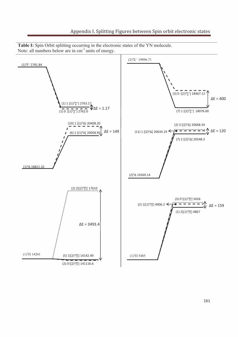
Appendix I. Splitting Figures between Spin orbit electronic states
161
Table I: Spin Orbit splitting occurring in the electronic states of the YN molecule. Note: all numbers below are in cm-1 units of energy.
(1)3Σ+ 2781.84
(1) 1 [(1)3∑+] 2763.17
(1) 0- [(1)3∑+] 2762.0 (7) 1 [(2)3∑+] 18076.00
(3) 0- [(2)3∑+] 18467.12
(2)3Σ+ 19096.71
(2) 3 [(2)3∆] 20668.34
(7) 2 [(2)3∆] 20548.3
(11) 1 [(2)3∆] 20634.19
(2)3Δ 19269.14
(1)3Π 14201
(2) 2[(2)3∏] 17610
(5) 1[(2)3∏] 14142.49
(2) 0-[(2)3∏] 141116.6
(1)3Π 5485
(1) 2[(1)3∏] 4867
(2) 1[(1)3∏] 4906.2 (3) 0+[(1)3∏] 5026
ΔE = 3493.4
ΔE = 159
ΔE = 149 ΔE = 120
ΔE = 400
ΔE = 1.17
(1)3Δ 18821.32
(6) 2 [(1)3∆] 20058.95
(10) 1 [(1)3∆] 20408.20
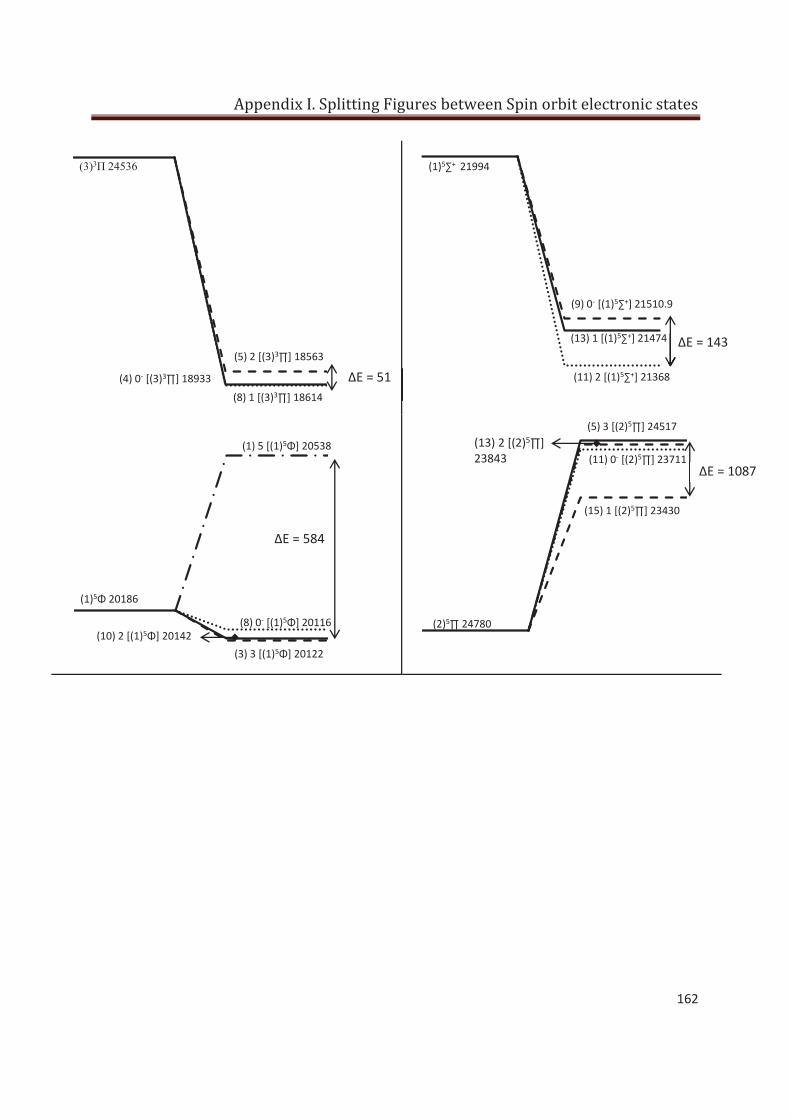
Appendix I. Splitting Figures between Spin orbit electronic states
162
(3)3Π 24536
(5) 2 [(3)3∏] 18563
(8) 1 [(3)3∏] 18614
(4) 0- [(3)3∏] 18933
(1)5∑+ 21994
(13) 1 [(1)5∑+] 21474
(11) 2 [(1)5∑+] 21368
(9) 0- [(1)5∑+] 21510.9
(1)5Φ 20186
(3) 3 [(1)5Φ] 20122
(1) 5 [(1)5Φ] 20538
(10) 2 [(1)5Φ] 20142 (8) 0- [(1)5Φ] 20116
ΔE = 584
(2)5∏ 24780
(11) 0- [(2)5∏] 23711
(15) 1 [(2)5∏] 23430
(13) 2 [(2)5∏] 23843
(5) 3 [(2)5∏] 24517
ΔE = 1087
ΔE = 143
ΔE = 51
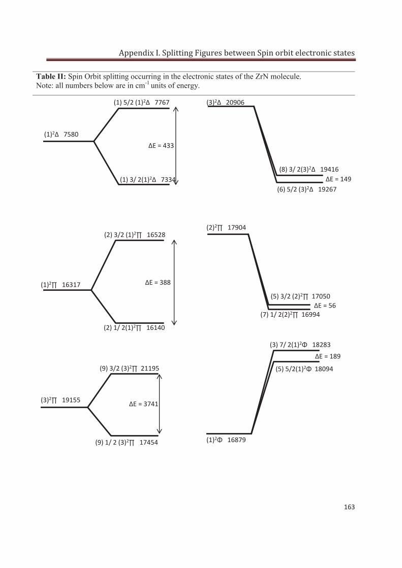
Appendix I. Splitting Figures between Spin orbit electronic states
163
Table II: Spin Orbit splitting occurring in the electronic states of the ZrN molecule. Note: all numbers below are in cm-1 units of energy.
(1)2∆ 7580
(1) 5/2 (1)2∆ 7767
(1) 3/ 2(1)2∆ 7334
∆E = 433
(3)2∆ 20906
(6) 5/2 (3)2∆ 19267
(8) 3/ 2(3)2∆ 19416 ∆E = 149
(1)2∏ 16317
(2) 3/2 (1)2∏ 16528
(2) 1/ 2(1)2∏ 16140
∆E = 388
(2)2∏ 17904
(5) 3/2 (2)2∏ 17050
(7) 1/ 2(2)2∏ 16994 ∆E = 56
(3)2∏ 19155
(9) 3/2 (3)2∏ 21195
(9) 1/ 2 (3)2∏ 17454
∆E = 3741
(1)2Φ 16879
(5) 5/2(1)2Φ 18094
(3) 7/ 2(1)2Φ 18283
∆E = 189
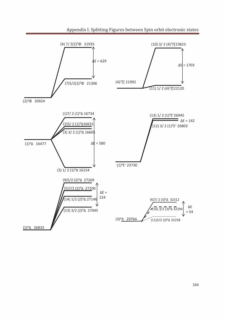
Appendix I. Splitting Figures between Spin orbit electronic states
164
(2)2Φ 20924
(4) 7/ 2(2)2Φ 21935
(7)5/2(2)2Φ 21306
∆E = 629
(4)2∏ 21992
(10) 3/ 2 (4)2∏23823
∆E = 1703
(11) 1/ 2 (4)2∏22120
(1)4∆ 16477
(3) 3/ 2 (1)4∆ 16605
∆E = 580
(3) 1/ 2 (1)4∆ 16154
(2)5/ 2 (1)4∆16631
(1)7/ 2 (1)4∆ 16734
(1)4Σ+ 23730
(12) 3/ 2 (1)4Σ+ 26803 ∆E = 142
(13) 1/ 2 (1)4Σ+26945
(2)4∆ 26833
(14) 1/2 (2)4∆ 27146
∆E = 224
(13) 3/2 (2)4∆ 27045
(5)7/2 (2)4∆ 27200
(9)5/2 (2)4∆ 27269
(3)4∆ 29764
∆E = 54
(16) 3/2 (3)4∆ 32294
(6)7/ 2 (3)4∆ 32312
(11)5/2 (3)4∆ 32258
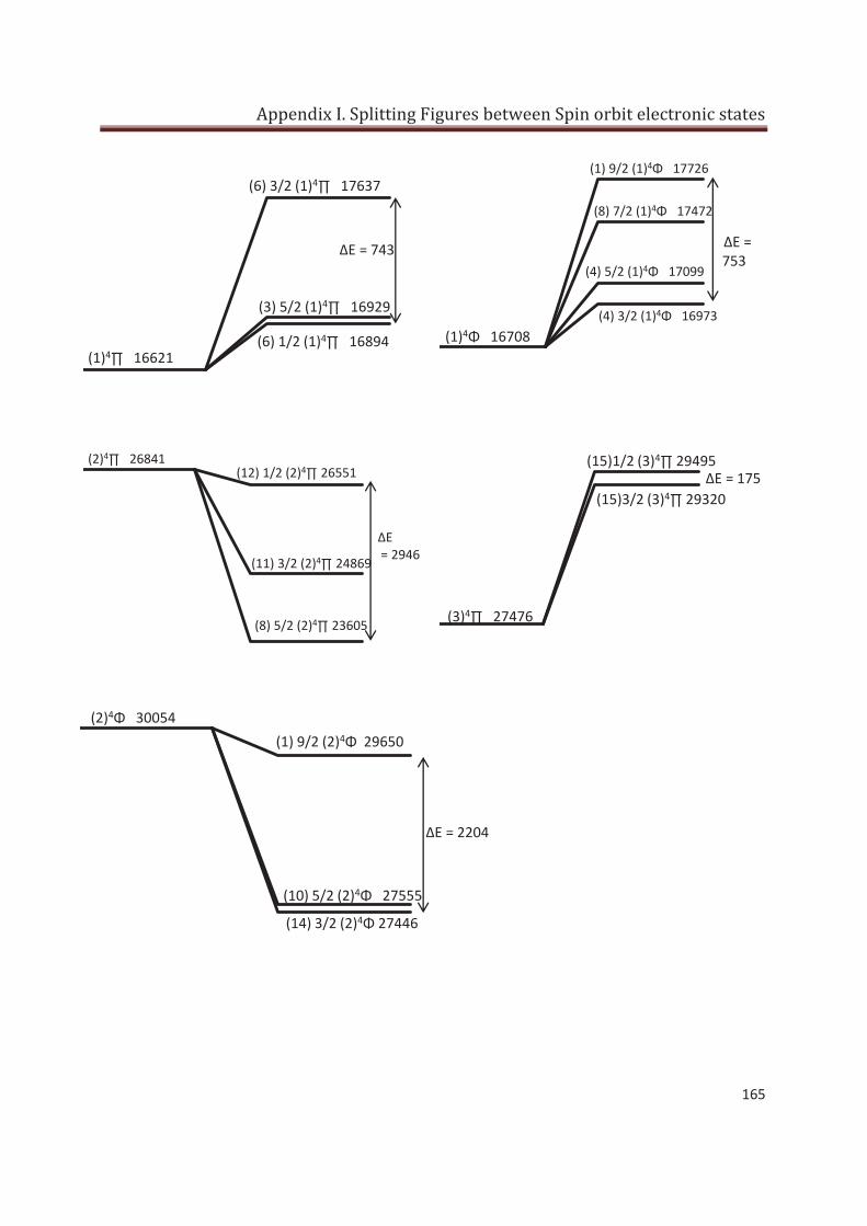
Appendix I. Splitting Figures between Spin orbit electronic states
165
(1)4∏ 16621
(6) 3/2 (1)4∏ 17637
(3) 5/2 (1)4∏ 16929
(6) 1/2 (1)4∏ 16894
∆E = 743
(1)4Φ 16708
(8) 7/2 (1)4Φ 17472
(4) 5/2 (1)4Φ 17099
(4) 3/2 (1)4Φ 16973
∆E = 753
(1) 9/2 (1)4Φ 17726
(2)4∏ 26841 (12) 1/2 (2)4∏ 26551
(11) 3/2 (2)4∏ 24869
(8) 5/2 (2)4∏ 23605
∆E = 2946
(3)4∏ 27476
(15)1/2 (3)4∏ 29495
(15)3/2 (3)4∏ 29320 ∆E = 175
(2)4Φ 30054 (1) 9/2 (2)4Φ 29650
(14) 3/2 (2)4Φ 27446
(10) 5/2 (2)4Φ 27555
∆E = 2204
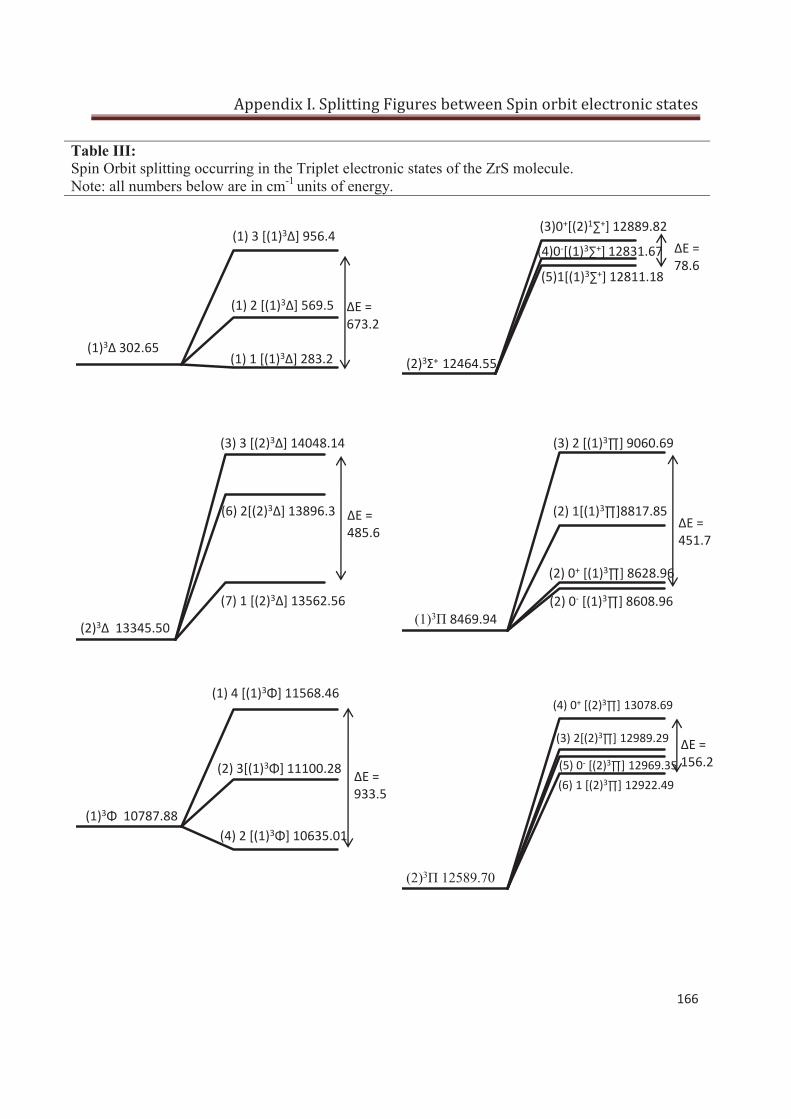
Appendix I. Splitting Figures between Spin orbit electronic states
166
Table III: Spin Orbit splitting occurring in the Triplet electronic states of the ZrS molecule. Note: all numbers below are in cm-1 units of energy.
(1)3∆ 302.65 (1) 1 [(1)3∆] 283.2
(1) 2 [(1)3∆] 569.5
(1) 3 [(1)3∆] 956.4
∆E = 673.2
(2)3Σ+ 12464.55
(5)1[(1)3∑+] 12811.18
(4)0-[(1)3∑+] 12831.67
(3)0+[(2)1∑+] 12889.82 ∆E = 78.6
(2)3∆ 13345.50
(7) 1 [(2)3∆] 13562.56
(6) 2[(2)3∆] 13896.3
(3) 3 [(2)3∆] 14048.14
∆E = 485.6
(1)3Π 8469.94
(2) 0+ [(1)3∏] 8628.96
(2) 1[(1)3∏]8817.85
(3) 2 [(1)3∏] 9060.69
∆E = 451.7
(2) 0- [(1)3∏] 8608.96
(1)3Φ 10787.88 (4) 2 [(1)3Φ] 10635.01
(2) 3[(1)3Φ] 11100.28
(1) 4 [(1)3Φ] 11568.46
∆E = 933.5
(2)3Π 12589.70
(6) 1 [(2)3∏] 12922.49
(3) 2[(2)3∏] 12989.29
(4) 0+ [(2)3∏] 13078.69
∆E = 156.2 (5) 0- [(2)3∏] 12969.35
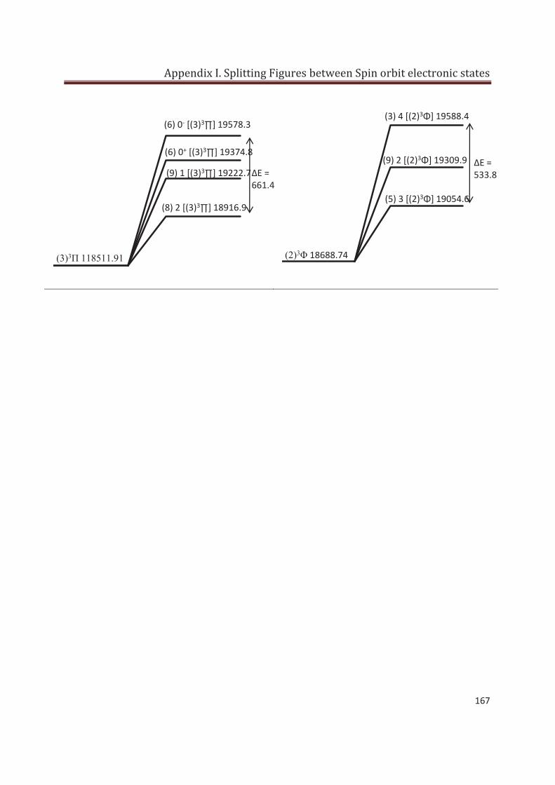
Appendix I. Splitting Figures between Spin orbit electronic states
167
(3)3Π 118511.91
(8) 2 [(3)3∏] 18916.9
(6) 0+ [(3)3∏] 19374.8
(6) 0- [(3)3∏] 19578.3
∆E = 661.4
(9) 1 [(3)3∏] 19222.7
(2)3Φ 18688.74
(5) 3 [(2)3Φ] 19054.6
(9) 2 [(2)3Φ] 19309.9
(3) 4 [(2)3Φ] 19588.4
∆E = 533.8
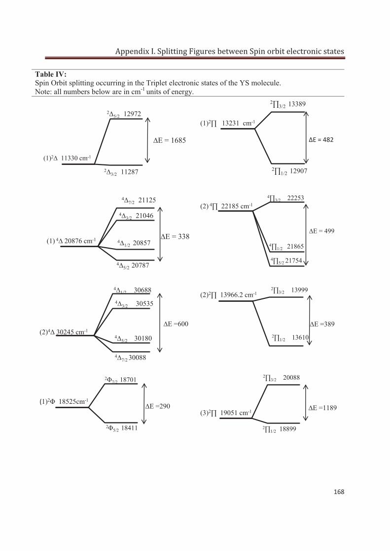
Appendix I. Splitting Figures between Spin orbit electronic states
168
Table IV: Spin Orbit splitting occurring in the Triplet electronic states of the YS molecule. Note: all numbers below are in cm-1 units of energy.
(1)2∆ 11330 cm-1
2∆5/2 12972
2∆3/2 11287
∆E = 1685
(1)2∏ 13231 cm-1
2∏3/2 13389
2∏1/2 12907
∆E = 482
(1) 4∆ 20876 cm-1
4∆5/2 20787
4∆1/2 20857
4∆3/2 21046
∆E = 338
4∆7/2 21125 (2) 4∏ 22185 cm-1
4∏5/2 21754
4∏3/2 22253
4∏1/2 21865
∆E = 499
(2)4Δ 30245 cm-1
4∆1/2 30688
4∆3/2 30535
4∆5/2 30180
4∆7/2 30088
∆E =600
(2)2∏ 13966.2 cm-1
2∏3/2 13999
2∏1/2 13610
∆E =389
(1)2Φ 18525cm-1
2Φ7/2 18701
∆E =290
2Φ5/2 18411
(3)2∏ 19051 cm-1
2∏3/2 20088
2∏1/2 18899
∆E =1189
Appendix II. Results of Vibrational Calculations
169
Appendix II
Results of Vibrational Calculations
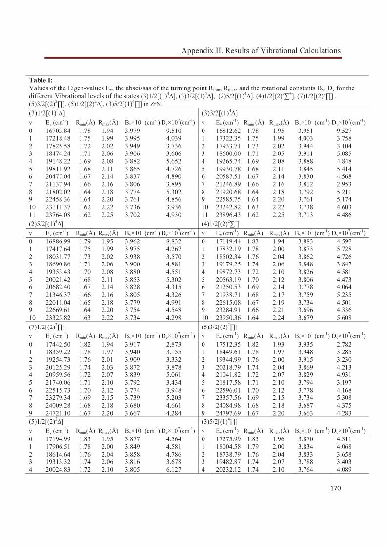
Appendix II. Results of Vibrational Calculations
170
Table I: Values of the Eigen-values Ev, the abscissas of the turning point Rmin, Rmax, and the rotational constants Bv, Dv for the different Vibrational levels of the states (3)1/2[(1)4∆], (3)3/2[(1)4∆], (2)5/2[(1)4∆], (4)1/2[(2)2∑+], (7)1/2[(2)2∏] , (5)3/2[(2)2∏], (5)1/2[(2)2∆], (3)5/2[(1)4∏] in ZrN. (3)1/2[(1)4∆] (3)3/2[(1)4∆] v Ev (cm-1) Rmin(Å) Rmax(Å) Bv×101 (cm-1) Dv×107(cm-1) v Ev (cm-1) Rmin (Å) Rmax(Å) Bv×101 (cm-1) Dv×107(cm-1) 0 16703.84 1.78 1.94 3.979 9.510 0 16812.62 1.78 1.95 3.951 9.527 1 17218.48 1.75 1.99 3.995 4.039 1 17322.35 1.75 1.99 4.003 3.758 2 17825.58 1.72 2.02 3.949 3.736 2 17933.71 1.73 2.02 3.944 3.104 3 18474.24 1.71 2.06 3.906 3.606 3 18600.00 1.71 2.05 3.911 5.085 4 19148.22 1.69 2.08 3.882 5.652 4 19265.74 1.69 2.08 3.888 4.848 5 19811.92 1.68 2.11 3.865 4.726 5 19930.78 1.68 2.11 3.845 5.414 6 20477.04 1.67 2.14 3.837 4.890 6 20587.51 1.67 2.14 3.830 4.568 7 21137.94 1.66 2.16 3.806 3.895 7 21246.89 1.66 2.16 3.812 2.953 8 21802.02 1.64 2.18 3.774 5.302 8 21920.68 1.64 2.18 3.792 5.211 9 22458.36 1.64 2.20 3.761 4.856 9 22585.75 1.64 2.20 3.761 5.174 10 23111.37 1.62 2.22 3.736 3.936 10 23242.82 1.63 2.22 3.738 4.603 11 23764.08 1.62 2.25 3.702 4.930 11 23896.43 1.62 2.25 3.713 4.486 (2)5/2[(1)4∆] (4)1/2[(2)2∑+] v Ev (cm-1) Rmin(Å) Rmax(Å) Bv×101 (cm-1) Dv×107(cm-1) v Ev (cm-1) Rmin(Å) Rmax(Å) Bv×101 (cm-1) Dv×107(cm-1) 0 16886.99 1.79 1.95 3.962 8.832 0 17119.44 1.83 1.94 3.883 4.597 1 17417.64 1.75 1.99 3.975 4.267 1 17832.19 1.78 2.00 3.873 5.728 2 18031.77 1.73 2.02 3.938 3.570 2 18502.34 1.76 2.04 3.862 4.726 3 18690.86 1.71 2.06 3.900 4.881 3 19179.25 1.74 2.06 3.848 3.847 4 19353.43 1.70 2.08 3.880 4.551 4 19872.73 1.72 2.10 3.826 4.581 5 20021.42 1.68 2.11 3.853 5.302 5 20563.19 1.70 2.12 3.806 4.473 6 20682.40 1.67 2.14 3.828 4.315 6 21250.53 1.69 2.14 3.778 4.064 7 21346.37 1.66 2.16 3.805 4.326 7 21938.71 1.68 2.17 3.759 5.235 8 22011.04 1.65 2.18 3.779 4.991 8 22615.08 1.67 2.19 3.734 4.501 9 22669.61 1.64 2.20 3.754 4.548 9 23284.91 1.66 2.21 3.696 4.336 10 23325.82 1.63 2.22 3.734 4.298 10 23950.36 1.64 2.24 3.679 5.608 (7)1/2[(2)2∏] (5)3/2[(2)2∏] v Ev (cm-1) Rmin(Å) Rmax(Å) Bv×101 (cm-1) Dv×107(cm-1) v Ev (cm-1) Rmin(Å) Rmax(Å) Bv×101 (cm-1) Dv×107(cm-1) 0 17442.50 1.82 1.94 3.917 2.873 0 17512.35 1.82 1.93 3.935 2.782 1 18359.22 1.78 1.97 3.940 3.155 1 18449.61 1.78 1.97 3.948 3.285 2 19254.73 1.76 2.01 3.909 3.332 2 19344.99 1.76 2.00 3.915 3.230 3 20125.29 1.74 2.03 3.872 3.878 3 20218.79 1.74 2.04 3.869 4.213 4 20959.56 1.72 2.07 3.839 5.061 4 21041.82 1.72 2.07 3.829 4.931 5 21740.06 1.71 2.10 3.792 3.434 5 21817.58 1.71 2.10 3.794 3.197 6 22515.73 1.70 2.12 3.774 3.948 6 22596.01 1.70 2.12 3.778 4.168 7 23279.34 1.69 2.15 3.739 5.203 7 23357.56 1.69 2.15 3.734 5.308 8 24009.28 1.68 2.18 3.680 4.661 8 24084.98 1.68 2.18 3.687 4.375 9 24721.10 1.67 2.20 3.667 4.284 9 24797.69 1.67 2.20 3.663 4.283 (5)1/2[(2)2∆] (3)5/2[(1)4∏] v Ev (cm-1) Rmin(Å) Rmax(Å) Bv×101 (cm-1) Dv×107(cm-1) v Ev (cm-1) Rmin(Å) Rmax(Å) Bv×101 (cm-1) Dv×107(cm-1) 0 17194.99 1.83 1.95 3.877 4.564 0 17275.99 1.83 1.96 3.870 4.311 1 17906.51 1.78 2.00 3.849 4.581 1 18004.58 1.79 2.00 3.834 4.068 2 18614.64 1.76 2.04 3.858 4.786 2 18738.79 1.76 2.04 3.833 3.658 3 19313.32 1.74 2.06 3.816 3.678 3 19482.87 1.74 2.07 3.788 3.403 4 20024.83 1.72 2.10 3.805 6.127 4 20232.12 1.74 2.10 3.764 4.089
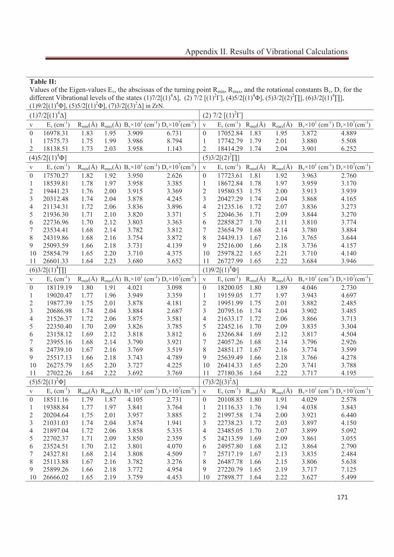
Appendix II. Results of Vibrational Calculations
171
Table II: Values of the Eigen-values Ev, the abscissas of the turning point Rmin, Rmax, and the rotational constants Bv, Dv for the different Vibrational levels of the states (1)7/2[(1)4∆], (2) 7/2 [(1)2Г], (4)5/2[(1)4Φ], (5)3/2[(2)2∏], (6)3/2[(1)4∏], (1)9/2[(1)4Φ], (5)5/2[(1)2Φ], (7)3/2[(3)2∆] in ZrN. (1)7/2[(1)4∆] (2) 7/2 [(1)2Г] v Ev (cm-1) Rmin(Å) Rmax(Å) Bv×101 (cm-1) Dv×107(cm-1) v Ev (cm-1) Rmin(Å) Rmax(Å) Bv×101 (cm-1) Dv×107(cm-1) 0 16978.31 1.83 1.95 3.909 6.731 0 17052.84 1.83 1.95 3.872 4.889 1 17575.73 1.75 1.99 3.986 8.794 1 17742.79 1.79 2.01 3.880 5.508 2 18138.51 1.73 2.03 3.958 1.143 2 18414.29 1.74 2.04 3.901 6.252 (4)5/2[(1)4Φ] (5)3/2[(2)2∏] v Ev (cm-1) Rmin(Å) Rmax(Å) Bv×101 (cm-1) Dv×107(cm-1) v Ev (cm-1) Rmin(Å) Rmax(Å) Bv×101 (cm-1) Dv×107(cm-1) 0 17570.27 1.82 1.92 3.950 2.626 0 17723.61 1.81 1.92 3.963 2.760 1 18539.81 1.78 1.97 3.958 3.385 1 18672.84 1.78 1.97 3.959 3.170 2 19441.23 1.76 2.00 3.915 3.369 2 19580.53 1.75 2.00 3.913 3.939 3 20312.48 1.74 2.04 3.878 4.245 3 20427.29 1.74 2.04 3.868 4.165 4 21134.31 1.72 2.06 3.836 3.896 4 21235.16 1.72 2.07 3.836 3.273 5 21936.30 1.71 2.10 3.820 3.371 5 22046.36 1.71 2.09 3.844 3.270 6 22736.96 1.70 2.12 3.803 3.363 6 22858.27 1.70 2.11 3.810 3.774 7 23534.41 1.68 2.14 3.782 3.812 7 23654.79 1.68 2.14 3.780 3.884 8 24319.86 1.68 2.16 3.754 3.872 8 24439.13 1.67 2.16 3.765 3.644 9 25093.59 1.66 2.18 3.731 4.139 9 25216.00 1.66 2.18 3.736 4.157 10 25854.79 1.65 2.20 3.710 4.375 10 25978.22 1.65 2.21 3.710 4.140 11 26601.33 1.64 2.23 3.680 3.652 11 26727.99 1.65 2.22 3.684 3.946 (6)3/2[(1)4∏] (1)9/2[(1)4Φ] v Ev (cm-1) Rmin(Å) Rmax(Å) Bv×101 (cm-1) Dv×107(cm-1) v Ev (cm-1) Rmin(Å) Rmax(Å) Bv×101 (cm-1) Dv×107(cm-1) 0 18119.19 1.80 1.91 4.021 3.098 0 18200.05 1.80 1.89 4.046 2.730 1 19020.47 1.77 1.96 3.949 3.359 1 19159.05 1.77 1.97 3.943 4.697 2 19877.39 1.75 2.01 3.878 4.181 2 19951.99 1.75 2.01 3.882 2.485 3 20686.98 1.74 2.04 3.884 2.687 3 20795.16 1.74 2.04 3.902 3.485 4 21526.37 1.72 2.06 3.875 3.581 4 21633.17 1.72 2.06 3.866 3.713 5 22350.40 1.70 2.09 3.826 3.785 5 22452.16 1.70 2.09 3.835 3.304 6 23158.12 1.69 2.12 3.818 3.812 6 23266.84 1.69 2.12 3.817 4.504 7 23955.16 1.68 2.14 3.790 3.921 7 24057.26 1.68 2.14 3.796 2.926 8 24739.10 1.67 2.16 3.769 3.519 8 24851.17 1.67 2.16 3.774 3.599 9 25517.13 1.66 2.18 3.743 4.789 9 25639.49 1.66 2.18 3.766 4.278 10 26275.79 1.65 2.20 3.727 4.225 10 26414.33 1.65 2.20 3.741 3.788 11 27022.26 1.64 2.22 3.692 3.769 11 27180.36 1.64 2.22 3.717 4.195 (5)5/2[(1)2Φ] (7)3/2[(3)2∆] v Ev (cm-1) Rmin(Å) Rmax(Å) Bv×101 (cm-1) Dv×107(cm-1) v Ev (cm-1) Rmin(Å) Rmax(Å) Bv×101 (cm-1) Dv×107(cm-1) 0 18511.16 1.79 1.87 4.105 2.731 0 20108.85 1.80 1.91 4.029 2.578 1 19388.84 1.77 1.97 3.841 3.764 1 21116.33 1.76 1.94 4.038 3.843 2 20204.64 1.75 2.01 3.957 3.885 2 21997.58 1.74 2.00 3.921 6.440 3 21031.03 1.74 2.04 3.874 1.941 3 22738.23 1.72 2.03 3.897 4.150 4 21897.04 1.72 2.06 3.858 5.335 4 23485.05 1.70 2.07 3.899 5.092 5 22702.37 1.71 2.09 3.850 2.359 5 24213.59 1.69 2.09 3.861 3.055 6 23524.51 1.70 2.12 3.801 4.070 6 24957.80 1.68 2.12 3.864 2.790 7 24327.81 1.68 2.14 3.808 4.509 7 25717.19 1.67 2.13 3.835 2.484 8 25113.88 1.67 2.16 3.782 3.276 8 26487.78 1.66 2.15 3.806 5.638 9 25899.26 1.66 2.18 3.772 4.954 9 27220.79 1.65 2.19 3.717 7.125 10 26666.02 1.65 2.19 3.759 4.453 10 27898.77 1.64 2.22 3.627 5.499
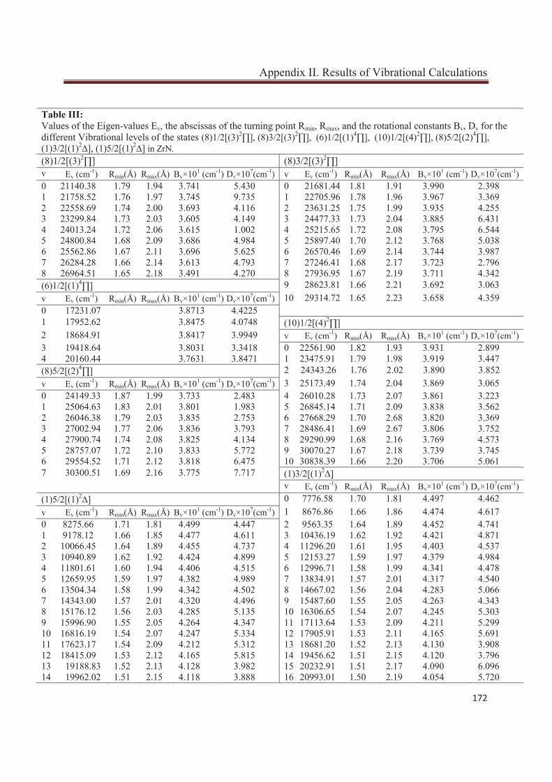
Appendix II. Results of Vibrational Calculations
172
Table III: Values of the Eigen-values Ev, the abscissas of the turning point Rmin, Rmax, and the rotational constants Bv, Dv for the different Vibrational levels of the states (8)1/2[(3)2∏], (8)3/2[(3)2∏], (6)1/2[(1)4∏], (10)1/2[(4)2∏], (8)5/2[(2)4∏], (1)3/2[(1)2∆], (1)5/2[(1)2∆] in ZrN. (8)1/2[(3)2∏] (8)3/2[(3)2∏] v Ev (cm-1) Rmin(Å) Rmax(Å) Bv×101 (cm-1) Dv×107(cm-1) v Ev (cm-1) Rmin(Å) Rmax(Å) Bv×101 (cm-1) Dv×107(cm-1) 0 21140.38 1.79 1.94 3.741 5.430 0 21681.44 1.81 1.91 3.990 2.398 1 21758.52 1.76 1.97 3.745 9.735 1 22705.96 1.78 1.96 3.967 3.369 2 22558.69 1.74 2.00 3.693 4.116 2 23631.25 1.75 1.99 3.935 4.255 3 23299.84 1.73 2.03 3.605 4.149 3 24477.33 1.73 2.04 3.885 6.431 4 24013.24 1.72 2.06 3.615 1.002 4 25215.65 1.72 2.08 3.795 6.544 5 24800.84 1.68 2.09 3.686 4.984 5 25897.40 1.70 2.12 3.768 5.038 6 25562.86 1.67 2.11 3.696 5.625 6 26570.46 1.69 2.14 3.744 3.987 7 26284.28 1.66 2.14 3.613 4.793 7 27246.41 1.68 2.17 3.723 2.796 8 26964.51 1.65 2.18 3.491 4.270 8 27936.95 1.67 2.19 3.711 4.342 (6)1/2[(1)4∏] 9 28623.81 1.66 2.21 3.692 3.063 v Ev (cm-1) Rmin(Å) Rmax(Å) Bv×101 (cm-1) Dv×107(cm-1) 10 29314.72 1.65 2.23 3.658 4.359 0 17231.07 3.8713 4.4225 1 17952.62 3.8475 4.0748 (10)1/2[(4)2∏] 2 18684.91 3.8417 3.9949 v Ev (cm-1) Rmin(Å) Rmax(Å) Bv×101 (cm-1) Dv×107(cm-1) 3 19418.64 3.8031 3.3418 0 22561.90 1.82 1.93 3.931 2.899 4 20160.44 3.7631 3.8471 1 23475.91 1.79 1.98 3.919 3.447 (8)5/2[(2)4∏] 2 24343.26 1.76 2.02 3.890 3.852 v Ev (cm-1) Rmin(Å) Rmax(Å) Bv×101 (cm-1) Dv×107(cm-1) 3 25173.49 1.74 2.04 3.869 3.065 0 24149.33 1.87 1.99 3.733 2.483 4 26010.28 1.73 2.07 3.861 3.223 1 25064.63 1.83 2.01 3.801 1.983 5 26845.14 1.71 2.09 3.838 3.562 2 26046.38 1.79 2.03 3.835 2.753 6 27668.29 1.70 2.68 3.820 3.369 3 27002.94 1.77 2.06 3.836 3.793 7 28486.41 1.69 2.67 3.806 3.752 4 27900.74 1.74 2.08 3.825 4.134 8 29290.99 1.68 2.16 3.769 4.573 5 28757.07 1.72 2.10 3.833 5.772 9 30070.27 1.67 2.18 3.739 3.745 6 29554.52 1.71 2.12 3.818 6.475 10 30838.39 1.66 2.20 3.706 5.061 7 30300.51 1.69 2.16 3.775 7.717 (1)3/2[(1)2∆] v Ev (cm-1) Rmin(Å) Rmax(Å) Bv×101 (cm-1) Dv×107(cm-1) (1)5/2[(1)2∆] 0 7776.58 1.70 1.81 4.497 4.462 v Ev (cm-1) Rmin(Å) Rmax(Å) Bv×101 (cm-1) Dv×107(cm-1) 1 8676.86 1.66 1.86 4.474 4.617 0 8275.66 1.71 1.81 4.499 4.447 2 9563.35 1.64 1.89 4.452 4.741 1 9178.12 1.66 1.85 4.477 4.611 3 10436.19 1.62 1.92 4.421 4.871 2 10066.45 1.64 1.89 4.455 4.737 4 11296.20 1.61 1.95 4.403 4.537 3 10940.89 1.62 1.92 4.424 4.899 5 12153.27 1.59 1.97 4.379 4.984 4 11801.61 1.60 1.94 4.406 4.515 6 12996.71 1.58 1.99 4.341 4.478 5 12659.95 1.59 1.97 4.382 4.989 7 13834.91 1.57 2.01 4.317 4.540 6 13504.34 1.58 1.99 4.342 4.502 8 14667.02 1.56 2.04 4.283 5.066 7 14343.00 1.57 2.01 4.320 4.496 9 15487.60 1.55 2.05 4.263 4.343 8 15176.12 1.56 2.03 4.285 5.135 10 16306.65 1.54 2.07 4.245 5.303 9 15996.90 1.55 2.05 4.264 4.347 11 17113.64 1.53 2.09 4.211 5.299 10 16816.19 1.54 2.07 4.247 5.334 12 17905.91 1.53 2.11 4.165 5.691 11 17623.17 1.54 2.09 4.212 5.312 13 18681.20 1.52 2.13 4.130 3.908 12 18415.09 1.53 2.12 4.165 5.815 14 19456.62 1.51 2.15 4.120 3.796 13 19188.83 1.52 2.13 4.128 3.982 15 20232.91 1.51 2.17 4.090 6.096 14 19962.02 1.51 2.15 4.118 3.888 16 20993.01 1.50 2.19 4.054 5.720
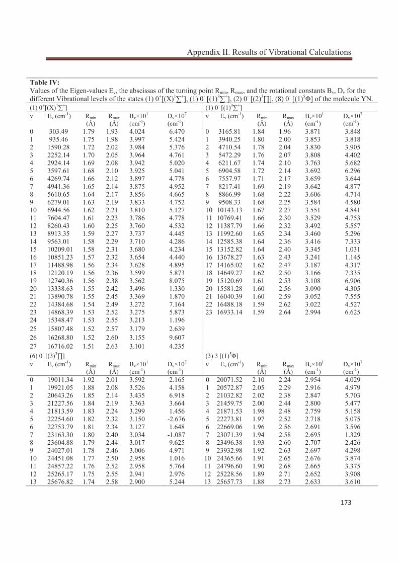
Appendix II. Results of Vibrational Calculations
173
Table IV: Values of the Eigen-values Ev, the abscissas of the turning point Rmin, Rmax, and the rotational constants Bv, Dv for the different Vibrational levels of the states (1) 0+[(X)1∑+], (1) 0- [(1)3∑+], (2) 0- [(2)3∏], (8) 0- [(1)5Φ] of the molecule YN. (1) 0+[(X)1∑+] (1) 0- [(1)3∑+] v Ev (cm-1) Rmin
(Å) Rmax (Å)
Bv×101 (cm-1)
Dv×107
(cm-1) v Ev (cm-1) Rmin
(Å) Rmax (Å)
Bv×101 (cm-1)
Dv×107
(cm-1) 0 303.49 1.79 1.93 4.024 6.470 0 3165.81 1.84 1.96 3.871 3.848 1 935.46 1.75 1.98 3.997 5.424 1 3940.25 1.80 2.00 3.853 3.818 2 1590.28 1.72 2.02 3.984 5.376 2 4710.54 1.78 2.04 3.830 3.905 3 2252.14 1.70 2.05 3.964 4.761 3 5472.29 1.76 2.07 3.808 4.402 4 2924.14 1.69 2.08 3.942 5.020 4 6211.67 1.74 2.10 3.763 5.682 5 3597.61 1.68 2.10 3.925 5.041 5 6904.58 1.72 2.14 3.692 6.296 6 4269.74 1.66 2.12 3.897 4.778 6 7557.97 1.71 2.17 3.659 3.644 7 4941.36 1.65 2.14 3.875 4.952 7 8217.41 1.69 2.19 3.642 4.877 8 5610.65 1.64 2.17 3.856 4.665 8 8866.99 1.68 2.22 3.606 4.714 9 6279.01 1.63 2.19 3.833 4.752 9 9508.33 1.68 2.25 3.584 4.580 10 6944.56 1.62 2.21 3.810 5.127 10 10143.13 1.67 2.27 3.551 4.841 11 7604.47 1.61 2.23 3.786 4.778 11 10769.41 1.66 2.30 3.529 4.753 12 8260.43 1.60 2.25 3.760 4.532 12 11387.79 1.66 2.32 3.492 5.557 13 8913.35 1.59 2.27 3.737 4.445 13 11992.60 1.65 2.34 3.460 5.296 14 9563.01 1.58 2.29 3.710 4.286 14 12585.38 1.64 2.36 3.416 7.333 15 10209.01 1.58 2.31 3.680 4.234 15 13152.82 1.64 2.40 3.345 1.031 16 10851.23 1.57 2.32 3.654 4.440 16 13678.27 1.63 2.43 3.241 1.145 17 11488.98 1.56 2.34 3.628 4.895 17 14165.02 1.62 2.47 3.187 4.317 18 12120.19 1.56 2.36 3.599 5.873 18 14649.27 1.62 2.50 3.166 7.335 19 12740.36 1.56 2.38 3.562 8.075 19 15120.69 1.61 2.53 3.108 6.906 20 13338.63 1.55 2.42 3.496 1.330 20 15581.28 1.60 2.56 3.090 4.305 21 13890.78 1.55 2.45 3.369 1.870 21 16040.39 1.60 2.59 3.052 7.555 22 14384.68 1.54 2.49 3.272 7.164 22 16488.18 1.59 2.62 3.022 4.527 23 14868.39 1.53 2.52 3.275 5.873 23 16933.14 1.59 2.64 2.994 6.625 24 15348.47 1.53 2.55 3.213 1.196 25 15807.48 1.52 2.57 3.179 2.639 26 16268.80 1.52 2.60 3.155 9.607 27 16716.02 1.51 2.63 3.101 4.235 (6) 0- [(3)3∏] (3) 3 [(1)5Φ] v Ev (cm-1) Rmin
(Å) Rmax (Å)
Bv×101 (cm-1)
Dv×107
(cm-1) v Ev (cm-1) Rmin
(Å) Rmax (Å)
Bv×101 (cm-1)
Dv×107
(cm-1) 0 19011.34 1.92 2.01 3.592 2.165 0 20071.52 2.10 2.24 2.954 4.029 1 19921.05 1.88 2.08 3.526 4.158 1 20572.87 2.05 2.29 2.916 4.979 2 20643.26 1.85 2.14 3.435 6.918 2 21032.82 2.02 2.38 2.847 5.703 3 21227.56 1.84 2.19 3.363 3.664 3 21459.75 2.00 2.44 2.800 5.477 4 21813.59 1.83 2.24 3.299 1.456 4 21871.53 1.98 2.48 2.759 5.158 5 22254.60 1.82 2.32 3.150 -2.676 5 22273.81 1.97 2.52 2.718 5.075 6 22753.79 1.81 2.34 3.127 1.648 6 22669.06 1.96 2.56 2.691 3.596 7 23163.30 1.80 2.40 3.034 -1.087 7 23071.39 1.94 2.58 2.695 1.329 8 23604.88 1.79 2.44 3.017 9.625 8 23496.38 1.93 2.60 2.707 2.426 9 24027.01 1.78 2.46 3.006 4.971 9 23932.98 1.92 2.63 2.697 4.298 10 24451.08 1.77 2.50 2.958 1.016 10 24365.66 1.91 2.65 2.676 3.874 11 24857.22 1.76 2.52 2.958 5.764 11 24796.60 1.90 2.68 2.665 3.375 12 25265.17 1.75 2.55 2.941 2.976 12 25228.56 1.89 2.71 2.652 3.908 13 25676.82 1.74 2.58 2.900 5.244 13 25657.73 1.88 2.73 2.633 3.610
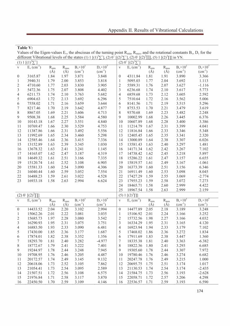
Appendix II. Results of Vibrational Calculations
174
Table V: Values of the Eigen-values Ev, the abscissas of the turning point Rmin, Rmax, and the rotational constants Bv, Dv for the different Vibrational levels of the states (1) 1 [(1)3∑+], (2) 0+ [(2)1∑+], (2) 0- [(2)3∏], (5) 1 [(2)3∏] in YN. (1) 1 [(1)3∑+] (2) 0+ [(2)1∑+] v Ev (cm-1) Rmin
(Å) Rmax (Å)
Bv×101 (cm-1)
Dv×107
(cm-1) v Ev (cm-1) Rmin
(Å) Rmax (Å)
Bv×101 (cm-1)
Dv×107
(cm-1) 0 3165.87 1.84 1.97 3.871 3.848 0 4311.84 1.81 1.91 3.890 3.366 1 3940.31 1.79 2.00 3.853 3.818 1 5095.03 1.77 2.04 3.692 1.113 2 4710.60 1.77 2.03 3.830 3.905 2 5589.31 1.76 2.07 3.627 -1.116 3 5472.36 1.75 2.07 3.808 4.402 3 6236.68 1.74 2.10 3.617 5.773 4 6211.73 1.74 2.10 3.763 5.682 4 6859.68 1.73 2.12 3.605 2.592 5 6904.63 1.72 2.13 3.692 6.296 5 7510.64 1.72 2.16 3.562 5.006 6 7558.02 1.71 2.16 3.659 3.644 6 8141.56 1.71 2.19 3.515 5.296 7 8217.46 1.70 2.19 3.642 4.877 7 8753.53 1.70 2.21 3.479 3.619 8 8867.05 1.69 2.21 3.606 4.713 8 9370.68 1.69 2.23 3.482 2.248 9 9508.38 1.68 2.25 3.584 4.580 9 10002.99 1.68 2.26 3.445 6.376 10 10143.18 1.67 2.27 3.551 4.840 10 10607.89 1.68 2.28 3.400 3.386 11 10769.47 1.66 2.30 3.529 4.753 11 11214.79 1.67 2.31 3.399 4.041 12 11387.86 1.66 2.31 3.492 5.556 12 11816.84 1.66 2.33 3.346 5.348 13 11992.69 1.65 2.34 3.460 5.298 13 12405.45 1.65 2.35 3.341 2.320 14 12585.46 1.64 2.36 3.415 7.336 14 13000.89 1.64 2.38 3.307 6.026 15 13152.89 1.63 2.39 3.345 1.030 15 13581.43 1.63 2.40 3.297 1.481 16 13678.32 1.63 2.41 3.241 1.145 16 14171.34 1.62 2.42 3.267 7.102 17 14165.07 1.62 2.47 3.187 4.319 17 14738.42 1.62 2.45 3.218 5.897 18 14649.32 1.61 2.51 3.166 7.335 18 15286.22 1.61 2.47 3.157 6.655 19 15120.74 1.61 2.52 3.108 6.905 19 15819.57 1.61 2.49 3.167 -1.061 20 15581.33 1.60 2.54 3.090 4.306 20 16373.39 1.60 2.51 3.156 6.346 21 16040.44 1.60 2.59 3.052 7.554 21 16911.49 1.60 2.53 3.098 8.045 22 16488.23 1.59 2.61 3.022 4.528 22 17427.29 1.59 2.55 3.069 -2.774 23 16933.18 1.58 2.63 2.994 6.624 23 17955.23 1.59 2.58 3.072 7.273 24 18465.71 1.58 2.60 2.999 4.422 25 18967.54 1.58 2.63 2.999 2.159 (2) 0- [(2)3∏] (5) 1 [(2)3∏] v Ev (cm-1) Rmin
(Å) Rmax (Å)
Bv×101 (cm-1)
Dv×107
(cm-1) v Ev (cm-1) Rmin
(Å) Rmax (Å)
Bv×101 (cm-1)
Dv×107
(cm-1) 0 14433.52 2.04 2.20 3.102 2.994 0 14477.89 2.05 2.18 3.189 3.248 1 15062.26 2.01 2.22 3.081 3.035 1 15106.92 2.01 2.24 3.166 3.252 2 15685.73 1.97 2.28 3.080 3.542 2 15732.56 1.98 2.27 3.166 4.032 3 16290.93 1.95 2.31 3.075 3.751 3 16334.29 1.95 2.31 3.165 4.120 4 16883.50 1.93 2.33 3.090 6.481 4 16923.94 1.94 2.33 3.179 7.102 5 17430.00 1.85 2.36 3.177 1.687 5 17468.02 1.86 2.36 3.272 1.834 6 17874.01 1.82 2.38 3.352 1.356 6 17911.69 1.83 2.38 3.447 1.360 7 18293.70 1.81 2.40 3.282 -4.977 7 18335.38 1.81 2.40 3.363 -6.382 8 18772.67 1.79 2.41 3.222 7.401 8 18822.36 1.80 2.41 3.293 6.685 9 19244.97 1.78 2.44 3.248 7.945 9 19305.60 1.78 2.44 3.307 7.972 10 19708.95 1.76 2.46 3.205 4.487 10 19780.46 1.76 2.46 3.274 6.682 11 20172.57 1.74 2.49 3.145 9.132 11 20247.78 1.76 2.49 3.215 1.000 12 20618.06 1.73 2.52 3.105 7.862 12 20695.75 1.75 2.51 3.174 1.017 13 21054.41 1.73 2.54 3.095 2.589 13 21130.53 1.74 2.54 3.174 -2.435 14 21507.51 1.72 2.56 3.108 6.575 14 21584.75 1.73 2.56 3.193 -2.628 15 21976.84 1.71 2.58 3.117 3.870 15 22058.71 1.72 2.57 3.206 4.298 16 22450.50 1.70 2.59 3.109 4.146 16 22536.57 1.71 2.59 3.193 6.590
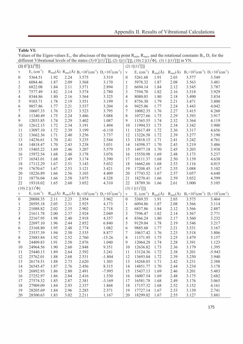
Appendix II. Results of Vibrational Calculations
175
Table VI: Values of the Eigen-values Ev, the abscissas of the turning point Rmin, Rmax, and the rotational constants Bv, Dv for the different Vibrational levels of the states (3) 0+[(1)3∏], (2) 1[(1)3∏], (10) 2 [(1)5Φ], (3) 1 [(1)1∏] in YN. (3) 0+[(1)3∏] (2) 1[(1)3∏] v Ev (cm-1) Rmin(Å) Rmax(Å) Bv×101(cm-1) Dv×107(cm-1) v Ev (cm-1) Rmin(Å) Rmax(Å) Bv×101(cm-1) Dv×107(cm-1) 0 5364.51 1.92 2.24 3.575 3.519 0 5261.68 1.91 2.03 3.577 3.549 1 6084.46 1.87 2.09 3.568 3.170 1 5978.32 1.87 2.08 3.563 3.481 2 6822.08 1.84 2.11 3.571 2.894 2 6694.14 1.84 2.12 3.545 3.787 3 7577.49 1.82 2.14 3.574 2.780 3 7394.70 1.82 2.16 3.518 3.929 4 8344.86 1.80 2.16 3.564 3.325 4 8080.03 1.80 2.18 3.490 3.834 5 9103.71 1.78 2.19 3.551 3.199 5 8756.30 1.79 2.21 3.471 3.800 6 9857.86 1.77 2.21 3.537 3.204 6 9425.06 1.77 2.24 3.443 4.042 7 10607.33 1.76 2.23 3.523 3.795 7 10082.35 1.76 2.27 3.415 4.260 8 11340.49 1.75 2.24 3.486 5.088 8 10727.66 1.75 2.29 3.393 3.917 9 12033.85 1.74 2.29 3.402 1.087 9 11365.55 1.74 2.32 3.364 4.119 10 12612.15 1.72 2.34 3.191 1.494 10 11994.53 1.73 2.34 3.342 3.900 11 13097.10 1.72 2.39 3.199 -6.110 11 12617.49 1.72 2.36 3.317 4.656 12 13662.36 1.71 2.40 3.256 3.737 12 13226.58 1.72 2.39 3.277 5.190 13 14236.61 1.70 2.41 3.235 2.544 13 13818.15 1.71 2.41 3.242 4.761 14 14818.47 1.70 2.43 3.238 3.031 14 14398.37 1.70 2.43 3.219 3.486 15 15403.22 1.69 2.46 3.207 5.579 15 14977.18 1.70 2.45 3.203 3.938 16 15972.54 1.68 2.48 3.178 3.076 16 15550.98 1.69 2.48 3.173 5.237 17 16543.01 1.68 2.49 3.174 3.390 17 16111.37 1.68 2.50 3.139 4.638 18 17112.29 1.67 2.51 3.143 5.032 18 16662.66 1.68 2.53 3.116 4.015 19 17670.67 1.67 2.53 3.121 3.421 19 17208.45 1.67 2.55 3.088 5.102 20 18226.89 1.66 2.56 3.103 4.409 20 17743.52 1.67 2.57 3.057 4.640 21 18776.04 1.66 2.58 3.075 4.328 21 18270.41 1.66 2.59 3.032 4.599 22 19318.02 1.65 2.60 3.052 4.310 22 18789.36 1.66 2.61 3.000 5.105 (10) 2 [(1)5Φ] (3) 1 [(1)1∏] v Ev (cm-1) Rmin(Å) Rmax(Å) Bv×101(cm-1) Dv×107(cm-1) v Ev (cm-1) Rmin(Å) Rmax(Å) Bv×101(cm-1) Dv×107(cm-1) 0 20088.35 2.11 2.23 2.954 3.962 0 5369.55 1.91 2.03 3.575 3.464 1 20595.18 2.05 2.31 2.925 4.173 1 6094.86 1.87 2.08 3.566 3.114 2 21088.82 2.02 2.35 2.902 2.718 2 6837.86 1.84 2.12 3.566 2.887 3 21611.78 2.00 2.37 2.924 2.049 3 7596.47 1.82 2.14 3.567 2.771 4 22167.95 1.98 2.40 2.918 4.357 4 8366.24 1.80 2.17 3.560 3.232 5 22697.10 1.96 2.44 2.852 6.840 5 9129.04 1.78 2.19 3.546 3.217 6 23168.80 1.95 2.48 2.774 1.082 6 9885.60 1.77 2.21 3.531 3.167 7 23537.39 1.94 2.50 2.535 8.877 7 10637.42 1.76 2.23 3.518 3.806 8 23883.84 1.92 2.52 2.760 -15.26 8 11371.95 1.75 2.25 3.479 5.157 9 24409.83 1.91 2.58 2.876 1.040 9 12064.28 1.74 2.28 3.391 1.123 10 24964.56 1.90 2.60 2.848 9.351 10 12636.82 1.73 2.36 3.179 1.395 11 25440.13 1.89 2.64 2.592 3.241 11 13124.36 1.72 2.38 3.201 -5.943 12 25762.01 1.88 2.68 2.531 -1.804 12 13693.04 1.72 2.39 3.250 3.940 13 26174.51 1.88 2.73 2.620 1.303 13 14268.03 1.71 2.42 3.231 2.388 14 26545.47 1.87 2.76 2.456 8.315 14 14851.77 1.70 2.44 3.234 3.178 15 26892.93 1.86 2.80 2.491 -7.995 15 15437.13 1.69 2.46 3.201 5.483 16 27252.97 1.86 2.84 2.416 1.530 16 16007.54 1.69 2.48 3.175 2.682 17 27574.32 1.85 2.87 2.381 -3.169 17 16581.78 1.68 2.49 3.176 3.065 18 27909.09 1.84 2.93 2.337 1.868 18 17157.32 1.68 2.52 3.152 4.161 19 28205.69 1.84 2.96 2.285 2.571 19 17727.14 1.67 2.53 3.139 2.741 20 28500.63 1.83 3.02 2.211 1.167 20 18299.02 1.67 2.55 3.127 3.881
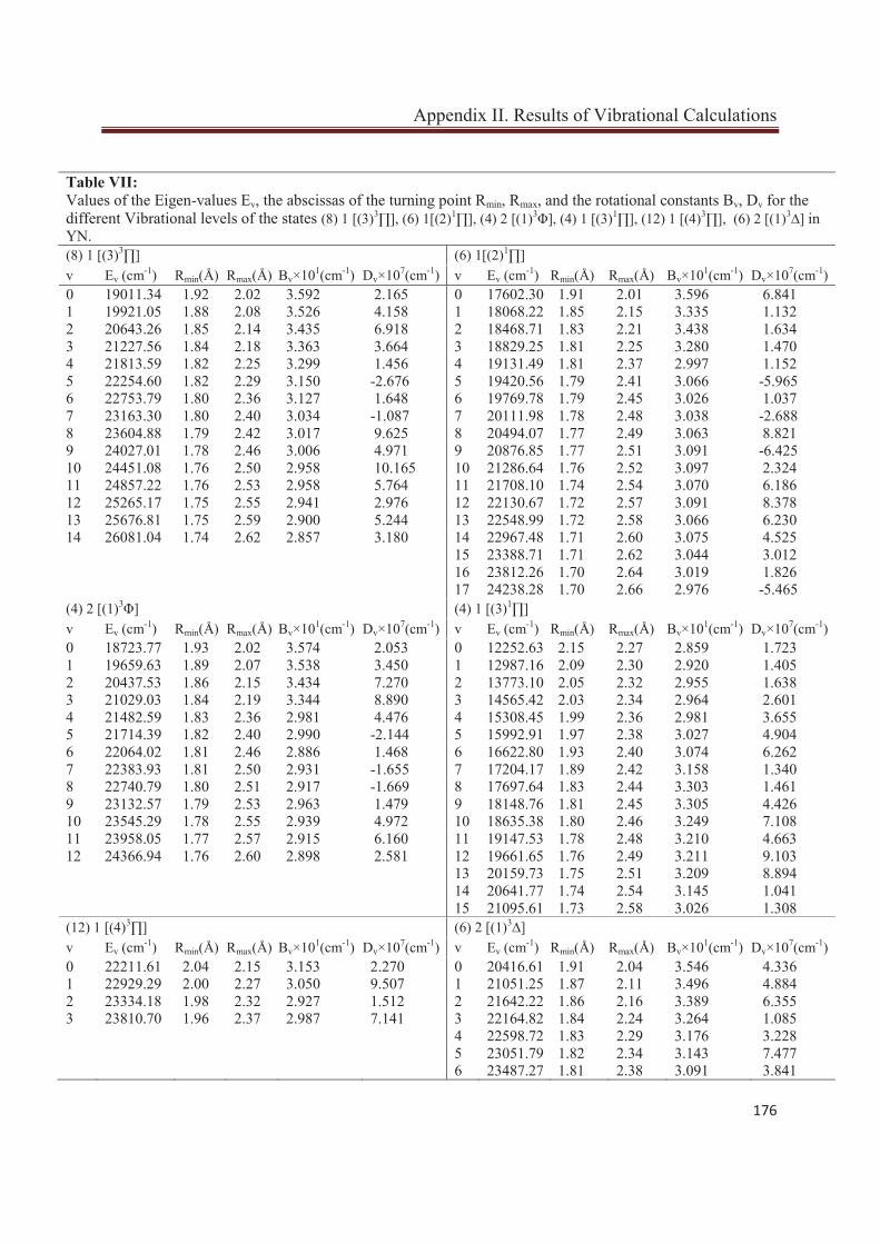
Appendix II. Results of Vibrational Calculations
176
Table VII: Values of the Eigen-values Ev, the abscissas of the turning point Rmin, Rmax, and the rotational constants Bv, Dv for the different Vibrational levels of the states (8) 1 [(3)3∏], (6) 1[(2)1∏], (4) 2 [(1)3Φ], (4) 1 [(3)1∏], (12) 1 [(4)3∏], (6) 2 [(1)3∆] in YN. (8) 1 [(3)3∏] (6) 1[(2)1∏] v Ev (cm-1) Rmin(Å) Rmax(Å) Bv×101(cm-1) Dv×107(cm-1) v Ev (cm-1) Rmin(Å) Rmax(Å) Bv×101(cm-1) Dv×107(cm-1) 0 19011.34 1.92 2.02 3.592 2.165 0 17602.30 1.91 2.01 3.596 6.841 1 19921.05 1.88 2.08 3.526 4.158 1 18068.22 1.85 2.15 3.335 1.132 2 20643.26 1.85 2.14 3.435 6.918 2 18468.71 1.83 2.21 3.438 1.634 3 21227.56 1.84 2.18 3.363 3.664 3 18829.25 1.81 2.25 3.280 1.470 4 21813.59 1.82 2.25 3.299 1.456 4 19131.49 1.81 2.37 2.997 1.152 5 22254.60 1.82 2.29 3.150 -2.676 5 19420.56 1.79 2.41 3.066 -5.965 6 22753.79 1.80 2.36 3.127 1.648 6 19769.78 1.79 2.45 3.026 1.037 7 23163.30 1.80 2.40 3.034 -1.087 7 20111.98 1.78 2.48 3.038 -2.688 8 23604.88 1.79 2.42 3.017 9.625 8 20494.07 1.77 2.49 3.063 8.821 9 24027.01 1.78 2.46 3.006 4.971 9 20876.85 1.77 2.51 3.091 -6.425 10 24451.08 1.76 2.50 2.958 10.165 10 21286.64 1.76 2.52 3.097 2.324 11 24857.22 1.76 2.53 2.958 5.764 11 21708.10 1.74 2.54 3.070 6.186 12 25265.17 1.75 2.55 2.941 2.976 12 22130.67 1.72 2.57 3.091 8.378 13 25676.81 1.75 2.59 2.900 5.244 13 22548.99 1.72 2.58 3.066 6.230 14 26081.04 1.74 2.62 2.857 3.180 14 22967.48 1.71 2.60 3.075 4.525 15 23388.71 1.71 2.62 3.044 3.012 16 23812.26 1.70 2.64 3.019 1.826 17 24238.28 1.70 2.66 2.976 -5.465 (4) 2 [(1)3Φ] (4) 1 [(3)1∏] v Ev (cm-1) Rmin(Å) Rmax(Å) Bv×101(cm-1) Dv×107(cm-1) v Ev (cm-1) Rmin(Å) Rmax(Å) Bv×101(cm-1) Dv×107(cm-1) 0 18723.77 1.93 2.02 3.574 2.053 0 12252.63 2.15 2.27 2.859 1.723 1 19659.63 1.89 2.07 3.538 3.450 1 12987.16 2.09 2.30 2.920 1.405 2 20437.53 1.86 2.15 3.434 7.270 2 13773.10 2.05 2.32 2.955 1.638 3 21029.03 1.84 2.19 3.344 8.890 3 14565.42 2.03 2.34 2.964 2.601 4 21482.59 1.83 2.36 2.981 4.476 4 15308.45 1.99 2.36 2.981 3.655 5 21714.39 1.82 2.40 2.990 -2.144 5 15992.91 1.97 2.38 3.027 4.904 6 22064.02 1.81 2.46 2.886 1.468 6 16622.80 1.93 2.40 3.074 6.262 7 22383.93 1.81 2.50 2.931 -1.655 7 17204.17 1.89 2.42 3.158 1.340 8 22740.79 1.80 2.51 2.917 -1.669 8 17697.64 1.83 2.44 3.303 1.461 9 23132.57 1.79 2.53 2.963 1.479 9 18148.76 1.81 2.45 3.305 4.426 10 23545.29 1.78 2.55 2.939 4.972 10 18635.38 1.80 2.46 3.249 7.108 11 23958.05 1.77 2.57 2.915 6.160 11 19147.53 1.78 2.48 3.210 4.663 12 24366.94 1.76 2.60 2.898 2.581 12 19661.65 1.76 2.49 3.211 9.103 13 20159.73 1.75 2.51 3.209 8.894 14 20641.77 1.74 2.54 3.145 1.041 15 21095.61 1.73 2.58 3.026 1.308 (12) 1 [(4)3∏] (6) 2 [(1)3∆] v Ev (cm-1) Rmin(Å) Rmax(Å) Bv×101(cm-1) Dv×107(cm-1) v Ev (cm-1) Rmin(Å) Rmax(Å) Bv×101(cm-1) Dv×107(cm-1) 0 22211.61 2.04 2.15 3.153 2.270 0 20416.61 1.91 2.04 3.546 4.336 1 22929.29 2.00 2.27 3.050 9.507 1 21051.25 1.87 2.11 3.496 4.884 2 23334.18 1.98 2.32 2.927 1.512 2 21642.22 1.86 2.16 3.389 6.355 3 23810.70 1.96 2.37 2.987 7.141 3 22164.82 1.84 2.24 3.264 1.085 4 22598.72 1.83 2.29 3.176 3.228 5 23051.79 1.82 2.34 3.143 7.477 6 23487.27 1.81 2.38 3.091 3.841
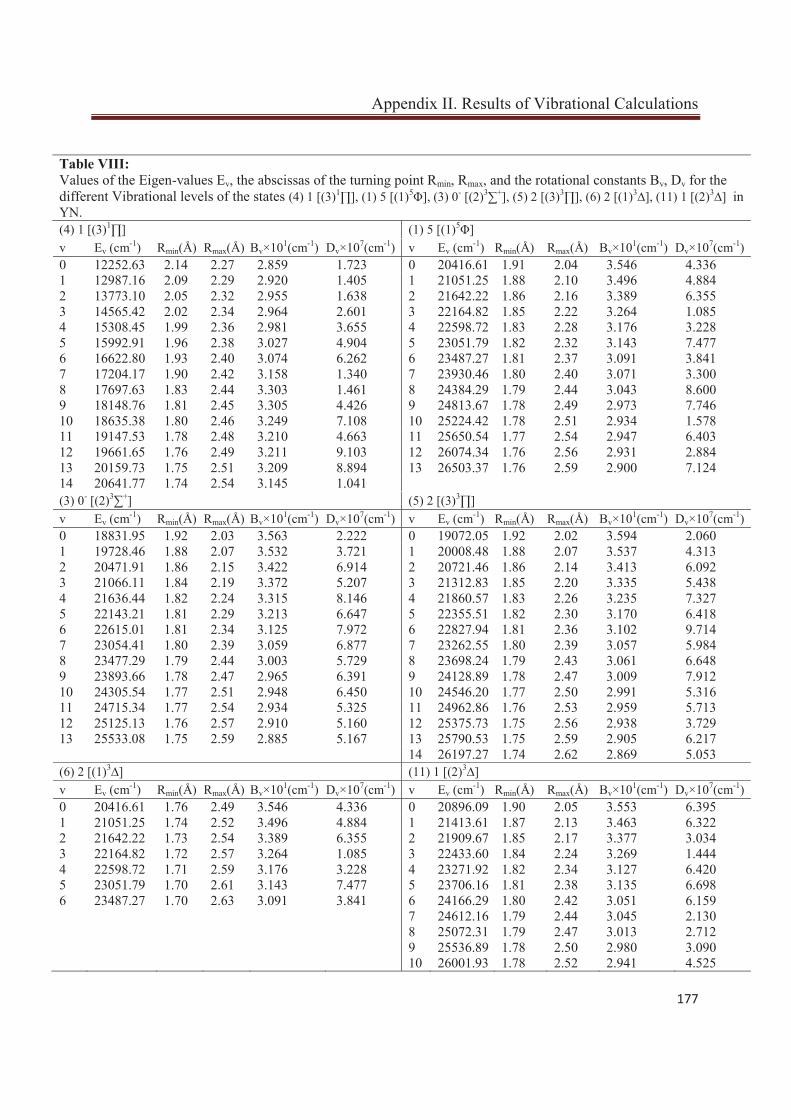
Appendix II. Results of Vibrational Calculations
177
Table VIII: Values of the Eigen-values Ev, the abscissas of the turning point Rmin, Rmax, and the rotational constants Bv, Dv for the different Vibrational levels of the states (4) 1 [(3)1∏], (1) 5 [(1)5Φ], (3) 0- [(2)3∑+], (5) 2 [(3)3∏], (6) 2 [(1)3∆], (11) 1 [(2)3∆] in YN. (4) 1 [(3)1∏] (1) 5 [(1)5Φ] v Ev (cm-1) Rmin(Å) Rmax(Å) Bv×101(cm-1) Dv×107(cm-1) v Ev (cm-1) Rmin(Å) Rmax(Å) Bv×101(cm-1) Dv×107(cm-1) 0 12252.63 2.14 2.27 2.859 1.723 0 20416.61 1.91 2.04 3.546 4.336 1 12987.16 2.09 2.29 2.920 1.405 1 21051.25 1.88 2.10 3.496 4.884 2 13773.10 2.05 2.32 2.955 1.638 2 21642.22 1.86 2.16 3.389 6.355 3 14565.42 2.02 2.34 2.964 2.601 3 22164.82 1.85 2.22 3.264 1.085 4 15308.45 1.99 2.36 2.981 3.655 4 22598.72 1.83 2.28 3.176 3.228 5 15992.91 1.96 2.38 3.027 4.904 5 23051.79 1.82 2.32 3.143 7.477 6 16622.80 1.93 2.40 3.074 6.262 6 23487.27 1.81 2.37 3.091 3.841 7 17204.17 1.90 2.42 3.158 1.340 7 23930.46 1.80 2.40 3.071 3.300 8 17697.63 1.83 2.44 3.303 1.461 8 24384.29 1.79 2.44 3.043 8.600 9 18148.76 1.81 2.45 3.305 4.426 9 24813.67 1.78 2.49 2.973 7.746 10 18635.38 1.80 2.46 3.249 7.108 10 25224.42 1.78 2.51 2.934 1.578 11 19147.53 1.78 2.48 3.210 4.663 11 25650.54 1.77 2.54 2.947 6.403 12 19661.65 1.76 2.49 3.211 9.103 12 26074.34 1.76 2.56 2.931 2.884 13 20159.73 1.75 2.51 3.209 8.894 13 26503.37 1.76 2.59 2.900 7.124 14 20641.77 1.74 2.54 3.145 1.041 (3) 0- [(2)3∑+] (5) 2 [(3)3∏] v Ev (cm-1) Rmin(Å) Rmax(Å) Bv×101(cm-1) Dv×107(cm-1) v Ev (cm-1) Rmin(Å) Rmax(Å) Bv×101(cm-1) Dv×107(cm-1) 0 18831.95 1.92 2.03 3.563 2.222 0 19072.05 1.92 2.02 3.594 2.060 1 19728.46 1.88 2.07 3.532 3.721 1 20008.48 1.88 2.07 3.537 4.313 2 20471.91 1.86 2.15 3.422 6.914 2 20721.46 1.86 2.14 3.413 6.092 3 21066.11 1.84 2.19 3.372 5.207 3 21312.83 1.85 2.20 3.335 5.438 4 21636.44 1.82 2.24 3.315 8.146 4 21860.57 1.83 2.26 3.235 7.327 5 22143.21 1.81 2.29 3.213 6.647 5 22355.51 1.82 2.30 3.170 6.418 6 22615.01 1.81 2.34 3.125 7.972 6 22827.94 1.81 2.36 3.102 9.714 7 23054.41 1.80 2.39 3.059 6.877 7 23262.55 1.80 2.39 3.057 5.984 8 23477.29 1.79 2.44 3.003 5.729 8 23698.24 1.79 2.43 3.061 6.648 9 23893.66 1.78 2.47 2.965 6.391 9 24128.89 1.78 2.47 3.009 7.912 10 24305.54 1.77 2.51 2.948 6.450 10 24546.20 1.77 2.50 2.991 5.316 11 24715.34 1.77 2.54 2.934 5.325 11 24962.86 1.76 2.53 2.959 5.713 12 25125.13 1.76 2.57 2.910 5.160 12 25375.73 1.75 2.56 2.938 3.729 13 25533.08 1.75 2.59 2.885 5.167 13 25790.53 1.75 2.59 2.905 6.217 14 26197.27 1.74 2.62 2.869 5.053 (6) 2 [(1)3∆] (11) 1 [(2)3∆] v Ev (cm-1) Rmin(Å) Rmax(Å) Bv×101(cm-1) Dv×107(cm-1) v Ev (cm-1) Rmin(Å) Rmax(Å) Bv×101(cm-1) Dv×107(cm-1) 0 20416.61 1.76 2.49 3.546 4.336 0 20896.09 1.90 2.05 3.553 6.395 1 21051.25 1.74 2.52 3.496 4.884 1 21413.61 1.87 2.13 3.463 6.322 2 21642.22 1.73 2.54 3.389 6.355 2 21909.67 1.85 2.17 3.377 3.034 3 22164.82 1.72 2.57 3.264 1.085 3 22433.60 1.84 2.24 3.269 1.444 4 22598.72 1.71 2.59 3.176 3.228 4 23271.92 1.82 2.34 3.127 6.420 5 23051.79 1.70 2.61 3.143 7.477 5 23706.16 1.81 2.38 3.135 6.698 6 23487.27 1.70 2.63 3.091 3.841 6 24166.29 1.80 2.42 3.051 6.159 7 24612.16 1.79 2.44 3.045 2.130 8 25072.31 1.79 2.47 3.013 2.712 9 25536.89 1.78 2.50 2.980 3.090 10 26001.93 1.78 2.52 2.941 4.525
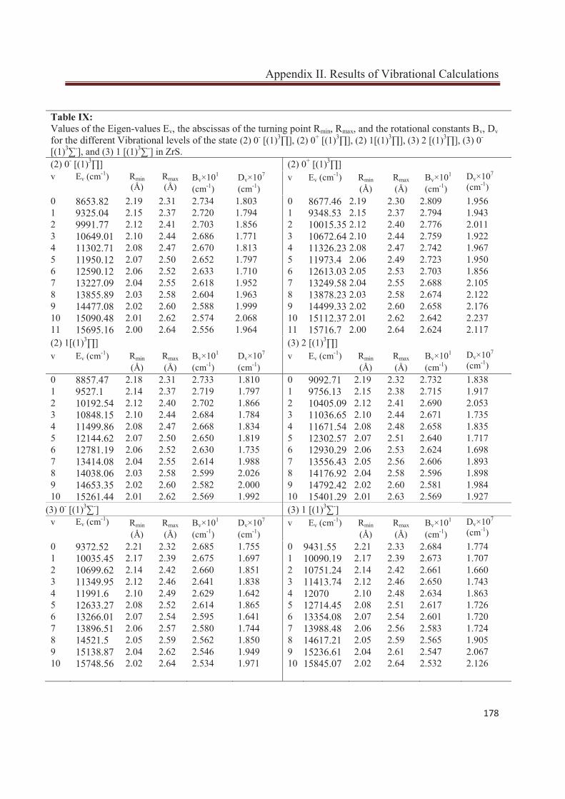
Appendix II. Results of Vibrational Calculations
178
Table IX: Values of the Eigen-values Ev, the abscissas of the turning point Rmin, Rmax, and the rotational constants Bv, Dv for the different Vibrational levels of the state (2) 0- [(1)3∏], (2) 0+ [(1)3∏], (2) 1[(1)3∏], (3) 2 [(1)3∏], (3) 0- [(1)3∑-], and (3) 1 [(1)3∑-] in ZrS. (2) 0- [(1)3∏] (2) 0+ [(1)3∏] v Ev (cm-1) Rmin
(Å) Rmax (Å)
Bv×101 (cm-1)
Dv×107
(cm-1) v Ev (cm-1) Rmin
(Å) Rmax
(Å) Bv×101 (cm-1)
Dv×107
(cm-1) 0 8653.82 2.19 2.31 2.734 1.803 0 8677.46 2.19 2.30 2.809 1.956 1 9325.04 2.15 2.37 2.720 1.794 1 9348.53 2.15 2.37 2.794 1.943 2 9991.77 2.12 2.41 2.703 1.856 2 10015.35 2.12 2.40 2.776 2.011 3 10649.01 2.10 2.44 2.686 1.771 3 10672.64 2.10 2.44 2.759 1.922 4 11302.71 2.08 2.47 2.670 1.813 4 11326.23 2.08 2.47 2.742 1.967 5 11950.12 2.07 2.50 2.652 1.797 5 11973.4 2.06 2.49 2.723 1.950 6 12590.12 2.06 2.52 2.633 1.710 6 12613.03 2.05 2.53 2.703 1.856 7 13227.09 2.04 2.55 2.618 1.952 7 13249.58 2.04 2.55 2.688 2.105 8 13855.89 2.03 2.58 2.604 1.963 8 13878.23 2.03 2.58 2.674 2.122 9 14477.08 2.02 2.60 2.588 1.999 9 14499.33 2.02 2.60 2.658 2.176 10 15090.48 2.01 2.62 2.574 2.068 10 15112.37 2.01 2.62 2.642 2.237 11 15695.16 2.00 2.64 2.556 1.964 11 15716.7 2.00 2.64 2.624 2.117 (2) 1[(1)3∏] (3) 2 [(1)3∏] v Ev (cm-1) Rmin
(Å) Rmax
(Å) Bv×101 (cm-1)
Dv×107
(cm-1) v Ev (cm-1) Rmin
(Å) Rmax
(Å) Bv×101 (cm-1)
Dv×107
(cm-1) 0 8857.47 2.18 2.31 2.733 1.810 0 9092.71 2.19 2.32 2.732 1.838 1 9527.1 2.14 2.37 2.719 1.797 1 9756.13 2.15 2.38 2.715 1.917 2 10192.54 2.12 2.40 2.702 1.866 2 10405.09 2.12 2.41 2.690 2.053 3 10848.15 2.10 2.44 2.684 1.784 3 11036.65 2.10 2.44 2.671 1.735 4 11499.86 2.08 2.47 2.668 1.834 4 11671.54 2.08 2.48 2.658 1.835 5 12144.62 2.07 2.50 2.650 1.819 5 12302.57 2.07 2.51 2.640 1.717 6 12781.19 2.06 2.52 2.630 1.735 6 12930.29 2.06 2.53 2.624 1.698 7 13414.08 2.04 2.55 2.614 1.988 7 13556.43 2.05 2.56 2.606 1.893 8 14038.06 2.03 2.58 2.599 2.026 8 14176.92 2.04 2.58 2.596 1.898 9 14653.35 2.02 2.60 2.582 2.000 9 14792.42 2.02 2.60 2.581 1.984 10 15261.44 2.01 2.62 2.569 1.992 10 15401.29 2.01 2.63 2.569 1.927
(3) 0- [(1)3∑-] (3) 1 [(1)3∑-] v Ev (cm-1) Rmin
(Å) Rmax
(Å) Bv×101 (cm-1)
Dv×107
(cm-1) v Ev (cm-1) Rmin
(Å) Rmax
(Å) Bv×101 (cm-1)
Dv×107
(cm-1) 0 9372.52 2.21 2.32 2.685 1.755 0 9431.55 2.21 2.33 2.684 1.774 1 10035.45 2.17 2.39 2.675 1.697 1 10090.19 2.17 2.39 2.673 1.707 2 10699.62 2.14 2.42 2.660 1.851 2 10751.24 2.14 2.42 2.661 1.660 3 11349.95 2.12 2.46 2.641 1.838 3 11413.74 2.12 2.46 2.650 1.743 4 11991.6 2.10 2.49 2.629 1.642 4 12070 2.10 2.48 2.634 1.863 5 12633.27 2.08 2.52 2.614 1.865 5 12714.45 2.08 2.51 2.617 1.726 6 13266.01 2.07 2.54 2.595 1.641 6 13354.08 2.07 2.54 2.601 1.720 7 13896.51 2.06 2.57 2.580 1.744 7 13988.48 2.06 2.56 2.583 1.724 8 14521.5 2.05 2.59 2.562 1.850 8 14617.21 2.05 2.59 2.565 1.905 9 15138.87 2.04 2.62 2.546 1.949 9 15236.61 2.04 2.61 2.547 2.067 10 15748.56 2.02 2.64 2.534 1.971 10 15845.07 2.02 2.64 2.532 2.126
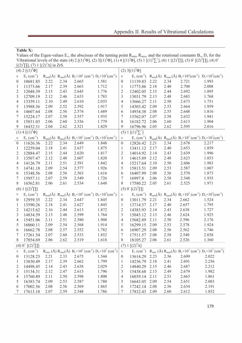
Appendix II. Results of Vibrational Calculations
179
Table X: Values of the Eigen-values Ev, the abscissas of the turning point Rmin, Rmax, and the rotational constants Bv, Dv for the Vibrational levels of the state (4) 2 [(1)3Φ], (2) 3[(1)3Φ], (1) 4 [(1)3Φ], (5) 1 [(1)3∑+], (6) 1 [(2)3∏], (5) 0- [(2)3∏], (4) 0+ [(2)3∏], (7) 1 [(2)3∆] in ZrS. (4) 2 [(1)3Φ] (2) 3[(1)3Φ] v Ev (cm-1) Rmin(Å) Rmax(Å) Bv×101 (cm-1) Dv×107(cm-1) v Ev (cm-1) Rmin(Å) Rmax (Å) Bv×101(cm-1) Dv×107(cm-1) 0 10681.85 2.22 2.34 2.665 1.581 0 11139.83 2.22 2.34 2.721 1.993 1 11373.66 2.17 2.39 2.663 1.712 1 11773.86 2.18 2.40 2.708 2.008 2 12048.39 2.15 2.43 2.645 1.776 2 12402.05 2.15 2.44 2.692 1.895 3 12709.19 2.12 2.46 2.633 1.783 3 13031.79 2.13 2.48 2.683 1.768 4 13359.11 2.10 2.49 2.610 2.035 4 13666.27 2.11 2.50 2.673 1.751 5 13988.36 2.09 2.52 2.592 1.917 5 14303.42 2.09 2.53 2.664 1.959 6 14607.64 2.08 2.56 2.574 1.689 6 14934.38 2.08 2.55 2.648 1.816 7 15224.17 2.07 2.58 2.557 1.935 7 15562.07 2.07 2.58 2.632 1.941 8 15831.03 2.06 2.60 2.536 1.779 8 16182.72 2.06 2.60 2.613 1.904 9 16432.31 2.04 2.62 2.521 1.829 9 16796.96 2.05 2.62 2.595 2.016
(1) 4 [(1)3Φ] (5) 1 [(1)3∑+] v Ev (cm-1) Rmin(Å) Rmax(Å) Bv×101 (cm-1) Dv×107(cm-1) v Ev (cm-1) Rmin(Å) Rmax(Å) Bv×101 (cm-1) Dv×107(cm-1) 0 11626.36 2.22 2.34 2.649 1.848 0 12826.42 2.21 2.34 2.678 2.217 1 12259.04 2.18 2.41 2.637 1.875 1 13411.12 2.17 2.40 2.653 1.859 2 12884.47 2.15 2.44 2.620 1.817 2 14014.92 2.14 2.43 2.639 1.996 3 13507.47 2.12 2.48 2.607 1.820 3 14615.89 2.12 2.48 2.623 1.853 4 14126.79 2.11 2.51 2.591 1.842 4 15217.64 2.10 2.50 2.606 1.983 5 14741.18 2.09 2.54 2.577 1.926 5 15813.51 2.09 2.53 2.587 1.807 6 15348.56 2.08 2.56 2.563 1.616 6 16407.99 2.08 2.56 2.570 1.873 7 15957.11 2.07 2.59 2.549 1.726 7 16997.8 2.06 2.58 2.548 1.935 8 16562.81 2.06 2.61 2.534 1.648 8 17580.22 2.05 2.61 2.525 1.971
(6) 1 [(2)3∏] (5) 0- [(2)3∏] v Ev (cm-1) Rmin(Å) Rmax(Å) Bv×101 (cm-1) Dv×107(cm-1) v Ev (cm-1) Rmin(Å) Rmax(Å) Bv×101 (cm-1) Dv×107(cm-1) 0 12959.35 2.22 2.34 2.647 1.845 0 13011.79 2.21 2.34 2.662 1.524 1 13590.26 2.18 2.41 2.627 1.845 1 13714.57 2.17 2.40 2.657 1.795 2 14215.62 2.16 2.44 2.613 1.872 2 14383.93 2.14 2.43 2.638 1.727 3 14834.59 2.13 2.48 2.599 1.764 3 15043.12 2.13 2.46 2.624 1.925 4 15451.06 2.11 2.51 2.580 1.908 4 15682.89 2.11 2.50 2.596 2.176 5 16060.11 2.09 2.54 2.568 1.914 5 16299.15 2.09 2.53 2.578 1.924 6 16662.78 2.08 2.57 2.552 1.782 6 16907.29 2.08 2.56 2.562 1.746 7 17261.54 2.07 2.60 2.533 1.852 7 17511.57 2.08 2.58 2.540 2.038 8 17854.69 2.06 2.62 2.519 1.618 8 18105.27 2.06 2.61 2.526 1.360
(4) 0+ [(2)3∏] (7) 1 [(2)3∆] v Ev (cm-1) Rmin
(Å) Rmax(Å) Bv×101 (cm-1) Dv×107 (cm-1) v Ev (cm-1) Rmin (Å) Rmax(Å) Bv×101 (cm-1) Dv×107 (cm-1)
0 13128.23 2.21 2.33 2.675 1.544 0 13614.29 2.23 2.36 2.699 2.022 1 13830.49 2.17 2.39 2.662 1.799 1 14236.79 2.18 2.41 2.691 2.256 2 14498.45 2.14 2.43 2.638 2.029 2 14840.29 2.15 2.46 2.687 2.212 3 15134.31 2.12 2.47 2.613 1.796 3 15438.68 2.13 2.49 2.679 1.982 4 15760.89 2.11 2.50 2.598 1.800 4 16039.14 2.11 2.51 2.663 1.861 5 16383.74 2.09 2.53 2.587 1.780 5 16643.05 2.09 2.54 2.651 2.083 6 17002.56 2.08 2.56 2.569 1.865 6 17242.14 2.08 2.56 2.634 2.191 7 17613.18 2.07 2.59 2.548 1.786 7 17832.43 2.09 2.60 2.612 1.852
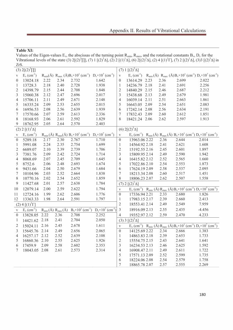
Appendix II. Results of Vibrational Calculations
180
Table XI: Values of the Eigen-values Ev, the abscissas of the turning point Rmin, Rmax, and the rotational constants Bv, Dv for the Vibrational levels of the state (3) 2[(2)3∏], (7) 1 [(2)3∆], (2) 2 [(1)1∆], (6) 2[(2)3∆], (2) 4 [(1)1Γ], (7) 2 [(2)1∆], (3)3 [(2)3∆] in ZrS. (3) 2[(2)3∏] (7) 1 [(2)3∆] v Ev (cm-1) Rmin(Å) Rmax
(Å) Bv×101 (cm-1) Dv×107 (cm-1) v Ev (cm-1) Rmin (Å) Rmax
(Å) Bv×101 (cm-1) Dv×107 (cm-1) 0 13024.18 2.22 2.34 2.732 1.642 0 13614.29 2.23 2.36 2.699 2.022 1 13728.3 2.18 2.40 2.728 1.938 1 14236.79 2.18 2.41 2.691 2.256 2 14398.79 2.15 2.44 2.708 1.848 2 14840.29 2.15 2.46 2.687 2.212 3 15060.38 2.12 2.47 2.696 2.017 3 15438.68 2.13 2.49 2.679 1.981 4 15706.11 2.11 2.49 2.671 2.148 4 16039.14 2.11 2.51 2.663 1.861 5 16335.24 2.09 2.53 2.655 2.015 5 16643.05 2.09 2.54 2.651 2.083 6 16956.53 2.08 2.56 2.639 1.939 6 17242.14 2.08 2.56 2.634 2.191 7 17570.66 2.07 2.59 2.613 2.336 7 17832.43 2.09 2.60 2.612 1.851 8 18168.93 2.06 2.61 2.592 1.829 8 18421.24 2.06 2.62 2.597 1.913 9 18762.95 2.05 2.64 2.570 2.403
(2) 2 [(1)1∆] (6) 2[(2)3∆] v Ev (cm-1) Rmin
(Å) Rmax(Å) Bv×101 (cm-1) Dv×107 (cm-1) v Ev (cm-1) Rmin (Å) Rmax
(Å) Bv×101 (cm-1) Dv×107 (cm-1) 0 5289.18 2.17 2.30 2.767 1.710 0 13963.06 2.22 2.36 2.644 2.014 1 5991.08 2.24 2.35 2.754 1.699 1 14564.92 2.18 2.41 2.621 1.608 2 6689.07 2.10 2.39 2.739 1.706 2 15192.55 2.16 2.45 2.601 1.897 3 7381.76 2.09 2.42 2.724 1.714 3 15809.95 2.14 2.49 2.590 1.942 4 8068.69 2.07 2.45 2.709 1.645 4 16415.82 2.12 2.52 2.565 1.660 5 8752.6 2.06 2.48 2.693 1.674 5 17022.86 2.10 2.54 2.553 1.873 6 9431.66 2.04 2.50 2.679 1.684 6 17624.19 2.09 2.58 2.537 2.095 7 10104.96 2.03 2.52 2.664 1.838 7 18213.34 2.08 2.60 2.517 1.451 8 10770.16 2.02 2.54 2.652 1.859 8 18806.23 2.07 2.62 2.507 1.558 9 11427.68 2.01 2.57 2.638 1.784 (7) 2 [(2)1∆]
10 12079.14 2.00 2.59 2.622 1.794 v Ev (cm-1) Rmin (Å) Rmax
(Å) Bv×101 (cm-1) Dv×107 (cm-1) 11 12724.16 1.99 2.62 2.606 1.776 0 17336.94 2.21 2.33 2.680 1.826 12 13363.33 1.98 2.64 2.591 1.797 1 17983.15 2.17 2.39 2.660 2.413
(2) 4 [(1)1Γ] 2 18553.41 2.14 2.49 2.549 7.959 v Ev (cm-1) Rmin
(Å) Rmax (Å) Bv×101 (cm-1) Dv×107 (cm-1) 3 18916.09 2.13 2.55 2.435 -4.456
0 13828.05 2.22 2.36 2.708 2.252 4 19352.97 2.12 2.59 2.470 4.233 1 14421.62 2.18 2.41 2.704 2.050 (3) 3 [(2)3∆] 2 15024.11 2.16 2.45 2.678 1.611 v Ev (cm-1) Rmin
(Å) Rmax (Å) Bv×101 (cm-1) Dv×107 (cm-1)
3 15645.76 2.14 2.49 2.656 2.065 0 14125.69 2.22 2.34 2.666 1.383 4 16257.17 2.12 2.52 2.639 2.108 1 14863.83 2.18 2.39 2.653 1.733 5 16860.36 2.10 2.55 2.625 1.926 2 15554.75 2.15 2.43 2.641 1.641 6 17459.9 2.09 2.58 2.602 2.353 3 16234.53 2.13 2.46 2.625 1.592 7 18043.05 2.08 2.61 2.573 2.314 4 16908.47 2.11 2.49 2.611 1.722 5 17571.13 2.09 2.52 2.599 1.735 6 18224.06 2.08 2.54 2.579 1.758 7 18865.78 2.07 2.57 2.555 2.269
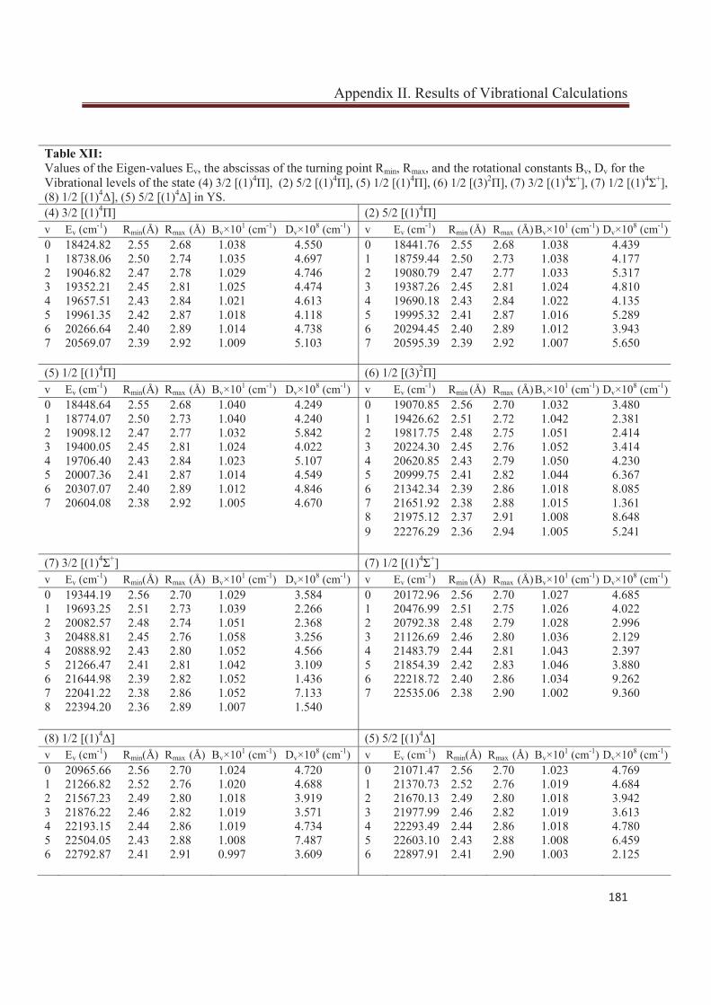
Appendix II. Results of Vibrational Calculations
181
Table XII: Values of the Eigen-values Ev, the abscissas of the turning point Rmin, Rmax, and the rotational constants Bv, Dv for the Vibrational levels of the state (4) 3/2 [(1)4Π], (2) 5/2 [(1)4Π], (5) 1/2 [(1)4Π], (6) 1/2 [(3)2Π], (7) 3/2 [(1)4Σ+], (7) 1/2 [(1)4Σ+], (8) 1/2 [(1)4Δ], (5) 5/2 [(1)4Δ] in YS. (4) 3/2 [(1)4Π] (2) 5/2 [(1)4Π] v Ev (cm-1) Rmin(Å) Rmax
(Å) Bv×101 (cm-1) Dv×108 (cm-1) v Ev (cm-1) Rmin (Å) Rmax
(Å) Bv×101 (cm-1) Dv×108 (cm-1) 0 18424.82 2.55 2.68 1.038 4.550 0 18441.76 2.55 2.68 1.038 4.439 1 18738.06 2.50 2.74 1.035 4.697 1 18759.44 2.50 2.73 1.038 4.177 2 19046.82 2.47 2.78 1.029 4.746 2 19080.79 2.47 2.77 1.033 5.317 3 19352.21 2.45 2.81 1.025 4.474 3 19387.26 2.45 2.81 1.024 4.810 4 19657.51 2.43 2.84 1.021 4.613 4 19690.18 2.43 2.84 1.022 4.135 5 19961.35 2.42 2.87 1.018 4.118 5 19995.32 2.41 2.87 1.016 5.289 6 20266.64 2.40 2.89 1.014 4.738 6 20294.45 2.40 2.89 1.012 3.943 7 20569.07 2.39 2.92 1.009 5.103 7 20595.39 2.39 2.92 1.007 5.650 (5) 1/2 [(1)4Π] (6) 1/2 [(3)2Π] v Ev (cm-1) Rmin(Å) Rmax
(Å) Bv×101 (cm-1) Dv×108 (cm-1) v Ev (cm-1) Rmin (Å) Rmax
(Å) Bv×101 (cm-1) Dv×108 (cm-1) 0 18448.64 2.55 2.68 1.040 4.249 0 19070.85 2.56 2.70 1.032 3.480 1 18774.07 2.50 2.73 1.040 4.240 1 19426.62 2.51 2.72 1.042 2.381 2 19098.12 2.47 2.77 1.032 5.842 2 19817.75 2.48 2.75 1.051 2.414 3 19400.05 2.45 2.81 1.024 4.022 3 20224.30 2.45 2.76 1.052 3.414 4 19706.40 2.43 2.84 1.023 5.107 4 20620.85 2.43 2.79 1.050 4.230 5 20007.36 2.41 2.87 1.014 4.549 5 20999.75 2.41 2.82 1.044 6.367 6 20307.07 2.40 2.89 1.012 4.846 6 21342.34 2.39 2.86 1.018 8.085 7 20604.08 2.38 2.92 1.005 4.670 7 21651.92 2.38 2.88 1.015 1.361 8 21975.12 2.37 2.91 1.008 8.648 9 22276.29 2.36 2.94 1.005 5.241 (7) 3/2 [(1)4Σ+] (7) 1/2 [(1)4Σ+] v Ev (cm-1) Rmin(Å) Rmax
(Å) Bv×101 (cm-1) Dv×108 (cm-1) v Ev (cm-1) Rmin (Å) Rmax
(Å) Bv×101 (cm-1) Dv×108 (cm-1) 0 19344.19 2.56 2.70 1.029 3.584 0 20172.96 2.56 2.70 1.027 4.685 1 19693.25 2.51 2.73 1.039 2.266 1 20476.99 2.51 2.75 1.026 4.022 2 20082.57 2.48 2.74 1.051 2.368 2 20792.38 2.48 2.79 1.028 2.996 3 20488.81 2.45 2.76 1.058 3.256 3 21126.69 2.46 2.80 1.036 2.129 4 20888.92 2.43 2.80 1.052 4.566 4 21483.79 2.44 2.81 1.043 2.397 5 21266.47 2.41 2.81 1.042 3.109 5 21854.39 2.42 2.83 1.046 3.880 6 21644.98 2.39 2.82 1.052 1.436 6 22218.72 2.40 2.86 1.034 9.262 7 22041.22 2.38 2.86 1.052 7.133 7 22535.06 2.38 2.90 1.002 9.360 8 22394.20 2.36 2.89 1.007 1.540 (8) 1/2 [(1)4Δ] (5) 5/2 [(1)4Δ] v Ev (cm-1) Rmin(Å) Rmax
(Å) Bv×101 (cm-1) Dv×108 (cm-1) v Ev (cm-1) Rmin(Å) Rmax (Å) Bv×101 (cm-1) Dv×108 (cm-1)
0 20965.66 2.56 2.70 1.024 4.720 0 21071.47 2.56 2.70 1.023 4.769 1 21266.82 2.52 2.76 1.020 4.688 1 21370.73 2.52 2.76 1.019 4.684 2 21567.23 2.49 2.80 1.018 3.919 2 21670.13 2.49 2.80 1.018 3.942 3 21876.22 2.46 2.82 1.019 3.571 3 21977.99 2.46 2.82 1.019 3.613 4 22193.15 2.44 2.86 1.019 4.734 4 22293.49 2.44 2.86 1.018 4.780 5 22504.05 2.43 2.88 1.008 7.487 5 22603.10 2.43 2.88 1.008 6.459 6 22792.87 2.41 2.91 0.997 3.609 6 22897.91 2.41 2.90 1.003 2.125
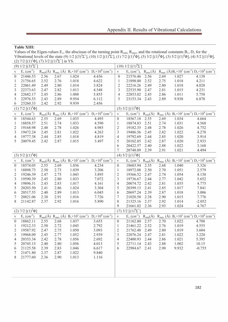
Appendix II. Results of Vibrational Calculations
182
Table XIII: Values of the Eigen-values Ev, the abscissas of the turning point Rmin, Rmax, and the rotational constants Bv, Dv for the Vibrational levels of the state (9) 1/2 [(3)2Σ+], (10) 1/2 [(1)4Σ-], (1) 7/2 [(1)4Φ], (5) 3/2 [(1)4Φ], (3) 5/2 [(1)4Φ], (4) 5/2 [(1)2Φ], (2) 7/2 [(1)2Φ], (7) 3/2 [(1)4Σ+] in YS. (9) 1/2 [(3)2Σ+] (10) 1/2 [(1)4Σ-] v Ev (cm-1) Rmin(Å) Rmax
(Å) Bv×101 (cm-1) Dv×108 (cm-1) v Ev (cm-1), Rmin (Å) Rmax
(Å) Bv×101 (cm-1) Dv×108 (cm-1) 0 21446.53 2.56 2.67 1.024 4.436 0 21576.46 2.56 2.69 1.027 4.138 1 21756.65 2.52 2.76 1.018 4.622 1 21898.00 2.52 2.75 1.018 4.211 2 22061.49 2.49 2.80 1.014 3.824 2 22216.26 2.49 2.80 1.018 4.028 3 22373.63 2.47 2.82 1.013 4.548 3 22535.90 2.47 2.81 1.015 4.231 4 22682.17 2.45 2.86 1.008 5.855 4 22853.02 2.45 2.86 1.011 5.758 5 22976.53 2.43 2.89 9.954 6.112 5 23153.34 2.43 2.89 9.938 6.870 6 23260.33 2.42 2.92 9.939 2.456 (1) 7/2 [(1)4Φ] (5) 3/2 [(1)4Φ] v Ev (cm-1) Rmin(Å) Rmax
(Å) Bv×101 (cm-1) Dv×108 (cm-1) v Ev (cm-1) Rmin(Å) Rmax (Å) Bv×101 (cm-1) Dv×108 (cm-1)
0 18544.63 2.55 2.69 1.035 4.495 0 18567.18 2.55 2.69 1.034 4.664 1 18858.57 2.51 2.74 1.033 4.590 1 18874.83 2.51 2.74 1.031 4.568 2 19168.98 2.48 2.78 1.026 4.985 2 19182.35 2.48 2.78 1.026 4.752 3 19472.24 2.45 2.81 1.022 4.263 3 19486.56 2.45 2.82 1.022 4.278 4 19777.38 2.44 2.85 1.018 4.819 4 19792.69 2.44 2.85 1.020 3.914 5 20079.45 2.42 2.87 1.015 3.497 5 20102.85 2.42 2.87 1.020 2.933 6 20422.57 2.40 2.88 1.022 3.168 7 20748.09 2.39 2.91 1.021 4.494 (3) 5/2 [(1)4Φ] (4) 5/2 [(1)2Φ] v Ev (cm-1) Rmin(Å) Rmax
(Å) Bv×101 (cm-1) Dv×108 (cm-1) v Ev (cm-1) Rmin(Å) Rmax (Å) Bv×101 (cm-1) Dv×108 (cm-1)
0 18574.05 2.55 2.69 1.036 4.234 0 18603.94 2.55 2.68 1.040 3.326 1 18898.73 2.50 2.73 1.039 3.206 1 18972.08 2.50 2.70 1.051 2.579 2 19246.39 2.47 2.75 1.043 3.895 2 19366.52 2.47 2.74 1.054 4.130 3 19590.39 2.45 2.80 1.033 7.072 3 19736.67 2.44 2.77 1.042 5.652 4 19896.31 2.43 2.83 1.017 4.161 4 20074.72 2.42 2.81 1.035 4.775 5 20203.50 2.41 2.86 1.024 3.304 5 20399.13 2.41 2.85 1.017 7.841 6 20517.55 2.40 2.89 1.013 6.045 6 20697.24 2.39 2.87 1.018 3.006 7 20821.06 2.38 2.91 1.016 7.726 7 21020.58 2.38 2.90 1.015 7.776 8 21142.87 2.37 2.92 1.016 5.890 8 21325.16 2.37 2.92 1.014 -2.052 9 21661.02 2.36 2.93 1.024 4.767 (2) 7/2 [(1)2Φ] (7) 3/2 [(1)4Σ+] v Ev (cm-1) Rmin(Å) Rmax
(Å) Bv×101 (cm-1) Dv×108 (cm-1) v Ev (cm-1) Rmin(Å) Rmax (Å) Bv×101 (cm-1) Dv×108 (cm-1)
0 18862.11 2.55 2.68 1.037 3.655 0 21162.80 2.57 2.70 1.022 4.788 1 19212.33 2.50 2.72 1.045 2.792 1 21461.22 2.52 2.76 1.019 4.555 2 19587.92 2.47 2.75 1.050 3.093 2 21762.48 2.49 2.80 1.019 3.604 3 19968.09 2.45 2.77 1.052 2.939 3 22076.24 2.47 2.81 1.022 3.220 4 20353.34 2.42 2.78 1.056 2.692 4 22400.93 2.44 2.86 1.021 5.395 5 20745.15 2.40 2.80 1.056 4.013 5 22711.14 2.43 2.88 1.002 10.15 6 21125.58 2.39 2.83 1.046 6.617 6 22984.67 2.41 2.90 9.932 -0.755 7 21471.80 2.37 2.87 1.022 9.840 8 21777.60 2.36 2.90 1.013 1.116
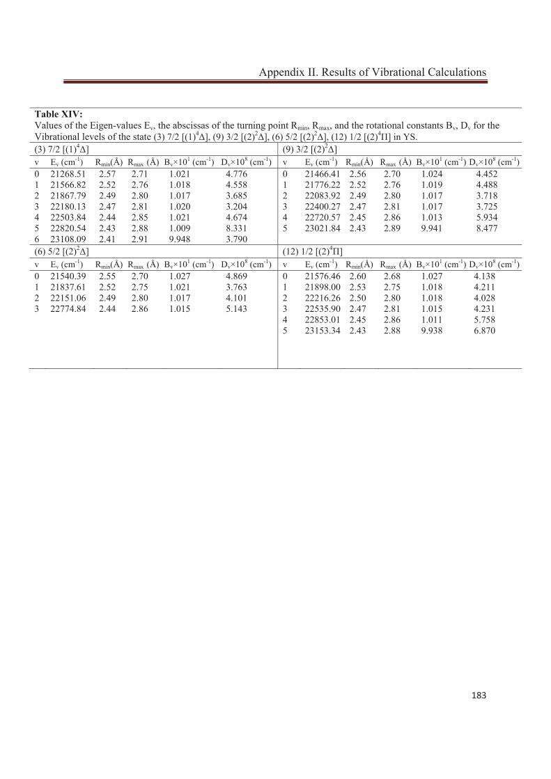
Appendix II. Results of Vibrational Calculations
183
Table XIV: Values of the Eigen-values Ev, the abscissas of the turning point Rmin, Rmax, and the rotational constants Bv, Dv for the Vibrational levels of the state (3) 7/2 [(1)4Δ], (9) 3/2 [(2)2Δ], (6) 5/2 [(2)2Δ], (12) 1/2 [(2)4Π] in YS. (3) 7/2 [(1)4Δ] (9) 3/2 [(2)2Δ] v Ev (cm-1) Rmin(Å) Rmax
(Å) Bv×101 (cm-1) Dv×108 (cm-1) v Ev (cm-1) Rmin(Å) Rmax (Å) Bv×101 (cm-1) Dv×108 (cm-1)
0 21268.51 2.57 2.71 1.021 4.776 0 21466.41 2.56 2.70 1.024 4.452 1 21566.82 2.52 2.76 1.018 4.558 1 21776.22 2.52 2.76 1.019 4.488 2 21867.79 2.49 2.80 1.017 3.685 2 22083.92 2.49 2.80 1.017 3.718 3 22180.13 2.47 2.81 1.020 3.204 3 22400.27 2.47 2.81 1.017 3.725 4 22503.84 2.44 2.85 1.021 4.674 4 22720.57 2.45 2.86 1.013 5.934 5 22820.54 2.43 2.88 1.009 8.331 5 23021.84 2.43 2.89 9.941 8.477 6 23108.09 2.41 2.91 9.948 3.790 (6) 5/2 [(2)2Δ] (12) 1/2 [(2)4Π] v Ev (cm-1) Rmin(Å) Rmax
(Å) Bv×101 (cm-1) Dv×108 (cm-1) v Ev (cm-1) Rmin(Å) Rmax (Å) Bv×101 (cm-1) Dv×108 (cm-1)
0 21540.39 2.55 2.70 1.027 4.869 0 21576.46 2.60 2.68 1.027 4.138 1 21837.61 2.52 2.75 1.021 3.763 1 21898.00 2.53 2.75 1.018 4.211 2 22151.06 2.49 2.80 1.017 4.101 2 22216.26 2.50 2.80 1.018 4.028 3 22774.84 2.44 2.86 1.015 5.143 3 22535.90 2.47 2.81 1.015 4.231 4 22853.01 2.45 2.86 1.011 5.758 5 23153.34 2.43 2.88 9.938 6.870

Appendix III. Dipole Moment Results
184
Appendix III
Dipole Moment Results
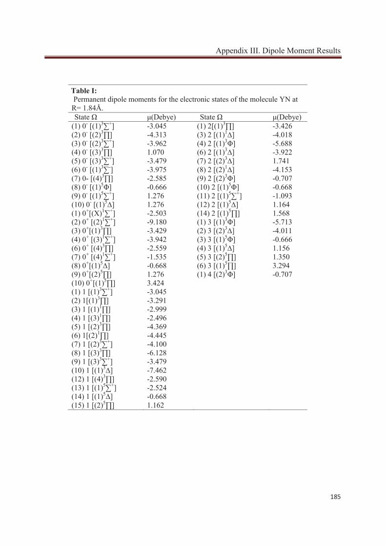
Appendix III. Dipole Moment Results
185
Table I: Permanent dipole moments for the electronic states of the molecule YN at R= 1.84Å. State Ω μ(Debye) State Ω μ(Debye)
(1) 0- [(1)3∑+] -3.045 (1) 2[(1)3∏] -3.426 (2) 0- [(2)3∏] -4.313 (3) 2 [(1)1∆] -4.018 (3) 0- [(2)3∑+] -3.962 (4) 2 [(1)3Φ] -5.688 (4) 0- [(3)3∏] 1.070 (6) 2 [(1)3∆] -3.922 (5) 0- [(3)3∑+] -3.479 (7) 2 [(2)3∆] 1.741 (6) 0- [(1)3∑-] -3.975 (8) 2 [(2)1∆] -4.153 (7) 0- [(4)3∏] -2.585 (9) 2 [(2)3Φ] -0.707 (8) 0- [(1)5Φ] -0.666 (10) 2 [(1)5Φ] -0.668 (9) 0- [(1)5∑+] 1.276 (11) 2 [(1)5∑+] -1.093 (10) 0- [(1)5∆] 1.276 (12) 2 [(1)5∆] 1.164 (1) 0+[(X)1∑+] -2.503 (14) 2 [(1)5∏] 1.568 (2) 0+ [(2)1∑+] -9.180 (1) 3 [(1)3Φ] -5.713 (3) 0+[(1)3∏] -3.429 (2) 3 [(2)3∆] -4.011 (4) 0+ [(3)1∑+] -3.942 (3) 3 [(1)5Φ] -0.666 (6) 0+ [(4)3∏] -2.559 (4) 3 [(1)5∆] 1.156 (7) 0+ [(4)1∑+] -1.535 (5) 3 [(2)5∏] 1.350 (8) 0+[(1)5∆] -0.668 (6) 3 [(1)5∏] 3.294 (9) 0+[(2)5∏] 1.276 (1) 4 [(2)3Φ] -0.707 (10) 0+[(1)5∏] 3.424 (1) 1 [(1)3∑+] -3.045 (2) 1[(1)3∏] -3.291 (3) 1 [(1)1∏] -2.999 (4) 1 [(3)1∏] -2.496 (5) 1 [(2)3∏] -4.369 (6) 1[(2)1∏] -4.445 (7) 1 [(2)3∑+] -4.100 (8) 1 [(3)3∏] -6.128 (9) 1 [(3)3∑+] -3.479 (10) 1 [(1)3∆] -7.462 (12) 1 [(4)3∏] -2.590 (13) 1 [(1)5∑+] -2.524 (14) 1 [(1)5∆] -0.668 (15) 1 [(2)5∏] 1.162
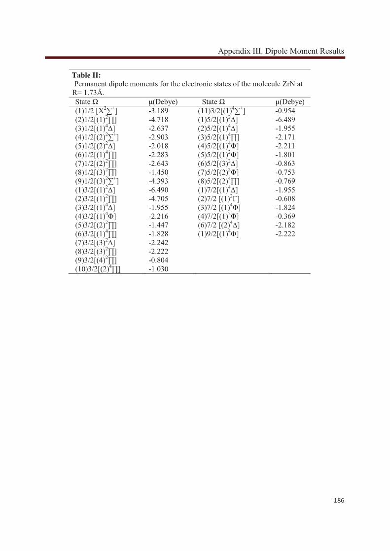
Appendix III. Dipole Moment Results
186
Table II: Permanent dipole moments for the electronic states of the molecule ZrN at R= 1.73Å. State Ω μ(Debye) State Ω μ(Debye) (1)1/2 [X2∑+] -3.189 (11)3/2[(1)4∑+] -0.954 (2)1/2[(1)2∏] -4.718 (1)5/2[(1)2∆] -6.489 (3)1/2[(1)4∆] -2.637 (2)5/2[(1)4∆] -1.955 (4)1/2[(2)2∑+] -2.903 (3)5/2[(1)4∏] -2.171 (5)1/2[(2)2∆] -2.018 (4)5/2[(1)4Φ] -2.211 (6)1/2[(1)4∏] -2.283 (5)5/2[(1)2Φ] -1.801 (7)1/2[(2)2∏] -2.643 (6)5/2[(3)2∆] -0.863 (8)1/2[(3)2∏] -1.450 (7)5/2[(2)2Φ] -0.753 (9)1/2[(3)2∑+] -4.393 (8)5/2[(2)4∏] -0.769 (1)3/2[(1)2∆] -6.490 (1)7/2[(1)4∆] -1.955 (2)3/2[(1)2∏] -4.705 (2)7/2 [(1)2Г] -0.608 (3)3/2[(1)4∆] -1.955 (3)7/2 [(1)4Φ] -1.824 (4)3/2[(1)4Φ] -2.216 (4)7/2[(1)2Φ] -0.369 (5)3/2[(2)2∏] -1.447 (6)7/2 [(2)4∆] -2.182 (6)3/2[(1)4∏] -1.828 (1)9/2[(1)4Φ] -2.222 (7)3/2[(3)2∆] -2.242 (8)3/2[(3)2∏] -2.222 (9)3/2[(4)2∏] -0.804 (10)3/2[(2)4∏] -1.030
187
Curriculum Vitae Ayman K. Farhat
Lyon, France Mobile: 0033787431172 [email protected]
Target Job: Post-Doctoral Research Fellow
Education:
September 2009 → June 2012
PhD research fellow in physics with emphasis on computational material sciences from the University of Claude Bernard – Lyon1, Laboratoire de Physique de la matiére Condensée et Nanostructures, France.
September 2006 → May 2009
M.S. in Molecular Computational Quantum physics from Beirut Arab University (GPA = 3, in first M.S. year courses, during the courses and the thesis work I obtained the first rank over all my classmates).
September 2003 → June 2006
B.S in physics from the Lebanese International University (major courses GPA=3.2, I got the first rank over all my classmates, 10 students).
September 2007 → June 2007
Registered in a double major program of Mechanical Engineering at the Lebanese International University (GPA = 3.5).
June- 2003
Lebanese Baccalaureate degree - life science section. Research Experience:
September 2009 → June 2012
My PhD research experience includes high quality post Hartree Fock Multireference Single and Double Excitation Configuration Interaction (MRSDCI) ab initio calculations for the electronic structures of the transition metal nitrides and sulfides of Yttrium and Zirconium. In my PhD thesis work we studied the electronic structures of the four molecules YS, YN, ZrN, and ZrS with the inclusion of relativistic spin orbit effects. The results of these calculations yielded accurate spectroscopic constants which are in excellent agreement with the experimental and
188
theoretical results available in literature. Several molecular properties were also computed such as the permanent electric dipole moments, internal molecular electric fields, and diamagnetic shielding tensors. We further used a Fortran 95 code, developed by our research group, that solves the time independent Schrödinger equation within the canonical functions approach for the vibrational and rotational motions of each molecule. The implemented program yielded accurate vibrational energy levels and rotational constants that are only within 10% of experimental accuracy. I further expect to develop the code into solving the time dependent vibrational-rotational Schrödinger equation under the effect of an oscillating laser field perturbation for a selected two vibrational level transition. This should have applications in quantum computing as selected transition between vibrational levels may be followed by designing an optimal laser pulse that is sufficient to cause transition between the quantum states (qubits) of a polar diatomic molecule. The results of our relativistic ab inito calculations are the first of their kind on these molecules reported in literature. Finally, I searched for applications of the molecules of interest in three domains; in quantum computing on heteronuclear diatomic molecules, in the search for variations in the fundamental constants in nature such as the fine structure constant and the electron to proton mass ratio, and in the search for the electric dipole moment of the electron. I found in the ZrS molecule several degenerate vibrational energy levels of order < 10cm-1 which can enhance the experimental sensitivity measurement to orders of 10-15 year-1 for slight variations of the fine structure constant in laboratory experiments and in S type stars. As a member of the theoretical and computational spectroscopy group of Prof. Miguel Marques I developed an excellent research experience in applying DFT calculations within the abinit code to search for different stable metallic Silicon structures which might have superconducting characteristics. This research work was performed in the past 5 months at the Theoretical and Computational Spectroscopy group of Prof. Miguel Marques at the University of Lyon 1. Please check the following website http://www.tddft.org/bmg/index.php for an overview of our research activities.
September 2007 → June 2009
I gained a great research experience during my M.S. studies with my supervisor Prof. Mahmoud Korek in which I applied non-relativistic quantum mechanical calculations for the electronic structure of the diatomic gaseous molecule Yttrium monosulfides YS.
October 2003 → June 2006
During my undergraduate studies I participated in building the Murex submarine at the Lebanese International University (LIU), weighing 5 tons the Murex submarine could submerge into a depth of 125 meters with two persons inside, it has been successfully tested several times in the Mediterranean Sea.
Summer 2008
I won the first prize at the American University of Beirut (AUB) science fair contest for the project "Energy saving in architectural design of Buildings and concert halls", and I had a
189
training session in operating a geode device to investigate underground surface layers at Beirut Arab University
Work Experience:
September 2006 → June 2009 I worked as a full time physics teacher at Omar Mokhtar educational center, (Lebanon) for the grades 8, 9, 10, 11, and 12.
September 2007 → June 2009 I worked as a part time assistant in physics and chemistry for the first and second year science and engineering students at both the Lebanese International University and Beirut Arab University.
Research Interests:
As a PhD research fellow at the University of Claude Bernard, I developed the basic skills and techniques that allow me to pursue a research career in computational sciences. I believe that my experience in DFT calculations as well as MRSDCI relativistic calculations developed at the Theoretical and Computational Spectroscopy Group of Dr. Miguel Marques and at the group of Molecular physics of Prof. Mahmoud Korek at Beirut Arab University is very beneficial in launching my research career in higher education. I am currently interested in expanding my research experience towards other research domains.
Publications:
As a result of my M.S. and PhD thesis I wrote the following papers:
1- A. Farhat, M. Korek, S. Abdul-Al, M. A. L. Marques., Enhanced Sensitivity to the Time Variation of the Fine-Structure Constant and mp/me in Zirconium Mono-Sulfide. (In preparation) 2- A. Farhat, M. Korek, S. Abdul-Al, M. A. L. Marques., All-electron ab initio calculations of the ground and excited states of the YN molecule including vibro-rotational calculations. (In preparation). 3- M. Korek, A. Farhat, S. Abdul-Al., Theoretical Calculations of the Low-Lying Electronic States of the Molecule YS., JTCC, 9, 757 (2010). 4- A. Farhat, M. Korek, S. Abdul-Al, M. A. L. Marques., All-electron ab initio calculations of the low-lying electronic states of the molecule ZrN. (Submitted to the Canadian Journal of Chemistry). 5- A. Farhat, M. Korek, S. Abdul-Al, M. A. L. Marques., All-electron ab initio calculations of the ground and excited electronic states of the ZrS molecule without spin-orbit effects. (submitted to the Journal of Chemical Physics). 6- A. Farhat, M. Korek, S. Abdul-Al, M. A. L. Marques., All-electron ab initio calculations of the ground and excited states of the ZrN molecule including spin-orbit effects. (In Preparation).
7- A. Farhat, M. Korek, S. Abdul-Al, M. A. L. Marques., All-electron ab initio calculations of the ground and excited states of the YS molecule including spin-orbit effects. (In Preparation).
190
Conferences invited to / attended:
1. One of my research papers “Ab initio Calculation of Molecular States of Compounds of the Lanthanum and Yttrium Molecules”, was accepted and I was invited to present my work at the ICCMSE seventh International Conference of Computational Methods in Sciences and Engineering, Rhodes, Greece September 2009
2. I was invited to present my research achievements at the 16th International Lebanese Scientific Conference (LAAS), at Beirut Arab University, Beirut - Lebanon November 2009.
3. I participated with an oral presentation in the 17th International Lebanese Scientific Conference (LAAS), at the Université Saint Esprit de Kaslik (USEK), Beirut - Lebanon, November 2010.
Honors and Awards:
PhD research fellow at the University of Claude Bernard, Lyon 1, 2011 – 2012.
I was honored for participating in building the Murex submarine, and I gave a speech on behalf of the participating students in the project.
Scientific Research Groups:
I am a member of the Theoretical and Computational Spectroscopy Group of Prof. Miguel A. L. Marques at the Lab. de Physique de la Matiére Condensée et Nanostructure; Université Lyon 1.
I am a member of the molecular spectroscopy group of Prof. Mahmoud Korek at Beirut Arab University.
Presentations:
“Einstein’s general theory of relativity and Black holes” (B.S. seminar). Theoretical calculations with spin orbit effect of the molecule Yttrium monosulfide YS” (M.S Thesis.
“Electron Beam lithography and it applications to nanotechnology” (performed at Beirut Arab University).
“X – Ray emission, a Theoretical investigation” (performed at Beirut Arab University). “Uranium enrichment in heavy water nuclear reactors” (performed at Beirut Arab University). “Theoretical Calculation with spin-orbit effect of Yttrium sulfide” (performed at Université Saint Joseph de Kaslik, Liban).
“Carbon nanotubes, discovery and current applications” (performed at Beirut Arab University). “New Prospects of Molecular Quantum Computing on the Vibrational States of Heteronuclear Diatomic Molecules” (Seminar expected to be performed at the University of Lyon 1 on the 14th of February 2012).
Languages:
Fluent in Arabic and English, my TOEFL IBT test score is 90/120.
191
Intermediate in French, my level is B1. My GRE test scores are:
Math Quantitative Reasoning: 730/800 English Verbal Reasoning: 480/800.
Recently read books (in the past 14 months):
1. Quantum (A Guide for the Perplexed) by Jim Al-Khalili 2003. (Finished) 2. Entanglement (The Spooky action of a distance) by Amir D. Aczel 2002.(Finished) 3. Many Body Problems and Quantum Field Theory, An Introduction by Philippe Marin and François Rothen. (Finished) 4. Concepts of Nuclear Physics by Bernard L Cohen 1997. (Finished) 5. The Self-Aware Universe by Goswani and Amit. (Finished) 6. Quantum electrodynamics (The Strange Theory of Light and Matter) by Richard Feynman. (Finished) 7. The Universe in a Nutshell by Stephan Hawking. (Finished) 8. The Conceptual Basis of Quantum Field Theory by Gerard ’t Hooft (Institute of Theoretical Physics, Utrecht University the Netherlands)., Elsevier 2004. (Finished) 9. Molecular Electronic Structure Theory by Trygve Helgaker, Poul Jorgensen, and Jeppe Olsen. (Finished) 10. Essentials of Computational Chemistry, Theories and Models by Christopher Cramer. (Finished) 11. Quantum Field Theory In a Nutshell by A. Zee. (I finished the first 120 pages).
Community Services:
I am former volunteer/member at the Lebanese Red Cross organization.
Computer Skills:
Experienced user of Linux commands, Molpro and Abinit computational Physics programs and their applications to material science and physical chemistry research. I am an active user of the computational nanotechnology resources available online (www.nanohub.org) by the university of Purdue/USA. I know C++ programming language. I am a professional user of the AutoCAD program. I am a professional user of the Microsoft office programs (Word, Excel, and PowerPoint). I also master dealing with windows vista, windows 7, and XP.