Embed Size (px)
Citation preview
�
� 电FSS电FSS电FSS电FSS
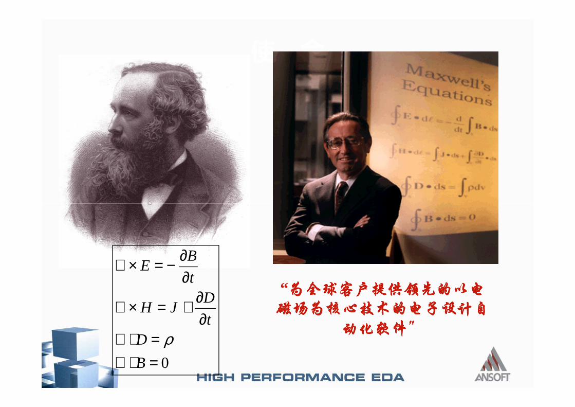
使 命
“为全球客户提供为全球客户提供为全球客户提供为全球客户提供领先的以电领先的以电领先的以电领先的以电磁场为磁场为磁场为磁场为核心技术核心技术核心技术核心技术的电子设计自的电子设计自的电子设计自的电子设计自
动化软件动化软件动化软件动化软件””””
0=⋅∇=⋅∇
∂∂+=×∇
∂∂−=×∇
B
Dt
DJH
t
BE
ρ
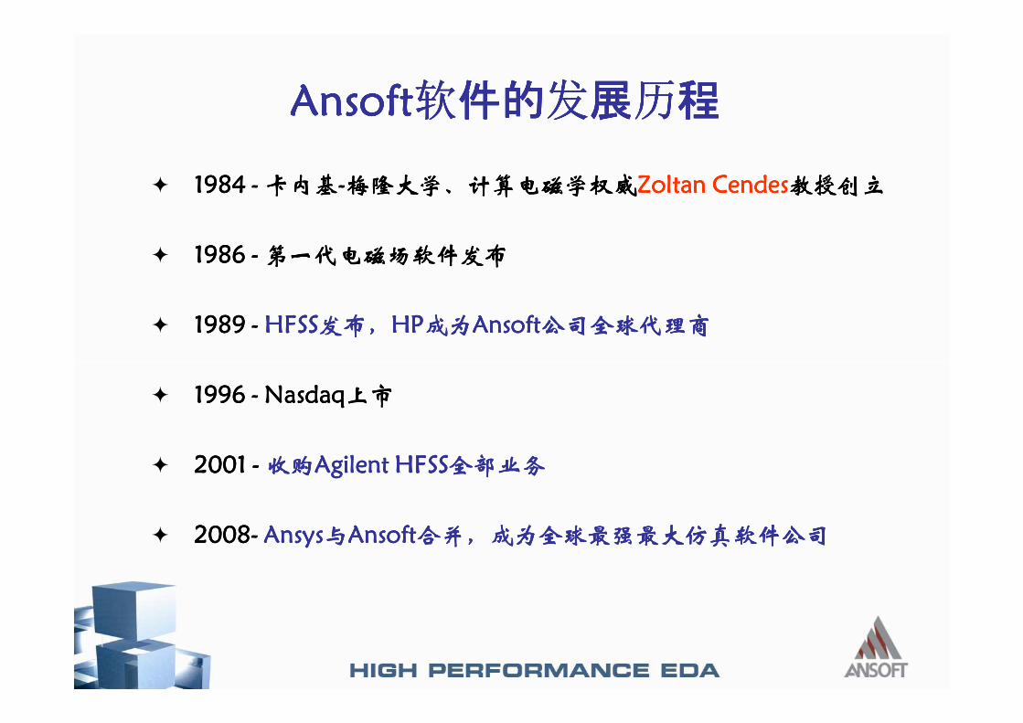
AnsoftAnsoftAnsoftAnsoftAnsoftAnsoftAnsoftAnsoft 件的件的件的件的件的件的件的件的 展展展展展展展展 程程程程程程程程
� 最984 最984 最984 最984 务务务务 务务务务 ZoltanZoltanZoltanZoltan CendesCendesCendesCendes
� 最986 最986 最986 最986 务务务务
� 最989 最989 最989 最989 务务务务 HFSSHFSSHFSSHFSS HPHPHPHP AnsoftAnsoftAnsoftAnsoft
� 最996 最996 最996 最996 务务务务 NasdaqNasdaqNasdaqNasdaq
� 2真真最 2真真最 2真真最 2真真最 务务务务 Agilent HFSSAgilent HFSSAgilent HFSSAgilent HFSS
� 2真真2真真2真真2真真8888务务务务 AnsysAnsysAnsysAnsys AnsoftAnsoftAnsoftAnsoft
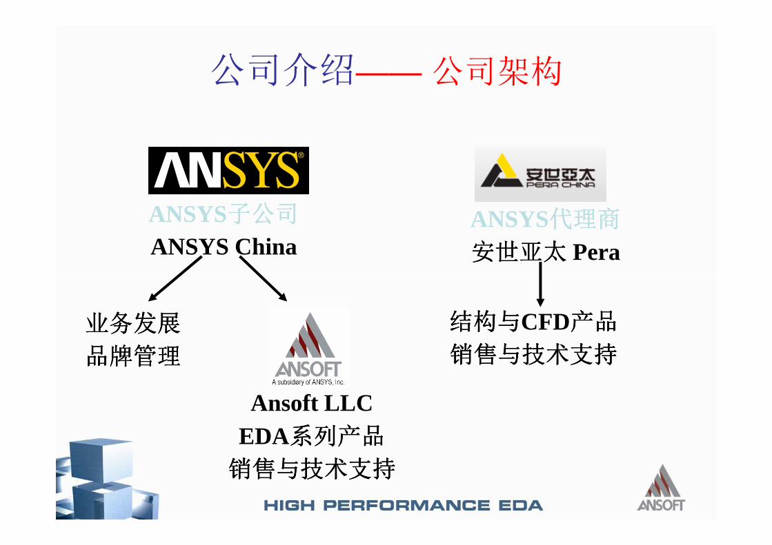
——
ANSYSANSYS China
ANSYSPera
Ansoft LLC EDA
CFD
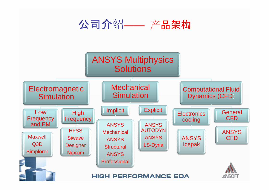
公司介 —— 品架构
ANSYS MultiphysicsSolutions
ElectromagneticSimulation
Mechanical Simulation
Computational Fluid Dynamics (CFD)Simulation
Low Frequency
and EM
MaxwellQ3D
Simplorer
High Frequency
HFSSSiwave
DesignerNexxim
Simulation
Implicit
ANSYSMechanical
ANSYSStructuralANSYS
Professional
Explicit
ANSYS AUTODYN
ANSYSLS-Dyna
Dynamics (CFD)
Electronics cooling
ANSYS Icepak
General CFD
ANSYS CFD
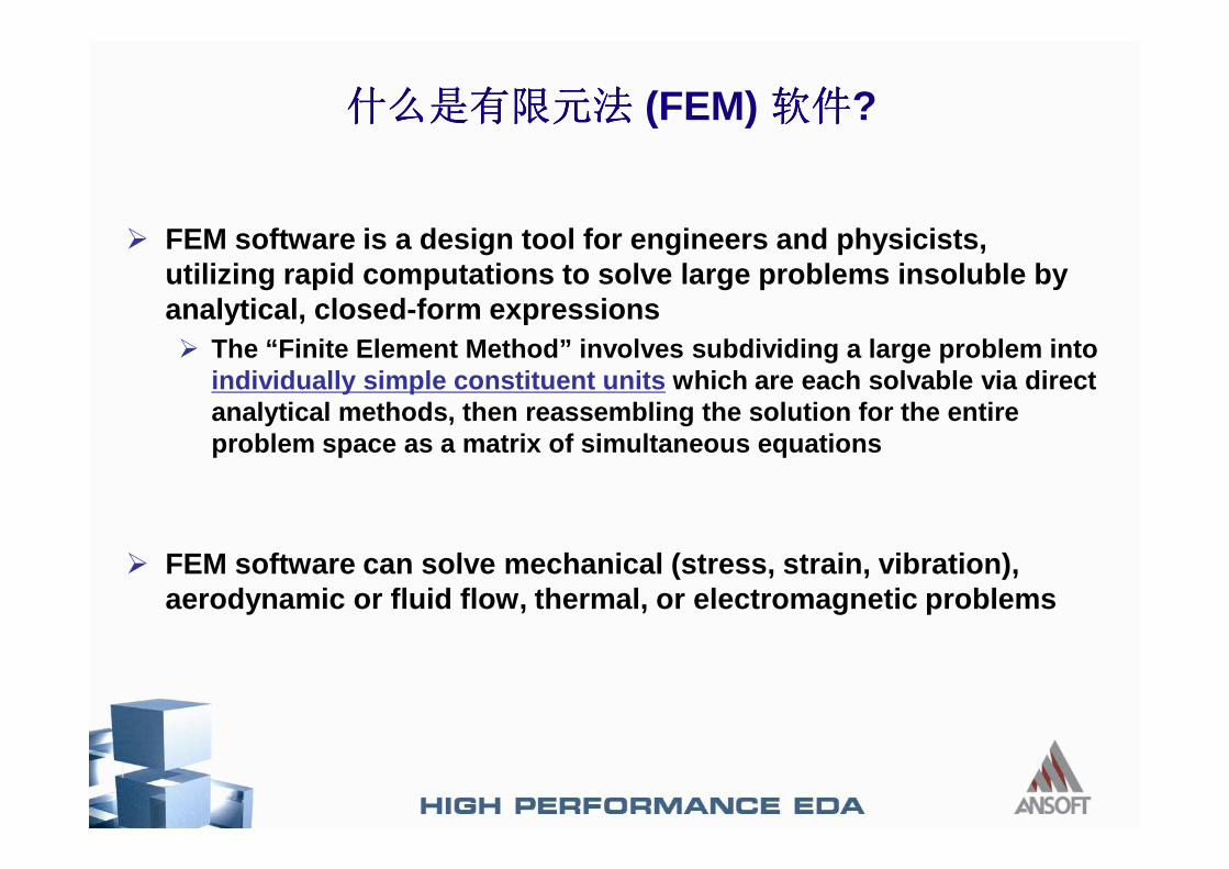
(FEM) ?
� FEM software is a design tool for engineers and phy sicists, utilizing rapid computations to solve large problem s insoluble by analytical, closed-form expressions� The “Finite Element Method” involves subdividing a la rge problem into
individually simple constituent units which are each solvable via direct analytical methods, then reassembling the solution for the entire problem space as a matrix of simultaneous equationsproblem space as a matrix of simultaneous equations
� FEM software can solve mechanical (stress, strain, vibration), aerodynamic or fluid flow, thermal, or electromagne tic problems
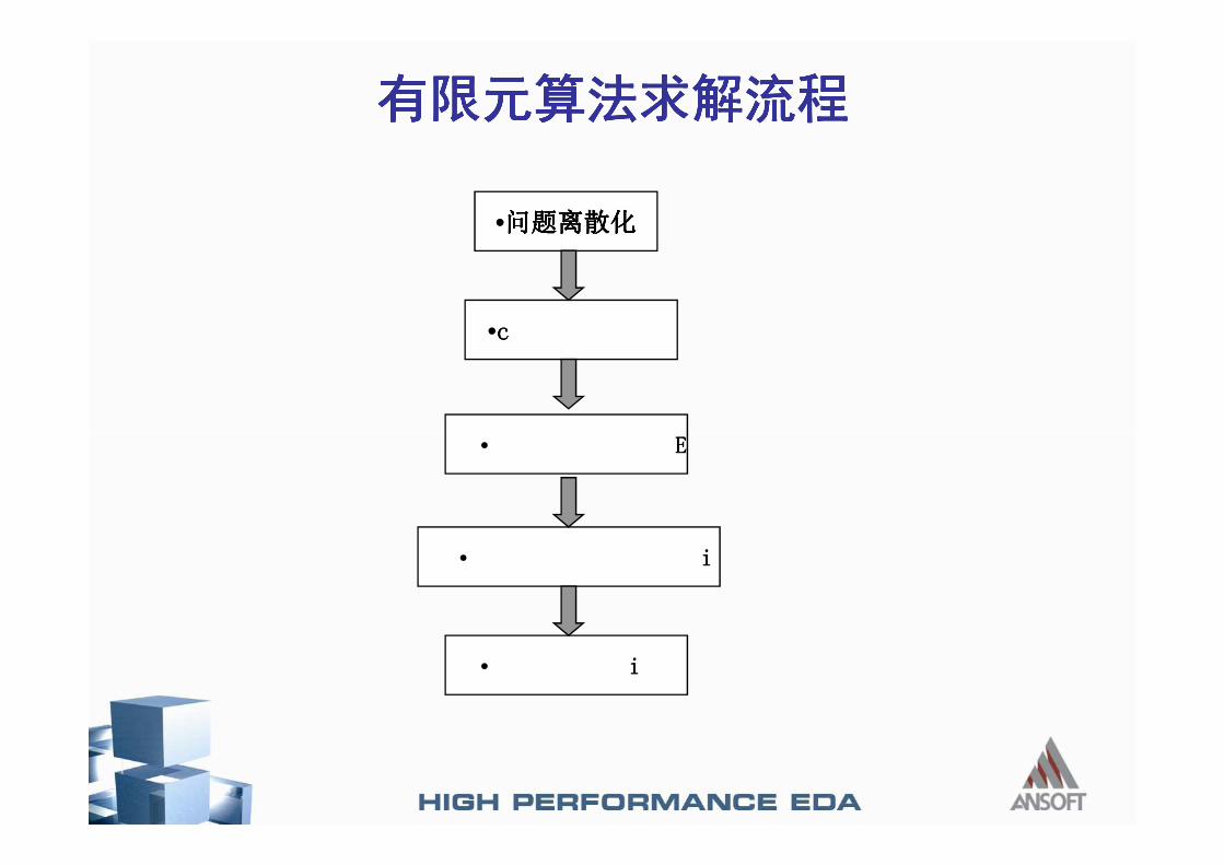
••
•
••
•
•
////
////
(((( //// ))))
(((( , , , , ))))
(((( ))))
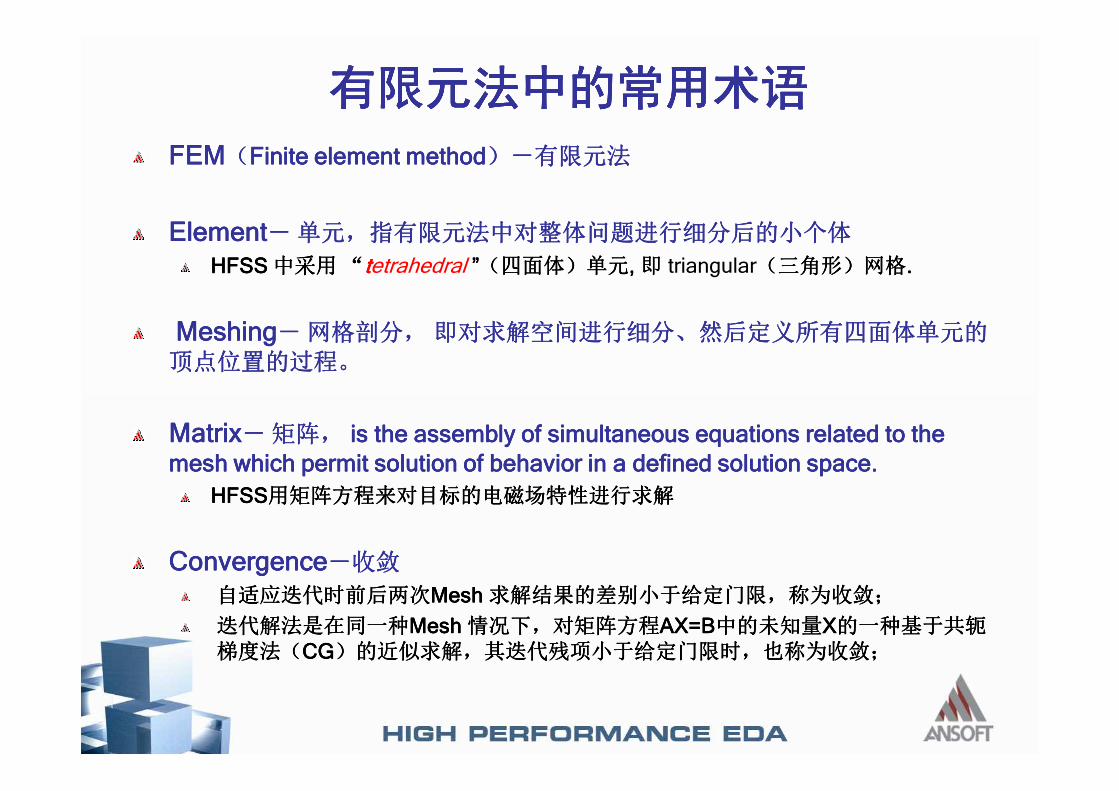
FEMFEMFEMFEM Finite element methodFinite element methodFinite element methodFinite element method
ElementElementElementElement
HFSS HFSS HFSS HFSS ttttetrahedral ”””” , , , , triangular ....
MeshingMeshingMeshingMeshing
MatrixMatrixMatrixMatrix is the assembly of simultaneous equations is the assembly of simultaneous equations is the assembly of simultaneous equations is the assembly of simultaneous equations related related related related to the to the to the to the
mesh which permit solution of behavior in a mesh which permit solution of behavior in a mesh which permit solution of behavior in a mesh which permit solution of behavior in a defined defined defined defined solution space.solution space.solution space.solution space.
HFSSHFSSHFSSHFSS
ConvergenceConvergenceConvergenceConvergence
Mesh Mesh Mesh Mesh
Mesh Mesh Mesh Mesh AX=BAX=BAX=BAX=B XXXX
CGCGCGCG
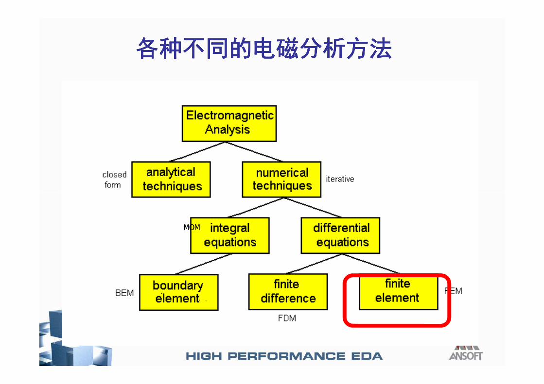
MOM
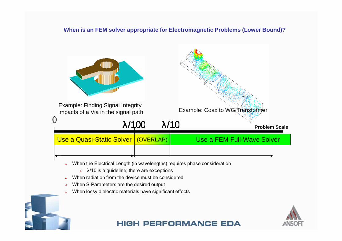
When is an FEM solver appropriate for Electromagnet ic Problems (Lower Bound)?
λλλλ/100/100/100/1000
Example: Finding Signal Integrity impacts of a Via in the signal path
λλλλ/10/10/10/10
Example: Coax to WG Transformer
λλλλ/100/100/100/1000
Use a Quasi-Static Solver
When the Electrical Length (in wavelengths) requires phase consideration
λ/10 is a guideline; there are exceptionsWhen radiation from the device must be considered
When S-Parameters are the desired output
When lossy dielectric materials have significant effects
Use a FEM Full-Wave Solver
Problem Scaleλλλλ/10/10/10/10(OVERLAP)
�
� 电FSS电FSS电FSS电FSS
�
� HFSS
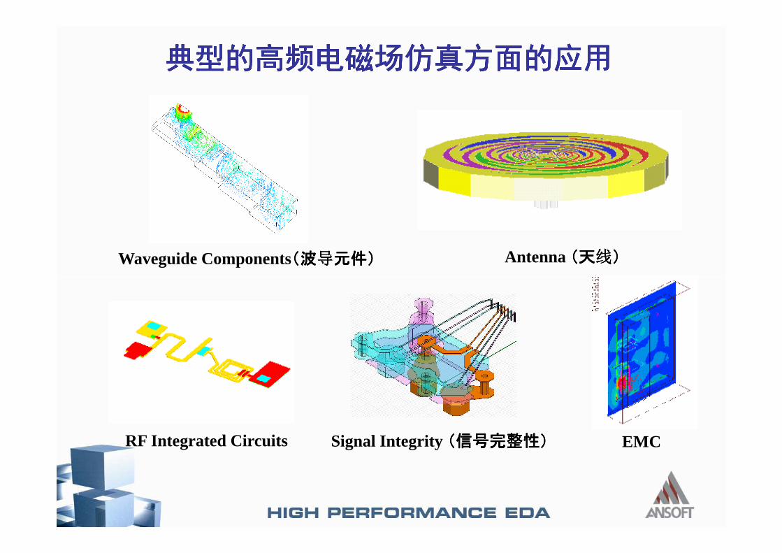
Antenna (天(天(天(天 ))))Waveguide Components(波(波(波(波 元件)元件)元件)元件)
RF Integrated Circuits EMCSignal Integrity (信号完整性)(信号完整性)(信号完整性)(信号完整性)
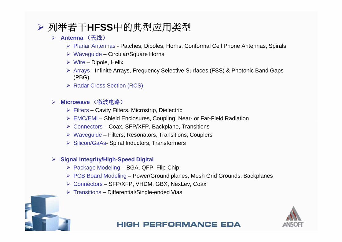
� HFSS� Antenna
� Planar Antennas - Patches, Dipoles, Horns, Conformal Cell Phone Antennas, Spirals� Waveguide – Circular/Square Horns� Wire – Dipole, Helix� Arrays - Infinite Arrays, Frequency Selective Surfaces (FSS) & Photonic Band Gaps
(PBG)� Radar Cross Section (RCS)
� Microwave � Filters – Cavity Filters, Microstrip, Dielectric� EMC/EMI – Shield Enclosures, Coupling, Near- or Far-Field Radiation� EMC/EMI – Shield Enclosures, Coupling, Near- or Far-Field Radiation� Connectors – Coax, SFP/XFP, Backplane, Transitions� Waveguide – Filters, Resonators, Transitions, Couplers� Silicon/GaAs- Spiral Inductors, Transformers
� Signal Integrity/High-Speed Digital� Package Modeling – BGA, QFP, Flip-Chip� PCB Board Modeling – Power/Ground planes, Mesh Grid Grounds, Backplanes� Connectors – SFP/XFP, VHDM, GBX, NexLev, Coax� Transitions – Differential/Single-ended Vias
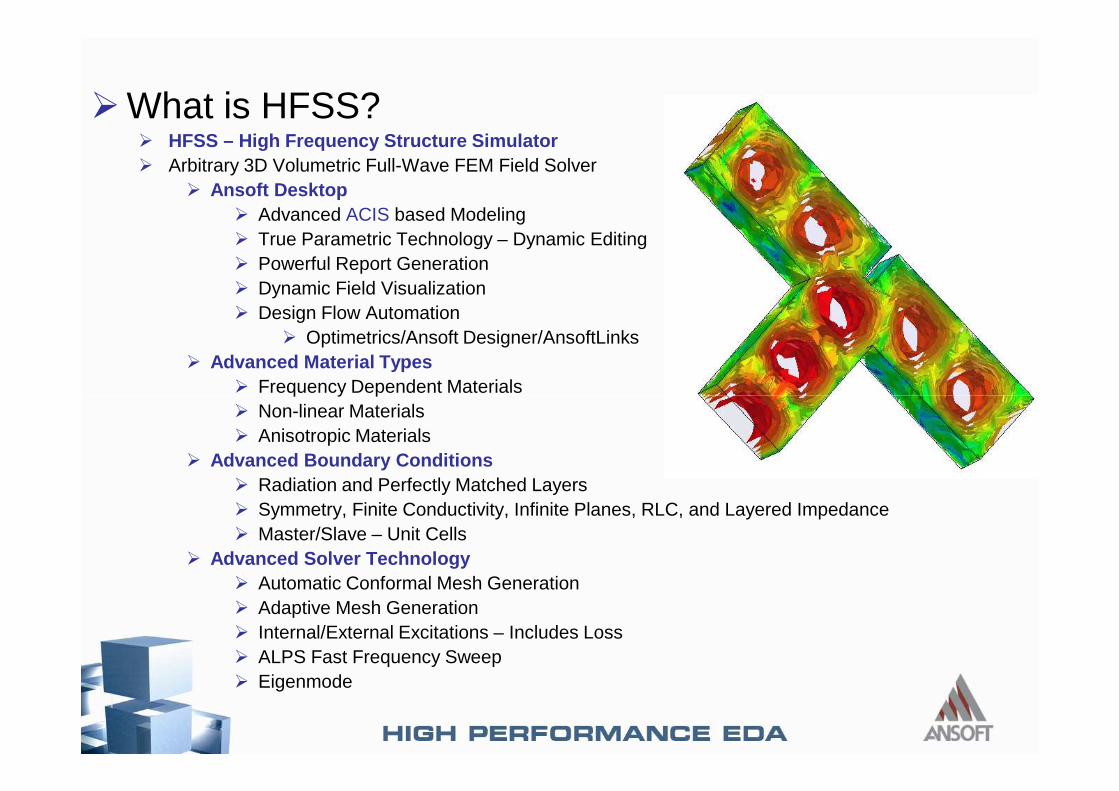
�What is HFSS?� HFSS – High Frequency Structure Simulator� Arbitrary 3D Volumetric Full-Wave FEM Field Solver
� Ansoft Desktop� Advanced ACIS based Modeling� True Parametric Technology – Dynamic Editing� Powerful Report Generation� Dynamic Field Visualization� Design Flow Automation
� Optimetrics/Ansoft Designer/AnsoftLinks� Advanced Material Types
� Frequency Dependent Materials� Frequency Dependent Materials� Non-linear Materials� Anisotropic Materials
� Advanced Boundary Conditions� Radiation and Perfectly Matched Layers� Symmetry, Finite Conductivity, Infinite Planes, RLC, and Layered Impedance� Master/Slave – Unit Cells
� Advanced Solver Technology� Automatic Conformal Mesh Generation� Adaptive Mesh Generation� Internal/External Excitations – Includes Loss� ALPS Fast Frequency Sweep� Eigenmode
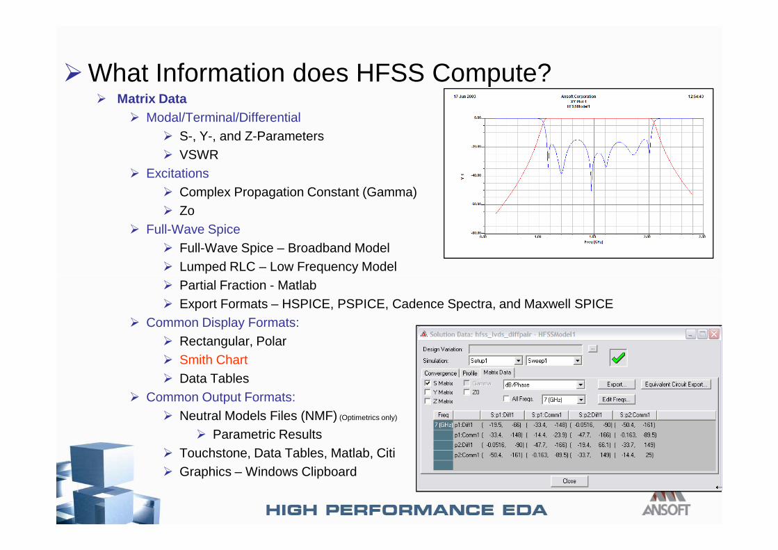
�What Information does HFSS Compute?� Matrix Data
� Modal/Terminal/Differential� S-, Y-, and Z-Parameters� VSWR
� Excitations� Complex Propagation Constant (Gamma)� Zo
� Full-Wave Spice� Full-Wave Spice – Broadband Model� Lumped RLC – Low Frequency Model� Partial Fraction - Matlab� Export Formats – HSPICE, PSPICE, Cadence Spectra, and Maxwell SPICE
� Common Display Formats:� Rectangular, Polar� Smith Chart� Data Tables
� Common Output Formats:� Neutral Models Files (NMF) (Optimetrics only)
� Parametric Results� Touchstone, Data Tables, Matlab, Citi� Graphics – Windows Clipboard
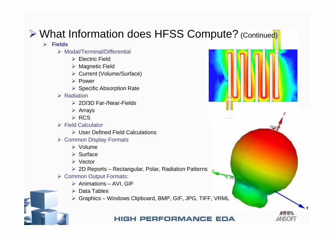
�What Information does HFSS Compute? (Continued)� Fields
� Modal/Terminal/Differential� Electric Field� Magnetic Field� Current (Volume/Surface)� Power� Specific Absorption Rate
� Radiation� 2D/3D Far-/Near-Fields� Arrays� RCS� RCS
� Field Calculator� User Defined Field Calculations
� Common Display Formats� Volume� Surface� Vector� 2D Reports – Rectangular, Polar, Radiation Patterns
� Common Output Formats:� Animations – AVI, GIF� Data Tables� Graphics – Windows Clipboard, BMP, GIF, JPG, TIFF, VRML
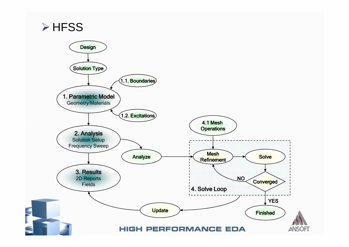
�HFSS
DesignDesignDesignDesign
Solution TypeSolution TypeSolution TypeSolution Type
1.1. Boundaries1.1. Boundaries1.1. Boundaries1.1. Boundaries
1.2. Excitations1.2. Excitations1.2. Excitations1.2. Excitations
4.1 Mesh 4.1 Mesh 4.1 Mesh 4.1 Mesh
1. Parametric Model1. Parametric Model1. Parametric Model1. Parametric ModelGeometry/Materials
4.1 Mesh 4.1 Mesh 4.1 Mesh 4.1 Mesh
OperationsOperationsOperationsOperations2. Analysis2. Analysis2. Analysis2. AnalysisSolution Setup
Frequency Sweep
3. Results3. Results3. Results3. Results2D Reports
Fields
MeshMeshMeshMesh
RefinementRefinementRefinementRefinementSolveSolveSolveSolve
UpdateUpdateUpdateUpdate
ConvergedConvergedConvergedConverged
AnalyzeAnalyzeAnalyzeAnalyze
FinishedFinishedFinishedFinished
4. Solve Loop4. Solve Loop4. Solve Loop4. Solve Loop
NONONONO
YESYESYESYES
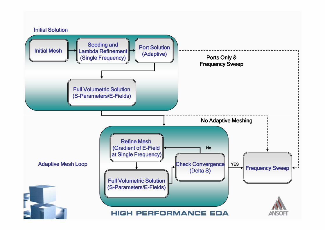
Initial SolutionInitial SolutionInitial SolutionInitial Solution
Ports Only &Ports Only &Ports Only &Ports Only &Frequency SweepFrequency SweepFrequency SweepFrequency Sweep
Initial MeshInitial MeshInitial MeshInitial MeshSeeding andSeeding andSeeding andSeeding and
Lambda RefinementLambda RefinementLambda RefinementLambda Refinement(Single Frequency)(Single Frequency)(Single Frequency)(Single Frequency)
Port SolutionPort SolutionPort SolutionPort Solution(Adaptive)(Adaptive)(Adaptive)(Adaptive)
Full Volumetric SolutionFull Volumetric SolutionFull Volumetric SolutionFull Volumetric Solution(S(S(S(S----Parameters/EParameters/EParameters/EParameters/E----Fields)Fields)Fields)Fields)
Frequency SweepFrequency SweepFrequency SweepFrequency SweepYESYESYESYESAdaptive Mesh LoopAdaptive Mesh LoopAdaptive Mesh LoopAdaptive Mesh Loop
No Adaptive MeshingNo Adaptive MeshingNo Adaptive MeshingNo Adaptive Meshing
Refine Mesh Refine Mesh Refine Mesh Refine Mesh (Gradient of E(Gradient of E(Gradient of E(Gradient of E----Field Field Field Field at Single Frequency)at Single Frequency)at Single Frequency)at Single Frequency)
Full Volumetric SolutionFull Volumetric SolutionFull Volumetric SolutionFull Volumetric Solution(S(S(S(S----Parameters/EParameters/EParameters/EParameters/E----Fields)Fields)Fields)Fields)
Check ConvergenceCheck ConvergenceCheck ConvergenceCheck Convergence(Delta S)(Delta S)(Delta S)(Delta S)
NoNoNoNo
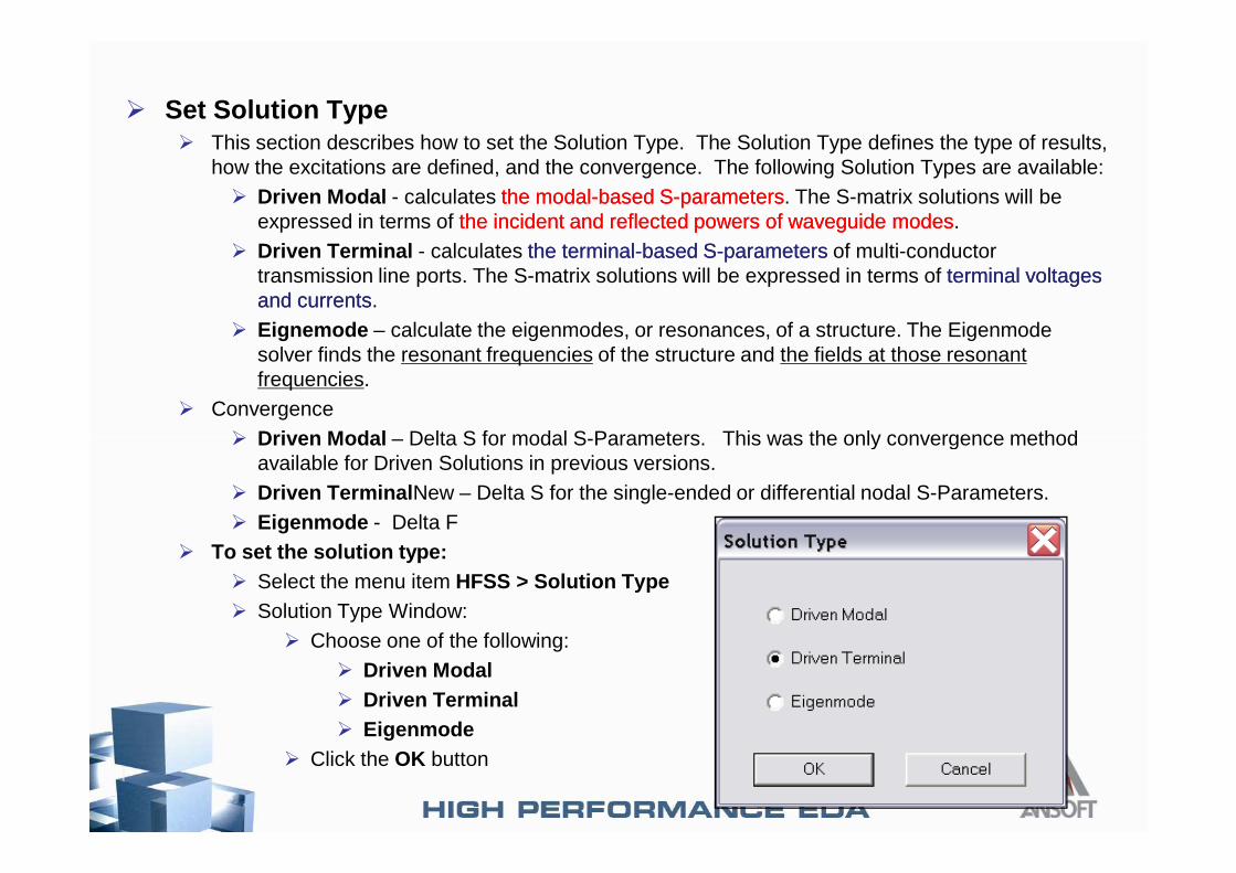
� Set Solution Type� This section describes how to set the Solution Type. The Solution Type defines the type of results,
how the excitations are defined, and the convergence. The following Solution Types are available:� Driven Modal - calculates the modalthe modal--based Sbased S--parametersparameters. The S-matrix solutions will be
expressed in terms of the incident and reflected powers of waveguide modesthe incident and reflected powers of waveguide modes.� Driven Terminal - calculates the terminalthe terminal--based Sbased S--parameters parameters of multi-conductor
transmission line ports. The S-matrix solutions will be expressed in terms of terminal voltages terminal voltages and currentsand currents.
� Eignemode – calculate the eigenmodes, or resonances, of a structure. The Eigenmodesolver finds the resonant frequencies of the structure and the fields at those resonant frequencies.
� Convergence� Driven Modal – Delta S for modal S-Parameters. This was the only convergence method � Driven Modal – Delta S for modal S-Parameters. This was the only convergence method
available for Driven Solutions in previous versions.� Driven Terminal New – Delta S for the single-ended or differential nodal S-Parameters. � Eigenmode - Delta F
� To set the solution type:� Select the menu item HFSS > Solution Type� Solution Type Window:
� Choose one of the following:� Driven Modal� Driven Terminal� Eigenmode
� Click the OK button
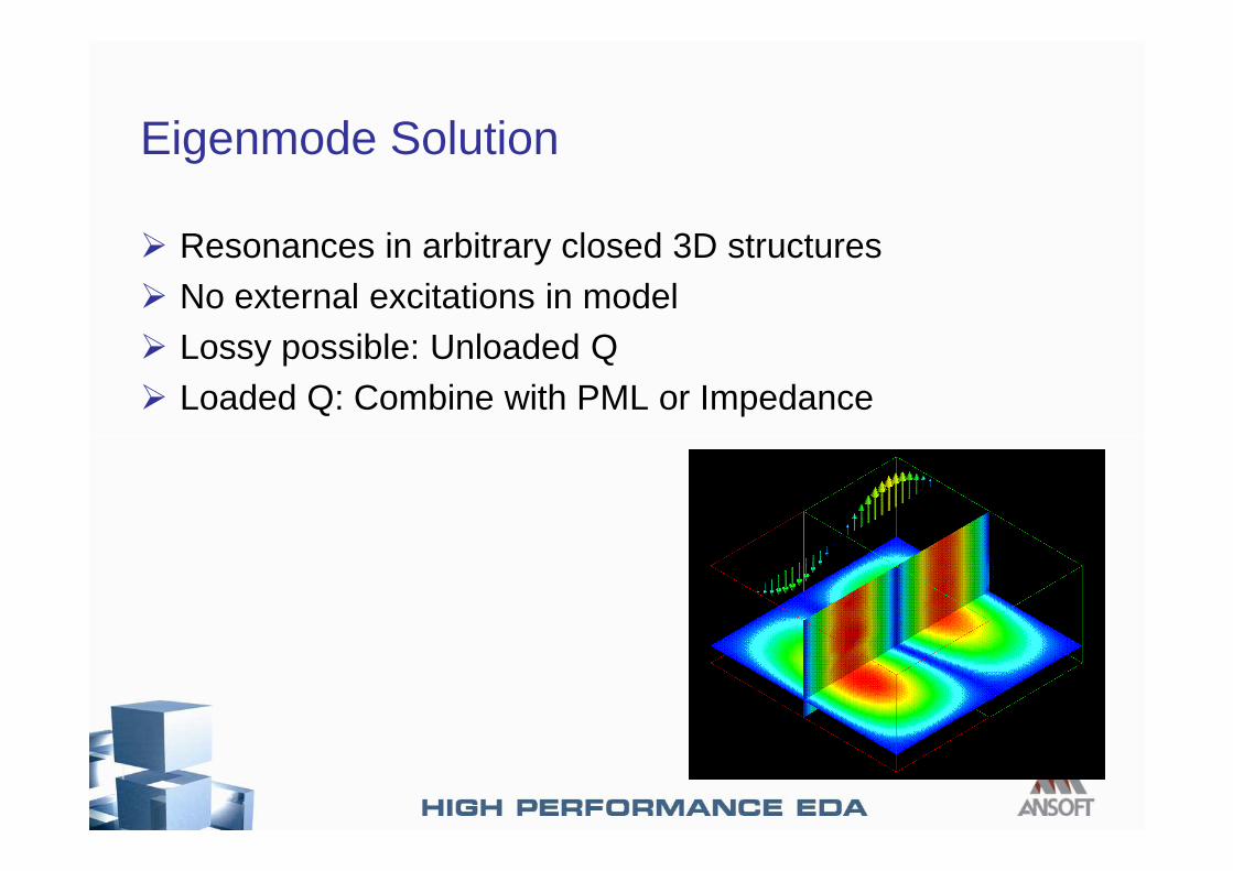
Eigenmode Solution
� Resonances in arbitrary closed 3D structures� No external excitations in model� Lossy possible: Unloaded Q� Loaded Q: Combine with PML or Impedance
电FSS 电FSS 电FSS 电FSS
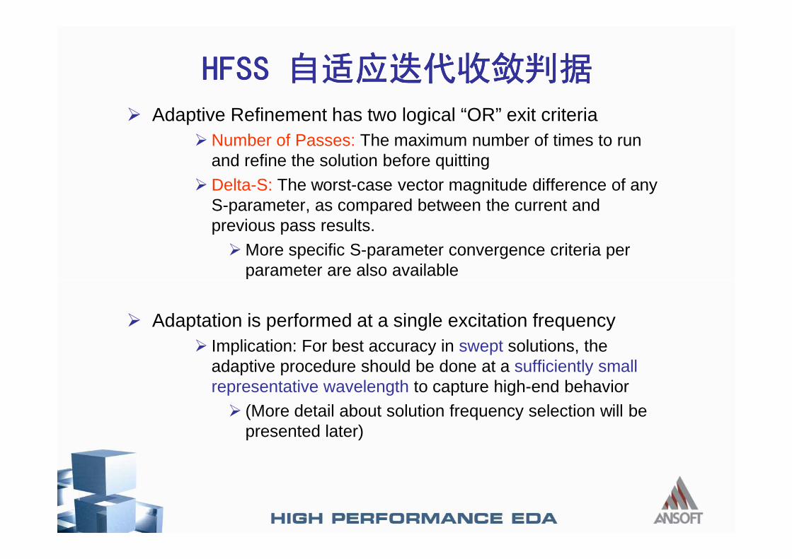
� Adaptive Refinement has two logical “OR” exit criteria� Number of Passes: The maximum number of times to run
and refine the solution before quitting� Delta-S: The worst-case vector magnitude difference of any
S-parameter, as compared between the current and previous pass results.� More specific S-parameter convergence criteria per
parameter are also available
� Adaptation is performed at a single excitation frequency� Implication: For best accuracy in swept solutions, the
adaptive procedure should be done at a sufficiently small representative wavelength to capture high-end behavior� (More detail about solution frequency selection will be
presented later)
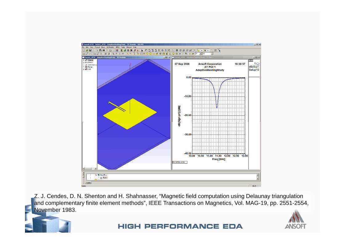
Z. J. Cendes, D. N. Shenton and H. Shahnasser, “Magnetic field computation using Delaunay triangulation and complementary finite element methods”, IEEE Transactions on Magnetics, Vol. MAG-19, pp. 2551-2554, November 1983.
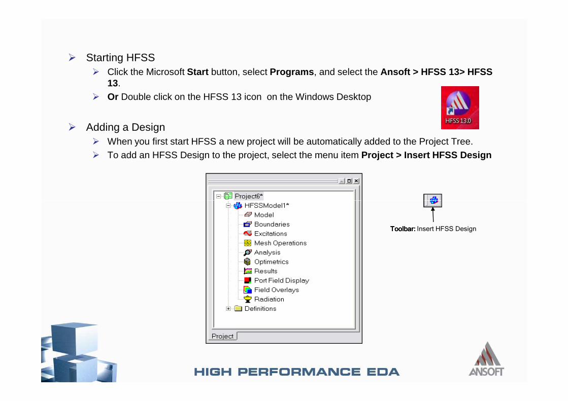
� Starting HFSS� Click the Microsoft Start button, select Programs , and select the Ansoft > HFSS 13> HFSS
13.� Or Double click on the HFSS 13 icon on the Windows Desktop
� Adding a Design� When you first start HFSS a new project will be automatically added to the Project Tree.� To add an HFSS Design to the project, select the menu item Project > Insert HFSS Design
Toolbar:Toolbar:Toolbar:Toolbar: Insert HFSS Design
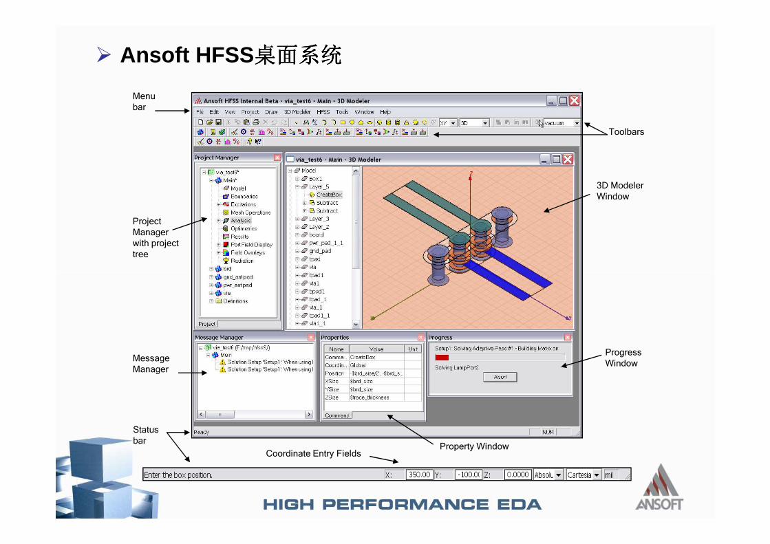
� Ansoft HFSS
Menu
bar
Project
Manager
with project
tree
3D Modeler
Window
Toolbars
Progress
Window
Property Window
Message
Manager
Status
bar
Coordinate Entry Fields
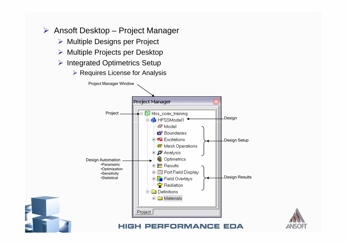
� Ansoft Desktop – Project Manager� Multiple Designs per Project� Multiple Projects per Desktop� Integrated Optimetrics Setup
� Requires License for Analysis
Project
Design
Project Manager Window
Design Results
Design Setup
Design Automation•Parametric
•Optimization
•Sensitivity
•Statistical
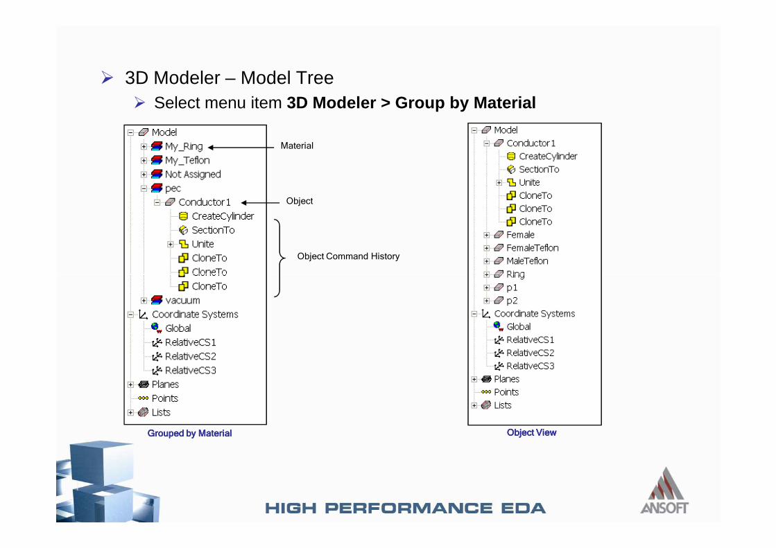
� 3D Modeler – Model Tree� Select menu item 3D Modeler > Group by Material
Material
Object
Object Command History
Grouped by MaterialGrouped by MaterialGrouped by MaterialGrouped by Material Object ViewObject ViewObject ViewObject View
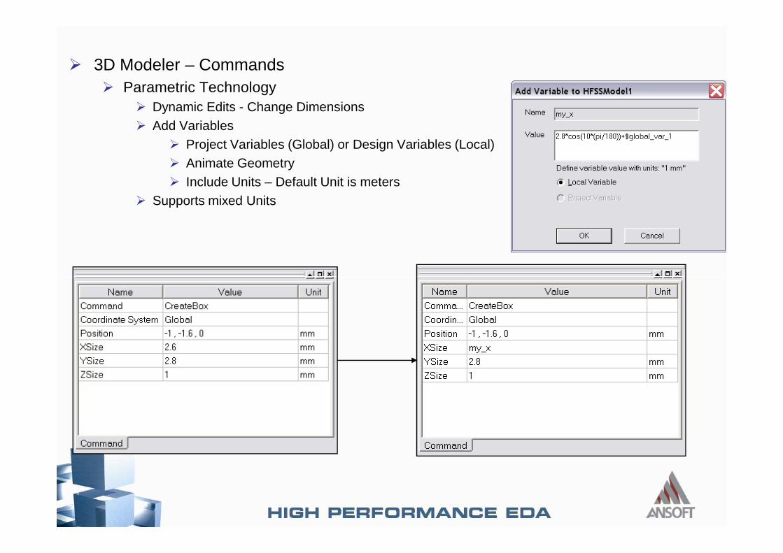
� 3D Modeler – Commands� Parametric Technology
� Dynamic Edits - Change Dimensions� Add Variables
� Project Variables (Global) or Design Variables (Local)� Animate Geometry� Include Units – Default Unit is meters
� Supports mixed Units
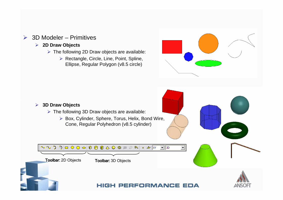
� 3D Modeler – Primitives� 2D Draw Objects
� The following 2D Draw objects are available:� Rectangle, Circle, Line, Point, Spline,
Ellipse, Regular Polygon (v8.5 circle)
� 3D Draw Objects� The following 3D Draw objects are available:
� Box, Cylinder, Sphere, Torus, Helix, Bond Wire, Cone, Regular Polyhedron (v8.5 cylinder)
Toolbar:Toolbar:Toolbar:Toolbar: 2D Objects Toolbar:Toolbar:Toolbar:Toolbar: 3D Objects
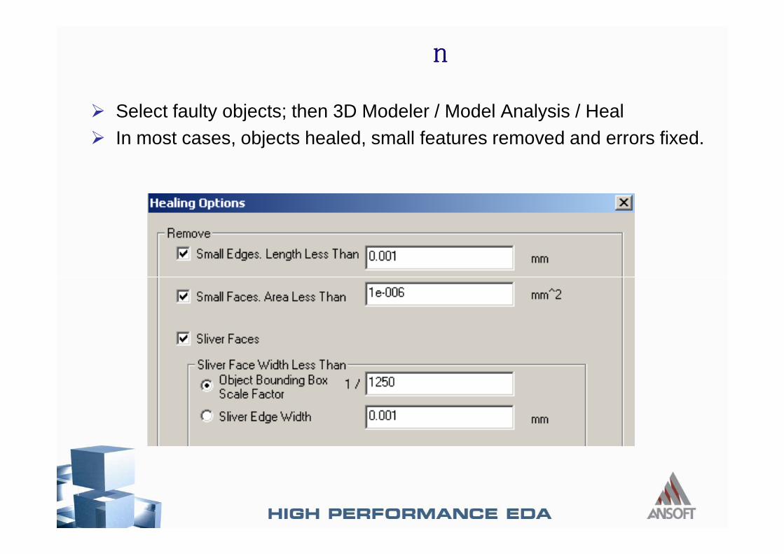
� Select faulty objects; then 3D Modeler / Model Analysis / Heal� In most cases, objects healed, small features removed and errors fixed.
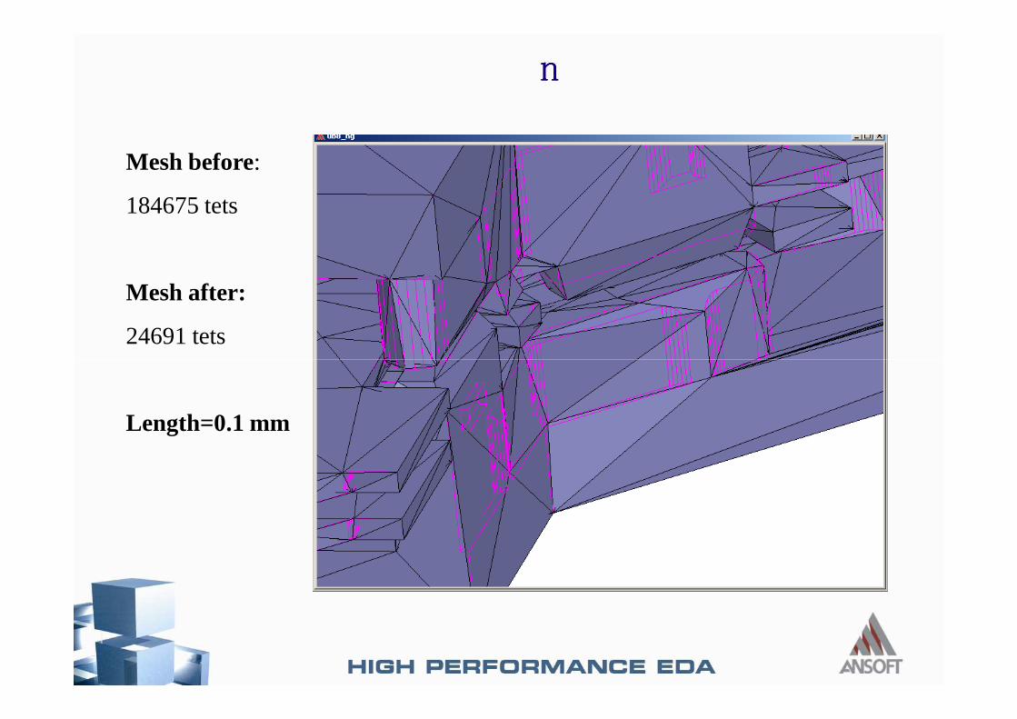
Mesh before:
184675 tets
Mesh after:
24691 tets
Length=0.1 mm
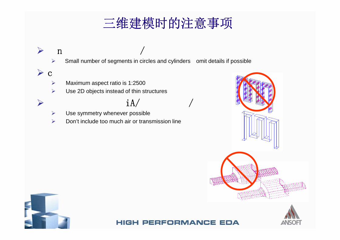
�� Small number of segments in circles and cylinders omit details if possible
�� Maximum aspect ratio is 1:2500� Use 2D objects instead of thin structures
�� Use symmetry whenever possible� Don’t include too much air or transmission line� Don’t include too much air or transmission line
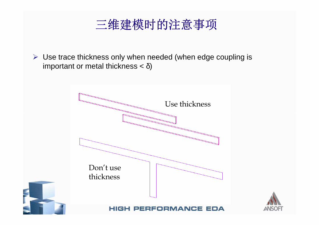
� Use trace thickness only when needed (when edge coupling is important or metal thickness < δ)
Use thickness
Don’t use thickness
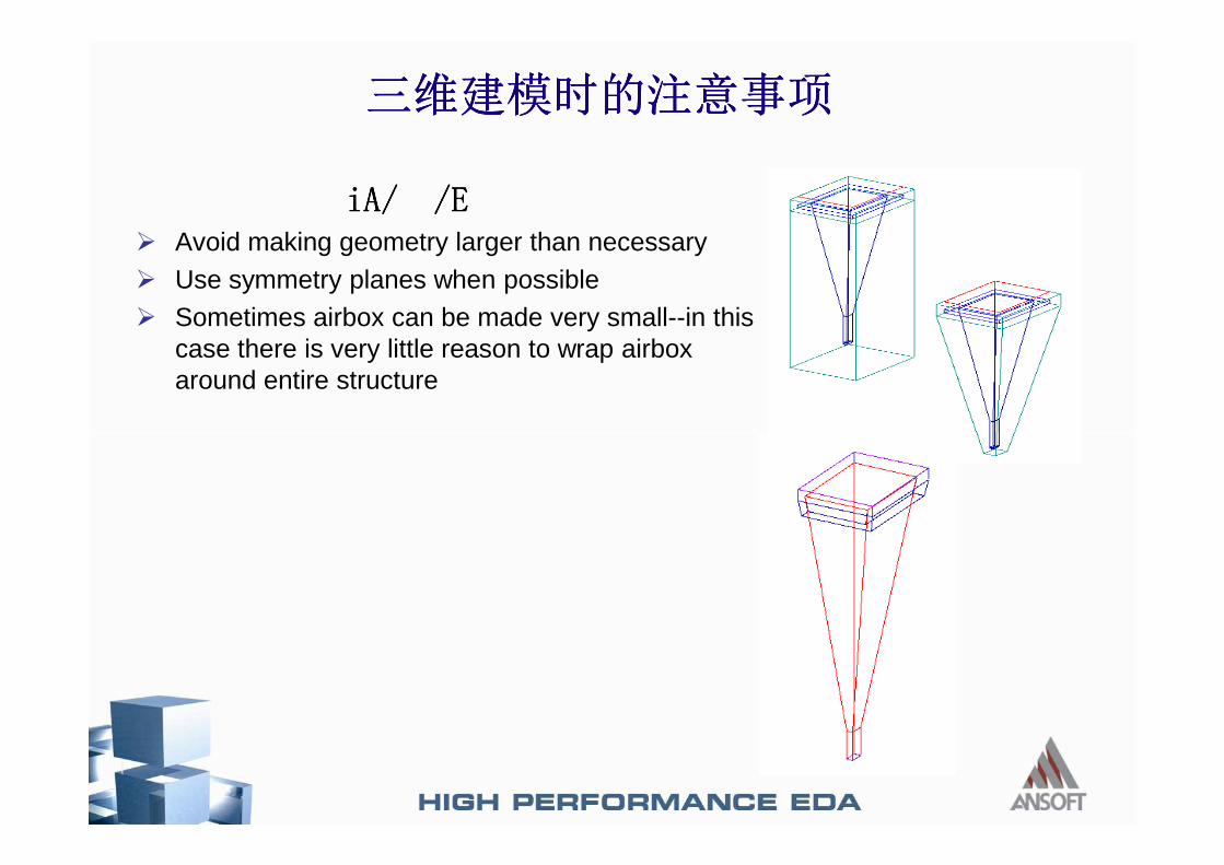
� Avoid making geometry larger than necessary� Use symmetry planes when possible� Sometimes airbox can be made very small--in this
case there is very little reason to wrap airboxaround entire structure
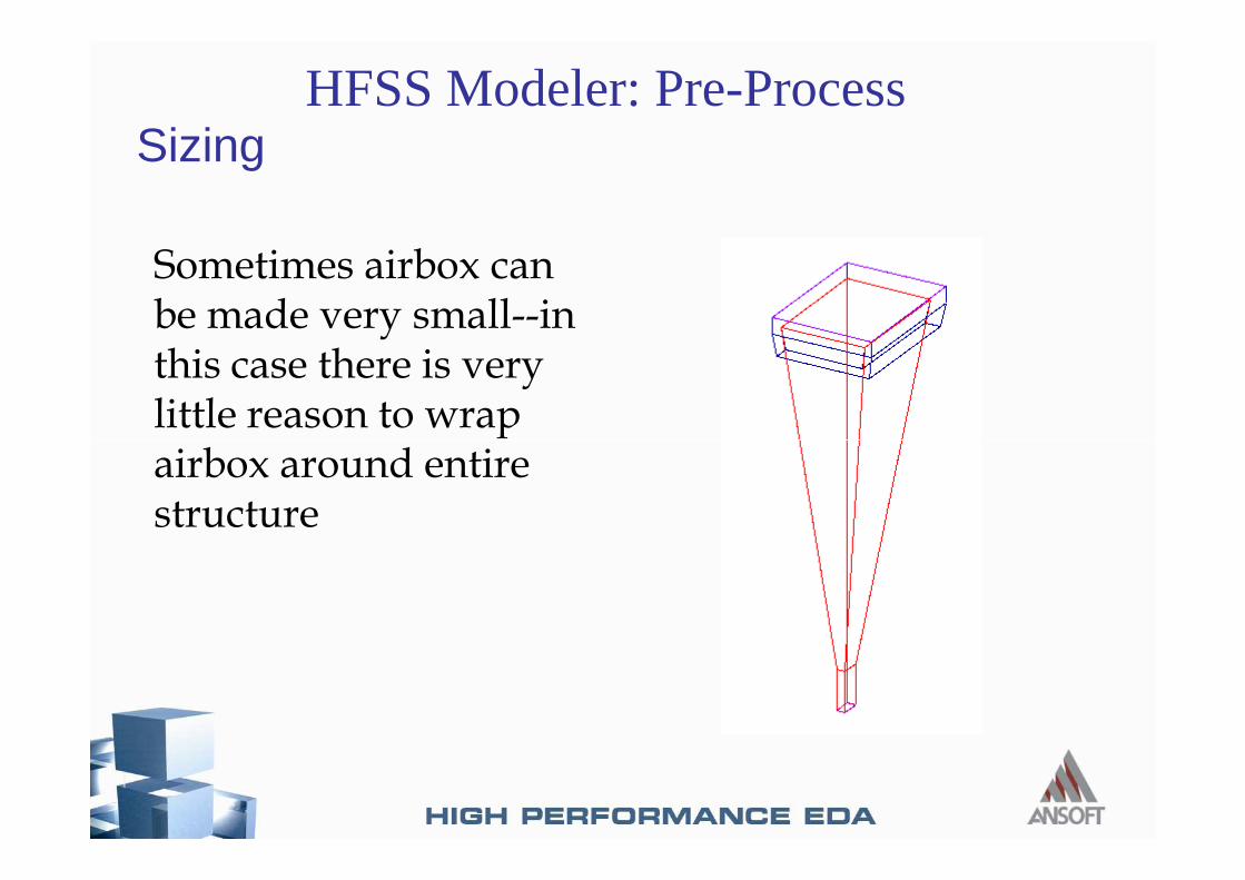
Sizing
Sometimes airbox can be made very small--in this case there is very little reason to wrap airbox around entire
HFSS Modeler: Pre-Process
airbox around entire structure
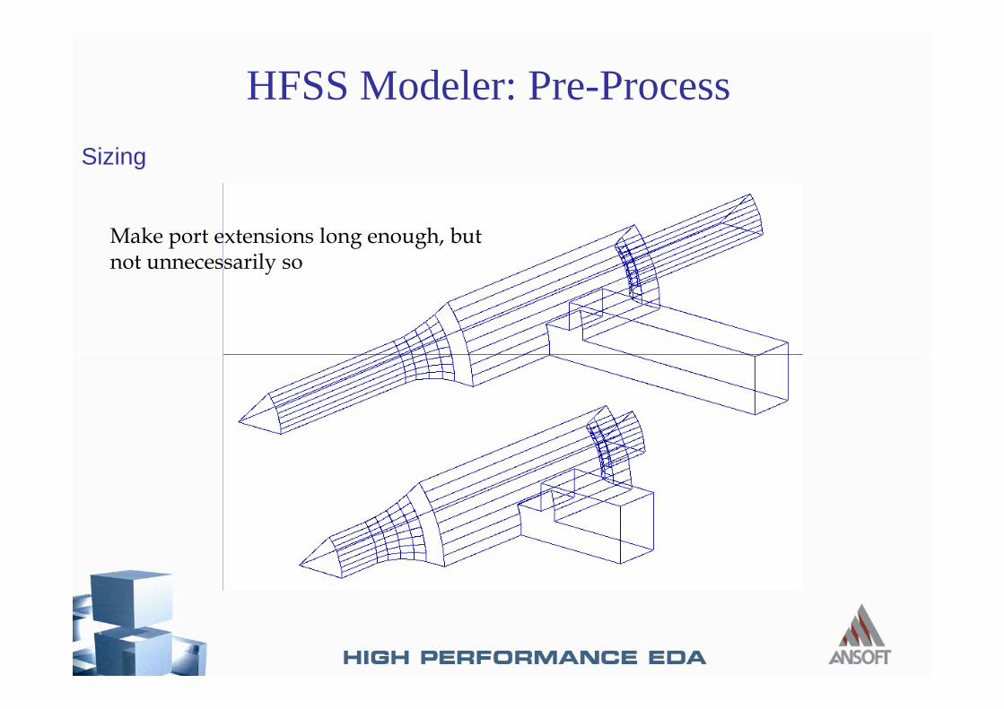
Sizing
Make port extensions long enough, but not unnecessarily so
HFSS Modeler: Pre-Process
Virtual Objects
� Virtual Objects Are Dummy 2D or 3D Objects that do not change the physics of the model (e.g. an air object inside another air object).
HFSS Modeler: Pre-Process
� They Are Used to Assist in Getting a Higher-Quality Mesh
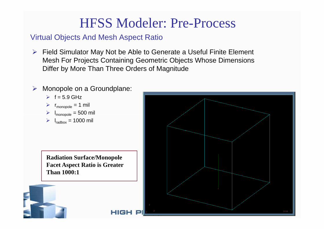
Virtual Objects And Mesh Aspect Ratio
� Field Simulator May Not be Able to Generate a Useful Finite Element Mesh For Projects Containing Geometric Objects Whose Dimensions Differ by More Than Three Orders of Magnitude
� Monopole on a Groundplane:� f = 5.9 GHz� rmonopole = 1 mil� lmonopole = 500 mil
HFSS Modeler: Pre-Process
� lmonopole = 500 mil� lradbox = 1000 mil
Radiation Surface/MonopoleFacet Aspect Ratio is GreaterThan 1000:1
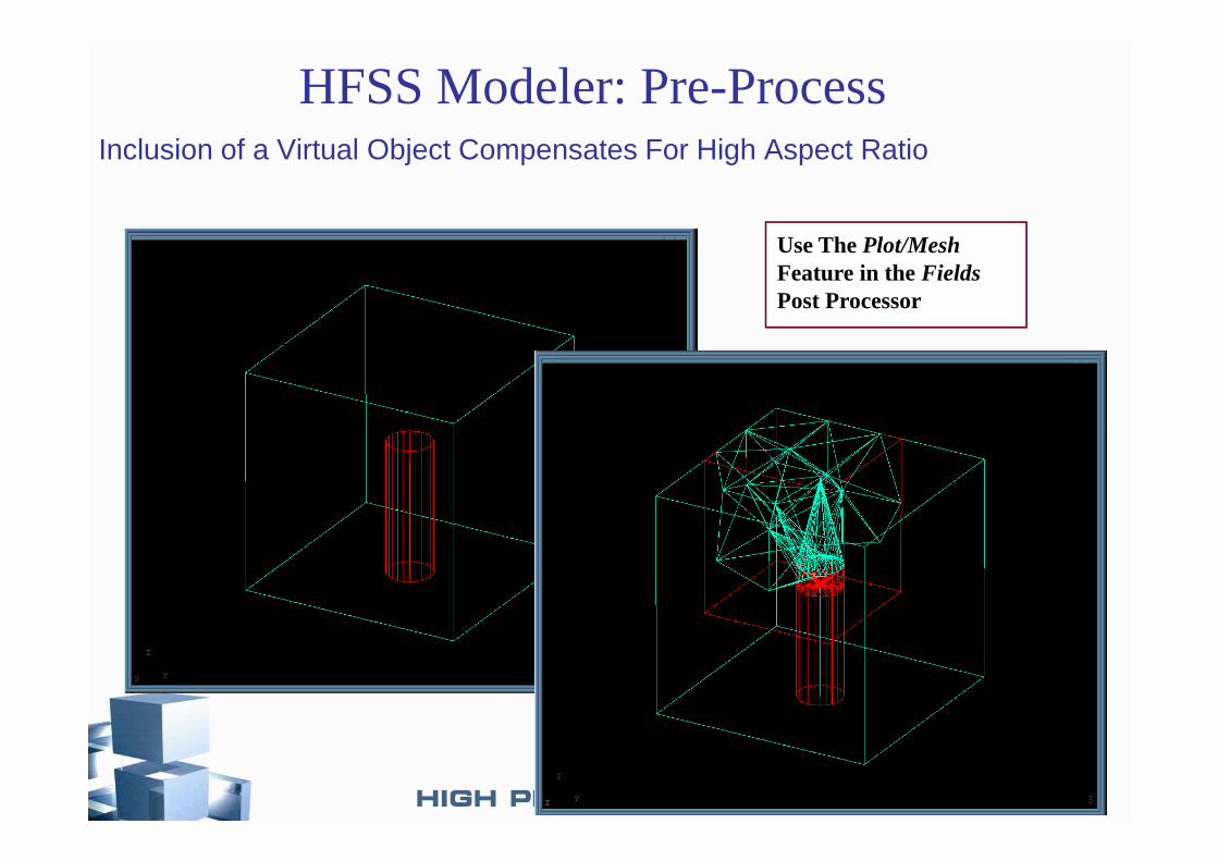
Inclusion of a Virtual Object Compensates For High Aspect Ratio
Use The Plot/MeshFeature in theFieldsPost Processor
HFSS Modeler: Pre-Process
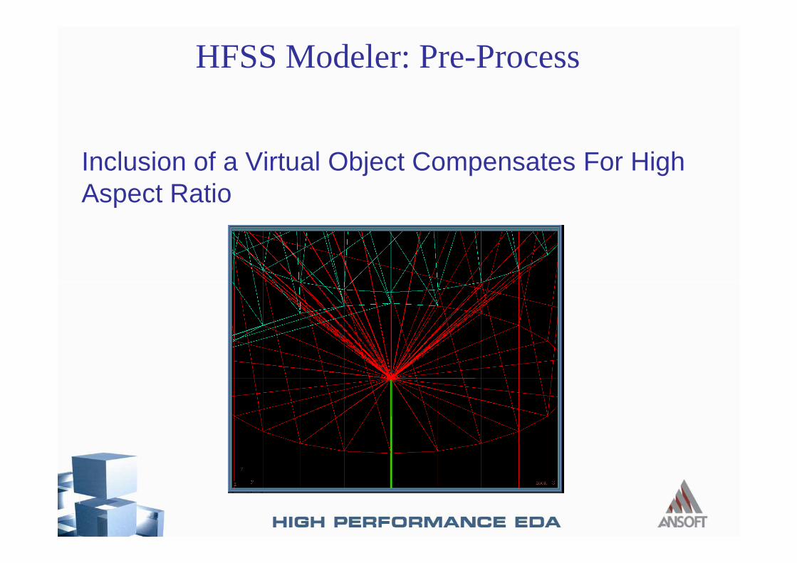
Inclusion of a Virtual Object Compensates For High Aspect Ratio
HFSS Modeler: Pre-Process
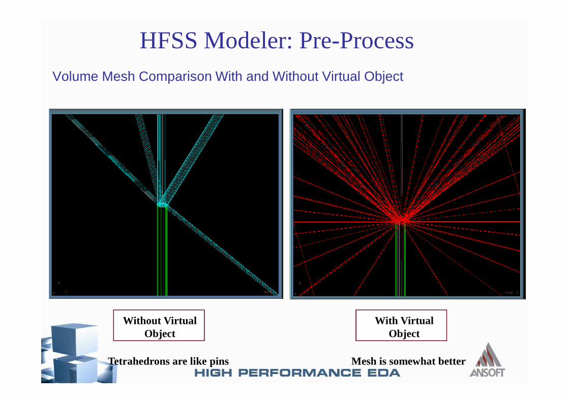
Volume Mesh Comparison With and Without Virtual Object
HFSS Modeler: Pre-Process
Without VirtualObject
With VirtualObject
Mesh is somewhat betterTetrahedrons are like pins
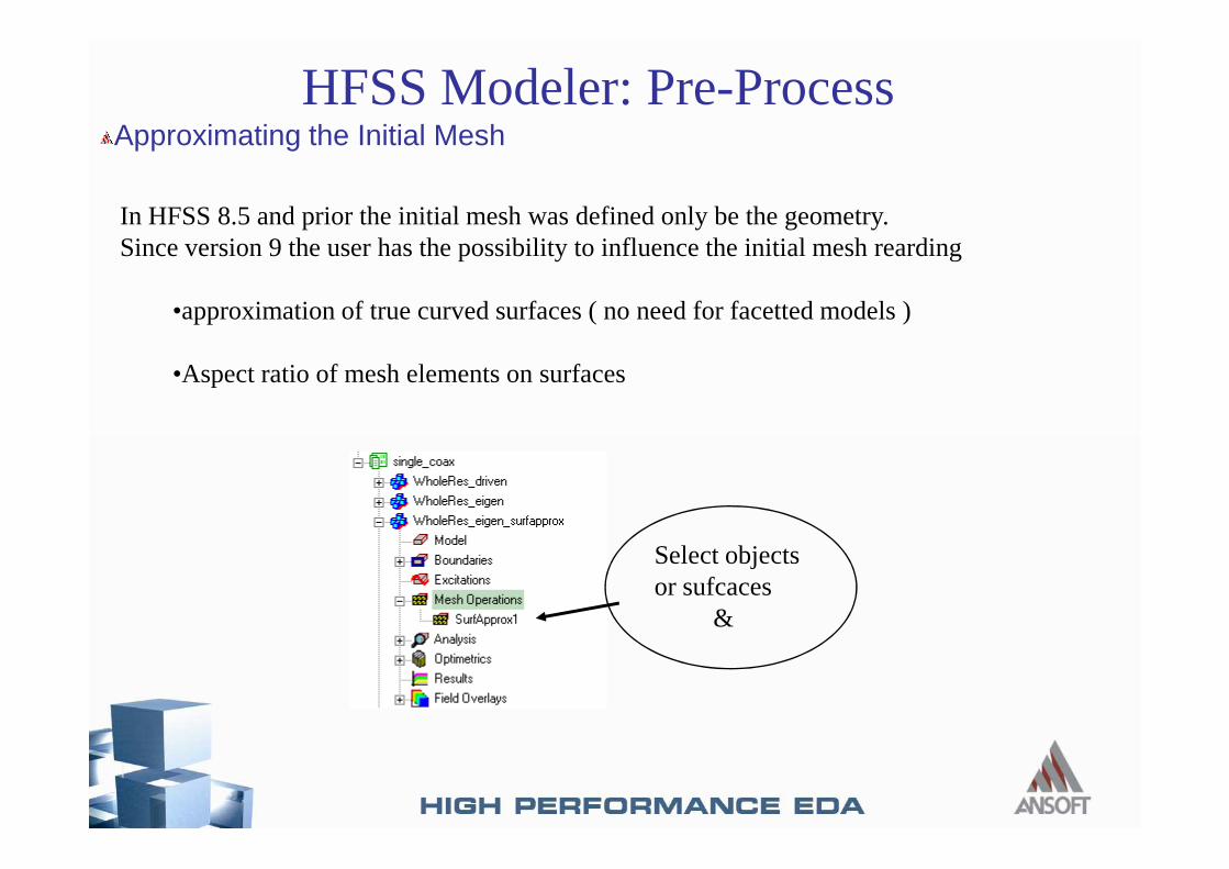
Approximating the Initial Mesh
In HFSS 8.5 and prior the initial mesh was defined only be the geometry.Since version 9 the user has the possibility to influence the initial mesh rearding
•approximation of true curved surfaces ( no need for facetted models )
•Aspect ratio of mesh elements on surfaces
HFSS Modeler: Pre-Process
Select objects or sufcaces
&
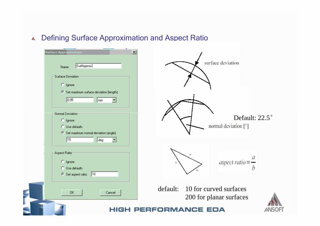
Defining Surface Approximation and Aspect Ratio
default: 10 for curved surfaces200 for planar surfaces
Default: 22.5°
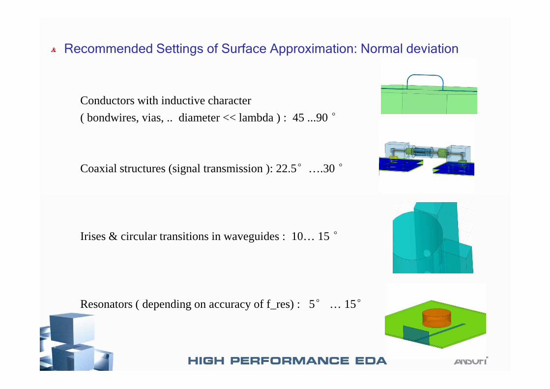
Recommended Settings of Surface Approximation: Normal deviation
Conductors with inductive character
( bondwires, vias, .. diameter << lambda ) : 45 ...90 °
Coaxial structures (signal transmission ): 22.5°….30 °
Irises & circular transitions in waveguides : 10… 15 °
Resonators ( depending on accuracy of f_res) : 5° … 15°
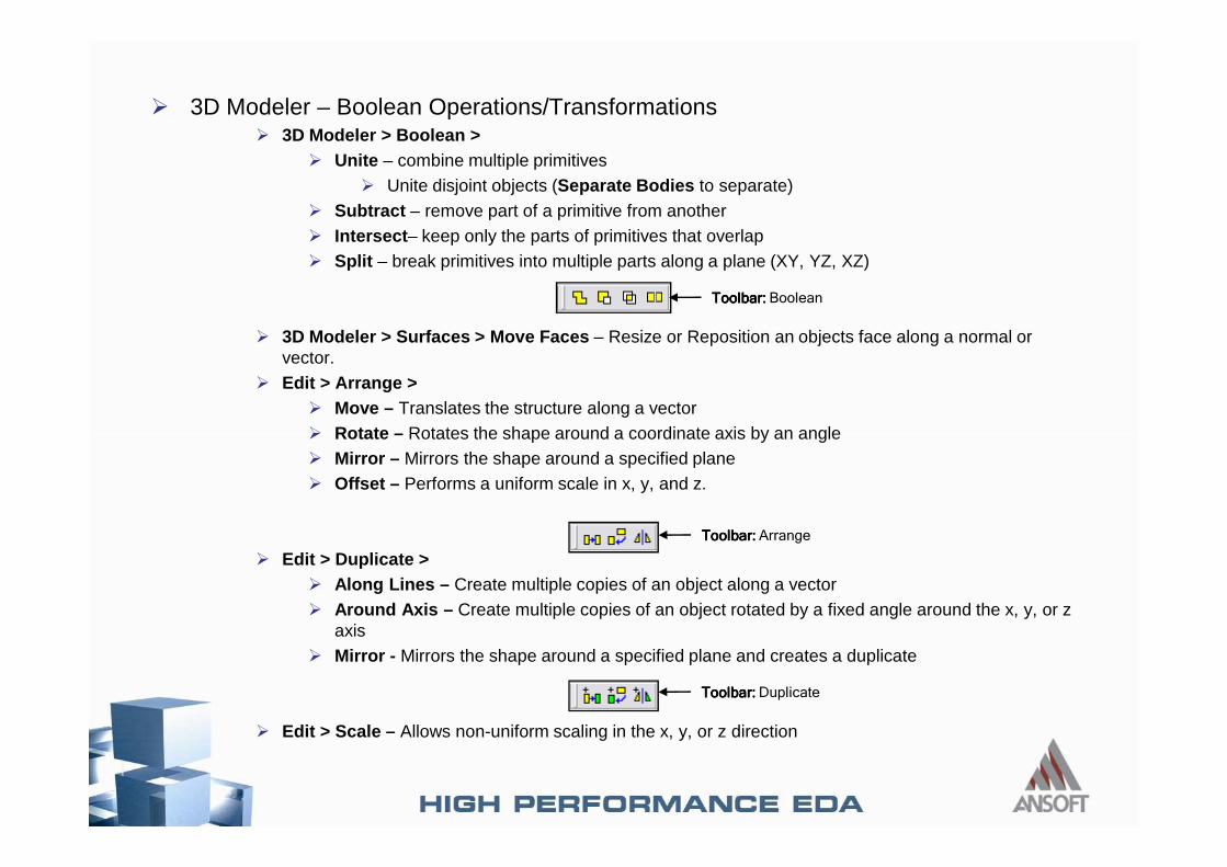
� 3D Modeler – Boolean Operations/Transformations� 3D Modeler > Boolean >
� Unite – combine multiple primitives� Unite disjoint objects (Separate Bodies to separate)
� Subtract – remove part of a primitive from another� Intersect – keep only the parts of primitives that overlap� Split – break primitives into multiple parts along a plane (XY, YZ, XZ)
� 3D Modeler > Surfaces > Move Faces – Resize or Reposition an objects face along a normal or vector.
� Edit > Arrange >� Move – Translates the structure along a vector� Rotate – Rotates the shape around a coordinate axis by an angle
Toolbar:Toolbar:Toolbar:Toolbar: Boolean
� Rotate – Rotates the shape around a coordinate axis by an angle� Mirror – Mirrors the shape around a specified plane� Offset – Performs a uniform scale in x, y, and z.
� Edit > Duplicate >� Along Lines – Create multiple copies of an object along a vector� Around Axis – Create multiple copies of an object rotated by a fixed angle around the x, y, or z
axis� Mirror - Mirrors the shape around a specified plane and creates a duplicate
� Edit > Scale – Allows non-uniform scaling in the x, y, or z direction
Toolbar:Toolbar:Toolbar:Toolbar: Arrange
Toolbar:Toolbar:Toolbar:Toolbar: Duplicate
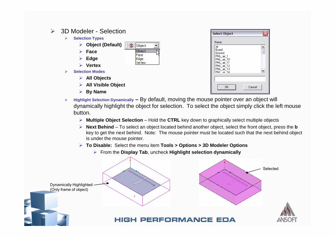
� 3D Modeler - Selection� Selection Types
� Object (Default)� Face� Edge� Vertex
� Selection Modes
� All Objects� All Visible Object� By Name
� Highlight Selection Dynamically – By default, moving the mouse pointer over an object will dynamically highlight the object for selection. To select the object simply click the left mouse button.
� Multiple Object Selection – Hold the CTRL key down to graphically select multiple objects� Multiple Object Selection – Hold the CTRL key down to graphically select multiple objects� Next Behind – To select an object located behind another object, select the front object, press the b
key to get the next behind. Note: The mouse pointer must be located such that the next behind object is under the mouse pointer.
� To Disable: Select the menu item Tools > Options > 3D Modeler Options� From the Display Tab , uncheck Highlight selection dynamically
Dynamically Highlighted
(Only frame of object)
Selected
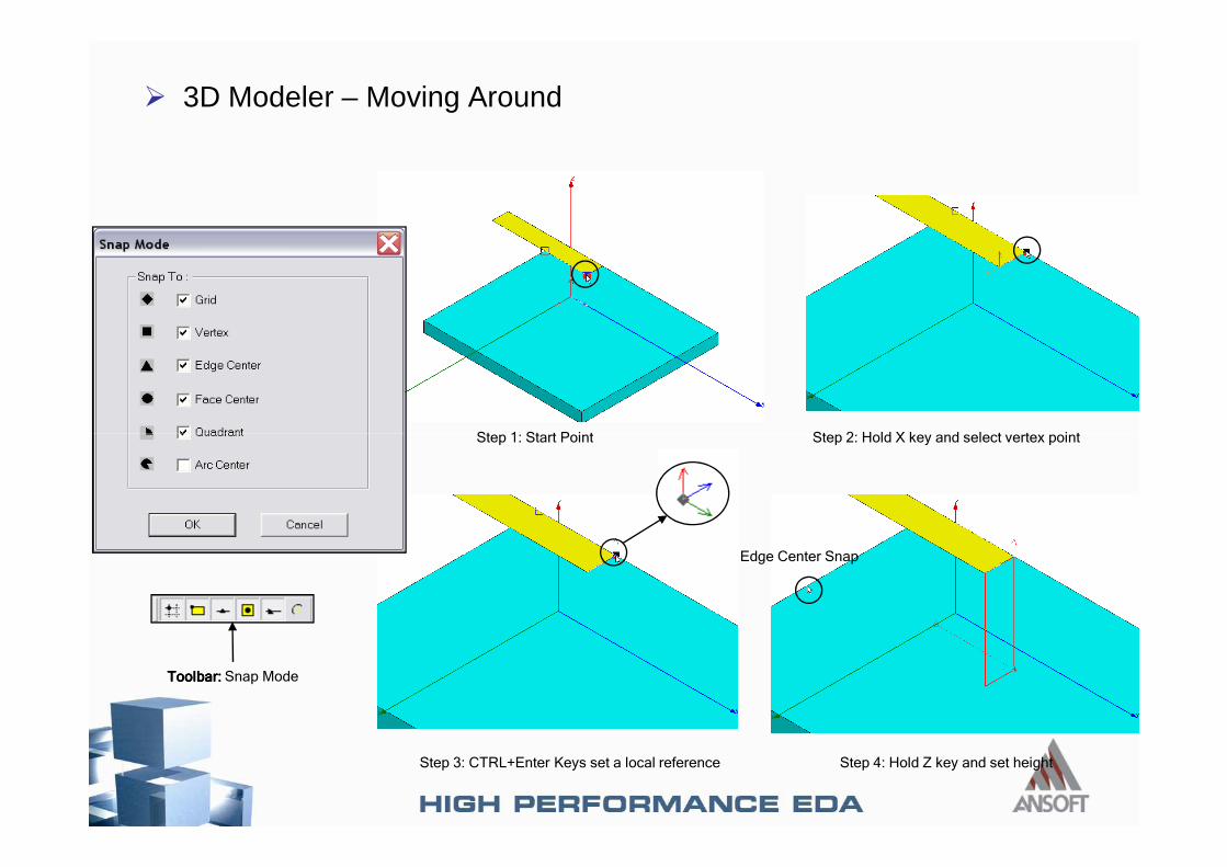
� 3D Modeler – Moving Around
Step 1: Start Point Step 2: Hold X key and select vertex pointStep 1: Start Point Step 2: Hold X key and select vertex point
Step 3: CTRL+Enter Keys set a local reference Step 4: Hold Z key and set height
Edge Center Snap
Toolbar:Toolbar:Toolbar:Toolbar: Snap Mode
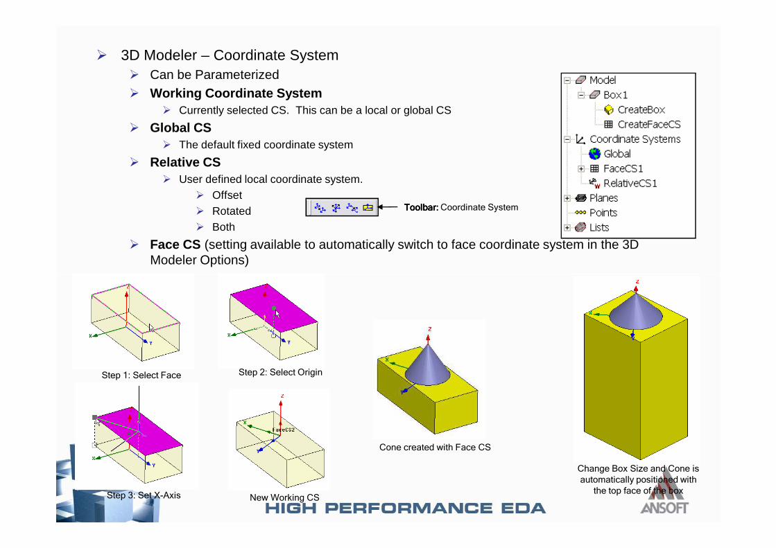
� 3D Modeler – Coordinate System� Can be Parameterized� Working Coordinate System
� Currently selected CS. This can be a local or global CS
� Global CS� The default fixed coordinate system
� Relative CS� User defined local coordinate system.
� Offset� Rotated� Both
� Face CS (setting available to automatically switch to face coordinate system in the 3D Modeler Options)
Toolbar:Toolbar:Toolbar:Toolbar: Coordinate System
Step 1: Select Face Step 2: Select Origin
Step 3: Set X-Axis New Working CS
Cone created with Face CS
Change Box Size and Cone is
automatically positioned with
the top face of the box
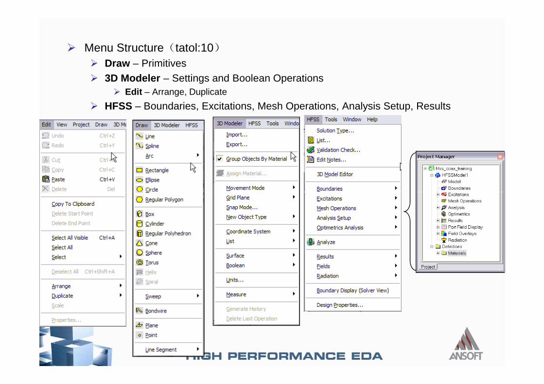
� Menu Structure tatol:10� Draw – Primitives� 3D Modeler – Settings and Boolean Operations
� Edit – Arrange, Duplicate
� HFSS – Boundaries, Excitations, Mesh Operations, Analysis Setup, Results
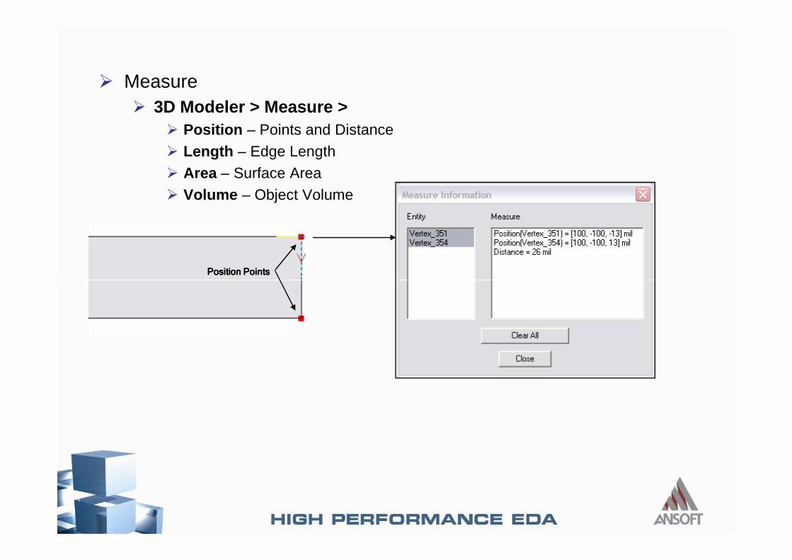
� Measure � 3D Modeler > Measure >
� Position – Points and Distance� Length – Edge Length� Area – Surface Area� Volume – Object Volume
Position PointsPosition PointsPosition PointsPosition Points
� Support in China, P.R� Support E-mail: [email protected]
� Ansoft Beijing Office
� Tel:(010)82861715/16
� Fax:(010)82861613
� Ding Haiqaing, [email protected]
� Liu Ying, [email protected]
� Ansoft Shanghai Office
� Tel:(021)62886350/51
� Fax:(021)62181142
� Ansoft Chengdu Office
� Tel:(028)86200675
� Fax:(028)86200677
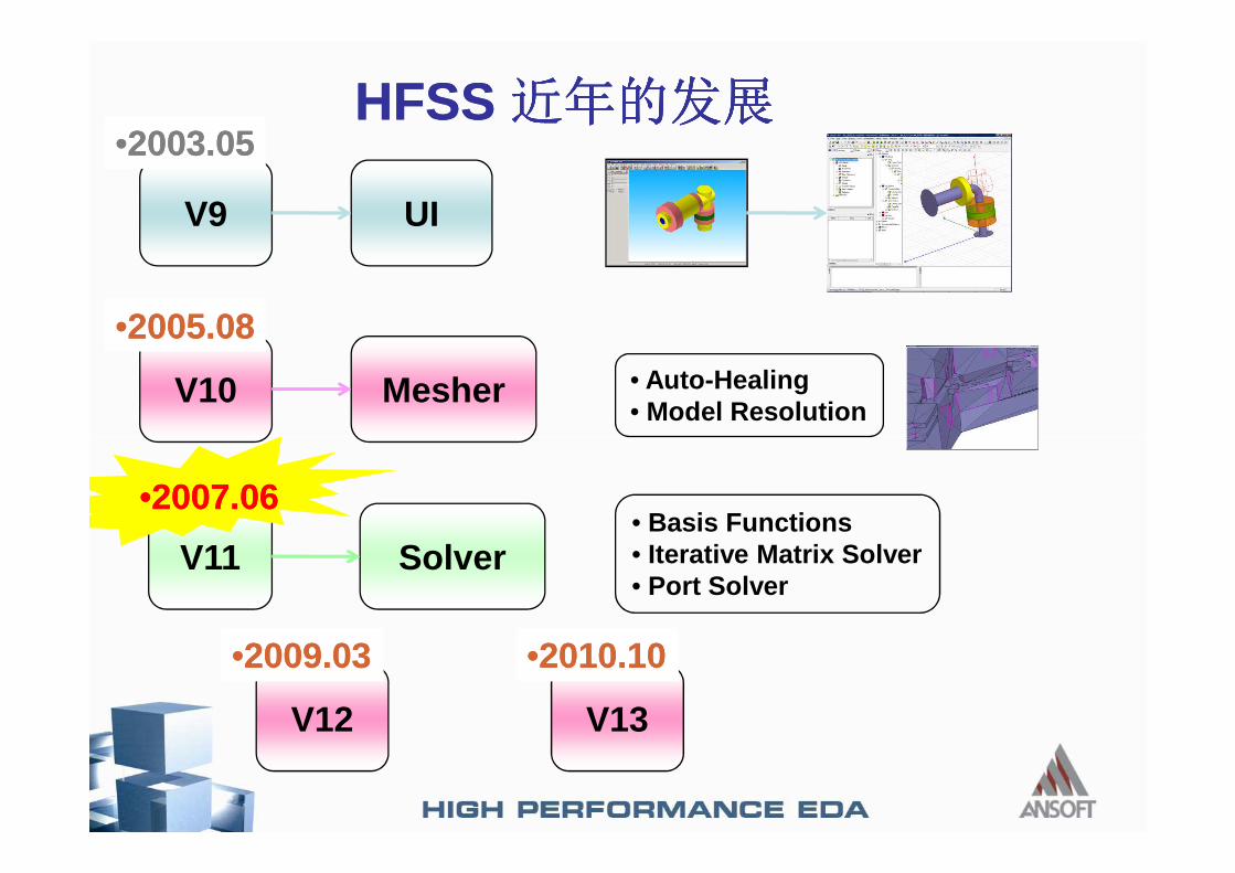
HFSSHFSS
UI
Mesher
V9
V10 • Auto-Healing• Model Resolution
••2003.052003.05
••2005.082005.08
SolverV11• Basis Functions• Iterative Matrix Solver• Port Solver
••2007.062007.06
V12
••2009.032009.03
V13
••2010.102010.10
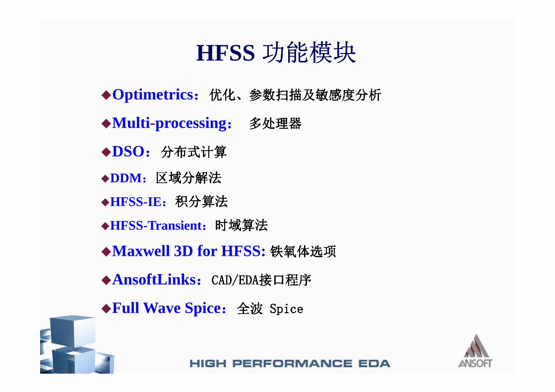
�Optimetrics
�Multi-processing
�DSO
�DDM
HFSS-IE
HFSS
�HFSS-IE
�HFSS-Transient
�Maxwell 3D for HFSS:
�AnsoftLinks 点点点点点点点点A然展A然展A然展A然展A然展A然展A然展A然展特然A特然A特然A特然A特然A特然A特然A特然A
�Full Wave Spice Sp限避釐 Sp限避釐 Sp限避釐 Sp限避釐 Sp限避釐 Sp限避釐 Sp限避釐 Sp限避釐
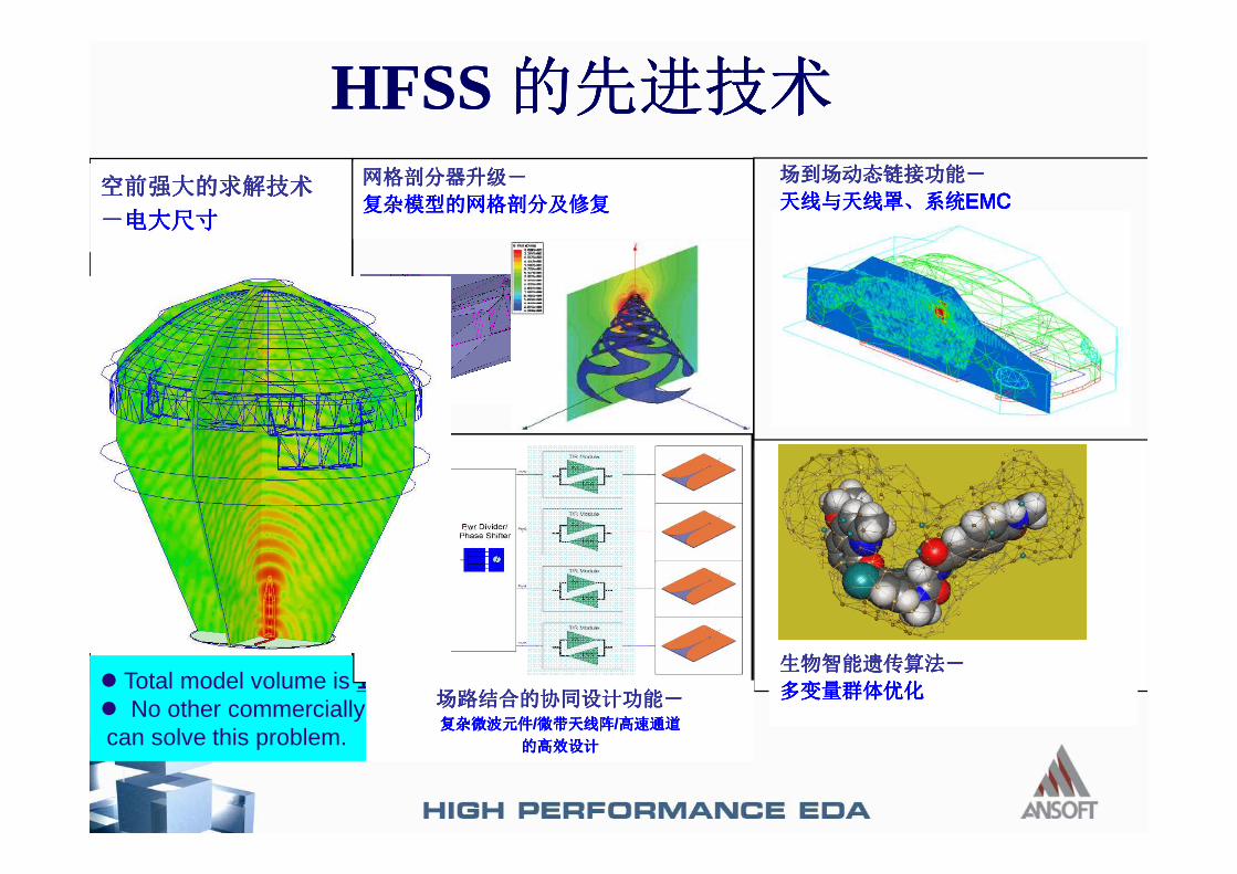
HFSSHFSS
EMCEMCEMCEMCEMCEMCEMCEMC
� Total model volume is 18000 λ3!� No other commercially available softwarecan solve this problem.
// //
专注于微波、射频、天线设计人才的培养 易迪拓培训 网址:http://www.edatop.com
射 频 和 天 线 设 计 培 训 课 程 推 荐
易迪拓培训(www.edatop.com)由数名来自于研发第一线的资深工程师发起成立,致力并专注于微
波、射频、天线设计研发人才的培养;我们于 2006 年整合合并微波 EDA 网(www.mweda.com),现
已发展成为国内最大的微波射频和天线设计人才培养基地,成功推出多套微波射频以及天线设计经典
培训课程和 ADS、HFSS 等专业软件使用培训课程,广受客户好评;并先后与人民邮电出版社、电子
工业出版社合作出版了多本专业图书,帮助数万名工程师提升了专业技术能力。客户遍布中兴通讯、
研通高频、埃威航电、国人通信等多家国内知名公司,以及台湾工业技术研究院、永业科技、全一电
子等多家台湾地区企业。
易迪拓培训课程列表:http://www.edatop.com/peixun/rfe/129.html
射频工程师养成培训课程套装
该套装精选了射频专业基础培训课程、射频仿真设计培训课程和射频电
路测量培训课程三个类别共 30 门视频培训课程和 3 本图书教材;旨在
引领学员全面学习一个射频工程师需要熟悉、理解和掌握的专业知识和
研发设计能力。通过套装的学习,能够让学员完全达到和胜任一个合格
的射频工程师的要求…
课程网址:http://www.edatop.com/peixun/rfe/110.html
ADS 学习培训课程套装
该套装是迄今国内最全面、最权威的 ADS 培训教程,共包含 10 门 ADS
学习培训课程。课程是由具有多年 ADS 使用经验的微波射频与通信系
统设计领域资深专家讲解,并多结合设计实例,由浅入深、详细而又
全面地讲解了 ADS 在微波射频电路设计、通信系统设计和电磁仿真设
计方面的内容。能让您在最短的时间内学会使用 ADS,迅速提升个人技
术能力,把 ADS 真正应用到实际研发工作中去,成为 ADS 设计专家...
课程网址: http://www.edatop.com/peixun/ads/13.html
HFSS 学习培训课程套装
该套课程套装包含了本站全部 HFSS 培训课程,是迄今国内最全面、最
专业的HFSS培训教程套装,可以帮助您从零开始,全面深入学习HFSS
的各项功能和在多个方面的工程应用。购买套装,更可超值赠送 3 个月
免费学习答疑,随时解答您学习过程中遇到的棘手问题,让您的 HFSS
学习更加轻松顺畅…
课程网址:http://www.edatop.com/peixun/hfss/11.html
`

专注于微波、射频、天线设计人才的培养 易迪拓培训 网址:http://www.edatop.com
CST 学习培训课程套装
该培训套装由易迪拓培训联合微波 EDA 网共同推出,是最全面、系统、
专业的 CST 微波工作室培训课程套装,所有课程都由经验丰富的专家授
课,视频教学,可以帮助您从零开始,全面系统地学习 CST 微波工作的
各项功能及其在微波射频、天线设计等领域的设计应用。且购买该套装,
还可超值赠送 3 个月免费学习答疑…
课程网址:http://www.edatop.com/peixun/cst/24.html
HFSS 天线设计培训课程套装
套装包含 6 门视频课程和 1 本图书,课程从基础讲起,内容由浅入深,
理论介绍和实际操作讲解相结合,全面系统的讲解了 HFSS 天线设计的
全过程。是国内最全面、最专业的 HFSS 天线设计课程,可以帮助您快
速学习掌握如何使用 HFSS 设计天线,让天线设计不再难…
课程网址:http://www.edatop.com/peixun/hfss/122.html
13.56MHz NFC/RFID 线圈天线设计培训课程套装
套装包含 4 门视频培训课程,培训将 13.56MHz 线圈天线设计原理和仿
真设计实践相结合,全面系统地讲解了 13.56MHz线圈天线的工作原理、
设计方法、设计考量以及使用 HFSS 和 CST 仿真分析线圈天线的具体
操作,同时还介绍了 13.56MHz 线圈天线匹配电路的设计和调试。通过
该套课程的学习,可以帮助您快速学习掌握 13.56MHz 线圈天线及其匹
配电路的原理、设计和调试…
详情浏览:http://www.edatop.com/peixun/antenna/116.html
我们的课程优势:
※ 成立于 2004 年,10 多年丰富的行业经验,
※ 一直致力并专注于微波射频和天线设计工程师的培养,更了解该行业对人才的要求
※ 经验丰富的一线资深工程师讲授,结合实际工程案例,直观、实用、易学
联系我们:
※ 易迪拓培训官网:http://www.edatop.com
※ 微波 EDA 网:http://www.mweda.com
※ 官方淘宝店:http://shop36920890.taobao.com
专注于微波、射频、天线设计人才的培养
官方网址:http://www.edatop.com 易迪拓培训 淘宝网店:http://shop36920890.taobao.com