1.2.4 Topologie quotient by week/ANAH3… · 1. Vocabulaire: Topologie 25 2) Action de groupe Soit G un groupe et X un ensemble. Une action (à gauche) de G sur X est une application

1. Vocabulaire: Topologie 23

1.2.4 Topologie quotient

1.2.60 DÉFINITIONSoit X un ensemble. Une relation R sur X est un sous-ensemble de X ⇥ X. Si(x, y) 2 X ⇥ X, on écrit souvent xRy pour signifier (x, y) 2 R. On dit qu’une rela-tion binaire R est une relation d’équivalence si elle vérifie les conditions suivantes :

1. R est réflexive : xRx pour tout x 2 X.2. R est symérique : xRy est équivalent à yRx.3. R est transitive : si xRy et yRz, alors xRz.

Si R est une relation d’équivalence sur X, et si x 2 X, la classe d’équivalence dex est l’ensemble Cx = {y 2 X, yRx}. Un sous-ensemble C de X est une classedéquivalence (pour R), s’il existe x 2 X tel que C = Cx. Si x, y 2 X, alors xRy si etseulement si Cx = Cy, sinon Cx \ Cy = ∆. Les classes d’équivalence forment doncune partition de X.

Réciproquement, soit (Ci)i2I une partition de X,( i.e. X = [i2ICi et i 6= j entrîneCi \ Cj = ∆) alors les Ci sont les classes d’équivalence de la relation d’équivalenceR définie par xRy si et seulement si il existe i 2 I tel que {x, y} ⇢ Ci.

1.2.61 EXEMPLE. Par exemple, sur Rn, on peut définir la relation d’équivalence :

xRy , x � y 2 Zn.

1.2.62 DÉFINITIONSoit X un ensemble et R une relation d’équivalence sur X. On définit le quotientX/R de X par la relation d’équivalence R comme l’ensemble des classes d’équi-valence. L’application p de X dans X/R, qui à x associe sa classe d’équivalence(souvent notée [x] ou x̄), est surjective ; elle est appelée projection canonique (ouapplication quotient).

On note souvent x ⇠ y au lieu de xRy et X/⇠ à la place de X/R.

1.2.63 DÉFINITION (SATURÉ)Soit A une partie de X, l’ensemble des points de X qui sont équivalents à un pointde A est appelé le saturé de A pour la relation d’équivalence.Le saturé de A s’écrit alors p

�1(p(A)) où p est la projection canonique de X surX/ ⇠


1.2.64 DÉFINITION (PASSAGE AU QUOTIENT)Une application f : X ! Y est compatible avec la relation d’équivalence (ou passeau quotient) si elle est constante sur les classes d’équivalence i.e. on a f (x) = f (y)pour tout (x, y) élément de X ⇥ X vérifiant x ⇠ y, on définit alors f̄ : X/⇠! Y parf̄ ([x]) = f (x) , on a f = f̄ � p; on dit que f se factorise à travers X/⇠ ou que f sefactorise à travers p, ce qui signifie que l’équation f = g � p a une solution g = f̄ .

On a le diagramme commutatif : Xf//

p

✏✏

Y

X/⇠f̄

==

Examples d’espaces quotients

Quelques exemples importants d’espace quotients :1) Quotients d’espaces vectorielsSoit E un K-espace vectoriel, soit ⇠ une relation d’équivalence sur E, et soit F ⇢ Ela classe d’équivalence de 0.Pour que la structure d’espace vectoriel de E passe au quotient, on doit en parti-culier avoir lx 2 F si l 2 K et x 2 F (puisque l0 = 0 dans E/⇠) et x + y 2 F six, y 2 F (puisque 0 + 0 = 0 dans E/⇠) ; en d’autres termes, F doit être un sous-espace vectoriel de E. De plus, comme a + 0 = a dans E/R, les classes d’équiva-lence doivent être les espaces affines a + F.Réciproquement, si F est un sous-espace vectoriel de E, la relation ⇠ définie sur Epar x ⇠ y ssi x � y 2 F est une relation d’équivalence. Le quotient E/ ⇠ estnoté E/F. Comme x � y 2 F ) lx � ly 2 F , et que x � y 2 F et x0 � y0 2 F )(x + x0) � (y + y0) 2 F, la structure d’espace vectoriel sur E passe au quotient. Ona alors, pour tous x, y 2 E et l 2 K, [x] + [y] := [x + y] et l[x] := [lx].

1.2.65 DÉFINITIONLa dimension de l’espace quotient de E par F est appelée la codimension de F dansE, ainsi codim K(F) := dimK(E/F).

1.2.66 EXEMPLE. L’espace c0 des suites qui convergent vers 0 est un sous-espace de co-dimension 1 de l’espace c des suites convergentes.

1.2.67 REMARQUESi G ⇢ E est un sous-espace vectoriel supplémentaire de F, les classes d’équiva-lence pour ⇠ sont les sous-espaces affines a + F, avec a 2 G. La restriction del’application quotient à G est un isomorphisme d’espaces vectoriels de G ! E/F.


2) Action de groupeSoit G un groupe et X un ensemble. Une action (à gauche) de G sur X est uneapplication G ⇥ X ! X, (g, x) 7! g.x telle que

8x 2 X, 8g, h 2 G, (gh).x = g(h.x) et e.x = x, où e est l’élément neutre de G.

On peut alors considérer la relation d’équivalence associée dont les classes d’équi-valences sont les orbites de l’action de G : x ⇠ y , 9g 2 G, y = g.x.L’espace quotient est noté X/G.

Par exemple, Tn := Rn/Zn le tore de dimension n est défini comme le quotientde Rn par la relation d’équivalence : x ⇠ y , x � y 2 Zn.3) Quotient par une fonctionSoit f : X ! Y une application entre deux ensembles. On définit la relation d’équi-valence x ⇠ x0 , f (x) = f (x0). Les classes d’équivalence s’appellent les fibres def ; ce sont les sous-ensembles de la forme f �1(y), y 2 Y.

Par construction, f est compatible avec ⇠ et l’application quotient f̄ : X/⇠! Yest injective. Si de plus f est surjective, alors f̄ est bijective.

1.2.68 DÉFINITION (TOPOLOGIE QUOTIENT)

Soit X un espace topologique et ⇠ une relation d’équivalence sur X et p la projec-tion canonique de X sur X/⇠. La topologie quotient sur X/⇠ est celle pour laquelleU est ouvert si et seulement si p

�1(U) est ouvert.C’est équivalent à : F est fermé si et seulement si p

�1(F) fermé. En effet, F estfermé , X/⇠ \F est ouvert , p

�1(X/⇠ \F) est ouvert. Puisque p

�1(X/⇠ \F) =X\p

�1(F), ceci équivaut à : p

�1(F) est fermé.

1.2.69 THÉORÈMEi) La topologie quotient est la topologie la plus fine telle que p est continue.

ii) Soit Y un espace topologique et f : X ! Y une application qui passe auquotient en f̄ . Alors

f est continue () f̄ est continue .

(i.e. l’application de C 0(X/⇠, Y) dans { f 2 C 0(X, Y)| x ⇠ y ) f (x) = f (y)}définie par g 7! g � p, est une application bijective)

iii) Si l’application f est ouverte alors f̄ est aussi ouverte.Si l’application f est fermée alors f̄ est aussi fermée.


Démonstration: i) Soit T une topologie sur le quotient. Alors, p est continue pourT , p

�1(U) est ouvert pour tout U 2 T , tout ouvert de T est un ouvertde la topologie quotient , T est moins fine que la topologie quotient.

ii) Si f̄ , il en est de même pour la composée f = f̄ � p. Réciproquement, pourtout ouvert U de Y on a puisque f̄ � p = f , p

�1( f̄ �1(U)) = ( f � p)�1(U) =f �1(U) qui est ouvert par continuité de f . Donc f̄ �1(U) est ouvert, donc f̄ estcontinue.

iii) Soit U un ouvert de X/⇠ . Alors f̄ (U) = f (p

�1(U)), qui est ouvert, carp

�1(U) est ouvert dans X et f est ouverte. ⌅

1.2.71 EXEMPLE ( LE CERCLE). On considère sur R la relation d’équivalence : x ⇠ y ()x � y 2 Z.Soit f : R ! S1 définie par f (t) = (cos(2pt), sin(2pt)), où S1 est le cercle unité deR2.L’application f passe au quotient parce que cos(2pt) et sin(2pt) sont compatiblesavec ⇠ . On vérifie que f̄ est bijective, d’où T = R/Z est en bijection avec le cercleS1. D’autre part, f est continue et ouverte, et alors f̄ est continue et ouverte. Ainsi,f̄ est un homéomorphisme de T sur S1.

1.2.72 EXEMPLE. Si X est un espace topologique on considère les actions de groupe parhoméomorphisme i.e. il existe un homomorphisme de groupes f : G ! Homeo(X)i.e. pour chaque g 2 G, f(g) est un homéomorphisme. Souvent, f(g)(x) est notég.x et on considère l’action G ⇥ X ! X, (g, x) 7! g.x.

1.2.73 EXEMPLE. (1) L’exemple du cercle S1 ( voir 1.2.71) se généralise en dimension su-périeure. Regardons le cas de la sphère de dimension deux :

S2 = {(x1, x2, x3) 2 R3|x21 + x2

2 + x23 = 1}

Si s, t 2 [0, 1], on pose q = 2ps, j = pt, de sorte que 0 q 2p, 0 j p.Définissons g : [0, 1] ⇥ [0, 1] ! R3 par :

g(s, t) = (cos(q) sin(j), sin(q) sin(j), cos(j))

On peut vérifier que g induit un homéomorphisme :

g : [0, 1] ⇥ [0, 1]/⇠ ! S2

où ⇠ est la relation d’équivalence définie par : (0, t) ⇠ (1, t), (s, 0) ⇠ (s0, 0) et(s, 1) ⇠ (s0, 1), 8s, s0 2 [0, 1].


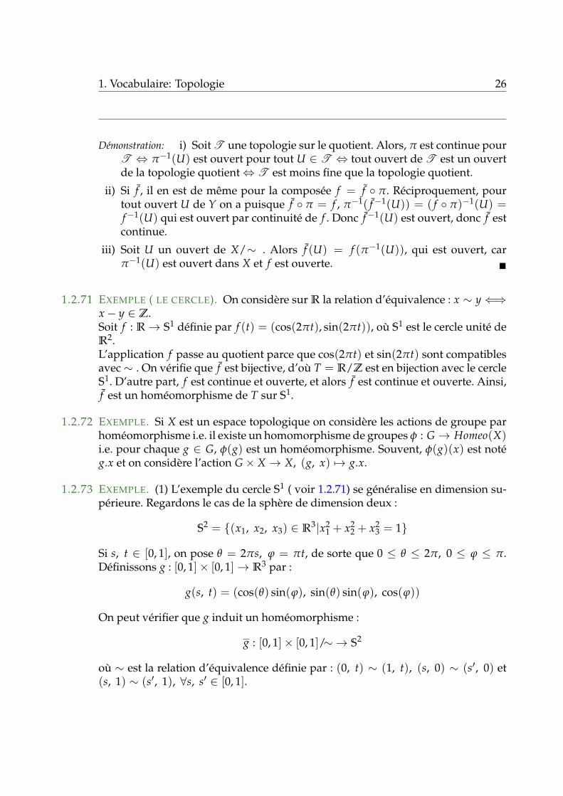
(2) Le ruban simple est défini comme le quotient du carré [0, 1] ⇥ [0, 1] par larelation (0, t) ⇠ (1, t)(il est sous-entendu que (s, t) ⇠ (s, t) si s 6= 0, 1).

(3) Le ruban de Möbius, est défini comme le quotient du carré [0, 1] ⇥ [0, 1] parl’identification : (0, t) ⇠ (1, 1 � t).

5. THE MOEBIUS BAND 15

5. The Moebius band

“The Moebius band” is a standard name for subspaces of R3 which are obtained from the unitsquare [0, 1]⇥ [0, 1] by “gluing” two opposite sides after twisting the square one time, as shown inFigure 14. As in the discussion about the unit circle (obtained from the unit interval by “gluing”

IV: the Moebius band

(the orientations do not match!)II: approach the vertical sides

III: twist so that the orientations of the sides match

I: Start with [0, 1]x[0, 1]

Figure 14.

its end points), this “gluing process” should be understood intuitively, and the precise meaningin topology will be explained later. The following exercise provides a possible parametrizationof the Moebius band (inside R3).

Exercise 1.12. Considerf : [0, 1] ⇥ [0, 1] ! R3,

f(t, s) = ((2 + (2s � 1)sin(�t))cos(2�t), (2 + (2s � 1)sin(�t))sin(2�t), (2s � 1)cos(�t)).

You may want to check that f(t, s) = f(t�, s�) holds only in the following cases:

(1) (t, s) = (t�, s�).(2) t = 0, t� = 1 and s� = 1 � s.(3) t = 1, t� = 0 and s� = 1 � s.

(but this also follows from the discussion below). Based on this, explain why the image of f canbe considered as the result of gluing the opposite sides of a square with the reverse orientation.

To understand where these formulas come from, and to describe explicit models of the Moebiusband in R3, we can imagine the Moebius band as obtained by starting with a segment in R3

and rotating it around its middle point, while its middle point is being rotated on a circle. SeeFigure 15.

The rotations take place at the same time (uniformly), and while the segment rotates by 180�,the middle point makes a full rotation (360�). To write down explicit formulas, assume that

• the circle is situated in the XOY plane, is centered at the origin, and has radius R.• the length of the segment is 2r and the starting position A0B0 of the segment is per-

pendicular on XOY with middle point P0 = (R, 0, 0).• at any moment, the segment stays in the plane through the origin and its middle point,

which is perpendicular on the XOY plane.

6. THE TORUS 17

6. The torus

“The torus” is a standard name for subspaces of R3 which look like a doughnut.The simplest construction of the torus is by a gluing process: one starts with the unit square

and then one glues each pair of opposite sides, as shown in Figure 16.

a a aa

b

b

b

a

b

Figure 16.

As in the case of circles, spheres, disks, etc, by a torus we mean any space which is homeo-morphic to the doughnut. Let’s find explicit models (in R3) for the torus. To achieve that, wewill build it by placing our hand in the origin in the space, and use it to rotate a rope which atthe other end has attached a non-flexible circle. The surface that the rotating circle describesis clearly a torus (see Figure 17).

O

X

Y

Z

Rr

TR, r

b

a

Figure 17.

To describe the resulting space explicitly, we assume that the rope rotates inside the XOYplane (i.e. the circle rotates around the OZ axis). Also, we assume that the initial position ofthe circle is in the XOZ plane, with center of coordinates (R, 0, 0), and let r be the radius of

5. THE MOEBIUS BAND 15

5. The Moebius band

“The Moebius band” is a standard name for subspaces of R3 which are obtained from the unitsquare [0, 1]⇥ [0, 1] by “gluing” two opposite sides after twisting the square one time, as shown inFigure 14. As in the discussion about the unit circle (obtained from the unit interval by “gluing”

IV: the Moebius band

(the orientations do not match!)II: approach the vertical sides

III: twist so that the orientations of the sides match

I: Start with [0, 1]x[0, 1]

Figure 14.

its end points), this “gluing process” should be understood intuitively, and the precise meaningin topology will be explained later. The following exercise provides a possible parametrizationof the Moebius band (inside R3).

Exercise 1.12. Considerf : [0, 1] ⇥ [0, 1] ! R3,

f(t, s) = ((2 + (2s � 1)sin(�t))cos(2�t), (2 + (2s � 1)sin(�t))sin(2�t), (2s � 1)cos(�t)).

You may want to check that f(t, s) = f(t�, s�) holds only in the following cases:

(1) (t, s) = (t�, s�).(2) t = 0, t� = 1 and s� = 1 � s.(3) t = 1, t� = 0 and s� = 1 � s.

(but this also follows from the discussion below). Based on this, explain why the image of f canbe considered as the result of gluing the opposite sides of a square with the reverse orientation.

To understand where these formulas come from, and to describe explicit models of the Moebiusband in R3, we can imagine the Moebius band as obtained by starting with a segment in R3

and rotating it around its middle point, while its middle point is being rotated on a circle. SeeFigure 15.

The rotations take place at the same time (uniformly), and while the segment rotates by 180�,the middle point makes a full rotation (360�). To write down explicit formulas, assume that

• the circle is situated in the XOY plane, is centered at the origin, and has radius R.• the length of the segment is 2r and the starting position A0B0 of the segment is per-

pendicular on XOY with middle point P0 = (R, 0, 0).• at any moment, the segment stays in the plane through the origin and its middle point,

which is perpendicular on the XOY plane.

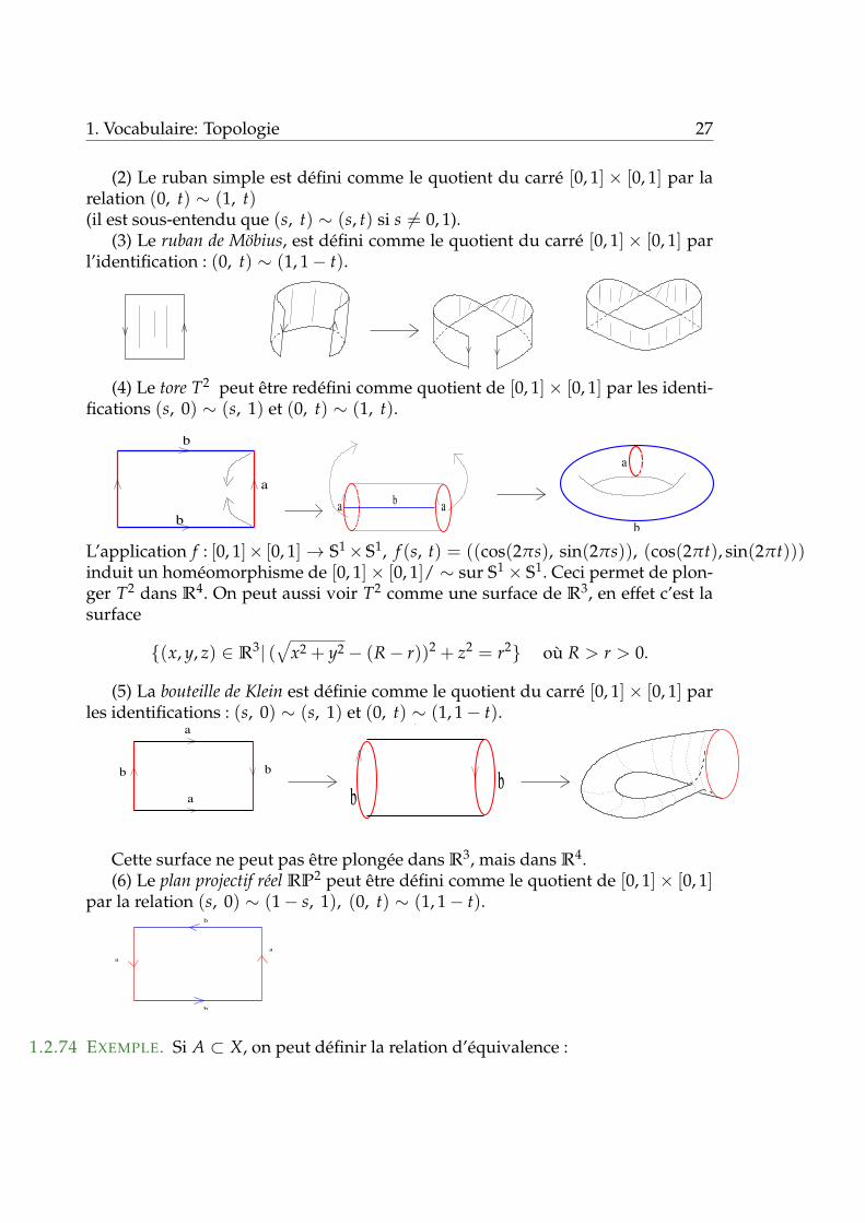
(4) Le tore T2 peut être redéfini comme quotient de [0, 1] ⇥ [0, 1] par les identi-fications (s, 0) ⇠ (s, 1) et (0, t) ⇠ (1, t).

6. THE TORUS 17

6. The torus



a a aa

b

b

b

a

b

Figure 16.


O

X

Y

Z

Rr

TR, r

b

a

Figure 17.


6. THE TORUS 17

6. The torus



a a aa

b

b

b

a

b

Figure 16.


O

X

Y

Z

Rr

TR, r

b

a

Figure 17.


6. THE TORUS 17

6. The torus



a a aa

b

b

b

a

b

Figure 16.


O

X

Y

Z

Rr

TR, r

b

a

Figure 17.


6. THE TORUS 17

6. The torus



a a aa

b

b

b

a

b

Figure 16.


O

X

Y

Z

Rr

TR, r

b

a

Figure 17.


L’application f : [0, 1]⇥ [0, 1] ! S1 ⇥ S1, f (s, t) = ((cos(2ps), sin(2ps)), (cos(2pt), sin(2pt)))induit un homéomorphisme de [0, 1] ⇥ [0, 1]/ ⇠ sur S1 ⇥ S1. Ceci permet de plon-ger T2 dans R4. On peut aussi voir T2 comme une surface de R3, en effet c’est lasurface

{(x, y, z) 2 R3| (»

x2 + y2 � (R � r))2 + z2 = r2} où R > r > 0.

(5) La bouteille de Klein est définie comme le quotient du carré [0, 1] ⇥ [0, 1] parles identifications : (s, 0) ⇠ (s, 1) et (0, t) ⇠ (1, 1 � t).

7. THE KLEIN BOTTLE 21

7. The Klein bottle

We have seen that, starting from an unit square and gluing some of its sides, we can producethe sphere (Figure 13), the Moebius band (Figure 14) or the torus (Figure 16). What if we tryto glue the sides di�erently? The next in this list of example would be the space obtained bygluing the opposite sides of the square but reversing the orientation for one of them, as indicatedin Figure 24. The resulting space is called the Klein bottle, denoted here by K. Trying to repeatwhat we have done in the previous examples, we have trouble when “twisting the cylinder”. Isthat really a problem? It is now worth having a look back at what we have already seen:

- starting with an interval and gluing its end points, although the interval sits on thereal line, we did not require the gluing to be performed without leaving the real line(it would not have been possible). Instead, we used one extra-dimension to have morefreedom and we obtained the circle.

- similarly, when we constructed the Moebius band or the torus, although we started inthe plane with a square, we did not require the gluing to take place inside the plane (itwouldn’t even have been possible). Instead, we used an extra-dimension to have morefreedom for “twisting”, and the result was sitting in the space R3 = R2 ⇥ R.

Something very similar happens in the case of the Klein bottle: what seems to be a problemonly indicates the fact that the gluing cannot be performed in R3; instead, it indicates that Kcannot be pictured in R3, or, more precisely, that K cannot be embedded in R3. Instead, K canbe embedded in R4. The following exercise is an indication of that.

b b

a

a

b b

first glue the sides a

and glue them then twist the sides b (not possible on |R )3

3 The Klein botlle: fake picture in |R

Figure 24.

Exercise 1.24. Consider the map

f̃ : [0, 1] ⇥ [0, 1] ! R4,

f̃(t, s) = ((2 � cos(2�s)cos(2�t), (2 � cos(2�s)sin(2�t), sin(2�s)cos(�t), sin(2�s)sin(�t)).

Explain why the image of this map in R4 can be interpreted as the space obtained from the squareby gluing its opposite sides as indicated in the picture (hence can serve as a model for the Kleinbottle).

6. THE TORUS 17

6. The torus



a a aa

b

b

b

a

b

Figure 16.


O

X

Y

Z

Rr

TR, r

b

a

Figure 17.



7. The Klein bottle





b b

a

a

b b




Figure 24.


f̃ : [0, 1] ⇥ [0, 1] ! R4,



6. THE TORUS 17

6. The torus



a a aa

b

b

b

a

b

Figure 16.


O

X

Y

Z

Rr

TR, r

b

a

Figure 17.



7. The Klein bottle





b b

a

a

b b




Figure 24.


f̃ : [0, 1] ⇥ [0, 1] ! R4,



Cette surface ne peut pas être plongée dans R3, mais dans R4.(6) Le plan projectif réel RP2 peut être défini comme le quotient de [0, 1] ⇥ [0, 1]

par la relation (s, 0) ⇠ (1 � s, 1), (0, t) ⇠ (1, 1 � t).

8. THE PROJECTIVE PLANE P2 23

8. The projective plane P2

In the same spirit as that of the Klein bottle, let’s now try to glue the sides of the square asindicated on the left hand side of Figure 26.

~−a

b

b

a

b

b

a

a

Figure 26.

Still as in the case of the Klein bottle, it is di�cult to picture the result because it cannotbe embedded in R3 (but it can be embedded in R4!). However, the result is very interesting: itcan be interpreted as the set of all lines in R3 passing through the origin- denoted P2. Let’s usadopt here the standard definition of the projective space:

P2 := {l : l ⇢ R3 is a line through the origin},

(i.e. l ⇢ R3 is a one-dimensional vector subspace). Note that this is a “space” in the sense thatthere is a clear intuitive meaning for “two lines getting close to each other”. We will explainhow P2 can be interpreted as the result of the gluing that appears in Figure 26.

Step 1: First of all, there is a simple map:

f : S2 ! P2

which associates to a point on the sphere, the line through it and the origin. Since every lineintersects the sphere exactly in two (antipodal) points, this map is surjective and has the specialproperty:

f(z) = f(z�) () z = z� or z = �z� (z and z� are antipodal).

In other words, P2 can be seen as the result of gluing the antipodal points of the sphere.

Step 2: In this gluing process, the lower hemisphere is glued over the upper one. We seethat, the result of this gluing can also be seen as follows: start with the upper hemisphere S2

+and then glue the antipodal points which are on its boundary circle.

Step 3: Next, the upper hemisphere is homeomorphic to the horizontal unit disk (by theprojection on the horizontal plane). Hence we could just start with the unit disk D2 and gluethe opposite points on its boundary circle.

Step 4: Finally, recall that the unit ball is homeomorphic to the square (by a homeomor-phism that sends the unit circle to the contour of the square). We conclude that our space canbe obtained by the gluing indicated in the initial picture (Figure 26).

Note that, since P2 can be interpreted as the result of gluing the antipodal points of S2, thefollowing exercise indicates why P2 can be seen inside R4:

1.2.74 EXEMPLE. Si A ⇢ X, on peut définir la relation d’équivalence :


xRy , x 2 X\A et x = y ou bien x, y 2 ALes classes d’équivalence sont donc de la forme :

Cx =®

{x} si x 2 X\AA si x 2 A

L’espace quotient est noté X/A. La projection canonique p : X ! X/A envoiele sous-ensemble A sur un seul point, la classe d’équivalence A ; elle est injectivesur X\A.

1.2.75 Exercice Montrer que Bn/Sn�1 est homéomorphe à Sn, où Bn est la boule unitéfermée dans Rn et Sn�1 la sphère associée.

On pourra considérer l’application

f : Bn ! Sn, x 7! (x1

||x|| sin(p||x||), . . . ,xn

||x|| sin(p||x||), cos(p||x||))

pour x 6= 0 et qui envoie 0 sur le pôle nord (0, . . . , 0, 1).On pourra vérifier que : f (x) = f (x0) , x = x0 ou x, x0 2 Sn�1.

1.2.5 Critères de séparation d’un quotientUn quotient d’un espace séparé n ‘est pas toujours séparé, par exemple le quo-

tient de R ⇥ {0, 1} où l’on identifie (x, 0) et (x, 1) si x 6= 0 : le quotient est loca-lement homéomorphe à R, mais les points distincts [(0, 0)] et [(0, 1)] n’ont pas devoisinages disjoints.

1.2.76 Exercice On considère sur R la relation d’équivalence x ⇠ y , x � y 2 Q.Montrer que R/Q n’est pas séparé.

1.2.77 DÉFINITIONLe graphe d’une relation d’équivalence ⇠ sur un ensemble X est l’ensembleR = {(x, y) 2 X ⇥ X| x ⇠ y}.

1.2.78 PROPOSITIONLa projection p : X ! X/⇠ est ouverte si et seulement si le saturé de tout ouvertest un ouvert.

La projection p : X ! X/⇠ est fermée si et seulement si le saturé de tout ferméest un fermé.

Démonstration: Par définition, p est ouverte si et seulement si, pour tout ouvert U ⇢X, p(U) est ouvert, ce qui équivaut à p

�1(p(U)) est ouvertc‘est-à-dire si p

�1(U)est ouvert. ⌅


1.2.80 REMARQUELa projection peut être fermée sans être ouverte. En effet, on considère [0, 1] avec

l’identification 0 ⇠ 1. Le saturé de l’ouvert [0,12[, est [0,

12[[{1}, qui n’est pas

ouvert ; donc la projection canonique p : [0, 1] ! [0, 1]/ ⇠ n’est pas ouverte. Parcontre, on voit facilement que le saturé d’un fermé F de [0, 1] est soit F soit F [ {0}ou F [ {1}, qui sont des fermés, ainsi la projection canonique est fermée.

1.2.81 EXEMPLE. Si la relation d’équivalence est associée à une action de groupe alors p

est ouverte :En effet, si U est ouvert, p

�1(p(U)) =[

g2Gg.U est ouvert car les g.U sont ouverts

(g est un homéomorphisme).

1.2.82 PROPOSITIONSoit X un espace topologique muni d’une relation d’équivalence ⇠.

i) Si le quotient X/⇠ soit séparé, alors le graphe R de ⇠ est fermé.ii) Si p est ouverte et R est fermé, alors X/⇠ est séparé.

Démonstration: i) Le graphe R est l’image réciproque de la diagonale par

p ⇥ p : X ⇥ X ! (X/⇠) ⇥ (X/⇠).

Celle-ci est fermée puisque X/⇠ est séparé, donc R est fermé puisque p ⇥ p

est continue.ii) Soient [x] et [y] deux points distincts de X/⇠. Donc (x, y) 62 R, donc il existe

des voisinages ouverts Vx de x et Vy de Y tels (Vx ⇥ Vy) \ R = ∆. Alors p(Vx)et p(Vy) sont des voisinages ouverts disjoints de [x] et de [y] respectivement,donc X/⇠ est séparé. ⌅

1.2.84 REMARQUEOn peut très bien avoir un quotient séparé sans que la projection p soit ouverte,(voir 1.2.80). Par contre dans le cas d’action de groupe la projection canonique esttoujours ouverte, donc pour montrer que le quotient est séparé il suffit, d’après1.2.82, de montrer que le graphe est fermé. Nous allons donner une condition suf-fisante.

1.2.85 PROPOSITIONSoit (g, x) 7! g.x une action propre d’un groupe G sur un espace topologique sé-paré X. On suppose que G agit proprement sur X i.e. pour tous x, y 2 X, il existedes voisinages Vx de x et Vy de Y tels que {g 2 G | g.Vx \ Vy 6= ∆} est fini. Alors lequotient X/G est séparé.

En particulier, si G est fini, X/G est séparé.


Démonstration: On sait déjà que p est ouverte (1.2.82), il suffit de montrer que songraphe R = {(x, y) 2 X ⇥ X|y 2 G.x} est fermé. Soit (x, y) 62 R c’est-à-dire y 62G.x, il suffit de trouver des voisinages ouverts Ux et Uy tels que Ux ⇥ Uy ⇢ X\R,c’est-à-dire G. Ux \ Uy = ∆.

Soient Vx et Vy des voisinages ouverts donner par la proprieté. On écrit {g 2G | g.Vx \ Vy 6= ∆} = {g1, . . . , gn}.

Puisque y 62 G.x et que X est séparé, pour tout i 2 {1, . . . , n}, il existe desvoisinages ouverts Wi,x ⇢ Vx et Wi,y ⇢ Vy tels que gi.Wi,x \ Wi,y = ∆. Posant

Ux =\

g2G(Vx,Vy)

Wg,x et Uy =n\

i=1Wi,y, on obtient des voisinages ouverts de x et de y.

Alors, pour g 2 G, on a soit g 2 {g1, . . . , gn} donc g.Ux \ Uy ⇢ g.Wg,x \ Wg,y = ∆,soit g 62 {g1, . . . , gn} donc g.Ux \ Uy ⇢ g.Vx \ Vy = ∆. Donc G.Ux \ Uy = ∆. ⌅

1.2.87 Exercice Monter que Tn = Rn/Zn est séparé.

Espace quotient d’un evn

Soit (E, ||.||) un espace vectoriel normé et F un sous-espace de E. On veut défi-nir une norme sur l’espace quotient ; on pose pour cela

N([x]) := d(x, F) = infy2F

kx � yk

il faut commencer par montrer que cette quantité ne dépend pas du choix du re-présentant de la classe [x]. Si x ⇠ x0 alors x � x0 2 F et par conséquent

d(x, F) = infy2F

kx � yk = infy2F

kx0 � (y + x0 � x)k = infy02F

kx0 � y0k = d(x0, F).

On peut à présent vérifier les axiomes d’une semi-norme :1) On a N([0]) = d(0, F) = 0.2) Pour l 6= 0 on a

N([lx]) = infy2F

klx � yk = |l| infy2F

kx � l

�1yk

= |l|d(x, F) = |l|N([x]).

3) Il reste à vérifier l’inégalité triangulaire, soit

N([x] + [x0]) = d(x + x0, F) d(x, F) + d(x0, F) = N([x]) + N([x0]).

Or pour tout y, y0 2 F on a y + y0 2 F et donc

d(x + x0, F) kx + x0 � y � y0k kx � yk + kx0 � y0k.

En passant à la borne inférieure dans l’inégalité précédente successivementdans la variable y puis y0, on obtient l’inégalité désirée.


On a défini ainsi une semi-norme sur E/F.

1.2.88 PROPOSITION1) N une norme sue E/F si et seulement si F est fermé.2) La projection canonique est une application linéaire continue et ouverte de

(E, k.k) sur (E/F, N(.)).3) La norme N définit la topologie quotient.

Démonstration: 1) En effet, N([x]) = 0 , d(x, F) = 0 , x 2 F. Ainsi N([x]) = 0 ,[x] = [0] est équivalent à x 2 F , x 2 F, i.e. F = F donc F est fermé dans E.

2) La linéarité de la projection canonique p : E ! E/F est conséquence de ladéfinition de la structure linéaire sur E/F et pour la continuité on a :

N(p(x)) = N([x]) = d(x, F) = infy2F

kx � yk kxk

ce qui implique kpk 1.On va montrer que p est une application ouverte. Comme p est linéaire, il suffit devérifier que p(BE(0, 1)) est un voisinage de l’origine. Ce dernière point découlerade l’égalité

p(BE(0, 1)) = BE/F([0], 1).

Soit [x] 2 BE/F([0], 1) alors d(x, F) < 1 et il existe donc y 2 F tel que kx � yk < 1par conséquent [x] = p(x � y) 2 p(BE(0, 1). Réciproquement, si [x] = p(x) 2p(BE(0, 1)) alors N([x]) kpk.kxk < 1, donc [x] 2 BE/F([0], 1).

3) La topologie quotient est la topologie la plus fine rendant la projection ca-nonique p continue, elle est donc plus fine que la topologie induite par la normeN.

Réciproquement, si U est un ouvert, pour la topologie quotient, et [x] 2 U,alors p

�1(U) est un ouvert contenant x. Il existe alors un r > 0 tel que BE(x, r) ⇢p

�1(U), d’où

BE/F([x], r) = p(BE(x, r)) ⇢ p(p

�1(U)) = U.

Ainsi U est un ouvert pour la topologie définie par la norme. ⌅

1. Vocabulaire: Complétude 32

1.3 ComplétudeSoit (X, d) un espace métrique. Une suite (xn)n2N de X est de Cauchy si

limn,m!•

d(xn, xm) = 0,

i. e. pour tout # > 0, il existe N(#) tel que

d(xn, xm) < #

pour n, m � N.

1.3.1 DÉFINITIONL’espace (X, d) est complet si toute suite de Cauchy converge.

Soit A une partie de X.Le diamètre d(A) de A est par définition sup{d(x, y) : x, y 2 A}.

1.3.2 THÉORÈMEUn espace mérique est complet si et seulement si toute intersection dénombrabledécroissante de fermés non vides dont le diamètre tend vers 0, est non vide.Elle est alors égale à un singleton.

Démonstration: 1. Supposons (X, d) complet, et soit (Fn)n2N une telle suite defermés. Soit xn 2 Fn une suite, elle est de Cauchy car d(xn, xm) d(Fmin(m,n)).Elle a donc une limite a, et a est adhérent à tous les Fn donc appartient à touspuisqu’ils sont fermés.

2. Réciproquement, supposons vérifiée la propriété sur les fermés. Soit (xn)n2N

une suite de Cauchy de X, posons Fn = {xm|m � n}. Alors (Fn)n2N est unesuite décroissante de fermés, et lim

n!+•d(Fn) = 0 puisque (xn) est de Cau-

chy. Donc\

n2N

Fn est un singleton a : ainsi la suite (xn) admet a pour valeur

d’adhérence, et comme elle est de Cauchy, elle converge vers a. ⌅

1.3.4 REMARQUESi le diamètre ne tend pas vers 0 (même si il est borné), l’intersection peut êtrevide.

Exemple : 1) Soit N muni de la métrique d(n, m) =

(0 si n = m,

1 + 1n+m sinon. .

(N, d) est complet (car la topologie induite est la topologie discrète).


Pour n � 1, on prend Fn = B(n, 1 + 12n ). Alors, Fn = {n + 1, n + 2, n + 3, . . .} est

fermé, Fn+1 ⇢ Fn, 1 < d(Fn) < 2 + 1n mais,

\

n2N⇤Fn = ∆.

2) Dans `2(N, R), soit (en)n2N, où en = (dk,n)k2N la suite canonique. On posepour tout n 2 N, Fn = {el | l � n}. Alors Fn est fermé, Fn+1 ⇢ Fn, d(Fn) =

p2,

mais,\

n2N

Fn = ∆.

1.3.5 THÉORÈMESoit Y un sous-espace d’un espace métrique (X, d).(Y, d) est complet si et seulement si Y est fermé dans X.

Démonstration: ” =) ” Si x 2 Y, il est limite d’une suite (xn) 2 YN qui convergedans X. Comme Y est complet, (xn) converge dans Y, donc x 2 Y.” (= ” Si (xn) 2 YN est une suite de Cauchy, elle est de Cauchy dans X doncconverge dans X. Comme Y est fermé, sa limite est dans Y donc elle convergedans Y.

Continuité uniforme. Prolongement des applications uniformément continues

1.3.7 DÉFINITIONUne application f : (X, d) ! (Y, d0) entre deux espaces métriques est unifor-mément continue si pour tout # > 0, il existe d > 0 tel que (d(x, x0) d )d0( f (x), f (x0)) #.

Bien sur, l’uniforme continuité implique la continuité, mais la réciproque est fausse :l’application f : x 7! x2 de R dans R est continue, mais pas uniformément :

en effet, f (n +1n) � f (n) = 2 +

1n2 > 2, alors que d(n, n +

1n) =

1n

! 0.

1.3.8 DÉFINITION (MODULE DE CONTINUITÉ)Un module de continuité pour f : (X, d) ! (Y, d0) est une fonction continuem : [0, d0[! R+, 0 telle que m(0) = 0 et

d(x, x0) < d0 ) d0( f (x), f (x0)) m(d(x, x0)).


1.3.9 PROPOSITIONSoit f : (X, d) ! (Y, d0) une application entre deux espaces métriques. Les pro-priétés suivantes sont équivalentes :

i) f est uniformément continue.ii) f admet un module de continuité.

Démonstration: (i) ) (ii). Pour tout n 2 N, il existe dn > 0 tel que (d(x, x0) < dn )d0( f (x), f (x0)) 2�n). Quitte à diminuer dn, on peut supposer que (dn) décroitstrictement vers 0. On définit alors m(dn) = 2�n+1, qu’on prolonge de façon affinesur chaque [dn+1, dn], et par m(0) = 0. La fonction m : [0, d0[! [0, 1] ainsi obtenueest croissante bijective, donc continue. De plus, si 0 < d(x, x0) d0, il existe n telque dn+1 d(x, x0) dn, donc d0( f (x), f (x0)) 2�n = m(dn+1) m(d(x, x0)).

(ii) ) (i). Si on se donne # > 0, par continuité de m il existe d > 0 tel quem(r) # pour r d, d’où

d(x, x0) d ) d0( f (x), f (x0)) m(d(x, x0)) #.

1.3.11 EXEMPLE. Les deux exemples classiques de module de continuité sonti)m(r) = Cr : une application f telle que d0( f (x), f (x0)) Cd(x, x0) est dite

C-lipschitzienne (ou C- Lipschitz), lipschitzienne si l’on ne précise pas C.ii)m(r) = Cra, a > 0 : une application f telle que d0( f (x), f (x0)) Cd(x, x0)a

est dite a-hölderienne (ou a-Hölder), hölderienne si l’on ne précise pas a.

1.3.12 Exercice Soit f : [a, b] ! R, une fonction a-hölderienne avec a > 1. Montrer quef est constante.

1.3.13 THÉORÈME (LE THÉORÈME DE PROLONGEMENT)Soit (E, dE) un espace métrique, A ⇢ E une partie dense et (F, dF) un espace mé-trique complet. Soit f : A ! F une application uniformément continue.

Alors, il existe une unique application uniformément continue f̃ : E ! F telleque f̃ |A = f . De plus f et f̃ ont même module de continuité.

Démonstration: L’unicité résulte du prolongement des identités puisque E est sé-paré. Reste à montrer l’existence. Soit x 2 E, par densité il existe une suite (an) 2AN tendant vers x. Alors (an) est une suite de Cauchy, et l’uniforme continuité im-plique que ( f (an)) aussi. Donc par complétude de F, ( f (an)) converge. La limitene dépend pas de la suite (an), car si l’on prend une autre suite (a0

n) tendant versx, on en fabrique une troisième (a00

n) en alternant les termes des deux premières.En prenant cette limite pour valeur de f̃ (x), on obtient l’extension cherchée. On abien une extension car si x 2 A on prend la suite constante (an = a).


Enfin, montrons que f̃ est uniformément continue. En effet, soit # > 0 et d > 0donné par l’uniforme continuité de f . Si d(x, x0) < d et an ! x, a0

n ! x0, alorspour n assez grand on a d(an, a0

n) < d, donc d( f (an), f (a0n)) d. Donc à la limite

on a d( f̃ (x), f̃ (x0)) d. Ceci implique f̃ est uniformément continue.Soit (d 7! m(d)) un module de continuité pour f . Soient d > 0, x, x0 2 X tels

que d(x, x0) < d. Soient (an), (bn) dans A tels que an ! x, bn ! x0, alors pourn assez grand on a d(an, bn) < d, donc d( f (an), f (bn)) m(d). Donc à la limiteon a d( f̃ (x), f̃ (x0)) m(d). Ceci implique f̃ est uniformément continue et d est unmodule de continuité pour f̃ . ⌅

Complétion

1.3.15 THÉORÈMESoit X un espace métrique. Il existe un plongement isométrique i : X ,! X̂ deX dans un espace métrique complet, tel que i(X) est un sous-espace dense. Un telplongement est unique à une isométrie près : si j : X ,! X̃ est un autre plongementde X dans un espace métrique complet X̃ tel que j(X) est sous-espace dense, alorsil existe une isométrie f : X̂ ! X̃ telle que f � i = j.

1.3.16 DÉFINITIONLe couple (“X, i) formé d’un espace métrique complet “X et d’un plongement iso-métrique i de X dans “X tel que i(X) est un sous-espace dense, s’appelle le complétéde X. Souvent, par abus de langage, on parle de l’espace “X comme le complété deX. Ceci permet d’identifier X à un sous-espace dense de “X.

Le théorème 1.3.15 est une conséquence des deux théorèmes suivants.

1.3.17 THÉORÈME (PLONGEMENT DE KURATOWSKI)Tout espace métrique (X, d) se plonge isométriquement dans l’espace vectorielnormé

`•(X) := {x = (x(y))y2X 2 RX | kxk• = supy2X

|x(y)| < •}

des applications bornées de X à valeurs dans R.


Démonstration: Nous allons définir un plongement isométrique

i : X ,! `•(X),

appelé plongement de Kuratowski. Fixons un point x0 2 X et pour tout x 2 X défi-nissons l’image i(x) dans `•(X) comme suit : i(x)y = d(x, y) � d(x0, y).Étant donné un point x 2 X, la fonction y 7! i(x)y = d(x, y) � d(x0, y) est majoréegrâce à l’inégalité triangulaire : |d(x, y) � d(x0, y)| d(x, x0), la borne ne dépendpas de y, seulement de x. Étant donné deux points x, z 2 X quelconques, on a pourtout y 2 X :

|i(x)y � i(z)y| = |d(x, y) � d(x0, y) � d(z, y) + d(x0, y)|= |d(x, y) � d(z, y)| d(x, y).

D’autre part, en posant y = x, on obtient

|i(x)x � i(z)x| = |d(x, x) � d(z, x)| = d(x, z).

D’où d•(i(x), i(z)) = supy2X|i(x)y � i(z)y| = d(x, z) i.e. i est une isométrie. ⌅

1.3.19 THÉORÈMESoit G un ensemble. L’espace métrique

`•(G, R) = {x = (x(g))g2G 2 RG | kxk• = sup

g2G|x(g)| < •}

muni de la norme k.k• est complet.

Démonstration: (1) Soit (xn) une suite de Cauchy dans `•(G). Cela veut dire quepour tout # > 0 il existe N tel que, pour tout g 2 G, |xn(g) � xm(g)| < # si n, m �N. Par conséquent, la suite (xn(g)) est une suite de Cauchy dans R, donc ellepossède une limite. Notons-là x(g). Nous avons construit une fonction x : G ! R,telle que

8g 2 G, xn(g) ! x(g). (1.3.1)

(2) Montrons que cette fonction est bornée. Choisissons une valeur de #0 > 0quelconque (par exemple, #0 = 1). Il existe N tel que pour tout n � N et toutg 2 G, |xn(g) � xN(g)| < 1. Cela implique 8g 2 G, |x(g)| |xN(g)| + 1, et parconséquent sup

gG|x(g)| supg2G|xN(g)| + 1 < •. Ainsi, x 2 `•(G).

(3) Finalement, on va montrer que xn ! x par rapport à la distance uniformed•. Soit # > 0. Fixons N tel que quelque soit n, m � N, on ait d•(xm, xn) < #. On


en déduit que pour tout g 2 G, |xm(g) � xn(g)| < #, donc, en prenant la limitem ! • dans R, |x(g) � xn(g)| # et, en prenant la borne supérieure sur tousg 2 G, on obtient

d•(x, xn) = supg2G

|xm(g) � xn(g)| #.

On a montré que pour tout # > 0 il existe N tel que quel que soit n � N, on ad•(x, xn) #, ce qui veut dire xn ! x lorsque n ! •, par rapport à la distanced• (la distance uniforme) sur l’espace `•(G, R). ⌅

Documents

1.2.4 Topologie quotient by week/ANAH3… · 1. Vocabulaire: Topologie 25 2) Action de groupe Soit G un groupe et X un ensemble. Une action (à gauche) de G sur X est une application