A nonlinear unmixing method in the infrared domain

A nonlinear unmixing method in the infrared domain

Guillaume Fontanilles2,3,* and Xavier Briottet1

1Office National d'Etudes et de Recherches Aérospatiales/Département Optique Théorique et Appliquée,2 Avenue E. Belin, F-31055 Toulouse, France

2Université de Toulouse, ISAE, 10 Avenue E. Belin, F-31055 Toulouse, France3Laboratoire de Mécanique des Fluides, UMR CNRS 6598 & FR 2488 CNRS,

Ecole Centrale de Nantes, B.P. 92101, F-44321 Nantes Cedex 3, France

*Corresponding author: guillaume.fontanilles@acri‐st.fr

Received 10 December 2010; revised 27 March 2011; accepted 16 May 2011;posted 19 May 2011 (Doc. ID 139421); published 8 July 2011

This paper presents the physical principle of a new (to our knowledge) unmixing method to retrieve op-tical properties (reflectance and emissivity) and surface temperatures over a heterogeneous and a foldedlandscape using hyperspectral and multiangular airborne images acquired with high spatial resolution.In fact, over such a complex scene, the linear mixing model of the reflectance commonly used in the re-flective domain is no longer valid in the IR range for the two following reasons: multiple reflections due tothe three-dimensional (3D) structure and the radiative phenomenon introduced by the temperature byway of the black body law. Thus, to solve this nonlinear unmixing problem, a new physical model of ag-gregation is used. Our model requires as inputs knowledge of the 3D scene structure and the spatialcontribution of each material in the scene. Each elementary scene element is characterized by its opticalproperties, and its temperature, spectral, andmultiangular acquisitions are required. This paper focusesonly on the theoretical feasibility of such a method. In addition, an analysis is conducted evaluating theimpact of the misregistration between the radiometric image and its digital terrain model, estimating athreshold of the relative importance of every elementary material to retrieve its corresponding opticalproperties and temperature. The results show that the 3D geometry must be accurately known (accuracyof 1m for a spatial resolution of 20m), and the relative contribution of material in the mixed areamust beabove 15% to retrieve its surface temperature with an accuracy better than 1K. So, thismethod is appliedon three different landscapes (heterogeneous flat surface, V shape, and urban canyon), and the resultsexhibit performances better than 1% for optical properties and 1K for surface temperatures. © 2011Optical Society of AmericaOCIS codes: 280.0280, 260.3060, 100.3190.

1. Introduction

The unmixing method, used in such scientific do-mains as biology [1], medicine [2], remote sensing ap-plications such as geology [3], and meteorology [4],aims at retrieving the elementary characteristicsof pure material over a heterogeneous scene from amultidimensional measure. In remote sensing, sucha method [5] has been widely used with hyperspec-

tral images to retrieve the surface reflectances inthe [0:4–2:5 μm] spectral range. Using the assump-tions that the landscape is flat and uniformly irra-diated where the reflection due to the environmentmay be neglected [6], the mixed reflectance is the re-sult of a linear mixing of the elementary optical prop-erties characterizing each pure material [7,8], whichcan be expressed as

P ¼ A � S; ð1Þ

with0003-6935/11/203666-12$15.00/0© 2011 Optical Society of America

3666 APPLIED OPTICS / Vol. 50, No. 20 / 10 July 2011

26664P1ð1Þ … P1ðwÞ

..

. . .. ..

.

Ppð1Þ … PpðwÞ

37775 ¼

26664a11 … a1M

..

. . .. ..

.

ap1 … apM

37775

×

26664S1ð1Þ … S1ðwÞ

..

. . .. ..

.

SMð1Þ … SMðwÞ

37775; ð2Þ

where the matrix P contains w spectral values ofmixed pixels measured by the sensor and S is thespectral reflectance matrix of each elementarymaterial in the pixel, i.e., S is the unknown matrix,and the matrix A corresponds to the relative contri-bution of each material present in the pixel. p is thenumber of pixels in the image, and M is the numberof materials in the scene. This model, commonlyknown as linear mixing model, has two constraints:positivity and additivity on the matrix coefficients A.Knowing the matrix A, S can be retrieved using themethod of least squares:

S ¼ ðAT :AÞ−1AT :P: ð3ÞIf the matrix A is unknown, methods based on

blind signal separation may be used [9]. Suchmethodhas been applied in the IR spectral domain forheterogeneous surfaces to retrieve only the spectralreflectance [9].

Nevertheless, very few methods exist to solvethe nonlinear unmixing either on a statistical basis(neural networks [6], support vector machines [10],Monte Carlo [11]) or with a physical approach(radiometric approach [12], normalized differencevegetation index [13–15]). The statistical methodsprovide generally good performance but are verytime consuming. Similarly, the drawback of physicalapproaches is that methods are limited for high spa-tial resolutions (below 100m).

Thus, most of the existing methods are based on alinear mixing assumption. Nevertheless, a few non-linear methods consider the effects of relief, but theyare unfortunately limited to the visible or near IRspectral domain [10,16], or they are not valid for veryhigh spatial resolutions (a few tenths of meters)[17,18]. Such consideration is very important for fu-ture thermal IR sensors with higher spatial resolu-tion [such as Micro Satellite for Thermal InfraredGround Surface Imaging (MISTIGRI [19])].

Thus, a new physically based method using themixing model described in [20] is proposed. Themethod is explained in Section 2. Then, in Section 3,a sensitivity study is conducted over two simple syn-thetic landscapes to evaluate its intrinsic perfor-mance, and the unmixing method is applied andanalyzed on three different landscapes.

2. Description of the Method

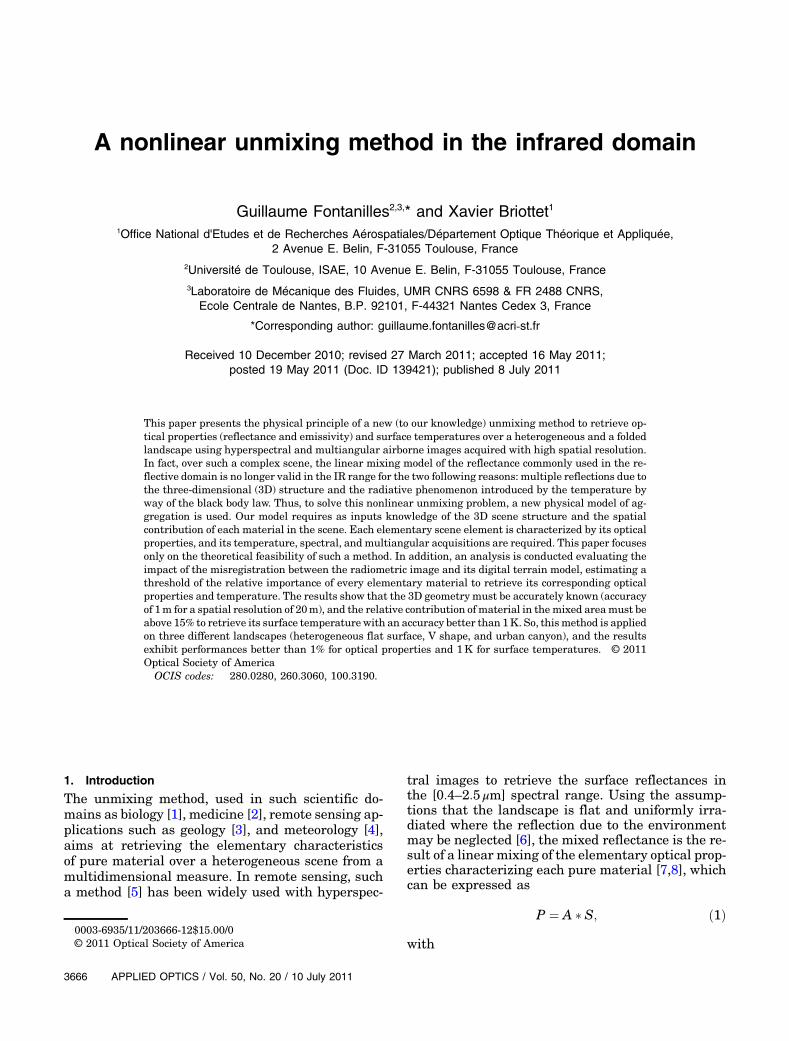
First, the mixing model is explained before the de-scription of the retrieval method. Before introducingour model, the surface delimited by the projection ofthe sensor instantaneous field of view (IFOV), namedhere equivalent surface, must be defined. In otherwords, this equivalence principle aims at assimilat-ing the heterogeneous surface by a flat and homoge-neous surface, in terms of optical properties andtemperature. In fact, when the landscape is hetero-geneous and not flat, Norman [21] mentions suchequivalent is rarely well defined.

Our present model focuses on the unmixing pro-cess of data acquired by IR sensors having a spatialresolution of a few tenths of a meter. With such as-sociated IFOV, the equivalent surface is defined atthe urban canopy level (Fig. 1). Although this choiceis very intuitive and simple, its main drawback isthat the equivalent radiative parameters will dependon the atmosphere inside the volume delimited bythe equivalent surface and the three-dimensional(3D) structure included in the projected IFOV. Then,the mixing model can be deduced by linking theequivalent parameters to the elementary ones. Inaddition, from remote sensing acquisitions, the

Fig. 1. (Color online) Unmixing principle.

10 July 2011 / Vol. 50, No. 20 / APPLIED OPTICS 3667

preprocessing, including atmospheric compensationand temperature emissivity separation, is supposedto be solved to retrieve the equivalent parameters:reflectance, emissivity, and temperature.

A. Mixing Model

Our physically basedmixing model is widely detailedin [20]. This model [20] takes into account the radia-tive effects induced by the 3D structure. From theBecker and Li approach [12], the conservation prin-ciple of the radiative budget at sensor level is used todeduce the aggregated or mixed expressions of theequivalent (or ensemble) parameters:

– The equivalent reflectance hρi:

hρi ¼Xk

Sk × t↑k-esρddk ð~usun;~us;kÞED;k

ED

þZZ

m∈NðkÞ

ρddk ð~ukm;~us;kÞπ gmðkÞρddm ð~usun;~umkÞ

×ED;mðkÞED

dSmðkÞ; ð4Þ

– the equivalent emissivity hεi:

hεi ¼Xk

Sk

�εkð~usÞ

þZZ

m∈NðkÞ

ρddk ð~ukm;~usÞπ gmðkÞεmð~umkÞdSmðkÞ

�; ð5Þ

– the equivalent temperature hTi:

hTi ¼ L−1BB

0B@PkSk

ht↑k-es

hεkð~usÞLBBðTkÞ þ

RRm∈NðkÞ

ρddk ð~ukm;~usÞπ gmðkÞεmð~umkÞLBBðTmÞdSmðkÞ

iþ Latm;↑

k-es

i

hεi

1CA; ð6Þ

where

– Sk is the normalized solid angle (NSA) underwhich the surface element k is seen by the sen-sor (

PkSk ¼ P

kdωkΩ ¼ 1);

– t↑k–es is the upwelling atmospheric transmissionbetween the surface element k and the equivalentsurface (Fig. 1);

– ρddk is the bidirectional reflectance of the surfaceelement k;

– ~usun is the unit vector in the sun direction and~us is the unit vector in the sensor direction;

– ED is the direct solar irradiance incident to thesurface;

– NðkÞ represents all the neighboring surfaces ofsurface element k;

– ~ukm is the unit vector of the surface element k inthe direction of the surface element m;

– gmðkÞ is the form factor (gmðkÞ ¼ h~nm:~umki: h~nk:~ukmiπ×r2

with r the distance between elements m and k);– LBB is the black body radiance (Planck’s law);– Latm;↑

k–es is the upwelling atmospheric radiancebetween the surface element k and the equivalentsurface (es);

– εk is the spectral emissivity of element k.

The nonlinearity of these three equations comesfrom the multiple reflections due to the 3D structureof the scene [for Eqs. (4)–(6)] and to the black bodylaw in Eq. (6). However, although this nonlinearityis generally weak in Eqs. (4) and (5) [22] for most nat-ural materials, this does not apply to some manmadematerials like metal.

Further, in Eq. (4), we could note that the equiva-lent reflectance also depends on the irradiance,which may differ in the landscape.

B. Unmixing Method

From Eqs. (4)–(6), the unmixing process aims at re-trieving the reflectance, emissivity, and temperatureof every k element. To this end, several inputs aresupposed to be known: the spatial distribution ofevery k element, the scene geometry, and finallythe sun and sensor directions.

The first input is not so restrictive. In fact, as ur-ban areas have slow temporal variations, it seemsreasonable to access such information using panchro-matic imagery in the visible spectral domain with a

high spatial resolution [23]. The second input as-sumes that a digital elevation model (DEM) is avail-able. As mentioned by Flamanc and Maillet [24],most modern towns now have their DEM, which isaccessible by users.

Thus, Eqs. (4)–(6) can be written as f ðxÞ ¼ 0[Eq. (7)], where the equivalent parameters hρiλ, hεiλ(λ designates the wavelength), and hTi are measuredby the sensor and x refers to the unknowns ρk, εk,and Tk. Finally, the resolution method consists inminimizing the residual function f ðxÞ using an itera-tive method and starting with an initial conditionsset:


f ðρkÞ ¼ hρiλ − hρi0; f ðεkÞ ¼ hεiλ − hεi0;f ðTkÞ ¼ hTi − hTi0; ð7Þ

where hρi0, hεi0, and hTi0 correspond to Eqs. (4)–(6)(right part).

This system is solved using the Gauss–Newton op-timization algorithm [25] improved by Levenbergand Marquardt [26]. Furthermore, this system ac-cepts a solution if the number of measurementsis sufficient in comparison with the number ofunknowns. In Eq. (7), the N unknowns [N ¼ 2×ðm ×wÞ þm] are the m reflectances at w wave-lengths, the m emissivities at w wavelengths, and fi-nally the m temperatures. To solve this system, atleast N measurements are required. However, froma hyperspectral sensor with w spectral bands, afteratmospheric compensation and the temperatureand emissivity separation (TES) algorithm [18,27],we are able to retrieve the spectral equivalent reflec-tance and the spectral equivalent emissivity, both inw bands and one measured equivalent temperature,which conducts to (2wþ 1) equations. So, to comple-tely solve this system, other measures are requiredthat may be delivered by m multiangular acquisi-tions. This gives m × ð2wþ 1Þ ¼ N equations.

In fact, such a system is a little bit overestimatedfor the following reason. A material is considered dif-ferent from another if one of its elementary radiativeproperties is different. For example, a given materialat two temperatures will be considered two differentmaterials, but with the same optical properties.

3. Sensitivity Analysis and Applications

In this section, the sensitivity of our method is ana-lyzed and then applied on three generic scenes: flatlandscape, V-shaped landscape, and an urban can-yon. The sensitivity analysis aims at evaluatingthe impact of the input factors on the performanceof our unmixing method. The input factors are essen-tially linked to the scene geometry through the factorSk. Thus, it is important to know this factor precisely.This estimation depends on the absolute referencing(or georeferencing) of the DEM and also on the rela-tive weight of every material. Their impact will beevaluated independently in the following.

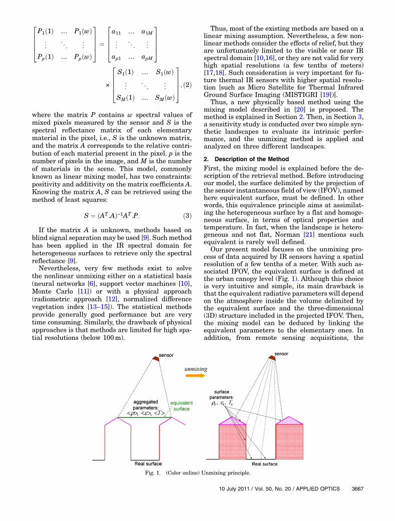
The impact of misregistration between the radio-metric image and the DEM is evaluated using syn-thetic data. First, a synthetic scene is generated,and the corresponding parameters are deduced usingEqs. (4)–(6). The unmixing is then applied before ap-plying a slight misregistration of the DEM (Fig. 2).

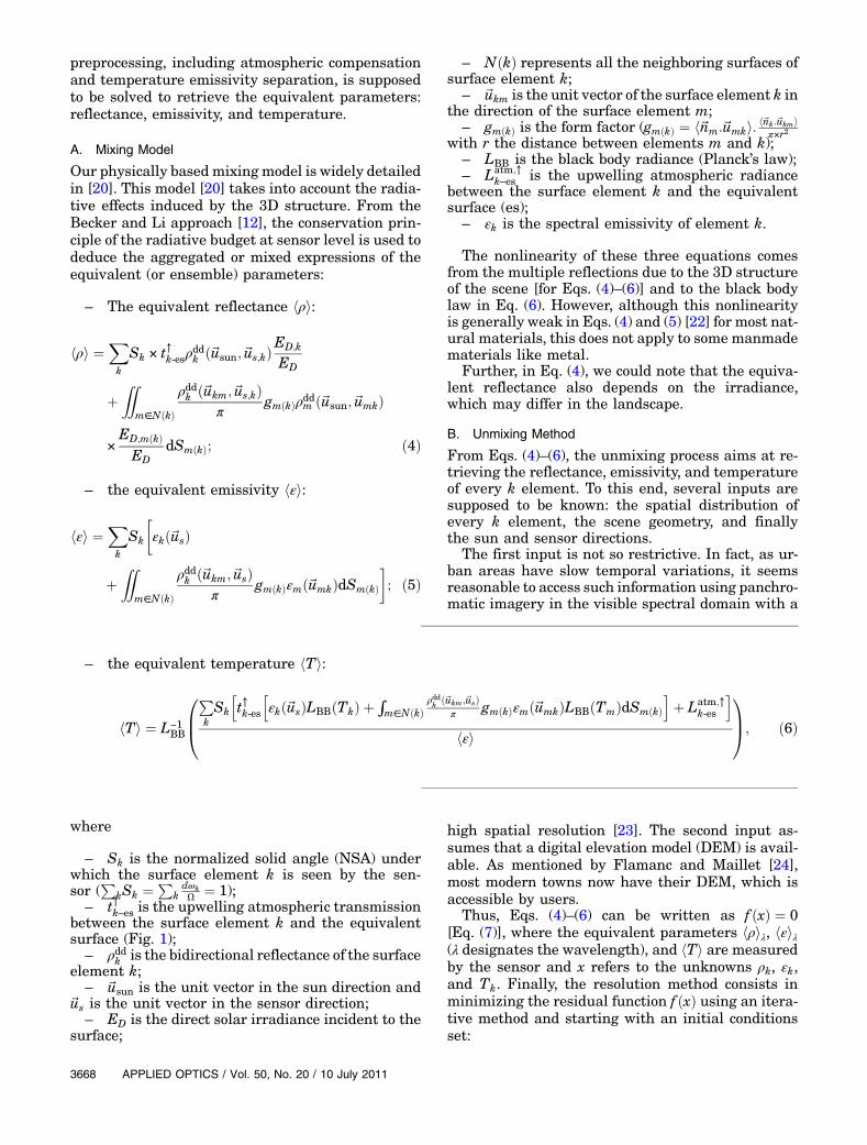
Second, it is of importance to evaluate the minimalNSA allowing the parameters retrieval with an ac-ceptable accuracy (Fig. 3). Such accuracy is fixed hereto 1% for the emissivity or the reflectance and to 1Kfor the surface temperature. This study was primar-ily intended to give orders of magnitude. The opticalproperties of each surface element are consideredLambertian.

A. Case 1: Heterogeneous and Flat Landscape

1. Surface Description

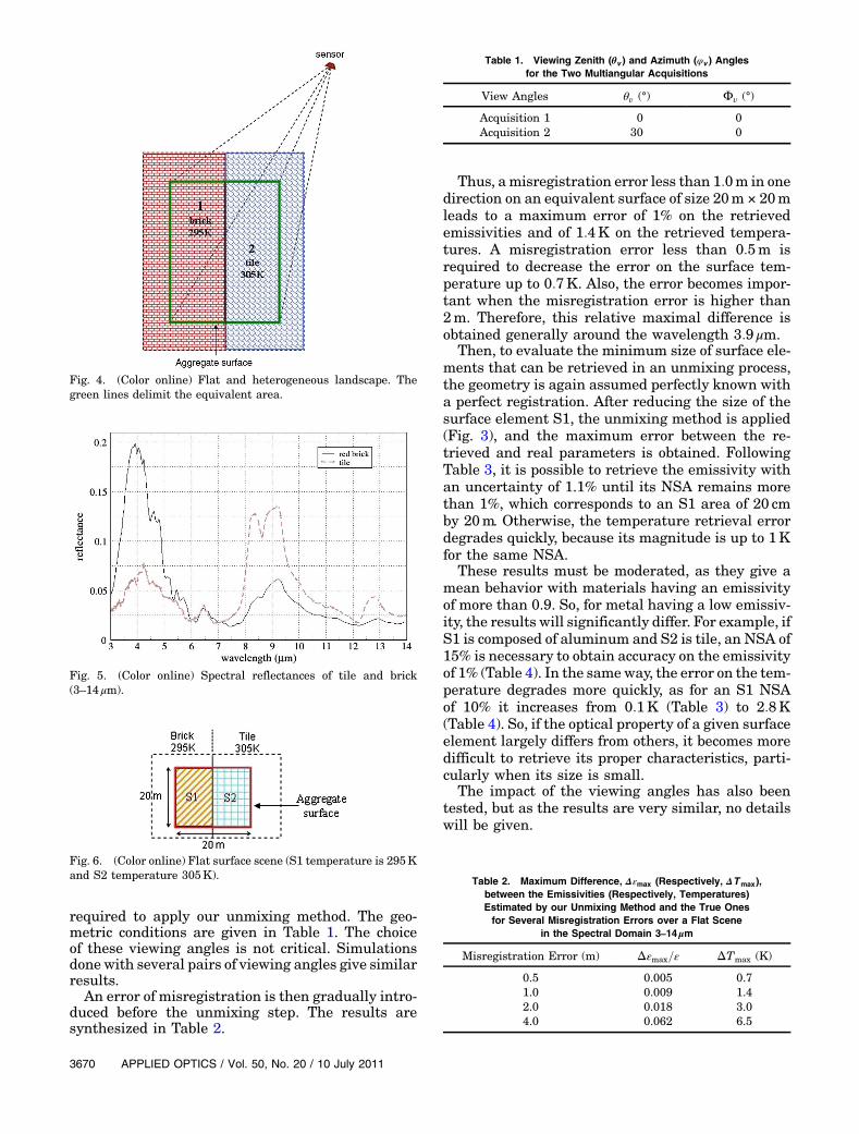
The scene, described in Fig. 4, is composed of two sur-face elements, one made of brick at temperature295K (material 1) and one of tile at 305K. Theirspectral reflectances have been measured duringthe Canopy and Aerosol Particles in Toulouse UrbanLayer (CAPITOUL) campaign [28] and are shownin Fig. 5.

The aggregated area is of size 20mby 20m (Fig. 6).The sensor is at a 500m height.

2. Sensitivity Analysis

As the aggregated surface is composed of two surfaceelements, two different viewing acquisitions are

Fig. 2. (Color online) Misregistration error between theDEM and the radiometric image over a flat scene composed oftwo materials.

Fig. 3. (Color online) Principle to evaluate the minimal normal-ized solid angle allowing the parameters retrieval with a givenaccuracy over a flat surface composed of two materials.


required to apply our unmixing method. The geo-metric conditions are given in Table 1. The choiceof these viewing angles is not critical. Simulationsdone with several pairs of viewing angles give similarresults.

An error of misregistration is then gradually intro-duced before the unmixing step. The results aresynthesized in Table 2.

Thus, amisregistration error less than 1:0m in onedirection on an equivalent surface of size 20m × 20mleads to a maximum error of 1% on the retrievedemissivities and of 1:4K on the retrieved tempera-tures. A misregistration error less than 0:5m isrequired to decrease the error on the surface tem-perature up to 0:7K. Also, the error becomes impor-tant when the misregistration error is higher than2m. Therefore, this relative maximal difference isobtained generally around the wavelength 3:9 μm.

Then, to evaluate the minimum size of surface ele-ments that can be retrieved in an unmixing process,the geometry is again assumed perfectly known witha perfect registration. After reducing the size of thesurface element S1, the unmixing method is applied(Fig. 3), and the maximum error between the re-trieved and real parameters is obtained. FollowingTable 3, it is possible to retrieve the emissivity withan uncertainty of 1.1% until its NSA remains morethan 1%, which corresponds to an S1 area of 20 cmby 20m. Otherwise, the temperature retrieval errordegrades quickly, because its magnitude is up to 1Kfor the same NSA.

These results must be moderated, as they give amean behavior with materials having an emissivityof more than 0.9. So, for metal having a low emissiv-ity, the results will significantly differ. For example, ifS1 is composed of aluminum and S2 is tile, an NSA of15% is necessary to obtain accuracy on the emissivityof 1% (Table 4). In the sameway, the error on the tem-perature degrades more quickly, as for an S1 NSAof 10% it increases from 0:1K (Table 3) to 2:8K(Table 4). So, if the optical property of a given surfaceelement largely differs from others, it becomes moredifficult to retrieve its proper characteristics, parti-cularly when its size is small.

The impact of the viewing angles has also beentested, but as the results are very similar, no detailswill be given.

Fig. 5. (Color online) Spectral reflectances of tile and brick(3–14 μm).

Fig. 6. (Color online) Flat surface scene (S1 temperature is 295Kand S2 temperature 305K).

Table 1. Viewing Zenith (θv ) and Azimuth (φv ) Anglesfor the Two Multiangular Acquisitions

View Angles θv (°) Φv (°)

Acquisition 1 0 0Acquisition 2 30 0

Table 2. Maximum Difference, Δεmax (Respectively, ΔTmax),between the Emissivities (Respectively, Temperatures)Estimated by our Unmixing Method and the True Onesfor Several Misregistration Errors over a Flat Scene

in the Spectral Domain 3–14 μm

Misregistration Error (m) Δεmax=ε ΔTmax (K)

0.5 0.005 0.71.0 0.009 1.42.0 0.018 3.04.0 0.062 6.5

Fig. 4. (Color online) Flat and heterogeneous landscape. Thegreen lines delimit the equivalent area.


3. Application and Results

In this present case, only the equation for the emis-sivity [Eq. (5)] is considered, because the reflectanceis linked to the emissivity by Kirchhoff ’s law, andtherefore the results are identical for these twoparameters.

For a flat landscape, the real and equivalentsurfaces are identical and the neighborhood termsare null. Then, Eqs. (5) and (6) become

hεi ¼Xk

Skεk; ð8Þ

hTi ¼ L−1BB

0@PkSkεkLBBðTkÞ

hεi

1A: ð9Þ

With two surfaces, Eq. (8) becomes

hεiλ ¼ S1ε1;λ þ S2ε2;λ: ð10Þ

Further, by approximating Planck’s law by Wienapproximation, Eq. (9) becomes

hTiλ ¼b

ln�

S1ε1;λ×ebT1þS2ε2;λ×e

bT2

hεiλ

� ; ð11Þ

which may be written as

hεiλ × eb

hTiλ ¼ S1ε1;λ × ebT1 þ S2ε2;λ × e

bT2 : ð12Þ

Finally, using matrix formalism, Eqs. (10) and (12)become

�S1;ðθc1;φc1Þ S2;ðθc1;φc1ÞS1;ðθc2;φc2Þ S2;ðθc2;φc2Þ

��ε1;λε2;λ

�¼

� hεiλ;ðθc1;φc1Þhεiλ;ðθc2;φc2Þ

�; ð13Þ

�S1;ðθc1;φc1Þε1;λ S2;ðθc1;φc1Þε2;λS1;ðθc2;φc2Þε1;λ S2;ðθc2;φc2Þε2;λ

��X1

X2

�¼

�Y ðθc1;φc1ÞY ðθc2;φc2Þ

�;

ð14Þ

where Xi ¼ ebTi and Y ¼ hεiλ × e

bhTiλ .

As mentioned above, only two viewing acquisitionsare needed. This system is defined for one wave-length; to have all the spectral emissivities, this al-gorithm must be repeated for each wavelength.

The surface temperatures are retrieved using theGauss–Newtonmethod [25], minimizing the residualfunction f ðTkÞ:

f ðTkÞ ¼ hTik −b

ln�

S1ε1;λ×ebT1þS2ε2;λ×e

bT2

hεiλ

� : ð15Þ

This method needs initial conditions (T1 andT2), whose values are fixed to the equivalenttemperature hTi.

In the first step, the elementary spectral emissiv-ities are estimated. Then, using Eq. (15), the elemen-tary surface temperatures are retrieved. So, thesurface temperatures are obtained optimally byusing all spectral values between 3 and 14 μm.

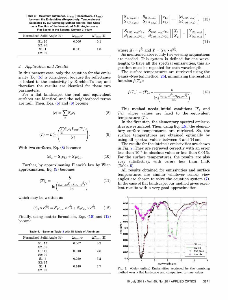
The results for the intrinsic emissivities are shownin Fig. 7. They are retrieved correctly with an errorless than 10−4 in absolute value or less than 0.01%.For the surface temperatures, the results are alsovery satisfactory, with errors less than 1mK(Table 5).

All results obtained for emissivities and surfacetemperatures are similar whatever sensor viewangles are chosen to solve the equation system (7).In the case of flat landscape, our method gives excel-lent results with a very good approximation.

Table 3. Maximum Difference, Δεmax (Respectively, ΔTmax),between the Emissivities (Respectively, Temperatures)Estimated by our Unmixing Method and the True Onesas a Function of the Normalized Solid Angle over a

Flat Scene in the Spectral Domain 3–14 μm

Normalized Solid Angle (%) Δεmax=ε ΔTmax (K)

S1: 10 0.006 0.1S2: 90S1: 1 0.011 1.0S2: 99

Table 4. Same as Table 3 with S1 Made of Aluminum


S1: 15 0.007 0.2S2: 85S1: 10 0.010 2.8S2: 90S1: 5 0.030 3.2S2: 95S1: 1 0.140 7.7S2: 99 Fig. 7. (Color online) Emissivities retrieved by the unmixing

method over a flat landscape and comparison to true values


B. Case 2: Heterogeneous and Valley-Shaped Landscape


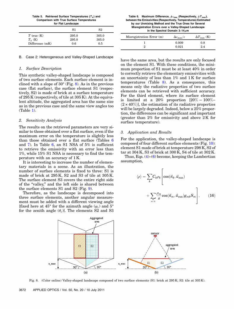
This synthetic valley-shaped landscape is composedof two surface elements. Each surface element is in-clined with a slope of 30° (Fig. 8). As in the previouscase (flat surface), the surface element S1 (respec-tively, S2) is made of brick at a surface temperatureof 295K (respectively, of tile at 305K). At the equiva-lent altitude, the aggregated area has the same sizeas in the previous case and the same view angles too(Table 1).

2. Sensitivity Analysis

The results on the retrieved parameters are very si-milar to those obtained over a flat surface, even if themaximum error on the temperature is slightly lessthan those obtained over a flat surface (Tables 6and 7). In Table 6, an S1 NSA of 5% is sufficientto retrieve the emissivity with an error less than1%, while 15% S1 NSA is necessary to find the tem-perature with an accuracy of 1K.

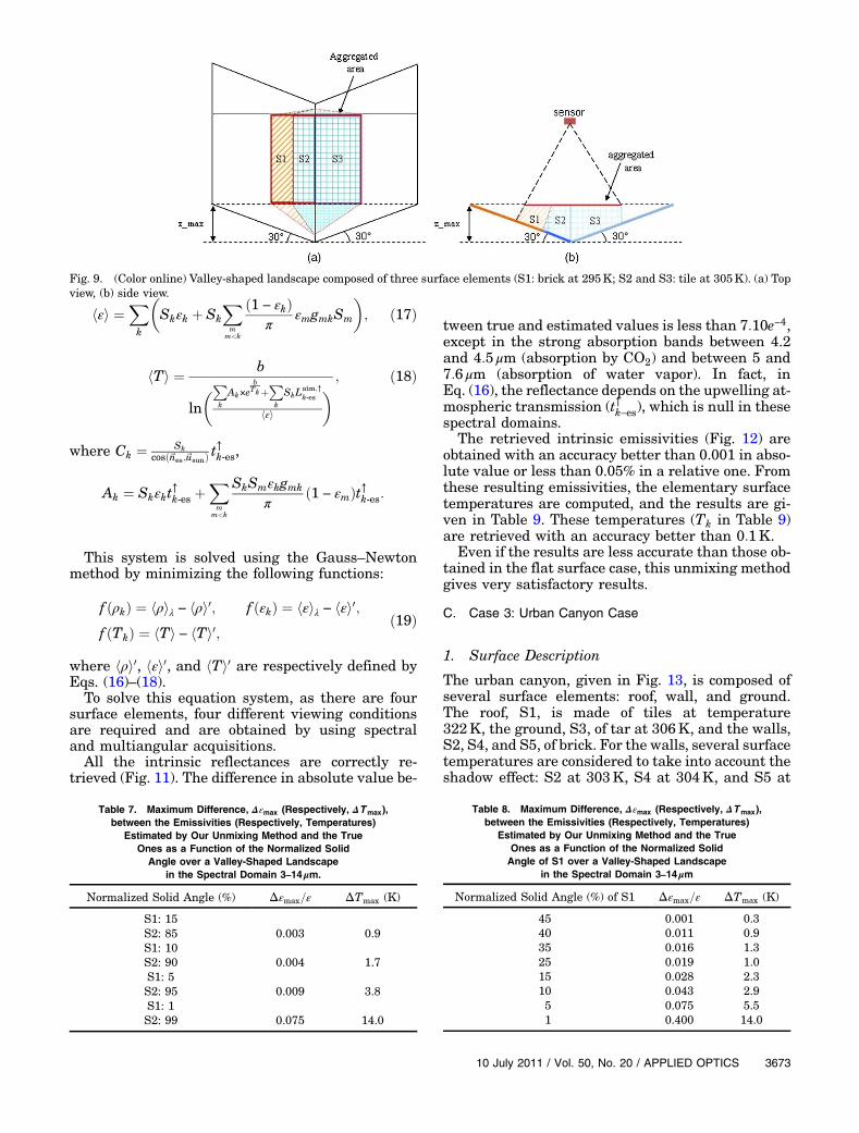
It is interesting to increase the number of elemen-tary materials in a scene. As an illustration, thenumber of surface elements is fixed to three: S1 ismade of brick at 295K, S2 and S3 of tile at 305K.The surface element S3 covers the entire right sideof the “valley,” and the left side is shared betweenthe surface elements S1 and S2 (Fig. 9).

Therefore, as the landscape is decomposed intothree surface elements, another angular measure-ment must be added with a different viewing angle[fixed here at 45° for the azimuth angle (φc) and 5°for the zenith angle (θc)]. The elements S2 and S3

have the same area, but the results are only focusedon the element S1. With these conditions, the mini-mum proportion of S1 must be at least 40% in orderto correctly retrieve the elementary emissivities withan uncertainty of less than 1% and 1K for surfacetemperatures (Table 8). As a consequence, thismeans only the radiative properties of two surfaceelements can be retrieved with sufficient accuracy.For the third element, where its surface elementis limited at a 20% proportion [20% ¼ 100%−

ð2 × 40%Þ], the estimation of its radiative propertieswill be largely degraded. Indeed, below a 25% propor-tion, the differences can be significant and important(greater than 2% for emissivity and above 2K forsurface temperature).

3. Application and Results

For the application, the valley-shaped landscape iscomposed of four different surface elements (Fig. 10):element S1made of brick at temperature 298K, S2 oftar at 304K, S3 of brick at 300K, S4 of tile at 302K.

Thus, Eqs. (4)–(6) become, keeping the Lambertianassumption,

hρi ¼Xk

Ckρk

264cosð~nk;~usunÞ

þXm

m<k

ρmπ cosð~nm;~usunÞgmkSm

375; ð16Þ

Table 5. Retrieved Surface Temperatures (T k ) andComparison with True Surface Temperatures

for Flat Landscape

S1 S2

T true (K) 295.0 305.0Tk (K) 295.0 305.0Difference (mK) 0.6 0.5

Fig. 8. (Color online) Valley-shaped landscape composed of two surface elements (S1: brick at 295K; S2: tile at 305K).

Table 6. Maximum Difference, Δεmax (Respectively, ΔTmax),between the Emissivities (Respectively, Temperatures) Estimated

by our Unmixing Method and the True Ones for SeveralMisregistration Errors over a Valley-Shaped Landscape


Misregistration Error (m) Δεmax=ε ΔTmax (K)

1 0.009 0.82 0.021 2.4


hεi ¼Xk

�Skεk þ Sk

Xm

m<k

ð1 − εkÞπ εmgmkSm

�; ð17Þ

hTi ¼ b

ln�P

k

Ak×ebTkþ

Pk

SkLatm;↑k-es

hεi

� ; ð18Þ

where Ck ¼ Skcosð~nes;~usunÞ t

↑k-es,

Ak ¼ Skεkt↑k-es þXm

m<k

SkSmεkgmk

π ð1 − εmÞt↑k-es:

This system is solved using the Gauss–Newtonmethod by minimizing the following functions:

f ðρkÞ ¼ hρiλ − hρi0; f ðεkÞ ¼ hεiλ − hεi0;f ðTkÞ ¼ hTi − hTi0;

ð19Þ

where hρi0, hεi0, and hTi0 are respectively defined byEqs. (16)–(18).

To solve this equation system, as there are foursurface elements, four different viewing conditionsare required and are obtained by using spectraland multiangular acquisitions.

All the intrinsic reflectances are correctly re-trieved (Fig. 11). The difference in absolute value be-

tween true and estimated values is less than 7:10e−4,except in the strong absorption bands between 4.2and 4:5 μm (absorption by CO2) and between 5 and7:6 μm (absorption of water vapor). In fact, inEq. (16), the reflectance depends on the upwelling at-mospheric transmission (t↑k–es), which is null in thesespectral domains.

The retrieved intrinsic emissivities (Fig. 12) areobtained with an accuracy better than 0.001 in abso-lute value or less than 0.05% in a relative one. Fromthese resulting emissivities, the elementary surfacetemperatures are computed, and the results are gi-ven in Table 9. These temperatures (Tk in Table 9)are retrieved with an accuracy better than 0:1K.

Even if the results are less accurate than those ob-tained in the flat surface case, this unmixing methodgives very satisfactory results.

C. Case 3: Urban Canyon Case


The urban canyon, given in Fig. 13, is composed ofseveral surface elements: roof, wall, and ground.The roof, S1, is made of tiles at temperature322K, the ground, S3, of tar at 306K, and the walls,S2, S4, and S5, of brick. For the walls, several surfacetemperatures are considered to take into account theshadow effect: S2 at 303K, S4 at 304K, and S5 at

Fig. 9. (Color online) Valley-shaped landscape composed of three surface elements (S1: brick at 295K; S2 and S3: tile at 305K). (a) Topview, (b) side view.

Table 7. Maximum Difference, Δεmax (Respectively, ΔTmax),between the Emissivities (Respectively, Temperatures)

Estimated by Our Unmixing Method and the TrueOnes as a Function of the Normalized Solid

Angle over a Valley-Shaped Landscapein the Spectral Domain 3–14 μm.


S1: 15S2: 85 0.003 0.9S1: 10S2: 90 0.004 1.7S1: 5S2: 95 0.009 3.8S1: 1S2: 99 0.075 14.0

Table 8. Maximum Difference, Δεmax (Respectively, ΔTmax),between the Emissivities (Respectively, Temperatures)

Estimated by Our Unmixing Method and the TrueOnes as a Function of the Normalized SolidAngle of S1 over a Valley-Shaped Landscape


Normalized Solid Angle (%) of S1 Δεmax=ε ΔTmax (K)

45 0.001 0.340 0.011 0.935 0.016 1.325 0.019 1.015 0.028 2.310 0.043 2.95 0.075 5.51 0.400 14.0


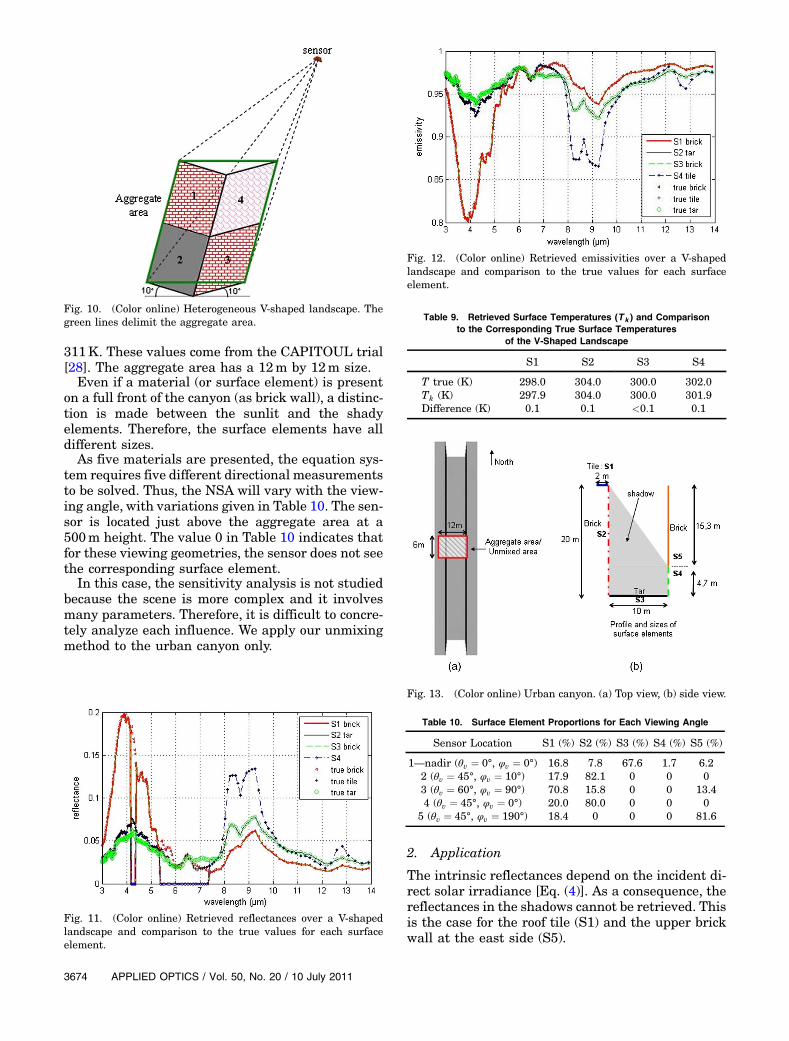
311K. These values come from the CAPITOUL trial[28]. The aggregate area has a 12m by 12m size.

Even if a material (or surface element) is presenton a full front of the canyon (as brick wall), a distinc-tion is made between the sunlit and the shadyelements. Therefore, the surface elements have alldifferent sizes.

As five materials are presented, the equation sys-tem requires five different directional measurementsto be solved. Thus, the NSA will vary with the view-ing angle, with variations given in Table 10. The sen-sor is located just above the aggregate area at a500m height. The value 0 in Table 10 indicates thatfor these viewing geometries, the sensor does not seethe corresponding surface element.

In this case, the sensitivity analysis is not studiedbecause the scene is more complex and it involvesmany parameters. Therefore, it is difficult to concre-tely analyze each influence. We apply our unmixingmethod to the urban canyon only.

2. Application

The intrinsic reflectances depend on the incident di-rect solar irradiance [Eq. (4)]. As a consequence, thereflectances in the shadows cannot be retrieved. Thisis the case for the roof tile (S1) and the upper brickwall at the east side (S5).

Fig. 10. (Color online) Heterogeneous V-shaped landscape. Thegreen lines delimit the aggregate area.

Fig. 11. (Color online) Retrieved reflectances over a V-shapedlandscape and comparison to the true values for each surfaceelement.

Fig. 12. (Color online) Retrieved emissivities over a V-shapedlandscape and comparison to the true values for each surfaceelement.

Table 9. Retrieved Surface Temperatures (T k ) and Comparisonto the Corresponding True Surface Temperatures

of the V-Shaped Landscape

S1 S2 S3 S4

T true (K) 298.0 304.0 300.0 302.0Tk (K) 297.9 304.0 300.0 301.9Difference (K) 0.1 0.1 <0:1 0.1

Fig. 13. (Color online) Urban canyon. (a) Top view, (b) side view.

Table 10. Surface Element Proportions for Each Viewing Angle

Sensor Location S1 (%) S2 (%) S3 (%) S4 (%) S5 (%)

1—nadir (θv ¼ 0°, φv ¼ 0°) 16.8 7.8 67.6 1.7 6.22 (θv ¼ 45°, φv ¼ 10°) 17.9 82.1 0 0 03 (θv ¼ 60°, φv ¼ 90°) 70.8 15.8 0 0 13.44 (θv ¼ 45°, φv ¼ 0°) 20.0 80.0 0 0 0

5 (θv ¼ 45°, φv ¼ 190°) 18.4 0 0 0 81.6


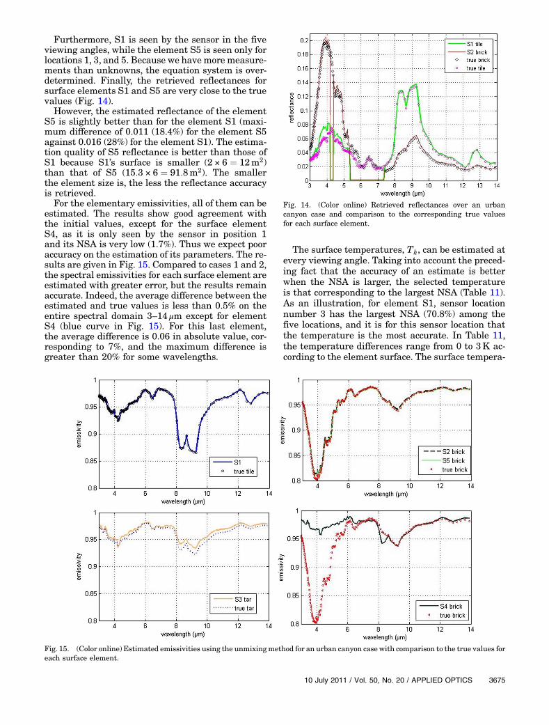
Furthermore, S1 is seen by the sensor in the fiveviewing angles, while the element S5 is seen only forlocations 1, 3, and 5. Because we havemore measure-ments than unknowns, the equation system is over-determined. Finally, the retrieved reflectances forsurface elements S1 and S5 are very close to the truevalues (Fig. 14).

However, the estimated reflectance of the elementS5 is slightly better than for the element S1 (maxi-mum difference of 0.011 (18.4%) for the element S5against 0.016 (28%) for the element S1). The estima-tion quality of S5 reflectance is better than those ofS1 because S1’s surface is smaller (2 × 6 ¼ 12m2)than that of S5 (15:3 × 6 ¼ 91:8m2). The smallerthe element size is, the less the reflectance accuracyis retrieved.

For the elementary emissivities, all of them can beestimated. The results show good agreement withthe initial values, except for the surface elementS4, as it is only seen by the sensor in position 1and its NSA is very low (1.7%). Thus we expect pooraccuracy on the estimation of its parameters. The re-sults are given in Fig. 15. Compared to cases 1 and 2,the spectral emissivities for each surface element areestimated with greater error, but the results remainaccurate. Indeed, the average difference between theestimated and true values is less than 0.5% on theentire spectral domain 3–14 μm except for elementS4 (blue curve in Fig. 15). For this last element,the average difference is 0.06 in absolute value, cor-responding to 7%, and the maximum difference isgreater than 20% for some wavelengths.

The surface temperatures, Tk, can be estimated atevery viewing angle. Taking into account the preced-ing fact that the accuracy of an estimate is betterwhen the NSA is larger, the selected temperatureis that corresponding to the largest NSA (Table 11).As an illustration, for element S1, sensor locationnumber 3 has the largest NSA (70.8%) among thefive locations, and it is for this sensor location thatthe temperature is the most accurate. In Table 11,the temperature differences range from 0 to 3K ac-cording to the element surface. The surface tempera-

Fig. 14. (Color online) Retrieved reflectances over an urbancanyon case and comparison to the corresponding true valuesfor each surface element.

Fig. 15. (Color online) Estimated emissivities using the unmixingmethod for an urban canyon case with comparison to the true values foreach surface element.


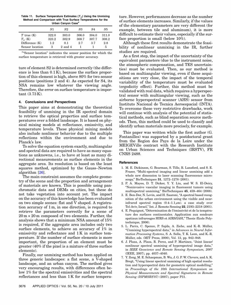
ture of element S2 is determined correctly (the differ-ence is less than 0:1K), because the surface propor-tion of this element is high, above 80% for two sensorpositions (positions 2 and 4). As expected for S4, itsNSA remains low whatever the viewing angle.Therefore, the error on surface temperature is impor-tant (3:73K).

4. Conclusions and Perspectives

This paper aims at demonstrating the theoreticalfeasibility of unmixing in the IR spectral domainto retrieve the optical properties and surface tem-peratures over a folded landscape. It is based on phy-sical mixing models at reflectance, emissivity, andtemperature levels. These physical mixing modelsalso include nonlinear behavior due to the multiplereflections within the environment and due toPlanck’s law.

To solve the equation system exactly, multiangularand spectral data are required to have as many equa-tions as unknowns, i.e., to have at least as many di-rectional measurements as surface elements in theaggregate area. Its resolution is based on the leastsquares method, optimized by the Gauss–Newtonalgorithm [26].

The main constraint assumes the complete geome-try of the scene and the proportion and arrangementof materials are known. This is possible using pan-chromatic data and DEMs on cities, but these donot take vegetation into account yet. The impacton the accuracy of this knowledge has been evaluatedon two simple scenes: flat and V shaped. A registra-tion accuracy of 1m, in one direction, is required toretrieve the parameters correctly for a scene of20m× 20m composed of two elements. Further, theanalysis shows that a minimum NSA amount of 15%is required, if the aggregate area includes only twosurface elements, to achieve an accuracy of 1% inemissivity and reflectance and 1K in surface tem-perature. If the number of surface elements is moreimportant, the proportion of an element must begreater (40% if the pixel is a mixture of three surfaceelements).

Finally, our unmixing method has been applied onthree generic landscapes: a flat scene, a V-shapedlandscape, and an urban canyon. The method givesvery encouraging results, with differences often be-low 1% for the spectral emissivities and the spectralreflectances and less than 1K for surface tempera-

ture. However, performances decrease as the numberof surface elements increases. Similarly, if the valuesof the elementary parameters are very different (forexample, between tile and aluminum), it is moredifficult to estimate their values, especially if the sur-face proportion is small (below 10%).

Although these first results demonstrate the feasi-bility of nonlinear unmixing in the IR, furtherstudies are required.

As a first step, the impact of the uncertainty of theequivalent parameters (due to the instrument noise,the atmospheric compensation, and TES uncertain-ties) must be evaluated. Then, as our method isbased on multiangular viewing, even if these acqui-sitions are very close, the impact of the temporalvariability of the temperature must be evaluated(ergodicity effect). Further, this method must bevalidated with real data, which requires a hyperspec-tral sensor with multiangular viewing, such as theairborne hyperspectral scanner (AHS) sensor fromInstituto Nacional de Tecnica Aeroespacial (INTA).To overcome these very restrictive drawbacks, workwill continue with analysis of the potential of statis-tical methods, such as blind separation source meth-ods. Then, this method could be used to classify andidentify urban materials more precisely, for example.

This paper was written while the first author (G.Fontanilles) was supported by a postdoctoral grantfrom the Region des Pays de la Loire under theMEIGEVille contract with the Research Instituteon Urban Sciences and Techniques (IRSTV), FRCNRS 2488.

References1. M. E. Dickinson, G. Bearman, S. Tille, R. Lansford, and S. E.

Fraser, “Multi-spectral imaging and linear unmixing add awhole new dimension to laser scanning fluorescence micro-scopy,” BioTechniques 31, 1272–1278 (2001).

2. P. A. Mayes, D. T. Dicker, Y. Y. Liu, and W. S. El-Deiry,“Noninvasive vascular imaging in fluorescent tumors usingmultispectral unmixing,” BioTechniques 45, 459–464 (2008).

3. E. Ben-Dor, N. Levin, and H. Saaroni, “A spectral based recog-nition of the urban environment using the visible and near-infrared spectral region (0:4–1:1 μm). a case study overTel-Aviv, Israel,” Int. J. Remote Sensing 22, 2193–2218 (2001).

4. E. Pequignot, “Détermination de l’émissivité et de la tempéra-ture des surfaces continentales. Application aux sondeursspatiaux infrarouges HIRS et AIRS/IASI,” Thesis (Ecole Poly-technique, 2006).

5. L. Parra, C. Spence, P. Sajda, A. Ziehe, and K.-R. Müller,“Unmixing hyperspectral data,” in Advances in Neural Infor-mation Processing Systems, S. A. Solla, T. K. Leen, and K.-R.Müller, eds. (MIT Press, 2000), Vol. 12, pp. 942–948.

6. J. Plaza, A. Plaza, R. Perez, and P. Martinez, “Joint linear/nonlinear spectral unmixing of hyperspectral image data,”in IEEE Geoscience and Remote Sensing Symposium, 2007(IEEE, 2007), pp. 4037–4040.

7. Y. Zeng, M. E. Schaepman, B. Wu, J. G. P. W. Clevers, and A. K.Bregt, “Using linear spectral unmixing of high spatial resolu-tion and hyperspectral data for geometric optical modelling,”in Proceedings of the 10th International Symposium onPhysical Measurements and Spectral Signatures in RemoteSensing (ISPMSRS’07) (2007), paper P31.

Table 11. Surface Temperature Estimates (T k ) Using the UnmixingMethod and Comparison with True Surface Temperatures for the

Urban Canyon Casea

S1 S2 S3 S4 S5

T true (K) 322.0 303.0 306.0 304.0 311.0Tk (K) 323.2 302.9 308.7 307.7 308.2Difference (K) 1.2 0.1 2.7 3.7 2.8Sensor location 3 2 and 4 1 1 5a“Sensor location” indicates the sensor position for which the

surface temperature is retrieved with greater accuracy.


8. P. Gong and A. Zhang, “Noise effect on linear spectralunmixing,” Ann. GIS 5, 52–57 (1999).

9. N. Dobigeon, “Choix et implantation d’une méthode d’extrac-tion de pôles de mélange dans une image hyperspectrale,”internal report (ONERA-DOTA, 2004).

10. M. Brown, S. R. Gunn, and H. G. Lewis, “Support vectormachines for optimal classification and spectral unmixing,”Ecol. Modell. 120, 167–179 (1999).

11. G. P. Asner and D. B. Lobell, “AutoSwir: a spectral unmixingalgorithm using 2000–2400nm endmembers andMonte Carloanalysis,” in Proceedings of the 9th Annual Airborne Visible/Infrared Imaging Spectrometer (AVIRIS), R. O. Green, ed. (JetPropulsion Laboratory, 2000), pp. 29–38.

12. F. Becker and Z.-L. Li, “Surface temperature and emissivity atvarious scales: definition, measurement and related prob-lems,” Remote Sens. Rev. 12, 225–253 (1995).

13. A. Guignard, G. Boulet, and B. Coudert, “Evaluation d’uneméthode statistique de désagrégation de la température desurface en vue d’un suivi régulier de l’état hydrique,” internalreport (Pierre and Marie Curie University, 2008).

14. W. P. Kustas, J. M. Norman,M. C. Anderson, and A. N. French,“Estimating subpixel surface temperature and energy fluxesfrom the vegetation index radiometric temperature relation-ship,” Remote Sens. Environ. 85, 429–440 (2003).

15. O. Merlin, B. Duchemin, O. Hagolle, F. Jacob, B. Coudert, G.Chehbouni, G. Dedieu, J. Garatuzac, and Y. Kerr, “Disaggre-gation of MODIS surface temperature over an agriculturalarea using a time series of Formosat-2 images,” Remote Sens.Environ. 114, 2500–2512 (2010).

16. G. P. Asner and D. B. Lobell, “A biogeophysical approach forautomated SWIR unmixing of soil and vegetation,” RemoteSens. Environ. 74, 99–112 (2000).

17. N. Agam, W. P. Kustas, M. C. Anderson, L. Fuqin, and C. M. U.Neale, “A vegetation index based technique for spatial shar-pening of thermal imagery,” Remote Sens. Environ. 107,545–558 (2007).

18. J. Cheng, S. Liang, J. Wang, and X. Li, “A stepwise refiningalgorithm of temperature and emissivity separation for hyper-spectral thermal infrared data,” IEEE Trans. Geosci. RemoteSens. 48, 1588–1597 (2010).

19. J.-P. Lagouarde, M. Bach, G. Boulet, X. Briottet, S. Cherchali,G. Dedieu, O. Hagolle, F. Jacob, F. Nerry, A. Olioso, C. Ottlé, V.Pascal, J.-L. Roujean, J. A. Sobrino, and F. Tintó Garcia-

Moreno, “Combining high spatial resolution and revisit cap-abilities in the thermal infrared: the MISTIGRI missionproject,” in Proceedings of EARSeL Symposium 2010(EARseL, 2010), pp. 165–172.

20. G. Fontanilles, X. Briottet, S. Fabre, S. Lefebvre, and P.-F.Vandenhaute, “Aggregation process of optical properties andtemperature over heterogeneous surfaces in the infrareddomain,” Appl. Opt. 49, 4655–4669 (2010).

21. J. M. Norman and F. Becker, “Terminology in thermal infraredremote sensing of natural surfaces,” Agric. For. Meteorol. 77,153–166 (1995).

22. S. Pallotta, “Compréhension du signal issu d’une surface hét-érogène dans le domaine infrarouge en télédétection : analysede l’agrégation des propriétés thermo-optiques de ses consti-tuants,” Ph.D. dissertation (Ecole Nationale Supérieure del’Aéronautique et de l’Espace, 2006).

23. J. E. Nichol, W. Y. Fung, K. Lam, and M. S. Wong, “Urban heatisland diagnosis using ASTER satellite images and ‘in situ’ airtemperature,” Atmos. Res. 94, 276–284 (2009).

24. D. Flamanc and G. Maillet, “Evaluation of 3D city model pro-duction from Pleiades-HR satellite images and 2D groundmaps,” presented at the 3rd International SymposiumRemoteSensing and Data Fusion Over Urban Areas/5th InternationalSymposium Remote Sensing of Urban Areas, Tempe, Ariz.,USA, 14–16 March 2005.

25. P. Deuflhard, Newton Methods for Nonlinear Problems:Affine Variance and Adaptative Algorithms, Vol. 35 ofSpringer Series in Computational Mathematics, (Springer,2004).

26. D. Marquardt, “An algorithm for least squares estimation ofnonlinear parameters,” SIAM J. Appl. Math. 11, 431–441(1963).

27. A. R. Gillespie, S. Rokugawa, S. J. Hook, T. Matsunaga, andA. B. Kahle, “Temperature/emissivity separation algorithmtheoretical basis document, version 2.4,” NASA contract(Contract NAS5-31372, 1999).

28. V. Masson, G. Pigeon, P. Durand, L. Gomes, L. Salmond,J.-P. Lagouarde, J. Voogt, T. Oke, C. Lac, C. Liousse, and D.Maro, “The Canopy and Aerosol Particles In Toulouse UrbanLayer (CAPITOUL) experiments: first results,” presented atthe 5th Symposium of the Urban Environment, AmericanMeteorological Society, Vancouver, BC, Canada, 23–26 August2004.


Documents

A nonlinear unmixing method in the infrared domain