Embed Size (px)
Citation preview
ANNALESDE LA FACULTÉ
DES SCIENCES
MathématiquesSTÉPHANE LAMY
Combinatorics of the tame automorphism group
Tome XXVIII, no 1 (2019), p. 145-207.
<http://afst.cedram.org/item?id=AFST_2019_6_28_1_145_0>
© Université Paul Sabatier, Toulouse, 2019, tous droits réservés.L’accès aux articles de la revue « Annales de la faculté des sci-ences de Toulouse Mathématiques » (http://afst.cedram.org/), impliquel’accord avec les conditions générales d’utilisation (http://afst.cedram.org/legal/). Toute reproduction en tout ou partie de cet article sous quelqueforme que ce soit pour tout usage autre que l’utilisation à fin strictementpersonnelle du copiste est constitutive d’une infraction pénale. Toute copieou impression de ce fichier doit contenir la présente mention de copyright.
cedramArticle mis en ligne dans le cadre du
Centre de diffusion des revues académiques de mathématiqueshttp://www.cedram.org/
Annales de la faculté des sciences de Toulouse Volume XXVIII, no 1, 2019pp. 145-207
Combinatorics of the tame automorphism group (∗)
Stéphane Lamy (1)
ABSTRACT. — We study the group Tame(A3) of tame automorphisms of the3-dimensional affine space, over a field of characteristic zero. We recover, in a uni-fied way, previous results of Kuroda, Shestakov, Umirbaev and Wright, about thetheory of reduction and the relations in Tame(A3). The novelty in our presentationis the emphasis on a simply connected 2-dimensional simplicial complex on whichTame(A3) acts by isometries.
RÉSUMÉ. — Nous étudions le groupe Tame(A3) des automorphismes modérés del’espace affine de dimension 3, sur un corps de caractéristique nulle. Nous retrouvons,de manière unifiée, des résultats de Kuroda, Shestakov, Umirbaev et Wright, concer-nant la théorie des réductions et les relations dans Tame(A3). La nouveauté dansnotre approche réside dans la mise en avant d’un complexe simplicial de dimension 2simplement connexe sur lequel Tame(A3) agit par isométries.
Introduction
Let k be a field, and let An = Ank be the affine space over k. We areinterested in the group Aut(An) of algebraic automorphisms of the affinespace. Concretely, we choose once and for all a coordinate system (x1, . . . , xn)for An. Then any element f ∈ Aut(An) is a map of the form
f : (x1, . . . , xn) 7→ (f1(x1, . . . , xn), . . . , fn(x1, . . . , xn)),where the fi are polynomials in n variables, such that there exists a map gof the same form satisfying f g = id. We shall abbreviate this situation bywriting f = (f1, . . . , fn), and g = f−1. Observe a slight abuse of notationhere, since we are really speaking about polynomials, and not about theassociated polynomial functions. For instance over a finite base field, the
(*) Reçu le 14 septembre 2016, accepté le 18 mars 2017.(1) Institut de Mathématiques de Toulouse, Université Paul Sabatier, 118 route de
Narbonne, 31062 Toulouse Cedex 9, France — [email protected] research was partially supported by ANR Grant “BirPol” ANR-11-JS01-004-01.Article proposé par Vincent Guedj.
– 145 –
Stéphane Lamy
group Aut(An) is infinite (for n > 2) even if there is only a finite number ofinduced bijections on the finite number of k-points of An.
The group Aut(An) contains the following natural subgroups. First wehave the affine group An = GLn(k)nkn. Secondly we have the group En ofelementary automorphisms, which have the form
f : (x1, . . . , xn) 7→ (x1 + P (x2, . . . , xn), x2, . . . , xn),
for some choice of polynomial P in n− 1 variables. The subgroup
Tame(An) = 〈An, En〉
generated by the affine and elementary automorphisms is called the subgroupof tame automorphisms.
A natural question is whether the inclusion Tame(An) ⊆ Aut(An) is infact an equality. It is a well-known result, which goes back to Jung (seee.g. [8] for a review of some of the many proofs available in the literature),that the answer is yes for n = 2 (over any base field), and it is a result byShestakov and Umirbaev [13] that the answer is no for n = 3, at least whenk is a field of characteristic zero.
The main purpose of the present paper is to give a self-contained re-worked proof of this last result: see Theorem 4.1 and Corollary 4.2. Wefollow closely the line of argument by Kuroda [7]. However, the novelty inour approach is the emphasis on a 2-dimensional simplicial complex C onwhich Tame(A3) acts by isometries. In fact, this construction is not partic-ular to the 3-dimensional case: In §1 we introduce, for any n > 2 and overany base field, a (n− 1)-dimensional simplicial complex on which Tame(An)naturally acts.
We now give an outline of the main notions and results of the paper. Sincethe paper is quite long and technical, we hope that this informal outline willserve as a guide for the reader, even if we cannot avoid being somewhatimprecise at this point.
• The 2-dimensional complex C contains three kinds of vertices, corre-sponding to three orbits under the action of Tame(A3). In this introduc-tion we shall focus on the so-called type 3 vertices, which correspond to atame automorphism (f1, f2, f3) up to post-composition by an affine auto-morphism. Such an equivalence class is denoted v3 = [f1, f2, f3] (see §1.3and Figure 1.1).
• Given a vertex v3 one can always choose a representative (f1, f2, f3)such that the top monomials of the fi are pairwise distinct. Such a goodrepresentative is not unique, but the top monomials are. This allows todefine a degree function (with values in N3) on vertices, with the identity
– 146 –
Combinatorics of the tame automorphism group
automorphism corresponding to the unique vertex of minimal degree (see§1.2).
• By construction of the complex C, two type 3 vertices v3 and v′3 areat distance 2 in C if and only if they admit representatives of the formv3 = [f1, f2, f3] and v′3 = [f1 + P (f2, f3), f2, f3], that is, representativesthat differ by an elementary automorphism. If moreover deg v3 > deg v′3, wesay that v′3 is an elementary reduction of v3. The whole idea is that it is‘almost’ true that any vertex admits a sequence of elementary reductions tothe identity. However a lot of complications lie in this ‘almost’, as we nowdiscuss.
• Some particular tame automorphisms are triangular automorphisms,of the form (up to a permutation of the variables) (x1 + P (x2, x3), x2 +Q(x3), x3). There are essentially two ways to decompose such an automor-phism as a product of elementary automorphisms, namely
(x1 + P (x2, x3), x2 +Q(x3), x3)= (x1, x2 +Q(x3), x3) (x1 + P (x2, x3), x2, x3)= (x1 + P (x2 −Q(x3), x3), x2, x3) (x1, x2 +Q(x3), x3).
This leads to the presence of squares in the complex C, see Figure 3.2. Con-versely, the fact that a given vertex admits two distinct elementary reduc-tions often leads to the presence of such a square, in particular if one of thereductions corresponds to a polynomial that depends only on one variable in-stead of two, like Q(x3) above. We call ‘simple’ such a particular elementaryreduction.
• When v′3 = [f1 + P (f2, f3), f2, f3] is an elementary reduction of v3 =[f1, f2, f3], we shall encounter the following situations (see Corollary 4.20):
(i) The most common situation is when the top monomial of f1 is thedominant one, that is, the largest among the top monomials of the fi.
(ii) Another (non-exclusive) situation is when P depends only on onevariable. As mentioned before this is typically the case when v3 admits sev-eral elementary reductions. This corresponds to the fact that the top mono-mial of a component is a power of another one, and we name ‘resonance’such a coincidence (see definition in §1.2).
(iii) Finally another situation is when f1 does not realize the dominantmonomial, but f2, f3 nevertheless satisfy a kind of minimality condition vialooking at the degree of the 2-form df2∧df3. We call this last case an elemen-tary K-reduction (see §3.3 for the definition, Corollary 3.10 for the charac-terization in terms of the minimality of deg df2 ∧ df3, and §6 for examples).This case is quite rigid (see Proposition 3.19), and at posteriori it forbids theexistence of any other elementary reduction from v3 (see Proposition 5.1).
• Finally we define (see §3.3 again) an exceptional case, under the ter-minology ‘normal proper K-reduction’, that corresponds to moving from a
– 147 –
Stéphane Lamy
vertex v3 to a neighbor vertex w3 of the same degree, and then realizing anelementary K-reduction from w3 to another vertex u3. The fact that v3 andw3 share the same degree is not part of the technical definition, but again istrue only at posteriori (see Corollary 5.2).
• Then the main result (Reducibility Theorem 4.1) is that we can go fromany vertex to the vertex corresponding to the identify by a finite sequenceof elementary reductions or normal proper K-reductions.
• The proof proceeds by a double induction on degrees which is quiteinvolved. The Induction Hypothesis is precisely stated on page 191. Theanalysis is divided into two main branches:
(i) §4.2 where the slogan is “a vertex that admits an elementary K-reduction does not admit any other reduction” (Proposition 4.19 is an inter-mediate technical statement, and Proposition 5.1 the final one);
(ii) §4.3 where the slogan is “a vertex that admits several elementaryreductions must admit some resonance” (see in particular Lemmas 4.24and 4.26).
For readers familiar with previous works on the subject, we now give a fewword about terminology. In the work of Kuroda [7], as in the original work ofShestakov and Umirbaev [13], elementary reductions are defined with respectto one of the three coordinates of a fixed coordinate system. In contrast, asexplained above, we always work up to an affine change of coordinates. In-deed our simplicial complex C is designed so that two tame automorphismscorrespond to two vertices at distance 2 in the complex if and only if theydiffer by the left composition of an automorphism of the form a1ea2, wherea1, a2 are affine and e is elementary. This slight generalization of the defi-nition of reduction allows us to absorb the so-called “type I” and “type II”reductions of Shestakov and Umirbaev in the class of elementary reductions:In our terminology they become “elementary K-reductions” (see §3.3). Onthe other hand, the “type III” reductions, which are technically difficult tohandle, are still lurking around. One can suspect that such reductions donot exist (as the most intricate “type IV” reductions which were excludedby Kuroda [7]), and an ideal proof would settle this issue. Unfortunately wewere not able to do so, and these hypothetical reductions still appear in ourtext under the name of “normal proper K-reduction”. See Example 6.5 formore comments on this issue.
One could say that the theory of Shestakov, Umirbaev and Kuroda con-sists in understanding the relations inside the tame group Tame(A3). Thiswas made explicit by Umirbaev [14], and then it was proved by Wright [16]that this can be rephrased in terms of an amalgamated product structureover three subgroups (see Corollary 5.8). In turn, it is known that such a
– 148 –
Combinatorics of the tame automorphism group
structure is equivalent to the action of the group on a 2-dimensional sim-ply connected simplicial complex, with fundamental domain a simplex. Ourapproach allows to recover a more transparent description of the relationsin Tame(A3). After stating and proving the Reducibility Theorem 4.1 in §4,we directly show in §5 that the natural complex on which Tame(A3) actsis simply connected (see Proposition 5.7), by observing that the reductionprocess of [7, 13] corresponds to local homotopies.
We should stress once more that this paper contains no original result,and consists only in a new presentation of previous works by the above citedauthors. In fact, for the sake of completeness we also include in Section 2some preliminary results where we only slightly differ from the original arti-cles [5, 12].
Our motivation for reworking this material is to prepare the way for newresults about Tame(A3), such as the linearizability of finite subgroups, theTits alternative or the acylindrical hyperbolicity. From our experience inrelated settings (see [1, 3, 10, 11]), such results should follow from some non-positive curvature properties of the simplicial complex. We plan to explorethese questions in some follow-up papers (see [9] for a first step).
Acknowledgement
In August 2010 I was assigned the paper [7] as a reviewer for MathSciNet.I took this opportunity to understand in full detail his beautiful proof, andin November of the same year, at the invitation of Adrien Dubouloz, I gavesome lectures in Dijon on the subject. I thank all the participants of thisstudy group “Automorphismes des Espaces Affines”, and particularly JérémyBlanc, Eric Edo, Pierre-Marie Poloni and Stéphane Vénéreau who gave meuseful feedback on some early version of these notes.
A few years later I embarked on the project to rewrite this proof focusingon the related action on a simplicial complex. At the final stage of the presentversion, when I was somehow loosing faith in my endurance, I greatly ben-efited from the encouragements and numerous suggestions of Jean-PhilippeFurter.
Finally, I am of course very much indebted to Shigeru Kuroda. Indeedwithout his work the initial proof of [13] would have remained a mysteriousblack box to me.
– 149 –
Stéphane Lamy
1. Simplicial complex
We define a (n − 1)-dimensional simplicial complex on which the tameautomorphism group of An acts. This construction makes sense in any di-mension n > 2, over any base field k.
1.1. General construction
For any 1 6 r 6 n, we call r-tuple of components a morphismf : An → Ar
x = (x1, . . . , xn) 7→ (f1(x), . . . , fr(x))that can be extended as a tame automorphism f = (f1, . . . , fn) of An. Onedefines n distinct types of vertices, by considering r-tuple of componentsmodulo composition by an affine automorphism on the range, r = 1, . . . , n.We use a bracket notation to denote such an equivalence class:
[f1, . . . , fr] := Ar(f1, . . . , fr) = a (f1, . . . , fr); a ∈ Arwhere Ar = GLr(k) n kr is the r-dimensional affine group. We say thatvr = [f1, . . . , fr] is a vertex of type r, and that (f1, . . . , fr) is a representativeof vr. We shall always stick to the convention that the index corresponds tothe type of a vertex: for instance vr, v′r, ur, wr,mr will all be possible notationfor a vertex of type r.
Now given n vertices v1, . . . , vn of type 1, . . . , n, we attach a standard Eu-clidean (n−1)-simplex on these vertices if there exists a tame automorphism(f1, . . . , fn) ∈ Tame(An) such that for all i ∈ 1, . . . , n:
vi = [f1, . . . , fi].We obtain a (n − 1)-dimensional simplicial complex Cn on which the tamegroup acts by isometries, by the formulas
g · [f1, . . . , fr] := [f1 g−1, . . . , fr g−1].
Lemma 1.1. — The group Tame(An) acts on Cn with fundamental do-main the simplex
[x1], [x1, x2], . . . , [x1, . . . , xn].In particular the action is transitive on vertices of a given type.
Proof. — Let v1, . . . , vn be the vertices of a simplex (recall that the in-dex corresponds to the type). By definition there exists f = (f1, . . . fn) ∈Tame(An) such that vi = [f1, . . . , fi] for each i. Then
[x1, . . . , xi] = [(f1, . . . , fi) f−1] = f · vi.
– 150 –
Combinatorics of the tame automorphism group
Remark 1.2. — (1) One could make a similar construction by workingwith the full automorphism group Aut(An) instead of the tame group. Thecomplex Cn we consider is the gallery connected component of the standardsimplex [x1], [x1, x2], . . . , [x1, . . . , xn] in this bigger complex. See [1, §6.2.1]for more details.
(2) When n = 2, the previous construction yields a graph C2. It is notdifficult to show (see [1, §2.5.2]) that C2 is isomorphic to the classical Bass-Serre tree of Aut(A2) = Tame(A2).
1.2. Degrees
We shall compare polynomials in k[x1, . . . , xn] by using the graded lex-icographic order on monomials. We find it more convenient to work withan additive notation, so we introduce the degree function, with value inNn ∪ −∞, by taking
deg xa11 xa2
2 . . . xann = (a1, a2, . . . , an)
and by convention deg 0 = −∞. We extend this order to Qn ∪ −∞, sincesometimes it is convenient to consider difference of degrees, or degrees mul-tiplied by a rational number. The top term of g ∈ k[x1, . . . , xn] is theuniquely defined g = cxd1
1 . . . xdnn such that
(d1, . . . , dn) = deg g > deg(g − g).Observe that two polynomials f, g ∈ k[x1, . . . , xn] have the same degree ifand only if their top terms f , g are proportional. If f = (f1, . . . , fr) is ar-tuple of components, we call top degree of f the maximum of the degreeof the fi:
topdeg f := max deg fi ∈ Nn.
Lemma 1.3. — Let f = (f1, . . . , fr) be a r-tuple of components, andconsider V ⊂ k[x1, . . . , xn] the vector space generated by the fi. Then
(1) The set H of elements g ∈ V satisfying topdeg f > deg g is a hy-perplane in V ;
(2) There exist a sequence of degrees δr > · · · > δ1 and a flag of sub-spaces V1 ⊂ · · · ⊂ Vr = V such that dimVi = i and deg g = δi forany g ∈ Vi r Vi−1.
Proof. —
(1) Up to permuting the fi we can assume topdeg f = deg fr. Then foreach i = 1, . . . , r−1 there exists a unique ci ∈ k such that deg fr > deg(fi+cifr). The conclusion follows from the observation that an element of V isin H if and only if it is a linear combination of the fi+ cifr, i = 1, . . . , r− 1.
– 151 –
Stéphane Lamy
(2) Immediate, by induction on dimension.
Using the notation of the lemma, we call r-deg f = (δ1, . . . , δr) the r-degree of f , and deg f =
∑ri=1 δi ∈ Nn the degree of f . Observe that for
any affine automorphism a ∈ Ar we have r-deg f = r-deg(a f), so we geta well-defined notion of r-degree and degree for any vertex of type r.
If vr = [f1, . . . , fr] ∈ Cn with the deg fi pairwise distinct, we say that f isa good representative of vr (we do not ask deg fr > · · · > deg f2 > deg f1).We use a double bracket notation such as v2 = [[f1, f2]] or v3 = [[f1, f2, f3]],to indicate that we are using a good representative.
Lemma 1.4. — Let v1, . . . , vn be a (n − 1)-simplex in Cn. Then thereexists f = (f1, . . . , fn) ∈ Tame(An) such that vi = [[f1, . . . , fi]] for eachn > i > 1.
Proof. — We pick f1 such that v1 = [[f1]], and we define the other fi byinduction as follows. If the i-degree of vi = [[f1, . . . , fi]] is (δ1, . . . , δi) (recallthat by definition the δj are equal to the degrees of the fj only up to apermutation), then there exist δ ∈ N3 and i + 1 > s > 1 such that the(i+ 1)-degree of vi+1 is (δ1, . . . , δs−1, δ, δs, . . . , δi). That exactly means thatthere exists fi+1 of degree δ such that vi+1 = [[f1, . . . , fi+1]].
1.3. The complex in dimension 3
Now we specialize the general construction to the dimension n = 3, whichis our main interest in this paper. We drop the index and simply denote by Cthe 2-dimensional simplicial complex associated to Tame(A3). To get a firstfeeling of the complex one can draw pictures such as Figure 1.1, where weuse the following convention for vertices: , • or corresponds respectivelyto a vertex of type 1, 2 and 3. However one should keep in mind, as thefollowing formal discussion makes it clear, that the complex is not locallyfinite. A first step in understanding the geometry of the complex C is tounderstand the link of each type of vertex. In fact, we will now see that ifthe base field k is uncountable, then the link of any vertex or any edge alsohas uncountably many vertices.
Consider first the link L(v3) of a vertex of type 3. By transitivity of theaction of Tame(A3), it is sufficient to describe the link L([id]). A vertex oftype 1 at distance 1 from [id] has the form [a1x1 + a2x2 + a3x3] where theai ∈ k are uniquely defined up to a common multiplicative constant. In otherwords, vertices of type 1 in L([id]) are parametrized by P2. We denote byP2(v3) this projective plane of vertices of type 1 in the link of v3. Similarly,vertices of type 2 in L(v3) correspond to lines in P2(v3), that is, to points in
– 152 –
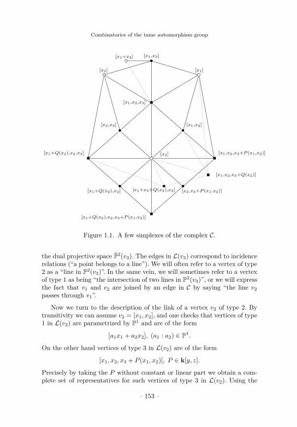
Combinatorics of the tame automorphism group
•
•
•
•
•
•
[x1,x2,x3]
[x2,x3]
[x1+Q(x2),x2,x3]
[x1+Q(x2),x2]
[x1+Q(x2),x2,x3+P (x1,x2)]
[x2,x3+P (x1,x2)]
[x1,x2,x3+P (x1,x2)]
[x1,x2]
[x2]
[x3]
[x1,x3]
[x1]
[x1+x3+Q(x2),x2]
[x1,x2,x3+Q(x2)]
[x1+x3]
Figure 1.1. A few simplexes of the complex C.
the dual projective space P2(v3). The edges in L(v3) correspond to incidencerelations (“a point belongs to a line”). We will often refer to a vertex of type2 as a “line in P2(v3)”. In the same vein, we will sometimes refer to a vertexof type 1 as being “the intersection of two lines in P2(v3)”, or we will expressthe fact that v1 and v2 are joined by an edge in C by saying “the line v2passes through v1”.
Now we turn to the description of the link of a vertex v2 of type 2. Bytransitivity we can assume v2 = [x1, x2], and one checks that vertices of type1 in L(v2) are parametrized by P1 and are of the form
[a1x1 + a2x2], (a1 : a2) ∈ P1.
On the other hand vertices of type 3 in L(v2) are of the form
[x1, x2, x3 + P (x1, x2)], P ∈ k[y, z].
Precisely by taking the P without constant or linear part we obtain a com-plete set of representatives for such vertices of type 3 in L(v2). Using the
– 153 –
Stéphane Lamy
transitivity of the action of Tame(A3) on vertices of type 2, the followinglemma and its corollary are then immediate:
Lemma 1.5. — The link L(v2) of a vertex of type 2 is the complete bi-partite graph between vertices of type 1 and 3 in the link.
Corollary 1.6. — Let v2 = [f1, f2] and v3 = [f1, f2, f3] be vertices oftype 2 and 3. Then any vertex u3 distinct from v3 such that v2 ∈ P2(u3) hasthe form
u3 = [f1, f2, f3 + P (f1, f2)]where P ∈ k[y, z] is a non-affine polynomial in two variables (that is, not ofthe form P (y, z) = ay+ bz+ c). In particular, v2 is the unique type 2 vertexin P2(v3) ∩ P2(u3).
The link of a vertex of type 1 is more complicated. Let us simply mentionwithout proof, since we won’t need it in this paper (but see Lemma 5.6 for apartial result, and also [9, §3]), that in contrast with the case of vertices oftype 2 or 3, the link of a vertex of type 1 is a connected unbounded graph,which admits a projection to an unbounded tree.
2. Parachute Inequality and Principle of Two Maxima
We recall here two results from [5] (in turn they were adaptations from [12,13]). The Parachute Inequality is the most important; we also recall somedirect consequences. From now on k denotes a field of characteristic zero.
2.1. Degree of polynomials and forms
Recall that we define a degree function on k[x1, x2, x3] with value inN3∪−∞ by taking deg xa1
1 xa22 xa3
3 = (a1, a2, a3) and by convention deg 0 =−∞. We compare degrees using the graded lexicographic order.
We now introduce the notion of virtual degree in two distinct situations,which should be clear by context.
Let g ∈ k[x1, x2, x3], and ϕ =∑i∈I Piy
i ∈ k[x1, x2, x3][y] where Pi 6= 0for all i ∈ I, that is, I is the support of ϕ. We define the virtual degree of ϕwith respect to g as
degvirt ϕ(g) := maxi∈I
(degPigi) = maxi∈I
(degPi + i deg g).
– 154 –
Combinatorics of the tame automorphism group
Denoting by I ⊆ I the subset of indexes i that realize the maximum, we alsodefine the top component of ϕ with respect to g as
ϕg :=∑i∈I
Piyi.
Similarly if g, h ∈ k[x1, x2, x3], and ϕ =∑
(i,j)∈S ci,jyizj ∈ k[y, z] with
support S, we define the virtual degree of ϕ with respect to g and h as
degvirt ϕ(g, h) := max(i,j)∈S
deg gihj = max(i,j)∈S
(ideg g + j deg h).
Observe that ϕ(g, h) can be seen either as an element coming fromϕh(y) := ϕ(y, h) ∈ k[h][y] ⊂ k[x1, x2, x3][y] or from ϕ(y, z) ∈ k[y, z], andthat the two possible notions of virtual degree coincide:
degvirt ϕh(g) = degvirt ϕ(g, h).
Example 2.1. — In general we have degvirt ϕ(g) > degϕ(g) anddegvirt ϕ(g, h) > degϕ(g, h). We now give two simple examples where theseinequalities are strict.
(1) Let ϕ = x23y − x3y
2, and g = x3. Then ϕ(g) = 0, but
degvirt ϕ(g) = deg x33 = (0, 0, 3).
(2) Let ϕ = y2 − z3, and g = x31, h = x2
1. Then ϕ(g, h) = 0, but
degvirt ϕ(g, h) = deg x61 = (6, 0, 0).
We extend the notion of degree to algebraic differential forms. Given
ω =∑
fi1,··· ,ikdxi1 ∧ · · · ∧ dxik
where k = 1, 2 or 3 and fi1,··· ,ik ∈ k[x1, x2, x3], we define
degω := maxdeg fi1,··· ,ikxi1 · · ·xik ∈ N3 ∪ −∞.
We gather some immediate remarks for future reference (observe thathere we use the assumption char k = 0).
Lemma 2.2. — If ω, ω′ are forms, and g is a non constant polynomial,we have
degω + degω′ > degω ∧ ω′;deg g = deg dg;
deg gω = deg g + degω.
– 155 –
Stéphane Lamy
2.2. Parachute Inequality
If ϕ ∈ k[x1, x2, x3][y], we denote by ϕ(n) ∈ k[x1, x2, x3][y] the nth deriv-ative of ϕ with respect to y. We simply write ϕ′ instead of ϕ(1).
Lemma 2.3. — Let ϕ ∈ k[x1, x2, x3][y] and g ∈ k[x1, x2, x3]. Then:
(1) If degy ϕg > 1, then degvirt ϕ′(g) = degvirt ϕ(g)− deg g.
(2) If degy ϕg > j > 1, then ϕ(j)g = (ϕg)(j).
Proof. — We note as before
ϕ =∑i∈I
Piyi, ϕg =
∑i∈I
Piyi and ϕ′ =
∑i∈Ir0
iPiyi−1,
where I is the support of ϕ, and I ⊆ I is the subset of indexes i that realizethe maximum maxi∈I(degPi + i deg g).
Now if degy ϕg > 1, that is, if I 6= 0, then the indexes in I r 0 areprecisely those that realize the maximum maxi∈Ir0(degPi+ (i−1) deg g).Thus we get assertion (1), and ϕ′g = (ϕg)′. Assertion (2) for j > 2 followsby induction.
Lemma 2.4. — Let ϕ ∈ k[x1, x2, x3][y] and g ∈ k[x1, x2, x3]. Then, form > 0, the following two assertions are equivalent:
(1) For j = 0, . . . ,m− 1 we have degvirt ϕ(j)(g) > degϕ(j)(g), but
degvirt ϕ(m)(g) = degϕ(m)(g).
(2) There exists ψ ∈ k[x1, x2, x3][y] such that ψ(g) 6= 0 and
ϕg = (y − g)m · ψ.
Proof. — Observe that we have the equivalences
degvirt ϕ(g) > degϕ(g) ⇐⇒ ϕg(g) = 0 ⇐⇒ y − g divides ϕg. (2.1)
First we prove (2) ⇒ (1). Assuming (2), by Lemma 2.3(2) we haveϕ(j)g = (ϕg)(j) for j = 0, . . . ,m − 1. The second equivalence in (2.1) yields(ϕg)(j)(g) = 0 for j = 0, . . . ,m − 1, and (ϕg)(m)(g) 6= 0, and then the firstequivalence gives the result.
To prove (1) ⇒ (2), it is sufficient to show that if degvirt ϕ(j)(g) >
degϕ(j)(g) for j = 0, . . . , k − 1, then ϕg = (y − g)k · ψk for some ψk ∈k[x1, x2, x3][y]. The remark (2.1) gives it for k = 1. Moreover, by Lemma 2.3(2),if ϕg depends on y then ϕ′g = (ϕg)′, hence the result by induction.
– 156 –
Combinatorics of the tame automorphism group
In the situation of Lemma 2.4, we call the integer m the multiplicity ofϕ with respect to g, and we denote it by m(ϕ, g). In other words, the topterm g is a multiple root of ϕg of order m(ϕ, g).
Following Vénéreau [15], where a similar inequality is proved, we call thenext result a “Parachute Inequality”. Indeed its significance is that the realdegree cannot drop too much with respect to the virtual degree. However wefollow Kuroda for the proof.
Recall that (over a field k of characteristic zero) some polynomialsf1, · · · , fr ∈ k[x1, . . . , xn] are algebraically independent if and only if df1 ∧· · ·∧dfr 6= 0. Indeed this is equivalent to asking that the map f = (f1, . . . , fr)from An to Ar is dominant, which in turn is equivalent to saying that thedifferential of this map has maximal rank on an open set of An (for detailssee for instance [4, Theorem III p 135]).
Proposition 2.5 (Parachute Inequality, see [5, Theorem 2.1]). — Letr = 2 or 3, and let f1, · · · , fr ∈ k[x1, x2, x3] be algebraically independent.Let ϕ ∈ k[f2, · · · , fr][y] r 0. Then
degϕ(f1) > degvirt ϕ(f1)−m(ϕ, f1)(degω + deg f1 − deg df1 ∧ ω).
where ω = df2 if r = 2, or ω = df2 ∧ df3 if r = 3.
Proof. — Denoting as before ϕ′ the derivative of ϕ with respect to y, wehave
d(ϕ(f1)) = ϕ′(f1)df1 + other terms involving df2 or df3.
So we obtain d(ϕ(f1)) ∧ ω = ϕ′(f1)df1 ∧ ω. Using Lemma 2.2 this yields
degϕ(f1) + degω = deg d(ϕ(f1)) + degω > deg d(ϕ(f1)) ∧ ω= degϕ′(f1)df1 ∧ ω = degϕ′(f1) + deg df1 ∧ ω,
which we can write as
− deg df1 ∧ ω + degω + degϕ(f1) > degϕ′(f1). (2.2)
Now we are ready to prove the inequality of the statement, by inductionon m(ϕ, f1).
If m(ϕ, f1) = 0, that is, if degϕ(f1) = degvirt ϕ(f1), there is nothing todo.
If m(ϕ, f1) > 1, it follows from Lemma 2.4 that m(ϕ′, f1) = m(ϕ, f1)−1.Moreover, the condition m(ϕ, f1) > 1 implies that ϕf1 does depend on y,hence by Lemma 2.3(1) we have
degvirt ϕ′(f1) = degvirt ϕ(f1)− deg f1.
– 157 –
Stéphane Lamy
By induction hypothesis, we havedegϕ′(f1) > degvirt ϕ
′(f1)−m(ϕ′, f1)(degω + deg f1 − deg df1 ∧ ω)= degvirt ϕ(f1)− deg f1
− (m(ϕ, f1)− 1)(degω + deg f1 − deg df1 ∧ ω)= degvirt ϕ(f1)−m(ϕ, f1)(degω + deg f1 − deg df1 ∧ ω)− deg df1 ∧ ω + degω.
Combining with (2.2), and canceling the terms −deg df1∧ω+ degω on eachside, one obtains the expected inequality.
2.3. Consequences
We shall use the Parachute Inequality 2.5 mostly when r = 2, and whenwe have a strict inequality degvirt ϕ(f1, f2) > degϕ(f1, f2). In this contextthe following easy lemma is crucial. Ultimately this is here that lies thedifficulty when one tries to extend the theory in dimension 4 (or more!).
Lemma 2.6. — Let f1, f2 ∈ k[x1, x2, x3] be algebraically independent,and ϕ ∈ k[y, z] such that degvirt ϕ(f1, f2) > degϕ(f1, f2). Then:
(1) There exist coprime p, q ∈ N∗such thatp deg f1 = q deg f2.
In particular, there exists δ ∈ N3 such that deg f1 = qδ, deg f2 = pδ,so that the top terms of fp1 and fq2 are equal up to a constant: thereexists c ∈ k such that fp1 = cfq2 .
(2) Considering ϕ(f1, f2) as coming from ϕ(y, f2) ∈ k[x1, x2, x3][y], wehave
ϕf1 = (yp − fp1 )m(ϕ,f1) · ψ = (yp − cfq2 )m(ϕ,f1) · ψfor some ψ ∈ k[x1, x2, x3][y].
Proof. —
(1) We write ϕ(f1, f2) =∑ci,jf
i1fj2 . Since degvirt ϕ(f1, f2) > degϕ(f1, f2),
there exist distinct (a, b) and (a′, b′) such that
deg fa1 f b2 = deg fa′
1 fb′
2 = degvirt ϕ(f1, f2).Moreover we can assume that a, a′ are respectively maximal and minimalfor this property. We obtain
(a− a′) deg f1 = (b′ − b) deg f2.
Dividing by m, the GCD of a− a′ and b′ − b, we get the expected relation.
– 158 –
Combinatorics of the tame automorphism group
(2) With the same notation, we have a = a′ + pm where m > 1, and inparticular degy ϕ(y, f2) > p. So if p > degy P (y, f2) for some P ∈ k[f2][y],we have degvirt P (f1, f2) = degP (f1, f2). By the first assertion, there existsc ∈ k such that deg fp1 > deg (fp1 − cf
q2 ). By successive Euclidean divisions
in k[f2][y] we can write:
ϕ(y, f2) =∑
Ri(y) (yp − cfq2 )i
with p > degy Ri for all i. Denote by I the subset of indexes such that
ϕf1 =∑i∈I
Rif1 (
yp − cfq2)i. (2.3)
Let i0 be the minimal index in I. We want to prove that i0 > m(ϕ, f1).By contradiction, assume that m(ϕ, f1) > i0. Since y − f1 is a simple factorof (yp − cfq2 ) = (yp − fp1 ), and is not a factor of any Ri
f1 , we obtain that(y − f1)i0+1 divides all summands of (2.3) except Ri0
f1(yp − cfq2 )i0 . In par-ticular (y − f1)i0+1, hence also (y − f1)m(ϕ,f1), do not divide ϕf1 : This is acontradiction with Lemma 2.4.
We now list some consequences of the Parachute Inequality 2.5.
Corollary 2.7. — Let f1, f2 ∈ k[x1, x2, x3] be algebraically indepen-dent with deg f1 > deg f2, and ϕ ∈ k[y, z] such that degvirt ϕ(f1, f2) >degϕ(f1, f2). Following Lemma 2.6, we write pdeg f1 = q deg f2 where p, q ∈N∗ are coprime. Then:
(1) degϕ(f1, f2) > p deg f1 − deg f1 − deg f2 + deg df1 ∧ df2;(2) If deg f1 6∈ Ndeg f2, then degϕ(f1, f2) > deg df1 ∧ df2;(3) Assume deg f1 6∈ N deg f2 and deg f1 > degϕ(f1, f2). Then p = 2,
q > 3 is odd, and
degϕ(f1, f2) > deg f1 − deg f2 + deg df1 ∧ df2.
If moreover deg f2 > degϕ(f1, f2), then q = 3.(4) Assume deg f1 6∈ N deg f2 and deg f1 > degϕ(f1, f2). Then
deg d(ϕ(f1, f2)) ∧ df2 > deg f1 + deg df1 ∧ df2.
Proof. —
(1) By Lemma 2.6(2), we have
degvirt ϕ(f1, f2) > m(ϕ, f1)p deg f1. (2.4)
On the other hand the Parachute Inequality 2.5 applied to ϕ(y, f2) ∈ k[f2][y]yields
degϕ(f1, f2) > degvirt ϕ(f1, f2)−m(ϕ, f1)(deg f1 + deg f2 − deg df1 ∧ df2).
– 159 –
Stéphane Lamy
Combining with (2.4), and remembering that m(ϕ, f1) > 1, we obtain
degϕ(f1, f2) > degϕ(f1, f2)m(ϕ, f1) > p deg f1 − deg f1 − deg f2 + deg df1 ∧ df2.
(2) From Lemma 2.6 we have deg f1 = qδ and deg f2 = pδ for someδ ∈ N3. The inequality (1) gives
degϕ(f1, f2) > p deg f1 − deg f1 − deg f2 + deg df1 ∧ df2 =(pq − p− q)δ + deg df1 ∧ df2. (2.5)
The assumption deg f1 6∈ N deg f2 implies q > p > 2. Thus pq − p − q > 0,and finally
degϕ(f1, f2) > deg df1 ∧ df2.
(3) Again the assumptions imply q > p > 2. Since qδ = deg f1 >degϕ(f1, f2), we get from (2.5) that q > pq − p − q. This is only possi-ble if p = 2, and so q > 3 is odd. Replacing p by 2 in (2.5), we get theinequality.
If deg f2 > degϕ(f1, f2), we obtain 2δ > (q − 2)δ, hence q = 3.
(4) Denote ϕ(y, z) =∑ci,jy
izj , and consider the partial derivatives
ϕ′y(y, z) =∑
ici,jyi−1zj ;
ϕ′z(y, z) =∑
jci,jyizj−1.
We have d(ϕ(f1, f2)) = ϕ′y(f1, f2)df1 + ϕ′z(f1, f2)df2. In particulard(ϕ(f1, f2)) ∧ df2 = ϕ′y(f1, f2)df1 ∧ df2, and
deg d(ϕ(f1, f2)) ∧ df2 = degϕ′y(f1, f2) + deg df1 ∧ df2.
Now we consider ϕ′y(f1, f2) as coming from ϕ′y(y, f2) ∈ k[f2][y], and wesimply write ϕ′(f1) instead of ϕ′y(f1, f2), in accordance with the conven-tion for derivatives introduced at the beginning of §2.2. We want to showdegϕ′(f1) > deg f1. Recall that by (2.4), degvirt ϕ(f1) > 2m(ϕ, f1) deg f1,and so, using also Lemma 2.3(1):
degvirt ϕ′(f1) = degvirt ϕ(f1)− deg f1 > 2(m(ϕ, f1)− 1) deg f1 + deg f1.
The Parachute Inequality 2.5 then gives (for the last inequality recall thatdeg f1 > deg f2 by assumption):degϕ′(f1) > degvirt ϕ
′(f1)−m(ϕ′, f1)(deg f1 + deg f2 − deg df1 ∧ df2)> 2(m(ϕ, f1)− 1) deg f1 + deg f1
− (m(ϕ, f1)− 1)(deg f1 + deg f2 − deg df1 ∧ df2)= (m(ϕ, f1)− 1)(deg f1 − deg f2 + deg df1 ∧ df2) + deg f1
> deg f1.
– 160 –
Combinatorics of the tame automorphism group
Corollary 2.8. — Let f1, f2, f3 ∈ k[x1, x2, x3] be algebraically inde-pendent, and ϕ ∈ k[y, z] such that
degvirt ϕ(f1, f2) > degϕ(f1, f2),degvirt ϕ(f1, f2) > deg f3.
Following Lemma 2.6, we write p deg f1 = q deg f2 where p, q ∈ N∗ arecoprime. Then
deg(f3 + ϕ(f1, f2)) > pdeg f1 − deg df2 ∧ df3 − deg f1,
Proof. — The Parachute Inequality 2.5 applied to ψ = f3 + ϕ(y, f2) ∈k[f2, f3][y] gives
deg(f3 + ϕ(f1, f2)) > degvirt ψ(f1)−m(ψ, f1)(deg df2 ∧ df3 + deg f1 − deg df1 ∧ df2 ∧ df3). (2.6)
By assumption degvirt ϕ(f1, f2) > deg f3. Thus not only degvirt ψ(f1) =degvirt ϕ(f1), but also ψ
f1 = ϕf1 , hence m(ψ, f1) = m(ϕ, f1) > 1. ByLemma 2.6(2), we obtain
degvirt ψ(f1) > m(ϕ, f1)p deg f1 = m(ψ, f1)p deg f1
Replacing in (2.6), and dividing by m(ψ, f1), we get the result.
2.4. Principle of Two Maxima
The proof of the next result, which we call the “Principle of Two Max-ima”, is one of the few places where the formalism of Poisson brackets usedby Shestakov and Umirbaev seems to be more transparent (at least for us)than the formalism of differential forms used by Kuroda. In this section wepropose a definition that encompasses the two points of view, and then werecall the proof following [12, Lemma 5].
Proposition 2.9 (Principle of Two Maxima, [5, Theorem 5.2] and [12,Lemma 5]). — Let (f1, f2, f3) be an automorphism of A3. Then the maxi-mum between the following three degrees is realized at least twice:
deg f1 + deg df2 ∧ df3, deg f2 + deg df1 ∧ df3, deg f3 + deg df1 ∧ df2.
Let Ω be the space of algebraic 1-forms∑fidgi where fi, gi ∈ k[x1, x2, x3].
We consider Ω as a free module of rank three over k[x1, x2, x3], with basisdx1, dx2, dx3, and we denote by
T =∞⊕p=0
Ω⊗p
– 161 –
Stéphane Lamy
the associative algebra of tensorial powers of Ω, where as usual Ω⊗0 =k[x1, x2, x3]. The degree function on Ω extends naturally to a degree functionon T. Recall that T has a natural structure of Lie algebra: For any ω, µ ∈ T,we define their bracket as
[ω, µ] := ω ⊗ µ− µ⊗ ω.In particular, if df, dg ∈ Ω are 1-forms, we have
[df, dg] = df ⊗ dg − dg ⊗ df = df ∧ dg.It is easy to check that the bracket satisfies the Jacobi identity: For anyα, β, γ ∈ T, we have
[[α, β], γ] + [[β, γ], α] + [[γ, α], β]= α⊗ β ⊗ γ − β ⊗ α⊗ γ − γ ⊗ α⊗ β + γ ⊗ β ⊗ α+ β ⊗ γ ⊗ α− γ ⊗ β ⊗ α− α⊗ β ⊗ γ + α⊗ γ ⊗ β+ γ ⊗ α⊗ β − α⊗ γ ⊗ β − β ⊗ γ ⊗ α+ β ⊗ α⊗ γ= 0
since each one of the six possible permutations appears twice, with differentsigns.
Lemma 2.10. — The nine elements [dxi ∧ dxj , dxk], for 1 6 i < j 6 3and 1 6 k 6 3 generate a 8-dimensional free submodule in T, the onlyrelation between them being the Jacobi identity:
[dx1 ∧ dx2, dx3] + [dx2 ∧ dx3, dx1]− [dx1 ∧ dx3, dx2] = 0.
Proof. — We work inside the 27-dimensional free sub-module of T gen-erated by the dxi ⊗ dxj ⊗ dxk for 1 6 i, j, k 6 3. We compute, for i < j:[dxi ∧ dxj , dxi] = [dxi ⊗ dxj − dxj ⊗ dxi, dxi]
= 2dxi ⊗ dxj ⊗ dxi − dxj ⊗ dxi ⊗ dxi − dxi ⊗ dxi ⊗ dxj ,[dxi ∧ dxj , dxj ] = [dxi ⊗ dxj − dxj ⊗ dxi, dxj ]
= −2dxj ⊗ dxi ⊗ dxj + dxi ⊗ dxj ⊗ dxj + dxj ⊗ dxj ⊗ dxi.This shows that the elements [dxi ∧ dxj , dxi] and [dxi ∧ dxj , dxj ], for i < j,generate a 6-dimensional free submodule. On the other hand, for i, j, k =1, 2, 3:
[dxi ∧ dxj , dxk] = [dxi ⊗ dxj − dxj ⊗ dxi, dxk]= dxi⊗ dxj ⊗ dxk − dxj ⊗ dxi⊗ dxk − dxk ⊗ dxi⊗ dxj + dxk ⊗ dxj ⊗ dxi,so that [dx1 ∧ dx2, dx3] and [dx2 ∧ dx3, dx1] are independent, and togetherwith the above family they generate a 8-dimensional free submodule.
The proof of the Principle of Two Maxima 2.9 now follows from theobservation:
– 162 –
Combinatorics of the tame automorphism group
Lemma 2.11. — Let f, g, h ∈ k[x1, x2, x3], with h non-constant. Then
deg [[df, dg] , dh] = deg h+ deg df ∧ dg.
Proof. — We havedh =
∑16k63
∂h∂xk
dxk
and[df, dg] = df ∧ dg =
∑16i<j63
(∂f∂xi
∂g∂xj− ∂f
∂xj
∂g∂xi
)dxi ∧ dxj .
Thus
[[df, dg], dh] =∑
16k63
∑16i<j63
∂h∂xk
(∂f∂xi
∂g∂xj− ∂f
∂xj
∂g∂xi
)[dxi ∧ dxj , dxk] .
If the degree of dh is realized by at most two of the terms ∂h∂xk
dxk, k = 1, 2, 3,then by Lemma 2.10 the terms realizing the maximum of the degrees
deg(∂h∂xk
(∂f∂xi
∂g∂xj− ∂f
∂xj
∂g∂xi
)[dxi ∧ dxj , dxk]
)(2.7)
are independent (because at most two of them occur in the Jacobi relation),hence the result since deg [dxi ∧ dxj , dxk] = deg xixjxk.
On the other hand if the three terms ∂h∂xk
dxk have the same degree, thenamong the indexes (i, j, k) that realize the maximum of the degrees in (2.7),we must find some with k = i or k = j, hence again we get the conclusionsince by Lemma 2.10 such terms cannot cancel each other.
Proof of the Principle of Two Maxima 2.9. — Since by the Jacobi iden-tity
[[df1, df2], df3] + [[df2, df3], df1] + [[df3, df1], df2] = 0,the dominant terms must cancel each other. In particular the maximum ofthe degrees, which are computed in Lemma 2.11, is realized at least twice:This is the five lines proof of the Principle of Two Maxima by Shestakov andUmirbaev!
3. Geometric theory of reduction
In this section we mostly follow Kuroda [7], but we reinterpret his theoryof reduction in a combinatorial way, using the complex C. Recall that k is afield of characteristic zero.
– 163 –
Stéphane Lamy
3.1. Degree of automorphisms and vertices
Recall that in §1.2 we defined a notion of degree for an automorphismf = (f1, f2, f3) ∈ Tame(A3). The point is that we want a degree that isadapted to the theory of reduction of Kuroda, so for instance taking themaximal degree of the three components of an automorphism is not good,because we would not detect a reduction of the degree on one of the two lowercomponents (such reductions do exist, see §6). We also want a definition thatis adapted to working on the complex C, so directly taking the sum of thedegree of the three components is no good either, since it would not give adegree function on vertices of C.
Recall that the 3-degree of f ∈ Tame(A3), or of the vertex v3 = [f ], isthe triple (δ1, δ2, δ3) given by Lemma 1.3, where in particular δ3 > δ2 > δ1.By definition the top degree of v3 is δ3 ∈ N3, and the degree of v3 is thesum
deg v3 := δ1 + δ2 + δ3 ∈ N3.
Similarly we have a 2-degree (ν1, ν2) associated with any vertex v2 of type 2,a top degree equal to ν2 and a degree deg v2 := ν1 + ν2. Finally for a vertexof type 1 the notions of 1-degree, top degree and degree coincide.
Lemma 3.1. — Let v3 be a vertex of type 3. Then
deg v3 > (1, 1, 1)
with equality if and only if v3 = [id].
Proof. — If v3 = [f ] with deg v3 = (1, 1, 1), then the 3-degree (δ1, δ2, δ3)of v3 must be equal to
((0, 0, 1), (0, 1, 0), (0, 0, 1)
), hence the result.
Let v3 be a vertex with 3-degree (δ1, δ2, δ3). The unique m1 ∈ P2(v3)such that degm1 = δ1 is called the minimal vertex in P2(v3), and theunique m2 ∈ P2(v3) such that degm2 = (δ1, δ2) is called the minimal linein P2(v3). If v2 ∈ P2(v3) has 2-degree (ν1, ν2), there is a unique degree δ suchthat v3 has degree ν1 +ν2 + δ. We denote this situation by δ := deg(v3 rv2).Observe that, by definition, deg(v3 r v2) = deg v3 − deg v2. There is also aunique v1 such that v2 passes through v1 and deg v1 = ν1: we call v1 theminimal vertex of v2. Observe that if v2 = m2 ∈ P2(v3), then the minimalvertex of v2 coincides with the minimal vertex of v3, and if v2 6= m2, thenv1 is the intersection of v2 with m2.
We call triangle T in P2(v3) the data of three non-concurrent lines. Agood triangle T in P2(v3) is the data of three distinct lines m2, v2, u2, suchthat m2 is the minimal line, v2 passes through the minimal vertex m1, andu2 does not pass through m1. Equivalently, a good triangle corresponds to
– 164 –
Combinatorics of the tame automorphism group
a good representative v3 = [[f1, f2, f3]] with deg f1 > deg f2 > deg f3, byputting m2 = [[f2, f3]], v2 = [[f1, f3]], u2 = [[f1, f2]]. If v1, v2, v3 is a simplex inC, we say that a good triangle T in P2(v3) is compatible with this simplexif v2 is one of the lines of T , and v1 is the intersection of v2 with another lineof T . Each simplex v1, v2, v3 admits such a compatible good triangle (notunique in general): Indeed it corresponds to a choice of good representativesas given by Lemma 1.4.
Let v2 ∈ P2(v3) be a vertex with 2-degree (δ1, δ2). We say that v2 hasinner resonance if δ2 ∈ Nδ1. We say that v2 has outer resonance in v3if deg(v3 r v2) ∈ Nδ1 + Nδ2.
3.2. Elementary reductions
Let v3, v′3 be vertices of type 3. We say that v′3 is a neighbor of v3 if
v′3 6= v3 and there exists a vertex v2 of type 2 such that v2 ∈ P2(v3)∩ P2(v′3).Equivalently, this means that v3 and v′3 are at distance 2 in C. We denotethis situation by v′3 G v3, or if we want to make v2 explicit, by v′3 Gv2 v3 Wealso say that v2 is the center of v3 G v′3. Recall that the center v2 is uniquelydefined, and that we can choose representatives as in Corollary 1.6.
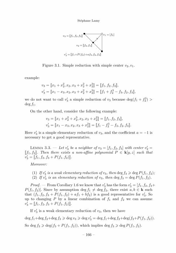
We say that v′3 is an elementary reduction (resp. a weak elementaryreduction) of v3 with center v2, if deg v3 > deg v′3 (resp. deg v3 > deg v′3) andv′3 Gv2 v3. Let v1 be the minimal vertex in the line v2. We say that v1, v2, v3is the pivotal simplex of the reduction, and that v1 is the pivot of thereduction. Moreover we say that the reduction is optimal if v′3 has minimaldegree among all neighbors of v3 with center v2. We say that v′3 is a simpleelementary reduction (resp. a weak simple elementary reduction) of v3 ifthere exist good representatives v3 = [[f1, f2, f3]] and v′3 = [[f1 + P (f2) +af3, f2, f3]] for some a ∈ k and non-affine polynomial P , satisfying
deg f1 > maxf1 + P (f2), f1 + P (f2) + af3;(resp. f1 > maxf1 + P (f2), f1 + P (f2) + af3).
In this situation we say that v2 = [[f2, f3]], v1 = [[f2]] is the simple centerof the reduction, and when drawing pictures we represent this relation byadding an arrow on the edge from v2 to v1 (see Figure 3.1). Beware thatthis representation is imperfect, since the arrow does not depend only onthe edge from v2 to v1 but indicates a relation between the two vertices v3and v′3.
Remark 3.2. — In the definition of a (weak) simple elementary reduction,if deg f3 = topdeg v3, then we must have a = 0. For instance in the following
– 165 –
Stéphane Lamy
•
v3 = [[f1,f2,f3]]
v2 = [[f2,f3]]
v′3 = [[f1+P (f2)+af3,f2,f3]]
??v1 = [f2]
Figure 3.1. Simple reduction with simple center v2, v1.
example:
v3 = [[x1 + x22, x2, x3 + x2
2 + x32]] = [[f1, f2, f3]],
v′3 = [[x1 − x3, x2, x3 + x22 + x3
2]] = [[f1 + f32 − f3, f2, f3]],
we do not want to call v′3 a simple reduction of v3 because deg(f1 + f32 ) >
deg f1.
On the other hand, consider the following example:
v3 = [[x1 + x22 + x3
2, x2, x3 + x22]] = [[f1, f2, f3]],
v′3 = [[x1 − x3, x2, x3 + x22]] = [[f1 − f3
2 − f3, f2, f3]].
Here v′3 is a simple elementary reduction of v3, and the coefficient a = −1 isnecessary to get a good representative.
Lemma 3.3. — Let v′3 be a neighbor of v3 = [f1, f2, f3] with center v′2 =[[f1, f2]]. Then there exists a non-affine polynomial P ∈ k[y, z] such thatv′3 = [[f1, f2, f3 + P (f1, f2)]].
Moreover:
(1) If v′3 is a weak elementary reduction of v3, then deg f3 > degP (f1, f2);(2) If v′3 is an elementary reduction of v3, then deg f3 = degP (f1, f2).
Proof. — From Corollary 1.6 we know that v′3 has the form v′3 = [f1, f2, f3+P (f1, f2)]. Since by assumption deg f1 6= deg f2, there exist a, b ∈ k suchthat (f1, f2, f3 + P (f1, f2) + af1 + bf2) is a good representative for v′3. Soup to changing P by a linear combination of f1 and f2 we can assumev′3 = [[f1, f2, f3 + P (f1, f2)]].
If v′3 is a weak elementary reduction of v3, then we have
deg f1+deg f2+deg f3 > deg v3 > deg v′3 = deg f1+deg f2+deg(f3+P (f1, f2)).
So deg f3 > deg(f3 + P (f1, f2)), which implies deg f3 > degP (f1, f2).
– 166 –
Combinatorics of the tame automorphism group
Finally if v′3 is an elementary reduction of v3, that is, deg v3 > deg v′3,then the same computation gives deg f3 > deg(f3 +P (f1, f2)), which impliesthat deg f3 = degP (f1, f2).
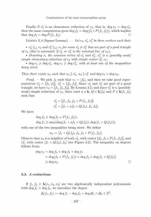
Lemma 3.4 (Square Lemma). — Let v3, v′3, v′′3 be three vertices such that:
• v′3 Gv′2v3 and v′′3 Gv′′
2v3 for some v′2 6= v′′2 that are part of a good triangle
of v3 (this is automatic if v′2 or v′′2 is the minimal line of v3);• Denoting v1 the common vertex of v′2 and v′′2 , v′′3 is a (possibly weak)
simple elementary reduction of v3 with simple center v′′2 , v1;• deg v3 > deg v′3, deg v3 > deg v′′3 , with at least one of the inequalities
being strict.
Then there exists u3 such that u3 G v′3, u3 G v′′3 and deg v3 > deg u3.
Proof. — We pick f2 such that v1 = [f2], and then we take good repre-sentatives v′2 = [[f1, f2]], v′′2 = [[f2, f3]]. Since v′2 and v′′2 are part of a goodtriangle, we have v3 = [[f1, f2, f3]]. By Lemma 3.3, and since v′′3 is a (possiblyweak) simple reduction of v3, there exist a ∈ k, Q ∈ k[f2] and P ∈ k[f1, f2]such that
v′3 = [[f1, f2, f3 + P (f1, f2)]];v′′3 = [[f1 + af3 +Q(f2), f2, f3]].
We havedeg f3 > deg(f3 + P (f1, f2)),deg f1 > maxdeg(f1 + af3 +Q(f2)),deg(f1 +Q(f2)),
with one of the two inequalities being strict. We defineu3 := [f1 +Q(f2), f2, f3 + P (f1, f2)].
Observe that u3 is a neighbor of both v′3, with center [[f2, f3 +P (f1, f2)]], andv′′3 , with center [f1 + Q(f2), f2] (see Figure 3.2). The inequality on degreesfollows from:
deg v3 = deg f3 + deg f2 + deg f1
> deg(f3 + P (f1, f2)) + deg f2 + deg(f1 +Q(f2))> deg u3.
3.3. K-reductions
If f1, f2 ∈ k[x1, x2, x3] are two algebraically independent polynomialswith deg f1 > deg f2, we introduce the degree
∆(f1, f2) := deg f1 − deg f2 + deg df1 ∧ df2 ∈ Z3.
– 167 –
Stéphane Lamy
•
•
•
•
v3=[[f1,f2,f3]]
v′2=[[f1,f2]]
v′3=[[f1,f2,f3+P (f1,f2)]]
u′′2 =[[f2,f3+P (f1,f2)]]
u3=[f1+Q(f2),f2,f3+P (f1,f2)]
u′2=[f1+Q(f2),f2]
v′′3 =[[f1+af3+Q(f2),f2,f3]]
v′′2 =[[f2,f3]]
__
v1=[f2]
Figure 3.2. Square Lemma 3.4.
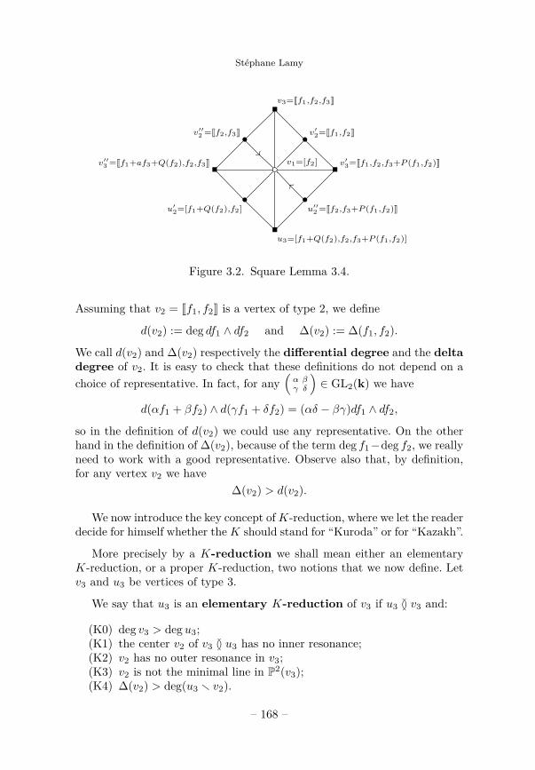
Assuming that v2 = [[f1, f2]] is a vertex of type 2, we define
d(v2) := deg df1 ∧ df2 and ∆(v2) := ∆(f1, f2).
We call d(v2) and ∆(v2) respectively the differential degree and the deltadegree of v2. It is easy to check that these definitions do not depend on achoice of representative. In fact, for any
(α βγ δ
)∈ GL2(k) we have
d(αf1 + βf2) ∧ d(γf1 + δf2) = (αδ − βγ)df1 ∧ df2,
so in the definition of d(v2) we could use any representative. On the otherhand in the definition of ∆(v2), because of the term deg f1−deg f2, we reallyneed to work with a good representative. Observe also that, by definition,for any vertex v2 we have
∆(v2) > d(v2).
We now introduce the key concept ofK-reduction, where we let the readerdecide for himself whether theK should stand for “Kuroda” or for “Kazakh”.
More precisely by a K-reduction we shall mean either an elementaryK-reduction, or a proper K-reduction, two notions that we now define. Letv3 and u3 be vertices of type 3.
We say that u3 is an elementary K-reduction of v3 if u3 G v3 and:
(K0) deg v3 > deg u3;(K1) the center v2 of v3 G u3 has no inner resonance;(K2) v2 has no outer resonance in v3;(K3) v2 is not the minimal line in P2(v3);(K4) ∆(v2) > deg(u3 r v2).
– 168 –
Combinatorics of the tame automorphism group
•
v3=[[f1,f2,f3]]
v2=[[f1,f2]]
u3=[[f1,f2,g3]]v1=[f2]
• •v3=[[f1,f2,f3]]
v1=[f2]
m2=[[f2,f3]]
w3=[[g1,f2,f3]]
u3=[[g1,f2,g3]]
w2=[[g1,f2]]
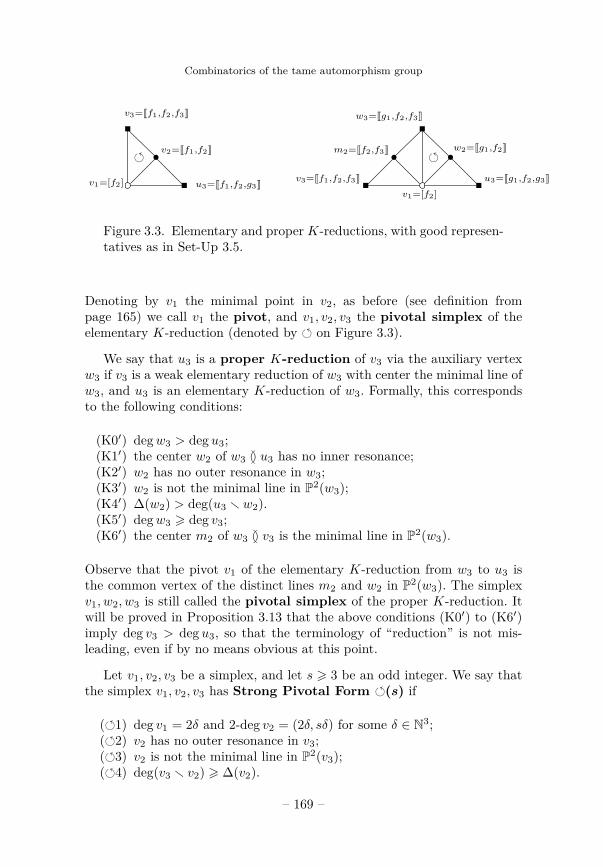
Figure 3.3. Elementary and properK-reductions, with good represen-tatives as in Set-Up 3.5.
Denoting by v1 the minimal point in v2, as before (see definition frompage 165) we call v1 the pivot, and v1, v2, v3 the pivotal simplex of theelementary K-reduction (denoted by on Figure 3.3).
We say that u3 is a proper K-reduction of v3 via the auxiliary vertexw3 if v3 is a weak elementary reduction of w3 with center the minimal line ofw3, and u3 is an elementary K-reduction of w3. Formally, this correspondsto the following conditions:
(K0′) degw3 > deg u3;(K1′) the center w2 of w3 G u3 has no inner resonance;(K2′) w2 has no outer resonance in w3;(K3′) w2 is not the minimal line in P2(w3);(K4′) ∆(w2) > deg(u3 r w2).(K5′) degw3 > deg v3;(K6′) the center m2 of w3 G v3 is the minimal line in P2(w3).
Observe that the pivot v1 of the elementary K-reduction from w3 to u3 isthe common vertex of the distinct lines m2 and w2 in P2(w3). The simplexv1, w2, w3 is still called the pivotal simplex of the proper K-reduction. Itwill be proved in Proposition 3.13 that the above conditions (K0′) to (K6′)imply deg v3 > deg u3, so that the terminology of “reduction” is not mis-leading, even if by no means obvious at this point.
Let v1, v2, v3 be a simplex, and let s > 3 be an odd integer. We say thatthe simplex v1, v2, v3 has Strong Pivotal Form (s) if
(1) deg v1 = 2δ and 2-deg v2 = (2δ, sδ) for some δ ∈ N3;(2) v2 has no outer resonance in v3;(3) v2 is not the minimal line in P2(v3);(4) deg(v3 r v2) > ∆(v2).
– 169 –
Stéphane Lamy
In all the previous definitions we took care of working with vertices, andnot with particular representatives. However for writing proofs it will oftenbe useful to choose representatives.
Set-Up 3.5. (1) Let u3 be an elementary K-reduction of v3, withpivotal simplex v1, v2, v3. Then there exist representatives
v1 = [f2] v3 = [[f1, f2, f3]]v2 = [[f1, f2]] u3 = [[f1, f2, g3]]
such that g3 = f3+ϕ3(f1, f2), where ϕ3 ∈ k[x, y]. Observe that, by definition,deg f1 > deg f2 and deg f1 > deg f3 > deg g3.
(2) Let u3 be a proper K-reduction of v3, with pivotal simplex v1, w2, w3.Then there exist representatives
v1 = [f2] w3 = [[g1, f2, f3]]m2 = [[f2, f3]] v3 = [[f1, f2, f3]]w2 = [[g1, f2]] u3 = [[g1, f2, g3]]
such that g1 = f1+ϕ1(f2, f3) and g3 = f3+ϕ3(g1, f2), where ϕ1, ϕ3 ∈ k[x, y].
Proof. —
(1) Pick any good representatives v1 = [f2], v2 = [[f1, f2]], v3 = [[f1, f2, f3]]as given by Lemma 1.4, and apply Lemma 3.3 to get g3.
(2) Pick any representative v1 = [f2], and then pick f3, g1 such thatv2 = [[f2, f3]] and w2 = [[g1, f2]]. Since m2 is the minimal line in P2(w3),we have deg g1 > deg f2 and deg g1 > deg f3, hence (g1, f2, f3) is a goodrepresentative for w3. Now apply Lemma 3.3 twice to get f1 and g3.
We establish a first property of a simplex with Strong Pivotal Form.
Lemma 3.6. — Let v1, v2, v3 be a simplex with Strong Pivotal Form (s)for some odd s > 3. Then the minimal line m2 in P2(v3) has no innerresonance.
Proof. — We pick representatives v1 = [f2], v2 = [[f1, f2]], v3 = [[f1, f2, f3]]as given by Lemma 1.4. By (1) we have deg f1 = sδ > 2δ = deg f2. Sincev2 is not the minimal line by (3), the minimal line must be m2 = [[f2, f3]].Then by (4) we have deg f3 > (s−2)δ > δ, so that deg f2 6∈ N deg f3. Sinceby (2) we also have deg f3 6∈ N deg f2, we conclude that the minimal linem2 = [[f2, f3]] has no inner resonance.
We can rephrase results from Corollary 2.7 with the previous definitions(see also Example 6.3 for some complements):
Proposition 3.7. — Let v3 be a vertex that admits an elementary re-duction with pivotal simplex v1, v2, v3.
– 170 –
Combinatorics of the tame automorphism group
(1) Assume v2 has no inner resonance, and no outer resonance in v3.Then
deg(v3 r v2) > d(v2).(2) If moreover v2 is not the minimal line in P2(v3), then v1, v2, v3 has
Strong Pivotal Form (s) for some odd s > 3.
Proof. —
(1) We pick good representatives v1 = [f2], v2 = [[f1, f2]], v3 = [[f1, f2, f3]]as given by Lemma 1.4. By Lemma 3.3, the elementary reduction has theform u3 = [[f1, f2, f3 + P (f1, f2)]] with deg f3 = degP (f1, f2). Since v2 hasno outer resonance in v3, we have deg f3 6∈ Ndeg f1 + N deg f2, hence
degvirt P (f1, f2) > degP (f1, f2).Since moreover v2 has no inner resonance, we can apply Corollary 2.7(2) toget the inequality deg(v3 r v2) > d(v2).
(2) By assumption the simplex v1, v2, v3 already satisfies conditions (2)and (3). The condition that v2 is not the minimal line in P2(v3) is equivalentto
maxdeg f1,deg f2 > deg f3 = degP (f1, f2),hence we can apply Corollary 2.7(3), which yields conditions (1) and (4).
3.4. Elementary K-reductions
Here we list some properties of an elementary K-reduction. First we havethe following corollary from Proposition 3.7.
Corollary 3.8. — The pivotal simplex of a K-reduction has StrongPivotal Form (s) for some odd s > 3.
Proof. — First, let v1, v2, v3 be the pivotal simplex of an elementary K-reduction. We know that, by (K1), v2 has no inner resonance, by (K2), v2has no outer resonance in v3, and by (K3), v2 is not the minimal line in v3,so we can apply Proposition 3.7(2).
Now the pivotal simplex of properK-reduction is by definition the pivotalsimplex of an elementary K-reduction from the auxiliary vertex, so that theabove argument applies.
Lemma 3.9. — Let u3 be an elementary K-reduction of v3 with centerv2, m2 the minimal line in P2(v3), and u2 ∈ P2(v3) a line not passing throughthe pivot v1 of the reduction. Then
(1) d(m2) > deg(v3 rm2) + d(v2);
– 171 –
Stéphane Lamy
(2) d(u2) > d(m2) > d(v2);(3) The function
t2 ∈ P2(v3) 7→ d(t2) ∈ N3
only takes the three distinct values d(u2) > d(m2) > d(v2), and ittakes its minimal value only at the point v2;
(4) deg(v1) + d(u2) > 2 deg(v3 rm2).
Proof. — The assumption means that v2,m2, u2 form a (not necessarilygood) triangle. We use the notation from Set-Up 3.5, we therefore havem2 = [[f2, f3]], v2 = [[f1, f2]] and v1 = [f2].
(1) On the one hand:df2 ∧ df3 = df2 ∧ dg3 − df2 ∧ d(ϕ3(f1, f2)).
On the other hand, the following sequence of inequalities holds, where thefirst one comes from Corollary 2.7(4), the second one from (K4), and thethird one from Lemma 2.2:deg df2∧d(ϕ3(f1, f2)) > deg f1+deg df1∧df2 > deg f2+deg g3 > deg df2∧dg3.
(3.1)So deg df2 ∧ df3 = deg df2 ∧ d(ϕ3(f1, f2)), and replacing in (3.1) we obtainthe expected inequality:d(m2) = deg df2 ∧ df3 > deg f1 + deg df1 ∧ df2 = deg(v3 rm2) + d(v2).(2) By the previous point we have
deg f1 + deg df2 ∧ df3 > deg f3 + deg df1 ∧ df2,
hence by the Principle of Two Maxima 2.9 we getdeg f2 + deg df1 ∧ df3 = deg f1 + deg df2 ∧ df3. (3.2)
Since deg f1 > deg f2 we get deg df1 ∧ df3 > deg df2 ∧ df3, and finallydeg df1 ∧ df3 > deg df2 ∧ df3 > deg df1 ∧ df2. (3.3)
The general form of u2 being u2 = [[f1 + αf2, f3 + βf2]], we haved(u2) = deg(df1 + αdf2) ∧ (df3 + β df2) = deg df1 ∧ df3,
so that the expected result is exactly (3.3).(3) We just saw that if t2 is any line not passing through [f2], then
d(t2) = deg df1 ∧ df3 = d(u2).Now consider t2 passing through [f2] but not equal to v2. Then t2 =
[f2, f3 + αf1] for some α ∈ k and, using (3.3):d(t2) = deg
(df2 ∧ df3 − αdf1 ∧ df2
)= deg df2 ∧ df3 = deg(m2).
We obtain that v2 is the unique minimum of the functiont2 ∈ P2(v3) 7→ d(t2).
– 172 –
Combinatorics of the tame automorphism group
(4) By (3.2) we have
deg(v1) + d(u2) = deg(v3 rm2) + d(m2).
Since by assertion (1) we have d(m2) > deg(v3 \m2), the result follows.
As an immediate consequence of Lemma 3.9(3) we get:
Corollary 3.10. — Assume that v3 admits an elementary K-reduction,and that one of the following holds:
(1) There exists a (non necessarily good) triangle u2, v2, w2 ∈ P2(v3)such that
d(u2) > d(w2) > d(v2);(2) m2 is the minimal line in P2(v3), and v2 is another line in P2(v3)
such thatd(m2) > d(v2).
Then v2 is the center of the K-reduction.
3.5. Proper K-reductions
In this section we list some properties of proper K-reductions, and intro-duce the concept of a normal K-reduction.
Proposition 3.11. — Let u3 be a proper K-reduction of v3, via w3.Then (using notation from Set-Up 3.5):
(1) g1 = f1 + ϕ1(f2, f3) with degvirt ϕ1(f2, f3) = degϕ1(f2, f3).(2) If the pivotal simplex has Strong Pivotal Form (s) with s > 5, then
v3 is a weak simple elementary reduction of w3, with simple centerm2, v1, and deg v3 = degw3.
Proof. — First observe that by Corollary 3.8 we know that the pivotalsimplex v1, w2, w3 has Strong Pivotal Form (s). In particular by Lemma 3.6the minimal line m2 = [[f2, f3]] of w3 has no inner resonance.
(1) Assume by contradiction that degvirt ϕ1(f2, f3) > degϕ1(f2, f3).By non resonance of [[f2, f3]] we can apply Corollary 2.7(2) and Lemma 3.9(1)
to get the contradiction
degϕ1(f2, f3) > deg df2 ∧ df3 = d(m2) > deg g1.
(2) We just established
deg g1 > degϕ1(f2, f3) = degvirt ϕ1(f2, f3).
– 173 –
Stéphane Lamy
Since v1, w2, w3 has Strong Pivotal Form (s), we have deg g1 = sδ, deg f2 =2δ and deg f3 > (s − 2)δ, so that deg(f2f3) > deg g1. As soon as s > 5 wealso have 2(s − 2) > s, hence deg f2
3 > deg g1. This implies that if s > 5then ϕ1 has the form ϕ1(f2, f3) = af3 +Q(f2), as expected. Moreover sincedegQ(f2) = 2rδ for some r > 2 and since s is odd, we have deg g1 >degvirt ϕ1(f2, f3) = degϕ(f2, f3) hence deg f1 = deg g1 and deg v3 = degw3.
In view of the previous proposition, we introduce the following definition.We say that u3 is a normal K-reduction of v3 in any of the two followingsituations:
• either u3 is an elementary K-reduction of v3;• or u3 is a proper K-reduction of v3 via an auxiliary vertex w3, and,denoting by v1 the pivot of the reduction and m2 the minimal linein w3, the vertex v3 is not a weak simple elementary reduction ofw3 with center m2, v1.
Given a proper K-reduction, Corollary 3.8 and Proposition 3.11(2) saythat if the reduction is normal then the pivotal simplex has Strong PivotalForm (3). We now prove the converse, and give some estimations on thedegrees involved.
Lemma 3.12. — Assume that u3 is a proper K-reduction of v3, via w3,and that the pivotal simplex has Strong Pivotal Form (3). Then the reduc-tion is normal, and using representatives as from Set-Up 3.5, we have:
deg g1 = 3δ, deg f2 = 2δ, 32δ > deg f3 > δ, (3.4)
deg df1 ∧ df3 = δ + deg df2 ∧ df3 > 4δ + deg dg1 ∧ df2, (3.5)deg df1 ∧ df2 = deg f3 + deg df2 ∧ df3. (3.6)
Moreover we have the implications:degw3 > deg v3 =⇒ deg f3 = 3
2δ, deg f1 >52δ. (3.7)
degw3 = deg v3 =⇒ deg f1 = deg g1 = 3δ. (3.8)In any case we have
deg f1 > deg f2 > deg f3, (3.9)deg df1 ∧ df2 > deg df1 ∧ df3 > deg df2 ∧ df3, (3.10)
m2 = [[f2, f3]] is the minimal line of v3, and for any other line `2 ∈ P2(v3),we have
d(`2) > d(m2). (3.11)
Proof. — The equalities deg g1 = 3δ and deg f2 = 2δ come from thefact that the pivotal simplex has Strong Pivotal Form (3). Property (4)gives deg f3 > δ, and Proposition 3.11(1) says that degvirt ϕ1(f2, f3) =
– 174 –
Combinatorics of the tame automorphism group
degϕ1(f2, f3). Hence apart from f2, f3 and f23 , any monomial in f2, f3 has
degree strictly bigger than g1. So there exists a, b, c ∈ k such that
w3 = [[g1 = f1 + af23 + bf2 + cf3, f2, f3]].
Moreover, since w3 6= v3, we have a 6= 0, which implies 3δ = deg g1 >2 deg f3. This proves (3.4), and the fact that the K-reduction is normal.
By Lemma 3.9(1) we have
deg df2∧df3 = d(m2) > deg(w3rm2)+d(w2) = deg g1+deg dg1∧df2. (3.12)
This implies
deg g1 + deg df2 ∧ df3 > deg f3 + deg dg1 ∧ df2.
By the Principle of Two Maxima 2.9, we get
deg g1 + deg df2 ∧ df3 = deg f2 + deg dg1 ∧ df3. (3.13)
Now dg1 ∧ df3 = df1 ∧ df3 + bdf2 ∧ df3, and the previous equality impliesdeg dg1 ∧ df3 > deg df2 ∧ df3, so that
deg dg1 ∧ df3 = deg df1 ∧ df3.
Now combining (3.12) and (3.13) we get the expected inequality (3.5):
deg df1 ∧ df3 = δ + deg df2 ∧ df3 > 4δ + deg dg1 ∧ df2.
Observe that degw3 > deg v3 is equivalent to deg g1 = deg f23 > deg f1.
So in this situation deg f3 = 32δ, and since by Lemma 2.2 we have deg f1 +
deg f3 > deg df1 ∧ df3, from (3.5) we also get deg f1 > 4δ − 32δ = 5
2δ. Thisproves (3.7), and (3.8) is immediate. These two assertions imply that wealways have deg f1 >
52δ, so that we get (3.9), and the minimal line m2 =
[[f2, f3]] of w3 also is the minimal line of v3.
For the equality (3.6) we start again from g1 = f1 +af23 +bf2 +cf3, which
givesdg1 ∧ df2 = df1 ∧ df2 − 2af3df2 ∧ df3 − c df2 ∧ df3.
Since (3.12) implies deg(f3df2 ∧ df3) > deg dg1 ∧ df2, the first two termson the right-hand side must have the same degree, which is the expectedequality.
Now (3.5), (3.6) and the inequality deg f3 > δ from (3.4) immediatelyimplies (3.10).
Finally, for any line `2 distinct from m2 = [[f2, f3]], we have
d(`2) = deg(αdf1 ∧ df2 + β df1 ∧ df3 + γ df2 ∧ df3)
with (α, β) 6= (0, 0), from which we obtain (3.11).
– 175 –
Stéphane Lamy
Now we can justify the terminology of “reduction”, as announced whenwe gave the definition of a proper K-reduction:
Proposition 3.13. — Let u3 be a proper K-reduction of a vertex v3.Then
deg v3 > deg u3.
Proof. — We use the notation from Set-Up 3.5. Observe that if degw3 =deg v3, then the proposition is obvious from (K0′).
Assume first that the reduction is not normal, that is, g1 = f1 + af3 +Q(f2). We know by Corollary 3.8 that deg g1 = sδ, deg f2 = 2δ and sδ >deg f3 > (s − 2)δ, where s > 3 is odd. An inequality deg g1 > deg f1 wouldimply sδ = deg(g1) = degQ(f2) = 2rδ for some integer r (the degree of Q), acontradiction with s odd. Thus we obtain deg g1 = deg f1 > deg(af3+Q(f2)),hence degw3 = deg v3 and we are done.
Now assume we have a normal proper K-reduction, and that degw3 >deg v3. By Proposition 3.11(2) (see also the discussion just before Lemme 3.12),we are in the setting of Lemma 3.12. By condition (K4′) we have
δ + deg dg1 ∧ df2 > deg g3.
Adding 3δ = deg g1, and using (3.5) from Lemma 3.12, we getdeg df1 ∧ df3 > 4δ + deg dg1 ∧ df2 > deg g1 + deg g3.
Finally adding deg f2 we getdeg v3 = deg f1 + deg f2 + deg f3
> deg df1 ∧ df3 + deg f2 by Lemma 2.2> deg g1 + deg g3 + deg f2
= deg u3.
In the following result we prove that if a vertex admits a non-normalproper K-reduction, then it already admits an elementary (and thereforenormal) K-reduction. It follows that any vertex admitting a K-reductionadmits a normal K-reduction.
Lemma 3.14 (Normalization of a K-reduction). — Let u3 be a non-normal proper K-reduction of v3, via w3. Then there exists u′3 such that
(1) u′3 G v3 and u′3 G u3;(2) u′3 is an elementary (hence by definition normal) K-reduction of v3.
Proof. — By Corollary 3.8 the pivotal simplex of the reduction has StrongPivotal Form (s) for some odd s, and by Lemma 3.12 we have s > 5. Notealso that by Proposition 3.11 we have deg v3 = degw3, and v3 is a weak
– 176 –
Combinatorics of the tame automorphism group
•
•
•
•
w3=[[g1,f2,f3]]
m2=[[f2,f3]]
v3=[[f1=g1−af3−Q(f2),f2,f3]]
v2=[[g1−Q(f2),f2]]
u′3=[[g1−Q(f2),f2,f3+P (g1,f2)]]
u2=[[f2,f3+P (g1,f2)]]
u3=[[g1,f2,f3+P (g1,f2)]]
w2=[[g1,f2]]
__
v1=[f2]
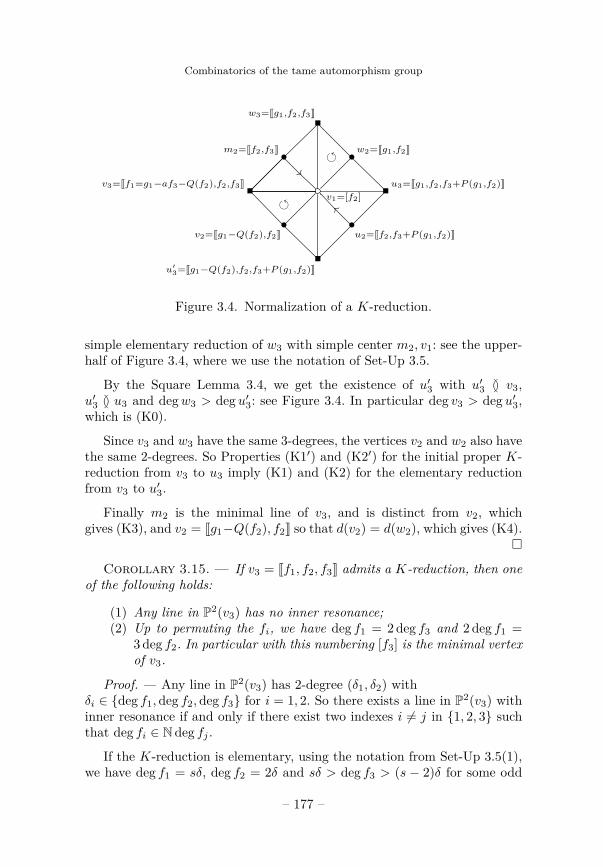
Figure 3.4. Normalization of a K-reduction.
simple elementary reduction of w3 with simple center m2, v1: see the upper-half of Figure 3.4, where we use the notation of Set-Up 3.5.
By the Square Lemma 3.4, we get the existence of u′3 with u′3 G v3,u′3 G u3 and degw3 > deg u′3: see Figure 3.4. In particular deg v3 > deg u′3,which is (K0).
Since v3 and w3 have the same 3-degrees, the vertices v2 and w2 also havethe same 2-degrees. So Properties (K1′) and (K2′) for the initial proper K-reduction from v3 to u3 imply (K1) and (K2) for the elementary reductionfrom v3 to u′3.
Finally m2 is the minimal line of v3, and is distinct from v2, whichgives (K3), and v2 = [[g1−Q(f2), f2]] so that d(v2) = d(w2), which gives (K4).
Corollary 3.15. — If v3 = [[f1, f2, f3]] admits a K-reduction, then oneof the following holds:
(1) Any line in P2(v3) has no inner resonance;(2) Up to permuting the fi, we have deg f1 = 2 deg f3 and 2 deg f1 =
3 deg f2. In particular with this numbering [f3] is the minimal vertexof v3.
Proof. — Any line in P2(v3) has 2-degree (δ1, δ2) withδi ∈ deg f1,deg f2,deg f3 for i = 1, 2. So there exists a line in P2(v3) withinner resonance if and only if there exist two indexes i 6= j in 1, 2, 3 suchthat deg fi ∈ N deg fj .
If the K-reduction is elementary, using the notation from Set-Up 3.5(1),we have deg f1 = sδ, deg f2 = 2δ and sδ > deg f3 > (s − 2)δ for some odd
– 177 –
Stéphane Lamy
s > 3. Moreover an inner resonance in [[f2, f3]] would be of the form deg f3 =(s− 1)δ = s−1
2 deg f2 for s > 5, but this is impossible by Property (K2). Sothe only possible resonance is between deg f1 and deg f3, in the case s = 3,as stated in (2).
If the K-reduction is proper, we use the notation from Set-Up 3.5(2).Either deg g1 = deg f1 and we are reduced to the previous case; or deg g1 >deg f1 and by Lemma 3.14 we can assume that the K-reduction is normal(and proper, otherwise again we are reduced to the previous case). Then byLemma 3.12 we have 3δ > deg f1 > 5
2δ, deg f2 = 2δ, deg f3 = 32δ, hence
there is no relation of the form deg fi ∈ N deg fj for any i 6= j and we are incase (1).
Remark 3.16. — We shall see later in Corollary 5.3 that in fact Case (2)in the previous corollary never happens.
3.6. Stability of K-reductions
Consider v3 a vertex that admits a normal K-reduction. In this sectionwe want to show that most elementary reductions of v3 still admit a K-reduction. First we prove two lemmas that give some constraint on the (weak)elementary reductions that such a vertex v3 can admit.
Lemma 3.17. — Let u3 be a normal K-reduction of v3, with pivot v1.Let u2 be any line in P2(v3) not passing through v1. Then v3 does not admita weak elementary reduction with center u2.
Proof. — We start with the notation v3 = [[f1, f2, f3]] from Set-Up 3.5(1)when u3 is an elementary K-reduction of v3, and with the Set-Up 3.5(2) towhich we apply Lemma 3.12 when u3 is a normal proper K-reduction of v3.It follows that m2 = [[f2, f3]] is in both cases the minimal line of v3. We haveu2 = [[h1, h3]] where h1 = f1 + af2, h3 = f3 + bf2 for some a, b ∈ k. Then[f2, h3] is the minimal line m2 in P2(v3), however it is possible that [f2, h3]is not a good representative of m2. There are two possibilities:
• either (h1, f2, h3) is still a good representative for v3, and we havedeg h3 = deg f3, deg f2 = deg(v3 r u2);
• or deg f2 = deg h3 > degm1 where m1 = [f3] is the minimal point ofv3, and deg f2 > deg(v3 r u2) = deg f3.
In both cases we have
deg h1 = topdeg v3, deg f2 > deg(v3 r u2) and deg h3 > deg f3.
– 178 –
Combinatorics of the tame automorphism group
Assume by contradiction that v3 admits a weak elementary reductionwith center u2. By Lemma 3.3 there exists a non-affine polynomial P ∈ k[y, z]such that
deg(v3 r u2) > degP (h1, h3).On the other hand we know from Corollary 3.8 that the pivotal simplex ofthe K-reduction has Strong Pivotal Form (s) for some odd s > 3, hence
deg h3 > deg f3 > (s− 2)δ > δ which implies 2 deg h3 > 2δ = deg f2.
In consequence, since deg h1 > deg h3, we have
degvirt P (h1, h3) > 2 deg h3 > deg f2 > deg(v3 r u2),
so thatdegvirt P (h1, h3) > degP (h1, h3).
If u2 has no inner resonance, then we get a contradiction as follows, inboth cases of an elementary or a normal proper K-reduction:
deg(v3 r u2) > degP (h1, h3)> deg dh1 ∧ dh3 = d(u2) by Corollary 2.7(2),> d(m2) by Lemma 3.9(2) or (3.11),> deg(v3 rm2) by Lemma 3.9(1).
More precisely, in the case of a normal properK-reduction the last inequalitycomes from d(m2) > deg(w3 rm2) > deg(v3 rm2) by Lemma 3.9(1) andby (K5′).
Now consider the case where u2 = [[h1, h3]] has inner resonance. By Corol-lary 3.15(2) we have deg h3 = mindeg f2,deg f3, and since by assumptiondeg h3 > deg f3 we get deg h3 = deg f3. Then Corollary 3.15(2) gives the tworelations
12 deg(v3 rm2) = 1
2 deg h1 = deg h3,
23 deg(v3 rm2) = 2
3 deg h1 = deg f2 > deg(v3 r u2).(3.14)
In particular we have deg f1 > deg f2 > deg f3, and b = 0, that is, h3 = f3.We apply Corollary 2.7(1) which gives
deg(v3 r u2) > degP (h1, h3) > d(u2)− deg h3,
which we rewrite as
deg h3 + 2 deg(v3 r u2) > deg(v3 r u2) + d(u2). (3.15)
If u3 is an elementary K-reduction of v3, and since in our situation deg(v3 ru2) = deg[f2], by Lemma 3.9(4) we have
deg(v3 r u2) + d(u2) > 2 deg(v3 rm2). (3.16)
– 179 –
Stéphane Lamy
If on the other hand u3 is a proper K-reduction of v3 via w3, let us provethat (3.16) still holds, by using Lemma 3.12. First note that deg(v3 r u2) =deg f2, deg(v3 rm2) = deg f1 andd(u2) = deg dh1 ∧ dh3 = deg d(f1 + af2) ∧ df3 = deg df1 ∧ df3 by (3.5).
Then, using (3.4) and (3.5) from Lemma 3.12, we getdeg f2 + deg df1 ∧ df3 > 2δ + 4δ = 2 deg g1 > 2 deg f1
as expected.
Adding the first equality of (3.14) to twice the second one, and combiningwith (3.15) and (3.16), we get the contradiction
( 12 + 2.2
3 ) deg(v3 rm2) > 2 deg(v3 rm2).
Lemma 3.18. — Let u3 be a normal proper K-reduction of v3, with pivotv1. Let v′2 6= m2 be a line in P2(v3) passing through v1. If v′3 is a weakelementary reduction of v3 with center v′2, then this reduction is simple withcenter v′2, v1.
Proof. — We use the notation from Set-Up 3.5(2), and set v′2 = [[h1, f2]]with h1 = f1 + af3. By Lemma 3.12, h1 realizes the top degree of v3.Then v3 = [[f1, f2, f3]] = [[h1, f2, f3]], and by Lemma 3.3 we have v′3 =[[h1, f2, f3 + P (h1, f2)]] for some non-affine polynomial P . We want to provethat P (h1, f2) ∈ k[f2]. It is sufficient to prove deg h1 > degvirt P (h1, f2).Assume the contrary. Then
degvirt P (h1, f2) > deg h1 > deg f3 > degP (h1, f2).By Lemma 3.12, we have deg f1 > deg f2 > deg f3, so that by Corollary 3.15we have deg h1 = deg f1 6∈ N deg f2. Thus we can apply Corollary 2.7(2) toget
deg f1 > degP (h1, f2) > deg dh1 ∧ df2.
By (3.6) of Lemma 3.12 we getdeg dh1 ∧ df2 = deg(df1 ∧ df2 − adf2 ∧ df3) = deg df1 ∧ df2 > deg df2 ∧ df3.
Then by (3.5) and (3.4) of Lemma 3.12 we havedeg df2 ∧ df3 > 3δ = deg g1 > deg f1,
hence the contradiction deg f1 > deg dh1 ∧ df2 > deg f1.
Proposition 3.19 (Stability of a K-reduction). — Let u3 be a normalK-reduction of v3, and v′3 a weak elementary reduction of v3 with center v′2.Denote by m2 the minimal line of v3. If u3 is an elementary K-reduction,assume moreover that the centers of v′3 G v3 and u3 G v3 are distinct. Thenu3 is a K-reduction of v′3, and more precisely, we are in one of the followingcases:
– 180 –
Combinatorics of the tame automorphism group
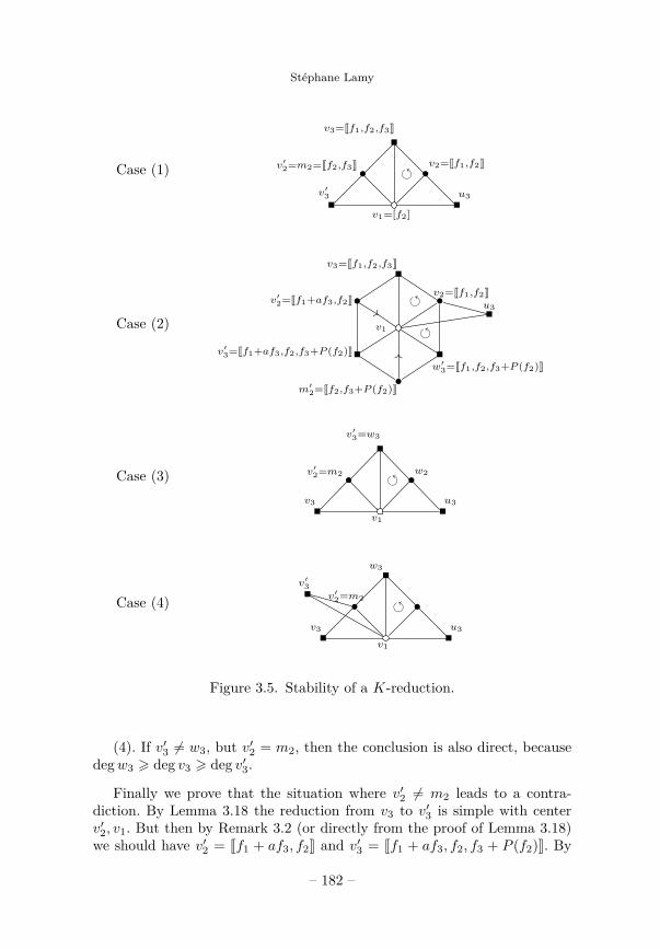
(1) u3 is an elementary K-reduction of v3, and v′2 = m2: then u3 is a(possibly non-normal) proper K-reduction of v′3, via v3;
(2) u3 is an elementary K-reduction of v3, and v′2 6= m2: then u3 isa (possibly non-normal) proper K-reduction of v′3, via an auxiliaryvertex w′3 that satisfies degw′3 = deg v3;
(3) u3 is a normal proper K-reduction of v3 via w3, and v′3 = w3: thenu3 is an elementary K-reduction of v′3;
(4) u3 is a normal proper K-reduction of v3 via w3, and v′2 = m2: thenu3 also is a normal proper K-reduction of v′3 via w3.
Proof. — First assume that u3 is an elementary K-reduction of v3. Wedenote by v1 = [f2], v2 = [[f1, f2]], v3 = [[f1, f2, f3]] the pivotal simplex ofthe K-reduction u3 (following Set-Up 3.5(1)). By Lemma 3.17, the line v′2passes through v1.
(1). If v′2 = m2, since by assumption deg v3 > deg v′3, we directly get thatu3 is a proper K-reduction of v′3, via v3.
(2). Now assume that v′2 6= m2, so that v′2 = [[f1 +af3, f2]] for some a ∈ k,and a 6= 0 since we assume v′2 6= v2. Then by Lemma 3.3 we can writev′3 = [[f1 + af3, f2, f3 + P (f1 + af3, f2)]] with deg f3 > degP (f1 + af3, f2).If we can show that P depends only on f2 we are done: indeed then deg f3 6=degP (f2), because m2 = [[f2, f3]] has no inner resonance by Corollary 3.15,hence we have deg f3 = deg(f3 + P (f2)). It follows that u3 is a proper K-reduction of v′3 via w′3 = [[f1, f2, f3 +P (f2)]], where m′2 = [[f2, f3 +P (f2)]] isthe minimal line of w′3 (see Figure 3.5, Case (2)).
To show that P depends only on f2 it is sufficient to show that deg f3 >degvirt P (f1 + af3, f2). By contradiction, assume that this is not the case.Then
degvirt P (f1 + af3, f2) > deg f3 > degP (f1 + af3, f2).Since v′2 has the same 2-degree as v2, it has no inner resonance by (K1), andby Corollary 2.7(2) we get
degP (f1 + af3, f2) > deg(df1 ∧ df2 − adf2 ∧ df3).By Lemma 3.9(1) we have deg df2∧df3 > df1∧df2 and deg df2∧df3 > deg f3,so finally we obtain the contradiction
degP (f1 + af3, f2) > deg df2 ∧ df3 > deg f3.
Now assume that u3 is a normal proper K-reduction of v3, via an auxiliaryvertex w3. Recall that the minimal line m2 of v3 is also the minimal line ofthe intermediate vertex w3 (last assertion of Lemma 3.12).
(3). If v′3 = w3, then by definition u3 is an elementary K-reduction of v′3.
– 181 –
Stéphane Lamy
Case (1) • •v′
3
v1=[f2]
v′2=m2=[[f2,f3]]
v3=[[f1,f2,f3]]
u3
v2=[[f1,f2]]
Case (2)• •
•
v′
3=[[f1+af3,f2,f3+P (f2)]]
v′2=[[f1+af3,f2]]
v3=[[f1,f2,f3]]
v2=[[f1,f2]]u3
v1
%%
m′2=[[f2,f3+P (f2)]]
w′3=[[f1,f2,f3+P (f2)]]
OO
Case (3) • •v3
v1
v′2=m2
v′3=w3
u3
w2
Case (4) • •v3
w3
u3
v′2=m2
v′3
v1
Figure 3.5. Stability of a K-reduction.
(4). If v′3 6= w3, but v′2 = m2, then the conclusion is also direct, becausedegw3 > deg v3 > deg v′3.
Finally we prove that the situation where v′2 6= m2 leads to a contra-diction. By Lemma 3.18 the reduction from v3 to v′3 is simple with centerv′2, v1. But then by Remark 3.2 (or directly from the proof of Lemma 3.18)we should have v′2 = [[f1 + af3, f2]] and v′3 = [[f1 + af3, f2, f3 + P (f2)]]. By
– 182 –
Combinatorics of the tame automorphism group
Lemma 3.12 we havedeg f2 = 2δ > 3
2δ > deg f3,
so degP (f2) > deg f3 and we get a contradiction with deg v3 > deg v′3.
4. Reducibility Theorem
In this section we state and prove the main result of this paper, that is,the Reducibility Theorem 4.1.
4.1. Reduction paths
Given a vertex v3 with a choice of good triangle T , we call elementaryT -reduction any elementary reduction with center one of the three lines ofT .
We now define the notion of a reducible vertex in a recursive manneras follows:
• We declare that the vertex [id] is reducible, where by Lemma 3.1 [id]is the unique type 3 vertex realizing the minimal degree (1, 1, 1).
• Let µ > ν be two consecutive degrees, and assume that we have alreadydefined the subset of reducible vertices among type 3 vertices of degree atmost ν. Then we say that a vertex v3 with deg v3 = µ is reducible if for anygood triangle T in P2(v3), there exists either a T -elementary reduction or a(proper or elementary) K-reduction from v3 to u3, with u3 reducible.
Let v3, v′3 be vertices of type 3. A reduction path of length n > 0 fromv3 to v′3 is a sequence of type 3 vertices v3(0), v3(1), . . . , v3(n) such that:
• v3(0) = v3 and v3(n) = v′3;• v3(i) is reducible for all i = 0, . . . , n;• For all i = 0, . . . , n− 1, v3(i+ 1) is either an elementary reduction,or a K-reduction, of v3(i).
Observe that, by definition, a reducible vertex v3 admits a reduction pathfrom v3 to the vertex [id].
In the following sections we shall prove the main result:
Theorem 4.1 (Reducibility Theorem). — Any vertex of type 3 in thecomplex C is reducible.
– 183 –
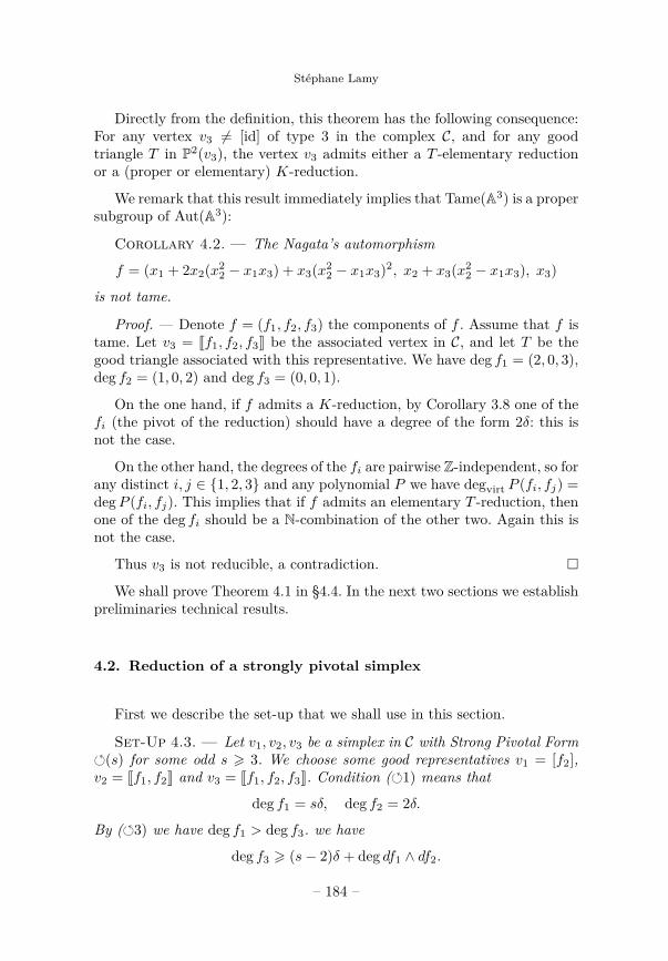
Stéphane Lamy
Directly from the definition, this theorem has the following consequence:For any vertex v3 6= [id] of type 3 in the complex C, and for any goodtriangle T in P2(v3), the vertex v3 admits either a T -elementary reductionor a (proper or elementary) K-reduction.
We remark that this result immediately implies that Tame(A3) is a propersubgroup of Aut(A3):
Corollary 4.2. — The Nagata’s automorphism
f = (x1 + 2x2(x22 − x1x3) + x3(x2
2 − x1x3)2, x2 + x3(x22 − x1x3), x3)
is not tame.
Proof. — Denote f = (f1, f2, f3) the components of f . Assume that f istame. Let v3 = [[f1, f2, f3]] be the associated vertex in C, and let T be thegood triangle associated with this representative. We have deg f1 = (2, 0, 3),deg f2 = (1, 0, 2) and deg f3 = (0, 0, 1).
On the one hand, if f admits a K-reduction, by Corollary 3.8 one of thefi (the pivot of the reduction) should have a degree of the form 2δ: this isnot the case.
On the other hand, the degrees of the fi are pairwise Z-independent, so forany distinct i, j ∈ 1, 2, 3 and any polynomial P we have degvirt P (fi, fj) =degP (fi, fj). This implies that if f admits an elementary T -reduction, thenone of the deg fi should be a N-combination of the other two. Again this isnot the case.
Thus v3 is not reducible, a contradiction.
We shall prove Theorem 4.1 in §4.4. In the next two sections we establishpreliminaries technical results.
4.2. Reduction of a strongly pivotal simplex
First we describe the set-up that we shall use in this section.
Set-Up 4.3. — Let v1, v2, v3 be a simplex in C with Strong Pivotal Form(s) for some odd s > 3. We choose some good representatives v1 = [f2],v2 = [[f1, f2]] and v3 = [[f1, f2, f3]]. Condition (1) means that
deg f1 = sδ, deg f2 = 2δ.
By (3) we have deg f1 > deg f3. we have
deg f3 > (s− 2)δ + deg df1 ∧ df2.
– 184 –
Combinatorics of the tame automorphism group
Condition (2) is equivalent to the condition
deg f3 6∈ N deg f2.
Since deg f3 > (s− 2)δ > δ, we also obtain
deg f23 > deg f2 and deg f2 6∈ N deg f3. (4.1)
In particular, as already noticed in Lemma 3.6, the minimal line m2 =[[f2, f3]] of v3 has no inner resonance. Observe also that
deg f1 6∈ Ndeg f3 except if s = 3 and deg f1 = 2 deg f3. (4.2)
Lemma 4.4. — Assume Set-Up 4.3. Then v3 does not admit a normalproper K-reduction.
Proof. — Assume v3 admits a normal proper K-reduction, via w3. Thenwe get a contradiction as follows:
d(m2) > deg(w3 rm2) by Lemma 3.9(1)> deg(v3 rm2) by (K5′)> deg(v3 r v2) > ∆(v2) by (3) and (4)> d(v2) > d(m2) by (3.11) in Lemma 3.12.
Lemma 4.5. — Assume Set-Up 4.3, and deg f1 6= 2 deg f3. Assume thatv3 admits a weak elementary reduction v′3 with center v′2. Then v′2 passesthrough v1.
Proof. — By contradiction, assume that v′2 does not pass through v1.Recall that v1 = [f2] and v2 = [[f1, f2]] with deg f1 > deg f2. Up to replacingf1 by f1 + af2 for some a ∈ k, we can assume v2 ∩ v′2 = [f1] while keepingall the properties stated in Set-Up 4.3. Then let [h3] = [f3 + af2] be theintersection of v′2 with the minimal line [[f2, f3]] of P2(v3). Then we have v′2 =[[f1, h3]], v3 = [f1, f2, h3], and by Lemma 3.3 v′3 = [[f1, f2 +ϕ2(f1, h3), h3]] forsome non-affine polynomial ϕ2, with deg f1 > deg f2 > degϕ2(f1, h3). Wehave either deg f2 = deg h3 or deg f3 = deg h3, hence in any case by (4.1)
degvirt ϕ2(f1, h3) > degϕ2(f1, h3).
In particular ϕ2(f1, h3) 6∈ k[h3], and then the inequality deg f1 > deg f2implies
degvirt ϕ2(f1, h3) > deg f2.
By Lemma 2.6 there exist coprime q > p such that
q deg h3 = pdeg f1 = psδ.
Moreover if p = 1, we would have deg h3 = deg f3 and deg f1 = 2 deg f3, incontradiction with our assumption. Hence we have q > p > 2.
– 185 –
Stéphane Lamy
Observe that even if (f2, h3) is not a good representative of the minimalline in P2(v3), in any case we have deg h3 > deg(v3 r v2) = deg f3, andProperty (4) gives
deg h3 > (s− 2)δ + deg df1 ∧ df2.
Then Corollary 2.8 yields:
2δ = deg f2 > deg(f2 + ϕ2(f1, h3)) > q deg h3 − deg df1 ∧ df2 − deg h3
> q deg h3 − deg h3 + (s− 2)δ − deg h3.
Multiplying by q and replacing q deg h3 = psδ we get:
0 > (pqs− 2ps+ sq − 4q)δ,
hence0 > ps(q − 2) + q(s− 4).
This implies s = 3, and we get the contradiction:
0 > 3pq − 6p− q = (3p− 1)(q − 2)− 2 > 5− 2.
Lemma 4.6. — Assume Set-Up 4.3. Assume that v3 admits an elemen-tary reduction v′3 with center m2, the minimal line of v3. Assume moreoverthat v′3 is reducible. Then v′3 also admits an elementary reduction with centerm2.
Proof. — By Lemma 3.3 we can write v′3 = [[f ′1, f2, f3]], where f ′1 has theform
f ′1 = f1 + ϕ1(f2, f3)
for some non-affine polynomial ϕ1, with deg f1 = degϕ1(f2, f3) > deg f ′1.Without loss in generality we can assume that ϕ1 has no constant term.Moreover we can also assume
deg f ′1 6∈ N deg f2 + Ndeg f3, (4.3)
otherwise the result is immediate.
Working with the good triangle associated with the representative(f ′1, f2, f3), we want to prove that v′3 does not admit a K-reduction, noran elementary reduction with center [[f ′1, f2]] or [[f ′1, f3]]: Indeed since v′3 isreducible by assumption, the only remaining possibility will be that v′3 admitsan elementary reduction with center m2 = [[f2, f3]], as expected. The proofis quite long, so we prove several facts along the way. The first one is:
Fact 4.7. — If degvirt ϕ1(f2, f3) > degϕ1(f2, f3) then Lemma 4.6 holds.
– 186 –
Combinatorics of the tame automorphism group
Proof. — If degvirt ϕ1(f2, f3) > degϕ1(f2, f3) then by Lemma 2.6, thereexist coprime p, q such that q deg f2 = p deg f3. Observe that (2) and (4.1)imply p, q 6= 1. We have
sδ = deg f1 > deg f ′1 = deg(f1 + ϕ1(f2, f3)) by Lemma 3.3> pdeg f3 − deg df1 ∧ df2 − deg f3 by Corollary 2.8> p deg f3 − (deg f3 − (s− 2)δ))− deg f3 by (4)
= (p− 2) deg f3 − 2δ + sδ.
Multiplying by p, recalling that deg f2 = 2δ, p deg f3 = q deg f2 and puttingδ in factor we get:
0 > 2q(p− 2)− 2p = (2p− 4)(q − 1)− 4 > 2p− 8. (4.4)
It follows that 3 > p. Now we deduce p = 3. If p = 2, then deg f3 = qδ.Condition (4) gives
sδ > deg f3 > (s− 2)δ,so q = s− 1, which contradicts q coprime with 2.
Replacing p = 3 in the first inequality of (4.4) we get 6 > 2q, hence q = 2.We obtain deg f3 = 4
3δ, and the condition deg f3 > (s − 2)δ yields s = 3.Finally
deg f1 = 3δ, deg f2 = 2δ, deg f3 = 43δ, 3δ > deg f ′1 > 7
3δ. (4.5)
First we observe that these values are not compatible with v′3 admittinga K-reduction. Indeed, by Corollary 3.8 an elementary K-reduction wouldimply 2 deg f ′1 = s′ deg fj for some odd integer s′ > 3 and j ∈ 2, 3, andone checks from (4.5) that there is no such relation. Indeed if s′ = 3, we have2 deg f1 >
143 δ > 4δ = s′ deg f3, and if s′ > 5 we have s′ deg f3 > 20
3 δ > 6δ >2 deg f ′1. Finally, for any s′ > 3 we have s′ deg f2 > 6δ > 2 deg f ′1.
Now if v′3 admits a normal properK-reduction, then, noting that deg f ′1 >deg f2 > deg f3, there should exist δ′ ∈ N3 such that all the conclusions ofLemma 3.12 hold, with f ′1, f2, f3, δ
′ instead of f1, f2, f3, δ. In particular (3.7)gives deg f2 = 2δ′, hence δ′ = δ. Now since 3δ > deg f ′1, by (3.7) and (3.8)from Lemma 3.12 would imply deg f3 = 3
2δ, incompatible with deg f3 = 43δ.
On the other hand, if v′3 admits an elementary reduction with center[[f ′1, fj ]] with j = 2 or 3, then, denoting by k the integer such that j, k =2, 3, there would exist a non-affine polynomial ϕ such that deg fk >deg(fk + ϕ(f ′1, fj)), and in particular deg f ′1 > deg fk = degϕ(f ′1, fj). Since[[f2, f3]] has no inner resonance this implies ϕ(f ′1, fj) 6∈ k[fj ], so thatdegvirt ϕ(f ′1, fj) > deg f ′1, and finally degvirt ϕ(f ′1, fj) > degϕ(f ′1, fj). Now
– 187 –
Stéphane Lamy
by (4.3) we can apply Corollary 2.7(3) to get an odd integer q′ > 3 such that2 deg f ′1 = q′ deg fj : again this is not compatible with (4.5).
From now on we assume degvirt ϕ1(f2, f3) = degϕ1(f2, f3).
Fact 4.8. — deg f1 = 2 deg f3.
Proof. — By contradiction, assume deg f1 6= 2 deg f3. Then deg f1 6∈Ndeg f3 by (4.2). Moreover we know that deg f1 6∈ N deg f2 and deg f2 +deg f3 > deg f1. This is not compatible with the equalities
deg f1 = degϕ1(f2, f3) = degvirt ϕ1(f2, f3).
We deduce from (4.2) and Fact 4.8 that s = 3, so thatdeg f1 = 3δ, deg f2 = 2δ, deg f3 = 3
2δ,
and there exist a, c, e ∈ k such that (recall that ϕ1 has no constant term):ϕ1(f2, f3) = af2
3 + cf3 + ef2 with a 6= 0. (4.6)
Now come some technical facts.
Fact 4.9. — deg df1 ∧ df3 = deg df ′1 ∧ df3 = δ + deg df2 ∧ df3.
Proof. — Recall from Set-Up 4.3 that we have 32δ = deg f3 > deg df1∧df2,
so3δ > deg f3 + deg df1 ∧ df2.
Since deg f1 = 3δ we getdeg f1 + deg df2 ∧ df3 > deg f3 + deg df1 ∧ df2.
By the Principle of Two Maxima 2.9 we havedeg f2 + deg df1 ∧ df3 = deg f1 + deg df2 ∧ df3.
Passing deg f2 to the right-hand side we get one of the expected equalitiesdeg df1 ∧ df3 = deg f1 − deg f2 + deg df2 ∧ df3 = δ + deg df2 ∧ df3.
From (4.6) we getdf ′1 ∧ df3 = df1 ∧ df3 + e df2 ∧ df3.
By the previous equality we obtain deg df1 ∧ df3 = deg df ′1 ∧ df3.
Fact 4.10. — deg df ′1 ∧ df2 = 32δ + deg df2 ∧ df3.
Proof. — From (4.6) we getdf ′1 ∧ df2 = df1 ∧ df2 + 2af3 df3 ∧ df2 + c df3 ∧ df2.
By (4) we have deg f3 > deg df1 ∧ df2, so 2af3 df3 ∧ df2 has strictly largerdegree than the two other terms of the right-hand side. Finally,
deg df ′1 ∧ df2 = deg f3 df3 ∧ df2 = 32δ + deg df2 ∧ df3.
– 188 –
Combinatorics of the tame automorphism group
Fact 4.11. — deg f ′1 > δ.
Proof. — Consider P = f1 + ay2 + cy + ef2 ∈ k[f1, f2][y]. We havedegvirt P (f3) = deg f1 > deg f ′1 = degP (f3).
On the other hand P ′ = 2ay+c, so that degvirt P′(f3) = degP ′(f3) = deg f3.
Thus m(P, f3) = 1, and the Parachute Inequality 2.5 yieldsdeg f ′1 = degP (f3) > degvirt P (f3) + deg df1 ∧ df2 ∧ df3 − deg df1 ∧ df2
− deg f3
> deg f1 − deg df1 ∧ df2 − deg f3
= deg f3 − deg df1 ∧ df2.
Recall that by (4) we havedeg f3 > deg f1 − deg f2 + deg df1 ∧ df2 = δ + deg df1 ∧ df2.
Replacing in the previous inequality we get the result.
Fact 4.12. — The vertices [[f ′1, f2]] and [[f ′1, f3]] do not have outer reso-nance in v′3 = [[f ′1, f2, f3]].
Proof. — We have (the last inequality is Fact 4.11):deg f2 = 2δ, deg f3 = 3
2δ, deg f ′1 > δ.
Moreover these degrees are pairwise distinct, because (f ′1, f2, f3) is a goodrepresentative of v′3. This implies that deg f3 is not a N-combination of deg f ′1and deg f2, and deg f2 is not a N-combination of deg f ′1 and deg f3.
Now we are ready to finish the proof of Lemma 4.6. Observe that byLemma 3.14, to prove that v′3 does not admit a K-reduction it is sufficientto exclude normal K-reductions. Recall also that from Facts 4.9 and 4.10 wehave
deg f ′1 ∧ f2 > deg f ′1 ∧ f3 > deg f2 ∧ f3. (4.7)
Fact 4.13. — v′3 does not admit an elementary K-reduction.
Proof. — By contradiction, assume that v′3 admits an elementary K-reduction. By (4.7) and Corollary 3.10(1), it follows that the center of thereduction is [[f2, f3]]. But then by Corollary 3.8 we should have 2 deg f2 =s′ deg f3 for some odd integer s′ > 3, and this is not compatible withdeg f2 = 2δ and deg f3 = 3
2δ.
Fact 4.14. — v′3 does not admit a normal proper K-reduction.
Proof. — By contradiction, assume that v′3 admits a normal proper K-reduction u3 via w3. By comparing (4.7) with (3.10) from Lemma 3.12, weobtain that the center v′2 of v′3 G w3 is equal to v′2 = [[f2, f3]], that v′2 isthe minimal line of v′3, and that degw3 = 3δ + deg f2 + deg f3 = deg v3.
– 189 –
Stéphane Lamy
Since [[f2, f3]] is also the minimal line of v3, we get that u3 is also a properK-reduction of v3 via w3. This is a contradiction with Lemma 4.4.
Now we are left with the task of proving that v′3 does not admit anelementary reduction with center [[f ′1, f2]] or [[f ′1, f3]].
Fact 4.15. — v′3 does not admit an elementary reduction with center[[f ′1, f2]].
Proof. — By contradiction, assume there exists ϕ3(f ′1, f2) such thatdegϕ3(f ′1, f2) = deg f3.
By Fact 4.12 we have degvirt ϕ3(f ′1, f2) > degϕ3(f ′1, f2), and on the otherhand Proposition 3.7(1) gives
32δ = deg f3 = degϕ3(f ′1, f2) > deg df ′1 ∧ df2.
This is a contradiction with Fact 4.10.
Fact 4.16. — v′3 does not admit an elementary reduction with center[[f ′1, f3]].
Proof. — By contradiction, assume there exists ϕ2(f ′1, f3) such thatdeg f2 > deg(f2 + ϕ2(f ′1, f3)), which implies
degϕ2(f ′1, f3) = deg f2.
By Fact 4.12 we have degvirt ϕ2(f ′1, f3) > degϕ2(f ′1, f3). By Lemma 2.6 thereexist coprime p, q ∈ N∗ and γ ∈ N3 such that
deg f ′1 = pγ, deg f3 = qγ.
Corollary 2.7(1) then yields2δ = deg f2 = degϕ2(f ′1, f3) > pqγ + deg df ′1 ∧ df3 − pγ − qγ.
By Fact 4.9 we know that deg df ′1 ∧ df3 = δ + deg df2 ∧ df3, so thatδ > deg df2 ∧ df3 + (pq − p− q)γ. (4.8)
We know that qγ = deg f3 = 32δ > δ, and by Fact 4.11 we have pγ = deg f ′1 >
δ, sominp, q > pq − p− q.
By Fact 4.12 we know that p 6= 1 and q 6= 1. The only possibilities for thepair (p, q) are then (2, 3) or (3, 2).
If (p, q) = (2, 3) then Fact 4.11 gives the contradiction3δ = 2 deg f3 = 3 deg f ′1 > 3δ.
If (p, q) = (3, 2), the equalities deg f ′1 = 3γ and deg f3 = 2γ = 32δ yield
γ = 34δ, deg f ′1 = 9
4δ, pq − p− q = 1.
– 190 –
Combinatorics of the tame automorphism group
The inequality (4.8) becomesδ4 > deg df2 ∧ df3.
Corollary 2.8 then yieldsdeg(f2 + ϕ2(f ′1, f3)) > 2 deg f ′1 − deg df2 ∧ df3 − deg f ′1
>( 9
4 −14)δ
= 2δ.This is a contradiction with 2δ = deg f2 > deg(f2 + ϕ2(f ′1, f3)).
This finishes the proof of Lemma 4.6.
We now introduce an induction hypothesis that will be the corner-stonefor the proof of the Reducibility Theorem 4.1.
Induction Hypothesis 4.17 (for degrees ν, µ in N3). — Let v3 be areducible vertex such that ν > deg v3. Then any neighbor u3 of v3 with µ >deg u3 also is reducible.
We shall refer to this situation by saying that we can apply the (ν, µ)-Induction Hypothesis 4.17 to v3 G u3.
Lemma 4.18. — Let µ > ν ∈ N3 be two consecutive degrees, and assumeInduction Hypothesis 4.17 for degrees ν, ν. Let v3 be a reducible vertex dis-tinct from [id], with µ > deg v3, and let T be a good triangle for v3. Thenthere exists a reducible vertex u3 such that
• either u3 is an optimal elementary T -reduction or an optimal ele-mentary K-reduction of v3;
• or u3 is a normal proper K-reduction of v3.
Proof. — Let v3(1) be the first step of a reduction path from v3, withrespect to the triangle T . By this we mean that v3(1) is a reducible vertexthat is either a T -elementary reduction of v3, or a K-reduction of v3.
First assume that v3(1) is an elementary reduction of v3. If this reductionis optimal, we can take u3 = v3(1) and we are done. If the reduction is non-optimal, denote by v2 the center of v3 G v3(1). Then let u3 be an optimalelementary reduction of v3 with the same center v2. Since µ > ν are twoconsecutive degrees, the inequalities
µ > deg v3, deg v3 > deg v3(1) and deg v3 > deg u3
implyν > deg v3(1) and ν > deg u3.
By the (ν, ν)-Induction Hypothesis 4.17 applied to v3(1) G u3 we get thatu3 is reducible, as expected. Moreover since u3 is an elementary reduction
– 191 –
Stéphane Lamy
with center v2, by construction u3 is an optimal elementary T -reduction oran optimal elementary K-reduction of v3.
Now assume that v3(1) is a proper K-reduction of v3. If this reductionis normal, we are done. Otherwise, by Lemma 3.14, there exists u′3 an el-ementary K-reduction of v3, such that u′3 G v3(1). By the (ν, ν)-InductionHypothesis 4.17 applied to v3(1) G u′3 we get that u′3 is reducible. So we cantake u′3 as the first step of a reduction path from v3, and we are reduced tothe first case of the proof.
Proposition 4.19. — Let µ > ν ∈ N3 be two consecutive degrees, andassume Induction Hypothesis 4.17 for degrees ν, ν. Let v3 be a vertex thatis part of a simplex v1, v2, v3 with Strong Pivotal Form (s) for some odds > 3. Let T be any good triangle compatible with the simplex v1, v2, v3.Assume that v3 is reducible, and that µ > deg v3. Then
(1) There exists a reduction path from v3 to [id] that starts with anelementary T -reduction or an elementary K-reduction;
(2) Any elementary T -reduction or elementary K-reduction of v3 admitsv2 as a center;
(3) Any optimal elementary T -reduction of v3 is an elementary K-reduction;
(4) There exists an elementary K-reduction u3 of v3 with center v2,such that u3 is reducible.
Proof. — Let v3(1) be the first step of a reduction path from v3 to [id],with respect to the choice of good triangle T . By Lemma 4.18 we can assumethat if this first step is a K-reduction, then it is a normal K-reduction.Moreover we know from Lemma 4.4 that v3 does not admit any normalproper K-reduction. This gives (1).
We write v3 = [[f1, f2, f3]] as in Set-Up 4.3, such that the triangle T corre-sponds to the choice of representative (f1, f2, f3). The remaining possibilitiesfor the first step v3(1) of the reduction path are:
(i) An elementary T -reduction with center [[f2, f3]];(ii) An elementary T -reduction with center [[f1, f3]];(iii) An elementary K-reduction;(iv) An elementary T -reduction with center v2 = [[f1, f2]].
In case (i), by Lemma 4.18 we can moreover assume that the elementaryreduction is optimal. Then Lemma 4.6 gives a contradiction.
In case (ii), Lemma 4.5 implies that deg f1 = 2 deg f3, so there exists a ∈ ksuch that w3 := [f1 + af2
3 , f2, f3] satisfies deg v3 > degw3. By the SquareLemma 3.4, there exists u3 such that u3 G w3, u3 G v3(1) and deg v3 > deg u3.
– 192 –
Combinatorics of the tame automorphism group
By the (ν, ν)-Induction Hypothesis 4.17 applied successively to v3(1) G u3and u3 G w3, we obtain that w3 is reducible, and so could be chosen as thefirst step of a reduction path. We are reduced to case (i), which leads to acontradiction.
In case (iii), by Lemma 3.9(1) we have
d(m2) > topdeg v3.
Moreover by (4) we have
topdeg v3 > deg(v3 r v2) > ∆(v2) > d(v2).
By Corollary 3.10(2) we conclude that v2 is the center of the K-reduction,hence we also are in case (iv), which gives (2).
Now assume that u3 is an optimal elementary T -reduction of v3. By (2),we know that the center of this reduction is v2, and by the (ν, ν)-InductionHypothesis 4.17 applied to v3(1) Gv2 u3, we get that u3 is reducible. Wewant to prove that ∆(v2) > deg(u3 r v2), that is, Property (K4), which willimply that u3 is a K-reduction of v3. By contradiction, assume deg(u3 rv2) > ∆(v2), which is condition (4) for the simplex v1, v2, u3. Moreoverconditions (1) and (3) for the simplex v1, v2, u3 directly follow from theanalogous conditions for the simplex v1, v2, v3, and condition (2) followsfrom the optimality of the reduction u3. Thus v1, v2, u3 has Strong PivotalForm (s), and from assertions (1) and (2) we conclude that u3 admits anelementary reduction with center v2. This contradicts the optimality of thereduction from v3 to u3, and so we obtain (3).
Finally to prove (4), consider a first step of a reduction path from v3to [id], with respect to the good triangle T , as given by Lemma 4.18. ByLemma 4.4 this first step is not a normal proper K-reduction, so that itis an optimal elementary reduction, hence by (3) this is an elementary K-reduction, as expected.
Corollary 4.20. — Let µ > ν ∈ N3 be two consecutive degrees, andassume Induction Hypothesis 4.17 for degrees ν, ν. Let v3 be a reducible vertexwith µ > deg v3, and assume that u3 is an optimal elementary reductionof v3 with pivotal simplex v1, v2, v3. If v2 has no inner resonance, and noouter resonance in v3, then either v2 is the minimal line of v3, or u3 is anelementary K-reduction of v3.
Proof. — Assume v2 is not the minimal line of v3. By Proposition 3.7(2),the simplex v1, v2, v3 has Strong Pivotal Form. Let T be a good triangle com-patible with the simplex v1, v2, v3. In particular u3 is an optimal elementaryT -reduction of v3, so we can conclude by Proposition 4.19(3).
– 193 –
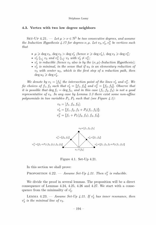
Stéphane Lamy
4.3. Vertex with two low degree neighbors
Set-Up 4.21. — Let µ > ν ∈ N3 be two consecutive degrees, and assumethe Induction Hypothesis 4.17 for degrees ν, µ. Let v3, v
′3, v′′3 be vertices such
that
• µ > deg v3, deg v3 > deg v′3 (hence ν > deg v′3), deg v3 > deg v′′3 ;• v′3 Gv′
2v3 and v′′3 Gv′′
2v3 with v′2 6= v′′2 ;
• v′3 is reducible (hence v3 also is by the (ν, µ)-Induction Hypothesis);• v′2 is minimal, in the sense that if u3 is an elementary reduction ofv3 with center u2, which is the first step of a reduction path, thendeg u2 > deg v′2.
We denote by v1 = [f2] the intersection point of the lines v′2 and v′′2 . Wefix choices of f1, f3 such that v′2 = [[f1, f2]] and v′′2 = [[f2, f3]]. Observe thatit is possible that deg f1 = deg f3, and in this case (f1, f2, f3) is not a goodrepresentative of v3. In any case by Lemma 3.3 there exist some non-affinepolynomials in two variables P1, P3 such that (see Figure 4.1):
v3 = [f1, f2, f3];v′3 = [[f1, f2, f3 + P3(f1, f2)]];v′′3 = [[f1 + P1(f2, f3), f2, f3]].
••v′
3=[[f1,f2,f3+P3(f1,f2)]]
v1=[f2]
v′2=[[f1,f2]]
v3=[f1,f2,f3]
v′′3 =[[f1+P1(f2,f3),f2,f3]]
v′′2 =[[f2,f3]]
Figure 4.1. Set-Up 4.21.
In this section we shall prove:
Proposition 4.22. — Assume Set-Up 4.21. Then v′′3 is reducible.
We divide the proof in several lemmas. The proposition will be a directconsequence of Lemmas 4.24, 4.25, 4.26 and 4.27. We start with a conse-quence from the minimality of v′2.
Lemma 4.23. — Assume Set-Up 4.21. If v′2 has inner resonance, thenv′2 is the minimal line of v3.
– 194 –
Combinatorics of the tame automorphism group
Proof. — Assume first that there exists a ∈ k and r > 2 such thatdeg f2 > deg(f2 + afr1 ). Then consider the vertex w3 = [f1, f2 + afr1 , f3],which satisfies deg v3 > degw3. Assume by contradiction that v′2 is not theminimal line of v3. Then we have deg f2 > deg f3, hence m2 = [f1, f3] isthe minimal line of v3. By the Square Lemma 3.4, we find u3 such thatu3 G w3, u3 G v′3 and deg v3 > deg u3. By applying the (ν, µ)-InductionHypothesis 4.17 successively to v′3 G u3 and u3 G w3, we find that w3 isreducible. So we can take w3 as the first step of a reduction path from v3,which contradicts the minimality of v′2.
Now assume that there exist a ∈ k∗ and r > 2 such that deg f1 >deg(f1 + afr2 ). If v′2 is not the minimal line, we have deg f1 > deg f3.
If deg f1 = deg f3, there exists b ∈ k∗ such that deg f1 > deg(f1 + bf3).Then [f2, f1 + bf3] is the minimal line of v3, and we consider w′3 = [f1 +afr2 , f2, f1 + bf3], which satisfies deg v3 > degw′3. As above, by the SquareLemma 3.4 and the (ν, µ)-Induction Hypothesis 4.17, we obtain that w′3 canbe chosen to be the first step of a reduction path from v3. This contradictsthe minimality of v′2.
If deg f1 > deg f3, v′′2 = [[f2, f3]] is the minimal line of v3. We considerw′′3 = [f1 + afr2 , f2, f3] which satisfies deg v3 > degw′′3 . As before w′′3 can bechosen to be the first step of a reduction path from v3, with center v′′2 : againthis contradicts the minimality of v′2.
Lemma 4.24. — Assume Set-Up 4.21. If v′2 is not the minimal line inv3, and has outer resonance in v3, then v′′3 is reducible.
Proof. — Since v′2 = [[f1, f2]] is not the minimal line in v3, one of thedegrees deg f1 or deg f2 must realize the top degree of v3.
First consider the case deg f2 = topdeg v3. In this case, we have deg f1 6=deg f3. Indeed, assuming by contradiction that deg f1 = deg f3, there wouldexist α ∈ k∗ such that f ′3 = f3−αf1 satisfies deg f3 > deg f ′3. Then, we wouldhave deg f2 > deg f1 > deg f ′3, and the line v′2 = [[f1, f2]] could not have outerresonance in v3. Therefore, (f1, f2, f3) is a good representative of v3, and theassumption on outer resonance means that deg f3 = deg fr1 for some r > 2.Recall that by Lemma 3.3, the non-affine polynomial P1 ∈ k[y, z] associatedwith the weak elementary reduction v′′3 of v3 satisfies deg f1 > P1(f2, f3).We have deg f2 6∈ N deg f3, otherwise we would have deg f2 ∈ N deg f1, thatis, v′2 would have inner resonance, and by Lemma 4.23 this would contradictv′2 6= m2. Corollary 2.7(3) then gives 2 deg f2 = 3 deg f3, and deg(v3 r v′′2 ) >∆(v′′2 ). But then the existence of δ ∈ N such that deg f2 = 3δ, deg f3 = 2δand deg f1 > δ is not compatible with the existence of r > 2 such thatdeg f3 = r deg f1: contradiction.
– 195 –
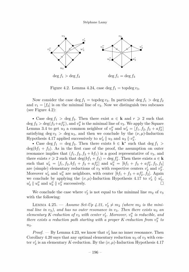
Stéphane Lamy
•
•
•
•
u3
v′′3
v3
w′3
v′3
??
•
• •v′′3
v3
v′3##
u′′3 u′
3
deg f1 > deg f3 deg f1 = deg f3
Figure 4.2. Lemma 4.24, case deg f1 = topdeg v3.
Now consider the case deg f1 = topdeg v3. In particular deg f1 > deg f2and v1 = [f2] is on the minimal line of v3. Now we distinguish two subcases(see Figure 4.2):
• Case deg f1 > deg f3. Then there exist a ∈ k and r > 2 such thatdeg f3 > deg(f3+afr2 ), and v′′2 is the minimal line of v3. We apply the SquareLemma 3.4 to get u3 a common neighbor of v′′3 and w′3 = [f1, f2, f3 + afr2 ]satisfying deg v3 > deg u3, and then we conclude by the (ν, µ)-InductionHypothesis 4.17 applied successively to w′3 G u3 and u3 G v′′3 .
• Case deg f1 = deg f3. Then there exists b ∈ k∗ such that deg f1 >deg(bf1 + f3). As in the first case of the proof, the assumption on outerresonance implies that (f1, f2, f3 + bf1) is a good representative of v3, andthere exists r > 2 such that deg(bf1 + f3) = deg fr2 . Then there exists a ∈ ksuch that u′3 = [f1, f2, bf1 + f3 + afr2 ] and u′′3 = [bf1 + f3 + afr2 , f2, f3]are (simple) elementary reductions of v3 with respective centers v′2 and v′′2 .Moreover u′3 and u′′3 are neighbors, with center [bf1 + f3 + afr2 , f2]. Againwe conclude by applying the (ν, µ)-Induction Hypothesis 4.17 to v′3 G u′3,u′3 G u
′′3 and u′′3 G v′′3 successively.
We conclude the case where v′2 is not equal to the minimal line m2 of v3with the following:
Lemma 4.25. — Assume Set-Up 4.21, v′2 6= m2 (where m2 is the mini-mal line in v3), and has no outer resonance in v3. Then there exists u3 anelementary K-reduction of v3 with center v′2. Moreover, v′′3 is reducible, andthere exists a reduction path starting with a proper K-reduction from v′′3 tou3.
Proof. — By Lemma 4.23, we know that v′2 has no inner resonance. ThenCorollary 4.20 says that any optimal elementary reduction u3 of v3 with cen-ter v′2 is an elementary K-reduction. By the (ν, µ)-Induction Hypothesis 4.17
– 196 –
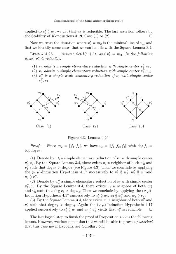
Combinatorics of the tame automorphism group
applied to v′3 G u3, we get that u3 is reducible. The last assertion follows bythe Stability of K-reductions 3.19, Case (1) or (2).
Now we treat the situation where v′2 = m2 is the minimal line of v3, andfirst we identify some cases that we can handle with the Square Lemma 3.4.
Lemma 4.26. — Assume Set-Up 4.21, and v′2 = m2. In the followingcases, v′′3 is reducible:
(1) v3 admits a simple elementary reduction with simple center v′2, v1;(2) v3 admits a simple elementary reduction with simple center v′′2 , v1;(3) v′′3 is a simple weak elementary reduction of v3 with simple center
v′′2 , v1.
v1
•
•
•
•
u3
v′′3
v3
w′3
v′2
v′3
??
v1
•
•
•
•
u3
w′′3
v3
v′3
v′′2
v′′3
__v1
•
•
•
•
u3
v′′3
v′′2
v3
v′3
__
Case (1) Case (2) Case (3)
Figure 4.3. Lemma 4.26.
Proof. — Since m2 = [[f1, f2]], we have v3 = [[f1, f2, f3]] with deg f3 =topdeg v3.
(1) Denote by w′3 a simple elementary reduction of v3 with simple centerv′2, v1. By the Square Lemma 3.4, there exists u3 a neighbor of both w′3 andv′′3 such that deg v3 > deg u3 (see Figure 4.3). Then we conclude by applyingthe (ν, µ)-Induction Hypothesis 4.17 successively to v′3 G w′3, w′3 G u3 andu3 G v′′3 .
(2) Denote by w′′3 a simple elementary reduction of v3 with simple centerv′′2 , v1. By the Square Lemma 3.4, there exists u3 a neighbor of both w′′3and v′3 such that deg v3 > deg u3. Then we conclude by applying the (ν, µ)-Induction Hypothesis 4.17 successively to v′3 G u3, u3 G w′′3 and w′′3 G v′′3 .
(3) By the Square Lemma 3.4, there exists u3 a neighbor of both v′′3 andv′3 such that deg v3 > deg u3. Again the (ν, µ)-Induction Hypothesis 4.17applied successively to v′3 G u3 and u3 G v′′3 yields that v′′3 is reducible.
The last logical step to finish the proof of Proposition 4.22 is the followinglemma. However, we should mention that we will be able to prove a posteriorithat this case never happens: see Corollary 5.4.
– 197 –
Stéphane Lamy
Lemma 4.27. — Assume Set-Up 4.21, v′2 = m2, and that we are not inone of the cases covered by Lemma 4.26. Then there exists u′′3 an elementaryK-reduction of v3 with center v′′2 such that u′′3 is reducible. In particular, bythe (ν, µ)-Induction Hypothesis 4.17, v′′3 is reducible.
Proof. — It is sufficient to check that the simplex v1, v′′2 , v3 has Strong
Pivotal Form (s) for some odd s > 3: Indeed then one can apply Proposi-tion 4.19(4) to get the result.
On the one hand deg f3 > deg f1 > degP1(f2, f3), and on the other handsince we are not in the situation of Lemma 4.26(3) we have P1(f2, f3) 6∈ k[f2],so that
degvirt P1(f2, f3) > degP1(f2, f3).We also have deg f3 6∈ N deg f2 since otherwise we could apply Lemma 4.26(1).So we are in the hypotheses of Corollary 2.7(3), and there exist a degreeδ ∈ N3 and an odd integer s > 3 such that deg f2 = 2δ, deg f3 = sδ and
sδ > degP1(f2, f3) > ∆(f3, f2).It remains to check (2): if v′′2 = [[f2, f3]] had outer resonance in v3 then wewould have deg f1 ∈ N deg f2, and we could apply Lemma 4.26(2), contraryto our assumption.
4.4. Proof of the Reducibility Theorem
Clearly Theorem 4.1 is a corollary of
Proposition 4.28. — If a vertex v3 of type 3 in the complex C is re-ducible, then any neighbor of v3 also is reducible.
Proof. — We plan to prove Proposition 4.28 by induction on degree: weneed to prove that for any ν ∈ N3, the Induction Hypothesis 4.17 holds fordegrees ν, ν. Clearly when ν = (1, 1, 1) this is true (because empty!).
Let µ > ν be two consecutive degrees in N3. It is sufficient to prove thetwo following facts.
Fact 4.29. — Assume the Induction Hypothesis 4.17 for degrees ν, ν.Then it also holds for degrees ν, µ.
Fact 4.30. — Assume the Induction Hypothesis 4.17 for degrees ν, µ.Then it also holds for degrees µ, µ.
To prove Fact 4.29, consider v′3 a reducible vertex with ν > deg v′3, andlet v3 be a neighbor of v′3, with center v′2, and with deg v3 = µ (otherwisethere is nothing to prove). We want to prove that v3 is reducible.
– 198 –
Combinatorics of the tame automorphism group
If v′2 is the minimal line of v3, then v′3 is a T -reduction of v3 for any goodtriangle T and we are done.
If v′2 is not the minimal line of v3, and has no inner or outer resonancein v3, then by Corollary 4.20 any optimal reduction u3 of v3 with respect tothe center v′2 is an elementary K-reduction of v3. Since u3 is a neighbor ofv′3 and ν > deg u3, we conclude by the (ν, ν)-Induction Hypothesis 4.17 thatu3 is reducible. Hence v3 also is reducible, with first step of a reduction paththe K-reduction to u3.
Finally assume that v′2 has resonance, and that v′2 is not the minimal lineof v3. By Lemma 3.3 we can write
v3 = [[f1, f2, f3]], v′3 = [[f1, f2, g3]], v′2 = [[f1, f2]],with deg f1 > maxdeg f3,deg f2 and g3 = f3 + P (f1, f2) for some polyno-mial P .
If v′2 has inner resonance, then deg f1 = r deg f2 for some r > 2. Thereexists a ∈ k such that v′′3 = [f1 +afr2 , f2, f3] is a simple elementary reductionof v3 with center [[f2, f3]], which is the minimal line of v3, hence belongs toany good triangle T . Then we can apply the Square Lemma 3.4 to get u3with ν > deg u3 and u3 G v′3, u3 G v′′3 . We conclude by the (ν, ν)-InductionHypothesis 4.17, applied successively to v′3 G u3 and u3 G v′′3 , that v′′3 isreducible, hence v3 also is.
If v′2 has no inner resonance, but has outer resonance in v3, then deg f1 >deg f3 > deg f2 and deg f3 = r deg f2 for some r > 2. There exists Q(f2)such that deg f3 > deg(f3 +Q(f2)) and deg(f3 +Q(f2)) 6∈ Ndeg f2. Let T bea good triangle of v3. One of the lines in T has the form u2 = [[f1 + af3, f2]].Set u3 = [[f1 + af3, f2, f3 + Q(f2)]], which is an elementary T -reduction ofv3 with center u2, and a neighbor of w3 = [[f1, f2, f3 +Q(f2)]]. By the (ν, ν)-Induction Hypothesis 4.17 applied successively to v′3 G w3 and w3 G u3, weobtain that u3 is reducible, hence v3 also is.
To prove Fact 4.30, consider v3 a reducible vertex with deg v3 = µ, andlet v′′3 be a neighbor of v3, with center v′′2 , such that
deg v3 > deg v′′3 .We want to prove that v′′3 is reducible.
First assume that v3 admits a reduction path such that the first stepv′3 is an elementary reduction, with center v′2. Moreover we assume thatv′2 has minimal degree between all possible such first center of a reductionpath. If v′2 = v′′2 , then v′′3 is a neighbor of v′3 and by the (ν, µ)-InductionHypothesis 4.17 we are done. If on the contrary v′2 and v′′2 are two different
– 199 –
Stéphane Lamy
lines in P2(v3), we are in the situation of Set-Up 4.21. Then we conclude byProposition 4.22.
Finally assume that v3 admits a reduction path such that the first stepis a proper K-reduction v′3. If this proper K-reduction is normal, then byStability of K-reduction 3.19, Case (3) or (4), we obtain that v′3 is also aK-reduction of v′′3 , and we are done. On the other hand if v′3 is a non-normalproper K-reduction of v3, then by Lemma 3.14 we get the existence of avertex u3 that is both an elementary K-reduction of v3 and a neighbor ofv′3. By applying the (ν, µ)-Induction Hypothesis 4.17 to v′3 G u3 we get thatu3 is reducible, and we are reduced to the previous case of the proof.
5. Simple connectedness
In this section we prove that the complex C is simply connected, whichamounts to saying that the group Tame(A3) is the amalgamated product ofthree subgroups along their pairwise intersections.
5.1. Consequences of the Reducibility Theorem
Now that the Reducibility Theorem 4.1 is proved, all previous resultsthat were dependent of a reducibility assumption become stronger. This isthe case in particular for:
• The Induction Hypothesis 4.17, which is always true;• Lemma 4.6, which now implies that if v3 is part of a simplex withStrong Pivotal Form, then v3 does not admit an elementary reduc-tion with center m2 the minimal line of v3: see the proof of Propo-sition 5.1 below;
• Proposition 4.19 and Corollary 4.20;• Set-Up 4.21, hence also all results in §4.3.
In particular we single out the following striking consequences of the Re-ducibility Theorem 4.1.
Proposition 5.1. — Let u3 be an elementary K-reduction of v3, withcenter v2. Then v3 does not admit any elementary reduction with centerdistinct from v2.
Proof. — By contradiction, assume that v′3 is an elementary reduction ofv3, with center v′2 distinct from v2. Then by Stability of K-reduction 3.19,Case (1) or (2), there exists w′3 with degw′3 = deg v3 such that u3 is a
– 200 –

Combinatorics of the tame automorphism group
proper K-reduction of v′3 via w′3. In particular, v′3 is an elementary reductionof w′3 with center m2, the minimal line of w′3. Moreover, by Corollary 3.8,the pivotal simplex of this proper K-reduction has Strong Pivotal Form.Now consider v′′3 an optimal elementary reduction of w′3 with center m2:Lemma 4.6 gives a contradiction.
Corollary 5.2. — Let u3 be a proper K-reduction of v3, via w3. Thendegw3 = deg v3.
Proof. — By Proposition 5.1 we cannot have degw3 > deg v3.
Corollary 5.3. — Let v3 admitting a K-reduction, then any line u2 inP2(v3) has no inner resonance. In other words, Case (2) in Corollary 3.15never happens.
Proof. — We use the notation v3 = [[f1, f2, f3]] from Corollary 3.15, whichsays that if there exists a line in v3 with inner resonance, then deg f1 =2 deg f3 and deg f1 = 3
2 deg f2. But in this case we would have an elementaryreduction [f1 + af2
3 , f2, f3] of v3 with center the minimal line [[f2, f3]] 6= v2,in contradiction with Proposition 5.1
We also obtain that the situation of Lemma 4.27 never happens:
Corollary 5.4. — Assume Set-Up 4.21, and v′2 = m2. Then we are inone of the cases covered by Lemma 4.26.
Proof. — Otherwise by Lemma 4.27 there would exist an elementary K-reduction of v3 with center v′′2 , in addition to the elementary reduction withcenter v′2: This is not compatible with Proposition 5.1.
5.2. Local homotopies
To prove the simple connectedness of C, the following terminology willbe convenient.
We call combinatorial path a sequence of vertices v3(i), i = 0, . . . , n,such that for all i = 0, . . . , n − 1, v3(i) G v3(i + 1). Denoting by v2(i) thecenter of v3(i) G v3(i + 1), we think of such a sequence as equivalent to apath γ : [0, 2n] → C where for each i = 0, . . . , n − 1, the interval [2i, 2i + 2]is mapped isometrically onto the union of the two edges v3(i), v2(i) andv2(i), v3(i+ 1). In particular we have these parameterizations in mind whenwe say that two such combinatorial paths are homotopic in C. We say thata combinatorial path is locally geodesic if for all i, v2(i) 6= v2(i+ 1) (andv3(i) 6= v3(i + 1), but this is already contained in the definition of v3(i) Gv3(i+ 1)). Observe that starting from any combinatorial path, by removing
– 201 –
Stéphane Lamy
some vertices we can always obtain a locally geodesic one. If v3(0) = v3(n) wesay that the path is a combinatorial loop with base point v3(0). If v3(0) =[id], the maximal vertex of such a loop is defined as the vertex v3(i0) thatrealizes the maximum max deg v3(i), with i0 maximal. In particular, we have
deg v3(i0) > deg v3(i0 + 1) and deg v3(i0) > deg v3(i0 − 1).
Lemma 5.5. — Let v3(i), i = 0, . . . , n, be a locally geodesic loop with basepoint at [id], and let v3(i0) be the maximal vertex. Then the combinatorialpath v3(i0 − 1), v3(i0), v3(i0 + 1) is homotopic in C to a combinatorial pathfrom v3(i0−1) to v3(i0 +1) where all type 3 intermediate vertices have degreestrictly less than deg v3(i0).
Proof. — Since deg v3(i0) > deg v3(i0 + 1), we know that v3(i0) admitsan elementary reduction, so it makes sense to choose v′2 a vertex of minimaldegree such that v3 = v3(i0) admits an elementary reduction v′3 with centerv′2. Then we are going to apply Set-Up 4.21 twice, taking v′′3 to be successivelyv3(i0 − 1) and v3(i0 + 1). It is sufficient to prove that in both cases thecombinatorial path v′′3 , v3, v
′3 is homotopic to a combinatorial path from v′′3
to v′3 where all type 3 intermediate vertices have degree strictly less thandeg v3. Observe that there are degenerate cases which are easy to handle.First if v′3 = v′′3 , we just take the combinatorial path with one single vertexv′3. Second, if v′3 and v′′3 share the same center with v3, we can just discardv3 to obtain a combinatorial path from v′′3 to v′3 without any intermediatevertex, so we can indeed assume that the centers v′2 and v′′2 are distinct asrequired in Set-Up 4.21.
If v′2 = m2 then by Corollary 5.4 we are in one of the cases covered byLemma 4.26, and the homotopy is clear in all cases (see Figure 4.3). Forinstance in Case (1) we replace the path v′′3 , v3, v
′3 by v′′3 , u3, w
′3, v′3, and the
other cases are similar.
If v′2 6= m2, and v′2 has outer resonance in v3, then we are in one ofthe two cases covered by Lemma 4.24, and again the homotopy is clear (seeFigure 4.2).
If v′2 6= m2, and v′2 has no outer resonance in v3, then by Lemma 4.25 thereexists u3 an elementary K-reduction of v3 with center v′2. Therefore, in thatcase, up to replacing v′3 by u3 we may assume without loss in generality thatv′3 is an elementary K-reduction of v3. By Proposition 5.1, this can only hap-pen in the case v′′3 = v3(i0− 1), and deg v3(i0) = deg v3(i0− 1). By Stabilityof K-reduction 3.19, Case (1) or (2), v′3 is a proper K-reduction of v3(i0−1),and up to a local homotopy (see Figure 3.5, Case (2)) we can assume thatthe intermediate vertex is v3 = v3(i0). If this proper K-reduction is not nor-mal, we obtain the expected homotopy from the normalization process ofLemma 3.14 (see Figure 3.4). Otherwise, By Stability of K-reduction 3.19,
– 202 –
Combinatorics of the tame automorphism group
Case (3) or (4), we get that v′3 is a normal proper K-reduction of v3(i0− 2),with v2(i0 − 2) = v2(i0 − 1) the minimal line of v3(i0): This contradicts ourassumption that we started with a locally geodesic loop.
We need one last ingredient before proving the simple connectedness ofthe complex C.
Lemma 5.6. — The link L(v1) of a vertex of type 1 is a connected graph.
Proof. — By transitivity of the action of Tame(A3) on vertices of type1, it is sufficient to work with the link L([x3]). Let v3 = [[f1, f2, x3]] be avertex of type 3 in L([x3]), where we choose our representative such thatdeg f1 > deg f2.
First observe that v3 does not admit any elementary K-reduction. Indeedby Corollary 3.8 the pivotal simplex of such a reduction should have StrongPivotal Form (s) for some odd s > 3. In particular there exist δ ∈ N3 anda reordering g2, g3 = f2, x3 such that
deg f1 = sδ, deg g2 = 2δ and sδ > deg g3 > (s− 2)δ.But since deg x3 = (0, 0, 1) is the minimal possible degree of a component ofan automorphism, both cases g2 = x3 or g3 = x3 are impossible.
It follows that v3 also does not admit a proper K-reduction: such a re-duction would be via w3 = [[g1, f2, x3]], but we just proved that such a w3cannot admit an elementary K-reduction.
By Theorem 4.1, we conclude that v3 admits an elementary reductionv′3, which clearly must admit [x3] as pivot, since there is no non-constantpolynomial P ∈ k[x1, x2, x3] with deg x3 > degP . In particular, v′3 also is inL([x3]), and by induction on degree, we obtain the existence of a reductionpath from v3 to [id] that stays in L([x3]).
Now we recover a result of [14] and [16], about relations in Tame(A3). Pre-cisely, Umirbaev gives an algebraic description of the relations, and Wrightshows that this result can be rephrased in terms of an amalgamated productstructure over three subgroups. Our proof follows the same strategy as in [1,Proposition 3.10].
Proposition 5.7. — The complex C is simply connected.
Proof. — Let γ be a loop in C. We want to show that it is homotopicto a trivial loop. Without loss in generality, we can assume that the imageof γ is contained in the 1-skeleton of the square complex, and that γ(0) =[[x1, x2, x3]] is the vertex of type 3 associated with the identity.
A priori (the image of) γ is a sequence of edges of arbitrary type. ByLemma 5.6, we can perform a homotopy to avoid each vertex of type 1. So
– 203 –
Stéphane Lamy
now we assume that vertices in γ are alternatively of type 2 and 3. Precisely,up to a reparametrization we can assume that for each i, γ(2i) has type 3and γ(2i + 1) has type 2, so that γ defines a combinatorial path by settingv3(i) = γ(2i) for each i. By removing some of these vertices we can alsoassume that γ is a locally geodesic loop.
Let v3(i0) be the maximal vertex of the loop, and δ0 its degree. Then byLemma 5.5 we can conclude by induction on the couple (δ0, i0), ordered withlexicographic order.
Since Tame(A3) acts on a simply connected 2-dimensional simplicial com-plex with fundamental domain a simplex, we can recover the group from thedata of the stabilizers of each type of vertex. This is a simple instance of thetheory of developable complexes of groups in the sense of Haefliger (see [2,III.C]). Following Wright we can phrase this fact as follows:
Corollary 5.8 ([16, Theorem 2]). — The group Tame(A3) is the amal-gamated product of the three following subgroups along their pairwise inter-sections:
Stab([x1, x2, x3]) = A3;Stab([x1, x2]) = (ax1 + bx2 + c, a′x1 + b′x2 + c′, αx3 + P (x1, x2));
Stab([x1]) = (ax1 + b, f2(x1, x2, x3), f3(x1, x2, x3).
6. Examples
We gather in this last section a few examples of interesting reductions.
Example 6.1 (Elementary K-reduction with s = 3). — Letg = (x1, x2, x3 + x2
1 − x32),
t1 = (x1 + αx2x3 + x33, x2 + x2
3, x3).Clearly in the composition g t1 the terms of degree 6 cancel each other.Moreover, if we choose α = 3
2 this is also the case for terms of degree 5:
gt1 =(x1 + 3
2x2x3 + x33, x2 + x2
3, x3 + x21 − x3
2 + 3x1x2x3 + x23
4 (8x1x3 − 3x22)).
Consider now a triangular automorphism preserving the quadratic form8x1x3 − 3x2
2 that appears as a factor:t2 = (x1, x2 + x2
1, x3 + 34x1x2 + 3
8x31).
A direct computation shows that the components of f = g t1 t2 =(f1, f2, f3) admits the following degrees:
(9, 0, 0), (6, 0, 0), (7, 0, 1).
– 204 –
Combinatorics of the tame automorphism group
Finally, u3 = [t1 t2], whose degrees of components are(9, 0, 0), (6, 0, 0), (3, 0, 0),
is an elementaryK-reduction of v3 = [f1, f2, f3]. Following notation from thedefinition of Strong Pivotal Form, we have s = 3 and δ = (3, 0, 0). Moreover
df1 ∧ df2 = − 32 (x2
1 − x2)dx2 ∧ dx3 + ( 2716x
21x2 + 9
8x22 + 3
2x1x3 + 1)dx1 ∧ dx2
+ (− 94x
31 − 3
2x1x2 + 2x3)dx1 ∧ dx3.
so that deg df1∧df2 = (4, 0, 1), from the contribution of the factor x31dx1∧dx3.
Example 6.2 (Elementary K-reduction with s = 5, see also [6]). — Onecan apply the same strategy to produce examples of K-reduction with s > 3an arbitrary odd number. We give the construction for s = 5, and leave thegeneralization to the reader. Let
g = (x1, x2, x3 + x21 − x5
2),t1 = (x1 + αx2
2x3 + βx2x33 + x5
3, x2 + x23, x3).
Observe that αx22x3 + βx2x
33 + x5
3 is homogeneous of degree 5, by puttingweight 1 on x3 and weight 2 on x2. By choosing α = 15
8 , β = 52 , we minimize
the degree of the composition:gt1 =
(x1 + 15
8 x22x3 + 5
2x2x33 + x5
3, x2 + x23, x3 + 1
8x43(16x1x3 − 5x3
2) + · · ·).
Now take the following triangular automorphism, which preserves the poly-nomial 16x1x3 − 5x3
2:t2 =
(x1, x2 + x2
1, x3 + 516 (3x1x
22 + 3x3
1x2 + x51)).
We compute the degrees of the components of f = g t1 t2 = (f1, f2, f3):(25, 0, 0), (10, 0, 0), (20, 3, 0).
Finally, u3 = [t1 t2], whose degrees of components are(25, 0, 0), (10, 0, 0), (5, 0, 0),
is an elementary K reduction of v3 = [f1, f2, f3]. Here we have s = 5 andδ = (5, 0, 0). Moreover
df1∧df2 = − 158(x2
1 + x2)2dx2∧dx3+
(2x3 − 5
8 (5x51 − 9x3
1x2 − 3x1x22))dx1∧dx3
+( 75
128 (5x41x
22 + 9x2
1x32 + 3x4
2) + 158 (x3
1x3 + 2x1x2x3) + 1)dx1 ∧ dx2,
so that deg df1∧df2 = (5, 3, 0), from the contribution of the factor x41x
22dx1∧
dx2.
Example 6.3 (Elementary reduction without Strong Pivotal Form). — Wegive examples of elementary reduction that show that the three assumptionsin Proposition 3.7 are necessary to get Strong Pivotal Form.
– 205 –
Stéphane Lamy
(1) Let f = (f1, f2, f3) ∈ Tame(A3) and r > 2 such that
deg f1 > deg f3 = r deg f2.
In particular there exists a ∈ k such that deg f3 > deg(f3+afr2 ). For instancef = (x1 + x3
3, x2, x3 + x22) is such an automorphism, for r = 2 and a = −1.
Then u3 = [[f1, f2, f3 + afr2 ]] is an elementary reduction of v3 = [[f1, f2, f3]],and the pivotal simplex does not have Strong Pivotal Form. Observe thatv2 = [[f1, f2]] has outer resonance in v3.
(2) Let u3 = [[f1, f2, f3 + P (f1, f2)]] be an elementary K-reduction ofw3 = [[f1, f2, f3]], with 2 deg f1 = sdeg f2 for some odd s > 3. For instancewe can start with one of the examples 6.1 or 6.2. Pick any integer r > s+1
2 .Then v′3 = [[f1 + fr2 , f2, f3 + P (f1 − fr2 , f2)]] is an elementary reduction ofv3 = [[f1 + fr2 , f2, f3]], and the pivotal simplex does not have Strong PivotalForm. Observe that the center v2 = [[f1 + fr2 , f2]] has inner resonance.
(3) With the notation of Example 6.1 or 6.2, the elementary reductionfrom [[g t1]] to [[t1]] gives an example of an elementary reduction where thecenter m2, which is the minimal line, does not have inner or outer resonance,and again the pivotal simplex does not have Strong Pivotal Form.
Example 6.4 (Non-normal proper K-reduction). — Pick the elementaryK-reduction from Example 6.2, and set v′3 = [f1 +f2
2 , f2, f3], which is a weakelementary reduction of v3. Then u3 is a non-normal proper K-reduction ofv′3, via v3. This corresponds to Case (1) of Stability of aK-reduction 3.19. Wemention again that it is an open question whether there exists any normalproper K-reduction.
Non Example 6.5 (Hypothetical type II and type III reductions). — FromCorollary 3.8 we know that if v3 admits an elementary K-reduction, thenthe pivotal simplex has Strong Pivotal Form (s) for some odd s > 3. Inparticular if s = 3, then v3 = [[f1, f2, f3]] with deg f1 = 3δ, deg f2 = 2δ anddeg f3 > δ for some δ ∈ N3. It is not clear if there exists an example of sucha reduction with 3
2δ > deg f3, or even 2δ > deg f3. Observe that such anexample would be the key for the existence of the following reductions (forthe definition of a reduction of type II or III, see the original paper [13],or [7, §7]):
(1) If 32δ > deg f3, then v′3 = [[f1 + f2
3 , f2, f3]] would admit a normalproper K-reduction, via v3: This would correspond to a type IIIreduction.
(2) If 2δ > deg f3 >32δ, then v3 would admit an elementaryK-reduction
such that the pivot [f2] is distinct from the minimal vertex [f3]: Thiswould correspond to a type II reduction.
(3) If 32δ > deg f3, then v′′3 = [[f1, f2 + f2
3 , f3]] would be an example of avertex that admits a reduction along a center with outer resonance
– 206 –
Combinatorics of the tame automorphism group
in v′′3 , but that does not admit a reduction with center the minimalline of v′′3 (see Lemma 4.24).
Bibliography
[1] C. Bisi, J. P. Furter & S. Lamy, “The tame automorphism group of an affinequadric threefold acting on a square complex”, Journal de l’École Polytechnique -Mathématiques 1 (2014), p. 161-223.
[2] M. R. Bridson & A. Haefliger, Metric spaces of non-positive curvature,Grundlehren der Mathematischen Wissenschaften, vol. 319, Springer, 1999.
[3] S. Cantat & S. Lamy, “Normal subgroups in the Cremona group”, Acta Math. 210(2013), no. 1, p. 31-94, With an appendix by Yves de Cornulier.
[4] W. Hodge & D. Pedoe, Methods of algebraic geometry. Vol. I, Cambridge Mathe-matical Library, Cambridge University Press, 1994, Book I: Algebraic preliminaries,Book II: Projective space, Reprint of the 1947 original.
[5] S. Kuroda, “A generalization of the Shestakov-Umirbaev inequality”, J. Math. Soc.Japan 60 (2008), no. 2, p. 495-510.
[6] ———, “Automorphisms of a polynomial ring which admit reductions of type I”,Publ. Res. Inst. Math. Sci. 45 (2009), no. 3, p. 907-917.
[7] ———, “Shestakov-Umirbaev reductions and Nagata’s conjecture on a polynomialautomorphism”, Tôhoku Math. J. 62 (2010), no. 1, p. 75-115.
[8] S. Lamy, “Une preuve géométrique du théorème de Jung”, Enseign. Math. (2) 48(2002), no. 3-4, p. 291-315.
[9] S. Lamy & P. Przytycki, “Acylindrical hyperbolicity of the three-dimensional tameautomorphism group”, https://arxiv.org/abs/1610.05457, 2016.
[10] A. Lonjou, “Non simplicité du groupe de Cremona sur tout corps”, Ann. Inst.Fourier 66 (2016), no. 5, p. 2021-2046.
[11] A. Martin, “On the acylindrical hyperbolicity of the tame automorphism group ofSL2(C)”, Bull. Lond. Math. Soc. 49 (2017), no. 5, p. 881-894.
[12] I. P. Shestakov & U. U. Umirbaev, “Poisson brackets and two-generated subalge-bras of rings of polynomials”, J. Am. Math. Soc. 17 (2004), no. 1, p. 181-196.
[13] ———, “The tame and the wild automorphisms of polynomial rings in three vari-ables”, J. Am. Math. Soc. 17 (2004), no. 1, p. 197-227.
[14] U. U. Umirbaev, “Defining relations of the tame automorphism group of polynomialalgebras in three variables”, J. Reine Angew. Math. 600 (2006), p. 203-235.
[15] S. Vénéreau, “A parachute for the degree of a polynomial in algebraically indepen-dent ones”, Math. Ann. 349 (2011), no. 3, p. 589-597.
[16] D. Wright, “The generalized amalgamated product structure of the tame automor-phism group in dimension three”, Transform. Groups 20 (2015), no. 1, p. 291-304.
– 207 –