Universita degli Studi di SienaDipartimento di Ingegneria dell’Informazione

Dottorato di Ricerca in

Ingegneria dell’Informazione

Analysis and design of efficientplanar leaky-wave antennas

Tesi di Dottorato di

Mauro Ettorre

Prof. Stefano Maci

Dr. Andrea Neto

Ciclo XXAnno Accademico 2007/2008

To my mother and my father

Abstract

This thesis deals with the effective design of planar leaky-wave antennas.

The work describes a methodology based on the polar expansion of Green’s

function representations to address very different geometrical configurations

which might appear to have little in common. In fact leaky waves with

planar and cylindrical spreadings, as well as in slotted, dipole, pin based and

purely dielectric configurations have been addressed. However the unifying

goal of this thesis has been the systematic search for low cost structures

characterized by high quality beams, with high efficiency and minimal ohmic

losses. In our view this goal has been achieved.

Part of this thesis was developed and funded by the Defence, Security

and Safety Institute of the Netherlands Organization for Applied Scientific

Research (TNO), The Hague, The Netherlands.

Contents

Introduction xii

1 Modal Analysis of leaky wave antennas 1

1.1 Transverse Resonance Method . . . . . . . . . . . . . . . . . . 2

1.1.1 Discrimination of the modes guided in a planar structure 4

1.1.2 Example of a multi-layer planar structure . . . . . . . 8

1.2 Field radiated by a leaky-wave antenna . . . . . . . . . . . . . 11

1.3 Summary . . . . . . . . . . . . . . . . . . . . . . . . . . . . . 15

2 Leaky-wave antenna made by using a 2-D periodic array of

metal dipoles 16

2.1 Equivalence between the super-layer configuration and grounded

substrate loaded periodically . . . . . . . . . . . . . . . . . . . 17

2.1.1 Mathematical relations for the equivalence between a

dielectric and metallic super-layer configuration. . . . . 19

2.1.2 Example of equivalence between a dielectric and metal-

lic super-layer configuration. . . . . . . . . . . . . . . . 21

2.2 2-D leaky-wave antenna: planar array covered by a printed

periodic surface . . . . . . . . . . . . . . . . . . . . . . . . . . 24

2.3 Summary . . . . . . . . . . . . . . . . . . . . . . . . . . . . . 31

i

Contents ii

3 Leaky-wave antenna made by using planar circularly sym-

metric EBG 32

3.1 Substrate and Feed design . . . . . . . . . . . . . . . . . . . . 33

3.2 Dispersion Analysis of the local periodic surface . . . . . . . . 38

3.3 Prototype and Experimental results . . . . . . . . . . . . . . . 40

3.4 Summary and remarks . . . . . . . . . . . . . . . . . . . . . . 43

4 Leaky-Wave Slot Array Antenna Fed by a Dual Reflector

System 46

4.1 Dual offset reflector Gregorian System made by pins . . . . . . 49

4.1.1 Design of the two dimensional Gregorian system . . . . 51

4.2 Excitation of the Gregorian System . . . . . . . . . . . . . . . 58

4.2.1 Green’s function of the pin-made feed . . . . . . . . . . 63

4.2.2 Dispersion analysis of the pin-made feed . . . . . . . . 66

4.3 MoM analysis for the dual offset Gregorian system fed by the

pin-made feed . . . . . . . . . . . . . . . . . . . . . . . . . . . 68

4.3.1 Validation of the MoM code . . . . . . . . . . . . . . . 72

4.3.2 Circuit parameters for the Gregorian system: Z, Y and

S matrix . . . . . . . . . . . . . . . . . . . . . . . . . . 73

4.4 Dispersion Analysis of the slot array . . . . . . . . . . . . . . 76

4.5 Prototype and Experimental Results . . . . . . . . . . . . . . 80

4.6 Multi Beam Gregorian System: analysis and results . . . . . . 84

4.6.1 MoM modification to calculate the embedded pattern

associate to the source of the pin-made feed . . . . . . 89

4.7 Summary . . . . . . . . . . . . . . . . . . . . . . . . . . . . . 90

5 Conclusion and Future Developments 91

Bibliography 94

Contents iii

Biography 100

Publications 101

Acknowledgements 103

List of Figures

1.1 Transmission line used to illustrate the transverse resonance

method. . . . . . . . . . . . . . . . . . . . . . . . . . . . . . . 3

1.2 Schematization of a planar guiding structure. It is assumed no

variation along y. (a) General view of the problem. (b) Trans-

mission line model used to derive the dispersion relation. The

planar structure is represented by the boundary impedance

Z(kx, k0). . . . . . . . . . . . . . . . . . . . . . . . . . . . . . 4

1.3 Classification of the possible TM polarized modes guided by

a planar structure, adapted from [8]. . . . . . . . . . . . . . . 7

1.4 Multi-layer structure used as example. (a) Geometrical de-

tails. (b) Equivalent transmission line model for TE and TM

modes. . . . . . . . . . . . . . . . . . . . . . . . . . . . . . . . 9

1.5 Dispersion diagram for the super-layer configuration with εr1 =

1 and εr2 = 4.5, 20.25. The transverse propagation constant

kρ is normalized with respect to the free space propagation

constant k0. . . . . . . . . . . . . . . . . . . . . . . . . . . . . 10

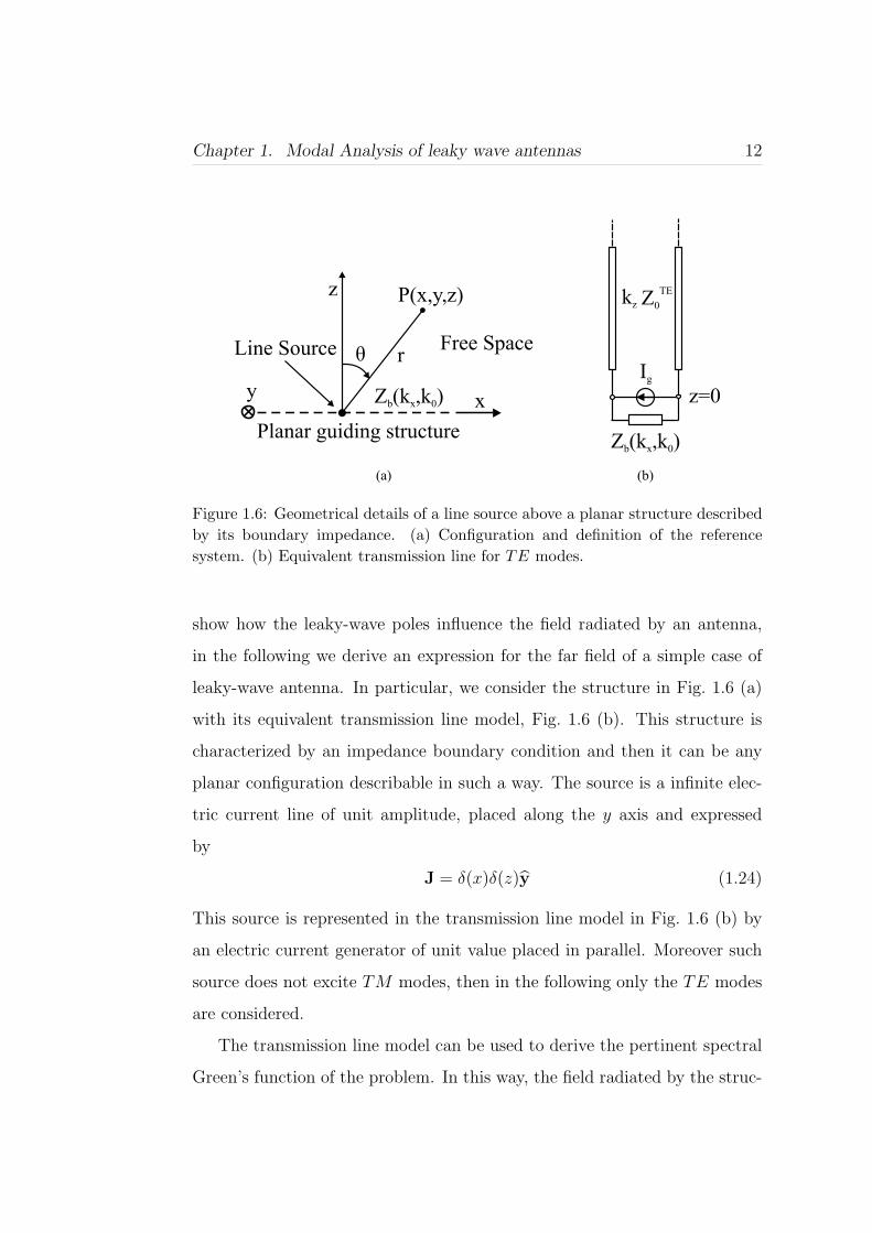
1.6 Geometrical details of a line source above a planar structure

described by its boundary impedance. (a) Configuration and

definition of the reference system. (b) Equivalent transmission

line for TE modes. . . . . . . . . . . . . . . . . . . . . . . . . 12

iv

List of Figures v

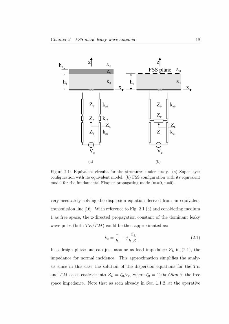
2.1 Equivalent circuits for the structures under study. (a) Super-

layer configuration with its equivalent model. (b) FSS config-

uration with its equivalent model for the fundamental Floquet

propagating mode (m=0, n=0). . . . . . . . . . . . . . . . . . 18

2.2 Geometrical details of the FSS used to replace the dielectric

slab of εr2 = 20.25. The FSS presents a rectangular lattice

and is made by printed dipoles on air. . . . . . . . . . . . . . . 22

2.3 Real and imaginary part of the load impedance ZL for the

dielectric and metallic super-layer stratification made respec-

tively by a dielectric slab of εr2 = 20.25 and the dipole FSS of

Fig. 2.2. . . . . . . . . . . . . . . . . . . . . . . . . . . . . . . 23

2.4 Leaky-wave antenna made by using printed dipoles. (a) Stackup

of the antenna. A glue layer is present between the feeding

layer and the substrate where the the dipoles are printed. (b)

Geometrical details of the FSS made by printed dipoles. . . . 25

2.5 Geometrical details of the array of slots and of the correspond-

ing feeding network. The slots are etched on the ground plane

of the feeding network. . . . . . . . . . . . . . . . . . . . . . . 26

2.6 Dispersion diagram for the FSS over the ground plane without

considering the glue. The two principal TE and TM w.r.t. z

modes are considered. In particular the TE and TM mode

are propagating respectively along y and x, as shown in the

inset in the figure. . . . . . . . . . . . . . . . . . . . . . . . . . 27

2.7 Reflection coefficient of the antenna. . . . . . . . . . . . . . . 28

List of Figures vi

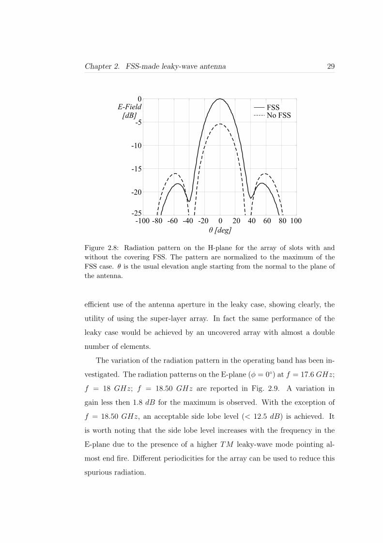
2.8 Radiation pattern on the H-plane for the array of slots with

and without the covering FSS. The pattern are normalized to

the maximum of the FSS case. θ is the usual elevation angle

starting from the normal to the plane of the antenna. . . . . . 29

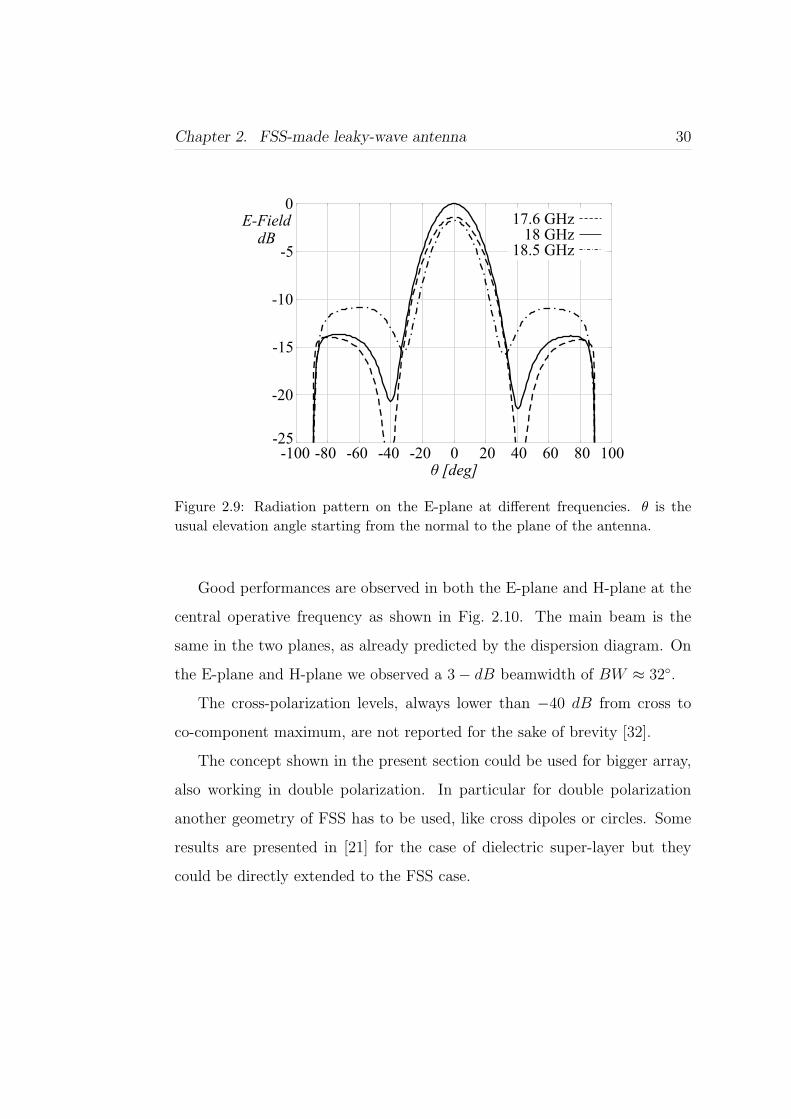
2.9 Radiation pattern on the E-plane at different frequencies. θ

is the usual elevation angle starting from the normal to the

plane of the antenna. . . . . . . . . . . . . . . . . . . . . . . . 30

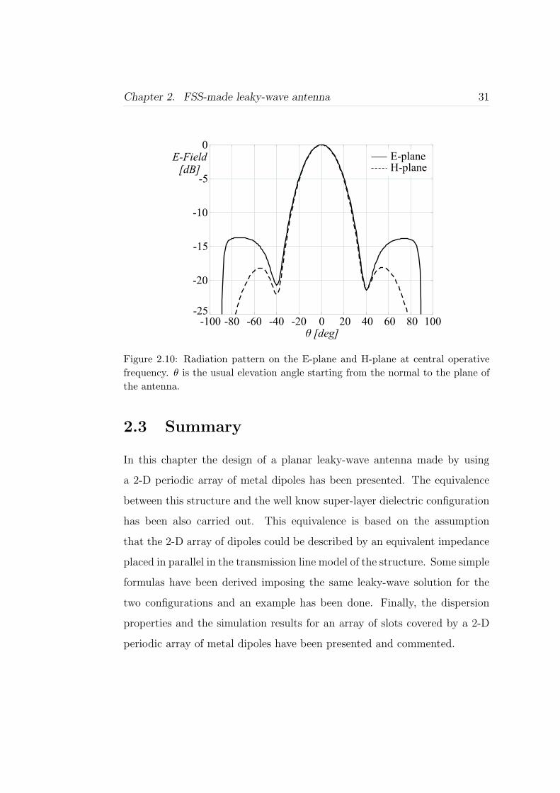
2.10 Radiation pattern on the E-plane and H-plane at central op-

erative frequency. θ is the usual elevation angle starting from

the normal to the plane of the antenna. . . . . . . . . . . . . . 31

3.1 Prototype of the sector PCS-EBG Antenna. The feed is a slot

type surface wave Yagi-Uda launcher (Fig. 3.3), etched on the

opposite side. . . . . . . . . . . . . . . . . . . . . . . . . . . . 34

3.2 Normalized power radiated by a slot on a ground plane un-

derlying a substrate with permittivity εr = 9.8. The power

is normalized to that radiated in the lower half free space by

the slot and plotted as a function of the height in terms of the

wavelength in the dielectric. . . . . . . . . . . . . . . . . . . . 35

3.3 Yagi-Uda coplanar-waveguide (CPW)-fed slot launcher. . . . . 36

3.4 Electric field inside the dielectric substrate. A color scale is

used to represent the field, that is the red color corresponds

to the maximum of the field whereas the dark blue to the

minimum. (a) Yagi-Uda coplanar-waveguide (CPW)-fed slot

launcher. (b) Single slot launcher. . . . . . . . . . . . . . . . . 37

3.5 Stack-up of the structure in a radial cut: p is the periodicity

of the dipoles of the EBG and ld is their length. The dipole

are 0.5 mm width. . . . . . . . . . . . . . . . . . . . . . . . . 38

List of Figures vii

3.6 Dispersion diagrams of the leaky-wave and EBG sectors for

the dominant TM −mode, propagating in the direction of the

printed strips in the equivalent 2-D-EBGs structure with 1-D

periodicity. kt represents the longitudinal complex propaga-

tion wavenumber that locally identifies the radial wavenumber

of the 3-D antenna geometry. . . . . . . . . . . . . . . . . . . 39

3.7 Measured Input Reflection Coefficient. . . . . . . . . . . . . . 40

3.8 Measured radiation patterns in the E-plane at different fre-

quencies. θ is the usual elevation angle starting from the nor-

mal to the plane of the antenna. . . . . . . . . . . . . . . . . . 41

3.9 Measured Radiation Patterns: electric field at the central fre-

quency (11.75 GHz) on the E-plane and H-plane. θ is the

usual elevation angle starting from broadside for the E-plane

and from the direction of maximum radiation for the H-plane . 42

3.10 Dispersion diagrams for the TM0 mode for two strip loaded

grounded substrate with different permittivity. The geometry

is the one in Fig. 3.5. kt represents the longitudinal complex

propagation constant. (a) εr = 10, ld = 20 mm, p = 30 mm,

h = 5 mm. (b) εr = 2.2, ld = 50.75 mm, p = 60.75 mm,

h = 10 mm . . . . . . . . . . . . . . . . . . . . . . . . . . . . 44

4.1 (a) 3-D view of the antenna. The dual reflector feed system is

made by pins connecting the two plates of the parallel plate

waveguide. (b) Top view of the antenna. . . . . . . . . . . . . 47

4.2 Geometry of the dual offset reflector system made by pins in

PPW. . . . . . . . . . . . . . . . . . . . . . . . . . . . . . . . 49

4.3 Geometry of the Gregorian dual offset reflector system. . . . . 52

4.4 Geometry of the equivalent parabola for a a Gregorian system. 53

List of Figures viii

4.5 Pin-made feed geometry. The pins connect the upper and

lower wall of the parallel plate waveguide. The center of the

reference system xl−yl corresponds to the center of the system

xf − yf − zf of Fig. 4.3. Note that yl is oriented along the

equivalent parabola axis and then along xf with θl = −φf . . . 59

4.6 Dispersion diagram of the pins-made feed. For comparison,

the dispersion characteristics of unperturbed TE1 mode are

shown. The propagation constants in both cases are normal-

ized to that of the medium km. . . . . . . . . . . . . . . . . . 60

4.7 Geometry of the matching network for the two vias of the feed.

The 50 Ohm input line is connected to a SMA connector to

measure the antenna prototype. . . . . . . . . . . . . . . . . . 61

4.8 Normalized amplitude of the cylindrical wave launched in the

PPW by the pins-made feed (continuous line) and comparison

with the incident field of the feed without upper grid (dashed

line). . . . . . . . . . . . . . . . . . . . . . . . . . . . . . . . . 63

4.9 Geometry of the structure analyzed. The definitions of the

parameters of this structure are equal to the ones in Fig. 4.5. . 64

4.10 Infinite line source displaced from the origin at the point (ρ′, φ′).

The observation point for the electric field is (ρ, φ). The field

does not depend on z. (a) Prospective view. (b) Top view. . . 69

4.11 Comparison between the electric field on the H-plane of the

prototype antenna and the MoM solution. The reference sys-

tem is x− y − z in Fig. 4.3 . . . . . . . . . . . . . . . . . . . . 72

4.12 Double pins configuration. The couples of pin sources are fed

by ideal power dividers. . . . . . . . . . . . . . . . . . . . . . 75

List of Figures ix

4.13 Geometry of the radiating slots. The slots are etched on the

upper plate of the parallel plate waveguide. The periodicity

of the slots is such as to have a backward radiation in the

operating band. . . . . . . . . . . . . . . . . . . . . . . . . . . 77

4.14 Detail of the transition from PPW to radiating slots. . . . . . 78

4.15 (a) Brillouin dispersion diagram of the slots along the x di-

rection. (b) Zoom of the region pertinent to the (-1) indexed

backward mode in a k − f graph. . . . . . . . . . . . . . . . . 79

4.16 Prototype of the antenna. For better visibility the pins have

been enhanced. . . . . . . . . . . . . . . . . . . . . . . . . . . 81

4.17 Zoom of the pin-made feed area. . . . . . . . . . . . . . . . . . 81

4.18 Measured Input Reflection Coefficient. . . . . . . . . . . . . . 82

4.19 Measured radiation patterns in the E-plane at different fre-

quencies. θ is the usual elevation angle starting from the nor-

mal to the plane of the antenna. . . . . . . . . . . . . . . . . . 83

4.20 Measured Radiation Patterns: electric field at the frequency

(9.3 GHz) on the E-plane and H-plane. θ is the usual elevation

angle starting from broadside for the E-plane and from the

direction of maximum radiation for the H-plane. . . . . . . . . 84

4.21 Pin-made feed geometry for the multi beam case. The pa-

rameters assume the values of Tab. 4.2 except for Nr = 25

and Ng = 269. The period between neighboring feeds is

dds = 32 mm. . . . . . . . . . . . . . . . . . . . . . . . . . . . 85

4.22 Mutual coupling for the multi beam system. An ideal 50 Ohm

input line is considered for each feed. . . . . . . . . . . . . . . 86

4.23 Normalized amplitude of the cylindrical wave launched in the

PPW by each source of the pins-made feed . . . . . . . . . . . 87

List of Figures x

4.24 Normalized amplitude of the cylindrical wave in PPW for the

Gregorian system. Each pattern corresponds to one source in

the pin-made feed. The reference system is the system x−y−z

described in Fig. 4.3. . . . . . . . . . . . . . . . . . . . . . . . 88

List of Tables

2.1 Geometrical dimensions in mm of the antenna substrates and

FSS. . . . . . . . . . . . . . . . . . . . . . . . . . . . . . . . . 26

2.2 Geometrical dimensions in mm of the feeding network of an-

tenna. . . . . . . . . . . . . . . . . . . . . . . . . . . . . . . . 27

3.1 Dimensions in mm of the Geometrical Parameters of the Feed 36

4.1 Parameters of The Dual Offset Gregorian System in terms of

the free space wavelength λ . . . . . . . . . . . . . . . . . . . 51

4.2 Geometrical dimensions in mm of the pins-made feed . . . . . 60

4.3 Geometrical dimensions in mm of the matching network for

the pins-made feed . . . . . . . . . . . . . . . . . . . . . . . . 62

4.4 Geometrical dimensions in mm of the slots and of the substrate

of the parallel plate waveguide . . . . . . . . . . . . . . . . . . 77

4.5 Pointing angle from the measured pattern (θm) and the dis-

persion diagram of the kx−1 of Fig. 4.15 (b) (θd) . . . . . . . . 82

xi

Introduction

Leaky-wave antennas have received much attention in the recent years for ap-

plications in the millimeter-wave ranges. In particular, the compatibility with

printed circuit board technology, their low profile, easiness of fabrication and

integration with other planar components are the strongest features of these

antennas. Leaky-wave antennas belong to the traveling wave antenna class.

Traveling wave antennas are characterized by a simple feed launching one or

more traveling wave modes in a guiding structure. The modes launched in the

guiding structure can be classified as “slow” or “fast”, if their phase velocity

is respectively lower or higher than the free space velocity. Surface waves

are examples of slow waves, whereas leaky waves are examples of fast waves.

The modes traveling in the guiding structure control the field distribution on

the radiating aperture of the antenna and then the radiation mechanism as-

sociated to the antenna. In particular leaky-wave antennas are characterized

by a complex propagation constant kt = βt− jαt with |βt| lower than k0, the

free space propagation constant. The leaky-wave mode then travels in the

guiding structure faster than the speed of the light and at the same time it

leaks energy in reason of the attenuation constant αt. In the lossless case,

this energy is totally radiated by the structure and so the leaky-mode couples

the guided power into free space. On the other hand, traveling wave anten-

nas that support surface waves, like surface wave antennas, radiate power

xii

Introduction xiii

flow from discontinuities in the structure that interrupt the bound wave on

the antenna surface. The different radiation mechanism has direct effect on

the mismatch problems of the two structures. Those problems are normally

encountered either at the transition from the feeding mode to the traveling

mode or at the end of the structure. Focusing on the leaky-wave antennas,

it is worth noting that the leaky mode is normally a small degradation of

the feeding mode coming from the feed and then no mismatch problems are

found at this point. Moreover, as already addressed introducing the radiation

mechanism of these antennas, the leaky mode leaks power traveling along the

structure and then an insignificant amount of power is left by the time the

wave reaches the end of the structure. Even if reflected, this vestigial power

cannot cause any serious mismatch problem. Consequently normally leaky-

wave antennas, if adequately fed, do not present any mismatch problem, in

contrast with the case of surface wave antennas where both the feed and the

end termination can pose serious design problems. From a radiation point

of view leaky-wave antennas are characterized by a main beam pointing at

an angle θ with respect to broadside given by sin(θ) = βt/k0 and that theo-

retically can be scanned anywhere between forward and back end fire, that

is −π/2 < θ < π/2. Another useful property of leaky wave antennas is that

their beam can be usually frequency-scanned with little beam shape deterio-

ration over relatively large sweep angles. Moreover the possibility to control

the phase and the amplitude of the field on the aperture on the antenna gives

the possibility to shape the pattern within a certain degree of freedom.

Since leaky-wave antennas are based on guided modes traveling along the

structure, the first step in the analysis and design of this kind of antennas is

the complete description of the dispersion properties of the structure in terms

of the transverse propagation constants kt of the relevant modes. These prop-

Introduction xiv

erties are usually determined by a functional relation D(kt, k0) = 0 between

the transverse propagation constant kt, the free space propagation constant

k0 and the physical parameters of the guiding structure. The solutions of

this relation for open structure, that is structures with boundaries perme-

able to radiation, as in the case of leaky-wave antennas, can be divided in a

proper and improper spectrum. The proper spectrum is constituted by the

modes that do not violate the radiation condition, decaying away from the

structure, on the contrary, the improper spectrum includes all that modes

that violate the radiation condition growing away from the structure. The

leaky-wave modes belong to the improper spectrum. Note that being im-

proper modes, leaky-waves can only be used to describe the field over the

aperture of the antenna, where actually they have reason to exist and they

can not be directly observed in the far field.

It is worth mentioning that to describe the field radiated by leaky-wave

antennas it is sufficient the information given by the proper and continuous

spectrum associated to such an open structure. The latter spectrum is con-

stituted by all homogeneous and inhomogeneous standing plane waves that

individually satisfy the boundary conditions on the guiding structure. How-

ever, this spectral representation is usually unwieldy, because the integrals

arising from the superposition of contributions of the continuous spectrum

cannot be evaluated in a simple and closed form. An alternative, far-field

representation which involves leaky-wave contributions is by far more con-

vergent, to the extent that often a single dominant leaky-wave is sufficient

to adequately describe the field in the radiation aperture.

During the years different solutions for leaky-wave antennas have been

proposed, as it can be found in literature [1], [2]. Two widely known ex-

ample are the slotted rectangular guide [3] and the slitted circular line [4].

Introduction xv

In the present thesis, the attention is focused in solutions completely planar

and suitable for printed circuit board technology. Planar antennas are attrac-

tive for all those applications where the mechanical impact of the antenna

is a crucial point, as automotive and aeronautical applications. The present

PhD dissertation treats structures made by thin substrates loaded periodi-

cally with printed or slotted periodic elements. Two of the three proposed

antennas have been realized and tested in order to prove their feasibility and

applicability and logically the theory and analysis behind them. This thesis

is divided in four chapters.

Chapter 1 presents a general method used to derive the spectral propri-

eties of leaky-wave antennas; the transverse resonance method. The possible

solutions of the dispersion equation are then classified in relation with the

physical proprieties of the guiding structure. The example of a simple planar

structure is analyzed and the solutions of the transverse resonance method

are linked to poles of the pertinent Green’s function. The influence of leaky-

wave modes in the description of the field on the aperture of the antenna and

its relation to the far field pattern is also shown.

Chapter 2 shows the design of a leaky-wave antenna made by loading a

grounded substrate with a printed array of patches. In particular the antenna

considered is an array of slots on the ground plane of a dielectric substrate

loaded by the array of patches. The antenna is designed to radiate broadside

and in order to maximize the gain reducing the number of elements required

for the array, simplifying at the same time, the beam forming network design.

The equivalence between this structure and a dielectric super-layer configu-

ration is also carried out, introducing some practical formulas and showing

an example.

In Chapter 3 a leaky-wave antenna made by using printed planar circu-

Introduction xvi

larly symmetric EBG is presented. In particular, it is shown the possibility to

use different periodicities of the planar circularly symmetric EBG to control

the excited surface wave and then the radiated field. The antenna proposed

in this chapter is able to scan in the elevation plane thanks to the dispersion

nature of the leaky effect. An array solution is required to scan the beam

also in the azimuth plane. The array solution would have the disadvantages

of a cumbersome feeding network accompanied by a probable low efficiency.

In Chapter 4 we overcome the limits of the antenna designed in Chap-

ter 3 by introducing a new type of planar leaky-wave antenna. The antenna

proposed is a leaky-wave slot array antenna fed by a dual offset Gregorian re-

flector system realized by pins in a parallel plate waveguide. This antenna can

scan in both the azimuth and the elevation plane. In particular a frequency

reuse scheme and a multi feed focal plane render possible, respectively, the

scanning in the elevation and azimuth plane. As feed of the Gregorian sys-

tem we use a novel pin-made feed. Thanks to this feed, we can shape the

pattern of the field impinging on the sub reflector of the Gregorian system,

reducing the spill-over losses and then improving the efficiency of the system.

The shaping of the pattern is achieved by using a leaky-wave mode traveling

inside the pin-made feed and still confined in the parallel plate waveguide.

Consequently, two leaky-wave effects are used in this structure: one at the

feed level and the other to radiate from the slot array. Overall, the feed

concept and the planar dual reflector system open possibility for all those

applications that are right now implemented with 3-D focusing imaging-like

systems.

Finally, the conclusions and future developments of the present work are

described in Chapter 5.

Chapter 1

Modal Analysis of leaky wave

antennas

This chapter deals with the general theory to derive the dispersion proper-

ties of guiding structures, in general, with special attention to leaky-wave

antennas. What we are presenting here does not aim to be complete and

exhaustive, since we would like to give a simple overview of the subject. For

more details please refer to [5]-[8].

The chapter starts introducing the transverse resonance method that is

normally used to derive the dispersion relation of guiding structures. In par-

ticular this method is useful whenever it is possible to describe the structure

under analysis with equivalent circuit parameters, like impedance or reflec-

tion coefficient.

For a planar lossless case, the possible solutions of the dispersion equation

are successively classified and related to the physical proprieties of the guiding

structure. The general conditions for the propagation of leaky, surface or

complex modes are found. To illustrate the transverse resonance method a

simple planar example is made and the corresponding solutions are linked to

1

Chapter 1. Modal Analysis of leaky wave antennas 2

the poles of the pertinent Green’s function. Finally, the influence of leaky-

wave modes in the description of the field on the aperture of leaky-wave

antennas and on the properties of the far field pattern, are shown.

1.1 Transverse Resonance Method

The structures considered in this chapter are planar with a homogeneous

transverse cross-section. As explained in [8] and [9], the field related to such

a structure can be described in the spectral domain in terms of transverse

electric (TE) and magnetic (TM) modes, traveling in an equivalent trans-

mission line model. This model permits to find in a simple way the solution

of the relevant Maxwell equations, as long as all the transverse discontinuities

of the structure can be modeled in terms of equivalent network parameters.

Moreover this equivalence allows to use all the techniques known in the net-

work theory [10]. One of these techniques is the transverse resonance method,

that is used to derive the free oscillations of a network.

To illustrate the method let consider Fig. 1.1. The transverse resonance

method states that the free oscillations of the network are the solutions of

the following equation:←−Z (z) +

−→Z (z) = 0 (1.1)

where←−Z and

−→Z are respectively the impedances looking toward the left and

the right side of the z point. The solutions of this equation are independent

on the choice of z. With simple algebraic manipulations it is possible to show

that this equation is also equivalent to the followings:

←−Y (z) +

−→Y (z) = 0 (1.2)

←−Γ (z) · −→Γ (z) = 1 (1.3)

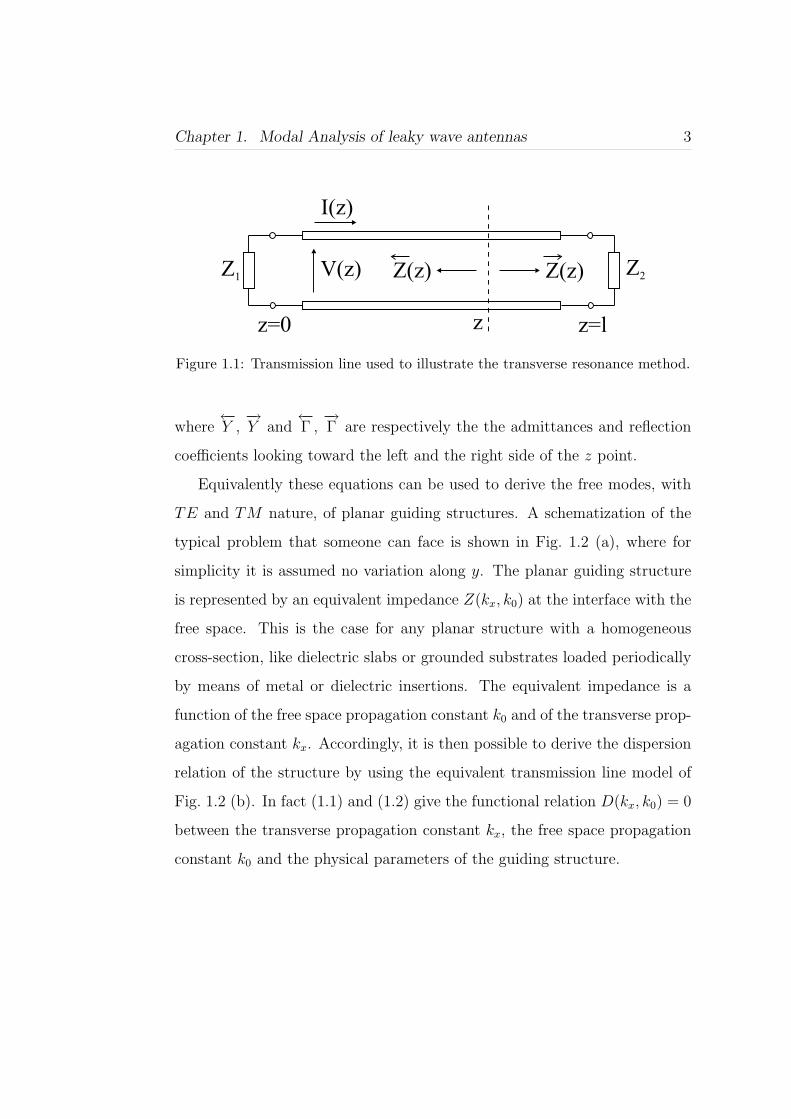
Chapter 1. Modal Analysis of leaky wave antennas 3

Z2Z1

I(z)

V(z)

z=0 z z=l

Z(z) Z(z)

Figure 1.1: Transmission line used to illustrate the transverse resonance method.

where←−Y ,

−→Y and

←−Γ ,

−→Γ are respectively the the admittances and reflection

coefficients looking toward the left and the right side of the z point.

Equivalently these equations can be used to derive the free modes, with

TE and TM nature, of planar guiding structures. A schematization of the

typical problem that someone can face is shown in Fig. 1.2 (a), where for

simplicity it is assumed no variation along y. The planar guiding structure

is represented by an equivalent impedance Z(kx, k0) at the interface with the

free space. This is the case for any planar structure with a homogeneous

cross-section, like dielectric slabs or grounded substrates loaded periodically

by means of metal or dielectric insertions. The equivalent impedance is a

function of the free space propagation constant k0 and of the transverse prop-

agation constant kx. Accordingly, it is then possible to derive the dispersion

relation of the structure by using the equivalent transmission line model of

Fig. 1.2 (b). In fact (1.1) and (1.2) give the functional relation D(kx, k0) = 0

between the transverse propagation constant kx, the free space propagation

constant k0 and the physical parameters of the guiding structure.

Chapter 1. Modal Analysis of leaky wave antennas 4

Planar guiding structure

Free Space

z

xZ(k ,k )x 0

(a)

Z0

TE/TM

I(z)

Z(k ,k )x 0

z=0Z(z)

Z(z)

V(z)

(b)

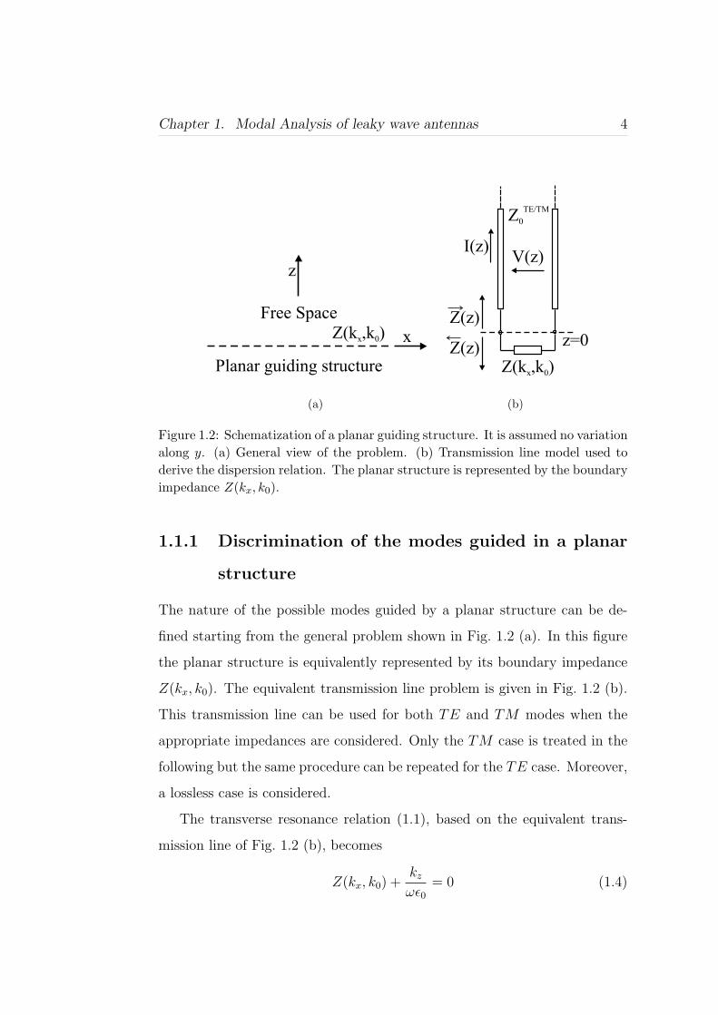
Figure 1.2: Schematization of a planar guiding structure. It is assumed no variationalong y. (a) General view of the problem. (b) Transmission line model used toderive the dispersion relation. The planar structure is represented by the boundaryimpedance Z(kx, k0).

1.1.1 Discrimination of the modes guided in a planar

structure

The nature of the possible modes guided by a planar structure can be de-

fined starting from the general problem shown in Fig. 1.2 (a). In this figure

the planar structure is equivalently represented by its boundary impedance

Z(kx, k0). The equivalent transmission line problem is given in Fig. 1.2 (b).

This transmission line can be used for both TE and TM modes when the

appropriate impedances are considered. Only the TM case is treated in the

following but the same procedure can be repeated for the TE case. Moreover,

a lossless case is considered.

The transverse resonance relation (1.1), based on the equivalent trans-

mission line of Fig. 1.2 (b), becomes

Z(kx, k0) +kz

ωε0

= 0 (1.4)

Chapter 1. Modal Analysis of leaky wave antennas 5

where kx is the transverse propagation constant, k0 is the free space propa-

gation constant, kz =√

k02 − kx

2 is the normal propagation constant, ω is

the angular frequency and ε0 is the free space permittivity. If the expression

of Z(kx, k0) is known, the resolution of this equation gives the transverse

propagation constants kx of the TM modes supported by the structure. In

particular, if the configuration is isotropic, both kx and −kx are simultane-

ously solutions of (1.4).

The possible types of waves guided by a planar structure have the form of

inhomogeneous plane waves. It is then important, before starting to classify

the possible guided modes, to consider the properties of an inhomogeneous

plane wave when both the normal and the transverse propagation constants

can assume complex values, that is

kx = βx − jαx (1.5)

kz = βz − jαz (1.6)

with

kx2 + kz

2 = k02 > 0 (1.7)

(1.7) in conjunction with (1.5) and (1.6) yields

βx2 + βz

2 − (αx2 + αz

2) = k02 (1.8)

αxβx + αzβz = 0 (1.9)

Defining the propagation vector β and attenuation vector α by

β = βxx + βzz (1.10)

α = αxx + αzz (1.11)

(1.8) and (1.9) can be written as

|β|2 − |α|2 = k02 (1.12)

Chapter 1. Modal Analysis of leaky wave antennas 6

α · β = 0 (1.13)

The planes α · r = a and β · r = b, where a and b are generic constant values

and r is the radius vector r = xx + zz, are respectively the loci of constant

amplitude and constant phase of an inhomogeneous plane wave. α and β

are the normals of these planes. In particular α points in the direction of the

most rapid amplitude decrease, while β gives the direction of propagation and

that of the power flow of the wave. (1.13) indicates that the equi-amplitude

and equi-phase planes are orthogonal to each other.

Once we have derived these proprieties for inhomogeneous plane waves,

let consider again (1.4). For complex values of the propagation constants,

the boundary impedance of Fig. 1.2, even in the considered lossless case,

becomes

Z(kx, k0) = R + jX (1.14)

where R = Re(Z(kx, k0)) and X = Im(Z(kx, k0)). Using this expression and

the relation (1.6) in (1.4) we obtain

βz − jαz

ωε0

= −R− jX (1.15)

The solutions of this equation for z > 0 correspond to the possible classes of

plane waves which may exist in free space above the interface defined by the

boundary impedance Z(kx, k0). These plane waves are characterized by the

various combinations of kz and kx in accordance with the signs of R and X,

that is

−sign(R) = sign(βz) (1.16)

sign(X) = sign(αz) (1.17)

Considering only waves with βx > 0, in the isotropic case also the one with

βx < 0 is solution, and in view of (1.9), (1.17) and (1.16), the sign of αx is

Chapter 1. Modal Analysis of leaky wave antennas 7

β

β

β

β

(a)x

z

x

z

( )b ( )c

( )e (f)( )d

R = 0X > 0

R > 0X > 0

R < 0X > 0

R = 0X < 0

R < 0X < 0

R > 0X < 0

β

ααα

α

β

α α

Figure 1.3: Classification of the possible TM polarized modes guided by a planarstructure, adapted from [8].

uniquely determined by the signs of R and X. The various wave types re-

sulting are shown in Fig. 1.3. Cases (a), (b), (c) correspond to solutions that

satisfy the radiation conditions, decaying away from the interface (proper

solutions), whereas (d), (e), (f) do not satisfy this condition, growing away

from the interface (improper solutions). The various cases can be classified

as follow:

(a) represents a surface wave

(b) corresponds to a TM surface wave propagating in a lossy interface

(c) is a complex wave which radiates out of the surface but decays away

from it

(d) is an improper surface wave

(e) represents a leaky-wave that radiates in the forward direction

(f) corresponds to an improper wave growing away from the structure but

bringing power inside the interface.

Chapter 1. Modal Analysis of leaky wave antennas 8

It is worth noting that all the proper solutions correspond to an inductive

impedance X > 0, whereas the improper ones to the capacitive case X < 0.

A similar classification can be done for the TE case by simply interchanging

these roles of X.

1.1.2 Example of a multi-layer planar structure

A multi-layer structure is considered in this section to illustrate with a prac-

tical example the transverse resonance method. The structure analyzed is

shown in Fig. 1.4 (a). It is made by a grounded substrate with permittiv-

ity εr1 covered by another layer with different permittivity εr2 and fed by a

infinitesimal magnetic dipole on the ground plane. The thicknesses of the

first and second substrate are chosen, at the operative frequency, as half and

quarter wavelength in the dielectrics, respectively: h1 = λd1/2, h2 = λd2/4

with λdi = λ0/√

eri and λ0 the free space wavelength. In literature such a

structure is called super-layer configuration [11]-[13] and it is normally used

to enhance the gain performances of printed antennas thanks to a leaky-wave

effect [14], under the condition εr2 > εr1. Fig. 1.4 (b) reports the equivalent

TE/TM transmission line model to analyze the multi-layer structure. In

this figure kzi =√

εrik02 − kρ

2 and Zi for i = 0, 1, 2 indicate the propagation

constant and the TE/TM characteristic impedance in the medium 0 (free

space), 1 and 2 respectively with kρ, the transverse propagation constant,

given by kρ =√

kx2 + ky

2. The transverse resonance condition applied to

this transmission line at the point z = z′ states

−→Z up +

←−Z down = 0 (1.18)

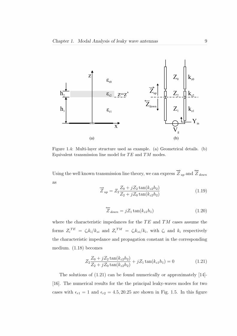
Chapter 1. Modal Analysis of leaky wave antennas 9

z

z=z’

x

h1 εr1

εr2

εr0

h2

Z0

Z1

Yin

Z2

kz1

kz0

kz2

Zdown

Zup

Vg

(a) (b)

Figure 1.4: Multi-layer structure used as example. (a) Geometrical details. (b)Equivalent transmission line model for TE and TM modes.

Using the well known transmission line theory, we can express−→Z up and

←−Z down

as−→Z up = Z2

Z0 + jZ2 tan(kz2h2)

Z2 + jZ0 tan(kz2h2)(1.19)

←−Z down = jZ1 tan(kz1h1) (1.20)

where the characteristic impedances for the TE and TM cases assume the

forms ZiTE = ζiki/kzi and Zi

TM = ζikzi/ki, with ζi and ki respectively

the characteristic impedance and propagation constant in the corresponding

medium. (1.18) becomes

Z2Z0 + jZ2 tan(kz2h2)

Z2 + jZ0 tan(kz2h2)+ jZ1 tan(kz1h1) = 0 (1.21)

The solutions of (1.21) can be found numerically or approximately [14]-

[16]. The numerical results for the the principal leaky-waves modes for two

cases with εr1 = 1 and εr2 = 4.5, 20.25 are shown in Fig. 1.5. In this figure

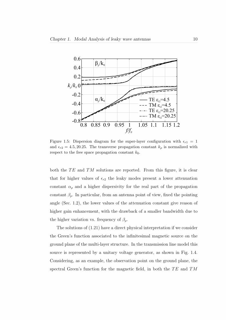
Chapter 1. Modal Analysis of leaky wave antennas 10

0.8 0.85 0.9 0.95 1

αρ/k0

βρ/k0

f/f0

k /kρ 0

1.05 1.1 1.15 1.2-0.8

-0.6

-0.4

-0.2

0

0.2

0.4

0.6

TE =20.25εr2

TE =4.5εr2

TM =4.5εr2

TM =20.25εr2

Figure 1.5: Dispersion diagram for the super-layer configuration with εr1 = 1and εr2 = 4.5, 20.25. The transverse propagation constant kρ is normalized withrespect to the free space propagation constant k0.

both the TE and TM solutions are reported. From this figure, it is clear

that for higher values of εr2 the leaky modes present a lower attenuation

constant αρ and a higher dispersivity for the real part of the propagation

constant βρ. In particular, from an antenna point of view, fixed the pointing

angle (Sec. 1.2), the lower values of the attenuation constant give reason of

higher gain enhancement, with the drawback of a smaller bandwidth due to

the higher variation vs. frequency of βρ.

The solutions of (1.21) have a direct physical interpretation if we consider

the Green’s function associated to the infinitesimal magnetic source on the

ground plane of the multi-layer structure. In the transmission line model this

source is represented by a unitary voltage generator, as shown in Fig. 1.4.

Considering, as an example, the observation point on the ground plane, the

spectral Green’s function for the magnetic field, in both the TE and TM

Chapter 1. Modal Analysis of leaky wave antennas 11

case, is equal to the line input admittance

Yin(kρ) =1

Z1

Z1 + j−→Z up tan(kz1h1)−→

Z up + jZ1 tan(kz1h1)(1.22)

The guided mode of the structure are the poles of the Green’s function, that

is the zeros of the denominator of the previous expression

−→Z up + jZ1 tan(kz1h1) = 0 (1.23)

This expression, after substituting−→Z up with (1.23), is the same of that one

obtained using the transverse resonance method (1.21). Then the leaky-

wave modes are poles of the Green’s function of the structure. This result

is obviously independent from the kind of excitation used. The same results

would be obtained considering electric currents in place of magnetic currents.

1.2 Field radiated by a leaky-wave antenna

In Sec. 1.1.1 we have seen that leaky-wave modes belong to the improper

discrete spectrum of a structure since they do not respect the radiation con-

dition, growing away from the structure. For this reason these modes can not

be used to describe the field in the far field region but they can only describe

the field on the antenna’s aperture or on a surface close to the antenna [17],

[18]. In particular in the following two conditions are assumed:

1. The antenna under investigation supports at least one leaky-wave mode.

2. In the near field of the antenna the contribution due to the leaky-wave

mode is predominant.

These two conditions are necessary to classify an antenna as leaky-wave an-

tenna and to adopt the leaky-wave approach to analyze it. To generally

Chapter 1. Modal Analysis of leaky wave antennas 12

(a) (b)

Planar guiding structure

Line Source Free Space

z

xy

rθ

Z (k ,k )b x 0

P x,y,z( ) Z0

TEkz

Z (k ,k )b x 0

z=0

Ig

Figure 1.6: Geometrical details of a line source above a planar structure describedby its boundary impedance. (a) Configuration and definition of the referencesystem. (b) Equivalent transmission line for TE modes.

show how the leaky-wave poles influence the field radiated by an antenna,

in the following we derive an expression for the far field of a simple case of

leaky-wave antenna. In particular, we consider the structure in Fig. 1.6 (a)

with its equivalent transmission line model, Fig. 1.6 (b). This structure is

characterized by an impedance boundary condition and then it can be any

planar configuration describable in such a way. The source is a infinite elec-

tric current line of unit amplitude, placed along the y axis and expressed

by

J = δ(x)δ(z)y (1.24)

This source is represented in the transmission line model in Fig. 1.6 (b) by

an electric current generator of unit value placed in parallel. Moreover such

source does not excite TM modes, then in the following only the TE modes

are considered.

The transmission line model can be used to derive the pertinent spectral

Green’s function of the problem. In this way, the field radiated by the struc-

Chapter 1. Modal Analysis of leaky wave antennas 13

ture can be expressed in terms of an inverse Fourier transformation. Precisely

the integral representation of the electric field E = E(x, z) y is given by

E(x, z) =1

2π

∫

−∞

∞Gyy

ej(kx)e−j(kxx+kzz)dkx (1.25)

where kx and kz are the usual propagation constants and Gyyej(kx) is the

spectral Green’s function of the line source for the electric field, at z = 0.

Since the line source is infinitely extended along the y axis, (1.25) does not

depend on ky. Using the well known network theory we can express the

spectral Green’s function as

Gyyej(kx) =

Z0Zb

Z0 + Zb

(1.26)

where Z0 = k0η0/kz is the TE mode impedance, with k0 and η0 respectively

the usual free space propagation constant and impedance. Note that kz =√

k20 − k2

x.

The far field radiated by the structure can be found by an asymptotic

evaluation [9] of the integral in (1.25), which yields

E(r, θ) ≈ e−j(k0r−π/4)

√2πk0r

k0 cos(θ)Gyyej(k0 cos(θ)) (1.27)

So far we have not used the conditions expressed in points (1) and (2).

The first condition imposes the presence of at least one leaky-wave mode.

As seen in the example of Sec. 1.1.2, these modes are poles of the pertinent

Green’s function and then in the present case, poles of Gyyej(kx). The poles

are the zeros of the denominator of Gyyej(kx)

Z0 + Zb = 0 (1.28)

For conditions (1) we must have a certain pair of complex values for (kx, kz),

say (kpx, kpz), which satisfy this relation. In particular, due to the symmetry

Chapter 1. Modal Analysis of leaky wave antennas 14

of the analyzed problem, if the couple (kpx, kpz) is solution of (1.28) also

(−kpx, kpz) is solution. The two poles kpx and −kpx account for the presence

of the leaky wave in the spatial regions x > 0 and x < 0, respectively.

Let now express condition (2). It states that the contribution to the near

field of the structure of the leaky-wave mode is predominant. In mathemat-

ical form this fact can be expressed approximating Gyyej(kx) with the terms

corresponding to the leaky-wave modes. Using the residue theory, Gyyej(kx)

becomes

Gyyej(kx) ≈ 2kpx

k2x − k2

px

Res(Gyyej)

∣∣kpx

(1.29)

where Res(Gyyej)

∣∣kpx

= −Res(Gyyej)

∣∣−kpx

is the residue of the Green’s function

at the leaky-wave pole kpx. It is again important to highlight that (1.29) is

valid only if the near field of the structure is dominated by the leaky-wave

contribution. Finally, the expression (1.27) for the far field of the considered

structure becomes

E(r, θ) ≈ e−j(k0r−π/4)

√2πk0r

2k0 cos(θ)kpx

k2x − k2

px

Res(Gyyej)

∣∣kpx

(1.30)

From (1.30) it is possible to derive the properties of the far field radiate by

the leaky-wave antenna. Several books treat in detail the argument [1], [2],

please refer to them for a more accurate and complete overview. Anyway,

we would like just to point out that the maximum of the radiated field is

obtained when

cos(θ) = | cos(ωp)| =√

cosh2(ηp)− sin2(ξp) (1.31)

where wp = ξp − jηp is a complex angle related to the pole by the transfor-

mation

kpx = k0 sin(wp) (1.32)

Chapter 1. Modal Analysis of leaky wave antennas 15

that isβpx − jαpx

k0

= sin(ξp) cosh(ηp)− j cos(ξp) sinh(ηp) (1.33)

In particular when the attenuation constant of the leaky-wave pole is small,

(1.31) gives the well known formula for the pointing angle of a leaky-wave

antenna

θ = arcsin

(βpx

k0

)(1.34)

Note that two maxima occur, only when | cos(ωp)| > 1 there is only one

maximum at θ = 0.

1.3 Summary

In this chapter the general theory to derive the dispersion properties of planar

guiding structures has been presented. In particular the transverse resonance

method has been introduced and used to derive the dispersion properties of

planar structures describable by means of circuit parameters. The general

conditions for the propagation of leaky, surface or complex modes have been

successively found and related to the physical proprieties of the guiding struc-

ture. A practical example has been carried out to show the link between the

solutions of the transverse resonant method and the poles of the Green’s

function associated to the structure under analysis. Finally, the influence of

leaky-wave modes on the description of the near field and on the properties

of the far field of a leaky-wave antenna have been shown.

Chapter 2

Leaky-wave antenna made by

using a 2-D periodic array of

metal dipoles

This chapter deals with the analysis and design of a leaky-wave antenna made

by loading a grounded substrate with a printed array of dipoles. The goal

is to show the possibility to increase the directivity of an array of slots on a

ground plane of a dielectric substrate by means of a leaky-wave phenomenon.

For the single element case other works can be found in literature [19], [20],

actually published during the present PhD work. An array of 2x2 elements

has been designed in cooperation with Jet Propulsion Laboratory (JPL),

Nasa.

The chapter starts analyzing the equivalence between the well known

dielectric super-layer configuration [11]-[15] and the present case. The equiv-

alence is carried out looking at their dispersion properties and a design pro-

cedure is obtained. Afterwards, the dispersion results for the considered

structure are presented and used for the design process. The geometrical

16

Chapter 2. FSS-made leaky-wave antenna 17

details of the final antenna structure and the simulation results are then

showed.

2.1 Equivalence between the super-layer con-

figuration and grounded substrate loaded

periodically

Different papers [11]-[13] have shown that the gain of printed small antennas

could be increased by covering the structure with dielectric super-layers.

In [14] the fact that the enhancement in gain is due to the excitation of

leaky waves has been clarified. Moreover, most recently [21] studied the

compromise between bandwidth and directivity for printed antennas and

arrays in presence of periodic super-layers.

On the other hand, when the requirements demand for dielectric layers

characterized by dielectric constants higher than those that are easily com-

mercially available, or the operative environment does not allow the use of

materials that can trigger ionizing discharges, it makes sense to look for alter-

native super-layer solutions to obtain equivalent performances. A simple and

effective way to achieve a similar gain enhancement is the use of a metallic

frequency selective surfaces (FSS), that is a periodic arrangement of printed

or slotted elements. The equivalence between these super-layer geometries

can be directly linked to the similarities of the Green’s Functions (GF) of

a slot etched on an infinite ground plane and covered by a FSS or by a di-

electric layer [22]. In both cases the lower portion of the spectrum of the

GF’s are dominated by a couple of dominant leaky TE/TM poles. For the

dielectric slab case the location of the poles can be found approximately but

Chapter 2. FSS-made leaky-wave antenna 18

ZL

Z1 kz1

Z0 kz0

Z2 kz2

Vg

h1

h2εr0

εr1

εr2

x

z

(a)

ZP

ZL

Z1 kz1

Z0 kz0

Vg

h1εr1

εr0FSS plane

x

z

(b)

Figure 2.1: Equivalent circuits for the structures under study. (a) Super-layerconfiguration with its equivalent model. (b) FSS configuration with its equivalentmodel for the fundamental Floquet propagating mode (m=0, n=0).

very accurately solving the dispersion equation derived from an equivalent

transmission line [16]. With reference to Fig. 2.1 (a) and considering medium

1 as free space, the z-directed propagation constant of the dominant leaky

wave poles (both TE/TM) could be then approximated as:

kz =π

h1

+ jZL

h1Z1

(2.1)

In a design phase one can just assume as load impedance ZL in (2.1), the

impedance for normal incidence. This approximation simplifies the analy-

sis since in this case the solution of the dispersion equations for the TE

and TM cases coalesce into ZL = ζ0/εr, where ζ0 = 120π Ohm is the free

space impedance. Note that as seen already in Sec. 1.1.2, at the operative

Chapter 2. FSS-made leaky-wave antenna 19

frequency, h1 and h2 are half and quarter wavelength in the dielectrics.

Also in the periodic FSS case [23], the relevant poles can be approximated

solving an equivalent transmission line with an equivalent impedance ZL and

using (2.1). In this case the transmission line to be solved is the one pertinent

to the fundamental (m=0, n=0) mode in a complete Floquet Wave expansion

of the Green’s Function [24]. The equivalent circuit that characterizes the

behavior of the dominant FW is described in Fig. 1 of [25] and for clarity it

is also reported in Fig. 2.1 (b). In a design phase, also in this case one can

approximate the load impedance ZL to be included in (2.1) as the one for

normal incidence.

In particular since the relation (2.1) could be applied to both configura-

tions, their equivalence may be found imposing the same solutions for the

axial propagation constant kz. Then the two configurations would respond to

the same dispersion relation and support the same leaky-wave modes. In the

following paragraph the steps of the procedure and the consequent relations

are shown.

2.1.1 Mathematical relations for the equivalence be-

tween a dielectric and metallic super-layer con-

figuration.

In the present paragraph we assume that the medium 1 in Fig. 2.1 is free

space and that ZL and Z1 can be approximated with their values for modes

propagating along z. With this assumption the TE and TM modes degen-

erate in a TEM mode and respond to the same transmission line model. In

particular these approximations are particularly true for structures guiding

a leaky-wave mode pointing broadside, as the antenna shown in the follow-

Chapter 2. FSS-made leaky-wave antenna 20

ing, but as pointed in [16], in the case of ZL it can be used also to analyze

approximately the structure even for modes propagating obliquely.

The equivalence between the structure in Fig. 2.1 (a) and (b) is found by

imposing the same solution for (2.1). In the case of the dielectric super-layer

structure, where at the central frequency h2 is a quarter wavelength in the

dielectric and h1 is half free space wavelength (Fig. 2.1 (a)), ZL and Z1 are

respectively equal to η0/εr2 and η0 and (2.1) reads

kz1 =π

h1

+ j1

h1εr2

(2.2)

where λ0 is the free space wavelength at the central operative frequency.

In the case of Fig. 2.1 (b) ZL can be expressed as

ZL =η0X

2p

η20 + X2

p

+ jη2

0Xp

η20 + X2

p

(2.3)

where it is taken into account the fact that for lossless FSS the shunt admit-

tance Zp presents only a reactive part, Zp = j Xp. Thanks to the assumption

of normal propagation, both the real and imaginary part are only function

of Xp. Substituting this expression in (2.1) we get

kz1 =π

hx

− η0Xp

hx(η20 + X2

p )+ j

X2p

hx(η20 + X2

p )(2.4)

Where hx corresponds to the value assumed by h1 for the FSS case. The

equivalence between the two structures can now be found equaling the real

and imaginary parts of (2.4) and (2.2)

π

h1

=1

hx

(π − η0Xp

η20 + X2

p

)(2.5)

1

h1εr2

=1

hx

X2p

η20 + X2

p

(2.6)

The unknowns of this system are hx and Xp. Xp controls ZL, that in the

present case presents both a real and an imaginary part. It is worth noting

Chapter 2. FSS-made leaky-wave antenna 21

that the real part of the impedance controls the amount of real power leaked

from the structure and then it is strongly related to the attenuation constant

of the leaky propagation constant. On the other hand the imaginary part of

the impedance controls together with the reactive load of the ground plane

and then through hx, the exact position of the resonance. After some simple

algebraic manipulations, the solutions of the system for the equivalence of

the two structures, are given by

Xp = η0

−1±√

1 + 4π2(εr2 − 1)

2π(εr2 − 1)(2.7)

hx = h1εr21

1 +

(2π(εr2−1)

−1±√

1+4π2(εr2−1)

)2 (2.8)

The two values for the solutions correspond respectively to printed and slot-

ted FSS. In fact printed FSS are a capacitive load whereas slotted FSS an

inductive one. One should note that even if this procedure is useful for a first

order dimensioning of the FSS, the level of accuracy in using the approxima-

tion (2.1) for the uniform slabs is higher than for the FSS case. Indeed in the

FSS case, the equivalent circuit only refers to the first mode of the complete

GF. Even if the considered mode is dominant in the FW expansion, small

deviations in the order of a few percent of the poles’ propagation constant

have to be expected.

2.1.2 Example of equivalence between a dielectric and

metallic super-layer configuration.

The relations found in the previous paragraph, (2.7) and (2.8), have been

applied to a practical example. The dielectric super-layer configuration con-

sidered has a covering dielectric with permittivity εr2 = 20.25. The geometry

of the used FSS is shown in Fig. 2.2. It is made by printed dipoles arranged

Chapter 2. FSS-made leaky-wave antenna 22

in a a rectangular lattice, standing in air. Substituting the value of εr2 in

(2.7) and (2.8) yields

Xp = −89 Ohm (2.9)

hx = 0.54 λ0 (2.10)

where λ0 is the free space wavelength at the central operative frequency,

chosen equal to 10 GHz. Commercially available analysis tools [26], capable

of analyzing periodic structures for normal incidence, were used to fine tune

the FSS impedance Zp to the value given by (2.9). The final dimensions of

x

dx

ld

dy

wd

y

Figure 2.2: Geometrical details of the FSS used to replace the dielectric slab ofεr2 = 20.25. The FSS presents a rectangular lattice and is made by printed dipoleson air.

the FSS are dx = 13.5 mm, dy = 3 mm, ld = 13.15 mm and wd = 3 mm.

Fig. 2.3 reports the load impedance ZL for the two structures vs. the

frequency. Note that, at the central operative frequency, both configura-

tions present the same value for the real part of the impedance because the

amount of real power leaked from the two structures is the same. In fact,

as already pointed before, the real part of the impedance is related to the

attenuation constant of the leaky propagation constant, that is the same for

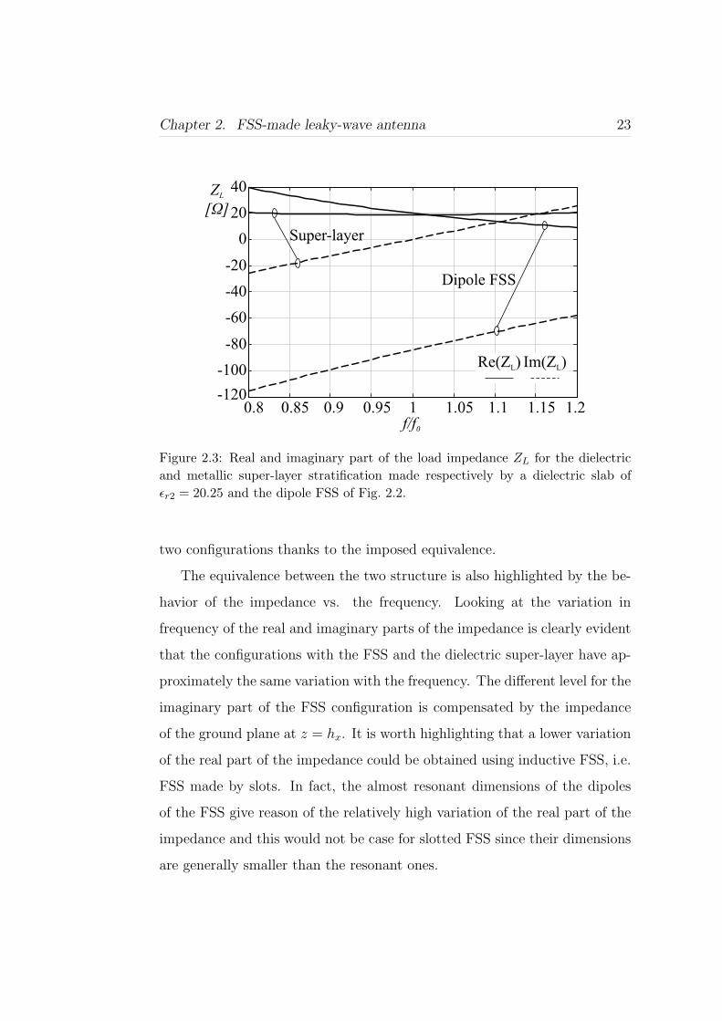
Chapter 2. FSS-made leaky-wave antenna 23

0.8 0.85 0.9 0.95 1f/f0

Z

[ ]L

Ω

1.05 1.1 1.15 1.2-120

-100

-80

-60

-40

-20

0

20

40

Re(Z )L Im(Z )L

Super-layer

Dipole FSS

Figure 2.3: Real and imaginary part of the load impedance ZL for the dielectricand metallic super-layer stratification made respectively by a dielectric slab ofεr2 = 20.25 and the dipole FSS of Fig. 2.2.

two configurations thanks to the imposed equivalence.

The equivalence between the two structure is also highlighted by the be-

havior of the impedance vs. the frequency. Looking at the variation in

frequency of the real and imaginary parts of the impedance is clearly evident

that the configurations with the FSS and the dielectric super-layer have ap-

proximately the same variation with the frequency. The different level for the

imaginary part of the FSS configuration is compensated by the impedance

of the ground plane at z = hx. It is worth highlighting that a lower variation

of the real part of the impedance could be obtained using inductive FSS, i.e.

FSS made by slots. In fact, the almost resonant dimensions of the dipoles

of the FSS give reason of the relatively high variation of the real part of the

impedance and this would not be case for slotted FSS since their dimensions

are generally smaller than the resonant ones.

Chapter 2. FSS-made leaky-wave antenna 24

2.2 2-D leaky-wave antenna: planar array cov-

ered by a printed periodic surface

Planar leaky-wave antennas with super-layers have been used during the

last years to increase the gain of simple planar antennas, like patches or

slots. The achievable increments of gain depends on the leaky-wave pole that

controls the near field distribution over the antenna aperture. In particular

for configurations with a leaky-wave pole with a small attenuation constant,

it is possible to achieve extremely high gain performance but at expense

of really small bandwidth and a very critical design. It is then important

to find a trade-off between enhancement in gain and bandwidth. Planar

array covered by a super-layer supporting a leaky-wave pole with a moderate

attenuation constant could be a possible solution. In fact the moderate leaky-

wave pole enhances the gain of every element without almost affecting the

bandwidth of the antenna.

The same results in terms of bandwidth and gain could be achieved by a

usual dense array without super-layer, but as shown in [21], the super-layer

configuration presents some advantages. In particular, since the gain of every

element is increased by the leaky-wave pole, a lower number of elements is

required to achieve the required total antenna gain and this means larger

spacing between the elements and then lower coupling between them and

simpler feeding networks. Moreover the use of a leaky effect increases the

aperture efficiency of the antenna and the simpler feeding network improves

the overall efficiency of the antenna.

The antenna presented in this section is a 2x2 array of slots on a ground

plane of a dielectric substrate covered by a FSS made by printed periodic

dipoles. The operative frequency of the antenna is f0 = 18 GHz and it is

Chapter 2. FSS-made leaky-wave antenna 25

h1

h3

εr1

εr2h2

εr3

Glue

Feeding Network planeGround plane

x

FSS plane

z

(a)

x

dx

ld

dy

wd

y

(b)

Figure 2.4: Leaky-wave antenna made by using printed dipoles. (a) Stackup ofthe antenna. A glue layer is present between the feeding layer and the substratewhere the the dipoles are printed. (b) Geometrical details of the FSS made byprinted dipoles.

pointing broadside in the entire bandwidth. The slots are fed by microstrip

lines under the ground plane [27]-[29]. The periodicity of the array is about

λ0 in order to prevent grating lobes. In [21] bigger periodicities are considered

and the element pattern minimum is used to reduce the grating lobe level

and in turn the side lobe level, to acceptable values.

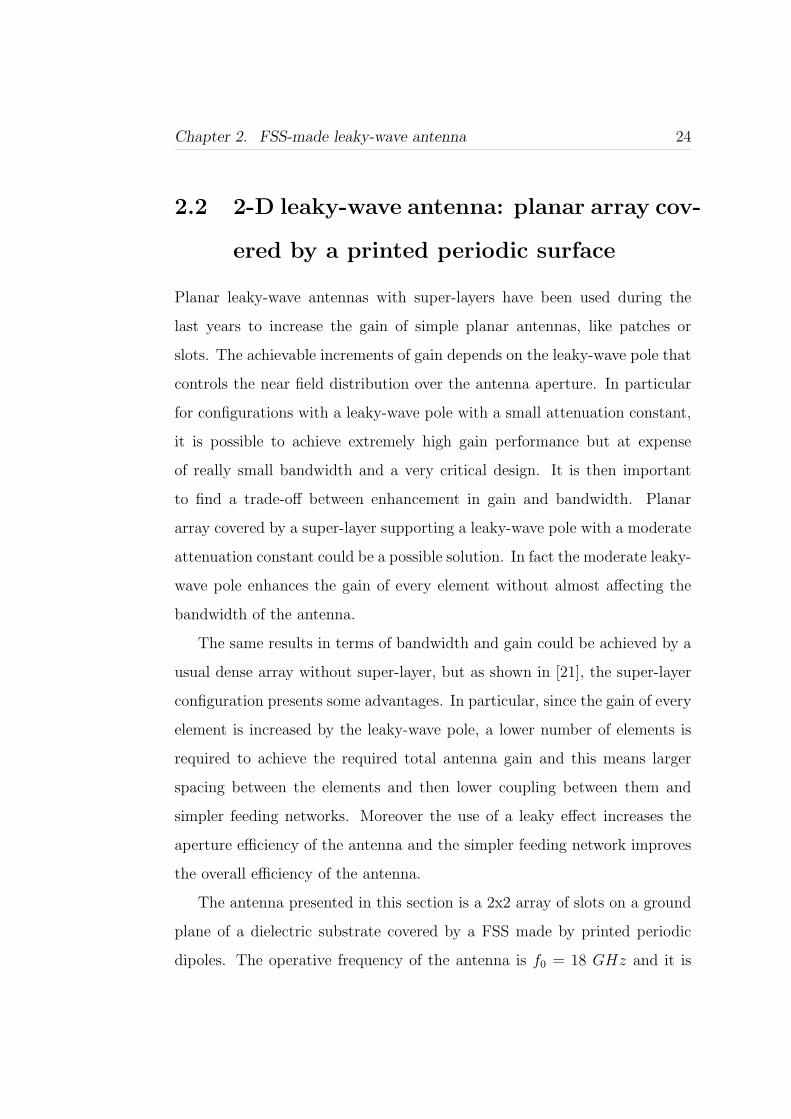
The stackup of the antenna with the geometrical details of the FSS and

the array of slots are shown in Fig. 2.4 and Fig. 2.5. The FSS is printed on a

commercially available substrate Arlon AR 450 TM with permittivity of 4.5

and thickness h3 = 4.572 mm. The feeding network is made on a substrate

Arlon AR 1000 TM with permittivity of 9.7 and thickness h1 = 0.381 mm.

The slots are etched on the ground plane of the feeding network and fed

in phase by a 50 Ω microstrip line. The T-junctions present in the feeding

network have the same characteristics. In particular the 50 Ω output lines,

thanks to quarter wavelength transformers, are brought to a 100 Ω level to

match in parallel the 50 Ω input line. The substrates of the feeding network

Chapter 2. FSS-made leaky-wave antenna 26

Input Port

x

y

ws

ls

lt

w50

Dax

Day

w100

lo

Figure 2.5: Geometrical details of the array of slots and of the correspondingfeeding network. The slots are etched on the ground plane of the feeding network.

dx dy wd ld h1 h2 h3 εr1 εr2 εr3

4.43 2 0.5 3.93 0.381 0.057 4.572 9.7 2.7 4.5

Table 2.1: Geometrical dimensions in mm of the antenna substrates and FSS.

and of the FSS are stuck together with a glue that presents a permittivity

of 2.7 and a thickness of h2 = 0.057 mm. The glue is considered in all

the simulations shown next. The parameters used for the antenna and the

feeding network are reported respectively in Tab. 2.1 and Tab. 2.2.

The leaky-wave pole used to enhance the performances of the slots is

trapped between the ground plane and the FSS. In particular the FSS is

designed to guide a leaky-wave pole pointing at broadside at the operative

frequency, as the uncovered array. Even if it could be possible to analyze the

structure using the equivalence method shown in the previous section, the

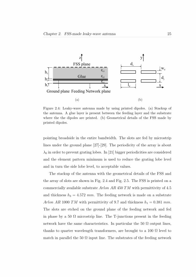
Chapter 2. FSS-made leaky-wave antenna 27

Dax Day ws ls l0 lt w50 w100

13.29 14 0.2 2.88 0.29 3.28 0.3756 0.135

Table 2.2: Geometrical dimensions in mm of the feeding network of antenna.

f [GHz]

k / kleaky 0

-1

-0.8

-0.6

-0.4

-0.2

0

0.2

0.4

0.6

0.8

1

17 17.5 18 18.5 19

kTM

kTE

kTM

kTE

x

y

Re(k /k )leaky 0 Im(k /k )leaky 0

Figure 2.6: Dispersion diagram for the FSS over the ground plane without consid-ering the glue. The two principal TE and TM w.r.t. z modes are considered. Inparticular the TE and TM mode are propagating respectively along y and x, asshown in the inset in the figure.

dispersion properties of the FSS super-layer have been derived with a home-

made MoM code. In fact as already pointed before, the equivalence method

could be used in a first step design but for a more precise analysis other

methods have to be used. The details of the code are not given because they

have not been part of the present work [30]. Anyway, it worth mentioning

that the dispersion properties of the structure have been derived finding the

zeros of the determinant of the pertinent MoM matrix.

The dispersion diagram of the structure without considering the glue

is shown in Fig. 2.6. The propagation constants of the the two possible

Chapter 2. FSS-made leaky-wave antenna 28

-35

-30

-25

-20

-15

-10

-5

17.4 17.6 17.8 18 18.2 18.4 18.6

f [GHz]

Γ [dB]

Figure 2.7: Reflection coefficient of the antenna.

polarizations TM , TE with respect to z, propagating respectively along x

and y, are shown. At the operative frequency the two polarizations present

almost the same value for the transverse propagation constant and so a pencil

beam can be achieved [31]. The moderate level of the leaky-wave solution is

directly related to the slow variation, with the frequency, of the dispersion

proprieties that preserves the bandwidth of the system.

In order to avoid edge effects the FSS covering the 2x2 array of slots is

designed to reduce the leaky wave field at the edges, to less than 1/3 of the

field present close to the feed points. The FSS thus presents 6 columns and

14 rows of dipoles with a final dimension of 26.08 x 26.5 mm. The antenna

has been simulated using the commercial tool Ansoft Designer [26]. The

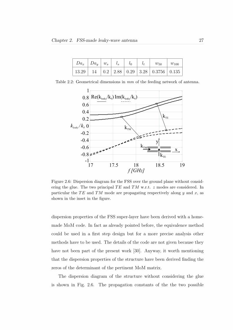
reflection coefficient is shown in Fig. 2.7. The antenna presents a −10 dB

relative bandwidth of Brel ≈ 5.3%. Fig. 2.8 shows the radiation pattern on

the H-plane (φ = 90) of the array with an without super-layer at the central

operative frequency. A difference of about 3 dB is observed due to a more

Chapter 2. FSS-made leaky-wave antenna 29

-25

-20

-15

-10

-5

0

-100 -80 -60 -40 -20 0

θ [ ]deg

E-Field[dB]

20 40 60 80 100

No FSS

FSS

Figure 2.8: Radiation pattern on the H-plane for the array of slots with andwithout the covering FSS. The pattern are normalized to the maximum of theFSS case. θ is the usual elevation angle starting from the normal to the plane ofthe antenna.

efficient use of the antenna aperture in the leaky case, showing clearly, the

utility of using the super-layer array. In fact the same performance of the

leaky case would be achieved by an uncovered array with almost a double

number of elements.

The variation of the radiation pattern in the operating band has been in-

vestigated. The radiation patterns on the E-plane (φ = 0) at f = 17.6 GHz;

f = 18 GHz; f = 18.50 GHz are reported in Fig. 2.9. A variation in

gain less then 1.8 dB for the maximum is observed. With the exception of

f = 18.50 GHz, an acceptable side lobe level (< 12.5 dB) is achieved. It

is worth noting that the side lobe level increases with the frequency in the

E-plane due to the presence of a higher TM leaky-wave mode pointing al-

most end fire. Different periodicities for the array can be used to reduce this

spurious radiation.

Chapter 2. FSS-made leaky-wave antenna 30

-25

-20

-15

-10

-5

0

-100 -80 -60 -40 -20 0 20 40 60 80 100

E-FielddB

θ [deg]

17.6 GHz

18 GHz

18.5 GHz

Figure 2.9: Radiation pattern on the E-plane at different frequencies. θ is theusual elevation angle starting from the normal to the plane of the antenna.

Good performances are observed in both the E-plane and H-plane at the

central operative frequency as shown in Fig. 2.10. The main beam is the

same in the two planes, as already predicted by the dispersion diagram. On

the E-plane and H-plane we observed a 3− dB beamwidth of BW ≈ 32.

The cross-polarization levels, always lower than −40 dB from cross to

co-component maximum, are not reported for the sake of brevity [32].

The concept shown in the present section could be used for bigger array,

also working in double polarization. In particular for double polarization

another geometry of FSS has to be used, like cross dipoles or circles. Some

results are presented in [21] for the case of dielectric super-layer but they

could be directly extended to the FSS case.

Chapter 2. FSS-made leaky-wave antenna 31

-25

-20

-15

-10

-5

0

-100 -80 -60 -40 -20 0 20 40 60 80 100

E-Field[dB]

θ [ ]deg

E-planeH-plane

Figure 2.10: Radiation pattern on the E-plane and H-plane at central operativefrequency. θ is the usual elevation angle starting from the normal to the plane ofthe antenna.

2.3 Summary

In this chapter the design of a planar leaky-wave antenna made by using

a 2-D periodic array of metal dipoles has been presented. The equivalence

between this structure and the well know super-layer dielectric configuration

has been also carried out. This equivalence is based on the assumption

that the 2-D array of dipoles could be described by an equivalent impedance

placed in parallel in the transmission line model of the structure. Some simple

formulas have been derived imposing the same leaky-wave solution for the

two configurations and an example has been done. Finally, the dispersion

properties and the simulation results for an array of slots covered by a 2-D

periodic array of metal dipoles have been presented and commented.

Chapter 3

Leaky-wave antenna made by

using planar circularly

symmetric EBG

In this chapter we propose a new topology of antenna based on the use of

Planar Circularly Symmetric EBG with different periodicities. The use of

Planar Circularly Symmetric Electromagnetic Band Gap (PCS-EBG) struc-

tures to avoid surface waves has been investigated in three recent works [33],

[34], [35]. The common foundation of these works is the use of a radial

symmetric pattern on a completely planar structure to control the surface

waves that are particularly significant for substrates that are thick in terms

of wavelength. The reason for using thick substrates in [33]-[35] was pri-

marily to achieve wide band behavior while preserving good front to back

ratios in completely planar structures. In the present work the philosophy

is different. Here, the printed surface operating as EBGs is used only in

one sector of the antenna aperture, while on the other sector the printed

surface converts the surface waves into leaky waves. The realized antenna,

32

Chapter 3. Planar circularly symmetric EBG leaky-wave antenna 33

completely manufactured in planar technology, is shown in Fig. 3.1. The use

of a printed EBG-type surface to convert surface waves into leaky waves has

been recently applied in [36] with reference to holographic concepts. The so

called holographic antennas present a modulated high impedance surface as

dictated by an interference pattern between the wave radiated by a feeder

and a plane wave coming from a chosen direction of maximum radiation.

The antenna presented here can be seen as a particular type of holographic

antenna, designed using the full information of the dispersion diagrams [33]

more than a pure optical concept. Indeed, one sector of the printed sur-

face is characterized by a complex leaky wave propagation constant, locally

designed by means of a rigorous dispersion analysis. On the other hand,

in our antenna, one sector of the printed surface is designed in the conven-

tional EBG sense to reduce undesired surface wave diffraction effects at the

substrate termination.

The chapter is organized as follow. Sec. 3.1 presents the design of the

substrate where the antenna is printed and of the feed. In Sec. 3.2 the dis-

persion properties of the EBG and leaky sector are derived and commented.

Sec. 3.3 presents the measurements results for the built prototype. Finally

in Sec. 3.4 some conclusions and remarks are drawn.

3.1 Substrate and Feed design

The dielectric substrate considered to print the antenna has a thickness such

that only the mode TM0 can propagate within the unloaded grounded slab.

To this end the thickness h of the substrate is selected according to:

h <λ0

4√

εr − 1(3.1)

where εr is the relative dielectric constant of the substrate and λ0 is the free

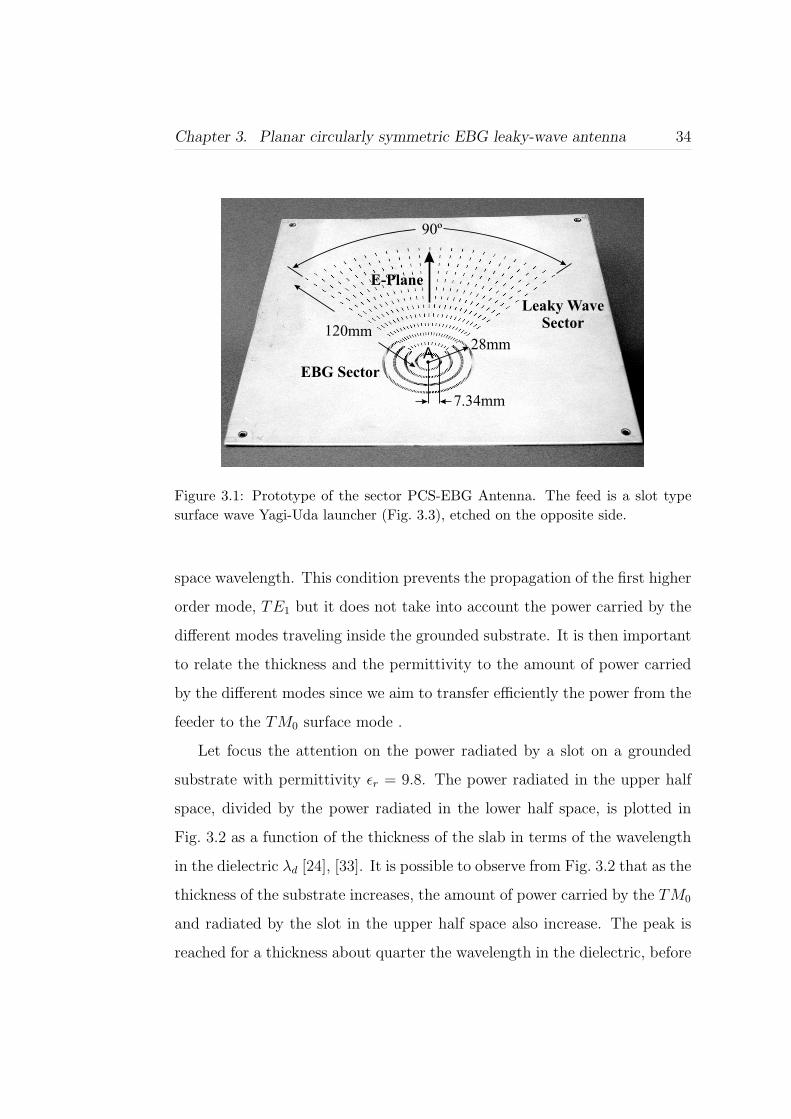
Chapter 3. Planar circularly symmetric EBG leaky-wave antenna 34

90º

Leaky WaveSector

EBG Sector

E-Plane

120mm28mm

A

7.34mm

Figure 3.1: Prototype of the sector PCS-EBG Antenna. The feed is a slot typesurface wave Yagi-Uda launcher (Fig. 3.3), etched on the opposite side.

space wavelength. This condition prevents the propagation of the first higher

order mode, TE1 but it does not take into account the power carried by the

different modes traveling inside the grounded substrate. It is then important

to relate the thickness and the permittivity to the amount of power carried

by the different modes since we aim to transfer efficiently the power from the

feeder to the TM0 surface mode .

Let focus the attention on the power radiated by a slot on a grounded

substrate with permittivity εr = 9.8. The power radiated in the upper half

space, divided by the power radiated in the lower half space, is plotted in

Fig. 3.2 as a function of the thickness of the slab in terms of the wavelength

in the dielectric λd [24], [33]. It is possible to observe from Fig. 3.2 that as the

thickness of the substrate increases, the amount of power carried by the TM0

and radiated by the slot in the upper half space also increase. The peak is

reached for a thickness about quarter the wavelength in the dielectric, before

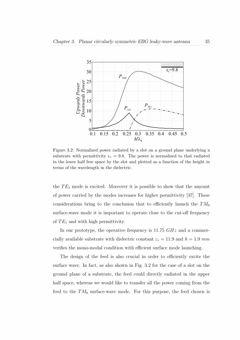
Chapter 3. Planar circularly symmetric EBG leaky-wave antenna 35

0

5

10

15

20

25

30

35

0.1 0.15 0.2 0.25 0.3 0.35 0.4 0.45 0.5

h/ld

Prad

PTE1

PTM0

εr=9.8

Upw

ard

s P

ow

erD

ow

nw

ard

s P

ow

er

Figure 3.2: Normalized power radiated by a slot on a ground plane underlying asubstrate with permittivity εr = 9.8. The power is normalized to that radiatedin the lower half free space by the slot and plotted as a function of the height interms of the wavelength in the dielectric.

the TE1 mode is excited. Moreover it is possible to show that the amount

of power carried by the modes increases for higher permittivity [37]. These

considerations bring to the conclusion that to efficiently launch the TM0

surface-wave mode it is important to operate close to the cut-off frequency

of TE1 and with high permittivity.

In our prototype, the operative frequency is 11.75 GHz and a commer-

cially available substrate with dielectric constant εr = 11.9 and h = 1.9 mm

verifies the mono-modal condition with efficient surface mode launching.

The design of the feed is also crucial in order to efficiently excite the

surface wave. In fact, as also shown in Fig. 3.2 for the case of a slot on the

ground plane of a substrate, the feed could directly radiated in the upper

half space, whereas we would like to transfer all the power coming from the

feed to the TM0 surface-wave mode. For this purpose, the feed chosen is

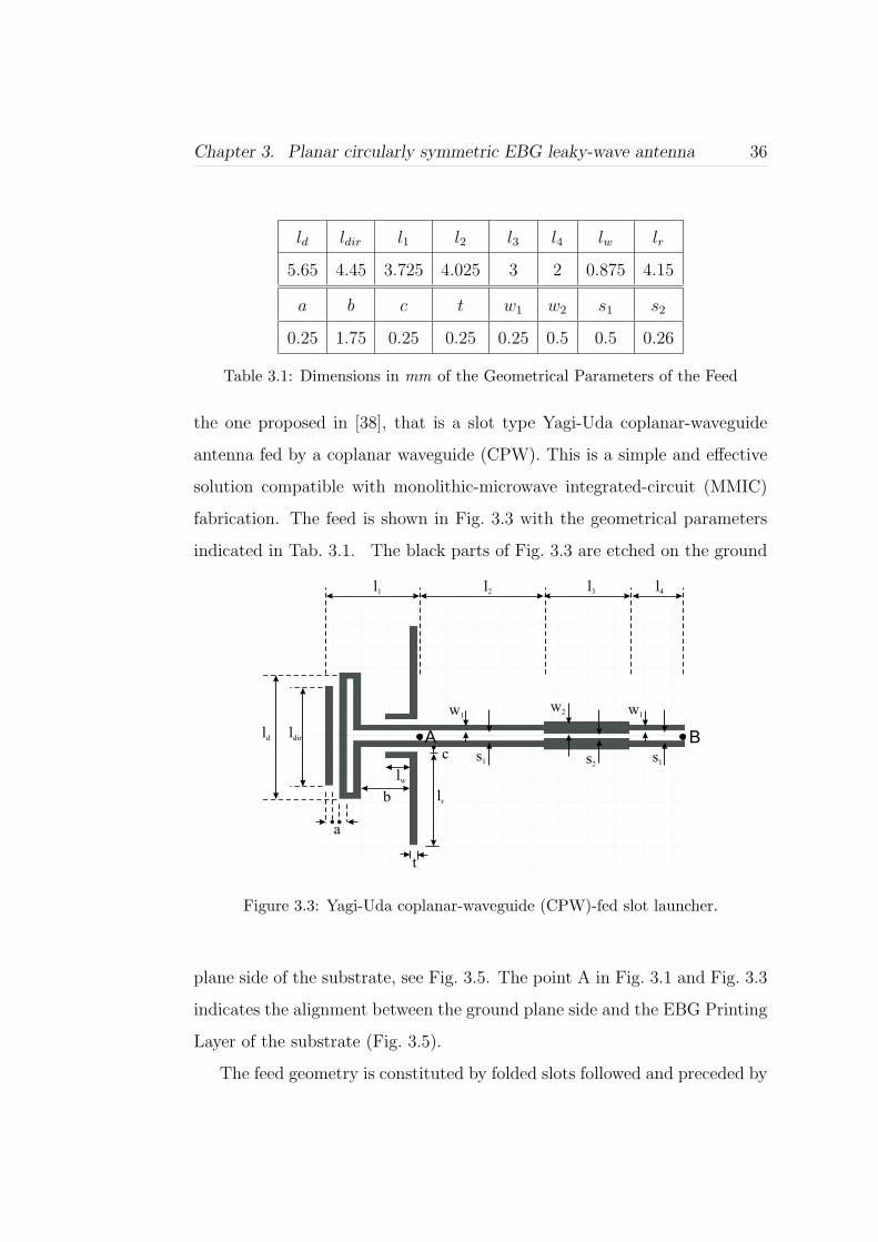
Chapter 3. Planar circularly symmetric EBG leaky-wave antenna 36

ld ldir l1 l2 l3 l4 lw lr

5.65 4.45 3.725 4.025 3 2 0.875 4.15

a b c t w1 w2 s1 s2

0.25 1.75 0.25 0.25 0.25 0.5 0.5 0.26

Table 3.1: Dimensions in mm of the Geometrical Parameters of the Feed

the one proposed in [38], that is a slot type Yagi-Uda coplanar-waveguide

antenna fed by a coplanar waveguide (CPW). This is a simple and effective

solution compatible with monolithic-microwave integrated-circuit (MMIC)

fabrication. The feed is shown in Fig. 3.3 with the geometrical parameters

indicated in Tab. 3.1. The black parts of Fig. 3.3 are etched on the ground

w1

s1 s

2

w2 w

1

s1

ld

ldir

a

t

b

lw

lr

c

l1

l3

A

l2

B

l4

Figure 3.3: Yagi-Uda coplanar-waveguide (CPW)-fed slot launcher.

plane side of the substrate, see Fig. 3.5. The point A in Fig. 3.1 and Fig. 3.3

indicates the alignment between the ground plane side and the EBG Printing

Layer of the substrate (Fig. 3.5).

The feed geometry is constituted by folded slots followed and preceded by

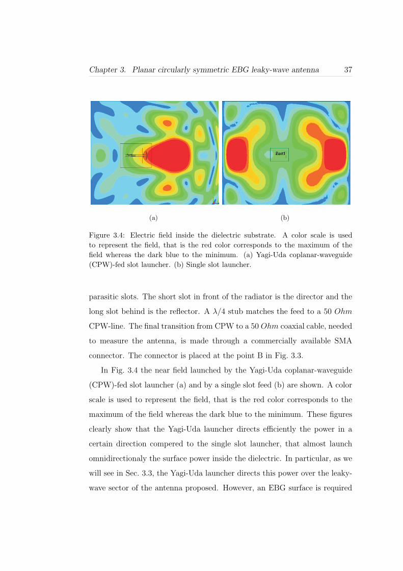
Chapter 3. Planar circularly symmetric EBG leaky-wave antenna 37

(a) (b)

Figure 3.4: Electric field inside the dielectric substrate. A color scale is usedto represent the field, that is the red color corresponds to the maximum of thefield whereas the dark blue to the minimum. (a) Yagi-Uda coplanar-waveguide(CPW)-fed slot launcher. (b) Single slot launcher.

parasitic slots. The short slot in front of the radiator is the director and the

long slot behind is the reflector. A λ/4 stub matches the feed to a 50 Ohm

CPW-line. The final transition from CPW to a 50 Ohm coaxial cable, needed

to measure the antenna, is made through a commercially available SMA

connector. The connector is placed at the point B in Fig. 3.3.

In Fig. 3.4 the near field launched by the Yagi-Uda coplanar-waveguide

(CPW)-fed slot launcher (a) and by a single slot feed (b) are shown. A color

scale is used to represent the field, that is the red color corresponds to the

maximum of the field whereas the dark blue to the minimum. These figures

clearly show that the Yagi-Uda launcher directs efficiently the power in a

certain direction compered to the single slot launcher, that almost launch

omnidirectionaly the surface power inside the dielectric. In particular, as we

will see in Sec. 3.3, the Yagi-Uda launcher directs this power over the leaky-

wave sector of the antenna proposed. However, an EBG surface is required

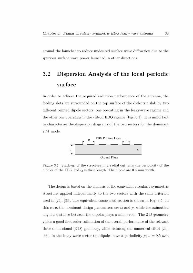
Chapter 3. Planar circularly symmetric EBG leaky-wave antenna 38

around the launcher to reduce undesired surface wave diffraction due to the

spurious surface wave power launched in other directions.

3.2 Dispersion Analysis of the local periodic

surface

In order to achieve the required radiation performance of the antenna, the

feeding slots are surrounded on the top surface of the dielectric slab by two

different printed dipole sectors, one operating in the leaky-wave regime and

the other one operating in the cut-off EBG regime (Fig. 3.1). It is important

to characterize the dispersion diagrams of the two sectors for the dominant

TM mode.

er

EBG Printing Layer

Ground Plane

h

p ld

Figure 3.5: Stack-up of the structure in a radial cut: p is the periodicity of thedipoles of the EBG and ld is their length. The dipole are 0.5 mm width.

The design is based on the analysis of the equivalent circularly symmetric

structure, applied independently to the two sectors with the same criterion

used in [24], [33]. The equivalent transversal section is shown in Fig. 3.5. In

this case, the dominant design parameters are ld and p, while the azimuthal

angular distance between the dipoles plays a minor role. The 2-D geometry

yields a good first order estimation of the overall performance of the relevant

three-dimensional (3-D) geometry, while reducing the numerical effort [24],

[33]. In the leaky-wave sector the dipoles have a periodicity pLW = 9.5 mm

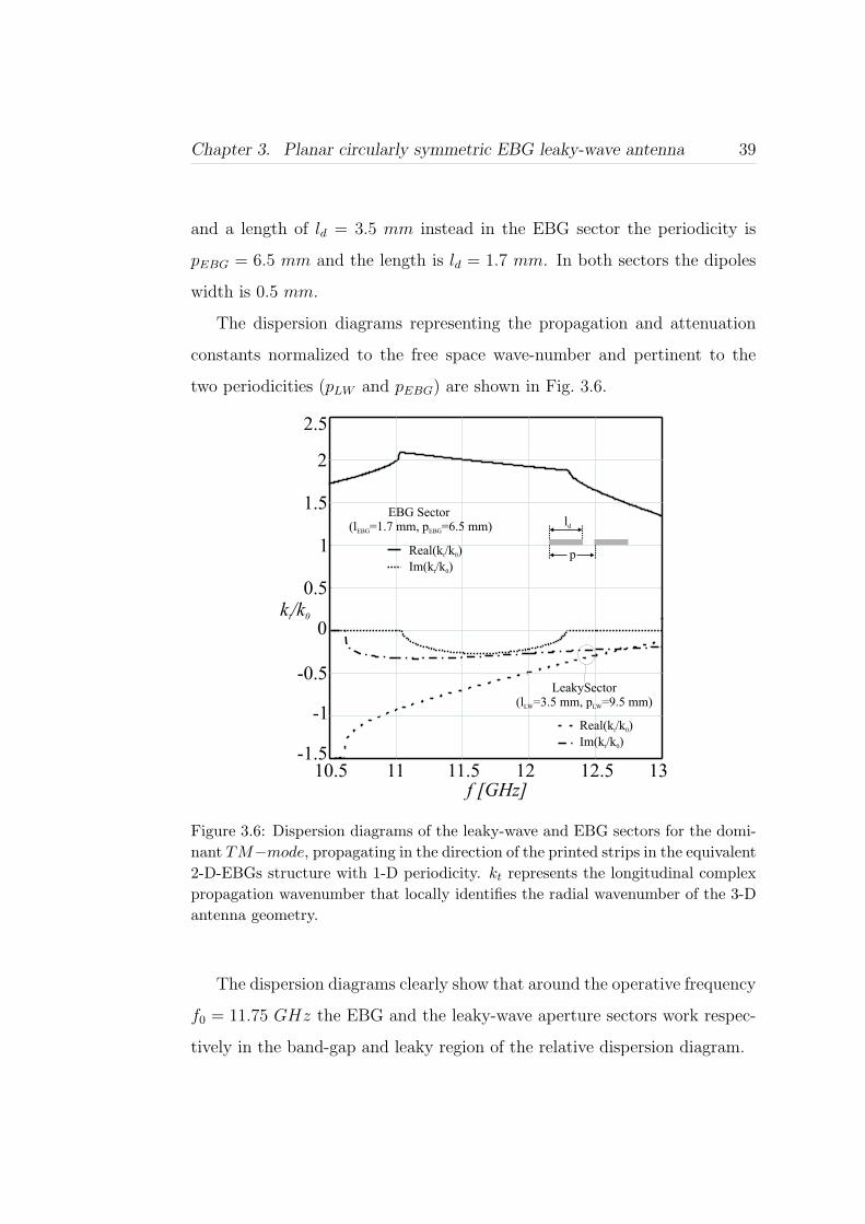
Chapter 3. Planar circularly symmetric EBG leaky-wave antenna 39

and a length of ld = 3.5 mm instead in the EBG sector the periodicity is

pEBG = 6.5 mm and the length is ld = 1.7 mm. In both sectors the dipoles

width is 0.5 mm.

The dispersion diagrams representing the propagation and attenuation

constants normalized to the free space wave-number and pertinent to the

two periodicities (pLW and pEBG) are shown in Fig. 3.6.

-0.5

0

0.5

1

1.5

2

2.5

10.5 11 11.5 12 12.5 13

LeakySector(l =3.5 mm, p =9.5 mm)LW LW

Real(k /k )t 0

EBG Sector(l =1.7 mm, p =6.5 mm)EBG EBG

Im(k /k )t 0

Real(k /k )t 0

Im(k /k )t 0

ld

p

f [GHz]

-1

-1.5

k /kt 0

Figure 3.6: Dispersion diagrams of the leaky-wave and EBG sectors for the domi-nant TM−mode, propagating in the direction of the printed strips in the equivalent2-D-EBGs structure with 1-D periodicity. kt represents the longitudinal complexpropagation wavenumber that locally identifies the radial wavenumber of the 3-Dantenna geometry.

The dispersion diagrams clearly show that around the operative frequency

f0 = 11.75 GHz the EBG and the leaky-wave aperture sectors work respec-

tively in the band-gap and leaky region of the relative dispersion diagram.

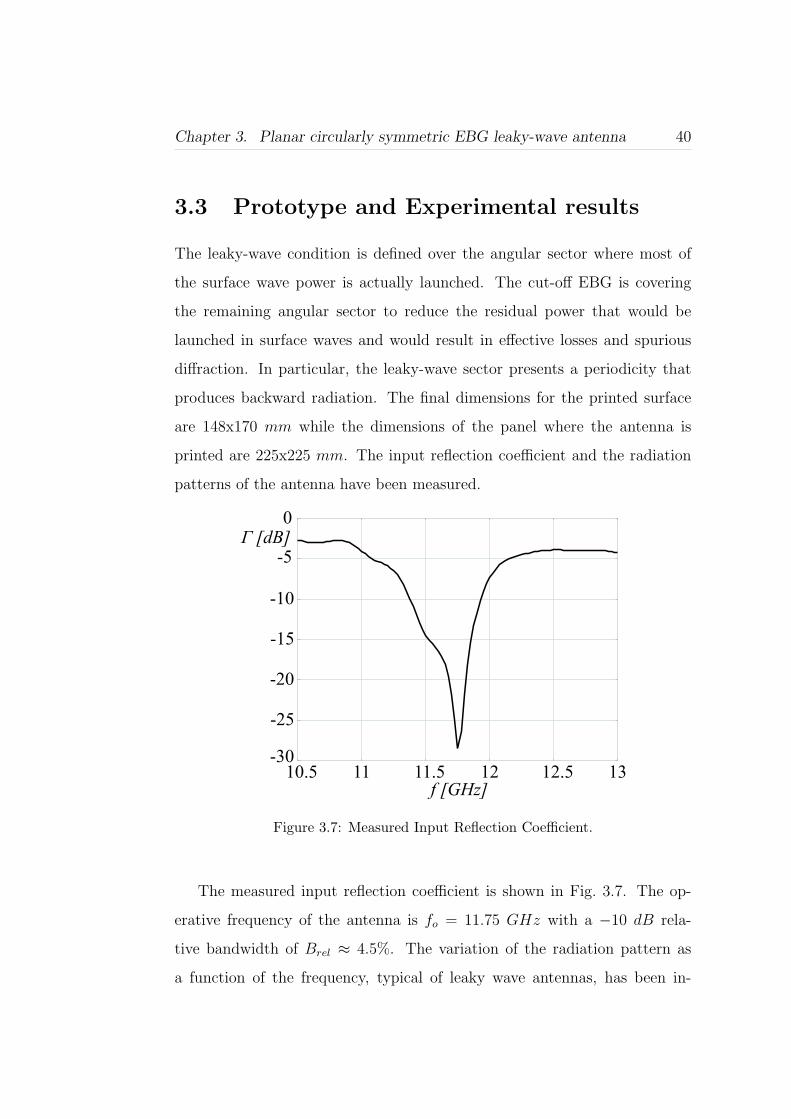
Chapter 3. Planar circularly symmetric EBG leaky-wave antenna 40

3.3 Prototype and Experimental results

The leaky-wave condition is defined over the angular sector where most of

the surface wave power is actually launched. The cut-off EBG is covering

the remaining angular sector to reduce the residual power that would be

launched in surface waves and would result in effective losses and spurious

diffraction. In particular, the leaky-wave sector presents a periodicity that

produces backward radiation. The final dimensions for the printed surface

are 148x170 mm while the dimensions of the panel where the antenna is

printed are 225x225 mm. The input reflection coefficient and the radiation

patterns of the antenna have been measured.

-30

-25

-20

-15

-10

-5

0

10.5 11 11.5 12 12.5 13

f [GHz]

Γ [dB]

Figure 3.7: Measured Input Reflection Coefficient.

The measured input reflection coefficient is shown in Fig. 3.7. The op-

erative frequency of the antenna is fo = 11.75 GHz with a −10 dB rela-

tive bandwidth of Brel ≈ 4.5%. The variation of the radiation pattern as

a function of the frequency, typical of leaky wave antennas, has been in-

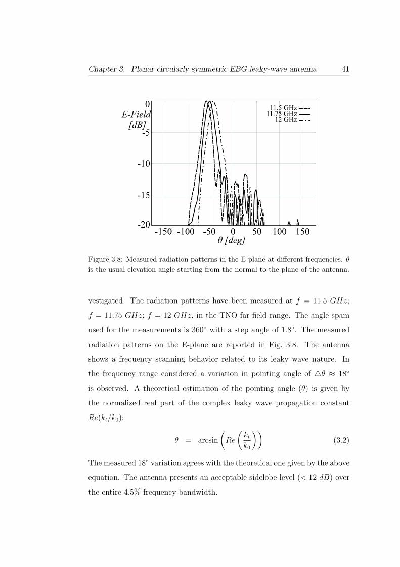
Chapter 3. Planar circularly symmetric EBG leaky-wave antenna 41

-20

-15

-10

-5

0

-150 -100 -50 0 50 100 150

θ [deg]

11.5 GHz11.75 GHz

12 GHzE-Field

[dB]

Figure 3.8: Measured radiation patterns in the E-plane at different frequencies. θ

is the usual elevation angle starting from the normal to the plane of the antenna.

vestigated. The radiation patterns have been measured at f = 11.5 GHz;

f = 11.75 GHz; f = 12 GHz, in the TNO far field range. The angle spam

used for the measurements is 360 with a step angle of 1.8. The measured

radiation patterns on the E-plane are reported in Fig. 3.8. The antenna

shows a frequency scanning behavior related to its leaky wave nature. In

the frequency range considered a variation in pointing angle of 4θ ≈ 18

is observed. A theoretical estimation of the pointing angle (θ) is given by

the normalized real part of the complex leaky wave propagation constant

Re(kt/k0):

θ = arcsin

(Re

(kt

k0

))(3.2)

The measured 18 variation agrees with the theoretical one given by the above

equation. The antenna presents an acceptable sidelobe level (< 12 dB) over

the entire 4.5% frequency bandwidth.

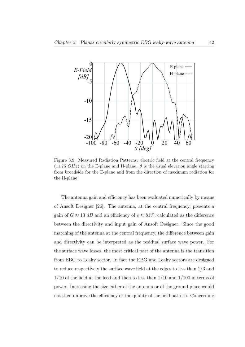
Chapter 3. Planar circularly symmetric EBG leaky-wave antenna 42

-20

-15

-10

-5

0

-100 -80 -60 -40 -20 0 20 40 60

E-plane

H-plane

θ [deg]

E-Field[dB]

Figure 3.9: Measured Radiation Patterns: electric field at the central frequency(11.75 GHz) on the E-plane and H-plane. θ is the usual elevation angle startingfrom broadside for the E-plane and from the direction of maximum radiation forthe H-plane

The antenna gain and efficiency has been evaluated numerically by means

of Ansoft Designer [26]. The antenna, at the central frequency, presents a

gain of G ≈ 13 dB and an efficiency of e ≈ 81%, calculated as the difference

between the directivity and input gain of Ansoft Designer. Since the good

matching of the antenna at the central frequency, the difference between gain

and directivity can be interpreted as the residual surface wave power. For

the surface wave losses, the most critical part of the antenna is the transition

from EBG to Leaky sector. In fact the EBG and Leaky sectors are designed

to reduce respectively the surface wave field at the edges to less than 1/3 and

1/10 of the field at the feed and then to less than 1/10 and 1/100 in terms of

power. Increasing the size either of the antenna or of the ground place would

not then improve the efficiency or the quality of the field pattern. Concerning

Chapter 3. Planar circularly symmetric EBG leaky-wave antenna 43

the last point, good performances are achieved in both the E-plane and H-

plane, as shown in Fig. 3.8 and Fig. 3.9. Anyway the residual surface wave

power could give reason of spurious side lobes or broadening effect in other

cuts of the field pattern.

Fig. 3.9 shows the measured radiation patterns on the E-plane and H-

plane at the central frequency. On the E-plane we observed a 3 − dB

beamwidth of BW ≈ 20 and on the H-plane of BW ≈ 33. The pat-

terns on these two planes could be shaped independently within a certain

degree of freedom. In fact the patten on the E-plane is dictated by the leaky

wave contribution. In particular the 3 − dB beamwidth is proportional to

the attenuation constant of the leaky wave and the pointing angle is related

to the propagation constant of the leaky wave through (3.2). On the other

hand, in the case of large radiating aperture, the pattern on the H-plane is

linked to the surface wave directivity of the feed.

3.4 Summary and remarks

In this chapter a design strategy based on the use of PCS-EBG to realize

directive antennas on printed circuit board technology has been proposed.

An antenna prototype has been successfully manufactured and tested. The

proposed antenna is suitable for implementing, with an economical solution,

similar function of that now obtained via standard slotted traveling wave

waveguide arrays, in particular it can be used for directive frequency scanning

applications.

The antenna however can scan the beam only in the E-plane, controlled

by the leaky-wave mode traveling inside the substrate. Array solutions has

to be used to scan the beam also in the H-plane. Besides, in this plane the

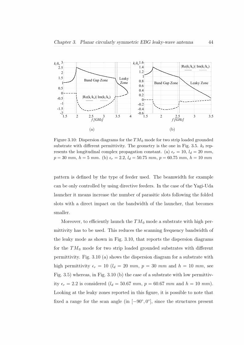
Chapter 3. Planar circularly symmetric EBG leaky-wave antenna 44

1.5 2 2.5 3 3.5 4

|Re(k /k )|t 0 Im(k /k )t 0

Band Gap Zone LeakyZone

f [GHz]

-1.5

-0.5

0.5

1.5

2.5

-2

-1

0

1

2

3k /kt 0

(a)

f [GHz]

-0.6-0.4

-0.2

0

0.2

0.4

0.6

0.8

1

1.2

1.4

1.6k /kt 0

1.5 2 2.5 3 3.5

|Re(k /k )|t 0 Im(k /k )t 0

Band Gap Zone Leaky Zone

(b)

Figure 3.10: Dispersion diagrams for the TM0 mode for two strip loaded groundedsubstrate with different permittivity. The geometry is the one in Fig. 3.5. kt rep-resents the longitudinal complex propagation constant. (a) εr = 10, ld = 20 mm,p = 30 mm, h = 5 mm. (b) εr = 2.2, ld = 50.75 mm, p = 60.75 mm, h = 10 mm

pattern is defined by the type of feeder used. The beamwidth for example

can be only controlled by using directive feeders. In the case of the Yagi-Uda

launcher it means increase the number of parasitic slots following the folded

slots with a direct impact on the bandwidth of the launcher, that becomes

smaller.

Moreover, to efficiently launch the TM0 mode a substrate with high per-

mittivity has to be used. This reduces the scanning frequency bandwidth of

the leaky mode as shown in Fig. 3.10, that reports the dispersion diagrams

for the TM0 mode for two strip loaded grounded substrates with different

permittivity. Fig. 3.10 (a) shows the dispersion diagram for a substrate with

high permittivity εr = 10 (ld = 20 mm, p = 30 mm and h = 10 mm, see

Fig. 3.5) whereas, in Fig. 3.10 (b) the case of a substrate with low permittiv-

ity εr = 2.2 is considered (ld = 50.67 mm, p = 60.67 mm and h = 10 mm).

Looking at the leaky zones reported in this figure, it is possible to note that

fixed a range for the scan angle (in [−90, 0], since the structures present

Chapter 3. Planar circularly symmetric EBG leaky-wave antenna 45

a backward radiation in the considered band), in the case (b) the frequency

variation is almost three times larger than case (a), that is case (b) is less

dispersive. Then to increase the frequency scanning capability of printed

antennas the permittivity of the substrate should be low. It is worth men-

tioning that the EBG zone has an opposite trend as shown in Fig. 3.10, in

fact case (a) has a band gap zone almost two times larger then case (b).

All the limitations of the present antenna will be overcome by the antenna

presented in the next chapter, that allows a complete independent control

of the E-plane and H-plane patterns together with the possibility to scan

the beam in both planes. A new kind of feed is also presented that allows

to efficiently launch and shape the surface wave field inside the substrate

relaxing the requirement on the dielectric permittivity.

Chapter 4

Leaky-Wave Slot Array

Antenna Fed by a Dual

Reflector System

In this chapter we propose a leaky-wave slot array antenna fed by a dual

offset Gregorian reflector system realized by pins in a parallel plate waveg-

uide. The proposed antenna belongs to the class of planar leaky-wave anten-

nas. Planar LWAs can be categorized in different topologies depending on

the geometry of the structure and on the kind of traveling wave mode [19],

[20]. In particular the nature of the traveling wave mode classifies mono and

two-dimensional leaky-wave antennas. These classifications have a direct im-

plication on the type of beam, that however maintains the typical scanning

behavior vs. frequency.

Mono dimensional planar leaky-wave antennas are characterized by a fun

beam; then, array solutions or two-dimensional planar leaky-wave antennas

are needed to radiate a pencil beam.

An array solution of mono dimensional planar leaky-wave antennas would

46

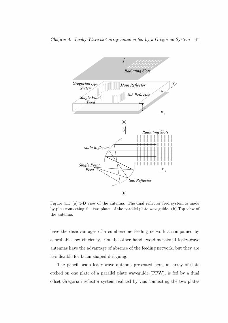
Chapter 4. Leaky-Wave slot array antenna fed by a Gregorian System 47

x

y

h

z

Main Reflector

Sub ReflectorSingle Point

Feed

Radiating Slots

Gregorian typeSystem

εr

(a)

Radiating Slots

Main Reflector

Sub Reflector

Single PointFeed x

y

(b)

Figure 4.1: (a) 3-D view of the antenna. The dual reflector feed system is madeby pins connecting the two plates of the parallel plate waveguide. (b) Top view ofthe antenna.

have the disadvantages of a cumbersome feeding network accompanied by

a probable low efficiency. On the other hand two-dimensional leaky-wave

antennas have the advantage of absence of the feeding network, but they are

less flexible for beam shaped designing.

The pencil beam leaky-wave antenna presented here, an array of slots

etched on one plate of a parallel plate waveguide (PPW), is fed by a dual

offset Gregorian reflector system realized by vias connecting the two plates

Chapter 4. Leaky-Wave slot array antenna fed by a Gregorian System 48

of the PPW. The antenna is shown in Fig. 4.1.

This antenna could be classified as a periodic one-dimensional slot array

leaky-wave antenna. A probe-type source has been used to feed the Grego-

rian system. This arrangement is suited to printed circuit board fabrication

processes (PCB). Furthermore it has the advantage to avoid a beam forming

network while preserving the freedom to shape the amplitude of the plane

feeding wavefront. The azimuth and elevation plane of the slot array can

be thus shaped independently by acting on the focal plane feeding of the

Gregorian system and on the parameters of the leaky-wave radiating slots.

This leads various degree of freedom in the design. In particular a frequency

reuse scheme renders possible the scanning in the E-plane, while a multi-feed

focal plane renders possible the scanning in the H-plane. Overall this solu-

tion opens possibilities for those applications that are right now implemented

with 3-D focusing imaging-like systems.

This chapter is organized in seven sections. In Sec. 4.1 the 2-D Grego-

rian system is designed by resorting to a Geometrical Optics (GO) tracing

of the rays associated to the dominant PPW TEM mode. In Sec. 4.2 a

pin-made feed of the dual reflector system (more complex of the one in-

dicated in Fig. 4.1) is presented; this feed allows the improvement of the

spill-over efficiency of the Gregorian system. Sec. 4.3 gives the details of the

MoM procedure used to analyze the feed and Gregorian system. In Sec. 4.4,

simplified formulas are derived and used to design the radiating slot array.

Sec. 4.5 presents experimental results for a prototype. In Sec. 4.6 the case

of a multi-beam system is considered. Finally, Sec. 4.7 concludes outlining

future applications and development of the present antenna.

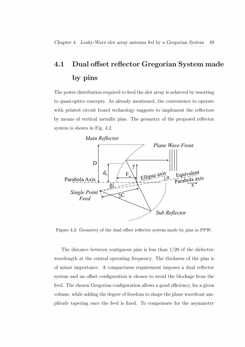
Chapter 4. Leaky-Wave slot array antenna fed by a Gregorian System 49

4.1 Dual offset reflector Gregorian System made

by pins

The power distribution required to feed the slot array is achieved by resorting

to quasi-optics concepts. As already mentioned, the convenience to operate

with printed circuit board technology suggests to implement the reflectors

by means of vertical metallic pins. The geometry of the proposed reflector

system is shown in Fig. 4.2.

Main Reflector

Sub Reflector

Single PointFeed

Plane Wave Front

d0

D

α

β

Equivalent

Parabola axisEllipse axis

Parabola AxisFm

y

2C

x

Figure 4.2: Geometry of the dual offset reflector system made by pins in PPW.

The distance between contiguous pins is less than 1/20 of the dielectric

wavelength at the central operating frequency. The thickness of the pins is

of minor importance. A compactness requirement imposes a dual reflector

system and an offset configuration is chosen to avoid the blockage from the

feed. The chosen Gregorian configuration allows a good efficiency, for a given

volume, while adding the degree of freedom to shape the plane wavefront am-

plitude tapering once the feed is fixed. To compensate for the asymmetry

Chapter 4. Leaky-Wave slot array antenna fed by a Gregorian System 50

of the dual offset reflector, the Mizugutch’s condition is used, that ensures

good symmetry of the plane wave front and good scan capability [39], [40].

The design is a simple two-dimensional version of a classic three dimen-

sional Gregorian configuration and it is described in depth in Sec. 4.1.1. The

Mizugutch’s condition is given by:

tan(α) =|1− e2| sin(β)

(1 + e2) cos(β)− 2e(4.1)

where α is the angle between the ellipse and the equivalent parabola main

axes, β is the angle between the parabola and the ellipse main axes and

e is the eccentricity of the ellipse (see Fig. 4.2). It’s worth noting that in

this case the magnification ratio (i.e. the ratio between the equivalent focal

length (Feq) and the main reflector parabola focal length (Fm)) is given by:

M =|1− e2|

(1 + e2)− 2e cos(β)(4.2)

We just underline the fact that we are treating as a bundle of rays the

cylindrical TEM wavefront excited by the source, thus obtaining a quasi−TEM (qTEM) plane wave modulated in amplitude along the planar wave

front. This wavefront is used next to feed the slot array. More details can

be found in [41], [42].

To completely define a dual offset reflector five parameters have to be

fixed and the others can be found using geometric relations. In our case we

started the design from Fm, 2C, e, d0 and the feed illumination angle φfi

(φf in Fig. 4.3), that is the −10dB beamwidth corresponding to the level of

sub-reflector tapering adopted. The reason of this choice is in the necessity

to integrate the feed in the same substrate of the reflector system. In fact the

limited size of the substrate does not allow to choose the feed a posteriori once

the reflector design has been completed. Generally speaking the lower φfi

is, the bigger the reflector system and the feed are and the less they would

Chapter 4. Leaky-Wave slot array antenna fed by a Gregorian System 51

D d0 Fm Feq e 2C M |α| β

5.67λ 2.96λ 2.49λ 5.3λ 0.4 4.68λ 2.13 38.56 17.06

Table 4.1: Parameters of The Dual Offset Gregorian System in terms of the freespace wavelength λ

fit in a commercially available substrate. Moreover as we will see in the

following, a leaky effect is used to shape the feed pattern and then attention

has be taken in a multi-beam design in order to reduce the mutual coupling

between neighboring feeds. In particular a trade-off between coupling and

directivity of the feed pattern has to be found and reflected in the reflector

design through φfi.

For our prototype a source illumination angle of θfi = 50 has been chosen

to get a system with an equivalent Feq/D of 0.933. The principal geometry

parameters characterizing the dual offset reflector system are reported in

Tab. 4.1 in terms of the free space wavelength λ.

4.1.1 Design of the two dimensional Gregorian system

In this section we derive the equations to design a two dimensional Gregorian

system once the parameters Fm, 2C, e, d0 and the feed illumination angle φfi

are fixed. In the following we explicitly refer to the work [42] using the same

definitions for the coordinate systems and for the geometry of the confocal

Gregorian system, as shown in Fig. 4.3. The surface of the Gregorian system

is generated by translation of the conic sections of the main and sub reflector

along the z axis. In particular the parabola (main reflector) has a focal length

Fm. The ellipse (sub reflector) has eccentricity e and interfocal distance 2C.

The axis of the ellipse is tilted an angle β with respect to the axis of the

parabola. To describe the system by ray optical analysis the four coordinate

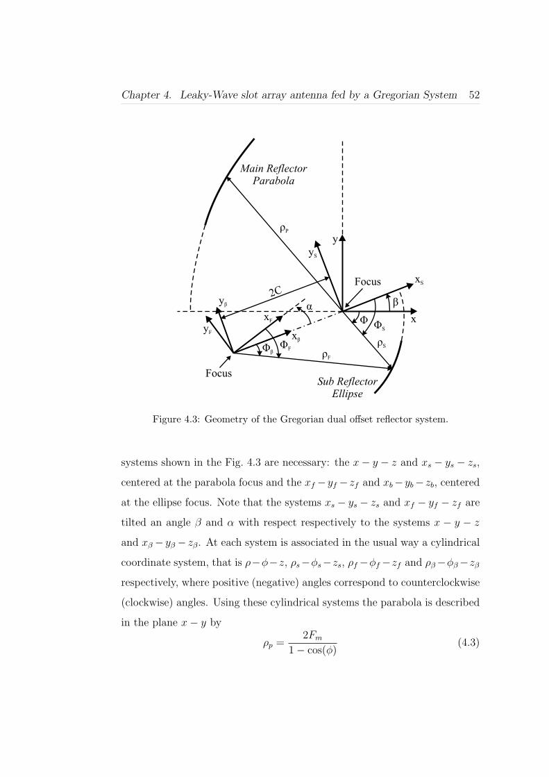
Chapter 4. Leaky-Wave slot array antenna fed by a Gregorian System 52

x

α β

ΦS

ρSΦF

ρF

ρP

Φβ

Φ

xS

y

2C

Main ReflectorParabola

Focus

Focus

Sub ReflectorEllipse

yS

yβ

yF

xF

xβ

Figure 4.3: Geometry of the Gregorian dual offset reflector system.

systems shown in the Fig. 4.3 are necessary: the x− y − z and xs − ys − zs,

centered at the parabola focus and the xf −yf − zf and xb−yb− zb, centered

at the ellipse focus. Note that the systems xs − ys − zs and xf − yf − zf are

tilted an angle β and α with respect respectively to the systems x − y − z

and xβ − yβ − zβ. At each system is associated in the usual way a cylindrical

coordinate system, that is ρ−φ−z, ρs−φs−zs, ρf−φf−zf and ρβ−φβ−zβ

respectively, where positive (negative) angles correspond to counterclockwise

(clockwise) angles. Using these cylindrical systems the parabola is described

in the plane x− y by

ρp =2Fm

1− cos(φ)(4.3)

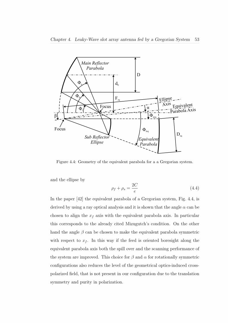
Chapter 4. Leaky-Wave slot array antenna fed by a Gregorian System 53

Feq

Deq

D

β

α

Φleq

Φl

Φueq

Φu

Φ0

d0

Main ReflectorParabola

EquivalentParabola

Focus

Focus

Sub ReflectorEllipse

Ellipse

AxisEquivalent

Parabola Axis

Figure 4.4: Geometry of the equivalent parabola for a a Gregorian system.

and the ellipse by

ρf + ρs =2C

e(4.4)

In the paper [42] the equivalent parabola of a Gregorian system, Fig. 4.4, is

derived by using a ray optical analysis and it is shown that the angle α can be

chosen to align the xf axis with the equivalent parabola axis. In particular

this corresponds to the already cited Mizugutch’s condition. On the other

hand the angle β can be chosen to make the equivalent parabola symmetric

with respect to xf . In this way if the feed is oriented boresight along the

equivalent parabola axis both the spill over and the scanning performance of

the system are improved. This choice for β and α for rotationally symmetric

configurations also reduces the level of the geometrical optics-induced cross-

polarized field, that is not present in our configuration due to the translation

symmetry and purity in polarization.

Chapter 4. Leaky-Wave slot array antenna fed by a Gregorian System 54

The condition on β to have a symmetric equivalent parabola is expressed

by

tan

(β

2

)=

(e− 1

e + 1

)2

tan

(β − φ0

2

)(4.5)

where the angle φ0 is shown in Fig. 4.4 and given by

tan

(φ0

2

)= − d0

2Fm

(4.6)

Once β is known α can be found thanks to an equivalent expression of the

Mizugutch’s condition

tan(α

2

)=

(e + 1

e− 1

)tan

(β

2

)(4.7)

Let now derive the solutions for (4.5). By using the trigonometric formula

tan (γ ± ψ) =tan(γ)± tan(ψ)

1∓ tan(γ) tan(ψ)(4.8)

this equation can be written as

tan

(β

2

)=

(e− 1

e + 1

)2tan(β/2)− tan(φ0/2)

1 + tan(β/2) tan(φ0/2)(4.9)

For simplicity, we write (4.9) as

x = kx− a

1 + xa(4.10)

where

x = tan

(β

2

)(4.11)

k =

(e− 1

e + 1

)2

(4.12)

and

a = tan

(φ0

2

)(4.13)

Note that 0 < k < 1 since the sub reflector is an ellipse with eccentricity

0 < e < 1 and a < 0 due the Gregorian configuration. After some algebraic

Chapter 4. Leaky-Wave slot array antenna fed by a Gregorian System 55

manipulations, supposing that 1 + xa 6= 0 and a 6= 0, (4.10) assumes the

normal expression for an equation of the second degree

x2 +

(1− k

a

)x + k = 0 (4.14)

The two solutions of this equation are

x1,2 = −1− k

2a± 1

2

√(1− k

a

)2

− 4k (4.15)

Then β and α can be found by substituting x for its real expression (4.11):

β1,2 = 2 arctan(x1,2) (4.16)

and

α1,2 = 2 arctan

[(e + 1

e− 1

)x1,2

](4.17)

These solutions will be real if the argument of the square root in (4.15)

has a positive value. The argument of the square root is the discriminant of

the quadratic polynomial of (4.15). In particular if

∆ =

(1− k

a

)2

− 4k > 0 (4.18)

then a priori, by considering the signs of the coefficients of the quadratic

polynomial, we can say that (4.15) has two real and positive solutions, that is

x1 > x2 > 0. The two solutions give reason of two different Gregorian system

with same characteristics but different orientation of the sub reflector. For

compactness and to avoid any blockage from the feed, the smallest solution

x2 is always chosen

x2 = −1− k

2a− 1

2

√(1− k

a

)2

− 4k (4.19)

and then β and α becomes

β = 2 arctan(x2) (4.20)

Chapter 4. Leaky-Wave slot array antenna fed by a Gregorian System 56

and

α = 2 arctan

[(e + 1

e− 1

)x2

](4.21)

These solutions have been found supposing that ∆ > 0, 1 + xa 6= 0 and a 6=0. Before proceeding it is important to understand the possible limitations

introduced by these conditions on the Gregorian system. Starting from the

last one, a 6= 0 means that the system can not be symmetric and this is

actually the case since we are considering offset systems with the sub reflector

axis tilted with respect to the main reflector axis. The second one, 1+xa 6= 0,

yields

tan(β/2) 6= − cot(φ0/2) (4.22)

This last equation is not verified only when φ0 = −π/2 and β0 = π/2 and

for geometrical reason φ0 will never approach −π/2, then this condition is

always satisfied. The only condition that imposes some limitations to the

Gregorian system is the first one, on the discriminant ∆ of (4.15). In fact

after some algebraic manipulations this condition becomes

|a| < 1− k√4k

(4.23)

or by using (4.13) and the fact that a < 0

−1− k√4k

< tan(φ0/2) < 0 (4.24)

Unfortunately the first member of the latter relation can be, in absolute

value, lower than one, limiting the range of values for φ0 and then the possible

configurations for the Gregorian system. Note that if this condition is not

satisfied, complex solutions for (4.15) are found. However, since φ0 is derived

from the fixed values Fm and d0 and the second member of (4.24) depends

only on the eccentricity e of the sub reflector, we can always choose a set of

values that satisfies (4.24).

Chapter 4. Leaky-Wave slot array antenna fed by a Gregorian System 57

Once we have derived the angles β and α, we are able to describe, thanks

to (4.4), the ellipse of the sub reflector, knowing e, 2C and φfi. However,

since the feed is placed at the origin of the system ρf −φf − zf and the angle

φfi is relative to this system, it more useful to use the following relation in

place of (4.4)

ρf =C

e

e2 − 1

e cos(φf + α)− 1(4.25)

where φleq < φf < φueq, Fig. 4.4. Finally these extreme angles φueq and φleq

can be found thanks to the symmetry of the sub reflector around the xf axis

that brings to

|φueq| = |φleq| = φfi/2, (4.26)

that is the angles φueq and φleq are equal in absolute value to half the illumi-

nation angle φfi.

The last information needed to describe the complete Gregorian system

is that the equivalent and real parabola have the same diameter: Deq = D

(a demonstration can be found in [42]). The three parameters Deq, d0 and

Fm then completely describe the sector of the main parabola with its focus

at the origin of the system ρ− φ− z and its main axis oriented along x.

The equivalent parabola diameter is given by (see Fig. 4.4) [41]

Deq = 2 (tan(φueq/2)− tan(φleq/2)) Feq (4.27)

where Feq = M · Fm is the focal length of the equivalent parabola with M

the magnification ratio (4.2). Using the relation (4.26), (4.27) becomes

Deq = 4 tan(φueq/2)Feq (4.28)

As already done for the ellipse, we can now use (4.3) and the information on

the angles φl and φu, Fig. 4.4, to characterize the sector of the main reflector.

Chapter 4. Leaky-Wave slot array antenna fed by a Gregorian System 58

The extreme angles φl and φu are given by

φu = −2 arctan

(D + 2d0

4Fm

)(4.29)

φl = −2 arctan

(2d0 −D

4Fm

)(4.30)

The relations found in this section clearly show that the five fixed param-

eters Fm, 2C, e, d0 and φfi are sufficient to complete describe a dual offset

Gregorian system. In particular these relations have been used to derive the

values reported in Tab. 4.1 for our special case. Finally, it is worth saying

that the same procedure can be used to derive equivalent conditions for a

Cassegrain system.

4.2 Excitation of the Gregorian System

The efficient excitation of reflector feeds has been investigated for decades

and is one of the main problems in the antenna field. Recently a strategy

has been proposed to excite conventional reflector antennas to achieve either

high-efficiency in single feed reflectors [44] or overlapping apertures in multi-

beam imaging systems [45].

In this case the feed is integrated in the PCB structure and realized via

metallic posts just like the reflector, Fig. 4.5. A leaking mode propagates in a

partially reflecting waveguide constituted by two grids of pins. The lower wall

of this waveguide is well sampled (Ng pins) and provides the equivalent of a

continuous metallization , while the upper wall, being constituted by a larger

period (Nr pins), allows a spill-over of energy in the external environment.

The two walls are separated by a distance 0.44λ/√

εr at the central operating

frequency. It is worth saying that the center of the reference system adopted

in Fig. 4.5 corresponds to that of the reference system xf−yf−zf of Fig. 4.3.

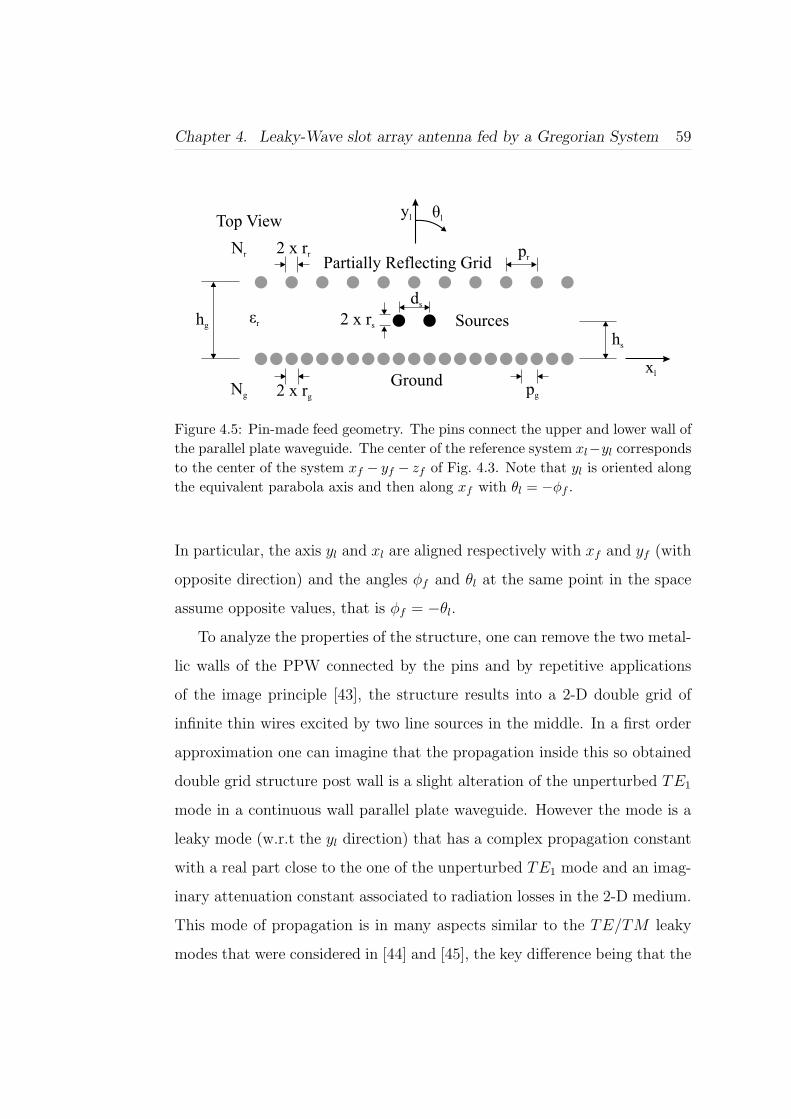
Chapter 4. Leaky-Wave slot array antenna fed by a Gregorian System 59

2 x rgpg

2 x rr pr

hs

hg

Ng

Nr

εr 2 x rs

ds

xl

yl θl

Sources

Ground

Partially Reflecting Grid

Top View

Figure 4.5: Pin-made feed geometry. The pins connect the upper and lower wall ofthe parallel plate waveguide. The center of the reference system xl−yl correspondsto the center of the system xf − yf − zf of Fig. 4.3. Note that yl is oriented alongthe equivalent parabola axis and then along xf with θl = −φf .

In particular, the axis yl and xl are aligned respectively with xf and yf (with

opposite direction) and the angles φf and θl at the same point in the space

assume opposite values, that is φf = −θl.

To analyze the properties of the structure, one can remove the two metal-

lic walls of the PPW connected by the pins and by repetitive applications

of the image principle [43], the structure results into a 2-D double grid of

infinite thin wires excited by two line sources in the middle. In a first order

approximation one can imagine that the propagation inside this so obtained

double grid structure post wall is a slight alteration of the unperturbed TE1

mode in a continuous wall parallel plate waveguide. However the mode is a

leaky mode (w.r.t the yl direction) that has a complex propagation constant

with a real part close to the one of the unperturbed TE1 mode and an imag-

inary attenuation constant associated to radiation losses in the 2-D medium.

This mode of propagation is in many aspects similar to the TE/TM leaky

modes that were considered in [44] and [45], the key difference being that the

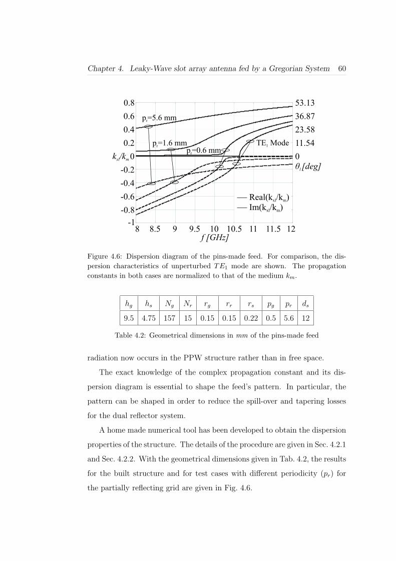
Chapter 4. Leaky-Wave slot array antenna fed by a Gregorian System 60

-1

-0.8

-0.6

-0.4

-0.2

0

0.2

0.4

0.6

0.8

0

11.54

23.58

36.87

53.13

k /kxl m

θl [deg]

8 8.5 9 9.5 10 10.5 11 11.5 12f [GHz]

p =5.6 mmr

p =1.6 mmr

p =0.6 mmr

TE Mode1

Real(k /k )xl m

Im(k /k )xl m

Figure 4.6: Dispersion diagram of the pins-made feed. For comparison, the dis-persion characteristics of unperturbed TE1 mode are shown. The propagationconstants in both cases are normalized to that of the medium km.

hg hs Ng Nr rg rr rs pg pr ds

9.5 4.75 157 15 0.15 0.15 0.22 0.5 5.6 12

Table 4.2: Geometrical dimensions in mm of the pins-made feed

radiation now occurs in the PPW structure rather than in free space.

The exact knowledge of the complex propagation constant and its dis-

persion diagram is essential to shape the feed’s pattern. In particular, the

pattern can be shaped in order to reduce the spill-over and tapering losses

for the dual reflector system.

A home made numerical tool has been developed to obtain the dispersion

properties of the structure. The details of the procedure are given in Sec. 4.2.1

and Sec. 4.2.2. With the geometrical dimensions given in Tab. 4.2, the results

for the built structure and for test cases with different periodicity (pr) for

the partially reflecting grid are given in Fig. 4.6.

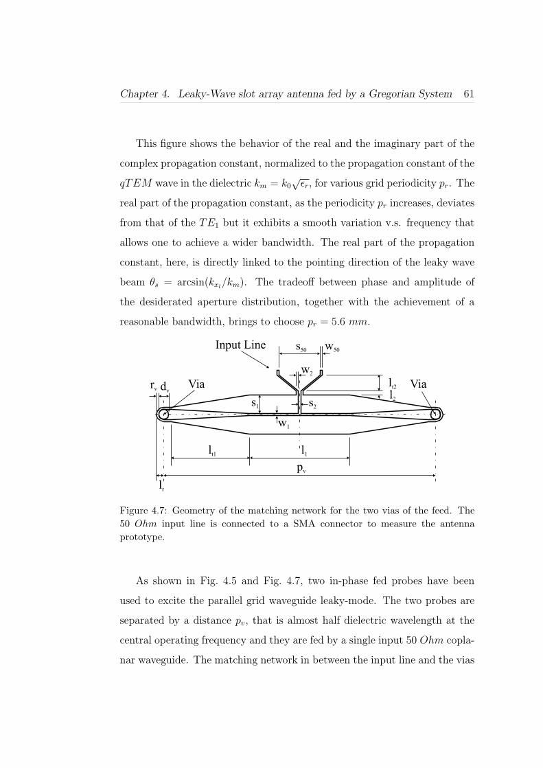
Chapter 4. Leaky-Wave slot array antenna fed by a Gregorian System 61

This figure shows the behavior of the real and the imaginary part of the

complex propagation constant, normalized to the propagation constant of the

qTEM wave in the dielectric km = k0√

εr, for various grid periodicity pr. The

real part of the propagation constant, as the periodicity pr increases, deviates

from that of the TE1 but it exhibits a smooth variation v.s. frequency that

allows one to achieve a wider bandwidth. The real part of the propagation

constant, here, is directly linked to the pointing direction of the leaky wave

beam θs = arcsin(kxl/km). The tradeoff between phase and amplitude of

the desiderated aperture distribution, together with the achievement of a

reasonable bandwidth, brings to choose pr = 5.6 mm.

Input Line s50

w2

w1

s2s1

dv

pv

lr

rv

lt1

lt2

l1

l2

w50

Via Via

Figure 4.7: Geometry of the matching network for the two vias of the feed. The50 Ohm input line is connected to a SMA connector to measure the antennaprototype.

As shown in Fig. 4.5 and Fig. 4.7, two in-phase fed probes have been

used to excite the parallel grid waveguide leaky-mode. The two probes are

separated by a distance pv, that is almost half dielectric wavelength at the

central operating frequency and they are fed by a single input 50 Ohm copla-

nar waveguide. The matching network in between the input line and the vias

Chapter 4. Leaky-Wave slot array antenna fed by a Gregorian System 62

rv dv lr l1 l2 lt1 lt2

0.1 0.44 0.325 2.15 0.2 3.475 0.7

pv s1 w1 s2 w2 s50 w50

12 0.8 0.1 0.1 0.1 1.8 0.1

Table 4.3: Geometrical dimensions in mm of the matching network for the pins-made feed

takes care of the inductive load of the vias and brings their parallel impedance

to the 50 Ohm level through impedance transformations. Tab. 4.3 reports

the final dimensions of the matching network.

The double probe solution has been preferred to that with a single probe

because it leads to an intrinsical narrower beam that allows the use of a

flatter curve in Fig. 4.6, being fixed the requirements of beamwidth. The

feed integrated in the antenna prototype has been finally designed to achieve

a tapering of −10 dB, corresponding to a beamwidth of θs = 50 (θs = φfi,

see Fig. 4.4) of the Gregorian sub-reflector. The calculated pattern at the

central frequency (fc = 9.35 GHz) is shown in Fig. 4.8. Note that only one

beam appears even if two leaky-waves aiming at two angles, symmetric with

respect to yl, are originated. This because the two values are very close one

to the other and coalesce. The pattern is normalized with respect to the

square-root of the distance from the phase center, being the field relevant

to a cylindrical qTEM wave into the PPW. For comparison also the feed

pattern that would be obtained with the backing reflector grid but without

the partially reflecting grid, is shown. These patterns are calculated by using

the home made code described in Sec. 4.3.

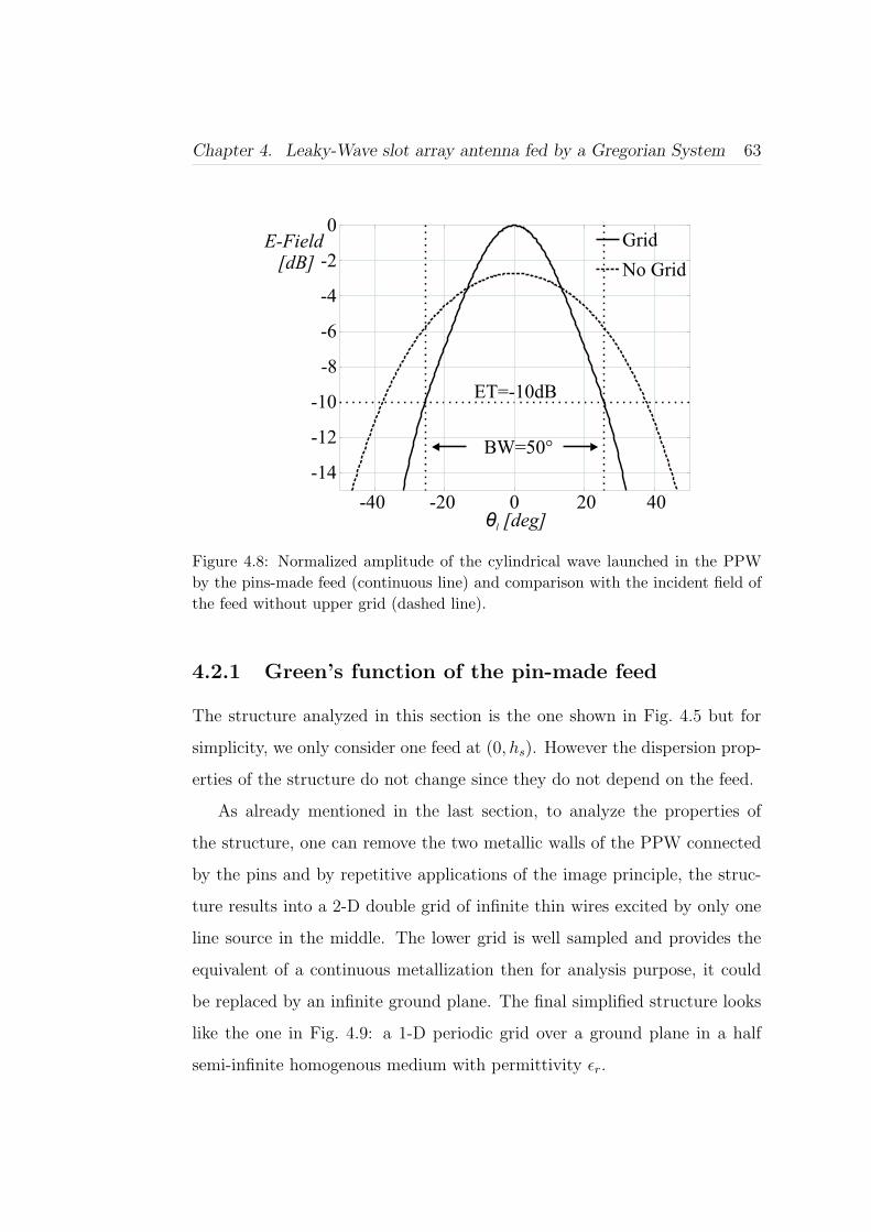
Chapter 4. Leaky-Wave slot array antenna fed by a Gregorian System 63

-14

-12

-10

-8

-6

-4

-2

0

-40 -20 0 20 40

E-Field[dB]

θl [deg]

ET=-10dB

BW=50°

Grid

No Grid

Figure 4.8: Normalized amplitude of the cylindrical wave launched in the PPWby the pins-made feed (continuous line) and comparison with the incident field ofthe feed without upper grid (dashed line).

4.2.1 Green’s function of the pin-made feed

The structure analyzed in this section is the one shown in Fig. 4.5 but for

simplicity, we only consider one feed at (0, hs). However the dispersion prop-

erties of the structure do not change since they do not depend on the feed.

As already mentioned in the last section, to analyze the properties of

the structure, one can remove the two metallic walls of the PPW connected

by the pins and by repetitive applications of the image principle, the struc-

ture results into a 2-D double grid of infinite thin wires excited by only one

line source in the middle. The lower grid is well sampled and provides the

equivalent of a continuous metallization then for analysis purpose, it could

be replaced by an infinite ground plane. The final simplified structure looks

like the one in Fig. 4.9: a 1-D periodic grid over a ground plane in a half

semi-infinite homogenous medium with permittivity εr.

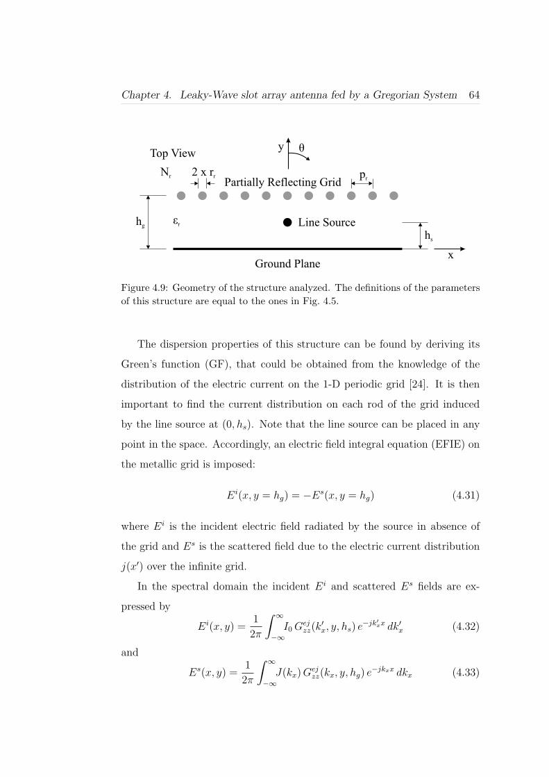
Chapter 4. Leaky-Wave slot array antenna fed by a Gregorian System 64

pr

hs

hgεr

x

y θ

Line Source

Ground Plane

Partially Reflecting Grid2 x rrNr

Top View

Figure 4.9: Geometry of the structure analyzed. The definitions of the parametersof this structure are equal to the ones in Fig. 4.5.

The dispersion properties of this structure can be found by deriving its

Green’s function (GF), that could be obtained from the knowledge of the

distribution of the electric current on the 1-D periodic grid [24]. It is then

important to find the current distribution on each rod of the grid induced

by the line source at (0, hs). Note that the line source can be placed in any

point in the space. Accordingly, an electric field integral equation (EFIE) on

the metallic grid is imposed:

Ei(x, y = hg) = −Es(x, y = hg) (4.31)

where Ei is the incident electric field radiated by the source in absence of

the grid and Es is the scattered field due to the electric current distribution

j(x′) over the infinite grid.

In the spectral domain the incident Ei and scattered Es fields are ex-

pressed by

Ei(x, y) =1

2π

∫ ∞

−∞I0 Gej

zz(k′x, y, hs) e−jk′xx dk′x (4.32)

and

Es(x, y) =1

2π

∫ ∞

−∞J(kx) Gej

zz(kx, y, hg) e−jkxx dkx (4.33)

Chapter 4. Leaky-Wave slot array antenna fed by a Gregorian System 65

where I0 represent the amplitude of the line source, Gejzz(k

′x, y, hs/hg) is the

z component of the spectral GF, in absence of the grid, of the electric field

radiated at the quote y by a electric line source lying at hs/hg along z and

J(kx) is the Fourier Transform (FT) of the current j(x′).

The current j(x′) is induced by the incident field coming from the line

source, that as been expressed in (4.32) as a superposition of plane waves

with wave number k′x. Each of these plane waves will induce a periodic

current on the infinite grid given by

jper(x′, k′x) =∞∑

n=−∞jper0 (x′ − npr, k

′x) e−jk′xnpr (4.34)

where jper0 (x′, k′x) is the current on the central rod. Moreover since the thick-

ness of the rods is much smaller than the dielectric wavelength at central

operating frequency, the current distribution on each rod can be approxi-

mated by a Dirac delta function and then jper0 (x′, k′x) becomes

jper0 (x′, k′x) = I(k′x) δ(x′) (4.35)

where δ denotes the Dirac delta function and I(k′x) is the amplitude of the

current induced on the central rod by a plane wave coming from the source.

Substituting (4.35) in (4.34) yields

jper(x′, k′x) = I(k′x)∞∑

n=−∞δ(x′ − npr) e−jk′xnpr (4.36)

The non periodic current can finally be found by integrating over k′x

j(x′) =

∫ ∞

−∞I(k′x)

∞∑n=−∞

δ(x′ − npr) e−jk′xnpr dk′x (4.37)

The FT of (4.37), needed for the scattered field Es , can now be found

J(kx) =

∫ ∞

−∞I(k′x)

∞∑n=−∞

ej(kx−k′x)npr dk′x (4.38)

Chapter 4. Leaky-Wave slot array antenna fed by a Gregorian System 66

Using (4.38) and the infinite Poisson formula, the integral equation (4.31)

becomes ∫ ∞

−∞I(k′x) Z(k′x) dk′x =

∫ ∞

−∞V (k′x) dk′x (4.39)

where

V (k′x) = − 1

2πI0 Gej

zz(k′x, hg, hs) (4.40)

and

Z(k′x) =1

pr

∞∑n=−∞

Gejzz

(k′x −

2π n

pr

, hg, hg

)(4.41)

Finally the electric current on the rod of index n0 is given by

i(n0) =

∫ ∞

−∞I(k′x) e−jk′xn0pr dk′x (4.42)

where

I(k′x) =V (k′x)Z(k′x)

(4.43)

Note that the GFs Gejzz used in the above expressions are well known in lit-

erature [9]. In particular they can be derived by an equivalence between

the planar structure under analysis and a transmission line. In the follow-

ing we will just use the result of such equivalence for the special case of

Gejzz(kx, hg, hg):

Gejzz(kx, hg, hg) =

ζ0k0

2

1− e−j2kyhg

ky

(4.44)

where ζ0 and k0 are respectively the characteristic impedance and propaga-

tion constant in free space and ky =√

k20εr − k2

x .

4.2.2 Dispersion analysis of the pin-made feed

Once the Green’s function of the pin made feed has been found, it possible

to derive the dispersion properties of the structure. In fact the propagation

Chapter 4. Leaky-Wave slot array antenna fed by a Gregorian System 67

constants of the free modes guided by structure are given by the zeros of

Z(k′x) (Sec. 4.2.1), in other words the dispersion equation is

Z(k′x) = 0 (4.45)

Considering (4.41) and (4.44), (4.45) becomes

∞∑n=−∞

1− e−j2kynhg

kyn

= 0 (4.46)

where kyn =√

k20εr − (k′x − 2π n

pr)2.

The solutions of the dispersion equation (4.46) have been found numeri-

cally by using a first order Taylor expansion of Z(k′x). In fact once the proper

choices for the square root born branch cuts are made, the function Z(k′x) is

an analytical function on its entire domain. Since we are interested on the

leaky-wave solutions of (4.46), the branch cuts have been chosen in order to

be in the Bottom Rieman plane, that is Im[√

k20 − k′2x ] > 0. The first order

Taylor expansion of Z(k′x) around k′x0 then becomes

Z(k′x)|k′x≈k′x0≈ Z(k′x0) + (k′x − k′x0) Z ′(k′x0) (4.47)

where

Z ′(k′x0) =∂

∂k′xZ(k′x)

∣∣∣∣k′x≈k′x0

(4.48)

If k′x is a solution of the dispersion equation (4.45), a first order approximation

of its values is then given by [46]

k′x ≈ (k′x0)−Z(k′x0)

Z ′(k′x0)(4.49)

where k′x0 is a known starting point. A good starting point can be found

by making some considerations on the structure. In particular for lower fre-

quency the periodicity pr of the upper grid becomes less important and then

the grid resembles a continuous metal plate. In this way the mode guided

Chapter 4. Leaky-Wave slot array antenna fed by a Gregorian System 68

by the structure will be similar to the TE1 in an equivalent parallel plate

waveguide, traveling with a known propagation constant. This propagation

constant can be a good starting point k′x0, then a tracking in frequency of

the solution can be made, that is for a discrete sweep in frequency, to use

the solution k′x(fi−1) found at frequency fi−1, as starting point in (4.49) to

calculate the new solution k′x(fi), at the frequency fi.

4.3 MoM analysis for the dual offset Grego-

rian system fed by the pin-made feed

In Sec. 4.1.1 we have derived the fundamental geometrical relations of a dual

offset Gregorian system using a ray optical analysis. As already highlighted

in Sec. 4.1 and shown in Fig. 4.1, the final geometry of the dual offset reflector

system is implemented by means of vertical pins. The analysis of this pin-

made Gregorian system fed by the pin-made feed can be performed using the

same approach adopted in Sec. 4.2.1. One can then remove the two metallic

walls of the PPW connected by the pins and by repetitive applications of the

image principle, the structure results into a 2-D set of thin wires excited by

the line sources of the pin-made feed. The number of wires can be reasonably

high, since both the Gregorian system and the ground plane of the pin-made

feed are sampled with a step lower than 1/20 of the dielectric wavelength,

at the central operating frequency, to resemble a continuous surface. Just as

an example, for the prototype antenna presented in this chapter, the final

number of pins was 873. It is then quite time costly to analyze such a

structure with commercial tools.

However the simplicity of the structure suggests to make a home made

method of moment (MoM) code. In fact, the field radiated by every thin

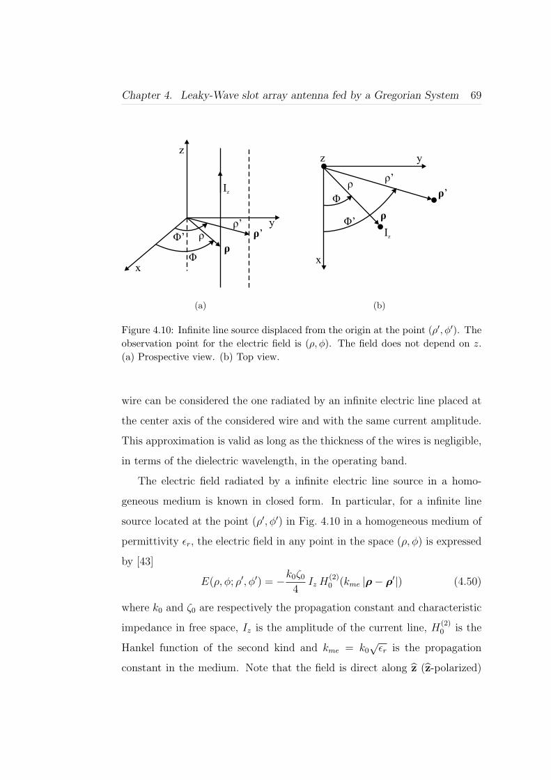
Chapter 4. Leaky-Wave slot array antenna fed by a Gregorian System 69

y

x

z

Φ

Φ’ ρ

ρ

ρ’

ρ’

Iz

(a)

y

Iz

x

z

Φ

Φ’

ρ

ρ

ρ’

ρ’

(b)

Figure 4.10: Infinite line source displaced from the origin at the point (ρ′, φ′). Theobservation point for the electric field is (ρ, φ). The field does not depend on z.(a) Prospective view. (b) Top view.

wire can be considered the one radiated by an infinite electric line placed at

the center axis of the considered wire and with the same current amplitude.

This approximation is valid as long as the thickness of the wires is negligible,

in terms of the dielectric wavelength, in the operating band.

The electric field radiated by a infinite electric line source in a homo-

geneous medium is known in closed form. In particular, for a infinite line

source located at the point (ρ′, φ′) in Fig. 4.10 in a homogeneous medium of

permittivity εr, the electric field in any point in the space (ρ, φ) is expressed

by [43]

E(ρ, φ; ρ′, φ′) = −k0ζ0

4Iz H

(2)0 (kme |ρ− ρ′|) (4.50)

where k0 and ζ0 are respectively the propagation constant and characteristic

impedance in free space, Iz is the amplitude of the current line, H(2)0 is the

Hankel function of the second kind and kme = k0√

εr is the propagation

constant in the medium. Note that the field is direct along z (z-polarized)

Chapter 4. Leaky-Wave slot array antenna fed by a Gregorian System 70

and it depends only by the distance of the point (ρ, φ) from the source. The

expression (4.50) suggests that the magnitude of the current on each wire is

sufficient to describe its distribution, indeed it does not require any expansion

in basis functions. The MoM solution and the problem are then extremely

simplified.

Before starting the derivation of the MoM solution, it is worth mentioning

that the location of each wire of the system is known from the design made in

Sec. 4.1.1 and Sec. 4.2. In particular in the following this location is assumed

to be relative to the global system x−y−z, centered at the focus of the main

reflector (see Fig. 4.3). The position of the axis of the wire i is indicated by

the vector pi = φi φ+ ρi ρ. Note that the z component is not important due

to geometry of the problem. We would suppose to be always on the z = 0

plane.

The current on the wires can be found imposing an opportune electric

field integral equation (EFIE) on the surface of the metallic wires

Ei = −Es (4.51)

where Ei is the incident electric field due to the kind of feed used for the

sources of the pin-made feed in absence of the wires and Es is the scattered

field due to the electric current distribution over the wires. In particular the

feed of the sources is assumed to be an infinitesimal delta-gap voltage and

then Ei will be constant on the feed points and zero elsewhere. The scattered

fields at any point in the space p = φ φ + ρ ρ can be expressed, using (4.50),

as

Es(p) = −k0ζ0

4

NT∑i=1

Ii H(2)0 (kme |p− pi

′|) (4.52)

where NT is the total number of pins and Ii is current magnitude of the rod

Chapter 4. Leaky-Wave slot array antenna fed by a Gregorian System 71

i. NT is given by

NT = Nr + Ng + Nsub + Nmain + Ns (4.53)

where Nr, Ng, Nsub, Nmain and Ns are respectively the number of rods for the

partially reflecting grid, the ground of the pin-made feed, the sub reflector,

the main reflector and the sources of the pin-made feed.

The unknown of the problem are NT . Imposing (4.51) on the NT rods we

find the independent equations needed to find the NT currents on the wires;

in matrix form:

[Zmn][In] = [Vm] (4.54)

with

Zmn = −k0ζ0

4H

(2)0 (kme |pm − pn|) (4.55)

where pm and pn are respectively the positions of the the rod m and n, [In]

is the unknown vector of the currents and [Vm] is vector of the incident field

values. As already said, the incident field Ei is assumed to be unitary on

the source locations and zero elsewhere, then the first NT − Ns rows of the

[Vm] are zero and the last Ns, in accordance with the particular configuration

analyzed, could be equal to minus one or zero.

The solution of (4.54) can then be found

[In] = [Zmn]−1[Vm] (4.56)

The total field, equal to the scattered field in any point in the space,

except at the delta-gap feed locations, can be now calculated by using the

expression (4.52). In particular this field is confined in the PPW waveguide

of Fig. 4.1.

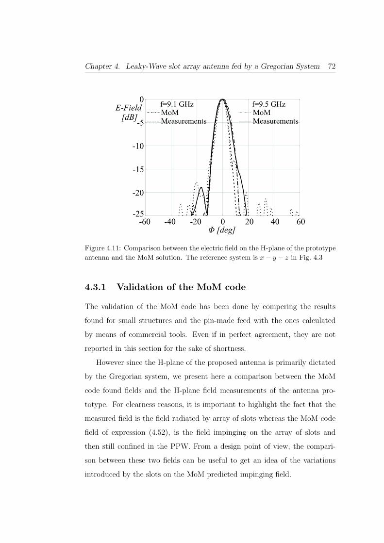
Chapter 4. Leaky-Wave slot array antenna fed by a Gregorian System 72

-25

-20

-15

-10

-5

0

-60 -40 -20 0

Φ [deg]

E-Field[dB]

20 40 60

f=9.5 GHz

Measurements

MoM

f=9.1 GHz

Measurements

MoM

Figure 4.11: Comparison between the electric field on the H-plane of the prototypeantenna and the MoM solution. The reference system is x− y − z in Fig. 4.3

4.3.1 Validation of the MoM code

The validation of the MoM code has been done by compering the results

found for small structures and the pin-made feed with the ones calculated

by means of commercial tools. Even if in perfect agreement, they are not

reported in this section for the sake of shortness.

However since the H-plane of the proposed antenna is primarily dictated

by the Gregorian system, we present here a comparison between the MoM

code found fields and the H-plane field measurements of the antenna pro-

totype. For clearness reasons, it is important to highlight the fact that the

measured field is the field radiated by array of slots whereas the MoM code

field of expression (4.52), is the field impinging on the array of slots and

then still confined in the PPW. From a design point of view, the compari-

son between these two fields can be useful to get an idea of the variations

introduced by the slots on the MoM predicted impinging field.

Chapter 4. Leaky-Wave slot array antenna fed by a Gregorian System 73

Fig. 4.11 reports the comparison, at the frequency f = 9.1 GHz and

f = 9.5 GHz, between the measured electric field and the MoM solution for

the Gregorian system derived in Sec. 4.1 fed by the pin-made feed of Sec. 4.2.

This figure clearly shows that the H-plane pattern is primarily dictated by

the Gregorian system, at least in the main beam. However, the measured

field presents a broader beam and lower side lobe level due to the radiation

effects of the slot array. In both cases, the beam does not change with the

frequency.

4.3.2 Circuit parameters for the Gregorian system: Z,

Y and S matrix

So far, not so much attention has been devoted to the feed problem. For

the MoM analysis of Sec. 4.3, we just considered an infinitesimal delta-gap

model for the central sources of the pin-made feed to derive the currents

on each rod. However the sources of the pin-made feed, in the reality, have

to be fed through a transmission line or connector and then attention has

to be made on the transition from the feeding network to the sources’ pins.

This transition is important to derive the circuit parameters of the Gregorian

system.

The coaxial probe feeding technique can be a good solution. In fact in

this case the pins of the sources would be the inner conductors of the probes.

The analysis of the transition from coaxial probes to parallel plate waveguide

has been carried out by different authors. In particular in [47] it is shown

that if a uniform-current model is assumed for the probe, its input impedance

is given by

Zin =k1ζ1

4hH

(2)0 (k1a) J0(k1a) (4.57)

Chapter 4. Leaky-Wave slot array antenna fed by a Gregorian System 74

where k1 and ζ1 are the propagation constant and impedance of the medium

inside the PPW, h is the height of the PPW and a is the radius of the inner

conductor of the probe. H(2)0 and J0 are, respectively, the Hankel function of

the second kind and the Bessel function of the first kind, of zero order. Note

that this impedance is accurate for very low profile PPW.

From (4.57) and considering that for small arguments the Bessel function

is almost one, the admittance matrix Y of the Gregorian system can be

calculated as

Y = [Iij/h] (4.58)

where h is the height of the PPW ad Iij is the current on the pin source i

when the pin source j is the only one active. This current can be found with

our MoM by setting in 4.54 equal to minus one the row of [Vm] corresponding

to the source i.

Once the Y matrix is known, both the Z and S matrixes can be derived:

Z = Y −1 (4.59)

and

S = (Z + Z0)−1 · (Z − Z0) (4.60)

where Z0 is a diagonal matrix with elements equal to the characteristic

impedances of the probes connected to the pin sources. Generally those

impedances assume the same value.

The circuit parameters so obtained represent a situation where the Gre-

gorian system is fed by single sources. As explained in Sec. 4.2, this would

not be the case since we consider couples of pins as feed for our Gregorian

system. However the circuit parameters for this new scenario can be easily

found by rearranging the elements of the Y matrix (4.58). The procedure

used to rearrange the data is based on the assumption that each couples of

Chapter 4. Leaky-Wave slot array antenna fed by a Gregorian System 75

sources can be fed by means of an ideal power divider that does not introduce

any delay or impedance transformation from the new input port to the pin

sources. This means that the voltage level presents at the new input port is

equal to that one of the pins and when the new port is short-circuited, the

pins see a zero impedance at their terminals.

Let then consider Ns single sources joined in Nc = Ns/2 couples, as shown

in Fig. 4.12. For definition [48], the term Yij of the new matrix Yc for double

pin feeds, is given by

Single Pin Feeds

Double Pin Feeds

1

Vj Ii

V =V2j-1 j V =V2j j I2i-1 I2i

2 2j 2i2j-1 2i-1

Ideal PowerDividers1 j i Nc

NsN -1s

Figure 4.12: Double pins configuration. The couples of pin sources are fed by idealpower dividers.

Yij =Ii

Vj

∣∣∣∣Vl=0 for l 6=j

(4.61)

which stated that Yij can be determined by driving port j with the voltage

Vj, short circuiting all other ports (Vl = 0 for l 6= j), and measuring the

short circuit current Ii at the port i. From Fig. 4.12 Ii is equal to

Ii = I2i−1 + I2i (4.62)

The terms I2i−1 and I2i are the currents on the pins (2i− 1) and (2i) for an

excitation V2j−1 = V2j = −1 in the MoM system (4.54) and so for (4.58),

(4.61) becomes

Yij = Y(2i−1)(2j−1) + Y(2i−1)(2j) + Y(2i)(2j−1) + Y(2i)(2j) (4.63)

Chapter 4. Leaky-Wave slot array antenna fed by a Gregorian System 76

Relation (4.63) is the rule to rearrange the Y matrix obtained for single

pin sources. Finally, from (4.59) and (4.60), the matrices Zc and Sc can be

derived.

At the end of this section it is important to highlight that for our proto-

type a coplanar waveguide solution (Fig. 4.7) has been adopted to feed the

couples of pins in Fig. 4.5. We used coplanar waveguides to preserve the

planarity of the system, as they can be easily integrated in the lower plane

of the PPW, and they make easier the design of power dividers. Even if the

analysis performed in this section is still valid and particularly useful in a

preliminary design process, the feeding network of our prototype has been

designed by using the commercial software Ansoft Designer [26]. This choice

was dictated essentially by two factors. The first was to better analyze the

transition from pin to coplanar waveguide, whereas the second was to design

and analyze a real power divider. Note that for the design of the feeding

network of the total system, it is not important to include all the parts of

the antenna as long as they do not introduce strong reflections. The only

place in the antenna structure where strong reflections can occur (Fig. 4.1),

is the transition from the dual offset Gregorian system to the array of slots.

However as explained in Sec. 4.4, the transition has been designed in order

to eliminate such reflections. In this way only the feed in Fig. 4.5 can be

analyzed and the simulations are faster and can be made using commercial

tools.

4.4 Dispersion Analysis of the slot array

The radiating part of the proposed antenna is composed by an array of slots

etched on the upper plate of a parallel plate waveguide structure, operating

Chapter 4. Leaky-Wave slot array antenna fed by a Gregorian System 77

z

x

hε

r

Leaky-WaveBackward Radiation

qTEM Wave

ls

wsdx

dy

Figure 4.13: Geometry of the radiating slots. The slots are etched on the upperplate of the parallel plate waveguide. The periodicity of the slots is such as to havea backward radiation in the operating band.

h εr ls1 ls2 ls3 ls ws dx dy

1.575 2.2 6 8 10 12 3.33 14 14

Table 4.4: Geometrical dimensions in mm of the slots and of the substrate of theparallel plate waveguide

in a backward leaky-wave mode. The geometric parameters of the slots used

in our antenna prototype are given in Tab. 4.4. In the working bandwidth

(9.1 − 9.6 GHz), the periodicity of the slots gives reason of a backward

radiation in the x − z plane, as in Fig. 4.13. Moreover to achieve a smooth

transition from the PPW to the radiating slots the first three rows of slots

have been designed with different length, as shown in Fig. 4.14.

While the procedure to derive the dispersion equation characterizing such

a structure will not be given here, it is important to highlight the effect of the

most significant geometrical parameters that affect the dispersion equation

for propagation along the x direction, where the incident wave is traveling

in the present case. These considerations will give approximate equations to

predict the radiation properties of the slots in the x− z plane.

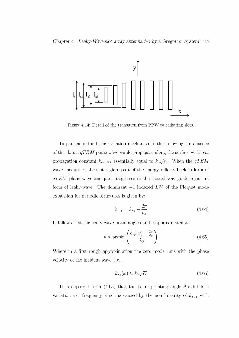
Chapter 4. Leaky-Wave slot array antenna fed by a Gregorian System 78

ls ls3 ls2 ls1

x

y

Figure 4.14: Detail of the transition from PPW to radiating slots.

In particular the basic radiation mechanism is the following. In absence

of the slots a qTEM plane wave would propagate along the surface with real

propagation constant kqTEM essentially equal to k0√

εr. When the qTEM

wave encounters the slot region, part of the energy reflects back in form of

qTEM plane wave and part progresses in the slotted waveguide region in

form of leaky-wave. The dominant −1 indexed LW of the Floquet mode

expansion for periodic structures is given by:

kx−1 = kx0 −2π

dx

(4.64)

It follows that the leaky wave beam angle can be approximated as:

θ ≈ arcsin

(kx0(ω)− 2π

dx

k0

)(4.65)

Where in a first rough approximation the zero mode runs with the phase

velocity of the incident wave, i.e.,

kx0(ω) ≈ k0

√εr (4.66)

It is apparent from (4.65) that the beam pointing angle θ exhibits a

variation vs. frequency which is caused by the non linearity of kx−1 with

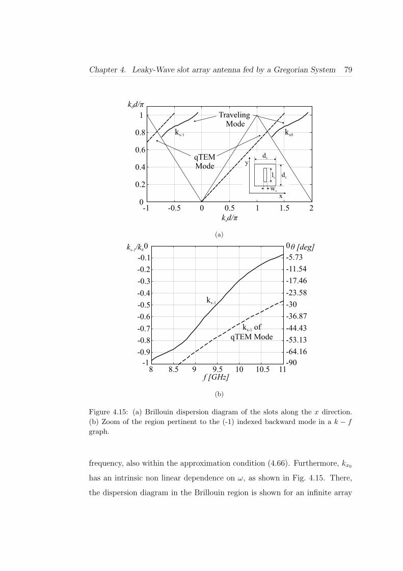
Chapter 4. Leaky-Wave slot array antenna fed by a Gregorian System 79

k d/x

π

k d/0

π

-1 -0.5 0 0.5 1 1.5 20

0.2

0.4

0.6

0.8

1

kx-1 kx0

qTEMMode

TravelingMode

x

ydx

dyls

ws

(a)

8 8.5 9 9.5 10 10.5 11-1 -90

-0.9 -64.16

-0.8 -53.13

-0.7 -44.43

-0.6 -36.87

-0.5 -30

-0.4 -23.58

-0.3 -17.46

-0.2 -11.54

-0.1 -5.73

0 0

kx-1

f [GHz]

θ [deg]k /kx-1 0

k of

qTEM Modex-1

(b)

Figure 4.15: (a) Brillouin dispersion diagram of the slots along the x direction.(b) Zoom of the region pertinent to the (-1) indexed backward mode in a k − f

graph.

frequency, also within the approximation condition (4.66). Furthermore, kx0

has an intrinsic non linear dependence on ω, as shown in Fig. 4.15. There,

the dispersion diagram in the Brillouin region is shown for an infinite array

Chapter 4. Leaky-Wave slot array antenna fed by a Gregorian System 80

of slots with the geometry shown in the inset. We note from the zoom

of Fig. 4.15 (b) that the approximation (4.66) is not extremely accurate

when compared with the results from HFSS [49] although it could give an

acceptable starting point in the design process. The non-linearity of kx0 with

frequency increases for higher permittivity.

4.5 Prototype and Experimental Results

An antenna prototype has been built and measured. For any part of the an-

tenna the dimensions given previously have been used. Moreover the number

of radiating slot rows have been chosen to reduce the surface wave field at

the last row of slots to less than 1/10, indicating that 99.9% leaky-wave end

point efficiency is achieved. The number of slot rows is 23. The antenna is

shown in Fig. 4.16, its dimensions are 378x596 mm while the panel size where

the antenna is built is 457x610 mm. Fig. 4.17 shows a zoom of the pin-made

feed. The extremely low profile of the antenna, h < 0.5 cm, should be

appreciated. The input reflection coefficient and the radiation patterns of

the antenna have been measured. The directivity and gain of the complete

structure have been calculated using the commercial tool Ansoft Designer

[26]. A total efficiency of 81% is observed, that is mostly due to the residual

spill-over losses.

The measured input reflection coefficient is shown in Fig. 4.18. The initial

design of the antenna was been performed in the band range 9.1− 9.6 GHz,

with a central operative frequency of fc = 9.35 GHz and a −10 dB relative

bandwidth of Brel ≈ 5.4%. The measured reflection coefficient has a −10 dB

bandwidth in the range 8.85−9.65 GHz, with a resonance at fr ≈ 9.136 GHz.

The small difference between fr and fc is ∆f ≈ 214 MHz and it can be due

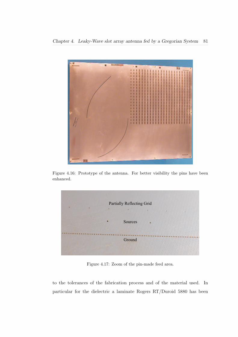
Chapter 4. Leaky-Wave slot array antenna fed by a Gregorian System 81

Figure 4.16: Prototype of the antenna. For better visibility the pins have beenenhanced.

Partially Reflecting Grid

Ground

Sources

Figure 4.17: Zoom of the pin-made feed area.

to the tolerances of the fabrication process and of the material used. In

particular for the dielectric a laminate Rogers RT/Duroid 5880 has been

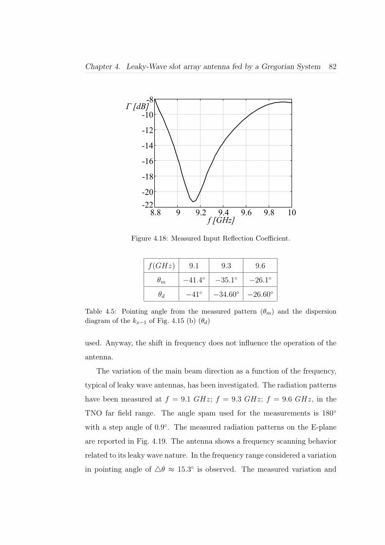
Chapter 4. Leaky-Wave slot array antenna fed by a Gregorian System 82

8.8 9 9.2 9.4 9.6 9.8 10

-22

-20

-18

-16

-14

-12

-10

-8

f [GHz]

Γ [dB]

Figure 4.18: Measured Input Reflection Coefficient.

f(GHz) 9.1 9.3 9.6

θm −41.4 −35.1 −26.1

θd −41 −34.60 −26.60

Table 4.5: Pointing angle from the measured pattern (θm) and the dispersiondiagram of the kx−1 of Fig. 4.15 (b) (θd)

used. Anyway, the shift in frequency does not influence the operation of the

antenna.

The variation of the main beam direction as a function of the frequency,

typical of leaky wave antennas, has been investigated. The radiation patterns

have been measured at f = 9.1 GHz; f = 9.3 GHz; f = 9.6 GHz, in the

TNO far field range. The angle spam used for the measurements is 180

with a step angle of 0.9. The measured radiation patterns on the E-plane

are reported in Fig. 4.19. The antenna shows a frequency scanning behavior

related to its leaky wave nature. In the frequency range considered a variation

in pointing angle of 4θ ≈ 15.3 is observed. The measured variation and

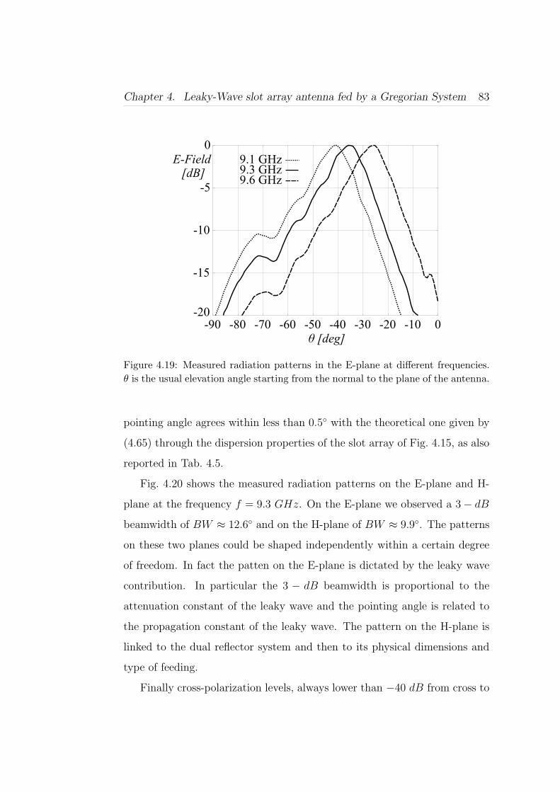
Chapter 4. Leaky-Wave slot array antenna fed by a Gregorian System 83

-20

-15

-10

-5

0

-90 -80 -70 -60 -50 -40 -30 -20 -10 0

θ [deg]

E-Field[dB]

9.1 GHz9.3 GHz9.6 GHz

Figure 4.19: Measured radiation patterns in the E-plane at different frequencies.θ is the usual elevation angle starting from the normal to the plane of the antenna.

pointing angle agrees within less than 0.5 with the theoretical one given by

(4.65) through the dispersion properties of the slot array of Fig. 4.15, as also

reported in Tab. 4.5.

Fig. 4.20 shows the measured radiation patterns on the E-plane and H-

plane at the frequency f = 9.3 GHz. On the E-plane we observed a 3− dB

beamwidth of BW ≈ 12.6 and on the H-plane of BW ≈ 9.9. The patterns

on these two planes could be shaped independently within a certain degree

of freedom. In fact the patten on the E-plane is dictated by the leaky wave

contribution. In particular the 3 − dB beamwidth is proportional to the

attenuation constant of the leaky wave and the pointing angle is related to

the propagation constant of the leaky wave. The pattern on the H-plane is

linked to the dual reflector system and then to its physical dimensions and

type of feeding.

Finally cross-polarization levels, always lower than −40 dB from cross to

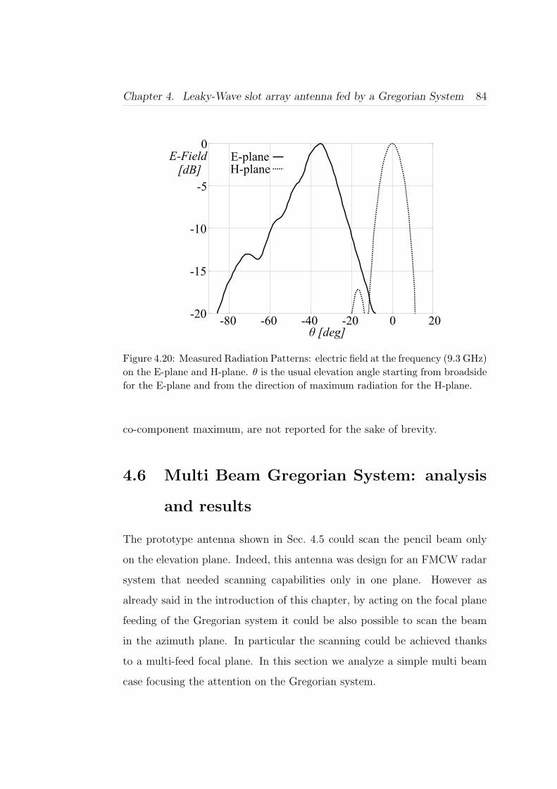
Chapter 4. Leaky-Wave slot array antenna fed by a Gregorian System 84

-20

-15

-10

-5

0

-80 -60 -40 -20 0 20

E-planeH-plane

θ [deg]

E-Field[dB]

Figure 4.20: Measured Radiation Patterns: electric field at the frequency (9.3 GHz)on the E-plane and H-plane. θ is the usual elevation angle starting from broadsidefor the E-plane and from the direction of maximum radiation for the H-plane.

co-component maximum, are not reported for the sake of brevity.

4.6 Multi Beam Gregorian System: analysis

and results

The prototype antenna shown in Sec. 4.5 could scan the pencil beam only

on the elevation plane. Indeed, this antenna was design for an FMCW radar

system that needed scanning capabilities only in one plane. However as

already said in the introduction of this chapter, by acting on the focal plane

feeding of the Gregorian system it could be also possible to scan the beam

in the azimuth plane. In particular the scanning could be achieved thanks

to a multi-feed focal plane. In this section we analyze a simple multi beam

case focusing the attention on the Gregorian system.

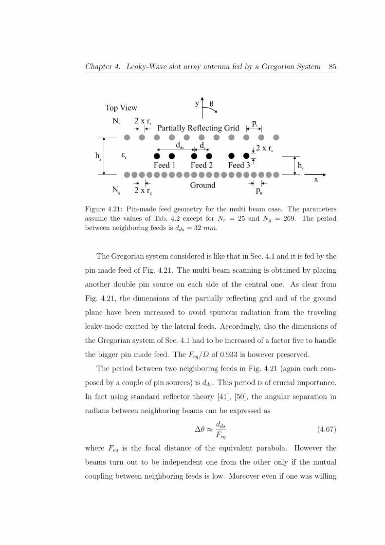
Chapter 4. Leaky-Wave slot array antenna fed by a Gregorian System 85

2 x rgpg

2 x rr pr

hs

hg

Ng

Nr

εr

2 x rsds

dds

x

y θ

Feed 1 Feed 2 Feed 3

Ground

Partially Reflecting Grid

Top View

Figure 4.21: Pin-made feed geometry for the multi beam case. The parametersassume the values of Tab. 4.2 except for Nr = 25 and Ng = 269. The periodbetween neighboring feeds is dds = 32 mm.

The Gregorian system considered is like that in Sec. 4.1 and it is fed by the

pin-made feed of Fig. 4.21. The multi beam scanning is obtained by placing

another double pin source on each side of the central one. As clear from

Fig. 4.21, the dimensions of the partially reflecting grid and of the ground

plane have been increased to avoid spurious radiation from the traveling

leaky-mode excited by the lateral feeds. Accordingly, also the dimensions of

the Gregorian system of Sec. 4.1 had to be increased of a factor five to handle

the bigger pin made feed. The Feq/D of 0.933 is however preserved.

The period between two neighboring feeds in Fig. 4.21 (again each com-

posed by a couple of pin sources) is dds. This period is of crucial importance.

In fact using standard reflector theory [41], [50], the angular separation in

radians between neighboring beams can be expressed as

∆θ ≈ dds

Feq

(4.67)

where Feq is the focal distance of the equivalent parabola. However the

beams turn out to be independent one from the other only if the mutual

coupling between neighboring feeds is low. Moreover even if one was willing

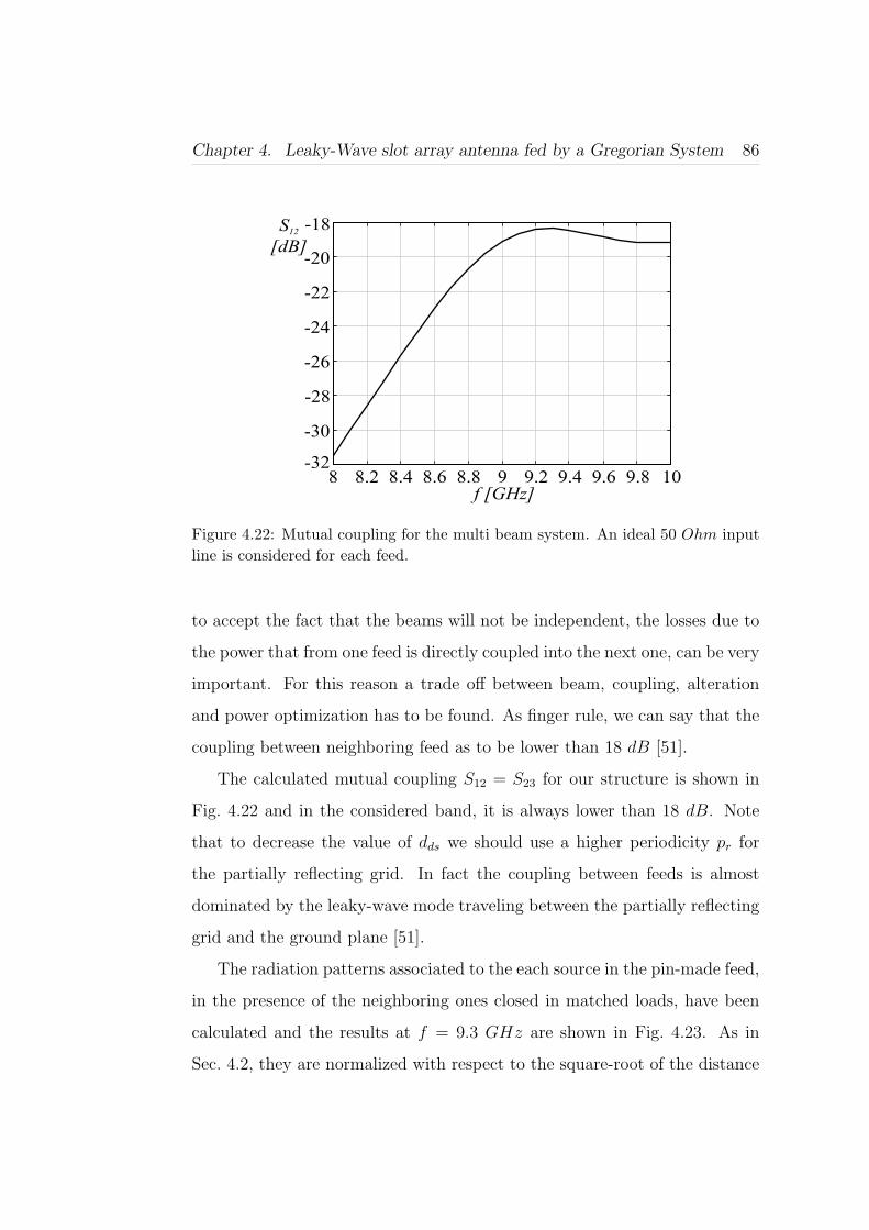
Chapter 4. Leaky-Wave slot array antenna fed by a Gregorian System 86

8 8.2 8.4 8.6 8.8 9

f [GHz]

S

[dB]12

9.2 9.4 9.6 9.8 10-32

-30

-28

-26

-24

-22

-20

-18

Figure 4.22: Mutual coupling for the multi beam system. An ideal 50 Ohm inputline is considered for each feed.

to accept the fact that the beams will not be independent, the losses due to

the power that from one feed is directly coupled into the next one, can be very

important. For this reason a trade off between beam, coupling, alteration

and power optimization has to be found. As finger rule, we can say that the

coupling between neighboring feed as to be lower than 18 dB [51].

The calculated mutual coupling S12 = S23 for our structure is shown in

Fig. 4.22 and in the considered band, it is always lower than 18 dB. Note

that to decrease the value of dds we should use a higher periodicity pr for

the partially reflecting grid. In fact the coupling between feeds is almost

dominated by the leaky-wave mode traveling between the partially reflecting

grid and the ground plane [51].

The radiation patterns associated to the each source in the pin-made feed,

in the presence of the neighboring ones closed in matched loads, have been

calculated and the results at f = 9.3 GHz are shown in Fig. 4.23. As in

Sec. 4.2, they are normalized with respect to the square-root of the distance

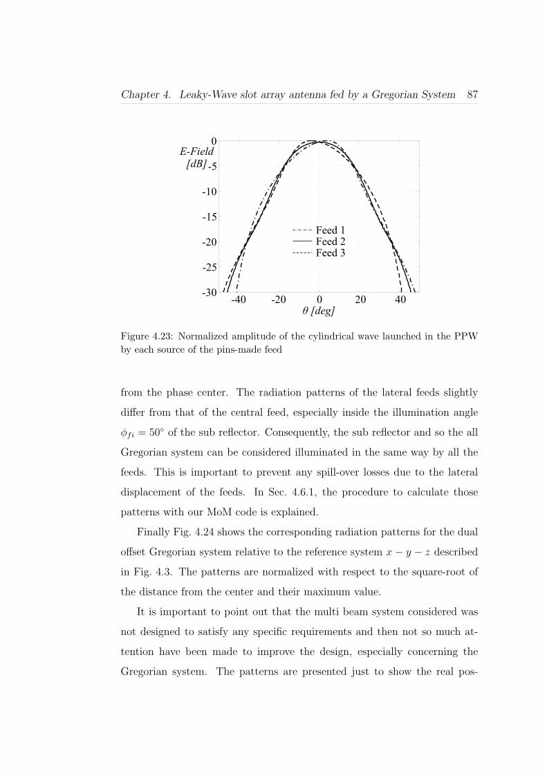
Chapter 4. Leaky-Wave slot array antenna fed by a Gregorian System 87

-30

-25

-20

-15

-10

-5

0

-40 -20 0

θ [ ]deg

E-Field[dB]

20 40

Feed 1

Feed 2

Feed 3

Figure 4.23: Normalized amplitude of the cylindrical wave launched in the PPWby each source of the pins-made feed

from the phase center. The radiation patterns of the lateral feeds slightly

differ from that of the central feed, especially inside the illumination angle

φfi = 50 of the sub reflector. Consequently, the sub reflector and so the all

Gregorian system can be considered illuminated in the same way by all the

feeds. This is important to prevent any spill-over losses due to the lateral

displacement of the feeds. In Sec. 4.6.1, the procedure to calculate those

patterns with our MoM code is explained.

Finally Fig. 4.24 shows the corresponding radiation patterns for the dual

offset Gregorian system relative to the reference system x− y − z described

in Fig. 4.3. The patterns are normalized with respect to the square-root of

the distance from the center and their maximum value.

It is important to point out that the multi beam system considered was

not designed to satisfy any specific requirements and then not so much at-

tention have been made to improve the design, especially concerning the

Gregorian system. The patterns are presented just to show the real pos-

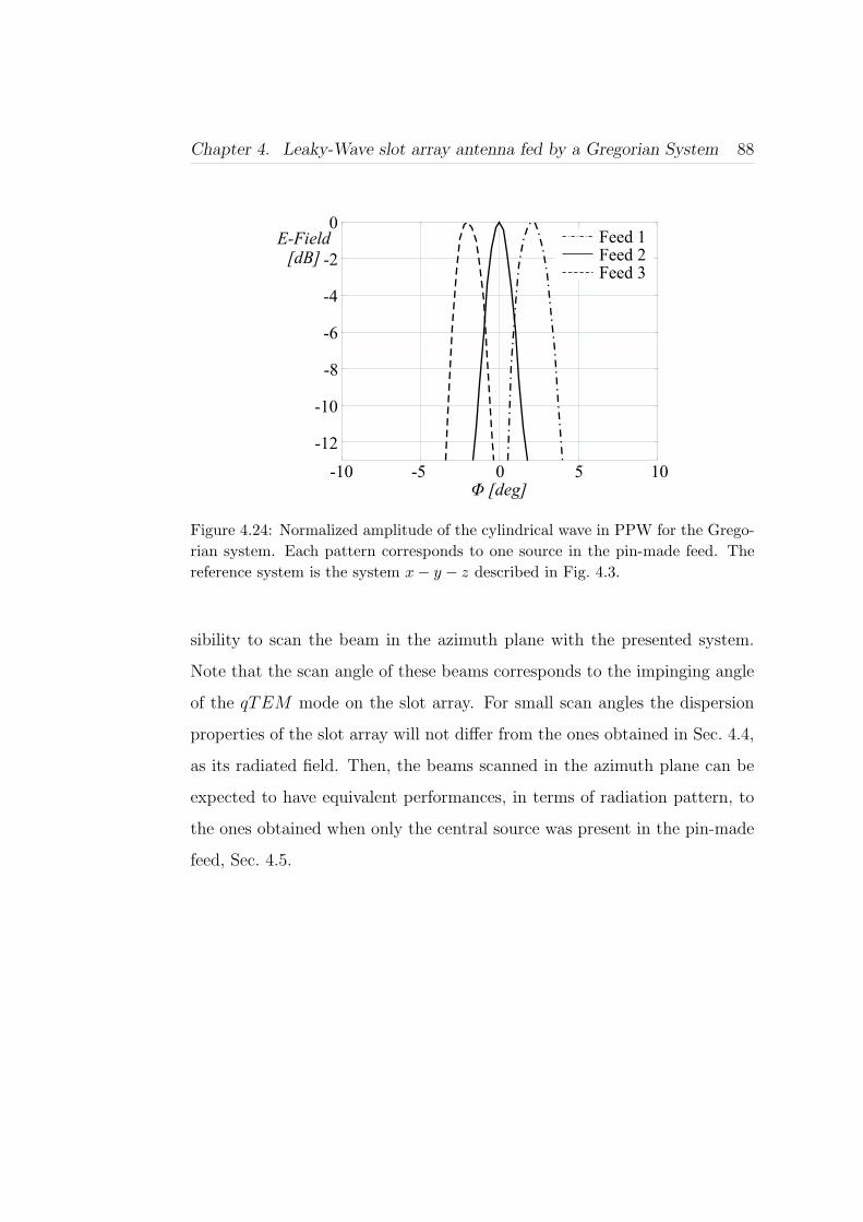
Chapter 4. Leaky-Wave slot array antenna fed by a Gregorian System 88

-12

-10

-8

-6

-4

-2

0

-10 -5 0 5 10

Φ [ ]deg

E-Field[dB]

Feed 1

Feed 2

Feed 3

Figure 4.24: Normalized amplitude of the cylindrical wave in PPW for the Grego-rian system. Each pattern corresponds to one source in the pin-made feed. Thereference system is the system x− y − z described in Fig. 4.3.

sibility to scan the beam in the azimuth plane with the presented system.

Note that the scan angle of these beams corresponds to the impinging angle

of the qTEM mode on the slot array. For small scan angles the dispersion

properties of the slot array will not differ from the ones obtained in Sec. 4.4,

as its radiated field. Then, the beams scanned in the azimuth plane can be

expected to have equivalent performances, in terms of radiation pattern, to

the ones obtained when only the central source was present in the pin-made

feed, Sec. 4.5.

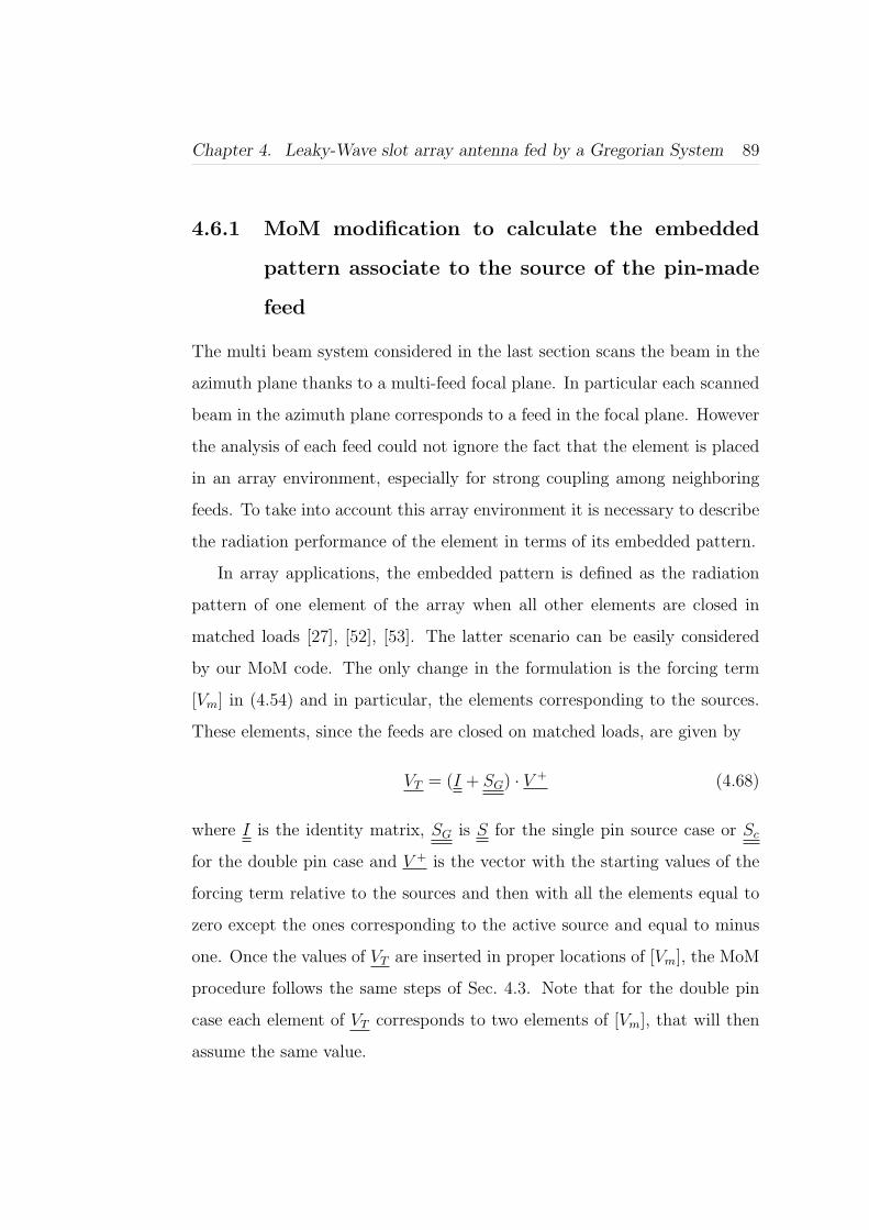
Chapter 4. Leaky-Wave slot array antenna fed by a Gregorian System 89

4.6.1 MoM modification to calculate the embedded

pattern associate to the source of the pin-made

feed

The multi beam system considered in the last section scans the beam in the

azimuth plane thanks to a multi-feed focal plane. In particular each scanned

beam in the azimuth plane corresponds to a feed in the focal plane. However

the analysis of each feed could not ignore the fact that the element is placed

in an array environment, especially for strong coupling among neighboring

feeds. To take into account this array environment it is necessary to describe

the radiation performance of the element in terms of its embedded pattern.

In array applications, the embedded pattern is defined as the radiation

pattern of one element of the array when all other elements are closed in

matched loads [27], [52], [53]. The latter scenario can be easily considered

by our MoM code. The only change in the formulation is the forcing term

[Vm] in (4.54) and in particular, the elements corresponding to the sources.

These elements, since the feeds are closed on matched loads, are given by

VT = (I + SG) · V + (4.68)

where I is the identity matrix, SG is S for the single pin source case or Sc

for the double pin case and V + is the vector with the starting values of the

forcing term relative to the sources and then with all the elements equal to

zero except the ones corresponding to the active source and equal to minus

one. Once the values of VT are inserted in proper locations of [Vm], the MoM

procedure follows the same steps of Sec. 4.3. Note that for the double pin

case each element of VT corresponds to two elements of [Vm], that will then

assume the same value.

Chapter 4. Leaky-Wave slot array antenna fed by a Gregorian System 90

4.7 Summary

In this chapter, a dual offset Gregorian system exciting a planar leaky-wave

antenna has been described. The entire system is realized in PCB technol-

ogy. A prototype antenna has been designed, manufactured and successfully

tested. The measured input reflection coefficient and radiation patterns have

been presented and explained thanks to the dispersion properties of the struc-

tures and of characteristics of the dual reflector system. A pins-made feed,

based on EBG concepts, has been used to feed the dual reflector system.

The performances of the antenna are in perfect agreement with expectation

and perfectly meet the FMCW front-end requirements that drove the design.

Also the case of a multi beam Gregorian system has been analyzed. The cal-

culated results are very promising and encourage the use of the feed concept

and the planar dual reflector system in future planar imaging system ap-

plications, to achieve antennas with independent beams in the azimuth and

elevation planes resorting to frequency reuse and multiple focal plane feeds.

We would like to highlight that the novel antenna system presented in this

chapter is at moment patent pending [54].

Chapter 5

Conclusion and Future

Developments

Even if the leaky-wave effect and the theory behind are known since many

years, as already pointed out in Chap. 1, new technologies or applications

stimulate the research of new types of leaky-wave antennas, as described in

this PhD dissertation.

In particular the main topic of this PhD dissertation has been the analysis

and design of planar leaky-wave antennas, that are receiving much attention

in the recent years, especially for applications in the millimeter-wave ranges,

due their low profile, good performances, easiness in the design and compat-

ibility with printed circuit board technology.

During the last three years, three topologies of planar leaky-wave antenna

were analyzed. The various designs were driven by different system require-

ments and in all cases we tried to fulfill the usual commercial rule of good

performances at low cost. For two antennas proposed a prototype has been

built and tested to verify the performances of the antennas. In particular

the prototypes, together with the measurements, prove the feasibility and

91

Chapter 5. Conclusion and future developments 92

applicability of the proposed antennas.

The methodology used to analyze the antennas has been briefly intro-

duced in Chap. 1. In particular for all the structures considered, the relative

dispersion properties have been derived by means of home made numerical

tools and then used to design the various antennas. The knowledge of the

dispersion properties allowed the complete control of the leaky-wave effect.

Afterwards, commercial tools were used to finalize the antenna designs. Only

for the antenna proposed in Chap. 4, a MoM code was developed to derive

the field radiated by the Gregorian system present in this antenna. The rea-

son was primarily due to the necessity of reducing drastically the simulation

time needed by commercial tools to analyze such kind of structure.

Finally I would like to summarize chapter by chapter all the antennas

presented, outlining the possible future developments.

In Chap. 2 the design of a planar leaky-wave antenna made by covering

an array of slots with a super-state of printed periodic dipoles (dipole FSS)

was shown. The antenna was supposed to be used in a medical system that

requires a high directive beam. The design goal was to maximize the gain

reducing the number of elements required for the array. The results achieved

can be useful in all that applications where a good sampling of the aperture

field of the antenna is required and one is willing to reduce the number of

elements in an array design, simplifying at the same time the beam forming

network design.

In Chap. 3 a leaky-wave antenna made by using planar circularly sym-

metric EBG was considered. The antenna was designed for an automotive

radar system where, the low profile, efficiency and scanning capability of the

antenna were the main requirements. In particular during this work the pos-

sibility to use different periodicities of the planar circularly symmetric EBG

Chapter 5. Conclusion and future developments 93

to control the excited surface wave has been shown. A future development of

this work could analyze the possibility to shape the pattern of the antenna

by using more periodicities [55], [56]. The control of the transitions from

one periodicity to the other will be the most critical part of the analysis and

design.

Chap. 4 is the main core of the present thesis. A leaky-wave slot array

antenna fed by a dual reflector system was presented and analyzed thanks

to a home made code. In this case, the antenna design was driven by the

requirements of a FMCW front-end radars. Moreover, in this work, the

possibility to use the innovative pin-made feed and planar dual offset system

for multi beam planar applications has been exploited. In particular the

possibility to achieve antennas with independent beams in the azimuth and

elevation planes resorting to frequency reuse and multiple focal plane feeds

has been shown. Having shown such results, we have opened possibilities

to implement in planar technology those applications that are right now

implemented with 3-D focusing imaging-like systems. The system presented

here is patent pending [54].

The results of this thesis have been presented at several international

conferences and in the frame of the European antenna network of excellence

(ACE) [57]. Part of this work has already been published in IEEE Antennas

and Wireless Propagation Letters and another full paper has been submitted

on IEEE Transaction on Antenna and Propagation.

Bibliography

[1] T. Tamir, “Leaky wave antennas”, Antenna Theory, R. E. Collin andF. J. Zucker, Eds. New York: McGraw-Hill, 1969, pt. 2, ch. 20.

[2] A. A. Oliner, “Leaky-wave antennas”Antennas Engineering Hand-book,3rd ed, R. C. Johnson, Ed. New York: McGraw-Hill, 1993, ch. 10.

[3] L. O. Goldstone, A. A. Oliner, “Leaky-wave antennas I, rectangularwaveguides”, IRE Trans. Antennas Propagation, Vol. AP-7, pp. 307-319, October 1959.

[4] L. O. Goldstone, A. A. Oliner, “Leaky-wave antennas II, circular waveg-uides”, IRE Trans. Antennas Propagation, Vol. AP-9, pp. 280-290,May 1961.

[5] T. Tamir, A. A. Oliner, “Guided complex waves, Part I, Fields at aninterface”, Proc. IEE, Vol. 110, pp. 310-324, February 1963.

[6] T. Tamir, A. A. Oliner, “Guided complex waves, Part II, Relation toradiation patterns”, Proc. IEE, Vol. 110, pp. 325-334, February 1963.

[7] R. E. Collin, Field theory of guided complex waves, McGraw-Hill BookCompany, New York, 1960.

[8] A. Hessel, “General characteristic of traveling-wave antennas”, AntennaTheory, R. E. Collin and F. J. Zucker, Eds. New York: McGraw-Hill,1969, pt. 2, ch. 19.

[9] L.B. Felsen and N. Marcuvitz, Radiation and Scattering of Waves,Prentice-Hall, Englewood Cliffs, NJ, also IEEE Press, Piscataway, NJ,1994.

[10] L.B. Felsen and N. Marcuvitz, Modal Analysis and Synthesis of Elec-tromagnetic Fields, Rep. R. 446a, b of Microwave Research Institute,Brooklyn Polytechnic Institute, New York, 1956.

94

Bibliography 95

[11] N. G. Alexopoulos and D. R. Jackson, “Fundamental superstrate ef-fects on printed circuit antennas”, IEEE Transactions on Antennas andPropagation, vol. 32, no. 8, pp. 807-816, Aug. 1984.

[12] D. R. Jackson, N. G. Alexopoulos, “Gain enhancement methods forprinted circuit antennas”, IEEE Transactions on Antennas and Propa-gation, Vol. 33, no. 9, pp. 967-987, Sep. 1985.

[13] H. Y. Yang, N. G. Alexopoulos, “Gain enhancement methods for printedcircuit antennas through multiple superstrates”, IEEE Transactions onAntennas and Propagation, Vol. 35, no. 7, pp. 860-863, Jul. 1987.

[14] D. R. Jackson and A. A. Oliner, “A leaky-wave analysis of the high-gainprinted antenna configuration”, IEEE Transactions on Antennas andPropagation, vol. 36, no. 7, pp. 905-910, Jul. 1988.

[15] D. R. Jackson, A. A. Oliner, A. Ip, “Leaky-wave propagation and ra-diation for a narrow-beam multiple-layer dielectric structure”, IEEETransactions on Antennas and Propagation, Vol. 41, no. 3, pp. 344-348,Mar. 1993.

[16] A. Neto, N. Llombart, “Wideband Localization of the Dominant LeakyWave Poles in Dielectric Covered Antennas”, IEEE Antennas and Wire-less Propagation Letters, Vol. 5, no. 1, pp. 549-551, Dec. 2006.

[17] N. Marcuvitz, “On field representation in terms of leaky modes or eigen-modes”, IRE Trans. Antennas Propagation, Vol. AP-10, pp. 646-647,September 1962.

[18] A. Hessel, “On the influence of complex poles on the radiation patternof leaky wave antennas”, IRE Trans. Antennas Propagation, Vol. AP-4,pp. 192-194, July 1956.

[19] T. Zhao, D. R. Jackson, J. T. Williams, H. D. Yang, A.A Oliner, “2-DPeriodic Leaky-Wave Antennas- Part I: Metal Patch Design”, IEEETransactions on Antennas and Propagation, Vol. 53, no.11, pp. 3505-3514, Nov. 2005.

[20] T. Zhao, D. R. Jackson, J. T. Williams, “2-D Periodic Leaky-WaveAntennas- Part II: Slot Design”, IEEE Transactions on Antennas andPropagation, Vol. 53, no.11, pp. 3515-3524, Nov. 2005.

[21] R. Gardelli, M. Albani, F. Capolino, “Array Thinning by Using Anten-nas in a FabryPerot Cavity for Gain Enhancement”, IEEE Transactionson Antennas and Propagation, Vol. 54,, no.7, pp. 1979-1990, Jul. 2006.

Bibliography 96

[22] S. Maci, M. Caiazzo, A. Cucini, M. Casaletti, “A pole-zero match-ing method for EBG surfaces composed of a dipole FSS printed on agrounded dielectric slab”, IEEE Transactions on Antennas and Propa-gation, Vol. 53, no.1, pp. 70-81, Jan. 2005.

[23] R. E. Collin, “Analytical solution for a leaky-wave antenna”, IRE Trans.Antennas Propagation, Vol. AP-10, pp. 561-565, September 1962.

[24] N. Llombart, “Development of Integratd Printed Array Antennas UsingEBG Substrates”, Doctoral Thesis, Universidad Politecnica de Valencia,Valencia, April 2006.

[25] T. Zhao, D. R. Jackson, J. T. Williams, A. A. Oliner, “General Formulasfor 2-D Leaky-Wave Antennas”, IEEE Transactions on Antennas andPropagation, Vol. 53, no.11, pp. 3525-3533, Nov. 2005.

[26] Ansoft Designer version 3.0.0, 1984-2007 Ansoft Corporation.

[27] J. R. James, P. S. Hall Handbook of Microstrip Antennas, Peter Pere-grinus Ltd. for IEE, 1989.

[28] D. M. Pozar, D. H. Schaubert Microstrip Antennas, IEEE Press, NewYork, 1995.

[29] C. A. Balanis, Antennas Theory, John Wiley & Sons Inc., New York,1997.

[30] A. Cucini, M. Nannetti, F. Caminita, S. Maci, “A Pole MatchingMethod for the Analysis of Frequency Selective Surfaces”, ComplexComputing-Networks Brain-like and Wave-oriented Electrodynamic Al-gorithms, I. C. Goknar, L. Sevgi, Springer Berlin Heidelberg, 2006, ch. 7.

[31] A. Ip, D. R. Jackson, “Radiation from cylindrical leaky waves”, IEEETransactions on Antennas and Propagation, Vol. 38, no. 4, pp. 482-488,Apr. 1990.

[32] A. Polemi, S. Maci, “On the Polarization Properties of a Dielectric LeakyWave Antenna”, IEEE Antennas and Wireless Propagation Letters, Vol.5, no. 1, pp. 306-310, Dec. 2006.

[33] N. Llombart, A. Neto, G. Gerini, P. De Maagt, “Planar circularly sym-metric EBG structures for reducing surface waves in printed antennas”,IEEE Transactions on Antennas and Propagation, Vol. 53, no.10, pp.3210-3218, Oct. 2005.

Bibliography 97

[34] A. Neto, N. Llombart, G. Gerini, P. De Maagt, “On the optimal radi-ation bandwidth of printed slot antennas surrounded by EBGs”, IEEETransactions on Antennas and Propagation, Vol. 54, no.4, pp. 1074-1083, Apr. 2006.

[35] N. Llombart, A. Neto, G. Gerini, P. De Maagt, “1-D Scanning Arrayson Dense Dielectrics Using PCS-EBG Technology”, IEEE Transactionson Antennas and Propagation, Vol. 55, no.1, pp. 26-35, Jan. 2007.

[36] D. Sievenpiper, J. Colburn, B. Fong, J. Ottush, J. Visher, “Holographicartificial impedance surfaces for conformal antennas”, Antennas andPropagation Society International Symposium, 2005, Vol. 1B, 3-8 July2005, Page(s):256 - 259.

[37] N. G. Alexopoulus, P. B. Katehi, D. B. Rutledge, “Substrate optimiza-tion for integrated circuit antennas” Microwave Theory and Techniques,IEEE Transactions Vol. 83, no.7, pp. 550-557, Jul. 1983.

[38] Hany F. Hammad, Yahia M. M. Antar, Al P. Freundorfer, Samir F. Mah-moud, “Uni-Planar CPW-Fed Slot Launchers for Efficient TM0 Surface-Wave Excitation” Microwave Theory and Techniques, IEEE Transac-tions Vol. 51, no.4, pp. 1234-1240, Apr. 2003.

[39] Y. Mizughchi, A. Akagawa, H. Yokoi, “Offeset Gregorian antenna”,Trans Inst. Electron. Commun. Eng. Japan, Vol. 161-B, no.3, pp. 166-173, Mar. 1978.

[40] Y. Mizughtch, A. Akagawa, H. Yokoi, “Offset dual reflector antennas”,IEEE Antennas Propagat. Soc. Symp. Dig, Amherst, MA, Oct. 1976,pp. 2-5.

[41] Y. Rahmat-Samii, “Antenna Handbook”, Chapter 15: Reflector Anten-nas, from Y. T. Lo ans S. W. Lee, Van Nostrand Reinhold Company,New York 1988.

[42] W. V. T. Rush, A. Prata, Y. Rahmat-Samii, R. A. Shore, “Deriva-tion and Application of the Equivalent Paraboloid for Classical OffsetCassegrein and Gregorain Antennas”, IEEE Transactions on Antennasand Propagation, Vol. 38, no.8, pp. 1141-1149, Aug. 1990.

[43] C. A. Balanis, Advanced Engineering Electromagnetics, John Wiley &Sons Inc., New York, 1989.

Bibliography 98

[44] A. Neto, N. Llombart, G. Gerini, M. D. Bonnedal, P. De Maagt, “EBGEnhanced Feeds for the Improvement of the Aperture Efficiency of Re-flector Antennas”, IEEE Transactions on Antennas and Propagation,Vol. 55, no. 8, pp. 2185-2193, Aug. 2007.

[45] N. Llombart, A. Neto, G. Gerini, M. D. Bonnedal, P. De Maagt, “LeakyWave Enhanced Feed Arrays for the Improvement of the Edge of Cov-erage Gain in Multi Beam Reflector Antennas”, accepeted on IEEETransactions on Antennas and Propagation.

[46] A. Neto and S. Maci, “Green’s Function for an Infinite Slot Printed Be-tween Two Homogeneous DielectricsPart I: Magnetic Currents”, IEEETransactions on Antennas and Propagation, Vol. 51, no. 7, pp. 1572-1581, Jul. 2003.

[47] H. Xu, D. R. Jackson, J. T. Williams, “Comparison of Models forthe Probe Inductance for a Parallel-Plate Waveguide and a MicrostripPatch”, IEEE Transactions on Antennas and Propagation, Vol. 53, no.10, pp. 3229-3235, Oct. 2005.

[48] D. M. Pozar, Microwave Engineering, John Wiley & Sons Inc., NewYork, 2004.

[49] Ansoft HFSS version 10.0, 1984-2007 Ansoft Corporation.

[50] S. D. Rao, “Design and Analysis of Multiple-Beam Reflector”, IEEE An-tennas and Propagation Magazine, Vol. 41, no. 4, pp. 53-59, Aug. 1999.

[51] N. Llombart, A. Neto, G.Gerini, M. Bonnedal, P. De Maagt, “Impact ofMutual Coupling in Leaky Wave Enhanced Imaging Arrays”, submittedto IEEE Transactions on Antennas and Propagation

[52] D. M. Pozar, “The Active Element Pattern”, IEEE Transactions onAntennas and Propagation, Vol. 42, no. 8, pp. 1176-1178, Aug. 1994.

[53] D. M. Pozar, “A Relation Between the Active Input Impedance andthe Active Element Pattern of a Phased Array”, IEEE Transactions onAntennas and Propagation, Vol. 51, no. 9, pp. 2486-2489, Sep. 2003.

[54] A. Neto, M. Ettorre, G. Gerini, “Leaky wave antenna using waves prop-agating between parallel surfaces”, Patent Application EP07113133.8,2007.

Bibliography 99

[55] A. A. Oliner, A. Hessel, “Guided waves on sinusoidally modualted re-actance surfaces”, IRE Trans. Antennas Propagation, Vol. AP-7, pp.201-208, December 1959.

[56] P. Burghignoli, F. Frezza, A. Galli, G. Schettini, “Synthesis of broad-beam patterns through leaky-wave antennas with rectilinear geometry”,IEEE Antennas and Wireless Propagation Letters, Vol. 2, pp. 136-139,Dec. 2003.

[57] Antenna Centre of Excellence - ACE, EU Sixth Framework programme.http://www.antennasvce.org/

Biography

Mauro Ettorre was born in Tricarico, Matera, Italy, in 1979. He received

the laurea degree (summa cum laude) in telecommunication engineering from

the University of Siena, Italy, in 2004. During his master degree studies he

spent five months at the Technical University of Denmark (DTU), Lyngby,

Denmark. Part of his PhD has been developed at the Defence, Security

and Safety Institute of the Netherlands Organization for Applied Scientific

Research (TNO), The Hague, The Netherlands, where he is currently working

as an antenna researcher.

His research interests include the analysis and design of leaky-wave an-

tennas, periodic structures and electromagnetic band-gap structures.

100

Publications

Journal Papers

[R1] M. Ettorre, S. Bruni, G. Gerini, A. Neto, N. Llombart, S. Maci,

“Sector PCS-EBG Antenna for Low Cost High Directivity Applications”,

Antennas and Wireless Propagation Letters, Vol.6, pp. 537-539, Dec. 2007.

[R2] M. Ettorre, A. Neto, G. Gerini, S. Maci, “Leaky-Wave Slot Array

Antenna Fed by a Dual Reflector System”, Submitted to IEEE Trans. on

Antennas and Propagation, 2008.

101

Publications 102

Conference Proceedings

[C1] M. Ettorre, P. Focardi, F. Mariottini, S. Maci, W. R. McGrath, “Pla-

nar Array Covered by Metamaterial Surfaces for Micro-wave and Millimeter-

wave Applications”, IEEE AP-S Symposium, Washington, DC, July 2005.

[C2] M. Ettorre, A. Polemi, A. Toccafondi, S. Maci, “Edge Diffraction

at Truncated Metamaterial Surfaces”, IEEE AP-S Symposium, Washington,

DC, July 2005.

[C3] M. Nannetti, M. Ettorre, F. Caminita, S. Maci, “Adiabatic and

exact analysis of periodically modulated artificial surfaces for holographic

antenna applications”, IEEE AP-S Symposium, Albuquerque, New Mexico,

July 2006.

[C4] M. Ettorre, S. Maci, M. Nannetti, A. Neto, M. Sabbadini, “Leaky

Wave Radiation of a Dipole-Excited Slot Line Printed on an Artificial Plasma”,

IEEE AP-S Symposium, Albuquerque, New Mexico, July 2006.

[C5] M. Ettorre, S. Bruni, G. Gerini, A. Neto, N. Llombart, S. Maci,

“Multi Sector PCS-EBG Antenna for low cost high directivity applications”,

IEEE AP-S Symposium, Honolulu, Hawaii, June 2007.

[C6] M. Albani, M. Ettorre, S. Maci, P. Balling, G. Gerini, K. Pontoppi-

dan, Z. Sipus, D. Sjoberg, G. Vecchi, F. Vipiana, “Reflector Surface Modeling

- A European Collaboration”, Eucap 2007, Edinburgh, UK, November 2007.

Acknowledgements

Lastly, I would like to say GRAZIE to who contributed somehow to make

my PhD frame-time enjoyable under a human as well as a scientific point of

view.

To my former supervisor Prof. Roberto Tiberio, whose memory I would

like to dedicate a special thought at the end of this PhD thesis.

To my supervisor, Prof. Stefano Maci, who always believed in me and in

this project, let me attempt this exciting experience in Netherlands at TNO

and give me useful advice for my work and my future. Grazie Prof.!

To Dott. Andrea Neto for giving me advices and the “tools” important

for my future carrier. I think my PhD could never be the same without his

help. His energies, passion and positive view could not be described and I

feel really lucky because I had the opportunity to work with him. Grazie

davvero Andrea!

To Dott. Giampiero Gerini for making me part of this big community

at TNO and to find always time for me, even when his agenda was already

overbooked. Grazie Giampiero!

To Andre Verweij for giving me the opportunity to spend part of my PhD

project in his department at TNO.

To all my friends and colleagues at University of Siena and at TNO: Ag-

nese, Alessio, Alessia, Cristian, Daniele, Enrica, Francesco, Frans, Gabriele,

103

Acknowledgements 104

Giorgio, Giovanni, “Il Mariottini”, Magnus, Massimiliano, Michael, Nicomino,

Nuria, Paolo Facchini, Paolo Braconi, Roland, Simona, Stefania, Teis, . . . , for

the wonderful time, advices, exchange of scientific ideas and relaxing chats.

Massimo alla fine ce l’abbiamo fatta. Tre anni sono passati in fretta, ma non

cosı veloci per non segnare in modo profondo la nostra vita e per averci dato

l’opportunita di conoscerci e legarci con una forte amicizia. Grazie Massimo,

grazie per essermi stato vicino. Sinisa il dottorato e arrivato e sara un altro

motivo di festa e una delle tante occasione per fare due chiacchiere. Grazie

Skok per tutte le discussioni e il tuo incoraggiamento a procedere!

To all the people I have met during these three years and with whom

I shared nice and weak moments: Annalisa, Charlene, Javier, Luca, Lucia,

Maurizio, Piotr, Sheila, . . . . Especially I would like to thank Julien for his

happiness and constant help, really important during the very hard Dutch

winters and when the time was not even enough to cook my “simple pasta”

and so some nice “French Cuisine” was already waiting for me.

To all my friends and I am sorry that I would never manage to write

down a complete list: Alessandro, Andrea, Caterina, Cecilia, Ermira, Fabio,

Federica, Francesco, Laura, Leticia, Manfredi, Manuela, Marcello, Mario,

Mauro, Mavi, Tanya, Tiziana, Xenia, . . .

Al mio amico di sempre, al Caro Pennello che sempre avrei voluto al mio

fianco in tutte le esperienze e nei tanti viaggi che ci hanno separato. A lui va

sempre il mio pensiero, alla sua energia, forza e voglia di vivere dimostrata

in momenti difficili che hanno toccato la sua e inevitabilmente la mia vita.

A Fulvio, il mio insegnante di surf, anche se il surf e ancora sul tetto

di casa di Cristian. Al suo costante appoggio durante tutti questi anni, da

quella scuola superiore che ci ha fatto conoscere a quel giorno in cui insieme,

pieni di speranza, partimmo da Taranto per iniziare le nostre vite.

Acknowledgements 105

To Paolo, “il Pif” for always being close to me and ready to spend hours

talking and sharing ideas on life. I met Paolo during my “Erasmus” when

I still did not know how big was Europe and the world and since that time

the world is getting closer and closer also thanks to him. Idolo Grazie!

To my family, who supported me all over these years and in particular to

my wonderful and unique sister who participated actively in the development

of this PhD dissertation and whose example has always been a guideline for

my life.