i

ANALYSIS, SIMULATION AND OPTIMIZATION OF

VENTILATION OF ALUMINUM SMELTING CELLS

AND POTROOMS FOR WASTE HEAT RECOVERY

Thèse

Ruijie Zhao

Doctorat en génie mécanique

Philosophiae Doctor (Ph.D.)

Québec, Canada

© Ruijie Zhao, 2015

ii

iii

RÉSUMÉ

En raison des quantités d’énergie requises par la production primaire d’aluminium et le

rendement relativement faible, les rejets thermiques de cette industrie sont énormes. Ils

sont par contre difficiles à utiliser à cause de leur faible température. De plus, tout

changement apporté pour augmenter la température des rejets peut avoir un impact

important sur la production. La compréhension du transfert thermique et de l’écoulement

d’air dans une cuve peut aider à maintenir les conditions de la cuve lorsque des

modifications y sont apportées. Le présent travail vise à développer cette compréhension

et à apporter des solutions pour faciliter la capture des rejets thermiques.

Premièrement, un circuit thermique est développé pour étudier les pertes

thermiques par le dessus de la cuve. En associant des résistances thermiques aux

paramètres physiques et d’opération, une analyse de sensibilité par rapport aux

paramètres d’intérêt est réalisée pour déterminer les variables qui ont le plus d’influence

sur la qualité thermique des rejets de chaleur dans les effluents gazeux. Il a été montré

que la réduction du taux de ventilation des cuves était la solution la plus efficace. Ensuite,

un modèle CFD a été développé. Un bon accord a été trouvé entre les deux modèles.

Deuxièmement, une analyse systématique de la réduction de la ventilation des

cuves a été réalisée par la simulation CFD. Trois problèmes qui peuvent survenir suite à

une réduction du taux de ventilation sont étudiés et des modifications sont proposées et

vérifiées par des simulations CFD. Le premier problème, maintenir les pertes thermiques

via le dessus de la cuve, peut être résolu en exposant davantage les rondins à l’air pour

augmenter les pertes radiatives. Le second problème soulevé par la réduction de

ventilation concerne les conditions thermiques dans la salle des cuves et une influence

limitée de la ventilation est observée par les simulations. Finalement, l’étanchéité des

cuves est augmentée par une réduction des ouvertures de la cuve de manière à limiter les

émissions fugitives sous des conditions de ventilation réduite. Les résultats ont révélé

qu’une réduction de 50% du taux de ventilation est techniquement réalisable et que la

température des effluents d’une cuve peut être augmentée de 50 à 60C.

iv

v

ABSTRACT

Due to the high energy requirement and ~50% efficiency of energy conversion in

aluminum reduction technology, the waste heat is enormous but hard to be recovered.

The main reason lay in its relatively low temperature. Moreover, any changes may affect

other aspects of the production process, positively or negatively. A complete

understanding of the heat transfer and fluid flow in aluminum smelting cells can help to

achieve a good trade-off between modifications and maintenance of cell conditions. The

present work aims at a systematic understanding of the heat transfer in aluminum

smelting cell and to propose the most feasible way to collect the waste heat in the cell.

First, a thermal circuit network is developed to study the heat loss from the top of

a smelting cell. By associating the main thermal resistances with material or operating

parameters, a sensitivity analysis with respect to the parameters of interest is performed

to determine the variables that have the most potential to maximize the thermal quality of

the waste heat in the pot exhaust gas. It is found that the reduction of pot draft condition

is the most efficient solution. Then, a more detailed Computational Fluid Dynamics (CFD)

model is developed. A good agreement between the two models is achieved.

Second, a systematic analysis of the reduction of draft condition is performed

based on CFD simulations. Three issues that may be adversely affected by the draft

reduction are studied and corresponding modifications are proposed and verified in CFD

simulations. The first issue, maintaining total top heat loss, is achieved by exposing more

anode stubs to the air and enhancing the radiative heat transfer. The second one is to

verify the influence of the draft reduction on the heat stress in potroom and limited

influence is observed in the simulations. Finally, the pot tightness is enhanced by

reducing pot openings in order to constrain the level of fugitive emissions under reduced

pot draft condition. The results have revealed that 50% reduction in the normal draft level

is technically realisable and that the temperature of pot exhaust gas can be increased by

50-60 ˚C.

vi

vii

CONTENT

RÉSUMÉ...........................................................................................................................iii

ABSTRACT........................................................................................................................v

CONTENT.......................................................................................................................vii

TABLE LIST....................................................................................................................xi

FIGURE LIST................................................................................................................xiii

NOMENCLATURE ...................................................................................................... xvii

ACKNOWLEDGEMENTS .......................................................................................... xxi

FOREWORD…............................................................................................................ xxiii

CHAPTER 1 INTRODUCTION ................................................................................... 1

1.1 Introduction ........................................................................................................... 2

1.2 Current progress .................................................................................................... 3

1.2.1 Mathematical models of the electrolytic cell ............................................ 3

1.2.2 Top heat transfer in smelting cells ............................................................ 5

1.2.3 Sidewalls heat transfer in smelting cells ................................................... 7

1.2.4 Fluoride emissions from electrolytic cells ................................................ 9

1.2.5 Heat and mass transport in potroom ....................................................... 10

1.3 Problematic and objectives ................................................................................. 10

1.4 Overview ............................................................................................................. 12

CHAPTER 2 HEAT TRANSFER IN UPPER PART OF ELECTROLYTIC CELLS: THERMAL CIRCUIT AND SENSITIVITY ANALYSIS…………………………………………………………….15

Abstract ......................................................................................................................... 16

2.1 Introduction ......................................................................................................... 18

2.2 Description of the system ................................................................................... 20

2.3 Thermal circuit representation ............................................................................ 21

2.3.1 Conduction and convection sub-network ................................................ 24

2.3.2 Radiation sub-network ............................................................................ 28

2.4 Resistance of fin-like components with internal heat generation ....................... 29

2.5 Numerical implementation and validation .......................................................... 34

2.6 Effect of ventilation rate ..................................................................................... 37

2.7 Effect of heat transfer coefficients on different surfaces .................................... 40

2.8 Effect of the surface emissivity .......................................................................... 44

2.9 Influence of hoods insulation .............................................................................. 46

2.10 Influence of the potroom air temperature ........................................................... 48

viii

2.11 Influence of anode height ................................................................................... 50

2.12 Conclusions ......................................................................................................... 52

CHAPTER 3 HEAT TRANSFER AND AIRFLOW ANALYSIS IN UPPER PART OF ELECTROLYTIC CELLS BASED ON CFD ............................. 55

Abstract ......................................................................................................................... 56

3.1 Introduction ......................................................................................................... 58

3.2 CFD Model ......................................................................................................... 59

3.2.1 Domain .................................................................................................... 59

3.2.2 Governing equations and modeling options ........................................... 62

3.2.3 Boundary conditions ............................................................................... 66

3.3 Model verification .............................................................................................. 68

3.3.1 Verification of mesh requirements .......................................................... 68

3.3.2 Validation with literature ........................................................................ 69

3.4 Comparison between CFD simulations and a thermal resistance circuit model….. ............................................................................................................................ 71

3.5 Correlations for average convection coefficients ............................................... 75

3.6 Spatial variations of the local convection coefficients ....................................... 79

3.7 Forced versus natural convection ....................................................................... 81

3.8 Pressure drop-flow rate relationship ................................................................... 83

3.9 Conclusions ......................................................................................................... 85

CHAPTER 4 REDUCED VENTILATION OF UPPER PART OF ALUMINUM SMELTING POT: POTENTIAL BENEFITS, DRAWBACKS, AND DESIGN MODIFICATIONS ............................................................... 87

Abstract ......................................................................................................................... 88

4.1 Introduction ......................................................................................................... 90

4.2 CFD Model ......................................................................................................... 91

4.2.1 Simplifying Assumptions ....................................................................... 91

4.2.2 Governing Equations .............................................................................. 92

4.2.3 Turbulence Model ................................................................................... 93

4.2.4 Numerical Modeling and Mesh .............................................................. 94

4.2.5 Boundary Conditions .............................................................................. 95

4.3 Verification and Validation ................................................................................ 96

4.4 Top Heat Loss in Current Pots under Normal and Reduced Ventilation Rates ...... ............................................................................................................................ 98

4.5 Addition of Fins on Anode Assembly .............................................................. 100

4.6 Modification of Hood Gaps Geometry ............................................................. 102

ix

4.7 Modifications on Anode Cover ........................................................................ 105

4.8 Conclusions ....................................................................................................... 106

CHAPTER 5 AIRFLOW AND THERMAL CONDITIONS IN ALUMINUM SMELTING POTROOMS UNDER DIFFERENT CONDITIONS .... ............................................................................................................... 107

Abstract ....................................................................................................................... 108

5.1 Introduction ....................................................................................................... 110

5.2 Description of the ventilation in potrooms ....................................................... 112

5.3 CFD modeling .................................................................................................. 113

5.3.1 Description of the numerical domain .................................................... 113

5.3.2 Governing equations ............................................................................. 115

5.3.3 Boundary conditions ............................................................................. 117

5.3.4 Mesh independence study ..................................................................... 122

5.4 Model validation from measurements in potroom ............................................ 123

5.5 Ventilation and thermal conditions in potroom under different pot ventilations ... .......................................................................................................................... 126

5.5.1 Outdoor condition scenarios ................................................................. 127

5.5.2 Effect of pot ventilation reduction on potroom ventilation .................. 127

5.5.3 Effect of pot ventilation reduction on temperature distribution in potroom ............................................................................................................... 129

5.6 Assessment of body heat stress under different pot ventilations ...................... 132

5.7 Conclusions ....................................................................................................... 137

CHAPTER 6 ESTIMATION OF THE EFFICIENCY OF POT TIGHTNESS IN REDUCED POT DRAFT BASED ON CFD SIMULATIONS ....... 139

Abstract ....................................................................................................................... 140

6.1 Introduction ....................................................................................................... 142

6.2 Description of pot ventilation principles .......................................................... 144

6.3 Numerical model .............................................................................................. 147

6.3.1 Computational domains and simplifying assumptions ......................... 147

6.3.2 Governing equations ............................................................................. 148

6.3.3 Boundary conditions ............................................................................. 151

6.3.4 Mesh independence study ..................................................................... 153

6.4 Model validation ............................................................................................... 153

6.5 Pot tightness in various pot conditions ............................................................. 155

6.5.1 Effect of different pot drafts ................................................................. 155

6.5.2 Effect of the gap space between hoods ................................................. 160

x

6.5.3 Effect of air flow pattern in potroom .................................................... 162

6.5.4 Effect of the crust conditions (crust integrity and heat flux on it) ........ 163

6.6 Improvement of pot tightness ........................................................................... 164

6.6.1 Installation of fiber brushes .................................................................. 165

6.6.2 Covering of the lower half of the gaps between hoods ......................... 165

6.7 Conclusions ....................................................................................................... 168

CHAPTER 7 CONCLUSIONS AND FUTURE WORK ........................................ 169

7.1 Mechanism of heat transfer in the upper part of an aluminum smelting cell ......... .......................................................................................................................... 170

7.2 The reduction of pot draft condition ................................................................. 171

7.2.1 Heat management in reduced pot draft ................................................. 172

7.2.2 Heat stress of potroom in reduced pot draft .......................................... 172

7.2.3 Pot tightness and emission control in reduced pot draft ....................... 173

7.2.4 Other “side” contributions of this thesis ............................................... 173

7.3 Future work ....................................................................................................... 174

REFERENCES .............................................................................................................. 177

APPENDIX.....................................................................................................................185

xi

TABLE LIST

Table 2.1 Correlations for average convection coefficients on four surfaces of the

cavity, as a function of volumetric flow rate Q for one pot [Nm3/s] (Zhao

et al. 2013)…………………………………………..................................24

Table 2.2 Best-fits for electrical resistivity of aluminum and steel…………………27

Table 2.3 Thermo-physical parameters considered in the calculations……………..36

Table 3.1 Boundary conditions used in the present study…………………………..67

Table 3.2 Thermal conductivity and Joule heating source term for aluminum and

steel……………………………………………………………………….68

Table 3.3 Comparison of the results of the present work with other results taken from

literature…………………………………………………………………..71

Table 3.4 Correlations for average convection coefficients on four surfaces of the

cavity, as a function of volumetric flow rate Q for one pot [Nm3/s] and the

average and maximum relative error between correlations and CFD

results……………………………………………………………………..78

Table 4.1 Comparison of CFD results with two meshes, for two ventilation

conditions (shaded lines are for reduced ventilation)…………………….97

Table 4.2 Convection and radiation heat transfer enhancement (in W) provided by

different scenarios compared to case_1/2………………………………104

Table 5.1 Pressure boundary conditions [Pa]……………………………………...119

Table 5.2 Imposed thermal boundary conditions………………………………….122

Table 5.3 Effect of the mesh on the parameters of interest………………………..123

Table 5.4 Temperature difference between CFD results and measurements, in K

…………………………………………………………………….….....126

xii

xiii

FIGURE LIST

Figure 2.1 Representation of the upper part of a typical electrolytic cell with its main

components……………………………………………………………….21

Figure 2.2 Thermal circuit representation of Fig. 1, with: (b) convection and

conduction sub-network, and (c) radiation sub-network…………………23

Figure 2.3 Example of a fin-like element and its thermal resistance representation

……………………………………………………………………………33

Figure 2.4 The variation of the off gas temperature and its heat content with the draft

conditions Q (effluents volumetric flow rate for one pot in ADQ),

2.4Nm3/s is the normal ventilation condition in ADQ…………………...38

Figure 2.5 Effect of the pot ventilation rate Q on: a) the temperature of the

components of the superstructure, and b) the heat transfer rate through

these components………………………………………………………...39

Figure 2.6 Effect on gas temperature of increasing convection coefficients on

different surfaces on the gas temperature for: a) normal ventilation rate,

and b) reduced ventilation rate (40% of normal draft). (c, h, r, ys represent

anode cover, hood and superstructure, rod and yoke and stubs respectively)

……………………………………………………………………………42

Figure 2.7 Effect on heat transfer rates of increasing convection coefficients on

different surfaces on the gas temperature for: a) normal ventilation rate,

and b) reduced ventilation rate (40% of normal draft)…………………...43

Figure 2.8 Effect of the emissivity of hoods on: a) the temperature of different

components, and b) the heat transfer rates through these components…..45

Figure 2.9 Effect of the hoods insulation on: a) the temperature of different

components, and b) the heat transfer rates through these components…..47

Figure 2.10 Effect of the potroom air temperature on: a) the temperature of different

components, and b) the heat transfer rates through these components…..49

Figure 2.11 Effect of the height of anodes on: a) the temperature of different

components, and b) the heat transfer rates through these components…..51

Figure 3.1 The structure of an aluminum reduction cell, (a) complete view, and (b)

simulated domain consisting in the top portion of the cell……………….61

xiv

Figure 3.2 y+ distribution (a) on the surfaces of anode cover and anode assembly; (b)

on the internal surfaces of hoods and superstructure…………………….70

Figure 3.3 Comparison between average temperatures obtained from the CFD model

and from the thermal resistance circuit (TRC) model, as a function of the

ventilation, for: (a) the exhaust gas (including Gadd’s experiments); (b) the

top surface of the anode cover; (c) the surfaces of hoods and

superstructure; and (d) the base of aluminum rod………………………..73

Figure 3.4 Comparison between heat transfer rates obtained from the CFD model and

from the thermal resistance circuit (TRC) model, as a function of the

ventilation, for: (a) heat content in exhaust gas; (b) radiation heat transfer

from the top surface of the anode cover; (c) radiation heat transfer on the

surfaces of hoods and superstructure; and (d) radiation heat transfer from

the surfaces of yoke and stubs (y,s)………………………………………75

Figure 3.5 Average convection coefficients (solid symbols) and correlations (red

lines) with variable draft conditions, (a) on the top surface of anode cover,

(b) on the surface of hoods and superstructure, (c) on the surface of rod,

(d) on the surface of yoke and stubs……………………………………...77

Figure 3.6 (a) Local convection coefficient hcover (W/m2·K) on the top of anode cover

in normal draft condition; (b) local convection coefficient hys (W/m2·K) on

the surface of the anode assembly in normal draft condition…………….80

Figure 3.7 Average forced and mixed convection coefficients with variable draft

conditions, (a) average convection coefficients on the top surface of anode

cover, (b) average convection coefficients on the surface of hoods and

superstructure, (c) average convection coefficients on the surface of rod,

(d) average convection coefficients on the surface of yoke and stubs…...83

Figure 3.8 Inlet-to-outlet pressure drop (solid symbols) and correlation (red line)

versus draft condition…………………………………………………….85

Figure 4.1 Schematic view of the domain of the CFD model……………………….93

Figure 4.2 Heat losses due to convection and radiation from different components in

different ventilation conditions………………………………………...…99

Figure 4.3 Schematic of fins addition on anode assembly (case a2)………….........101

xv

Figure 4.4 The difference of heat transfer rate extracted from bath by the top of the

cell between normal condition and simulated scenarios………………..101

Figure 4.5 Schematics of sealed hood gaps (case b1, left) and horizontal hood gaps

(case b2, right)……………………………………………………….….104

Figure 4.6 Schematic of more exposed stubs in the cavity (case c2)........................106

Figure 5.1 (a) A plan of the studied smelter and (b) simulated domain representing a

slice of potroom…………………………………………………………114

Figure 5.2 Positions where temperature measurements were performed…………..125

Figure 5.3 Air mass flow rate through different potroom openings under both normal

and reduced pot ventilations…………………………………………….129

Figure 5.4 Air temperature profile in the middle plane of the sliced potroom under:

(a) normal and (b) 50% reduced pot ventilations……………………….131

Figure 5.5 Air temperature profile on a horizontal surface at height of 1.3 m above the

catwalk floor under: (a) normal and (b) 50% reduced pot ventilations…131

Figure 5.6 Temperature on hoods and superstructure under: (a) normal and (b) 50%

reduced pot ventilations…………………………………………………132

Figure 5.7 Mean radiant temperature on a horizontal surface at a height of 1.3 m

above the catwalk floor under (a) normal and (b) 50% reduced pot

ventilations……………………………………………………………...132

Figure 5.8 Comparison of the estimated DLE in 3 scenarios with normal pot

ventilation……………………………………………………………….135

Figure 5.9 Difference of DLE between normal and 50% reduced pot ventilations, in 3

scenarios………………………………………………………………...136

Figure 5.10 Vertical distribution of the DLE in scenario 1, under 50% reduced pot

ventilation……………………………………………………………….137

Figure 6.1 Three CFD sub-models considered in this work: (a) potroom model; (b)

sliced pot model; (c) a 3D slice of potroom…………………………….145

Figure 6.2 Schematic representation of the pressure difference distribution along the

hoods……………………………………………………………………147

xvi

Figure 6.3 Comparison of flow patterns between smoke tests and CFD results, (a)

airflow in smoke tests; (b) airflow streamlines in the potroom model; (c)

airflow streamlines in the sliced pot model……………………………..156

Figure 6.4 Flow pathlines starting from the hood gaps under different scenarios: (a)

normal pot draft condition; (b) 50% reduced draft condition; (c) 50%

reduced draft condition and one hood slid down……………………….158

Figure 6.5 Static pressure profile at a cross-section 0.85 m away from the central-plan

of the pot in the sliced pot model under different scenarios: (a) normal pot

draft condition; (b) 50% reduced draft condition; (c) 50% reduced draft

condition with the modification of coving of the lower half of hood gaps.

…………………………………………………………………………..159

Figure 6.6 Estimated additional equivalent HF emissions in different scenarios of

hood placement under both normal and 50% reduced draft conditions…

…………………………………………………………………………..162

Figure 6.7 Static pressure on the pot shell due to the air flow in potroom, (a) normal

draft condition; (b) 50% reduced draft condition………………………164

Figure 6.8 schematic representation illustrating the sealing of the lower half of hood

gaps……………………………………………………………………...166

Figure 6.9 Additional equivalent HF emissions from the pot when reducing the draft

by half and sealing the lower half of the gaps between hoods, under

different hood placement scenarios……………………………………..167

xvii

NOMENCLATURE

A surface area, m2

Al abbreviation of aluminum

Af free area or total area of the holes, m2

Ap area of the plate (solid and holes), m2

a constant of the best fit for electrical resistivity, Ω·m

b constant of the best fit for electrical resistivity, Ω·m/°C

Cskin heat exchange on the skin by convection, W

Cd discharge coefficient through opening or hole

Ce expansion coefficient through opening

Cp specific heat, J/kg·K

Cp_wind wind-induced pressure coefficient

Cres respiratory heat loss by convection, W

Dh hydraulic diameter of the opening on building wall, m

Dmax maximal water loss for human bodies, Wh/m2

Ebi emissive power of a blackbody from ith surface, W/m2

Eres respiratory heat loss by evaporation, W

Ereq required heat exchange by evaporation of sweat for thermal equilibrium, W

Fij view factor from surface i to surface j

Gr Grashof number

g gravity, m/s2

H height, m

Href reference height in calculating wind speed profile from ground

Hmet height of the meteological tower, m

h gas sensible enthalpy, J/kg

hconv convection coefficient, W/m2·K

convh average convection heat transfer coefficient, W/m2·K

hrad radiative coefficient, W/m2·K

I current in each rod, A

Ji radiosity from ith surface, W/m2

k thermal conductivity, W/m·K

xviii

k turbulent kinetic energy,m2/s2

L length of a component in the direction of heat flux, m

M metabolic heat generation, W

Mw molecular weight of the gas, kg/mol

m fin parameter in Eq. (2.17), m–1

m mass flow rate, kg/s

n second fin parameter in Eq. (2.17), K/m2

P perimeter of cross-section of a fin-like component, m

p pressure, Pa

p’ “reduced pressure”, equal to pressure minus hydrostatic pressure, Pa

pwind wind induced pressure, Pa

Qmax maximal heat storage, Wh/m2

q heat transfer rate, W

jhq volumetric Joule heating, W/m3

q total heat flux, W/m2

radq radiative heat flux, W/m2

R universal gas constant, J/ K·mol

Rskin heat exchange on the skin by radiation, W

Re Reynolds number

RSI R-factor, m2·K/W

Ri ith equivalent thermal resistance in the circuit (i=1-14) in Fig. 2.2b, K/W

rj jth equivalent thermal resistance in the sub-circuit (j=1-6) in Fig. 2.3b, K/W

rreq evaporative efficiency at required sweat rate

Sh heat source term in energy equation, W/m3

Sreq required sweat rate, W

T temperature, K

t plate thickness, m

Tdp dew point of air, Cº

Tsky sky temperature, K

Umet mean wind speed measured at the tip of the weather station tower

xix

Uref mean wind speed at an external reference position, m/s

ui, uj time averaged velocity components, m/s

W mechanical power and normally taken 0,

x Cartesian coordinate, m

y+ dimensionless wall distance

Greek symbols

α, δ atmospheric boundary layer parameters and determined based on the classification

of terrain category

fin system efficiency

θ temperature difference (TTgas), K

ρ density, kg/m3

ρe electrical resistivity, Ω·m

μ dynamic viscosity, Pa·s

ε radiation emissivity

εi ith surface emissivity

δij Kronecker delta

Subscripts

b base of a fin-like component, boundary condition

cond conduction

conv convection

cover1 anode cover on crust layer

cover2 anode cover on carbon anode

d discharge

e expansion

eff effective

gas gases in the cavity under hood

i internal

jh Joule heating

xx

L tip of a fin-like component, boundary condition

max maximum

mec mechanical ventilation

met metology

nat natural ventilation

o exterior of building

op operation

op operating pressure

rad radiation

ref reference

req required

superhood superstructure and hoods in the pot

t turbulence

xxi

ACKNOWLEDGEMENTS

This thesis represents not only a summary of the results that I have achieved during the

four-year Ph.D. program, it is also an evidence of a pleasant collaboration between an

academic institute and an industrial enterprise, namely Université Laval and Alcoa.

Without a close coordination between these partners, it would have been impossible to

achieve the outcomes reported in this thesis. Based on this point, I will take this chance to

express the deepest appreciation to the people who have made efforts in this project.

Professor Louis Gosselin has been a supervisor, colleague and friend, since I was

recruited into his laboratory in 2010. His guidance has made this an amazing and

rewarding journey. His patience and persistence have made a feeling that he always back

up on me whenever I was in difficulties. His amity and generosity have helped me to be

easily adapted to the new environment. During the four years, he spent much time to

teach me, guide me and unselfishly convey his intelligence to me. Moreover, he also

supported me not only academically and financially but also emotionally. Within his

persistent helps, I have been able to work in a pleasant environment.

I would like to thank my co-supervisor, Professor Mario Fafard in Department of

Civil Engineering and Water Engineering, who is also the director of the Aluminium

Research Centre – REGAL and the NSERC/Alcoa chairholder. His involvement and

coordination provided me some useful ideas and opportunities to attend in several

international conferences. They enriched my knowledge and experiences and may

encourage me pursuing higher level in this field. Special acknowledgements are given to

the Alcoa’s staff, Donald P. Zeigler and Jayson Tessier. Donald, as my industrial advisor,

helped me a lot by providing ideas and comments from industrial perspective during the

course of my program. His guidance transferred me to think of questions in the

perspective of industry and engineering. Jayson is a friendly person who devoted much

time in my project. He always tried his best to help me performing experiments and

inquiring the information I asked for.

I will also take this chance to appreciate all of my great colleagues in the

laboratory. I would like to thank Guillaume Gauvin, who is responsible for my

connection with the industrial partner. Abdellah Ousegui gave me a lot of academic

comments in numerical simulations. All of my Ph.D. fellows, François Mathieu-Potvin,

xxii

François Grégoire, Benoît Allen and Maxime Tye-Gingras (research assistant), contribute

their knowledge and experiences in my project. Thank you to other graduate and

undergraduate colleagues in the laboratory and to my friends accompanying me during

the four years.

This thesis has been funded by several organizations. The Chinese Scholarship

Council (CSC) is the most appreciated sponsor. Without its four-year financial support, it

is impossible to finish the thesis. The Fonds de recherche du Québec – Nature et

technologie (FQRNT) provided a partially financial support in the thesis. A part of the

research presented in this thesis was also financed by the intermediary of the Aluminium

Research Centre – REGAL and the NSERC research chaire – Advanced Modelling of

Electrolytic Cells and Energy Efficiency (MACE3). It is also grateful to Alcoa for its

active involvement in the project.

I will finish the acknowledgements with a thank you to my family, which is also

my fundamentally energy source for pursuing the Ph.D. degree. Thank you to my

grandparents who taught me and cultivated me during my childhood. My parents, they

are continuously supporting me in both finance and emotion to pursue high education

level and are encouraging me to achieve more grand successes. My wife, Cen, came here

to accompany me and made my life more comfortable. Thank you for your

comprehension and contributions. Without the persistent supports from my family, I

could not have been writing the thesis at this moment.

xxiii

FOREWORD

Chapter 1 is an introduction to the background and current research progress of the

subject studied in this work. Chapters 2 to 6 present scientific articles, each covering a

sub-subject associated with the main topic. A comprehensive summary of the results is

presented in Chapter 7, and also includes ideas for future work. The literature review of

each article has been kept in each of their respective chapter. All the papers included in

this thesis are listed below, and a brief statement of the role of each author in preparing

each article follows, as requested by the FESP.

Chapter 2

Zhao, R., Gosselin, L., Fafard, M., Ziegler, D.P., Heat transfer in upper part of

electrolytic cells: thermal circuit and sensitivity analysis, Applied Thermal

Engineering, 54, 212-225 (2013).

Chapter 3

Zhao, R., Gosselin, L., Ousegui, A., Fafard, M., Ziegler D.P., Heat transfer and

airflow analysis in upper part of electrolytic cells based on CFD, Numerical Heat

Transfer, A: Application, 64(4), 317-338 (2013).

Chapter 4

Zhao, R., Gosselin, L., Fafard, M., Ziegler, D.P., Reduced ventilation of upper

part of aluminum smelting pot: potential benefits, drawbacks, and design

modifications, TMS-Light Metals, San Antonio, U.S., March 3-7 2013.

Chapter 5

Zhao, R., Gosselin, L., Fafard, M., Tessier, J., Airflow and thermal conditions in

aluminum smelting potrooms under reduced pot ventilation conditions, Building

Services Engineering Research and Technology, under review (2014).

Chapter 6

Zhao, R., Gosselin, L., Fafard, M., Tessier, J., Ziegler, D.P., Efficiency of pot

tightness in reduced pot draft based on CFD simulations, International Journal of

Heat and Fluid Flow, under review (2014).

For the paper in Chapter 2, my role was to propose the core idea of the paper and

to develop the thermal circuit network for calculating the heat flux in the upper section of

xxiv

an aluminum smelting cell. I also developed a new expression for calculating the thermal

resistance of a fin-like component with both convection and radiation with the

environment. I wrote most of the paper. The second author (my supervisor) helped me to

develop the model by presenting ideas and some derivations. He also contributed in the

improvement of the writing and pictures. The third and fourth authors revised the paper

and provided critical comments and suggestions from the industrial perspective.

For the paper in Chapter 3, I was involved in the development of the CFD model

and the analysis of simulated results. I also proposed some ideas for the discussion based

on the simulated results and wrote 80% of the text of the paper. The second author

provided most important ideas in the analysis of the results and helped to edit the whole

paper structure and to improve the writing. The third author guided me in both the

general knowledge of CFD simulation and the detailed simulation procedure involved in

the paper. The fourth and fifth authors were involved in the review of the paper and

providing critical comments to improve it.

For the paper in chapter 4, I developed a CFD model to simulate the heat transfer

in the upper part of aluminum smelting cell. In order to maintain the heat balance, I

proposed and simulated several scenarios and designs of pot structure to estimate their

efficiency on the enhancement of top heat loss. I was also in charge of the paper writing.

The second author revised the paper and added 20% of text. The other authors were

actively involved in the discussion and writing.

For the paper in Chapter 5, my role was to propose the topic and develop the

required numerical model. I wrote 80% of the text and analyse the simulated results. The

second author fully participated in the discussion and provided many critical questions.

He also helped to improve the writing and added some new stuff. The third author

performed the experiments for the validation of the numerical model, and provided an

industrial point of view on the topic.

For the paper in Chapter 6, I suggested the main innovations of the paper and

performed all numerical simulations. I also analysed the main results and wrote most of

the paper. The second author revised the paper and added some ideas in the sections of

validation and discussion. He also wrote 10% of the text. The other authors revised the

paper and provided critical comments and suggestions from the industrial perspective.

xxv

During my study in Université Laval, I also published other papers related to the

aluminum industry. Due to the volume of the thesis, they were not included in this

document, but they listed here:

Zhao, R., Nowicki, C., Gosselin, L., Duchesne, C., Energy and exergy inventory

in aluminum smelter from a thermal integration point-of-view, manuscript in preparation.

Zhao, R., Gosselin, L., Fafard, M., Investigation of pot tightness and fugitive

emissions based on CFD simulation, ICSOBA 2014, Zhengzhou, China, Oct. 12-14.

Zhao, R., Gosselin, L., Natural ventilation of a tall industrial building:

investigation on the impact of modeling assumptions, eSim 2014, IBPSA-Canada’s

biennial conference, Ottawa, May 7-10.

xxvi

1

CHAPTER 1 INTRODUCTION

2

1.1 Introduction

Modern primary aluminum production is based on Hall-Héroult process. A schematic of

a modern aluminum smelting cell is presented in Fig. 3.1a. The anode block is made from

carbon and suspended in the electrolytic bath by an anode assembly. A carbon cathode is

installed at the bottom of the pot cradle. Electrical current of high amperage circulates

between the anode and the cathode through the electrolytic bath where alumina is

periodically fed and dissolved. Electrochemical reactions that take place in the bath yield

to the accumulation of a liquid aluminum layer on the cathode. The aluminum is

siphoned out periodically. The carbon anode is consumed as deoxidizer, and CO2 is

continuously generated in the bath. Due to the effect of Joule heating, approximately half

of the electrical energy is converted into heat. In a compact and very simplified way, the

overall process is represented in the following way: 2Al2O3 + 3C + electricity 4Al +

3CO2. A layer of crust (a mixture of alumina and frozen electrolyte) is formed above the

bath and serves as a thermal insulator and gas scrubber.

Although the Hall-Héroult process is over a century old, the energy efficiency of

modern cells is still relatively low, with roughly half of the electrical energy that leaves

the cells in the form of waste heat (Grjotheim and Kvande 1986). Since primary

production of aluminum is a process that requires extensive amounts of electricity

(approximately 13-15 MWh/ton of aluminum produced), heat losses represent a large

amount of energy. With an increasing demand in energy (especially in emerging

countries) and a relatively slow development of alternative energy resources, the energy

has becoming a global concern and energy saving is attracting increasing attention, not

only in the aluminum industry but for the society in general. The primary aluminum

production, as a traditional energy-intensive industry, should pay more attention on

improving its energy efficiency. One promising solution lays in the utilization of large

amount of waste heat dissipated from aluminum smelters.

The heat sources in an aluminum smelter can be summarized in three major

processes. The anode baking process is required to convert the raw anode into green

anode, in which combustion of released volatiles and natural gas is used to heat the

carbon anode. The combusted gases are exhausted out of the baking furnace at

approximately 150 °C which indicates a moderate heat content in the gases. The

3

aluminum casting process also dissipates heat. The liquid aluminum at 920°C is casted

and eventually cooled to the ambient temperature. Compared with the two other

processes, the aluminum electrolysis is the most energy-intensive process and

approximately 50% of the electricity input is dissipated out of smelting pots. How to

efficiently optimize the waste heat recovery from the pots should be addressed before an

efficient usage of the heat be implemented. Moreover, the changes for the optimization

will inevitably influence the pot working conditions in other aspects, such as the heat

balance, pot tightness and so on. To predict and address these issues is also the

prerequisite for an advanced waste heat collection from the pots.

1.2 Current progress

Good initiatives of waste heat recovery in aluminum industry require a comprehensive

understanding of the production processes, especially for the aluminum electrolysis. This

is because any strategy for waste heat recovery will inevitably influence current working

conditions, positively or negatively. How to achieve a good trade-off between

maximizing collection of waste heat and minimizing influences on the production is a

crucial question. To address this question, researchers or engineers need a good

knowledge of aluminum reduction cells. Many investigations have been aimed at gaining

a better understanding of the electrolysis process and the heat transfer in reduction cells

based on either analytical calculations or experimental measurements. In the following

sub-sections, research progresses in aluminum reduction cells are introduced in different

aspects that are strongly relevant to our initiative of waste heat recovery.

1.2.1 Mathematical models of the electrolytic cell

To better understand the heat and mass transfer in electrolytic cells, many simplified and

convenient mathematical models of the electrolytic cell are established based on mass

and energy balances. A dynamic model for the enthalpy balance of a specific aluminum

electrolytic cell was built and the combined effect of all process kinetics can be observed

over time (Taylor et al. 1996). Then the model was applied to analyse the generic energy

imbalance in a modern industrial electrolytic cell and to guide a better control on the cell

4

performance. Another mathematical model of the electrolytic cell based on the heat

balance was proposed in the PhD thesis of Biedler (Biedler 2003). This model was also

used to predict the cell performance and guide the cell control. Yurkov and Mann (2005)

proposed a simple dynamic real-time model for aluminum reduction cell control system.

This model is simply solved and can provide sufficient adequacy to the real object. Jessen

(2008) developed a comprehensive mathematical model of an electrolytic cell based on

the previous models and this model can be used to predict the cell performance in various

operating conditions and aid to maintain high productivity, energy efficiency and

minimize the overall cost of operation. More recently, a new model considering the

reactions in the cell space under hoods was developed in the literature (Gusberti et al.

2012) and the modeling of mass and energy balance is extend to the hooded cell space

and provided a more comprehensive understanding of the electrolytic cell. These

mathematical models are easily adjusted to a specific electrolytic cell and can provide

relatively accurate predictions of the pot conditions.

Computational fluid dynamics (CFD) simulation has been employed to simulate

the fluid flow and heat transfer in electrolytic cells in the last two decades. The

electrolytic cell is discretized into small control volumes, and the governing equations

that express the mass, momentum and energy balances can be solved in each volume via

the finite volume method. Another set of equations that describes the electromagnetic

field is solved and coupled with the flow movement in electrolytic cell to consider the

interaction between the electromagnetic field and the electrolytic bath. The integrated

simulation is known as the Magnetohydrodynamic (MHD) simulation of electrolytic cell.

A 3D numerical model was developed by coupling the commercial codes ANSYS and

CFX via in-house programs and customization subroutines (Severo et al. 2005). An

electromagnetic model was built using Finite Element Method and the MHD flows of

electrolytic cell were simulated in both steady-state and transient. The transient bath-

metal interface was studied for cell stability. Doheim et al. (2007) considered the effects

of gas bubbles and electromagnetic forces on the flow pattern and cell performance by

using numerical simulations. A recent work reviewed the progress of the simulation

methods on the flow and MHD instabilities in aluminum smelting cells in terms of their

benefits, limitations and effectiveness (Zhang et al. 2010). Due to a huge volume of

5

relevant papers, only a few are mentioned here to indicate the importance of numerical

simulations (CFD, MHD) in modeling aluminum reduction cells.

1.2.2 Top heat transfer in smelting cells

Although the abovementioned models involve the heat transfer from the top and sidewall

of electrolytic cells, it is worth to summarize the literature that is specifically focused on

the top or sidewall heat losses. Top heat loss refers to the heat transfer through a series of

resistances from the electrolytic bath to the cavity under pot hoods. Heat is mostly

generated in bath and transferred to the bottom of the crust by radiation and convection.

Radiation heat transfer dominates in the process because of the extremely high

temperature in the bath. A value of 100 W/m2K was employed to indicate the overall

heat transfer coefficient for the process with the bath temperature of 960°C in an 180kA

cell simulation (Taylor et al. 1996). Taylor (2007) also proposed a thermal resistance

model to describe the heat loss through the anode cover and anode assembly. The result

indicated that the thermal resistance of the anode cover plays an important role in

transferring the heat from the bath to the air in pot cavity. A stable crust layer with

sufficient strength is necessary to maintain the integrity of the anode cover, and the cover

with a proper thickness can prevent the anode from burning with the air. Tessier et al.

(2008) found that the mixing and segregation of anode cover materials during cell

operation can significantly change the anode cover composition, which leads to variations

in the cover density and thermal resistance. The influence of particles size of anode cover

materials on thermal conductivity was also reported in literature (Rye et al. 1995). The

temperature dependence of the thermal conductivity of anode cover was investigated in

cases with different particle size distributions in the work of (Shen 2006). More recently,

Shen et al. (2008) performed measurements on the heat flux through anode cover in real

plants. In the case of a loose alumina cover, the surface temperatures on anode cover

varied from 160°C-300°C and the heat flux is correlated with the local cover temperature

and is increased from 1500 W/m2 to 4000 W/m2. The surface temperatures of the crushed

bath cover were in the range between 170°C-260°C and the heat flux varied from 1500

W/m2 -3000 W/m2. The difference, the authors believed, was attributed to the different

6

material thermal conductivities in the two cases. The results indicated that the surface

temperature and heat flux of the loose alumina cover are lower but have a stronger

correlation between them than those of the loose crushed bath cover. Moreover, a

correlation of the heat flux versus the cover thickness was also proposed in this work. A

general tendency was found that the heat flux through anode cover is increased as the

cover surface temperature increases (Eggen et al. 1992). The impact of moisture in

alumina grains was studied in (Llavona 1988). The influence of the open holes in anode

cover on the top heat loss was investigated in real plans in (Nagem et al. 2006; Gadd

2003). Cell fluoride emissions were increased with an increase of the collapsed anode

cover, as reported in the literature (Nagem et al. 2005; Tarcy 2003; Dando and Tang

2006). It can be concluded that the thermal properties of anode cover has received much

attention, and the variations in anode cover have a strong influence on the top heat losses.

Heat transfer through anode assembly was also investigated based on a simple 2D

thermal resistance model in literature (Taylor et al. 2004). Relationship between anode

cover thickness and the temperature of anode assembly is revealed by using this model.

The results have illustrated that convective heat transfer dominates in normal condition

while radiation should be considered in low draft condition because of extremely high

surface temperature on anode assembly.

Heat loss in the pot cavity under hoods was studied in several papers.

Experiments were performed to measure the exhaust gas temperature and the heat loss

under different pot draft condition. For example, under normal condition, the heat loss

from effluents can take up to 76% of the top heat loss in a 160 kA cell (Shen et al. 2008).

In literature (Gadd 2003), a correlation of the exhaust gas temperature and the gas heat

loss versus the draft condition was presented, and linear relation was found for both

parameters but with opposite tendency. Nagem et al. (2006) used the exhaust gas

temperature as an indicator to monitor the variation of the cell fluoride emissions in

different operating conditions. Both of the two above papers also reported the variation of

gas temperature in different hood openings and during anode changing. A comprehensive

investigation on the top heat loss was found in most recent literature (Abbas et al. 2009),

(Abbas 2010). The influence of various factors on the gas temperature and heat loss was

7

studied based on numerical simulations and some proposed modifications in pot structure

aimed at enhancing the thermal quality of the exhaust heat.

More recently, waste heat recovery from the pot exhaust gas has received much

attention. Sørhuus and Wedde (2009) developed a heat exchanger with a good trade-off

between heat recovery and cost efficient cooling of pot gas. Promisingly stable heat

exchange and minimum fouling deposits over longer test periods have been observed and

encouraged manufacturer to continuously develop a commercial product. In 2010, they

published their new tested results of a real heat exchanger in smelting cell plant (Sorhuus

et al. 2010). A stable working of the heat exchanger provides heat directly to local

heating system. The installation of this facility can not only further reduce the power

consumption and total HF emission, but significant reduce the size of gas treatment

center. Another work has reported to perform experiment to measure the potential heat

recovery from pots, and a detailed analysis of fouling in heat exchanger was present

(Fleer et al. 2010). Fanisalek et al. (2011) further studied a specific implementation of

combining the waste heat recovery from pot exhaust gas with the water vaporization in

desalination industry. Lorentsen et al. (2009) reported that Hydro in Norway has

developed a new gas suction technology, which has a more efficient CO2 capture from

electrolytic cells, as well as reducing the total suction flow volume and fan power

consumption.

1.2.3 Sidewalls heat transfer in smelting cells

Heat losses through sidewalls of smelting pots have received a lot of attention, in

particular because it is very critical to maintain a frozen bath layer between the sidewalls

and the liquid bath and metal, which is used to prevent the cell lining suffering from the

aggressive environment in the bath (Grjotheim and Kvande 1986; Taylor 1984). A

mathematic model was proposed to calculate a proper thickness of the frozen bath layer

in smelting cells by solving a set of heat transfer equations (Haupin 1971). More recently,

full 3D thermo-electric numerical models in high amperage cells were presented in the

literature (Dupuis et al. 2004; Dupuis 2010). However, the values of heat transfer

coefficients at the ledge surface are still not well determined. Severo and Gusberti (2009)

have performed systematic and detailed numerical simulations to study the sensitivity of

8

the heat transfer coefficients between the ledge and the liquids (bath and metal) on

different working conditions. Another numerical model, considering phase change in the

cavity and bath regions, was presented in literature (Marois et al. 2009). A relatively

simple mathematical model was presented to predict the variation of ledge thickness in

the bath for different operating conditions in the literature (Kiss and Dassylva-Raymond

2008). A very high level of turbulence occurs in this region, which create a high heat

transfer coefficient at the interface of bath and metal (Fraser et al. 1990). For example,

1000 W/m2K was adopted by Taylor to describe the heat transfer at the interface in

simulation work (Taylor et al. 1996). In conclusion, the mechanism of heat transfer at the

interface of ledge and liquid (bath and metal) is still an open question (Solheim 2011).

The heat transfer coefficient in the bath can vary significantly according to different

operating conditions.

The overall heat transfer coefficient from the sidewalls to ambient was measured

in the range of 18-20 W/m2K for a 165 kA aluminum reduction cell (Eick and Vogelsang

1999). In reference (Haugland et al. 2003), theoretical calculations were performed to

calculate the free convection and radiation heat transfer coefficients separately. The

results indicate that the convection coefficient is insensitive to the sidewall surface

temperature, and on the other hand, the radiation coefficient is increased significantly

with the increasing surface temperature. The overall coefficient is varied from 15

W/m2K to 30 W/m2K when the surface temperature is increased from 150°C to 350°C

with the ambient temperature of 20°C. Recently, researchers and engineers studied to

achieve a better cooling on the sidewall by installing a series of heat exchanger modules

(Namboothiri et al. 2009). The goal of this implementation is to add a more active

sidewall cooling control which can remove more waste heat from the sidewall when a

load creeping occurs in the pot. This application, called power modulation, is particularly

beneficial for industries because it allows the pot to increase the productivity during night

when the electricity price is usually lowest. However, there is still no systematic studies

on the sidewall heat loss in the perspective of waste heat recovery.

9

1.2.4 Fluoride emissions from electrolytic cells

One of the environmental issues in the aluminum industry is the emissions of hazardous

gases (mainly consisting of gaseous and particulate fluorides) produced in the electrolysis

process as by-products. In modern electrolytic cells, a large volume of air is suctioned

into the hooded pot space and dilutes the process gases. A collecting duct is installed

above the pot superstructure and conducts the mixture of air and process gases into a gas

treatment center. However, 100% hooding efficiency is barely guaranteed in real pot

operation because pot hoods are periodically removed for operations, such as anode

change, tapping of aluminum and so on. As a result, the vacuum in the hooded pot space

is diminished and pot gases can escape from the upper openings on pot shell. Many

efforts were devoted to enhancing pot tightness in such situations.

Fugitive emissions may occur in the pot superstructure all the time, even though

the main source of emission comes from the gas leakage during pot operations. Since the

control of hazardous gases is of great importance for the employees’ health in the

potroom and for environmental reasons, an intensive research has been done to study the

fugitive emissions of pots. The study of fugitive emissions was mainly based on

experimental measurements and qualitative analysis. The early efforts were mainly

devoted to monitoring the HF concentration in the pot off gas under different pot

conditions and during various pot operations (Tarcy 2003; Slaugenhaupt et al. 2003;

Dando and Tang 2005; Dando and Tang 2006). More recently, HF concentration was

measured in the pot cavity to determine where HF is released from and to develop

correlations between the various sources of water and the resulting HF emissions (Osen

et al. 2011; Sommerseth et al. 2011). Although literature is abundant in this field, fewer

works are available on the gas leakage into the potroom from the pot gaps. Dando and

Tang (2005; 2006) reported the transient measurement of the HF concentration profile in

the area just above pot hoods in different pot conditions. It was found that the thermal

buoyancy from crust holes and the leakage of the pneumatic system of the alumina

feeding system are the two main reasons explaining the HF release from pots when the

hoods are into place. In addition to experiments, models were developed to calculate the

pot draft and to investigate pot hooding efficiency (Dernedde 1990; Karlsen et al. 1998).

These models consider the flow infiltration through pot gaps due to natural and

10

mechanical ventilations in the pot, but they are too simple to provide accurate results. The

literature review indicates that there are few studies of fugitive emissions via numerical

simulations, e.g., CFD simulations.

1.2.5 Heat and mass transport in potroom

In aluminum smelting plants, hundreds of electrolytic cells are lined up and hosted by a

potroom with an extreme long length. Natural ventilation is normally employed in the

potroom to remove the waste heat dissipated from cells. A proper design of the potroom

is crucial to achieve an adequate cooling of the room space. Meanwhile, the potroom

ventilation plays a role in diluting the hazardous gases in potroom, because current cells

are not 100% tightness during the operation and an amount of fluoride materials is

emitted into the potroom. To control the fluoride under certain regulatory limits is also an

important parameter of potroom design. A relatively early study on the potroom

ventilation was made by Dupuis (2001) where a 3D potroom model is developed in the

CFX-4 commercial code and the turbulence can be properly simulated. A computational

fluid dynamics (CFD) model was developed to aid the design of potooms in the Fjarðaál

smelter (Berkoe et al. 2005). The flow in both the potrooms and the atmosphere

surrounding the smelter is simulated and the design is verified based on the temperature

and HF concentration. A more delicate CFD model was proposed to study the potroom

ventilation by coupling with an innovative approach for the calculation of cell emission

rates (Vershenya et al. 2011). The potroom design is also verified based on the air

temperature and HF concentration in potroom. More recently, a new work consisting of

building several CFD models of varying complexities is introduced to study the potroom

ventilation in different working conditions (Menet et al. 2014). Another novel model,

based on purely analytic calculation, provided a convenient tool to calculate the

ventilation rate in potroom (Dernedde 2004).

1.3 Problematic and objectives

The literature review illustrated abundant research resources in the field of aluminum

reduction cells. However, few papers were found to focus on the waste heat recovery

11

from cells. Although many analytical models were developed to describe the mass and

heat transfer in electrolytic cells, there were few models that can perform a systematic

analysis on the heat transfer from the standpoint of waste heat recovery. Since the

working condition of electrolytic cells is very sensitive to the heat transfer from pot

sidewalls, the focus of the present work will be on the top of the cell. It requires a simple

but comprehensive method to model the heat transfer by conduction, convection and

radiation. Meanwhile the model is capable of performing sensitivity analysis on some

parameters of interest (e.g. the temperature and thermal content of pot exhaust gas).

By accounting for the different paths followed by the heat flux in the top of

electrolytic cells, the pot exhaust gas is the most efficient access to the dissipated waste

heat. Provided a reduction in the ventilated rate of the exhaust gas, thermal quality of the

heat in the exhaust gas can be further enhanced. Recuperating heat from pots is not a new

idea, as explained in the literature section. However, most of the findings are focused on

collecting the flue heat in current working conditions, where the gas temperature is

relatively low (~130˚C in summer and ~90˚C in winter) for advanced applications, such

as power generation and heating a distant location. A few publications refereed to the

reduction of pot draft condition in order to get higher flue temperature and concentration

of CO2. However, a systematic analysis based on the practical viewpoint was not found in

literature.

In fact, there are at least three engineering problems that need to be addressed

before a successful application of pot draft reduction. First, current heat balance should

be maintained in the pot. A reduction of pot draft will sacrifice the capability of carrying

away the top waste heat by the exhaust gas. More heat will be either accumulated in the

bath or dissipated from the pot sidewalls. Neither of the ways is desirable for controlling

the cell performance. Modifications should be done in the pot geometry or material

properties to facilitate a better heat dissipation from the top of cell. Meanwhile it is

expected that an additional portion of the heat will escape into the potroom, where the

influence on temperature and flow pattern should be verified in a reduced pot draft

condition. The last and most important aspect is how to deal with the fugitive emissions

(i.e. hazardous materials, mostly consisting of gaseous and particulate fluoride, can leave

from the hooded pot cavity into the potroom) under a reduced pot draft condition. A

12

reduction in gas suction inevitably creates a low vacuum in the hooded pot cavity, which

can bring in a risk of emitting more gases into potroom.

Since the study of fugitive emissions is of great importance in the pot design, a

design tool is required when doing any modifications. Experiments are a good choice but

they are very expensive and time-consuming. In a conceptual design stage, it is

impossible to build a prototype for real experiments. Moreover, the experiment can only

provide the information on limited measured points. Numerical simulation has become a

popular tool for the initial design in almost all industrial fields. A CFD model can provide

a detailed flow tracking in and out of the pot and it is also easy to change the model

geometry to represent different pot designs. Some of the publications presented the CFD

simulation of hazardous gas transport in potroom (e.g. HF). Others mentioned in-house

models to predict fugitive emissions. The CFD study of pot fugitive emissions in the

coupling area (i.e. the modeling domain focused on the areas both in the hooded pot

cavity and its surrounding potroom environment) is scarce and it requires a suitable

model in this field.

Overall, the objectives of this thesis can be summarized as follows:

To develop a simple mathematical model for analyzing the heat recovery potential

from the exhaust gases of electrolytic cells

To provide a systematical analysis of the feasibility of pot draft reduction,

including the heat management in the cell and the potroom, the fluid flow in pot

and potroom, and pot tightness for emission control

To develop a CFD model that can simulate the fugitive emissions from the

hooded pot cavity to the potroom

To achieve a better understanding of the heat transfer and air flow patterns in pot

and potroom.

1.4 Overview

In this section, a brief introduction is given for each of the following chapters. The

introductions from chapter 3 to chapter 8 demonstrate the innovations or contributions of

each article in this field.

13

In Chapter 2, an advanced thermal circuit model is developed to calculate the heat

transfer in the top section of an aluminum reduction cell. One sub-network considers

conduction and convection and the other one, radiation. They are coupled by substituting

the calculated irradiation into the conduction equation as a source term. All major parts in

the top section are considered and the parameters can easily be changed to perform a

sensitivity analysis. A systematic analysis of the pot flue temperature and its heat content

with respect to some pot parameters is performed and it is proved that the pot draft

condition is the most influencing factor on the pot flue temperature. This conclusion led

us to think about how to reduce the pot draft condition in order to increase the thermal

quality of waste heat in the pot flue.

In Chapter 3, a CFD model is developed to study the heat transfer in the top

section of an aluminum reduction cell. The simulated results are compared with those

calculated from the thermal circuit model, and good agreement is obtained between them.

By using the CFD model, the heat transfer coefficients on the main surfaces under the

hooded pot cavity are studied and the results provide detailed information of heat transfer

in the pot cavity. The relative importance of natural convection and forced convection in

the pot cavity is revealed by analysis, for different draft rates. A good understanding of

the heat transfer mechanisms in the top part of the cell is achieved.

In Chapter 4, the CFD model of top section of the cell is further developed to

represent different modified pot designs. The purpose of the modifications is to maintain

current top heat loss under a reduced pot draft condition, because the carried heat in the

pot exhaust gas is also reduced with the draft reduction. A reduced pot draft can

significantly increase the pot flue temperature, and at the same, save large amount of

electricity for the ventilation system. It is found that the heat loss by radiation is also as

important as that by convection in the hooded pot cavity, because the exposed yoke and

stubs possess high surface temperatures and can emit a large amount of heat to the hoods

and superstructure. The efficiencies of different scenarios are estimated and it is

illustrated that the top heat loss can be enhanced to current level in 50% reduced pot draft.

In Chapter 5, a 3D potroom sliced model is presented to study the air flow and

heat transfer patterns in potroom. The model is used to assess the thermal comfort in the

potroom under different pot draft conditions and outdoor conditions (wind and ambient

14

temperature). The influences of outdoor wind and pot-induced buoyancy force on the

potroom ventilation are illustrated in the simulations. The results have indicated that

reducing pot draft condition increases the heat stress very little in the potroom.

In Chapter 6, the pot tightness is investigated in a smelting cell with reduced draft,

down to half of the current level. Several CFD models with different simulation length

scales are created in order to iteratively define proper boundary conditions around the

leaking area. A systematic analysis of the pot tightness is presented by considering

various factors, e.g., pot draft, hood placement. The results have shown that current pot

structure, even within ideal operating conditions, fails to maintain 100% hooding

efficiency under a 50% reduced pot draft. Two design modifications are proposed and

verified. An efficient sealing is observed when covering the lower half of the gaps

between hoods.

15

CHAPTER 2 HEAT TRANSFER IN UPPER PART OF ELECTROLYTIC

CELLS: THERMAL CIRCUIT AND SENSITIVITY ANALYSIS

16

Abstract

A model based on a thermal circuit representation was developed to study the heat

transfer mechanisms in the top section of an aluminum smelting pot. In view of waste

heat recovery applications, the sensitivity of the off-gas temperature and of the heat

content in the gas with respect to several parameters was investigated. It was found that

the draft condition was the most influential parameter. Additionally, the convection

coefficients on the anode cover, and on the yoke and stubs proved to have a stronger

influence on exhaust gas temperature, compared with the heat transfer coefficients on the

hoods and rod. The results indicate that it is conceptually possible to increase both the gas

temperature and the heat content, while maintaining at the same time the current

operating conditions of the cell. Variations of the potroom temperature, hood insulation

and anode height were also considered and affected significantly the gas temperature.

17

Résumé

Un modèle de type circuit thermique a été développé pour étudier les mécanismes de

transfert thermique par le dessus de la cuve d’électrolyse. En vue de récupérer les rejets

de chaleur, la sensibilité de la température des gaz d’échappement et de la quantité de

chaleur qu’ils contiennent a été étudiée par rapport à plusieurs paramètres. Il a été trouvé

que le taux de ventilation des cuves était le paramètre le plus influent. De plus, les

coefficients de convection sur la couverture anodique, sur la barre transversale (yoke), sur

les rondins ont aussi une grande influence sur la température des gaz, comparés aux

coefficients de convection sur les capots et les tiges anodiques. Les résultats indiquent

qu’il est conceptuellement possible d’augmenter à la fois la température et le contenu

thermique, tout en maintenant en même temps les conditions d’opérations actuelles de la

cuve. Les impacts de la température de la salle des cuves, de l’isolation des capots et de

la dimension des anodes ont aussi été considérés et affectent significativement la

température des gaz.

18

2.1 Introduction

Today’s dominant technology of aluminum production is based on the Hall-Héroult

process. Electrical current circulates between a carbon anode and a cathode through an

electrolytic bath in which alumina is dissolved. Thermo-chemical reactions that take

place in the pot yield to the accumulation of an aluminum layer in the bottom of the cell

which can be taken out of the cell periodically. The carbon anode is consumed during the

process and consequently, CO2 is released. In a compact and very simplistic way, one can

write the overall process as: 2Al2O3 + 3C + electricity 4Al + 3CO2.

Although the Hall-Héroult process was patented in 1886, the energy efficiency of

modern pots is still relatively low, with roughly half of the input energy leaving the pots

in the form of waste heat. Since primary production of aluminum is a process that

requires extensive amounts of electricity (approximately 13-15 MWh/ton of aluminum

produced), heat losses represent large amounts of energy. Over the years, intensive

research thus aimed at gaining a better understanding of how heat is lost through the

different components of the pots (Grjotheim and Kvande 1986; Taylor et al. 1996; Rye et

al. 1995).

Heat losses through sidewalls of smelting pots have received a lot of attention, in

particular because they influence directly the thickness of the frozen electrolyte layer that

forms on the internal surface of the refractory bricks and which is required to preserve the

pot integrity (Grjotheim and Kvande 1986). Recently, sidewall heat exchangers have also

been developed in view of controlling pot heat balance under power modulation and

eventually using the recovered heat loss from sidewalls (Namboothiri et al. 2009).

Heat loss from the top of smelting pots (including the energy carried away by the

effluents) is also important since it account for more than half of the total waste heat of

smelting cells. Heat is transferred from the bath through the anodes and the anode cover

(porous layer above the bath and anodes), and finally evacuated into the gas under hoods

(Taylor et al. 2004). In the analysis of top heat losses, most attention has been devoted to

the influence of the anode cover. Taylor (2007) proposed a simplified thermal circuit

model describing the heat losses through the crust and anode cover. The result indicated

that the thermal resistance of the anode cover plays an important role in transferring the

heat from the bath to the air under hoods. Tessier et al. (2008) found that the mixing and

19

segregation of anode cover materials during cell operation can significantly change the

uniformity of the anode cover composition, which leads to variations in the cover density

and thermal resistance. This phenomenon has also been observed in (Hatem et al. 1988).

The influence of particle size of anode cover materials on thermal conductivity was also

reported in Rye’s research (Rye et al. 1995). More recently, Shen et al. (2008) performed

measurements of the heat flux through different anode covers. The results indicated that

the surface temperature and heat flux of the loose alumina cover are lower than those of

the loose crushed bath cover. Moreover, a correlation of the heat flux versus the cover

thickness was proposed in that work.

The studies regarding top heat loss associated with the effluents are scarcer in

open literature. Gadd et al. (2000) had reported the measurements of the duct gas

temperature and gas flow heat content in various process operations. Nagem et al. (2006)

further studied the influence of the collapsed holes in the crust on the temperature of the

effluent. Additionally, Taylor et al. (2004) created a simple 2D model to study the heat

loss from the anode assembly, and demonstrated that convective heat transfer dominates

radiative heat transfer under normal ventilation condition. Measurements have shown that

the heat exhausted by the effluents represents 76% of the top heat loss (Shen et al. 2008).

A simplified analytical model was presented by Karlsen et al. (1998) to estimate the cell

tightness and gas collection efficiency in the cavity under hoods. One of the most

comprehensive studies of top heat losses was presented by Abbas (2010). Based on CFD

simulations and thermal circuits, different parameters of the pot were studied to find their

influence on the top heat loss, and some geometrical modifications were proposed in

view of waste heat recovery. In literature (Zhao et al. 2013), a detailed CFD analysis of

the upper domain of the pot is proposed, in order to determine heat transfer coefficients

on the main components under different ventilation rates.

As can be seen from the above review of open literature on the topic of heat loss

from pot upper structure, the main focus so far has been on studying the physical and

thermal properties of one specific component of the pot at a time. In the present paper, we

propose a thermal circuit model describing the overall heat losses through the upper

structure of a pot, from the free surface of bath to the ambient in potroom. Thermal

circuits, thanks to their easiness to use and speed to solve, are thoroughly used to study

20

heat transfer management and control in a wide variety of complex systems such as

electronic devices (Luo et al. 2008), buildings (Zueco and Campo 2006) (Dussault et al.

2012), magnets (Kolondzovski et al. 2009), heat drains (Chataigner et al. 2009), etc., in

which case they are often coupled to more advanced computational tools such as CFD.

The main objective of this work is to provide more insights on the thermal interactions in

the pots and to provide simple and convenient tools to facilitate the thermal management

of the superstructure, in particular in view of future waste heat recovery applications or

design modifications. For the sake of illustration, the study was based on actual pot

design and operation at the Alcoa Deschambault smelter (ADQ), in Canada.

2.2 Description of the system

A schematic representation of the system considered in the present study is shown in Fig.

2.1. The system consists of the upper part of a typical electrolytic cell used for aluminum

production. Anodes are partly immersed in an electrolytic bath which is maintained at an

approximate temperature of 955C. A layer of crushed bath and fines is deposited above

the bath surface and on the anodes. This isolating layer is called anode cover. Each anode

assembly is composed of steel stubs and a yoke connected to an aluminum rod. The

purpose of the anode assemblies is to hold the anodes in place and to conduct the

electrical current into the pot. Hoods are installed above the cell in order to diminish heat

losses to the ambient and to prevent the release of effluents into the potroom

environment.

As the reduction takes place, the anode is consumed and CO2 is released into the

space under the hoods, mainly through the feedholes (locations where alumina is added to

the bath). A duct network collects the effluents of the pots by creating a negative pressure

inside of the cavity. Thanks to small gaps on the hoods, air flow goes inside the cavity

and dilutes the CO2 and other hazardous gases. In other words, the cavity is ventilated

with the ambient air of the potroom. Current ventilation rates are quite large, e.g., a few

Nm3/s of air per cell (the N stands for normal or standard conditions, i.e. at 1 atm and 300

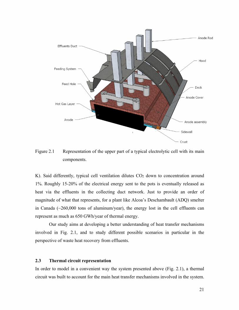
21

Figure 2.1 Representation of the upper part of a typical electrolytic cell with its main

components.

K). Said differently, typical cell ventilation dilutes CO2 down to concentration around

1%. Roughly 15-20% of the electrical energy sent to the pots is eventually released as

heat via the effluents in the collecting duct network. Just to provide an order of

magnitude of what that represents, for a plant like Alcoa’s Deschambault (ADQ) smelter

in Canada (~260,000 tons of aluminum/year), the energy lost in the cell effluents can

represent as much as 650 GWh/year of thermal energy.

Our study aims at developing a better understanding of heat transfer mechanisms

involved in Fig. 2.1, and to study different possible scenarios in particular in the

perspective of waste heat recovery from effluents.

2.3 Thermal circuit representation

In order to model in a convenient way the system presented above (Fig. 2.1), a thermal

circuit was built to account for the main heat transfer mechanisms involved in the system.

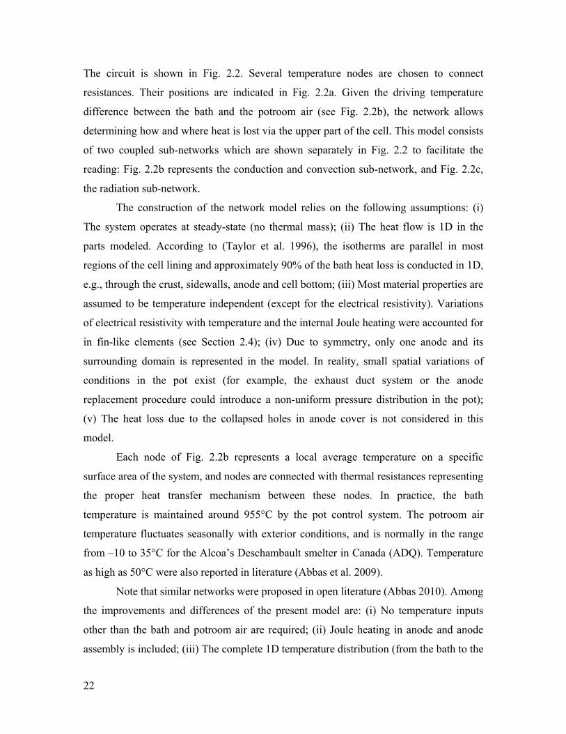
22

The circuit is shown in Fig. 2.2. Several temperature nodes are chosen to connect

resistances. Their positions are indicated in Fig. 2.2a. Given the driving temperature

difference between the bath and the potroom air (see Fig. 2.2b), the network allows

determining how and where heat is lost via the upper part of the cell. This model consists

of two coupled sub-networks which are shown separately in Fig. 2.2 to facilitate the

reading: Fig. 2.2b represents the conduction and convection sub-network, and Fig. 2.2c,

the radiation sub-network.

The construction of the network model relies on the following assumptions: (i)

The system operates at steady-state (no thermal mass); (ii) The heat flow is 1D in the

parts modeled. According to (Taylor et al. 1996), the isotherms are parallel in most

regions of the cell lining and approximately 90% of the bath heat loss is conducted in 1D,

e.g., through the crust, sidewalls, anode and cell bottom; (iii) Most material properties are

assumed to be temperature independent (except for the electrical resistivity). Variations

of electrical resistivity with temperature and the internal Joule heating were accounted for

in fin-like elements (see Section 2.4); (iv) Due to symmetry, only one anode and its

surrounding domain is represented in the model. In reality, small spatial variations of

conditions in the pot exist (for example, the exhaust duct system or the anode

replacement procedure could introduce a non-uniform pressure distribution in the pot);

(v) The heat loss due to the collapsed holes in anode cover is not considered in this

model.

Each node of Fig. 2.2b represents a local average temperature on a specific

surface area of the system, and nodes are connected with thermal resistances representing

the proper heat transfer mechanism between these nodes. In practice, the bath

temperature is maintained around 955°C by the pot control system. The potroom air

temperature fluctuates seasonally with exterior conditions, and is normally in the range

from –10 to 35°C for the Alcoa’s Deschambault smelter in Canada (ADQ). Temperature

as high as 50°C were also reported in literature (Abbas et al. 2009).

Note that similar networks were proposed in open literature (Abbas 2010). Among

the improvements and differences of the present model are: (i) No temperature inputs

other than the bath and potroom air are required; (ii) Joule heating in anode and anode

assembly is included; (iii) The complete 1D temperature distribution (from the bath to the

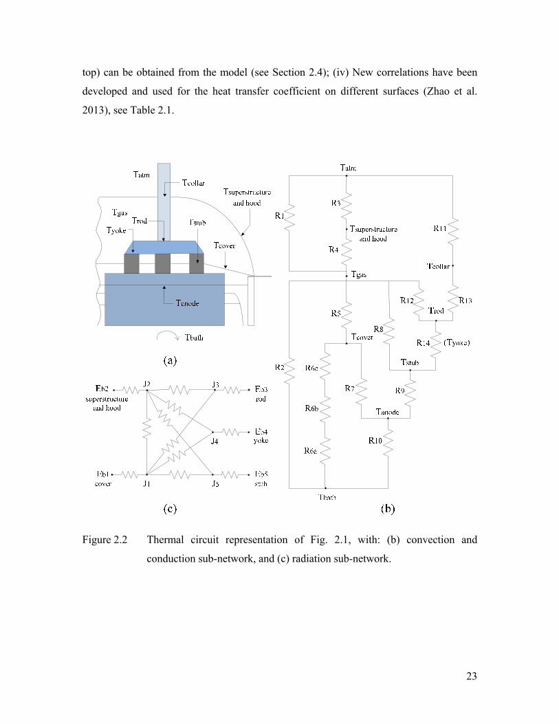
23

top) can be obtained from the model (see Section 2.4); (iv) New correlations have been

developed and used for the heat transfer coefficient on different surfaces (Zhao et al.

2013), see Table 2.1.

Figure 2.2 Thermal circuit representation of Fig. 2.1, with: (b) convection and

conduction sub-network, and (c) radiation sub-network.

24

Table 2.1 Correlations for average convection coefficients on four surfaces of the

cavity, as a function of volumetric flow rate Q for one pot [Nm3/s] (Zhao

et al. 2013).

Surface Correlation

Anode cover ch = 5.32 + 1.79Q

Hoods, superstructure hh = 3.87 + 2.28Q

Rod rh = 2.33 + 1.89Q

Yoke and stubs ysh = 6.28 + 1.73Q

2.3.1 Conduction and convection sub-network

Heat can escape from bath to potroom through three different pathways in the conduction

and convection sub-network. First, the hot gases (mainly CO2) released from the bath to

the space under the hoods carry thermal energy, and the corresponding thermal resistance

between Tbath and Tgas (Tgas is the temperature of gases in the cavity under the hood) is

2 2

2CO p,CO

1R

m c

(2.1)

This “ventilation” resistance comes from the fact that performing an energy balance in

the space under the hood, the difference between the energy provided to the control

volume by the CO2 released at Tbath and that removed from the control volume by the

CO2 leaving the cavity at temperature Tgas is 2 2CO p,CO bath gasm c T T .

In the second pathway, heat is transmitted from the bath through the crust and

anode cover, and is eventually dissipated in the gas flow under the hoods. An overall heat

transfer coefficient of 100 W/m2K was considered between the bath and the surface of

the crust facing the bath (Taylor et al. 1996) (resistance R6a). As mentioned above, heat

conduction in the anode, crust, cover and stubs immersed in cover is considered as a one-

dimensional problem. The conduction thermal resistance of the components without

Joule heating is thus of the form

cond

LR

kA (2.2)

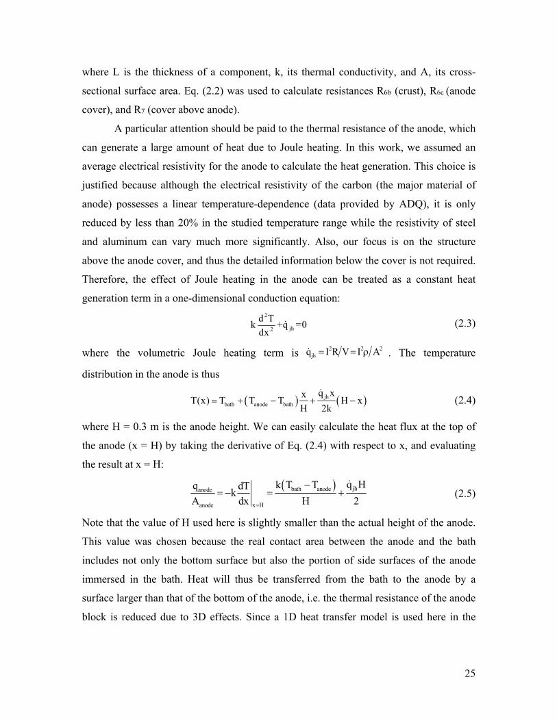
25

where L is the thickness of a component, k, its thermal conductivity, and A, its cross-

sectional surface area. Eq. (2.2) was used to calculate resistances R6b (crust), R6c (anode

cover), and R7 (cover above anode).

A particular attention should be paid to the thermal resistance of the anode, which

can generate a large amount of heat due to Joule heating. In this work, we assumed an

average electrical resistivity for the anode to calculate the heat generation. This choice is

justified because although the electrical resistivity of the carbon (the major material of

anode) possesses a linear temperature-dependence (data provided by ADQ), it is only

reduced by less than 20% in the studied temperature range while the resistivity of steel

and aluminum can vary much more significantly. Also, our focus is on the structure

above the anode cover, and thus the detailed information below the cover is not required.

Therefore, the effect of Joule heating in the anode can be treated as a constant heat

generation term in a one-dimensional conduction equation:

2

jh2

d Tk +q =0

dx (2.3)

where the volumetric Joule heating term is 2 2 2jhq I R V I A . The temperature

distribution in the anode is thus

jhbath anode bath

q xxT(x) T T T H x

H 2k

(2.4)

where H = 0.3 m is the anode height. We can easily calculate the heat flux at the top of

the anode (x = H) by taking the derivative of Eq. (2.4) with respect to x, and evaluating

the result at x = H:

jhbath anodeanode

x Hanode

q Hk T Tq dTk

A dx H 2

(2.5)

Note that the value of H used here is slightly smaller than the actual height of the anode.

This value was chosen because the real contact area between the anode and the bath

includes not only the bottom surface but also the portion of side surfaces of the anode

immersed in the bath. Heat will thus be transferred from the bath to the anode by a

surface larger than that of the bottom of the anode, i.e. the thermal resistance of the anode

block is reduced due to 3D effects. Since a 1D heat transfer model is used here in the

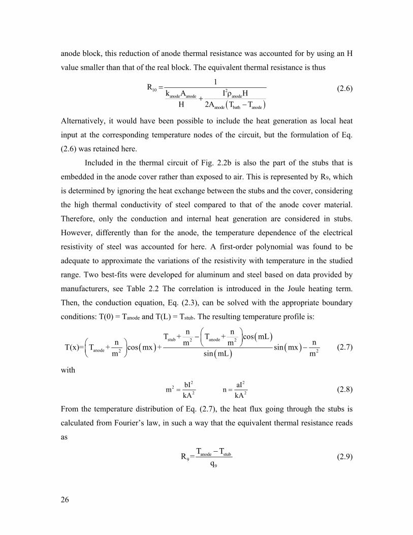
26

anode block, this reduction of anode thermal resistance was accounted for by using an H

value smaller than that of the real block. The equivalent thermal resistance is thus

10 2

anode anode anode

anode bath anode

1R

k A I H

H 2A T T

(2.6)

Alternatively, it would have been possible to include the heat generation as local heat

input at the corresponding temperature nodes of the circuit, but the formulation of Eq.

(2.6) was retained here.

Included in the thermal circuit of Fig. 2.2b is also the part of the stubs that is

embedded in the anode cover rather than exposed to air. This is represented by R9, which

is determined by ignoring the heat exchange between the stubs and the cover, considering

the high thermal conductivity of steel compared to that of the anode cover material.

Therefore, only the conduction and internal heat generation are considered in stubs.

However, differently than for the anode, the temperature dependence of the electrical

resistivity of steel was accounted for here. A first-order polynomial was found to be

adequate to approximate the variations of the resistivity with temperature in the studied

range. Two best-fits were developed for aluminum and steel based on data provided by

manufacturers, see Table 2.2 The correlation is introduced in the Joule heating term.

Then, the conduction equation, Eq. (2.3), can be solved with the appropriate boundary

conditions: T(0) = Tanode and T(L) = Tstub. The resulting temperature profile is:

stub anode2 2

anode 2 2

n nT + T + cos mL

n nm mT(x)= T + cos mx + sin mx

m sin mL m

(2.7)

with

2 2

22 2

bI aIm n

kA kA (2.8)

From the temperature distribution of Eq. (2.7), the heat flux going through the stubs is

calculated from Fourier’s law, in such a way that the equivalent thermal resistance reads

as

anode stub9

9

T TR =

q

(2.9)

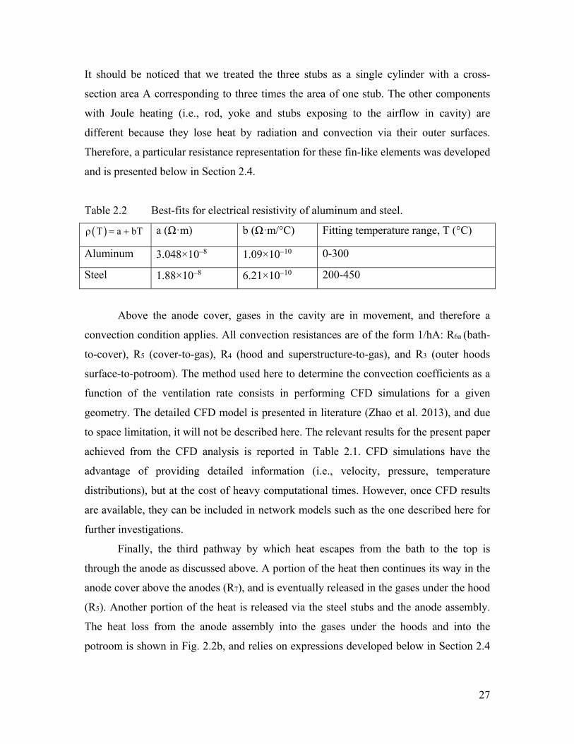
27

It should be noticed that we treated the three stubs as a single cylinder with a cross-

section area A corresponding to three times the area of one stub. The other components

with Joule heating (i.e., rod, yoke and stubs exposing to the airflow in cavity) are

different because they lose heat by radiation and convection via their outer surfaces.

Therefore, a particular resistance representation for these fin-like elements was developed

and is presented below in Section 2.4.

Table 2.2 Best-fits for electrical resistivity of aluminum and steel.

T a bT a (Ω·m) b (Ω·m/°C) Fitting temperature range, T (°C)

Aluminum 3.048×108 1.09×1010 0-300

Steel 1.88×108 6.21×1010 200-450

Above the anode cover, gases in the cavity are in movement, and therefore a

convection condition applies. All convection resistances are of the form 1/hA: R6a (bath-

to-cover), R5 (cover-to-gas), R4 (hood and superstructure-to-gas), and R3 (outer hoods

surface-to-potroom). The method used here to determine the convection coefficients as a

function of the ventilation rate consists in performing CFD simulations for a given

geometry. The detailed CFD model is presented in literature (Zhao et al. 2013), and due

to space limitation, it will not be described here. The relevant results for the present paper

achieved from the CFD analysis is reported in Table 2.1. CFD simulations have the

advantage of providing detailed information (i.e., velocity, pressure, temperature

distributions), but at the cost of heavy computational times. However, once CFD results

are available, they can be included in network models such as the one described here for

further investigations.

Finally, the third pathway by which heat escapes from the bath to the top is

through the anode as discussed above. A portion of the heat then continues its way in the

anode cover above the anodes (R7), and is eventually released in the gases under the hood

(R5). Another portion of the heat is released via the steel stubs and the anode assembly.

The heat loss from the anode assembly into the gases under the hoods and into the

potroom is shown in Fig. 2.2b, and relies on expressions developed below in Section 2.4

28

for fin-like elements with internal heat generation (resistances R8, R9, R11, R12, R13, and

R14).

The rest of the thermal circuit corresponds to the heat gained by the air flow in the

cavity under the hood (ventilation), R1, which is calculated as in Eq. (2.1). Also

accounted for is the heat that is transferred through the hoods and superstructure into the

potroom (R3). A convection coefficient of 10 W/m2K was applied on the outer surface of

the hoods which represents a typical value for natural convection conditions (Abbas

2010).

2.3.2 Radiation sub-network

The radiation sub-network is illustrated in Fig. 2.2c. In this model, some components

with relatively small surface area were neglected, including the feed hole, the gaps

between hoods and the gas outlet. In addition, the air with low CO2 concentration

(typically ~1-1.5%) in the space under the hoods can be regarded as a non-participating

medium, and thus only surface-to-surface radiation needs to be considered. The alumina

feeding system is simplified as a part of the superstructure. Thus, in the end, five surfaces

were included in the sub-network: (i) anode cover, (ii) hoods and superstructure, (iii) rod,

(iv) yoke and (v) three stubs. As can be seen in Fig. 2.2c, the radiative interactions

between the rod, yoke and stubs were neglected, because of their small areas for radiation

heat exchange. Also, due to the geometrical symmetry and periodicity of the anode

disposition (i.e., anodes are aligned in two columns in the pot), the heat loss from a sub-

section containing only one anode to the surrounding sections by convection and

radiation is compensated by heat influx from the others. Accordingly, we assume that the

radiation heat exchanges involved in each section containing one anode can be

considered as those in an isolated system.

To solve the radiation sub-network, it is required to calculate the view factors for

each possible pair of surfaces. Since the heat loss from one unit (i.e., a sub-domain with

only one anode) to neighbors is compensated by the surrounding units heat loss based on

the symmetrical structure, we can use a closed network to calculate the radiation heat

exchange among all involved surfaces. When calculating the view factor for each pair of

29

surfaces, we assumed that the rod and assembly is surrounded by the anode cover and the

hoods and superstructure, both of which can be viewed as infinite surfaces. Thus, the

view factor from rod, yoke or stubs to anode cover or hoods and superstructure can be

approximately assumed to 0.5. For example, for the view factor from the rod to the anode

cover, Frod-cover0.5, and then Fcover-rod is calculated by reciprocity (Modest 2013)

rod rod cov ercov er rod

cov er

A FF

A

(2.10)

where A is the area of the corresponding surface. This strategy was also applied to the

remaining components. Surfaces are assumed to be gray and diffuse. A network

representation of radiative exchanges between surfaces was built (Fig. 2.2c). Energy

balance was performed at each J-node. Note that this network is not a thermal circuit as

the one in Fig. 2.2b. For example, nodes represent radiative fluxes rather than

temperature. Radiative resistances between two J-nodes i and j are of the form (AiFij)1,

whereas radiative resistances between Ei and Ji nodes assume the form (1i)/(Aii). The

corresponding radiative network was solved in the form of a matrix system, the

unknowns of which were the radiosities Ji at all involved surfaces, see Refs. (Modest

2013; Bergman et al. 2011).

2.4 Resistance of fin-like components with internal heat generation

The anode assembly above the anode cover has a geometrical similarity with pin fins

(Bergman et al. 2011). Three different cross-sections are observed in the anode assembly,

i.e. that of the rod, the yoke, and the three exposed stubs. The straightforward expression

of thermal resistance for a pin fin is not valid here, because it is developed by considering

only conduction in the fin and convection at the surface of the fin. The heat transfer in the

anode assembly, however, also involves significant radiation losses from the surface of

the fin-like element, and Joule heating inside the fin-like element. The thermal resistance

for such fin-like components is derived in the present section. In order to do so, an energy

balance is performed below.

Applying the conservation of energy law to the fin differential element in Fig.

2.3a, we obtained

30

x jh x dx conv radq dq q dq dq (2.11)

where qx and qx+dx are the conduction heat transfer rate at position x and x+dx

respectively, dqjh is the heat generated by Joule heating within the differential element,

and finally dqconv and dqrad are the convection and radiation heat losses from the exposed

surface of the differential element. From Fourier’s law, the heat transported by

conduction is simply

x

x

dTq kA

dx (2.12)

where A is the cross-sectional area. Here, we assumed k to be constant, because in the

range of temperatures under investigation and for the materials considered, variations of

k were found to be below 20% based on data from manufacturers.

The Joule heating term in Eq. (2.11) can be evaluated by:

2

jh

T dxdq I

A

(2.13)

where I is the electric current through the anode assembly and (T) is the temperature-

dependent electrical resistivity.

Based on Newton’s law of cooling, the convection heat losses at the surface of the

infinitesimal control volume of Fig. 2.3a is expressed as

conv conv s gasdq h dA T T (2.14)

where hconv is the convection coefficient at the surface, and dAs is the surface area of the

control volume exposed to convection. T and Tgas represent the temperature of the

differential element and the temperature of gases in the core of the cavity, respectively.

The heat transfer coefficient could be estimated based on correlations between the

Nusselt number and other dimensionless numbers (e.g., Reynolds, Rayleigh, Prandtl) for

a specified flow geometry and flow regime. For example, as a first approximation, the

fin-like elements considered here could be approximated as cylinders in cross-flows, but

it should be clear that the fluid flow is actually more complex than that. Therefore, in this

work, we employed CFD simulations to obtain specific correlations for the average

convection coefficients. The detailed method to calculate the coefficients is discussed in

(Zhao et al. 2013).

31

As for the radiation losses by the surface of the fin-like elements, it was linearized

through the use of an average linearized coefficient, hrad. Applying the conservation of

energy principle, one can calculate this coefficient as

radrad L

gas0

qh

P T x T dx

(2.15)

where qrad is the total radiation heat transfer rate at the surface of the component, which is

taken from the results of the radiation heat transfer network. P is the perimeter of the

cross-section and L, the length of the fin-like element. The temperature T(x) in Eq. (2.15)

is the temperature along the fin-like element, and will be derived below (Eq. (2.20)).

Since the calculation of hrad depends on the fin temperature, and since the fin temperature

depends on hrad, an iterative procedure needs to be implemented. The integral in Eq.

(2.15) was performed numerically in the present work. This choice was based on the fact

that the temperature along the fin-like elements is likely to vary substantially, resulting in

significantly different local heat losses along the fin. Fin like elements were divided into

small slices and the heat losses for each slice was deduced based on the fin local

temperature. Then, the total losses were calculated by summing the losses of each slice.

This method also applies to the calculation of convection heat transfer rates on surfaces

of fin-like elements such as R12.

Note that it would have been possible to implement a simpler model in which the

calculation of radiation exchanges by fin-like element surfaces would have relied on an

average temperature (e.g., arithmetic average of the base and tip temperatures) rather than

on a numerical discretization. This simplified method was tested by comparing resulting

temperatures with the results of the above-mentioned model. After simulations,

differences of 10 to 15˚C were found for the temperature of anode assembly components

(i.e., Tstub, Tyoke, and Trod). Therefore, depending on the precision required, the simplified

or the integral approach could be used. For achieving the results presented in this work,

only the integral method was used though.

Once hrad is known, the radiation heat transfer rate of the differential element can

be expressed as

rad rad s gasdq h dA T T (2.16)

32

Combining Eqs. (2.11)-(2.16), and introducing = T Tgas, one can obtain the

following governing equation for fin-like elements with both radiative and convective

heat transfer at their boundary, and with Joule heating:

2

22

dm n 0

dx

(2.17)

with

2

conv rad22

h h P bIm

kA kA

22

gas

2 2

bI TaIn

kA kA (2.18)

The solution of the fin equation is of the form

mx mx1 2 3C e C e C (2.19)

The two boundary conditions that apply are: (0) = b and (L) = L. These conditions

are used to determine the constants C1 and C2. C3 is obtained by simply inserting Eq.

(2.19) into Eq. (2.17) (i.e., C3 = n/m2). The temperature profile is calculated as

L b2 2

n nsinh mx sinh m L x

m mx

sin mL

(2.20)

Knowing the temperature profile (x) from Eq. (2.20), the heat transfer rate at the base

(qb) and at the tip (ql) of the fin-like element can be calculated from Fourier’s law, Eq.

(2.12).

Furthermore, the total heat generated by Joule heating, qjh, is calculated by

integrating Eq. (2.13) from x = 0 to x = L with the temperature profile as calculated

previously.

Finally, the heat transfer rate lost by convection and radiation is

am b jh Lq q q q (2.21)

The thermal circuit representation of the fin-like element treated in this section is shown

in Fig. 2.3a. A resistance from the base of the fin to the gas is used to account for the heat

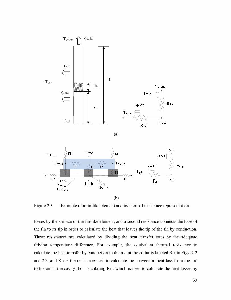
33

(a)

(b)

Figure 2.3 Example of a fin-like element and its thermal resistance representation.

losses by the surface of the fin-like element, and a second resistance connects the base of

the fin to its tip in order to calculate the heat that leaves the tip of the fin by conduction.

These resistances are calculated by dividing the heat transfer rates by the adequate

driving temperature difference. For example, the equivalent thermal resistance to

calculate the heat transfer by conduction in the rod at the collar is labeled R13 in Figs. 2.2

and 2.3, and R12 is the resistance used to calculate the convection heat loss from the rod

to the air in the cavity. For calculating R11, which is used to calculate the heat losses by

qrad

Tgas

qconv

x

dx

Trod

Tcollar qcollar

L

34

the part of the rod that extends outside of the pot, Eq. (2.17) can also be used by

assuming a prescribed temperature tip condition (Ttip=Tatm) corresponding to the upmost

tip of the rod and an effective heat transfer coefficient (heff) representing the combination

of convection and radiation coefficients. Detailed expressions are summarized in

appendix.

Note that in the thermal circuit in Fig. 2.2, resistances R8 (stub-to-gas resistance)

and R14 (stub-yoke-rod resistance) are actually a combination of resistances, representing

the overall convection and conduction resistances of the joint structure shown in Fig. 2.3b.

Heat coming from the anode is first conducted into the three stubs, then converges to the

center of the yoke, and finally travels into the rod. Along the surface of these components,

heat is lost by convection and radiation. Only the conductive (r1, r3, r5) and convective (r2,

r4, r6) resistances are shown in Fig. 2.3b, the radiative heat transfer having already been

considered in the radiation sub-network. The three stubs of the anode assembly were

treated as three parallel fin-like elements and the above yoke was divided as two

horizontal fin-like elements. For each element, the equivalent resistances were

determined by using the aforementioned analysis. The network of Fig. 2.3b (left) is then

simplified by combining resistances in series and in parallel until it becomes as the one

on the right side of Fig. 2.3b. Detailed expressions are also summarized in appendix.

2.5 Numerical implementation and validation

The thermal circuit described above was solved in Matlab. An energy balance was

performed at all temperature nodes of the network (i.e., 7 nodes). The resulting set of

equations was written in a matrix form. Due to non-linearity (e.g., properties that depend

on temperature, radiation, etc.), an iterative solution procedure needed to be

implemented. Starting from an initial guess for the temperature at each node, the matrix

components were computed. Then, the matrix system was solved. The matrix

components were updated based on the new values of temperature, and so on. The

procedure is repeated until convergence. Convergence was declared when the change at

each node temperature was smaller than 0.01 K compared to the values of the previous

iteration. Note that under-relaxation was required to achieve convergence. Typically, a

simulation took 1 minute with an under-relaxation factor of 0.01.

35

For the calculations presented in this work, the geometrical features of the system

considered were that representative of the electrolytic cells at ADQ. The parameters in

normal operating conditions were taken either from ADQ or from literature, see Table

2.3. A particular challenge consisted in determining the values of the heat transfer

coefficient on different components of the system. The flow pattern under the hood is

complex and it is hazardous to use correlations for flat plates with parallel flow or for

cylinders in cross-flow since this is far from the actual heat transfer and flow

configuration. Here, CFD simulations were used to obtain accurate convection

coefficients (Zhao et al. 2013).

The resulting program was validated thoroughly in different ways. First, the

exhaust gas temperature for different ventilation rates was compared to that of

experimental measurements (Gadd et al. 2000). A conversion of the draft condition

should be performed in order to achieve the same ventilation rate per anode. A good

agreement between our results and (Gadd et al. 2000) was found. At high ventilation rate,

our resulting exhaust temperature deviates from their results by less than 5°C while the

difference is about 10°C in low ventilation rate (<40% normal condition).

In addition, several specific parameters were compared with the data available in

literature. For example, experiments (Taylor 2007; Eggen et al. 1992) have demonstrated

that the heat transfer coefficient on the anode cover is in the range from 9 W/m2K to 14

W/m2K. In our model, this parameter is 13.1 W/m2K in normal condition. The heat flux

through the anode cover of the mixed crushed bath and alumina reported in Shen et al.

work (Shen et al. 2008) is in the range from 1700 W/m2 to 2700 W/m2. Here, we obtained

a value of 2123 W/m2. Another coarse validation is based on the “rule of thumb” that the

total top heat loss is about 25% of the total energy input. Since the total voltage drop in

the pot is about 4 V and the current imposed in one aluminum bar is 8750 A, the top heat

loss should be of the order of magnitude of 8750 W. Our modeled result is 8196 W.

Therefore, the model is considered to capture adequately the heat transfer mechanisms in

the system considered.

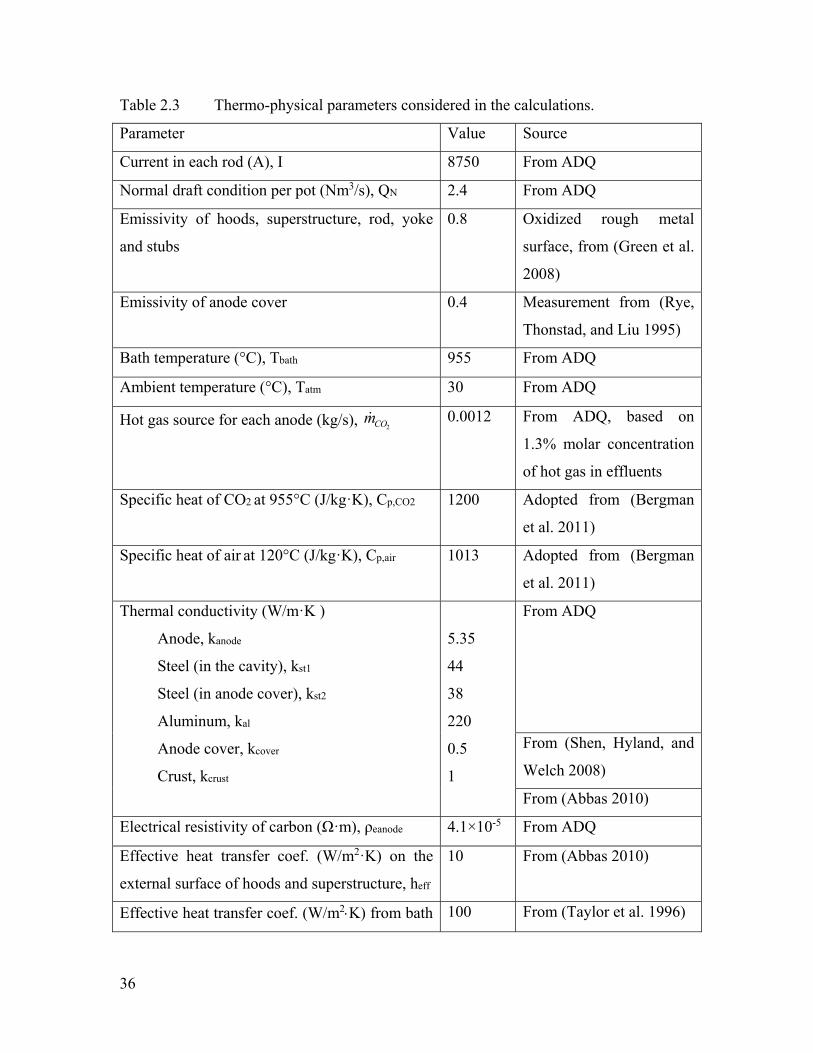
36

Table 2.3 Thermo-physical parameters considered in the calculations.

Parameter Value Source

Current in each rod (A), I 8750 From ADQ

Normal draft condition per pot (Nm3/s), QN 2.4 From ADQ

Emissivity of hoods, superstructure, rod, yoke

and stubs

0.8 Oxidized rough metal

surface, from (Green et al.

2008)

Emissivity of anode cover 0.4 Measurement from (Rye,

Thonstad, and Liu 1995)

Bath temperature (°C), Tbath 955 From ADQ

Ambient temperature (°C), Tatm 30 From ADQ

Hot gas source for each anode (kg/s), 2COm 0.0012 From ADQ, based on

1.3% molar concentration

of hot gas in effluents

Specific heat of CO2 at 955°C (J/kg·K), Cp,CO2 1200 Adopted from (Bergman

et al. 2011)

Specific heat of air at 120°C (J/kg·K), Cp,air 1013 Adopted from (Bergman

et al. 2011)

Thermal conductivity (W/m·K )

Anode, kanode

Steel (in the cavity), kst1

Steel (in anode cover), kst2

Aluminum, kal

Anode cover, kcover

Crust, kcrust

5.35

44

38

220

0.5

1

From ADQ

From (Shen, Hyland, and

Welch 2008)

From (Abbas 2010)

Electrical resistivity of carbon (Ω·m), ρeanode 4.1×10-5 From ADQ

Effective heat transfer coef. (W/m2·K) on the

external surface of hoods and superstructure, heff

10 From (Abbas 2010)

Effective heat transfer coef. (W/m2K) from bath 100 From (Taylor et al. 1996)

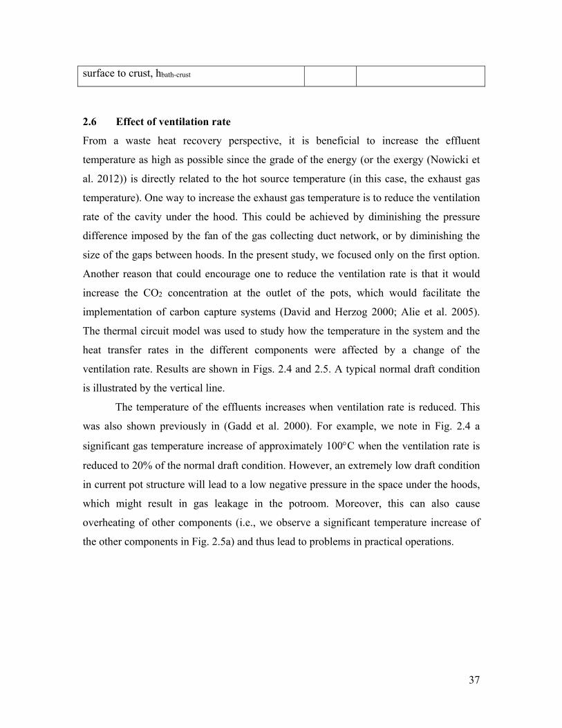
37

surface to crust, hbath-crust

2.6 Effect of ventilation rate

From a waste heat recovery perspective, it is beneficial to increase the effluent

temperature as high as possible since the grade of the energy (or the exergy (Nowicki et

al. 2012)) is directly related to the hot source temperature (in this case, the exhaust gas

temperature). One way to increase the exhaust gas temperature is to reduce the ventilation

rate of the cavity under the hood. This could be achieved by diminishing the pressure

difference imposed by the fan of the gas collecting duct network, or by diminishing the

size of the gaps between hoods. In the present study, we focused only on the first option.

Another reason that could encourage one to reduce the ventilation rate is that it would

increase the CO2 concentration at the outlet of the pots, which would facilitate the

implementation of carbon capture systems (David and Herzog 2000; Alie et al. 2005).

The thermal circuit model was used to study how the temperature in the system and the

heat transfer rates in the different components were affected by a change of the

ventilation rate. Results are shown in Figs. 2.4 and 2.5. A typical normal draft condition

is illustrated by the vertical line.

The temperature of the effluents increases when ventilation rate is reduced. This

was also shown previously in (Gadd et al. 2000). For example, we note in Fig. 2.4 a

significant gas temperature increase of approximately 100C when the ventilation rate is

reduced to 20% of the normal draft condition. However, an extremely low draft condition

in current pot structure will lead to a low negative pressure in the space under the hoods,

which might result in gas leakage in the potroom. Moreover, this can also cause

overheating of other components (i.e., we observe a significant temperature increase of

the other components in Fig. 2.5a) and thus lead to problems in practical operations.

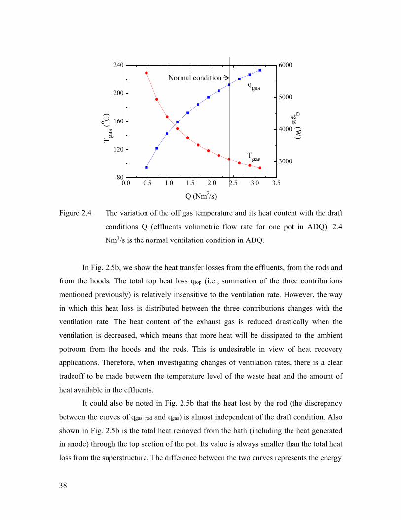
38

0.0 0.5 1.0 1.5 2.0 2.5 3.0 3.580

120

160

200

240

Tga

s (o C

)

Q (Nm3/s)

3000

4000

5000

6000

Tgas

Normal condition

qgas (W

)

qgas

Figure 2.4 The variation of the off gas temperature and its heat content with the draft

conditions Q (effluents volumetric flow rate for one pot in ADQ), 2.4

Nm3/s is the normal ventilation condition in ADQ.

In Fig. 2.5b, we show the heat transfer losses from the effluents, from the rods and

from the hoods. The total top heat loss qtop (i.e., summation of the three contributions

mentioned previously) is relatively insensitive to the ventilation rate. However, the way

in which this heat loss is distributed between the three contributions changes with the

ventilation rate. The heat content of the exhaust gas is reduced drastically when the

ventilation is decreased, which means that more heat will be dissipated to the ambient

potroom from the hoods and the rods. This is undesirable in view of heat recovery

applications. Therefore, when investigating changes of ventilation rates, there is a clear

tradeoff to be made between the temperature level of the waste heat and the amount of

heat available in the effluents.

It could also be noted in Fig. 2.5b that the heat lost by the rod (the discrepancy

between the curves of qgas+rod and qgas) is almost independent of the draft condition. Also

shown in Fig. 2.5b is the total heat removed from the bath (including the heat generated

in anode) through the top section of the pot. Its value is always smaller than the total heat

loss from the superstructure. The difference between the two curves represents the energy

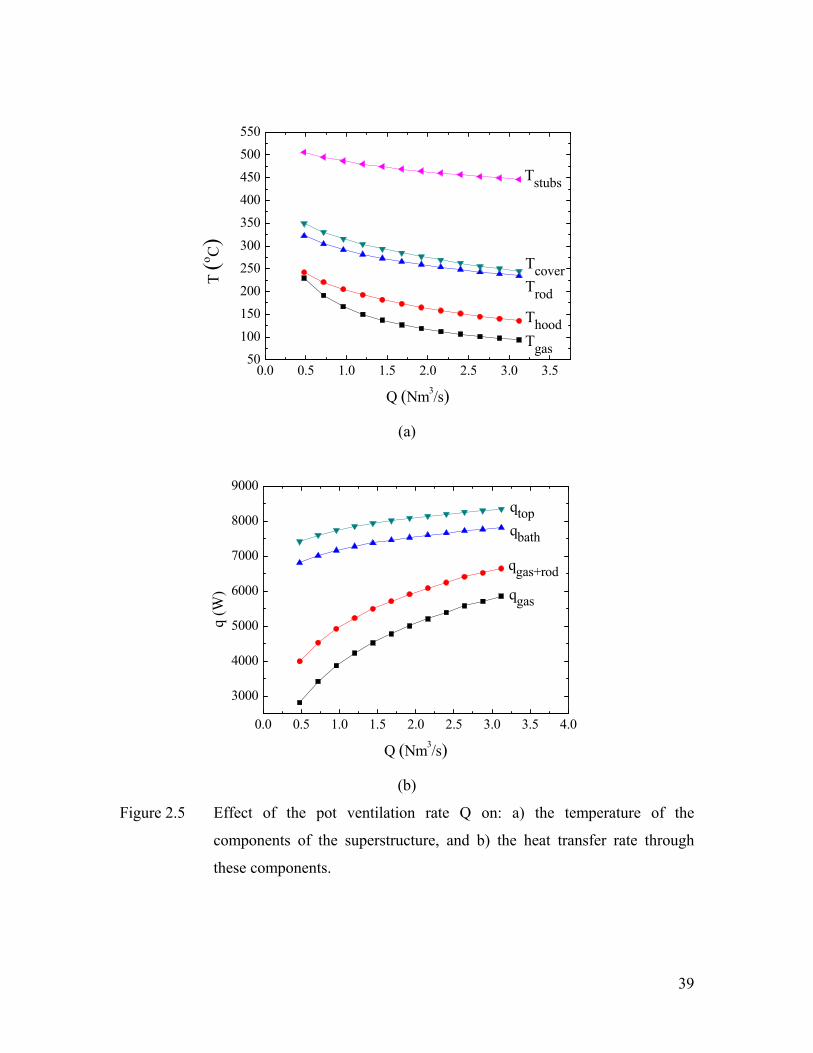
39

0.0 0.5 1.0 1.5 2.0 2.5 3.0 3.550

100

150

200

250

300

350

400

450

500

550

Tstubs

TcoverTrod

Thood

T (o C

)

Q (Nm3/s)

Tgas

(a)

0.0 0.5 1.0 1.5 2.0 2.5 3.0 3.5 4.0

3000

4000

5000

6000

7000

8000

9000

qtopqbath

qgas+rod

q (W

)

Q (Nm3/s)

qgas

(b)

Figure 2.5 Effect of the pot ventilation rate Q on: a) the temperature of the

components of the superstructure, and b) the heat transfer rate through

these components.

40

dissipated in the cavity by Joule heating in the anode assemblies. This difference is also

relatively independent of the ventilation conditions. Nevertheless, the heat extracted from

the bath could be reduced by almost 1 kW per anode as the draft condition goes down to

low levels. This over-insulating effect in top heat loss could influence the global thermal

balance in a pot and disturb the working conditions in the bath, since the frozen

electrolyte layer (protecting the pot ledge from suffering harsh conditions in bath) on

sidewall is very sensitive to the heat flux through it and the sidewall heat flux is directly

influenced by the top heat loss. Careful pot redesign or change of pot operation should be

considered to prevent thermal imbalance when trying to reduce the ventilation.

2.7 Effect of heat transfer coefficients on different surfaces

As described in the previous section, in view of waste heat recovery applications, the

ideal situation would be to reduce the draft in order to increase the effluent temperature,

and at the same time, try to increase the heat content of the effluent and maintain the heat

removed from the bath. In order to meet these conditions, one should try increasing the

heat removal from the components in the cavity, including from the bath. This means

increasing the effective heat transfer coefficients while reducing at the same time the

ventilation rate in the cavity. This could be achieved, for example, by changes of

geometry of the gaps and hoods, by the addition of fins (for example, the effective heat

transfer coefficient would be hAf/A where is the fin system efficiency and Af, its

surface area, while A is the unfined surface), etc.

When the mass flow rate of the exhaust gas is reduced, the effective thermal

resistance from the bath to the ambient is increased and the heat flux is reduced. Since

heat is transferred into the gas under the hoods by convection, the convective resistance

can be diminished by enhancing the convective heat transfer coefficient on the contact

surface to counterbalance the effect of the reduced mass flow rate. As discussed above,

four surfaces with relatively large area are considered in the network, including the top

surface of the anode cover, the surfaces of yoke, stubs and rod and the internal surface of

the hoods and superstructure. The sensitivity of the gas temperature and heat transfer

rates to the variation of the convective coefficient on each of these surfaces should be

tested to find the most influencing factor.

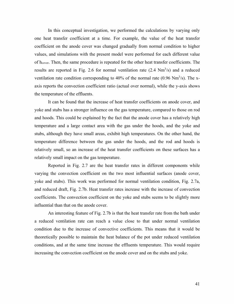
41

In this conceptual investigation, we performed the calculations by varying only

one heat transfer coefficient at a time. For example, the value of the heat transfer

coefficient on the anode cover was changed gradually from normal condition to higher

values, and simulations with the present model were performed for each different value

of hcover. Then, the same procedure is repeated for the other heat transfer coefficients. The

results are reported in Fig. 2.6 for normal ventilation rate (2.4 Nm3/s) and a reduced

ventilation rate condition corresponding to 40% of the normal rate (0.96 Nm3/s). The x-

axis reports the convection coefficient ratio (actual over normal), while the y-axis shows

the temperature of the effluents.

It can be found that the increase of heat transfer coefficients on anode cover, and

yoke and stubs has a stronger influence on the gas temperature, compared to those on rod

and hoods. This could be explained by the fact that the anode cover has a relatively high

temperature and a large contact area with the gas under the hoods, and the yoke and

stubs, although they have small areas, exhibit high temperatures. On the other hand, the

temperature difference between the gas under the hoods, and the rod and hoods is

relatively small, so an increase of the heat transfer coefficients on these surfaces has a

relatively small impact on the gas temperature.

Reported in Fig. 2.7 are the heat transfer rates in different components while

varying the convection coefficient on the two most influential surfaces (anode cover,

yoke and stubs). This work was performed for normal ventilation condition, Fig. 2.7a,

and reduced draft, Fig. 2.7b. Heat transfer rates increase with the increase of convection

coefficients. The convection coefficient on the yoke and stubs seems to be slightly more

influential than that on the anode cover.

An interesting feature of Fig. 2.7b is that the heat transfer rate from the bath under

a reduced ventilation rate can reach a value close to that under normal ventilation

condition due to the increase of convective coefficients. This means that it would be

theoretically possible to maintain the heat balance of the pot under reduced ventilation

conditions, and at the same time increase the effluents temperature. This would require

increasing the convection coefficient on the anode cover and on the stubs and yoke.

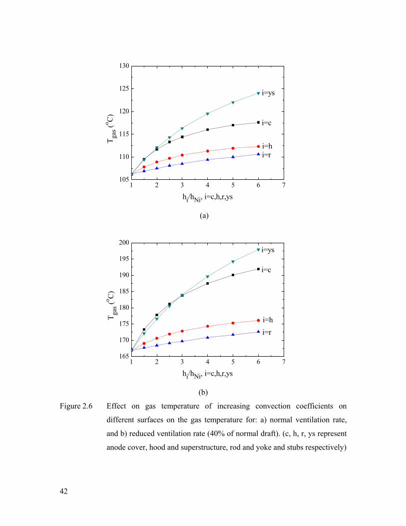
42

1 2 3 4 5 6 7105

110

115

120

125

130

i=ys

i=c

i=h

Tga

s (o C

)

hi/hNi, i=c,h,r,ys

i=r

(a)

1 2 3 4 5 6 7165

170

175

180

185

190

195

200i=ys

i=c

i=h

Tga

s (o C

)

hi/hNi, i=c,h,r,ys

i=r

(b)

Figure 2.6 Effect on gas temperature of increasing convection coefficients on

different surfaces on the gas temperature for: a) normal ventilation rate,

and b) reduced ventilation rate (40% of normal draft). (c, h, r, ys represent

anode cover, hood and superstructure, rod and yoke and stubs respectively)

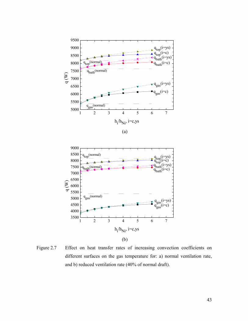
43

1 2 3 4 5 6 75000

5500

6000

6500

7000

7500

8000

8500

9000

9500

qtop(normal)

qbath(normal)

qgas(normal)

qgas(i=c)

qgas(i=ys)

qtop(i=ys)qtop(i=c)qbath(i=ys)qbath(i=c)

q (W

)

hi/hNi, i=c,ys

(a)

1 2 3 4 5 6 73500

4000

4500

5000

5500

6000

6500

7000

7500

8000

8500

9000

qtop(normal)

qbath(normal)

qgas(normal)qgas(i=ys)qgas(i=c)

q (W

)

hi/hNi, i=c,ys

qbath(i=c)qbath(i=ys)qtop(i=c)qtop(i=ys)

(b)

Figure 2.7 Effect on heat transfer rates of increasing convection coefficients on

different surfaces on the gas temperature for: a) normal ventilation rate,

and b) reduced ventilation rate (40% of normal draft).

44

2.8 Effect of the surface emissivity

Another way to modify the heat transfer balance within the superstructure is by changing

the emissivity of the internal surfaces of the hoods. As for the anode cover, it appears

difficult, if at all possible, to modify its surface emissivity in a simple way. The other

surfaces have a small surface area (surface of the yoke, stubs, and rod) and changing their

emissivity will not affect significantly the gas temperature. Simulations with different

values for the emissivity of the internal surface of hoods were performed in normal

condition and results are reported in Fig. 2.8. The temperature of most superstructure

components is only changed slightly by the value of emissivity (Fig. 2.8a). In particular,

the gas temperature is almost insensitive to the emissivity value. The only temperature

that changes significantly is in fact that of the hoods, which increases with the emissivity.

In Fig. 2.8b, we show that the corresponding heat transfer rate transported by the

effluent decreases slightly when the emissivity increases, but the change is very small

(less than 2%). On the other hand, the heat dissipated in the potroom increases with the

emissivity since more heat is absorbed by the inner hood surfaces.

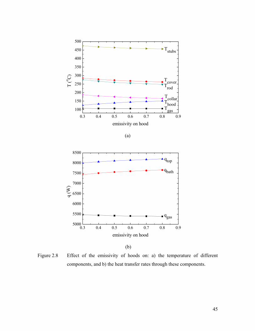
45

0.3 0.4 0.5 0.6 0.7 0.8 0.9

100

150

200

250

300

350

400

450

500

Tcollar

T (

o C)

emissivity on hood

Tgas

Thood

Trod

Tcover

Tstubs

(a)

0.3 0.4 0.5 0.6 0.7 0.8 0.95000

5500

6000

6500

7000

7500

8000

8500

q (W

)

emissivity on hood

qgas

qbath

qtop

(b)

Figure 2.8 Effect of the emissivity of hoods on: a) the temperature of different

components, and b) the heat transfer rates through these components.

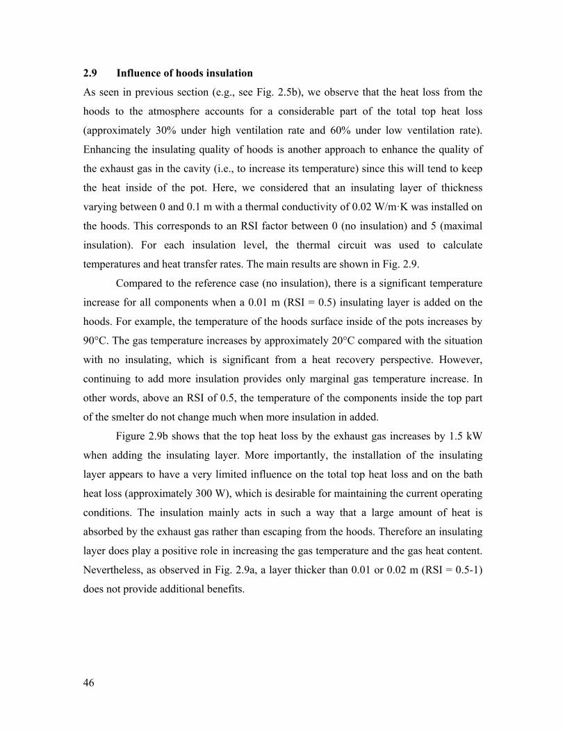
46

2.9 Influence of hoods insulation

As seen in previous section (e.g., see Fig. 2.5b), we observe that the heat loss from the

hoods to the atmosphere accounts for a considerable part of the total top heat loss

(approximately 30% under high ventilation rate and 60% under low ventilation rate).

Enhancing the insulating quality of hoods is another approach to enhance the quality of

the exhaust gas in the cavity (i.e., to increase its temperature) since this will tend to keep

the heat inside of the pot. Here, we considered that an insulating layer of thickness

varying between 0 and 0.1 m with a thermal conductivity of 0.02 W/m·K was installed on

the hoods. This corresponds to an RSI factor between 0 (no insulation) and 5 (maximal

insulation). For each insulation level, the thermal circuit was used to calculate

temperatures and heat transfer rates. The main results are shown in Fig. 2.9.

Compared to the reference case (no insulation), there is a significant temperature

increase for all components when a 0.01 m (RSI = 0.5) insulating layer is added on the

hoods. For example, the temperature of the hoods surface inside of the pots increases by

90°C. The gas temperature increases by approximately 20°C compared with the situation

with no insulating, which is significant from a heat recovery perspective. However,

continuing to add more insulation provides only marginal gas temperature increase. In

other words, above an RSI of 0.5, the temperature of the components inside the top part

of the smelter do not change much when more insulation in added.

Figure 2.9b shows that the top heat loss by the exhaust gas increases by 1.5 kW

when adding the insulating layer. More importantly, the installation of the insulating

layer appears to have a very limited influence on the total top heat loss and on the bath

heat loss (approximately 300 W), which is desirable for maintaining the current operating

conditions. The insulation mainly acts in such a way that a large amount of heat is

absorbed by the exhaust gas rather than escaping from the hoods. Therefore an insulating

layer does play a positive role in increasing the gas temperature and the gas heat content.

Nevertheless, as observed in Fig. 2.9a, a layer thicker than 0.01 or 0.02 m (RSI = 0.5-1)

does not provide additional benefits.

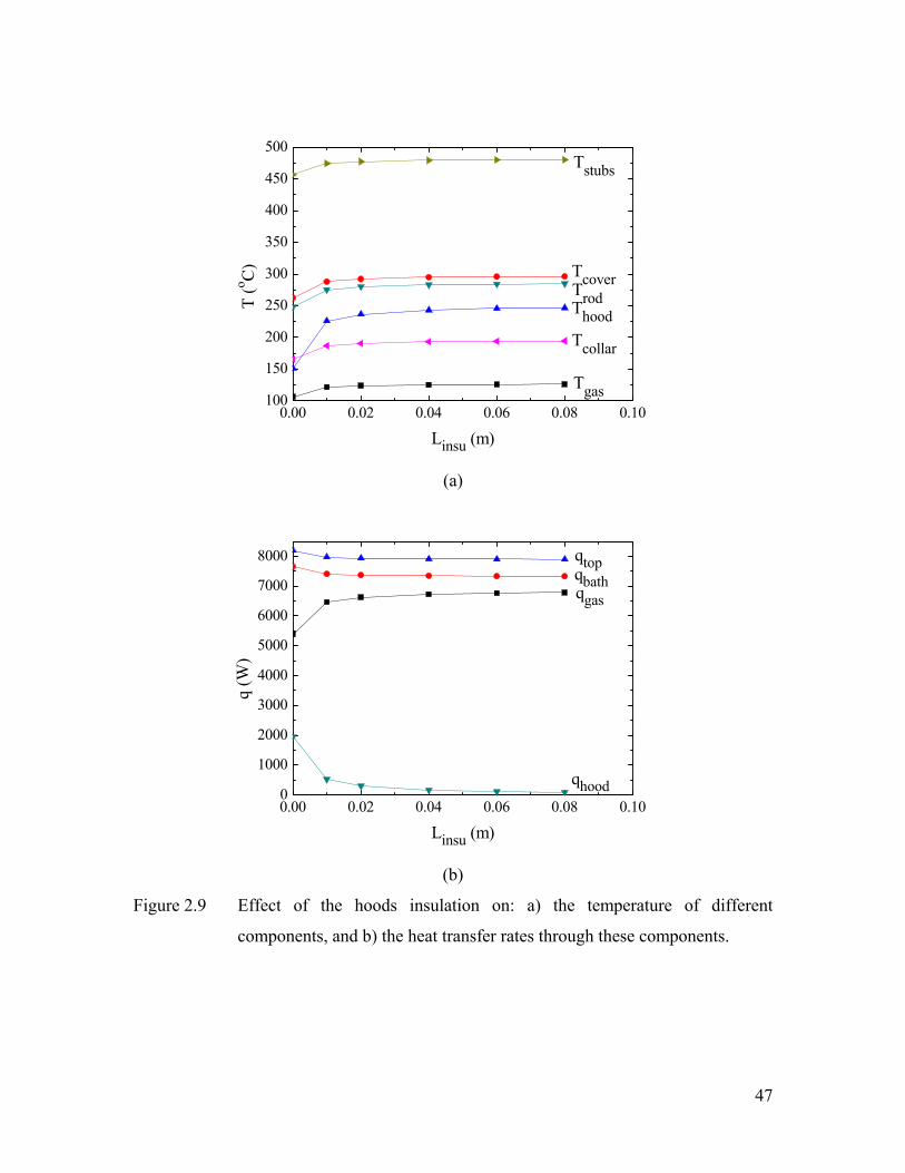
47

0.00 0.02 0.04 0.06 0.08 0.10100

150

200

250

300

350

400

450

500

T (

o C)

Linsu (m)

Tgas

Thood

Tcollar

Trod

Tcover

Tstubs

(a)

0.00 0.02 0.04 0.06 0.08 0.100

1000

2000

3000

4000

5000

6000

7000

8000

qhood

q (W

)

Linsu (m)

qgas

qbath

qtop

(b)

Figure 2.9 Effect of the hoods insulation on: a) the temperature of different

components, and b) the heat transfer rates through these components.

48

2.10 Influence of the potroom air temperature

The temperature of the air in the potroom can vary significantly as a function of the

seasons. The envelope of the building in which pots are installed is typically very loose

and provides little isolation. Therefore, the temperature of air inside the potroom is

affected considerably by outdoor conditions. Typical values in potrooms can range from

–10C to 50C. Therefore, the sensitivity of the results to the potroom air temperature

was tested with the model. The temperature and heat transfer rates of different upper pot

components are shown in Fig. 2.10. The increase of temperature of all components with

that of the air in the potroom is quasi linear, see Fig. 2.10a. The impact of the potroom

temperature is quite important. For example, the gas temperature can be reduced from

125C to 70C simply due to seasonal weather changes (i.e., summer vs winter). From a

waste heat recovery perspective, this has a strong impact since the technology that would

be implemented to recover the waste heat would need to work over an extended range of

temperature. Fig. 2.10b shows the corresponding heat transfer rates. When the potroom

air gets cooler, all heat transfer rates increase nearly linearly (approximately 5 W per

variation of 1C). This means that the heat content of the effluents is actually larger when

it is cold in the potroom. This is due to the fact that more heat is removed from the bath

by the cold air inflow in such a case.

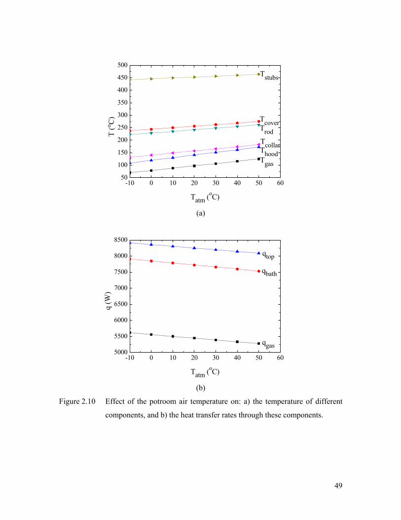
49

-10 0 10 20 30 40 50 6050

100

150

200

250

300

350

400

450

500

T (

o C)

Tatm (oC)

Tgas

Thood

Tcollar

Trod

Tcover

Tstubs

(a)

-10 0 10 20 30 40 50 605000

5500

6000

6500

7000

7500

8000

8500

q (W

)

Tatm (oC)

qgas

qbath

qtop

(b)

Figure 2.10 Effect of the potroom air temperature on: a) the temperature of different

components, and b) the heat transfer rates through these components.

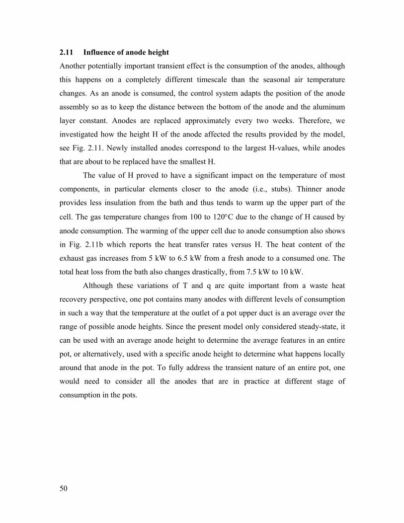
50

2.11 Influence of anode height

Another potentially important transient effect is the consumption of the anodes, although

this happens on a completely different timescale than the seasonal air temperature

changes. As an anode is consumed, the control system adapts the position of the anode

assembly so as to keep the distance between the bottom of the anode and the aluminum

layer constant. Anodes are replaced approximately every two weeks. Therefore, we

investigated how the height H of the anode affected the results provided by the model,

see Fig. 2.11. Newly installed anodes correspond to the largest H-values, while anodes

that are about to be replaced have the smallest H.

The value of H proved to have a significant impact on the temperature of most

components, in particular elements closer to the anode (i.e., stubs). Thinner anode

provides less insulation from the bath and thus tends to warm up the upper part of the

cell. The gas temperature changes from 100 to 120C due to the change of H caused by

anode consumption. The warming of the upper cell due to anode consumption also shows

in Fig. 2.11b which reports the heat transfer rates versus H. The heat content of the

exhaust gas increases from 5 kW to 6.5 kW from a fresh anode to a consumed one. The

total heat loss from the bath also changes drastically, from 7.5 kW to 10 kW.

Although these variations of T and q are quite important from a waste heat

recovery perspective, one pot contains many anodes with different levels of consumption

in such a way that the temperature at the outlet of a pot upper duct is an average over the

range of possible anode heights. Since the present model only considered steady-state, it

can be used with an average anode height to determine the average features in an entire

pot, or alternatively, used with a specific anode height to determine what happens locally

around that anode in the pot. To fully address the transient nature of an entire pot, one

would need to consider all the anodes that are in practice at different stage of

consumption in the pots.

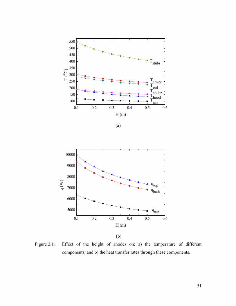
51

0.1 0.2 0.3 0.4 0.5 0.6

100

150

200

250

300

350

400

450

500

550

T (

o C)

H (m)

Tgas

Thood

Tcollar

Trod

Tcover

Tstubs

(a)

0.1 0.2 0.3 0.4 0.5 0.6

5000

6000

7000

8000

9000

10000

q (W

)

H (m)

qgas

qbath

qtop

(b)

Figure 2.11 Effect of the height of anodes on: a) the temperature of different

components, and b) the heat transfer rates through these components.

52

2.12 Conclusions

This chapter had two main objectives: (i) describe the enhanced thermal circuit that was

developed to model heat transfer mechanisms in the upper part of an electrolytic cell, and

(ii) perform a sensitivity analysis of temperatures and heat transfer rates with respect to

the main design and operation parameters.

As for the first objective, the main outcomes are:

An enhanced and complete thermal circuit representing the upper part of a pot is

documented here. The circuit solves quickly, and can determine temperatures and

heat transfer rates in each component.

We developed an original formulation to account for fin-like elements with internal

heat generation in thermal circuit model.

New correlations are used to determine the convective heat transfer coefficients on

the surfaces of interest.

By using the model, we were able to address the second objective. The following

observations could be made:

The mass flow rate of the pot exhaust gas has the most influence on the exhaust

temperature and heat content.

Convection heat transfer is more influential on the top surface of anode cover and on

the surface of the yoke and stubs, rather than those of aluminum rod and hoods and

superstructure. Further modifications of pot ventilation design should be focused on

these efficient areas in the perspective of waste heat recovery.

Additional insulation on the hoods could increase the exhaust gas temperature and

heat content. An RSI of 0.5 appears to be an optimal choice of an insulating level.

The influence of changing the emissivity of internal hoods and superstructure

surfaces provides only a marginal contribution in enhancing the thermal quality of

the gas.

Both the potroom temperature and the anode height significantly affect the heat

transfer in the upper structure of the pot. When designing any modifications in the

pot, their influences should be carefully taken into account.

Further work should be done to complete the thermal circuit by including a more detailed

representation of the superstructure and of the rest of the pot, possibly with thermal

53

capacitances to account for transient dynamics. Furthermore, an entire pot could be

modeled with anodes at different level of consumption. It would also be interesting to

verify that the increase of temperature of the joint between the anode rod and yoke under

the different scenarios is below the maximal acceptable temperature, which is of

importance to maintain the joint strength.

54

55

CHAPTER 3 HEAT TRANSFER AND AIRFLOW ANALYSIS IN UPPER

PART OF ELECTROLYTIC CELLS BASED ON CFD

56

Abstract

A CFD model of the top part of an electrolytic cell used in the primary aluminum

industry is presented. The model is used to determine average heat transfer coefficients

on the main surfaces, under different ventilation rates. Correlations have been developed

for the heat transfer coefficient and pressure drop versus pot draft condition. Non-

uniformity of the heat transfer coefficient is studied. Finally, the relative importance of

natural convection versus forced convection is revealed by the analysis. The knowledge

developed in this paper is useful for the heat transfer design and analysis of electrolytic

cells, which is crucial in this industry.

57

Résumé

Un modèle de type CFD du dessus d’une cuve d’électrolyse utilisée pour la production

primaire d’aluminium est présenté. Le modèle est utilisé pour déterminer les coefficients

de transfert thermique sur les principales surfaces, sous différentes conditions de

ventilation. Des corrélations ont été développées pour le coefficient de convection et la

perte de charge en fonction du taux de ventilation de la cuve. La non-uniformité du

coefficient de convection est étudiée. Finalement, l’importance relative de la convection

naturelle versus la convection forcée est révélée par l’analyse. La connaissance

développée dans cet article est utile pour le design thermique et l’analyse des cuves

d’électrolyse.

58

3.1 Introduction

The Hall-Héroult process is very intense energetically, and typically electricity accounts

for 40% of the total cost in the aluminum production process. Although this technology

has been developed one century ago and tremendous efforts have been deployed to

enhance performance of smelters, the energy efficiency in modern pots is still relatively

low, with about half of the energy input eventually dissipating into the atmosphere in the

form of waste heat. Therefore, increasing the overall energy efficiency of smelters still

offers promising opportunities of significant economical and environmental outcomes

(Nowicki and Gosselin 2012). For example, Nowicki et al. (2012) showed that the exergy

(useful work potential) of the exhaust gases from the cells is 0.65 MWh per ton of

aluminum produced, and that it is even larger for the heat losses from the different pot

surfaces.

Over the years, many investigations have been performed to develop a better

understanding of the Hall-Héroult process and to optimize the pot design and operation.

With the continuous improvement of computational resources, numerical simulation has

become an attractive method to achieve these objectives. Most of the heat transfer studies

related to aluminum smelting cells found in open literature have focused on the bath,

metal pad, and sidewalls. In particular, the pot domain below the anode cover has

received a lot of attention, with the development of several thermal numerical models,

often coupled with magnetic, electrical or mechanical numerical models, (e.g.,

Bruggeman and Danka 1990; Dupuis 1998; Shcherbinin et al. 2003; Dupuis et al. 2004;

Severo and Gusberti 2009; Yu et al. 2004; Fortin et al. 2012). These studies helped to

improve the operation, control and design of smelting pots.

Despite the rich literature available on numerical models for solving thermo-

electrical, thermo-mechanical, and magneto-hydrodynamic problems in aluminum

smelters, relatively few numerical models were published to study the top heat loss in the

section above the anode cover. Karlsen et al. (1998) proposed a simplified model to

estimate the pot gas collection efficiency in the top cavity under hoods based on different

draft conditions and pot tightness. A simple thermal circuit model (Taylor et al. 2004)

was presented to study the impact of the anode thickness on the temperature of the anode

assembly, which interacts with the cross-flow air under the hoods. Recently, Abbas et al.

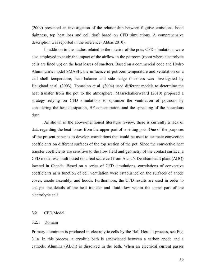
59

(2009) presented an investigation of the relationship between fugitive emissions, hood

tightness, top heat loss and cell draft based on CFD simulations. A comprehensive

description was reported in the reference (Abbas 2010).

In addition to the studies related to the interior of the pots, CFD simulations were

also employed to study the impact of the airflow in the potroom (room where electrolytic

cells are lined up) on the heat losses of smelters. Based on a commercial code and Hydro

Aluminum’s model SMASH, the influence of potroom temperature and ventilation on a

cell shell temperature, heat balance and side ledge thickness was investigated by

Haugland et al. (2003). Tomasino et al. (2004) used different models to determine the

heat transfer from the pot to the atmosphere. Maarschalkerwaard (2010) proposed a

strategy relying on CFD simulations to optimize the ventilation of potroom by

considering the heat dissipation, HF concentration, and the spreading of the hazardous

dust.

As shown in the above-mentioned literature review, there is currently a lack of

data regarding the heat losses from the upper part of smelting pots. One of the purposes

of the present paper is to develop correlations that could be used to estimate convection

coefficients on different surfaces of the top section of the pot. Since the convective heat

transfer coefficients are sensitive to the flow field and geometry of the contact surface, a

CFD model was built based on a real scale cell from Alcoa’s Deschambault plant (ADQ)

located in Canada. Based on a series of CFD simulations, correlations of convective

coefficients as a function of cell ventilation were established on the surfaces of anode

cover, anode assembly, and hoods. Furthermore, the CFD results are used in order to

analyse the details of the heat transfer and fluid flow within the upper part of the

electrolytic cell.

3.2 CFD Model

3.2.1 Domain

Primary aluminum is produced in electrolytic cells by the Hall-Héroult process, see Fig.

3.1a. In this process, a cryolitic bath is sandwiched between a carbon anode and a

cathode. Alumina (Al2O3) is dissolved in the bath. When an electrical current passes

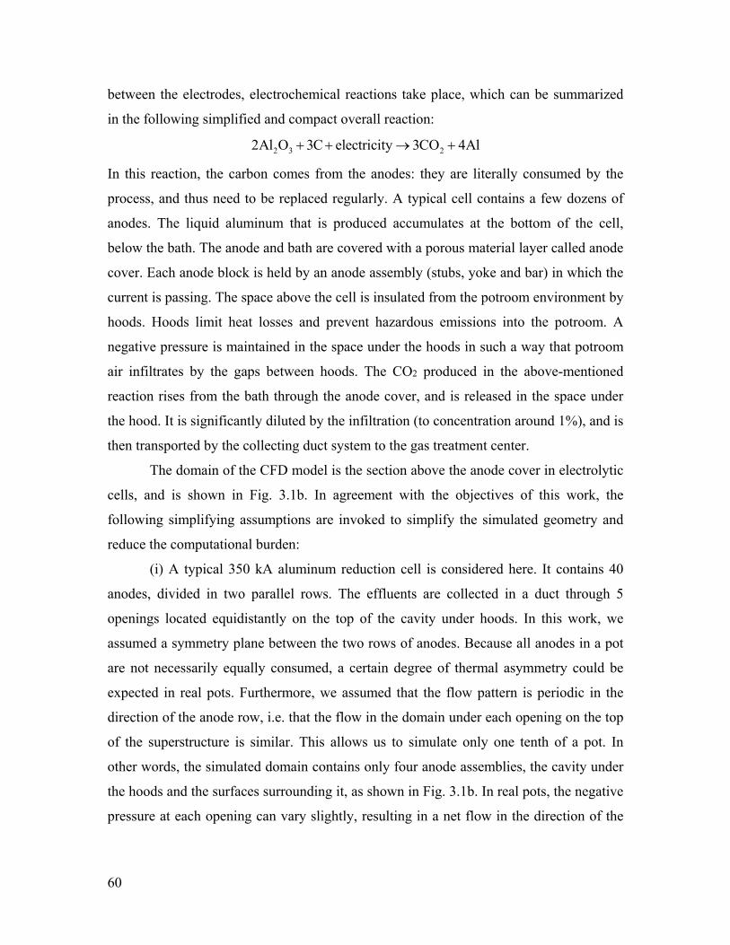
60

between the electrodes, electrochemical reactions take place, which can be summarized

in the following simplified and compact overall reaction:

2 3 22Al O 3C electricity 3CO 4Al

In this reaction, the carbon comes from the anodes: they are literally consumed by the

process, and thus need to be replaced regularly. A typical cell contains a few dozens of

anodes. The liquid aluminum that is produced accumulates at the bottom of the cell,

below the bath. The anode and bath are covered with a porous material layer called anode

cover. Each anode block is held by an anode assembly (stubs, yoke and bar) in which the

current is passing. The space above the cell is insulated from the potroom environment by

hoods. Hoods limit heat losses and prevent hazardous emissions into the potroom. A

negative pressure is maintained in the space under the hoods in such a way that potroom

air infiltrates by the gaps between hoods. The CO2 produced in the above-mentioned

reaction rises from the bath through the anode cover, and is released in the space under

the hood. It is significantly diluted by the infiltration (to concentration around 1%), and is

then transported by the collecting duct system to the gas treatment center.

The domain of the CFD model is the section above the anode cover in electrolytic

cells, and is shown in Fig. 3.1b. In agreement with the objectives of this work, the

following simplifying assumptions are invoked to simplify the simulated geometry and

reduce the computational burden:

(i) A typical 350 kA aluminum reduction cell is considered here. It contains 40

anodes, divided in two parallel rows. The effluents are collected in a duct through 5

openings located equidistantly on the top of the cavity under hoods. In this work, we

assumed a symmetry plane between the two rows of anodes. Because all anodes in a pot

are not necessarily equally consumed, a certain degree of thermal asymmetry could be

expected in real pots. Furthermore, we assumed that the flow pattern is periodic in the

direction of the anode row, i.e. that the flow in the domain under each opening on the top

of the superstructure is similar. This allows us to simulate only one tenth of a pot. In

other words, the simulated domain contains only four anode assemblies, the cavity under

the hoods and the surfaces surrounding it, as shown in Fig. 3.1b. In real pots, the negative

pressure at each opening can vary slightly, resulting in a net flow in the direction of the

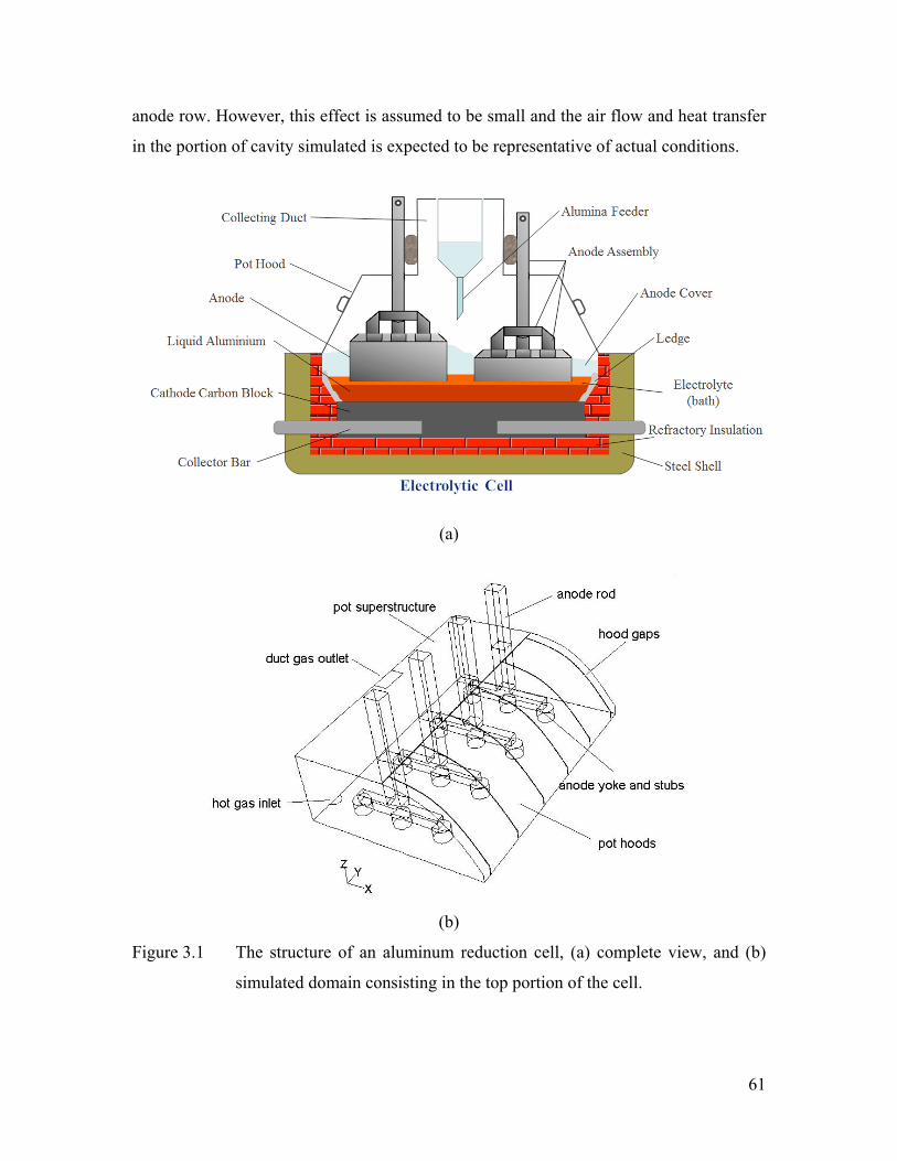
61

anode row. However, this effect is assumed to be small and the air flow and heat transfer

in the portion of cavity simulated is expected to be representative of actual conditions.

(a)

(b)

Figure 3.1 The structure of an aluminum reduction cell, (a) complete view, and (b)

simulated domain consisting in the top portion of the cell.

62

(ii) The bottom surface of the simulated domain is the top surface of the anode

cover, i.e. the anode cover, anodic blocks and electrolytic bath are not simulated. The

inclusion of these components would significantly increase the complexity of the model

and the computational cost while they have less influence on the flow and heat in the

simulated domain. Open holes due to the collapse of crust were not considered in current

simulation. We imposed a uniform heat flux on the anode cover surface which will not

affect significantly the results, since the objective here is mainly to determine the

convection coefficients.

(iii) The feeding system is omitted in the simulated domain in order to simplify

the generation of the domain and mesh.

(iv) The infiltration of air in the cavity under the hood comes from gaps between

hoods and at the connection between the hoods and superstructure. No open hoods are

simulated.

3.2.2 Governing equations and modeling options

The governing equations for the present problems are those expressing conservation of

mass, momentum in each direction and energy, along with a turbulence model.

Incompressible flow and steady-state conditions are considered. Pressure work and

kinetic energy terms are neglected in energy equation since the gas is treated as an

incompressible flow. No species diffusion is involved in the problem. Therefore, the

continuity equation (conservation of mass) reads as:

i

i

(ρu )0

x

(3.1)

The conservation of momentum equations are (written in a Cartesian tensor form):

i j jieff ij

i i j j i

(ρu u ) uup 2 = – + μ + – ρδ + ρg

x x x x x 3k

(3.2)

Finally, the conservation of energy equation is:

ieff h

i i i

(ρu h) T= k + S

x x x

(3.3)

63

where the sensible enthalpy of the gas h is defined as ref

T

pTh= C dT . Cp is the temperature-

dependent heat specific of air. The Reynolds stresses term due to the turbulence is

modeled based on the Boussinesq eddy viscosity assumption. Therefore, μeff is the

effective viscosity (μ+μt, where μt is the turbulent viscosity, defined according to the

turbulence model that is used), k is the turbulent kinetic energy and δij=0 (i≠j) or 1 (i=j).

keff is the effective thermal conductivity (k+kt, where kt is the turbulent thermal

conductivity, defined according to the turbulence model being used). Sh includes the

volumetric heat source due to the Joule heating effect in solids. Viscous heating is

ignored in the simulation. Note that in the solids, only the energy equation is solved, and

without the advective terms. The volumetric heat generation (Joule heating) is assumed to

be uniform in the solids and was calculated based on the typical current and resistivity in

each part of the anode assembly.

The air properties (i.e., specific heat, thermal conductivity, and viscosity) are

functions of temperature (polynomial fittings based on data published in (Bergman et al.

2011)). The air density was determined based on the “incompressible-ideal-gas” model of

the CFD software used (Fluent 2012), and was calculated by:

op

w

pρ=

RT

M

(3.4)

where R is the universal gas constant, Mw, the molecular weight of the gas, and pop, the

defined operating pressure. Under this approach, the density depends only on the

operating pressure, and not on the local relative pressure field. In this form, the local

density field depends on the local temperature field, and thus buoyancy forces can be

considered in the momentum equations.

To account for turbulence, each variable was expressed as the summation of a

time-average variable plus a fluctuating component, and then the conservation equations

were averaged over time. A turbulence model is required to close the model. Generally

speaking, two approaches are available to simulate the region close to the walls of the

domain. One approach relies on semi-empirical formulas called “wall functions”, while

the other calculates the detailed flow in the wall region. The first method is popular in

industrial applications because it uses a wall function to calculate the near wall flow

64

feature and thus tremendously reduces the computational time. However, despite of its

advantages, the wall function method appears weakly adequate to describe the near wall

region with low Reynolds number flows, since the empirical formulas were established

from experiments with high Reynolds number flows (typical turbulent flows). The

airflow in the present study is relatively weak and does not have a high Reynolds number.

Moreover, when reducing the pot draft condition, buoyancy will significantly influence

the flow feature in the cavity. Therefore, it was decided to compare the two approaches

(see Section 3.3), and the explicit calculation of flow feature close to the walls proved to

be better than the use of wall functions.

A proper choice of turbulence model is required to achieve an adequate trade-off

between accuracy and computational time. The airflow pattern in the cavity under the

hoods shares many similarities with the induced airflow in enclosed environments (e.g.,

jet flow and impingement on a wall, recirculation and buoyancy-driven flow). In the last

years, the k-ε family of turbulence models has been very popular for indoor environment

and jet flow simulations, which share several similarities with the present problem. In

particular, the renormalization group (RNG) k-ε model was found to be reliable and

accurate for a wide variety of applications (e.g., Chen 1995; Isman et al. 2008; Sharif and

Mothe 2009). Recently, the SST (shear stress transport) k-ω model has attracted more

attention for solving flow problems similar to the present one. This model was developed

by Menter (1994) to model separation flows around solid obstructions, and it can blend

the robust and accurate formulation of the k-ω model in the near-wall region with the k-ε

model in the far field through blending functions. Stamou et al. (2008) used the SST k-ω

model in their CFD model to evaluate the thermal comfort conditions in the indoor

stadium of the Galatsi Arena. Hofmann et al. (2007) simulated steady and pulsating

impinging jets by using 13 widely used turbulence models, and the SST k-ω turbulence

model with the transitional flow option captured properly the heat transfer and flow field

patterns in the entire domain compared to experimental results. Recently, Hussain and

Oosthuizen (2012a) developed a CFD model with the SST k-ω turbulence model to

simulate the buoyancy-driven natural ventilation in a simple atrium building. A

comprehensive review on the validation of turbulence models was reported in literature

(Zhai et al. 2007; Zhang et al. 2007). They compared CFD simulations to experimental

65

results, and the best agreement was achieved with the RNG k-ε or the SST k-ω models.

In cases with strong buoyancy forces and high-Reynolds number jet flow (as in the

present problem), the SST k-ω model provided better results. Based on the literature

survey we decided to use this mode as the turbulence model in present problem. The SST

k-ω model adopts a high Reynolds number turbulence model (the standard k-ε model),

except in the region near the walls where a low Reynolds number model (the k-ω model)

is used. The wall-adjacent mesh recommended for applying this model is to create either

a coarse (y+30) or refined (y+≈1) mesh in the near wall areas. However, a refined mesh

is necessary if it is intended to resolve the viscosity-affected region. The detailed

algorithm of the SST k-ω model will not be repeated here for the sake of conciseness, and

is available in (Fluent 2012).

As for radiation heat transfer, since the gas in the cavity is essentially air, the gas

is treated as a non-participating medium. The way in which radiation heat transfer

between surfaces was considered is described in Section 3.2.3.

A commercial CFD software, ANSYS FLUENT 12.0/12.1, was used for solving

the set of equations. The governing equations are discretized based on the finite volume

formulation. Default criteria were used to declare that the convergence of a simulation

was achieved (Fluent 2012). In order to reach convergence, different strategies were

employed, such as starting simulations with smaller imposed pressure drop, reaching

convergence, and continuing to increase gradually the pressure drop until the desired

values be reached. In the end, the mass and energy imbalances (the ratio of the difference

between the inflow and outflow to the total inflow) can be reduced to less than 106 and

102, respectively. The mesh is created in GAMBIT 2.4 and consisted in prism control

volumes in the boundary layer, and Tet/Hybrid control volumes in the core of the

domain. As described later, mesh independence was thoroughly tested. A typical mesh

contained over 2 million control volumes, considering that the mesh is refined enough to

catch the main feature of the turbulent flow in the pot. Approximately 10 hours were

required for performing one simulation using 4 cores of 2.67GHz.

66

3.2.3 Boundary conditions

This sub-section presents all the boundary conditions that were used in this study. The

pressure at all gaps was set to the atmospheric pressure while that at the outlet was an

adjustable negative pressure. The total ventilation rate can thus be varied by changing the

driving inlet-to-outlet pressure difference. To simulate the release of CO2 from the bath in

the cavity under the hood, a small region that correspond to the feed hole on anode cover

was considered from which hot gases (CO2) are released at 700ºC with a mass flow rate

of 0.0048 kg/s for our simulated domain (based on 1.3% molar concentration of hot gas

in effluents). Since the specific heat of CO2 is very close to air and no species

consideration is involved in the current simulations, we replaced the CO2 properties with

that of air for simplifying the model. The turbulence intensity was set at 1% at all inlets

and outlet considering the low turbulent flow in the cavity. Turbulence length scale was

defined as 7×10-4 m at the gap inlets, considering that the width of gaps is about 0.01 m,

as recommended in (Fluent 2012). Hydraulic diameter was used to define the turbulence

parameters at the exit outlet and hot gas inlet (Fluent 2012). Impermeability and no-slip

flow are assumed on all solid surfaces. For all vertical surfaces facing other anode

assemblies, symmetry was imposed.

According to the geometrical simplifications presented above, the thermal

boundary condition on the bottom surface (i.e., top surface of anode cover) is represented

by a uniform heat flux of 2000 W/m2. This value is the average heat flux through the

anode cover of a mix of crushed bath and alumina obtained from practical measurements

in literature (Shen et al. 2008). The temperature at the small surfaces that correspond to

the bottom of the stubs was fixed at 450°C based on Abbas’s thesis (Abbas 2010). For the

external surfaces of hoods and superstructure, the effective heat transfer coefficient for

convection and radiation is fixed to 10 W/m2K, which is typical for natural convection

dominated heat transfer (Abbas 2010). The ambient potroom temperature in this work is

set to 30°C and a heat flux of 800 W/m2 is imposed on the top tip of anode rod. All

boundary conditions used in the present study are presented in Table 3.1.

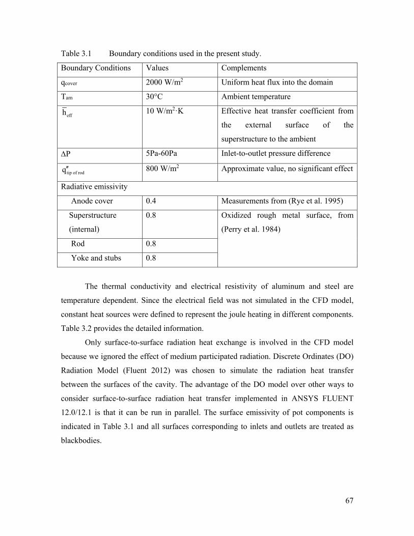
67

Table 3.1 Boundary conditions used in the present study.

Boundary Conditions Values Complements

qcover 2000 W/m2 Uniform heat flux into the domain

Tam 30°C Ambient temperature

effh 10 W/m2·K Effective heat transfer coefficient from

the external surface of the

superstructure to the ambient

P 5Pa-60Pa Inlet-to-outlet pressure difference

tip of rodq 800 W/m2 Approximate value, no significant effect

Radiative emissivity

Anode cover 0.4 Measurements from (Rye et al. 1995)

Superstructure

(internal)

0.8 Oxidized rough metal surface, from

(Perry et al. 1984)

Rod 0.8

Yoke and stubs 0.8

The thermal conductivity and electrical resistivity of aluminum and steel are

temperature dependent. Since the electrical field was not simulated in the CFD model,

constant heat sources were defined to represent the joule heating in different components.

Table 3.2 provides the detailed information.

Only surface-to-surface radiation heat exchange is involved in the CFD model

because we ignored the effect of medium participated radiation. Discrete Ordinates (DO)

Radiation Model (Fluent 2012) was chosen to simulate the radiation heat transfer

between the surfaces of the cavity. The advantage of the DO model over other ways to

consider surface-to-surface radiation heat transfer implemented in ANSYS FLUENT

12.0/12.1 is that it can be run in parallel. The surface emissivity of pot components is

indicated in Table 3.1 and all surfaces corresponding to inlets and outlets are treated as

blackbodies.

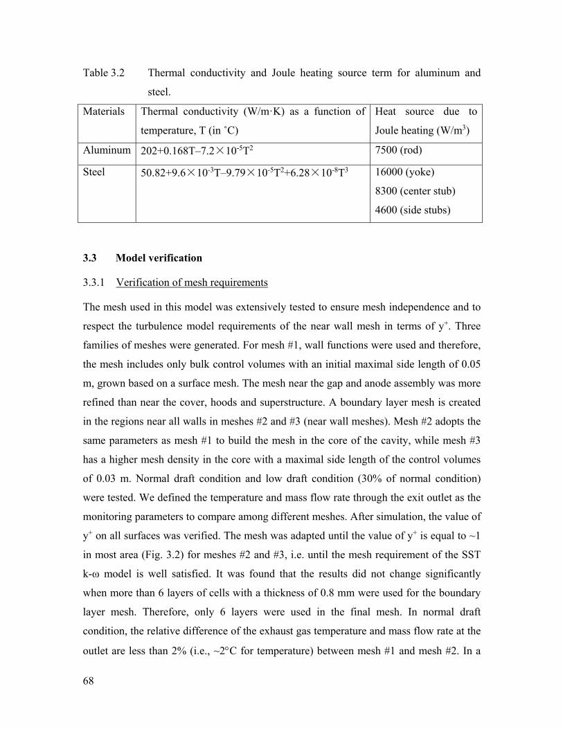
68

Table 3.2 Thermal conductivity and Joule heating source term for aluminum and

steel.

Materials Thermal conductivity (W/m·K) as a function of

temperature, T (in ˚C)

Heat source due to

Joule heating (W/m3)

Aluminum 202+0.168T–7.2×10-5T2 7500 (rod)

Steel 50.82+9.6×10-3T–9.79×10-5T2+6.28×10-8T3 16000 (yoke)

8300 (center stub)

4600 (side stubs)

3.3 Model verification

3.3.1 Verification of mesh requirements

The mesh used in this model was extensively tested to ensure mesh independence and to

respect the turbulence model requirements of the near wall mesh in terms of y+. Three

families of meshes were generated. For mesh #1, wall functions were used and therefore,

the mesh includes only bulk control volumes with an initial maximal side length of 0.05

m, grown based on a surface mesh. The mesh near the gap and anode assembly was more

refined than near the cover, hoods and superstructure. A boundary layer mesh is created

in the regions near all walls in meshes #2 and #3 (near wall meshes). Mesh #2 adopts the

same parameters as mesh #1 to build the mesh in the core of the cavity, while mesh #3

has a higher mesh density in the core with a maximal side length of the control volumes

of 0.03 m. Normal draft condition and low draft condition (30% of normal condition)

were tested. We defined the temperature and mass flow rate through the exit outlet as the

monitoring parameters to compare among different meshes. After simulation, the value of

y+ on all surfaces was verified. The mesh was adapted until the value of y+ is equal to ~1

in most area (Fig. 3.2) for meshes #2 and #3, i.e. until the mesh requirement of the SST

k-ω model is well satisfied. It was found that the results did not change significantly

when more than 6 layers of cells with a thickness of 0.8 mm were used for the boundary

layer mesh. Therefore, only 6 layers were used in the final mesh. In normal draft

condition, the relative difference of the exhaust gas temperature and mass flow rate at the

outlet are less than 2% (i.e., ~2C for temperature) between mesh #1 and mesh #2. In a

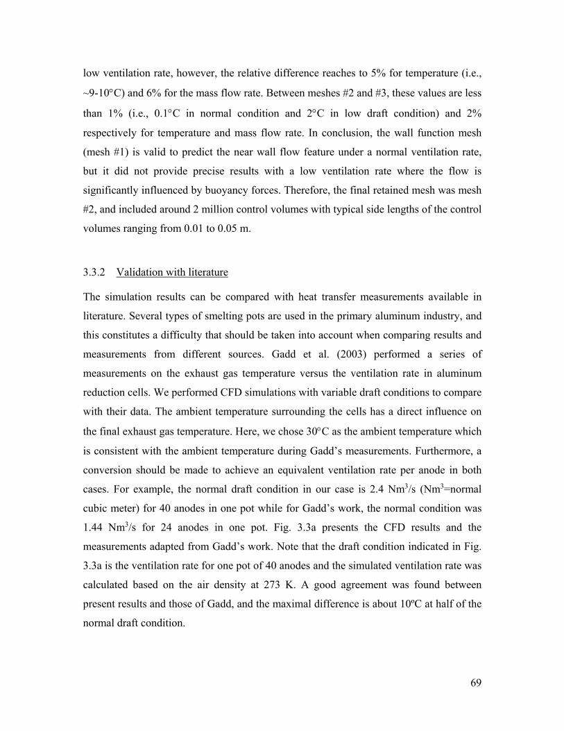
69

low ventilation rate, however, the relative difference reaches to 5% for temperature (i.e.,

~9-10C) and 6% for the mass flow rate. Between meshes #2 and #3, these values are less

than 1% (i.e., 0.1C in normal condition and 2C in low draft condition) and 2%

respectively for temperature and mass flow rate. In conclusion, the wall function mesh

(mesh #1) is valid to predict the near wall flow feature under a normal ventilation rate,

but it did not provide precise results with a low ventilation rate where the flow is

significantly influenced by buoyancy forces. Therefore, the final retained mesh was mesh

#2, and included around 2 million control volumes with typical side lengths of the control

volumes ranging from 0.01 to 0.05 m.

3.3.2 Validation with literature

The simulation results can be compared with heat transfer measurements available in

literature. Several types of smelting pots are used in the primary aluminum industry, and

this constitutes a difficulty that should be taken into account when comparing results and

measurements from different sources. Gadd et al. (2003) performed a series of

measurements on the exhaust gas temperature versus the ventilation rate in aluminum

reduction cells. We performed CFD simulations with variable draft conditions to compare

with their data. The ambient temperature surrounding the cells has a direct influence on

the final exhaust gas temperature. Here, we chose 30C as the ambient temperature which

is consistent with the ambient temperature during Gadd’s measurements. Furthermore, a

conversion should be made to achieve an equivalent ventilation rate per anode in both

cases. For example, the normal draft condition in our case is 2.4 Nm3/s (Nm3=normal

cubic meter) for 40 anodes in one pot while for Gadd’s work, the normal condition was

1.44 Nm3/s for 24 anodes in one pot. Fig. 3.3a presents the CFD results and the

measurements adapted from Gadd’s work. Note that the draft condition indicated in Fig.

3.3a is the ventilation rate for one pot of 40 anodes and the simulated ventilation rate was

calculated based on the air density at 273 K. A good agreement was found between

present results and those of Gadd, and the maximal difference is about 10ºC at half of the

normal draft condition.

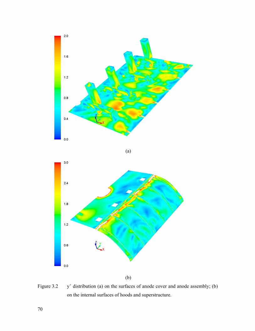
70

(a)

(b)

Figure 3.2 y+ distribution (a) on the surfaces of anode cover and anode assembly; (b)

on the internal surfaces of hoods and superstructure.

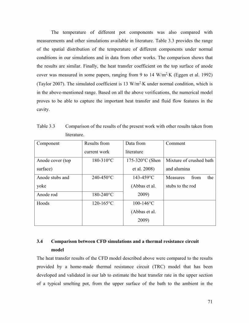
71

The temperature of different pot components was also compared with

measurements and other simulations available in literature. Table 3.3 provides the range

of the spatial distribution of the temperature of different components under normal

conditions in our simulations and in data from other works. The comparison shows that

the results are similar. Finally, the heat transfer coefficient on the top surface of anode

cover was measured in some papers, ranging from 9 to 14 W/m2K (Eggen et al. 1992)

(Taylor 2007). The simulated coefficient is 13 W/m2K under normal condition, which is

in the above-mentioned range. Based on all the above verifications, the numerical model

proves to be able to capture the important heat transfer and fluid flow features in the

cavity.

Table 3.3 Comparison of the results of the present work with other results taken from

literature.

Component Results from

current work

Data from

literature

Comment

Anode cover (top

surface)

180-310°C 175-320°C (Shen

et al. 2008)

Mixture of crushed bath

and alumina

Anode stubs and

yoke

240-450°C 143-459°C

(Abbas et al.

2009)

Measures from the

stubs to the rod

Anode rod 180-240°C

Hoods 120-165°C 100-146°C

(Abbas et al.

2009)

3.4 Comparison between CFD simulations and a thermal resistance circuit

model

The heat transfer results of the CFD model described above were compared to the results

provided by a home-made thermal resistance circuit (TRC) model that has been

developed and validated in our lab to estimate the heat transfer rate in the upper section

of a typical smelting pot, from the upper surface of the bath to the ambient in the

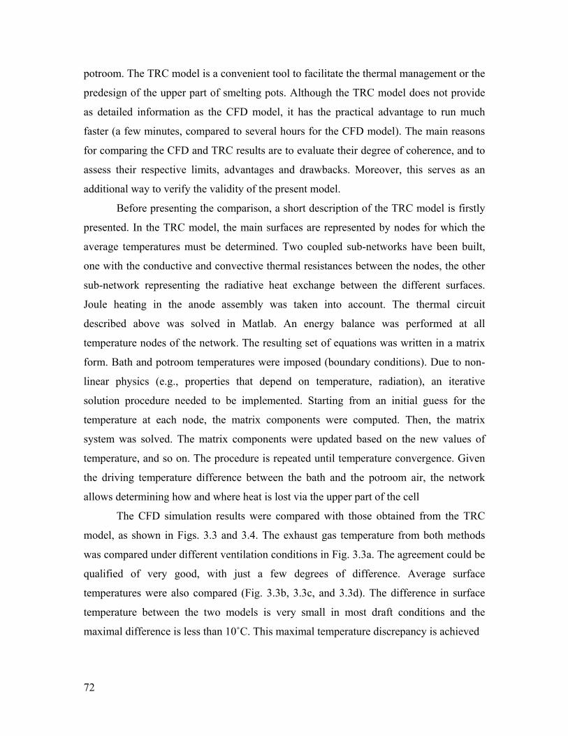
72

potroom. The TRC model is a convenient tool to facilitate the thermal management or the

predesign of the upper part of smelting pots. Although the TRC model does not provide

as detailed information as the CFD model, it has the practical advantage to run much

faster (a few minutes, compared to several hours for the CFD model). The main reasons

for comparing the CFD and TRC results are to evaluate their degree of coherence, and to

assess their respective limits, advantages and drawbacks. Moreover, this serves as an

additional way to verify the validity of the present model.

Before presenting the comparison, a short description of the TRC model is firstly

presented. In the TRC model, the main surfaces are represented by nodes for which the

average temperatures must be determined. Two coupled sub-networks have been built,

one with the conductive and convective thermal resistances between the nodes, the other

sub-network representing the radiative heat exchange between the different surfaces.

Joule heating in the anode assembly was taken into account. The thermal circuit

described above was solved in Matlab. An energy balance was performed at all

temperature nodes of the network. The resulting set of equations was written in a matrix

form. Bath and potroom temperatures were imposed (boundary conditions). Due to non-

linear physics (e.g., properties that depend on temperature, radiation), an iterative

solution procedure needed to be implemented. Starting from an initial guess for the

temperature at each node, the matrix components were computed. Then, the matrix

system was solved. The matrix components were updated based on the new values of

temperature, and so on. The procedure is repeated until temperature convergence. Given

the driving temperature difference between the bath and the potroom air, the network

allows determining how and where heat is lost via the upper part of the cell

The CFD simulation results were compared with those obtained from the TRC

model, as shown in Figs. 3.3 and 3.4. The exhaust gas temperature from both methods

was compared under different ventilation conditions in Fig. 3.3a. The agreement could be

qualified of very good, with just a few degrees of difference. Average surface

temperatures were also compared (Fig. 3.3b, 3.3c, and 3.3d). The difference in surface

temperature between the two models is very small in most draft conditions and the

maximal difference is less than 10˚C. This maximal temperature discrepancy is achieved

73

0.5 1.0 1.5 2.0 2.5 3.080

100

120

140

160

180

200

220

240

0.5 1.0 1.5 2.0 2.5 3.0240

260

280

300

320

340

360

0.5 1.0 1.5 2.0 2.5 3.0

140

160

180

200

220

240

260

0.5 1.0 1.5 2.0 2.5 3.0220

240

260

280

300

320

(b)(a)

Q (Nm3/s)

TRC CFD Gadd's data [29]

Tco

ver

( o C

)

Q (Nm3/s)

TRC CFD

Tga

s ( o C

)

Tho

od (

oC

)

Q (Nm3/s)

TRC CFD

(d)(c)

Tro

d ( o

C)

Q (Nm3/s)

TRC CFD

Figure 3.3 Comparison between average temperatures obtained from the CFD model

and from the thermal resistance circuit (TRC) model, as a function of the

ventilation, for: (a) the exhaust gas (including Gadd’s experiments); (b) the

top surface of the anode cover; (c) the surfaces of hoods and

superstructure; and (d) the base of aluminum rod.

at the base of the aluminum rod under normal and higher draft conditions in Fig. 3.3d.

This discrepancy is likely caused by the simplifications of the anode assembly to 1D

component in the TRC model. The TRC tends to underestimate the rod temperature

compared to the CFD model. However, the influence of this discrepancy on the overall

heat transfer in the system is weak.

Reported in Fig. 3.4a is the heat content in the exhaust gas. Results from both

models are coherent and the maximal difference is just of the order of 250 W (relative

difference of 5%). Besides, the radiation heat transfer rates on surfaces as achieved by the

two models were compared in Figs. 3.4b, 3.4c and 3.4d. A good agreement was found on

the top surface of anode cover in Fig. 3.4b (maximal difference of ~100 W and relative

74

difference of 10%). On the surface of the superstructure and hoods, Fig. 3.4c, a similar

trend is found with both models, but discrepancies become more important as the

ventilation rate goes down (around 10% of discrepancy). The relatively large error is due

to the geometrical simplification of the surfaces in the TRC model for calculating

radiation. In reality, there is a large non-uniformity of surface temperature on the hoods

and superstructure. CFD has shown its capacity of predicting the temperature spatial

variation while it is obviously not the advantage of the TRC model. This non-uniform

temperature distribution will result in an error in calculating the energy irradiated from

the surface. Fig. 3.4d shows the radiative heat transfer rate from the surfaces of yoke and

stubs, where high temperatures prevail. Both models provide heat transfer rates of the

same order of magnitude (around 2 kW). Nevertheless the radiative heat transfer rate was

almost the same in CFD simulations for all draft conditions, whereas it increases with the

reduction of ventilation rate in TRC calculations. The difference in terms of trends is due

to the approximate boundary condition defined at the bottom of the three stubs in the

CFD model. As mentioned previously, a fixed temperature of 450˚C on the bottom of the

stubs was assumed in the CFD model, which might not represent well the stub

temperature under low ventilation level. For example, it was shown that this temperature

increases up to 500C at low draft condition (based on the calculation of TRC model).

The fact that the yoke and stubs temperature is smaller in the CFD model will tend to

underestimate radiative heat transfer from these components. This problem could be

solved in future work by extending the computational domain of the CFD model to the

bath itself where a constant operating temperature can be assumed at all time.

In conclusion, the TRC temperature predictions are quite coherent with the CFD

simulations in most areas of the top section of an aluminum smelting pot. Considering the

most interesting parameters, i.e. the exhaust gas temperature and the heat content in the

gas, TRC calculations can provide a good agreement with CFD simulations. It is worth to

mention that the convection heat transfer coefficients in the TRC were based on the CFD

simulations (see next section). Therefore, knowing that this aspect was consistent

between the two models, it is worth to verify that the rest of the two modeling approaches

provide coherent (i.e., similar) results. As exemplified below, the CFD model provides a

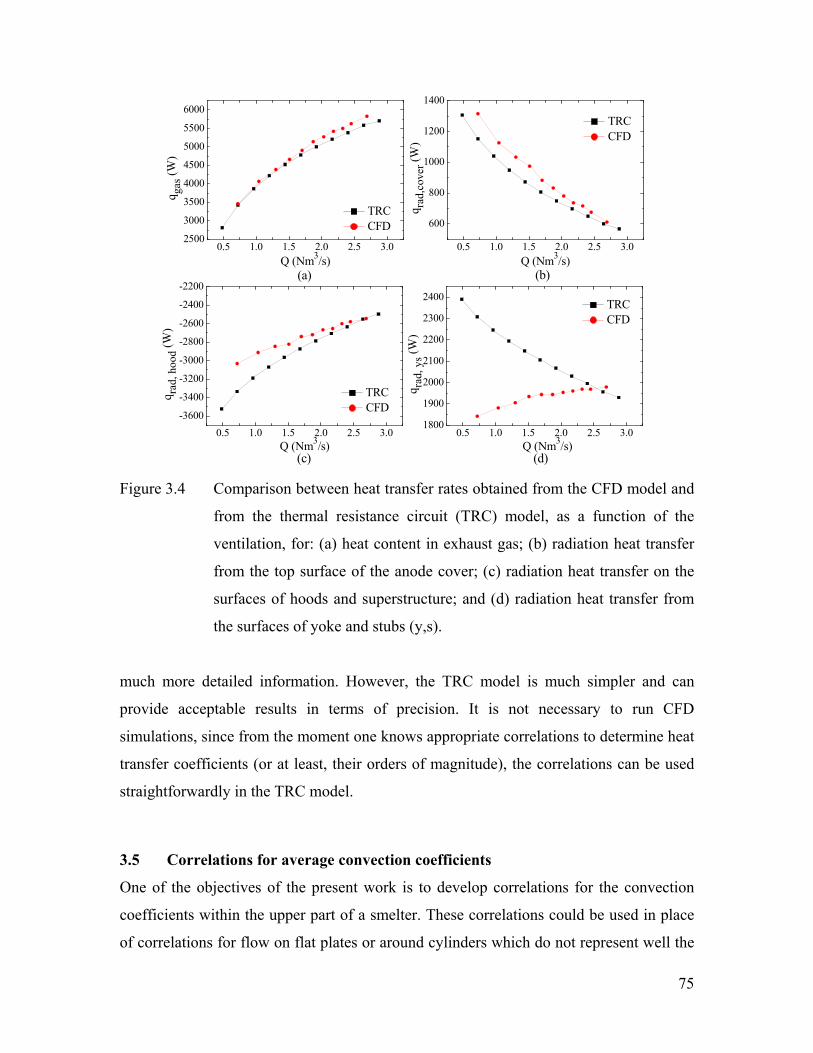
75

0.5 1.0 1.5 2.0 2.5 3.02500

3000

3500

4000

4500

5000

5500

6000

0.5 1.0 1.5 2.0 2.5 3.0

600

800

1000

1200

1400

0.5 1.0 1.5 2.0 2.5 3.0

-3600

-3400

-3200

-3000

-2800

-2600

-2400

-2200

0.5 1.0 1.5 2.0 2.5 3.01800

1900

2000

2100

2200

2300

2400

(d)(c)

(b)

q gas (

W)

Q (Nm3/s)

TRC CFD

(a)

q rad,

cove

r (W

)

Q (Nm3/s)

TRC CFD

q rad,

hoo

d (W

)

Q (Nm3/s)

TRC CFD

q rad,

ys (

W)

Q (Nm3/s)

TRC CFD

Figure 3.4 Comparison between heat transfer rates obtained from the CFD model and

from the thermal resistance circuit (TRC) model, as a function of the

ventilation, for: (a) heat content in exhaust gas; (b) radiation heat transfer

from the top surface of the anode cover; (c) radiation heat transfer on the

surfaces of hoods and superstructure; and (d) radiation heat transfer from

the surfaces of yoke and stubs (y,s).

much more detailed information. However, the TRC model is much simpler and can

provide acceptable results in terms of precision. It is not necessary to run CFD

simulations, since from the moment one knows appropriate correlations to determine heat

transfer coefficients (or at least, their orders of magnitude), the correlations can be used

straightforwardly in the TRC model.

3.5 Correlations for average convection coefficients

One of the objectives of the present work is to develop correlations for the convection

coefficients within the upper part of a smelter. These correlations could be used in place

of correlations for flow on flat plates or around cylinders which do not represent well the

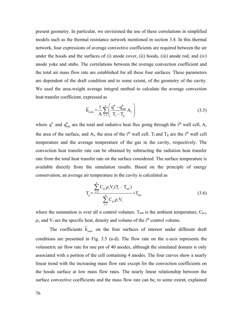
76

present geometry. In particular, we envisioned the use of these correlations in simplified

models such as the thermal resistance network mentioned in section 3.4. In this thermal

network, four expressions of average convective coefficients are required between the air

under the hoods and the surfaces of (i) anode cover, (ii) hoods, (iii) anode rod, and (iv)

anode yoke and stubs. The correlations between the average convection coefficient and

the total air mass flow rate are established for all these four surfaces. These parameters

are dependent of the draft condition and to some extent, of the geometry of the cavity.

We used the area-weight average integral method to calculate the average convection

heat transfer coefficient, expressed as

nrad

conv ii=1 i g

q – q1h = A

A T – T

(3.5)

where q and radq are the total and radiative heat flux going through the ith wall cell, A,

the area of the surface, and Ai, the area of the ith wall cell. Ti and Tg are the ith wall cell

temperature and the average temperature of the gas in the cavity, respectively. The

convection heat transfer rate can be obtained by subtracting the radiation heat transfer

rate from the total heat transfer rate on the surface considered. The surface temperature is

available directly from the simulation results. Based on the principle of energy

conservation, an average air temperature in the cavity is calculated as

n

p,i i i i ami=1

g amn

p,i i ii=1

C ρ V (T – T )T = +T

C ρ V

(3.6)

where the summation is over all n control volumes. Tam is the ambient temperature, Cp,i,

ρi, and Vi are the specific heat, density and volume of the ith control volume.

The coefficients convh on the four surfaces of interest under different draft

conditions are presented in Fig. 3.5 (a-d). The flow rate on the x-axis represents the

volumetric air flow rate for one pot of 40 anodes, although the simulated domain is only

associated with a portion of the cell containing 4 anodes. The four curves show a nearly

linear trend with the increasing mass flow rate except for the convection coefficients on

the hoods surface at low mass flow rates. The nearly linear relationship between the

surface convective coefficients and the mass flow rate can be, to some extent, explained

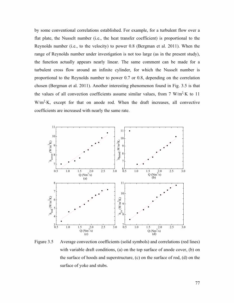
77

by some conventional correlations established. For example, for a turbulent flow over a

flat plate, the Nusselt number (i.e., the heat transfer coefficient) is proportional to the

Reynolds number (i.e., to the velocity) to power 0.8 (Bergman et al. 2011). When the

range of Reynolds number under investigation is not too large (as in the present study),

the function actually appears nearly linear. The same comment can be made for a

turbulent cross flow around an infinite cylinder, for which the Nusselt number is

proportional to the Reynolds number to power 0.7 or 0.8, depending on the correlation

chosen (Bergman et al. 2011). Another interesting phenomenon found in Fig. 3.5 is that

the values of all convection coefficients assume similar values, from 7 W/m2K to 11

W/m2K, except for that on anode rod. When the draft increases, all convective

coefficients are increased with nearly the same rate.

0.5 1.0 1.5 2.0 2.5 3.0

7

8

9

10

11

0.5 1.0 1.5 2.0 2.5 3.06

7

8

9

10

11

0.5 1.0 1.5 2.0 2.5 3.03

4

5

6

7

8

0.5 1.0 1.5 2.0 2.5 3.07

8

9

10

11

Q (Nm3/s)

hco

ver (

W/m

2 K)

Q (Nm3/s)

hho

od (W

/m2 K

)

hro

d (W

/m2 K

)

Q (Nm3/s)(d)(c)

hys

(W

/m2 K

)

Q (Nm3/s)

(a) (b)

Figure 3.5 Average convection coefficients (solid symbols) and correlations (red lines)

with variable draft conditions, (a) on the top surface of anode cover, (b) on

the surface of hoods and superstructure, (c) on the surface of rod, (d) on the

surface of yoke and stubs.

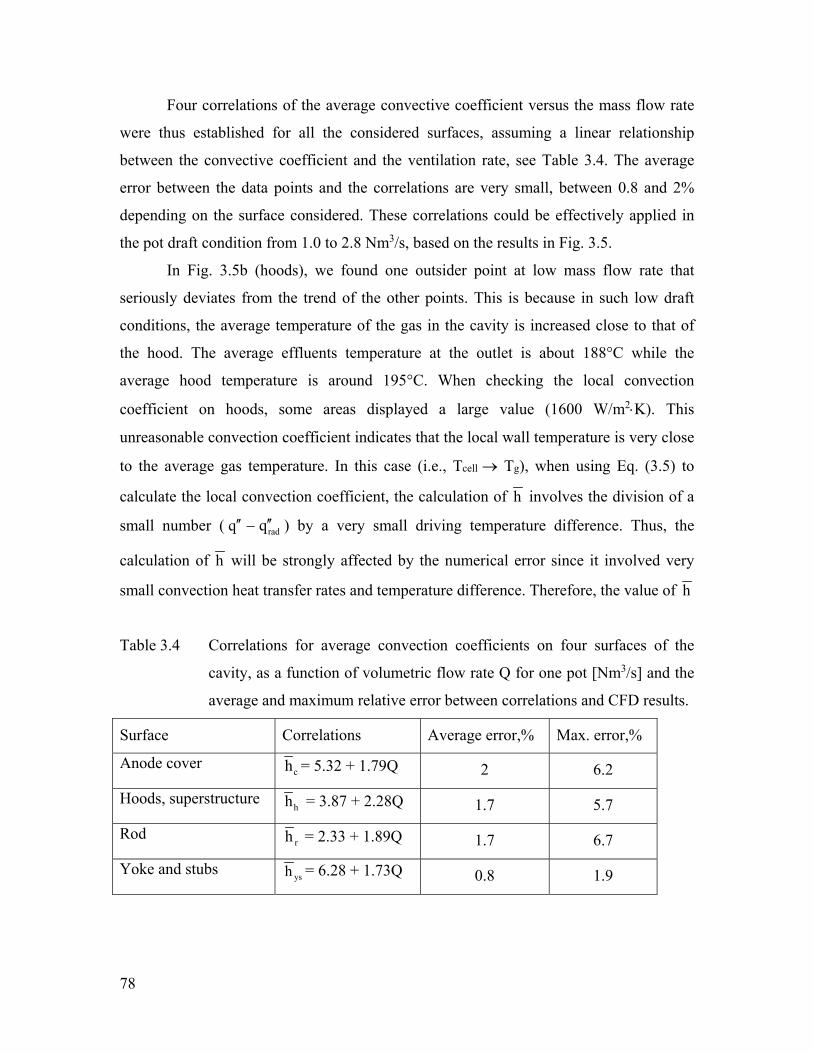
78

Four correlations of the average convective coefficient versus the mass flow rate

were thus established for all the considered surfaces, assuming a linear relationship

between the convective coefficient and the ventilation rate, see Table 3.4. The average

error between the data points and the correlations are very small, between 0.8 and 2%

depending on the surface considered. These correlations could be effectively applied in

the pot draft condition from 1.0 to 2.8 Nm3/s, based on the results in Fig. 3.5.

In Fig. 3.5b (hoods), we found one outsider point at low mass flow rate that

seriously deviates from the trend of the other points. This is because in such low draft

conditions, the average temperature of the gas in the cavity is increased close to that of

the hood. The average effluents temperature at the outlet is about 188°C while the

average hood temperature is around 195°C. When checking the local convection

coefficient on hoods, some areas displayed a large value (1600 W/m2K). This

unreasonable convection coefficient indicates that the local wall temperature is very close

to the average gas temperature. In this case (i.e., Tcell Tg), when using Eq. (3.5) to

calculate the local convection coefficient, the calculation of h

involves the division of a

small number ( q radq ) by a very small driving temperature difference. Thus, the

calculation of h

will be strongly affected by the numerical error since it involved very

small convection heat transfer rates and temperature difference. Therefore, the value of h

Table 3.4 Correlations for average convection coefficients on four surfaces of the

cavity, as a function of volumetric flow rate Q for one pot [Nm3/s] and the

average and maximum relative error between correlations and CFD results.

Surface Correlations Average error,% Max. error,%

Anode cover ch = 5.32 + 1.79Q 2 6.2

Hoods, superstructure hh = 3.87 + 2.28Q 1.7 5.7

Rod rh = 2.33 + 1.89Q 1.7 6.7

Yoke and stubs ysh = 6.28 + 1.73Q 0.8 1.9

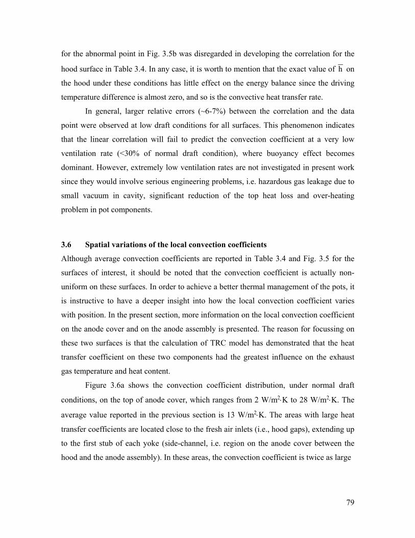
79

for the abnormal point in Fig. 3.5b was disregarded in developing the correlation for the

hood surface in Table 3.4. In any case, it is worth to mention that the exact value of h on

the hood under these conditions has little effect on the energy balance since the driving

temperature difference is almost zero, and so is the convective heat transfer rate.

In general, larger relative errors (~6-7%) between the correlation and the data

point were observed at low draft conditions for all surfaces. This phenomenon indicates

that the linear correlation will fail to predict the convection coefficient at a very low

ventilation rate (<30% of normal draft condition), where buoyancy effect becomes

dominant. However, extremely low ventilation rates are not investigated in present work

since they would involve serious engineering problems, i.e. hazardous gas leakage due to

small vacuum in cavity, significant reduction of the top heat loss and over-heating

problem in pot components.

3.6 Spatial variations of the local convection coefficients

Although average convection coefficients are reported in Table 3.4 and Fig. 3.5 for the

surfaces of interest, it should be noted that the convection coefficient is actually non-

uniform on these surfaces. In order to achieve a better thermal management of the pots, it

is instructive to have a deeper insight into how the local convection coefficient varies

with position. In the present section, more information on the local convection coefficient

on the anode cover and on the anode assembly is presented. The reason for focussing on

these two surfaces is that the calculation of TRC model has demonstrated that the heat

transfer coefficient on these two components had the greatest influence on the exhaust

gas temperature and heat content.

Figure 3.6a shows the convection coefficient distribution, under normal draft

conditions, on the top of anode cover, which ranges from 2 W/m2K to 28 W/m2K. The

average value reported in the previous section is 13 W/m2K. The areas with large heat

transfer coefficients are located close to the fresh air inlets (i.e., hood gaps), extending up

to the first stub of each yoke (side-channel, i.e. region on the anode cover between the

hood and the anode assembly). In these areas, the convection coefficient is twice as large

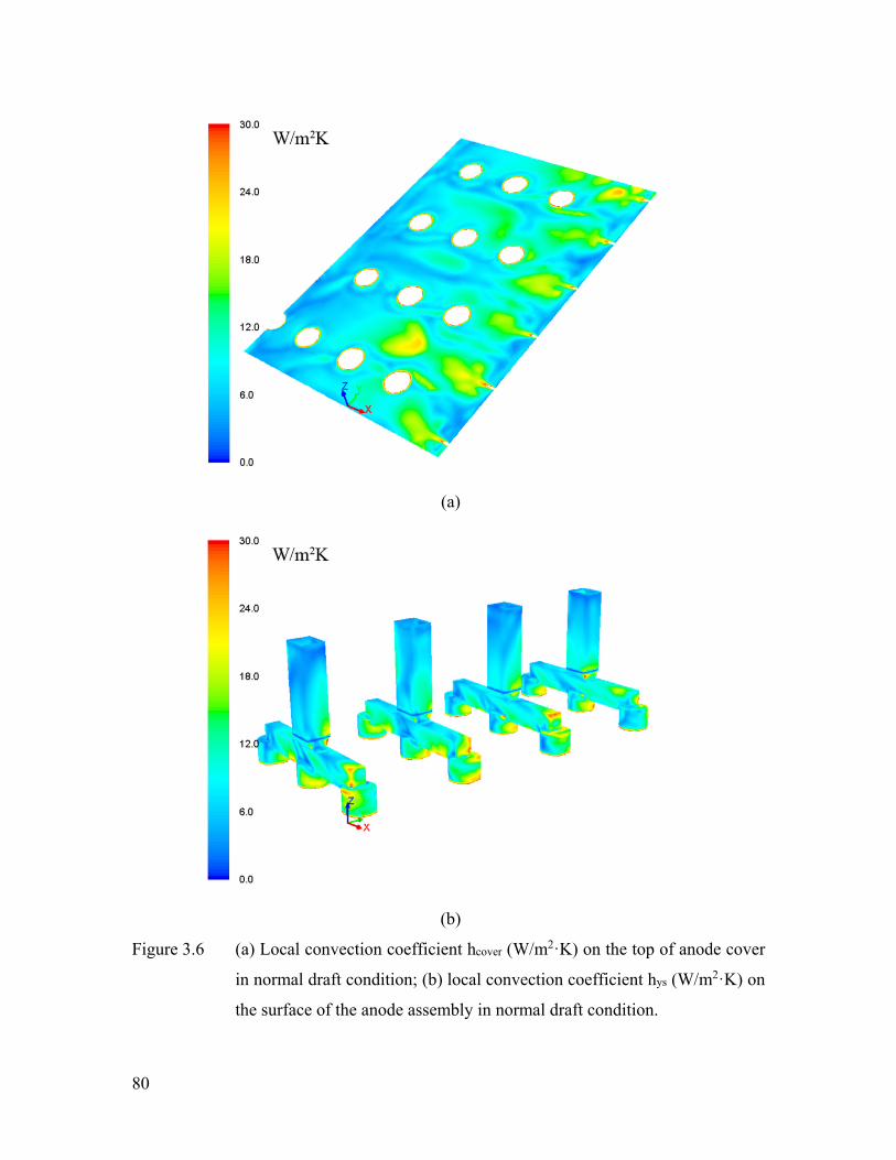
80

(a)

(b)

Figure 3.6 (a) Local convection coefficient hcover (W/m2·K) on the top of anode cover

in normal draft condition; (b) local convection coefficient hys (W/m2·K) on

the surface of the anode assembly in normal draft condition.

81

as the average value on the anode cover. The gaps between hoods create jets of cold air

into the cavity. An intense heat exchange occurs in the side-channels of the smelter

because of the relatively high velocity of the jet and of a large temperature difference

between the cold air and the anode cover surface. Then, the anode assemblies act as

obstacles to the flow, and reduce flow velocity along with momentum diffusion. The

smallest values of the local convective coefficient were found in the internal channel (the

middle area of the pots) and in the vicinity of the bottom edge of the hoods.

Another important surface is that of the anode assembly, which is shown in Fig.

3.6b. The range of local convection coefficient is similar to that observed on the anode

cover, with values up to 30 W/m2·K (the same scale as in Fig. 3.6a is used in Fig. 3.6b for

the sake of comparison). It is seen that the convection coefficient is generally higher on

yoke and stubs than on rods. The most efficient convective areas are all located at the

surfaces that face the upstream flow.

3.7 Forced versus natural convection

When modeling a system such as the one considered in the present study, one of the

initial questions that arises is which of natural or forced convection dominates. As

described in the previous section, it was decided to include buoyancy forces in the model.

Nevertheless, we wanted to quantify the importance of these forces on the overall heat

transfer in the cavity. Developing this understanding is important in order to eventually

propose design modifications either to enhance or block heat transfer in the top section of

electrolytic cells.

In engineering applications, one often compares the role of natural and forced

convection by looking at the ratio of the Grashof number to the square of the Reynolds

number, Gr/Re2, which is sometimes called the Richardson number. When the ratio is

much smaller than 1, natural convection is negligible. Unfortunately, such an approach

proved to be hardly feasible here since the fluid flow and heat transfer patterns are quite

complex, and far from that a parallel flow over a flat plate. Therefore, it was decided to

evaluate the influence of natural convection by performing additional simulations in

which the gravitational force would be disregarded (i.e., in the sole presence of forced

convection), and then to compare the results with that achieved in the presence of gravity.

82

Using the same procedure as previously, we calculated the average convection

coefficients on all studied surfaces, and reported them in Fig. 3.7 (a-d).

First, we note that the convection coefficients are typically smaller when gravity

forces are disregarded. This means that buoyancy forces work to enhance the heat

transfer coefficient. For example, the anode cover temperature is much larger than that of

the air in the cavity, and thus, the cover is a “hot surface facing up”, which will boost the

heat transfer coefficient when gravity forces are accounted for (Jacobs 1987). A similar

observation can be made for the other surfaces, except for the hood. Since the hood is a

“warm surface facing down”, the flow pattern generated by buoyancy forces is weak

since the density pattern is more stable.

When the mass flow rate is reduced, the role of natural convection becomes more

important. This is caused by reduced jet flows (i.e., low value of Re) from the gaps

between hoods in these conditions, and also by the fact that the temperature of all

surfaces will go up which will tend to promote buoyancy forces. In Fig. 3.7(a-d), the

discrepancy between purely forced and mixed convection coefficients is increased as the

pot draft condition is reduced and the forced convection coefficients on the surfaces of

anode cover and yoke and stubs only have approximately half of the value of the mixed

convection coefficients under low draft conditions. This means that natural convection

accounts for roughly half of the convective heat transfer on these surfaces in low draft

conditions, but nevertheless forced convection cannot be neglected. In other words, the

low draft condition is truly a mixed convection situation.

On the other hand, under normal and high ventilation rate, the role of buoyancy

forces is weaker. The difference in heat transfer coefficients (under normal ventilation)

with and without gravity forces is relatively small, less than 5% for the hoods and rods,

less than 10% for the yoke and stubs, and less than 20% for the anode cover surface.

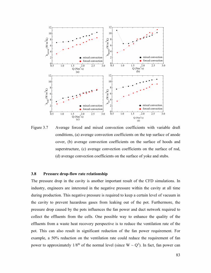
83

0.5 1.0 1.5 2.0 2.5 3.00

2

4

6

8

10

12

0.5 1.0 1.5 2.0 2.5 3.00

2

4

6

8

10

12

0.5 1.0 1.5 2.0 2.5 3.00

2

4

6

8

10

12

0.5 1.0 1.5 2.0 2.5 3.00

2

4

6

8

10

12

h co

ver

(W/m

2 K)

Q (Nm3/s)

mixed convection forced convection

hho

od (

W/m

2 K)

Q (Nm3/s)

mixed convection forced convection

hro

d (W

/m2 K

)

Q (Nm3/s)

mixed convection forced convection

(d)(c)

(b)(a)

hys

(W

/m2 K

)

Q (Nm3/s)

mixed convection forced convection

Figure 3.7 Average forced and mixed convection coefficients with variable draft

conditions, (a) average convection coefficients on the top surface of anode

cover, (b) average convection coefficients on the surface of hoods and

superstructure, (c) average convection coefficients on the surface of rod,

(d) average convection coefficients on the surface of yoke and stubs.

3.8 Pressure drop-flow rate relationship

The pressure drop in the cavity is another important result of the CFD simulations. In

industry, engineers are interested in the negative pressure within the cavity at all time

during production. This negative pressure is required to keep a certain level of vacuum in

the cavity to prevent hazardous gases from leaking out of the pot. Furthermore, the

pressure drop caused by the pots influences the fan power and duct network required to

collect the effluents from the cells. One possible way to enhance the quality of the

effluents from a waste heat recovery perspective is to reduce the ventilation rate of the

pot. This can also result in significant reduction of the fan power requirement. For

example, a 50% reduction on the ventilation rate could reduce the requirement of fan

power to approximately 1/8th of the normal level (since W ~ Q3). In fact, fan power can

Q (Nm3/s) (d)

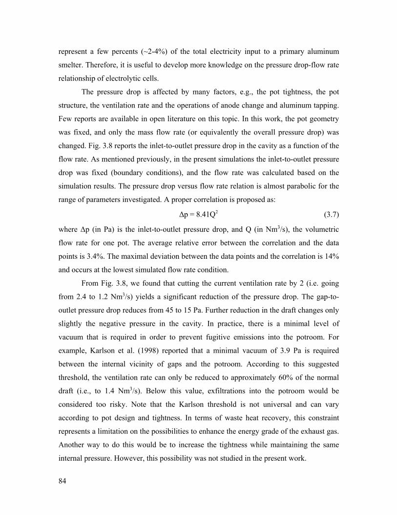
84

represent a few percents (~2-4%) of the total electricity input to a primary aluminum

smelter. Therefore, it is useful to develop more knowledge on the pressure drop-flow rate

relationship of electrolytic cells.

The pressure drop is affected by many factors, e.g., the pot tightness, the pot

structure, the ventilation rate and the operations of anode change and aluminum tapping.

Few reports are available in open literature on this topic. In this work, the pot geometry

was fixed, and only the mass flow rate (or equivalently the overall pressure drop) was

changed. Fig. 3.8 reports the inlet-to-outlet pressure drop in the cavity as a function of the

flow rate. As mentioned previously, in the present simulations the inlet-to-outlet pressure

drop was fixed (boundary conditions), and the flow rate was calculated based on the

simulation results. The pressure drop versus flow rate relation is almost parabolic for the

range of parameters investigated. A proper correlation is proposed as:

2Δp = 8.41Q (3.7)

where Δp (in Pa) is the inlet-to-outlet pressure drop, and Q (in Nm3/s), the volumetric

flow rate for one pot. The average relative error between the correlation and the data

points is 3.4%. The maximal deviation between the data points and the correlation is 14%

and occurs at the lowest simulated flow rate condition.

From Fig. 3.8, we found that cutting the current ventilation rate by 2 (i.e. going

from 2.4 to 1.2 Nm3/s) yields a significant reduction of the pressure drop. The gap-to-

outlet pressure drop reduces from 45 to 15 Pa. Further reduction in the draft changes only

slightly the negative pressure in the cavity. In practice, there is a minimal level of

vacuum that is required in order to prevent fugitive emissions into the potroom. For

example, Karlson et al. (1998) reported that a minimal vacuum of 3.9 Pa is required

between the internal vicinity of gaps and the potroom. According to this suggested

threshold, the ventilation rate can only be reduced to approximately 60% of the normal

draft (i.e., to 1.4 Nm3/s). Below this value, exfiltrations into the potroom would be

considered too risky. Note that the Karlson threshold is not universal and can vary

according to pot design and tightness. In terms of waste heat recovery, this constraint

represents a limitation on the possibilities to enhance the energy grade of the exhaust gas.

Another way to do this would be to increase the tightness while maintaining the same

internal pressure. However, this possibility was not studied in the present work.

85

0.0 0.5 1.0 1.5 2.0 2.5 3.00

10

20

30

40

50

60

P (

Pa)

Q (Nm3/s)

Figure 3.8 Inlet-to-outlet pressure drop (solid symbols) and correlation (red line)

versus draft condition.

3.9 Conclusions

In this chapter, we presented a CFD model of the upper part of an aluminum smelting

pot. The model was employed to study the heat transfer mechanisms in that domain. A

comparison with the thermal circuit model showed that both models yielded coherent

results in terms of temperatures and heat transfer rates. The TRC model has the

advantage that is much simpler and faster to use, whereas the CFD model provides more

detailed information.

We have been able to develop new correlations with the CFD model in order to

determine the average convection coefficient on specific surfaces, under different draft

conditions. These correlations are used in our TRC model. The non-uniformity of the

heat transfer coefficient was also revealed by the CFD model, with some surface areas

exhibiting a high heat transfer density and others, a smaller. The relative importance of

natural convection versus forced convection was also studied. We showed that natural

convection works to enhance the heat transfer coefficients most of the times, and that

under normal ventilation rates, most of the heat transfer is due to forced convection,

2ΔP Q

86

whereas under reduced draft, both natural and forced convections are equally important.

Finally, a quadratic pressure drop versus mass flow rate correlation gives a good fit to the

pot CFD results. All the above knowledge can be used in order to analyze current pot

designs and guide future pot developments.

87

CHAPTER 4 REDUCED VENTILATION OF UPPER PART OF ALUMINUM

SMELTING POT: POTENTIAL BENEFITS, DRAWBACKS,

AND DESIGN MODIFICATIONS

88

Abstract

Maintaining current draft conditions in the upper part of Al smelting cell requires

important electricity consumption for the fans. A reduction of the ventilation rate could

significantly diminish the total power requirement at the blowers. However, adverse

changes in operating conditions due to this ventilation reduction may disrupt the pot

thermal equilibrium. A CFD model was created to investigate the influence of ventilation

reduction on pot thermal balance. With the objective of maintaining normal heat losses

by the top of the cell, several modifications are simulated, such as using plate fins on the

anode assembly, changing hood gap geometry and modifying anode cover thickness.

Heat transfer rates are determined for these modified designs, and compared to those

currently achieved.

89

Résumé

Maintenir les conditions de ventilation actuelle dans la partie supérieure des cuves

d’électrolyse requiert une grande quantité d’électricité pour actionner les ventilateurs.

Réduire le taux de ventilation pourrait significativement réduire la consommation des

ventilateurs. Par contre, des impacts négatifs sur les conditions d’opération pourraient

résulter d’une réduction du taux de ventilation. Un modèle CFD a été créé pour étudier

l’impact de la réduction de ventilation sur les cuves. L’objectif est de maintenir le même

taux de dissipation thermique par le dessus des cuves. Des modifications sont proposées à

cet effet, telles que l’ajout d’ailettes sur l’assemblage anodique, des changements dans la

géométrie des gaps entre les capots et sur l’épaisseur de la couverture anodique. Les taux

de transfert thermique ont été déterminés pour chaque nouveau design et comparé à la

situation actuelle.

90

4.1 Introduction

Today’s aluminum reduction technology is based on the Hall-Héroult process, which

requires intensive energy input. Typically, ~13-15 MWh are required for producing 1 ton

of Al, and roughly half of the energy input is lost from pots as waste heat. Due to the

extensive amount of heat lost in the Al production industry, waste heat recovery has

become a much researched topic in recent years. The “simplest” way to capture waste

heat is from the pot exhaust gas which contains ~35%-40% of the heat lost by pots.

Sørhuus and Wedde (2009) presents the design of a heat exchanger (HEX) for cooling the

collected pot gases and thus recovering heat from them. Fouling on the HEX surfaces

was analyzed and it was found that an annual cleaning was sufficient to maintain a proper

heat transfer in the HEX even though the pot exhaust is largely contaminated with fouling

agents. Fleer et al. (2010) paid attention to the particle characteristics in the effluent,

exhaust gas properties, and fouling propensity in the gas stream in front of the dry

scrubber. The aforementioned works are mainly focused on current pot effluents, which

are at a relatively low temperature (~100-130˚C). Such low energy grade limits the

potential usage of the waste heat.

Several theoretical and experimental studies have shown that the cell ventilation

condition has the most influence on the pot exhaust temperature and heat content. Based

on reported measurements in Gadd’s thesis (Gadd 2003), the exhaust temperature could

increase by 50˚C when cell draft is reduced to 40% of the normal condition. Abbas et al.

(2009) has determined the top heat losses in different draft conditions (i.e., from 3% to

160% of normal draft conditions) based on CFD simulations. This work shows that the

pot effluents temperature can increase by over 100˚C as the draft condition decreases to

20% of normal conditions. This work also proposes some geometrical modifications of

the smelting pot to enhance the thermal quality of the pot gases (Abbas 2010). Lorentsen

et al. (2009) reported that Hydro (Norway) has developed a gas suction technology that

collects the CO2 close to the feed hole, yielding a warmer and more concentrated flue

gas, with less fan power required. An increase of temperature means an enhancement of

the thermal quality of the waste heat, while an increase of CO2 concentration is desirable

in view of CO2 capture processes. Moreover, reducing the cell ventilation rate can reduce

drastically the fan power requirement, since it is typically proportional to the flow rate to

91

power 3 (Pfan~Q3). For the sake of illustration, let us consider the fan energy consumption

at a typical modern plant producing ~260,000 ton/y of Al. Two fans work to transport the

flue gases to the gas treatment center, each with a power of 8467 kW, for a total annual

electricity consumption as high as 148.3 GWh. Assuming 0.05 US$/kWh, the annual cost

of electricity for fans would be 7.4 MUS$. If one can reduce the ventilation rate by half,

the fan power can be roughly reduced to 1/8th of the normal consumption.

However, reducing pot ventilation may disturb current operating conditions. For

instance, reduced ventilation means that less heat is extracted through the top section of

the smelting pot (Abbas et al. 2009; Zhao et al. 2013a), and therefore, more heat has to be

dissipated via sidewalls which could melt the frozen electrolyte and jeopardize pot

integrity. Another aspect to be considered is the fume emissions from the pots to the

potroom. A certain level of negative pressure should be maintained in the pots to prevent

emissions to potroom.

In this work, we studied the heat transfer impacts of ventilation reduction in an Al

smelting pot with CFD simulations. The model is based on actual pot design and

operation. Different modifications are studied to overcome the adverse changes due to

ventilation reduction. The objective of this work is to compare different scenarios in

order to reduce the ventilation to a minimum level while maintaining current thermal

equilibrium in the bath.

4.2 CFD Model

4.2.1 Simplifying Assumptions

The domain of interest is the upper section of an aluminum reduction cell, above the

electrolytic bath. Several assumptions are made to reduce the computational burden:

(i) A typical 350kA aluminum cell contains 40 anodes, divided in two parallel rows.

By imposing a negative pressure at exit, air in the potroom enters the domain

through gaps between hoods, around anode rods and other superstructure

openings, and dilutes the CO2 released by the Hall-Héroult process. The effluents

are collected in a duct through 5 inlets located equidistantly on the bottom of the

superstructure. Neglecting side effects and considering that the heat transfer and

92

flow pattern is the same below each of the 5 inlets, only the domain above two

anodes needs to be simulated, as shown in Fig. 4.1. Such a unit consists of two

anodes, 1/4 feed hole, 1/4 duct inlet, and the corresponding anode cover,

superstructure and hoods. The flow pattern is periodic in the direction of the

anodes row. This allows simulating only 1/20th of a pot.

(ii) The bottom boundaries of the simulated domain are the immersed part of the

anodic blocks and the bottom surface of crust. The CO2 layer due to the

accumulation of the hot gas emissions from the bath is not included. Here, we

estimated the mass flow rate of the hot gas and imposed it as a mass inflow to the

domain at the feed hole.

(iii) A typical new anode has a height of ~0.6 m, and it is consumed to ~0.15 m before

removal from the pot. The heat transfer rate through an anode varies strongly

during anode consumption. However, since each pot contains 40 anodes at

different levels of consumption, an average height of 0.4 m was assumed for the

anodic blocks.

(iv) A part of the potroom and upper cavity neighboring to the superstructure and

hoods was included in the domain with an extended length of 0.5 m. The

infiltration of air in the cavity under hoods comes from the gaps between hoods.

Other very narrow gaps were ignored in the model. The gap width is 1 cm.

The simulation domain is different from the model presented in chapter 3, because the

purpose of the CFD model right now is to find the influence of different geometrical

modifications on the top heat loss. The model was extended downward to include the

anodes and anode cover, and the prediction error of heat transfer in the pot cavity under

hoods due to the assumed boundary conditions at bottom can be attenuated. New

boundary conditions were defined at the bottom of the anodes and anode cover to

represent the heat exchange with the bath.

4.2.2 Governing Equations

The governing equations are those expressing the conservation of mass, momentum in

each direction, energy, and electrical charge. Reynolds-Averaged Navier-Stokes (RANS)

equations are applied to simulate the turbulent flow. Incompressible fluid flow and

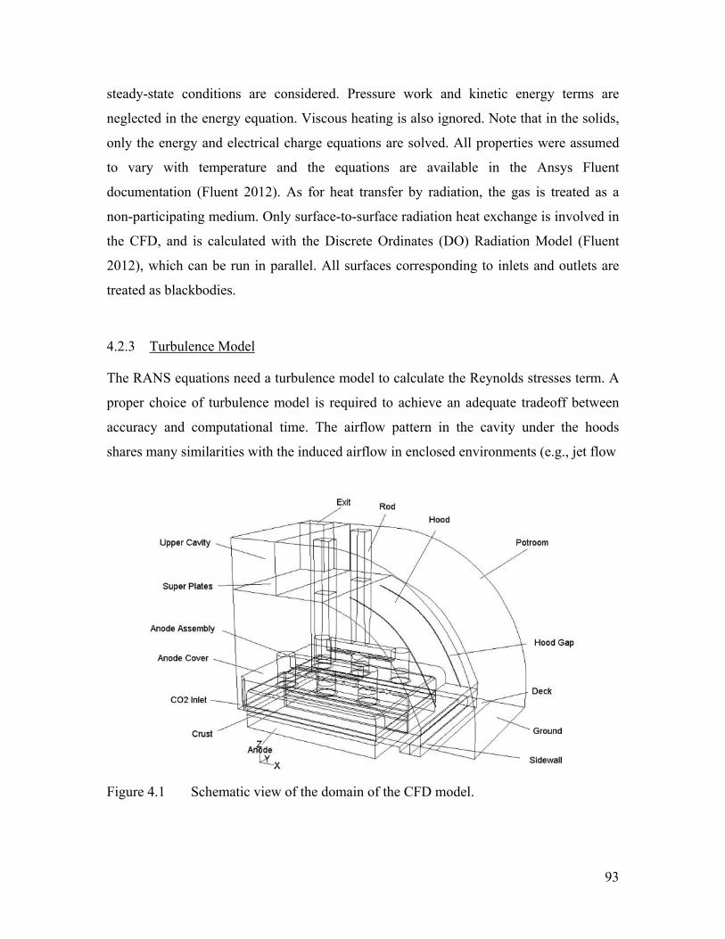
93

steady-state conditions are considered. Pressure work and kinetic energy terms are

neglected in the energy equation. Viscous heating is also ignored. Note that in the solids,

only the energy and electrical charge equations are solved. All properties were assumed

to vary with temperature and the equations are available in the Ansys Fluent

documentation (Fluent 2012). As for heat transfer by radiation, the gas is treated as a

non-participating medium. Only surface-to-surface radiation heat exchange is involved in

the CFD, and is calculated with the Discrete Ordinates (DO) Radiation Model (Fluent

2012), which can be run in parallel. All surfaces corresponding to inlets and outlets are

treated as blackbodies.

4.2.3 Turbulence Model

The RANS equations need a turbulence model to calculate the Reynolds stresses term. A

proper choice of turbulence model is required to achieve an adequate tradeoff between

accuracy and computational time. The airflow pattern in the cavity under the hoods

shares many similarities with the induced airflow in enclosed environments (e.g., jet flow

Figure 4.1 Schematic view of the domain of the CFD model.

94

and impingement on a wall, and buoyancy-driven flow). Before 2005, the k-ε family of

turbulence models was very popular in indoor environment simulation and a general

conclusion is that overall the RNG k-ε model provides the best performance. Recently,

the k-ω turbulence models have attracted more attention in industrial applications. A

comprehensive review on validation of turbulence models was reported in literature (Zhai

et al. 2007; Zhang et al. 2007). They compared CFD simulations to experimental results.

The RNG k-ε and SST k-ω have shown the best performance. In cases with strong natural

convection and high-Reynolds number jet flow, the SST k-ω model provided better

results. In the present problem, airflow at potroom temperature is induced into the cavity

under hoods where the wall temperature can reach 200-300˚C. Strong natural convection

thus occurs between the walls and the airflow in the cavity (Zhao et al. 2013) and for this

reason the SST k-ω model was chosen.

4.2.4 Numerical Modeling and Mesh

The equations of the present model were solved with a CFD commercial software that

relies on the finite volume approach (Fluent 2012). Meshing of the domain was built so

as to respect the requirements of the turbulence model. The SST k-ω model in the CFD

software applies a two-layer zonal model to simulate the flow in the region close to the

walls. However, to avoid first near-wall nodes in the buffer layer region, the near-wall

meshes should ideally be either coarse (y+>30) or fine (y+≈1). Based on earlier work from

Zhao (Zhao et al. 2013), the wall function method (applied to coarse meshes) poorly

describes the near wall region with low Reynolds number flows. The airflow in the

present study is relatively weak and does not have a high Reynolds number near walls.

Moreover, when reducing the pot draft condition, buoyancy will significantly influence

the flow features. Therefore, a fine near-wall mesh is used.

The mesh is created in GAMBIT 2.4 and consists of prism volumes in the

boundary layer and Tet/Hybrid volumes in the core of the domain. A mesh independence

study is presented below. A typical mesh contained ~2.5 million control volumes. The

SIMPLE algorithm was used to solve flow equations. Default criteria in the software

were used to declare convergence of a simulation. The solution strategy relied on a step-

by-step procedure. One can first launch the simulation with a low value of gravity, and

95

converge it using first-order schemes. Following that the resulting physical fields are

used as an initial guess for a new simulation in which gravity is adjusted properly.

Similarly, second-order schemes could then be introduced. Approximately 24 hours were

required for performing one simulation.

4.2.5 Boundary Conditions

Atmospheric pressure is imposed at the potroom boundary. The pressure at the exit (inlet

of the collecting duct) was an adjustable negative pressure (10 to 50 Pa). The exhaust

draft condition can be varied by changing the inlet-to-outlet pressure difference, which is

the sum of pressure losses through hood gaps and in the cavity under hoods. To simulate

the CO2 emission from the bath into the cavity, the bottom surface of feed hole was

defined as a mass inflow boundary from which hot gases (CO2) are released at 940˚C

with a mass flow rate of 2.6 g/s for our simulated domain (based on 1.3 vol% hot gas

concentration in the pot effluents). Since the properties of CO2 are close to those of air

and the typical CO2 concentration is just ~1-2% in the exhaust, we replaced the CO2 gas

with air to simplify the model. The turbulence intensity was set to 1% at all flow

boundaries to indicate a low turbulent inflow. Turbulent viscosity ratio was fixed to 1 at

the potroom boundary for simulating an external free flow (Fluent 2012). The hydraulic

diameter was used to define the turbulence at the mass inflow and outlet boundaries.

Impermeability and no-slip flow are assumed on all other solid surfaces.

Convective heat transfer is imposed at the surface of anode blocks immersed in

the bath, at the external surface of the sidewall and at the surface of deck and ground. The

bath temperature was set at 955˚C. Combined external radiation and convection heat

transfer is defined at the bottom surface of the crust and the surfaces of anode exposed in

the CO2 layer. The gas temperature representing CO2 was 940˚C in the present

simulations. The convection coefficient in the pseudo CO2 layer was determined by an

analysis presented in the next section. At the potroom boundary, the ambient temperature

near the pot is set to 50˚C while the temperature is assumed to 70˚C at the boundary of

upper cavity. Radiation between the pot surfaces and the far-field environment is also

considered in the model. The background temperature in the potroom was 30˚C, and that

96

for the upper cavity, 70˚C. On sidewalls, a heat transfer coefficient of 10 W/m2K was

considered with an ambient temperature of 100˚C. The emissivity of anode cover and

crust were 0.4 and 0.3, respectively (Rye et al. 1995). The emissivity of metal surfaces in

the cavity was 0.8, while it was 0.5 at the surfaces outside the cavity (Perry et al. 1984).

Electrical insulation is imposed on all surfaces of the domain except for the top surface of

rod where a current of 8500 A/rod is imposed and the bottom of anodes imposed by a

zero voltage.

4.3 Verification and Validation

Values of y+ were verified on all wall boundaries. The value of y+ is equal to ~1 in the

cavity under hoods and ~1-3 in the potroom and upper cavity, which satisfies the

requirement of the enhanced wall function used in SST k-ω model. Also, the blending

function, which is incorporated in the SST k-ω model and which controls the turbulent

model transition between the standard k-ε model in the core area and the k-ω model in

the near-wall regions, was looked at. It was found that the k-ε model was successfully

applied in the areas of jet flow and the core space of the cavity, while the k-ω mode was

activated in the area near wall surfaces.

Mesh independence was thoroughly investigated. Previous work (Zhao et al.

2013) showed that a maximum control volume length scale of 5 cm in the core area of

flow domain is fine enough to capture the main heat transfer and flow patterns. However,

a refined surface mesh is required in particular areas such as for the gaps and anode

assembly. The bulk volumes are created based on the surface mesh and gradually grown

to 5 cm (mesh#1, 2.45 million control volumes). A mesh with a maximum volume length

scale of 3 cm was also created (mesh#2), with 3.98 million control volumes. Mesh#1 was

compared to mesh#2 for both ventilation rates (i.e., normal 2.4 Nm3/s, and reduced to 1.2

Nm3/s). Results did not change significantly from mesh#1 to mesh#2 (Table 4.1).

Therefore, mesh#1 is considered adequate for the rest of this work. An analysis was

performed to determine proper values for some uncertain simulation parameters. For

example, a series of simulations was performed with different distances from the surface

of hoods to the potroom boundary. It was found that the mass flow rate and temperature

of the exhaust, and the heat transfer rate from the bath did not change when the potroom

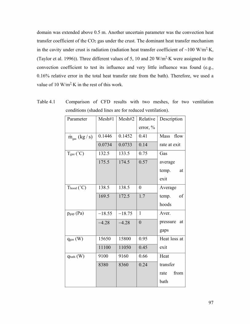
97

domain was extended above 0.5 m. Another uncertain parameter was the convection heat

transfer coefficient of the CO2 gas under the crust. The dominant heat transfer mechanism

in the cavity under crust is radiation (radiation heat transfer coefficient of ~100 W/m2K,

(Taylor et al. 1996)). Three different values of 5, 10 and 20 W/m2K were assigned to the

convection coefficient to test its influence and very little influence was found (e.g.,

0.16% relative error in the total heat transfer rate from the bath). Therefore, we used a

value of 10 W/m2K in the rest of this work.

Table 4.1 Comparison of CFD results with two meshes, for two ventilation

conditions (shaded lines are for reduced ventilation).

Parameter Mesh#1 Mesh#2 Relative

error, %

Description

gasm (kg / s) 0.1446 0.1452 0.41 Mass flow

rate at exit 0.0734 0.0733 0.14

Tgas (˚C) 132.5 133.5 0.75 Gas

average

temp. at

exit

175.5 174.5 0.57

Thood (˚C) 138.5 138.5 0 Average

temp. of

hoods

169.5 172.5 1.7

pgap (Pa) 18.55 18.75 1 Aver.

pressure at

gaps

4.28 4.28 0

qgas (W) 15650 15800 0.95 Heat loss at

exit 11100 11050 0.45

qbath (W) 9100 9160 0.66 Heat

transfer

rate from

bath

8380 8360 0.24

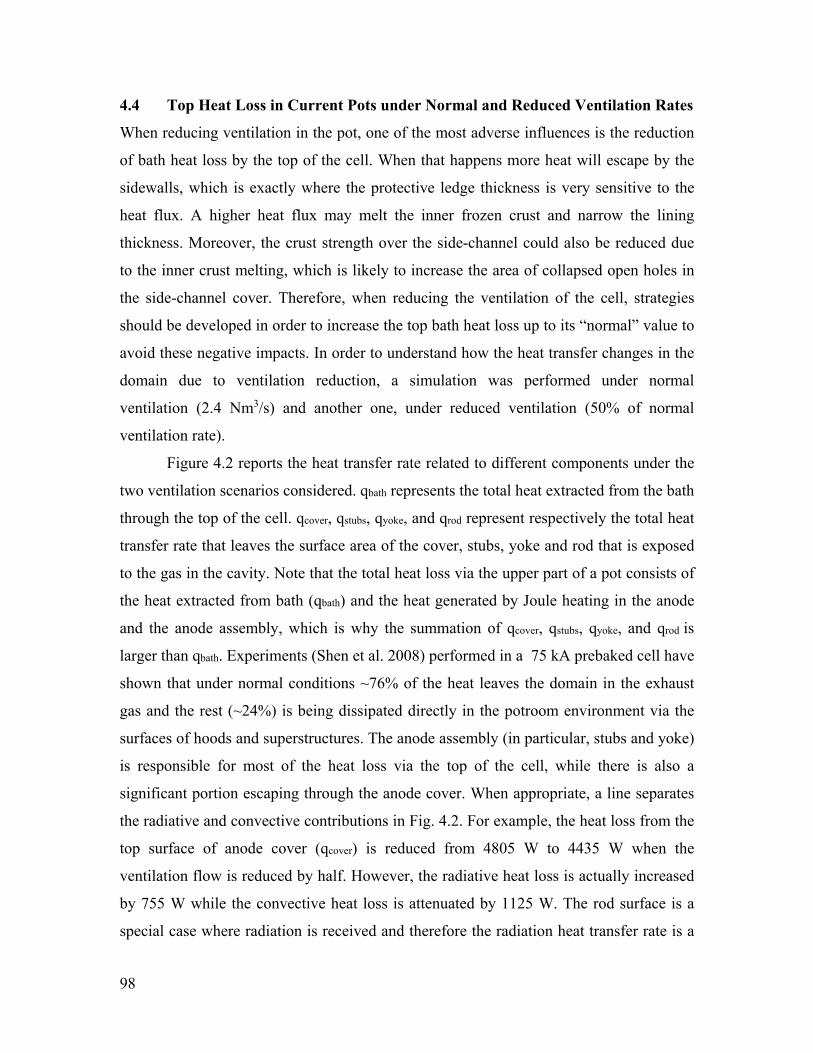
98

4.4 Top Heat Loss in Current Pots under Normal and Reduced Ventilation Rates

When reducing ventilation in the pot, one of the most adverse influences is the reduction

of bath heat loss by the top of the cell. When that happens more heat will escape by the

sidewalls, which is exactly where the protective ledge thickness is very sensitive to the

heat flux. A higher heat flux may melt the inner frozen crust and narrow the lining

thickness. Moreover, the crust strength over the side-channel could also be reduced due

to the inner crust melting, which is likely to increase the area of collapsed open holes in

the side-channel cover. Therefore, when reducing the ventilation of the cell, strategies

should be developed in order to increase the top bath heat loss up to its “normal” value to

avoid these negative impacts. In order to understand how the heat transfer changes in the

domain due to ventilation reduction, a simulation was performed under normal

ventilation (2.4 Nm3/s) and another one, under reduced ventilation (50% of normal

ventilation rate).

Figure 4.2 reports the heat transfer rate related to different components under the

two ventilation scenarios considered. qbath represents the total heat extracted from the bath

through the top of the cell. qcover, qstubs, qyoke, and qrod represent respectively the total heat

transfer rate that leaves the surface area of the cover, stubs, yoke and rod that is exposed

to the gas in the cavity. Note that the total heat loss via the upper part of a pot consists of

the heat extracted from bath (qbath) and the heat generated by Joule heating in the anode

and the anode assembly, which is why the summation of qcover, qstubs, qyoke, and qrod is

larger than qbath. Experiments (Shen et al. 2008) performed in a 75 kA prebaked cell have

shown that under normal conditions ~76% of the heat leaves the domain in the exhaust

gas and the rest (~24%) is being dissipated directly in the potroom environment via the

surfaces of hoods and superstructures. The anode assembly (in particular, stubs and yoke)

is responsible for most of the heat loss via the top of the cell, while there is also a

significant portion escaping through the anode cover. When appropriate, a line separates

the radiative and convective contributions in Fig. 4.2. For example, the heat loss from the

top surface of anode cover (qcover) is reduced from 4805 W to 4435 W when the

ventilation flow is reduced by half. However, the radiative heat loss is actually increased

by 755 W while the convective heat loss is attenuated by 1125 W. The rod surface is a

special case where radiation is received and therefore the radiation heat transfer rate is a

99

negative value (indicated by the dotted bars, in Fig. 4.2). The convective heat loss is

actually the sum of the solid bar (net heat loss) and the dotted bar in each case.

Figure 4.2 Heat losses due to convection and radiation from different

components in different ventilation conditions.

When the ventilation flow is reduced by half, the total heat transfer rate extracted

from bath by the top of the cell is decreased from 9040 W to 8165 W, i.e. a reduction of

875 W (in the two anodes model). In practice, this extra heat of 875 W would have to

escape from other pot components. It is found that the heat losses from all surfaces are

reduced somehow. And although the heat loss reduction by each surface seems relatively

weak, their sum is large enough to potentially influence the overall pot thermal balance.

Looking at Fig. 4.2, one can also conclude that convective heat losses are reduced in a

less ventilated pot, while the radiation increases due to warmer surfaces. However, the

overall enhanced radiative heat loss is not enough to compensate the reduction in

convective heat loss. Convection is the main mechanism for heat loss from anode cover

surface, while radiation dominates the heat loss from anode assembly surface.

Some conclusions can be drawn from the abovementioned analysis. These will

help to design proper modifications to the pot in order to maintain thermal equilibrium

under low ventilation scenarios:

(i) The convective heat loss in the cavity is decreased as the ventilation is reduced, while

the raditive heat loss has the opposite behavior.

0

1

2

3

4

5

6

7

8

9

10

bath cover stubs yoke rod

2.4 Nm3/s

1.2 Nm3/s

q(k

W)

rad

conv

conv

convrad

rad

100

(ii) The enhanced radiative heat loss is not enough to compensate the reduction of

convective heat loss due to ventilation reduction, and this is the main reason why the net

top heat loss is reduced.

(iii) Radiation plays a significant role on the yoke and stubs for the two draft conditions.

When ventilation is reduced, radiation becomes the most influencing mechanism in the

top heat loss.

Three types of modifications are studied in the following sections to achieve

proper thermal equilibrium (i.e., to extract from the bath the missing 875 W of heat

mentioned previously): use of fins on the anode assembly, change of the gaps geometry,

and change of anode cover geometry and surface properties.

4.5 Addition of Fins on Anode Assembly

The first group of scenarios is the addition of fins on the anode assembly. Plate fins were

positioned on anode yoke and stubs, as shown in Fig. 4.3. The purpose of the fins is to

increase the convective heat loss from the anode assembly to the airflow in the cavity.

Traditionally, the design of fins involves an optimization of different design variables,

e.g. fin dimensions, materials and arrangement. Here, we studied two designs (cases a1

and a2) to evaluate their efficiency in maintaining top heat loss under low flow of

ventilation. We fixed the fin width and thickness at 5 cm and 1 cm, respectively. Fin

material is steel (as yoke and stubs). Case a1 only has one plate fin, while case a2 has

three plate fins. New meshes were built with the fins and CFD simulations were

performed under reduced ventilation for these designs.

The influence of fins on the total heat transfer rate from bath is shown in Fig. 4.4.

Compared to the 1.2 Nm3/s ventilated situation with no fins (case_1/2), case a1 increases

the heat transfer rate from the bath by 315W and case a2 by 385W, respectively (see Fig.

4.4). It is found that using one or three fins does not change significantly the net top heat

losses. However, in both cases, there is still a significant gap for achieving the “normal”

heat transfer rate dissipated via the top section under normal level of ventilation flow.

The use of fins on anode assembly was thus found to be inadequate to fully compensate

the reduction of top heat loss caused by such reduced ventilation flow. Even though this

scenario could be applied, the addition of fins on anode assembly needs to deal with

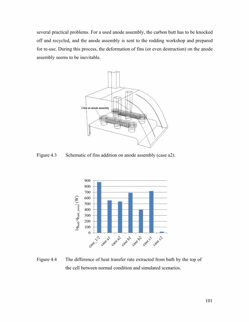
101

several practical problems. For a used anode assembly, the carbon butt has to be knocked

off and recycled, and the anode assembly is sent to the rodding workshop and prepared

for re-use. During this process, the deformation of fins (or even destruction) on the anode

assembly seems to be inevitable.

Figure 4.3 Schematic of fins addition on anode assembly (case a2).

Figure 4.4 The difference of heat transfer rate extracted from bath by the top of

the cell between normal condition and simulated scenarios.

0

100

200

300

400

500

600

700

800

900

|qba

th-q

bath

_nor

m|(

W)

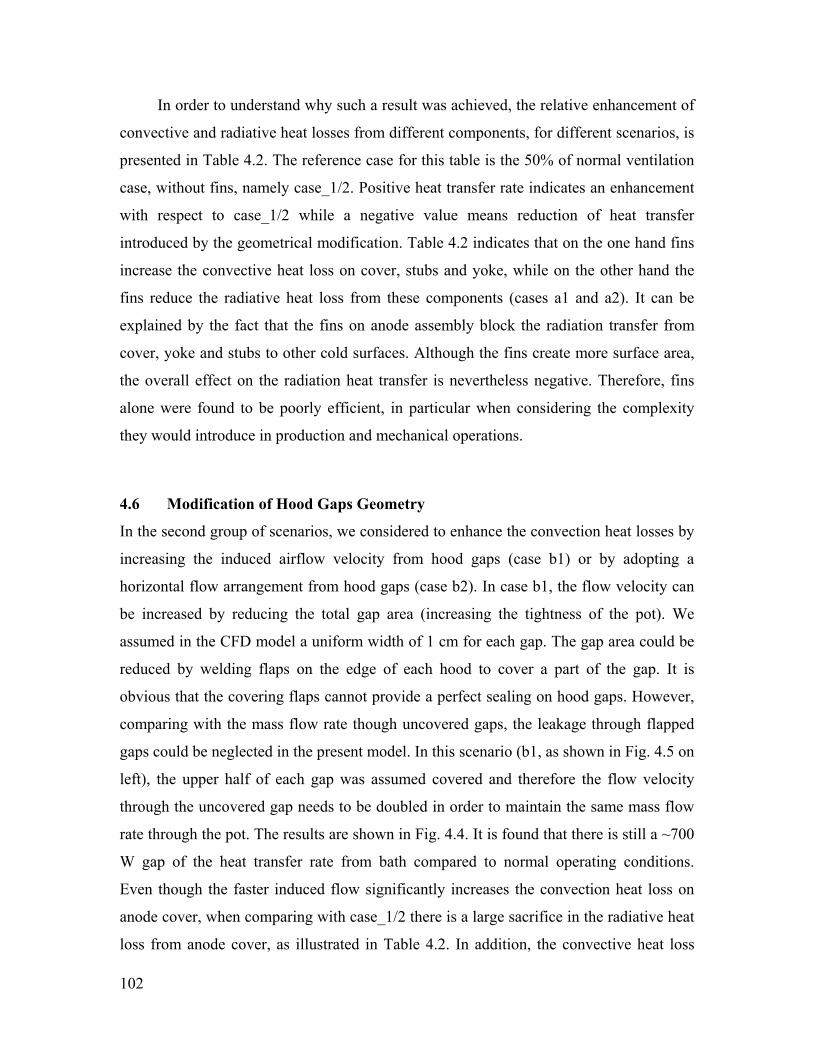
102

In order to understand why such a result was achieved, the relative enhancement of

convective and radiative heat losses from different components, for different scenarios, is

presented in Table 4.2. The reference case for this table is the 50% of normal ventilation

case, without fins, namely case_1/2. Positive heat transfer rate indicates an enhancement

with respect to case_1/2 while a negative value means reduction of heat transfer

introduced by the geometrical modification. Table 4.2 indicates that on the one hand fins

increase the convective heat loss on cover, stubs and yoke, while on the other hand the

fins reduce the radiative heat loss from these components (cases a1 and a2). It can be

explained by the fact that the fins on anode assembly block the radiation transfer from

cover, yoke and stubs to other cold surfaces. Although the fins create more surface area,

the overall effect on the radiation heat transfer is nevertheless negative. Therefore, fins

alone were found to be poorly efficient, in particular when considering the complexity

they would introduce in production and mechanical operations.

4.6 Modification of Hood Gaps Geometry

In the second group of scenarios, we considered to enhance the convection heat losses by

increasing the induced airflow velocity from hood gaps (case b1) or by adopting a

horizontal flow arrangement from hood gaps (case b2). In case b1, the flow velocity can

be increased by reducing the total gap area (increasing the tightness of the pot). We

assumed in the CFD model a uniform width of 1 cm for each gap. The gap area could be

reduced by welding flaps on the edge of each hood to cover a part of the gap. It is

obvious that the covering flaps cannot provide a perfect sealing on hood gaps. However,

comparing with the mass flow rate though uncovered gaps, the leakage through flapped

gaps could be neglected in the present model. In this scenario (b1, as shown in Fig. 4.5 on

left), the upper half of each gap was assumed covered and therefore the flow velocity

through the uncovered gap needs to be doubled in order to maintain the same mass flow

rate through the pot. The results are shown in Fig. 4.4. It is found that there is still a ~700

W gap of the heat transfer rate from bath compared to normal operating conditions.

Even though the faster induced flow significantly increases the convection heat loss on

anode cover, when comparing with case_1/2 there is a large sacrifice in the radiative heat

loss from anode cover, as illustrated in Table 4.2. In addition, the convective heat loss

103

from the anode assembly is not significantly increased in this case. The flow induced

from the lower half gap is “trapped” in the side-channel which is formed by the height

difference between the anodic block and the pot deck. Another negative effect is that the

more tight pot structure introduces a significant increase on the driving pressure

difference (i.e. from 10 Pa to 40 Pa) and would therefore need additional fan power to

maintain 50% of normal ventilation. In the future, an optimization on the flow pattern

could be helpful for the convection enhancement on the anode assembly.

To replace current vertical gaps, a horizontal gap was considered in case b2, as

shown in Fig. 4.5 on right. With such geometry, the flow passes more efficiently over the

anode cover and anode assembly. A horizontal gap on hoods was created in the CFD

model and the gaps between hoods were covered by flaps as in case b1. From Fig. 4.4,

we found that the heat transfer rate from bath was increased by ~475 W when compared

with the 50% normal ventilation case. In other words, there is still ~400 W of heat

extracted from the bath that is missing compared to normal conditions. Table 4.2

indicates that the convective heat losses from cover, stubs and yoke are distinctly

enhanced by such flow arrangement. However, the overall enhancement of heat loss is

attenuated by the reduction of radiation heat transfer on all three surfaces. This is due to

the strong temperature-dependence of radiative emissions. A small surface temperature

reduction induced by convection can result in a large radiative heat transfer reduction. In

any case, both strategies b1 and b2 are not adequate enough to recover the reduction of

top heat loss under the low ventilation condition studied here. Moreover, a reduction in

the gap area will also induce a significant additional pressure difference to maintain the

ventilation rate as it is.

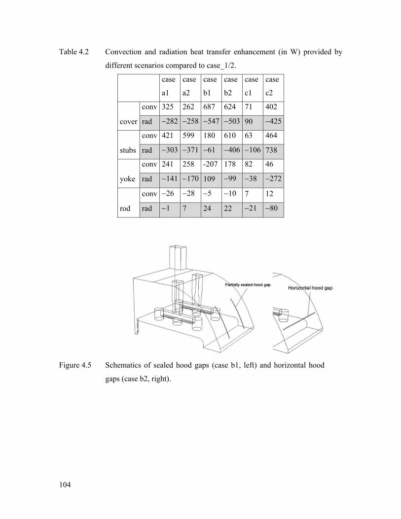
104

Table 4.2 Convection and radiation heat transfer enhancement (in W) provided by

different scenarios compared to case_1/2.

case

a1

case

a2

case

b1

case

b2

case

c1

case

c2

cover

conv 325 262 687 624 71 402

rad 282 258 547 503 90 425

stubs

conv 421 599 180 610 63 464

rad 303 371 61 406 106 738

yoke

conv 241 258 -207 178 82 46

rad 141 170 109 99 38 272

rod

conv 26 28 5 10 7 12

rad 1 7 24 22 21 80

Figure 4.5 Schematics of sealed hood gaps (case b1, left) and horizontal hood

gaps (case b2, right).

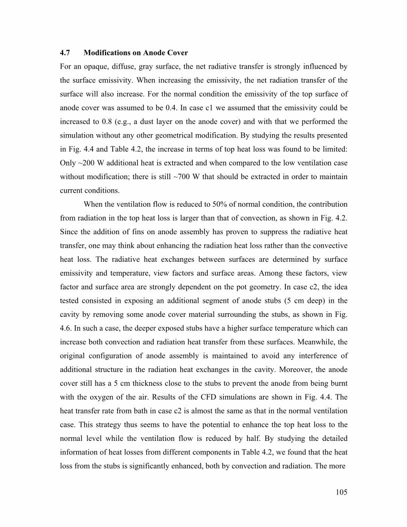
105

4.7 Modifications on Anode Cover

For an opaque, diffuse, gray surface, the net radiative transfer is strongly influenced by

the surface emissivity. When increasing the emissivity, the net radiation transfer of the

surface will also increase. For the normal condition the emissivity of the top surface of

anode cover was assumed to be 0.4. In case c1 we assumed that the emissivity could be

increased to 0.8 (e.g., a dust layer on the anode cover) and with that we performed the

simulation without any other geometrical modification. By studying the results presented

in Fig. 4.4 and Table 4.2, the increase in terms of top heat loss was found to be limited:

Only ~200 W additional heat is extracted and when compared to the low ventilation case

without modification; there is still ~700 W that should be extracted in order to maintain

current conditions.

When the ventilation flow is reduced to 50% of normal condition, the contribution

from radiation in the top heat loss is larger than that of convection, as shown in Fig. 4.2.

Since the addition of fins on anode assembly has proven to suppress the radiative heat

transfer, one may think about enhancing the radiation heat loss rather than the convective

heat loss. The radiative heat exchanges between surfaces are determined by surface

emissivity and temperature, view factors and surface areas. Among these factors, view

factor and surface area are strongly dependent on the pot geometry. In case c2, the idea

tested consisted in exposing an additional segment of anode stubs (5 cm deep) in the

cavity by removing some anode cover material surrounding the stubs, as shown in Fig.

4.6. In such a case, the deeper exposed stubs have a higher surface temperature which can

increase both convection and radiation heat transfer from these surfaces. Meanwhile, the

original configuration of anode assembly is maintained to avoid any interference of

additional structure in the radiation heat exchanges in the cavity. Moreover, the anode

cover still has a 5 cm thickness close to the stubs to prevent the anode from being burnt

with the oxygen of the air. Results of the CFD simulations are shown in Fig. 4.4. The

heat transfer rate from bath in case c2 is almost the same as that in the normal ventilation

case. This strategy thus seems to have the potential to enhance the top heat loss to the

normal level while the ventilation flow is reduced by half. By studying the detailed

information of heat losses from different components in Table 4.2, we found that the heat

loss from the stubs is significantly enhanced, both by convection and radiation. The more

106

Figure 4.6 Schematic of more exposed stubs in the cavity (case c2).

exposed stubs with higher temperature (~500ºC) can emit more radiation while

convective heat loss is also increased as a result from more stubs in contact with the

airflow in the cavity. Lastly, this modification will induce little effect on the total

driving pressure between the gaps and exit.

4.8 Conclusions

Different advantages can be envisioned by a reduction of cell ventilation. However, it

also creates thermal imbalance compared to current pot operation since less heat is

removed from the bath by the top of the cell. A CFD model of the upper part of a typical

cell was developed in order to investigate different scenarios. The objective was to find

how to maintain the same amount of heat removed from the bath even when the

ventilation is reduced. The most promising set-up found was to expose a larger portion of

the stubs to the flow of air. In future work, different simultaneous combinations of the

different scenarios could be investigated.

107

CHAPTER 5 AIRFLOW AND THERMAL CONDITIONS IN ALUMINUM

SMELTING POTROOMS UNDER DIFFERENT CONDITIONS

108

Abstract

Potrooms are elongated buildings in which electrolysis of alumina is carried out, and

have the particularity, among others, to be naturally ventilated. A CFD model is

developed to simulate the ventilation and heat transfer patterns within a smelter potroom.

The model is used to study thermal comfort in the potroom under different wind and

outdoor temperature scenarios. The influence of wind and buoyancy on the airflow rate

though potroom openings is demonstrated. The heat stress during hot weather is assessed

for the different cases. In particular, the reduction of pot ventilation rate, a potential

strategy for facilitating waste heat recovery from smelting cells, is assessed in terms of its

influence on the thermal conditions in the potroom. It is found that the pot draft reduction

can be realised without significantly increasing the heat stress.

109

Résumé

Les salles de cuves sont des bâtiments alongés où l’électrolyse de l’aluminium est

réalisée et qui ont comme particularité d’être ventilées naturellement. Un modèle CFD est

développé pour simuler la ventilation et le transfert thermique dans ce bâtiment. Le

modèle est utilisé pour étudier le confort thermique dans la salle de cuves sous différentes

conditions de vent et de température extérieure. L’influence du vent et de la force

d’Archimède sur le débit d’air évacué est démontrée. Le stress thermique pendant l’été

est déterminé pour différents cas. En particulier, la réduction de la ventilation des cuves,

(une stratégie potentielle pour faciliter la récupération des rejets thermiques d’une cuve)

est étudiée en termes de son influence sur les conditions thermiques dans la salle de

cuves. Il est montré que les modifications de ces conditions n’ont pas d’impacts

significatifs.

110

5.1 Introduction

Primary aluminum is produced via the Hall-Héroult process (Grjotheim and Kvande

1986). Electrolytic cells (often called “pots”) are aligned in a long building named a

“potroom”, as shown in Fig. 5.1a. As our reference, this is an Alcoa’s smelter at

Deschambault in Québec, Canada (ADQ). Although this process is over a century old, the

energy efficiency is still relatively low, with roughly half of the energy input dissipated

into the atmosphere in the form of waste heat. Considering that efficiency, the electricity

requirement of 13-15 MWh to produce one ton of aluminum, and typical plant

dimensions and productivity, it can be estimated that the smelting process corresponds to

a continuous internal heat gain of ~6500 W/m2 of floor. This value is quite large

compared to internal gains in other types of buildings. The typical ventilation system to

cope with this heat gain in potrooms is described with more details in Section 5.2.

The process heat escapes from a pot in part through its shell directly into the

potroom air. Also, heat is released via the pot exhaust gases (mixture of dilution air

introduced into the pot and of process by-products such as CO2), collected by a duct

system. The exhaust gas can contain ~35-40% of the total waste heat, at a temperature

approximately 100C above ambient. Although the amount of heat released from pots is

enormous, most of the heat either has a relatively low thermal quality (low temperature)

or is difficult to recover (sensitive to working conditions). In order to increase the

potential benefits of using pot gas for waste heat recovery, its temperature would need to

be increased. Several theoretical and experimental studies have illustrated that the pot

exhaust gas temperature is significantly increased by reducing the amount of dilution air

introduced in the pot, i.e. the pot ventilation level (Gadd 2003; Abbas et al. 2009; Abbas

2010; Lorentsen et al. 2009). Recently, Zhao et al. (2013; 2013a) have studied the top

heat losses in a smelting pot, and their results have demonstrated the potential of

increasing pot gas temperature up to 50C by reducing half of the pot normal draft level.

Considering an application such as power generation with an Organic Rankine Cycle, this

temperature raise could significantly increase the efficiency of the cycle in such a way

that it could become more viable. However, attention should be paid on the influence of

pot draft condition on potroom building performance and workers’ health. A reduced pot

ventilation redistributes the heat losses in the upper part of smelting cells (Abbas et al.

111

2009; Zhao et al. 2013a). A portion of the heat, previously taken away by the exhaust gas

will be redirected into the potroom. Considering current high internal heat gain in

potroom, it is required to verify how reduced pot ventilation would modify thermal

conditions in potroom and how the overall potroom ventilation would be affected. Also,

the influence of outdoor weather conditions combing with the reduced pot draft condition

is yet to be addressed. Building heat stress in harsh environments such as potrooms in

summer should be carefully assessed to maintain people’s safety and health.

Modifications in the potroom, if necessary, should thus be done before implementing pot

ventilation reduction.

Computational Fluid Dynamics (CFD) has become very popular to study

ventilation patterns in the built environment over the past 20 years (Chow 1995; Li et al.

2013). Building ventilation can be qualified of either mechanical or natural depending on

the driving mechanisms. Ventilation in potrooms is almost entirely driven by buoyancy

forces due to the heat released from smelting pots. Furthermore, wind is also important as

it creates a pressure difference at the openings of the building. One of the exploratory

works on simulating turbulent flow in the presence of strong buoyancy forces in a

building enclosure was performed by Cook and Lomas (1998), where they validated the

two eddy viscosity turbulence model for predicting a buoyancy-driven ventilated flow by

comparing simulation results with experimental measurements. Cook et al. (2003) used

CFD simulations to study the wind-assisted stack ventilation of a single-storey enclosure

with high and low-level openings. They developed an approach to impose constant

pressure boundary conditions at the inlet and outlet of the enclosure rather than to

simulate the flow transport through them from an external domain. This approach can

significantly reduce the simulated domain while maintaining an accurate prediction of

flow and thermal conditions in the enclosure. Recently, Ji et al. (Ji et al. 2007; Ji and

Cook 2007) extended their CFD models into more complicated building structures, such

as single-storey with atrium and multi-storey with atrium.

In the present paper, we estimate the influence of pot ventilation reduction on the

flow pattern and thermal conditions in potroom by using CFD simulations. In addition to

presenting an advanced potroom ventilation model, the main purpose is to verify whether

the thermal conditions in the potroom under low pot ventilation levels are acceptable. An

112

allowable working time is calculated to assess the heat stress based on the thermal

balance between the human metabolism and the hot environment. In addition, the

changes in airflow patterns and temperature fields around the pot are of interest. In order

to reduce the computational burden, the outdoor environment was not included in the

CFD model and we considered the wind-assisted ventilation by imposing an equivalent

pressure difference between the inlet and outlet of the potroom. Several typical scenarios,

considering the influences of wind, ambient temperature, and solar radiation, were

simulated.

5.2 Description of the ventilation in potrooms

In modern smelters, aluminum is produced in a series of elongated buildings called

potrooms, each of which containing several dozens of smelting pots. A typical potroom

can have a footprint of 1000 m by 30 m, and a height of 25 m. Pots are lined up along the

potroom length and are electrically connected in series. Figure 5.1b shows the simulated

geometry, which consists of one slice of potroom where two half-pots and other pieces of

equipment are included. Normally, one end of the pot is facing the working aisle for

tapping operations, and the other end is connected with the ducts collecting pot exhaust

gases. Between two pots, a space is reserved for the installation of busbars and for pot

operations (e.g., anode change).

Because the aluminum reduction process releases a large amount of heat from pot

shell into the potroom (~450 kW per pot), outdoor air is used for cooling down the pots

and keeping the potroom environment comfortable. Additionally, a certain amount of air

from the potroom is driven into the pots (to collect CO2 and other gases emitted by the

process) and must be replaced by fresh air. Finally, pollutants released from pots and

other equipment into the potroom (such as HF, SO2, etc.), if any, must be diluted by the

makeup air to acceptable concentration levels.

Ventilation of smelters relies essentially on buoyancy forces. The potroom can be

viewed as a two-storey building. The lower floor is the basement, where openings are

created on the two long façades of the building. The openings are equipped with panels

that can be adjusted to increase or reduce their effective areas, and thus, the amount of

makeup air. This adjustment is performed on a seasonal timescale and panels are usually

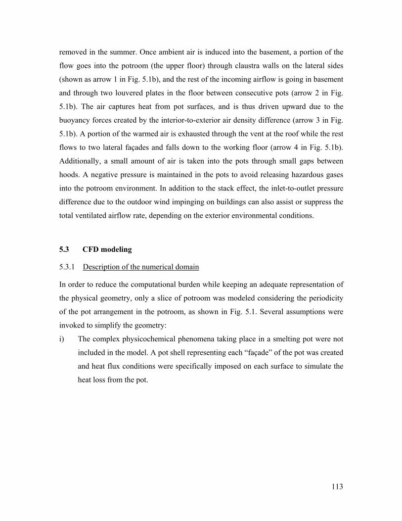
113

removed in the summer. Once ambient air is induced into the basement, a portion of the

flow goes into the potroom (the upper floor) through claustra walls on the lateral sides

(shown as arrow 1 in Fig. 5.1b), and the rest of the incoming airflow is going in basement

and through two louvered plates in the floor between consecutive pots (arrow 2 in Fig.

5.1b). The air captures heat from pot surfaces, and is thus driven upward due to the

buoyancy forces created by the interior-to-exterior air density difference (arrow 3 in Fig.

5.1b). A portion of the warmed air is exhausted through the vent at the roof while the rest

flows to two lateral façades and falls down to the working floor (arrow 4 in Fig. 5.1b).

Additionally, a small amount of air is taken into the pots through small gaps between

hoods. A negative pressure is maintained in the pots to avoid releasing hazardous gases

into the potroom environment. In addition to the stack effect, the inlet-to-outlet pressure

difference due to the outdoor wind impinging on buildings can also assist or suppress the

total ventilated airflow rate, depending on the exterior environmental conditions.

5.3 CFD modeling

5.3.1 Description of the numerical domain

In order to reduce the computational burden while keeping an adequate representation of

the physical geometry, only a slice of potroom was modeled considering the periodicity

of the pot arrangement in the potroom, as shown in Fig. 5.1. Several assumptions were

invoked to simplify the geometry:

i) The complex physicochemical phenomena taking place in a smelting pot were not

included in the model. A pot shell representing each “façade” of the pot was created

and heat flux conditions were specifically imposed on each surface to simulate the

heat loss from the pot.

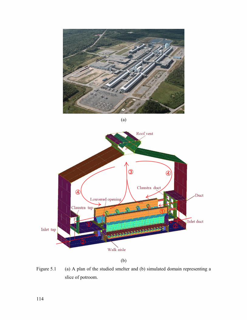
114

(a)

(b)

Figure 5.1 (a) A plan of the studied smelter and (b) simulated domain representing a

slice of potroom.

115

ii) We ignored the detailed geometry of the structure above the super plate (i.e., anode

bars, holding beam, and joint parts). Five busbars were considered. The assumption

is reasonable since in the present work we are not interested in the detailed heat

transfer and fluid flow in the vicinity of these parts. At the duct end, a segment of

the pot collecting duct was included in the model. Although the pot geometry is

significantly simplified, the thermal boundary conditions are defined in such a way

that the total amount of heat released in the potroom is as in the actual one.

iii) The only pot gaps included in the model are the openings between hoods. However,

due to the tremendous scale variation between the gap breadth (~0.005-0.05 m) and

the potroom width (~20 m), it is difficult to model the real gap geometry, and at the

same time, maintain the number of control volumes of the mesh to an acceptable

value. A series of ten gaps with a width 0.1 m were thus created to represent hood

gaps on each side of a pot. Gaps between hoods and superstructure, and around

anode rods were not considered, because of their small surface areas.

iv) The pot shell has many extrusive structures which could tremendously increase the

number of modelling cells. A series of pot cradles was considered since it creates a

significant resistance to airflow. Moreover, there exist other components in the

basement between two pots, such as the cathode collecting bar, the anode and

cathode busbars. All these structures were represented by a single large bar located

in the area between two pots. A porous jump surface was created beneath the bar

for simulating the resistance to airflow of these bars on the up-rising air flow.

v) The perforated claustra wall and louvered pot sides create additional resistance to

airflow. In the model, a porous zone is defined to simulate the claustra wall, and a

porous jump surface is considered at the louver area.

5.3.2 Governing equations

The governing equations representing the conservations of mass, momentum in each

direction, and energy are discretized and solved with a commercial CFD software, Ansys

Fluent 13.0. Turbulence was considered in the governing equations via the Reynolds-

averaged Navier-Stokes (RANS) method. The Reynolds stresses term due to turbulence is

modeled based on the Boussinesq eddy viscosity assumption. Detailed formulas are

116

available in literature (Fluent 2012). In the present problem, incompressible flow and

steady-state conditions are considered. Pressure work and kinetic energy terms are

neglected in the energy equation since the gas is treated as an incompressible flow.

Viscous heating is also disregarded in the simulation. Species diffusion is not considered

in the problem.

The air properties (i.e., specific heat, thermal conductivity and viscosity) are

functions of temperature (polynomial fittings based on the data published in (Bergman et

al. 2011)). The air density is modeled by using the “incompressible-ideal-gas” model, and

is defined as:

op

w

p

RT

M

(5.1)

where R is the universal gas constant, Mw, the molecular weight of the gas, and pop, the

defined operating pressure (constant) which is the mean pressure in the simulated

domain. Under this approach, the air density is only influenced by the local temperature

field and the buoyancy force in the momentum equations is proportional to density

variations. A “reduced pressure” (pressure minus hydrostatic pressure, i.e.

,refp p gH ), is considered in the momentum equations. Therefore, a reference

density ref should be defined. In the present case, it is equal to that at the outdoor

temperature in order to consider stack effect appropriately. Detailed description of these

choices is presented in (Zhao and Gosselin 2014).

A turbulence model is required to close the model. Two equation eddy-viscosity

turbulence models are generally suitable for the simulation of air flow and heat transfer of

indoor environments, particularly when the time-averaged parameters, such as mean

temperature or mean flow velocity, are the results of interest (Zhai et al. 2007; Zhang et

al. 2007). Based on a literature review, it was found that the RNG k-ε model and the SST

k-ω model are the most appreciated two equation eddy-viscosity models used in the

simulation of indoor air flow. Since the SST k-ω model shows a good performance in the

simulations of various types of natural ventilation in buildings (Hussain and Oosthuizen

2012b; Ramponi and Blocken 2012), it is determined to simulate the turbulence in all

simulations in this work.

117

Discrete Ordinates (DO) model was used in the simulations to account for

radiation, since this model is supported for parallel calculations. Although air is treated as

a non-participating medium, DOs allow determining surface-to-surface heat transfer rates

in the complex geometry of this problem. Additionally, this radiation model can also

provide the radiant temperature field within the entire domain, which is required in order

to assess thermal comfort of the workers (Parsons 1999).

The model is solved in steady-state conditions. The method to interpolate the

variable gradient is the least squares cell-based gradient evaluation. PRESTO! scheme is

chosen for the pressure interpolation at the surfaces of control volume. Pressure-velocity

coupling is achieved by using SIMPLE segregated algorithm. All of the other variables

are interpolated with a second-order upwind scheme except for the radiative intensity,

which can be appropriately calculated in the first-order because the air is considered as

non-participating medium and the optical thickness is thus zero in the radiation transport

equation. Convergence is achieved when scaled residues of the governing equation are

reaching the default recommended values (Fluent 2012).

5.3.3 Boundary conditions

As mentioned previously, the exterior of the potroom was not included in the simulation.

Based on the approach developed in (Cook et al. 2003), pressure was imposed at the

inlets and outlets of the potroom to represent the wind force. The pressure created by the

wind on the building façade is calculated by the following equation:

2_

1

2wind p wind o refp C U (5.2)

where Cp_wind is the pressure coefficient, ρo the exterior air density, and refU the mean

wind speed at an external reference position. Cp_wind is a dimensionless parameter and is

influenced by the shape of the building, the wind direction and the neighboring terrain.

Although Cp_wind values can be obtained from some established correlations or calculation

programs, determining the correct pressure coefficient is a challenge in itself. A CFD

model was created to simulate the air movement around a potroom building (Zhao and

Gosselin 2014). The results illustrated that the Cp_wind values are quite different from

118

those calculated from the available tools, because of the geometrical specificity of

potroom (i.e. an extremely elongated shape). We adopted the interpolated wind pressure

coefficients at windward, leeward and top roof from the CFD model of the previous

work. It should be noticed that these Cp_wind values are only valid for the wind direction

perpendicular to the lateral potroom walls.

A special attention needs to be devoted to determining Uref in Eq. (5.2). Normally,

the mean wind speed is measured at the height of a meteorological station tower which is

located in a relatively flat terrain and with no local shielding. The variation of mean wind

speed with the height is most commonly represented by a power law expression. Eq. (5.3)

was used to adjust the mean wind speed from a local meteorological station to the terrain

of the studied building.

met

refmetref met

met

HU U

H

(5.3)

where Umet is the mean wind speed measured at the tip of the weather station tower, and

Hmet, the height of the tower, usually 33 ft (10 m) above ground level. The reference

height Href is usually defined as 10 m from the ground. α and δ are atmospheric boundary

layer parameters and determined based on the classification of terrain category

(ASHRAE 2009). The values of wind speed measured at the closest weather station were

thus adjusted with Eq. (5.3) to obtain the required reference velocity. In this work,

reference velocity values of 0, 5 and 15 km/h were found to be representative of different

levels of wind strength. Once the reference velocity, along with the average pressure

coefficients at the inlets and outlets are obtained, the imposed pressure boundary

conditions could be calculated using Eq. (5.2). For the smelter considered (ADQ), two

wind directions are of particular interest, from northwest and from southeast, both of

which being approximately perpendicular to the two long façades of the potroom. As

seen in Fig. 5.1, the potroom-slice model has an inlet at the tapping end (the side close to

the walking aisle), an inlet at the duct end (the side close to the off-gas collecting ducts)

and an outlet at the roof vent. With the CFD model that was developed, one can define

either the tapping end or the duct end as the windward side (positive pressure) to simulate

the wind blowing from either direction. Table 5.1 presents the calculated pressure

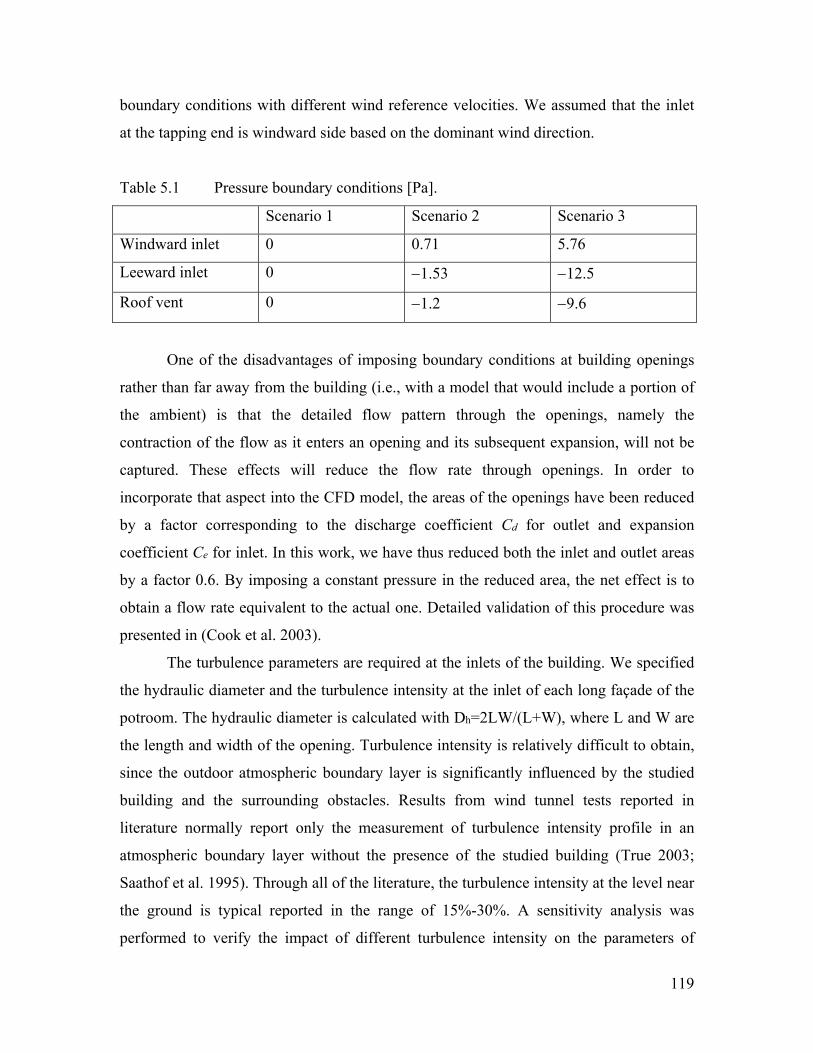
119

boundary conditions with different wind reference velocities. We assumed that the inlet

at the tapping end is windward side based on the dominant wind direction.

Table 5.1 Pressure boundary conditions [Pa].

Scenario 1 Scenario 2 Scenario 3

Windward inlet 0 0.71 5.76

Leeward inlet 0 1.53 12.5

Roof vent 0 1.2 9.6

One of the disadvantages of imposing boundary conditions at building openings

rather than far away from the building (i.e., with a model that would include a portion of

the ambient) is that the detailed flow pattern through the openings, namely the

contraction of the flow as it enters an opening and its subsequent expansion, will not be

captured. These effects will reduce the flow rate through openings. In order to

incorporate that aspect into the CFD model, the areas of the openings have been reduced

by a factor corresponding to the discharge coefficient Cd for outlet and expansion

coefficient Ce for inlet. In this work, we have thus reduced both the inlet and outlet areas

by a factor 0.6. By imposing a constant pressure in the reduced area, the net effect is to

obtain a flow rate equivalent to the actual one. Detailed validation of this procedure was

presented in (Cook et al. 2003).

The turbulence parameters are required at the inlets of the building. We specified

the hydraulic diameter and the turbulence intensity at the inlet of each long façade of the

potroom. The hydraulic diameter is calculated with Dh=2LW/(L+W), where L and W are

the length and width of the opening. Turbulence intensity is relatively difficult to obtain,

since the outdoor atmospheric boundary layer is significantly influenced by the studied

building and the surrounding obstacles. Results from wind tunnel tests reported in

literature normally report only the measurement of turbulence intensity profile in an

atmospheric boundary layer without the presence of the studied building (True 2003;

Saathof et al. 1995). Through all of the literature, the turbulence intensity at the level near

the ground is typical reported in the range of 15%-30%. A sensitivity analysis was

performed to verify the impact of different turbulence intensity on the parameters of

120

interest, e.g., the ventilated airflow rates through inlets and outlet, the temperature at the

vent, etc. The results have shown that increasing the turbulence intensity at the inlet from

10% to 30% only had a marginal effect on the parameters of interest. The turbulence

conditions in the upstream flow have a very limited influence on the flow condition

inside the potroom since the ventilated air flow pattern is strongly redefined when it is

going through the claustra walls and the louvered sides.

A special attention was devoted to the pot louvered sides and to the two lateral

claustra walls, which consist of internal sub-structures and provide additional resistances

to the airflow represented by porous jumps. The software user’s guide (Fluent 2012)

provides an analytical expression, which is widely applied for calculating the mass flow

rate of a turbulent flow through square-edged holes in a plate:

2(2 ) / (1 ( / ) )d f f pm C A p A A (5.4)

Rearranging the equation and using the relationship pm vA , we can obtain

2

22

( / ) 11 1

2p f

d

p

A Apv

x C t

C

(5.5)

where the right-hand side term corresponds to a pressure loss coefficient, pC . Smith and

Winkle have proposed correlations for the discharge coefficient, C, through perforated

plates with square-edged holes on equilateral triangular spacing for different Reynolds

numbers (Smith and Van Winkle 1958). The claustra wall at the side of the walking aisle

is actually a square-hole perforated wall. We found an approximate discharge coefficient

of Cd=0.95 based on these correlations and the geometrical characteristics of the claustra

wall (i.e. thickness of the wall, hydraulic diameter of the holes, and ratio of hole pitch and

hole diameter). Then the pressure loss coefficient of the claustra wall was calculated. As

for the other claustra wall (at the duct end), 6 empty blocks were created in the wall body.

Since the porosity in each hole is extremely high (~ 0.95), we assumed no flow resistance

there. Finally, a porous-jump wall was defined on the louvered surfaces. The porous

thickness is set at 6 cm and the pressure loss coefficient, 20 m–1.

Thermal boundary conditions were applied on the surface of the potshells. Based

on a series of measurements of heat losses from potshells performed by Alcoa, the

121

thermal boundary conditions were determined in order to achieve the same level of heat

dissipation in the potroom as in practice. Uniform heat fluxes were assumed on all pot

surfaces except for the pot sidewall where large variations of heat flux were observed in

measurements. A polynomial fit of the heat flux versus position was created at the

sidewall based on experimental measurements. As mentioned in the introduction,

scenarios with reduced pot ventilation will be simulated in this work. In such a case, the

capacity of the pot exhaust flow to carry away heat from the pot will be reduced due to

smaller mass flow rate. A portion of the dissipated heat that was previously exhausted by

the pot flue gases will be redirected to the pot superstructures (including hoods). A new

distribution of the heat losses from the upper part of the pot was obtained based on our

previous work (Zhao et al. 2013; Zhao et al. 2013a). The heat losses distribution among

the pot gas, pot superstructure and hoods was established for a variety of ventilation

conditions. Even in reduced pot ventilation scenarios, it is assumed that the total heat loss

will remain constant, only its distribution between the different pot components will

change. This is a prerequisite condition for reducing pot ventilation because the heat

balance in bath should be maintained all the time. Zhao et al. (2013a) have shown that it

is possible to maintain the pot thermal balance in reduced pot ventilation by adjusting

different aspects of the pot design and operation. Table 5.2 presents the defined heat flux

on pot shell under normal and 50% reduced pot ventilation rates.

For the surfaces of the façade (external wall of the potroom), convection and sky

radiation were considered. A “universal” correlation was (Palyvos 2008) used to

determine the convective heat transfer coefficient on windward and leeward walls for

different wind speeds. Based on the book of heat transfer (Mills 1999), it is possible to

define a sky temperature for radiative heat transfer based on the air temperature at ground

level and a sky effective emissivity, Tsky=((0.727+0.0060Tdp ( C) )T(Kelvin)4)1/4, with the

ambient temperature T and the dewpoint of the air, Tdp. The solar irradiation incident on

potroom walls was calculated based on the time and solar position. A detailed procedure

for its calculation is shown in (McQuiston et al. 2010). Heat sources were applied in each

parts of the potroom envelope (e.g. roof at tap side, wall at tap side) to represent the

absorbed solar radiation. Finally, all boundaries in the domain, except the openings, were

modeled as no-slip wall boundaries.

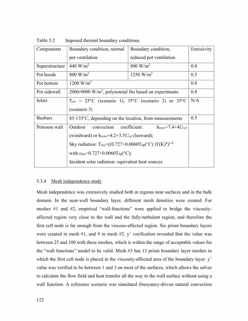
122

Table 5.2 Imposed thermal boundary conditions.

Components Boundary condition, normal

pot ventilation

Boundary condition,

reduced pot ventilation

Emissivity

Superstructure 440 W/m2 800 W/m2 0.8

Pot hoods 800 W/m2 1250 W/m2 0.5

Pot bottom 1200 W/m2 0.8

Pot sidewall 2000-9000 W/m2, polynomial fits based on experiments 0.8

Inlets Tair = 25C (scenario 1), 35C (scenario 2) or 35C

(scenario 3)

N/A

Busbars 85-135C, depending on the location, from measurements 0.5

Potroom wall Outdoor convection coefficient: hconv=7.4+4Uref

(windward) or hconv=4.2+3.5Uref (leeward);

Sky radiation: Tsky=((0.727+0.0060Tdp(C) )T(K)4)1/4

with εsky=0.727+0.0060Tdp(C);

Incident solar radiation: equivalent heat sources

5.3.4 Mesh independence study

Mesh independence was extensively studied both at regions near surfaces and in the bulk

domain. In the near-wall boundary layer, different mesh densities were created. For

meshes #1 and #2, empirical “wall-functions” were applied to bridge the viscosity-

affected region very close to the wall and the fully-turbulent region, and therefore the

first cell node is far enough from the viscous-affected region. Six prism boundary layers

were created in mesh #1, and 9 in mesh #2. y+ verification revealed that the value was

between 25 and 100 with these meshes, which is within the range of acceptable values for

the “wall functions” model to be valid. Mesh #3 has 13 prism boundary layer meshes in

which the first cell node is placed in the viscosity-affected area of the boundary layer. y+

value was verified to be between 1 and 3 on most of the surfaces, which allows the solver

to calculate the flow field and heat transfer all the way to the wall surface without using a

wall function. A reference scenario was simulated (buoyancy-driven natural convection

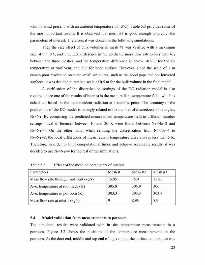
123

with no wind present, with an ambient temperature of 15˚C). Table 5.3 provides some of

the most important results. It is observed that mesh #1 is good enough to predict the

parameters of interest. Therefore, it was chosen in the following simulations.

Then the size effect of bulk volumes in mesh #1 was verified with a maximum

size of 0.3, 0.5, and 1 m. The difference in the predicted mass flow rate is less than 4%

between the three meshes, and the temperature difference is below ~0.5˚C for the air

temperature at roof vent, and 2˚C for hood surface. However, since the scale of 1 m

causes poor resolution on some small structures, such as the hood gaps and pot louvered

surfaces, it was decided to retain a scale of 0.5 m for the bulk volume in the final model.

A verification of the discretization settings of the DO radiation model is also

required since one of the results of interest is the mean radiant temperature field, which is

calculated based on the total incident radiation at a specific point. The accuracy of the

predictions of the DO model is strongly related to the number of discretized solid angles,

Nθ×NΦ. By comparing the predicted mean radiant temperature field in different number

settings, local differences between 10 and 20 K were found between Nθ=NΦ=2 and

Nθ=NΦ=4. On the other hand, when refining the discretization from Nθ=NΦ=4 to

Nθ=NΦ=8, the local differences of mean radiant temperature were always less than 5 K.

Therefore, in order to limit computational times and achieve acceptable results, it was

decided to use Nθ=NΦ=4 for the rest of the simulations.

Table 5.3 Effect of the mesh on parameters of interest.

Parameters Mesh #1 Mesh #2 Mesh #3

Mass flow rate through roof vent (kg/s) 15.95 15.9 15.85

Ave. temperature at roof neck (K) 305.8 305.9 306

Ave. temperature in potroom (K) 303.3 303.3 303.7

Mass flow rate at inlet 1 (kg/s) 9 8.95 8.9

5.4 Model validation from measurements in potroom

The simulated results were validated with in situ temperature measurements in a

potroom. Figure 5.2 shows the positions of the temperature measurements in the

potroom. At the duct end, middle and tap end of a given pot, the surface temperature was

124

measured at 4 points on the hood, 3 on the upper part of sidewall, and 1 on the lower part

of sidewall (i.e., 24 data points). Temperature was also measured at two pot cradles for

each sidewall position (only one cradle is shown in the figure). Temperature of potroom

roof and side walls was measured at 4 locations. Finally, air temperature was measured at

the roof vent, and at 3 positions at shoulder-level on the catwalk (the zone between two

pots) indicated by red triangles in Figure 5.2. In the end, 34 measurement points were

taken as a set of data. This set of data has been measured at 5 different days in order to

consider different exterior conditions (i.e., high vs. low wind speed, daytime vs.

nighttime, etc.).

A comparison between the CFD results and the measurements is reported in Table

5.4. A positive value means that the CFD result is larger than the measurement, and vice

versa. Due to space limitation, only selected results are shown here. Measurement

campaign A was done at noon during a sunny day. The wind speed was 5 km/h, based on

a nearby meteorological station. Measurement campaign B was performed in a partly-

sunny morning, and the wind speed was 10 km/h. The wind direction was perpendicular

to the potroom wall at the tap. It is important to mention that due the inherent nature of

industrial systems such as the one studied in this work, variability can be quite important.

Temperatures is affected by a number of incontrollable elements such as the level of

consumption of the anodes, the level of erosion of the refractories and cathodes, the plant

operations, etc., and actually varies from pot to pot. In other words, an “exact” agreement

between measurements and CFD simulations is not possible, and is actually not sought.

The model is used to compare the scenarios with different pot ventilation levels and

outdoor wind conditions. The purpose of the validation is to evaluate or quantify the level

of agreement between the model and the reality, and to verify that the model can predict

adequately the most important trends related to the objectives of this work.

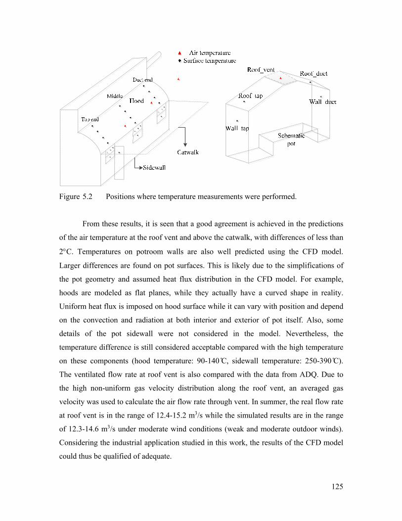
125

Figure 5.2 Positions where temperature measurements were performed.

From these results, it is seen that a good agreement is achieved in the predictions

of the air temperature at the roof vent and above the catwalk, with differences of less than

2C. Temperatures on potroom walls are also well predicted using the CFD model.

Larger differences are found on pot surfaces. This is likely due to the simplifications of

the pot geometry and assumed heat flux distribution in the CFD model. For example,

hoods are modeled as flat planes, while they actually have a curved shape in reality.

Uniform heat flux is imposed on hood surface while it can vary with position and depend

on the convection and radiation at both interior and exterior of pot itself. Also, some

details of the pot sidewall were not considered in the model. Nevertheless, the

temperature difference is still considered acceptable compared with the high temperature

on these components (hood temperature: 90-140 C, sidewall temperature: 250-390 C).

The ventilated flow rate at roof vent is also compared with the data from ADQ. Due to

the high non-uniform gas velocity distribution along the roof vent, an averaged gas

velocity was used to calculate the air flow rate through vent. In summer, the real flow rate

at roof vent is in the range of 12.4-15.2 m3/s while the simulated results are in the range

of 12.3-14.6 m3/s under moderate wind conditions (weak and moderate outdoor winds).

Considering the industrial application studied in this work, the results of the CFD model

could thus be qualified of adequate.

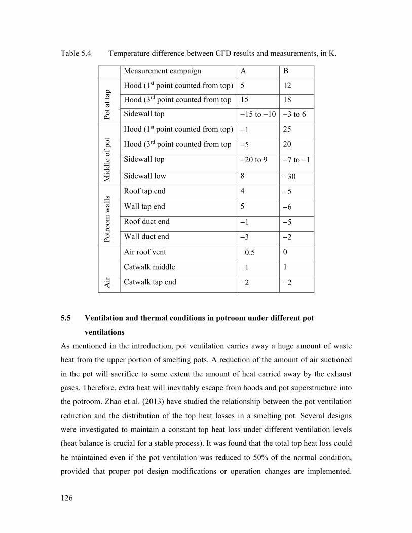
126

Table 5.4 Temperature difference between CFD results and measurements, in K.

Measurement campaign A B

Pot

at t

ap

d

Hood (1st point counted from top) 5 12

Hood (3rd point counted from top 15 18

Sidewall top 15 to 10 3 to 6 M

iddl

e of

pot

Hood (1st point counted from top) 1 25

Hood (3rd point counted from top 5 20

Sidewall top 20 to 9 7 to 1

Sidewall low 8 30

Pot

room

wal

ls Roof tap end 4 5

Wall tap end 5 6

Roof duct end 1 5

Wall duct end 3 2

Air

Air roof vent 0.5 0

Catwalk middle 1 1

Catwalk tap end 2 2

5.5 Ventilation and thermal conditions in potroom under different pot

ventilations

As mentioned in the introduction, pot ventilation carries away a huge amount of waste

heat from the upper portion of smelting pots. A reduction of the amount of air suctioned

in the pot will sacrifice to some extent the amount of heat carried away by the exhaust

gases. Therefore, extra heat will inevitably escape from hoods and pot superstructure into

the potroom. Zhao et al. (2013) have studied the relationship between the pot ventilation

reduction and the distribution of the top heat losses in a smelting pot. Several designs

were investigated to maintain a constant top heat loss under different ventilation levels

(heat balance is crucial for a stable process). It was found that the total top heat loss could

be maintained even if the pot ventilation was reduced to 50% of the normal condition,

provided that proper pot design modifications or operation changes are implemented.

127

However, heat will be redistributed among different components of the pot. In the present

work, we study cases in which pot ventilation is reduced by half while the total top heat

loss is unchanged. Therefore, proper thermal boundary conditions on pot hoods and

superstructure both for the normal and 50% reduced ventilation levels should be properly

defined, as shown in Table 5.2. The heat losses from pot sidewalls and bottom are

assumed to be unchanged.

5.5.1 Outdoor condition scenarios

The outdoor environmental conditions influence strongly the conditions in the potroom.

Therefore, three scenarios were designed to represent different environmental conditions.

Scenario 1 assumes that the outdoor air temperature is 25˚C, with a 0 km/h wind. In other

words, the potroom ventilation is driven only by buoyancy forces. This scenario is valid

when the exterior wind is weak (e.g., wind speed smaller than 5 km/h). It is typically a

good representation of what happens at the night, when the atmosphere boundary layer is

calm. 25 C is the maximum local ambient temperature at night in summer in the plant

considered. Scenario 2 is designed to simulate potroom ventilation with a 5 km/h local

wind speed perpendicularly approaching to the potroom wall at the tap end. The outdoor

air temperature under this scenario is 35˚C. This scenario represents a situation with a

very hot environment and moderate wind-assisted potroom ventilation during daytime.

Finally, the wind speed is increased to 15 km/h in scenario 3. The outdoor air temperature

is still considered to be 35˚C. This third scenario represents hot daytime with windy

conditions.

5.5.2 Effect of pot ventilation reduction on potroom ventilation

First, the influence of reduced pot ventilation on the potroom ventilation was

investigated. The airflow rates through different openings of the potroom (e.g., roof vent,

claustra walls and louvered opening) were determined from the CFD simulations, under

both normal and 50% reduced pot ventilation levels, see Fig. 5.3a-e. In practice, it is

desirable to maintain or enhance the total ventilated air flow from roof vent to provide an

adequate cooling of the potroom. In Fig. 5.3a, the mass flow rate at the roof vent is

128

actually increased by ~1 kg/s in all scenarios when 50% reduced pot ventilation is

simulated. This can be explained by the fact that the pots dissipate more heat into the

potroom as pot ventilation goes down, which actually promotes buoyancy forces and thus

induces more make-up air into the potroom. Fig. 5.3b shows the airflow temperature at

the roof vent. It is increased by 2-3˚C under 50% reduced pot ventilation for all scenarios.

Figs. 5.3c-e reveal that the mass flow rate experiences no significant reduction through

internal openings (<0.4 kg/s) between the two different pot ventilations. However, large

variations are found among the different scenarios, i.e. under different wind conditions. It

is seen that the ventilated air from the roof vent is suppressed when the outdoor wind

becomes significant. The claustra wall at the tap end (windward) introduces much more

air into potroom when the wind-assisted ventilation becomes stronger. On the other side

(leeward), the direction of the flow is actually reversed through the other claustra wall

when the outdoor wind reaches 15 km/h, and cross ventilation between the two lateral

inlets occurs. A portion of air coming from the claustra wall at tapping end will leave

from the claustra wall at duct end. The air flowing through the louvered plates into the

potroom is also suppressed, but to a lesser extent.

It can be concluded that the reduced pot ventilation causes limited changes in the

potroom ventilation, while the outdoor wind can significantly influence the ventilation

pattern in the potroom. As the wind speed increases, it tends to suppress the ventilation

from roof vent and can even create cross ventilation between two inlets at the basement.

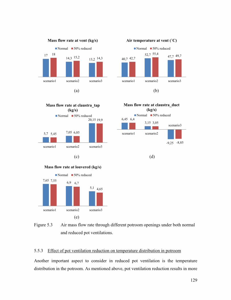
129

(a) (b)

(c) (d)

(e)

Figure 5.3 Air mass flow rate through different potroom openings under both normal

and reduced pot ventilations.

5.5.3 Effect of pot ventilation reduction on temperature distribution in potroom

Another important aspect to consider in reduced pot ventilation is the temperature

distribution in the potroom. As mentioned above, pot ventilation reduction results in more

1714,3 13,2

1815,2 14,3

scenario1 scenario2 scenario3

Mass flow rate at vent (kg/s)

Normal 50% reduced

40,752,7 47,742,7

55,449,7

scenario1 scenario2 scenario3

Air temperature at vent (˚C)

Normal 50% reduced

5,7 7,05

20,15

5,45 6,85

19,9

scenario1 scenario2 scenario3

Mass flow rate at claustra_tap (kg/s)

Normal 50% reduced6,45

3,15

-9,25

6,43,05

-8,85

scenario1 scenario2

Mass flow rate at claustra_duct (kg/s)

Normal 50% reduced

7,656,9

5,1

7,556,7

4,65

scenario1 scenario2 scenario3

Mass flow rate at louvered (kg/s)

Normal 50% reduced

scenario3

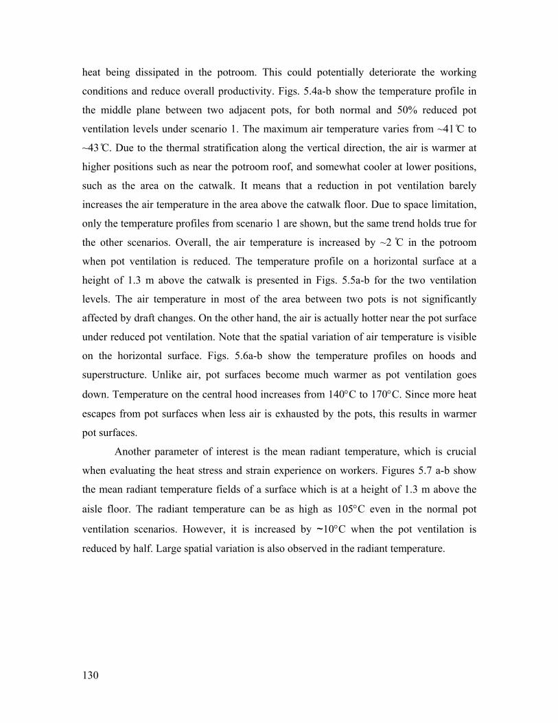
130

heat being dissipated in the potroom. This could potentially deteriorate the working

conditions and reduce overall productivity. Figs. 5.4a-b show the temperature profile in

the middle plane between two adjacent pots, for both normal and 50% reduced pot

ventilation levels under scenario 1. The maximum air temperature varies from ~41 C to

~43 C. Due to the thermal stratification along the vertical direction, the air is warmer at

higher positions such as near the potroom roof, and somewhat cooler at lower positions,

such as the area on the catwalk. It means that a reduction in pot ventilation barely

increases the air temperature in the area above the catwalk floor. Due to space limitation,

only the temperature profiles from scenario 1 are shown, but the same trend holds true for

the other scenarios. Overall, the air temperature is increased by ~2 C in the potroom

when pot ventilation is reduced. The temperature profile on a horizontal surface at a

height of 1.3 m above the catwalk is presented in Figs. 5.5a-b for the two ventilation

levels. The air temperature in most of the area between two pots is not significantly

affected by draft changes. On the other hand, the air is actually hotter near the pot surface

under reduced pot ventilation. Note that the spatial variation of air temperature is visible

on the horizontal surface. Figs. 5.6a-b show the temperature profiles on hoods and

superstructure. Unlike air, pot surfaces become much warmer as pot ventilation goes

down. Temperature on the central hood increases from 140C to 170C. Since more heat

escapes from pot surfaces when less air is exhausted by the pots, this results in warmer

pot surfaces.

Another parameter of interest is the mean radiant temperature, which is crucial

when evaluating the heat stress and strain experience on workers. Figures 5.7 a-b show

the mean radiant temperature fields of a surface which is at a height of 1.3 m above the

aisle floor. The radiant temperature can be as high as 105C even in the normal pot

ventilation scenarios. However, it is increased by ~10C when the pot ventilation is

reduced by half. Large spatial variation is also observed in the radiant temperature.

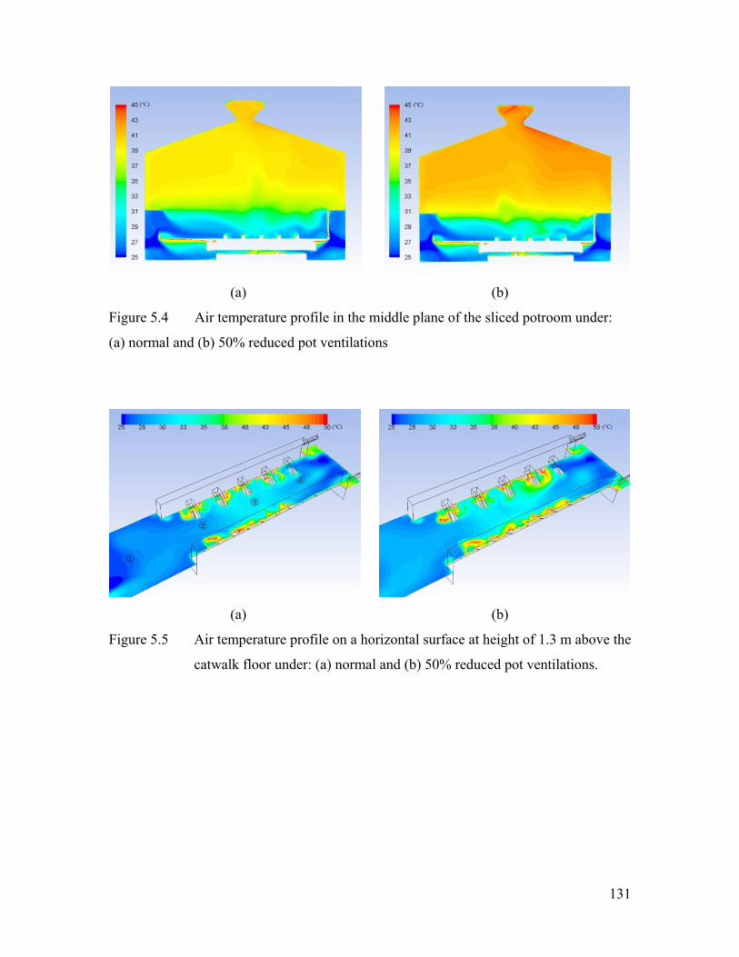
131

(a) (b)

Figure 5.4 Air temperature profile in the middle plane of the sliced potroom under:

(a) normal and (b) 50% reduced pot ventilations

(a) (b)

Figure 5.5 Air temperature profile on a horizontal surface at height of 1.3 m above the

catwalk floor under: (a) normal and (b) 50% reduced pot ventilations.

132

(a) (b)

Figure 5.6 Temperature on hoods and superstructure under: (a) normal and (b) 50%

reduced pot ventilations.

(a) (b)

Figure 5.7 Mean radiant temperature on a horizontal surface at a height of 1.3 m

above the catwalk floor under (a) normal and (b) 50% reduced pot

ventilations.

(

5.6 Assessment of body heat stress under different pot ventilations

To assess the overall influence of different environmental factors on the thermal comfort

of human body, a quantitative method is required. The dry bulb temperature (i.e., the air

temperature in potroom) is not the only parameter to consider for maintaining a

comfortable environment. For example, thermal radiation from hot surrounding surfaces

can increase the temperature of human skin, a high relative humidity (RH) reduces the

133

heat losses by respiration and perspiration, and so on. In this work, we used the ISO 7933

standard (Parsons 1999) to assess the heat stress in potroom during the hottest time of the

year. This standard was chosen instead of more traditional approaches for assessing

thermal comfort (e.g., PMV, PPD), since due to its harshness, the potroom environment

is far beyond the scope of these comfort models. The method specified in the standard

ISO 7933 is based on the calculation of a required sweat rate (Sreq). The method was

developed and modified by continuous efforts both in laboratory and industrial

investigations. The idea behind a “required sweat rate” is that this sweat rate is required

to maintain the thermal equilibrium of the body in a hot environment. The body energy

imbalance Ereq is:

req res res skin skinE =M-W-C -E -C -R (5.6)

where M is the metabolic heat generation, W, the mechanical power and normally taken

0, Cres, the respiratory heat loss by convection, Eres, the respiratory heat loss by

evaporation, Cskin, the heat exchange on the skin by convection, Rskin, the heat exchange

on the skin by radiation, and Ereq, the required heat exchange by evaporation of sweat for

thermal equilibrium. Based on Ereq, the required sweat rate can be established

req req reqS =E /r (5.7)

where Sreq is the required sweat rate and rreq, the evaporative efficiency at required sweat

rate.

The calculation required 4 environmental parameters, i.e. air temperature, mean

radiant temperature, humidity and air velocity, and two factors related to the activities in

the potroom, namely the metabolic rate and insulation of clothing. The environmental

parameters are the results obtained from the CFD simulations, except for humidity, which

was assumed to be 45% in potroom. This typical potroom RH corresponds to a situation

where the exterior RH would be 90% in local summer season, based on psychrometric

charts (McQuiston et al. 2010). The metabolic rate for the operators in potroom can cover

a wide range (Logan and Bernard 1999). When a worker waits or rests in the walking

aisle, his/her metabolic rate is 110 W. When he/she performs pot maintenance on

catwalks, 300 W is a good estimation of the body metabolic rate. The insulation of

clothing is 0.2 m2K/W or 1.3 clo which represents the thermal resistance of the

mandatory clothing requirement in the plant.

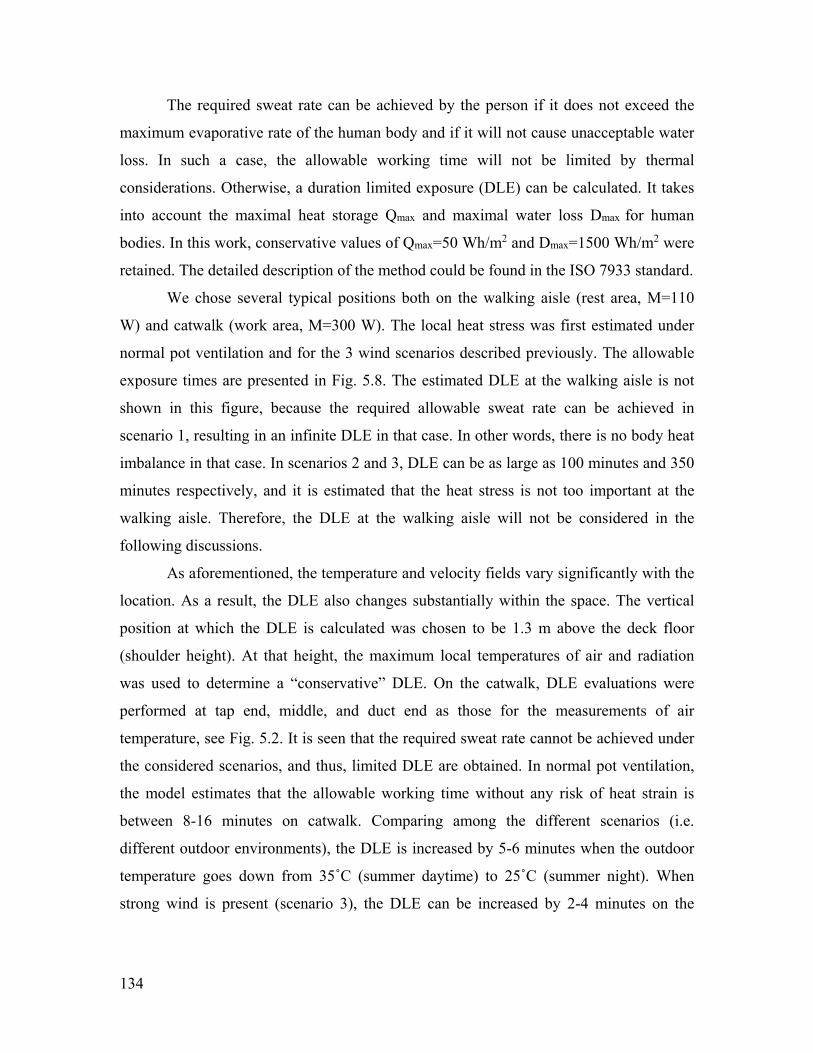
134

The required sweat rate can be achieved by the person if it does not exceed the

maximum evaporative rate of the human body and if it will not cause unacceptable water

loss. In such a case, the allowable working time will not be limited by thermal

considerations. Otherwise, a duration limited exposure (DLE) can be calculated. It takes

into account the maximal heat storage Qmax and maximal water loss Dmax for human

bodies. In this work, conservative values of Qmax=50 Wh/m2 and Dmax=1500 Wh/m2 were

retained. The detailed description of the method could be found in the ISO 7933 standard.

We chose several typical positions both on the walking aisle (rest area, M=110

W) and catwalk (work area, M=300 W). The local heat stress was first estimated under

normal pot ventilation and for the 3 wind scenarios described previously. The allowable

exposure times are presented in Fig. 5.8. The estimated DLE at the walking aisle is not

shown in this figure, because the required allowable sweat rate can be achieved in

scenario 1, resulting in an infinite DLE in that case. In other words, there is no body heat

imbalance in that case. In scenarios 2 and 3, DLE can be as large as 100 minutes and 350

minutes respectively, and it is estimated that the heat stress is not too important at the

walking aisle. Therefore, the DLE at the walking aisle will not be considered in the

following discussions.

As aforementioned, the temperature and velocity fields vary significantly with the

location. As a result, the DLE also changes substantially within the space. The vertical

position at which the DLE is calculated was chosen to be 1.3 m above the deck floor

(shoulder height). At that height, the maximum local temperatures of air and radiation

was used to determine a “conservative” DLE. On the catwalk, DLE evaluations were

performed at tap end, middle, and duct end as those for the measurements of air

temperature, see Fig. 5.2. It is seen that the required sweat rate cannot be achieved under

the considered scenarios, and thus, limited DLE are obtained. In normal pot ventilation,

the model estimates that the allowable working time without any risk of heat strain is

between 8-16 minutes on catwalk. Comparing among the different scenarios (i.e.

different outdoor environments), the DLE is increased by 5-6 minutes when the outdoor

temperature goes down from 35˚C (summer daytime) to 25˚C (summer night). When

strong wind is present (scenario 3), the DLE can be increased by 2-4 minutes on the

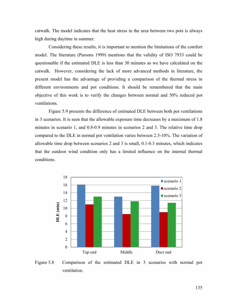
135

catwalk. The model indicates that the heat stress in the area between two pots is always

high during daytime in summer.

Considering these results, it is important to mention the limitations of the comfort

model. The literature (Parsons 1999) mentions that the validity of ISO 7933 could be

questionable if the estimated DLE is less than 30 minutes as we have calculated on the

catwalk. However, considering the lack of more advanced methods in literature, the

present model has the advantage of providing a comparison of the thermal stress in

different environments and pot conditions. It should be remembered that the main

objective of this work is to verify the changes between normal and 50% reduced pot

ventilations.

Figure 5.9 presents the difference of estimated DLE between both pot ventilations

in 3 scenarios. It is seen that the allowable exposure time decreases by a maximum of 1.8

minutes in scenario 1, and 0.8-0.9 minutes in scenarios 2 and 3. The relative time drop

compared to the DLE in normal pot ventilation varies between 2.5-10%. The variation of

allowable time drop between scenarios 2 and 3 is small, 0.1-0.3 minutes, which indicates

that the outdoor wind condition only has a limited influence on the internal thermal

conditions.

Figure 5.8 Comparison of the estimated DLE in 3 scenarios with normal pot

ventilation.

0

2

4

6

8

10

12

14

16

18

Tap end Middle Duct end

DL

E (

min

)

scenario 1

scenario 2

scenario 3

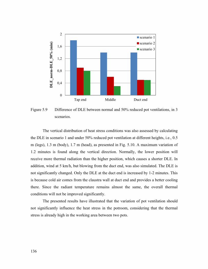
136

Figure 5.9 Difference of DLE between normal and 50% reduced pot ventilations, in 3

scenarios.

The vertical distribution of heat stress conditions was also assessed by calculating

the DLE in scenario 1 and under 50% reduced pot ventilation at different heights, i.e., 0.5

m (legs), 1.3 m (body), 1.7 m (head), as presented in Fig. 5.10. A maximum variation of

1.2 minutes is found along the vertical direction. Normally, the lower position will

receive more thermal radiation than the higher position, which causes a shorter DLE. In

addition, wind at 5 km/h, but blowing from the duct end, was also simulated. The DLE is

not significantly changed. Only the DLE at the duct end is increased by 1-2 minutes. This

is because cold air comes from the claustra wall at duct end and provides a better cooling

there. Since the radiant temperature remains almost the same, the overall thermal

conditions will not be improved significantly.

The presented results have illustrated that the variation of pot ventilation should

not significantly influence the heat stress in the potroom, considering that the thermal

stress is already high in the working area between two pots.

0

0,4

0,8

1,2

1,6

2

Tap end Middle Duct end

DL

E_n

orm

-DL

E_5

0% (

min

)

scenario 1

scenario 2

scenario 3

137

Figure 5.10 Vertical distribution of the DLE in scenario 1, under 50% reduced pot

ventilation.

5.7 Conclusions

Potrooms are industrial buildings where electrolytic cells are lined up to carry on the

Hall-Héroult alumina reduction process. These buildings are mainly ventilated naturally,

based on buoyancy and wind. Therefore, any modification in terms of pot design and

operations, as well as in outdoor conditions, is likely to affect the heat transfer and air

flow patterns within a given potroom.

This chapter presents a detailed study of the natural ventilation in potrooms by

using CFD simulations. Both buoyancy and wind driven forces were considered in the

simulations. The advanced model was validated with air and surface temperature

measurements performed in the plant. In the end, airflow and temperature fields can be

determined from the simulation results. A thermal comfort model was also developed to

calculate the duration limitation exposure for operators working in the potroom

environment.

In this chapter, the model was used to study, among other things, the impact of the

pot ventilation level on the overall ventilation in the potroom, under different scenarios

(wind speed, wind direction, outdoor temperature). It was found that the reduction of the

pot ventilation level can result in larger heat dissipation rates in the potroom, but that the

10

11

12

13

14

15

Tap end Middle Duct end

DL

E (

min

)

h=0.5 m

h=1.3 m

h=1.7 m

138

effect in terms of DLE is limited for all the scenarios considered. The model that has

been developed could be used in the future to study the impact of a variety of other

modifications in terms of potroom design.

139

CHAPTER 6 ESTIMATION OF THE EFFICIENCY OF POT TIGHTNESS IN

REDUCED POT DRAFT BASED ON CFD SIMULATIONS

140

Abstract

Reduction of pot draft is a promising approach for energy saving and waste heat recovery

in aluminum smelting cells. Pot tightness, or control of fugitive emissions, is investigated

in a smelting cell with reduced draft, down to half of the current level based on CFD

simulations. Models with different simulation length scales are created in order to

iteratively define proper boundary conditions around the leaking area. A systematic

analysis of the pot tightness is presented by considering various factors, e.g., pot draft,

hood placement. The results have shown that current pot structure, even within ideal

operating conditions, fails to maintain 100% hooding efficiency under a 50% reduced pot

draft. Two design modifications are proposed and verified. An efficient sealing is

observed when covering the lower half of the gaps between hoods. An estimation of the

leaking hydrogen fluoride is made under different scenarios in order to quantitatively

verify the modifications.

141

Résumé

Réduire le taux de ventilation de cuves est une approche prometteuse pour économiser de

l’énergie et faciliter la récupération des rejets thermiques. L’étanchéité des cuves, pour

contrôler les fuites de gaz, est investiguée dans une cuve avec un taux de ventilation

réduit avec un modèle CFD. Des sous-modèles avec différentes dimensions sont créés

pour définir itérativement les conditions aux limites. Une analyse systématique de

l’étanchéité est présentée pour considérer différents facteurs comme le taux de ventilation

et le positionnement des capots. Les résultats ont montré que le design actuel, même avec

un parfait positionnement des capots, ne permet pas de maintenir l’étanchéité si on réduit

de moitié le taux de ventilation de la cuve. Le scellement du bas de l’espace entre les

capots permet cependant d’améliorer l’étanchéité. Une estimation des émissions de HF

dans la salle de cuves est proposée.

142

6.1 Introduction

The current aluminum reduction technology is based on the Hall-Héroult process. An

electric current circulates between a carbon anode and a cathode through an electrolytic

bath in which alumina is dissolved. The alumina reacts with carbon by a series of electro-

chemical reactions, and as a result, carbon dioxide (CO2) is emitted as a by-product. A

liquid aluminum layer accumulates at the bottom of the pot, and can be periodically

syphoned out. The overall process can be written in a very simplified and compact

formula: 2Al2O3 + 3C + electricity → 4Al +3CO2. Within the process, only half of the

consumed electricity can be converted efficiently. The remaining energy is dissipated into

the environment as waste heat.

As the global aluminum industry becomes less profitable and as the cost of energy

rises up, producers have to improve process efficiency. Waste heat recovery is an

interesting possibility to do that. An energy and exergy balance of the electrolysis process

was performed in literature (Nowicki and Gosselin 2012). Several authors have proposed

concepts to collect the waste heat contained in pot effluents (Sorhuus et al. 2010; Sørhuus

and Wedde 2009; Fleer et al. 2010). Nevertheless, these concepts are still preliminary.

Currently, the low temperature of the pot gas (~130C in summer and ~100C in winter

in a plant such as ADQ (Alcoa’s smelter in Deschambault, Québec, Canada)) is a major

handicap for an economically beneficial recovery of the waste heat. Zhao et al. (2013a)

developed a thermal circuit network to investigate the heat transfer in pots under different

scenarios and they found that the reduction of the pot ventilation rate is the most efficient

way to rise the temperature of the exhaust gas. Meanwhile, a reduction of the ventilation

rate could tremendously reduce the total power requirement of the fans, because the fan

power is proportional to the flow rate to power 3. Considering that currently ~2% of a

smelter’s total electricity consumption (~0.3 MWh/ton Al) is used for the fans, the

potential saving is considerable. In addition, the draft reduction will extract less diluted

air from the potroom. Since the reduced air suction introduces less moisture into the pots,

a reduction of HF (Hydrogen Fluoride) evolution in pot cavity is also expected as a side-

effect (Patterson 2002; Meghlaoui 2002).

However, there are number of challenges to address before pot ventilation

reduction could be implemented in practice. The gases released by the electrolytic

143

reactions contain a small portion of hazardous components, among which gaseous and

particulate fluoride, and SO2. Modern smelting pots are equipped with a pot ventilation

system to collect the flue gases. The pot draft condition is chosen to achieve a vacuum in

the pot, which results in a virtually leakage free pot. Since the control of hazardous gases

is of great importance for the employees’ health in the potroom and for environmental

reasons, an intensive research has been done to understand the mechanisms of fluoride

emissions from pots. The early efforts were mainly devoted to monitoring the HF

concentration in the pot exhaust gas under different pot conditions and during various pot

operations (Tarcy 2003; Slaugenhaupt et al. 2003; Dando and Tang 2005; Dando and

Tang 2006). More recently, HF concentration was measured in the pot cavity to

determine where HF is released from and to develop correlations between various sources

of water and the resulting HF emissions (Osen et al. 2011; Sommerseth et al. 2011).

Although literature is abundant in this field, fewer works are available on the pot gas

leakage into the potroom. Dando and Tang (2005; 2006) reported the transient

measurement of the HF concentration profile in the area just above pot hoods in different

pot conditions. It was found that the thermal buoyancy from crust holes and the air

leakage of the pneumatic system of the alumina feeding system are the two main reasons

explaining HF release from pots when the hoods are into place. In addition to

experiments, analytical models were developed to calculate the pot draft and to

investigate pot hooding efficiency (Dernedde 1990; Karlsen et al. 1998). These models

considered the flow infiltration through pot gaps due to natural and mechanical

ventilations in the pot, but they were too simple to provide accurate results.

Computational Fluid Dynamics (CFD) simulation has been used over the last

decades for simulating the ventilation in built environments. It was also employed to

predict the air ventilation and HF distribution in aluminum smelting potrooms (Berkoe et

al. 2005; Vershenya et al. 2011), i.e. the building where the pots are aligned. CFD

simulations of fugitive emissions from aluminum smelting pots were realized in (Abbas

et al. 2009). The model was built to predict the fugitive emissions in both normal and

reduced ventilation conditions. It was estimated from CFD models that the pot could

remain free of leakage until the pot ventilation is reduced to 10% of normal condition,

although this conclusion seemed to be inconsistent with the measurements of HF in

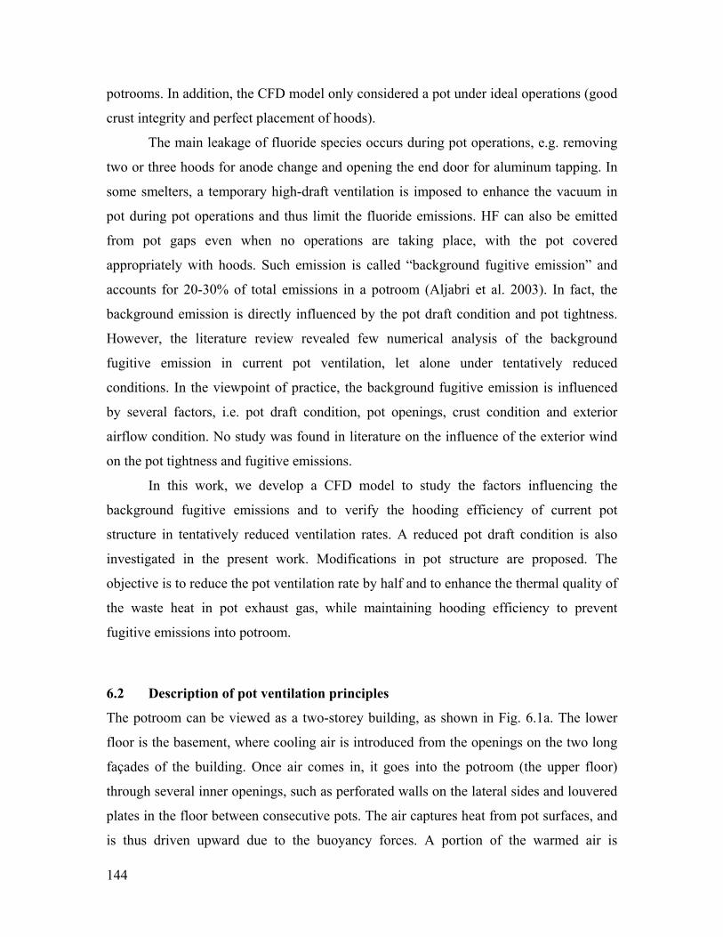
144

potrooms. In addition, the CFD model only considered a pot under ideal operations (good

crust integrity and perfect placement of hoods).

The main leakage of fluoride species occurs during pot operations, e.g. removing

two or three hoods for anode change and opening the end door for aluminum tapping. In

some smelters, a temporary high-draft ventilation is imposed to enhance the vacuum in

pot during pot operations and thus limit the fluoride emissions. HF can also be emitted

from pot gaps even when no operations are taking place, with the pot covered

appropriately with hoods. Such emission is called “background fugitive emission” and

accounts for 20-30% of total emissions in a potroom (Aljabri et al. 2003). In fact, the

background emission is directly influenced by the pot draft condition and pot tightness.

However, the literature review revealed few numerical analysis of the background

fugitive emission in current pot ventilation, let alone under tentatively reduced

conditions. In the viewpoint of practice, the background fugitive emission is influenced

by several factors, i.e. pot draft condition, pot openings, crust condition and exterior

airflow condition. No study was found in literature on the influence of the exterior wind

on the pot tightness and fugitive emissions.

In this work, we develop a CFD model to study the factors influencing the

background fugitive emissions and to verify the hooding efficiency of current pot

structure in tentatively reduced ventilation rates. A reduced pot draft condition is also

investigated in the present work. Modifications in pot structure are proposed. The

objective is to reduce the pot ventilation rate by half and to enhance the thermal quality of

the waste heat in pot exhaust gas, while maintaining hooding efficiency to prevent

fugitive emissions into potroom.

6.2 Description of pot ventilation principles

The potroom can be viewed as a two-storey building, as shown in Fig. 6.1a. The lower

floor is the basement, where cooling air is introduced from the openings on the two long

façades of the building. Once air comes in, it goes into the potroom (the upper floor)

through several inner openings, such as perforated walls on the lateral sides and louvered

plates in the floor between consecutive pots. The air captures heat from pot surfaces, and

is thus driven upward due to the buoyancy forces. A portion of the warmed air is

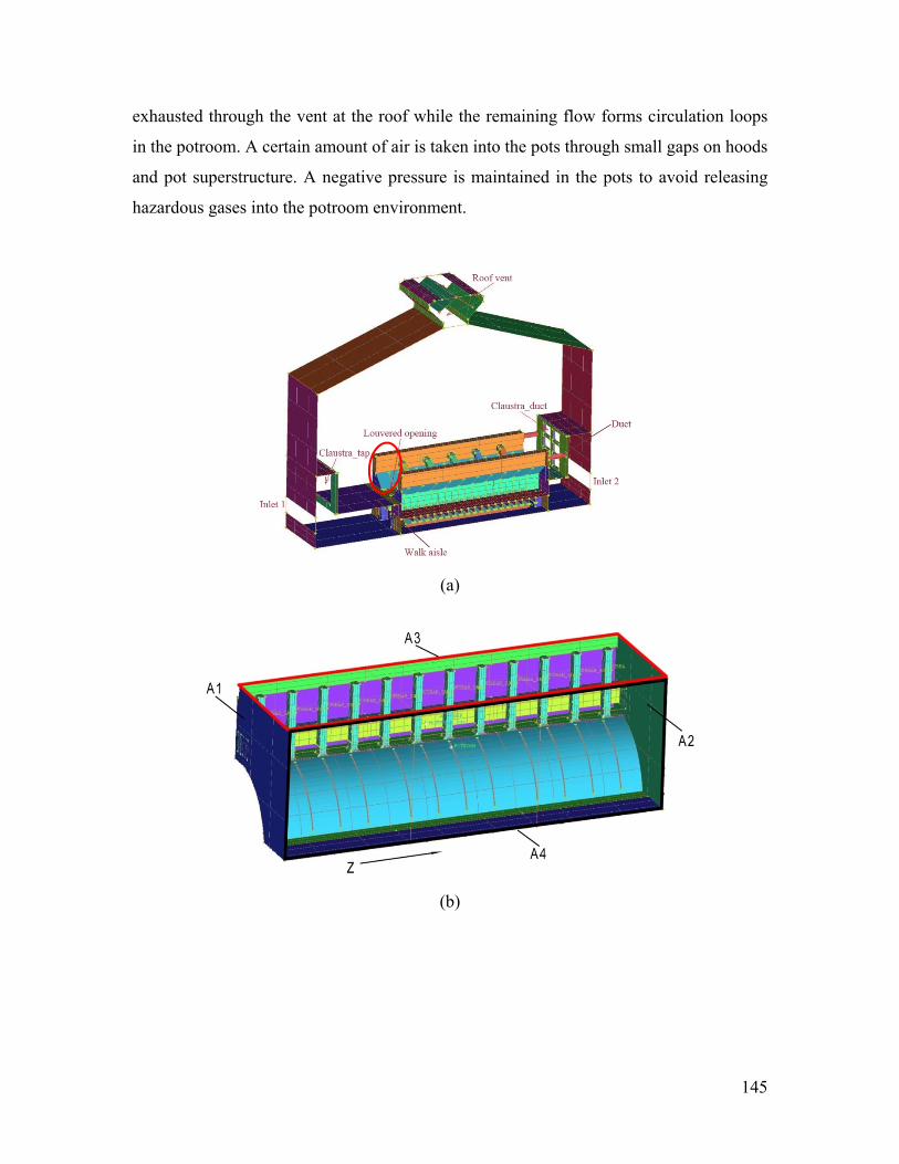
145

exhausted through the vent at the roof while the remaining flow forms circulation loops

in the potroom. A certain amount of air is taken into the pots through small gaps on hoods

and pot superstructure. A negative pressure is maintained in the pots to avoid releasing

hazardous gases into the potroom environment.

(a)

(b)

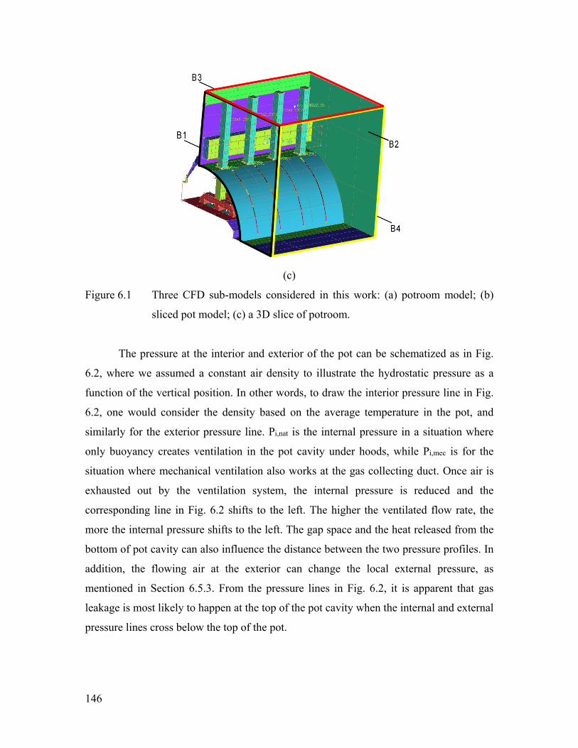
146

(c)

Figure 6.1 Three CFD sub-models considered in this work: (a) potroom model; (b)

sliced pot model; (c) a 3D slice of potroom.

The pressure at the interior and exterior of the pot can be schematized as in Fig.

6.2, where we assumed a constant air density to illustrate the hydrostatic pressure as a

function of the vertical position. In other words, to draw the interior pressure line in Fig.

6.2, one would consider the density based on the average temperature in the pot, and

similarly for the exterior pressure line. Pi,nat is the internal pressure in a situation where

only buoyancy creates ventilation in the pot cavity under hoods, while Pi,mec is for the

situation where mechanical ventilation also works at the gas collecting duct. Once air is

exhausted out by the ventilation system, the internal pressure is reduced and the

corresponding line in Fig. 6.2 shifts to the left. The higher the ventilated flow rate, the

more the internal pressure shifts to the left. The gap space and the heat released from the

bottom of pot cavity can also influence the distance between the two pressure profiles. In

addition, the flowing air at the exterior can change the local external pressure, as

mentioned in Section 6.5.3. From the pressure lines in Fig. 6.2, it is apparent that gas

leakage is most likely to happen at the top of the pot cavity when the internal and external

pressure lines cross below the top of the pot.

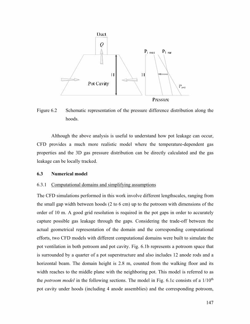
147

Figure 6.2 Schematic representation of the pressure difference distribution along the

hoods.

Although the above analysis is useful to understand how pot leakage can occur,

CFD provides a much more realistic model where the temperature-dependent gas

properties and the 3D gas pressure distribution can be directly calculated and the gas

leakage can be locally tracked.

6.3 Numerical model

6.3.1 Computational domains and simplifying assumptions

The CFD simulations performed in this work involve different lengthscales, ranging from

the small gap width between hoods (2 to 6 cm) up to the potroom with dimensions of the

order of 10 m. A good grid resolution is required in the pot gaps in order to accurately

capture possible gas leakage through the gaps. Considering the trade-off between the

actual geometrical representation of the domain and the corresponding computational

efforts, two CFD models with different computational domains were built to simulate the

pot ventilation in both potroom and pot cavity. Fig. 6.1b represents a potroom space that

is surrounded by a quarter of a pot superstructure and also includes 12 anode rods and a

horizontal beam. The domain height is 2.8 m, counted from the walking floor and its

width reaches to the middle plane with the neighboring pot. This model is referred to as

the potroom model in the following sections. The model in Fig. 6.1c consists of a 1/10th

pot cavity under hoods (including 4 anode assemblies) and the corresponding potroom,

148

named later the sliced pot model. The overall simulation procedure starts by performing a

simulation in the potroom model to determine the flow field and heat transfer patterns in

that zone (e.g. velocity, static pressure, turbulent parameters, air temperature, etc.). Then,

depending on the pot segment of interest, the flow information at different cross-section

surfaces is extracted from the potroom model, and introduced into the sliced pot model as

boundary conditions. The second simulation is performed in the pot model which can

predict the coupling between the pot interior and exterior at the gaps. In both models, we

made the following simplifications in order to focus on the issues of interest and facilitate

the simulations:

Only half of the area between two pots is included in the models and the surface A4

(depicted by thick black lines) in Fig. 6.1b and B4 (thick yellow lines) in Fig. 6.1c

are treated as symmetry planes. In fact, there are 4-5 anode busbars standing in this

area and connecting to the pot at one side. The real flow could be influenced by these

obstacles. However, they are normally installed at a distance of 0.3-0.4 m away from

the pot shell and the influence of the busbar is limited compared to other parts, such

as anode rods and supporting beam.

Other trivial structures and parts, such as connecting pieces, are ignored in the

models in order to minimize the required number of control volumes.

The geometry of anode assemblies is represented by more regular shapes in order to

create a mesh with good quality.

Only the gaps around anode rod and between hoods are modeled while the gaps

between the hoods and the superstructure’s horizontal plate are ignored, because they

are very small compared with the other considered gap areas.

6.3.2 Governing equations

The conservation equations for mass, momentum, and energy are discretized and solved

in the commercial CFD code, ANSYS FLUENT 14.5, via the finite volume method.

Steady-state conditions are considered. Pressure work and kinetic energy variations are

neglected in the energy equation since the gas is treated as incompressible. No species

diffusion is simulated in the problem. Therefore, the governing equations (conservations

of mass, momentum and energy) are written as follows:

149

( )0i

i

u

x

(6.1)

( ) 2 – –

3i j ji

eff iji i j j i

u u uupK g

x x x x x

(6.2)

( ) i

eff hi i i

u h Tk S

x x x

(6.3)

where the sensible enthalpy of the gas h is defined as ref

T

pTh C dT . Cp is the

temperature-dependent heat capacity of air. The Reynolds stresses term due to the

turbulence is modeled based on the Boussinesq eddy viscosity assumption. Therefore, μeff

is the effective viscosity (i.e., μ+μt, where μt is the turbulent viscosity, defined according

to the turbulence model that is used), K is the turbulent kinetic energy and δij=0 (i≠j) or 1

(i=j). keff is the effective thermal conductivity (e.g., k+kt, where kt is the turbulent thermal

conductivity, defined according to the turbulence model being used). Sh includes the

volumetric heat source due to the Joule heating effect in solids where a current passes,

such as in the anode assembly. The volumetric heat generation (Joule heating) is assumed

to be uniform in the solids and was calculated based on the typical current and resistivity

in each part of the anode assembly. Viscous heating is ignored in the simulation. Note

that in the solids, only the energy equation is solved, without the advective terms.

The air properties (i.e., specific heat, thermal conductivity, and viscosity) are user-

defined functions with respect to temperature (polynomial fittings based on data

published in (Bergman et al. 2011)). The air density is determined based on the

“incompressible-ideal-gas” model of the CFD code used (Fluent 2012), which is defined

as:

op

w

p

RT

M

(6.4)

where R is the universal gas constant, Mw, the molecular weight of the gas, and pop, the

defined operating pressure normally representing the mean pressure in the computational

domain. The density, defined by Eq. (6.4), depends only on the local temperature field,

150

and thus buoyancy forces can be considered in the momentum equations. The Boussinesq

assumption for the air density was not used in the work, since its validity is questionable

in the case of large temperature differences as experienced in pots and potrooms (Zhao

and Gosselin 2014).

A proper choice of turbulence models should be made to achieve a trade-off

between accuracy and computational time. The flow pattern in pot and potroom shares

many similarities with the ventilated airflow around and in buildings (e.g., jet flow

through hood gaps, flow impingement on surfaces, and both natural and mechanical

ventilation). The two equation eddy-viscosity turbulence models are widely used in the

simulations of air ventilation and heat transfer in buildings, particularly when the time-

averaged parameters, e.g. averaged velocity, pressure, and temperature, are of interest in

the simulations.

The SST k-ω model applies the k-ω model to simulate turbulence in near wall

area and it gradually converts to the standard k-ε model when the modeling flow goes

away from wall. When modeling the flow in the near wall region, the central point of the

first mesh layer should be placed in the viscous sublayer, i.e. y+<5. At least 10 cells are

required to accurately resolve the flow boundary layer near wall. The SST k-ω model

also accepts a coarse boundary mesh (y+>25) and applies empirical formulas (i.e. wall

functions) to resolve the viscously-affected region. However, it is recommended to avoid

to place the central point of the first mesh layer in the transitional layer (5<y+<25)

although such mesh can be solved in the SST k-ω model. In this work, a hybrid mesh

scheme is used to resolve different areas. Prism meshes are created in the near wall

region and tetra meshes, in the bulk area. Different mesh scales are used depending on

the local flow characteristics. Thin prism layers are paved on the surfaces of pot

superstructure and the surfaces surrounding the pot cavity under hoods, because the

nearby flow exhibits the features of a low Reynolds flow. They are either driven by

mixed convection or circulating around obstacles. Therefore, 10 prism layers are created

to resolve the flow boundary layer near wall and the first layer thickness satisfies the

requirement of y+<5. The maximum mesh size in the pot cavity is 0.05 m while it can

reach 0.2 m in the potroom for both the potroom model and the sliced pot model.

Attention should be paid to some specific areas. For instance, the control volume side

151

length is as small as 0.005 m in the area near the gaps between anode rod and pot

superstructure, since a good resolution is required to determine whether there is an

exfiltration of pot gas from the gap. Small mesh is also required at the exterior and

interior of the gap space between hoods in order to solve jet flow through it. The potroom

model contains approximately 4.5 million cells and the sliced pot model, 6 million cells.

Finer meshes were tested and did not change significantly the results, as will be described

later.

The entire fluid domain is treated as a non-participating material in terms of

radiative heat transfer. Discrete Ordinates (DO) model is used to calculate surface-to-

surface radiation heat transfer, considering the possibility to implement it with parallel

calculations in the software used. Default values are used in setting the parameters of

angular discretization and pixelation of space.

The two models are solved in steady-state condition and the gravitational

acceleration, g, is gradually increased from 0.1 m/s2 to 9.81 m/s2 to facilitate

convergence. The method to interpolate the variable gradient is the least squares cell-

based gradient evaluation. The interpolation scheme of surface pressure between two

cells is PRESTO! which is suitable for flows with high swirling and high Rayleigh

number (buoyancy driven flow) (Fluent 2012). Pressure-velocity coupling is achieved by

using SIMPLE segregated algorithm. All of the other variables are interpolated with the

second-order upwind scheme except for radiative intensity, which is calculated via the

first-order upwind scheme because the air is considered as a non-participating medium

and the optical thickness is therefore zero in the radiation transport equation. Default

under-relaxation factors are retained, except that for momentum equations which had to

be reduced for a better convergence. Default values of the scaled residuals are considered

to declare convergence. The CFD models are solved in parallel with 4 processors, each

having frequency of 3.40 GHz. It takes approximately 20 hours to run one simulation of

the potroom model and 30 hours for the sliced pot model.

6.3.3 Boundary conditions

For the potroom model (Fig. 6.1b), a velocity inlet is imposed on the surface A1, while a

pressure outlet is used for the surfaces A2 and A3. A4 is treated as symmetrical surface.

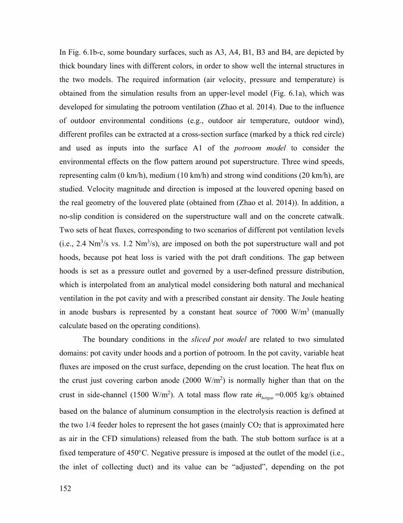
152

In Fig. 6.1b-c, some boundary surfaces, such as A3, A4, B1, B3 and B4, are depicted by

thick boundary lines with different colors, in order to show well the internal structures in

the two models. The required information (air velocity, pressure and temperature) is

obtained from the simulation results from an upper-level model (Fig. 6.1a), which was

developed for simulating the potroom ventilation (Zhao et al. 2014). Due to the influence

of outdoor environmental conditions (e.g., outdoor air temperature, outdoor wind),

different profiles can be extracted at a cross-section surface (marked by a thick red circle)

and used as inputs into the surface A1 of the potroom model to consider the

environmental effects on the flow pattern around pot superstructure. Three wind speeds,

representing calm (0 km/h), medium (10 km/h) and strong wind conditions (20 km/h), are

studied. Velocity magnitude and direction is imposed at the louvered opening based on

the real geometry of the louvered plate (obtained from (Zhao et al. 2014)). In addition, a

no-slip condition is considered on the superstructure wall and on the concrete catwalk.

Two sets of heat fluxes, corresponding to two scenarios of different pot ventilation levels

(i.e., 2.4 Nm3/s vs. 1.2 Nm3/s), are imposed on both the pot superstructure wall and pot

hoods, because pot heat loss is varied with the pot draft conditions. The gap between

hoods is set as a pressure outlet and governed by a user-defined pressure distribution,

which is interpolated from an analytical model considering both natural and mechanical

ventilation in the pot cavity and with a prescribed constant air density. The Joule heating

in anode busbars is represented by a constant heat source of 7000 W/m3 (manually

calculate based on the operating conditions).

The boundary conditions in the sliced pot model are related to two simulated

domains: pot cavity under hoods and a portion of potroom. In the pot cavity, variable heat

fluxes are imposed on the crust surface, depending on the crust location. The heat flux on

the crust just covering carbon anode (2000 W/m2) is normally higher than that on the

crust in side-channel (1500 W/m2). A total mass flow rate hotgasm =0.005 kg/s obtained

based on the balance of aluminum consumption in the electrolysis reaction is defined at

the two 1/4 feeder holes to represent the hot gases (mainly CO2 that is approximated here

as air in the CFD simulations) released from the bath. The stub bottom surface is at a

fixed temperature of 450C. Negative pressure is imposed at the outlet of the model (i.e.,

the inlet of collecting duct) and its value can be “adjusted”, depending on the pot

153

ventilation that one wants to simulate. Joule heating in anode yoke and stubs is treated as

a constant heat source of 12,000 W/m3. Effective outside convection is used on the

surfaces of pot superstructure that are not connected to the potroom domain. The

boundary types of the potroom domain are the same as those in the potroom model.

Specifically, a velocity profile extracted from the results of the potroom model is imposed

at the surface B1. By using the velocity profile extracted from the surfaces at different z

positions of the potroom model, the simulation of the sliced pot representing different

segment of a smelting pot can be performed. Boundary conditions on the other surfaces

(e.g. B2, B3 and B4) are the same as those in the potroom model.

6.3.4 Mesh independence study

A mesh independence study is performed in order to verify the errors due to grid

discretization. The boundary layer mesh in near-wall region is verified by comparing the

results achieved with a reference mesh (with 10 prism mesh layers) to those obtained

with a denser mesh (with 14 prism mesh layers). In both cases, the thickness of the first

layer is only 0.0008 m, which makes y+ value smaller than 3 in most areas. The

discrepancy between the two meshes in terms of predicted air temperature at the outlet is

within 1C (Tair≈120˚C), with a variation of the ventilated mass rate changes of less than

1.5%. The average temperature on the surface of hoods and anode rods changed by only

2 to 4C. Therefore, the boundary mesh with 10 prism mesh layers is used in the

following study.

The length scale of control volumes in the bulk of the pot cavity and potroom was

gradually reduced to determine a proper size for the simulation. It was found that 0.05 m

in pot cavity and 0.2 m in potroom for both potroom model and sliced pot model yields a

good trade-off between simulation accuracy and computational efforts. Finer meshes

were considered and did not affect significantly the monitored parameters.

6.4 Model validation

The numerical model was validated by comparing different measurements performed at

the ADQ plant to the results of the model.

154

First, a series of temperature measurements was performed on pot surfaces and in

the potroom. Surface temperature was measured in 24 positions on pot shells and 4

positions on building walls. Air temperature was also measured at 3 positions at shoulder-

level between two consecutive pots. This series of measurements was repeated 5 times

for different weather conditions. The CFD model was used to simulate these conditions.

It is found that the model could accurately predict the temperature distribution. A

maximal discrepancy of 25C is found for the surface of the pot shell (on average the

difference was below 10C) and 6C for the potroom walls. The maximal discrepancy for

air temperature is even less, about 2C. These values are considered acceptable,

compared with the high surface temperatures (hood temperature: 90-140C, sidewall

temperature: 250-390C, potroom walls and air temperatures: 15-50C) and considering

the geometrical simplification of the CFD model.

Additionally, the mass flow rate at the roof vent, which was measured at the plant,

was compared to the one achieved in the simulations. In summer, the real flow rate at the

roof vent is in the range of 12.4-15.2 m3/s while the simulated results are in the range of

12.3-14.6 m3/s under moderate wind conditions (weak and moderate outdoor winds).

Another comparison was made between the measured static pressure in the pot

cavity and the simulated results. The sensor was positioned under one hood located in the

middle of a cell and the pressure was measured at different heights (from the bottom of

the pot cavity to the middle height of the pot cavity) and varied between -6 Pa and -12 Pa.

Under the same pot ventilation rate and hooding conditions, the simulated pressure is

well stratified in the vertical direction. The pressure is as low as -8 Pa in the side channel

just above anode cover and it is about -6 Pa in the middle height of the pot cavity. A large

discrepancy is observed in the lowest position of the pot cavity, because the real

situations may be different than the ideal conditions of the simulation (e.g. the surface

profile of the anode cover, the emission of hot gases from the openings on anode cover,

etc.). Nevertheless, the pressure profile agrees relatively well in the rest of the cavity

where the influence of the uncertain boundary situation mentioned above is minor.

Finally, the results of smoke tests that had been done in the potroom were also

used to validate the main flow patterns, at least in a qualitative way. The comparison

between the smoke tests and the model was good, and all the main features observed

155

during the smoke tests were predicted by the model. For example, smoke tests have

revealed the vortex (arrow 1 in Fig. 6.3a) where the air is going over the edge of the pot

end, as well as the plume shape above the pot (arrow 3 in Fig. 6.3a). Also, the smoke

tests showed the creeping flow along pot hoods (arrow 2 in Fig. 6.3a), where air is

flowing up all the way to the top of the pot. These flow structures were also revealed by

the CFD simulations. The vortex flow is clearly seen in the similar position of Fig. 6.3b,

which is the flow pattern in the potroom model. The flow near the hoods and pot

superstructure is also consistent with the smoke tests. Fig. 6.3c is the flow pattern in the

sliced pot model, representing the middle section of a pot. The creeping flow on pot

hoods and the uprising flow along pot structure were well predicted by the model.

Considering the industrial application studied in this work, and the purpose of this work,

the results of the CFD model could thus be qualified of adequate.

6.5 Pot tightness in various pot conditions

In this section, different factors that influence the pot tightness are studied with CFD

simulations. The pot ventilation rate is one of the most important parameters to determine

the negative pressure in the pot cavity in order to avoid leakage. A higher draft condition

demands a higher vacuum, and vice visa. The gap width between two neighbouring

hoods is another factor that significantly controls the suction rate of potroom air into the

pot cavity. A loose placement of hoods due to the hood deformation or incautious

manipulations may cause a significant reduction of vacuum in the pot and allow fugitive

emissions. Another factor influencing leakage relates to the air flow pattern itself. For

example, the air in the potroom blows over the shell of pot superstructure and may

impose either positive or negative pressure (depending on the flow direction and the

structure itself) on the external surface of pot superstructure. Finally, the release of pot

gas from crust openings could also increase the risk of leakage. These factors are studied

in the next sub-sections.

6.5.1 Effect of different pot drafts

The pot draft condition is adjustable in the numerical model by specifying

different pressures at the outlet of the sliced pot model. A series of simulations were

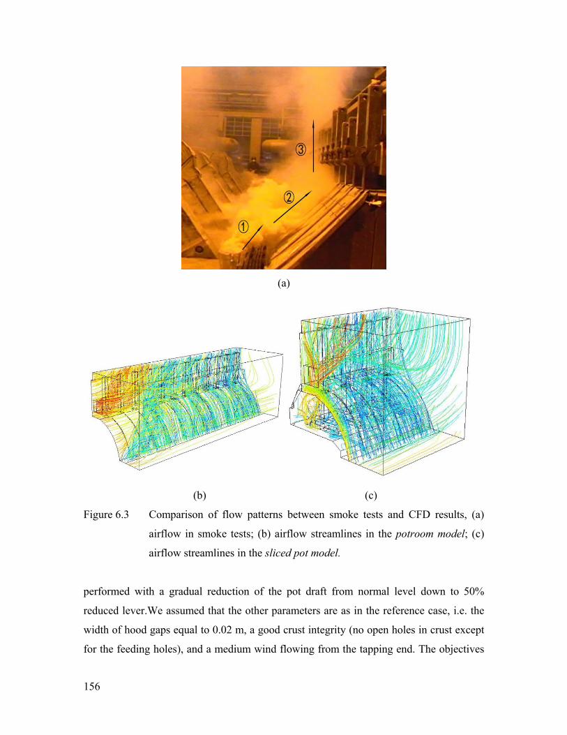
156

(a)

(b) (c)

Figure 6.3 Comparison of flow patterns between smoke tests and CFD results, (a)

airflow in smoke tests; (b) airflow streamlines in the potroom model; (c)

airflow streamlines in the sliced pot model.

performed with a gradual reduction of the pot draft from normal level down to 50%

reduced lever.We assumed that the other parameters are as in the reference case, i.e. the

width of hood gaps equal to 0.02 m, a good crust integrity (no open holes in crust except

for the feeding holes), and a medium wind flowing from the tapping end. The objectives

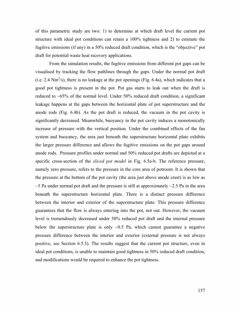
157

of this parametric study are two: 1) to determine at which draft level the current pot

structure with ideal pot conditions can retain a 100% tightness and 2) to estimate the

fugitive emissions (if any) in a 50% reduced draft condition, which is the “objective” pot

draft for potential waste heat recovery applications.

From the simulation results, the fugitive emissions from different pot gaps can be

visualised by tracking the flow pathlines through the gaps. Under the normal pot draft

(i.e. 2.4 Nm3/s), there is no leakage at the pot openings (Fig. 6.4a), which indicates that a

good pot tightness is present in the pot. Pot gas starts to leak out when the draft is

reduced to ~65% of the normal level. Under 50% reduced draft condition, a significant

leakage happens at the gaps between the horizontal plate of pot superstructure and the

anode rods (Fig. 6.4b). As the pot draft is reduced, the vacuum in the pot cavity is

significantly decreased. Meanwhile, buoyancy in the pot cavity induces a monotonically

increase of pressure with the vertical position. Under the combined effects of the fan

system and buoyancy, the area just beneath the superstructure horizontal plate exhibits

the larger pressure difference and allows the fugitive emissions on the pot gaps around

anode rods. Pressure profiles under normal and 50% reduced pot drafts are depicted at a

specific cross-section of the sliced pot model in Fig. 6.5a-b. The reference pressure,

namely zero pressure, refers to the pressure in the core area of potroom. It is shown that

the pressure at the bottom of the pot cavity (the area just above anode crust) is as low as

5 Pa under normal pot draft and the pressure is still at approximately 2.5 Pa in the area

beneath the superstructure horizontal plate. There is a distinct pressure difference

between the interior and exterior of the superstructure plate. This pressure difference

guarantees that the flow is always entering into the pot, not out. However, the vacuum

level is tremendously decreased under 50% reduced pot draft and the internal pressure

below the superstructure plate is only 0.5 Pa, which cannot guarantee a negative

pressure difference between the interior and exterior (external pressure is not always

positive, see Section 6.5.3). The results suggest that the current pot structure, even in

ideal pot conditions, is unable to maintain good tightness in 50% reduced draft condition,

and modifications would be required to enhance the pot tightness.

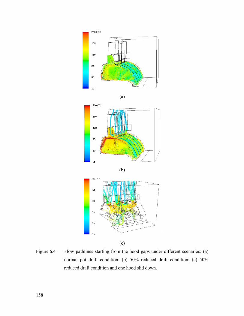
158

(a)

(b)

(c)

Figure 6.4 Flow pathlines starting from the hood gaps under different scenarios: (a)

normal pot draft condition; (b) 50% reduced draft condition; (c) 50%

reduced draft condition and one hood slid down.

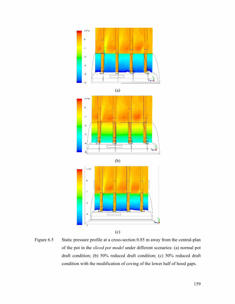
159

(a)

(b)

(c)

Figure 6.5 Static pressure profile at a cross-section 0.85 m away from the central-plan

of the pot in the sliced pot model under different scenarios: (a) normal pot

draft condition; (b) 50% reduced draft condition; (c) 50% reduced draft

condition with the modification of coving of the lower half of hood gaps.

160

6.5.2 Effect of the gap space between hoods

Although the normal gap space between hoods is typically around 2 cm, it can vary

significantly in practice, as mentioned previously. In this sub-section, the gap space is

changed to simulate different hooding conditions. The reference case is when all gaps

between hoods have a width of 2 cm. Then, 4 cm gap is assigned to one of the four gaps

in the 1/10 sliced pot model to represent a very common scenario where some of the

hoods are not well placed due to their deformation in time or incautious placement. In the

next scenario, all gaps between hoods are 4 cm wide which corresponds to a very bad

placement of hoods. Finally, one hood mismatched with the pot superstructure is

simulated by creating a large gap space around the mismatched hood (Fig. 6.4c). In all

hooding scenarios, the pot draft condition was varied from normal to 50% reduced levels.

The estimation of how much fugitive emissions are released out of a pot is not

trivial. No universal model can be applied to establish HF evolution for any type of

smelting pot. The locations where HF is emitted from pot bath and crust can also vary in

time, and from pot to pot. As a result, it can be difficult to precisely simulate the HF

transport in the pot. In this work, two assumptions are invoked to simplify the

calculations. First, one assumes that the HF concentration in the leaking pot gas is the

same as that measured at the inlet of the collecting duct, which is available in literature.

For a modern pot with more than 300 kA, the HF concentration at the inlet of the

collecting duct is around 300-400 ppm (Dando and Tang 2006; Osen et al. 2011;

Sommerseth et al. 2011) . Due to its high temperature, emitted HF is lighter than the air

in the cavity under the hoods. It will thus be driven upward and will accumulate at the top

of the pot cavity under the superstructure horizontal plate. Therefore, the HF

concentration is expected to be relatively uniform at the top of the pot cavity and we

choose 350 ppm for the HF concentration in that zone under normal pot ventilation.

Another assumption is that the HF concentration of the leakage linearly increases

with the reduced pot draft condition. In order words, the HF concentration of the leakage

is doubled to 700 ppm as the draft is reduced by 50%. It is also reasonable because the

diluted air flow rate dominates the total gas volume in the pot.

Using the two above-mentioned assumptions and knowing the mass flow rate of

the leaking gas through pot openings, one can calculate how much HF escapes from a

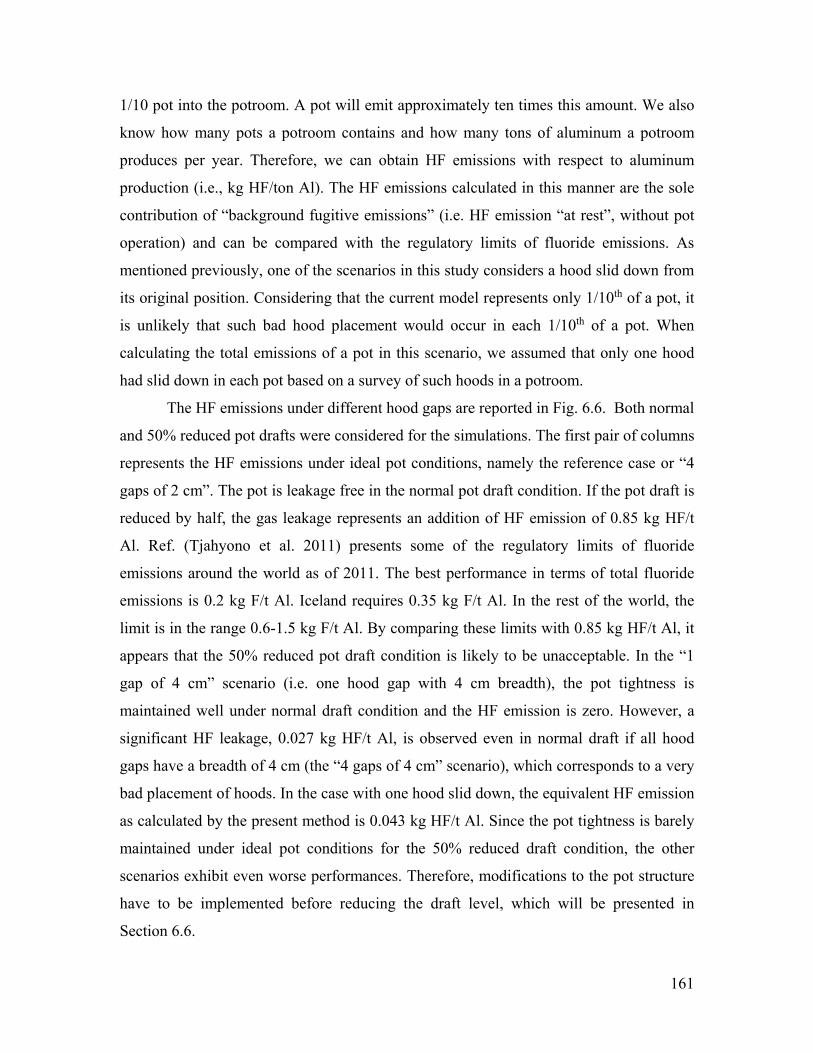
161

1/10 pot into the potroom. A pot will emit approximately ten times this amount. We also

know how many pots a potroom contains and how many tons of aluminum a potroom

produces per year. Therefore, we can obtain HF emissions with respect to aluminum

production (i.e., kg HF/ton Al). The HF emissions calculated in this manner are the sole

contribution of “background fugitive emissions” (i.e. HF emission “at rest”, without pot

operation) and can be compared with the regulatory limits of fluoride emissions. As

mentioned previously, one of the scenarios in this study considers a hood slid down from

its original position. Considering that the current model represents only 1/10th of a pot, it

is unlikely that such bad hood placement would occur in each 1/10th of a pot. When

calculating the total emissions of a pot in this scenario, we assumed that only one hood

had slid down in each pot based on a survey of such hoods in a potroom.

The HF emissions under different hood gaps are reported in Fig. 6.6. Both normal

and 50% reduced pot drafts were considered for the simulations. The first pair of columns

represents the HF emissions under ideal pot conditions, namely the reference case or “4

gaps of 2 cm”. The pot is leakage free in the normal pot draft condition. If the pot draft is

reduced by half, the gas leakage represents an addition of HF emission of 0.85 kg HF/t

Al. Ref. (Tjahyono et al. 2011) presents some of the regulatory limits of fluoride

emissions around the world as of 2011. The best performance in terms of total fluoride

emissions is 0.2 kg F/t Al. Iceland requires 0.35 kg F/t Al. In the rest of the world, the

limit is in the range 0.6-1.5 kg F/t Al. By comparing these limits with 0.85 kg HF/t Al, it

appears that the 50% reduced pot draft condition is likely to be unacceptable. In the “1

gap of 4 cm” scenario (i.e. one hood gap with 4 cm breadth), the pot tightness is

maintained well under normal draft condition and the HF emission is zero. However, a

significant HF leakage, 0.027 kg HF/t Al, is observed even in normal draft if all hood

gaps have a breadth of 4 cm (the “4 gaps of 4 cm” scenario), which corresponds to a very

bad placement of hoods. In the case with one hood slid down, the equivalent HF emission

as calculated by the present method is 0.043 kg HF/t Al. Since the pot tightness is barely

maintained under ideal pot conditions for the 50% reduced draft condition, the other

scenarios exhibit even worse performances. Therefore, modifications to the pot structure

have to be implemented before reducing the draft level, which will be presented in

Section 6.6.

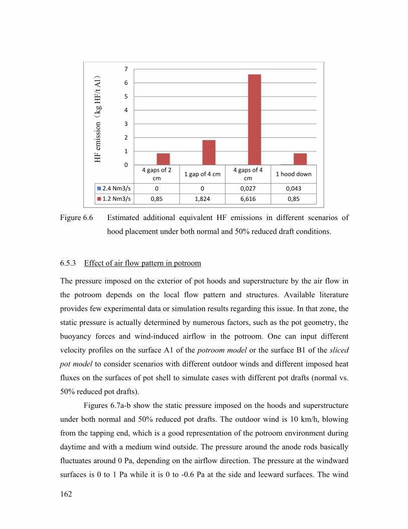
162

Figure 6.6 Estimated additional equivalent HF emissions in different scenarios of

hood placement under both normal and 50% reduced draft conditions.

6.5.3 Effect of air flow pattern in potroom

The pressure imposed on the exterior of pot hoods and superstructure by the air flow in

the potroom depends on the local flow pattern and structures. Available literature

provides few experimental data or simulation results regarding this issue. In that zone, the

static pressure is actually determined by numerous factors, such as the pot geometry, the

buoyancy forces and wind-induced airflow in the potroom. One can input different

velocity profiles on the surface A1 of the potroom model or the surface B1 of the sliced

pot model to consider scenarios with different outdoor winds and different imposed heat

fluxes on the surfaces of pot shell to simulate cases with different pot drafts (normal vs.

50% reduced pot drafts).

Figures 6.7a-b show the static pressure imposed on the hoods and superstructure

under both normal and 50% reduced pot drafts. The outdoor wind is 10 km/h, blowing

from the tapping end, which is a good representation of the potroom environment during

daytime and with a medium wind outside. The pressure around the anode rods basically

fluctuates around 0 Pa, depending on the airflow direction. The pressure at the windward

surfaces is 0 to 1 Pa while it is 0 to -0.6 Pa at the side and leeward surfaces. The wind

4 gaps of 2cm

1 gap of 4 cm4 gaps of 4

cm1 hood down

2.4 Nm3/s 0 0 0,027 0,043

1.2 Nm3/s 0,85 1,824 6,616 0,85

0

1

2

3

4

5

6

7

HF

em

issi

on（

kg H

F/t

Al）

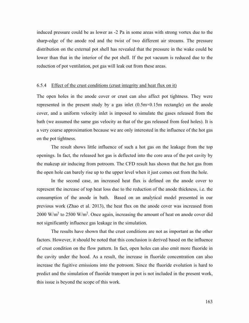
163

induced pressure could be as lower as -2 Pa in some areas with strong vortex due to the

sharp-edge of the anode rod and the twist of two different air streams. The pressure

distribution on the external pot shell has revealed that the pressure in the wake could be

lower than that in the interior of the pot shell. If the pot vacuum is reduced due to the

reduction of pot ventilation, pot gas will leak out from these areas.

6.5.4 Effect of the crust conditions (crust integrity and heat flux on it)

The open holes in the anode cover or crust can also affect pot tightness. They were

represented in the present study by a gas inlet (0.5m×0.15m rectangle) on the anode

cover, and a uniform velocity inlet is imposed to simulate the gases released from the

bath (we assumed the same gas velocity as that of the gas released from feed holes). It is

a very coarse approximation because we are only interested in the influence of the hot gas

on the pot tightness.

The result shows little influence of such a hot gas on the leakage from the top

openings. In fact, the released hot gas is deflected into the core area of the pot cavity by

the makeup air inducing from potroom. The CFD result has shown that the hot gas from

the open hole can barely rise up to the upper level when it just comes out from the hole.

In the second case, an increased heat flux is defined on the anode cover to

represent the increase of top heat loss due to the reduction of the anode thickness, i.e. the

consumption of the anode in bath. Based on an analytical model presented in our

previous work (Zhao et al. 2013), the heat flux on the anode cover was increased from

2000 W/m2 to 2500 W/m2. Once again, increasing the amount of heat on anode cover did

not significantly influence gas leakage in the simulation.

The results have shown that the crust conditions are not as important as the other

factors. However, it should be noted that this conclusion is derived based on the influence

of crust condition on the flow pattern. In fact, open holes can also emit more fluoride in

the cavity under the hood. As a result, the increase in fluoride concentration can also

increase the fugitive emissions into the potroom. Since the fluoride evolution is hard to

predict and the simulation of fluoride transport in pot is not included in the present work,

this issue is beyond the scope of this work.

164

(a)

(b)

Figure 6.7 Static pressure on the pot shell due to the air flow in potroom, (a) normal

draft condition; (b) 50% reduced draft condition.

6.6 Improvement of pot tightness

As mentioned previously, the objective of this chapter is to assess the pot tightness under

reduced pot ventilation, and if required, to enhance it. The preceding section has

illustrated that current pot structure cannot maintain satisfactory pot tightness under only

half of the normal pot draft. Therefore, several modifications to the pot structures are

proposed and their efficiency for retaining pot tightness and preventing gas leakages are

estimated from simulations. Only scenarios with 50% reduced pot draft is simulated in

this section.

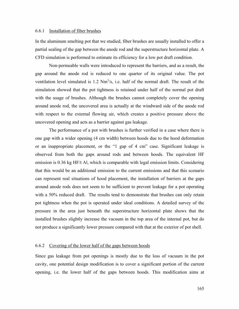
165

6.6.1 Installation of fiber brushes

In the aluminum smelting pot that we studied, fiber brushes are usually installed to offer a

partial sealing of the gap between the anode rod and the superstructure horizontal plate. A

CFD simulation is performed to estimate its efficiency for a low pot draft condition.

Non-permeable walls were introduced to represent the barriers, and as a result, the

gap around the anode rod is reduced to one quarter of its original value. The pot

ventilation level simulated is 1.2 Nm3/s, i.e. half of the normal draft. The result of the

simulation showed that the pot tightness is retained under half of the normal pot draft

with the usage of brushes. Although the brushes cannot completely cover the opening

around anode rod, the uncovered area is actually at the windward side of the anode rod

with respect to the external flowing air, which creates a positive pressure above the

uncovered opening and acts as a barrier against gas leakage.

The performance of a pot with brushes is further verified in a case where there is

one gap with a wider opening (4 cm width) between hoods due to the hood deformation

or an inappropriate placement, or the “1 gap of 4 cm” case. Significant leakage is

observed from both the gaps around rods and between hoods. The equivalent HF

emission is 0.36 kg HF/t Al, which is comparable with legal emission limits. Considering

that this would be an additional emission to the current emissions and that this scenario

can represent real situations of hood placement, the installation of barriers at the gaps

around anode rods does not seem to be sufficient to prevent leakage for a pot operating

with a 50% reduced draft. The results tend to demonstrate that brushes can only retain

pot tightness when the pot is operated under ideal conditions. A detailed survey of the

pressure in the area just beneath the superstructure horizontal plate shows that the

installed brushes slightly increase the vacuum in the top area of the internal pot, but do

not produce a significantly lower pressure compared with that at the exterior of pot shell.

6.6.2 Covering of the lower half of the gaps between hoods

Since gas leakage from pot openings is mostly due to the loss of vacuum in the pot

cavity, one potential design modification is to cover a significant portion of the current

opening, i.e. the lower half of the gaps between hoods. This modification aims at

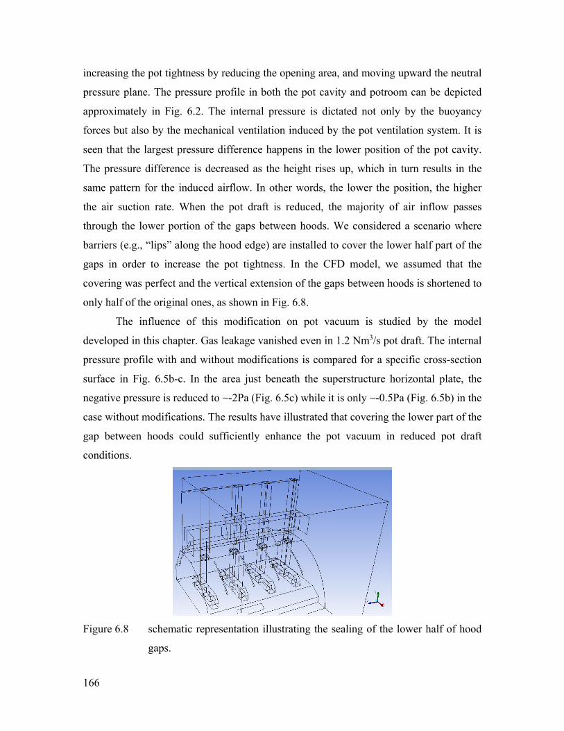
166

increasing the pot tightness by reducing the opening area, and moving upward the neutral

pressure plane. The pressure profile in both the pot cavity and potroom can be depicted

approximately in Fig. 6.2. The internal pressure is dictated not only by the buoyancy

forces but also by the mechanical ventilation induced by the pot ventilation system. It is

seen that the largest pressure difference happens in the lower position of the pot cavity.

The pressure difference is decreased as the height rises up, which in turn results in the

same pattern for the induced airflow. In other words, the lower the position, the higher

the air suction rate. When the pot draft is reduced, the majority of air inflow passes

through the lower portion of the gaps between hoods. We considered a scenario where

barriers (e.g., “lips” along the hood edge) are installed to cover the lower half part of the

gaps in order to increase the pot tightness. In the CFD model, we assumed that the

covering was perfect and the vertical extension of the gaps between hoods is shortened to

only half of the original ones, as shown in Fig. 6.8.

The influence of this modification on pot vacuum is studied by the model

developed in this chapter. Gas leakage vanished even in 1.2 Nm3/s pot draft. The internal

pressure profile with and without modifications is compared for a specific cross-section

surface in Fig. 6.5b-c. In the area just beneath the superstructure horizontal plate, the

negative pressure is reduced to ~-2Pa (Fig. 6.5c) while it is only ~-0.5Pa (Fig. 6.5b) in the

case without modifications. The results have illustrated that covering the lower part of the

gap between hoods could sufficiently enhance the pot vacuum in reduced pot draft

conditions.

Figure 6.8 schematic representation illustrating the sealing of the lower half of hood

gaps.

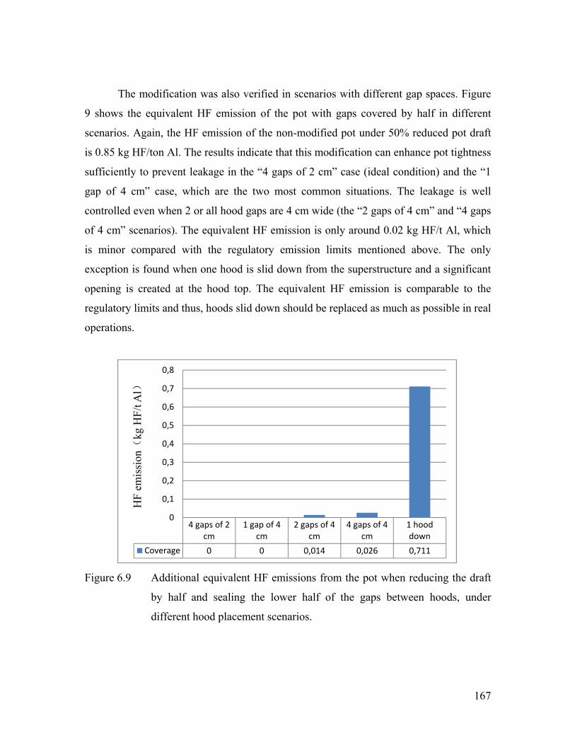
167

The modification was also verified in scenarios with different gap spaces. Figure

9 shows the equivalent HF emission of the pot with gaps covered by half in different

scenarios. Again, the HF emission of the non-modified pot under 50% reduced pot draft

is 0.85 kg HF/ton Al. The results indicate that this modification can enhance pot tightness

sufficiently to prevent leakage in the “4 gaps of 2 cm” case (ideal condition) and the “1

gap of 4 cm” case, which are the two most common situations. The leakage is well

controlled even when 2 or all hood gaps are 4 cm wide (the “2 gaps of 4 cm” and “4 gaps

of 4 cm” scenarios). The equivalent HF emission is only around 0.02 kg HF/t Al, which

is minor compared with the regulatory emission limits mentioned above. The only

exception is found when one hood is slid down from the superstructure and a significant

opening is created at the hood top. The equivalent HF emission is comparable to the

regulatory limits and thus, hoods slid down should be replaced as much as possible in real

operations.

Figure 6.9 Additional equivalent HF emissions from the pot when reducing the draft

by half and sealing the lower half of the gaps between hoods, under

different hood placement scenarios.

4 gaps of 2cm

1 gap of 4cm

2 gaps of 4cm

4 gaps of 4cm

1 hooddown

Coverage 0 0 0,014 0,026 0,711

0

0,1

0,2

0,3

0,4

0,5

0,6

0,7

0,8

HF

em

issi

on（

kg H

F/t

Al）

168

6.7 Conclusions

In the present paper, a CFD model is developed and validated to study pot tightness under

different scenarions. Two domains with different simulation lengthscales are created to

simulate the heat transfer and air flow in both interior and exterior of pots. In the

perspective of waste heat recovery and energy savings, a particular attention is devoted to

the possible reduction of pot draft conditions.

The CFD results reveal that current pot structure can maintain good tightness in

normal draft condition, but fails in 50% reduced draft. Since the leakage of pot gas in a

reduced draft condition would add up to the currently existing fluoride emissions, it

would be required to enhance pot tightness in order to reduce the pot ventilation rate.

Two pot designs are tested under 50% reduced draft. The installation of barriers at the

gaps around anode rods gives a good tightness within ideal pot conditions. Nevertheless,

based on our model, it fails if only one hood gap space extends to 4 cm. Covering half of

the hood gaps has shown a desirable tightness even when all gaps are 4 cm wide.

The simulation results have illustrated that the pot gas can be constrained in the

pot with only 50% of normal ventilation rate with a proper sealing of the pot. In addition,

the influence of the air flow in the potroom on the pressure on the pot shell is

demonstrated and can extract pot gas out if the pot vacuum is too small. Heat flux and

open holes on anode cover had little influence on the leakage of pot gas in our

simulations.

169

CHAPTER 7 CONCLUSIONS AND FUTURE WORK

170

This thesis aims at solving two key questions: how to efficiently collect the waste heat

from aluminum smelting cells and how to technically realize the recovery. Based on the

distribution of waste heat dissipation in cells, the pot exhaust gas carries away 35%-40%

of heat content while the rest is released from the pot shell, i.e., hoods and superstructure,

sidewall and bottom. It is therefore required to determine a most effective way to retrieve

the heat from pots. Besides, different pot parameters need to be optimized in order to

maximize the thermal quality of the waste heat. Once it was determined to reduce the

draft of pot exhaust gas, a detailed study was done on how to achieve a pot draft

reduction without other adverse effects. In the present work, three expected problems

associated with the draft reduction were investigated using CFD simulations. The main

results are summarized in the following sections. The simulated results have illustrated a

successful realization of the pot draft reduction. Future works may include an

experimental validation in real smelters and an economical application of the recovered

waste heat.

7.1 Mechanism of heat transfer in the upper part of an aluminum smelting cell

Although a few papers suggested to collect waste heat through pot sidewalls, it is still not

recommended because of the subtle thermal balance between the electrolytic bath and the

heat loss from sidewalls. Therefore, in this thesis, attention was paid to the upper part of

an aluminum smelting cell.

A simple mathematical model based on a thermal circuit representation was first

developed to study how heat is dissipated in the cell upper part. This model considered all

mechanisms of heat transfer (i.e., conduction, convection and radiation) occurring in the

cell and can be solved quickly. It only requires the bath temperature and ambient

temperature as boundary conditions and can determine the internal temperatures and heat

transfer rates in each component. We developed an original formulation to be applied in

fin-like elements with internal Joule heating, such as anode rod, yoke and stubs.

Within this model, a sensitivity analysis of the parameters of interest was done.

The purpose is to maximize the temperature of the pot exhaust gas while taking into

account the thermal management in the cell. Among different parameters, the mass flow

rate of the pot exhaust gas has the larger influence on its temperature and heat content. A

171

50% reduction of the normal draft level can increase the gas temperature by 50-60˚C,

which is a significant augmentation in terms of thermal quality. The gas temperature is

also strongly correlated to the convection on the top surface of anode cover and on the

surface of yoke and stubs. In order to achieve a proper heat management under reduced

pot ventilation, these areas may play a role of modulation. Strengthening the thermal

insulation of hoods redirected more heat in the pot gas, and an optimal insulating level

was obtained. Ambient temperature and anode height are also important factors when

designing any modification in the pot.

A CFD model was then developed to obtain more details than with the simple

model. Besides, the CFD model provided more accurate correlations between the

convective heat transfer coefficient and pot draft condition, which were applied in the

thermal circuit model. The non-uniformity of heat transfer in surfaces was visualized and

the relative importance of natural vs. forced convections was revealed under different pot

ventilation. The results show that the forced convection is dominating heat transfer under

normal pot draft while both mechanisms are equally important under reduced drafts.

This model can be easily adapted to any type of industrial pots and used to

calculate the heat condition in pot. It is also a quick tool to estimate any possible changes

in pot and operating parameters. The calculated results can give the engineers some

coarse results in order to reduce the experimental scales.

7.2 The reduction of pot draft condition

Based on the above mentioned study, it has become apparent that the reduction of pot

draft is the most promising strategy for waste heat recovery from smelting cells. In fact,

the reduction of pot draft condition can bring out some other benefits, such as a

tremendous saving of electricity for fan operation, downsizing the collecting ducts and

less fluoride evolution. In the present studies, our objective was set to achieve a reduction

by half of the normal pot draft condition. For the smelters in ADQ, that means to reduce

the single pot draft from 2.4 Nm3/s to 1.2 Nm3/s. Further reduction is possible but the

corresponding modifications would become more stringent.

We have expected three main issues that might result from the implementation of

pot draft reduction. The first influence is the satisfaction in the top heat loss, which may

172

cause heat imbalance in the bath. Enhancement in heat transfer is required in the upper

part of smelting cells. Then, the reduction of pot draft redirects a portion of the dissipated

heat into the potroom. It is important to estimate the influence of the additional heat on

the heat stress in potroom. The final mission is to guarantee the hooding efficiency of pot

superstructure under reduced pot draft, because of the control of fugitive emissions.

7.2.1 Heat management in reduced pot draft

The first problem in relation with the pot draft reduction is the heat loss from the upper

part of a smelting cell. The total top heat loss is reduced by ~10% as the pot draft goes

down to half of its normal value. According to the engineers’ experiences, it would be a

significant change in the total heat balance of the pot and modification is required to

enhance the top heat loss.

A CFD model was developed to investigate how to remove the same amount of

heat from the bath under the 50% reduced pot draft scenario. Different modifications

were simulated, including addition of fins on anode assembly, geometrical modification

of hood gaps and geomorphological modification of anode cover. The results have

shown that the scenario of exposing more stubs to the air in the hooded space can

perfectly compensate the missing capacity in the top heat loss. The installation of fins on

anode assembly gave little contribution to the top heat loss. Although more heat can be

convectively removed from the increased area of anode assembly, the fins also created

interferences with radiative heat transfer. The net effect was marginal. A scenario with

moderate effect lied in horizontally oriented hood gaps. However, the enhancement in top

heat loss was not enough to recover the missing part.

7.2.2 Heat stress of potroom in reduced pot draft

In the second part, the heat stress in potroom was estimated under a 50% reduced pot

draft. To address this issue, air ventilation and heat transfer were simulated in a potroom.

In order to limit the number of control volumes, the fluid boundary conditions were

directly defined on the building’s openings. Both buoyancy and wind driven forces were

considered in the simulations. Higher heat flux was imposed on the pot shell to represent

a new heat loss distribution in 50% reduced pot draft. An international standard, which is

173

usually applied in extremely hot environment, was employed to estimate the heat stress in

potroom. A specific parameter, During Limitation Exposure, was obtained from the

standard to measure heat stress on working operators. The results have revealed an

intensive heat stress existing in the potroom in summer season while the heat stress,

compared with that in normal pot draft, was only slightly increased in the 50% reduced

pot draft condition. This model also provided our industrial partner with a tool to study

other modifications related to potroom design.

7.2.3 Pot tightness and emission control in reduced pot draft

The final work was focused on the pot tightness under reduced pot draft. Two CFD

models with different simulation scales were created to simulate the flow in both the

interior and exterior of a pot. It was found that current pot structure can maintain good

tightness in normal draft condition while it is likely to fail in 50% reduced draft. The

constant leakage of pot gas will contribute to an additional fluoride emission even more

than the current baseline. Two modifications in the pot structure were proposed and

verified. If the pot was maintained in ideal conditions, the installation of barriers at the

gaps around anode rods provided a good tightness. Nevertheless, leakage occurred if only

one hood gap space is as large as 0.04m which frequently occurs in reality. Covering the

lower half of the hood gap has shown a desirable tightness even when all gaps were 4 cm

wide. The results have illustrated that the pot gas can be constrained in the pot with only

50% of normal ventilation rate if proper sealing was realised on pots.

7.2.4 Other “side” contributions of this thesis

It is important to mention that although this work was initially motivated by the desire to

facilitate waste heat recovery from pots, several other practical benefits have resulted

from our work, such as:

The air ventilation in potroom can be simulated by using the CFD model

representing a slice of potroom. Optimization of the ventilation was performed

based on the interests from industrial partners. For example, potroom ventilation

was simulated in different scenarios where the interior openings on wall and floor

174

were modified. The potroom structure was optimized to achieve a better sidewall

cooling, which is of critical importance for the “load creeping” in smelting cells.

New pressure coefficients on the exterior wall of potroom were established for the

specific potroom geometry, as the coefficients calculated from some conventional

correlations were not suitable for such buildings.

CFD simulations of fugitive emissions from smelting pot provided with deep

insight in the pot tightness, which in turn helped to improve the emission control

in current cells.

A procedure of CFD simulation of the air ventilation in a tall building with strong

heat source, such as the potroom, was presented for the CFD simulation in other

types of buildings with the similar conditions. Different modeling settings, such

as the definition of air density, the choice of reference density and the influence of

environment, were studied and verified in the simulations.

7.3 Future work

This thesis has demonstrated the possibility of a 50% reduction of the normal pot draft in

an aluminum smelting cell based on numerical simulations. Several technical problems

associated with the draft reduction have been addressed. Possible future work can be

summarized as follows:

Although the simulated results are verified and validated with experimental

measurements in real pots, large-scale experiments in real smelters are required to

directly validate the simulated results. All validated scenarios are limited in a

normal pot draft condition. Therefore, the reduced pot draft should be applied to

real pots with the proper modifications for testing pot functionality.

All works involved in this thesis are focused on the pot upper part while it is also

crucial to design facilities for extracting heat from the exhaust gas. A heat

exchanger should be designed and well integrated into the duct system. Moreover,

the application of waste heat should be studied case-by-case, depending on the

local situation and potential users. For instance, it can provide a heat source for

neighboring residences or greenhouses. If the local electricity price is high, an

175

Organic Rankine Cycle may be considered to produce electricity. Direct use in the

pot, such as for alumina preheating, could also be considered.

Our thermal circuit model can be further extended to the sidewalls and bottom. It

could be used as a quick tool for controlling the heat balance in the pot. Thermal

capacitances may be included to take into account transient dynamics.

The transport of hydrogen fluoride in the pot hooded space should be added in the

CFD simulation. To have the information of HF concentration may help us to

design new pot structures for a better control of fugitive emissions. The challenge

of this work is to find a proper way to define the HF evolution in the pot.

176

177

REFERENCES

Abbas, H., 2010. Mechanism of Top Heat Loss from Aluminium Smelting Cells. Ph.D. Thesis, Chemical and Material Engineering, University of Auckland.

Abbas, H., Taylor M.P., Farid, M. and Chen, J.J., 2009. The Impact of Cell Ventilation on the Top Heat Losses and Fugitive Emissions in an Aluminium Smelting Cell. TMS-Light Metals, p. 551-561.

Alie, C., Backham, L., Croiset, E. and Douglas, P.L., 2005. Simulation of CO2 Capture Using MEA Scrubbing: A Flowsheet Decomposition Method. Energy Conversion and Management 46 (3), p. 475–487.

Aljabri, N., Venkatasubramaniam, K.G., AlFarsi, Y.A.M. and Dubai, J.A., 2003. HF Emission from Dubal’s Electrolysis Cell. TMS-Light Metals, p. 487–494.

ASHRAE. 2009. ASHRAE Handbook–Fundamentals. Atlanta, GA, 24.3–24.5.

Bergman, T.L., Lavine, A.S., Incropera, F.P. and Dewitt, D.P., 2011. Introduction to Heat Transfer. John Wiley & Sons, Incorporated.

Berkoe, J., Diwakar, P., Martin, L., Baxter, B., Read, C.M., Grover, P. and Ziegler, D., 2005. CFD Modeling of the Fjardaal Smelter Potroom Ventilation. TMS-Light Metals, p. 373–378.

Biedler, P., 2003. Modeling of an Aluminum Reduction Cell for the Development of a State Estimator. West Virginia University.

Bruggeman, J.N., and Danka, D.J., 1990. Two-Dimensional Thermal Modeling of the Hall–Heroult Cell. TMS-Light Metals, p. 203-209.

Chataigner, Y., Gosselin, L. and Doré, G., 2009. Optimization of Embedded Inclined Open-Ended Channel in Natural Convection Used as Heat Drain. International Journal of Thermal Sciences 48 (6), p. 1151–1160.

Chen, Q., 1995. Comparison of Different k-ε Models for Indoor Air Flow Computations. Numerical Heat Transfer, Part B: Fundamental 28 (3), p. 353–369.

Chow, W.K., 1995. Ventilation Design: Use of Computational Fluid Dynamics as a Study Tool. Building Services Engineering Research and Technology 16 (2), p. 63–76.

Cook, M.J., Ji, Y. and Hunt, G.R., 2003. CFD Modelling of Natural Ventilation: Combined Wind and Buoyancy Forces. International Journal of Ventilation 1 (3), p. 169-179.

Cook, M.J. and Lomas, K.J., 1998. Buoyancy-Driven Displacement Ventilation Flows: Evaluation of Two Eddy Viscosity Turbulence Models for Prediction. Building Services Engineering Research and Technology 19 (1), p. 15–21.

Dando, N.R. and Tang, R., 2006. Impact of Tending Practices on Fluoride Evolution and Emission from Aluminum Smelting Pots. TMS-Light Metals, p. 203-206.

Dando, N.R. and Tang, R., 2005. Fluoride Evolution/Emission from Aluminum Smelting Pots–Impact of Ore Feeding and Cover Practices. TMS-Light Metals, p. 363-366.

178

David, J., and Herzog, H., 2000. The Cost of Carbon Capture. In Fifth International Conference on Greenhouse Gas Control Technologies, Cairns, Australia, p. 13-16.

Dernedde, E., 1990. Gas Collection Efficiency on Prebake Reduction Cells. The American Industrial Hygiene Association Journal 51 (1), p. 44–49.

Dernedde, E., 2004. Ventilation Rates of Smelter Buildings in Northern Climates. TMS-Light Metals, p. 347–350.

Doheim, M.A., El-Kersh, A.M. and Ali, M.M., 2007. Computational Modeling of Flow in Aluminum Reduction Cells due to Gas Bubbles and Electromagnetic Forces. Metallurgical and Materials Transactions B 38 (1), p. 113–119.

Dupuis, M., 1998. Computation of Aluminum Reduction Cell Energy Balance Using ANSYS® Finite Element Models. TMS-Light Metals, p. 409–418.

Dupuis, M., 2001. 3D Modeling of the Ventilation Pattern in an Aluminium Smelter Potroom Building Using CFX-4. In Proceedings of the CFDSC Conference, p. 161–166.

Dupuis, M., 2010. Development and Application of an ANSYS (r) Based Thermo-Electro- Mechanical Anode Stub Hole Design Tool. TMS-Light Metals.

Dupuis, M., Bojarevics, V. and Freilbergs, J., 2004. Demonstration Thermo-Electric and MHD Mathematical Models of a 500 kA Aluminum Electrolysis Cell: Part 2. TMS-Light Metals, p. 453–460.

Dussault, J., Gosselin, L. and Galstian, T., 2012. Integration of Smart Windows into Building Design for Reduction of Yearly Overall Energy Consumption and Peak Loads. Solar Energy 86 (11), p. 3405–3416.

Eggen, T., Rolseth, S., Rye, K.A. and Thonstad, J., 1992. Alumina Crusting in Cryolite Melts, Part I: Penetration of Molten Electrolyte into Alumina. TMS-Light Metals.

Eick, I., and Vogelsang, D., 1999. Dimensioning of Cooling Fins for High-Amperage Reduction Cells. TMS-Light Metals, p. 527–533.

Fanisalek, H., Bashiri, M. and Kamali, R., 2011. Waste Heat Recovery Trial from Aluminum Reduction Cell Exhaust Gases. Energy Technology 2011: Carbon Dioxide and Other Greenhouse Gas Reduction Metallurgy and Waste Heat Recovery, p. 65.

Fleer, M., Lorentsen, O.A., Harvey, W., Palsson, H., and Saevarsdottir, G., 2010. Heat Recovery from the Exhaust Gas of Aluminum Reduction Cells. Minerals, Metals and Materials Society/AIME, 420 Commonwealth Dr., P. O. Box 430 Warrendale PA 15086 USA.

Fluent Ansys, 2012. Ansys Fluent 14.5 Users Guide. Fluent Inc., Lebanon, NH.

Fortin, H., Kandev, N. and Fafard, M., 2012. FEM Analysis of Voltage Drop in the Anode Connector Induced by Steel Stub Diameter Reduction. Finite Elements in Analysis and Design 52, p. 71–82.

179

Fraser, K.J., Taylor, M.P. and Jenkin, A.M., 1990. Electrolyte Heat and Mass Transport Processes in Hall Heroult Electrolysis Cells. TMS-Light Metals, p. 221–226.

Gadd, M.D., Ph.D. Thesis. 2003. Aluminium Smelter Cell Energy Flow Monitoring. Chemical and Materials Engineering, University of Auckland.

Gadd, M.D., Welch, B.J. and Ackland, A.D., 2000. The Effect of Process Operations on Smelter Cell Top Heat Losses. TMS-Light Metals.

Green, D.W., and others. 2008. Perry’s Chemical Engineers’ Handbook. Vol. 796. McGraw-hill New York.

Grjotheim, K, and Kvande, H., 1986. Understanding the Hall–Heroult Process for Production of Aluminium. Aluminum-Verlag, P. O. Box 1207, D-4000 Dusseldorf 1, FRG, 1986.

Gusberti, V., Severo, D.S., Welch, B.J. and Skyllas-Kazacos, M., 2012. Modeling the Mass and Energy Balance of Different Aluminium Smelting Cell Technologies. TMS-Light Metals, p. 929–934.

Hatem, G., Llavona, M., Log, T., Sancho, J.P. and OSTVOLD, T., 1988. Thermal-Conductivity of Some Alumina Powders and Synthetic Hall-Heroult Crusts. JOURNAL OF METALS, 40, p. 127.

Haugland, E., Borset, H., Gikling, H. and Hoie, H., 2003. Effects of Ambient Temperature and Ventilation on Shell Temperature, Heat Balance and Side Ledge of an Alumina Reduction Cell. TMS-Light Metals, p. 269–276.

Haupin, W.E., 1971. Calculating Thickness of Containing Walls Frozen from Melt. J METALS 23 (7), p. 41–44.

Hofmann, H.M., Kaiser, R., Kind, M. and Martin, H., 2007. Calculations of Steady and Pulsating Impinging Jets—an Assessment of 13 Widely Used Turbulence Models. Numerical Heat Transfer, Part B: Fundamentals 51 (6), p. 565–583.

Hussain, S., and Oosthuizen, P.H., 2012a. Numerical Investigations of Buoyancy-Driven Natural Ventilation in a Simple Atrium Building and Its Effect on the Thermal Comfort Conditions. Applied Thermal Engineering 40, p. 358–372.

Hussain, S. and Oosthuizen, P.H., 2012b. Validation of Numerical Modeling of Conditions in an Atrium Space with a Hybrid Ventilation System. Building and Environment 52, p. 152–161.

Isman, M.K., Pulat, E., Etemoglu, A.B. and Can, M., 2008. Numerical Investigation of Turbulent Impinging Jet Cooling of a Constant Heat Flux Surface. Numerical Heat Transfer, Part A: Applications 53 (10), p. 1109–1132.

Jacobs, H.R., 1987. Convection Heat Transfer: A. Bejan. Elsevier.

Jessen, S.W., Master Thesis. 2008. Mathematical Modeling of a Hall Héroult Aluminum Reduction Cell. Technical University of Denmark.

Ji, Y., and Cook, M.J., 2007. Numerical Studies of Displacement Natural Ventilation in Multi-Storey Buildings Connected to an Atrium. Building Services Engineering Research and Technology 28 (3), p. 207–222.

180

Ji, Y., Cook, M.J. and Hanby, V., 2007. CFD Modelling of Natural Displacement Ventilation in an Enclosure Connected to an Atrium. Building and Environment 42 (3), p. 1158–1172.

Karlsen, M., Kielland, V., Kvande, H. and Vestre, S.B., 1998. Factors Influencing Cell Hooding and Gas Collection Efficiencies. TMS-Light Metals, p. 910–917.

Kiss, L., and Dassylva-Raymond, V., 2008. Freeze Thickness in the Aluminum Electrolysis Cells. TMS-Light Metals, p. 431.

Kolondzovski, Z., Belahcen, A. and Arkkio, A., 2009. Multiphysics Thermal Design of a High-Speed Permanent-Magnet Machine. Applied Thermal Engineering 29 (13), p. 2693–2700.

Li, Z.R., Ai, Z.T., Wang, W.J., Xu, Z.R., Gao, X.Z. and Wang, H.S., 2013. Evaluation of Airflow Pattern in Wind-Driven Naturally Ventilated Atrium Buildings: Measurement and Simulation. Building Services Engineering Research and Technology.

Llavona, M., 1988. Some New Considerations on the Measurement of Humidity, M. O. I. and L. O. I. TMS-Light Metals, p. 103–108.

Logan, P.W., and Bernard, T.E., 1999. Heat Stress and Strain in an Aluminum Smelter. American Industrial Hygiene Association Journal 60 (5), 659–665.

Lorentsen, O.A., Dyrøy, A., and Karlsen, M., 2009. Handling Co2EQ from an Aluminum Electrolysis Cell. TMS-Light Metals, p. 263.

Luo, Z., Cho, H., Luo, X. and Cho, K., 2008. System Thermal Analysis for Mobile Phone. Applied Thermal Engineering 28 (14), p. 1889–1895.

Maarschalkerwaard, A., 2010. The Use of CFD Simulations to Optimise Ventilation of Potrooms. Minerals, Metals and Materials Society/AIME, 420 Commonwealth Dr., P. O. Box 430 Warrendale PA 15086 USA.

Marois, M.A., Bertrand, C., Désilets, M, Coulombe M.M., and Lacroix, M., 2009. Comparison of Two Different Numerical Methods for Predicting the Formation of the Side Ledge in an Aluminium Electrolysis Cell. TMS-Light Metals, p. 563–568.

McQuiston, F.C., Parker, J.D. and Spitler, J.D., 2010. Heating, Ventilating, and Air Conditioning: Analysis and Design. Vol. 6. Wiley.

Meghlaoui, A., Farsi, Y.A.A. and Aljabri, N.H., 2002. Analytical and Experimental Study of Fluoride Evolution. TMS-Light Metals, p. 283–288.

Menet, N., Girault, G., Monnet, N., Turpin, C., and Soulhac, L., 2013. Latest Developments in Potroom Building Ventilation CFD Modelling. TMS-Light Metals, p. 811–816.

Menter, F.R., 1994. Two-Equation Eddy-Viscosity Turbulence Models for Engineering Applications. AIAA Journal 32 (8), p. 1598–1605.

Mills, A.F., 1999. Heat Transfer. 2nd edition. New Jersey: Prentice Hall.

Modest, M.F., 2013. Radiative Heat Transfer. Academic Press.

181

Nagem, N.F., Batista, E., Silva, A.F., Gomes, V., Ferreira, H., Mendes, R.R.S. and Souza, L.J.P., 2006. Correlation of Fluoride Evolution with on Line off Gas Duct Temperature. TMS-Light Metals, p. 207.

Nagem, N.F., Batista, E., Silva, A.F., Gomes, V., Venâncio, L.C.A. and Souza, L.J.P., 2005. Understanding Fugitive Fluoride Emissions at the Alumar. TMS-Light Metals, p. 289–292.

Namboothiri, S., Lavoie, P., Cotton, D. and Taylor, M., 2009. Controlled Cooling of Aluminium Smelting Cell Sidewalls Using Heat Exchangers Supplied with Air. TMS-Light Metals, p. 317–322.

Nowicki, C., and Gosselin L., 2012. An Overview of Opportunities for Waste Heat Recovery and Thermal Integration in the Primary Aluminum Industry. JOM 64 (8), p. 990–996.

Nowicki, C., Gosselin, L. and Duchesne, C., 2012. Waste Heat Integration Potential Assessment through Exergy Analysis in an Aluminium Production Facility. TMS-Energy Technology 2012: Carbon Dioxide Management and Other Technologies, p. 165–172.

Osen, K.S., Aarhaug, T.A., Solheim, A., Skybakmoen, E. and Sommerseth, C., 2011. HF Measurements inside an Aluminium Electrolysis Cell. TMS-Light Metals.

Palyvos, J.A., 2008. A Survey of Wind Convection Coefficient Correlations for Building Envelope Energy Systems’ Modeling. Applied Thermal Engineering 28 (8), p. 801–808.

Parsons, K.C., 1999. International Standards for the Assessment of the Risk of Thermal Strain on Clothed Workers in Hot Environments. Annals of Occupational Hygiene 43 (5), p. 297–308.

Patterson, E.C., Ph.D. Thesis. 2002. Fluoride Emissions from Aluminium Electrolysis Cells. ResearchSpace@Auckland.

Perry, R.H., Green, D.W. and Maloney, J.O., 1984. Perry’s Chemical Engineering Handbook. Don Green, New York.

Ramponi, R., and Blocken, B., 2012. CFD Simulation of Cross-Ventilation for a Generic Isolated Building: Impact of Computational Parameters. Building and Environment 53, p. 34–48.

Rye, K.A.A., Thonstad, J. and Liu X., 1995. Heat Transfer, Thermal Conductivity, and Emissivity of Hall-Heroult Top Crust. TMS-Light Metals, p. 630–638.

Saathof, P.J., Stathopoulos, T. and Dobrescu, M., 1995. Effects of Model Scale in Estimating Pollutant Dispersion near Buildings. Journal of Wind Engineering and Industrial Aerodynamics 54, p. 549–559.

Severo, D.S., and Gusberti, V., 2009. A Modelling Approach to Estimate Bath and Metal Heat Transfer Coefficients. TMS-Light Metals, p. 309–314.

182

Severo, D.S., Schneider, A.F., Pinto, Elton C.V., Gusberti, V. and Potocnik, V., 2005. Modeling Magnetohydrodynamics of Aluminum Electrolysis Cells with ANSYS and CFX. TMS-Light Metals, p. 475-480.

Sharif, M.A.R., and Mothe, K.K., 2009. Evaluation of Turbulence Models in the Prediction of Heat Transfer due to Slot Jet Impingement on Plane and Concave Surfaces. Numerical Heat Transfer, Part B: Fundamentals 55 (4), p. 273–294.

Shcherbinin, S.A., Rozin, A.V. and Lukashchuk, S.Y., 2003. The 3D Modeling of MHD-Stability of Aluminum Reduction Cells. TMS-Light Metals, p. 373–378.

Shen, X.C., Ph.D. Thesis. 2006. Top Cover and Energy Balance in Hall-Heroult Cells. ResearchSpace@ Auckland.

Shen, X.C., Hyland, M. and Welch, B., 2008. Top Heat Loss in Hall-Heroult Cells. TMS-Light Metals, p. 501.

Slaugenhaupt, M.L., Bruggeman, J.N., Tarcy, G.P. and Dando, N.R., 2003. Effect of Open Holes in the Crust on Gaseous Fluoride Evolution from Pots. TMS-Light Metals, p. 199–204.

Smith, P.L., and Winkle, M.V., 1958. Discharge Coefficients through Perforated Plates at Reynolds Numbers of 400 to 3,000. AIChE Journal 4 (3), p. 266–268.

Solheim, A., 2011. Some Aspects of Heat Transfer between Bath and Sideledge in Aluminium Reduction Cells. TMS-Light Metals, p. 381–386.

Sommerseth, C., Osen, K.S., Aarhaug, T.A., Skybakmoen, E., Solheim, A., Rosenkilde, C. and Ratvik, A.P., 2011. Correlation between Moisture and HF Formation in the Aluminium Process. TMS-Light Metals, p. 339–344.

Sørhuus, A., and Wedde, G., 2009. Pot Gas Heat Recovery and Emission Control. TMS-Light Metals, p. 987–992.

Sorhuus, A., Wedde, G., Rye, K. and Nyland, G., 2010. Increased Energy Efficiency and Reduced HF Emissions with New Heat Exchanger. Minerals, Metals and Materials Society/AIME, 420 Commonwealth Dr., P. O. Box 430 Warrendale PA 15086 USA.

Stamou, A.I., Katsiris, I. and Schaelin, A., 2008. Evaluation of Thermal Comfort in Galatsi Arena of the Olympics ‘Athens 2004’ Using a CFD Model. Applied Thermal Engineering 28 (10), p. 1206–1215.

Tarcy, G.P., 2003. The Affect of Pot Operation and Work Practices on Gaseous and Particulate Fluoride Evolution. TMS-Light Metals, p. 193–198.

Taylor, M.P., 2007. Anode Cover Material–science, Practice and Future Needs. In Proceedings of 9th Australasian Aluminium Smelting Technology Conference, p. 4–9.

Taylor, M.P., Johnson, G.L., Andrews, E.W. and Welch, B.J., 2004. The Impact of Anode Cover Control and Anode Assembly Design on Reduction Cell Performance. TMS-Light Metals, p. 199–206.

183

Taylor, M.P., 1984. The Influence of Process Dynamics on the Heat Balance and Cell Operation in the Electrowinning of Aluminium. ResearchSpace@ Auckland.

Taylor, M.P., Zhang, W.D., Wills, V. and Schmid, S., 1996. A Dynamic Model for the Energy Balance of an Electrolysis Cell. Chemical Engineering Research and Design 74 (8), p. 913–933.

Tessier, J., Duchesne, C., Gauthier, C. and Dufour, G., 2008. Image Analysis for Estimation of Anode Cover Material Composition. TMS-Light Metals, p. 293.

Tjahyono, N., Gao, Y., Wong, D., Zhang, W. and Taylor, M.P., 2011. Fluoride Emissions Management Guide (FEMG) for Aluminium Smelters. TMS-Light Metals. John Wiley & Sons, Inc. Hoboken, NJ.

Tomasino, T., Martin, C., Waz, E. and Renaudier S., 2004. Numerical Modeling of Heat Transfer around an Aluminum Reduction Pot Shell.” TMS-Light Metals, p. 433–438.

True, J.P.J., Ph.D. Thesis. 2003. Openings in Wind Driven Natural Ventilation. Aalborg University, Faculties of Engineering, Science and Medicine, Institut for Bygningsteknik, Department of Building Technology and Structural Engineering.

Vershenya, A., Shah, U., Broek, S., Plikas, T., Woloshyn, J. and Schneider, A.F., 2011. Modern Design of Potroom Ventilation. TMS-Light Metals, p. 531–535.

Yu, H.L., Cui, Q.L., Liu, X.H., Zhao, X.M. and Tian, T.L., 2004. Analysis of 3D Thermo-Electric Field Potential for 300 kA Aluminum Electrolysis Cell Using ANSYS. Non-Ferrous Mining and Metallurgy 3, p. 009.

Yurkov, V. and Mann, V., 2005. A Simple Dynamic Realtime Model for Aluminum Reduction Cell Control System. TMS-Light Metals, 423-428.

Zhai, Z., Zhang, Z., Zhang, W. and Chen, Q., 2007. Evaluation of Various Turbulence Models in Predicting Airflow and Turbulence in Enclosed Environments by CFD: Part 1—Summary of Prevalent Turbulence Models. Hvac&R Research 13 (6), p. 853-870.

Zhang, H., Li, J., Wang, Z., Xu, Y. and Lai, Y., 2010. The Numerical Modeling of Melt Flow and MHD Instabilities in an Aluminum Reduction Cell. JOM 62 (11), p. 26-31.

Zhang, Z., Zhang, W., Zhai, Z. and Chen, Q., 2007. Evaluation of Various Turbulence Models in Predicting Airflow and Turbulence in Enclosed Environments by CFD: Part 2—Comparison with Experimental Data from Literature. Hvac&R Research 13 (6), p. 871-886.

Zhao, R., Gosselin, L., Ousegui, A., Fafard, M. and Ziegler D.P., 2013. Heat Transfer and Airflow Analysis in the Upper Part of Electrolytic Cells Based on CFD.” Numerical Heat Transfer, Part A: Applications 64 (4), p. 317-338.

Zhao, R., Gosselin, L., Fafard, M. and Ziegler D.P., 2013a. Heat Transfer in Upper Part of Electrolytic Cells: Thermal Circuit and Sensitivity Analysis. Applied Thermal Engineering 54 (1), p. 212–225.

184

Zhao, R., Gosselin, L., Fafard, M. and Ziegler D.P., 2013b. Reduced Ventilation of Upper Part of Aluminum Smelting Pot: Potential Benefits, Drawbacks, and Design Modifications. TMS-Light Metals, p. 805–810.

Zhao, R. and Gosselin, L., Natural Ventilation of a Tall Industrial Builindg: Investigation on the Impact of Modeling Assumptions. eSim 2014, May 7-10th, Ottawa.

Zhao, R., Gosselin, L., and Tessier, J., 2014. Airflow and Thermal Conditions in Aluminum Smelting Potrooms under Different Conditions. Building Services Engineering Research and Technology, under review.

Zueco, J. and Campo, A., 2006. Network Model for the Numerical Simulation of Transient Radiative Transfer Process between the Thick Walls of Enclosures. Applied Thermal Engineering 26 (7), p. 673–79.

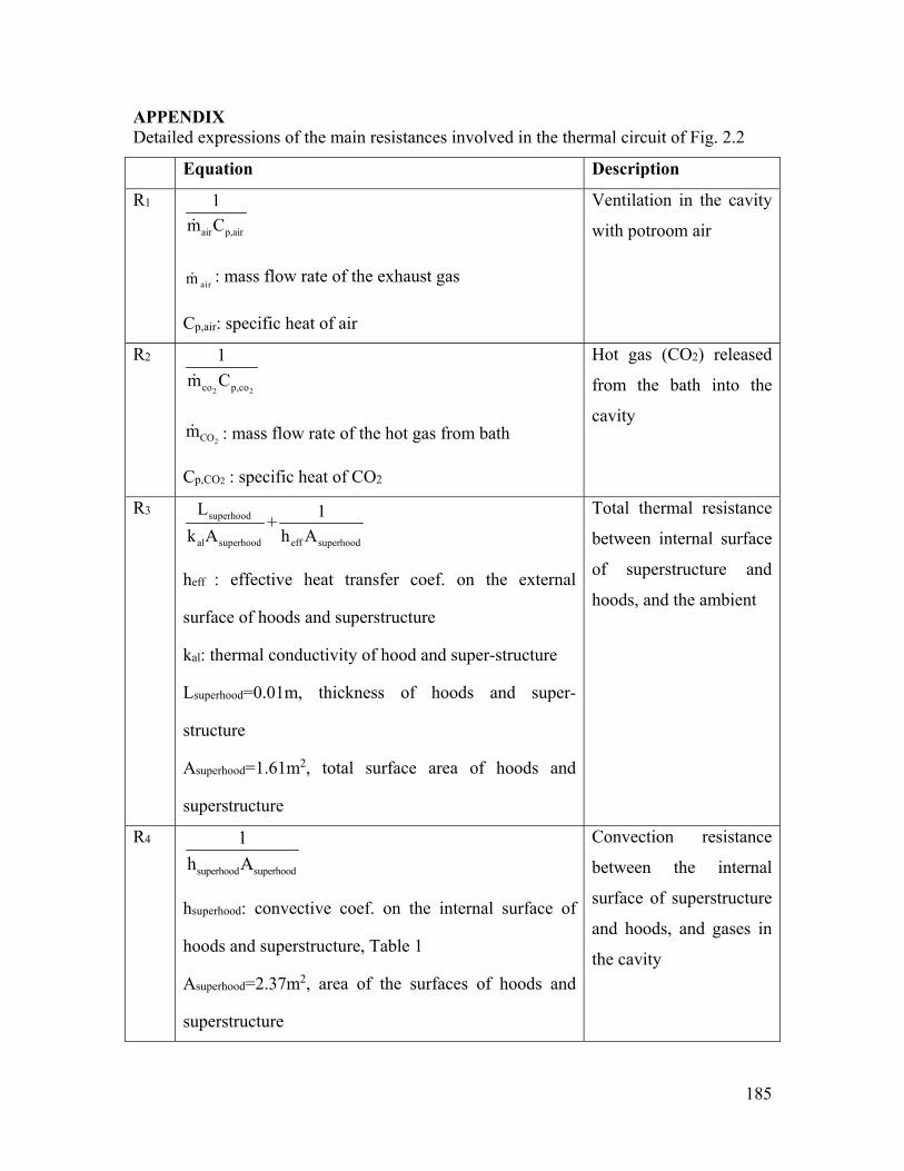
185

APPENDIX Detailed expressions of the main resistances involved in the thermal circuit of Fig. 2.2

Equation Description

R1

air p,air

1

m C

airm : mass flow rate of the exhaust gas

Cp,air: specific heat of air

Ventilation in the cavity

with potroom air

R2

2 2co p,co

1

m C

2COm : mass flow rate of the hot gas from bath

Cp,CO2 : specific heat of CO2

Hot gas (CO2) released

from the bath into the

cavity

R3 superhood

al superhood eff superhood

L 1+

k A h A

heff : effective heat transfer coef. on the external

surface of hoods and superstructure

kal: thermal conductivity of hood and super-structure

Lsuperhood=0.01m, thickness of hoods and super-

structure

Asuperhood=1.61m2, total surface area of hoods and

superstructure

Total thermal resistance

between internal surface

of superstructure and

hoods, and the ambient

R4

superhood superhood

1

h A

hsuperhood: convective coef. on the internal surface of

hoods and superstructure, Table 1

Asuperhood=2.37m2, area of the surfaces of hoods and

superstructure

Convection resistance

between the internal

surface of superstructure

and hoods, and gases in

the cavity

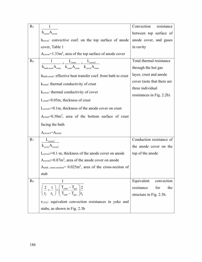
186

R5

cover cover

1

h A

hcover: convective coef. on the top surface of anode

cover, Table 1

Acover=1.33m2, area of the top surface of anode cover

Convection resistance

between top surface of

anode cover, and gases

in cavity

R6 crust cover1

bath-crust crust crust crust cover crust

L L1+ +

h A k A k A

hbath-crust: effective heat transfer coef. from bath to crust

kcrust: thermal conductivity of crust

kcover: thermal conductivity of cover

Lcrust=0.05m, thickness of crust

Lcover1=0.1m, thickness of the anode cover on crust

Acrust=0.38m2, area of the bottom surface of crust

facing the bath

Acover1=Acrust

Total thermal resistance

through the hot gas

layer, crust and anode

cover (note that there are

three individual

resistances in Fig. 2.2b)

R7 cover2

cover cover2

L

k A

Lcover2=0.1 m, thickness of the anode cover on anode

Acover2=0.87m2, area of the anode cover on anode

Astub, cross-section= 0.025m2, area of the cross-section of

stub

Conduction resistance of

the anode cover on the

top of the anode

R8

yoke gas

2 6 stub gas 4

1

T T2 1 2+ +

r r T T r

r2,4,6: equivalent convection resistances in yoke and

stubs, as shown in Fig. 2.3b

Equivalent convection

resistance for the

structure in Fig. 2.3b.

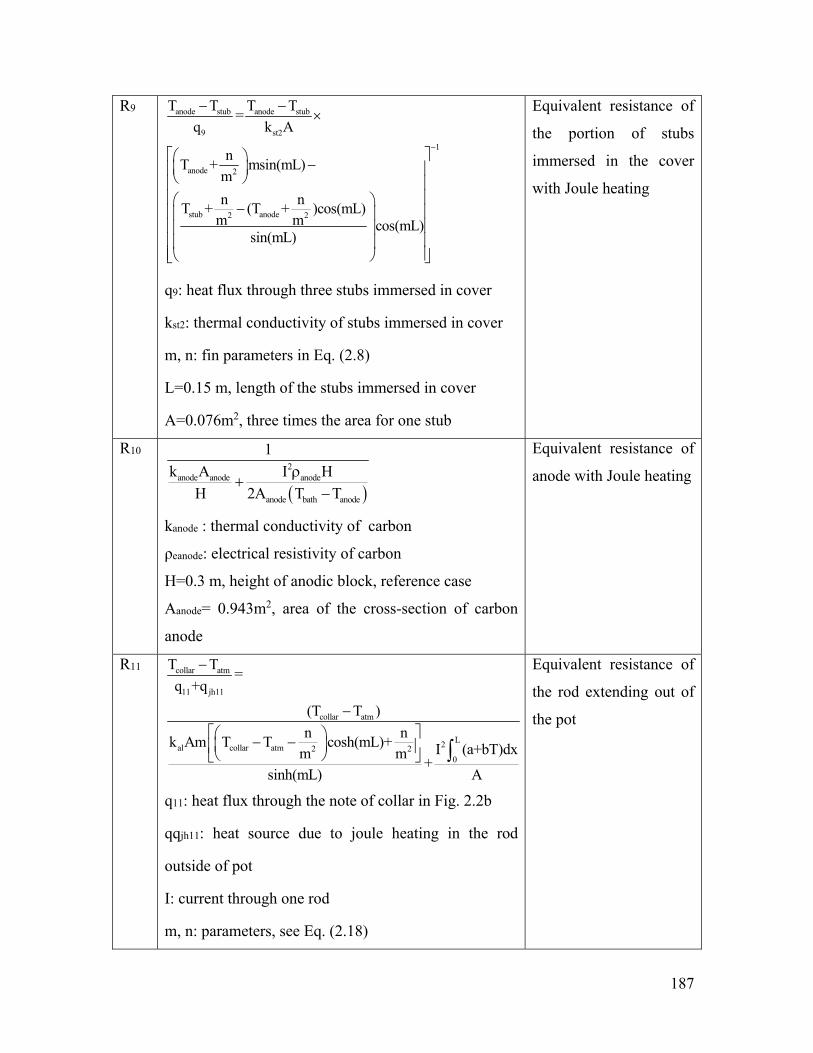
187

R9 anode stub anode stub

9 st2

1

anode 2

stub anode2 2

T T T T=

q k A

nT + msin(mL)

m

n nT + (T + )cos(mL)

m m cos(mL)sin(mL)

q9: heat flux through three stubs immersed in cover

kst2: thermal conductivity of stubs immersed in cover

m, n: fin parameters in Eq. (2.8)

L=0.15 m, length of the stubs immersed in cover

A=0.076m2, three times the area for one stub

Equivalent resistance of

the portion of stubs

immersed in the cover

with Joule heating

R10

2

anode anode anode

anode bath anode

1

k A I H

H 2A T T

kanode : thermal conductivity of carbon

ρeanode: electrical resistivity of carbon

H=0.3 m, height of anodic block, reference case

Aanode= 0.943m2, area of the cross-section of carbon

anode

Equivalent resistance of

anode with Joule heating

R11 collar atm

11 jh11

collar atm

L2al collar atm 2 20

T T=

q +q

(T T )

n nk Am T T cosh(mL)+ I (a+bT)dxm m

+sinh(mL) A

q11: heat flux through the note of collar in Fig. 2.2b

qqjh11: heat source due to joule heating in the rod

outside of pot

I: current through one rod

m, n: parameters, see Eq. (2.18)

Equivalent resistance of

the rod extending out of

the pot

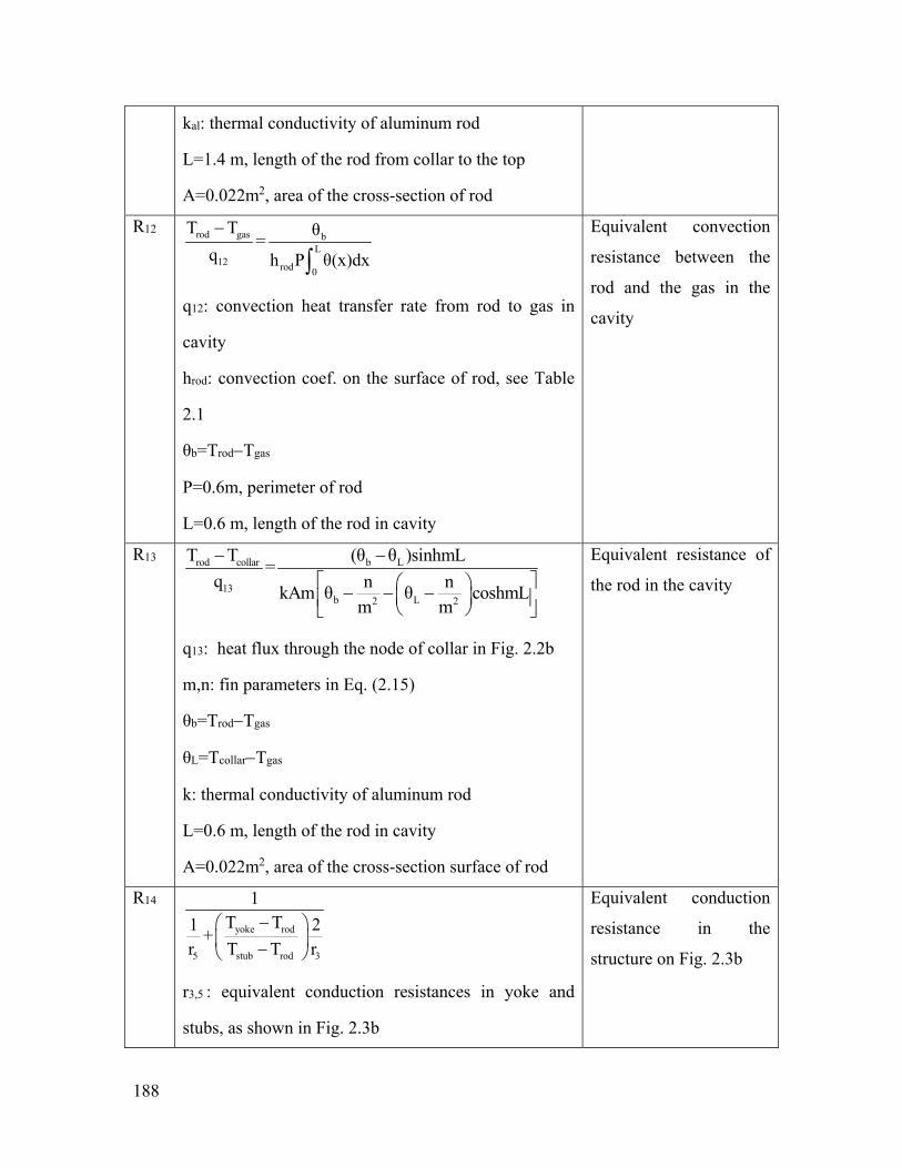
188

kal: thermal conductivity of aluminum rod

L=1.4 m, length of the rod from collar to the top

A=0.022m2, area of the cross-section of rod

R12 rod gas bL

12 rod 0

T T θ=

q h P θ(x)dx

q12: convection heat transfer rate from rod to gas in

cavity

hrod: convection coef. on the surface of rod, see Table

2.1

θb=TrodTgas

P=0.6m, perimeter of rod

L=0.6 m, length of the rod in cavity

Equivalent convection

resistance between the

rod and the gas in the

cavity

R13 rod collar b L

13b L2 2

T T (θ θ )sinhmL=

q n nkAm θ θ coshmL

m m

q13: heat flux through the node of collar in Fig. 2.2b

m,n: fin parameters in Eq. (2.15)

θb=TrodTgas

θL=TcollarTgas

k: thermal conductivity of aluminum rod

L=0.6 m, length of the rod in cavity

A=0.022m2, area of the cross-section surface of rod

Equivalent resistance of

the rod in the cavity

R14

yoke rod

5 stub rod 3

1T T1 2

+r T T r

r3,5 : equivalent conduction resistances in yoke and

stubs, as shown in Fig. 2.3b

Equivalent conduction

resistance in the

structure on Fig. 2.3b

189