Application of the systematic renormalization scheme Application of the systematic renormalization scheme in the covariant form of lightin the covariant form of light--front dynamics front dynamics

to chiral perturbation theoryto chiral perturbation theory

N.A. TsirovaLaboratoire de Physique Corpusculaire, Aubiere, France

J.-F. MathiotLaboratoire de Physique Corpusculaire, Aubiere, France

Light Cone 2011

OutlineOutline

• Introduction: LFχEFT• Covariant Light-Front Dynamics• Fock sector dependent renormalization scheme• Taylor-Lagrange regularization scheme• Application to ChPT• Perspectives

IntroductionIntroduction

To understand the nucleon structure at low energy from a chiral effective Lagrangian we need an appropriatecalculational scheme:

• relativistic• non-perturbative• well-controlled approximation scheme

We present LFχEFT – Light-Front Chiral Effective Field Theory

Light Front Chiral Effective Field TheoryLight Front Chiral Effective Field Theory

Key points:

• CLFDexplicitly covariant formulation of light-front dynamics[J.Carbonell et al. Phys.Rep. 300 (1998) 215]

• FSDRFock sector dependent renormalization scheme[V. Karmanov et al. PRD 77 (2008) 085028]

• TLRSTaylor-Lagrange regularization scheme[P.Grangé et al. Phys. Rev. D 82 (2010) 025012]

Already doneAlready done

CLFD + FSDR + Pauli-Villars

• Yukawa N=2, N=3• QED N=2

[V. Karmanov et al. PRD 77 (2008) 085028]

• ChPT N=2

CLFD + FSDR + TLRS

• Yukawa N=2[P.Grangé et al. Phys.Rev.D 80 (2009) 105012]

ChPT is the first “realistic” test of this approach

Covariant LightCovariant Light--Front DynamicsFront Dynamics

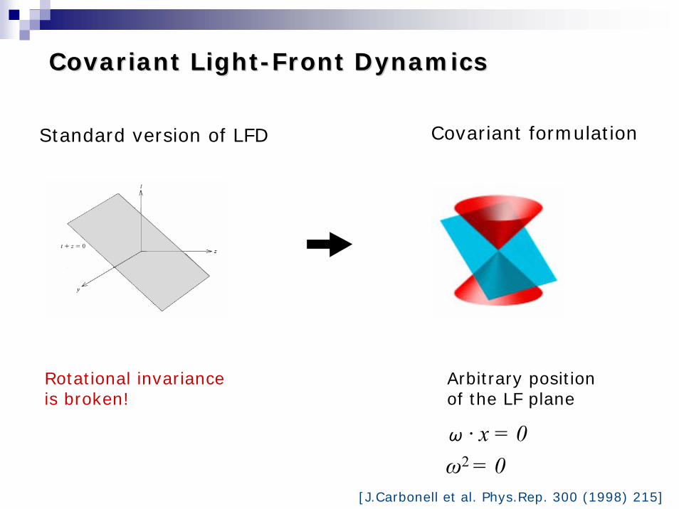
Standard version of LFD Covariant formulation

Rotational invariance is broken!

Arbitrary position of the LF plane

[J.Carbonell et al. Phys.Rep. 300 (1998) 215]

ω2 = 0ω · x = 0

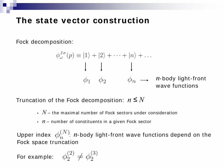
The state vector constructionThe state vector construction

Upper index : n-body light-front wave functions depend on the Fock space truncation

Fock decomposition:

n-body light-front wave functions

Truncation of the Fock decomposition: n ≤ N• N – the maximal number of Fock sectors under consideration

• n – number of constituents in a given Fock sector

For example:

Vertex functionsVertex functions

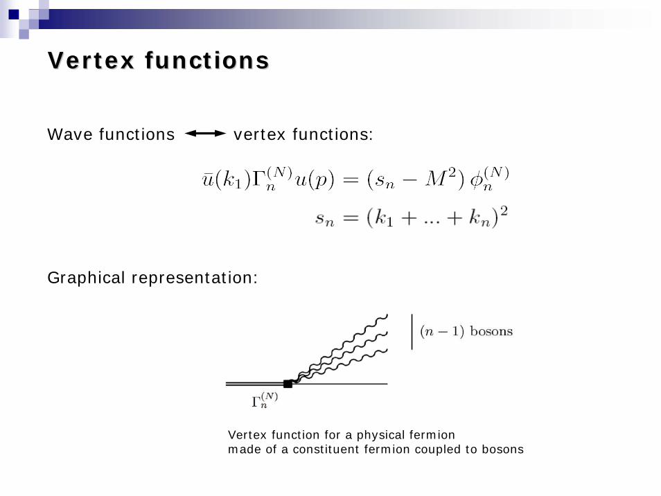
Wave functions vertex functions:

Graphical representation:

Vertex function for a physical fermionmade of a constituent fermion coupled to bosons

Vertex functionsVertex functions

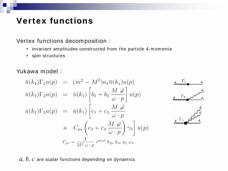
Vertex functions decomposition :• invariant amplitudes constructed from the particle 4-momenta• spin structures

Yukawa model :

a, b, c are scalar functions depending on dynamics

Renormalization schemeRenormalization scheme

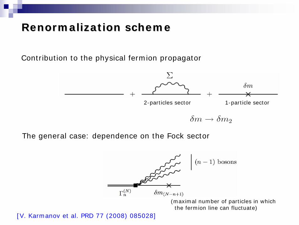
Contribution to the physical fermion propagator

The general case: dependence on the Fock sector

(maximal number of particles in whichthe fermion line can fluctuate)

2-particles sector 1-particle sector

[V. Karmanov et al. PRD 77 (2008) 085028]

Renormalization schemeRenormalization scheme

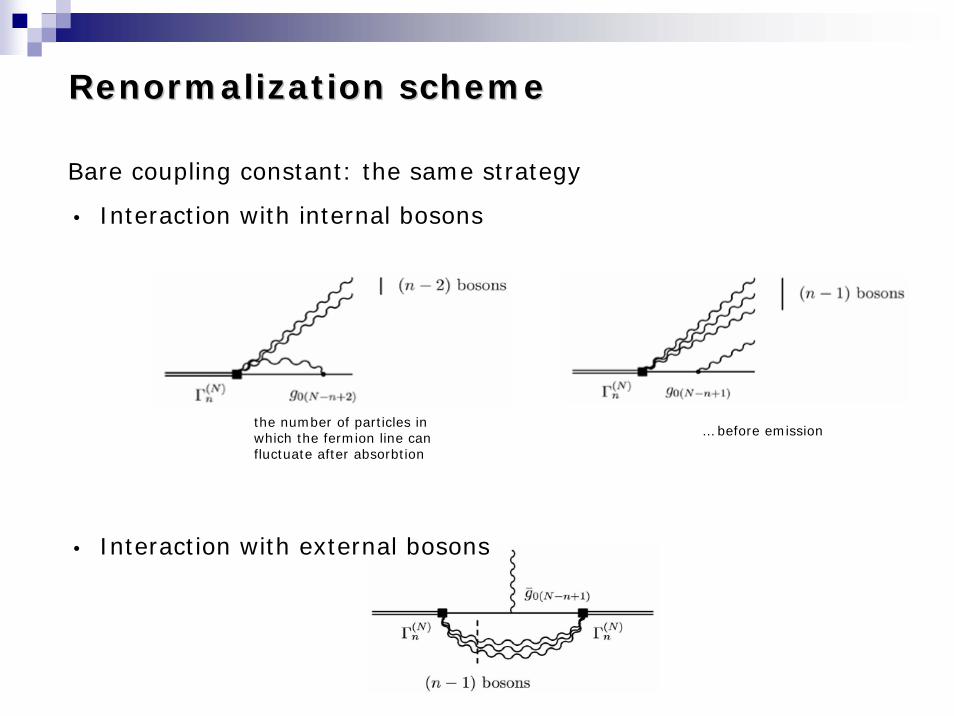
Bare coupling constant: the same strategy

the number of particles in which the fermion line can fluctuate after absorbtion

… before emission

• Interaction with internal bosons

• Interaction with external bosons

Renormalization schemeRenormalization scheme

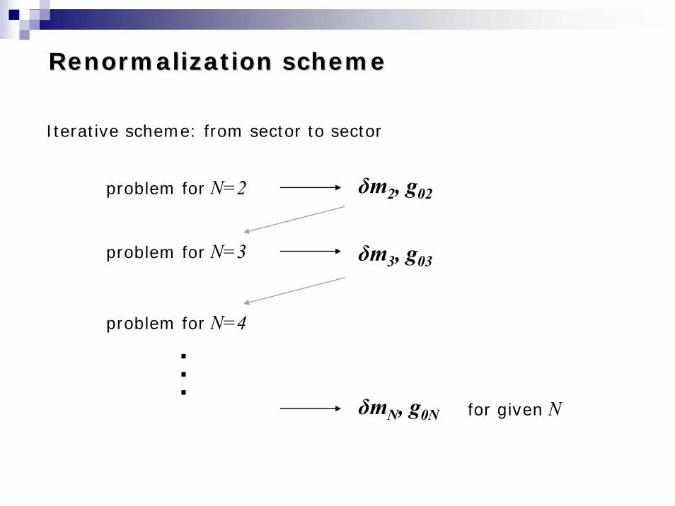
Iterative scheme: from sector to sector

δm2, g02problem for N=2

problem for N=3 δm3, g03

...δmN, g0N for given N

problem for N=4

Renormalization schemeRenormalization scheme

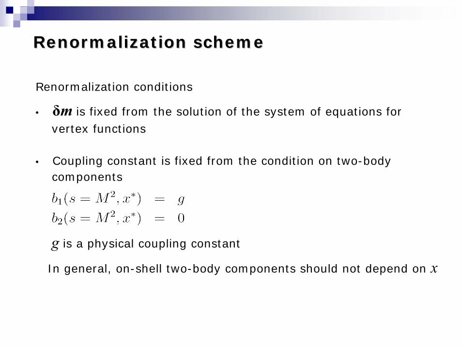
Renormalization conditions

• δm is fixed from the solution of the system of equations for vertex functions

• Coupling constant is fixed from the condition on two-body components

g is a physical coupling constant

In general, on-shell two-body components should not depend on x

RegularizationRegularization

Infinite regularization schemes:

• Cut-off

• Dimensional regularization

• Pauli-Villars regularization scheme

All these schemes deal with infinitely large contributions

We use TLRS: systematic finite regularization scheme

Amplitudes depend on arbitrary finite scale

Basics of TLRSBasics of TLRS

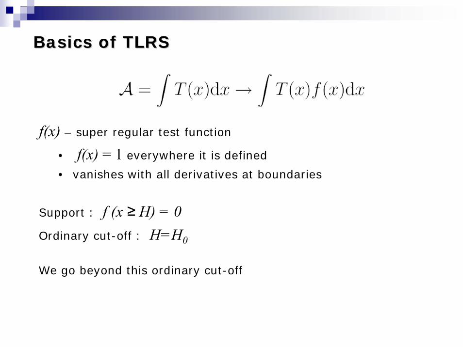
f(x) – super regular test function

• f(x) = 1 everywhere it is defined• vanishes with all derivatives at boundaries

Support : f (x ≥ H) = 0Ordinary cut-off : H=H0

We go beyond this ordinary cut-off

Basics of TLRSBasics of TLRS

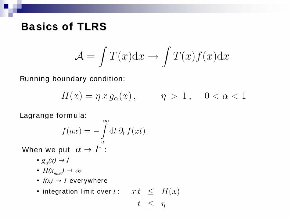
Lagrange formula:

When we put a Ø 1- :• ga(x) Ø 1• H(xmax) Ø ¶• f(x) Ø 1 everywhere• integration limit over t :

Running boundary condition:

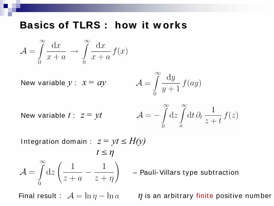
Basics of TLRS : how it worksBasics of TLRS : how it works

New variable t : z = yt

Integration domain : z = yt § H(y)t § h

– Pauli-Villars type subtraction

Final result : h is an arbitrary finite positive number

New variable y : x = ay

Application to Chiral Perturbation Theory Application to Chiral Perturbation Theory N=2N=2

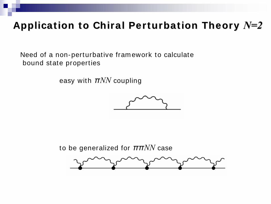
Need of a non-perturbative framework to calculatebound state properties

easy with πNN coupling

to be generalized for ππNN case

ChPT LagrangianChPT Lagrangian

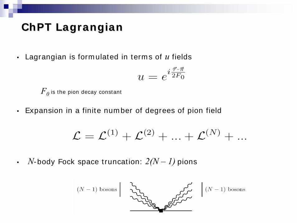
• Lagrangian is formulated in terms of u fields

F0 is the pion decay constant

• Expansion in a finite number of degrees of pion field

• N-body Fock space truncation: 2(N – 1) pions

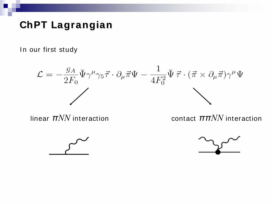
ChPT LagrangianChPT Lagrangian

linear πNN interaction contact ππNN interaction

In our first study

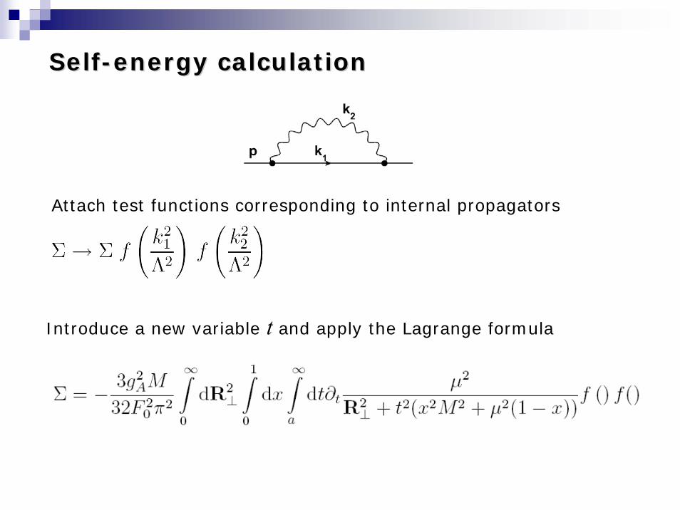
SelfSelf--energy calculationenergy calculation

Attach test functions corresponding to internal propagators

Introduce a new variable t and apply the Lagrange formula

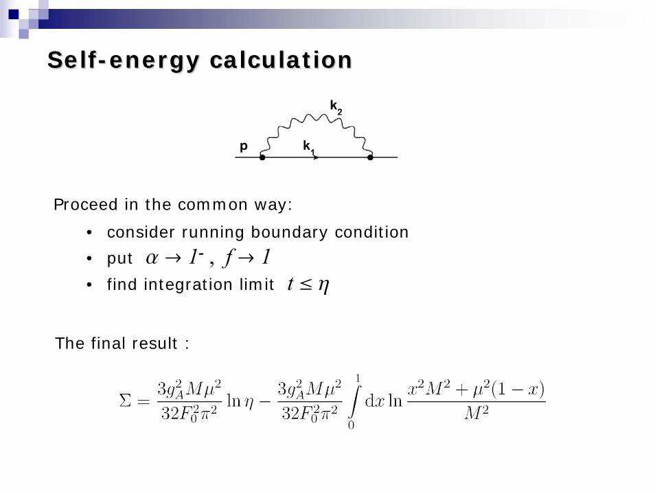
SelfSelf--energy calculationenergy calculation

The final result :

Proceed in the common way:• consider running boundary condition• put a Ø 1- , f Ø 1• find integration limit t § h

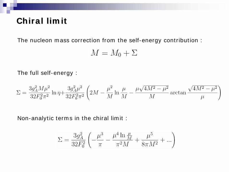
Chiral limitChiral limit

The nucleon mass correction from the self-energy contribution :

The full self-energy :

Non-analytic terms in the chiral limit :

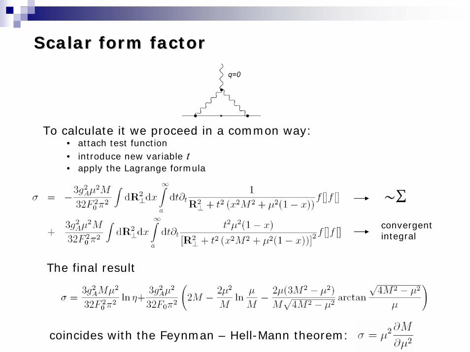
Scalar form factorScalar form factor

To calculate it we proceed in a common way:• attach test function• introduce new variable t• apply the Lagrange formula

~S

convergentintegral

The final result

coincides with the Feynman – Hell-Mann theorem:

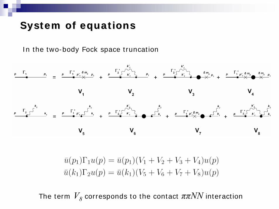
System of equationsSystem of equations

In the two-body Fock space truncation

The term V8 corresponds to the contact ππNN interaction

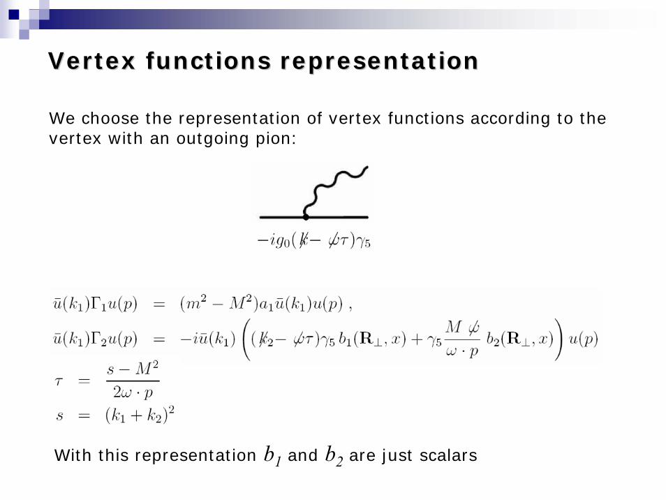
Vertex functions representationVertex functions representation

We choose the representation of vertex functions according to thevertex with an outgoing pion:

With this representation b1 and b2 are just scalars

SolutionSolution

Condition :

Bare coupling constant :

Mass counterterm :

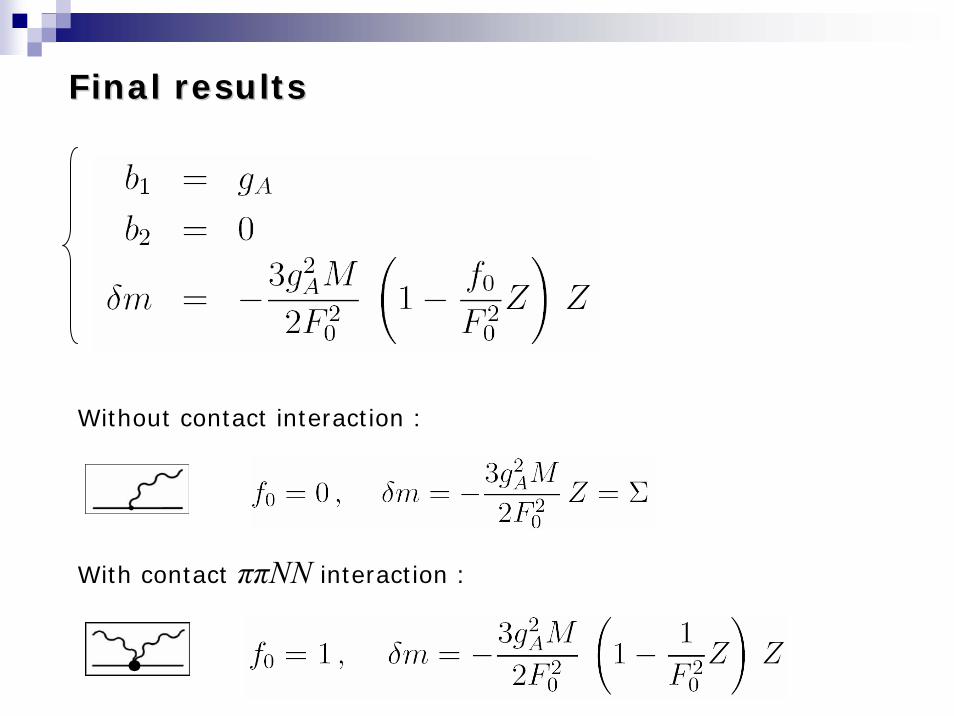
Final resultsFinal results

Without contact interaction :

With contact ππNN interaction :

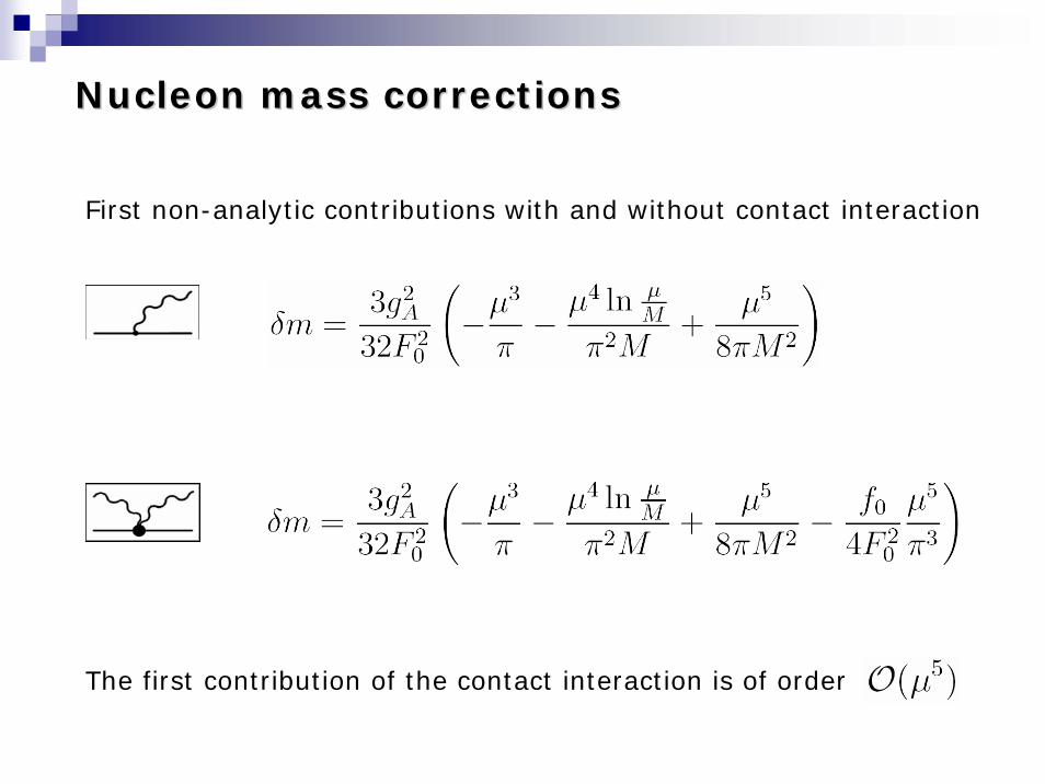
Nucleon mass correctionsNucleon mass corrections

First non-analytic contributions with and without contact interaction

The first contribution of the contact interaction is of order

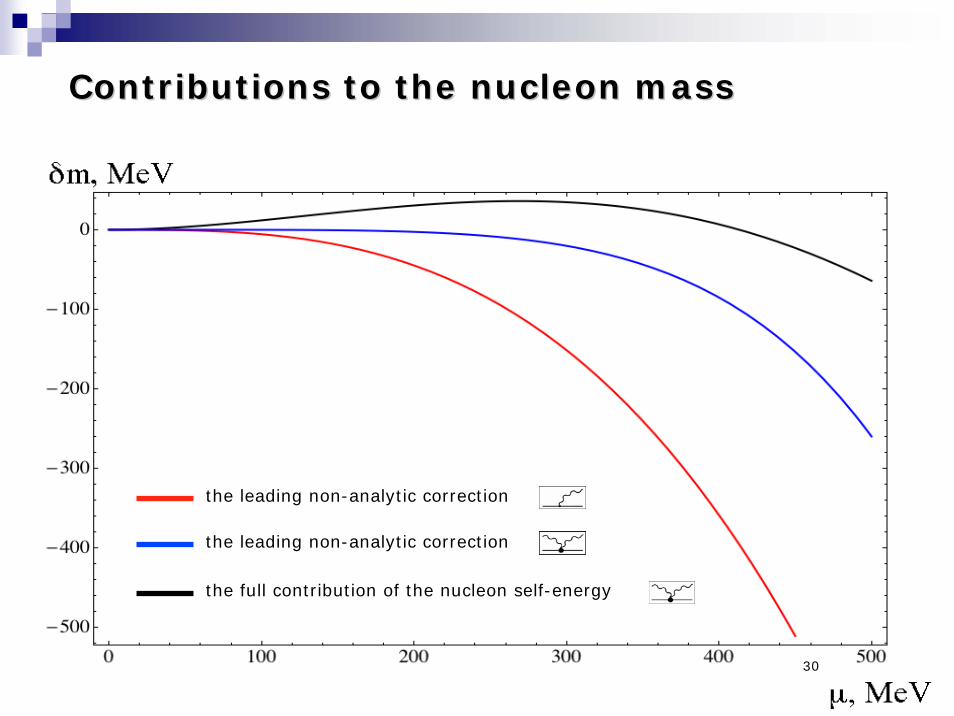
Contributions to the nucleon massContributions to the nucleon mass

30

the leading non-analytic correction

the leading non-analytic correction

the full contribution of the nucleon self-energy

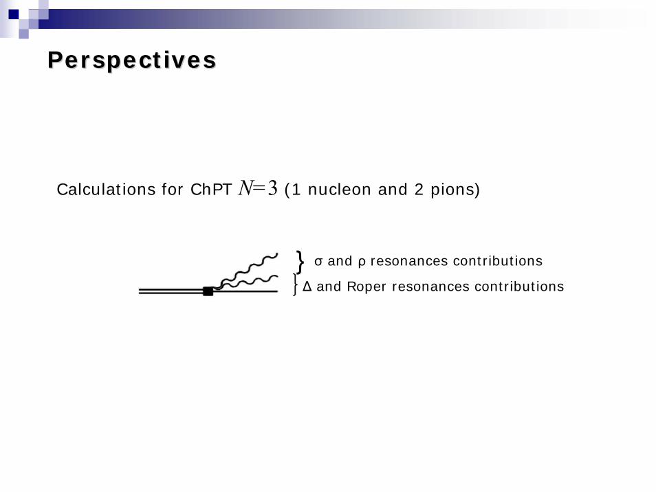
PerspectivesPerspectives

Calculations for ChPT N=3 (1 nucleon and 2 pions)

∆ and Roper resonances contributions} σ and ρ resonances contributions