AVERTISSEMENT Ce document est le fruit d’un long travail approuvé par le jury de soutenance et mis à disposition de l’ensemble de la communauté universitaire élargie. Il est soumis à la propriété intellectuelle de l’auteur : ceci implique une obligation de citation et de référencement lors de l’utilisation de ce document. D’autre part, toute contrefaçon, plagiat, reproduction illicite de ce travail expose à des poursuites pénales. Contact : portail-publi@ut-capitole.fr

LIENS Code la Propriété Intellectuelle – Articles L. 122-4 et L. 335-1 à L. 335-10 Loi n°92-597 du 1er juillet 1992, publiée au Journal Officiel du 2 juillet 1992 http://www.cfcopies.com/V2/leg/leg-droi.php http://www.culture.gouv.fr/culture/infos-pratiques/droits/protection.htm

TTHHÈÈSSEE

En vue de l'obtention du

DDOOCCTTOORRAATT DDEE LL’’UUNNIIVVEERRSSIITTÉÉ DDEE TTOOUULLOOUUSSEE

Délivré par l’ Université Toulouse 1 Capitole Discipline : Sciences Economiques

Présentée et soutenue par

Xingyi LIU Le 17 octobre 2014

Titre :

Essays in Industrial Organization

JURY

Zhijun CHEN, professeur, Auckland University Régis RENAULT, professeur, Université de Cergy-Pontoise Patrick REY, professeur, Université Toulouse 1 Michael RIORDAN, professeur, Columbia University Wilfried SAND-ZANTMAN, professeur, Université Toulouse 1

Ecole doctorale : Toulouse School of Economics Unité de recherche : GREMAQ - TSE

Directeurs de Thèse : Patrick REY et Wilfried SAND-ZANTMAN

Abstract

In my thesis, I study three important issues in industrial organization.

Chapter 1 studies the impact of vertical integration on innovation in an industry where firms

need to undertake risky R&D investments at both production and distribution stages. Vertical

integration brings better coordination within the integrated firm, which boosts its investment

incentive at both upstream and downstream levels. However, it is only mutually beneficial for firms

to integrate when both upstream and downstream innovations are important. When innovation

only matters at one level, firms favor instead vertical separation. The analysis provides insights

for the wave of mergers and R&D outsourcing observed in the pharmaceutical industry and other

vertically related industries.

Chapter 2 studies the effect of quality discrimination on product designs. In the context

of Internet, content providers are subject to quality discrimination from the Internet Service

Providers. We show that content providers are biased to choose broader designs. This reduces

product differentiation in the market, and intervention is necessary to achieve efficiency in the

content market. The result brings new insights into the discussion about net neutrality, which

mandates equal access to every participant on the Internet.

Chapter 3 studies the role of advertisements in attracting and manipulating attention from

consumers. When a product is characterized by several attributes, firms also strategically use

advertisements to manipulate the attention of consumers. A monopolist tends to advertise too few

attributes, and competition does not necessarily improve the situation. Moreover, in an attention-

scarce economy, competition for consumers attention leads firms to advertise fewer attributes and

reduces information available to consumers.

2

Resume

Dans ma these, j’etudie trois questions importantes dans l’economie industrielle.

Chapitre 1 etudie l’impact de l’integration verticale sur l’innovation dans une industrie ou les

entreprises doivent entreprendre des R&D investissements risques a des etapes de production et

de distribution. L’integration verticale permet une meilleure coordination au sein de l’entreprise

integree, qui renforce son incitation a l’investissement aux niveaux amont et en aval. Cependant,

ce n’est que benefique pour les entreprises d’integrer quand innovations a la fois en amont et en

aval sont importantes. Quand l’innovation compte qu’a un seul niveau, les entreprises favorisent

la separation verticale. L’analyse donne un apercu de la vague de fusions et R&D sous-traitance

observees dans l’industrie pharmaceutique et d’autres industries verticale.

Chapitre 2 etudie l’effet de la discrimination de la qualite sur la conception des produits.

Dans le contexte de l’Internet, les fournisseurs de contenu sont l’objet de discrimination de la

qualite des fournisseurs de services Internet. Nous montrons que les fournisseurs de contenu sont

biaisees a choisir un design plus larges. Cela reduit la differenciation des produits sur le marche,

et l’intervention est necessaire pour atteindre l’efficacite dans le marche du contenu. Le resultat

apporte un nouvel eclairage sur le debat sur la neutralite du net, qui impose l’egalite d’acces a

tous les participants sur Internet.

Chapitre 3 etudie le role de la publicite pour attirer et manipuler l’attention des consom-

mateurs. Quand un produit est caracterise par plusieurs attributs, les entreprises utilisent aussi

strategique annonces de manipuler l’attention des consommateurs. Un monopole a tendance a

annoncer trop peu d’attributs, et la concurrence n’ameliore pas necessairement la situation. En

outre, dans une economie de l’attention-rares, la concurrence pour l’attention des consommateurs

conduit les entreprises a annoncer moins d’attributs et reduit l’information a la disposition des

consommateurs.

3

Acknowledgements

I am very grateful to my advisors, Professor Patrick Rey and Professor Wilfried Sand-Zantman,

for their supports and encouragements during my thesis. Their valuable suggestions and comments

have hugely improved the quality of my work. I am also grateful to my jury members, who have

kindly accepted to evaluate my work.

I am grateful for useful discussion and comments from Emanuele Bacchiega, Stephane Caprice,

Jacques Cremer, Florian Englmaier, Guido Friebel, Jan Kramer, Fabio Manenti, Pedro Pereira,

and participants in various seminars and conferences.

I want to thank Aude Schloesing for her help during my study, which allows me to concentrate

on my research.

Lastly, I am indebted to my family for their continuous support.

4

Contents

1 Vertical Integration 10

1.1 Introduction . . . . . . . . . . . . . . . . . . . . . . . . . . . . . . . . . . . . . . . 10

1.2 The Framework . . . . . . . . . . . . . . . . . . . . . . . . . . . . . . . . . . . . . 14

1.3 Two Benchmarks: One-Sided Innovation . . . . . . . . . . . . . . . . . . . . . . . 17

1.3.1 Only Downstream Innovation matters . . . . . . . . . . . . . . . . . . . . . 18

1.3.2 Only Upstream Innovation matters . . . . . . . . . . . . . . . . . . . . . . 18

1.3.3 Comparing the Two Benchmarks . . . . . . . . . . . . . . . . . . . . . . . 22

1.4 Two-Sided Innovation . . . . . . . . . . . . . . . . . . . . . . . . . . . . . . . . . 22

1.4.1 Downstream Investment . . . . . . . . . . . . . . . . . . . . . . . . . . . . 23

1.4.2 Upstream Innovation . . . . . . . . . . . . . . . . . . . . . . . . . . . . . . 26

1.4.3 Incentives to Integrate . . . . . . . . . . . . . . . . . . . . . . . . . . . . . 28

1.4.4 Industry Overview . . . . . . . . . . . . . . . . . . . . . . . . . . . . . . . 29

1.5 Welfare Implications . . . . . . . . . . . . . . . . . . . . . . . . . . . . . . . . . . 30

1.5.1 One-Sided Innovation . . . . . . . . . . . . . . . . . . . . . . . . . . . . . . 30

1.5.2 Two-Sided Innovation . . . . . . . . . . . . . . . . . . . . . . . . . . . . . 32

1.6 Discussion and Extension . . . . . . . . . . . . . . . . . . . . . . . . . . . . . . . . 33

1.6.1 Robustness . . . . . . . . . . . . . . . . . . . . . . . . . . . . . . . . . . . 33

1.6.2 Upstream Differentiation . . . . . . . . . . . . . . . . . . . . . . . . . . . . 35

1.6.3 Non-Drastic Innovation . . . . . . . . . . . . . . . . . . . . . . . . . . . . . 36

1.6.4 Information Disclosure by Upstream Firms . . . . . . . . . . . . . . . . . . 37

1.6.5 Contracting for Innovation–Outsourcing . . . . . . . . . . . . . . . . . . . 38

1.7 Conclusion . . . . . . . . . . . . . . . . . . . . . . . . . . . . . . . . . . . . . . . . 40

1.8 Appendix . . . . . . . . . . . . . . . . . . . . . . . . . . . . . . . . . . . . . . . . 40

5

2 Net Neutrality 53

2.1 Introduction . . . . . . . . . . . . . . . . . . . . . . . . . . . . . . . . . . . . . . . 53

2.2 The Network/Design Model . . . . . . . . . . . . . . . . . . . . . . . . . . . . . . 55

2.2.1 The Model . . . . . . . . . . . . . . . . . . . . . . . . . . . . . . . . . . . . 55

2.2.2 Benchmark: Industry Profit Maximization and Commitment . . . . . . . . 58

2.2.3 No Commitment . . . . . . . . . . . . . . . . . . . . . . . . . . . . . . . . 60

2.2.4 An Example . . . . . . . . . . . . . . . . . . . . . . . . . . . . . . . . . . . 62

2.3 Discussion and Extension . . . . . . . . . . . . . . . . . . . . . . . . . . . . . . . . 64

2.3.1 Bidding for Connection Quality . . . . . . . . . . . . . . . . . . . . . . . . 64

2.3.2 Non-Competing Content Providers . . . . . . . . . . . . . . . . . . . . . . 65

2.3.3 Asymmetric Content Providers . . . . . . . . . . . . . . . . . . . . . . . . 65

2.3.4 Competing ISPs . . . . . . . . . . . . . . . . . . . . . . . . . . . . . . . . . 66

2.3.5 Investments of CP s . . . . . . . . . . . . . . . . . . . . . . . . . . . . . . . 67

2.4 Concluding Remarks on Net Neutrality . . . . . . . . . . . . . . . . . . . . . . . . 68

2.5 Appendix . . . . . . . . . . . . . . . . . . . . . . . . . . . . . . . . . . . . . . . . 69

3 Limited Attention 76

3.1 Introduction . . . . . . . . . . . . . . . . . . . . . . . . . . . . . . . . . . . . . . . 76

3.2 The Model . . . . . . . . . . . . . . . . . . . . . . . . . . . . . . . . . . . . . . . . 79

3.2.1 Benchmark: The Monopoly Case . . . . . . . . . . . . . . . . . . . . . . . 79

3.2.2 The Case of Competition . . . . . . . . . . . . . . . . . . . . . . . . . . . . 83

3.2.3 Attention Attraction vs. Attention Manipulation . . . . . . . . . . . . . . 86

3.3 Extensions and Discussions . . . . . . . . . . . . . . . . . . . . . . . . . . . . . . . 88

3.3.1 Multiple Attributes . . . . . . . . . . . . . . . . . . . . . . . . . . . . . . . 88

3.3.2 Heterogeneous Consumers . . . . . . . . . . . . . . . . . . . . . . . . . . . 88

3.3.3 Asymmetric Firms . . . . . . . . . . . . . . . . . . . . . . . . . . . . . . . 90

3.3.4 Costly Advertising . . . . . . . . . . . . . . . . . . . . . . . . . . . . . . . 92

3.4 Conclusion . . . . . . . . . . . . . . . . . . . . . . . . . . . . . . . . . . . . . . . . 93

3.5 Appendix . . . . . . . . . . . . . . . . . . . . . . . . . . . . . . . . . . . . . . . . 93

3.5.1 Proof of Proposition 3.3 . . . . . . . . . . . . . . . . . . . . . . . . . . . . 93

3.5.2 Heterogeneous Consumers with Asymmetric Attributes . . . . . . . . . . . 94

3.5.3 Proof of Proposition 3.4 . . . . . . . . . . . . . . . . . . . . . . . . . . . . 95

6

3.5.4 Proof of Proposition 3.5 . . . . . . . . . . . . . . . . . . . . . . . . . . . . 95

Bibliography 97

7

List of Tables

1.1 Final Product Market Payoffs . . . . . . . . . . . . . . . . . . . . . . . . . . . . . 16

1.2 Upstream Payoff Under Separation . . . . . . . . . . . . . . . . . . . . . . . . . . 19

1.3 Upstream Payoffs under Integration . . . . . . . . . . . . . . . . . . . . . . . . . . 19

1.4 Downstream Payoffs under Separation . . . . . . . . . . . . . . . . . . . . . . . . 23

1.5 Downstream Payoffs under Integration . . . . . . . . . . . . . . . . . . . . . . . . 24

1.6 Upstream Payoffs under Separation . . . . . . . . . . . . . . . . . . . . . . . . . . 26

1.7 Upstream Payoffs under Integration . . . . . . . . . . . . . . . . . . . . . . . . . . 27

1.8 Only Upstream Innovation matters . . . . . . . . . . . . . . . . . . . . . . . . . . 48

1.9 Only Downstream Innovation matters . . . . . . . . . . . . . . . . . . . . . . . . . 49

1.10 Only Upstream Investment . . . . . . . . . . . . . . . . . . . . . . . . . . . . . . . 49

1.11 Only Downstream Investment . . . . . . . . . . . . . . . . . . . . . . . . . . . . . 50

8

List of Figures

1.1 Upstream Investment when only Upstream Innovation Matters . . . . . . . . . . . 20

1.2 Downstream Investment under Upstream Monopoly . . . . . . . . . . . . . . . . . 25

1.3 Vertical Separation vs Pairwise Integration . . . . . . . . . . . . . . . . . . . . . . 29

1.4 Welfare Effect of Single Integration when only Upstream Innovation matters . . . 31

1.5 Welfare Effect with Two-Sided Innovation . . . . . . . . . . . . . . . . . . . . . . 33

9

Chapter 1

Vertical Integration

Innovation is a driving force for most industries, where it moreover affects many

stages of the vertical chain. We study the impact of vertical integration on innovation

in an industry where firms need to undertake risky R&D investments at both produc-

tion and distribution stages. Vertical integration brings better coordination within the

integrated firm, which boosts its investment incentive at both upstream and down-

stream levels. However, it is only mutually beneficial for firms to integrate when both

upstream and downstream innovations are important. When innovation only matters

at one level, firms favor instead vertical separation. The analysis provides insights for

the wave of mergers and R&D outsourcing observed in the pharmaceutical industry

and other vertically related industries.

1.1 Introduction

In a number of vertically related industries, innovative investment takes place at both upstream

and downstream levels. For instance, in the pharmaceutical industry, upstream firms invest into

the discovery of new drugs, and downstream firms seek to enhance development and manufacturing.

This industry, in which some firms are vertically integrated whereas others are not,1 has moreover

gone through a consolidation process in recent years, where integration with biotech firms plays

1Big Pharmaceutical companies are vertically integrated, but many biotech companies and research institutions

are only present in the upstream market, and most generic manufacturers are only active in the downstream market.

10

an important role.2 At the same time, however, we also witness an outburst of R&D outsourcing,3

especially in the more traditional segment which relies on chemistry-based technology.

Our purpose in this paper is to study firms’ integration decision when innovation matters.

We show that it is optimal for firms to integrate vertically only when innovation is important

at both upstream and downstream levels. This provides an explanation for the two opposing

trends observed in the pharmaceutical industry. Vertical integration is observed in the biotech

segment, where biology-based drug development processes requires innovation from both discovery

and development, and even from manufacturing; by contrast, outsourcing occurs in the more

traditional segment, where chemistry-based processes requires innovation mostly at the discovery

stage.4

We derive our insights within a simple model where both upstream and downstream markets

of a vertically related industry are characterized by a duopoly. Key ingredients are: (i) upstream

inputs are homogeneous and downstream firms have unit demand; (ii) at each level, a firm may

need to undertake risky investment; and (iii) firms bargain over the terms of supply ex post, if

investment has been successful.

Vertical integration changes merging firms’ investment incentives in three ways. First, there

2Horizontal mergers between Big Pharmaceutical companies have attracted most of the attention, (For instance,

Pfizer has acquired Warner−Lambert, Pharmacia, Wyeth and King Pharmaceuticals since 2000. Other mergers

include Merck/Schering-Plough, Teva/Barr, and so forth.) but vertical integration is also an important part of this

consolidation process. According to the Global Pharma and Biotech M&A Report 2012 of IMAP, 6 out of the 15

largest transactions in 2011 are R&D driven. The most notable acquisitions include Merck’s 5.4 billion euros bid

for Millipore and Astellas Pharma’s 3.5 billion dollars bid for OSI Pharmaceuticals. More recently, the world third

largest pharmaceutical company Roche has attempted to acquire the two leading gene-testing companies Illumina

and Life Technologies. Not only does vertical integration happen in developed markets such as North America,

Europe and Japan, it is also becoming more and more important in emerging markets such as China. In 2012,

China Pharmaceutical Group acquired the research and production capacity of Robust Sun Holdings for 1.2 billion

dollars.3For instance, outsourcing of preclinical development in China is projected to increase at an annual rate of 16%,

according to the report of JZMed, 2012.4The insights also apply to other industries where innovation plays an important role. For instance, in the

satellite navigation industry, Tele Atlas and Navteq are the two main upstream firms for navigable digital map

databases. In 2008, Tele Atlas and Navteq were subsequently acquired by two main downstream firms TomTom

and Nokia. Also in the smartphone and tablet industry, industry giants Google and Microsoft both integrate to

the design stage, rather than remain only as operating system providers.

11

is a coordination effect. Vertical integration brings better coordination within the integrated

firm, by eliminating the hold-up problem. This enhances investment incentives at both upstream

and downstream levels. Furthermore, as investments are strategic substitutes, independent firms

invest less, which generates additional benefit for the integrated firm. The magnitude of this

effect is the greatest when innovation matters both upstream and downstream, whereas it is null

when only downstream innovation matters. Second, there is a downstream amplifying effect: the

benefit from better coordination in the downstream market augments the benefit from better

coordination in the upstream market. This is because for an integrated upstream firm, when

it is the only upstream innovator, it captures a larger downstream profit, as integration fosters

higher downstream investment. This effect is present only when risky investments take place both

upstream and downstream. Third, there is also an insurance effect which lowers the investment

incentive of the integrated firm. This effect stems from the risky nature of investment, and reflects

the fact that each division of the integrated firm obtains positive profit even if its investment fails,

provided that the other division was successful. The overall effect of vertical integration is a boost

of both upstream and downstream investments for the integrated firm.

It follows that single integration is always profitable: the joint profit of an upstream firm

and a downstream firm is higher when they are integrated than when separated, assuming that

the other firms remain separated. The remaining independent firms also have incentive to inte-

grate, however, since a first vertical merger has already taken place. Hence, in a static setting,

we would expect pairwise integration, each upstream firm being integrated with a downstream

firm. However, the profit of an integrated firm is higher under pairwise integration than under

vertical separation only when innovation matters both upstream and downstream. Hence, when

innovation matters only upstream, firms fall into a prisoner’s dilemma: their joint profit is actu-

ally higher under vertical separation. When innovation matters both upstream and downstream,

inefficiency stems from under-investment; vertical integration then reduces the inefficiency and

benefits all firms. When instead innovation matters only upstream, the inefficiency comes from

over-investment; vertical integration thus exacerbates the inefficiency. When firms interact repeat-

edly, they may thus want and be able to avoid the prisoner’s dilemma, in which case firms may

remain separated (or outsource upstream production if such outsourcing contract is feasible). This

is what happened in the pharmaceutical industry: for traditional drug development processes, the

risk of investment concentrates more and more in the discovery stage; firms then favor vertical

12

separation and outsource their R&D activities through contract research organizations(CROs).

But for the newer processes based on biology, risk persists from discovery to development, and

firms choose to integrate vertically.

Our paper contributes to the literature on vertical integration and foreclosure, which dates

back to the seminal paper of Ordover, Saloner and Salop (1990). Most of the literature along

this line focuses on downstream foreclosure, which rests on the concern that the integrated up-

stream firm may restrict its supply to independent downstream firms. In a successive duopoly

model, downstream foreclosure could benefit the independent upstream firm: by restricting its

supply to the independent downstream firm, the integrated upstream firm grants market power

to the independent upstream firm vis-a-vis the independent downstream firm. Our results can

be interpreted as the upstream foreclosure effect of vertical integration through the channel of

investment. Moreover, when taken upstream investment into consideration, vertical integration

instead hurts the independent upstream firm. Most of previous works on the effect of vertical

integration on investments tends to focus on investment decisions on one level only, upstream or

downstream. Bolton and Whinston (1993), Buehler and Schmutzler (2008) and Allain et al. (2012)

focus for instance on downstream investment; whereas Brocas (2003) and Chen and Sappington

(2010) study instead upstream investment. Hart and Tirole (1990) consider the case with both

upstream and downstream investments, but there the investment is a discrete, riskiness choice.

We provide instead a unified model where risky, continuous investment can take place at both

levels of a vertically related industry. This allows us to compare the effect of vertical integration

under different market configurations, and to understand how the importance of innovation affects

industry dynamics. Our paper is also related to the literature on innovation of complementary

products. Farrell and Katz (2000) show that integration into a complementary product market

allows a monopolist to extract more rent from its core market. Schmidt (2009) studies how ver-

tical integration affects a patent holder’s incentive to license its patent to downstream producers.

Horizontal complementarity is the main focus of these papers, whereas complementarity is vertical

in our paper.

The paper proceeds as follows: We present the basic framework in Section 2. Section 3 stud-

ies two benchmark situations, where only upstream innovation or only downstream innovation

matters. Section 4 analysis the case when both upstream and downstream innovations are impor-

tant. We discuss the welfare implications in Section 5. Section 6 provides some extensions and

13

discussion. Section 7 concludes. All proofs are presented in the Appendices.

1.2 The Framework

We consider an industry which consists of an upstream market and a downstream market.

There are two upstream firms UA and UB, and two downstream firms D1 and D2. All firms are

risk neutral. Each Dj, for j = 1, 2, requires one (non-divisible) unit of input.5 In order to produce

in the market, each firm may need to make a costly investment, the outcome of which is uncertain.

We consider the following four-stage game:

• Stage 1: Upstream Investment. Upstream firms choose their investments Ei, for i = A,B;

their outcomes realize and are observed by all firms.

• Stage 2: Downstream Investment. Downstream firms choose their investments ej, for j =

1, 2; their outcomes realize and are also observed by all firms.

• Stage 3: Bargaining. Successful upstream and downstream firms bargain over supply con-

ditions; inputs are delivered and payments made accordingly.

• Stage 4: Final Product Market. Final product market and payoffs to downstream firms

realize. Competition in the downstream market determines the profits (gross of payments

for input) of D1 and D2.

Upstream Technology. We model the upstream investment as follows: by investing CU(Ei) =

cuE2i /2, with probability Ei, Ui obtains an innovation that enables it to supply downstream firms.

With probability 1 − Ei, the investment fails and Ui stays out of the market. We assume that

there is no marginal cost of production. Thus, the total cost for an upstream firm is the fixed cost

of investment. Furthermore, there is no capacity constraint or any other shock that may constrain

the production of Ui, and each Ui can supply both downstream firms if it wishes so.

Downstream Technology. Similarly, by investing CD(ej) = cde2j/2, each Dj succeeds with

probability ej in becoming able to transform the input into the final product on a one-to-one basis

5We make this unit demand assumption for ease of exposition. This is also a natural assumption for the phar-

maceutical industry, where downstream prices are heavily regulated, and demand is moreover mainly determined

by other factors than prices. However, our main results remain valid with an elastic demand.

14

at zero cost.6 In case of failure, which happens with probability 1− ej, Dj is out of the market.

We consider non-channel specific investments, and thus any successful upstream or downstream

firm can trade with both firms on the other side. In other words, upstream inputs are perfect

substitutes for both downstream firms.7 This reflects the fact that downstream development

methods and resources are not designed for a particular drug, instead they are flexible and can be

easily adapted.

Bargaining. To model the bargaining between successful upstream and downstream firms, we

adopt a simple procedure which applies to all scenarios with either a monopoly or a duopoly at each

level, and with or without vertical integration, namely, with equal probability, either the upstream

firms, or the downstream firms, make offers to the other side.8 More Specifically, the bargaining

procedure goes as follows: With probability 1/2, upstream firms make simultaneous offers to

downstream firms, which choose whether to accept or reject each offer; With complementary

probability 1/2, downstream firms make offers and upstream firms make acceptance or rejection

decisions; having observed all offers and acceptance decisions, downstream firms then choose

whether to purchase the input and from which upstream firm to purchase.

We do not allow explicit exclusive dealing offers.9 An offer is therefore simply a price for one

unit of input. Note however that, upstream firms can make constructive refusal offers (where the

offer to one downstream firm will be rejected), and downstream firms can offer payments that are

conditional on actually purchasing the input, both of which may lead to ex post exclusive dealing.

All offers and acceptance decisions are publicly observable. For ease of exposition, we assume

that whenever a firm is indifferent between accepting and rejecting an offer, it chooses to accept.

Moreover, when D1 is indifferent between purchasing from UA and UB, it chooses to purchase from

6Zero production cost at both upstream and downstream markets is also a natural assumption for the pharma-

ceutical industry, where a dominant part of total cost comes from R&D.7The assumption of perfect substitution simplifies our analysis, but is not crucial to our results. In pharmaceu-

tical industries, downstream investments mainly include equipments, clinical tests, human resources and etc, which

are not specific to upstream inputs. In other words, a downstream firm can develop any potential drugs discovered

by upstream firms as long as it gets access to those drugs. Also in the satellite navigation industry, downstream

manufacturers can easily adapt their devices to any upstream map database provider.8That is, whether the offers are made upstream or downstream is channel independent: ex post, the bargaining

power is at market level rather than at firm level.9Whether exclusive dealing should be allowed or not is not the focus of this paper. However, we briefly discuss

the situation when exclusive offers are allowed in Section 6.

15

UA; similarly, D2 chooses to purchase from UB in case of indifference.

Final Product Market. Given the unit demand assumption, input prices do not affect down-

stream firms’ gross payoffs in the final product market; these payoffs depend on whether they are

competing or not. If Dj is the only active firm in the downstream market, it gets (gross) profit

∆; if both downstream firms are active, each one only gets a profit of δ. Hence, the payoffs for

downstream firms are described as Table 1,

Table 1.1: Final Product Market PayoffsHH

HHHHHHH

D1

D2A N

A δ,δ ∆,0

N 0,∆ 0,0

where “A”and “N”indicate whether a firm is active or not active in the downstream market. We

assume that 0 < 2δ < ∆: competition dissipates part of the industry profit, but not all of it. It

follows that if Ui is the only upstream innovator, the industry profit is maximized when Ui only

sells to one of the two downstream firms.

When conducting welfare analysis, we will interpret the final product market using a simple

Hotelling model. The two downstream firms are located at the end points of a segment of length 1.

A representative unit demand consumer is randomly located on the line, according to the uniform

distribution, and the consumer has valuation v for the product. In addition, the consumer incurs

a transportation cost which is t per unit distance. We assume that v is large enough compared to

t, i.e. v > 2t, to ensure that the market is always fully covered, regardless of the market structure.

Hence, when there is only one downstream firm, it charges price v− t and obtains profit ∆ = v− t;

when there are two downstream firms, they charge the same price p = t and obtain profit δ = t/2.

Finally, to guarantee that profit functions are well-defined and optimal investments are interior

solutions, we assume that:

Assumption 1.1. cu ≥ ∆ and cd ≥ ∆.

Remarks. We make three remarks about the game. First, we assume that downstream firms

invest after observing the outcomes of upstream investments. This simplifies the analysis and

16

allows us to better separate the effect of vertical integration at upstream and downstream level.

Moreover, with sequential investments, we avoid socially wasteful downstream investment.10

Second, we assume that if the investment failed, the firm is out of the market. That is,

innovation is drastic, which is a good approximation for the pharmaceutical industry; yet, our

main results hold for non-drastic innovation as well. Similarly, the main insights of our paper still

hold when there is a competitive fringe in the upstream and/or the downstream markets, which

does not invest but can produce a basic version of the product.

Third, we assume that innovations are protected by patents, and we do not consider issues such

as information leakage, reverse engineering, infringement and so forth. These topics are interesting

on their own, but we focus here on the effect of vertical integration.

1.3 Two Benchmarks: One-Sided Innovation

To distinguish the main forces at work, we start with two benchmark situations where innova-

tion matters at only one level, either upstream or downstream. When only downstream innovation

matters, vertical integration has no effect on downstream investment incentives. This is because

upstream competition is always present in this situation, and thus upstream firms supply at cost.

When only upstream innovation matters, vertical integration improves the coordination within

the integrated firm, which fosters its incentive to invest; as investments are strategic substitutes,

the other upstream firm invests less. However, firms may fall into a prisoner’s dilemma: each pair

of upstream and downstream firms has incentive to integrate, but their joint profit is higher when

all firms are separated than when all are integrated.

We proceed backwards. The outcome of the bargaining stage is common in both benchmark

situations. Lemma 1.1 summarizes the findings.

Lemma 1.1. (i) If there is monopoly on one market and a duopoly on the other market, the mo-

nopolist obtains ∆ and the duopolists obtain zero profit; (ii) if there is bilateral duopoly, upstream

firms supply at cost (0), and each downstream firm obtains δ.11

Proof. See Appendix A.

10If both upstream firms failed in investments, there would be no value of downstream investments.11In these two benchmark situations, there is a duopoly in at least one market. The situation of bilateral

monopoly only appears when both upstream and downstream innovations matter.

17

1.3.1 Only Downstream Innovation matters

We begin with the situation when only downstream innovation matters. Clearly, the presence

of upstream competition drives the input price down to zero. Therefore, whether or not it is

integrated, each downstream firm obtains ∆ when it is the sole innovator in downstream market,

and δ when instead both downstream firms are successful. Thus the payoffs to downstream firms

are as described by Table 1. It follows that Dj chooses its investment ej so as to maximize, for

j′ 6= j ∈ {1, 2},

ejej′δ + ej(1− ej′)∆− CD(ej).

As cu ≥ ∆, Dj’s best response has slope between −1 and 0, and the unique equilibrium in the

investment game is

e1 = e2 = eD =∆

cd + ∆− δ.

This leads to:

Proposition 1.1. Downstream Innovation. When only downstream innovation matters,

downstream investments are not affected by vertical integration. Firms are indifferent between

integration and separation.

Bolton and Whinston (1993) show instead that an integrated downstream firm invests more

than an independent downstream firm, when there is an upstream monopolist and supply un-

certainty. Allain et al. (2012) show that vertical integration has a foreclosure effect in case of

concerns about information leakage. This neutrality result stems from the assumption that both

upstream firms are reliable suppliers of a homogenous input.

1.3.2 Only Upstream Innovation matters

Suppose now that both downstream firms are always active, and only upstream innovation

matters.

1.3.2.1 Vertical Separation

When only one upstream firm succeeds, it monopolizes the input market and obtains ∆. When

instead both succeed, Bertrand-like competition leads both upstream firms to supply at cost. The

payoff matrix for upstream firms is therefore given by:

18

Table 1.2: Upstream Payoff Under SeparationHHH

HHHHHH

UA

UBS F

S 0,0 ∆,0

F 0,∆ 0,0

where “S”and “F”indicate whether Ui succeeds or fails in investment.

It follows that each Ui chooses an investment level Ei so as to maximize, for i′ 6= i ∈ {A,B},

Ei(1− Ei′)∆− CU(Ei),

leading to a best response function BRV Si (Ei′), characterized by

cuEi = (1− Ei′)∆. (1.1)

As cu ≥ ∆, the investment game has a unique equilibrium, given by

EA = EB = EU =∆

cu + ∆.

1.3.2.2 Single Vertical Integration

Suppose now that UA and D1, say, are vertically integrated whereas UB and D2 remain sepa-

rated. The only difference with the situation of vertical separation is when both upstream firms

are successful. As shown in Lemma 1.1, the input price is then driven down to zero no matter

who makes the offers; the independent upstream firm thus gets zero profit, but the integrated firm

obtains profit δ from its downstream affiliate. The payoff matrix for UA −D1 and UB is thus as

given by Table 1.3.

Table 1.3: Upstream Payoffs under IntegrationHHHH

HHHHH

UA −D1

UBS F

S δ,0 ∆,0

F 0,∆ 0,0

Hence UB’s investment EUB is still given by the best response (1.1), whereas UA −D1 chooses

EUA so as to maximize

EA(1− EUB )∆ + EAE

UBδ − CU(EA),

19

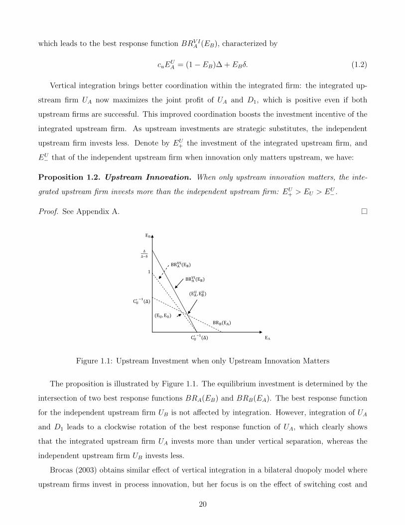
which leads to the best response function BRV IA (EB), characterized by

cuEUA = (1− EB)∆ + EBδ. (1.2)

Vertical integration brings better coordination within the integrated firm: the integrated up-

stream firm UA now maximizes the joint profit of UA and D1, which is positive even if both

upstream firms are successful. This improved coordination boosts the investment incentive of the

integrated upstream firm. As upstream investments are strategic substitutes, the independent

upstream firm invests less. Denote by EU+ the investment of the integrated upstream firm, and

EU− that of the independent upstream firm when innovation only matters upstream, we have:

Proposition 1.2. Upstream Innovation. When only upstream innovation matters, the inte-

grated upstream firm invests more than the independent upstream firm: EU+ > EU > EU

− .

Proof. See Appendix A.

EB

1

EA

Figure 1.1: Upstream Investment when only Upstream Innovation Matters

The proposition is illustrated by Figure 1.1. The equilibrium investment is determined by the

intersection of two best response functions BRA(EB) and BRB(EA). The best response function

for the independent upstream firm UB is not affected by integration. However, integration of UA

and D1 leads to a clockwise rotation of the best response function of UA, which clearly shows

that the integrated upstream firm UA invests more than under vertical separation, whereas the

independent upstream firm UB invests less.

Brocas (2003) obtains similar effect of vertical integration in a bilateral duopoly model where

upstream firms invest in process innovation, but her focus is on the effect of switching cost and

20

technology choice. Chen and Sappington (2010) also consider the effect of vertical integration on

upstream investment incentives. However, they only consider the case with an upstream monopo-

list, and their focus is on how the effect of vertical integration depends on downstream competition.

Our focus in the paper is not restricted to the effect of integration on upstream investments, but

rather on the difference between different market settings.

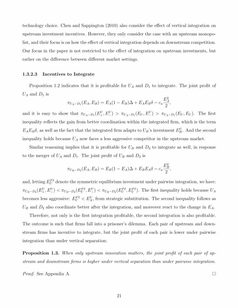
1.3.2.3 Incentives to Integrate

Proposition 1.2 indicates that it is profitable for UA and D1 to integrate. The joint profit of

UA and D1 is

πUA−D1(EA, EB) = EA(1− EB)∆ + EAEBδ − cuE2A

2,

and it is easy to show that πUA−D1(EU+ , E

U−) > πUA−D1(EU , E

U−) > πUA−D1(EU , EU). The first

inequality reflects the gain from better coordination within the integrated firm, which is the term

EAEBδ, as well as the fact that the integrated firm adapts to UB’s investment EUB . And the second

inequality holds because UA now faces a less aggressive competitor in the upstream market.

Similar reasoning implies that it is profitable for UB and D2 to integrate as well, in response

to the merger of UA and D1. The joint profit of UB and D2 is

πUB−D2(EA, EB) = EB(1− EA)∆ + EBEAδ − cuE2B

2,

and, letting EPIU denote the symmetric equilibrium investment under pairwise integration, we have:

πUB−D2(EU+ , E

U−) < πUB−D2(E

PIU , EU

−) < πUB−D2(EPIU , EPI

U ). The first inequality holds because UA

becomes less aggressive: EPIU < EU

A , from strategic substitution. The second inequality follows as

UB and D2 also coordinate better after the integration, and moreover react to the change in EA.

Therefore, not only is the first integration profitable, the second integration is also profitable.

The outcome is such that firms fall into a prisoner’s dilemma. Each pair of upstream and down-

stream firms has incentive to integrate, but the joint profit of each pair is lower under pairwise

integration than under vertical separation:

Proposition 1.3. When only upstream innovation matters, the joint profit of each pair of up-

stream and downstream firms is higher under vertical separation than under pairwise integration.

Proof. See Appendix A.

21

When innovation matters only at the upstream level, competition leads to over-investment.

Integration further boosts investment incentives, which exacerbates the situation. Hence, in a

static game, firms are worse off under pairwise integration. Repeated interaction can provide an

easy solution to the prisoner’s dilemma: in a game where firms play the above investment game

repeatedly over time, and firms choose whether to integrate or not at the beginning of each new

period, then patient enough firms could sustain a collusive-like market outcome where all firms

remain separated.12

1.3.3 Comparing the Two Benchmarks

Vertical integration has different effects in the two benchmark situations. When only upstream

innovation matters, vertical integration results in a crowding-out effect; when instead only down-

stream innovation matters, it has no effect. The divergence is here extreme, due to the assumption

of homogeneous products upstream. Still, we show in Section 6 that, more generally, vertical in-

tegration has a larger impact on upstream investment than on downstream investment. This is

because upstream competition is more intense than downstream competition. Simply speaking,

upstream firms compete to sell to each of the two downstream firms, whereas downstream firms

would not compete to purchase the input from both upstream firms.

This suggests that it is the upstream firms that benefit more from integration, and that incen-

tives to integrate are higher when innovative investments take place in the upstream market rather

than downstream. Our result differs from that of de Fontenay and Gans (2005), who show that

either upstream firm or downstream firm may benefit more from integration. Their analysis relies

on the Shapley value, and thus in case of a monopoly, the industry profit depends on whether the

monopolist is upstream or downstream. By contrast, in our setting, the industry profit is ∆ no

matter where is the monopolist.

1.4 Two-Sided Innovation

When innovation matters at both levels, upstream and downstream investments are comple-

mentary, as there is no value for the final product when innovation fails at either level. It follows

12As we show in the extension, if we allow firms to contract on upstream innovation, they can do at least as well

as under vertical separation, or may do even better.

22

that vertical integration affects downstream market as well, which in turn reinforces the impact

on upstream investments identified in the previous section. As we will see, vertical integration can

now moreover be mutually beneficial for all firms.

1.4.1 Downstream Investment

Vertical integration has no impact on downstream investments when both or none of the

upstream firms succeed. In the former situation, downstream firms invest as if only downstream

innovation mattered, and Proposition 1.1 shows that vertical integration has no impact. In the

latter situation, downstream innovation is worthless, and thus no downstream firm invests. Vertical

integration however has an impact when only one upstream firm succeeds, say UA.

1.4.1.1 Vertical Separation

If UA is vertically separated, when only one downstream firm succeeds, there is a bilateral

monopoly. Hence, the downstream firm shares the profit with UA and obtains ∆/2. When both

downstream firms succeed, UA monopolizes the market and each downstream firm obtains 0. The

payoff matrix for downstream firms is thus given by:

Table 1.4: Downstream Payoffs under SeparationHHHH

HHHHH

D1

D2S F

S 0,0 ∆2

,0

F 0,∆2

0,0

Then Dj chooses an investment level ej so as to maximize, for j′ 6= j ∈ {1, 2},

ej(1− ej′)∆

2− cd

e2j

2.

Hence, each Dj’s best response BRV Sj (ej′), is characterized by

cdej = (1− ej′)∆

2. (1.3)

Under Assumption 1, there exists a unique equilibrium : e1 = e2 = eV S, given by

cdeV S = (1− eV S)

∆

2.

23

It is obvious that, under vertical separation, downstream firms are subject to serious hold-up

problem, and thus their investments are insufficient.

Proposition 1.4. If only one upstream firm succeeds and it is vertically separated, downstream in-

vestment is insufficient: it is lower than the industry profit maximizing and the welfare maximizing

level of investment.

Proof. See Appendix A.

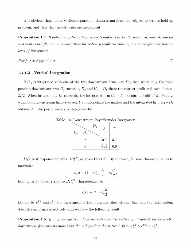
1.4.1.2 Vertical Integration

If UA is integrated with one of the two downstream firms, say D1, then when only the inde-

pendent downstream firm D2 succeeds, D2 and UA−D1 share the market profit and each obtains

∆/2. When instead only D1 succeeds, the integrated firm UA −D1 obtains a profit of ∆. Finally,

when both downstream firms succeed, UA monopolizes the market and the integrated firm UA−D1

obtains ∆. The payoff matrix is thus given by:

Table 1.5: Downstream Payoffs under IntegrationHHH

HHHHHH

UA −D1

D2S F

S ∆,0 ∆,0

F ∆2

,∆2

0,0

D2’s best response remains BRV S2 , as given by (1.3). By contrast, D1 now chooses e1 so as to

maximize

e1∆ + (1− e1)e2∆

2− cd

e21

2,

leading to D1’s best response BRV I1 , characterized by

cde1 = ∆− e2∆

2.

Denote by eV I+ and eV I− the investment of the integrated downstream firm and the independent

downstream firm, respectively, and we have the following result:

Proposition 1.5. If only one upstream firm succeeds and it is vertically integrated, the integrated

downstream firm invests more than the independent downstream firm: eV I+ > eV S > eV I− .

24

Proof. See Appendix A.

e2

2

1

e1

Figure 1.2: Downstream Investment under Upstream Monopoly

Proposition 1.5 is illustrated by Figure 2. Vertical integration does not affect the independent

D2’s best response, but now boost that of the integrated D1, as it eliminates the hold-up problem

within the integrated firm. As downstream investments are strategic substitutes, in equilibrium

the independent downstream firm invests less. We now show that this effect on downstream

investments contributes here to foster upstream investment incentives. Denote by πV S the benefit

from its innovation for the only upstream innovator when it is vertically separated, given by

πV S = 2eV S(1− eV S)∆

2+ (eV S)2∆;

and denote by πV I the benefit when it is vertically integrated, given by

πV I = eV I+ ∆ + eV I− (1− eV I+ )∆

2− cd

(eV I+ )2

2.

Lemma 1.2. If only one upstream firm succeeds, the benefit from its innovation is higher when it

is vertically integrated than when it is separated: πV I > πV S.

Proof. See Appendix A.

When the upstream monopolist is vertically separated, there is serious under-investment in the

downstream market due to hold-up problem. Vertical integration eliminates the problem within

the integrated firm, and fosters downstream investment; integration moreover reduces investment

of the independent firm, which further increases the benefit of the integrated firm.

25

1.4.2 Upstream Innovation

Under vertical separation, when only one upstream firm succeeds, the subgame goes as in

Section 1.4.1.1, the upstream monopolist gets continuation payoff πV S. When both upstream

firms are successful, the subgame goes as Section 1.3.1, where each upstream firm obtains zero

profit. Therefore, the payoff matrix for the upstream firms is given by Table 1.6.

Table 1.6: Upstream Payoffs under SeparationHHHH

HHHHH

UA

UBS F

S 0,0 πV S,0

F 0,πV S 0,0

Each upstream firm’s best response, BRV Si (Ei′), is given by

cuEi = (1− Ei′)πV S. (1.4)

There is a unique equilibrium in the investment game: EA = EB = EV S, given by

EV S =πV S

cu + πV S.

Suppose now UA and D1 integrate. When only the independent upstream firm UB succeeds,

the subgame goes as Section 1.4.1.1, where UB obtains πV S. In this circumstance, even though

UA does not have a successful upstream innovation, the integrated firm UA−D1 still gets positive

profit from D1 when it is the only downstream innovator. UA −D1’s expected profit, πDV S, which

is the profit of a downstream firm when the upstream monopolist is vertically separated, is thus

given by

πDV S = eV S(1− eV S)∆

2− cd

(eV S)2

2.

When the integrated upstream firm UA is the only upstream innovator, the subgame goes as

Section 1.4.1.2, and UA obtains πV I .

When both upstream firms are successful, the subgame goes as Section 1.3.1. However, the

profit for the two upstream firms are different: the independent upstream firm UB obtains zero

profit; but the integrated firm obtains positive profit from its downstream affiliate; its expected

profit, πDV I , is given by

πDV I = e2Dδ + eD(1− eD)∆− cd

e2D

2,

26

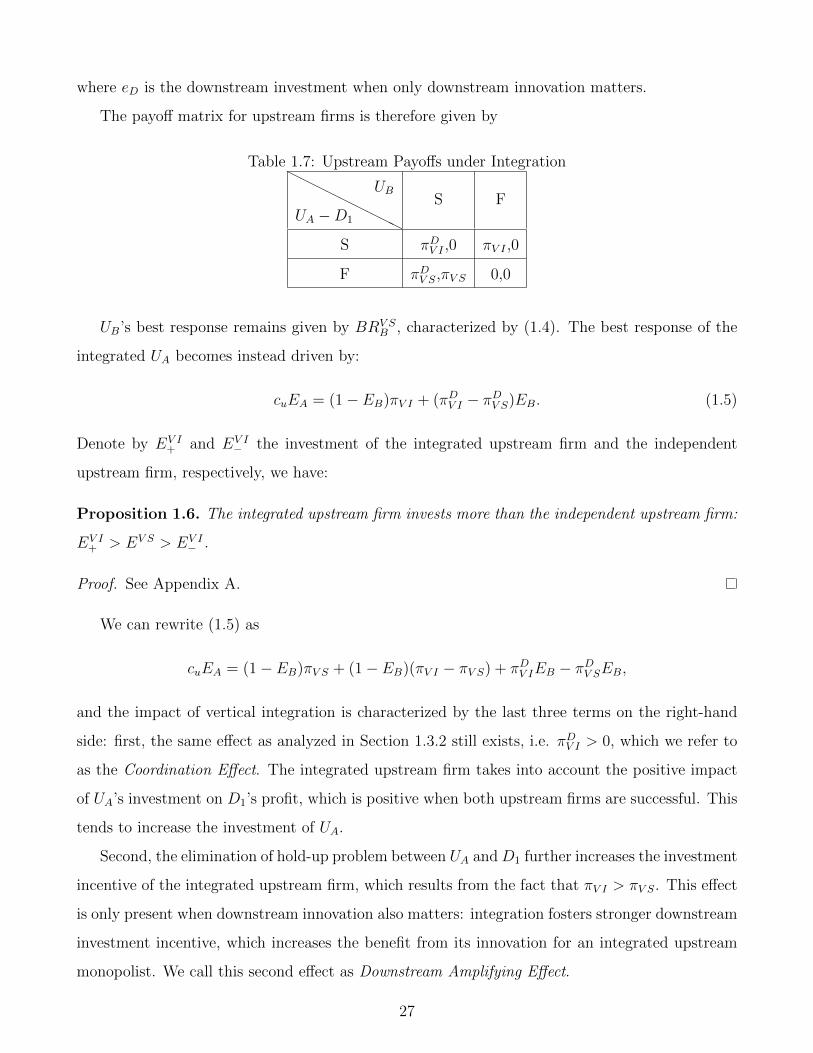
where eD is the downstream investment when only downstream innovation matters.

The payoff matrix for upstream firms is therefore given by

Table 1.7: Upstream Payoffs under IntegrationHH

HHHHHHH

UA −D1

UBS F

S πDV I ,0 πV I ,0

F πDV S,πV S 0,0

UB’s best response remains given by BRV SB , characterized by (1.4). The best response of the

integrated UA becomes instead driven by:

cuEA = (1− EB)πV I + (πDV I − πDV S)EB. (1.5)

Denote by EV I+ and EV I

− the investment of the integrated upstream firm and the independent

upstream firm, respectively, we have:

Proposition 1.6. The integrated upstream firm invests more than the independent upstream firm:

EV I+ > EV S > EV I

− .

Proof. See Appendix A.

We can rewrite (1.5) as

cuEA = (1− EB)πV S + (1− EB)(πV I − πV S) + πDV IEB − πDV SEB,

and the impact of vertical integration is characterized by the last three terms on the right-hand

side: first, the same effect as analyzed in Section 1.3.2 still exists, i.e. πDV I > 0, which we refer to

as the Coordination Effect. The integrated upstream firm takes into account the positive impact

of UA’s investment on D1’s profit, which is positive when both upstream firms are successful. This

tends to increase the investment of UA.

Second, the elimination of hold-up problem between UA andD1 further increases the investment

incentive of the integrated upstream firm, which results from the fact that πV I > πV S. This effect

is only present when downstream innovation also matters: integration fosters stronger downstream

investment incentive, which increases the benefit from its innovation for an integrated upstream

monopolist. We call this second effect as Downstream Amplifying Effect.

27

Third, the combination of upstream innovation and downstream innovation gives rise to an

Insurance Effect which reduces the investment incentive of the integrated upstream firm. This

originates from the fact that the integrated firm obtains positive profit even if it fails in upstream

investment, as the downstream affiliate D1 obtains a profit of ∆/2 when it is the only downstream

innovator, that is πDV S > 0. This negative effect is dominated, however, and the overall effect of

vertical integration is a strengthened crowding-out effect.

1.4.3 Incentives to Integrate

Similar to the arguments made in Section 1.3.2.3, it is profitable for UA and D1 to integrate,

the benefit of which comes from both the elimination of hold-up problem and lower investments

from independent firms. Moreover, given that UA and D1 have merged, it is also profitable for UB

and D2 to integrate. The joint profit of UB and D2 under vertical separation is

πV SUB−D2(EA, EB) = EAEBπ

DV I + EB(1− EA)[πV S + πDV S] + EA(1− EB)πFV I − cu

E2B

2,

where πDV S is the profit for a downstream firm when the only upstream innovator is vertically

separated; and πFV I is the profit of the independent downstream firm when the upstream monopolist

is vertically integrated, given by

πFV I = eV I− (1− eV I+ )∆

2− cd

(eV I− )2

2.

And the joint profit under pairwise integration is

πPIUB−D2(EA, EB) = EAEBπ

DV I + EB(1− EA)πV I + EA(1− EB)πFV I − cu

E2B

2.

It is easy to check that πV SUB−D2(EV I

+ , EV I− ) < πPIUB−D2

(EV I+ , EV I

− ) < πPIUB−D2(EPI , EPI), where

EPI is the equilibrium upstream investment when there is pairwise integration. The first inequality

reflects the stand-alone gain from the elimination of hold-up problem; and the second inequality

shows the gain from being more aggressive, which lowers the investment of UA. As a result, the

integration of UA and D1 would be followed by the integration of UB and D2. However, the joint

profit of UA and D1 is still higher than what they would obtain under vertical separation.

Proposition 1.7. When innovation matters both upstream and downstream, industry profit is

higher under pairwise integration than under vertical separation.

28

Proof. See Appendix A.

Therefore, when innovation matters at both upstream and downstream markets, we are likely to

observe merger waves, as this leads to the market structure that maximizes industry profit (As each

integrated firm gets half of the industry profit, it also maximizes the profit of each integrated firm).

This is in contrast to when innovation only matters at one level, where pairwise integration either

has no effect (downstream innovation) or hurts both firms (upstream innovation). The reason is

intuitive: In all cases, vertical integration eliminates hold-up problems and boosts investments.

But when innovation matters only at one level, competition leads to over-investment, which is

then further exacerbated by vertical integration. When instead innovation matters at both levels,

multiplication of hold-up problems leads to under-investment (Proposition 1.4), which is alleviated

by vertical integration.

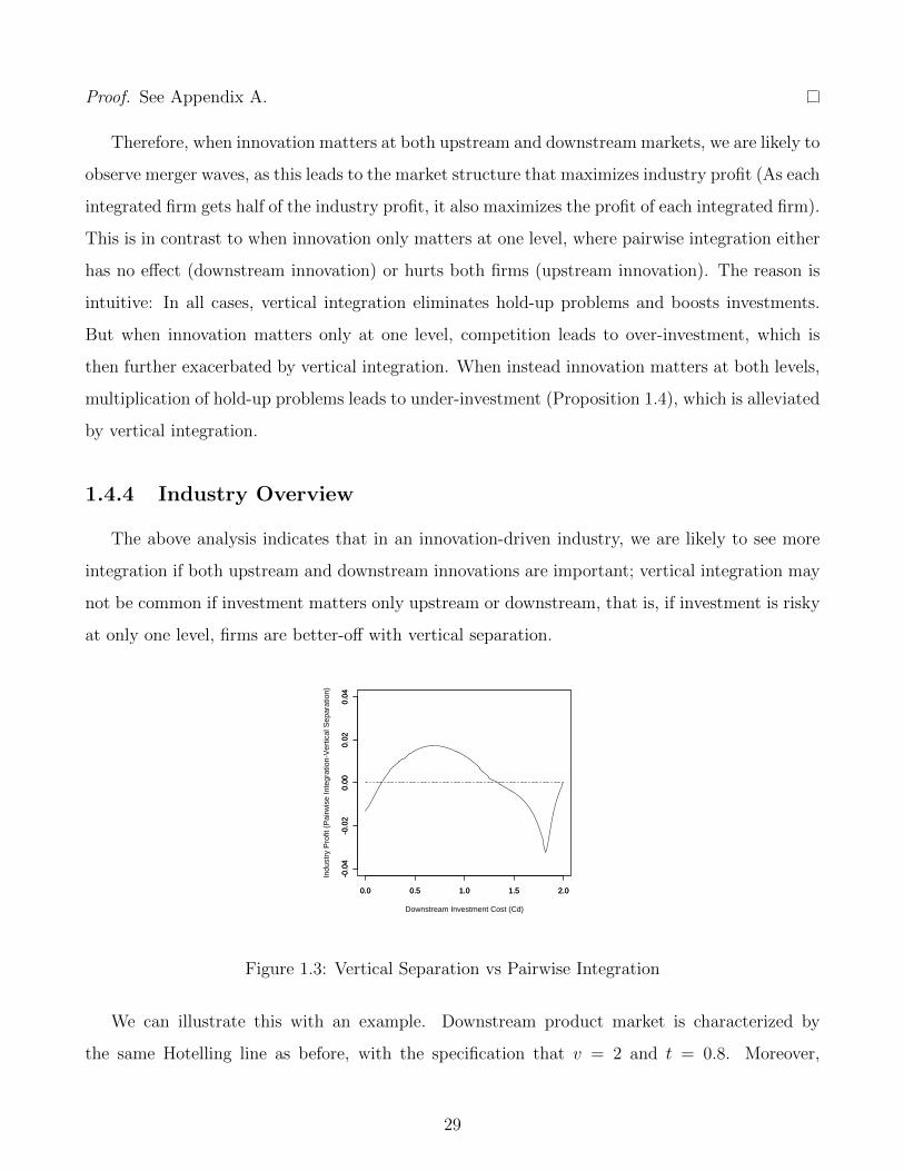
1.4.4 Industry Overview

The above analysis indicates that in an innovation-driven industry, we are likely to see more

integration if both upstream and downstream innovations are important; vertical integration may

not be common if investment matters only upstream or downstream, that is, if investment is risky

at only one level, firms are better-off with vertical separation.

0.0 0.5 1.0 1.5 2.0

-0.0

4-0

.02

0.00

0.02

0.04

Downstream Investment Cost (Cd)

Indu

stry

Pro

fit (

Pai

rwis

e In

tegr

atio

n-V

ertic

al S

epar

atio

n)

0.0 0.5 1.0 1.5 2.0

-0.0

4-0

.02

0.00

0.02

0.04

Figure 1.3: Vertical Separation vs Pairwise Integration

We can illustrate this with an example. Downstream product market is characterized by

the same Hotelling line as before, with the specification that v = 2 and t = 0.8. Moreover,

29

suppose that cu + cd = 2.13 Figure 1.3 shows the difference between industry profit under pairwise

integration and vertical separation, as the cost structure varies. As we can see, as cd → 0, we

are in the situation when only upstream innovation matters, where pairwise integration is strictly

dominated. As cu → 0 (cd → 2), we approach the situation when only downstream innovation

matters, and firms are indifferent between integration and separation. Integration is beneficial

and the equilibrium market structure features pairwise integration only when both innovations

are important.

From the point view of industry dynamics, at an early stage of the development of an industry,

innovation is likely to be important at each stage of the value chain and firms choose to integrate

vertically. As the importance of innovation moves more and more to one stage, firms begin to favor

vertical separation (or outsourcing when it is feasible). As what happens in the pharmaceutical

industry, for the traditional technology, it becomes more and more difficult to make discoveries in

the upstream research stage, and firms start to outsource their R&D activities.

1.5 Welfare Implications

We briefly discuss the welfare effect of vertical integration in this section. When only down-

stream innovation matters, vertical integration does not affect welfare; when only upstream inno-

vation matters, vertical integration improves social welfare if product differentiation in the final

product market is strong. Finally, if both upstream and downstream innovations are important,

vertical integration generally increases welfare.

1.5.1 One-Sided Innovation

When only downstream innovation matters, vertical integration has no effect on downstream

investments, and thus does not affect social welfare. When only upstream innovation matters,

consider first single vertical integration, the welfare effect comes from two aspects: on the benefit

side, total investment increases; on the cost side, vertical integration may lead to over-investment.

This is because the private gain from integration exceeds the social gain. With only one down-

stream firm, social surplus is v − t/2. With two downstream firms, this surplus becomes v − t/4.

13Thus we do not focus on the situation when optimal investments are interior. Instead, either upstream or

downstream investment can be zero or one.

30

Thus, when one firm has already been successful, the social gain from a second successful firm is

t/4, whereas the private gain for the second firm is t/2.

The welfare function is given by

W = (EA + EB − EAEB)(v − t

2) + EAEB

t

4− cu

E2A

2− cu

E2B

2.

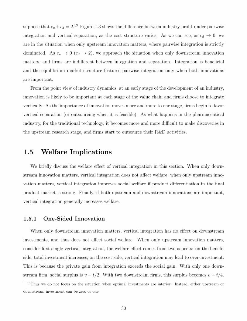
Thus, if the investment cost is high, welfare is largely determined by total investment, (EA +

EB)(v− t/2), which is higher under vertical integration. If instead investment cost is low, whether

vertical integration increases social welfare critically depends on the extent of downstream product

differentiation: when it is weak, the welfare gain from further upstream investment is limited, and

the negative effect of over-investment dominates. With stronger product differentiation, however,

the positive effect of higher upstream investment dominates and vertical integration increases

social welfare. A numerical example in Figure 4 (where we set v = 1) confirms this point.

1.0 1.1 1.2 1.3 1.4

0.00

0.05

0.10

0.15

0.20

0.25

0.30

Welfare Effect of Single Integration

Investment Cost(Cu)

Pro

duct

Diff

eren

tiatio

n (t

)

VI<VS

VI>VS

Figure 1.4: Welfare Effect of Single Integration when only Upstream Innovation matters

Now consider pairwise integration, as cu > ∆ = v − t, it is always optimal to have both firms

investing, and W is maximized at

EA = EB = E∗ =v − t/2

cu + v − 3t/4,

whereas the equilibrium investment levels under separation and pairwise integration are respec-

tively given by:

EU =v − t

cu + v − t< E∗ and EPI

U =v − t

cu + v − 3t/2> E∗.

31

It is easy to check that, if cu ≥ 3t/2, we have EU + EPIU ≤ 2E∗, and pairwise integration always

increases social welfare compared with vertical separation. This comes from the fact the incentive

to over-invest is weaker under pairwise integration than under single integration, and the positive

effect of higher total investment dominates.

1.5.2 Two-Sided Innovation

Now consider the situation when innovation matters both upstream and downstream. Denote

by WD the social welfare in the continuation game when both upstream firms succeed; similarly,

denote by W V SM and W V I

M the social welfare in the continuation game when there is only one

successful upstream firm, which is vertically separated or vertically integrated, respectively. Total

social welfare under vertical separation is then given by

W V S = (EV S)2WD + 2EV S(1− EV S)W V SM − 2CU(EV S),

whereas under single vertical integration, it is given by

W V I = EV I+ EV I

− WD + EV I+ (1− EV I

− )W V IM + EV I

− (1− EV I+ )W V S

M − CU(EV I+ )− CU(EV I

− ).

When investments are substantially lower than the efficient level (which is indeed the case

when innovation matters both upstream and downstream), welfare effects are mainly driven by

the impact on total investment. Single vertical integration increases social welfare in two ways:

First, social welfare is higher when the upstream monopolist is vertically integrated than when it

is vertically separated: W V SM < W V I

M . Vertical integration moreover implies that the integrated

upstream firm is more likely to be the sole innovator in the upstream market. Second, total

investment is higher: EV I+ + EV I

− > 2EV S. Indeed, when innovation is important both upstream

and downstream, investment incentives are insufficient due to hold-up problems being present at

both levels. Vertical integration partially overcomes this problem and pushes investment levels

towards social optimum.

This suggests that pairwise integration may further increase social welfare, which becomes

W PI = (EPI)2WD + 2EPI(1− EPI)W V IM − 2CU(EPI).

Further welfare improvement from pairwise integration comes from the fact that hold-up problem

is now eliminated within each integrated firm, and total investment is even higher: 2EPI >

32

EV I+ + EV I

− . The numerical example in Figure 5 (Where we set v = cu = cd = 1) confirms this

welfare effect.

0.0 0.1 0.2 0.3 0.4 0.5

0.00

0.05

0.10

0.15

Welfare Effect with Two-Sided Innovation

Product Differentiation (t)

Soc

ial W

elfa

re

0.0 0.1 0.2 0.3 0.4 0.5

0.00

0.05

0.10

0.15

0.0 0.1 0.2 0.3 0.4 0.5

0.00

0.05

0.10

0.15

Vertical SeparationSingle IntegrationPairwise Integration

Figure 1.5: Welfare Effect with Two-Sided Innovation

1.6 Discussion and Extension

1.6.1 Robustness

Timing and Observability of Investments. We have assumed that upstream investment takes

place before downstream investment. However, the observability and the timing of investments

do not affect our main results. This is clearly the case when innovation only matters at one level.

When innovation matters both upstream and downstream, the driving force for our results is

the better coordination from the elimination of the hold-up problem within the integrated firm.

However, by assuming that downstream firms invest after observing the outcomes of upstream

investments, we avoid wasteful downstream investments when no upstream firm succeeds. More-

over, sequential investment allows us to better separate the impact of vertical integration on the

upstream market from its impact on the downstream market.

Secret Contracting. We have assumed that in the bargaining stage, all offers and acceptance

decisions are publicly observable. Secret offers may reduce the profit of an upstream monopolist,

due to the classic opportunistic problem. And thus there is additional incentive to integrate

33

vertically if offers are not observable.

Elastic Demand. A simplification in our analysis is that downstream firms have unit demands.

When instead downstream firms have an elastic demand, vertical integration generates additional

foreclosure for independent downstream firms through a “raising rivals’ cost”effect, which has

been extensively analyzed in the literature. This foreclosure effect exacerbates crowding-out down-

stream, which in turn further strengthens crowding-out upstream. Our qualitative results do not

change, however, as the resolution of coordination problems within the integrated firm still plays

a role in these settings. However, by relying on unit demand and observable offers, we can better

focus on the effect of vertical integration through the channel of investment.

Interim Bargaining. In the discussion above, we have assumed that firms bargain after all

outcomes of investments have realized and been observed by all firms. The main insights in

our paper still hold if bargaining happens in an interim stage, that is, if successful upstream firms

bargain with downstream firms before downstream firms make investments. In this situation, there

is no hold-up problem for downstream firms, but vertical integration still affects the investment

incentives of upstream firms. When both upstream firms are successful, the integrated upstream

firm obtains positive profit, whereas the independent upstream firm obtains zero profit. And when

only one upstream firm succeeds, this integrated upstream monopolist is able to obtain a higher

profit, even if the bargaining outcome does not affect downstream investment incentives. This

is because the integrated upstream monopolist holds a stronger bargaining position vis-a-vis the

downstream firms, as it benefits from a better outside option.

Exclusive Dealing. Explicit exclusive dealing contracts can have an impact when there is

bilateral duopoly. If all firms are separated, then exclusive dealing does not change the payoffs

when upstream firms make offers. But when instead downstream firms are the ones making the

offers, both firms asking to be supplied at cost (i.e., a zero price) is no longer an equilibrium if

exclusive dealing offers are allowed. If D2 asks for this, D1 can profitably deviate by making an

exclusive dealing offer with a small positive price ε/2 to each upstream firm. Both upstream firms

are willing to accept the exclusive dealing offer, and D2 is excluded from the market. D1 gets

profit ∆− ε, which is higher than the profit δ that it would obtain if it also made non exclusive,

zero price offers. We show in Appendix B that in this case, downstream firms end up with zero

profit.

When UA and D1 integrate, the integrated firm can use exclusive dealing offers to exclude the

34

independent upstream firm or the independent downstream firm. As emphasized by Chen and

Riordan (2007), the combination of vertical integration and exclusive dealing can lead to ex post

cartelization. For instance, when it is downstream firms that make offers, the highest price that

D2 can offer UB is δ; whereas UA−D1 can offer UB an exclusive deal with a price δ+ ε; this will be

accepted by UB, and D2 is then excluded from the market. UA −D1 gets profit ∆− δ − ε, which

is higher than when exclusive dealing is not allowed (δ). Therefore, when exclusive dealing is

allowed, upstream crowding-out effect still exists, and vertical integration still affects downstream

investments. Exclusive dealing intensifies downstream competition, however, which contributes to

restore symmetry between upstream and downstream markets.

1.6.2 Upstream Differentiation

In our two benchmark situations, the extreme divergence between the effect of integration

on upstream and downstream investments stems from the assumption of perfect substitution of

inputs. However, the general logic is that upstream competition is more intense than downstream

competition, and upstream firms benefit more from vertical integration.

Maintaining the assumption that upstream inputs are not channel specific, consider a simple

modification of our basic model to incorporate also upstream differentiation: Both upstream and

downstream markets are characterized by a simple Hotelling model, with transportation cost tu

and td respectively. The consumer can be two types: he cares only upstream differentiation or only

downstream differentiation. All firms observe the type of the consumer, and downstream firms

can moreover price discriminate between different types of consumers.14 When downstream firms

purchase from the same supplier, competition for consumers who care only upstream differentiation

leads to zero profit, but each firm gets expected profit δD = td/4 from consumers who care about

downstream differentiation. When they instead purchase from different suppliers, each firm gets

additional profit δU = tu/4 from consumers who care only upstream differentiation.

Therefore, if downstream firms buy from the same upstream firm, each obtains profit δD; if

instead they buy from different upstream firms, each gets profit δD + δU . Thus, δD measures

downstream differentiation whereas δU instead measures upstream differentiation; as before, we

assume that 2(δD + δU) < ∆. We prove the following result in the Appendix:

Proposition 1.8. Vertical integration has a larger impact on investment when innovation matters

14With this modification, all previous analysis remains valid.

35

only upstream than when it matters only downstream; and vertical integration has the same impact

only if there is no differentiation downstream.

Proof. See Appendix A.

This proposition generalizes the insights of our benchmark case where there is no upstream dif-

ferentiation, in which vertical integration only affects upstream investments, and not downstream

ones. As made clear in the proof, the intuition is that upstream competition is more intense, and

thus upstream firms benefit more from integration. Only when all differentiation lies upstream is

the effect of vertical integration symmetric on upstream and downstream investments.

1.6.3 Non-Drastic Innovation

We have so far assumed that innovation is “drastic”, in that it is necessary to enter a market.

When innovation is non-drastic, a failed firm is still active in the market, but with a less effective

technology (lower quality and/or higher cost, say).

Consider a slight modification of our framework in which upstream firms invest in order to

improve the quality of the input, and downstream firms invest to improve the quality of the final

product. The original value of the final product is v as given in our main model. We assume

that successful upstream investment can increase the value of the final product by αω, whereas

successful downstream investment further increases this value by (1 − α)ω. Notice that if ω is

relatively small (ω < 3t in our Hotelling interpretation), then the innovation is indeed “non-

drastic”: a downstream firm cannot drive the other one out of the market even if it obtains

both upstream and downstream innovation. When α → 0, we are in the situation where only

downstream innovation matters; and when α→ 1, only upstream innovation matters.

In this case, successful innovation is no longer required to be active in the market. This has

two consequences: first, it changes the bargaining procedure as all firms are present no matter

how many firms are successful. The presence of an inferior competitor constrains the profit that a

successful innovator can extract, but does not qualitatively affect the benefit of better coordina-

tion from integration. Second, downstream investment is subject to weaker appropriation by an

upstream monopolist. This is because successful investment increases the value of outside option

of a downstream firm, which cannot be appropriated by the upstream monopolist. As a result,

the hold-up problem is present mostly for upstream firms. This is consistent with our insight that

36

vertical integration has a larger impact at upstream than downstream. It moreover suggests that

firms are more likely to find themselves in a prisoner’s dilemma situation.

1.6.4 Information Disclosure by Upstream Firms

In our model, a final product requires both upstream and downstream innovation, but down-

stream innovation does not require any cooperation in the form of information disclosure or actual

delivery of upstream innovation. In this subsection, we relax this assumption and assume that

downstream firms need information about the upstream innovation in order to make successful

investment. We modify the game as follows:

• Upstream Investment Stage. Each Ui makes investment Ei; the outcomes of investments

realize and are observed; if both firms fail, the game ends;

• Information Disclosure Stage. Successful upstream firms decide whether to disclose infor-

mation about this innovation to any downstream firm; the disclosure decision is observed;

• Downstream Investment Stage. Each Dj makes investment ej if it receives information from

an upstream firm; if both firms receive no information or fail, the game ends;

• Bargaining Stage. The successful upstream firm(s) and successful downstream firm(s) bar-

gain over the supply condition; Payments are made and inputs are delivered accordingly;

• Payoff Stage. Final product market realizes and game ends.

Suppose there is a cost K associated with disclosure. Such cost may be the risk of information

leakage, or about how to convey the information correctly to downstream firms. We assume that

when an upstream firm is indifferent between disclosing and not disclosing, it chooses to disclose.

When only one upstream firm is successful, the incentive to disclose may differ depending on

whether it is vertically integrated or not. Under vertical separation, the profit for the upstream

monopolist is πV S if it discloses information to both downstream firms; if it only discloses to one

downstream firm, downstream investment is ∆/2cd, and the profit for the upstream monopolist

is π1V S = ∆2/4cd. When the upstream monopolist is vertically integrated, the profit is πV I if it

also discloses the information to the independent downstream firm. When it does not disclose,

downstream investment is given by ∆/cd and the profit for the integrated firm is π1V I = ∆2/2cd.

Then an integrated upstream monopolist has less incentive to disclose to both downstream firms.

37

Proposition 1.9. There exists a range of value K ∈ (K,K) such that an monopolist discloses

information to both downstream firms when it is independent, but does not disclose to the inde-

pendent downstream rival when it is vertically integrated.

Proof. See Appendix A.

The reason is simple: By disclosing information to both downstream firms, the upstream

monopolist may benefit from intensified downstream competition. But an integrated upstream firm

has less to gain from such strategy, as competition also deteriorates the profit of its downstream

affiliate. This leads to a strengthened downstream amplifying effect, as the difference between the

profit of an integrated upstream monopolist and a separated one is even larger for K belonging

to the range in the proposition.

When both upstream firms are successful, under vertical separation, neither upstream firm

has incentive to disclose: as upstream competition drives input price down to zero, no upstream

firm can cover the cost of disclosure if it were to disclose to any downstream firm. Under single

integration, no upstream firm discloses to the independent downstream firm,15 whereas the inte-

grated downstream firm can always get the information from the upstream affiliate (provided that

K ≤ π1V I). Hence, when both upstream firms succeed, the integrated upstream firm generates

positive benefit from its innovation, whereas the independent upstream firm gets zero profit. This

may further amplify the coordination effect if K is not too large.

1.6.5 Contracting for Innovation–Outsourcing

We have shown that for each pair of upstream and downstream firms, integration is a dominant

strategy in the static game. But when only upstream innovation matters, firms face a prisoner’s

dilemma situation. Hence, when firms interact repeatedly and are patient enough, we can have a

collusive-like equilibrium where all firms remain separated.

However, under vertical separation, when there is only one upstream innovator, downstream

firms have to compete to be the distributor for the upstream monopolist. Then a downstream

firm may want to sign an exclusive contract with an upstream firm, in order to secure the input

if the upstream firm succeeds.

15The independent upstream firm has no incentive to disclose, as it always gets zero profit. The integrated

upstream firm has no incentive to disclose to the independent downstream firm, as this intensifies downstream

competition and lowers its profit.

38

We consider a simple form of such contract between, say, D1 and UA: D1 makes an upfront

payment f to UA, and it commits to pay UA additionally p1 if only UA succeeds, and p2 if both

upstream firms succeed; in return, UA only supplies to D1 whenever it succeeds. If D2 makes a

similar offer to UB, which UB accepts, D1’s optimal offer is the solution to:

maxp1,p2 EA(1− EB)(∆− p1) + EAEB(δ − p2)− f,

s.t. EA = maxEAEA(1− EB)pB1 + EAEBp

B2 − 1

2cuE

2A; (IC − A)

EB = maxEBEB(1− EA)p1 + EAEBp2 − 1

2cuE

2B; (IC −B)

EA(1− EB)p1 + EAEBp2 − 12cuE

2A + f ≥ 1

2cu(

∆cu+∆

)2; (IR− A)

EA(1− EB)(∆− p1) + EAEB(δ − p2)− f ≥ δ( ∆cu+∆

)2. (IR− 1)

The first two constraints are the Incentive Compatibility constraints which say that upstream

firms choose their investments optimally; the last two constraints are the Individual Rationality

constraints which require that firms should be better than when they are independent.

Consider a symmetric equilibrium where D1 and D2 make the same offer to UA and UB re-

spectively. When upfront payment is not allowed, i.e., f = 0, for simplicity, consider the case

cu = ∆ = 1, the two IC constraints mean that

EA = EB =p1

1 + p1 − p2

,

and the upstream IR constraint (IR-A) requires that

p1 + p2 ≥ 1.

Then downstream firms will make such an offer that p1 + p2 = 1. Substituting this into the

downstream IR constraint (IR-1), it shows that the IR-1 holds with equality. Therefore, with this

optimal contract, downstream firms can achieve the same outcome as if they are all vertically

separated.

Nonetheless, firms can do better if upfront payment is allowed. In this case, it is easy to

check that the profit maximizing investment EA = EB = 1/(3− 2δ) can be achieved by setting

f = 1/8−1/2(3− 2δ)2 and p2 + 2(1− δ)p1 = 1. Therefore, depending on the outsourcing contract

allowed, firms can do as well as vertical separation or even better when only upstream innovation

matters.

39

1.7 Conclusion

In this paper, we study firms’ decision of integration in a vertically related industry where

innovation matters. Vertical integration brings better coordination within the integrated firm,

and boosts its investment incentive both upstream and downstream. However, it is only mutually

beneficial for firms to integrate when innovation is important at both levels, in which case multi-

plication of hold-up problem leads to under-investment, and integration reduces the inefficiency.

When instead innovation only matters at one level, firms prefer to stay vertically separated.

Our analysis provides an explanation for recent developments of the global pharmaceutical

industry, where vertical integration and R&D outsourcing happen at the same time. We show

that a key determinant of these two trends is the relative importance of innovative investment

in the upstream and downstream markets. Vertical integration in the pharmaceutical industry

occurs between biotech firms, where innovation matters both at the research and at the devel-

opment/manufacturing stage; whereas outsourcing takes place for more traditional technologies,

where innovation matters mostly at the upstream research stage.

Our insights suggest that when evaluating the impact of vertical integration, especially in in-

dustries with intensive innovative investments, the exact nature of the interplay between upstream

and downstream investments may be a key point for the decision. Studying the impact of vertical

integration in a more general bargaining environment, or in the presence of other forms of comple-

mentarity might be interesting avenues for future research. In addition, whereas there has been a

number of empirical papers studying the effect of horizontal mergers on innovation, it would also

be valuable to study/test empirically the theory predictions developed in this paper.

1.8 Appendix

Most of the propositions in our analysis can be obtained with generic cost function C(e) such

that: it is increasing and convex, C ′(0) > 0, C ′(1) > ∆, and C ′′(e) > ∆ for all e ∈ [0, 1]. However,

we provide the proofs with quadratic cost functions, which satisfy Assumption 1.

40

1.8.1 Appendix A

1.8.1.1 Proof of Lemma 1.1

When only one side innovation matters, at least in one market both firms are active. There are

three cases where the market is viable: upstream monopoly with downstream duopoly; upstream

duopoly with downstream monopoly; and bilateral duopoly.

Case 1: Upstream Monopoly.

Suppose only one upstream firm succeeds, say UA. When UA makes offers to downstream firms,

UA can always guarantee a payoff of ∆. To do so, UA offers (∆, p) with p > ∆ to D1 and D2

respectively, which will be accepted and only D1 purchases from UA.16

When D1 and D2 make offers to UA, the only equilibrium is that both propose a price ∆, and

UA accepts one of them. To see this, suppose D1 proposes a price p1 and D2 proposes p2. First,

any prices such that 0 < pj ≤ δ cannot be an equilibrium. In this case, UA would accept both

offers, as it would then be a dominant strategy for both Dj to purchase the input. Then each Dj

would deviate to propose a lower price which would still be accepted by UA. Second, pj = 0 cannot

be an equilibrium either. Suppose not, either Dj can propose a price p′j = δ + ε, which leads UA

to only accept the offer of Dj. This gives Dj a profit of ∆− δ − ε, which is higher than δ. Third,

any offers such that δ < pj < ∆ cannot be an equilibrium. In this case, UA would only accept the

offer with higher price or randomize when both downstream firms offer the same price, then at

least one downstream firm can profitably deviate by increasing price so as to win. Therefore, the

only candidate for equilibrium is that both downstream firms propose ∆. Neither of downstream

firms has incentive to increase price, and reducing price leads UA to accept only the offer of the

other firm.

Hence, when there is only one upstream innovator, it obtains the industry profit ∆.

Case 2: Downstream Monopoly.

Suppose only D1 is successful. Clearly, D1 obtains ∆ when it makes offers. When upstream

firms make offers, they both offer zero is the only equilibrium: any positive offer will be undercut

by the competitor. Therefore, in this case, the downstream monopolist always obtains ∆.

Case 3: Bilateral Duopoly.

When upstream firms make offers to downstream firms, the only equilibrium is that each Ui

16It is a weakly dominant strategy for D2 not to purchase, then to purchase is a best response of D1.

41

offers zero price to both downstream firms, and both downstream firm accept both offers and

purchase the input. As each downstream firm only purchases from the firm who offers lower price,

any positive offer would be undercut by the other upstream firm, and thus such offers cannot be

the equilibrium.

When downstream firms make offers, they will ask for zero price to both upstream firms, and

both upstream firms accept both offers. The reason is simple: the only reason that a downstream

firm may offer positive price is that both upstream firms choose to only accept the offer from it.

However, this cannot be part of the equilibrium. As the downstream firm only purchases from

one of them(either from the one with lower price or the preferred one when indifferent), then

at least one upstream firm would accept both offers. As there is no way to exclude the other

downstream firm from the market, each downstream firm cannot do better by just offering zero

prices to upstream firms.

Therefore, when there is bilateral duopoly, upstream firms supply at cost and each downstream

firm obtains δ.

1.8.1.2 Proof of Proposition 1.2

Denote by EU+ and EU

− the investment of the integrated and the independent upstream firm

respectively, when only upstream innovation matters. Rewrite the best response functions as cuEU+ = ∆(1− EU

−) + αδEU− ,

cuEU− = ∆(1− EU

+).

When α = 0, the solution corresponds to the investment under vertical separation; when α = 1, it

is the solution under single vertical integration; and when α ∈ (0, 1), we have partial integration,

where the integrated upstream firm gets a share of the profit of the downstream affiliate. It is

clear to see that∂EU

+

∂α=δEU−

cu,

which is always positive. Therefore, we must have EU+ > EU . Furthermore, we have ∂EU

−/∂EU+ =

−∆ < 0, and thus EU− < EU . Actually, EU

+ is increasing in α and EU− is decreasing, and thus

the crowding-out upstream is also increasing in α. The effect of integration on investment is the

largest when the integration is full.

42

1.8.1.3 Proof of Proposition 1.3

The joint profit of each pair Ui −Dj when both upstream firms invest E is given by

πUi−Dj= E(1− E)∆ + E2δ − cu

E2

2,

which is decreasing if

E > E =∆

cu + 2(∆− δ).

As in the above proof of Proposition 1.2, the upstream investment under symmetric market

structure (vertical separation or pairwise integration) is determined by

cuE = (1− E)∆ + αδE.

α = 0 corresponds to the case of vertical separation, whereas α = 1 is the case of pairwise

integration. It is easy to see that∂E

∂α> 0.

Therefore, the investment under pairwise integration is higher than under vertical separation.

Moreover, when α = 0, we have EU > E. Hence, EPIU > EU > E. Pairwise integration leads to

more over-investment, and the profit of the integrated firm is lower than under vertical separation.

Moreover, the over-investment problem is increasing in α, and thus the over-investment is more

severe under full integration than under partial integration.

1.8.1.4 Proof of Proposition 1.4

The downstream investment is this case is determined by

cdeV S = (1− eV S)

∆

2.

The industry profit is given by

Π = (e1 + e2 − e1e2)∆− cde2

1

2− cd

e22

2,

which is maximized at e∗, given by

cde∗ = (1− e∗)∆.

Social welfare is given by

W = (e1 + e2 − e1e2)(v − t

2)− cd

e21

2− cd

e22

2,

43

which is maximized at eo, given by

cdeo = (1− eo)(v − t

2).

Clearly, as ∆/2 < ∆ < v − t/2, we have eV S < e∗ < eo. Hence, downstream investment is

insufficient compared with either industry profit maximizing or welfare maximizing investment.

1.8.1.5 Proof of Proposition 1.5

Denote by eV I+ and eV I− the investment of the integrated and the independent downstream firm

respectively, and we can rewrite the best response functions as cdeV I+ = (1− eV I− )∆

2+ α∆

2,

cdeV I− = (1− eV I+ )∆

2.

When α = 0, the solution corresponds to the investment under vertical separation, eV S. When

α = 1, the solution is the optimal investment under single integration. Clearly, we have

∂eV I+

∂α=

∆

2cd,

which is always positive. Therefore, we must have eV I+ > eV S; moreover, as ∂eV I− /∂eV I+ < 0, we

have eV I− < eV S.

1.8.1.6 Proof of Lemma 1.2

The benefit for the upstream monopolist when it is vertically separated is

πV S = 2eV S(1− eV S)∆

2+ (eV S)2∆ = eV S∆;

and the benefit for an integrated upstream monopolist is

πV I = eV I+ ∆ + eV I− (1− eV I+ )∆

2− cd

(eV I+ )2

2.

As shown in the proof of Proposition 1.5, if α = 0, we have

πV I = eV S∆ + eV S(1− eV S)∆

2− cd

(eV S)2

2,

which is higher than πV S, as the last two terms is the profit for an independent downstream firm,

which is positive (we denote this profit as πDV S). Moreover, we have

∂πV I∂α

= −∆

2

∂eV I−∂α

> 0,

as eV I− is decreasing in α. Therefore, we must have πV I > πV S, and the difference is larger for

larger α.

44

1.8.1.7 Proof of Proposition 1.6

The best response function for the independent upstream firm is unchanged after integration.

The best response function for the integrated upstream firm is given by

cuEV I+ = (1− EV I

− )πV I + (πDV I − πDV S)EV I− ,

which can be rewritten as

cuEV I+ = (1− EV I

− )πV S + α(1− EV I− )(πV I − πV S) + α(πDV I − πDV S)EV I

−

When α = 0, this corresponds to the case of vertical separation; and when α = 1, it is the case

of vertical integration. Lemma 1.2 has shown that πV I > πV S; in addition, we can show that

πDV S < πDV I :

πDV S =1

2cd(

∆

2cd + ∆)2,

and

πDV I =1

2cd(

∆

cd + ∆− δ)2.

Clearly we have πDV S < πDV I , as 2cd + ∆ > cd + ∆ − δ. Therefore, we must have ∂EV I+ /∂α > 0;

moreover, we have ∂EV I− /∂EV I

+ < 0. And hence, it must be the case that EV I+ > EV S > EV I

− .

1.8.1.8 Proof of Proposition 1.7

We show in this proof that the joint profit of UA−D1 is higher under pairwise integration than

under vertical separation. Denote EV S and EPI as the upstream investments under vertical sepa-

ration and pairwise integration respectively. The joint profit of UA−D1 under vertical separation

is

πV SUA−D1(EV S) = (EV S)2 [e2

Dδ + eD(1− eD)∆− 1

2cde

2D]︸ ︷︷ ︸

πDV I

+EV S(1− EV S)[eV S∆ + eV S(1− eV S)∆− 1

2cd(e

V S)2 − 1

2cd(e

V S)2︸ ︷︷ ︸πindV S

]

−12cu(E

V S)2,

45

and the joint profit under pairwise integration is

πPIUA−D1(EPI) = (EPI)2 [e2

Dδ + eD(1− eD)∆− 1

2cde

2D]︸ ︷︷ ︸

πDV I

+EPI(1− EPI)[eV I+ ∆ + eV I− (1− eV I+ )∆− 1

2cd(e

V I+ )2 − 1

2cd(e

V I− )2︸ ︷︷ ︸

πindPI

]

−12cu(E

PI)2.

First, we have EV S < EPI , the upstream investments are higher under pairwise integration than

separation. Then, it is easy to check that πindV S < πindPI , which says that when there is an upstream

monopolist, the industry profit is higher when it is vertically integrated than separated. Thus,

if the investment cost is relatively high, the difference between vertical separation and pairwise

integration is determined by the first order term: EV SπindV S and EPIπindPI . Thus the joint profit is

higher under pairwise integration.

Actually, the intuition holds for all cu, cd ≥ ∆. We have

EV S =πV S

cu + πV S,

EPI =πV I

cu + πV I + πFV I − πDV I,

where πV S, πV I , πFV I and πDV are as given in the context. We prove for the case where δ = 0 and

∆ = 1.17 We can show that for all cu, cd ≥ 1, the joint profit is higher under pairwise integration

than separation, i.e. πV SUA−D1(EV S) < πPIUA−D1

(EPI).

1.8.1.9 Proof of Proposition 1.8

In both cases (when only upstream innovation matters or only downstream innovation matters),

if both firms fail in investment, the payoffs for all firms are zero. Similarly, if only one firm succeeds,

it is able to extract the industry profit ∆.

If both firms are successful, then we have bilateral duopoly. The case when it is the downstream

firms who make offers is simple. Each downstream firm asks p = 0 to both upstream firms is an

equilibrium, and each downstream firm gets profit δD + δU . There is no profitable deviation for

either downstream firm. This is because there is no equilibrium such that both upstream firms

17As a result of continuity, the result still holds for relatively small δ. Moreover, as all investments are proportional

to ∆, it is just a normalization to set ∆ equal to 1.

46

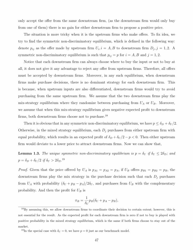
only accept the offer from the same downstream firm, (as the downstream firm would only buy

from one of them) there is no gain for either downstream firm to propose a positive price.

The situation is more tricky when it is the upstream firms who make offers. To fix idea, we

try to find the symmetric non-discriminatory equilibrium, which is defined in the following way:

denote pij as the offer made by upstream firm Ui, i = A,B to downstream firm Dj, j = 1, 2. A

symmetric non-discriminatory equilibrium is such that pij = p for i = A,B and j = 1, 2.

Notice that each downstream firm can always choose where to buy the input or not to buy at

all, it does not give it any advantage to reject any offer from upstream firms. Therefore, all offers

must be accepted by downstream firms. Moreover, in any such equilibrium, when downstream

firms make purchase decisions, there is no dominant strategy for each downstream firm. This

is because, when upstream inputs are also differentiated, downstream firms would try to avoid

purchasing from the same upstream firm. We assume that the two downstream firms play the

mix-strategy equilibrium where they randomize between purchasing from UA or UB. Moreover,

we assume that when this mix-strategy equilibrium gives negative expected profit to downstream

firms, both downstream firms choose not to purchase.18

Then it is obvious that in any symmetric non-discriminatory equilibrium, we have p ≤ δD + δU/2.

Otherwise, in the mixed strategy equilibrium, each Dj purchases from either upstream firm with

equal probability, which results in an expected profit of δD + δU/2− p < 0. Then either upstream

firm would deviate to a lower price to attract downstream firms. Now we can show that,

Lemma 1.3. The unique symmetric non-discriminatory equilibrium is p = δU if δU ≤ 2δD; and

p = δD + δU/2 if δU > 2δD.19

Proof. Given that the price offered by UA is pA1 = pA2 = pA, if UB offers pB1 = pB2 = pB, the

downstream firms play the mix strategy in the purchase decision such that each Dj purchases

from UA with probability (δU + pB − pA)/2δU , and purchases from UB with the complementary

probability. And then the profit for UB is

πB =1

δUpB(δU + pA − pB),

18By assuming this, we allow downstream firms to coordinate their decision to certain extent; however, this is

not essential for the result. As the expected profit for each downstream firm is zero if not to buy is played with

positive probability in the mixed strategy equilibrium, which is the same if both firms choose to stay out of the

market.19In the special case with δU = 0, we have p = 0 just as our benchmark model.

47

which gives us the best response function of UB

pB =δU + pA

2.

Similarly, for UA, we have

pA =δU + pB

2.

Then the unique solution is given by pA = pB = δU . However, this leaves the expected profit

of downstream firms as δD − δU/2. Therefore, if δU ≤ 2δD, this is the unique equilibrium. If

δU > 2δD, the upstream price is δD + δU/2 so as to keep downstream firms in the market.20

Now we can investigate the effect of vertical integration on investment incentives. If δU ≤ 2δD,

when only upstream innovation matters, the payoff matrix is shown Table 1.8.

Table 1.8: Only Upstream Innovation matters(a) Vertical Separation

HHHH

HHHHH

UA

UBS F

S δU2

, δU2

∆,0

F 0,∆ 0,0

→

(b) Vertical IntegrationH

HHHHHH

HHUA −D1

UBS F

S δU + δD, δU2

∆,0

F 0,∆ 0,0

In the left panel (a), each upstream firm gets profit δU when it is the upstream firms who

make offers to downstream firms, which happens with probability 1/2. Under vertical integration,

the independent upstream firm can still ask for δU from D2, since now inputs are differentiated.

We measure the impact of vertical integration on investment incentives as the relative gain for

the integrated firm when both firms are successful. Then this impact in the case of upstream

innovation is δD + δU/2.

If only downstream innovation matters, the payoff matrix is given by Table 1.9.

20This is so because each upstream firm would want to deviate to a higher price, however such deviating leads

both downstream firms to leave the market.

48

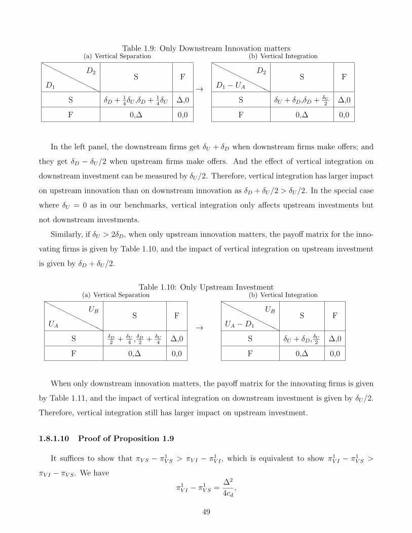
Table 1.9: Only Downstream Innovation matters(a) Vertical Separation

HHHH

HHHHH

D1

D2S F

S δD + 14δU ,δD + 1

4δU ∆,0

F 0,∆ 0,0

→

(b) Vertical IntegrationHHHH

HHHHH

D1 − UA

D2S F

S δU + δD,δD + δU2

∆,0

F 0,∆ 0,0

In the left panel, the downstream firms get δU + δD when downstream firms make offers; and

they get δD − δU/2 when upstream firms make offers. And the effect of vertical integration on

downstream investment can be measured by δU/2. Therefore, vertical integration has larger impact

on upstream innovation than on downstream innovation as δD + δU/2 > δU/2. In the special case

where δU = 0 as in our benchmarks, vertical integration only affects upstream investments but

not downstream investments.

Similarly, if δU > 2δD, when only upstream innovation matters, the payoff matrix for the inno-

vating firms is given by Table 1.10, and the impact of vertical integration on upstream investment

is given by δD + δU/2.

Table 1.10: Only Upstream Investment(a) Vertical Separation

HHHHH

HHHHUA

UBS F

S δD2

+ δU4

, δD2

+ δU4

∆,0

F 0,∆ 0,0

→

(b) Vertical IntegrationHH

HHHHHHH

UA −D1

UBS F

S δU + δD, δU2

∆,0

F 0,∆ 0,0

When only downstream innovation matters, the payoff matrix for the innovating firms is given

by Table 1.11, and the impact of vertical integration on downstream investment is given by δU/2.

Therefore, vertical integration still has larger impact on upstream investment.

1.8.1.10 Proof of Proposition 1.9

It suffices to show that πV S − π1V S > πV I − π1

V I , which is equivalent to show π1V I − π1

V S >

πV I − πV S. We have

π1V I − π1

V S =∆2

4cd,

49

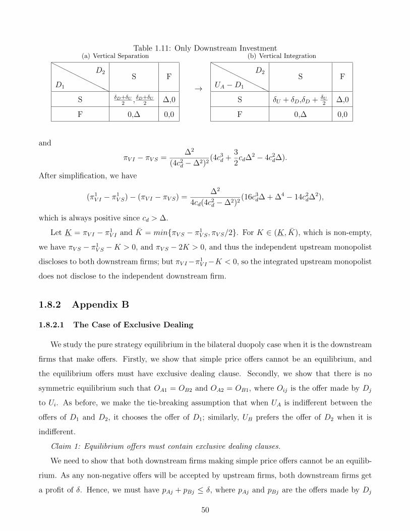
Table 1.11: Only Downstream Investment(a) Vertical Separation

HHHH

HHHHH

D1

D2S F

S δD+δU2

, δD+δU2

∆,0

F 0,∆ 0,0

→

(b) Vertical IntegrationHHHH

HHHHH

UA −D1

D2S F

S δU + δD,δD + δU2

∆,0

F 0,∆ 0,0

and

πV I − πV S =∆2

(4c2d −∆2)2

(4c3d +

3

2cd∆

2 − 4c2d∆).

After simplification, we have

(π1V I − π1

V S)− (πV I − πV S) =∆2

4cd(4c2d −∆2)2

(16c3d∆ + ∆4 − 14c2

d∆2),

which is always positive since cd > ∆.

Let K = πV I − π1V I and K = min{πV S − π1

V S, πV S/2}. For K ∈ (K, K), which is non-empty,

we have πV S − π1V S −K > 0, and πV S − 2K > 0, and thus the independent upstream monopolist

discloses to both downstream firms; but πV I−π1V I−K < 0, so the integrated upstream monopolist

does not disclose to the independent downstream firm.

1.8.2 Appendix B

1.8.2.1 The Case of Exclusive Dealing

We study the pure strategy equilibrium in the bilateral duopoly case when it is the downstream

firms that make offers. Firstly, we show that simple price offers cannot be an equilibrium, and

the equilibrium offers must have exclusive dealing clause. Secondly, we show that there is no

symmetric equilibrium such that OA1 = OB2 and OA2 = OB1, where Oij is the offer made by Dj

to Ui. As before, we make the tie-breaking assumption that when UA is indifferent between the

offers of D1 and D2, it chooses the offer of D1; similarly, UB prefers the offer of D2 when it is

indifferent.

Claim 1: Equilibrium offers must contain exclusive dealing clauses.

We need to show that both downstream firms making simple price offers cannot be an equilib-

rium. As any non-negative offers will be accepted by upstream firms, both downstream firms get

a profit of δ. Hence, we must have pAj + pBj ≤ δ, where pAj and pBj are the offers made by Dj

50

to UA and UB respectively. Then Dj′ can profitably deviate by make two exclusive dealing offers

(pAj + ε/2, E) and (pBj + ε/2, E) to the two upstream firms respectively. Then both UA and UB

will take the exclusive dealing offer, and the profit for Dj′ is ∆ − pAj − pBj − ε, which is higher

than δ.(As ∆ > 2δ and pAj + pBj ≤ δ)

Claim 2: There exists no symmetric equilibrium.

Consider a symmetric equilibrium with both exclusive dealing offers, i.e. D1 offers {(p1, E) and

(p2, E)} to UA and UB respectively. Then we must have max{p1, p2} ≤ δ. To see this: it cannot

be the case that both upstream firms accept the offers from the same downstream firm due to our

tie-breaking assumption. And thus each downstream firm must get profit δ, which means that the

offered price cannot be higher than δ. Hence, given that D1 makes such offers, D2 can deviate

by offering {(p1 + ε/2, E), (p2 + ε/2, E)}, which will be accepted by both upstream firms and give

D2 a profit of ∆ − p1 − p2 − ε > δ − p1. Therefore, there is no symmetric equilibrium with both

exclusive dealing offers. Similar argument also indicates that there is no symmetric equilibrium

where each downstream firm makes an exclusive dealing offer to one upstream firm and a simple

price offer to the other upstream firm.

Thus there are only asymmetric equilibria, and any such equilibrium must have the following

property.

Claim 3: In any equilibrium, one downstream firm is excluded from the market.

If both downstream firms are active in the market, each of them is supplied by one upstream

firm and gets profit δ. And thus, it must be the case that all four prices offered by downstream

firms are no higher than δ, which in turn means that each downstream firm has incentive to overbid

and exclude the other downstream firm as the argument in Claim 2.

Claim 4: In any equilibrium, we must have pAj + pBj = ∆ for the active downstream firm Dj;

and min{pAj, pBj} ≥ δ.

Suppose D1 is active and D2 is excluded from the market. For the first part, if not, D2 can

profitably deviate by offering slightly higher prices to both upstream firms and thus exclude D1.

For the second part, if not, suppose pB1 < δ, then D2 can profitably deviate by offering pB1 + ε to

UB.

Therefore, in any pure strategy equilibrium, both downstream firms earn zero profit. And the

industry profit is shared between the two upstream firms. However, pure strategy equilibrium may

fail to exist. For instance, suppose D1 is active in the equilibrium, and D1 offers {(p, E), (∆−p, E)}

51

to UA and UB, where δ ≤ p ≤ ∆− δ. Then the best response of D2 is to offer {(p1 ≤ p, ·), (p2 <

∆−p, ·)}. However, given that D2 offers p2 < ∆−p to UB, the best response for D1 is not to offer

∆−p to UB but rather to offer p2 +ε to UB. To circumvent such circumstances, we can restrict the

price quote to be discrete numbers with equal distance ε, i.e. prices can only be ∆,∆−ε,∆−2ε, ....

Then D1 offers {(p, E), (∆ − p, E)} to UA and UB, and D2 offers {(p, ·), (∆ − p − ε, ·)} is a pure

strategy equilibrium.

52

Chapter 2

Net Neutrality

Quality discrimination plays an important role in a number of markets. In the

context of Internet, content providers are subject to quality discrimination from the

Internet Service Providers. We study the effect of quality discrimination on product

designs in this paper. We show that content providers are biased to choose broader

designs. This reduces product differentiation in the market, and intervention is nec-

essary to achieve efficiency in the content market. The result brings new insights into

the discussion about net neutrality, which mandates equal access to every participant

on the Internet.

2.1 Introduction

The Internet had been working under the non-discrimination regulation, which requires all

contents, sites, and platforms being treated equally. This remained to be the situation until 2005,

when the Federal Communication Commission (FCC) changed the classification of Internet trans-

mission from “telecommunication services”to “information services”, which allows the Internet

Service Providers to “create different tiers of online service. They (ISP) would be able to sell

access to the express lane to deep-pocketed corporations and relegate everyone else to the digi-

tal equivalent of a winding dirt road. Worse still, these gatekeepers would determine who gets

premium treatment and who doesn’t”1.

1Lawrence Lessig and Robert W. McChesney (8 June 2006). “No Tolls on The Internet”, The Washington Post.

53

This policy change, backed up and put into practice2 by large Internet Service Providers, has

encountered strong opponent opinions from large content providers such as Google, who has tried

to maintain the non-discrimination regulation regime, i.e. a “neutral”network.3

We study the economic consequence of such policy change on the content market. Specifically,

we analyze the impact on how content providers (hereafter CP ) design their products if Internet

Service Providers (hereafter ISP ) can differentiate the quality of access to the network among

different CP s. We show that without net neutrality regulation, if the ISP lacks the ability to

commit to how each CP would be treated in the network, the CP s are biased to design their

products as broader ones.

To show this, we study the interaction between one ISP and two CP s. The CP s can only

reach consumers through the network of the ISP . A consumer values both the match between

a content and his taste, and the quality of connection when he consumers the content. That is

to say, a consumer’s utility from consuming a content depends on both the design of the content

and how the ISP treats this CP . Building on the concept of “demand rotation”introduced by

Johnson and Myatt (2006), we assume that each CP chooses a design, ranging from the broadest

one which is acceptable for a general public, to the most niche one which is tailored to specific

consumer taste. And the ISP chooses a network, which can be either neutral or discriminatory.

In a neutral network, both CP s are treated equally; whereas in a discriminatory network, the ISP

favors one CP and discriminates against the other one.

If the ISP commits to ex ante to a given network priority rule, the the CP s have an incentive

to choose the efficient design. When instead the ISP cannot commit ex ante to how it will treat

the CP s, then it favors the CP with the broader product. The reason is simple: Broader products

attract more consumers, and favoring these products thus increases the demand more than it

decreases the demand for niche products. Anticipating this, each CP tends to choose a broader

design than its rival so as to avoid being discriminated against. Hence, when the most niche design

is efficient, there is prisoner’s dilemma: the CP s would be better off with niche products, but each

CP has an incentive to design a broader product so as to be favored by the ISP .

2“Comcast Blocks Some Internet Traffic”, NBC news, 19/10/2007.3“The broadband carriers should not be permitted to use their market power to discriminate against competing

applications or content. Just as telephone companies are not permitted to tell consumers who they can call or what

they can say, broadband carriers should not be allowed to use their market power to control activity online.”–Guide

to Net Neutrality for Google Users.

54

Therefore, without net neutrality, lack of commitment from the ISP can lead to inefficient

design choices, which can significantly reduce production differentiation in the content market.

Enforcing net neutrality endows the ISP the commitment power that it lacks, which can eliminate

such distortion of designs in the content market.

The analysis brings new insight into the economic debate4 on net neutrality, which has so far

focused on issues related to pricing and investment incentives.5 For instance, Economides and

Tag (2012) and Hermalin and Katz (2007) analyzed the pricing of the ISP in a two-sided market

framework; Choi and Kim (2010), Kramer and Wiewiorra (2012), and Bourreau et al (2012)

studied the investment incentives of ISP s and CP s in similar frameworks.

The insight that discrimination in quality can have large impact on product designs applies to

other markets as well, especially to those where the quality of access to consumers is important.

For instance, the shelves in a supermarket differ in their locations and easiness to find, and the

owner is likely to locate broader products on those easy-to-find shelves. Thus if the owner lacks

the ability to commit, the manufacturers may be biased to choose broader products.

The paper is organized as follows: in section 2, we present the model and main results, where

a linear example is also shown; we briefly discuss some extensions and robustness of our results in

section 3; and section 4 concludes. All omitted proofs are given in the appendix.

2.2 The Network/Design Model

2.2.1 The Model

Consider a market with a representative consumer/user(U), a monopolistic Internet Service

Provider(ISP ), and two Content Providers(CP1 and CP2). The CP s distribute their products to

the user through the network of the ISP .6

Consumer The representative consumer values both the content and the quality of connection

in an additive way, and only consumes the product with a higher overall valuation.7 His utility

4Schuett(2010) and Kramer et al (2013) provide thorough surveys of the economic literatures on net neutrality.5The ISP s invest in the network capacity, and the CP s invest in the qualities of their contents.6We consider a situation where the network serves as a “bottleneck”for the market, so both the consumer and

the CP s cannot bypass the ISP .7In other words, the two CP s compete for the consumer.

55

function is given by

U = max{v1 + q1, v2 + q2} − p,

where vi is the match value between the consumer and the product of CPi, qi is the connection

quality of CPi, and p is the price charged by the ISP .

The match value vi is randomly drawn from a distribution F (vi, si), where si is the design

chosen by CPi.8 We assume that given designs s1 and s2, the realizations of v1 and v2 are

independent. The connection qualities are determined by how the ISP arranges the network. In

addition, we normalize the reservation utility of the consumer to zero.

Internet Service Provider The ISP charges a price p for the consumer.9 More importantly, the

ISP can choose how to treat the CP s: The ISP can choose a connection quality q1 = δ ∈ [−∆,∆]

for CP1, and the connection quality of CP2 is q2 = −δ.10 When δ = 0, the ISP chooses a neutral

network where both CP s are treated equally; when δ < 0, the ISP favors CP2; and when δ > 0,

the ISP instead favors CP1.11

Content Providers Each CP chooses a design s ∈ S = [B,N ] which ranges from the broadest

(B) to the most niche (N). Each design s induces the consumer’s match value v to be distributed

according to F (v; s), with density f(v; s) which is positive everywhere in the support [vs, vs]. We

follow Johnson and Myatt(2006) by assuming that different designs induce demand rotation:

Definition 2.1. (Johnson and Myatt 2006): A local change of s leads to a rotation of F (v; s)

8In the basic model, we consider the case where the match value is the only valuation that the user derives from

the content. The content of CPi may also have an intrinsic value θi that is independent from the match value; in

this sense we consider the case of homogeneous CP s where θ1 = θ2 in the basic model.9We do not consider the case when the ISP also charge CP s for connection. Since the main focus in this paper

is how the possibility of quality discrimination affects the design on the content market, but not how the ISP sets

prices for the user and CP s. For more references on the price setting of the ISP , see the literatures on two-sided

market.

In a discriminatory network, the ISP may auction out the priority or charge the favored CP in other manners,

we consider this possibility in the next section.10That is, the connection qualities of the two CP s always sum up to zero. Increasing the connection quality of

one CP necessarily decreases that of the other one. For instance, giving priority to CP1 means CP2 has to wait.11The consumer may value connection quality in a multiplicative way. For instance, U = max{v1q1, v2q2} − p,

and then we can alternatively assume that if the connection quality of CP1 is 1 + δ, then the connection quality of

CP2 is 1− δ, for δ ∈ [−∆,∆]. However, this does not change our qualitative result.

56

if for some v∗s and each v ∈ (vs, vs)

v > v∗s ⇔∂F (v; s)

∂s< 0 and v < v∗s ⇔

∂F (v; s)

∂s> 0.

If this holds for all s, then {F (v; s)} is ordered by a sequence of rotations.

The concept of demand rotation formalizes the idea that some designs induce a wider spread

of consumer valuations than others; for instance, some designs cater to a particular group of

consumers whereas others cater to a more general public. An increase in s leads to a clockwise

rotation of the distribution function around the rotation point v∗s , so there are more consumers

with high valuation, but also more consumers with low valuation. A higher s means a more niche

product, and the bounds on s correspond to the broadest and the most niche product.

We focus on a class of rotation-ordered functions such that v∗s is decreasing in s. As shown

in Johnson and Myatt(2006), with such rotation-ordered functions, the monopoly profit is quasi-

convex in s, and thus maximized at extreme designs.

Assumption 2.1. {F (v; s)} is rotation-ordered in s and the rotation point v∗s is decreasing in s.

Demands and Profits For given designs s1 and s2, network choice δ, and price p, the demand

for CP1 is given by

D1(s1, s2; δ; p) =∫ ∞p−δ

F (v + 2δ; s2)dF (v; s1). (2.1)

Similarly, the demand for CP2 is given by

D2(s1, s2; δ; p) =∫ ∞p+δ

F (v − 2δ; s1)dF (v; s2). (2.2)

The demand for the ISP service equals the sum of the demands for each CP , which is

D(s1, s2; δ; p) = D1 +D2

= Prob(max{v1 + δ, v2 − δ} ≥ p)

= 1− F (p− δ; s1)F (p+ δ; s2);

(2.3)

Hence the profit of the ISP is

πδ0(s1, s2, p) = p ·D(s1, s2; δ; p).

We assume that each CP can costlessly choose any design s ∈ S, and the marginal cost of

production is zero. Moreover, the CP s do not directly charge the consumer; instead, each CPi

57

obtains a profit α from one unit of demand for its product through activities such as advertising.12

Therefore, the profit of each CPi is

πδi (s1, s2, p) = α ·Di(s1, s2; δ; p).

2.2.2 Benchmark: Industry Profit Maximization and Commitment

We start with the situation where the ISP can commit to a network characteristic, where we

show that CP s are induced to choose the industry profit maximizing designs.

2.2.2.1 Industry Profit Maximization

The industry profit is given by

Πδ(s1, s2; p) = πδ0(s1, s2; p) + πδ1(s1, s2; p) + πδ2(s1, s2; p)

= (p+ α)D(s1, s2; δ; p).

It is easy to show that the industry profit is quasi-convex in the designs and we focus on the

situation where both the ISP and CP s are better-off with the most niche products than the

broadest products. Specifically, denote Dδ(s, s′) as the demand for CP1 in a network δ, when

CP1’s design is s and CP2’s design is s′, and we assume that

Assumption 2.2. πδ0(N,N) > πδ0(B,N) > πδ0(B,B), and Dδ(N, s) > Dδ(B, s) for δ ∈ [−∆,∆]

and s ∈ S.13

Then it is straightforward to show that:

Proposition 2.1. Under Assumptions 1,2, the industry profit is maximized when both CP s choose

the most niche design.

Proof. See Appendix 2.5.1.

12The result in this paper is not sensitive to this assumption. We can readily make other assumptions on how

CP s generate profits. For instance, the ISP and each CP may share the profit that is generated from the demand

for the product of the CP , which is the situation in the pay-TV market.

And we briefly discuss the more general case where CP s differentiate in their profitability in section 3.13The price is set at the profit-maximizing level by the ISP , given the network and designs chosen by CP s.

58

2.2.2.2 Commitment

When the ISP commits to a network characteristic δ, the game goes as follows:

• Stage 0: The ISP announces a network choice δ ∈ [−∆,∆];

• Stage 1: The two CP s choose their designs, s1 and s2, simultaneously;

• Stage 2: The ISP sets the price p;

• Stage 3: The consumer observes both match values v1, v2, network characteristic δ and price

p, then decides whether to connect to the service and which content to consume.

Notice that in the commitment case, the ISP only commits to a network characteristic δ, but

not to a price p. Hence, the optimal price depends on the designs chosen by the CP s, which we

denote as p(s1, s2). And we make the following assumption to facilitate our analysis:

Assumption 2.3. |∂Di

∂si| > |∂Dj

∂si|,for j 6= i; and |∂Di

∂si| > |∂Di

∂p∂p∂si|.14

The first part of Assumption 2.3 says that for each CP , keeping the price fixed, changing its

product design has a larger impact on its own demand than on the demand of the other CP .15

The second part of the Assumption says that the indirect effect on demand resulting from the

induced change in price is dominated by the direct effect following a change in design. Now we

can show the following result:

Proposition 2.2. Under Assumptions 2.2 and 2.3, if F (v; s) is log-concave in v, when the ISP

can commit to a network characteristic, it commits to δ ∈ {−∆,∆}, and both CP s choose the

most niche design.

Proof. See Appendix 2.5.3

So, the ISP always commit to a maximally discriminatory network, and the CP s choose the

“efficient”designs that maximize industry profit. The reason (which is shown in detail in the

proof) is as follows: Given the network characteristic, under Assumption 2.3, each CP ’s profit is

14A detailed assumption on the demand function is given in the appendix.15Similar assumptions are widely made in industry organization literatures. For example, in Bertrand competition

with differentiated goods, we usually assume that the demand for a seller is more sensitive to his own price than

to the rival’s price.

59

quasi-convex in its own design and thus maximized at either B or N ; and Assumption 2.2 implies

that each CP prefers to choose N . Moreover, given that both CP s choose the same design,

introducing discrimination increases the demand for the favored CP and decreases the demand

for the discriminated CP . The log-concavity assumption ensures that the first effect dominates

and the overall demand increases. Therefore, the ISP prefers a discriminatory network. And we

assume that in this situation the ISP randomly favors one of the CP s.

2.2.3 No Commitment

Now we turn to the situation when the ISP cannot commit, the CP s have to choose their

designs before the ISP makes any arrangement for the network. The game proceeds as follows:

• Stage 1: The two CP s choose their designs, s1 and s2, simultaneously;

• Stage 2: The ISP sets the price p and chooses whether to discriminate, i.e. chooses a

network characteristic δ;

• Stage 3: The consumer observes both match values v1, v2, network characteristic δ, and

price p, then decides whether to connect to the service and which content to consume.

We solve the game backwards.

At Stage 3, the consumer’s behavior is given by the demand function specified above: he only

consumes the content with higher overall value if it is greater than the price. We study the ISP

and CP ’s behavior in the following.

2.2.3.1 Stage 2: ISP ’s Behavior

For the ISP , two decisions have to be made: what price to charge for the consumer and

whether to discriminate any of the CP s. The above Proposition 2.2 has shown that when the two

CP s choose the same design s, the ISP will choose a network with maximum discrimination.

The logic also extends to the situation when the two CP s chooses different designs, say CP1

chooses a product which is broader than that of CP2, i.e. s1 < s2, then we have the following

result:

Proposition 2.3. When the designs of the two CP s are different, if F (v; s) is log-concave in v

and s, the ISP will maximally favor the CP with broader design.

60

Proof. See Appendix 2.5.4.

The reason why the ISP always favors the broader product is simple. For a given price,

choosing a discriminatory network shifts down the distribution function of match value for the

favored CP , and shifts up that for the discriminated one. The assumption on F (v; s) ensures

that the downward-shift is larger when the broader product is favored and thus demand increases

more. Simply speaking, improving the quality of a product that suits more consumers leads to a

larger increase in demand than improving the quality of a product which is popular only among

a small group of consumers.

Then the problem for the ISP is simply to choose a price to maximize profit under a network

with maximum discrimination which favors the broader product. That is to say, for any s1 ≤ s2,16

ISP ’s Problem: maxpπ∆0 (s1, s2; p) = p · (1− F (p−∆; s1)F (p+ ∆; s2)).

2.2.3.2 Stage 1: CP s’ Behavior

When the ISP lacks the ability to commit, the CP s have to make their decisions anticipating

how they would be treated ex post. Denote D(B,B) as the demand for each CP when they both

choose the broadest design.17 The following proposition shows that both CP s choosing the most

niche design is no longer an equilibrium, and they are biased to choose broader designs.

Proposition 2.4. Under Assumption 2.2 and 2.3, and F (v; s) is log-concave in both s and v, when

the ISP cannot commit to a network, (B,B) is the only equilibrium if D(B,B) > D−∆(N,B);

and there is no pure strategy equilibrium if D(B,B) < D−∆(N,B).

Proof. See Appendix 2.5.5.

The intuition for this results is simple: when the ISP cannot commit to a network, under the

assumption that F (v; s) is log-concave in s and v, it is equivalent to say that the ISP commits

to favor the broader product ex post, and therefore each CP is biased to choose broader designs

in order to gain competitive advantage.

When the most niche design is the “efficient”choice for the CP , without uncertainty about the

network, each CP can maximize his own profit without considering the design of the other CP .

16This is the case subject to a relabeling of the two content providers.

17We have D(B,B) = D1(B,B)+D2(B,B)2 .

61

When such uncertainty prevails, on one hand, each CP intends to choose a more niche design so

as to increase his profit; on the other hand, each CP is inclined to choose a broader design so

as not to be discriminated against ex post. The lack of commitment from the ISP creates such

strategic concerns, which biases the CP s’ choices to broader designs.

Remark When pure-strategy equilibrium does not exist, there exist mixed strategy equilibrium,

where each CP randomizes among different designs. Nevertheless, more broader products would

emerge in such equilibrium and the result of broad-biased design still holds.

2.2.4 An Example

We consider a linear example with the characteristic that the rotation point is fixed, which

enables us to show explicitly how lack of commitment from the ISP could distort the product

designs in the content market.

Take the symmetric case θ1 = θ2 = θ; and the match value vs for a design s follows a uniform

distribution on the interval [−s, s]. Thus, for each design s, the user valuation follows a uniform

distribution on [θ−s, θ+s], and the rotation point is θ for any design s. We assume that the design

s ∈ S = [s, s], where s = s is the most broad design and the user valuation is more concentrated

around θ; and s = s is the most niche design, the user may get very high or very low value.

In this linear case, we have F (v; s) = v+s−θ2s

and f(v; s) = 12s

, and thus

f

F(s, v) =

1

v + s− θ,

which is indeed decreasing in both s and v. Therefore, if s1 < s2, and the corresponding optimal

price is such that f(v; s1) is positive, the ISP prefers to give better connection to CP1; explicitly,

at such price, the demand in a network favoring CP1 is

D1 = 1− p+ s1 − δ − θ2s1

·p+ s2 + δ − θ2s2

.

The demand in a neutral network and a network favoring CP2 is

DN = 1− p+ s1 − θ2s1

·p+ s2 − θ2s2

and D2 = 1− p+ s1 + δ − θ2s1

·p+ s2 − δ − θ2s2

.

Then it is easy to see that D1 > DN and D1 > D2.

Therefore, if the two CP s choose the same design s, the ISP would choose a discriminatory

network which randomly favors either one of the two CP s. The profit is then

Π = p(1− p+ s− θ − δ2s

p+ s− θ + δ

2s),

62

then the optimal price is

p∗ =−(2s− 2θ) +

√(2s− 2θ)2 + 12s2 − 3(s− θ − δ)(s− θ + δ)

3.

Thus for a given δ, we have

p∗ > θ + δ if s > s,

where s = 23θ if δ = 0; and s increases with δ. We focus on the case where s ≥ s, so that when s1

and s2 are greater than s, the optimal price is above the higher rotation point θ+ δ; and thus the

industry profit is increasing in si and attains maximum at si = s.

Then we need to check if Assumption 2 is satisfied, which is equivalent to check that if increasing

si can increase the profit of the ISP , then it also increases the profit of CPi. In this linear example,

when s ≥ s, it is clear that the profit of the ISP is increasing in si. Moreover, increasing si also

increases the demand for CPi. Take CP1 for example, if s1 < s2, the ISP chooses a network

favoring CP1,

D1 =∫ θ+s1

p−δF (s2, v + 2δ)dF (s1, v),

and

D2 =∫ θ+s2

p+δF (s1, v − 2δ)dF (s2, v).

Note that, for a given price p, we can see D1 as a weighted summation of F (v; s2), increasing s1

leads to a clockwise rotation of F (v; s1), this rotation shifts more weight to higher v, and thus

more weight on higher F (v; s2). Similarly, for D2, it’s a weighted summation over F (v; s1), an

increase in S1 lowers the value of F (v; s1) for each v, and thus lower the demand D2. Thus, we

must have ∂D1

∂s1> 0 > ∂D2

∂s1; moreover, as ∂D

∂s1> 0, we have |∂D1

∂s1| > |∂D2

∂s1|. Tedious algebra also

shows that if ∂D1

∂s1> 0, then ∂π1

∂s1> 0, and vise versa. Hence, Assumption 2 is satisfied in the

relevant range we consider.

Therefore, in this linear example, the equilibrium must be extreme ones. Specifically, if the

ISP can commit to a network, either neutral or discriminatory, as the profit for each CP increases

with more niche designs, (s, s) is the only equilibrium.

However, with limited commitment, (s, s) cannot be an equilibrium. And there exists a thresh-

old s > s such that for s < s, D(s, s) > Ds(s, s). So for s < s, (s, s) is the only equilibrium.

Moreover in this linear example, it is easy to show that the socially efficient designs and network

are the most niche designs with a discriminatory network. Thus if the ISP is able to commit, the

social optimal designs can be achieved; if not, the social optimal designs are never obtained.

63

2.3 Discussion and Extension

2.3.1 Bidding for Connection Quality

In the model above, we assume that the ISP does not charge the CP for better connection. If

the ISP can auction out the higher connection quality q, will this change the results? To see this,

suppose s1 < s2, so CP1 is favored by the ISP if there is no auction. For a given discriminatory

policy δ 6= 0, denote D1i and p1 as the demand for product CPi and price charged by ISP when

CP1 is favored; similarly D2i and p2 as the demand and price when CP2 is favored. Then the

maximum amount CPi, (i = 1, 2) is willing to bid for high connection quality is

b1 = α(D11 −D2

1) and b2 = α(D22 −D1

2).

Thus, CP2 cannot outbid CP1 if D11 +D1

2 > D21 +D2

2, which is satisfied.

Proposition 2.5. When the ISP auctions out the high connection quality, if F (v; s) is log-concave

in both s and v, the broader CP outbids the other one. And if a pure-strategy symmetric equilibrium

exists, it must be that both CP s choose the broadest design.

Proof. See Appendix 2.5.6.

Therefore, even we allow the CP s to bid for better connection quality, the CP with the more

niche design cannot outbid the broader one; and the bias towards broader designs still exists.

However, this result may change if there is a large difference in the profitabilities of CP s. Suppose

CPi generates profit αi for each unit of demand Di, then the maximum amount CPi is willing to

bid for high connection quality is

bi = αi(Dii −D

ji ), j 6= i

For CP2 to win the auction and the ISP chooses the network that favors CP2, we need

α2(D22 −D1

2) > α1(D11 −D2

1) (CP2 wins),

p2(D21 +D2

2) + α2(D22 −D1

2) > p1(D11 +D1

2) + α1(D11 −D2

1) (ISP favors CP2).

When α2 is larger enough compared to α1, CP2 may outbid CP1 and ISP may actually choose

to discriminate the broader product. Thus, if there is systematic difference in the profitability of

broad CP and niche CP , the CP s may instead tend to choose niche products.18

18For example, this may be the case if consumers with higher valuation for the product also create higher profit for

64

2.3.2 Non-Competing Content Providers

Up to now, we have focused on the case when the two CP s compete for the user in the sense

that the user only consumes the product with higher realized match value. In this subsection,

we briefly discuss the case when the CP s do not directly compete for the user, i.e. the user can

potentially consume both products. For simplicity, we assume that the utility of the consumer is

given by

U = max{v1 + q1, v2 + q2, v1 + q1 + v2 + q2} − p,

implying that the demand is

D(s1, s2; q1, q2; p) = Prob(max{v1 + q1, v2 + q2, v1 + q1 + v2 + q2} > p).

Suppose s1 < s2, we show that the ISP still favors the broader CP1 under a slightly stronger

assumption than the previous section.

Proposition 2.6. When the content providers do not compete for the user, if f(v; s) is log-concave

in both s and v, then the ISP maximally favors the broader product. And therefore, if a pure-

strategy symmetric equilibrium exists, it must be that both CP s choose the broadest design.

Proof. See Appendix 2.5.7.

The result of broad-biased design in the previous section still holds when the two CP s do not

directly compete for the user. The intuition remains the same: an increase in the connection

quality of a broader product leads to a larger increase in demand than a niche product, as the

valuation of the user is more concentrated around the center.

2.3.3 Asymmetric Content Providers

In the previous section, we studied the case of symmetric content providers, i.e. the intrinsic

value of CPi is the same for i = 1, 2; and the user valuations only differ in the match value. When

the two CP s are asymmetric in the sense that one CP has a higher intrinsic value, the result of

favoring the broader CP may be weakened.

Denote the two CP s as CPL and CPH , CPi has an intrinsic value to the user θi, we suppose

θL < θH . The user’s valuation for the product of CPi consists of three parts: the intrinsic value

the CP in the advertising market. In this case, the niche product catering to particular high valuation consumers

may indeed obtain higher profit than a broader product.

65

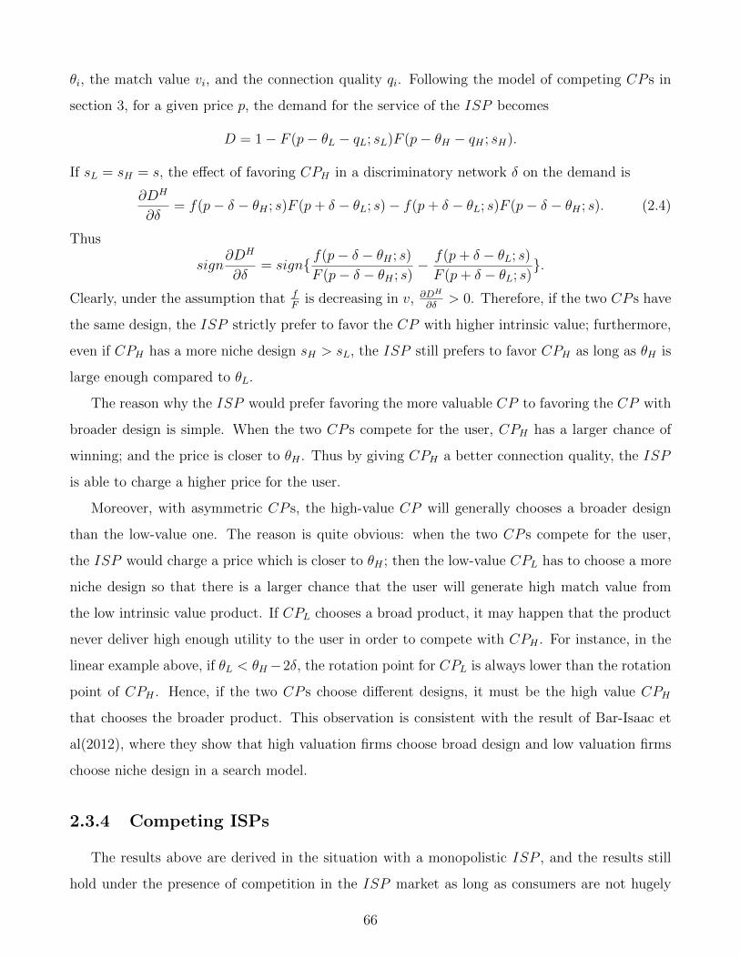
θi, the match value vi, and the connection quality qi. Following the model of competing CP s in

section 3, for a given price p, the demand for the service of the ISP becomes

D = 1− F (p− θL − qL; sL)F (p− θH − qH ; sH).

If sL = sH = s, the effect of favoring CPH in a discriminatory network δ on the demand is

∂DH

∂δ= f(p− δ − θH ; s)F (p+ δ − θL; s)− f(p+ δ − θL; s)F (p− δ − θH ; s). (2.4)

Thus

sign∂DH

∂δ= sign{ f(p− δ − θH ; s)

F (p− δ − θH ; s)− f(p+ δ − θL; s)

F (p+ δ − θL; s)}.

Clearly, under the assumption that fF

is decreasing in v, ∂DH

∂δ> 0. Therefore, if the two CP s have

the same design, the ISP strictly prefer to favor the CP with higher intrinsic value; furthermore,

even if CPH has a more niche design sH > sL, the ISP still prefers to favor CPH as long as θH is

large enough compared to θL.

The reason why the ISP would prefer favoring the more valuable CP to favoring the CP with

broader design is simple. When the two CP s compete for the user, CPH has a larger chance of

winning; and the price is closer to θH . Thus by giving CPH a better connection quality, the ISP

is able to charge a higher price for the user.

Moreover, with asymmetric CP s, the high-value CP will generally chooses a broader design

than the low-value one. The reason is quite obvious: when the two CP s compete for the user,

the ISP would charge a price which is closer to θH ; then the low-value CPL has to choose a more

niche design so that there is a larger chance that the user will generate high match value from

the low intrinsic value product. If CPL chooses a broad product, it may happen that the product

never deliver high enough utility to the user in order to compete with CPH . For instance, in the

linear example above, if θL < θH−2δ, the rotation point for CPL is always lower than the rotation

point of CPH . Hence, if the two CP s choose different designs, it must be the high value CPH

that chooses the broader product. This observation is consistent with the result of Bar-Isaac et

al(2012), where they show that high valuation firms choose broad design and low valuation firms

choose niche design in a search model.

2.3.4 Competing ISPs

The results above are derived in the situation with a monopolistic ISP , and the results still

hold under the presence of competition in the ISP market as long as consumers are not hugely

66

differentiated in their tastes. In the simplest scenario, two ISP s locate at the end points of a

Hotelling line, and consumers are uniformly distributed along the line. If consumers are only

differentiated in their location, each ISP would still favor the CP with broader product, because

any other network would reduce the utility a consumer would generate from connecting to his

service.

When consumers are highly differentiated in their tastes, for example, some consumers strongly

prefer the product of CP1 while the others strongly prefer that of CP2, then each ISP would have

incentive to differentiate himself from the other. In this case, we may have each ISP favors a

different CP and each CP chooses his design without distortion.

2.3.5 Investments of CP s

So far, we have been focusing on the situation where there is no cost for CP s to choose any

design, nor is there any cost for them to enter the market. Now suppose that each CP has to pay

a fixed cost E to enter the market.19

When the ISP cannot commit to a network characteristic, we focus on the case of D(B,B) >

D−∆(N,B), so (B,B) is the only equilibrium if both CP s chose to enter. And thus, if E ≤

αD(B,B), both CP s choose to enter with the broadest design.

When the ISP can commit to a network characteristic δ ≥ 0,20 if a CP decides to enter,

it must choose to enter with the most niche product. However, if the profit of the CP2, who

is discriminated against, is not enough to cover the entry cost, then it won’t enter. That is, if

E ≥ D−δ(N,N), only one CP enters under network characteristic δ. Hence, the ISP may want

to commit to a less discriminatory network so as to induce both CP s to enter, which is beneficial

for both consumers and the ISP . In the situation where the ISP is constrained in the networks

that it can choose, it may be that when the ISP can commit, it commits to a neutral network.

For instance, when the ISP can only choose a neutral network and a network with maximal

19In other words, the entry cost does not depend on the design chosen by the CP . Therefore, Assumption 2.2 is

still verified in this situation. However, we can also assume that the entry cost is increasing in the design chosen

(as it demands more information to design a niche product), and the analysis goes through as long as Assumption

2.2 is satisfied.20That is, the ISP either chooses a neutral network or a network favoring CP1. And this is the situation only

subject to a relabeling of CP s.

67

discrimination,21 if the profit of the discriminated CP is too low, then the ISP prefers to commit

to the neutral network.

2.4 Concluding Remarks on Net Neutrality

In this paper we studied a simple model where the Internet Service Provider and content

providers interact. The main result shows that if the ISP cannot commit to a network structure,

the CP s are biased to choose broader designs. In some circumstances such as our linear example,

such biases take an extreme form. The social optimal designs are achieved with commitment, while

they are never achieved with limited commitment. The underlying reason is simple, with limited

commitment, ex post the ISP prefers a network which favors the broader product; and thus each

CP is inclined to design its product as broader ones in fear that it might be discriminated against

ex post.

This raises the concerns about the effect of net neutrality regulation if we take into account

such impact it may have on the content market. Enforcing such regulation may reduce the biases

on the designs of products, but it may also increase the biases on the network structure in case

where a discriminatory network may be socially beneficial. Abandoning such regulation may not

do much harm if the ISP is able to commit. However, if the ISP behaves opportunistically, the

content markets may end up with many similar products, which the consumers like but don’t love.

Especially, this may be the case in emerging content markets, where content providers are less

differentiated and there is a larger chance that the ISP would be opportunistic.

Although this paper proceeds in the framework of net neutrality, we believe the intuition

that lack of commitment may have serious consequences on the upstream designs works in other

environments also. For instance, a search engine is more likely to put a link which everybody may

click at a higher click-through rate position rather than a link which only a few consumers might

be interested in; a supermarket is likely to put a product that most consumers like at an easy-to-

find shelf rather than a product that attracts only consumers with special tastes. The key insight

is that if the downstream resource owner can potentially practice certain forms of discrimination,

lack of commitment may seriously distort upstream investments.

21This would be the case where one CP gets priority, and the other CP has to wait.

68

2.5 Appendix

2.5.1 Proof of Proposition 2.1

To prove proposition 1, we start with the following lemma:

Lemma 2.1. Under Assumption 1, the industry profit is quasi-convex in the designs and thus

maximized at extreme designs.

Proof. The result follows immediately from proposition 1 of Johnson and Myatt(2006). First, it

is obvious that F (v; s) is rotation-ordered implies that F (v; s1)F (v; s2) is rotation-ordered in both

s1 and s2. Then with a given network characteristic δ, for any designs s1 < s2,22 suppose the price

that maximizes Πδ is above the highest rotation point, i.e. p∗ > v∗s1 , so that the profit maximizing

quantity is below 1−F (v∗s1 ; s1) ·F (v∗s1 ; s2), then by the definition of rotation-ordering, an increase

in either s1 or s2 would shift down F (v∗s1 ; s1, ·F (v∗s1 ; s2) as both v∗si are decreasing in si, and thus

demand increases even if the price is unchanged. Therefore a higher si always leads to higher

profit. Similarly, if p∗ < v∗s2 , decreasing both s1 and s2 would increase demand when price is fixed.

If v∗s2 < p∗ < v∗s1 , increasing s2 and decreasing s1 at the same time would increase profit. Thus

the profit maximizing designs must be extreme ones.

Then by Assumption 2.2, both the ISP and CP s prefer the most niche design to the broadest

design, so we have the industry profit is maximized with the most niche designs.

2.5.2 Details of Assumption 2.3

Assumption 2.3 can be obtained from two assumptions on the demand function D(s1, s2; p)

and Di(s1, s2; p).

• (2.1) ∂2D∂P 2 ≤ 0 and |∂D

∂p| > p|∂2D

∂p2| for any p;

• (2.2) |∂Di/∂si||∂Di/∂p| ≥

12|∂2D/∂p∂si||∂2D/∂p2| ≥

|∂Dj/∂si||∂Dj/∂p| ;

We need to show that the above two conditions imply that sign{∂πi/∂si} = sign{∂Di/∂si}.

First, we have∂πi∂si

= α[∂Di

∂si+∂Di

∂p

∂p

∂si]

22Without loss of generality, we suppose s1 < s2, so that v∗s1 > v∗s2 .

69

then what we need to show is simply

|∂Di

∂si| ≥ |∂Di

∂p

∂p

∂si|

The profit maximization problem for the ISP gives us the following first order condition

D(s1, s2; p) + p(s1, s2)∂D(s1, s2; p)

∂p(s1, s2)= 0

and thus we have∂p

∂si= −

∂D∂si

+ p ∂2D∂p∂si

2∂D∂p

+ p∂2D∂p2

Thus we need to show that|∂D∂si

+ p ∂2D∂p∂si|

|2∂D∂p

+ p∂2D∂p2|≤|∂Di

∂si|

|∂Di

∂p|

From (2.1) we have

|∂D∂si

+ p ∂2D∂p∂si|

|2∂D∂p

+ p∂2D∂p2|≤|∂D∂si|+ p| ∂2D

∂p∂si|

2|∂D∂p|+ p|∂2D

∂p2|≤|∂D∂si|+ p| ∂2D

∂p∂si|

|∂D∂p|+ 2p|∂2D

∂p2|≤|∂Di

∂si|+ |∂Dj

∂si|+ p| ∂2D

∂p∂si|

|∂Di

∂p|+ |∂Dj

∂p|+ 2p|∂2D

∂p2|

The right hand side of the above equation is smaller than |∂Di

∂si|/|∂Di

∂p| if

|∂Dj

∂si|+ p| ∂2D

∂p∂si|

|∂Dj

∂p|+ 2p|∂2D

∂p2|≤|∂Di

∂si|

|∂Di

∂p|

which is implied by (2.2), as

|∂Dj

∂si|+ p| ∂2D

∂p∂si|

|∂Dj

∂p|+ 2p|∂2D

∂p2|≤ 1

2

| ∂2D∂p∂si|

|∂2D∂p2|≤|∂Di

∂si|

|∂Di

∂p|

2.5.3 Proof of Proposition 2.2

We first show that given the network characteristic δ and the design chosen by CPj, sj, the

profit of CPi is quasi-convex in si and thus maximized at one of the extreme designs, i.e. si ∈

{B,N}.

Lemma 2.2. If Assumption 2.3 is satisfied, then for i ∈ {1, 2}, sign{∂πδ0/∂si} = sign{∂πδi /∂si}

for a given network characteristic δ ∈ [−∆,∆].

Proof. It suffices to show that sign{∂πδ0/∂si} = sign{∂Dδi /∂si}. First, we have

πδ0(si, sj) = p(si, sj)D(si, sj; δ; p(si, sj))

70

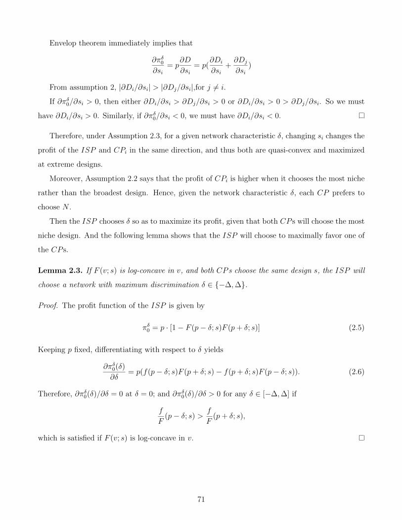
Envelop theorem immediately implies that

∂πδ0∂si

= p∂D

∂si= p(

∂Di

∂si+∂Dj

∂si)

From assumption 2, |∂Di/∂si| > |∂Dj/∂si|,for j 6= i.

If ∂πδ0/∂si > 0, then either ∂Di/∂si > ∂Dj/∂si > 0 or ∂Di/∂si > 0 > ∂Dj/∂si. So we must

have ∂Di/∂si > 0. Similarly, if ∂πδ0/∂si < 0, we must have ∂Di/∂si < 0.

Therefore, under Assumption 2.3, for a given network characteristic δ, changing si changes the

profit of the ISP and CPi in the same direction, and thus both are quasi-convex and maximized

at extreme designs.

Moreover, Assumption 2.2 says that the profit of CPi is higher when it chooses the most niche

rather than the broadest design. Hence, given the network characteristic δ, each CP prefers to

choose N .

Then the ISP chooses δ so as to maximize its profit, given that both CP s will choose the most

niche design. And the following lemma shows that the ISP will choose to maximally favor one of

the CP s.

Lemma 2.3. If F (v; s) is log-concave in v, and both CP s choose the same design s, the ISP will

choose a network with maximum discrimination δ ∈ {−∆,∆}.

Proof. The profit function of the ISP is given by

πδ0 = p · [1− F (p− δ; s)F (p+ δ; s)] (2.5)

Keeping p fixed, differentiating with respect to δ yields

∂πδ0(δ)

∂δ= p(f(p− δ; s)F (p+ δ; s)− f(p+ δ; s)F (p− δ; s)). (2.6)

Therefore, ∂πδ0(δ)/∂δ = 0 at δ = 0; and ∂πδ0(δ)/∂δ > 0 for any δ ∈ [−∆,∆] if

f

F(p− δ; s) > f

F(p+ δ; s),

which is satisfied if F (v; s) is log-concave in v.

71

2.5.4 Proof of Proposition 2.3

If s1 < s2, we first show the profit is higher when the ISP favors CP1 than when it chooses a

neutral network. The profit of the ISP is

πδ0 = p(1− F (p− δ; s1)F (p+ δ; s2))

If δ = 0, the network is neutral; if δ > 0, the ISP favors CP1. Fix p, take FOC w.r.t. δ,

∂πδ0∂δ

= p(f(p− δ; s1)F (p+ δ; s2)− f(p+ δ; s2)F (p− δ; s1))

sign{∂πδ0

∂δ} = sign{ f

F(p− δ; s1)− f

F(p+ δ; s2)}

If F (v; s) is log-concave in s and v, we have

f

F(p− δ; s1) >

f

F(p− δ; s2) >

f

F(p+ δ; s2) for all δ ∈ [0,∆]

Thus, we have ∂πδ0/∂δ > 0 for all δ ∈ [0,∆]. Therefore, the ISP prefers a maximum discriminatory

network which favors CP1 to a neutral network.

Then we show that a discriminatory network favoring CP1 is preferred to a network favoring

CP2. It suffices to show that for a given p and δ ≥ 0,

F (p− δ; s1)F (p+ δ; s2) < F (p+ δ; s1)F (p− δ; s2)

which is equivalent toF (p− δ; s1)

F (p− δ; s2)<F (p+ δ; s1)

F (p+ δ; s2)

which in turn is satisfied if F (x; s1)/F (x; s2) is increasing in x,

sign{∂ F (x;s1)F (x;s2)

∂x} = sign{ f

F(x; s1)− f

F(x; s2)}

as F (v; s) is log-concave in s, we have f/F (x; s1) > f/F (x; s2). Thus, favoring CP1 is better for

the ISP than favoring CP2.

2.5.5 Proof of Proposition 2.4

It is easy to show that (N,N) is not an equilibrium anymore. Suppose not, at s1 = s2 = N ,

the ISP will randomly favor one of the two CP s. Then by choosing a design slightly broader

72

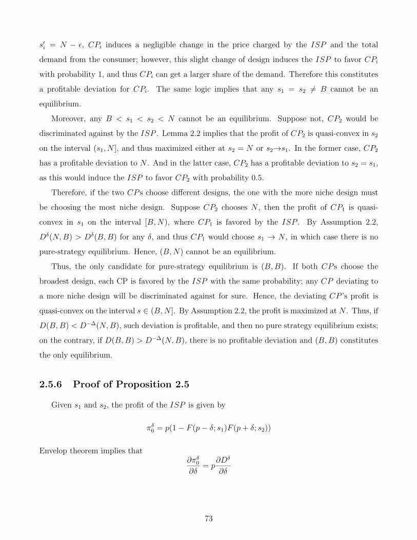
s′i = N − ε, CPi induces a negligible change in the price charged by the ISP and the total

demand from the consumer; however, this slight change of design induces the ISP to favor CPi

with probability 1, and thus CPi can get a larger share of the demand. Therefore this constitutes

a profitable deviation for CPi. The same logic implies that any s1 = s2 6= B cannot be an

equilibrium.

Moreover, any B < s1 < s2 < N cannot be an equilibrium. Suppose not, CP2 would be

discriminated against by the ISP . Lemma 2.2 implies that the profit of CP2 is quasi-convex in s2

on the interval (s1, N ], and thus maximized either at s2 = N or s2→s1. In the former case, CP2

has a profitable deviation to N . And in the latter case, CP2 has a profitable deviation to s2 = s1,

as this would induce the ISP to favor CP2 with probability 0.5.

Therefore, if the two CP s choose different designs, the one with the more niche design must

be choosing the most niche design. Suppose CP2 chooses N , then the profit of CP1 is quasi-

convex in s1 on the interval [B,N), where CP1 is favored by the ISP . By Assumption 2.2,

Dδ(N,B) > Dδ(B,B) for any δ, and thus CP1 would choose s1 → N , in which case there is no

pure-strategy equilibrium. Hence, (B,N) cannot be an equilibrium.

Thus, the only candidate for pure-strategy equilibrium is (B,B). If both CP s choose the

broadest design, each CP is favored by the ISP with the same probability; any CP deviating to

a more niche design will be discriminated against for sure. Hence, the deviating CP ’s profit is

quasi-convex on the interval s ∈ (B,N ]. By Assumption 2.2, the profit is maximized at N . Thus, if

D(B,B) < D−∆(N,B), such deviation is profitable, and then no pure strategy equilibrium exists;

on the contrary, if D(B,B) > D−∆(N,B), there is no profitable deviation and (B,B) constitutes

the only equilibrium.

2.5.6 Proof of Proposition 2.5

Given s1 and s2, the profit of the ISP is given by

πδ0 = p(1− F (p− δ; s1)F (p+ δ; s2))

Envelop theorem implies that∂πδ0∂δ

= p∂Dδ

∂δ

73

where Dδ = 1−F (p− δ; s1)F (p+ δ; s2), under the assumption that F (v; s) is log-concave in s and

v, Proposition 2.3 has shown that∂πδ0∂δ

= p∂D(δ)

∂δ> 0

so the demand is higher in a network which favors the broader product CP1.

2.5.7 Proof of Proposition 2.6

First, we show that if f(v; s) is log-concave in s and v, then F (v; s) is also log-concave in s

and v. And therefore the condition in the proposition is stronger than that in the main model.

Bagnoli and Bergstrom (2005) shows that if the p.d.f f(x) is log-concave, then the c.d.f. F (x) is

also log-concave, which proves the “log-concave in v”part. If f(v; s) is log-concave in s, then it is

easy to show that f(v; s1)/f(v; s2) is increasing in v for s1 < s2. Moreover, we have

f(v; s1)

F (v; s1)− f(v; s2)

F (v; s2)=

∫ v−∞(f(v; s1)f(x; s2)− f(v; s2)f(x; s1))dx

F (v; s1)F (v; s2)

as f(v; s1)/f(v; s2) > f(x; s1)/f(x; s2) for any x < v, we must have f(v; s1)/F (v; s1) > f(v; s2)/F (v; s2).

So F (v; s) is also log-concave in s.

For a given price p, the user will connect to the services in a neutral network if either v1 > p,

or v2 > p or v1 + v2 > p; in a discriminatory network which favors CP1, the user connects if either

v1 + δ > p, or v2 − δ > p or v1 + v2 > p. Hence, if the ISP switches from neutral network to the

discriminatory network favoring CP1, that is, if δ ≥ 0, the change in demand is

∆D(δ) =∫ p

p−δF (p− x; s2)dF (x; s1)−

∫ p+δ

pF (p− x; s1)dF (x; s2),

Clearly, ∆D(δ) = 0 for δ = 0; then the ISP prefers a network favoring CP1 to a neutral network

if∂∆D(δ)

∂δ= F (δ; s2)f(p− δ; s1)− F (−δ; s1)f(p+ δ; s2) > 0

we have

sign{∂∆D(δ)

∂δ} = sign{f(p− δ; s1)

F (−δ; s1)− f(p+ δ; s2)

F (δ; s2)}

then it is easy to show that

f(p− δ; s1)

F (−δ; s1)>f(p+ δ; s1)

F (δ; s1)>f(p+ δ; s2)

F (δ; s2)

74

hence ∂∆D(δ)/∂δ > 0 for all δ, so the ISP prefers a maximum discriminatory network favoring

CP1 to a neutral network. Similarly, when the ISP favors CP2, the demand increases and the

change in demand is

∆D(−δ) =∫ p

p−δF (p− x; s1)dF (x; s2)−

∫ p+δ

pF (p− x; s2)dF (x; s1)

Therefore, we have

∆D(δ)−∆D(−δ) =∫ p+δ

p−δ(f(x; s1)F (p− x; s2)− f(x; s2)F (p− x; s1))dx

Then as long as δ is small enough(δ < p − δ), we must have ∆D(δ) > ∆D(−δ) for all δ. So

the ISP always prefers to favor CP1 rather than CP2.

75

Chapter 3

Limited Attention

An important feature of advertisements is that they attract attention from con-

sumers. When a product is characterized by several attributes, firms also strategically

use advertisements to manipulate the attention of consumers. A monopolist tends

to advertise too few attributes, and competition does not necessarily improve the

situation. Moreover, in an attention-scarce economy, competition for consumers at-

tention leads firms to advertise fewer attributes and reduces information available to

consumers.

3.1 Introduction

Two important roles of advertisements have been well analyzed in the literature: informational

and persuasive. The former one refers to the fact that advertisements inform consumers the

existence of a product; and the latter one improves the perceived value of a product and persuades

consumers to purchase. In this paper, we try to explore the role of advertisements in attracting

and manipulating the attention of consumers.

It is a well-documented fact that consumers have limited attention,1 i.e. they don’t pay at-

tention to all available information, instead they sample a subset of information and base their

decisions on the sample. A consumer may not know the existence of a product unless he sees an

advertisement of the product; in addition, the consumer may not pay attention to specific features

of the product unless they are evoked in the advertisement. Therefore, an advertisement not only

1See DellaVigna (2009) for a survey on empirical evidences of limited attention.

76

indicates the existence and valuation of a product, it also attracts consumers’ attention to the

advertised features of the product.

For instance, a car manufacturer advertises its new model, in addition to features that con-

sumers know well such as color and fuel efficiency, it can also decide whether and how much to

advertise its new internal design, of which consumers differentiate in their tastes. If this new design

draws the attention of a consumer, his valuation for the new model will be more dispersed com-

pared to a consumer who does not pay attention to the new design, as this new design introduces

additional variation. Therefore, when this new design is more heavily advertised, more consumers

will pay attention to this new attribute, and valuations for the new model becomes more dispersed.

In other words, increasing the advertising intensity of more attributes brings more information

into consumers’ attention, which results in more consumers with higher valuations (when they like

the new design), but also more consumers with lower valuations (when they do not like the new

design). In the terminology of Johnson and Myatt (2006), this leads to a rotation of the demand

function for the product.

Thus, for a monopolist whose product having a mass market position and targeting the general

public, its main objective is to reduce the number of consumers who have low valuations. Hence,

it advertises as less attributes as possible, so as to limit the attention that consumers pay to

those attributes and reduce the dispersion of valuations. This leads to distortions in consumers’

choices and reduces consumer welfare, as all purchase decisions are based on limited information.

However, competition does not necessarily improve the information available to consumers.

Consider first the situation where consumers know the existence of competing firms, and firms

only decides how intensive to advertise new attributes of their products. In the case of sym-

metric firms, the effect of competition on advertising strategies crucially depends on the form of

advertising. If advertisements are out-of-store, any advertised attributes will be brought to each

consumer’s attention. This not only affects how consumers evaluate the advertised product, but

also how they evaluate other products in the same industry. In this case, firms do not advertise

more attributes than a monopolist. This is because each firm’s advertising changes the way how

consumers evaluate the whole industry, which hurts all firms. On the contrary, if advertisements

are in-store, they have a larger effect on the attention paid to the advertised product and a weaker

effect on how consumers evaluate other products. In this situation, firms have incentives to adver-

tise more so as to induce more high-value consumers, which improves their competitive advantages.

77

And consumers are better-off as well due to improved information. When we take into account

that advertising also attract consumers’ attention to the existence of a product, our analysis shows

that firms advertise more out-of-store and less in-store in an attention-scarce economy, i.e. when

most consumers are attention limited. This is because firms’ primary goal is to attract consumers’

attention to the existence of their products, and this is done by out-of-store advertising, which is

accompanied with less information.

If firms are asymmetric, i.e. each firm holds a competitive advantage over others on cer-

tain attributes, then each firm has an incentive to advertise its advantageous attributes even if

advertisements are out-of-store. However, this incentive may be dominated by the incentive to

manipulate consumers’ attention, when consumers are heterogeneous in their attention capacity.

We show that firms may advertise too little if there are a large number of consumers who have high

attention capacity. The reason is straightforward: each firm advertising its advantageous attribute

leads to more consumers who pay attention to all attributes of a product, and this reduces total

demand. The incentive to manipulate the attention of those high attention consumers dominates

the incentive to build competitive advantage when there are a large number of such consumers.

Therefore, consumer welfare could be reduced when there are more rational consumers with high

attention capacity, as this induces firms to advertise less and reduces the amount of information

available.

Our paper belongs to the growing literature on psychology and economics, especially on effects

of limited attention. Several papers have studied the consequence of limited attention on hierarchy

(Geanakoplos and Milgrom (1991)), product quality (Armstrong and Chen (2009)), information

disclosure (Hirshleifer and Teoh (2003)) etc. In terms of limited attention and advertising, most

papers (Van Zandt (2004), Falkinger (2007, 2008), Anderson and De Palma (2012), Hefti (2012),

etc) have explored the informational role of advertising, i.e. they assume that advertising is to

inform consumers the existence of products and firms have to compete for such awareness. We

take a step further in assuming that advertisements not only inform consumers the existence

but also specific attributes of products. In other words, our focus is not on the intensity of

advertising, but on the “content”of advertising (Anderson and Renault (2006)). Secondly, our

paper is related to the literature on competition and information disclosure, especially on the

disclosure of horizontal match information. Among others, Sun (2011), Hotz and Xiao (2013) have

shown that competition may not lead to full disclosure when there is also vertical differentiation.

78

Anderson and Renault (2009) also explored the incentive to disclose horizontal match information

in the context comparative advertising. In their model, quality difference between firms plays a

key role in determining firms’ disclosure incentives. In addition, consumers have access to the same

set of information in their model; whereas consumers may have access to different information due

to their attention limitations in our model. In our paper, the intention to manipulate consumers’

attention provides another reason why competition does not improve information availability in

a market even without vertical differentiation. Another closely related paper is Persson (2012),

where the incentive to manipulate attention is derived in a principal-agent framework.

The paper is organized as follows: We present the basic model in Section 2, where we study the

strategy of a monopolist and the effect of competition with out-of-store and in-store advertising;

Section 3 shows several extensions and discussions; Section 4 concludes. All omitted proofs are

presented in the Appendix.

3.2 The Model

3.2.1 Benchmark: The Monopoly Case

A monopolistic firm sells a product to a unit mass of consumers. Each consumer demands only

one unit of the product. The product is characterized by two attributes: a “default”attribute 0

and an additional attribute a. The valuation that a consumer generates from the product is given

by

v = v0 + γva,

where v0 and va are the values that a consumer generates from attribute 0 and attribute a respec-

tively, and γ measures how much attention a consumer pays to attribute a. The outside option is

u, if a consumer chooses not to buy the product.

The idiosyncratic match value v0 and va are independently drawn from distribution F0(·)

and Fa(·), and the values drawn by different consumers are independent. We assume that both

distributions have zero mean2, with variance σ0 and σa respectively, and they are symmetric

2This is without loss of generality: we can write the utility function as v = E(v0) + (v0 − E(v0)) + γva, where

E(v0) is the expectation of v0. Clearly, v0 − E(v0) has zero mean. And our main result is not affected by such

variation.

79

around 0. Then the distribution of v is given by

F (v; γ) =∫ ∫

v0+γva≤vdF0(v0)dFa(va).

The attention level γ captures the fact that consumers have limited attention, which is well

documented in a lot of experiments. Attention as a resource is constrained in capacity either

physically or psychologically. For instance, when a consumer shops for some wine in a supermarket,

she may not pay attention to all information available (either the information on the price tag, or

the information printed on the bottle) due to time constraint or lack of knowledge.

We assume that γ can be either 0 or 1. A consumer with γ = 0 only cares about the default

attribute, and pays no attention to the additional attribute a, and thus his valuation for the

product is simply drawn from F (v; 0) = F0(·). Instead, a consumer with γ = 1 pays full attention

to attributes a, and his valuation is drawn from F (v; 1), which has mean zero, and variance σ0+σa.

When there is a proportion s of consumers paying attention to attribute a, and the rest 1− s

only paying attention to the default attribute, the valuation for the firm’s product in the whole

population is drawn from

G(v; s) = (1− s)F (v; 0) + sF (v; 1).

Clearly, we have∂G(v; s)

∂s= F (v; 1)− F (v; 0).

And it is straightforward to show that

∂G(v; s)

∂s= F (v; 1)− F (v; 0)

< 0 if v > 0;

> 0 if v < 0.(3.1)

i.e. G(v; s) is increasing in s for v < 0 and decreasing in s for v > 0. Following the definition of

Johnson and Myatt (2006):

Definition 3.1. (Johnson and Myatt 2006): A local change of s leads to a rotation of G(v; s)

if for some v∗ and any v ∈ (−∞,∞),

v > v∗ ⇔ ∂G(v; s)

∂s< 0 and v < v∗ ⇔ ∂G(v; s)

∂s> 0.

We easily see that:

Lemma 3.1. G(v; s) is rotation-ordered in s with rotation point 0.

80

Higher attention level in the population leads to a more dispersed valuation distribution: more

consumers have very high valuation, and more consumers have very low valuation as well. Simply

speaking, high attention consumers pay attention to more details of a product, and thus their

valuation distributions have a larger variance. In the terminology of Johnson and Myatt, higher

s makes the firm’s product a more niche one. A simple example is when both F0(v) and Fa(v)

are the standard normal distribution φ(·), then F (v; 1) is a normal distribution with expectation

0, and standard variation√

2. Therefore, G(v; s) gradually rotates from Φ(0, 1) to Φ(0,√

2) as s

increases from 0 to 1.3

Given that the outside option is u, the demand for the product is

D(s) = 1−G(u; s).

We assume that the firm makes a profit of 1 from one unit of demand, then the above equation

also represents total profit of the firm. It is straightforward to show that:4

Lemma 3.2. The firm’s profit is quasi-convex in s. Moreover, if the outside option u < 0, then

the profit is decreasing in s.

Proof. This is a direct consequence of the Proposition 1 of Johnson and Myatt (2006). As the

demand function is rotation-ordered with rotation point being 0, if the outside option is such

that u < 0, it is the same situation as in Johnson and Myatt where the optimal price is below

the rotation point, so the profit is decreasing in s. To be more specific, the demand is D(s) =

1 − G(u; s). As u < 0, G(u; s) is increasing in s from Lemma 1, and thus D(s) is decreasing in

s.

When the outside option is below 0, the product has a mass product position. And thus to

maximize profit, the firm needs to minimize the number of consumers with low valuations, which

is achieved when the variance of the valuation distribution is minimized, that is when s = 0. In

3Another example is the linear distribution: If F0(v) and Fa(v) are uniform distributions on [−θ, θ], we can also

show that changes in s also lead to a rotation of G(v; s).4We focus on the advertising strategy of the firm, so the firm only chooses s but not the price. The result still

holds even when the firm also makes price decisions. To incorporate this, we need to assume that E(v0) > 0, and

the optimal price when the firm does not advertise the additional attribute is p < E(v0). The important thing

is that the product features a mass-market position. This also facilitates our comparison between monopoly and

competition.

81

other words, when the product features a mass market, profit is maximized with the broadest

design.

Lemma 3.2 implies that consumers with higher attention level actually hurts the firm if the

firm’s product features a mass-market position. More attentive consumers care about more details

of the product, which implies that it is more likely that they would find out some negative facts

of the product and thus choose not to purchase.

In the following, we focus on the situation where the outside option is negative.

Assumption 3.1. u < 0.

In reality, a firm has a number of ways to affect the attention level of consumers, i.e. s depends

on strategies chosen by the firm. Here, we focus on advertising and the information content of

advertisements. The firm has free access to one unit of resource for advertising. For now, we

suppose that informing consumers about the existence of a product is not a concern, the firm

rather advertises to keep their products imposed to consumers. So the firm always fully uses

its advertising resource, and it chooses whether to spend any of this resource on the additional

attribute a. If the firm advertises attribute a with intensity s, a proportion s of consumers pay

attention to a, and the rest do not.5 Then it is straightforward to have the following proposition:

Proposition 3.1. Under Assumption 3.1, the firm does not advertise the additional attribute a,

i.e. s = 0.

When the firm’s product features a mass market, information hurts the firm and thus it chooses

to minimize the information provided to consumers, that is to advertise no additional attribute

except the default one which every consumer pays attention to.6 In other words, the firm only

informs consumers about the existence of its product, but not any information about the product

in addition to what consumers have already known.

5We can think of the situation where each consumer has a capacity of attention equal to 1: this unit of attention

is randomly drawn by one of the advertising messages. Hence, if the attention is drawn by a message containing the

information about attribute a, this consumer pays attention to a; otherwise, he does not pay attention to a. When

the firm sends out s messages that contains information about a, the proportion of consumers that eventually pay

attention to a is then s.6This result does not depend on whether consumers have limited attention or not. As long as the attention level

is manipulatable, the firm has incentive to divert consumers’ attention to the default attribute.

82

3.2.2 The Case of Competition

As shown in the previous section, a monopolist advertises “too little”. And consumers make

suboptimal decisions based only on information about the default attribute. A natural question

to ask is whether competition can mitigate such problem, i.e. would competition induce firms to

advertise the additional attribute, and bring everything into consumers’ attention?

Suppose now there are two firms: firm 1 and firm 2. As before, each firm has one unit

of advertising resource to allocate. We distinguish between two cases: the first is out-of-store

advertising where each firm’s advertising affects consumers’ attention allocation when evaluating

both firms’ products; the second is in-store advertising where one firm’s advertising only affects

how consumers evaluate its own product. We start with the out-of-store advertising case.

3.2.2.1 Out-of-Store Advertising

Advertisements such as outdoor billboards advertisements draw attention of all consumers,

and thus an advertisement of one product may also affect how a consumer thinks about other

products in the same market. For instance, an outdoor advertisement of BMW which introducing

some new features also induces consumers to think about whether Benz offers the same features.

In others words, any information contained in such advertisements not only attracts consumers

attention when they visit the store of the advertised product, but also has long-lasting effect when

they are out-of-store.7 To capture this effect, we assume that an attribute advertised by one firm

attracts consumers attention when they evaluate both firms’ products. Specifically, suppose each

firm i has one unit of advertising resource, and it decides a share si of this resource to be spent on

the additional attribute a. And then the proportion of consumers who pay attention to attribute

a is

s =s1 + s2

2,

which is increasing in both s1 and s2. And we have the following result:8

7This type of out-of-store advertising not only includes various types of outdoor advertising, but also some

information pamphlets which consumers can take away in the sense that the information contained in the pamphlets

may still affect how consumers think when they evaluate other products.8As in the monopoly case, we assume that firms only choose advertising strategies but not prices. In the

competition case, firms’ prices will be constrained by the outside option. And the following results hold as long as

the constrained prices are below E(v0).

83

Proposition 3.2. When advertising is out-of-store, both firms do not advertise the additional

attribute, i.e. s1 = s2 = 0.

Proof. Given that firm j chooses sj, the demand for firm i is

Di(si, sj) =1

2(1−G2(u;

si + sj2

)),

as two firms share the total demand which is 1−G2(u; si+sj2

). Therefore, given sj, any positive si

leads to a wider dispersion of consumers’ valuations, which lowers the total demand and thus the

demand for firm i. Hence, we have si = 0.

When advertising is out-of-store, any information in advertising affects consumers’ valuation

for the products symmetrically, i.e. consumers’ valuations for both products are drawn from the

same distribution. Hence, any advertising that increases the dispersion of valuations will hurt both

firms. And thus competition does not improve the information available to consumers with out-of-

store advertising. In addition, the joint profit of two firms attains its maximum with out-of-store

advertising, which acts as a coordinating device for the two firms.

Remark Out-of-store advertising does not improve the information available to consumers, but

consumers can still benefit from competition: they have more firms to choose, which increases the

probability that they find something better than the outside option.

3.2.2.2 In-Store Advertising

Now we turn to the case of in-store advertising: this type of advertising is mostly carried

out through sales talks, information contained in such advertisements would attract consumers’

attention only when they visit the store, and thus only affect consumers’ evaluation for the ad-

vertised product. In other words, such advertising has strong effects in-store, but has limited long

lasting effect when consumers are out-of-store. This distinction between out-of-store and in-store

advertising may be too extreme, however, we emphasize that in-store advertising has a weaker

“spillover”effect than out-of-store advertising in affecting consumers’ attention towards products

other than the advertised one.9

As before, each firm has one unit of advertising resource to allocate, if firm 1 and 2 allocates s1

and s2 of their advertising resource to attribute a, then the attention level that a consumer pays

9For instance, the information from a salesman of BMW may still affect a consumer’s evaluation for a Benz, but

this effect is weaker than a take-away pamphlet due to short-memory, or manipulation from a salesman of Benz.

84

to attribute a of product 1 is s1, and s2 is the attention level paid to the additional attribute of

product 2. Hence, consumers’ valuations for products of firm 1 and 2 are drawn from distribution

G(v1; s1) and G(v2; s2) respectively.

The demands for firm 1 and firm 2 are then given by

D1 =∫ ∞u

G(v1; s2)dG(v1; s1)

and

D2 =∫ ∞u

G(v2; s1)dG(v2; s2)

And we have the following proposition:

Proposition 3.3. When advertising is in-store, each firm fully advertises the additional attribute,

i.e. s1 = s2 = 1, if the outside option is not too small.

Proof. See Appendix 3.5.1.

When advertising is in-store, each firm has incentive to induce more consumers to pay attention

to every detail of its product: this leads to a higher probability that a consumer has higher

valuation for its product than that of the opponent, and thus improves its competitive advantage.

However, both firms are worse-off than in the case of out-of-store advertising.

Corollary 3.1. The demands for both firms are lower with in-store advertising than with out-of-

store advertising.

Proof. Under in-store advertising, each firm gets a demand of

D(1, 1) =1

2(1−G(u; 1)G(u; 1))

and the demand under out-of-store advertising is

D(0, 0) =1

2(1−G(u; 0)G(u; 0))

And clearly D(1, 1) < D(0, 0) as G(u; 1) > G(u; 0) for u < 0.

The equilibrium under in-store advertising is a form of prisoner’s dilemma: each firm wants

to draw consumers’ attention to more details of its product, but in the end this reduces the total

demand. However, consumers benefit from such in-store advertising: each consumer makes the

right choice based on all information available under in-store advertising, whereas with out-of-store

advertising they might make the wrong choice.

85

Corollary 3.2. Consumers are better-off under in-store advertising than under out-of-store ad-

vertising.

Remark We have focused on the two extreme cases of out-of-store advertising and in-store

advertising. In reality, firms normally use a mixture of these two. The above analysis indicates

that the information available to consumers decreases with the share of out-of-store advertising.

In addition, this implies that if firms could cooperate on their advertising strategy, they would

favor out-of-store advertising and this again reduces information availability.

3.2.3 Attention Attraction vs. Attention Manipulation

The above two extreme cases show us the incentive for attention manipulation when consumers

have already known the existence of both firms. And they are the building blocks when we take

into account the fact that advertisements attract consumers’ attention to the advertised product

at the first place. Specifically, consumers get to notice the existence of a product when they

see advertisements of the product, and then they will pay additional attention to details of the

product.

In our model, we can simply incorporate this feature of advertising by assuming that a consumer

gets aware of a product when he sees an out-of-store advertisement of the product; and when he

enters the store, he gets further information from in-store advertisement in addition to what has

been contained in the out-of-store advertisement. Under this assumption, out-of-store advertising

serves to attract consumers’ attention, and both out-of-store and in-store advertising serve to

manipulate consumers’ attention.

As before, each firm i has one unit of advertising resource, which can be allocated between

out-of-store advertising souti and in-store advertising sini . Furthermore, firms also decide what

information to include in the out-of-store and in-store advertising. For simplicity, we also assume

that a proportion of 1 − α consumers are attention limited, they only pay attention to one out-

of-store advertising message and thus get aware of at most one product; the rest α proportion

of consumers are attention unlimited and they get aware of both products as long as they are

advertised. Then it is easy to show that:

Proposition 3.4. In the symmetric equilibrium, there exist α such that, if α < α, both firms only

use out-of-store advertising and they do not advertise the additional attribute.

86

Proof. See Appendix 3.5.3.

A firm faces a trade-off between exploiting limited attention consumers and competing for

full attention consumers. On one hand, a firm wants to advertise more out-of-store and disclose

limited information in order to attract those limited attention consumers (each firm has monopoly

power over limited attention consumers who are aware of only its product, and thus it does

not advertise any additional attribute); on the other hand, a firm wants to advertise more in-

store and disclose more information in order to win those full attention consumers. Hence, in

an attention-scarce economy (α small), the first incentive dominates and competing to attract

consumers attention leads firms to rely more on out-of-store advertising, which correspondingly

results in less information availability.

The analysis in the section resembles that of Section III.B in Johnson and Myatt (2006), where

they differentiated between advertisements consisting of hype information and real information.

In their analysis, advertisements with hype information do not change the dispersion of value

distribution, whereas advertisements with real information lead to demand rotation. Under their

assumption, a monopolist prefers either full information (real information advertising) or total

ignorance (hype information advertising).

We depart from their analysis in several ways: First, in our model advertisements always

provide real information, but firms can choose how much real information to advertise. Second,

we explicitly model the role of advertising in attracting and manipulating attention of consumers.

Third, and most importantly, we show how competition affects firms’ choice between out-of-

store advertising (which provides less real information) and in-store advertising (which provides

more real information). Particularly, we show that this effect depends on the attention level

of consumers. In other words, we present a simple situation where firms indeed prefer hype

information advertising: when firms have to compete for consumer awareness in an attention-

scarce economy.

Anderson and Renault (2009) also studies whether firms disclose horizontal information in

the presence of vertical differentiation. In their model, once a firm discloses some horizontal

information, all consumers get aware of that information (although they differentiate in their

valuation for that information). We take a different approach and emphasize that consumers may

evaluate different products based on different information sets, due to the fact that attention of a

consumer is limited and manipulable.

87

3.3 Extensions and Discussions

3.3.1 Multiple Attributes

So far, we have focused on a single attribute in addition to the default one. The situation

is basically the same when there are possibly more than one attribute to advertise, as long as

consumers evaluate the products in the same way (they have the same attention level).

Suppose there are two additional attributes a and b, the valuations of which are drawn from

the same distribution. All consumers are attention limited: they pay attention to at most one

additional attribute. It is clear that in the out-of-store advertising case, no firm advertises any of

the additional attributes. In the in-store advertising case, each firm fully advertises the additional

attributes.10

The situation is slightly different when the additional attributes are asymmetric: Suppose that

the valuation of one attribute, say a, is drawn from a distribution with a larger variance than

the other attribute b.11 It is obvious that no firm advertises if advertising is out-of-store. In the

in-store advertising case, the only equilibrium is that both firms fully advertise attribute b. The

reason is the same as Proposition 3.3: each firm wants to induce more high value consumers to

build its competitive advantage over the other firm. Even though competition in this case does

not lead to complete advertising, it does induce firms to provide the more valuable information to

consumers.

3.3.2 Heterogeneous Consumers

In the above analysis, we have assumed that consumers are homogeneous. Now we briefly

study the situation when consumers are heterogeneous in their attention levels: a proportion p

of consumers have their attention capacity equal to one, so they randomly draw one advertising

message and pay attention to the attribute contained in this message if there were any; the rest

1 − p of the consumers have larger attention capacity, for simplicity, say two units of attention.

So they draw two advertising messages and pay attention to what is contained in the messages.

Heterogeneous consumers does not bring any difference when there is only one additional attribute

10A firm can divide the advertising space between the two additional attributes, as a consumer’s valuation is

drawn from the same distribution no matter whether he pays attention to a or b.11Both distributions still have zero mean.

88

or in the out-of-store advertising case, so we focus on in-store advertising with two attributes a

and b.

Consider a simple extension of the above model: Each firm i can spend sai proportion of its

advertising space on attribute a, and sbi on attribute b. Then the proportion of consumers who

only pay attention to attribute a is

αa(sai , s

bi) = sai p+ ((sai )

2 + 2sai (1− sai − sbi))(1− p),

where the first term is those consumers who have one attention capacity and draw an advertising

message about a; the second term is those consumers who have two attention capacity and draw

two messages about a, or one message about a and one with no additional attribute. Similarly,

the proportion of consumers who only pay attention to attribute b is

αb(sai , s

bi) = sbip+ ((sbi)

2 + 2sbi(1− sai − sbi))(1− p);

the proportion of consumers who pay attention to both attributes is

αa,b(sai , s

bi) = 2sai s

bi(1− p).

And the rest of consumers only pay attention to the default attribute.12

The valuation of a consumer who pays attention to both attribute is

u = v + va + vb.

It is clear that these consumers have a valuation distribution that is more dispersed than those

who only pay attention to one attribute.

Therefore, in the in-store advertising case, if the two attributes are symmetric, each firm has

an incentive to induce more consumers to pay attention to both attributes. Hence, both firms

must choose to allocate equally the advertising resource to both attributes, that is

sai = sbi =1

2, for i = 1, 2.

12It is easy to see that αa(1, 0) = 1 and αb(0, 1) = 1. When the firm only advertise one attribute, those consumers

with higher attention level also only pay attention to the advertised attribute. In this setup, if the attention level

of a consumer goes to infinity, then this consumer pays attention to everything that is advertised, no matter what

is the advertising intensity.

89

Competition for high attention capacity consumers, who are also more valuable, leads firms to

advertise more about their products, and this in turn benefit these high attention consumers, as

they now evaluate the product more thoroughly.

Remark When the two attributes are asymmetric, it might be the case that each firm only

advertises one attribute, and we present such a case in Appendix 3.5.2.

3.3.3 Asymmetric Firms

In the previous analysis, we have assumed that the two firms are symmetric, i.e. the valuations

for the same attribute of the two products are drawn from the same distribution. Suppose now

the two firms are differentiated, and firm 1 has a competitive advantage over firm 2 on attribute a:

the valuation for attribute a of firm 1 is drawn from a distribution that first-order-stochastically

dominates that of firm 2. For simplicity, we assume that the distribution of attribute a for firm

1 is drawn from Fa(v) with zero mean and variance σ; whereas for firm 2 it is drawn from F δ(v)

with mean δ < 0 and variance σ, that is F δ(v) = Fa(v − δ).

We have seen that when firms are symmetric, no firm advertises the additional attribute in the

out-of-store advertising case. This may not be the case when firms are asymmetric, as firm 1, who

has a competitive advantage over firm 2, has an incentive to advertise attribute a. To see this, if

firm 2 does not advertise, the demand of firm 1 when it advertises a with intensity s is given by

D(s, 0) = s∫ ∞u

F (v, δ; 1)dF (v; 1) + (1− s)∫ ∞u

F (v; 0)dF (v; 0),

where the first term on the right hand side is the demand from consumers who pay attention to

a, and

F (v, δ; 1) =∫ ∫

v0+va≤vdF0(v0)dFa(va − δ),

is the valuation distribution for product 2 when consumers pay attention to attribute a; and the

second term is the demand from those who do not pay attention to a.

Therefore, firm 1 will advertise attribute a if

D+ =∫ ∞u

F (v, δ; 1)dF (v; 1) >∫ ∞u

F (v; 0)dF (v; 0) = D0.

Clearly, the inequality does not satisfy when δ = 0, which is the case of symmetric firms. It is

easy to see that the left-hand-side is decreasing in δ, and thus the inequality is satisfied for δ small

90

enough, i.e. if the competitive advantage of firm 1 over attribute a is high enough (as δ < 0). On

the other hand, firm 2 has no incentive to advertise a, as this always decreases its demand.

This implies that if there are multiple attributes, and firms have their competitive advantage

over different attributes, then it might be the case that all attributes would be advertised even

with out-of-store advertising. This is true when all consumers are attention limited, i.e. they only

pay attention to at most one attribute. Specifically, suppose there are two attributes a and b: firm

1 has competitive advantage over a as defined above, and firm 2 has competitive advantage over b

which can be similarly defined. The above analysis has shown that firm 1 will advertise attribute

a if the competitive advantage is high enough. The same reasoning indicates that firm 2 also has

an incentive to advertise b.

However, this may not necessarily be the case if consumers are heterogeneous, i.e. when

some have higher attention level.13 Suppose as before a proportion p consumers have one unit of

attention capacity, and the rest 1− p have two units of attention capacity. We have the following

result:

Proposition 3.5. In the asymmetric firm case, firms’ advertising intensity on the additional

attributes decreases with the proportion of consumers with high attention capacity.

Proof. See Appendix 3.5.4, where we also give a proof when the high attention capacity consumers

have infinite attention capacity.

The logic of the above proposition is straightforward: each firm has an incentive to advertise

the attribute over which it has a competitive advantage. However, by doing so, all full attention

consumers will pay attention to both attributes and this hurts both firms. Therefore, when there

is a large number of such consumers, firms instead choose to advertise less.

The proposition shows that when a lot of consumers are attention-limited, competition induces

firms to advertise both attributes which benefit full attention consumers; however, when a large

proportion of consumers have full attention, the information available is reduced. And thus con-

sumer welfare may not be monotonic with the attention level p: as p decreases, firms gradually

change their strategy to “hide”some attributes of their products. In other words, the presence of

low attention consumers exerts positive externality on full attention consumers. Individually, each

13Here, we abstract from attention attraction as in Section 3.2.3, and assume that all consumers know the

existence of both products.

91

consumer would be better off if he pays full attention to firms’ products; however, collectively it

would be better for the whole population to maintain some level of attention limitation. This also

relates to some discussion about consumer knowledge: if most consumers only understand a small

subset of aspects of a product, firms may choose to disclose all information so as to win those

knowledgeable consumers; however, if more and more consumers get to understand every detail of

the product, firms may choose to disclose less information which in turn hurt consumers.

This may also shed light on the difference between online shopping and off-line shopping: online

shopping is characterized by information overload, which can be a result of the fact that online

shoppers are more time-constrained than off-line shoppers, and thus online shoppers exhibit more

attention limitation.

3.3.4 Costly Advertising

The above analysis has focus on costless advertising where firms have free access to advertising

resource. This can be thought of as the situation in the short-run, where firms have sunk their

costs of acquiring advertising space such as billboards and they only decide what information to

be included in the advertisements. In the long-run, firms may also need to decide how much

advertising resource to invest, especially as in-store advertising is probably less costly than out-

of-store advertising.14

Incorporating costly advertising introduces additional trade-offs between marginal benefits and

marginal costs of out-of-store and in-store advertising. Compared with our benchmark costless

advertising model, firms use relatively more in-store advertising due to its low cost, however, this

does not alter our basic intuition. In an attention-scarce economy, the marginal benefit of out-of-

store advertising would be higher than that of in-store advertising, which is the dominating effect

as long as the cost difference between two types of advertising is not too large. And thus firms

tends to advertise more out-of-store and information available to consumers is limited.15

14The cost of out-of-store advertising includes, for instance, bidding for billboards, designing advertisements, etc.

The cost of in-store advertising includes training salesmen and providing pamphlets, etc.15A firm may incur additional costs when it includes more information in advertising, however such costs are

likely to be less significant than bidding for advertising space and training employees.

92

3.4 Conclusion

We study how firms may use advertisements to manipulate consumers’ attention. A monopolist

advertises too few attributes and this reduces consumer welfare. Whether competition improves

this situation depends on the form of advertising. When advertisements are out-of-store and

affect how consumers evaluate products at the industry level, competition does not increase the

information available to consumers; when advertisements are in-store and mainly affect consumers’

evaluation at the product level, competition may lead to higher information availability. We also

show that consumer heterogeneity plays a key role in shaping firms’ advertising strategy when they

are asymmetric. Our results suggest that instead of information overload, attention manipulation

and the resulting information insufficiency may also be a serious concern.

3.5 Appendix

3.5.1 Proof of Proposition 3.3

Given s2, we have

∂D1

∂s1=

∫∞u G(v; s2)d∂G(v;s1)

∂s1

= −G(u; s2)∂G(u;s1)∂s1

−∫∞u

∂G(v;s1)∂s1

dG(v; s2)

= −(∫u−∞

∂G(u;s1)∂s1

dG(v; s2) +∫∞u

∂G(v;s1)∂s1

dG(v; s2))

= −∫∞−u(∂G(v;s1)

∂s1− ∂G(−u;s1)

∂s1)dG(v; s2). (use the symmetry of G(v; s) and g(v; s))

If u = 0, we have∂G(v; s1)

∂s1

< 0 for all v > 0, and∂G(0; s1)

∂s1

= 0.

Therefore, ∂D1/∂s1 > 0. Hence, for all u that is close to zero, we have that the demand for firm

1 is increasing in s1. So we must have s1 = 1 in equilibrium. The same reasoning indicates that

s2 = 1 also.

Notice that

∂∂G(v; s1)

∂s1

/∂v =∂g(v; s1)

∂s1

Due to the symmetry of g(v; s), there must exist v such that

∂g(v; s1)

∂s1

< 0 for 0 < v < v and∂g(v; s1)

∂s1

> 0 for v > v.

93

Hence, if u = −v, we have

∂G(v; s1)

∂s1

≥ ∂G(−u; s1)

∂s1

for all v ≥ −u,

and then ∂D1/∂s1 < 0. Therefore, there exists u ∈ (−v, 0) such that

∂D1

∂s1

(u; s1)|u=u = 0.

And ∂D1/∂s1 > 0 for all u ∈ (u, 0].

3.5.2 Heterogeneous Consumers with Asymmetric Attributes

When consumers are heterogeneous in their attention capacity, and the valuation of attribute

b is drawn from a more dispersed distribution, both firms advertising only attribute b may also be

an equilibrium.

Suppose firm 2 only advertise b, if firm 1 advertises both attributes, the profit is given by

πpa,b = αa(sa, sb)D(a, b) + αb(sa, sb)D(b, b) + (1− αa − αb)(sa, sb)D(ab, b)

where D(k, b) denotes the demand for firm 1 when the consumer only pays attention to attribute

b of firm 2 and pays attention to attribute k of firm 1. As we can see, there is a gain from full

attention consumers, as D(ab, b) > D(b, b); but there is a loss from partial attention consumers

who only pay attention to attribute a, as D(a, b) < D(b, b). Therefore, if it is difficult to induce

consumers to pay attention to both attributes, firm 1 may find it profitable to only advertise

attribute b; specifically, this is satisfied if

αa1 − αa2

αb2 − αb1>D(ab, b)−D(b, b)

D(ab, b)−D(a, b)

which means that the marginal effect of advertising attribute a on the proportion of consumers

who only pay attention to a is relatively large compared to the proportion of consumers who pay

attention to both attributes. 16

16As we can see, whether this condition holds depends on the shape of α(sa, sb). In the quadratic interpretation,

this condition is not satisfied.

94

3.5.3 Proof of Proposition 3.4

In the symmetric equilibrium, sout1 = sout2 = sout and sin1 = sin2 = sin. If sout = 1 and sin = 0,

the profit of each firms is given by

π =1− α

2D(0) + αD(0; 0).

In order for this to be an equilibrium, both firms have no incentive to reduce out-of-store advertising

and use the resource for in-store advertising. Precisely, the condition means that

(1− α)[∂D(s)

∂s|s=0 −

1

4] + α

∂D(s1; 0)

∂s1

|s1=0 < 0,

which is satisfied if α < α, where α satisfies

α =(1− α)(∂D(s)

∂s|s=0 − 1

4)

∂D(s1;0)∂s1

|s1=0

.

It can be easily seen that α ∈ (0, 1), as the right hand side is positive when α = 0 (as ∂D(s)∂s|s=0 < 0),

and equals zero when α = 1 (as ∂D(s1;0)∂s1

|s1=0 > 0) .

Moreover, in this equilibrium, both firms do not advertise the additional attribute, as this cor-

responds to the pure out-of-store advertising case and the result follows directly from Proposition

3.2.

3.5.4 Proof of Proposition 3.5

If one firm decides to advertise some additional attributes, it only advertise the one that it has

competitive advantage. Advertising the attribute in which it is disadvantageous either increases

the proportion of consumers who only pay attention to this attribute, or reduces the proportion

of those who pay attention to no additional attributes, both of which hurt the firm. Hence, firm

1 chooses to advertise attribute a with intensity sa and firm 2 chooses sb to advertise attribute b.

Given sa, the demand of firm 2 is given by

D2(sa, sb) = [p2sa + (1− p)(( sa

2)2 + sa(1− sa+sb

2))]D−

+[p2sb + (1− p)(( sb

2)2 + sb(1− sa+sb

2))]D+

+12sasb(1− p)Df

+[p(1− sa+sb2

) + (1− p)(1− sa+sb2

)2]D0

95

where D+ and D0 are given in the main text; D− is demand for a firm from consumers who only

pay attention to its disadvantageous attribute, that is

D− =∫ ∞u

F (v; 1)dF (v, δ; 1);

and Df is the demand from those consumers who pay attention to both attributes, that is

Df =∫ ∞u

F (v, δ; 1, 1)dF (v, δ; 1, 1),

where

F (v, δ; 1, 1) =∫ ∫ ∫

v0+va+vb≤vdF0(v0)dFa(va)dFa(vb − δ),

is the valuation distribution of those consumers who pay attention to both attributes.

The first order condition is given by

∂D2

∂sb=

1− p2

sa(Df −D−) + (1− p)(1− sa + sb2

)(D+ −D0) +p

2(D+ −D0).

If p = 1, i.e. all consumers are attention limited, then

∂D2

∂sb=

1

2(D+ −D0) > 0,

which means that both firms fully advertise their advantageous attribute. If sa = 0, all consumers

only pay attention to b if sb > 0, and we have

∂D2

∂sb= ((1− p)(1− sb

2) +

p

2)(D+ −D0) > 0,

so firm 2 fully advertises attribute b.

If p < 1, and sa > 0, the best response function of firm 2 is such that

∂sa∂sb

=Df −D−

D+ −D0

− 1;

therefore, an symmetric equilibrium exists if Df−D− < 0, and the symmetric equilibrium is given

by

sa = sb = s =(2− p)(D+ −D0)

(1− p)(2(D+ −D0)− (Df −D−)).

Then it is easy to check that s < 1 if

p <D− −Df

(D+ −D0) + (D− −Df ).

96

Otherwise, when p is big enough, the only equilibrium is sa = sb = 1. Moreover, it is obvious that

s is increasing in p. Therefore, when there are more consumers with high attention capacity, the

equilibrium intensity of advertising on additional attribute is lower.

The case of infinite attention capacity

The proof is basically the same as above except that: For those consumers with infinity atten-

tion capacity, they pay attention to both attribute as long as min(sa, sb) > 0. If sa, sb > 0, the

demand of firm 1 is given by

D1(sa, sb) = psa2D+ + p

sb2D− + p

2− sa − sb2

D0 + (1− p)Df ,

As D+ > D0, firm 1 chooses sa = 1 if it were to advertise a. If sa = 0, the demand of firm 1 is

D1(0, sb) = (psb2

+ 1− p)D− + p2− sb

2D0.

Therefore, firm 1 does not advertise a if

D1(0, sb) > D1(1, sb)⇔ (1− p)(D− −Df ) >p

2(D+ −D0);

That is if

p <2(D− −Df )

2(D− −Df ) + (D+ −D0);

and such p exists if D− > Df .

Thus, if p is small enough, firm 1 chooses not to advertise its advantageous attribute if firm 2

has already advertised the other attribute. However, if sb = 0, then firm 1 fully advertise attribute

a as if all consumers are attention limited. Hence, there are two pure-strategy equilibrium when p

is small, either sa = 1, sb = 0 or sa = 0, sb = 1, in both of which only one attribute is advertised.

There is also a mix-strategy equilibrium, where each firm randomize between fully advertis-

ing its advantageous attribute and not advertising at all. However, in such an equilibrium, the

probability that both attributes are advertised is still smaller than one.

97

Bibliography

[1] Allain, M.-L., Chambolle, C., and Rey, P. Vertical integration, innovation and fore-

closure. working paper (2011).

[2] Anderson, S., and de Palma, A. Competition for attention in the information (overload)

age. RAND Journal of Economics 43, 1 (2012), 1–25.

[3] Anderson, S., and Renault, R. Advertising content. The American Economic Review

96, 1 (2006), 93–113.

[4] Anderson, S., and Renault, R. Comparative advertising: Disclosing horizontal match

information. The RAND Journal of Economics 40, 3 (2009), 558–581.

[5] Anton, J., and Yao, D. The sale of ideas: Strategic disclosure, peoperty rights, and

contracting. The Review of Economic Studies 69, 3 (2002), 513–231.

[6] Anton, J., and Yao, D. Little patents and big secrets: Managing intellectual property.

The RAND Journal of Economics 35, 1 (2004), 1–22.

[7] Armstrong, M. Competition in two-sided markets. The RAND Journal of Economics 37,

3 (2006), 668–691.

[8] Armstrong, M., and Chen, Y. Inattentive consumers and product quality. Journal of

the European Economic Association 7, 3 (2009), 411–422.

[9] Bagnoli, M., and Bergstrom, T. Log-concave probablility and its applications. Eco-

nomic Theory 26 (2005), 445–469.

[10] Bagwell, K. The economic analysis of advertising.

98

[11] Bar-Isaac, H., Caruana, G., and Cunat, V. Search, design, and market structure.

American Economics Review 102, 2 (2012), 1140–1160.

[12] Berges-Sennou, F., Bontems, P., and Requillart, V. Economics of private labels:

A survey of literature. Journal of Agricultural & Food Industrial Organization 2 (2004).

[13] Board, O. Competition and disclosure. The Journal of Industrial Economics 57, 1 (2009),

197–213.

[14] Bolton, P., and Whinston, M. D. Incomplete contracts, vertical integration, and supply

assurance. The Review of Economic Studies 60, 1 (Jan. 1993), 121–148.

[15] Bourreau, M., Kourandi, F., and Valletti, T. Net neutrality with competiting

internet platforms. working paper (2012).

[16] Brocas, I. Vertical integration and incentives to innovate. International Journal of Indus-

trial Organization 21 (2003), 457–488.

[17] Buehler, S., and Schmutzler, A. Intimidating competitors-endogenous vertical integra-

tion and downstream investment in successive oligopoly. International Journal of Industrial

Organization 26 (2008), 247–265.

[18] Caillaud, B., and Jullien, B. Chicken & egg: Competition among intermediation service

providers. The RAND Journal of Economics 34, 2 (2003), 309–328.

[19] Calin, M., Dellarocas, C., Palme, E., and Sutanto, J. Attention allocation in

information-rich environments: The case of news aggregators. Working Paper (2013).

[20] Chen, Y. On vertical mergers and their competitive effects. The RAND Journal of Eco-

nomics 32, 4 (2001), 667–685.

[21] Chen, Y. Refusal to deal, intellectual property rights, and antitrust. working paper (2011).

[22] Chen, Y., and Riordan, M. Vertical integration, exclusive dealing, and ex post carteliza-

tion. The RAND Journal of Economics 38, 1 (2007), 1–21.

[23] Chen, Y., and Sappington, D. Innovation in vertically related markets. Journal of

Industrial Economics 58, 2 (2010), 373–401.

99

[24] Cheng, H., Bandyopadhyay, S., and Guo, H. The debate on net neutrality: A policy

perspective. Information Systems Research 22, 1 (2011), 60–82.

[25] Choi, J., and Kim, B. Net neutrality and investment incentives. RAND Journal of Eco-

nomics 41, 3 (2010), 446–471.

[26] Choi, J. P., and Yi, S.-S. Vertical foreclosure with the choice of input specifications. The

RAND Journal of Economics 31, 4 (2000), 717–743.

[27] Comanor, W., and Scherer, F. Mergers and innovation in the pharmaceutical industry.

working paper (2011).

[28] Cremer, J., Rey, P., and Tirole, J. Connectivity in the commercial internet. Journal

of Industrial Economics 48 (2000), 433–472.

[29] de Fontenay, C., and Gans, J. Vertical integration in the presence of upstream compe-

tition. The RAND Journal of Economics 36, 3 (2005), 544–572.

[30] Economides, N., and Hermalin, B. The economics of network neutrality. The RAND

Journal of Economics, forthcoming (2012).

[31] Economides, N., and Tag, J. Net neutrality on the internet: A two-sided market analysis.

Informaiton Economics and Policy 24, 2 (2012), 91–104.

[32] Falkinger, J. Attention economies. Journal of Economic Theory 133 (2007), 266–294.

[33] Falkinger, J. Limited attention as a scarce resource in information-rich economies. The

Economic Journal 118 (2008), 1596–1620.

[34] Farrell, J., and Katz, M. L. Innovation, rent extraction, and integration in systems

markets. The Journal of Industrial Economics 48, 4 (Dec. 2000), 413–432.

[35] Farrell, J., and Saloner, G. Standardization, compatibility and innovation. RAND

Journal of Economics 16, 1 (1985), 70–83.

[36] Ford, G., Koutsky, T., and Spiwak, L. Network neutrality and industry structure.

Phoenix Center Policy Paper (24) (2006).

100

[37] Gabaix, X., and Laibson, D. Shrouded attributes, consumer myopia, and information

suppression in competitive markets. Quarterly Journal of Economics 121, 2 (2006), 505–540.

[38] Geanakoplos, J., and Milgrom, P. A theory of hierarchies based on limited managerial

attention. Journal of The Japanese and International Economies 5 (1991), 205–225.

[39] Grabowski, H., and Kyle, M. Mergers, acquisitions, and alliances. The Oxford Handbook

of the Economics of the Biopharmaceutical Industry (2012).

[40] Haan, M., and Moraga-Gonzalez, J. Advertising for attention in a consumer search

model. The Economic Journal 121, May (2011), 552–579.

[41] Hart, O., and Tirole, J. Vertical integration and market foreclosure. Brookings Papers

on Economic Activity. Microeconomics (1990), 205–286.

[42] Hefti, A. Attention competition. Working Paper (2011).

[43] Hefti, A. Attention, competition and obfuscation. Working Paper (2012).

[44] Hermalin, B., and Katz, M. The economics of product-line restrictions with an appli-

cation to the network neutrality debate. Information Economics and Policy 19, 2 (2007),

215–248.

[45] Hermalin, B., and Katz, M. Information and the hold-up problem. RAND Journal of

Economics 40, 3 (2009), 405–423.

[46] Hirshleifer, D., Lim, S. S., and Teoh, S. H. Disclosure to an audience with limited

attention. Working Paper (2004).

[47] Hirshleifer, D., and Teoh, S. H. Limited attention, information disclosure, and financial

reporting. Journal of Accounting and Economics 36, 1-3 (2003), 337–386.

[48] Hogendorn, C. Spillovers and network neutrality. working paper (2010).

[49] Hombert, J., Pouyet, J., and Schutz, N. Anticompetitive vertical merger waves.

working paper (2012).

[50] Hotz, J., and Xiao, M. Strategic information disclosure: The case of multi-attribute

products with heterogeneous consumers. Working Paper (2010).

101

[51] Inderst, R., and Wey, C. Buyer power and supplier incentives. European Economic

Review 51 (2007), 647–667.

[52] Johnson, J., and Myatt, D. On the simple economics of advertising, markeing and

product design. American Economics Review 96, 3 (2006), 756–784.

[53] Jullien, B., and Sand-Zantman, W. Congestion pricing and net neutrality, 2012.

[54] JZMed. The new trends of drug R&D outsourcing in China and India.

[55] Kocsis, V., and Bijl, P. D. Network neutrality and the nature of competition between

network operators. International Economics and Economic Policy 4 (2007), 159–184.

[56] Kohler, C., and Rammer, C. Buyer power and suppliers’ incentives to innovate. working

paper (2010).

[57] Kramer, J., and Wiewiorra, L. Network neutrality and congestion sensitive content

providers: Implications for content variety, broadband investment, and regulation. Informa-

tion Systems Research 23, 4 (2012), 1303–1321.

[58] Kramer, J., Wiewiorra, L., and Weinhardt, C. Net neutrality: A progress report.

Telecommunications Policy, forthcoming .

[59] Laffont, J., Rey, P., and Tirole, J. Network competition: I overview and nondiscrim-

inatory pricing. The RAND Journal of Economics 29, 1 (1998a), 1–37.

[60] Laffont, J., Rey, P., and Tirole, J. Network competition: Ii price discrimination. The

RAND Journal of Economics 29, 1 (1998b), 38–56.

[61] Lee, R., and Wu, T. Subsidizing creativity through network design: Zero-pricing and net

neutrality. Journal of Economic Perspectives 23, 3 (2009), 61–76.

[62] Musacchio, J., Schwartz, G., and Walrand, J. A two-sided market analysis of

provider investment incentives with an application to the net-neutrality issue. Review of

Network Economics 8, 1 (2009), 22–39.

[63] Nocke, V., and Rey, P. Vertical integration and foreclosure in multilateral relations.

working paper (2012).

102

[64] Nocke, V., and White, L. Do vertical mergers facilitate upstream collusion? The

American Economic Review 97, 4 (2007), 1321–1339.

[65] Ordover, J., Saloner, G., and Salop, S. Equilibrium vertical foreclosure. The Amer-

ican Economic Review 80, 1 (1990), 127–142.

[66] Persson, P. Attention manipulation and information overload. Working Paper (2012).

[67] Riordan, M. Anticompetitive vertical integration by a dominant firm. The American

Economic Review 88, 5 (1998), 1232–1248.

[68] Rochet, J., and Tirole, J. Platform competition in two-sided markets. Journal of the

European Economic Association 1 (2003), 990–1029.

[69] Rochet, J., and Tirole, J. Two-sided markets: A progress report. The RAND Journal

of Economics 37, 3 (2006), 645–667.

[70] Salinger, M. Vertical mergers and market foreclosure. The Quarterly Journal of Economics

103, 2 (1988), 345–356.

[71] Schmidt, K. Complementary patents and market structure. Discussion Paper (2009).

[72] Schuett, F. Network neutrality: A survey of the economic literature. Review of Network

Economics 9, 2 (2010).

[73] Segal, I., and Whinston, M. Exclusive contracts and protection of investments. The

RAND Journal of Economics 31, 4 (2000), 603–633.

[74] Wallsten, S., and Hausladen, S. Net neutrality, unbundling, and their effects on inter-

national investment in next-generation networks. Review of Network Economics 8, 1 (2009),

90–112.

[75] Wu, T. Network neutrality, broadband discrimination. Journal of Telecommunications and

High Technology Law 2 (2003), 141–176.

[76] Yoo, C. What can antitrust contribute to the network neutrality debate? Scholarship at

Penn Law (2007).

103

[77] Zandt, T. V. Information overload in a network of targeted communication. The RAND

Journal of Economics 35, 3 (2004), 542–560.

104