Embed Size (px)
Citation preview
Bound States of the
Magnetic Schrodinger Operator
Nicolas Raymond1
1IRMAR, Universite de Rennes 1, Campus de Beaulieu, F-35042 Rennes cedex, France; e-mail:[email protected]
January 13, 2017

mon livre, grace auquel je leur
fournirais le moyen de lire en
eux-memes
Proust

iv
Prolegomenes francophones
Toute oeuvre qui se destine aux hommes ne devrait jamais etre ecrite que sous le
nom de Οὖτίς. C’est le nom par lequel ΄Οδυσσεύς (Ulysse) s’est presente au cyclope
Polypheme dont il venait de crever l’oeil. Rares sont les moments de l’Odyssee ou ΄Οδυσ-
σεύς communique son veritable nom ; il est le voyageur anonyme par excellence et ne sera
reconnu qu’a la fin de son periple par ceux qui ont fidelement preserve sa memoire. Mais
que vient faire un tel commentaire au debut d’un livre de mathematiques ? Toutes les
activites de pensee nous amenent, un jour ou l’autre, a nous demander si nous sommes
bien les proprietaires de nos pensees. Peut-on seulement les enfermer dans un livre et y
associer notre nom ? N’en va-t-il pas pour elles comme il en va de l’amour ? Aussitot
possedees, elles perdent leur attrait, aussitot enfermees elles perdent vie. Plus on touche
a l’universel, moins la possession n’a de sens. Les Idees n’appartiennent a personne et la
verite est ingrate : elle n’a que faire de ceux qui la disent. O lecteur ! Fuis la renommee !
Car, aussitot une reconnaissance obtenue, tu craindras de la perdre et, tel Don Quichotte,
tu t’agiteras a nouveau pour te placer dans une vaine lumiere. C’est un plaisir tellement
plus delicat de laisser aller et venir les Idees, de constater que les plus belles d’entre elles
trouvent leur profondeur dans l’ephemere et que, a peine saisies, elles ne sont deja plus
tout a fait ce qu’on croit. Le doute est essentiel a toute activite de recherche. Il s’agit non
seulement de verifier nos affirmations, mais aussi de s’etonner devant ce qui se presente.
Sans le doute, nous nous contenterions d’arguments d’autorite et nous passerions devant
les problemes les plus profonds avec indifference. On ecrit rarement toutes les interro-
gations qui ont jalonne la preuve d’un theoreme. Une fois une preuve correcte etablie,
pourquoi se souviendrait-on de nos errements ? Il est si reposant de passer d’une cause a
une consequence, de voir dans le present l’expression mecanique du passe et de se liberer
ainsi du fardeau de la memoire. Dans la vie morale, personne n’oserait pourtant penser
ainsi et cette paresse demonstrative passerait pour une terrible insouciance. Ce Livre
Magnetique presente une oeuvre continue et tissee par la memoire de son auteur au cours
de trois annees de meditation. L’idee qui l’a constamment irrigue est sans doute qu’une
intuition a plus de valeur qu’un discours abstrait et parfaitement rigoureux. A l’instar
de Bergson, on peut en effet penser que les abstractions enoncent du monde ce qu’il a
de plus insignifiant. Avec lui, on peut aussi croire qu’un discours trop bien rode et trop
systematique peut etre le signe d’un manque d’idees et d’intuitions. Ici, demarches scien-
tifique et existentielle coıncident. Quelle difference en effet entre une psychologie enrichie
par des epreuves et des theoremes faconnes par des exemples ? Quelle difference entre
une existence passee a l’imitation des conventions et des theoremes sans ames ? Pourquoi
courir apres les modes, si nous voulons durer ? Pourquoi vouloir changer, puisque la
realite elle-meme est changement ? O lecteur, prends le temps de juger des articulations
et du developpement des concepts pour t’en forger une idee vivante ! Si ce livre fait naıtre
le doute et l’etonnement, c’est qu’il aura rempli son oeuvre.
A Aarhus, le 10 juin 2015
v

vi
Preface
This book was born in September 2012 during a summer school in Tunisia organized
by H. Najar. I would like to thank him very much for this exciting invitation! This
book also (strictly) contains my lecture notes for a Master’s Degree. At its birth, it was
entitled “Little Magnetic Book”. There were mainly two reasons for this. Firstly, it was a
implied reference to the impressive book by V. Ivrii. Secondly, its former title underlined
that its ambition was delimited by a small number of clear and purified intuitions, as the
antique Manual of Epictetus was.
It is aimed to be a synthesis of recent advances in the spectral theory of the magnetic
Schrodinger operator. It is also the opportunity for the author to rethink, simplify, and
sometimes correct the ideas of his papers and to present them in a more unified way.
Therefore this book can be considered as a catalog of concrete examples of magnetic
spectral asymptotics. Since the presentation involves many notions from Spectral The-
ory, Part 1 provides a concise account of the main concepts and strategies used in the book
as well as many examples. Part 2 is devoted to an overview of some known results and
to the statement of the main theorems proved in the book. Many points of view are used
to describe the discrete spectrum, as well as the eigenfunctions, of the magnetic Lapla-
cian as functions of the (not necessarily) semiclassical parameter: naive powers series
expansions, Feshbach-Grushin reductions, WKB constructions, coherent states decompo-
sitions, normal forms, etc. It turns out that, despite the simplicity of the expression of
the magnetic Laplacian, the influence of the geometry (smooth or not) and of the space
variation of the magnetic field often give rise to completely different semiclassical struc-
tures, which are governed by effective Hamiltonians reflecting the magnetic geometry. In
this spirit, two generic examples are presented in Part 4 for the two-dimensional case and
three canonical examples involving a boundary in three dimensions are given in Part 5.
A feature emphasized here is that many asymptotic problems related to the magnetic
Laplacian lead to a dimensional reduction in the spirit of the famous Born-Oppenheimer
approximation; accordingly Part 3 is devoted to a simplified theory to get access to the
essential ideas. Actually, in the attempt to understand the normal forms of the magnetic
Schrodinger operator, one may be tempted to make an analogy with spectral problems
coming from the waveguide framework: this is the aim of Part 6.
The reader is warned that this book gravitates towards ideas so that, occasionally,
part of the arguments might stay in the shadow to avoid burdensome technical details.
Last but not least, I would like to thank my collaborators, colleagues or students for
all our magnetic discusssions: Z. Ammari, V. Bonnaillie-Noel, B. Boutin, C. Cheverry,
M. Dauge, N. Dombrowski, V. Duchene, F. Faure, S. Fournais, B. Helffer, F. Herau,
P. Hislop, P. Keraval, Y. Kordyukov, D. Krejcirık, Y. Lafranche, L. Le Treust, F. Mehats,
J-P. Miqueu, T. Ourmieres-Bonafos, N. Popoff, K. Pravda-Starov, M. P. Sundqvist, M.
Tusek, J. Van Schaftingen and S. Vu Ngo.c. This book is the story of our discussions.
vii

Contents
Prolegomenes francophones v
Preface vii
Chapter 0. A magnetic story 1
1. A magnetic realm 1
1.1. Once upon a time... 1
1.2. What is the magnetic Laplacian? 3
1.3. Magnetic wells 7
1.4. The magnetic curvature 9
1.5. Some model operators 10
2. A connection with waveguides 11
2.1. Existence of a bound state for the Lu-Pan operator 11
2.2. A result by Duclos and Exner 12
2.3. Waveguides and magnetic fields 13
3. General presentation of the book 14
3.1. Elements of spectral theory and examples 14
3.2. Main theorems 14
3.3. Spectral reductions 15
3.4. Normal form philosophy and the magnetic semi-excited states 15
3.5. The spectrum of waveguides 16
Part 1. Methods and examples 19
Chapter 1. Elements of spectral theory 21
1. Spectrum 21
1.1. Spectrum of an unbounded operator 21
1.2. A representation theorem 26
1.3. Reminders about compact operators 28
2. Min-max principle and spectral theorem 32
2.1. Statement of the theorems 32
2.2. Examples of applications 36
2.3. Persson’s theorem 40
2.4. A magnetic example of determination of the essential spectrum 43
3. Simplicity and Harnack’s inequality 45
Chapter 2. Examples 49
ix
1. Harmonic oscillator 49
2. A δ-interaction 52
3. Robin Laplacians 54
3.1. Robin Laplacian on an interval 54
3.2. Robin Laplacian on a weighted space 55
4. De Gennes operator and applications 56
4.1. About the de Gennes operator 56
4.2. Magnetic wall 60
5. Analytic families 65
5.1. Kato-Rellich’s theorem 65
5.2. An application to the Lu-Pan operator 67
5.3. The return of the Robin Laplacian 68
6. Examples of Feynman-Hellmann formulas 68
6.1. De Gennes operator 68
6.2. Lu-Pan operator (bis) 70
Chapter 3. First semiclassical examples 73
1. Semiclassical estimate of the number of eigenvalues 73
1.1. Two examples 73
1.2. Weyl’s law in one dimension 74
2. Harmonic approximation in dimension one 76
3. Helffer-Kordyukov’s toy operator 78
Chapter 4. From local models to global estimates 81
1. A localization formula 81
1.1. Partition of unity and localization formula 81
1.2. Harmonic approximation in dimension one (bis) 83
1.3. Magnetic example 84
2. Agmon-Persson estimates 85
2.1. Agmon formula 85
2.2. Agmon-Persson estimates 86
3. Applications 87
3.1. Harmonic approximation in dimension one (ter) 87
3.2. A model with parameter 90
3.3. Pan-Kwek operator 91
3.4. Other applications 94
Chapter 5. Birkhoff normal form in dimension one 97
1. Symplectic geometry and pseudo-differential calculus 97
1.1. A result of Darboux, Moser, and Weinstein 97
1.2. Pseudo-differential calculus 99
2. Birkhoff normal form 101
x

2.1. Formal series and homological equations 101
2.2. Quantizing 102
2.3. Microlocalizing 104
2.4. Spectral estimates 106
Part 2. Main theorems 107
Chapter 6. Spectral reductions 109
1. Vanishing magnetic fields and boundary 109
1.1. Why considering vanishing magnetic fields? 109
1.2. Montgomery operator 109
1.3. Generalized Montgomery operators 110
1.4. A broken Montgomery operator 111
1.5. Singular limit 112
2. Magnetic Born-Oppenheimer approximation 113
2.1. Electric Born-Oppenheimer approximation 113
2.2. Magnetic case 115
3. Magnetic WKB expansions: examples 119
3.1. WKB analysis and Agmon estimates 119
3.2. WKB expansions for a canonical model 119
3.3. Curvature induced magnetic bound states 120
Chapter 7. Magnetic wells in dimension two 123
1. Vanishing magnetic fields 123
1.1. Framework 123
1.2. Montgomery operator and rescaling 124
1.3. Semiclassical asymptotics with vanishing magnetic fields 125
2. Non-vanishing magnetic fields 126
2.1. Classical dynamics 126
2.2. Classical magnetic normal forms 128
2.3. Semiclassical magnetic normal forms 130
Chapter 8. Boundary magnetic wells in dimension three 133
1. Magnetic half-space 133
1.1. A toy model 133
1.2. A generic model 135
2. Magnetic wedge 137
2.1. Geometry and local models 137
2.2. Normal form 140
2.3. Magnetic wells induced by the variations of a singular geometry 140
3. Magnetic cone 141
3.1. Why studying magnetic cones? 141
xi
3.2. The magnetic Laplacian in spherical coordinates 142
3.3. Spectrum of the magnetic cone in the small angle limit 143
Chapter 9. Waveguides 147
1. Magnetic waveguides 147
1.1. The result of Duclos and Exner 147
1.2. Waveguides with more geometry 149
1.3. Two-dimensional waveguides 149
1.4. Three-dimensional waveguides 150
1.5. Limiting models and asymptotic expansions 151
1.6. Norm resolvent convergence 154
1.7. A magnetic Hardy inequality 154
2. Magnetic layers 155
2.1. Normal form 156
2.2. The effective operator 156
3. Broken waveguides 157
3.1. Semiclassical triangles 157
3.2. Broken waveguides 158
Chapter 10. On some connected non-linear problems 163
1. Non-linear magnetic eigenvalues 163
1.1. Definition of the non-linear eigenvalue 163
1.2. A result by Esteban and Lions 164
2. Non-linear dynamics in waveguides 165
Part 3. Spectral reductions 169
Chapter 11. Electric Born-Oppenheimer approximation 171
1. Quasimodes 171
2. Essential spectrum and Agmon estimates 173
3. Projection argument 174
4. Accurate lower bound 176
5. An alternative point of view 177
5.1. A general strategy 177
5.2. Robin Laplacian in the Born-Oppenheimer approximation 180
Chapter 12. Magnetic Born-Oppenheimer approximation 185
1. Quasimodes 185
2. Rough estimates of the eigenfunctions 187
3. Coherent states and microlocalization 188
3.1. A first lower bound 188
3.2. Localization in the phase space 189
3.3. Approximation lemmas 191
xii
Chapter 13. Examples of magnetic WKB constructions 195
1. Vanishing magnetic fields 195
1.1. Renormalization 196
1.2. Solving the operator-valued eikonal equation 197
1.3. Solving the transport equation 197
2. Curvature induced magnetic bound states 198
Part 4. Magnetic wells in dimension two 203
Chapter 14. Vanishing magnetic fields in dimension two 205
1. Normal form 205
1.1. A first normal form 205
1.2. A second normal form 207
1.3. Quasimodes 207
2. Agmon estimates 209
3. Projection argument 213
Chapter 15. Non-vanishing magnetic fields 217
1. Magnetic Birkhoff normal form 217
1.1. Symplectic normal bundle of the characteristic manifold 217
1.2. A first normal form 219
1.3. Semiclassical Birkhoff normal form 220
1.4. Quantizing the formal procedure 221
2. Microlocalization 222
2.1. Counting the eigenvalues 222
2.2. Microlocalization of the eigenfunctions 224
Chapter 16. Semiclassical non-linear magnetic eigenvalues 227
1. About the concentration-compactness principle 227
1.1. Concentration-compactness lemma 227
1.2. Application of the principle 229
1.3. Exponential decay 232
2. Proof of the non-linear semiclassical asymptotics 232
2.1. Upper bound 232
2.2. Lower bound 234
Part 5. Boundary magnetic wells in dimension three 239
Chapter 17. Magnetic half-space 241
1. Quasimodes 241
2. Agmon estimates 242
2.1. Agmon estimates of first order 242
2.2. Agmon estimates of higher order 244
xiii

2.3. Normal form 244
3. Relative polynomial localizations in the phase space 245
3.1. Localizations related to the Lu-Pan operator 245
3.2. A first approximation of the eigenfunctions 249
4. Localization induced by the effective harmonic oscillator 250
4.1. Control of the eigenfunctions with respect to the Fourier variable 250
4.2. Refined approximation and conclusion 251
Chapter 18. Magnetic wedge 253
1. Quasimodes 253
2. Agmon estimates 256
3. Projection method 257
Chapter 19. Magnetic cone 261
1. Quasimodes in the axisymmetric case 261
2. Agmon estimates 263
3. Axisymmetry of the first eigenfunctions 265
3.1. Dirichlet condition on the axis of the cone 266
3.2. Proof of the axisymmetry 266
4. Spectral gap in the axisymmetric case 267
4.1. Approximation of the eigenfunctions 267
4.2. Spectral lower bound 269
5. Dimensional reduction for a general orientation 270
Part 6. Waveguides 273
Chapter 20. Magnetic effects in curved waveguides 275
1. Two-dimensional waveguides 275
1.1. Proof of the convergence of the resolvent 275
1.2. Eigenvalues expansions 279
2. Three-dimensional waveguides 280
2.1. Expression of the operator in curvilinear coordinates 280
2.2. Proof of the convergence of the resolvent 282
2.3. Eigenvalue expansions 285
Chapter 21. Spectrum of thin triangles and broken waveguides 287
1. Quasimodes and boundary layer 287
1.1. From the triangle to the rectangle 287
1.2. Quasimodes 287
2. Agmon estimates and projection method 290
3. Reduction of the broken waveguide to the triangle 291
Chapter 22. Non-linear dynamics in bidimensional waveguides 293
xiv
1. A priori estimates of the non-linearity 293
1.1. Norm equivalences 293
1.2. A priori estimates 294
2. Lower bound of the energy and consequences 296
2.1. Lower bound 296
2.2. Global existence 298
Bibliography 301
xv

CHAPTER 0
A magnetic story
Γνῶθι σεαυτόν.
1. A magnetic realm
1.1. Once upon a time... Let us present two reasons which lead to the analysis of
the magnetic Laplacian.
The first motivation arises in the mathematical theory of superconductivity. A model
for this theory (see [194]) is given by the Ginzburg-Landau functional
G(ψ,A) =
∫Ω
|(−i∇+ κσA)ψ|2 − κ2|ψ|2 +κ2
2|ψ|4 dx+ κ2
∫Ω
|σ∇×A− σB|2 dx ,
where Ω ⊂ Rd is the place occupied by the superconductor, ψ is the so-called order pa-
rameter (|ψ|2 is the density of Cooper pairs), A is a magnetic potential and B the applied
magnetic field. The parameter κ is characteristic of the sample (the superconductors of
type II are such that κ 1) and σ corresponds to the intensity of the applied magnetic
field. Roughly speaking, the question is to determine the nature of the minimizers of
G. Are they normal, that is (ψ,A) = (0,F) with ∇ × F = B (and ∇ · F = 0), or not?
We can mention the important result of Giorgi and Phillips [90] which states that, if the
applied magnetic field does not vanish, then, for σ large enough, the normal state is the
unique minimizer of G (with the divergence free condition). When analyzing the local
minimality of (0,F), we are led to computing the Hessian of G at (0,F) and analyzing
the positivity of the operator
(−i∇+ κσA)2 − κ2 .
For further details, we refer to the book by Fournais and Helffer [80] and to the papers
by Lu and Pan [147, 148]. Therefore, the theory of superconductivity leads to the
investigation of the lowest eigenvalue λ1(h) of the Neumann realization of the magnetic
Laplacian, that is (−ih∇+ A)2, where h > 0 is small (κ is assumed to be large).
The second motivation is to understand to what extent there is an analogy between the
electric Laplacian −h2∆ +V (x) and the magnetic Laplacian (−ih∇+ A)2. For instance,
in the electric case (and in dimension one), when V admits a unique and non-degenerate
minimum at 0 and satisfies lim inf|x|→+∞
V (x) > V (0), we know that the n-th eigenvalue λn(h)
1
exists and satisfies
(0.1.1) λn(h) = V (0) + (2n− 1)
√V ′′(0)
2h+O(h2) .
Therefore a natural question arises:
“Are there results similar to (0.1.1) in pure magnetic cases?”
In order to answer this question we develop here a theory of the Magnetic Harmonic
Approximation. Concerning the Schrodinger equation in the presence of a magnetic field
the reader may consult [9] (see also [44]) and the surveys [159], [69] and [107]. This
book mainly focuses on the behavior of the discrete spectrum of the magnetic Schrodinger
operator in the semiclassical limit. Many other magnetic aspects have been developed in
the last years about: resonances (with the works of Bony, Bruneau, Raikov, etc., see for
instance [25]), edge currents (see [34, 58, 122]), the Pauli and Dirac operators (see for
instance the collaborations of Rozenblum [193, 156, 192]) or the Weyl asymptotics (see
the well known book by Ivrii). Of course, the above mentioned references do not cover
all the field of magnetic operators, but hopefully they will stimulate the reader to learn
more about this fascinating and active subject.
Jointly with (0.1.1) it is also well-known that we can perform WKB constructions for
the electric Laplacian (see the book of Dimassi and Sjostrand [56, Chapter 3]). Unfor-
tunately, such constructions do not seem to be possible in full generality for the pure
magnetic case (see the course of Helffer [97, Section 6] and the paper by Martinez and
Sordoni [154]), and the naive localization estimates of Agmon are no longer optimal (see
[118], the paper by Erdos [67] or the papers by Nakamura [162, 163]). For the magnetic
situation, such accurate expansions of the eigenvalues (and eigenfunctions) are difficult
to obtain. In fact, the more we know about the expansion of the eigenpairs, the bet-
ter we can estimate the tunnel effect in the spirit of the electric tunnel effect of Helffer
and Sjostrand (see, for instance, [116, 117] and the papers by Simon [196, 197]) on
the case with symmetries. Estimating the magnetic tunnel effect is still a widely open
question directly related to the approximation of the eigenfunctions (see [118] and [36]
for electric tunneling in presence of a magnetic field and [17] for the case with corners).
Hopefully, the main philosophy underlying this book will prepare future investigations
on this fascinating subject. In particular, we will provide the first examples of magnetic
WKB constructions inspired by the recent work [21]. We emphasize that this book pro-
poses a change of perspective in the study of the magnetic Laplacian. In fact, during
the past decades, the philosophy behind the spectral analysis was essentially variational.
Many papers dealt with the construction of quasimodes used as test functions for the
quadratic form associated with the magnetic Laplacian. In any case the attention was
focused on the functions of the domain more than on the operator itself. In this book
we systematically try to revert the point of view: the main problem is no longer to find
appropriate quasimodes, but an appropriate (and sometimes microlocal) representation
2
of the operator. By doing this we will partially leave the min-max principle and the
variational theory for the spectral theorem and the microlocal and hypoelliptic spirit.
1.2. What is the magnetic Laplacian? Let Ω be a Lipschitzian domain in Rd,
and A = (A1, . . . , Ad) be a smooth vector potential on Ω. We consider the 1-form (see
[7, Chapter 7] for a brief introduction to differential forms)
ωA =d∑
k=1
Ak dxk .
The exterior derivative of ωA is
σB = dωA =∑
1≤k<`≤d
Bk` dxk ∧ dx` ,
with
Bk` = ∂kA` − ∂`Ak .For further use, let us also introduce the magnetic matrix MB = (Bk`)1≤k,`≤d. In dimen-
sion two, the only coefficient is B12 = ∂x1A2 − ∂x2A1. In dimension three, the magnetic
field is defined as
B = (B1, B2, B3) = (B23,−B13, B12) = ∇×A .
In this book we will discuss the spectral properties of some self-adjoint realizations of the
magnetic operator
Lh,A,Ω =d∑
k=1
(−ih∂k + Ak)2 ,
where h > 0 is a parameter (related to the Planck constant). We notice the fundamental
property, called gauge invariance:
e−iφ/h(−ih∇+ A)eiφ/h = −ih∇+ A +∇φ ,
so that
(0.1.2) e−iφ/h(−ih∇+ A)2eiφ/h = (−ih∇+ A +∇φ)2 ,
for any φ ∈ H1(Ω,R).
Before describing important spectral results obtained in the last twenty years or so,
let us discuss some basic properties of the magnetic Laplacian when Ω = Rd.
First, we observe that the presence of a magnetic field increases the energy of the
system in the following sense.
Theorem 0.1. Let A : Rd → Rd be in L2loc(Rd) and suppose that f ∈ L2
loc(Rd) is such
that (−i∇+ A)f ∈ L2loc(Rd). Then |f | ∈ H1
loc(Rd) and
|∇|f || ≤ |(−i∇+ A)f | , almost everywhere.
3
The inequality of Theorem 0.1 is called diamagnetic inequality and a proof may be
found, e. g. , in [80, Chapter 2].
The following proposition also gives an idea of the effect of the magnetic field on the
magnetic energy.
Proposition 0.2. Let A ∈ C∞(Rd,Rd). Then, for all ϕ ∈ C∞0 (Rd), we have, for all
k, ` ∈ 1, · · · , d,
QA(ϕ) :=
∫Rd|(−i∇+ A)ϕ|2 dx ≥
∣∣∣∣∫RdBk`|ϕ|2 dx
∣∣∣∣ .Proof. We have
[Dxk + Ak, Dx` + A`] = −iBk` ,
and thus, for all ϕ ∈ C∞0 (Rd),
〈[Dxk + Ak, Dx` + A`]ϕ, ϕ〉L2(Rd) = −i∫RdBk`|ϕ|2 dx .
By integration by parts, we obtain∣∣〈[Dxk + Ak, Dx` + A`]ϕ, ϕ〉L2(Rd)
∣∣ ≤ ‖(Dxk + Ak)ϕ‖L2(Rd)‖(Dx` + A`)ϕ‖L2(Rd) ,
and thus∣∣〈[Dxk + Ak, Dx` + A`]ϕ, ϕ〉L2(Rd)
∣∣ ≤ ‖(Dxk + Ak)ϕ‖2L2(Rd) + ‖(Dx` + A`)ϕ‖2
L2(Rd) .
The conclusion easily follows.
It is a classical fact that the operator Lh,A,Rd = (−ih∇ + A)2, acting on C∞0 (Rd),
is essentially self-adjoint (see [80, Theorem 1.2.2]). Let us describe its spectrum when
d = 2, 3 and when the magnetic field is constant. The reader may find requisite results
from spectral theory in Chapter 1.
1.2.1. Where is the magnetic field? We started with a given 1-form and then we
defined the magnetic field as its exterior derivative. The reason for this comes from the
expression of the magnetic Laplacian, involving only the vector potential. In fact, one
could start from a closed 2-form σ and define a 1-form ω such that dω = σ. Let us recall
how we can do this with the help of classical concepts from differential geometry. We
summarize this in the following lemma.
Lemma 0.3 (Poincare’s lemma). Let p ≥ 1 and σ be a closed p-form defined and
smooth in a neighborhood of 0. Set
ωx(·) =
∫ 1
0
tp−1σtx(x, ·) dt .
Then, we have dω = σ.
Proof. The reader may skip this proof and read instead the forthcoming examples.
Nevertheless, we recall these classical details for further use (especially, see Chapter 5
4
where we recall some basic concepts). Note that the proof may be done by a direct
computation.
We introduce the family ϕt(x) = tx, for t ∈ [0, 1]. For t ∈ (0, 1], this is a family of
smooth diffeomorphisms. Setting Xt(x) = t−1x, we have
d
dtϕt = Xt(ϕt) .
We notice that
σx = ϕ∗1σ − ϕ∗0σ =
∫ 1
0
d
dtϕ∗tσ dt ,
where ∗ denotes the pull-back of the form. Then, by definition of the Lie derivative,
σx =
∫ 1
0
ϕ∗tLXtσ dt ,
Now we apply the general Cartan formula,
LXσ = d(ιXσ) + ιX dσ ,
where the interior product ιX means that we replace the first entry of the form by X.
Since σ is closed ( dσ = 0), we get
σx =
∫ 1
0
ϕ∗t d(ιXtσ) dt ,
and we deduce (by commuting d with the pull-back and the integration) that
σx = d
∫ 1
0
ϕ∗t ιXtσ dt .
Then, by homogeneity, ∫ 1
0
ϕ∗t ιXtσ dt =
∫ 1
0
tp−1σtx(x, ·) dt .
When the magnetic 2-form is constant, a possible vector potential is given by
〈A(x), ·〉Rd =
∫ 1
0
σB(tx, ·) dt =1
2σB(x, ·) .
This choice of vector potential is called Lorentz gauge. Explicitly, we have
A(x) =1
2MBx ,
where MB is the d× d anti-symmetric matrix (Bk`).
1.2.2. From the magnetic matrix to the magnetic field. Note that, in dimension three,
we have, with the usual vector product,
MBx = B× x .
5
Let us discuss here the effect of changes of coordinates on the magnetic form. If Φ is a
local diffeomorphism, we let x = Φ(y) and
Φ∗ωA =d∑j=1
Aj dyj , where A = (dΦ)TA(Φ) .
Since the exterior derivative commutes with the pull-back, we get
d(Φ∗ωA) = Φ∗σB .
In the new coordinates y, the new magnetic matrix is given by
MB = (dΦ)TMBdΦ .
In the case of dimension three, we can write the explicit relation between the fields B
and B. We have
〈MBy, z〉R3 = 〈B × y, z〉R3 = 〈y × z,B〉R3 ,
and also
〈MBy, z〉R3 = 〈dΦ(y)× dΦ(z),B〉R3 .
It is a classical exercise to see that
〈dΦ(y)× dΦ(z),B〉R3 = det(dΦ)〈y × z, (dΦ)−1B〉R3 .
Thus, we get the formula
∇y ×A = B = det(dΦ)(dΦ)−1B , or B = dΦB ,
where dΦ is the adjugate matrix of dΦ.
1.2.3. Constant magnetic field in dimension two. In dimension two, thanks to the
gauge invariance (0.1.2), when B = 1, we may assume that the vector potential is given
by
A(x1, x2) = (0, x1) ,
so that
Lh,A,R2 = h2D2x1
+ (hDx2 + x1)2 , with the notation D = −i∂ .
By using the partial Fourier transform Fx2 7→ξ2 (normalized to be unitary), we get
Fx2 7→ξ2Lh,A,R2F−1x2 7→ξ2 = h2D2
x1+ (hξ2 + x1)2 .
Then, we introduce the unitary transform
Tf(x1, x2) = f(x1 − hξ2, ξ2) ,
and we get the operator
TFx2 7→ξ2Lh,A,R2F−1x2 7→ξ2T
−1 = h2D2x1
+ x21 ,
acting on L2(R2x1,ξ2
). We recognize a rescaled version of the harmonic oscillator (see, for
instance, Chapter 2, Section 1) and we deduce that the spectrum of Lh,A,R2 is essential
6
and given by the set of Landau levels
(2n− 1)h, n ∈ N∗ .
Let us underline that each element of the spectrum is an eigenvalue of infinite multiplicity.
1.2.4. Constant magnetic field in dimension three. In dimension three, we are easily
reduced to the investigation of
(0.1.3) Lh,A,R3 = h2D2x1
+ (hDx2 + x1)2 + h2D2x3,
and, thanks to partial Fourier transforms with respect to x2 and x3 and then to a transvec-
tion with respect to x1, we again get that the magnetic Laplacian is unitarily equivalent
to the operator
h2D2x1
+ x21 + h2ξ2
3 ,
acting on L2(R3x1,ξ2,ξ3
). In this case, the spectrum of the magnetic Laplacian is essential
and given by the interval
[h,+∞) .
This can be seen by using appropriate Weyl sequences.
1.2.5. Higher dimensions. Let us briefly discuss the higher-dimension case. We would
like to generalize the simplified form given in (0.1.3).
For Q ∈ O(d), we let x = Qy and then, modulo a unitary transform, the magnetic
Laplacian becomes (−ih∇y +
1
2QTBQy
)2
.
By the classical diagonalization result for skew-symmetric matrices, there exists an el-
ement Q ∈ O(d) such that QTBQ is bloc diagonal, with 2 by 2 blocs of the form(0 βj−βj 0
), with j = 1, . . . ,
⌊d2
⌋and βj > 0. By applying the analysis in dimension
two, we get, via separation of variables, that the bottom of the spectrum is given by
hTr+B, where
Tr+B =
b d2c∑j=1
|βj| .
When d = 3, since the Hilbert-Schmidt norm is preserved by rotations, we have Tr+B =
‖B‖.
1.3. Magnetic wells. When the magnetic field is variable (say in dimension two or
three), it is possible to approximate the spectrum thanks to a local approximation of the
magnetic field by the constant field. From the classical point of view, this means that,
locally, the motion of a particle in such a field is well described (on a small time scale)
by the cyclotron motion (see the discussion in Chapter 7, Section 2.1). In particular, if
the magnetic field is large enough at infinity and if its norm admits a positive minimum,
7
we have the estimate
(0.1.4) λ1(h) = b0h+ o(h) ,
where b0 > 0 is the minimum of |B| in dimension two, or the minimum of ‖B‖ in
dimension three. This result was proved by Helffer and Morame in [110, Theorem 1.1].
One calls the point where the minimum is obtained a “magnetic well”.
As suggested a few lines above, the semiclassical limit should have something to do
with classical mechanics. In some way, one should be able to interpret the semiclassical
approximations of the magnetic eigenvalues from a classical point of view. In many cases,
the classical interpretation turns out to be difficult in the magnetic case (in presence of a
boundary, for instance). The main term in the asymptotic expansion of λ1(h) is related
to the cyclotron motion or, equivalently, to the approximation by the constant magnetic
field. But, in the classical world (see, e.g. , [12] or [42] in a nonlinear context), it is
known that the cyclotron motion is not enough to describe the fancy dynamics in variable
magnetic fields that give rise to magnetic bottles, magnetic bananas, or magnetic mirror
points. The moral of these rough classical considerations is that, to get the classical-
quantum correspondence, one should go further in the semiclassical expansion of λ1(h)
and also consider the next eigenvalues. Roughly speaking, the magnetic motion, in di-
mension three, can be decomposed into three elementary motions: the cyclotron motion,
the oscillation along the field lines, and the oscillation within the space of field lines. The
concept of magnetic harmonic approximation developed in this book is an attempt to
reveal, at the quantum level, these three motions in various geometric settings, without a
deep understanding of the classical dynamics (one could call this a semiquantum approx-
imation). To stimulate the reader, let us give two examples of semiclassical expansions
tackling these issues. In dimension two, if the magnetic field admits a unique minimum
at q0 that is non-degenerate and that the magnetic field is large enough at infinity, we
have
λn(h) = b0h+
[θ2D(q0)
(n− 1
2
)+ ζ2D(q0)
]h2 +O(h3)
where
(0.1.5) b0 = minR2
B , θ2D(q0) =
√detHessq0B
b20
,
and where ζ2D(q0) is another explicit constant. Here the term b0h is related to the
cyclotron motion and θ2D(q0)(n− 1
2
)h2 is related to the magnetic drift motion (the
oscillation in the space of field lines). This expansion was obtained by different means in
[103, 106, 185]. We will present one of them in this book.
In dimension three, by denoting b = ‖B‖ and assuming again the uniqueness and non-
degeneracy of the minimum at q0, we have the following striking asymptotic expansion:
λn(h) = b0h+ σ3D(q0)h32 +
[θ3D(q0)
(n− 1
2
)+ ζ3D(q0)
]h2 +O(h
52 )
8
where
(0.1.6) b0 = minR3
b , σ3D(q0) =
√Hessq0b (B,B)
2b20
, θ3D(q0) =
√detHessq0b
Hessq0b (B,B),
and where ζ3D(q0) is again an explicit constant. In this case, b0h is related with the
cyclotron motion, the term σ3D(q0)h32 with the oscillation along field lines, and θ3D(q0)h2
within the oscillation in the space of field lines. This asymptotic expansion in dimension
three was obtained in [108]. We will not provide a proof of this one (which is way beyond
the scope of this book).
1.4. The magnetic curvature. Let us now discuss the influence of geometry (and
especially of a boundary) on the spectrum of the magnetic Laplacian, in the semiclassical
limit. Before we define the concrete model operators, let us first present the nature of
some known results.
1.4.1. Constant magnetic field. In dimension two, the case of a constant magnetic
field (with intensity 1) is treated when Ω is the unit disk (with Neumann condition) by
Bauman, Phillips and Tang in [11] (see [14] and [68] for the Dirichlet case). In particular,
they prove a two-term expansion of the form
(0.1.7) λ1(h) = Θ0h−C1
Rh
32 + o(h
32 ) ,
where Θ0 ∈ (0, 1) and C1 > 0 are universal constants. This result, which was conjectured
in [13, 55], is generalized to smooth and bounded domains by Helffer and Morame in
[110], where it is proved that
(0.1.8) λ1(h) = Θ0h− C1κmaxh32 + o(h
32 ) ,
where κmax is the maximal curvature of the boundary. Let us emphasize that, in these
papers, the authors are only concerned with the first terms of the asymptotic expansion
of λ1(h). In the case of smooth domains, the complete asymptotic expansion of all the
eigenvalues is provided by Fournais and Helffer in [79]. For the case when the boundary is
not smooth, we mention the papers of Jadallah and Pan [126, 169]. For the semiclassical
regime, we refer to the papers of Bonnaillie-Noel, Dauge and Fournais [15, 16, 20], where
perturbation theory is used in relation with the estimates of Agmon. For numerical
investigations the reader may consider the paper [17].
In dimension three the constant magnetic field case (with intensity 1) is treated by
Helffer and Morame in [112] under generic assumptions on the (smooth) boundary of Ω:
λ1(h) = Θ0h+ γ0h43 + o(h
43 ) ,
where the constant γ0 is related to the magnetic curvature of a curve in the boundary
along which the magnetic field is tangent to the boundary. The case of the ball is analyzed
in details by Fournais and Persson in [81].
9
1.4.2. Variable magnetic field. The case when the magnetic field is not constant arises
in the study of anisotropic superconductors (see, for instance, [39, 5]), or in the theory
of liquid crystals (see [113, 114, 180, 178]). For the case with a non-vanishing variable
magnetic field, we refer to [147, 177] for the first terms of the lowest eigenvalue expan-
sion. In particular, the paper [177] provides (under a generic condition) an asymptotic
expansion with two terms:
λ1(h) = Θ0b′h+ C2D
1 (x0,B, ∂Ω)h32 + o(h
32 ) ,
where C2D1 (x0,B, ∂Ω) depends on the geometry of the boundary and on the magnetic
field at x0, and where b′ = min∂Ω
B = B(x0). When the magnetic field vanishes, the first
analysis of the lowest eigenvalue is due to Montgomery in [160], followed by Helffer and
Morame in [109] (see also [170, 102, 104]).
In dimension three (with Neumann condition on a smooth boundary), the first term of
λ1(h) is given by Lu and Pan in [148]. The next terms in the expansion are investigated
in [179], where we can find in particular an upper bound in the form
λ1(h) ≤ ‖B(x0)‖s(θ(x0))h+ C3D1 (x0,B, ∂Ω)h
32 + C3D
2 (x0,B, ∂Ω)h2 + Ch52 ,
where s is a spectral invariant defined in the next section, θ(x0) is the angle B(x0) makes
with the boundary at x0, and the constants C3Dj (x0,B, ∂Ω) are related to the geometry
and the magnetic field at x0 ∈ ∂Ω. Let us finally mention the recent paper by Bonnaillie-
Noel, Dauge, and Popoff [18] which establishes a one-term asymptotics in the case of
Neumann boundaries with corners.
1.5. Some model operators. It turns out that the results listed in Section 1.4 are
related to many model operators. Let us introduce some of them.
1.5.1. De Gennes operator. The analysis of the magnetic Laplacian with Neumann
condition on R2+ leads to the so-called de Gennes operator. We refer to [50], where this
model is studied in detail (see also [80]). For ζ ∈ R, we consider the Neumann realization
on L2(R+) of
(0.1.9) L[0]ζ = D2
t + (ζ − t)2 .
We denote by ν[0]1 (ζ) the lowest eigenvalue of L[0](ζ). One can prove that the function
ζ 7→ ν[0]1 (ζ) admits a unique and non-degenerate minimum at a point ζ
[0]0 > 0, shortly
denoted by ζ0, and that we have
(0.1.10) Θ0 := minξ∈R
ν[0]1 (ζ) ∈ (0, 1) .
The proof is recalled in Chapter 2, Section 4.
1.5.2. Montgomery operator. Let us now introduce another important model, which
was introduced by Montgomery in [160] to study the case of vanishing magnetic fields
in dimension two (see also [170] and [112, Section 2.4]). This model was revisited by
10
Helffer in [98], generalized by Helffer and Persson in [115] and Fournais and Persson in
[83]. The Montgomery operator with parameter ζ ∈ R is the self-adjoint realization on
R of
(0.1.11) L[1]ζ = D2
t +
(ζ − t2
2
)2
.
1.5.3. Popoff operator. The investigation of the magnetic Laplacian on dihedral do-
mains (see [174]) leads to the analysis of the Neumann realization on L2(Sα, dt dz) of
(0.1.12) Leα,ζ = D2
t +D2z + (t− ζ)2 ,
where Sα is the sector with angle α,
Sα =
(t, z) ∈ R2 : |z| < t tan(α
2
).
1.5.4. Lu-Pan operator. Finally, we present a model operator appearing in dimension
three in the case of smooth Neumann boundary (see [148, 111, 19] and (0.1.3)). We
denote by (s, t) the coordinates in R2 and by R2+ the half-plane
R2+ = (s, t) ∈ R2, t > 0 .
We introduce the self-adjoint Neumann realization on the half-plane R2+ of the Schrodinger
operator LLPθ with potential Vθ:
(0.1.13) LLPθ = −∆ + Vθ = D2
s +D2t + V 2
θ ,
where Vθ is defined for any θ ∈ (0, π2) by
Vθ : (s, t) ∈ R2+ 7−→ t cos θ − s sin θ .
Note that V 2θ reaches its minimum 0 on the whole line t cos θ = s sin θ, which makes the
angle θ with ∂R2+. We denote by s1(θ) or simply s(θ) the infimum of the spectrum of
LLPθ . In [80] (and [111, 148]), it is proved that s is analytic and strictly increasing on(0, π
2
).
2. A connection with waveguides
2.1. Existence of a bound state for the Lu-Pan operator. Among other things
one can prove (cf. [111, 148]):
Lemma 0.4. For all θ ∈(0, π
2
), there exists an eigenvalue of LLP
θ below the essential
spectrum which equals [1,+∞).
A classical result combining an estimate of Agmon (cf. [3]) and a theorem due to
Persson (cf. [173]) implies that the corresponding eigenfunctions are localized near (0, 0).
This result is slightly surprising, since the existence of the discrete spectrum is related to
the association between the Neumann condition and the partial confinement of Vθ. After
11
translation and rescaling, we are led to the new operator
hD2s +D2
t + (t− ζ0 − sh1/2)2 −Θ0 ,
where h = tan θ. Then one can reduce the (semiclassical) analysis to the so-called Born-
Oppenheimer approximation
hD2s + ν
[0]1 (ζ0 + sh1/2)−Θ0 .
This last operator is very easy to analyze with the classical theory of harmonic approxi-
mation and we get (see [19]):
Theorem 0.5. The lowest eigenvalues of LLPθ admit the following expansions:
(0.2.1) sn(θ) ∼θ→0
∑j≥0
γj,nθj ,
with γ0,n = Θ0 et γ1,n = (2n− 1)
√(ν
[0]1 )′′(ζ0)
2.
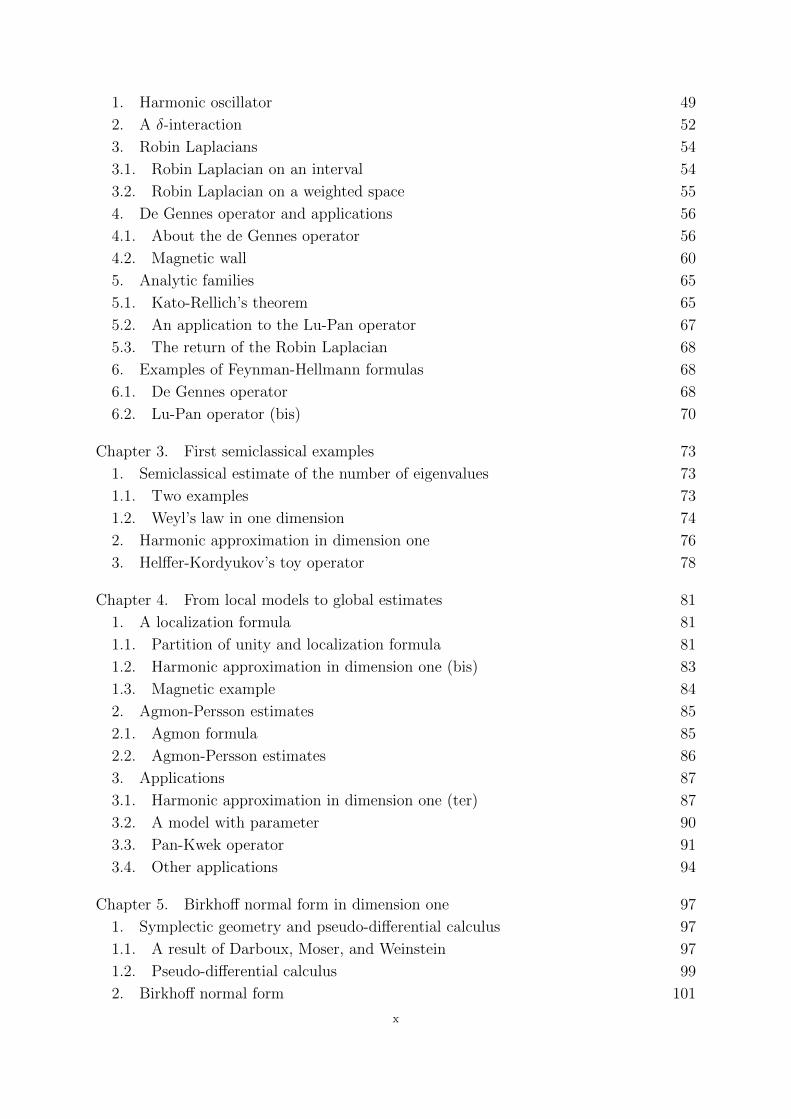
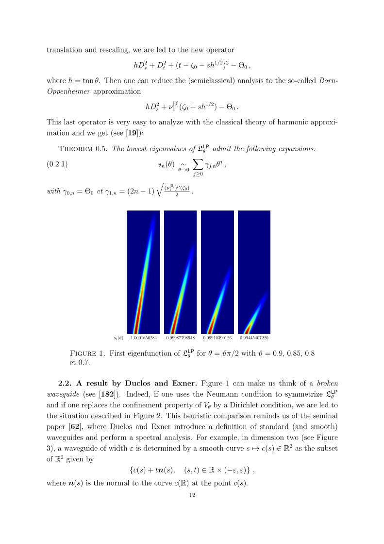
s1(θ) 1.0001656284 0.99987798948 0.99910390126 0.99445407220
Figure 1. First eigenfunction of LLPθ for θ = ϑπ/2 with ϑ = 0.9, 0.85, 0.8
et 0.7.
2.2. A result by Duclos and Exner. Figure 1 can make us think of a broken
waveguide (see [182]). Indeed, if one uses the Neumann condition to symmetrize LLPθ
and if one replaces the confinement property of Vθ by a Dirichlet condition, we are led to
the situation described in Figure 2. This heuristic comparison reminds us of the seminal
paper [62], where Duclos and Exner introduce a definition of standard (and smooth)
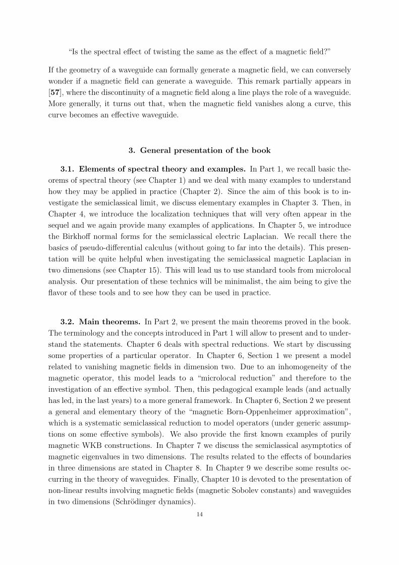
waveguides and perform a spectral analysis. For example, in dimension two (see Figure
3), a waveguide of width ε is determined by a smooth curve s 7→ c(s) ∈ R2 as the subset
of R2 given by
c(s) + tn(s), (s, t) ∈ R× (−ε, ε) ,where n(s) is the normal to the curve c(R) at the point c(s).
12
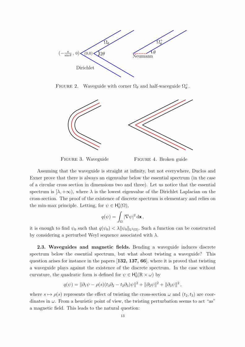
(0,0) 2θ θ(− πsin θ
, 0)
Dirichlet
Ωθ Ω+θ
Neumann
Figure 2. Waveguide with corner Ωθ and half-waceguide Ω+θ .
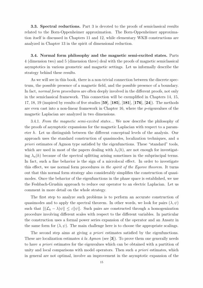
Figure 3. Waveguide Figure 4. Broken guide
Assuming that the waveguide is straight at infinity, but not everywhere, Duclos and
Exner prove that there is always an eigenvalue below the essential spectrum (in the case
of a circular cross section in dimensions two and three). Let us notice that the essential
spectrum is [λ,+∞), where λ is the lowest eigenvalue of the Dirichlet Laplacian on the
cross-section. The proof of the existence of discrete spectrum is elementary and relies on
the min-max principle. Letting, for ψ ∈ H10(Ω),
q(ψ) =
∫Ω
|∇ψ|2 dx ,
it is enough to find ψ0 such that q(ψ0) < λ‖ψ0‖L2(Ω). Such a function can be constructed
by considering a perturbed Weyl sequence associated with λ.
2.3. Waveguides and magnetic fields. Bending a waveguide induces discrete
spectrum below the essential spectrum, but what about twisting a waveguide? This
question arises for instance in the papers [132, 137, 66], where it is proved that twisting
a waveguide plays against the existence of the discrete spectrum. In the case without
curvature, the quadratic form is defined for ψ ∈ H10(R× ω) by
q(ψ) = ‖∂1ψ − ρ(s)(t3∂2 − t2∂3)ψ‖2 + ‖∂2ψ‖2 + ‖∂3ψ‖2 ,
where s 7→ ρ(s) represents the effect of twisting the cross-section ω and (t2, t3) are coor-
dinates in ω. From a heuristic point of view, the twisting perturbation seems to act “as”
a magnetic field. This leads to the natural question:
13
“Is the spectral effect of twisting the same as the effect of a magnetic field?”
If the geometry of a waveguide can formally generate a magnetic field, we can conversely
wonder if a magnetic field can generate a waveguide. This remark partially appears in
[57], where the discontinuity of a magnetic field along a line plays the role of a waveguide.
More generally, it turns out that, when the magnetic field vanishes along a curve, this
curve becomes an effective waveguide.
3. General presentation of the book
3.1. Elements of spectral theory and examples. In Part 1, we recall basic the-
orems of spectral theory (see Chapter 1) and we deal with many examples to understand
how they may be applied in practice (Chapter 2). Since the aim of this book is to in-
vestigate the semiclassical limit, we discuss elementary examples in Chapter 3. Then, in
Chapter 4, we introduce the localization techniques that will very often appear in the
sequel and we again provide many examples of applications. In Chapter 5, we introduce
the Birkhoff normal forms for the semiclassical electric Laplacian. We recall there the
basics of pseudo-differential calculus (without going to far into the details). This presen-
tation will be quite helpful when investigating the semiclassical magnetic Laplacian in
two dimensions (see Chapter 15). This will lead us to use standard tools from microlocal
analysis. Our presentation of these technics will be minimalist, the aim being to give the
flavor of these tools and to see how they can be used in practice.
3.2. Main theorems. In Part 2, we present the main theorems proved in the book.
The terminology and the concepts introduced in Part 1 will allow to present and to under-
stand the statements. Chapter 6 deals with spectral reductions. We start by discussing
some properties of a particular operator. In Chapter 6, Section 1 we present a model
related to vanishing magnetic fields in dimension two. Due to an inhomogeneity of the
magnetic operator, this model leads to a “microlocal reduction” and therefore to the
investigation of an effective symbol. Then, this pedagogical example leads (and actually
has led, in the last years) to a more general framework. In Chapter 6, Section 2 we present
a general and elementary theory of the “magnetic Born-Oppenheimer approximation”,
which is a systematic semiclassical reduction to model operators (under generic assump-
tions on some effective symbols). We also provide the first known examples of purily
magnetic WKB constructions. In Chapter 7 we discuss the semiclassical asymptotics of
magnetic eigenvalues in two dimensions. The results related to the effects of boundaries
in three dimensions are stated in Chapter 8. In Chapter 9 we describe some results oc-
curring in the theory of waveguides. Finally, Chapter 10 is devoted to the presentation of
non-linear results involving magnetic fields (magnetic Sobolev constants) and waveguides
in two dimensions (Schrodinger dynamics).
14
3.3. Spectral reductions. Part 3 is devoted to the proofs of semiclassical results
related to the Born-Oppenheimer approximation. The Born-Oppenheimer approxima-
tion itself is discussed in Chapters 11 and 12, while elementary WKB constructions are
analyzed in Chapter 13 in the spirit of dimensional reduction.
3.4. Normal form philosophy and the magnetic semi-excited states. Parts
4 (dimension two) and 5 (dimension three) deal with the proofs of magnetic semiclassical
asymptotics in various geometric and magnetic settings. Let us informally describe the
strategy behind these results.
As we will see in this book, there is a non-trivial connection between the discrete spec-
trum, the possible presence of a magnetic field, and the possible presence of a boundary.
In fact, normal form procedures are often deeply involved in the different proofs, not only
in the semiclassical framework. This connection will be exemplified in Chapters 14, 15,
17, 18, 19 (inspired by results of five studies [59], [185], [181], [176], [24]). The methods
are even cast into a non-linear framework in Chapter 16, where the p-eigenvalues of the
magnetic Laplacian are analyzed in two dimensions.
3.4.1. From the magnetic semi-excited states... We now describe the philosophy of
the proofs of asymptotic expansions for the magnetic Laplacian with respect to a param-
eter h. Let us distinguish between the different conceptual levels of the analysis. Our
approach uses the standard construction of quasimodes, localization techniques, and a
priori estimates of Agmon type satisfied by the eigenfunctions. These “standard” tools,
which are used in most of the papers dealing with λ1(h), are not enough for investigat-
ing λn(h) because of the spectral splitting arising sometimes in the subprincipal terms.
In fact, such a fine behavior is the sign of a microlocal effect. In order to investigate
this effect, we use normal form procedures in the spirit of the Egorov theorem. It turns
out that this normal form strategy also considerably simplifies the construction of quasi-
modes. Once the behavior of the eigenfunctions in the phase space is established, we use
the Feshbach-Grushin approach to reduce our operator to an electric Laplacian. Let us
comment in more detail on the whole strategy.
The first step to analyze such problems is to perform an accurate construction of
quasimodes and to apply the spectral theorem. In other words, we look for pairs (λ, ψ)
such that ‖(Lh − λ)ψ‖ ≤ ε‖ψ‖. Such pairs are constructed through a homogenization
procedure involving different scales with respect to the different variables. In particular
the construction uses a formal power series expansion of the operator and an Ansatz in
the same form for (λ, ψ). The main challenge here is to choose the appropriate scalings.
The second step aims at giving a priori estimates satisfied by the eigenfunctions.
These are localization estimates a la Agmon (see [3]). To prove them one generally needs
to have a priori estimates for the eigenvalues which can be obtained with a partition of
unity and local comparisons with model operators. Then such a priori estimates, which
in general are not optimal, involve an improvement in the asymptotic expansion of the
15

eigenvalues. If we are just interested in the first terms of λ1(h), these classical tools
suffice.
In fact, the major difference with the electric Laplacian arises precisely in the analysis
of the spectral splitting between the lowest eigenvalues. Let us describe what is done in
[79] (dimension two, constant magnetic field) and in [183] (non-constant magnetic field).
In [79, 183] quasimodes are constructed and the usual localization estimates are proved.
Then the behavior with respect to a phase variable needs to be determined to allow a
dimensional reduction. Let us emphasize here that this phenomenon of phase localization
is characteristic of the magnetic Laplacian and is intimately related to the structure of the
low lying spectrum. In [79] Fournais and Helffer are led to using the pseudo-differential
calculus and the Grushin formalism. In [183] the approach is structurally different.
In [183], in the spirit of the Egorov theorem (see [64, 190, 152]), we use successive
canonical transforms of the symbol of the operator corresponding to unitary transforms
(change of gauge, change of variable, Fourier transform), and we reduce the operator,
modulo remainders that are controlled thanks to the a priori estimates, to an electric
Laplacian that is in the Born-Oppenheimer form (see [43, 150] and more recently [19]).
This reduction demonstrates the crucial point that the inhomogeneity of the magnetic
operator is responsible for its spectral structure.
3.4.2. ... to the Birkhoff procedure. As we indicated above, our magnetic normal
forms are close to the Birkhoff procedure, and it is rather surprising that it has never
been implemented to elucidate the effect of magnetic fields on the low lying eigenvalues of
the magnetic Laplacian. A reason might be that, compared to the case of a Schrodinger
operator with an electric potential, the purily magnetic case has the specific feature that
the symbol “itself” is not enough to generate a localization of the eigenfunctions. This
difficulty can be seen in the recent papers by Helffer and Kordyukov [103] (dimension
two) and [105] (dimension three), which treat cases without boundary. In dimension
two, they prove that if the magnetic field has a unique and non-degenerate minimum, the
n-th eigenvalue admits an expansion in powers of h12 of the form
λn(h) ∼ hminR2
B(q) + h2(c1(2n− 1) + c0) +O(h52 ) ,
where c0 and c1 are constants depending on the magnetic field (see the discussion in
Section 1.3). In Chapter 15 (whose main ideas are presented in Chapter 5), we extend
their result by obtaining a complete asymptotic expansion which actually applies to more
general magnetic wells and allows one to describe larger eigenvalues.
3.5. The spectrum of waveguides. We address the question:
“What is the spectral influence of a magnetic field on a waveguide ?”
We answer this question in Chapter 20. Then, when there is no magnetic field, we would
also like to analyze the effect of a corner on the spectrum and present a non-smooth
16
version of the result of Duclos and Exner (see Chapter 21). For that purpose we also
present some results concerning the semiclassical triangles in Chapter 21.
Finally, in Chapter 22, we cast the linear technics into a non-linear framework to
investigate the existence of global solutions to the cubic non-linear Schrodinger equation
in a bidimensional waveguide.
17
Magneti
cco
ne
•C
onic
alsi
ngu
lari
ty(C
h.
6,S
ec.
3.2)
•S
mal
lap
ertu
reli
mit
(Sec
.3.
3)
”V
anis
hin
g”
magneti
cfield
sin
two
dim
ensi
ons
•M
ontg
omer
yop
erat
ors
(Ch
.6,
Sec
.1)
•M
od
elfo
rva
nis
hin
gfi
eld
sw
ith
bou
nd
ary
(Sec
tion
1.4)
•N
orm
alfo
rm(C
h.
8,S
ec.
1)
Norm
al
Form
s
Adia
bati
cR
educt
ions
WK
BA
naly
sis
Non
vanis
hin
gm
agneti
cfield
intw
odim
ensi
ons
•C
h.
8,S
ec.
2
•S
ym
ple
ctic
geom
etry
•B
irkh
offn
orm
alfo
rm
•P
seu
do-
diff
eren
tial
calc
ulu
s
Magneti
cw
edge
•E
dge
sin
gula
rity
(Ch
.8,
Sec
.2)
•N
orm
alfo
rm(C
h.
8,S
ec.
2)
Magneti
chalf
-space
•C
h.
8,S
ec.
1
•P
olyn
omia
les
tim
ates
inth
ep
has
esp
ace
Born
-Opp
enheim
er
appro
xim
ati
on
•C
h.
6,S
ec.
2
•W
KB
con
stru
ctio
ns
(Sec
.3)
•C
oher
ent
stat
es(S
ec.
2.2.
2)
Bro
ken
waveguid
es
•C
h.
9
•S
emic
lass
ical
tria
ngl
es(S
ec.
3.1)
•B
oun
dar
yla
yer
Magneti
cw
aveguid
es
•C
h.
9
•E
ffec
tive
Ham
ilto
nia
ns
ala
Du
clos
-Exn
er
•N
orm
reso
lven
tco
nve
rgen
ce(S
ec.
1.6)
Part 1
Methods and examples

CHAPTER 1
Elements of spectral theory
It will neither be necessary to deliberate nor
to trouble ourselves, as if we shall do this
thing, something definite will occur, but if
we do not, it will not occur.
Organon, On Interpretation, Aristotle
This chapter is devoted to recalling basic tools of spectral analysis.
1. Spectrum
1.1. Spectrum of an unbounded operator. Let L be an unbounded operator on
a separable Hilbert space (H, 〈·, ·〉) with domain Dom (L) dense in H.
Definition 1.1. The operator (L,Dom (L)) is closed if
(Dom (L) 3 un −→ u ∈ H, Lun −→ v) =⇒ (u ∈ Dom (L), Lu = v) .
Definition 1.2. The adjoint of (L,Dom (L)) is defined as follows. We let
Dom (L∗) := u ∈ Dom (L), v 7−→ 〈Lv, u〉 is continuous on Dom (L)
and, for u ∈ DomL∗, L∗u is defined via the Riesz representation theorem as the unique
element in H such that 〈Lv, u〉 = 〈v,L∗u〉, for all v ∈ DomL.
We say that (L,Dom (L)) is self-adjoint when (L∗,Dom (L∗)) = (L,Dom (L)).
Proposition 1.3. The operator (L∗,Dom (L∗)) is always a closed operator i.e., with
closed graph. If (L,Dom (L)) is closable, then Dom (L∗) is dense and (L∗)∗ = L, where L
is the smallest closed extension of L.
Definition 1.4. An operator (L,Dom (L)) is said to be Fredholm if kerL is of finite
dimension, ImL is closed and with finite codimension. Its index is, by definition, the
number indL = dim kerL− dim kerL∗.
Note that if a Fredholm operator L is self-adjoint, then its index is 0.
We now recall the following definitions of spectrum sp(L), essential spectrum spess(L),
and discrete spectrum spdis(L) of the operator L.
Definition 1.5. We define
21

i. spectrum: λ ∈ sp(L) if L− λ is not bijective from Dom (L) onto H,
ii. essential spectrum: λ ∈ spess(L) if L− λ is not Fredholm with index 0 from Dom (L)
into H,
iii. Fredholm spectrum: spfre(L) = sp(L) \ spess(L),
iv. discrete spectrum: λ ∈ spdis(L) if λ is isolated in the spectrum of L, with finite
algebraic multiplicity and such that Im (L− λ) is closed.
Obviously, spess(L) ⊂ sp(L).
1.1.1. About the discrete spectrum. Since we will often estimate the discrete spectrum
in this book, let us recall a number of classical lemmas. In particular, the following lemmas
aim at explaining the meaning of (iv) in Definition 1.5.
Let us consider an unbounded closed operator (L,Dom(L)) and λ an isolated element
of sp(L). Let Γλ be a contour that enlaces only λ as element of the spectrum of L and
define
Pλ :=1
2iπ
∫Γλ
(z − L)−1 dz .
The bounded operator Pλ : H→ Dom(L) ⊂ H commutes with L and does not depend on
Γλ (thanks to the holomorphy). We may prove that Pλ is a projection and that
(1.1.1) Pλ − Id =1
2iπ
∫Γλ
(ζ − λ)−1(ζ − L)−1(L− λ) dζ .
We say that λ has finite algebraic multiplicity when the rank of Pλ is finite.
Lemma 1.6 (Weyl sequences). Let us consider an unbounded closed operator (L,Dom(L)).
Assume that there exists a sequence (un) ∈ Dom (L) such that ‖un‖H = 1, (un) and
(L− λ)un −→n→+∞
0 in H. Then λ ∈ sp(L).
A sequence (un) as in Lemma 1.6 is called a Weyl sequence.
Lemma 1.7. Let us consider an unbounded closed operator (L,Dom(L)) and λ an
isolated element of sp(L). Then we have either 1 ∈ sp(P ∗λ ) or 1 ∈ sp(Pλ). In any case,
we have Pλ 6= 0.
Proof. Before starting the proof, let us observe that λ ∈ sp(L) iff λ ∈ sp(L∗).
We have just to consider the following cases:
i. L − λ is injective with closed range. We have ker(L∗ − λ) 6= 0 and we consider
0 6= u ∈ ker(L∗ − λ). We have
P ∗λ =1
2iπ
∫Γλ
(ζ − L∗)−1 dζ .
We apply Formula (1.1.1) to λ, Γλ and L∗ to get that P ∗λu = u.
ii. or there exists a Weyl sequence (un) associated with λ: the sequence ((L − λ)un)
goes to zero and ‖un‖ = 1. Again with Formula (1.1.1), we have (Pλ − Id)un → 0,
and thus 1 ∈ sp(Pλ) (by Lemma 1.6).
22
Lemma 1.8. If λ ∈ sp(L) is isolated with finite multiplicity, then it is an eigenvalue.
Proof. The projection P = Pλ commutes with L. Thus we may write
L = L|rangeP ⊕ L| kerP .
The spectrum of L is the union of the corresponding spectra and λ is still isolated in
these spectra.
By definition, we have
1
2iπ
∫Γ
(ζ − L| kerP )−1 dζ = 0 .
Thus (by the previous lemma), λ does not belong to sp(L| kerP ). Therefore, λ belongs to
the spectrum of the ”matrix” L|rangeP and it is an eigenvalue.
1.1.2. Lemmas for self-adjoint operators. For the Reader’s convenience, let us also
recall the proof of a few classical lemmas (see [186, Chapter VI] and [141, Chapter 3])
which can also be treated as exercises.
Lemma 1.9. If L is self-adjoint, we have the equivalence: λ ∈ sp(L) if and only if there
exists a sequence (un) ∈ Dom (L) such that ‖un‖H = 1, (un) and (L− λ Id)un −→n−→+∞
0 in
H.
Proof. Let us notice that if there exists a sequence (un) ∈ Dom (L) such that
‖un‖H = 1, (un) and (L − λ Id)un →n→+∞
0 then λ ∈ sp(L) (if not we could apply the
bounded inverse and get a contradiction).
If λ /∈ R, then since L is self-adjoint, L−λ is invertible (with bounded inverse because
L is closed). Now, for λ ∈ R, if there is no sequence (un) ⊂ Dom (L) such that ‖un‖H = 1,
(un) and (L− λ Id)un −→n→+∞
0, then we can find c > 0 such that
‖(L− λ)u‖ ≥ c‖u‖, ∀u ∈ Dom (L) .
Therefore L− λ is injective with closed range. But, since L− λ = (L− λ)∗, the range of
L− λ is dense in H and so L− λ is surjective.
Lemma 1.10 (Weyl criterion). If L is self-adjoint, then λ ∈ spess(L) if and only if
there exists a sequence (un) ⊂ Dom (L) such that ‖un‖H = 1, (un) has no subsequence
converging in H, and (L− λ)un →n−→+∞
0 in H.
Proof. If λ ∈ sp(L) \ spess(L), the operator L− λ is Fredholm. Let (un) ⊂ Dom (L)
such that ‖un‖H = 1 and (L − λ)un →n−→+∞
0. The operator L − λ : ker(L − λ)⊥ →range(L − λ) is injective with closed range. Therefore, there exists c > 0 such that, for
all w ∈ ker(L− λ)⊥, ‖(L− λ)w‖ ≥ c‖w‖. We write un = vn + wn, with vn ∈ ker(L− λ)
23
and wn ∈ ker(L − λ)⊥. We have ‖(L − λ)un‖2 = ‖(L − λ)vn‖2 + ‖(L − λ)wn‖2 and we
deduce that wn → 0. Moreover, (vn) is bounded in a finite dimensional space, thus there
exists a converging subsequence of (un).
Conversely, let us assume that λ ∈ sp(L) and that any sequence (un) ⊂ Dom (L) such
that ‖un‖H = 1 and (L−λ)un →n→+∞
0 has a converging subsequence. The kernel ker(L−λ)
is finite dimensional. Indeed, if it were of infinite dimension, one could construct a infinite
orthonormal family (un) in ker(L− λ) and in particular we would get un 0, which is a
contradiction. Let us now check that there exists c > 0 such that, for all u ∈ ker(L−λ)⊥,
‖(L− λ)u‖ ≥ c‖u‖. If not, there exists a normalized sequence (un) in ker(L− λ)⊥ such
that ‖(L−λ)un‖ → 0. By assumption, we may assume that (un) converges towards some
u∞ that necessarily belongs to ker(L− λ)⊥. But since L− λ is closed (it is self-adjoint),
we have (L− λ)u∞ = 0 so that u∞ = 0, and this is a contradiction. We deduce that the
image of L− λ is closed.
The following lemma is a slight improvement of Lemma 1.10.
Lemma 1.11. Assume that L is self-adjoint. Then λ ∈ spess(L) if and only if there
exists a sequence (un) ⊂ Dom (L) such that ‖un‖H = 1, (un) converges weakly to 0, and
(L− λ)un →n−→+∞
0 in H.
Proof. Let λ ∈ spess(L). If dim ker(L− λ Id) = +∞, then (by considering a Hilber-
tian basis of the kernel) we can easily construct a orthonormal sequence (vn) weakly
converging to 0 such that (L− λ)vn = 0.
Therefore, we consider the case when dim ker(L − λ) < +∞. By Lemma 1.10, there
exists a sequence (un) ⊂ Dom (L) such that ‖un‖H = 1 with no converging subsequence
such that we have (L − λ)un →n→+∞
0 in H. We can write un = un + kn with un ∈ker(L − λ)⊥ and kn ∈ ker(L − λ). We have (L − λ Id)un →
n→+∞0 and we may assume
(up to a subsequence extraction) that (kn) converges to k. Since (un) has no converging
subsequence, (un) does not converge, and so it does not go to 0. Therefore, up to another
extraction, we may assume that there exists ε0 > 0 such that, for all n ∈ N, ‖un‖ ≥ ε0.
Now set un = un‖un‖ ; then (L− λ)un →
n−→+∞0. Up to another extraction, we may assume
that (un) converges weakly to some u ∈ ker(L − λ)⊥. For all v ∈ Dom (L), we have
〈u, (L − λ)v〉H = 0. We deduce that u ∈ Dom (L∗) = Dom (L) and that (L − λ)u = 0.
Thus u = 0.
In any case, we have found a sequence with the required property. For the converse,
it is just an application of Lemma 1.10.
24
Let us now explain why, in the self-adjoint case, the discrete spectrum coincides with
the Fredholm spectrum.
Lemma 1.12. Let L be self-adjoint. We have the following properties.
i. If λ ∈ sp(L) is not isolated, then λ ∈ spess(L).
ii. The Fredholm spectrum is formed by isolated eigenvalues of finite multiplicity.
iii. If λ ∈ sp(L) is isolated, then it is an eigenvalue.
iv. All isolated eigenvalues of finite multiplicity belong to the Fredholm spectrum.
Proof. Let us prove (i) and (ii). Let λ ∈ sp(L) \ spess(L). There exists a Weyl
sequence (un) of unit vectors such that (L − λ)un → 0. We may assume that (un)
converges to some u (of norm 1) and we get (L − λ)u = 0. The eigenvalue λ has finite
multiplicity. Let us prove that it is isolated. If this were not the case, then one could
consider a non-constant sequence λn tending to λ. Moreover, one could find a sequence
(un) of unit vectors such that
‖(L− λn)un‖ ≤|λ− λn|
n.
We may assume that (un) converges to some u ∈ Dom (L) and thus one would get
(L− λ)u = 0, and so
〈(L− λn)u, un〉 = (λ− λn)〈u, un〉 .By the Cauchy-Schwarz inequality, 〈un, u〉 → 0 and we get u = 0, which is a contradiction.
Let us now prove (iii). Consider an isolated point λ ∈ sp(L). By definition, this
means that there exists ε0 > 0 such that, for all µ 6= λ such that |µ − λ| ≤ ε0, we have
µ /∈ sp(L). For all ε ∈ (0, ε0), we introduce
Pε =1
2iπ
∫Γε
(ζ − L)−1 dζ = P ,
where Γε is the circle of radius ε centered at λ (the integral is understood in the sense of
Riemann).
Since L is closed (and using Riemann sums), Pλ is valued in Dom (L) and
(L− λ)P =1
2iπ
∫Γε
(L− λ)(ζ − L)−1 dζ =1
2iπ
∫Γε
(ζ − λ)(ζ − L)−1 dζ .
Now, we use the spectral theorem (see Theorem 1.22) to get (as soon as ε0 is chosen small
enough):
‖(L− ζ)−1‖ ≤ 1
|λ− ζ|.
Thus, we infer that ‖(L−λ)P‖ ≤ ε for all ε ∈ (0, ε0). Therefore, P is valued in ker(L−λ).
It remains to apply Lemma 1.7.
25
Let us now consider (iv). Since λ is isolated, (iii) shows that it cannot belong to the
spectrum of the restriction L| ker(L−λ)⊥ . Thus, there exists c > 0 such that
∀u ∈ ker(L− λ)⊥ , ‖(L− λ)u‖ ≥ c‖u‖ .
We deduce that the range of L−λ is closed and that L−λ is Fredholm, because dim ker(L−λ) < +∞.
Finally, let us prove another useful property.
Lemma 1.13. Let L be self-adjoint. Consider λ ∈ spess(L). Then, for all N ∈ N∗ and
ε > 0, there exists an orthonormal family (uεn)1≤n≤N such that, for all n ∈ 1, . . . , N,‖(L− λ)uεn‖ ≤ ε.
Proof. If λ is isolated, then it is an eigenvalue of infinite multiplicity (see Lemma
1.12) and the conclusion follows. If λ is not isolated, we may consider a sequence of
distinct numbers of the spectrum (λn)n∈N tending to λ and such that, for all j, k ∈ N, we
have |λj − λk| ≤ ε2. If N = 1, by the Weyl criterion, we get the existence of uε1 such that
‖(L− λ1)uε1‖ ≤ ε2. The conclusion follows since |λ− λ1| ≤ ε
2. Let us now only treat the
case when N = 2. By the Weyl criterion, we can find uε1 and uε2 of norm 1 such that
‖(L− λ1)uε1‖ ≤ε
2, ‖(L− λ2)uε2‖ ≤
ε
2.
Since L is self-adjoint, we find |λ1 − λ2||〈uε1, uε2〉| ≤ ε. Setting
uε2 = uε2 − 〈uε2, uε1〉uε1 ,
we have
‖(L− λ2)uε2‖ ≤ε
2+
ε
|λ2 − λ1|
(|λ1 − λ2|+
ε
2
).
Moreover, ‖uε2‖ ≥√
1− ε2
|λ1−λ2|2 . Up to changing ε, we deduce the result. For N ≥ 3, we
proceed by induction.
1.2. A representation theorem.
1.2.1. The Lax-Milgram theorem. Let us recall the well-known Lax-Milgram theorem
that will allow the definition of many operators in this book.
Theorem 1.14 (Lax-Milgram). Let us consider two Hilbert spaces V and H such that
V ⊂ H with continuous injection and with V dense in H. If B is a continuous sesquilinear
form on V that is coercive, i.e., there exists α > 0 such that
|B(u, u)| ≥ α‖u‖2V , ∀u ∈ V ,
then we can define an operator (L,Dom (L)) whose domain is
Dom (L) := u ∈ V : v 7−→ B(u, v) is continuous on V for the topology of H26
and such that, for u ∈ Dom (L),
B(u, v) = 〈Lu, v〉H, ∀v ∈ V .
The operator L : Dom (L) → H is bijective and its inverse is continuous. Moreover
Dom (L) is dense in H.
If B is also Hermitian, then L is self-adjoint and its domain is dense in V.
Proof. We refer to the book by Helffer [99, Section 3.3] for a detailed proof. Let us
briefly discuss the different steps. By the Riesz representation theorem, we may find an
operator A ∈ L(V) such that, for all u, v ∈ V,
B(u, v) = 〈Au, v〉V .
We easily get that
∀u ∈ V , ‖Au‖V ≥ α‖u‖V ,
so that A is injective with closed range. Let us explain why the range is dense in V. Let
v ∈ V such that for all u ∈ V
〈Au, v〉V = 0 .
We get in particular B(v, v) = 0 and thus v = 0. Therefore A is bijective.
Then, we notice that L is well defined on Dom (L) by using the density of V in H and
the Riesz theorem. We easily see that L is injective. Let us explain why it is surjective.
Let us consider u′ ∈ H. By the Riesz theorem (on V and by using the continuous
embedding of V in H), there exists u ∈ V such that, for all v ∈ V,
〈u′, v〉H = 〈u, v〉V .
Since A is surjective, we find u ∈ V such that, for all v ∈ V,
〈u′, v〉H = 〈Au, v〉V = B(u, v) .
From this, we deduce that u ∈ Dom (L) and that, for all v ∈ V,
〈u′, v〉H = 〈Lu, v〉H .
By density of V in H, we get u′ = Lu.
Finally, we notice that, for all u ∈ Dom (L),
C‖Lu‖H‖u‖V ≥ ‖Lu‖H‖u‖H ≥ α‖u‖2V .
Thus L−1 is continuous from H to V and we deduce that (L,Dom (L)) is closed.
Note that this theorem is directly related to the Friedrichs procedure (see, for instance,
[186, p. 177]).
1.2.2. The Dirichlet realization. Let Ω be an open and bounded subset of Rd, and
A ∈ C1(Ω). Let us consider the following sesquilinear form, defined for u, v ∈ V = H10(Ω)
27
by
Bh,A(u, v) =
∫Ω
(−ih∇+ A)u (−ih∇+ A)v dx .
We have
∀u ∈ V, Bh,A(u, u) + (2‖A‖2∞ + 1)‖u‖2
H ≥1
2‖u‖2
V ,
which implies the coercivity on V. For this shifted sesquilinear form, V is a Hilbert space.
Here the domain of L is given by
Dom (LDirh,A) =
u ∈ H1
0(Ω) : Lh,Au ∈ L2(Ω).
The self-adjoint operator L = LDirh,A satisfies
〈LDirh,Au, v〉 = Bh,A(u, v), ∀u ∈ Dom (LDir
h,A), ∀v ∈ H10(Ω) .
When Ω is regular, we have the characterization:
Dom (LDirh,A) = H1
0(Ω) ∩ H2(Ω) .
Note that we could have defined the initial quadratic form on C∞0 (Ω) but this space is not
complete for the H10(Ω)-norm. Completing C∞0 (Ω) for the norm induced by the quadratic
form and then defining the self-adjoint operator L is called the Friedrichs procedure.
1.2.3. The Neumann realization. Let Ω be an open and bounded subset of Rd, and
A ∈ C1(Ω). We consider another quadratic form, defined by
Qh,A(u) =
∫Ω
|(−ih∇+ A)u|2 dx, u ∈ H1(Ω) .
We can define a self-adjoint operator LNeuh,A with domain
Dom (LNeuh,A) =
u ∈ H1(Ω) : Lh,Au ∈ L2(Ω), (−ih∇+ A)u · n = 0 on ∂Ω
.
When Ω is regular, this becomes
Dom (LNeuh,A) =
u ∈ H1(Ω) : u ∈ H2(Ω), (−ih∇+ A)u · n = 0 on ∂Ω
.
1.3. Reminders about compact operators.
1.3.1. Riesz-Frechet-Kolmogorov criterion and compact resolvent. Let us recall a cri-
terion of relative compactness in Lp(Ω) (see [32]).
Theorem 1.15 (Riesz-Frechet-Kolmogorov). Let Ω ⊂ RN be an open set and F a
bounded subset of Lp(Ω), with p ∈ [1,+∞). We assume that
∀ε > 0, ∃ω ⊂⊂ Ω, ∀f ∈ F , ‖f‖Lp(Ω\ω) ≤ ε
and that
∀ε > 0,∀ω ⊂⊂ Ω, ∃δ > 0, δ < dist(ω, Ω), ∀|h| ≤ δ, ∀f ∈ F , ‖τhf − f‖Lp(ω) ≤ ε ,
where τhf(x) = f(x+ h)− f(x). Then, F is relatively compact in Lp(Ω).
28
By using a density argument and the Taylor formula, we can get the following propo-
sition (see [32, Proposition 9.3]).
Proposition 1.16. Let p ∈ (1,+∞) and u ∈ Lp(Ω). Then u ∈ W1,p(Ω) if and only
if, for all ω ⊂⊂ Ω and h ∈ (0, dist(ω, Ω)), we have
‖τhu‖Lp(ω) ≤ C|h| .
In this case, we can take C = ‖∇u‖Lp(Ω).
Let us provide a useful criterion for the compactness of a resolvent.
Proposition 1.17. An operator (L,Dom (L)) has compact resolvent if and only if
the injection (Dom (L), ‖ · ‖L) → H is compact.
Proof. Thanks to the closed graph theorem, for z /∈ sp(L), (L− z)−1 : (H, ‖ · ‖H)→(Dom (L), ‖ · ‖L) is bounded.
Proposition 1.18. Consider two Hilbert spaces V and H such that V ⊂ H with
continuous injection and with V dense in H. Assume that B is a continuous, coercive
and Hermitian sesquilinear form on V and let L be the self-adjoint operator associated
with B. Let us denote by ‖ · ‖B the norm induced by B, i.e., ‖u‖B =√
B(u, u), and by
‖ · ‖L the graph norm on Dom (L).
If (Dom (B), ‖ · ‖B) → H is compact, then L has compact resolvent.
Proof. By the Cauchy-Schwarz inequality, (Dom (L), ‖ · ‖L) → (Dom (B), ‖ · ‖B) is
bounded. The conclusion follows since the compact operators form an ideal in the algebra
of bounded operators.
1.3.2. Facts about compact operators. Let us prove the following classical lemma.
Lemma 1.19. Let M ∈ L(H) be a Fredholm operator. We let n = dim ker(M) and
m = dim ker(M∗). We introduce (kj)1≤j≤n a basis of ker(M) and (k∗j )1≤j≤m a basis of
ker(M∗). We let
M =
(M R−
R+ 0
),
where R− : Cm → H is defined by R−α =∑m
j=1 αjk∗j and R+ : H → Cn is defined by
R+(u) = (〈u, kj〉)1≤j≤n. Then, M : H× Cm → H× Cn is bijective.
Moreover, there exists ε0 > 0 such that for all P ∈ L(H) with ‖P‖ ≤ ε0,(M + P R−R+ 0
),
is bijective. We denote by E its (bounded) inverse:
E =
(E E+
E− E0
).
29
Then, we have ind (M+P) = ind (E0) = n−m and M+P is bijective if and only if E0
is bijective.
Proof. We leave the proof of the bijectivity ofM to the reader. By using a Neumann
series, we can easily prove that (M + P R−
R+ 0
),
is bijective when P is small enough. We write that E is the inverse on the right:
(M + P)E +R−E− = Id
R+E+ = Id
(M + P)E+ +R−E0 = 0
R+E = 0
and on the left:
E(M + P) + E+R+ = Id
E−R− = Id
E−(M + P) + E0R+ = 0
ER− = 0 .
From this, we get that R+ and E− are surjective and that R− and E+ are injective. By
elementary considerations, we see that if M + P is bijective, E0 must be so. Conversely,
suppose that E0 is bijective. Then, consider
(1.1.2) E − E+E−10 E− ,
and check that it is the inverse of M + P.
Let us finally discuss the result about the index. We can check that the injective
application E+ sends kerE0 into ker(M + P) and that E+ : kerE0 → ker(M + P) is a
bijection. By taking the adjoint, we find in the the same way that the injective application
E∗− sends kerE∗0 into ker(M + P)∗ and induces a bijection. The conclusion about the
index follows.
In the following theorem, we recall some fundamental facts about compact operators.
In particular, we will notice that the non-zero spectrum of a compact operator is discrete.
Theorem 1.20 (Fredholm alternative). Let L ∈ L(H) be a compact operator. Then,
we have
(i) If H is of infinite dimension, then 0 ∈ sp(L).
(ii) For all z ∈ U = C \ 0, L− z is a Fredholm operator of index 0.
30
(iii) ker(L− Id) = 0 iff range(L− Id) = H.
(iv) The elements of sp(L)\0 are isolated with finite multiplicity and the only possible
accumulation point of the spectrum is 0. In other words, the non zero spectrum is
made of isolated eigenvalues of finite multiplicity.
Proof. The point (i) is a consequence of the fact that the set of compact operators
forms a ideal of bounded operators and from the Riesz theorem.
Let us consider the point (ii). Let us first prove that L− z is a Fredholm operator for
z ∈ U . The kernel of L−z has finite dimension by the Riesz theorem. Let us explain why
its range is closed. We consider a sequence (un) such that (L− z)un = vn → v ∈ H. We
write un = kn+rn, with kn ∈ ker(L−z) and rn ∈ ker(L−z)⊥ and we have (L−z)rn = vn.
If (rn) is bounded, by using that L is compact, we get that, up to a subsequence
extraction, Lrn converges. From this, we deduce that (rn) converges and the conclusion
follows. It remains to deal with the case when (‖rn‖) tends to +∞. We let rn := rn‖rn‖ .
We have (L− z)rn → 0. By using again the compactness of L, we deduce that, up to a
subsequence extraction, (rn) converges to some r ∈ ker(L− z)⊥ such that (L− z)r = 0.
We get that r = 0 and this is a contradiction. To see that ker(L∗−z) has finite dimension,
we use that L∗ is compact.
Then, by Lemma 1.19 (with P = (z− z1)Id and M = L− z1, z1 ∈ U), the application
U 3 z 7→ ind (L− zId) is locally constant and thus constant since U is connected. For z
large enough, we know that L−zId is bijective and thus of index 0. From this, we deduce
the point (iii). Let us now prove the point (iv). Let us introduce
V := z ∈ U : ∃r > 0 : D(z, r) ⊂ sp(L) .
V is open by definition. Let us prove that is closed in U . Let us consider a sequence
V 3 zn → z∞ ∈ U . We apply again Lemma 1.19 (with P = (z−z∞)Id and M = L−z∞).
In a neighborhood of z∞, L− z is not bijective if and only if detE0(z) = 0. But detE0 is
holomorphic in a neighborhood of z∞. Therefore, its zeros are isolated unless detE0 = 0.
By definition z∞, we must have detE0 = 0 in a neighborhood of z∞. Thus z∞ ∈ V . We
deduce that V = U or V = ∅ and we get that V = ∅. Now let us consider z1 ∈ sp(L)\0.Then, in a neighborhood of z1, L − z is not bijective if and only if detE0(z) = 0. Since
V = ∅, detE0 is not zero near z1 and thus (by holomorphy), its zeroes are isolated.
Finally, we recall (1.1.2) and thus we have, near each point of the spectrum in U ,
(L− z)−1 = E(z)− E+(z)E−10 (z)E−(z) ,
and we deduce that the resolvent is meromorphic in U . The poles are finite rank operators
and we deduce the result about the multiplicity (see Section 1.1.1).
31
If Ω is bounded and Lipschitzian, the form domains H10(Ω) and H1(Ω) are com-
pactly embedded in L2(Ω) (their unit balls satisfy the assumptions of the Riesz-Frechet-
Kolmogorov criterion, see [32] for details). Therefore LDirh,A and LNeu
h,A have compact resol-
vents, and so these operators have discrete spectra. We can consider the non-decreasing
sequences of their eigenvalues.
Exercise 1.21. Consider L = LDirh,A when Ω is bounded and regular. Let λ be an
eigenvalue of L (λ ∈ R since L is self-adjoint). As we have seen, ker(L − λ) has finite
dimension. Since P is self-adjoint, we can write:
range(L− λ) = ker(L− λ)⊥ .
Prove that the image of L− λ is closed by using that K = (L− λ+ i)−1 is compact.
2. Min-max principle and spectral theorem
2.1. Statement of the theorems. We state a theorem which will serve as one of
the fundamental tools in this book.
Theorem 1.22. Assume that (L,Dom (L)) is a self-adjoint operator. Then, if λ /∈sp(L), we have:
‖(L− λ)−1‖ ≤ 1
dist(λ, sp(L)).
Remark 1.23. A proof using the “spectral theorem” can be found in [187] and [128,
Section VI.5] . An immediate consequence of this theorem is that, for all ψ ∈ Dom (L):
‖ψ‖dist(λ, sp(L)) ≤ ‖(L− λ)ψ‖ .
In particular, if we find ψ ∈ Dom (L) such that ‖ψ‖ = 1 and ‖(L − λ)ψ‖ ≤ ε, then
dist(λ, sp(L)) ≤ ε.
Proof. This result may be proved without the general spectral theorem. Let us
provide the elements of the proof. First we establish the result when L is bounded and
normal (i.e., [L,L∗] = 0). For that purpose, we will use the following exercises.
Exercise 1.24. If P is a polynomial, we have λ ∈ sp(L) iff P (λ) ∈ sp(L).
Exercise 1.25. We define the spectral radius as
ρ(L) = supλ∈sp(L)
|λ| .
i. By using the convergence of a Neumann series, prove that
ρ(L) = lim supn→+∞
‖Ln‖1n
and then ρ(L) = infn ‖Ln‖1n .
ii. By using ‖L∗L‖ = ‖L‖2, prove that ρ(L) = ‖L‖ and deduce ‖P (L)‖ = ‖P‖∞ where
‖ · ‖∞ is the uniform norm on the spectrum K of L that is compact.
32

iii. By using the Stone-Weierstrass theorem, extend this equality to continuous functions
on K. If f is a continuous function on K, explain how we may define f(L).
If λ /∈ sp(L), the function r : K 3 z 7→ (z − λ)−1 is continuous and the result follows
when L is bounded and normal upon observing that r(L) = (L− λ)−1.
Now, let us assume that L is self-adjoint with domain Dom (L). Then this is not
difficult to prove that L± i Id is invertible. We introduce the function
g(x) =x− ix+ i
, x ∈ R
called Cayley transform, and the bounded and unitary operator
g (L) := U := (L− iId) (L + iId)−1 .
In particular, g(L) is normal. Easy computations show that g : sp (L) 7→ sp (g(L)) is
bijective. Then, for µ /∈ sp(L), we define, on sp (g (L)),
f(y) =1
g−1(y)− µ.
From the case of bounded and normal operators, we infer that
‖f(g(L))‖ ≤ ‖f‖∞,sp(g(L)) = ‖(· − µ)−1‖∞,sp(L) .
It remains to write that f(g(L)) = (L−µ)−1 by noticing that g−1(U)(Id−U) = i(U + Id)
(which implies that g−1(U) = L on Dom (L)) and (g−1(U)− µ)f(U) = Id, where g−1(U)
is understood in the sense of functional calculus of normal bounded operators.
As a consequence of the proof of Theorem 1.22, we deduce the Stone theorem.
Theorem 1.26. Let (L,Dom (L)) be a self-adjoint operator. For all ψ0 ∈ Dom (L),
there exists a unique local C1-solution t 7→ S(t)ψ0 of the equation
ψ′(t) = iLψ(t), ψ(0) = ψ0 .
This solution is global and, for all t ∈ R, ‖S(t)ψ0‖ = ‖ψ0‖. For all t ∈ R and for all
ψ0 ∈ Dom (L), we have S(t)ψ0 ∈ Dom (L). We denote S(t) = eitL and (eitL)t∈R is a
semi-group.
Proof. We let S(t) = eitg−1(U), where g−1(U) is defined in the proof of Theorem 1.22.
Then S ′(t) = ig−1(U)S(t) = iS(t)g−1(U), so that, for ψ ∈ Dom (L), S ′(t)ψ = iS(t)Lψ.
Let us prove that, for all t ∈ R and ψ ∈ Dom (L), we have S(t)ψ ∈ Dom (L) and that
LS(t)ψ = S(t)Lψ. We have, for all ϕ ∈ H and ψ ∈ Dom (L),
〈g−1(U)eitg−1(U)ϕ, ψ〉 = 〈eitg−1(U)ϕ,Lψ〉 .
33
This implies, by definition, that eitg−1(U)ϕ ∈ Dom (L∗) = Dom (L) and that Leitg
−1(U)ϕ =
g−1(U)eitg−1(U)ϕ. The proof of the uniqueness and of the group property is left to the
reader.
Exercise 1.27. The aim of this exercise is to investigate the functional calculus of a
simple self-adjoint operator on L2(R) and provide an explicit functional calculus. Let us
recall the expression of the Fourier transform on R. For ψ ∈ S(R), we let, for all ξ ∈ R,
Fψ(ξ) =1√2π
∫Re−ixξψ(x) dx .
It is well-known that F extends to an isometry of L2(R) and that, for all ψ ∈ S ′(R),
F(Dxψ) = ξF(ψ)
which may be written as FDxF−1 = ξ. In other words, the self-adjoint operator Dx with
domain H1(R) is diagonalized by means of the Fourier transform.
Let us now consider a smooth function on R denoted by δ bounded together with its
derivatives and such that there exists δ0 > 0 such that δ ≥ δ0.
i. Solve the equation δDx(δψ) = ξψ for ξ ∈ R.
ii. For ψ ∈ S(R), let
Fδ(ψ)(ξ) =1√2π
∫Rδ(x)−1eiξ
∫ x0 δ−2(y) dyψ(x) dx .
Prove that Fδ is unitary in L2(R).
iii. Prove that Fδ diagonalizes the operator δDxδ and F−1δ DξFδ =
∫ x0δ−2(y) dy.
We now give a standard method to estimate the discrete spectrum and the bottom of
the essential spectrum of a self-adjoint operator L on an Hilbert space H. We recall first
the definition of the Rayleigh quotients of a self-adjoint operator L.
Definition 1.28. The Rayleigh quotients associated with the self-adjoint operator L
on H with domain Dom (L) are defined for all positive natural number n by
µn(L) = supψ1,...,ψn−1
infu∈span(ψ1,...,ψn−1)⊥
u∈Dom (L),u6=0
〈Lu, u〉H〈u, u〉H
.
Lemma 1.29. If L is self-adjoint with non negative spectrum, then µ1(L) ≥ 0.
Proof. Let us assume that µ1(L) < 0. We define the sesquilinear form B(u, v) =
〈(L − µ1(L))−1u, v〉 on H; B is non-negative. Thus, the Cauchy-Schwarz inequality pro-
vides, for u, v ∈ H,
|〈(L− µ1(L))−1u, v〉| ≤ 〈(L− µ1(L))−1u, u〉12 〈(L− µ1(L))−1v, v〉
12 .
We take v = (L− µ1(L))−1u and deduce for all u ∈ H,
‖(L− µ1(L))−1u‖ ≤ ‖(L− µ1(L))−1‖12 〈(L− µ1(L))−1u, u〉
12 ,
34

and thus, for all v ∈ Dom (L),
‖v‖ ≤ ‖(L− µ1(L))−1‖12 〈v, (L− µ1(L))v〉
12 .
By the definition of µ1(L), there is a sequence (vn), ‖vn‖ = 1, such that 〈Lvn, vn〉 → µ1(L)
and we get a contradiction.
The following statement gives the relation between Rayleigh quotients and eigenval-
ues.
Theorem 1.30. Let L be a self-adjoint operator with domain Dom (L). We assume
that L is semi-bounded from below. Then the Rayleigh quotients µn of L form a non-
decreasing sequence and one of the following holds
i. µn(L) is the n-th eigenvalue counted with mutliplicity of L and L has only discrete
spectrum in (−∞, µn(L)].
ii. µn(L) is the bottom of the essential spectrum and, for all j ≥ n, µj(L) = µn(L).
Proof. Let us provide an elementary proof which does not use the spectral projec-
tions. First it is easy to see that the sequence (µn) is non-decreasing. Then, we notice
that
(1.2.1) a < µn =⇒ (−∞, a) ∩ spess(L) = ∅ .
Indeed, if λ ∈ (−∞, a) were in the essential spectrum, by Lemma 1.13, for all N ≥ 1 and
ε > 0, we could find an orthonormal family (uj)j∈1,...,N such that ‖(L − λ)uj‖ ≤ ε√N
.
Then, given n ≥ 1 and taking N ≥ n, for all (ψ1, . . . , ψn−1) ∈ H, there exists a non-zero u
in the intersection span(u1, . . . , uN) ∩ span(ψ1, . . . , ψn−1)⊥. We write u =∑N
j=1 αjuj and
notice that
〈Lu, u〉H〈u, u〉H
≤ λ+‖(L− λ)u‖‖u‖
≤ λ+
(N∑j=1
‖(L− λ)uj‖2
) 12
≤ λ+ ε ,
and thus µn ≤ λ + ε. For ε small enough, we get µn ≤ a, which is a contradiction. If γ
is the infimum of the essential spectrum (suppose that it is not empty), we have µn ≤ γ.
Note also that if µn = +∞ for some n, then the essential spectrum is empty. This implies
the second assertion.
It remains to prove the first assertion. Thus, we assume that µn < γ. By the same
considerations as above, if a < µn, the number of eigenvalues (with multiplicity) lying in
(−∞, a) is less than n − 1. Let us finally show that, if a ∈ (µn, γ), then the number of
eigenvalues in (−∞, a) is at least n. If not, the direct sum of eigenspaces associated with
eigenvalues below a would be spanned by ψ1, . . . , ψn−1 and
µn ≥ infu∈span(ψ1,...,ψn−1)⊥
u∈Dom (L),u6=0
〈Lu, u〉H〈u, u〉H
≥ a ,
35
where we have used Lemma 1.29 and the fact that sp(L|F ) ⊂ [a,+∞), with
F = span(ψ1, . . . , ψn−1)⊥ .
An often used consequence of this theorem (or of its proof) is the following proposition.
Proposition 1.31. Suppose that there exists a ∈ R with a < inf spess(L) and an
n-dimensional space V ⊂ DomL such that
〈Lψ, ψ〉H ≤ a‖ψ‖2 , ∀ψ ∈ V ,
Then, the n-th eigenvalue exists and satisfies
λn(L) ≤ a .
2.2. Examples of applications. Let us provide some applications of the min-max
principle.
2.2.1. Sturm-Liouville theory. We consider the operator L = Dxg(x)Dx + V (x), with
g, V ∈ C∞([0, 1]), g ≥ c > 0 on [0, 1] and domainψ ∈ H1
0((0, 1)) : (Dxg(x)Dx + V (x))ψ ∈ L2((0, 1)).
L is clearly a self-adjoint operator with compact resolvent. Therefore, we may consider
the non-decreasing sequence of its eigenvalues (λn)n≥1. By the Cauchy-Lipshitz theorem,
these eigenvalues are simple. For all n ≥ 1, let us consider an eigenfunction un associated
with λn. Notice that 〈un, um〉 = 0 if n 6= m and that the zeros of un are simple and thus
isolated.
Proposition 1.32. For all n ≥ 1, the function un admits exactly n−1 zeros in (0, 1).
Proof. Let us denote by Zn the number of zeros of un in (0, 1).
Let us prove that Zn ≤ n−1. If the eigenfunction un admits at least n zeros in (0, 1),
denoted by z1, . . . , zn and we define (un,j)j=0,...,n by un,j(x) = un(x) for x ∈ [zj, zj+1] and
un,j(x) = 0 elsewhere. It is clear that these functions belong to the form domain of L
and that they form an orthogonal family. One can verify (using an integration by parts)
that
∀v ∈ spanj∈0,...,nun,j, Q(v) ≤ λn‖v‖2L2((0,1)) .
By the min-max principle, we get λn+1 ≤ λn and this contradicts the simplicity of the
eigenvalues.
Let us now prove that Zn ≥ Zn−1 + 1. It is sufficient to show that if un−1 is zero in
z0 and z1, then un vanishes in (z0, z1). Indeed, this would imply that un vanishes at least
Zn−1 + 1 times. For that purpose we introduce W (f1, f2) = g (f ′1f2 − f1f′2) and compute
W (un−1, un)′ = (λn − λn−1)un−1un .
36

We have W (un−1, un)(z0) = W (un−1, un)(z1) = 0, thus W (un−1, un)′ vanishes somewhere
in (z0, z1), and so does un.
The conclusion follows easily.
2.2.2. Another example coming from spherical coordinates.
Notation 1.33. For α ∈ (0, π), consider the operator on L2((
0, 12
), sin(αϕ) dϕ
)de-
fined by
Pα = − 1
sin(αϕ)∂ϕ sin(αϕ)∂ϕ ,
with domain
Dom (Pα) =ψ ∈ L2
((0, 1
2), sin(αϕ) dϕ
),
1
sin(αϕ)∂ϕ sin(αϕ)∂ϕψ ∈ L2
((0, 1
2), sin(αϕ) dϕ
), ∂ϕψ
(12
)= 0, ψ(0) = 0
.
We denote by ν1(α) its first eigenvalue.
The aim of this section is to establish the following lemma.
Lemma 1.34. Let γ ≥ 0 be the lowest eigenvalue of the operator on the space L2((
0, 12
), ϕ dϕ
)defined by − 1
ϕ∂ϕϕ∂ϕ with Dirichlet condition at ϕ = 0 and Neumann condition at ϕ = 1
2.
We have γ > 0. Then, for all α ∈ (0, π), we have
ν1(α) ≥ γ
2.
Moreover,
(1.2.2) ν1(α) =α→0
γ +O(α2) .
Proof. Let us prove that γ > 0. Assuming the contrary, the corresponding eigen-
vector ψ would satisfy
− 1
ϕ∂ϕϕ∂ϕψ = 0 ,
so that
ψ(ϕ) = c lnϕ+ d, with c, d ∈ R .
The boundary conditions imply that c = d = 0, and thus ψ = 0, a contradiction, so
γ > 0.
Consider the quadratic form pα:
pα(ψ) =
∫ 12
0
sin(αϕ)|∂ϕψ|2 dϕ .
We notice that, for all ϕ ∈(0, 1
2
),
αϕ
(1− α2
24
)≤ αϕ
(1− (αϕ)2
6
)≤ sin(αϕ) ≤ αϕ .
37
Then, we have the elementary lower bound
pα(ψ) ≥∫ 1
2
0
αϕ
(1− (αϕ)2
6
)|∂ϕψ|2 dϕ ≥ 1
2
∫ 12
0
αϕ|∂ϕψ|2 dϕ ,
since 0 ≤ αϕ ≤ π2. We deduce that
pα(ψ) ≥ γ
2
∫ 12
0
αϕ|ψ|2 dϕ ≥ γ
2
∫ 12
0
sin(αϕ)|ψ|2 dϕ .
By the min-max principle, we conclude that, for all α ∈ (0, π),
ν1(α) ≥ γ
2> 0 .
For (1.2.2), it is sufficient to write, for all ψ ∈ Dom (pα) = Dom (q),(1− α2
24
)q(ψ)∫ 1
2
0|ψ|2ϕ dϕ
≤ pα(ψ)∫ 12
0sin(αϕ)|ψ|2 dϕ
≤(
1− α2
24
)−1q(ψ)∫ 1
2
0|ψ|2ϕ dϕ
,
where q(ψ) =∫ 1
2
0|∂ϕψ|2ϕ dϕ.
Then we again apply the min-max principle.
2.2.3. An example with small magnetic field. In this section, we let
Ω = B(0, 1) ⊂ R2 , A0(x1, x2) =1
2(x2,−x1) ,
and we consider the magnetic Neumann Laplacian LNeuαA0
on Ω with α > 0.
Proposition 1.35. If µ(α) denotes the lowest eigenvalue of LNeuαA0
, we have
µ(α) =α2
|Ω|
∫Ω
|A0(x)|2 dx +O(α52 ) .
Proof. Let us first notice that A0(x)·n(x) = 0 on ∂Ω and that∇·A0 = 0. Therefore,
the magnetic Neumann condition (−i∇+ αA0)ψ ·n = 0 becomes ∇ψ ·n = 0 on ∂Ω. In
particular, the domain is independent of α (due to our special choice of gauge). By using
the test function ψ = 1 and the min-max principle, we get
µ(α) ≤ α2
|Ω|
∫Ω
|A0(x)|2 dx .
Now consider a L2-normalized eigenfunction ψα associated with µ(α). We have∫Ω
|(−i∇+ αA0)ψα|2 dx = µ(α) = O(α2) .
By using a classical inequality, we get that, for all ε > 0,∫Ω
|(−i∇+ αA0)ψα|2 dx ≥ (1− ε)‖∇ψα‖2L2(Ω) − ε−1α2|Ω|max
x∈Ω|A0(x)|2 .
38
Taking ε = α, we deduce that
‖∇ψα‖2L2(Ω) = O(α) .
We have
‖∇ψα‖2L2(Ω) =
∥∥∥∥∇(ψα − 1
|Ω|
∫Ω
ψα dx
)∥∥∥∥2
L2(Ω)
≥ λ2(−∆Neu,Ω)
∥∥∥∥ψα − 1
|Ω|
∫Ω
ψα dx
∥∥∥∥2
L2(Ω)
,
where λ2(−∆Neu,Ω) is the second Rayleigh quotient associated with the Neumann Lapla-
cian on Ω and we used the fact that ψα − 1|Ω|
∫Ωψα dx is orthogonal to the constant
functions and the min-max principle. We now use that the first eigenvalue of the Neu-
mann Laplacian (that is, 0) on Ω is simple and associated with the constant functions.
This fact will be explained in general in Section 3 and is also known as the Poincare
inequality. We deduce that
(1.2.3)∥∥ψα − ψα∥∥L2(Ω)
= O(α12 ) , where ψα =
1
|Ω|
∫Ω
ψα dx .
We have, for all ε > 0,∫Ω
|(−i∇+ αA0)ψα|2 dx
≥ (1− ε)∫
Ω
| − i∇ψα + αA0ψα|2 dx− ε−1α2|Ω|maxx∈Ω|A0(x)|2
∥∥ψα − ψα∥∥2
L2(Ω).
Then we notice that∫Ω
| − i∇ψα + αA0ψα|2 dx
= ‖∇ψα‖2L2(Ω) + α2|ψα|2
∫Ω
|A0(x)|2 dx + 2α Imψα〈∇ψα,A0〉L2(Ω) .
Using the Green-Riemann formula and the fact that ∇ ·A0 = 0 and A0 · n = 0, we get
〈∇ψα,A0〉L2(Ω) = 0 ,
whence ∫Ω
| − i∇ψα + αA0ψα|2 dx ≥ α2|ψα|2|Ω|∫
Ω
|A0(x)|2 dx .
We take ε = α12 and, with (1.2.3), we deduce that
µ(α) =
∫Ω
|(−i∇+ αA0)ψα|2 dx ≥ α2(1− α12 )|ψα|2
∫Ω
|A0(x)|2 dx− Cα52 .
By using again (1.2.3), we get that
|ψα| =1
|Ω| 12+O(α
12 ) ,
and the conclusion follows.
39
Remark 1.36. The result of Proposition 1.35 may be easily generalized to smooth
domains by choosing a vector potential A0 such that
∇ ·A0 = 0 in Ω , A0 · n = 0 on ∂Ω .
Such a vector potential may be found by minimizing∫
Ω|A − ∇ϕ|2 dx for ϕ ∈ H1(Ω)
for the initial A such that ∇ × A = B. Moreover, for this particular choice of vector
potential, the domain does not depend on the parameter α and we may apply the analytic
perturbation theory (see Chapter 2, Section 5) to get the analyticity of µ(α).
2.3. Persson’s theorem. Let us give a characterization of the bottom of the essen-
tial spectrum in the Schrodinger case (see [173] and also [80]).
Theorem 1.37. Let V be real-valued, semi-bounded potential and A ∈ C1(Rn) a
magnetic potential. Let LA,V be the corresponding self-adjoint, semi-bounded Schrodinger
operator. Then, the bottom of the essential spectrum is given by
inf spess(LA,V ) = Σ(LA,V ) ,
where
Σ(LA,V ) = supK⊂Rn
[inf‖φ‖=1
〈LA,V φ, φ〉L2 |φ ∈ C∞0 (Rn \K)
].
Let us notice that generalizations including the presence of a boundary are possible.
In fact, we will not really need this theorem in this book, but only the following
criterion.
Proposition 1.38. Let Ω ⊂ Rd a non-empty open set. Consider a quadratic form
Q defined on the dense subset Dom (Q) ⊂ L2(Ω), bounded from below by 1 and such
that (Dom (Q),√
Q(·)) is an Hilbert space. Denote by (L,Dom (L)) the corresponding
self-adjoint operator. For all R > 0, let ΩR = Ω ∩B(0, R) and ιR : ψ → ψ|ΩR.
Assume that
i. For all M ≥ 0 and R > 0, ιR (ψ ∈ Dom (Q) : Q(ψ) ≤M) is a precompact part of
L2(ΩR).
ii. For all smooth cutoff functions χ supported in a neighborhood of 0 and for all ψ ∈Dom (Q), χψ ∈ Dom (Q). Moreover, for all smooth cutoff functions 0 ≤ χ ≤ 1 equal
to 0 in B(0, 1) and to 1 on B(0, 2) and for all ε > 0, there exists R0 > 0 such that
for all R ≥ R0 and all ψ ∈ Dom (L),
Q(χRψ) ≤ 〈Lψ, χ2Rψ〉L2(Ω) + ε‖ψ‖2
L2(Ω), with χR(x) = χ(R−1x
).
iii. There exist µ ∈ R and R0 > 0 such that for all R ≥ R0, all ψ ∈ Dom (Q) and all χ
supported in B(0, R),
Q(χψ) ≥ µ‖χψ‖2L2(Ω) .
Then we have inf spess (L) ≥ µ.
40
Proof. Consider λ ∈ sp(L) with λ < µ. We shall prove that λ is in the discrete
spectrum. Take a sequence (ψn)n≥0 ⊂ Dom (L) such that
‖ψn‖L2(Ω) = 1 and ‖(L− λ)ψn‖L2(Ω) −→ 0 .
We claim that (ψn)n≥0 is precompact in L2(Ω). Indeed, there exists N ≥ 0 such that, for
all n ≥ N , ‖(L− λ)ψn‖L2(R) ≤ ε. Then we notice that that there exists R0 > 0 such that
for all R ≥ R0 and all n ≥ N , we have
Q(χRψn) ≤ 〈Lψn, χ2Rψn〉L2(Ω) + ε‖ψn‖2
L2(Ω)
so that
Q(χRψn) ≤ λ‖χRψn‖2L2(Ω) + 2ε .
We get
(µ− λ)‖χRψn‖2L2(Ω) ≤ 2ε .
Choosing R0 larger if necessary, we have, for all R ≥ R0 and all n ∈ N,
(µ− λ)‖χRψn‖2L2(Ω) ≤ 2ε ,
whence
(µ− λ)‖ψn‖2L2(Ω∩B(0,2R0)) ≤ 2ε .
Now, the precompactness of the sequence (ι2R0(ψn))n∈N and this implies that (ψn) is a
precompact part of L2(Ω). It remains to use Lemma 1.10.
Exercise 1.39. Prove the lower bound of the infimum of the essential spectrum in
Theorem 1.37 by using Proposition 1.38.
The following exercise serves to prepare the understanding of the next proposition.
Exercise 1.40. If A ∈ L2loc, we recall that H1
A(Rd) denotes
ψ ∈ L2(Rd) : (−i∇+ A)ψ ∈ L2(Rd) .
i. Prove that, equipped with the scalar product
〈φ, ψ〉H1A(Rd) =
∫Rd
(−i∇+ A)φ (−i∇+ A)ψ dx +
∫Rdφψ dx ,
it is a Hilbert space.
ii. Prove that C∞0 (Rd) is dense in H1A(Rd).
Let us now provide an estimate of the essential spectrum of an electro-magnetic
Laplacian when we assume that the electric potential is “small” (sufficiently integrable)
at infinity.
Proposition 1.41. Let d ≥ 3. Let A ∈ L2loc(Rd,Rd) and V ∈ L
pp−2 (Rd), where
p ∈ (2, 2∗) and 2∗ = 2dd−2
. Then, the quadratic form defined for ϕ ∈ H1A(Rd) by
QA,V (ϕ) =
∫Rd|(−i∇+ A)ϕ|2 dx +
∫RdV |ϕ|2 dx ,
41
is well-defined, bounded from below and closed. Moreover, for all ε > 0, there exists R > 0
such that, for all ψ ∈ H1A(Rd) with suppψ ⊂ D(0, R),
(1.2.4) QA,V (ψ) ≥ (1− ε)QA(ψ) .
If A is linear, we have inf spess(LA,V ) ≥ sup1≤k<`≤d |Bk`|, where LA,V is the operator
associated with the form QA,V .
When d = 2, the same results hold if V ∈ Lq(Rd) for some q > 1.
Proof. First we notice that, for ψ ∈ H1A(Rd),∫
Rd|V ||ψ|2 dx ≤ ‖V ‖
Lpp−2 (Rd)
‖ψ‖2Lp(Rd) ≤ C‖V ‖
Lpp−2 (Rd)
‖|ψ|‖2H1(Rd) ,
where we used the Holder inequality and the Sobolev embedding H1(Rd) ⊂ Lp(Rd). Then,
the diamagnetic inequality implies that∫Rd|V ||ψ|2 dx ≤ C‖V ‖
Lpp−2 (Rd)
QA(ψ) .
Thus, the quadratic form is well-defined on H1A(Rd). Note that this argument also shows
that, if ψ is supported in D(0, R), we have∫Rd|V ||ψ|2 dx ≤ C‖V ‖
Lpp−2 (D(0,R))
QA(ψ) .
This implies (1.2.4). Let us now prove that the quadratic form is bounded from below.
We have ∫Rd|V ||ψ|2 dx ≤ C‖V ‖
Lpp−2 (Rd)
‖ψ‖2Lp(Rd) ,
and by interpolation, we get
‖ψ‖2Lp(Rd) ≤ ‖ψ‖
2θL2(Rd)‖ψ‖
2(1−θ)L2∗ (Rd)
,
for θ ∈ (0, 1) defined by 1p
= θ2
+ 1−θ2
. With the Sobolev embedding and the diamagnetic
inequality, we get
‖ψ‖2Lp(Rd) ≤ C‖ψ‖2θ
L2(Rd)QA(ψ)1−θ .
We recall the convexity inequality
∀a, b ≥ 0, ∀θ ∈ (0, 1), aθb1−θ ≤ θa+ (1− θ)b ,
which implies
∀ε, ∀a, b ≥ 0, ∀θ ∈ (0, 1), aθb1−θ ≤ θε−1a+ (1− θ)εθ
1−θ b .
It follows that
‖ψ‖2Lp(Rd) ≤ C
(θε−1‖ψ‖2
L2(Rd) + (1− θ)εθ
1−θQA(ψ))
and the lower bound follows by taking ε small enough.
The estimate of the essential spectrum comes from Proposition 1.38 ((ii) comes from
the formula (4.1.1) that will be proved later) and Proposition 0.2.
42
We leave the case d = 2 as an exercise.
2.4. A magnetic example of determination of the essential spectrum. In
this section, we work in two dimensions. Let us consider B ∈ C∞0 (R2) with B ≥ 0 and
B 6= 0. Since the magnetic field is zero at infinity, we could guess that the essential
spectrum is the same as the one of the free Laplacian: [0,+∞). This would be clear if
there would exist a compactly supported vector potential associated with B. However,
this is not the case in general (note that the naive considerations of this section are related
to scattering theory in presence of magnetic fields, see the book by Yafaev [207]).
2.4.1. A flux constraint. Let us introduce the flux
φB =1
2π
∫R2
B(x) dx ,
and assume that it is positive.
Since B is compactly supported, there exists R0 > 0 such that, for R ≥ R0, the
Green-Riemann formula yields,
φB =1
2π
∫D(0,R)
B(x) dx =1
2π
∫D(0,R)
∇×A(x) dx =1
2π
∫∂D(0,R)
A(x) ·−→T (s) ds ,
so that
R−1φB ≤ supx∈∂D(0,R)
|A(x)| .
Therefore, there is no vector potential A associated with B such that
|A(x)| ≤ C|x|−α with α > 1 .
In particular, A cannot be with compact support.
2.4.2. A convenient gauge. Due to the flux constraint, we first reduce the problem to
the case of zero flux.
For that purpose, let us consider a non-negative radial function Brad ∈ C∞0 (R2) with
Brad 6= 0. A natural vector potential associated with Brad by the Poincare lemma is
Arad(x) =
(∫ 1
0
tBrad(tx) dt
)x⊥ ,
where x⊥ = (x2,−x1). Explicitly,
Arad1 (x) = −x2
∫ 1
0
tBrad(tx) dt , Arad2 (x) = x1
∫ 1
0
tBrad(tx) dt .
Note that ∇ ·Arad = 0 and Arad · x = 0. Since Brad is radial, we have∫D(0,|x|)
Brad(y) dy = 2π
∫ |x|0
Brad(τe1)τ dτ .
43
Then we have, for |x| large enough,
Arad(x) = x⊥∫ 1
0
tBrad(tx) dt =x⊥
|x|2
∫ |x|0
Brad(τe1)τ dτ = φBrad
x⊥
|x|2.
Now, we notice that ∫R2
(B(x)− φB
φBrad
Brad(x)
)dx = 0 .
2.4.3. Lorentz gauge at infinity. Let us consider the A associated with B by the
Poincare lemma. We have ∇ ·A = 0 and x ·A = 0. If we introduce
A0 := A− φBφBrad
Arad ,
then for R ≥ R0 with R0 large enough, the flux on D(0, R) of the compactly supported
function B − φBφBrad
Brad is zero. Then we notice that, on the complement of D(0, R0),
∇ ·A0 = 0, ∇×A0 = 0, x ·A0 = 0.
Since the circulation of A0 is zero on all closed curves in R2\D(0, R0) and ∇×A0 = 0
in this region, we can find a smooth function ψ such that
(1.2.5) A0 = ∇ψ .
Actually, we can let
ψ(x) =
∫γx0,x
A0 dy ,
where γx0,x is any smooth curve from x0 to x. Thanks to the zero circulation, this function
is well defined. The path can locally be chosen as a line (and we are reduced to a classical
computation of the derivative to get (1.2.5)). Then, we integrate by parts to get∫R0≤|x|≤R
|∇ψ|2 dx = −∫R0≤|x|≤R
∆ψ ψ dx +
∫|x|=R0
ψ∇ψ · n dσ +
∫|x|=R
ψ∇ψ · n dσ .
The r.h.s. is zero since ∇ ·A0 = 0 and A0 · x = 0.
We deduce that A0 is zero in this region. Thus, we have A0 ∈ C∞0 (R2) (note that we
have proved that, if B is compactly supported and with flux zero, the Lorentz gauge is
compactly supported). This implies, in particular, that for x large,
A(x) = φBx⊥
|x|2.
2.4.4. Determination of the essential spectrum. We write
(−i∇+ A)2 = −∆ + 1− 1− 2iA · ∇+ V , V = |A|2 − i∇ ·A .
Note that, for all γ ∈ N2,
|∂γA(x)| ≤ Cγ(1 + |x|)−|γ|−1 .
It is then very easy to see that the operators
V (−∆ + 1)−1 , A · ∇(−∆ + 1)−1 ,
44
are compact (see Section 1.3.1): they send bounded sets of L2(R2) into bounded sets of
H1(R2) that are also L2-equi-integrable. By the Weyl criterion (see Lemma 1.11), we find
that
spess((−i∇+ A)2) = spess(−∆) = [0,+∞) .
3. Simplicity and Harnack’s inequality
This section is devoted to establishing the simplicity of the lowest eigenvalue of op-
erators of the form −∆ + V . For that purpose, we will use the following version of the
Harnack inequality.
Proposition 1.42. Let Ω be an non empty open set of Rd and V ∈ C∞(Ω). Let us fix
a ball D ⊂⊂ Ω. Then, there exists C > 0 such that, for any positive solution u ∈ C∞(Ω)
of
(−∆ + V )u = 0 on Ω ,
it holds that
maxD
u ≤ C minD
u .
Proof. Let us provide an elementary proof inspired by the presentation by Evans
(see [71, p. 351]). Let D ⊂⊂ Ω and let χ be a smooth cutoff function supported in Ω and
equal to 1 in a neighborhood of D. To simplify notation, in this proof, we will denote by
C constants that only depend on Ω, V , χ, and D.
We write v = lnu and notice that, on Ω,
(1.3.1) −∆v − |∇v|2 + V = 0 .
Let w = |∇v|2. We want to get a bound on w on D that only depends on D and V .
Let x0 ∈ Ω be a point where the maximum of z = χ4w is attained. Note here that the
presence of the cutoff function is due to the fact that we do not know if the maximum
of w is reached in Ω (it might be on the boundary). If v is not constant on D, we have
z(x0) > 0 and thus χ(x0) > 0, w(x0) > 0. Indeed, if z(x0) = 0, we get that, for all x ∈ D,
w(x) = 0. Therefore we assume that z(x0) > 0.
Since z attains its maximum at x0 ∈ Ω, we have
(1.3.2) ∇z(x0) = 0, ∆z(x0) ≤ 0 .
We deduce from the second inequality that
χ4(x0)∆w(x0) ≤ −(∆χ4)(x0)w(x0)− 2∇χ4(x0) · ∇w(x0) .
By using the first equality in (1.3.2) and χ(x0) 6= 0, we find that
χ(x0)∇w(x0) + 4w(x0)∇χ(x0) = 0 .
We get
(1.3.3) χ4(x0)∆w(x0) ≤ Cw(x0) .
45
By a simple computation,
∆w = 2|∇2v|2 + 2d∑
k=1
(∂kV − ∂kw) ∂kv ,
where |∇2v|2 is the sum of the squares of the elements of the Hessian matrix of v. In
particular, on D, we have
∆w ≥ 2|∇2v|2 − C|∇v| − 2∇w · ∇v
and, at x0, we find, using again the first equality in (1.3.2), that
χ4(x0)∆w(x0) ≥ 2χ4(x0)|∇2v(x0)|2 − Cw(x0)12 − Cχ3(x0)w(x0)
32 .
With (1.3.3) we get
χ4(x0)|∇2v(x0)|2 ≤ Cχ3(x0)w(x0)32 + Cw(x0) + Cw(x0)
12 .
Then, by using (1.3.1), we find w2(x0) ≤ C + |∇2v(x0)|2 and thus
χ4(x0)w(x0)2 ≤ Cχ3(x0)w(x0)32 + Cw(x0) + Cw(x0)
12 + Cχ4(x0) .
It follows that
(χ4(x0)w(x0)− Cχ3(x0)w(x0)12 )w(x0) ≤ Cχ4(x0) + Cw(x0) .
If χ4(x0)w(x0) − Cχ3(x0)w(x0)12 ≤ 0, then χ(x0)w(x0)
12 ≤ C and the reader can go to
(1.3.4). If not, we can write
(χ4(x0)w(x0)− Cχ3(x0)w(x0)12 )χ4(x0)w(x0) ≤ Cχ4(x0) + Cw(x0) .
so that (χ4(x0)w(x0)− Cχ3(x0)w(x0)
12
2
)2
≤ Cχ4(x0) + Cw(x0) .
We find
χ4(x0)w(x0) ≤ Cχ2(x0) + Cw(x0)12
and we can play the same game to get
χ4(x0)w(x0)12 ≤ Cχ2(x0) .
In any case,
(1.3.4) χ4(x0)w(x0) ≤ C .
In particular, since x0 is the maximum of z, we get
|∇v(x)|2 ≤ C ∀x ∈ D .
We infer that
|v(x)− v(y)| ≤√C|x− y| ≤
√C diam(D) ∀x,y ∈ D
46
so thatu(x)
u(y)≤ C , ∀x,y ∈ D ,
and the conclusion follows.
Corollary 1.43. Let Ω be an non-empty open set of Rd and V ∈ C∞(Ω). Fix a ball
D ⊂⊂ Ω. Then, there exists C > 0 such that, for all function u ≥ 0 belonging to C∞(Ω)
and solving
(−∆ + V )u = 0 on Ω ,
we have
maxD
u ≤ C minD
u .
Proof. We apply Proposition 1.42 to uε = u+ε, notice that C is uniformly bounded
in ε ∈ (0, 1) and then let make ε go to 0.
Corollary 1.44. Let Ω be an non-empty connected open set of Rd and V ∈ C∞(Ω).
We also assume that V ≥ 1. We define
Dom (QV ) =ψ ∈ H1(Ω) :
√V ψ ∈ L2(Ω)
.
and the quadratic form
QV (ψ) =
∫Ω
|∇ψ|2 + V (x)|ψ|2 dx , ∀ψ ∈ Dom (QV ) .
If LV denotes the associated self-adjoint operator, and if the infimum of its spectrum
belongs to the discrete spectrum, then it is simple and there exists an associated eigen-
function that is positive on Ω.
Proof. We first observe that (see [80, Proposition 2.1.2]), if ψ ∈ H1(Ω), then we
have |ψ| ∈ H1(Ω) and
‖∇|ψ|‖L2(Ω) ≤ ‖∇ψ‖L2(Ω) .
Let ψ be an eigenfunction associated with λ1. We have QV (|ψ|) ≤ QV (ψ) so that, by the
min-max principle and using that λ1 is the smallest Rayleigh quotient, we find that |ψ|is also an eigenfunction associated with λ1. By an elliptic regularity argument, u = |ψ|is smooth on Ω since it satisfies
−∆u+ (V − λ1)u = 0 .
If u vanishes at x0, then, by the Harnack inequality, it must vanish in a neighborhood
of x0. By a connectedness argument, u is identically zero if it vanishes at some point of
Ω. Therefore, all the eigenfunctions associated with λ1 do not vanish in Ω. If λ1 were
of multiplicity at least two, we would consider two orthogonal eigenfunctions u1 and u2.
But this is impossible since they do not vanish in Ω.
47

CHAPTER 2
Examples
Bene quidam dixit de amico suo : “dimidium animae
suae”. Nam ego sensi animam meam et animam illius
unam fuisse animam in duobus corporibus, et ideo
mihi horrori erat vita, quia nolebam dimidius vivere
et ideo forte mori metuebam, ne totus ille moreretur,
quem multum amaveram.1
Confessiones, Augustinus
This chapter aims at exemplifying some questions discussed in Chapter 1.
1. Harmonic oscillator
Before going further we shall discuss the spectrum of the harmonic oscillator, which we
will encounter many times in this book. We are interested in the self-adjoint realization
on L2(R) of:
Hharm = D2x + x2 .
This operator is defined as the self-adjoint operator associated with the quadratic form
Qharm(ψ) = ‖ψ′‖2 + ‖xψ‖2, ψ ∈ B1(R) ,
where
B1(R) = ψ ∈ L2(R) : ψ′ ∈ L2(R), xψ ∈ L2(R) .Note that B1(R) is a Hilbert space for the scalar product
〈u, v〉B1(R) =
∫Ru′v′ dx+
∫Rx2uv dx .
Exercise 2.1. Prove that B1(R) is dense in L2(R) and that C∞0 (R) is dense in B1(R).
The domain of Hharm is given by
Dom (Hharm) = ψ ∈ B1(R), (D2x + x2)ψ ∈ L2(R) .
The domain of the operator can be characterized by the following proposition.
1Well said one of his friend, “Thou half of my soul”; for I felt that my soul and his soul were “one soulin two bodies”: and therefore was my life a horror to me, because I would not live halved. And thereforeperchance I feared to die, lest he whom I had much loved should die wholly.
49
Proposition 2.2. We have
Dom (Hharm) = ψ ∈ L2(R) : ψ′′ ∈ L2(R), x2ψ ∈ L2(R) .
Proof. Let us provide an instructive proof. We use the difference quotients method
(see [32, Theorem 9.25]). Let ψ ∈ Dom (Hharm). It is sufficient to prove that ψ′′ ∈ L2(R).
There exists f ∈ L2(R) such that, in the sense of distributions, we have
∀ϕ ∈ S(R), 〈(D2x + x2)ψ, ϕ〉 = 〈f, ϕ〉
so that
∀ϕ ∈ S(R), 〈∂xψ, ∂xϕ〉+ 〈xψ, xϕ〉 = 〈f, ϕ〉 ,where the bracket is now the L2-bracket.
Since ψ ∈ B1(R) and S(R) is dense in B1(R), we can extend this equality:
∀ϕ ∈ B1(R), 〈∂xψ, ∂xϕ〉+ 〈xψ, xϕ〉 = 〈f, ϕ〉 .
Let us define the difference quotient
Qhϕ(x) =ϕ(x+ h)− ϕ(x)
h, x ∈ R, h 6= 0 .
If ϕ ∈ B1(R), then Qhϕ ∈ B1(R). We get
∀ϕ ∈ B1(R), 〈∂xψ, ∂xQhϕ〉+ 〈xψ, xQhϕ〉 = 〈f,Qhϕ〉 .
It follows that
〈∂xψ, ∂xQhϕ〉 = −〈∂xQ−hψ, ∂xϕ〉and
〈xψ, xQhϕ〉 = −〈xQ−hψ, xϕ〉 − 〈ψ(x− h), xϕ〉 − 〈xψ, ϕ(x+ h)〉 .We find, for all ϕ ∈ B1(R) and h 6= 0,
〈∂xQ−hψ, ∂xϕ〉+ 〈xQ−hψ, xϕ〉 = −〈f,Qhϕ〉 − 〈ψ(x− h), xϕ〉 − 〈xψ, ϕ(x+ h)〉 .
Applying this equality to ϕ = Q−hψ, we get
〈∂xQ−hψ, ∂xQ−hψ〉+ 〈xQ−hψ, xQ−hψ〉
= −〈f,QhQ−hψ〉 − 〈ψ(x− h), xQ−hψ〉 − 〈xψ,Q−hψ(x+ h)〉.
Then we notice that
|〈f,QhQ−hψ〉| ≤ ‖f‖L2(R)‖QhQ−hψ‖L2(R)
≤ ‖f‖L2(R)‖∂xQ−hψ‖L2(R)
≤ 1
2
(‖f‖2
L2(R) + ‖∂xQ−hψ‖2L2(R)
),
50
where we have used Proposition 1.16. We can deal with the other terms in the same way
and thus get
‖∂xQ−hψ‖2L2(R) + ‖xQ−hψ‖2
L2(R)
≤ 1
2
(‖f‖2
L2(R) + ‖∂xQ−hψ‖2L2(R) + ‖ψ‖2
L2(R) + ‖xQ−hψ‖2L2(R) + ‖ψ‖2
B1(R) + |h|‖ψ‖2H1(R)
).
We deduce that
‖Q−h∂xψ‖2L2(R) + ‖xQ−hψ‖2
L2(R) ≤ ‖f‖2L2(R) + ‖ψ‖2
L2(R) + ‖ψ‖2B1(R) + |h|‖ψ‖2
H1(R) .
We may again use Proposition 1.16 and we conclude that ∂xψ ∈ H1(R) and xψ ∈ H1(R).
The self-adjoint operator Hharm has compact resolvent, since B1(R) is compactly em-
bedded in L2(R). Its spectrum is a sequence of eigenvalues which tends to +∞. Let us
explain how we can get the spectrum of Hharm. We set
a =1√2
(d
dx+ x
), a∗ =
1√2
(− d
dx+ x
).
Then
[a, a∗] = aa∗ − a∗a = 1 .
We put
f0(x) = e−x2/2 .
We investigate the spectrum of a∗a. We have: af0 = 0. Denoting fn = (a∗)nf0, it is easy
to prove that a∗afn = nfn and that afn = nfn−1.
Exercise 2.3. Prove that the (fn) form a Hilbertian basis of L2(R). These functions
are called Hermite functions.The eigenvalues of Hharm are the numbers 2n + 1, n ∈ N.
They are simple and associated with the normalized Hermite’s functions.
Exercise 2.4. This exercise is an example of exact WKB expansion. We will recog-
nize there Laguerre polynomials. We wish to study the 2D harmonic oscillator −∆+ |x|2.
i. Write the operator in radial coordinates.
ii. Explain how the spectral analysis can be reduced to the study of:
−∂2ρ − ρ−1∂ρ + ρ−2m2 + ρ2 ,
on L2(ρdρ) with m ∈ Z.
iii. Perform the change of variable t = ρ2.
iv. For which α is t 7→ tαe−t/2 an eigenfunction ?
v. Conjugate the operator by t−m/2et/2. On which space is the new operator Lm acting
? Describe the new scalar product.
vi. Find the eigenvalues of Lm by noticing that RN [X] is stable under Lm.
vii. Conclude.
51
2. A δ-interaction
In this section we discuss a model on the line related to the so-called δ-interactions.
The reader is referred to [6, Chapter II.2] and to [31, 74, 75, 35, 72], where the spectral
properties of δ-interactions are analyzed. Let us define, for ψ ∈ H1(R),
qδ(ψ) =
∫R|ψ′(y)|2 dy − |ψ(0)|2 .
Proposition 2.5. The quadratic form qδ is well defined and semi-bounded from below.
Moreover, there exists C > 0 such that√qδ(·) + C‖ · ‖2
L2(R) is a norm equivalent to
‖ · ‖H1(R).
Proof. Let us recall the classical Sobolev embedding:
∃C > 0, ∀u ∈ H1(R), ‖u‖2L∞(R) ≤ C‖u‖2
H1(R) = C(‖u‖2L2(R) + ‖u′‖2
L2(R)) .
We apply this inequality to u(x) = v(λx) for λ > 0 and v ∈ H1(R). Choosing an
appropriate λ we get
‖v‖2L∞(R) ≤ 2C‖v‖L2(R)‖v′‖L2(R)
and thus, for all ε ∈ (0, 1),
‖v‖2L∞(R) ≤ C
(ε−1‖v‖2
L2(R) + ε‖v′‖2L2(R)
).
We deduce that, for all ψ ∈ H1(R),
(2.2.1) qδ(ψ) ≥ −Cε−1‖ψ‖2L2(R) + (1− Cε)‖ψ′‖2
L2(R) .
Choosing ε small enough, the conclusion follows.
Proposition 2.6. If Lδ denotes the self-adjoint operator associated with qδ, we have
Dom (Lδ) =u ∈ H1(R) : u ∈ H2(R \ 0) and u′(0+)− u′(0−) = −u(0)
.
Moreover, spess(Lδ) = [0,+∞) and spdis(L
δ) = −14.
Proof. By definition, we have, for all u ∈ Dom (Lδ) and v ∈ H1(R),
〈Lδu, v〉 = bδ(u, v) .
For v ∈ C∞0 (R \ 0), we get, in D′(R \ 0), Lδu = −u′′ ∈ L2(R \ 0), so that we
deduce u ∈ H2(R \ 0). We deduce that u′(0+) and u′(0−) are well defined by Sobolev
embedding. Then, for all v ∈ C∞0 (R), an integration by parts gives
bδ(u, v) = −∫Ru′′v dx+ (u′(0+)− u′(0−) + u(0))v(0) .
But 〈Lδu, v〉 = −∫R u′′v dx, and thus u′(0+) − u′(0−) + u(0) = 0. Conversely, if u ∈
H1(R) ∩ H2(R \ 0) satisfies this jump condition, it is in the domain.
Let us show that 0 ∈ spess(Lδ). We consider χR(x) = χ1(R−1(x − R)) with χ1 a
smooth cutoff function supported in [0,+∞). We get that ‖LδχR‖L2(R) tends to 0 when
52
R → +∞. We apply the Weyl criterion. If we use χR,ξ(x) = eixξχR(x), for ξ ∈ R, we
find that ξ2 ∈ spess(Lδ) so that [0,+∞) ⊂ spess(L
δ). Let us now establish the converse
inclusion.
Take λ ∈ sp(Lδ) with λ < 0. We shall prove that λ is in the discrete spectrum. For
that purpose, we use Proposition 1.38: the first item comes from (2.2.1) and the fact that
H1((a, b)) is compactly embedded in L2((a, b)), the second item from the formula
〈Lδψ, χ2Rψ〉L2(R) = qδ(χRψ)− ‖χ′Rψ‖2
L2(R) ,
and the third from the fact that the Laplacian is non-negative.
Finally, if λ ∈ spdis(Lδ), we can easily solve the eigenvalue equation and find that
λ = −14
is associated with the eigenfunction ψ(x) = e−|x|/2.
Exercise 2.7. For x ≥ 0, we introduce the quadratic form qx defined for ψ ∈ H1(R)
by
(2.2.2) qx(ψ) =
∫R|ψ′(y)|2 dy − |ψ(−x)|2 − |ψ(x)|2 .
i. Prove that qx is semi-bounded from below.
ii. We introduce the associated self-adjoint operator denoted by Dx. Prove that
Dom (Dx) =ψ ∈ H1(R) ∩ H2(R \ ±x) : ψ(±x+)− ψ(±x−) = −ψ(±x)
.
iii. Show that, for all x ≥ 0, the essential spectrum of Dx is given by
spess(Dx) = [0,+∞) .
iv. For x ≥ 0, we denote by µ1(x) the lowest eigenvalue of Dx and by ux the corresponding
positive and L2-normalized eigenfunction. Establish the following properties
a. For x ≥ 0, we have
µ1(x) = −(
1
2+
1
2xW (xe−x)
)2
,
where W : [−e−1,+∞) → [−1,+∞) is the Lambert function, i.e., the inverse of
[−1,+∞) 3 w 7→ wew ∈ [−e−1,+∞).
b. The second eigenvalue µ2(x) only exists for x > 1, and is given by
µ2(x) = −(
1
2+
1
2xW (−xe−x)
)2
.
c. µ1(x) =x→0−1 + 2x+O(x2).
d. µ1(x) =x→+∞
−14− e−x
2+O(xe−2x), µ2(x) =
x→+∞−1
4+ e−x
2+O(xe−2x).
e. For all x ≥ 0, −1 ≤ µ1(x) < −14
and for all x > 1, µ2(x) > −14.
f. µ1 admits a unique minimum at 0.
g. For all x ≥ 0 and all ψ ∈ H1(R), we have qx(ψ) ≥ −‖ψ‖2.
h. R(x) = ‖∂xux‖2L2(Ry) defines a bounded function for x > 0.
53
i. ‖∂yux‖2L2(Ry) defines a bounded function for x ≥ 0.
3. Robin Laplacians
In this section, we discuss some properties of a model closely related to the δ-
interaction.
3.1. Robin Laplacian on an interval. Let us define, for ψ ∈ H1(R+),
qR0 (ψ) =
∫ +∞
0
|ψ′(y)|2 dy − |ψ(0)|2 .
Proposition 2.8. The quadratic form qR0 is well-defined on H1(R+) and bounded from
below. If LR0 denotes the self-adjoint operator associated with qR
0 , we have
Dom (LR0 ) =
u ∈ H1(R+) : H2(R+) and ψ′(0) = −ψ(0)
.
Moreover, we have spess(LR0 ) = [0,+∞), and spdis(L
R0 ) = −1 and the L2-normalized
eigenfunction associated with −1 is 212 e−x.
Proof. The definition of the operator and the characterization of the domain follow
as for the δ-interaction case. The characterization of the essential spectrum also follows
from the same arguments. Let us only determine the discrete spectrum. We want to
solve
−ψ′′ = −ω2ψ , ψ′(0) = −ψ(0) ,
with ψ ∈ H2(R+) and ω > 0. Thus, we have ψ(x) = Ae−ωx so that, with the boundary
condition, ω = 1.
Let us now introduce a model that can be useful in practice (see for instance [140,
73, 172, 100, 101]). For T > 0 and ψ ∈ H1((0, T )) with ψ(T ) = 0, we let
qR,T0 (ψ) =
∫ T
0
|ψ′(y)|2 dy − |ψ(0)|2 .
We would like to investigate the behavior of the lowest eigenvalue when T → +∞.
Proposition 2.9. The quadratic form qR,T0 is well defined on ψ ∈ H1((0, T )) :
ψ(T ) = 0 and bounded from below. If LR,T0 denotes the self-adjoint operator associated
with qR,T0 , we have
Dom (LR,T0 ) =
u ∈ H1((0, T )) : H2((0, T )) and ψ′(0) = −ψ(0) , ψ(T ) = 0
.
The operator LR,T0 has compact resolvent and, if T is large enough, there exists only one
negative eigenvalue λ1(T ) and it satisfies, for all ε > 0,
λ1(T ) =T→+∞
−1 +O(e−2(1−ε)T ) .
A corresponding eigenfunction is
ψT (x) =√
2e−ωT x + e−2ωTT eωT x
, ωT =
√−λ1(T ) ,
54
and we have, for all ε > 0,
‖e−ωT x − e−x‖2L2((0,T )) = O(T 3e−(1−ε)4T ) ,
and
‖e−2ωTT eωT x‖2L2((0,T )) = O
(Te−(1−ε)2T ) .
Proof. Let us just describe the negative spectrum (the considerations of domain are
left to the reader as an exercise). We want to solve
−ψ′′ = −ω2ψ , ψ′(0) = −ψ(0) , ψ(T ) = 0 ,
where ω > 0. We have
ψ(x) = Aeωx +Be−ωx .
The boundary conditions lead to
AeωT +Be−ωT = 0 , A(ω + 1) +B(1− ω) = 0 .
This leads to the condition
FT (ω) = ω − 1 + e−2ωT (ω + 1) = 0 .
We consider the function FT on [0 +∞). We have F (0) = 0 and limω→+∞
FT (ω) = +∞. We
calculate
F ′T (ω) = 1 + e−2ωL(1− 2T − 2Tω)
and
F ′′T (ω) = −4Le−2ωT (1− T − Tω) .
If T > 1γ, then F ′′T (ω) > 0, for all ω > 0. Thus, F ′T is increasing from 2(1−T ) to 1 and F ′T
has only one zero zT in (0,+∞). We deduce that FT decreases on (0, zT ) and increases
on (zT ,+∞). For T > 1, FT has a unique zero ωT in (0,∞). Therefore, there is a unique
negative eigenvalue, namely λ1(T ) = −ω2T .
Proposition 2.8 and the min-max principle yield
∀T > 0 , λ1(T ) ≥ −1 .
By using the test function 212χ(T−1x)e−x, with χ a smooth function equal to 1 on |x| ≤
1 − ε and to 0 for x ≥ 1, and the min-max principle, we get the desired upper bound.
The estimates of the first eigenfunction follow easily.
3.2. Robin Laplacian on a weighted space. Let B ∈ R, T > 0 such that BT < 13.
Consider the self-adjoint operator, acting on L2((0, T ); (1−Bτ) dτ
)and defined by
(2.3.1) LR,TB = −(1−Bτ)−1∂τ (1−Bτ)∂τ = −∂2
τ +B(1−Bτ)−1∂τ ,
with domain
(2.3.2) Dom (LR,TB ) = u ∈ H2(0, T ) : u′(0) = −u(0) and u(T ) = 0 .
55
The operator LR,TB is the Friedrichs extension in L2
((0, T ); (1−Bτ) dτ
)associated with
the quadratic form defined for u ∈ V Th by
qR,TB (u) =
∫ T
0
|u′(τ)|2(1−Bτ) dτ − |u(0)|2 .
The operator LR,TB has a compact resolvent. The strictly increasing sequence of the
eigenvalues of LR,TB is denoted by
(λn(LR,T
B ))n∈N∗
.
It is easy to compare the spectra of LR,TB and LR,T
0 as B goes to 0.
Lemma 2.10. There exist T0 > 0 and C such that for all T ≥ T0, for all B ∈(−1/(3T ), 1/(3T )) and n ∈ N∗, there holds∣∣∣λn(LR,T
B )− λn(LR,T0 )
∣∣∣ ≤ CBT( ∣∣λn(LR,T
0 )∣∣+ 1
).
Proof. The proof follows from a direct comparison of the quadratic forms.
The next proposition states a two-term asymptotic expansion of the eigenvalue λ1(LR,TB ).
Proposition 2.11. There exist T0, ε0, C > 0 such that for all T ≥ T0, for all B ∈(−ε0T
−1, ε0T−1) there holds ∣∣∣λ1(LR,T
B )− (−1−B)∣∣∣ ≤ CB2 .
Proof. It is sufficient to use the quasimode vT (τ) = χ(T−1τ)e−τ with χ a smooth
cutoff function supported in(−1
2, 1
2
). We get, by an explicit computation,∥∥∥(LR,T
B − (−1−B))vT
∥∥∥L2((0,T );(1−Bτ) dτ)
≤ CB2 .
Therefore, by the spectral theorem, there is an eigenvalue close to −1−B modulo O(B2).
But, Lemma 2.10 and Proposition 2.9 show that the second eigenvalue of LR,TB is larger
than −12
(when T is large enough and |BT | < ε0). Thus, this eigenvalue, close to −1−B,
must be the first one.
4. De Gennes operator and applications
4.1. About the de Gennes operator. The analysis of the two-dimensional mag-
netic Laplacian with Neumann condition on R2+ leads to the so-called de Gennes operator.
We refer to [50] where this model is studied in detail (see also [80]). This operator is de-
fined as follows. For ζ ∈ R, we consider the Neumann realization L[0]ζ in L2(R+) associated
with the operator D2t + (ζ − t)2, with domain
(2.4.1) Dom (L[0]ζ ) =
u ∈ B1(R+) :
(D2t + (t− ζ)2
)u ∈ L2(R+), u′(0) = 0
.
Remark 2.12. Note that, by the difference quotient method, we may establish thatu ∈ B1(R+) :
(D2t + (t− ζ)2
)u ∈ L2(R+)
⊂ H2(R+) ,
56
so that, with a Sobolev embedding, u′(0) is well defined.
The operator L[0]ζ has compact resolvent, by standard arguments. By the Cauchy-
Lipschitz theorem, all the eigenvalues are simple.
Notation 2.13. The lowest eigenvalue of L[0]ζ is denoted ν
[0]1 (ζ).
Lemma 2.14. The function ζ 7→ ν[0]n (ζ) is real analytic.
Proof. The family (L[0]ζ )ζ∈R is analytic of type (A) in the sense of Kato (see [128, p.
375]) and thus one might apply directly the analytic perturbation theory. Nevertheless,
let us provide an elementary proof. Let us fix ζ1 ∈ R and prove that ν[0]n is continuous at
ζ1. We have, for all ψ ∈ B1(R+),∣∣∣Q[0]ζ (ψ)−Q
[0]ζ1
(ψ)∣∣∣ ≤ |ζ2 − ζ2
1 |‖ψ‖2 + 2|ζ − ζ1|‖t12ψ‖2
so that ∣∣∣Q[0]ζ (ψ)−Q
[0]ζ1
(ψ)∣∣∣ ≤ |ζ2 − ζ2
1 |‖ψ‖2 + 4|ζ − ζ1|Q[0]ζ1
(ψ) + 4ζ21 |ζ − ζ1|‖ψ‖2 .
We deduce that
Q[0]ζ (ψ) ≤ (1 + 4|ζ − ζ1|)Q[0]
ζ1(ψ) + 4ζ2
1 |ζ − ζ1|‖ψ‖2 + |ζ2 − ζ21 |‖ψ‖2
and
Q[0]ζ (ψ) ≥ (1− 4|ζ − ζ1|)Q[0]
ζ1(ψ)− 4ζ2
1 |ζ − ζ1|‖ψ‖2 − |ζ2 − ζ21 |‖ψ‖2 .
It remains to apply the min-max principle and we get the comparisons between the
eigenvalues. We shall now prove the analyticity. Let us fix ζ1 ∈ R and z ∈ C \ sp(L[0]ζ1
).
We observe that t(L[0]ζ1− z)−1 is bounded, with a uniform bound with respect to z in a
compact set avoiding the spectrum, so that for ζ close enough to ζ1, L[0]ζ − z is invertible.
Indeed, we can write
L[0]ζ − z = L
[0]ζ1− z + 2(ζ1 − ζ)t+ ζ2 − ζ2
1
=(Id + 2(ζ1 − ζ)t
(L
[0]ζ1− z)−1
+ (ζ2 − ζ21 )(L
[0]ζ1− z)−1 )(
L[0]ζ1− z).
By using the expression of the inverse and the fact that the domain of L[0]ζ does not depend
on ζ, we infer that ζ 7→ (L[0]ζ − z)−1 ∈ L
(L2(R+),
(Dom (L
[0]ζ1
), ‖ · ‖L
[0]ζ1
))is analytic near
ζ1, uniformly for z in a compact. Since L[0]ζ has compact resolvent and is self-adjoint, the
map, defined as the Riemannian integral
PΓ(ζ) =1
2iπ
∫Γ
(z − L[0]ζ )−1 dz
is the projection on the space spanned by the eigenfunctions associated with eigenvalues
enclosed by the smooth contour Γ. One consider a contour which encloses only ν[0]n (ζ1)
and, thus, only ν[0]n (ζ) provided that ζ is close enough to ζ1. We leave the final details to
the reader.
57
We may now consider the L2-normalized and positive eigenfunction u[0]ζ = u[0](·, ζ)
associated with ν[0]1 (ζ), which depends on ζ analytically.
Proposition 2.15. The function u[0]ζ belongs to S(R+).
Proof. This is a consequence of the following fact (by using difference quotients).
If u ∈ Bk(R) is such that L[0]ζ u = f with f ∈ Bk−1(R+), then u ∈ Bk+1(R+). Here we
denote
Bk(R+) =u ∈ L2(R+) : xα∂βxu ∈ L2(R+), α + β ≤ k
.
Then, we observe that u[0]ζ ∈
⋂k≥0
Bk(R+) ⊂ S(R+).
We have used the notion of holomorphic functions valued in a Banach space. The
aim of the following exercises is to prove that all the natural definitions of holomorphy
coincide.
Exercise 2.16. Let B be a Banach space and Ω ⊂ C an open set. We say that
f : Ω → B is holomorphic if, for all z0 ∈ Ω, f(z)−f(z0)z−z0 converges when z goes to z0. We
say that f is weakly holomorphic on Ω if, for all ` ∈ B∗, ` f is holomorphic on Ω.
i. Let us assume that f is weakly holomorphic on Ω and consider, for z0 ∈ Ω and r > 0
such that D(z0, r) ⊂ Ω,
C :=
f(z)− f(z0)
z − z0
, z ∈ D(z0, r) \ z0.
Prove that ` (C) is bounded for all ` ∈ B∗.
ii. Deduce that C is bounded by using the Banach-Steinhaus theorem.
iii. By using the Cauchy formula and the Hahn-Banach theorem, prove that f is holo-
morphic on Ω.
Exercise 2.17. Let B be a Banach space and H a Hilbert space. Let Ω ⊂ C an open
set.
i. By using the Banach-Steinhaus theorem, the Cauchy formula, and the Hahn-Banach
theorem, show that if f : Ω→ L(B,H) is such that Ω 3 z 7→ 〈f(z)ψ, ϕ〉H is holomor-
phic for all ψ ∈ B and ϕ ∈ H, then f is holomorphic.
ii. If (L,Dom (L)) is a closed operator on H, show that Ω 3 z 7→ R(z) = (L − z)−1 is
holomorphic on the resolvent set both if R is valued (H, ‖ · ‖H) and if R is valued in
(Dom (L), ‖ · ‖L) (where ‖ · ‖L is the graph norm).
Lemma 2.18. ζ 7→ ν[0]1 (ζ) admits a unique minimum and it is non-degenerate.
Proof. An easy application of the min-max principle gives
limζ→−∞
ν[0]1 (ζ) = +∞ .
58
Let us now show that
limζ→+∞
ν[0]1 (ζ) = 1 .
The de Gennes operator is equivalent to the operator−∂2t +t2 on (−ζ,+∞) with Neumann
condition at −ζ. Let us begin with the upper bound. An easy explicit computation gives:
ν[0]1 (ζ) ≤ (2π)−1〈(−∂2
t + t2)e−t2/2, e−t
2/2〉L2((−ζ,+∞)) −→ζ→+∞
1 .
Let us investigate the opposite inequality. Let us prove that in some sense u[0]ζ concentrates
near 0 when ζ increases (the reader can compare this with the estimates of Agmon in
Section 2). We have ∫ +∞
0
(t− ζ)2|u[0]ζ (t)|2 dt ≤ ν
[0]1 (ζ) .
If λ(ζ) is the lowest Dirichlet eigenvalue, then
ν[0]1 (ζ) ≤ λ(ζ) .
By the monotonicity of the Dirichlet eigenvalue with respect to the domain, we have, for
ζ > 0,
λ(ζ) ≤ λ(0) = 3 .
It follows that ∫ 1
0
|u[0]ζ (t)|2 dt ≤ 3
(ζ − 1)2, ζ ≥ 2 .
Let us introduce the test function χ(t)u[0]ζ (t), with χ supported in (0,+∞) and equal to
1 for t ≥ 1. We have
〈(−∂2t + (t− ζ)2)χ(t)u
[0]ζ (t), χ(t)u
[0]ζ (t)〉L2(R) ≥ ‖χ(·+ ζ)u
[0]ζ (·+ ζ)‖2
L2(R) = ‖χu[0]ζ ‖
2L2(R)
= 1 +O(|ζ|−2).
Moreover, we get
〈(−∂2t +(t−ζ)2)χ(t)u
[0]ζ (t), χ(t)u
[0]ζ (t)〉L2(R) = 〈(−∂2
t +(t−ζ)2)χ(t)u[0]ζ (t), χ(t)u
[0]ζ (t)〉L2(R+) .
We have
〈(−∂2t + (t− ζ)2)χ(t)u
[0]ζ (t), χ(t)u
[0]ζ (t)〉L2(R+) = ν
[0]1 (ζ)‖χu[0]
ζ ‖2 + ‖χ′u[0]
ζ ‖2 ,
which can be controlled by the concentration result. We infer that, for ζ large enough,
ν[0]1 (ζ) ≥ 1− C|ζ|−1 .
From these limits, we deduce the existence of a minimum strictly less than 1.
We now use the Feynman-Hellmann formula which will be established later (see Sec-
tion 6). We have
(ν[0]1 )′(ζ) = −2
∫t>0
(t− ζ)|u[0]ζ (t)|2 dt .
59
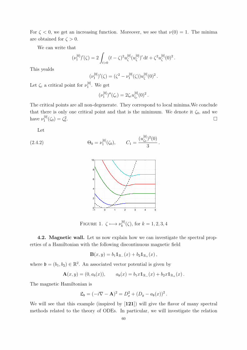
For ζ < 0, we get an increasing function. Moreover, we see that ν(0) = 1. The minima
are obtained for ζ > 0.
We can write that
(ν[0]1 )′(ζ) = 2
∫t>0
(t− ζ)2u[0]ζ (u
[0]ζ )′ dt+ ζ2u
[0]ζ (0)2 .
This yealds
(ν[0]1 )′(ζ) = (ζ2 − ν [0]
1 (ζ))u[0]ζ (0)2 .
Let ζc a critical point for ν[0]1 . We get
(ν[0]1 )′′(ζc) = 2ζcu
[0]ζc
(0)2 .
The critical points are all non-degenerate. They correspond to local minima.We conclude
that there is only one critical point and that is the minimum. We denote it ζ0, and we
have ν[0]1 (ζ0) = ζ2
0 .
Let
(2.4.2) Θ0 = ν[0]1 (ζ0), C1 =
(u[0]ζ0
)2(0)
3.
−1 0 1 2 3 4 50
2
4
6
8
10
Figure 1. ζ 7−→ ν[0]k (ζ), for k = 1, 2, 3, 4
4.2. Magnetic wall. Let us now explain how we can investigate the spectral prop-
erties of a Hamiltonian with the following discontinuous magnetic field
B(x, y) = b11R−(x) + b21R+(x) ,
where b = (b1, b2) ∈ R2. An associated vector potential is given by
A(x, y) = (0, ab(x)), ab(x) = b1x1R−(x) + b2x1R+(x) .
The magnetic Hamiltonian is
Lb = (−i∇−A)2 = D2x + (Dy − ab(x))2 .
We will see that this example (inspired by [121]) will give the flavor of many spectral
methods related to the theory of ODEs. In particular, we will investigate the relation
60
between the essential and the discrete spectra (how many eigenvalues are below the
essential spectrum?) by using the Sturm-Liouville theory, the min-max principle and
some special functions related to the de Gennes operator.
We observe that Lb = L−b, so that we may assume that b2 ≥ 0. If S denotes the
symmetry (x, y) 7→ (−x, y), we have SLb1,b2S = L−b2,−b1 = Lb2,b1 . For B > 0, we
introduce the L2-unitary transform
UBψ(x, y) = B−1/2ψ(B−1/2x,B−1/2y) .
Then we have
U−1B LbUB = B−1LBb .
These considerations allow the following reductions:
i. If b1 or b2 is zero, we may assume that b1 = 0 and, if b2 6= 0, we may assume that
b2 = 1. We call the case (b1, b2) = (0, 1) the “magnetic wall”.
ii. If b1 and b2 have opposite signs and |b1| 6= |b2|, we may only consider the case
|b1| < |b2|, and then b1 < 0 < b2 = 1. We call this case the “trapping magnetic step”.
iii. If b1 and b2 are such that |b1| = |b2|, we may only consider the cases (b1, b2) = (1, 1)
and (b1, b2) = (−1, 1).
iv. If b1 and b2 have the same sign, we may assume that 0 < b1 < b2 = 1. We call this
case the “non-trapping magnetic step”.
In order to perform the spectral analysis, we can use the translation invariance in the y-
direction and thus the direct integral decomposition (see [187, XIII.16]) associated with
the Fourier transform with respect to y, denoted by Fy:
FyLbF−1y =
∫ ⊕k∈R
hb(k) dk ,
where
hb(k) = D2x + Vb(x, k), with Vb(x, k) = (k − ab(x))2 .
The domain of hb(k) is
Dom (hb(k)) = ψ ∈ Dom (qb(k)) : (D2x + Vb(x, k))ψ ∈ L2(R) ,
where the quadratic form qb(k) is defined by
qb(k)(ψ) =
∫x∈R|ψ′(x)|2 + |(k − Vb(x, k))ψ|2 dx .
We have
sp(Lb) =⋃k∈R
sp(hb(k)) .
Notation 2.19. We denote by λb,n(k) the n-th Rayleigh quotient of hb(k). We recall
that if λb,n(k) is strictly less than the infimum of the essential spectrum, it coincides with
the n-th eigenvalue of hb(k).
61
We restrict ourselves to the case b = (0, 1). Since we have Vb(x, k) = k2 for x ≤ 0
and limx→+∞ Vb(x, k) = +∞, we easily deduce the following result.
Proposition 2.20. For b = (0, 1) and k ∈ R, the essential spectrum of hb(k) is
spess(hb(k)) = [k2,+∞) .
Moreover, sp(Lb) = [0,+∞).
In fact, we can prove slightly more.
Proposition 2.21. For b = (0, 1) and k ∈ R, the operator hb(k) has no eigenvalues
embedded in its essential spectrum.
Proof. Take λ ≥ k2 and ψ ∈ Dom (hb(k)) such that
(2.4.3) − ψ′′ + (k − ab(x))2ψ = λψ .
For x < 0, we have −ψ′′ = (λ − k2)ψ, the only solution of which in L2(R−) is zero.
But since the solutions of (2.4.3) belongs to H2loc and are in C1(R), this implies that
ψ(0) = ψ′(0) = 0, and thus ψ = 0 by the Cauchy-Lipschitz theorem.
Let us now describe the discrete spectrum, that is, the eigenvalues λ < k2. Since, for
k ≤ 0, we have qb(k) ≥ k2, we deduce the following result by the min-max principle.
Proposition 2.22. For b = (0, 1) and k ≤ 0, we have
sp(hb(k)) = spess(hb(k)) = [k2,+∞) .
Therefore, we need to analyze only the case when k > 0. The following lemma is a
reformulation of the eigenvalue problem.
Lemma 2.23. The eigenvalues λ < k2 of hb(k) are exactly the λ such that there exists
a non zero function ψ ∈ L2(R+) satisfying−ψ′′(x) + (x− k)2ψ = λψ(x),(2.4.4a)
ψ′(0)−√k2 − λψ(0) = 0 .(2.4.4b)
Moreover, the eigenfunctions of hb(k) can only vanish on R+. The eigenvalues of hb(k)
are simple.
Proof. We consider hb(k)ψ = λψ. Since ψ ∈ L2(R−), there exists A ∈ R such that,
for x ≤ 0, ψ(x) = Aex√k2−λ. Then we have to solve −ψ′′+Vb(x, k)ψ = λψ for x ≥ 0 with
the transmission conditions
ψ(0) = A and ψ′(0) = A√k2 − λ
or, equivalently,
ψ′(0)−√k2 − λψ(0) = 0 .
62

In particular, A cannot be zero. Simplicity is a consequence of the Cauchy-Lipschitz
theorem.
Lemma 2.24. The functions R+ 3 k 7→ λb,n(k) are non-decreasing.
Proof. We use the translation x = y + k to see that hb(k) is unitarily equivalent to
D2y + V (y, k) with V (y, k) = 1(−∞,−k)(y)k2 + 1(−k,+∞)(y)y2. For 0 < k1 < k2, we have
V (y, k2)− V (y, k1) = 1(−k2,−k1)(y)y2 + 1(−∞,−k2)(y)k22 − 1(−∞,−k1)(y)k2
1
≥ 1(−k2,−k1)(y)k21 + 1(−∞,−k2)(y)k2
2 − 1(−∞,−k1)(y)k21
= 1(−∞,−k2)(y)k22 − 1(−∞,−k2)(y)k2
1 ≥ 0 .
By the min-max principle, we infer the desired monotonicity.
The next lemma is a consequence of the Sturm-Liouville theory.
Lemma 2.25. Let n ∈ N be such that λb,n(k) < k2. Then, the corresponding eigenspace
is one-dimensional and is generated by a normalized function ψb,n(k), depending analyt-
ically on k, which has exactly n− 1 zeros, which are positive.
Proof. We have only to explain the part of the statement concerned with the zeros.
Thanks to Lemma 2.23, one knows that the zeros are necessarily positive. Then, we
apply the strategy of the proof of Proposition 1.32 (the integrability at infinity replaces
the cancellation of the eigenfunction).
Notation 2.26. We let E0 = 0 and, for n ≥ 1, En = 2n− 1.
By using the harmonic approximation in the semiclassical limit (see Chapter 1, Section
1 and, in this chapter, Sections 1.2 and 3.1; see also [56]), we can prove the following
lemma.
Lemma 2.27. For all n ≥ 1, we have
limk→+∞
λb,n(k) = En .
In particular, for k large enough, we have λb,n(k) ≤ En < k2.
Let us now prove that the n-th band function lies between the two consecutive Landau
levels En−1 and En.
Proposition 2.28. For all n ≥ 1 and for all k > 0 such that λb,n(k) < k2, it holds
that λb,n(k) ∈ (En−1, En).
Proof. By Lemmas 2.24 and 2.27, we have λb,n(k) < En (the strict inequality comes
from the analyticity). It remains to prove that λb,n(k) > En−1. We clearly have λb,1(k) >
E0. Let us introduce the Dirichlet realization hD(ζ) on R+ of D2t + (t − ζ)2, and its
eigenvalues (µD` (ζ))`≥1. For n ≥ 2, we consider the function ϕn(t) = ψb,n(t + zn,1(k)),
63
which satisfies hD(k− zn,1(k))ϕn = λb,n(k)ϕn and has exactly n− 2 zeros on R+. By the
Sturm oscillation theorem, ϕn is the (n−1)-th eigenfunction of hD(k−zn,1(k)). Therefore,
we have λb,n(k) = µDn−1(k − zn,1(k)). Moreover for all ` ≥ 1 and ζ ∈ R, µD
` (ζ) > E` (see
[53]). This provides the desired conclusion.
Notation 2.29. We recall (modulo a slight adaptation of the last section) that, for
all ` ≥ 1, the function ν[0]` admits a unique and non-degenerate minimum at ζ = ζ
[0]`−1,
denoted by Θ`−1, that belongs to (E`−1, E`). Moreover, ζ[0]`−1 is also the unique solution of
the equation ν[0]` (ζ) = ζ2 (see Figure 4.1).
Proposition 2.30. For all n ≥ 1, the equation λb,n(k) = k2 has a unique non-
negative solution, k = ζ[0]n−1, such that, locally, for k > kn, λb,n(k) < k2. Moreover, we
have λb,n(ζ[0]n−1) = Θn−1.
Proof. Thanks to Lemma 2.27, we can define kn = maxk ≥ 0 : λb,n(k) = k2. By
continuity, we have, for all k > kn, λb,n(k) < k2. Let us now prove the uniqueness. Let
us consider a solution kn ≥ 0. For all integers p ≥ p0 with p0 large enough, we have
λb,n
(kn + 1
p
)<(kn + 1
p
)2
. Let us now consider the eigenvalue equation
(2.4.5) D2xϕn,p + (kn,p − ab(x))2ϕn,p = λn,pϕn,p ,
where ϕn,p = ψb,n(kn,p), kn,p = kn + 1p, and λn,p = λb,n(kn,p). Let us investigate the limit
p → +∞. As seen in the proof of Lemma 2.23, we know that there exists α ∈ R∗ such
that, for x ≤ 0,
ϕn,p(x) = αex√k2n,p−λn,p .
We can relate the de Gennes eigenfunctions to the Weber functions (see for instance [1]).
Notation 2.31. We denote by U(a, x) the first Weber parabolic special function which
is solution of the linear ODE
−y′′(x) +1
4x2y(x) = −ay(x) .
It decays exponentially for x→ +∞. We let U = Re (U).
By solving (2.4.5) on x ≥ 0 and using the parabolic cylinder U function, we find that
there exists β such that, for x ≥ 0,
ϕn,p(x) = βU
(−λn,p
2;√
2(x− kn,p)).
Since ϕn,p 6= 0, we have (α, β) 6= (0, 0) and ϕn,p is C1 at x = 0, and we get the transmission
condition √k2n,p − λn,p U
(−λn,p
2;−kn,p
√2
)−√
2U ′(−λn,p
2;−kn,p
√2
)= 0 .
64
By continuity and taking the limit p→ +∞, we get
U ′
(− k
2n
2;−kn
√2
)= 0 .
Notice that the function x 7→ U(− k2
n
2;√
2(x− kn))
solves the differential equation− y′′(x) + (x− kn)2y(x) = k2
ny(x) ,
y′(0) = 0 and y(0) 6= 0
Moreover, it belongs to S(R+).
Therefore, there exists ` ≥ 1 such that ν[0]` (kn) = k2
n, and therefore kn = ζ[0]`−1 and
k2n = Θ`−1. By Proposition 2.28, we know that k2
n = λb,n(kn) ∈ [En−1, En]. Moreover, we
recall that Θ`−1 ∈ (E`−1, E`). This implies that ` = n.
Corollary 2.32. For n ≥ 1 and ζ[0]n−1 < k < ζ
[0]n , the operator hb(k) has n simple
eigenvalues below the threshold of its essential spectrum.
5. Analytic families
5.1. Kato-Rellich’s theorem. In Section 4, we proved that (L[0]ζ )ζ∈R is an “analytic
family”. In fact, this comes from the general theory of Kato (see [128, Chapter 7] and
also the older reference [189]).
Theorem 2.33. Consider a family (Lζ)ζ∈I of self-adjoint operators with compact re-
solvents that is also defined in a complex neighborhood V of I (where I is an open interval
of R). We assume that the family is holomorphic of type (A), i.e.,
i. the domain Dom (Lζ) does not depend on ζ ∈ V,
ii. for all ζ1 ∈ I, there exists r > 0, such that for all u ∈ Dom (Lζ), ζ 7→ Lζu is analytic
in B(ζ1, r).
Let ζ1 ∈ I and let Γ be a smooth contour avoiding the spectrum of Lζ1. There exists r > 0
such that if |ζ − ζ1| ≤ r, Γ avoids the spectrum of Lζ and
PΓ(ζ) =1
2iπ
∫Γ
(z − Lζ)−1 dz
is analytic near ζ1 and coincides with the orthogonal projection on the direct sum of the
eigenspaces associated with the eigenvalues of Lζ.
Moreover, if µ is an eigenvalue of Lζ1, with multiplicity m, then, in a neighborhood
of ζ1, the eigenvalues of Lζ (with ζ ∈ R) can be represented as the union of m analytic
curves (νk(ζ))k∈1,...,m intersecting at µ and there exists a corresponding analytic family
of eigenfunctions (wk(ζ))k∈1,...,m.
65
Proof. Let ζ1 ∈ I and let K be a compact set avoiding the spectrum of Lζ1 . For
z ∈ K, we write
Lζ − z = Lζ1 − z + Lζ − Lζ1 =(Id + (Lζ − Lζ1) (Lζ1 − z)−1) (Lζ1 − z) .
We let
Dzζ = (Lζ − Lζ1) (Lζ1 − z)−1 = (Lζ − Lζ1) (Lζ1 − i)−1 (Lζ1 − i) (Lζ1 − z)−1
and
A(ζ) = (Lζ − Lζ1) (Lζ1 − i)−1 , B(z) = (Lζ1 − i) (Lζ1 − z)−1
so that
Dzζ = A(ζ)B(z) .
We have already seen in Exercise 2.17 that B is analytic. Let us show that A is analytic.
In order to see this, it suffices to notice that it is pointwise analytic, i.e., ζ 7→ A(ζ)ψ is
analytic for all ψ ∈ H. Then, for all v ∈ H, we can find a sequence An(v) ∈ H such that
A(ζ)v =∞∑n=0
(ζ − ζ1)nAn(v) , ζ ∈ B(ζ1, r) .
By using the Cauchy formula (in the spirit of Exercise 2.16), we infer that ζ 7→ A(ζ) is
analytic and
A(ζ) =∞∑n=0
(ζ − ζ1)nAn, with A0 = 0 .
We will denote by RA > 0 the radius of convergence of this series.
Then we have Id +Dzζ = Id +A(ζ)B(z) and we notice that this operator is invertible
for ζ close enough to ζ1, uniformly in z ∈ K. Let us write
Id + A(ζ)B(z) =∞∑k=1
(ζ − ζ1)kak(z) ak(z) = AkB(z) ,
where the ak(z) satisfy, for r ∈ (0, RA),
rk‖ak(z)‖ ≤ ‖B‖L∞(K)M = M .
We may consider the formal inverse of the power series∑∞
k=1(ζ − ζ1)kak(z), denoted by∑k≥0(ζ−ζ1)kbk(z), where the sequence (bk(z))k≥1 is defined through the Cauchy product.
It is a classical exercise to see that
b0(z) = 1, |bk(z)| ≤ M(M + 1)k−1
rk, k ≥ 1 ,
so that the radius of convergence of∑
k≥0(ζ−ζ1)kbk(z) is at least r′ = rM+1
> 0. Moreover,
the convergence is uniform for z ∈ K and on D(ζ1,
r′
2
). We have
(Id + A(ζ)B(z))−1 =∞∑k≥0
(ζ − ζ1)kbk(z) .
66

We get
(Lζ − z)−1 = (Lζ1 − z)−1∞∑k≥0
(ζ − ζ1)kbk(z) ,
uniformly with respect to z ∈ K. It remains to integrate with respect to z on Γ.
Let us consider an eigenvalue µn(ζ1) of multiplicity m and a contour Γ enclosing only
µn(ζ1). Let us show that PΓ(ζ) has constant rank m as soon as ζ is close to ζ1. We use
an argument of Kato (see [128, I.4.6]). Choose r > 0 such that, for ζ ∈ D(ζ1, r), one has
‖PΓ(ζ)− PΓ(ζ1)‖ < 1. Let P = PΓ(ζ) and Q = PΓ(ζ1). Next, let
U = QP + (Id−Q)(Id− P ) ∈ L (range(P ), range(Q)) ,
V = PQ+ (Id− P )(Id−Q) ∈ L (range(Q), range(P )) ,
and notice that UV = V U = Id− (P −Q)2. Thus UV and V U are invertible, and so are
U and V , and then range(P ) = range(Q).
If u1, . . . , um is an eigenbasis associated with µn(ζ1), the family (PΓ(ζ)uk)k∈1,...,m is
a basis of the range of PΓ(ζ) (for ζ close enough to ζ1).
Let vk(ζ) = PΓ(ζ)uk. Then vk is analytic. Since range(PΓ(ζ)) is stable under Lζ , the
spectrum of Lζ enclosed in Γ is nothing but the spectrum of the restriction of PΓ(ζ) to this
finite-dimensional subspace. We may also orthonormalize the family (PΓ(ζ)uk)k∈1,...,m to
get an orthonormal basis depending on ζ analytically, thereby reducing the investigation
to a finite-dimensional matrix depending analytically on ζ. In this case the analytic
representation of the eigenvalues and eigenfunctions is well-known (see [128, Chapter II,
Theorem 6.1]).
5.2. An application to the Lu-Pan operator. Let us recall that LLPθ is defined
by
LLPθ = −∆ + Vθ = D2
s +D2t + Vθ ,
where Vθ is given for any θ ∈ (0, π2) by
Vθ : (s, t) ∈ R2+ 7−→ (t cos θ − s sin θ)2 .
The function Vθ reaches its minimum 0 all along the line t cos θ = s sin θ, which makes
the angle θ with ∂R2+. We denote by Dom (LLP
θ ) the domain of Lθ and we consider the
associated quadratic form QLPθ , defined by
QLPθ (u) =
∫R2
+
(|∇u|2 + Vθ|u|2
)ds dt ,
whose domain Dom (QLPθ ) is
Dom (QLPθ ) = u ∈ L2(R2
+) : ∇u ∈ L2(R2+),
√Vθ u ∈ L2(R2
+).67

Let sn(θ) denote the n-th Rayleigh quotient of LLPθ . Let us recall some fundamental
spectral properties of LLPθ when θ ∈
(0, π
2
).
It is proved in [111] that spess(LLPθ ) = [1,+∞) and that θ 7→ s1(θ) is non-decreasing.
Thanks to Corollary 1.44, we know that s1(θ) is a simple eigenvalue for(0, π
2
). One can
prove that, modulo a rotation and a rescaling, depending on θ analytically, LLPθ is an
analytic family (it satisfies (i) and (ii) in Theorem 2.33). As a consequence (we do not
really need to worry about the essential spectrum, since s1 is strictly below), we deduce
that θ 7→ s1(θ) is analytic. Then, we can show that the function (0, π2) 3 θ 7→ s1(θ) is
increasing (see [148, Lemma 3.6] and Chapter 4, Section 6.2, where a close problem is
analyzed).
5.3. The return of the Robin Laplacian. Let us continue the investigation of
the model introduced in Section 3.2.
Lemma 2.34. There exists T0 > 0 such that for all T ≥ T0, the functions
(−1/(3T ), 1/(3T )) 3 B 7−→ λ1
(LR,TB
), (−1/(3T ), 1/(3T )) 3 B 7−→ u
TB
are analytic. Here uTB is the positive normalized eigenfunction corresponding to λ1
(LR,TB
).
Proof. Let us use the change of function u = (1 − Bτ)−12 u, since the new Hilbert
space becomes L2((0, T ), dτ), the form domain is still independent from the parameter,
and the expression of the operator depends on B analytically:
(2.5.1) LR,TB = −(1−Bτ)−
12∂τ (1−Bτ)∂τ (1−Bτ)−
12 = −∂2
τ −B2
4(1−Bτ)2,
with the new Robin condition at 0 given by u′(0) =(−1− B
2
)u(0) and u(T ) = 0. The
price to pay is that the domain of the operator depends on B through the B-dependent
boundary condition. Note that the associated quadratic form is defined on H1(0, T ) by
(2.5.2) QR,TB (ψ) =
∫ T
0
|∂τψ|2 dτ −∫ T
0
B2
4(1−Bτ)2|ψ|2 dτ −
(1 +
B
2
)|ψ(0)|2 .
Thus the form domain does not depend on the parameter. This family is called a type
(B) family and there is a standard procedure to transform a type (B) family into a type
(A) family (see [128, Chapter VII, Theorem 4.2]).
6. Examples of Feynman-Hellmann formulas
In this section, we give examples of the so-called Feynman-Hellmann formulas (that
we used in Section 4).
6.1. De Gennes operator. Let us prove propositions which are often used in the
study of the magnetic Laplacian.
68
For ρ > 0 and ζ ∈ R, let us introduce the Neumann realization on R+ of
L[0]ρ,ζ = −ρ−1∂2
τ + (ρ1/2τ − ζ)2 .
By scaling, we observe that L[0]ρ,ζ is unitarily equivalent to L
[0]ζ and that L
[0]1,ζ = L
[0]ζ (the
corresponding eigenfunction is u[0]1,ζ = u
[0]ζ ).
Remark 2.35. The introduction of the scaling parameter ρ is related to the Virial
Theorem (see [204]), which was used by physicists in the theory of superconductivity
(see [60] and also [5, 39]). We also refer to the papers [179] and [183] where it is used
many times.
The domain of L[0]ρ,ζ is u ∈ B2(R+) : u′(0) = 0 and is independent of ρ and ζ, so
that the family(L
[0]ρ,ζ
)ρ>0,ζ∈R
is an analytic family of type (A) (with respect to ρ and
with respect to ζ2). The lowest eigenvalue of L[0]ρ,ζ is ν
[0]1 (ζ) and we denote by uρ,ζ the
corresponding normalized eigenfunction:
u[0]ρ,ζ(τ) = ρ1/4u
[0]ζ (ρ1/2τ) .
In order to lighten the notation and whenever there is no danger of confusion we will
write L for L[0]ρ,ζ , u for u
[0]ρ,ζ , and ν for ν
[0]1 (ζ).
The main idea is now to take derivatives of:
(2.6.1) Lu = νu
with respect to ρ and ζ. This yields the following result.
Proposition 2.36. We have
(2.6.2) (L− ν)∂ζu = 2(ρ1/2τ − ζ)u+ ν ′(ζ)u
and
(2.6.3) (L− ν)∂ρu =(−ρ−2∂2
τ − ζρ−1(ρ1/2τ − ζ)− ρ−1τ(ρ1/2τ − ζ)2)u .
Moreover, we get
(2.6.4) (L− ν)(Su) = Xu ,
where
X = −ζ2ν ′(ζ) + ρ−1∂2
τ + (ρ1/2τ − ζ)2
and
S = −ζ2∂ζ − ρ∂ρ .
Proof. Taking the derivatives with respect to ζ and ρ of (2.6.1), we get:
(L− ν)∂ζu = ν ′(ζ)u− ∂ζLu2Note that it may be extended to a holomorphic family near each (ρ, ζ). Thus the family is holomorphicwith respect to (ρ, ζ) (by Hartogs’ theorem), and not only separately in each variable.
69
and
(L− ν)∂ρu = −∂ρL .We have ∂ζL = −2(ρ1/2τ − ζ) and ∂ρL = ρ−2∂2
τ + ρ−1/2τ(ρ1/2τ − ζ).
Taking ρ = 1 and ζ = ζ0 in (2.6.2), we deduce, with the Fredholm alternative,
Corollary 2.37. We have
(L[0]ζ0− ν(ζ0))v
[0]ζ0
= 2(t− ζ0)u[0]ζ0,
with
v[0]ζ0
=(∂ζu
[0]ζ
)|ζ=ζ0
.
Moreover, ∫τ>0
(τ − ζ0)(u[0]ζ0
)2 dτ = 0 .
Corollary 2.38. We have, for all ρ > 0:∫τ>0
(ρ1/2τ − ζ0)(u[0]ρ,ζ0
)2 dτ = 0
and ∫τ>0
(τ − ζ0) (∂ρu)ρ=1,ζ=ζ0u dτ = −ζ0
4.
Corollary 2.39. We have
(L[0]ζ0− ν(ζ0))S0u =
(∂2τ + (τ − ζ0)2
)u
[0]ζ0, ,
where
S0u = −(∂ρu
[0]ρ,ζ
)|ρ=1,ζ=ζ0
− ζ0
2v
[0]ζ0.
Moreover,
‖∂τu[0]ζ0‖2 = ‖(τ − ζ0)u
[0]ζ0‖2 =
Θ0
2.
The next proposition deals with the second derivative of (2.6.1) with respect to ζ.
Proposition 2.40. We have
(L[0]ζ − ν
[0]1 (ζ))w
[0]ζ0
= 4(τ − ζ0)v[0]ζ0
+ ((ν[0]1 )′′(ζ0)− 2)u
[0]ζ0,
with
w[0]ζ0
=(∂2ζu
[0]ζ
)|ζ=ζ0
.
Moreover, ∫τ>0
(τ − ζ0)v[0]ζ0u
[0]ζ0
dτ =2− (ν
[0]1 )′′(ζ0)
4.
Proof. Taking the derivative of (2.6.2) with respect to ζ (with ρ = 1), we get:
(L[0]ζ − ν
[0]1 (ζ))∂2
ζu[0]ζ = 2ν ′(ζ)∂ζu
[0]ζ + 4(τ − ζ)∂ζu
[0]ζ + (ν ′′(ζ)− 2)u
[0]ζ .
It remains to take ζ = ζ0 and to use the Fredholm alternative.
70
6.2. Lu-Pan operator (bis). The following result was originally obtained in [19].
Proposition 2.41. For all θ ∈(0, π
2
), we have
s1(θ) cos θ − s′1(θ) sin θ > 0 .
Moreover,
limθ→π
2θ<π
2
s′1(θ) = 0 .
Proof. For γ ≥ 0, we introduce the operator
LLPθ,γ = D2
s +D2t + (t(cos θ + γ)− s sin θ)2
and we denote by s1(θ, γ) the bottom of its spectrum. Let ρ > 0 and α ∈ (0, π2) satisfy
cos θ + γ = ρ cosα and sin θ = ρ sinα.
We perform the rescaling t = ρ−1/2t, s = ρ−1/2s and obtain that LLPθ,γ is unitarily equivalent
to the operator
ρ(D2s +D2
t + (t cosα− s sinα)2) = ρLLPα .
In particular, we observe that s1(θ, γ) = ρs1(α) is a simple eigenvalue: there holds
(2.6.5) s1(θ, γ) =√
(cos θ + γ)2 + sin2 θ s1
(arctan
(sin θ
cos θ + γ
)).
Next, performing the rescaling t = (cos θ+γ)t, we get the operator LLPθ,γ which is unitarily
equivalent to LLPθ,γ :
LLPθ,γ = D2
s + (cos θ + γ)2D2t + (t− s sin θ)2 .
Note that the domain of LLPθ,γ does not depend on γ ≥ 0. Denoting by uθ,γ the L2-
normalized and positive eigenfunction of LLPθ,γ associated with s1(θ, γ), we write
LLPθ,γu
LPθ,γ = s1(θ, γ)uLP
θ,γ .
Taking the derivative with respect to γ, multiplying by uLPθ,γ, and integrating, we get the
Feynman-Hellmann formula:
∂γs1(θ, γ) = 2(cos θ + γ)
∫R2
+
|DtuLPθ,γ|2 dx ≥ 0 .
It follows that, if ∂γs1(θ, γ) = 0, then DtuLPθ,γ = 0 and uLP
θ,γ depends only on s, which is a
contradiction with uLPθ,γ ∈ L2(R2
+). Consequently, we have ∂γs1(θ, γ) > 0 for any γ ≥ 0.
An easy computation using formula (2.6.5) provides
∂γs1(θ, 0) = s1(θ) cos θ − s′1(θ) sin θ .
The function s1 is analytic and increasing. Thus we deduce
∀θ ∈(
0,π
2
), 0 ≤ s′1(θ) <
cos θ
sin θs1(θ) .
71

We get
0 ≤ lim infθ→π
2θ<π
2
s′1(θ) ≤ lim supθ→π
2θ<π
2
s′1(θ) ≤ 0 ,
which completes the proof.
72
CHAPTER 3
First semiclassical examples
Nous appelons ici intuition la sympathie par
laquelle on se transporte a l’interieur d’un
objet pour coıncider avec ce qu’il a d’unique
et par consequent d’inexprimable.
La pensee et le mouvant, Bergson
In this chapter, we give the first semiclassical examples of this book. In particular,
we essentially deal with the electric Laplacian in dimension one:
i. we prove a version of the Weyl law;
ii. we start the discussion about the harmonic approximation.
1. Semiclassical estimate of the number of eigenvalues
In this section we explain how we can estimate the number of eigenvalues of the
operator hh = h2D2x + V (x) below a given energy threshold, by using partitions of unity
and reduction to local models.
1.1. Two examples. If (L,Dom (L)) is a self-adjoint operator and E ∈ R, we recall
that N (L, E) denotes the number of eigenvalues of L below E.
Let L = HDirh = h2D2
x be the Dirichlet Laplacian on (0, 1). Its domain is just H2(0, 1)∩H1
0(0, 1) and L has compact resolvent. We can easily compute the eigenvalues:
λn(HDirh
)= h2n2π2 , n ∈ N \ 0 ,
so that, for E > 0,
N(HDirh , E
)∼h→0
√E
πh=
1
2πh
∫(x,ξ)∈(0,1)×R: ξ2≤E
dx dξ .
In the same way, we can explicitly compute the eigenvalues when L = Hharmh = h2D2
x +x2
(see Chapter 2, Section 1). We have
λn(Hharmh
)= (2n− 1)h , n ∈ N \ 0 ,
so that, for E > 0,
N(Hharmh , E
)∼h→0
E
2h=
1
2πh
∫(x,ξ)∈R2: ξ2+x2≤E
dx dξ .
73
From these examples, one could guess the more general formula
N (hh, E) ∼h→0
1
2πh
∫(x,ξ)∈R2: ξ2+V (x)≤E
dx dξ =1
πh
∫R
√(E − V )+ dx .
1.2. Weyl’s law in one dimension. We propose to prove the following version
of the Weyl law in dimension one (see Remark 3.2). It generalizes the previous two
asymptotic formulas.
Proposition 3.1. Let V : R → R be a piecewise Lipschitzian function with a finite
number of discontinuities and which satisfies:
i. V → `±∞ when x→ ±∞ with `+∞ ≤ `−∞;
ii.√
(`+∞ − V )+ belongs to L1(R).
Consider the operator hh = h2D2x + V (x) and assume that the function (0, 1) 3 h 7→
E(h) ∈ (−∞, `+∞) satisfies
i. for any h ∈ (0, 1), x ∈ R : V (x) ≤ E(h) = [xmin(E(h)), xmax(E(h))];
ii. h1/3(xmax(E(h))− xmin(E(h))) →h→0
0;
iii. E(h) →h→0
E0 ≤ `+∞.
Then
N(hh, E(h)) ∼h→0
1
πh
∫R
√(E0 − V )+ dx .
Proof. We consider a subdivision of the real axis (sj(hα))j∈Z, which contains the
discontinuities of V , for which there exist c > 0, C > 0 such that, for all j ∈ Z and h > 0,
chα ≤ sj+1(hα)− sj(hα) ≤ Chα, where α > 0 is to be determined. Denote
Jmin(hα) = minj ∈ Z : sj(hα) ≥ xmin(E(h)) ,
Jmax(hα) = maxj ∈ Z : sj(hα) ≤ xmax(E(h)) .
For j ∈ Z we introduce the Dirichlet (resp. Neumann) realization on (sj(hα), sj+1(hα)) of
h2D2x + V (x) denoted by hDir
h,j (resp. hNeuh,j ). The so-called Dirichlet-Neumann bracketing
(i.e., the application of the min-max principle and easy domain inclusions, see [187,
Chapter XIII, Section 15]) implies that
Jmax(hα)∑j=Jmin(hα)
N(hDirh,j , E(h)) ≤ N(hh, E(h)) ≤
Jmax(hα)+1∑j=Jmin(hα)−1
N(hNeuh,j , E(h)) .
Let us estimate N(hDirh,j , E(h)). If qDir
h,j denotes the quadratic form of hDirh,j , we have
qDirh,j(ψ) ≤
∫ sj+1(hα)
sj(hα)
h2|ψ′(x)|2 + Vj,sup,h|ψ(x)|2 dx, ∀ψ ∈ C∞0 ((sj(hα), sj+1(hα))) ,
where
Vj,sup,h = supx∈(sj(hα),sj+1(hα))
V (x) .
74
We infer that
N(hDirh,j , E(h)) ≥ #
n ≥ 1 : n ≤ 1
πh(sj+1(hα)− sj(hα))
√(E(h)− Vj,sup,h)+
,
so that
N(hDirh,j , E(h)) ≥ 1
πh(sj+1(hα)− sj(hα))
√(E(h)− Vj,sup,h)+ − 1 ,
and thus
Jmax(hα)∑j=Jmin(hα)
N(hDirh,j , E(h)) ≥
1
πh
Jmax(hα)∑j=Jmin(hα)
(sj+1(hα)− sj(hα))√
(E(h)− Vj,sup,h)+ − (Jmax(hα)− Jmin(hα) + 1) .
Let us consider the function
fh(x) =√
(E(h)− V (x))+
and analyze∣∣∣∣∣∣Jmax(hα)∑j=Jmin(hα)
(sj+1(hα)− sj(hα))√
(E(h)− Vj,sup,h)+ −∫Rfh(x) dx
∣∣∣∣∣∣≤
∣∣∣∣∣∣Jmax(hα)∑j=Jmin(hα)
∫ sj+1(hα)
sj(hα)
√(E(h)− Vj,sup,h)+ − fh(x) dx
∣∣∣∣∣∣+
∫ xmax(E(h))
sJmax (hα)
fh(x) dx+
∫ sJmin(hα)
xmin(E(h))
fh(x) dx
≤
∣∣∣∣∣∣Jmax(hα)∑j=Jmin(hα)
∫ sj+1(hα)
sj(hα)
√(E(h)− Vj,sup,h)+ − fh(x) dx
∣∣∣∣∣∣+ Chα .
Using the trivial inequality |√a+ −√b+| ≤
√|a− b|, we get∣∣∣fh(x)−
√(E(h)− Vj,sup,h)+
∣∣∣ ≤√|V (x)− Vj,sup,h| .
Since V is Lipschitzian on (sj(hα), sj+1(hα)), we get:∣∣∣∣∣∣
Jmax(hα)∑j=Jmin(hα)
∫ sj+1(hα)
sj(hα)
√(E(h)− Vj,sup,h)+ − fh(x) dx
∣∣∣∣∣∣ ≤ (Jmax(hα)−Jmin(hα)+1)Chαhα/2 .
This leads to the optimal choice α = 23
and we obtain the lower bound
Jmax(h2/3)∑j=Jmin(h2/3)
N(hDirh,j , E(h)) ≥ 1
πh
(∫Rfh(x) dx− Ch(Jmax(h2/3)− Jmin(h2/3) + 1)
).
75
It follows that
N(hh, E(h)) ≥ 1
πh
(∫Rfh(x) dx− Ch1/3(xmax(E(h))− xmin(E(h))− Ch
).
Note that fh(x) ≤√
(`+∞ − V (x))+, so that we can apply the dominated convergence
theorem. We can deal with the Neumann realizations in the same way.
Remark 3.2. Classical results (see [187, 190, 56, 208]) impose a fixed safety margin
below the edge of the essential spectrum (E(h) = E0 < l+∞) or deal with non-negative
potentials, V , with compact support. Both these cases are recovered by Proposition 3.1.
In our result, the maximal threshold for which one can ensure that the semiclassical
behavior of the counting function holds is dictated by the rate of convergence of the
potential towards its limit at infinity, through the assumption
h1/3(xmax(E(h))− xmin(E(h))) −→h→0
0 .
More precisely, assume that l−∞ > l+∞, so that xmin(E(h)) ≥ xmin(l+∞) is uniformly
bounded for E(h) in a neighborhood of l+∞. Then
(i) If l+∞ − V (x) ≤ Cx−γ for any x ≥ x0 and given x0, C > 0 and γ > 2, then one can
choose E(h) = l+∞ − Chρ and xmax(E(h)) ≤ h−ρ/γ, provided ρ < γ/3.
(ii) If l+∞ − V (x) ≤ C1 exp(−C2x) for any x ≥ x0 and given x0, C1, C2 > 0, then one
can choose E(h) = l+∞ − C1 exp(C2h−1/3 × o(h)) and the assumption is satisfied.
2. Harmonic approximation in dimension one
We illustrate the application of the spectral theorem in the case of the electric Lapla-
cian Lh,V = −h2∆ + V (x). We assume that V ∈ C∞(R,R), that V (x) → +∞ when
|x| → +∞, and that it admits a unique and non degenerate minimum at 0. This ex-
ample is also gives the opportunity of understanding in more detail how to construct
quasimodes in general. From a heuristic point of view, we guess that the lowest eigenval-
ues correspond to functions localized near the minimum of the potential (this intuition
comes from classical mechanics). Therefore, we can use a Taylor expansion of V near 0,
V (x) =V ′′(0)
2x2 +O(|x|3) .
We can then try to compare h2D2x + V (x) with h2D2
x +V ′′(0)
2x2.
Proposition 3.3. For all n ≥ 1, there exists a sequence (µn,j) with the property that,
for all J ≥ 1, there exist h0, C > 0 such that, for all h ∈ (0, h0),
dist
(h
J∑j=0
µn,jhj2 , sp(Lh,V )
)≤ Ch
J+12 .
Moreover, we have µn,0 = (2n− 1)√
V ′′(0)2
.
76
Proof. For reasons of homogeneity, we try the rescaling x = h1/2y. The electric
operator becomes:
Lh,V = hD2y + V (h1/2y) .
Let us use the Taylor formula
V (h1/2y) ∼ V ′′(0)
2hy2 +
∑j≥3
hj/2V (j)(0)
j!yj .
This provides the formal expansion
Lh,V ∼ h
(L0 +
∑j≥1
hj/2Lj
),
where
L0 = −∂2y +
V ′′(0)
2y2 .
We look for a quasimode and an eigenvalue in the form
u ∼∑j≥0
uj(y)hj/2, µ ∼ h∑j≥0
µjhj/2 .
Let us investigate the system of PDE that we get when solving in the formal series
Lh,V u ∼ µu .
We get the equation
L0u0 = µ0u0 .
Therefore, we can take for (µ0, u0) a L2-normalized eigenpair of the harmonic oscillator.
Then we solve
(L0 − µ0)u1 = (µ1 − L1)u0 .
We want to determine µ1 and u1. We can verify that H0− µ0 is a Fredholm operator, so
that a necessary and sufficient condition to solve this equation is
〈(µ1 − L1)u0, u0〉L2 = 0 .
Lemma 3.4. Let us consider the equation
(3.2.1) (L0 − µ0)u = f ,
with f ∈ S(R) such that 〈f, u0〉L2 = 0. The equation (3.2.1) admits a unique solution
which is orthogonal to u0, and this solution is in the Schwartz class.
Proof. Let us just sketch the proof to explain the general idea. We know that we
can find u ∈ Dom (H0) and that u is determined modulo u0, which is in the Schwartz
class. Therefore, we have y2u ∈ L2(R) and u ∈ H2(R). Let us introduce a smooth cutoff
function χR(y) = χ (R−1y). χRy2u is in the form domain of H0 as well as in the domain
of H0, so that we can write
〈L0(χRy2u), χRy
2u〉L2 = 〈[L0, χRy2]u, χRy
2u〉L2 + 〈χRy2u(µ0u+ f), χRy2u〉L2 .
77
The commutator can be easily estimated and, by dominated convergence, we find that
there exists a C > 0 such that for R large enough
‖χRy3u‖2 ≤ C .
The Fatou lemma yields
y3u ∈ L2(R) .
This is then a standard iteration procedure which gives that ∂ly(yku) ∈ L2(R). The
Sobolev injection (Hs(R) → Cs− 12 (R) for s > 1
2) gives the conclusion.
This determines a unique value of µ1 = 〈L1u0, u0〉L2 . For this value we can find a
unique u1 ∈ S(R) orthogonal to u0.
It is easy to see that this procedure can be continued at any order.
Let us consider the pairs (µj, uj) that we have constructed and introduce
UJ,h =J∑j=0
uj(y)hj/2, µJ,h = hJ∑j=0
µjhj/2 .
Let us estimate
‖(Lh,V − µJ,h)UJ,h‖ .By using the Taylor formula and the definition of the µj and uj, we have
‖(Lh,V − µJ,h)UJ,h‖ ≤ CJh(J+1)/2 ,
since h(J+1)/2‖y(J+1)/2UJ,h‖ ≤ CJh(J+1)/2 due to the fact that uj ∈ S(R). The spectral
theorem now implies
dist (µJ,h, spdis(Lh,V )) ≤ CJh(J+1)/2 .
3. Helffer-Kordyukov’s toy operator
Here we give an explicit example of construction of quasimodes for the magnetic
Laplacian in R2. We investigate the operator:
Lh,A = (hD1 + A1)2 + (hD2 + A2)2 ,
with domain
DomLh,A = ψ ∈ L2(R2) :((hD1 + A1)2 + (hD1 + A2)2
)ψ ∈ L2(R2) .
Let us state an easy lemma.
Lemma 3.5. We have
Qh,A(ψ) ≥∣∣∣∣∫
R2
hB(x)|ψ|2 dx
∣∣∣∣ , ∀ψ ∈ C∞0 (R2) .
78

Proof. This is a consequence of Proposition 0.2.
Proposition 3.6. Consider A ∈ C∞(R2,R2) such that ∇×A(x) = B(x) →|x|→+∞
+∞.
Then Lh,A has compact resolvent.
Proof. This is an application of Theorem 1.15 and Proposition 1.18.
Let us now give a simple example inspired by [103]. Let us choose A such that
B = 1 + x2 + y2. We take A1 = 0 and A2 = x + x3
3+ y2x. We study the Friedrichs
extension of
Lexh,A = h2D2
x +
(hDy + x+
x3
3+ y2x
)2
.
Proposition 3.7. There exists c ∈ R such that for all m ∈ N, there exists Cm > 0
and h0 > 0 such that, for h ∈ (0, h0),
dist(h+ (2m+ 1 + c)h2, spdis(L
exh,A)
)≤ Cmh
3 .
Proof. Let us try the rescaling x = h1/2u, y = h1/2v. We get the new operator
Lh,A = hD2u + h
(Dv + u+ h
u3
3+ hv2u
)2
.
Let us conjugate by the partial Fourier transform with respect to v; this yields the
unitarily equivalent operator
Lh,A = hD2u + h
(ξ + u+ h
u3
3+ huD2
ξ
)2
.
Let us now use the transvection u = u− ξ, ξ = ξ. We have
Du = Du, Dξ = Du +Dξ .
We are reduced to the study of
Lh,A = hD2u + h
(u+ h
(u− ξ)3
3+ h(u− ξ)(Dξ +Du)
2
)2
.
We can expand Lh,A in a formal power series
Lh,A = hP0 + h2P1 + . . . ,
where P0 = D2u + u2 and P1 = 2
3u(u− ξ)3 + (u− ξ)(Dξ +Du)
2u+ u(u− ξ)(Dξ +Du)2.
Let us look for quasimodes in the form
λ ∼ hλ0 + h2λ1 + · · · , ψ ∼ ψ0 + hψ1 + · · ·
We solve the equation
P0ψ0 = λ0ψ0 .
We take λ0 = 1 and ψ0(u, ξ) = g0(u)f0(ξ), where g0 is the first normalized eigenfunction
of the harmonic oscillator and f0 is a function to be determined. The second equation of
79
the formal system is
(P0 − λ0)ψ1 = (λ1 − P1)ψ0 .
The Fredholm condition gives, for all ξ,
〈(λ1 − P1)ψ0, g0〉L2(Ru) = 0 .
Let us analyze the different terms which appear in this differential equation. There should
be a term in ξ3. Its coefficient is: ∫Rug0(u)2 du = 0 .
For the same parity reason, there is no term in ξ. Let us now address the term in Dξ.
Its coefficient is
〈(Duu+ uDu)g0, ug0〉L2(Ru) = 0 ,
for a parity reason. In the same way, there is no term in ξD2ξ. The coefficient of ξDξ is
2
∫R(uDu −Duu)g0g0 du = 0 .
The compatibility equation reads
(aD2ξ
+ bξ2 + c)f0 = λ1f0 .
It turns out that (exercise):
a = b = 2
∫Ru2g2
0 du = 1 .
In the same way c can be explicitly found. This leads to a family of choices for (λ1, f0):
We can take λ1 = c+ (2m+ 1) and f0 = gm, the corresponding Hermite function.
This construction provides a family of quasimodes (which are in the Schwartz class)
and we can apply the spectral theorem.
Remark 3.8. One could continue the expansion at any order and one could also
consider the other possible values of λ0 (next eigenvalues of the harmonic oscillator).
Remark 3.9. The fact that the construction can be continued so far that the harmonic
oscillator appears in the picture is a clue that our initial scaling is actually the good one.
We can also guess that the lowest eigenfunctions are concentrated near zero at the scale
h1/2 if the quasimodes approximate the true eigenfunctions.
80
CHAPTER 4
From local models to global estimates
Zeno’s reasoning, however, is fallacious, when he
says that if everything when it occupies an equal
space is at rest, and if that which is in locomotion
is always occupying such a space at any moment,
the flying arrow is therefore motionless. This
is false, for time is not composed of indivisible
moments any more than any other magnitude is
composed of indivisibles.
Physics, Aristotle
In this chapter we introduce the notions of partition of unity, and of localization and
provide some examples.
1. A localization formula
We explain in this section how we can perform a reduction of the magnetic Laplacian
to local models.
1.1. Partition of unity and localization formula. Let us first introduce a qua-
dratic partition of the unity (see [2, Lemma 7.10] where this partition already appears).
Lemma 4.1. There exists C > 0 such that for all R > 0, there exists a family of
smooth cutoff functions (χj,R)j∈Z2 on Rd with the properties∑j
χ2j,R = 1,
∑j
‖∇χj,R‖2 ≤ CR−2 .
Moreover, the support of χj,R is a ball of center xj and radius R.
Proof. Take a cutoff function χ equal to 1 on B(0, 1) and to 0 away from B(0, 1),
and put
SR(x) =∑j∈Zd
χ2
(x−RjR
).
81

There exists N > 0 such that SR(x) ≤ N for all R > 0 and all x ∈ Rd. Moreover, we
have SR(x) ≥ 1 for all x ∈ Rd and thus we can define
χj,R(x) =χ(x−RjR
)S
12R(x)
.
It remains to notice that
∇SR(x) = 2R−1∑j
χj,R
(x−RjR
)∇χj,R
(x−RjR
),
so that
‖∇SR(x)‖ ≤ 2D∑j
1B(Rj,R)(x) .
By using support considerations, we get∑
j 1B(Rj,R)(x) ≤ N and ‖∇SR(x)‖ ≤ DR−1 and
easy arguments provide the control of the gradients.
The following formula is sometimes called “IMS formula” (named after Ismagilov-
Morgan-Sigal, see [46]). Actually, this formula is older: it is implicitly used in [89] (see
also [139]). Note that it also appears in the book [2, Lemma 7.11].
Proposition 4.2. We have
(4.1.1)
∀ψ ∈ Dom (Lh,A,V ) , ∀χ ∈ C∞0 (Rd) , Qh,A,V (χψ) = Re 〈Lh,A,V ψ, χ2ψ〉L2+h2‖(∇χ)ψ‖2L2 ,
and
(4.1.2) ∀ψ ∈ Dom (Qh,A,V ) , Qh,A,V (ψ) =∑j
Qh,A,V (χj,Rψ)− h2∑j
‖∇χj,Rψ‖2 .
Proof. The proof is easy and instructive. By a density argument, it is enough to
prove the formulas for ψ ∈ Dom (Lh,A,V ).
We let P = hDk + Ak and χ = χj,R. Then
〈Pψ, Pχ2ψ〉L2 = 〈χPψ, [P, χ]ψ〉L2 + 〈χPψ, Pχψ〉L2
= 〈χPψ, [P, χ]ψ〉L2 + 〈Pχψ, Pχψ〉L2 + 〈[χ, P ]ψ, Pχψ〉L2
= 〈Pχψ, Pχψ〉L2 − ‖[P, χ]ψ‖2 + 〈χPψ, [P, χ]ψ〉L2 − 〈[P, χ]ψ, χPψ〉L2 .
Taking the real part, we get
Re 〈Pψ, Pχ2ψ〉L2 = ‖Pχψ‖2 − ‖[P, χ]ψ‖2 .
We have [P, χ] = −ih∂kχ and it remains to sum over k and integrate by parts.
To get (4.1.2), we write
〈Lh,A,V ψ, ψ〉L2 =∑j
〈Lh,A,V ψ, χ2j,Rψ〉L2 ,
and apply (4.1.1).
82
Let us illustrate a possible use of (4.1.1).
Exercise 4.3. Consider(−∆x + V (x), C∞0 (RN)
), where V ∈ C0(RN ,R).
(1) Describe the domain of the adjoint.
(2) Prove that this operator is symmetric.
(3) Recall that any symmetric operator (with dense domain) is closable and that, by
definition, it is essentially self-adjoint if its closure is self-adjoint. We also recall
the characterization: (L,Dom (L)) is essentially self-adjoint iff ker(L∗± i) = 0.Prove that
(−∆x + V (x), C∞0 (RN)
)is essentially self-adjoint. For that purpose,
note that the elements of the above kernels are in H2loc(RN). Use a cutoff function
χR(x) = χ(R−1x) with χ ∈ C∞0 (Rd) equal to 1 near 0.
1.2. Harmonic approximation in dimension one (bis). In this section, we con-
tinue the analysis started in Chapter 1, Section 1. We recall that the operator is expressed
as Lh,V = h2D2x + V .
Proposition 4.4. We have
λ1(Lh,V ) = h
√V ′′(0)
2+O(h6/5) .
Proof. There exist δ0 > 0, ε0 > 0, and C > 0 such that
V (x) ≥ δ0 for |x| ≥ ε0
and ∣∣∣∣V (x)− V ′′(0)
2x2
∣∣∣∣ ≤ C|x|3 for |x| ≤ ε0 .
We introduce a partition of unity on R with balls of size r > 0 and centers xj and such
that
(4.1.3)∑j
χ2j,r = 1,
∑j
χ′2j,r ≤ Cr−2.
We may assume that x0 = 0 and that there exists c > 0 such that, for all j 6= 0, |xj| ≥ cr.
The localization formula gives
Qh,V (ψ) =∑j
Qh,V (χj,rψ)− h2∑j
‖χ′j,rψ‖2 ≥∑j
Qh,V (χj,rψ)− Ch2r−2‖ψ‖2 .
There exists c > 0 such that for j 6= 0, we have
Qh,V (χj,rψ) ≥ min(δ0, cr2)‖χj,rψ‖2 .
83
Moreover, by using a Taylor expansion and then the min-max principle for the harmonic
oscillator, we get
Qh,V (χ0,rψ) ≥∫R|hDx(χ0,rψ)|2 +
V ′′(0)
2x2|χ0,rψ|2 dx− Cr3‖χ0,rψ‖2
≥
(h
√V ′′(0)
2− Cr3
)‖χ0,rψ‖2.
We choose r = hρ for some ρ > 0 and we optimize the remainders by taking 2− 2ρ = 3ρ
and thus ρ = 25.
1.3. Magnetic example. As we are going to see, the localization formula is very
convenient for proving lower bounds for the spectrum. We consider an open bounded set
Ω ⊂ R3 and the Dirichlet realization of the magnetic Laplacian LDirh,A. Then we have the
lower bound for the lowest eigenvalues.
Proposition 4.5. For all n ∈ N∗, there exist h0 > 0 and C > 0 such that for
h ∈ (0, h0):
λn(h) ≥ minΩ‖B‖h− Ch5/4 .
Proof. We introduce a partition of unity (χj,R)j with radius R > 0. Let us consider
an eigenpair (λ, ψ). We have
Qh,A(ψ) =∑j
Qh,A(χj,Rψ)− h2∑j
‖∇χj,Rψ‖2 ,
so that
Qh,A(ψ) ≥∑j
Qh,A(χj,Rψ)− CR−2h2‖ψ‖2
and
λ‖ψ‖2 ≥∑j
Qh,A(χj,Rψ)− CR−2h2‖ψ‖2 .
It remains to provide a lower bound for Qh,A(χj,Rψ). We choose R = hρ with ρ > 0, to
be chosen. We approximate a magnetic field in each ball by the constant magnetic field
Bj:
‖B−Bj‖ ≤ C‖x− xj‖ .In a suitable gauge (using Lemma 0.3), we have
‖A−Alinj ‖ ≤ C‖x− xj‖2 ,
where C > 0 does not depend on j but only on the magnetic field. Then, we have, for
all ε ∈ (0, 1),
Qh,A(χj,Rψ) ≥ (1− ε)Qh,Alinj
(χj,Rψ)− C2ε−1R4‖χj,Rψ‖2 .
From the min-max principle, we deduce that
Qh,A(χj,Rψ) ≥((1− ε)‖Bj‖h− C2ε−1h4ρ
)‖χj,Rψ‖2 .
84
Optimizing ε, we take ε = h2ρ−1/2 and obtain
Qh,A(χj,Rψ) ≥(‖Bj‖h− Ch2ρ+1/2
)‖χj,Rψ‖2 .
We now choose ρ such that 2ρ + 1/2 = 2 − 2ρ. We are led to taking ρ = 38
and the
conclusion follows.
Exercise 4.6. This exercise aims at proving (0.1.4).
i. Let Ω be a bounded subset of R2 with 0 ∈ Ω. Assume that the magnetic field has
a positive minimum at 0 and consider the Dirichlet magnetic Laplacian. By using a
test function ψ in the form ψ(x) = χ(x)e−ρ|x|2/h, with ρ > 0 to be determined and χ
a smooth cutoff function near 0, prove that
λ1(h) = hminΩB + o(h) .
ii. Prove the same kind of asymptotic expansion in dimension three.
2. Agmon-Persson estimates
2.1. Agmon formula. This section is devoted to the Agmon formula in the semi-
classical framework. We refer to the classical references [3, 4, 96, 116, 117].
Proposition 4.7. Let Ω be an open domain in Rm with Lipschitzian boundary. Let
V ∈ C0(Ω,R), A ∈ C0(Ω,Rm), and Φ a real-valued Lipschitzian and bounded function
on Ω. Then, for u ∈ Dom (Lh,A,V ) (with Dirichlet or magnetic Neumann condition), we
have∫Ω
|(−ih∇+ A)eΦu|2 dx+
∫Ω
(V − h2|∇Φ|2
)e2Φ|u|2 dx = Re 〈Lh,A,V u, e2Φu〉L2(Ω) .
Proof. We give the proof when Φ is smooth. We use the Green-Riemann formula:
m∑k=1
〈(−ih∂k + Ak)2u, e2Φu〉L2 =
m∑k=1
〈(−ih∂k + Ak)u, (−ih∂k + Ak)e2Φu〉L2 ,
where the boundary term has disappeared thanks to the boundary condition. In order
to lighten the notation, we let P = −ih∂k + Ak. Then
〈Pu, Pe2Φu〉L2 = 〈eΦPu, [P, eΦ]u〉L2 + 〈eΦPu, PeΦu〉L2
= 〈eΦPu, [P, eΦ]u〉L2 + 〈PeΦu, PeΦu〉L2 + 〈[eΦ, P ]u, PeΦu〉L2
= 〈PeΦu, PeΦu〉L2 − ‖[P, eΦ]u‖2 + 〈eΦPu, [P, eΦ]u〉L2 − 〈[P, eΦ]u, eΦPu〉L2 .
It follows that
Re(〈Pu, Pe2Φu〉L2
)= 〈PeΦu, PeΦu〉L2 − ‖[P, eΦu]‖2 .
This is then enough to conclude.
In fact we can prove a more general localization formula (which generalizes Proposi-
tions 4.5 and 4.7).
85
Proposition 4.8 (“Localization” of P 2 with respect to A). Let (H, 〈·, ·〉) be a Hilbert
space and consider two unbounded operators P and A defined on a domain D ⊂ H.
Assume that P is symmetric and that P (D) ⊂ D, A(D) ⊂ D, and A∗(D) ⊂ D. Then, for
ψ ∈ D, we have
(4.2.1) Re 〈P 2ψ,AA∗ψ〉 = ‖P (A∗ψ)‖2 − ‖[A∗, P ]ψ‖2 + Re 〈Pψ, [[P,A],A∗]ψ〉
+ Re(〈Pψ,A∗[P,A]ψ〉 − 〈Pψ,A[P,A∗]ψ〉
).
Let us explain how Proposition 4.7 may be used. Assume that A = 0 and that u is
an eigenfunction of Lh,A,V associated with the eigenvalue E. Then, we easily get∫Ω
(V − h2|∇Φ|2 − E
)e2Φ|u|2 dx ≤ 0 .
In practice, it is natural to choose Φ such that V − h2|∇Φ|2 ≥ εV with ε ∈ (0, 1) so that
we may also write∫Ω
(εV − E)+ e2Φ|u|2 dx ≤
∫Ω
(εV − E)− e2Φ|u|2 dx ,
with ε close to 1 and where a± denotes the positive/negative part of a. Then, if Φ is
uniformly bounded (w.r.t. h) on the set εV − E ≤ 0, we get the estimate∫εV≥E
(εV − E) e2Φ|u|2 dx ≤ C
∫εV≤E
(E − εV )|u|2 dx .
This intuitively means that the function u decays exponentially away from the region
εV ≤ E (if Φ may be choosen large in this region). We will discuss many concrete
applications of this strategy.
2.2. Agmon-Persson estimates. It turns out that the estimates of Agmon are
closely related to the estimates of Persson. Those estimates state that, if an eigenfunction
of the electro-magnetic Laplacian is associated with a discrete eigenvalue smaller than
the bottom of the essential spectrum, then it has an exponential decay. The following
proposition is very convenient in concrete situations.
Proposition 4.9. Let V ∈ C0(Ω,R) bounded from below and A ∈ C1(Ω,Rm). Let us
also assume that there exist R0 > 0, µ∗ ∈ R, h0 ∈ (0, 1) such that, for all h ∈ (0, h0) and
for all ψ ∈ Dom (Lh,A,V ) with support in D(0, R0), we have
Qh,A,V (ψ) ≥ µ∗‖ψ‖2 .
Then, for h ∈ (0, h0), we have inf spess(Lh,A,V ) ≥ µ∗. Moreover, if ψ is an eigenfunction
associated with µ < µ∗, then for all ε ∈ (0,√µ∗ − µ), we have eε|x|ψ ∈ L2(Ω) and even
eε|x|ψ ∈ Dom (Qh,A,V ).
Proof. The first part of the statement is a consequence of Proposition 1.38.
86
Let ε ∈ (0,√µ∗ − µ). Let us consider the functions (χm)m≥1 defined as follows
(4.2.2) χm(s) :=
s for 0 ≤ s ≤ m,
2m− s for m ≤ s ≤ 2m,
0 for s ≥ 2m.
Note that |χ′m(s)| = 1 a.e. on [0, 2m] and |χ′m(s)| = 0 for s > 2m. By Proposition 4.7,
Qh,A,V (eεχm(|x|)ψ) ≤ µ‖eεχm(|x|)ψ‖2 + ‖(eεχm(|x|))′ψ‖2 .
But we have
‖(eεχm(|x|))′ψ‖2 ≤ ε2‖eεχm(|x|)ψ‖2 .
We get
(4.2.3) Qh,A,V (eεχm(|x|)ψ) ≤(µ+ ε2
)‖eεχm(|x|)ψ‖2 .
We consider a partition of the unity χ2R,1 + χ2
R,2 = 1 with∑2
j=1 |∇χR,j| ≤ CR−2 and
supp(χR,2) ⊂ B(0, R) (with R ≥ R0). The localization formula yields
Qh,A,V (eεχm(|x|)ψ) ≥ Qh,A,V (χR,1eεχm(|x|)ψ) + Qh,A,V (χR,2e
εχm(|x|)ψ)
− CR−2‖eεχm(|x|)ψ‖2 ,
so that
Qh,A,V (eεχm(|x|)ψ) ≥ Qh,A,V (χR,1eεχm(|x|)ψ) + µ∗‖χR,2eεχm(|x|)ψ‖2
− CR−2‖eεχm(|x|)ψ‖2 .
We deduce the existence of C(R, ε) > 0 such that, for all m ≥ 1,(µ∗ − µ− ε2 − CR−2
)‖χR,2eεχm(|x|)ψ‖2 ≤ C(R, ε)‖ψ‖2 .
Then, for R large enough, we find c(R, ε) > 0 such that, for all m ≥ 1,
c(R, ε)‖χR,2eεχm(|x|)ψ‖2 ≤ C(R, ε)‖ψ‖2 .
It follows that there exists C(R, ε) > 0 such that, for all m ≥ 1,
(4.2.4) ‖eεχm(|x|)ψ‖2 ≤ C(R, ε)‖ψ‖2 .
Then, we let m→ +∞ and use the Fatou lemma. To get the control of eε|x|ψ in the norm
of the quadratic form we use (4.2.3).
3. Applications
3.1. Harmonic approximation in dimension one (ter). We continue the anal-
ysis of Section 1.2. By Proposition 3.3, λn (Lh,V ) = O(h).
87

Proposition 4.10. For all ε ∈ (0, 1), there exist C > 0 and h0 > 0 such that, for all
h ∈ (0, h0), and all eigenfunction ψ associated with an eigenvalue of order h,
(4.3.1) ‖eεΦ0/hψ‖2 ≤ C‖ψ‖2, Qh,V (eεΦ0/hψ) ≤ Ch‖ψ‖2,
where Φ0 =∣∣∣∫ x0 √V (y) dy
∣∣∣.Proof. The proof follows the same strategy as the one of Proposition 4.9. Let
ε ∈ (0, 1). Let us consider an eigenvalue λ (= O(h)) and an associated eigenfunction ψ.
We have
Qh,V (eεχm(Φ0)/hψ) ≤ λ‖eεχm(Φ0)/hψ‖2 + h2‖(eεχm(Φ0)/h)′ψ‖2 ,
where χm is defined in (4.2.2).
We have
‖h(eεχm(Φ0)/h)′ψ‖2 ≤ ε2‖√V eεχm(Φ0)/hψ‖2 .
We let η = 1− ε2 > 0. We get
Qh,ηV (eεχm(Φ0)/hψ) ≤ Ch‖eεχm(Φ0)/hψ‖2
and thus ∫RηV e2εχm(Φ0)/h|ψ|2 dx ≤ Ch‖eεχm(Φ0)/hψ‖2 .
Given C0 > 0, we write∫RV e2εχm(Φ0)/h|ψ|2 dx =
∫|x|≥C0h1/2
V e2εχm(Φ0)/h|ψ|2 dx+
∫|x|≤C0h1/2
V e2εχm(Φ0)/h|ψ|2 dx .
Using the quadratic approximation of V at 0 and the fact that V admits a unique and
non-degenerate minimum, we deduce that there exists c > 0 such that for all C0 > 0,
there exist C, h0 > 0 such that, for h ∈ (0, h0) and all m ≥ 1,∫|x|≤C0h1/2
V e2εχm(Φ0)/h|ψ|2 dx ≤ Ch‖ψ‖2
and ∫|x|≥C0h1/2
V e2εχm(Φ0)/h|ψ|2 dx ≥ cC20h
∫|x|≥C0h1/2
e2εχm(Φ0)/h|ψ|2 dx .
Taking C0 large enough, we deduce that∫|x|≥C0h1/2
e2εχm(Φ0)/h|ψ|2 dx ≤ C‖ψ‖2 .
It follows that there exist C > 0, h0 > 0 such that, for all m ≥ 1 and h ∈ (0, h0),
‖eεχm(Φ0)/hψ‖2 ≤ C‖ψ‖2 .
Then we let m→ +∞ and use the Fatou lemma. We obtain the first estimate in (4.3.1),
and then easily deduce that
(4.3.2) Qh,V (eεΦ0/hψ) ≤ Ch‖ψ‖2.
88
Exercise 4.11. Prove that for all ζ ∈ R, we have∫R+
e2t|u[0]ζ (t)|2 dt < +∞, and
∫R+
e2t|(u[0]ζ )′(t)|2 dt < +∞ .
Proposition 4.12. For all n ≥ 1, there exists a sequence (µn,j) such that
λn (Lh,V ) ∼∑j≥0
µn,jhj2 .
Proof. For N ≥ 1, we can take a family of eigenpairs ((λn(Lh,V ), ψn,h))n=1,...,N such
that (ψn,h)n=1,...,N is an orthonormal family. We let
EN(h) = spann=1,...,N
ψn,h .
We leave as an exercise to check that the elements of EN(h) still satisfy the Agmon
estimates (4.3.1). By using these estimates of Agmon, we easily get that, for all ψ ∈EN(h),
Qh,V (ψ) ≥∫Rh2|Dxψ|2 +
V ′′(0)
2x2|ψ|2 dx− Ch3/2‖ψ‖2 .
Then, the min-max principle implies
λN(Lh,V ) ≥ (2N − 1)h
√V ′′(0)
2− Ch3/2 .
Finally, the expansion at any order of the n-th eigenvalue follows from Proposition 3.3.
It turns out that the Agmon estimates are related to the so-called WKB constructions.
We provide an example of such a construction in the following proposition (see [56,
Chapter 3] for further details and generalizations).
Proposition 4.13. For all n ≥ 1, there exist a neighborhood V of 0 and a smooth
function an,0 defined on V and h0, C > 0 such that, for all h ∈ (0, h0),∥∥∥∥∥(Lh,V − (2n− 1)h
√V ′′(0)
2
)χan,0e
−Φ0/h
∥∥∥∥∥ ≤ Ch2 ,
with Φ0 =∣∣∣∫ x0 √V (y) dy
∣∣∣ and χ a smooth cutoff function equal to 1 near 0.
Proof. We compute
(4.3.3) Lh,V(a0e−Φ0/h
)=(h2D2
xa0 − 2hDxa0DxΦ0 + ha0Φ′′0 − (Φ′0)2a0 + V a0
)e−Φ0/h
and solve
Lh,V(a0e−Φ0/h
)= λha0e
−Φ0/h .
We have (Φ′0)2 = V . Then, we consider
Φ′0∂xa0 + ∂x(Φ′0a0) = λa0 .
We have to solve this equation in a neighborhood of 0 (so that Φ′0 vanishes only at 0). It
can be explicitly solved on x > 0 and x < 0. Since we look for a smooth function a0, we
89
can check that this implies λ = (2n− 1)√
V ′′(0)2
, for n ≥ 1. Moreover an,0 behaves like sn
near 0. Finally, we write(Lh,V − (2n− 1)h
√V ′′(0)
2
)χan,0e
−Φ0/h
= χ
(Lh,V − (2n− 1)h
√V ′′(0)
2
)an,0e
−Φ0/h + [Lh,V , χ]an,0e−Φ0/h.
With support considerations, the second term in the r.h.s. is O(h∞). By using (4.3.3),
the first term in the l.h.s. is O(h2).
Proposition 4.13 can be used to prove that there are no odd powers of h12 in the
expansion given in Proposition 4.12.
3.2. A model with parameter. The Agmon estimates may be useful to analyze
the dependence of eigenvalues with respect to some parameters, especially when the
dependence of the quadratic form on the parameters is not clear. In this section, we
deal with a simple example of such a situation. For a ∈ [0, 1], we consider the Friedrichs
extension La of the differential operator,(Dx + ay + y(x2 + y2)
)2+D2
y ,
acting on C∞0 (R2). We recall that the domain of the associated quadratic form Qa is
Dom (Qa) =ψ ∈ L2(R2) : Dyψ ∈ L2(R2), (Dx + ay + y(x2 + y2))2ψ ∈ L2(R2)
.
The magnetic field is Ba(x) = a+ |x|2 and tends to +∞ when |x| → +∞. In particular,
by Proposition 3.6, La has compact resolvent. We recall that this comes from the lower
bound
(4.3.4) Qa(ψ) ≥∫R2
(a+ |x|2)|ψ|2 dx ≥∫R2
|x|2|ψ|2 dx .
We consider the lowest eigenvalue λ(a) of La.
Proposition 4.14. There exists C > 0 such that, for all a ∈ [0, 1],
|λ(a)− λ(0)| ≤ Ca .
Proof. Let us consider a normalized eigenfunction ua associated with λ(a). From
the lower bound (4.3.4) and Proposition 4.9, we have e|x|u0 ∈ L2(R2).Then
Qa(u0) = Q0(u0) + 2aRe 〈(Dx + y(x2 + y2))u0, yu0〉L2(R2) + a2‖yu0‖2L2(R2) ,
so that
λ(a) ≤ Qa(u0) ≤ λ(0) + 2a√
Q0(u0)‖yu0‖L2(R2) + a2‖yu0‖2L2(R2) ,
90
and we deduce the upper bound. Now, we know that there exists C0 > 0 such that for
all a ∈ [0, 1],
(4.3.5) λ(a) ≤ λ(0) + C0a ≤ λ(0) + C0 .
From the a-independent bounds (4.3.4) and (4.3.5) and from the proof of Proposition 4.9,
we deduce that there exists C > 0 such that, for all a ∈ [0, 1],
(4.3.6)
∫R2
e2|x||ua|2 dx ≤ C .
More precisely, this results from the fact that, for all µ∗ ≥ 2+λ0 +C0, there exists R0 > 0
such that, for all ψ supported in B(0, R0) and all a ∈ [0, 1], we have Qa(ψ) ≥ µ∗‖ψ‖2L2(R2).
We also notice that the constant in (4.2.4) does not depend on a ∈ [0, 1].
In the same way as before, we have
Q0(ua) = λ(a)− 2Re 〈〈(Dx + ay + y(x2 + y2))ua, yua〉L2(R2) + a2‖yua‖2L2(R2) ,
and thus
λ(0) ≤ Q0(ua) ≤ λ(a) + 2a√
Qa(ua)‖yua‖L2(R2) + a2‖yua‖2L2(R2) .
The conclusion easily follows since Qa(ua) = λ(a) ≤ λ(0) + C0 and with the uniform
estimate (4.3.6).
3.3. Pan-Kwek operator. By anticipating a little on a next chapter, we prove
Theorem 6.14.
3.3.1. Changing the parameters. To analyze the family of operatorsMNeux,ξ depending
on the parameters (x, ξ), we introduce the new parameters (x, η) using the change of
variables
P(x, ξ) = (x, η) =
(x, ξ +
x2
2
).
A straightforward computation shows that P : R2 → R2 is a C∞-diffeomorphism such
that
|x|+ |ξ| → +∞ ⇐⇒ |P(x, ξ)| → +∞ .
We have MNeux,ξ = NNeu
x,η , where
NNeux,η = D2
t +
((t− x)2
2− η)2
,
with Neumann condition on t = 0. Let us denote by νNeu1 (x, η) the lowest eigenvalue of
NNeux,η , so that
µNeu1 (x, ξ) = νNeu
1 (x, η) = νNeu1 (P(x, ξ)) .
We denote by Dom (QNeux,η ) the form domain of the operator and by QNeu
x,η the associated
quadratic form.
3.3.2. Existence of a minimum for µNeu1 (x, ξ). To prove Theorem 6.14, we establish
the following result:
91

Theorem 4.15. The function R×R 3 (x, η) 7→ νNeu1 (x, η) admits a minimum. More-
over, we have
lim inf|x|+|η|→+∞
νNeu1 (x, η) ≥ νMo > min
(x,η)∈R2νNeu
1 (x, η) .
To prove this, we decompose the plane into subdomains and analyze separately.
Lemma 4.16. For all (x, η) ∈ R2 such that η ≥ x2
2, we have
−∂xνNeu1 (x, η) +
√2η∂ην
Neu1 (x, η) > 0 .
Thus, there is no critical point in the domain η ≥ x2
2.
Proof. The Feynman-Hellmann formulas yield
∂xνNeu1 (x, η) = −2
∫ +∞
0
((t− x)2
2− η)
(t− x)u2x,η(t) dt,
∂ηνNeu1 (x, η) = −2
∫ +∞
0
((t− x)2
2− η)u2x,η(t) dt.
Consequently
−∂xνNeu1 (x, η)+
√2η∂ην
Neu1 (x, η) =
∫ +∞
0
(t−x−√
2η)(t−x+√
2η)(t−x−√
2η)u2x,η(t) dt .
We have ∫ +∞
0
(t− x−√
2η)2(t− x+√
2η)u2x,η(t) dt > 0 .
Lemma 4.17. It holds
inf(x,η)∈R2
νNeu1 (x, η) < νMo .
Proof. We apply Lemma 4.16 at x = 0 and η = ηMo to deduce that
∂xνNeu1 (0, ηMo) < 0 .
The following lemma is obvious.
Lemma 4.18. For all η ≤ 0, we have
νNeu1 (x, η) ≥ η2 .
In particular,
νNeu1 (x, η) > νMo, ∀η < −
√νMo .
Lemma 4.19. For x ≤ 0 and η ≤ x2
2, it holds
νNeu1 (x, η) ≥ ν
[1]1 (0) > νMo .
92
Proof. We have, for all ψ ∈ Dom (QNeux,η ), that
QNeux,η (ψ) =
∫R+
|Dtψ|2 +
((t− x)2
2− η)2
|ψ|2 dt
and ((t− x)2
2− η)2
=
(t2
2− xt+
x2
2− η)2
≥ t4
4.
The min-max principle yields
νNeu1 (x, η) ≥ ν
[1]1 (0) .
Moreover, thanks to the Feynman-Hellmann theorem, we get(∂ην
[1]1 (η)
)η=0
= −∫R+
t2u0(t)2 dt < 0 .
Lemma 4.20. There exist C,D > 0 such that for all x ∈ R and η ≥ D satisfyingx√η≥ −1, it holds that
νNeu1 (x, η) ≥ Cη1/2 .
Proof. For x ∈ R and η > 0, we can perform the change of variable
τ =t− x√η.
The operator η−2NNeux,η is unitarily equivalent to
NNeux,h = h2D2
τ +
(τ 2
2− 1
)2
,
on L2 ((−x,+∞)), with x = x√η
and h = η−3/2.
By using the harmonic approximation (see Section 1.2), we deduce that
νNeu1 (x, η) ≥ cη−3/2 ,
for η large enough.
Lemma 4.21. Let uη be an eigenfunction associated with the first eigenvalue of LMo,+η .
Let D > 0. There exist ε0, C > 0 satisfying, for all η such that |η| ≤ D, we have∫ +∞
0
e2ε0t3|uη|2 dt ≤ C‖uη‖2 .
Proof. We leave the proof to the reader as an exercise: it is sufficient to apply
Proposition 4.9.
Lemma 4.22. For all D > 0, there exist A > 0 and C > 0 such that for all |η| ≤ D
and x ≥ A, we have ∣∣∣ν1(x, η)− ν [1]1 (η)
∣∣∣ ≤ Cx−2 .
93
Proof. We perform the translation τ = t − x, so that NNeux,η is unitarily equivalent
to the operator
NNeux,η = D2
τ +
(τ 2
2− η)2
,
on L2(−x,+∞). The corresponding quadratic form writes
QNeux,η (ψ) =
∫ +∞
−x
[|Dτψ|2 +
(τ 2
2− η)2
|ψ|2]
dτ .
Let us first prove the upper bound. We take ψ(τ) = χ0(x−1τ)uη(τ). The localization
formula yields
QNeux,η (χ0(x−1τ)uη(τ)) = ν
[1]1 (η)‖χ0(x−1τ)uη(τ)‖2 + ‖(χ0(x−1τ))′uη(τ)‖2 .
Combining the min-max principle with Lemma 4.21, we infer that
ν1(x, η) ≤ ν[1]1 (η) +
‖(χ0(x−1τ))′uη(τ)‖2
‖χ0(x−1τ)uη(τ)‖2
≤ ν[1]1 (η) +
Cx−2
e2cε0x3 .
Now let us prove the lower bound. We establish the converse inequality. Denote by
ux,η the positive and L2-normalized groundstate of NNeux,η . On the one hand, with the
localization formula (4.1.1), we have
QNeux,η (χ0(x−1τ)ux,η) ≤ ν1(x, η)‖χ0(x−1τ)ux,η‖2 + Cx−2 .
On the other hand, notice that∫ +∞
−xt4|ux,η|2 dτ ≤ C,
∫ −x2
−xt4|ux,η|2 dτ ≤ C ,
and so ∫ −x2
−x|ux,η|2 dτ ≤ Cx−4 .
It follows that
QNeux,η (χ0(x−1τ)ux,η) ≤ (ν1(x, η) + Cx−2)‖χ0(x−1τ)ux,η‖2 ,
and so
ν[1]1 (η) ≤ ν1(x, η) + Cx−2 .
We have proved in Lemmas 4.18-4.20 and 4.22 that the limit inferior of ν1(x, η) in
these subdomains are not less than νMo. The existence of a minimum now follows from
Lemma 4.17.
3.4. Other applications.
94
3.4.1. Helffer-Kordyukov’s operator. Let us now apply the Agmon estimates to the
model introduced in Chapter 3, Section 3.
Proposition 4.23. There exist C > 0, h0 > 0, ε > 0 such that, for h ∈ (0, h0) and
(λ, ψ) an eigenpair of Lexh,A satisfying λ ≤ h+ Ch2, we have∫
R2
eεh−1/4|x||ψ|2 dx ≤ C‖ψ‖2 .
Proof. We consider an eigenpair (λ, ψ) as in the proposition and we use the Agmon
identity, jointly with the localization formula (with balls of size h3/8):
Qexh,A(eΦ/hδψ)− h2−2δ‖∇ΦeΦ/hδψ‖2 = λ‖eΦ/hδψ‖ ,
where δ > 0 and Φ are to be determined. For simplicity, we choose Φ(x) = ε‖x‖. We
infer that ∫R2
(hB(x, y)− h− Ch2 − 2ε2h2−2δ)|eΦ/hδψ|2 dx dy ≤ 0 .
We recall that B(x, y) = 1 +x2 + y2. We choose δ so that hh2δ = h2−2δ and we get δ = 14.
We now split the integral into two parts: for ‖x‖ ≥ C0h1/4 and for ‖x‖ ≤ C0h
1/4. If ε is
small enough, it follows that
‖eΦ/h1/4
ψ‖ ≤ C‖ψ‖ .
3.4.2. Robin Laplacian in dimension one. Consider the first L2-normalized eigenfunc-
tion uTB of LR,TB (defined in Chapter 2, Section 3). By using Proposition 2.11 and the fact
that the Dirichlet operator on (0, T ) is positive, deduce the following proposition.
Proposition 4.24. There exist T0, ε0 > 0, α > 0, and C > 0 such that for all T ≥ T0,
and for all B ∈ (−ε0T−1, ε0T
−1), it holds that,
‖eατuTB‖L2(
(0,T );(1−Bτ) dτ) ≤ C .
Let us give an example of application (that we state for further use). By using Lemma
2.34, the “Feynman-Hellmann” formulas, and Proposition 4.24, on can prove the following
lemma.
Lemma 4.25. There exist T0, ε0, C > 0 such that for all T ≥ T0 and B ∈ (−ε0T−1, ε0T
−1),∣∣∣∂Bλ1
(LR,TB
)∣∣∣ ≤ C ,(4.3.7)
‖∂BuTB ‖L2((0,T ),dτ) ≤ C .(4.3.8)
3.4.3. Semiclassical Robin Laplacian. Let Ω be a bounded, simply connected, and
smooth domain in dimension two. We consider the Robin Laplacian
(4.3.9) LRobh = −h2∆ ,
95
with domain
(4.3.10) Dom (LRobh ) = u ∈ H2(Ω) : n · h
12∇u+ u = 0 on ∂Ω .
The associated quadratic form is given by
∀u ∈ H1(Ω) , QRobh (u) =
∫Ω
|h∇u|2 dx− h32
∫∂Ω
|u|2 ds(x) ,
where ds is the surface measure on the boundary. Note that, by a classical trace theorem
(see for instance [32, Lemma 9.9] in the case of a straight boundary), the quadratic form
QRobh is well defined and bounded from below.
The following proposition (see [100]) states that the eigenfunctions associated to
(semiclassically) negative eigenvalues are concentrated in a neighborhood of size h12 of
the boundary.
Proposition 4.26. Let ε0 ∈ (0, 1) and α ∈ (0,√ε0). There exist constants C > 0
and h0 ∈ (0, 1) such that, for h ∈ (0, h0), if uh is a normalized eigenfunction of LRobh with
eigenvalue µ ≤ −ε0h, then,∫Ω
(|uh(x)|2 + h|∇uh(x)|2
)exp
(2α dist(x, ∂Ω)
h12
)dx ≤ C .
Proof. We leave the proof as an exercise and only notice that it is a consequence
(modulo a partition of unity with balls of size Rh12 with R large enough) of the fact that,
if the support of u avoids the boundary, we have QRobh (u) ≥ 0.
96
CHAPTER 5
Birkhoff normal form in dimension one
Cut away all that is excessive, straighten all
that is crooked, bring light to all that is over-
cast, labour to make all one glow of beauty.
Enneads, I. 6. 9, Plotinus
This chapter is an invitation to symplectic geometry and pseudo-differential calculus.
Therefore, we do not aim at full generality; rather we focus on an elementary application
(the Birkhoff normal form in dimension one) that will be very helpful in Chapter 15.
Since we only wish to highlight the main aspects of the proofs, we will often keep some
details in the shadow and refer to the nice available introductions to semiclassical analysis
[56, 152, 208].
1. Symplectic geometry and pseudo-differential calculus
1.1. A result of Darboux, Moser, and Weinstein.
1.1.1. Some definitions. Let us recall basic concepts related to differential forms. We
refer mainly to [208, Appendix B] for a concise introduction and to [7, Chapter 7] for
more details. We present the concepts when the dimension is even (and equals to 2d),
even if most of them do not depend on the parity of the dimension. If κ : R2d → R2d is a
smooth mapping, the pull-back by κ of a differential m-form ω on R2d, denoted by κ∗ω,
is the differential m-form defined by
∀(u1, . . . , um) ∈ (R2d)m, (κ∗ω)x(u1, . . . , um) = ωκ(x)(dκx(u1), . . . , dκx(um)) ,
where dκx is the usual differential of κ at the point x.
We say that κ is symplectic if
κ∗ω0 = ω0 , where ω0 = dξ ∧ dx .
In other words, κ is symplectic if it preserves the canonical symplectic form ω0 on R2d.
If X is a vector field on R2d and φs the associated flow, that is φ′ = X(φ), the Lie
derivative of a differential m-form ω is defined by
LXω = (∂sφ∗sω)s=0 .
The Lie derivative can be expressed thanks to the Cartan formula as
LXω = d(ιXω) + ιX dω ,
97
where ιX associates to a differential m-form ω the differential m − 1-form obtained by
replacing the first entry of ω by X.
Let us provide an abstract and fundamental example of symplectic mapping. Consider
a smooth function H (the Hamiltonian) and the vector field XH defined by dH(·) =
ω0(·, XH). The flow associated with XH , denoted by φs = esXH , is called the Hamiltonian
flow and, for all s, we have φ∗sω0 = ω0. In other words, for all s, the mapping φs : (x, ξ) 7→esXH (x, ξ) is symplectic. This can be seen from the Cartan formula. Finally, we will use
the standard definition of the Poisson bracket of smooth functions:
f, g = ω0(∇f,∇g) = ∂ξf · ∂xg − ∂xf · ∂ξg .
1.1.2. A lemma. The aim of this section is to prove the following classical result.
Lemma 5.1. Let ω0 and ω1 be two 2-forms on R2d which are closed and non-degenerate.
Assume that ω1 = ω0 on 0 × Ω, where Ω is a bounded open set of R2d−1. In a neigh-
borhood of 0 × Ω there exists a change of coordinates ψ1 such that
ψ∗1ω1 = ω0 and ψ1 = Id +O(x21) .
Proof. The reader is referred to [155, p. 92].
Let us explain how we can find a 1-form σ on R2d such that, in a neighborhood of
0 × Ω,
τ = ω1 − ω0 = dσ and σ = O(x21) .
In other words, we want to establish an explicit Poincare lemma. For that purpose we
introduce the family of diffeomorphisms (φt)0<t≤1 defined by
φt(x1, x) = (tx1, x)
and we let
φ0(x1, x) = (0, x) .
We have
(5.1.1) φ∗0τ = 0 and φ∗1τ = τ .
Denote by Xt the vector field associated with φt. We have
Xt =dφtdt
(φ−1t ) = (t−1x1, 0) = t−1x1e1 .
Let us compute the Lie derivative of τ along Xt,
d
dtφ∗t τ = φ∗tLXtτ .
The Cartan formula yields
LXt = ι(Xt) dτ + d(ι(Xt)τ) .
98

Since τ is closed on R2d, we have dτ = 0. It follows that
(5.1.2)d
dtφ∗t τ = d(φ∗t ι(Xt)τ) .
We consider the 1-form
σt = φ∗t ι(Xt)τ = x1τφt(x1,x2,ξ1,ξ2)(e1,∇φt(·)) = O(x21) .
We see from (5.1.2) that the map t 7→ φ∗t τ is smooth on [0, 1]. To conclude, let σ be
the 1-form defined on a neighborhood of 0 ×Ω by σ =∫ 1
0σt dt; it follows from (5.1.1)
and (5.1.2) thatd
dtφ∗t τ = dσt and τ = dσ .
Finally, we use a standard deformation argument due to Moser. For t ∈ [0, 1], we let
ωt = ω0 + t(ω1 − ω0) .
The 2-form ωt is closed and non degenerate (up to choosing a neighborhood of x1 = 0
small enough). We look for ψt such that
ψ∗tωt = ω0 .
For that purpose, let us determine a vector field Yt such that
d
dtψt = Yt(ψt) .
By using again the Cartan formula, we get
0 =d
dtψ∗tωt = ψ∗t
(d
dtωt + ι(Yt) dωt + d(ι(Yt)ωt)
).
This becomes
ω0 − ω1 = d(ι(Yt)ωt) .
We are led to solving
ι(Yt)ωt = −σ .By the non-degeneracy of ωt, this determines Yt. Since Yt vanishes on 0 × Ω, there
exists a neighborhood of 0×Ω small enough in the x1-direction, such that ψt exists up
to time t = 1 and satisfies ψ∗tωt = ω0. Since σ = O(x21), we get ψ1 = Id +O(x2
1).
1.2. Pseudo-differential calculus.
1.2.1. Symbols. Here we refer to [56, Chapter 7] and [208, Chapter 4].
A function m : R2d → [0,∞) is an order function if there exist constants N0, C0 > 0
such that
m(X) ≤ C0〈X − Y 〉N0m(Y )
for any X, Y ∈ R2d. For δ ∈(0, 1
2
), the symbol class Sδ(m) is the space of smooth
h-dependent functions ah : R2d → C such that
∀α ∈ N2d, |∂αxah(x)| ≤ Cαh−|α|δm(x), ∀h ∈ (0, 1].
99
We let S(m) = S0(m). For a classical symbol ah = a(x, ξ;h) ∈ Sδ(m), the Weyl quanti-
zation of a is defined as
(5.1.3) Opwh a (ψ)(x) =1
(2πh)d
∫R2d
ei〈x−y,ξ〉/ha
(x+ y
2, ξ
)ψ(y) dy dξ, ∀ψ ∈ S(Rd) .
It can be proved that the integral in (5.1.3) is actually convergent thanks to a succession
of integrations by parts and that Opwh (a) sends S(Rd) into S(Rd).
If m1 and m2 are order functions and if a ∈ Sδ(m1) and b ∈ Sδ(m2), we define the
Moyal product of a and b by letting
a ? b(x, ξ) = eih2ω0(Dx,Dξ,Dy ,Dη)a(x, ξ)b(y, η)|(y,η)=(x,ξ)
and
a ? b ∈ Sδ(m1m2) , Opwh (a ? b) = Opwh (a)Opwh (b) ,
as operators acting on S(Rd). Note that the verification is just a computation using the
inverse Fourier transform when a and b belong to S(Rd).
Moreover, thanks to the exponential expression and by the Taylor formula, the Moyal
product can be expanded in the sense of the S(m1m2)-topology as
a ? b = ab+h
2ia, b+OS(m1m2)(h
2−4δ) .
We recall the so-called Borel theorem: If (aj)j≥0 is a sequence of symbols in Sδ(m),
there exists a symbol in Sδ(m) such that
a ∼+∞∑j=0
hjaj, in Sδ(m) .
We will sometimes use the Calderon-Vaillancourt theorem: If a ∈ S(1), then Opwh (a)
is a bounded operator from L2(Rd) to L2(Rd) and
‖Opwh a‖ ≤∑|α|≤Md
supRd‖∂αa‖ .
Another important and classical theorem in the pseudo-differential theory is the Garding
inequality : If a ∈ S(1) is a real symbol such that a ≥ 0, then there exist C > 0, h0 > 0
such that, for all ψ ∈ L2(Rd) and h ∈ (0, h0),
〈Opwh aψ, ψ〉 ≥ −Ch‖ψ‖2 .
1.2.2. Egorov theorems. We now recall the following classical result (see for instance
[208, Theorem 11.1] and [190, Theoreme IV.10]).
Theorem 5.2 ([208, Theorem 11.1, Remark (ii)]). Let P and Q be h-pseudo-differential
operators on Rd, with P ∈ S(1) and Q ∈ S(1). Then the operator eihQPe−
ihQ is a pseudo-
differential operator in S(1), and
eihQPe−
ihQ − Opwh (p κ) ∈ hS(1).
100
Here p is the Weyl symbol of P , and the canonical transformation κ is the time-1 Hamil-
tonian flow associated to principal symbol of Q.
From this classical version of Egorov’s theorem, one can deduce the following refine-
ment that is useful when P does not belong to S(1) (see [108, Appendix]).
Theorem 5.3. Let P and Q be h-pseudo-differential operators on Rd, with P ∈ S(m)
and Q ∈ S(m′), where m and m′ are order functions such that
(5.1.4) m′ = O(1) , mm′ = O(1) .
Then eihQPe−
ihQ is a pseudo-differential operator in S(m), and we have e
ihQPe−
ihQ−
Opwh (p κ) ∈ hS(1).
2. Birkhoff normal form
This section provides some insight concerning the semiclassical Birkhoff normal form
in the simple case of the operator h2D2x + V (x). We will consider
Opwh (H) = h2D2x + V (x), H(x, ξ) = ξ2 + V (x) ,
where V is a standard symbol so that, for some order function m, H ∈ S(m). In this
section we follow the spirit of [40, 202] (see also [201]).
The aim of this section is to prove the following eigenvalue estimate (which improves
the result of Proposition 4.12).
Theorem 5.4. Let η ∈ (0, 1). There exists a smooth function f ? with compact support
arbitrarily small and satisfying |f ?(Z, h)| = O((Z + h)32 ) as (Z, h) → 0 such that the
eigenvalues of the operators Opwh (H) and Opwh (|z|2)+f ? (Opwh (|z|2) , h) below hη coincide
modulo O(h∞). Moreover, if we let
Nh =n ∈ N∗ : (2n− 1)h ≤ h
12
,
and if λn(h) is the n-th eigenvalue of Opwh (H), then
λn(h) = (2n− 1)h+O(h32 ) ,
uniformly for n ∈ Nh and h ∈ (0, h0).
2.1. Formal series and homological equations. We introduce the space of formal
series E = R[[x, ξ, h]]. We endow E with the Moyal product (compatible with the Weyl
quantization) denoted by ?.
Notation 5.5. The degree of xαξβhl is α + β + 2l. DN denotes the space of the
monomials of degree N . ON is the space of formal series with valuation at least N . For
τ, γ ∈ E, we denote adτγ = [τ, γ] = τ ? γ − γ ? τ . We notice that [ON1 ,ON2 ] ⊂ ON1+N2.
101
Lemma 5.6. We let z = x+ iξ. We have
E = ker|z|2, · ⊕ Im|z|2, · ,
where the Poisson bracket is given by
f, g =∂f
∂ξ
∂g
∂x− ∂f
∂x
∂g
∂ξ=
1
i
(∂f
∂z
∂g
∂z− ∂f
∂z
∂g
∂z
),
where∂
∂z=
1
2
(∂
∂x− i ∂
∂y
),
∂
∂z=
1
2
(∂
∂x+ i
∂
∂y
).
Proof. The family(zαzβhγ
)(α,β,γ)∈N3 is a basis of E . Then it is sufficient to notice
that |z|2,DN ⊂ DN and
|z|2, zαzβ =2
i(α− β)zαzβ .
Proposition 5.7. Given γ ∈ O3, there exist formal power series τ, κ ∈ O3 such that
eih−1adτ (|z|2 + γ) = |z|2 + κ ,
with [κ, |z|2] = 0.
Proof. First, we notice that ih−1adτ sends ON into ON+1, so that the exponential
is well defined in the formal series. Then, we proceed by induction. Let N ≥ 1. Assume
that we have, for N ≥ 1 and τN ∈ O3,
eih−1adτN (|z|2 + γ) = |z|2 +K3 + · · ·+KN+1 +RN+2 +ON+3 ,
where Ki ∈ Di commutes with |z|2 and where RN+2 ∈ DN+2.
Let τ ′ ∈ DN+2. A computation yields
eih−1adτN+τ ′ (|z|2 + γ) = H0 +K3 + · · ·+KN+1 +KN+2 +ON+3,
with
KN+2 = RN+2 + ih−1adτ ′|z|2 = RN+2 − ih−1ad|z|2τ′ ,
We can write
RN+2 = KN+2 + ih−1ad|z|2τ′ .
Note that ih−1ad|z|2 = |z|2, ·. Using Lemma 5.6, we deduce the existence of τ ′ and
KN+2 such that KN+2 commutes with |z|2.
2.2. Quantizing. Let us now quantize the formal procedure.
Proposition 5.8. There exist a real and compactly supported symbol c(x, ξ, h) and a
smooth function f ? with arbitrarily small compact support such that:
eih−1Opwh (c)Opwh (H) e−ih
−1Opwh (c)
102
is a pseudo-differential operator in S(m) and
eih−1Opwh (c)Opwh (H) e−ih
−1Opwh (c) = Nh + Opwh (sh) + h∞S(1) ,
where
i. Nh = Opwh (|z|2) + f ? (Opwh (|z|2) , h),
ii. sh is a symbol in S(m) whose Taylor series at (0, 0, 0) is zero,
iii. f ? satisfies |f(Z, h)| ≤ C(|Z|2 + h|Z|+ h2).
Proof. Thanks to the Borel lemma, we can find a smooth function with compact
support c(x, ξ, h) whose Taylor series at (0, 0, 0) is the series τ given in Proposition 5.7.
In particular, Opwh (c) is a bounded self-adjoint operator (by, for instance, the Calderon-
Vaillancourt theorem). Then, we consider the conjugate operator
eih−1Opwh (c)Opwh (H) e−ih
−1Opwh (c) ,
which is a pseudo-differential operator with symbol Nh, by the Egorov theorem. By the
Taylor formula, we can write
eih−1Opwh (c)Opwh (H) e−ih
−1Opwh (c) =N∑n=0
1
n!adnih−1Opwh (c)Op
wh (H)
+h−N−1
N !
∫ 1
0
(1− t)Neith−1Opwh (c)adN+1ih−1Opwh (c)Op
wh (H) e−ith
−1Opwh (c) dt .
By the Egorov theorem, the integral remainder
h−N−1
N !
∫ 1
0
(1− t)Neith−1Opwh (c)adN+1ih−1Opwh (c)Op
wh (H) e−ith
−1Opwh (c) dt
is a pseudo-differential operator whose symbol admits a Taylor expansion in ON+1. More-
over, the symbol ofN∑n=0
1
n!adnih−1Opwh (c)Op
wh (H)
admits a Taylor expansion that coincides with |z|2 + κ modulo ON+1. In other words,
the Taylor series of Nh is |z|2 + κ, where κ has the form∑
k+`≥1 dk,`|z|2kh`. Using again
the Borel lemma, we can find a smooth function f(I, h) with compact support (as small
as we want) such that its Taylor series at (0, 0) is∑k+`≥1
dk,`I2kh` .
We have
eih−1Opwh (c)Opwh (H) e−ih
−1Opwh (c) = Opwh(|z|2)
+ Opwh(f(|z|2, h)
)+ Opwh (Rh) ,
with Rh = Opwh (rh), where the Taylor series of rh at (0, 0, 0) is 0.
103
Note that κ can also be written in the form∑
k+`≥1 d?k,` (|z|2)
?kh` and we may also
find a smooth function f ?(I, h), with support arbitrarily small, with Taylor series∑k+`≥1
d?k,`I2kh` ,
and we have, by using the Taylor formula and the functional calculus of pseudo-differential
operators (see [56, Theorem 8.7] for a detailed presentation) to estimate the Taylor
remainder,
Opwh(|z|2)
+ Opwh(f(|z|2, h)
)= Opwh
(|z|2)
+ f ?(Opwh(|z|2), h) + Opwh
(Rh
)+ h∞S(1) ,
where Rh = Opwh (rh) and the Taylor series of rh at (0, 0, 0) is 0.
2.3. Microlocalizing. First, we have the following.
Lemma 5.9. It holds that
N (Nh, β) = O(h−1) .
Proof. If the support of f ? is small enough, for all ε ∈ (0, 1), we have, for all
ψ ∈ C∞0 (R) and h small enough,
(5.2.1) 〈Nhψ, ψ〉 ≥ (1− ε)〈Opwh (|z|2)ψ, ψ〉 .
Thus, by the min-max principle, we infer that
N (Nh, β) ≤ N(Opwh (|z|2), (1− ε)−1β
)and the result follows by counting the eigenvalues of the harmonic oscillator.
Then, we can use the Weyl asymptotic estimate (see for instance Chapter 3, Propo-
sition 3.1).
Lemma 5.10. If β ∈(
0, lim inf|x|→+∞
V
), we have
N (Opwh (H), β) = O(h−1) .
The following proposition is devoted to microlocalization estimates of the eigenfunc-
tions of Opwh (H) and Nh.
Proposition 5.11. Let η ∈ (0, 1), δ ∈(0, η
2
), and χ a smooth cutoff function sup-
ported away from a compact neighborhood of 0. Then, there exists h0 > 0 such that for
all h ∈ (0, h0), all eigenvalue λ of Opwh (H) or of Nh such that λ ≤ hη, and all associated
eigenfunction ψ, we have
‖Opwh (χ(h−δ(x, ξ)))ψ‖L2(R) = O(h∞)‖ψ‖L2(R) .
Proof. Let us prove this for the eigenfunctions of Nh. We write the eigenvalue
equation
Nhψ = λψ .
104
We have
NhOpwh (χ(h−δ(x, ξ))))ψ = λOpwh (χ(h−δx))ψ + [Nh,Opwh (χ(h−δ(x, ξ)))]ψ .
Taking the scalar product with Opwh (χ(h−δ(x, ξ)))ψ yields
〈NhOpwh (χ(h−δ(x, ξ)))ψ,Opwh (χ(h−δ(x, ξ)))ψ〉L2(R) ≤ hη‖Opwh (χ(h−δ(x, ξ)))ψ‖2L2(R)
+ 〈[Nh,Opwh (χ(h−δ(x, ξ)))]ψ,Opwh (χ(h−δ(x, ξ)))ψ〉L2(R) .
We use again the lower bound (5.2.1) to get
〈NhOpwh (χ(h−δ(x, ξ)))ψ,Opwh (χ(h−δ(x, ξ)))ψ〉L2(R)
≥ (1− ε)〈Opwh(|z|2)Opwh (χ(h−δ(x, ξ)))ψ,Opwh (χ(h−δ(x, ξ)))ψ〉 .
By a rescaling (x, ξ) = hδ(x, ξ), a support consideration, and the Garding inequality with
semiclassical parameter h1−2δ, we get
〈Opwh(|z|2)Opwh (χ(h−δ(x, ξ)))ψ,Opwh (χ(h−δ(x, ξ)))ψ〉
≥ h2δ(1− Ch1−2δ)‖Opwh (χ(h−δ(x, ξ)))ψ‖2L2(R) ,
whence
〈NhOpwh (χ(h−δ(x, ξ)))ψ,Opwh (χ(h−δ(x, ξ)))ψ〉L2(R)
≥ (1− ε)(h2δ − Ch1−2δ)‖Opwh (χ(h−δ(x, ξ)))ψ‖2L2(R) ,
and thus
((1− ε)(h2δ − Ch)− hη)‖Opwh (χ(h−δ(x, ξ)))ψ‖2L2(R)
≤ 〈[Nh,Opwh (χ(h−δ(x, ξ)))]ψ,Opwh (χ(h−δ(x, ξ)))ψ〉L2(R) .
The pseudo-differential operator [Nh,Opwh (χ(h−δ(x, ξ)))] has a symbol in the standard
class Sδ(m) (here we have δ ∈(0, 1
2
)). Its symbol is supported in supp(χ(h−δ(x, ξ)))
modulo h∞Sδ(1) and its main term is of order h1−2δ. Therefore, if we consider a cutoff
function χ supported on a slightly bigger set than χ, we obtain
((1− ε)(h2δ − Ch)− hη)‖Opwh (χ(h−δ(x, ξ)))ψ‖2L2(R) ≤ Ch1−2δ‖Opwh (χ(h−δ(x, ξ)))ψ‖2
L2(R) .
This implies the existence of δ > 0 such that
‖Opwh (χ(h−δ(x, ξ)))ψ‖2L2(R) ≤ Chδ‖Opwh (χ(h−δ(x, ξ)))ψ‖2
L2(R) .
Then the result follows via an iterative argument, by replacing χ by χ.
It is now easy to deduce the following.
Corollary 5.12. Let η ∈ (0, 1), δ ∈(0, η
2
), and χ a smooth cutoff function supported
away from a compact neighborhood of 0. Then, there exists h0 > 0 such that for all
105
h ∈ (0, h0), and for all ψ ∈ 1[−∞,hη)(Nh) or ψ ∈ 1[−∞,hη)(Opwh (H)), we have
‖Opwh (χ(h−δ(x, ξ)))ψ‖L2(R) = O(h∞)‖ψ‖L2(R) .
Proof. By Proposition 5.11, the estimate is clear when ψ is an eigenfunction. Thanks
to Lemmas 5.9 and 5.10, we have
dim range(1[−∞,hη)(Nh)
)= O(h−1), dim range
(1[−∞,hη)(Op
wh (H))
)= O(h−1) .
In particular, these numbers of eigenvalues below hη do not increase more than polyno-
mially in h−1. Then, the result follows by considering orthonormal bases of the spaces
range(1[−∞,hη)(Nh)
)and range
(1[−∞,hη)(Op
wh (H))
)and by applying Proposition 5.11 to
the elements of these bases.
2.4. Spectral estimates. We have now all the tools to deduce Theorem 5.4. It es-
sentially follows from an application of the min-max principle. Consider the sequence of
the eigenvalues of Nh, denoted by (λj(Nh))j≥1. Consider an associated orthonormal fam-
ily of eigenfunctions (ψj,h)≥1. LetM be a positive integer smaller than dim range(1[−∞,hη)(Nh)
).
With the notations of Proposition 5.8, we let
ϕj,h = e−ih−1Opwh (c)ψj,h
and we introduce
Vh = span1≤j≤M
ϕj,h .
Then, with Proposition 5.8, for all ϕ ∈ Vh we have
〈Opwh (H)ϕ, ϕ〉 ≤ λM(Nh)‖ψ‖2L2(R) + 〈Opwh (sh)ψ, ψ〉+O(h∞)‖ψ‖2
L2(R) ,
with ψ = eih−1Opwh (c)ϕ. Thanks to Corollary 5.12 and the fact that the Taylor series
of sh with respect to (x, ξ, h) is zero at (0, 0, 0), we deduce, by symbolic calculus for
pseudo-differential operators, that
|〈Opwh (sh)ψ, ψ〉| = O(h∞)‖ψ‖2L2(R) .
From the min-max principle, we infer that the M -th eigenvalue λM(h) of Opwh (H) satisfies
λM(h) ≤ λM(Nh) +O(h∞) .
We leave the proof of the opposite inequality to the reader. The rest of the proof of the
theorem easily follows from the functional calculus for self-adjoint operators.
106
Part 2
Main theorems

CHAPTER 6
Spectral reductions
The soul unfolds itself, like a lotus of countless petals.
The Prophet, Self-Knowledge, Kahlil Gibran
In this chapter we introduce a model operator (depending on parameters). It appears
in dimension two when studying vanishing magnetic fields in the case when the cancella-
tion line of the field intersects the boundary. Though this model seems very specific, we
will see how it can lead to a quite general strategy: the (magnetic) Born-Oppenheimer
approximation and its relations to WKB constructions.
1. Vanishing magnetic fields and boundary
1.1. Why considering vanishing magnetic fields? A motivation is related to
the papers of R. Montgomery [160], X-B. Pan and K-H. Kwek [170] and B. Helffer
and Y. Kordyukov [102] (see also [109], [97] and the thesis of Miqueu [157]) where the
authors analyze the spectral influence of the cancellation of the magnetic field in the
semiclassical limit. Another motivation appears in the paper [57], where the authors are
concerned with “magnetic waveguides” and inspired by physical considerations [188, 95]
(see also [123]). In any case, treating vanishing magnetic fields can inspire the analysis
of non-trivial examples of magnetic normal forms, as we will see later.
1.2. Montgomery operator. Without going into detail, let us describe the model
operator introduced in [160]. Montgomery was concerned by the magnetic Laplacian
(−ih∇ + A)2 on L2(R2) in the case when the magnetic field B = ∇×A vanishes along
a smooth curve Γ. Assuming that the magnetic field vanishes in non-degenerate way, he
was led to considering the self-adjoint realization on L2(R2) of
L = D2t + (Ds − st)2 .
In this case the magnetic field is given by β(s, t) = s so that the zero locus of β is the
line s = 0. Let us make the following change of gauge
LMo = e−is2t2 L ei
s2t2 = D2
s +
(Dt +
s2
2
)2
.
The Fourier transform (after changing ζ to −ζ) with respect to t gives the direct integral
LMo =
∫ ⊕L
[1]ζ dζ, where L
[1]ζ = D2
s +
(ζ − s2
2
)2
.
109
Note that this family of model operators will be seen as a special case of a more general
family in Section 2.2. Let us recall a few important properties of the lowest eigenvalue
ν[1]1 (ζ) of L
[1]ζ (for the proofs, see [170, 98, 115]).
Proposition 6.1. The following properties hold:
i. For all ζ ∈ R, ν[1]1 (ζ) is simple.
ii. The function ζ 7→ ν[1]1 (ζ) is analytic.
iii. lim|ζ|→+∞
ν[1]1 (ζ) = +∞.
iv. The function ζ 7→ ν[1]1 (ζ) has a unique minimum at a point ζ
[1]0 and it is non-
degenerate.
We have
(6.1.1) sp(L) = spess(L) = [νMo,+∞) ,
with νMo = ν[1]1 (ζ
[1]0 ). With a finite element method and the Dirichlet condition on
the artificial boundary, a upper bound of the minimum was obtained in [115, Table 1]
and the numerical simulations provided νMo ' 0.5698, reached for ζ[1]0 ' 0.3467 with
a discretization step at 10−4 for the parameter ζ. This numerical estimate is already
mentioned in [160]. In fact, we can prove the following lower bound (see [23] for a proof
using the Temple inequality).
Proposition 6.2. We have νMo ≥ 0.5.
If we consider the Neumann realization L[1],+ζ of D2
s +(ζ − s2
2
)2
on R+, then, by
symmetry, the bottom of the spectrum of this operator is linked to the Montgomery
operator:
Proposition 6.3. If we denote by ν[1],+1 (ζ) the bottom of the spectrum of L
[1],+ζ , then
ν[1],+1 (ζ) = ν
[1]1 (ζ) .
1.3. Generalized Montgomery operators. It turns out that we can generalize
the Montgomery operator by allowing a higher order of degeneracy of the magnetic field.
Let k be a positive integer. The generalized Montgomery operator of order k is the
self-adjoint realization on R defined by
L[k]ζ = D2
t +
(ζ − tk+1
k + 1
)2
.
The following result (which generalizes Proposition 6.1) is proved in [83, Theorem 1.3].
Theorem 6.4. ζ 7→ ν[k]1 (ζ) has a unique and non-degenerate minimum at ζ = ζ
[k]0 .
Notation 6.5. For real ζ, the lowest eigenvalue of L[k]ζ is denoted by ν
[k]1 (ζ) and we
denote by u[k]ζ the positive and L2-normalized eigenfunction associated with ν
[k]1 (ζ). We
denote in the same way its holomorphic extension near ζ[k]0 .
110
1.4. A broken Montgomery operator.
1.4.1. Heuristics and motivation. As mentioned above, the bottom of the spectrum
of L is essential. This fact is due to the translation invariance along the zero locus of B.
This situation reminds of what happens in the framework of waveguides. Guided by the
ideas developed for waveguides, we aim at analyzing the effect of breaking the zero locus
of B. Introducing the “breaking parameter” θ ∈ (−π, π], we will break the invariance of
the zero locus in two different ways:
i. Case of Dirichlet boundary: LDirθ . We let R2
+ = (s, t) ∈ R2, t > 0 and consider the
Dirichlet realization LDirθ on L2(R2
+) of
D2t +
(Ds +
t2
2cos θ − st sin θ
)2
.
ii. Case of Neumann boundary: LNeuθ . We consider the Neumann realization LNeu
θ on
L2(R2+) of
D2t +
(Ds +
t2
2cos θ − st sin θ
)2
.
The corresponding magnetic field is B(s, t) = t cos θ − s sin θ. It vanishes along the
half-line t = s tan θ.
Notation 6.6. We use the notation L•θ, where • can be Dir, Neu.
1.4.2. Properties of the spectra. Let us analyze the dependence of the spectra of L•θon the parameter θ. Denoting by S the axial symmetry (s, t) 7→ (−s, t), we get:
L•−θ = SL•θS ,
where the overline denotes complex conjugation. Then, we notice that L•θ and L•θ are
isospectral. Therefore, the analysis is reduced to θ ∈ [0, π). Moreover, we get:
SL•θS = L•π−θ ,
so the study is reduced to θ ∈[0, π
2
].
We observe that the domain of L•θ is not continuous at θ = 0 and θ = π2.
Lemma 6.7. The family (L•θ)θ∈(0,π2 ) is analytic of type (A).
The following proposition states that the infimum of the essential spectrum is the
same for LDirθ , LNeu
θ , and Lθ.
Proposition 6.8. For θ ∈(0, π
2
), we have inf spess(L
•θ) = νMo.
In the Dirichlet case, the spectrum is essential.
Proposition 6.9. For all θ ∈(0, π
2
), we have sp(LDir
θ ) = [νMo,+∞).
Notation 6.10. Let us denote by λ•n(θ) the n-th number in the sense of the Rayleigh
variational formula for L•θ.
111

The following proposition (the proof of which can be found in [170, Lemma 5.2])
states that LNeuθ admits an eigenvalue below its essential spectrum when θ ∈
(0, π
2
].
Proposition 6.11. For all θ ∈(0, π
2
], λNeu
1 (θ) < νMo.
1.5. Singular limit.
1.5.1. Normalization. Thanks to Proposition 6.11, one knows that breaking the in-
variance of the zero locus of the magnetic field with a Neumann boundary creates a bound
state. We also would like to tackle this question for Lθ and in any case to estimate more
quantitatively this effect. A way to do this is to consider the limit θ → 0, which reveals
new model operators.
Notation 6.12. We let h = tan θ.
First, we perform a scaling:
(6.1.2) s = h−1(cos θ)−1/3σ, t = (cos θ)−1/3τ .
The operator LNeuθ is thus unitarily equivalent to (cos θ)2/3LNeu
tan θ, where the expression of
LNeutan θ is given by
(6.1.3) D2τ +
(hDσ +
τ 2
2− στ
)2
.
1.5.2. New model operators. We are led to two families of one-dimensional operators
on L2(R2Neu) with two parameters (x, ξ) ∈ R2:
MNeux,ξ = D2
τ +
(−ξ − xτ +
τ 2
2
)2
.
These operators have compact resolvents and form analytic families with respect to the
variables (x, ξ) ∈ R2.
Notation 6.13. We denote by µNeun (x, ξ) the n-th eigenvalue of MNeu
x,ξ .
Roughly speaking,MNeux,−ξ is the operator-valued symbol of (6.1.3), so that we expect
that the behavior of the so-called “band function” (x, ξ) 7→ µNeu1 (x, ξ) determines the
structure of the low lying spectrum of MNeuh,x,ξ in the limit h→ 0.
The following theorem (proved in Chapter 4, Section 3.3) states that the band function
admits a minimum, and was initially proved in [23].
Theorem 6.14. The function R×R 3 (x, ξ) 7→ µNeu1 (x, ξ) admits a minimum denoted
by µNeu1
. Moreover, we have
lim inf|x|+|ξ|→+∞
µNeu1 (x, ξ) ≥ νMo > min
(x,ξ)∈R2µNeu
1 (x, ξ) = µNeu
1.
Remark 6.15. We have:
(6.1.4) µNeu
1≤ µ
1.
112
Numerical experiments lead to the following conjecture.
Conjecture 6.16. i. The inequality (6.1.4) is strict.
ii. The minimum µNeu1
is unique and non-degenerate.
Remark 6.17. Under Conjecture 6.16, it is possible to prove complete asymptotic
expansions of the first eigenvalues of LNeuθ . In fact, this can be done by using the magnetic
Born-Oppenheimer approximation (see Section 2).
2. Magnetic Born-Oppenheimer approximation
This section is devoted to the analysis of the operator
(6.2.1) Lh = (−ih∇s + A1(s, t))2 + (−i∇t + A2(s, t))2 ,
on L2(Rms × Rn
t , ds dt). We will assume that A1 and A2 are real analytic. We would like
to describe the lowest eigenvalues of this operator in the limit h → 0 under elementary
confining assumptions. The problem of considering partial semiclassical problems appears
for instance in the context of [150, 130], where the main issue is to approximate the
eigenvalues and eigenfunctions of operators of the form
(6.2.2) − h2∆s −∆t + V (s, t) .
The main idea, due to Born and Oppenheimer in [29], is to replace, for fixed s, the
operator −∆t + V (s, t) by its eigenvalues µk(s). Then we are led to considering for
instance, the reduced operator (called Born-Oppenheimer approximation):
−h2∆s + µ1(s)
and to apply the semiclassical techniques a la Helffer-Sjostrand [116, 117] to analyze in
particular the tunnel effect when the potential µ1 admits symmetries. The main point it
to make the reduction of dimension rigorous. Note that we always have the lower bound
(6.2.3) − h2∆s −∆t + V (s, t) ≥ −h2∆s + µ1(s) ,
which involves accurate Agmon estimates with respect to s.
2.1. Electric Born-Oppenheimer approximation. Before dealing with the so-
called Born-Oppenheimer approximation in the presence of magnetic fields, we shall recall
the philosophy in a simplified electric case.
2.1.1. Electric result. Let us explain the question in which we are interested. We shall
study operators in L2(R× Ω) (with Ω ⊂ Rn) of the form
Hh = h2D2s −∆t + V (s, t) ,
113
where V ∈ C∞(R× Ω) is a non-negative potential (with V a polynomial for simplicity).
The operator is defined as the self-adjoint extension associated with the quadratic form
Qh(ψ) =
∫R×Ω
h2|∂sψ|2 + |∇tψ|2 + V (s, t)|ψ|2 ds dt .
We will also need the partial operator V(s) = −∆t + V (t, s) defined in the same way by
its quadratic form
qs(ϕ) =
∫Ω
|∇tϕ|2 + V (s, t)|ϕ|2 dt .
We will assume that V (s, t) →|t|→+∞
+∞. Moreover, we will assume that (V(s))s∈R is an
analytic family of type (A) in the sense of Kato.
It can be shown that the lowest eigenvalue of V(s), denoted by ν(s), is simple (and
thus it is analytic).
Assumption 6.18. The function ν(s) has a unique and non-degenerate minimum ν0
at s0. Moreover,
lim inf|s|→+∞
ν(s) > ν0 .
We want to analyze the low lying eigenvalues of Hh first trying to understand the
heuristics. We hope that Hh can be described by its “Born-Oppenheimer” approximation,
HBOh = h2D2
s + ν1(s) ,
which is an electric Laplacian in dimension one. Then, we guess that HBOh is well approx-
imated by its Taylor expansion
h2D2s + ν(s0) +
ν ′′1 (s0)
2(s− s0)2 .
In fact, this heuristics can be made rigorous.
Assumption 6.19. For R ≥ 0, we let ΩR = R1+n \B(0, R). We denote by HDir,ΩRh the
Dirichlet realization on ΩR of h2D2s + D2
t + V (s, t). We assume that there exist R0 ≥ 0,
h0 > 0, and ν∗0 > ν0 such that, for all h ∈ (0, h0),
λDir,ΩR01 (h) ≥ ν∗0 .
Remark 6.20. In particular, due to the monotonicity of the Dirichlet realization with
respect to the domain, Assumption 6.27 implies that there exist R0 > 0 and h0 > 0 such
that for all R ≥ R0 and h ∈ (0, h0),
λDir,ΩR1 (h) ≥ λ
Dir,ΩR01 (h) ≥ ν∗0 .
By using the Persson’s theorem (see Chapter 1, Proposition 1.37), we have the fol-
lowing proposition.
Proposition 6.21. Under Assumption 6.27, there exists h0 > 0 such that for all
h ∈ (0, h0),
inf spess(Hh) ≥ ν∗0 .
114
The following result is proved in Chapter 11.
Theorem 6.22. Under Assumptions 6.18 and 6.19, the n-th eigenvalue of Hh has the
expansion
λn(h) = ν(s0) + h(2n− 1)
(ν ′′1 (s0)
2
)1/2
+O(h32 ) .
2.1.2. Counting function. In the last theorem we are only interested in the low lying
spectrum. It turns out that the so-called Born-Oppenheimer reduction is a slightly more
general procedure (see [150, 130]) that provides in general an effective Hamiltonian
which describes the spectrum below some fixed energy level (and allows, for instance, to
estimate the counting function).
Notation 6.23. Given a semi-bounded self-adjoint operator H and a < inf spess(H),
we denote
N(H, a) = #λ ∈ sp(H) : λ ≤ a < +∞ .
The eigenvalues are counted with multiplicity.
The following theorem (see the proof in Chapter 11, Section 5) provides the asymp-
totics of the number of bound states (see the related works [10, 161, 61]).
Theorem 6.24. Let us assume that ν1 is bounded, that lim inf|s|→+∞
ν1(s) > ν0. In addition,
if us denotes the positive and L2-normalized eigenfunction of V(s) associated with ν1(s),
we assume that R(s) = ‖∂sus‖2L2(Rt) is bounded. Then, for E ∈
(ν0, lim inf|s|→+∞
ν1(s)
)and if
ν2 ≥ E ′ > E, we have
N (Hh, E) ∼h→0
1
πh
∫R
√(E − ν1(s))+ ds .
2.2. Magnetic case. We would like to understand the analogy between (6.2.1) and
(6.2.2). In particular, even the formal dimensional reduction does not seem to be as clear
as in the electric case. Let us write the operator-valued symbol of Lh. For (x, ξ) ∈ Rn×Rn,
we introduce the electro-magnetic Laplacian acting on L2(Rn, dt)
Mx,ξ = (−i∇t + A2(x, t))2 + (ξ + A1(x, t))2 .
Denoting by µ1(x, ξ) = µ(x, ξ) its lowest eigenvalue, we would like to replace Lh by the
m-dimensional pseudo-differential operator
µ(s,−ih∇s) .
This can be done modulo O(h) (see [153]). Nevertheless, we do not have an obvious
comparison as in (6.2.3), so that the microlocal behavior of the eigenfunctions with respect
to s is not directly reachable (we cannot apply directly the exponential estimates of [151]
due to the possible essential spectrum, see Assumption 6.27). In particular, we shall
prove that the remainder O(h) is indeed small when acting on the eigenfunctions and
115
then estimate it precisely. In addition, the point of view presented below is rather self-
contained and does not assume more than the elements of pseudo-differential calculus.
2.2.1. Eigenvalue asymptotics in the magnetic Born-Oppenheimer approximation. We
will work under the following assumptions. The first assumption states that the lowest
eigenvalue of the operator symbol of Lh admits a unique and non-degenerate minimum.
Assumption 6.25. - The function Rm × Rm 3 (x, ξ) 7→ µ(x, ξ) is continuous
and admits a unique and non-degenerate minimum µ0 at a point denoted by
(x0, ξ0) and such that lim inf |x|+|ξ|→+∞ µ(x, ξ) > µ0.
- The family (Mx,ξ)(x,ξ)∈Rm×Rm can be extended to a holomorphic family of type
(A) in the sense of Kato [128, Chapter VII] in a complex neighborhood V0 of
(x0, ξ0).
- For all (x, ξ) ∈ V0 ∩ (Rm × Rm), µ(x, ξ) is a simple eigenvalue.
Assumption 6.26. Under Assumption 6.25, let us denote by Hessµ1(x0, ξ0) the Hes-
sian matrix of µ1 at (x0, ξ0). We assume that the spectrum of Hessµ1(x0, ξ0)(σ,Dσ) is
simple.
The next assumption is a spectral confinement.
Assumption 6.27. For R ≥ 0, we let ΩR = Rm+n \ B(0, R). We denote by LDir,ΩRh
the Dirichlet realization on ΩR of (−i∇t + A2(s, t))2 + (−ih∇s + A1(s, t))2. We assume
that there exist R0 ≥ 0, h0 > 0, and µ∗0 > µ0 such that for all h ∈ (0, h0),
λDir,ΩR01 (h) ≥ µ∗0 .
Proposition 6.28. Under Assumption 6.27, there exists h0 > 0 such that, for all
h ∈ (0, h0),
inf spess(Lh) ≥ µ∗0 .
We can now state a result concerning the spectral asymptotics (see Chapter 12 and
[21]).
Theorem 6.29. Under Assumptions 6.25, 6.26, 6.27 and assuming in addition that
A1 and A2 are polynomials, for all n ≥ 1, there exist a sequence (γj,n)j≥0 and h0 > 0
such that for all h ∈ (0, h0) the n-th eigenvalue of Lh exists and satifies
λn(h) ∼h→0
∑j≥0
γj,nhj/2 ,
where γ0,n = µ0, γ1,n = 0, and γ2,n is the n-th eigenvalue of 12Hessx0,ξ0 µ1(σ,Dσ).
2.2.2. Coherent states. Let us recall the formalism of coherent states, which play a
central role in the proof of Theorem 6.29. We refer to the books [78] and [45] for details
(see also [184]). We let
g0(σ) = π−1/4e−|σ|2/2
116

and introduce the usual creation and annihilation operators
aj =1√2
(σj + ∂σj), a∗j =1√2
(σj − ∂σj)
which satisfy the commutator identities
[aj, a∗j ] = 1, [aj, a
∗k] = 0 if k 6= j .
We have that
σj =aj + a∗j√
2, ∂σj =
aj − a∗j√2
, aja∗j =
1
2(D2
σj+ σ2
j + 1) .
For (u, p) ∈ Rm × Rm, we introduce the coherent state
fu,p(σ) = eip·σg0(σ − u) ,
and the associated projection
Πu,pψ = 〈ψ, fu,p〉L2(Rm)fu,p = ψu,pfu,p ,
which satisfies
ψ =
∫R2m
Πu,pψ du dp ,
and the Parseval formula
‖ψ‖2 =
∫Rn
∫R2m
|ψu,p|2 du dp dτ .
We recall that
ajfu,p =uj + ipj√
2fu,p
and
(aj)`(a∗k)
qψ =
∫R2m
(uj + ipj√
2
)`(uk − ipk√
2
)qΠu,pψ du dp .
Moreover (see (12.1.1)),
Lh = (−i∇τ + A2(x0 + h1/2σ, τ))2 + (ξ0 − ih1/2∇σ + A1(x0 + h1/2σ, τ))2
and, assuming that A1 and A2 are polynomial,
Lh = L0 + h1/2L1 + hL2 + · · ·+ (h1/2)MLM .
If we write the anti-Wick ordered operator, we get:
(6.2.4) Lh = L0 + h1/2L1 + hLW2 + · · ·+ (h1/2)MLW
M︸ ︷︷ ︸LWh
+hR2 + · · ·+ (h1/2)MRM︸ ︷︷ ︸Rh
,
where the Rj satisfy, for j ≥ 2,
(6.2.5) hj/2Rj = hj/2Oj−2(σ,Dσ)
117
and are the remainders in the so-called anti-Wick ordering. In the last formula Ok(σ,Dσ)
stands for a polynomial operator with total degree in (σ,Dσ) less than k. We recall that
LWh =
∫R2m
Mx0+h1/2u,ξ0+h1/2p du dp .
2.2.3. A family of examples. In order to make our Assumptions 6.25 and 6.27 more
concrete, let us provide a family of examples in dimension two which is related to [115]
and the more recent result by Fournais and Persson [83]. Our examples are strongly
connected with [102, Conjecture 1.1 and below].
For k ∈ N \ 0, we consider the following magnetic Laplacian on L2(R2, dx ds):
Lh,A[k] = h2D2t +
(hDs − γ(s)
tk+1
k + 1
)2
.
Let us perform the rescaling
s = s, t = h1
1+k t .
The operator becomes
h2k+2k+2
(D2t +
(h
1k+2Ds − γ(s)
tk+1
k + 1
)2),
and the investigation is reduced to one of
Lvf,[k]h = D2
t +
(h
1k+2Ds − γ(s)
tk+1
k + 1
)2
,
where vf refers to vanishing fields.
Proposition 6.30. Let us assume that either γ is polynomial and admits a unique
minimum γ0 > 0 at s0 = 0 which is non degenerate, or γ is analytic and such that
lim infx→±∞ γ = γ∞ ∈ (γ0,+∞). For k ∈ N \ 0, the operator L[k]h satisfies Assumptions
6.25, 6.26 and 6.27. Moreover, we can choose µ∗0 > µ0.
Proof. Let us verify Assumption 6.25. The h1k+2 -symbol of L
[k]h with respect to s is:
M[k]x,ξ = D2
t +
(ξ − γ(x)
tk+1
k + 1
)2
.
The lowest eigenvalue of M[k]x,ξ, denoted by µ
[k]1 (x, ξ), satisfies
µ[k]1 (x, ξ) = (γ(x))
2k+2ν
[k]1
((γ(x))−
1k+2 ξ
),
where ν[k]1 (ζ) denotes the first eigenvalue of
L[k]ζ = D2
t +
(ζ − tk+1
k + 1
)2
.
We recall that ζ 7→ ν[k]1 (ζ) has a unique and non-degenerate minimum at ζ = ζ
[k]0 (see
Theorem 6.4). The holomorphic extendability can be deduced from the Lax-Milgram
118
theorem. Therefore Assumption 6.25 is satisfied. This is much more delicate (and beyond
the scope of this book) to verify Assumption 6.27 and this relies on a basic normal form
procedure that we will use for our magnetic WKB constructions.
3. Magnetic WKB expansions: examples
3.1. WKB analysis and Agmon estimates. As we explained in Chapter 0, Sec-
tion 3.4.1, in many papers about asymptotic expansions of the magnetic eigenfunctions,
one of the methods consists in using a formal power series expansion. It turns out that
these constructions are never in the famous WKB form, but in a weaker and somehow
more flexible one. When there is an additional electric potential, WKB expansions are
possible, as we can see in [118] and [154]. The reason why we would like to have a
WKB description of the eigenfunctions is to get a precise estimate of the magnetic tun-
nel effect in the case of symmetries. Until now, such estimates are investigated only in
two-dimensional corner domains in [16] and [17] for the numerical counterpart. It turns
out that the crucial step in obtaining an accurate estimate of the exponentially small
splitting of the eigenvalues is to establish exponential decay estimates of Agmon type.
These localization estimates are rather easy to obtain (at least as far as the good scale
in the exponential decay is concerned) in the corner cases thanks to the fact that the
operator is “more elliptic” than in the regular case, in the following sense: the spectral
asymptotics is completely determined by the principal symbol. Nevertheless, let us notice
here that, on the one hand, the numerics suggests that the eigenvalues do not seem to
be simple and, on the other hand, establishing the optimal Agmon estimates is still an
open problem. In smooth cases, due to a lack of ellipticity and to the multiple scales,
the localization estimates obtained in the literature are in general not optimal, or rely on
the presence of an electric potential (see [162, 163]): the principal symbol provides only
a partial confinement, whereas the precise localization of the eigenfunctions seems to be
determined by the subprincipal terms. Our WKB analysis (inspired by our paper [21]),
in the explicit cases discussed in this book, will give some hints for the optimal candidate
to be the effective Agmon distance.
3.2. WKB expansions for a canonical model. The following theorem states that
the first eigenfunctions of Lvf,[k]h are in the WKB form. It turns out that this property is
very general and holds for the general Lh under our generic assumptions. Nevertheless,
this general and fundamental result is beyond the scope of this book. We will only give
the flavor of such constructions for our explicit model. As far as we know, such a result
was not even known on an example. Let us state one of the main results of this book
concerning the WKB expansions (see Chapter 13 and [21] for a more general statement
about Lh).
Theorem 6.31. Assume that either γ is polynomial and has a unique minimum γ0 >
0 at s0 = 0 which is non-degenerate, or γ is analytic and such that lim infx→±∞ γ =
119
γ∞ ∈ (γ0,+∞). There exist a function Φ = Φ(s) defined in a neighborhood V of 0 with
ReΦ′′(0) > 0 and a sequence of real numbers (λvfn,j)j≥0, such that the n-th eigenvalue of
Lvf,[k]h satisfies
λvfn (h) ∼
h→0
∑j≥0
λvfn,jh
jk+2
in the sense of formal series, with λvfn,0 = µ0 = ν
[k]1 (ζ
[k]0 ). Moreover, there exists a formal
series of smooth functions on V × Rnt ,
avfn (·, h) ∼
h→0
∑j≥0
avfn,jh
jk+2 ,
with avfn,0 6= 0, such that(
Lvf,[k]h − λn(h)
)(avfn (·, h)e−Φ/h
1k+2
)= O (h∞) e−Φ/h
1k+2
,
In addition, there exists c0 > 0 such that for all h ∈ (0, h0)
B(λvfn,0 + λvf
n,1h1k+2 , c0h
2k+2
)∩ sp
(L
vf,[k]h
)= λvf
n (h) ,
and λvfn (h) is a simple eigenvalue.
Remark 6.32. In fact, if γ(s)−1γ(0)−1 is small enough (weak magnetic barrier), our
construction of Φ can be made global, that is, one can take V = R. In this book, we will
provide a proof of this theorem when γ is a polynomial.
We will prove Theorem 6.31 in Chapter 13, Section 1.
3.3. Curvature induced magnetic bound states. As we have seen, in many
situations the spectral splitting appears in the second term of the asymptotic expansion
of the eigenvalues. It turns out that we can also deal with more degenerate situations. The
next lines are motivated by the initial paper [110], whose main result is recalled in (0.1.8).
The fundamental result therein establishes that a smooth Neumann boundary can trap
the lowest eigenfunctions near the points of maximal curvature. These considerations are
generalized in [79, Theorem 1.1], where the complete asymptotic expansion of the n-th
eigenvalue of Lch,A = (−ih∇+ A)2 is provided; it satisfies, in particular,
(6.3.1) Θ0h− C1κmaxh3/2 + (2n− 1)C1Θ
1/40
√3k2
2h7/4 + o(h7/4) ,
where k2 = −κ′′(0). In this book, as in [79], we will consider the magnetic Neumann
Laplacian on a smooth domain Ω such that the algebraic curvature κ satisfies the following
assumption.
Assumption 6.33. The function κ is smooth and has a unique and non-degenerate
maximum.
In Chapter 13, Section 2 we prove that the lowest eigenfunctions are approximated by
local WKB expansions which can be made global when, for instance, ∂Ω is the graph of
120
a smooth function. In particular we recover the term C1Θ1/40
√3k2
2by a method different
from the one of Fournais and Helffer and we explicitly provide a candidate for the optimal
Agmon distance in the boundary. Since it is quite unusual to exhibit a pure magnetic
Agmon distance, let us provide a precise statement. For that purpose, let us consider
the following Neumann realization on L2(R2+,m(s, t) ds dt), which is nothing but the
expression of the magnetic Laplacian in curvilinear coordinates:
(6.3.2) Lch = m(s, t)−1hDtm(s, t)hDt
+m(s, t)−1
(hDs + ζ0h
12 − t+ κ(s)
t2
2
)m(s, t)−1
(hDs + ζ0h
12 − t+ κ(s)
t2
2
),
where m(s, t) = 1− tκ(s). Here c refers to curvature. Thanks to the rescaling
t = h1/2τ, s = σ ,
and after division by h, the operator Lch becomes
Lch = m(σ, h1/2τ)−1Dτm(σ, h1/2τ)Dτ +m(σ, h1/2τ)−1Phm(σ, h1/2τ)−1Ph ,
on the space L2(m(σ, h1/2τ) dσ dτ), where
Ph = h1/2Dσ + ζ0 − τ + h1/2κ(σ)τ 2
2.
Theorem 6.34. Under Assumption 8.13, there exist a function
Φ = Φ(σ) =
(2C1
ν ′′1 (ζ0)
)1/2 ∣∣∣∣∫ σ
0
(κ(0)− κ(s))1/2 ds
∣∣∣∣defined in a neighborhood V of (0, 0), satisfying ReΦ′′(0) > 0, and a sequence of real
numbers (λcn,j) such that
λcn(h) ∼
h→0
∑j≥0
λcn,jh
j4 .
Moreover, there exists a formal series of smooth functions on V,
acn ∼h→0
∑j≥0
acn,jh
j4
such that
(Lch − λc
n(h))(acne−Φ/h
14
)= O (h∞) e−Φ/h
14 .
We also have that λcn,0 = Θ0, λc
n,1 = 0, λcn,2 = −C1κmax and λc
n,3 = (2n− 1)C1Θ1/40
√3k2
2.
The main term in the Ansatz is of the form
acn,0(σ, τ) = f c
n,0(σ)uζ0(τ) .
In addition, for all n ≥ 1, there exist h0 > 0, c > 0 such that for all h ∈ (0, h0), we have
B(λcn,0 + λc
n,2h1/2 + λc
n,3h34 , ch
34
)∩ sp (Lc
h) = λcn(h) ,
and λcn(h) is a simple eigenvalue.
121
Remark 6.35. In particular, Theorem 6.34 shows that there are no odd powers of
h18 in the expansion of the eigenvalues (see [79, Theorem 1.1]).
122
CHAPTER 7
Magnetic wells in dimension two
Ce n’est pas assez d’avoir l’esprit bon, mais
le principal est de l’appliquer bien.
Discours de la methode, Descartes
This chapter is devoted to the semiclassical analysis with magnetic fields in dimension
two in the following situations:
i the case when the magnetic field vanishes along a smooth curve;
ii the case when it does not vanish.
Each situation leads to different semiclassical behaviors and techniques:
i a dimensional reduction in the spirit of the Born-Oppenheimer approximation;
ii a semiclassical Birkhoff normal form.
1. Vanishing magnetic fields
In this section we study the influence of the vanishing of the magnetic field along a
smooth curve in dimension two.
1.1. Framework. We consider a vector potential A ∈ C∞(R2,R2) and the self-
adjoint operator on L2(R2) defined by
Lh,A = (−ih∇+ A)2 .
Notation 7.1. We denote by λn(h) the n-th eigenvalue of Lh,A.
1.1.1. How does B vanish? In order for Lh,A to have compact resolvent, we will as-
sume that
(7.1.1) B(x) −→|x|→+∞
+∞.
As in [170, 102], we will investigate the case when B vanishes along a closed and smooth
curve C in R2. We have already discussed the motivation in Chapter 6, Section 1. Let us
notice that the assumption (7.1.1) could clearly be relaxed so that one could also consider
a smooth, bounded and simply connected domain of R2 with Dirichlet or Neumann
condition on the boundary provided that the magnetic field does not vanish near the
boundary (in this case one should examine a model presented in Chapter 6, Section 1).
123
We let
C = c(s), s ∈ R .We assume that B is positive inside C and negative outside. We introduce the standard
tubular coordinates (s, t) near C defined by the map
(s, t) 7−→ c(s) + tn(s) ,
where n(s) denotes the inward pointing normal to C at c(s). The function B will denote
B in the coordinates (s, t), so that B(s, 0) = 0.
1.1.2. Heuristics and leading operator. Let us adopt first a heuristic point of view
to introduce the leading operator of the analysis presented in this section. We want
to describe the operator Lh,A near the vanishing line of B, that is near C. In a rough
approximation, near (s0, 0), we can imagine that the line is straight (t = 0) and that the
magnetic field vanishes linearly so that we can consider B(s, t) = γ(s0)t, where γ(s0) is
the derivative of B with respect to t. Therefore the operator to which we are reduced at
the leading order near s0 is
h2D2t +
(hDs − γ(s0)
t2
2
)2
.
This operator is a special case of the larger class introduced in Chapter 6; see also Chapter
12, Section 2.2.
1.2. Montgomery operator and rescaling. We will be led to using the Mont-
gomery operator with parameters η ∈ R and γ > 0:
(7.1.2) L[1]γ,ζ = D2
t +(ζ − γ
2t2)2
.
The Montgomery operator clearly has compact resolvent and we can consider its lowest
eigenvalue, denoted by ν[1]1 (γ, ζ). In fact one can take γ = 1 up to the rescaling t = γ−1/3τ
and L[1]γ,ζ is unitarily equivalent to
γ2/3
(D2τ + (−ηγ−1/3 +
1
2τ 2)2
)= γ2/3L
[1]
1,ζγ−1/3 .
Let us emphasize that this rescaling is related with the normal form analysis that we
will use in the semiclassical spectral asymptotics. For all γ > 0, we have (see Chapter 6,
Proposition 6.1):
(7.1.3) ζ 7→ ν[1]1 (γ, ζ) has a unique and non-degenerate minimum at a point ζ
[1]0 (γ) .
If γ = 1, we have ζ[1]0 (1) = ζ
[1]0 . We may write
(7.1.4) infζ∈R
ν[1]1 (γ, ζ) = γ2/3ν
[1]1 (ζ
[1]0 ) .
Let us recall some notation.
124
Notation 7.2. We notice that L[1]ζ = L
[1]1,ζ and we denote by u
[1]ζ the L2-normalized
and positive eigenfunction associated with ν[1]1 (ζ).
For fixed γ > 0, (L[1]γ,ζ)η∈R is an analytic family of type (A), so that (ν
[1]1 (ζ), u
[1]ζ ) has
an analytic dependence on ζ (see Chapter 2, Section 5 and also [128]).
1.3. Semiclassical asymptotics with vanishing magnetic fields. We consider
the normal derivative of B on C, i.e., the function γ : s 7→ ∂tB(s, 0). We will assume the
following.
Assumption 7.3. γ has a unique, non-degenerate, and positive minimum at x0.
We let γ0 = γ(0) and assume without loss of generality that x0 = (0, 0). Let us state
the main result of this section, proved in Chapter 14.
Theorem 7.4. Under Assumption 7.3, for all n ≥ 1, there exists a sequence (θnj )j≥0
such that we have
λn(h) ∼h→0
h4/3∑j≥0
θnj hj/6 ,
where
θn0 = γ2/30 ν
[1]1 (ζ
[1]0 ), θn1 = 0, θn2 = γ
2/30 C0 + γ
2/30 (2n− 1)
(αν
[1]1 (η0)(ν
[1]1 )′′(ζ
[1]0 )
3
)1/2
,
with the notation
(7.1.5) α =1
2γ−1
0 γ′′(0) > 0
and
C0 = 〈Lu[1]
ζ[1]0
, u[1]
ζ[1]0
〉L2(Rτ ) ,(7.1.6)
L = 2k(0)γ−4/30
(τ 2
2− ζ [1]
0
)τ 3 + 2τ γ
−1/30 κ(0)
(−ζ [1]
0 +τ 2
2
)2
,
and
k(0) =1
6∂2t B(0, 0)− κ(0)
3γ0 .
Remark 7.5. This theorem is mainly motivated by the paper of Helffer and Ko-
rdyukov [102] (see also [97, Section 5.2], where the above result is presented as a conjec-
ture and the paper [109], where the case of discrete wells is analyzed) where the authors
prove a one-term asymptotics for all the eigenvalues (see [102, Corollary 1.1]). Moreover,
they also prove an accurate upper bound in [102, Theorem 1.4] thanks to a Grushin
type method (see [94]). This result could be generalized to the case when the magnetic
vanishes on hypersurfaces at a given order.
125
2. Non-vanishing magnetic fields
As we will see, the result of Section 1 is essentially a consequence of a normal form
analysis. Other examples, in three dimensions, will be given in Chapter 8. For each
example, we will introduce an appropriate change of variable or, equivalently, a “Fourier
integral operator”, and we will normalize the magnetic Laplacian by transferring the
magnetic geometry to the coefficients of the operator. We can interpret this normalization
as a very explicit application of the Egorov theorem. Then, in the investigation, we are
led to use the Feshbach projection to simplify again the situation. This projection method
can also be heuristically interpreted as a normal form in the spirit of Egorov: taking the
average of the operator in a certain quantum state is nothing but the quantum analog of
averaging a full Hamiltonian with respect to a reduced Hamiltonian. In problems with
boundaries or with vanishing magnetic fields the dynamics of the reduced Hamiltonian is
less understood (due to the boundary conditions for instance) than the spectral theory of
its quantization. Keeping this remark in mind it is now natural that we should implement
a general normal form for instance in the simplest situation of dimension two, without
boundary and with a non-vanishing magnetic field.
2.1. Classical dynamics. Let us recall a basic example from classical mechanics.
After a normalization, Newton’s equation of a mass on a spring is given by Hook’s law
(the classical harmonic oscillator)d2q
dt2= −q .
Of course, it can be easily solved, but it can also be recast in the Hamiltonian formdqdt
= ∂pH ,dpdt
= −∂qH ,
where H(q, ξ) = 12(q2 + p2). Note that this also gives the flow of the Hamiltonian vector
field XH defined by dH = ω0(XH , ·), where ω0 is the canonical symplectic form on R2,
i.e.,
∀(u, v) ∈ R2 × R2 , ω0(u, v) = v1u2 − u1v2 .
If we let z = q + ip, we get dzdt
= −iz and thus z(t) = z0e−it.
Let us now investigate the case of a constant magnetic field in dimension two. New-
ton’s equation is now
(7.2.1)d2q
dt2=dq
dt×B ,
126
where B = B(0, 0, 1) = Be3 and where the right-hand side is the Lorentz force. Here we
have q = (q1, q2, 0). The equation becomesdq1dt
= p1 ,dq2dt
= p2 ,dp1
dt= Bp2 ,
dp2
dt= −Bp1 .
The last two equations are in a Hamiltonian form, as for the harmonic oscillator, and we
let v = p1 + ip2, so that the evolution of the velocity is given by v(t) = v(0)e−iBt. Letting
q = q1 + iq2, it follows that dqdt
= v(0)e−iBt and thus
q(t) = q(0)− i
Bv(0) +
i
Bv(0)e−iBt .
The particle rotates at a distance (the cyclotron radius) |v(0)||B| of the center q(0)− i
Bv(0).
The frequency of the rotation is B, so that the large-field limit is also a high frequency
regime (the semiclassical regime).
In fact, the general equation (7.2.1) may be put in a Hamiltonian form. To see this,
we introduce A ∈ C∞(Rd,Rd) (the source of the magnetic field) such that
B = dA ,
where we used the identification
A =d∑j=1
Aj dqj .
We recall that Equation (7.2.1) may also be put in the more general form
(7.2.2)d2q
dt2= −MB
(dq
dt
),
where MB is the (skew-symmetric) magnetic matrix (Bk`). The matrix MB is also the
skew-symmetric part of the differential (not to confuse with the exterior derivative dA)
dA:
MB = dA− (dA)T .
Thus equation (7.2.2) becomes
d2q
dt2+ dA
(dq
dt
)= (dA)T
(dq
dt
).
Further, if we let ξ = dqdt
, one obtains
d
dt(ξ + A (q)) = (dA)T (ξ) ,
and we get the new system dqdt
= p−A ,dpdt
= (dA)T (p−A) .
127
It is easy to see that the Hamiltonian of our system is
(7.2.3)1
2‖p−A(q)‖2 .
2.2. Classical magnetic normal forms. From now on we use the Euclidean norm
on R2, which allows the identification of R2 with (R2)∗ via
(7.2.4) ∀(v, p) ∈ R2 × (R2)∗, p(v) = 〈p, v〉 .
Thus, the canonical symplectic structure ω on T ∗R2 is given by
(7.2.5) ω0((Q1, P1), (Q2, P2)) = 〈P1, Q2〉 − 〈P2, Q1〉 .
Before considering the semiclassical magnetic Laplacian, we shall briefly discuss some
results concerning the classical dynamics for large time. We will not provide the proofs in
this book, but these considerations will give some insights allowing to answer semiclassical
questions. As we have already mentioned in the introduction, the large-time dynamics
problem has to face the issue that the conservation of the energy H is not enough to
confine the trajectories in a compact set.
The first result (see Chapter 15 for a proof) shows the existence of a smooth symplectic
diffeomorphism that reduces the initial Hamiltonian to a normal form, up to any order
in the distance to the zero energy surface.
Theorem 7.6. Let
H(q, p) = ‖p−A(q)‖2 , (q, p) ∈ T ∗R2 = R2 × R2,
where the magnetic potential A : R2 → R2 is smooth. Let B := ∂A2
∂q1− ∂A1
∂q2be the
corresponding magnetic field. Let Ω ⊂ R2 be a bounded open set where B does not vanish.
Then there exists a symplectic diffeomorphism Φ, defined in an open set Ω ⊂ Cz1 × R2z2
,
with values in T ∗R2, which sends the plane z1 = 0 to the surface H = 0, and such
that
(7.2.6) H Φ = |z1|2 f(z2, |z1|2) +O(|z1|∞) ,
where f : R2 × R→ R is smooth. Moreover, the map
(7.2.7) ϕ : Ω 3 q 7−→ Φ−1(q,A(q)) ∈ (0 × R2z2
) ∩ Ω
is a local diffeomorphism and
f (ϕ(q), 0) = |B(q)| .
In the following theorem we denote by K = |z1|2 f(z2, |z1|2) Φ−1 the (completely
integrable) normal form of H given by Theorem 7.6 above. Let ϕtH be the Hamiltonian
flow of H, and ϕtK the Hamiltonian flow of K. Let us state, without proofs, important
dynamical consequences of Theorem 7.6 (see Figure 1).
128

Theorem 7.7. Assume that the magnetic field B > 0 is confining: there exist C > 0
and M > 0 such that B(q) ≥ C if ‖q‖ ≥M . Let C0 < C. Then
i. The flow ϕtH is uniformly bounded for all starting points (q, p) such that B(q) ≤ C0
and H(q, p) = O(ε) and for times of order O(1/εN), where N is arbitrary.
ii. Up to a time of order Tε = O(|ln ε|), we have
(7.2.8)∥∥ϕtH(q, p)− ϕtK(q, p)
∥∥ = O(ε∞)
for all starting points (q, p) such that B(q) ≤ C0 and H(q, p) = O(ε).
It is interesting to notice that, if one restricts to regular values of B, one obtains the
same control for a much longer time, as stated below.
Theorem 7.8. Under the same confinement hypothesis as in Theorem 7.7, let J ⊂(0, C0) be a closed interval such that dB does not vanish on B−1(J). Then up to a time
of order T = O(1/εN), for an arbitrary N > 0, we have∥∥ϕtH(q, p)− ϕtK(q, p)∥∥ = O(ε∞)
for all starting points (q, p) such that B(q) ∈ J and H(q, p) = O(ε).
Figure 1. Numerical simulation of the flow of H when the magnetic fieldis given by B(x, y) = 2 + x2 + y2 + x3
3+ x4
20, and ε = 0.05, t ∈ [0, 500]. The
picture also displays in red some level sets of B. Graph courtesy of S. VuNgo.c
129
2.3. Semiclassical magnetic normal forms. We turn now to the quantum coun-
terpart of these results. Let Lh,A = (−ih∇ − A)2 be the magnetic Laplacian on R2,
where the potential A : R2 → R2 is smooth, and such that Lh,A ∈ S(m) for some order
function m on R4 (see Chapter 5 for a brief reminder and [56, Chapter 7]). We will work
with the Weyl quantization; for a classical symbol a = a(x, ξ) ∈ S(m) , it is defined as
Opwh aψ(x) =1
(2πh)2
∫ ∫ei(x−y)·ξ/ha
(x+ y
2, ξ
)ψ(y) dy dξ , ∀ψ ∈ S(R2) .
The first result (see Chapter 15, Sections 1, 2) shows that the spectral theory of Lh,Ais governed at first order by the magnetic field itself, viewed as a symbol.
Theorem 7.9. Assume that the magnetic field B is non-vanishing on R2 and confin-
ing: there exist constants C1 > 0, M0 > 0 such that
(7.2.9) B(q) ≥ C1 for |q| ≥M0 .
Let H0h = Opwh (H0), where H0 = B(ϕ−1(z2))|z1|2 and ϕ : R2 → R2 is a diffeomorphism.
Then there exists a bounded classical pseudo-differential operator Qh on R2, such that
i. Qh commutes with Opwh (|z1|2);
ii. Qh is relatively bounded with respect to H0h with an arbitrarily small relative bound;
iii. its Weyl symbol is Oz2(h2 + h |z1|2 + |z1|4),
so that the following holds. Let 0 < C1 < C1. Then the spectra of Lh,A and LNoh := H0
h+Qh
in (−∞, C1h] are discrete. We denote by 0 < λ1(h) ≤ λ2(h) ≤ · · · the eigenvalues of
Lh,A and by 0 < µ1(h) ≤ µ2(h) ≤ · · · the eigenvalues of LNoh . Then for all j ∈ N∗ such
that λj(h) ≤ C1h and µj(h) ≤ C1h, we have
|λj(h)− µj(h)| = O(h∞) .
As we will see in the proof, Theorem 7.9 is a consequence of the following result (see
[125] where a close form of this result appears), which provides, in particular, an accurate
description of Qh. In the statement, we use the notation of Theorem 7.6. We recall that
Σ is the zero set of the classical Hamiltonian H.
Theorem 7.10. For h small enough there exists a unitary operator Uh such that
(7.2.10) U∗hLh,AUh = LNoh +Rh + Sh ,
where
i. LNoh is a classical pseudo-differential operator in S(m) that commutes with
Ih := −h2 ∂2
∂x21
+ x21 ;
ii. for any Hermite function en,h(x1) such that Ihen,h = h(2n − 1)en,h, the operator
LNo,(n)h acting on L2(Rx2) by
en,h ⊗ LNo,(n)h (u) = LNo
h (en,h ⊗ u)
130
is a classical pseudo-differential operator in SR2(m) of h-order 1 with principal symbol
F (n)(x2, ξ2) = h(2n− 1)B(q) ,
where (0, x2 + iξ2) = ϕ(q) as in (7.2.7);
iii. the pseudo-differential operators Rh and Sh have symbols in S(m). The Taylor series
of the symbol of Rh with respect to (x1, ξ1, h) vanishes in a neighborhood of Σ and the
symbol of Sh vanishes in a neighborhood of Ω ∩ Σ.
iv. LNoh = H0
h + Qh, where H0h = Opwh (H0), H0 = B(ϕ−1(z2))|z1|2, and the operator Qh
is relatively bounded with respect to H0h with an arbitrarily small relative bound.
We recover the result of [103], adding the fact that no odd power of h12 can show up
in the asymptotic expansion (see the recent work [106], where a Grushin type method is
used to obtain a close result).
Corollary 7.11 (Low lying eigenvalues). Assume that B has a unique non-degenerate
minimum at q0. Then there exists a constant c0 such that for any j, the eigenvalue λj(h)
has a full asymptotic expansion in integral powers of h whose first terms have the form
λj(h) ∼ hminB + h2(c1(2j − 1) + c0) +O(h3) ,
with c1 =
√det(Hessq0B)
2b0, where b0 = B(q0).
Proof. The first eigenvalues of Lh,A are equal to the eigenvalues of LNo,(1)h (in item (ii)
of Theorem 7.10). Since B has a non-degenerate minimum, the symbol of LNo,(1)h has a
non-degenerate minimum, and the spectral asymptotics of the low-lying eigenvalues for
such a one-dimensional pseudo-differential operator are well known. We get
λj(h) ∼ hminB + h2(c1(2j − 1) + c0) +O(h3) ,
with c1 = 12
√det(Hess0(B ϕ−1). One can easily compute
c1 =
√detHessq0B
2 |det(dϕ−1(0))|=
√detHessq0B
2B ϕ−1(0),
where we used the definition of ϕ in (7.2.7) (it is a diffeomorphism that transforms the
2-form B dq1 ∧ dq2 into dq1 ∧ dq2).
131

CHAPTER 8
Boundary magnetic wells in dimension three
Now do you imagine he would have at-
tempted to inquire or learn what he thought
he knew, when he did not know it, until he
had been reduced to the perplexity of real-
izing that he did not know, and had felt a
craving to know?
Meno, Plato
In this chapter we enlighten the normal form philosophy explained in Chapter 0,
Section 3 by presenting three results of magnetic harmonic approximation induced by
the presence of a boundary in dimension three:
i. when the boundary is a half-space;
ii. when it is a wedge;
iii. when it is a cone.
We will see that the semiclassical structures are different in each case.
1. Magnetic half-space
This section is devoted to the relation between a smooth (Neumann) boundary and
a magnetic field in dimension three.
1.1. A toy model. Let us introduce the geometric domain
Ω0 = (x, y, z) ∈ R3 : |x| ≤ x0, |y| ≤ y0 and 0 < z ≤ z0 ,
where x0, y0, z0 > 0. The part of the boundary which carries the Dirichlet condition is
given by
∂DirΩ0 = (x, y, z) ∈ Ω0 : |x| = x0 or |y| = y0 or z = z0 .
1.1.1. Definition of the operator. For h > 0, α ≥ 0 and θ ∈(0, π
2
), we consider the
self-adjoint operator
(8.1.1) Lh,α,θ = h2D2y + h2D2
z + (hDx + z cos θ − y sin θ + αz(x2 + y2))2 ,
133
with domain
Dom (Lh,α,θ) = ψ ∈ L2(Ω0) : Lh,α,θψ ∈ L2(Ω0),
ψ = 0 on ∂DirΩ0 and ∂zψ = 0 on z = 0.
Since α and θ are fixed, we let Lh = Lh,α,θ. The vector potential is expressed as
A(x, y, z) = (Vθ(y, z) + αz(x2 + y2), 0, 0) ,
where
(8.1.2) Vθ(y, z) = z cos θ − y sin θ .
The associated magnetic field is given by
(8.1.3) ∇×A = B = (0, cos θ + α(x2 + y2), sin θ − 2αyz) .
In particular, θ is the angle between B(0, 0, 0) and the Neumann boundary z = 0.
1.1.2. Constant magnetic field (α = 0). Let us examine the case of constant magnetic
field. In this case, we have
Lh,0,θ = h2D2y + h2D2
z + (hDx + Vθ(y, z))2 ,
viewed as an operator on L2(R3+). After the rescaling
(8.1.4) x = h12 r, y = h
12 s, z = h
12 t ,
the operator becomes (after division by h)
L1,0,θ = D2s +D2
t + (Dr + Vθ(s, t))2 .
Making a Fourier transform in the variable r denoted by Fr→η, we get
(8.1.5) Fr→ηL1,0,θF−1r→η = D2
s +D2t + (η + Vθ(s, t))
2 .
Then, we use the change of coordinates
(8.1.6) Uθ(ρ, s, t) = (ρ, σ, τ) =(η, s− η
sin θ, t)
and obtain
HNeuθ = UθFr→ηL1,0,θF−1
r→ηU−1θ = D2
σ +D2τ + Vθ(σ, τ)2 .
Notation 8.1. We denote by QNeuθ the quadratic form associated with HNeu
θ .
The operator HNeuθ , viewed as an operator acting on L2(R2
+), is nothing but LLPθ (see
Chapter 0, Section 1.5.4). Let us also recall that the lower bound of the essential spectrum
is related, through Persson’s theorem (see Chapter 1), to the estimate
qLPθ (χRu) ≥ (1− ε(R))‖χRu‖2, ∀u ∈ Dom (qLP
θ ) ,
where qLPθ is the quadratic form associated with LLP
θ , χR is a cutoff function away from the
ball B(0, R), and ε(R) tends to zero when R tends to infinity. Moreover, if we consider
134
the Dirichlet realization LLP,Dirθ , we have
(8.1.7) qLP,Dirθ (u) ≥ ‖u‖2, ∀u ∈ Dom (qLP,Dir
θ ) .
1.2. A generic model. Let us explain why we are led to consider this model. We
introduce the variable angle θ(x, y), that is, the angle B(x, y, 0) makes with the boundary
z = 0 and defined by the relation
‖B(x, y, 0)‖ sin θ(x, y) = B(x, y, 0) · n(x, y) .
If we make the approximation of the magnetic field by the constant magnetic field near
the boundary, the Lu-Pan operator LLPθ appears and this leads us to introducing
Bs(x, y) = s(θ(x, y))‖B(x, y, 0)‖ ,
where n(x, y) is the inward normal at (x, y, 0). It is proved in [148] that the semiclassical
asymptotics of the lowest eigenvalue is given by
λ1(h) = min
inf Bs, inf
Ω0
‖B‖h+ o(h) .
We are interested in the case when the following genericity assumption is satisfied.
Assumption 8.2. We are in the case of “boundary attraction”:
(8.1.8) inf Bs < infΩ0
‖B‖ .
and in the case of “boundary magnetic well”:
(8.1.9) Bs has a unique and non-degenerate minimum.
Under Assumption 8.1.8, a three-term upper bound is proved for λ1(h) in [179]; the
corresponding lower bound, for a general domain, is still an open problem.
For α > 0, the toy operator (8.1.1) is the simplest example of Schrodinger operator
with variable magnetic field satisfying Assumptions (8.1.8) and (8.1.9). We have the
Taylor expansion
(8.1.10) Bs(x, y) = s(θ) + αC(θ)(x2 + y2) +O(|x|3 + |y|3) ,
with
C(θ) = cos θ s(θ)− sin θ s′(θ) .
Moreover, it is proved in Chapter 4, Proposition 2.41 that C(θ) > 0, for θ ∈(0, π
2
). Thus,
Assumption (8.1.9) is verified if x0, y0, and z0 are fixed small enough. Using s(θ) < 1
when θ ∈(0, π
2
)and ‖B(0, 0, 0)‖ = 1, we get Assumption (8.1.8).
1.2.1. Remark on the function Bs. Using the explicit expression of the magnetic field,
we have
Bs(x, y) = Bs,rad(R), R = α(x2 + y2)
135

and an easy computation gives
Bs,rad(R) = ‖Brad(R)‖s(
arctan
(sin θ
cos θ +R
)),
with
‖Brad(R)‖ =√
(cos θ +R)2 + sin2 θ .
The results of Chapter 4 imply that Bs,rad is strictly increasing and
∂RBs,rad(R = 0) = C(θ) > 0 .
Consequently, Bs has a unique and non-degenerate minimum on R3+ and tends to infinity
far from 0. This is easy to see that
infR3
+
‖B‖ = cos θ .
We deduce that, as long as s(θ) < cos θ, the generic assumptions are satisfied with
Ω0 = R3+.
1.2.2. Three-dimensional magnetic wells induced by the magnetic field and the (smooth)
boundary. Let us introduce the fundamental operator
(8.1.11)
Sθ(Dρ, ρ) =
(2
∫R2
+
τVθ(uLPθ )2 dσ dτ
)Hharm +
(2
sin θ
∫R2
+
τVθ(uLPθ )2 dσ dτ
)ρ+ d(θ) ,
where
Hharm = D2ρ +
ρ2
sin2 θand
d(θ) = sin−2 θ〈τ(D2σVθ + VθD
2σ)uLP
θ , uLPθ 〉+ 2
∫R2
+
τσ2Vθ(uLPθ )2 dσ dτ .
By using perturbation theory, we can establish the following formula (see [179, Formula
(2.31)] and also (2.41)):
2
∫R2
+
τVθ(uLPθ )2 dσ dτ = C(θ) > 0 ,
so that Sθ(Dρ, ρ) can be viewed as the harmonic oscillator up to a dilation and transla-
tions.
We can now state the main result of this section: a complete semiclassical expansion
of the n-th eigenvalue. The proof is given in Chapter 17.
Theorem 8.3. For all α > 0, θ ∈(0, π
2
), there exist a sequence (µj,n)j≥0 and ε0 > 0
such that, for |x0|+ |y0|+ |z0| ≤ ε0,
λn(h) ∼ h∑j≥0
µj,nhj
and we have µ0,n = s(θ) and µ1,n is the n-th eigenvalue of αSθ(Dρ, ρ).
136
2. Magnetic wedge
We analyze here the effect of an edge in the boundary and how its combines with the
magnetic field to produce a spectral asymptotic.
2.1. Geometry and local models. We consider the magnetic Laplacian on a wedge
of aperture α, denoted by Wα. In our situation the magnetic field B = (0, 0, 1) is normal
to the plane where the edge lies.
Here we are concerned with the case when the domain is a wedge with varying aper-
ture, that is with the Neumann magnetic Laplacian Leh,A = (−ih∇ + A)2 on the space
L2(Ws 7→α(s), ds dt dz).
2.1.1. Properties of the magnetic wedge. Let us recall the definition of the magnetic
wedge with constant aperture α. Many properties of the corresponding operator can be
found in the thesis of Popoff [174]. We let
Wα = R× Sα ,
where the bidimensional corner with fixed angle α ∈ (0, π) is defined by
Sα =
(t, z) ∈ R2 : |z| < t tan(α
2
).
Definition 8.4. Let Leα be the Neumann realization on L2(Wα, ds dt dz) of
(8.2.1) D2t +D2
z + (Ds − t)2 .
We denote by νe1(α) the bottom of the spectrum of Le
α.
Using the Fourier transform with respect to s, we have the decomposition
(8.2.2) Leα =
∫ ⊕Leα,ζ dζ ,
where Leα,ζ is the following Neumann realization on L2(Sα, dt dz):
(8.2.3) Leα,ζ = D2
t +D2z + (ζ − t)2 ,
with ζ ∈ R the Fourier parameter. Since
lim|(t,z)|→+∞
(t,z)∈Sα
(ζ − t)2 = +∞ ,
the Schrodinger operator Leα,ζ has compact resolvent for all (α, ζ) ∈ (0, π)× R.
Notation 8.5. For each α ∈ (0, π), we denote by νe1(α, η) the lowest eigenvalue of
Leα,ζ and we denote by ue
α,ζ a corresponding normalized eigenfunction.
Using (8.2.2), we have
(8.2.4) νe1(α) = inf
ζ∈Rνe
1(α, ζ) .
Let us list a few elementary properties.
137
Lemma 8.6. We have:
i. For all (α, ζ) ∈ (0, π)× R, νe1(α, ζ) is a simple eigenvalue of Le
α,ζ.
ii. The function (0, π)× R 3 (α, ζ) 7→ νe1(α, ζ) is analytic.
iii. For all ζ ∈ R, the function (0, π) 3 α 7→ νe1(α, ζ) is decreasing.
iv. The function (0, π) 3 α 7→ νe1(α) is non-increasing.
v. For all α ∈ (0, π),
(8.2.5) limη→−∞
νe1(α, ζ) = +∞ and lim
ζ→+∞νe
1(α, ζ) = s(π−α2
) .
Proof. We refer to [174, Section 3] for the first two statements. The monotonicity
comes from [174, Proposition 8.14] and the limits as ζ goes to ±∞ are computed in [174,
Theorem 5.2].
Remark 8.7. As νe1(π) = Θ0, we have:
(8.2.6) ∀α ∈ (0, π), νe1(α) ≥ Θ0 .
Let us note that it is proved in [174, Proposition 8.13] that νe1(α) > Θ0 for all α ∈ (0, π).
Proposition 8.8. There exists α ∈ (0, π) such that for α ∈ (0, α), the function
ζ 7→ νe1(α, ζ) reaches its infimum and
(8.2.7) νe1(α) < s
(π − α
2
),
where the spectral function s is defined in Chapter 0, Section 1.5.4.
Remark 8.9. Numerical computations seem to indicate that apparently (8.2.7) seems
to hold for all α ∈ (0, π).
We will work under the following conjecture:
Conjecture 8.10. For all α ∈ (0, π), ζ 7→ νe1(α, ζ) has a unique critical point,
denoted by ζe0(α), and it is a non-degenerate minimum.
Remark 8.11. A numerical analysis seems to indicate that Conjecture 8.10 is true
(see [174, Subsection 6.4.1]).
Under this conjecture and using the analytic implicit functions theorem, we deduce
the following statement.
Lemma 8.12. Under Conjecture 8.10, the function (0, π) 3 α 7→ ζe0(α) is analytic,
and so is (0, π) 3 α 7→ νe1(α). Moreover, the function (0, π) 3 α 7→ νe
1(α) is decreasing.
We will assume that there is a unique point of maximal aperture (which is non-
degenerate).
Assumption 8.13. The function s 7→ α(s) is analytic and has a unique and non-
degenerate maximum α0 at s = 0.
138
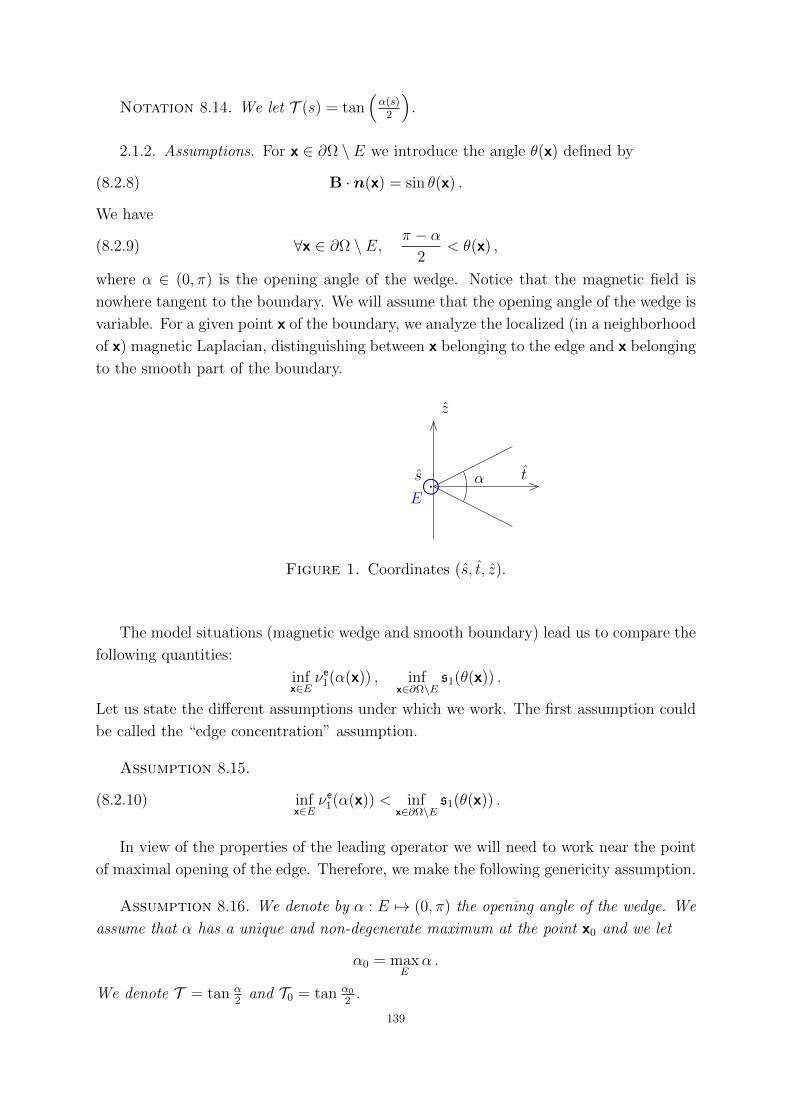
Notation 8.14. We let T (s) = tan(α(s)
2
).
2.1.2. Assumptions. For x ∈ ∂Ω \ E we introduce the angle θ(x) defined by
(8.2.8) B · n(x) = sin θ(x) .
We have
(8.2.9) ∀x ∈ ∂Ω \ E, π − α2
< θ(x) ,
where α ∈ (0, π) is the opening angle of the wedge. Notice that the magnetic field is
nowhere tangent to the boundary. We will assume that the opening angle of the wedge is
variable. For a given point x of the boundary, we analyze the localized (in a neighborhood
of x) magnetic Laplacian, distinguishing between x belonging to the edge and x belonging
to the smooth part of the boundary.
⊙sE
z
tα
Figure 1. Coordinates (s, t, z).
The model situations (magnetic wedge and smooth boundary) lead us to compare the
following quantities:
infx∈E
νe1(α(x)) , inf
x∈∂Ω\Es1(θ(x)) .
Let us state the different assumptions under which we work. The first assumption could
be called the “edge concentration” assumption.
Assumption 8.15.
(8.2.10) infx∈E
νe1(α(x)) < inf
x∈∂Ω\Es1(θ(x)) .
In view of the properties of the leading operator we will need to work near the point
of maximal opening of the edge. Therefore, we make the following genericity assumption.
Assumption 8.16. We denote by α : E 7→ (0, π) the opening angle of the wedge. We
assume that α has a unique and non-degenerate maximum at the point x0 and we let
α0 = maxE
α .
We denote T = tan α2
and T0 = tan α0
2.
139
In particular, under this assumption and Conjecture 8.10, the function s 7→ νe1(α(s))
has a unique and non-degenerate minimum.
2.2. Normal form. It is “classical” that Assumption 8.15 leads to localization prop-
erties of the eigenfunctions near the edge E, and more precisely, near the points of the
edge, where E 3 x 7→ ν(α(x)) is minimal. Therefore, since ν is decreasing and thanks to
Assumption 8.16, we expect that the first eigenfunctions concentrate near the point x0
where the opening is maximal.
Let us write below the expression of the magnetic Laplacian in the new local coor-
dinates (s, t, z), where s is a curvilinear abscissa of the edge. The normal form of the
magnetic Laplacian Ledgeh is given by Ledge
h := ∇2h, where
(8.2.11) ∇h =
hDs
hDt
hT (s)−1T (0)Dz
+
−t+ ζe0h
1/2 − h T ′2T (zDz +Dz z)
0
0
.
Remark 8.17. Such a normal form allows us to describe the leading structure of
this magnetic Laplace-Beltrami operator. Indeed, modulo some remainders, our operator
takes the simpler form
(hDs − t+ ζe0h
1/2)2 + h2D2t + h2T (0)2T (s)−2D2
z .
Performing another formal Taylor expansion near s = 0, we arrive at the following oper-
ator:
(hDs − t+ ζe0h
1/2)2 + h2D2t + h2D2
z + ch2s2D2z ,
where c > 0. Using a scaling, we get a rescaled operator Lh whose first term is the leading
operator Leα0
and which allows to construct quasimodes. Moreover, this form is suitable
for establishing microlocalization properties of the eigenfunctions with respect to Ds.
2.3. Magnetic wells induced by the variations of a singular geometry. The
main result of this section is a complete asymptotic expansion of all the first eigenvalues
of Ledgeh (see the proof in Chapter 18).
Theorem 8.18. Assume that Conjecture 8.10 is true and also that Assumptions 8.15
and 8.16 hold. For all n ≥ 1 there exists (µj,n)j≥0 such that we have
λn(h) ∼h→0
h∑j≥0
µj,nhj/4 .
Moreover, we have
µ0,n = νe1(α0), µ1,n = 0, µ2,n = (2n− 1)
√κτ−1
0 ‖Dzueζe0‖2∂2
ζνe1(α0, ζe
0) ,
where
(8.2.12) κ = −T′′(0)
2> 0 .
140
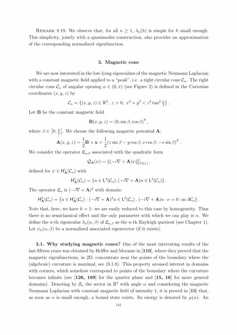
Remark 8.19. We observe that, for all n ≥ 1, λn(h) is simple for h small enough.
This simplicity, jointly with a quasimodes construction, also provides an approximation
of the corresponding normalized eigenfunction.
3. Magnetic cone
We are now interested in the low-lying eigenvalues of the magnetic Neumann Laplacian
with a constant magnetic field applied to a “peak”, i.e. a right circular cone Cα. The right
circular cone Cα of angular opening α ∈ (0, π) (see Figure 2) is defined in the Cartesian
coordinates (x, y, z) by
Cα = (x, y, z) ∈ R3, z > 0, x2 + y2 < z2 tan2 α2 .
Let B be the constant magnetic field
B(x, y, z) = (0, sin β, cos β)T ,
where β ∈[0, π
2
]. We choose the following magnetic potential A:
A(x, y, z) =1
2B× x =
1
2(z sin β − y cos β, x cos β,−x sin β)T .
We consider the operator Lα,β associated with the quadratic form
QA(ψ) = ‖(−i∇+ A)ψ‖2L2(Cα) ,
defined for ψ ∈ H1A(Cα) with
H1A(Cα) = u ∈ L2(Cα), (−i∇+ A)u ∈ L2(Cα) .
The operator Lα is (−i∇+ A)2 with domain:
H2A(Cα) = u ∈ H1
A(Cα) : (−i∇+ A)2u ∈ L2(Cα) , (−i∇+ A)u · ν = 0 on ∂Cα .
Note that, here, we have h = 1: we are easily reduced to this case by homogeneity. Thus
there is no semiclassical effect and the only parameter with which we can play is α. We
define the n-th eigenvalue λn(α, β) of Lα,β as the n-th Rayleigh quotient (see Chapter 1).
Let ψn(α, β) be a normalized associated eigenvector (if it exists).
3.1. Why studying magnetic cones? One of the most interesting results of the
last fifteen years was obtained by Helffer and Morame in [110], where they proved that the
magnetic eigenfunctions, in 2D, concentrate near the points of the boundary where the
(algebraic) curvature is maximal, see (0.1.8). This property aroused interest in domains
with corners, which somehow correspond to points of the boundary where the curvature
becomes infinite (see [126, 169] for the quarter plane and [15, 16] for more general
domains). Denoting by Sα the sector in R2 with angle α and considering the magnetic
Neumann Laplacian with constant magnetic field of intensity 1, it is proved in [15] that,
as soon as α is small enough, a bound state exists. Its energy is denoted by µ(α). An
141
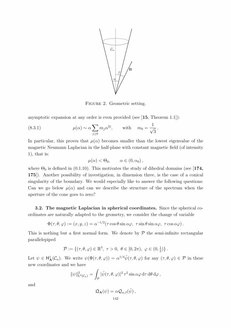
B
α
Cα
β
Figure 2. Geometric setting.
asymptotic expansion at any order is even provided (see [15, Theorem 1.1]):
(8.3.1) µ(α) ∼ α∑j≥0
mjα2j, with m0 =
1√3.
In particular, this proves that µ(α) becomes smaller than the lowest eigenvalue of the
magnetic Neumann Laplacian in the half-plane with constant magnetic field (of intensity
1), that is:
µ(α) < Θ0, α ∈ (0, α0) ,
where Θ0 is defined in (0.1.10). This motivates the study of dihedral domains (see [174,
175]). Another possibility of investigation, in dimension three, is the case of a conical
singularity of the boundary. We would especially like to answer the following questions:
Can we go below µ(α) and can we describe the structure of the spectrum when the
aperture of the cone goes to zero?
3.2. The magnetic Laplacian in spherical coordinates. Since the spherical co-
ordinates are naturally adapted to the geometry, we consider the change of variable
Φ(τ, θ, ϕ) := (x, y, z) = α−1/2(τ cos θ sinαϕ, τ sin θ sinαϕ, τ cosαϕ) .
This is nothing but a first normal form. We denote by P the semi-infinite rectangular
parallelepiped
P := (τ, θ, ϕ) ∈ R3, τ > 0, θ ∈ [0, 2π), ϕ ∈ (0, 12) .
Let ψ ∈ H1A(Cα). We write ψ(Φ(τ, θ, ϕ)) = α1/4ψ(τ, θ, ϕ) for any (τ, θ, ϕ) ∈ P in these
new coordinates and we have
‖ψ‖2L2(Cα) =
∫P|ψ(τ, θ, ϕ)|2 τ 2 sinαϕ dτ dθ dϕ ,
and
QA(ψ) = αQα,β(ψ) ,
142
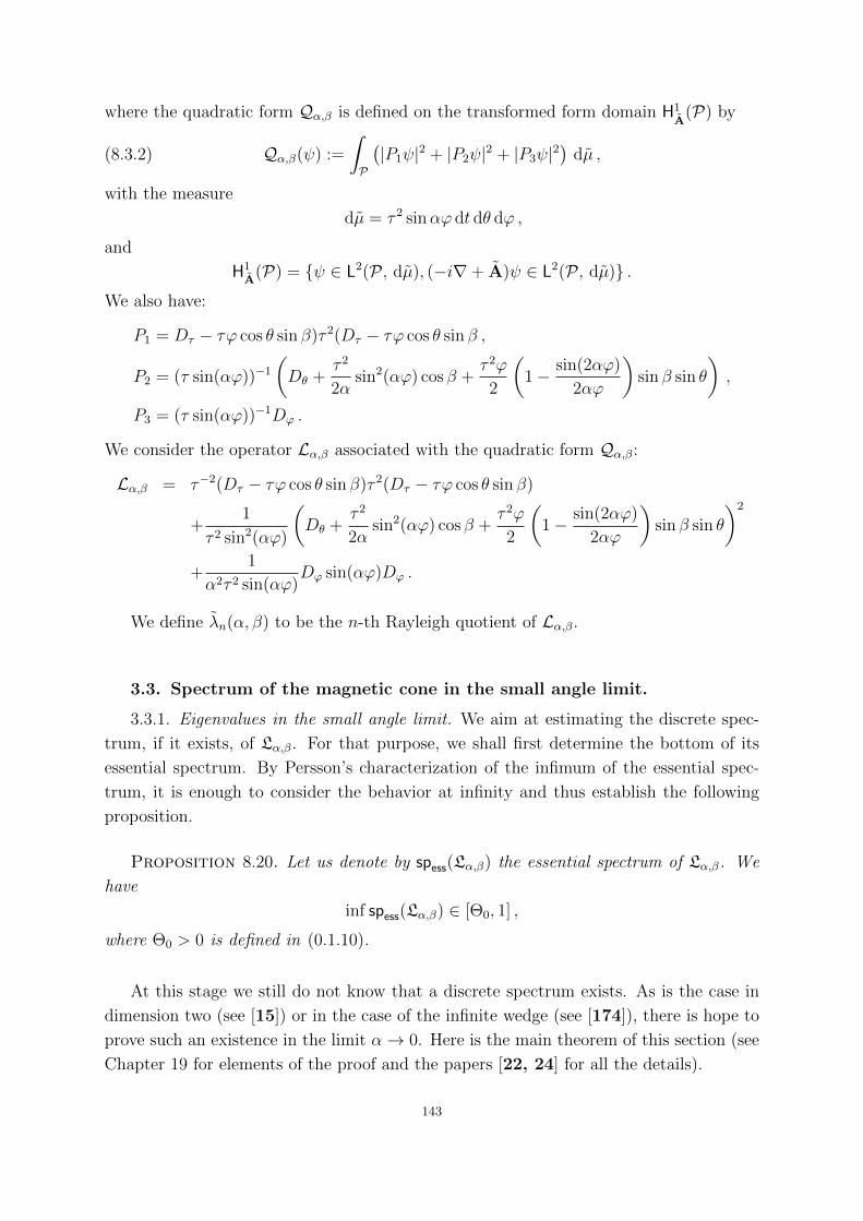
where the quadratic form Qα,β is defined on the transformed form domain H1A
(P) by
(8.3.2) Qα,β(ψ) :=
∫P
(|P1ψ|2 + |P2ψ|2 + |P3ψ|2
)dµ ,
with the measure
dµ = τ 2 sinαϕ dt dθ dϕ ,
and
H1A
(P) = ψ ∈ L2(P , dµ), (−i∇+ A)ψ ∈ L2(P , dµ) .We also have:
P1 = Dτ − τϕ cos θ sin β)τ 2(Dτ − τϕ cos θ sin β ,
P2 = (τ sin(αϕ))−1
(Dθ +
τ 2
2αsin2(αϕ) cos β +
τ 2ϕ
2
(1− sin(2αϕ)
2αϕ
)sin β sin θ
),
P3 = (τ sin(αϕ))−1Dϕ .
We consider the operator Lα,β associated with the quadratic form Qα,β:
Lα,β = τ−2(Dτ − τϕ cos θ sin β)τ 2(Dτ − τϕ cos θ sin β)
+1
τ 2 sin2(αϕ)
(Dθ +
τ 2
2αsin2(αϕ) cos β +
τ 2ϕ
2
(1− sin(2αϕ)
2αϕ
)sin β sin θ
)2
+1
α2τ 2 sin(αϕ)Dϕ sin(αϕ)Dϕ .
We define λn(α, β) to be the n-th Rayleigh quotient of Lα,β.
3.3. Spectrum of the magnetic cone in the small angle limit.
3.3.1. Eigenvalues in the small angle limit. We aim at estimating the discrete spec-
trum, if it exists, of Lα,β. For that purpose, we shall first determine the bottom of its
essential spectrum. By Persson’s characterization of the infimum of the essential spec-
trum, it is enough to consider the behavior at infinity and thus establish the following
proposition.
Proposition 8.20. Let us denote by spess(Lα,β) the essential spectrum of Lα,β. We
have
inf spess(Lα,β) ∈ [Θ0, 1] ,
where Θ0 > 0 is defined in (0.1.10).
At this stage we still do not know that a discrete spectrum exists. As is the case in
dimension two (see [15]) or in the case of the infinite wedge (see [174]), there is hope to
prove such an existence in the limit α→ 0. Here is the main theorem of this section (see
Chapter 19 for elements of the proof and the papers [22, 24] for all the details).
143

Theorem 8.21. For all n ≥ 1, there exist α0(n) > 0 and a sequence (γj,n)j≥0 such
that, for all α ∈ (0, α0(n)), the n-th eigenvalue exists and satisfies
λn(α, β) ∼α→0
α∑j≥0
γj,nαj, with γ0,n =
√1 + sin2 β
25/2(4n− 1) .
Remark 8.22. In particular, the main term is minimal when β = 0 and in this case
Theorem 8.21 states that λ1(α) ∼ 325/2α. We have 3
25/2 <1√3, so that the lowest eigenvalue
of the magnetic cone goes below the lowest eigenvalue of the two-dimensional magnetic
sector (see (8.3.1)).
Remark 8.23. As a consequence of Theorem 8.21, we deduce that the lowest eigen-
values are simple as soon as α is small enough. Therefore, the spectral theorem implies
that the quasimodes constructed in the proof are approximations of the eigenfunctions
of Lα,β. In particular, using the rescaled spherical coordinates, for all n ≥ 1, there exist
αn > 0 and Cn such that, for α ∈ (0, αn),
‖ψn(α, β)− fn‖L2(P, dµ) ≤ Cnα2 ,
where fn (which depends on β) is related to the n-th Laguerre function and ψn(α, β) is
the n-th normalized eigenfunction.
Let us sketch the proof of Theorem 8.21.
3.3.2. Axisymmetric case: β = 0. We apply the strategy presented in Chapter 0,
Section 3. In this situation, the phase variable that we should understand is the dual
variable of θ given by a Fourier series decomposition and denoted by m ∈ Z. In other
words, we make a Fourier decomposition of Lα,0 with respect to θ and we introduce the
family of two-dimensional operators (Lα,0,m)m∈Z acting on L2(R, dµ) by
Lα,0,m = − 1
τ 2∂ττ
2∂τ +1
τ 2 sin2(αϕ)
(m+
sin2(αϕ)
2ατ 2
)2
− 1
α2 τ 2 sin(αϕ)∂ϕ sin(αϕ)∂ϕ ,
with
R = (τ, ϕ) ∈ R2, τ > 0, ϕ ∈ (0, 12) ,
and
dµ = τ 2 sin(αϕ) dτ dϕ .
We denote by Qα,0,m the quadratic form associated with Lα,0,m. This normal form is
also the suitable form to construct quasimodes. Then an integrability argument proves
that the eigenfunctions are microlocalized in m = 0, i.e., they are axisymmetric. Thus,
this allows a first reduction of dimension. It remains to notice that the last term in
Lα,0,0 is penalized by α−2, so that the Feshbach-Grushin projection on the groundstate
of −α−2(sin(αϕ))−1∂ϕ sin(αϕ)∂ϕ (the constant function) acts as an approximation of the
identity on the eigenfunctions. Therefore, the spectrum of Lα,0,0 is described modulo lower
order terms by the spectrum of the average of Lα,0 with respect to ϕ, which involves the
so-called Laguerre operator (radial harmonic oscillator).
144
3.3.3. Case β ∈[0, π
2
]. In this case we cannot use the axisymmetry, but we are
still able to construct formal series and prove localization estimates of Agmon type.
Moreover, we notice that the magnetic momentum with respect to θ is strongly penalized
by (τ 2 sin2(αϕ))−1 so that, jointly with the localization estimates, it is possible to prove
that the eigenfunctions are asymptotically independent of θ and we are reduced to the
situation β = 0.
145

CHAPTER 9
Waveguides
Si on me presse de dire pourquoi je l’aimais,
je sens que cela ne se peut exprimer qu’en
repondant : Parce que c’etait lui : parce que
c’etait moi.
Les Essais, Livre I, Chapitre XXVIII,
Montaigne
This chapter presents recent progress in the spectral theory of waveguides. In Section 1
we describe magnetic waveguides in dimensions two and three and we analyze the spectral
influence of the width ε of the waveguide and the intensity b if the magnetic field. In
particular, we investigate the limit ε → 0. In Section 2 we describe the same problem
in the case of layers. In Sections 3.1 and 3.2 the effect of a corner in dimension two is
tackled.
1. Magnetic waveguides
This section is concerned with spectral properties of a curved quantum waveguide
when a magnetic field is applied. We will give a precise definition of what a waveguide is
in Sections 1.3 and 1.4. Without going into details, we can already mention that we will
use the definition given in the well-known (non-magnetic) paper of Duclos and Exner [62]
and its generalizations [41, 133, 85]. The waveguide is nothing but a tube Ωε about an
unbounded curve γ in the Euclidean space Rd, with d ≥ 2, where ε is a positive shrinking
parameter and the cross section is defined as εω = ετ : τ ∈ ω.
More precisely, this section is devoted to the spectral analysis of the magnetic operator
with Dirichlet boundary conditions L[d]ε,bA defined as
(9.1.1) (−i∇x + bA(x))2 on L2(Ωε, dx) .
where b > 0 is a positive parameter and A a smooth vector potential associated with a
given magnetic field B.
1.1. The result of Duclos and Exner. One of the deep facts proved by Duclos
and Exner is that the Dirichlet Laplacian on Ωε always has discrete spectrum below its
essential spectrum when the waveguide is not straight and asymptotically straight. Let
us sketch the proof of this result in the case of two-dimensional waveguides.
147

Let us consider a smooth and injective curve γ: R 3 s 7→ γ(s) which is parameterized
by its arc length s. The normal to the curve at γ(s) is defined as the unique unit vector
n(s) such that γ′(s) ·n(s) = 0 and det(γ′,n) = 1. We have the relation γ′′(s) = κ(s)n(s),
where κ(s) denotes the algebraic curvature at the point γ(s). We can now define standard
tubular coordinates. Consider the map
R× (−ε, ε) 3 (s, t) 7→ Φ(s, t) = γ(s) + tn(s) .
We always assume that
(9.1.2) Φ is injective and ε sups∈R|κ(s)| < 1 .
Then it is well known (see [133]) that Φ defines a smooth diffeomorphism from R×(−ε, ε)onto the image Ωε = Φ(R× (−ε, ε)), which we identify with our waveguide. In these new
coordinates, the operator becomes (exercise)
L[2]ε,0 = −m−1∂sm
−1∂s −m−1∂tm∂t, m(s, t) = 1− tκ(s) ,
which is acting in the weighted space L2(R × (−ε, ε),m(s, t) ds dt). We introduce the
shifted quadratic form
Q[2],shε,0 (φ) =
∫R×(−ε,ε)
(m−2|∂s(φ)|2 + |∂tφ|2 −
π2
4ε2|φ|2)m ds dt
and we let
φn(s, t) = χ0(n−1s) cos( π
2εt),
where χ0 is a smooth cutoff function which is 1 near 0. We can check thatQ[2],shε,0 (φn) →
n→+∞0. Let us now consider a smooth cutoff function χ1 which is 1 near a point where κ is
not zero, and define φ(s, t) = −χ21(s, t)L[2],sh
ε,0 φn(s, t) which does not depend on n as soon
as n is large enough. Then we have
Q[2],shε,0 (φn + ηφ) = Q[2],sh
ε,0 (φn)− 2ηB[2],shε,0 (φn, χ1(s)L[2],sh
ε,0 φn) + η2Q[2],shε,0 (φ) .
For n large enough, the quantity B[2],shε,0 (φn, χ1(s)L[2],sh
ε,0 φn) does not depend on n and is
positive. For such an n, we take η small enough and we get
Q[2],shε,0 (φn + ηφ) < 0 .
Therefore, the bottom of the spectrum is an eigenvalue due to the min-max principle.
Duclos and Exner also investigate the limit ε→ 0 to show that the Dirichlet Laplacian
on the tube Ωε converges in a suitable sense to the effective one-dimensional operator
Leff = −∂2s −
κ(s)2
4on L2(γ, ds) .
In addition, it is proved in [62] that each eigenvalue of this effective operator generates
an eigenvalue of the Dirichlet Laplacian on the tube.
148
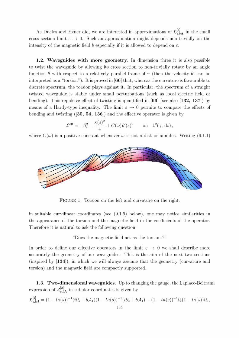
As Duclos and Exner did, we are interested in approximations of L[d]ε,bA in the small
cross section limit ε → 0. Such an approximation might depends non-trivially on the
intensity of the magnetic field b especially if it is allowed to depend on ε.
1.2. Waveguides with more geometry. In dimension three it is also possible
to twist the waveguide by allowing its cross section to non-trivially rotate by an angle
function θ with respect to a relatively parallel frame of γ (then the velocity θ′ can be
interpreted as a “torsion”). It is proved in [66] that, whereas the curvature is favourable to
discrete spectrum, the torsion plays against it. In particular, the spectrum of a straight
twisted waveguide is stable under small perturbations (such as local electric field or
bending). This repulsive effect of twisting is quantified in [66] (see also [132, 137]) by
means of a Hardy-type inequality. The limit ε → 0 permits to compare the effects of
bending and twisting ([30, 54, 136]) and the effective operator is given by
Leff = −∂2s −
κ(s)2
4+ C(ω)θ′(s)2 on L2(γ, ds) ,
where C(ω) is a positive constant whenever ω is not a disk or annulus. Writing (9.1.1)
Figure 1. Torsion on the left and curvature on the right.
in suitable curvilinear coordinates (see (9.1.9) below), one may notice similarities in
the appearance of the torsion and the magnetic field in the coefficients of the operator.
Therefore it is natural to ask the following question:
“Does the magnetic field act as the torsion ?”
In order to define our effective operators in the limit ε → 0 we shall describe more
accurately the geometry of our waveguides. This is the aim of the next two sections
(inspired by [134]), in which we will always assume that the geometry (curvature and
torsion) and the magnetic field are compactly supported.
1.3. Two-dimensional waveguides. Up to changing the gauge, the Laplace-Beltrami
expression of L[2]ε,bA in tubular coordinates is given by
L[2]ε,bA = (1− tκ(s))−1(i∂s + bA1)(1− tκ(s))−1(i∂s + bA1)− (1− tκ(s))−1∂t(1− tκ(s))∂t ,
149

with the gauge
A(s, t) = (A1(s, t), 0) , A1(s, t) =
∫ t
0
(1− t′κ(s))B(Φ(s, t′)) dt′ .
We let
m(s, t) = 1− tκ(s) .
The self-adjoint operator L[2]ε,bA on L2(R × (−ε, ε),m ds dt) is unitarily equivalent to the
self-adjoint operator
L[2]ε,bA = m1/2L
[2]ε,bAm
−1/2 ,
on L2(R× (−ε, ε), ds dt).
Introducing the rescaling
(9.1.3) t = ετ,
we let
Aε(s, τ) = (A1,ε(s, τ), 0) = (A1(s, ετ), 0)
and denote by L[2]ε,bAε the homogenized operator on L2(R× (−1, 1), ds dτ):
(9.1.4) L[2]ε,bAε = m−1/2
ε (i∂s + bA1,ε)m−1ε (i∂s + bA1,ε)m
−1/2ε − ε−2∂2
τ + Vε(s, τ) ,
with
mε(s, τ) = m(s, ετ), Vε(s, τ) = −κ(s)2
4(1− εκ(s)τ)−2 .
It is easy to verify that L[2]ε,bA, defined as the Friedrichs extension of the operator initially
defined on C∞0 (R×(−ε, ε)), has form domain H10(R×(−ε, ε)). Similarly, the form domain
of L[2]ε,bAε is H1
0(R× (−1, 1)).
1.4. Three-dimensional waveguides. The situation is geometrically more com-
plicated in dimension three. We consider a smooth curve γ which is parameterized by
its arc length s and does not self-intersect. We use the so-called Tang frame (or the
relatively parallel frame, see for instance [136]) to describe the geometry of the tubular
neighborhood of γ. Denoting the (unit) tangent vector by T (s) = γ′(s), the Tang frame
(T (s),M2(s),M3(s)) satisfies the relations:
T ′ = κ2M2 + κ3M3 ,
M ′2 = −κ2T ,
M ′3 = −κ3T .
The functions κ2 and κ3 are the curvatures related to the choice of the normal fields M2
and M3. Notice that κ2 = κ22 + κ2
3 = |γ′′|2 is the square of the usual curvature of γ.
Let θ : R→ R a smooth function (twisting). We introduce the map Φ : R×(εω)→ Ωε
defined by
(9.1.5)
x = Φ(s, t2, t3) = γ(s) + t2(cos θM2(s) + sin θM3(s)) + t3(− sin θM2(s) + cos θM3(s)) .
150
Below s will often be denoted by t1. As in dimension two, we always assume that
(9.1.6) Φ is injective and ε sup(τ2,τ3)∈ω
(|τ2|+ |τ3|) sups∈R|κ(s)| < 1 .
Sufficient conditions ensuring the injectivity hypothesis can be found in [66, App. A]. We
define A = (dΦ)TA(Φ) = (A1,A2,A3),
h = 1− t2(κ2 cos θ + κ3 sin θ)− t3(−κ2 sin θ + κ3 cos θ) ,
h2 = −t2θ′ ,
h3 = t3θ′ ,
and R = h3bA2 +h2bA3. We also introduce the angular derivative ∂α = t3∂t2 − t2∂t3 . We
will see in Chapter 20, Section 2 that the magnetic operator L[3]ε,bA is unitarily equivalent
to the operator on L2(Ωε, h dt) given by
(9.1.7) L[3]ε,bA =
∑j=2,3
h−1(−i∂tj + bAj)h(−i∂tj + bAj)
+ h−1(−i∂s + bA1 − iθ′∂α +R)h−1(−i∂s + bA1 − iθ′∂α +R) .
By considering the conjugate operator h1/2L[3]ε,bAh
−1/2, we find that L[3]ε,bA is unitarily
equivalent to the operator defined on L2(R× (εω), ds dt2 dt3) given by:
(9.1.8) L[3]ε,bA =
∑j=2,3
(−i∂tj + bAj)2 − κ2
4h2
+ h−1/2(−i∂s + bA1 − iθ′∂α +R)h−1(−i∂s + bA1 − iθ′∂α +R)h−1/2 .
Finally, introducing the rescaling
(t2, t3) = ε(τ2, τ3) = ετ ,
we define the homogenized operator on L2(R× ω, ds dτ):
(9.1.9) L[3]ε,bAε =
∑j=2,3
(−iε−1∂τj + bAj,ε)2 − κ2
4h2ε
+ h−1/2ε (−i∂s + bA1,ε − iθ′∂α +Rε)h
−1ε (−i∂s + bA1,ε − iθ′∂α +Rε)h
−1/2ε ,
where Aε(s, τ) = A(s, ετ), hε(s, τ) = h(s, ετ) and Rε = R(s, ετ).
We leave as an exercise the verification that the form domains of L[3]ε,bA and L[3]
ε,bAε are
H10(R× (−ε, ε)) and H1
0(R× (−1, 1)), respectively.
1.5. Limiting models and asymptotic expansions. We can now state our main
results concerning the effective models in the limit ε → 0. We will denote by λDirn (ω)
the n-th eigenvalue of the Dirichlet Laplacian −∆Dirω on L2(ω). The first positive and
L2-normalized eigenfunction will be denoted by J1.
151
Definition 9.1 (Case d = 2). For δ ∈ (−∞, 1), we define
Leff,[2]ε,δ = −ε−2∆Dir
ω − ∂2s −
κ(s)2
4
and for δ = 1, we let
Leff,[2]ε,1 = −ε−2∆Dir
ω + T [2] ,
where
T [2] = −∂2s +
(1
3+
2
π2
)B(γ(s))2 − κ(s)2
4.
The following theorem is proved in Chapter 20, Section 1.
Theorem 9.2 (Case d = 2). There exists K such that, for all δ ∈ (−∞, 1], there
exist ε0 > 0 and C > 0 such that, for all ε ∈ (0, ε0),∥∥∥∥(L[2]
ε,ε−δAε − ε−2λDir
1 (ω) +K)−1
−(Leff,[2]ε,δ − ε−2λDir
1 (ω) +K)−1∥∥∥∥ ≤ C max(ε1−δ, ε) ,
for δ < 1 ,
and ∥∥∥∥(L[2]
ε,ε−1Aε − ε−2λDir
1 (ω) +K)−1
−(Leff,[2]ε,1 − ε−2λDir
1 (ω) +K)−1∥∥∥∥ ≤ Cε .
In the critical regime δ = 1, we deduce the following corollary providing the asymp-
totic expansions of the lowest eigenvalues λ[2]n (ε) of L[2]
ε,ε−1Aε .
Corollary 9.3 (Case d = 2 and δ = 1). Let us assume that T [2] admits N (simple)
eigenvalues µ1, . . . , µN below the threshold of the essential spectrum. Then, for all n ∈1, . . . , N, there exist (γj,n)j≥0 and ε0 > 0 such that, for all ε ∈ (0, ε0),
λ[2]n (ε) ∼
ε→0
∑j≥0
γj,nε−2+j ,
with
γ0,n =π2
4, γ1,n = 0, γ2,n = µn .
Thanks to the spectral theorem, we also get the approximation of the corresponding
eigenfunctions at any order (see our quasimodes in (20.1.9)).
In order to present analogous results in dimension three, we introduce supplementary
notation. The norm and the inner product in L2(ω) will be denoted by ‖ · ‖ω and 〈·, ·〉ω,
respectively.
Definition 9.4 (Case d = 3). For δ ∈ (−∞, 1), we define
Leff,[3]ε,δ = −ε−2∆Dir
ω − ∂2s −
κ(s)2
4+ ‖∂αJ1‖2
ωθ′2
and for δ = 1, we let
Leff,[3]ε,1 = −ε−2∆Dir
ω + T [3] ,
152
where T [3] is defined by:
T [3] = 〈(−i∂s − iθ′∂α − B12(s, 0, 0)τ2 − B13(s, 0, 0)τ3)2Id(s)⊗ J1, Id(s)⊗ J1〉ω
+ B223(s, 0, 0)
(‖τJ1‖2
ω
4− 〈DαRω, J1〉ω
)− κ2(s)
4,
with Rω being given in (20.2.5) and
B23(s, 0, 0) = B(γ(s)) · T (s) ,
B13(s, 0, 0) = B(γ(s)) · (cos θM2(s)− sin θM3(s)) ,
B12(s, 0, 0) = B(γ(s)) · (− sin θM2(s) + cos θM3(s)) .
The following theorem is proved in Chapter 20, Section 2.
Theorem 9.5 (Case d = 3). There exists K such that for all δ ∈ (−∞, 1], there exist
ε0 > 0 and C > 0 such that, for all ε ∈ (0, ε0),∥∥∥∥(L[3]
ε,ε−δAε − ε−2λDir
1 (ω) +K)−1
−(Leff,[3]ε,δ − ε−2λDir
1 (ω) +K)−1∥∥∥∥ ≤ C max(ε1−δ, ε) ,
for δ < 1 ,
and ∥∥∥∥(L[3]
ε,ε−1Aε − ε−2λDir
1 (ω) +K)−1
−(Leff,[3]ε,1 − ε−2λDir
1 (ω) +K)−1∥∥∥∥ ≤ Cε .
In the same way, this theorem yields asymptotic expansions of eigenvalues λ[3]n (ε) of
L[3]
ε,ε−1Aε .
Corollary 9.6 (Case d = 3 and δ = 1). Let us assume that T [3] admits N (simple)
eigenvalues ν1, . . . , νN below the threshold of the essential spectrum. Then, for all n ∈1, . . . , N, there exist (γj,n)j≥0 and ε0 > 0 such that, for all ε ∈ (0, ε0),
λ[3]n (ε) ∼
ε→0
∑j≥0
γj,nε−2+j ,
with
γ0,n = λDir1 (ω), γ1,n = 0, γ2,n = νn .
As in two dimensions, we also get the corresponding expansion for the eigenfunctions.
Complete asymptotic expansions for eigenvalues in finite three-dimensional waveguides
without magnetic field were also previously established in [93, 26]. Such expansions were
also obtained in [92] in the case δ = 0 in a periodic framework.
Remark 9.7. As expected, when δ = 0, that is, when b is kept fixed, the magnetic
field does not persist in the limit ε→ 0 as well in dimension two, as in dimension three.
Indeed, in this limit Ωε converges to the one-dimensional curve γ and there is no magnetic
field in dimension one.
153
1.6. Norm resolvent convergence. Let us state an auxiliary result, inspired by
the approach of [87], which tells us that, in order to estimate the difference between two
resolvents, it is sufficient to analyse the difference between the corresponding sesquilinear
forms, provided their domains are the same.
Lemma 9.8. Let L1 and L2 be two positive self-adjoint operators on a Hilbert space
H. Let B1 and B2 be their associated sesquilinear forms. We assume that Dom (B1) =
Dom (B2). Assume that there exists η > 0 such that, for all φ, ψ ∈ Dom (B1),
|B1(φ, ψ)−B2(φ, ψ)| ≤ η√
Q1(ψ)√
Q2(φ) ,
where Qj(ϕ) = Bj(ϕ, ϕ) for j = 1, 2 and ϕ ∈ Dom (B1). Then,
‖L−11 − L−1
2 ‖ ≤ η‖L−11 ‖1/2‖L−1
2 ‖1/2 .
Proof. The original proof can be found in [136, Prop. 5.3]. Let us consider φ, ψ ∈ H.
We let φ = L−12 φ and ψ = L−1
1 ψ. We have φ, ψ ∈ Dom (B1) = Dom (B2). We notice that
B1(φ, ψ) = 〈L−12 φ, ψ〉, B2(φ, ψ) = 〈L−1
1 φ, ψ〉
and
Q1(ψ) = 〈ψ,L−11 ψ〉, Q2(φ) = 〈φ,L−1
2 φ〉 .It follows that ∣∣∣〈(L−1
1 − L−12 )φ, ψ〉
∣∣∣ ≤ η‖L−11 ‖1/2‖L−1
2 ‖1/2‖φ‖‖ψ‖
and the result elementarily follows.
1.7. A magnetic Hardy inequality. In dimension two, the limiting model (with
δ = 1) enlightens the fact that the magnetic field plays against the curvature, whereas in
dimension three this repulsive effect is not obvious (it can be seen that 〈DαRω, J1〉ω ≥ 0).
Nevertheless, if ω is a disk, we have 〈DαRω, J1〉ω = 0 and thus the component of the
magnetic field parallel to γ plays against the curvature (in comparison, a pure torsion
has no effect when the cross section is a disk). In the flat case (κ = 0), we can quantify this
repulsive effect by means of a magnetic Hardy inequality (see [65] where this inequality
is discussed in dimension two). We will not discuss the proof of this inequality in this
book.
Theorem 9.9. Let d ≥ 2. Let us consider Ω = R× ω. For R > 0, we let
Ω(R) = t ∈ Ω : |t1| < R .
Let A be a smooth vector potential such that σB is not zero on Ω(R0) for some R0 > 0.
Then, there exists C > 0 such that, for all R ≥ R0, there exists cR(B) > 0 such that
(9.1.10)
∫Ω
(|(−i∇+ A)ψ|2 − λDir
1 (ω)|ψ|2)
dt ≥∫
Ω
cR(B)
1 + s2|ψ|2 dt, ∀ψ ∈ C∞0 (Ω) .
154
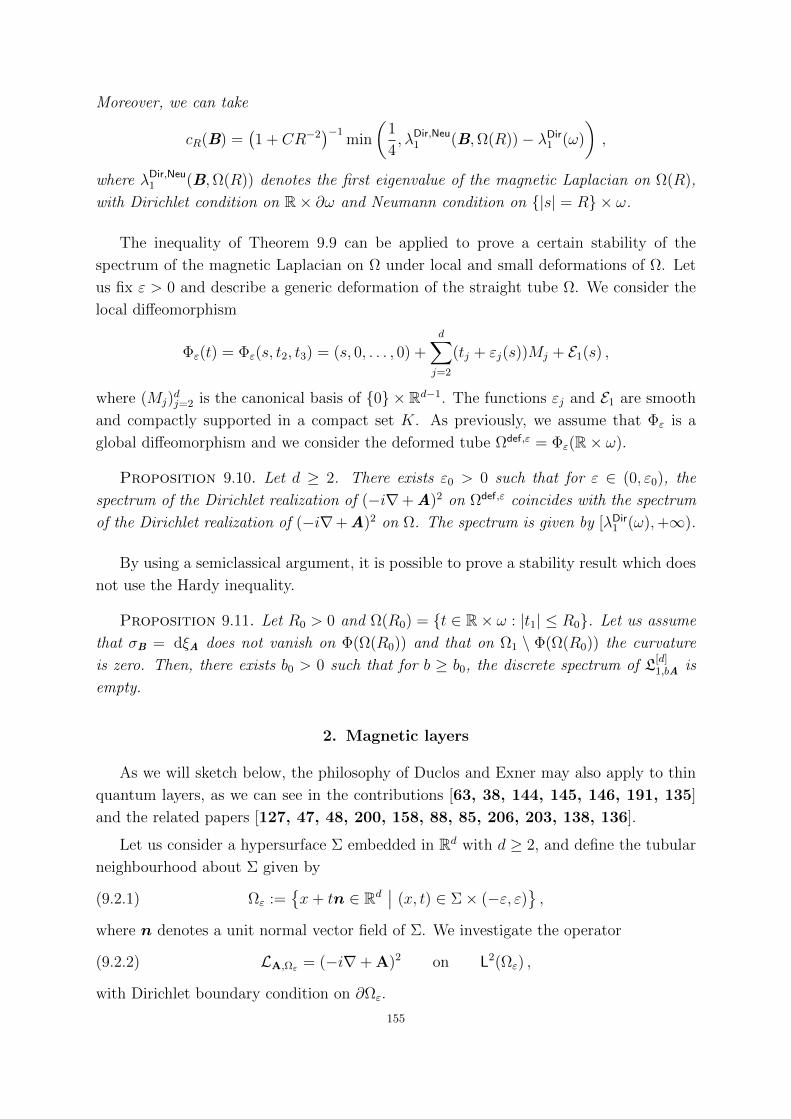
Moreover, we can take
cR(B) =(1 + CR−2
)−1min
(1
4, λDir,Neu
1 (B,Ω(R))− λDir1 (ω)
),
where λDir,Neu1 (B,Ω(R)) denotes the first eigenvalue of the magnetic Laplacian on Ω(R),
with Dirichlet condition on R× ∂ω and Neumann condition on |s| = R × ω.
The inequality of Theorem 9.9 can be applied to prove a certain stability of the
spectrum of the magnetic Laplacian on Ω under local and small deformations of Ω. Let
us fix ε > 0 and describe a generic deformation of the straight tube Ω. We consider the
local diffeomorphism
Φε(t) = Φε(s, t2, t3) = (s, 0, . . . , 0) +d∑j=2
(tj + εj(s))Mj + E1(s) ,
where (Mj)dj=2 is the canonical basis of 0 × Rd−1. The functions εj and E1 are smooth
and compactly supported in a compact set K. As previously, we assume that Φε is a
global diffeomorphism and we consider the deformed tube Ωdef,ε = Φε(R× ω).
Proposition 9.10. Let d ≥ 2. There exists ε0 > 0 such that for ε ∈ (0, ε0), the
spectrum of the Dirichlet realization of (−i∇+A)2 on Ωdef,ε coincides with the spectrum
of the Dirichlet realization of (−i∇+A)2 on Ω. The spectrum is given by [λDir1 (ω),+∞).
By using a semiclassical argument, it is possible to prove a stability result which does
not use the Hardy inequality.
Proposition 9.11. Let R0 > 0 and Ω(R0) = t ∈ R× ω : |t1| ≤ R0. Let us assume
that σB = dξA does not vanish on Φ(Ω(R0)) and that on Ω1 \ Φ(Ω(R0)) the curvature
is zero. Then, there exists b0 > 0 such that for b ≥ b0, the discrete spectrum of L[d]1,bA is
empty.
2. Magnetic layers
As we will sketch below, the philosophy of Duclos and Exner may also apply to thin
quantum layers, as we can see in the contributions [63, 38, 144, 145, 146, 191, 135]
and the related papers [127, 47, 48, 200, 158, 88, 85, 206, 203, 138, 136].
Let us consider a hypersurface Σ embedded in Rd with d ≥ 2, and define the tubular
neighbourhood about Σ given by
(9.2.1) Ωε :=x+ tn ∈ Rd
∣∣ (x, t) ∈ Σ× (−ε, ε),
where n denotes a unit normal vector field of Σ. We investigate the operator
(9.2.2) LA,Ωε = (−i∇+ A)2 on L2(Ωε) ,
with Dirichlet boundary condition on ∂Ωε.
155
2.1. Normal form. As usual, the game is to find an appropriate normal form for
the magnetic Laplacian. Given I := (−1, 1) and ε > 0, we define a layer Ωε of width 2ε
along Σ as the image of the mapping
(9.2.3) Φ : Σ× I −→ Rd , (x, u) 7→ x+ εun .
Let us denote by A the components of the vector potential, expressed in the curvilinear
coordinates induced by the embedding (9.2.3). Moreover, assume
(9.2.4) Ad = 0 .
Thanks to the diffeomorphism Φ : Σ× I → Ωε, we can identify LA,Ωε with the operator
H on L2(Σ× I, dΩε) that acts, in the form sense, as
H = |G|−1/2(−i∂xµ + Aµ)|G|1/2Gµν(−i∂xν + Aν)− ε−2|G|−1/2∂u|G|1/2∂u .
Let us define
J :=1
4ln|G||g|
=1
2
d−1∑µ=1
ln(1− εuκµ) =1
2ln
[1 +
d−1∑µ=1
(−εu)µ(d− 1
µ
)Kµ
].
Using the unitary transform
U : L2(Σ× I, dΩε) −→ L2(Σ× I, dΣ ∧ du) , ψ 7→ eJψ ,
we arrive at the unitarily equivalent operator
H := UHU−1 = |g|−1/2(−i∂xµ + Aµ)|g|1/2Gµν(−i∂xν + Aν)− ε−2∂2u + V ,
where
V := |g|−1/2 ∂xi(|g|1/2Gij(∂xjJ)
)+ (∂xiJ)Gij(∂xjJ) .
We get
H = UU(−∆ΩεD,A)U−1U−1 .
2.2. The effective operator. H is approximated in the norm resolvent sense (see
[135] for the details) by
(9.2.5) H0 = heff − ε−2∂2u ' heff ⊗ 1 + 1⊗ (−ε−2∂2
u)
on L2(Σ× I, dΣ ∧ du) ' L2(Σ, dΣ)⊗ L2(I, du), with the effective Hamiltonian
(9.2.6) heff := |g|−1/2(− i∂xµ + Aµ(·, 0)
)|g|1/2gµν
(− i∂xν + Aν(·, 0)
)+ Veff ,
where
(9.2.7) Veff := −1
2
d−1∑µ=1
κ2µ +
1
4
(d−1∑µ=1
κµ
)2
.
156
3. Broken waveguides
3.1. Semiclassical triangles. As we would like to analyze the spectrum of broken
waveguides (that is, waveguides with an angle), it is natural to prepare the investigation
by studying the Dirichlet eigenvalues of the Laplacian on some special shrinking triangles.
This subject is already dealt with in [84, Theorem 1], where a four-term asymptotic is
proved for the lowest eigenvalue, whereas a three-term asymptotic for the second eigen-
value is provided in [84, Section 2]. We can mention the papers [86, 87], whose results
provide two-term asymptotics for thin rhombi and also [27], which deals with a regular
case (thin ellipse for instance), see also [28]. We also invite the reader to take a look at
[120]. For a complete description of the low-lying spectrum of general shrinking triangles,
one may consult the paper by Ourmieres [167] (especially, the existence of a boundary
layer near the shrinking height is proved, see also [52, 149]), where tunnel effect estimates
are also established. In dimension three the generalization to cones with small aperture
is done in [166], which is motivated by [77].
Let us define the isosceles triangle in which we are interested:
(9.3.1) Triθ =
(x1, x2) ∈ R− × R : x1 tan θ < |x2| <(x1 +
π
sin θ
)tan θ
.
We will use the coordinates
(9.3.2) x = x1
√2 sin θ, y = x2
√2 cos θ ,
which transform Triθ into Triπ/4. The operator becomes:
DTri(h) = 2 sin2θ ∂2x − 2 cos2θ ∂2
y ,
with Dirichlet condition on the boundary of Tri. We let h = tan θ; after division by
2 cos2 θ, we get the new operator
(9.3.3) LTri(h) = −h2∂2x − ∂2
y .
This operator is thus in the “Born-Oppenheimer form”, and we shall introduce its Born-
Oppenheimer approximation, which is the Dirichlet realization on L2((−π√
2, 0)) of
(9.3.4) HBO,Tri(h) = −h2∂2x +
π2
4(x+ π√
2)2.
Theorem ?? is a consequence of the Born-Oppenheimer strategy (see Chapter 6, Section
2).
Theorem 9.12. The eigenvalues of HBO,Tri(h), denoted by λBO,Tri,n(h), admit the ex-
pansions
λBO,Tri,n(h) ∼h→0
∑j≥0
βj,nh2j/3 , with β0,n =
1
8and β1,n = (4π
√2)−2/3zAirev(n) ,
where zAirev(n) is the n-th zero of the reversed Airy function Airev(x) = Ai(−x).
157
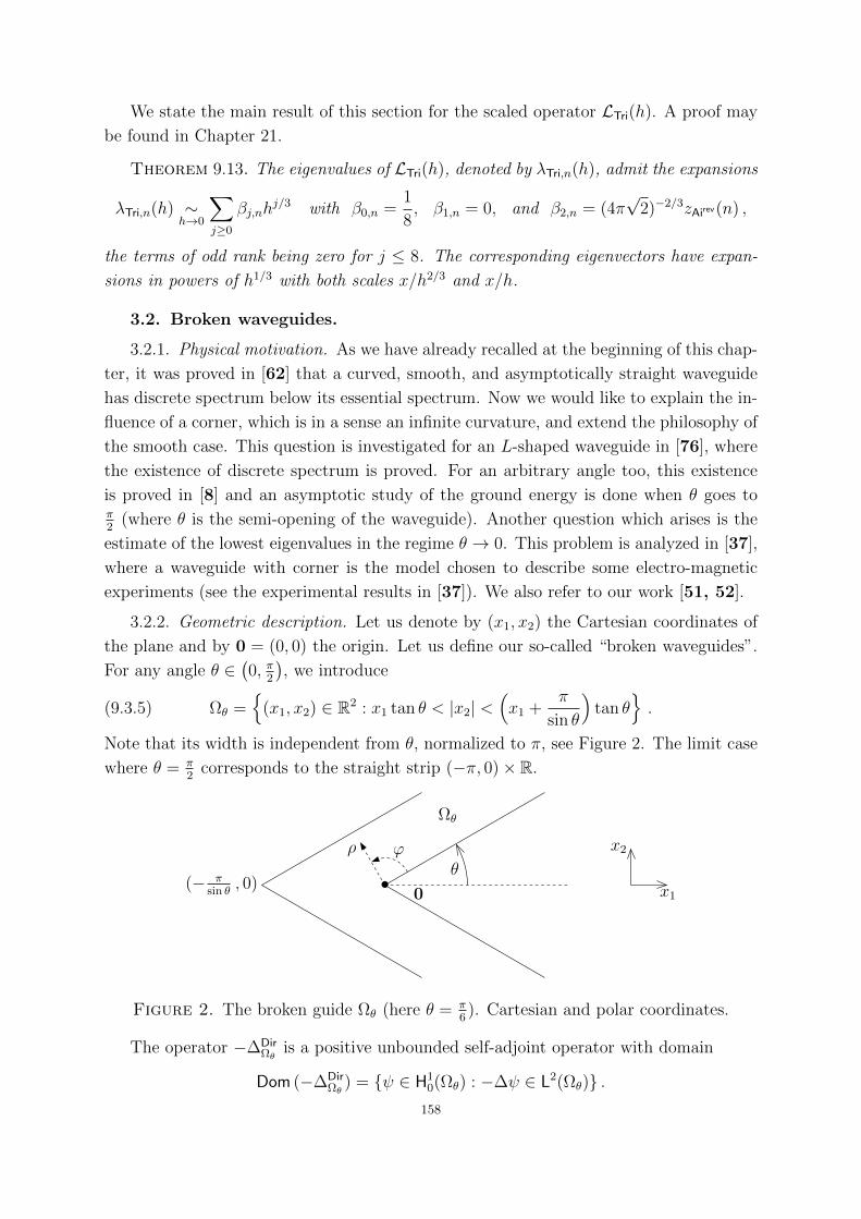
We state the main result of this section for the scaled operator LTri(h). A proof may
be found in Chapter 21.
Theorem 9.13. The eigenvalues of LTri(h), denoted by λTri,n(h), admit the expansions
λTri,n(h) ∼h→0
∑j≥0
βj,nhj/3 with β0,n =
1
8, β1,n = 0, and β2,n = (4π
√2)−2/3zAirev(n) ,
the terms of odd rank being zero for j ≤ 8. The corresponding eigenvectors have expan-
sions in powers of h1/3 with both scales x/h2/3 and x/h.
3.2. Broken waveguides.
3.2.1. Physical motivation. As we have already recalled at the beginning of this chap-
ter, it was proved in [62] that a curved, smooth, and asymptotically straight waveguide
has discrete spectrum below its essential spectrum. Now we would like to explain the in-
fluence of a corner, which is in a sense an infinite curvature, and extend the philosophy of
the smooth case. This question is investigated for an L-shaped waveguide in [76], where
the existence of discrete spectrum is proved. For an arbitrary angle too, this existence
is proved in [8] and an asymptotic study of the ground energy is done when θ goes toπ2
(where θ is the semi-opening of the waveguide). Another question which arises is the
estimate of the lowest eigenvalues in the regime θ → 0. This problem is analyzed in [37],
where a waveguide with corner is the model chosen to describe some electro-magnetic
experiments (see the experimental results in [37]). We also refer to our work [51, 52].
3.2.2. Geometric description. Let us denote by (x1, x2) the Cartesian coordinates of
the plane and by 0 = (0, 0) the origin. Let us define our so-called “broken waveguides”.
For any angle θ ∈(0, π
2
), we introduce
(9.3.5) Ωθ =
(x1, x2) ∈ R2 : x1 tan θ < |x2| <(x1 +
π
sin θ
)tan θ
.
Note that its width is independent from θ, normalized to π, see Figure 2. The limit case
where θ = π2
corresponds to the straight strip (−π, 0)× R.
x1
x2
(− πsin θ
, 0)
Ωθ
ϕθ
ρ
•0
Figure 2. The broken guide Ωθ (here θ = π6). Cartesian and polar coordinates.
The operator −∆DirΩθ
is a positive unbounded self-adjoint operator with domain
Dom (−∆DirΩθ
) = ψ ∈ H10(Ωθ) : −∆ψ ∈ L2(Ωθ) .158
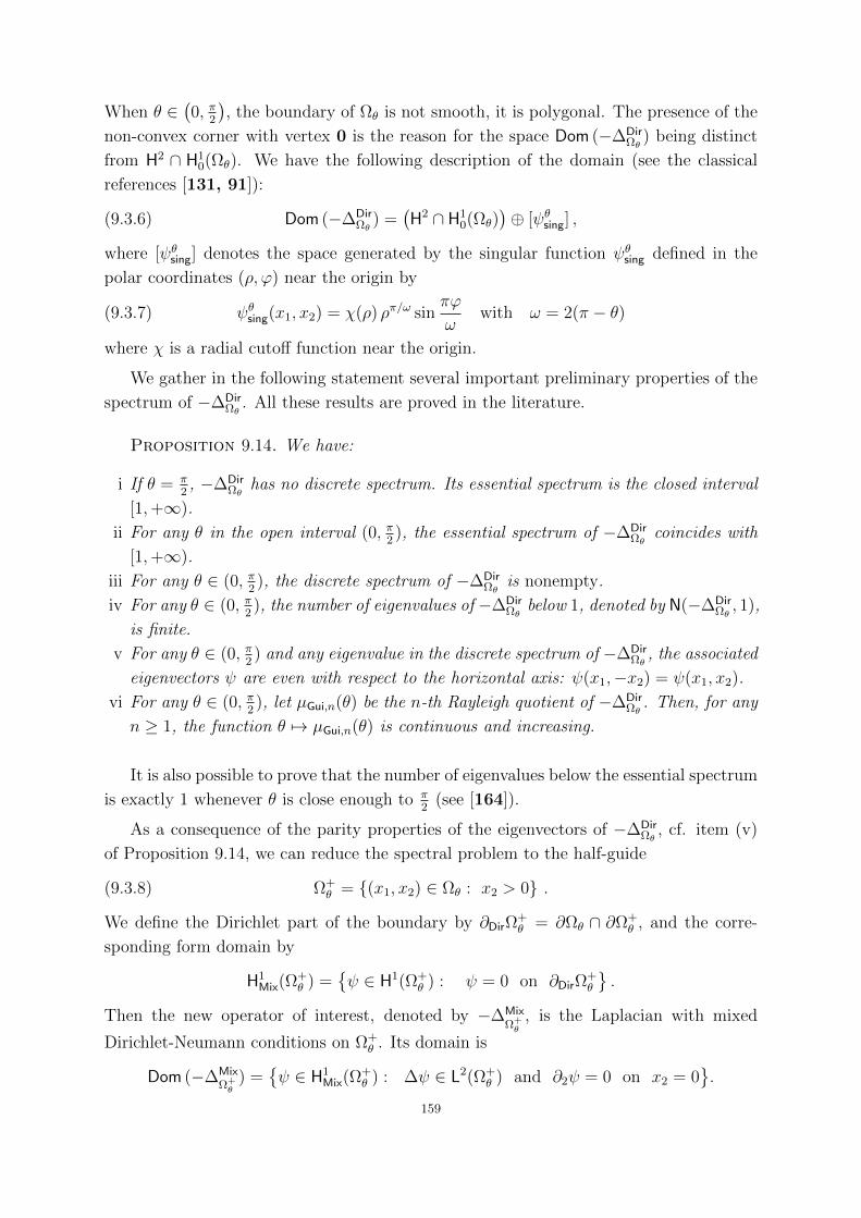
When θ ∈(0, π
2
), the boundary of Ωθ is not smooth, it is polygonal. The presence of the
non-convex corner with vertex 0 is the reason for the space Dom (−∆DirΩθ
) being distinct
from H2 ∩ H10(Ωθ). We have the following description of the domain (see the classical
references [131, 91]):
(9.3.6) Dom (−∆DirΩθ
) =(H2 ∩ H1
0(Ωθ))⊕ [ψθsing] ,
where [ψθsing] denotes the space generated by the singular function ψθsing defined in the
polar coordinates (ρ, ϕ) near the origin by
(9.3.7) ψθsing(x1, x2) = χ(ρ) ρπ/ω sinπϕ
ωwith ω = 2(π − θ)
where χ is a radial cutoff function near the origin.
We gather in the following statement several important preliminary properties of the
spectrum of −∆DirΩθ
. All these results are proved in the literature.
Proposition 9.14. We have:
i If θ = π2, −∆Dir
Ωθhas no discrete spectrum. Its essential spectrum is the closed interval
[1,+∞).
ii For any θ in the open interval (0, π2), the essential spectrum of −∆Dir
Ωθcoincides with
[1,+∞).
iii For any θ ∈ (0, π2), the discrete spectrum of −∆Dir
Ωθis nonempty.
iv For any θ ∈ (0, π2), the number of eigenvalues of −∆Dir
Ωθbelow 1, denoted by N(−∆Dir
Ωθ, 1),
is finite.
v For any θ ∈ (0, π2) and any eigenvalue in the discrete spectrum of −∆Dir
Ωθ, the associated
eigenvectors ψ are even with respect to the horizontal axis: ψ(x1,−x2) = ψ(x1, x2).
vi For any θ ∈ (0, π2), let µGui,n(θ) be the n-th Rayleigh quotient of −∆Dir
Ωθ. Then, for any
n ≥ 1, the function θ 7→ µGui,n(θ) is continuous and increasing.
It is also possible to prove that the number of eigenvalues below the essential spectrum
is exactly 1 whenever θ is close enough to π2
(see [164]).
As a consequence of the parity properties of the eigenvectors of −∆DirΩθ
, cf. item (v)
of Proposition 9.14, we can reduce the spectral problem to the half-guide
(9.3.8) Ω+θ = (x1, x2) ∈ Ωθ : x2 > 0 .
We define the Dirichlet part of the boundary by ∂DirΩ+θ = ∂Ωθ ∩ ∂Ω+
θ , and the corre-
sponding form domain by
H1Mix(Ω
+θ ) =
ψ ∈ H1(Ω+
θ ) : ψ = 0 on ∂DirΩ+θ
.
Then the new operator of interest, denoted by −∆MixΩ+θ
, is the Laplacian with mixed
Dirichlet-Neumann conditions on Ω+θ . Its domain is
Dom (−∆MixΩ+θ
) =ψ ∈ H1
Mix(Ω+θ ) : ∆ψ ∈ L2(Ω+
θ ) and ∂2ψ = 0 on x2 = 0.
159
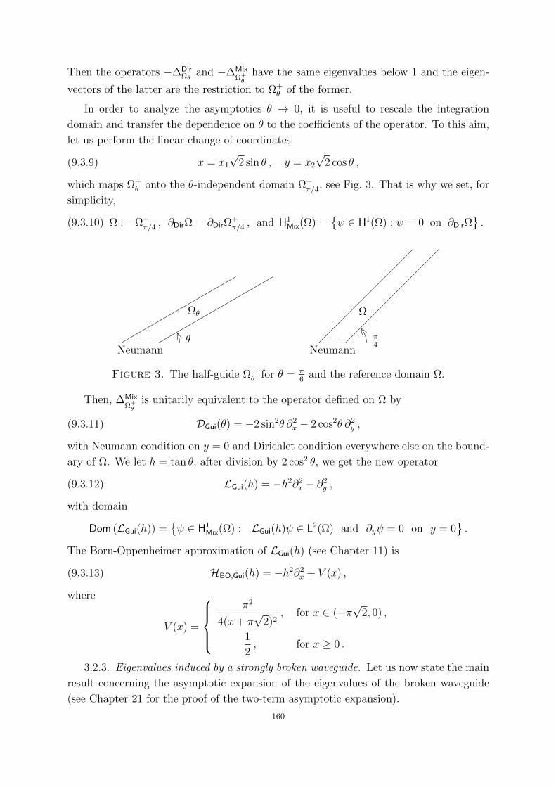
Then the operators −∆DirΩθ
and −∆MixΩ+θ
have the same eigenvalues below 1 and the eigen-
vectors of the latter are the restriction to Ω+θ of the former.
In order to analyze the asymptotics θ → 0, it is useful to rescale the integration
domain and transfer the dependence on θ to the coefficients of the operator. To this aim,
let us perform the linear change of coordinates
(9.3.9) x = x1
√2 sin θ , y = x2
√2 cos θ ,
which maps Ω+θ onto the θ-independent domain Ω+
π/4, see Fig. 3. That is why we set, for
simplicity,
(9.3.10) Ω := Ω+π/4 , ∂DirΩ = ∂DirΩ
+π/4 , and H1
Mix(Ω) =ψ ∈ H1(Ω) : ψ = 0 on ∂DirΩ
.
θ
Ωθ
π4
Ω
Neumann Neumann
Figure 3. The half-guide Ω+θ for θ = π
6and the reference domain Ω.
Then, ∆MixΩ+θ
is unitarily equivalent to the operator defined on Ω by
(9.3.11) DGui(θ) = −2 sin2θ ∂2x − 2 cos2θ ∂2
y ,
with Neumann condition on y = 0 and Dirichlet condition everywhere else on the bound-
ary of Ω. We let h = tan θ; after division by 2 cos2 θ, we get the new operator
(9.3.12) LGui(h) = −h2∂2x − ∂2
y ,
with domain
Dom (LGui(h)) =ψ ∈ H1
Mix(Ω) : LGui(h)ψ ∈ L2(Ω) and ∂yψ = 0 on y = 0.
The Born-Oppenheimer approximation of LGui(h) (see Chapter 11) is
(9.3.13) HBO,Gui(h) = −h2∂2x + V (x) ,
where
V (x) =
π2
4(x+ π√
2)2, for x ∈ (−π
√2, 0) ,
1
2, for x ≥ 0 .
3.2.3. Eigenvalues induced by a strongly broken waveguide. Let us now state the main
result concerning the asymptotic expansion of the eigenvalues of the broken waveguide
(see Chapter 21 for the proof of the two-term asymptotic expansion).
160
Theorem 9.15. For all N0, there exists h0 > 0, such that for h ∈ (0, h0) the N0
first eigenvalues of LGui(h) exist. These eigenvalues, denoted by λGui,n(h), admit the
expansions:
λGui,n(h) ∼h→0
∑j≥0
γj,nhj3 with γ0,n =
1
8, γ1,n = 0 , and γ2,n = (4π
√2)−2/3zAirev(n) .
161

CHAPTER 10
On some connected non-linear problems
L’explication que nous devons juger satisfaisante est
celle qui adhere a son objet : point de vide entre eux,
pas d’interstice ou une autre explication puisse aussi
bien se loger ; elle ne convient qu’a lui, il ne se prete
qu’a elle.
La pensee et le mouvant, Bergson
In this chapter we present two problems related to the non-linear Schrodinger equa-
tion:
i. the semiclassical limit for the p-eigenvalues of the magnetic Laplacian,
ii. the dimensional reduction of the time dependent non-linear Schrodinger equation.
1. Non-linear magnetic eigenvalues
1.1. Definition of the non-linear eigenvalue. Let Ω be a bounded simply con-
nected open set of R2. We introduce the following “non-linear eigenvalue” (or optimal
magnetic Sobolev constant):
(10.1.1) λ(Ω,A, p, h) = infψ∈H1
0(Ω),ψ 6=0
Qh,A(ψ)(∫Ω|ψ|p dx
) 2p
= infψ∈H1
0(Ω),‖ψ‖Lp(Ω)=1
Qh,A(ψ) ,
where the magnetic quadratic form is defined by
∀ψ ∈ H10(Ω), Qh,A(ψ) =
∫Ω
|(−ih∇+ A)ψ|2 dx .
Lemma 10.1. The infimum in (10.1.1) is attained.
Proof. Consider a minimizing sequence (ψj) that is normalized in Lp-norm. Then,
by a Holder inequality and using that Ω has bounded measure, (ψj) is bounded in L2.
Since A ∈ L∞(Ω), we conclude that (ψj) is bounded in H10(Ω). By the Banach-Alaoglu,
Theorem there exist a subsequence (still denoted by (ψj)) and ψ∞ ∈ H10(Ω) such that
ψj ψ∞ weakly in H10(Ω) and ψj → ψ∞ in Lq(Ω) for all q ∈ [2,+∞). This is enough to
conclude.
163
Lemma 10.2. The minimizers (which belong to H10(Ω)) of the Lp-normalized version
of (10.1.1) satisfy the following equation in the sense of distributions:
(10.1.2) (−ih∇+ A)2ψ = λ(Ω,A, p, h)|ψ|p−2ψ , ‖ψ‖Lp(Ω) = 1 .
In particular (by Sobolev embedding), the minimizers belong to the domain of Lh,A.
1.2. A result by Esteban and Lions. By using the famous concentration-compactness
method, Esteban and Lions proved the following result in [70].
Proposition 10.3. Let A ∈ L(Rd,Rd) such that B 6= 0 and p ∈ (2, 2∗), with 2∗ =2dd−2
. We let
(10.1.3) S = infψ∈Dom (QA),ψ 6=0
QA(ψ)
‖ψ‖2Lp(Rd)
.
Then, the infimum in (10.1.3) is attained.
Note that S > 0. Indeed, if (φj)j≥1 is a minimizing sequence, normalized in Lp, such
that QA(φj)→ 0, we deduce that, by diamagnetism, |φj| → 0 in H1(Rd). By the Sobolev
embedding H1(Rd) ⊂ Lp(Rd), we get that (φj)j≥1 goes to zero in Lp(Rd). We prove this
proposition in Chapter 16, Section 1 by using an alternative method to the concentration-
compactness principle. Moreover, it is possible to prove that the minimizers of (10.1.3)
have an exponential decay.
Proposition 10.4. There exists α > 0 such that, for any minimizer ψ of (10.1.3),
we have eα|x|ψ ∈ L2(Rd).
We focus on the two-dimensional case.
Definition 10.5. For p ∈ (2,+∞), we define
(10.1.4) λ[0](p) = λ(R2,A[0], p, 1) = infψ∈Dom (Q
A[0] ),ψ 6=0
QA[0](ψ)
‖ψ‖2Lp
,
where A[0](x, y) = (0,−x). Here
QA[0](ψ) =
∫R2
|(−i∇+ A[0])ψ|2 dx ,
with domain
Dom (QA[0]) =ψ ∈ L2(R2) : (−i∇+ A[0])ψ ∈ L2(R2)
.
Let us now state the main theorem of this section (the proof is given in Chapter 16,
Section 2, see also [82].
Theorem 10.6. Let p ≥ 2. Let us assume that A is smooth on Ω, that B = ∇×A
does not vanish on Ω, and that its minimum b0 is attained in Ω. Then there exist C > 0
and h0 > 0 such that, for all h ∈ (0, h0),
(1− Ch18 )λ[0](p)b
2p
0 h2h−
2p ≤ λ(Ω,A, p, h) ≤ (1 + Ch1/2)λ[0](p)b
2p
0 h2h−
2p .
164
2. Non-linear dynamics in waveguides
Let us now discuss another non-linear problem.
Consider a smooth, simple curve Γ in R2 defined by its normal parametrization γ :
x1 7→ γ(x1). For ε > 0 we introduce the map
(10.2.1) Φε : S = R× (−1, 1) 3 (x1, x2) 7−→ γ(x1) + εx2n(x1) = x ,
where n(x1) denotes the unit normal vector at the point γ(x1) such that det(γ′(x1),n(x1)) =
1. We recall that the curvature at the point γ(x1), denoted by κ(x1), is defined by
γ′′(x1) = κ(x1)n(x1) .
The waveguide is Ωε = Φε(S) and we will work under the following assumption which
states that waveguide does not overlap itself and that Φε is a smooth diffeomorphism.
Assumption 10.7. The function κ is bounded, together with its derivatives κ′ and
κ′′. Moreover, there exists ε0 ∈ (0, 1‖κ‖L∞
) such that, for ε ∈ (0, ε0), Φε is injective.
We will denote by −∆DirΩε
the Dirichlet Laplacian on Ωε. We are interested in the
equation
(10.2.2) i∂tψε = −∆Dir
Ωεψε + λεα|ψε|2ψε
on Ωε, with a Cauchy condition ψε(0; ·) = ψε0 and where α ≥ 1 and λ ∈ R are parameters.
By using the diffeomorphism Φε, we may rewrite (10.2.2) in the space coordinates
(x1, x2) given by (10.2.1). For that purpose, let us introduce mε(x1, x2) = 1 − εx2κ(x1)
and consider the function ψε transported by Φε,
Uεψε(t;x1, x2) = φε(t;x1, x2) = ε1/2mε(x1, x2)1/2ψε(t; Φε(x1, x2)) .
Note that Uε is unitary from L2(Ωε, dx) to L2(S, dx1 dx2) and maps H10(Ωε) (resp. H2(Ωε))
to H10(S) (resp. to H2(S)). Moreover, the operator −∆Dir
Ωεis unitarily equivalent to the
self-adjoint operator on L2(S, dx1 dx2) given by
Uε(−∆DirΩε )U−1
ε = Hε + Vε, with Hε = P2ε,1 + P2
ε,2 ,
where
Pε,1 = m−1/2ε Dx1m
−1/2ε , Pε,2 = ε−1Dx2
and where the effective electric Vε potential is defined by
Vε(x1, x2) = − κ(x1)2
4(1− εx2κ(x1))2.
Notice that, for all ε < ε0, we have mε ≥ 1−ε0‖κ‖L∞ > 0. The problem (10.2.2) becomes
(10.2.3) i∂tφε = Hεφ
ε + Vεφε + λεα−1m−1
ε |φε|2φε ,
with Dirichlet boundary conditions φε(t;x1,±1) = 0 and the Cauchy condition φε(·; 0) =
φε0 = Uεψε0. We notice that the domains of Hε and Hε + Vε coincide with H2(S) ∩H10(S).
165
In order to study (10.2.8), it is natural to conjugate the equation by the unitary group
eitHε so that the problem (10.2.8) becomes
(10.2.4) i∂tϕε = eitHε(Vε − ε−2µ1)e−itHεϕε + λWε(t; ϕ
ε), ϕε(0; ·) = φε0 ,
where
(10.2.5) Wε(t;ϕ) = eitHεm−1ε |e−itHεϕ|2e−itHεϕ
and where ϕε = eitHεϕε which satisfies ϕε(t;x1,±1) = 0.
We will analyze the critical case α = 1 where the non-linear term is of the same
order as the parallel kinetic energy associated to D2x1
. It is well known that (10.2.2)
(thus (10.2.3) also) has two conserved quantities: the L2 norm and the non-linear energy.
Let us introduce the first eigenvalue µ1 = π2
4of D2
x2on (−1, 1) with Dirichlet boundary
conditions, associated with the eigenfunction e1(x2) = cos(π2x2
)and define the energy
functional
(10.2.6)
Eε(φ) =1
2
∫S|Pε,1φ|2 dx1 dx2 +
1
2
∫S|Pε,2φ|2 dx1 dx2 +
1
2
∫S
(Vε −
µ1
ε2
)|φ|2 dx1 dx2
+λ
4
∫Sm−1ε |φ|4 dx1 dx2 .
Notice that we have substracted the conserved quantity µ1
2ε2‖φ‖2
L2 from the usual non-
linear energy, in order to deal with bounded energies. Indeed, we will consider initial
conditions with bounded mass and energy, which means more precisely the following
assumption.
Assumption 10.8. There exist two constants M0 > 0 and M1 > 0 such that the
initial datum φε0 satisfies, for all ε ∈ (0, ε0),
‖φε0‖L2 ≤M0 and Eε(φε0) ≤M1 .
Let us define the projection Π1 on e1 by Π1u = 〈u, e1〉L2((−1,1))e1. A consequence of
Assumption 10.8 is that φε0 has a bounded H1 norm and is close to its projection Π1φε0.
Indeed, we will prove the following lemma (see Chapter 22, Section 2).
Lemma 10.9. Assume that φε0 satisfies Assumption 10.8. Then there exist ε1(M0) ∈(0, ε0) and a constant C > 0 independent of ε such that, for all ε ∈ (0, ε1(M0)),
(10.2.7) ‖φε0‖H1(S) ≤ C and ‖φε0 − Π1φε0‖L2(R,H1(−1,1)) ≤ Cε .
It will be convenient to consider the following change of temporal gauge φε(t;x1, x2) =
e−iµ1ε−2tϕε(t;x1, x2). This leads to the equation
(10.2.8) i∂tϕε = Hεϕ
ε + (Vε − ε−2µ1)ϕε + λm−1ε |ϕε|2ϕε
with the conditions ϕε(t;x1,±1) = 0, ϕε(0; ·) = φε0.
We can now state the main theorem of this section (see Chapter 22, Section 2.2).
166
Theorem 10.10. Assume that φε0 ∈ H2 ∩ H10(S) and that there exist M0 > 0, M2 > 0
such that, for all ε ∈ (0, ε0),
(10.2.9) ‖φε0‖L2 ≤M0,∥∥∥(Hε −
µ1
ε2)φε0
∥∥∥L2≤M2 .
Then φε0 satisfies Assumption 10.8 and, for all ε ∈ (0, ε1(M0)), (10.2.8) admits a unique
solution ϕε ∈ C(R+;H2∩H10(S))∩C1(R+; L2(S)). Moreover, there exists C > 0 such that,
for all ε ∈ (0, ε1(M0)) and t ≥ 0, we have
‖ϕε(t)− Π1ϕε(t)‖L2 ≤ Cε .
167

Part 3
Spectral reductions


CHAPTER 11
Electric Born-Oppenheimer approximation
Le cogito d’un reveur cree son propre cosmos,
un cosmos singulier, un cosmos bien a lui. Sa
reverie est derangee, son cosmos est trouble
si le reveur a la certitude que la reverie d’un
autre oppose un monde a son propre monde.
La flamme d’une chandelle, Bachelard
This chapter presents the main idea behind the electric Born-Oppenheimer approxi-
mation (see [43, 150]). We prove Theorem 6.22.
1. Quasimodes
Let us explain the main steps in the construction of quasimodes behind Theorem 6.22.
We recall that
V(s)us = ν(s)us .
By using Feynman-Hellmann formulas (see Chapter 4, Section 6), it is easy to prove that
〈V ′(s0)us0 , us0〉 = 0 ,
(V(s0)− ν(s0))
(d
dsus
)|s=s0
= −V ′(s0)us0
and ⟨V ′(s0)
(d
dsus
)|s=s0
+V ′′(s0)
2us0 , us0
⟩=ν ′′(s0)
2.
Notation 11.1. We let
vs0(τ) =
(d
dsus
)|s=s0
, ws0(τ) =
(d2
ds2us
)|s=s0
.
As usual, we begin with the construction of suitable quasimodes. We perform the
change of variables s = s0 + h12σ, t = τ and, instead of Hh, we study
Hh = hD2σ + V(s0 + h
12σ) .
In terms of formal power series, we have
Hh = V(s0) + h12σV ′(s0) + h
(σ2V ′′(s0)
2+D2
σ
)+ · · ·
171
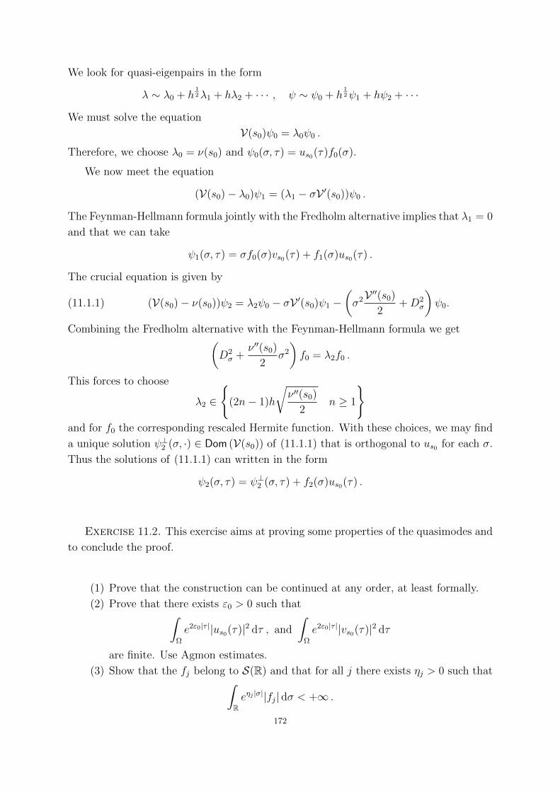
We look for quasi-eigenpairs in the form
λ ∼ λ0 + h12λ1 + hλ2 + · · · , ψ ∼ ψ0 + h
12ψ1 + hψ2 + · · ·
We must solve the equation
V(s0)ψ0 = λ0ψ0 .
Therefore, we choose λ0 = ν(s0) and ψ0(σ, τ) = us0(τ)f0(σ).
We now meet the equation
(V(s0)− λ0)ψ1 = (λ1 − σV ′(s0))ψ0 .
The Feynman-Hellmann formula jointly with the Fredholm alternative implies that λ1 = 0
and that we can take
ψ1(σ, τ) = σf0(σ)vs0(τ) + f1(σ)us0(τ) .
The crucial equation is given by
(11.1.1) (V(s0)− ν(s0))ψ2 = λ2ψ0 − σV ′(s0)ψ1 −(σ2V ′′(s0)
2+D2
σ
)ψ0.
Combining the Fredholm alternative with the Feynman-Hellmann formula we get(D2σ +
ν ′′(s0)
2σ2
)f0 = λ2f0 .
This forces to choose
λ2 ∈
(2n− 1)h
√ν ′′(s0)
2n ≥ 1
and for f0 the corresponding rescaled Hermite function. With these choices, we may find
a unique solution ψ⊥2 (σ, ·) ∈ Dom (V(s0)) of (11.1.1) that is orthogonal to us0 for each σ.
Thus the solutions of (11.1.1) can written in the form
ψ2(σ, τ) = ψ⊥2 (σ, τ) + f2(σ)us0(τ) .
Exercise 11.2. This exercise aims at proving some properties of the quasimodes and
to conclude the proof.
(1) Prove that the construction can be continued at any order, at least formally.
(2) Prove that there exists ε0 > 0 such that∫Ω
e2ε0|τ ||us0(τ)|2 dτ , and
∫Ω
e2ε0|τ ||vs0(τ)|2 dτ
are finite. Use Agmon estimates.
(3) Show that the fj belong to S(R) and that for all j there exists ηj > 0 such that∫Reηj |σ||fj| dσ < +∞ .
172
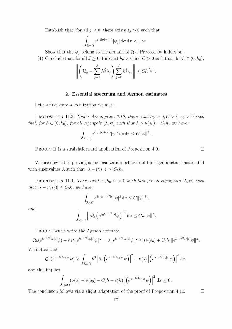
Establish that, for all j ≥ 0, there exists εj > 0 such that∫R×Ω
eεj(|σ|+|τ |)|ψj| dσ dτ < +∞ .
Show that the ψj belong to the domain of Hh. Proceed by induction.
(4) Conclude that, for all J ≥ 0, the exist h0 > 0 and C > 0 such that, for h ∈ (0, h0),∥∥∥∥∥(Hh −
J∑j=0
hj2λj
)J∑j=0
hj2ψj
∥∥∥∥∥ ≤ ChJ+1
2 .
2. Essential spectrum and Agmon estimates
Let us first state a localization estimate.
Proposition 11.3. Under Assumption 6.19, there exist h0 > 0, C > 0, ε0 > 0 such
that, for h ∈ (0, h0), for all eigenpair (λ, ψ) such that λ ≤ ν(s0) + C0h, we have:∫R×Ω
e2ε0(|s|+|τ |)|ψ|2 ds dτ ≤ C‖ψ‖2 .
Proof. It is a straightforward application of Proposition 4.9.
We are now led to proving some localization behavior of the eigenfunctions associated
with eigenvalues λ such that |λ− ν(s0)| ≤ C0h.
Proposition 11.4. There exist ε0, h0, C > 0 such that for all eigenpairs (λ, ψ) such
that |λ− ν(s0)| ≤ C0h, we have:∫R×Ω
e2ε0h−1/2|s||ψ|2 dx ≤ C‖ψ‖2 ,
and ∫R×Ω
∣∣∣h∂s (eε0h−1/2|s|ψ)∣∣∣2 dx ≤ Ch‖ψ‖2 .
Proof. Let us write the Agmon estimate
Qh(eh−1/2ε0|s|ψ)− hε2
0‖eh−1/2ε0|s|ψ‖2 = λ‖eh−1/2ε0|s|ψ‖2 ≤ (ν(s0) + C0h)‖eh−1/2ε0|s|ψ‖2 .
We notice that
Qh(eh−1/2ε0|s|ψ) ≥
∫R×Ω
h2∣∣∣∂s (eh−1/2ε0|s|ψ
)∣∣∣2 + ν(s)∣∣∣(eh−1/2ε0|s|ψ
)∣∣∣2 dx ,
and this implies∫R×Ω
(ν(s)− ν(s0)− C0h− ε20h)∣∣∣(eh−1/2ε0|s|ψ
)∣∣∣2 dx ≤ 0 .
The conclusion follows via a slight adaptation of the proof of Proposition 4.10.
173

3. Projection argument
As we have observed, it can be more convenient to study Hh instead of Hh. Let us
introduce the Feshbach-Grushin projection (see [94]) on us0 :
Π0ψ = 〈ψ, us0〉L2(Ω)us0(τ) .
We want to estimate the projection of the eigenfunctions associated with eigenvalues λ
such that |λ− ν(s0)| ≤ C0h. For that purpose, let us introduce the quadratic form
qs0(ψ) =
∫R×Ω
|∂τψ|2 + V (s0, τ)|ψ|2 dσ dτ .
This quadratic form is associated with the operator Idσ ⊗V(s0), and Π0 is the projection
on its first eigenspace.
Proposition 11.5. There exist C and h0 > 0 such that, for h ∈ (0, h0), for all
eigenfunction ψ of Hh associated with λ such that λ ≤ ν(s0) + C0h,
(11.3.1) 0 ≤ qs0(ψ)− ν(s0)‖ψ‖2 ≤ Ch12‖ψ‖2.
Moreover,
(11.3.2) ‖ψ − Π0ψ‖+ ‖∂τ (ψ − Π0ψ)‖ ≤ Ch14‖ψ‖ .
Proof. The proof uses the spectral gap ν2(s0)− ν1(s0) > 0. We write
(11.3.3) h‖∂σψ‖2 + ‖∂τψ‖2 +
∫R×Ω
V (s0 + h12σ, τ)|ψ|2 ds dτ ≤ (λ+ C0h)‖ψ‖2 .
Using the fact that V is a polynomial and the fact that, for k, n ∈ N,∫|τ |n|σ|k|ψ|2 dσ dτ ≤ C‖ψ‖2 ,
we get (11.3.1).
We notice that
qs0(ψ)− ν(s0)‖ψ‖2 = qs0(ψ − Π0ψ)− ν(s0)‖ψ − Π0ψ‖2 ,
due to the fact that Π0ψ belongs to the kernel of Idσ ⊗V(s0)− ν(s0)Id. We observe then
that
qs0(ψ − Π0ψ)− ν(s0)‖ψ − Π0ψ‖2 ≥∫R
∫Ω
|∂τ (ψ − Π0ψ)|2 + V (s0, τ)|(ψ − Π0ψ)|2 dτ dσ .
Since for each u, we have 〈ψ−Π0ψ, us0〉L2(Ω) = 0, we have (by using the min-max principle)
the lower bound
qs0(ψ − Π0ψ)− ν(s0)‖ψ − Π0ψ‖2 ≥∫R(ν2(s0)− ν(s0))
∫Ω
|ψ − Π0ψ|2 dτ dσ .
The estimate (11.3.2) follows.
174
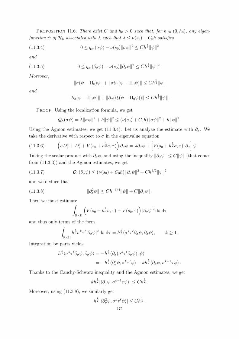
Proposition 11.6. There exist C and h0 > 0 such that, for h ∈ (0, h0), any eigen-
function ψ of Hh associated with λ such that λ ≤ ν(s0) + C0h satisfies
(11.3.4) 0 ≤ qs0(σψ)− ν(s0)‖σψ‖2 ≤ Ch12‖ψ‖2
and
(11.3.5) 0 ≤ qs0(∂σψ)− ν(s0)‖∂σψ‖2 ≤ Ch14‖ψ‖2 .
Moreover,
‖σ(ψ − Π0)ψ‖+ ‖σ∂τ (ψ − Π0ψ)‖ ≤ Ch14‖ψ‖
and
‖∂σ(ψ − Π0ψ)‖+ ‖∂σ(∂t(ψ − Π0ψ))‖ ≤ Ch18‖ψ‖ .
Proof. Using the localization formula, we get
Qh(σψ) = λ‖σψ‖2 + h‖ψ‖2 ≤ (ν(s0) + C0h)‖σψ‖2 + h‖ψ‖2 .
Using the Agmon estimates, we get (11.3.4). Let us analyze the estimate with ∂σ. We
take the derivative with respect to σ in the eigenvalue equation
(11.3.6)(hD2
σ +D2τ + V (s0 + h
12σ, τ)
)∂σψ = λ∂σψ +
[V (s0 + h
12σ, τ), ∂σ
]ψ .
Taking the scalar product with ∂σψ, and using the inequality ‖∂σψ‖ ≤ C‖ψ‖ (that comes
from (11.3.3)) and the Agmon estimates, we get
(11.3.7) Qh(∂σψ) ≤ (ν(s0) + C0h)‖∂σψ‖2 + Ch1/2‖ψ‖2
and we deduce that
(11.3.8) ‖∂2σψ‖ ≤ Ch−1/4‖ψ‖+ C‖∂σψ‖ .
Then we must estimate∫R×Ω
(V (s0 + h
12σ, τ)− V (s0, τ)
)|∂σψ|2 dσ dτ
and thus only terms of the form∫R×Ω
hk2σkτ `|∂σψ|2 dσ dτ = h
k2 〈σkτ `∂σψ, ∂σψ〉, k ≥ 1 .
Integration by parts yields
hk2 〈σkτ `∂σψ, ∂σψ〉 = −h
k2 〈∂σ(σkτ `∂σψ), ψ〉
= −hk2 〈∂2
σψ, σkτ `ψ〉 − kh
k2 〈∂σψ, σk−1τψ〉 .
Thanks to the Cauchy-Schwarz inequality and the Agmon estimates, we get
khk2 |〈∂σψ, σk−1τψ〉| ≤ Ch
12 .
Moreover, using (11.3.8), we similarly get
hk2 |〈∂2
σψ, σkτ `ψ〉| ≤ Ch
14 .
175
This is enough to obtain (11.3.5). The approximation results easily follow.
We can now use our approximation results to reduce the investigation to a model
operator in dimension one.
4. Accurate lower bound
For all N ≥ 1, let us consider an orthonormal family of eigenfunctions (ψn,h)1≤n≤N of
Hh such that ψn,h is associated with λn(h). We consider the N -dimensional space defined
by
EN(h) = span1≤n≤N
ψn,h .
It is rather easy to observe that, for ψ ∈ EN(h),
Qh(ψ) ≤ λN(h)‖ψ‖2 .
We are going to prove a lower bound of Qh on EN(h). We notice that
Qh(ψ) ≥∫R×Ω
[h|∂σψ|2 + ν(s0 + h
12σ)|ψ|2
]dσ dτ .
We have∫ [h|∂σψ|2 + ν(s0 + h
12σ)|ψ|2
]dσ dt =
∫|σh1/2|≤ε0
[h|∂σψ|2 + ν(s0 + h
12σ)|ψ|2
]dσ dτ
+
∫|σh
12 |≥ε0
[h|∂σψ|2 + ν(s0 + h
12σ)|ψ|2
]dσ dτ .
With the Taylor formula, we can write∫|σh1/2|≤ε0
[h|∂σψ|2 + ν(s0 + h
12σ)|ψ|2
]dσ dτ ≥∫
|σh1/2|≤ε0
[h|∂σψ|2 + ν(s0) + h
ν ′′(s0)
2σ2|ψ|2
]dσ dτ − Ch
32
∫|σh
12 |≤ε0
|σ|3|ψ|2 dσ dτ .
Thus, the Agmon estimates imply that∫|σh
12 |≤ε0
[h|∂σψ|2 + ν(s0 + h
12σ)|ψ|2
]dσ dt
≥∫|σh
12 |≤ε0
[h|∂σψ|2 + ν(s0)|ψ|2 + h
ν ′′(s0)
2σ2|ψ|2
]dσ dτ − Ch
32‖ψ‖2 .
Using again the Agmon estimates, we notice that∫|σh1/2|≥ε0
[h|∂σψ|2 + ν(s0)|ψ|2 + h
ν ′′(s0)
2σ2|ψ|2
]dσ dτ = O(h∞)‖ψ‖2 .
It follows that
Qh(ψ) ≥∫R×Ω
[h|∂σψ|2 + ν(s0)|ψ|2 + h
ν ′′(s0)
2σ2|ψ|2
]dσ dτ − Ch
32‖ψ‖2 .
176
Exercise 11.7. By using the approximation results, prove that
Qh(ψ) ≥ ν(s0)‖ψ‖2 +
∫R×Ω
[h|∂σΠ0ψ|2 + h
ν ′′(s0)
2σ2|Π0ψ|2
]dσ dτ + o(h)‖ψ‖2 .
Thanks to the orthogonality of the ψn,h with respect to the bilinear form associated
with Qh, we get
λN(h)‖ψ‖2 ≥ Qh(ψ) ≥ ν(s0)‖ψ‖2+
∫R×Ω
[h|∂σΠ0ψ|2 + h
ν ′′(s0)
2σ2|Π0ψ|2
]dσ dτ+o(h)‖ψ‖2 .
This becomes∫Rh|∂σ〈ψ, us0〉|2 + h
ν ′′(s0)
2σ2|〈ψ, us0〉|2 dσ ≤ (λN(h)− ν(s0) + o(h))‖〈ψ, us0〉‖2
L2(Rσ) .
Due to Proposition 11.5, the space 〈ψ, us0〉, ψ ∈ EN(h) is of dimension N . Thus, by
the min-max principle, we deduce that
λN(h) ≥ ν(s0) + (2N − 1)h
(ν ′′(s0)
2
)1/2
+ o(h) .
Let us end this section by examples, which can be treated as exercises.
Lu-Pan and de Gennes operator. Our first example (which comes from [19] and [183])
is the Neumann realization of the operator
h2D2ζ +D2
τ + (ζ − τ)2 ,
acting on L2(R2+, dζ dτ), where R2
+ = (ζ, τ) ∈ R2 : τ > 0.
Montgomery operator. The second example (which is the core of [59]) is the self-
adjoint realization on L2( dζ dτ) of
h2D2ζ +D2
τ +
(ζ − τ 2
2
)2
.
Popoff operator. Our last example (which comes from [176]) corresponds to the Neu-
mann realization on L2(Eα, dζ dz dτ) of
h2D2ζ +D2
τ +D2z + (ζ − τ)2 .
5. An alternative point of view
5.1. A general strategy. This section is devoted to the proof of Theorem 6.24.
It also gives us the opportunity to describe a quite general and elementary procedure
of dimensional reduction. We recall that we consider Lh = h2D2s + D2
t + V (s, t) whose
associated quadratic form is
Qh(ψ) =
∫R2
[h2|Dsψ|2 + |Dtψ|2 + V (s, t)|ψ|2
]ds dt .
177
We denote by us the first normalized eigenfunction of D2t + V (s, t) and we introduce the
projections defined for ψ ∈ L2(R2) by
Πsψ(s, t) = 〈ψ, us〉L2(Rt)us(t), Π⊥s ψ(s, t) = ψ(s, t)− Πsψ(s, t) .
We let R(s) = ‖∂sus‖2L2(Rt).
Lemma 11.8. For all ψ ∈ Dom (Qh), the function Πsψ belongs to Dom (Qh) and we
have
Qh(Πsψ) =
∫Rs
[h2|f ′(s)|2 + (ν1(s) + h2R(s))|f(s)|2
]ds, with f(s) = 〈ψ, us〉L2(Rt) .
Proof. It follows immediately that, for any ψ ∈ Dom (Qh),
∂s(Πsψ) = f(s)∂sus(t) + f ′(s)us(t) ∈ L2(R2),
since sups∈R |f ′(s)| ≤ sups∈R |〈ψ, ∂sus〉L2(Rt)|+ sups∈R |〈∂sψ, us〉L2(Rt)| <∞, and
∂t(Πsψ) = 〈ψ, us〉L2(Rt)∂tus(t) ∈ L2(R2).
Thus one has Πsψ ∈ Dom (Qh), and the calculations thereafter are valid.
By definition, one has
Qh(Πsψ)
=
∫R2
[h2|f(s)∂sus(t) + f ′(s)us(t)|2 + |f(s)|2|∂tus(t)|2
]ds dt+
∫R2
V (s, t)|f(s)|2|us(t)|2 ds dt,
and thus
Qh(Πsψ) =
∫Rs
[h2|f ′(s)|2 + h2|f(s)|2‖∂sus(t)‖2
L2(Rt)
]ds
+
∫Rs|f(s)|2
(∫Rt
[|∂tus(t)|2 + V (s, t)|us(t)|2
]dt
)ds
=
∫Rsh2|f ′(s)|2 ds+
∫Rsh2|f(s)|2R(s) ds+
∫Rsν1(s)|f(s)|2 ds.
where we used Fubini’s theorem, and the following properties on us:
(a) ∀s ∈ R, us is normalized in L2(Rt), and in particular,
〈us, ∂sus〉L2(Rt) =d
ds〈us, us〉L2(Rt) = 0.
(b) ∀s ∈ R, one has qs(us) = ν1(s).
Exercise 11.9. Prove that, for all ψ1, ψ2 ∈ Dom (Qh), we have
Bh(Πsψ1,Πsψ2) =
∫Rs
[h2f ′1(s)f ′2(s) + (ν1(s) + h2R(s))f ′1(s)f ′2(s)
]ds ,
where fj(s) = 〈ψj, us〉L2(Rt).
178

Proposition 11.10. For all ψ ∈ Dom (Qh) and all ε ∈ (0, 1), we have
Qh(ψ) ≥∫Rs
[(1− ε)h2|f ′(s)|2 +
(ν1(s)− 4ε−1h2R(s)
)|f(s)|2
]ds
+
∫Rs
[(1− ε)h2‖∂sΠ⊥s ψ‖2
L2(Rt) +(ν2(s)− 4ε−1h2R(s)
)‖Π⊥s ψ‖2
L2(Rt)
]ds .
Proof. We write
(11.5.1) Qh(ψ) =
∫R2
h2|Dsψ|2 ds dt+
∫Rs
qs(ψs) ds .
On the one hand, we have
(11.5.2) qs(ψs) = qs(Πsψ) + qs(Π⊥s ψ) ≥ ν1(s)|f(s)|2 + ν2(s)‖Π⊥s ψ‖2
L2(Rt) .
On the other hand, we get∫R2
|∂sψ|2 ds dt =
∫R2
|Πs∂sψ|2 ds dt+
∫R2
|Π⊥s ∂sψ|2 ds dt
But we have
[Πs, ∂s]ψ = −〈ψ, ∂sus〉L2(Rt)us − 〈ψ, us〉L2(Rt)∂sus = −[Π⊥s , ∂s]
and
‖[Πs, ∂s]ψ‖2 = ‖[Π⊥s , ∂s]ψ‖2 = ‖〈ψ, ∂sus〉L2(Rt)us‖2 + ‖〈ψ, us〉L2(Rt)∂sus‖2
so that
‖[Πs, ∂s]ψ‖2 = ‖[Π⊥s , ∂s]ψ‖2 ≤ 2
∫R2
R(s)|ψ|2 ds dt .
Writing Πs∂sψ = ∂sΠsψ + [Πs, ∂s]ψ, we get∫R2
|∂sψ|2 ds dt ≥ (1− ε)∫Rs|f ′(s)|2 ds+ (1− ε)
∫Rs‖∂sΠ⊥s ψ‖2
L2(Rt) ds
− 4ε−1
∫RsR(s)|f(s)|2 ds− 4ε−1
∫RsR(s)‖Π⊥s ψ‖2
L2(Rt) ds .
Combining this last estimate with (11.5.1) and (11.5.2), the result follows.
Proposition 11.11. Let us consider the following quadratic form, defined on Dom (qmodh )×
Dom (Qh) by
Qtensh (f, ϕ) =∫
Rs
[(1− h)h2|f ′(s)|2 +
(ν1(s)− 4Mh
)|f(s)|2
]ds+
∫R2
[(1− h)h2|∂sϕ|2 +
(ν2(s)− 4Mh
)|ϕ|2
]ds dt,
∀(f, ϕ) ∈ Dom (qmodh )× Dom (Qh) .
If Htensh denotes the associated operator, then we have, for all n ≥ 1,
λn(h) ≥ λtensn (h) .
179
Proof. Using Proposition 11.10 with ε = h, we get, for all ψ ∈ Dom (Qh),
Qh(ψ) ≥∫Rs
[(1− h)h2|f ′|2 +
(ν1(x)− 4Mh
)|f |2]
ds
+
∫R2
[(1− h)h2|∂sΠ⊥s ψ|2 +
(ν2(s)− 4Mh
)|Π⊥s ψ|2
]ds dt .
Thus we have
(11.5.3) Qh(ψ) ≥ Qtensh (〈ψ, us〉,Π⊥s ψ), ‖ψ‖2 = ‖f‖2 + ‖Π⊥s ψ‖2 .
With (11.5.3) we infer that
λn(h) ≥ infG⊂H1(R2)dimG=n
supψ∈G
Qtensh (〈ψ, us〉,Π⊥s ψ)
‖Πsψ‖2 + ‖Π⊥s ψ‖2.
Now, we define the linear injection
J :
Dom (Qh) −→ Dom (qmod
h )× Dom (Qh)
ψ 7−→ (〈ψ, us〉 , Π⊥s ψ),
so that we have
infG⊂Dom (Qh)
dimG=n
supψ∈G
Qtensh (Πsψ,Π
⊥s ψ)
‖Πsψ‖2 + ‖Π⊥s ψ‖2= inf
G⊂J (Dom (Qh))
dim G=n
sup(f,ϕ)∈G
Qtensh (f, ϕ)
‖f‖2 + ‖ϕ‖2,
and
infG⊂J (Dom (Qh))
dim G=n
sup(f,ϕ)∈G
Qtensh (f, ϕ)
‖f‖2 + ‖ϕ‖2≥ inf
G⊂Dom (qmodh )×Dom (Qh)
dim G=n
sup(f,ϕ)∈G
Qtensh (f, ϕ)
‖f‖2 + ‖ϕ‖2.
We recognize the n-th Rayleigh quotient of Htensh and the conclusion follows.
We can now prove Theorem 6.24. Let us introduce the model quadratic forms
qmodh (f) =
∫R
[h2|f ′(s)|2 + ν1(s)|f(s)|2
]ds .
Using Exercise 11.9 and the eigenfunctions of the operator associated with qmodh , we get
N (Qh, E) ≥ N(qmodh , E −Mh2
).
Conversely, we use the result of Proposition 11.11 to get
N (Qh, E) ≤ N (Qtensh , E) ≤ N
(qmodh , (E + 4Mh)(1− h)−1
),
the last inequality coming from the fact that, when h is small enough, there are no
eigenvalues of Htensh below the threshold (by the assumption in Theorem 6.24).
Therefore, we are reduced to the estimate of the counting function of qmodh in one
dimension and we apply Theorem 3.1.
5.2. Robin Laplacian in the Born-Oppenheimer approximation. Let us now
end our discussion about the electric Born-Oppenheimer approximation with an exercise
180
related to the semiclassical Robin Laplacian. We use the notations introduced in Chapter
4, Section 3.4.3.
5.2.1. A tubular neighborhood. Given δ ∈ (0, δ0) (with δ0 > 0 small enough), we
introduce the δ-neighborhood of the boundary
(11.5.4) Vδ = x ∈ Ω : dist(x, ∂Ω) < δ ,
and the quadratic form, defined on the variational space
Vδ = u ∈ H1(Vδ) : u(x) = 0 , for all x ∈ Ω such that dist(x, ∂Ω) = δ ,
by the formula
∀u ∈ Vδ , QRob,δh (u) =
∫Vδ|h∇u|2 dx− h
32
∫∂Ω
|u|2 ds(x) .
We denote by LRob,δh the corresponding operator. For simplicity, we take δ = h
14 . We
denote by λRobn (h) and λRob,δ
n (h) the n-th eigenvalue of LRobh and LRob,δ
h , respectively.
By using the estimates of Agmon, prove the following proposition.
Proposition 11.12. Let ε0 ∈ (0, 1) and α ∈ (0,√ε0).There exist two constants,
C > 0 and h0 ∈ (0, 1), such that, for all h ∈ (0, h0) and n ≥ 1 such that λRobn (h) ≤ −ε0h,
λRobn (h) ≤ λRob,δ
n (h) ≤ λRobn (h) + C exp
(− αh−
14
).
5.2.2. The rescaled operator in normal coordinates. Let us denote by c the normal
parametrization of the boundary. Now we introduce the change of coordinates
(11.5.5) Φ : R/(|∂Ω|Z)× (0, δ0) 3 (s, t) 7−→ x = c(s) + tn(s) ∈ Vδ0 .
We denote L = |∂Ω|/2. The determinant of the Jacobian of Φ is given by
(11.5.6) a(s, t) = 1− tκ(s).
The operator LRob,δh is expressed in (s, t) coordinates as
Lh = −h2a−1∂s(a−1∂s)− h2a−1∂t(a∂t) ,
acting on L2(a ds dt). In these coordinates, the Robin condition becomes
h2∂tu = −h32u for t = 0 .
It will be convenient to work with a rescaled version of Lh. We introduce the rescaling
(σ, τ) = (s, h−12 t) ,
the new semiclassical parameter ~ = h14 and the new weight
(11.5.7) a(σ, τ) = 1− ~2τκ(σ) .
We thus consider the operator
(11.5.8) L~ = h−1Lh ,181
acting on L2(a dσ dτ) and expressed in the coordinates (σ, τ). We let T = h−12 δ = h−
14
and
(11.5.9)
VT = (σ, τ) : σ ∈]− L,L] and 0 < τ < T ,
VT = u ∈ H1(VT ) : u(σ, T ) = 0 ,
DT = u ∈ H2(VT ) ∩ VT : ∂τu(σ, 0) = −u(σ, 0) ,
Q~(u) =
∫VT
(a−2~4|∂σu|2 + |∂τu|2
)a dσ dτ −
∫ L
−L|u(σ, 0)|2 dσ ,
L~ = −~4 a−1∂σa−1∂σ − a−1∂τ a∂τ .
5.2.3. Dimensional reduction. We use the notations introduced in Chapter 2, Section
3.2.
We let
Hκ(σ),~ = LR,TB ,
with B = h12κ(σ) = ~2κ(σ).
We introduce for σ ∈ [−L,L) the Feshbach projection Πσ on the normalized ground-
state of Hκ(σ),~, denoted by vκ(σ),~:
Πσψ = 〈ψ, vκ(σ),~〉L2((0,T ),adτ)vκ(σ),~ .
We also let
Π⊥σ = Id− Πσ
and
(11.5.10) R~(σ) = ‖∂σvκ(σ),~‖2L2((0,T ), a dτ) .
The quantity R~ is sometimes called the “Born-Oppenheimer correction”.
To reduce the analysis to classical considerations, the main point is to control the effect
of replacing a−2 by 1.
Lemma 11.13. We have, for all ψ ∈ Dom (Q~),∣∣∣∣∫VTa−2|∂σψ|2a dσ dτ −
∫VT|∂σψ|2a dσ dτ
∣∣∣∣≤ C
∫VT
[~2|f ′ψ(σ)|2 + ~R~(σ)|fψ(σ)|2 + ~|∂σΠ⊥σψ|2
]dσ dτ ,
with
fψ(σ) := 〈ψ(σ, ·), vκ(σ),~〉L2((0,T ), adτ) .
182
Proof. We write∣∣∣∣∫VTa−2|∂σψ|2 dσ dτ −
∫VT|∂σψ|2 dσ dτ
∣∣∣∣≤ C
∫VT
~2τ |∂σψ|2 dσ dτ
≤ 2C
∫VT
~2τ(|∂σΠσψ|2 + |∂σΠ⊥σψ|2
)dσ dτ
≤ C
∫VT
~2[|f ′ψ(σ)|2 + ~R~(σ)|fψ(σ)|2 + ~|∂σΠ⊥σψ|2
]dσ dτ ,
where we used the fact that
(11.5.11)
∫ T
0
τ |vκ(σ),~|2 dτ ≤ C
(which is a consequence of Proposition 4.24) and that τ~2 may be estimated by T~2 =
~.
Lemma 11.14. We have∫ T
0
vκ(σ),~∂σvκ(σ),~ a dτ = O(~2) .
Proof. It follows from the normalization of vκ(σ),~ that
∂σ
∫ T
0
vκ(σ),~vκ(σ),~a dτ = 0 ,
so that
2
∫ T
0
vκ(σ),~∂σvκ(σ),~ a dτ =
∫ T
0
vκ(σ),~vκ(σ),~(∂σa) dτ , with ∂σa = −τ~2κ′(σ) .
The conclusion follows from (11.5.11).
Lemma 11.15. There exist C > 0 and ~0 > 0 such that, for all ψ ∈ DT and ~ ∈ (0, ~0),
we have
Q~(Πσψ) ≤∫ L
−L
[~4(1 + C~2)|f ′ψ(σ)|2 +
(~4(1 + C~)R~(σ) + λ1(Hκ(σ),~) + C~6
)|fψ(σ)|2
]dσ .
The next lemma is slightly more delicate and follows from adaptations of the last
section.
Lemma 11.16. There exist C > 0 and ~0 > 0 such that, for all ψ ∈ DT , ε ∈(0, 1
2
)and ~ ∈ (0, ~0), we have
Q~(ψ) ≥∫ L
−L
[(1− ε)(1− C~2)~4|f ′ψ(σ)|2 +
λ1(Hκ(σ),~)− C(ε−1~4R~(σ) + ε−1~8 + ~6)
|fψ(σ)|2
]dσ
+
∫ L
−L
[(1− ε)(1− C~)~4‖∂σΠ⊥σψ‖2
L2(adτ) +λ2(Hκ(σ),~)− Cε−1~4R~(σ)− Cε−1~8
‖Π⊥σψ‖2
L2(adτ)
]dσ .
183
We apply Lemmas 11.15 and 11.16 with ε = ~2. Then, we use Proposition 2.9, Lemma
2.10, and Proposition 2.11 to deduce that
λ1(Hκ(σ),~) = −1− ~2κ(σ) +O(~4) ,
and that there exist h0 > 0 and C > 0 such that, for all h ∈ (0, h0),
λ2(Hκ(σ),~) ≥ −C~ > −ε02.
Then we notice that R~(σ) (introduced in (11.5.10)) satisfies R~(σ) = O(~4) thanks to
Lemma 4.25 and the relation B = κ(σ)~2. We deduce the following theorem.
Theorem 11.17. For ε0 ∈ (0, 1) and h > 0, we let
Nε0,h = n ∈ N∗ : λRobn (h) < −ε0h .
There exist positive constants h0, C+, C− such that, for all h ∈ (0, h0) and n ∈ Nε0,h,
λeff,−n (h) ≤ λRob
n (h) ≤ λeff,+n (h) ,
where λeff,±n (h) is the n-th eigenvalue of the operator Leff,±
h defined by
Leff,+h = −h+ (1 + C+h
12 )h2D2
σ − κ(σ)h32 + C+h
2 ,
and
Leff,−h = −h+ (1− C−h
12 )h2D2
σ − κ(σ)h32 − C−h2 ,
Remark 11.18. Let us end this section with the following observations.
i. As we can see in the proof of Theorem 11.17, we only need to use that the boundary
is C2 and that the curvature is Lipschitzian. In the terminology of [172], such an
assumption means that the boundary is admissible of order 3.
ii. It is possible to avoid the assumption that the curvature is Lipschitzian by considering
rather the projection Π0,h (which is done at some point in [172]) and by noticing that
is the first order approximation of Πκ(σ),h.
iii. Note also that we have here a uniform approximation of the spectrum. The choice
of δ = h14 was arbitrary. Such a choice is natural why studying the tunneling effect
between non-degenerate wells ([101]).
iv. Since the strategy does not depend on the dimension, for the case of higher dimension,
the same results holds as soon as we replace D2σ by the Laplace-Beltrami operator on
∂Ω and κ by the mean curvature.
v. The result of Theorem 11.17 can be applied to get a semiclassical estimate of the
counting function of eigenvalues less than −h+ Eh32 , that is
N(LRobh ,−h+ Eh
32
)∼h→0
1
πh14
∫∂Ω
√(E + κ)+ ds(x) .
184
CHAPTER 12
Magnetic Born-Oppenheimer approximation
Pour l’achevement de la science, il faut
passer en revue une a une toutes les choses
qui se rattachent a notre but par un mou-
vement de pensee continu et sans nulle in-
terruption, et il faut les embrasser dans une
enumeration suffisante et methodique.
Regles pour la direction de l’esprit,
Descartes
We explain in this chapter the main steps of the proof of Theorem 6.29. In particu-
lar, the reader is supposed to be familiar with the basics of pseudo-differential calculus.
We establish general Feynman-Hellmann formulas and we also recall the fundamental
properties of coherent states.
1. Quasimodes
This section is devoted to the proof of the following proposition.
Proposition 12.1. If Assumption 6.25 holds, then for all n ≥ 1, there exist a se-
quence (γj,n)j≥0 with the property that for all J ≥ 0 there exist C > 0 and h0 > 0 such
that for h ∈ (0, h0):
dist
(J∑j=0
γj,nhj/2, sp(Lh)
)≤ Ch(J+1)/2 ,
where
γ0,n = µ0, γ1,n = 0, γ2,n = νn
(1
2Hessx0,ξ0 µ(σ,Dσ)
).
In order to perform the investigation we use the following rescaling
s = h1/2σ ,
so that Lh becomes:
(12.1.1) Lh = (−i∇τ + A2(x0 + h1/2σ, τ))2 + (ξ0 − ih1/2∇σ + A1(x0 + h1/2σ, τ))2 .
We will also need generalizations of the Feynman-Hellmann formulas which are obtained
by taking the derivative of the eigenvalue equation
Mx,ξux,ξ = µ(x, ξ)ux,ξ
185
with respect to xj and ξk.
Proposition 12.2. We have
(12.1.2) (Mx,ξ − µ(x, ξ))(∂ηu)x,ξ = (∂ηµ(x, ξ)− ∂ηMx,ξ)ux,ξ
and
(12.1.3) (Mx0,ξ0 − µ0)(∂η∂θu)x0,ξ0
= ∂η∂θµ(x0, ξ0)ux0,ξ0 − ∂ηMx0,ξ0(∂θu)x0,ξ0 − ∂θMx0,ξ0(∂ηu)x0,ξ0 − ∂η∂θMx0,ξ0ux0,ξ0 ,
where η and θ denote one of the xj or ξk. Moreover,
(12.1.4) ∂ηµ(x, ξ) =
∫Rn∂ηMx,ξ ux,ξ(τ)ux,ξ(τ) dτ .
We can now prove Proposition 12.1. Since A1 and A2 are polynomials, we can write,
for some M ∈ N,
Lh =M∑j=0
hj/2Lj ,
with
L0 =Mx0,ξ0 , L1 =m∑j=1
(∂xjM)x0,ξ0σj +m∑j=1
(∂ξjM)x0,ξ0Dσj ,
L2 =1
2
m∑k,j=1
((∂xj∂xkM)x0,ξ0σjσk + (∂ξj∂ξkM)x0,ξ0DσjDσk + (∂ξj∂xkM)x0,ξ0Dσjσk
+ (∂xk∂ξjM)x0,ξ0σkDσj
).
We look for quasimodes in the form
ψ ∼∑j≥0
hj/2ψj
and quasi-eigenvalues in the form
γ ∼∑j≥0
hj/2γj ,
so that they solve in the sense of formal series the equation
Lhψ ∼ γψ .
By collecting the terms of order h0, we get the equation:
Mx0,ξ0ψ0 = γ0ψ0 .
This leads us to taking γ0 = µ0 and
ψ0(σ, τ) = f0(σ)u0(τ) ,
186
where u0 = ux0,ξ0 and f0 is a function to be determined in the Schwartz class. By
collecting the terms of order h1/2, we find:
(Mx0,ξ0 − µ(x0, ξ0))ψ1 = (γ1 − L1)ψ0 .
By using (12.1.2) and the Fredholm alternative (applied for σ fixed) we get γ1 = 0 and
the solution:
(12.1.5) ψ1(σ, τ) =m∑j=1
(∂xju)x0,ξ0 σjf0 +m∑j=1
(∂ξju)x0,ξ0 Dσjf0 + f1(σ)u0(τ) ,
where f1 is a function to be determined in the Schwartz class. The next equation reads
(Mx0,ξ0 − µ(x0, ξ0))ψ2 = (γ2 − L2)ψ0 − L1ψ1 .
The corresponding Fredholm condition is
(12.1.6) 〈L2ψ0 + L1ψ1, u0〉L2(Rn, dτ) = γ2f0 .
We obtain (exercise):1
2Hessµ(x0, ξ0)(σ,Dσ)f0 = γ2f0 .
We take γ2 in the spectrum of 12Hessµ(x0, ξ0)(σ,Dσ) and we choose for f0 a corresponding
normalized eigenfunction. The construction can be continued at any order.
We deduce from Propositions 6.28 and 12.1:
Corollary 12.3. For all n ≥ 1 there exist h0 > 0 and C > 0 such that for all
h ∈ (0, h0), the n-th eigenvalue of Lh exists and satisfies
λn(h) ≤ µ0 + Ch .
2. Rough estimates of the eigenfunctions
In this section we recall the basic and rough localization and microlocalization es-
timates satisfied by the eigenfunctions resulting from Assumptions 6.25 and 6.27 and
Corollary 12.3. The following two propositions are applications of Proposition 4.9.
Proposition 12.4. Let C0 > 0. There exist h0, C, ε0 > 0 such that for all eigenpairs
(λ, ψ) of Lh satisfying λ ≤ µ0 + C0h we have∥∥eε0|τ |ψ∥∥2 ≤ C‖ψ‖2, Qh
(eε0|τ |ψ
)≤ C‖ψ‖2 .
Proposition 12.5. Let C0 > 0. There exist h0, C, ε0 > 0 such that for all eigenpairs
(λ, ψ) of Lh satisfying λ ≤ µ0 + C0h, we have∥∥eε0|s|ψ∥∥2 ≤ C‖ψ‖2, Qh
(eε0|s|ψ
)≤ C‖ψ‖2 .
We deduce from Propositions 12.4 and 12.5 the following corollary.
187
Corollary 12.6. Let C0 > 0 and k, l ∈ N. There exist h0, C, ε0 > 0 such that for
all eigenpairs (λ, ψ) of Lh satisfying λ ≤ µ0 + C0h, we have
‖τ kslψ‖ ≤ C‖ψ‖, Qh(τkslψ) ≤ C‖ψ‖2 ,
‖ − i∇τslτ kψ‖ ≤ C‖ψ‖2, ‖ − ih∇ss
lτ kψ‖ ≤ C‖ψ‖2 .
Taking successive derivatives of the eigenvalue equation we deduce by induction:
Corollary 12.7. Let C0 > 0 and k, l, p ∈ N. There exist h0, C, ε0 > 0 such that for
all eigenpairs (λ, ψ) of Lh satisfying λ ≤ µ0 + C0h and all h ∈ (0, h0), we have
‖(−i∇τ )pslτ kψ‖ ≤ C‖ψ‖2, ‖(−ih∇s)
pslτ kψ‖ ≤ C‖ψ‖2 .
Using again Propositions 12.4 and 12.5 and an induction argument we get:
Proposition 12.8. Let k ∈ N. Let η > 0 and χ a smooth cutoff function equal to
zero in a neighborhood of 0. There exists h0 > 0 such that for all eigenpairs (λ, ψ) of Lhsatisfying λ ≤ µ0 + C0h and all h ∈ (0, h0), we have
‖χ(hηs)ψ‖Bk(Rm+n) ≤ O(h∞)‖ψ‖, ‖χ(hητ)ψ‖Bk(Rm+n) ≤ O(h∞)‖ψ‖ ,
where ‖ · ‖Bk(Rn+m) is the standard norm on
Bk(Rm+n) = ψ ∈ L2(Rm+n) : yqj∂pylψ ∈ L2(Rn+m),∀j, k ∈ 1, . . . ,m+ n, p+ q ≤ k .
By using a rough pseudo-differential calculus jointly with the space localization of
Proposition 12.8 and standard elliptic estimates, we get:
Proposition 12.9. Let k ∈ N. Let η > 0 and χ a smooth cutoff function being zero
in a neighborhood of 0. There exists h0 > 0 such that for all h ∈ (0, h0) and all eigenpairs
(λ, ψ) of Lh satisfying λ ≤ µ0 + C0h, we have
‖χ(hηhDs)ψ‖Bk(Rm+n) ≤ O(h∞)‖ψ‖, ‖χ(hηDτ )ψ‖Bk(Rm+n) ≤ O(h∞)‖ψ‖ .
3. Coherent states and microlocalization
3.1. A first lower bound. By using the formalism introduced in Chapter 6, Section
2.2.2, we get the following statement.
Proposition 12.10. There exist h0, C > 0 such that for all eigenpairs (λ, ψ) of Lhsatisfying λ ≤ µ0 + C0h and all h ∈ (0, h0), we have
(12.3.1) Qh(ψ) ≥∫R2m
Qh,u,p(ψu,p) du dp− Ch‖ψ‖2 ≥ (µ(x0, ξ0)− Ch)‖ψ‖2 ,
where Qh,u,p is the quadratic form associated with the operator Mx0+h1/2u,ξ0+h1/2p.
Proof. We use (6.2.4). Then the terms ofRh (see (6.2.5)) are in the form hhp/2σlDqστ
αDβτ
with l + q ≤ p and β = 0, 1. Using Corollary 12.7 and the rescaling (9.1.3), we have
‖hp/2σlDqστ
αDβτψ‖ ≤ C‖ψ‖
188

and the conclusion follows.
3.2. Localization in the phase space. This section is devoted to elliptic regularity
properties (both in space and frequency) satisfied by the eigenfunctions. We will use
the generalization of the localization formula given in Chapter 4, formula (4.2.1). The
following lemma is a straightforward consequence of Assumption 6.25.
Lemma 12.11. Under Assumption 6.25, there exist ε0 > 0 and c > 0 such that
µ(x0 + x, ξ0 + ξ)− µ(x0, ξ0) ≥ c(|x|2 + |ξ|2), ∀(x, ξ) ∈ B(ε0) ,
and
µ(x0 + x, ξ0 + ξ)− µ(x0, ξ0) ≥ c, ∀(x, ξ) ∈ B(ε0) ,
where B(ε0) = (x, ξ), |x|+ |ξ| ≤ ε0 and B(ε0) is its complement.
Notation 12.12. In what follows we will denote by η > 0 all the quantities that are
multiples of η > 0,i.e., of the form pη for p ∈ N\0. We recall that η > 0 can be chosen
arbitrarily small.
Proposition 12.13. There exist h0, C, ε0 > 0 such that for all h ∈ (0, h0) and all
eigenpairs (λ, ψ) of Lh such that λ ≤ µ0 + C0h, we have
‖σψ‖2 + ‖∇σψ‖2 ≤ C‖ψ‖2 .
Proof. Let (λ, ψ) be an eigenpair such that λ ≤ µ0 + C0h. We recall that (12.3.1)
holds. We have
Qh(ψ) = λ‖ψ‖2 ≤ (µ0 + C0h)‖ψ‖2 .
We deduce that ∫R2m
[Qh,u,p(ψu,p)− µ0|ψu,p|2
]du dp ≤ Ch‖ψ‖2
and thus, by the min-max principle, that∫R2m
(µ(x0 + h1/2u, ξ0 + h1/2p)− µ0
)|ψu,p|2 du dp ≤ Ch‖ψ‖2 .
We use the ε0 > 0 given in Lemma 12.11 and we split the integral into two parts. In this
way, we get ∫B(h−1/2ε0)
(|u|2 + |p|2)|ψu,p|2 du dp ≤ C‖ψ‖2,(12.3.2) ∫B(h−1/2ε0)
|ψu,p|2 du dp ≤ Ch‖ψ‖2 .(12.3.3)
The first inequality is not enough to get the conclusion. We also need a control of
momenta in the region B(h−1/2ε0). For that purpose, we write
(12.3.4) Qh(a∗jψ) =
∫R2m
Qh,u,p
(uj − ipj√
2ψu,p
)du dp+ 〈Rha
∗jψ, a
∗jψ〉 .
189
Up to lower order terms we must estimate terms of the form
h〈hp/2σlDqστ
αDβτ a∗jψ, a
∗jψ〉 ,
with l + q = p, α ∈ N and β = 0, 1. By using the a priori estimates of Propositions 12.8
and 12.9, we have
‖hp/2σlDqστ
αDβτ a∗jψ‖ ≤ Ch−η‖a∗jψ‖ .
The remainder is controlled by
|〈Rha∗jψ, a
∗jψ〉| ≤ Ch1−η(‖∇σψ‖2 + ‖σψ‖2) .
Then we analyze Qh(a∗jψ) by using (4.2.1) (Chapter 4) with A = aj. We need to estimate
the different remainder terms. We notice that
‖[a∗j , Pk,r,h]ψ‖ ≤ Ch1/2‖ψ‖,
|〈Pk,r,hψ, a∗j [Pk,r,h, aj]ψ〉| ≤ ‖Pk,r,hψ‖ ‖a∗j [Pk,r,h, aj]ψ‖ ,
|〈Pk,r,hψ, aj[Pk,r,h, a∗j ]ψ〉| ≤ ‖Pk,r,hψ‖ ‖aj[Pk,r,h, a∗j ]ψ‖ ,
|〈Pk,r,hψ, [[Pk,r,h, aj], a∗j ]ψ〉| ≤ ‖Pk,r,hψ‖ ‖[[Pk,r,h, aj], a∗j ]ψ‖ ,
where P1,r,h denotes the magnetic momentum h1/2Dσr + A1,r(x0 + h1/2σ, τ) and P2,r,h
denotes Dτr + A2,r(x0 + h1/2σ, τ). We have
‖Pk,r,hψ‖ ≤ C‖ψ‖
and
‖a∗j [Pk,r,h, aj]ψ‖ ≤ Ch1/2‖a∗jQ(h1/2σ, τ)ψ‖ ,where Q is polynomial. The other terms can be bounded in the same way. We apply the
estimates of Propositions 12.8 and 12.9 to get:
‖a∗jQ(h1/2σ, τ)ψ‖ ≤ Ch−η‖a∗jψ‖ .
Further,
Qh(a∗jψ) = λ‖a∗jψ‖2 +O(h)‖ψ‖2 +O(h12−η)(‖∇σψ‖2 + ‖σψ‖2) ,
so that
Qh(a∗jψ) ≤ µ(x0, ξ0)‖a∗jψ‖2 + Ch‖ψ‖2 +O(h12−η)(‖∇σψ‖2 + ‖σψ‖2) .
By using (12.3.4) and splitting again the integral into two parts, we get that∫B(h−1/2ε0)
(|u|2 + |p|2)|(uj − ipj)ψu,p|2 du dp ≤ C‖ψ‖2 + Ch−12−η(‖∇σψ‖2 + ‖σψ‖2) ,∫
B(h−1/2ε0)
|(uj − ipj)ψu,p|2 du dp ≤ Ch‖ψ‖2 + Ch12−η(‖∇σψ‖2 + ‖σψ‖2) .
Combining the last inequality with the first one in (12.3.2) and the Parseval formula we
get the conclusion.
190

By using the same ideas, we can establish the following result.
Proposition 12.14. Let P ∈ C2[X1, . . . , X2n]. There exist h0, C, ε0 > 0 such that for
all h ∈ (0, h0) and all eigenpairs (λ, ψ) of Lh satisfying λ ≤ µ0 + C0h, we have
‖P (σ,Dσ)ψ‖2 ≤ Ch−12−η‖ψ‖2 .
3.3. Approximation lemmas. We introduce the projection
Ψ0 = Π0ψ = 〈ψ, ux0,ξ0〉L2(Rn, dτ)ux0,ξ0
and, inspired by (12.1.5) with f0 replaced by 〈ψ, ux0,ξ0〉L2(Rn,dτ) and f1 by 0,
(12.3.5) Ψ1 =m∑j=1
(∂xju)x0,ξ0 σj〈ψ, ux0,ξ0〉L2(Rn, dτ) +m∑j=1
(∂ξju)x0,ξ0 Dσj〈ψ, ux0,ξ0〉L2(Rn, dτ).
This leads to defining the corrected Feshbach projection
(12.3.6) Πhψ = Ψ0 + h1/2Ψ1
and
Rh = ψ − Πhψ .
Let us note that this corrected Feshbach correction shares some features with the “super-
adiabatic” projections a la Panati-Spohn-Teufel-Wachsmuth (see for instance [199, 171,
203]).
Note that the functions Ψ0 and Ψ1 will be a priori h-dependent. By the L2-normalization
of ux,ξ (when ξ ∈ Rm), Ψ1 and Rh are orthogonal (with respect to the τ -variable) to u0
(and Ψ0). Furthermore, we have by construction and Proposition 12.2,
(12.3.7) (L0 − µ0)Ψ1 = −L1Ψ0
and, by the Fredholm alternative,
〈L1Ψ0,Ψ0〉L2(Rn, dτ) = 0 .
We can prove a first approximation.
Proposition 12.15. There exist h0 and C > 0 such that for all h ∈ (0, h0) and all
eigenpairs (λ, ψ) of Lh such that λ ≤ µ0 + C0h, we have
‖ψ − Π0ψ‖ ≤ Ch1/2−η‖ψ‖ .
Proof. We can write
(L0 − µ0)ψ = (λ− µ0)ψ − h1/2L1ψ − hL2ψ + · · · − hM/2LMψ .
By using the rough microlocalization given in Propositions 12.8 and 12.9 and Proposition
12.14, we infer that for p ≥ 2
(12.3.8) hp/2‖ταDβτ σ
lDqσψ‖ ≤ Ch
p2− p−2
2− 1
4−η‖ψ‖ = Ch
34−η‖ψ‖ ,
191
and thanks to Proposition 12.13
‖L1ψ‖ ≤ Ch−η‖ψ‖ ,
so that
‖(L0 − µ0)ψ‖ ≤ Ch12−η‖ψ‖ ,
and the conclusion follows.
Corollary 12.16. There exist h0, C > 0 such that for all h ∈ (0, h0) and all eigen-
pairs (λ, ψ) of Lh such that λ ≤ µ0 + C0h, we have
‖σ(ψ − Π0ψ)‖ ≤ Ch1/4−η‖ψ‖, ‖Dσ(ψ − Π0ψ)‖ ≤ Ch1/4−η‖ψ‖
We can now estimate ψ − Πhψ.
Proposition 12.17. There exist h0, C > 0 such that for all h ∈ (0, h0) and all
eigenpairs (λ, ψ) of Lh such that λ ≤ µ0 + C0h, we have
‖ψ − Πhψ‖ ≤ Ch3/4−η‖ψ‖ .
Proof. Let us write
Lhψ = λψ .
We have
(L0 + h1/2L1)ψ = (µ0 +O(h))ψ − hL2ψ − · · · − hM/2LMψ .Let us notice that, as in (12.3.8), for p ≥ 2
hp/2‖Lpψ‖ ≤ Ch34−η‖ψ‖ .
We get
(L0 − µ0)Rh = −h1/2L1(ψ −Ψ0) +O(h)ψ − hL2ψ − · · · − hM/2LMψ
It remains to apply Corollary 12.16 to obtain
h1/2‖L1(ψ −Ψ0)‖ ≤ Ch34−η‖ψ‖ .
Let us introduce a certain subspace of dimension P ≥ 1. For j ∈ 1, . . . , P we can
consider a L2-normalized eigenfunction of Lh denoted by ψj,h, and such that the family
(ψj,h)j∈1,...,P is orthogonal. We let:
EP (h) = spanj∈1,...,P
ψj,h .
Remark 12.18. We can extend all the local and microlocal estimates as well as our
approximations to ψ ∈ EP (h).
Proposition 12.19. For all n ≥ 1, there exists h0 > 0 such that, for all h ∈ (0, h0),
we have
λn(h) ≥ µ0 + λn,1h+ o(h) ,
192
where we recall that λn,1 is the n-th eigenvalue of 12Hessµ(x0, ξ0)(σ,Dσ).
Proof. Since we want to establish a lower bound for the eigenvalues, let us prove a
lower bound for the quadratic form on EP (h), for P ≥ 1 (in the spirit of Chapter 11).
We have
Qh(ψ) = 〈L0ψ, ψ〉+h1/2〈L1ψ, ψ〉+h〈L2ψ, ψ〉+ · · ·+hp/2〈Lpψ, ψ〉+ · · ·+hM/2〈LMψ, ψ〉 .
Using Propositions 12.13, 12.14, 12.8, and 12.9, we have, for ` ≥ 3,
|h`/2〈L`ψ, ψ〉| ≤ Ch`2− `−3
2−η− 1
4‖ψ‖2 = Ch54−η‖ψ‖2 .
It follows that
Qh(ψ) ≥ 〈L0ψ, ψ〉+ h1/2〈L1ψ, ψ〉+ h〈L2ψ, ψ〉 − Ch54−η‖ψ‖2 .
It remains to analyze the different terms. We have
〈L0ψ, ψ〉 = 〈L0(Ψ0 + h1/2Ψ1 +Rh),Ψ0 + h1/2Ψ1 +Rh〉 .
The orthogonality (with respect to τ) cancels the terms 〈L0Ψ1,Ψ0〉 and 〈Rh,Ψ0〉. More-
over, we have, by Propositions 12.8 and 12.9, that
h1/2|〈L0Rh,Ψ1〉| ≤ h1/2−η‖Rh‖‖Ψ1‖ .
Now we use Proposition 12.13 to get
‖Ψ1‖ ≤ C‖ψ‖ ,
so that, by Proposition 12.17,
〈L0ψ, ψ〉 = µ0‖Ψ0‖2 + h〈L0Ψ1,Ψ1〉+O(h54−η)‖ψ‖2 .
We have
〈L1ψ, ψ〉 = 〈L1Ψ0,Ψ0〉+ 2h1/2〈L1Ψ0,Ψ1〉+ h〈L1Ψ1,Ψ1〉+ 2〈L1ψ,Rh〉 .
Then, a Feynman-Hellmann formula provides 〈L1Ψ0,Ψ0〉 = 0. Using again Propositions
12.8, 12.9, 12.13, 12.14, and 12.17, we observe that
〈L1ψ, ψ〉 = 2h1/2〈L1Ψ0,Ψ1〉+O(h34−η)‖ψ‖2 .
Further,
〈L2ψ, ψ〉 = 〈L2Ψ0,Ψ0〉+ 〈L2(ψ −Ψ0), ψ〉+ 〈L2ψ, ψ −Ψ0〉 .Writing ψ −Ψ0 = h1/2Ψ1 +Rh, we obtain the estimate
|〈L2(ψ −Ψ0), ψ〉+ 〈L2ψ, ψ −Ψ0〉| ≤ Ch−14−ηh
12−η‖ψ‖2 .
It follows
Qh(ψ) ≥ µ0‖Ψ0‖2+h〈L0Ψ1,Ψ1〉+h〈L1Ψ0,Ψ1〉+h〈L1Ψ1,Ψ0〉+h〈L2Ψ0,Ψ0〉−Ch54−η‖ψ‖2 .
193
Using (12.3.7), we get
h〈L0Ψ1,Ψ1〉+ h〈L1Ψ0,Ψ1〉 = hµ0‖Ψ1‖2 ,
so that, by orthogonality,
Qh(ψ) ≥ µ0‖Ψ0 + h1/2Ψ1‖2 + h〈L1Ψ1,Ψ0〉+ h〈L2Ψ0,Ψ0〉 − Ch54−η‖ψ‖2 .
Since 〈Rh,Ψ0〉 = 0 we deduce that
‖Ψ0 + h1/2Ψ1‖2 = ‖Ψ0 + h1/2Ψ1 +Rh‖2 +O(h54−η)‖ψ‖2 ,
whence
Qh(ψ)− µ0‖ψ‖2 ≥ h〈L1Ψ1,Ψ0〉+ h〈L2Ψ0,Ψ0〉+O(h54−η)‖ψ‖2 ,
and, since Qh(ψ) ≤ λP (h)‖ψ‖2, we have
(λP (h)− µ0)‖ψ‖2 ≥ h〈L1Ψ1,Ψ0〉+ h〈L2Ψ0,Ψ0〉+O(h54−η)‖ψ‖2 .
Thus we get
(λP (h)− µ0)‖Ψ0‖2 ≥ h〈L1Ψ1,Ψ0〉+ h〈L2Ψ0,Ψ0〉+O(h54−η)‖ψ‖2 .
We recall that (see (12.1.6) and below)
〈L1Ψ1,Ψ0〉+ 〈L2Ψ0,Ψ0〉
=⟨
12Hessµ(x0, ξ0)(σ,Dσ)(〈ψ, u0〉L2(Rn, dτ)), 〈ψ, u0〉L2(Rn,dτ)
⟩L2(Rm,dσ)
.
Finally, we apply the min-max principle to the P -dimensional space 〈EP (h), u0〉L2(Rn,dτ).
Theorem 6.29 is a consequence of Propositions 12.19 and 12.1.
194
CHAPTER 13
Examples of magnetic WKB constructions
Mais la vision la plus belle qui nous
reste d’une œuvre est souvent celle
qui s’eleva au-dessus des sons faux
tires par des doigts malhabiles, d’un
piano desaccorde.
Du cote de chez Swann, Proust
In this chapter we give some examples of magnetic WKB constructions. Let us emphasize
that these examples are the first known results in the direction of WKB constructions in
presence of a pure magnetic field.
1. Vanishing magnetic fields
This section in devoted to the proof of Theorem 6.31. The fundamental ingredients
to succeed are a normal form procedure, an operator-valued WKB construction (see
Proposition 4.13 for an electric example), and a complex extension of the standard model
operators.
Lemma 13.1. For r > 0, let ν : D(0, r) → C be a holomorphic function such that
ν(0) = ν ′(0) = 0 and ν ′′(0) ∈ R+. Let F be a smooth function defined in a real neigh-
borhood of σ = 0 such that σ = 0 is a non-degenerate maximum. Then, there exists a
neighborhood of σ = 0 such that the equation
(13.1.1) ν(iϕ(σ)) = F (σ)
admits a smooth solution ϕ such that ϕ(0) = 0 and ϕ′(0) > 0.
Proof. We can apply the Morse lemma to deduce that (13.1.1) is equivalent to
ν(iϕ(σ))2 = −f(σ)2 ,
where f is a non-negative function such that f ′(0) =√−F ′′(0)
2and F (σ) = −f(σ)2 and
ν is a holomorphic function in a neighborhood of 0 such that ν2 = ν and ν ′(0) =√
ν′′(0)2
.
This yields the equations
ν(iϕ(σ)) = if(σ), ν(iϕ(σ)) = −if(σ) .
195
Since ν is a local biholomorphism and f(0) = 0, we can write the equivalent equations
ϕ(σ) = −iν−1(if(σ)), ϕ(σ) = −iν−1(−if(σ)) .
The function ϕ(s) = −iν−1(if(s)) satisfies our requirements since ϕ′(0) =√−F ′′(0)
ν′′(0).
1.1. Renormalization. We use the canonical transformation associated with the
change of variables
(13.1.2) t = (γ(σ))−1k+2 τ, s = σ .
Then L[k]h is unitarily equivalent to the operator
L[k],newh = γ(σ)
2k+2D2
τ +
(hDσ − γ(σ)
1k+2
τ k+1
k + 1+
h
2(k + 2)
γ′(σ)
γ(σ)(τDτ +Dττ)
)2
,
on L2( dσ dτ).
We can change the gauge by
e−ig(σ)/hL[k],newh eig(σ)/h
= γ(σ)2k+2D2
τ +
(hDσ + ζ
[k]0 γ(σ)
1k+2 − γ(σ)
1k+2
τ k+1
k + 1+
h
2(k + 2)
γ′(σ)
γ(σ)(τDτ +Dττ)
)2
,
with
g(σ) = ζ[k]0
∫ σ
0
γ(σ)1k+2 dσ .
For some function Φ = Φ(σ), to be determined, we consider
L[k],wgth = eΦ/he−ig(σ)/hL
[k],newh eig(σ)/he−Φ/h = L[k],wgt,0 + hL[k],wgt,1 + h2L[k],wgt,2 ,
with
L[k],wgt,0 = γ(σ)2k+2L
[k]w(σ) ,
L[k],wgt,1 = 12
(γ(σ)
1k+2∂ζL
[k]ζ Dσ +Dσγ(σ)
1k+2∂ζL
[k]ζ
)+ R1(σ, τ ;Dτ ) ,
L[k],wgt,2 = D2σ + R2(σ, τ ;Dσ, Dτ ) ,
where
w(σ) = ζ[k]0 + iγ(σ)−
1k+2 Φ′ ,
and where the R1(σ, τ ;Dτ ) is of order zero in Dσ and vanishes for σ = 0, whereas
R2(σ, τ ;Dσ, Dτ ) is of order one with respect to Dσ.
Now, let us try to solve, as usual, the eigenvalue equation
L[k],wgth a = λa
in the sense of formal series in h:
a ∼∑j≥0
hjaj, λ ∼∑j≥0
hjλj .
196
1.2. Solving the operator-valued eikonal equation. The first equation is
L[k],wgt,0a0 = λ0a0 .
We must choose
λ0 = γ2k+2
0 ν1(ζ[k]0 )
and we are led to taking
(13.1.3) a0(σ, τ) = f0(σ)u[k]w(σ)(τ) ,
so that the equation becomes
ν[k]1 (w(σ))− ν1(ζ
[k]0 ) =
(γ
2k+2
0 γ(σ)−2k+2 − 1
)ν
[k]1 (ζ
[k]0 ) .
Therefore, we are in the framework of Lemma 13.1. We use the lemma with F (σ) =(γ
2k+2
0 γ(σ)−2k+2 − 1
)ν
[k]1 (ζ
[k]0 ). Then, for the function ϕ given by the lemma we have
Φ′(σ) = γ(σ)1k+2ϕ(σ) ,
and we take
Φ(σ) =
∫ σ
0
γ(σ)1k+2ϕ(σ) dσ ,
which is defined in a fixed neighborhood of 0 and satisfies Φ(0) = Φ′(0) = 0 and
(13.1.4) Φ′′(0) = γ1k+2
0
√√√√√ 2
k + 2
γ′′(0)ν[k]1 (ζ
[k]0 )(
ν[k]1
)′′(ζ
[k]0 )γ(0)
> 0 .
Therefore, (13.1.3) is well defined in a neighborhood of σ = 0.
1.3. Solving the transport equation. We can now deal with the operator-valued
transport equation
(L[k],wgt,0 − λ0)a1 = (λ1 − L[k],wgt,1)a0 .
For each σ the Fredholm condition is⟨(λ1 − L[k],wgt,1)a0, u
[k]w(σ)
⟩L2(Rτ )
= 0 ,
where the complex conjugation is needed since L[k],wgt,1 is not necessarily self-adjoint. Let
us examine ⟨L[k],wgt,1a0, u
[k]w(σ)
⟩L2(Rτ )
.
We recall the Feynman-Hellmann formula
1
2
(ν
[k]1
)′(ζ) =
∫R
(ζ − τ k+1
k + 1
)u
[k]ζ u
[k]ζ dτ
and the relation ∫Ru
[k]ζ u
[k]ζ dτ = 1 ,
197
which are valid for ζ ∈ C close to ζ[k]0 by holomorphic extension of the formulas valid for
ζ ∈ R. We get an equation in the form⟨L[k],wgt,1a0, u
[k]w(σ)
⟩L2(Rτ )
=1
2
γ(σ)
1k+2
(ν
[k]1
)′(w(σ))Dσ +Dσγ(σ)
1k+2
(ν
[k]1
)′(w(σ))
a0 +R[k](σ)a0 ,
where R[k] is smooth and vanishes at σ = 0. Thus we are reduced to solving the transport
equation
1
2
γ(σ)
1k+2
(ν
[k]1
)′(w(σ))Dσ +Dσγ(σ)
1k+2
(ν
[k]1
)′(w(σ))
a0 + R[k](σ)a0 = λ1a0 .
The only point that we should verify is that the linearized transport equation near σ = 0
is indeed a transport equation in the sense of [56, Chapter 3] so that we have just to
consider the linearization of the first part of the equation. The linearized operator is(ν
[k]1
)′′(ζ
[k]0 )Φ′′(0)
2(σ∂σ + ∂σσ) .
The eigenvalues of this operator are
(13.1.5)
(ν
[k]1
)′′(ζ
[k]0 )Φ′′(0)
2(2j + 1), j ∈ N
.
Let us notice that(ν
[k]1
)′′(ζ
[k]0 )Φ′′(0)
2=γ
1k+2
0
2
√√√√ 2
k + 2
γ′′(0)ν[k]1 (ζ
[k]0 )(ν
[k]1
)′′(ζ
[k]0 )
γ(0).
This is exactly the expected expression for the second term in the asymptotic expansion
of the eigenvalues (see Theorem 6.29). Therefore, λ1 has to be chosen in the set (13.1.5),
the transport equation can be solved in a neighborhood of σ = 0 and the construction can
be continued at any order (see [56, Chapter 3]). Since the first eigenvalues are simple,
the spectral theorem implies that the constructed functions f0(σ)u[k]
ζ[k]0 +iγ(σ)
− 1k+2 Φ′
(τ)e−Φ(σ)h
are approximations of the true eigenfunctions of e−ig(σ)L[k],newh eig(σ). This is the content
of Theorem 6.31.
2. Curvature induced magnetic bound states
Let us prove Theorem 6.34. We introduce a phase function Φ = Φ(σ) defined in a
neighborhood of σ = 0, the unique and non-degenerate maximum of the curvature κ. We
consider the conjugate operator
Lc,wgth = eΦ(σ)/h
14 Lc
he−Φ(σ)/h
14 .
198
As usual, we look for
a ∼∑j≥0
hj4aj, λ ∼
∑j≥0
λjhj4
such that, in the sense of formal series, we have
Lc,wgth a ∼ λa .
We can write
Lc,wgth ∼ L0 + h
14L1 + h
12L2 + h
34L3 + . . . ,
where
L0 = D2τ + (ζ0 − τ)2 ,
L1 = 2(ζ0 − τ)iΦ′(σ) ,
L2 = κ(σ)∂τ + 2
(Dσ + κ(σ)
τ 2
2
)(ζ0 − τ)− Φ′(σ)2 + 2κ(σ)(ζ0 − τ)2τ ,
L3 =
(Dσ + κ(σ)
τ 2
2
)(iΦ′(σ)) + (iΦ′(σ))
(Dσ + κ(σ)
τ 2
2
)+ 4iΦ′(σ)τκ(σ)(ζ0 − τ) .
Let us now solve the formal system. The first equation is
L0a0 = λ0a0
and leads us to taking
λ0 = Θ0, a0(σ, τ) = f0(σ)uζ0(τ) ,
where f0 has to be determined. The second equation is
(L0 − λ0)a1 = (λ1 − L1)a0 = (λ1 − 2(ζ0 − τ))uζ0(τ)iΦ′(σ)f0
and, due to the Fredholm alternative, we must take λ1 = 0 and we put
a1(σ, τ) = iΦ′(σ)f0(σ) (∂ζu)ζ0 (τ) + f1(σ)uζ0(τ) ,
where f1 is to be determined in a next step. Then the third equation reads
(L0 − λ0)a2 = (λ2 − L2)a0 − L1a1 .
Let us write the r.h.s. explicitly. It equals
λ2uζ0f0 + Φ′2(uζ0 + 2(ζ0 − τ)(∂ζu)ζ0)f0 − 2(ζ0 − τ)uζ0(iΦ′f1 − i∂σf0)
+ κ(σ)f0(∂τuζ0 − 2(ζ0 − τ)2τuζ0 − τ 2(ζ0 − τ)uζ0) .
Therefore, the equation becomes
(L0−λ0)a2 = λ2uζ0f0 +ν ′′1 (ζ0)
2Φ′2uζ0f0 +κ(σ)f0(−∂τuζ0−2(ζ0− τ)2τuζ0− τ 2(ζ0− τ)uζ0) ,
where
a2 = a2 − vζ0(iΦ′f1 − i∂σf0) + 12(∂2ζu)ζ0Φ′2f0 .
199
The next step is to use the Fredholm alternative (with respect to τ). We will need
the following lemma, the proof of which relies on Feynman-Hellmann formulas (like in
Proposition 12.2) and on [79, p. 19] (for the last one).
Lemma 13.2. We have:∫R+
(ζ0 − τ)u2ζ0
(τ) dτ = 0,
∫R+
(∂ζu)ζ0(τ)uζ0(τ) dτ = 0 ,
2
∫R+
(ζ0 − τ)(∂ζu)ζ0(τ)uζ0(τ) dτ =ν ′′1 (ζ0)
2− 1 ,∫
R+
(2τ(ζ0 − τ)2 + τ 2(ζ0 − τ)
)u2ζ0
+ uζ0∂τuζ0 dτ = −C1 .
We get the equation
λ2 +ν ′′1 (ζ0)
2Φ′2(σ) + C1κ(σ) = 0, C1 =
u2ζ0
(0)
3.
This is the eikonal equation of a purely electric problem in dimension one whose potential
is given by the curvature. Thus we take
λ2 = −C1κ(0) ,
and
Φ(σ) =
(2C1
ν ′′1 (ζ0)
)1/2 ∣∣∣∣∫ σ
0
(κ(0)− κ(s))1/2 ds
∣∣∣∣ .In particular, we have
Φ′′(0) =
(k2C1
ν ′′1 (ζ0)
)1/2
,
where k2 = −κ′′(0) > 0.
This leads to setting
a2 = f0a2 + (∂ζu)ζ0(iΦ′f1 − i∂σf0)− 12(∂2ηu)ζ0Φ′2f0 + f2uζ0 ,
where a2 is the unique solution, orthogonal to uζ0 for all σ, of
(L0 − ν0)a2 = ν2uζ0 +ν ′′1 (ζ0)
2Φ′2uζ0 + κ(σ)
(−∂τuζ0 − 2(ζ0 − τ)2τuζ0 − τ 2(ζ0 − τ)uζ0
),
and f2 has to be determined.
Finally, we must solve the fourth equation, given by
(L0 − λ0)a3 = (λ3 − L3)a0 + (λ2 − L2)a1 − L1a2 .
The Fredholm condition provides the following equation in the variable σ:
〈L3a0 + (L2 − λ2)a1 + L1a2, uζ0〉L2(R+, dτ) = λ3f0 .
Using the previous steps of the construction, it is not very difficult to see that this
equation does not involve f1 and f2 (due to the choice of Φ and λ2 and Feynman-Hellmann
200
formulas). Using the same formulas, we may write it in the form
(13.2.1)ν ′′1 (ζ0)
2(Φ′(σ)∂σ + ∂σΦ′(σ)) f0 + F (σ)f0 = λ3f0 ,
where F is a smooth function which vanishes at σ = 0. Therefore, the linearized equation
at σ = 0 is given by
Φ′′(0)ν ′′1 (ζ0)
2(σ∂σ + ∂σσ) f0 = λ3f0 .
We recall thatν ′′1 (ζ0)
2= 3C1Θ
1/20
so that the linearized equation becomes
C1Θ1/40
√3k2
2(σ∂σ + ∂σσ) f0 = λ3f0 .
We have to choose λ3 in the spectrum of this transport equation, which is given by the
set (2n− 1)C1Θ
1/40
√3k2
2, n ≥ 1
.
If λ3 belongs to this set, we may solve locally the transport equation (13.2.1) and thus
find f0. This procedure can be continued at any order.
201

Part 4
Magnetic wells in dimension two

CHAPTER 14
Vanishing magnetic fields in dimension two
For it is not from any sureness in myself that
I cause others to doubt: it is from being in
more doubt than anyone else that I cause
doubt in others.
Meno, Plato
This chapter presents the main elements of the proof of Theorem 7.4. We provide a
flexible and “elementary” proof which can be adapted to other situations, especially less
regular situations, as in Chapter 18. A more conceptual proof, using a WKB method, is
possible by using the material introduced in Chapter 12, Section 2.2. Nevertheless, the
approach chosen for this chapter has the interest to reduce explicitly the spectral analysis
to an electric Laplacian in the Born-Oppenheimer form. In particular, we do not need
the notions of coherent states or of microlocalization.
1. Normal form
1.1. A first normal form. Let us start with an exercise.
Exercise 14.1. We recall that Φ : (s, t) 7→ c(s)+tn(s) defines a local diffeomorphism
near (s, t) = (0, 0). We letm(s, t) = 1−tκ(s) and we use tildes to indicate that we consider
a function in the variables (s, t).
i. Prove that, for all smooth functions supported near (0, 0), the quadratic form Qh,A
becomes
Qh,A(ψ) =
∫ (|hDtψ|2 + (1− tκ(s))−2|Pψ|2
)m(s, t) ds dt ,
where (read Chapter 0, Section 1.2.2)
(14.1.1) P = hDs − A(s, t), A(s, t) =
∫ t
0
(1− κ(s)t′)B(s, t′) dt′ .
ii. Prove that, near (0, 0), the operator becomes
Lh,A = h2(1− tκ(s))−1Dt(1− tκ(s))Dt + (1− tκ(s))−1P (1− tκ(s))−1P .
205
By a change of function (see [124, Theorem 18.5.9 and below]), we are led to the
following operator on L2(R2) that is unitarily equivalent to Lh,A:
Lnewh,A = m1/2Lh,Am
−1/2 = P 21 + P 2
2 −h2κ(s)2
4m2,
with P1 = m−1/2(hDs − A(s, t))m−1/2 and P2 = hDt.
We wish to use a system of coordinates more adapted to the magnetic situation. Let
us perform a Taylor expansion near t = 0. We have:
B(s, t) = γ(s)t+ ∂2t B(s, 0)
t2
2+O(t3) .
This yields
(14.1.2) A(s, t) =γ(s)
2t2 + k(s)t3 +O(t4) ,
with
k(s) =1
6∂2t B(s, 0)− κ(s)
3γ(s) .
This suggests, as for the model operator, to introduce the new magnetic coordinates in a
fixed neighborhood of (0, 0):
t = γ(s)1/3t, s = s .
This change of variable is fundamental in the analysis of the models introduced in Chapter
12, Section 2.2. The derivatives change as:
Dt = γ(s)1/3Dt, Ds = Ds +1
3γ′γ−1tDt .
The space L2(ds dt) becomes L2(γ(s)−1/3 ds dt). In the same way as before, we shall
conjugate Lnewh,A. We introduce the following self-adjoint operator
Lh,A = γ−1/6Lnewh,Aγ
1/6 ,
acting on L2(R2). We deduce that
Lh,A = h2γ(s)2/3D2t + P 2 ,
where
P = γ−1/6m−1/2
(hDs − A(s, t) + h
1
3γ′γ−1tDt
)m−1/2γ1/6 ,
with
A(s, t) = A(s, γ(s)−1/3t) .
A straightforward computation gives
P = m−1/2
(hDs − A(s, t) + h
1
6γ′γ−1(tDt +Dtt)
)m−1/2 ,
which involves the generator of dilations tDt + Dtt (and which is related to the virial
theorem, see [179, 183] where this theorem is often used). Up to a change of gauge, we
206
can replace P by
m−1/2
(hDs + ζ
[1]0 (γ(s))1/3h2/3 − A(s, t) + h
1
6γ′γ−1(tDt +Dtt)
)m−1/2 .
1.2. A second normal form. Thus, the operator takes the “a la Hormander” form:
(14.1.3) Lh,A = P1(h)2 + P2(h)2 − h2κ(s)2
4m(s, γ(s)1/3t)2,
where
P1(h) = m−1/2
(hDs + ζ
[1]0 (γ(s))1/3h2/3 − A(s, t) + h
1
6γ′γ−1(tDt +Dtt)
)m−1/2,
P2(h) = hγ(s)1/3Dt.
Computing a commutator, we can rewrite P1(h) as
P1(h) = m−1
(hDs + ζ
[1]0 (γ(s))1/3h2/3 − A(s, t) + h
1
6γ′γ−1(tDt +Dtt)
)+ Ch,(14.1.4)
where
Ch = hm−1/2(Dsm−1/2) +
hγ′γ−1
3tm−1/2(Dtm
−1/2) .
Notation 14.2. The quadratic form corresponding to Lh will be denoted by Qh.
1.3. Quasimodes. We can construct quasimodes using the classical recipe (see Chap-
ter 12) involving the scaling
t = h1/3τ, s = h1/6σ,(14.1.5)
and the Feynman-Hellmann formulas.
Notation 14.3. The operator h−4/3Lh,A will be denoted by Lh in these rescaled coor-
dinates.
This gives the following proposition.
Proposition 14.4. We assume (7.3). For all n ≥ 1, there exist a sequence (θnj )j≥0
with the property that, for all J ≥ 0, there exists h0 > 0 such that, for h ∈ (0, h0), we
have
dist
(h4/3
J∑j=0
θnj hj/6, sp(Lh,A)
)≤ Ch4/3h(J+1)/6 .
Moreover,
θn0 = γ2/30 ν
[1]1 (ζ
[1]0 ), θn1 = 0, θn2 = γ
2/30 C0 + γ
2/30 (2n− 1)
(αν
[1]1 (ζ
[1]0 )(ν
[1]1 )′′(ζ
[1]0 )
3
)1/2
.
Thanks to the localization formula and a partition of unity, we can prove the following
result.
207
Proposition 14.5. For all n ≥ 1, there exist h0 > 0 and C > 0 such that, for
h ∈ (0, h0),
λn(h) ≥ γ2/30 ν
[1]1 (ζ
[1]0 )h
43 − Ch
43
+ 215 .
Proof. We use a partition of unity (see Chapter 4, Section 1) with balls of size hρ:∑j
χ2j,h = 1 ,
and such that ∑j
|∇χj,h|2 ≤ Ch−2ρ .
We let
Bj,h = suppχj,h .
If λ is an eigenvalue and ψ a corresponding eigenfunction, we have the localization formula∑j
Qh,A(χj,hψ)− h2‖∇χj,hψ‖2 = λ∑j
‖χj,hψ‖2 .
We distinguish between the balls which intersect t = 0 and the others, so that we intro-
duce,
J1(h) = j : Bj,h ∩ C 6= ∅, J2(h) = j : Bj,h ∩ C = ∅ .If j ∈ J2(h), we use the inequality of Lemma 3.5 combined with the non-degeneracy of
the cancellation of B and Assumption 7.1.1. We deduce the existence of h0 > 0 and c > 0
such that, for h ∈ (0, h0),
Qh,A(χj,hψ) ≥ h
∣∣∣∣∫ B(x)|χj,hψ|2 dx
∣∣∣∣ ≥ ch1+ρ‖χj,hψ‖2 .
If j ∈ J1(h), we write
Qh,A(χj,hψ) ≥ (1− Chρ)∫|h∂t(χj,hψ)|2 + |(ih∂s + A)(χj,hψ)|2 ds dt ,
where A is defined in (14.1.1). Thanks to a Taylor expansion (see (14.1.2)), we infer, for
all ε ∈ (0, 1),
Qh,A(χj,hψ) ≥
(1− Chρ)(
(1− ε)∫|h∂t(χj,hψ)|2 + |(ih∂s +
γ(sj)t2
2)(χj,hψ)|2 ds dt− Ch6ρ
ε‖χj,hψ‖2
),
and we deduce that (see Section 1.2)
Qh,A(χj,hψ) ≥ (1− Chρ)(
(1− ε)h4/3ν[1]1 (ζ
[1]0 )γ
2/3j ‖χj,hψ‖2 − ε−1Ch6ρ‖χj,hψ‖2
).
Optimizing with respect to ε, we choose ε = h3ρ− 23 . Then, we take ρ such that 2− 2ρ =
3ρ+ 23
and we deduce ρ = 415
.
208
2. Agmon estimates
Two kinds of Agmon estimates can be proved by using standard partition-of-unity
arguments.
Proposition 14.6. Let (λ, ψ) be an eigenpair of Lh,A. There exist h0 > 0, C > 0,
and ε0 > 0 such that, for h ∈ (0, h0),
(14.2.1)
∫e2ε0|t(x)|h−1/3|ψ|2 dx ≤ C‖ψ‖2
and
(14.2.2) Qh,A(eε0|t(x)|h−1/3
ψ) ≤ Ch4/3‖ψ‖2.
Proof. Let us consider an eigenpair (λ, ψ) of Lh,A. We begin to write the localization
formula
(14.2.3) Qh,A(eΦψ) = λ‖eΦψ‖2 + h2‖∇ΦeΦψ‖2.
We use a partition of unity with balls of size Rh1/3:∑j
χ2j,h = 1 ,
and such that ∑j
|∇χj,h|2 ≤ CR−2h−2/3 .
We may assume that the balls which intersect the line t = 0 have their centers on it.
Using again the localisation formula, we get the decomposition into local “energies”:∑j
Qh,A(χj,heΦψ)− λ‖χj,heΦψ‖2 − h2‖χj,h∇ΦeΦψ‖2 − h2‖∇χj,heΦψ‖2 = 0 .
We distinguish between the balls which intersect t = 0 and the others:
J1(h) = j : Bj,h ∩ C 6= ∅, J2(h) = j : Bj,h ∩ C = ∅ .
If j ∈ J2(h), we get the existence of c > 0 (independent of R) and h0 > 0 such that, for
h ∈ (0, h0),
Qh,A(χj,heΦψ) ≥ h
∣∣∣∣∫ B(x)|χj,heΦψ|2 dx
∣∣∣∣ ≥ cRh4/3‖χj,heΦψ‖2 .
If j ∈ J1(h), we write
Qh,A(χj,heΦψ) ≥ (1− CRh1/3)
((1− ε)h4/3ν
[1]1 (ζ
[1]0 )γ
2/3j − ε−1Ch2‖|χj,heΦψ‖2
).
We take ε = h1/3. We use Proposition 14.4 to get that λn(h) ≤ γ2/30 ν
[1]1 (ζ
[1]0 )h
43 + Ch
53 .
We are led to choosing Φ(x) = ε0|t(x)|h−1/3 so that
h2|∇Φ|2 ≤ h4/3ε20 .
209
Taking ε0 small enough and R large enough, we infer the existence of c > 0, C > 0, and
h0 > 0 such that, for h ∈ (0, h0),
ch4/3∑
j∈J1(h)
∫e2Φ|χj,hψ|2 dx ≤ Ch4/3
∑j∈J2(h)
∫e2Φ|χj,hψ|2 dx .
Then, due to the assumption on the support of χj,h when j ∈ J2(h), we infer∑j∈J2(h)
∫e2Φ|χj,hψ|2 dx ≤ C
∑j∈J2(h)
∫|χj,hψ|2 dx .
We deduce (14.2.1). Finally, (14.2.2) follows from (14.2.1) and (14.2.3).
By using the same method, we can prove the following localization with respect to the
tangential variable s (here we use the fact that γ is non-degenerately minimal at s = 0).
Proposition 14.7. Let (λ, ψ) be an eigenpair of Lh,A. There exist h0 > 0, C > 0,
and ε0 > 0 such that, for h ∈ (0, h0),
(14.2.4)
∫e2χ(t(x))|s(x)|h−1/15|ψ|2 dx ≤ C‖ψ‖2
and
(14.2.5) Qh,A(eχ(t(x))|s(x)|h−1/15
ψ) ≤ Ch4/3‖ψ‖2,
where χ is a fixed smooth cutoff function equal to 1 near 0.
From Propositions 14.6 and 14.7, we are led to introduce a cutoff function living near
x0. We take ε > 0 and we let
χh,ε(x) = χ(h−1/3+εt(x)
)χ(h−1/15+εs(x)
),
where χ is a fixed smooth cutoff function supported near 0.
Notation 14.8. We will denote by ψ the function χh,ε(x)ψ(x) in the coordinates
(s, t).
The following exercise aims at proving some a priori estimates on the truncated eigen-
functions in the coordinates (s, t). They will be quite convenient in the rest of the proof.
Exercise 14.9. Let ψn,h be a L2-normalized eigenfunction associated with λn(h).
(1) By using the Agmon estimates, show that
Qh(ψn,h) = λn(h)‖ψn,h‖2 +O(h∞) .
(2) By applying the usual localization procedure to 〈Pj(h)2ψn,h, t2kψn,h〉, prove that,
for all k ≥ 1,
Qh(tkψn,h) ≤ λn(h)‖tkψn,h‖2 + Ch2‖tk−1ψn,h‖2 + Ch2‖tkψn,h‖2 +O(h∞) .
210
(3) By using the Agmon estimates, deduce that, for all k ≥ 1,
Qh(tkψn,h) = O(h
43h
2k3 ) .
(4) Prove that for all ψ in the domain of Qh and supported in a region |t| ≤ Ch13−ε,
we have
Qh(ψ) ≥ 1
2‖hDsψ‖2 + (γ
230 − Ch
23−2ε)‖hDtψ‖2 − Ch
43‖ψ‖2 − C‖t2ψ‖2 − Ch2‖tψ‖2 .
(5) Deduce that, for all k ≥ 1, we have
‖hDt(tkψn,h)‖2 = O(h
43h
2k3 ), ‖hDs(t
kψn,h)‖2 = O(h43h
2k3 ) .
Let us now establish the following proposition.
Proposition 14.10. For all n ≥ 1, there exist h0 > 0 and C > 0 such that, for
h ∈ (0, h0),
λn(h) ≥ γ2/30 ν
[1]1 (ζ
[1]0 )h4/3 − Ch5/3 .
Moreover, we have
‖sψn,h‖ ≤ Ch16‖ψn,h‖ .
Proof. We use the notations and the results of Exercise 14.9. We write
Qh(ψn,h) = λn(h)‖ψn,h‖2 +O(h∞)‖ψn,h‖2 .
Then, we have
Qh(ψn,h) ≥∫m−2
∣∣∣∣(hDs + ζ[1]0 γ1/3h2/3 − A+
h
6γ′γ−1(tDt +Dtt) + Ch
)ψn,h
∣∣∣∣2 ds dt
+ h2‖γ1/3Dtψn,h‖2 − Ch2‖ψn,h‖2.
Let us now use a Taylor expansion the get rid of the metrics m. The remainder can be
controlled with the results of Exercise 14.9, and we get
Qh(ψn,h) ≥(14.2.6) ∫ ∣∣∣∣(hDs + ζ[1]0 γ1/3h2/3 − A+
h
6γ′γ−1(tDt +Dtt) + Ch
)ψn,h
∣∣∣∣2 ds dt
+ h2‖γ1/3Dtψn,h‖2 − Ch53‖ψn,h‖2.
Expanding the square, we get
(14.2.7) Qh(ψn,h) ≥ (1− η)
∫ ∣∣∣∣(hDs + ζ[1]0 γ1/3h2/3 − γ
13t2
2
)ψn,h
∣∣∣∣2 ds dt
− Cη−1(‖t3ψn,h‖2 + h2+ 2
15‖ψn,h‖2)
+ h2‖γ1/3Dtψn,h‖2 − Ch53‖ψn,h‖2,
211
where we have used that 0 is a critical point of γ as well as the size of the support in s.
We choose η = h13 and get
Qh(ψn,h) ≥ (1− h13 )
∫ ∣∣∣∣(hDsγ− 1
3 + ζ[1]0 h2/3 − t2
2
)γ
13 ψn,h
∣∣∣∣2 ds dt
+ h2‖γ1/3Dtψn,h‖2 − Ch53‖ψn,h‖2.
Then, we write the symmetrization
Dsγ−1/3 = γ−1/6Dsγ
−1/6 − iγ−1/6(γ−1/6)′ .
Next, we estimate the double product involved by iγ−1/6(γ−1/6)′ to get∫ ∣∣∣∣(hDsγ− 1
3 + ζ[1]0 h2/3 − t2
2
)γ
13 ψn,h
∣∣∣∣2 ds dt
≥∫ ∣∣∣∣(hγ−1/6Dsγ
−1/6 + ζ[1]0 h2/3 − t2
2
)γ
13 ψn,h
∣∣∣∣2 ds dt− Ch2‖ψn,h‖2.
We deduce that
Qh(ψn,h) ≥h2‖γ13Dtψn,h‖2 +
∫ ∣∣∣∣(hγ−1/6Dsγ−1/6 + ζ
[1]0 h2/3 − t2
2
)γ
13 ψn,h
∣∣∣∣2 ds dt
− Ch53‖ψn,h‖2.(14.2.8)
We can apply the functional calculus to the self-adjoint operator γ−1/6Dsγ−1/6 (see Ex-
ercise 1.27) and get the lower bound
Qh(ψn,h) ≥h4/3ν[1]1 (ζ
[1]0 )‖γ
13 ψn,h‖2 − Ch5/3‖ψn,h‖2.
This implies the lower bound for λn(h). Since λn(h) ≤ γ130 ν
[1]1 (ζ
[1]0 )h
43 + Ch
53 , we get∫ (
γ(s)13 − γ
230
)|ψn,h|2 ds dt ≤ Ch
13 ,
and it remains to use the non-degeneracy of the minimum of γ at 0.
For all N ≥ 1, let us consider an L2-orthonormalized family (ψn,h)1≤n≤N , where ψn,his an eigenfunction associated with λn(h). We consider the N -dimensional space defined
by:
EN(h) = span1≤n≤N
ψn,h .
An easy consequence of Proposition 14.10 is
Proposition 14.11. There exist h0 > 0 and C > 0 such that, for h ∈ (0, h0) and for
all ψ ∈ EN(h),
‖sψ‖ ≤ Ch1/6‖ψ‖ .
With Proposition 14.11, we have a better lower bound for the quadratic form.
212
Proposition 14.12. There exists h0 > 0 such that for h ∈ (0, h0) and ψ ∈ EN(h),
Qh(ψ) ≥γ2/30
∫(1 + 2κ0tγ
−1/30 )|(γ−1/6hDsγ
−1/6 + ζ[1]0 h2/3 − t2
2− γ−4/3
0 k(0)t3)ψ|2 ds dt
+
∫γ
2/30 |hDtψ|2 ds dt+
2
3γ
2/30 αν
[1]1 (ζ
[1]0 )h4/3‖sψ‖2 + o(h5/3)‖ψ‖2,
where α is defined in (7.1.5).
Proof. Let us only indicate the changes that have to be made in the proof of Propo-
sition 14.10. We shall keep the next term in the expansion of the metrics in (14.2.6). In
(14.2.7) we also keep one more term in the expansion of A and we may choose a slightly
smaller η.
3. Projection argument
In this section, we establish a dimensional reduction. For that purpose, one needs a
localization result for Ds.
Proposition 14.13. There exist h0 > 0 and C > 0 such that, for h ∈ (0, h0) and for
all ψ ∈ EN(h),
‖Dsψ‖ ≤ Ch−1/6‖ψ‖ .
Proof. We only give some hints for the proof. Recallin (14.2.8) and Exercise 1.27,
we get
(14.3.1) h43
∫ (ν
[1]1 (ζ
[1]0 + h
13 ζ)− ν [1]
1 (ζ[1]0 ))|φ|2 dζ dt ≤ Ch
53‖φ‖2 ,
where
φ = Fγ−
16(γ
13 ψ) .
Choosing ε0 > 0 small enough and using the uniqueness and non-degeneracy of the
minimum of ν[1]1 , we get ∫
|h13 ζ|≤ε0
|h13 ζ|2
∣∣φ∣∣2 dζ dt ≤ Ch13‖φ‖2
and ∫|h
13 ζ|≥ε0
∣∣φ∣∣2 dζ dt ≤ Ch53‖φ‖2 .
By using the localization formula of Proposition 4.8 and estimating
〈Lhψ,(γ−
16Dsγ
− 16
)2ψ〉
we may essentially replace ψ by γ−16Dsγ
− 16 ψ in (14.3.1) and deduce that∫
|ζ|2∣∣φ∣∣2 dζ dt ≤ Ch−
13‖φ‖2 .
213

We can now prove an approximation result for the eigenfunctions. Let us recall the
rescaled coordinates (see (14.1.5)):
(14.3.2) s = h1/6σ, t = h1/3τ.
Notation 14.14. Lh denotes h−4/3Lh in the coordinates (σ, τ). The corresponding
quadratic form will be denoted by Qh. We will use the symbol EN(h) to denote EN(h)
after rescaling.
We introduce the Feshbach-Grushin projection:
Π0φ = 〈φ, u[1]
ζ[1]0
〉L(Rτ )u[1]
ζ[1]0
(τ) .
We will need to consider the quadratic form
Q0(φ) = γ2/30
∫|Dτφ|2 +
∣∣∣∣(−ζ [1]0 +
τ 2
2
)φ
∣∣∣∣2 dσ dτ .
The fundamental approximation result is given in the following proposition.
Proposition 14.15. There exist h0 > 0 and C > 0 such that for h ∈ (0, h0) and
ψ ∈ EN(h),
0 ≤ Q0(ψ)− γ2/30 ν
[1]1 (ζ
[1]0 )‖ψ‖2 ≤ Ch1/6‖ψ‖2(14.3.3)
and
‖Π0ψ − ψ‖ ≤ Ch1/12‖ψ‖ ,(14.3.4)
‖Dτ (Π0ψ − ψ)‖ ≤ Ch1/12‖ψ‖ ,
‖τ 2(Π0ψ − ψ)‖ ≤ Ch1/12‖ψ‖.
This permits to simplify the lower bound.
Proposition 14.16. There exist h0 > 0 and C > 0 such that, for h ∈ (0, h0) and
ψ ∈ EN(h),
Qh(ψ) ≥∫γ
2/30
(|hDtψ|2 + |(γ−1/6hDsγ
−1/6 + ζ[1]0 h2/3 − t2
2)ψ|2
)ds dt
+2
3γ
2/30 αν
[1]1 (ζ
[1]0 )h4/3‖sψ‖2 + C0h
5/3‖ψ‖2 + o(h5/3)‖ψ‖2,
where C0 is defined in (7.1.6).
Proof. We leave the proof to the reader, the main idea being to approximate the
“curvature terms” by their averages in the quantum state u[1]
ζ[1]0
.
It remains to diagonalize γ−1/6Dsγ−1/6.
214
Corollary 14.17. There exist h0 > 0 and C > 0 such that, for h ∈ (0, h0) and
ψ ∈ EN(h),
Qh(ψ) ≥∫γ
2/30
(|hDtφ|2 + |(hζ + ζ
[1]0 h2/3 − t2
2)φ|2
)dµ dt
+2
3γ
2/30 αν1(ζ
[1]0 )h4/3‖Dζ φ‖2 + C0h
5/3‖φ‖2 + o(h5/3)‖φ‖2,
with φ = Fγψ.
Let us introduce on L2(R2, dµ dt) the operator
(14.3.5)2
3γ
2/30 αν
[1]1 (ζ
[1]0 )h4/3D2
ζ + γ2/30
(h2D2
t +
(hζ + ζ
[1]0 h2/3 − t2
2
)2)
+ C0h5/3.
Exercise 14.18. Determine the asymptotic expansion of the lowest eigenvalues of
this operator thanks to the Born-Oppenheimer theory and prove the following theorem.
Theorem 14.19. Under Assumption (7.3), for all n ≥ 1, there exists h0 > 0 such
that for h ∈ (0, h0), we have
λn(h) ≥ θn0h4/3 + θn2h
5/3 + o(h5/3) .
With Proposition 14.4, this implies Theorem 7.4.
215

CHAPTER 15
Non-vanishing magnetic fields
Μηδείς ἀγεωμέτρητος εἰσίτω μου τὴν στέγην.
This chapter is devoted to the elements of the proofs of Theorems 7.10 and 7.9 an-
nounced in Chapter 7, Section 2. Many ideas involved in this chapter may be found in
Chapter 5.
1. Magnetic Birkhoff normal form
In this section we prove Theorem 7.10.
1.1. Symplectic normal bundle of the characteristic manifold. We introduce
the submanifold of all particles at rest:
Σ := H−1(0) = (q, p) : p = A(q) .
Since Σ is a graph, it is an embedded submanifold of R4, parametrized by q ∈ R2.
Lemma 15.1. Σ is a symplectic submanifold of R4, in the sense that the restriction
of ω0 to Σ is a non-degenerate 2-form. In fact,
j∗ωΣ = dA ' B ,
where j : R2 → Σ is the embedding j(q) = (q,A(q)).
Proof. We compute
j∗ω = j∗( dp1 ∧ dq1 + dp2 ∧ dq2) =
(−∂A1
∂q2
+∂A2
∂q1
)dq1 ∧ dq2 6= 0 .
Since we are interested in the low energy regime, we wish to describe a small neigh-
borhood of Σ in R4, which amounts to understanding the normal symplectic bundle of
Σ.
Notation 15.2. To avoid confusion with the exterior derivative d, for any X and
differentiable function f , we denote by TXf the tangent map of f at X.
The vectors (Q, TqA(Q)), with Q ∈ TqΩ = R2, span the tangent space Tj(q)Σ. It is
interesting to notice that the symplectic orthogonal Tj(q)Σ⊥ is very easy to describe as
well.
217
Lemma 15.3. For any q ∈ Ω, the vectors
u1 :=1√|B|
(e1, (TqA)T(e1)) , v1 :=
√|B|B
(e2, (TqA)T(e2))
form a symplectic basis of Tj(q)Σ⊥.
Proof. Let (Q1, P1) ∈ Tj(q)Σ and (Q2, P2) with P2 = (TqA)T(Q2). Then from (7.2.5)
we get
ω0((Q1, P1), (Q2, P2)) = 〈TqA(Q1), Q2〉 − 〈(TqA)T(Q2), Q1〉
= 0 .
This shows that u1 and v1 belong to Tj(q)Σ⊥. Finally
ω0(u1, v1) =1
B
(〈(TqA)T(e1), e2〉 − 〈(TqA)T(e2), e1〉
)=
1
B〈e1, (TqA− (TqA)T(e2)〉
=1
B〈e1, ~B ∧ e2〉 = −B
B〈e1, e1〉 = −1 .
Thanks to this lemma, we are able to give a simple formula for the transversal Hessian
of H, which governs the linearized (fast) motion.
Lemma 15.4. The transversal Hessian of H, as a quadratic form on Tj(q)Σ⊥, is given
by
∀q ∈ Ω, ∀(Q,P ) ∈ Tj(q)Σ⊥, T 2qH((Q,P )2) = 2‖Q ∧ ~B‖2.
Proof. Let (q, p) = j(q). From (7.2.3) we get
T(q,p)H = 2〈p−A, dp− TqA dq〉 .
Thus
T 2H(q,p)((Q,P )2) = 2‖( dp− TqA dq)(Q,P )‖2 + 〈p−A,M((Q,P )2)〉 ,
and it is not necessary to compute the quadratic form M , since p−A = 0. We obtain
T 2H(q,p)((Q,P )2) = 2‖P − TqA(Q)‖2
= 2‖((TqA)T − TqA)(Q)‖2 = 2‖Q ∧ ~B‖2 .
We may express this Hessian in the symplectic basis (u1, v1) given by Lemma 15.3:
(15.1.1) T 2HTj(q)Σ⊥ =
(2 |B| 0
0 2 |B|
).
Indeed, ‖e1 ∧ ~B‖2 = B2, and the off-diagonal term is 1B〈e1 ∧ ~B, e2 ∧ ~B〉 = 0.
218
1.2. A first normal form. We use the notation of the previous section. We endow
Cz1×R2z2
with canonical variables z1 = x1+iξ1, z2 = (x2, ξ2), and the symplectic structure
induced by ω0 = dξ ∧ dx.
Let us notice that there exists a diffeomorphism g : Ω → g(Ω) ⊂ R2z2
such that
g(q0) = 0 and
g∗( dξ2 ∧ dx2) = j∗ω .
(We identify g with ϕ in the statement of the theorem.) In other words, the new embed-
ding := j g−1 : R2 → Σ is symplectic. In fact we can give an explicit choice for g by
introducing the global change of variables
x2 = q1, ξ2 =
∫ q2
0
B(q1, s) ds .
Consider the following map Φ (where we identify Ω and g(Ω)):
C× ΩΦ−→ NΣ ,(15.1.2)
(x1 + iξ1, z2) 7−→ x1u1(z2) + ξ1v1(z2) ,(15.1.3)
where u1(z2) and v1(z2) are the vectors defined in Lemma 15.3 with q = g−1(z2). This is
an isomorphism between the normal symplectic bundle of 0 × Ω and NΣ, the normal
symplectic bundle of Σ. Indeed, Lemma 15.3 says that for fixed z2, z1 7→ Φ(z1, z2) is a
linear symplectic map. This implies, by a general result of Weinstein [205], that there
exists a symplectomorphism Φ from a neighborhood of 0 × Ω to a neighborhood of
(Ω) ⊂ Σ whose differential at 0 × Ω is equal to Φ. Let us recall how to prove this.
First, we may identify Φ with a map into R4 by
Φ(z1, z2) = (z2) + x1u1(z2) + ξ1v1(z2) .
Its Jacobian at z1 = 0 in the canonical basis of Tz1C×Tz2Ω = R4 is a matrix with column
vectors [u1, v1, Tz2 (e1), Tz2 (e2)], which by Lemma 15.3 is a basis of R4. Thus Φ is a
local diffeomorphism at every (0, z2). Therefore, if ε > 0 is small enough, then Φ is a
diffeomorphism of D(ε)× Ω into its image (D(ε) ⊂ C is the open ball of radius ε).
Since is symplectic, Lemma 15.3 implies that the basis [u1, v1, Tz2 (e1), Tz2 (e2)] is
symplectic in R4; thus the Jacobian of Φ on 0×Ω is symplectic. This can be expressed
by saying that the 2-form
ω0 − Φ∗ω0
vanishes on 0 × Ω.
Lemma 15.5. There exists a smooth and injective map S : D(ε) × Ω → D(ε) × Ω,
which is tangent to the identity along 0 × Ω, such that
S∗Φ∗ω = ω0.
Proof. It is sufficient to apply Lemma 5.1 to ω1 = Φ∗ω0.
219

We let Φ := ΦS; this is the claimed symplectic map. We let (z1, z2) = Φ(z1, z2). Let
us now analyze how the Hamiltonian H is transformed under Φ. The zero-set Σ = H−1(0)
is now 0×Ω, and the symplectic orthogonal T(0,z2)Σ⊥ is canonically equal to C×z2.
By (15.1.1), the matrix of the transversal Hessian of H Φ in the canonical basis of C is
simply
(15.1.4) T 2(H Φ)C×z2 = T 2Φ(0,z2)H (TΦ)2 =
(2 |B(g−1(z2))| 0
0 2 |B(g−1(z2))|
).
Therefore, by Taylor’s formula in the z1 variable (locally uniformly with respect to the
z2 variable seen as a parameter), we get
H Φ(z1, z2) = H Φz1=0 + TH Φz1=0(z1) +1
2T 2(H Φ)z1=0(z2
1) +O(|z1|3)
= 0 + 0 +∣∣B(g−1(z2))
∣∣ |z1|2 +O(|z1|3).
In order to obtain the result claimed in the theorem, it remains to apply a formal Birkhoff
normal form in the z1 variable, to simplify the remainder O(z31). This classical normal
form is a particular case of the semiclassical normal form that we prove below (Propo-
sition 15.6). Therefore, we simply refer to this proposition, and this finishes the proof
of the theorem, where, for simplicity of notation, the variables (z1, z2) actually refer to
(z1, z2).
1.3. Semiclassical Birkhoff normal form. In the coordinates x1, ξ1, x2, ξ2 (which
are defined in a neighborhood of 0 × Ω), the Hamiltonian takes the form:
(15.1.5) H(z1, z2) = H0 +O(|z1|3), where H0 = B(g−1(z2))|z1|2 .
Let us now consider the space of the formal power series in x1, ξ1, h with coefficients
depending smoothly on (x2, ξ2) : E = C∞x2,ξ2
[[x1, ξ1, h]]. We endow E with the Moyal
product (compatible with the Weyl quantization), denoted by ?, and the commutator of
two series κ1 and κ2 (in all variables (x1, ξ1, x2, ξ2)) is defined as
[κ1, κ2] = κ1 ? κ2 − κ2 ? κ1 .
Explicitly, we have
[κ1, κ2](x, ξ, h) = 2 sinh( h
2i)(f(x, ξ, h)g(y, η, h)
)∣∣∣x=y=x,
ξ=η=ξ
,
where
=2∑j=1
(∂ξj∂yj − ∂xj∂ηj
).
Proposition 15.6. Given γ ∈ O3, there exist formal power series τ, κ ∈ O3 such
that
eih−1adτ (H0 + γ) = H0 + κ ,
with [κ, |z1|2] = 0.
220
Proof. The proof is essentially the same as the proof of Proposition 5.7. The only
point to notice is that
ih−1adτ ′H0 = B(g−1(z2))ih−1adτ ′|z1|2 +ON+4.
1.4. Quantizing the formal procedure. Let us now prove Theorem 7.10
1.4.1. First Egorov theorem. Using (15.1.5) and applying the Egorov theorem (see
[152, Theorems 5.5.5 and 5.5.9], [190] or [208, Theorem 11.5]), we can find a unitary
operator Vh (a “Fourier Integral Operator”) such that
V ∗h Lh,AVh = C0h+H0h + Opwh (rh) ,
so that σT,w (Opwh (rh)) = γ ∈ O3, where σT,w means that we consider the formal Taylor
series of the Weyl symbol with respect to (h, z1). In fact, one can choose Vh such that the
subprincipal symbol is preserved by conjugation (see, for instance, [119, Appendix A]),
which implies that C0 = 0. Note that this version of the Egorov theorem is more general
than the one recalled in Chapter 5.
1.4.2. Second Egorov theorem. Let us now quantize the formal result of Proposition
15.6, as in Chapter 5, Section 2.2. Since the formal series κ given by Proposition 15.6
commutes with |z1|2, we can write it as a formal series in |z1|2, that is
κ =∑k≥0
∑l+m=k
hlcl,m(z2)|z1|2m .
This formal series can be reordered by using the monomials (|z1|2)?m:
κ =∑k≥0
∑l+m=k
hlc?l,m(z2)(|z1|2)?m .
Thanks to the Borel lemma, there exists a smooth function f ?(h, |z1|2, z2), compactly
supported, with the support in z1 arbitrarily small, such that the Taylor expansion with
respect to (h, |z1|2) of f ?(h, |z1|2, z2) is given by κ and, locally in z2,
(15.1.6) σT,w (Opwh (f ?(h, Ih, z2))) = κ .
Here, the operator Opwh (f ?(h, Ih, z2)) has to be understood as the Weyl quantization with
respect to z2 of an operator valued symbol. We can write it in the form
Opwh f?(h, Ih, z2) = C0h+H0 + Opwh f
?(h, Ih, z2) ,
whereH0h = Opwh (H0) and σT,w(Opwh (f ?(h, Ih, z2))) is in O4. Thus, by using the Calderon-
Vaillancourt theorem, given any η > 0, we may choose the support of f ? small enough
(with respect to z1) in order to have, for all ψ ∈ C∞0 (R2),
(15.1.7) |〈Opwh f ?(h, Ih, z2)ψ, ψ〉| ≤ η‖I1/2h ψ‖2 .
221
Now we introduce a smooth symbol ah with compact support such that, locally in z2,
σT,w(ah) = τ .
It remains to use Proposition 15.6 and again the Egorov theorem (see Chapter 5,
Section 1.2.2) to deduce that eih−1Opwh (ah)Opwh (rh)e
−ih−1Opwh (ah) is a pseudo-differential op-
erator such that the formal Taylor series of its symbol is κ. Therefore, recalling (15.1.6),
we have found a unitary Fourier Integral Operator Uh such that
(15.1.8) U∗hLh,AUh = H0h + Opwh
(f ?(h, Ih, z2)
)+Rh + Sh ,
where Rh and Sh are like in Theorem 7.10.
This ends the proof of Theorem 7.10.
2. Microlocalization
This section is devoted to the proof of Theorem 7.9. The strategy is presented in
Chapter 5, Section 2. The main idea is to use the eigenfunctions of Lh,A and LNoh as test
functions in the pseudo-differential identity (15.1.8) given in Theorem 7.10 and to apply
the variational characterization of the eigenvalues given by the min-max principle. In
order to control the remainders, we shall just prove the microlocalization of the eigen-
functions of Lh,A and LNoh thanks to the confinement assumption (7.2.9). This is the aim
of the next sections.
2.1. Counting the eigenvalues. Let us first estimate roughly the numbers of eigen-
values.
Lemma 15.7. We have
N(Lh,A, C1h) = O(h−1) .
Proof. We notice that
N(Lh,A, C1h) = N(L1,h−1A, C1h−1)
and that, for all ε ∈ (0, 1),
Q1,h−1A(ψ) ≥ (1− ε)Q1,h−1A(ψ) + ε
∫R2
B(q)
h|ψ|2 dq ,
so that we infer
N(Lh,A, C1h) ≤ N(L1,h−1A + ε(1− ε)−1h−1B, (1− ε)−1C1h−1) .
Then, the diamagnetic inequality1 jointly with a Lieb-Thirring estimate (see the original
paper [143]) provides for all γ > 0 the existence of Lγ,2 > 0 such that, for all h > 0 and
1See [46, Theorem 1.13] and the link with the control of the resolvent kernel in [129, 195].
222
λ > 0,
N(H1,h−1A+ε(1−ε)−1h−1B,λ)∑j=1
∣∣λj(h)− λ∣∣γ ≤ Lγ,2
∫R2
(ε(1− ε)−1h−1B(q)− λ)1+γ− dq .
We apply this inequality with λ = (1 + η)(1 − ε)−1C1h−1, for some η > 0. This implies
thatNε,h,η∑j=1
∣∣λj(h)− λ∣∣γ ≤ Lγ,2
∫B(q)≤(1+η)C1/ε
(λ− ε(1− ε)−1h−1B(q))1+γ dx
with Nε,h,η := N(L1,h−1A + ε(1− ε)−1h−1B, (1− ε)−1C1h−1), so that
(η(1− ε)−1C1h−1)γNε,h,η ≤ Lγ,2(h(1− ε))−1−γ
∫B(q)≤ (1+η)C1
ε
((1 + η)C1− εB(q))1+γ dq .
For η small enough and ε is close to 1, we have (1 + η)ε−1C1 < C1 so that the integral is
finite, which gives the required estimate.
Lemma 15.8. We have
N(LNoh , C1h) = O(h−1) .
Proof. Let ε ∈ (0, 1). By assertion (iv) of Theorem 7.10, it is enough to prove that
N(H0h,
C1h1−ε) = O(h−1), since
(15.2.1) ∀ψ ∈ C∞0 (R2), 〈LNoh ψ, ψ〉 ≥ (1− ε)〈H0
hψ, ψ〉 .
The eigenvalues and eigenfunctions of H0h can be found by separation of variables:
H0h = Ih ⊗ Opwh (B ϕ−1), where Ih acts on L2(Rx1) and Bh := Opwh (B ϕ−1) acts on
L2(Rx2). Thus,
N(H0h, hC1,ε) = #(n,m) ∈ (N∗)2; (2n− 1)hγm(h) ≤ hC1,ε ,
where C1,ε := C1
1−ε , and γ1(h) ≤ γ2(h) ≤ · · · are the eigenvalues of Bh. A simple estimate
gives
N(H0h, C1,ε) ≤
(1 +
⌊1
2+
C1,ε
2γ1(h)
⌋)·#m ∈ N∗; γm(h) ≤ C1,ε .
If ε is small enough, C1,ε < C1, and then Weyl asymptotics (see for instance [56, Chapter
9]) for Bh gives
N(Bh, C1,ε) ∼1
2πhvolB ϕ−1 ≤ C1,ε ,
and Garding’s inequality implies γ1(h) ≥ minq∈R2
B −O(h), which finishes the proof.
In the same spirit, if we consider the eigenvalues of LNoh lying below the threshold
C1h, only a finite number of components of LNoh in the Hilbertian decomposition
LNoh =
⊕n≥1
LNo,(n)h
contribute to the spectrum.
223
Lemma 15.9. There exists h0 > 0 such that for all h ∈ (0, h0) and all n ≥ 1, the
lowest eigenvalue of LNo,(n)h satisfies
λ1
(LNo,(n)h
)≥ (1− 2ε)(2n− 1)hminB .
In particular, there exist h0 > 0 and K ≥ 1 such that for all h ∈ (0, h0),⋃n≥1
sp(LNoh
)∩ λ ≤ C1h ⊂
K⋃n=1
sp(LNo,(n)h
)∩ λ ≤ C1h .
Moreover, for all eigenvalue λ of LNoh such that λ ≤ C1h, one can find a basis of
ker(LNoh − λ
)of the form (ek,h(x1)fj,h(x2)) 1≤k≤K
1≤j≤J(h)where ek,h is the k-th rescaled Her-
mite function (associated with h2D2x1
+ x21) and J(h) = O(h−1).
Proof. It is sufficient to apply the relative bound (15.2.1) to functions of the form
en,h(x1)f(x2) and then to use the Garding inequality to see that Opwh (B) ≥ minB−Ch.
The rest of the proof is standard and the bound on J(h) comes from Lemma 15.8.
2.2. Microlocalization of the eigenfunctions. The space localization of the eigen-
functions of Lh,A, which is the quantum analog of Theorem 7.7, is a consequence of the
Agmon estimates (see Chapter 4, Section 2).
Proposition 15.10. Assume (7.2.9) holds. Fix 0 < C1 < C1 and α ∈ (0, 12). There
exist C, h0, ε0 > 0 such that for all 0 < h ≤ h0 and for all eigenpair (λ, ψ) of Lh,A such
that λ ≤ C1h, we have ∫|eχ(q)h−α|q|ψ|2 dq ≤ C‖ψ‖2 ,
where χ is zero for |q| ≤M0 and 1 for |q| ≥M0 + ε0. Moreover, we have the weighted H1
estimate ∫|eχ(q)h−α|q|(−ih∇+ A)ψ|2 dq ≤ Ch‖ψ‖2 .
Remark 15.11. This estimate is interesting when |x| ≥ M0 + ε0. In this region,
we deduce by standard elliptic estimates that ψ = O(h∞) in suitable norms (see for
instance [96, Proposition 3.3.4] or more recently [181, Proposition 2.6]). Therefore, the
eigenfunctions are localized in space in the ball of center (0, 0) and radius M0 + ε0.
We shall now prove the microlocalization of the eigenfunctions near the zero set of
the magnetic Hamiltonian Σ. For the sake of simplicity, we express this microlocalization
result in terms of functional calculus.
Proposition 15.12. Assume (7.2.9) holds. Fix 0 < C1 < C1 and consider δ ∈(0, 1
2
).
Let (λ, ψ) be an eigenpair of Lh,A with λ ≤ C1h. Then,
ψ = χ1
(h−2δLh,A
)χ0(q)ψ +O(h∞) ,
where χ0 is smooth cutoff function supported in a compact set in the ball of center (0, 0)
and radius M0 + ε0 and where χ1 a smooth cutoff function equal to 1 near 0.
224
Proof. In view of Proposition 15.10, it is enough to prove that
(15.2.2)(1− χ1
(h−2δLh,A
))(χ0(q)ψ) = O(h∞) .
By the space localization, we have
Lh,A(χ0(q)ψ) = λχ0(q)ψ +O(h∞) .
Then, we get(1− χ1
(h−2δLh,A
))Lh,A(χ0(q)ψ) = λ
(1− χ1
(h−2δLh,A
))(χ0(x)ψ) +O(h∞) ,
whence
h2δ‖(1− χ1
(h−2δLh,A
))(χ0(q)ψ)‖2 ≤ Qh,A
((1− χ1
(h−2δLh,A
))Lh,A(χ0(q)ψ)
)≤ C1h‖
(1− χ1
(h−2δLh,A
))(χ0(q)ψ)‖2 +O(h∞)‖ψ‖2 .
Since δ ∈(0, 1
2
), we deduce (15.2.2).
Remark 15.13. The operator χ1
(h−2δLh,A
)χ0(q) is a pseudo-differential operator
whose principal symbol is given by χ1(h−2δH(q, p))χ0(q), whereas the subprincipal terms
are supported away from the region, where the principal symbol is 1. To see this, the
reader can adapt [56, Theorem 8.7]. Due to the localization of the eigenfunctions induced
by Lh,A in a compact K, we could also replace Lh,A by Lh,A + V , where V is a confining
electric potential supported away from K and directly apply [56, Theorem 8.7].
The next two propositions state the microlocalization of the eigenfunctions of the
normal form LNoh .
Proposition 15.14. Consider the pseudo-differential operator:
LNoh = H0
h + Opwh f?(h, Ih, z2) .
We assume the confinement assumption (7.2.9). We can consider M0 > 0 such that
B ϕ−1(z2) ≥ C1 for |z2| ≥ M0. Let us consider C1 < C1 and an eigenpair (λ, ψ) of LNoh
such that λ ≤ C1h. Then, for all ε0 > 0 and for all smooth cutoff function χ supported
in |z2| ≥ M0 + ε0, we have
Opwh (χ(z2))ψ = O(h∞) .
Proof. Thanks to Lemma 15.9, it is sufficient to establish the lemma when ψ is of
the form ψ(x1, x2) = en,h(x1)f(x2) (with 1 ≤ n ≤ K). But, we can write
LNo,(n)h f = λf .
and we can apply the same kind of microlocal estimates as in the proof of Proposition
5.11, the remainders being uniformly bounded with respect to n.
Proposition 15.15. Keeping the assumptions and the notation of Proposition 15.14,
we consider δ ∈(0, 1
2
)and an eigenpair (λ, ψ) of LNo
h with λ ≤ C1h. Then,
ψ = χ1
(h−2δIh
)Opwh (χ0(z2))ψ +O(h∞) ,
225
for all smooth cutoff function χ1 supported in a neighborhood of zero and all smooth cutoff
function χ0 equal to 1 near zero and supported in the ball of center 0 and radius M0 + ε0.
Proof. The proof follows the same lines as for Proposition 15.12.
226
CHAPTER 16
Semiclassical non-linear magnetic eigenvalues
Je preferais tatonner dans le noir
sans le secours de faibles lampes.
Memoires d’Hadrien, Yourcenar
In this chapter, we illustrate the methods of Chapter 4 by analyzing a non-linear
eigenvalue problem.
1. About the concentration-compactness principle
In this section we recall the concentration-compactness lemma.
1.1. Concentration-compactness lemma. Before stating the famous concentration-
compactness lemma, let us establish an elementary result.
Lemma 16.1 (Helly’s theorem). Let M > 0 and consider a sequence of non-decreasing
functions (fn)n∈N ∈ [0,M ]R. Then, there exists a subsequence (fnk)k∈N such that for all
x ∈ R, (fnk(x))k∈N converges.
Proof. Thanks to the Tikhonov theorem, one knows that [0,M ]Q is compact and,
since Q is countable, one also knows that the topology of [0,M ]Q is given by a dis-
tance. Therefore, by the Borel-Lebesgue theorem, the sequence (fn)n∈N ∈ [0,M ]Q (in
fact its restriction to Q) admits a converging subsequence (fnk)k∈N. For x ∈ Q, we let
f(x) = limk→+∞
fnk(x). Of course, f : Q→ R is non decreasing. We let
E = x ∈ R : limQ3q→x−
f(q) = limQ3q→x+
f(q) = `(x) .
We claim that E is at most countable. Indeed, if x ∈ E , the exists qx ∈ Q ∩(limQ3q→x− f(q), limQ3q→x+ f(q)) and the map E 3 x 7→ qx is injective (since f is non-
decreasing). Thus, up to another subsequence extraction, we may assume that (fnk(x))k≥0
converges for x ∈ Q ∪ E . Let us now analyze the convergence for x ∈ E . For all ε > 0,
there exists η > 0 such that for all t ∈ [x− η, x+ η]∩Q, we have |f(y)− `(x)| ≤ ε. Then,
if (α, β) ∈ ([x− η, x]× [x, x+ η])⋂
Q2, we have
fnk(α) ≤ fnk(x) ≤ fnk(β)
so that, for k large enough,
`(x)− 2ε ≤ f(α)− ε ≤ fnk(α) ≤ fnk(x) ≤ fnk(β) ≤ f(β) + ε ≤ `(x) + 2ε .
227
and thus (fnk(x))k∈N converges to `(x).
Lemma 16.2. Let λ > 0 and consider a sequence of non-negative and integrable func-
tions (ρn)n∈N such that
(16.1.1)
∫RNρn(x) dx = λ .
We denote by µn the measure associated to the density ρn. Then, there exists a subse-
quence such that one of the following holds:
i. (vanishing) ∀t > 0, limk→+∞
supy∈RN
µnk(B(y, t)) = 0.
ii. (compactness) ∃(yk)k∈N, ∀ε > 0, ∃R > 0, µnk(B(yk, R)) ≥ λ− ε.iii. (dichotomy) ∃α ∈ (0, λ), ∀ε > 0, ∃k0 ≥ 1, ∃(ρ1
k)k∈N, (ρ2k)k∈N, ∀k ≥ k0,
‖ρnk − ρ1k − ρ2
k‖L1 ≤ ε, |‖ρ1k‖L1 − α| ≤ ε ,
and with dist(supp(ρ1k), supp(ρ2
k)) = +∞.
Proof. Let us introduce the “concentration” functions
Qn(t) = supy∈RN
µn(B(y, t)) .
The functions Qn are non-negative and non-decreasing and for all t ≥ 0, Qn(t) ≤µn(RN) = λ. Note that limt→+∞Qn(t) = λ. Thus, Qn(t) goes from 0 to λ when t goes
from 0 to +∞. We can now use Lemma 16.1 and find a subsequence such that Qnk(t)
converges to Q(t) when k → +∞. The function Q is still non-negative, non-decreasing,
and bounded by λ. Therefore we may define
α = limk→+∞
Q(t) ∈ [0, λ] .
i. If α = 0, then Q = 0.
ii. Assume that α = λ. For all µ ∈[λ2, λ), there exists tµ > 0, such that, for k ≥ 1, we
have
Qnk(tµ) > µ .
Indeed, we have the existence of tµ > 0 such that Q(tµ) > µ, so that there exists
k0 ≥ 1 such that for k ≥ k0, Qnk(tµ) > µ. Furthermore, there exists t′ > 0 such that,
for k ∈ 1, . . . , k0, Qnk(t′) > µ. We take tµ = max(tµ, t
′).
We get the existence of (yk(µ)) such that
µnk(B(yk(µ), tµ)) > µ .
Now, for µ > λ2, we notice that
B(yk(µ), tµ) ∩ B(yk
(λ
2
), tλ
2
)6= ∅ .
228
Indeed, if these balls were disjoint, the total mass of µnk would exceed λ. This implies
that, for all µ > λ2,
µnk
(B(yk
(λ
2
), tλ
2+ 2tµ
))> µ .
iii. Let us finally assume that α ∈ (0, λ). Let ε > 0 and t > 0 such that α−ε < Q(t) ≤ α.
We get, for k ≥ k0,
α− ε < Qnk(t) < α + ε
and thus there is a sequence (yk) such that
α− ε < µnk (B(yk, t)) < α + ε .
We can find a sequence (Tk) tending to +∞ and such that
µnk (B(yk, Tk)) ≤ Qnk(Tk) ≤ α + ε .
Indeed, we may define
Tk = supt ≥ 0 : Qnk(t) ≤ α + ε
and, if (Tk) has a converging subsequence, it is bounded by T and for t ≥ T , and
k ≥ 1, Qnk(t) > α + ε. This is a contradiction when k goes to +∞.
Now put
ρ1k = ρnk1B(yk,t), ρ2
k = ρnk1B(yk,Tk) .
Then, a straightforward computation gives
‖ρnk − ρ1k − ρ2
k‖L1 = µnk (B(yk, Tk))− µnk (B(yk, t)) ≤ 2ε .
Remark 16.3. In Lemma 16.2, we can replace (16.1.1) by∫RNρn(x) dx −→
n→+∞λ .
1.2. Application of the principle. Let us now prove Proposition 10.3 (we leave
the case p = 2 as an exercise).
To this aim, we could use, as in [70], the concentration-compactness lemma. Never-
theless, we will use here a slightly more elementary point of view (even if we will recognize
the concentration-compactness alternative in the proof!) that was suggested to the author
by L. Le Treust (see the notes by Lewin [142]).
1.2.1. Excluding vanishing. Let us start with a useful lemma.
In what follows, we will assume that d ≥ 3 (and we leave to the reader the easy
adapations to deal with the case d = 2).
229
Lemma 16.4. Let us consider the paving
Rd =⊔k∈Zd
Ωk , Ωk = [0, 1]d + k .
For q ∈ (2, 2∗) and ψ ∈ L2(Rd), we introduce
Mq(ψ) = supk∈Zd‖ψ‖Lq(Ωk) .
For d ≥ 2, let S > 0 be the optimal Sobolev constant for the embedding
‖ψ‖Lq(Ω0) ≤ S‖ψ‖H1(Ω0) .
Then, we have
‖ψ‖Lq(Rd) ≤ S2q ‖ψ‖
2q
H1(Rd)Mq(ψ)1− 2
q .
Proof. We have
‖ψ‖qLq(Rd)
=∑k∈Zd
∫Ωk
|ψ|q dx .
By the Sobolev embedding, we get∫Ωk
|ψ|q dx ≤ S2(‖ψ‖2
L2(Ωk) + ‖∇ψ‖2L2(Ωk)
)(∫Ωk
|ψ|q dx
)1− 2q
.
We deduce that
‖ψ‖qLq(Rd)
≤ S2‖ψ‖2H1(Rd)M
q−2q (ψ) .
Let us consider a minimizing sequence (ψj)j≥1 of (10.1.3) such that ‖ψj‖Lp(Rd) = 1.
Thanks to the diamagnetic inequality, (|ψj|)j≥1 is bounded in H1(Rd). Taking q = p in
Lemma 16.4, we find that
lim infj→+∞
Mp(ψj) = m > 0 .
Indeed, if not, the normalization of (ψj) in Lp would lead to a contradiction. Therefore
we may assume that (ψj) is such that (Mp(ψj)) is larger than m2> 0. Thus, there exists
(τj) ⊂ Zd such that, for all j ≥ 1,
‖ψj(· − τj)‖Lp([0,1]d) ≥m
2> 0 .
We let
ϕj(x) = e−iA(τj)·xψj(x− τj) ,so that (A is linear)
(−i∇+ A)ϕj = e−iA(τj)·x(−i∇+ A(x− τj))ψj(x− τj) .
Thus (ϕj)j≥1 is also a minimizing sequence and it satisfies
‖ϕj‖L2([0,1]d) ≥m
2> 0 .
230
Up to another subsequence extraction, we may assume that ϕj weakly converges to ϕ
in H1A(Rd) (and also pointwise). Therefore, since H1
A([0, 1]d) is compactly embedded in
L2([0, 1]d), we have strong convergence in L2([0, 1]d) and
‖ϕ‖L2([0,1]d) ≥m
2> 0 .
In particular, the function ϕ ∈ H1A(Rd) is not zero. By the Fatou lemma, we have also
‖ϕ‖Lp(Rd) ≤ 1.
1.2.2. Excluding dichotomy. Let ψj = ϕj−ϕ; then the sequence (ψj) converges weakly
to 0 in H1A(Rd). We have
QA(ϕj) = QA(ψj) + QA(ϕ) + 2ReBA(ψj, ϕ) ,
where BA is the sesquilinear form associated with QA. Since ψj converges weakly to 0
in H1A(Rd), we deduce that BA(ψj, ϕ)→ 0. In other words, we can write
(16.1.2) QA(ϕj) = QA(ψj) + QA(ϕ) + εj ,
with εj → 0.
We must prove that the Lp norm also splits into two parts:
(16.1.3) ‖ϕj − ϕ‖pLp(Rd)+ ‖ϕ‖p
Lp(Rd)− ‖ϕj‖pLp(Rd)
= εj −→ 0 .
Let us temporarily assume that (16.1.3) holds. Thanks to (16.1.2), we have
QA(ϕj) ≥ S(‖ψj‖2
Lp(Rd) + ‖ϕ‖2Lp(Rd)
)+ εj ,
and then (16.1.3) yields
QA(ϕj) ≥ S(
(1− α + εj)2p + α
2p
)+ εj , with α = ‖ϕ‖p
Lp(Rd)∈ (0, 1] .
Since (ϕj)j≥1 is a minimizing sequence, we get
S ≥ S(
(1− α)2p + α
2p
).
But S > 0, so that
(1− α)2p + α
2p ≤ 1 , with α ∈ (0, 1] .
Since p > 2 and by strict convexity, we must have α = 1. Therefore, we conclude that
‖ϕ‖Lp(Rd) = 1. Finally, it remains to observe that
S = lim infj→+∞
QA(ϕj) ≥ QA(ϕ) ≥ S‖ϕ‖2Lp(Rd) = S ,
and thus ϕ is a minimizer. This achieves the proof of Proposition 10.3, modulo the proof
of (16.1.3). For that purpose we write
εj :=
∫Rd
[|ϕj − ϕ|p − |ϕj|p + |ϕ|p] dx .
To see that (εj)j≥1 tends to zero, we provide an argument slightly more elementary than
the one by Struwe in [198, p. 38].
231
Let us prove that the family (|ϕj − ϕ|p − |ϕj|p)j≥1 is equi-integrable on Rd. There
exists C(p) > 0 such that,
||ϕj − ϕ|p − |ϕj|p| ≤ C(p)(|ϕj|p−1 + |ϕ|p−1)|ϕ| .
For R > 0, by the Holder inequality, we get∫|x|≥R
|ϕj|p−1|ϕ| dx ≤(∫|x|≥R
|ϕj|p dx
) p−1p(∫|x|≥R
|ϕ|p) 1
p
≤(∫|x|≥R
|ϕ|p) 1
p
.
Thus, for all ε > 0, there exists R > 0, such that for all j ≥ 1,∣∣∣∣∫|x|≥R
[|ϕj − ϕ|p − |ϕj|p + |ϕ|p] dx
∣∣∣∣ ≤ ε
2.
Moreover, the embedding H1(B(0, R)) ⊂ Lp(B(0, R)) is compact, so that (ϕj)j≥1 strongly
converges to ϕ in Lp(B(0, R)) and thus, for j ≥ j(R, ε),∣∣∣∣∫|x|≤R
[|ϕj − ϕ|p − |ϕj|p + |ϕ|p] dx
∣∣∣∣ ≤ ε
2, .
This implies that |εj| ≤ ε.
1.3. Exponential decay. Let us now give the proof of Proposition 10.4. This is a
consequence of the following result.
Proposition 16.5. For all p ∈ (2, 2∗), there exists α > 0 such that for any minimizer
ψ of (10.1.3), we have eα|x|ψ ∈ L2(Rd).
Proof. If ψ is an Lp-normalized minimizer, it satisfies the Euler-Lagrange equation
(−ih∇+ A)2ψ = S|ψ|p−2ψ ,
which can be rewritten as
(−ih∇+ A)2ψ + V ψ = 0 , with V = −S|ψ|p−2 ,
or
Lh,A,V ψ = 0 .
It remains to apply Propositions 1.41 and 4.9.
2. Proof of the non-linear semiclassical asymptotics
This section is devoted to the proof of Theorem 10.6.
2.1. Upper bound. Consider a minimizer v associated with (10.1.4) for k = 0 and
let
ψ(x) = h−1p ei
φ(x)h χ(x)v
(x− x0
h12
),
232
where x0 denotes a point in Ω where the minimum of the magnetic field is attained and
where φ is a real function such that A = A +∇φ satisfies in a fixed neighborhood of x0∣∣∣A(x)− b0A[0]
(x)∣∣∣ ≤ C|x− x0|2, A
[0](x) =
1
2e3 × (x− x0) .
The existence of such a φ comes from Lemma 0.3. Note that C only depends on the
magnetic field. We have ∫Ω
|ψ(x)|p dx =
∫R2
|v(y)|p dy
and
Qh,A(ψ) = h−2p
∫Ω
∣∣∣∣(−ih∇+ A)v
(x− x0
h12
)∣∣∣∣2 dx ,
so that, for all ε > 0,
h2pQh,A(ψ) ≤ (1 + ε)
∫Ω
∣∣∣∣(−ih∇+ b0A[0])v
(x− x0
h12
)∣∣∣∣2 dx
+ (1 + ε−1)
∫Ω
∣∣∣∣(A− b0A[0])v
(x− x0
h12
)∣∣∣∣2 dx .
Due to the exponential decay of v, we have∫R2
|y|4|v(y)|2 dy < +∞ ,
and thus
h2pQh,A(ψ) ≤ (1 + ε)h2
∫R2
∣∣∣(−i∇+ b0A[0])v(y)
∣∣∣2 dy
+ C2(1 + ε−1)h3
∫R2
|v(y)|2 dx.
Further, ∫R2
∣∣∣(−i∇+ b0A[0])v(y)
∣∣∣2 dy ≥ b0
∫R2
|v(y)|2 dy .
We deduce the upper bound
h2pQh,A(ψ) ≤
((1 + ε)h2 + b−1
0 C2(1 + ε−1)h3) ∫
R2
∣∣∣(−i∇+ b0A[0])v(y)
∣∣∣2 dy .
We take ε = h1/2, so that,
h2pλ(Ω,A, p, h) ≤
(h2 + Ch5/2
) ∫R2
∣∣∣(− i∇+ b0A[0])v(y)
∣∣∣2 dy(∫R2 |v(y)|p dy
) 2p
.
We get
λ(Ω,A, p, h) ≤ h−2p(h2 + Ch5/2
)λ(1, b0A
[0], p) .
By homogeneity and gauge invariance, we have
λ(R2, b0A[0], p, 1) = b
2p
0 λ(R2,A[0], p, 1) .
233
We infer the upper bound
λ(Ω,A, p, h) ≤ h−2p(b
2p
0 h2λ(R2,A[0], p, 1) + Ch
52
).
2.2. Lower bound.
2.2.1. Semiclassical localization formula adapted to Lp-norms. Let us introduce a qua-
dratic partition of unity “with small interaction supports”.
Lemma 16.6. Let us consider E = (α, ρ, h, `) ∈ (R+)3 × Z2 : α ≥ ρ. There exists a
family of smooth cutoff functions (χ[`]α,ρ,h)(α,ρ,h,`)∈E on R2 such that 0 ≤ χ
[`]α,ρ,h ≤ 1,
χ[`]α,ρ,h = 1, for |x− (2hρ + hα)`|∞ ≤ hρ ,
χα,ρ,h = 0, for |x− hρ`|∞ ≥ hρ + hα ,
and such that ∑`∈Z2
(χ
[`]α,ρ,h
)2
= 1 .
Moreover, there exists D > 0 such that, for all h > 0,
(16.2.1)∑`∈Z2
|∇χ[`]α,ρ,h|
2 ≤ Dh−2α .
Proof. Let us consider F = (α, ρ, h) ∈ (R+)3 : α ≥ ρ. There exists a family of
smooth cutoff functions of one real variable (χα,ρ,h)(α,ρ,h)∈F such that 0 ≤ χα,ρ,h ≤ 1,
χα,ρ,h = 1 on |x| ≤ hρ + 12hα and χα,ρ,h = 0 on |x| ≥ hρ + hα, and such that for all (α, ρ)
with α ≥ ρ > 0, there exists C > 0 such that for all h > 0, |∇χα,ρ,h| ≤ Ch−α. Then, we
define
Sα,ρ,h(x) =∑`∈Z2
χ2α,ρ,h
(x1 − (2hρ + hα)`1
)χ2α,ρ,h
(x2 − (2hρ + hα)`2
),
and we have
∀x ∈ R2, 1 ≤ Sα,ρ,h(x) ≤ 4 .
We let
χ[`]α,ρ,h(x) =
χα,ρ,h(x1 − (2hρ + hα)`1)χα,ρ,h(x2 − (2hρ + hα)`2)√Sα,ρ,h(x)
,
which satisfies the wished estimates by standard arguments.
Given a “grid” and a non-negative and integrable function f , the following lemma
states that, up to a translation of the net, the mass of f carried by a slightly thickened
grid is controlled by a slight fraction of the total mass of f .
Lemma 16.7. For r > 0 and δ > 0, we define the net Λr = ((rZ) × R) ∪ (R × (rZ))
and the thickened net
Λr,δ = x ∈ R2 : dist(x,Λr) ≤ δ .234
Consider a non-negative function f belonging to L1(R2). Then there exists τ(r, δ, f) =
τ ∈ R2 such that ∫Λr,δ+τ
f(x) dx ≤ 3δ
r + 2δ
∫R2
f(x) dx .
Proof. We let e = 1√2(1, 1). We notice that
b r2δc+1∑
j=0
∫Λr,δ+jδe
f(x) dx =
∫R2
gr,δ(x)f(x) dx, with gr,δ(x) =
b r2δc+1∑
j=0
1Λδ+jδe(x) .
We have, for almost all x, gr,δ(x) ≤ 3, so that we get
b r2δc+1∑
j=0
∫Λr,δ+jδe
f(x) dx ≤ 3
∫R2
f(x) dx .
Therefore, there exists j ∈
0, . . . , b rδc+ 1
, such that∫
Λr,δ+jδe
f(x) dx ≤ 3
b r2δc+ 2
∫R2
f(x)
and the conclusion easily follows.
We can now establish the following lemma, which permits to recover the total Lp-norm
from the local contributions defined by the quadratic partition of unity.
Lemma 16.8. Let us consider the partition of unity (χ[`]α,ρ,h) defined in Lemma 16.6,
with α > ρ > 0. There exist C > 0 and h0 > 0 such that for all ψ ∈ Lp(Ω) and h ∈ (0, h0),
there exists τα,ρ,h,ψ = τ ∈ R2 such that∑`
∫Ω
|χ[`]α,ρ,hψ(x)|p dx ≤
∫Ω
|ψ(x)|p dx ≤ (1 + Chα−ρ)∑`
∫Ω
|χ[`]α,ρ,hψ(x)|p dx ,
with χ[`]α,ρ,h(x) = χ
[`]α,ρ,h(x − τ). Moreover, the translated partition (χ
[`]α,ρ,h) still satisfies
(16.2.1).
Proof. The first inequality is obvious since the cutoff functions are bounded by 1
and their squares sum to unity. For the second one, we write, for any translation τ ,∫Ω
|ψ(x)|p dx =∑`
∫Ω
(χ
[`]α,ρ,`
)p|ψ(x)|p dx +
∫Ω
ϕα,ρ(x)|ψ(x)|p dx ,
where
ϕα,ρ =∑`
((χ
[`]α,ρ,`
)2
−(χ
[`]α,ρ,`
)p).
The smooth function ϕα,ρ is supported on τ + Λhρ+hα
2,2hα and∫
Ω
ϕα,ρ(x)|ψ(x)|p dx ≤∫τ+Λ
hρ+hα2 ,2hα
f(x) dx ,
235
where f(x) = |ψ(x)|p for x ∈ Ω and f(x) = 0 elsewhere. Thus, by Lemma 16.7, we find
τ such that ∫Ω
ϕα,ρ(x)|ψ(x)|p dx ≤ Chα−ρ∫R2
f(x) dx
and the conclusion easily follows.
2.2.2. Lower bound. Let us consider ψ ∈ Dom (Qh,A). With the localization formula
associated with the partition (χ[`]α,ρ,h) that is adapted to ψ, we infer
Qh,A(ψ) =∑`
Qh,A(χ[`]α,ρ,hψ)− h2
∑`
‖∇χ[`]α,ρ,hψ‖
2L2(Ω) .
We have
(16.2.2) Qh,A(ψ) ≥∑`
(Qh,A(χ
[`]α,ρ,hψ)−Dh2−2α‖χ[`]
α,ρ,hψ‖2L2(Ω)
).
By the min-max principle, we get
(16.2.3) λ(Ω,A, 2, h)‖χ[`]α,ρ,hψ‖
2L2(Ω) ≤ Qh,A(χ
[`]α,ρ,hψ)
and we recall that (see (0.1.4) and Exercise 4.6)
(16.2.4) λ(Ω,A, 2, h) = b0h+O(h32 ) ,
so that
Qh,A(ψ) ≥ (1−Dh1−2α)∑`
Qh,A(χ[`]α,ρ,hψ) .
Then, we bound the local energies from below. Thanks to support considerations, we
have, modulo a local change of gauge,
Qh,A(χ[`]α,ρ,hψ) ≥ (1− ε)Qh,bjA
[1](χ[`]α,ρ,hψ)− Cε−1h4ρ‖χ[`]
α,ρ,hψ‖2L2(Ω)
so that it follows, by using again (16.2.3), that
Qh,A(χ[`]α,ρ,hψ) ≥ (1− ε− Cε−1h4ρ−1)Qh,bjA
[1](χ[`]α,ρ,hψ) .
We take ε = h2ρ− 12 and we deduce
(16.2.5) Qh,A(ψ) ≥ (1−Dh1−2α − Ch2ρ− 12 )∑`
b2/p` h2h−2/pλ[0](p)‖χ[`]
α,ρ,hψ‖2Lp(Ω) ,
so that
Qh,A(ψ) ≥ (1−Dh1−2α − Ch2ρ− 12 )b
2/p0 h2h−2/pλ[0](p)
∑`
‖χ[`]α,ρ,hψ‖
2Lp(Ω) .
Since p ≥ 2, we have
∑`
‖χ[`]α,ρ,hψ‖
2Lp(Ω) ≥
(∑`
∫Ω
|χ[`]α,ρ,hψ|
p dx
) 2p
.
236
Using Lemma 16.8, we infer that
(16.2.6)∑`
‖χ[`]α,ρ,hψ‖
2Lp(Ω) ≥ (1− Chα−ρ)‖ψ‖2
Lp(Ω) .
Finally, we get
Qh,A(ψ) ≥ (1−Dh1−2α − Ch2ρ− 12 )(1− Chα−ρ)b2/p
0 h2h−2/pλ[0](p)‖ψ‖2Lp(Ω) .
Optimizing the remainders, we choose 1−2α = 2ρ− 12
= α−ρ, so that ρ = 516
and α = 716
and
Qh,A(ψ) ≥ (1− Ch18 )b
2/p0 h2h−2/pλ[0](p)‖ψ‖2
Lp(Ω) .
237

Part 5
Boundary magnetic wells in dimension three

CHAPTER 17
Magnetic half-space
Sedulo curavi, humanas actiones non ridere,
non lugere, neque detestari, sed intelligere.1
Tractatus politicus, Spinoza
This chapter is devoted to the proof of Theorem 8.3. We keep the notation of Chapter
8, Section 1. We analyze here how a smooth boundary combines with the magnetic field
to generate a magnetic harmonic approximation.
1. Quasimodes
Theorem 17.1. For all α > 0, θ ∈(0, π
2
), there exists a sequence (µj,n)j≥0 and there
exist positive constants C, h0, such that for h ∈ (0, h0),
dist
(sp(Lh), h
J∑j=0
µj,nhj
)≤ ChJ+2 ,
and we have µ0,n = s(θ) and µ1,n is the n-th eigenvalue of αSθ(Dρ, ρ).
Proof. We perform the scaling (8.1.4) and, after division by h, Lh,α,θ becomes
Lh = D2s +D2
t + (Dr + t cos θ − s sin θ + hαt(r2 + s2))2 .
Using the partial Fourier transform Fr→η (see (8.1.5)) and the translation Uθ (see (8.1.6)),
we get the new expression of the operator
UθFr→ηLhF−1r→ηU
−1θ = D2
σ +D2τ +
(Vθ(σ, τ) + hατ
(Dρ −
Dσ
sin θ
)2
+(σ +
ρ
sin θ
)2)2
.
This normal form will be denoted by LNoh and the corresponding quadratic form by QNo
h .
By expanding the square, we can write
LNoh = LLP
θ + hL1 + h2L2 ,
where
L1 = ατ
(Dρ −
Dσ
sin θ
)2
Vθ + Vθ
(Dρ −
Dσ
sin θ
)2
+ 2Vθ
(σ +
ρ
sin θ
)2,
1I have laboured carefully, not to mock, lament, or execrate, but to understand human actions.
241
L2 = α2τ 2
(Dρ −
Dσ
sin θ
)2
+(σ +
ρ
sin θ
)22
≥ 0 .
We look for formal eigenvalues and eigenfunctions in the form:
µ ∼∑j≥0
µjhj, ψ ∼
∑j≥0
ψjhj .
In other words, we solve the following problem in the sense of formal series
LNoh ψ ∼ µψ .
The term in h0 leads to solving the equation
HNeuθ ψ0 = µ0ψ0 .
We take µ0 = s(θ) and
ψ0(ρ, σ, τ) = uLPθ (σ, τ)f0(ρ) ,
f0 being to be determined. Then, we must solve
(HNeuθ − s(θ))ψ1 = (µ1 − L1)ψ0 .
We apply the Fredholm alternative and we write
(17.1.1) 〈(µ1 − L1)ψ0, uLPθ 〉L2(R2
+,s,t) = 0 .
The compatibility equation becomes (see (8.1.11)):
αSθ(Dρ, ρ)f0 = µ1f0
and we take µ1 in the spectrum of αSθ(Dρ, ρ) and for f0 the corresponding L2-normalized
eigenfunction. Then, we can write the solution ψ1 in the form
ψ1 = ψ⊥1 + f1(ρ)uθ(σ, τ) ,
where ψ⊥1 is the unique solution orthogonal to uLPθ . We notice that it is in the Schwartz
class. This construction can be continued at any order and we apply the spectral theorem.
2. Agmon estimates
In this section we only state the standard Agmon estimates with respect to (x, y)
satisfied by an eigenfunction uh associated with λn(h). The reader may consider them
as an exercise. They are related to the following lower bound (which can be proved by
using the techniques of Chapter 4, Section 1, see also [148] and [80, Theorem 9.1.1]).
Proposition 17.2. There exist C > 0 and h0 > 0 such that, for h ∈ (0, h0),
λn(h) ≥ s(θ)h− Ch5/4 .
2.1. Agmon estimates of first order. We recall that Bs admits a unique and non
degenerate minimum (as stated in Assumption (8.1.9)), s(θ), at (0, 0). Thus, thanks to
242
the computations leading to Proposition 17.2 and by using the techniques of Chapter 4,
Section 1, we deduce the following Agmon estimates.
Proposition 17.3. For all δ > 0, there exist C > 0 and h0 > 0 such that, for all
h ∈ (0, h0),∫Ω0
eδ(x2+y2)/h1/4|uh|2 dx ≤ C‖uh‖2 ,
∫Ω0
eδ(x2+y2)/h1/4|∇uh|2 dx ≤ Ch−1‖uh‖2 .
Combining Proposition 17.2 and Theorem 17.1, we get that
λn(h) = s(θ)h+O(h5/4) .
Thanks to Assumption 8.1.8 (the interior energy is higher than the boundary energy),
this is standard to deduce the following normal Agmon estimates.
Proposition 17.4. There exist δ > 0, C > 0 and h0 > 0 such that, for all h ∈ (0, h0),∫Ω0
eδh−1/2z(|uh|2 + h−1|(−ih∇+ A)uh|2) dx ≤ C‖uh‖2 .
These last two propositions imply the following estimates.
Corollary 17.5. For all γ > 0 and ` ∈ N, we have∫|x|+|y|≥h1/8−γ
|x|`(|uh|2 + |∇uh|2) dx +
∫z≥h1/2−γ
|x|`(|uh|2 + |∇uh|2) dx = O(h∞)‖uh‖2 .
Thanks to this a priori localization of the eigenfunction near (0, 0, 0), we can cutoff
the eigenfunctions modulo a very small remainder. For that purpose, let us consider
γ > 0 small enough and introduce the cutoff function defined by
χh(x, y, z) = χ0
(h−1/8+γx, h−1/8+γy, h−1/2+γz
),
where χ0 is a smooth cutoff function equal to 1 near (0, 0, 0). We observe, by elliptic
regularity, that χhuh is smooth (as is supported away from the vertices).
Let us also consider N ≥ 1. For n = 1, . . . , N , let us consider an L2-normalized
eigenfunction un,h associated with λn(h) so that 〈un,h, um,h〉 = 0 for n 6= m. We let
EN(h) = span1≤n≤N
un,h .
We notice that Propositions 17.4 and 17.3 hold for the elements of EN(h). As a conse-
quence of Propositions 17.4 and 17.3, we get the following corollary.
Corollary 17.6. We have
Qh(uh) ≤ (λN(h) +O(h∞))‖uh‖2, with uh = χhuh ,
where uh ∈ EN(h) and where Qh denotes the quadratic form associated with Lh.
243
2.2. Agmon estimates of higher order. In the last section we stated Agmon
estimates for uh and its first derivatives. We will also need estimates for the higher order
derivatives. The main idea to obtain such estimates can be found for instance in [96].
The basic idea to obtain them is to consider derivatives of the eigenvalue equation and
use standard energy estimates.
Proposition 17.7. For all ν ∈ N3, there exist δ > 0, γ ≥ 0, h0 > 0, and C > 0 such
that, for h ∈ (0, h0),∫Ω0
eδh−1/2z|Dν uh|2 dx +
∫Ω0
eδh−1/4(x2+y2)|Dν uh|2 dx ≤ Ch−γ‖uh‖2 ,
where uh ∈ EN(h).
These estimates mean that the eigenfunctions and all their derivatives only live close
to (0, 0, 0). As usual, we immediately deduce the following.
Corollary 17.8. For all γ > 0, we have, for all ν ∈ N3 and ` ∈ N,∫|x|+|y|≥h1/8−γ
|x|`|Dν uh|2 dx +
∫z≥h1/2−γ
|x|`|Dν uh|2 dx = O(h∞)‖uh‖2 ,
where uh ∈ EN(h).
2.3. Normal form. Let us now transfer the initial eigenvalue problem onto the side
of the normal form LNoh . For uh ∈ EN(h), we introduce the rescaled and truncated
function
(17.2.1)
wh(r, s, t) = χresch (r, s, t)uresc
h (r, s, t) = χ0(h3/8+γr, h3/8+γs, hγt)uh(h1/2r, h1/2s, h1/2t)
and its version on the side of normal coordinates,
vh(ρ, σ, τ) = UθFr→ηwh .
We consider the image FN(h) of EN(h) by these transformations. We can reformulate
Corollary 17.6.
Corollary 17.9. With the previous notation, we have, for vh ∈ FN(h),
QNoh (vh) ≤ (λresc
N (h) +O(h∞))‖vh‖2 ,
where λrescN (h) = h−1λN(h).
We further observe that, when uh is an eigenfunction associated with λp(h), we have
(17.2.2) LNoh vh = λresc
p (h)vh + rh ,
where the remainder rh is O(h∞) in the sense of Corollary 17.8.
In the following, we aim at proving localization and approximation estimates for vhrather than uh. Moreover, these approximations will allow us to estimate the energy
QNoh (vh).
244
3. Relative polynomial localizations in the phase space
This section aims at estimating momenta of vh with respect to polynomials in the
phase space. Before starting the analysis, let us recall the link (cf. (8.1.6)) between the
variables (η, s, t) and (ρ, σ, τ):
(17.3.1) Dρ = Dη +1
sin θDs, Dσ = Ds, Dτ = Dt .
We will use the following obvious
Remark 17.10. If φ is supported in supp(χh), we have, for all ε ∈ (0, 1),
Qh(φ) ≥ (1− ε)Q1,0,θ(φ)− Ch1/2−6γε−1‖φ‖2 .
Optimizing in ε, we have:
Qh(φ) ≥ (1− h1/4−3γ)Q1,0,θ(φ)− Ch1/4−3γ‖φ‖2 .
Moreover, when the support of φ avoids the boundary, we have
Q1,0,θ(φ) ≥ ‖φ‖2 .
3.1. Localizations related to the Lu-Pan operator. This section is concerned
with many localizations lemmas with respect to σ and τ .
3.1.1. Estimates with respect to σ and τ . We begin to prove estimates depending only
on the variables σ and τ .
Lemma 17.11. Let N ≥ 1. For all k, n, there exist h0 > 0 and C(k, n) > 0 such that,
for all h ∈ (0, h0),
‖τ kσn+1vh‖ ≤ C(k, n)‖vh‖ ,(17.3.2)
‖τ kDσ(σnvh)‖ ≤ C(k, n)‖vh‖ ,(17.3.3)
‖τ kDτ (σnvh)‖ ≤ C(k, n)‖vh‖ ,(17.3.4)
for vh ∈ FN(h).
Proof. We prove the estimates when vh is the image of an eigenfunction associated
to λp(h) with p = 1, . . . , N .
Let us analyze the case n = 0. The estimate (17.3.4) follows from the normal Agmon
estimates. Multiplying (17.2.2) by τ k and taking the scalar product with τ kvh, we get
QNoh (τ kvh) ≤ λresc
p ‖τ kvh‖2 + |〈[D2τ , τ
k]wh, τkvh〉|+O(h∞)‖vh‖2 .
The normal Agmon estimates provide
|〈[D2τ , τ
k]vh, τkvh〉| ≤ C‖vh‖2 ,
and thus
QNoh (τ kvh) ≤ C‖vh‖2 .
245

We obtain (17.3.3). We also have
‖τ k(−σ sin θ + τ cos θ +Rh)vh‖2 ≤ C‖vh‖2 ,
where
(17.3.5) Rh = hατ(Dρ − (sin θ)−1Dσ
)2+(σ + (sin θ)−1ρ
)2.
We use the basic lower bound
‖τ k(−σ sin θ + τ cos θ +Rh)vh‖2 ≥ 1
2‖τ kσ sin θvh‖2 − 2‖(τ k+1 cos θ + τ kRh)vh‖2 .
Moreover, we have (using the support of χresch )
‖τ kRhvh‖ ≤ Ch(h−3/8−γ)2‖τ k+1vh‖ ≤ Ch(h−3/8−γ)2‖vh‖ ,
the last inequality coming from the normal Agmon estimates. Thus, we get
‖τ kσvh‖2 ≤ C‖vh‖2 .
We now proceed by induction. We multiply (17.2.2) by τ kσn+1, take the scalar product
with τ kσn+1vh and obtain
QNoh (τ kσn+1vh) ≤λresc
p (h)‖τ kσn+1vh‖2 + C‖τ k−2σn+1vh‖‖τ kσn+1vh‖
+ C‖τ k−1Dτσnvh‖‖τ kσn+1vh‖+ C‖τ kDσσ
nwh‖‖τ kσn+1vh‖
+ C‖τ kσn−1vh‖‖τ kσn+1vh‖
+ |〈τ k[σn+1, (−σ sin θ + τ cos θ +Rh)2]vh, τ
kσn+1〉| .
We have
[σn+1, (−σ sin θ + τ cos θ +Rh)2]
= [σn+1, Rh](−σ sin θ + τ cos θ +Rh) + (−σ sin θ + τ cos θ +Rh)[σn+1, Rh] .
Let us analyze the commutator [σn+1, Rh]. We can write
[σn+1, Rh] = αhτ [σn+1,(Dρ − (sin θ)−1Dσ
)2]
and
[(Dρ − (sin θ)−1Dσ
)2, σn+1] = (sin θ)−2n(n+ 1)σn−1
+ 2i(sin θ)−1(n+ 1)(Dρ − (sin θ)−1Dσ)σn .
We infer
[σn+1, (−σ sin θ + τ cos θ +Rh)2]
=(αhτ(sin θ)−2n(n+ 1)σn−1 + 2iαhτ(sin θ)−1(n+ 1)(Dρ − (sin θ)−1Dσ)σn
)(Vθ +Rh)
+ (Vθ +Rh)(αhτ(sin θ)−2n(n+ 1)σn−1 + 2iαhτ(sin θ)−1(n+ 1)(Dρ − (sin θ)−1Dσ)σn
).
246
After having computed a few more commutators, the terms of [σn+1, (−σ sin θ + τ cos θ +Rh)2]
are in the form
τ lσm ,
hτ l(Dρ − (sin θ)−1Dσ)σm ,
h2τ l(Dρ − (sin θ)−1Dσ)3σm ,
h2τ l(σ + (sin θ)−1ρ)2(Dρ + (sin θ)−1Dσ)σm ,
with m ≤ n+ 1 and l = 0, 1, 2.
Let us examine for instance the term h2τ l(σ + (sin θ)−1ρ)2(Dρ + (sin θ)−1Dσ)σm. We
obtain, after the inverse Fourier transform and translation,
h2‖τ l(σ + (sin θ)−1ρ)2(Dρ + (sin θ)−1Dσ)σmvh‖ ≤ Ch2(h−3/8−γ)3‖τ lσmvh‖
where we have used the support of χresch (see (17.2.1)). We get:
|〈τ k[σn+ 1, (−σ sin θ + τ cos θ +Rh)2]vh, τ
kσn+1vh〉| ≤ C‖τ kσn+1vh‖n+1∑j=0
k+2∑l=0
‖τ lσjvh‖ .
We deduce, by the induction assumption,
QNoh (τ kσn+1vh) ≤ C‖vh‖2 .
We infer that, for all k,
‖Dτ (τkσn+1)vh‖ ≤ C‖vh‖ and ‖Dσ(τ kσn+1)vh‖ ≤ C‖vh‖ .
Moreover,
‖(Vθ +Rh)τkσn+1vh‖ ≤ C‖vh‖ ,
from which we find
‖τ kσn+2vh‖ ≤ C‖vh‖ .
We also need a control of the derivatives with respect to σ. The next lemma is left
to the reader as an exercise (take successive derivatives of the eigenvalue equation and
estimate commutators by induction). Roughly speaking, it states that σ, τ , Dσ and Dτ
are bounded.
Lemma 17.12. For all m,n, k, there exist h0 > 0 and C(m,n, k) > 0 such that, for
all h ∈ (0, h0),
‖τ kDm+1σ σnvh‖ ≤ C(k,m, n)‖vh‖ ,(17.3.6)
‖τ kDmσ Dτσ
nvh‖ ≤ C(k,m, n)‖vh‖ ,(17.3.7)
for vh ∈ FN(h).
We now establish partial Agmon estimates with respect to σ and τ . Roughly speaking,
we can write the previous lemmas with ρvh and Dρvh instead of vh.
247
3.1.2. Partial estimates involving ρ. Let us begin to prove the following lemma.
Lemma 17.13. For all k ≥ 0, there exist h0 > 0 and C(k) > 0 such that, for all
h ∈ (0, h0),
‖τ kρvh‖ ≤ C(k)(‖ρvh‖+ ‖vh‖) ,
‖τ kDτρvh‖ ≤ C(k)(‖ρvh‖+ ‖vh‖) ,
‖τ kDσρvh‖ ≤ C(k)(‖ρvh‖+ ‖vh‖) ,
for vh ∈ FN(h).
Proof. For k = 0, we multiply (17.2.2) by ρ and take the scalar product with ρvh.
There is only one commutator to analyze,
[(Vθ +Rh)2, ρ] = [(Vθ +Rh), ρ](Vθ +Rh) + (Vθ +Rh)[(Vθ +Rh), ρ]
so that
[(Vθ +Rh)2, ρ] = [Rh, ρ](Vθ +Rh) + (Vθ +Rh)[Rh, ρ] .
We deduce, in view of the support of wh, that
|〈[(Vθ +Rh)2, ρ]vh, ρvh〉| ≤ C‖vh‖‖ρvh‖ ≤ C(‖ρvh‖2 + ‖vh‖2)
and we infer
QNoh (ρvh) ≤ C(‖ρvh‖2 + ‖vh‖2) .
We get
‖Dτρvh‖ ≤ C(‖ρvh‖+ ‖vh‖) and ‖Dσρvh‖ ≤ C(‖ρvh‖+ ‖vh‖) .Then it remains to prove the case k ≥ 1 by induction (use Remark 17.10 and that
s(θ) < 1).
As an easy consequence of the proof of Lemma 17.13, we have
Lemma 17.14. For all k ≥ 0, there exist h0 > 0 and C(k) > 0 such that, for all
h ∈ (0, h0),
‖τ kσρvh‖ ≤ C(k)(‖ρvh‖+ ‖vh‖) ,for vh ∈ FN(h).
We can now deduce the following lemma (exercise).
Lemma 17.15. For all k, n, there exist h0 > 0 and C(k, n) > 0 such that, for all
h ∈ (0, h0),
‖ρτ kσn+1vh‖ ≤ C(k, n)(‖ρvh‖+ ‖vh‖) ,(17.3.8)
‖ρτ kDσ(σnvh)‖ ≤ C(k, n)(‖ρvh‖+ ‖vh‖) ,(17.3.9)
‖ρτ kDτ (σnvh)‖ ≤ C(k, n)(‖ρvh‖+ ‖vh‖) ,(17.3.10)
for vh ∈ FN(h).
248
From this lemma, we deduce a stronger control with respect to the derivative with
respect to σ.
Lemma 17.16. For all m,n, k, there exist h0 > 0 and C(m,n, k) > 0 such that for all
h ∈ (0, h0):
‖ρτ kDm+1σ σnvh‖ ≤ C(k,m, n)(‖ρvh‖+ ‖vh‖) ,(17.3.11)
‖ρτ kDmσ Dτσ
nvh‖ ≤ C(k,m, n)(‖ρvh‖+ ‖vh‖) ,(17.3.12)
for vh ∈ FN(h).
Proof. The proof can be done by induction. The case m = 0 comes from the
previous lemma. Then, the recursion is the same as for the proof of Lemma 17.12 and
uses Lemma 17.12 to control the additional commutators.
By using the symmetry between ρ and Dρ, we have finally the following important
result.
Lemma 17.17. For all m,n, k, there exist h0 > 0 and C(k,m, n) > 0 such that, for
all h ∈ (0, h0),
‖DρτkDm+1
σ σnvh‖ ≤ C(k,m, n)(‖Dρvh‖+ ‖vh‖) ,(17.3.13)
‖DρτkDm
σ Dτσnvh‖ ≤ C(k,m, n)(‖Dρvh‖+ ‖vh‖) ,(17.3.14)
for vh ∈ FN(h).
3.2. A first approximation of the eigenfunctions. In this section, we prove that
vh behaves like uLPθ (σ, τ) with respect to σ and τ . Let us state the approximation result
of this section.
Proposition 17.18. There exists C > 0 and h0 > 0 such that, for h ∈ (0, h0),
‖vh − Πvh‖+ ‖Vθvh − VθΠvh‖+ ‖∇σ,t(vh − Πvh)‖ ≤ Ch1/4−2γ‖vh‖ ,
where Π is the projection on uLPθ and vh ∈ FN(h).
Proof. As usual, we start to prove the inequality when vh is the image of an eigen-
function associated with λp(h), the extension to vh ∈ FN(h) being standard. We want to
estimate
‖(HNeuθ − s(θ))vh‖ .
We have
‖(HNeuθ − s(θ))vh‖ ≤ ‖(HNeu(θ)− λp(h))vh‖+ Ch1/4‖vh‖ .
From the definition of vh and Corollary 17.8, it follows that
‖(HNeuθ − λp(h))vh‖ ≤ h‖L1vh‖+ h2‖L2vh‖+O(h∞)‖vh‖ .
249

Then, we can write
‖L1vh‖ ≤ C∥∥τVθ(Dρ −
Dσ
sin θ
)2vh∥∥+ C
∥∥τ(Dρ −Dσ
sin θ
)2Vθvh
∥∥+ C∥∥τVθ(σ +
ρ
sin θ
)2vh∥∥ .
With Lemma 17.11 and in view of the support of uh, we infer that
h‖L1vh‖ ≤ Ch1/4−2γ‖vh‖ .
In the same way, we get
h2‖L2vh‖ ≤ Ch1/2−4γ‖vh‖ .We deduce
‖(HNeuθ − s(θ))vh‖ ≤ Ch1/4−2γ‖vh‖ .
We have
‖(HNeuθ − s(θ))v⊥h ‖ ≤ Ch1/4−2γ‖vh‖ , vh = v⊥h + Πvh .
The resolvent, valued in the form domain, being bounded, the result follows.
4. Localization induced by the effective harmonic oscillator
In this section, we prove Theorem 8.3. In order to do that, we first prove a localization
with respect to ρ and then use it to improve the approximation of Proposition 17.18.
4.1. Control of the eigenfunctions with respect to the Fourier variable. Let
us prove an optimal localization estimate of the eigenfunctions with respect to ρ. Thanks
to our relative boundedness lemmas (Lemmas 17.16 and 17.17), we can compare the
initial quadratic form with the model quadratic form.
Proposition 17.19. There exist h0 > 0 and C > 0 such that, for all C0 > 0 and
h ∈ (0, h0),
QNoh (vh) ≥ (1− C0h)
(‖Dτvh‖2 + ‖Dσvh‖2 + ‖(Vθ(σ, τ) + αhτHharm) vh‖2)
− C
C0
h〈Hharmvh, vh〉 − Ch‖vh‖2 ,
for vh ∈ FN(h).
Proof. Let us consider
QNoh (vh) = ‖Dτvh‖2 + ‖Dσvh‖2 + ‖(Vθ(σ, τ) + αhτ Hharm + L(ρ,Dρ, σ,Dσ)) vh‖2 ,
where
L(ρ,Dρ, σ,Dσ) = (sin θ)−2(−2 sin θDσDρ + 2 sin θσρ+D2σ + σ2) .
For all ε > 0, we have
QNoh (vh) ≥ (1− ε)
(‖Dτvh‖2 + ‖Dσvh‖2 + ‖(Vθ(σ, τ) + αhτHharm) vh‖2)
− ε−1α2h2‖τL(ρ,Dρ, σ,Dσ)vh‖2 .
250
We take ε = C0h. We apply Lemmas 17.12, 17.16, and 17.17 to get
‖τL(ρ,Dρ, σ,Dσ)vh‖2 ≤ C(‖Dρvh‖2 + ‖ρvh‖2 + ‖vh‖2) .
From the last proposition, we are led to study the model operator
Hh = D2σ +D2
τ + (Vθ(σ, τ) + αhτHharm)2 .
We can write Hh as a direct sum:
Hh =⊕n≥1
Hnh ,
with
Hnh = D2
σ +D2τ + (Vθ(σ, τ) + αhτµn)2 ,
where µn is the n-the eigenvalue of Hharm. Therefore we shall analyze (see Chapter 4,
Section 6.2):
LLPθ,g = D2
σ +D2τ + (Vθ(σ, τ) + gτ)2 .
We deduce the existence of c > 0 such that, for all g ≥ 0,
s(θ, g) ≥ s(θ) + cg .
Taking C0 large enough in Proposition 17.19, we obtain the following result.
Proposition 17.20. There exist C > 0 and h0 > 0 such that, for all h ∈ (0, h0) and
for all vh ∈ FN(h),
〈Hharmvh, vh〉 ≤ C‖vh‖2
and
λrescN (h) ≥ s(θ)− Ch .
4.2. Refined approximation and conclusion. The control of vh with respect to
ρ provided by Proposition 17.20 permits to improve the approximation of vh.
Proposition 17.21. There exist C > 0, h0 > 0, and γ > 0 such that, if h ∈ (0, h0),
‖VθDρvh − VθDρΠvh‖+ ‖Dρvh −DρΠvh‖+ ‖∇σ,τ (Dρvh −DρΠvh)‖ ≤ Chγ‖vh‖ ,
‖Vθρvh − VθρΠvh‖+ ‖ρvh − ρΠvh‖+ ‖∇σ,τ (ρvh − ρΠvh)‖ ≤ Chγ‖vh‖ ,
for vh ∈ FN(h).
Proof. Let us apply Dρ to (17.2.2). We have the existence of γ > 0 such that
‖[LNoh , Dρ]vh‖ ≤ Chγ‖vh‖ .
We can write
‖(HNeuθ − σ(θ))Dρvh‖ ≤ ‖(HNeu
θ − λrescp (h))Dρvh‖+ Ch1/4‖Dρvh‖ .
251
Proposition 17.20 yields
‖(HNeuθ − σ(θ))Dρvh‖ ≤ ‖(HNeu
θ − λrescp (h))Dρvh‖+ Ch1/4‖vh‖ .
Then, we get
‖hL1Dρvh‖ ≤ Ch1/4−2γ‖vh‖and
‖h2L2Dρvh‖ ≤ Ch1/2−4γ‖vh‖ .It follows that
‖(HNeuθ − s(θ))Dρvh‖ ≤ Ch1/4−γ‖vh‖ .
The conclusion is the same as for the proof of Proposition 17.18. The analysis for ρ can
be done exactly in the same way.
We can now end the proof of Theorem 8.3. We recall that
QNoh (vh) = ‖Dτvh‖2 + ‖Dσvh‖2 + ‖(Vθ(σ, τ) + αhτ Hharm + L(ρ,Dρ, σ,Dσ)) vh‖2 ,
so that we get
QNoh (vh) ≥ s(θ)‖vh‖2
+ αh〈2τVθ(σ, τ)Hharm + τVθL(ρ,Dρ, σ,Dσ) + τL(ρ,Dρ, σ,Dσ)Vθ(σ, τ)vh, vh〉 .
It remains to approximate vh by Πvh modulo lower order remainders. We leave this as
an exercise (consider again Equation (17.1.1)). This implies
QNoh (vh) ≥ s(θ)‖vh‖2 + αh〈Sθ(Dρ, ρ)φh, φh〉L2(Rρ) + o(h)‖vh‖2 ,
where φh = 〈vh, uθ〉L2(Rσ,τ ) and vh ∈ FN(h). We have (see Corollary 17.9):
QNoh (vh) ≤ (λresc
N (h) +O(h∞))‖vh‖2 ,
and thus
(λrescN (h)− s(θ) + o(h))‖vh‖2 ≥ αh〈Sθ(Dρ, ρ)φh, φh〉L2(Rρ) .
With Proposition 17.18, we get
(λrescN (h)− s(θ) + o(h))‖φh‖2
L2(Rρ) ≥ αh〈Sθ(Dρ, ρ)φh, φh〉L2(Rρ) .
Applying the min-max principle (the dimension of the subspace ΠFN(h) is N by Propo-
sition 17.18), we obtain the spectral gap between the lowest eigenvalues. It remains to
use Theorem 17.1 to deduce Theorem 8.3.
252
CHAPTER 18
Magnetic wedge
On oublie vite du reste ce qu’on n’a pas pense
avec profondeur, ce qui vous a ete dicte par
l’imitation, par les passions environnantes.
A la recherche du temps perdu,
La Prisonniere, Proust
This chapter is devoted to the proof of Theorem 8.18 announced in Chapter 8, Section
2. We focus on the specific features induced by the presence of a non-smooth boundary.
1. Quasimodes
Before starting the analysis, we introduce the following scaling:
(18.1.1) s = h1/4σ, t = h1/2τ, z = h1/2Z ,
so that we denote by Lh and Ch the operators h−1Lh and h−1/2Ch in the coordinates
(σ, τ, Z).
Using Taylor expansions, we can write as formal power series the magnetic Laplacian
near the edge and the associated magnetic Neumann boundary condition:
Lh ∼h→0
∑j≥0
Ljhj/4
and
Ch ∼h→0
∑j≥0
Cjhj/4 ,
where the first Lj and Tj are given by (see Conjecture 8.10):
L0 = D2τ +D2
Z + (τ − ζe0)2 ,(18.1.2)
L1 = −2(τ − ζe0)Dσ ,(18.1.3)
L2 = D2σ + 2κT −1
0 σ2D2Z ,(18.1.4)
with
C0 = (−τ + ζe0, Dτ , DZ),
C1 = (Dσ, 0, 0),
C2 = (0, 0, κT −10 σ2DZ),
253
where κ is defined in (8.2.12).
We will also use an asymptotic expansion of the normal n(h). We recall that we have
n = (−T ′(s)t,−T (s),±1) so that we get:
n(h) ∼h→0
∑j≥0
njhj/4 ,
with
(18.1.5) n0 = (0,−T0,±1), n1 = (0, 0, 0), n2 = (0, κσ2, 0) .
We look for (λ(h), ψ(h)) in the form
λ(h) ∼h→0
∑j≥0
µjhj/4 ,
ψ(h) ∼h→0
∑j≥0
ψjhj/4 ,
which satisfies, in the sense of formal series, the following boundary value problem:
(18.1.6)
Lhψ(h) ∼h→0
λ(h)ψ(h),
n · Chψ(h) ∼h→0
0 on ∂NeuWα0 .
This yields an infinite system of PDE’s. We will use Notation 11.1 introduced in Chapter
11.
We solve the problem
L0ψ0 = µ0ψ0, in Wα0 , n0 · C0ψ0 = 0, on ∂NeuWα0 .
We notice that the boundary condition is exactly the Neumann condition. We are led
to choose µ0 = νe1(α0, ζ
e0) and ψ0(σ, τ, Z) = ue
ζe0(τ, Z)f0(σ), where f0 will be chosen (in the
Schwartz class) in a next step.
Collecting the terms of size h1/4, we find the equation
(L0 − µ0)ψ1 = (µ1 − L1)ψ0, n0 · C0ψ1 = 0, on ∂NeuWα0 .
As in the previous step, the boundary condition is just the Neumann condition. We use
the Feynman-Hellmann formulas to deduce:
(L0 − µ0)(ψ1 + veζe0(τ, Z)Dσf0(σ)) = µ1ψ0, n0 · C0ψ1 = 0, on ∂NeuWα0 .
Taking the scalar product of the r.h.s. of the first equation with ueζe0
with respect to (τ, Z)
and using the Neumann boundary condition for veζe0
and ψ1 when integrating by parts, we
find that µ1 = 0. This leads to choosing
ψ1(σ, τ, Z) = veζe0(τ, Z)Dσf0(σ) + f1(σ)ue
ζe0(τ, Z) ,
where f1 will be determined in a next step.
254
Let us now deal with the terms of order h1/2:
(L0 − µ0)ψ2 = (µ2 − L2)ψ0 − L1ψ1, n0 · C0ψ2 = −n0 · C2ψ0 − n2 · C0ψ0, on ∂NeuWα0 .
We analyze the boundary condition:
n0 · C2ψ0 + n2 · C0ψ0 = ±κT −10 σ2DZψ0 + κσ2Dτψ0
= κT −10 σ2(±DZ + T0Dτ )ψ0
= ± 2κT −10 σ2DZψ0 ,
where we have used the Neumann boundary condition of ψ0. Then, we use the Feynman-
Hellmann formulas together with (18.1.3) and (18.1.4) to get:
(18.1.7) (L0−µ0)(ψ2− veζe0Dσf1−
weζe0
2D2σf0) = µ2ψ0−
∂2ζν
e1(α0,ζe
0)
2D2σψ0− 2κT −1
0 σ2D2Zψ0 ,
with the boundary condition
n0 · C0ψ2 = ∓2κσ2T −10 DZψ0, on ∂NeuWα0 .
We use the Fredholm condition by taking the scalar product of the r.h.s. of (18.1.7) with
ueα0,ζe
0with respect to (τ, Z). Integrating by parts and using the Green-Riemann formula
(the boundary terms cancel), we arrive at the equation
Heharmf0 = µ2f0 ,
with
Heharm =
∂2ην
e1(α0,ζe
0)
2D2σ + 2κT −1
0 ‖DZueζe0‖2
L2(Sα0 )σ2 .
Up to a scaling, the one-dimensional operator Heharm is the harmonic oscillator on the line
(we have used that Conjecture 8.10 is true). Its spectrum is given by:(2n− 1)
√κT −1
0 ‖DZuζe0‖2∂2
ζνe1(α0, ζe
0), n ≥ 1
.
Therefore for µ2 we take:
(18.1.8) µ2 = (2n− 1)√κT −1
0 ‖DZueζe0‖2
L2(Sα0 )∂2ζν
e1(α0, ζe
0)
with n ∈ N∗ and for f0 the corresponding normalized eigenfunction. With this choice we
deduce the existence of ψ⊥2 such that
(18.1.9) (L0 − µ0)ψ⊥2 = µ2ψ0 −∂2ζν
e1(α0,ζe
0)
2D2σψ0 − 2κT −1
0 σ2D2Zψ0, and 〈ψ⊥2 , ue
ζe0〉τ,Z = 0.
We can write ψ2 as
ψ2 = ψ⊥2 + veζe0Dσf1 +D2
σf0
weζe0
2+ f2(σ)ue
ζe0,
where f2 has to be determined in a next step.
The construction can be continued (exercise).
255
By using the spectral theorem, we infer that
(18.1.10) λn(h) ≤ ν(α0)h+ Ch32 .
2. Agmon estimates
Thanks to a standard partition of unity, we can establish the following estimate for
the eigenvalues (use the strategy in the proof of Proposition 14.5).
Proposition 18.1. There exist C and h0 > 0 such that, for h ∈ (0, h0),
λn(h) ≥ ν(α0)h− Ch5/4 .
From (18.1.10) and Proposition 18.1, we infer that the main term in the asymptotic
expansion of λn(h) is ν(α0)h. Then, due to the difference of energy between the smooth
boundary and the wedge (see Assumption 8.2.10), this implies, with the Agmon estimates
(see the proof of Proposition 14.6 where the same ideas are used; here we choose balls of
size Rh12 ), a localization of the lowest eigenfunctions near E.
Proposition 18.2. Let ψ be an eigenfunction. There exist ε0 > 0, h0 > 0, and C > 0
such that, for all h ∈ (0, h0),∫Ω
e2ε0h−1/2d(x,E)|ψ|2 dx ≤ C‖ψ‖2,
Qh(eε0h−1/2d(x,E)ψ) ≤ Ch‖ψ‖2.
As a consequence, we can refine the lower bound.
Proposition 18.3. For all n ≥ 1, there exists h0 > 0 such that for h ∈ (0, h0),
λn(h) = ν(α0, ζe0)h+O(h3/2) .
Proof. We have
Qh(ψ) = 〈∇hψ, ∇hψ〉L2( dsdtdz) .
With the Agmon estimates with respect to t and z, we infer that
Qh(ψ) ≥ Qflath (ψ)− Ch3/2‖ψ‖2 ,
where
Qflath (ψ) = ‖hDtψ‖2 + ‖hT0T (s)−1Dzψ‖2 + ‖(hDs + ζe
0h1/2 − t)ψ‖2.
Moreover,
Qflath (ψ) ≥ ‖hDtψ‖2 + ‖hDzψ‖2 + ‖(hDs + ζe
0h1/2 − t)ψ‖2 ≥ ν(α0, ζ
e0)h .
A rough localization estimate is given by the following proposition (that follows again
by the Agmon estimates related to Proposition 18.1, see also Proposition 14.7).
256
Proposition 18.4. Let ψ be an eigenfunction. There exist h0 > 0 and C > 0 such
that, for all h ∈ (0, h0), ∫Ω
eχ(x)h−1/8|s(x)||ψ|2 dx ≤ C‖ψ‖2 ,
Qh(eχ(x)h−1/8|s(x)|ψ) ≤ Ch‖ψ‖2 ,
where χ is a smooth cutoff function supported in a fixed neighborhood of E.
We use a cutoff function χh(x) near x0 such that
χh(x) = χ0(h1/8−γ s(x))χ0(h1/2−γ t(x))χ0(h1/2−γ z(x)) .
For all N ≥ 1, let us consider L2-normalized eigenpairs (λn(h), ψn,h)1≤n≤N such that
〈ψn,h, ψm,h〉 = 0 when n 6= m. We consider the N -dimensional space defined by
EN(h) = span1≤n≤N
ψn,h, where ψn,h = χhψn,h .
Notation 18.5. We will denote by ψ(= χhψ) the elements of EN(h).
Let us state a proposition providing the localization of the eigenfunctions with respect
to Ds (the proof is left to the reader as an exercise, see Chapter 14 for a similar estimate).
Proposition 18.6. There exist h0 > 0 and C > 0 such that, for h ∈ (0, h0) and
ψ ∈ EN(h), we have
‖Dsψ‖ ≤ Ch−1/4‖ψ‖ .
3. Projection method
The result of Proposition 18.6 implies an approximation result for the eigenfunctions.
Let us recall the scaling defined in (18.1.1):
(18.3.1) s = h1/4σ, t = h1/2τ, z = h1/2Z.
Notation 18.7. We denote by EN(h) the set of the rescaled elements of EN(h). The
elements of EN(h) are denoted by ψ. Moreover, we denote by Lh the operator h−1Lh in
the rescaled coordinates. The corresponding quadratic form is denoted by Qh.
Lemma 18.8. There exist h0 > 0 and C > 0 such that, for h ∈ (0, h0) and ψ ∈ EN(h),
we have
‖ψ − Π0ψ‖+ ‖Dτ (ψ − Π0ψ)‖+ ‖DZ(ψ − Π0ψ)‖ ≤ Ch1/8‖ψ‖ ,(18.3.2)
‖σ(ψ − Π0ψ)‖+ ‖σDτ (ψ − Π0ψ)‖+ ‖σDZ(ψ − Π0ψ)‖ ≤ Ch1/8−γ(‖ψ‖+ (‖σψ‖) ,(18.3.3)
where Π0 is the projection on uζe0:
Π0ψ = 〈ψ, ueζe0〉L2(Sα0 )u
eζe0.
257
This approximation result allows us to catch the behavior of the eigenfunction with
respect to s. In fact, this is the core of the dimension reduction process of the next
proposition. Indeed, σ2D2Z is not an elliptic operator, but, once projected on uζe
0, it
becomes elliptic.
Proposition 18.9. There exist h0 > 0 and C > 0 such that, for h ∈ (0, h0) and
ψ ∈ EN(h), we have
‖sψ‖ ≤ Ch1/4‖ψ‖ .
Proof. Equivalently, we prove that
‖σψ‖ ≤ C‖ψ‖ .
The proof of Proposition 18.3 provides the inequality
‖Dτ ψ‖2 + ‖T0T (h1/4σ)−1DZψ‖2 + ‖(h1/4Dσ + ζe0 − τ)ψ‖2 ≤ (νe
1(α0, ζe0) + Ch1/2)‖ψ‖2 .
From the non-degeneracy of the maximum of α, we deduce the existence of c > 0 such
that
‖T0T (h1/4σ)−1DZψ‖2 ≥ ‖DZψ‖2 + ch1/2‖σDZψ‖2 ,
so that we have
ch1/2‖σDZψ‖2 ≤ Ch1/2‖ψ‖2
and
‖σDZψ‖ ≤ C‖ψ‖ .It remains to use Lemma 18.8 and especially (18.3.3). In particular, we get
‖σDZ(ψ − Π0ψ)‖ ≤ Ch1/8−γ(‖ψ‖+ (‖σψ‖) ,
whence
‖σDZΠ0ψ‖ ≤ C‖ψ‖+ Ch1/8−γ(‖ψ‖+ (‖σψ‖) .Let us write
Π0ψ = fh(σ)ueζe0(τ, Z) .
Then, we have
‖σDZΠ0ψ‖ = ‖DZueζe0‖L2(Sα0 )‖σfh‖L2(dσ) = ‖DZue
ζe0‖L2(Sα0 )‖σfhue
ζe0‖ = ‖DZue
ζe0‖L2(Sα0 )‖σΠ0ψ‖ .
We use again Lemma 18.8 to get
‖σDZΠ0ψ‖ = ‖DZuζe0‖L2(Sα0 )‖σψ‖+O(h1/8−γ)(‖ψ‖+ ‖σψ‖) ,
whence
‖DZueζe0‖L2(Sα0 )‖σψ‖ ≤ C‖ψ‖+ 2Ch1/8−γ(‖ψ‖+ (‖σψ‖) ,
and the conclusion follows.
258
Proposition 18.10. There exists h0 > 0 such that for h ∈ (0, h0) and ψ ∈ EN(h),
Qh(ψ) ≥‖Dτ ψ‖2 + ‖DZψ‖2 + ‖(h1/4Dσ − τ + ζe0)ψ‖2 + h1/2T −1
0 κ‖DZueζe0‖2
L2(Sα0 )σ2
+ o(h1/2)‖ψ‖2.
Let us introduce the operator
(18.3.4) D2τ +D2
Z + (h1/4Dσ − τ + ζe0)2 + h1/2T −1
0 κ‖DZueζe0‖2σ2.
After Fourier transform with respect to σ, it becomes
(18.3.5) D2τ +D2
Z + (h1/4ξ − τ + ζe0)2 + h1/2T −1
0 κ‖DZueζe0‖2
L2(Sα0 )D2ξ .
Exercise 18.11. Use the Born-Oppenheimer approximation to estimate the lowest
eigenvalues of this last operator and deduce Theorem 8.18.
259


CHAPTER 19
Magnetic cone
Ignarus enim praeterquam quod a cau-
sis externis multis modis agitatur nec un-
quam vera animi acquiescentia potitur, vivit
paeterea sui et Dei et rerum quasi inscius
et simulac pati desinit, simul etiam esse
desinit.1
Ethica, Pars V, Spinoza
This chapter deals with the proof of Theorem 8.21.
1. Quasimodes in the axisymmetric case
Here we prove the following result.
Proposition 19.1. For all N ≥ 1 and J ≥ 1, there exist CN,J and α0 such that for
all 1 ≤ n ≤ N , and 0 < α < α0, we have
dist
(spdis(Lα,0),
J∑j=0
γj,nα2j+1
)≤ CN,J α
2J+3 ,
where γ0,n = lN = 2−5/2(4n− 1).
Proof. We construct quasimodes which do not depend on θ. In other words, we
look for quasimodes for the operator
Lα,0 = − 1
τ 2∂ττ
2∂τ +sin2(αϕ)
4α2τ 2 − 1
α2 τ 2 sin(αϕ)∂ϕ sin(αϕ)∂ϕ .
We write a formal Taylor expansion of Lα,0 in powers of α2:
Lα,0 ∼ α−2M−1 +M0 +∑j≥1
α2jMj ,
where
M−1 = − 1
τ 2ϕ∂ϕϕ∂ϕ, M0 = − 1
τ 2∂ττ
2∂τ +ϕ2τ 2
4+
1
3τ 2ϕ∂ϕ .
1For the ignorant man is not only distracted in various ways by external causes without ever gaining thetrue acquiescence of his spirit, but moreover lives, as it were unwitting of himself, and of God, and ofthings, and as soon as he ceases to suffer, ceases also to be.
261
We look for quasimodes expressed as formal series:
ψ ∼∑j≥0
α2jψj, λ ∼ α−2λ−1 + λ0 +∑j≥1
α2jλj ,
so that, formally, we have
Lα,0ψ ∼ λψ .
We are led to solving the equation
M−1ψ0 = − 1
τ 2ϕ∂ϕϕ∂ϕψ0 = λ−1ψ0 .
We choose λ−1 = 0 and ψ0(τ, ϕ) = f0(τ), with f0 to be chosen in the next step. We shall
now solve the equation
M−1ψ1 = (λ0 −M0)ψ0 .
We look for ψ1 in the form ψ1(τ, ϕ) = t2ψ1(τ, ϕ) + f1(τ). The equation yields
(19.1.1) − 1
ϕ∂ϕϕ∂ϕψ1 = (λ0 −M0)ψ0 .
For each τ > 0, the Fredholm condition is 〈(λ0 −M0)ψ0, 1〉L2((0, 12
),ϕ dϕ) = 0, that is∫ 12
0
(M0ψ0)(τ, ϕ)ϕ dϕ =λ0
23f0(τ) .
Moreover, we have∫ 12
0
(M0ψ0)(τ, ϕ)ϕ dϕ = − 1
23τ 2∂ττ
2∂τf0(τ) +1
28τ 2f0(τ) ,
so that we get (− 1
τ 2∂ττ
2∂τ +1
25τ 2
)f0 = λ0f0 .
We are led to taking
λ0 = lN and f0(τ) = fn(τ) .
For this choice of f0, we infer the existence of a unique function denoted by ψ⊥1 (in
the Schwartz class with respect to t) orthogonal to 1 in L2((0, 12), ϕ dϕ) which satisfies
(19.1.1). Using the decomposition of ψ1, we have
ψ1(τ, ϕ) = τ 2ψ⊥1 (τ, ϕ) + f1(τ) ,
where f1 has to be determined in the next step.
We leave the construction of the next terms to the reader.
Now define
ΨJn(α)(τ, θ, ϕ) =
J∑j=0
α2jψj(τ, ϕ), ∀(τ, θ, ϕ) ∈ P ,(19.1.2)
ΛJn(α) =
J∑j=0
α2jλj .(19.1.3)
262
Using the exponential decay of the ψj and Taylor expansions, we see that there exists
Cn,J such that
‖(Lα − ΛJ
n(α))
ΨJn(α)‖L2(P, dµ) ≤ Cn,Jα
2J+2‖ΨJn(α)‖L2(P, dµ) .
Using the spectral theorem and going back to the operator Lα by a change of variables,
we obtain the conclusion of Proposition 19.1 with γj,n = λj.
Considering the main term of the asymptotic expansion, we deduce the three following
corollaries.
Corollary 19.2. For all N ≥ 1, there exist C and α0, and for all 1 ≤ n ≤ N and
0 < α < α0, there exists an eigenvalue λk(n,α) of Lα such that
|λk(n,α) − lN | ≤ Cα2 .
Corollary 19.3. For 1 ≤ n ≤ N and α ∈ (0, α0), it holds that
0 ≤ λn(α) ≤ λk(n,α) ≤ lN + Cα2 .
Corollary 19.4. For all n ≥ 1, there exist α0(n) > 0 and Cn > 0 such that, for all
α ∈ (0, α0(n)), the n-th eigenvalue exists and satisfies
λn(α) ≤ Cnα ,
or equivalently λn(α) ≤ Cn.
2. Agmon estimates
Let us first state the following convenient lemma.
Lemma 19.5. Let ρ > 0 and let µ(ρ) be the lowest eigenvalue of the magnetic Neumann
Laplacian on the disk of center (0, 0) and radius ρ. There exists c > 0 such that, for all
ρ ≥ 0,
µ(ρ) ≥ cmin(ρ2, 1) .
Proof. The magnetic Laplacian is in the form LA0,ρ = (−i∇+ A0)2, with
A0(x) =1
2(x2,−x1) .
In Proposition 1.35, we have seen that the magnetic Neumann condition is just the
classical Neumann condition. By using the rescaling x = ρy, we get that LA0,ρ = (−i∇+
A0)2 is unitarily equivalent to ρ−2LNeuρ2A0
acting on L2(B(0, 1)). Then it is easy to see that
µ is a continuous and positive function on (0,+∞). By Proposition 1.35, we get
µ(ρ) =ρ→0
ρ2
|Ω|
∫Ω
|A0(x)|2 dx + o(ρ2) .
Moreover, LA0,ρ is also equivalent to ρ2(−iρ−2∇+ A0)2 acting on L2(B(0, 1)). The limit
ρ → +∞ is a semiclassical limit (h = ρ−2) and we deduce (see for instance (0.1.7) and
263
[80, Theorem 8.1.1]) that
µ(ρ) −→ρ→+∞
Θ0 .
Let us now prove the following fine estimate when β ∈[0, π
2
).
Proposition 19.6. Let C0 > 0 and η ∈(0, 1
2
). For all β ∈
[0, π
2
), there exist α0 > 0,
ε0 and C > 0 such that for any α ∈ (0, α0) and for all eigenpair (λ, ψ) of Lα,β satisfying
λ ≤ C0α, it holds that
(19.2.1)
∫Cαe2ε0α1/2|z||ψ|2 dx ≤ C‖ψ‖2.
Proof. Thanks to a change of gauge, LA is unitarily equivalent to the Neumann
realization of the operator
LA = D2z + (Dx + z sin β)2 + (Dy + x cos β)2 .
The associated quadratic form is
QA(ψ) =
∫|Dzψ|2 + |(Dx + z sin β)ψ|2 + |(Dy + x cos β)ψ|2 dx dy dz .
Let us introduce a smooth cut-off function χ such that χ = 1 near 0 and consider, for
R ≥ 1 and ε0 > 0,
ΦR(z) = ε0α1/2χ
( zR
)|z| .
The Agmon formula gives
QA(eΦRψ) = λ‖eΦRψ‖2 − ‖∇ΦReΦRψ‖2 .
There exist α0 > 0 and C0 such that for α ∈ (0, α0), R ≥ 1 and ε0 ∈ (0, 1), we have
QA(eΦRψ) ≤ C0α‖eΦRψ‖2 .
We introduce a partition of unity with respect to z:
χ21(z) + χ2
2(z) = 1 ,
where χ1(z) = 1 for 0 ≤ z ≤ 1 and χ1(z) = 0 for z ≥ 2. For j = 1, 2 and γ > 0, we let
χj,γ(z) = χj(γ−1z) ,
so that
‖χ′j,γ‖ ≤ Cγ−1 .
The localization formula yields
(19.2.2) QA(eΦRχ1,γψ) + QA(eΦRχ2,γψ)− C2γ−2‖eΦRψ‖2 ≤ C0α‖eΦRψ‖2.
We want to write a lower bound for QA(eΦRχ2,γψ). Integrating by slices, we have
QA(ψ) ≥ cos β
∫µ(√
cos β z tan(α/2))‖ψ‖2 dz ,
264
where µ is defined in Lemma 19.5. From this lemma, it follows that
QA(eΦRχ2,γψ) ≥∫c cos βmin(z2α2 cos β, 1)‖eΦRχ2,γψ‖2 dz .
We choose γ = ε−10 α−1/2(cos β)−1/2. On the support of χ2,γ we have z ≥ γ. Hence,
QA(eΦRχ2,γψ) ≥∫c cos βmin(ε−2
0 α, 1)‖eΦRχ2,γψ‖2 dz .
For α such that α ≤ ε20, we have
QA(eΦRχ2,γψ) ≥∫cαε−2
0 cos β‖eΦRχ2,γψ‖2 dz .
We deduce that there exist c > 0, C > 0 and C0 > 0 such that for all ε0 ∈ (0, 1), there
exists α0 > 0 such that for all R ≥ 1 and α ∈ (0, α0):
(cε−20 cos βα− Cα)‖χ2,γe
ΦRψ‖2 ≤ C0α‖χ1,γeΦRψ‖2 .
Since cos β > 0 and η > 0, if we choose ε0 small enough, this implies
‖χ2,γeΦRψ‖2 ≤ C‖χ1,γe
ΦRψ‖2 ≤ C‖ψ‖2 .
It remains to take the limit R→ +∞.
Remark 19.7. It turns out that Proposition 19.6 is still true for β = π2. In this case
the argument must be changed as follows. Instead of decomposing the integration domain
with respect to z > 0, one should integrate by slices along a fixed direction which is not
parallel to the axis of the cone. Therefore, we are reduced to analyzing the bottom of the
spectrum of the Neumann Laplacian on ellipses instead of circles. We leave the details
to the reader.
3. Axisymmetry of the first eigenfunctions
Notation 19.8. From Propositions 8.20 and 19.1, we infer that, for all n ≥ 1, there
exists αn > 0 such that if α ∈ (0, αn), the n-th eigenvalue λn(α) of Lα exists. Due to
the fact that −i∂θ commutes with the operator, we deduce that for each n ≥ 1, we can
consider a basis (ψn,j(α))j=1,...,J(n,α) of the eigenspace of Lα associated with λn(α) such
that
ψn,j(α)(τ, θ, ϕ) = eimn,j(α)θΨn,j(τ, ϕ) .
As an application of the localization estimates of Section 2, we prove the following
proposition.
Proposition 19.9. For all n ≥ 1, there exists αn > 0 such that if α ∈ (0, αn), we
have
mn,j(α) = 0, j = 1, . . . , J(n, α) .
In other words, the functions of the n-th eigenspace are independent from θ as soon as α
is small enough.
265
In order to succeed, we use a contradiction argument: We consider an L2-normalized
eigenfunction of Lα associated to λn(α) in the form eim(α)θΨα(τ, ϕ) and we assume that
there exists α > 0 as small as we want such that m(α) 6= 0, or equivalently |m(α)| ≥ 1.
3.1. Dirichlet condition on the axis of the cone. Let us prove the following
lemma.
Lemma 19.10. For all t > 0, we have Ψα(t, 0) = 0.
Proof. We recall the eigenvalue equation:
Lα,0,m(α)Ψα = λn(α)Ψα .
We deduce that
Qα,0,m(α)(Ψα) ≤ C‖Ψα‖2L2(R, dµ) .
Hence,∫R
1
τ 2 sin2(αϕ)
(m(α) +
sin2(αϕ)
2ατ 2
)2
|Ψα(τ, ϕ)|2 dµ ≤ C‖Ψα‖2L2(R, dµ) < +∞ .
Using the inequality (a+ b)2 ≥ 12a2 − 2b2, we obtain
m(α)2
2
∫R
1
τ 2 sin2(αϕ)|Ψα(τ, ϕ)|2 dµ− 2
∫R
τ 2 sin2(αϕ)
4α2|Ψα(τ, ϕ)|2 dµ < +∞ ,
so that
m(α)2
∫R
1
τ 2 sin2(αϕ)|Ψα(τ, ϕ)|2 dµ < +∞ ,
and
(19.3.1)
∫R
1
τ 2 sin2(αϕ)|Ψα(τ, ϕ)|2 dµ < +∞ .
Therefore, for almost all τ > 0, we have
(19.3.2)
∫ 12
0
1
sin2(αϕ)|Ψα(τ, ϕ)|2 sin(αϕ) dϕ < +∞ .
The functionR 3 (τ, ϕ) 7→ Ψα(τ, ϕ) is smooth by elliptic regularity inside Cα (thusR). In
particular, it is continuous at ϕ = 0. By the integrability property (19.3.2), this imposes
that, for all τ > 0, we have Ψα(τ, 0) = 0.
3.2. Proof of the axisymmetry. We have
(19.3.3) Lα,0,m(α)(τΨα) = λn(α)τΨα + [Lα,0,m(α), τ ]Ψα .
Further,
[Lα,0,m(α), τ ] = [−τ−2∂ττ2∂τ , τ ] = −2∂τ −
2
τ.
We take the scalar product of the equation (19.3.3) with τΨα. We notice that:
〈[Lα,0,m(α), τ ]Ψα, τΨα〉L2(R, dµ) = −2‖Ψα‖2L2(R, dµ) + 3‖Ψα‖2
L2(R, dµ) = ‖Ψα‖2L2(R,dµ) .
266
The Agmon estimates yield
|〈τ [Lα,0,m(α), χα,η]Ψα, τΨα〉L2(R, dµ)| = O(α∞)‖Ψα‖2L2(R, dµ) .
It follows that
Qα,0,m(α)(τΨα) ≤ C(‖τΨα‖2L2(R, dµ) + ‖Ψα‖2
L2(R, dµ)) ,
and so
α−2
∫R|∂ϕΨα|2 dµ ≤ C
(‖τΨα‖2
L2(R, dµ) + ‖Ψα‖2L2(R, dµ)
).
Lemmas 19.10 and 1.34 imply that
c0α−2
∫R|Ψα|2 dµ ≤ C
(‖τΨα‖2
L2(R, dµ) + ‖Ψcut‖2L2(R,dµ)
).
With the Agmon estimates, we get
c0α−2‖Ψα‖2
L2(R, dµ) ≤ C‖Ψα‖2L2(R, dµ) .
We infer that, for α small enough, Ψα = 0, which this is a contradiction. This ends the
proof of Proposition 19.9.
4. Spectral gap in the axisymmetric case
This section is devoted to the proof of the following result.
Proposition 19.11. For all n ≥ 1, there exists α0(n) > 0 such that, for all α ∈(0, α0(n)), the n-th eigenvalue exists and satisfies
λn(α, 0) ≥ lnα + o(α) ,
or, equivalently, λn(α, 0) ≥ ln + o(1).
We first establish approximation results satisfied by the eigenfunctions in order to
catch their behavior with respect to the t-variable. Then, we can apply a reduction of
dimension and we arrive to a family of one-dimensional model operators.
4.1. Approximation of the eigenfunctions. Take N ≥ 1 and let us introduce the
space
EN(α) = spanψn,1(α), 1 ≤ n ≤ N ,where ψn,1(α)(t, θ, ψ) = Ψn,1(t, ϕ) are considered as functions defined in P .
Proposition 19.12. For all N ≥ 1, there exist α0(N) > 0 and CN > 0 such that,
for all ψ ∈ EN(α):
‖τ−1(ψ − ψ)‖2L2(P, dµ) ≤ CNα
2‖ψ‖2L2(P, dµ) ,(19.4.1)
‖ψ − ψ‖2L2(P, dµ) ≤ CNα
2‖ψ‖2L2(P, dµ) ,(19.4.2)
‖τ(ψ − ψ)‖2L2(P, dµ) ≤ CNα
2‖ψ‖2L2(P, dµ) ,(19.4.3)
267
where
(19.4.4) ψ(τ) =1∫ 1
2
0ϕ dϕ
∫ 12
0
ψ(τ, ϕ)ϕ dϕ .
Proof. It is sufficient to prove the proposition for ψ = ψn,1(α) and 1 ≤ n ≤ N . We
have
(19.4.5) LαΨn,1(α) = λn(α)Ψn,1(α) .
Further,
Qα(ψ) ≤ C‖ψ‖2L2(P, dµ) ,
and thus, regarding ψ as a function on P ,
1
α2
∫Pτ−2|∂ϕψ|2 dµ ≤ C‖ψ‖2
L2(P, dµ) .
We get ∫P|∂ϕψ|2 sinαϕ dτ dθ dϕ ≤ Cα2‖ψ‖2
L2(P,dµ) ,
so that (using the inequality sin(αϕ) ≥ αϕ2
),∫P
αϕ
2|∂ϕψ|2 dτ dθ dϕ ≤ Cα2‖ψ‖2
L2(P, dµ) .
It follows that ∫Pαϕ|∂ϕ(ψ − ψ)|2 dτ dθ dϕ ≤ Cα2‖ψ‖2
L2(P, dµ) .
Let us consider the Neumann realization of the operator − 1ϕ∂ϕϕ∂ϕ on L2((0, 1
2), ϕ dϕ).
The first eigenvalue is simple, equal to 0, and associated to constant functions. Let δ > 0
be the second eigenvalue. The function ψ − ψ is orthogonal to constant functions in
L2((0, 12)ϕ dϕ) by definition (19.4.4). Then, we apply the min-max principle to ψ−ψ and
deduce that ∫Pδαϕ|ψ − ψ|2 dτ dθ dϕ ≤ Cα2‖ψ‖2
L2(P,dµ) ,
and ∫Pτ−2|ψ − ψ|2 dµ ≤ Cα2‖ψ‖2
L2(P, dµ) ,
which ends the proof of (19.4.1).
Multiply (19.4.5) by τ and take the scalar product with τψ to get
Qα(τψ) ≤ λn(α)‖τψ‖2L2(P, dµ) +
∣∣〈[−τ−2∂ττ2∂τ , τ ]ψ, τψ〉L2(P, dµ)
∣∣ .Recalling that
[−τ−2∂ττ2∂τ , τ ] = −2∂τ −
2
τ,
we get
Qα,0(tψ) ≤ C‖ψ‖2L2(P, dµ) .
We deduce (19.4.2) in the same way as (19.4.1).
268
Finally, we easily obtain
Qα,0(τ 2ψ) ≤ λn(α)‖τ 2ψ‖2L2(P,dµ) +
∣∣〈[−τ−2∂ττ2∂τ , τ
2]ψ, τ 2ψ〉L2(P, dµ)
∣∣ .The commutator is
[−τ−2∂ττ2∂τ , τ
2] = −6− 4τ∂τ .
This implies that
Qα,0(τ 2ψ) ≤ C‖ψ‖2L2(P, dµ) .
The approximation (19.4.3) follows.
4.2. Spectral lower bound. We have now the elements to prove Proposition 19.11.
The main idea is to apply the min-max principle to the quadratic form Qα,0 and to the
space EN(α).
Lemma 19.13. For all N ≥ 1, there exist αN > 0 and CN > 0 such that, for all
α ∈ (0, αN) and for all ψ ∈ EN(α),∫P
(|∂τψ|2 + 2−5|τψ|2 +
1
α2τ 2|∂ϕψ|2
)dµ ≤ λN(α)‖ψ‖2
L2(P,dµ) + CNα‖ψ‖2L2(P, dµ) .
Proof. Recall that,
Qα,0(ψ) ≤ λN(α)‖ψ‖2L2(P, dµ) ,
for all ψ ∈ EN(α). We infer that∫P
(|∂τψ|2 +
sin2(αϕ)
4α2|τψ|2 +
1
α2τ 2|∂ϕψ|2
)dµ ≤ λN(α)‖ψ‖2
L2(P, dµ) .
Let us analyze the term∫P
sin2(αϕ)4α2 |τψ|2 dµ. We get:∣∣∣∣∫
P
sin2(αϕ)
4α2τ 2|ψ|2 dµ−
∫P
sin2(αϕ)
4α2τ 2|ψ|2 dµ
∣∣∣∣ ≤ C‖τψ − τψ‖L2(P,dµ)‖ψ‖L2(P,dµ) ,
and thus∫P
sin2(αϕ)
4α2τ 2|ψ|2 dµ ≥
∫P
sin2(αϕ)
4α2τ 2|ψ|2 dµ− C‖τψ − τψ‖L2(P,dµ)‖ψ‖L2(P,dµ) .
Proposition 19.12 yields
(19.4.6) ‖τψ − τψ‖L2(P, dµ) ≤ Cα‖ψ‖L2(P, dµ) ,
so that ∫P
sin2(αϕ)
4α2τ 2|ψ|2 dµ ≥
∫P
sin2(αϕ)
4α2τ 2|ψ|2 dµ− Cα1/2−η‖ψ‖2
L2(P,dµ) .
It follows that
(19.4.7)
∫P
sin2(αϕ)
4α2τ 2|ψ|2 dµ ≥ (2−5 − Cα2)
∫P|τψ|2 dµ− Cα‖ψ‖2
L2(P, dµ) .
269

Now Proposition 19.6 and (19.4.7) show that∫P
sin2(αϕ)
4α2τ 2|ψ|2 dµ ≥ 2−5
∫P|τψ|2 dµ− Cα‖ψ‖2
L2(P, dµ) .
An straightforward consequence of Lemma 19.13 is:
Lemma 19.14. For all N ≥ 1, there exist αN > 0 and CN > 0 such that, for all
α ∈ (0, αN) and for all ψ ∈ EN(α):∫P
(|∂τψ|2 + 2−5|τψ|2 +
1
α2τ 2|∂ϕψ|2
)dµ ≤
(λN(α) + CNα
)‖ψ‖2
L2(P,dµ) ,
with dµ = t2ϕ dτ dϕ dθ.
Proof. It is sufficient to write for any ϕ ∈ (0, 12):
ϕ =1
αsin(αϕ)
αϕ
sin(αϕ)=
1
αsin(αϕ)(1 +O(α2)) as α→ 0 .
With Lemma 19.14, we deduce (from the min-max principle) that there exists αNsuch that
∀α ∈ (0, αN), λN(α) ≥ lN − Cα .This completes the proof of Proposition 19.11.
5. Dimensional reduction for a general orientation
By using commutator formulas in the spirit of Proposition 4.8 jointly with Agmon
estimates, one can prove
Lemma 19.15. Let k ≥ 0 and C0 > 0. There exist α0 > 0 and C > 0 such that for all
α ∈ (0, α0) and all eigenpairs (λ, ψ) of Lα,β such that λ ≤ C0, it holds that
‖τ kψ − τ kψθ‖ ≤ Cα1/2‖ψ‖ ,
with
ψθ(τ, ϕ) =
1
2π
∫ 2π
0
ψ(τ, θ, ϕ) dθ .
We also get an approximation of Dtψ.
Lemma 19.16. Let C0 > 0. There exist α0 > 0 and C > 0 such that for all α ∈ (0, α0)
and all eigenpair (λ, ψ) of Lα,β such that λ ≤ C0, it holds that
‖Dτψ −Dτψθ‖ ≤ Cα1/2‖ψ‖ .
The last two lemmas imply the following proposition:
270
Proposition 19.17. There exist C > 0 and α0 > 0 such that for any α ∈ (0, α0) and
all ψ ∈ EN(α), we have
(19.5.1) Qα,β(ψ) ≥ (1− α)Qmodelα,β (ψ)− Cα1/2‖ψ‖2,
where
Qmodelα,β (ψ) =∫
P|Dτψ|2 dµ+
1
24
∫P
cos2(αϕ)τ 2 sin2 β|ψ|2 dµ+
∫P
1
τ 2 sin2(αϕ)|(Dθ+Aθ,1)ψ|2 dµ+‖P3ψ‖2.
The spectral analysis is then reduced to the axisymmetric case.
271

Part 6
Waveguides


CHAPTER 20
Magnetic effects in curved waveguides
Hic, ne deficeret, metuens avidusque videndi
Flexit amans oculos, et protinus illa relapsa est.
Bracchiaque intendens prendique et prendere certans
Nil nisi cedentes infelix arripit auras.1
Metamorphoses, Liber X, Ovidius
In this chapter we prove Theorem 9.2 and we give the main steps in the proof of
Theorem 9.5, which is much more technically involved. In particular we show on this
non-trivial example how to establish the norm resolvent convergence (see Lemma 9.8).
1. Two-dimensional waveguides
This section is devoted to the proof of Theorem 9.2.
1.1. Proof of the convergence of the resolvent. Let us consider δ ≤ 1 and
K ≥ 2 sup κ2
4.
A first approximation. We let:
L[2]ε,δ = L[2]
ε,ε−δAε − ε−2λDir
1 (ω) +K
and
Lapp,[2]ε,δ = (i∂s + ε1−δB(s, 0)τ)2 − κ2
4− ε−2∂2
τ − ε−2λDir1 (ω) +K .
The corresponding quadratic forms, defined on H10(Ω), are denoted by Q[2]
ε,δ and Qapp,[2]ε,δ
whereas the sesquilinear forms are denoted by B[2]ε,δ and Bapp,[2]
ε,δ . We observe that∣∣∣∣Vε(s, τ)−(−κ(s)2
4
)∣∣∣∣ ≤ Cε ,
so that the operators L[2]ε,δ and Lapp,[2]
ε,δ are invertible for ε small enough. Moreover, there
exists c > 0 such that for all ϕ ∈ H10(Ω):
Q[2]ε,δ(ϕ) ≥ c‖ϕ‖2, Qapp,[2]
ε,δ (ϕ) ≥ c‖ϕ‖2 .
1His longing eyes, impatient, backward castTo catch a lover’s look, but look’d his last;For, instant dying, she again descends,While he to empty air his arms extends.
275
Let φ, ψ ∈ H10(Ω). We have to analyse the difference of the sesquilinear forms
B[2]ε,δ(φ, ψ)− Bapp,[2]
ε,δ (φ, ψ) .
We easily get∣∣∣∣〈Vεφ, ψ〉 − 〈−κ2
4φ, ψ〉
∣∣∣∣ ≤ Cε‖φ‖‖ψ‖ ≤ Cε
√Q[2]ε,δ(ψ)
√Qapp,[2]ε,δ (φ) .
Let us estimate the expression
〈m−1ε (i∂s + bA1(s, ετ))m−1/2
ε φ, (i∂s + bA1(s, ετ))m−1/2ε ψ〉 .
First, observe that
|∂sm−1/2ε | ≤ Cε, |m−1/2
ε − 1| ≤ Cε .
Then
|〈m−1ε (i∂s + bA1(s, ετ))m−1/2
ε φ, (i∂s + bA1(s, ετ))(m−1/2ε − 1)ψ〉|
≤ Cε‖m−1/2ε (i∂s + bA1(s, ετ))m−1/2
ε φ‖(‖ψ‖+ ‖m−1/2ε (i∂s + bA1(s, ετ))ψ‖)
≤ Cε(‖(i∂s + bA1(s, ετ))φ‖+ ‖φ‖)(‖ψ‖+ ‖m−1/2ε (i∂s + bA1(s, ετ))ψ‖) .
By the Taylor formula, we get (since δ ≤ 1)
(20.1.1) |A1(s, ετ)− εbB(s, 0)τ | ≤ Cbε2 ≤ Cε ,
so that
‖(i∂s + bA1(s, ετ))φ‖ ≤ ‖(i∂s + εbB(s, 0)τ)φ‖+ Cbε2‖φ‖ .We infer that
|〈m−1ε (i∂s + bA1(s, ετ))m−1/2
ε φ, (i∂s + bA1(s, ετ))(m−1/2ε − 1)ψ〉|
≤ Cε
(‖φ‖‖ψ‖+ ‖φ‖
√Q[2]ε,δ(ψ) + ‖ψ‖
√Qapp,[2]ε,δ (φ) +
√Q[2]ε,δ(ψ)
√Qapp,[2]ε,δ (φ)
)≤ Cε
√Q[2]ε,δ(ψ)
√Qapp,[2]ε,δ (φ) .
It remains to analyze
〈m−1ε (i∂s + bA1(s, ετ))m−1/2
ε φ, (i∂s + bA1(s, ετ))ψ〉 .
With the same kind of arguments, we deduce that
|〈m−1ε (i∂s + bA1(s, ετ))m−1/2
ε φ, (i∂s + bA1(s, ετ))ψ〉
− 〈(i∂s + bA1(s, ετ))φ, (i∂s + bA1(s, ετ))ψ〉| ≤ Cε
√Q[2]ε,δ(ψ)
√Qapp,[2]ε,δ (φ) .
We again use (20.1.1) to obtain
〈(i∂s + bA1(s, ετ))φ, (i∂s + bA1(s, ετ))ψ〉 − 〈(i∂s + bA1(s, ετ))φ, (i∂s + bεB(s, 0)τ)ψ〉|
≤ Cε‖(i∂s + bA1(s, ετ))φ‖‖ψ‖. ≤ Cε
√Q[2]ε,δ(ψ)
√Qapp,[2]ε,δ (φ) .
276
In the same way, we obtain
〈(i∂s + bA1(s, ετ))φ, (i∂s + bA1(s, ετ))ψ〉 − 〈(i∂s + bεB(s, 0)τ)φ, (i∂s + bεB(s, 0)τ)ψ〉|
≤ Cε
√Q[2]ε,δ(ψ)
√Qapp,[2]ε,δ (φ) .
Next, we get ∣∣∣B[2]ε,δ(φ, ψ)− Bapp,[2]
ε,δ (φ, ψ)∣∣∣ ≤ Cε
√Q[2]ε,δ(ψ)
√Qapp,[2]ε,δ (φ) .
By Lemma 9.8,
(20.1.2)∥∥(L[2]
ε,δ
)−1
−(Lapp,[2]ε,δ
)−1 ∥∥ ≤ Cε.
Case δ < 1. The same kind of arguments yields∣∣∣Bapp,[2]ε,δ (φ, ψ)− Beff,[2]
ε,δ (φ, ψ)∣∣∣ ≤ Cε1−δ
√Qapp,[2]ε,δ (ψ)
√Qeff,[2]ε,δ (φ)
By Lemma 9.8, ∥∥∥∥(Lapp,[2]ε,δ
)−1
−(Leff,[2]ε,δ
)−1∥∥∥∥ ≤ Cε1−δ .
Case δ = 1. This case is slightly more complicated to analyze. We must estimate the
difference of the sesquilinear forms
Dε(φ, ψ) = Bapp,[2]ε,1 (φ, ψ)− Beff,[2]
ε,1 (φ, ψ) .
We have
Dε(φ, ψ) = 〈i∂sφ,B(s, 0)τψ〉+〈B(s, 0)τφ, i∂sψ〉+〈B(s, 0)2τ 2φ, ψ〉−‖τJ1‖2ω〈B(s, 0)2φ, ψ〉 .
We introduce the projection defined for ϕ ∈ H10(Ω) by
Π0ϕ = 〈ϕ, J1〉ω J1
and we let, for all ϕ ∈ H10(Ω),
ϕ‖ = Π0ϕ, ϕ⊥ = (Id− Π0)ϕ .
We can write
Dε(φ, ψ) = Dε(φ‖, ψ‖) +Dε(φ‖, ψ⊥) +Dε(φ⊥, ψ‖) +Dε(φ⊥, ψ⊥) .
By using that 〈τJ1, J1〉ω = 0, we get
Dε(φ‖, ψ‖) = 0 .
Further,
(20.1.3) ‖τJ1‖2ω〈B(s, 0)2φ‖, ψ⊥〉 = 0 , |〈B(s, 0)2τ 2φ‖, ψ⊥〉| ≤ C‖φ‖‖‖ψ⊥‖ .
277
Applying the min-max principle, we obtain
(20.1.4)
Qapp,[2]ε,1 (ψ⊥) ≥ λDir
2 (ω)− λDir1 (ω)
ε2‖ψ⊥‖2, Qeff,[2]
ε,1 (φ⊥) ≥ λDir2 (ω)− λDir
1 (ω)
ε2‖φ⊥‖2.
Consequently,
|〈B(s, 0)2τ 2φ‖, ψ⊥〉| ≤ Cε‖φ‖√Qapp,[2]ε,1 (ψ⊥) .
We have
Qapp,[2]ε,1 (ψ) = Qapp,[2]
ε,1 (ψ‖) +Qapp,[2]ε,1 (ψ⊥) + Bapp,[2]
ε,1 (ψ‖, ψ⊥) + Bapp,[2]ε,1 (ψ⊥, ψ‖) .
We can write
Bapp,[2]ε,1 (ψ‖, ψ⊥) = 〈(i∂s + B(s, 0)τ)ψ‖, (i∂s + B(s, 0)τ)ψ⊥〉 .
Now notice that
(20.1.5) 〈(i∂s)ψ‖, (i∂s)ψ⊥〉 = 0, |〈B(s, 0)τψ‖,B(s, 0)τψ⊥〉| ≤ C‖ψ‖‖‖ψ⊥‖ ≤ C‖ψ‖2.
Moreover,
|〈(i∂s)ψ‖,B(s, 0)τψ⊥〉| ≤ C‖(i∂sψ)‖‖‖ψ⊥‖ ≤ C‖i∂sψ‖‖ψ‖ ≤ C‖ψ‖2+C‖ψ‖√Qapp,[2]ε,1 (ψ) .
The term Bapp,[2]ε,1 (ψ⊥, ψ‖) can be analyzed in the same way yielding
Qapp,[2]ε,1 (ψ⊥) ≤ Qapp,[2]
ε,1 (ψ) + C‖ψ‖2 + C‖ψ‖√Qapp,[2]ε,1 (ψ) ≤ C(‖ψ‖2 +Qapp,[2]
ε,1 (ψ)) .
It follows that
(20.1.6) |〈B(s, 0)2τ 2φ‖, ψ⊥〉| ≤ Cε‖φ‖(‖ψ‖+
√Qapp,[2]ε,1 (ψ)
).
We must now deal with the term
〈i∂sφ‖,B(s, 0)τψ⊥〉 .
We have
|〈i∂sφ‖,B(s, 0)τψ⊥〉| ≤ C‖i∂sφ‖‖ψ⊥‖and we easily deduce that:
(20.1.7) |〈i∂sφ‖,B(s, 0)τψ⊥〉| ≤ Cε
√Qeff,[2]ε,1 (φ)
(‖ψ‖+
√Qapp,[2]ε,1 (ψ)
),
We also get the same kind of estimate by exchanging ψ and φ. Gathering (20.1.3),
(20.1.5), (20.1.6) and (20.1.7), we get the estimate
|Dε(φ‖, ψ⊥)| ≤ Cε
√Qapp,[2]ε,1 (ψ)
√Qeff,[2]ε,1 (φ) .
By exchanging the roles of ψ and φ, we can also prove that
|Dε(φ⊥, ψ‖)| ≤ Cε
√Qapp,[2]ε,1 (ψ)
√Qeff,[2]ε,1 (φ) .
278
Finally, we must estimate Dε(φ⊥, ψ⊥). With (20.1.4), we immediately deduce that:
|〈B(s, 0)2τ 2φ⊥, ψ⊥〉 − ‖τJ1‖2ω〈B(s, 0)2φ⊥, ψ⊥〉| ≤ Cε2‖φ‖‖ψ‖ .
We find that
|〈i∂sφ⊥,B(s, 0)τψ⊥〉| ≤ C‖ψ⊥‖‖i∂sφ‖and this term can be treated as the others. It follows that
|Dε(φ, ψ)| ≤ Cε
√Qapp,[2]ε,1 (ψ)
√Qeff,[2]ε,1 (φ) .
We apply Lemma 9.8 and the estimate (20.1.2) to obtain Theorem 9.2.
1.2. Eigenvalues expansions. Let us now prove Corollary 9.3.
We expand the operator L[2]ε,bAε in formal power series
L[2]ε,bAε ∼
∑j=0
εj−2Lj ,
where
L0 = −∂2τ , L1 = 0, L2 = (i∂s + τB(s, 0))2 − κ(s)2
4.
We look for a quasimode in the form of a formal power series
ψ ∼∑j≥0
εjψj
and for a quasi-eigenvalue:
γ ∼∑j≥0
γjεj−2 .
We must solve
(L0 − γ0)u0 = 0 .
We choose γ0 = π2
4and we take:
ψ0(s, t) = f0(s)J1(τ) ,
with J1(τ) = cos(πτ2
). Then, we must solve
(L0 − γ0)ψ1 = γ1ψ0 .
We have γ1 = 0 and ψ1 = f1(s)J1(τ). Next, we solve
(20.1.8) (L0 − γ0)ψ2 = γ2u0 − L2u0 .
The Fredholm condition implies the equation:
−∂2sf +
((1
3+
2
π2
)B(s, 0)2 − κ(s)2
4
)f0 = T [2]f0 = γ2f0
and we take for γ2 = γ2,n = µn a negative eigenvalue of T [2] and for f0 a corresponding
normalized eigenfunction (which has an exponential decay).
279
This leads to the choice:
ψ2 = ψ⊥2 (s, τ) + f2(s)J1(τ) ,
where ψ⊥2 is the unique solution of (20.1.8) which satisfies 〈ψ⊥2 , J1〉τ = 0. We can continue
the construction at any order. We write (γj,n, ψj,n) instead of (γj, ψj) to emphasize the
dependence on n (determined in the choice of γ2). We let
(20.1.9) ΨJ,n(ε) =J∑j=0
εjψj,n , and ΓJ,n(ε) =J∑j=0
ε−2+jγj,n .
A computation yields
‖(L[2]ε,bAε − ΓJ,n(ε))ΨJ,n(ε)‖ ≤ CεJ+1 ,
and now the spectral theorem implies that
dist(ΓJ,n(ε), spdis(L[2]ε,bAε)) ≤ CεJ+1 .
It remains to use the spectral gap given by the approximation of the resolvent in Theo-
rem 9.2 and Corollary 9.3 follows.
2. Three-dimensional waveguides
This section is devoted to the proof of Theorem 9.5.
2.1. Expression of the operator in curvilinear coordinates. We will adopt the
following notation.
Notation 20.1. Given an open set U ⊂ Rd and a vector field F = F(y1, . . . , yd) :
U → Rd in dimension d = 2, 3, we put
curl F =
∂y1F2 − ∂y2F1 , if d = 2 ,
(∂y2F3 − ∂y3F2, ∂y3F1 − ∂y1F3, ∂y1F2 − ∂y2F1) , if d = 3 .
We recall the relations between A, B and A, B. This can be done in terms of
differential forms. Consider the 1-form
ξA = A1 dx1 + A2 dx2 + A3 dx3 .
Let Φ be the diffeomorphism defined in (9.1.5). The pull-back of ξA by Φ is given by
Φ∗ξA = A1 dt1 +A2 dt2 +A3 dt3 ,
where A = (dΦ)TA(Φ), since x = Φ(t). Then, thanks to Chapter 0, Section 1.2.2, we get
B = dΦB = det(dΦ)(dΦ)−1B ,
where dΦ denotes the adjugate matrix of dΦ. Let us give an interpretation of the com-
ponents of B.
280
A straightforward computation yields the following expression for dΦ:
[hT (s)+h2(sin θM2−cos θM3)+h3(− cos θM2−sin θM3), cos θM2+sin θM3,− sin θM2+cos θM3]
so that det dΦ = h and
B23 = h(h2 + h22 + h2
3)−1/2B · T (s),
B13 = −hB · (− cos θM2 − sin θM3),
B12 = hB · (− sin θM2 + cos θM3) .
Let us check that the operator L[3]ε,bA (whose quadratic form is denoted by Q
[3]ε,bA) is
unitarily equivalent to L[3]ε,bA given in (9.1.7). For that purpose we denote
G = (dΦ)TdΦ
and then a computation shows that
G =
h2 + h22 + h2
3 −h3 −h2
−h3 1 0
−h2 0 1
and
G−1 =
0 0 0
0 1 0
0 0 1
+ h−2
1
h3
h2
(1 h3 h2
).
Clearly, |G| = h2. In terms of the quadratic form we write
Q[3]ε,bA(ψ) =
∫R×(εω)
|(dΦ−1)T(−i∇t + (dΦ)TA(Φ))|2 h dt
and
Q[3]ε,bA(ψ) =
∫R×(εω)
(|(−i∂t2 + bA2)ψ|2 + |(−i∂t3 + bA3)ψ|2
)h dt
+
∫R×(εω)
h−2| (−i∂s + bA1 + h3(−i∂t2 + bA2) + h2(−i∂t3 + bA3))ψ|2 h dt ,
so that
Q[3]ε,bA(ψ)
=
∫R×(εω)
(|(−i∂t2 + bA2)ψ|2 + |(−i∂t3 + bA3)ψ|2 + h−2|(−i∂s + bA1 − iθ′∂α +R)ψ|2
)h dt .
281
Since ω is simply connected (and so is Ωε) we may change the gauge and assume that
the vector potential is given by
A1(s, t2, t3) = −t2t3∂sB23(s, 0, 0)
2−∫ t2
0
B12(s, t2, t3) dt2 −∫ t3
0
B13(s, 0, t3) dt3 ,
A2(s, t2, t3) = −t3B23(s, 0, 0)
2,(20.2.1)
A3(s, t2, t3) = −t2B23(s, 0, 0)
2+
∫ t2
0
B23(s, t2, t3) dt2 .
In other words, thanks to the Poincare lemma, there exists a (smooth) phase function ρ
such that (dΦ)TA(Φ) +∇tρ = A. In particular, we have Aj(s, 0) = 0, ∂jAj(s, 0) = 0 for
j ∈ 1, 2, 3.
2.2. Proof of the convergence of the resolvent. Take δ ≤ 1 and K ≥ 2 sup κ2
4.
A first approximation. We let
L[3]ε,δ = L[3]
ε,ε−δAε − ε−2λDir
1 (ω) +K
and
Lapp,[3]ε,δ =
∑j=2,3
(−iε−1∂τj + bAlinj,ε)
2 + (−i∂s+ bAlin1,ε− iθ′∂α)2− κ
2
4− ε−2∂2
τ − ε−2λDir1 (ω) +K ,
where
Alinj,ε(s, τ) = Aj(s, 0) + ετ2∂2Aj(s, 0) + ετ3∂3Aj(s, 0) .
Recall that A is given by (20.2.1) and that L[3]
ε,ε−δAε is defined in (9.1.9). We have to
analyse the difference of the corresponding sesquilinear forms,
B[3]ε,δ(φ, ψ)− Bapp,[3]
ε,δ (φ, ψ) .
We leave as an exercise the following estimate:
(20.2.2)∥∥∥(L[3]
ε,δ)−1 − (Lapp,[3]
ε,δ )−1∥∥∥ ≤ Cε .
2.2.1. Case δ < 1. This case is similar to that in dimension 2, since |bAlinj,ε| ≤ Cε1−δ.
If we let
Lapp2,[3]ε,δ =
∑j=2,3
(−iε−1∂τj)2 + (−i∂s − iθ′∂α)2 − κ2
4− ε−2∂2
τ − ε−2λDir1 (ω) +K ,
we easily get ∥∥∥(Lapp2,[3]ε,δ )−1 − (Lapp,[3]
ε,δ )−1∥∥∥ ≤ Cε1−δ .
It remains to decompose the sesquilinear form associated with Lapp2,[3]ε,δ by using the or-
thogonal projection Π0 and the analysis follows the same lines as in dimension 2.
282
2.2.2. Case δ = 1. This case cannot be analysed in the same way as in dimension 2.
Using the explicit expression of the vector potential (20.2.1), we can write our approxi-
mated operator in the form
Lapp2,[3]ε,1 =
(−ε−1i∂τ2 −
B23(s,0,0)2
τ3
)2
+(−ε−1i∂τ3 + B23(s,0,0)
2τ2
)2
+(−i∂s − iθ′∂α − τ2B12(s, 0, 0)− τ3B13(s, 0, 0))2 − ε−2λDir1 (ω) +K .
2.2.3. Perturbation theory. Let us introduce the operator on L2(ω) (with Dirichlet
boundary condition) and depending on s:
P2ε =
(−ε−1i∂τ2 −
B23(s, 0, 0)
2τ3
)2
+
(−ε−1i∂τ3 +
B23(s, 0, 0)
2τ2
)2
.
By perturbation theory, the lowest eigenvalue ν1,ε(s) of P2ε is simple and we can consider
an associated L2 normalized eigenfunction uε(s). Let us provide an estimate for the
eigenpair (ν1,ε(s), uε(s)). We have to be careful with the dependence on s in the estimates.
Firstly, we notice that there exist ε0 > 0 and C > 0 such that for all s, ε ∈ (0, ε0) and all
ψ ∈ H10(ω),
(20.2.3)
∫ω
∣∣∣∣(−ε−1i∂τ2 −B23(s, 0, 0)
2τ3
)ψ
∣∣∣∣2 +
∣∣∣∣(−ε−1i∂τ3 +B23(s, 0, 0)
2τ2
)ψ
∣∣∣∣2 dτ
≥ ε−2
∫ω
|∂τ2ψ|2 + |∂τ3ψ|2 dτ − Cε−1‖ψ‖2.
From the min-max principle we infer that
(20.2.4) νn,ε(s) ≥ ε−2λDirn (ω)− Cε−1 .
Let us analyze the corresponding upper bound. Thanks to the Fredholm alternative, we
may introduce Rω, the unique function satisfying
(20.2.5) (−∆Dirω − λDir
1 (ω))Rω = DαJ1, 〈Rω, J1〉ω = 0 .
We use vε = J1 + εB23(s, 0, 0)Rω as a test function for P2ε . Then an easy computation
shows that there exist ε0 > 0 and C > 0 such that, for all s, ε ∈ (0, ε0),∥∥∥∥(P2ε −
(ε−2λDir
1 (ω) + B223(s, 0, 0)
(‖τJ1‖2
ω
4− 〈DαRω, J1〉ω
)))vε
∥∥∥∥ω
≤ Cε .
The spectral theorem implies that there exists n(ε, s) ≥ 1 such that∣∣∣∣νn(ε,s),ε(s)− ε−2λDir1 (ω)− B2
23(s, 0, 0)
(‖τJ1‖2
ω
4− 〈DαRω, J1〉ω
)∣∣∣∣ ≤ Cε .
Due to the spectral gap uniform in s given by (20.2.4) we deduce that there exist ε0 > 0
and C > 0 such that for all s, ε ∈ (0, ε0),∣∣∣∣ν1,ε(s)− ε−2λDir1 (ω)− B2
23(s, 0, 0)
(‖τJ1‖2
4− 〈DαRω, J1〉ω
)∣∣∣∣ ≤ Cε .
283

It follows that ∥∥(P2ε − ν1,ε(s)
)vε∥∥ω≤ Cε ,
and thus ∥∥(P2ε − ν1,ε(s)
)(vε − 〈vε, uε〉ωuε)
∥∥ω≤ Cε .
Hence, with the spectral theorem and the uniform gap between the eigenvalues,
‖vε − 〈vε, uε〉ωuε‖ω ≤ Cε3 .
Up to changing uε in −uε, we infer that
||〈vε, uε〉ω| − ‖vε‖ω| ≤ Cε3, ‖vε − ‖vε‖ωuε‖ω ≤ Cε3 .
Therefore,
‖uε − vε‖ω ≤ Cε3, vε =vε‖vε‖ω
,
and this is now easy to conclude that
(20.2.6) ‖∇τ2,τ3 (uε − vε)‖ω ≤ Cε3 .
2.2.4. Projection arguments. We shall analyze the difference of the sesquilinear forms:
Dε(φ, ψ) = Lapp2,[3]ε,1 (φ, ψ)− Leff,[3]
ε,1 (φ, ψ) .
We write
Dε(φ, ψ) = Dε,1(φ, ψ) +Dε,2(φ, ψ) ,
where
Dε,1(φ, ψ) = 〈Pεφ,Pεψ〉 −⟨(−ε−2∆Dir
ω + B223(s, 0, 0)
(‖τJ1‖2
ω
4− 〈DαRω, J1〉ω
))φ, ψ
⟩and
Dε,2(φ, ψ) = 〈Mφ, ψ〉 − 〈Meffφ, ψ〉 ,with
M = (−i∂s − iθ′∂α − τ2B12(s, 0, 0)− τ3B13(s, 0, 0))2,
Meff = 〈(−i∂s − iθ′∂α − B12(s, 0, 0)τ2 − B13(s, 0, 0)τ3)2Id(s)⊗ J1, Id(s)⊗ J1〉ω .We introduce the projection on uε(s):
Πε,sϕ = 〈ϕ, uε〉ω uε(s)
and, for ϕ ∈ H10(Ω), we let
ϕ‖ε = Πε,sϕ, ϕ⊥ε = ϕ− Πε,sϕ .
Then we can write
Dε,1(φ, ψ) = Dε,1(φ‖ε , ψ‖) +Dε,1(φ‖ε , ψ⊥) +Dε,1(φ⊥ε , ψ‖) +Dε,1(φ⊥ε , ψ⊥) ,
284
where ψ‖ = Π0ψ = 〈ψ, J1〉ω J1 and ψ⊥ = ψ − ψ‖. Using our mixed decomposition, we
can get the following bound on Dε,1(φ, ψ):
(20.2.7) |Dε,1(φ, ψ)| ≤ Cε
√Qapp2,[3]ε,1 (ψ)
√Qeff,[3]ε,1 (φ) .
Moreover, we easily get
(20.2.8) |Dε,2(φ, ψ)| ≤ Cε
√Qapp2,[3]ε,1 (ψ)
√Qeff,[3]ε,1 (φ) .
Combining (20.2.7) and (20.2.8) yields
|Dε(φ, ψ)| ≤ Cε
√Qapp2,[3]ε,1 (ψ)
√Qeff,[3]ε,1 (φ) .
With Lemma 9.8, we infer that
(20.2.9)
∥∥∥∥(Lapp2,[3]ε,1
)−1
−(Leff,[3]ε,1
)−1∥∥∥∥ ≤ Cε .
Finally we deduce Theorem 9.5 from (20.2.2) and (20.2.9).
2.3. Eigenvalue expansions. For the asymptotic expansions of the eigenvalues
claimed in Corollary 9.6, we leave the proof to the reader since it is a slight adapta-
tion of the proof of Corollary 9.3.
285

CHAPTER 21
Spectrum of thin triangles and broken waveguides
O egregiam artem! Scis rotunda metiri,
in quadratum redigis quamcumque acceperis
formam, interualla siderum dicis, nihil est
quod in mensuram tuam non cadat: si ar-
tifex es, metire hominis animum, dic quam
magnus sit, dic quam pusillus sit.1
Epistulae morales ad Lucilium, LXXXVIII,
Seneca
This chapter is devoted to the proof of Theorems ?? and 9.15.
1. Quasimodes and boundary layer
1.1. From the triangle to the rectangle. We first perform a change of variables
to transform the triangle into a rectangle:
(21.1.1) u = x ∈ (−π√
2, 0), t =y
x+ π√
2∈ (−1, 1) ,
so that Tri is transformed into
(21.1.2) Rec = (−π√
2, 0)× (−1, 1) .
The operator LTri(h) becomes
(21.1.3) LRec(h)(u, t; ∂u, ∂t) = −h2(∂u −
t
u+ π√
2∂t
)2
− 1
(u+ π√
2)2∂2t ,
with Dirichlet boundary conditions on ∂Rec. The equation LTri(h)ψh = βhψh is trans-
formed into the equation
LRec(h)ψh = βhψh , with ψh(u, t) = ψh(x, y).
1.2. Quasimodes. We construct quasimodes (βh, ψh) for the operator LTri(h)(∂x, ∂y).
It will be more convenient to work on the rectangle Rec with the operator LRec(h)(u, t; ∂u, ∂t).
1O what marvellous skill! You know how to measure the circle; you find the square of any shape whichis set before you; you compute the distances between the stars; there is nothing which does not comewithin the scope of your calculations. But if you are a real master of your profession, measure me themind of man! Tell me how great it is, or how puny!
287
We introduce the new scales
(21.1.4) s = h−2/3u and σ = h−1u ,
and we look for quasimodes (βh, ψh) in the form of series
(21.1.5) βh ∼∑j≥0
βjhj/3 and ψh(u, t) ∼
∑j≥0
(Ψj(s, t) + Φj(σ, t)
)hj/3
in order to solve LRec(h)ψh = βhψh in the sense of formal series. As will be seen below,
an Ansatz containing the scale h−2/3u alone (like for the Born-Oppenheimer operator
HBO,Tri(h)) is not sufficient to construct quasimodes for LRec(h). Expanding the operator
in powers of h2/3, we obtain the formal series
(21.1.6)
LRec(h)(h2/3s, t;h−2/3∂s, ∂t) ∼∑j≥0
L2jh2j/3 with leading term L0 = − 1
2π2∂2t ,
and in powers of h
(21.1.7) LRec(h)(hσ, t;h−1∂σ, ∂t) ∼∑j≥0
N3jhj with leading term N0 = −∂2
σ −1
2π2∂2t .
In what follows, in order to finally ensure the Dirichlet conditions on the triangle Tri, we
will require for our Ansatz the boundary conditions, for any j ∈ N:
Ψj(0, t) + Φj(0, t) = 0, −1 ≤ t ≤ 1 ,(21.1.8)
Ψj(s,±1) = 0, s < 0 and Φj(σ,±1) = 0, σ ≤ 0 .(21.1.9)
More specifically, we are interested in the ground energy λ = 18
of the Dirichlet
problem for L0 on the interval (−1, 1). Thus we have to solve Dirichlet problems for the
operators N0 − 18
and L0 − 18
on the half-strip
(21.1.10) Hst = R− × (−1, 1) ,
and look for exponentially decaying solutions. The situation is similar to that encountered
in thin structure asymptotics with Neumann boundary conditions. The following lemma
shares common features with the Saint-Venant principle, see for example [49, §2].
Lemma 21.1. We denote the first normalized eigenfunction of L0 on H10((−1, 1)) by
c0:
c0(t) = cos
(πt
2
).
Let F = F (σ, t) be a function in L2(Hst) with exponential decay with respect to σ and let
G ∈ H3/2((−1, 1)) be a function of t with G(±1) = 0. Then there exists a unique γ ∈ Rsuch that the problem(
N0 −1
8
)Φ = F in Hst, Φ(σ,±1) = 0, Φ(0, t) = G(t) + γc0(t) ,
288

admits a (unique) solution in H2(Hst) with exponential decay. There holds
γ = −∫ 0
−∞
∫ 1
−1
F (σ, t)σc0(t) dσ dt−∫ 1
−1
G(t) c0(t) dt .
The following two lemmas are consequences of the Fredholm alternative.
Lemma 21.2. Let F = F (s, t) be a function in L2(Hst) with exponential decay with
respect to s. Then, there exist solution(s) Ψ such that:(L0 −
1
8
)Ψ = F in Hst, Ψ(s,±1) = 0 ,
if and only if⟨F (s, ·), c0
⟩L2( dt)
= 0 for all s < 0. In this case, Ψ(s, t) = Ψ⊥(s, t)+g(s)c0(t)
where Ψ⊥ satisfies⟨Ψ(s, ·), c0
⟩L2( dt)
≡ 0 and also has an exponential decay.
Lemma 21.3. Let n ≥ 1. We recall that zAirev(n) is the n-th zero of the reverse Airy
function, and we denote by
g(n) = Airev((4π√
2)−1/3s+ zAirev(n))
the eigenfunction of the operator −∂2s − (4π
√2)−1s with Dirichlet condition on R− asso-
ciated with the eigenvalue (4π√
2)−2/3zAirev(n). Let f = f(s) be a function in L2(R−) with
exponential decay and let c ∈ R. Then there exists a unique β ∈ R such that the problem:(−∂2
s −s
4π√
2− (4π
√2)−2/3zAirev(n)
)g = f + βg(n) in R−, with g(0) = c ,
has a solution in H2(R−) with exponential decay.
Now we can start the construction of the terms of our Ansatz (21.1.5).
The equations provided by the constant terms are
L0Ψ0 = β0Ψ0(s, t), N0Φ0 = β0Φ0(s, t) ,
with boundary conditions (21.1.8)-(21.1.9) for j = 0, so that we choose β0 = 18
and
Ψ0(s, t) = g0(s)c0(t). The boundary condition (21.1.8) yields Φ0(0, t) = −g0(0)c0(t)
so that, with Lemma 21.1, we get g0(0) = 0 and Φ0 = 0. The function g0(s) will be
determined later. Collecting the terms of order h1/3, we are led to:
(L0 − β0)Ψ1 = β1Ψ0 − L1Ψ1 = β1Ψ0, (N0 − β0)Φ1 = β1Φ0 −N1Φ1 = 0 ,
with boundary conditions (21.1.8)–(21.1.9) for j = 1. Using Lemma 21.2, we find β1 = 0,
Ψ1(s, t) = g1(s)c0(t), g1(0) = 0, and Φ1 = 0. Then, we get
(L0 − β0)Ψ2 = β2Ψ0 − L2Ψ0, (N0 − β0)Φ2 = 0 ,
where L2 = −∂2s + s
π3√
2∂2t and with boundary conditions (21.1.8)-(21.1.9) for j = 2.
Lemma 21.2 yields the equation in s variable⟨(β2Ψ0 − L2Ψ0(s, ·)), c0
⟩L2( dt)
= 0, s < 0 .
289
Using the formula Ψ0 = g0(s)c0(t), this becomes
β2g0(s) =
(−∂2
s −s
4π√
2
)g0(s) .
This equation leads one to taking β2 = (4π√
2)−2/3zA(n) and for g0 the corresponding
eigenfunction g(n). We deduce (L0 − β0)Ψ2 = 0, then get Ψ2(s, t) = g2(s)c0(t) with
g2(0) = 0 and Φ2 = 0.
We find
(L0 − β0)Ψ3 = β3Ψ0 + β2Ψ1 − L2Ψ1, (N0 − β0)Φ3 = 0 ,
with boundary conditions (21.1.8)-(21.1.9) for j = 3. The scalar product with c0 (Lemma
21.2) and then the scalar product with g0 (Lemma 21.3) yield β3 = 0 and g1 = 0. We
deduce Ψ3(s, t) = g3(s)c0(t), and g3(0) = 0, Φ3 = 0. Finally, we get the equation
(L0 − β0)Ψ4 = β4Ψ0 + β2Ψ2 − L4Ψ0 − L2Ψ2, (N0 − β0)Φ4 = 0 ,
where
L4 =
√2
πt∂t∂s −
3
4π4s2∂2
t ,
and with boundary conditions (21.1.8)–(21.1.9) for j = 4. The scalar product with c0
provides an equation for g2 and the scalar product with g0 determines β4. By Lemma
21.2, this step determines Ψ4 = Ψ⊥4 + c0(t)g4(s) with a non-zero Ψ⊥4 and g4(0) = 0. Since
by construction⟨Ψ⊥4 (0, ·), c0
⟩L2( dt)
= 0, Lemma 21.1 yields a solution Φ4 with exponential
decay. Note that it also satisfies⟨Φ4(σ, ·), c0
⟩L2( dt)
= 0 for all σ < 0.
We leave the obtention of the other terms as an exercise.
2. Agmon estimates and projection method
Let us state the Agmon estimates that can be proved. These estimates follows from
the Born-Oppenheimer lower bound
QTri,h(ψ) ≥∫
Tri
h2|∂xψ|2 +π2
4(x+ π√
2)2|ψ|2 dx dy ,
so that, by convexity,
(21.2.1) QTri,h(ψ) ≥∫
Tri
h2|∂xψ|2 +1
8
(1− 2x
π√
2
)|ψ|2 dx dy .
Proposition 21.4. Let Γ0 > 0. There exist h0 > 0, C0 > 0, and η0 > 0 such that
for h ∈ (0, h0) and all eigenvalue λ of LTri(h) satisfying |λ− 18| ≤ Γ0h
23 , we have, for all
associated eigenfunctions ψ,∫Tri
eη0h−1|x|3/2(|ψ|2 + |h
23∂xψ|2
)dx dy ≤ C0‖ψ‖2 .
290
Proposition 21.5. Let Γ0 > 0. There exist h0 > 0, C0 > 0, and ρ0 > 0 such that
for h ∈ (0, h0) and all eigenpairs(λ, ψ) of LTri(h) satisfying |λ− 18| ≤ Γ0h
2/3, we have∫Tri
(x+ π√
2)−ρ0/h(|ψ|2 + |h ∂xψ|2
)dx dy ≤ C0‖ψ‖2 .
Let us consider the first N0 eigenvalues of LRec(h) (shortly denoted by λn). In each
corresponding eigenspace, we choose a normalized eigenfunction ψn so that 〈ψn, ψm〉 = 0
if n 6= m. We introduce
EN0(h) = span(ψ1, . . . , ψN0) .
Let us define the quadratic form
Q0Rec(ψ) =
∫Rec
(1
2π2|∂tψ|2 −
1
8|ψ|2
)(u+ π
√2) du dt ,
associated with the operator L0Rec = Idu⊗
(− 1
2π2∂2t − 1
8
)on L2(Rec, (u+ π
√2) du dt). We
consider the projection on the eigenspace associated with the eigenvalue 0 of − 12π2∂
2t − 1
8:
(21.2.2) Π0ψ(u, t) =⟨ψ(u, ·), c0
⟩L2( dt)
c0(t) ,
where we recall that c0(t) = cos(π2t). We can now state a first approximation result:
Proposition 21.6. There exist h0 > 0 and C > 0 such that, for h ∈ (0, h0) and all
ψ ∈ EN0(h),
0 ≤ Q0Rec(ψ) ≤ Ch
23‖ψ‖2
and
‖(Id− Π0)ψ‖+ ‖∂t(Id− Π0)ψ‖ ≤ Ch13‖ψ‖ .
Moreover, Π0 : EN0(h)→ Π0(EN0(h)) is an isomorphism.
It remains to change the variables and replace ψ by Π0ψ in (21.2.1) when ψ is in
the space spanned by the first eigenfunctions. It is then enough to apply the min-max
principle to deduce the spectral gap between the first eigenvalues. Finally we deduce
Theorem ?? thanks to the contruction of quasimodes of the previous section.
3. Reduction of the broken waveguide to the triangle
In this section, we prove Theorem 9.15 (in fact, we confine ourselves to the first
two terms). For that purpose, we first state Agmon estimates to show that the first
eigenfunctions are essentially living in the triangle Tri, so that we can compare the problem
in the whole guide with the triangle.
Proposition 21.7. Let (λ, ψ) be an eigenpair of LGui(h) such that |λ − 18| ≤ Ch2/3.
There exist α > 0, h0 > 0, and C > 0 such that for all h ∈ (0, h0), we have∫x≥0
eαh−1x(|ψ|2 + |h∂xψ|2
)dx dy ≤ C‖ψ‖2 .
291
Proof. The proof is left to the reader, the main ingredients being the localization
formula and the fact that HBO,Gui is a lower bound of LGui(h) in the sense of quadratic
forms. See also [51, Proposition 6.1] for a more direct method.
We can now achieve the proof of Theorem 9.15. Let ψhn be an eigenfunction associated
with λGui,n(h) and assume that the ψhn are orthogonal in L2(Ω), and thus for the bilinear
form BGui,h associated with the operator LGui(h).
Choose ε ∈ (0, 13) and introduce a smooth cutoff χh at the scale h1−ε for positive x by
χh(x) = χ(xhε−1) with χ ≡ 1 if x ≤ 12, χ ≡ 0 if x ≥ 1 ,
and consider the functions χhψhn. Denote
EN0(h) = span(χhψh1 , . . . , χhψhN0
) .
We have
QGui,h(ψhn) = λGui,n(h)‖ψhn‖2
and deduce by the Agmon estimates of Proposition 21.7 that
QGui,h(χhψhn) =
(λGui,n(h) +O(h∞)
)‖χhψhn‖2 .
In the same way, we get the “almost-orthogonality”, for n 6= m,
BGui,h(χhψhn, χ
hψhm) = O(h∞) .
We deduce, for all v ∈ EN0(h),
QGui,h(v) ≤(λGui,N0(h) +O(h∞)
)‖v‖2 .
We can extend the elements of EN0(h) by zero so thatQGui,h(v) = QTriε,h(v) for v ∈ EN0(h),
where Triε,h is the triangle with vertices (−π√
2, 0), (h1−ε, 0), and (h1−ε, h1−ε + π√
2). A
dilation reduces us to (1 +
h1−ε
π√
2
)−2
(−h2∂2x − ∂2
y)
on the triangle Tri. The lowest eigenvalues of this new operator admit the lower bounds18
+ zA(n)h2/3 − Ch1−ε ; in particular, we deduce that
λGui,N0(h) ≥ 1
8+ zA(N0)h2/3 − Ch1−ε .
For the converse inequality, it suffices to notice that, by the monotonicity of the Dirichlet
boundary condition and the min-max principle, we have, for all n ≥ 1,
λGui,n(h) ≤ λTri,n(h) ,
and we apply Theorem ??.
292
CHAPTER 22
Non-linear dynamics in bidimensional waveguides
Pour que le caractere d’un etre humain devoile des qualites
vraiment exceptionnelles, il faut avoir la bonne fortune de
pouvoir observer son action pendant de longues annees.
L’homme qui plantait des arbres, Giono
This chapter is devoted to the proof of Theorem 10.10.
1. A priori estimates of the non-linearity
1.1. Norm equivalences. Let us first remark that
Pε,1 = (1− εx2κ(x1))−1Dx1 −iεx2κ
′(x1)
2(1− εx2κ(x1))2.
Hence, by Assumption 10.7, there exist three positive constants C1, C2, C3 such that, for
all ε ∈ (0, ε0) and all u ∈ H10(S),
(22.1.1) (1− C1ε) ‖∂x1u‖L2 ≤ ‖Pε,1u‖L2 + C2ε‖u‖L2 ≤ (1 + C3ε)‖∂x1u‖L2 + C3ε‖u‖L2 .
Furthermore, the graph norm of Hε is equivalent to the H2 norm for all ε ∈ (0, ε0), with
constants depending on ε. More precisely, we have the following result.
Lemma 22.1. There exist positive constants C4 and C5 such that, for all ε ∈ (0, ε0)
and for all u ∈ H2 ∩ H10(S),
C4
(∥∥D2x1u∥∥
L2 +1
ε2
∥∥(D2x2− µ1
)u∥∥
L2 + ‖u‖L2
)≤
(22.1.2)
≤∥∥∥(Hε −
µ1
ε2
)u∥∥∥
L2+ ‖u‖L2 ≤ C5
(∥∥D2x1u∥∥
L2 +1
ε2
∥∥(D2x2− µ1
)u∥∥
L2 + ‖u‖L2
).
Proof. To prove the left inequality in (22.1.2), we use standard elliptic estimates.
For u ∈ H2 ∩ H10(S), we let
(22.1.3) f =(Hε −
µ1
ε2
)u = P2
ε,1u+ ε−2(D2x2− µ1)u
and take the L2-scalar product of f with D2x1u, to get
〈Dx1P2ε,1u,Dx1u〉L2 + ε−2‖Dx1
(D2x2− µ1
)1/2u‖2
L2 ≤ ‖f‖L2‖D2x1u‖L2 .
293
Then we write
〈Dx1P2ε,1u,Dx1u〉L2 = ‖Pε,1Dx1u‖
2L2 + 〈[Dx1 ,Pε,1]u,Pε,1Dx1u〉L2
− 〈Pε,1u, [Dx1 ,Pε,1]Dx1u〉L2
and use
(22.1.4) ‖[Dx1 ,Pε,1]u‖L2 ≤ Cε (‖Dx1u‖L2 + ‖u‖L2) ,
together with (22.1.1) and the interpolation estimate ‖Dx1u‖L2 ≤ C‖D2x1u‖1/2
L2 ‖u‖1/2
L2 , to
get
〈Dx1P2ε,1u,Dx1u〉L2 ≥ (1− Cε)‖D2
x1u‖2
L2 − Cε‖u‖2L2 .
It follows that
‖D2x1u‖L2 ≤ C‖f‖L2 + C‖u‖L2
and then, using (22.1.3) and again (22.1.1),
ε−2∥∥(D2
x2− µ1)u
∥∥L2 ≤ ‖f‖L2 + ‖P2
ε,1u‖L2 ≤ ‖f‖L2 + C‖D2x1u‖L2 + C‖u‖L2
≤ C‖f‖L2 + C‖u‖L2 .
This proves the left inequality in (22.1.2). The right inequality can be easily obtained by
using the Minkowski inequality, (22.1.1) and (22.1.4).
1.2. A priori estimates. In this section, we give some results concerning the non-
linear function Wε defined in (10.2.5).
Let us first recall a Sobolev inequality due to Brezis and Gallouet (see the original
paper [33, Lemma 2] and the recent paper [168]).
Lemma 22.2. For all v ∈ H2(R2), we have,
(22.1.5) ‖v‖L∞(R2) ≤√
2π(‖v‖H1(R2)
(ln(1 + ‖v‖H2(R2))
) 12 + 1
).
Proof. We write the classical inequality
‖v‖L∞(R2) ≤ ‖v‖L1(R2) ,
and we notice that, for all R ≥ 0,
‖v‖L1(R2) =
∫|ξ|<R
|v(ξ)| dξ +
∫|ξ|≥R
|v(ξ)| dξ .
Letting 〈ξ〉 = (1 + |ξ|2)12 , we have∫
|ξ|<R|v(ξ)| dξ ≤
∫|ξ|<R〈ξ〉−1〈ξ〉|v(ξ)| dξ ≤
(∫|ξ|<R
1
1 + |ξ|2dξ
) 12
‖v‖H1(R2) ,
and ∫|ξ|<R
1
1 + |ξ|2dξ = π ln(1 +R2) .
294
Moreover, we can write∫|ξ|≥R
|v(ξ)| dξ ≤∫|ξ|≥R〈ξ〉−2〈ξ〉2|v(ξ)| dξ ≤
√2‖v‖H2(R2)
(∫|ξ|≥R
1
(1 + |ξ|2)2dξ
) 12
and ∫|ξ|≥R
1
(1 + |ξ|2)2dξ = π(1 +R2)−1 .
We deduce that
‖v‖L∞(R2) ≤ ‖v‖H1(R2)
√π(ln(1 +R2)
) 12 + ‖v‖H2(R2)
√2π(1 +R2)−
12 ,
and then we take R = ‖v‖H2(R2) and use ln(1 +R2) ≤ 2 ln(1 +R).
Then, we can provide some estimates on Wε.
Lemma 22.3. For all ε ∈ (0, ε0), the function Wε is locally Lipschitz continuous on
H2 ∩ H10(S): there exists Cε > 0 such that
(22.1.6)
∀u1, u2 ∈ H2 ∩H10(S), sup
t∈R‖Wε(t;u1)−Wε(t;u2)‖H2 ≤ Cε(‖u1‖2
H2 + ‖u2‖2H2)‖u1− u2‖H2 .
Then, for all M > 0 and for all ε ∈ (0, ε0), there exists a constant Cε(M) > 0 such that,
for all u ∈ H2 ∩ H10(S) with ‖u‖H1 ≤M , one has
(22.1.7) supt∈R‖Wε(t;u)‖H2 ≤ Cε(M)
(1 + log (1 + ‖u‖H2)
)‖u‖H2 .
Proof. The group e−iτHε , defined thanks to the Stone theorem (see Theorem 1.26),
is unitary on L2(S), H10(S) and H2(S) ∩ H1
0(S), if these two last spaces are respectively
equipped with the norms ‖(Hε)12u‖L2 and ‖Hεu‖L2 , which are equivalent to the H1 and
H2 norms with ε-dependent constants, by (22.1.2).
We let vj = e−itHεuj and we estimate
‖Wε(t;u1)−Wε(t;u2)‖H2 ≤ Cε‖m−1ε (|v1|2v1 − |v2|2v2)‖H2 ≤ C ′ε‖|v1|2v1 − |v2|2v2‖H2 ,
where we have used the unitarity of e−itHε for the graph norm ofHε. Then, the conclusion
follows by using the embeddings H2(S) → L∞(S) and H2(S) → W1,4(S).
Let us now deal with (22.1.7). We first recall the Gagliardo-Nirenberg inequality1 in
dimension two (see [165, p. 129]):
(22.1.8) ‖v‖2W1,4 . ‖v‖L∞‖v‖H2 .
1It can be proved by an integration by parts.
295

By using continuous extensions from H2(S) to H2(R2), one obtains the same inequality
as in (22.1.5) for u ∈ H2 ∩ H10(S). Hence, for all v ∈ H2(S) with ‖v‖H1 ≤M ,
‖|v|2v‖H2 . ‖v3‖L2 + ‖∆(v3)‖L2 . ‖v‖3L6 + ‖v2∆v‖L2 + ‖v|∇v|2‖L2
. ‖v‖3H1 + ‖v‖2
L∞‖∆v‖L2 + ‖v‖L∞‖v‖2W1,4
. C(M) (1 + log(1 + ‖v‖H2)) ‖v‖H2 ,
where we used the Sobolev embedding H1(S) → L6(S), (22.1.8) and (22.1.5). Finally, for
all u ∈ H2 ∩ H10(S) with ‖u‖H1 ≤M , setting v = e−itHεu we get ‖v‖H1 ≤ CεM and
‖Wε(t;u)‖H2 ≤ Cε‖|v|2v‖H2 ≤ Cε(M) (1 + log(1 + ‖v‖H2)) ‖v‖H2
≤ C ′ε(M) (1 + log(1 + ‖u‖H2)) ‖u‖H2 .
This establishes (22.1.7) and the proof of the lemma is complete.
2. Lower bound of the energy and consequences
2.1. Lower bound. We will need the following easy result.
Lemma 22.4. For all u ∈ H1(R), we have
(22.2.1) ‖u‖4L4 ≤ 2‖u‖3
L2‖u′‖L2 .
For all u ∈ H10(S), we have
(22.2.2) ‖u‖4L4 ≤ 4‖u‖2
L2(S)‖∂x1u‖L2(S)‖∂x2u‖L2(S) .
Proof. The proof of (22.2.1) is a consequence of the standard inequality, for any
f ∈ H1(R), ‖f‖2L∞ ≤ 2‖f‖L2‖f ′‖L2 . To prove (22.2.2), we recall the inequality∫S|f |2 dx1 dx2 ≤ ‖∂x1f‖L1(S)‖∂x2f‖L1(S), ∀f ∈ W1,1(S) .
Indeed, by density and extension, we may assume that f ∈ C∞0 (R2) and write
f(x1, x2) =
∫ x1
−∞∂x1f(u, x2) du, f(x1, x2) =
∫ x2
−∞∂x2f(x1, v) dv .
We get
|f(x1, x2)|2 ≤(∫
R|∂x1f(u, x2)| du
)(∫ 1
−1
|∂x2f(x1, v)| dv)
and it remains to integrate with respect to x1 and x2. Applying this inequality to f = u2,
and using the Cauchy-Schwarz inequality, we get (22.2.2).
Now, we prove a technical lemma on the energy functional.
Lemma 22.5. There exists ε2 ∈ (0, ε0) such that, for all ε ∈ (0, ε2), the energy func-
tional defined by (10.2.6) satisfies the following estimate. For all M > 0, there exists
296

C0 > 0 such that, for all ϕ ∈ H10(S) with ‖ϕ‖L2 ≤M , one has
(22.2.3) Eε(ϕ) ≥ 1
4‖∂x1ϕ‖2
L2(S) +
(3
8ε2− C0M
4
)‖∂x2(Id− Π)ϕ‖2
L2(S) − C0M2 − C0M
6 .
Proof. Remark that
Eε(ϕ) =1
2
∫S|Pε,1ϕ|2 dx1 dx2 +
1
2ε2
⟨(D2x2− µ1
)ϕ, ϕ
⟩L2 +
1
2
∫SVε|ϕ|2 dx1 dx2
+λ
4
∫Sm−1ε |ϕ|4 dx1 dx2 .
Next, recalling that Π1 denotes the projection on the first eigenfunction e1 of D2x2
, we
easily get
‖ϕ‖4L4(S) ≤ 8‖Π1ϕ‖4
L4(S) + 8‖(Id− Π1)ϕ‖4L4(S) .
We may write Π1ϕ(x1, x2) = θ(x1)e1(x2) so that, with (22.2.1),
‖Π1ϕ‖4L4(S) = γ
∫Rθ(x1)4 dx1 ≤ 2γ‖θ‖3
L2(R)‖θ′‖L2(R) = 2γ‖Π1ϕ‖3L2(S)‖∂x1(Π1ϕ)‖L2(S)
≤ 2γ‖ϕ‖3L2(S)‖∂x1(Π1ϕ)‖L2(S) ,(22.2.4)
where γ =∫ 1
−1e1(x2)4 dx2, and thus, for all η ∈ (0, 1),
‖Π1ϕ‖4L4(S) ≤ η‖Π1∂x1ϕ‖2
L2(S) + η−1γ2‖ϕ‖6L2(S) .
Moreover, thanks to (22.2.2), we have, for all η ∈ (0, 1),
‖(Id− Π1)ϕ‖4L4(S) ≤ 4‖ϕ‖2
L2(S)‖∂x1(Id− Π1)ϕ‖L2(S)‖∂x2(Id− Π1)ϕ‖L2(S)
≤ η‖∂x1(Id− Π1)ϕ‖2L2(S) + 4η−1‖ϕ‖4
L2(S)‖∂x2(Id− Π1)ϕ‖2L2(S) .(22.2.5)
Now we remark that, if µ2 = π2 denotes the second eigenvalue of D2x2
on (−1, 1) with
Dirichlet boundary conditions, we have
(22.2.6)⟨(D2x2− µ1
)ϕ, ϕ
⟩L2(S)
≥(
1− µ1
µ2
)‖∂x2(Id− Π1)ϕ‖2
L2(S) =3
4‖∂x2(Id− Π1)ϕ‖2
L2(S) .
Therefore, using (22.1.1), (22.2.5), (22.2.6), using that
‖Vε‖L∞ ≤ C , 0 ≤ m−1ε ≤ 1 + Cε ,
we obtain
Eε(ϕ) ≥ 1
2(1− Cε)‖∂x1ϕ‖2
L2(S) − C‖ϕ‖2L2(S) +
3
8ε2‖∂x2(Id− Π1)ϕ‖2
L2(S)
− 2|λ|(1 + Cε)(η‖∂x1ϕ‖2
L2(S) + 4η−1‖ϕ‖4L2(S) ‖∂x2(Id− Π1)ϕ‖2
L2(S)
)− C‖ϕ‖6
L2(S)
≥ 1
4‖∂x1ϕ‖2
L2(S) +
(3
8ε2− C‖ϕ‖4
L2(S)
)‖∂x2(Id− Π1)ϕ‖2
L2(S) − C‖ϕ‖2L2(S) − C‖ϕ‖6
L2(S)
where we have chosen η = 1−2Cε8|λ|(1+Cε)
, which is positive for ε small enough.
297
Proof. It is now easy to deduce Lemma 10.9 from Lemma 22.5. Indeed, consider a
sequence φε0 satisfying Assumption 10.8 and introduce the constants
(22.2.7) ε1(M0) = min
(ε2,
(3
16C0M40
)1/2).
We deduce from (22.2.3) that, if ε ∈ (0, ε1(M0)), we have
3
16
(‖∂x1φ
ε0‖2
L2 +1
ε2‖∂x2(Id− Π1)φε0‖2
L2
)≤ 1
4‖∂x1φ
ε0‖2
L2 +
(3
8ε2− C0M
4
)‖∂x2(Id− Π1)φε0‖2
L2
≤ Eε(φε0) + C0M20 + C0M
60
≤M1 + C0M20 + C0M
60 .(22.2.8)
The conclusion (7.2.9) stems from (22.2.8) by remarking that
‖∂x2Π1φε0‖L2 = ‖〈φε0, e1〉L2((−1,1))∂x2e1‖L2 ≤ π
2‖φε0‖L2 ≤ π
2M0
and using the Poincare inequality
‖(Id− Π1)φε0‖L2(R,H1(−1,1)) ≤√
1 + π2
π‖∂x2(Id− Π1)φε0‖L2 .
2.2. Global existence.
Proposition 22.6. Let φε0 ∈ H2 ∩ H10(S) and let ε ∈ (0, ε0). Then, the following
properties hold:
i. The problem (10.2.8) admits a unique maximal solution ϕε ∈ C([0, T εmax);H2∩H10(S))∩
C1([0, T εmax); L2(S)), with T εmax ∈ (0,+∞] that satisfies the following conservation laws
‖ϕε(t; ·)‖L2 = ‖φε0‖L2 (mass),(22.2.9)
Eε(ϕε(t; ·)) = Eε(φε0) (non-linear energy) ,(22.2.10)
where Eε is defined in (10.2.6).
ii. There exists a constant C1 > 0 such that, if ε < ε2 (given in Lemma 22.5) and if
ε‖φε0‖2L2 ≤ C1, then T εmax = +∞.
Proof. i. Let us fix ε ∈ (0, ε0) and analyze in a first step the well-posedness in
H2 ∩ H10(S). For φε0 ∈ H2 ∩ H1
0(S), we consider the conjugate problem of (10.2.8)
(given in (10.2.4)) in its Duhamel form
ϕε(t) = φε0 − i∫ t
0
(eisHε(Vε − ε−2µ1)e−isHεϕε(s) + λWε(s; ϕ
ε(s)))
ds =Wε(ϕε)(t) .
For M,T > 0, we consider the complete space
GT,M = C([0, T ];H2 ∩ H10(S)) : ∀t ∈ [0, T ], θ(t) ∈ BH2(θ0,M) .
298
The mapping Wε is a contraction from GT,M to GT,M for T small enough. Indeed,
thanks to (22.1.6), there exists Cε > 0 such that for all T > 0, M > 0, t ∈ [0, T ] and
ϕ1, ϕ2 ∈ GT,M ,
‖Wε(ϕ1)(t)− ϕ0‖H2 ≤ CεT + CεTM3 ,
‖Wε(ϕ1)(t)−Wε(ϕ2)(t)‖H2 ≤ (CεT + CεTM2) sup
t∈[0,T ]
‖ϕ1(t)− ϕ2(t)‖H2 ,
where we have again used the unitarity of eitHε with respect to the graph norm of Hε
and the equivalence between the graph norm of Hε and the H2-norm, for each fixed
ε. Therefore the Banach fixed point theorem ensures the existence and uniqueness
of a local in time solution and thus of (10.2.8) for each given ε ∈ (0, ε0). In fact, it is
not difficult to deduce the existence of a maximal existence time T εmax,H2 ∈ (0,+∞]
such that ϕε ∈ C([0, T εmax,H2);H2 ∩ H10(S)) ∩ C1([0, T εmax,H2); L2(S)) and such that we
have the alternative
(22.2.11) T εmax,H2 = +∞ or limt→T ε
max,H2
‖ϕε(t)‖H2 = +∞ .
The conservation of the L2-norm is obtained by considering the scalar product of the
equation with ϕε and then taking the imaginary part. For the conservation of the
energy, we consider the scalar product of the equation with ∂tϕε and take the real
part.
ii. Thanks to the energy conservation and Assumption (10.2.9) and by using a Sobolev
embedding, we can bound the initial energy uniformly w.r.t. ε. Then, we deduce
from Lemma 22.2.3 that ϕε(t; ·) is uniformly bounded in H1.
From (10.2.8) and (22.1.7) we get
‖∂tϕε‖H2 ≤ Cε(1 + log (1 + ‖ϕε(t; ·)‖H2)
)‖ϕε(t; ·)‖H2 .
It remains to use an argument a la Gronwall. Given a Banach space G, let us consider
a function ϕ ∈ C1([0, T ∗), G) such that for, t ∈ [0, T ∗),
‖ϕ′(t)‖ ≤ C(1 + log(1 + ‖ϕ(t)‖))‖ϕ(t)‖ .
We easily get
‖ϕ(t)‖ ≤ F (t), with F (t) = ‖ϕ0‖+ C
∫ t
0
(1 + log(1 + ‖ϕ(τ)‖))‖ϕ(τ)‖ dτ
and
d
dtF (t) = C(1 + log(1 + ‖ϕ(t)‖))‖ϕ(t)‖ ≤ C(1 + log(1 + F (t)))F (t) ,
so thatd
dtlog (1 + log(1 + F (t))) ≤ C .
Consequently, we find an estimate of the form
‖ϕ(t)‖ ≤ F (t) ≤ eaebt
.
299
Applying this inequality to ϕε with G = H2(S), one gets a bound for the H2-norm of
ϕε on the interval [0, T εmax,H2), which is a contradiction.
The conservation of energy and Lemma 22.5 imply Theorem 10.10.
300
Bibliography
[1] M. Abramowitz and I. A. Stegun. Handbook of mathematical functions with formulas, graphs, and
mathematical tables, volume 55 of National Bureau of Standards Applied Mathematics Series. For
sale by the Superintendent of Documents, U.S. Government Printing Office, Washington, D.C.,
1964.
[2] S. Agmon. Lectures on elliptic boundary value problems. Prepared for publication by B. Frank
Jones, Jr. with the assistance of George W. Batten, Jr. Van Nostrand Mathematical Studies, No.
2. D. Van Nostrand Co., Inc., Princeton, N.J.-Toronto-London, 1965.
[3] S. Agmon. Lectures on exponential decay of solutions of second-order elliptic equations: bounds
on eigenfunctions of N -body Schrodinger operators, volume 29 of Mathematical Notes. Princeton
University Press, Princeton, NJ, 1982.
[4] S. Agmon. Bounds on exponential decay of eigenfunctions of Schrodinger operators. In Schrodinger
operators (Como, 1984), volume 1159 of Lecture Notes in Math., pages 1–38. Springer, Berlin, 1985.
[5] S. Alama, L. Bronsard, and B. Galvao-Sousa. Thin film limits for Ginzburg-Landau with strong
applied magnetic fields. SIAM J. Math. Anal., 42(1):97–124, 2010.
[6] S. Albeverio, F. Gesztesy, R. Høegh-Krohn, and H. Holden. Solvable models in quantum mechanics.
Texts and Monographs in Physics. Springer-Verlag, New York, 1988.
[7] V. I. Arnol′d. Mathematical methods of classical mechanics, volume 60 of Graduate Texts in Math-
ematics. Springer-Verlag, New York, 199? Translated from the 1974 Russian original by K. Vogt-
mann and A. Weinstein, Corrected reprint of the second (1989) edition.
[8] Y. Avishai, D. Bessis, B. G. Giraud, and G. Mantica. Quantum bound states in open geometries.
Phys. Rev. B, 44(15):8028–8034, Oct 1991.
[9] J. Avron, I. Herbst, and B. Simon. Schrodinger operators with magnetic fields. I. General interac-
tions. Duke Math. J., 45(4):847–883, 1978.
[10] A. Balazard-Konlein. Asymptotique semi-classique du spectre pour des operateurs a symbole
operatoriel. C. R. Acad. Sci. Paris Ser. I Math., 301(20):903–906, 1985.
[11] P. Bauman, D. Phillips, and Q. Tang. Stable nucleation for the Ginzburg-Landau system with an
applied magnetic field. Arch. Rational Mech. Anal., 142(1):1–43, 1998.
[12] G. Benettin and P. Sempio. Adiabatic invariants and trapping of a point charge in a strong nonuni-
form magnetic field. Nonlinearity, 7(1):281–303, 1994.
[13] A. Bernoff and P. Sternberg. Onset of superconductivity in decreasing fields for general domains.
J. Math. Phys., 39(3):1272–1284, 1998.
[14] C. Bolley and B. Helffer. The Ginzburg-Landau equations in a semi-infinite superconducting film
in the large κ limit. European J. Appl. Math., 8(4):347–367, 1997.
[15] V. Bonnaillie. On the fundamental state energy for a Schrodinger operator with magnetic field in
domains with corners. Asymptot. Anal., 41(3-4):215–258, 2005.
[16] V. Bonnaillie-Noel and M. Dauge. Asymptotics for the low-lying eigenstates of the Schrodinger
operator with magnetic field near corners. Ann. Henri Poincare, 7(5):899–931, 2006.
301
[17] V. Bonnaillie-Noel, M. Dauge, D. Martin, and G. Vial. Computations of the first eigenpairs for the
Schrodinger operator with magnetic field. Comput. Methods Appl. Mech. Engrg., 196(37-40):3841–
3858, 2007.
[18] V. Bonnaillie-Noel, M. Dauge, and N. Popoff. Ground state energy of the magnetic Laplacian on
general three-dimensional corner domains. Preprint: arXiv:1403.7043, 2015.
[19] V. Bonnaillie-Noel, M. Dauge, N. Popoff, and N. Raymond. Discrete spectrum of a model
Schrodinger operator on the half-plane with Neumann conditions. Z. Angew. Math. Phys.,
63(2):203–231, 2012.
[20] V. Bonnaillie-Noel and S. Fournais. Superconductivity in domains with corners. Rev. Math. Phys.,
19(6):607–637, 2007.
[21] V. Bonnaillie-Noel, F. Herau, and N. Raymond. Magnetic WKB constructions. Preprint, 2014.
[22] V. Bonnaillie-Noel and N. Raymond. Peak power in the 3D magnetic Schrodinger equation. J.
Funct. Anal., 265(8):1579–1614, 2013.
[23] V. Bonnaillie-Noel and N. Raymond. Breaking a magnetic zero locus: model operators and numer-
ical approach. ZAMM Z. Angew. Math. Mech., 95(2):120–139, 2015.
[24] V. Bonnaillie-Noel and N. Raymond. Magnetic Neumann Laplacian on a sharp cone. Calc. Var.
Partial Differential Equations, 53(1-2):125–147, 2015.
[25] J.-F. Bony, V. Bruneau, and G. Raikov. Resonances and spectral shift function singularities
for magnetic quantum Hamiltonians. In Spectral and scattering theory and related topics, RIMS
Kokyuroku Bessatsu, B45, pages 77–100. Res. Inst. Math. Sci. (RIMS), Kyoto, 2014.
[26] D. Borisov and G. Cardone. Complete asymptotic expansions for the eigenvalues of the Dirichlet
Laplacian in thin three-dimensional rods. ESAIM: Control, Optimisation, and Calculus of Varia-
tion, 17:887–908, 2011.
[27] D. Borisov and P. Freitas. Singular asymptotic expansions for Dirichlet eigenvalues and eigen-
functions of the Laplacian on thin planar domains. Ann. Inst. H. Poincare Anal. Non Lineaire,
26(2):547–560, 2009.
[28] D. Borisov and P. Freitas. Asymptotics of Dirichlet eigenvalues and eigenfunctions of the Laplacian
on thin domains in Rd . J. Funct. Anal., 258:893–912, 2010.
[29] M. Born and R. Oppenheimer. Zur Quantentheorie der Molekeln. Ann. Phys., 84:457–484, 1927.
[30] G. Bouchitte, M. L. Mascarenhas, and L. Trabucho. On the curvature and torsion effects in one
dimensional waveguides. ESAIM Control Optim. Calc. Var., 13(4):793–808 (electronic), 2007.
[31] J. F. Brasche, P. Exner, Y. A. Kuperin, and P. Seba. Schrodinger operators with singular interac-
tions. J. Math. Anal. Appl., 184(1):112–139, 1994.
[32] H. Brezis. Functional analysis, Sobolev spaces and partial differential equations. Universitext.
Springer, New York, 2011.
[33] H. Brezis and T. Gallouet. Nonlinear Schrodinger evolution equations. Nonlinear Anal., 4(4):677–
681, 1980.
[34] P. Briet, P. D. Hislop, G. Raikov, and E. Soccorsi. Mourre estimates for a 2D magnetic quantum
Hamiltonian on strip-like domains. In Spectral and scattering theory for quantum magnetic systems,
volume 500 of Contemp. Math., pages 33–46. Amer. Math. Soc., Providence, RI, 2009.
[35] B. M. Brown, M. S. P. Eastham, and I. G. Wood. An example on the discrete spectrum of a star
graph. In Analysis on graphs and its applications, volume 77 of Proc. Sympos. Pure Math., pages
331– 335. Amer. Math. Soc., Providence, RI, 2008.
[36] J. Bruning, S. Y. Dobrokhotov, and R. Nekrasov. Splitting of lower energy levels in a quan-
tum double well in a magnetic field and tunneling of wave packets. Theoret. and Math. Phys.,
175(2):620–636, 2013.
302
[37] J. P. Carini, J. T. Londergan, K. Mullen, and D. P. Murdock. Multiple bound states in sharply
bent waveguides. Phys. Rev. B, 48(7):4503–4515, Aug 1993.
[38] G. Carron, P. Exner, and D. Krejcirık. Topologically nontrivial quantum layers. J. Math. Phys.,
45(2):774–784, 2004.
[39] S. J. Chapman, Q. Du, and M. D. Gunzburger. On the Lawrence-Doniach and anisotropic
Ginzburg-Landau models for layered superconductors. SIAM J. Appl. Math., 55(1):156–174, 1995.
[40] L. Charles and S. Vu Ngo.c. Spectral asymptotics via the semiclassical Birkhoff normal form. Duke
Math. J., 143(3):463–511, 2008.
[41] B. Chenaud, P. Duclos, P. Freitas, and D. Krejcirık. Geometrically induced discrete spectrum in
curved tubes. Differential Geom. Appl., 23(2):95–105, 2005.
[42] C. Cheverry. Can one hear whistler waves? Comm. Math. Phys., 338(2):641–703, 2015.
[43] J.-M. Combes, P. Duclos, and R. Seiler. The Born-Oppenheimer approximation. Rigorous atomic
and molecular physics (eds G. Velo, A. Wightman)., pages 185–212, 1981.
[44] J. M. Combes, R. Schrader, and R. Seiler. Classical bounds and limits for energy distributions of
Hamilton operators in electromagnetic fields. Ann Physics, 111(1):1–18, 1978.
[45] M. Combescure and D. Robert. Coherent states and applications in mathematical physics. Theo-
retical and Mathematical Physics. Springer, Dordrecht, 2012.
[46] H. L. Cycon, R. G. Froese, W. Kirsch, and B. Simon. Schrodinger operators with application
to quantum mechanics and global geometry. Texts and Monographs in Physics. Springer-Verlag,
Berlin, study edition, 1987.
[47] R. C. T. da Costa. Quantum mechanics of a constrained particle. Phys. Rev. A (3), 23(4):1982–
1987, 1981.
[48] R. C. T. da Costa. Constraints in quantum mechanics. Phys. Rev. A (3), 25(6):2893–2900, 1982.
[49] M. Dauge and I. Gruais. Asymptotics of arbitrary order for a thin elastic clamped plate. II. Analysis
of the boundary layer terms. Asymptot. Anal., 16(2):99–124, 1998.
[50] M. Dauge and B. Helffer. Eigenvalues variation. I. Neumann problem for Sturm-Liouville operators.
J. Differential Equations, 104(2):243–262, 1993.
[51] M. Dauge, Y. Lafranche, and N. Raymond. Quantum waveguides with corners. In Actes du Congres
SMAI 2011), ESAIM Proc. EDP Sciences, Les Ulis, 2012.
[52] M. Dauge and N. Raymond. Plane waveguides with corners in the small angle limit. J. Math. Phys.,
53(12):123529, 34, 2012.
[53] S. De Bievre and J. Pule. Propagating edge states for a magnetic hamiltonian. Math. Phys. Electron.
J., 5(3), 1999.
[54] C. R. de Oliveira. Quantum singular operator limits of thin Dirichlet tubes via Γ-convergence. Rep.
Math. Phys., 66:375–406, 2010.
[55] M. del Pino, P. L. Felmer, and P. Sternberg. Boundary concentration for eigenvalue problems
related to the onset of superconductivity. Comm. Math. Phys., 210(2):413–446, 2000.
[56] M. Dimassi and J. Sjostrand. Spectral asymptotics in the semi-classical limit, volume 268 of London
Mathematical Society Lecture Note Series. Cambridge University Press, Cambridge, 1999.
[57] N. Dombrowski, F. Germinet, and G. Raikov. Quantization of edge currents along magnetic barriers
and magnetic guides. Annales Henri Poincare, 12(6):1169–1197, 2011.
[58] N. Dombrowski, P. D. Hislop, and E. Soccorsi. Edge currents and eigenvalue estimates for magnetic
barrier Schrodinger operators. Asymptot. Anal., 89(3-4):331–363, 2014.
[59] N. Dombrowski and N. Raymond. Semiclassical analysis with vanishing magnetic fields. J. Spectr.
Theory, 3(3):423–464, 2013.
[60] M. M. Doria and S. C. B. de Andrade. Virial theorem for the anisotropic Ginzburg-Landau theory.
Phys. Rev. B, 53:3440–3454, Feb 1996.
303
[61] V. Duchene and N. Raymond. Spectral asymptotics of a broken δ-interaction. J. Phys. A,
47(15):155203, 19, 2014.
[62] P. Duclos and P. Exner. Curvature-induced bound states in quantum waveguides in two and three
dimensions. Rev. Math. Phys., 7(1):73–102, 1995.
[63] P. Duclos, P. Exner, and D. Krejcirık. Bound states in curved quantum layers. Comm. Math. Phys.,
223(1):13–28, 2001.
[64] J. V. Egorov. Canonical transformations and pseudodifferential operators. Trudy Moskov. Mat.
Obsc., 24:3–28, 1971.
[65] T. Ekholm and H. Kovarık. Stability of the magnetic Schrodinger operator in a waveguide. Comm.
Partial Differential Equations, 30(4-6):539–565, 2005.
[66] T. Ekholm, H. Kovarık, and D. Krejcirık. A Hardy inequality in twisted waveguides. Arch. Ration.
Mech. Anal., 188(2):245–264, 2008.
[67] L. Erdos. Gaussian decay of the magnetic eigenfunctions. Geom. Funct. Anal., 6(2):231–248, 1996.
[68] L. Erdos. Rayleigh-type isoperimetric inequality with a homogeneous magnetic field. Calc. Var.
Partial Differential Equations, 4(3):283–292, 1996.
[69] L. Erdos. Recent developments in quantum mechanics with magnetic fields. In Spectral theory and
mathematical physics: a Festschrift in honor of Barry Simon’s 60th birthday, volume 76 of Proc.
Sympos. Pure Math., pages 401–428. Amer. Math. Soc., Providence, RI, 2007.
[70] M. J. Esteban and P.-L. Lions. Stationary solutions of nonlinear Schrodinger equations with an
external magnetic field. In Partial differential equations and the calculus of variations, Vol. I,
volume 1 of Progr. Nonlinear Differential Equations Appl., pages 401–449. Birkhauser Boston,
Boston, MA, 1989.
[71] L. C. Evans. Partial differential equations, volume 19 of Graduate Studies in Mathematics. Amer-
ican Mathematical Society, Providence, RI, second edition, 2010.
[72] P. Exner. Leaky quantum graphs: a review. In Analysis on graphs and its applications, volume 77
of Proc. Sympos. Pure Math., pages 523–564. Amer. Math. Soc., Providence, RI, 2008.
[73] P. Exner, A. Minakov, and L. Parnovski. Asymptotic eigenvalue estimates for a Robin problem
with a large parameter. Port. Math., 71(2):141–156, 2014.
[74] P. Exner and K. Nemcova. Bound states in point-interaction star graphs. J. Phys. A, 34(38):7783–
7794, 2001.
[75] P. Exner and K. Nemcova. Leaky quantum graphs: approximations by point-interaction Hamilto-
nians. J. Phys. A, 36(40):10173–10193, 2003.
[76] P. Exner, P. Seba, and P. Stovıcek. On existence of a bound state in an L-shaped waveguide .
Czech. J. Phys., 39(11):1181–1191, 1989.
[77] P. Exner and M. Tater. Spectrum of Dirichlet Laplacian in a conical layer. J. Phys. A,
43(47):474023, 11, 2010.
[78] G. B. Folland. Harmonic analysis in phase space, volume 122 of Annals of Mathematics Studies.
Princeton University Press, Princeton, NJ, 1989.
[79] S. Fournais and B. Helffer. Accurate eigenvalue asymptotics for the magnetic Neumann Laplacian.
Ann. Inst. Fourier (Grenoble), 56(1):1–67, 2006.
[80] S. Fournais and B. Helffer. Spectral methods in surface superconductivity. Progress in Nonlinear
Differential Equations and their Applications, 77. Birkhauser Boston Inc., Boston, MA, 2010.
[81] S. Fournais and M. Persson. Strong diamagnetism for the ball in three dimensions. Asymptot.
Anal., 72(1-2):77–123, 2011.
[82] S. Fournais and N. Raymond. Optimal magnetic Sobolev constants in the semiclassical limit. Ann.
Inst. H. Poincare Anal. Non Lineaire, 33(5):1199–1222, 2016.
304
[83] S. Fournais and M. P. Sundqvist. A uniqueness theorem for higher order anharmonic oscillators.
J. Spectr. Theory, 5(2):235–249, 2015.
[84] P. Freitas. Precise bounds and asymptotics for the first Dirichlet eigenvalue of triangles and rhombi
. J. Funct. Anal., 251:376–398, 2007.
[85] P. Freitas and D. Krejcirık. Location of the nodal set for thin curved tubes. Indiana Univ. Math.
J., 57(1):343–375, 2008.
[86] L. Friedlander and M. Solomyak. On the spectrum of narrow periodic waveguides. Russ. J. Math.
Phys., 15(2):238–242, 2008.
[87] L. Friedlander and M. Solomyak. On the spectrum of the Dirichlet Laplacian in a narrow strip.
Israel J. Math., 170:337–354, 2009.
[88] R. Froese and I. Herbst. Realizing holonomic constraints in classical and quantum mechanics.
Comm. Math. Phys., 220(3):489–535, 2001.
[89] L. Garding. Dirichlet’s problem for linear elliptic partial differential equations. Math. Scand., 1:55–
72, 1953.
[90] T. Giorgi and D. Phillips. The breakdown of superconductivity due to strong fields for the Ginzburg-
Landau model. SIAM J. Math. Anal., 30(2):341–359 (electronic), 1999.
[91] P. Grisvard. Boundary Value Problems in Non-Smooth Domains. Pitman, London, 1985.
[92] V. V. Grushin. Asymptotic behavior of the eigenvalues of the Schrodinger operator in thin closed
tubes. Math. Notes, 83:463–477, 2008.
[93] V. V. Grushin. Asymptotic behavior of the eigenvalues of the Schrodinger operator in thin infinite
tubes. Math. Notes, 85:661–673, 2009.
[94] V. V. Grusin. Hypoelliptic differential equations and pseudodifferential operators with operator-
valued symbols. Mat. Sb. (N.S.), 88(130):504–521, 1972.
[95] M. Hara, A. Endo, S. Katsumoto, and Y. Iye. Transport in two-dimensional electron gas narrow
channel with a magnetic field gradient. Phys. Rev. B, 69, 2004.
[96] B. Helffer. Semi-classical analysis for the Schrodinger operator and applications, volume 1336 of
Lecture Notes in Mathematics. Springer-Verlag, Berlin, 1988.
[97] B. Helffer. Introduction to semi-classical methods for the Schrodinger operator with magnetic
field. In Aspects theoriques et appliques de quelques EDP issues de la geometrie ou de la physique,
volume 17 of Semin. Congr., pages 49–117. Soc. Math. France, Paris, 2009.
[98] B. Helffer. The Montgomery model revisited. Colloq. Math., 118(2):391–400, 2010.
[99] B. Helffer. Spectral theory and its applications. Cambridge University Press, 2013.
[100] B. Helffer and A. Kachmar. Eigenvalues for the Robin Laplacian in domains with variable curvature.
Preprint. ArXiv:1411.2700, 2015.
[101] B. Helffer, A. Kachmar, and N. Raymond. Tunneling for the Robin Laplacian in smooth domains.
In progress, 2015.
[102] B. Helffer and Y. A. Kordyukov. Spectral gaps for periodic Schrodinger operators with hypersurface
magnetic wells: analysis near the bottom. J. Funct. Anal., 257(10):3043–3081, 2009.
[103] B. Helffer and Y. A. Kordyukov. Semiclassical spectral asymptotics for a two-dimensional magnetic
Schrodinger operator: the case of discrete wells. In Spectral theory and geometric analysis, volume
535 of Contemp. Math., pages 55–78. Amer. Math. Soc., Providence, RI, 2011.
[104] B. Helffer and Y. A. Kordyukov. Semiclassical spectral asymptotics for a two-dimensional mag-
netic Schrodinger operator II: The case of degenerate wells. Comm. Partial Differential Equations,
37(6):1057–1095, 2012.
[105] B. Helffer and Y. A. Kordyukov. Eigenvalue estimates for a three-dimensional magnetic Schrodinger
operator. Asymptot. Anal., 82(1-2):65–89, 2013.
305

[106] B. Helffer and Y. A. Kordyukov. Accurate semiclassical spectral asymptotics for a two-dimensional
magnetic Schrodinger operator. Ann. Henri Poincare, 16(7):1651–1688, 2015.
[107] B. Helffer and Y. A. Kordyukov. Semiclassical spectral asymptotics for a magnetic schrodinger
operator with non-vanishing magnetic field. In Geometric Methods in Physics: XXXII Workshop,
Bialowieza, Trends in Mathematics, pages 259–278. Birkhauser, Poland, 2015.
[108] B. Helffer, Y. A. Kordyukov, N. Raymond, and S. Vu Ngo.c. Magnetic wells in dimension three.
Preprint, 2015.
[109] B. Helffer and A. Mohamed. Semiclassical analysis for the ground state energy of a Schrodinger
operator with magnetic wells. J. Funct. Anal., 138(1):40–81, 1996.
[110] B. Helffer and A. Morame. Magnetic bottles in connection with superconductivity. J. Funct. Anal.,
185(2):604–680, 2001.
[111] B. Helffer and A. Morame. Magnetic bottles for the Neumann problem: the case of dimension 3.
Proc. Indian Acad. Sci. Math. Sci., 112(1):71–84, 2002. Spectral and inverse spectral theory (Goa,
2000).
[112] B. Helffer and A. Morame. Magnetic bottles for the Neumann problem: curvature effects in the
case of dimension 3 (general case). Ann. Sci. Ecole Norm. Sup. (4), 37(1):105–170, 2004.
[113] B. Helffer and X.-B. Pan. Reduced Landau-de Gennes functional and surface smectic state of liquid
crystals. J. Funct. Anal., 255(11):3008–3069, 2008.
[114] B. Helffer and X.-B. Pan. On some spectral problems and asymptotic limits occurring in the
analysis of liquid crystals. Cubo, 11(5):1–22, 2009.
[115] B. Helffer and M. Persson. Spectral properties of higher order anharmonic oscillators. J. Math. Sci.
(N. Y.), 165(1):110–126, 2010. Problems in mathematical analysis. No. 44.
[116] B. Helffer and J. Sjostrand. Multiple wells in the semiclassical limit. I. Comm. Partial Differential
Equations, 9(4):337–408, 1984.
[117] B. Helffer and J. Sjostrand. Puits multiples en limite semi-classique. II. Interaction moleculaire.
Symetries. Perturbation. Ann. Inst. H. Poincare Phys. Theor., 42(2):127–212, 1985.
[118] B. Helffer and J. Sjostrand. Effet tunnel pour l’equation de Schrodinger avec champ magnetique.
Ann. Scuola Norm. Sup. Pisa Cl. Sci. (4), 14(4):625–657 (1988), 1987.
[119] B. Helffer and J. Sjostrand. Semiclassical analysis for Harper’s equation. III. Cantor structure of
the spectrum. Mem. Soc. Math. France (N.S.), 39:1–124, 1989.
[120] L. Hillairet and C. Judge. Spectral simplicity and asymptotic separation of variables. Comm. Math.
Phys., 302(2):291–344, 2011.
[121] P. D. Hislop, N. Popoff, N. Raymond, and M. P. Sundqvist. Band functions in the presence of
magnetic steps. Math. Models Methods Appl. Sci., 26(1):161–184, 2016.
[122] P. D. Hislop and E. Soccorsi. Edge states induced by Iwatsuka Hamiltonians with positive magnetic
fields. J. Math. Anal. Appl., 422(1):594–624, 2015.
[123] M. A. Hoefer and M. I. Weinstein. Defect modes and homogenization of periodic Schrodinger
operators. SIAM J. Math. Anal., 43(2):971–996, 2011.
[124] L. Hormander. The analysis of linear partial differential operators. III. Classics in Mathematics.
Springer, Berlin, 2007. Pseudo-differential operators, Reprint of the 1994 edition.
[125] V. Ivrii. Microlocal analysis and precise spectral asymptotics. Springer Monographs in Mathematics.
Springer-Verlag, Berlin, 1998.
[126] H. T. Jadallah. The onset of superconductivity in a domain with a corner. J. Math. Phys.,
42(9):4101–4121, 2001.
[127] H. Jensen and H. Koppe. Quantum mechanics with constraints. Ann. Phys., 63:586–591, 1971.
[128] T. Kato. Perturbation theory for linear operators. Die Grundlehren der mathematischen Wis-
senschaften, Band 132. Springer-Verlag New York, Inc., New York, 1966.
306
[129] T. Kato. Schrodinger operators with singular potentials. In Proceedings of the International Sym-
posium on Partial Differential Equations and the Geometry of Normed Linear Spaces (Jerusalem,
1972), volume 13, pages 135–148 (1973), 1972.
[130] M. Klein, A. Martinez, R. Seiler, and X. P. Wang. On the Born-Oppenheimer expansion for poly-
atomic molecules. Comm. Math. Phys., 143(3):607–639, 1992.
[131] V. A. Kondrat’ev. Boundary-value problems for elliptic equations in domains with conical or an-
gular points. Trans. Moscow Math. Soc., 16:227–313, 1967.
[132] D. Krejcirık. Twisting versus bending in quantum waveguides. In Analysis on graphs and its ap-
plications, volume 77 of Proc. Sympos. Pure Math., pages 617–637. Amer. Math. Soc., Providence,
RI, 2008.
[133] D. Krejcirık and J. Krız. On the spectrum of curved quantum waveguides. Publ. RIMS, Kyoto
University, 41:757–791, 2005.
[134] D. Krejcirık and N. Raymond. Magnetic Effects in Curved Quantum Waveguides. Ann. Henri
Poincare, 15(10):1993–2024, 2014.
[135] D. Krejcirık, N. Raymond, and M. Tusek. The magnetic Laplacian in shrinking tubular neighbor-
hoods of hypersurfaces. J. Geom. Anal., 25(4):2546–2564, 2015.
[136] D. Krejcirık and H. Sedivakova. The effective Hamiltonian in curved quantum waveguides and
when it does not work. In Microlocal methods in mathematical physics and global analysis, Trends
Math., pages 29–32. Birkhauser/Springer, Basel, 2013.
[137] D. Krejcirık and E. Zuazua. The Hardy inequality and the heat equation in twisted tubes. J. Math.
Pures Appl., 94:277–303, 2010.
[138] J. Lampart, S. Teufel, and J. Wachsmuth. Effective Hamiltonians for thin Dirichlet tubes with
varying cross-section. In Mathematical results in quantum physics, pages 183–189. World Sci. Publ.,
Hackensack, NJ, 2011.
[139] J. Leray. Hyperbolic differential equations. The Institute for Advanced Study, Princeton, N. J.,
1953.
[140] M. Levitin and L. Parnovski. On the principal eigenvalue of a Robin problem with a large parameter.
Math. Nachr., 281(2):272–281, 2008.
[141] P. Levy-Bruhl. Introduction a la theorie spectrale. Sciences Sup. Dunod, Paris, 2003.
[142] M. Lewin. Variational methods in quantum mechanics. Unpublished lecture notes, 2010.
[143] E. Lieb and W. Thirring. Inequalities for the moments of the eigenvalues of the schrodinger hamil-
tonian and their relation to sobolev inequalities. Studies in Mathematical Physics, pages 269–303,
1976.
[144] C. Lin and Z. Lu. On the discrete spectrum of generalized quantum tubes. Comm. Partial Differ-
ential Equations, 31(10-12):1529–1546, 2006.
[145] C. Lin and Z. Lu. Existence of bound states for layers built over hypersurfaces in Rn+1. J. Funct.
Anal., 244(1):1–25, 2007.
[146] C. Lin and Z. Lu. Quantum layers over surfaces ruled outside a compact set. J. Math. Phys.,
48(5):053522, 14, 2007.
[147] K. Lu and X.-B. Pan. Eigenvalue problems of Ginzburg-Landau operator in bounded domains. J.
Math. Phys., 40(6):2647–2670, 1999.
[148] K. Lu and X.-B. Pan. Surface nucleation of superconductivity in 3-dimensions. J. Differential
Equations, 168(2):386–452, 2000. Special issue in celebration of Jack K. Hale’s 70th birthday, Part
2 (Atlanta, GA/Lisbon, 1998).
[149] Z. Lu and J. Rowlett. The fundamental gap of simplices. Comm. Math. Phys., 319(1):111–145,
2013.
307
[150] A. Martinez. Developpements asymptotiques et effet tunnel dans l’approximation de Born-
Oppenheimer. Ann. Inst. H. Poincare Phys. Theor., 50(3):239–257, 1989.
[151] A. Martinez. Estimates on complex interactions in phase space. Math. Nachr., 167:203–254, 1994.
[152] A. Martinez. An introduction to semiclassical and microlocal analysis. Universitext. Springer-
Verlag, New York, 2002.
[153] A. Martinez. A general effective Hamiltonian method. Atti Accad. Naz. Lincei Cl. Sci. Fis. Mat.
Natur. Rend. Lincei (9) Mat. Appl., 18(3):269–277, 2007.
[154] A. Martinez and V. Sordoni. Microlocal WKB expansions. J. Funct. Anal., 168(2):380–402, 1999.
[155] D. McDuff and D. Salamon. Introduction to symplectic topology. Oxford Mathematical Monographs.
The Clarendon Press Oxford University Press, New York, second edition, 1998.
[156] M. Melgaard and G. Rozenblum. Eigenvalue asymptotics for weakly perturbed Dirac and
Schrodinger operators with constant magnetic fields of full rank. Comm. Partial Differential Equa-
tions, 28(3-4):697–736, 2003.
[157] J.-P. Miqueu. Equation de Schrodinger en presence d’un champ magnetique qui s’annule. Thesis
in progress, 2014.
[158] K. A. Mitchell. Gauge fields and extrapotentials in constrained quantum systems. Phys. Rev. A
(3), 63(4):042112, 20, 2001.
[159] A. Mohamed and G. D. Raıkov. On the spectral theory of the Schrodinger operator with electro-
magnetic potential. In Pseudo-differential calculus and mathematical physics, volume 5 of Math.
Top., pages 298–390. Akademie Verlag, Berlin, 1994.
[160] R. Montgomery. Hearing the zero locus of a magnetic field. Comm. Math. Phys., 168(3):651–675,
1995.
[161] A. Morame and F. Truc. Remarks on the spectrum of the Neumann problem with magnetic field
in the half-space. J. Math. Phys., 46(1):012105, 13, 2005.
[162] S. Nakamura. Gaussian decay estimates for the eigenfunctions of magnetic Schrodinger operators.
Comm. Partial Differential Equations, 21(5-6):993–1006, 1996.
[163] S. Nakamura. Tunneling estimates for magnetic Schrodinger operators. Comm. Math. Phys.,
200(1):25–34, 1999.
[164] S. A. Nazarov and A. V. Shanin. Trapped modes in angular joints of 2D waveguides. Appl. Anal.,
93(3):572–582, 2014.
[165] L. Nirenberg. On elliptic partial differential equations. Ann. Scuola Norm. Sup. Pisa (3), 13:115–
162, 1959.
[166] T. Ourmieres-Bonafos. Dirichlet eigenvalues of cones in the small aperture limit. J. Spectr. Theory,
4(3):485–513, 2014.
[167] T. Ourmieres-Bonafos. Dirichlet eigenvalues of asymptotically flat triangles. Asymptot. Anal., 92(3-
4):279–312, 2015.
[168] T. Ozawa and N. Visciglia. An improvement on the Brezis-Gallouet technique for 2D NLS and 1D
half-wave equation. Annales de l’Institut Henri Poincare (C) Non Linear Analysis, 2015.
[169] X.-B. Pan. Upper critical field for superconductors with edges and corners. Calc. Var. Partial
Differential Equations, 14(4):447–482, 2002.
[170] X.-B. Pan and K.-H. Kwek. Schrodinger operators with non-degenerately vanishing magnetic fields
in bounded domains. Trans. Amer. Math. Soc., 354(10):4201–4227 (electronic), 2002.
[171] G. Panati, H. Spohn, and S. Teufel. The time-dependent Born-Oppenheimer approximation. M2AN
Math. Model. Numer. Anal., 41(2):297–314, 2007.
[172] K. Pankrashkin and N. Popoff. An effective Hamiltonian for the eigenvalues asymptotics of a Robin
Laplacian with a large parameter. Preprint: arXiv:1502.00877v1, 2015.
308
[173] A. Persson. Bounds for the discrete part of the spectrum of a semi-bounded Schrodinger operator.
Math. Scand., 8:143–153, 1960.
[174] N. Popoff. Sur l’operateur de Schrodinger magnetique dans un domaine diedral (These de doctorat).
Universite de Rennes 1, 2012.
[175] N. Popoff. The Schrodinger operator on an infinite wedge with a tangent magnetic field. J. Math.
Phys., 54(4):041507, 16, 2013.
[176] N. Popoff and N. Raymond. When the 3D magnetic Laplacian meets a curved edge in the semi-
classical limit. SIAM J. Math. Anal., 45(4):2354–2395, 2013.
[177] N. Raymond. Sharp asymptotics for the Neumann Laplacian with variable magnetic field: case of
dimension 2. Ann. Henri Poincare, 10(1):95–122, 2009.
[178] N. Raymond. Contribution to the asymptotic analysis of the Landau-de Gennes functional. Adv.
Differential Equations, 15(1-2):159–180, 2010.
[179] N. Raymond. On the semiclassical 3D Neumann Laplacian with variable magnetic field. Asymptot.
Anal., 68(1-2):1–40, 2010.
[180] N. Raymond. Uniform spectral estimates for families of Schrodinger operators with magnetic field
of constant intensity and applications. Cubo, 12(1):67–81, 2010.
[181] N. Raymond. Semiclassical 3D Neumann Laplacian with variable magnetic field: a toy model.
Comm. Partial Differential Equations, 37(9):1528–1552, 2012.
[182] N. Raymond. Une excursion semi-classique dans l’univers des guides d’ondes. Gaz. Math., (131):5–
15, 2012.
[183] N. Raymond. From the Laplacian with variable magnetic field to the electric Laplacian in the
semiclassical limit. Anal. PDE, 6(6):1289–1326, 2013.
[184] N. Raymond. Breaking a magnetic zero locus: asymptotic analysis. Math. Models Methods Appl.
Sci., 24(14):2785–2817, 2014.
[185] N. Raymond and S. Vu Ngo.c. Geometry and spectrum in 2D magnetic wells. Ann. Inst. Fourier
(Grenoble), 65(1):137–169, 2015.
[186] M. Reed and B. Simon. Methods of modern mathematical physics. II. Fourier analysis, self-
adjointness. Academic Press [Harcourt Brace Jovanovich Publishers], New York, 1975.
[187] M. Reed and B. Simon. Methods of modern mathematical physics. IV. Analysis of operators. Aca-
demic Press [Harcourt Brace Jovanovich Publishers], New York, 1978.
[188] J. Reijniers, , A. Matulis, K. Chang, and F. Peeters. Confined magnetic guiding orbit states.
Europhysics Letters, 59(5), 2002.
[189] F. Rellich. Storungstheorie der Spektralzerlegung. V. Math. Ann., 118:462–484, 1942.
[190] D. Robert. Autour de l’approximation semi-classique, volume 68 of Progress in Mathematics.
Birkhauser Boston Inc., Boston, MA, 1987.
[191] J. Rowlett and Z. Lu. On the discrete spectrum of quantum layers. J. Math. Phys., 53, 2012.
[192] G. Rozenblum and N. Shirokov. Infiniteness of zero modes for the Pauli operator with singular
magnetic field. J. Funct. Anal., 233(1):135–172, 2006.
[193] G. Rozenblum and M. Solomyak. On the number of negative eigenvalues for the two-dimensional
magnetic Schrodinger operator. In Differential operators and spectral theory, volume 189 of Amer.
Math. Soc. Transl. Ser. 2, pages 205–217. Amer. Math. Soc., Providence, RI, 1999.
[194] D. Saint-James, G. Sarma, and E. Thomas. Type II Superconductivity. Pergamon, Oxford, 1969.
[195] B. Simon. Kato’s inequality and the comparison of semigroups. J. Funct. Anal., 32(1):97–101, 1979.
[196] B. Simon. Semiclassical analysis of low lying eigenvalues. I. Nondegenerate minima: asymptotic
expansions. Ann. Inst. H. Poincare Sect. A (N.S.), 38(3):295–308, 1983.
[197] B. Simon. Semiclassical analysis of low lying eigenvalues. II. Tunneling. Ann. of Math. (2),
120(1):89–118, 1984.
309
[198] M. Struwe. Variational methods, volume 34 of Ergebnisse der Mathematik und ihrer Grenzgebiete.
3. Folge. A Series of Modern Surveys in Mathematics [Results in Mathematics and Related Areas.
3rd Series. A Series of Modern Surveys in Mathematics]. Springer-Verlag, Berlin, fourth edition,
2008. Applications to nonlinear partial differential equations and Hamiltonian systems.
[199] S. Teufel. Adiabatic perturbation theory in quantum dynamics, volume 1821 of Lecture Notes in
Mathematics. Springer-Verlag, Berlin, 2003.
[200] J. Tolar. On a quantum mechanical d’Alembert principle. In Group theoretical methods in physics
(Varna, 1987), volume 313 of Lecture Notes in Phys., pages 268–274. Springer, Berlin, 1988.
[201] S. Vu Ngo.c. Systemes integrables semi-classiques: du local au global, volume 22 of Panoramas et
Syntheses [Panoramas and Syntheses]. Societe Mathematique de France, Paris, 2006.
[202] S. Vu Ngo.c. Quantum Birkhoff normal forms and semiclassical analysis. In Noncommutativity and
singularities, volume 55 of Adv. Stud. Pure Math., pages 99–116. Math. Soc. Japan, Tokyo, 2009.
[203] J. Wachsmuth and S. Teufel. Effective Hamiltonians for constrained quantum systems. Mem. Amer.
Math. Soc., 230(1083):vi+83, 2014.
[204] J. Weidmann. The virial theorem and its application to the spectral theory of Schrodinger operators.
Bull. Amer. Math. Soc., 73:452–456, 1967.
[205] A. Weinstein. Symplectic manifolds and their lagrangian submanifolds. Advances Math., 6:329–346,
1971.
[206] O. Wittich. L2-homogenization of heat equations on tubular neighborhoods. arXiv:0810.5047
[math.AP], 2008.
[207] D. R. Yafaev. Mathematical scattering theory, volume 158 of Mathematical Surveys and Mono-
graphs. American Mathematical Society, Providence, RI, 2010. Analytic theory.
[208] M. Zworski. Semiclassical analysis, volume 138 of Graduate Studies in Mathematics. American
Mathematical Society, Providence, RI, 2012.
310