Bulletin - e Math

Bulletin

SOCIÉTÉ MATHÉMATIQUE DE FRANCEPublié avec le concours du Centre national de la recherche scientifique

de la SOCIÉTÉ MATHÉMATIQUE DE FRANCE

Tome 141Fascicule 3

2013

pages 481-516

EXTREMAL KÄHLER METRICSON BLOW-UPS OF PARABOLIC

RULED SURFACES

Carl Tipler

Bull. Soc. math. France141 (3), 2013, p. 481–516

EXTREMAL KÄHLER METRICS ON BLOW-UPS OFPARABOLIC RULED SURFACES

by Carl Tipler

Abstract. — New examples of extremal Kähler metrics are given on blow-ups ofparabolic ruled surfaces. The method used is based on the gluing construction ofArezzo, Pacard and Singer [5]. This enables to endow ruled surfaces of the form P( O⊕L)

with special parabolic structures such that the associated iterated blow-up admits anextremal metric of non-constant scalar curvature.

Résumé (Métriques de Kähler extrémales sur les éclatements de surfaces réglées pa-raboliques)

De nouveaux exemples de métriques de Kähler extrémales sont donnés sur deséclatements de surfaces réglées paraboliques. La technique utilisée est basée sur laméthode de recollement de Arezzo, Pacard et Singer [5]. Ceci permet de munir lessurfaces réglées de la forme P( O⊕L) de structures paraboliques particulières telles queles éclatements itérés associés supportent des métriques extrémales à courbure scalairenon constante.

Texte reçu le 12 octobre 2011, révisé le 7 janvier 2012 et accepté le 18 janvier 2013.

Carl Tipler, Carl Tipler, Laboratoire Jean Leray LMJL, Nantes France •E-mail : [email protected]

2010 Mathematics Subject Classification. — 53C55; 32Q26.

Key words and phrases. — Extremal Kähler metrics, Hirzebruch-Jung singularities, resolu-tion, iterated blow-ups, parabolic structures.

BULLETIN DE LA SOCIÉTÉ MATHÉMATIQUE DE FRANCE 0037-9484/2013/481/$ 5.00© Société Mathématique de France

482 C. TIPLER

1. Introduction

In this paper is adressed the problem of existence of extremal Kähler metricson ruled surfaces. An extremal Kähler metric on a compact Kähler manifoldM is a metric that minimizes the Calabi functional in a given Kähler class Ω:

ω ∈ Ω1,1(M,R), dω = 0, ω > 0 /[ω] = Ω → Rω 7→

∫Ms(ω)2ωn.

Here, s(ω) stands for the scalar curvature of ω and n is the complex dimen-sion ofM . Constant scalar curvature metrics are examples of extremal metrics.If the manifold is polarized by an ample line bundle L the existence of such ametric in the class c1(L) is related to a notion of stability of the pair (M,L).More precisely, the works of Yau [30], Tian [28], Donaldson [10] and lastlySzékelyhidi [25], led to the conjecture that a polarized manifold (M,L) admitsan extremal Kähler metric in the Kähler class c1(M) if and only if it is rela-tively K-polystable. So far it has been proved that the existence of a constantscalar curvature Kähler metric implies K-stability [18] and the existence of anextremal metric implies relative K-polystability [24].

We will focus on the special case of complex ruled surfaces. First consider ageometrically ruled surface M . This is the total space of a fibration

P(E)→ Σ

where E is a holomorphic bundle of rank 2 on a compact Riemann surface Σ.In that case, the existence of extremal metrics is related to the stability of thebundle E. A lot of work has been done in this direction, we refer to [2] for asurvey on this topic.

Moreover, in this paper, Apostolov, Calderbank, Gauduchon and Tønnesen-Friedman prove that if the genus of Σ is greater than two, then M admits ametric of constant scalar curvature in some class if and only if E is polystable.Another result due to Tønnesen-Friedman [29] is that if the genus of Σ is greaterthan two, then there exists an extremal Kähler metric of non-constant scalarcurvature on M if and only if M = P( O ⊕ L) with L a line bundle of positivedegree (see also [26]). Note that in that case the bundle is unstable.

The above results admit partial counterparts in the case of parabolic ruledsurfaces (see definition 1.0.1). In the papers [20] and [21], Rollin and Singershowed that the parabolic polystability of a parabolic ruled surface S impliesthe existence of a constant scalar curvature metric on an iterated blow-up of Sencoded by the parabolic structure.

It is natural to ask for such a result in the extremal case. If there existsan extremal metric of non-constant scalar curvature on an iterated blow-upof a parabolic ruled surface, the existence of the extremal vector field implies

tome 141 – 2013 – no 3

EXTREMAL KÄHLER METRICS ON BLOW-UPS OF PARAB. RULED SURFACES 483

that M is of the form P( O⊕ L). Moreover, the marked points of the parabolicstructure must lie on the zero or infinity section of the ruling. Inspired by theresults mentioned above, we can ask if for every unstable parabolic structureon a minimal ruled surface of the form M = P( O⊕ L), with marked points onthe infinity section of the ruling, one can associate an iterated blow-up of Msupporting an extremal Kähler metric of non-constant scalar curvature.

Arezzo, Pacard and Singer, and then Székelyhidi, proved that under somestability conditions, one can blow-up an extremal Kähler manifold and ob-tain an extremal Kähler metric on the blown-up manifold for sufficiently smallmetric on the exceptional divisor. This blow-up process enables to prove thatmany of the unstable parabolic structures give rise to extremal Kähler metricsof non-constant scalar curvature on the associated iterated blow-ups. A modi-fication of their argument will enable to get more examples of extremal metricson blow-ups encoded by unstable parabolic structures.

In order to state the result, we need some definitions about parabolic struc-tures. Let Σ be a Riemann surface and M a geometrically ruled surface, totalspace of a fibration

π : P(E)→ Σ

with E a holomorphic bundle.

Definition 1.0.1. — A parabolic structure P on

π : M = P (E)→ Σ

is the data of s distinct points (Ai)1≤i≤s on Σ and for each of these points theassignment of a point Bi ∈ π−1(Ai) with a weight αi ∈ (0, 1) ∩ Q. A geomet-rically ruled surface endowed with a parabolic structure is called a parabolicruled surface.

In the paper [20], to each parabolic ruled surface is associated an iteratedblow-up

Φ : Bl(M, P)→ M.

We will describe the process to construct Bl(M, P) in the case of a parabolicruled surface whose parabolic structure consists of a single point, the generalcase being obtained operating the same way for each marked point. Let M → Σ

be such a parabolic ruled surface with A ∈ Σ, marked point Q ∈ F := π−1(A)

and weight α =p

q, with p and q coprime integers, 0 < p < q. Denote the

BULLETIN DE LA SOCIÉTÉ MATHÉMATIQUE DE FRANCE

484 C. TIPLER

expansions ofp

qand

q − pq

into continuous fractions by:

p

q=

1

e1 −1

e2 − ...1

ek

andq − pq

=1

e′1 −1

e′2 − ...1

e′l

.

Suppose that the integers ei and e′i are greater or equal than two so that theseexpansions are unique. Then from [20] there exists a unique iterated blow-up

Φ : Bl(M, P)→ M

with Φ−1(F ) equal to the following chain of curves:

−e1 −e2 −ek−1 −ek −1 −e′l −e′l−1 −e′2 −e′1

The edges stand for the rational curves, with self-intersection number abovethem. The dots are the intersection of the curves, of intersection number 1.Moreover, the curve of self-intersection −e1 is the proper transform of the fiberF . In order to get this blow-up, start by blowing-up the marked point andobtain the following curves:

−1 −1.

Here the curve on the left is the proper transform of the fiber and the one onthe right is the first exceptional divisor. Then blow-up the intersection of thesetwo curves to obtain

−2 −1 −2.

Then choosing one of the two intersection points that the last exceptionaldivisor gives and iterating the process, one obtain the following chain of curves

−e1 −e2 −ek−1 −ek −1 −e′l −e′l−1 −e′2 −e′1

Remark 1.0.2. — The chain of curves on the left of the one of self-intersectionnumber −1 is the chain of a minimal resolution of a singularity of Ap,q typeand the one on the right of a singularity of Aq−p,q type (see section 2).

tome 141 – 2013 – no 3


Remark 1.0.3. — In [20], the curve of self-intersection−e1 is the proper trans-form of the exceptional divisor of the first blow-up while here this is the propertransform of the fiber F .

Recall that the zero section of a ruled surface P( O ⊕ L) is the section givenby the zero section of L → Σ and the inclusion L ⊂ P( O ⊕ L). The infinitysection is given by the zero section of O → Σ in the inclusion O ⊂ P( O ⊕ L).Given a surface Σ, K stands for its canonical bundle and if A ∈ Σ, [A] is theline bundle associated to the divisor A. Then we can state:

Theorem A. — Let r and (qj)j=1..s be positive integers such that for each j,qj ≥ 3 and

gcd(qj , r) = 1.

For each j, letpj ≡ −r [qj ], 0 < pj < qj , nj =

pj + r

qj.

Let Σ be a Riemann surface of genus g and s marked points (Aj) on it. Definea parabolic structure P on

M = P( O ⊕ ( K r ⊗j [Aj ]r−nj ))

consisting of the points (Bj) in the infinity section of the ruling of M over thepoints (Aj) together with the weights (

pj

qj). If

χ(Σ)−∑j

(1− 1

qj) < 0

then there exists an extremal Kähler metric of non-constant scalar curvatureon Bl(M, P). This metric is not small on every exceptional divisor.

Remark 1.0.4. — The parabolic structure is unstable. We will see that theinfinity section destabilises the parabolic surface.

Remark 1.0.5. — The Kähler classes of the blow-up which admits the ex-tremal metric can be explicitly computed; this will be explained in Section 3.5.Moreover, these classes are different from the one that could be obtained fromthe work of Arezzo, Pacard and Singer.

Using a slightly more general construction, we will obtain:

Theorem B. — Let M = P( O⊕L) be a ruled surface over a Riemann surfaceof genus g, with L a line bundle of degree d. If g ≥ 2 we suppose d = 2g − 2

or d ≥ 4g − 3. Then there exists explicit unstable parabolic structures on M

such that each associated iterated blow-up Bl(M, P) admits an extremal Kählermetric of non-constant scalar curvature. The Kähler class obtained is not smallon every exceptional divisor.


486 C. TIPLER

Remark 1.0.6. — In fact, a combination of the results in [25] and [24] showsthat the extremal Kähler metrics obtained by Tønnesen-Friedman in [29] lieexactly in the Kähler classes that give relatively stable polarizations. Thusthe unstable parabolic structures obtained might be in fact ”relatively stable“parabolic structures, in a sense that remains to be understood.

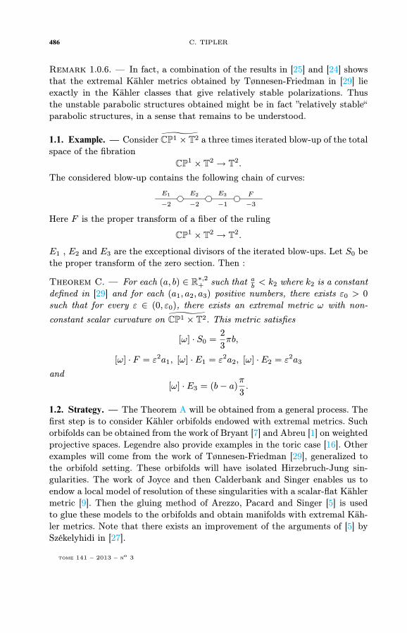
1.1. Example. — Consider „CP1 × T2 a three times iterated blow-up of the totalspace of the fibration

CP1 × T2 → T2.

The considered blow-up contains the following chain of curves:

E1

−2

E2

−2

E3

−1

F

−3

Here F is the proper transform of a fiber of the ruling

CP1 × T2 → T2.

E1 , E2 and E3 are the exceptional divisors of the iterated blow-ups. Let S0 bethe proper transform of the zero section. Then :

Theorem C. — For each (a, b) ∈ R∗,2+ such that ab < k2 where k2 is a constantdefined in [29] and for each (a1, a2, a3) positive numbers, there exists ε0 > 0

such that for every ε ∈ (0, ε0), there exists an extremal metric ω with non-constant scalar curvature on „CP1 × T2. This metric satisfies

[ω] · S0 =2

3πb,

[ω] · F = ε2a1, [ω] · E1 = ε2a2, [ω] · E2 = ε2a3

and[ω] · E3 = (b− a)

π

3.

1.2. Strategy. — The Theorem A will be obtained from a general process. Thefirst step is to consider Kähler orbifolds endowed with extremal metrics. Suchorbifolds can be obtained from the work of Bryant [7] and Abreu [1] on weightedprojective spaces. Legendre also provide examples in the toric case [16]. Otherexamples will come from the work of Tønnesen-Friedman [29], generalized tothe orbifold setting. These orbifolds will have isolated Hirzebruch-Jung sin-gularities. The work of Joyce and then Calderbank and Singer enables us toendow a local model of resolution of these singularities with a scalar-flat Kählermetric [9]. Then the gluing method of Arezzo, Pacard and Singer [5] is usedto glue these models to the orbifolds and obtain manifolds with extremal Käh-ler metrics. Note that there exists an improvement of the arguments of [5] bySzékelyhidi in [27].

tome 141 – 2013 – no 3


Remark 1.2.1. — The gluing process described in [5] works in higher dimen-sion but there are no such metrics on local models of every resolution of isolatedsingularities in higher dimension. However, Joyce constructed ALE scalar-flatmetrics on Crepant resolutions [14]. Then one can expect to generalize theprocess described below in some cases of higher dimension.

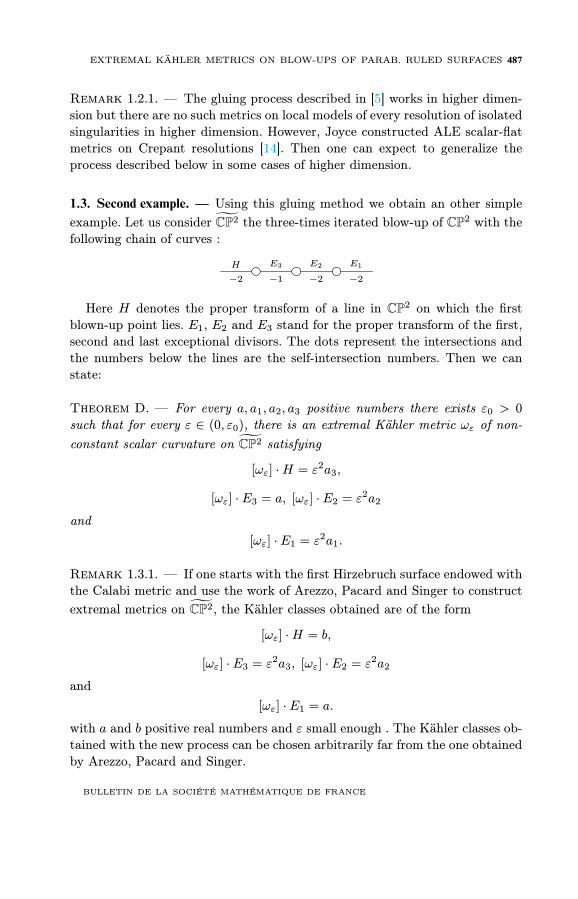
1.3. Second example. — Using this gluing method we obtain an other simpleexample. Let us consider fiCP2 the three-times iterated blow-up of CP2 with thefollowing chain of curves :

H

−2

E3

−1

E2

−2

E1

−2

Here H denotes the proper transform of a line in CP2 on which the firstblown-up point lies. E1, E2 and E3 stand for the proper transform of the first,second and last exceptional divisors. The dots represent the intersections andthe numbers below the lines are the self-intersection numbers. Then we canstate:

Theorem D. — For every a, a1, a2, a3 positive numbers there exists ε0 > 0

such that for every ε ∈ (0, ε0), there is an extremal Kähler metric ωε of non-constant scalar curvature on fiCP2 satisfying

[ωε] ·H = ε2a3,

[ωε] · E3 = a, [ωε] · E2 = ε2a2

and[ωε] · E1 = ε2a1.

Remark 1.3.1. — If one starts with the first Hirzebruch surface endowed withthe Calabi metric and use the work of Arezzo, Pacard and Singer to constructextremal metrics on fiCP2, the Kähler classes obtained are of the form

[ωε] ·H = b,

[ωε] · E3 = ε2a3, [ωε] · E2 = ε2a2

and[ωε] · E1 = a.

with a and b positive real numbers and ε small enough . The Kähler classes ob-tained with the new process can be chosen arbitrarily far from the one obtainedby Arezzo, Pacard and Singer.


488 C. TIPLER

1.4. Plan of the paper. — In the section 2 we set up the general gluing theoremfor resolutions following [3] and [5]. In section 3 we build the orbifolds with ex-tremal metrics that we use in the gluing construction, and identify the surfacesobtained after resolution. This will prove Theorem A. Then in the section 4 wediscuss unstable parabolic structures and give the proof of the Theorem B. Inthe last section we show how to obtain the examples of the introduction.

Acknowledgments. — I’d like to thank especially my advisor Yann Rollin forhis help and encouragement. I am grateful to Paul Gauduchon and MichaelSinger for all the discussions we had. I’d also like to thank Vestislav Apostolovwho pointed to me Abreu’s and Legendre’s work. I thank Frank Pacard andGabor Székelyhidi for their remarks on the first version of this paper, as wellas the referee whose comments enabled to improve the paper. And last but notleast a special thank to Andrew Clarke for all the time he spend listening tome and all the suggestions he made to improve this paper.

2. Hirzebruch-Jung singularities and extremal metrics

The aim of this section is to present the method of desingularization ofextremal Kähler orbifolds.

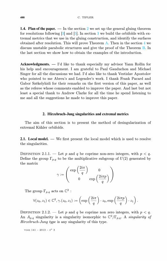
2.1. Local model. — We first present the local model which is used to resolvethe singularities.

Definition 2.1.1. — Let p and q be coprime non-zero integers, with p < q.Define the group Γp,q to be the multiplicative subgroup of U(2) generated bythe matrix

γ :=

Öexp

Å2iπ

q

ã0

0 exp

Å2iπp

q

ãèThe group Γp,q acts on C2 :

∀(z0, z1) ∈ C2, γ.(z0, z1) :=

Åexp

Å2iπ

q

ã· z0, exp

Å2iπp

q

ã· z1

ã.

Definition 2.1.2. — Let p and q be coprime non zero integers, with p < q.An Ap,q singularity is a singularity isomorphic to C2/Γp,q. A singularity ofHirzebruch-Jung type is any singularity of this type.

tome 141 – 2013 – no 3


We recall some results about the resolutions of these singularities. First,from the algebraic point of view, C2/Γp,q is a complex orbifold with an isolatedsingularity at 0. There exists a minimal resolution

π : Yp,q → C2/Γp,q

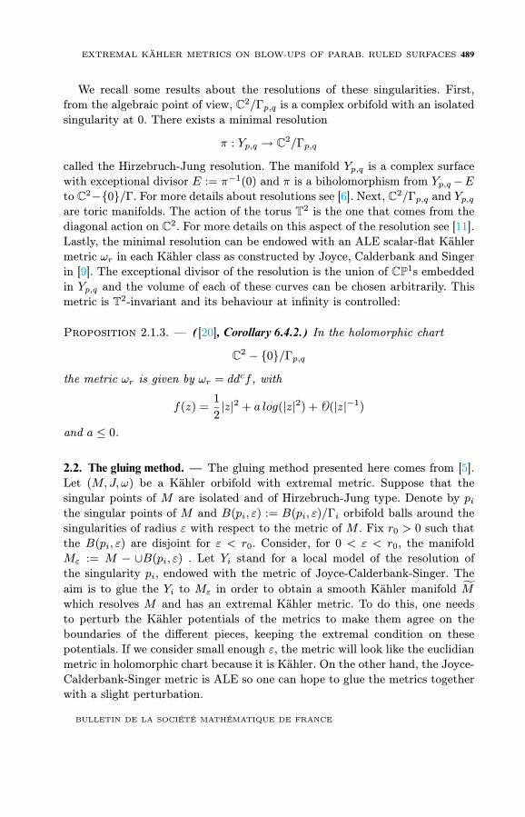
called the Hirzebruch-Jung resolution. The manifold Yp,q is a complex surfacewith exceptional divisor E := π−1(0) and π is a biholomorphism from Yp,q−Eto C2−0/Γ. For more details about resolutions see [6]. Next, C2/Γp,q and Yp,qare toric manifolds. The action of the torus T2 is the one that comes from thediagonal action on C2. For more details on this aspect of the resolution see [11].Lastly, the minimal resolution can be endowed with an ALE scalar-flat Kählermetric ωr in each Kähler class as constructed by Joyce, Calderbank and Singerin [9]. The exceptional divisor of the resolution is the union of CP1s embeddedin Yp,q and the volume of each of these curves can be chosen arbitrarily. Thismetric is T2-invariant and its behaviour at infinity is controlled:

Proposition 2.1.3. — ([20], Corollary 6.4.2.) In the holomorphic chart

C2 − 0/Γp,q

the metric ωr is given by ωr = ddcf , with

f(z) =1

2|z|2 + a log(|z|2) + O(|z|−1)

and a ≤ 0.

2.2. The gluing method. — The gluing method presented here comes from [5].Let (M,J, ω) be a Kähler orbifold with extremal metric. Suppose that thesingular points of M are isolated and of Hirzebruch-Jung type. Denote by pithe singular points of M and B(pi, ε) := B(pi, ε)/Γi orbifold balls around thesingularities of radius ε with respect to the metric of M . Fix r0 > 0 such thatthe B(pi, ε) are disjoint for ε < r0. Consider, for 0 < ε < r0, the manifoldMε := M − ∪B(pi, ε) . Let Yi stand for a local model of the resolution ofthe singularity pi, endowed with the metric of Joyce-Calderbank-Singer. Theaim is to glue the Yi to Mε in order to obtain a smooth Kähler manifold M

which resolves M and has an extremal Kähler metric. To do this, one needsto perturb the Kähler potentials of the metrics to make them agree on theboundaries of the different pieces, keeping the extremal condition on thesepotentials. If we consider small enough ε, the metric will look like the euclidianmetric in holomorphic chart because it is Kähler. On the other hand, the Joyce-Calderbank-Singer metric is ALE so one can hope to glue the metrics togetherwith a slight perturbation.


490 C. TIPLER

Let s be the scalar curvature of ω. Define the operator :

Pω : C∞(M)→ Λ0,1(M,T 1,0)

f 7→ 12∂Ξf

withΞf = J∇f + i∇f.

A result of Calabi asserts that a metric is extremal if and only if the gradientfield of the scalar curvature is a real holomorphic vector field. Therefore a metricω′ is extremal if and only if Pω′(s(ω′)) = 0, with s(ω′) denoting the scalarcurvature. Let P ∗ω be the adjoint operator of Pω. We will use the followingproposition:

Proposition 2.2.1. — [17] Ξ ∈ T 1,0 is a Killing vector field with zeros if andonly if there is a real function f solution of P ∗ωPω(f) = 0 such that ω(Ξ, .) =

−df .

This result is initially proved for manifolds but the proof extends directlyto orbifolds with isolated singularities, working equivariently in the orbifoldcharts.

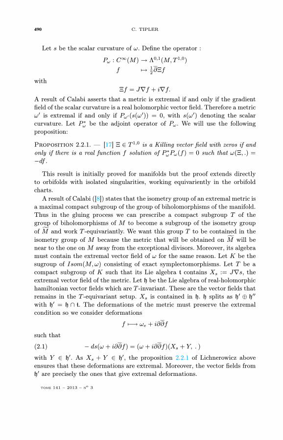
A result of Calabi ([8]) states that the isometry group of an extremal metric isa maximal compact subgroup of the group of biholomorphisms of the manifold.Thus in the gluing process we can prescribe a compact subgroup T of thegroup of biholomorphisms of M to become a subgroup of the isometry groupof M and work T -equivariantly. We want this group T to be contained in theisometry group of M because the metric that will be obtained on M will benear to the one onM away from the exceptional divisors. Moreover, its algebramust contain the extremal vector field of ω for the same reason. Let K be thesugroup of Isom(M,ω) consisting of exact symplectomorphisms. Let T be acompact subgroup of K such that its Lie algebra t contains Xs := J∇s, theextremal vector field of the metric. Let h be the Lie algebra of real-holomorphichamiltonian vector fields which are T -invariant. These are the vector fields thatremains in the T -equivariant setup. Xs is contained in h. h splits as h′ ⊕ h′′with h′ = h ∩ t. The deformations of the metric must preserve the extremalcondition so we consider deformations

f 7−→ ωe + i∂∂f

such that

(2.1) − ds(ω + i∂∂f) = (ω + i∂∂f)(Xs + Y, . )

with Y ∈ h′. As Xs + Y ∈ h′, the proposition 2.2.1 of Lichnerowicz aboveensures that these deformations are extremal. Moreover, the vector fields fromh′ are precisely the ones that give extremal deformations.

tome 141 – 2013 – no 3


In order to obtain such deformations, consider the moment map ξω associ-ated to the action of K:

ξω : M → k∗.ξω is defined such that for every X ∈ k the function 〈ξω, X〉 on M is a hamil-tonian for X, wich means

ω(X, . ) = −d〈ξω, X〉.

Moreover, ξω is normalized such that∫M

〈ξω, X〉ωn = 0.

The equation (2.1) can now be reformulated:

s(ω + i∂∂f) = 〈ξω+i∂∂f , Xs + Y 〉+ constant.

If we work T -equivariantly, we are interested in the operator :

F : h× C∞(M)T × R → C∞(M)T

(X, f, c) 7→ s(ω + i∂∂f)− 〈ξω+i∂∂f , X〉 − c− cs

where C∞(M)T stands for the T -invariant functions and cs is the average ofthe scalar curvature of ω. There is a result which is due to Calabi and Lebrun-Simanca:

Proposition 2.2.2. — [5] If ω is extremal and if Xs ∈ h, then the linearizationof F at 0 is given by

(f,X, c) 7→ −1

2P ∗ωPωf − 〈ξω, X〉 − c.

The vector fields in h′ are the ”good ones" as they will give perturbations inthe isometry group of the future metric. It remains to use the implicit functiontheorem to get the scalar curvature in term of these vector fields and the algebrah′′ stands for the obstruction.

2.3. Extremal metrics on resolutions. — We choose a group T of isometries ofM so that working T -equivariantly will simplify the analysis. It is necessary tochoose a neighborhood of the singularities in which T will appear as a subgroupof the isometry group of the metric of Joyce-Calderbank-Singer. Moreover, inorder to lift the action of T to M , it is necessary that T fixes the singularities.We will see in lemma 2.4.3 that if we let T be a maximal torus in K then theseconditions will be satisfied. Thus the equivariant setup of [5] can be used allthe same in this orbifold case. Lastly, we will have h = t and no obstructionwill appear in the analysis. Following [3] and [5], we can state the theorem:


492 C. TIPLER

Theorem 2.4. — Let (M,ω) be an extremal Kähler orbifold of dimension 2.Suppose that the singularities of M are isolated and of Hirzebruch-Jung type.Denote by π : M → M the minimal resolution of M obtained using theHirzebruch-Jung strings. Denote by Ej the CP1s that forms the Hirzebruch-Jung strings in the resolution. Then for every choice of positive numbers ajthere exists ε0 > 0 such that ∀ε ∈ (0, ε0) there is an extremal Kähler metric onM in the Kähler class

[π∗ω]− ε2∑j

ajPD[Ej ]

Remark 2.4.1. — We notice that if s(ω) is not constant, the metrics obtainedon the resolution are extremal of non-constant scalar curvature. Indeed, themetrics converge to π∗ω away from the exceptional divisors, so does the scalarcurvature. On the other hand, if ω is of constant scalar curvature, then theextremal metric obtained on the resolution need not be of constant scalar cur-vature. Genericity and balancing conditions have to be satisfied to preserve aCSC metric [4] and [21].

Remark 2.4.2. — The proof is the one in [5] so we refer to this text. Thetools and ideas are used here in an orbifold context, using the work of [3].In the paper [3] the gluing method is developped in the orbifold context forconstant scalar curvature metrics. On the other hand, the paper [5] deals withextremal metrics but in the smooth case. One of the differences in the analysisbetween the constant scalar curvature case and the extremal case is that oneneeds to lift objects to the resolution such as holomorphic vector fields. Thuswe will only give a proof of the following lemma which ensures that we can liftthe vector fields needed during the analysis.

Lemma 2.4.3. — Let (M,ω) be an extremal Kähler orbifold of dimension 2.Suppose that the singularities of M are isolated and of Hirzebruch-Jung type.Let K be the subgroup of Isom(M,ω) which are exact symplectomorphisms. LetT be a maxixmal torus in K. Then T fixes the singularities. Its Lie algebra con-tains the extremal vector field. Moreover at each singularity of M with orbifoldgroup Γ there exists an orbifold chart U/Γ, U ⊂ C2 such that in this chart Tappears as a subgroup of the torus acting in the standard way on C2.

Proof. — Let p ∈ M be a singularity with orbifold group Γ and U ⊂ C2 suchthat U/Γ is an open neighbourhood of p in M . T ⊂ Isom(M,ω) so we can liftthe action of T to U such that it commutes with the action of Γ. Thus T fixesp.We see that Xs belongs to t. Indeed,

∀X ∈ h, [X,Xs] = LXXs = 0

tome 141 – 2013 – no 3


because X preserves the metric. Thus Xs ∈ h and as h = t, Xs ∈ t. Thenwe follow the proof of [5]. By a result of Cartan, we can find holomorphiccoordinates on U such that the action of T is linear. More than that, we cansuppose that the lift of ω in these coordinates (z1, z2) satisfies

ω = ∂∂(1

2|z|2 + φ)

where φ is T invariant and φ = O(|z|4). In this coordinates T appears asa subgroup of U(2). Thus T is conjugate to a group whose action on C2 isdiagonal. As T and Γ commute, we can diagonalize simultaneously these groups.In the new coordinates, the action of Γ is described by definition 2.1.1 andT ⊂ T2 with T2 action on C2 given by

T2 × C2 → C2

(θ1, θ2), (w1, w2) 7→ (eiθ1w1, eiθ2w2).

Remark 2.4.4. — Note that there exists a refinement of the proof of Arezzo,Pacard and Singer in the blow-up case. This is given in the paper of Székelyhidi[27]. Basically, the idea is to glue the metric of Burns-Simanca to the extremalmetric on the blow-up manifold. This give an almost extremal metric. It remainsto perturb the metric to obtain an extremal one. Moving the blown-up point ifnecessary, this problem becomes a finite dimensional problem. This argumentmight be used in the case of resolution of isolated singularities.

3. Extremal metrics on orbisurfaces

The aim of this section is to prove Theorem A. We first construct extremalmetrics on special orbisurfaces. Then we apply Theorem 2.4 to these examples,and identify the smooth surfaces obtained after resolution.

3.1. Construction of the orbifolds. — In this section we generalize to an orbifoldsetting the so-called Calabi construction. We shall construct extremal metricson projectivization of rank 2 orbibundles over orbifold Riemann surfaces. Wewill focus on the case where the orbifold Euler characteristic χorb of the Rie-mann surface is strictly negative, thought the method would extend directly tothe other cases. See for example [13] for a unified treatment of the constructionin the smooth case. Our restriction will present the advantage of being veryexplicit and will help to keep track of the manifolds considered in section 3.4.

The starting point is the pseudo-Hirzebruch surfaces constructed byTønnesen-Friedman in [29]. These are total spaces of fibrations

P( O ⊕ L)→ Σg


494 C. TIPLER

where Σg is a Riemann surface of genus g and L a positive line bundle. Webriefly recall the construction of extremal metrics on such a surface. Let

U := (z0, z1)/|z0|2 > |z1|2 ⊂ C2

andD := (z0, z1) ∈ U/z0 = 1.

We can then consider U as a principal bundle over the Poincaré disc D whichadmits the trivialisation :

U → C∗ × D(z0, z1) 7→ (z0, (1,

z1z0

)).

The vector bundle associated to U is trivial and we can consider it as theextension of U over zero. We will denote by Uq the tensor powers of this vectorbundle.

Recall that U(1, 1) is the group of isomorphisms of C2 which preserve theform

u(z, w) = −z0w0 + z1w1.

Moreover,

U(1, 1) = eiθ(α β

β α

);αα− ββ = 1; θ ∈ R, (α, β) ∈ C2.

and U(1, 1) acts on U . One of the central results of this work of Tønnesen-Friedman is then (see [29]):

Theorem 3.2. — Let q be a non zero integer. There exists a constant kq suchthat for every choice of constants 0 < a < b such that b

a < kq, there is aU(1, 1)-invariant extremal Kähler metric with non-constant scalar curvatureon U . This metric can be extended in a smooth way on P( O ⊕ Uq).

Remark 3.2.1. — The value of the scalar curvature is − 4b on the zero section

and − 4a on the infinity section.

Remark 3.2.2. — Here the considered manifolds are non-compact and we saythat the metric is extremal if the vector field J∇s associated to the metric isholomorphic.

Tønnesen-Friedman uses this result to obtain extremal metrics on pseudo-Hirzebruch surfaces. Let Σ a Riemann surface of genus greater or equal thantwo and let Γ be its fundamental group. Γ can be represented as a subgroup ofU(1, 1) and we obtain a holomorphic bundle:

P( O ⊕ Uq)/Γ→ D/Γ = Σ.

tome 141 – 2013 – no 3


Tønnesen-Friedman shows that P( O⊕Uq) is isomorphic to P( O⊕ Kq2 ) where K

stands for the canonical line bundle. The result of Tønnesen-Friedman providesextremal metrics on P( O ⊕ K

q2 ).

Now we consider an orbifold Riemann surface Σ of genus g, and refer to [20]for more details on orbifold Riemann surfaces. The genus g is no longer assumedto be greater than two but we assume that the orbifold Euler characteristic isstrictly negative. In that case, the orbifold fundamental group Γ of Σ can berepresented as a subgroup of U(1, 1) such that

Σ = D/Γ.

We saw thatU ∼= C∗ × D

The action of U(1, 1) in this chart is given by:

γ · (ξ, z) 7→ (eiθ(α+ βz)ξ,β + αz

α+ βz)

where

γ = eiθ

(α β

β α

)∈ U(1, 1).

The action of U(1, 1) on C⊗q × D is then given by:

γ · (ξ, z) 7→ (eiqθ(α+ βz)qξ,β + αz

α+ βz)

and the change of coordinates

(ξ, z)→ (ξ−1, z)

enables to extend this action and to define

M = P( O ⊕ Uq)/Γ.

This naturally fibres over Σ and define an orbifold bundle

π : M → Σ.

We adopt the convention from [23] for the definition below.

Definition 3.2.3. — An orbifold line bundle over an orbifold M is given bylocal invariant line bundles Li over each orbifold charts Ui such that the fol-lowing cocycle condition is satisfied:Suppose that V1, V2 and V3 are open sets in M with orbifold groups Gi, andorbifold charts Ui, such that Vi = Ui/Gi, i = 1..3.

Then by definition of an orbifold there are charts Uij such that Vi ∩ Vj =

Vij ∼= Uij/Gij with inclusions Uij → Ui and Gij → Gi, i, j ⊂ 1, 2, 3.Pulling back Lj and Li to Uij , there exists an isomorphism φij from Lj to


496 C. TIPLER

Li intertwining the actions of Gij . Moreover, pulling-back to U123, the cocyclecondition is that over U123 we have:

φ12φ23φ31 = 1 ∈ L1 ⊗ L∗2 ⊗ L2 ⊗ L∗3 ⊗ L3 ⊗ L∗1.

This definition can be generalized to define orbifold vector bundles, tensorproducts, direct sums and projectivizations of orbifold bundles. It is enoughto define these operations on orbifold charts Ui and verify that the cocyclecondition is still satisfied. The orbifold canonical bundle K orb is defined to beKU on each orbifold chart U .

With these definitions in mind, we prove the following:

Lemma 3.2.4. — Suppose that q = 2r. Then the surface M is isomorphic toP( O ⊕ K r

orb).

Remark 3.2.5. — We will see in the study of the singularities that we needto consider q even.

Proof. — Following Tønnesen-Friedman ([29]), we compute the transitionfunctions. Recall that the action of Γ is given by:

∀γ ∈ Γ, γ · (ξ, z) = (e2irθ(α+ βz)2rξ,β + αz

α+ βz)

in the chart C⊗2r × D. As D/Γ = Σ, the transition functions are induced bythe maps:

z 7→ γ · z

with γ ∈ Γ. Thus the transition functions for the bundle U2r/Γ are

z 7→ (α+ βz)2r.

Now the transition functions for K orb are computed by

d(γ · z) = d(β + αz

α+ βz) = (

1

α+ βz)2dz

because γ ∈ U(1, 1). It shows that they are equal to

z 7→ (α+ βz)−2

and U2r/Γ = K rorb. So M = P( O ⊕ K r

orb) on Σ.

The extremal metric mentioned in Theorem 3.2 is Γ-invariant as it is U(1, 1)-invariant and the result of [29] extend to the case of orbibundles:

tome 141 – 2013 – no 3


Proposition 3.2.6. — Let q = 2r be a non zero even integer. There existsa constant kq such that for every choice of constants 0 < a < b such thatba < kq, there is an extremal Kähler metric with non-constant scalar curvatureon P( O⊕ K r

orb). The restrictions of this metric to the zero and infinity sectionsof

P( O ⊕ K rorb)→ Σ

are constant scalar curvature metrics. The value of the scalar curvature on thezero section is − 4

b and − 4a on the infinity section.

We have obtained extremal metrics on orbifold ruled surfaces.

3.3. Singularities and resolution. — We now proceed to the study of the singu-larities of the orbifolds. Let (Ai) denote the singular points of Σ and let qi bethe order of the singular point Ai.

As χorb(Σ) < 0, there exists a morphism :

φ : Γ→ Sl2(R)/Z2 = Isom(H2)

such that Σ = H2/Im(φ). The transformation

z 7→ z − iz + i

that sends the half-plane to the Poincaré disc gives :

φ0 : Γ→ SU(1, 1)/Z2.

We recall a description of Γ:

Γ =< (ai, bi)i=1..g , (li)i=1..s |Π[ai, bi] Πli = lqi

i = 1 > .

Then φ0 defines matrices Ai, Bi, Li in SU(1, 1) satisfying the relations

Π[Ai, Bi] ΠLi = ±Id ; Lqi

i = ±Id.

The action of −Id on C⊗q × D is :

(ξ, z)→ ((−1)qξ, z).

In order to obtain isolated singularities, we will suppose that q is even.To simplify notation we will denote by Γ the image of φ0. The singular points

of M come from the points of P( O ⊕ Uq) with non-trivial stabilizer under theaction of Γ/Z2. We will deal with points on the zero section in the chart C⊗q×D.Let (ξ0, z0) be a point whose stabilizer under the action of Γ is not reducedto ±Id and let γ 6= ±id in Γ fix (ξ0, z0). The element γ ∈ U(1, 1) can bewritten:

γ = ±

(α β

β α

)BULLETIN DE LA SOCIÉTÉ MATHÉMATIQUE DE FRANCE

498 C. TIPLER

and satisfiesβ + αz0

α+ βz0= z0.

The stabilizer of (ξ0, z0) is then include in the one of z0 ∈ D under the actionof Γ on D. The point z0 gives a singular point Ai of Σ = D/Γ and the point(ξ0, z0) gives rise to a singular point in M in the singular fiber π−1(Ai). Theisotropy group of Ai is Zqi

and we can suppose that γ is a generator of thisgroup. As γ is an element of SU(1, 1) of order qi, its characteristic polynomialis

X2 ± 2Re(α)X + 1.

If Re(α) = δ with δ ∈ −1,+1, there exists a basis in which γ is one of thefollowing matrices: (

δ 0

0 δ

);

(δ 1

0 δ

).

It is not possible because γ is suppose to be different from ±Id and of finiteorder. Thus the characteristic polynomial of γ admits two distinct complexroots and γ is diagonalizable in SU(1, 1) so we can fix P ∈ SU(1, 1) such that

P−1.γ.P =

(a 0

0 b

).

Then γ is of finite order qi and det(γ) = 1 so we can fix ξqi a primitive qthi rootof unity such that

P−1.γ.P =

(ξqi

0

0 ξ−1qi

).

As P ∈ SU(1, 1), P preserves the open set U and induces a change of coordi-nates in a neighbourhood of the fixed point.Indeed, the action of P on the coordinates (ξ, z) is given by:

P.(ξ, z) = ((c+ dz)qξ,d+ cz

c+ dz)

with

P =

(c d

d c

).

We compute the differential at (ξ0, z0):

DP(ξ0,z0) =

(qd(c+ dz0)q−1ξ0 (c+ dz0)q

1/(c+ dz0)2 0

).

and the determinant of this matrix is

det(DP(ξ0,z0)) = −(c+ dz0)q−2.

tome 141 – 2013 – no 3


Note that q ≥ 2. As we don’t have c = d = 0, this determinant is zero if andonly if z0 = − c

d. But |z0|2 < 1 so it would imply |c|2 < |d|2 which is impossible

becausedet(P ) = |c|2 − |d|2 = 1.

Thus P defines a change of coordinates near the singular point. In these newcoordinates (ξ′, z′), the action of γ is

(ξ′, z′) 7→ (ξqqiξ′, ξ−2

qiz′).

The only fixed points of γ in this local chart are (0, 0) and (∞, 0), the point atinfinity corresponding to the action

(ξ′, z′) 7→ (ξ−qqiξ′, ξ−2

qiz′).

As the singular points of Σ are isolated, the singular fibers of M are isolated.Moreover, we see that the singular points are on the zero and infinity sectionsin the initial coordinates system, as the transformation P preserves the rulingand the zero and infinity sections. We can recognize precisely the Hirzebruch-Jung type of these singularities using the method described in [6]. To simplifywe will suppose gcd(r, qj) = 1. If we set ζi = ξ−2

qi, the action is

(ξ′, z′) 7→ (ζ−ri ξ′, ζi z′).

Summarizing:

Proposition 3.3.1. — Let Σ be an orbifold Riemann surface with strictly neg-ative orbifold Euler characteristic. Let (Ai)1≤i≤s be its singular points that wesuppose to be of order strictly greater than 2. Then if q = 2r is an even inte-ger, the orbifold P( O⊕ K r

orb) defined in the above construction has 2s singularpoints, two of them in each fiber π−1(Ai). Moreover, if gcd(r, qj) = 1, thesingular points are of type Api,qi

and Aqi−pi,qiin each fiber, with pi ≡ −r[qi].

Remark 3.3.2. — The hypothesis on the order of the singularity of Σ is neededto avoid an isotropy group of the form ±Id.

We can now apply the Theorem 2.4.

Corollary 3.3.3. — Let M be a orbifold surface as in Proposition 3.3.1, en-dowed with an extremal metric arising from Proposition 3.2.6. Let π : M →M

be the Hirzebruch-Jung resolution of M . Then, M admits extremal Kähler met-rics with non-constant scalar curvature that converge to π∗ω on every compactset away from the exceptional divisors.


500 C. TIPLER

3.4. Identification of the resolution M . — We want to describe the surface thatwe obtain after desingularization. Let’s consider M obtained in the Corol-lary 3.3.3. This is the total space of a singular fiber bundle

π : M = P( O ⊕ K rorb)→ Σ.

The 2s singular points are situated on s singular fibers Fi, each of them admitsa singularity of type Api,qi

on the zero section and of type Aqi−pi,qion the

infinity section.Let Σ be the smooth Riemann surface topologically equivalent to Σ. We

define a parabolic ruled surface M in the following way: first we set

nj =pj + r

qj

for each singular fiber. Note that by construction nj is an integer. We definethe line bundle L on Σ:

L = K r ⊗j [Aj ]r−nj

where the Aj stand for the points on Σ corresponding to the singular points ofΣ. We set M to be the total space of the fibration

P( O ⊕ L)→ Σ.

The parabolic structure on M consists in the s points Aj ∈ Σ, the pointsBj in the fiber over Aj on the infinity section and the corresponding weightsαj :=

pjqj

. Let Bl(M, P) be the iterated blow-up associated to M as defined in

the introduction.

Proposition 3.4.1. — The smooth surface obtained by the minimal resolutionof M is Bl(M, P).

Note that together with corollary 3.3.3, proposition 3.4.1 ends the proofof Theorem A. More precisions on the Kähler classes obtained are given insection 3.5.

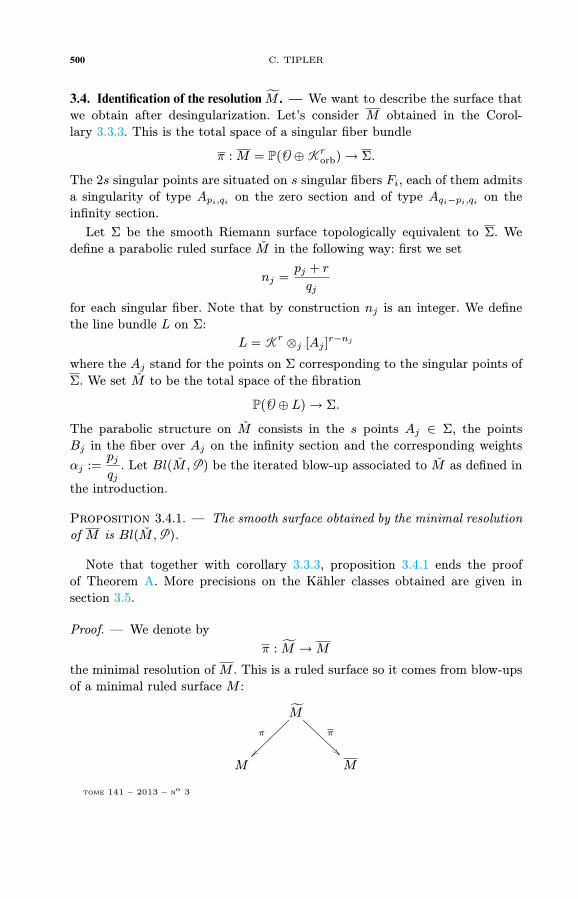
Proof. — We denote byπ : M →M

the minimal resolution of M . This is a ruled surface so it comes from blow-upsof a minimal ruled surface M :

M

π

~~

π

M M

tome 141 – 2013 – no 3


M is the total space of a fibration P( O⊕L′) over Σ. Indeed,M is birationallyequivalent to M so M is a ruled surface over Σ. As M is minimal, it is of theform P(E) where E is a holomorphic bundle of rank 2 on Σ. Then, to showthat E splits, we consider the vector field Xs = J∇s on M , with s the scalarcurvature of a metric from Corollary 3.3.3. The vector field Xs is vertical andcan be lifted to M . It projects to a vertical holomorphic vector field onM . Thelatter admits two zeros on each fiber because it generates an S1 action and nota R action. The two zeros of this vector field restricted to each fiber give twoholomorphic sections of P(E) and describe the splitting we look for. Tensoringby a line bundle if necessary, we can suppose that P(E) = P( O ⊕ L′).

M

π

zz

π

P( O ⊕ L′) M

It remains to recognize L′.

We set M∗ := D∗ × CP1/Γ, where D∗ denotes the Poincaré disc minus thefixed points under the action of Γ. M∗ is the surface obtained from M bytaking away the singular fibers. As π and π are biholomorphisms away fromthe exceptional divisors, we get a natural injection from M∗ to M . M appearsas a smooth compactification of M∗. Moreover, M∗ = P( O ⊕ K r

orb) on Σ∗.

M

π

zz

π

P( O ⊕ L′) M

M∗

dd >>

We can understand the way of going from M to M in the neighbourhood ofthe singular fibers using the work of [20]. If Aj is a singular point of Σ of orderqj and ∆j a small disc around Aj then ∆j × CP1/Zqj is a neighbourhood ofthe singular fiber over Aj . It follows from section 3.1 that the action of Zqj

isgiven by:

∆j × CP1 → ∆j × CP1

(z, [u, v]) 7→ (ζqjz, [u, ζ

pjqj v]).


502 C. TIPLER

with ζqj a qthj primitive root of unity and pj ≡ −r[qj ]. We get a neighbourhood∆j × CP1 of the corresponding point in M by the map:

φj : (∆j × CP1)/Zq → ∆j × CP1

(z, [u, v]) 7→ (x = zqj , [u, z−pjv]).

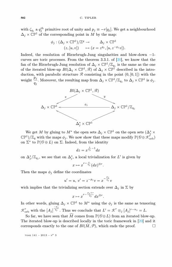
Indeed, the resolution of Hirzebrugh-Jung singularities and blow-down −1-curves are toric processes. From the theorem 3.3.1. of [20], we know that thefan of the Hirzebrugh-Jung resolution of ∆j ×CP1/Zqj is the same as the oneof the iterated blow-up Bl(∆j × CP1, R) of ∆j × CP1 described in the intro-duction, with parabolic structure R consisting in the point (0, [0, 1]) with theweight

pjqj

. Moreover, the resulting map from ∆j ×CP1/Zqjto ∆j ×CP1 is φj .

Bl(∆j × CP1, R)

π

vv

π

((∆j × CP1 ∆j × CP1/Zqj

φjoo

∆∗j × CP1

gg 66

We get M by gluing to M∗ the open sets ∆j ×CP1 on the open sets (∆∗j ×CP1)/Zq with the maps φj . We now show that these maps modify P( O⊕ K r

orb)

on Σ∗ to P( O ⊕ L) on Σ. Indeed, from the identity

dz = x1

qj−1dx

on ∆∗j/Zqj , we see that on ∆∗j , a local trivialization for L′ is given by

x 7→ xr− r

qj (dx)⊗r.

Then the maps φj define the coordinates

u′ = u, v′ = z−pjv = x−

pjqj v

wich implies that the trivializing section extends over ∆j in Σ by

x 7→ xr−

pj+r

qj dx⊗r.

In other words, gluing ∆j × CP1 to M∗ using the φj is the same as tensoring

K rorb with the [Aj ]

−pjqj . Thus we conclude that L′ = K r ⊗j [Aj ]

r−nj = L.So far, we have seen that M comes from P( O⊕L) from an iterated blow-up.

The iterated blow-up is described locally in the toric framework in [20] and itcorresponds exactly to the one of Bl(M, P), which ends the proof.

tome 141 – 2013 – no 3


3.5. The Kähler classes. — Let (M,ω) be an orbifold extremal Kähler surfaceand (M, ωε) the smooth surface obtained after desingularization with an ex-tremal metric as in Corollary 3.3.3

π : M →M.

Away from the exceptional divisors, ωε is obtained by a perturbation of theform ωε = ω + ∂∂f so the Kähler class doesn’t change. In order to determine[ωε] it is sufficient to integrate ωε along a basis for H2(M,R). We will computethe Kähler class in the case of a unique singular fiber, the general case can bededuced from this one. Denote byM = P( O⊕L) the minimal model associatedto M

π : M →M.

It’s homology H2(M,R) is generated by the zero section and the class of a fiber.Thus the homology H2(M,R) is generated by the proper transform of thesetwo cycle and the exceptional divisors. Consider the chain of curves comingfrom the resolution of the singular fiber of M

−e1E1

−e2E2

−ek−1

Ek−1

−ek

Ek

−1

S

−e′l

E′l

−e′l−1

E′l−1

−e′2

E′2

−e′1

E′1

Note that S is the proper transform under π of the singular fiber of M . E′1is the proper transform under π of a fiber of M . The construction of ωε showsthat integrating ∑

j

∫Ej

ωε = ε2V

or ∑i

∫E′

i

ωε = ε2V ′

for small positive number ε and V and V ′ depending on the volume of themetric on each resolution. The construction of the metric of Joyce, Calderbankand Singer enables to choose the volume of each curve Ej and E′i provided thatthe sum is equal to V and V ′ respectively. Thus if we choose (aj) and (a′i) suchthat ∑

j

aj = V

and ∑i

a′i = V ′

we get ∫Ej

ωε = ε2aj


504 C. TIPLER

and ∫E′

i

ωε = ε2a′i

If we denote by S0 the proper transform of the zero section of M with π, itremains to compute [ωε] ·S0 and [ωε] ·S. These two integrals can be computedon M following Tønnesen-Friedman [29]. On the zero section, the metric isof constant sectional curvature and its scalar curvature is equal to b so theGauss-Bonnet formula for orbifolds gives

A =

∫S0

ωε = −πbχorb.

On S, the explicit form of the metric on U enables to compute

B =

∫S

ωε = 2π(b− a)

2rq.

where r is related to the degree d of L by d = −rχ +∑j(r − nj), a and b

are constants satisfyinga

b< k2r and q is the order of the singularities of the

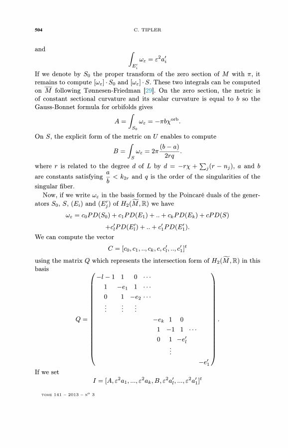
singular fiber.Now, if we write ωε in the basis formed by the Poincaré duals of the gener-

ators S0, S, (Ei) and (E′j) of H2(M,R) we have

ωε = c0PD(S0) + c1PD(E1) + ..+ ckPD(Ek) + cPD(S)

+c′lPD(E′l) + ..+ c′1PD(E′1).

We can compute the vector

C = [c0, c1, .., ck, c, c′l, .., c

′1]t

using the matrix Q which represents the intersection form of H2(M,R) in thisbasis

Q =

−l − 1 1 0 · · ·1 −e1 1 · · ·0 1 −e2 · · ·...

......

−ek 1 0

1 −1 1 · · ·0 1 −e′l

...−e′1

.

If we setI = [A, ε2a1, ..., ε

2ak, B, ε2a′l, ..., ε

2a′1]t

tome 141 – 2013 – no 3


the vector which represents the integration of ωε along the divisors, we have

I = Q · C

soC = Q−1I

and this gives the parameters (ci) we were looking for, determining the Kählerclass of ωε.

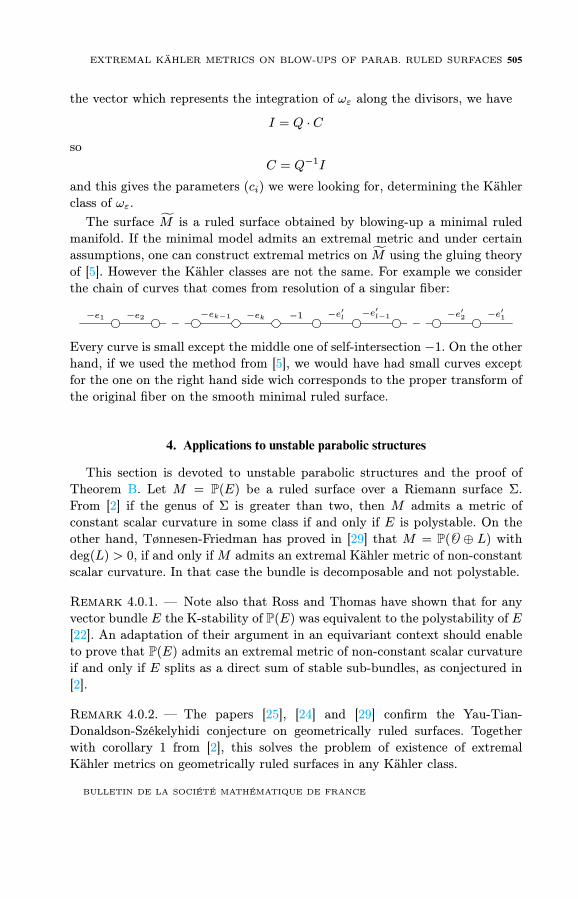
The surface M is a ruled surface obtained by blowing-up a minimal ruledmanifold. If the minimal model admits an extremal metric and under certainassumptions, one can construct extremal metrics on M using the gluing theoryof [5]. However the Kähler classes are not the same. For example we considerthe chain of curves that comes from resolution of a singular fiber:

−e1 −e2 −ek−1 −ek −1 −e′l −e′l−1 −e′2 −e′1

Every curve is small except the middle one of self-intersection −1. On the otherhand, if we used the method from [5], we would have had small curves exceptfor the one on the right hand side wich corresponds to the proper transform ofthe original fiber on the smooth minimal ruled surface.

4. Applications to unstable parabolic structures

This section is devoted to unstable parabolic structures and the proof ofTheorem B. Let M = P(E) be a ruled surface over a Riemann surface Σ.From [2] if the genus of Σ is greater than two, then M admits a metric ofconstant scalar curvature in some class if and only if E is polystable. On theother hand, Tønnesen-Friedman has proved in [29] that M = P( O ⊕ L) withdeg(L) > 0, if and only ifM admits an extremal Kähler metric of non-constantscalar curvature. In that case the bundle is decomposable and not polystable.

Remark 4.0.1. — Note also that Ross and Thomas have shown that for anyvector bundle E the K-stability of P(E) was equivalent to the polystability of E[22]. An adaptation of their argument in an equivariant context should enableto prove that P(E) admits an extremal metric of non-constant scalar curvatureif and only if E splits as a direct sum of stable sub-bundles, as conjectured in[2].

Remark 4.0.2. — The papers [25], [24] and [29] confirm the Yau-Tian-Donaldson-Székelyhidi conjecture on geometrically ruled surfaces. Togetherwith corollary 1 from [2], this solves the problem of existence of extremalKähler metrics on geometrically ruled surfaces in any Kähler class.


506 C. TIPLER

We now focus on parabolic ruled surfaces, performing an analogy with theprevious results mentioned. Suppose that the ruled surface is equipped with aparabolic structure P. Let’s recall the definition of parabolic stability from [20]:we consider a geometrically ruled surface π : M → Σ with a parabolic structuregiven by s points Aj in Σ, and for each of these points a point Bj ∈ π−1(Aj)

with a weight αj ∈]0, 1[∩Q.

Definition 4.0.3. — A parabolic ruled surfaceM is parabolically stable if forevery holomorphic section S of π its slope is strictly positive:

µ(S) = S2 +∑j /∈I

αj −∑j∈I

αj > 0

where j ∈ I if and only if Bj ∈ S.

Remark 4.0.4. — IfM = P(E), one can check that this definition is equivalentto the parabolic stability of E in the sense of Mehta-Seshadri [19].

In that case, Rollin and Singer have shown [20] that if the bundle is parabol-ically stable then there exists a scalar-flat Kähler metric on Bl(M, P). Moregenerally, if the surface is parabolically polystable and non-sporadic, then thereexists a constant-scalar curvature metric on Bl(M, P) ([21]).

Given a parabolically unstable ruled surface, is there an extremal metric ofnon-constant scalar curvature on Bl(M, P)?

First of all, we show that if Bl(M, P) admits an extremal metric of non-constant scalar curvature, then the bundle E is decomposable and one of thezero or infinity section might destabilise M . Thus the situation looks like inthe case studied by Tønnesen-Friedman.

Proposition 4.0.5. — Let M = P(E) be a parabolic ruled surface over a Rie-mann surface of genus g with a parabolic structure P. Let pj

qjbe the weights of

the parabolic structure. Suppose that Bl(M, P) admits an extremal metric ofnon-constant scalar curvature. Then M = P( O ⊕ L). Moreover, if

2− 2g −∑j

(1− 1

qj) ≤ 0

the marked points of the parabolic structure all lie on the zero section or theinfinity section induced by L.

Remark 4.0.6. — If2− 2g −

∑j

(1− 1

qj) ≤ 0

we can suppose that the marked point all lie on the same section. Indeed, theiterated blow-up associated to a point on the zero section with weight p

q is thesame as the one with marked point in the same fiber on the infinity section with

tome 141 – 2013 – no 3


weight q−pq . Moreover, we see that the infinity and zero sections have opposite

slopes so one of them might destabilize the surface.

Proof. — Let χorb = 2− 2g −∑j(1− 1

qj). In the case χorb > 0 the genus g of

Σ is 0 and in that case every ruled surface is of the form P( O⊕L). We supposethat χorb ≤ 0.Bl(M, P) admits an extremal metric of non-constant scalar curvature. Thus

the extremal vector field is not zero. It generates an action by isometries onthe manifold. Using the openness theorem of Lebrun and Simanca [15] wecan suppose that the Kähler class of the metric is rational. In that case, theperiodicity theorem of Futaki and Mabuchi [12] implies that the action inducedby the extremal metric is a S1-action. The extremal vector field is the lift underthe iterated blow-up process of a vector field X onM . This vector field projectsto the basis of the ruling Σ.

The projection vanishes andX is vertical. Indeed, as χorb ≤ 0, this projectionis parallel and as X lifts to the blow-ups it has to vanish somewhere, thus itsprojection vanishes and is zero. The restriction ofX on each fiber vanishes twicebecause it induces an S1 action. The zero locus provides two sections of theruling and E splits. Moreover, in order to preserve this vector field under theblow-up process, the marked point need to be on the zero or infinity section.

We can state a partial answer to the question of this section:

Proposition 4.0.7. — Let M = P( O⊕ L) be a ruled surface over a Riemannsurface of genus g ≥ 1 with L a holomorphic line bundle of strictly positivedegree. If P is an unstable parabolic structure on M with every marked pointon the infinity or zero section, then the iterated blow-up Bl(M, P) carries anextremal Kähler metric of non-constant scalar curvature.

Remark 4.0.8. — With the work of Tønnesen-Friedman in mind, and the pre-vious result, one could expect that every unstable parabolic structure whichgives rise to extremal metric of non-constant scalar curvature on the associatediterated blow-up would lie on a surface of the form P( O ⊕ L) with L of degreedifferent from zero. The theorem 4.1 proves that this is not the case.

Proof. — This is an application of the main theorem in [5].From [2] (see also [26]), we know that there exists extremal Kähler metrics

of non-constant scalar curvature onM . Then, the action of the extremal vectorfield is an S1 action which rotates the fibers, fixing the zero and infinity sections.Indeed, the maximal compact subgroup of biholomorphisms of these surfaces isisomorphic to S1 and by Calabi’s theorem the isometry group of these metricsmust be isomorphic to S1. Then we can apply the result of Arezzo, Pacard and


508 C. TIPLER

Singer to each step of the blow-up process, working modulo this maximal torusof hamiltonian isometries.

The gluing method of section 2 enables to obtain more extremal metrics fromunstable parabolic structures. The end of this section consists in the proof ofthe following, stated as Theorem B in the introduction:

Theorem 4.1. — Let Σ be a Riemann surface of Euler characteristic χ and La line bundle of degree d on Σ. If χ < 0, we suppose that d = −χ or d ≥ 1−2χ.Then there exists an unstable parabolic structure on P( O ⊕ L) such that theassociated iterated blow-up admits an extremal Kähler metric of non-constantscalar curvature. The Kähler class obtained is not small on every exceptionaldivisor.

Remark 4.1.1. — This theorem provides extremal metrics on iterated blow-ups of parabolically unstable surfaces in different Kähler classes that the onethat we got in the proposition 4.0.7. It also gives examples in the case g = 0.In the cases where g = 0 or g = 1, it also provides examples in the case of aline bundle of degree 0.

Remark 4.1.2. — The work of Székelyhidi [25], and [24], show that the Käh-ler classes of the metrics constructed by Tønnesen-Friedman are exactly thosewhich are relatively K-polystable. It might be possible to find a notion of rel-ative parabolic stability that corresponds to the different parabolic unstablestructures considered.

We will slightly modify the construction of section 3 in order to obtain moregeneral results. Let Σ be a Riemann surface. If L1 and L2 are two line bundlesover Σ of same degree, then L1⊗L−1

2 is a flat line bundle. We will try to writeevery line bundle on Σ in the following manner:

K r ⊗j [Aj ]r−nj ⊗ L0

with L0 a flat line bundle.Let L be a flat line bundle on Σ. Let Σ be an orbifold Riemann surface

topologically equivalent to Σ with strictly negative orbifold euler characteristic. Recall that

πorb1 (Σ) ∼=< (ai, bi)i=1..g , (li)i=1..s |Π[ai, bi] Πli = lqi

i = 1 > .

andπ1(Σ) ∼=< (ai, bi)i=1..g |Π[ai, bi] = 1 > .

There is a morphism:ψ : πorb

1 (Σ)→ π1(Σ)

tome 141 – 2013 – no 3


which sends li to 1. As L is flat, there exists a representation

ρ : π1(Σ)→ U(1)

such thatL = Σ× C/π1(Σ),

where Σ is the universal cover of Σ. The action on the first factor comes fromthe universal covering and on the second factor from ρ. Thus we have an otherrepresentation:

ρ′ : πorb1 (Σ)→ U(1)

given byρ′ = ρ ψ

and a flat bundle on Σ:L′ = D× C/πorb

1 (Σ).

We consider the orbifold Kähler surface

M = P( O ⊕ ( K rorb ⊗ L′)).

Following an idea of Tønnesen-Friedman , we see that this orbifold admits anextremal Kähler metric of non-constant scalar curvature. Indeed, there is anextremal metric on K r

orb which extends to P( O⊕ K rorb). This metric and the flat

metric on L′ provide an extremal metric on K rorb⊗L′ which extends similarly.

The singularities of this orbifold are the same as the one of P( O⊕ K rorb). Indeed,

the choice of the representation

ρ′ : πorb1 (Σ)→ U(1)

is such thatρ′(li) = 1

so the computations done in section 3.3 work in the same way. We can use theresult of theorem 2.4 and we obtain a smooth ruled surface with an extremalKähler metric. This surface is an iterated blow-up of a ruled surface which is

P( O ⊕ (Lr,(qj) ⊗ L))

whereLr,(qj) = K r ⊗j [Aj ]

r−nj

as in section 3.4 because the resolution and blow-down process does not affectthe “L′ part”. We can state:

Proposition 4.1.3. — Fix positive integers r and (qj)j=1..s such that for eachj, qj ≥ 3 and gcd(r, qj) = 1. For each j, let

pj ≡ −r [qj ], 0 < pj < qj , nj =pj + r

qj.


510 C. TIPLER

Then consider a Riemann surface Σ of genus g with s marked points Aj. Theprevious integers define a parabolic structure on

M = P( O ⊕ (Lr,(qj) ⊗ L0))

withLr,(qj) = K r ⊗j [Aj ]

r−nj

and L0 any flat line bundle. The parabolic structure P consists of the pointsBj in the infinity section of the ruling of M over the points Aj together withthe weights

pjqj. If

χ(Σ)−∑j

(1− 1

qj) < 0

then Bl(M, P) admits an extremal Kähler metric of non-constant scalar cur-vature.

We now end the proof of theorem 4.1

Proof. — In order to prove theorem 4.1, it remains to show that to any Rie-mann surface Σ and to each line bundle L on it, we can associate an orbifoldRiemann surface Σ defined by Σ, marked points (Aj) and weights qj ≥ 3 suchthat χorb(Σ) < 0 and

L = K r ⊗j [Aj ]r−nj ⊗ L0

where L0 is a flat line bundle. Then the associated iterated blow-up admits anextremal metric from proposition 4.1.3.

So let L be a line bundle over Σ and let d be its degree. We only need toshow that there is a line bundle of the form

Lr = K r ⊗j [Aj ]r−nj

with degree d on Σ, keeping in mind the euler characteristic condition. If wemanage to build such a line bundle, then L0 = L ⊗ L−1

r is a flat line bundleand following the last proposition, we know how to obtain an iterated blow-upof P( O ⊕ L) with an extremal metric.

We can suppose d ≥ 0 because

P( O ⊕ L) ∼= P(L−1 ⊕ O)

and deg(L) = −deg(L−1). We will consider three cases.First we suppose that the genus g of Σ is 0, that is χ = 2. We consider the

orbifold Riemann surface with s ≥ 4 marked points Aj with orders q1 = q2 =

.. = qs = 3 and we set r = 2. With this choice we have

χorb = (2− 2g)−∑

(1− 1

qj) < 0.

tome 141 – 2013 – no 3


Then we compute the degree d′ of

K r ⊗ [Aj ]r−nj .

d′ = r(2g − 2) +∑

(r − nj) = −2r + s(r − 1) = −4 + s.

Then s = 4 + d gives the desired degree.For g = 1, we consider d marked points of order 3 and r = 2. The degree of

the bundle is then equal to d.It remains to study the χ < 0 case. We use the same method, s marked point

of order 3. Then d′ = −χr+ s(r− 1) if r = 1 or r = 2. r = 1 gives d′ = −χ andr = 2 gives d′ = s− 2χ, which give the restriction stated in 4.1.

It is not difficult to see that the surfaces considered in the theorem A withthe parabolic structure of section 3.4 are not parabolically stable. Indeed, if weconsider P( O ⊕ L), and if we denote S0 and S∞ the zero and infinity sections,following [20] we have

µ(S∞) = S2∞ −

∑j

αj

andS2∞ = deg( O ⊕ L)− 2deg(L) = −deg(L).

Soµ(S∞) = −(−rχ+

∑j

(r − nj))−∑ pj

qj

µ(S∞) = r(χ−∑j

(1− 1

qj))

Thusµ(S∞) = rχorb < 0

And S∞ destabilises M .

Remark 4.1.4. — If we consider more general constructions, we have

d′ = (−χ+ s)r −∑j

nj

with s marked points. However the left part grows linearly in r while if we writer = qjrj − pj the right part decreeses as −rj so we do not expect to obtainsmaller degrees with this method.

5. Examples

We will give two examples which lead to the results Theorem D and Theo-rem C.


512 C. TIPLER

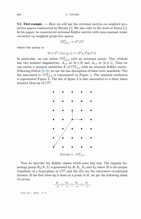
5.1. First example. — Here we will use the extremal metrics on weighted pro-jective spaces constructed by Bryant [7]. We also refer to the work of Abreu [1].In his paper, he constructed extremal Kähler metrics with non-constant scalarcurvature on weighted projective spaces

CP2a,b,c := C3/C∗

where the action is

∀t ∈ C∗, t.(x, y, z) := (tax, tby, tcz).

In particular, we can endow CP21,2,3 with an extremal metric. This orbifold

has two isolated singularities: A1,2 at [0, 1, 0] and A2,3 at [0, 0, 1]. Thus wecan endow a minimal resolution X of CP2

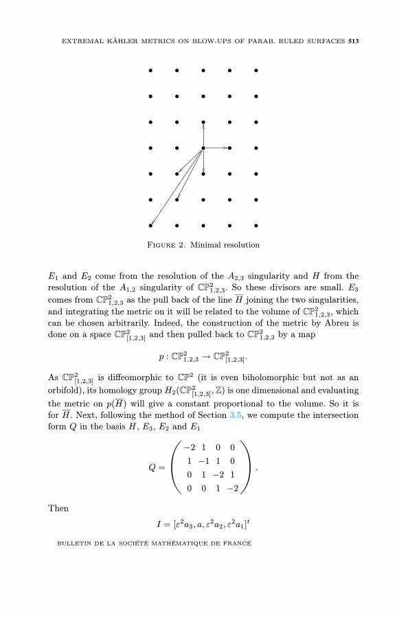
1,2,3 with an extremal Kähler metric.Following Fulton ([11]), we use the fan description of these toric manifolds. Thefan associated to CP2

1,2,3 is represented on Figure 1. The minimal resolutionis represented Figure 2. The fan of figure 2 is also associated to a three timesiterated blow-up of CP2.

• • • • •

• • • • •

• • • • •

• • •

OO

//

• •

• • • • •

• • • • •

• • • • •

Figure 1. CP21,2,3

Now we describe the Kähler classes which arise this way. The singular ho-mology groupH2(X,Z) is generated byH,E1, E2 and E3 whereH is the propertransform of a hyperplane in CP2 and the E′is are the successive exceptionaldivisors. If the first blow-up is done on a point of H, we get the following chainof curves:

H

−2

E3

−1

E2

−2

E1

−2.

tome 141 – 2013 – no 3


• • • • •

• • • • •

• • • • •

• • •

OO

//

• •

• • • • •

• • • • •

• • • • •

Figure 2. Minimal resolution

E1 and E2 come from the resolution of the A2,3 singularity and H from theresolution of the A1,2 singularity of CP2

1,2,3. So these divisors are small. E3

comes from CP21,2,3 as the pull back of the line H joining the two singularities,

and integrating the metric on it will be related to the volume of CP21,2,3, which

can be chosen arbitrarily. Indeed, the construction of the metric by Abreu isdone on a space CP2

[1,2,3] and then pulled back to CP21,2,3 by a map

p : CP21,2,3 → CP2

[1,2,3].

As CP2[1,2,3] is diffeomorphic to CP2 (it is even biholomorphic but not as an

orbifold), its homology group H2(CP2[1,2,3],Z) is one dimensional and evaluating

the metric on p(H) will give a constant proportional to the volume. So it isfor H. Next, following the method of Section 3.5, we compute the intersectionform Q in the basis H, E3, E2 and E1

Q =

à−2 1 0 0

1 −1 1 0

0 1 −2 1

0 0 1 −2

í.

Then

I = [ε2a3, a, ε2a2, ε

2a1]t


514 C. TIPLER

with a and the ai arbitrary positive numbers and ε small enough. The compu-tation of Q−1 · I gives the Kähler class

(3a+ ε2(a3 + 2a2 + a1))PD(H) + (2a+ ε2(a3 + a2))PD(E1)

+(4a+ ε2(2a3 + 2a2 + a1))PD(E2) + (6a+ ε2(3a3 + 4a2 + 2a1))PD(E3).

It proves Theorem D.

5.2. Second example. — We now consider the orbifold Riemann surface of genus1 with a singularity of order 3. In this case χorb < 0 and we can use the resultsof Corollary 3.3.3 with r = 1. The associated orbifold ruled surface has twosingular points of order 3 and from Proposition 3.4.1 we know that a minimalresolution is a three times iterated blow-up of the surface P( O⊕L) over Σ1 ' T2.Here L = O. Thus we get an extremal Kähler metric on a three times blow-upof CP1 × T2. The iterated blow-up can be made more precise. The first pointto be blown-up is the point on the zero section above the marked point of Σ.The iterated blow-up replace the fiber F by the chain of curves:

−2 −2 −1 −3

with the −3 self-intersection curve corresponding to the proper transform of thefiber F above the first blown-up point. This ends the proof of the Theorem Cstated in the introduction.

BIBLIOGRAPHY

[1] M. Abreu – “Kähler metrics on toric orbifolds”, J. Differential Geom. 58(2001), p. 151–187.

[2] V. Apostolov, D. M. J. Calderbank, P. Gauduchon & C. W.Tønnesen-Friedman – “Extremal Kähler metrics on projective bundlesover a curve”, Adv. Math. 227 (2011), p. 2385–2424.

[3] C. Arezzo & F. Pacard – “Blowing up and desingularizing constantscalar curvature Kähler manifolds”, Acta Math. 196 (2006), p. 179–228.

[4] , “Blowing up Kähler manifolds with constant scalar curvature. II”,Ann. of Math. 170 (2009), p. 685–738.

[5] C. Arezzo, F. Pacard & M. Singer – “Extremal metrics on blowups”,Duke Math. J. 157 (2011), p. 1–51.

[6] W. Barth, C. Peters & A. Van de Ven – Compact complex surfaces,Ergebn. Math. Grenzg., vol. 4, Springer, 1984.

[7] R. L. Bryant – “Bochner-Kähler metrics”, J. Amer. Math. Soc. 14 (2001),p. 623–715.

tome 141 – 2013 – no 3

http://smf.emath.fr/Publications/Bulletin/141/html/smf_bull_141_481-516.html#1








[8] E. Calabi – “Extremal Kähler metrics. II”, in Differential geometry andcomplex analysis, Springer, 1985, p. 95–114.

[9] D. M. J. Calderbank & M. A. Singer – “Einstein metrics and complexsingularities”, Invent. Math. 156 (2004), p. 405–443.

[10] S. K. Donaldson – “Scalar curvature and stability of toric varieties”,J. Differential Geom. 62 (2002), p. 289–349.

[11] W. Fulton – Introduction to toric varieties, Annals of Math. Studies,vol. 131, Princeton Univ. Press, 1993.

[12] A. Futaki & T. Mabuchi – “Bilinear forms and extremal Kähler vectorfields associated with Kähler classes”, Math. Ann. 301 (1995), p. 199–210.

[13] P. Gauduchon – “Calabi’s extremal metrics: An elementary introduc-tion”, book in preparation.

[14] D. D. Joyce – Compact manifolds with special holonomy, Oxford Math-ematical Monographs, Oxford Univ. Press, 2000.

[15] C. LeBrun & S. R. Simanca – “Extremal Kähler metrics and complexdeformation theory”, Geom. Funct. Anal. 4 (1994), p. 298–336.

[16] E. Legendre – “Toric geometry of convex quadrilaterals”, J. SymplecticGeom. 9 (2011), p. 343–385.

[17] A. Lichnerowicz – Géométrie des groupes de transformations, Travauxet Recherches Mathématiques, III. Dunod, Paris, 1958.

[18] T. Mabuchi – “K-stability of constant scalar curvature polarization”,preprint arXiv:0812.4093.

[19] V. B. Mehta & C. S. Seshadri – “Moduli of vector bundles on curveswith parabolic structures”, Math. Ann. 248 (1980), p. 205–239.

[20] Y. Rollin & M. Singer – “Non-minimal scalar-flat Kähler surfaces andparabolic stability”, Invent. Math. 162 (2005), p. 235–270.

[21] , “Constant scalar curvature Kähler surfaces and parabolic polysta-bility”, J. Geom. Anal. 19 (2009), p. 107–136.

[22] J. Ross & R. Thomas – “An obstruction to the existence of constantscalar curvature Kähler metrics”, J. Differential Geom. 72 (2006), p. 429–466.

[23] , “Weighted projective embeddings, stability of orbifolds, and con-stant scalar curvature Kähler metrics”, J. Differential Geom. 88 (2011),p. 109–159.

[24] J. Stoppa & G. Székelyhidi – “Relative K-stability of extremal metrics”,J. Eur. Math. Soc. (JEMS) 13 (2011), p. 899–909.

[25] G. Székelyhidi – “Extremal metrics and K-stability”, Bull. Lond. Math.Soc. 39 (2007), p. 76–84.

[26] , “The Calabi functional on a ruled surface”, Ann. Sci. Éc. Norm.Supér. 42 (2009), p. 837–856.













http://arxiv.org/abs/0812.4093









516 C. TIPLER

[27] , “On blowing up extremal Kähler manifolds”, Duke Math. J. 161(2012), p. 1411–1453.

[28] G. Tian – “Kähler-Einstein metrics with positive scalar curvature”, In-vent. Math. 130 (1997), p. 1–37.

[29] C. W. Tønnesen-Friedman – “Extremal Kähler metrics on minimalruled surfaces”, J. reine angew. Math. 502 (1998), p. 175–197.

[30] S.-T. Yau – “Open problems in geometry”, in Differential geometry: par-tial differential equations on manifolds (Los Angeles, CA, 1990), Proc.Sympos. Pure Math., vol. 54, Amer. Math. Soc., 1993, p. 1–28.

tome 141 – 2013 – no 3





Documents

Bulletin - e Math