THÈSEPour obtenir le grade de

DOCTEUR DE L’UNIVERSITÉ DE GRENOBLESpécialité : Mathématiques Appliquées

Arrêté ministérial : 7 août 2006

Présentée par

Gildas Mazo

Thèse dirigée par Stéphane Girardet codirigée par Florence Forbes

préparée au sein du Laboratoire Jean Kuntzmannet de l’École Doctorale Mathématiques, Sciences et Technologies del’Information, Informatique

Construction et estimation de co-pules en grande dimension

Thèse soutenue publiquement le 17 novembre 2014,devant le jury composé de :

M. Fabrizio DURANTEAssistant Professor, Free University of Bozen-Bolzano (Italie), Rapporteur

M. Johan SEGERSProfesseur, Université Catholique de Louvain (Belgique), Rapporteur

Mme Anne-Catherine FAVRE-PUGINProfesseur, Université Joseph Fourier, Examinateur

M. Ivan KOJADINOVICProfesseur, Université de Pau et des Pays de l’Adour, Examinateur

M. Stéphane GIRARDChargé de Recherche, Inria Rhône-Alpes, Directeur de thèse

Mme Florence FORBESDirecteur de Recherche, Inria Rhône-Alpes, Co-Directeur de thèse

❘❡♠❡r❝✐❡♠❡♥ts

❚♦✉t ❞✬❛❜♦r❞✱ ❥❡ r❡♠❡r❝✐❡ ♠❡s ❞✐r❡❝t❡✉rs ❞❡ t❤ès❡✱ ❋❧♦r❡♥❝❡ ❋♦r❜❡s ❡t ❙té✲♣❤❛♥❡ ●✐r❛r❞✱ ♣♦✉r ♠✬❛✈♦✐r ♣r♦♣♦sé ❝❡ s✉❥❡t ❞❡ t❤ès❡ très ♦✉✈❡rt ❡t ❛❝t✉❡❧✳ ❊♥♣❛rt✐❝✉❧✐❡r✱ ♠❡r❝✐ à ❙té♣❤❛♥❡ ♣♦✉r s♦♥ s✉✐✈✐ ❀ ❥✬❛✐ é❣❛❧❡♠❡♥t ❜❡❛✉❝♦✉♣ ❛♣♣ré❝✐és❛ ❝❧❛✐r✈♦②❛♥❝❡ ❡t s♦♥ ❤✉♠♦✉r✳ ❏❡ ♥❡ ♣❡♥s❡ ♣❛s ♣r❡♥❞r❡ ❜❡❛✉❝♦✉♣ ❞❡ r✐sq✉❡s❡♥ ❛✣r♠❛♥t q✉❡ ♥♦✉s ♥♦✉s s♦♠♠❡s très ❜✐❡♥ ❡♥t❡♥❞✉ t♦✉t ❛✉ ❧♦♥❣ ❞❡ ❝❡s tr♦✐s❛♥♥é❡s✳

❏❡ r❡♠❡r❝✐❡ ❋❛❜r✐③✐♦ ❉✉r❛♥t❡ ❡t ❏♦❤❛♥ ❙❡❣❡rs✱ ♣♦✉r ❛✈♦✐r ❛❝❝❡♣té s❛♥s ❤é✲s✐t❛t✐♦♥ ❡t r❡s♣❡❝t✐✈❡♠❡♥t s✬êtr❡ ♣r♦♣♦sé ❞❡ r❛♣♣♦rt❡r ❝❡tt❡ t❤ès❡✳ ❏❡ s✉✐s très❤♦♥♦ré ❞❡ ❧✬✐♥térêt q✉✬✐❧s ♦♥t ♣♦rté à ♠♦♥ tr❛✈❛✐❧✳ ▼❡r❝✐ é❣❛❧❡♠❡♥t à ■✈❛♥ ❑♦❥❛✲❞✐♥♦✈✐❝ ❡t ❆♥♥❡✲❈❛t❤❡r✐♥❡ ❋❛✈r❡ ♣♦✉r ♠✬❛✈♦✐r ❢❛✐t ❧✬❤♦♥♥❡✉r ❞❡ ❢❛✐r❡ ♣❛rt✐❡ ❞❡♠♦♥ ❥✉r②✳ ▼❡r❝✐ ❡♥ ♣❛rt✐❝✉❧✐❡r à ■✈❛♥ ♣♦✉r ❧❡s s✉❣❣❡st✐♦♥s ❡t r❡♠❛rq✉❡s ❞ét❛✐❧❧é❡ss✉r ♠♦♥ ♠❛♥✉s❝r✐t✳

❏❡ r❡♠❡r❝✐❡ ❇❡♥❥❛♠✐♥ ❘❡♥❛r❞ ♣♦✉r ❛✈♦✐r ré♣♦♥❞✉ à ♠❛ ❞❡♠❛♥❞❡ ❡♥ ♠❡♣r♦♣♦s❛♥t s♦♥ ❡①♣❡rt✐s❡ ❡t ❡♥ ♠❡ ❢♦✉r♥✐ss❛♥t ❧❡s ❞♦♥♥é❡s ❤②❞r♦❧♦❣✐q✉❡s ❛♥❛❧②sé❡s❞❛♥s ❝❡tt❡ t❤ès❡✳ ❏❡ r❡♠❡r❝✐❡ é❣❛❧❡♠❡♥t ❚r✉♥❣✱ ✓ ♠♦♥ ✔ ét✉❞✐❛♥t✱ ❛✈❡❝ q✉✐ ❥✬❛✐♣✉ ❝♦❧❧❛❜♦r❡r ♣♦✉r ✐♠♣❧é♠❡♥t❡r ✉♥ ❛❧❣♦r✐t❤♠❡ ❞✬✐♥❢ér❡♥❝❡✳

●râ❝❡ à s❡s ♠❡♠❜r❡s✱ ✐❧ ② ❛ t♦✉❥♦✉rs ❡✉ ✉♥❡ très ❜♦♥♥❡ ❛♠❜✐❛♥❝❡ ❡t très❜♦♥♥❡ ❤✉♠❡✉r ❞❛♥s ♠♦♥ éq✉✐♣❡ à ■♥r✐❛✱ ❧✬éq✉✐♣❡ ▼■❙❚■❙✳ ❏❡ ❧❡s r❡♠❡r❝✐❡ ❝❤❛✲❧❡✉r❡✉s❡♠❡♥t ♣♦✉r ❝❡❧❛✳ P❡✉t✲êtr❡ q✉❡ ❝❡tt❡ ❛t♠♦s♣❤èr❡ ❛ été ♣♦ss✐❜❧❡ ❣râ❝❡ à❧❛ s✐♠♣❧✐❝✐té ❞❡ ❝❤❛❝✉♥✳ ❯♥ ❣r❛♥❞ ♠❡r❝✐ à ❡✉①✱ ♠❡s ❛♠✐s✳ ➱✈✐❞❡♠♠❡♥t✱ ❥✬✐♥❝❧✉s❞❛♥s ❧❡ ❧♦t ♠❡s ❝♦♠♣èr❡s ❞❡ ❧✬éq✉✐♣❡ ■❇■❙ ✦

▼❡r❝✐ à ♠❡s ♣❛r❡♥ts✱ ♣♦✉r t♦✉t ✕ ❡♥ ♣❛rt✐❝✉❧✐❡r✱ ❥❡ ♥✬♦✉❜❧✐❡ ♣❛s q✉❡ ❝✬❡st❣râ❝❡ à ♠❛ ♠èr❡ q✉❡ ❥✬❛✐ ❝♦♠♠❡♥❝é ✉♥❡ ❧✐❝❡♥❝❡ ❡♥ st❛t✐st✐q✉❡ ✦

❊♥✜♥✱ ♠❡r❝✐ à ◗✉②♥❤✱ ♣♦✉r s❛ ♣rés❡♥❝❡ ❜✐❡♥✈❡✐❧❧❛♥t❡✳

✐✐✐

❘és✉♠é

❈❡s ❞❡r♥✐èr❡s ❞é❝❡♥♥✐❡s✱ ♥♦✉s ❛✈♦♥s ❛ss✐sté à ❧✬é♠❡r❣❡♥❝❡ ❞✉ ❝♦♥❝❡♣t ❞❡❝♦♣✉❧❡ ❡♥ ♠♦❞é❧✐s❛t✐♦♥ st❛t✐st✐q✉❡✳ ❈❡t ❡ss♦r ❡st ❥✉st✐✜é ♣❛r ❧❡ ❢❛✐t q✉❡ ❧❡s ❝♦✲♣✉❧❡s ♣❡r♠❡tt❡♥t ❞❡ ❢❛✐r❡ ✉♥❡ ❛♥❛❧②s❡ sé♣❛ré❡ ❞❡s ♠❛r❣❡s ❡t ❞❡ ❧❛ str✉❝t✉r❡ ❞❡❞é♣❡♥❞❛♥❝❡ ✐♥❞✉✐t❡ ♣❛r ✉♥❡ ❞✐str✐❜✉t✐♦♥ st❛t✐st✐q✉❡✳ ❈❡tt❡ sé♣❛r❛t✐♦♥ ❢❛❝✐❧✐t❡❧✬✐♥❝♦r♣♦r❛t✐♦♥ ❞❡ ❧♦✐s ♥♦♥ ❣❛✉ss✐❡♥♥❡s ❡t ❧❛ ♣r✐s❡ ❡♥ ❝♦♠♣t❡ ❞❡s ❞é♣❡♥❞❛♥❝❡s♥♦♥ ❧✐♥é❛✐r❡s ❡♥tr❡ ❧❡s ✈❛r✐❛❜❧❡s ❛❧é❛t♦✐r❡s✳ ▲❛ ✜♥❛♥❝❡ ❡t ❧✬❤②❞r♦❧♦❣✐❡ s♦♥t ❞❡✉①❡①❡♠♣❧❡s ❞❡ ❞♦♠❛✐♥❡s ♦ù ❧❡s ❝♦♣✉❧❡s s♦♥t très ✉t✐❧✐sé❡s✳ P✉✐sq✉✬✐❧ ❡①✐st❡ ❜❡❛✉✲❝♦✉♣ ❞❡ ❢❛♠✐❧❧❡s ❞❡ ❝♦♣✉❧❡s ❜✐✈❛r✐é❡s✱ ✐❧ s❡r❛ t♦✉❥♦✉rs ♣♦ss✐❜❧❡ à ❧✬✉t✐❧✐s❛t❡✉r ❞✬❡♥❝❤♦✐s✐r ✉♥❡ q✉✐ ❧✉✐ ❝♦♥✈✐❡♥♥❡✳ ▼❛❧❤❡✉r❡✉s❡♠❡♥t✱ ♦♥ ♥❡ ♣❡✉t ♣❛s ❡♥ ❞✐r❡ ❛✉t❛♥t❞❛♥s ❧❡ ❝❛s ♠✉❧t✐✈❛r✐é✳ ▲❛ ❣❛♠♠❡ ❞❡ ❝❡s ♠♦❞è❧❡s ♥✬❡st ♣❛s ❡♥❝♦r❡ ❛ss❡③ r✐❝❤❡♣♦✉r ♣♦✉✈♦✐r ❡♥ ❝❤♦✐s✐r ✉♥ q✉✐ s❛t✐s❢❛ss❡ t♦✉t❡s ❧❡s ♣r♦♣r✐étés q✉❡ ❧✬♦♥ s♦✉❤❛✐t❡✲r❛✐t ❛ ♣r✐♦r✐✳ ❈❡tt❡ t❤ès❡ s✬✐♥s❝r✐t ❞❛♥s ❝❡ ❝♦♥t❡①t❡✳ ◆♦✉s ♣r♦♣♦s♦♥s ❞❡✉① ❝❧❛ss❡s❞❡ ❝♦♣✉❧❡s ♠✉❧t✐✈❛r✐é❡s ❛✈❡❝ ❞❡s ♣r♦♣r✐étés ♦r✐❣✐♥❛❧❡s✱ ❝❡ q✉✐ ♣❡r♠❡t ❞✬é❧❛r❣✐r❧❛ ❣❛♠♠❡ ❞❡s ♠♦❞è❧❡s ❡①✐st❛♥ts✳ ▲❛ ♣r❡♠✐èr❡ ❝❧❛ss❡ ♣r♦♣♦sé❡ s✬é❝r✐t ❝♦♠♠❡ ✉♥♣r♦❞✉✐t ❞❡ ❝♦♣✉❧❡s ❜✐✈❛r✐é❡s✱ ♦ù ❝❤❛q✉❡ ❝♦♣✉❧❡ ❜✐✈❛r✐é❡ s❡ ❝♦♠❜✐♥❡ ❛✉① ❛✉tr❡s✈✐❛ ✉♥ ❣r❛♣❤❡ ❡♥ ❛r❜r❡✳ ❊❧❧❡ ♣❡r♠❡t ❞❡ ♣r❡♥❞r❡ ❡♥ ❝♦♠♣t❡ ❧❡s ❞✐✛ér❡♥ts ❞❡❣rés❞❡ ❞é♣❡♥❞❛♥❝❡ ❡♥tr❡ ❧❡s ❞✐✛ér❡♥t❡s ♣❛✐r❡s ❞❡ ✈❛r✐❛❜❧❡s✳ ▲❛ s❡❝♦♥❞❡ ❝❧❛ss❡ ❡st✉♥ ♠♦❞è❧❡ à ❢❛❝t❡✉rs✱ ❛✈❡❝ ✉♥❡ ❝♦♠♣♦s❛♥t❡ s✐♥❣✉❧✐èr❡✱ ❜❛sé❡ s✉r ✉♥❡ ❢❛♠✐❧❧❡♥♦♥♣❛r❛♠étr✐q✉❡ ❞❡ ❝♦♣✉❧❡s ❜✐✈❛r✐é❡s✳ ❊❧❧❡ ♣❡r♠❡t ❞✬♦❜t❡♥✐r ✉♥ ❜♦♥ éq✉✐❧✐❜r❡❡♥tr❡ ✢❡①✐❜✐❧✐té ❡t ♠❛♥✐❛❜✐❧✐té✳ P✉✐sq✉❡ ❧❡s ❝♦♣✉❧❡s ❞❡ ❧❛ ❞❡✉①✐è♠❡ ❝❧❛ss❡ ♣r♦♣♦✲sé❡ ♣♦ssè❞❡♥t ✉♥❡ ❝♦♠♣♦s❛♥t❡ s✐♥❣✉❧✐èr❡✱ ❧❡s ♠ét❤♦❞❡s ❝❧❛ss✐q✉❡s ❞✬✐♥❢ér❡♥❝❡ ♥❡♣❡r♠❡tt❡♥t ♣❛s ❞✬❡st✐♠❡r ❧❡✉rs ♣❛r❛♠ètr❡s✳ P♦✉r ❝❡tt❡ r❛✐s♦♥ ✕ ❡t ❝✬❡st ❛✉ss✐ ✉♥❡❝♦♥tr✐❜✉t✐♦♥ ❞❡ ❝❡tt❡ t❤ès❡ ✕✱ ♥♦✉s ❛❜♦r❞♦♥s é❣❛❧❡♠❡♥t ❧✬❡st✐♠❛t✐♦♥ ❞❡ ❝♦♣✉❧❡s❞❛♥s ❧❡ ❝❛s ❣é♥ér❛❧✱ ❡t ❡①❤✐❜♦♥s ❧❡s ♣r♦♣r✐étés ❛s②♠♣t♦t✐q✉❡s ❞✬✉♥ ❡st✐♠❛t❡✉r ❞❡s♠♦✐♥❞r❡s ❝❛rrés ♣♦♥❞érés ❜❛sé s✉r ❧❡s ❝♦❡✣❝✐❡♥ts ❞❡ ❞é♣❡♥❞❛♥❝❡ s❛♥s ❢❛✐r❡ ❛♣♣❡❧à ❞❡s ❤②♣♦t❤ès❡s ❞❡ ré❣✉❧❛r✐té s✉r ❧❡s ❝♦♣✉❧❡s✳ ▲❡s ♠♦❞è❧❡s ❡t ♠ét❤♦❞❡s ♣r♦♣♦séss♦♥t ❛♣♣❧✐q✉és s✉r ❞❡s ❞♦♥♥é❡s ❤②❞r♦❧♦❣✐q✉❡s ✭♣❧✉✐❡s ❡t ❞é❜✐ts ❞❡ r✐✈✐èr❡s✮✳

✐✈

❆❜str❛❝t

■♥ t❤❡ ❧❛st ❞❡❝❛❞❡s✱ ❝♦♣✉❧❛s ❤❛✈❡ ❜❡❡♥ ♠♦r❡ ❛♥❞ ♠♦r❡ ✉s❡❞ ✐♥ st❛t✐st✐❝❛❧ ♠♦✲❞❡❧✐♥❣✳ ❚❤❡✐r ♣♦♣✉❧❛r✐t② ♦✇❡s ♠✉❝❤ t♦ t❤❡ ❢❛❝t t❤❛t t❤❡② ❛❧❧♦✇ t♦ s❡♣❛r❛t❡ t❤❡❛♥❛❧②s✐s ♦❢ t❤❡ ♠❛r❣✐♥s ❢r♦♠ t❤❡ ❛♥❛❧②s✐s ♦❢ t❤❡ ❞❡♣❡♥❞❡♥❝❡ str✉❝t✉r❡ ✐♥❞✉❝❡❞ ❜②t❤❡ ✉♥❞❡r❧②✐♥❣ ❞✐str✐❜✉t✐♦♥✳ ❚❤✐s r❡♥❞❡rs ❡❛s✐❡r t❤❡ ♠♦❞❡❧✐♥❣ ♦❢ ♥♦♥ ●❛✉ss✐❛♥❞✐str✐❜✉t✐♦♥s✱ ❛♥❞✱ ♠♦r❡♦✈❡r✱ ✐t ❛❧❧♦✇s t♦ t❛❦❡ ✐♥t♦ ❛❝❝♦✉♥t ♥♦♥ ❧✐♥❡❛r ❞❡♣❡♥✲❞❡♥❝✐❡s ❜❡t✇❡❡♥ r❛♥❞♦♠ ✈❛r✐❛❜❧❡s✳ ❋✐♥❛♥❝❡ ❛♥❞ ❤②❞r♦❧♦❣② ❛r❡ t✇♦ ❡①❛♠♣❧❡s ♦❢s❝✐❡♥t✐✜❝ ✜❡❧❞s ✇❤❡r❡ t❤❡ ✉s❡ ♦❢ ❝♦♣✉❧❛s ✐s ♥♦✇❛❞❛②s st❛♥❞❛r❞✳ ❙✐♥❝❡ t❤❡r❡ ❡①✐sts♠❛♥② ❢❛♠✐❧✐❡s ♦❢ ❜✐✈❛r✐❛t❡ ❝♦♣✉❧❛s✱ ✐t ✐s ❛❧✇❛②s ♣♦ss✐❜❧❡ ❢♦r t❤❡ ✉s❡r t♦ ❝❤♦♦s❡♦♥❡ t❤❛t s✉✐ts ❤✐s✴❤❡r ♥❡❡❞s✳ ❯♥❢♦rt✉♥❛t❡❧②✱ t❤❡ ♠✉❧t✐✈❛r✐❛t❡ ❝❛s❡ ✐s ♥♦t t❤❛ts✐♠♣❧❡✳ ❚❤❡ r❛♥❣❡ ♦❢ t❤❡s❡ ♠♦❞❡❧s ✐s st✐❧❧ ♥♦t r✐❝❤ ❡♥♦✉❣❤ ❢♦r t❤❡ ✉s❡r t♦ ❝❤♦♦s❡♦♥❡ t❤❛t s❛t✐s✜❡s ❛❧❧ t❤❡ ❞❡s✐r❡❞ ♣r♦♣❡rt✐❡s✳ ❚❤✐s t❤❡s✐s ❛❞❞r❡ss❡s t❤✐s ✐ss✉❡✳ ❲❡♣r♦♣♦s❡ t✇♦ ❝❧❛ss❡s ♦❢ ♠✉❧t✐✈❛r✐❛t❡ ❝♦♣✉❧❛s ✇✐t❤ ♥♦✈❡❧ ♣r♦♣❡rt✐❡s✱ r❡s✉❧t✐♥❣ ✐♥❛♥ ❡♥❧❛r❣❡♠❡♥t ♦❢ t❤❡ r❛♥❣❡ ♦❢ t❤❡ ❡①✐st✐♥❣ ♠♦❞❡❧s✳ ❚❤❡ ✜rst ♠♦❞❡❧ ✇r✐t❡s ❛s❛ ♣r♦❞✉❝t ♦❢ ❜✐✈❛r✐❛t❡ ❝♦♣✉❧❛s ❛♥❞ ✐s ✉♥❞❡r❧❛✐♥ ❜② ❛ tr❡❡ str✉❝t✉r❡ ✇❤❡r❡ ❡❛❝❤❡❞❣❡ r❡♣r❡s❡♥ts ❛ ❜✐✈❛r✐❛t❡ ❝♦♣✉❧❛✳ ❍❡♥❝❡✱ ✇❡ ❛r❡ ❛❜❧❡ t♦ ♠♦❞❡❧ ❞✐✛❡r❡♥t ♣❛✐rs✇✐t❤ ❞✐✛❡r❡♥t ❞❡♣❡♥❞❡♥❝❡ ♣r♦♣❡rt✐❡s✳ ❚❤❡ s❡❝♦♥❞ ♦♥❡ ✐s ❛ ❢❛❝t♦r ♠♦❞❡❧✱ ✇✐t❤❛ s✐♥❣✉❧❛r ❝♦♠♣♦♥❡♥t✱ ❜✉✐❧t ♦♥ ❛ ♥♦♥♣❛r❛♠❡tr✐❝ ❝❧❛ss ♦❢ ❜✐✈❛r✐❛t❡ ❝♦♣✉❧❛s✳ ■t❡①❤✐❜✐ts ❛ ❣♦♦❞ ❜❛❧❛♥❝❡ ❜❡t✇❡❡♥ tr❛❝t❛❜✐❧✐t② ❛♥❞ ✢❡①✐❜✐❧✐t②✳ ❙✐♥❝❡ t❤❡ ❝♦♣✉❧❛s❜❡❧♦♥❣✐♥❣ t♦ t❤❡ s❡❝♦♥❞ ♣r♦♣♦s❡❞ ❝❧❛ss ❤❛✈❡ ❛ s✐♥❣✉❧❛r ❝♦♠♣♦♥❡♥t✱ t❤❡ st❛♥✲❞❛r❞ ♠❡t❤♦❞s ♦❢ ✐♥❢❡r❡♥❝❡ ❞♦ ♥♦t ♣❡r♠✐t t♦ ❡st✐♠❛t❡ t❤❡✐r ♣❛r❛♠❡t❡rs✳ ❋♦r t❤✐sr❡❛s♦♥ ✕ ❛♥❞ t❤✐s ✐s ❛ ❝♦♥tr✐❜✉t✐♦♥ ♦❢ ♦✉r t❤❡s✐s ❛s ✇❡❧❧ ✕✱ ✇❡ ❛❧s♦ ❞❡❛❧ ✇✐t❤ t❤❡❡st✐♠❛t✐♦♥ ♦❢ ❝♦♣✉❧❛s ✐♥ ❣❡♥❡r❛❧✱ ❛♥❞ ❡st❛❜❧✐s❤ t❤❡ ❛s②♠♣t♦t✐❝ ♣r♦♣❡rt✐❡s ♦❢ ❛❧❡❛st✲sq✉❛r❡s ❡st✐♠❛t♦r ❜❛s❡❞ ♦♥ ❞❡♣❡♥❞❡♥❝❡ ❝♦❡✣❝✐❡♥ts ✇✐t❤♦✉t ✐♠♣♦s✐♥❣ r❡✲❣✉❧❛r✐t② ❝♦♥❞✐t✐♦♥s ♦♥ t❤❡ ❝♦♣✉❧❛s✳ ❚❤❡ ♠♦❞❡❧s ❛♥❞ ♠❡t❤♦❞s ❤❛✈❡ ❜❡❡♥ ❛♣♣❧✐❡❞t♦ ❤②❞r♦❧♦❣✐❝❛❧ ❞❛t❛ ✭✢♦✇ r❛t❡s ❛♥❞ r❛✐♥ ❢❛❧❧s✮✳

✈

❚❛❜❧❡ ❞❡s ♠❛t✐èr❡s

❘és✉♠é ✐✈

❆❜str❛❝t ✈

■♥tr♦❞✉❝t✐♦♥ ✶

■ ❈♦♣✉❧❡s ✹

✶ ▲❡s ❝♦♣✉❧❡s ♦✉ ❧✬ét✉❞❡ ❞❡ ❧❛ ❞é♣❡♥❞❛♥❝❡ ✺

✶✳✶ ❉é✜♥✐t✐♦♥ ✳ ✳ ✳ ✳ ✳ ✳ ✳ ✳ ✳ ✳ ✳ ✳ ✳ ✳ ✳ ✳ ✳ ✳ ✳ ✳ ✳ ✳ ✳ ✳ ✳ ✳ ✳ ✳ ✳ ✳ ✳ ✻✶✳✷ ▼❡s✉r❡r ❧❛ ❞é♣❡♥❞❛♥❝❡ ✳ ✳ ✳ ✳ ✳ ✳ ✳ ✳ ✳ ✳ ✳ ✳ ✳ ✳ ✳ ✳ ✳ ✳ ✳ ✳ ✳ ✳ ✳ ✳ ✼

✶✳✷✳✶ ❙♣❡❝tr❡ ❞❡ ❞é♣❡♥❞❛♥❝❡ ✳ ✳ ✳ ✳ ✳ ✳ ✳ ✳ ✳ ✳ ✳ ✳ ✳ ✳ ✳ ✳ ✳ ✳ ✳ ✳ ✽✶✳✷✳✷ ❈♦❡✣❝✐❡♥ts ❞❡ ❞é♣❡♥❞❛♥❝❡ ✳ ✳ ✳ ✳ ✳ ✳ ✳ ✳ ✳ ✳ ✳ ✳ ✳ ✳ ✳ ✳ ✳ ✽

✶✳✸ ❉❡✉① ❝❧❛ss❡s ❞❡ ❝♦♣✉❧❡s ♣❛rt✐❝✉❧✐èr❡s ✳ ✳ ✳ ✳ ✳ ✳ ✳ ✳ ✳ ✳ ✳ ✳ ✳ ✳ ✳ ✳ ✶✶✶✳✸✳✶ ❈♦♣✉❧❡s ❞❡s ✈❛❧❡✉rs ❡①trê♠❡s ✳ ✳ ✳ ✳ ✳ ✳ ✳ ✳ ✳ ✳ ✳ ✳ ✳ ✳ ✳ ✳ ✶✶✶✳✸✳✷ ❈♦♣✉❧❡s ❛✈❡❝ ✉♥❡ ❝♦♠♣♦s❛♥t❡ s✐♥❣✉❧✐èr❡ ✳ ✳ ✳ ✳ ✳ ✳ ✳ ✳ ✳ ✳ ✶✷

✷ ▼♦❞è❧❡s ❞❡ ❝♦♣✉❧❡s ❡♥ ❣r❛♥❞❡ ❞✐♠❡♥s✐♦♥ ✶✺

✷✳✶ ❈♦♣✉❧❡s ❛r❝❤✐♠é❞✐❡♥♥❡s ✳ ✳ ✳ ✳ ✳ ✳ ✳ ✳ ✳ ✳ ✳ ✳ ✳ ✳ ✳ ✳ ✳ ✳ ✳ ✳ ✳ ✳ ✳ ✶✺✷✳✷ ❈♦♣✉❧❡s ❛r❝❤✐♠é❞✐❡♥♥❡s ✐♠❜r✐q✉é❡s ✳ ✳ ✳ ✳ ✳ ✳ ✳ ✳ ✳ ✳ ✳ ✳ ✳ ✳ ✳ ✳ ✳ ✶✻✷✳✸ ❱✐♥❡s ✳ ✳ ✳ ✳ ✳ ✳ ✳ ✳ ✳ ✳ ✳ ✳ ✳ ✳ ✳ ✳ ✳ ✳ ✳ ✳ ✳ ✳ ✳ ✳ ✳ ✳ ✳ ✳ ✳ ✳ ✳ ✳ ✳ ✶✼✷✳✹ ❈♦♣✉❧❡s ❡❧❧✐♣t✐q✉❡s ✳ ✳ ✳ ✳ ✳ ✳ ✳ ✳ ✳ ✳ ✳ ✳ ✳ ✳ ✳ ✳ ✳ ✳ ✳ ✳ ✳ ✳ ✳ ✳ ✳ ✳ ✶✾

✸ ■♥❢ér❡♥❝❡ ✷✶

✸✳✶ ❊st✐♠❛t✐♦♥ ✳ ✳ ✳ ✳ ✳ ✳ ✳ ✳ ✳ ✳ ✳ ✳ ✳ ✳ ✳ ✳ ✳ ✳ ✳ ✳ ✳ ✳ ✳ ✳ ✳ ✳ ✳ ✳ ✳ ✳ ✷✷✸✳✶✳✶ ▲❛ ♠ét❤♦❞❡ ❞✉ ♠❛①✐♠✉♠ ❞❡ ✈r❛✐s❡♠❜❧❛♥❝❡ ✳ ✳ ✳ ✳ ✳ ✳ ✳ ✳ ✷✷✸✳✶✳✷ ▲❛ ♠ét❤♦❞❡ ❞❡s ♠♦♠❡♥ts ❜❛sé❡ s✉r ❧❡s ❝♦❡✣❝✐❡♥ts ❞❡ ❞é✲

♣❡♥❞❛♥❝❡ ✳ ✳ ✳ ✳ ✳ ✳ ✳ ✳ ✳ ✳ ✳ ✳ ✳ ✳ ✳ ✳ ✳ ✳ ✳ ✳ ✳ ✳ ✳ ✳ ✳ ✳ ✳ ✷✸✸✳✶✳✸ ▲❡s ♠ét❤♦❞❡s ♥♦♥ ♣❛r❛♠étr✐q✉❡s ✳ ✳ ✳ ✳ ✳ ✳ ✳ ✳ ✳ ✳ ✳ ✳ ✳ ✳ ✷✺

✸✳✷ ❚❡sts ✳ ✳ ✳ ✳ ✳ ✳ ✳ ✳ ✳ ✳ ✳ ✳ ✳ ✳ ✳ ✳ ✳ ✳ ✳ ✳ ✳ ✳ ✳ ✳ ✳ ✳ ✳ ✳ ✳ ✳ ✳ ✳ ✳ ✳ ✷✻

■■ ❉❡✉① ♥♦✉✈❡❧❧❡s ❝❧❛ss❡s ❞❡ ❝♦♣✉❧❡s ❡t ❧❡✉r ❡st✐♠❛t✐♦♥ ✷✼

✹ ❯♥ ♠♦❞è❧❡ ❞❡ ❝♦♣✉❧❡s ❜❛sé s✉r ❞❡s ♣r♦❞✉✐ts ❞❡ ❝♦♣✉❧❡s ❜✐✈❛✲

r✐é❡s ✷✽

✈✐

✺ ❊st✐♠❛t✐♦♥ ❞❡ ❝♦♣✉❧❡s ♠✉❧t✐✈❛r✐é❡s ♣❛r ❧❛ ♠ét❤♦❞❡ ❞❡s ♠♦✐♥❞r❡s

❝❛rrés ♣♦♥❞érés ❜❛sé❡ s✉r ❧❡s ❝♦❡✣❝✐❡♥ts ❞❡ ❞é♣❡♥❞❛♥❝❡ ✹✼

✻ ❯♥❡ ❝❧❛ss❡ ❞❡ ❝♦♣✉❧❡s ♠❛♥✐❛❜❧❡ ❡t ✢❡①✐❜❧❡ ✼✷

❈♦♥❝❧✉s✐♦♥ ✶✵✶

✈✐✐

■♥tr♦❞✉❝t✐♦♥

▲❡ ❜❡s♦✐♥ ❞❡ r❡❝♦✉r✐r à ❞❡s ♠♦❞è❧❡s st❛t✐st✐q✉❡s ♥♦♥ ❣❛✉ss✐❡♥s✱ ♦✉ ♥♦♥ ♥♦r✲♠❛✉① ✶ ❛ t♦✉❥♦✉rs ❡①✐sté ❡♥ st❛t✐st✐q✉❡✱ ♠❛✐s ✐❧ ét❛✐t ❝♦♥s✐❞éré ♣❡♥❞❛♥t ❧♦♥❣t❡♠♣s❝♦♠♠❡ ♠♦✐♥s ❧❛ rè❣❧❡ q✉❡ ❧✬❡①❝❡♣t✐♦♥✳ ❘é❝❡♠♠❡♥t✱ ❝❡ ❜❡s♦✐♥ s✬❡st ❢❛✐t ❞❡ ♣❧✉s❡♥ ♣❧✉s ♣r❡ss❛♥t✳ ❉❛♥s ♣❧✉s✐❡✉rs ❞♦♠❛✐♥❡s ❞✬❛♣♣❧✐❝❛t✐♦♥✱ ❝♦♠♠❡ ♣❛r ❡①❡♠♣❧❡❧✬❤②❞r♦❧♦❣✐❡ ♦✉ ❧❛ ✜♥❛♥❝❡ ✷✱ ♦♥ r❡❝♦♥♥❛✐t ❧✬✉t✐❧✐té ❞❡ ❝❡s ♠♦❞è❧❡s q✉✐ s♦♥t ❝❛✲♣❛❜❧❡s ❞❡ ♣r❡♥❞r❡ ❡♥ ❝♦♠♣t❡ ❧❡s ❞é♣❡♥❞❛♥❝❡s ❞❡ t②♣❡s ♥♦♥ ❛✣♥❡s✱ ❡t s✉rt♦✉t✱❧❡s ❞é♣❡♥❞❛♥❝❡s ❡♥tr❡ ❧❡s ✈❛❧❡✉rs ❡①trê♠❡s ❞❡s ❢❛❝t❡✉rs ❞✬✐♥térêts✳ ❊♥ ❡✛❡t✱ ✐❧ ❡st❜✐❡♥ ❝♦♥♥✉ q✉❡ ❧❡s ❧♦✐s ❣❛✉ss✐❡♥♥❡s✱ ❡♥ ♣❛rt✐❝✉❧✐❡r✱ s♦♥t ✐♥❝❛♣❛❜❧❡s ❞❡ ♠♦❞é❧✐s❡r❞❡ t❡❧❧❡s ❞é♣❡♥❞❛♥❝❡s ❬✽✺❪✳ ❈♦♥s✐❞ér♦♥s t♦✉t ❞❡ s✉✐t❡ tr♦✐s ❡①❡♠♣❧❡s✳

❘❡t♦✉r s✉r ✐♥✈❡st✐ss❡♠❡♥t✳ ▲❡ r❡t♦✉r s✉r ✐♥✈❡st✐ss❡♠❡♥t s✉r d ❛♥♥é❡s ❞✬✉♥♣❧❛❝❡♠❡♥t ✜♥❛♥❝✐❡r ❡st ❞♦♥♥é ♣❛r 1000(1+X1)×· · ·×(1+Xd)✱ ♦ù Xi ❡st ❧❡ t❛✉①❞✬✐♥térêt s✉r ❧✬❛♥♥é❡ i✳ ❙✉♣♣♦s♦♥s✱ ♣❛r ❡①❡♠♣❧❡✱ q✉❡ ❝❤❛q✉❡ Xi s♦✐t ❞✐str✐❜✉é✉♥✐❢♦r♠é♠❡♥t ❡♥tr❡ ✵✳✵✺ ❡t ✵✳✶✺✳ ❙✐ ❧❡s t❛✉① ét❛✐❡♥t ✐♥❞é♣❡♥❞❛♥ts ❞✬✉♥❡ ❛♥♥é❡ à❧✬❛✉tr❡✱ ♥♦✉s ♣♦✉rr✐♦♥s ❝❛❧❝✉❧❡r ❧❛ ❞✐str✐❜✉t✐♦♥ ❞✉ r❡t♦✉r s✉r ❧❡s d ❛♥♥é❡s ❀ ♠❛✐s✱é✈✐❞❡♠♠❡♥t✱ ✐❧s ♥❡ ❧❡ s♦♥t ♣❛s✳ ■❧ ♥♦✉s ❢❛✉t ❛❧♦rs tr♦✉✈❡r ✉♥ ♠♦❞è❧❡ ♣♦✉r ❧❛ ❧♦✐❥♦✐♥t❡ ❞❡s t❛✉① Xi✳ ❈❡t ❡①❡♠♣❧❡ ❡st t✐ré ❞❡ ❬✺✼❪✳

●❡st✐♦♥ ❞❡ ♣♦rt❡✲❢❡✉✐❧❧❡✳ ▲♦rsq✉❡ ❧✬♦♥ ♣♦ssè❞❡ ✉♥ ♣♦rt❡✲❢❡✉✐❧❧❡ ❞✬❛❝t✐❢s ✜✲♥❛♥❝✐❡rs✱ ♦♥ s♦✉❤❛✐t❡ s❛✈♦✐r ❝♦♠♠❡♥t ❡st ❞✐str✐❜✉é❡ ❧❛ ♣❡rt❡ ♣♦t❡♥t✐❡❧❧❡ q✉✐ ❧✉✐❡st ❛ss♦❝✐é❡✳ ❆✐♥s✐✱ s♦✐t P ti ❧❡ ♣r✐① ❞✉ i✲è♠❡ ❛❝t✐❢ ❞❡ ♥♦tr❡ ♣♦rt❡✲❢❡✉✐❧❧❡ à ✉♥t❡♠♣s ❞❡ ré❢ér❡♥❝❡ t ❡t s♦✐t Xi = −(logP t+1

i − logP ti ) ❧❛ ♣❡rt❡ ❡♥r❡❣✐stré❡ ♣♦✉r❝❡t ❛❝t✐❢ à ✉♥ ♣❛s ❞❡ t❡♠♣s ❞❛♥s ❧❡ ❢✉t✉r✳ ▲❛ ♣❡rt❡ t♦t❛❧❡ ❛ss♦❝✐é❡ à ♥♦tr❡ ♣♦rt❡✲❢❡✉✐❧❧❡ q✉✐ ❝♦♥t✐❡♥t d ❛❝t✐❢s s✬é❝r✐t ❛❧♦rs X1+X2+ · · ·+Xd✳ P♦✉r ❝❛❧❝✉❧❡r s❛ ❧♦✐✱♥♦✉s ❛✈♦♥s ❜❡s♦✐♥ ❞❡ ❧❛ ❧♦✐ ❥♦✐♥t❡ ❞❡ (X1, . . . , Xd)✳

❊st✐♠❛t✐♦♥ ❞❡ ♥✐✈❡❛✉① ❝r✐t✐q✉❡s ❡♥ ❤②❞r♦❧♦❣✐❡✳ ❖♥ ❞✐s♣♦s❡ ❞❡ d ♣❧✉✈✐♦✲♠ètr❡s ❞✐s♣♦sés ❞❛♥s ✉♥❡ ré❣✐♦♥ ❞✬✐♥térêt✳ ❖♥ ♥♦t❡ Xi ❞❡ ❢♦♥❝t✐♦♥ ❞❡ ré♣❛rt✐✲t✐♦♥ Fi ❧❛ q✉❛♥t✐té ❞❡ ♣❧✉✐❡ ♠❛①✐♠❛❧❡ ❡♥r❡❣✐stré❡ s✉r ✉♥❡ ❛♥♥é❡ ❞❛♥s ❧❡ i✲è♠❡

✶✳ ❇✐❡♥ q✉❡ ❝❡s ❞❡✉① t❡r♠❡s s♦✐❡♥t ❛❝❝❡♣tés ♣❛r t♦✉s ❝♦♠♠❡ ét❛♥t éq✉✐✈❛❧❡♥ts✱ ♥♦✉s ♣ré❢é✲r♦♥s ✉t✐❧✐s❡r ❧❡ t❡r♠❡ ✓ ❣❛✉ss✐❡♥ ✔ ❞❛♥s ✉♥ ❝♦♥t❡①t❡ ❞❡ ♠♦❞é❧✐s❛t✐♦♥✱ ❝❛r✱ s✐ ❧❡ t❡r♠❡ ✓ ♥♦r♠❛❧ ✔ét❛✐t ❡♠♣❧♦②é✱ ❝❡❧❛ s♦✉s ❡♥t❡♥❞r❛✐t q✉❡ ❧❡s ❛✉tr❡s ♠♦❞è❧❡s ♥❡ s♦♥t ♣❛s ♥♦r♠❛✉① ❛✉ s❡♥s ❧✐tté✲r❛❧ ❞✉ t❡r♠❡✳ ❖r✱ ❡t ❝✬❡st ❥✉st❡♠❡♥t ❧❡ ♠❡ss❛❣❡ ❞❡ ❝❡tt❡ ✐♥tr♦❞✉❝t✐♦♥ ❞❡ t❤ès❡✱ ❝❡ ♥✬❡st ♣❧✉s✈r❛✐ ❛✉❥♦✉r❞✬❤✉✐✳ ❖♥ ♣♦✉rr❛ s❡ ❝♦♥s♦❧❡r ❡♥ ❣❛r❞❛♥t ❧❡ t❡r♠❡ ✓ ♥♦r♠❛❧ ✔ ❞❛♥s ✉♥ ❝♦♥t❡①t❡❞❡ st❛t✐st✐q✉❡ ♠❛t❤é♠❛t✐q✉❡✱ ♣✉✐sq✉❡ ❝❡ t❡r♠❡ s❡r❛ t♦✉❥♦✉rs ❥✉st✐✜é ♣❛r ❧❡ t❤é♦rè♠❡ ❝❡♥tr❛❧❧✐♠✐t❡✳

✷✳ ❙✉rt♦✉t ❧❛ ✜♥❛♥❝❡ ✿ ✐❧ ② ❛ ✺ ❢♦✐s ♣❧✉s ❞❡ ❝♦♠❜✐♥❛✐s♦♥s ✓ ❝♦♣✉❧❛ ❆◆❉ ✜♥❛♥❝❡ ✔ q✉❡✓ ❝♦♣✉❧❛ ❆◆❉ ❤②❞r♦❧♦❣② ✔ r❡♥✈♦②é❡s ♣❛r ●♦♦❣❧❡ ❙❝❤♦❧❛r✳

✶

♣❧✉✈✐♦♠ètr❡✳ ❖♥ s♦✉❤❛✐t❡ é✈❛❧✉❡r ❧❛ ♣r♦❜❛❜✐❧✐té ❞✬❛♣♣❛r✐t✐♦♥ ❞❡ ❧✬é✈è♥❡♠❡♥t s❡✲❧♦♥ ❧❡q✉❡❧ t♦✉t❡s ❧❡s ✈❛r✐❛❜❧❡s ❞é♣❛ss❡♥t ❧❡✉r q✉❛♥t✐❧❡ ❞✬♦r❞r❡ ✾✾✪✱ ❝✬❡st à ❞✐r❡{X1 > F−1

1 (0.99), . . . , Xd > F−1d (0.99)}✳ P♦✉r ❝❡❧❛✱ ♥♦✉s ❛✈♦♥s ❜❡s♦✐♥ ❞❡ ❧❛ ❧♦✐

❞❡ min(X1, . . . , Xd)✱ ❝❡ q✉✐ s❡r❛✐t ♣♦ss✐❜❧❡ s✐ ♥♦✉s ❛✈✐♦♥s ❝❡❧❧❡ ❞❡ (X1, . . . , Xd)✳❈❡t ❡①❡♠♣❧❡ s❡r❛ r❡♣r✐s ❞❛♥s ❧❡ ❝❤❛♣✐tr❡ ✻✳

❉❛♥s ❧❡s tr♦✐s ❡①❡♠♣❧❡s ♣ré❝é❞❡♥ts✱ ❧✬ét✉❞❡ ❞❡ ❧❛ q✉❡✉❡ ❞❡ ❞✐str✐❜✉t✐♦♥ ❞❡ ❧❛❧♦✐ ❝♦♥s✐❞éré❡ ❡st ❞✬✉♥❡ ✐♠♣♦rt❛♥❝❡ ❝❛♣✐t❛❧❡✳ ❊♥ ❡✛❡t✱ ❝❡ s♦♥t ❧❡s é✈è♥❡♠❡♥ts ❞❡❝❡tt❡ q✉❡✉❡ ❞❡ ❞✐str✐❜✉t✐♦♥ q✉✐ ✐♠♣❛❝t❡♥t ❧❡ ♣❧✉s ❢♦rt❡♠❡♥t ❞❡s ♣❡rt❡s ✜♥❛♥❝✐èr❡s♦✉ ❞❡s ✐♥♦♥❞❛t✐♦♥s s✉❜✐❡s✳ ❖r✱ ❧❡s é✈è♥❡♠❡♥ts ❞❡ ❧❛ q✉❡✉❡ ❞❡ ❞✐str✐❜✉t✐♦♥ s♦♥t❡✉① ♠ê♠❡s ♣r✐♥❝✐♣❛❧❡♠❡♥t ✐ss✉s ❞❡ ❧❛ ❝♦✲♦❝❝✉r❡♥❝❡ ❞❡s ✈❛❧❡✉rs ❡①trê♠❡s ❞❡♥♦s ✈❛r✐❛❜❧❡s✳ ❈✬❡st ♣♦✉rq✉♦✐ ✐❧ ❡st ♣r✐♠♦r❞✐❛❧ ❞❡ ♠♦❞é❧✐s❡r ❝♦rr❡❝t❡♠❡♥t ❧❡s❞é♣❡♥❞❛♥❝❡s ❡♥tr❡ ❧❡s ✈❛❧❡✉rs ❡①trê♠❡s✳

❆✐♥s✐✱ ♥♦♥ s❡✉❧❡♠❡♥t ♦♥ s♦✉❤❛✐t❡ ❝♦♥str✉✐r❡ ❞❡s ♠♦❞è❧❡s ♠✉❧t✐✈❛r✐és ♥♦♥❣❛✉ss✐❡♥s✱ ♠❛✐s ❡♥ ♣❧✉s✱ ✐❧ ❢❛✉t s♦✉✈❡♥t ❧❡ ❢❛✐r❡ s♦✉s ❧❛ ❝♦♥tr❛✐♥t❡ q✉❡ ❧❡s ❧♦✐s♠❛r❣✐♥❛❧❡s ❞❡s ❢❛❝t❡✉rs ❞✬✐♥térêts s♦♥t ❞♦♥♥é❡s ✭❝✬❡st ❧❡ ❝❛s ❞❡s ❡①❡♠♣❧❡s ❝✐✲❞❡ss✉s✮✳ P♦✉r ré♣♦♥❞r❡ à ❝❡tt❡ ❛tt❡♥t❡✱ ❧❡s ❝♦♣✉❧❡s s❡ s♦♥t ✐♠♣♦sé❡s ❝♦♠♠❡ ✉♥♦✉t✐❧ ✐♥❝♦♥t♦✉r♥❛❜❧❡✳ ❊♥ rés✉♠é ✕ ♥♦✉s ❞ét❛✐❧❧❡r♦♥s ♣❧✉s ❛✉ ❝❤❛♣✐tr❡ ✶ ✕✱ ✸ ✉♥❡❝♦♣✉❧❡ ❡st ✉♥ ♠♦❞è❧❡ q✉✐ ♣❡r♠❡t ❞❡ r❡✢ét❡r ✜❞è❧❡♠❡♥t ❧❛ ❞é♣❡♥❞❛♥❝❡ ❡♥tr❡ ❧❡s❢❛❝t❡✉rs ❝♦♥s✐❞érés✳ ■❧ ❡st ❞♦♥❝ ✐♠♣♦rt❛♥t ♣♦✉r ❧✬✉t✐❧✐s❛t❡✉r ❞❡ ❞✐s♣♦s❡r ❞✬✉♥❡❣❛♠♠❡ ❛✉ss✐ ❝♦♠♣❧èt❡ q✉❡ ♣♦ss✐❜❧❡ ❞❡ ♠♦❞è❧❡s ❞❡ ❝♦♣✉❧❡s ❛✜♥ ❞❡ s✬❛ss✉r❡r q✉❡❧✬✉♥ ❞✬❡♥tr❡ ❡✉① s❛t✐s❢❡r❛ à s❡s ❜❡s♦✐♥s✳ ❉❛♥s ❧❡ ❝❛s ❜✐✈❛r✐é✱ ❝✬❡st à ❞✐r❡ ❧♦rsq✉✬✐❧♥✬② ❛ q✉❡ ❞❡✉① ✈❛r✐❛❜❧❡s à ét✉❞✐❡r✱ ✐❧ ② ❛ ❞❡ ♥♦♠❜r❡✉s❡s ❢❛♠✐❧❧❡s ❞❡ ❝♦♣✉❧❡s ♣❛r♠✐❧❡sq✉❡❧❧❡s ✐❧ tr♦✉✈❡r❛ ❝❡rt❛✐♥❡♠❡♥t ❝❡❧❧❡ q✉✐ ❧✉✐ ❝♦♥✈✐❡♥t✳ ▼❛❧❤❡✉r❡✉s❡♠❡♥t✱ ♦♥♥❡ ♣❡✉t ♣❛s ❡♥ ❞✐r❡ ❛✉t❛♥t ❞❛♥s ❧❡ ❝❛s ♠✉❧t✐✈❛r✐é✳ ▲❛ ❣❛♠♠❡ ❞❡ ❝❡s ♠♦❞è❧❡s♥✬❡st ♣❛s ❡♥❝♦r❡ ❛ss❡③ r✐❝❤❡ ♣♦✉r ♣♦✉✈♦✐r ❡♥ ❝❤♦✐s✐r ✉♥ q✉✐ s❛t✐s❢❛ss❡ t♦✉t❡s ❧❡s♣r♦♣r✐étés q✉❡ ❧✬♦♥ s♦✉❤❛✐t❡r❛✐t ❛ ♣r✐♦r✐✳ ❇✐❡♥ s♦✉✈❡♥t✱ ❧✬✉t✐❧✐s❛t❡✉r ❞❡✈r❛ ❛❝❝❡♣✲t❡r ❞❡ ♣❡r❞r❡ ✉♥ ♣❡✉ ❞✬✉♥❡ ♣r♦♣r✐été ♣♦✉r ❡♥ ❣❛❣♥❡r ✉♥❡ ❛✉tr❡✳ ❈❡ ❝♦♠♣r♦♠✐s❡st ♥♦t❛♠♠❡♥t ✈r❛✐ ❧♦rsq✉❡ ❧✬♦♥ ❝♦♥s✐❞èr❡ ❧❛ ✢❡①✐❜✐❧✐té ❡t ❧❛ ♠❛♥✐❛❜✐❧✐té ❞✬✉♥♠♦❞è❧❡✳ ❉❡ ❧✬❛✈❡✉ ♠ê♠❡ ❞❡ ❞❡✉① ❞❡s ❝❤❡r❝❤❡✉rs ❧❡s ♣❧✉s r❡❝♦♥♥✉s ❞❛♥s ❝❡ ❞♦✲♠❛✐♥❡ ❬✹✼✱ ✻✾❪✱ ❧❛ ❝♦♥str✉❝t✐♦♥ ❞❡ ❝♦♣✉❧❡s ♠✉❧t✐✈❛r✐é❡s ❡st ✉♥ ♣r♦❜❧è♠❡ ❞✐✣❝✐❧❡❝❛r✱ ❝♦♠♠❡ ❧❡ s♦✉❧✐❣♥❡ ❏♦❡ ❬✹✼❪✱ ✓ ♦♥❡ ❝❛♥♥♦t ❥✉st ✇r✐t❡ ❞♦✇♥ ❛ ❢❛♠✐❧② ♦❢ ❢✉♥❝✲t✐♦♥s ❛♥❞ ❡①♣❡❝t ✐t t♦ s❛t✐s❢② t❤❡ ♥❡❝❡ss❛r② ❝♦♥❞✐t✐♦♥ ❢♦r ♠✉❧t✐✈❛r✐❛t❡ ❝✉♠✉❧❛t✐✈❡❞✐str✐❜✉t✐♦♥ ❢✉♥❝t✐♦♥s ✔✳ ▲❛ ♣❤r❛s❡ ❞❡ ◆❡❧s❡♥ q✉✐ ✐♥tr♦❞✉✐t ❧❛ ♣❛rt✐❡ ✸✳✺ ❞❡ s♦♥❧✐✈r❡ ❬✻✾❪ s✉r ❧❛ ❝♦♥str✉❝t✐♦♥ ❞❡ ❝♦♣✉❧❡s ♠✉❧t✐✈❛r✐é❡s✱ ❡st ❛✉ss✐ r❡sté❡ ❝é❧è❜r❡ ✿✓ ❋✐rst✱ ❛ ✇♦r❞ ♦❢ ❝❛✉t✐♦♥ ✿ ❈♦♥str✉❝t✐♥❣ ❬♠✉❧t✐✈❛r✐❛t❡❪ ❝♦♣✉❧❛s ✐s ❞✐✣❝✉❧t ✔✳

❈❡tt❡ t❤ès❡ ❛♣♣♦rt❡ s❛ ❝♦♥tr✐❜✉t✐♦♥ à ❧✬ét✉❞❡ ❞❡s ❝♦♣✉❧❡s à tr❛✈❡rs ❞❡✉① ❛①❡s✳Pr❡♠✐èr❡♠❡♥t✱ ♥♦✉s ❡♥r✐❝❤✐ss♦♥s ❧❛ ❣❛♠♠❡ ❞❡s ♠♦❞è❧❡s ♠✉❧t✐✈❛r✐és ❞❡ ❞❡✉①❝❧❛ss❡s ❛✉① ♣r♦♣r✐étés ♦r✐❣✐♥❛❧❡s✳ ▲❡s ❝♦♣✉❧❡s ❞❡ ❧❛ ♣r❡♠✐èr❡ ❝❧❛ss❡ s✬é❝r✐✈❡♥t❝♦♠♠❡ ✉♥ ♣r♦❞✉✐t ❞❡ ❝♦♣✉❧❡s ❜✐✈❛r✐é❡s✱ ♦ù ❝❤❛q✉❡ ❝♦♣✉❧❡ ❜✐✈❛r✐é❡ s❡ ❝♦♠❜✐♥❡❛✉① ❛✉tr❡s ✈✐❛ ✉♥ ❣r❛♣❤❡ ❡♥ ❛r❜r❡✳ ❈❡ ♠♦❞è❧❡ ♣❡r♠❡t ❞❡ ♣r❡♥❞r❡ ❡♥ ❝♦♠♣t❡ ❧❡s❞✐✛ér❡♥ts ❞❡❣rés ❞❡ ❞é♣❡♥❞❛♥❝❡ ❡♥tr❡ ❧❡s ❞✐✛ér❡♥t❡s ♣❛✐r❡s✳ ▲❛ s❡❝♦♥❞❡ ❝❧❛ss❡❞❡ ❝♦♣✉❧❡s ❡st ✉♥ ♠♦❞è❧❡ à ❢❛❝t❡✉rs✱ ❛✈❡❝ ✉♥❡ ❝♦♠♣♦s❛♥t❡ s✐♥❣✉❧✐èr❡✱ ❜❛sé s✉r✉♥❡ ❝❧❛ss❡ ♥♦♥♣❛r❛♠étr✐q✉❡ ❞❡ ❝♦♣✉❧❡s ❜✐✈❛r✐é❡s✳ ❊❧❧❡ ♣❡r♠❡t ❞✬♦❜t❡♥✐r ✉♥ ❜♦♥éq✉✐❧✐❜r❡ ❡♥tr❡ ✢❡①✐❜✐❧✐té ❡t ♠❛♥✐❛❜✐❧✐té✳ ❉❡✉①✐è♠❡♠❡♥t✱ ♥♦✉s ❡♥✈✐s❛❣❡♦♥s ❧✬❡st✐✲♠❛t✐♦♥ ❞❡ ❝♦♣✉❧❡s ❞❛♥s ❧❡ ❝❛s ❣é♥ér❛❧✱ ❝✬❡st à ❞✐r❡ ♣♦✉r ❧❡sq✉❡❧❧❡s ✐❧ ♥✬❡①✐st❡ ♣❛s♥é❝❡ss❛✐r❡♠❡♥t ❞❡ ❞ér✐✈é❡s ♣❛rt✐❡❧❧❡s ✭❝♦♠♠❡ ♣❛r ❡①❡♠♣❧❡ ❧❡s ❝♦♣✉❧❡s ❛♣♣❛rt❡✲♥❛♥t à ❧❛ s❡❝♦♥❞❡ ❝❧❛ss❡ ♣r♦♣♦sé❡✮✱ ❡t ét❛❜❧✐ss♦♥s ❧❡s ♣r♦♣r✐étés ❛s②♠♣t♦t✐q✉❡s

✸✳ ▲❡ ❧❡❝t❡✉r ♣♦✉rr❛ ❛❞♠✐r❡r ✐❝✐ ✉♥❡ ♠❛❣♥✐✜q✉❡ ❝♦♠♣♦s✐t✐♦♥ s②♥t❛①✐q✉❡ ✿ ❧❡ ❢❛♠❡✉① t✐r❡t✲✈✐r❣✉❧❡✳

✷

❞✬✉♥ ❡st✐♠❛t❡✉r ❞❡s ♠♦✐♥❞r❡s ❝❛rrés ♣♦♥❞érés ❜❛sé s✉r ❧❡s ❝♦❡✣❝✐❡♥ts ❞❡ ❞é✲♣❡♥❞❛♥❝❡✳ ❈❤❛❝✉♥ ❞❡ ♥♦s ♠♦❞è❧❡s ❡t ♠ét❤♦❞❡s ♣r♦♣♦sés s♦♥t ❛♣♣❧✐q✉és s✉r ❞❡s❞♦♥♥é❡s ❤②❞r♦❧♦❣✐q✉❡s ✭♣❧✉✐❡s ❡t ❞é❜✐ts ❞❡ r✐✈✐èr❡s✮✳

▲❡ ♣❧❛♥ ❞❡ ❧❛ t❤ès❡ ❡st ❧❡ s✉✐✈❛♥t✳ ▲❛ ♣❛rt✐❡ ■ ❝♦♥t✐❡♥t ✉♥❡ ✐♥tr♦❞✉❝t✐♦♥ ❛✉①❝♦♣✉❧❡s ❞❛♥s ❧❡ ❝❤❛♣✐tr❡ ✶✱ ♣rés❡♥t❡ ✉♥❡ r❡✈✉❡ ❞❡ ❧❛ ❧✐ttér❛t✉r❡ s✉r ❧❡s ♣r✐♥❝✐✲♣❛✉① ♠♦❞è❧❡s ❞❡ ❝♦♣✉❧❡s ♠✉❧t✐✈❛r✐é❡s ❛✉ ❝❤❛♣✐tr❡ ✷✱ ❡t ❛❜♦r❞❡ ❧❡s ♣r♦❜❧è♠❡s❞✬✐♥❢ér❡♥❝❡ ❞❛♥s ❧❡ ❝❤❛♣✐tr❡ ✸✳ ▲❛ ♣❛rt✐❡ ■■ ♣rés❡♥t❡ ♥♦s ❝♦♥tr✐❜✉t✐♦♥s✳ ❈❤❛❝✉♥❞❡s ❝❤❛♣✐tr❡s ❧❛ ❝♦♠♣♦s❛♥t ❡st ❝♦♥st✐t✉é ❞✬✉♥❡ ❜rè✈❡ ✐♥tr♦❞✉❝t✐♦♥ s✉✐✈✐❡ ❞✬✉♥❛rt✐❝❧❡ s♦✉♠✐s ♣♦✉r ♣✉❜❧✐❝❛t✐♦♥✱ ❡♥ ❛♥❣❧❛✐s✳ ▲❛ ❝❧❛ss❡ ❜❛sé❡ s✉r ✉♥ ♣r♦❞✉✐t ❞❡❝♦♣✉❧❡s ❡st ✐♥tr♦❞✉✐t❡ ❞❛♥s ❧❡ ❝❤❛♣✐tr❡ ✹ ❡t ❧❡ ♠♦❞è❧❡ à ❢❛❝t❡✉r ❡st ✐♥tr♦❞✉✐t❞❛♥s ❧❡ ❝❤❛♣✐tr❡ ✻✳ ▲❡ ❝❤❛♣✐tr❡ ✺ ♣rés❡♥t❡ ♥♦tr❡ ♠ét❤♦❞❡ ❞✬❡st✐♠❛t✐♦♥✳ ❊♥✜♥✱✉♥❡ ❝♦♥❝❧✉s✐♦♥ ✈✐❡♥❞r❛ ❝❧♦r❡ ❧❛ t❤ès❡✳

✸

Pr❡♠✐èr❡ ♣❛rt✐❡

❈♦♣✉❧❡s

✹

❈❤❛♣✐tr❡ ✶

▲❡s ❝♦♣✉❧❡s ♦✉ ❧✬ét✉❞❡ ❞❡ ❧❛

❞é♣❡♥❞❛♥❝❡

▲❡s ❝♦♣✉❧❡s ♣❡r♠❡tt❡♥t ❞✬ét✉❞✐❡r ❧❛ ❞é♣❡♥❞❛♥❝❡ ❡♥tr❡ ♣❧✉s✐❡✉rs ✈❛r✐❛❜❧❡s❛❧é❛t♦✐r❡s✱ ❛✈❡❝ ❧✬✐❞é❡ q✉❡ ❝❡tt❡ ❞é♣❡♥❞❛♥❝❡ ♥❡ ❞♦✐t ♣❛s ❝♦♥t❡♥✐r ❞✬✐♥❢♦r♠❛t✐♦♥♣r♦✈❡♥❛♥t ❞❡s ❧♦✐s ♠❛r❣✐♥❛❧❡s ❞❡s ✈❛r✐❛❜❧❡s ❡❧❧❡s✲♠ê♠❡s✳ P♦✉r ❝❡ ❢❛✐r❡✱ ♦♥ ❧❡s✓ ✉♥✐❢♦r♠✐s❡ ✔✱ ❝✬❡st à ❞✐r❡ q✉✬♦♥ s❡ ♣ré♠✉♥✐ ❞❡ ✓ ❧✬❡✛❡t ❞✬♦♣t✐q✉❡ ✔ ❞û ❛✉ ❢❛✐t q✉❡❝❡s ✈❛r✐❛❜❧❡s ♣❡✉✈❡♥t ❛✈♦✐r ❞❡s ❧♦✐s ♠❛r❣✐♥❛❧❡s très ❞✐✛ér❡♥t❡s✳ ❊♥ ♣❛rt✐❝✉❧✐❡r✱ ❧❡s❝♦♣✉❧❡s ♣❡r♠❡tt❡♥t ❞✬✐♠♣♦s❡r ✉♥❡ str✉❝t✉r❡ ❞❡ ❞é♣❡♥❞❛♥❝❡ à ❞❡s ❧♦✐s ♠❛r❣✐♥❛❧❡s✭♦✉ ❞❡s ✈❛r✐❛❜❧❡s ❛❧é❛t♦✐r❡s✮ ❞♦♥♥é❡s sé♣❛ré♠❡♥t✳ P❛r ❡①❡♠♣❧❡✱ ❧♦rsq✉❡ ♥♦✉s❛✈✐♦♥s ❞♦♥♥é ❝♦♠♠❡ ❡①❡♠♣❧❡ ❧✬❡st✐♠❛t✐♦♥ ❞❡s ♥✐✈❡❛✉① ❝r✐t✐q✉❡s ❛ss♦❝✐és à ✉♥é✈è♥❡♠❡♥t ❡①trê♠❡ ❡♥ ❤②❞r♦❧♦❣✐❡ ❞❛♥s ❧✬✐♥tr♦❞✉❝t✐♦♥ ❞❡ ❝❡tt❡ t❤ès❡✱ ♥♦✉s ❛✈✐♦♥s✈✉ q✉❡ Xi ét❛✐t ❧❛ q✉❛♥t✐té ❞❡ ♣❧✉✐❡ ♠❛①✐♠❛❧❡ ♦❜s❡r✈é❡ s✉r ✉♥❡ ❛♥♥é❡ à ✉♥❡❝❡rt❛✐♥❡ st❛t✐♦♥ i✳ ❖r✱ ♥♦✉s s❛✈♦♥s✱ ❞✬❛♣rès ❧❛ t❤é♦r✐❡ ❞❡s ✈❛❧❡✉rs ❡①trê♠❡s ✭✈♦✐r♣❛r ❡①❡♠♣❧❡ ❬✶✶✱ ✶✸✱ ✼✻❪✮✱ q✉❡ ❧❛ ❧♦✐ Fi ❞✉ ♠❛①✐♠✉♠ ❞✬✉♥ é❝❤❛♥t✐❧❧♦♥✱ ❞❡✈r❛✐têtr❡ r❛✐s♦♥♥❛❜❧❡♠❡♥t ❜✐❡♥ ❛♣♣r♦❝❤é❡ ♣❛r ❧❛ ❧♦✐ ❞❡s ✈❛❧❡✉rs ❡①trê♠❡s ❣é♥ér❛❧✐sé❡✭●❡♥❡r❛❧✐③❡❞ ❊①tr❡♠❡ ❱❛❧✉❡ ♦✉ ●❊❱ ❡♥ ❛♥❣❧❛✐s✮✱ ❞♦♥♥é❡ ♣❛r

GEV (x;µi, σi, ξi) = exp

[−(1 + ξi

x− µiσi

)−1/ξi],

♦ù σi > 0, −∞ < µi, ξi <∞ ❡t 1+ξi(x−µi)/σi > 0✳ ❆✐♥s✐✱ ♣♦✉r ❝❤❛q✉❡ st❛t✐♦♥i✱ ❧❛ ❞✐str✐❜✉t✐♦♥ Fi ❡st ❝♦♥♥✉❡ ✭❛✉① ♣❛r❛♠ètr❡s ♣rès✮✳ ▼❛✐s ❝♦♠♠❡♥t ♠♦❞é❧✐s❡r❧❡s ❞é♣❡♥❞❛♥❝❡s ❡♥tr❡ ❧❡s ❞✐✛ér❡♥t❡s st❛t✐♦♥s ❄ ❈✬❡st ✐❝✐ ✉♥ ♣r♦❜❧è♠❡ t②♣✐q✉❡q✉❡ ❧✬♦♥ ♣❡✉t ✈♦✉❧♦✐r rés♦✉❞r❡ ❛✈❡❝ ❧❡s ❝♦♣✉❧❡s ✶✳ ▲❡s ❛✉tr❡s ❡①❡♠♣❧❡s ♣rés❡♥tés❧♦rs ❞❡ ❧✬✐♥tr♦❞✉❝t✐♦♥ ❞❡ ❝❡tt❡ t❤ès❡ s♦♥t ❛✉ss✐ ❞❡s ❝❛s ❞✬é❝♦❧❡ ♣♦✉r ❧❡s ❝♦♣✉❧❡s✳❱♦✐❝✐ ✉♥ ❞❡r♥✐❡r ❡①❡♠♣❧❡✱ tr❛✐t❛♥t ❞✉ r✐sq✉❡ ❞❡ ❝ré❞✐t ❡t t✐ré ❞❡ ❬✻✶❪ ✷✳ ▲♦rsq✉✬✉♥ét❛❜❧✐ss❡♠❡♥t ❞❡ ❝ré❞✐t ♣rêt❡ à ♣❧✉s✐❡✉rs ❡♥tr❡♣r✐s❡s✱ ❝❡s ❞❡r♥✐èr❡s r❡♠❜♦✉rs❡♥tà é❝❤é❛♥❝❡✱ s❛✉❢ s✐ ❡❧❧❡s ❢♦♥t ❢❛✐❧❧✐t❡ ❀ ❡❧❧❡s s♦♥t ❛❧♦rs ❡♥ ❞é❢❛✉t ❞❡ ♣❛✐❡♠❡♥t✳ P♦✉r

✶✳ P♦✉rt❛♥t✱ ❧❡s st❛t✐st✐❝✐❡♥s s♣é❝✐❛❧✐st❡s ❞❡ ❧❛ t❤é♦r✐❡ ❞❡s ✈❛❧❡✉rs ❡①trê♠❡s ✉t✐❧✐s❡♥t très♣❡✉ ❧❡s ❝♦♣✉❧❡s✳ P❛r ❡①❡♠♣❧❡✱ ❧✬♦✉✈r❛❣❡ ❞❡ ❙✳ ❈♦❧❡s ❬✶✶❪ ♥❡ ❧❡s ♠❡♥t✐♦♥♥❡ ♣❛s ❞✉ t♦✉t✳

✷✳ ❉❡♣✉✐s ✉♥ ❛rt✐❝❧❡ ❞✉ ❲✐r❡❞ ▼❛❣❛③✐♥❡ ❞❛té ❞✉ ✷✸ ❢é✈r✐❡r ✷✵✵✾✱ ❝❡tt❡ ♣✉❜❧✐❝❛t✐♦♥ ❡st❞❡✈❡♥✉❡ tr✐st❡♠❡♥t ❝é❧è❜r❡ ✿ ❧❛ ❢♦r♠✉❧❡ ❧✐❛♥t ❧❛ ♣r♦❜❛❜✐❧✐té q✉❡ ♣❧✉s✐❡✉rs ❡♠♣r✉♥t❡✉rs ❢❛ss❡♥t❞é❢❛✉t ❡♥s❡♠❜❧❡ ❛✈❡❝ ❧❛ ❝♦♣✉❧❡ ✭❣❛✉ss✐❡♥♥❡✮ ❛ été ❛♣♣❡❧é❡ ✓ t❤❡ ❢♦r♠✉❧❛ t❤❛t ❦✐❧❧❡❞ ❲❛❧❧

❙tr❡❡t ✔✳ ❊✈✐❞❡♠♠❡♥t✱ ❝✬❡st ♠♦✐♥s ❧❛ ❢♦r♠✉❧❡ ❡❧❧❡ ♠ê♠❡ q✉❡ ❧✬✉t✐❧✐s❛t✐♦♥ q✉✐ ❡♥ ❛ été ❢❛✐t❡q✉✐ ét❛✐t ❡rr♦♥é❡✳ ❚♦✉t❡❢♦✐s✱ ❝❡❧❛ ✐❧❧✉str❡ ❜✐❡♥ ❧❡s ❡♥❥❡✉①✱ ♣♦✉✈❛♥t êtr❡ ❝♦♥s✐❞ér❛❜❧❡s✱ ❞❡ ❧❛♠♦❞é❧✐s❛t✐♦♥✳

✺

é✈❛❧✉❡r ❧❡ r✐sq✉❡ ❞❡ ❝ré❞✐t s✉♣♣♦rté ♣❛r ❧❡ ♣rêt❡✉r✱ ♦♥ ❝♦♠♠❡♥❝❡ ♣❛r é✈❛❧✉❡r❧❛ ♣r♦❜❛❜✐❧✐té q✉❡ ❝❤❛q✉❡ ❡♥tr❡♣r✐s❡✱ ♣r✐s❡ ✐♥❞✐✈✐❞✉❡❧❧❡♠❡♥t✱ ❢❛ss❡ ❞é❢❛✉t✳ ❊♥❢❛✐t✱ ♦♥ ♣❡✉t ♠♦❞é❧✐s❡r ❝❡s ♣r♦❜❛❜✐❧✐tés ♣❛r ❧❡s ♦✉t✐❧s ❝❧❛ss✐q✉❡s ❞❡ ❧✬❛♥❛❧②s❡ ❞❡s✉r✈✐❡ ❡♥ st❛t✐st✐q✉❡✳ ❯♥❡ ❢♦✐s ❧❡s ♠♦❞è❧❡s ❞❡ s✉r✈✐❡ ❝❤♦✐s✐s✱ ♦♥ ♣❡✉t ❡st✐♠❡r ❧❡s♣❛r❛♠ètr❡s ❞❡ ❝❡s ♠♦❞è❧❡s ❞❡ ♣❧✉s✐❡✉rs ❢❛ç♦♥s✱ ✈♦✐r ❬✻✶❪✳ ▼❛✐s✱ ♣♦✉r ♣r❡♥❞r❡ ❡♥❝♦♠♣t❡ ❧❛ ❞é♣❡♥❞❛♥❝❡ ❡♥tr❡ ❧❡s ❡♠♣r✉♥t❡✉rs✱ ✐❧ ❢❛✉t ♣♦✉✈♦✐r s♣é❝✐✜❡r ✉♥❡ ❧♦✐❥♦✐♥t❡ ét❛♥t ❞♦♥♥é❡s ❧❡s ❧♦✐s ♠❛r❣✐♥❛❧❡s✳

❉❛♥s ❧❡s ♠✐s❡s ❡♥ s✐t✉❛t✐♦♥ ♣ré❝é❞❡♥t❡s✱ ✐❧ ❢❛✉t s♣é❝✐✜❡r ✉♥❡ ❧♦✐ ❥♦✐♥t❡ ét❛♥t❞♦♥♥é❡s ❧❡s ❧♦✐s ♠❛r❣✐♥❛❧❡s✳ ▲❡s ❝♦♣✉❧❡s ❛✐❞❡♥t à ❢❛✐r❡ ❝❡❧❛✳ ❊❧❧❡s ❢❛❝✐❧✐t❡♥t ❧❛♠♦❞é❧✐s❛t✐♦♥ ❡♥ ❧❛ ❞é❝♦✉♣❛♥t ❡♥ ❞❡✉① ét❛♣❡s ✿ ❧❛ ♠♦❞é❧✐s❛t✐♦♥ ❞❡s ♠❛r❣❡s ♣✉✐s❝❡❧❧❡ ❞❡ ❧❛ str✉❝t✉r❡ ❞❡ ❞é♣❡♥❞❛♥❝❡✳ ❈♦♠♠❡ ♥♦✉s ❧❡ ✈❡rr♦♥s ❞❛♥s ❧❡ ❝❤❛♣✐tr❡ ✸✱❝❡ ❞é❝♦✉♣❛❣❡ s❡ r❡tr♦✉✈❡ ❛✉ss✐ ❞❛♥s ❧✬✐♥❢ér❡♥❝❡✱ q✉✐ s✬❡♥ tr♦✉✈❡ ❛✉ss✐ ❢❛❝✐❧✐té❡✭❞✬✉♥ ♣♦✐♥t ❞❡ ✈✉❡ ♣r❛t✐q✉❡ ❀ é✈✐❞❡♠♠❡♥t✱ ❞✬✉♥❡ ♣♦✐♥t ❞❡ ✈✉❡ t❤é♦r✐q✉❡✱ ♦♥✐♥tr♦❞✉✐t ♣❧✉tôt ❞❡ ♥♦✉✈❡❛✉① ❝❤❛❧❧❡♥❣❡s✮✳

▲❡s ❝♦♣✉❧❡s ❝♦♥♥❛✐ss❡♥t ✉♥ ❡ss♦r r❡♠❛rq✉❛❜❧❡ ❞❡♣✉✐s ✉♥❡ ❞✐③❛✐♥❡ ❞✬❛♥♥é❡s✱❝♦♠♠❡ ❡♥ té♠♦✐❣♥❡ ❧❡ t❛❜❧❡❛✉ ✶✳✶✳ ❊♥ ❞é❝❡♠❜r❡ ✷✵✶✵✱ ❧❡ s✐t❡ ✐♥t❡r♥❡t ❙❝✐❡♥❝❡❲❛t❝❤✳❝♦♠ ❛ ♠ê♠❡ é❧✉ ❧❛ ❞✐s❝✐♣❧✐♥❡ ✓ ❈♦♣✉❧❛ ♠♦❞❡❧✐♥❣ ✔ ❝♦♠♠❡ ✓ t♦♣ t♦♣✐❝ ✔ ♣❛r♠✐t♦✉s ❧❡s ❞♦♠❛✐♥❡s ❞❡ ❧❛ ❝❛té❣♦r✐❡ ✓ ▼❛t❤❡♠❛t✐❝s ✔ ❬✽✽❪✳

❛♥♥é❡s ♥♦♠❜r❡ ❞❡ ♣✉❜❧✐❝❛t✐♦♥s✶✾✼✸✲✶✾✽✸ ✶✶✾✽✸✲✶✾✾✸ ✾✶✾✾✸✲✷✵✵✸ ✻✽✷✵✵✸✲✷✵✶✸ ✽✷✹

❚❛❜❧❡ ✶✳✶ ✕ ◆♦♠❜r❡ ❞❡ ♣✉❜❧✐❝❛t✐♦♥s ❞❛♥s ❧❛ ❜❛s❡ ❞❡ ❞♦♥♥é❡s ▼❛t❤❙❝✐◆❡t ❛✈❡❝❞❛♥s ❧❡ t✐tr❡ ✓ ❝♦♣✉❧❛ ✔ ❡♥ ❢♦♥❝t✐♦♥ ❞❡ ❧✬❛♥♥é❡✳

▲❡ r❡st❡ ❞✉ ❝❤❛♣✐tr❡ ❡st ♦r❣❛♥✐sé ❝♦♠♠❡ s✉✐t✳ ❉❛♥s ❧❛ ♣❛rt✐❡ ✶✳✶✱ ♥♦✉s ❞♦♥✲♥♦♥s ❧❛ ❞é✜♥✐t✐♦♥ ❞✬✉♥❡ ❝♦♣✉❧❡✳ ❉❛♥s ❧❛ ♣❛rt✐❡ ✶✳✷✱ ♥♦✉s ♠♦♥tr♦♥s ❝♦♠♠❡♥tq✉❛♥t✐✜❡r ❧❛ ❞é♣❡♥❞❛♥❝❡ à ❧✬❛✐❞❡ ❞❡s ❝♦♣✉❧❡s✳ ❊♥✜♥✱ ❞❛♥s ❧❛ ♣❛rt✐❡ ✶✳✸✱ ♥♦✉s♣rés❡♥t♦♥s ❞❡✉① ❝❧❛ss❡s ❞❡ ❝♦♣✉❧❡s ♣❛rt✐❝✉❧✐èr❡s ✿ ❧❡s ❝♦♣✉❧❡s ❞❡s ✈❛❧❡✉rs ❡①✲trê♠❡s ❡t ❧❡s ❝♦♣✉❧❡s ❛✈❡❝ ✉♥❡ ❝♦♠♣♦s❛♥t❡ s✐♥❣✉❧✐èr❡✳

✶✳✶ ❉é✜♥✐t✐♦♥

❙♦✐❡♥tX1, . . . , Xd ❞❡s ✈❛r✐❛❜❧❡s ❛❧é❛t♦✐r❡s ❞❡ ❢♦♥❝t✐♦♥s ❞❡ ré♣❛rt✐t✐♦♥ F1, . . . , Fd✱❡t s♦✐t F ❧❛ ❢♦♥❝t✐♦♥ ❞❡ ré♣❛rt✐t✐♦♥ ❞✉ ✈❡❝t❡✉r (X1, . . . , Xd)✳ ▲❛ ❝♦♣✉❧❡✱ s♦✉✈❡♥t♥♦té❡ C✱ ❛ss♦❝✐é❡ à ❧❛ ❧♦✐ ❝✐❜❧❡ F ✱ ❡st ❧❛ ❢♦♥❝t✐♦♥ ❞❡ ré♣❛rt✐t✐♦♥ ❞✉ ✈❡❝t❡✉r(F1(X1), . . . , Fd(Xd))✳ ❊❧❧❡ ❡st ❞♦♥❝ ❛✉ss✐ ❧❛ ❢♦♥❝t✐♦♥ q✉✐ à (u1, . . . , ud) ❛ss♦❝✐❡❧❡ ♥♦♠❜r❡ F (F−1

1 (u1), . . . , F−11 (u1))✳

❉❡✜♥✐t✐♦♥ ✶ ✭❈♦♣✉❧❡✮✳ ❯♥❡ ❝♦♣✉❧❡ d✲✈❛r✐é❡ ❡st ✉♥❡ ❢♦♥❝t✐♦♥ ❞é✜♥✐❡ s✉r [0, 1]d

t❡❧❧❡ q✉❡

✶✳ C(u1, . . . , ud) = 0 s✐ ui = 0 ♣♦✉r ❛✉ ♠♦✐♥s ✉♥ ✐♥❞✐❝❡ i ❞❛♥s {1, . . . , d}✱✷✳ ♣♦✉r ❝❤❛q✉❡ ♣❛✈é B = [a1, b1] × · · · × [ad, bd] ✐♥❝❧✉ ❞❛♥s ❧❡ ❝✉❜❡ ✉♥✐té

[0, 1]d✱ ❧❡ ✈♦❧✉♠❡ ❞❡ ❝❡ ♣❛✈é∑

s❣♥(u1, . . . , ud)C(u1, . . . , ud) ❡st ♣♦s✐t✐❢✱ ♦ù

✻

❧❛ s♦♠♠❡ ❡st ♣r✐s❡ s✉r t♦✉s ❧❡s s♦♠♠❡ts (u1, . . . , ud) ❞❡ B ❡t

s❣♥(u1, . . . , ud) =

{1 s✐ uk = ak ♣♦✉r ✉♥ ♥♦♠❜r❡ ♣❛✐r ❞❡ k ∈ {1, . . . , d},

−1 s✐ uk = ak ♣♦✉r ✉♥ ♥♦♠❜r❡ ✐♠♣❛✐r ❞❡ k ∈ {1, . . . , d},

✸✳ ❧❡s ♠❛r❣❡s ✉♥✐✈❛r✐é❡s ❞❡ C s♦♥t ✉♥✐❢♦r♠❡s✱ ❝✬❡st à ❞✐r❡ C(1, . . . , ui, . . . , 1) =ui, i = 1, . . . , d ✭❞❛♥s ❧❡ ♠❡♠❜r❡ ❞❡ ❣❛✉❝❤❡✱ ui ❡st à ❧❛ i✲è♠❡ ♣♦s✐t✐♦♥✮✳

■❧ ❡①✐st❡ ✉♥❡ ✉♥✐q✉❡ ❝♦♣✉❧❡ C ❛ss♦❝✐é❡ à F ✱ à ❝♦♥❞✐t✐♦♥ q✉❡ ❧❡s ♠❛r❣❡s Fis♦✐❡♥t ❝♦♥t✐♥✉❡s✳ ▲❛ ré❝✐♣r♦q✉❡ ❡st é❣❛❧❡♠❡♥t ✈r❛✐❡✳ ❈❡ rés✉❧t❛t✱ ♣ré❝✐sé ❞❛♥s❧❡ t❤é♦rè♠❡ s✉✐✈❛♥t✱ ❛♣♣❡❧é t❤é♦rè♠❡ ❞❡ ❙❦❧❛r ❬✽✻❪ ❡st ❧❡ rés✉❧t❛t ❢♦♥❞❛♠❡♥t❛❧❥✉st✐✜❛♥t ❧❛ ♠♦❞é❧✐s❛t✐♦♥ ❜❛sé❡ s✉r ❧❡s ❝♦♣✉❧❡s✳

❚❤❡♦r❡♠ ✶✳ ❙♦✐t F ✉♥❡ ❢♦♥❝t✐♦♥ ❞❡ ré♣❛rt✐t✐♦♥ d✲✈❛r✐é❡ ❞❡ ♠❛r❣❡s ❝♦♥t✐♥✉❡sF1, . . . , Fd✳ ❆❧♦rs ✐❧ ❡①✐st❡ ✉♥❡ ✉♥✐q✉❡ ❝♦♣✉❧❡ C t❡❧❧❡ q✉❡

F (x1, . . . , xd) = C(F1(x1), . . . , Fd(xd)), (x1, . . . , xd) ∈ (−∞,∞)d. ✭✶✳✶✮

❘é❝✐♣r♦q✉❡♠❡♥t✱ s✐ C ❡st ✉♥❡ ❝♦♣✉❧❡ ❡t s✐ F1, . . . , Fd s♦♥t ❞❡s ❢♦♥❝t✐♦♥s ❞❡ ré✲♣❛rt✐t✐♦♥s✱ ❛❧♦rs ❧❛ ❢♦♥❝t✐♦♥ F ❞é✜♥✐❡ ♣❛r ✭✶✳✶✮ ❡st ✉♥❡ ❢♦♥❝t✐♦♥ ❞❡ ré♣❛rt✐t✐♦♥❞❡ ♠❛r❣❡s F1, . . . , Fd✳

▲✬éq✉❛t✐♦♥ ✭✶✳✶✮ ré✈è❧❡ q✉❡ ❧❛ ❞♦♥♥é❡ ❞❡ ❧❛ ❝♦♣✉❧❡ C ❡t ❞❡s ♠❛r❣❡s Fi ♣❡r♠❡t❞❡ r❡❝♦♥str✉✐r❡ ❧❛ ❧♦✐ ❝✐❜❧❡ F ✳ ❆✐♥s✐✱ ♦♥ ✐♥t❡r♣rèt❡ ❧❛ ❝♦♣✉❧❡ C ❛ss♦❝✐é❡ à ❧❛ ❧♦✐F ❝♦♠♠❡ ❧❛ str✉❝t✉r❡ ❞❡ ❞é♣❡♥❞❛♥❝❡ ✓ ♣✉r❡ ✔ ✕ ❝✬❡st à ❞✐r❡ ✉♥❡ ❢♦✐s ❡♥❧❡✈é❧✬❡✛❡t ❞❡ ❞✐st♦rs✐♦♥ ❞❡s ❧♦✐s ♠❛r❣✐♥❛❧❡s ✕ q✉✬✐❧ ② ❛ ❡♥tr❡ ❧❡s ✈❛r✐❛❜❧❡s ❞✬✐♥térêt✳▼❛t❤é♠❛t✐q✉❡♠❡♥t✱ ❝❡❧❛ s❡ tr❛❞✉✐t ♣❛r ❧❡ ❢❛✐t q✉❡ ❧❛ ❝♦♣✉❧❡ ❡st ✐♥✈❛r✐❛♥t❡ ♣❛rtr❛♥s❢♦r♠❛t✐♦♥ ❝r♦✐ss❛♥t❡ ❞❡s ♠❛r❣❡s✳ ❙✐ g1, . . . , gd s♦♥t ❞❡s ❢♦♥❝t✐♦♥s str✐❝t❡♠❡♥t❝r♦✐ss❛♥t❡s✱ ❧❛ ❝♦♣✉❧❡ ❛ss♦❝✐é❡ à (X1, . . . , Xd) ❡st é❣❛❧❡ à ❧❛ ❝♦♣✉❧❡ ❛ss♦❝✐é❡ à(g1(X1), . . . , gd(Xd))✳ ❙✐ ❧❡s ❝♦♣✉❧❡s s♦♥t ❛❜s♦❧✉❡♠❡♥t ❝♦♥t✐♥✉❡s ✭♣❛r r❛♣♣♦rt à❧❛ ♠❡s✉r❡ ❞❡ ▲❡❜❡s❣✉❡✮✱ ❧❡ t❤é♦rè♠❡ ✶ s❡ tr❛❞✉✐t ♣❛r ❧❛ ❞é❝♦♠♣♦s✐t✐♦♥ ❞❡ ❧❛❞❡♥s✐té f ❞❡ F ❡♥ ❧❡ ♣r♦❞✉✐t ❞❡ s❡s ♠❛r❣✐♥❛❧❡s fi ❡t ❞❡ ❧❛ ❞❡♥s✐té c ❞❡ ❧❛ ❝♦♣✉❧❡C✱ ❝✬❡st ❞✐r❡ q✉❡ ❧✬♦♥ ❛

f(x1, . . . , xd) = c(F1(x1), . . . , Fd(xd))f1(x1) . . . fd(xd). ✭✶✳✷✮

▲❡ ♥♦♠ ✓ ❝♦♣✉❧❡ ✔ ✈✐❡♥t ❞❡ ❝❡ q✉❡ ❧❛ ❝♦♣✉❧❡ ✓ ❝♦✉♣❧❡ ✔ ❧❡s ♠❛r❣❡s Fi ❡♥tr❡❡❧❧❡s✳ ▲❡s ❝♦♣✉❧❡s✱ ❡♥ ♣❧✉s ❞❡ ♣❡r♠❡ttr❡ ✉♥❡ ❛♥❛❧②s❡ sé♣❛ré❡ ❞❡s ♠❛r❣❡s ❡t ❞❡❧❛ str✉❝t✉r❡ ❞❡ ❞é♣❡♥❞❛♥❝❡ s♦✉s ❥❛❝❡♥t❡ à ✉♥❡ ❧♦✐ ❝✐❜❧❡✱ ♦♥t ❛✉ss✐ ❧✬❛✈❛♥t❛❣❡ ❞❡❢♦✉r♥✐r ✉♥ ❧❛♥❣❛❣❡ ❝♦♠♠✉♥ ❛✉① st❛t✐st✐❝✐❡♥s✳ ❉❡✉① ❧✐✈r❡s s♦♥t ❞❡✈❡♥✉s ✐♥❝♦♥✲t♦✉r♥❛❜❧❡s ❞❛♥s ❝❡ ❞♦♠❛✐♥❡ ✿ ❧❡ ❧✐✈r❡ ❞❡ ❏♦❡ ❬✹✼❪ ❡t ❝❡❧✉✐ ❞❡ ◆❡❧s❡♥ ❬✻✾❪✳ ❈❡tt❡❛♥♥é❡✱ ✉♥ ♥♦✉✈❡❧ ♦✉✈r❛❣❡ é❝r✐t ♣❛r ❏♦❡ ✈✐❡♥t ❞✬êtr❡ ♣✉❜❧✐é ❬✹✽❪✳ ❉❛♥s ❬✷✺❪✱ ♦♥♣♦✉rr❛ tr♦✉✈❡r ✉♥ ❛rt✐❝❧❡ très ♣é❞❛❣♦❣✐q✉❡✱ ❛❝❝❡ss✐❜❧❡ ❡t ❝♦♠♣❧❡t s✉r ❧❛ ♠♦❞é❧✐✲s❛t✐♦♥ à ❧✬❛✐❞❡ ❞❡s ❝♦♣✉❧❡s✳ ❊♥✜♥✱ ❧❡s ❝♦♣✉❧❡s s♦♥t très ❢❛❝✐❧❡s à ✉t✐❧✐s❡r ❞❛♥s ❧❛♣r❛t✐q✉❡ ❣râ❝❡ ❛✉ ♣❛❝❦❛❣❡ ❝♦♣✉❧❛ ❬✹✶❪ ❞✉ ❧❛♥❣❛❣❡ ❞❡ ♣r♦❣r❛♠♠❛t✐♦♥ st❛t✐st✐q✉❡❘ ❬✼✺❪✳

✶✳✷ ▼❡s✉r❡r ❧❛ ❞é♣❡♥❞❛♥❝❡

❉❛♥s ❝❡tt❡ s❡❝t✐♦♥✱ ♥♦✉s ♣rés❡♥t♦♥s ❧❡s ♣r✐♥❝✐♣❛✉① ♦✉t✐❧s ❜❛sés s✉r ❧❡s ❝♦♣✉❧❡s♣❡r♠❡tt❛♥t ❞❡ q✉❛♥t✐✜❡r ❧❛ ❞é♣❡♥❞❛♥❝❡ ❡♥tr❡ ❞❡✉① ✈❛r✐❛❜❧❡s ❛❧é❛t♦✐r❡s✳ ▲♦rsq✉✬✐❧② ❛ ♣❧✉s ❞❡ ❞❡✉① ✈❛r✐❛❜❧❡s ❛❧é❛t♦✐r❡s✱ ❞❡s ❡①t❡♥s✐♦♥s s♦♥t ♣♦ss✐❜❧❡s ♠❛✐s ♥♦♥é✈✐❞❡♥t❡s ❡t ♣❡✉ ✉t✐❧✐sé❡s✳ ◆♦✉s ❛✈♦♥s ❞♦♥❝ ❝❤♦✐s✐ ❞❡ ♥❡ ♣❛s ❧❡s ✐♥tr♦❞✉✐r❡✱ ♠❛✐s♥♦✉s ❢❛✐s♦♥s ré❢ér❡♥❝❡ à ❧❛ ❧✐ttér❛t✉r❡✳

✼

✶✳✷✳✶ ❙♣❡❝tr❡ ❞❡ ❞é♣❡♥❞❛♥❝❡

❚♦✉t❡ ❝♦♣✉❧❡ ❜✐✈❛r✐é❡ C ❡st ❜♦r♥é❡ ♣❛r ❧❡s ❝♦♣✉❧❡s ❛ss♦❝✐é❡s à ❧❛ ❞é♣❡♥❞❛♥❝❡✓ ♣❛r❢❛✐t❡ ✔ ✭♦✉ ✓ ❝♦♠♣❧èt❡ ✔✮ ❝♦♠♠❡ s✉✐t ✿

W (u1, u2) ≤ C(u1, u2) ≤M(u1, u2), (u1, u2) ∈ [0, 1]2, ✭✶✳✸✮

♦ù W (u1, u2) = max(u1 + u2 − 1, 0) ❡st ❧❛ ❝♦♣✉❧❡ ❞❡ ❞é♣❡♥❞❛♥❝❡ ♥é❣❛t✐✈❡ ♣❛r✲❢❛✐t❡ ❡t M(u1, u2) = min(u1, u2) ❡st ❧❛ ❝♦♣✉❧❡ ❞❡ ❞é♣❡♥❞❛♥❝❡ ♣♦s✐t✐✈❡ ♣❛r❢❛✐t❡✭❧❛ ♣r♦♣r✐été ❞❡ ❞é♣❡♥❞❛♥❝❡ ♣❛r❢❛✐t❡ ❡st é❣❛❧❡♠❡♥t ❛♣♣❡❧é❡ ❝♦✲♠♦♥♦t♦♥✐❝✐té✮✳▲❡s ❜♦r♥❡s ❞❛♥s ✭✶✳✸✮ s♦♥t ❛♣♣❡❧é❡s ❧❡s ❜♦r♥❡s ❞❡ ❋ré❝❤❡t✲❍♦❡✛❞✐♥❣ ❬✻✾❪ ❙❡❝✲t✐♦♥ ✷✳✷✳ P♦✉r ✉♥❡ ❣é♥ér❛❧✐s❛t✐♦♥ ❞❡ ❝❡s ❜♦r♥❡s ❡♥ ❞✐♠❡♥s✐♦♥ q✉❡❧❝♦♥q✉❡✱ ✈♦✐r♣❛r ❡①❡♠♣❧❡ ❬✻✾❪✳ ▲❛ ❞é♣❡♥❞❛♥❝❡ ♥é❣❛t✐✈❡ ❝♦♠♣❧èt❡ ❡♥tr❡ ❞❡✉① ✈❛r✐❛❜❧❡s ❛❧é❛✲t♦✐r❡s X1 ❡t X2 ❡st ❞é✜♥✐❡ ♣❛r ❧❛ r❡❧❛t✐♦♥ X2 = f(X1) ✭♣r❡sq✉❡ sûr❡♠❡♥t✱♦✉ ♣✳s✳✮ ♦ù f ❡st ✉♥❡ ❢♦♥❝t✐♦♥ str✐❝t❡♠❡♥t ❞é❝r♦✐ss❛♥t❡✳ ❖♥ ♣❡✉t ❛❧♦rs ❢❛❝✐✲❧❡♠❡♥t ♠♦♥tr❡r q✉❡ ❧❛ ❝♦♣✉❧❡ ❛ss♦❝✐é❡ à ❧❛ ❧♦✐ ❞❡ (X1, X2) ❡st ❞♦♥♥é❡ ♣❛rW (u1, u2) = max(u1 + u2 − 1, 0)✳ ▲❡ ✈❡❝t❡✉r ❛❧é❛t♦✐r❡ (U1, U2) q✉✐ ❛ ♣♦✉r ❧♦✐❝❡tt❡ ❝♦♣✉❧❡ ✈ér✐✜❡ U2 = 1 − U1 ✭♣✳s✳✮✳ ▲❛ ❞é♣❡♥❞❛♥❝❡ ♣♦s✐t✐✈❡ ❝♦♠♣❧èt❡ ❡♥tr❡❞❡✉① ✈❛r✐❛❜❧❡s ❛❧é❛t♦✐r❡s X1 ❡t X2 ❡st ❞é✜♥✐❡ ♣❛r ❧❛ r❡❧❛t✐♦♥ X2 = f(X1) ♦ù f❡st ✉♥❡ ❢♦♥❝t✐♦♥ str✐❝t❡♠❡♥t ❝r♦✐ss❛♥t❡✳ ❖♥ ♣❡✉t ❛❧♦rs ❢❛❝✐❧❡♠❡♥t ♠♦♥tr❡r q✉❡ ❧❛❝♦♣✉❧❡ ❛ss♦❝✐é❡ à ❧❛ ❧♦✐ ❞❡ (X1, X2) ❡st ❞♦♥♥é❡ ♣❛r M(u1, u2) = min(u1, u2)✳ ▲❡✈❡❝t❡✉r ❛❧é❛t♦✐r❡ (U1, U2) q✉✐ ❛ ♣♦✉r ❧♦✐ ❝❡tt❡ ❝♦♣✉❧❡ ✈ér✐✜❡ U2 = U1 ✭♣✳s✳✮✳ ❙✐ ❧❡s❞❡✉① ✈❛r✐❛❜❧❡s ❛❧é❛t♦✐r❡s X1 ❡t X2 s♦♥t ✐♥❞é♣❡♥❞❛♥t❡s✱ ❧❡✉r ❝♦♣✉❧❡ ❡st ❞♦♥♥é❡♣❛r C(u1, u2) = u1u2✳ ❖♥ ♥♦t❡ ❡♥ ❣é♥ér❛❧ ❝❡tt❡ ❝♦♣✉❧❡ ♣❛r ❧❡ s②♠❜♦❧❡ Π✱ ❝✬❡stà ❞✐r❡ q✉❡ Π(u1, u2) = u1u2✳

❯♥❡ ❢❛♠✐❧❧❡ ❞❡ ❝♦♣✉❧❡s (Cθ)✱ ♦ù θ ❡st ❧❡ ♣❛r❛♠ètr❡ ✐♥❞❡①❛♥t ❧❛ ❢❛♠✐❧❧❡✱ ❡st❞✐t❡ ❝♦♠♣❧èt❡ ✭❝♦♠♣r❡❤❡♥s✐✈❡ ❡♥ ❛♥❣❧❛✐s✮ s✐ ❡❧❧❡ ♣❡✉t ❛tt❡✐♥❞r❡ ❧❡s ❜♦r♥❡s ❞❡❋ré❝❤❡t✲❍♦❡✛❞✐♥❣ ❡♥ ♣❛ss❛♥t ♣❛r ❧❛ ❝♦♣✉❧❡ ❞✬✐♥❞é♣❡♥❞❛♥❝❡✳ P❛r ❡①❡♠♣❧❡✱ ❝✬❡st❧❡ ❝❛s ❞❡ ❧❛ ❢❛♠✐❧❧❡ ❞❡ ❈❧❛②t♦♥ ❬✶✵❪✱ ❞♦♥♥é❡ ♣❛r

Cθ(u, v) =[max(u−θ + v−θ − 1, 0)

]−1/θ, θ ∈ [−1,∞). ✭✶✳✹✮

▲♦rsq✉❡ θ = −1✱ r❡s♣❡❝t✐✈❡♠❡♥t 0✱ ♦♥ ❛ C−1 = W ✱ r❡s♣❡❝t✐✈❡♠❡♥t C0 = Π✳▲♦rsq✉❡ θ → ∞✱ ♦♥ ❛ C∞ =M ✳ ▲❡ ♣❛r❛♠ètr❡ ❡st ❞♦♥❝ ✉♥❡ ♠❡s✉r❡ ❞❡ ❧❛ ❞é♣❡♥✲❞❛♥❝❡ ♠♦❞é❧✐sé❡ ♣❛r ❧❛ ❝♦♣✉❧❡✳ ◆é❛♥♠♦✐♥s✱ ❞✬✉♥❡ ♣❛rt✱ q✉❛♥t✐✜❡r ❧❛ ❞é♣❡♥❞❛♥❝❡❛✈❡❝ ❧❡s ♣❛r❛♠ètr❡s ❞❡ ❞✐✛ér❡♥t❡s ❢❛♠✐❧❧❡s ♥❡ ♣❡r♠❡t ♣❛s ❞❡ ❧❡s ❝♦♠♣❛r❡r ❡♥tr❡❡❧❧❡s✳ ❉✬❛✉tr❡ ♣❛rt✱ q✉✐❞ ❞❡s ❝♦♣✉❧❡s q✉✐ ♥✬❛♣♣❛rt✐❡♥♥❡♥t à ❛✉❝✉♥❡ ❢❛♠✐❧❧❡ ♣❛r❛✲♠étr✐q✉❡ ❄ ■❧ ♥♦✉s ❢❛✉t ❞♦♥❝ ❞❡s ♦✉t✐❧s ♣♦✉r ♣♦✉✈♦✐r ❝♦♠♣❛r❡r ❧❡s ❞é♣❡♥❞❛♥❝❡s❡♥tr❡ ❝♦♣✉❧❡s✳ ❈✬❡st ❧✬♦❜❥❡t ❞❡ ❧❛ ♣❛rt✐❡ ✶✳✷✳✷✱ q✉✐ tr❛✐t❡ ❞❡s ❝♦❡✣❝✐❡♥ts ❞❡ ❞é✲♣❡♥❞❛♥❝❡✳

✶✳✷✳✷ ❈♦❡✣❝✐❡♥ts ❞❡ ❞é♣❡♥❞❛♥❝❡

▲❡s ❝♦❡✣❝✐❡♥ts ❞❡ ❞é♣❡♥❞❛♥❝❡ ♣❡r♠❡tt❡♥t ❞❡ q✉❛♥t✐✜❡r ❧❛ ❞é♣❡♥❞❛♥❝❡ ❡♥tr❡❞❡✉① ✈❛r✐❛❜❧❡s ❛❧é❛t♦✐r❡s✱ ❡t ❝♦♠♣❛r❡r ❧❛ q✉❛♥t✐té ❞❡ ❞é♣❡♥❞❛♥❝❡ ❡♥tr❡ ♣❧✉s✐❡✉rs❝♦✉♣❧❡s ❞❡ ✈❛r✐❛❜❧❡s✳ ❈✐✲❞❡ss♦✉s✱ ♥♦✉s ♣rés❡♥t♦♥s ❧❡s ♣❧✉s ✉t✐❧✐sés ✸✱ ❝✬❡st à ❞✐r❡

✸✳ ▲❡ ❝♦❡✣❝✐❡♥t ❞❡ ❝♦rré❧❛t✐♦♥ q✉❡ ❧✬♦♥ tr♦✉✈❡ ❞❛♥s t♦✉s ❧❡s ♠❛♥✉❡❧s ❞❡ st❛t✐st✐q✉❡ ✕❝❡❧✉✐ ❞❡ P❡❛rs♦♥ ✕ ♥✬❡st ♣❛s ❛❞❛♣té ♣♦✉r ♠❡s✉r❡r ❧❛ ❞é♣❡♥❞❛♥❝❡ ❞❡ ❧♦✐s ♥♦♥ ❣❛✉ss✐❡♥♥❡s✳ ▲❡❝♦❡✣❝✐❡♥t ❞❡ P❡❛rs♦♥ ✈❛✉t ✶ s✐ ❡t s❡✉❧❡♠❡♥t s✐ X2 ❡st ✉♥❡ ❢♦♥❝t✐♦♥ ❛✣♥❡ ❞❡ X1✳ ❙✐ X2 ❡st ✉♥❡❢♦♥❝t✐♦♥ str✐❝t❡♠❡♥t ❝r♦✐ss❛♥t❡ ❞❡ X1 ❛✉tr❡ q✉✬✉♥❡ ❢♦♥❝t✐♦♥ ❛✣♥❡✱ ❧❛ ❞é♣❡♥❞❛♥❝❡ ❡st ❝♦♠♣❧èt❡♠❛✐s ❧❡ ❝♦❡✣❝✐❡♥t ❞❡ P❡❛rs♦♥ ❡st ♣❧✉s ♣❡t✐t q✉❡ ✶ ❡♥ ✈❛❧❡✉r ❛❜s♦❧✉❡✳ ❙✐ ❧❛ ❧♦✐ ❞❡ (X1, X2) ❡st✉♥❡ ❧♦✐ ❣❛✉ss✐❡♥♥❡✱ ❛❧♦rs ❝❡tt❡ ❢♦♥❝t✐♦♥ str✐❝t❡♠❡♥t ❝r♦✐ss❛♥t❡ ❞♦✐t êtr❡ ✉♥❡ ❢♦♥❝t✐♦♥ ❛✣♥❡✳

✽

❧❡ τ ❞❡ ❑❡♥❞❛❧❧ ❡t ρ ❞❡ ❙♣❡❛r♠❛♥✱ ❞é✜♥✐s r❡s♣❡❝t✐✈❡♠❡♥t ❝♦♠♠❡

τ =P[(X

(1)1 −X

(2)1 )(X

(1)2 −X

(2)2 ) > 0

]− P

[(X

(1)1 −X

(2)1 )(X

(1)2 −X

(2)2 ) < 0

]

ρ =3{P[(X

(1)1 −X

(2)1 )(X

(1)2 −X

(3)2 ) > 0

]− P

[(X

(1)1 −X

(2)1 )(X

(1)2 −X

(3)2 ) < 0

]}

♦ù (X(1)1 , X

(1)2 )✱ (X(2)

1 , X(2)2 ) ❡t (X

(3)1 , X

(3)2 ) s♦♥t tr♦✐s ❝♦♣✐❡s ✐♥❞é♣❡♥❞❛♥t❡s ❡t

✐❞❡♥t✐q✉❡♠❡♥t ❞✐str✐❜✉é❡s ❞❡ (X1, X2)✳ ❊♥ ❢❛✐t✱ ♦♥ ♣❡✉t ❝❛❧❝✉❧❡r q✉❡

τ = 4

∫

[0,1]2CdC − 1, ❡t ρ = 12

∫

[0,1]2CdΠ− 3,

❝❡ q✉✐ ♠♦♥tr❡ q✉❡ ❧❡ t❛✉ ❞❡ ❑❡♥❞❛❧❧ ❡t ❧❡ r❤♦ ❞❡ ❙♣❡❛r♠❛♥ ♥❡ ❞é♣❡♥❞❡♥t q✉❡ ❞❡❧❛ ❝♦♣✉❧❡✳ ❈❡s ❞❡✉① ❝♦❡✣❝✐❡♥ts ❞❡ ❞é♣❡♥❞❛♥❝❡ ✈❛❧❡♥t ✶ q✉❛♥❞ ❧❛ ❞é♣❡♥❞❛♥❝❡ ❡st♣♦s✐t✐✈❡ ❡t ♣❛r❢❛✐t❡✱ ✲✶ q✉❛♥❞ ❧❛ ❞é♣❡♥❞❛♥❝❡ ❡st ♥é❣❛t✐✈❡ ❡t ♣❛r❢❛✐t❡✱ ❡t ✵ ❞❛♥s ❧❡❝❛s ❞❡ ❧✬✐♥❞é♣❡♥❞❛♥❝❡✳ ❆✐♥s✐✱ ❝❡s ❝♦❡✣❝✐❡♥ts s♦♥t ✐♥✈❛r✐❛♥ts ♣❛r tr❛♥s❢♦r♠❛t✐♦♥str✐❝t❡♠❡♥t ❝r♦✐ss❛♥t❡ ❞❡s ✈❛r✐❛❜❧❡s X1 ❡t X2✳ ❖♥ ♣♦✉rr❛ ❝♦♥s✉❧t❡r ❬✹✼✱✻✾❪ ♣♦✉r♣❧✉s ❞❡ ❞ét❛✐❧s✳ ❈♦♥❝❡r♥❛♥t ❧❡s ❡①t❡♥s✐♦♥s ♠✉❧t✐✈❛r✐é❡s ❞❡ ❝❡s ❝♦❡✣❝✐❡♥ts✱ ♦♥♣❡✉t ❧❡s tr♦✉✈❡r r❡s♣❡❝t✐✈❡♠❡♥t ❞❛♥s ❬✹✼✱✼✹❪ ❡t ❬✼✾❪✳

P♦✉r q✉❛♥t✐✜❡r ❧❛ ❞é♣❡♥❞❛♥❝❡ ❡♥tr❡ ❧❡s très ❣r❛♥❞❡s ✈❛❧❡✉rs ❞❡ X1 ❡t ❞❡X2✱ ♦♥ ✉t✐❧✐s❡ ❡♥ ❣é♥ér❛❧ ❧❡s ❝♦❡✣❝✐❡♥ts ❞❡ ❞é♣❡♥❞❛♥❝❡ ❞✐ts ✓ ❞❡ q✉❡✉❡ ✔ ✐♥❢é✲r✐❡✉rs ❡t s✉♣ér✐❡✉rs ✭❧♦✇❡r t❛✐❧ ❞❡♣❡♥❞❡♥❝❡ ❝♦❡✣❝✐❡♥ts ❡t ✉♣♣❡r t❛✐❧ ❞❡♣❡♥❞❡♥❝❡❝♦❡✣❝✐❡♥ts ❡♥ ❛♥❣❧❛✐s✮✱ ❞é✜♥✐s r❡s♣❡❝t✐✈❡♠❡♥t ❝♦♠♠❡

λ(L) = limu↓0

P [F2(X2) ≤ u|F1(X1) ≤ u] , ❡t λ(U) = limu↑1

P [F2(X2) > u|F1(X1) > u] .

❈♦♠♠❡ ❧❡ r❤♦ ❞❡ ❙♣❡❛r♠❛♥ ❡t ❧❡ t❛✉ ❞❡ ❑❡♥❞❛❧❧ q✉❡ ♥♦✉s ❛✈♦♥s ✈✉ ♣ré❝é❞❡♠✲♠❡♥t✱ ❝❡s ❝♦❡✣❝✐❡♥ts ♥❡ ❞é♣❡♥❞❡♥t q✉❡ ❞❡ ❧❛ ❝♦♣✉❧❡ ✿

λ(L) = limu↓0

C(u, u)

u, ❡t λ(U) = lim

u↑1

1− 2u+ C(u, u)

1− u. ✭✶✳✺✮

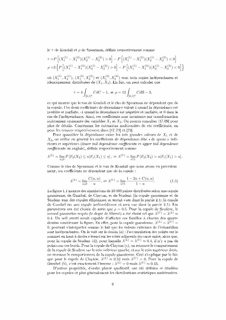
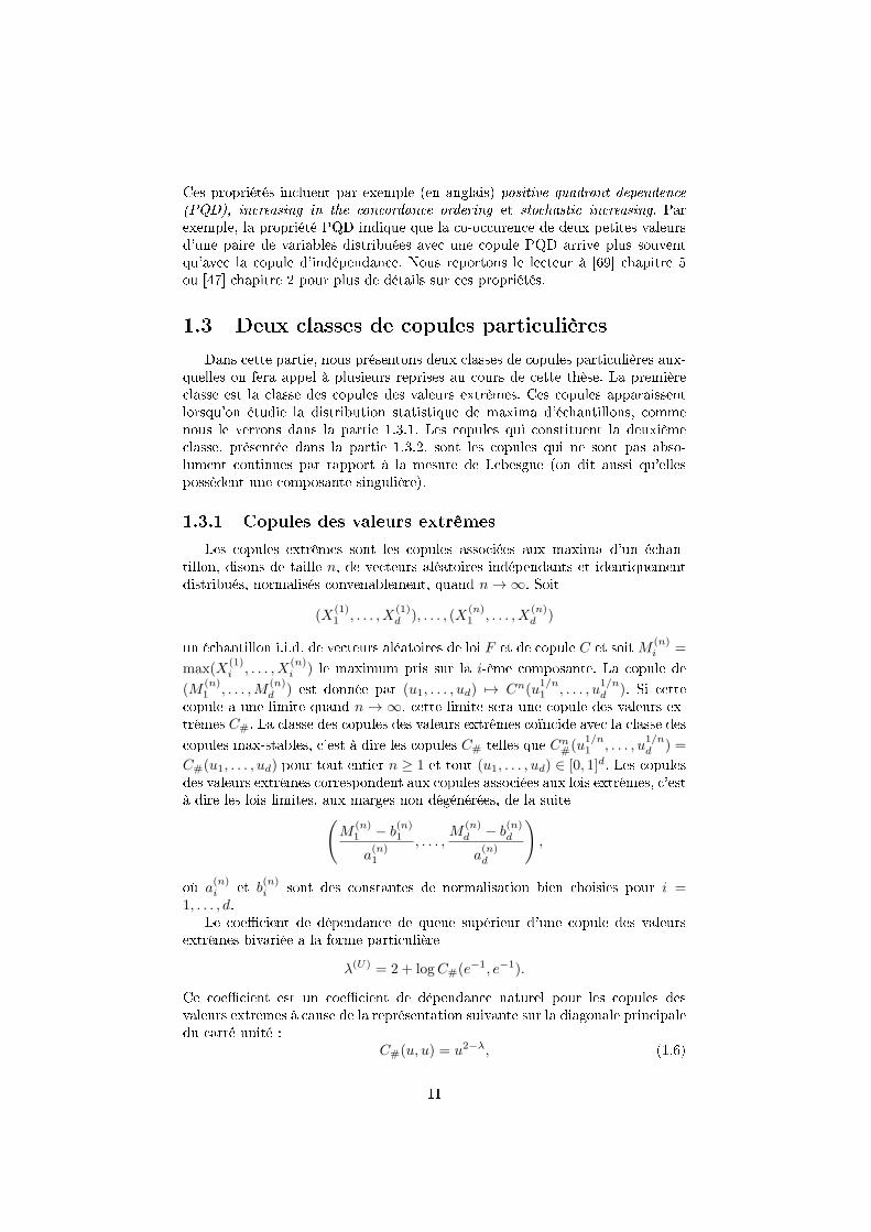
▲❛ ✜❣✉r❡ ✶✳✶ ♠♦♥tr❡ ❞❡s s✐♠✉❧❛t✐♦♥s ❞❡ ✶✵ ✵✵✵ ♣❛✐r❡s ❞✐str✐❜✉é❡s s❡❧♦♥ ✉♥❡ ❝♦♣✉❧❡❣❛✉ss✐❡♥♥❡✱ ❞❡ ●✉♠❜❡❧✱ ❞❡ ❈❧❛②t♦♥✱ ❡t ❞❡ ❙t✉❞❡♥t ✭❧❛ ❝♦♣✉❧❡ ❣❛✉ss✐❡♥♥❡ ❡t ❞❡❙t✉❞❡♥t s♦♥t ❞❡s ❝♦♣✉❧❡s ❡❧❧✐♣t✐q✉❡s✱ ❡t s❡r♦♥t ✈✉❡s ❞❛♥s ❧❛ ♣❛rt✐❡ ✷✳✹ ❀ ❧❛ ❝♦♣✉❧❡❞❡ ●✉♠❜❡❧ ❡st ✉♥❡ ❝♦♣✉❧❡ ❛r❝❤✐♠é❞✐❡♥♥❡ ❡t s❡r❛ ✈✉❡ ❞❛♥s ❧❛ ♣❛rt✐❡ ✷✳✶✮✳ ▲❡s♣❛r❛♠ètr❡s ♦♥t été ❝❤♦✐s✐s ❞❡ s♦rt❡ q✉❡ ρ = 0.5✳ P♦✉r ❧❛ ❝♦♣✉❧❡ ❞❡ ❙t✉❞❡♥t✱ ❧❡s❡❝♦♥❞ ♣❛r❛♠ètr❡ r❡q✉✐s ✭❧❡ ❞❡❣ré ❞❡ ❧✐❜❡rté✮ ❛ été ❝❤♦✐s✐ t❡❧ q✉❡ λ(U) = λ(L) ≈0.4✳ ❯♥ ♦❡✐❧ ❛✈❡rt✐ s❡r❛✐t ❝❛♣❛❜❧❡ ❞✬❛✛❡❝t❡r ❝❡s ❢❛♠✐❧❧❡s à ❝❤❛❝✉♥ ❞❡s q✉❛tr❡❞❡ss✐♥s ❝♦♥st✐t✉❛♥t ❧❛ ✜❣✉r❡✳ ❊♥ ❡✛❡t✱ ♣♦✉r ❧❛ ❝♦♣✉❧❡ ❣❛✉ss✐❡♥♥❡✱ λ(L) = λ(U) =0✱ ♣♦✉✈❛♥t s✬✐♥t❡r♣rét❡r ❝♦♠♠❡ ❧❡ ❢❛✐t q✉❡ ❧❡s ✈❛❧❡✉rs ❡①trê♠❡s ❞❡ ❧✬é❝❤❛♥t✐❧❧♦♥s♦♥t ✐♥❞é♣❡♥❞❛♥t❡s✳ ❖♥ ❧❡ ✈♦✐t s✉r ❧❡ ❞❡ss✐♥ ✭❛✮ ✿ ❧✬❛❝❝✉♠✉❧❛t✐♦♥ ❞❡s ♣♦✐♥ts s✉r ❧❡s♦♠♠❡t ❡♥ ❤❛✉t à ❞r♦✐t❡ s✬ét❡♥❞ s✉r ❧❡s ❝ôtés ❛❞❥❛❝❡♥ts ❞✉ ❝❛rré ✉♥✐té✱ ❛❧♦rs q✉❡✱♣♦✉r ❧❛ ❝♦♣✉❧❡ ❞❡ ❙t✉❞❡♥t ✭❞✮✱ ♣♦✉r ❧❛q✉❡❧❧❡ λ(L) = λ(U) ≈ 0.4✱ ✐❧ ♥✬② ❛ ♣❛s ❞❡♣♦✐♥ts s✉r ❝❡s ❜♦r❞s✳ P♦✉r ❧❛ ❝♦♣✉❧❡ ❞❡ ❈❧❛②t♦♥ ✭❝✮✱ ♦♥ r❡tr♦✉✈❡ ❧❡ ❝♦♠♣♦rt❡♠❡♥t❞❡ ❧❛ ❝♦♣✉❧❡ ❞❡ ❙t✉❞❡♥t s✉r ❧❡ ❝♦✐♥ ✐♥❢ér✐❡✉r ❣❛✉❝❤❡✱ ❡t s✉r ❧❡ ❝♦✐♥ s✉♣ér✐❡✉r ❞r♦✐t✱♦♥ r❡tr♦✉✈❡ ❧❡ ❝♦♠♣♦rt❡♠❡♥t ❞❡ ❧❛ ❝♦♣✉❧❡ ❣❛✉ss✐❡♥♥❡✳ ❈❡❝✐ s✬❡①♣❧✐q✉❡ ♣❛r ❧❡ ❢❛✐tq✉❡ ♣♦✉r ❧❡ ❝♦♣✉❧❡ ❞❡ ❈❧❛②t♦♥✱ λ(L) ≈ 0.52 ♠❛✐s λ(U) = 0✳ P♦✉r ❧❛ ❝♦♣✉❧❡ ❞❡●✉♠❜❡❧ ✭❜✮✱ ❝✬❡st ❡①❛❝t❡♠❡♥t ❧✬✐♥✈❡rs❡ ✿ λ(L) = 0 ♠❛✐s λ(U) ≈ 0.43✳

❉✬❛✉tr❡s ♣r♦♣r✐étés✱ ❞✬♦r❞r❡ ♣❧✉tôt q✉❛❧✐t❛t✐❢✱ ♦♥t été ❞é✜♥✐❡s ❡t ét✉❞✐é❡s♣♦✉r ❧❡s ❝♦♣✉❧❡s ❡t ♣❧✉s ❣é♥ér❛❧❡♠❡♥t ❧❡s ❞✐str✐❜✉t✐♦♥s st❛t✐st✐q✉❡s ♠✉❧t✐✈❛r✐é❡s✳

✾

0.0 0.2 0.4 0.6 0.8 1.0

0.0

0.2

0.4

0.6

0.8

1.0

✭❛✮

0.0 0.2 0.4 0.6 0.8 1.0

0.0

0.2

0.4

0.6

0.8

1.0

✭❜✮

0.0 0.2 0.4 0.6 0.8 1.0

0.0

0.2

0.4

0.6

0.8

1.0

✭❝✮

0.0 0.2 0.4 0.6 0.8 1.0

0.0

0.2

0.4

0.6

0.8

1.0

✭❞✮

❋✐❣✉r❡ ✶✳✶ ✕ ❊❝❤❛♥t✐❧❧♦♥ ❞❡ ✶✵ ✵✵✵ ♣❛✐r❡s ❞✐str✐❜✉é❡s s❡❧♦♥ ❧❛ ❝♦♣✉❧❡ ❣❛✉s✲s✐❡♥♥❡ ✭❛✮✱ ❧❛ ❝♦♣✉❧❡ ❞❡ ●✉♠❜❡❧ ✭❜✮✱ ❧❛ ❝♦♣✉❧❡ ❞❡ ❈❧❛②t♦♥ ✭❝✮✱ ❡t ❧❛ ❝♦♣✉❧❡ ❞❡❙t✉❞❡♥t ✭❞✮✳ ▲❡s ♣❛r❛♠ètr❡s ♦♥t été ❝❤♦✐s✐s t❡❧s q✉❡ ρ = 0.5✱ ❡t λ(U) = λ(L) ≈ 0.4♣♦✉r ❧❛ ❝♦♣✉❧❡ ❞❡ ❙t✉❞❡♥t✳

✶✵

❈❡s ♣r♦♣r✐étés ✐♥❝❧✉❡♥t ♣❛r ❡①❡♠♣❧❡ ✭❡♥ ❛♥❣❧❛✐s✮ ♣♦s✐t✐✈❡ q✉❛❞r❛♥t ❞❡♣❡♥❞❡♥❝❡✭P◗❉✮✱ ✐♥❝r❡❛s✐♥❣ ✐♥ t❤❡ ❝♦♥❝♦r❞❛♥❝❡ ♦r❞❡r✐♥❣ ❡t st♦❝❤❛st✐❝ ✐♥❝r❡❛s✐♥❣✳ P❛r❡①❡♠♣❧❡✱ ❧❛ ♣r♦♣r✐été P◗❉ ✐♥❞✐q✉❡ q✉❡ ❧❛ ❝♦✲♦❝❝✉r❡♥❝❡ ❞❡ ❞❡✉① ♣❡t✐t❡s ✈❛❧❡✉rs❞✬✉♥❡ ♣❛✐r❡ ❞❡ ✈❛r✐❛❜❧❡s ❞✐str✐❜✉é❡s ❛✈❡❝ ✉♥❡ ❝♦♣✉❧❡ P◗❉ ❛rr✐✈❡ ♣❧✉s s♦✉✈❡♥tq✉✬❛✈❡❝ ❧❛ ❝♦♣✉❧❡ ❞✬✐♥❞é♣❡♥❞❛♥❝❡✳ ◆♦✉s r❡♣♦rt♦♥s ❧❡ ❧❡❝t❡✉r à ❬✻✾❪ ❝❤❛♣✐tr❡ ✺♦✉ ❬✹✼❪ ❝❤❛♣✐tr❡ ✷ ♣♦✉r ♣❧✉s ❞❡ ❞ét❛✐❧s s✉r ❝❡s ♣r♦♣r✐étés✳

✶✳✸ ❉❡✉① ❝❧❛ss❡s ❞❡ ❝♦♣✉❧❡s ♣❛rt✐❝✉❧✐èr❡s

❉❛♥s ❝❡tt❡ ♣❛rt✐❡✱ ♥♦✉s ♣rés❡♥t♦♥s ❞❡✉① ❝❧❛ss❡s ❞❡ ❝♦♣✉❧❡s ♣❛rt✐❝✉❧✐èr❡s ❛✉①✲q✉❡❧❧❡s ♦♥ ❢❡r❛ ❛♣♣❡❧ à ♣❧✉s✐❡✉rs r❡♣r✐s❡s ❛✉ ❝♦✉rs ❞❡ ❝❡tt❡ t❤ès❡✳ ▲❛ ♣r❡♠✐èr❡❝❧❛ss❡ ❡st ❧❛ ❝❧❛ss❡ ❞❡s ❝♦♣✉❧❡s ❞❡s ✈❛❧❡✉rs ❡①trê♠❡s✳ ❈❡s ❝♦♣✉❧❡s ❛♣♣❛r❛✐ss❡♥t❧♦rsq✉✬♦♥ ét✉❞✐❡ ❧❛ ❞✐str✐❜✉t✐♦♥ st❛t✐st✐q✉❡ ❞❡ ♠❛①✐♠❛ ❞✬é❝❤❛♥t✐❧❧♦♥s✱ ❝♦♠♠❡♥♦✉s ❧❡ ✈❡rr♦♥s ❞❛♥s ❧❛ ♣❛rt✐❡ ✶✳✸✳✶✳ ▲❡s ❝♦♣✉❧❡s q✉✐ ❝♦♥st✐t✉❡♥t ❧❛ ❞❡✉①✐è♠❡❝❧❛ss❡✱ ♣rés❡♥té❡ ❞❛♥s ❧❛ ♣❛rt✐❡ ✶✳✸✳✷✱ s♦♥t ❧❡s ❝♦♣✉❧❡s q✉✐ ♥❡ s♦♥t ♣❛s ❛❜s♦✲❧✉♠❡♥t ❝♦♥t✐♥✉❡s ♣❛r r❛♣♣♦rt à ❧❛ ♠❡s✉r❡ ❞❡ ▲❡❜❡s❣✉❡ ✭♦♥ ❞✐t ❛✉ss✐ q✉✬❡❧❧❡s♣♦ssè❞❡♥t ✉♥❡ ❝♦♠♣♦s❛♥t❡ s✐♥❣✉❧✐èr❡✮✳

✶✳✸✳✶ ❈♦♣✉❧❡s ❞❡s ✈❛❧❡✉rs ❡①trê♠❡s

▲❡s ❝♦♣✉❧❡s ❡①trê♠❡s s♦♥t ❧❡s ❝♦♣✉❧❡s ❛ss♦❝✐é❡s ❛✉① ♠❛①✐♠❛ ❞✬✉♥ é❝❤❛♥✲t✐❧❧♦♥✱ ❞✐s♦♥s ❞❡ t❛✐❧❧❡ n✱ ❞❡ ✈❡❝t❡✉rs ❛❧é❛t♦✐r❡s ✐♥❞é♣❡♥❞❛♥ts ❡t ✐❞❡♥t✐q✉❡♠❡♥t❞✐str✐❜✉és✱ ♥♦r♠❛❧✐sés ❝♦♥✈❡♥❛❜❧❡♠❡♥t✱ q✉❛♥❞ n→ ∞✳ ❙♦✐t

(X(1)1 , . . . , X

(1)d ), . . . , (X

(n)1 , . . . , X

(n)d )

✉♥ é❝❤❛♥t✐❧❧♦♥ ✐✳✐✳❞✳ ❞❡ ✈❡❝t❡✉rs ❛❧é❛t♦✐r❡s ❞❡ ❧♦✐ F ❡t ❞❡ ❝♦♣✉❧❡ C ❡t s♦✐tM (n)i =

max(X(1)i , . . . , X

(n)i ) ❧❡ ♠❛①✐♠✉♠ ♣r✐s s✉r ❧❛ i✲è♠❡ ❝♦♠♣♦s❛♥t❡✳ ▲❛ ❝♦♣✉❧❡ ❞❡

(M(n)1 , . . . ,M

(n)d ) ❡st ❞♦♥♥é❡ ♣❛r (u1, . . . , ud) 7→ Cn(u

1/n1 , . . . , u

1/nd )✳ ❙✐ ❝❡tt❡

❝♦♣✉❧❡ ❛ ✉♥❡ ❧✐♠✐t❡ q✉❛♥❞ n → ∞✱ ❝❡tt❡ ❧✐♠✐t❡ s❡r❛ ✉♥❡ ❝♦♣✉❧❡ ❞❡s ✈❛❧❡✉rs ❡①✲trê♠❡s C#✳ ▲❛ ❝❧❛ss❡ ❞❡s ❝♦♣✉❧❡s ❞❡s ✈❛❧❡✉rs ❡①trê♠❡s ❝♦ï♥❝✐❞❡ ❛✈❡❝ ❧❛ ❝❧❛ss❡ ❞❡s

❝♦♣✉❧❡s ♠❛①✲st❛❜❧❡s✱ ❝✬❡st à ❞✐r❡ ❧❡s ❝♦♣✉❧❡s C# t❡❧❧❡s q✉❡ Cn#(u1/n1 , . . . , u

1/nd ) =

C#(u1, . . . , ud) ♣♦✉r t♦✉t ❡♥t✐❡r n ≥ 1 ❡t t♦✉t (u1, . . . , ud) ∈ [0, 1]d✳ ▲❡s ❝♦♣✉❧❡s❞❡s ✈❛❧❡✉rs ❡①trê♠❡s ❝♦rr❡s♣♦♥❞❡♥t ❛✉① ❝♦♣✉❧❡s ❛ss♦❝✐é❡s ❛✉① ❧♦✐s ❡①trê♠❡s✱ ❝✬❡stà ❞✐r❡ ❧❡s ❧♦✐s ❧✐♠✐t❡s✱ ❛✉① ♠❛r❣❡s ♥♦♥ ❞é❣é♥éré❡s✱ ❞❡ ❧❛ s✉✐t❡

(M

(n)1 − b

(n)1

a(n)1

, . . . ,M

(n)d − b

(n)d

a(n)d

),

♦ù a(n)i ❡t b(n)i s♦♥t ❞❡s ❝♦♥st❛♥t❡s ❞❡ ♥♦r♠❛❧✐s❛t✐♦♥ ❜✐❡♥ ❝❤♦✐s✐❡s ♣♦✉r i =

1, . . . , d✳▲❡ ❝♦❡✣❝✐❡♥t ❞❡ ❞é♣❡♥❞❛♥❝❡ ❞❡ q✉❡✉❡ s✉♣ér✐❡✉r ❞✬✉♥❡ ❝♦♣✉❧❡ ❞❡s ✈❛❧❡✉rs

❡①trê♠❡s ❜✐✈❛r✐é❡ ❛ ❧❛ ❢♦r♠❡ ♣❛rt✐❝✉❧✐èr❡

λ(U) = 2 + logC#(e−1, e−1).

❈❡ ❝♦❡✣❝✐❡♥t ❡st ✉♥ ❝♦❡✣❝✐❡♥t ❞❡ ❞é♣❡♥❞❛♥❝❡ ♥❛t✉r❡❧ ♣♦✉r ❧❡s ❝♦♣✉❧❡s ❞❡s✈❛❧❡✉rs ❡①trê♠❡s à ❝❛✉s❡ ❞❡ ❧❛ r❡♣rés❡♥t❛t✐♦♥ s✉✐✈❛♥t❡ s✉r ❧❛ ❞✐❛❣♦♥❛❧❡ ♣r✐♥❝✐♣❛❧❡❞✉ ❝❛rré ✉♥✐té ✿

C#(u, u) = u2−λ, ✭✶✳✻✮

✶✶

0.0 0.2 0.4 0.6 0.8 1.0

0.0

0.2

0.4

0.6

0.8

1.0

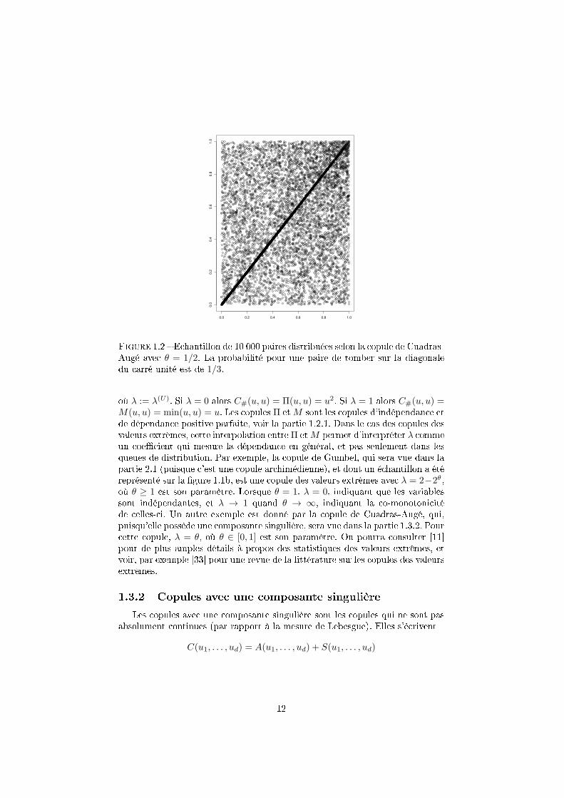
❋✐❣✉r❡ ✶✳✷ ✕ ❊❝❤❛♥t✐❧❧♦♥ ❞❡ ✶✵ ✵✵✵ ♣❛✐r❡s ❞✐str✐❜✉é❡s s❡❧♦♥ ❧❛ ❝♦♣✉❧❡ ❞❡ ❈✉❛❞r❛s✲❆✉❣é ❛✈❡❝ θ = 1/2✳ ▲❛ ♣r♦❜❛❜✐❧✐té ♣♦✉r ✉♥❡ ♣❛✐r❡ ❞❡ t♦♠❜❡r s✉r ❧❛ ❞✐❛❣♦♥❛❧❡❞✉ ❝❛rré ✉♥✐té ❡st ❞❡ 1/3✳

♦ù λ := λ(U)✳ ❙✐ λ = 0 ❛❧♦rs C#(u, u) = Π(u, u) = u2✳ ❙✐ λ = 1 ❛❧♦rs C#(u, u) =M(u, u) = min(u, u) = u✳ ▲❡s ❝♦♣✉❧❡s Π ❡tM s♦♥t ❧❡s ❝♦♣✉❧❡s ❞✬✐♥❞é♣❡♥❞❛♥❝❡ ❡t❞❡ ❞é♣❡♥❞❛♥❝❡ ♣♦s✐t✐✈❡ ♣❛r❢❛✐t❡✱ ✈♦✐r ❧❛ ♣❛rt✐❡ ✶✳✷✳✶✳ ❉❛♥s ❧❡ ❝❛s ❞❡s ❝♦♣✉❧❡s ❞❡s✈❛❧❡✉rs ❡①trê♠❡s✱ ❝❡tt❡ ✐♥t❡r♣♦❧❛t✐♦♥ ❡♥tr❡ Π ❡tM ♣❡r♠❡t ❞✬✐♥t❡r♣rét❡r λ ❝♦♠♠❡✉♥ ❝♦❡✣❝✐❡♥t q✉✐ ♠❡s✉r❡ ❧❛ ❞é♣❡♥❞❛♥❝❡ ❡♥ ❣é♥ér❛❧✱ ❡t ♣❛s s❡✉❧❡♠❡♥t ❞❛♥s ❧❡sq✉❡✉❡s ❞❡ ❞✐str✐❜✉t✐♦♥✳ P❛r ❡①❡♠♣❧❡✱ ❧❛ ❝♦♣✉❧❡ ❞❡ ●✉♠❜❡❧✱ q✉✐ s❡r❛ ✈✉❡ ❞❛♥s ❧❛♣❛rt✐❡ ✷✳✶ ✭♣✉✐sq✉❡ ❝✬❡st ✉♥❡ ❝♦♣✉❧❡ ❛r❝❤✐♠é❞✐❡♥♥❡✮✱ ❡t ❞♦♥t ✉♥ é❝❤❛♥t✐❧❧♦♥ ❛ étér❡♣rés❡♥té s✉r ❧❛ ✜❣✉r❡ ✶✳✶❜✱ ❡st ✉♥❡ ❝♦♣✉❧❡ ❞❡s ✈❛❧❡✉rs ❡①trê♠❡s ❛✈❡❝ λ = 2−2θ✱♦ù θ ≥ 1 ❡st s♦♥ ♣❛r❛♠ètr❡✳ ▲♦rsq✉❡ θ = 1✱ λ = 0✱ ✐♥❞✐q✉❛♥t q✉❡ ❧❡s ✈❛r✐❛❜❧❡ss♦♥t ✐♥❞é♣❡♥❞❛♥t❡s✱ ❡t λ → 1 q✉❛♥❞ θ → ∞✱ ✐♥❞✐q✉❛♥t ❧❛ ❝♦✲♠♦♥♦t♦♥✐❝✐té❞❡ ❝❡❧❧❡s✲❝✐✳ ❯♥ ❛✉tr❡ ❡①❡♠♣❧❡ ❡st ❞♦♥♥é ♣❛r ❧❛ ❝♦♣✉❧❡ ❞❡ ❈✉❛❞r❛s✲❆✉❣é✱ q✉✐✱♣✉✐sq✉✬❡❧❧❡ ♣♦ssè❞❡ ✉♥❡ ❝♦♠♣♦s❛♥t❡ s✐♥❣✉❧✐èr❡✱ s❡r❛ ✈✉❡ ❞❛♥s ❧❛ ♣❛rt✐❡ ✶✳✸✳✷✳ P♦✉r❝❡tt❡ ❝♦♣✉❧❡✱ λ = θ✱ ♦ù θ ∈ [0, 1] ❡st s♦♥ ♣❛r❛♠ètr❡✳ ❖♥ ♣♦✉rr❛ ❝♦♥s✉❧t❡r ❬✶✶❪♣♦✉r ❞❡ ♣❧✉s ❛♠♣❧❡s ❞ét❛✐❧s à ♣r♦♣♦s ❞❡s st❛t✐st✐q✉❡s ❞❡s ✈❛❧❡✉rs ❡①trê♠❡s✱ ❡t✈♦✐r✱ ♣❛r ❡①❡♠♣❧❡ ❬✸✸❪ ♣♦✉r ✉♥❡ r❡✈✉❡ ❞❡ ❧❛ ❧✐ttér❛t✉r❡ s✉r ❧❡s ❝♦♣✉❧❡s ❞❡s ✈❛❧❡✉rs❡①trê♠❡s✳

✶✳✸✳✷ ❈♦♣✉❧❡s ❛✈❡❝ ✉♥❡ ❝♦♠♣♦s❛♥t❡ s✐♥❣✉❧✐èr❡

▲❡s ❝♦♣✉❧❡s ❛✈❡❝ ✉♥❡ ❝♦♠♣♦s❛♥t❡ s✐♥❣✉❧✐èr❡ s♦♥t ❧❡s ❝♦♣✉❧❡s q✉✐ ♥❡ s♦♥t ♣❛s❛❜s♦❧✉♠❡♥t ❝♦♥t✐♥✉❡s ✭♣❛r r❛♣♣♦rt à ❧❛ ♠❡s✉r❡ ❞❡ ▲❡❜❡s❣✉❡✮✳ ❊❧❧❡s s✬é❝r✐✈❡♥t

C(u1, . . . , ud) = A(u1, . . . , ud) + S(u1, . . . , ud)

✶✷

❛✈❡❝

A(u1, . . . , ud) =

∫

[0,u1]×···×[0,ud]

∂dC(x1, . . . , xd)

∂x1 . . . ∂xd1{∂dC(x1, . . . , xd)

∂x1 . . . ∂xd❡①✐st❡

}dx1 . . . dxd

ét❛♥t ❧❛ ♣❛rt✐❡ ❛❜s♦❧✉♠❡♥t ❝♦♥t✐♥✉❡ ❡t S = C − A ❧❛ ❝♦♠♣♦s❛♥t❡ s✐♥❣✉❧✐èr❡ ❞❡❧❛ ❝♦♣✉❧❡✳

▲❛ ❧♦✐ ❛✈❡❝ ✉♥❡ ❝♦♠♣♦s❛♥t❡ s✐♥❣✉❧✐èr❡ ❧❛ ♣❧✉s ❝♦♥♥✉❡ ❡st s❛♥s ❞♦✉t❡ ❧❛ ❧♦✐❞❡ ▼❛rs❤❛❧❧✲❖❧❦✐♥ ❬✻✹❪✱ ✈♦✐r ❛✉ss✐ ❬✻✾❪ s❡❝t✐♦♥ ✸✳✶✳✶✱ ❞♦♥t ❧❛ ❝♦♣✉❧❡ ❞❡ s✉r✈✐❡ ❡st❞♦♥♥é❡ ♣❛r

Cθ(u1, . . . , ud) =P [F1(X1) > u1, . . . , Fd(Xd) > ud]

=(1− u1)θ1 . . . (1− ud)

θd min(u1−θ11 , . . . , u1−θdd ),

♦ù θ = (θ1, . . . , θd) ∈ [0, 1]d✳ ▲❛ ❝♦♣✉❧❡ ❞❡ ▼❛rs❤❛❧❧✲❖❧❦✐♥ ❡st✱ ❡♥ ♣r✐♥❝✐♣❡ ✹✱✐♥tér❡ss❛♥t❡ ♣♦✉r ♠♦❞é❧✐s❡r ❞❡s s②stè♠❡s q✉✐ ♣rés❡♥t❡♥t ❞❡s ✓ ❝❤♦❝s ✔✳ P❧✉s ♣ré✲❝✐sé♠❡♥t✱ s♦✐❡♥t Z1, . . . , Zd ❡t Z0 ❞❡s ✈❛r✐❛❜❧❡s ❛❧é❛t♦✐r❡s ✐♥❞é♣❡♥❞❛♥t❡s ❞❡ ❧♦✐s❡①♣♦♥❡♥t✐❡❧❧❡s q✉✐ r❡♣rés❡♥t❡♥t ❧❡s ✐♥st❛♥ts ♦ù ❧❡s ❝❤♦❝s ❛rr✐✈❡♥t ❞❛♥s ❧❡ s②stè♠❡✱❝❛✉s❛♥t ❞❡s ❞♦♠♠❛❣❡s à s❡s ❝♦♠♣♦s❛♥ts✳ ▲❡s ✈❛r✐❛❜❧❡s Z1, . . . , Zd r❡♣rés❡♥t❡♥t❞❡s ❝❤♦❝s ❡♥❞♦❣è♥❡s q✉✐ ♥✬❛✛❡❝t❡♥t q✉❡ ❧❡s ❝♦♠♣♦s❛♥ts 1, . . . , d r❡s♣❡❝t✐✈❡♠❡♥t✱❡t Z0 r❡♣rés❡♥t❡ ✉♥ ❝❤♦❝ ❡①♦❣è♥❡ q✉✐ ❛✛❡❝t❡ t♦✉t ❧❡ s②stè♠❡ (1, . . . , d)✳ ❙♦✐❡♥tX1 = min(Z1, Z0), . . . , Xd = min(Zd, Z0) ❧❡s ✐♥st❛♥ts ♦ù ❧❡s ❝♦♠♣♦s❛♥ts 1, . . . , ds✉❜✐ss❡♥t ✉♥ ❝❤♦❝✱ q✉✐ ❧❡✉r ❡st ❢❛t❛❧✳ ❖♥ ♣❡✉t ❛❧♦rs ♠♦♥tr❡r q✉❡ ❧❛ ❝♦♣✉❧❡ ❞❡s✉r✈✐❡ ❛ss♦❝✐é❡ à (X1, . . . , Xd) ❡st ❧❛ ❝♦♣✉❧❡ ❞❡ s✉r✈✐❡ ❞❡ ▼❛rs❤❛❧❧✲❖❧❦✐♥✱ ♦ù❧❡s ♣❛r❛♠ètr❡s s♦♥t ❞ét❡r♠✐♥és ♣❛r ❧❡s ♣❛r❛♠ètr❡s ❞❡s ❧♦✐s ❡①♣♦♥❡♥t✐❡❧❧❡s ❞❡Z1, . . . , Zd ❡t Z0✳ ❉❛♥s ❧❡ ❝❛s ❜✐✈❛r✐é✱ ❧❛ ❝♦♣✉❧❡ ❞❡ ▼❛rs❤❛❧❧✲❖❧❦✐♥ ❡st ❞♦♥♥é❡♣❛r

C(θ1,θ2)(u1, u2) = min(u1−θ11 u2, u1u1−θ22 ) =

{u1−θ11 u2 s✐ uθ11 ≥ uθ22 ,

u1u1−θ22 s✐ uθ11 ≤ uθ22 ,

♣♦✉r 0 ≤ θ1, θ2 ≤ 1✳ P♦✉r ❝❡tt❡ ❝♦♣✉❧❡✱ ♦♥ ♣❡✉t ✈♦✐r ❢❛❝✐❧❡♠❡♥t q✉❡ ♠ê♠❡ ❧❡s❞ér✐✈é❡s ♣❛rt✐❡❧❧❡s ❞❡ C(θ1,θ2) ♥✬❡①✐st❡♥t ♣❛s s✉r ❧❛ ❞✐❛❣♦♥❛❧❡ ♣r✐♥❝✐♣❛❧❡ ❞✉ ❝❛rré✉♥✐té✳ ▲❛ ❝♦♠♣♦s❛♥t❡ s✐♥❣✉❧✐èr❡ ❡st ❞♦♥♥é❡ ♣❛r

S(u1, u2) =

∫ min(uθ11 ,u

θ22 )

0

t1/θ1+1/θ2−2dt.

❊♥ ♣❛rt✐❝✉❧✐❡r✱ ♦♥ ❛ q✉❡ P [Uθ11 = Uθ22 ] = θ1θ2/(θ1 + θ2 − θ1θ2)✳ ❉❛♥s ❧❡ ❝❛s♦ù θ1 = θ2 ≡ θ✱ ❧❛ ❝♦♣✉❧❡ ❞❡ ▼❛rs❤❛❧❧✲❖❧❦✐♥ s❡ ré❞✉✐t à ❧❛ ❝♦♣✉❧❡ ❞❡ ❈✉❛❞r❛s✲❆✉❣é ❬✶✷❪✱ ❞♦♥♥é❡ ♣❛r

Cθ(u1, u2) = min(u1, u2)max(u1, u2)1−θ ✭✶✳✼✮

✭❝❡tt❡ ❝♦♣✉❧❡ ♣❡✉t ❛✉ss✐ êtr❡ ✈✉❡ ❝♦♠♠❡ ✉♥ ❝❛s ♣❛rt✐❝✉❧✐❡r ❞❡ ❬✸❪✮✳ ❙✉r ❧❛ ✜✲❣✉r❡ ✶✳✷✱ ♦ù ✉♥ é❝❤❛♥t✐❧❧♦♥ ❞❡ t❛✐❧❧❡ ✶✵ ✵✵✵ ❡st r❡♣rés❡♥té✱ ♦♥ ✈♦✐t ❜✐❡♥ ❧❛ ❝♦♠✲♣♦s❛♥t❡ s✐♥❣✉❧✐èr❡ s✉r ❧❛ ❞✐❛❣♦♥❛❧❡ ♣r✐♥❝✐♣❛❧❡ ❞✉ ❝❛rré ✉♥✐té✳ ▲❡s ❝❤♦❝s s❡r❛✐❡♥t

✹✳ ▼❛❧❣ré ❧✬❛ttr❛✐t ❞❡ ❝❡tt❡ ✐♥t❡r♣rét❛t✐♦♥ ❡♥ t❡r♠❡s ❞❡ ❝❤♦❝s✱ ❧✬✐♥térêt ❞❡ ❧❛ ❝♦♣✉❧❡ ❞❡▼❛rs❤❛❧❧✲❖❧❦✐♥ r❡st❡ s✉rt♦✉t t❤é♦r✐q✉❡✳ ❊♥ ❡✛❡t✱ ✐❧ ❡st ❞✐✣❝✐❧❡ ❞❡ tr♦✉✈❡r ❞❡s ♣✉❜❧✐❝❛t✐♦♥s♣rés❡♥t❛♥t ❞❡s ❛♣♣❧✐❝❛t✐♦♥s ❛✈❡❝ ❞❡s ❥❡✉① ❞❡ ❞♦♥♥é❡s ré❡❧❧❡s ❧♦rsq✉❡ ❧✬♦♥ ❡✛❡❝t✉❡ ❞❡s r❡q✉êt❡s♣❛r ♠♦ts ❝❧és ❞❛♥s ❧❡s ♠♦t❡✉rs ❞❡ r❡❝❤❡r❝❤❡✳ ▲❛ s❡✉❧❡ ❛♣♣❧✐❝❛t✐♦♥ q✉❡ ♥♦✉s ❛②♦♥s tr♦✉✈é❡ ❬✺✻❪❡st ♣❧✉tôt ❞é❝❡✈❛♥t❡ ✿ ❡❧❧❡ ❝♦♥s✐st❛✐t ❡♥ ❧✬❛♥❛❧②s❡ ❞❡ ✸✼ ♠❛t❝❤s ❞❡ ❢♦♦t ❀ ❞✬❛✐❧❧❡✉rs✱ ❧❡s ❛✉t❡✉rs❡✉① ♠ê♠❡s ❛❞♠❡tt❡♥t q✉❡ ❧✬❛♣♣❧✐❝❛t✐♦♥ ét❛✐t ♣rés❡♥té❡ ✉♥✐q✉❡♠❡♥t ♣♦✉r ✓ ✐❧❧✉str❡r ✔ ❧❡✉r♠ét❤♦❞❡ ❞✬❡st✐♠❛t✐♦♥✳

✶✸

❧❡s ♣♦✐♥ts ❞❡ ❧❛ ❞✐❛❣♦♥❛❧❡ ♣r✐♥❝✐♣❛❧❡✳ ▲❛ ré❢ér❡♥❝❡ ♦r✐❣✐♥❛❧❡ ❞❛♥s ❧❡q✉❡❧ ✜❣✉r❡ ❝❡♠♦❞è❧❡ ❡♥ t❡r♠❡s ❞❡ ❧♦✐s ❡①♣♦♥❡♥t✐❡❧❧❡s ❡st ❬✻✹❪✳

❯♥❡ ❛✉tr❡ ❝❧❛ss❡ ❞❡ ❝♦♣✉❧❡s ❛✈❡❝ ❝♦♠♣♦s❛♥t❡s s✐♥❣✉❧✐èr❡s✱ ❡t q✉✐ ♣❡✉✈❡♥t❛✉ss✐ êtr❡ ✐♥t❡r♣rété❡s ❝♦♠♠❡ ❞❡s ♠♦❞è❧❡s ❛✈❡❝ ❞❡s ❝❤♦❝s✱ ❡st ❞♦♥♥é❡ ❝✐✲❛♣rès✳▲❛ ❝❧❛ss❡ ❞❡s ❝♦♣✉❧❡s ❞❡ ✓ ❉✉r❛♥t❡ ✔ ❬✶✼✱✶✾❪ ❝♦♥s✐st❡ ❡♥ ❧❡s ❝♦♣✉❧❡s ❞❡ ❧❛ ❢♦r♠❡

C(u1, . . . , ud) = min(u1, . . . , ud)f(max(u1, . . . , ud)), ✭✶✳✽✮

♦ù f : [0, 1] → [0, 1]✱ ❛♣♣❡❧é ❧❡ ❣é♥ér❛t❡✉r ❞❡ C✱ ❡st ✉♥❡ ❢♦♥❝t✐♦♥ ❞ér✐✈❛❜❧❡ ❡tstr✐❝t❡♠❡♥t ❝r♦✐ss❛♥t❡ t❡❧❧❡ q✉❡ f(1) = 1 ❡t t 7→ f(t)/t ❡st str✐❝t❡♠❡♥t ❞é❝r♦✐s✲s❛♥t❡✳ ▲✬✐♥t❡r♣rét❛t✐♦♥ ❡♥ t❡r♠❡s ❞❡ ❝❤♦❝s s✬♦❜t✐❡♥t ❡♥ r❡♠❛rq✉❛♥t q✉❡ ✭✶✳✽✮❡st ❧❛ ❧♦✐ ❞❡ (U1, . . . , Ud)✱ ❛✈❡❝ Ui = max(Zi, Z0), i = 1, . . . , d ❀ Z1, . . . , Zd s♦♥t❞❡s ✈❛r✐❛❜❧❡s ✐♥❞é♣❡♥❞❛♥t❡s ❞✐str✐❜✉é❡s s❡❧♦♥ ✉♥❡ ♠ê♠❡ ❧♦✐ f ✱ ❡t Z0 ❡st ✉♥❡✈❛r✐❛❜❧❡ ✐♥❞é♣❡♥❞❛♥t❡ ❞❡ (Z1, . . . , Zd) ❞✐str✐❜✉é❡ s❡❧♦♥ t 7→ t/f(t)✳ ❉❛♥s ❧❡ ❝❛s♠✉❧t✐✈❛r✐é✱ ♣✉✐sq✉✬✐❧ ♥✬② ❛ q✉✬✉♥ s❡✉❧ ❣é♥ér❛t❡✉r ♣♦✉r ❞ét❡r♠✐♥❡r ❧❛ str✉❝t✉r❡❞❡ ❞é♣❡♥❞❛♥❝❡✱ ❝❡tt❡ ❝❧❛ss❡ ♥✬❡st ♣❛s très ✉t✐❧❡ ♣♦✉r ❧❡s ❛♣♣❧✐❝❛t✐♦♥s✳ ❉❛♥s ❧❡❝❛s ❜✐✈❛r✐é✱ ❡♥ r❡✈❛♥❝❤❡✱ ❧❛ ❝❧❛ss❡ ❞❡ ❝♦♣✉❧❡s ❞❡ ❉✉r❛♥t❡ ❡st ✢❡①✐❜❧❡ ❡t ♠❛✲♥✐❛❜❧❡ ✭✈♦✐r ❧❡ ❝❤❛♣✐tr❡ ✻✮✳ ❖♥ ♣❡✉t é❣❛❧❡♠❡♥t ♦❜t❡♥✐r ❞❡s ❝♦♣✉❧❡s ❜✐❡♥ ❝♦♥♥✉❡s❝♦♠♠❡ ❝❛s ♣❛rt✐❝✉❧✐❡rs✳ ❆✐♥s✐✱ s✐ f(t) = t1−θ, θ ∈ [0, 1]✱ ♦♥ ♦❜t✐❡♥t ❧❛ ❢❛♠✐❧❧❡ ❞❡❈✉❛❞r❛s✲❆✉❣é ✭✶✳✼✮✱ ❡t s✐ f(t) = (1− θ)t+ θ, θ ∈ [0, 1]✱ ♦♥ ♦❜t✐❡♥t ❧❛ ❢❛♠✐❧❧❡ ❞❡❋ré❝❤❡t ❬✷✹❪✱ ❞♦♥♥é❡ ♣❛r

Cθ(u1, u2) = (1− θ)Π(u1, u2) + θM(u1, u2),

❡t q✉✐ ❡st ❧❛ ♠♦②❡♥♥❡ ❛r✐t❤♠ét✐q✉❡ ❡♥tr❡ ❧❛ ❝♦♣✉❧❡ ❞✬✐♥❞é♣❡♥❞❛♥❝❡ Π ❡t ❧❛ ❝♦♣✉❧❡❞❡ ❧❛ ❞é♣❡♥❞❛♥❝❡ ♣♦s✐t✐✈❡ ♣❛r❢❛✐t❡ M ✳ ▲❛ ❝❧❛ss❡ ❞❡ ❝♦♣✉❧❡s ❜✐✈❛r✐é❡s ❞❡ ❉✉r❛♥t❡s❡r❛ ✉t✐❧✐sé❡ ❞❛♥s ❧❛ ❝♦♥str✉❝t✐♦♥ ❞✉ ♠♦❞è❧❡ q✉❡ ♥♦✉s ♣r♦♣♦s♦♥s ❛✉ ❝❤❛♣✐tr❡ ✻✳❊♥ ♣❛rt✐❝✉❧✐❡r✱ ❞❛♥s ❝❡ ❝❤❛♣✐tr❡✱ ♥♦✉s ❝♦♥str✉✐s♦♥s ❞❡s ❝♦♣✉❧❡s ♠✉❧t✐✈❛r✐é❡s✱✢❡①✐❜❧❡s ❡t ♠❛♥✐❛❜❧❡s✱ ❞♦♥t ❧❡s ♠❛r❣❡s ❜✐✈❛r✐é❡s ❛♣♣❛rt✐❡♥♥❡♥t à ❝❡tt❡ ❝❧❛ss❡✳ ❖♥♣❡✉t ❞♦♥❝ ✈♦✐r ♥♦tr❡ tr❛✈❛✐❧ ❝♦♠♠❡ ✉♥❡ ❡①t❡♥s✐♦♥ ❛✉ ❝❛s ♠✉❧t✐✈❛r✐é ❞❡ ❧❛ ❝❧❛ss❡❞❡s ❝♦♣✉❧❡s ❜✐✈❛r✐é❡s ❞❡ ❉✉r❛♥t❡ ♣❧✉s ✢❡①✐❜❧❡ ♣♦✉r ❧❡s ❛♣♣❧✐❝❛t✐♦♥s q✉❡ ✭✶✳✽✮✳

❆ ❧❛ ✈✉❡ ❞❡ ❧❛ ✜❣✉r❡ ✶✳✷✱ ✐❧ ♥❡ ✈✐❡♥t ♣❛s à ❧✬❡s♣r✐t q✉❡ ❧✬♦♥ ♣♦✉rr❛✐t ♠♦❞é❧✐✲s❡r ✉♥ ♣❤é♥♦♠è♥❡ ❧✐ss❡✱ ♣rés❡♥t ❞❛♥s ❧❛ ♥❛t✉r❡✱ t❡❧ q✉❡ ♣❛r ❡①❡♠♣❧❡ ❧❡s ❞é❜✐ts❞❡ r✐✈✐èr❡s ♦✉ ❧❛ q✉❛♥t✐té ❞❡ ♣❧✉✐❡ q✉✐ t♦♠❜❡ s✉r ♣❧✉s✐❡✉rs s✐t❡s ré♣❛rt✐s ❞❛♥s❧✬❡s♣❛❝❡✱ ❛✈❡❝ ✉♥ ♠♦❞è❧❡ ♣♦ssé❞❛♥t ✉♥❡ ❝♦♠♣♦s❛♥t❡ s✐♥❣✉❧✐èr❡✳ ❈✬❡st ♣♦✉rt❛♥t❝❡ q✉✬♦♥ ❢❛✐t ❧❡s ❛✉t❡✉rs ❞❛♥s ❬✷✵✱ ✼✼❪✳ ▲❡✉rs rés✉❧t❛ts s✉❣❣èr❡♥t q✉❡ ❝❡rt❛✐♥❡s❝❛r❛❝tér✐st✐q✉❡s ❞✬✐♥térêt ❞❡ ❧❛ ❧♦✐ s♦✉s ❥❛❝❡♥t❡ ♦♥t ♣û êtr❡ ❛♣♣r♦❝❤é❡s ♣❛r ✉♥♠♦❞è❧❡ à ❝❤♦❝s✱ ❛❧♦rs ♠ê♠❡ q✉✬✐❧ ❡st ❝❧❛✐r q✉❡✱ ♣❛r ❡①❡♠♣❧❡✱ ❧❛ ♣r♦❜❛❜✐❧✐té q✉❡❞❡✉① ❞é❜✐ts ❞❛♥s ❞❡✉① r✐✈✐èr❡s ❞✐✛ér❡♥t❡s s♦✐❡♥t ❡①❛❝t❡♠❡♥t é❣❛✉① ❡st ♥✉❧❧❡✳❈❡tt❡ ❛♣♣r♦❝❤❡ ✺✱ q✉✐ s✬✐♥tér❡ss❡ ♠♦✐♥s à ♠♦❞é❧✐s❡r ❧❛ ❞✐str✐❜✉t✐♦♥ s♦✉s ❥❛❝❡♥t❡q✉✬à ❡st✐♠❡r ❝❡rt❛✐♥❡s ❝❛r❛❝tér✐st✐q✉❡s ❞❡ ❝❡❧❧❡✲❝✐✱ ❝♦♠♠❡ ♣❛r ❡①❡♠♣❧❡ ❧❡ ♥✐✈❡❛✉❝r✐t✐q✉❡ ❛ss♦❝✐é à ✉♥❡ é✈è♥❡♠❡♥t ❞❡ ♣❧✉✐❡ ❡①trê♠❡ ✭❝❡s ❞❡r♥✐❡rs s❡r♦♥t ✈✉s ❛✉①❝❤❛♣✐tr❡s ✻ ❡t ✸✮✱ ❜✐❡♥ q✉❡ ❞♦✉t❡✉s❡ ❡♥ ❞✐♠❡♥s✐♦♥ ♣❡t✐t❡✱ ❞❡✈✐❡♥t ✐♥tér❡ss❛♥t❡q✉❛♥❞ ❧❛ ❞✐♠❡♥s✐♦♥ ❛✉❣♠❡♥t❡✳ ❈✬❡st ❛✉ss✐ ❧✬❛♣♣r♦❝❤❡ q✉❡ ♥♦✉s ❛✈♦♥s s✉✐✈✐❡✱❝♦♠♠❡ ♥♦✉s ❧❡ ✈❡rr♦♥s ❛✉ ❝❤❛♣✐tr❡ ✻✳

✺✳ ❈❡tt❡ str❛té❣✐❡ s❡ r❛♣♣r♦❝❤❡ ❞❡ ❧❛ ♠ét❤♦❞❡ ✓ ❜♦ît❡ ♥♦✐r❡ ✔ ✉t✐❧✐sé❡ ❡♥ ♠❛❝❤✐♥❡ ❧❡❛r♥✐♥❣✳▲❡s ❞❡✉① ❛♣♣r♦❝❤❡s✱ ✓ ❜♦ît❡ ♥♦✐r❡ ✔ ❡t ✓ ♠♦❞è❧❡ ✔✱ s♦♥t ❞✐s❝✉té❡s ♣❛r ❡①❡♠♣❧❡ ❞❛♥s ❬✼❪✱ ♦ù❧✬❛✉t❡✉r s❡ ❢❛✐t ♣❛r ❛✐❧❧❡✉rs ❧✬❛✈♦❝❛t ❞❡ ❧❛ ♣r❡♠✐èr❡✳

✶✹

❈❤❛♣✐tr❡ ✷

▼♦❞è❧❡s ❞❡ ❝♦♣✉❧❡s ❡♥ ❣r❛♥❞❡

❞✐♠❡♥s✐♦♥

▲❡s ❝♦♣✉❧❡s ❡♥ ❣r❛♥❞❡ ❞✐♠❡♥s✐♦♥✱ ♦✉ s✐♠♣❧❡♠❡♥t ♠✉❧t✐✈❛r✐é❡s✱ s♦♥t ♣❧✉s ❞✐❢✲✜❝✐❧❡s à ❝♦♥str✉✐r❡ q✉❡ ❧❡s ❝♦♣✉❧❡s ❜✐✈❛r✐é❡s✳ ❆ ❝❛✉s❡ ❞❡ ❝❡❧❛✱ ❧❡ t❡r♠❡ ♠✉❧t✐✈❛r✐és❡ ré❢èr❡ s♦✉✈❡♥t ❛✉ ❝❛s ♦ù ❧❡ ♥♦♠❜r❡ ❞❡ ✈❛r✐❛❜❧❡s d ❡st s✉♣ér✐❡✉r à ✷ str✐❝t❡✲♠❡♥t✳ ▲❡ t❡r♠❡ ❣r❛♥❞❡ ❞✐♠❡♥s✐♦♥✱ q✉❛♥❞ à ❧✉✐✱ ❡st très s✉❜❥❡❝t✐❢✳ ▲❛ ✓ ❣r❛♥❞❡❞✐♠❡♥s✐♦♥ ✔✱ t❡❧❧❡ q✉✬❡❧❧❡ ❡st ♣❛r❢♦✐s ❡♥t❡♥❞✉❡ ♣❛r ❧❛ ❝♦♠♠✉♥❛✉té ❞❡s ❝❤❡r❝❤❡✉rs❞❛♥s ❧❡ ❞♦♠❛✐♥❡ ❞❡s ❝♦♣✉❧❡s✱ ♣❡✉t ❝♦♠♠❡♥❝❡r à ♣❛rt✐r ❞❡ d = 3 ✶✳✳✳

❉❛♥s ❝❡ ❝❤❛♣✐tr❡✱ ♥♦✉s ♣rés❡♥t♦♥s ❧❡s ♣r✐♥❝✐♣❛✉① ✷ ♠♦❞è❧❡s ❞❡ ❝♦♣✉❧❡s ❞❡❧❛ ❧✐ttér❛t✉r❡✳ ❊♥ ❣r❛♥❞❡ ❞✐♠❡♥s✐♦♥✱ ✐❧ ② ❛ ♣r✐♥❝✐♣❛❧❡♠❡♥t tr♦✐s ❢❛♠✐❧❧❡s ❞❡ ♠♦✲❞è❧❡s ✿ ❧❡s ❝♦♣✉❧❡s ❛r❝❤✐♠é❞✐❡♥♥❡s ✭♣❛rt✐❡ ✷✳✶✮ ❡t ❧❡✉r ❡①t❡♥s✐♦♥s✱ ❧❡s ❝♦♣✉❧❡s ❛r✲❝❤✐♠é❞✐❡♥♥❡s ✐♠❜r✐q✉é❡s ✭✷✳✷✮✱ ❧❡s ❱✐♥❡s ✭♣❛rt✐❡ ✷✳✸✮✱ ❡t ❧❡s ❝♦♣✉❧❡s ❡❧❧✐♣t✐q✉❡s✭♣❛rt✐❡ ✷✳✹✮✳

✷✳✶ ❈♦♣✉❧❡s ❛r❝❤✐♠é❞✐❡♥♥❡s

❯♥❡ ❝♦♣✉❧❡ ❛r❝❤✐♠é❞✐❡♥♥❡ ❡st ✉♥❡ ❝♦♣✉❧❡ q✉✐ s✬é❝r✐t

C(u1, . . . , ud) = ψ(ψ−1(u1) + · · ·+ ψ−1(ud)) ✭✷✳✶✮

♦ù ψ ❡st ✉♥❡ ❢♦♥❝t✐♦♥ ❞é❝r♦✐ss❛♥t❡ ❡t ❝♦♥t✐♥✉❡ ❞❡ [0,∞) ❞❛♥s [0, 1]✱ str✐❝t❡♠❡♥t❞é❝r♦✐ss❛♥t❡ s✉r [0, inf{x : ψ(x) = 0})✱ ❡t t❡❧❧❡ q✉❡ ψ(0) = 1 ❡t ψ(x) → 0 q✉❛♥❞x → ∞✳ ❊♥ ❢❛✐t✱ ❝❡s ❝♦♥❞✐t✐♦♥s s✉r ψ s♦♥t ♥é❝❡ss❛✐r❡s ♠❛✐s ♣❛s s✉✣s❛♥t❡s✳ ❈❡s❞❡r♥✐èr❡s ♦♥t été ét❛❜❧✐❡s ❞❛♥s ❬✻✼❪✳ ❉❛♥s ❧❡ ❝❛s ♦ù inf{x : ψ(x) = 0} = ∞✱ ✭✷✳✶✮❡st ✉♥❡ ❝♦♣✉❧❡ ❜✐❡♥ ❞é✜♥✐❡ s✐ ❡t s❡✉❧❡♠❡♥t s✐ ψ ❡st ❝♦♠♣❧èt❡♠❡♥t ♠♦♥♦t♦♥❡ ❬✹✾❪✱❝✬❡st à ❞✐r❡ q✉❡ (−1)iψ(i)(s) ≥ 0 ♣♦✉r t♦✉t i ❡t t♦✉t s ≥ 0✱ ♦ù ψ(i) ❡st ❧❛ i✲è♠❡❞ér✐✈é❡ ❞❡ ψ✳ ❉❡ ♣❧✉s✱ ❞❛♥s ❝❡ ❝❛s✱ ♦♥ ♣❡✉t ♠♦♥tr❡r q✉❡ ψ ❡st ✉♥❡ tr❛♥s❢♦r♠é❡ ❞❡

✶✳ ❆ ❧✬❤❡✉r❡ ❞❡s ❜✐❣ ❞❛t❛✱ ♦♥ ♣♦✉rr❛✐t ❛✈♦✐r ❞✉ ♠❛❧ à ❝❛❝❤❡r s❛ ❞é❝❡♣t✐♦♥✳ ❈❡♣❡♥❞❛♥t✱ ✐❧❝♦♥✈✐❡♥t ❞❡ ❣❛r❞❡r à ❧✬❡s♣r✐t q✉❡ ❝❡ ♥❡ s♦♥t ♣❛s ❧❡s ♠ê♠❡s q✉❡st✐♦♥s s❝✐❡♥t✐✜q✉❡s q✉✐ s♦♥t♣♦sé❡s✱ ❡t q✉❡ ❝❡ ♥❡ s♦♥t ♣❛s ♥♦♥ ♣❧✉s ❧❡s ♠ê♠❡s ♠♦❞è❧❡s q✉✐ s♦♥t ✉t✐❧✐sés✳ P❛r ❡①❡♠♣❧❡✱ ❞❛♥s❧❡s ❣❡♥♦♠❡✲✇✐❞❡ ❛ss♦❝✐❛t✐♦♥ st✉❞✐❡s ❡♥ ❜✐♦✐♥❢♦r♠❛t✐q✉❡ ✕ ♦ù ♦♥ ❛♥❛❧②s❡ ♣❧✉s✐❡✉rs ♠✐❧❧✐❡rs ❞❡✈❛r✐❛❜❧❡s ✕✱ ♦♥ s✬❛✉t♦r✐s❡ ❧❡s ♠♦❞è❧❡s ❧✐♥é❛✐r❡s ❣❛✉ss✐❡♥s ♣♦✉r ♠♦❞é❧✐s❡r ❧❡ ❜r✉✐t ❬✹✻❪✳ ❉❛♥s❧❡ ❞♦♠❛✐♥❡ ❞❡s ❝♦♣✉❧❡s✱ ❧✬❛❧é❛ ♥✬❡st ♣❛s ❞✉ ❜r✉✐t✱ ✐❧ ❡st ❝♦♥s✐❞éré ❝♦♠♠❡ ✐♥tr✐♥sèq✉❡✱ ❡t ❧❡s♠♦❞è❧❡s ❧✐♥é❛✐r❡s ❣❛✉ss✐❡♥s ❡♥ s❡r❛✐❡♥t ✉♥❡ tr♦♣ ♠❛✉✈❛✐s❡ ❛♣♣r♦①✐♠❛t✐♦♥✳

✷✳ ❝❡t ❛❞❥❡❝t✐❢ ❝♦♠♣♦rt❡ ✐♥é✈✐t❛❜❧❡♠❡♥t ✉♥❡ ♣❛rt ❞❡ s✉❜❥❡❝t✐✈✐té

✶✺

▲❛♣❧❛❝❡ ❞✬✉♥ ✈❡❝t❡✉r str✐❝t❡♠❡♥t ♣♦s✐t✐❢✳ ❆✉tr❡♠❡♥t ❞✐t✱ ✐❧ ❡①✐st❡ ✉♥❡ ❢♦♥❝t✐♦♥❞❡ ré♣❛rt✐t✐♦♥ H t❡❧❧❡ q✉❡

ψ(s) =

∫ ∞

0

exp(−sy)dH(y), s ≥ 0.

❊♥ ♦✉tr❡✱ ❞❛♥s ❝❡ ❝❛s✱ ✐❧ ❡①✐st❡ ❞❡ ♠❛♥✐èr❡ ✉♥✐q✉❡ d ❢♦♥❝t✐♦♥s ❞❡ ré♣❛rt✐t✐♦♥G1, . . . , Gd t❡❧❧❡s q✉❡

✭✷✳✶✮ =∫ ∞

0

(G1 . . . Gd)αdH(α) = ψ

(−

d∑

i=1

logGi

).

P❛r ❡①❡♠♣❧❡✱ ❧❛ ❝♦♣✉❧❡ ❞❡ ●✉♠❜❡❧ ❬✸✻❪✱ ❞♦♥♥é❡ ♣❛r

C(u1, . . . , ud) = exp{−[(− log u1)

θ + · · ·+ (− log ud)θ]1/θ}

, ✭✷✳✷✮

❡st ✉♥❡ ❝♦♣✉❧❡ ❛r❝❤✐♠é❞✐❡♥♥❡ ❞❡ ❧❛ ❢♦r♠❡ ✭✷✳✶✮ ❛✈❡❝ ψ−1(t) = (− log t)θ ♣♦✉rθ ≥ 1 ✭♥♦t♦♥s q✉❡ ❝✬❡st ❛✉ss✐ ✉♥❡ ❝♦♣✉❧❡ ❞❡s ✈❛❧❡✉rs ❡①trê♠❡s✮✳ ▲❛ ❝♦♣✉❧❡ ❞❡❈❧❛②t♦♥ ✭✶✳✹✮ ❡st ❛✉ss✐ ✉♥❡ ❝♦♣✉❧❡ ❛r❝❤✐♠é❞✐❡♥♥❡ ❛✈❡❝ ψ−1(t) = (t−θ−1)/θ, θ >0✳ ▲❡s ❝♦♣✉❧❡s ❛r❝❤✐♠é❞✐❡♥♥❡s ♣♦ssè❞❡♥t ❧✬❛✈❛♥t❛❣❡ ❞✬êtr❡ s✐♠♣❧❡s✱ ❡①♣❧✐❝✐t❡s ❡t✐♥t❡r♣rét❛❜❧❡s✳ ❆✐♥s✐✱ ♣♦✉r ✉♥❡ ❝♦♣✉❧❡ ❛r❝❤✐♠é❞✐❡♥♥❡ ❜✐✈❛r✐é❡✱ ❧❡ t❛✉ ❞❡ ❑❡♥❞❛❧❧❡st ❞♦♥♥é ♣❛r

τ = 1 + 4

∫ 1

0

ψ−1(t)

(ψ−1)′(t)dt.

P❛r ❡①❡♠♣❧❡✱ ❝❡❧✉✐ ❞❡ ❧❛ ❝♦♣✉❧❡ ❞❡ ❈❧❛②t♦♥ ✈❛✉t θ/(θ + 2)✳ ❊♥ ❣é♥ér❛❧✱ ❧❡ ❣é♥é✲r❛t❡✉r ψ ❡st ❞ét❡r♠✐♥é ♣❛r ✉♥ ♦✉ ❞❡✉① ♣❛r❛♠ètr❡✭s✮✱ ❞♦♥t ♦♥ ♣♦✉rr❛ ❡♥ tr♦✉✈❡r✉♥❡ ❧✐st❡ ❞❛♥s ❬✻✾❪ s❡❝t✐♦♥ ✹✳

▲❡s ❝♦♣✉❧❡s ❛r❝❤✐♠é❞✐❡♥♥❡s ♦♥t ❝❡♣❡♥❞❛♥t ✉♥ ❞é❢❛✉t ❞❡ ♣♦✐❞s ✿ ❧❡✉rs q✉❡❧q✉❡s♣❛r❛♠ètr❡s s♦♥t s✉♣♣♦sés r❡♥❞r❡ ❝♦♠♣t❡ ❞❡ t♦✉t❡ ❧❛ r✐❝❤❡ss❡ ❞❡ ❧❛ str✉❝t✉r❡ ❞❡❞é♣❡♥❞❛♥❝❡ ❡♥tr❡ t♦✉t❡s ❧❡s ✈❛r✐❛❜❧❡s q✉❡❧❧❡ q✉❡ s♦✐t ❧❛ ❞✐♠❡♥s✐♦♥ ❝♦♥s✐❞éré❡✳❈❡s ❝♦♣✉❧❡s s♦♥t é❝❤❛♥❣❡❛❜❧❡s✱ ❝✬❡st à ❞✐r❡ q✉❡

C(u1, . . . , ud) = C(uπ(1), . . . , uπ(d))

♣♦✉r t♦✉t❡ ♣❡r♠✉t❛t✐♦♥ π ❞❡ (1, . . . , d)✳ ❈❡❝✐ ✐♠♣❧✐q✉❡ ❡♥ ♣❛rt✐❝✉❧✐❡r q✉❡ t♦✉t❡s❧❡s ♣❛✐r❡s ❞❡ ✈❛r✐❛❜❧❡s ♦♥t ❧❛ ♠ê♠❡ ❧♦✐ st❛t✐st✐q✉❡✳

▲❡s ❛♣♣❧✐❝❛t✐♦♥s ❞❡s ❝♦♣✉❧❡s ❛r❝❤✐♠é❞✐❡♥♥❡s ❡♥ ❣r❛♥❞❡ ❞✐♠❡♥s✐♦♥ ❝♦✉✈r❡♥t✱❡♥tr❡ ❛✉tr❡✱ ❧❛ ♠♦❞é❧✐s❛t✐♦♥ ❡t ❧✬é✈❛❧✉❛t✐♦♥ ❞✉ r✐sq✉❡ ❛ss♦❝✐é à ❞❡s ♣♦rt❡❢❡✉✐❧❧❡s❝♦♥t❡♥❛♥t ✉♥ ❣r❛♥❞ ♥♦♠❜r❡ ❞✬❛❝t✐❢s ✜♥❛♥❝✐❡rs✱ ❝♦♠♠❡ ❞❛♥s ❧✬❡①❡♠♣❧❡ ✐♥tr♦❞✉❝t✐❢q✉❡ ♥♦✉s ❛✈♦♥s ✈✉ ❞❛♥s ❧✬✐♥tr♦❞✉❝t✐♦♥✱ ✈♦✐r ❛✉ss✐ ❬✹✷❪ ❡t ❬✻✺❪✳ ❉✉ ❢❛✐t ❞❡ ❧❛ ♣r♦✲♣r✐été ❞✬é❝❤❛♥❣❡❛❜✐❧✐té✱ ❞❡ ♠❡✐❧❧❡✉rs rés✉❧t❛ts s♦♥t ❛tt❡♥❞✉s s✐ ❝❡s ♣♦rt❡❢❡✉✐❧❧❡ss♦♥t r❡❧❛t✐✈❡♠❡♥t ❤♦♠♦❣è♥❡s✱ ♠❛✐s✱ ❝♦♠♠❡ ✐❧ ❡st ❢❛✐t r❡♠❛rq✉❡r ❞❛♥s ❬✹✷❪✱ ❧❡s❝♦♣✉❧❡s ❛r❝❤✐♠é❞✐❡♥♥❡s ♥❡ s♦♥t ♣❛s ✉t✐❧✐sé❡s ♣♦✉r ❛❥✉st❡r ❛✉ ♠✐❡✉① ❧❡s ❞♦♥♥é❡s ❀♦♥ ❧❡s ✉t✐❧✐s❡ ♣❧✉tôt ❡♥ ✈❡rt✉ ❞❡ ❧❡✉r ♠❛♥✐❛❜✐❧✐té✱ ❞✬✉♥❡ ♣♦✐♥t ❞❡ ✈✉❡ ♥✉♠ér✐q✉❡♥♦t❛♠♠❡♥t✱ ❡t ♦♥ ❛tt❡♥❞ q✉✬❡❧❧❡ rés✉♠❡ t♦✉t ❞❡ ♠ê♠❡ ❧❛ ❞é♣❡♥❞❛♥❝❡ ❞❡ ♠❛♥✐èr❡❣❧♦❜❛❧❡✳

✷✳✷ ❈♦♣✉❧❡s ❛r❝❤✐♠é❞✐❡♥♥❡s ✐♠❜r✐q✉é❡s

▲❡s ❝♦♣✉❧❡s ❛r❝❤✐♠é❞✐❡♥♥❡s ✐♠❜r✐q✉é❡s ✭❈❆■✮✱ ♦✉ ❤✐ér❛r❝❤✐q✉❡s✱ s♦♥t ✉♥❡t❡♥t❛t✐✈❡ ❞✬❛ss♦✉♣❧✐r ❧❛ str✉❝t✉r❡ ❞❡ ❞é♣❡♥❞❛♥❝❡ ❞❡s ❝♦♣✉❧❡s ❛r❝❤✐♠é❞✐❡♥♥❡s

✶✻

❝❧❛ss✐q✉❡s✳ ❊❧❧❡s s♦♥t ❛♣♣❛r✉❡s ❞❛♥s ❬✹✼❪ ❙❡❝t✐♦♥ ✹✳✷✱ ♣✉✐s ♦♥t ❢❛✐t ❧✬♦❜❥❡t ❞✬ét✉❞❡s♥✉♠ér✐q✉❡s très ♣♦✉ssé❡s ❬✹✵✱✻✽✱✼✷❪ ❡t ❝♦♠♠❡♥❝❡♥t à êtr❡ ✉t✐❧✐sé❡s ❞❛♥s ♣❧✉s✐❡✉rs❛♣♣❧✐❝❛t✐♦♥s ❡♥ ✜♥❛♥❝❡ ❡t é❝♦♥♦♠étr✐❡ ❬✹✸✱✼✽❪ ❡t ❤②❞r♦❧♦❣✐❡ ❬✽✸❪✳

❯♥❡ ❈❆■ ❡st ✉♥❡ ❝♦♣✉❧❡ ❝♦♥str✉✐t❡ ❡♥ ✐♠❜r✐q✉❛♥t ❞❡s ❝♦♣✉❧❡s ❛r❝❤✐♠é❞✐❡♥♥❡s❧❡s ✉♥❡s ❞❛♥s ❧❡s ❛✉tr❡s✳ P❛r ❡①❡♠♣❧❡✱ ❡♥ ❞✐♠❡♥s✐♦♥ ✸✱ ❧❛ ❝♦♣✉❧❡

C(u1, u2, u3) = Cψ0(u1, Cψ23(u2, u3)) ✭✷✳✸✮

❡st ✉♥❡ ❈❆■ ❝❛r ❧❛ ❝♦♣✉❧❡ Cψ0♣r❡♥❞ ♣♦✉r s❡❝♦♥❞ ❛r❣✉♠❡♥t ✉♥❡ ❛✉tr❡ ❝♦♣✉❧❡

Cψ23 ✳ ❊♥ ♥♦t❛♥t ψ0 ❡t ψ23 ❧❡s ❣é♥ér❛t❡✉rs ❞❡s ❝♦♣✉❧❡s ❛r❝❤✐♠é❞✐❡♥♥❡s Cψ0 ❡tCψ23 ✱ ✭✷✳✸✮ s❡ réé❝r✐t

C(u1, u2, u3) = ψ0

(ψ−10 (u1) + ψ−1

0 (ψ23(ψ−123 (u2) + ψ−1

23 (u3)))). ✭✷✳✹✮

▲❡ ♠ê♠❡ ♣r✐♥❝✐♣❡ s✬❛♣♣❧✐q✉❡ ♣♦✉r ❝♦♥str✉✐r❡ ❞❡s ❝♦♣✉❧❡s ❡♥ ♣❧✉s ❣r❛♥❞❡ ❞✐♠❡♥✲s✐♦♥✳ ▲✬❛✈❛♥t❛❣❡ ♣❛r r❛♣♣♦rt ❛✉① ❝♦♣✉❧❡s ❛r❝❤✐♠é❞✐❡♥♥❡s ❝❧❛ss✐q✉❡s rés✐❞❡ ❞❛♥s❧❛ ♣♦ss✐❜✐❧✐té ❞❡ ❝♦♥str✉✐r❡ ❞❡s str✉❝t✉r❡s ❞❡ ❞é♣❡♥❞❛♥❝❡ ♣❧✉s s♦✉♣❧❡s✳ ❆✐♥s✐✱❞❛♥s ✭✷✳✸✮✱ ❧❛ ❧♦✐ ❞❡ (U2, U3) ❞✐✛èr❡ ❞❡ ❝❡❧❧❡ ❞❡ (U1, U2)✳ ▼❛❧❤❡✉r❡✉s❡♠❡♥t✱ ♠ê♠❡s✐ ❝❡tt❡ r✉st✐♥❡ ❛♣♣♦rté❡ ❛✉① ❝♦♣✉❧❡s ❛r❝❤✐♠é❞✐❡♥♥❡s ❛ été ❧✬♦❜❥❡t ❞❡ ♣❧✉s✐❡✉rsét✉❞❡s ✭✈♦✐r ❧❡s ré❢ér❡♥❝❡s ❝✐té❡s ♣❧✉s ❤❛✉t✮✱ ❡❧❧❡ ❛♣♣❛r❛✐t ❝♦♠♠❡ ✉♥ ❜✐❡♥ ♠❛✐❣r❡ré❝♦♥❢♦rt ❢❛❝❡ ❛✉① ♣r♦❜❧è♠❡s q✉✬✐❧ r❡st❡ à rés♦✉❞r❡✱ ❡t✱ ♣✐r❡✱ q✉✬❡❧❧❡ ❡♥❣❡♥❞r❡✳❚♦✉t ❞✬❛❜♦r❞✱ ❧❡ ♠❛♥q✉❡ ❞❡ s♦✉♣❧❡ss❡ ❞❡s ❝♦♣✉❧❡s ❛r❝❤✐♠é❞✐❡♥♥❡s ♥✬❛ ♣❛s été❝♦♠♣❧ét❡♠❡♥t é❧✐♠✐♥é✳ P❛r ❡①❡♠♣❧❡✱ ♣♦✉r r❡♣r❡♥❞r❡ ♥♦tr❡ ❈❆■ ✭✷✳✸✮✱ ❧❡s ♣❛✐r❡s(U1, U2) ❡t (U1, U3) ♦♥t ❧❛ ♠ê♠❡ ❞✐str✐❜✉t✐♦♥✳ ❉❡ ♣❧✉s✱ ❧❡s ❢♦♥❝t✐♦♥s q✉✐ s✬é❝r✐✈❡♥ts♦✉s ❧❛ ❢♦r♠❡ ✭✷✳✹✮ ♥❡ s♦♥t ♣❛s ♥é❝❡ss❛✐r❡♠❡♥t ❞❡s ❝♦♣✉❧❡s✳ ▲❡s ❝♦♥❞✐t✐♦♥s ♥é❝❡s✲s❛✐r❡s s✉r ❧❡s ❣é♥ér❛t❡✉rs ❞❡♠❡✉r❡♥t ✐♥❝♦♥♥✉❡s✳ ▲❛ ❝♦♥❞✐t✐♦♥ s✉✣s❛♥t❡ q✉❡ ❧✬♦♥tr♦✉✈❡ ❞❛♥s ❬✹✼❪ ❙❡❝t✐♦♥ ✹✳✷ ♦✉ ❞❛♥s ❬✻✽❪ ❡st ❞✐✣❝✐❧❡ à ✈ér✐✜❡r ❡♥ ♣r❛t✐q✉❡✳ ❉❛♥s❧❡ ❝❛s ♣❛rt✐❝✉❧✐❡r ♦ù ❧❡s ❣é♥ér❛t❡✉rs s♦♥t ❞❡ ❧❛ ♠ê♠❡ ❢❛♠✐❧❧❡✱ ❝❡tt❡ ❝♦♥❞✐t✐♦♥ ❡st✈ér✐✜é❡ s✐ ❧❛ s✉✐t❡ ❞❡s ♣❛r❛♠ètr❡s ❞❡s ❣é♥ér❛t❡✉rs ❝r♦✐t ❡♥ ❞❡s❝❡♥❞❛♥t ❞❛♥s ❧❛str✉❝t✉r❡ ❞✬✐♠❜r✐❝❛t✐♦♥✳ P❛r ❡①❡♠♣❧❡✱ ❞❛♥s ❧❡s ❡①♣r❡ss✐♦♥s ✭✷✳✹✮ ♦✉ ✭✷✳✸✮✱ ❝❡❧❛r❡✈✐❡♥❞r❛✐t à ❞✐r❡ q✉❡✱ s✐ ♦♥ ❝❤♦✐s✐ss❛✐t ❞❡s ❣é♥ér❛t❡✉rs ❞❡ ❧❛ ❢❛♠✐❧❧❡ ❞❡ ●✉♠✲❜❡❧✱ ✐❧ ❢❛✉❞r❛✐t q✉❡ ❧❡s ♣❛r❛♠ètr❡s ✈ér✐✜❡♥t θψ0 ≤ θψ23 ✱ ❝❡ q✉✐ ♣❡✉t êtr❡ ❛ss❡③r❡str✐❝t✐❢✳

✷✳✸ ❱✐♥❡s

▲❡s ♠♦❞è❧❡s ❱✐♥❡s ✭q✉✐ s✐❣♥✐✜❡ ✓ ✈✐❣♥❡s✱ ❣r❛♣♣❡s✱ ♣❧❛♥t❡s ❣r✐♠♣❛♥t❡s ✔ ❡♥❢r❛♥ç❛✐s ✸✮ s♦♥t ❜❛sés s✉r ❧❛ ❞é❝♦♠♣♦s✐t✐♦♥ ❞✬✉♥❡ ❞❡♥s✐té f ❡♥ ✉♥ ♣r♦❞✉✐t ❞❡❞❡♥s✐tés ❝♦♥❞✐t✐♦♥♥❡❧❧❡s ❞❡ ❝♦♣✉❧❡s ❜✐✈❛r✐é❡s ♠✉❧t✐♣❧✐é ♣❛r ❧❡ ♣r♦❞✉✐t ❞❡s ❞❡♥s✐tés♠❛r❣✐♥❛❧❡s✳

❉✬❛♣rès ❧❛ ❢♦r♠✉❧❡ ❞❡ ❞é♣❡♥❞❛♥❝❡ ❝♦♥❞✐t✐♦♥♥❡❧❧❡✱ ✉♥❡ ❞❡♥s✐té ❞❡ ♣r♦❜❛❜✐❧✐téf ♣❡✉t s❡ ❞é❝♦♠♣♦s❡r ❝♦♠♠❡

f(x1, . . . , xd) = fd(xd)fd−1|d(xd−1|xd) . . . f1|2...d(x1|x2, . . . , xd). ✭✷✳✺✮

❈❤❛q✉❡ t❡r♠❡ ❞✉ ♠❡♠❜r❡ ❞❡ ❞r♦✐t❡ ❞❡ ✭✷✳✺✮ ♣❡✉t ❧✉✐ ♠ê♠❡ s❡ ❞é❝♦♠♣♦s❡r ❡♥✉♥ ♣r♦❞✉✐t ❞❡ ❞❡♥s✐tés ❞❡ ❝♦♣✉❧❡s ❝♦♥❞✐t✐♦♥♥❡❧❧❡s ♠✉❧t✐♣❧✐é ♣❛r ✉♥ ♣r♦❞✉✐t ❞❡

✸✳ ❈❡tt❡ ❛♣♣❡❧❧❛t✐♦♥ ✈✐❡♥t ❞✉ ❢❛✐t q✉❡ ❧❛ r❡♣rés❡♥t❛t✐♦♥ ❣r❛♣❤✐q✉❡ ❞❡ ❝❡s ♠♦❞è❧❡s✱ q✉✐ ♥✬❡st♣❛s ❛❜♦r❞é ❞❛♥s ❝❡tt❡ t❤ès❡✱ r❡ss❡♠❜❧❡r❛✐t à ❞❡s ✈✐❣♥❡s✳

✶✼

♠❛r❣✐♥❛❧❡s ❡♥ ✉t✐❧✐s❛♥t ❧❛ r❡❧❛t✐♦♥ ✭✶✳✷✮✱ ✈✉❡ ❞❛♥s ❧❛ ♣❛rt✐❡ ✶✳✶✱ ❡t r❛♣♣❡❧é❡ ❝✐✲❞❡ss♦✉s ✿

f(x1, . . . , xd) = c(F1(x1), . . . , Fd(xd))f1(x1) . . . fd(xd).

❆✐♥s✐✱ f ❞❛♥s ✭✷✳✺✮ s✬é❝r✐t ❝♦♠♠❡ ✉♥ ♣r♦❞✉✐t ❞❡ ❞❡♥s✐tés ❞❡ ❝♦♣✉❧❡s ❝♦♥❞✐t✐♦♥✲♥❡❧❧❡s ♠✉❧t✐♣❧✐é ♣❛r ✉♥ ♣r♦❞✉✐t ❞❡ ❞❡♥s✐tés ♠❛r❣✐♥❛❧❡s✳ P❛r ❡①❡♠♣❧❡✱ ❡♥ ❞✐♠❡♥✲s✐♦♥ d = 3✱ ✉♥❡ ❞é❝♦♠♣♦s✐t✐♦♥ ♣♦ss✐❜❧❡ ❡st ✿

f123(x1, x2, x3) = f3(x3)f2|3(x2|x3)f1|23(x1|x2, x3).

❖♥ réé❝r✐t ❧❡s t❡r♠❡s ❞❡ ❧❛ ❞é❝♦♠♣♦s✐t✐♦♥✳ ❉✬❛❜♦r❞✱

f2|3(x2|x3) =f23(x2, x3)

f3(x3)

=c23(F2(x2), F3(x3))f2(x2)f3(x3)

f3(x3)

=c23(F2(x2), F3(x3))f2(x2).

❊♥s✉✐t❡✱

f1|23(x1|x2, x3) =f12|3(x1, x2|x3)f3(x3)

f23(x2, x3)

=c12|3(F1|3(x1|x3), F2|3(x2|x3))f1|3(x1|x3)f2|3(x2|x3)f3(x3)

f23(x2, x3)

=c12|3(F1|3(x1|x3), F2|3(x2|x3))f1|3(x1|x3)=c12|3(F1|3(x1|x3), F2|3(x2|x3))c13(F1(x1), F3(x3))f1(x1).

❆✉ ✜♥❛❧✱ ♦♥ ❛

f(x1, x2, x3) =c23(F2(x2), F3(x3))c13(F1(x1), F3(x3)) ✭✷✳✻✮

c12|3(F1|3(x1|x3), F2|3(x2|x3))f1(x1)f2(x2)f3(x3).

❉✬❛♣rès ✭✶✳✷✮✱ ❧❡ ♣r♦❞✉✐t ❞❡ ❞❡♥s✐tés ❞❡ ❝♦♣✉❧❡s ❝♦♥❞✐t✐♦♥♥❡❧❧❡s ❞❛♥s ✭✷✳✻✮ ❡st✉♥❡ ❞é❝♦♠♣♦s✐t✐♦♥ ❞❡ ❧❛ ❞❡♥s✐té ❞❡ ❧❛ ❝♦♣✉❧❡ c ❛ss♦❝✐é❡ à f ✳ P❧✉s ❧❛ ❞✐♠❡♥s✐♦♥❛✉❣♠❡♥t❡✱ ♣❧✉s ❧❡ ♥♦♠❜r❡ ❞❡ ❞é❝♦♠♣♦s✐t✐♦♥s ♣♦ss✐❜❧❡s ❛✉❣♠❡♥t❡✳ ▲❡s ❱✐♥❡s ♦✉❱✐♥❡s ré❣✉❧✐èr❡s ❬✹✱ ✺❪ s♦♥t ✉♥ t②♣❡ ❞❡ ❞é❝♦♠♣♦s✐t✐♦♥s ♣♦ss✐❜❧❡✱ ♠❛✐s ❡♥❝♦r❡tr♦♣ ❧❛r❣❡ ♣✉✐sq✉❡ ❧❡s ❝❛s ♣❛rt✐❝✉❧✐❡rs ❛♣♣❡❧és ❱✐♥❡s ❝❛♥♦♥✐q✉❡s ✭❈✲✈✐♥❡s ❡♥❛♥❣❧❛✐s✮ ❡t ❱✐♥❡s ✓ ❞❡ss✐♥❛❜❧❡s ✔ ✭❉✲✈✐♥❡s✮ ♦♥t été ✐♥tr♦❞✉✐t❡s q✉❡❧q✉❡s ❛♥♥é❡s❛♣rès ❬✺✽❪✳ ▲❡s ❞é❝♦♠♣♦s✐t✐♦♥s ❈✲✈✐♥❡s ❡t ❉✲✈✐♥❡s ♣❡✉✈❡♥t êtr❡ r❡♣rés❡♥té❡s ♣❛r❞❡s ♠♦❞è❧❡s ❣r❛♣❤✐q✉❡s ❝♦♥s✐st❛♥t ❡♥ ✉♥❡ s✉✐t❡ ❞✬❛r❜r❡s✳ ❖♥ ♣♦✉rr❛ ❝♦♥s✉❧t❡r❧❡s ré❢ér❡♥❝❡s ♣ré❝é❞❡♥t❡s ♣♦✉r ♣❧✉s ❞❡ ❞ét❛✐❧s✳

▲✬❛t♦✉t ♣r✐♥❝✐♣❛❧ ❞❡s ❱✐♥❡s ❡st ❧❡✉r ❣r❛♥❞❡ ✢❡①✐❜✐❧✐té✳ ❊♥ ❡✛❡t✱ ♣❛ssé ❧✬ét❛♣❡❞✉ ❝❤♦✐① ❞❡ ❧❛ ❞é❝♦♠♣♦s✐t✐♦♥ ❞❡ f ✱ ❛✉❝✉♥ ♠♦❞è❧❡ ♥✬❡st ❡♥❝♦r❡ ❞é✜♥✐✳ ◗✉❡❧❧❡q✉❡ s♦✐t ❧❛ ❞é❝♦♠♣♦s✐t✐♦♥ ❝❤♦✐s✐❡✱ ♦♥ s❛✐t q✉✬✐❧ ❡①✐st❡ ❞❡s ❞❡♥s✐tés ❞❡ ❝♦♣✉❧❡sq✉✐ ♣❡r♠❡tt❡♥t ❞❡ r❡tr♦✉✈❡r f ❡①❛❝t❡♠❡♥t✳ ❊♥ ♣r❛t✐q✉❡✱ ❝❡❧❛ ❧❛✐ss❡ ❧❡ ❝❤♦✐① à❧✬✉t✐❧✐s❛t❡✉r ❞❡ q✉❡❧❧❡s ♣❛✐r❡s ✐❧ ✈❛ ♠♦❞é❧✐s❡r s❛♥s ❢❛✐r❡ ❞❡ r❡str✐❝t✐♦♥s s✉r f ✳❊♥✜♥✱ ✉♥❡ ❢♦✐s ❧❛ ❞é❝♦♠♣♦s✐t✐♦♥ ❞❡ f ❝❤♦✐s✐❡✱ ♦♥ ♣❡✉t ❢❛✐r❡ ✉♥❡ ♠♦❞é❧✐s❛t✐♦♥✜♥❡ ♣❛✐r❡ ♣❛r ♣❛✐r❡ ❡t t✐r❡r ♣r♦✜t ❞❡ ❧❛ ❣r❛♥❞❡ r✐❝❤❡ss❡ ❞❡ ❧❛ ❣❛♠♠❡ ❞❡ ❢❛♠✐❧❧❡s❞❡ ❝♦♣✉❧❡s ❜✐✈❛r✐é❡s q✉✐ ❡①✐st❡ ❞❛♥s ❧❛ ❧✐ttér❛t✉r❡✳

✶✽

▲❡s ✐♥❝♦♥✈é♥✐❡♥ts ❞❡s ❱✐♥❡s s♦♥t ❧❡s s✉✐✈❛♥ts✳ ❉✬❛❜♦r❞✱ ❞❛♥s ❧❛ ❞é❝♦♠♣♦s✐✲t✐♦♥ ❞❡ ❧❛ ❞❡♥s✐té✱ ❡♥ ♣r❛t✐q✉❡✱ ♦♥ ❢❛✐t ❧✬❤②♣♦t❤ès❡ q✉❡ ❧❡s ❝♦♣✉❧❡s ❝♦♥❞✐t✐♦♥♥❡❧❧❡s♥❡ ❞é♣❡♥❞❡♥t ♣❛s ❞❡s ✈❛❧❡✉rs ❝♦♥❞✐t✐♦♥♥❛♥t❡s✳ P❛r ❡①❡♠♣❧❡✱ ❞❛♥s ✭✷✳✻✮✱ ❧❛ ❧♦✐ ❞❡(U1, U2) s❛❝❤❛♥t U3 = u3✱ c12|3(·, ·|u3)✱ ❡st s✉♣♣♦sé❡ ♥❡ ♣❛s ❞é♣❡♥❞r❡ ❡♥ ❢❛✐t ❞❡u3✱ ❝✬❡st à ❞✐r❡ q✉❡ ❧❛ ❧♦✐ ❡st ❧❛ ♠ê♠❡ q✉❡❧❧❡s q✉❡ s♦✐❡♥t ❧❡s ✈❛❧❡✉rs ♣r✐s❡s ♣❛rU3 = u3✳ ❈❡tt❡ ❤②♣♦t❤ès❡✱ ❢❛✐t❡ ❞❛♥s ❧❛ ♣r❛t✐q✉❡ ❛✜♥ ❞❡ ♣♦✉✈♦✐r ❝❤♦✐s✐r ♣♦✉r❧❡s ❝♦♣✉❧❡s ❝♦♥❞✐t✐♦♥♥❡❧❧❡s ❞❡s ♠♦❞è❧❡s ♣❛r❛♠étr✐q✉❡s ❜✐✈❛r✐és ❛❜♦♥❞❛♥t ❞❛♥s ❧❛❧✐ttér❛t✉r❡✱ ❛ été ❞✐s❝✉té❡ ❞❛♥s ❬✷❪✳ ❉❡ ♣❧✉s✱ ét❛♥t ❞♦♥♥é ❧❡ très ❣r❛♥❞ ♥♦♠❜r❡ ❞❡♣♦ss✐❜✐❧✐tés ❧♦rs ❞❡ ❧❛ ♠♦❞é❧✐s❛t✐♦♥ ♣❛r ✉♥ ♠♦❞è❧❡ ❱✐♥❡s ✕ ♣♦ss✐❜✐❧✐tés ♦✛❡rt❡sà ❧❛ ❢♦✐s ♣❛r ❧❡ ❝❤♦✐① ❞❡ ❧❛ ❞é❝♦♠♣♦s✐t✐♦♥ ❡t ❧❡ ❝❤♦✐① ❞❡s ❢❛♠✐❧❧❡s ♣❛r❛♠étr✐q✉❡sà ✉t✐❧✐s❡r ❞❛♥s ❝❡tt❡ ❞é❝♦♠♣♦s✐t✐♦♥ ✕✱ ✐❧ ♥✬❡st ♣❛s ❡♥❝♦r❡ ❝❧❛✐r ❝♦♠♠❡♥t ❝❤♦✐✲s✐r ❧❡ ✓ ♠❡✐❧❧❡✉r ✔ ♠♦❞è❧❡ ❱✐♥❡s ❡t ❝♦♠♠❡♥t t❡st❡r ❧❛ r♦❜✉st❡ss❡ ❞❡ ❝❡ ❝❤♦✐①✳❊♥✜♥✱ ❧❡s ♠♦❞è❧❡s ❱✐♥❡s ♥❡ s♦♥t ♣❛s ❞❡s ♠♦❞è❧❡s très ♠❛♥✐❛❜❧❡s ♣♦✉r ❧✬✉t✐❧✐s❛✲t❡✉r✳ ▲❡s ❝♦ûts ❞❡ ❝❛❧❝✉❧ ♥é❝❡ss❛✐r❡s ♣♦✉r ❧❛ s✐♠✉❧❛t✐♦♥ ♦✉ ❧✬❡st✐♠❛t✐♦♥ s♦♥t ♣❧✉s✐♠♣♦rt❛♥ts q✉❡ ♣♦✉r ❞✬❛✉tr❡s ♠♦❞è❧❡s ❞❡ ❝♦♣✉❧❡s ❡t ❧✬ét✉❞❡ ❞❡s ♣r♦♣r✐étés ❞❡❞é♣❡♥❞❛♥❝❡ ❡st é❣❛❧❡♠❡♥t ♠♦✐♥s ❛✐sé❡✳ ❖♥ ♣♦✉rr❛ ❝♦♥s✉❧t❡r ❬✶❪ ♣♦✉r ✉♥ rés✉♠éà ❧❛ ❢♦✐s ❝♦♠♣❧❡t ❡t ❛❝❝❡ss✐❜❧❡ ❞❡ ❧❛ ♠♦❞é❧✐s❛t✐♦♥ ❞❡ ❞♦♥♥é❡s ♣❛r ❱✐♥❡s ❡t ❬✺✾❪♣♦✉r ✉♥❡ ré❢ér❡♥❝❡ ♣❧✉s ❡①❤❛✉st✐✈❡✳

✷✳✹ ❈♦♣✉❧❡s ❡❧❧✐♣t✐q✉❡s

❯♥❡ ❝♦♣✉❧❡ ❡❧❧✐♣t✐q✉❡ ❡st ✉♥❡ ❝♦♣✉❧❡ ❛ss♦❝✐é❡ à ✉♥❡ ❧♦✐ ❡❧❧✐♣t✐q✉❡✳ ❯♥❡ ❧♦✐❡❧❧✐♣t✐q✉❡ ❡st ✉♥❡ tr❛♥s❢♦r♠❛t✐♦♥ ❛✣♥❡ ❞✬✉♥❡ ❧♦✐ s♣❤ér✐q✉❡✳ ❯♥ ✈❡❝t❡✉r Y =(Y1, . . . , Yd) ❡st ❞✐str✐❜✉é s❡❧♦♥ ✉♥❡ ❧♦✐ s♣❤ér✐q✉❡ s✐ Y ❛ ❧❛ ♠ê♠❡ ❧♦✐ q✉❡ QY♣♦✉r t♦✉t❡ ♠❛tr✐❝❡ ♦rt❤♦❣♦♥❛❧❡ Q✱ ❝✬❡st à ❞✐r❡ ♣♦✉r t♦✉t❡ ♠❛tr✐❝❡ t❡❧❧❡ q✉❡QTQ = QQT = Id✱ ♦ù Id ❡st ❧❛ ♠❛tr✐❝❡ ✐❞❡♥t✐té ❞❡ t❛✐❧❧❡ d✳ ❆✉tr❡♠❡♥t ❞✐t✱✉♥❡ ❧♦✐ s❤ér✐q✉❡ ❡st ✉♥❡ ❧♦✐ ✐♥✈❛r✐❛♥t❡ ♣❛r r♦t❛t✐♦♥✳ ▲❛ ❞❡♥s✐té fY ❞✬✉♥❡ ❧♦✐s♣❤ér✐q✉❡ s✬é❝r✐t fY (t) = g(‖t‖2), t ∈ R

d✱ ♦ù g ❡st ✉♥❡ ❢♦♥❝t✐♦♥ ✉♥✐✈❛r✐é❡ ❛♣♣❡❧é❡❧❡ ❣é♥ér❛t❡✉r ❞❡ ❞❡♥s✐té ❞❡ ❧❛ ❧♦✐ s♣❤ér✐q✉❡ q✉❡ ❧✬♦♥ ♥♦t❡ Sd(g)✳ ❯♥ ✈❡❝t❡✉rY ∼ Sd(g) ❛ ❧❛ r❡♣rés❡♥t❛t✐♦♥

Y = RS ✭✷✳✼✮

♦ù S ❡st ✉♥ ✈❡❝t❡✉r ❛❧é❛t♦✐r❡ ❞✐str✐❜✉é ✉♥✐❢♦r♠é♠❡♥t s✉r ❧❛ s♣❤èr❡ ✉♥✐t❛✐r❡{s ∈ R

d : sT s = 1} ❡t R ≥ 0 ❡st ✉♥❡ ✈❛r✐❛❜❧❡ ❛❧é❛t♦✐r❡ ✐♥❞é♣❡♥❞❛♥t❡ ❞❡ S✳ ❯♥✈❡❝t❡✉r X = (X1, . . . , Xd) ❡st ❞✐str✐❜✉é s❡❧♦♥ ✉♥❡ ❧♦✐ ❡❧❧✐♣t✐q✉❡ Ed(µ,Σ, g) s✬✐❧s✬é❝r✐t X = µ+ Σ1/2Y ♦ù Y ∼ Sd(g) ❡t Σ ❡st ✉♥❡ ♠❛tr✐❝❡ ❞é✜♥✐❡ ♣♦s✐t✐✈❡ t❡❧❧❡q✉❡ Σ1/2Σ1/2 = Σ✳ ▲❛ ❞❡♥s✐té fX ❞❡ X s✬é❝r✐t

fX(t) = |Σ|−1/2g((t− µ)TΣ−1(t− µ)

), t ∈ R

d

❡t ♣❛r ❝♦♥séq✉❡♥t ❡st ❝♦♥st❛♥t❡ s✉r ❧❡s ❡❧❧✐♣s♦ï❞❡s ❞❡ ❧❛ ❢♦r♠❡ {x : (x−µ)TΣ−1(x−µ) = c} ♣♦✉r ✉♥❡ ❝❡rt❛✐♥❡ ❝♦♥st❛♥t❡ c✳ ▲❛ ♠❛tr✐❝❡ ❞❡ ✈❛r✐❛♥❝❡✲❝♦✈❛r✐❛♥❝❡ ❞❡ X✱❧♦rsq✉✬❡❧❧❡ ❡①✐st❡✱ ❡st ❞♦♥♥é❡ ♣❛r E(R2)Σ/d ♦ù E ❡st s②♠❜♦❧✐s❡ ❧✬❡s♣ér❛♥❝❡ ♠❛✲t❤é♠❛t✐q✉❡ ❡t R ❡st ❞é✜♥✐❡ ❞❛♥s ✭✷✳✼✮✳

❈♦♠♠❡ ♥♦✉s ❧✬❛✈♦♥s ❞✐t ♣❧✉s ❤❛✉t✱ ✉♥❡ ❝♦♣✉❧❡ ❡❧❧✐♣t✐q✉❡ ❡♥ ❞✐♠❡♥s✐♦♥ d ❡st ❧❛❝♦♣✉❧❡ ❛ss♦❝✐é❡ à ✉♥❡ ❧♦✐ ❡❧❧✐♣t✐q✉❡ Ed(µ,Σ, g)✳ P✉✐sq✉✬✉♥❡ ❝♦♣✉❧❡ ❡st ✐♥✈❛r✐❛♥t❡♣❛r st❛♥❞❛r❞✐s❛t✐♦♥ ❞❡s ❧♦✐s ♠❛r❣✐♥❛❧❡s✱ Ed(µ,Σ, g) ❡t Ed(0, P, g) ♦♥t ❧❛ ♠ê♠❡❝♦♣✉❧❡✱ ♦ù P ❡st ❧❛ ♠❛tr✐❝❡ ❞❡ ❝♦rré❧❛t✐♦♥ ♦❜t❡♥✉❡ à ♣❛rt✐r ❞❡ ❧❛ ♠❛tr✐❝❡ Σ✳ ❉❡✉①♣r♦♣r✐étés r❡♠❛rq✉❛❜❧❡s ❞❡s ❝♦♣✉❧❡s ❡❧❧✐♣t✐q✉❡s s♦♥t ❧❡s s✉✐✈❛♥t❡s✳ ❉✬❛❜♦r❞✱ ♦♥

✶✾

♣❡✉t ♠♦♥tr❡r ❬✻✸❪ q✉❡ ❧❡ t❛✉ ❞❡ ❑❡♥❞❛❧❧ ❞✬✉♥❡ ❧♦✐ ❡❧❧✐♣t✐q✉❡ ❡st ❞♦♥♥é ♣❛r

τ =2

πarcsin(ρij), ✭✷✳✽✮

♦ù ρij ❡st ❧✬é❧é♠❡♥t ❞❡ ❧❛ i✲è♠❡ ❧✐❣♥❡ ❡t j✲è♠❡ ❝♦❧♦♥♥❡ ❞❡ P ✳ ❊♥s✉✐t❡✱ ✉♥❡ ❧♦✐❡❧❧✐♣t✐q✉❡ Ed(µ,Σ, g) ❡st ✉♥❡ ❧♦✐ s②♠♠étr✐q✉❡ ♣❛r r❛♣♣♦rt à s♦♥ r❛②♦♥ µ✱ ❝✬❡stà ❞✐r❡ q✉❡ X − µ ❡st ❞✐str✐❜✉é ❝♦♠♠❡ µ−X✳ ❈❡tt❡ ♣r♦♣r✐été ✐♠♣❧✐q✉❡ q✉❡ ❧❡s❝♦❡✣❝✐❡♥ts ❞❡ ❞é♣❡♥❞❛♥❝❡ ❞❡ q✉❡✉❡s ✐♥❢ér✐❡✉rs ❡t s✉♣ér✐❡✉rs s♦♥t é❣❛✉①

λ(L) = λ(U). ✭✷✳✾✮

❉❡✉① ❡①❡♠♣❧❡s ❞❡ ❝♦♣✉❧❡s très ❝♦♥♥✉❡s s♦♥t ❧❡s ❝♦♣✉❧❡s ❞❡ ❙t✉❞❡♥t ❡t ❣❛✉s✲s✐❡♥♥❡s✳ ▲❛ ❝♦♣✉❧❡ ❞❡ ❙t✉❞❡♥t ❛✈❡❝ ❞❡❣ré ❞❡ ❧✐❜❡rté ν ❡st ✉♥❡ ❝♦♣✉❧❡ ❡❧❧✐♣t✐q✉❡♣♦✉r ❧❛q✉❡❧❧❡

gν(x) =Γ( ν+d2 )

Γ( ν2 )√(πν)d

(1 +

x

ν

)−(ν+d)/2

, ν > 2, x ≥ 0

❡t ❧❛ ❝♦♣✉❧❡ ❣❛✉ss✐❡♥♥❡ ❡st ✉♥❡ ❝♦♣✉❧❡ ♣♦✉r ❧❛q✉❡❧❧❡

g(x) = (2π)−d/2 exp(−x/2), x ≥ 0.

▲❡ ❝♦❡✣❝✐❡♥t ❞❡ ❞é♣❡♥❞❛♥❝❡ ❞❡ q✉❡✉❡ ❞❡ ❧❛ ❝♦♣✉❧❡ ❞❡ ❙t✉❞❡♥t ❜✐✈❛r✐é❡ ✐ss✉❡ ❞❡❧❛ ❧♦✐ E2(0, ρ, gν) ❡st ❞♦♥♥é ♣❛r

λ(U) = λ(L) = 2tν+1

(−√ν + 1

√1− ρ/

√1 + ρ

),

♦ù tν ❡st ❧❛ ❢♦♥❝t✐♦♥ ❞❡ ré♣❛rt✐t✐♦♥ ❞❡ ❧❛ ❧♦✐ ✉♥✐✈❛r✐é❡ ❞❡ ❙t✉❞❡♥t st❛♥❞❛r❞✳ ▲❡❝♦❡✣❝✐❡♥t ❞❡ ❞é♣❡♥❞❛♥❝❡ ❞❡ q✉❡✉❡ ❞❡ ❧❛ ❝♦♣✉❧❡ ❣❛✉ss✐❡♥♥❡ ✈❛✉t ✵ ✭q✉❛♥❞ ❧❡ ❝♦✲❡✣❝✐❡♥t ❞❡ ❝♦rré❧❛t✐♦♥ ❡st str✐❝t❡♠❡♥t ✐♥❢ér✐❡✉r à ✶✮ ✿ ❡❧❧❡ ♥✬❛ ♣❛s ❞❡ ❞é♣❡♥❞❛♥❝❡❞❡ q✉❡✉❡✳

▲✬❛✈❛♥t❛❣❡ ❞❡s ❝♦♣✉❧❡s ❡❧❧✐♣t✐q✉❡s ❡st q✉❡ ❧✬♦♥ ♣❡✉t ♠♦❞✉❧❡r ❧✬éq✉✐❧✐❜r❡ ❡♥tr❡❧❛ ✢❡①✐❜✐❧✐té ❡t ❧❛ ♠❛♥✐❛❜✐❧✐té ❞❛♥s ❧❛ ♠♦❞é❧✐s❛t✐♦♥✳ ❖♥ ♣❡✉t ♣❛r ❡①❡♠♣❧❡ ré❞✉✐r❡❧❡ ♥♦♠❜r❡ ❞❡ ♣❛r❛♠ètr❡s ❡♥ ✐♠♣♦s❛♥t ✉♥❡ str✉❝t✉r❡ ♣❛rt✐❝✉❧✐èr❡ à ❧❛ ♠❛tr✐❝❡ ❞❡✈❛r✐❛♥❝❡✲❝♦✈❛r✐❛♥❝❡ Σ✱ ✈♦✐r ♣❛r ❡①❡♠♣❧❡ ❬✺✶❪✳ ❉❡ ♣❧✉s✱ ❧❛ r❡❧❛t✐♦♥ ❜✐❥❡❝t✐✈❡ ❡♥tr❡❧❡s ♣❛r❛♠ètr❡s ❞❡ ❧❛ ♠❛tr✐❝❡ P ❡t ❧❡s t❛✉s ❞❡ ❑❡♥❞❛❧❧ ✭✷✳✽✮ ♣❡r♠❡t ❞✬❡st✐♠❡r ❝❡s♣❛r❛♠ètr❡s ♣❛r ❧❛ ♠ét❤♦❞❡ ❞✬✐♥✈❡rs✐♦♥ ❞✉ t❛✉ ❞❡ ❑❡♥❞❛❧❧✱ ✈♦✐r ♣❛r ❡①❡♠♣❧❡ ❬✶✻❪❡t ❧❛ ♣❛rt✐❡ ✸✳✶✳✷ ❞❡ ❝❡tt❡ t❤ès❡✳ ▲❡s ❝♦♣✉❧❡s ❡❧❧✐♣t✐q✉❡s ♦♥t ❧✬✐♥❝♦♥✈é♥✐❡♥t q✉❡❧❡s ❝♦❡✣❝✐❡♥ts ❞❡ ❞é♣❡♥❞❛♥❝❡ s✉♣ér✐❡✉rs ❡t ✐♥❢ér✐❡✉rs s♦♥t é❣❛✉① ✭✷✳✾✮✳ ❊❧❧❡s ♥❡s♦♥t ❞♦♥❝ ♣❛s ❞❡s ♠♦❞è❧❡s ré❛❧✐st❡s ♣♦✉r ♠♦❞é❧✐s❡r ❞❡s ❞♦♥♥é❡s ♣rés❡♥t❛♥t ❞❡s❞é♣❡♥❞❛♥❝❡s ❞❡ q✉❡✉❡ s❡✉❧❡♠❡♥t ♣♦✉r ❧❡s ❣r❛♥❞❡s ✈❛❧❡✉rs ♦✉ ❧❡s ♣❡t✐t❡s ✈❛❧❡✉rs✳❊♥ ♦✉tr❡✱ ❧✬❛❥✉st❡♠❡♥t ❞❡ ❝♦♣✉❧❡s ❡❧❧✐♣t✐q✉❡s à ❞❡s ❞♦♥♥é❡s rés✉❧t❡ ♣❛r❢♦✐s ✕✈♦✐r❡ s♦✉✈❡♥t✱ ❧♦rsq✉❡ ❧❡ ♥♦♠❜r❡ ❞❡ ✈❛r✐❛❜❧❡s ❡st ❣r❛♥❞ ♣❛r r❛♣♣♦rt à ❧❛ t❛✐❧❧❡ ❞❡❧✬é❝❤❛♥t✐❧❧♦♥ ✕ ❡♥ ✉♥❡ ♠❛tr✐❝❡ ❞❡ ❝♦✈❛r✐❛♥❝❡ ♠❛❧ ❝♦♥❞✐t✐♦♥♥é❡ ♦✉ ♥♦♥ ✐♥✈❡rs✐❜❧❡✳❖r✱ ❞❛♥s ❧❡s ❛♣♣❧✐❝❛t✐♦♥s✱ ✐❧ ❡st ♥é❝❡ss❛✐r❡ ❞❡ ❝❛❧❝✉❧❡r ❧✬✐♥✈❡rs❡ ❛✜♥ ❞❡ ♣♦✉✈♦✐ré✈❛❧✉❡r ❧❛ ❞❡♥s✐té ❬✻✵❪✳

◆♦tr❡ ♣rés❡♥t❛t✐♦♥ ❞❡s ❧♦✐ s♣❤ér✐q✉❡s ❡t ❡❧❧✐♣t✐q✉❡s s✬❡st ❛♣♣✉②é❡ s✉r ❧❡s ❞♦✲❝✉♠❡♥ts ❬✷✸❪ ❡t ❬✻✻❪ ❙❡❝t✐♦♥ ✸✳✸ q✉❡ ❧✬♦♥ ♣♦✉rr❛ ❝♦♥s✉❧t❡r ♣♦✉r ♣❧✉s ❞❡ ❞ét❛✐❧s✳P♦✉r ✉♥ ❡①♣♦sé ❝♦♠♣❧❡t ❡t ❛❝❝❡ss✐❜❧❡ s✉r ❧❛ ❝♦♣✉❧❡ ❞❡ ❙t✉❞❡♥t ❡t s❡s ❡①t❡♥✲s✐♦♥s✱ ❝♦♠♠❡ ♣❛r ❡①❡♠♣❧❡ ✉♥❡ ❝♦♣✉❧❡ ❞❡s ✈❛❧❡✉rs ❡①trê♠❡s r❡❧✐é❡ à ❧❛ ❝♦♣✉❧❡❞❡ ❙t✉❞❡♥t✱ ♦♥ ♣♦✉rr❛ ❝♦♥s✉❧t❡r ❬✶✻❪✳ ❈❡t ❛rt✐❝❧❡ tr❛✐t❡ ❛✉ss✐ ❞❡ ❧✬✐♥❢ér❡♥❝❡✳ ▲❛❝♦♣✉❧❡ ❞❡ ❙t✉❞❡♥t ❡st très ✉t✐❧✐sé❡ ❡♥ ✜♥❛♥❝❡ ❡t ❣❡st✐♦♥ ❞✉ r✐sq✉❡✱ ✈♦✐r ♣❛r❡①❡♠♣❧❡ ❬✻✻❪ ❡t s❡s ré❢ér❡♥❝❡s✳

✷✵

❈❤❛♣✐tr❡ ✸

■♥❢ér❡♥❝❡

❙✉♣♣♦s♦♥s q✉❡ ❧✬♦♥ ❞✐s♣♦s❡ ❞✬✉♥ é❝❤❛♥t✐❧❧♦♥ ❞✬✉♥❡ ❝♦♣✉❧❡ ❛♣♣❛rt❡♥❛♥t à✉♥❡ ❢❛♠✐❧❧❡ ♣❛r❛♠étr✐q✉❡ (Cθ)✱ ❡t q✉❡ ❧✬♦♥ s♦✉❤❛✐t❡ ❡st✐♠❡r ❧❡ ♣❛r❛♠ètr❡ θ✱♣♦ss✐❜❧❡♠❡♥t ♠✉❧t✐✈❛r✐é✱ ❞❡ ♥♦tr❡ ❝♦♣✉❧❡✳ ◆♦t♦♥s ♥♦tr❡ é❝❤❛♥t✐❧❧♦♥ ♣❛r

(X(1)1 , . . . , X

(1)d ), . . . , (X

(n)1 , . . . , X

(n)d ), ✭✸✳✶✮

❡t r❡♠❛rq✉♦♥s q✉❡ s✐ ❧❡s ❢♦♥❝t✐♦♥s ❞❡ ré♣❛rt✐t✐♦♥ F1, . . . , Fd ❞❡X1, . . . , Xd ét❛✐❡♥t❝♦♥♥✉❡s✱ ❧✬é❝❤❛♥t✐❧❧♦♥

(F1(X(1)1 ), . . . , Fd(X

(1)d )), . . . , (F1(X

(n)1 ), . . . , Fd(X

(n)d )),

s❡r❛✐t ✉♥ é❝❤❛♥t✐❧❧♦♥ ❞❡ ❧❛ ❝♦♣✉❧❡ C ❡❧❧❡ ♠ê♠❡✱ ❡t ❛❧♦rs ♦♥ ♣♦✉rr❛✐t s❡ r❛♠❡♥❡r❛✉① ♠ét❤♦❞❡s ❞✬✐♥❢ér❡♥❝❡ ❝❧❛ss✐q✉❡s ❞❡ ❧❛ st❛t✐st✐q✉❡✳ ▼❛✐s✱ ♣✉✐sq✉❡ ❧❡s ♠❛r❣❡ss♦♥t ❡♥ ❢❛✐t ✐♥❝♦♥♥✉❡s✱ ♥♦✉s ♥❡ ❞✐s♣♦s♦♥s ♣❛s ❞✬✉♥ é❝❤❛♥t✐❧❧♦♥ ❞❡ ♥♦tr❡ ❝♦✲♣✉❧❡✳ P♦✉r s✉r♠♦♥t❡r ❝❡tt❡ ❞✐✣❝✉❧té✱ ♣r✐♥❝✐♣❛❧❡♠❡♥t ❞❡✉① ❛♣♣r♦❝❤❡s ♣❡✉✈❡♥têtr❡ ❛❞♦♣té❡s✳ ❉❛♥s ❧✬❛♣♣r♦❝❤❡ ♣❛r❛♠étr✐q✉❡✱ ♦♥ s✉♣♣♦s❡ q✉❡ ❧❡s ❧♦✐s ♠❛r❣✐♥❛❧❡s❛♣♣❛rt✐❡♥♥❡♥t ❡❧❧❡s ❛✉ss✐ à ✉♥❡ ❢❛♠✐❧❧❡ ✐♥❞❡①é❡ ♣❛r ✉♥ ♣❛r❛♠ètr❡✳ P♦✉r ❡st✐✲♠❡r ❧❡s ♠❛r❣❡s✱ ✐❧ s✉✣t ❛❧♦rs ❞✬❡st✐♠❡r ❧❡✉r ♣❛r❛♠ètr❡✳ ❉❛♥s ❧✬❛♣♣r♦❝❤❡ s❡♠✐✲♣❛r❛♠étr✐q✉❡✱ ♦♥ ♥❡ ❢❛✐t ♣❛s ❧✬❤②♣♦t❤ès❡ q✉❡ ❧❡s ❧♦✐s ♠❛r❣✐♥❛❧❡s ❛♣♣❛rt✐❡♥♥❡♥tà ✉♥❡ q✉❡❧❝♦♥q✉❡ ❢❛♠✐❧❧❡✳ ❖♥ ❡st✐♠❡ ❧❡s ♠❛r❣❡s ♥♦♥ ♣❛r❛♠étr✐q✉❡♠❡♥t✱ ♣❛r❡①❡♠♣❧❡ ❛✈❡❝ ❧❛ ✈❡rs✐♦♥ ❞❡ ❧✬❡st✐♠❛t❡✉r ❡♠♣✐r✐q✉❡ ❞♦♥♥é❡ ♣❛r

Fi(x) =1

n+ 1

n∑

k=1

1(X(k)i ≤ x). ✭✸✳✷✮

◗✉❡❧❧❡ q✉❡ s♦✐t ❧❛ ❢❛ç♦♥ ❞♦♥t ♦♥ ♠♦❞é❧✐s❡ ❡t ❡st✐♠❡ ❧❡s ❧♦✐s ♠❛r❣✐♥❛❧❡s✱ ❧❡ ♣❛r❛✲♠ètr❡ θ ❞❡ ❧❛ ❝♦♣✉❧❡ ❞♦✐t ❡♥s✉✐t❡ êtr❡ ❡st✐♠é✳ ■❧ ② ♣r✐♥❝✐♣❛❧❡♠❡♥t ❞❡✉① str❛té❣✐❡s✳▲❛ ♣r❡♠✐èr❡ ❡st ❜❛sé❡ s✉r ❧❛ ♠❛①✐♠✐s❛t✐♦♥ ❞✬✉♥❡ ❝❡rt❛✐♥❡ ❢♦♥❝t✐♦♥ ❞❡ ✈r❛✐s❡♠✲❜❧❛♥❝❡✱ ❡t ❧❛ ❞❡✉①✐è♠❡ ❡st ✉♥❡ ♠ét❤♦❞❡ ❞❡s ♠♦♠❡♥ts ❜❛sé❡ s✉r ❧❡s ❝♦❡✣❝✐❡♥ts❞❡ ❞é♣❡♥❞❛♥❝❡✳ ❙✐ ❧✬♦♥ s♦✉❤❛✐t❡ s❡ ♣❛ss❡r ❞❡ ❧✬❤②♣♦t❤ès❡ s❡❧♦♥ ❧❛q✉❡❧❧❡ ❧❛ ❝♦✲♣✉❧❡ ❛♣♣❛rt✐❡♥t à ✉♥❡ ❢❛♠✐❧❧❡ ♣❛r❛♠étr✐q✉❡✱ ✐❧ ❢❛✉t ❡st✐♠❡r ❧❛ ❝♦♣✉❧❡ ❛✈❡❝ ❞❡s♠ét❤♦❞❡s ♥♦♥✲♣❛r❛♠étr✐q✉❡s✳ P✉✐sq✉❡ ❝❡s ♠ét❤♦❞❡s ♦♥t ♣❡✉ ❞❡ ❝❤❛♥❝❡s ❞❡ s✉❝✲❝ès ❡♥ ❣r❛♥❞❡ ❞✐♠❡♥s✐♦♥✱ ♥♦✉s ♥❡ ❧❡s ❛❜♦r❞❡r♦♥s ♣❛s ❡♥ ❞ét❛✐❧✱ ♠❛✐s ❞♦♥♥♦♥sq✉❡❧q✉❡s ré❢ér❡♥❝❡s à ❧❛ ❧✐ttér❛t✉r❡✳

▲❛ s✉✐t❡ ❞❡ ❝❡ ❝❤❛♣✐tr❡ ❡st ♦r❣❛♥✐sé❡ ❝♦♠♠❡ s✉✐t✳ ▲❛ ♣❛rt✐❡ ✸✳✶ tr❛✐t❡ ❞❡❧✬❡st✐♠❛t✐♦♥ ❞❡ ❝♦♣✉❧❡s✱ ❡♥ ♣rés❡♥t❛♥t ❧❡s ♠ét❤♦❞❡s ❜❛sé❡s s✉r ❧❛ ✈r❛✐s❡♠❜❧❛♥❝❡

✷✶

✭♣❛rt✐❡ ✸✳✶✳✶✮ ❡t s✉r ❧❡s ❝♦❡✣❝✐❡♥ts ❞❡ ❞é♣❡♥❞❛♥❝❡ ✭♣❛rt✐❡ ✸✳✶✳✷✮✳ P♦✉r ❧❡s ♠é✲t❤♦❞❡s ♥♦♥ ♣❛r❛♠étr✐q✉❡s✱ ❧❡s ré❢ér❡♥❝❡s à ❧❛ ❧✐ttér❛t✉r❡ s♦♥t ❞♦♥♥é❡s ❞❛♥s ❧❛♣❛rt✐❡ ✸✳✶✳✸✳ ▲❛ ♣❛rt✐❡ ✸✳✷ tr❛✐t❡ ❜r✐è✈❡♠❡♥t ❞❡s t❡sts ❞✬❛❞éq✉❛t✐♦♥✳

✸✳✶ ❊st✐♠❛t✐♦♥

✸✳✶✳✶ ▲❛ ♠ét❤♦❞❡ ❞✉ ♠❛①✐♠✉♠ ❞❡ ✈r❛✐s❡♠❜❧❛♥❝❡

▲❛ ❞❡♥s✐té ❛ss♦❝✐é❡ à ♥♦tr❡ é❝❤❛♥t✐❧❧♦♥ ✭✸✳✶✮ ❛ été ❞♦♥♥é❡ ❞❛♥s ✭✶✳✷✮ ❀ ♥♦✉s❧❛ r❛♣♣❡❧♦♥s ❝✐✲❞❡ss♦✉s ✿

f(x1, . . . , xd; θ) = c(F1(x1), . . . , Fd(xd); θ)

d∏

i=1

fi(xi), ✭✸✳✸✮

♦ù c ❡st ❧❛ ❞❡♥s✐té ❞❡ ❧❛ ❝♦♣✉❧❡ ❞✬✐♥térêt✱ Fi s♦♥t ❧❡s ❢♦♥❝t✐♦♥s ❞❡ ré♣❛rt✐t✐♦♥♠❛r❣✐♥❛❧❡s ❡t fi ❧❡s ❞❡♥s✐tés✳ ❈✐✲❞❡ss♦✉s✱ ❧❡s ♠ét❤♦❞❡s ♣rés❡♥té❡s✱ ♣❛r❛♠étr✐q✉❡s❡t s❡♠✐✲♣❛r❛♠étr✐q✉❡s✱ ❝❤❡r❝❤❡♥t t♦✉t❡s ❧❡s ❞❡✉① à ♠❛①✐♠✐s❡r ✉♥❡ ❛♣♣r♦①✐♠❛✲t✐♦♥ ❞❡ ❧❛ ✈r❛✐s❡♠❜❧❛♥❝❡ ❜❛sé❡ s✉r ✭✸✳✸✮✳ ▲❛ ❞✐✛ér❡♥❝❡ ❡♥tr❡ ❧❡s ❞❡✉① ♠ét❤♦❞❡st✐❡♥t ❛✉ ❢❛✐t q✉❡ ❞❛♥s ❧✬❛♣♣r♦❝❤❡ ♣❛r❛♠étr✐q✉❡✱ ♥♦✉s s✉♣♣♦s♦♥s q✉❡ ❧❡s ♠❛r❣❡sF1, . . . , Fd ❛♣♣❛rt✐❡♥♥❡♥t à ✉♥❡ ❝❡rt❛✐♥❡ ❢❛♠✐❧❧❡ ♣❛r❛♠étr✐q✉❡✱ ❝❡ q✉✐ ♥✬❡st ♣❛s❧❡ ❝❛s ❞❡ ♠ét❤♦❞❡ s❡♠✐✲♣❛r❛♠étr✐q✉❡✳ ❊✈✐❞❡♠♠❡♥t✱ ❧✬✐♥térêt ❞❡ ❧✬❛♣♣r♦❝❤❡ ♣❛✲r❛♠étr✐q✉❡ rés✐❞❡ ❞❛♥s ❧❡ ❢❛✐t q✉❡✱ s✐ ❧❡ ♠♦❞è❧❡ ❛❥✉sté ♣♦✉r ❧❡s ❧♦✐s ♠❛r❣✐♥❛❧❡s❡st r❛✐s♦♥♥❛❜❧❡✱ ❝❡tt❡ ❛♣♣r♦❝❤❡ ♣❡r♠❡t ✉♥❡ ré❞✉❝t✐♦♥ ❞❡ ❧❛ ✈❛r✐❛❜✐❧✐té ❡t ✉♥❡❛✉❣♠❡♥t❛t✐♦♥ ❞❡ ❧❛ ♠❛♥✐❛❜✐❧✐té ❞✉ ♠♦❞è❧❡✳ ❊♥ r❡✈❛♥❝❤❡✱ s✐ ❧❡ ♠♦❞è❧❡ ❡st ♠❛❧❛❥✉sté✱ ❧❡s rés✉❧t❛ts ♣❡✉✈❡♥t ❞♦♥♥❡r ❧✐❡✉ à ❞❡s ✐♥t❡r♣rét❛t✐♦♥s ❢❛✉ss❡s ❬✷✶❪✳ ❈✬❡st♣♦✉r ❝❡tt❡ r❛✐s♦♥ q✉❡ ❧✬❛♣♣r♦❝❤❡ s❡♠✐✲♣❛r❛♠étr✐q✉❡ ❡st ✐♥tér❡ss❛♥t❡✳

▲✬❛♣♣r♦❝❤❡ ♣❛r❛♠étr✐q✉❡ s✉♣♣♦s❡ q✉❡ ❝❤❛q✉❡ ♠❛r❣❡ Fi ❛♣♣❛rt✐❡♥t à ✉♥❡❢❛♠✐❧❧❡ ❞❡ ❧♦✐s ✐♥❞❡①é❡ ♣❛r ✉♥ ♣❛r❛♠ètr❡ αi✳ ❆✐♥s✐✱ ❧❛ ❞❡♥s✐té ✭✸✳✸✮ s❡ réé❝r✐t❝♦♠♠❡

f(x1, . . . , xd;α1, . . . , αd; θ) = c(F1(x1;α1), . . . , Fd(xd;αd); θ)

d∏

i=1

fi(xi;αi).

✭✸✳✹✮P♦✉r ❡st✐♠❡r ❧❡ ✈❡❝t❡✉r ❞❡s ♣❛r❛♠ètr❡s (α1, . . . , αd, θ)✱ ♦♥ ♣❡✉t ✈♦✉❧♦✐r ♠❛①✐♠✐✲s❡r ❧❛ ✈r❛✐s❡♠❜❧❛♥❝❡ str✐❝t♦ s❡♥s✉

L(α1, . . . , αd, θ) :=

n∏

k=1

f(X(k)1 , . . . , X

(k)d ;α1, . . . , αd, θ).

❈❡♣❡♥❞❛♥t✱ ❝❡tt❡ ✈r❛✐s❡♠❜❧❛♥❝❡ ♣❡✉t êtr❡ ❝♦♠♣❧✐q✉é❡✱ ✈♦✐r❡ ✐♠♣♦ss✐❜❧❡ à ❝❛❧✲❝✉❧❡r✱ ♦✉ ❛❧♦rs ❧✬♦♣t✐♠✐s❛t✐♦♥ ♥✉♠ér✐q✉❡ ♣❡✉t êtr❡ tr♦♣ ❧❡♥t❡ ♦✉ tr♦♣ ❝♦♠♣❧❡①❡✳❉❛♥s ❝❡s s✐t✉❛t✐♦♥s✱ ♦♥ ❢❡r❛ ❛♣♣❡❧ à ✉♥❡ ♠ét❤♦❞❡ ❡♥ ❞❡✉① ét❛♣❡s✱ q✉✐ t✐r❡ ♣r♦✜t❞❡ ❧❛ r❡♣rés❡♥t❛t✐♦♥ ✭✸✳✹✮✳ ❆✈❡❝ ❝❡tt❡ ♠ét❤♦❞❡✱ ❛♣♣❡❧é❡ ❧❛ ♠ét❤♦❞❡ ■❋▼ ✭■♥❢❡✲r❡♥❝❡ ❋✉♥❝t✐♦♥s ❢♦r ▼❛r❣✐♥s✱ ❬✹✼❪✱ ❙❡❝t✐♦♥ ✶✵✮✱ ♦♥ ♣r♦❝è❞❡ ❡♥ ❞❡✉① ét❛♣❡s✳

✶✮ ▲❡ ♣❛r❛♠ètr❡ αi ❡st ❡st✐♠é ♣❛r αi ❡♥ ♠❛①✐♠✐s❛♥t ❧❛ ✈r❛✐s❡♠❜❧❛♥❝❡ ♠❛r❣✐♥❛❧❡

Li(αi) =

n∏

k=1

fi(X(k)i ;αi).

✷✷

✷✮ ❯♥❡ ❢♦✐s ❧❡s ♣❛r❛♠ètr❡s ♠❛r❣✐♥❛✉① ❡st✐♠és ❞❛♥s ❧✬ét❛♣❡ ♣ré❝é❞❡♥t❡✱ ❧❡ ✈❡❝t❡✉r❞❡ ♣❛r❛♠ètr❡s θ ❞❡ ❧❛ ❝♦♣✉❧❡ ❡st ❡st✐♠é ♣❛r θ ❡♥ ♠❛①✐♠✐s❛♥t ❧❛ ♣❛rt✐❡ ❞❡ ❧❛✈r❛✐s❡♠❜❧❛♥❝❡ q✉✐ ❞é♣❡♥❞ ❞❡ θ✱ ❝✬❡st à ❞✐r❡ q✉❡ ❧✬♦♥ ♠❛①✐♠✐s❡

L(θ) =

n∏

k=1

c(F1(X(k)1 ; α1), . . . , Fd(X

(k)d ; αd); θ).

▲✬❡st✐♠❛t❡✉r ■❋▼ ❡st ❝♦♥s✐st❛♥t ❡t ❛s②♠♣t♦t✐q✉❡♠❡♥t ♥♦r♠❛❧ s♦✉s ❝❡rt❛✐♥❡s❝♦♥❞✐t✐♦♥s ❞❡ ré❣✉❧❛r✐té✱ ✈♦✐r ♣❛r ❡①❡♠♣❧❡ ❬✽✷❪✳ ▲✬❛♣♣r♦❝❤❡ ■❋▼ ❡st ✐♥tér❡ss❛♥t❡❞✬✉♥ ♣♦✐♥t ❞❡ ✈✉❡ ♥✉♠ér✐q✉❡ ❝❛r ❧✬♦♣t✐♠✐s❛t✐♦♥ ♣❛r ♦r❞✐♥❛t❡✉r ❛ ♣❧✉s ❞❡ ❝❤❛♥❝❡s❞❡ s✉❝❝ès q✉❡ ❧❛ ♠❛①✐♠✐s❛t✐♦♥ ❞❡ ❧❛ ✈r❛✐s❡♠❜❧❛♥❝❡ str✐❝t♦ s❡♥s✉✳ ❆✉ ✈✉ ❞❡ ❝❡q✉✐ ♣ré❝è❞❡✱ ♦♥ ♣❡✉t s❡ ❞❡♠❛♥❞❡r q✉❡❧❧❡ ❡st ❧✬❡✣❝❛❝✐té r❡❧❛t✐✈❡ ❞❡ ❧✬❡st✐♠❛t❡✉r■❋▼ ♣❛r r❛♣♣♦rt à ❧✬❡st✐♠❛t❡✉r ❞✉ ♠❛①✐♠✉♠ ❞❡ ✈r❛✐s❡♠❜❧❛♥❝❡✳ ❉❛♥s ❬✹✼❪ s❡❝✲t✐♦♥ ✶✵✱ ✐❧ ❡st s✉❣❣éré ❞❡ ❝♦♠♣❛r❡r ✭♥✉♠ér✐q✉❡♠❡♥t✮ ❧❡s ♠❛tr✐❝❡s ❛s②♠♣t♦t✐q✉❡s❞❡ ✈❛r✐❛♥❝❡✲❝♦✈❛r✐❛♥❝❡s ❞❡s ❞❡✉① ❡st✐♠❛t❡✉rs✱ ♦✉ ❜✐❡♥ ❞❡ ❝♦♠♣❛r❡r ❧❡s ❞❡✉①❡st✐♠❛t❡✉rs ❛✉ ♠♦②❡♥ ❞❡ s✐♠✉❧❛t✐♦♥s ♥✉♠ér✐q✉❡s✳ ❉❛♥s ❧❡s ❝♦♠♣❛r❛✐s♦♥s ♣♦✉rq✉❡❧q✉❡s ♠♦❞è❧❡s ❢❛✐t❡s ❞❛♥s ❬✹✼❪✱ ❧✬❛✉t❡✉r r❛♣♣♦rt❡ ✉♥❡ ❡✣❝❛❝✐té r❡❧❛t✐✈❡ ♣r♦❝❤❡❞❡ ✶✱ ♦ù ❧✬❡✣❝❛❝✐té r❡❧❛t✐✈❡ ❛ été ♠❡s✉ré❡ ❝♦♠♠❡ ❧❡ r❛♣♣♦rt ❞❡ ❧✬❡rr❡✉r q✉❛❞r❛✲t✐q✉❡ ♠♦②❡♥♥❡ ❞❡ ❧✬❡st✐♠❛t❡✉r ■❋▼ ❛✈❡❝ ❝❡❧❧❡ ❞❡ ❧✬❡st✐♠❛t❡✉r ❞✉ ♠❛①✐♠✉♠ ❞❡✈r❛✐s❡♠❜❧❛♥❝❡✳

▲✬❛♣♣r♦❝❤❡ s❡♠✐✲♣❛r❛♠étr✐q✉❡ ♥❡ ❢❛✐t ♣❛s ❧✬❤②♣♦t❤ès❡ q✉❡ ❧❡s ♠❛r❣❡s F1, . . . , Fd❛♣♣❛rt✐❡♥♥❡♥t à ✉♥❡ q✉❡❧❝♦♥q✉❡ ❢❛♠✐❧❧❡ ♣❛r❛♠étr✐q✉❡✳ ❖♥ ❧❡s ❡st✐♠❡ ❞✐r❡❝t❡♠❡♥t♣❛r ❧✬❡st✐♠❛t❡✉r ♥♦♥ ♣❛r❛♠étr✐q✉❡ ❞♦♥♥é ❞❛♥s ✭✸✳✷✮✱ r❛♣♣❡❧é ❝✐✲❞❡ss♦✉s✱

Fi(x) =1

n+ 1

n∑

k=1

1(X(k)i ≤ x).

P♦✉r ❡st✐♠❡r θ✱ ♦♥ r❡♠♣❧❛❝❡ ❧❡s ♠❛r❣❡s ♣❛r ❧❡✉r ❡st✐♠❛t✐♦♥ ❞❛♥s ✭✸✳✸✮✱ ❡t ♦♥♠❛①✐♠✐s❡ ❧❛ ♣❛rt✐❡ ❞❡ ❧❛ ✈r❛✐s❡♠❜❧❛♥❝❡ ❢❛✐s❛♥t ✐♥t❡r✈❡♥✐r θ✱ ❝✬❡st à ❞✐r❡✱

L(θ) =

n∏

k=1

c(F1(X(k)1 ), . . . , Fd(X

(k)d ); θ).

▲✬❡st✐♠❛t❡✉r q✉✐ ❡♥ rés✉❧t❡ ❡st ❝♦♥s✐st❛♥t ❡t ❛s②♠♣t♦t✐q✉❡♠❡♥t ♥♦r♠❛❧ s♦✉s ❞❡s❝♦♥❞✐t✐♦♥s ❞❡ ré❣✉❧❛r✐té ♣❡✉ r❡str✐❝t✐✈❡s✱ ✈♦✐r ❬✷✻❪✳ ❚♦✉t❡❢♦✐s✱ ♠❛❧❣ré ❝❡s ♣r♦✲♣r✐étés ❞❡ ❝♦♥✈❡r❣❡♥❝❡✱ ✐❧ ♥✬❡st ♣❛s✱ ❡♥ ❣é♥ér❛❧✱ ❡✣❝❛❝❡ ❬✸✷❪✱ s❛✉❢ ❞❛♥s ❧❡ ❝❛s ❞❡❧❛ ❝♦♣✉❧❡ ❣❛✉ss✐❡♥♥❡ ❜✐✈❛r✐é❡ ❬✺✵❪✳ ▲❛ ❝♦♥str✉❝t✐♦♥ ❞✬❡st✐♠❛t❡✉rs ❛s②♠♣t♦t✐q✉❡✲♠❡♥t ❡✣❝❛❝❡s ❡st ✉♥ s✉❥❡t ❞❡ r❡❝❤❡r❝❤❡ très ré❝❡♥t✱ s❡ ❢♦❝❛❧✐s❛♥t ♣♦✉r ❧✬✐♥st❛♥ts✉r ❧❡s ♠♦❞è❧❡s ❣❛✉ss✐❡♥s ✿ ❧✬♦❜t❡♥t✐♦♥ ❞✬✉♥❡ ❜♦r♥❡ ✐♥❢ér✐❡✉r❡ ♣♦✉r ❧❛ ♠❛tr✐❝❡❞❡ ✈❛r✐❛♥❝❡✲❝♦✈❛r✐❛♥❝❡ ❛s②♠♣t♦t✐q✉❡✱ ❡t ❧❛ ♣r❡✉✈❡ q✉❡ ❝❡tt❡ ❜♦r♥❡ ♣♦✉✈❛✐t êtr❡❛tt❡✐♥t❡ ♣❛r ✉♥ ❡st✐♠❛t❡✉r s❡♠✐✲♣❛r❛♠étr✐q✉❡ ❛ été ré❛❧✐sé ❞❛♥s ❬✹✹❪✳ ❉❛♥s ❬✽✶❪✱❧❡s ❛✉t❡✉rs ♦♥t ❝♦♥str✉✐t ❡①♣❧✐❝✐t❡♠❡♥t ✉♥ ❡st✐♠❛t❡✉r ❛tt❡✐❣♥❛♥t ❧❛ ❜♦r♥❡ ✐♥❢é✲r✐❡✉r❡✳

✸✳✶✳✷ ▲❛ ♠ét❤♦❞❡ ❞❡s ♠♦♠❡♥ts ❜❛sé❡ s✉r ❧❡s ❝♦❡✣❝✐❡♥ts

❞❡ ❞é♣❡♥❞❛♥❝❡

❉❛♥s ❧❛ ❧✐ttér❛t✉r❡✱ ❧✬❡st✐♠❛t✐♦♥ ❜❛sé❡ s✉r ❧❡s ♠♦♠❡♥ts ❡st s♦✉✈❡♥t ❡♥t❡♥❞✉❡❝♦♠♠❡ ✉♥ ♥♦♠ ❣é♥ér✐q✉❡ s❡ ré❢ér❛♥t ❡♥ ❢❛✐t à ❧❛ ♠ét❤♦❞❡ ❜❛sé❡ s✉r ❧✬✐♥✈❡rs✐♦♥

✷✸

❞✉ r❤♦ ❞❡ ❙♣❡❛r♠❛♥ ♦✉ ❞✉ t❛✉ ❞❡ ❑❡♥❞❛❧❧ ✭q✉✐ ♣❡✉✈❡♥t ❡♥ ❡✛❡t s❡ ✈♦✐r ❞❡ ❧❛s♦rt❡✮✳ ❈❡s ♠ét❤♦❞❡s t✐r❡♥t ♣r♦✜t ❞❡ ❧❛ r❡❧❛t✐♦♥✱ ♣❧✉s ♦✉ ♠♦✐♥s ❡①♣❧✐❝✐t❡✱ q✉✬✐❧♣❡✉t ② ❛✈♦✐r ❡♥tr❡ ❧❡ r❤♦ ❞❡ ❙♣❡❛r♠❛♥ ❡t ❧❡ t❛✉ ❞❡ ❑❡♥❞❛❧❧ ❡t ❧❡ ♣❛r❛♠ètr❡ ❞❡❧❛ ❝♦♣✉❧❡ θ✳ ◆♦✉s ❛✈♦♥s ✈✉ ❞❛♥s ❧❛ ♣❛rt✐❡ ✶✳✷✳✷ ❧❛ ❞é✜♥✐t✐♦♥ ❞❡ ❝❡s ❝♦❡✣❝✐❡♥ts❞❡ ❞é♣❡♥❞❛♥❝❡✳ ▲❛ ✈❡rs✐♦♥ ❡♠♣✐r✐q✉❡ ❞❡ ❝❡s ❝♦❡✣❝✐❡♥ts ♣♦✉r ❧❛ ♣❛✐r❡ (Xi, Xj)❡st r❡s♣❡❝t✐✈❡♠❡♥t ❞♦♥♥é❡ ♣❛r

ρi,j =

∑nk=1

(U

(k)i − U i

)(U

(k)j − U j

)

[∑nk=1

(U

(k)i − U i

)2∑nk=1

(U

(k)j − U j

)2]1/2 , ❡t ✭✸✳✺✮

τi,j =

(n

2

)−1∑

k<l

s✐❣♥((X

(k)i −X

(l)i )(X

(k)j −X

(l)j )), ✭✸✳✻✮

♦ù U(k)i = Fi(X

(k)i )✱ Ui =

∑nk=1 U

(k)i /n, i = 1, . . . , d ❡t s✐❣♥(x) = 1 s✐ x > 0✱

−1 s✐ x < 0 ❡t 0 s✐ x = 0✳ ❉❡♣✉✐s ❬✸✾❪✱ ♦♥ s❛✐t q✉❡ ❝❡s ❞❡✉① ❡st✐♠❛t❡✉rs s♦♥t❝♦♥s✐st❛♥ts ❡t ❛s②♠♣t♦t✐q✉❡♠❡♥t ♥♦♥ ❜✐❛✐sés ❡t ♥♦r♠❛✉①✳ ❉❛♥s ❧❡ ❝❛s ❜✐✈❛r✐é✭d = 2✮ ❡t ❧♦rsq✉✬✐❧ ♥✬② ❛ q✉✬✉♥ s❡✉❧ ♣❛r❛♠ètr❡ ré❡❧ à ❡st✐♠❡r✱ ❧❛ ♠ét❤♦❞❡ ♣❛r✐♥✈❡rs✐♦♥ ❞✉ t❛✉ ❞❡ ❑❡♥❞❛❧❧ s✬❛♣♣❧✐q✉❡ à ❢❛✐r❡ ❝♦rr❡s♣♦♥❞r❡ ❧✬❡st✐♠❛t✐♦♥ s♦✉s ❧❡♠♦❞è❧❡ ❛✈❡❝ s♦♥ ❡st✐♠❛t✐♦♥ ❡♠♣✐r✐q✉❡✳ ❊♥ ❞✬❛✉tr❡s t❡r♠❡s✱ ❧✬❡st✐♠❛t❡✉r θ ✈ér✐✜❡

τ(θ) = τ1,2,

❡t ❞♦♥❝✱ s✐ θ 7→ τ(θ) ❡st ✐♥✈❡rs✐❜❧❡

θ = τ−1(τ1,2). ✭✸✳✼✮

▲❡s ♣r♦♣r✐étés ❛s②♠♣t♦t✐q✉❡s ❞❡ ✭✸✳✼✮ s✬♦❜t✐❡♥♥❡♥t ✐♠♠é❞✐❛t❡♠❡♥t ❞✬❛♣rès ❧❡s♣r♦♣r✐étés ❛s②♠♣t♦t✐q✉❡s ❞❡ τ1,2 ❧✉✐ ♠ê♠❡ ❡t ❧❛ ♠ét❤♦❞❡ ✓ ❞❡❧t❛ ✔ ✭❞❡❧t❛✲♠❡t❤♦❞❡♥ ❛♥❣❧❛✐s✱ ✈♦✐r ♣❛r ❡①❡♠♣❧❡ ❬✽✹❪✮✳ ❙✐ ❛✉ ❧✐❡✉ ❞✉ t❛✉ ❞❡ ❑❡♥❞❛❧❧✱ ♦♥ s♦✉❤❛✐t❡ ✉t✐✲❧✐s❡r ❧❡ r❤♦ ❞❡ ❙♣❡❛r♠❛♥✱ ✈♦✐r❡ ❞✬❛✉tr❡s ❝♦❡✣❝✐❡♥ts ❞❡ ❞é♣❡♥❞❛♥❝❡✱ ❧❛ ♠ét❤♦❞❡❢♦♥❝t✐♦♥♥❡ ❞❡ ❧❛ ♠ê♠❡ ♠❛♥✐èr❡✳ ◆♦t♦♥s ❡♥✜♥ q✉❡ ❧❛ ♠ét❤♦❞❡ ♣❛r ✐♥✈❡rs✐♦♥ ❞✉t❛✉ ❞❡ ❑❡♥❞❛❧❧ ♦✉ ❞✉ r❤♦ ❞❡ ❙♣❡❛r♠❛♥ ❡st s❡♠✐✲♣❛r❛♠étr✐q✉❡✱ ♣✉✐sq✉❡ ❞❛♥s❧❡s ❡①♣r❡ss✐♦♥s ✭✸✳✻✮ ❡t ✭✸✳✺✮✱ ❧❡s ♠❛r❣❡s F1, . . . , Fd s♦♥t ✐♠♣❧✐❝✐t❡♠❡♥t ❡st✐♠é❡s♣❛r ✭✸✳✷✮✳ ❖♥ ♣♦✉rr❛ ❝♦♥s✉❧t❡r ❬✷✺❪ ♣♦✉r ✉♥❡ ✐♥tr♦❞✉❝t✐♦♥ ❛❝❝❡ss✐❜❧❡ ❞❡ ❝❡s ♠é✲t❤♦❞❡s✱ ❡t ❬✸✵❪ ♣♦✉r ♣❧✉s ❞❡ ❞ét❛✐❧s ❞❛♥s ❧❡ ❝❛s ❞✉ t❛✉ ❞❡ ❑❡♥❞❛❧❧ ❡t ❞❡s ❝♦♣✉❧❡s❛r❝❤✐♠é❞✐❡♥♥❡s✳ ❉❡s ❣é♥ér❛❧✐s❛t✐♦♥s ❞❡ ❧❛ ♠ét❤♦❞❡ ❞❡s ♠♦♠❡♥ts ❜❛sé❡ s✉r ❧❡s❝♦❡✣❝✐❡♥ts ❞❡ ❞é♣❡♥❞❛♥❝❡ ♦♥t été ♣r♦♣♦sé❡s ❞❛♥s ❧❛ ❧✐ttér❛t✉r❡ ♣♦✉r ♣♦✉✈♦✐r❡st✐♠❡r ❞❡s ❝♦♣✉❧❡s ♣❧✉s ❝♦♠♣❧❡①❡s✳

❈♦♣✉❧❡s ❡❧❧✐♣t✐q✉❡s✳ ▲❛ ♠ét❤♦❞❡ ♣❛r ✐♥✈❡rs✐♦♥ ❞✉ t❛✉ ❞❡ ❑❡♥❞❛❧❧ ❡st très✉t✐❧✐sé❡ ♣♦✉r ❡st✐♠❡r ❧❡s ♣❛r❛♠ètr❡s ❞❡ ❧❛ ♠❛tr✐❝❡ ❞❡ ❝♦rré❧❛t✐♦♥ P ❞❡s ❝♦♣✉❧❡s❡❧❧✐♣t✐q✉❡s ✭✈✉❡s ❞❛♥s ❧❛ ♣❛rt✐❡ ✷✳✹✮✱ ❝❛r✱ ♣♦✉r ❝❤❛q✉❡ ♠❛r❣❡ ❜✐✈❛r✐é❡ ❞❡ ❝❡s❝♦♣✉❧❡s✱ ✐❧ ② ❛ ✉♥❡ ❝♦rr❡s♣♦♥❞❛♥❝❡ ✉♥ à ✉♥ ❡♥tr❡ ❧✬é❧é♠❡♥t ❞❡ ❧❛ i✲è♠❡ ❧✐❣♥❡❡t ❞❡ ❧❛ j✲è♠❡ ❝♦❧♦♥♥❡ ❞❡ P ❡t ❧❡ t❛✉ ❞❡ ❑❡♥❞❛❧❧ ✭✷✳✽✮✳ ❱♦✐r ♣❛r ❡①❡♠♣❧❡ ❬✻✻❪❝❤❛♣✐tr❡ ✺✳✺✱ ♦✉ ❬✶✻❪ ❞❛♥s ❧❡ ❝♦♥t❡①t❡ ❞❡s ❝♦♣✉❧❡s ❞❡ ❙t✉❞❡♥t✳ ❉❛♥s ❧❡ ❝❛s ❞✬✉♥♠♦❞è❧❡ ♣❛r❝✐♠♦♥✐❡✉①✱ ❝✬❡st à ❞✐r❡ ❧♦rsq✉❡ ❧✬♦♥ ✐♠♣♦s❡ ✉♥❡ str✉❝t✉r❡ à ❧❛ ♠❛tr✐❝❡❞❡ ✈❛r✐❛♥❝❡✲❝♦✈❛r✐❛♥❝❡✱ ❝❡tt❡ ❝♦rr❡s♣♦♥❞❛♥❝❡ ❡st ❜r✐sé❡✳ ❈❡♣❡♥❞❛♥t✱ ♦♥ ♣❡✉t t♦✉t❞❡ ♠ê♠❡ ❡st✐♠❡r ❧❡ ✈❡❝t❡✉r ❞❡s ♣❛r❛♠ètr❡s ❡♥ ♠✐♥✐♠✐s❛♥t ❧❛ ❢♦♥❝t✐♦♥ ✭✸✳✽✮✱❝♦♠♠❡ ❡①♣❧✐q✉é ❝✐✲❞❡ss♦✉s✳

✷✹

▲❡ ❝❛s ♠✉❧t✐✈❛r✐é✱ ♠❛✐s ❛✈❡❝ ✉♥ s❡✉❧ ♣❛r❛♠ètr❡ ré❡❧✳ ❆✉ ❞❡❧à ❞✉ ❝❛s❜✐✈❛r✐é ✭d > 2✮✱ ♠❛✐s ❧♦rsq✉✬✐❧ ♥✬② ❛ q✉✬✉♥ s❡✉❧ ♣❛r❛♠ètr❡ à ❡st✐♠❡r ✕ ❝✬❡st ❧❡ ❝❛s♣❛r ❡①❡♠♣❧❡ ❞❡s ❝♦♣✉❧❡s ❛r❝❤✐♠é❞✐❡♥♥❡s✱ ✈♦✐r ❧❛ ♣❛rt✐❡ ✷✳✶ ✕ ✉♥❡ ❡①t❡♥s✐♦♥ ❛ étéét✉❞✐é❡ ❞❛♥s ❬✷✼❪✳ ❈♦♠♠❡ ✐❧ ② ❛ ❝❡tt❡ ❢♦✐s ♣❧✉s✐❡✉rs ♣❛✐r❡s✱ ❧❡s ❛✉t❡✉rs ét✉❞✐❡♥t❧✬❡st✐♠❛t❡✉r q✉✐ ✈ér✐✜❡

τ(θ) =1

d(d− 1)/2

∑

i<j

τi,j ,

♦ù ❧❡s τi,j s♦♥t ❧❡s t❛✉s ❞❡ ❑❡♥❞❛❧❧ ❡♠♣✐r✐q✉❡s ❞❡s ♣❛✐r❡s (Xi, Xj)✳ ❚♦✉❥♦✉rs ❡♥s❡ ❜❛s❛♥t s✉r ❬✸✾❪✱ ♦♥ ♣❡✉t ét❛❜❧✐r ❧❡s ♣r♦♣r✐étés ❛s②♠♣t♦t✐q✉❡s ❞❡ θ✳

▲❡ ❝❛s ❣é♥ér❛❧✳ ▲✬❡st✐♠❛t❡✉r r❡✈êt ❧❛ ❢♦r♠❡

θ = argminθ∈Θ

(r − r(θ))TW (r − r(θ)) , ✭✸✳✽✮

♦ù W ❡st ✉♥❡ ♠❛tr✐❝❡ ❞❡ ♣♦✐❞s ❡t r = (r1,2, . . . , rd−1,d), r = (r1,2, . . . , rd−1,d)✳P♦✉r ❝♦♥str✉✐r❡ ❧✬❡st✐♠❛t❡✉r✱ ri,j ❞♦✐t êtr❡ r❡♠♣❧❛❝é ♣❛r ✉♥ ❝♦❡✣❝✐❡♥t ❞❡ ❞é✲♣❡♥❞❛♥❝❡ ❡♥tr❡ Xi ❡t Xj ❡t ri,j ♣❛r s❛ ❝♦♥tr❡♣❛rt✐❡ ❡♠♣✐r✐q✉❡✳ P❛r ❡①❡♠♣❧❡✱❧❡ ❝❛s ❞❡s ❝♦♣✉❧❡s ❡❧❧✐♣t✐q✉❡s ❛✈❡❝ ri,j = ❈♦r(Xi, Xj) ❛ été ❝♦♥s✐❞éré ❞❛♥s ❬✺✶❪✳▲❡ ❝❛s ♣❧✉s ❣é♥ér❛❧ ♦ù ri,j ♣❡✉t êtr❡ ♥✬✐♠♣♦rt❡ q✉❡❧ ❝♦❡✣❝✐❡♥t ❞❡ ❞é♣❡♥❞❛♥❝❡✭s♦✉s ❞❡s ❝♦♥❞✐t✐♦♥s ❞❡ ❝♦♥✈❡r❣❡♥❝❡ ❞❡ s❛ ❝♦♥tr❡♣❛rt✐❡ ❡♠♣✐r✐q✉❡✮ ❛ été ❝♦♥s✐❞éré❞❛♥s ❬✼✶❪✳ ❉❛♥s ❝❡t ❛rt✐❝❧❡✱ ❧❡s ❛✉t❡✉rs ♣❛rt❡♥t ❞✉ ♣r✐♥❝✐♣❡ q✉❡ ❧❡s ❝♦❡✣❝✐❡♥ts❞❡ ❞é♣❡♥❞❛♥❝❡ ri,j ♥❡ ♣❡✉✈❡♥t ♣❛s êtr❡ ❝❛❧❝✉❧és✱ ♠ê♠❡ ♥✉♠ér✐q✉❡♠❡♥t✳ ▲❡✉r♣♦✐♥t ❞❡ ✈✉❡ ❡st ♠♦t✐✈é ♣❛r ❧❡ ❢❛✐t q✉❡ ❧❡s ❝♦♣✉❧❡s q✉✬✐❧s ❝♦♥s✐❞èr❡♥t ❬✼✵✱✼✶❪ s♦♥t❞é✜♥✐❡s ✐♠♣❧✐❝✐t❡♠❡♥t✳ P♦✉r rés♦✉❞r❡ ❝❡ ♣r♦❜❧è♠❡✱ ✐❧s ♣r♦♣♦s❡♥t ❞✬❛♣♣r♦❝❤❡r ri,j♣❛r s✐♠✉❧❛t✐♦♥✳ ◆♦✉s r❡♥✈♦②♦♥s à ❬✼✶❪ ♣♦✉r ♣❧✉s ❞❡ ❞ét❛✐❧s✳ ▲✬❡st✐♠❛t❡✉r ❛ été♣r♦✉✈é ❝♦♥s✐st❛♥t ❡t ❛s②♠♣t♦t✐q✉❡♠❡♥t ♥♦r♠❛❧ s♦✉s ❞❡s ❝♦♥❞✐t✐♦♥s ❞❡ ré❣✉❧❛r✐té♥❛t✉r❡❧❧❡s✳

❉❛♥s ❧❡ ❝❛s ❣é♥ér❛❧✱ ♣♦✉r ét❛❜❧✐r ❧❡s ♣r♦♣r✐étés ❛s②♠♣t♦t✐q✉❡s ❞❡ ✭✸✳✽✮✱ ❧❡s ❛✉✲t❡✉rs ❞❡ ❬✼✶❪ ♦♥t ❜❡s♦✐♥ ❞❡ ❧✬❡①✐st❡♥❝❡ ✭❡t ❞❡ ❧❛ ❝♦♥t✐♥✉✐té✮ ❞❡s ❞ér✐✈é❡s ♣❛rt✐❡❧❧❡s❞❡s ❝♦♣✉❧❡s s♦✉s ❥❛❝❡♥t❡s✳ ❉♦♥❝✱ s✐ ❧✬♦♥ s♦✉❤❛✐t❡ ❡st✐♠❡r ❧❡s ♣❛r❛♠ètr❡s ❞❡ ❝♦✲♣✉❧❡s ♣♦✉r ❧❡sq✉❡❧❧❡s ❝❡s ❞ér✐✈é❡s ♥✬❡①✐st❡♥t ♣❛s✱ ❝♦♠♠❡ ♣❛r ❡①❡♠♣❧❡ ❧❡s ❝♦♣✉❧❡ss✐♥❣✉❧✐èr❡s ✈✉❡s ❞❛♥s ❧❛ ♣❛rt✐❡ ✶✳✸✳✷ ❡t ❧❡ ❝❤❛♣✐tr❡ ✻✱ ✐❧ ♥✬② ❛ ❛✉❝✉♥ ❛r❣✉♠❡♥tt❤é♦r✐q✉❡ ♣♦✉r ✉t✐❧✐s❡r ❝❡tt❡ ♠ét❤♦❞❡✳ ❉❛♥s ❝❡ ❝♦♥t❡①t❡✱ ❧✬♦❜❥❡t ❞✉ ❝❤❛♣✐tr❡ ✺❡st ❞❡ ❧❡✈❡r ❝❡tt❡ ❤②♣♦t❤ès❡✳ ❆✐♥s✐✱ ♥♦✉s ♣♦✉✈♦♥s ❡st✐♠❡r ❧❡s ♣❛r❛♠ètr❡s ❞❡s❝♦♣✉❧❡s ♣r♦♣♦sé❡s ❞❛♥s ❧❡ ❝❤❛♣✐tr❡ ✻✳

✸✳✶✳✸ ▲❡s ♠ét❤♦❞❡s ♥♦♥ ♣❛r❛♠étr✐q✉❡s

▲❛ ♣❧✉♣❛rt ❞❡s ♠ét❤♦❞❡s ♥♦♥✲♣❛r❛♠étr✐q✉❡s s♦♥t ❜❛sé❡s s✉r ❧❛ ❝♦♣✉❧❡ ❡♠♣✐✲r✐q✉❡ ❬✶✹❪ ❞é✜♥✐❡ ♣❛r

C(u1, . . . , ud) = F (F−11 (u1), . . . , F

−1d (ud)),

♦ù F ❡st ✉♥ ❡st✐♠❛t❡✉r ❞❡ ❧❛ ❢♦♥❝t✐♦♥ ❞❡ ré♣❛rt✐t✐♦♥ ✕ ♣❛r ❡①❡♠♣❧❡ ❧❛ ❢♦♥❝t✐♦♥❞❡ ré♣❛rt✐t✐♦♥ ❡♠♣✐r✐q✉❡✱ ♦✉ ❜✐❡♥ ✉♥ ❡st✐♠❛t❡✉r ❝♦♥str✉✐t à ❧✬❛✐❞❡ ❞✬✉♥ ♥♦②❛✉ ✕✱❡t F−1

i ❡st ✉♥ ❡st✐♠❛t❡✉r ♥♦♥ ♣❛r❛♠étr✐q✉❡ ❞❡ ❧❛ ❢♦♥❝t✐♦♥ q✉❛♥t✐❧❡ ❣é♥ér❛❧✐sé❡✱♣❛r ❡①❡♠♣❧❡✱ F−1

i (x) = inf{y : Fi(y) ≥ x}✳ ▲❛ ❝♦♥s✐st❛♥❝❡ ❡t ♥♦r♠❛❧✐té ❛s②♠♣✲t♦t✐q✉❡ ❞❡ ❧❛ ❝♦♣✉❧❡ ❡♠♣✐r✐q✉❡ ♦♥t été ét❛❜❧✐❡s ❞❛♥s ❬✷✷❪ s♦✉s ❞❡s ❝♦♥❞✐t✐♦♥s ❞❡

✷✺

ré❣✉❧❛r✐té s✉r ❧❡s ❞ér✐✈é❡s ♣❛rt✐❡❧❧❡s✳ ❱♦✐r ❛✉ss✐ ❬✽✵❪ ♣♦✉r ❧❛ ♣♦ss✐❜✐❧✐té ❞❡ r❡❧❛①❡r❝❡rt❛✐♥❡s ❞❡ ❝❡s ❝♦♥❞✐t✐♦♥s✳

❉❛♥s ❧❡ ❝❛s ❞❡s ❝♦♣✉❧❡s ❞❡s ✈❛❧❡✉rs ❡①trê♠❡s✱ ♦♥ ♣❡✉t ❡♥✈✐s❛❣❡r ❞✬❛✉tr❡s♠ét❤♦❞❡s q✉✐ s❡ ❜❛s❡♥t s✉r ✉♥❡ r❡♣rés❡♥t❛t✐♦♥ ❞❡ ❝❡❧❧❡s✲❝✐ ❡♥ t❡r♠❡ ❞✬✉♥❡ ❢♦♥❝✲t✐♦♥ ❞❡ ❞é♣❡♥❞❛♥❝❡ ✉♥✐✈❛r✐é❡ q✉✐ ❞♦✐t ✈ér✐✜❡r ❝❡rt❛✐♥❡s ♣r♦♣r✐étés✱ ✈♦✐r ♣❛r❡①❡♠♣❧❡ ❬✸✸❪✳ ❉❛♥s ❧❡ ❝❛s ♦ù ❧❡s ❧♦✐s ♠❛r❣✐♥❛❧❡s Fi s♦♥t s✉♣♣♦sé❡s ❝♦♥♥✉❡s✱♦♥ ♣♦✉rr❛ ❝♦♥s✉❧t❡r ❬✾✱ ✶✺✱✸✽❪ ❞❛♥s ❧❡ ❝❛s ❜✐✈❛r✐é✱ ❡t ❬✼✸❪ ❞❛♥s ❧❡ ❝❛s ♠✉❧t✐✈❛r✐é✳❉❛♥s ❧❡ ❝❛s ♦ù ❡❧❧❡s s♦♥t s✉♣♣♦sé❡s ✐♥❝♦♥♥✉❡s✱ ✈♦✐r ❬✽✱ ✸✶❪ ❞❛♥s ❧❡ ❝❛s ❜✐✈❛r✐é❡t ❬✸✹✱✸✺❪ ❞❛♥s ❧❡ ❝❛s ♠✉❧t✐✈❛r✐é✳

❘é❝❡♠♠❡♥t✱ ❧❡s ♠ét❤♦❞❡s ♥♦♥ ♣❛r❛♠étr✐q✉❡s ♦♥t été ✉t✐❧✐sé❡s ♣♦✉r ❡st✐♠❡r❞❡s ❝♦♣✉❧❡s ❱✐♥❡s ❬✸✼❪✳ P✉✐sq✉❡ ❧❡s ❝♦♣✉❧❡s ❱✐♥❡s s♦♥t ❝♦♥str✉✐t❡s à ♣❛rt✐r ❞❡❝♦♣✉❧❡s ❜✐✈❛r✐é❡s✱ ❝❡s ♠ét❤♦❞❡s ♦♥t ❞❡ ♠❡✐❧❧❡✉r❡s ❝❤❛♥❝❡s ❞❡ s✉❝❝ès ❞❛♥s ❝❡ ❝❛s✳

❊♥✜♥✱ ❧❛ ❝♦♣✉❧❡ ❞❡ ❉✉r❛♥t❡ ✈✉❡ ❞❛♥s ❧❛ ♣❛rt✐❡ ✶✳✸✳✷ ❛ ❛✉ss✐ été ❧❡ t❡rr❛✐♥ ❞❡❥❡✉① ❞❡ ♠ét❤♦❞❡s ♥♦♥ ♣❛r❛♠étr✐q✉❡s✱ ✈♦✐r ❬✶✽❪✳

✸✳✷ ❚❡sts

❊t❛♥t ❝❤♦✐s✐❡ ✉♥❡ ❢❛♠✐❧❧❡ ♣❛r❛♠étr✐q✉❡ ♣♦✉r ❧❛ ❝♦♣✉❧❡ ❞✬✐♥térêt✱ ✐❧ ❡st ❝r✐t✐q✉❡❞❡ s❡ ❞❡♠❛♥❞❡r s✐ ❝❡ ❝❤♦✐① ét❛✐t ❧❡ ❜♦♥✳ P♦✉r ré♣♦♥❞r❡ à ❝❡tt❡ q✉❡st✐♦♥✱ ♦♥ ❢❛✐t❞♦♥❝ ❧❡ t❡st H0 ✿ ✓ ❧❛ ❝♦♣✉❧❡ ❛♣♣❛rt✐❡♥t à ❧❛ ❢❛♠✐❧❧❡ ♣❛r❛♠étr✐q✉❡ ❝❤♦✐s✐❡ ✔ ❝♦♥tr❡H1 ✿ ✓ ❧❛ ❝♦♣✉❧❡ ♥✬❛♣♣❛rt✐❡♥t ♣❛s à ❧❛ ❢❛♠✐❧❧❡ ✔✳ ❉✬❛♣rès ❬✻✱✷✾❪✱ ❧❡s t❡sts ❧❡s ♣❧✉s♣✉✐ss❛♥ts s♦♥t ❜❛sés s✉r ❧❡ ♣r♦❝❡ss✉s

√n(C − Cθ),

♦ù C ❡st ❧❛ ❝♦♣✉❧❡ ❡♠♣✐r✐q✉❡ ❡t Cθ ❡st ❧✬❡st✐♠❛t✐♦♥ ♣❛r❛♠étr✐q✉❡ ♦❜t❡♥✉❡ s♦✉sH0✳ ❊♥ ♣❛rt✐❝✉❧✐❡r✱ ❧❛ st❛t✐st✐q✉❡ ❞❡ t❡st ❞❡ ❈r❛♠ér✲✈♦♥ ▼✐s❡s

∫

[0,1]dn(C − Cθ)dC

❞♦♥♥❡ ❧❡s ♠❡✐❧❧❡✉rs rés✉❧t❛ts✳ P♦✉r ♦❜t❡♥✐r ❞❡s p ✈❛❧❡✉rs✱ ♦♥ ♣❡✉t r❡❝♦✉r✐r ❛✉❜♦♦tstr❛♣ ❬✷✽❪ ♠❛✐s ❛✉ ♣r✐① ❞✬✉♥ ❝♦ût ❞❡ ❝❛❧❝✉❧ é❧❡✈é✳ ❯♥❡ ❛❧t❡r♥❛t✐✈❡✱ ❛♣♣❡❧é❡❛♣♣r♦❝❤❡♠✉❧t✐♣❧✐❡r✱ ♣r♦♣♦sé❡ ❞❛♥s ❬✺✸✱✺✺❪ ❡t ✐♠♣❧é♠❡♥té❡ ❞❛♥s ❧❡ ♣❛q✉❡t ❝♦♣✉❧❛❬✺✹❪ ❞✉ ❧♦❣✐❝✐❡❧ ❘ ✱ ♣❡r♠❡t ❞❡ ré❞✉✐r❡ ❝❡ ❝♦ût✳ ❊♥✜♥✱ ❞❡s t❡sts ❡①✐st❡♥t ♣♦✉ré✈❛❧✉❡r s✐ ✉♥❡ ❝♦♣✉❧❡ ❡st ✉♥❡ ❝♦♣✉❧❡ ❞❡s ✈❛❧❡✉rs ❡①trê♠❡s✱ ✈♦✐r ♣❛r ❡①❡♠♣❧❡ ❬✺✷❪✳

✷✻

❉❡✉①✐è♠❡ ♣❛rt✐❡

❉❡✉① ♥♦✉✈❡❧❧❡s ❝❧❛ss❡s ❞❡

❝♦♣✉❧❡s ❡t ❧❡✉r ❡st✐♠❛t✐♦♥

✷✼

❈❤❛♣✐tr❡ ✹

❯♥ ♠♦❞è❧❡ ❞❡ ❝♦♣✉❧❡s ❜❛sé

s✉r ❞❡s ♣r♦❞✉✐ts ❞❡ ❝♦♣✉❧❡s

❜✐✈❛r✐é❡s

❯♥ ♣r♦❞✉✐t ❞❡ ❝♦♣✉❧❡s ♥✬❡st ♣❛s✱ ❡♥ ❣é♥ér❛❧✱ ✉♥❡ ❝♦♣✉❧❡✳ ❯♥ ❝♦♥tr❡ ❡①❡♠♣❧❡é✈✐❞❡♥t s❡r❛✐t ❞❡ ♣r❡♥❞r❡ C1(u, v) = C2(u, v) = uv ❧❛ ❝♦♣✉❧❡ ❞✬✐♥❞é♣❡♥❞❛♥❝❡ ❡t❞❡ r❡♠❛rq✉❡r q✉❡

C(u, v) = C1(u, v)C1(u, v) = u2v2 ✭✹✳✶✮

♥✬❡st ♣❛s ✉♥❡ ❝♦♣✉❧❡✱ ❝❛r s❡s ♠❛r❣❡s ♥❡ s♦♥t ♣❛s ✉♥✐❢♦r♠❡s✳ ❚♦✉t❡❢♦✐s✱ ❡♥ ♠♦✲❞✐✜❛♥t ❧❡s ❛r❣✉♠❡♥ts ❞❡s ❝♦♣✉❧❡s ❛♠❡♥é❡s à ❝♦♠♣♦s❡r ❧❡ ♣r♦❞✉✐t✱ ❡t ❡♥ ❧❡✉r✐♠♣♦s❛♥t ❝❡rt❛✐♥❡s ❝♦♥tr❛✐♥t❡s✱ ✐❧ ❡st ♣♦ss✐❜❧❡ ❞❡ ré✉ss✐r à ❝❡ q✉❡ ❝❡ ❞❡r♥✐❡r✈ér✐✜❡ t♦✉t❡s ❧❡s ❝♦♥❞✐t✐♦♥s ♣♦✉r êtr❡ ✉♥❡ ❝♦♣✉❧❡ ❜✐❡♥ ❞é✜♥✐❡✳ ❉❛♥s ❧✬❡①❡♠♣❧❡♣ré❝é❞❡♥t ✭✹✳✶✮✱ ✐❧ s✉✣t ❞✬é❧❡✈❡r ❧❡s ❛r❣✉♠❡♥ts ❞❡ C1 ❡t C2 à ❧❛ ♣✉✐ss❛♥❝❡ 1/2✱❝✬❡st à ❞✐r❡ C(u, v) = C1(u

1/2, v1/2)C1(u1/2, v1/2) = uv ♣♦✉r q✉❡ C s♦✐t ❜✐❡♥

✉♥❡ ❝♦♣✉❧❡✳ ❉❡ ♠❛♥✐èr❡ ❣é♥ér❛❧❡✱ ❝♦♥s✐❞ér♦♥s ❧❡ ♣r♦❞✉✐t

C(u1, . . . , ud) =

K∏

e=1

Ce (ge1(u1), . . . , ged(ud)) ✭✹✳✷✮

♦ù ❧❡s gei s♦♥t ❞❡s ❢♦♥❝t✐♦♥s ❞❡ [0, 1] ❞❛♥s [0, 1] ❡t ❧❡s Ce s♦♥t ❞❡s ❝♦♣✉❧❡s ❛r❜✐✲tr❛✐r❡s✳ ❉❛♥s ❬✻✷❪✱ ❧✬❛✉t❡✉r ❞♦♥♥❡ ❞❡s ❝♦♥❞✐t✐♦♥s s✉✣s❛♥t❡s s✉r ❧❡s gei ♣♦✉r q✉❡✭✹✳✷✮ s♦✐t ✉♥❡ ❝♦♣✉❧❡ ❜✐❡♥ ❞é✜♥✐❡✳ ❉❛♥s ❧❛ s✉✐t❡✱ ♥♦✉s ♣❛r❧❡r♦♥s ❞♦♥❝ ❞❡ ♣r♦❞✉✐t❞❡ ❝♦♣✉❧❡s ❡♥ s♦✉s ❡♥t❡♥❞❛♥t ❧❡ ♣r♦❞✉✐t ✭✹✳✷✮✱ ❡t ♣❛s ❧❡ ♣r♦❞✉✐t str✐❝t♦ s❡♥s✉✳❊♥tr❡ ❛✉tr❡✱ gei ❞♦✐t s❛t✐s❢❛✐r❡ ❧❛ ❝♦♥tr❛✐♥t❡

K∏

e=1

gei(v) = v, v ∈ [0, 1]. ✭✹✳✸✮

P❛r ❡①❡♠♣❧❡✱ s✐ ♦♥ ♣r❡♥❞ ❧❛ ❢♦r♠❡ ♣❛r❛♠étr✐q✉❡ gei(v) = vθei ✱ ❧❛ ❝♦♥tr❛✐♥t❡❞❡✈✐❡♥t

K∑

e=1

θei = 1.

❆✉ t♦t❛❧✱ ✐❧ ② ❛ d ❝♦♥tr❛✐♥t❡s ❞❡ ❧❛ s♦rt❡ à s❛t✐s❢❛✐r❡✱ ✉♥❡ ♣♦✉r ❝❤❛q✉❡ ✐♥❞✐❝❡ i✳

✷✽

▲❛ ❝❧❛ss❡ ❞❡ ❝♦♣✉❧❡s ✭✹✳✷✮ ♥✬❛ ♣♦✉r ❧✬✐♥st❛♥t ✉♥ ✐♥térêt q✉❡ t❤é♦r✐q✉❡✳ ❊♥ ❡✛❡t✱❡♥ ♣r❛t✐q✉❡✱ ❧❡s ♣r♦❜❧è♠❡s ❛♣♣❛r❛✐ss❡♥t✱ ❝♦♠♠❡ ❧❡ ❝❤♦✐① ❞❡s gei ❡t ❧❛ s❛t✐s❢❛❝t✐♦♥❞❡s ❝♦♥tr❛✐♥t❡s ✭✹✳✸✮✳ ❊♥ ♦✉tr❡✱ ❝♦♠♠❡♥t ❝♦♥str✉✐r❡ ✉♥ ♠♦❞è❧❡ ♣❛r❝✐♠♦♥✐❡✉① à♣❛rt✐r ❞❡ ✭✹✳✷✮ ❄ ▼ê♠❡ s✐ ❞❡ t❡❧❧❡s ❝♦♣✉❧❡s ♣♦✉✈❛✐❡♥t êtr❡ ❝♦♥str✉✐t❡s✱ ❝♦♠♠❡♥t❛❜♦r❞❡r ❧✬✐♥❢ér❡♥❝❡ ❄ ❊♥ ❡✛❡t✱ ❧❛ ♠ét❤♦❞❡ ❞✉ ♠❛①✐♠✉♠ ❞❡ ✈r❛✐s❡♠❜❧❛♥❝❡ ♥é❝❡s✲s✐t❡ ❞❡ ❝❛❧❝✉❧❡r ❧❛ ❞❡♥s✐té ❞❡ ❧❛ ❝♦♣✉❧❡ ét✉❞✐é❡✳ P✉✐sq✉❡ ❧❛ ❝♦♣✉❧❡ q✉✐ ♥♦✉s ♦❝❝✉♣❡❡st ✉♥ ♣r♦❞✉✐t✱ ✐❧ ❡st ❝❧❛✐r q✉❡ s♦♥ ❝❛❧❝✉❧ s❡r❛ très ❝♦♠♣❧❡①❡✳ ▼ê♠❡ s✐✱ ❞✉ ❢❛✐t ❞❡s❞✐✣❝✉❧tés é♥♦♥❝é❡s ♣❧✉s ❤❛✉t✱ ♣❡✉ ❞❡ ♠♦❞è❧❡s ♦♥t été ❝♦♥str✉✐ts ❡♥ ♣r❛t✐q✉❡✱♦♥ ❝✐t❡r❛ t♦✉t ❞❡ ♠ê♠❡ ❬✷✵❪✱ ♦ù ❧❡s ❛✉t❡✉rs ✉t✐❧✐s❡♥t ✭✹✳✷✮ ♣♦✉r ❝♦♥str✉✐r❡ ❞❡s❝♦♣✉❧❡s ❞❡s ✈❛❧❡✉rs ❡①trê♠❡s✳ ❈❡♣❡♥❞❛♥t✱ ❞❛♥s ❝❡s tr❛✈❛✉①✱ ❧❡s ❝♦♥tr❛✐♥t❡s s✉r❧❡s ♣❛r❛♠ètr❡s ♥✬♦♥t ♣❛s ♣✉ êtr❡ ❧❡✈é❡s ❞❛♥s ❧❡ ❝❛s ♦ù ❧✬♦♥ s♦✉❤❛✐t❡ ✉♥ ♣❛r❛♠ètr❡♣❛r ♣❛✐r❡ ❞❡ ✈❛r✐❛❜❧❡s✳

❉❛♥s ❝❡ ❝♦♥t❡①t❡✱ ♥♦tr❡ ❝♦♥tr✐❜✉t✐♦♥ s✬❛rt✐❝✉❧❡ ❛✉t♦✉r ❞❡ ❞❡✉① ❛①❡s✳ ❉✬✉♥❡♣❛rt✱ ♥♦✉s ♣r♦♣♦s♦♥s ✉♥❡ ❝❧❛ss❡ ❞❡ ❝♦♣✉❧❡s ❝♦♥str✉✐t❡ à ♣❛rt✐r ❞❡ ♣r♦❞✉✐ts ❞❡❝♦♣✉❧❡s ❜✐✈❛r✐é❡s ❡t ❞♦♥t ❧❡s ❝♦♥tr❛✐♥t❡s ✭✹✳✸✮ s♦♥t ❛✉t♦♠❛t✐q✉❡♠❡♥t s❛t✐s❢❛✐t❡s✳❉✬❛✉tr❡ ♣❛rt✱ ♥♦✉s ❢❛✐s♦♥s ❧❡ ❧✐❡♥ ❛✈❡❝ ✉♥ ❛❧❣♦r✐t❤♠❡ ♠❡ss❛❣❡✲♣❛ss✐♥❣ ré❝❡♥t ❬✹✺❪q✉✐ ♣❡r♠❡t ❞❡ ❝❛❧❝✉❧❡r ❧❛ ❞❡♥s✐té ❛ss♦❝✐é❡ à ✉♥ ✉♥ ♣r♦❞✉✐t ❞❡ ❢♦♥❝t✐♦♥s ❞❡ ré✲♣❛rt✐t✐♦♥✱ ❡t ❞♦♥❝✱ ❛ ❢♦rt✐♦r✐✱ ❞✬✉♥ ♣r♦❞✉✐t ❞❡ ❝♦♣✉❧❡s✳ ◆♦✉s ♠♦♥tr♦♥s ❞❛♥s ❧❡❚❤é♦rè♠❡ ✶ ❞❡ ♥♦tr❡ ❛rt✐❝❧❡ q✉❡ ❝❡tt❡ ♥♦✉✈❡❧❧❡ ❝❧❛ss❡ ❡st ♦❜t❡♥✉❡ ❛✈❡❝ s❡✉❧❡♠❡♥t❞❡✉① ❤②♣♦t❤ès❡s ♥❛t✉r❡❧❧❡s✳ ◆♦tr❡ ❝♦♣✉❧❡ s✬é❝r✐t

C(u1, . . . , ud) =∏

{ij}∈E

Cij(u1/ni

i , u1/nj

j ), ✭✹✳✹✮

♦ù ❧❡s Cij s♦♥t ❞❡s ❝♦♣✉❧❡s ❝♦♠♣❧èt❡♠❡♥t ❛r❜✐tr❛✐r❡s✱ E ❡st ❧✬❡♥s❡♠❜❧❡ ❞❡s ❛r✲rêt❡s {ij} ❞✬✉♥ ❣r❛♣❤❡ ❛r❜✐tr❛✐r❡ ({1, . . . , d}, E) ❡t nk ❡st ❧❡ ♥♦♠❜r❡ ❞❡ ✈♦✐s✐♥s❞✉ s♦♠♠❡t k ❞❛♥s ❝❡ ❣r❛♣❤❡✳ P❛r ❡①❡♠♣❧❡✱ ❛✈❡❝ E = {{12}, {24}, {23}, {35}}❝♦♠♠❡ s✉r ❧❛ ❋✐❣✉r❡ ✶ ❞❡ ❧✬❛rt✐❝❧❡✱ ♥♦tr❡ ❝♦♣✉❧❡ s✬é❝r✐t

C(u1, u2, u3, u4, u5) =C12(u1, u1/32 )C24(u

1/32 , u4)C23(u

1/32 , u

1/23 )C35(u

1/23 , u5).

▲❛ ♠❛r❣✐♥❛❧❡ ❜✐✈❛r✐é❡ ❞❡ ✭✹✳✹✮ ❛ss♦❝✐é❡ ❛✉① ✈❛r✐❛❜❧❡s ✐♥❞❡①é❡s ♣❛r k ❡t l s✬é❝r✐t

Ckl(uk, ul) =

{u(nk−1)/nk

k u(nl−1)/nl

l Ckl(u1/nk

k , u1/nl

l ) s✐ {kl} ∈ E,ukul s✐♥♦♥✳

❆ ❧❛ ✈✉❡ ❞❡ ❧❛ ❢♦r♠✉❧❡ ❞✉ ❞❡ss✉s✱ ✐❧ ❛♣♣❛r❛✐t ✐♠♠é❞✐❛t❡♠❡♥t q✉❡ ❞❡✉① ✈❛r✐❛❜❧❡s♥❡ s♦♥t ♣❛s ❝♦♥♥❡❝té❡s ❞❛♥s ❧❡ ❣r❛♣❤❡ ❛ss♦❝✐é ❛✉ ♠♦❞è❧❡ s♦♥t ♠❛r❣✐♥❛❧❡♠❡♥t✐♥❞é♣❡♥❞❛♥t❡s✳ ❉❛♥s ❧✬❛rt✐❝❧❡✱ ♥♦✉s ♠♦♥tr♦♥s ♣❛r ❛✐❧❧❡✉rs q✉❡ ❧❡s ❝♦❡✣❝✐❡♥ts❞❡ ❞é♣❡♥❞❛♥❝❡ ❞❡s ♠❛r❣✐♥❛❧❡s ❜✐✈❛r✐é❡s s♦♥t ❜♦r♥és✱ ❡t ❧❡s ❜♦r♥❡s s♦♥t ❞✬❛✉✲t❛♥t ♣❧✉s sé✈èr❡s q✉❡ ❧❡ ❣r❛♣❤❡ ❡st ❝♦♥♥❡❝té✳ ▲✬✉t✐❧✐s❛t❡✉r ❞✬✉♥ t❡❧ ♠♦❞è❧❡ ❞♦✐t❛❧♦rs ❢❛✐r❡ ❢❛❝❡ à ✉♥ ❝♦♠♣r♦♠✐s✳ ❉✬✉♥ ❝ôté✱ ✐❧ s♦✉❤❛✐t❡ ❝♦♥♥❡❝t❡r ❧❡s ✈❛r✐❛❜❧❡s❛✜♥ q✉✬❡❧❧❡s ♥❡ s♦✐❡♥t ♣❛s ♠❛r❣✐♥❛❧❡♠❡♥t ✐♥❞é♣❡♥❞❛♥t❡s✱ ❡t ❞❡ ❧✬❛✉tr❡✱ ♣❧✉s ❝❡s✈❛r✐❛❜❧❡s s♦♥t ❝♦♥♥❡❝té❡s✱ ♣❧✉s ❧❡s ❞é♣❡♥❞❛♥❝❡s ♠♦❞é❧✐sé❡s s♦♥t ❢❛✐❜❧❡s✳ ▲✬✐♥✲❢ér❡♥❝❡ ❞❡ ❧❛ ❝♦♣✉❧❡ ✭✹✳✹✮ ♣❡✉t s❡ ❢❛✐r❡ ♣❛r ♠❛①✐♠✉♠ ❞❡ ✈r❛✐s❡♠❜❧❛♥❝❡✱ ❜✐❡♥q✉❡ s♦♥ ❡①♣r❡ss✐♦♥ s✬é❝r✐✈❡ s♦✉s ❧❛ ❢♦r♠❡ ❞✬✉♥ ♣r♦❞✉✐t✱ ❣râ❝❡ à ❧✬✉t✐❧✐s❛t✐♦♥ ❞✬✉♥❛❧❣♦r✐t❤♠❡ ❞❡ ♠❡ss❛❣❡✲♣❛ss✐♥❣ ❬✹✺❪ q✉✐ t✐r❡ ♣r♦✜t ❞❡ ❧❛ str✉❝t✉r❡ ❞❡ ❣r❛♣❤❡❛ss♦❝✐é❡ à ❧❛ ❝♦♣✉❧❡✳ ◆♦✉s ❞♦♥♥♦♥s ❧✬✐♥t✉✐t✐♦♥ ❞❡ ❝❡t ❛❧❣♦r✐t❤♠❡ ré❝❡♥t ❞❛♥s❧✬❛♣♣❡♥❞✐❝❡ ❞❡ ♥♦tr❡ ❛rt✐❝❧❡✱ ❡t ♥♦✉s ❧✬❛✈♦♥s ✐♠♣❧é♠❡♥té ❞❛♥s ♥♦tr❡ ❝❛s✳ ❈❡♣❛q✉❡t ❘ ❡st ❞✐s♣♦♥✐❜❧❡ ❧✐❜r❡♠❡♥t s✉r ❧❡ s❡r✈❡✉r ❞✉ ❈❘❆◆ ❬✽✼❪✳ ▲✬❛rt✐❝❧❡ ♣ré✲s❡♥té ❝✐✲❞❡ss♦✉s ❛ été s♦✉♠✐s ♣♦✉r ♣✉❜❧✐❝❛t✐♦♥✱ ❡t ❡st ❞✐s♣♦♥✐❜❧❡ à ❧✬❛❞r❡ss❡❤tt♣✿✴✴❤❛❧✳❛r❝❤✐✈❡s✲♦✉✈❡rt❡s✳❢r✴❤❛❧✲✵✵✾✶✵✼✼✺✳

✷✾

A class of multivariate copulas based on products

of bivariate copulas

Gildas Mazo (gildas.mazo@free.fr), Stephane Girardand Florence Forbes

Inria and Laboratoire Jean Kuntzmann, Grenoble, France

Abstract

Copulas are a useful tool to model multivariate distributions. While

there exist various families of bivariate copulas, much fewer has been

done when the dimension is higher. In this paper we propose a class of

multivariate copulas based on products of transformed bivariate copulas.

No constraints on the parameters refrain the applicability of the proposed

class. Furthermore the analytical forms of the copulas within this class

allow to naturally associate a graphical structure which helps to visualize

the dependencies and to compute the likelihood efficiently even in high

dimension.

Keywords: maximum-likelihood inference, graphical models, message-passingalgorithm, multivariate, copula.

1 Introduction

The modelling of random multivariate events is a central problem in variousscientific domains and the construction of multivariate distributions able toproperly model the variables at play is challenging. A useful tool to deal withthis problem is the concept of copulas. Let (X1, . . . , Xd) be a random vectorwith distribution function F . Let Fi be the (continuous) marginal distributionfunction of Xi, i = 1, . . . , d. By Sklar’s Theorem [17], there exists a uniquefunction C such that

F (x1, . . . , xd) = C(F1(x1), . . . , Fd(xd)). (1)

This function C is called the copula of F and is the d-dimensional distributionfunction of the random vector (F1(X1), . . . , Fd(Xd)). For a general account oncopulas, see, e.g. [16]. Copulas are interesting since they permit to impose adependence structure on pre-determined marginal distributions.

While there exist many copulas in the bivariate case, it is less clear howto construct copulas in higher dimension. In the presence of non-Gaussianityand/or tail dependence, various constructions have been adopted, such as, forinstance, Archimedean copulas [9], Vines [1] or elliptical copulas [5]. BecauseArchimedean copulas possess only a few parameters, they lack flexibility in high-dimension. Vines, on the opposite, achieve greater flexibility but at the priceof increased complexity in the modeling process. The use of elliptical copulas

30

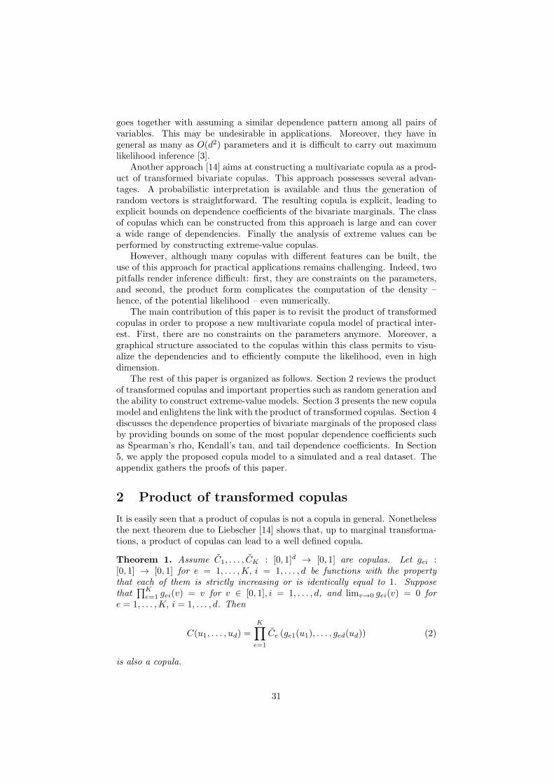
goes together with assuming a similar dependence pattern among all pairs ofvariables. This may be undesirable in applications. Moreover, they have ingeneral as many as O(d2) parameters and it is difficult to carry out maximumlikelihood inference [3].

Another approach [14] aims at constructing a multivariate copula as a prod-uct of transformed bivariate copulas. This approach possesses several advan-tages. A probabilistic interpretation is available and thus the generation ofrandom vectors is straightforward. The resulting copula is explicit, leading toexplicit bounds on dependence coefficients of the bivariate marginals. The classof copulas which can be constructed from this approach is large and can covera wide range of dependencies. Finally the analysis of extreme values can beperformed by constructing extreme-value copulas.

However, although many copulas with different features can be built, theuse of this approach for practical applications remains challenging. Indeed, twopitfalls render inference difficult: first, they are constraints on the parameters,and second, the product form complicates the computation of the density –hence, of the potential likelihood – even numerically.

The main contribution of this paper is to revisit the product of transformedcopulas in order to propose a new multivariate copula model of practical inter-est. First, there are no constraints on the parameters anymore. Moreover, agraphical structure associated to the copulas within this class permits to visu-alize the dependencies and to efficiently compute the likelihood, even in highdimension.

The rest of this paper is organized as follows. Section 2 reviews the productof transformed copulas and important properties such as random generation andthe ability to construct extreme-value models. Section 3 presents the new copulamodel and enlightens the link with the product of transformed copulas. Section 4discusses the dependence properties of bivariate marginals of the proposed classby providing bounds on some of the most popular dependence coefficients suchas Spearman’s rho, Kendall’s tau, and tail dependence coefficients. In Section5, we apply the proposed copula model to a simulated and a real dataset. Theappendix gathers the proofs of this paper.

2 Product of transformed copulas

It is easily seen that a product of copulas is not a copula in general. Nonethelessthe next theorem due to Liebscher [14] shows that, up to marginal transforma-tions, a product of copulas can lead to a well defined copula.

Theorem 1. Assume C1, . . . , CK : [0, 1]d → [0, 1] are copulas. Let gei :[0, 1] → [0, 1] for e = 1, . . . ,K, i = 1, . . . , d be functions with the propertythat each of them is strictly increasing or is identically equal to 1. Supposethat

∏Ke=1 gei(v) = v for v ∈ [0, 1], i = 1, . . . , d, and limv→0 gei(v) = 0 for

e = 1, . . . ,K, i = 1, . . . , d. Then

C(u1, . . . , ud) =

K∏

e=1

Ce (ge1(u1), . . . , ged(ud)) (2)

is also a copula.

31

The probabilistic interpretation of (2) is as follows. Let

(U(1)1 , . . . , U

(1)d ), . . . , (U

(K)1 , . . . , U

(K)d )

be K independent random vectors having distribution function C1, . . . , CK re-spectively. Let gei, e = 1, . . . ,K, i = 1, . . . , d be as in Theorem 1 and defineg−1ei (v) := 0 for v ≤ gei(0) and Ji = {e ∈ {1, . . . ,K} : gei 6= 1}. Then C is thejoint distribution function of the random vector

(maxe∈J1

g−1e1 (U

(e)1 ), . . . ,max

e∈Jdg−1ed (U

(e)d )

). (3)

If there exists a random generation procedure for Ce, e = 1, . . . ,K then thanksto (3) a random generation procedure for C can be derived as well.

The statistical analysis of extreme values should theoretically be carriedout with the help of extreme-value copulas [8]. Recall that a copula C# is anextreme-value copula if there exists a copula C such that

C#(u1, . . . , ud) = limn↑∞

Cn(u1/n1 , . . . , u

1/nd ), (4)

for every (u1, . . . , ud) ∈ [0, 1]d. A copula C# is said to be max-stable if for everyinteger n ≥ 1 and every (u1, . . . , ud) ∈ [0, 1]d

Cn#(u1/n1 , . . . , u

1/nd ) = C#(u1, . . . , ud).

Extreme-value copulas correspond exactly to max-stable copulas [8]. Theorem 1can be used to construct extreme-value copulas as shown in the next propositiondue to [4].

Proposition 1. In (2), let gei(v) = vθei , v ∈ [0, 1] with θei ∈ [0, 1] and∑Ke=1 θei = 1 for i = 1, . . . , d. If Ce, e = 1, . . . ,K is max-stable then so is

C.

Out of the context of extreme values, applications of Theorem 1 can befound, for instance, in the analysis of directional dependence [13] (K = d = 2),finance [2] (K = d = 2) and hydrology [4] (K = 2, d = 3).

We are not aware of applications of Theorem 1 in practice when K > 2 ord > 3. As pointed out in the introduction, the product form (2) renders the

density ∂dC(u1,...,ud)∂u1...∂ud

, hence the likelihood, complicated to compute even numer-

ically. Furthermore, the constraints∏Ke=1 gei(v) = v, v ∈ [0, 1], i = 1, . . . , d in

Theorem 1 are not easy to deal with in practice.The next section aims at overcoming these drawbacks.

3 Product of transformed copulas revisited

The product over e ∈ {1, . . . ,K} in (2) can be taken over e ∈ E, where E is anarbitrary finite set, yielding

C(u1, . . . , ud) =∏

e∈E

Ce (ge1(u1), . . . , ged(ud)) . (5)

32

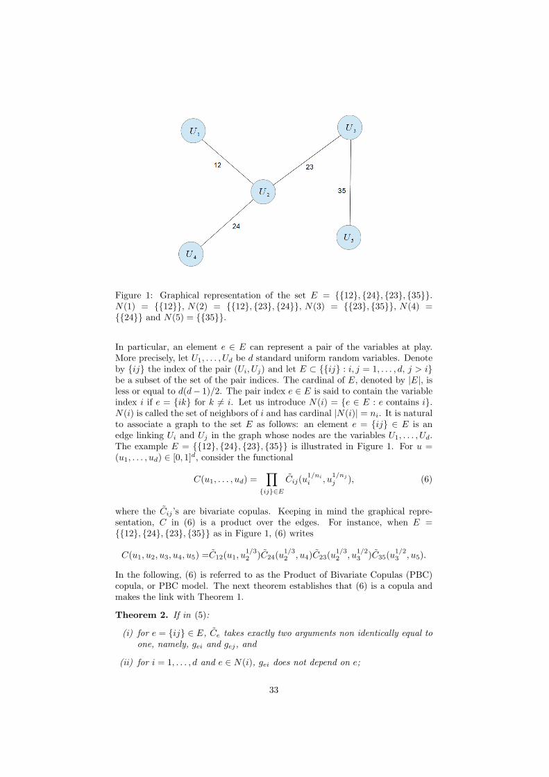
Figure 1: Graphical representation of the set E = {{12}, {24}, {23}, {35}}.N(1) = {{12}}, N(2) = {{12}, {23}, {24}}, N(3) = {{23}, {35}}, N(4) ={{24}} and N(5) = {{35}}.

In particular, an element e ∈ E can represent a pair of the variables at play.More precisely, let U1, . . . , Ud be d standard uniform random variables. Denoteby {ij} the index of the pair (Ui, Uj) and let E ⊂ {{ij} : i, j = 1, . . . , d, j > i}be a subset of the set of the pair indices. The cardinal of E, denoted by |E|, isless or equal to d(d− 1)/2. The pair index e ∈ E is said to contain the variableindex i if e = {ik} for k 6= i. Let us introduce N(i) = {e ∈ E : e contains i}.N(i) is called the set of neighbors of i and has cardinal |N(i)| = ni. It is naturalto associate a graph to the set E as follows: an element e = {ij} ∈ E is anedge linking Ui and Uj in the graph whose nodes are the variables U1, . . . , Ud.The example E = {{12}, {24}, {23}, {35}} is illustrated in Figure 1. For u =(u1, . . . , ud) ∈ [0, 1]d, consider the functional

C(u1, . . . , ud) =∏

{ij}∈E

Cij(u1/ni

i , u1/nj

j ), (6)

where the Cij ’s are bivariate copulas. Keeping in mind the graphical repre-sentation, C in (6) is a product over the edges. For instance, when E ={{12}, {24}, {23}, {35}} as in Figure 1, (6) writes

C(u1, u2, u3, u4, u5) =C12(u1, u1/32 )C24(u

1/32 , u4)C23(u

1/32 , u

1/23 )C35(u

1/23 , u5).

In the following, (6) is referred to as the Product of Bivariate Copulas (PBC)copula, or PBC model. The next theorem establishes that (6) is a copula andmakes the link with Theorem 1.

Theorem 2. If in (5):

(i) for e = {ij} ∈ E, Ce takes exactly two arguments non identically equal toone, namely, gei and gej, and

(ii) for i = 1, . . . , d and e ∈ N(i), gei does not depend on e;

33

then the only copula which can be constructed from (5) is the PBC model (6),where Cij is defined by

Cij(u, v) = C{ij}(1, . . . , 1, u, 1, . . . , 1, v, 1, . . . , 1), (u, v) ∈ [0, 1]2,

and where in (1, . . . , 1, u, 1, . . . , 1, v, 1, . . . , 1), u and v are at the i-th and j-thpositions respectively.

Condition (i) in Theorem 2 simply means that only bivariate copulas areallowed in the construction. The simplification (ii) achieves two goals: firstto reduce the number of parameters (an important feature in high-dimension),and second to intrinsically satisfy the constraints

∏e∈E gei(v) = v, v ∈ [0, 1], i =

1, . . . , d in the assumptions of Theorem 1. If assumption (ii) in Theorem 2 wasnot made, one could take gei(v) = vθei , e ∈ E, i = 1, . . . , d, θei ∈ [0, 1] with theconstraints ∑

e∈N(i)

θei =∑

k:{ki}∈E

θki,i = 1, i = 1, . . . , d. (7)

These constraints would be difficult to handle in practice, and, furthermore,the number of parameters would increase quadratically with the dimension.Indeed, one would have (|E| − 1)d parameters θei plus an additional number|E| of parameters for each copula Ce. If the graph associated to E is a tree, forinstance, then |E| = d− 1, yielding O(d2) parameters. As a comparison, in thePBC model (6), there are no constraints and only O(d) parameters in total.

From (1), the PBC copula (6) is associated to a distribution function F withcontinuous marginals Fi, i = 1, . . . , d, such that

F (x1, . . . , xd) = C(F1(x1), . . . , Fd(xd)), (x1, . . . , xd) ∈ Rd. (8)

By substituting (6) into (8), it is easy to see that F writes

F (x1, . . . , xd) =∏

{ij}∈E

Fij(xi, xj), (x1, . . . , xd) ∈ Rd, (9)

where Fij , {ij} ∈ E, is a bivariate distribution function such that the first(respectively the second) marginal Fij,1 (respectively Fij,2) only depends on i(respectively j). It is interesting to note that the converse is also true as statedin the following proposition.

Proposition 2. The distribution function corresponding to the PBC copula (6)writes as F in (9). Conversely, the copula corresponding to the distributionfunction F in (9) writes as the PBC copula (6).

4 Dependence properties and max-stability

Let C be the PBC copula (6). First the dependence properties of a pair (Uk, Ul)whose copula is the bivariate copula Ckl(uk, ul) = C(1, . . . , 1, uk, 1, . . . , 1, ul, 1, . . . , 1)are studied. The conditions under which the PBC model (6) is an extreme-valuecopula are given afterwards.

Proposition 3. The bivariate marginal Ckl is given by

Ckl(uk, ul) =

{u(nk−1)/nk

k u(nl−1)/nl

l Ckl(u1/nk

k , u1/nl

l ) if {kl} ∈ E,ukul otherwise.

(10)

34

Example 1. If in (10) Ckl is a Marshall-Olkin copula (see for instance [16],p.53) with parameters 0 ≤ α, β ≤ 1 (denoted by MO(α, β)), that is,

Ckl(uk, ul) = min(u1−αk ul, u1−βl uk),

then Ckl is MO(α/nk, β/nl). If α = β then Ckl is a Cuadras-Auge copulaand Ckl is MO(α/nk, α/nl). If α = β = 0 then both Ckl and Ckl are theindependence copula. If α = β = 1 then Ckl is the Frechet upper bound copulaand Ckl is MO(1/nk, 1/nl).

Remark 1. If in (10) one puts κ = 1/nk and λ = 1/nl, then the copulas takethe form Ckl(uk, ul) = u1−κk u1−λl Ckl(u

κk , u

λl ). This class of copulas, sometimes

referred to as Khoudraji copulas, was proposed in [6] Proposition 2.

Let (U, V ) be a random vector with copula C. The dependence between Uand V is positive if, roughly speaking, U and V tend to be large or small to-gether. Below are recalled a few definitions of statistical concepts about positivedependence. The copula C has the TP2 (totally positive of order 2) property ifand only if

C(u1, u2)C(v1, v2) ≥ C(u1, v2)C(v1, u2), for all u1 < v1 and u2 < v2. (11)

Also, C is said to be PQD (positive quadrant dependent) if C(u, v) ≥ uv for all(u, v) ∈ [0, 1]2. The random variable V is said to be LTD (left tail decreasing)in U if for all v ∈ [0, 1], the function u 7→ P (V ≤ v|U ≤ u) is decreasing inu. The dependence between U and V can be quantified through dependencemeasures such as the Kendall’s tau or Spearman’s rho respectively given by

τ =4

∫

[0,1]2C(u, v) dC(u, v)− 1, (12)

ρ =12

∫

[0,1]2C(u, v) du dv − 3. (13)

The dependence in the upper and lower tails can be respectively measured with

λ(U) = limu↑1

1− 2u+ C(u, u)

1− u∈ [0, 1], λ(L) = lim

u↓0

C(u, u)

u∈ [0, 1].

See [16] and [12] for further details about these concepts. Let us denote by τkl,

ρkl, λ(U)kl and λ

(L)kl the Kendall’s tau, Spearman’s rho, upper tail dependence

coefficient and lower tail dependence coefficient of the copula Ckl in (10) re-spectively. As shown in Proposition 3, Ckl is a bivariate marginal of the PBCcopula (6) and one may apply the results of [14] to obtain the following.

Proposition 4. If in (10) Ckl is TP2, LTD or PQD then Ckl is also TP2,LTD or PQD respectively.

Explicit bounds in terms of the number of neighbors for the dependencecoefficients of PBC bivariate marginals are given in the next proposition. Thebehavior of (10) when the number of neighbors tends to infinity is also studied.

35

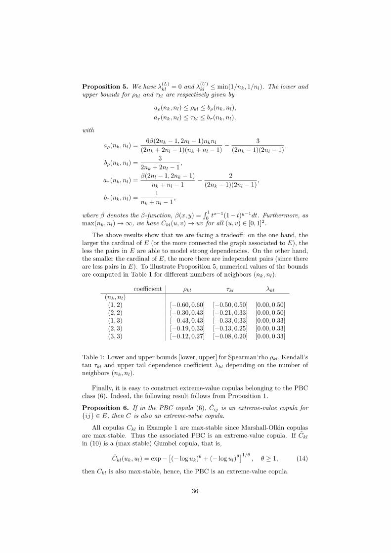
Proposition 5. We have λ(L)kl = 0 and λ

(U)kl ≤ min(1/nk, 1/nl). The lower and

upper bounds for ρkl and τkl are respectively given by

aρ(nk, nl) ≤ ρkl ≤ bρ(nk, nl),

aτ (nk, nl) ≤ τkl ≤ bτ (nk, nl),

with

aρ(nk, nl) =6β(2nk − 1, 2nl − 1)nknl

(2nk + 2nl − 1)(nk + nl − 1)− 3

(2nk − 1)(2nl − 1),

bρ(nk, nl) =3

2nk + 2nl − 1,

aτ (nk, nl) =β(2nl − 1, 2nk − 1)

nk + nl − 1− 2

(2nk − 1)(2nl − 1),

bτ (nk, nl) =1

nk + nl − 1,

where β denotes the β-function, β(x, y) =∫ 1

0tx−1(1− t)y−1dt. Furthermore, as

max(nk, nl) → ∞, we have Ckl(u, v) → uv for all (u, v) ∈ [0, 1]2.

The above results show that we are facing a tradeoff: on the one hand, thelarger the cardinal of E (or the more connected the graph associated to E), theless the pairs in E are able to model strong dependencies. On the other hand,the smaller the cardinal of E, the more there are independent pairs (since thereare less pairs in E). To illustrate Proposition 5, numerical values of the boundsare computed in Table 1 for different numbers of neighbors (nk, nl).

coefficient ρkl τkl λkl(nk, nl)(1, 2) [−0.60, 0.60] [−0.50, 0.50] [0.00, 0.50](2, 2) [−0.30, 0.43] [−0.21, 0.33] [0.00, 0.50](1, 3) [−0.43, 0.43] [−0.33, 0.33] [0.00, 0.33](2, 3) [−0.19, 0.33] [−0.13, 0.25] [0.00, 0.33](3, 3) [−0.12, 0.27] [−0.08, 0.20] [0.00, 0.33]

Table 1: Lower and upper bounds [lower, upper] for Spearman’rho ρkl, Kendall’stau τkl and upper tail dependence coefficient λkl depending on the number ofneighbors (nk, nl).

Finally, it is easy to construct extreme-value copulas belonging to the PBCclass (6). Indeed, the following result follows from Proposition 1.

Proposition 6. If in the PBC copula (6), Cij is an extreme-value copula for{ij} ∈ E, then C is also an extreme-value copula.

All copulas Ckl in Example 1 are max-stable since Marshall-Olkin copulasare max-stable. Thus the associated PBC is an extreme-value copula. If Cklin (10) is a (max-stable) Gumbel copula, that is,

Ckl(uk, ul) = exp−[(− log uk)

θ + (− log ul)θ]1/θ

, θ ≥ 1, (14)

then Ckl is also max-stable, hence, the PBC is an extreme-value copula.

36

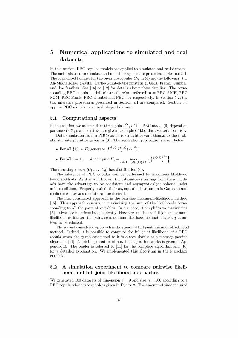
5 Numerical applications to simulated and realdatasets

In this section, PBC copulas models are applied to simulated and real datasets.The methods used to simulate and infer the copulas are presented in Section 5.1.The considered families for the bivariate copulas Cij in (6) are the following: theAli-Mikhail-Haq (AMH), Farlie-Gumbel-Morgenstern (FGM), Frank, Gumbel,and Joe families. See [16] or [12] for details about these families. The corre-sponding PBC copula models (6) are therefore referred to as PBC AMH, PBCFGM, PBC Frank, PBC Gumbel and PBC Joe respectively. In Section 5.2, thetwo inference procedures presented in Section 5.1 are compared. Section 5.3applies PBC models to an hydrological dataset.

5.1 Computational aspects

In this section, we assume that the copulas Cij of the PBC model (6) depend onparameters θij ’s and that we are given a sample of i.i.d data vectors from (6).

Data simulation from a PBC copula is straightforward thanks to the prob-abilistic interpretation given in (3). The generation procedure is given below.

• For all {ij} ∈ E, generate (U(ij)i , U

(ij)j ) ∼ Cij .

• For all i = 1, . . . , d, compute Ui = maxk∈{1,...,d}:{ki}∈E

{(U

(ki)i

)ni}.

The resulting vector (U1, . . . , Ud) has distribution (6).The inference of PBC copulas can be performed by maximum-likelihood

based methods. As it is well known, the estimators resulting from these meth-ods have the advantage to be consistent and asymptotically unbiased undermild conditions. Properly scaled, their asymptotic distribution is Gaussian andconfidence intervals or tests can be derived.

The first considered approach is the pairwise maximum-likelihood method[15]. This approach consists in maximizing the sum of the likelihoods corre-sponding to all the pairs of variables. In our case, it simplifies to maximizing|E| univariate functions independently. However, unlike the full joint maximumlikelihood estimator, the pairwise maximum-likelihood estimator is not guaran-teed to be efficient.

The second considered approach is the standard full joint maximum-likelihoodmethod. Indeed, it is possible to compute the full joint likelihood of a PBCcopula when the graph associated to it is a tree thanks to a message-passingalgorithm [11]. A brief explanation of how this algorithm works is given in Ap-pendix B. The reader is referred to [11] for the complete algorithm and [10]for a detailed explanation. We implemented this algorithm in the R packagePBC [18].

5.2 A simulation experiment to compare pairwise likeli-hood and full joint likelihood approaches

We generated 100 datasets of dimension d = 9 and size n = 500 according to aPBC copula whose tree graph is given in Figure 2. The amount of time required

37

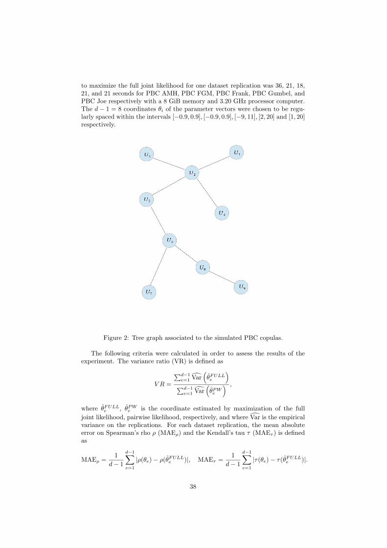
to maximize the full joint likelihood for one dataset replication was 36, 21, 18,21, and 21 seconds for PBC AMH, PBC FGM, PBC Frank, PBC Gumbel, andPBC Joe respectively with a 8 GiB memory and 3.20 GHz processor computer.The d− 1 = 8 coordinates θi of the parameter vectors were chosen to be regu-larly spaced within the intervals [−0.9, 0.9], [−0.9, 0.9], [−9, 11], [2, 20] and [1, 20]respectively.

Figure 2: Tree graph associated to the simulated PBC copulas.

The following criteria were calculated in order to assess the results of theexperiment. The variance ratio (VR) is defined as

V R =

∑d−1e=1 Var

(θFULLe

)

∑d−1e=1 Var

(θPWe

) ,

where θFULLe , θPWe is the coordinate estimated by maximization of the full

joint likelihood, pairwise likelihood, respectively, and where Var is the empiricalvariance on the replications. For each dataset replication, the mean absoluteerror on Spearman’s rho ρ (MAEρ) and the Kendall’s tau τ (MAEτ ) is definedas

MAEρ =1

d− 1

d−1∑

e=1

|ρ(θe)− ρ(θFULLe )|, MAEτ =1

d− 1

d−1∑

e=1

|τ(θe)− τ(θFULLe )|.

38

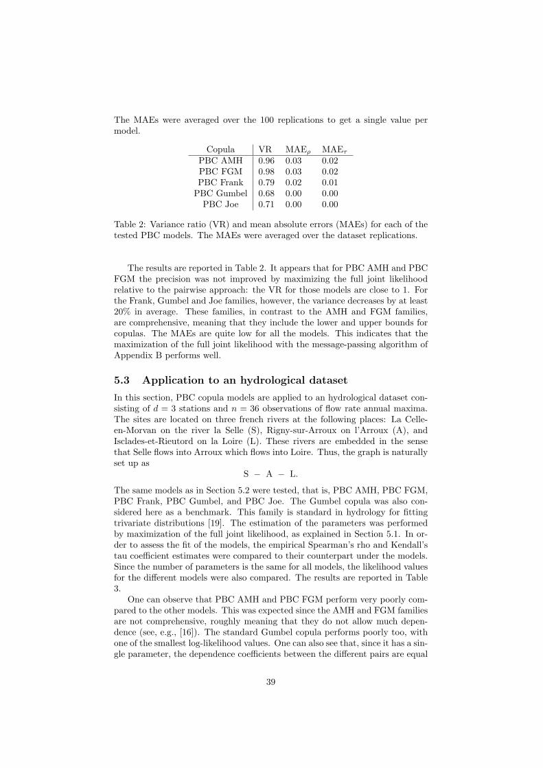
The MAEs were averaged over the 100 replications to get a single value permodel.

Copula VR MAEρ MAEτPBC AMH 0.96 0.03 0.02PBC FGM 0.98 0.03 0.02PBC Frank 0.79 0.02 0.01PBC Gumbel 0.68 0.00 0.00PBC Joe 0.71 0.00 0.00

Table 2: Variance ratio (VR) and mean absolute errors (MAEs) for each of thetested PBC models. The MAEs were averaged over the dataset replications.

The results are reported in Table 2. It appears that for PBC AMH and PBCFGM the precision was not improved by maximizing the full joint likelihoodrelative to the pairwise approach: the VR for those models are close to 1. Forthe Frank, Gumbel and Joe families, however, the variance decreases by at least20% in average. These families, in contrast to the AMH and FGM families,are comprehensive, meaning that they include the lower and upper bounds forcopulas. The MAEs are quite low for all the models. This indicates that themaximization of the full joint likelihood with the message-passing algorithm ofAppendix B performs well.

5.3 Application to an hydrological dataset

In this section, PBC copula models are applied to an hydrological dataset con-sisting of d = 3 stations and n = 36 observations of flow rate annual maxima.The sites are located on three french rivers at the following places: La Celle-en-Morvan on the river la Selle (S), Rigny-sur-Arroux on l’Arroux (A), andIsclades-et-Rieutord on la Loire (L). These rivers are embedded in the sensethat Selle flows into Arroux which flows into Loire. Thus, the graph is naturallyset up as

S − A − L.

The same models as in Section 5.2 were tested, that is, PBC AMH, PBC FGM,PBC Frank, PBC Gumbel, and PBC Joe. The Gumbel copula was also con-sidered here as a benchmark. This family is standard in hydrology for fittingtrivariate distributions [19]. The estimation of the parameters was performedby maximization of the full joint likelihood, as explained in Section 5.1. In or-der to assess the fit of the models, the empirical Spearman’s rho and Kendall’stau coefficient estimates were compared to their counterpart under the models.Since the number of parameters is the same for all models, the likelihood valuesfor the different models were also compared. The results are reported in Table3.

One can observe that PBC AMH and PBC FGM perform very poorly com-pared to the other models. This was expected since the AMH and FGM familiesare not comprehensive, roughly meaning that they do not allow much depen-dence (see, e.g., [16]). The standard Gumbel copula performs poorly too, withone of the smallest log-likelihood values. One can also see that, since it has a sin-gle parameter, the dependence coefficients between the different pairs are equal

39

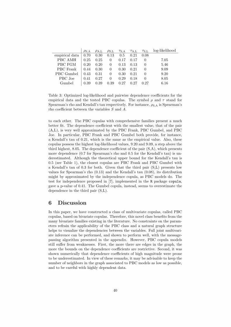
ρS,A ρA,L ρS,L τS,A τA,L τS,L log-likelihoodempirical data 0.70 0.30 0.13 0.5 0.21 0.08PBC AMH 0.25 0.25 0 0.17 0.17 0 7.05PBC FGM 0.20 0.20 0 0.13 0.13 0 5.46PBC Frank 0.44 0.30 0 0.30 0.21 0 9.09PBC Gumbel 0.43 0.31 0 0.30 0.21 0 9.20PBC Joe 0.41 0.27 0 0.29 0.18 0 8.05Gumbel 0.39 0.39 0.39 0.27 0.27 0.27 6.16

Table 3: Optimized log-likelihood and pairwise dependence coefficients for theempirical data and the tested PBC copulas. The symbol ρ and τ stand forSpearman’s rho and Kendall’s tau respectively. For instance, ρS,A is Spearman’srho coefficient between the variables S and A.

to each other. The PBC copulas with comprehensive families present a muchbetter fit. The dependence coefficient with the smallest value, that of the pair(A,L), is very well approximated by the PBC Frank, PBC Gumbel, and PBCJoe. In particular, PBC Frank and PBC Gumbel both provide, for instance,a Kendall’s tau of 0.21, which is the same as the empirical value. Also, thesecopulas possess the highest log-likelihood values, 9.20 and 9.09, a step above thethird highest, 8.05. The dependence coefficient of the pair (S,A), which presentsmore dependence (0.7 for Spearman’s rho and 0.5 for the Kendall’s tau) is un-derestimated. Although the theoretical upper bound for the Kendall’s tau is0.5 (see Table 1), the closest copulas are PBC Frank and PBC Gumbel witha Kendall’s tau of 0.3 for both. Given that the third pair (S,L) presents lowvalues for Spearman’s rho (0.13) and the Kendall’s tau (0.08), its distributionmight by approximated by the independence copula, as PBC models do. Thetest for independence proposed in [7], implemented in the R package copula,gave a p-value of 0.41. The Gumbel copula, instead, seems to overestimate thedependence in the third pair (S,L).

6 Discussion

In this paper, we have constructed a class of multivariate copulas, called PBCcopulas, based on bivariate copulas. Therefore, this novel class benefits from themany bivariate families existing in the literature. No constraints on the param-eters refrain the applicability of the PBC class and a natural graph structurehelps to visualize the dependencies between the variables. Full joint multivari-ate inference can be performed, and shown to perform well, with the message-passing algorithm presented in the appendix. However, PBC copula modelsstill suffer from weaknesses. First, the more there are edges in the graph, themore the bounds on the dependence coefficients are restrictive. Second, it wasshown numerically that dependence coefficients of high magnitude were proneto be underestimated. In view of these remarks, it may be advisable to keep thenumber of neighbors in the graph associated to PBC models as low as possible,and to be careful with highly dependent data.

40

Acknowledgment. The authors thank “Banque HYDRO du Ministere del’Ecologie, du Developpement durable et de l’Energie” for providing the data andBenjamin Renard for fruitful dicussions about statistical issues in hydrologicalscience.

41

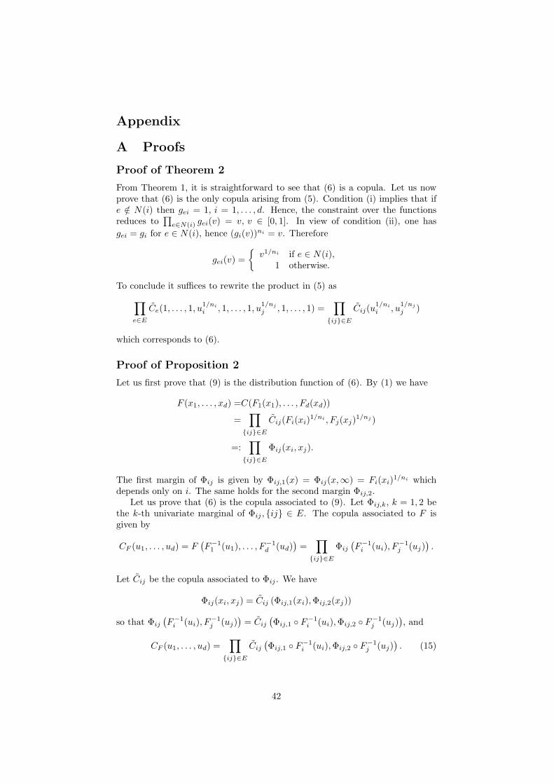
Appendix

A Proofs

Proof of Theorem 2

From Theorem 1, it is straightforward to see that (6) is a copula. Let us nowprove that (6) is the only copula arising from (5). Condition (i) implies that ife /∈ N(i) then gei = 1, i = 1, . . . , d. Hence, the constraint over the functionsreduces to

∏e∈N(i) gei(v) = v, v ∈ [0, 1]. In view of condition (ii), one has

gei = gi for e ∈ N(i), hence (gi(v))ni = v. Therefore

gei(v) =

{v1/ni if e ∈ N(i),

1 otherwise.

To conclude it suffices to rewrite the product in (5) as

∏

e∈E

Ce(1, . . . , 1, u1/ni

i , 1, . . . , 1, u1/nj

j , 1, . . . , 1) =∏

{ij}∈E

Cij(u1/ni

i , u1/nj

j )

which corresponds to (6).

Proof of Proposition 2

Let us first prove that (9) is the distribution function of (6). By (1) we have

F (x1, . . . , xd) =C(F1(x1), . . . , Fd(xd))

=∏

{ij}∈E

Cij(Fi(xi)1/ni , Fj(xj)

1/nj )

=:∏

{ij}∈E

Φij(xi, xj).

The first margin of Φij is given by Φij,1(x) = Φij(x,∞) = Fi(xi)1/ni which

depends only on i. The same holds for the second margin Φij,2.Let us prove that (6) is the copula associated to (9). Let Φij,k, k = 1, 2 be

the k-th univariate marginal of Φij , {ij} ∈ E. The copula associated to F isgiven by

CF (u1, . . . , ud) = F(F−11 (u1), . . . , F

−1d (ud)

)=

∏

{ij}∈E

Φij(F−1i (ui), F

−1j (uj)

).

Let Cij be the copula associated to Φij . We have

Φij(xi, xj) = Cij (Φij,1(xi),Φij,2(xj))

so that Φij(F−1i (ui), F

−1j (uj)

)= Cij

(Φij,1 ◦ F−1

i (ui),Φij,2 ◦ F−1j (uj)

), and

CF (u1, . . . , ud) =∏

{ij}∈E

Cij(Φij,1 ◦ F−1

i (ui),Φij,2 ◦ F−1j (uj)

). (15)

42

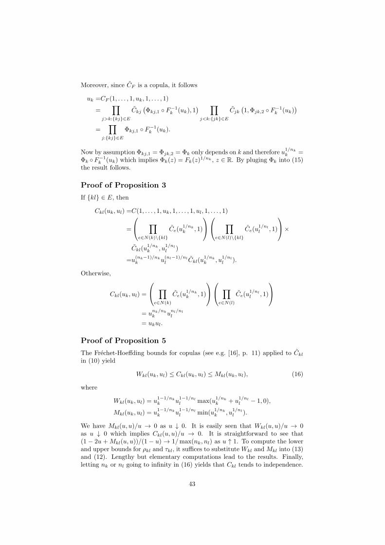
Moreover, since CF is a copula, it follows

uk =CF (1, . . . , 1, uk, 1, . . . , 1)

=∏

j>k:{kj}∈E

Ckj(Φkj,1 ◦ F−1

k (uk), 1) ∏

j<k:{jk}∈E

Cjk(1,Φjk,2 ◦ F−1

k (uk))

=∏

j:{kj}∈E

Φkj,1 ◦ F−1k (uk).

Now by assumption Φkj,1 = Φjk,2 = Φk only depends on k and therefore u1/nk

k =Φk ◦F−1

k (uk) which implies Φk(z) = Fk(z)1/nk , z ∈ R. By pluging Φk into (15)

the result follows.

Proof of Proposition 3

If {kl} ∈ E, then

Ckl(uk, ul) =C(1, . . . , 1, uk, 1, . . . , 1, ul, 1, . . . , 1)

=

∏

e∈N(k)\{kl}

Ce(u1/nk

k , 1)

∏

e∈N(l)\{kl}

Ce(u1/nl

l , 1)

×

Ckl(u1/nk

k , u1/nl

l )

=u(nk−1)/nk

k u(nl−1)/nl

l Ckl(u1/nk

k , u1/nl

l ).

Otherwise,

Ckl(uk, ul) =

∏

e∈N(k)

Ce(u1/nk

k , 1)

∏

e∈N(l)

Ce(u1/nl

l , 1)

= unk/nk

k unl/nl

l

= ukul.

Proof of Proposition 5

The Frechet-Hoeffding bounds for copulas (see e.g. [16], p. 11) applied to Cklin (10) yield

Wkl(uk, ul) ≤ Ckl(uk, ul) ≤Mkl(uk, ul), (16)

where

Wkl(uk, ul) = u1−1/nk

k u1−1/nl

l max(u1/nk

k + u1/nl

l − 1, 0),

Mkl(uk, ul) = u1−1/nk

k u1−1/nl

l min(u1/nk

k , u1/nl

l ).

We have Mkl(u, u)/u → 0 as u ↓ 0. It is easily seen that Wkl(u, u)/u → 0as u ↓ 0 which implies Ckl(u, u)/u → 0. It is straightforward to see that(1− 2u +Mkl(u, u))/(1− u) → 1/max(nk, nl) as u ↑ 1. To compute the lowerand upper bounds for ρkl and τkl, it suffices to substituteWkl andMkl into (13)and (12). Lengthy but elementary computations lead to the results. Finally,letting nk or nl going to infinity in (16) yields that Ckl tends to independence.

43

B Algorithm to compute the full joint likelihoodof PBC copulas

Denote the parameter vector by θ = (θij){ij}∈E . Recall that the graph isassumed to be a tree, that is, there is no cycles in the graph (then |E| = d− 1).Let V = {1, . . . , d} and u = (u1, . . . , ud) a vector in [0, 1]d. For a subset A ⊂ V ,the notation ∂uA

C(u;θ) stands for the derivative of C with respect to all thevariables in A. For instance the density (hence the likelihood) writes

∂dC(u;θ)

∂u1 . . . ∂ud

= ∂uVC(u;θ) = c(u;θ), (17)

and the gradient with respect to the parameter vector,(∂c(u;θ)

θij

)

{ij∈E}

.

To keep the notation simple, the dependence on the parameter vector θ isdropped in the remaining of the section. The purpose here is not to give thealgorithm, but rather to provide an intuitive idea of it.

Let us write

C(u1, . . . , ud) =∏

{ij}∈E

Cij(u1/ni

i , u1/nj

j ) =:∏

{ij}∈E

Φij(ui, uj).

and let an arbitrary variable index i (the root) be given. Let τ is denote thesubtree rooted at the variable indexed by i and containing the edge indexed bye (see Figure 3). The idea is to note that, since the graph is a tree, the copulaC can be decomposed over the subtrees rooted at i:

C(u) =∏

e∈E

Φe(u) =:∏

e∈N(i)

Tτ ie(u), u = (u1, . . . , ud),

where Tτ ie(u) corresponds to the product of all edges located in the subtree τ ie.

Since the Tτ ie(u)’s do not share any variables (except the root), the derivative

and the product operations commute, more precisely,

∂uVC(u) = ∂ui,uV \i

∏

e∈N(i)

Tτ ie(u)

= ∂ui

∏

e∈N(i)

∂uτie\iTτ i

e(u)

= ∂ui

∏

e∈N(i)

µe→i(u)

. (18)

The quantity µe→i(u) := ∂uτie\iTτ i

e(u) is called a message from the edge indexed

by e to the variable indexed by i. Now consider Tτ ie(u) and let j be the neighbor

variable index of e. One can go deeper in the tree, that is, we have

Tτ ie(u) = Φe(ui, uj)Tτe

j(u)

44

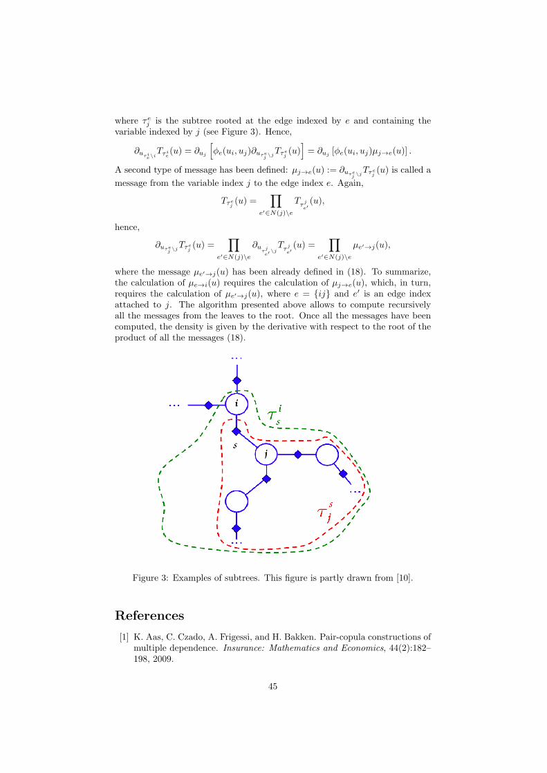
where τej is the subtree rooted at the edge indexed by e and containing thevariable indexed by j (see Figure 3). Hence,

∂uτie\iTτ i

e(u) = ∂uj

[φe(ui, uj)∂uτe

j\jTτe

j(u)]= ∂uj [φe(ui, uj)µj→e(u)] .

A second type of message has been defined: µj→e(u) := ∂uτej\jTτe

j(u) is called a

message from the variable index j to the edge index e. Again,

Tτej(u) =

∏

e′∈N(j)\e

Tτj

e′(u),

hence,

∂uτej\jTτe

j(u) =

∏

e′∈N(j)\e

∂uτje′

\jTτj

e′(u) =

∏

e′∈N(j)\e

µe′→j(u),

where the message µe′→j(u) has been already defined in (18). To summarize,the calculation of µe→i(u) requires the calculation of µj→e(u), which, in turn,requires the calculation of µe′→j(u), where e = {ij} and e′ is an edge indexattached to j. The algorithm presented above allows to compute recursivelyall the messages from the leaves to the root. Once all the messages have beencomputed, the density is given by the derivative with respect to the root of theproduct of all the messages (18).

Figure 3: Examples of subtrees. This figure is partly drawn from [10].

References

[1] K. Aas, C. Czado, A. Frigessi, and H. Bakken. Pair-copula constructions ofmultiple dependence. Insurance: Mathematics and Economics, 44(2):182–198, 2009.

45

[2] L.B.G Andersen and V.V. Piterbarg. Interest Rate Modeling. AtlanticFinancial Press, 2010.

[3] S. Demarta and A. J. McNeil. The t copula and related copulas. Interna-tional Statistical Review, 73(1):111–129, 2005.

[4] F. Durante and G. Salvadori. On the construction of multivariate extremevalue models via copulas. Environmetrics, 21(2):143–161, 2010.

[5] G. Frahm, M. Junker, and A. Szimayer. Elliptical copulas: applicabilityand limitations. Statistics & Probability Letters, 63(3):275–286, 2003.

[6] C. Genest, K. Ghoudi, and L-P. Rivest. Understanding relationships usingcopulas. North American Actuarial Journal, 2(3):143–149, 1998.

[7] C. Genest and B. Remillard. Test of independence and randomness basedon the empirical copula process. Test, 13(2):335–369, 2004.

[8] G. Gudendorf and J. Segers. Extreme-value copulas. In Copula Theory andIts Applications, page 127–145. Springer, 2010.

[9] M. Hofert, M. Machler, and A. J. McNeil. Archimedean copulas in highdimensions: Estimators and numerical challenges motivated by financialapplications. Journal de la Societe Francaise de Statistique, 154(1):25–63,2012.

[10] J. C. Huang. Cumulative distribution networks: Inference, estimation andapplications of graphical models for cumulative distribution functions. PhDthesis, University of Toronto, 2009.

[11] J.C. Huang and N. Jojic. Maximum-likelihood learning of cumulative distri-bution functions on graphs. Journal of Machine Learning Research W&CPSeries, 9:342–349, 2010.

[12] H. Joe. Multivariate models and dependence concepts. Chapman &Hall/CRC, 2001.

[13] D. Kim and J.M. Kim. Analysis of directional dependence using asymmetriccopula-based regression models. Journal of Statistical Computation andSimulation, 84(9):1990–2010, 2014.

[14] E. Liebscher. Construction of asymmetric multivariate copulas. Journal ofMultivariate Analysis, 99(10):2234–2250, 2008.

[15] B. G. Lindsay. Composite likelihood methods. Contemporary Mathematics,80(1):221–39, 1988.

[16] R.B. Nelsen. An introduction to copulas. Springer, 2006.

[17] M. Sklar. Fonctions de repartition a n dimensions et leurs marges. Publi-cations de l’Institut de Statistique de l’Universite de Paris, 8:229-231, 1959.

[18] T. Van Pham and G. Mazo. PBC: product of bivariate copulas.http://cran.r-project.org, 2014. R package version 1.2.

[19] L. Zhang and V. P. Singh. Gumbel–Hougaard copula for trivariate rainfallfrequency analysis. Journal of Hydrologic Engineering, 12(4):409–419, 2007.

46

❈❤❛♣✐tr❡ ✺

❊st✐♠❛t✐♦♥ ❞❡ ❝♦♣✉❧❡s

♠✉❧t✐✈❛r✐é❡s ♣❛r ❧❛ ♠ét❤♦❞❡

❞❡s ♠♦✐♥❞r❡s ❝❛rrés ♣♦♥❞érés

❜❛sé❡ s✉r ❧❡s ❝♦❡✣❝✐❡♥ts ❞❡

❞é♣❡♥❞❛♥❝❡

❙✉♣♣♦s♦♥s q✉❡ ❧✬♦♥ ❞✐s♣♦s❡ ❞✬✉♥ é❝❤❛♥t✐❧❧♦♥ ❞✬✉♥❡ ❢♦♥❝t✐♦♥ ❞❡ ré♣❛rt✐t✐♦♥F d✲✈❛r✐é❡ ✭d > 2✮ ❞♦♥t ❧❛ ❝♦♣✉❧❡ ❛♣♣❛rt✐❡♥t à ✉♥❡ ❢❛♠✐❧❧❡ ✐♥❞❡①é❡ ♣❛r ✉♥✈❡❝t❡✉r ❞❡ ♣❛r❛♠ètr❡s θ ❡t q✉❡ ❧✬♦♥ s♦✉❤❛✐t❡ ❡st✐♠❡r ❝❡s ♣❛r❛♠ètr❡s✳ ❙✉♣♣♦s♦♥s❛✉ss✐ q✉❡ ❝❡tt❡ ❝♦♣✉❧❡ ♥✬❛❞♠❡tt❡ ♣❛s ❞❡ ❞ér✐✈é❡s ♣❛rt✐❡❧❧❡s s✉r s♦♥ ❡♥s❡♠❜❧❡ ❞❡❞é✜♥✐t✐♦♥ ❡t q✉❡ ♣❛r ❝♦♥séq✉❡♥t✱ ❝♦♠♠❡ ♥♦✉s ❧✬❛✈✐♦♥s ❢❛✐t r❡♠❛rq✉❡r ❞❛♥s ❧❛♣❛rt✐❡ ✸✳✶✳✷✱ ✐❧ ♥✬❡st ♣❛s ♣♦ss✐❜❧❡ ❞❡ s✬❛ss✉r❡r ❞❡s ♣r♦♣r✐étés ❛s②♠♣t♦t✐q✉❡s ❞❡s♠ét❤♦❞❡s ❜✐❡♥ ❝♦♥♥✉❡s ❞❡ ❧❛ ❧✐ttér❛t✉r❡✳ ❈❡rt❛✐♥❡s ❞❡ ❝❡s ❝♦♣✉❧❡s ♦♥t ❞é❥à été♣rés❡♥té❡s ❞❛♥s ❧❛ ♣❛rt✐❡ ✶✳✸✳✷✳ ❉✬❛✉tr❡s ♦♥t été ✉t✐❧✐sé❡s ❞❛♥s ❧❛ ♣r❛t✐q✉❡ ❛✈❡❝s✉❝❝ès ❬✷✵✱ ✼✼❪✳ ❊♥✜♥✱ ❡t s✉rt♦✉t✱ ❝✬❡st ❧❡ ❝❛s ❞❡ ❧❛ ❝❧❛ss❡ ❞❡ ❝♦♣✉❧❡s ❝♦♥str✉✐t❡❞❛♥s ❧❡ ❝❤❛♣✐tr❡ ✻✳

❉❛♥s ❝❡ ❝❤❛♣✐tr❡✱ ♣♦✉r ❡st✐♠❡r ❧❡ ♣❛r❛♠ètr❡ θ✱ ♥♦✉s r❡❝♦♥s✐❞ér♦♥s ❧✬❡st✐♠❛✲t❡✉r ❞❡s ♠♦✐♥❞r❡s ❝❛rrés ♣♦♥❞érés ❜❛sé s✉r ❧❡s ❝♦❡✣❝✐❡♥ts ❞❡ ❞é♣❡♥❞❛♥❝❡s ✭✸✳✽✮❞❡ ❧❛ ♣❛rt✐❡ ✸✳✶✳✷ ❡t ét❛❜❧✐ss♦♥s s❡s ♣r♦♣r✐étés ❛s②♠♣t♦t✐q✉❡s s❛♥s s✉♣♣♦s❡r q✉❡❧❡s ❝♦♣✉❧❡s ❛❞♠❡tt❡♥t ❞❡s ❞ér✐✈é❡s ♣❛rt✐❡❧❧❡s✳ ❘❛♣♣❡❧♦♥s q✉❡ ❧✬❡st✐♠❛t❡✉r ❡st♦❜t❡♥✉ ❡♥ ♠✐♥✐♠✐s❛♥t ❧❛ ❢♦♥❝t✐♦♥

l(θ) =(D −D(θ)

)TW(D −D(θ)

), ✭✺✳✶✮

♦ù D(θ) = (D1,2(θ), . . . ,Dd−1,d(θ))✱ D = (D1,2, . . . , Dd−1,d) ❡t W ❡st ✉♥❡ ♠❛✲tr✐❝❡ ❞❡ ♣♦✐❞s ❀ Di,j(θ) ❡st ❧❡ ❝♦❡✣❝✐❡♥t ❞❡ ❞é♣❡♥❞❛♥❝❡ ❡♥tr❡ ❧❛ i✲è♠❡ ❡t ❧❛j✲è♠❡ ✈❛r✐❛❜❧❡ ❞✬✐♥térêt s♦✉s ❧❡ ♠♦❞è❧❡✱ ❡t Di,j ❡st ✉♥❡ ❡st✐♠❛t✐♦♥ ❡♠♣✐r✐q✉❡ ❞❡❝❡ ❝♦❡✣❝✐❡♥t✳ P❛r ❡①❡♠♣❧❡✱ ♣♦✉r Di,j(θ)✱ ♦♥ ♣❡✉t ♣r❡♥❞r❡ ❧❡ ❝♦❡✣❝✐❡♥t r❤♦ ❞❡❙♣❡❛r♠❛♥ ✭✶✳✺✮✱ ❡t ♣♦✉r Di,j ✱ ♦♥ ♣r❡♥❞r❛✐t ❜✐❡♥ sûr s❛ ✈❡rs✐♦♥ ❡♠♣✐r✐q✉❡ ✭✸✳✺✮✳▲❡s rés✉❧t❛ts s♦♥t ♦❜t❡♥✉s s♦✉s ❞❡s ❝♦♥❞✐t✐♦♥s ♥❛t✉r❡❧❧❡s ❞✬✐❞❡♥t✐✜❛❜✐❧✐té ❞❡s♠♦❞è❧❡s✳ ◆♦✉s ❡♥t❡♥❞♦♥s ♣❛r ❧à q✉❡ ❧✬❡♥s❡♠❜❧❡ ❞❡s ❝♦❡✣❝✐❡♥ts ❞❡ ❞é♣❡♥❞❛♥❝❡

✹✼

❞❡s ♣❛✐r❡s ❞ét❡r♠✐♥❡ ❧❛ ❝♦♣✉❧❡ à ❧✬✐♥tér✐❡✉r ❞✬✉♥❡ ❢❛♠✐❧❧❡ ❞♦♥♥é❡✳ ❊♥ ♣❛rt✐❝✉❧✐❡r✱❧✬❛♣♣❧✐❝❛t✐♦♥

θ 7→ (D1,2(θ), . . . ,Dd−1,d(θ))

❞❡✈r❛ êtr❡ ❜✐❥❡❝t✐✈❡✱ ❝♦♥t✐♥✉❡✱ ❡t s♦♥ ✐♥✈❡rs❡ ❝♦♥t✐♥✉❡ é❣❛❧❡♠❡♥t✳ ▲❡s rés✉❧t❛tst❤é♦r✐q✉❡s s♦♥t ✐❧❧✉strés s✉r ❞❡s s✐♠✉❧❛t✐♦♥s ❡t ❞❡s ❞♦♥♥é❡s ❤②❞r♦❧♦❣✐q✉❡s✱ ♦ù♥♦✉s ❡st✐♠♦♥s ❞❡s ❝♦♣✉❧❡s ♣♦ssè❞❛♥t ✉♥❡ ❝♦♠♣♦s❛♥t❡ s✐♥❣✉❧✐èr❡✳ ▲✬❛rt✐❝❧❡ ♣ré✲s❡♥té ❝✐✲❞❡ss♦✉s ❛ été s♦✉♠✐s ♣♦✉r ♣✉❜❧✐❝❛t✐♦♥✱ ❡t ❡st ❞✐s♣♦♥✐❜❧❡ à ❧✬❛❞r❡ss❡❤tt♣✿✴✴❤❛❧✳❛r❝❤✐✈❡s✲♦✉✈❡rt❡s✳❢r✴❤❛❧✲✵✵✾✼✾✶✺✶✳

✹✽

Weighted least-squares inference based on

dependence coefficients for multivariate copulas

Gildas Mazo, Stephane Girard and Florence Forbes

MISTIS, Inria - Laboratoire Jean Kuntzmann, France

Abstract

In this paper, we address the issue of estimating the parameters of

general multivariate copulas, that is, copulas whose partial derivatives

may not exist. To this aim, we consider a weighted least-squares esti-

mator based on dependence coefficients, and establish its consistency and

asymptotic normality. The estimator’s performance on finite samples is

illustrated on simulations and a real dataset.

Keywords: partial derivatives, singular component, least-squares, method-of-moments, dependence coefficients, parametric inference, copulas, multivari-ate.

1 Introduction

The concept of copulas is useful to model multivariate distributions. Given amultivariate random vector of interest, copulas allow to separate the analysisof the margins from the dependence structure. Standard books covering thissubject include [9, 24, 28]. See also [13] for an introduction to this topic.

Some copulas possess a singular component, meaning that they are not ab-solutely continuous (with respect to the Lebesgue measure). For instance, takethe copula given below, introduced in [8]:

C(u1, u2, u3, u4) =

4∏

i=1

u1−

∑j 6=i θij

i

∏

i<j

min(ui, uj)θij , (1)

∑

j 6=i

θij ≤ 1, i = 1, . . . , 4, θij = θji ∈ [0, 1].

One can see that, on the diagonal of the unit hypercube, the partial derivativesdo not exist. Yet, most inference methods for multivariate copulas make theassumption that these derivatives exist, and even be continuous. This is the case,for example, of the minimum-distance estimator [33], the simulated method ofmoments [30], and, of course, likelihood-based methods (Section 10.1 [24], [14]).When one does not make this assumption, some methods can still be applied butonly in specific situations. For example, when there are only two dimensions,one can rely on the inversion of Kendall’s tau, see [18] and [13]. When theyare an arbitrary number of dimensions but only one parameter to estimate, anextension of this method can also be found in [15]. Also, if the copulas of interest

49

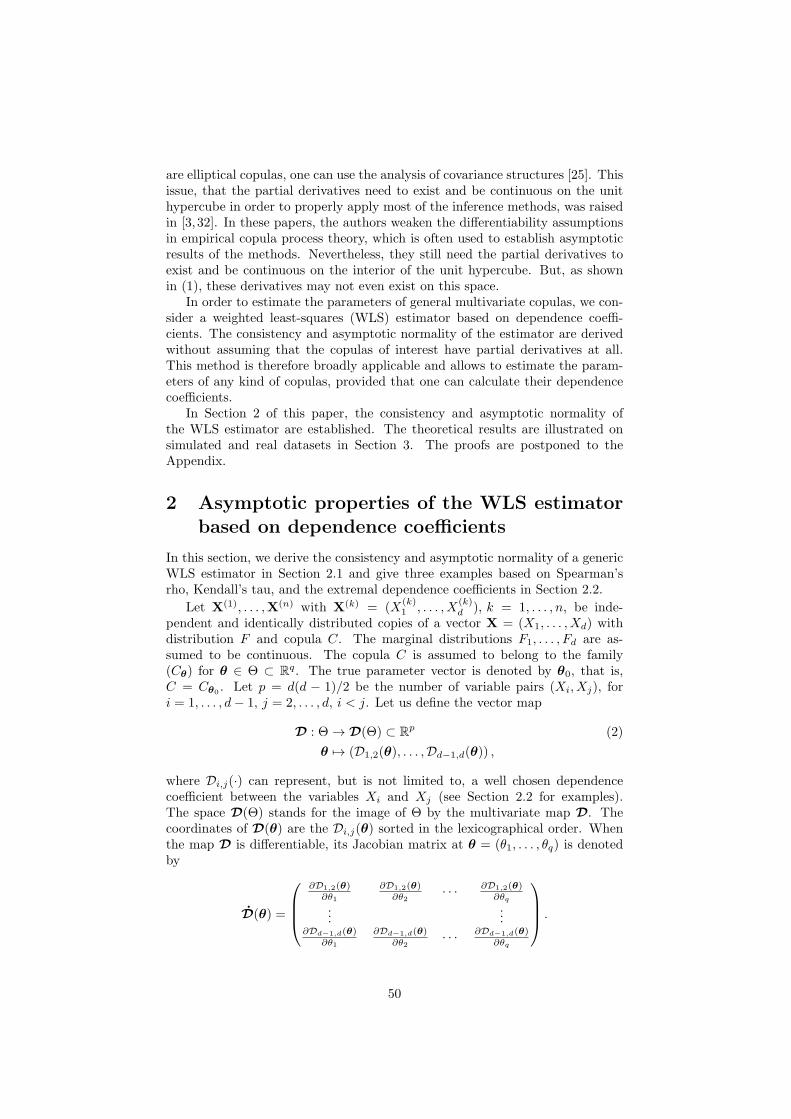
are elliptical copulas, one can use the analysis of covariance structures [25]. Thisissue, that the partial derivatives need to exist and be continuous on the unithypercube in order to properly apply most of the inference methods, was raisedin [3,32]. In these papers, the authors weaken the differentiability assumptionsin empirical copula process theory, which is often used to establish asymptoticresults of the methods. Nevertheless, they still need the partial derivatives toexist and be continuous on the interior of the unit hypercube. But, as shownin (1), these derivatives may not even exist on this space.

In order to estimate the parameters of general multivariate copulas, we con-sider a weighted least-squares (WLS) estimator based on dependence coeffi-cients. The consistency and asymptotic normality of the estimator are derivedwithout assuming that the copulas of interest have partial derivatives at all.This method is therefore broadly applicable and allows to estimate the param-eters of any kind of copulas, provided that one can calculate their dependencecoefficients.

In Section 2 of this paper, the consistency and asymptotic normality ofthe WLS estimator are established. The theoretical results are illustrated onsimulated and real datasets in Section 3. The proofs are postponed to theAppendix.

2 Asymptotic properties of the WLS estimatorbased on dependence coefficients

In this section, we derive the consistency and asymptotic normality of a genericWLS estimator in Section 2.1 and give three examples based on Spearman’srho, Kendall’s tau, and the extremal dependence coefficients in Section 2.2.

Let X(1), . . . ,X(n) with X(k) = (X(k)1 , . . . , X

(k)d ), k = 1, . . . , n, be inde-

pendent and identically distributed copies of a vector X = (X1, . . . , Xd) withdistribution F and copula C. The marginal distributions F1, . . . , Fd are as-sumed to be continuous. The copula C is assumed to belong to the family(Cθ) for θ ∈ Θ ⊂ R

q. The true parameter vector is denoted by θ0, that is,C = Cθ0

. Let p = d(d − 1)/2 be the number of variable pairs (Xi, Xj), fori = 1, . . . , d− 1, j = 2, . . . , d, i < j. Let us define the vector map

D : Θ → D(Θ) ⊂ Rp (2)

θ 7→ (D1,2(θ), . . . ,Dd−1,d(θ)) ,

where Di,j(·) can represent, but is not limited to, a well chosen dependencecoefficient between the variables Xi and Xj (see Section 2.2 for examples).The space D(Θ) stands for the image of Θ by the multivariate map D. Thecoordinates of D(θ) are the Di,j(θ) sorted in the lexicographical order. Whenthe map D is differentiable, its Jacobian matrix at θ = (θ1, . . . , θq) is denotedby

D(θ) =

∂D1,2(θ)∂θ1

∂D1,2(θ)∂θ2

· · · ∂D1,2(θ)∂θq

......

∂Dd−1,d(θ)∂θ1

∂Dd−1,d(θ)∂θ2

· · · ∂Dd−1,d(θ)∂θq

.

50

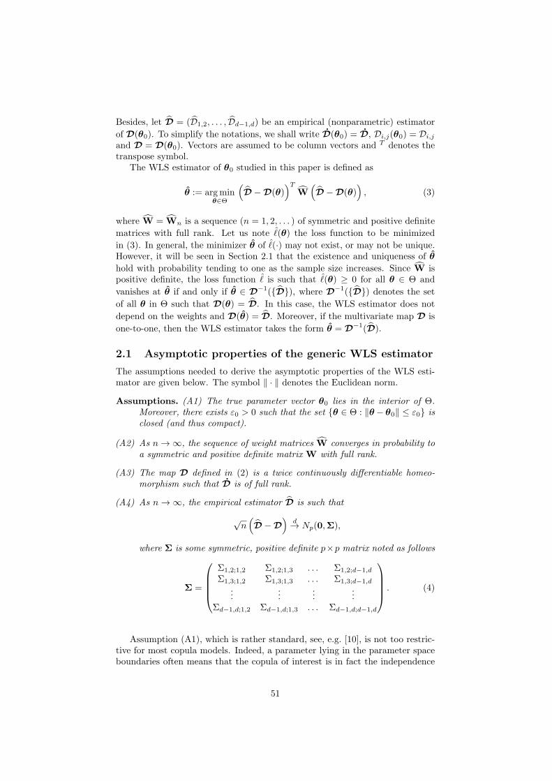
Besides, let D = (D1,2, . . . , Dd−1,d) be an empirical (nonparametric) estimator

of D(θ0). To simplify the notations, we shall write D(θ0) = D, Di,j(θ0) = Di,jand D = D(θ0). Vectors are assumed to be column vectors and T denotes thetranspose symbol.

The WLS estimator of θ0 studied in this paper is defined as

θ := argminθ∈Θ

(D −D(θ)

)TW(D −D(θ)

), (3)

where W = Wn is a sequence (n = 1, 2, . . . ) of symmetric and positive definite

matrices with full rank. Let us note ℓ(θ) the loss function to be minimized

in (3). In general, the minimizer θ of ℓ(·) may not exist, or may not be unique.However, it will be seen in Section 2.1 that the existence and uniqueness of θ

hold with probability tending to one as the sample size increases. Since W ispositive definite, the loss function ℓ is such that ℓ(θ) ≥ 0 for all θ ∈ Θ and

vanishes at θ if and only if θ ∈ D−1({D}), where D

−1({D}) denotes the set

of all θ in Θ such that D(θ) = D. In this case, the WLS estimator does not

depend on the weights and D(θ) = D. Moreover, if the multivariate map D is

one-to-one, then the WLS estimator takes the form θ = D−1(D).

2.1 Asymptotic properties of the generic WLS estimator

The assumptions needed to derive the asymptotic properties of the WLS esti-mator are given below. The symbol ‖ · ‖ denotes the Euclidean norm.

Assumptions. (A1) The true parameter vector θ0 lies in the interior of Θ.Moreover, there exists ε0 > 0 such that the set {θ ∈ Θ : ‖θ− θ0‖ ≤ ε0} isclosed (and thus compact).

(A2) As n→ ∞, the sequence of weight matrices W converges in probability toa symmetric and positive definite matrix W with full rank.

(A3) The map D defined in (2) is a twice continuously differentiable homeo-morphism such that D is of full rank.

(A4) As n→ ∞, the empirical estimator D is such that

√n(D −D

)d→ Np(0,Σ),

where Σ is some symmetric, positive definite p×p matrix noted as follows

Σ =

Σ1,2;1,2 Σ1,2;1,3 . . . Σ1,2;d−1,d

Σ1,3;1,2 Σ1,3;1,3 . . . Σ1,3;d−1,d

......

......

Σd−1,d;1,2 Σd−1,d;1,3 . . . Σd−1,d;d−1,d

. (4)

Assumption (A1), which is rather standard, see, e.g. [10], is not too restric-tive for most copula models. Indeed, a parameter lying in the parameter spaceboundaries often means that the copula of interest is in fact the independence

51

copula or the upper Frechet-Hoeffding bound, that is, a copula where the depen-dence is “perfect”, see for instance [28] chapter 2. This is not an issue becauseone does not encounter perfect dependence in practice. As for independence,one might carry out a statistical test as in [16], and, based on the results, decidewether independence holds or not. If not, then one can safely assume that theparameters lie in the interior of the parameter space. A sequence of weightmatrices verifying Assumption (A2) can always be constructed. A trivial ex-

ample is W = Ip, where Ip is the identity matrix of size p. The constructionof optimal weights is addressed in Proposition 1 below. The estimation of thecopula parameter vector is performed by matching the theoretical and empiricaldependence coefficients. Hence, a successful match should ensure that the re-sulting parameter vector estimate is close to the true value. This identifyabilitycondition, also made in [10] in order to estimate extreme-value copulas witha singular component, is the essence of Assumption (A3). The last assump-tion, (A4), naturally states that one should have convergence of the dependencecoefficient empirical estimator to ensure convergence of the WLS estimator.

Theorem 1. Assume that (A1)–(A4) hold. Then, as n → ∞ and with prob-ability tending to one, the WLS estimator defined by (3) exists and is unique.Moreover, it is consistent and asymptotically normal:

√n(θ − θ0)

d→ Nq (0,Ξ) , where (5)

Ξ =(DTWD

)−1

DTWΣWD

(DTWD

)−1

.

As usual, the results of Theorem 1 allow to derive the asymptotic distributionof quadratic forms in θ and D(θ). These asymptotics serve to build confidenceregions and statistical tests for the parameters and the dependence coefficients.Let χ2

q denote the Chi square distribution with q degrees of freedom. Let uswrite Ξ = Ξ(θ) and Σ = Σ(θ) to emphasize that in general these matricesdepend on θ. The continuity of matrices with respect to the parameter vector θis meant elementwise. Corollary 1, given below, may serve to build confidenceregions around θ or D(θ).

Corollary 1. Suppose that the assumptions of Theorem 1 hold.

(i) If Ξ(θ) is invertible for all θ in Θ and Σ(·) is continuous at θ0, then, asn→ ∞,

n(θ − θ0)TΞ(θ)−1(θ − θ0)

d→ χ2q.

(ii) Define Σ such that Σ is invertible and converges to Σ(θ0) in probabilityas n→ ∞. Then as n→ ∞,

n(D −D(θ0))T Σ

−1(D −D(θ0))

d→ χ2p.

For a particular value θ⋆1 ∈ Rr, r ≤ q − 1, the test H0 : θ01 = θ⋆1 against

H1 : θ01 6= θ⋆1, where θ0 = (θ01,θ02) ∈ Rr × R

q−r, may be carried out usingthe asymptotic approximation suggested by Corollary 2, given next. In general,write θ = (θ1,θ2) ∈ R

r × Rq−r for θ ∈ Θ, and, likewise, θ = (θ1, θ2) . Let

Ξ1(θ1,θ2) denote the asymptotic covariance r × r matrix corresponding to θ1,that is, the upper left part of Ξ(θ1,θ2).

52

Corollary 2. Under the assumptions of Corollary 1 (i), as n→ ∞,

n(θ1 − θ⋆1)TΞ1(θ

⋆1, θ2)

−1(θ1 − θ⋆1)d→ χ2

r.

The test H0: “the chosen parametric model is the true model of the under-lying copula” against H1 “the chosen parametric model is false” may be carriedout by using the asymptotic approximation suggested by Corollary 3 below,adapted from [22].

Corollary 3. Suppose that the assumptions of Theorem 1 and Corollary 1 (ii)hold. For θ ∈ Θ, define

A(θ) := D(θ)(D(θ)T D(θ)

)−1

D(θ)T ,

A = A(θ), and note k the rank of Ip −A(θ0). If Σ(θ) is invertible for all θ inΘ and Σ(·) is continuous at θ0, then as n→ ∞,

n(D(θ)− D

)T(Ip − A)[(Ip − A)Σ(Ip − A) + A]−1(Ip − A)

(D(θ)− D

)→ χ2

k.

The asymptotic covariance matrix Ξ in (5) depends on the weight matrixW. The optimal weight matrix W⋆, in the sense that it allows to minimize theasymptotic covariance matrix Ξ, is given in Proposition 1 below (due to [22]).The above mentionned ordering of covariance matrices is to be understood in thefollowing sense. The notation A ≥ 0 means that the matrix A is nonnegativedefinite. For two nonnegative definite matrices A and B, define A to be lessor equal than B if B − A ≥ 0. It is easily checked that A ≤ B impliestr(A) ≤ tr(B), where tr(·) stands for the trace operator of matrices. Thus,the distribution with the smallest covariance matrix is the one for which thesum of the variances is minimum. In view of (6), an optimal estimator, that is,an estimator that leads to the smallest asymptotic covariance matrix, can beconstructed by letting the sequence of weight matrices converge to Σ−1.

Proposition 1. Suppose that Σ defined in (A4) is invertible. Then the asymp-totic covariance matrix Ξ is minimum for W⋆ such that

W⋆D ∝ Σ−1

D, (6)

where the symbol ∝ denotes proportionality.

An estimate of the optimal weight matrix Σ−1 can be based on empirical

data or constructed as follows. Define the zero-step estimator θ0to be the

WLS estimator (3) with W = Ip. Define the one-step estimator θ1to be the

WLS estimator with W = Σ−1(θ0), where Σ(θ

0) is an estimate of Σ based

on the zero-step estimator. For instance, one may simulate data according

to C = C(θ0) and use them to construct Σ(θ

0). This one-step estimator is

then an optimal estimator. The performances of the zero-step and the optimalestimators will be compared in Section 3.1.

When there are as many pairs as parameters, the WLS estimator does notdepend on the weights, as stated in the next proposition.

53

Proposition 2. Suppose that the assumptions of Theorem 1 hold. If p = qthen, as n→ ∞ and with probability tending to one,

θ = D−1(D

), (7)

and

√n(θ − θ0)

d→ Nq

(0,(DTD

)−1

DTΣD

(DTD

)−1). (8)

2.2 Examples of three dependence coefficients verifyingAssumption (A4)

Three examples of a dependence coefficient for which the pair of vectors (D, D)satisfies Assumption (A4) are provided. These coefficients are Spearman’s rho,Kendall’s tau, and the extremal dependence coefficient. They are widely usedin practice, and that is why we illustrate our methodology on them. But otherscan be used, as long as (A4) holds. See [24,28] for more about these coefficientsand [23] for their asymptotic properties. Recall that Fi is the distribution of Xi

and let

Fi(x) =1

n+ 1

n∑

k=1

1(X(k)i ≤ x), x ∈ R.

Put Ui = Fi(Xi) and U(k)i = Fi(X

(k)i ). Recall that Fi,j is the distribution

function of (Xi, Xj) and that Ci,j denotes its copula.

Example 1 (Spearman’s rho). The Spearman’s rho dependence coefficient ofthe pair (Xi, Xj) is given by

Di,j = 12

∫

[0,1]2Ci,j(u, v) du dv − 3. (9)

Its empirical counterpart is defined as

Di,j =∑nk=1

(U

(k)i − U i

)(U

(k)j − U j

)

[∑nk=1

(U

(k)i − U i

)2∑nk=1

(U

(k)j − U j

)2]1/2 ,

where Ui =∑nk=1 U

(k)i /n. From [23] Theorem 7.1, Assumption (A4) holds with

Σi,j;k,l = 9

∫

[0,1]2[3(4Ci,j(ui, uj) + 1− 2ui − 2uj)−Di,j ]

× [3(4Ck,l(uk, ul) + 1− 2uk − 2ul)−Dk,l] dC(u1, . . . , ud).

Example 2 (Kendall’s tau). The Kendall’s tau dependence coefficient of thepair (Xi, Xj) is given by

Di,j = 4

∫

[0,1]2Ci,j(u, v) dCi,j(u, v)− 1. (10)

54

Its empirical counterpart is defined as

Di,j =(n

2

)−1∑

k<l

sign((X

(k)i −X

(l)i )(X

(k)j −X

(l)j )), (11)

where sign(x) = 1 if x > 0, −1 if x < 0 and 0 if x = 0. From [23] Theorem 7.1,Assumption (A4) holds with

Σi,j;k,l = 4

∫

[0,1]2[4Ci,j(ui, uj) + 1−Di,j − 2ui − 2uj ] (12)

× [4Ck,l(uk, ul) + 1−Dk,l − 2uk − 2ul] dC(u1, . . . , ud).

The third example deals with extreme-value copulas, which are theoreticallywell grounded for performing a statistical analysis of extreme values, such asmaxima of samples. Recall that a copula C# is an extreme-value copula if there

exists a copula C such that

C#(u1, . . . , ud) = limn↑∞

Cn(u1/n1 , . . . , u

1/nd ), (u1, . . . , ud) ∈ [0, 1]d,

see, e.g. [20]. The class of extreme-value copulas corresponds exactly to theclass of max-stable copulas, that is, the copulas C# such that

Cn#(u1/n1 , . . . , u

1/nd ) = C#(u1, . . . , ud), n ≥ 1, (u1, . . . , ud) ∈ [0, 1]d.

The extremal dependence coefficient is implicitely defined by the following rep-resentation of bivariate extreme-value copulas on the diagonal of the unit square:

C#(u, u) = u2−λ, λ ∈ [0, 1]. (13)

If λ = 0 then C#(u, u) = Π(u, u) = u2, where Π stands for the independencecopula. If λ = 1 then C#(u, u) = M(u, u) = min(u, u) = u, where M standsfor the Frechet-Hoeffding upper bound for copulas, that is, the case of perfectdependence. In the case of extreme-value copulas, the extremal dependencecoefficient corresponds to the well known upper tail dependence coefficient

λ = limu↑1

1− 2u+ C#(u, u)

1− u,

which measures the dependence in the tails. Nonetheless, for extreme-value cop-ulas, the interpolation between Π andM on the diagonal of the unit square (13)makes the extremal dependence coefficient a natural coefficient of general de-pendence, and not just a coefficient that measures dependence in the tails. Forfurther information about extreme-value statistics, see, e.g. [5]. An accountabout extreme-value copulas can be found in [20].

Estimators of the extremal dependence coefficient for which the asymptoticproperties are derived under unknwon margins can be found in [2, 19]. How-ever, in order to obtain the results, the existence of partial derivatives for theunderlying copulas was assumed. Hence, these estimators cannot be used sincewe aim at estimating the parameters of copulas for which these derivatives maynot exist.

55

If the marginal distributions are assumed to be known, however, various es-timators of the extremal dependence coefficient and their asymptotic propertiescan be found in the literature [4,7,11,21,31]. A review can be found in [20]. Ourchoice of the estimator presented in Example 3 below, that of [11], is arbitrary.One can choose an other estimator in the literature and adapt the results.

Example 3 (Extremal dependence coefficient). Assume that the copula of in-terest C is an extreme-value copula and let Di,j be the extremal dependencecoefficient of the pair (Xi, Xj), implicitely defined in (13), and given by

Di,j = 2 + logCi,j(e−1, e−1). (14)

Its empirical counterpart, as defined in [11], is given by

Di,j = 3− 1

1−∑nk=1 max(U

(k)i , U

(k)j )/n

.

By adapting [11] to the multivariate case, Assumption (A4) holds with

Σi,j;k,l = (3−Di,j)2(3−Dk,l)2 Cov (max(Ui, Uj),max(Uk, Ul)) . (15)

In practice, one usually does not know the margins. However, assumingthat F is an extreme-value distribution, the margins should be GeneralizedExtreme-Value (GEV) distributions, see [5]. Hence, one can fit a GEV to themargins and act as if the marginal distributions were known, provided that thisapproximation has been carefully checked.

3 Illustrations on simulated and real datasets

In order to assess the WLS estimator’s performance on finite samples, numericalexperiments are undertaken in Section 3.1 and a real dataset application ispresented in Section 3.2. In both the experiments and the application, weaim at estimating the parameters of multivariate copulas possessing a singularcomponent.

3.1 Estimating the parameters of multivariate copulas pos-sessing a singular component

By substituting the Frechet copulas [12]

C0k(u0, uk) = θkmin(u0, uk) + (1− θk)u0uk, θk ∈ [0, 1]

into the one-factor copula [27]

C(u1, . . . , ud) =

∫ 1

0

d∏

k=1

∂C0k(u0, uk)

∂u0du0,

one obtains a copula C with a singular component and whose bivariate marginsare given by the following Frechet copulas

Cij(ui, uj) = θiθj min(ui, uj) + (1− θiθj)uiuj , θi, θj ∈ [0, 1]. (16)

56

The Spearman’s rho and Kendall’s tau coefficients of (16) are respectively equalto θiθj and θiθj(θiθj +2)/3. The extreme-value copula C# associated to C canbe derived by calculating the limit

C#(u1, . . . , ud) = limn↑∞

Cn(u1/n1 , . . . , u

1/nd ).

It appears that the bivariate margins of C# are Cuadras-Auge copulas [6]

C#,ij(ui, uj) = min(ui, uj)max(ui, uj)1−θiθj , θi, θj ∈ [0, 1]

with extremal dependence coefficient given by θiθj . As C, C# possess a singularcomponent.

d = 4 d = 10zero-step one-step zero-step one-step

(S1) 0.11 0.11 0.10 0.12n = 50 (S2) 0.10 0.10 0.09 0.10

(S3) 0.18 0.18 0.17 0.20(S1) 0.06 0.06 0.05 0.05

n = 200 (S2) 0.05 0.05 0.04 0.04(S3) 0.10 0.10 0.09 0.09(S1) 0.04 0.04 0.03 0.03

n = 500 (S2) 0.03 0.03 0.03 0.03(S3) 0.06 0.06 0.06 0.05

Table 1: Averaged MAEs for the three studied situations with respect to thedataset sample size n and dimension d.

The two copulas C and C# are considered in the following numerical ex-periment. For each combination (d, n) with d = 4, 10 and n = 50, 200, 500, wegenerated 200 datasets according to these copulas. The true parameter vectorcoordinates θ0k, k = 1, . . . , d, were chosen to be regularly spaced between 0.3and 0.9. Three situations were studied:

(S1) the parameters of C are estimated with Spearman’s rho (see Example 1),

(S2) the parameters of C are estimated with Kendall’s tau (see Example 2),and

(S3) the parameters of C# are estimated with the extremal dependence coeffi-cient (see Example 3).

For each situation (Si) above, the zero-step and one-step WLS estimators of Sec-tion 2.1 were tested (recall that the one-step estimator is optimal, see Propo-sition 1). For each dataset and each situation (Si), the mean absolute error,defined as

MAE =1

d

d∑

k=1

|θk − θ0k|

was computed and averaged over the replications. These criteria are reportedin Table 1. From this Table, we see that there is almost no difference be-tween the zero-step and one-step estimators. This lack of weighting effect was

57

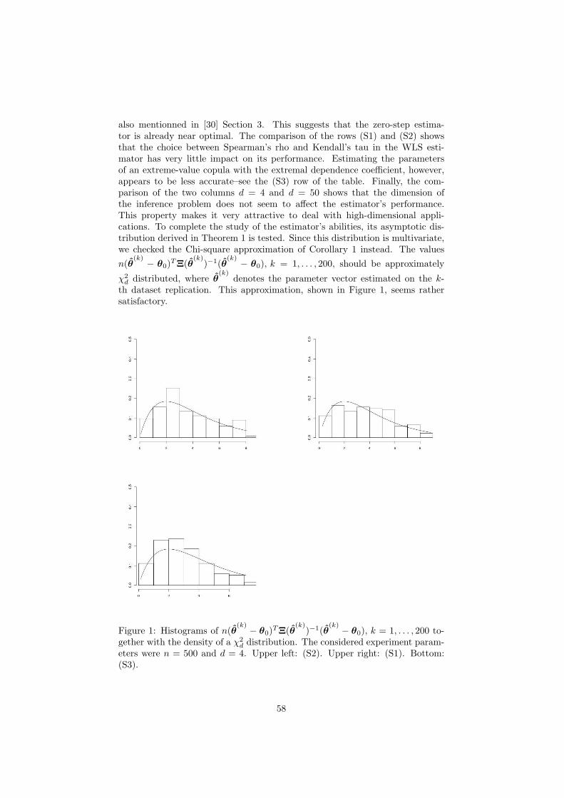
also mentionned in [30] Section 3. This suggests that the zero-step estima-tor is already near optimal. The comparison of the rows (S1) and (S2) showsthat the choice between Spearman’s rho and Kendall’s tau in the WLS esti-mator has very little impact on its performance. Estimating the parametersof an extreme-value copula with the extremal dependence coefficient, however,appears to be less accurate–see the (S3) row of the table. Finally, the com-parison of the two columns d = 4 and d = 50 shows that the dimension ofthe inference problem does not seem to affect the estimator’s performance.This property makes it very attractive to deal with high-dimensional appli-cations. To complete the study of the estimator’s abilities, its asymptotic dis-tribution derived in Theorem 1 is tested. Since this distribution is multivariate,we checked the Chi-square approximation of Corollary 1 instead. The values

n(θ(k) − θ0)

TΞ(θ(k)

)−1(θ(k) − θ0), k = 1, . . . , 200, should be approximately

χ2d distributed, where θ

(k)denotes the parameter vector estimated on the k-

th dataset replication. This approximation, shown in Figure 1, seems rathersatisfactory.

Figure 1: Histograms of n(θ(k) − θ0)

TΞ(θ(k)

)−1(θ(k) − θ0), k = 1, . . . , 200 to-

gether with the density of a χ2d distribution. The considered experiment param-

eters were n = 500 and d = 4. Upper left: (S2). Upper right: (S1). Bottom:(S3).

58

3.2 Measuring uncertainty for multivariate return periodsin hydrology

In hydrology, the severity and frequency of extreme events must be quantified.Such potentially dangerous events are underlain by the behavior of a randomvector (X1, . . . , Xd) distributed according to a certain distribution F with con-tinuous margins F1, . . . , Fd and copula C. Suppose that C is determined by aparameter vector θ in Θ. For a certain potentially dangerous event, define thereturn period T and the critical level p through the relationship

T =1

1−Kθ(p), (17)

where Kθ(t) = P (C(F1(X1), . . . , Fd(Xd)) ≤ t), t ∈ [0, 1], is called the Kendall’sdistribution function associated to C, see [29]. The return period can be inter-preted as the average time elapsing between two dangerous events. For instance,T = 30 years means that the event happens once every 30 years in average. Thecritical level can be viewed as a measure of how dangerous the underlying eventis. The following question naturally arises: given a certain return period, whatis the critical level of the underlying event? To answer this question, it sufficesto invert (17) to get p as a function of T :

pT (θ) = K−1θ

(1− 1/T ).

Let θ0 denote the true parameter vector and let pT = pT (θ0). The estimationof pT , or, in other words, the estimation of θ0, was performed in [8] for all thepairs of d = 3 sites in Italy (Airole, Merelli and Poggi). The parametric modelproposed for C was the extreme-value copula

C(u1, . . . , ud) =

(d∏

i=1

u1−θii

)min

i=1,...,d(uθii ), θi ∈ [0, 1], i = 1, . . . , d. (18)

As it is seen from (18), this copula has a singular component. The authorschose to base the inference on Kendall’s tau (see Example 2). For θ in [0, 1]d,Kendall’s tau coefficients are given by

τi,j(θ) =θiθj

θi + θj − θiθj, i < j. (19)

By inverting (19), one obtains

θi =1

2

(1 +

1

τ i,j+

1

τ i,k− 1

τ j,k

), (20)

where i, j, k denote the indexes of the three sites and τi,j is given by (11).Observe that this is the solution of the equation (7), and, under the light ofProposition 2 (since p = q = d = 3), we see that this estimator has the smallestasymptotic variance within the class (3). However, in [8], the asymptotic be-

havior of θ = (θ1, θ2, θ3) was not derived. This is done next, and we shall seethat it allows to quantify the uncertainties around the critical levels.

The asymptotic normality of√n(θ − θ0) is established by applying Theo-

rem 1. It suffices to verify that assumption (A3) holds, which is easily checked

59

from (19). Hence, as n→ ∞√n(θ − θ0)

d→ N(0,Ξ), (21)

where Ξ is given by (8) and (12). Now, the derivation of the asymptotic behaviorof the critical levels is straightforward. From (21), we get by the delta-methodthat, as n→ ∞

√n(pT (θ)− pT

)d→ N(0, s2T ), (22)

with s2T = pTΞpTT , and where pT is the Jacobian of pT (·) at the true parametervalue. It follows that confidence intervals can be computed from the finite-sample approximation of (22), provided that the sample size is large enough.In [8], the critical levels in terms of return periods were reported for the threepair of sites (Airole-Merelli, Airole-Poggi and Merelli-Poggi). We added to theirfigure 95% confidence intervals for the critical levels (Figure 2).

The test based on Corollary 3 has no power to detect a wrong model in thissituation. Indeed, since D(θ) = D, the test statistic is always zero. Other testscan be performed to achieve such a task, see the original paper [8].

When studying extreme events, it is common to have only a limited amountof data. For instance, in [8], only n = 34 (multivariate) observations wereavailable. With such a small sample size, the approximation of the distribu-tion of

√n(pT (θ) − pT ) to a normal distribution may be questionable. To

assess the goodness of this approximation for small and moderate sample sizes,we carried out the following numerical experiment. N = 500 dataset of sizen were generated according to (18) with θ0 = (0.6, 0.7, 0.2). For the m-th

dataset (m = 1, . . . , N), the parameter vector estimate θ(m)

was computed. Let

sT (θ(m)

) be the asymptotic standard deviation in (22) at θ(m)

where sT (θ) is

regarded as a function of θ. The critical levels pT (θ(m)

) together with the 95%

confidence bands pT (θ(m)

)±1.96sT (θ(m)

)/√n were computed for T = 10, 20, 30.

Some of the θ(m)

did not lie in their theoretical bounds [0, 1], which led to nu-

merical difficulties for computing sT (θ(m)

). Therefore, these were dropped fromthe experiment. The results reported Table 2 show that the finite sample ap-proximation is rather good for n = 100. Even for n = 34, this approximationappears to be good for the pair Airole-Merelli. Despite these encouraging re-sults for moderate and small samples, we finish by stressing that the number

of missing outputs (recall that this happens when θ(m)

do not belong to [0, 1])were quite high: 354 and 298 over the 500 dataset replications for n = 34 andn = 100 respectively. Consequently, it would be of interest to improve theestimator (20) to reduce this vexing effect.

One can observe from Figure 2 that the curves for the pairs (Airole,Poggi)and (Merelli,Poggi) are similar comparing to that of the pair (Airole,Merelli).Hence to illustrate the use of Corollary 2, we performed the test H0 : θ1 = θ2versus H1 : θ1 6= θ2. The change of parameters µ1 := θ1 − θ2, µ2 := θ1 + θ2 andµ3 := θ3 was applied to the copula model (18). By Corollary 2, the test statisticsnµ2

1/Ξ1(0, µ2, µ3) converges in distribution to a χ21 variable. We obtained a p-

value of 95%, indicating that there is no statistical arguments against the nullhypothesis. This high p-value also suggests that this test has little power for

60

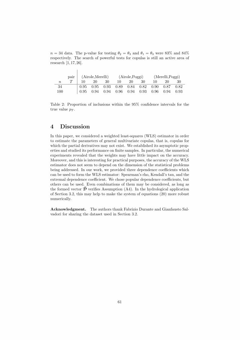
n = 34 data. The p-value for testing θ2 = θ3 and θ1 = θ3 were 83% and 84%respectively. The search of powerful tests for copulas is still an active area ofresearch [1, 17, 26].

pair (Airole,Merelli) (Airole,Poggi) (Merelli,Poggi)n T 10 20 30 10 20 30 10 20 3034 0.95 0.95 0.93 0.89 0.84 0.82 0.90 0.87 0.82100 0.95 0.94 0.94 0.96 0.94 0.93 0.96 0.94 0.93

Table 2: Proportion of inclusions within the 95% confidence intervals for thetrue value pT .

4 Discussion

In this paper, we considered a weighted least-squares (WLS) estimator in orderto estimate the parameters of general multivariate copulas, that is, copulas forwhich the partial derivatives may not exist. We established its asymptotic prop-erties and studied its performance on finite samples. In particular, the numericalexperiments revealed that the weights may have little impact on the accuracy.Moreover, and this is interesting for practical purposes, the accuracy of the WLSestimator does not seem to depend on the dimension of the statistical problemsbeing addressed. In our work, we provided three dependence coefficients whichcan be used to form the WLS estimator: Spearman’s rho, Kendall’s tau, and theextremal dependence coefficient. We chose popular dependence coefficients, butothers can be used. Even combinations of them may be considered, as long asthe formed vector D verifies Assumption (A4). In the hydrological applicationof Section 3.2, this may help to make the system of equations (20) more robustnumerically.

Acknowledgment. The authors thank Fabrizio Durante and Gianfausto Sal-vadori for sharing the dataset used in Section 3.2.

61

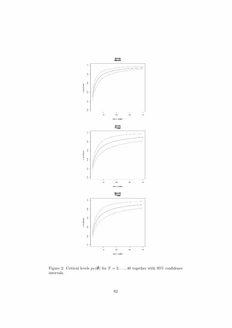
Figure 2: Critical levels pT (θ) for T = 2, . . . , 40 together with 95% confidenceintervals.

62

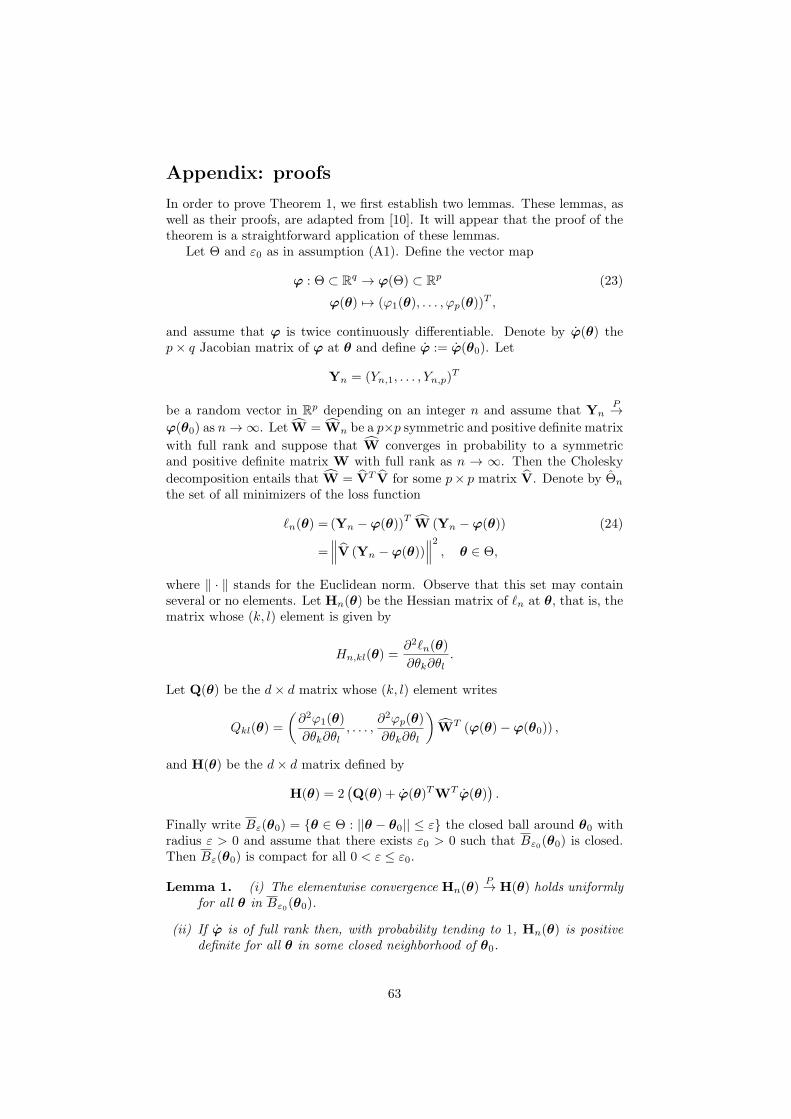
Appendix: proofs

In order to prove Theorem 1, we first establish two lemmas. These lemmas, aswell as their proofs, are adapted from [10]. It will appear that the proof of thetheorem is a straightforward application of these lemmas.

Let Θ and ε0 as in assumption (A1). Define the vector map

ϕ : Θ ⊂ Rq → ϕ(Θ) ⊂ R

p (23)

ϕ(θ) 7→ (ϕ1(θ), . . . , ϕp(θ))T ,

and assume that ϕ is twice continuously differentiable. Denote by ϕ(θ) thep× q Jacobian matrix of ϕ at θ and define ϕ := ϕ(θ0). Let

Yn = (Yn,1, . . . , Yn,p)T

be a random vector in Rp depending on an integer n and assume that Yn

P→ϕ(θ0) as n→ ∞. Let W = Wn be a p×p symmetric and positive definite matrix

with full rank and suppose that W converges in probability to a symmetricand positive definite matrix W with full rank as n → ∞. Then the Cholesky

decomposition entails that W = VT V for some p× p matrix V. Denote by Θnthe set of all minimizers of the loss function

ℓn(θ) = (Yn −ϕ(θ))TW (Yn −ϕ(θ)) (24)

=∥∥∥V (Yn −ϕ(θ))

∥∥∥2

, θ ∈ Θ,

where ‖ · ‖ stands for the Euclidean norm. Observe that this set may containseveral or no elements. Let Hn(θ) be the Hessian matrix of ℓn at θ, that is, thematrix whose (k, l) element is given by

Hn,kl(θ) =∂2ℓn(θ)

∂θk∂θl.

Let Q(θ) be the d× d matrix whose (k, l) element writes

Qkl(θ) =

(∂2ϕ1(θ)

∂θk∂θl, . . . ,

∂2ϕp(θ)

∂θk∂θl

)WT (ϕ(θ)−ϕ(θ0)) ,

and H(θ) be the d× d matrix defined by

H(θ) = 2(Q(θ) + ϕ(θ)TWT ϕ(θ)

).

Finally write Bε(θ0) = {θ ∈ Θ : ||θ − θ0|| ≤ ε} the closed ball around θ0 withradius ε > 0 and assume that there exists ε0 > 0 such that Bε0(θ0) is closed.Then Bε(θ0) is compact for all 0 < ε ≤ ε0.

Lemma 1. (i) The elementwise convergence Hn(θ)P→ H(θ) holds uniformly

for all θ in Bε0(θ0).

(ii) If ϕ is of full rank then, with probability tending to 1, Hn(θ) is positivedefinite for all θ in some closed neighborhood of θ0.

63

Proof. (i) It is easily seen that Hn(θ) = 2(ϕ(θ)TWT ϕ(θ) +Qn(θ)

)where

Qn(θ) is a [d× d] matrix such that its (k, l) element is given by

Qn,kl(θ) =

(∂2ϕ1(θ)

∂θk∂θl, . . . ,

∂2ϕp(θ)

∂θk∂θl

)WT (ϕ(θ)−Yn) .

Let Wji denote the element of W in the j-th row and i-th column. For all θ inBε0(θ0),

|Hn,kl(θ)−Hkl(θ)| = 2

∣∣∣∣∣∣

p∑

i,j=1

∂2ϕi(θ)

∂θk∂θlWji (ϕj(θ0)− Yn,j)

∣∣∣∣∣∣

≤p∑

i,j=1

∣∣∣∣∂2ϕi(θ)

∂θk∂θl

∣∣∣∣ |Wji| |ϕj(θ0)− Yn,j |

≤ constant×p∑

i,j=1

|Wji| |ϕj(θ0)− Yn,j | ,

the last inequality holding because, since the second order derivatives of the ϕi’sare continuous on the closed and thus compact set Bε0(θ0), they are uniformlybounded by some constant on this set. Therefore, as n→ ∞,

supθ∈Bε0

(θ0)

|Hn,kl(θ)−Hkl(θ)| ≤ constant×p∑

i,j=1

|Wji| |ϕj(θ0)− Yn,j | P→ 0,

which follows from the weak consistency of Yn and W.(ii) Notice that since ϕ is of full rank, H(θ0) is positive definite. Hence

for every x 6= 0 ∈ Rq, the map θ 7→ xTH(θ)x is continuous and one can

choose a sufficiently small ε(x) > 0 such that there exists δ(x) > 0 for whichxTH(θ)x ≥ xTH(θ0)x − ε(x) > 0. In other words, ∀x ∈ R

q, ∃δ(x) > 0 :‖θ − θ0‖ ≤ δ(x) =⇒ xTH(θ)x > 0. Define 0 ≤ δ := infx∈Rq {δ(x)}. Then forall θ in Θ, ‖θ − θ0‖ ≤ δ implies xTH(θ)x > 0 for all x 6= 0. We have shownthat H(θ) is positive definite on Bδ(θ0). Now define

Aij =

{sup

θ∈Bε0 (θ0)

|Hn,ij(θ)−Hij(θ)| ≤ infx∈Rq,x 6=0, θ∈Bδ(θ0)

xTH(θ)x

2∑qi,j=1 |xixj |

}

and put A =⋂i,j

Aij . On the event A, for all x 6= 0 and for all θ in Bε0(θ0), we

have

∣∣xT (H(θ)−Hn(θ))x∣∣ ≤

q∑

i,j=1

|xixj | infx∈Rq,x 6=0, θ∈Bδ(θ0)

xTH(θ)x

2∑qi,j=1 |xixj |

≤ infθ∈Bδ(θ0)

xTH(θ)x

2.

If, moreover, θ ∈ Bδ(θ0), then

xTHn(θ)x ≥ xTH(θ)x

2> 0

64

because H(θ) is positive definite on Bδ(θ0). Hence on A and for all θ inBδ(θ0)

⋂Bε0(θ0), the matrix Hn(θ) is positive definite. By (i), P (A) → 1

as n→ ∞, which concludes the proof.

Lemma 2. (i) If ϕ in (23) is an homeomorphism, then for all ε such that0 < ε ≤ ε0, as n→ ∞,

P[Θn 6= ∅ and Θn ⊂ Bε(θ0)

]→ 1.

(ii) If, moreover, ϕ(θ0) is of full rank then as n→ ∞,

P[card Θ = 1

]→ 1,

where card denotes the cardinal of a set. Define θ to be the unique element

of Θ if card Θ = 1, and any arbitrary point otherwise. Then θP→ θ0 as

n→ ∞.

(iii) If in addition to the assumptions of (i) and (ii)

√n(Yn −ϕ(θ0))

d→ Np(0,Σ)

then

√n(θ − θ0)

d→ Nq

(0,(ϕTWϕ

)−1ϕTWΣWϕ

(ϕTWϕ

)−1)

Proof. (i) Let 0 < ε < ε0. Since ϕ is a homeomorphism and W has

full rank, Vϕ is also homeomorphism. Hence there exists δ > 0 such thatθ ∈ Θ and ‖V (ϕ(θ)−ϕ(θ0)) ‖ ≤ δ imply ‖θ − θ0‖ ≤ ε. Thus for every

θ ∈ Θ with ‖θ − θ0‖ > ε we have ‖V (ϕ(θ)−ϕ(θ0)) ‖ > δ. On the event

An = {‖V (ϕ(θ0)−Yn) ‖ ≤ δ/2} and for θ outside θ ∈ Bε(θ0), the inequality

‖V (ϕ(θ)−ϕ(θ0)) ‖ ≤ ‖V (ϕ(θ)−Yn) ‖+ ‖V (Yn −ϕ(θ0)) ‖

implies

‖V (ϕ(θ)−Yn) ‖ ≥ ‖V (ϕ(θ)−ϕ(θ0)) ‖ − ‖V (Yn −ϕ(θ0)) ‖> δ − δ/2

= δ/2

≥ ‖V (Yn −ϕ(θ0)) ‖.

Therefore

minθ∈Bε(θ0)

‖V (Yn −ϕ(θ)) ‖ ≤ infθ/∈Bε(θ0)

‖V (Yn −ϕ(θ)) ‖,

where in the left hand side the minimum is attained because Bε(θ0) is compact.

By consistency of Yn and W, we have P (An) → 1. It follows that the event{Θn 6= ∅ and Θn ⊂ Bε(θ0)

}has probability tending to 1.

65

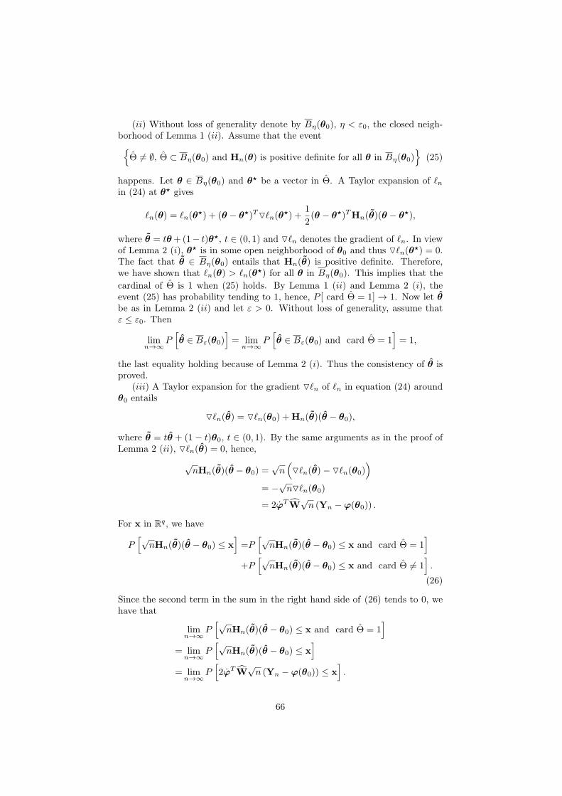
(ii) Without loss of generality denote by Bη(θ0), η < ε0, the closed neigh-borhood of Lemma 1 (ii). Assume that the event{Θ 6= ∅, Θ ⊂ Bη(θ0) and Hn(θ) is positive definite for all θ in Bη(θ0)

}(25)

happens. Let θ ∈ Bη(θ0) and θ⋆ be a vector in Θ. A Taylor expansion of ℓnin (24) at θ⋆ gives

ℓn(θ) = ℓn(θ⋆) + (θ − θ⋆)T▽ℓn(θ

⋆) +1

2(θ − θ⋆)THn(θ)(θ − θ⋆),

where θ = tθ+(1− t)θ⋆, t ∈ (0, 1) and ▽ℓn denotes the gradient of ℓn. In viewof Lemma 2 (i), θ⋆ is in some open neighborhood of θ0 and thus ▽ℓn(θ

⋆) = 0.The fact that θ ∈ Bη(θ0) entails that Hn(θ) is positive definite. Therefore,we have shown that ℓn(θ) > ℓn(θ

⋆) for all θ in Bη(θ0). This implies that the

cardinal of Θ is 1 when (25) holds. By Lemma 1 (ii) and Lemma 2 (i), theevent (25) has probability tending to 1, hence, P [ card Θ = 1] → 1. Now let θbe as in Lemma 2 (ii) and let ε > 0. Without loss of generality, assume thatε ≤ ε0. Then

limn→∞

P[θ ∈ Bε(θ0)

]= limn→∞

P[θ ∈ Bε(θ0) and card Θ = 1

]= 1,

the last equality holding because of Lemma 2 (i). Thus the consistency of θ isproved.

(iii) A Taylor expansion for the gradient ▽ℓn of ℓn in equation (24) aroundθ0 entails

▽ℓn(θ) = ▽ℓn(θ0) +Hn(θ)(θ − θ0),

where θ = tθ + (1− t)θ0, t ∈ (0, 1). By the same arguments as in the proof ofLemma 2 (ii), ▽ℓn(θ) = 0, hence,

√nHn(θ)(θ − θ0) =

√n(▽ℓn(θ)− ▽ℓn(θ0)

)

= −√n▽ℓn(θ0)

= 2ϕTW√n (Yn −ϕ(θ0)) .

For x in Rq, we have

P[√

nHn(θ)(θ − θ0) ≤ x]=P

[√nHn(θ)(θ − θ0) ≤ x and card Θ = 1

]

+P[√

nHn(θ)(θ − θ0) ≤ x and card Θ 6= 1].

(26)

Since the second term in the sum in the right hand side of (26) tends to 0, wehave that

limn→∞

P[√

nHn(θ)(θ − θ0) ≤ x and card Θ = 1]

= limn→∞

P[√

nHn(θ)(θ − θ0) ≤ x]

= limn→∞

P[2ϕTW

√n (Yn −ϕ(θ0)) ≤ x

].

66

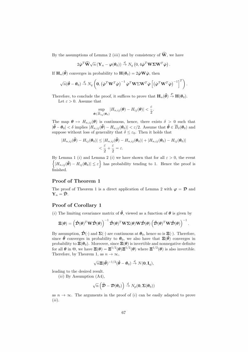
By the assumptions of Lemma 2 (iii) and by consistency of W, we have

2ϕTW√n (Yn −ϕ(θ0))

d→ Nq(0, 4ϕTWΣWT ϕ

).

If Hn(θ) converges in probability to H(θ0) = 2ϕWϕ, then

√n(θ − θ0)

d→ Nq

(0,(ϕTWT ϕ

)−1ϕTWΣWT ϕ

[(ϕTWT ϕ

)−1]T)

.

Therefore, to conclude the proof, it suffices to prove that Hn(θ)P→ H(θ0).

Let ε > 0. Assume that

supθ∈Bε0

(θ0)

|Hn,ij(θ)−Hij(θ)| <ε

2.

The map θ 7→ Hn,ij(θ) is continuous, hence, there exists δ > 0 such that

|θ− θ0| < δ implies |Hn,ij(θ)−Hn,ij(θ0)| < ε/2. Assume that θ ∈ Bδ(θ0) andsuppose without loss of generality that δ ≤ ε0. Then it holds that

|Hn,ij(θ)−Hij(θ0)| ≤ |Hn,ij(θ)−Hn,ij(θ0)|+ |Hn,ij(θ0)−Hij(θ0)|<ε

2+ε

2= ε.

By Lemma 1 (i) and Lemma 2 (i) we have shown that for all ε > 0, the event{|Hn,ij(θ)−Hij(θ0)| ≤ ε

}has probability tending to 1. Hence the proof is

finished.

Proof of Theorem 1

The proof of Theorem 1 is a direct application of Lemma 2 with ϕ = D andYn = D.

Proof of Corollary 1

(i) The limiting covariance matrix of θ, viewed as a function of θ is given by

Ξ(θ) =(D(θ)TWD(θ)

)−1

D(θ)TWΣ(θ)WD(θ)(D(θ)TWD(θ)

)−1

.

By assumption, D(·) and Σ(·) are continuous at θ0, hence so is Ξ(·). Therefore,since θ converges in probability to θ0, we also have that Ξ(θ) converges inprobability to Ξ(θ0). Moreover, since Ξ(θ) is invertible and nonnegative definite

for all θ in Θ, we have Ξ(θ) = Ξ1/2(θ)Ξ1/2(θ) where Ξ1/2(θ) is also invertible.Therefore, by Theorem 1, as n→ ∞,

√nΞ(θ)−1/2(θ − θ0)

d→ N(0, Iq),

leading to the desired result.(ii) By Assumption (A4),

√n(D −D(θ0)

)d→ Np(0,Σ(θ0))

as n → ∞. The arguments in the proof of (i) can be easily adapted to prove(ii).

67

Proof of Corollary 2

The proof of Corollary 2 is similar to that of Corollary 1 (i).

Proof of Corollary 3

Note D0 := D(θ0) and write

D(θ)− D = D(θ)−D0 +D0 − D. (27)

A Taylor expansion yields

D(θ)−D0 =˜D(θ − θ0) (28)

where˜D := D(θ) with θ being a vector between θ and θ0. Substitute (28)

into (27) to get

D(θ)− D =˜D(θ − θ0) +D0 − D. (29)

From (28), we have

θ − θ0 = (˜D

T ˜D)−1 ˜

D

T

(D(θ)−D0). (30)

Substitute (30) into (29) to obtain

D(θ)− D =˜D

(˜D

T ˜D

)−1 ˜D

T (D(θ)−D0

)+(D0 − D

).

Since

D(θ)−D0 =(D(θ)− D

)+(D −D0

),

we have(Ip − ˜

D

(˜D

T ˜D

)−1 ˜D

T)(

D(θ)− D

)=

(Ip − ˜

D

(˜D

T ˜D

)−1 ˜D

T)(

D0 − D

).

Take θ ∈ Θ and define A = A(θ) := D(θ)(D(θ)T D(θ)

)−1

D(θ)T . Like-

wise, write A := A(θ). By Assumption (A4) and because D is continuouslydifferentiable, as n→ ∞,

(Ip − A)√n(D(θ)− D

)d→ N (0, (Ip −A0)Σ(Ip −A0)) (31)

where A0 := D0

(DT

0 D0

)−1

DT

0 and D0 := D(θ0). Now write Ip − A0 =

Q∆QT , where QQT = QTQ = Ip, and ∆ = diag(1, . . . , 1, 0, . . . , 0) with thenumber of ones being equal to k. Pre-multiply the left member of (31) by

QT [(Ip −A0)Σ(Ip −A0) +A0]−1/2

=[∆QTΣQ∆+ Ip −∆

]−1/2QT ,

Note that the matrix between the brackets in the right-hand side is bloc-diagonal. It then can be verified that the limit normal distribution in the rightmember will have covariance matrix ∆, entailing

n(D(θ)− D

)T(Ip − A)[(Ip −A0)Σ(Ip −A0) +A0]

−1(Ip − A)(D(θ)− D

)→ χ2

k.

Put A := A(θ). Since A → A0 in probability, we can replace A and A0 by A

to get the desired result.

68

Proof of Proposition 1

(This proof is adapted from [22] but is given here for sake of completeness.)Without loss of generality, assume that W⋆

D = αΣ−1D for some scalar α.

Let θ = θ(W) and note θ(W⋆) the estimator for which W = W⋆. Denote byΞ(W) and Ξ(W⋆) the associated limiting covariance matrices of Theorem 1.We have

Ξ(W)−Ξ(W⋆)

=(DTWD

)−1

DTWΣWD

(DTWD

)−1

− α(DTW⋆

D

)−1

=(DTWD

)−1(DTWΣWD − D

TWDα

(DTW⋆

D

)−1

DTWD

)(DTWD

)−1

=(DTWD

)−1

DTWΣ1/2

(Ip −Σ−1/2

Dα(DTW⋆

D

)−1

DTΣ−1/2

)Σ1/2WD

(DTWD

)−1

,

where Σ1/2 is the symmetric and invertible matrix such that Σ = Σ1/2Σ1/2.

Write A = Σ−1/2Dα

(DTW⋆

D

)−1

DTΣ−1/2. Note that A is idempotent,

that is, A2 = A. Indeed,

A2 =Σ−1/2Dα

(DTW⋆

D

)−1

DTΣ−1

Dα(DTW⋆

D

)−1

DTΣ−1/2

=Σ−1/2Dα

(DTW⋆

D

)−1

DTW⋆

D

(DTW⋆

D

)−1

DTΣ−1/2

=Σ−1/2Dα

(DTW⋆

D

)−1

DTΣ−1/2

=A.

Hence Ip −A is idempotent as well and therefore

Ξ(W)−Ξ(W⋆) =(DTWD

)−1

DTWΣ1/2(Ip −A)(Ip −A)Σ1/2WD

(DTWD

)−1

which is easily seen to be nonnegative definite.

Proof of Proposition 2

The gradient of the loss function (3) is equal to 0 if and only if

DTW(D(θ)− D

)= 0.

But since D is of full rank and p = q, the kernel of DTis null, hence

W(D(θ)− D

)= 0.

The fact that W is of full rank concludes the proof.

69

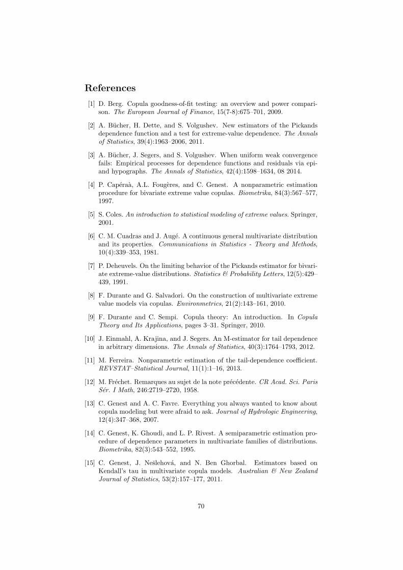
References

[1] D. Berg. Copula goodness-of-fit testing: an overview and power compari-son. The European Journal of Finance, 15(7-8):675–701, 2009.

[2] A. Bucher, H. Dette, and S. Volgushev. New estimators of the Pickandsdependence function and a test for extreme-value dependence. The Annalsof Statistics, 39(4):1963–2006, 2011.

[3] A. Bucher, J. Segers, and S. Volgushev. When uniform weak convergencefails: Empirical processes for dependence functions and residuals via epi-and hypographs. The Annals of Statistics, 42(4):1598–1634, 08 2014.

[4] P. Caperaa, A.L. Fougeres, and C. Genest. A nonparametric estimationprocedure for bivariate extreme value copulas. Biometrika, 84(3):567–577,1997.

[5] S. Coles. An introduction to statistical modeling of extreme values. Springer,2001.

[6] C. M. Cuadras and J. Auge. A continuous general multivariate distributionand its properties. Communications in Statistics - Theory and Methods,10(4):339–353, 1981.

[7] P. Deheuvels. On the limiting behavior of the Pickands estimator for bivari-ate extreme-value distributions. Statistics & Probability Letters, 12(5):429–439, 1991.

[8] F. Durante and G. Salvadori. On the construction of multivariate extremevalue models via copulas. Environmetrics, 21(2):143–161, 2010.

[9] F. Durante and C. Sempi. Copula theory: An introduction. In CopulaTheory and Its Applications, pages 3–31. Springer, 2010.

[10] J. Einmahl, A. Krajina, and J. Segers. An M-estimator for tail dependencein arbitrary dimensions. The Annals of Statistics, 40(3):1764–1793, 2012.

[11] M. Ferreira. Nonparametric estimation of the tail-dependence coefficient.REVSTAT–Statistical Journal, 11(1):1–16, 2013.

[12] M. Frechet. Remarques au sujet de la note precedente. CR Acad. Sci. ParisSer. I Math, 246:2719–2720, 1958.

[13] C. Genest and A. C. Favre. Everything you always wanted to know aboutcopula modeling but were afraid to ask. Journal of Hydrologic Engineering,12(4):347–368, 2007.

[14] C. Genest, K. Ghoudi, and L. P. Rivest. A semiparametric estimation pro-cedure of dependence parameters in multivariate families of distributions.Biometrika, 82(3):543–552, 1995.

[15] C. Genest, J. Neslehova, and N. Ben Ghorbal. Estimators based onKendall’s tau in multivariate copula models. Australian & New ZealandJournal of Statistics, 53(2):157–177, 2011.

70

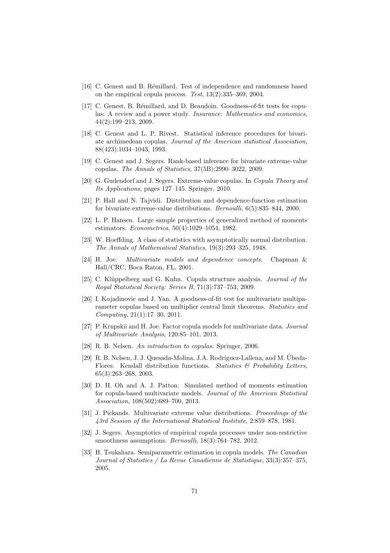
[16] C. Genest and B. Remillard. Test of independence and randomness basedon the empirical copula process. Test, 13(2):335–369, 2004.

[17] C. Genest, B. Remillard, and D. Beaudoin. Goodness-of-fit tests for copu-las: A review and a power study. Insurance: Mathematics and economics,44(2):199–213, 2009.

[18] C. Genest and L. P. Rivest. Statistical inference procedures for bivari-ate archimedean copulas. Journal of the American statistical Association,88(423):1034–1043, 1993.

[19] C. Genest and J. Segers. Rank-based inference for bivariate extreme-valuecopulas. The Annals of Statistics, 37(5B):2990–3022, 2009.

[20] G. Gudendorf and J. Segers. Extreme-value copulas. In Copula Theory andIts Applications, pages 127–145. Springer, 2010.

[21] P. Hall and N. Tajvidi. Distribution and dependence-function estimationfor bivariate extreme-value distributions. Bernoulli, 6(5):835–844, 2000.

[22] L. P. Hansen. Large sample properties of generalized method of momentsestimators. Econometrica, 50(4):1029–1054, 1982.

[23] W. Hoeffding. A class of statistics with asymptotically normal distribution.The Annals of Mathematical Statistics, 19(3):293–325, 1948.

[24] H. Joe. Multivariate models and dependence concepts. Chapman &Hall/CRC, Boca Raton, FL, 2001.

[25] C. Kluppelberg and G. Kuhn. Copula structure analysis. Journal of theRoyal Statistical Society: Series B, 71(3):737–753, 2009.

[26] I. Kojadinovic and J. Yan. A goodness-of-fit test for multivariate multipa-rameter copulas based on multiplier central limit theorems. Statistics andComputing, 21(1):17–30, 2011.

[27] P. Krupskii and H. Joe. Factor copula models for multivariate data. Journalof Multivariate Analysis, 120:85–101, 2013.

[28] R. B. Nelsen. An introduction to copulas. Springer, 2006.

[29] R. B. Nelsen, J. J. Quesada-Molina, J.A. Rodrıguez-Lallena, and M. Ubeda-Flores. Kendall distribution functions. Statistics & Probability Letters,65(3):263–268, 2003.

[30] D. H. Oh and A. J. Patton. Simulated method of moments estimationfor copula-based multivariate models. Journal of the American StatisticalAssociation, 108(502):689–700, 2013.

[31] J. Pickands. Multivariate extreme value distributions. Proceedings of the43rd Session of the International Statistical Institute, 2:859–878, 1981.

[32] J. Segers. Asymptotics of empirical copula processes under non-restrictivesmoothness assumptions. Bernoulli, 18(3):764–782, 2012.

[33] H. Tsukahara. Semiparametric estimation in copula models. The CanadianJournal of Statistics / La Revue Canadienne de Statistique, 33(3):357–375,2005.

71

❈❤❛♣✐tr❡ ✻

❯♥❡ ❝❧❛ss❡ ❞❡ ❝♦♣✉❧❡s

♠❛♥✐❛❜❧❡ ❡t ✢❡①✐❜❧❡

▲❛ ✢❡①✐❜✐❧✐té ❡t ❧❛ ♠❛♥✐❛❜✐❧✐té ❞❡ ❝♦♣✉❧❡s ♠✉❧t✐✈❛r✐é❡s s♦♥t ❞❡✉① ♣r♦♣r✐étés❞és✐ré❡s ♠❛✐s ♣❧✉tôt ❛♥t❛❣♦♥✐st❡s✳ ❯♥❡ ❝♦♣✉❧❡ ❞♦♥♥é❡ ❡st s♦✉✈❡♥t s♦✐t ♠❛♥✐❛❜❧❡✱s♦✐t ✢❡①✐❜❧❡✱ ♠❛✐s r❛r❡♠❡♥t ❧❡s ❞❡✉① à ❧❛ ❢♦✐s✳ Pr❡♥♦♥s ❧❡s ❝♦♣✉❧❡s ❛r❝❤✐♠é❞✐❡♥♥❡s✱✈✉❡s ❞❛♥s ❧❛ ♣❛rt✐❡ ✷✳✶ ❞✉ ❝❤❛♣✐tr❡ ✷ ✿ ❡❧❧❡s s♦♥t ♠❛♥✐❛❜❧❡s ✭♦♥ ♣❡✉t ♣❛r ❡①❡♠♣❧❡❝❛❧❝✉❧❡r ❧❡✉r t❛✉ ❞❡ ❑❡♥❞❛❧❧ ❢❛❝✐❧❡♠❡♥t✮ ♠❛✐s ♣❛s ❞✉ t♦✉t ✢❡①✐❜❧❡s ✭❡❧❧❡s ♥✬♦♥tq✉✬✉♥ ♦✉ ❞❡✉① ♣❛r❛♠ètr❡s✮✳ ❆ ❧✬♦♣♣♦sé✱ ♦♥ ♣♦✉rr❛✐t ♣r❡♥❞r❡ ❧❡s ❱✐♥❡s ✭✈✉❡s ❞❛♥s❧❛ ♣❛rt✐❡ ✷✳✸✮✱ q✉✐ s♦♥t ❡①trê♠❡♠❡♥t ✢❡①✐❜❧❡s✱ ♠❛✐s ❛✉ ♣r✐① ❞✬✉♥❡ ♠♦❞é❧✐s❛t✐♦♥❝♦♠♣❧❡①❡✳ ❈❡ s♦♥t ❧❡s ❝♦♣✉❧❡s ❡❧❧✐♣t✐q✉❡s q✉✐ ré❛❧✐s❡♥t ❧❡ ♠❡✐❧❧❡✉r ❝♦♠♣r♦♠✐s❡♥tr❡ ✢❡①✐❜✐❧✐té ❡t ♠❛♥✐❛❜✐❧✐té✳ ▲❡s ❝♦♣✉❧❡s ❡❧❧✐♣t✐q✉❡s ♦♥t ✉♥ ♥♦♠❜r❡ ❞❡ ♣❛r❛✲♠ètr❡s ❞❡ ❧✬♦r❞r❡ ❞❡ d2 ✭r❛♣♣❡❧♦♥s q✉❡ d ❡st ❧❡ ♥♦♠❜r❡ ❞❡ ✈❛r✐❛❜❧❡s✮✱ ♠❛✐s ♦♥ ♣❡✉tr❡♥❞r❡ ❝❡ ♥♦♠❜r❡ ❜❡❛✉❝♦✉♣ ♣❧✉s ♣❡t✐t ❡♥ ✐♠♣♦s❛♥t ✉♥❡ str✉❝t✉r❡ à ❧❛ ♠❛tr✐❝❡❞❡ ❝♦rré❧❛t✐♦♥✳ ▲❡ ♣r✐♥❝✐♣❛❧ r❡♣r♦❝❤❡ ❢❛✐t ❛✉① ❝♦♣✉❧❡s ❡❧❧✐♣t✐q✉❡s rés✐❞❡ ❞❛♥s ❧❡❢❛✐t q✉❡ ❧❡✉r q✉❡✉❡s ❞❡ ❞✐str✐❜✉t✐♦♥ s✉♣ér✐❡✉r❡s ❡t ✐♥❢ér✐❡✉r❡s s♦♥t s②♠étr✐q✉❡s✳❈❡s ❝♦♣✉❧❡s ♦♥t été ✈✉❡s ❞❛♥s ❧❛ ♣❛rt✐❡ ✷✳✹ ❝❤❛♣✐tr❡ ✷✳

❉❛♥s ❝❡ ❝❤❛♣✐tr❡✱ ♥♦✉s ❝♦♥str✉✐s♦♥s ✉♥❡ ❝❧❛ss❡ ✭❛♣♣❡❧é❡ ❝❧❛ss❡ ❋❉●✮ ❞❡ ❝♦✲♣✉❧❡s ♠✉❧t✐✈❛r✐é❡s t♦✉t à ❢❛✐t ✐♥tér❡ss❛♥t❡ ❡♥ ❝❡❝✐ q✉✬❡❧❧❡ ❛❧❧✐❡ à ❧❛ ❢♦✐s ✢❡①✐❜✐❧✐té❡t ♠❛♥✐❛❜✐❧✐té✳ ❙❛ ❝♦♥str✉❝t✐♦♥ ❡st très s✐♠♣❧❡ ✿ ❡❧❧❡ ♥❡ ♥é❝❡ss✐t❡ r✐❡♥ ❞✬❛✉tr❡q✉❡ ❞❡ s❡ ❞♦♥♥❡r U0, U1, . . . , Ud ❞❡s ✈❛r✐❛❜❧❡s ❛❧é❛t♦✐r❡s ❞✐str✐❜✉é❡s s❡❧♦♥ ✉♥❡ ❧♦✐✉♥✐❢♦r♠❡ st❛♥❞❛r❞✱ ❡t t❡❧❧❡s q✉❡ ✭✐✮ ❧❡s Ui s♦♥t ✐♥❞é♣❡♥❞❛♥t❡s s❛❝❤❛♥t ❧❛ ✈❛r✐❛❜❧❡U0✱ ❡t ✭✐✐✮ ❧❡ ❝♦✉♣❧❡ (U0, Ui) ∼ Cfi ≡ C0i ❡st ❞✐str✐❜✉é s❡❧♦♥ ✉♥❡ ❝♦♣✉❧❡ ❞❡ ❧❛❝❧❛ss❡ ❞❡ ❉✉r❛♥t❡ ✭✈✉❡ ❞❛♥s ❧❛ ♣❛rt✐❡ ✶✳✸✳✷✮ ♣♦✉r ❝❤❛q✉❡ ✐♥❞✐❝❡ i✳ ❊♥ ✉t✐❧✐s❛♥t ❧❛♣r♦♣r✐été ❞✬✐♥❞é♣❡♥❞❛♥❝❡ ❝♦♥❞✐t✐♦♥♥❡❧❧❡✱ ❧❛ ❧♦✐ ❥♦✐♥t❡ C ❞❡ (U1, . . . , Ud) s✬é❝r✐ttrès ❢❛❝✐❧❡♠❡♥t ❝♦♠♠❡

C(u1, . . . , ud) =

∫ 1

0

C1|0(u1|u0) . . . Cd|0(ud|u0) du0, ✭✻✳✶✮

♦ù Ci|0(ui|u0) ❡st ❧❛ ❧♦✐ ❝♦♥❞✐t✐♦♥♥❡❧❧❡ ❞❡ Ui s❛❝❤❛♥t U0 = u0✳ ❊♥ t✐r❛♥t ♣r♦✜t❞❡ ❧❛ ❢♦r♠❡ ❞❡ ❧❛ ❝♦♣✉❧❡ ❞❡ ❉✉r❛♥t❡✱ r❛♣♣❡❧é❡ ❝✐✲❞❡ss♦✉s✱

C0i(u0, ui) = min(u0, ui)fi(max(u0, ui)),

♦ù fi ❡st ❧❡ ❣é♥ér❛t❡✉r ❞❡ ❧❛ ❝♦♣✉❧❡✱ ♥♦✉s ♣♦✉✈♦♥s ♠ê♠❡ ❝❛❧❝✉❧❡r ❧✬✐♥té❣r❛❧❡ ✭✻✳✶✮❡t ♦❜t❡♥✐r ✉♥❡ ❡①♣r❡ss✐♦♥ ❡①♣❧✐❝✐t❡ ❞❡ ❧❛ ❝♦♣✉❧❡✳ ❊♥ ♣❛rt✐❝✉❧✐❡r✱ ❧❡s ♠❛r❣❡s ❛♣✲♣❛rt✐❡♥♥❡♥t t♦✉❥♦✉rs à ❧❛ ❝❧❛ss❡ ❞❡ ❉✉r❛♥t❡✳ ❊❣❛❧❡♠❡♥t✱ ❡t ❝✬❡st très ✐♥tér❡ss❛♥t✱

✼✷

♦♥ ♣❡✉t ♦❜t❡♥✐r t♦✉t❡s ❧❡s ❝♦♠❜✐♥❛✐s♦♥s ❞❡ ❞é♣❡♥❞❛♥❝❡ ❞❡ q✉❡✉❡ ✐♥❢ér✐❡✉r❡s ❡ts✉♣ér✐❡✉r❡s✳ P❛r ❡①❡♠♣❧❡✱ ❧❡s ♠❛r❣❡s ❜✐✈❛r✐é❡s ♣❡✉✈❡♥t êtr❡ ❞é♣❡♥❞❛♥t❡s ❞❛♥s❧❛ q✉❡✉❡ s✉♣ér✐❡✉r❡✱ ♠❛✐s ✐♥❞é♣❡♥❞❛♥t❡s ❞❛♥s ❧❛ q✉❡✉❡ ✐♥❢ér✐❡✉r❡✱ ♦✉ ❧✬✐♥✈❡rs❡✱♦✉ ❞é♣❡♥❞❛♥t❡s ❞❛♥s ❧❡s ❞❡✉① q✉❡✉❡s✳ ▲❛ ❝❧❛ss❡ ❋❉● ♣rés❡♥t❡ ❛✉ss✐ ✉♥ ✐♥térêt♣♦✉r ré❛❧✐s❡r ✉♥❡ ❛♥❛❧②s❡ st❛t✐st✐q✉❡ ❞❡ ✈❛❧❡✉rs ❡①trê♠❡s✱ ❝♦♠♠❡ ♣❛r ❡①❡♠♣❧❡ét✉❞✐❡r ❧❛ ❞✐str✐❜✉t✐♦♥ st❛t✐st✐q✉❡ ❞❡s ♠❛①✐♠❛ ❞✬✉♥ é❝❤❛♥t✐❧❧♦♥✱ ❝❛r ✐❧ ❡st ♣♦s✲s✐❜❧❡ ❞❡ ❝❛❧❝✉❧❡r ❡①♣❧✐❝✐t❡♠❡♥t ❧❡s ❝♦♣✉❧❡s ❞❡s ✈❛❧❡✉rs ❡①trê♠❡s ❛ss♦❝✐é❡s ❛✉①❝♦♣✉❧❡s ❋❉●✳ ❉❛♥s ❧✬❛rt✐❝❧❡ ♣rés❡♥té ❝✐✲❞❡ss♦✉s✱ ✉♥❡ ✐❧❧✉str❛t✐♦♥ s✉r ✉♥ ❥❡✉❞❡ ❞♦♥♥é❡s ré❡❧❧❡s t✐ré ❞❡ ❧✬❤②❞r♦❧♦❣✐❡ ❡st ❢♦✉r♥✐❡ ✿ ❞❡s ♥✐✈❡❛✉① ❝r✐t✐q✉❡s ❛s✲s♦❝✐és à ❞❡s é✈è♥❡♠❡♥ts ❤②❞r♦♠étr✐q✉❡s ❡①trê♠❡s s♦♥t ❡st✐♠és✳ ▲✬❛rt✐❝❧❡ ♣ré✲s❡♥té ❝✐✲❞❡ss♦✉s ❛ été s♦✉♠✐s ♣♦✉r ♣✉❜❧✐❝❛t✐♦♥✱ ❡t ❡st ❞✐s♣♦♥✐❜❧❡ à ❧✬❛❞r❡ss❡❤tt♣✿✴✴❤❛❧✳❛r❝❤✐✈❡s✲♦✉✈❡rt❡s✳❢r✴❤❛❧✲✵✵✾✼✾✶✹✼✳

✼✸

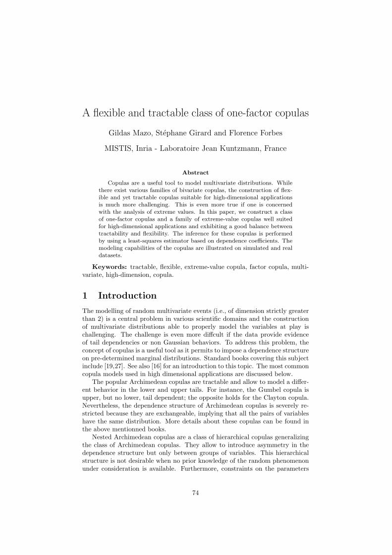
A flexible and tractable class of one-factor copulas

Gildas Mazo, Stephane Girard and Florence Forbes

MISTIS, Inria - Laboratoire Jean Kuntzmann, France

Abstract

Copulas are a useful tool to model multivariate distributions. While

there exist various families of bivariate copulas, the construction of flex-

ible and yet tractable copulas suitable for high-dimensional applications

is much more challenging. This is even more true if one is concerned

with the analysis of extreme values. In this paper, we construct a class

of one-factor copulas and a family of extreme-value copulas well suited

for high-dimensional applications and exhibiting a good balance between

tractability and flexibility. The inference for these copulas is performed

by using a least-squares estimator based on dependence coefficients. The

modeling capabilities of the copulas are illustrated on simulated and real

datasets.

Keywords: tractable, flexible, extreme-value copula, factor copula, multi-variate, high-dimension, copula.

1 Introduction

The modelling of random multivariate events (i.e., of dimension strictly greaterthan 2) is a central problem in various scientific domains and the constructionof multivariate distributions able to properly model the variables at play ischallenging. The challenge is even more diffcult if the data provide evidenceof tail dependencies or non Gaussian behaviors. To address this problem, theconcept of copulas is a useful tool as it permits to impose a dependence structureon pre-determined marginal distributions. Standard books covering this subjectinclude [19,27]. See also [16] for an introduction to this topic. The most commoncopula models used in high dimensional applications are discussed below.

The popular Archimedean copulas are tractable and allow to model a differ-ent behavior in the lower and upper tails. For instance, the Gumbel copula isupper, but no lower, tail dependent; the opposite holds for the Clayton copula.Nevertheless, the dependence structure of Archimedean copulas is severely re-stricted because they are exchangeable, implying that all the pairs of variableshave the same distribution. More details about these copulas can be found inthe above mentionned books.

Nested Archimedean copulas are a class of hierarchical copulas generalizingthe class of Archimedean copulas. They allow to introduce asymmetry in thedependence structure but only between groups of variables. This hierarchicalstructure is not desirable when no prior knowledge of the random phenomenonunder consideration is available. Furthermore, constraints on the parameters

74

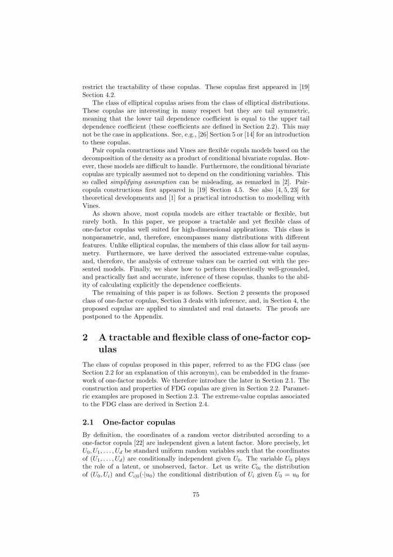
restrict the tractability of these copulas. These copulas first appeared in [19]Section 4.2.

The class of elliptical copulas arises from the class of elliptical distributions.These copulas are interesting in many respect but they are tail symmetric,meaning that the lower tail dependence coefficient is equal to the upper taildependence coefficient (these coefficients are defined in Section 2.2). This maynot be the case in applications. See, e.g., [26] Section 5 or [14] for an introductionto these copulas.

Pair copula constructions and Vines are flexible copula models based on thedecomposition of the density as a product of conditional bivariate copulas. How-ever, these models are difficult to handle. Furthermore, the conditional bivariatecopulas are typically assumed not to depend on the conditioning variables. Thisso called simplifying assumption can be misleading, as remarked in [2]. Pair-copula constructions first appeared in [19] Section 4.5. See also [4, 5, 23] fortheoretical developments and [1] for a practical introduction to modelling withVines.

As shown above, most copula models are either tractable or flexible, butrarely both. In this paper, we propose a tractable and yet flexible class ofone-factor copulas well suited for high-dimensional applications. This class isnonparametric, and, therefore, encompasses many distributions with differentfeatures. Unlike elliptical copulas, the members of this class allow for tail asym-metry. Furthermore, we have derived the associated extreme-value copulas,and, therefore, the analysis of extreme values can be carried out with the pre-sented models. Finally, we show how to perform theoretically well-grounded,and practically fast and accurate, inference of these copulas, thanks to the abil-ity of calculating explicitly the dependence coefficients.

The remaining of this paper is as follows. Section 2 presents the proposedclass of one-factor copulas, Section 3 deals with inference, and, in Section 4, theproposed copulas are applied to simulated and real datasets. The proofs arepostponed to the Appendix.

2 A tractable and flexible class of one-factor cop-ulas

The class of copulas proposed in this paper, referred to as the FDG class (seeSection 2.2 for an explanation of this acronym), can be embedded in the frame-work of one-factor models. We therefore introduce the later in Section 2.1. Theconstruction and properties of FDG copulas are given in Section 2.2. Paramet-ric examples are proposed in Section 2.3. The extreme-value copulas associatedto the FDG class are derived in Section 2.4.

2.1 One-factor copulas

By definition, the coordinates of a random vector distributed according to aone-factor copula [22] are independent given a latent factor. More precisely, letU0, U1, . . . , Ud be standard uniform random variables such that the coordinatesof (U1, . . . , Ud) are conditionally independent given U0. The variable U0 playsthe role of a latent, or unobserved, factor. Let us write C0i the distributionof (U0, Ui) and Ci|0(·|u0) the conditional distribution of Ui given U0 = u0 for

75

i = 1, . . . , d. It is easy to see that the distribution of (U1, . . . , Ud), called aone-factor copula, is given by

C(u1, . . . , ud) =

∫ 1

0

C1|0(u1|u0) . . . Cd|0(ud|u0) du0. (1)

The copulas C0i are called the linking copulas because they link the factor U0

to the variables of interest Ui. The one-factor model has many advantages toaddress high dimensional problems. We recall and briefly discuss them below.

Nonexchangeability. The one-factor model is nonexchangeable. Recall thata copula C is said to be exchangeable if C(u1, . . . , ud) = C(uπ(1), . . . , uπ(d)) forany permutation π of (1, . . . , d). This means in particular that all the bivari-ate marginal distributions are equal to each other. For example, Archimedeancopulas are exchangeable copulas. Needless to say, this assumption may be toostrong in practice.

Parsimony. The one-factor model is parsimonious. Indeed, only d linkingcopulas are involved in the construction of the one-factor model, and since theyare typically governed by one parameter, the number of parameters in total isno more than d, which increases only linearly with the dimension. Parsimonyis more and more desirable as the dimension increases.

Random generation. The conditional independence property of the one fac-tor model allows to easily generate data (U1, . . . , Ud) from this copula.

1 Generate U0, V1, . . . , Vd independent standard uniform random variables.

2 For i = 1, . . . , d, put Ui = C−1i|0 (Vi|U0) where V 7→ C−1

i|0 (V |U0) denotes the

inverse of V 7→ Ci|0(V |U0).

Dependence properties of the one-factor model have been studied in [22]. Theauthors investigated how positive dependence properties of the linking copulasextend to the bivariate margins

Cij(ui, uj) := C(1, . . . , 1, ui, 1, . . . , 1, uj , 1, . . . , 1).

These properties included positive quadrant dependence, increasing in the con-cordance ordering, stochastic increasing, and tail dependence. For details aboutthese dependence concepts, see [19] Section 2. The copulas proposed in thispaper, presented in Section 2.2 and Section 2.4, possess simple expressions andtherefore the properties mentionned above can be made more precise.

2.2 Construction and properties of FDG copulas

The class of FDG copulas is constructed by choosing appropriate linking copulasfor the one-factor copula model (1). The class of linking copulas which servedto build the FDG copulas is referred to as the Durante class [9] of bivariatecopulas, which can also be viewed as part of the framework of [3]. The Duranteclass consists of the copulas C of the form

C(u, v) = min(u, v)f(max(u, v)), (2)

76

where f : [0, 1] → [0, 1], called the generator of C, is a differentiable and in-creasing function such that f(1) = 1 and t 7→ f(t)/t is decreasing. Hence thechoice of the acronym, FDG, which stands for “one-Factor copula with DuranteGenerators”. The advantages of taking Durante linking copulas are twofold:the integral (1) can be calculated and the resulting multivariate copula is non-parametric.

Theorem 1. Let C be defined by (1) and assume that C0i belongs to the Duranteclass (2) with given generator fi. Then

C(u1, . . . , ud) = u(1)

d∏

j=2

u(j)

∫ 1

u(d)

d∏

j=1

f ′j(x)dx+ f(1)(u(2))

d∏

j=2

f(j)(u(j))

(3)

+d∑

k=3

k−1∏

j=2

u(j)

d∏

j=k

f(j)(u(j))

∫ u(k)

u(k−1)

k−1∏

j=1

f ′(j)(x)dx

,

where u(i) := uσ(i), f(i) := fσ(i) and σ is the permutation of (1, . . . , d) such thatuσ(1) ≤ · · · ≤ uσ(d).

The particularity of the copula expression (3) is that it depends on thegenerators through their reordering underlain by the permutation σ. For in-stance, with d = 3 and u1 < u3 < u2 we have u(1) = u1, u(2) = u3, u(3) = u2,σ = {1, 3, 2} and f(1) = fσ(1) = f1, f(2) = fσ(2) = f3, f(3) = fσ(3) = f2. Thisfeature gives its flexibility to the model. Observe also that C(u1, . . . , ud) writesas u(1) multiplied by a functional of u(2), . . . , u(d), form that is similar to (2).Although the expression of a FDG copula has the merit to be explicit, it israther cumbersome. Hence, we shall continue its analysis through the prism ofits bivariate margins.

Proposition 1. Let Cij be a bivariate margin of the FDG copula (3). ThenCij belongs to the Durante class (2) with generator

fij(t) = fi(t)fj(t) + t

∫ 1

t

f ′i(x)f′j(x)dx.

In other words,

Cij(ui, uj) = Cfij (ui, uj) = min(ui, uj)fij(max(ui, uj)).

In view of Proposition 1, the FDG copula can be regarded as a multivari-ate generalization of the Durante class of bivariate copulas. In fact, such ageneralization was already proposed in the literature [11]:

Cf (u1, . . . , ud) = u(1)

d∏

i=2

f(u(i)),

where f is a generator in the usual sense of the Durante class of bivariate cop-ulas. Nonetheless, since there is only one generator to determine the wholecopula in arbitrary dimension, this generalization lacks flexibility to be used in

77

applications. This issue is overcome by the FDG copula. To illustrate this fur-ther, its pairwise dependence coefficients are given next. (Note that, since thebivariate margins of the FDG copula belong to the Durante class of bivariatecopulas, a more detailed account of their properties can be found in the orig-inal paper [9]). Recall that Spearman’s rho ρ, Kendall’s tau τ , the lower λ(L)

and upper λ(U) tail dependence coefficients of a general bivariate copula C arerespectively given by

ρ = 12

∫

[0,1]2C(u, v)dudv − 3, τ = 4

∫

[0,1]2C(u, v)dC(u, v)− 1, (4)

λ(L) = limu↓0

C(u, u)

u, and λ(U) = lim

u↑1

1− 2u+ C(u, u)

1− u.

In the case where C belongs to the Durante class with generator f , these coef-ficients are respectively given by

ρ = 12

∫ 1

0

x2f(x)dx− 3, τ = 4

∫ 1

0

xf(x)2dx− 1,

λ(L) = f(0), and λ(U) = 1− f ′(1). (5)

Hence, to get the dependence coefficients of the FDG bivariate margins, it isenough to apply the above formulas and Proposition 1. The obtained coefficientexpressions are given in Proposition 2 below.

Proposition 2. The Spearman’s rho, Kendall’s tau, the lower and upper taildependence coefficients of the FDG bivariate margins Cij are respectively givenby

ρij = 12

∫ 1

0

x2fi(x)fj(x)dx+ 3

∫ 1

0

x4f ′i(x)f′j(x)dx− 3,

τij = 4

∫ 1

0

x

(fi(x)fj(x) + x

∫ 1

x

f ′i(t)f′j(t)dt

)2

dx− 1,

λ(L)ij = λ

(L)i λ

(L)j and

λ(U)ij = λ

(U)i λ

(U)j ,

where λ(L)i := fi(0), λ

(U)i := 1− f ′i(1), i = 1, . . . , d are the lower and upper tail

dependence coefficients of the bivariate linking copulas respectively.

2.3 Examples of parametric families

Four examples of families indexed by a real parameter for the generators f1, . . . , fdare given below.

Example 1 (Cuadras-Auge generators). In (3), let

fi(t) = t1−θi , θi ∈ [0, 1]. (6)

A copula belonging to the Durante class with generator (6) gives rise to thewell known Cuadras-Auge copula with parameter θi [7]. By Proposition 1, the

78

generator for the bivariate margin Cij of the FDG copula is given by

fij(t) =

{t2−θi−θj

(1− (1−θi)(1−θj)

1−θi−θj

)+ t

(1−θi)(1−θj)1−θi−θj

if θi + θj 6= 1

t(1− (1− θ)θ log t) if θ = θj = 1− θi.

The Spearman’s rho, the lower and upper tail dependence coefficients are respec-tively given by

ρij =3θiθj

5− θi − θj, λ

(L)ij = 0 and λ

(U)ij = θiθj .

The Kendall’s tau is given by

τij =

{θiθj(θiθj+6−2(θi+θj))(θi+θj)2−8(θi+θj)+15 if θi + θj 6= 1

θ(θ−1)(θ2−θ−4)8 if θ = θi = 1− θj .

Example 2 (Frechet generators). In (3), let

fi(t) = (1− θi)t+ θi, θi ∈ [0, 1]. (7)

A copula belonging to the Durante class with generator (7) gives rise to the wellknown Frechet copula with parameter θi [15]. By Proposition 1, the generatorfor the bivariate margin Cij of the FDG copula is given by

fij(t) = (1− θiθj) t+ θiθj .

By noting that fij is of the form (7) with parameter θiθj, one can see that the bi-variate margins of the FDG copula based on Frechet generators are still Frechetcopulas. The Spearman’s rho, the lower and upper tail dependence coefficientsare respectively given by

ρij = λ(L)ij = λ

(U)ij = θiθj ,

Kendall’s tau is given by

τij =θiθj(θiθj + 2)

3.

Example 3 (Durante-sinus generators). In (3), let

fi(t) =sin(θit)

sin(θi), θi ∈ (0, π/2]. (8)

This generator was proposed in [9]. By Proposition 1, the generator for thebivariate margin Cij of the FDG copula is given by

fij(t) =sin(θit) sin(θjt)

sin(θi) sin(θj)+

tθiθj2(θ2j − θ2i ) sin(θi) sin(θj)

×{(θi + θj) [sin ((θi − θj)t) + sin (θj − θi)]

+ (θj − θi) [sin(θi + θj)− sin ((θi + θj)t)]

}if θi 6= θj , and

fij(t) =4 sin(tθ)2 + tθ (2(1− t)θ + sin(2θ)− sin(2tθ))

4 sin(θ)2if θi = θj = θ.

79

The Spearman’s rho, the lower and upper tail dependence coefficients are respec-tively given by

ρij =12(sin θi sin θj)−1

∫ 1

0

x2 sin(θix) sin(θjx) +1

4θiθjx

4 cos(θix) cos(θjx)dx− 3,

(9)

λ(L)ij =0 and λ

(U)ij =

(1− θi

tan(θi)

)(1− θj

tan(θj)

). (10)

Example 4 (Durante-exponential generators). In (3), let

fi(t) = exp

(tθi − 1

θi

), θi > 0 (11)

This generator was proposed in [9]. By Proposition 1, the generator for thebivariate margin Cij of the FDG copula is given by

fij(t) = exp

(tθi − 1

θi+tθj − 1

θj

)+ t

∫ 1

t

exp

(xθi − 1

θi+xθj − 1

θj

)xθi+θj−2dx.

The Spearman’s rho, the lower and upper tail dependence coefficients are respec-tively given by

ρij =12

∫ 1

0

exp

(xθi − 1

θi+xθj − 1

θj

)(x2 +

1

4x2+θi+θj

)dx− 3,

λ(L)ij =exp

(− 1

θi− 1

θj

), and λ

(U)ij = 0.

Remark 1. The calculation of the integral in (9) with θi = θj = π/2 showsthat for the FDG copula with Durante-sinus generators, Spearman’s rho is suchthat

0 ≤ ρij ≤3π4 − 100π2 + 840

40π2≃ 0.37.

The Spearman’s rho values for all the other models in the examples above spreadthe entire interval [0, 1].

The four examples above allow to get all possible types of tail dependencies,as shown in Table 1. The Cuadras-Auge and Durante-sinus families allow forupper but no lower tail dependence, the Durante-exponential family allows forlower but no upper tail dependence, and the Frechet family allows for both. Inthe Frechet case, furthermore, the lower and upper tail dependence coefficientsare equal: this is called tail symmetry, a property of elliptical copulas.

2.4 Extreme-value attractors associated to FDG copulas

Extreme-value copulas are theoretically well-grounded copulas to perform a sta-tistical analysis of extreme values such as maxima of random samples. Recallthat a copula C# is an extreme-value copula if there exists a copula C such that

C#(u1, . . . , ud) = limn↑∞

Cn(u1/n1 , . . . , u

1/nd ), (u1, . . . , ud) ∈ [0, 1]d, (12)

80

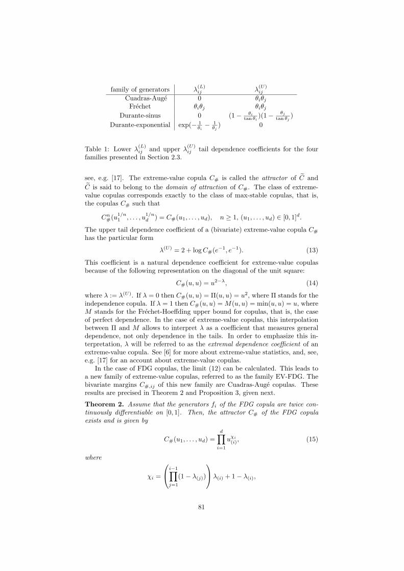
family of generators λ(L)ij λ

(U)ij

Cuadras-Auge 0 θiθjFrechet θiθj θiθj

Durante-sinus 0 (1− θitan θi

)(1− θjtan θj

)

Durante-exponential exp(− 1θi

− 1θj) 0

Table 1: Lower λ(L)ij and upper λ

(U)ij tail dependence coefficients for the four

families presented in Section 2.3.

see, e.g. [17]. The extreme-value copula C# is called the attractor of C and

C is said to belong to the domain of attraction of C#. The class of extreme-value copulas corresponds exactly to the class of max-stable copulas, that is,the copulas C# such that

Cn#(u1/n1 , . . . , u

1/nd ) = C#(u1, . . . , ud), n ≥ 1, (u1, . . . , ud) ∈ [0, 1]d.

The upper tail dependence coefficient of a (bivariate) extreme-value copula C#

has the particular form

λ(U) = 2 + logC#(e−1, e−1). (13)

This coefficient is a natural dependence coefficient for extreme-value copulasbecause of the following representation on the diagonal of the unit square:

C#(u, u) = u2−λ, (14)

where λ := λ(U). If λ = 0 then C#(u, u) = Π(u, u) = u2, where Π stands for theindependence copula. If λ = 1 then C#(u, u) =M(u, u) = min(u, u) = u, whereM stands for the Frechet-Hoeffding upper bound for copulas, that is, the caseof perfect dependence. In the case of extreme-value copulas, this interpolationbetween Π and M allows to interpret λ as a coefficient that measures generaldependence, not only dependence in the tails. In order to emphasize this in-terpretation, λ will be referred to as the extremal dependence coefficient of anextreme-value copula. See [6] for more about extreme-value statistics, and, see,e.g. [17] for an account about extreme-value copulas.

In the case of FDG copulas, the limit (12) can be calculated. This leads toa new family of extreme-value copulas, referred to as the family EV-FDG. Thebivariate margins C#,ij of this new family are Cuadras-Auge copulas. Theseresults are precised in Theorem 2 and Proposition 3, given next.

Theorem 2. Assume that the generators fi of the FDG copula are twice con-tinuously differentiable on [0, 1]. Then, the attractor C# of the FDG copulaexists and is given by

C#(u1, . . . , ud) =d∏

i=1

uχi

(i), (15)

where

χi =

i−1∏

j=1

(1− λ(j))

λ(i) + 1− λ(i),

81

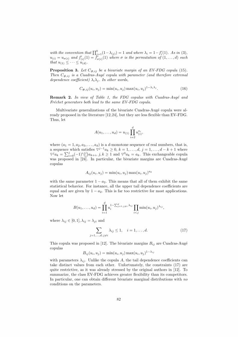
with the convention that∏0j=1(1−λ(j)) = 1 and where λi = 1−f ′i(1). As in (3),

u(i) = uσ(i) and f ′(i)(1) = f ′σ(i)(1) where σ is the permutation of (1, . . . , d) suchthat u(1) ≤ · · · ≤ u(d).

Proposition 3. Let C#,ij be a bivariate margin of an EV-FDG copula (15).Then C#,ij is a Cuadras-Auge copula with parameter (and therefore extremaldependence coefficient) λiλj. In other words,

C#,ij(ui, uj) = min(ui, uj)max(ui, uj)1−λiλj . (16)

Remark 2. In view of Table 1, the FDG copulas with Cuadras-Auge andFrechet generators both lead to the same EV-FDG copula.

Multivariate generalizations of the bivariate Cuadras-Auge copula were al-ready proposed in the literature [12,24], but they are less flexible than EV-FDG.Thus, let

A(u1, . . . , ud) = u(1)

d∏

i=2

uai(i),

where (a1 = 1, a2, a3, . . . , ad) is a d-monotone sequence of real numbers, that is,a sequence which satisfies ▽j−1ak ≥ 0, k = 1, . . . , d, j = 1, . . . , d− k + 1 where▽jak =

∑ji=0(−1)i

(ji

)ak+i, j, k ≥ 1 and ▽

0ak = ak. This exchangeable copulawas proposed in [24]. In particular, the bivariate margins are Cuadras-Augecopulas

Aij(ui, uj) = min(ui, uj)max(ui, uj)a2

with the same parameter 1− a2. This means that all of them exhibit the samestatistical behavior. For instance, all the upper tail dependence coefficients areequal and are given by 1− a2. This is far too restrictive for most applications.Now let

B(u1, . . . , ud) =d∏

i=1

u1−

∑dj=1,j 6=i λij

i

∏

i<j

min(ui, uj)λij ,

where λij ∈ [0, 1], λij = λji and

∑

j=1,...,d; j 6=i

λij ≤ 1, i = 1, . . . , d. (17)

This copula was proposed in [12]. The bivariate margins Bij are Cuadras-Augecopulas

Bij(ui, uj) = min(ui, uj)max(ui, uj)1−λij

with parameters λij . Unlike the copula A, the tail dependence coefficients cantake distinct values from each other. Unfortunately, the constraints (17) arequite restrictive, as it was already stressed by the original authors in [12]. Tosummarize, the class EV-FDG achieves greater flexibility than its competitors.In particular, one can obtain different bivariate marginal distributions with noconditions on the parameters.

82

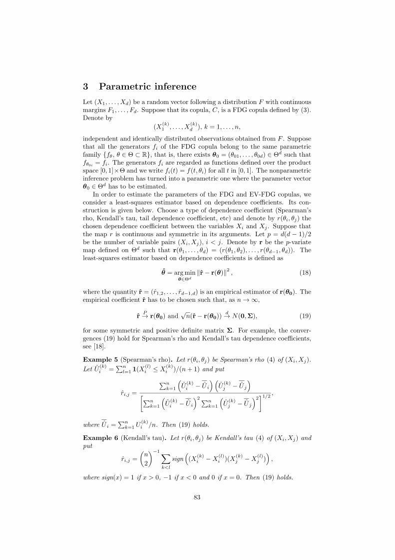
3 Parametric inference

Let (X1, . . . , Xd) be a random vector following a distribution F with continuousmargins F1, . . . , Fd. Suppose that its copula, C, is a FDG copula defined by (3).Denote by

(X(k)1 , . . . , X

(k)d ), k = 1, . . . , n,

independent and identically distributed observations obtained from F . Supposethat all the generators fi of the FDG copula belong to the same parametricfamily {fθ, θ ∈ Θ ⊂ R}, that is, there exists θ0 = (θ01, . . . , θ0d) ∈ Θd such thatfθ0i = fi. The generators fi are regarded as functions defined over the productspace [0, 1]×Θ and we write fi(t) = f(t, θi) for all t in [0, 1]. The nonparametricinference problem has turned into a parametric one where the parameter vectorθ0 ∈ Θd has to be estimated.

In order to estimate the parameters of the FDG and EV-FDG copulas, weconsider a least-squares estimator based on dependence coefficients. Its con-struction is given below. Choose a type of dependence coefficient (Spearman’srho, Kendall’s tau, tail dependence coefficient, etc) and denote by r(θi, θj) thechosen dependence coefficient between the variables Xi and Xj . Suppose thatthe map r is continuous and symmetric in its arguments. Let p = d(d − 1)/2be the number of variable pairs (Xi, Xj), i < j. Denote by r be the p-variatemap defined on Θd such that r(θ1, . . . , θd) = (r(θ1, θ2), . . . , r(θd−1, θd)). Theleast-squares estimator based on dependence coefficients is defined as

θ = argminθ∈Θd

‖r− r(θ)‖2 , (18)

where the quantity r = (r1,2, . . . , rd−1,d) is an empirical estimator of r(θ0). Theempirical coefficient r has to be chosen such that, as n→ ∞,

rP→ r(θ0) and

√n(r− r(θ0))

d→ N(0,Σ), (19)

for some symmetric and positive definite matrix Σ. For example, the conver-gences (19) hold for Spearman’s rho and Kendall’s tau dependence coefficients,see [18].

Example 5 (Spearman’s rho). Let r(θi, θj) be Spearman’s rho (4) of (Xi, Xj).

Let U(k)i =

∑nl=1 1(X

(l)i ≤ X

(k)i )/(n+ 1) and put

ri,j =

∑nk=1

(U

(k)i − U i

)(U

(k)j − U j

)

[∑nk=1

(U

(k)i − U i

)2∑nk=1

(U

(k)j − U j

)2]1/2 ,

where U i =∑nk=1 U

(k)i /n. Then (19) holds.

Example 6 (Kendall’s tau). Let r(θi, θj) be Kendall’s tau (4) of (Xi, Xj) andput

ri,j =

(n

2

)−1∑

k<l

sign((X

(k)i −X

(l)i )(X

(k)j −X

(l)j )),

where sign(x) = 1 if x > 0, −1 if x < 0 and 0 if x = 0. Then (19) holds.

83

The relationship (14) suggests that the extremal dependence coefficient canbe used to estimate the parameters of an extreme-value copula. If the marginsFi are known, (19) holds with various empirical estimators of the extremaldependence coefficient, see [25]. In the following example, an estimator proposedin [13] is used.

Example 7 (extremal dependence coefficient). Assume that C is an extreme-

value copulas and put U(k)i = Fi(X

(k)i ). Let r(θi, θj) be the extremal dependence

coefficient (4) of (Xi, Xj). Put

ri,j = 3− 1

1−∑nk=1 max(U

(k)i , U

(k)j )/n

.

Then (19) holds.

The least-squares estimator is unique with probability tending to one, con-sistent, and asymptotically normal under mild assumptions that are stated inthe following proposition, due to [25].

Proposition 4. Suppose that (19) and the following assumptions hold.

(A1) The map r is a twice continuously differentiable homeomorphism from Θd

to its image r(Θd).

(A2) The Jacobian matrix of the map r at θ0, that is,

J :=

∂r(θ)∂θ1

∣∣∣θ=θ0

∂r(θ)∂θ2

∣∣∣θ=θ0

· · · ∂r(θ)∂θd

∣∣∣θ=θ0

......

∂r(θ)∂θ1

∣∣∣θ=θ0

∂r(θ)∂θ2

∣∣∣θ=θ0

· · · ∂r(θ)∂θd

∣∣∣θ=θ0

,

is of full rank.

Then, as n → ∞, the estimator θ defined in (18) is unique with probabilitytending to one, consistent for θ0, and asymptotically normal

√n(θ − θ0)

d→ N(0,Ξ), where Ξ =(JTJ

)−1JTΣJ

(JTJ

)−1.

Remark 3. From the asymptotic normality of θ, standard arguments in math-ematical statistics yield, as n→ ∞,

n(θ − θ0)TΞ(θ)−1(θ − θ0)

d→ χ2d,

where χ2d stands for a chi-square distribution with d degrees of freedom. This

result will be useful in Section 4.1.1 to assess the accuracy of the inference.

The map r of one-factor copula models possesses the property that all of itscomponents involve the same bivariate function r. This allows to establish alemma that gives sufficient conditions for the assumptions of Proposition 4 tohold.

84

Lemma 1. (i) Define the univariate function rθj (θi) := r(θi, θj) and as-sume that it is a twice continuously differentiable homeomorphism. Letr1,2, . . . , rd−1,d be p elements of r(Θd). Define si,j(θ) := r−1

θ (ri,j) forθ ∈ Θ. Then, the function s1,3 ◦ s1,2 ◦ s2,3 has at least one fix point, thatis, the equation

s1,3 ◦ s1,2 ◦ s2,3(θ) = θ, θ ∈ Θ (20)

has at least one solution.

(ii) If, moreover, the function s1,3 ◦ s1,2 ◦ s2,3 has exactly one fix point, thatis, equation (20) has exactly one solution, then the assumptions (A1) and(A2) of Proposition 4 hold.

The fact that the extremal dependence coefficients of the EV-FDG bivariatemargins write λi,j(θ) = λ(θi)λ(θj), where

λ(θ) = 1− ∂f(t, θ)

∂t

∣∣∣t=1

, θ ∈ Θ,

allows to apply Lemma 1 and therefore to satisfy the assumptions of Proposi-tion 4.

Corollary 1. Assume that (X1, . . . , Xd) has EV-FDG (15) as copula and con-sider one of the following cases:

• The generators are Cuadras-Auge (6) and Θ = (0, 1).

• The generators are Frechet (7) and Θ = (0, 1).

• The generators are Durante-sinus (8) and Θ = (0, π/2).

Then the assumptions (A1) and (A2) of Proposition 4 hold with r(θi, θj) and r

being as in Example 7.

Remark 4. For the FDG copula with Frechet generators presented in Exam-ple 2, Spearman’s rho dependence coefficient is equal to the extremal dependencecoefficient, hence, one can also apply Lemma 1 to this copula. Therefore, also forthis model, the assumptions (A1) and (A2) of Proposition 4 hold with r(θi, θj)and r being as in Example 5.

Except for the FDG copula with Frechet generators (see Remark 4), the re-sults of Corollary 1 could not be extended to general FDG copulas because theanalytical forms of Spearman’s rho and Kendall’s tau dependence coefficientsare not as simple as the forms of the extremal dependence coefficients. Nonethe-less, we shall provide empirical evidence by means of numerical experiments inSection 4.1 that the assumptions of Proposition 4 are likely to hold.

4 Applications to simulated and real datasets

The modeling of data with (EV-)FDG copulas is illustrated through numericalexperiments in Section 4.1 and a real dataset application in Section 4.2. Inthe numerical experiments, we first provide empirical evidence to support theassumptions (A1) and (A2) of Proposition 4. We then illustrate, by fittingdata of dimension d = 50, that the proposed FDG copulas are well suited for

85

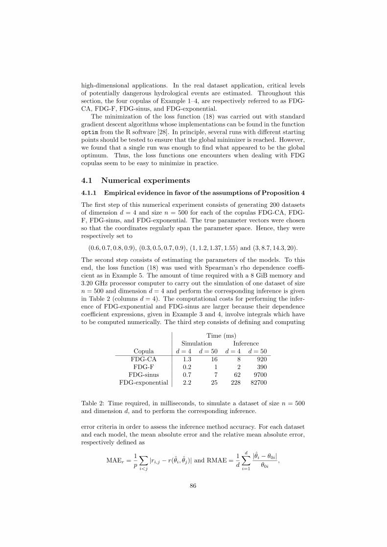
high-dimensional applications. In the real dataset application, critical levelsof potentially dangerous hydrological events are estimated. Throughout thissection, the four copulas of Example 1–4, are respectively referred to as FDG-CA, FDG-F, FDG-sinus, and FDG-exponential.

The minimization of the loss function (18) was carried out with standardgradient descent algorithms whose implementations can be found in the functionoptim from the R software [28]. In principle, several runs with different startingpoints should be tested to ensure that the global minimizer is reached. However,we found that a single run was enough to find what appeared to be the globaloptimum. Thus, the loss functions one encounters when dealing with FDGcopulas seem to be easy to minimize in practice.

4.1 Numerical experiments

4.1.1 Empirical evidence in favor of the assumptions of Proposition 4

The first step of this numerical experiment consists of generating 200 datasetsof dimension d = 4 and size n = 500 for each of the copulas FDG-CA, FDG-F, FDG-sinus, and FDG-exponential. The true parameter vectors were chosenso that the coordinates regularly span the parameter space. Hence, they wererespectively set to

(0.6, 0.7, 0.8, 0.9), (0.3, 0.5, 0.7, 0.9), (1, 1.2, 1.37, 1.55) and (3, 8.7, 14.3, 20).

The second step consists of estimating the parameters of the models. To thisend, the loss function (18) was used with Spearman’s rho dependence coeffi-cient as in Example 5. The amount of time required with a 8 GiB memory and3.20 GHz processor computer to carry out the simulation of one dataset of sizen = 500 and dimension d = 4 and perform the corresponding inference is givenin Table 2 (columns d = 4). The computational costs for performing the infer-ence of FDG-exponential and FDG-sinus are larger because their dependencecoefficient expressions, given in Example 3 and 4, involve integrals which haveto be computed numerically. The third step consists of defining and computing

Time (ms)Simulation Inference

Copula d = 4 d = 50 d = 4 d = 50FDG-CA 1.3 16 8 920FDG-F 0.2 1 2 390

FDG-sinus 0.7 7 62 9700FDG-exponential 2.2 25 228 82700

Table 2: Time required, in milliseconds, to simulate a dataset of size n = 500and dimension d, and to perform the corresponding inference.

error criteria in order to assess the inference method accuracy. For each datasetand each model, the mean absolute error and the relative mean absolute error,respectively defined as

MAEr =1

p

∑

i<j

|ri,j − r(θi, θj)| and RMAE =1

d

d∑

i=1

|θi − θ0i|θ0i

,

86

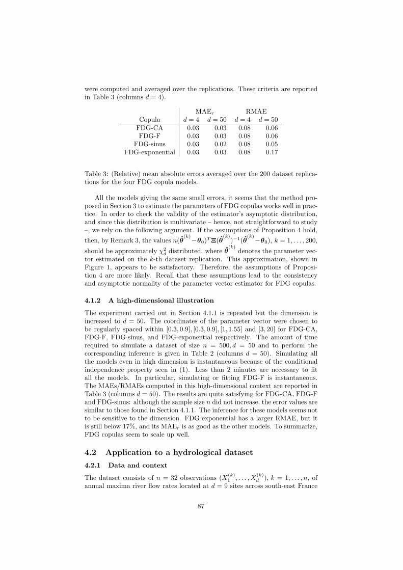
were computed and averaged over the replications. These criteria are reportedin Table 3 (columns d = 4).

MAEr RMAECopula d = 4 d = 50 d = 4 d = 50FDG-CA 0.03 0.03 0.08 0.06FDG-F 0.03 0.03 0.08 0.06

FDG-sinus 0.03 0.02 0.08 0.05FDG-exponential 0.03 0.03 0.08 0.17

Table 3: (Relative) mean absolute errors averaged over the 200 dataset replica-tions for the four FDG copula models.

All the models giving the same small errors, it seems that the method pro-posed in Section 3 to estimate the parameters of FDG copulas works well in prac-tice. In order to check the validity of the estimator’s asymptotic distribution,and since this distribution is multivariate – hence, not straightforward to study–, we rely on the following argument. If the assumptions of Proposition 4 hold,

then, by Remark 3, the values n(θ(k)−θ0)

TΞ(θ(k)

)−1(θ(k)−θ0), k = 1, . . . , 200,

should be approximately χ2d distributed, where θ

(k)denotes the parameter vec-

tor estimated on the k-th dataset replication. This approximation, shown inFigure 1, appears to be satisfactory. Therefore, the assumptions of Proposi-tion 4 are more likely. Recall that these assumptions lead to the consistencyand asymptotic normality of the parameter vector estimator for FDG copulas.

4.1.2 A high-dimensional illustration

The experiment carried out in Section 4.1.1 is repeated but the dimension isincreased to d = 50. The coordinates of the parameter vector were chosen tobe regularly spaced within [0.3, 0.9], [0.3, 0.9], [1, 1.55] and [3, 20] for FDG-CA,FDG-F, FDG-sinus, and FDG-exponential respectively. The amount of timerequired to simulate a dataset of size n = 500, d = 50 and to perform thecorresponding inference is given in Table 2 (columns d = 50). Simulating allthe models even in high dimension is instantaneous because of the conditionalindependence property seen in (1). Less than 2 minutes are necessary to fitall the models. In particular, simulating or fitting FDG-F is instantaneous.The MAEs/RMAEs computed in this high-dimensional context are reported inTable 3 (columns d = 50). The results are quite satisfying for FDG-CA, FDG-Fand FDG-sinus: although the sample size n did not increase, the error values aresimilar to those found in Section 4.1.1. The inference for these models seems notto be sensitive to the dimension. FDG-exponential has a larger RMAE, but itis still below 17%, and its MAEr is as good as the other models. To summarize,FDG copulas seem to scale up well.

4.2 Application to a hydrological dataset

4.2.1 Data and context

The dataset consists of n = 32 observations (X(k)1 , . . . , X

(k)d ), k = 1, . . . , n, of

annual maxima river flow rates located at d = 9 sites across south-east France

87

Figure 1: Histograms of n(θ(k) − θ0)

TΞ(θ(k)

)−1(θ(k) − θ0), k = 1, . . . , 200,

together with the density of a χ2d distribution. From left to right, top to bottom:

FDG-CA, FDG-F, FDG-sinus, and FDG-exponential.

between 1969 and 2007 (some records are missing). Let us denote by F the dis-tribution with continuous margins F1, . . . , Fd of the random vector (X1, . . . , Xd)whose realizations provide the observed dataset. The location of the sites areshown in Figure 2. The number of variable pairs is p = 36. Due to the hetero-geneous dispersion of the sites, the span of positive dependence is almost maxi-mum; for instance, Spearman’s rho dependence coefficients range from about 0to 0.9.

In hydrology, it is of interest to get information about the statistical distri-bution of a potentially dangerous event, such as {F1(X1) > q, . . . , Fd(Xd) > q},or, equivalently, {min(F1(X1), . . . , Fd(Xd)) > q}, where q is the critical levelassociated to that event. The return period T is defined as

T =1

1−M(q), where M(q) = P (min(F1(X1), . . . , Fd(Xd)) ≤ q). (21)

For instance, a return period of T = 30 years and a critical level of q = 0.7 meansthat each Xi exceeds its quantile of order 70% once every 30 years in average.A common question in the study of extreme events is the following. Given areturn period T , how dangerous is the corresponding event? In other words,

88

Figure 2: Location of the 9 sites for the flow rate dataset. The sea in dark blueat the bottom (south) is the Mediterranean sea. The rivers are shown in lightblue. The river flowing from north to south in the green area is the Rhone.Green indicates low altitude, and orange high altitude. The map of this figurewas drawn with Geoportail www.geoportail.gouv.fr.

what is the associated critical level q? The answer is obtained by inverting (21)

q =M−1

(1− 1

T

). (22)

Thus, the answer q is the quantile of order 1 − 1/T of the distribution M .This quantile can be estimated empirically from the data and parametrically byfitting a model to the data.

Potentially dangerous events happen with the co-occurrence of extremelyhigh flow rates at several locations. Thus, it is clear that the models to de-scribe this dataset should be upper tail dependent. Hence, good candidates arethe copulas of Example 1–3, referred to as FDG-CA, FDG-F, and FDG-sinusrespectively, and all the extreme-value copulas. However, as it was shown inRemark 1, Spearman’s rho of FDG-sinus cannot take values greater than 0.37.Hence, this copula is removed from the candidate models. So the consideredmodels are FDG-CA, FDG-F, and their extreme-value attractor EV-FDG-CAFgiven in (15) (recall that FDG-CA and FDG-F lead to the same extreme-valuecopula). Two other popular copula models, the Gumbel and Student copulas,are also fitted to the data. The Gumbel copula is famous among hydrologists [30]and the Student copula is well known in risk management [26]. They serve asa benchmark for our models. A factor structure is assumed for the Studentcopula, that is, its (i, j)-th element (i 6= j) of its correlation matrix writes θiθj ,

89

where θ1, . . . , θd belong to [−1, 1]. Recall that a Gumbel copula is an extreme-value copula. More details about the Gumbel and the Student copula can befound respectively in, e.g., [19, 27] and [8].

4.2.2 Method

A practically convenient approach dicted the estimation of the copula param-eters. For each copula model, the dependence coefficients with the simplestmathematical forms were chosen to build the loss function (18). In other words,the parameters of FDG-F and FDG-CA were estimated with Spearman’s rho asin Example 5. The parameters of EV-FDG-CAF were estimated with the ex-tremal dependence coefficient as in Example 7. The parameters of the Gumbeland Student copulas were estimated with Kendall’s tau as in Example 6. Fi-nally, the degree of freedom of the Student copula was estimated by maximizingits likelihood but with all the parameters of the correlation matrix held fixed.This approach improves the speed, tractability, and chances of success of theminimization procedure.

To be valid, the asymptotic properties of the estimator based on the ex-tremal dependence coefficients require the knowledge of the marginal distribu-tions Fi. Assuming that the data come from an extreme-value distribution,the marginal distributions theoretically pertain to the family of the GeneralizedExtreme Value (GEV) distributions. The good results of the GEV fit to thedata margins are depicted by the quantile-quantile plot in Figure 3. In addi-tion to transform the data to have standard uniform margins, these fitted GEVdistributions served to calculate the critical levels of (22) as well. This primarystep, that of fitting a parametric model to the margins, is standard in extreme-value statistics; see, for instance, [6] Chapter 8 and [29]. Details for the GEVdistribution are to be found, e.g., in [6] Chapter 3.

4.2.3 Results

The fit of the tested copulas was assessed by comparing the pairwise dependencecoefficients and the critical levels.

Pairwise dependence coefficients. The mean absolute error (MAE), de-fined as

MAEr =1

p

∑

i<j

∣∣ri,j − r(θi, θj)∣∣

was computed for Spearman’s rho (MAEρ), Kendall’s tau (MAEτ ) and theextremal dependence coefficient (MAEλ). They are reported in Table 4. MAEλwas computed only for EV-FDG-CAF and the Gumbel copula because, with thisdependence coefficient, (19) holds only for extreme-value copulas, see Example 7.The Gumbel copula has the largest errors (more than 0.17) and does not seem tofit the data well. This was expected, because this model has only one parameterto account for a d = 9 dimensional phenomenon. All the remaining errors(but MAEρ for EV-FDG-CAF) are smaller and of the same magnitude. Thus,according to these criteria, the Gumbel copula is not appropriate.

90

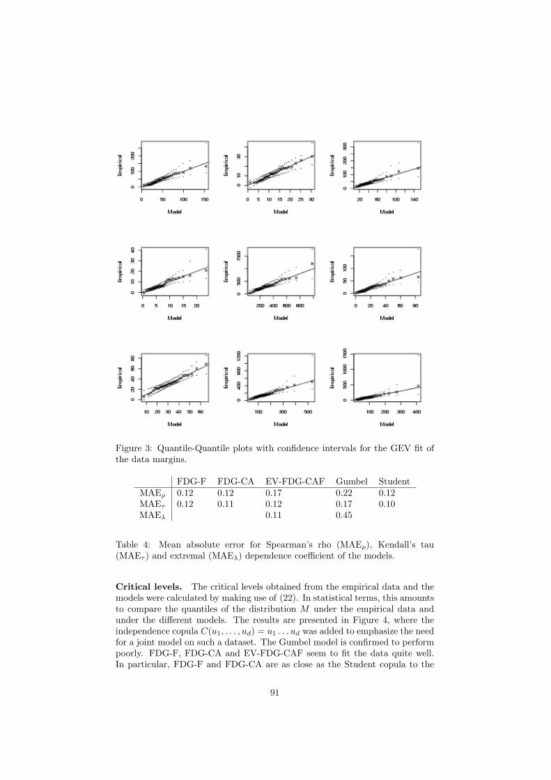
Figure 3: Quantile-Quantile plots with confidence intervals for the GEV fit ofthe data margins.

FDG-F FDG-CA EV-FDG-CAF Gumbel StudentMAEρ 0.12 0.12 0.17 0.22 0.12MAEτ 0.12 0.11 0.12 0.17 0.10MAEλ 0.11 0.45

Table 4: Mean absolute error for Spearman’s rho (MAEρ), Kendall’s tau(MAEτ ) and extremal (MAEλ) dependence coefficient of the models.

Critical levels. The critical levels obtained from the empirical data and themodels were calculated by making use of (22). In statistical terms, this amountsto compare the quantiles of the distribution M under the empirical data andunder the different models. The results are presented in Figure 4, where theindependence copula C(u1, . . . , ud) = u1 . . . ud was added to emphasize the needfor a joint model on such a dataset. The Gumbel model is confirmed to performpoorly. FDG-F, FDG-CA and EV-FDG-CAF seem to fit the data quite well.In particular, FDG-F and FDG-CA are as close as the Student copula to the

91

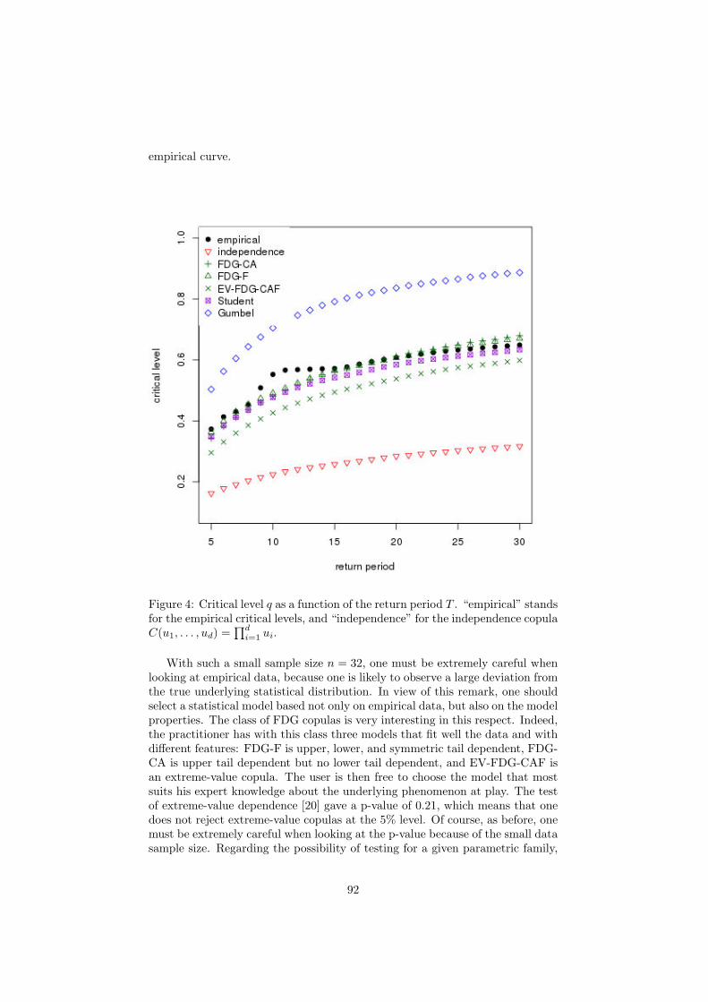
empirical curve.

Figure 4: Critical level q as a function of the return period T . “empirical” standsfor the empirical critical levels, and “independence” for the independence copulaC(u1, . . . , ud) =

∏di=1 ui.

With such a small sample size n = 32, one must be extremely careful whenlooking at empirical data, because one is likely to observe a large deviation fromthe true underlying statistical distribution. In view of this remark, one shouldselect a statistical model based not only on empirical data, but also on the modelproperties. The class of FDG copulas is very interesting in this respect. Indeed,the practitioner has with this class three models that fit well the data and withdifferent features: FDG-F is upper, lower, and symmetric tail dependent, FDG-CA is upper tail dependent but no lower tail dependent, and EV-FDG-CAF isan extreme-value copula. The user is then free to choose the model that mostsuits his expert knowledge about the underlying phenomenon at play. The testof extreme-value dependence [20] gave a p-value of 0.21, which means that onedoes not reject extreme-value copulas at the 5% level. Of course, as before, onemust be extremely careful when looking at the p-value because of the small datasample size. Regarding the possibility of testing for a given parametric family,

92

one can see [21].

5 Discussion

In this article, we have constructed a new class of copulas by combining one-factor copulas, that is, a conditional independent property, together with a classof bivariate copulas called the Durante class of bivariate copulas. This combi-nation led to many advantageous properties. The copulas within the proposedclass, referred to as FDG copulas, are tractable, flexible, and cover all typesof tail dependencies. The theoretically well grounded least-squares inferenceestimator is particularly well suited for FDG copulas because their dependencecoefficients are easy to compute, if not in closed form. This allows to performfast and reliable inference in the parametric case. We have demonstrated, fur-thermore, that FDG copulas work well in practice and are able to model bothhigh-dimensional and real datasets. Finally, we have derived the extreme-valuecopulas (EV-FDG) associated to FDG copulas, yielding a new extreme-valuecopula, which can be viewed as a generalisation of the well known Cuadras-Augecopula. This copula benefits from almost all the many advantageous propertiesof FDG copulas, and therefore opens the door for statistical analyses of extremedata in high dimension.

One may argue that a model with a singular component, as a FDG copula, isnot natural nor realistic to model hydrological data. While this may be true inthe bivariate case, this argument becomes weaker when the dimension increases.Indeed, in high-dimensional applications, the focus is less on the distributionitself than on a feature of interest of the data, such as, for instance, the criticallevels defined in (22). If alleged “unrealistic” models are able to better estimatethese features than “realistic” models – compare the fit of the Gumbel copulato the fit of FDG copulas in Section 4.2 – then one should consider using them.

This work raises several research questions. First, how to estimate the gen-erators nonparametrically? The generator of a bivariate Durante copula wasestimated nonparametrically in [10], but the matter is more complicated in ourcase because this bivariate relationship occurs between the variable of interestand the unobserved latent factor. Second, one may add more factors whenbuilding an FDG copula. Nonetheless, the model might not be as tractable asit is and therefore it may be less appealing in practice. Finally, FDG copulaspossess the conditional independence property, but the extreme-value EV-FDGcopulas were not shown to do so. If this property held, this would be of greatinterest for the simulation of datasets from this model.

Acknowledgment. The authors thank “Banque HYDRO du Ministere del’Ecologie, du Developpement durable et de l’Energie” for providing the data andBenjamin Renard for fruitful discussions about statistical issues in hydrologicalscience.

93

A Appendix

Proof of Theorem 1

Let Cj|0(·|u0) be the conditional distribution of Uj given U0 = u0. The Uj ’s areconditionally independent given U0, hence,

C(u) =

∫ 1

0

d∏

j=1

Cj|0(uj |u0)du0 (23)

=

∫ 1

0

d∏

j=1

∂C0j(u0, uj)

∂u0du0

=

∫ 1

0

d∏

j=1

∂C0(j)(u0, u(j))

∂u0du0

=

∫ u(1)

0

d∏

j=1

∂C0(j)(u0, u(j))

∂u0du0

+d∑

k=2

∫ u(k)

u(k−1)

k−1∏

j=1

∂C0(j)(u0, u(j))

∂u0

d∏

j=k

∂C0(j)(u0, u(j))

∂u0

+

∫ 1

u(d)

d∏

j=1

∂C0(j)(u0, u(j))

∂u0du0.

Since

∂C0j(u0, uj)

∂u0=

{fj(uj) if u0 < uj

ujf′j(u0) if u0 > uj ,

(23) yields

C(u) =u(1)

d∏

j=1

fj(uj) +d∑

k=2

d∏

j=k

f(j)(u(j))

∫ u(k)

u(k−1)

k−1∏

j=1

u(j)f′(j)(u0)du0

+

d∏

j=1

uj

∫ 1

u(d)

f ′j(u0)du0.

Putting u(1) in factor and noting that∫ u(2)

u(1)f ′(1)(x)dx = f(1)(u(2)) − f(1)(u(1))

finishes the proof.

Proof of Proposition 1

It suffices to set all uk equal to one but ui and uj in the formula (3).

Proof of Proposition 2

It suffices to apply the formulas (5) with fij given in Proposition 1. To computeSpearman’s rho, note that

∫ 1

0

x2fij(x)dx =

∫ 1

0

x2fi(x)fj(x)dx+

∫ 1

0

x3∫ 1

x

f ′i(z)f′j(z)dzdx.

94

An integration by parts yields∫ 1

0x3∫ 1

xf ′i(z)f

′j(z)dzdx = (1/4)

∫ 1

0x4f ′i(x)f

′j(x)dx

and the result follows.

Proof of Theorem 2

Fix (u1, . . . , ud) ∈ [0, 1]d and let n ≥ 1 be an integer. Put

αn :=u1/n(1)

d∏

j=1

fj(u1/nj )

u1/nj

,

βn :=

∫ 1

u1/n

(d)

d∏

j=1

f ′j(u0)du0,

γn :=d∏

j=k

f(j)(u1/n(j) )

u1/n(j)

,

δn,k :=

∫ u1/n

(k)

u1/n

(k−1)

k−1∏

j=1

f ′(j)(u0)du0,

and define

An := αn + βn +

d∑

k=2

γn,kδn,k.

We are going to derive asymptotic equivalent sequences for αn, βnγn and δn.Let ∼ denote the equivalent symbol at infinity (i.e., an ∼ bn means an/bn → 1as n → ∞). By using the well known formulas ex ∼ 1 + x (when x → 0),log x ∼ x− 1 (when x→ 1) and fj(x) ∼ 1 + (x− 1)f ′j(1) (when x→ 1) we get

αn ∼(1 +

1

nlog u(1)

)(1− 1

nlog(u1 . . . ud)

)1 +

1

n

d∑

j=1

log u(j)f′(j)(1)

and

γn,k ∼

1− 1

n

d∑

j=k

log u(j)

1 +

1

n

d∑

j=k

log u(j)f′(j)(1)

.

For βn the equivalence is obtained as follows. Let F (x) be a primitive of∏dj=1 f

′j(x). It follows that βn = F (1)− F (u

1/n(d) ). A Taylor expansion yields

F (u1/n(d) ) = F (1) + (u

1/n(d) − 1)F ′(1) +

(u1/n(d) − 1)2

2F ′′(xn)

where xn is between u1/n(d) and 1. Since F ′′ is assumed to be continuous on [0, 1],

it is uniformly bounded on this set and therefore (u1/n(d) − 1)2F ′′(xn)/2 = o(1/n)

where o(1/n) is a quantity such that no(1/n) → 0 as n → ∞. Hence, since

u1/n(d) = exp(log(u(d))/n) ∼ 1 + log(u(d))/n, we have as n→ ∞

F (1)− F (u1/n(d) ) ∼ − 1

nlog(u(d))F

′(1).

95

The same arguments apply to get

βn ∼ − 1

nlog u(d)

d∏

j=1

f ′j(1)

δn,k ∼ 1

nlog

(u(k)

u(k−1)

) k−1∏

j=1

f ′(j)(1).

The quantity An is a polynomial with respect to n−1 of order at most three.In (24), the coefficients of order 0, 2, and 3 vanish at infinity. Only remain theterms of order 1, hence,

limn↑∞

n(An − 1) = log u(1) − log(u1 . . . ud) +

d∑

j=1

log u(j)f′(j)(1) (24)

− log u(d)

d∏

j=1

f ′(j)(1) +d∑

k=2

k−1∏

j=1

f ′(j)(1) log

(u(k)

u(k−1)

).

From Abel’s identity, that is,∑d−1i=1 ai(bi+1−bi) =

∑d−1i=1 bi(ai−1−ai)+ad−1bd−

a1b1 for two sequences (ai) and (bi) of real numbers, we can write

limn↑∞

n(An − 1) =

d∑

k=1

k−1∏

j=1

f ′(j)(1)

(1− f ′(k)(1)) + f ′(k)(1)− 1

︸ ︷︷ ︸=:χk

log u(k),

with the convention that∏0j=1 f

′(j)(1) = 1. From (3) it follows that

Cn(u1/n1 , . . . , u

1/nd ) =u1 . . . ud exp [n logAn]

=u1 . . . ud exp [n(An − 1)(1 + o(1))]

→d∏

i=k

uχk

(k)

as n→ ∞.

Proof of Lemma 1

(i) Since the p-uple (r1,2, . . . , rd−1,d) belongs to the image space r(Θd), thesystem

r(θ1, θ2) =r1,2

...

r(θd−1, θd) =rd−1,d

has at least one solution. In particular, there exists (θ1, θ2, θ3) in Θ3 such that

r(θ1, θ2) =r1,2

r(θ1, θ3) =r1,3

r(θ2, θ3) =r2,3. (25)

96

The system (25) rewrites

rθ2(θ1) =r1,2

rθ3(θ1) =r1,3

rθ3(θ2) =r2,3,

or equivalently,

θ1 =s1,2(θ2)

θ1 =s1,3(θ3)

θ2 =s2,3(θ3).

This yields

s1,3(θ3) = s1,2 ◦ s2,3(θ3). (26)

Note that s1,3 is involutive at θ3, that is, s1,3 ◦s1,3(θ3) = θ3. Indeed, r(θ1, θ3) =rθ3(θ1) = r1,3 is equivalent to θ1 = r−1

θ3(r1,3) = s1,3(θ3). This implies r(s1,3(θ3), θ3) =

r1,3, and, composing by r−1s1,3(θ3)

in both sides, we get r−1s1,3(θ3)

(r1,3) = s1,3(s1,3(θ3)) =

θ3. Therefore, one can compose both sides of (26) by s1,3 to get

θ3 = s1,3 ◦ s1,2 ◦ s2,3(θ3).

Hence (20) has at least one solution.(ii) If (20) admits exactly one solution θ3, then θ2 and θ1 are also unique.

Furthermore, for all j ≥ 3,

θj+1 = sj,j+1(θj)

which concludes the proof that assumption (A1) holds. It is now shown thatassumption (A2) holds as well. Define ∂1r, respectively, ∂2r, the derivative of rwith respect to the first, respectively, second, variable of r. Hence for all θi andθj in Θ, the quantities ∂1r(θi, θj) and rθj (θi) only differ in the notation. Thefirst step in the proof is to consider the case d = 3. The Jacobian matrix of rat θ0 is given by

J =

∂1r(θ01, θ02) ∂2r(θ01, θ02) 0∂1r(θ01, θ03) 0 ∂2r(θ01, θ03)

0 ∂1r(θ02, θ03) ∂2r(θ02, θ03)

.

To show that J has full rank, we show that its determinant

∂1r(θ01, θ02)∂2r(θ01, θ03)∂1r(θ02, θ03) + ∂2r(θ02, θ03)∂1r(θ01, θ03)∂2r(θ01, θ02)

is nonzero. Indeed, note that for all θ in Θ, the map rθ : Θ → rθ(Θ) is a twicecontinuously differentiable homeomorphism. Furthermore, by assumption, thetrue parameter vector θ0 lies in the interior of Θ that is open. Finally, bysymmetry, for all i < j,

∂r1(θ0i, θ0j) > 0 (respectively ∂r1(θ0i, θ0j) < 0)

is equivalent to

∂r2(θ0j , θ0i) > 0 (respectively ∂r2(θ0j , θ0i) < 0).

97

For the general case, we proceed by mathematical induction. When thedimension is d, write J(θ) = J(d)(θ) to emphasize the dependence on the di-mension. Notice that it was already shown above that J(3)(θ) has full rank.Now suppose that the kernel of J(d−1)(θ) is null when the dimension is d − 1.Let A = J(d)(θ). Each row of A writes

(0, . . . , 0, ∂1r(θi, θj), 0 . . . , 0, ∂2r(θi, θj), 0, . . . , 0)

where ∂1r(θi, θj) is at the i-th position and ∂2r(θi, θj) at the j-th position.There are d−1 rows of A which depend on θd and p−d+1 which do not (recallp = d(d− 1)/2 is the number of pairs). Since the kernel of a matrix is invariantby permutation, we can without loss of generality put all the rows which do notdepend on θd on the top. More precisely, decompose A as

A =

(A11 A12

A21 A22

)

such that A11 is a (p− d+1)× (d− 1) matrix containing all the rows which donot depend on θd and A12 and A22 are (p− d+1)× 1 and (d− 1)× 1 matricesrespectively. Note that A12 is the null vector of size p− d+ 1× 1. Let x ∈ R

d,x = (xT1 , x2)

T where x1 ∈ Rd−1, x2 ∈ R. It follows that Ax = 0 is equivalent

to{

A11x1 +A12x2 = 0

A21x1 +A22x2 = 0.

But A12 = 0 and since A11 = J(d−1)(θ) whose kernel is null, x1 = 0. ThenA22x2 = 0 and the assumptions imply x2 = 0, which concludes the proof.

Proof of Corollary 1

To prove Corollary 1, it suffices to apply Lemma 1. Since r(θi, θj) denotes theextremal dependence coefficient of the E copula bivariate marginal C#,ij definedin (16), we have

r(θi, θj) = λ(θi)λ(θj), where

λ(θ) := 1− ∂f(t, θ)

∂t

∣∣∣t=1

. (27)

In the Cuadras-Auge and the Frechet cases, (27) is given by λ(θ) = θ, and in thesinus case, λ(θ) = 1− θ/ tan(θ). In all these situations, it is easy to see that themap rθj (·) is a twice continuously differentiable homeomorphism. Therefore,Lemma 1 (i) applies.

To apply the second part of Lemma 1, note that equation (20) translatesinto

λ(θ)2 =r1,3r2,3r1,2

.

Since it has a unique solution, Lemma 1 (ii) applies, and the result is proved.

98

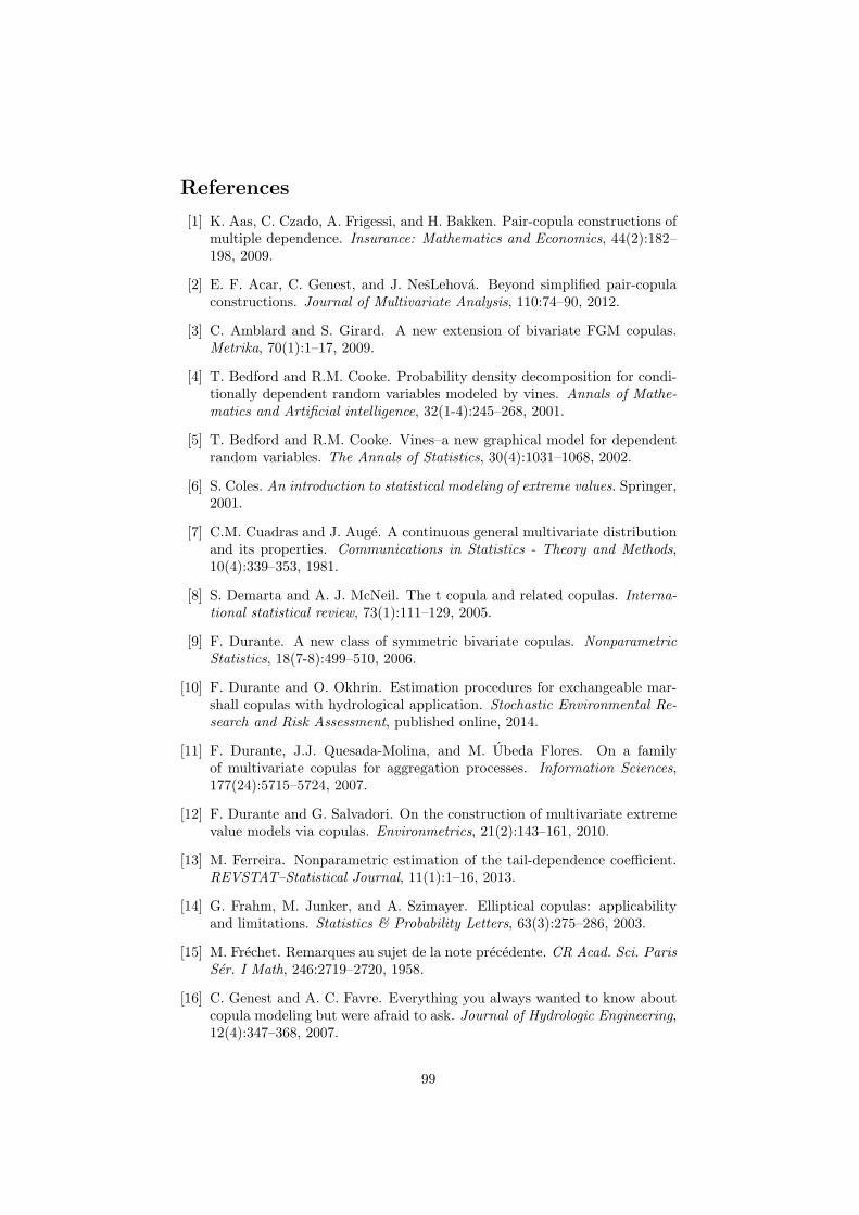
References

[1] K. Aas, C. Czado, A. Frigessi, and H. Bakken. Pair-copula constructions ofmultiple dependence. Insurance: Mathematics and Economics, 44(2):182–198, 2009.

[2] E. F. Acar, C. Genest, and J. NesLehova. Beyond simplified pair-copulaconstructions. Journal of Multivariate Analysis, 110:74–90, 2012.

[3] C. Amblard and S. Girard. A new extension of bivariate FGM copulas.Metrika, 70(1):1–17, 2009.

[4] T. Bedford and R.M. Cooke. Probability density decomposition for condi-tionally dependent random variables modeled by vines. Annals of Mathe-matics and Artificial intelligence, 32(1-4):245–268, 2001.

[5] T. Bedford and R.M. Cooke. Vines–a new graphical model for dependentrandom variables. The Annals of Statistics, 30(4):1031–1068, 2002.

[6] S. Coles. An introduction to statistical modeling of extreme values. Springer,2001.

[7] C.M. Cuadras and J. Auge. A continuous general multivariate distributionand its properties. Communications in Statistics - Theory and Methods,10(4):339–353, 1981.

[8] S. Demarta and A. J. McNeil. The t copula and related copulas. Interna-tional statistical review, 73(1):111–129, 2005.

[9] F. Durante. A new class of symmetric bivariate copulas. NonparametricStatistics, 18(7-8):499–510, 2006.

[10] F. Durante and O. Okhrin. Estimation procedures for exchangeable mar-shall copulas with hydrological application. Stochastic Environmental Re-search and Risk Assessment, published online, 2014.

[11] F. Durante, J.J. Quesada-Molina, and M. Ubeda Flores. On a familyof multivariate copulas for aggregation processes. Information Sciences,177(24):5715–5724, 2007.

[12] F. Durante and G. Salvadori. On the construction of multivariate extremevalue models via copulas. Environmetrics, 21(2):143–161, 2010.

[13] M. Ferreira. Nonparametric estimation of the tail-dependence coefficient.REVSTAT–Statistical Journal, 11(1):1–16, 2013.

[14] G. Frahm, M. Junker, and A. Szimayer. Elliptical copulas: applicabilityand limitations. Statistics & Probability Letters, 63(3):275–286, 2003.

[15] M. Frechet. Remarques au sujet de la note precedente. CR Acad. Sci. ParisSer. I Math, 246:2719–2720, 1958.

[16] C. Genest and A. C. Favre. Everything you always wanted to know aboutcopula modeling but were afraid to ask. Journal of Hydrologic Engineering,12(4):347–368, 2007.

99

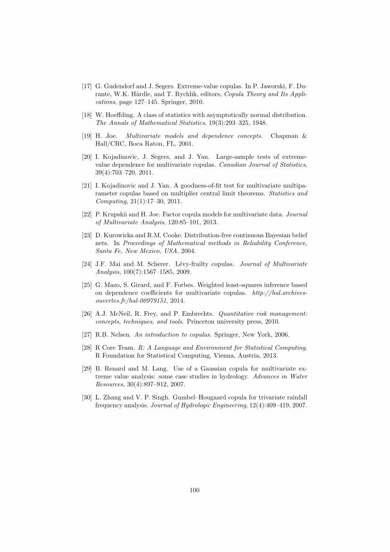
[17] G. Gudendorf and J. Segers. Extreme-value copulas. In P. Jaworski, F. Du-rante, W.K. Hardle, and T. Rychlik, editors, Copula Theory and Its Appli-cations, page 127–145. Springer, 2010.

[18] W. Hoeffding. A class of statistics with asymptotically normal distribution.The Annals of Mathematical Statistics, 19(3):293–325, 1948.

[19] H. Joe. Multivariate models and dependence concepts. Chapman &Hall/CRC, Boca Raton, FL, 2001.

[20] I. Kojadinovic, J. Segers, and J. Yan. Large-sample tests of extreme-value dependence for multivariate copulas. Canadian Journal of Statistics,39(4):703–720, 2011.

[21] I. Kojadinovic and J. Yan. A goodness-of-fit test for multivariate multipa-rameter copulas based on multiplier central limit theorems. Statistics andComputing, 21(1):17–30, 2011.

[22] P. Krupskii and H. Joe. Factor copula models for multivariate data. Journalof Multivariate Analysis, 120:85–101, 2013.

[23] D. Kurowicka and R.M. Cooke. Distribution-free continuous Bayesian beliefnets. In Proceedings of Mathematical methods in Reliability Conference,Santa Fe, New Mexico, USA, 2004.

[24] J.F. Mai and M. Scherer. Levy-frailty copulas. Journal of MultivariateAnalysis, 100(7):1567–1585, 2009.

[25] G. Mazo, S. Girard, and F. Forbes. Weighted least-squares inference basedon dependence coefficients for multivariate copulas. http://hal.archives-ouvertes.fr/hal-00979151, 2014.

[26] A.J. McNeil, R. Frey, and P. Embrechts. Quantitative risk management:concepts, techniques, and tools. Princeton university press, 2010.

[27] R.B. Nelsen. An introduction to copulas. Springer, New York, 2006.

[28] R Core Team. R: A Language and Environment for Statistical Computing.R Foundation for Statistical Computing, Vienna, Austria, 2013.

[29] B. Renard and M. Lang. Use of a Gaussian copula for multivariate ex-treme value analysis: some case studies in hydrology. Advances in WaterResources, 30(4):897–912, 2007.

[30] L. Zhang and V. P. Singh. Gumbel–Hougaard copula for trivariate rainfallfrequency analysis. Journal of Hydrologic Engineering, 12(4):409–419, 2007.

100

❈♦♥❝❧✉s✐♦♥

❉❛♥s ❝❡tt❡ t❤ès❡✱ ♥♦✉s ❛✈♦♥s ♣r♦♣♦sé ❞❡✉① ♥♦✉✈❡❧❧❡s ❝❧❛ss❡s ❞❡ ❝♦♣✉❧❡s✳ ▲❛♣r❡♠✐èr❡ ❡st ❝♦♥str✉✐t❡ à ♣❛rt✐r ❞✬✉♥❡ ❝❧❛ss❡ ♣r❡♥❛♥t ❧❛ ❢♦r♠❡ ❞✬✉♥ ♣r♦❞✉✐t ❣é♥é✲r❛❧✐sé ❞❡ ❝♦♣✉❧❡s✳ ❊t❛♥t r❡❝♦♥♥✉ q✉❡ ❝❡tt❡ ❝❧❛ss❡ ❞♦✐t êtr❡ s✐♠♣❧✐✜é❡ ♣♦✉r ♣♦✉✈♦✐rêtr❡ ✉t✐❧❡ ❡♥ ♣r❛t✐q✉❡✱ ♥♦✉s ❛✈♦♥s ♠♦♥tré q✉❡✱ s✐ ❧❡s ❢♦♥❝t✐♦♥s gei ❞❡ ▲✐❡❜s❝❤❡r♥❡ ❞é♣❡♥❞❡♥t ❡♥ ❢❛✐t ♣❛s ❞❡ ❧✬✐♥❞✐❝❡ e✱ ❡t s✐ ❧✬♦♥ s♦✉❤❛✐t❡ t✐r❡r ♣r♦✜t ❞❡ ❧❛ ❧❛r❣❡❣❛♠♠❡ ❞❡ ❢❛♠✐❧❧❡s ❞❡ ❝♦♣✉❧❡s ❜✐✈❛r✐é❡s ❞✐s♣♦♥✐❜❧❡s ❞❛♥s ❧❛ ❧✐ttér❛t✉r❡✱ ❛❧♦rs ❧❛s❡✉❧❡ ❝❧❛ss❡ ♣♦ss✐❜❧❡ q✉❡ ❧✬♦♥ ♣❡✉t ❝♦♥str✉✐r❡ ❡st ❧❛ ❝❧❛ss❡ ❞❡s ❝♦♣✉❧❡s P❇❈ ❞✉❝❤❛♣✐tr❡ ✹✳ ❉❡ ♣❧✉s✱ ♥♦✉s ❛✈♦♥s ♠♦♥tré ❧❡ ❧✐❡♥ ❛✈❡❝ ✉♥ ❛❧❣♦r✐t❤♠❡ ♠❡ss❛❣❡✲♣❛ss✐♥❣✱ ❝❡ q✉✐ ♣❡r♠❡t ❞❡ ❢❛✐r❡ ❧✬❡st✐♠❛t✐♦♥ ❞❡s ❝♦♣✉❧❡s P❇❈ ♣❛r ♠❛①✐♠✉♠ ❞❡✈r❛✐s❡♠❜❧❛♥❝❡✳ ❚♦✉t❡❢♦✐s✱ ♥♦✉s ❛✈♦♥s ♠♦♥tré é❣❛❧❡♠❡♥t q✉❡ ❧❡s ❝♦♣✉❧❡s P❇❈ ♥❡s♦♥t ♣❛s ❝❛♣❛❜❧❡s ❞❡ ♠♦❞é❧✐s❡r ❞❡s ✈❛r✐❛❜❧❡s très ❞é♣❡♥❞❛♥t❡s✱ ❡t✱ ♣❛r ❝♦♥sé✲q✉❡♥t✱ s♦♥t ❞✬✉♥❡ ✉t✐❧✐té ❧✐♠✐té❡ ♣♦✉r ❧❡s ❛♣♣❧✐❝❛t✐♦♥s✳

▲❛ ❞❡✉①✐è♠❡ ❝❧❛ss❡ ❞❡ ❝♦♣✉❧❡s q✉❡ ♥♦✉s ❛✈♦♥s ♣r♦♣♦sé❡s ✭❧❡s ❝♦♣✉❧❡s ❋❉●✮❡st✱ à ♥♦tr❡ ❛✈✐s✱ ❜❡❛✉❝♦✉♣ ♣❧✉s ✐♥tér❡ss❛♥t❡ ♣♦✉r ❧❡s ❛♣♣❧✐❝❛t✐♦♥s✳ ❊♥ ❡✛❡t✱❝❡tt❡ ❝❧❛ss❡ ❡st très ♠❛♥✐❛❜❧❡✱ ♣❛r❝✐♠♦♥✐❡✉s❡ ✕ ♣✉✐sq✉❡ ❧❡ ♥♦♠❜r❡ ❞❡ ♣❛r❛♠ètr❡s♥✬❛✉❣♠❡♥t❡ q✉❡ ♣r♦♣♦rt✐♦♥♥❡❧❧❡♠❡♥t ♣❛r r❛♣♣♦rt à ❧❛ ❞✐♠❡♥s✐♦♥ ✕✱ ❡t ❧❡s ❡①✲♣r❡ss✐♦♥s ❞❡s ❝♦❡✣❝✐❡♥ts ❞❡ ❞é♣❡♥❞❛♥❝❡ s♦♥t ❡①♣❧✐❝✐t❡s✱ ❝❡ q✉✐ ♣❡r♠❡t ❞✬ét✉❞✐❡r❡t ❞❡ q✉❛♥t✐✜❡r ❧❛ ❞é♣❡♥❞❛♥❝❡ ❛✈❡❝ ❛✐s❛♥❝❡✳ ◆♦✉s ❛✈♦♥s ♠♦♥tré q✉❡ ❧❛ ❝❧❛ss❡❋❉● ♣❡r♠❡t ❞✬♦❜t❡♥✐r ❞❡s ❞é♣❡♥❞❛♥❝❡s ❞❛♥s ❧❡s q✉❡✉❡s ✐♥❢ér✐❡✉r❡s ♠❛✐s ♣❛ss✉♣ér✐❡✉r❡s✱ ♦✉ ❧✬✐♥✈❡rs❡✱ ♦✉ ❧❡s ❞❡✉①✳ ▲❡s ✈❛r✐❛❜❧❡s ❞✬✐♥térêts s♦♥t ❝♦♥❞✐t✐♦♥♥❡❧✲❧❡♠❡♥t ✐♥❞é♣❡♥❞❛♥t❡s ♣❛r r❛♣♣♦rt à ✉♥ ❢❛❝t❡✉r ❧❛t❡♥t✱ ❝❡ q✉✐ ♣❡r♠❡t ❞❡ s✐♠✉❧❡rtrès ❢❛❝✐❧❡♠❡♥t s❡❧♦♥ ❝❡s ❝♦♣✉❧❡s✳ ❈❡ ❢❛❝t❡✉r ❧❛t❡♥t ♣❡✉t êtr❡ ✐❣♥♦ré✱ ♦✉ ♣❡✉t êtr❡✈✉ ❝♦♠♠❡ ✉♥ ❛ttr❛✐t s✉♣♣❧é♠❡♥t❛✐r❡ ❞✉ ♠♦❞è❧❡ ❡♥ ❝❡❧❛ q✉✬✐❧ ❢❛❝✐❧✐t❡ s♦♥ ✐♥t❡r✲♣rét❛t✐♦♥✳ ❊♥✜♥✱ ❧❡s ❝♦♣✉❧❡s ❋❉● ♣rés❡♥t❡♥t ✉♥❡ ❝♦♠♣♦s❛♥t❡ s✐♥❣✉❧✐èr❡✳ ❊❧❧❡s♣❡✉✈❡♥t ❞♦♥❝ êtr❡ ✉t✐❧✐sé❡s ❞❛♥s ❧❡ ❝❛❞r❡ ❞❡ ♠♦❞è❧❡s à ❝❤♦❝s✱ ❝♦♠♠❡ ✈✉ ❞❛♥s❧❛ ♣❛rt✐❡ ✶✳✸✳✷✳ ▼❛✐s ♥♦✉s ❛✈♦♥s ♠♦♥tré q✉❡ ❧❡s ❝♦♣✉❧❡s ❋❉● ♣❡✉✈❡♥t ❛✉ss✐ êtr❡✉t✐❧✐sé❡s ❛✈❡❝ s✉❝❝ès ❞❛♥s ❞❡s ❛♣♣❧✐❝❛t✐♦♥s ❞❡ ♥❛t✉r❡s ❞✐✛ér❡♥t❡s✱ ❝✬❡st à ❞✐r❡✱♠ê♠❡ q✉❛♥❞ ✐❧ ♥✬② ❛ ♣❛s ❞❡ ❝❤♦❝s✳ ❊♥ ♣❛rt✐❝✉❧✐❡r✱ ♥♦✉s ❛✈♦♥s ❡st✐♠é ❧❡ ♥✐✈❡❛✉❝r✐t✐q✉❡ ❛ss♦❝✐é ❛✉① é✈è♥❡♠❡♥ts ❞❡ ❞é❜✐ts ❡①trê♠❡s ❞❡ ❧❛ ré❣✐♦♥ ❞❡s ❈é✈❡♥♥❡s✭s✉❞ ❞❡ ❧❛ ❋r❛♥❝❡✮✳ ◆♦s rés✉❧t❛ts s♦♥t r♦❜✉st❡s à ❧✬✐♥tér✐❡✉r ❞❡ ❧❛ ❝❧❛ss❡ ❋❉●✱❛❥✉st❡♥t ❜✐❡♥ ❧❡s ❞♦♥♥é❡s✱ ❡t s♦♥t ❡♥ ❝♦❤ér❡♥❝❡ ❛✈❡❝ ❧❡s rés✉❧t❛ts ♦❜t❡♥✉s ❛✈❡❝✉♥❡ ❝♦♣✉❧❡ ❞❡ ❙t✉❞❡♥t✳ ❊♥✜♥✱ ♥♦✉s ❛✈♦♥s ♠♦♥tré q✉❡ ❧✬♦♥ ♣♦✉✈❛✐t ❝❛❧❝✉❧❡r ❧❡s❝♦♣✉❧❡s ❡①trê♠❡s ❛ss♦❝✐é❡s ❛✉① ❝♦♣✉❧❡s ❋❉● ✭❧❡s ❝♦♣✉❧❡s ❊❱✲❋❉●✮✱ ❡♥r✐❝❤✐s✲s❛♥t ❛✐♥s✐ ❧❛ ❣❛♠♠❡ ❞❡s ❝♦♣✉❧❡s ❡①trê♠❡s✱ ❞✬❛✉t❛♥t q✉❡ ❧❡s ❝♦♣✉❧❡s ❡①trê♠❡s✐ss✉❡s ❞❡s ❝♦♣✉❧❡s ❋❉● ré❛❧✐s❡♥t ❡❧❧❡s ❛✉ss✐ ✉♥ ❜♦♥ ❝♦♠♣r♦♠✐s ❡♥tr❡ ✢❡①✐❜✐❧✐té❡t ♠❛♥✐❛❜✐❧✐té✳ ❊❧❧❡s ♦♥t ❞✬❛✐❧❧❡✉rs été t❡sté❡s ❡t ✉t✐❧✐sé❡s ❡♥ ♣r❛t✐q✉❡ ❛✉ ♠ê♠❡t✐tr❡ q✉❡ ❧❡s ❛✉tr❡s ❝♦♣✉❧❡s✳

❉❛♥s ❧❡ ❝❛❞r❡ ❞❡ ❝❡tt❡ t❤ès❡✱ ♥♦✉s ❛✈♦♥s é❣❛❧❡♠❡♥t ❛♣♣♦rté ♥♦tr❡ ❝♦♥tr✐✲❜✉t✐♦♥ à ❧✬❡st✐♠❛t✐♦♥ ❞❡ ❝♦♣✉❧❡s✳ ◆♦✉s ❛✈♦♥s s♦✉❧✐❣♥é q✉❡ ❧❡s ♠ét❤♦❞❡s ❛❝✲

✶✵✶

t✉❡❧❧❡s ❞✬❡st✐♠❛t✐♦♥ ♥✬❛✈❛✐❡♥t ♣❛s ❞❡ ❢♦♥❞❡♠❡♥ts t❤é♦r✐q✉❡s s✐ ❧❡s ❝♦♣✉❧❡s ❝♦♥s✐✲❞éré❡s ♥✬♦♥t ♣❛s ❞❡ ❞ér✐✈é❡s ♣❛rt✐❡❧❧❡s✱ ❝❡ q✉✐ ❡st ❧❡ ❝❛s ❞❡s ❝♦♣✉❧❡s ❋❉●✳ ◆♦✉s❛✈♦♥s ♠♦♥tré q✉❡✱ s♦✉s ❞❡s ❝♦♥❞✐t✐♦♥s ❞✬✐❞❡♥t✐✜❛❜✐❧✐té ♥❛t✉r❡❧❧❡s✱ ❧✬❡st✐♠❛t❡✉r❞❡s ♠♦✐♥❞r❡s ❝❛rrés ♣♦♥❞érés ❜❛sé s✉r ❧❡s ❝♦❡✣❝✐❡♥ts ❞❡ ❞é♣❡♥❞❛♥❝❡ ❡①✐st❡ ❡t❡st ✉♥✐q✉❡ ❛✈❡❝ ✉♥❡ ♣r♦❜❛❜✐❧✐té s✬❛♣♣r♦❝❤❛♥t ❞❡ ✶ ❛✉ ❢✉r ❡t à ♠❡s✉r❡ q✉❡ ❧❛ t❛✐❧❧❡❞❡ ❧✬é❝❤❛♥t✐❧❧♦♥ ❛✉❣♠❡♥t❡✱ ❡t q✉✬✐❧ ét❛✐t ❛s②♠♣t♦t✐q✉❡♠❡♥t ❝♦♥s✐st❛♥t ❡t ♥♦r♠❛❧✱❡t ❝❡✱ ♠ê♠❡ s✐ ❧❡s ❝♦♣✉❧❡s ❝♦♥s✐❞éré❡s ♥✬❛❞♠❡tt❡♥t ♣❛s ❞❡ ❞ér✐✈é❡s ♣❛rt✐❡❧❧❡s✳

▲❡s ♣❡rs♣❡❝t✐✈❡s à ♥♦s ❞✐✛ér❡♥ts tr❛✈❛✉① ♦♥t été ❞✐s❝✉té❡s ❞❛♥s ❧❡s ❝❤❛♣✐tr❡s❧❡s ❝♦♥❝❡r♥❛♥t✳ P♦✉r ❧❡s ❝♦♣✉❧❡s P❇❈✱ ✐❧ ❛✈❛✐t été s✉❣❣éré q✉❡ ❝❡s ❞❡r♥✐èr❡sét❛✐❡♥t ♣❡✉t✲êtr❡ ❞✬✉♥ ✐♥térêt ♣❧✉s t❤é♦r✐q✉❡ q✉❡ ♣r❛t✐q✉❡✳ ❈♦♥❝❡r♥❛♥t ❧❡s ❝♦✲♣✉❧❡s ❋❉●✱ ❛✈❛✐t été ♣♦sé ❧❛ q✉❡st✐♦♥ ❞❡ ❧✬❡st✐♠❛t✐♦♥ ♥♦♥ ♣❛r❛♠étr✐q✉❡ ❞❡s❣é♥ér❛t❡✉rs✳ ◆♦✉s ❛✈✐♦♥s ❛✉ss✐ ❢❛✐t r❡♠❛rq✉❡r q✉❡ ♣❧✉s✐❡✉rs ❢❛❝t❡✉rs ❝❛❝❤és ♣♦✉r✲r❛✐❡♥t êtr❡ ❡♥✈✐s❛❣és ❧♦rs ❧❛ ❝♦♥str✉❝t✐♦♥ ❞❡ ❝❡s ❝♦♣✉❧❡s✱ ♠❛✐s q✉❡ ❝❡❧❛ r✐sq✉❡r❛✐t❞❡ ❧❡s r❡♥❞r❡ ♠♦✐♥s ♠❛♥✐❛❜❧❡s✳ ▲❛ ♣r♦♣r✐été ❞✬✐♥❞é♣❡♥❞❛♥❝❡ ❝♦♥❞✐t✐♦♥♥❡❧❧❡✱ ét❛✲❜❧✐❡ ✭♣❛r ❝♦♥str✉❝t✐♦♥✮ ♣♦✉r ❧❡s ❝♦♣✉❧❡s ❋❉●✱ ♥✬❛ ♣❛s été ❞é♠♦♥tré❡ ♣♦✉r ❧❡s❝♦♣✉❧❡s ❊❱✲❋❉●✳ ❖r s✐ ❝❡tt❡ ♣r♦♣r✐été ét❛✐t ✈r❛✐❡✱ ❡❧❧❡ s❡r❛✐t ✉t✐❧❡✱ ❡♥tr❡ ❛✉tr❡✱♣♦✉r s✐♠✉❧❡r ❞❡s ❞♦♥♥é❡s s❡❧♦♥ ❝❡s ❝♦♣✉❧❡s✳ ❊♥✜♥✱ ❝♦♥❝❡r♥❛♥t ❧✬❡st✐♠❛t❡✉r ❞❡s♠♦✐♥❞r❡s ❝❛rrés ❜❛sé s✉r ❧❡s ❝♦❡✣❝✐❡♥ts ❞❡ ❞é♣❡♥❞❛♥❝❡✱ ❧✬❛♣♣❧✐❝❛t✐♦♥ ❤②❞r♦❧♦✲❣✐q✉❡ ❛ ré✈é❧é q✉❡ ❝❡ ❞❡r♥✐❡r ♣♦✉✈❛✐t êtr❡ ✐♥st❛❜❧❡ ♥✉♠ér✐q✉❡♠❡♥t ❧♦rsq✉❡ ❧❡♥♦♠❜r❡ ❞❡ ♣❛r❛♠ètr❡s à ❡st✐♠❡r ❡st é❣❛❧ ❛✉① ♥♦♠❜r❡ ❞❡ ♣❛✐r❡s ❞❡ ✈❛r✐❛❜❧❡s✳❉❛♥s ❝❡ ❝❛s✱ ♦♥ ♣♦✉rr❛✐t ❡♥✈✐s❛❣❡r ✉♥❡ ❝♦♠❜✐♥❛✐s♦♥ ❞❡ ❝♦❡✣❝✐❡♥ts ❞❡ ❞✐✛ér❡♥tst②♣❡s ✭r❤♦ ❞❡ ❙♣❡❛r♠❛♥✱ t❛✉ ❞❡ ❑❡♥❞❛❧❧✳✳✳✮ ❛✜♥ ❞❡ r❡♥❞r❡ ❧❡ s②stè♠❡ ❞✬éq✉❛t✐♦♥sà rés♦✉❞r❡ ♣❧✉s r♦❜✉st❡ ♥✉♠ér✐q✉❡♠❡♥t✳

◆♦s tr❛✈❛✉① s✬✐♥s❝r✐✈❡♥t ❞❛♥s ✉♥ ❝♦♥t❡①t❡ ♣❧✉s ❣❧♦❜❛❧✱ ❞♦♥t ♥♦✉s ❢❛✐s♦♥s ✉♥❡s②♥t❤ès❡ ❝✐✲❞❡ss♦✉s✳ ▲❛ r❡❝❤❡r❝❤❡ ❞❡ ♠♦❞è❧❡s ♠✉❧t✐✈❛r✐és ❛✈❡❝ ❛✉t❛♥t ❞❡ q✉❛❧✐tésq✉❡ ♣♦ss✐❜❧❡ ét❛✐t ✉♥ s✉❥❡t ✐♠♣♦rt❛♥t ✐❧ ② ❛ ✉♥❡ ❞✐③❛✐♥❡ ❞✬❛♥♥é❡s✳ ◆♦✉s ❛✈♦♥s ❧❡s❡♥t✐♠❡♥t✱ q✉❡✱ ❞❡ ♥♦s ❥♦✉rs✱ ✐❧ ❡♥ ❡①✐st❡ ✉♥❡ ❣❛♠♠❡ ❛ss❡③ ❞✐✈❡rs✐✜é❡✳ ❈❡s t♦✉t❡s❞❡r♥✐èr❡s ❛♥♥é❡s✱ ❡♥ ♣❛rt✐❝✉❧✐❡r✱ ♦♥t ✈✉ ❛♣♣❛r❛✐tr❡ ✉♥❡ ❝❧❛ss❡ ❞❡ ♠♦❞è❧❡s très✢❡①✐❜❧❡s✱ ❧❡s ❱✐♥❡s✳ ❇✐❡♥ sûr✱ ✐❧ r❡st❡ ❡♥❝♦r❡ ❜❡❛✉❝♦✉♣ ❞❡ r❡❝❤❡r❝❤❡ à ❡✛❡❝t✉❡r✱♥♦t❛♠♠❡♥t ♣♦✉r r❡♥❞r❡ ❝❡s ♠♦❞è❧❡s ♣❧✉s ♣❛r❝✐♠♦♥✐❡✉①✱ ❡t ♠✐❡✉① ❝♦♠♣r❡♥❞r❡❧❡✉r s❡♥s✐❜✐❧✐té ♣❛r r❛♣♣♦rt ❛✉ ❝❤♦✐① ❞❡ ❧❛ ❞é❝♦♠♣♦s✐t✐♦♥ ❞❡ ❧❛ ❞❡♥s✐té✱ ♦✉ ❞❡s❢❛♠✐❧❧❡s ♣❛r❛♠étr✐q✉❡s ❜✐✈❛r✐é❡s à ✐♥❝♦r♣♦r❡r✳ ❊♥ ♦✉tr❡✱ ❧❡ r✐sq✉❡ ❡st ❣r❛♥❞✱❛✈❡❝ ❝❡s ♠♦❞è❧❡s✱ ❞❡ s✉r✲❛❥✉st❡r ✭♦✈❡r✜t ❡♥ ❛♥❣❧❛✐s✮ ❧❡s ❞♦♥♥é❡s✳ ❊♥ ❝❡ s❡♥s✱❧❡s ♠♦❞è❧❡s à ❢❛❝t❡✉r✱ ❡t ❡♥ ♣❛rt✐❝✉❧✐❡r à ✉♥ ❢❛❝t❡✉r ✭❝♦♠♠❡ ❝❡❧✉✐ q✉❡ ♥♦✉s❛✈♦♥s ♣r♦♣♦sé✮✱ s♦♥t très ✐♥tér❡ss❛♥ts✳ ■❧s ♣❡✉✈❡♥t ❞✬❛✐❧❧❡✉rs êtr❡ ✈✉s ❝♦♠♠❡❞❡s ♠♦❞è❧❡s ❱✐♥❡s ✓ tr♦♥q✉és ✔✳ ◆♦✉s ❛✐♠❡r✐♦♥s t❡r♠✐♥❡r ❝❡tt❡ t❤ès❡ ♣❛r ❧❡q✉❡st✐♦♥♥❡♠❡♥t ✓ ♠ét❛✲st❛t✐st✐q✉❡ ✔ s✉✐✈❛♥t ✿ q✉❡ ✈♦✉❧♦♥s✲♥♦✉s ❢❛✐r❡ ❛✈❡❝ ♥♦s♠♦❞è❧❡s ❄ ▲❡ ❜✉t ❡st✲✐❧ ✈r❛✐♠❡♥t ❞✬❛❥✉st❡r ❧❡s ❞♦♥♥é❡s ❧❡ ♠✐❡✉① ♣♦ss✐❜❧❡✱ ❝♦♠♠❡✐❧ ❡♥ r❡ss♦rt ❧✬✐♠♣r❡ss✐♦♥ à ❧❛ ❧❡❝t✉r❡ ❞❡ ❝❡rt❛✐♥❡s ♣✉❜❧✐❝❛t✐♦♥s ❄ ❆ ♥♦tr❡ ❛✈✐s✱ ❡♥❣r❛♥❞❡ ❞✐♠❡♥s✐♦♥✱ ❧❛ ❞✐str✐❜✉t✐♦♥ q✉❡ ♥♦✉s t❡♥t♦♥s ❞❡ ♠♦❞é❧✐s❡r ♥♦✉s ✐♠♣♦rt❡♠♦✐♥s q✉✬✉♥❡ ❝❛r❛❝tér✐st✐q✉❡ ❞❡ ❝❡tt❡ ❞❡r♥✐èr❡✳ ❆✉tr❡♠❡♥t ❞✐t✱ ❝✬❡st ♠♦✐♥s ❧❛❧♦✐ ❞❡ (X1, . . . , Xd) q✉❡ ❝❡❧❧❡ ❞❡ ϕ(X1, . . . , Xd)✱ ❛✈❡❝ ϕ : R

d 7→ R✱ q✉✐ ♥♦✉s✐♥tér❡ss❡✳ P❛r ❡①❡♠♣❧❡✱ ❞❛♥s ❧❡ ❝❛s ❞❡s ❛♣♣❧✐❝❛t✐♦♥s ❡♥ ❤②❞r♦❧♦❣✐❡ q✉❡ ♥♦✉s❛✈♦♥s tr❛✐té❡s à ♣❧✉s✐❡✉rs r❡♣r✐s❡s ❞❛♥s ❝❡tt❡ t❤ès❡✱ ♥♦✉s ❛✈♦♥s ϕ(X1, . . . , Xd) =min(X1, . . . , Xd)✳ ■❧ ② ❛ tr♦✐s ♣♦ss✐❜✐❧✐tés ❞✬❡st✐♠❡r ❧❛ ❧♦✐ ❞❡ ϕ(X1, . . . , Xd) ✿

✶✳ ❡♥ ✉t✐❧✐s❛♥t ✉♥ ❤✐st♦r✐q✉❡ ❞❡s ❞♦♥♥é❡s ❞❡ ϕ(X1, . . . , Xd) ❧✉✐ ♠ê♠❡✱

✷✳ ❡♥ ♠♦❞é❧✐s❛♥t ❧❛ ❧♦✐ ❞❡ ϕ(X1, . . . , Xd) ❡❧❧❡ ♠ê♠❡✱ ♦✉✱

✸✳ ❡♥ ♠♦❞é❧✐s❛♥t ❧❛ ❧♦✐ ❞❡ (X1, . . . , Xd)✳

❈✬❡st s❡✉❧❡♠❡♥t ❞❛♥s ❧❛ ❞❡r♥✐èr❡ s✐t✉❛t✐♦♥ q✉❡ ♥♦✉s ❛✈♦♥s ❜❡s♦✐♥ ❞✬✉♥ ♠♦❞è❧❡

✶✵✷

♠✉❧t✐✈❛r✐é✱ ❡t s✐ ❝✬ét❛✐t ❝❛s✱ ❝❡ ♠♦❞è❧❡ ❞❡✈r❛✐t êtr❡ ❝❤♦✐s✐ ❛✉ss✐ ❡♥ ❢♦♥❝t✐♦♥ ❞❡s❡s ❝❛♣❛❝✐tés r❡❧❛t✐✈❡♠❡♥t à ❧❛ ❢♦♥❝t✐♦♥♥❡❧❧❡ ϕ✱ ❡t ♣❛s s❡✉❧❡♠❡♥t r❡❧❛t✐✈❡♠❡♥t às❡s ❝❛♣❛❝✐tés à ✓ ❛❥✉st❡r ❧❡s ❞♦♥♥é❡s ✔✳ ▼ê♠❡ ✉♥ ♠♦❞è❧❡ ❛ ♣r✐♦r✐ ♣❡✉ ✢❡①✐❜❧❡♣❡✉① ❞♦♥♥❡r ❞❡s rés✉❧t❛ts s❛t✐s❢❛✐s❛♥ts✳ ▲❛ r❡♣r♦❞✉❝t✐❜✐❧✐té ❞❡s rés✉❧t❛ts✱ ❡♥♣❛rt✐❝✉❧✐❡r✱ ❞♦✐t êtr❡ ✈ér✐✜é❡ ❛✈❡❝ ❛tt❡♥t✐♦♥✳

✶✵✸

❇✐❜❧✐♦❣r❛♣❤✐❡

❬✶❪ ❑✳ ❆❛s✱ ❈✳ ❈③❛❞♦✱ ❆✳ ❋r✐❣❡ss✐✱ ❛♥❞ ❍✳ ❇❛❦❦❡♥✳ P❛✐r✲❝♦♣✉❧❛ ❝♦♥str✉❝t✐♦♥s ♦❢♠✉❧t✐♣❧❡ ❞❡♣❡♥❞❡♥❝❡✳ ■♥s✉r❛♥❝❡ ✿ ▼❛t❤❡♠❛t✐❝s ❛♥❞ ❊❝♦♥♦♠✐❝s✱ ✹✹✭✷✮ ✿✶✽✷✕✶✾✽✱ ✷✵✵✾✳

❬✷❪ ❊✳ ❋✳ ❆❝❛r✱ ❈✳ ●❡♥❡st✱ ❛♥❞ ❏✳ ◆❡➨▲❡❤♦✈á✳ ❇❡②♦♥❞ s✐♠♣❧✐✜❡❞ ♣❛✐r✲❝♦♣✉❧❛❝♦♥str✉❝t✐♦♥s✳ ❏♦✉r♥❛❧ ♦❢ ▼✉❧t✐✈❛r✐❛t❡ ❆♥❛❧②s✐s✱ ✶✶✵ ✿✼✹✕✾✵✱ ✷✵✶✷✳

❬✸❪ ❈✳ ❆♠❜❧❛r❞ ❛♥❞ ❙✳ ●✐r❛r❞✳ ❆ ♥❡✇ ❡①t❡♥s✐♦♥ ♦❢ ❜✐✈❛r✐❛t❡ ❋●▼ ❝♦♣✉❧❛s✳▼❡tr✐❦❛✱ ✼✵✭✶✮ ✿✶✕✶✼✱ ✷✵✵✾✳

❬✹❪ ❚✳ ❇❡❞❢♦r❞ ❛♥❞ ❘✳ ▼✳ ❈♦♦❦❡✳ Pr♦❜❛❜✐❧✐t② ❞❡♥s✐t② ❞❡❝♦♠♣♦s✐t✐♦♥ ❢♦r ❝♦♥❞✐✲t✐♦♥❛❧❧② ❞❡♣❡♥❞❡♥t r❛♥❞♦♠ ✈❛r✐❛❜❧❡s ♠♦❞❡❧❡❞ ❜② ✈✐♥❡s✳ ❆♥♥❛❧s ♦❢ ▼❛t❤❡✲♠❛t✐❝s ❛♥❞ ❆rt✐✜❝✐❛❧ ✐♥t❡❧❧✐❣❡♥❝❡✱ ✸✷✭✶✲✹✮ ✿✷✹✺✕✷✻✽✱ ✷✵✵✶✳

❬✺❪ ❚✳ ❇❡❞❢♦r❞ ❛♥❞ ❘✳ ▼✳ ❈♦♦❦❡✳ ❱✐♥❡s ✿ ❆ ♥❡✇ ❣r❛♣❤✐❝❛❧ ♠♦❞❡❧ ❢♦r ❞❡♣❡♥❞❡♥tr❛♥❞♦♠ ✈❛r✐❛❜❧❡s✳ ❆♥♥❛❧s ♦❢ ❙t❛t✐st✐❝s✱ ✸✵✭✹✮ ✿✶✵✸✶✕✶✵✻✽✱ ✷✵✵✷✳

❬✻❪ ❉✳ ❇❡r❣✳ ❈♦♣✉❧❛ ❣♦♦❞♥❡ss✲♦❢✲✜t t❡st✐♥❣ ✿ ❛♥ ♦✈❡r✈✐❡✇ ❛♥❞ ♣♦✇❡r ❝♦♠♣❛r✐✲s♦♥✳ ❚❤❡ ❊✉r♦♣❡❛♥ ❏♦✉r♥❛❧ ♦❢ ❋✐♥❛♥❝❡✱ ✶✺✭✼✲✽✮ ✿✻✼✺✕✼✵✶✱ ✷✵✵✾✳

❬✼❪ ▲✳ ❇r❡✐♠❛♥✳ ❙t❛t✐st✐❝❛❧ ♠♦❞❡❧✐♥❣ ✿ ❚❤❡ t✇♦ ❝✉❧t✉r❡s ✭✇✐t❤ ❝♦♠♠❡♥ts ❛♥❞❛ r❡❥♦✐♥❞❡r ❜② t❤❡ ❛✉t❤♦r✮✳ ❙t❛t✐st✐❝❛❧ ❙❝✐❡♥❝❡✱ ✶✻✭✸✮ ✿✶✾✾✕✷✸✶✱ ✷✵✵✶✳

❬✽❪ ❆✳ ❇ü❝❤❡r✱ ❍✳ ❉❡tt❡✱ ❛♥❞ ❙✳ ❱♦❧❣✉s❤❡✈✳ ◆❡✇ ❡st✐♠❛t♦rs ♦❢ t❤❡ P✐❝❦❛♥❞s❞❡♣❡♥❞❡♥❝❡ ❢✉♥❝t✐♦♥ ❛♥❞ ❛ t❡st ❢♦r ❡①tr❡♠❡✲✈❛❧✉❡ ❞❡♣❡♥❞❡♥❝❡✳ ❚❤❡ ❆♥♥❛❧s♦❢ ❙t❛t✐st✐❝s✱ ✸✾✭✹✮ ✿✶✾✻✸✕✷✵✵✻✱ ✷✵✶✶✳

❬✾❪ P✳ ❈❛♣ér❛à✱ ❆✳ ▲✳ ❋♦✉❣èr❡s✱ ❛♥❞ ❈✳ ●❡♥❡st✳ ❆ ♥♦♥♣❛r❛♠❡tr✐❝ ❡st✐♠❛t✐♦♥♣r♦❝❡❞✉r❡ ❢♦r ❜✐✈❛r✐❛t❡ ❡①tr❡♠❡ ✈❛❧✉❡ ❝♦♣✉❧❛s✳ ❇✐♦♠❡tr✐❦❛✱ ✽✹✭✸✮ ✿✺✻✼✕✺✼✼✱✶✾✾✼✳

❬✶✵❪ ❉✳ ●✳ ❈❧❛②t♦♥✳ ❆ ♠♦❞❡❧ ❢♦r ❛ss♦❝✐❛t✐♦♥ ✐♥ ❜✐✈❛r✐❛t❡ ❧✐❢❡ t❛❜❧❡s ❛♥❞ ✐ts❛♣♣❧✐❝❛t✐♦♥ ✐♥ ❡♣✐❞❡♠✐♦❧♦❣✐❝❛❧ st✉❞✐❡s ♦❢ ❢❛♠✐❧✐❛❧ t❡♥❞❡♥❝② ✐♥ ❝❤r♦♥✐❝ ❞✐s❡❛s❡✐♥❝✐❞❡♥❝❡✳ ❇✐♦♠❡tr✐❦❛✱ ✻✺✭✶✮ ✿✶✹✶✕✶✺✶✱ ✶✾✼✽✳

❬✶✶❪ ❙✳ ❈♦❧❡s✳ ❆♥ ✐♥tr♦❞✉❝t✐♦♥ t♦ st❛t✐st✐❝❛❧ ♠♦❞❡❧✐♥❣ ♦❢ ❡①tr❡♠❡ ✈❛❧✉❡s✳ ❙♣r✐♥❣❡r✱✷✵✵✶✳

❬✶✷❪ ❈✳ ▼✳ ❈✉❛❞r❛s ❛♥❞ ❏✳ ❆✉❣é✳ ❆ ❝♦♥t✐♥✉♦✉s ❣❡♥❡r❛❧ ♠✉❧t✐✈❛r✐❛t❡ ❞✐str✐❜✉t✐♦♥❛♥❞ ✐ts ♣r♦♣❡rt✐❡s✳ ❈♦♠♠✉♥✐❝❛t✐♦♥s ✐♥ ❙t❛t✐st✐❝s ✲ ❚❤❡♦r② ❛♥❞ ▼❡t❤♦❞s✱✶✵✭✹✮ ✿✸✸✾✕✸✺✸✱ ✶✾✽✶✳

❬✶✸❪ ▲✳ ❞❡ ❍❛❛♥ ❛♥❞ ❆✳ ❋❡rr❡✐r❛✳ ❊①tr❡♠❡ ✈❛❧✉❡ t❤❡♦r② ✿ ❛♥ ✐♥tr♦❞✉❝t✐♦♥✳ ❙♣r✐♥✲❣❡r✱ ✷✵✵✼✳

❬✶✹❪ P✳ ❉❡❤❡✉✈❡❧s✳ ❆ ♥♦♥♣❛r❛♠❡tr✐❝ t❡st ❢♦r ✐♥❞❡♣❡♥❞❡♥❝❡✳ P✉❜❧✐❝❛t✐♦♥s ❞❡❧✬■♥st✐t✉t ❞❡ ❙t❛t✐st✐q✉❡ ❞❡ ❧✬❯♥✐✈❡rs✐té ❞❡ P❛r✐s✱ ✷✻ ✿✷✾✕✺✵✱ ✶✾✽✶✳

✶✵✹

❬✶✺❪ P✳ ❉❡❤❡✉✈❡❧s✳ ❖♥ t❤❡ ❧✐♠✐t✐♥❣ ❜❡❤❛✈✐♦r ♦❢ t❤❡ P✐❝❦❛♥❞s ❡st✐♠❛t♦r ❢♦r❜✐✈❛r✐❛t❡ ❡①tr❡♠❡✲✈❛❧✉❡ ❞✐str✐❜✉t✐♦♥s✳ ❙t❛t✐st✐❝s ✫ Pr♦❜❛❜✐❧✐t② ▲❡tt❡rs✱✶✷✭✺✮ ✿✹✷✾✕✹✸✾✱ ✶✾✾✶✳

❬✶✻❪ ❙✳ ❉❡♠❛rt❛ ❛♥❞ ❆✳ ❏✳ ▼❝◆❡✐❧✳ ❚❤❡ t ❝♦♣✉❧❛ ❛♥❞ r❡❧❛t❡❞ ❝♦♣✉❧❛s✳ ■♥t❡r♥❛✲t✐♦♥❛❧ ❙t❛t✐st✐❝❛❧ ❘❡✈✐❡✇✱ ✼✸✭✶✮ ✿✶✶✶✕✶✷✾✱ ✷✵✵✺✳

❬✶✼❪ ❋✳ ❉✉r❛♥t❡✳ ❆ ♥❡✇ ❝❧❛ss ♦❢ s②♠♠❡tr✐❝ ❜✐✈❛r✐❛t❡ ❝♦♣✉❧❛s✳ ◆♦♥♣❛r❛♠❡tr✐❝❙t❛t✐st✐❝s✱ ✶✽✭✼✲✽✮ ✿✹✾✾✕✺✶✵✱ ✷✵✵✻✳

❬✶✽❪ ❋✳ ❉✉r❛♥t❡ ❛♥❞ ❖✳ ❖❦❤r✐♥✳ ❊st✐♠❛t✐♦♥ ♣r♦❝❡❞✉r❡s ❢♦r ❡①❝❤❛♥❣❡❛❜❧❡ ▼❛r✲s❤❛❧❧ ❝♦♣✉❧❛s ✇✐t❤ ❤②❞r♦❧♦❣✐❝❛❧ ❛♣♣❧✐❝❛t✐♦♥✳ ❙t♦❝❤❛st✐❝ ❊♥✈✐r♦♥♠❡♥t❛❧ ❘❡✲s❡❛r❝❤ ❛♥❞ ❘✐s❦ ❆ss❡ss♠❡♥t✱ ♣✉❜❧✐s❤❡❞ ♦♥❧✐♥❡✱ ✷✵✶✹✳

❬✶✾❪ ❋✳ ❉✉r❛♥t❡✱ ❏✳ ❏✳ ◗✉❡s❛❞❛✲▼♦❧✐♥❛✱ ❛♥❞ ▼✳ Ú❜❡❞❛ ❋❧♦r❡s✳ ❖♥ ❛ ❢❛♠✐❧②♦❢ ♠✉❧t✐✈❛r✐❛t❡ ❝♦♣✉❧❛s ❢♦r ❛❣❣r❡❣❛t✐♦♥ ♣r♦❝❡ss❡s✳ ■♥❢♦r♠❛t✐♦♥ ❙❝✐❡♥❝❡s✱✶✼✼✭✷✹✮ ✿✺✼✶✺✕✺✼✷✹✱ ❉❡❝❡♠❜❡r ✷✵✵✼✳

❬✷✵❪ ❋✳ ❉✉r❛♥t❡ ❛♥❞ ●✳ ❙❛❧✈❛❞♦r✐✳ ❖♥ t❤❡ ❝♦♥str✉❝t✐♦♥ ♦❢ ♠✉❧t✐✈❛r✐❛t❡ ❡①tr❡♠❡✈❛❧✉❡ ♠♦❞❡❧s ✈✐❛ ❝♦♣✉❧❛s✳ ❊♥✈✐r♦♥♠❡tr✐❝s✱ ✷✶✭✷✮ ✿✶✹✸✕✶✻✶✱ ✷✵✶✵✳

❬✷✶❪ ❉✳ ❋❛♥t❛③③✐♥✐✳ ❚❤❡ ❡✛❡❝ts ♦❢ ♠✐ss♣❡❝✐✜❡❞ ♠❛r❣✐♥❛❧s ❛♥❞ ❝♦♣✉❧❛s ♦♥ ❝♦♠✲♣✉t✐♥❣ t❤❡ ✈❛❧✉❡ ❛t r✐s❦ ✿ ❆ ♠♦♥t❡ ❝❛r❧♦ st✉❞②✳ ❈♦♠♣✉t❛t✐♦♥❛❧ ❙t❛t✐st✐❝s ✫❉❛t❛ ❆♥❛❧②s✐s✱ ✺✸✭✻✮ ✿✷✶✻✽✕✷✶✽✽✱ ✷✵✵✾✳

❬✷✷❪ ❏✳ ❉✳ ❋❡r♠❛♥✐❛♥✱ ❉✳ ❘❛❞✉❧♦✈✐❝✱ ❛♥❞ ▼✳ ❲❡❣❦❛♠♣✳ ❲❡❛❦ ❝♦♥✈❡r❣❡♥❝❡ ♦❢❡♠♣✐r✐❝❛❧ ❝♦♣✉❧❛ ♣r♦❝❡ss❡s✳ ❇❡r♥♦✉❧❧✐✱ ✶✵✭✺✮ ✿✽✹✼✕✽✻✵✱ ✷✵✵✹✳

❬✷✸❪ ●✳ ❋r❛❤♠✱ ▼✳ ❏✉♥❦❡r✱ ❛♥❞ ❆✳ ❙③✐♠❛②❡r✳ ❊❧❧✐♣t✐❝❛❧ ❝♦♣✉❧❛s ✿ ❛♣♣❧✐❝❛❜✐❧✐t②❛♥❞ ❧✐♠✐t❛t✐♦♥s✳ ❙t❛t✐st✐❝s ✫ Pr♦❜❛❜✐❧✐t② ▲❡tt❡rs✱ ✻✸✭✸✮ ✿✷✼✺✕✷✽✻✱ ✷✵✵✸✳

❬✷✹❪ ▼✳ ❋ré❝❤❡t✳ ❘❡♠❛rq✉❡s ❛✉ s✉❥❡t ❞❡ ❧❛ ♥♦t❡ ♣ré❝é❞❡♥t❡✳ ❈♦♠♣t❡ ❘❡♥❞✉ ❞❡❧✬❆❝❛❞é♠✐❡ ❞❡s ❙❝✐❡♥❝❡s ❞❡ P❛r✐s✱ ❙ér✐❡ ■✱ ▼❛t❤é♠❛t✐q✉❡✱ ✷✹✻ ✿✷✼✶✾✕✷✼✷✵✱✶✾✺✽✳

❬✷✺❪ ❈✳ ●❡♥❡st ❛♥❞ ❆✳ ❋❛✈r❡✳ ❊✈❡r②t❤✐♥❣ ②♦✉ ❛❧✇❛②s ✇❛♥t❡❞ t♦ ❦♥♦✇ ❛❜♦✉t❝♦♣✉❧❛ ♠♦❞❡❧✐♥❣ ❜✉t ✇❡r❡ ❛❢r❛✐❞ t♦ ❛s❦✳ ❏♦✉r♥❛❧ ♦❢ ❍②❞r♦❧♦❣✐❝ ❊♥❣✐♥❡❡r✐♥❣✱✶✷✭✹✮ ✿✸✹✼✕✸✻✽✱ ✷✵✵✼✳

❬✷✻❪ ❈✳ ●❡♥❡st✱ ❑✳ ●❤♦✉❞✐✱ ❛♥❞ ▲✳ P✳ ❘✐✈❡st✳ ❆ s❡♠✐♣❛r❛♠❡tr✐❝ ❡st✐♠❛t✐♦♥ ♣r♦✲❝❡❞✉r❡ ♦❢ ❞❡♣❡♥❞❡♥❝❡ ♣❛r❛♠❡t❡rs ✐♥ ♠✉❧t✐✈❛r✐❛t❡ ❢❛♠✐❧✐❡s ♦❢ ❞✐str✐❜✉t✐♦♥s✳❇✐♦♠❡tr✐❦❛✱ ✽✷✭✸✮ ✿✺✹✸✕✺✺✷✱ ✶✾✾✺✳

❬✷✼❪ ❈✳ ●❡♥❡st✱ ❏✳ ◆❡➨❧❡❤♦✈á✱ ❛♥❞ ◆✳ ❇❡♥ ●❤♦r❜❛❧✳ ❊st✐♠❛t♦rs ❜❛s❡❞ ♦♥ ❑❡♥✲❞❛❧❧✬s t❛✉ ✐♥ ♠✉❧t✐✈❛r✐❛t❡ ❝♦♣✉❧❛ ♠♦❞❡❧s✳ ❆✉str❛❧✐❛♥ ✫ ◆❡✇ ❩❡❛❧❛♥❞ ❏♦✉r♥❛❧♦❢ ❙t❛t✐st✐❝s✱ ✺✸✭✷✮ ✿✶✺✼✕✶✼✼✱ ✷✵✶✶✳

❬✷✽❪ ❈✳ ●❡♥❡st ❛♥❞ ❇✳ ❘é♠✐❧❧❛r❞✳ ❱❛❧✐❞✐t② ♦❢ t❤❡ ♣❛r❛♠❡tr✐❝ ❜♦♦tstr❛♣ ❢♦r❣♦♦❞♥❡ss✲♦❢✲✜t t❡st✐♥❣ ✐♥ s❡♠✐♣❛r❛♠❡tr✐❝ ♠♦❞❡❧s✳ ❆♥♥❛❧❡s ❞❡ ❧✬■♥st✐t✉t❍❡♥r✐ P♦✐♥❝❛ré ✿ Pr♦❜❛❜✐❧✐tés ❡t ❙t❛t✐st✐q✉❡s✱ ✹✹✭✻✮ ✿✶✵✾✻✕✶✶✷✼✱ ✷✵✵✽✳

❬✷✾❪ ❈✳ ●❡♥❡st✱ ❇✳ ❘é♠✐❧❧❛r❞✱ ❛♥❞ ❉✳ ❇❡❛✉❞♦✐♥✳ ●♦♦❞♥❡ss✲♦❢✲✜t t❡sts ❢♦r ❝♦♣✉✲❧❛s ✿ ❆ r❡✈✐❡✇ ❛♥❞ ❛ ♣♦✇❡r st✉❞②✳ ■♥s✉r❛♥❝❡ ✿ ▼❛t❤❡♠❛t✐❝s ❛♥❞ ❡❝♦♥♦♠✐❝s✱✹✹✭✷✮ ✿✶✾✾✕✷✶✸✱ ✷✵✵✾✳

❬✸✵❪ ❈✳ ●❡♥❡st ❛♥❞ ▲✳ P✳ ❘✐✈❡st✳ ❙t❛t✐st✐❝❛❧ ✐♥❢❡r❡♥❝❡ ♣r♦❝❡❞✉r❡s ❢♦r ❜✐✈❛r✐❛t❡❆r❝❤✐♠❡❞❡❛♥ ❝♦♣✉❧❛s✳ ❏♦✉r♥❛❧ ♦❢ t❤❡ ❆♠❡r✐❝❛♥ st❛t✐st✐❝❛❧ ❆ss♦❝✐❛t✐♦♥✱✽✽✭✹✷✸✮ ✿✶✵✸✹✕✶✵✹✸✱ ✶✾✾✸✳

❬✸✶❪ ❈✳ ●❡♥❡st ❛♥❞ ❏✳ ❙❡❣❡rs✳ ❘❛♥❦✲❜❛s❡❞ ✐♥❢❡r❡♥❝❡ ❢♦r ❜✐✈❛r✐❛t❡ ❡①tr❡♠❡✲✈❛❧✉❡❝♦♣✉❧❛s✳ ❚❤❡ ❆♥♥❛❧s ♦❢ ❙t❛t✐st✐❝s✱ ✸✼✭✺❇✮ ✿✷✾✾✵✕✸✵✷✷✱ ✷✵✵✾✳

✶✵✺

❬✸✷❪ ❈✳ ●❡♥❡st ❛♥❞ ❇✳ ❏✳ ▼✳ ❲❡r❦❡r✳ ❈♦♥❞✐t✐♦♥s ❢♦r t❤❡ ❛s②♠♣t♦t✐❝ s❡♠✐♣❛✲r❛♠❡tr✐❝ ❡✣❝✐❡♥❝② ♦❢ ❛♥ ♦♠♥✐❜✉s ❡st✐♠❛t♦r ♦❢ ❞❡♣❡♥❞❡♥❝❡ ♣❛r❛♠❡t❡rs ✐♥❝♦♣✉❧❛ ♠♦❞❡❧s✳ ■♥ ❈✳ ▼✳ ❈✉❛❞r❛s ❛♥❞ ❏✳ ❆✳ ❘✳ ▲❛❧❧❡♥❛✱ ❡❞✐t♦rs✱ Pr♦❝❡❡❞✐♥❣s♦❢ t❤❡ ❈♦♥❢❡r❡♥❝❡ ♦♥ ❉✐str✐❜✉t✐♦♥s ❲✐t❤ ●✐✈❡♥ ▼❛r❣✐♥❛❧s ❛♥❞ ❙t❛t✐st✐❝❛❧▼♦❞❡❧❧✐♥❣✱ ♣❛❣❡s ✶✵✸✕✶✶✷✱ ❑❧✉✇❡r ❆❝❛❞❡♠✐❝ P✉❜❧✐s❤❡rs✱ ❉♦r❞r❡❝❤t✱ ✷✵✵✷✳

❬✸✸❪ ●✳ ●✉❞❡♥❞♦r❢ ❛♥❞ ❏✳ ❙❡❣❡rs✳ ❊①tr❡♠❡✲✈❛❧✉❡ ❝♦♣✉❧❛s✳ ■♥ P✳ ❏❛✇♦rs❦✐✱ ❋✳ ❉✉✲r❛♥t❡✱ ❲✳ ❑✳ ❍är❞❧❡✱ ❛♥❞ ❚✳ ❘②❝❤❧✐❦✱ ❡❞✐t♦rs✱ ❈♦♣✉❧❛ ❚❤❡♦r② ❛♥❞ ■ts ❆♣✲♣❧✐❝❛t✐♦♥s✱ ♣❛❣❡ ✶✷✼✕✶✹✺✳ ❙♣r✐♥❣❡r✱ ✷✵✶✵✳

❬✸✹❪ ●✳ ●✉❞❡♥❞♦r❢ ❛♥❞ ❏✳ ❙❡❣❡rs✳ ◆♦♥♣❛r❛♠❡tr✐❝ ❡st✐♠❛t✐♦♥ ♦❢ ❛♥ ❡①tr❡♠❡✲✈❛❧✉❡ ❝♦♣✉❧❛ ✐♥ ❛r❜✐tr❛r② ❞✐♠❡♥s✐♦♥s✳ ❏♦✉r♥❛❧ ♦❢ ▼✉❧t✐✈❛r✐❛t❡ ❆♥❛❧②s✐s✱✶✵✷✭✶✮ ✿✸✼✕✹✼✱ ✷✵✶✶✳

❬✸✺❪ ●✳ ●✉❞❡♥❞♦r❢ ❛♥❞ ❏✳ ❙❡❣❡rs✳ ◆♦♥♣❛r❛♠❡tr✐❝ ❡st✐♠❛t✐♦♥ ♦❢ ♠✉❧t✐✈❛r✐❛t❡❡①tr❡♠❡✲✈❛❧✉❡ ❝♦♣✉❧❛s✳ ❏♦✉r♥❛❧ ♦❢ ❙t❛t✐st✐❝❛❧ P❧❛♥♥✐♥❣ ❛♥❞ ■♥❢❡r❡♥❝❡✱✶✹✷✭✶✷✮ ✿✸✵✼✸✕✸✵✽✺✱ ✷✵✶✷✳

❬✸✻❪ ❊✳ ❏✳ ●✉♠❜❡❧✳ ❉✐str✐❜✉t✐♦♥s ❞❡s ✈❛❧❡✉rs ❡①trê♠❡s ❡♥ ♣❧✉s✐❡✉rs ❞✐♠❡♥s✐♦♥s✳P✉❜❧✐❝❛t✐♦♥s ❞❡ ❧✬■♥st✐t✉t ❞❡ ❙t❛t✐st✐q✉❡ ❞❡ ❧✬❯♥✐✈❡rs✐té ❞❡ P❛r✐s✱ ✾ ✿✶✼✶✕✶✼✸✱✶✾✻✵✳

❬✸✼❪ ■✳ ❍✳ ❍❛✛ ❛♥❞ ❏✳ ❙❡❣❡rs✳ ◆♦♥♣❛r❛♠❡tr✐❝ ❡st✐♠❛t✐♦♥ ♦❢ ♣❛✐r✲❝♦♣✉❧❛ ❝♦♥str✉❝✲t✐♦♥s ✇✐t❤ t❤❡ ❡♠♣✐r✐❝❛❧ ♣❛✐r✲❝♦♣✉❧❛✳ ❛r❳✐✈ ♣r❡♣r✐♥t ✿✶✷✵✶✳✺✶✸✸✱ ✷✵✶✷✳

❬✸✽❪ P✳ ❍❛❧❧ ❛♥❞ ◆✳ ❚❛❥✈✐❞✐✳ ❉✐str✐❜✉t✐♦♥ ❛♥❞ ❞❡♣❡♥❞❡♥❝❡✲❢✉♥❝t✐♦♥ ❡st✐♠❛t✐♦♥❢♦r ❜✐✈❛r✐❛t❡ ❡①tr❡♠❡✲✈❛❧✉❡ ❞✐str✐❜✉t✐♦♥s✳ ❇❡r♥♦✉❧❧✐✱ ✻✭✺✮ ✿✽✸✺✕✽✹✹✱ ✷✵✵✵✳

❬✸✾❪ ❲✳ ❍♦❡✛❞✐♥❣✳ ❆ ❝❧❛ss ♦❢ st❛t✐st✐❝s ✇✐t❤ ❛s②♠♣t♦t✐❝❛❧❧② ♥♦r♠❛❧ ❞✐str✐❜✉t✐♦♥✳❚❤❡ ❆♥♥❛❧s ♦❢ ▼❛t❤❡♠❛t✐❝❛❧ ❙t❛t✐st✐❝s✱ ✶✾✭✸✮ ✿✷✾✸✕✸✷✺✱ ✶✾✹✽✳

❬✹✵❪ ▼✳ ❍♦❢❡rt✳ ❈♦♥str✉❝t✐♦♥ ❛♥❞ s❛♠♣❧✐♥❣ ♦❢ ♥❡st❡❞ ❆r❝❤✐♠❡❞❡❛♥ ❝♦♣✉❧❛s✳ ■♥P✳ ❏❛✇♦rs❦✐✱ ❋✳ ❉✉r❛♥t❡✱ ❲✳ ❑✳ ❍är❞❧❡✱ ❛♥❞ ❚✳ ❘②❝❤❧✐❦✱ ❡❞✐t♦rs✱ ❈♦♣✉❧❛❚❤❡♦r② ❛♥❞ ■ts ❆♣♣❧✐❝❛t✐♦♥s✱ ♣❛❣❡s ✶✹✼✕✶✻✵✳ ❙♣r✐♥❣❡r✱ ✷✵✶✵✳

❬✹✶❪ ▼✳ ❍♦❢❡rt✱ ■✳ ❑♦❥❛❞✐♥♦✈✐❝✱ ▼✳ ▼❛❡❝❤❧❡r✱ ❛♥❞ ❏✳ ❨❛♥✳ ❝♦♣✉❧❛ ✿ ▼✉❧t✐✈❛r✐❛t❡❉❡♣❡♥❞❡♥❝❡ ✇✐t❤ ❈♦♣✉❧❛s✱ ✷✵✶✹✳ ❘ ♣❛❝❦❛❣❡ ✈❡rs✐♦♥ ✵✳✾✾✾✲✽✳

❬✹✷❪ ▼✳ ❍♦❢❡rt✱ ▼✳ ▼ä❝❤❧❡r✱ ❛♥❞ ❆✳ ❏✳ ▼❝◆❡✐❧✳ ❆r❝❤✐♠❡❞❡❛♥ ❝♦♣✉❧❛s ✐♥ ❤✐❣❤❞✐♠❡♥s✐♦♥s ✿ ❊st✐♠❛t♦rs ❛♥❞ ♥✉♠❡r✐❝❛❧ ❝❤❛❧❧❡♥❣❡s ♠♦t✐✈❛t❡❞ ❜② ✜♥❛♥❝✐❛❧❛♣♣❧✐❝❛t✐♦♥s✳ ❏♦✉r♥❛❧ ❞❡ ❧❛ ❙♦❝✐été ❋r❛♥ç❛✐s❡ ❞❡ ❙t❛t✐st✐q✉❡✱ ✶✺✹✭✶✮ ✿✷✺✕✻✸✱✷✵✶✷✳

❬✹✸❪ ▼✳ ❍♦❢❡rt ❛♥❞ ▼✳ ❙❝❤❡r❡r✳ ❈❉❖ ♣r✐❝✐♥❣ ✇✐t❤ ♥❡st❡❞ ❆r❝❤✐♠❡❞❡❛♥ ❝♦♣✉❧❛s✳◗✉❛♥t✐t❛t✐✈❡ ❋✐♥❛♥❝❡✱ ✶✶✭✺✮ ✿✼✼✺✕✼✽✼✱ ✷✵✶✶✳

❬✹✹❪ P✳ ❉✳ ❍♦✛✱ ❳✳ ◆✐✉✱ ❛♥❞ ❏✳ ❆✳ ❲❡❧❧♥❡r✳ ■♥❢♦r♠❛t✐♦♥ ❜♦✉♥❞s ❢♦r ●❛✉ss✐❛♥❝♦♣✉❧❛s✳ ❇❡r♥♦✉❧❧✐✱ ✷✵✭✷✮ ✿✻✵✹✕✻✷✷✱ ✷✵✶✹✳

❬✹✺❪ ❏✳ ❈✳ ❍✉❛♥❣✱ ◆✳ ❏♦❥✐❝✱ ❛♥❞ ❈✳ ▼❡❡❦✳ ❊①❛❝t ✐♥❢❡r❡♥❝❡ ❛♥❞ ❧❡❛r♥✐♥❣ ❢♦r❝✉♠✉❧❛t✐✈❡ ❞✐str✐❜✉t✐♦♥ ❢✉♥❝t✐♦♥s ♦♥ ❧♦♦♣② ❣r❛♣❤s✳ ◆❡✉r❛❧ ■♥❢♦r♠❛t✐♦♥Pr♦❝❡ss✐♥❣ ❙②st❡♠s✱ ✷✵✶✵✳

❬✹✻❪ ▲✐ ❏✳✱ ❉❛s ❑✳✱ ❋✉ ●✳✱ ▲✐ ❘✳✱ ❛♥❞ ❲✉ ❘✳ ❚❤❡ ❇❛②❡s✐❛♥ ❧❛ss♦ ❢♦r ❣❡♥♦♠❡✲✇✐❞❡❛ss♦❝✐❛t✐♦♥ st✉❞✐❡s✳ ❇✐♦✐♥❢♦r♠❛t✐❝s✱ ✷✼✭✹✮ ✿✺✶✻✕✺✷✸✱ ✷✵✶✵✳

❬✹✼❪ ❍✳ ❏♦❡✳ ▼✉❧t✐✈❛r✐❛t❡ ♠♦❞❡❧s ❛♥❞ ❞❡♣❡♥❞❡♥❝❡ ❝♦♥❝❡♣ts✳ ❈❤❛♣♠❛♥ ✫❍❛❧❧✴❈❘❈✱ ✷✵✵✶✳

❬✹✽❪ ❍✳ ❏♦❡✳ ❉❡♣❡♥❞❡♥❝❡ ▼♦❞❡❧✐♥❣ ✇✐t❤ ❈♦♣✉❧❛s✳ ❈❘❈ Pr❡ss✱ ✷✵✶✹✳

❬✹✾❪ ❈✳ ❍✳ ❑✐♠❜❡r❧✐♥❣✳ ❆ ♣r♦❜❛❜✐❧✐st✐❝ ✐♥t❡r♣r❡t❛t✐♦♥ ♦❢ ❝♦♠♣❧❡t❡ ♠♦♥♦t♦♥✐❝✐t②✳❆❡q✉❛t✐♦♥❡s ▼❛t❤❡♠❛t✐❝❛❡✱ ✶✵✭✷✮ ✿✶✺✷✕✶✻✹✱ ✶✾✼✹✳

✶✵✻

❬✺✵❪ ❈✳ ❆✳ ❏✳ ❑❧❛❛ss❡♥ ❛♥❞ ❏✳ ❆✳ ❲❡❧❧♥❡r✳ ❊✣❝✐❡♥t ❡st✐♠❛t✐♦♥ ✐♥ t❤❡ ❜✐✈❛r✐❛t❡♥♦r♠❛❧ ❝♦♣✉❧❛ ♠♦❞❡❧ ✿ ♥♦r♠❛❧ ♠❛r❣✐♥s ❛r❡ ❧❡❛st ❢❛✈♦✉r❛❜❧❡✳ ❇❡r♥♦✉❧❧✐✱✸ ✿✺✺✕✼✼✱ ✶✾✾✼✳

❬✺✶❪ ❈✳ ❑❧ü♣♣❡❧❜❡r❣ ❛♥❞ ●✳ ❑✉❤♥✳ ❈♦♣✉❧❛ str✉❝t✉r❡ ❛♥❛❧②s✐s✳ ❏♦✉r♥❛❧ ♦❢ t❤❡❘♦②❛❧ ❙t❛t✐st✐❝❛❧ ❙♦❝✐❡t② ✿ ❙❡r✐❡s ❇ ✭❙t❛t✐st✐❝❛❧ ▼❡t❤♦❞♦❧♦❣②✮✱ ✼✶✭✸✮ ✿✼✸✼✕✼✺✸✱ ✷✵✵✾✳

❬✺✷❪ ■✳ ❑♦❥❛❞✐♥♦✈✐❝✱ ❏✳ ❙❡❣❡rs✱ ❛♥❞ ❏✳ ❨❛♥✳ ▲❛r❣❡✲s❛♠♣❧❡ t❡sts ♦❢ ❡①tr❡♠❡✲✈❛❧✉❡ ❞❡♣❡♥❞❡♥❝❡ ❢♦r ♠✉❧t✐✈❛r✐❛t❡ ❝♦♣✉❧❛s✳ ❈❛♥❛❞✐❛♥ ❏♦✉r♥❛❧ ♦❢ ❙t❛t✐st✐❝s✱✸✾✭✹✮ ✿✼✵✸✕✼✷✵✱ ✷✵✶✶✳

❬✺✸❪ ■✳ ❑♦❥❛❞✐♥♦✈✐❝ ❛♥❞ ❏✳ ❨❛♥✳ ❆ ❣♦♦❞♥❡ss✲♦❢✲✜t t❡st ❢♦r ♠✉❧t✐✈❛r✐❛t❡ ♠✉❧t✐♣❛✲r❛♠❡t❡r ❝♦♣✉❧❛s ❜❛s❡❞ ♦♥ ♠✉❧t✐♣❧✐❡r ❝❡♥tr❛❧ ❧✐♠✐t t❤❡♦r❡♠s✳ ❙t❛t✐st✐❝s ❛♥❞❈♦♠♣✉t✐♥❣✱ ✷✶✭✶✮ ✿✶✼✕✸✵✱ ✷✵✶✶✳

❬✺✹❪ ■✳ ❑♦❥❛❞✐♥♦✈✐❝ ❛♥❞ ❏✳ ❨❛♥✳ ❝♦♣✉❧❛ ✿ ▼✉❧t✐✈❛r✐❛t❡ ❞❡♣❡♥❞❡♥❝❡ ✇✐t❤ ❝♦♣✉❧❛s✳❘ ♣❛❝❦❛❣❡✱ ✷✵✶✹✳

❬✺✺❪ ■✳ ❑♦❥❛❞✐♥♦✈✐❝✱ ❏✳ ❨❛♥✱ ❛♥❞ ▼✳ ❍♦❧♠❡s✳ ❋❛st ❧❛r❣❡✲s❛♠♣❧❡ ❣♦♦❞♥❡ss✲♦❢✲✜tt❡sts ❢♦r ❝♦♣✉❧❛s✳ ❙t❛t✐st✐❝❛ ❙✐♥✐❝❛✱ ✷✶✭✷✮ ✿✽✹✶✕✽✼✶✱ ✷✵✶✶✳

❬✺✻❪ ❉✳ ❑✉♥❞✉ ❛♥❞ ❆✳ ❑✳ ❉❡②✳ ❊st✐♠❛t✐♥❣ t❤❡ ♣❛r❛♠❡t❡rs ♦❢ t❤❡ ▼❛rs❤❛❧❧✕❖❧❦✐♥❜✐✈❛r✐❛t❡ ❲❡✐❜✉❧❧ ❞✐str✐❜✉t✐♦♥ ❜② ❊▼ ❛❧❣♦r✐t❤♠✳ ❈♦♠♣✉t❛t✐♦♥❛❧ ❙t❛t✐st✐❝s✫ ❉❛t❛ ❆♥❛❧②s✐s✱ ✺✸✭✹✮ ✿✾✺✻✕✾✻✺✱ ✷✵✵✾✳

❬✺✼❪ ❉✳ ❑✉r♦✇✐❝❦❛✳ ■♥tr♦❞✉❝t✐♦♥ ✿ ❉❡♣❡♥❞❡♥❝❡ ▼♦❞❡❧✐♥❣✳ ■♥ ❉✳ ❑✉r♦✇✐❝❦❛❛♥❞ ❍✳ ❏♦❡✱ ❡❞✐t♦rs✱ ❉❡♣❡♥❞❡♥❝❡ ▼♦❞❡❧✐♥❣✱ ❱✐♥❡ ❈♦♣✉❧❛ ❍❛♥❞❜♦♦❦✳ ❲♦r❧❞❙❝✐❡♥t✐✜❝✱ ✷✵✶✶✳

❬✺✽❪ ❉✳ ❑✉r♦✇✐❝❦❛ ❛♥❞ ❘✳▼✳ ❈♦♦❦❡✳ ❉✐str✐❜✉t✐♦♥✲❢r❡❡ ❝♦♥t✐♥✉♦✉s ❇❛②❡s✐❛♥ ❜❡❧✐❡❢♥❡ts✳ ■♥ Pr♦❝❡❡❞✐♥❣s ♦❢ ▼❛t❤❡♠❛t✐❝❛❧ ♠❡t❤♦❞s ✐♥ ❘❡❧✐❛❜✐❧✐t② ❈♦♥❢❡r❡♥❝❡✱❙❛♥t❛ ❋❡✱ ◆❡✇ ▼❡①✐❝♦✱ ❯❙❆✱ ✷✵✵✹✳

❬✺✾❪ ❉✳ ❑✉r♦✇✐❝❦❛ ❛♥❞ ❍✳ ❏♦❡✱ ❡❞✐t♦rs✳ ❱✐♥❡ ❈♦♣✉❧❛ ❍❛♥❞❜♦♦❦✳ ❲♦r❧❞ ❙❝✐❡♥t✐✜❝✱✷✵✶✶✳

❬✻✵❪ ❖✳ ▲❡❞♦✐t ❛♥❞ ❲♦❧❢ ▼✳ ■♠♣r♦✈❡❞ ❡st✐♠❛t✐♦♥ ♦❢ t❤❡ ❝♦✈❛r✐❛♥❝❡ ♠❛tr✐① ♦❢st♦❝❦ r❡t✉r♥s ✇✐t❤ ❛♥ ❛♣♣❧✐❝❛t✐♦♥ t♦ ♣♦rt❢♦❧✐♦ s❡❧❡❝t✐♦♥✳ ❏♦✉r♥❛❧ ♦❢ ❊♠♣✐✲r✐❝❛❧ ❋✐♥❛♥❝❡✱ ✶✵✭✺✮ ✿✻✵✸✕✻✷✶✱ ✷✵✵✸✳

❬✻✶❪ ❉✳ ❳✳ ▲✐✳ ❖♥ ❞❡❢❛✉❧t ❝♦rr❡❧❛t✐♦♥ ✿ ❆ ❝♦♣✉❧❛ ❢✉♥❝t✐♦♥ ❛♣♣r♦❛❝❤✳ ❚❤❡ ❏♦✉r♥❛❧♦❢ ❋✐①❡❞ ■♥❝♦♠❡✱ ✾✭✹✮ ✿✹✸✕✺✹✱ ✷✵✵✵✳

❬✻✷❪ ❊✳ ▲✐❡❜s❝❤❡r✳ ❈♦♥str✉❝t✐♦♥ ♦❢ ❛s②♠♠❡tr✐❝ ♠✉❧t✐✈❛r✐❛t❡ ❝♦♣✉❧❛s✳ ❏♦✉r♥❛❧ ♦❢▼✉❧t✐✈❛r✐❛t❡ ❆♥❛❧②s✐s✱ ✾✾✭✶✵✮ ✿✷✷✸✹✕✷✷✺✵✱ ✷✵✵✽✳

❬✻✸❪ ❋✳ ▲✐♥❞s❦♦❣✱ ❆✳ ▼❝◆❡✐❧✱ ❛♥❞ ❯✳ ❙❝❤♠♦❝❦✳ ❑❡♥❞❛❧❧✬s t❛✉ ❢♦r ❡❧❧✐♣t✐❝❛❧ ❞✐s✲tr✐❜✉t✐♦♥s✳ ❙♣r✐♥❣❡r✱ ✷✵✵✸✳

❬✻✹❪ ❆✳ ❲✳ ▼❛rs❤❛❧❧ ❛♥❞ ■✳ ❖❧❦✐♥✳ ❆ ♠✉❧t✐✈❛r✐❛t❡ ❡①♣♦♥❡♥t✐❛❧ ❞✐str✐❜✉t✐♦♥✳❏♦✉r♥❛❧ ♦❢ t❤❡ ❆♠❡r✐❝❛♥ ❙t❛t✐st✐❝❛❧ ❆ss♦❝✐❛t✐♦♥✱ ✻✷✭✸✶✼✮ ✿✸✵✕✹✹✱ ✶✾✻✼✳

❬✻✺❪ ❆✳ ❏✳ ▼❝ ◆❡✐❧✳ ◗✉❛♥t✐t❛t✐✈❡ r✐s❦ ♠❛♥❛❣❡♠❡♥t ✿ ❝♦♥❝❡♣ts✱ t❡❝❤♥✐q✉❡s ❛♥❞t♦♦❧s✳ Pr✐♥❝❡t♦♥ s❡r✐❡s ✐♥ ✜♥❛♥❝❡✳ Pr✐♥❝❡t♦♥ ❯♥✐✈❡rs✐t② Pr❡ss✱ Pr✐♥❝❡t♦♥✱◆✳❏✱ ✷✵✵✺✳

❬✻✻❪ ❆✳ ❏✳ ▼❝◆❡✐❧✱ ❘✳ ❋r❡②✱ ❛♥❞ P✳ ❊♠❜r❡❝❤ts✳ ◗✉❛♥t✐t❛t✐✈❡ r✐s❦ ♠❛♥❛❣❡♠❡♥t ✿❝♦♥❝❡♣ts✱ t❡❝❤♥✐q✉❡s✱ ❛♥❞ t♦♦❧s✳ Pr✐♥❝❡t♦♥ ✉♥✐✈❡rs✐t② ♣r❡ss✱ ✷✵✶✵✳

❬✻✼❪ ❆✳ ❏✳ ▼❝◆❡✐❧ ❛♥❞ ❏✳ ◆❡➨❧❡❤♦✈á✳ ▼✉❧t✐✈❛r✐❛t❡ ❆r❝❤✐♠❡❞❡❛♥ ❝♦♣✉❧❛s✱ ❞✲♠♦♥♦t♦♥❡ ❢✉♥❝t✐♦♥s ❛♥❞ ❧✶✲♥♦r♠ s②♠♠❡tr✐❝ ❞✐str✐❜✉t✐♦♥s✳ ❚❤❡ ❆♥♥❛❧s ♦❢❙t❛t✐st✐❝s✱ ✸✼✭✺❇✮ ✿✸✵✺✾✕✸✵✾✼✱ ✷✵✵✾✳

✶✵✼

❬✻✽❪ ❆✳❏✳ ▼❝◆❡✐❧✳ ❙❛♠♣❧✐♥❣ ♥❡st❡❞ ❆r❝❤✐♠❡❞❡❛♥ ❝♦♣✉❧❛s✳ ❏♦✉r♥❛❧ ♦❢ ❙t❛t✐st✐❝❛❧❈♦♠♣✉t❛t✐♦♥ ❛♥❞ ❙✐♠✉❧❛t✐♦♥✱ ✼✽✭✻✮ ✿✺✻✼✕✺✽✶✱ ✷✵✵✽✳

❬✻✾❪ ❘✳ ❇✳ ◆❡❧s❡♥✳ ❆♥ ✐♥tr♦❞✉❝t✐♦♥ t♦ ❝♦♣✉❧❛s✳ ❙♣r✐♥❣❡r✱ ✷✵✵✻✳

❬✼✵❪ ❉✳ ❍✳ ❖❤ ❛♥❞ ❆✳ ❏✳ P❛tt♦♥✳ ▼♦❞❡❧❧✐♥❣ ❞❡♣❡♥❞❡♥❝❡ ✐♥ ❤✐❣❤ ❞✐♠❡♥s✐♦♥s ✇✐t❤❢❛❝t♦r ❝♦♣✉❧❛s✳ ▼❛♥✉s❝r✐♣t✱ ❉✉❦❡ ❯♥✐✈❡rs✐t②✱ ✷✵✶✷✳

❬✼✶❪ ❉✳ ❍✳ ❖❤ ❛♥❞ ❆✳ ❏✳ P❛tt♦♥✳ ❙✐♠✉❧❛t❡❞ ♠❡t❤♦❞ ♦❢ ♠♦♠❡♥ts ❡st✐♠❛t✐♦♥❢♦r ❝♦♣✉❧❛✲❜❛s❡❞ ♠✉❧t✐✈❛r✐❛t❡ ♠♦❞❡❧s✳ ❏♦✉r♥❛❧ ♦❢ t❤❡ ❆♠❡r✐❝❛♥ ❙t❛t✐st✐❝❛❧❆ss♦❝✐❛t✐♦♥✱ ✶✵✽✭✺✵✷✮ ✿✻✽✾✕✼✵✵✱ ✷✵✶✸✳

❬✼✷❪ ❖✳ ❖❦❤r✐♥✱ ❨✳ ❖❦❤r✐♥✱ ❛♥❞ ❲✳ ❙❝❤♠✐❞✳ ❖♥ t❤❡ str✉❝t✉r❡ ❛♥❞ ❡st✐♠❛t✐♦♥ ♦❢❤✐❡r❛r❝❤✐❝❛❧ ❆r❝❤✐♠❡❞❡❛♥ ❝♦♣✉❧❛s✳ ❏♦✉r♥❛❧ ♦❢ ❊❝♦♥♦♠❡tr✐❝s✱ ✶✼✸✭✷✮ ✿✶✽✾✕✷✵✹✱ ✷✵✶✸✳

❬✼✸❪ ❏✳ P✐❝❦❛♥❞s✳ ▼✉❧t✐✈❛r✐❛t❡ ❡①tr❡♠❡ ✈❛❧✉❡ ❞✐str✐❜✉t✐♦♥s✳ ■♥ Pr♦❝❡❡❞✐♥❣s ✹✸r❞❙❡ss✐♦♥ ■♥t❡r♥❛t✐♦♥❛❧ ❙t❛t✐st✐❝❛❧ ■♥st✐t✉t❡✱ ✈♦❧✉♠❡ ✷✱ ♣❛❣❡s ✽✺✾✕✽✼✽✱ ✶✾✽✶✳

❬✼✹❪ ❏✳ ❋✳ ◗✉❡ss②✱ ▼✳ ❙❛✐❞✱ ❛♥❞ ❆✳ ❈✳ ❋❛✈r❡✳ ▼✉❧t✐✈❛r✐❛t❡ ❑❡♥❞❛❧❧✬s t❛✉ ❢♦r❝❤❛♥❣❡ ♣♦✐♥t ❞❡t❡❝t✐♦♥ ✐♥ ❝♦♣✉❧❛s✳ ❚❤❡ ❈❛♥❛❞✐❛♥ ❥♦✉r♥❛❧ ♦❢ st❛t✐st✐❝s✱✹✶ ✿✻✺✕✽✷✱ ✷✵✶✸✳

❬✼✺❪ ❘ ❈♦r❡ ❚❡❛♠✳ ❘ ✿ ❆ ▲❛♥❣✉❛❣❡ ❛♥❞ ❊♥✈✐r♦♥♠❡♥t ❢♦r ❙t❛t✐st✐❝❛❧ ❈♦♠♣✉t✐♥❣✳❘ ❋♦✉♥❞❛t✐♦♥ ❢♦r ❙t❛t✐st✐❝❛❧ ❈♦♠♣✉t✐♥❣✱ ❱✐❡♥♥❛✱ ❆✉str✐❛✱ ✷✵✶✸✳

❬✼✻❪ ❙✳ ■✳ ❘❡s♥✐❝❦✳ ❊①tr❡♠❡ ✈❛❧✉❡s✱ r❡❣✉❧❛r ✈❛r✐❛t✐♦♥✱ ❛♥❞ ♣♦✐♥t ♣r♦❝❡ss❡s✳ ❙♣r✐♥✲❣❡r✱ ✷✵✵✼✳

❬✼✼❪ ●✳ ❙❛❧✈❛❞♦r✐ ❛♥❞ ❈✳ ❉❡ ▼✐❝❤❡❧❡✳ ❊st✐♠❛t✐♥❣ str❛t❡❣✐❡s ❢♦r ♠✉❧t✐♣❛r❛♠❡t❡r♠✉❧t✐✈❛r✐❛t❡ ❡①tr❡♠❡ ✈❛❧✉❡ ❝♦♣✉❧❛s✳ ❍②❞r♦❧♦❣② ❛♥❞ ❊❛rt❤ ❙②st❡♠ ❙❝✐❡♥❝❡s✱✶✺✭✶✮ ✿✶✹✶✕✶✺✵✱ ✷✵✶✶✳

❬✼✽❪ ❈✳ ❙❛✈✉ ❛♥❞ ▼✳ ❚r❡❞❡✳ ❍✐❡r❛r❝❤✐❡s ♦❢ ❆r❝❤✐♠❡❞❡❛♥ ❝♦♣✉❧❛s✳ ◗✉❛♥t✐t❛t✐✈❡❋✐♥❛♥❝❡✱ ✶✵✭✸✮ ✿✷✾✺✕✸✵✹✱ ✷✵✶✵✳

❬✼✾❪ ❋✳ ❙❝❤♠✐❞ ❛♥❞ ❘✳ ❙❝❤♠✐❞t✳ ▼✉❧t✐✈❛r✐❛t❡ ❡①t❡♥s✐♦♥s ♦❢ ❙♣❡❛r♠❛♥✬s r❤♦ ❛♥❞r❡❧❛t❡❞ st❛t✐st✐❝s✳ ❙t❛t✐st✐❝s ✫ Pr♦❜❛❜✐❧✐t② ▲❡tt❡rs✱ ✼✼✭✹✮ ✿✹✵✼✕✹✶✻✱ ✷✵✵✼✳

❬✽✵❪ ❏✳ ❙❡❣❡rs✳ ❆s②♠♣t♦t✐❝s ♦❢ ❡♠♣✐r✐❝❛❧ ❝♦♣✉❧❛ ♣r♦❝❡ss❡s ✉♥❞❡r ♥♦♥✲r❡str✐❝t✐✈❡s♠♦♦t❤♥❡ss ❛ss✉♠♣t✐♦♥s✳ ❇❡r♥♦✉❧❧✐✱ ✶✽✭✸✮ ✿✼✻✹✕✼✽✷✱ ✷✵✶✷✳

❬✽✶❪ ❏✳ ❙❡❣❡rs✱ ❘✳ ❱✳ ❉✳ ❆❦❦❡r✱ ❛♥❞ ❇✳ ❏✳ ▼✳ ❲❡r❦❡r✳ ❙❡♠✐♣❛r❛♠❡tr✐❝ ●❛✉s✲s✐❛♥ ❝♦♣✉❧❛ ♠♦❞❡❧s ✿ ●❡♦♠❡tr② ❛♥❞ r❛♥❦✲❜❛s❡❞ ❡✣❝✐❡♥t ❡st✐♠❛t✐♦♥✳ ❛r❳✐✈♣r❡♣r✐♥t ✿✶✸✵✻✳✻✻✺✽✱ ✷✵✶✸✳

❬✽✷❪ ❘✳ ❏✳ ❙❡r✢✐♥❣✳ ❆♣♣r♦①✐♠❛t✐♦♥ t❤❡♦r❡♠s ♦❢ ♠❛t❤❡♠❛t✐❝❛❧ st❛t✐st✐❝s✳ ❲✐❧❡②✱✶✾✽✵✳

❬✽✸❪ ❋✳ ❙❡r✐♥❛❧❞✐ ❛♥❞ ❙✳ ●r✐♠❛❧❞✐✳ ❋✉❧❧② ♥❡st❡❞ ✸✲❝♦♣✉❧❛ ✿ ♣r♦❝❡❞✉r❡ ❛♥❞ ❛♣♣❧✐✲❝❛t✐♦♥ ♦♥ ❤②❞r♦❧♦❣✐❝❛❧ ❞❛t❛✳ ❏♦✉r♥❛❧ ♦❢ ❍②❞r♦❧♦❣✐❝ ❊♥❣✐♥❡❡r✐♥❣✱ ✶✷✭✹✮ ✿✹✷✵✕✹✸✵✱ ✷✵✵✼✳

❬✽✹❪ ❏✳ ❙❤❛♦✳ ▼❛t❤❡♠❛t✐❝❛❧ ❙t❛t✐st✐❝s✳ ❙♣r✐♥❣❡r✱ ✶✾✾✾✳

❬✽✺❪ ▼✳ ❙✐❜✉②❛✳ ❇✐✈❛r✐❛t❡ ❡①tr❡♠❡ st❛t✐st✐❝s✳ ❆♥♥❛❧s ♦❢ t❤❡ ■♥st✐t✉t❡ ♦❢ ❙t❛t✐st✐❝❛❧▼❛t❤❡♠❛t✐❝s✱ ✶✶ ✿✶✾✺✕✷✶✵✱ ✶✾✻✵✳

❬✽✻❪ ❆✳ ❙❦❧❛r✳ ❋♦♥❝t✐♦♥ ❞❡ ré♣❛rt✐t✐♦♥ ❞♦♥t ❧❡s ♠❛r❣❡s s♦♥t ❞♦♥♥é❡s✳ P✉❜❧✐❝❛t✐♦♥s❞❡ ❧✬■♥st✐t✉t ❞❡ ❙t❛t✐st✐q✉❡ ❞❡ ❧✬❯♥✐✈❡rs✐té ❞❡ P❛r✐s✱ ✽ ✿✷✷✾✕✷✸✶✱ ✶✾✺✾✳

❬✽✼❪ ❚✳ ❱❛♥ P❤❛♠ ❛♥❞ ●✳ ▼❛③♦✳ P❇❈ ✿ ♣r♦❞✉❝t ♦❢ ❜✐✈❛r✐❛t❡ ❝♦♣✉❧❛s✳❤tt♣ ✿✴✴❝r❛♥✳r✲♣r♦❥❡❝t✳♦r❣✱ ✷✵✶✹✳ ❘ ♣❛❝❦❛❣❡ ✈❡rs✐♦♥ ✶✳✷✳

❬✽✽❪ ❙❝✐❡♥❝❡ ❲❛t❝❤✳ ❤tt♣✿✴✴❛r❝❤✐✈❡✳s❝✐❡♥❝❡✇❛t❝❤✳❝♦♠✴❞r✴tt✴✷✵✶✵✴

✶✵❞❡❝tt✲▼❆❚❍✴✳

✶✵✽