Embed Size (px)
Citation preview
1
Contrôle non destructif champ complet Techniques et Applications
Dr. Marc GEORGES Centre Spatial de Liège – Université de Liège
CMOI-FLUVISU 2017
Le Mans, 20 Mars 2017
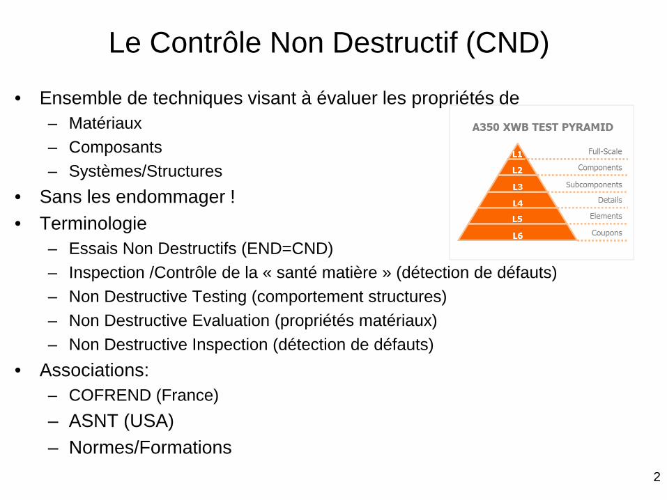
• Ensemble de techniques visant à évaluer les propriétés de – Matériaux – Composants – Systèmes/Structures
• Sans les endommager ! • Terminologie
– Essais Non Destructifs (END=CND) – Inspection /Contrôle de la « santé matière » (détection de défauts) – Non Destructive Testing (comportement structures) – Non Destructive Evaluation (propriétés matériaux) – Non Destructive Inspection (détection de défauts)
• Associations: – COFREND (France) – ASNT (USA) – Normes/Formations
2
Le Contrôle Non Destructif (CND)
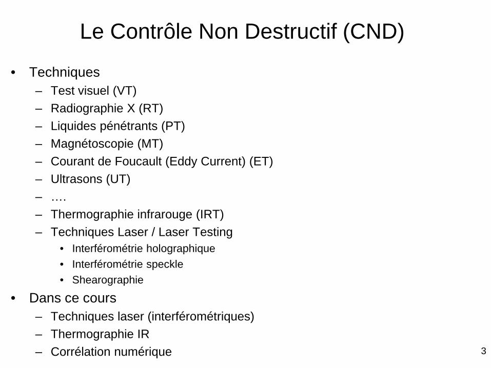
• Techniques – Test visuel (VT) – Radiographie X (RT) – Liquides pénétrants (PT) – Magnétoscopie (MT) – Courant de Foucault (Eddy Current) (ET) – Ultrasons (UT) – …. – Thermographie infrarouge (IRT) – Techniques Laser / Laser Testing
• Interférométrie holographique • Interférométrie speckle • Shearographie
• Dans ce cours – Techniques laser (interférométriques) – Thermographie IR – Corrélation numérique 3
Le Contrôle Non Destructif (CND)
4
Plan de l’exposé
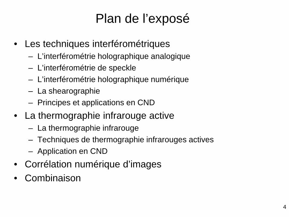
• Les techniques interférométriques – L’interférométrie holographique analogique – L’interférométrie de speckle – L’interférométrie holographique numérique – La shearographie – Principes et applications en CND
• La thermographie infrarouge active – La thermographie infrarouge – Techniques de thermographie infrarouges actives – Application en CND
• Corrélation numérique d’images • Combinaison
5
Les techniques interférométriques
6
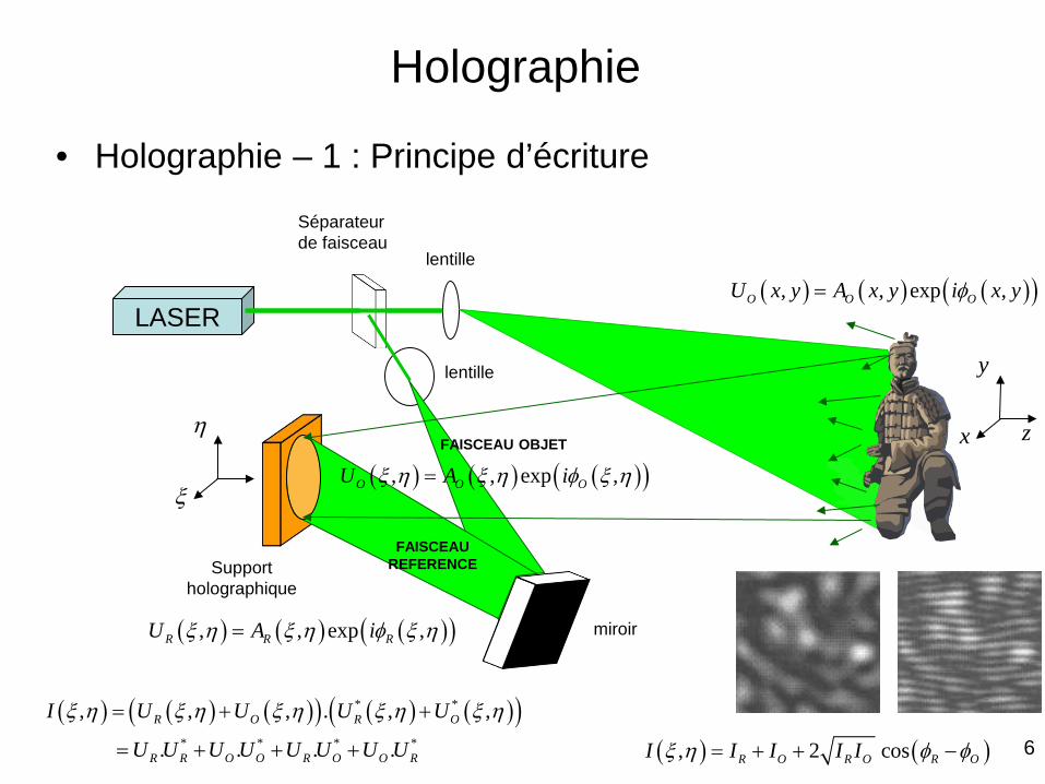
Holographie
• Holographie – 1 : Principe d’écriture
miroir
LASER
lentille
lentille
Séparateur de faisceau
Support holographique
FAISCEAU REFERENCE
FAISCEAU OBJET
( ) ( ) ( )( ), , exp ,O O OU x y A x y i x yφ=
( ) ( ) ( )( ), , exp ,R R RU A iξ η ξ η φ ξ η=
( ) ( ) ( )( ), , exp ,O O OU A iξ η ξ η φ ξ η=ξ
η x
y
z
( ) ( ) ( )( ) ( ) ( )( )* *, , , . , ,R O R OI U U U Uξ η ξ η ξ η ξ η ξ η= + +* * * *. . . .R R O O R O O RU U U U U U U U= + + + ( ) ( ), 2 cosR O R O R OI I I I Iξ η φ φ= + + −
7
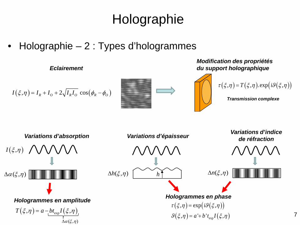
Holographie
• Holographie – 2 : Types d’hologrammes
( ) ( ), 2 cosR O R O R OI I I I Iξ η φ φ= + + −
Eclairement
Hologrammes en amplitude
Variations d’absorption
( ),I ξ η
( , )α ξ η∆
Modification des propriétés du support holographique
Variations d’épaisseur
( , )h ξ η∆ h
Variations d’indice de réfraction
( , )n ξ η∆
( ) ( )( )( ) ( )exp
, exp ,
, ' ' ,
i
a b t I
τ ξ η ϑ ξ η
ϑ ξ η ξ η
=
= +
Hologrammes en phase
( ) ( )exp, ,T a bt Iξ η ξ η= −
( , )α ξ η∆
( ) ( ) ( )( ), , .exp ,T iτ ξ η ξ η ϑ ξ η=
Transmission complexe
8
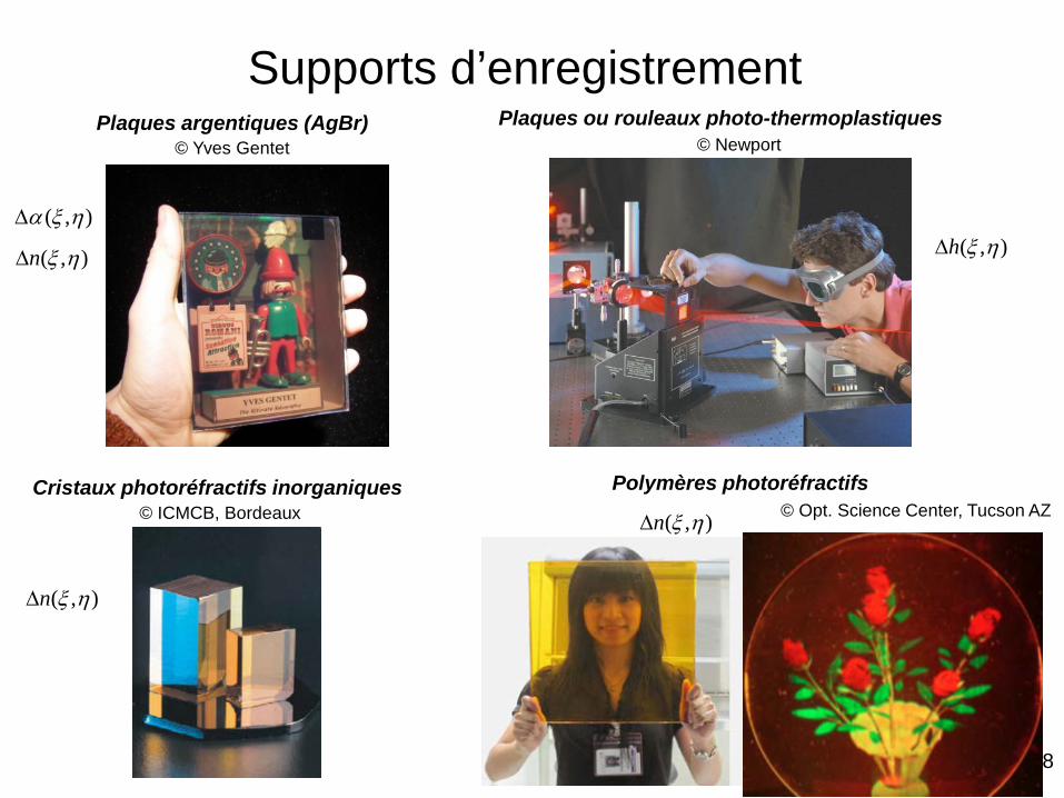
Supports d’enregistrement
Polymères photoréfractifs
( , )n ξ η∆ © Opt. Science Center, Tucson AZ
Plaques ou rouleaux photo-thermoplastiques
( , )h ξ η∆
© Newport Plaques argentiques (AgBr)
( , )α ξ η∆
( , )n ξ η∆
© Yves Gentet
Cristaux photoréfractifs inorganiques
( , )n ξ η∆
© ICMCB, Bordeaux
9
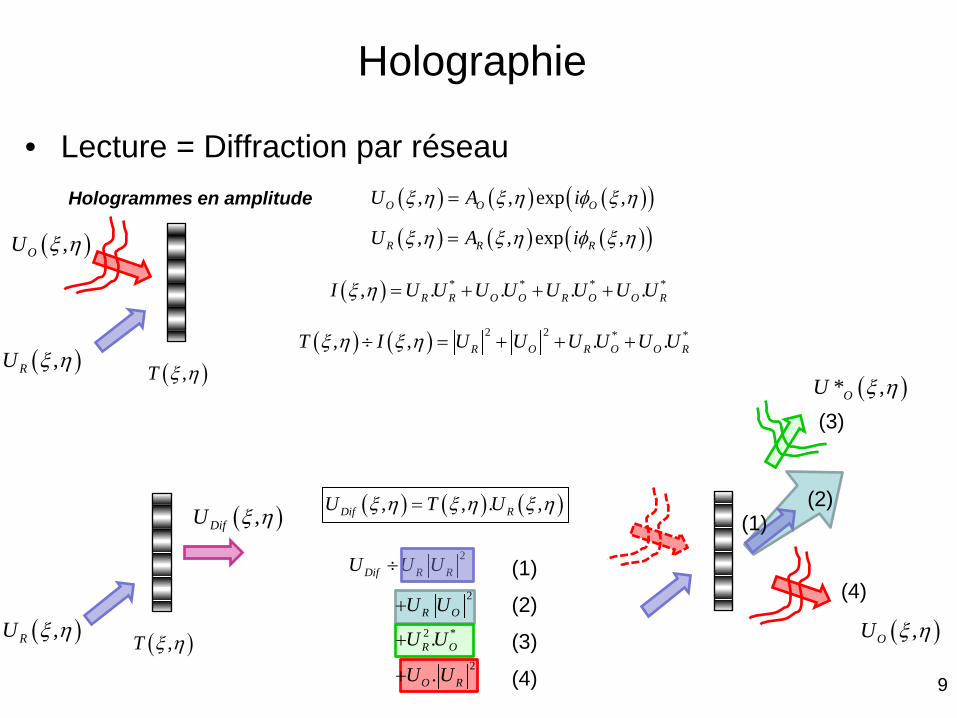
Holographie
• Lecture = Diffraction par réseau
( ) ( ) ( ), , . ,Dif RU T Uξ η ξ η ξ η=
Hologrammes en amplitude
( ) * * * *, . . . .R R O O R O O RI U U U U U U U Uξ η = + + +
( ),RU ξ η
( ),OU ξ η
( ),T ξ η
( ) ( ) ( )( ), , exp ,R R RU A iξ η ξ η φ ξ η=
( ) ( ) ( )( ), , exp ,O O OU A iξ η ξ η φ ξ η=
( ) ( ) 2 2 * *, , . .R O R O O RT I U U U U U Uξ η ξ η÷ = + + +
2Dif R RU U U÷
( ),RU ξ η ( ),T ξ η
( ),DifU ξ η
( ),OU ξ η
( )* ,OU ξ η
(1)
(1)
(2)
(2)
(3)
(3)
(4)
(4) 2
2 *
2
.
.
R O
R O
O R
U U
U U
U U
+
+
+
10
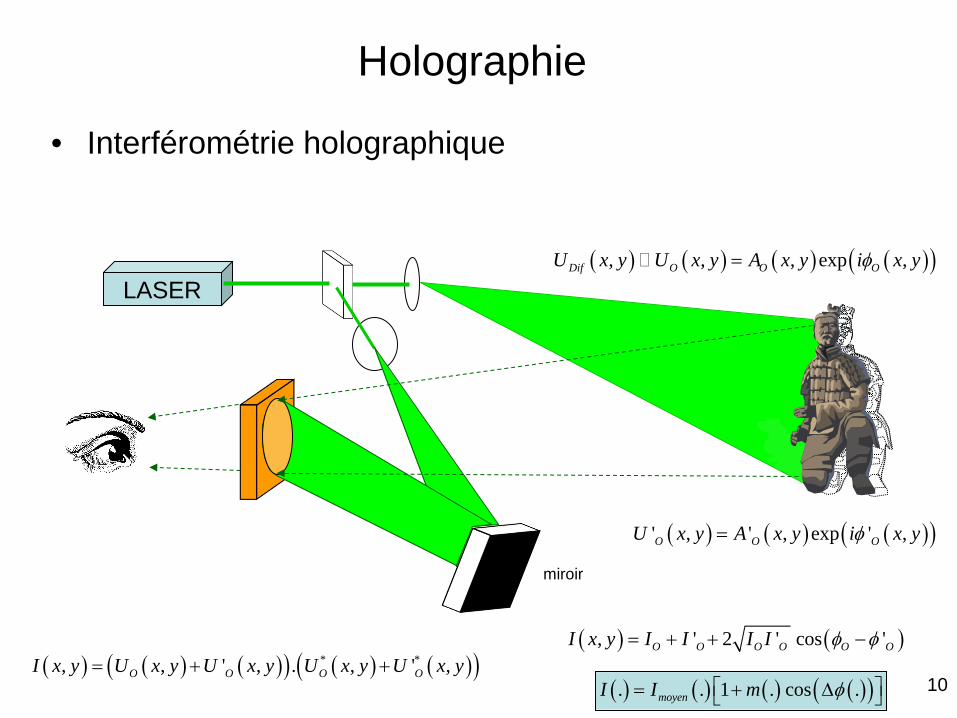
• Interférométrie holographique
LASER
miroir
( ) ( ) ( ) ( )( ), , , exp ,Dif O O OU x y U x y A x y i x yφ=
( ) ( ) ( )( )' , ' , exp ' ,O O OU x y A x y i x yφ=
( ) ( ) ( )( ) ( ) ( )( )* *, , ' , . , ' ,O O O OI x y U x y U x y U x y U x y= + +( ) ( ), ' 2 ' cos 'O O O O O OI x y I I I I φ φ= + + −
( ) ( ) ( ) ( )( ). . 1 . cos .moyenI I m φ = + ∆
Holographie
11
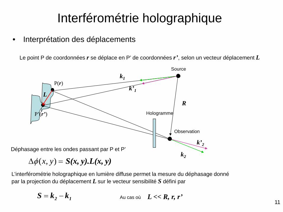
• Interprétation des déplacements
( , )x yφ∆ = S(x, y).L(x, y)
Source
Observation
Hologramme
k’1
k1
k’2
k2
12 kkS −=
Déphasage entre les ondes passant par P et P’
P(r)
L
L’interférométrie holographique en lumière diffuse permet la mesure du déphasage donné par la projection du déplacement L sur le vecteur sensibilité S défini par
Au cas où
R
P’(r’)
L << R, r, r’
Le point P de coordonnées r se déplace en P’ de coordonnées r’, selon un vecteur déplacement L
Interférométrie holographique
12
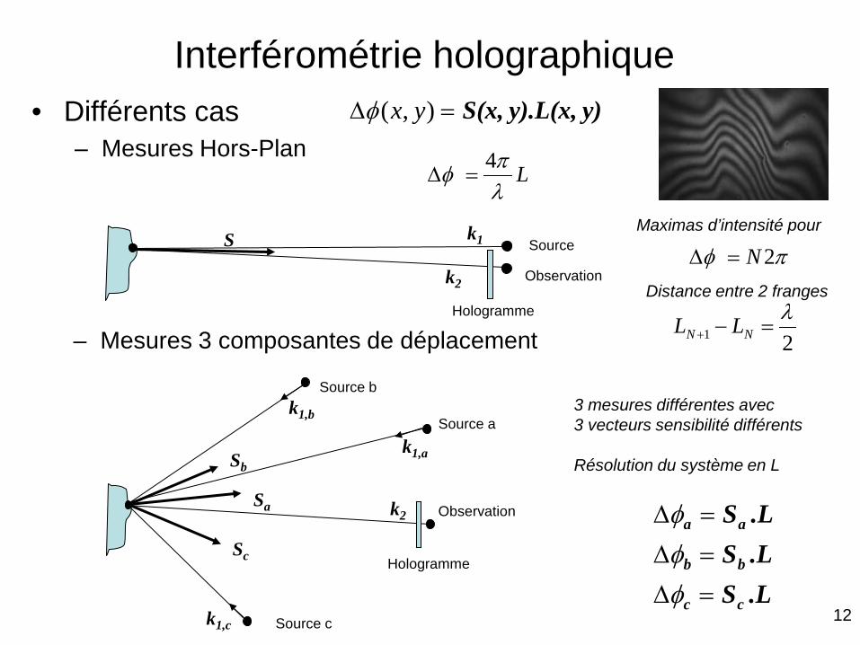
Interférométrie holographique • Différents cas
– Mesures Hors-Plan
.LS
.LS
.LS
cc
bb
aa
=∆=∆=∆
φφφ
Source
Observation
Hologramme
k2
S k1
Source c
Source a
Observation
Hologramme
k2 Sa
k1,a
Source b
Sb
Sc
k1,b
k1,c
3 mesures différentes avec 3 vecteurs sensibilité différents Résolution du système en L
Lλπφ 4
=∆
πφ 2N=∆Maximas d’intensité pour
Distance entre 2 franges
21λ
=−+ NN LL
( , )x yφ∆ = S(x, y).L(x, y)
– Mesures 3 composantes de déplacement
13
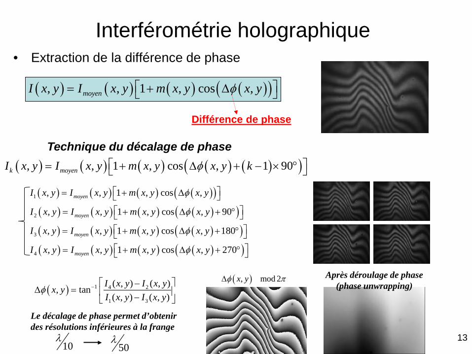
• Extraction de la différence de phase
Interférométrie holographique
( ) ( ) ( ) ( )( ), , 1 , cos ,moyenI x y I x y m x y x yφ = + ∆
Différence de phase
Après déroulage de phase (phase unwrapping)
( ) ( ) ( ) ( ) ( )( ), , 1 , cos , 1 90k moyenI x y I x y m x y x y kφ = + ∆ + − × °
( ) ( ) ( ) ( )( )( ) ( ) ( ) ( )( )( ) ( ) ( ) ( )( )( ) ( ) ( ) ( )( )
1
2
3
4
, , 1 , cos ,
, , 1 , cos , 90
, , 1 , cos , 180
, , 1 , cos , 270
moyen
moyen
moyen
moyen
I x y I x y m x y x y
I x y I x y m x y x y
I x y I x y m x y x y
I x y I x y m x y x y
φ
φ
φ
φ
= + ∆ = + ∆ + ° = + ∆ + ° = + ∆ + °
( ) 1 4 2
1 3
( , ) ( , ), tan
( , ) ( , )I x y I x yx yI x y I x y
φ − −∆ = −
Technique du décalage de phase
( ), mod 2x yφ π∆
Le décalage de phase permet d’obtenir des résolutions inférieures à la frange
10λ
50λ
14
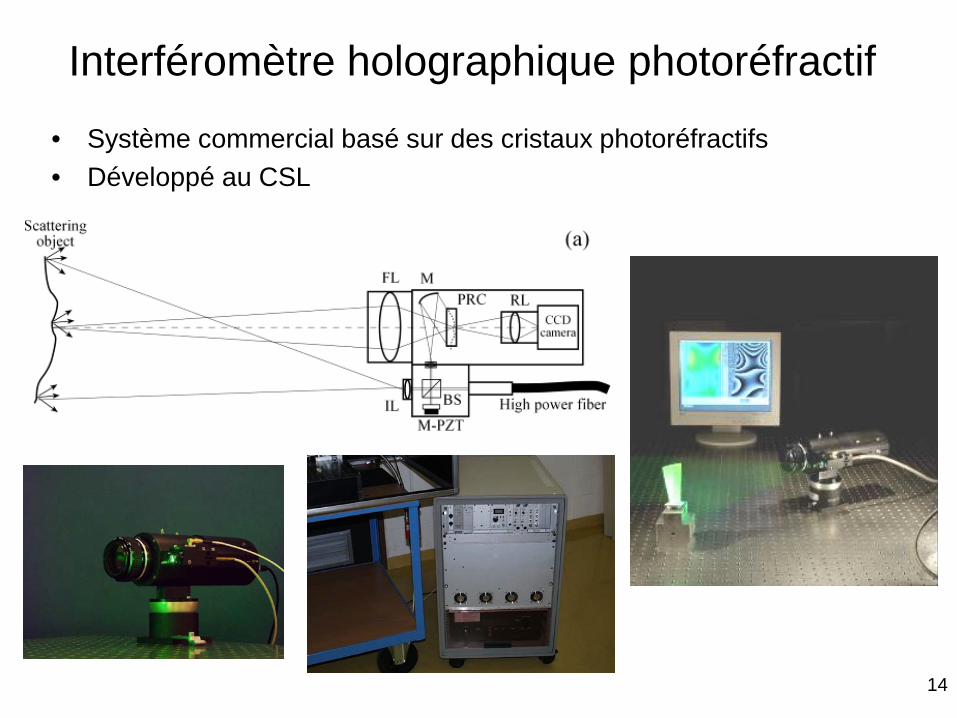
Interféromètre holographique photoréfractif
• Système commercial basé sur des cristaux photoréfractifs • Développé au CSL
15
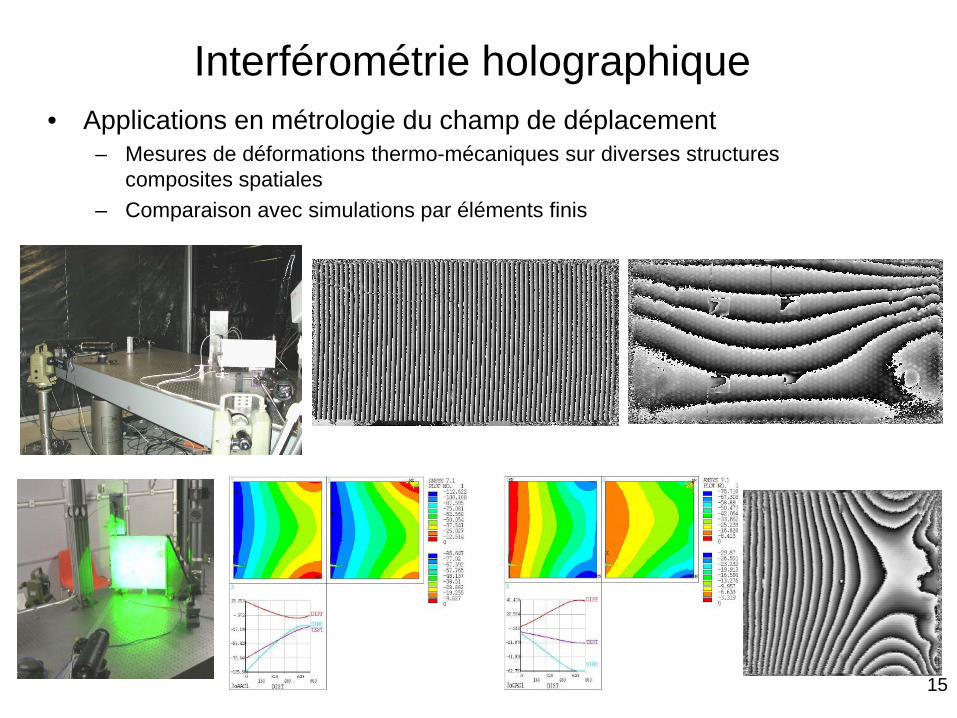
• Applications en métrologie du champ de déplacement – Mesures de déformations thermo-mécaniques sur diverses structures
composites spatiales – Comparaison avec simulations par éléments finis
Interférométrie holographique

16
• Champ de déplacement 3D
Displacement X [µm]
-1
-0.5
0
0.5
1
1.5
2
2.5
3
3.5X - Test X - Sim X - Diff.
-4
-3.5
-3
-2.5
-2
-1.5
-1
-0.5
0
0.5Y - Test Y - Sim Y - Diff.
2
2.5
3
3.5
4
4.5
-0.2
0
0.2
0.4
0.6
0.8
Z - Test Z - Sim Z - Diff.
Interférométrie holographique
17
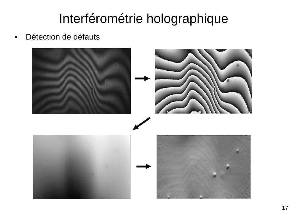
• Détection de défauts
Interférométrie holographique
18
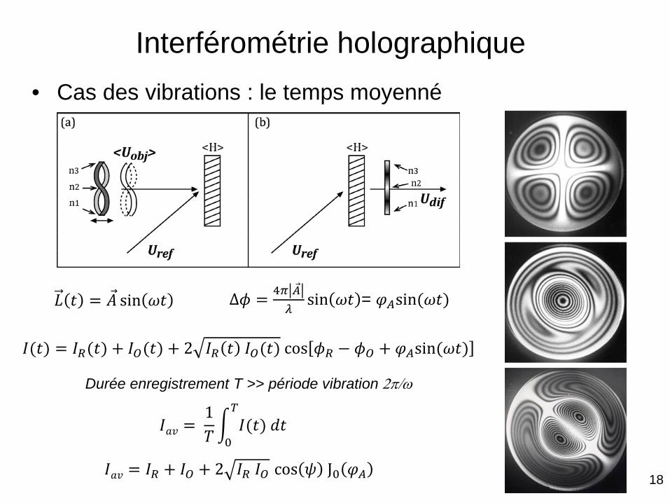
• Cas des vibrations : le temps moyenné
Interférométrie holographique
𝐿𝐿 𝑡𝑡 = 𝐴𝐴 sin 𝜔𝜔𝑡𝑡 Δ𝜙𝜙 = 4𝜋𝜋 �⃗�𝐴𝜆𝜆
sin 𝜔𝜔𝑡𝑡 = 𝜑𝜑𝐴𝐴sin (𝜔𝜔𝑡𝑡)
𝐼𝐼(𝑡𝑡) = 𝐼𝐼𝑅𝑅(𝑡𝑡) + 𝐼𝐼𝑂𝑂(𝑡𝑡) + 2 𝐼𝐼𝑅𝑅 𝑡𝑡 𝐼𝐼𝑂𝑂(𝑡𝑡) cos 𝜙𝜙𝑅𝑅 − 𝜙𝜙𝑂𝑂 + 𝜑𝜑𝐴𝐴sin (𝜔𝜔𝑡𝑡)
𝐼𝐼𝑎𝑎𝑎𝑎 = 1𝑇𝑇� 𝐼𝐼(𝑡𝑡) 𝑑𝑑𝑡𝑡
𝑇𝑇
0
𝐼𝐼𝑎𝑎𝑎𝑎 = 𝐼𝐼𝑅𝑅 + 𝐼𝐼𝑂𝑂 + 2 𝐼𝐼𝑅𝑅 𝐼𝐼𝑂𝑂 cos 𝜓𝜓 J0 𝜑𝜑𝐴𝐴
Durée enregistrement T >> période vibration 2π/ω
19
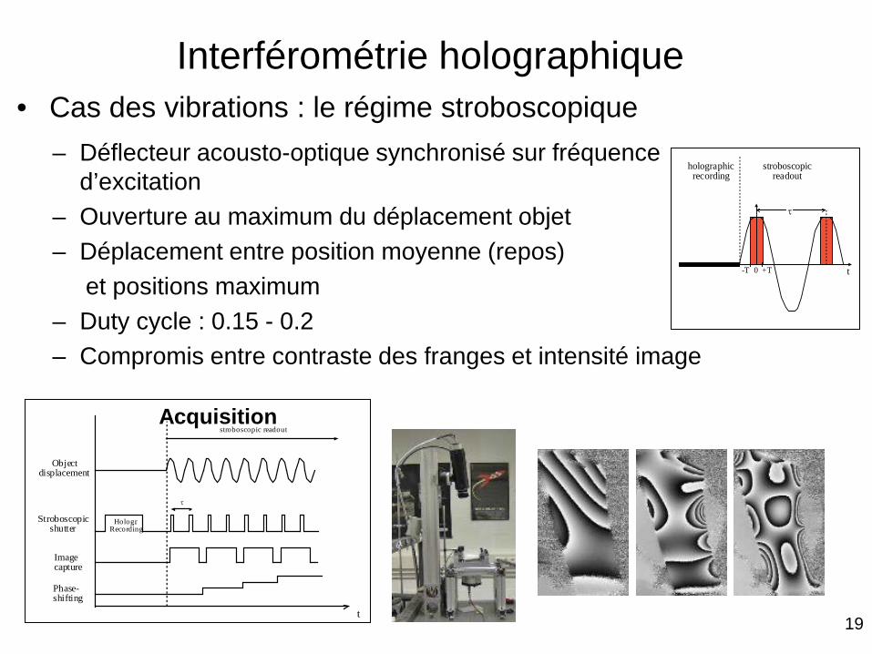
– Déflecteur acousto-optique synchronisé sur fréquence d’excitation
– Ouverture au maximum du déplacement objet – Déplacement entre position moyenne (repos) et positions maximum – Duty cycle : 0.15 - 0.2 – Compromis entre contraste des franges et intensité image
t0-T +T
τ
holographicrecording
stroboscopicreadout
t
stroboscopic readout
Stroboscopicshutter
Hologr.Recording
Imagecapture
Phase-shifting
Objectdisplacement
τ
Acquisition
• Cas des vibrations : le régime stroboscopique Interférométrie holographique
20
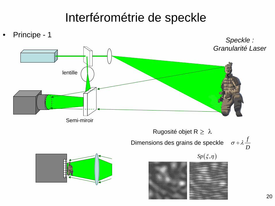
Interférométrie de speckle • Principe - 1
Semi-miroir
lentille
( ),Sp ξ η
Speckle : Granularité Laser
Rugosité objet R λ ≥fD
σ λ÷Dimensions des grains de speckle
21
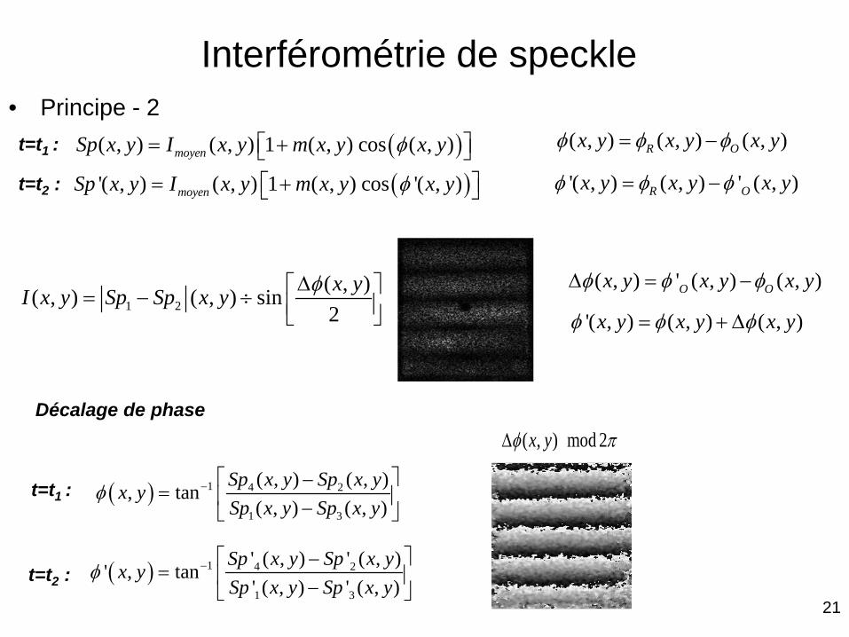
Interférométrie de speckle
( )( , ) ( , ) 1 ( , ) cos ( , )moyenSp x y I x y m x y x yφ= + t=t1 :
( )'( , ) ( , ) 1 ( , ) cos '( , )moyenSp x y I x y m x y x yφ= + t=t2 :
1 2( , )( , ) ( , ) sin2x yI x y Sp Sp x y φ∆ = − ÷
This image cannot currently be displayed.
( , ) mod 2x yφ π∆Décalage de phase
( ) 1 4 2
1 3
( , ) ( , ), tan
( , ) ( , )Sp x y Sp x yx ySp x y Sp x y
φ − −= −
( , ) ( , ) ( , )R Ox y x y x yφ φ φ= −• Principe - 2
'( , ) ( , ) ' ( , )R Ox y x y x yφ φ φ= −
'( , ) ( , ) ( , )x y x y x yφ φ φ= + ∆
( ) 1 4 2
1 3
' ( , ) ' ( , )' , tan
' ( , ) ' ( , )Sp x y Sp x yx ySp x y Sp x y
φ − −= −
t=t1 :
t=t2 :
( , ) ' ( , ) ( , )O Ox y x y x yφ φ φ∆ = −
22
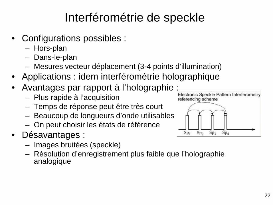
• Configurations possibles : – Hors-plan – Dans-le-plan – Mesures vecteur déplacement (3-4 points d’illumination)
• Applications : idem interférométrie holographique • Avantages par rapport à l’holographie :
– Plus rapide à l’acquisition – Temps de réponse peut être très court – Beaucoup de longueurs d’onde utilisables – On peut choisir les états de référence
• Désavantages : – Images bruitées (speckle) – Résolution d’enregistrement plus faible que l’holographie
analogique
Interférométrie de speckle
23
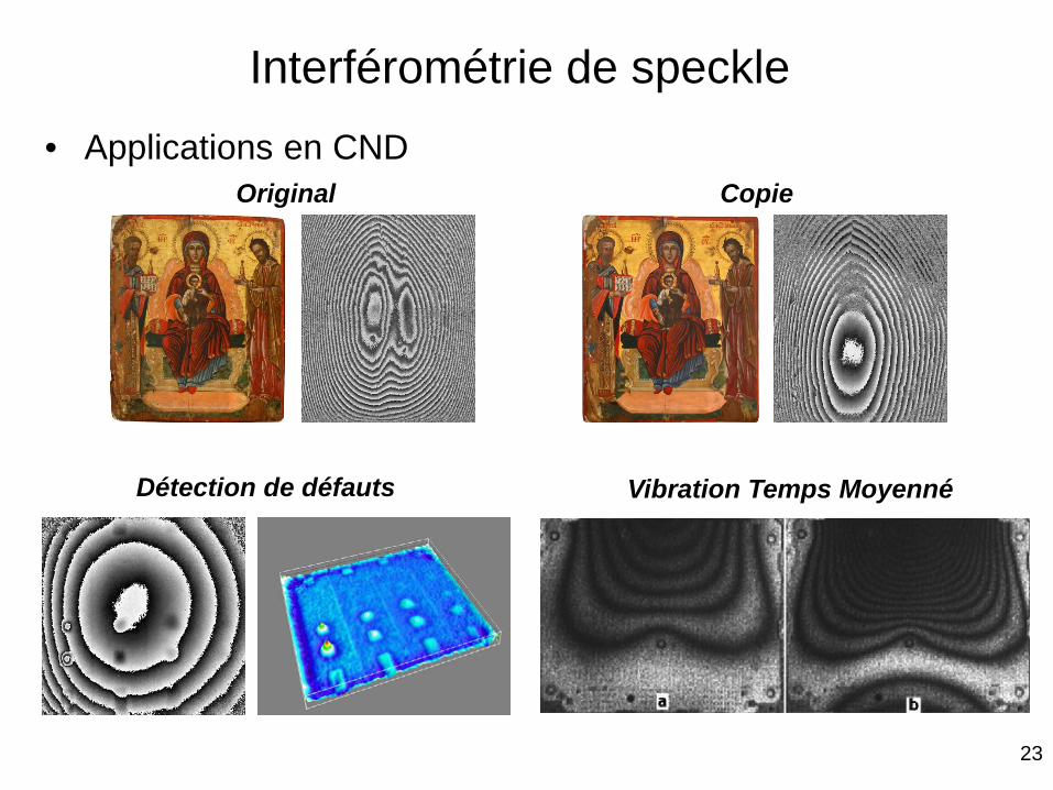
• Applications en CND
Interférométrie de speckle
Original Copie
Détection de défauts Vibration Temps Moyenné
24
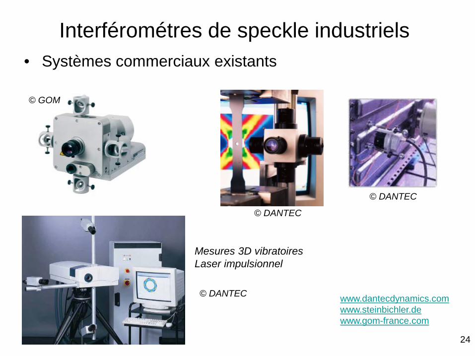
• Systèmes commerciaux existants
www.dantecdynamics.com www.steinbichler.de www.gom-france.com
© GOM
© DANTEC
© DANTEC
© DANTEC
Mesures 3D vibratoires Laser impulsionnel
Interférométres de speckle industriels
25
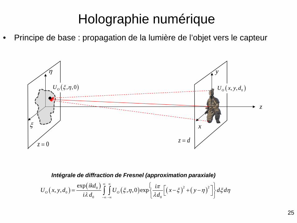
Holographie numérique • Principe de base : propagation de la lumière de l’objet vers le capteur
( ) ( ) ( ) ( ) ( )2 200
0 0
exp, , , ,0 expO O
ikd iU x y d U x y d di d d
πξ η ξ η ξ ηλ λ
∞ ∞
−∞ −∞
= − + − ∫ ∫
ξ
η
x
y
z d=
z
0z =
( )0, ,OU x y d( ), ,0OU ξ η
Intégrale de diffraction de Fresnel (approximation paraxiale)
26
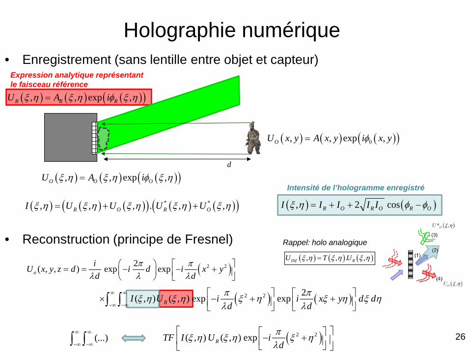
Holographie numérique • Enregistrement (sans lentille entre objet et capteur)
( )2 22( , , ) exp expoiU x y z d i d i x yd d
π πλ λ λ
= = − − +
( ) ( )2 2 2( , ) ( , ) exp expRI U i i x y d dd d
π πξ η ξ η ξ η ξ η ξ ηλ λ
∞ ∞
−∞ −∞
× − + + ∫ ∫
( ) ( ) ( )( )0, , exp ,OU x y A x y i x yφ=
( ) ( ) ( )( ), , exp ,R R RU A iξ η ξ η φ ξ η=
( ) ( ) ( )( ) ( ) ( )( )* *, , , . , ,R O R OI U U U Uξ η ξ η ξ η ξ η ξ η= + + ( ) ( ), 2 cosR O R O R OI I I I Iξ η φ φ= + + −
( ) ( ) ( )( ), , exp ,O O OU A iξ η ξ η φ ξ η=
• Reconstruction (principe de Fresnel)
( )2 2( , ) ( , ) expRTF I U id
πξ η ξ η ξ ηλ
− + (...)
∞ ∞
−∞ −∞∫ ∫
Intensité de l’hologramme enregistré
( ) ( ) ( ), , . ,Dif RU T Uξ η ξ η ξ η=
Rappel: holo analogique
Expression analytique représentant le faisceau référence
d
27
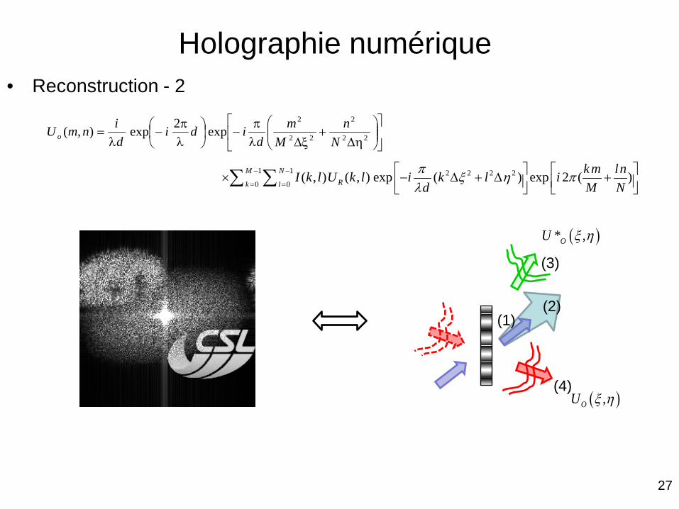
Holographie numérique • Reconstruction - 2
(1)
(4)
(3)
(2)
( ),OU ξ η
( )* ,OU ξ η
η∆
+ξ∆λ
π−
λπ
−λ
= 22
2
22
2
exp2exp),(N
nM
md
ididinmU o
1 1 2 2 2 20 0
( , ) ( , ) exp ( ) exp 2 ( )M NRk l
km lnI k l U k l i k l id M N
π ξ η πλ
− −
= =
× − ∆ + ∆ + ∑ ∑
28
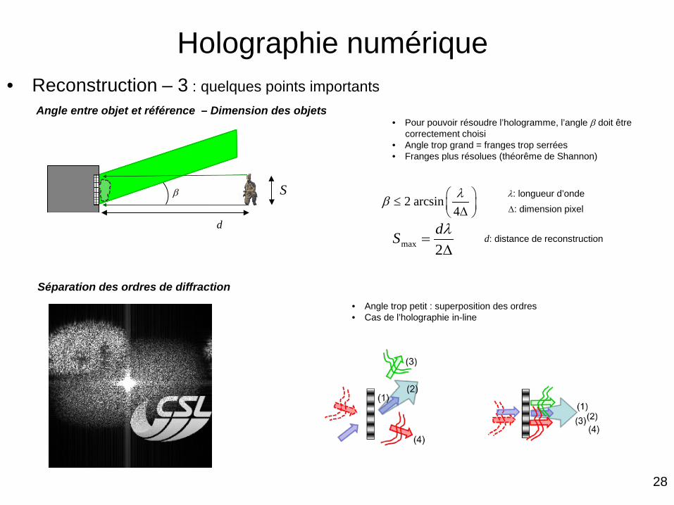
Holographie numérique • Reconstruction – 3 : quelques points importants
2 arcsin4λβ ≤ ∆
∆=
2maxλdS
Séparation des ordres de diffraction
β S λ: longueur d’onde ∆: dimension pixel
d: distance de reconstruction
Angle entre objet et référence – Dimension des objets • Pour pouvoir résoudre l’hologramme, l’angle β doit être correctement choisi • Angle trop grand = franges trop serrées • Franges plus résolues (théorême de Shannon)
• Angle trop petit : superposition des ordres • Cas de l’holographie in-line
d
29
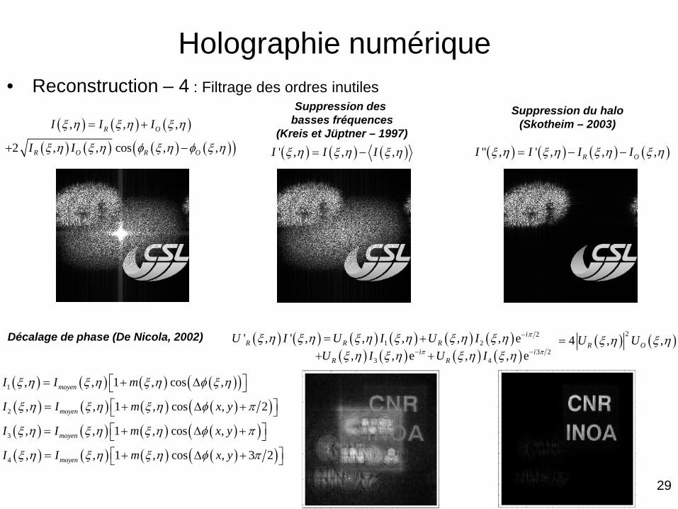
Holographie numérique • Reconstruction – 4 : Filtrage des ordres inutiles
Suppression des basses fréquences
(Kreis et Jüptner – 1997) ( ) ( ) ( )' , , ,I I Iξ η ξ η ξ η= −
( ) ( ) ( ), , ,R OI I Iξ η ξ η ξ η= +
( ) ( ) ( ) ( )( )2 , , cos , ,R O R OI Iξ η ξ η φ ξ η φ ξ η+ −
Suppression du halo (Skotheim – 2003)
( ) ( ) ( ) ( )" , ' , , ,R OI I I Iξ η ξ η ξ η ξ η= − −
Décalage de phase (De Nicola, 2002) ( ) ( ) ( ) ( ) ( ) ( ) 21 2' , ' , , , , , e i
R R RU I U I U I πξ η ξ η ξ η ξ η ξ η ξ η −= +
( ) ( ) ( ) ( )( )( ) ( ) ( ) ( )( )( ) ( ) ( ) ( )( )( ) ( ) ( ) ( )( )
1
2
3
4
, , 1 , cos ,
, , 1 , cos , 2
, , 1 , cos ,
, , 1 , cos , 3 2
moyen
moyen
moyen
moyen
I I m
I I m x y
I I m x y
I I m x y
ξ η ξ η ξ η φ ξ η
ξ η ξ η ξ η φ π
ξ η ξ η ξ η φ π
ξ η ξ η ξ η φ π
= + ∆ = + ∆ + = + ∆ + = + ∆ +
( ) ( ) ( ) ( ) 3 23 4, , e , , ei i
R RU I U Iπ πξ η ξ η ξ η ξ η− −+ +( ) ( )2
4 , ,R OU Uξ η ξ η=
30
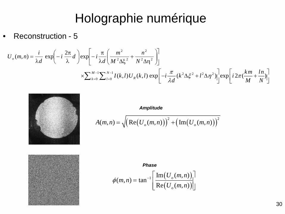
Holographie numérique • Reconstruction - 5
η∆
+ξ∆λ
π−
λπ
−λ
= 22
2
22
2
exp2exp),(N
nM
md
ididinmU o
1 1 2 2 2 20 0
( , ) ( , ) exp ( ) exp 2 ( )M NRk l
km lnI k l U k l i k l id M N
π ξ η πλ
− −
= =
× − ∆ + ∆ + ∑ ∑
( )( ) ( )( )2 2( , ) Re ( , ) Im ( , )o oA m n U m n U m n= +
Amplitude
Phase
( )( )
1 Im ( , )( , ) tan
Re ( , )o
o
U m nm n
U m nφ −
=
31
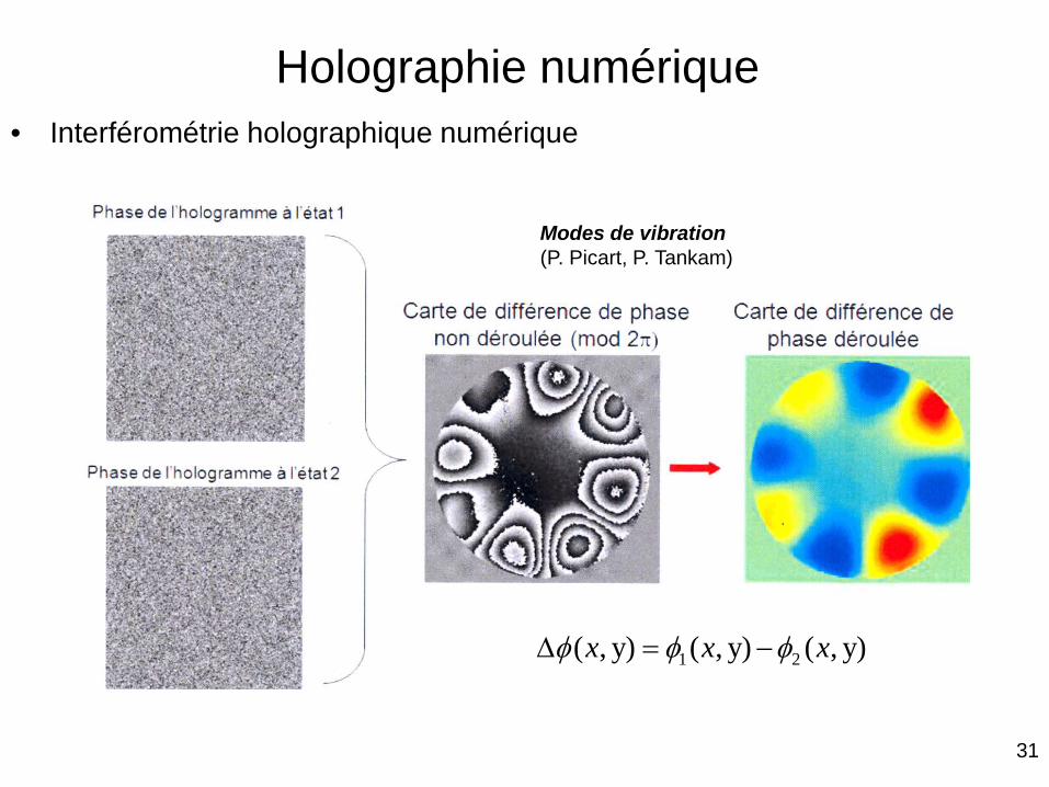
Holographie numérique • Interférométrie holographique numérique
1 2( , y) ( , y) ( , y)x x xφ φ φ∆ = −
Modes de vibration (P. Picart, P. Tankam)
32
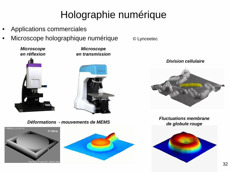
Holographie numérique • Applications commerciales • Microscope holographique numérique
Déformations - mouvements de MEMS
Division cellulaire
Fluctuations membrane de globule rouge
© Lynceetec
Microscope en transmission
Microscope en réflexion
33
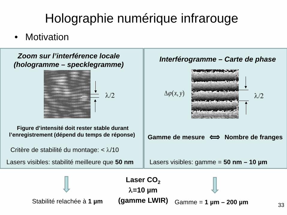
• Motivation
Holographie numérique infrarouge
Laser CO2
λ=10 µm (gamme LWIR)
Zoom sur l’interférence locale (hologramme – specklegramme)
λ/2
Figure d’intensité doit rester stable durant l’enregistrement (dépend du temps de réponse)
Critère de stabilité du montage: < λ/10
Lasers visibles: stabilité meilleure que 50 nm
λ/2
This image cannot currently be displayed.
Interférogramme – Carte de phase
),( yxϕ∆
Gamme de mesure Nombre de franges
Lasers visibles: gamme = 50 nm – 10 µm
Gamme = 1 µm – 200 µm Stabilité relachée à 1 µm
34
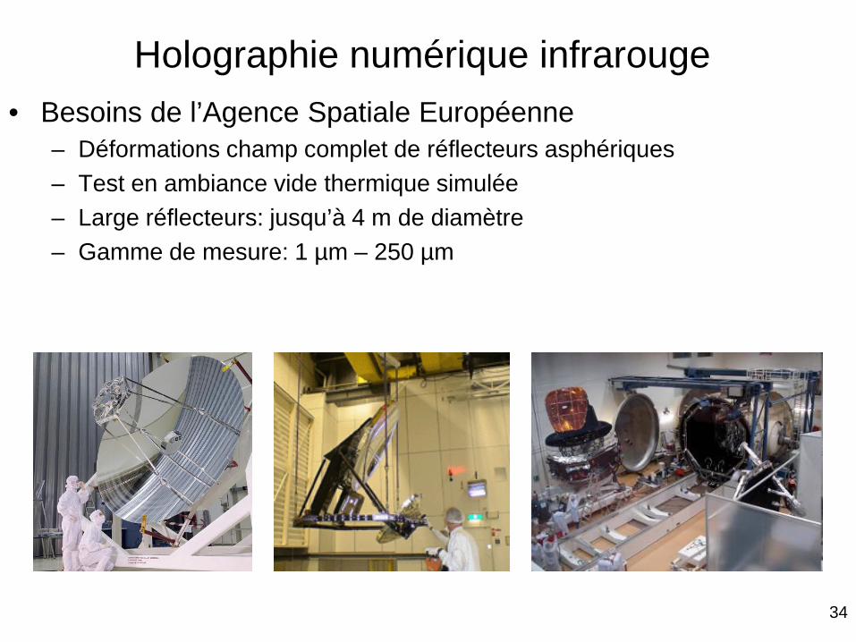
Holographie numérique infrarouge • Besoins de l’Agence Spatiale Européenne
– Déformations champ complet de réflecteurs asphériques – Test en ambiance vide thermique simulée – Large réflecteurs: jusqu’à 4 m de diamètre – Gamme de mesure: 1 µm – 250 µm
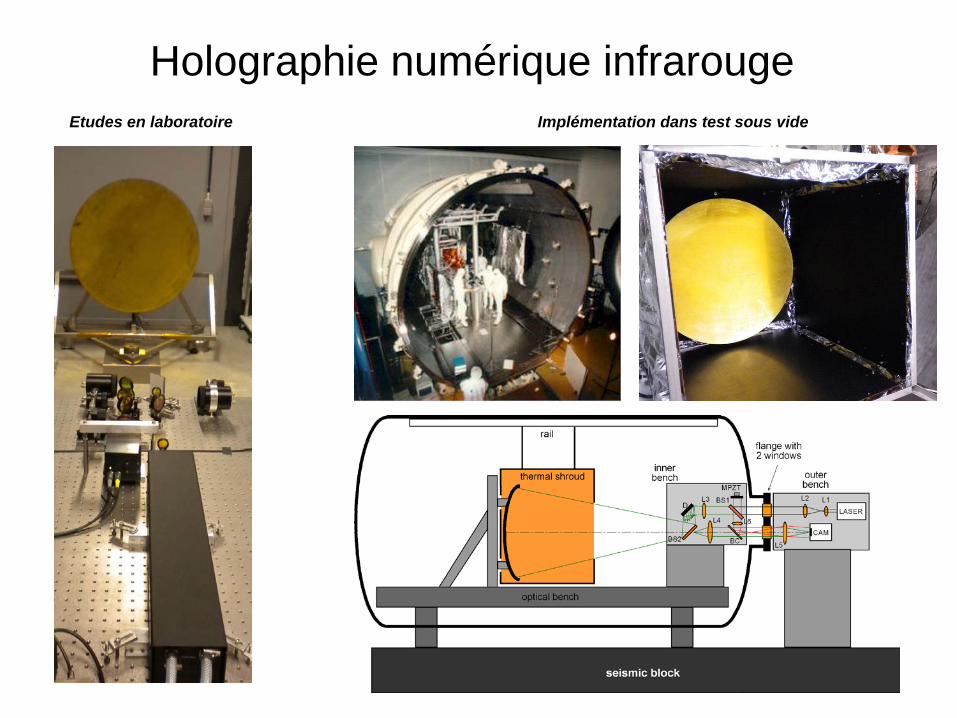
Holographie numérique infrarouge Etudes en laboratoire Implémentation dans test sous vide
36
Holographie numérique infrarouge
36 slide 36
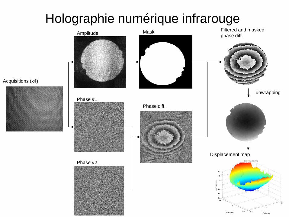
Amplitude
Phase #1
Acquisitions (x4)
Phase #2
Mask
Phase diff.
Filtered and masked phase diff.
unwrapping
Displacement map
37
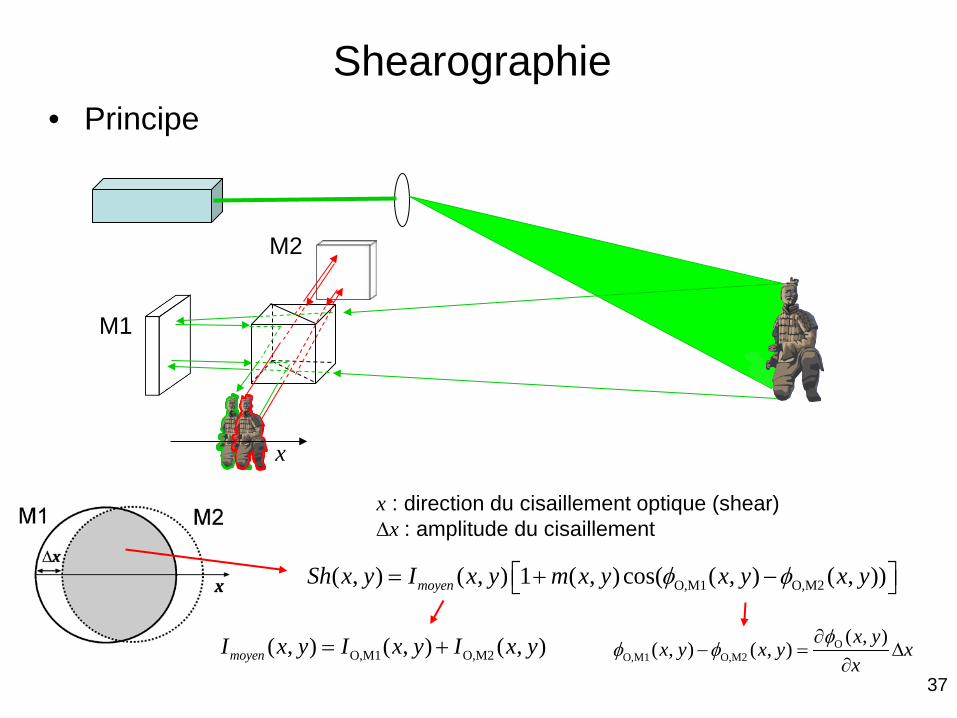
Shearographie • Principe
x ξ
M1
M2
O,M1 O,M2( , ) ( , ) 1 ( , ) cos( ( , ) ( , ))moyenSh x y I x y m x y x y x yφ φ = + −
x : direction du cisaillement optique (shear) ∆x : amplitude du cisaillement
O,M1 O,M2( , ) ( , ) ( , )moyenI x y I x y I x y= + OO,M1 O,M2
( , )( , ) ( , )
x yx y x y x
xφ
φ φ∂
− = ∆∂
38
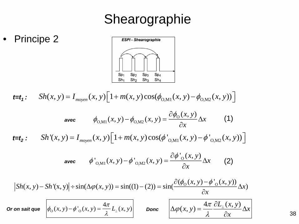
• Principe 2
Shearographie
O O( ( , ) ' ( , ))( , ) '(x, y) sin( ( , )) sin((1) (2)) sin( )
x y x ySh x y Sh x y x
xφ φ
ϕ∂ −
− ÷ ∆ = − = ∆∂
O,M1 O,M2( , ) ( , ) 1 ( , ) cos( ( , ) ( , ))moyenSh x y I x y m x y x y x yφ φ = + − t=t1 :
O,M1 O,M2'( , ) ( , ) 1 ( , ) cos( ' ( , ) ' ( , ))moyenSh x y I x y m x y x y x yφ φ = + − t=t2 :
xx
yxLyx ∆∂
∂=∆ ⊥ ),(4),(
λπϕDonc Or on sait que O O
4( , ) ' ( , ) ( , )x y x y L x yπφ φλ ⊥− =
(1) OO,M1 O,M2
( , )( , ) ( , )
x yx y x y x
xφ
φ φ∂
− = ∆∂
avec
(2) OO,M1 O,M2
' ( , )' ( , ) ' ( , )
x yx y x y x
xφ
φ φ∂
− = ∆∂
avec
39
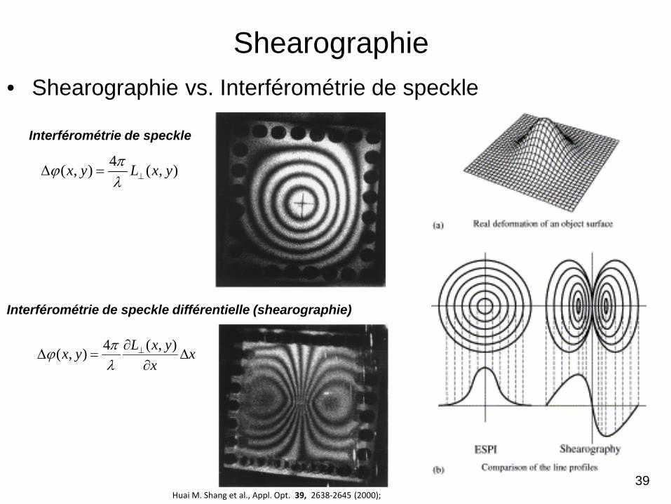
• Shearographie vs. Interférométrie de speckle
Huai M. Shang et al., Appl. Opt. 39, 2638-2645 (2000);
),(4),( yxLyx ⊥=∆λπϕ
xx
yxLyx ∆∂
∂=∆ ⊥ ),(4),(
λπϕ
Shearographie
Interférométrie de speckle
Interférométrie de speckle différentielle (shearographie)
40
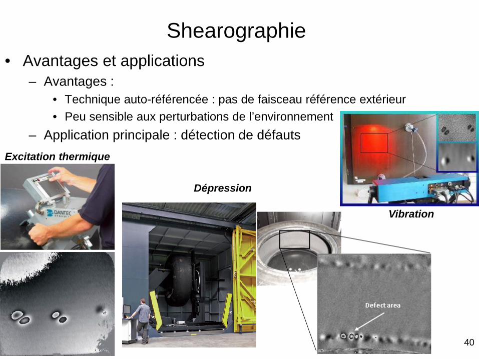
• Avantages et applications – Avantages :
• Technique auto-référencée : pas de faisceau référence extérieur • Peu sensible aux perturbations de l’environnement
– Application principale : détection de défauts Excitation thermique
Dépression
Vibration
Shearographie
41
La thermographie infrarouge
42
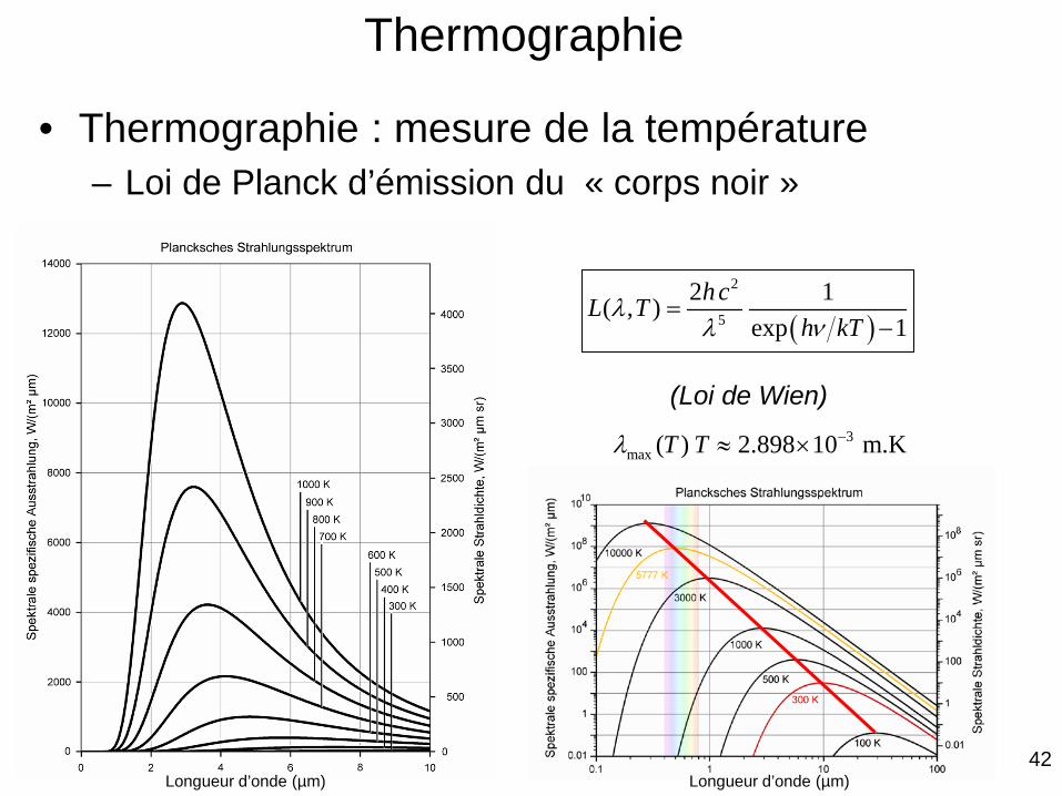
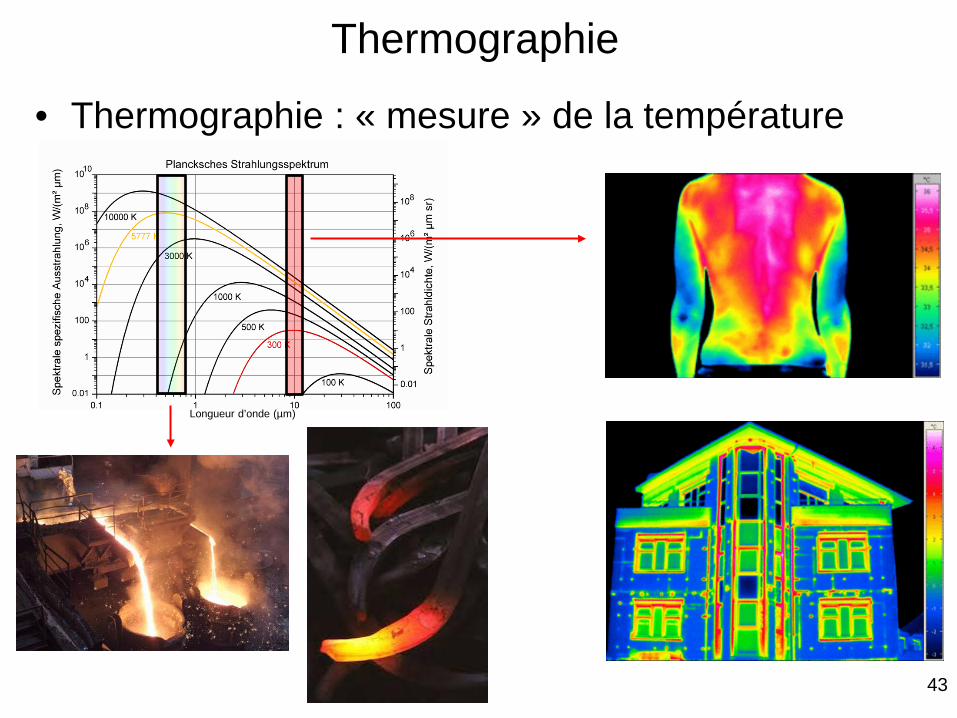
• Thermographie : mesure de la température – Loi de Planck d’émission du « corps noir »
Thermographie
Longueur d’onde (µm) Longueur d’onde (µm)
( )2
5
2 1( , )exp 1
hcL Th kT
λνλ
=−
3max ( ) 2.898 10 m.KT Tλ −≈ ×
(Loi de Wien)
43
• Thermographie : « mesure » de la température
Longueur d’onde (µm)
Thermographie
44
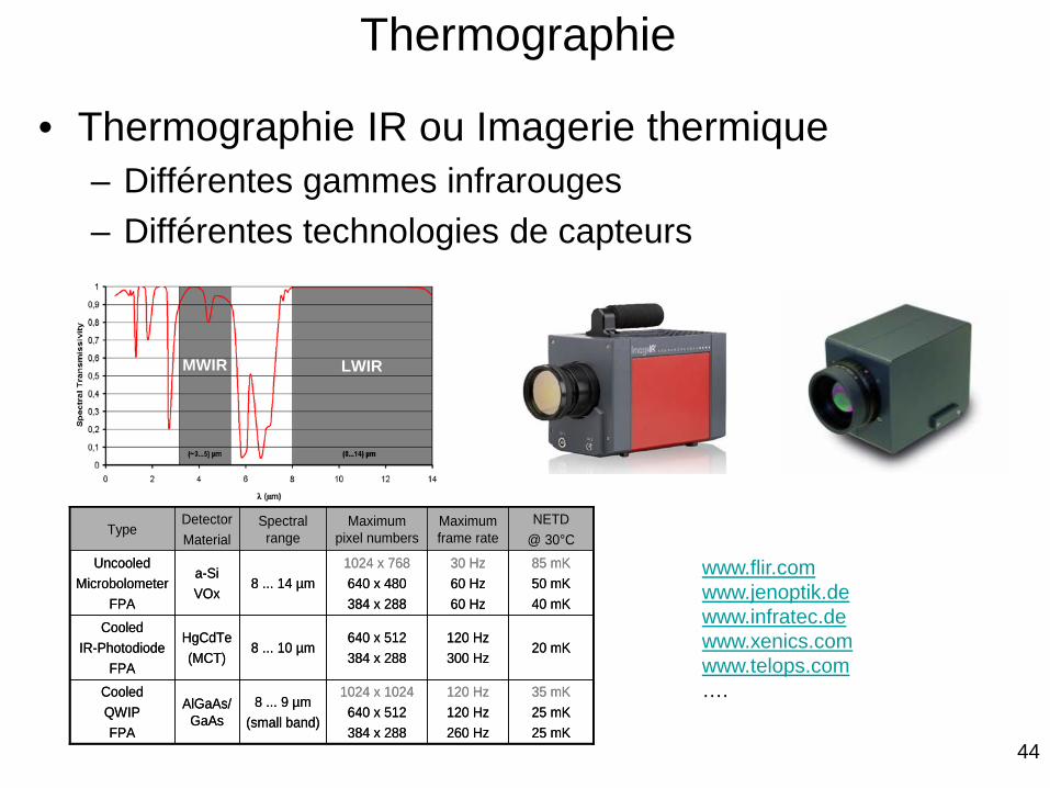
• Thermographie IR ou Imagerie thermique – Différentes gammes infrarouges – Différentes technologies de capteurs
120 Hz120 Hz260 Hz
120 Hz300 Hz
30 Hz60 Hz60 Hz
Maximum frame rate
35 mK25 mK25 mK
1024 x 1024640 x 512384 x 288
8 ... 9 µm(small band)
AlGaAs/ GaAs
Cooled QWIPFPA
20 mK640 x 512384 x 288
8 ... 10 µmHgCdTe(MCT)
Cooled IR-Photodiode
FPA
85 mK50 mK40 mK
1024 x 768640 x 480384 x 288
8 ... 14 µma-SiVOx
Uncooled Microbolometer
FPA
NETD@ 30°C
Maximum pixel numbers
Spectral range
Detector Material
Type
LWIR MWIR
www.flir.com www.jenoptik.de www.infratec.de www.xenics.com www.telops.com ….
Thermographie
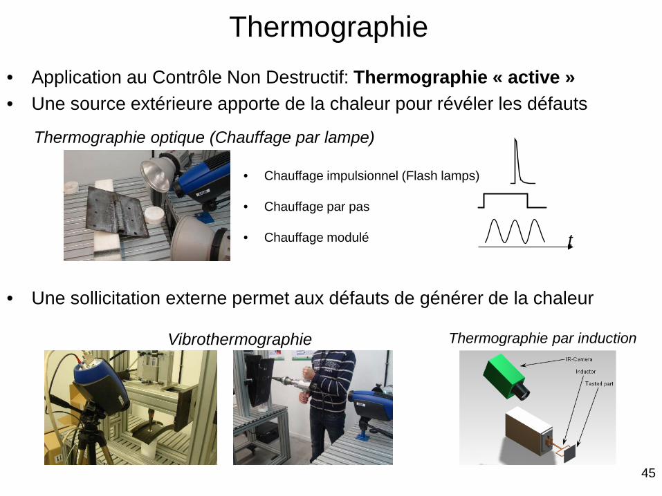
• Application au Contrôle Non Destructif: Thermographie « active » • Une source extérieure apporte de la chaleur pour révéler les défauts
• Une sollicitation externe permet aux défauts de générer de la chaleur
Vibrothermographie Thermographie par induction
Thermographie optique (Chauffage par lampe)
• Chauffage impulsionnel (Flash lamps)
• Chauffage par pas
• Chauffage modulé t
Thermographie
45
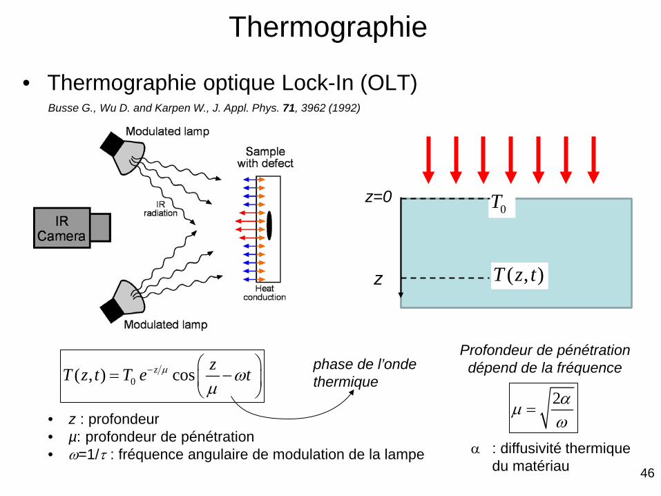
• Thermographie optique Lock-In (OLT)
0( , ) cosz zT z t T e tµ ωµ
− = −
• z : profondeur • µ: profondeur de pénétration • ω=1/τ : fréquence angulaire de modulation de la lampe
z
z=0
2αµω
=
0T
( , )T z t
Busse G., Wu D. and Karpen W., J. Appl. Phys. 71, 3962 (1992)
α : diffusivité thermique du matériau
phase de l’onde thermique
Profondeur de pénétration dépend de la fréquence
Thermographie
46
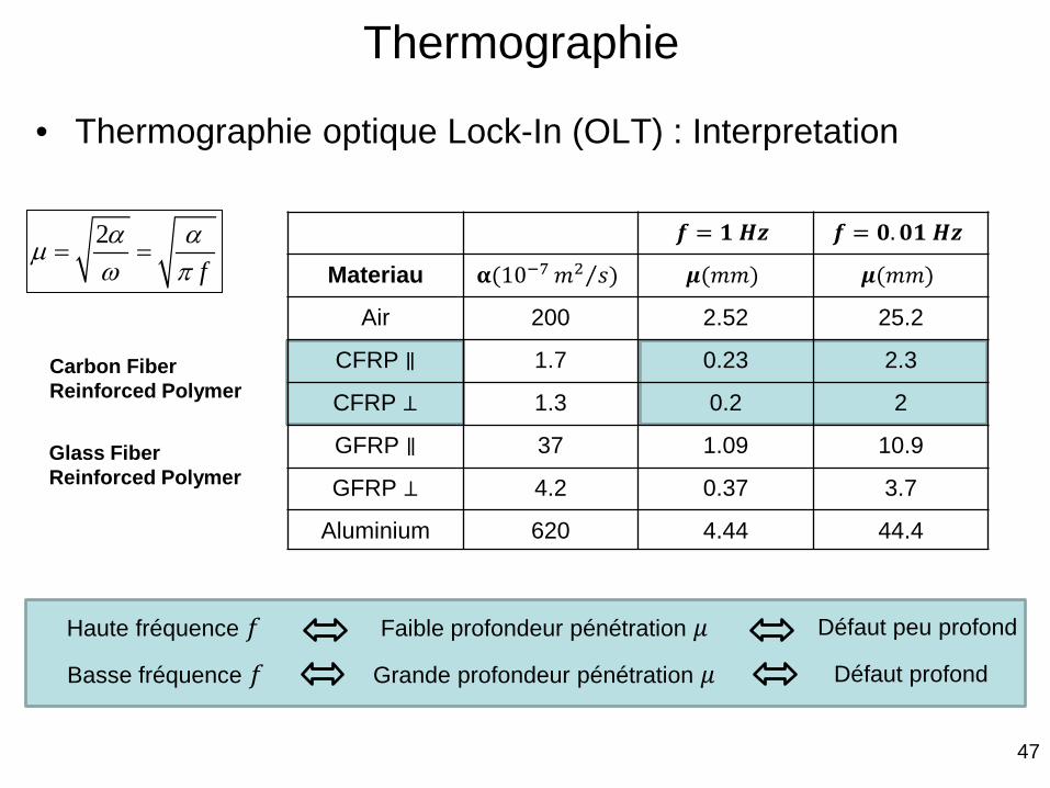
𝒇𝒇 = 𝟏𝟏 𝑯𝑯𝑯𝑯 𝒇𝒇 = 𝟎𝟎.𝟎𝟎𝟏𝟏 𝑯𝑯𝑯𝑯
Materiau 𝛂𝛂(10−7 𝑚𝑚2 𝑠𝑠⁄ ) 𝝁𝝁(𝑚𝑚𝑚𝑚) 𝝁𝝁(𝑚𝑚𝑚𝑚)
Air 200 2.52 25.2
CFRP ∥ 1.7 0.23 2.3
CFRP ⊥ 1.3 0.2 2
GFRP ∥ 37 1.09 10.9
GFRP ⊥ 4.2 0.37 3.7
Aluminium 620 4.44 44.4
• Thermographie optique Lock-In (OLT) : Interpretation
2f
α αµω π
= =
Haute fréquence 𝑓𝑓 Faible profondeur pénétration 𝜇𝜇 Défaut peu profond
Basse fréquence 𝑓𝑓 Grande profondeur pénétration 𝜇𝜇 Défaut profond
Thermographie
47
Carbon Fiber Reinforced Polymer
Glass Fiber Reinforced Polymer
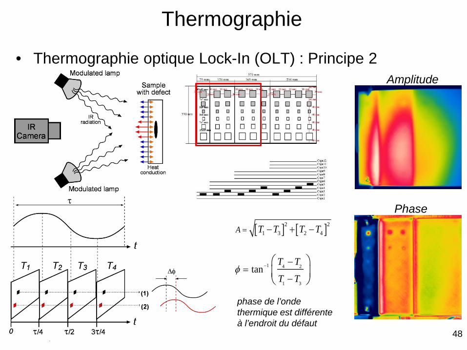
• Thermographie optique Lock-In (OLT) : Principe 2
1 4 2
1 3
tanT T
T Tφ − −
=−
[ ] [ ]2 21 3 2 4A T T T T= − + −
phase de l’onde thermique est différente à l’endroit du défaut
Amplitude
Phase
Thermographie
48
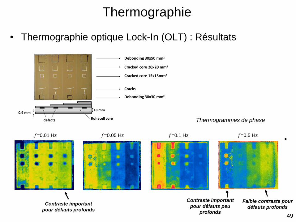
𝑓𝑓=0.01 Hz 𝑓𝑓=0.05 Hz 𝑓𝑓=0.1 Hz 𝑓𝑓=0.5 Hz
• Thermographie optique Lock-In (OLT) : Résultats
Thermogrammes de phase
Contraste important pour défauts profonds
Contraste important pour défauts peu
profonds
Faible contraste pour défauts profonds
Thermographie
49
50
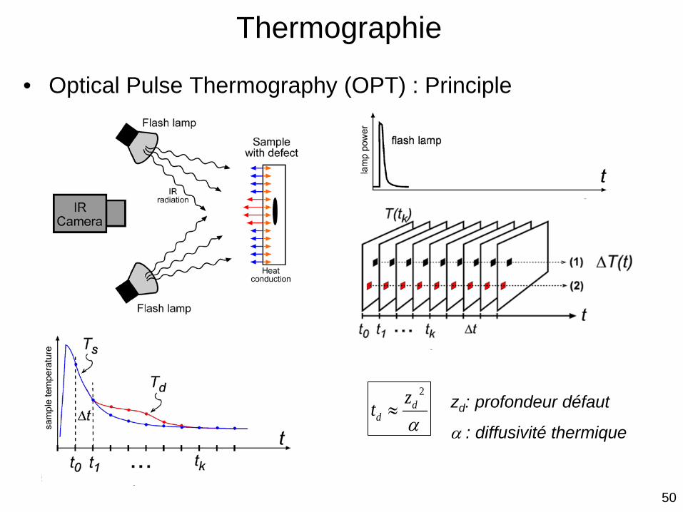
• Optical Pulse Thermography (OPT) : Principle
2d
dztα
≈ zd: profondeur défaut
α : diffusivité thermique
Thermographie
50
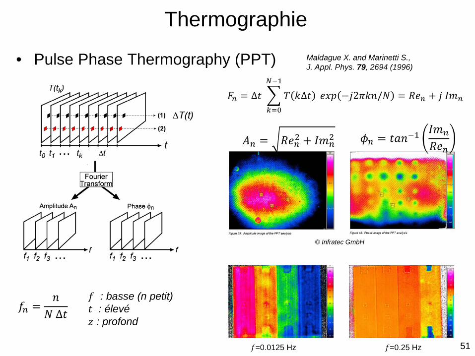
𝑓𝑓 : basse (n petit) 𝑡𝑡 : élevé 𝑧𝑧 : profond
𝑓𝑓=0.0125 Hz 𝑓𝑓=0.25 Hz
• Pulse Phase Thermography (PPT)
𝐹𝐹𝑛𝑛 = ∆𝑡𝑡 �𝑇𝑇 𝑘𝑘∆𝑡𝑡𝑁𝑁−1
𝑘𝑘=0
𝑒𝑒𝑒𝑒𝑒𝑒 −𝑗𝑗𝑗𝑗𝑗𝑘𝑘𝑗𝑗/𝑁𝑁 = 𝑅𝑅𝑒𝑒𝑛𝑛 + 𝑗𝑗 𝐼𝐼𝑚𝑚𝑛𝑛
𝐴𝐴𝑛𝑛 = 𝑅𝑅𝑒𝑒𝑛𝑛2 + 𝐼𝐼𝑚𝑚𝑛𝑛2 𝜙𝜙𝑛𝑛 = 𝑡𝑡𝑎𝑎𝑗𝑗−1
𝐼𝐼𝑚𝑚𝑛𝑛𝑅𝑅𝑒𝑒𝑛𝑛
𝑓𝑓𝑛𝑛 =𝑗𝑗
𝑁𝑁 Δ𝑡𝑡
Maldague X. and Marinetti S., J. Appl. Phys. 79, 2694 (1996)
© Infratec GmbH
Thermographie
51
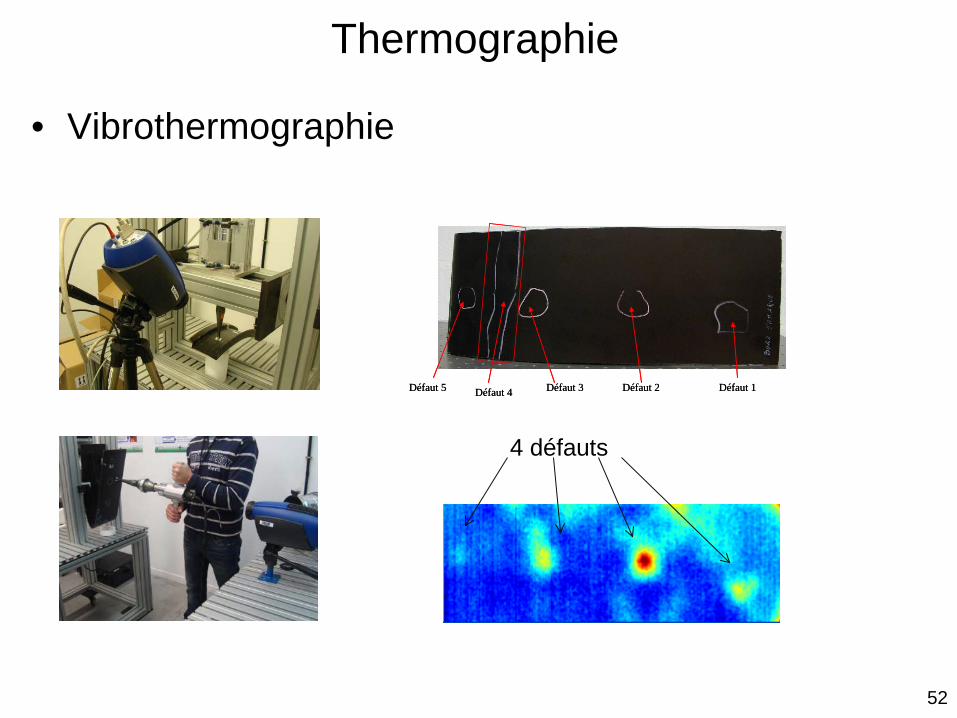
• Vibrothermographie
Thermographie
52
4 défauts
Défaut 1Défaut 2Défaut 3Défaut 4Défaut 5 Défaut 1Défaut 2Défaut 3Défaut 4Défaut 5
Défaut 1Défaut 2Défaut 3Défaut 4Défaut 5 Défaut 1Défaut 2Défaut 3Défaut 4Défaut 5
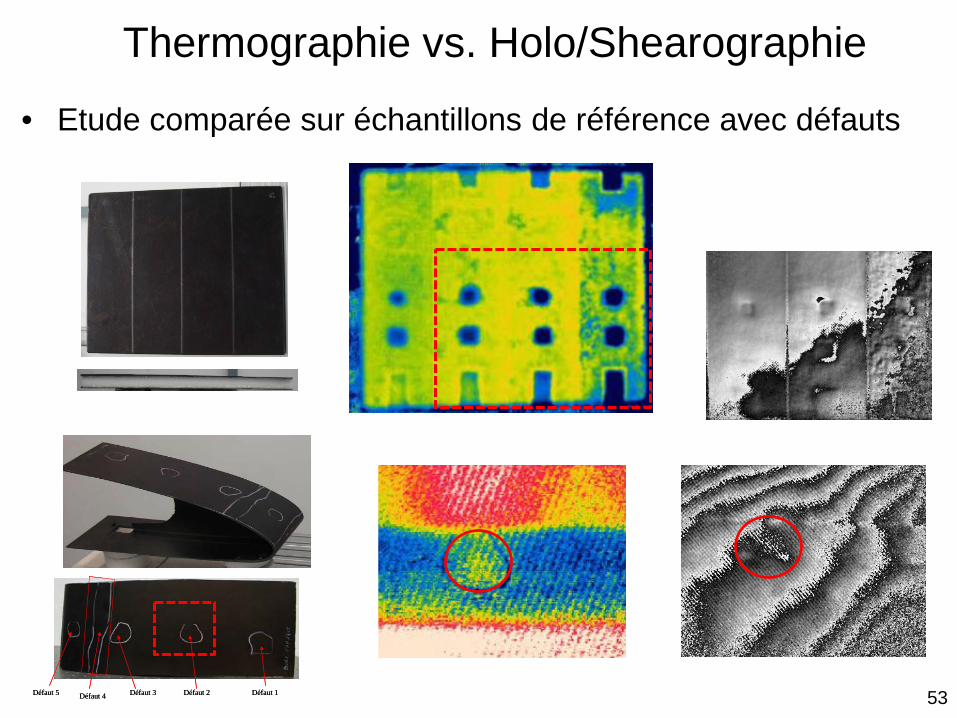
• Etude comparée sur échantillons de référence avec défauts
Thermographie vs. Holo/Shearographie
53
54
La corrélation numérique d’images
Corrélation numérique d’images
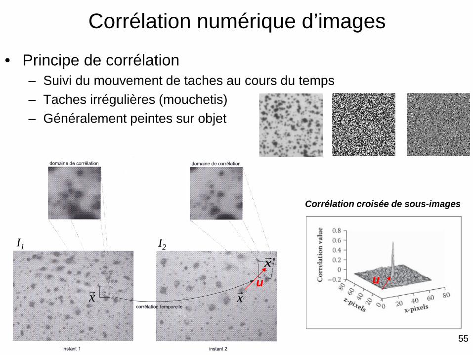
• Principe de corrélation – Suivi du mouvement de taches au cours du temps – Taches irrégulières (mouchetis) – Généralement peintes sur objet
I1 I2
u x
'x
x
Corrélation croisée de sous-images
u
55
Corrélation numérique d’images
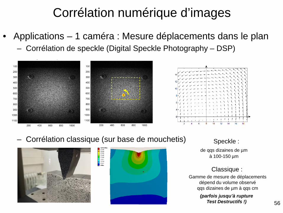
• Applications – 1 caméra : Mesure déplacements dans le plan – Corrélation de speckle (Digital Speckle Photography – DSP)
– Corrélation classique (sur base de mouchetis) Speckle :
Classique :
de qqs dizaines de µm à 100-150 µm
Gamme de mesure de déplacements dépend du volume observé
qqs dizaines de µm à qqs cm (parfois jusqu’à rupture
Test Destructifs !) 56
Corrélation numérique d’images
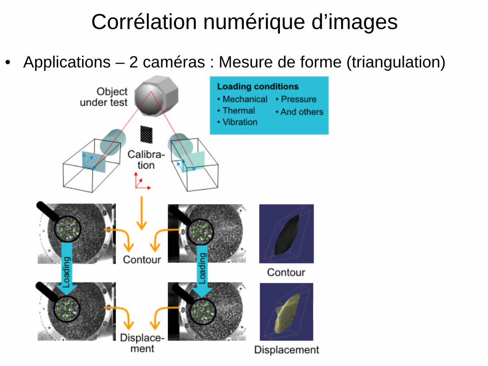
• Applications – 2 caméras : Mesure de forme (triangulation)
Corrélation numérique d’images
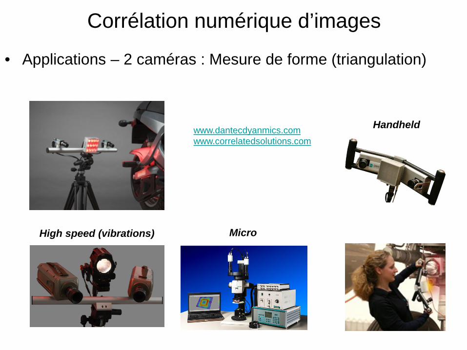
• Applications – 2 caméras : Mesure de forme (triangulation)
www.dantecdyanmics.com www.correlatedsolutions.com
High speed (vibrations) Micro
Handheld
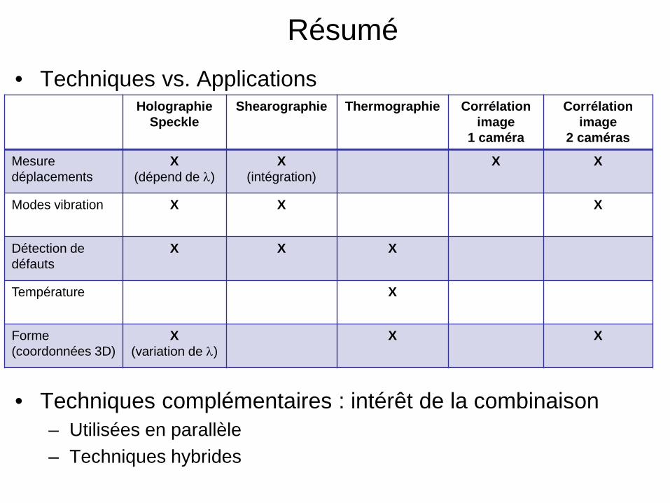
Résumé • Techniques vs. Applications
• Techniques complémentaires : intérêt de la combinaison – Utilisées en parallèle – Techniques hybrides
Holographie Speckle
Shearographie Thermographie Corrélation image
1 caméra
Corrélation image
2 caméras
Mesure déplacements
X (dépend de λ)
X (intégration)
X
X
Modes vibration X X X
Détection de défauts
X X X
Température X
Forme (coordonnées 3D)
X (variation de λ)
X X
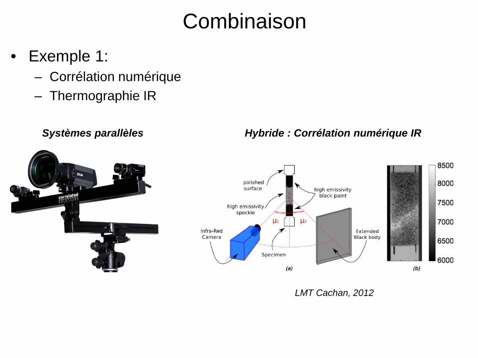
Combinaison • Exemple 1:
– Corrélation numérique – Thermographie IR
Systèmes parallèles Hybride : Corrélation numérique IR
LMT Cachan, 2012
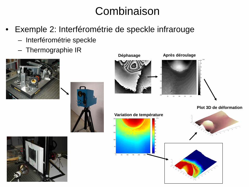
Combinaison • Exemple 2: Interférométrie de speckle infrarouge
– Interférométrie speckle – Thermographie IR
Déphasage Après déroulage
Variation de température
Plot 3D de déformation