Embed Size (px)
Citation preview
En vue de l'obtention du
DOCTORAT DE L'UNIVERSITÉ DE TOULOUSEDélivré par :
Institut National Polytechnique de Toulouse (INP Toulouse)Discipline ou spécialité :
Dynamique des fluides
Présentée et soutenue par :M. TOBIAS ANSALDI
le vendredi 14 octobre 2016
Titre :
Unité de recherche :
Ecole doctorale :
COMPRESSIBLE SINGLE AND DUAL STREAM JET STABILITY ANDADJOINT-BASED SENSITIVITY ANALYSIS IN RELATIONSHIP WITH
AEROACOUSTICS
Mécanique, Energétique, Génie civil, Procédés (MEGeP)
Institut de Mécanique des Fluides de Toulouse (I.M.F.T.)Directeur(s) de Thèse :M. CHRISTOPHE AIRIAU
Rapporteurs :M. JEAN-CHRISTOPHE ROBINET, ENSAM - ARTS ET METIERS PARISTECH
M. UWE EHRENSTEIN, AIX-MARSEILLE UNIVERSITE
Membre(s) du jury :1 M. YVES GERVAIS, UNIVERSITE DE POITIERS, Président2 M. JEAN-PHILIPPE BRAZIER, ONERA TOULOUSE, Membre2 M. JEROME HUBER, AIRBUS FRANCE, Membre

Abstract
This thesis leads to a better knowledge of the physic and of the control of acoustic ra-diation in turbulent single and dual-stream jets. It is known that jet noise is producedby the turbulence present in the jet that can be separated in large coherent structuresand fine structures. It is also concluded that these large-scale coherent structures arethe instability waves of the jet and can be modelled as the flow field generated by theevolution of instability waves in a given turbulent jet. The growth rate and the stream-wise wavenumber of a disturbance with a fixed frequency and azimuthal wavenumber areobtained by solving the non-local approach called Parabolized Stability Equations (PSE).Typically the Kelvin-Helmholtz instability owes its origin into the shear layer of the flowand, moreover, the inflection points of the mean velocity profile has a crucial importancein the instability of such a flow. The problem is more complex in case of imperfectlyexpanded jet where shock-cells manifest inside the jet and strongly interaction with theinstability waves has been observed. Several configurations are tested in this thesis, froma subsonic incompressible case to the dual-stream underexpanded supersonic jet obtainedby solving Large Eddy Simulations LES (CERFACS). The acoustic far-field is determinedby the Ffowcs-Williams-Hawkings acoustic analogy. Then a sensitivity analysis of the jetwith respect to external forcing acting in a localized region of the flow are investigated bysolving the adjoint PSE equations. High sensitivity appeared in the shear-layer of the flowshowing, also, a high dependency in the streamwise and radial direction. In the case ofdual-stream jet the propagation of the instability in the inner and outer shear layer shouldbe taken into account. This configuration leads to two different distinct Klevin-Helmholtzmodes that are computed separately. The highest sensitivity is determined in the exitof the nozzle outside of the potential core of the jet. In addition, comparison betweensensitivity computed by adjoint equations and Uncertainty Quantification (UQ) methodshas been done, in the case of a single-stream jet, showing a link between these two meth-ods for small variations of the input parameters. This result leads to the application of alower cost tool for mathematical analysis of complex problem of industrial interest. Thiswork and in particular the sensitivity theory investigated in this thesis contribute to adevelopment of a new noise control strategy for aircraft jet.
iii

iv

Resume
La these est relative a la comprehension de la physique et au contrle des emissions acous-tiques dans les jets tubulents simples et double-flux. La generation du bruit est associe ades structures turbulentes de grandes tailles caracteristiques et a la turbulence de petitesechelles. i Il est maintenant admis que les structures de grandes echelles sont des insta-bilites se propageant dans un champ moyen turbulent. Ici elle sont analysees sur la basede la theorie lineaire non locale appelees PSE pour Parabolized Stability Equations. Cesinstabilites inflexionnelles associees a la presence de couche de cisaillement sont des modesde Kelvin-Helmhotz. Dans le cas du jet sous detentu des cellules de choc apparaissent etinfluencent tres fortement les taux damplification et frequences des modes propres. Diversecoulements sont investigues, de faible nombre de Mach au jet double-flux supersoniquedont le champ moyen provient de simulation LES (Cerfacs). Le champ acoustique lointainest determine par lanalogie de Ffowcs-Williams-Hawkings. Ensuite une etude de sensi-bilite originales des instabilites et du bruits par rapport a divers forage locaux est produitesur la base des equations de stabilite PSE adjointes. Les fortes sensibilites apparaissentdans les couches de cisaillements et aussi dans une moindre mesure autour des cellules dechocs. Les sensibilites sont plus complexes pour le jet double flux et dependent du modeinstable etudie lie soit au jet primaire soit au jet secondaire. Les sensibilites maximalesse trouvent au voisinage de la sortie de la tuyere et a la limite ou a l’exterieur du cnepotentiel. En complement une etude sur le jet simple flux permet de mettre en rapportles approches de quantification dincertitude et la sensibilite calculee par des equations ad-jointes. Les resultats de sensibilite vont permettre de contribuer a proposer des strategiesde contrle aeroacoustique dans les jets de turboreacteurs.
v

vi

Contents
1 Introduction aeroacoustics and sensitivity 31.1 Jet noise . . . . . . . . . . . . . . . . . . . . . . . . . . . . . . . . . . . . . 31.2 Acoustic analogy . . . . . . . . . . . . . . . . . . . . . . . . . . . . . . . . 91.3 Instability models of large scale coherent structures . . . . . . . . . . . . . 161.4 Sensitivity analysis . . . . . . . . . . . . . . . . . . . . . . . . . . . . . . . 25
2 Non local jet stability 332.1 Non local stability theory: PSE approach . . . . . . . . . . . . . . . . . . . 342.2 Applications . . . . . . . . . . . . . . . . . . . . . . . . . . . . . . . . . . . 44
3 Sensitivity analysis 713.1 Deeper knowledge of adjoint approach . . . . . . . . . . . . . . . . . . . . 713.2 Pedagogical example of adjoint procedure . . . . . . . . . . . . . . . . . . . 723.3 Adjoint PSE theory . . . . . . . . . . . . . . . . . . . . . . . . . . . . . . . 733.4 Validation of the adjoint PSE theory . . . . . . . . . . . . . . . . . . . . . 773.5 Supersonic under-expanded single-stream jet . . . . . . . . . . . . . . . . . 83
4 Uncertainty Quantifications and adjoint PSE 894.1 Introduction . . . . . . . . . . . . . . . . . . . . . . . . . . . . . . . . . . . 894.2 A model toy problem . . . . . . . . . . . . . . . . . . . . . . . . . . . . . . 904.3 PSE and UQ in jet stability analysis . . . . . . . . . . . . . . . . . . . . . 964.4 Conclusions . . . . . . . . . . . . . . . . . . . . . . . . . . . . . . . . . . . 97
5 Acoustic field analysis 995.1 Introduction . . . . . . . . . . . . . . . . . . . . . . . . . . . . . . . . . . . 995.2 PSE coupled with AFW-H analogy . . . . . . . . . . . . . . . . . . . . . . 1025.3 Validation . . . . . . . . . . . . . . . . . . . . . . . . . . . . . . . . . . . . 1035.4 Conclusion . . . . . . . . . . . . . . . . . . . . . . . . . . . . . . . . . . . . 108
Bibliography 117
Appendix 128
i

Introduction
ii
Introduction
Recent rise in aviation transport and environmental concern has caused a growing inter-est in environmentally friendly aircrafts. Pollutant emissions have raised over the pastyears. The concentration of carbon dioxide (CO2) in the atmosphere has increased bymore than 30% after the industrial revolution. Greenhouse gases contribute to climatechange and global warming, in addition to other environmental impacts, such as sulphuricacid formation in the atmosphere, and health problems like respiratory diseases. Froman aerodynamic point of view, gas emissions from aircrafts can be related to the gasconsumption caused by the drag. Furthermore, there is another issue which concernsaircrafts and causes environmental and health problems: the noise. Continuous exposureto high levels of noise, for example in the vicinity of an airport, may induce temporalor permanent health problems. Some of them are increase in stress, blood pressure andheart rate. Cardiovascular effects are associated with long-term exposure to values in therange of 65 to 70 dB or more, for both air- and road-traffic noise. A mechanical damageof the ear can occur with very high instantaneous Sound Pressure Levels (around 140dBfor adults and 120dB for children). Aircraft noise has three main sources, namely me-chanical, aerodynamic and from aircraft systems. Mechanical noise is mainly producedby the engines. The aerodynamic noise is created by the unsteady flow around airframes.Aircraft systems contribute to the interior cabin noise. During landing, aerodynamicnoise is as important as mechanical noise, thus the interest to reduce it. Nowadays theunderstanding of these problems are motivating the research on environmentally friendlyaircrafts, that is to say aircrafts which are more affordable, safer, cleaner and quieter.
AeroTraNet 2 project
This PhD thesis is part of an European Project named AEROnautical TRAining NET-work 2. he AeroTraNet project concerns the investigation of modelling shock cell noisein a wide-body aircraft engine configuration from private sector partner Airbus France,by shock-tolerant numerical modelling for under-expanded jets (ULEIC), large eddy sim-ulations for turbulent jets with weak shocks (Cerfacs), advanced flow-noise correlations(UNIROMA TRE), jet and near-field noise experiments (VKI), reduced-order modellingand flow control (IMFT-INP), and advanced laser-based measurement techniques (IN-SEAN).
1
Introduction
Overview of the thesis
The objective of this thesis is to propose a mathematical model to analyse sensitivityin jets. Several cases are investigated in this work. The analysis is permormed froman incompressible semi-empirical case to the interaction between shock cell and Kelvin-Helmholtz instabilities for an under-expanded dual stream jet case. In order to modelthe flow instability the Parabolized Stability Equations (PSE) are solved. This approachtakes into account of the streamwise variation of the base flow and in presence of shock-cellthe interaction between instabilities and shock-cells.
A sensitivity analysis is performed to determine the most sensitive region of the flowto external forcing. The adjoint code developed at IMFT is used to solve the sensitivityfunctions. The code shows a good flexibility to analyze different cases with increasingcomplexity. In particular, four cases are taken in exam:
1. Incompressible single stream jet (calculated by semi-empirical law).
2. Supersonic perfectly expanded single stream jet (calculated by semi-empirical law).
3. Supersonic under-expanded single stream jet (calculated by Large Eddy Simulation).
4. Supersonic under-expanded dual stream jet (calculated by Large Eddy Simulation).
Necessarily, a ”complex” numerical chain to connect PSE and adjoint PSE solver hasbeen developed and implemented with blocks written in FORTRAN 90 and MATLAB.The different blocks exchange data between each others through shell BASH scripts.
A general overview of the bibliography in jet noise is given in chapter I. Theoretical,numerical and experimental approaches are discussed highlighting the previous works thatprovide the base of this thesis.
Chapter II describes the numerical method used to implement the direct simulationalgorithm (PSE solver). The PSE solver has been developed by the ONERA’s team[63].First, the code is validated by comparing with known results, then the direct algorithmis used to investigate the interaction between shock-cell and instabilities.
In chapter III the mathematical formulation of the adjoint methods is given, as wellas its numerical implementation. The validation of the adjoint algorithm is describedfor different cases. Finally, the sensitivity analysis of dual stream under-expanded jet isperformed and some physical conclusions are drawn.
Chapter IV investigates the relationship between adjoint-based sensitivity and Uncer-tainty Quantification analyses. The theory is developed, firstly, for a toy model and thenapplied to the PSE approach.
The last Chapter associates the PSE solution to an acoustic simulation, based onFfowcs Williams and Hawkings theory (FW-H) and analyzes wave propagation in thenear and far field for a simple test case.
Three appendix describing details about PSE, adjoint PSE and advanced FfowcsWilliams and Hawkings theory are also written.
2

Chapter 1
Introduction aeroacoustics andsensitivity
Aviation has fundamentally transformed society over the past 40 years. The economicand social benefits throughout the world have been immense in ’shrinking the planet’with the efficient and fast transportation of people and goods. The growth of air trafficover the past 20 years has been spectacular, and will continue in the future. As expected,the important progresses in aviation directly exposed to the higher noise levels associatedwith aircraft operations. Initial attempts to reduce the community noise exposure haveincluded changes in takeoff and approach procedures, development of acoustically treatedinlets and mounting jet noise suppressor on the exhaust nozzle. The Federal noise aviationregulations have established noise limits for new airplanes that are significantly lower thanprevious jet operation levels. More over, the Advisory Council for Aviation Researchand Innovation in Europe has estimated then 65% of aircraft noise has to be reducedbefore 2050. This continuous restrictions on aircraft noise have resulted in considerableacoustics related research and development activities. These activities are focused manyinvestigator toward the identification of the noise generation mechanism of aircraft enginesand then to the reduction of the noise at its source trough design innovations, suppressiondevices or passive/active external controls. In order to obtain a global noise reduction inaircraft noise it is absolutely necessary to study and analyzed the noise produced by jets,since they are one of the most important source of noise component in a modern aircraft.The following of this chapter is based to a collection of different articles and books, to giveto the reader a general overview of the mechanism of jet noise and sensitivity analysis.
1.1 Jet noise
Research into the jet noise generation and radiation process culminated in the birth of anew field, Aeroacoustics, with Sir James Lighthill, Lighthill (1952) [66], widely consideras the mentor of this branch. In the years many progress have been done in term ofreduction of noise, the most common way to reduce jet noise in aircraft is to increasethe bypass ratio of turbofan engines and very good results have been obtained usingthis procedure. This bypass ratio has steadily increased over the past 30 years. On the
3

Chapter 1 : Introduction aeroacoustics and sensitivity
most recent large engines the bypass ratio exceeds 10:1. However, this trend can notbe continued indefinitely due to practical limitations, such as the size and weight of theengine nacelle and this poses new challenges for noise reduction. Other approaches tonoise reduction have been pursued like introducing acoustically absorbent material on theinterior surfaces, or like using the passive or active manipulation of the boundary layernear the nozzle lip e.g. serrated nozzles or tabs technologies. As explained in Colonius andLele (2004) [26] the complexity of the nozzle design in modern aircraft engine required astrong sophistication of the theoretical and computational approaches in order to correctlypredict noise and to propose new noise controls strategies. Furthermore, the flows thatgenerate the undesired noise are usually nonlinear, unsteady and turbulent. Typicallythe unsteady flow region contains significant vortex that are eddying motions which alsohave associated near field pressure disturbances. To conclude, the radiated noise is farsmaller than these near field pressure fluctuations. Due to all these considerations and thelimitation in terms of power computation of Direct Numerical Simulations of realistic jets astrong theoretical background of this phenomena can be found in literature. The first issuefor these researchers was the identification of the source mechanisms that are responsibleto noise generation. Since 1960, with the work of Mollo-Christensen and Narashima[83] large scale structures are identified as one of the most important mechanism in theproduction of noise.
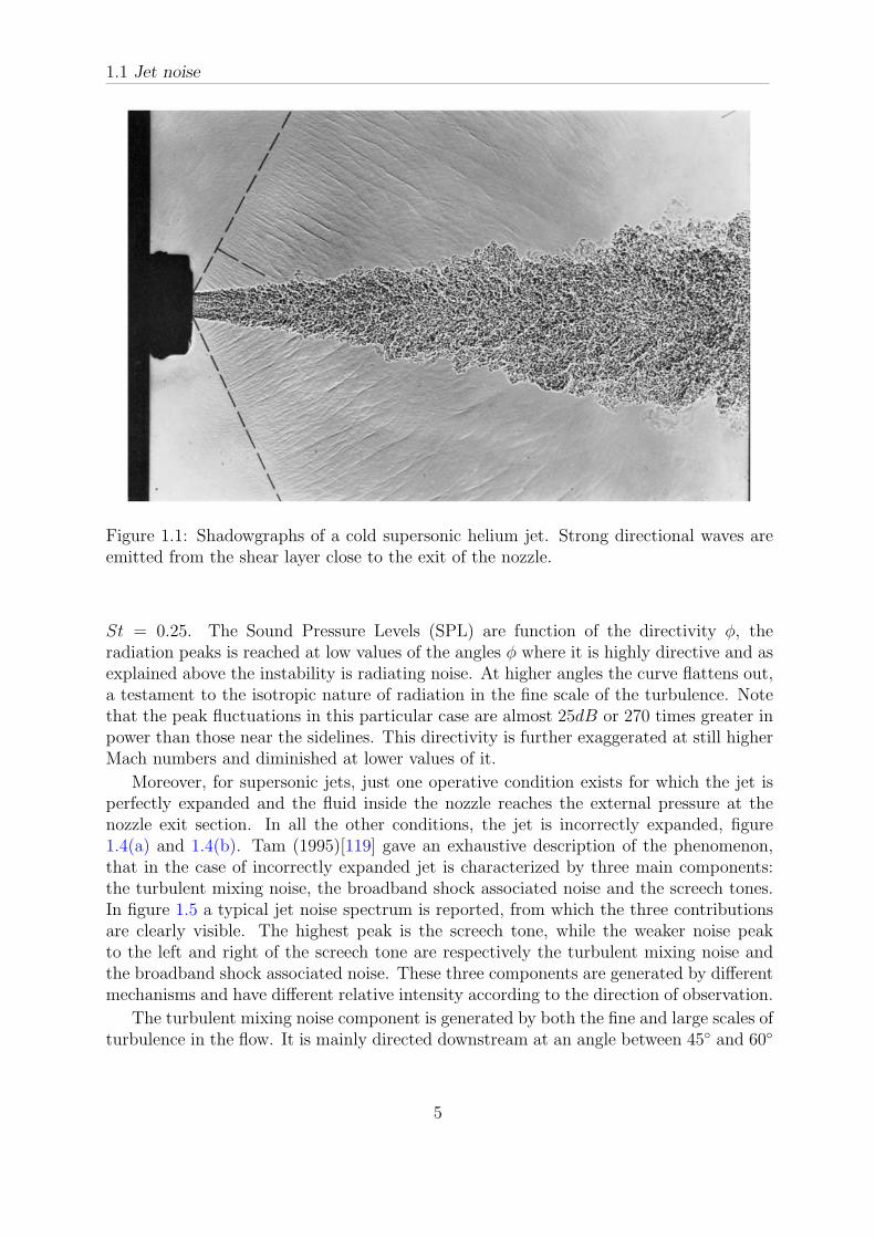
One of the first evidence of instability as source of jet noise can be found in the workof Tam (1971) [121] where a theory based on the concept of instability of the shear layeris developed. his theory prediction shows as the directional sound waves radiated fromthe shear layer of a supersonic jet are the direct result of instability of the shear layer. Infigure 1.1 can be observed the strong directional waves emitted from the shear layer closeto the exit of the nozzle [70]. This results are in according to those found in our workwhen computing sensitivity analysis as explained in chapter 3.
In parallel Crow and Champagne (1971)[27] report the observation of large scale co-herent structures in turbulent jet and free shear layers. Since those works, there has beenan abundance of papers in the literature devoted to the measurement [79, 78, 57, 43], andto the numerical simulations[121, 122, 133, 134, 98, 102] focused on large scale structuresof the turbulence as a dominant noise generation mechanism for jet flows.
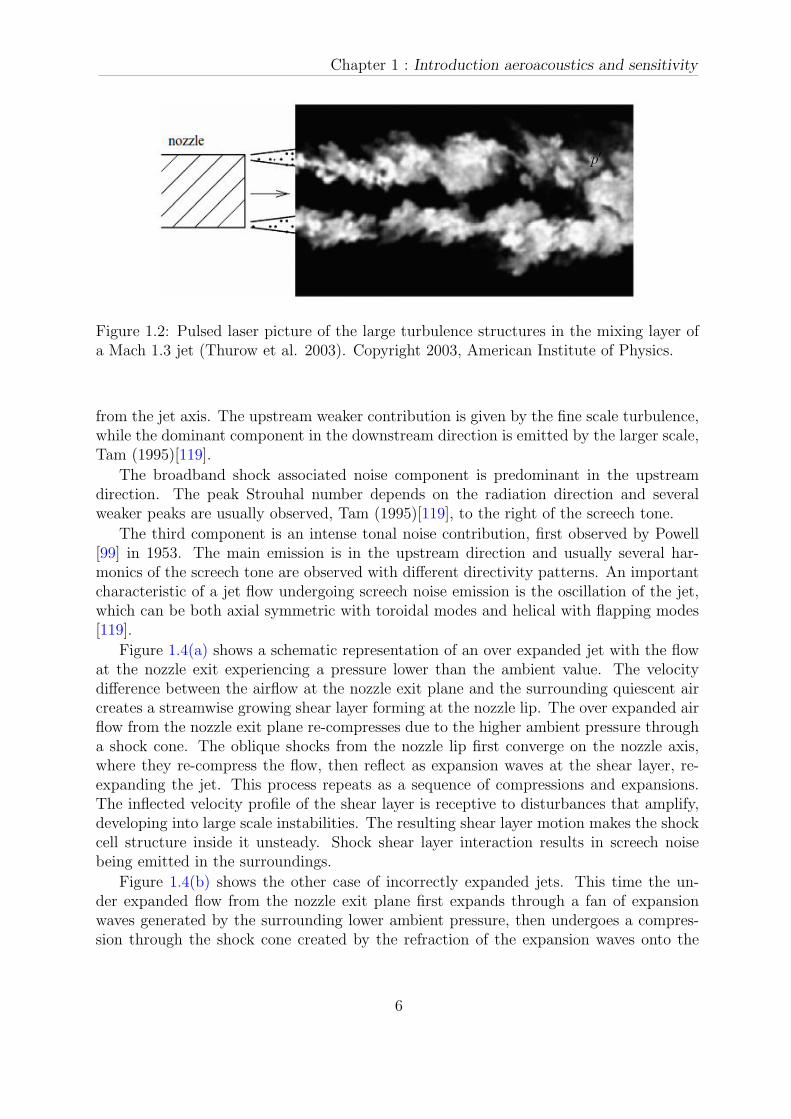
Figure 1.2 is a pulsed laser picture where are clearly observed the large turbulencestructures in the mixing layer of a supersonic jet with Mach 1.3, Thurow et al. (2003)[126]. This picture is typical of most optical observations of large turbulence structuresin a turbulent jet flow and put in evidence the complexity of such a flow. It is shown theevolution of the shear layer along the axial direction.
The turbulence present in the jet, figure 1.2, can be separated in large structures andfine structures. It is now generally accepted that jet noise is created by both fine andlarge scale turbulence structures. A consistent part of subsonic jet noise is producedby fine scale turbulence, whereas large turbulence structures are dominant noise sourcesof supersonic and high temperature jets. Figure 1.3 illustrate pressure measurementstaken along an arc in the farfield of a jet with an upstream Mach number M∞ = 1.5.These measurements have been Fourier transformed in time t and azimuthal angle θ; thefigure 1.3 shows axisymmetric fluctuations (azimuthal wavenumber m = 0) of frequency
4
1.1 Jet noise
Figure 1.1: Shadowgraphs of a cold supersonic helium jet. Strong directional waves areemitted from the shear layer close to the exit of the nozzle.
St = 0.25. The Sound Pressure Levels (SPL) are function of the directivity φ, theradiation peaks is reached at low values of the angles φ where it is highly directive and asexplained above the instability is radiating noise. At higher angles the curve flattens out,a testament to the isotropic nature of radiation in the fine scale of the turbulence. Notethat the peak fluctuations in this particular case are almost 25dB or 270 times greater inpower than those near the sidelines. This directivity is further exaggerated at still higherMach numbers and diminished at lower values of it.
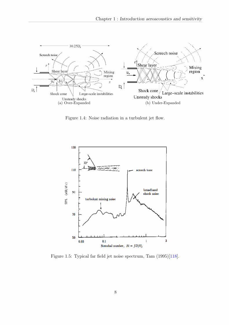
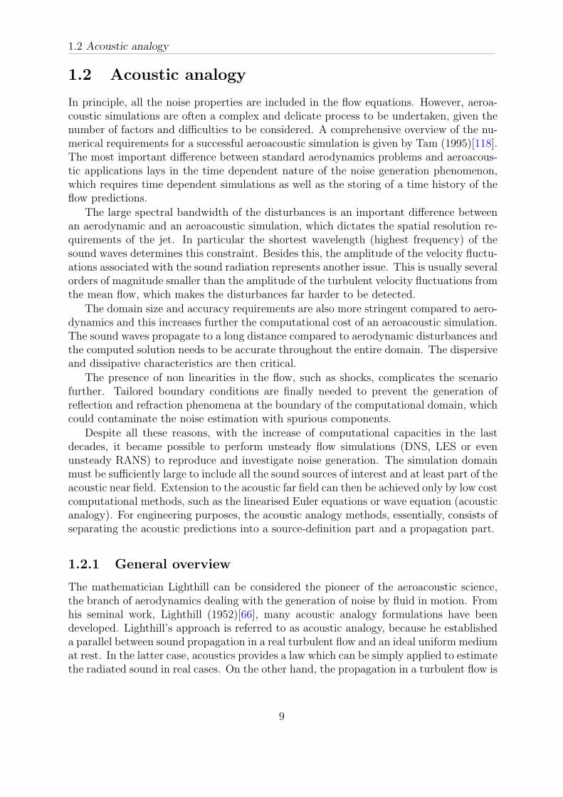
Moreover, for supersonic jets, just one operative condition exists for which the jet isperfectly expanded and the fluid inside the nozzle reaches the external pressure at thenozzle exit section. In all the other conditions, the jet is incorrectly expanded, figure1.4(a) and 1.4(b). Tam (1995)[119] gave an exhaustive description of the phenomenon,that in the case of incorrectly expanded jet is characterized by three main components:the turbulent mixing noise, the broadband shock associated noise and the screech tones.In figure 1.5 a typical jet noise spectrum is reported, from which the three contributionsare clearly visible. The highest peak is the screech tone, while the weaker noise peakto the left and right of the screech tone are respectively the turbulent mixing noise andthe broadband shock associated noise. These three components are generated by differentmechanisms and have different relative intensity according to the direction of observation.
The turbulent mixing noise component is generated by both the fine and large scales ofturbulence in the flow. It is mainly directed downstream at an angle between 45 and 60
5
Chapter 1 : Introduction aeroacoustics and sensitivity
p′
Figure 1.2: Pulsed laser picture of the large turbulence structures in the mixing layer ofa Mach 1.3 jet (Thurow et al. 2003). Copyright 2003, American Institute of Physics.
from the jet axis. The upstream weaker contribution is given by the fine scale turbulence,while the dominant component in the downstream direction is emitted by the larger scale,Tam (1995)[119].
The broadband shock associated noise component is predominant in the upstreamdirection. The peak Strouhal number depends on the radiation direction and severalweaker peaks are usually observed, Tam (1995)[119], to the right of the screech tone.
The third component is an intense tonal noise contribution, first observed by Powell[99] in 1953. The main emission is in the upstream direction and usually several har-monics of the screech tone are observed with different directivity patterns. An importantcharacteristic of a jet flow undergoing screech noise emission is the oscillation of the jet,which can be both axial symmetric with toroidal modes and helical with flapping modes[119].
Figure 1.4(a) shows a schematic representation of an over expanded jet with the flowat the nozzle exit experiencing a pressure lower than the ambient value. The velocitydifference between the airflow at the nozzle exit plane and the surrounding quiescent aircreates a streamwise growing shear layer forming at the nozzle lip. The over expanded airflow from the nozzle exit plane re-compresses due to the higher ambient pressure througha shock cone. The oblique shocks from the nozzle lip first converge on the nozzle axis,where they re-compress the flow, then reflect as expansion waves at the shear layer, re-expanding the jet. This process repeats as a sequence of compressions and expansions.The inflected velocity profile of the shear layer is receptive to disturbances that amplify,developing into large scale instabilities. The resulting shear layer motion makes the shockcell structure inside it unsteady. Shock shear layer interaction results in screech noisebeing emitted in the surroundings.
Figure 1.4(b) shows the other case of incorrectly expanded jets. This time the un-der expanded flow from the nozzle exit plane first expands through a fan of expansionwaves generated by the surrounding lower ambient pressure, then undergoes a compres-sion through the shock cone created by the refraction of the expansion waves onto the
6

1.1 Jet noise
Figure 1.3: Acoustic power measurements of a heated M∞ = 1.5 jet. Azimuthal modem = 0 and frequency St = 0.25. Data obtained from measurements of Suzuki andColonius (2006)[117].
shear layer. Afterwards the process is similar to the one described for over expanded jets,with the flow experiencing a sequence of compressions and expansions.
Summarizing, the problem becomes more complex in case of imperfectly expandedsupersonic jet where the noise associated with the presence of shocks has to be taken intoaccount. In this configuration the jet is characterized by a train of shock waves. In thepresence of the shock cells, the jets emits two additional components of noise. They arereferred to as screech tones and broadband shock associated noise.
Indeed, for those jets sound is generated not only by the interactions between instabil-ities and the coherent structures in the shear turbulent flows, but also by the weakly nonlinear interaction between instabilities and shock cell structure, producing shock associ-ated noise Panda et al. (1998)[92]. In the work of Ray and Lele (2007) [103], source termsrepresenting the instability wave/shock cell interaction are assembled and the radiatingcomponents have been isolated, providing very good approximation to the full problem.Inspired to this previous work a non local stability approach, presented in chapter 2, isimplemented to study these interactions.
7
Chapter 1 : Introduction aeroacoustics and sensitivity
(a) Over-Expanded (b) Under-Expanded
Figure 1.4: Noise radiation in a turbulent jet flow.
Figure 1.5: Typical far field jet noise spectrum, Tam (1995)[118].
8
1.2 Acoustic analogy
1.2 Acoustic analogy
In principle, all the noise properties are included in the flow equations. However, aeroa-coustic simulations are often a complex and delicate process to be undertaken, given thenumber of factors and difficulties to be considered. A comprehensive overview of the nu-merical requirements for a successful aeroacoustic simulation is given by Tam (1995)[118].The most important difference between standard aerodynamics problems and aeroacous-tic applications lays in the time dependent nature of the noise generation phenomenon,which requires time dependent simulations as well as the storing of a time history of theflow predictions.
The large spectral bandwidth of the disturbances is an important difference betweenan aerodynamic and an aeroacoustic simulation, which dictates the spatial resolution re-quirements of the jet. In particular the shortest wavelength (highest frequency) of thesound waves determines this constraint. Besides this, the amplitude of the velocity fluctu-ations associated with the sound radiation represents another issue. This is usually severalorders of magnitude smaller than the amplitude of the turbulent velocity fluctuations fromthe mean flow, which makes the disturbances far harder to be detected.
The domain size and accuracy requirements are also more stringent compared to aero-dynamics and this increases further the computational cost of an aeroacoustic simulation.The sound waves propagate to a long distance compared to aerodynamic disturbances andthe computed solution needs to be accurate throughout the entire domain. The dispersiveand dissipative characteristics are then critical.
The presence of non linearities in the flow, such as shocks, complicates the scenariofurther. Tailored boundary conditions are finally needed to prevent the generation ofreflection and refraction phenomena at the boundary of the computational domain, whichcould contaminate the noise estimation with spurious components.
Despite all these reasons, with the increase of computational capacities in the lastdecades, it became possible to perform unsteady flow simulations (DNS, LES or evenunsteady RANS) to reproduce and investigate noise generation. The simulation domainmust be sufficiently large to include all the sound sources of interest and at least part of theacoustic near field. Extension to the acoustic far field can then be achieved only by low costcomputational methods, such as the linearised Euler equations or wave equation (acousticanalogy). For engineering purposes, the acoustic analogy methods, essentially, consists ofseparating the acoustic predictions into a source-definition part and a propagation part.
1.2.1 General overview
The mathematician Lighthill can be considered the pioneer of the aeroacoustic science,the branch of aerodynamics dealing with the generation of noise by fluid in motion. Fromhis seminal work, Lighthill (1952)[66], many acoustic analogy formulations have beendeveloped. Lighthill’s approach is referred to as acoustic analogy, because he establisheda parallel between sound propagation in a real turbulent flow and an ideal uniform mediumat rest. In the latter case, acoustics provides a law which can be simply applied to estimatethe radiated sound in real cases. On the other hand, the propagation in a turbulent flow is
9

Chapter 1 : Introduction aeroacoustics and sensitivity
a complex phenomenon, which was first addressed by Lighthill. Just a part of the energycontent of the flow actually propagates as sound undergoing the conversion between kineticand acoustic energy and such energy is radiated through pressure waves. For modest speedLighthill [66] estimated through dimensional analysis the intensity of the radiated soundbeing proportional to the 8th power of a typical velocity in the flow. The sound producedby a turbulent flow interacts with the complex flow structures of different scales andfrequencies, giving rise to sound convection and propagation with a variable speed[66], aswell as refraction and reflection phenomena. Taking into account all these complexities isnot trivial and Lighthill developed a simple concept to tackle them. By rearranging theNavier-Stokes equations he obtained a convenient formulation in the form of a linear waveequation for a uniform medium at rest. Adopting this approach, sound can be consideredas if generated in a uniform medium at rest and the noise estimation is reduced to theevaluation of a quadrupole type source term, which appears on the right-hand side of therearranged equation:
Tij = ρuiuj + Pij − c20ρδij, Pij = pδij + τij (1.1)
Lighthill assumed that this term, representing applied fluctuating stresses acting upona uniform medium at rest, is known or can be modelled from the flow field prediction.In Figure 1.6, a turbulent jet flow is compared with the uniform medium at rest in theacoustic analogy approach. The schematic representation of the under expanded jet infigure 1.6(b) shows both the aerodynamic feature of the flow and the noise radiation withdownstream and upstream components. In Figure 1.6(a) the same phenomenon of noiseradiation is modelled with a volume distribution of quadrupole source terms in the jetshear layer, which reproduces the same acoustic effect of the real flow.
(a) Noise radiation in a real turbulent jet flow (b) Noise radiation model in an acoustic analogy ap-proach
Figure 1.6: Schematic representation of the acoustic analogy approach.
In this acoustic analogy flow the noise propagates in a uniform medium at rest fol-lowing the linear wave equation of acoustics. All the effects of the turbulence of the
10
1.2 Acoustic analogy
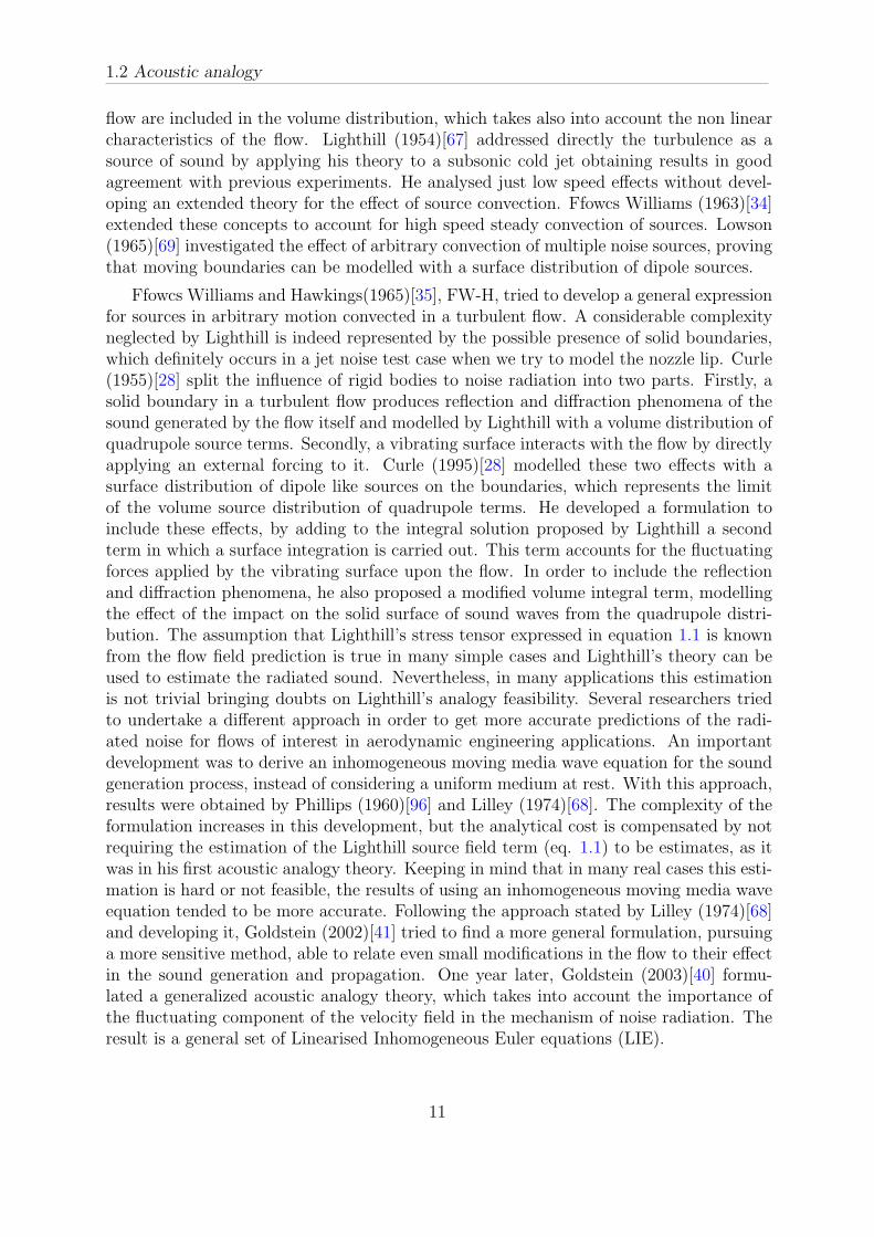
flow are included in the volume distribution, which takes also into account the non linearcharacteristics of the flow. Lighthill (1954)[67] addressed directly the turbulence as asource of sound by applying his theory to a subsonic cold jet obtaining results in goodagreement with previous experiments. He analysed just low speed effects without devel-oping an extended theory for the effect of source convection. Ffowcs Williams (1963)[34]extended these concepts to account for high speed steady convection of sources. Lowson(1965)[69] investigated the effect of arbitrary convection of multiple noise sources, provingthat moving boundaries can be modelled with a surface distribution of dipole sources.
Ffowcs Williams and Hawkings(1965)[35], FW-H, tried to develop a general expressionfor sources in arbitrary motion convected in a turbulent flow. A considerable complexityneglected by Lighthill is indeed represented by the possible presence of solid boundaries,which definitely occurs in a jet noise test case when we try to model the nozzle lip. Curle(1955)[28] split the influence of rigid bodies to noise radiation into two parts. Firstly, asolid boundary in a turbulent flow produces reflection and diffraction phenomena of thesound generated by the flow itself and modelled by Lighthill with a volume distribution ofquadrupole source terms. Secondly, a vibrating surface interacts with the flow by directlyapplying an external forcing to it. Curle (1995)[28] modelled these two effects with asurface distribution of dipole like sources on the boundaries, which represents the limitof the volume source distribution of quadrupole terms. He developed a formulation toinclude these effects, by adding to the integral solution proposed by Lighthill a secondterm in which a surface integration is carried out. This term accounts for the fluctuatingforces applied by the vibrating surface upon the flow. In order to include the reflectionand diffraction phenomena, he also proposed a modified volume integral term, modellingthe effect of the impact on the solid surface of sound waves from the quadrupole distri-bution. The assumption that Lighthill’s stress tensor expressed in equation 1.1 is knownfrom the flow field prediction is true in many simple cases and Lighthill’s theory can beused to estimate the radiated sound. Nevertheless, in many applications this estimationis not trivial bringing doubts on Lighthill’s analogy feasibility. Several researchers triedto undertake a different approach in order to get more accurate predictions of the radi-ated noise for flows of interest in aerodynamic engineering applications. An importantdevelopment was to derive an inhomogeneous moving media wave equation for the soundgeneration process, instead of considering a uniform medium at rest. With this approach,results were obtained by Phillips (1960)[96] and Lilley (1974)[68]. The complexity of theformulation increases in this development, but the analytical cost is compensated by notrequiring the estimation of the Lighthill source field term (eq. 1.1) to be estimates, as itwas in his first acoustic analogy theory. Keeping in mind that in many real cases this esti-mation is hard or not feasible, the results of using an inhomogeneous moving media waveequation tended to be more accurate. Following the approach stated by Lilley (1974)[68]and developing it, Goldstein (2002)[41] tried to find a more general formulation, pursuinga more sensitive method, able to relate even small modifications in the flow to their effectin the sound generation and propagation. One year later, Goldstein (2003)[40] formu-lated a generalized acoustic analogy theory, which takes into account the importance ofthe fluctuating component of the velocity field in the mechanism of noise radiation. Theresult is a general set of Linearised Inhomogeneous Euler equations (LIE).
11
Chapter 1 : Introduction aeroacoustics and sensitivity
1.2.2 Computational Aeroacoustics (CAA) simulation
The origin of Computational Aeroacoustics (CAA) can be dated back to the middle ofthe 1980s, with a publication of Hardin and Lamkin (1984)[46]. Few years later the sameauthors introduced the abbreviation CAA. The term was initially used for a low Machnumber approach (Expansion of the acoustic perturbation field about an incompressibleflow). Later in the beginning 1990s the growing CAA community picked up the termand extensively used it for any kind of numerical method describing the noise radiationfrom an aeroacoustic source or the propagation of sound waves in an inhomogeneous flowfield. Mankbadi et al. (1994)[75] discussed the application of direct CAA simulationto supersonic jet aeroacoustics compared to a Lighthill’s analogy approach. He foundthe direct CAA simulation more computational expensive in order to get the sound fieldpredictions. He also pointed out the difficulties of the Lighthill acoustic analogy in dealingwith acoustically non compact sources. Di Francescantonio[36] and Lyrintzis[73] alsoargued the direct CAA computation not to be an appropriate method for the standarddistance between source region and observer positions in most of the real applications.However, when the geometry of the problem does not allow the direct estimation ofthe pressure fluctuations on the observer positions, an integral method is required toproject the solution onto the acoustic far field. Furthermore, the separation between theaerodynamics and aeroacoustics simulation usually offers the possibility of a better insightof the problem and the use of different physical models describing the flow in regions wherethe flow does follow different laws.
1.2.3 The FW-H acoustic analogy
Ffowcs Williams and Hawkings (1965)[35] developed an acoustic analogy formulationmodelling the noise radiation with three kinds of different sound sources, i.e., monopoles,dipoles and quadrupoles, in order to take into account the different aspects of a sig-nificantly heterogeneous phenomenon. The FW-H equation and integral solutions arereported in Chapter 4. Ffowcs Williams and Hawkings [35] obtained a generalized in-homogeneous wave equation (eq.1.2) by introducing the use of the generalized functiontheory, which represented an important turning point in the acoustic analogy historicaldevelopment.
2
(ρ− ρ0)c20H(g)
=∂2 TijH(g)
∂xi∂xj
−∂ Liδ(g)
∂xi
+∂ Qδ(g)
∂t, (1.2)
where H(g) is the Heaviside function, in the first source term on the right-hand sideTij is the Lighthill stress tensor and δ is the Dirac delta function.
All details are given in chapter 4. The FW-H equation introduced the new concept ofan unbounded fluid, which is defined everywhere in space. The unbounded fluid followsthe real motion (modelled by the Navier-Stokes equations) on and outside a fictitioussurface that can be taken as coincident with a solid boundary. Inside the surface theconservation laws are assumed not to apply and the flow state can be defined arbitrarily,so generating a discontinuity at the surface itself. In order to maintain this discontinuity
12
1.2 Acoustic analogy
mass and momentum sources are distributed on the integration surface and they act assound generators. The strength of this mass and momentum source distribution is givenby the difference between the flux requirements in the two regions in which the FW-Hsurface splits the flow. This acoustic analogy, that is a generalization of Lighthill’s one,gave birth to a more applicable and reproducible model, which still appears in many recentformulations. The generalized function theory has been widely used in the aeroacousticfield after Ffowcs Williams and Hawkings and it is developed with a rigorous mathematicalapproach by Farassat (1994)[31]. Farassat (1975)[30] applied the FW-H acoustic analogyto helicopter rotors showing the power of the theory in predicting aerodynamic soundin the presence of moving surfaces in an unsteady turbulent flow even for non compactsource problems. The embedding procedure, which converts the standard fluid dynamicproblem to an unbounded fluid case through the use of the generalised function theory, isdetailed.
In computational simulations, the FW-H acoustic analogy’s main disadvantage is theneed to perform a volume integration that is far more expensive than a two dimensionalnumerical integration. However, the quadrupole source term is usually some order ofmagnitude smaller than the surface source distribution and in many applications it isneglected, as in Di Francescantonio (1997) [36]. In the case this assumption is not valid,an increase in the computational cost inevitably occurs. Thanks to the increasing compu-tational power, numerical applications including a volume integration have recently beendeveloped by Brentner (1997)[17].
1.2.4 The porous FW-H formulation
Di Francescantonio (1997) [36] proposed the use of a FW-H acoustic analogy with apermeable surface, trying to combine the advantages of Kirchhoff’s method and the FW-Hacoustic analogy. He therefore referred to the new equation as Kirchhoff FW-H (KFWH),pointing out that the main advantage was that no derivatives of CFD quantities wererequired as in the standard Kirchhoff’s formula. The KFWH equation was used by DiFrancescantonio[36] neglecting the volume source distribution. By considering a surfaceplaced in a linear region, the Kirchhoff method speed up is recovered. However, thegeneral form of the KFWH equation included a volume integration to take into accountpossible non negligible quadrupole sources outside the permeable surface.
1.2.5 Advanced time vs retarded time
A retarded time equation of the type of equation 1.3 is usually solved for the estimationof the retarded time.
τret = t−|x− y(τret)|
c0(1.3)
Equation 1.3 expresses that a disturbance emitted from the source position y at time τretwill reach the observer x at time t, due to the time of flight of the noise propagating at
13
Chapter 1 : Introduction aeroacoustics and sensitivity
the speed of sound c0. Two different approaches can be adopted to take into account thispropagation of the disturbances. In the retarded time approach the simulation runs in theobserver time, meaning that the simulation time axis is representative of the receptionphenomenon. In this case an implicit retarded time equation needs to be solved. Differentdisturbances reaching the observer at the same time can be emitted at different retardedtimes. A different approach was proposed by Casalino (2003)[19]. In this case the simu-lation runs in the emission time and, for each different disturbance, an advanced time iscalculated for a specific observer. This represents the time of flight for the disturbance totravel from the emission to the reception point. Casalino used the definition of advancedtime analysing the differences between the two approaches. He pointed out the advantagesof the advanced time formulation in the possibility to run the aeroacoustic prediction si-multaneously with the CFD simulation. Furthermore he showed that the advanced timecan be explicitly estimated by an algebraic equation with no iterative method required.
1.2.6 A convective FW-H acoustic analogy
Most of the FW-H acoustic analogy formulations assume the propagation of sound wavesin a medium at rest as in Lighthill’s original assumption. A usual way to take intoaccount a moving medium relative to a fixed observer is to circumnavigate the problem,considering a case in which the observer moves in a medium at rest[32]. In 2011 Najafi-Yazdi et al. [90] developed an interesting convective formulation of the FW-H acousticanalogy explicitly taking into account the presence of a mean flow. In such a formulationthe standard wave operator is modified to obtain a convective wave operator. A uniformconvective velocity is considered directly in the equations originating additional termscompared to the standard FW-H equation. A convective Green’s function suggested byBlokhintsev is also adopted to take into account the mean flow, rather than the free spaceGreen’s function for a medium at rest (1994)[31]. A Lagrangian derivative appears inthe thickness noise, which is slightly different from the FW-H integral solution. A clearDoppler effect caused by the mean flow is showed in the results from elementary sourceapplications.
1.2.7 Alternative aeroacoustic techniques
a- The Kirchhoff formulation
The Kirchhoff formula was first published in 1883[60]. Later on, Lyrintzis (1994)[72]published a review of the application of this theory in the aeroacoustics field, referringto the methodology as a surface integral method[73]. The basic concept of the methodis the use of a control surface on which pressure and its normal and time derivativesare estimated by numerical method. The acoustic pressure in the far field can then beobtained from an integration on this control surface of the above mentioned quantities.The control surface is required to enclose all the non linearities of the flow and the noisesources. The position of the control surface is critical, because the noise propagationon the surroundings is assumed to follow the linear wave equation. Consequently, thesurface needs to be placed in a region of the flow where the linear wave equation is valid
14
1.2 Acoustic analogy
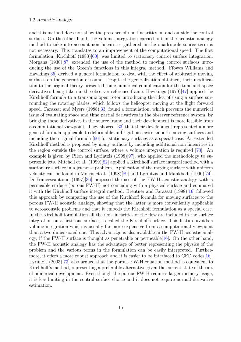
and this method does not allow the presence of non linearities on and outside the controlsurface. On the other hand, the volume integration carried out in the acoustic analogymethod to take into account non linearities gathered in the quadrupole source term isnot necessary. This translates to an improvement of the computational speed. The firstformulation, Kirchhoff (1983)[60], was limited to stationary control surface integration.Morgans (1930)[87] extended the use of the method to moving control surfaces intro-ducing the use of the Green’s functions in this integral method. Ffowcs Williams andHawkings[35] derived a general formulation to deal with the effect of arbitrarily movingsurfaces on the generation of sound. Despite the generalization obtained, their modifica-tion to the original theory presented some numerical complication for the time and spacederivatives being taken in the observer reference frame. Hawkings (1979)[47] applied theKirchhoff formula to a transonic open rotor introducing the idea of using a surface sur-rounding the rotating blades, which follows the helicopter moving at the flight forwardspeed. Farassat and Myers (1988)[33] found a formulation, which prevents the numericalissue of evaluating space and time partial derivatives in the observer reference system, bybringing these derivatives in the source frame and their development is more feasible froma computational viewpoint. They showed [33] that their development represented a moregeneral formula applicable to deformable and rigid piecewise smooth moving surfaces andincluding the original formula [60] for stationary surfaces as a special case. An extendedKirchhoff method is proposed by many authors by including additional non linearities inthe region outside the control surface, where a volume integration is required [73]. Anexample is given by Pilon and Lyrintzis (1998)[97], who applied the methodology to su-personic jets. Mitchell et al. (1999)[82] applied a Kirchhoff surface integral method with astationary surface in a jet noise problem. Application of the moving surface with uniformvelocity can be found in Morris et al. (1998)[89] and Lyrintzis and Mankbadi (1996)[74].Di Francescantonio (1997)[36] proposed the use of the FW-H acoustic analogy with apermeable surface (porous FW-H) not coinciding with a physical surface and comparedit with the Kirchhoff surface integral method. Brentner and Farassat (1998)[16] followedthis approach by comparing the use of the Kirchhoff formula for moving surfaces to theporous FW-H acoustic analogy, showing that the latter is more conveniently applicableto aeroacoustic problems and that it embeds the Kirchhoff formulation as a special case.In the Kirchhoff formulation all the non linearities of the flow are included in the surfaceintegration on a fictitious surface, so called the Kirchhoff surface. This feature avoids avolume integration which is usually far more expensive from a computational viewpointthan a two dimensional one. This advantage is also available in the FW-H acoustic anal-ogy, if the FW-H surface is thought as penetrable or permeable[16]. On the other hand,the FW-H acoustic analogy has the advantage of better representing the physics of theproblem and the various terms in the formulation can be easily interpreted. Further-more, it offers a more robust approach and it is easier to be interfaced to CFD codes[16].Lyrintzis (2003)[73] also argued that the porous FW-H equation method is equivalent toKirchhoff’s method, representing a preferable alternative given the current state of the artof numerical development. Even though the porous FW-H requires larger memory usage,it is less limiting in the control surface choice and it does not require normal derivativeestimation.
15
Chapter 1 : Introduction aeroacoustics and sensitivity
b- Theory of vortex sound
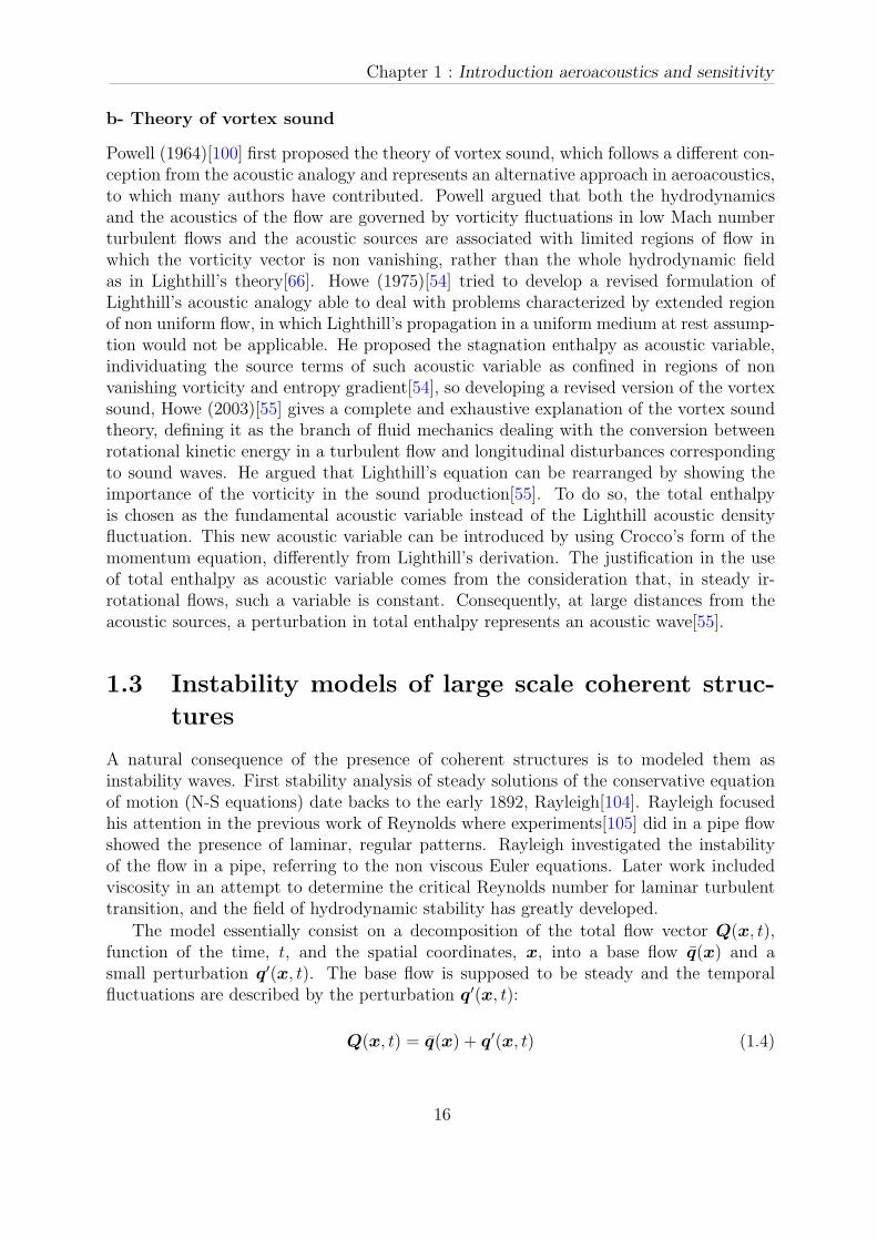
Powell (1964)[100] first proposed the theory of vortex sound, which follows a different con-ception from the acoustic analogy and represents an alternative approach in aeroacoustics,to which many authors have contributed. Powell argued that both the hydrodynamicsand the acoustics of the flow are governed by vorticity fluctuations in low Mach numberturbulent flows and the acoustic sources are associated with limited regions of flow inwhich the vorticity vector is non vanishing, rather than the whole hydrodynamic fieldas in Lighthill’s theory[66]. Howe (1975)[54] tried to develop a revised formulation ofLighthill’s acoustic analogy able to deal with problems characterized by extended regionof non uniform flow, in which Lighthill’s propagation in a uniform medium at rest assump-tion would not be applicable. He proposed the stagnation enthalpy as acoustic variable,individuating the source terms of such acoustic variable as confined in regions of nonvanishing vorticity and entropy gradient[54], so developing a revised version of the vortexsound, Howe (2003)[55] gives a complete and exhaustive explanation of the vortex soundtheory, defining it as the branch of fluid mechanics dealing with the conversion betweenrotational kinetic energy in a turbulent flow and longitudinal disturbances correspondingto sound waves. He argued that Lighthill’s equation can be rearranged by showing theimportance of the vorticity in the sound production[55]. To do so, the total enthalpyis chosen as the fundamental acoustic variable instead of the Lighthill acoustic densityfluctuation. This new acoustic variable can be introduced by using Crocco’s form of themomentum equation, differently from Lighthill’s derivation. The justification in the useof total enthalpy as acoustic variable comes from the consideration that, in steady ir-rotational flows, such a variable is constant. Consequently, at large distances from theacoustic sources, a perturbation in total enthalpy represents an acoustic wave[55].
1.3 Instability models of large scale coherent struc-
tures
A natural consequence of the presence of coherent structures is to modeled them asinstability waves. First stability analysis of steady solutions of the conservative equationof motion (N-S equations) date backs to the early 1892, Rayleigh[104]. Rayleigh focusedhis attention in the previous work of Reynolds where experiments[105] did in a pipe flowshowed the presence of laminar, regular patterns. Rayleigh investigated the instabilityof the flow in a pipe, referring to the non viscous Euler equations. Later work includedviscosity in an attempt to determine the critical Reynolds number for laminar turbulenttransition, and the field of hydrodynamic stability has greatly developed.
The model essentially consist on a decomposition of the total flow vector Q(x, t),function of the time, t, and the spatial coordinates, x, into a base flow q(x) and asmall perturbation q′(x, t). The base flow is supposed to be steady and the temporalfluctuations are described by the perturbation q′(x, t):
Q(x, t) = q(x) + q′(x, t) (1.4)
16
1.3 Instability models of large scale coherent structures
Those fluctuations, following the methods of normal modes, are composed of an ex-ponential like wave term and a shape function. In the particular case of an axisymmetricjet, with cylindrical coordinates x = (x, r, θ), the perturbation q′ propagating in thex-direction can be written as:
q′ = q(x, r) exp (iΘ(x, θ, t)) (1.5)
In the above equation i stands for the square root of −1, q(x, r) is the amplitude function,or shape function, and Θ a general phase function. Typically in the Kelvin-Helmholtz(K-H) instability owes its origin to the inertia of the fluids, viscosity does not play animportant role, otherwise the inflection points of the mean velocity profile has a crucial im-portance in the instability of such a flow. More details about hydrodynamics instabilitiescould be found in Godreche et al [39].
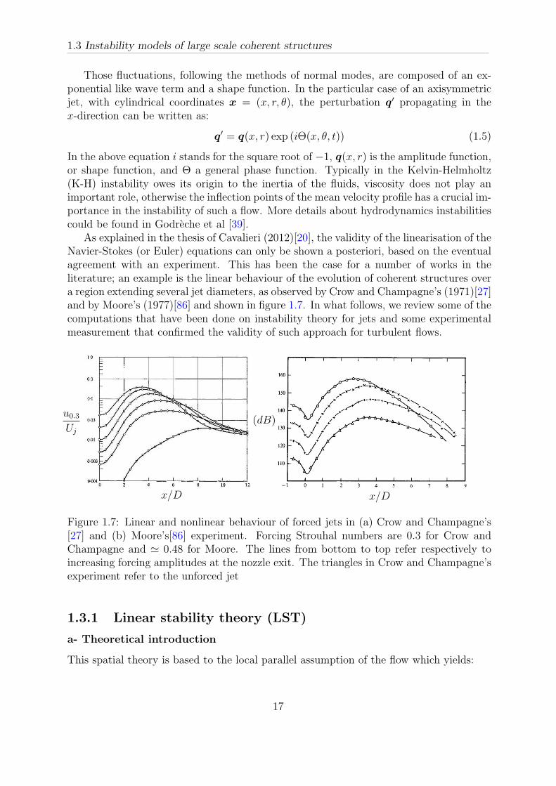
As explained in the thesis of Cavalieri (2012)[20], the validity of the linearisation of theNavier-Stokes (or Euler) equations can only be shown a posteriori, based on the eventualagreement with an experiment. This has been the case for a number of works in theliterature; an example is the linear behaviour of the evolution of coherent structures overa region extending several jet diameters, as observed by Crow and Champagne’s (1971)[27]and by Moore’s (1977)[86] and shown in figure 1.7. In what follows, we review some of thecomputations that have been done on instability theory for jets and some experimentalmeasurement that confirmed the validity of such approach for turbulent flows.
x/D
u0.3
Uj
(dB)
x/D
Figure 1.7: Linear and nonlinear behaviour of forced jets in (a) Crow and Champagne’s[27] and (b) Moore’s[86] experiment. Forcing Strouhal numbers are 0.3 for Crow andChampagne and ≃ 0.48 for Moore. The lines from bottom to top refer respectively toincreasing forcing amplitudes at the nozzle exit. The triangles in Crow and Champagne’sexperiment refer to the unforced jet
1.3.1 Linear stability theory (LST)
a- Theoretical introduction
This spatial theory is based to the local parallel assumption of the flow which yields:
17

Chapter 1 : Introduction aeroacoustics and sensitivity
q′ = q(r)e(i(αx+mθ − ωt) (1.6)
where α and m are the wavenumbers in the streamwise and azimuthal direction, re-spectively; ω represents the frequency of the perturbation. The complex amplitude of theperturbation q(r) depends only on the radial coordinates. In the frame of spatial theoryα is a complex value while m is en integer number and ω is real. Substituting 1.6 intothe Linear Euler Equation, LEE, the system could be rewritten as a classical OrdinaryDifferential Equation, ODE, function of the pressure shape function p(r), known as thenon viscous axysimmetric Pridmore-Brown equation:
d2p
dr2+
(
1
r−
1
ρ
dρ
dr−
2α
αux − ω
)
dp
dr+
(
ρM2(αux − ω)2 −m2
r2− α2
)
p = 0 (1.7)
that written in a compact way gives:
L(p) = 0 (1.8)
Associated to homogeneous boundary conditions, Tam and Burton (1984)[123] , this sys-tem corresponds to an eigenvalue problem with streamwise wavenumber α as the eigen-value and q(r) as the associated eigenfunction. The eigenvalue problem must to be solveby satisfying the dispersion relation:
D(α,m, ω) = 0 (1.9)
The growth rate of the disturbance, σ, is given by:
σ = −αi (1.10)
where subscript i refers to the imaginary part of the quantities. A disturbance is stable,neutral or unstable if its growth rate is less, equal or greater then zero, respectively.
b- Some results (for parallel base flows)
Preliminary studies of LST apply to the jet and free shear layer are based to work ofCrow and Champagne (1971)[27] when it was discovered the presence of large turbulencestructures in jets and as well their main role as jet noise sources. Morris (1976)[88]studied the spatial linear stability of axisymmetric (m = 0) and helical (m = 1) jets. Theflows are assumed to be incompressible and viscous, analyzed from the exit of the nozzleto the fully developed turbulent region. An accurate numerical method is proposed tosolve the eigenvalue problem and are computed for three different mean velocity profiles.The results show as the axial position where the instability is maximum increase if thefrequency decrease. It was also observed that only the helical mode, m = 1, will continueto amplify in the developed jet flow. In the work of [81] a LST was performed for around supersonic jet. In a axisymmetric inviscid jet the influence of the spatial growthrate and disturbance phase velocity is studied. The base flow is considered as a parallel
18
1.3 Instability models of large scale coherent structures
flow which is infinite upstream and downstream, with radial velocity equal to zero. Theauthor found that flow becomes more stable if the free stream Mach number increase.The good agreement if compared with experimental results[27] confirmed that instabilityof turbulent jet approximately follow the spatial linearised theory.
The first original description of these coherent structures as statistical instability waveswas proposed by Tam and Chen (1979) [124]. This work is based to the fact that large tur-bulence structures are somewhat more deterministic than the fine scale turbulent motions,moreover comparison with experimental results is made and very favorable agreement isfound. In particular, this work point out several difficulties of the comparisons betweentheoretical and experimental results due to the high influence of the initial condition andto some upstream disturbances that could influence the not fully developed mixing layer.The most important assumption of this model is that the turbulent jet flow spreads outvery slowly in the streamwise direction, consequently the flow variables change very slowlyas well. This means that, i.e., the turbulence statistics are nearly constants locally. In-deed the flow is stochastically stationary in time and in the axial flow direction. For asystem in (quasi) dynamical equilibrium, statistical mechanics theory can be representedmathematically by a superposition of its normal modes. In the case of high speed jets, thelarge scale fluctuations are the statistical mechanism while the dominant normal modesare the instability wave modes of the mean flow, computed using LST.
Very few works can be found in literature regarding LST for dual stream jets. Perrault-Joncas et Maslowe (2008)[95] applied the LST to a subsonic compressible coaxial jet. Thecomputation have been done with two different mean flow, one with ”cold” temperatureprofile is taken from Papamoschou’s experiments[93] and one with ”hot” temperatureprofile is taken from the mean data of a typical turbofan engine. They work has notcomparison with experimental results, but their parametric studies show the influence ofthe diameter ratio, compressibility, azimuthal wavenumber and the ratio between of thetwo mean velocities in the stability of the jet.
Concluding, large scale structures are an important source of noise and linear insta-bility is the first step in their formation.
1.3.2 Parabolized Stability Equations
All the cited works were based on the parallel flow hypothesis. An improvement on theapproximations of spatial stability can be done with the assumption of a base flow evolvingslowly in the streamwise direction. Herbert (1993)[49] developed the Parabolized StabilityEquations (PSE) theory to consider the non parallel effect of the flow in the instabilitywaves in the boundary layer region, inspired by the multiple scale methods.
The fundamental assumption of the PSE theory is that the disturbances consist of afast oscillatory part and an amplitude that varies slowly in the streamwise direction. Thedecomposition into fast and slow variations aims at a set of equations that is ”almost”parabolic in the streamwise coordinates direction and is suitable to a numerical marchingprocedure. In this work starting with the Euler equations which are not parabolic in space,appropriate approximations are called for to ensure the removal of elliptic components.Once these approximations are carried out, the Parabolized Stability Equations, PSE,
19
Chapter 1 : Introduction aeroacoustics and sensitivity
can be solved as a fraction of the computational costs of Direct Numerical Simulation,Large Eddy Simulation etc, but still conserving a good accuracy in the results. Finally,thanks to the contribution of many investigators [61, 42, 106, 107] it’s now known thatParabolized Stability Equations are a powerful tool for the prediction of subsonic andsupersonic jet noise.
a- Theoretical introduction
PSE approach is now well known and applied in various stability problems. Severaladvantages can be shed on light. Indeed, contrary to the Linear Stability Theory (LST)where local parallel flow is assumed, they take into account of the small streamwisevariations of the base flow and of the disturbances directly in the formulation. Since PSEare mathematically PDE, it is simple to solve them by adding various boundary conditionsand source terms. This leads to use them for receptivity and sensitivity analysis [7], inoptimal flow control approaches [5] and for weakly nonlinear stability studies[50].
In the following, all the variables are made non-dimensional. The characteristic lengthis based on the nozzle diameter and the characteristic flow properties are chosen to bethose of the flow on the axis at the nozzle exit [98].
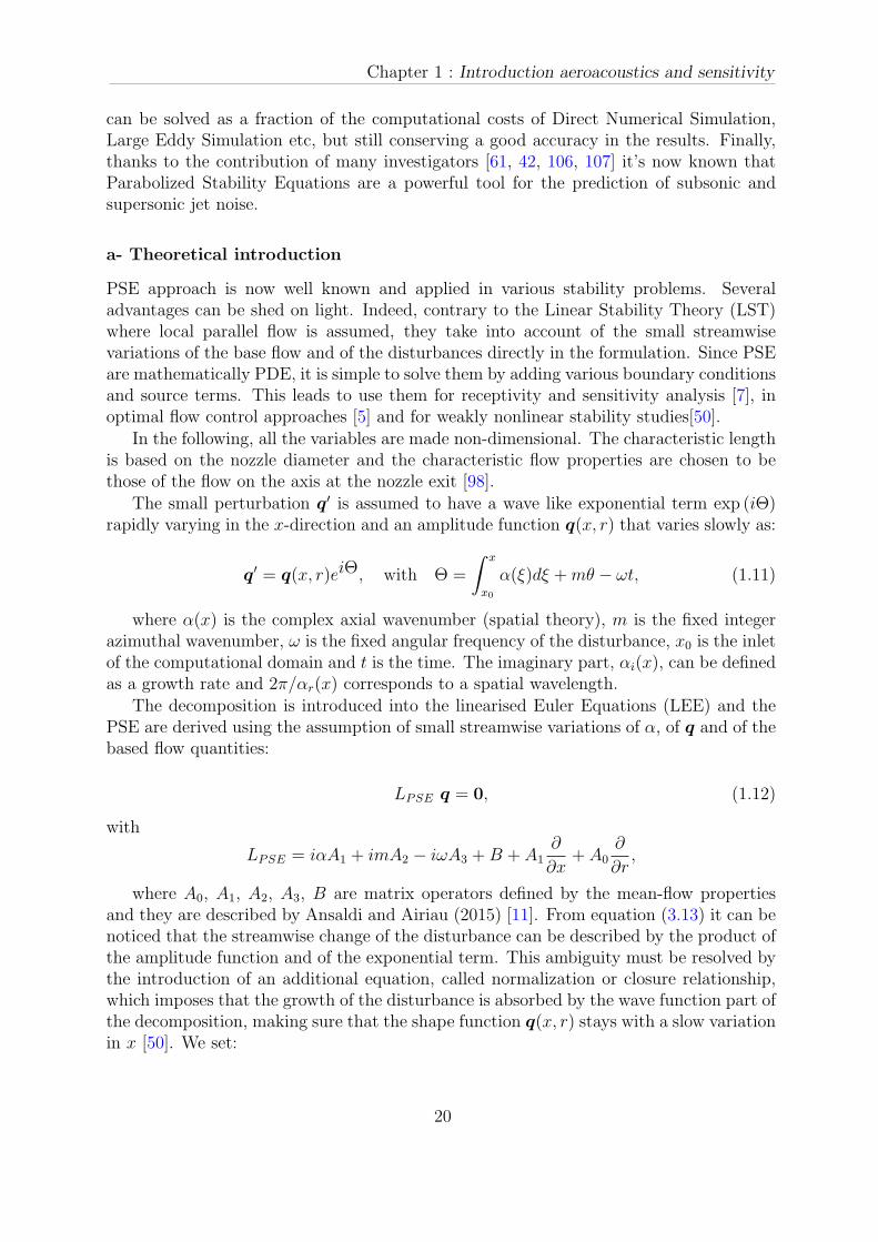
The small perturbation q′ is assumed to have a wave like exponential term exp (iΘ)rapidly varying in the x-direction and an amplitude function q(x, r) that varies slowly as:
q′ = q(x, r)eiΘ, with Θ =
ˆ x
x0
α(ξ)dξ +mθ − ωt, (1.11)
where α(x) is the complex axial wavenumber (spatial theory), m is the fixed integerazimuthal wavenumber, ω is the fixed angular frequency of the disturbance, x0 is the inletof the computational domain and t is the time. The imaginary part, αi(x), can be definedas a growth rate and 2π/αr(x) corresponds to a spatial wavelength.
The decomposition is introduced into the linearised Euler Equations (LEE) and thePSE are derived using the assumption of small streamwise variations of α, of q and of thebased flow quantities:
LPSE q = 0, (1.12)
with
LPSE = iαA1 + imA2 − iωA3 +B + A1∂
∂x+ A0
∂
∂r,
where A0, A1, A2, A3, B are matrix operators defined by the mean-flow propertiesand they are described by Ansaldi and Airiau (2015) [11]. From equation (3.13) it can benoticed that the streamwise change of the disturbance can be described by the product ofthe amplitude function and of the exponential term. This ambiguity must be resolved bythe introduction of an additional equation, called normalization or closure relationship,which imposes that the growth of the disturbance is absorbed by the wave function part ofthe decomposition, making sure that the shape function q(x, r) stays with a slow variationin x [50]. We set:
20
1.3 Instability models of large scale coherent structures
N (q, x) =
ˆ
∞
0
qh∂q
∂xr dr = 0, (1.13)
where the superscript h denotes the transpose conjugate. The system with the un-known (q, α) is only quasi parabolic because a residual ellipticity due to the normaliza-tion condition and a streamwise pressure gradient term remains, see Airiau and Casalis(1993)[6], and Andersson et al. (1998)[8].
b- Some results
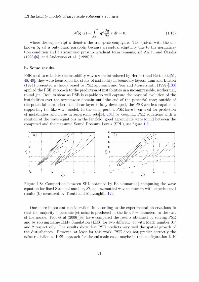
PSE used to calculate the instability waves were introduced by Herbert and Bertolotti[51,48, 49], they were focused on the study of instability in boundary layers. Tam and Burton(1984) presented a theory based to PSE approach and Yen and Messersmith (1998)[133]applied the PSE approach to the prediction of instabilities in a incompressible, isothermal,round jet. Results show as PSE is capable to well capture the physical evolution of theinstabilities over the streamwise domain until the end of the potential core; outside ofthe potential core, where the shear layer is fully developed, the PSE are less capable ofsupporting the like wave model. In the same period, PSE have been used for predictionof instabilities and noise in supersonic jets[14, 134] by coupling PSE equations with asolution of the wave equations in the far field; good agreements were found between thecomputed and the measured Sound Pressure Levels (SPL), see figure 1.8.
a) b)
Figure 1.8: Comparison between SPL obtained by Balakumar (a) computing the waveequation for fixed Strouhal number, St, and azimuthal wavenumber m with experimentalresults (b) measured by Troutt and McLaughlin[129].
One more important consideration, in according to the experimental observations, isthat the majority supersonic jet noise is produced in the first few diameters to the exitof the nozzle. Piot et al (2006)[98] have compared the results obtained by solving PSEand by solving Large Eddy Simulation (LES) for two different jet with Mach number 0.7and 2 respectively. The results show that PSE predicts very well the spatial growth ofthe disturbances. However, at least for this work, PSE does not predict correctly thenoise radiation as LES approach for the subsonic case, maybe in this configuration K-H
21
Chapter 1 : Introduction aeroacoustics and sensitivity
instability waves has not an important role in the production of noise. The agreement isvery good when compare the supersonic case, showing the crucial role of K-H instabilitiesin supersonic jets. Also in this work to compute the acoustic pressure from the PSEresults, the wave equation have been solved and again the noise sources is concentratednear the jet exit.
More recent works have focused attention of the non linear effect of the instabilitywaves. A natural approach to investigate the non linear effect is to compute the Nonlin-ear PSE equations (NPSE). A very good analysis of the non linear effects of the insta-bility waves in terms of noise radiation have been successfully made by Cheung and Lele(2009)[24]. Three jet configurations are tested, one supersonic and two subsonic; actuallynon linear approach may capture the sound generation process more accurately then thelinear instability theory.
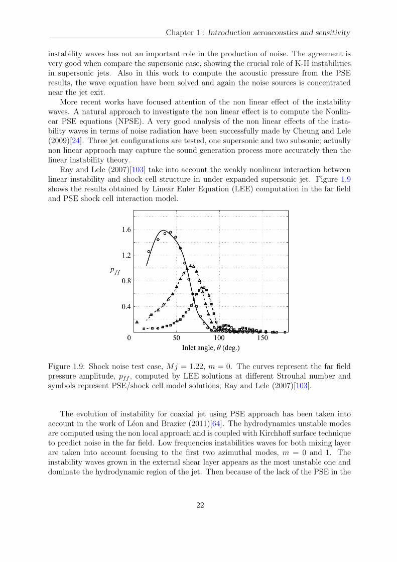
Ray and Lele (2007)[103] take into account the weakly nonlinear interaction betweenlinear instability and shock cell structure in under expanded supersonic jet. Figure 1.9shows the results obtained by Linear Euler Equation (LEE) computation in the far fieldand PSE shock cell interaction model.
Figure 1.9: Shock noise test case, Mj = 1.22, m = 0. The curves represent the far fieldpressure amplitude, pff , computed by LEE solutions at different Strouhal number andsymbols represent PSE/shock cell model solutions, Ray and Lele (2007)[103].
The evolution of instability for coaxial jet using PSE approach has been taken intoaccount in the work of Leon and Brazier (2011)[64]. The hydrodynamics unstable modesare computed using the non local approach and is coupled with Kirchhoff surface techniqueto predict noise in the far field. Low frequencies instabilities waves for both mixing layerare taken into account focusing to the first two azimuthal modes, m = 0 and 1. Theinstability waves grown in the external shear layer appears as the most unstable one anddominate the hydrodynamic region of the jet. Then because of the lack of the PSE in the
22

1.3 Instability models of large scale coherent structures
prediction of noise in the far field, the model is coupled with a acoustic wave propagation.Results are compared with experiment and with LES computation obtaining encouragingresults. Recently, PSE approach applied to LES computation of a subsonic dual streamjet illustrate very well the propagation of the instability in the inner and outer shear layer.A parametric study of different Strouhal and azimuthal wave number for the two unstablemodes (one in the primary and one in the secondary shear layer) has been performed,Sinha et al. (2016)[111]. In this work is well presented the problem of PSE for dualstream jet, in fact PSE can not well distinguish between the two unstable modes if theircomplex wavenumbers are to similar, or if one stabilize during the streamwise marching,but the other stay unstable.
Finally, with the work of Sinha et al (2014) [112] that demonstrate the validity oflinear instability to predict the average wavepacket evolution in supersonic jet inside thepotential core, leads to the conclusion that large scale structure manifest in the subsonicand supersonic jets and its evolution is well predicted inside of the potential core of thejet.
c- Non linear PSE
Also if in this thesis we only treated linear PSE problem a briefly introduction of nonlinear PSE approach is done in this section. In the linear PSE approach described above,the disturbance amplitude is assumed to be infinitesimally small so that the non linearinteraction of waves with different frequencies and azimuthal wave numbers is neglected.When finite amplitude waves are present in the flow, the linear approach is no longer valid.For non linear studies, we assume that the total disturbance is again periodic in time andin the azimuthal direction, thus, the total disturbance function q′ can be expressed bythe following Fourier series[29, 63].
q′ =N∑
n=−N
M∑
m=−M
qm,n(x, r)ei
(ˆ x
x0
αm,n(ξ)dξ +mθ − nωt
)
(1.14)
where αm,n and qm,n are the Fourier components of the streamwise wave number andshape function corresponding to the Fourier mode (nω,m), while, M and N are the totalnumber of modes kept in the truncated Fourier series. Notice that the frequency ω and thewave number m are set as the smallest values, respectively. Because of the characteristicsymmetry of a jet flow only a quarter of modes (m ranging from 0 to M and n rangingfrom 0 to N) are computed in the marching process. Finally, similar to the Linear PSEapproach, an additional closing equation is imposed for each mode (nω,m). These lastequations ensure the hypothesis of small variations of each shape function qm,n in thestreamwise direction.
Nm,n =
ˆ
∞
0
qhm,n
∂qm,n
∂xdr = 0 (1.15)
23
Chapter 1 : Introduction aeroacoustics and sensitivity
1.3.3 Convective and absolute instability
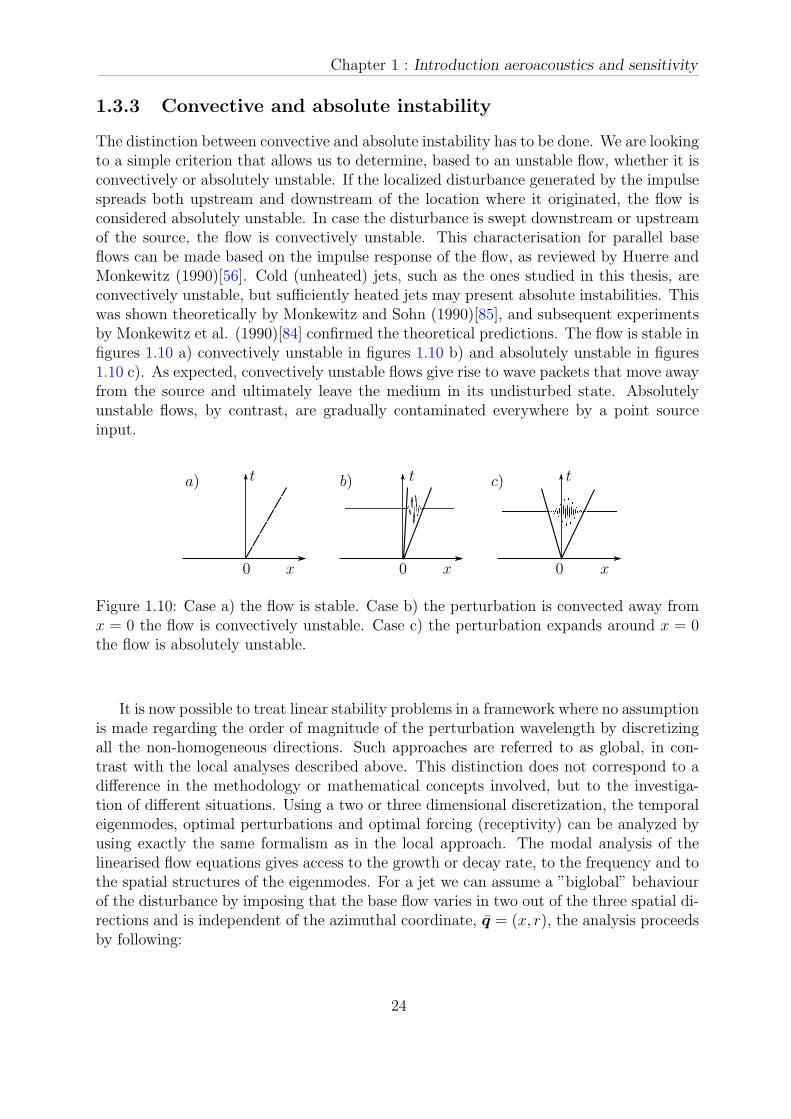
The distinction between convective and absolute instability has to be done. We are lookingto a simple criterion that allows us to determine, based to an unstable flow, whether it isconvectively or absolutely unstable. If the localized disturbance generated by the impulsespreads both upstream and downstream of the location where it originated, the flow isconsidered absolutely unstable. In case the disturbance is swept downstream or upstreamof the source, the flow is convectively unstable. This characterisation for parallel baseflows can be made based on the impulse response of the flow, as reviewed by Huerre andMonkewitz (1990)[56]. Cold (unheated) jets, such as the ones studied in this thesis, areconvectively unstable, but sufficiently heated jets may present absolute instabilities. Thiswas shown theoretically by Monkewitz and Sohn (1990)[85], and subsequent experimentsby Monkewitz et al. (1990)[84] confirmed the theoretical predictions. The flow is stable infigures 1.10 a) convectively unstable in figures 1.10 b) and absolutely unstable in figures1.10 c). As expected, convectively unstable flows give rise to wave packets that move awayfrom the source and ultimately leave the medium in its undisturbed state. Absolutelyunstable flows, by contrast, are gradually contaminated everywhere by a point sourceinput.
x x x
t t ta) b) c)
0 0 0
Figure 1.10: Case a) the flow is stable. Case b) the perturbation is convected away fromx = 0 the flow is convectively unstable. Case c) the perturbation expands around x = 0the flow is absolutely unstable.
It is now possible to treat linear stability problems in a framework where no assumptionis made regarding the order of magnitude of the perturbation wavelength by discretizingall the non-homogeneous directions. Such approaches are referred to as global, in con-trast with the local analyses described above. This distinction does not correspond to adifference in the methodology or mathematical concepts involved, but to the investiga-tion of different situations. Using a two or three dimensional discretization, the temporaleigenmodes, optimal perturbations and optimal forcing (receptivity) can be analyzed byusing exactly the same formalism as in the local approach. The modal analysis of thelinearised flow equations gives access to the growth or decay rate, to the frequency and tothe spatial structures of the eigenmodes. For a jet we can assume a ”biglobal” behaviourof the disturbance by imposing that the base flow varies in two out of the three spatial di-rections and is independent of the azimuthal coordinate, q = (x, r), the analysis proceedsby following:
24

1.4 Sensitivity analysis
q′(x, r, θ, t) = q(x, r) + q(x, r)ei[mθ − ωt]. (1.16)
This amounts to considering the disturbance as harmonic dependence along the timeand azimuth direction. The flow variables are expanded as two dimensional eigenfunctionsin (x, r) with a exp[i(ωt − mθ)] dependence, with integer m and complex ω. Unstableglobal modes have negative imaginary parts of ω, and, inversely, for stable modes Im(ω) >0. Such calculations are nowadays feasible, but much more numerically intensive thanthe application of methods based on parallel or slowly diverging base flows. A reviewof applications of global instability is made by Theofilis (2003)[125]. Since cold jetsare convectively unstable, they present only globally stable modes, but combinations ofsuch decaying modes, which are not orthogonal, may lead to amplitude growth duringtransients (see discussion by Schmid (2007)[110]). An example was recently shown byNichols and Lele (2011)[91], who determined, for a supersonic jet, optimal combinationsof global modes for transient growth of the fluctuation energy. Such transient growthcauses emission of bursts of acoustic energy to the far field. The use of global linear theoryis only justified when local modal analysis suggests that the flow will contain regions oflocal absolute instability. In that case, global linear theory can provide definitive answerswhich are free from the assumptions of local theory. However, when the instability inquestion is convective, convective instability analysis tools not only are adequate froma physical point of view but also orders of magnitude more efficient than global lineartheory.
1.4 Sensitivity analysis
1.4.1 Introduction
Sensitivity analysis (SA) is the study of how the variation to different sources in theinput of a mathematical model will modified, qualitatively or quantitatively, the outputof the model. Or also, it is a technique for systematically changing parameters in a modelto determine the effects of such changes. Such analysis is common in different fields offluid dynamics since it is closely ’related’ to optimisation problems and optimal control.’Related’ here means that these different fields of study (sensitivity, optimisation andcontrol) can be outlined such that the sensitivity calculation becomes crucial.
The interest of sensitivity optimization and control in complex physical phenomenahave grown in the years as economic, but also environmental needs. The field of aerody-namics is no exception. For example, large amounts of money could be saved if one couldlower the fuel consumption of an airplane by just a fraction. To achieve this goal, controlthe flow around the aircraft might be one way.
In this thesis the idea is to use sensitivity analysis to identify the most sensitive regionof the flow with respect to external forcing in order to propose some new noise controlstrategy.
During the last decade, new approaches to solve SA problems have emerged. Byformulating the flow SA as the first step of optimization problems where one wants to
25
Chapter 1 : Introduction aeroacoustics and sensitivity
minimize or maximize some flow characteristic quantity, one obtains a problem similarto what is studied in optimal control theory. The early publications regarding optimalflow control problems, such as Abergel and Temam (1990)[1], Glowinski (1991) [38], Gun-zburger et al. (1989)[44], Sritharan (1991a)[115], and Gunzburger et al. (1992) [45]are mostly concerned with theoretical aspects of the optimal control problem. Once thetheoretical foundation was built, subsequent publications present results from numericalsimulations where the optimal control for different flow configurations is computed. Onesuch publication is Joslin et al. (1997)[58] where the optimal control of spatially growingtwo-dimensional disturbances in a boundary layer over a flat plate is computed.
When the number of parameters to analyse are small, direct search methods can beused, but when having many degrees of freedom, gradient based optimization algorithmsare usually much more efficient. The gradient information can be computed in manydifferent ways. In this thesis we compute it by solving the adjoint equations associatedwith the equations modeling the physics. The adjoint formulation is useful when one isseeking to obtain one or a few outputs of a system for a wide range of possible inputs.As said above, there are several such cases in fluid mechanics (and other disciplines), inparticular in stability theory as concerning here, but the greatest advantage is obtainedin optimization. In fact, the typical optimization problem has a single objective func-tion (possibly combining multiple objectives through suitable weights) that has to beminimized or maximized with respect to a large number, or even a continuum, of inputvariables. From the solution of the adjoint equations, we obtain information about wherethe process is most sensitive to small modifications in the control or in the parameters.That information can also be used to compute the gradient in a procedure that is inde-pendent of the dimensionality of the optimization problem. The advantage of the adjointapproach, in fact, is that the sensitivity of a disturbance can be obtained by solving thestate and adjoint equations once. This means that the adjoint method can provide thesensitivity to external forcing with an extremely low computational cost, if compared todirect search methods.
The first documented use of adjoint equations refers to Lord Lagrange (1763), but theuse of adjoint equations in flow instability dates back to the 1990s, Hill (1992,1995)[52, 53],Chomaz (1993) [25] and Airiau (2000,2001) [3, 131], but did not become widespreaduntil the late 2000s, Giannetti and Luchini (2007)[37], Marquet et al. (2008)[76]. Werecommended the review articles Luchini and Bottaro (2014)[71] and Airiau (2004)[4]where the concepts of SA are spell out in details.
1.4.2 Sensitivity Analysis theoretical background
From a mathematically point of view sensitivity analysis leads to the determination of agradient function. This gradient can be performed by finite difference or by complex-stepderivatives but this is computationally expensive and prone to numerical error. A moreefficient and more accurate method is to use adjoint equations.
It’s a common notation call E (q) cost functional and q state vector. Generally q mustverified a constrained equation called state equation. In the following sections we assumethat n is the dimensions of q and E(q) is a scalar number.
26
1.4 Sensitivity analysis
Sensitivity of a function E with respect to a component of the vector q, qi, is simplydefined as the directional gradient of E with respect to qi, ∇Eqi .
The (scalar) directional derivative d(q,p) of a continuous quantity E(q) is defined by:
d(q,p) =∂E(q)
∂q· p = lim
ε→0+
1
ε[E(q + εp)− E(q)] (1.17)
which is the amount E(q) changes when q is updated in the direction p, scaled bythe size of the update, in the limit that the size of the update approaches zero. Notethat the computation of E(q) itself may involve large numerical simulations such as themarching of an ODE. The (vector) directional gradient g(q) of some continuous functionE(q) is given in each component i by the directional derivative in the direction of thecorresponding Cartesian unit vector ei as:
gi(q) = d(q, ei) =∂E(q)
∂q· ei =⇒ g(q) = ∇E(q) (1.18)
a- Finite-difference approximation (FD)
One simple way to compute the directional derivate is to consider a Taylor series expansionfrom which the first order finite difference (FD) formula for the directional derivative iseasily obtained:
d(q,p) =E(q + εp)− E(q)
ε+O(ε) (1.19)
A second order version, using central differences, of the same approach can be written
d(q,p) =E(q + εp)− E(q − εp)
2ε+O(ε2) (1.20)
A drawback with the FD approach when using a computer with finite precision arith-metic is the difficulty to find a suitable value for the step size ε. If it is large then theTaylor series truncation is not valid and when it is small then the subtractive cancellationerrors might dominate. For small ε the error of FD formulas is O(1/ε) due to subtractivecancellation errors. This means that when comparing two numbers which are almost thesame using finite precision arithmetic, the relative round off error is proportional to theinverse of the difference between the two numbers; thus, if the difference between thetwo numbers is decreased by an order of magnitude, the relative error with which thisdifference may be calculated using finite precision arithmetic is increased by an order ofmagnitude. Note that to evaluate ∂E(q)
∂qas given by equations 1.19 and 1.20 requires n+1
and 2n computations, respectively. This can certainly be computationally expensive ifeach evaluation of E requires the solution of an ODE.
b- Complex step derivative (CSD)
The Complex Step Derivative (CSD) approximation makes use of complex variables inorder to compute the directional derivative in a more robust fashion than the FD. If the
27
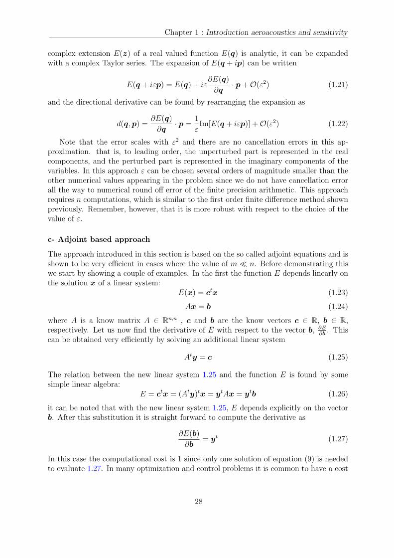
Chapter 1 : Introduction aeroacoustics and sensitivity
complex extension E(z) of a real valued function E(q) is analytic, it can be expandedwith a complex Taylor series. The expansion of E(q + ip) can be written
E(q + iεp) = E(q) + iε∂E(q)
∂q· p+O(ε2) (1.21)
and the directional derivative can be found by rearranging the expansion as
d(q,p) =∂E(q)
∂q· p =
1
εIm[E(q + iεp)] +O(ε2) (1.22)
Note that the error scales with ε2 and there are no cancellation errors in this ap-proximation. that is, to leading order, the unperturbed part is represented in the realcomponents, and the perturbed part is represented in the imaginary components of thevariables. In this approach ε can be chosen several orders of magnitude smaller than theother numerical values appearing in the problem since we do not have cancellation errorall the way to numerical round off error of the finite precision arithmetic. This approachrequires n computations, which is similar to the first order finite difference method shownpreviously. Remember, however, that it is more robust with respect to the choice of thevalue of ε.
c- Adjoint based approach
The approach introduced in this section is based on the so called adjoint equations and isshown to be very efficient in cases where the value of m ≪ n. Before demonstrating thiswe start by showing a couple of examples. In the first the function E depends linearly onthe solution x of a linear system:
E(x) = ctx (1.23)
Ax = b (1.24)
where A is a know matrix A ∈ Rn,n , c and b are the know vectors c ∈ R, b ∈ R,
respectively. Let us now find the derivative of E with respect to the vector b, ∂E∂b. This
can be obtained very efficiently by solving an additional linear system
Aty = c (1.25)
The relation between the new linear system 1.25 and the function E is found by somesimple linear algebra:
E = ctx = (Aty)tx = ytAx = ytb (1.26)
it can be noted that with the new linear system 1.25, E depends explicitly on the vectorb. After this substitution it is straight forward to compute the derivative as
∂E(b)
∂b= yt (1.27)
In this case the computational cost is 1 since only one solution of equation (9) is neededto evaluate 1.27. In many optimization and control problems it is common to have a cost
28

1.4 Sensitivity analysis
function with depends on the square of the linear system. An example of this is givenbelow.
E(x) =1
2xtx (1.28)
Ax = b (1.29)
In this case we start by linearising the system, which actually involves only the functionE. For this purpose we decompose x and b into mean and a perturbation as x = x+ εx′
and b = b + εb′. Introducing the decomposition into equations 2.1-2.2 and droppinghigher order ε-terms we obtain a system of equations for x′ and b′. This is written
δE = xtx′ (1.30)
Ax′ = b′. (1.31)
The additional linear system is now given as
Aty = x (1.32)
and the function δE can be evaluated as
δE = xtx′ = (Aty)tx′ = ytAx′ = ytb′ (1.33)
The gradient is then evaluated easily as
∂E(b)
∂b= yt (1.34)
Note that in this case the right hand side of the new linear system 1.32 is a functionof the solution of the original linear equation 1.31. This means that the computationalcost in this case is 2; first we need to solve 1.31, and successively equation 1.32. Further,this must be done for each dimension of E, as in the case of the FD and CSD, that is 1in this example.
d- Comparison of computational effort
We can now compare the computational effort of computing the gradient ∇E(q) using thethree methods that were outline above. In table 4.1 the number of function evaluationsis given as a function of a given method. Here, n and m denote the dimensions of qand E(q), respectively. Values for both first order (FD1) and second order (FD2) finitedifference method are shown. It is evident that using adjoint equations is computationallyefficient. The computational efficiency of the CSD is comparable to the FD1. However, theCSD is more robust since it does not involve any difference operations which means thatnumerical cancellation errors are avoided. In many applications the number of functionvalues m is much smaller than the parameter or variable that one perturb which hasdimension n. For example, considering the case of the variation of the total energy of aflow (m = 1) is estimated as a function of an external source acting in a localized regionof the flow. In this case n are the number of discrete points where the forcing could beplaced, typically of the order of 102 − 103.
29

Chapter 1 : Introduction aeroacoustics and sensitivity
Approach E(x) = c · x E(x) = x · xFD1FD2CSDADJ
(n+ 1) (n+ 1)2 · n 2 · nn n1 2
Table 1.1: Number of function evaluations to compute the gradient using Finite Differenceapproximation (FD), Complex step derivative (CSD) and adjoint equations (ADJ). Firstand second order FD approach are denoted FD1 and FD2.
1.4.3 Some Results
The idea of an adjoint equation assembles together a number of mathematical concepts,physical theories, and computational methods. Historically, it has evolved from a deviceto lower the order of an ordinary differential equation, more recently, adjoint equationshave been identify as a powerful tool in the study of the sensitivity of some global quan-tity (an objective) with respect to some input data of a complicated problem (e.g., thenumerical discretization of an ordinary or partial differential equation). Sensitivity can besimultaneously computed by an adjoint algorithm having approximately the same compu-tation time as a single run of the original simulation. This is much faster than a classicallinearisation approach in which one would have to numerically solve a separate linearisedproblem for the increment in each input variable.
Adjoint based sensitivity analysis is exploited in many different engineering fields notonly in fluid dynamics, including nuclear reactor physics, electromagnetism, seismic to-mography, dynamic meteorology, illumination computations in computer graphics, inversedesign problems, heat conduction, etc.
In this work the main goal is to identify the regions of the flow more sensitive toexternal perturbations in the momentum forcing and mass or heat injection.
Sensitivity coefficients can be therefore explained as how the response of any variationin the output of a system expressed as a mathematical functional can be apportionedto different sources of variation in the input of the model. Such analysis is common indifferent fields of engineering and in the field of fluid dynamics since it is closely related tooptimization problems and optimal control (Walther et al.[131] and Airiau [3]). In the last45 years receptivity of boundary layers flows was investigated in different theoretical andcomputational manners. Recently, [7] has demonstrated that receptivity coefficients andthe approach based on adjoint equations [3] can be associated to an optimization problemand therefore they were strongly closed to sensitivity coefficients. Later it was usedby [131, 5] to perform optimal control in the laminar boundary layer flow. Sensitivityanalysis based on the adjoint of compressible Navier-Stokes were also recently derived[101, 114, 132] and have led to some optimal control studies of the two dimensional shearlayer in the aeroacoustic framework. Some other examples of sensitivity can be found inthe mesh optimization and in the optimization of structures.
A first sensitivity analysis of jet instabilities associated to compressible jet at low
30

1.4 Sensitivity analysis
Mach number has been performed and validated recently by coupling the ParabolizedStability Equations (PSE) and the Adjoint-PSE method[11, 131]. In 2014 Kim et al. [59]used the adjoint solutions of the Euler equations to provide a definitive direction in whichadjust a model control actuation in order to reduce turbulent jet noise. In parallel, Tissotet al[127] has proposed, using some PSE-4D-Var approach to investigate the role of thecritical layer in jet in presence of non linear wave interactions. Following this previousworks, an extension of the compressible laminar flow to turbulent and supersonic flow ismade.
In this thesis sensitivity for a subsonic and supersonic flow [134] are implemented astest case for the validation of the model. Finally single and double jet flow has beencomputed from Large-Eddy-Simulation [12]. In particular the most sensitive zones tosome local forcing in the conservation stability equations are identified.
From our knowledge, the sensitivity analysis in the framework of adjoint of PSE sta-bility equations for supersonic jets in relation with aeroacoustic has never been done yet.Investigate flow sensitivities to any external source hopefully will lead to define some newnoise control strategies.
31

Chapter 1 : Introduction aeroacoustics and sensitivity
32

Chapter 2
Non local jet stability
In this chapter the Parabolized Stability Equations based to the linearised Euler Equa-tions are treated. The PSE were initially proposed by Herbert and Bertolotti (1987)[51]and some other authors during the same period [6] to study the linear and non lineardevelopment of Tollmien-Schlichting waves in boundary layers. Later 2000, works from[23, 22, 103] have extended PSE to jet flow. The main advantages of the choice of PSEinstead of Local Stability Theory (LST) are at least three:
• the small streamwise variations of the base flow and of the disturbances are directlytaken into account in the formulation (contrarily to LST where local parallel flowis assumed).
• the eigenvalue problem no longer exists and the PSE is set of Partial DifferentialEquations (PDE) mostly parabolic in the streamwise direction
• since PSE are PDE, it is simpler to solve it by adding various boundary conditionsand source terms. That means that they are used for receptivity and sensitivityanalysis, in optimal flow control approaches and for weakly non linear stabilityanalysis
The equations 2.17-2.19 are developing in cylindrical coordinates, as shown in figure2.1: x is the streamwise coordinates, ,r is the redial coordinates and θ the azimuthaldirection.
33
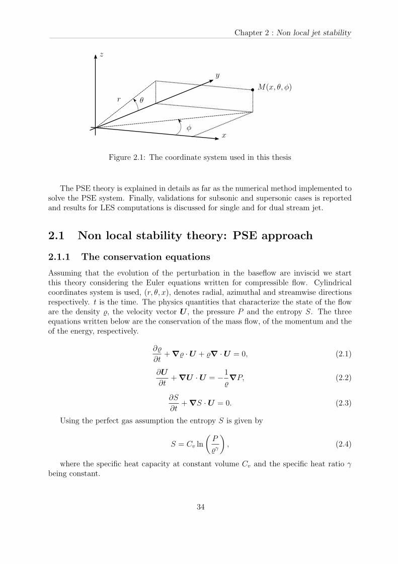
Chapter 2 : Non local jet stability
x
z
y
θ
φ
M(x, θ, φ)
r
Figure 2.1: The coordinate system used in this thesis
The PSE theory is explained in details as far as the numerical method implemented tosolve the PSE system. Finally, validations for subsonic and supersonic cases is reportedand results for LES computations is discussed for single and for dual stream jet.
2.1 Non local stability theory: PSE approach
2.1.1 The conservation equations
Assuming that the evolution of the perturbation in the baseflow are inviscid we startthis theory considering the Euler equations written for compressible flow. Cylindricalcoordinates system is used, (r, θ, x), denotes radial, azimuthal and streamwise directionsrespectively. t is the time. The physics quantities that characterize the state of the floware the density , the velocity vector U , the pressure P and the entropy S. The threeequations written below are the conservation of the mass flow, of the momentum and theof the energy, respectively.
∂
∂t+∇ ·U + ∇ ·U = 0, (2.1)
∂U
∂t+∇U ·U = −
1
∇P, (2.2)
∂S
∂t+∇S ·U = 0. (2.3)
Using the perfect gas assumption the entropy S is given by
S = Cv ln
(
P
γ
)
, (2.4)
where the specific heat capacity at constant volume Cv and the specific heat ratio γbeing constant.
34

2.1 Non local stability theory: PSE approach
2.1.2 Non dimensional equations
Before considering any kind of theoretical approach is important to normalize the variablesof the system by a dimensional analysis. This techniques allows us to determine importantnon dimensional parameters of the flow and to compare different flows with respect tothose parameters. The subscript ”j” refers to the conditions at the exit of the nozzlemeasured in the axis position. The lengths are non dimensionalized by the diameter Dj,the velocity by the streamwise exit velocity Uj, the density by ρj, the pressure by ρjU
2j ,
the time by Dj/Uj and other variables by the corresponding jet exit conditions. TheMach, Reynolds and Prandtl numbers are defined as follow:
Mj =Uj
aj(2.5)
Red =UjρjDj
µj
(2.6)
Pr =µjCp
λj
(2.7)
where aj is the sound velocity, µj the dynamic viscosity and λj is the thermal conduc-tivity coefficient of the flow. Generally, the sound velocity is defines as:
a =
√
γP
=
√
γR
MT, (2.8)
where R (approximately 8.314, 5 J/(mol ·K)) is the molar gas constant and M is themolar mass of the gas (the mean molar mass for dry air is about 0.028, 964, 5 kg/mol).Under these conditions the non dimensional term of the pressure P can be written as:
Pj
ρjU2j
=1
γM2j
(2.9)
To be clear, the dimensionless Euler equations are written with the same notation asin equation 2.1-2.3.
2.1.3 Linearisation
A common approach in the analysis of nonlinear systems is linearisation around a givenstate, in which the full solution is split into a steady term and a small time variantperturbation. The total flow vector Q = (U , , P )t is decomposed as follow:
Q = q + εq′(x, t) (2.10)
where q and q respectively denote the time invariant and the (low energy) fluctuatingstates. The constant ε is supposed to be small enough to neglet the non linear terms.Under the normalization introduced in section 2.1.2 the decomposition in equation 2.10becomes
35
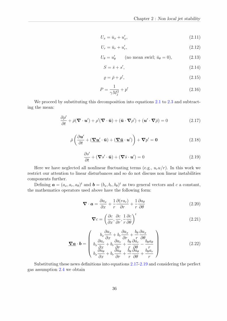
Chapter 2 : Non local jet stability
Ux = ux + u′
x, (2.11)
Ur = ur + u′
r, (2.12)
Uθ = u′
θ (no mean swirl; uθ = 0), (2.13)
S = s+ s′, (2.14)
= ρ+ ρ′, (2.15)
P =1
γM2j
+ p′ (2.16)
We proceed by substituting this decomposition into equations 2.1 to 2.3 and subtract-ing the mean:
∂ρ′
∂t+ ρ(∇ · u′) + ρ′(∇ · u) + (u ·∇ρ′) + (u′ ·∇ρ) = 0 (2.17)
ρ
(
∂u′
∂t+ (∇u′ · u) + (∇u · u′)
)
+∇p′ = 0 (2.18)
∂s′
∂t+ (∇s′ · u) + (∇s · u′) = 0 (2.19)
Here we have neglected all nonlinear fluctuating terms (e.g., uru/r). In this work werestrict our attention to linear disturbances and so do not discuss non linear instabilitiescomponents further.
Defining a = (ax, ar, aθ)t and b = (bx, br, bθ)
t as two general vectors and c a constant,the mathematics operators used above have the following form:
∇ · a =∂ax∂x
+1
r
∂(rar)
∂r+
1
r
∂aθ∂θ
(2.20)
∇c =
(
∂c
∂x,∂c
∂r,1
r
∂c
∂θ
)t
(2.21)
∇a · b =
bx∂ax∂x
+ br∂ax∂r
+bθr
∂ax∂θ
bx∂ar∂x
+ br∂ar∂r
+bθr
∂ar∂θ
−bθaθr
bx∂aθ∂x
+ br∂aθ∂r
+bθr
∂aθ∂θ
+bθarr
(2.22)
Substituting these news definitions into equations 2.17-2.19 and considering the perfectgas assumption 2.4 we obtain
36

2.1 Non local stability theory: PSE approach
Dρ′
Dt+ ρ
(
∂u′
x
∂x+
1
r
∂(ru′
r)
∂r+
1
r
∂u′
θ
∂θ
)
+
ρ′(
∂ux
∂x+
1
r
∂(rur)
∂r
)
+
(
u′
x
∂p
∂x+ u′
r
∂ρ
∂r
)
= 0
ρ
(
Dur
Dt+ u′
x
∂ur
∂x+ u′
r
∂ur
∂r
)
+∂p′
∂r= 0
ρ
(
Duθ
Dt+
u′
θur
r
)
+1
r
∂p′
∂θ= 0
ρ
(
Dux
Dt+ u′
x
∂ux
∂x+ u′
r
∂ux
∂r
)
+∂p′
∂x= 0
ρM2j
Dp′
Dt−
Dρ′
Dt− u′
x
∂ρ
∂x− u′
r
∂ρ
∂r= 0
where the derivative D/Dt is defined with respect to the base flow as
D
Dt=
∂
∂t+ ux
∂
∂x+ ur
∂
∂r(2.23)
This system of 5 equations and 5 unknowns, (u′
x, u′
r, u′
θ, ρ′, p′) is the final system which
is finally based the linear PSE analysis.
2.1.4 Considerations about the baseflow
The results of stability analysis are sensitive to the choice of mean flow. Typically aircraftjets are highly turbulent and the effects of this on the mean flow must be accounted for. Tothis end, one could compute the mean flow from experimental measurements of such flowsor by time and azimuthal average of computation results (as DNS, LES, RANS etc..). Thisis particularly attractive as nonlinear effects are then partially included via their effect onthe time invariant state. However, Bagheri et al (2009)[13] computed the base flow withrespect to the nonlinear Navier-Stokes equations using the selective frequency dampingmethod. With this method an equilibrium state of the jet flow, that it is different to theaverage to the azimuthal and temporal average of the flow, is identified. This methodcan not be apply at our analysis because of the high values of the Reynolds numbers inthe different cases investigated. Inspired to the work of the many others researcher, justto cite one of them[98, 64, 43], The time average from LES or from RANS computationhave been adopted in this work.
Questions regarding the evolution of small perturbations into the equilibrium statemay then be addressed via the solution q′ of the linearised Euler Equations (LEE). If thelinear solution is unstable then the nonlinear solution is also unstable. Linear stabilitydoes not necessarily imply nonlinear stability, however, as nonlinear bifurcations to otherstates may occur.
37
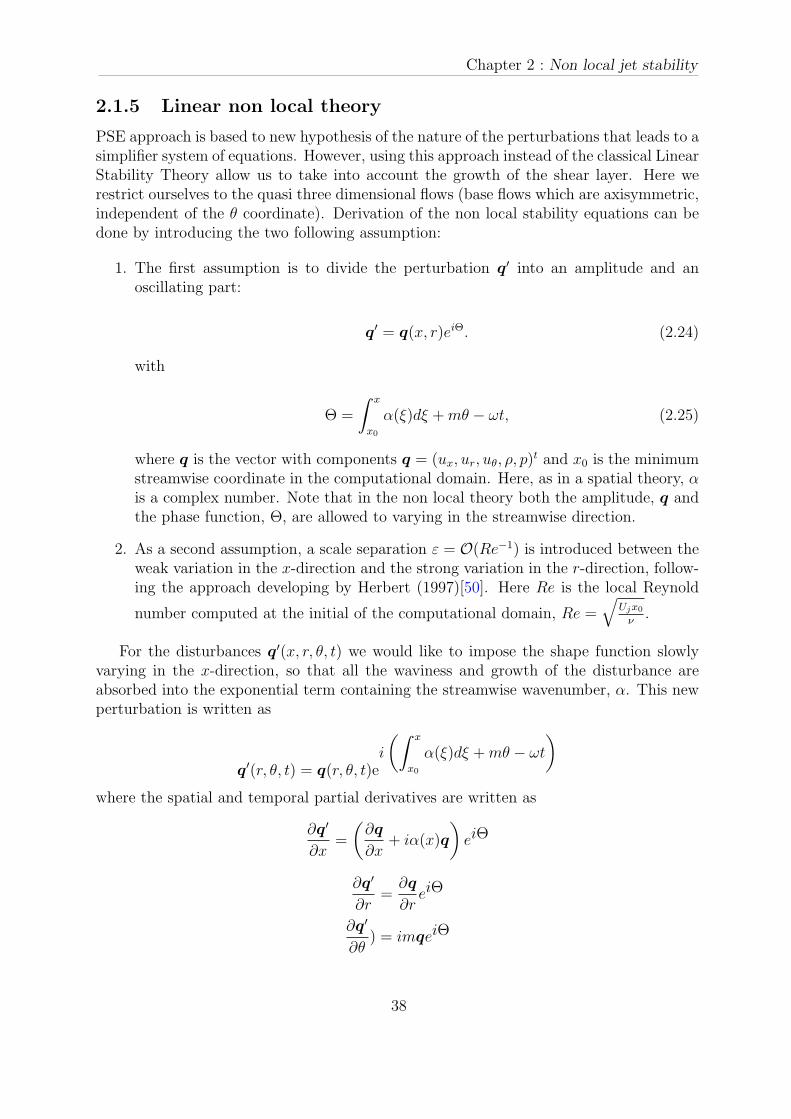
Chapter 2 : Non local jet stability
2.1.5 Linear non local theory
PSE approach is based to new hypothesis of the nature of the perturbations that leads to asimplifier system of equations. However, using this approach instead of the classical LinearStability Theory allow us to take into account the growth of the shear layer. Here werestrict ourselves to the quasi three dimensional flows (base flows which are axisymmetric,independent of the θ coordinate). Derivation of the non local stability equations can bedone by introducing the two following assumption:
1. The first assumption is to divide the perturbation q′ into an amplitude and anoscillating part:
q′ = q(x, r)eiΘ. (2.24)
with
Θ =
ˆ x
x0
α(ξ)dξ +mθ − ωt, (2.25)
where q is the vector with components q = (ux, ur, uθ, ρ, p)t and x0 is the minimum
streamwise coordinate in the computational domain. Here, as in a spatial theory, αis a complex number. Note that in the non local theory both the amplitude, q andthe phase function, Θ, are allowed to varying in the streamwise direction.
2. As a second assumption, a scale separation ε = O(Re−1) is introduced between theweak variation in the x-direction and the strong variation in the r-direction, follow-ing the approach developing by Herbert (1997)[50]. Here Re is the local Reynold
number computed at the initial of the computational domain, Re =√
Ujx0
ν.
For the disturbances q′(x, r, θ, t) we would like to impose the shape function slowlyvarying in the x-direction, so that all the waviness and growth of the disturbance areabsorbed into the exponential term containing the streamwise wavenumber, α. This newperturbation is written as
q′(r, θ, t) = q(r, θ, t)ei
(ˆ x
x0
α(ξ)dξ +mθ − ωt
)
where the spatial and temporal partial derivatives are written as
∂q′
∂x=
(
∂q
∂x+ iα(x)q
)
eiΘ
∂q′
∂r=
∂q
∂reiΘ
∂q′
∂θ) = imqeiΘ
38
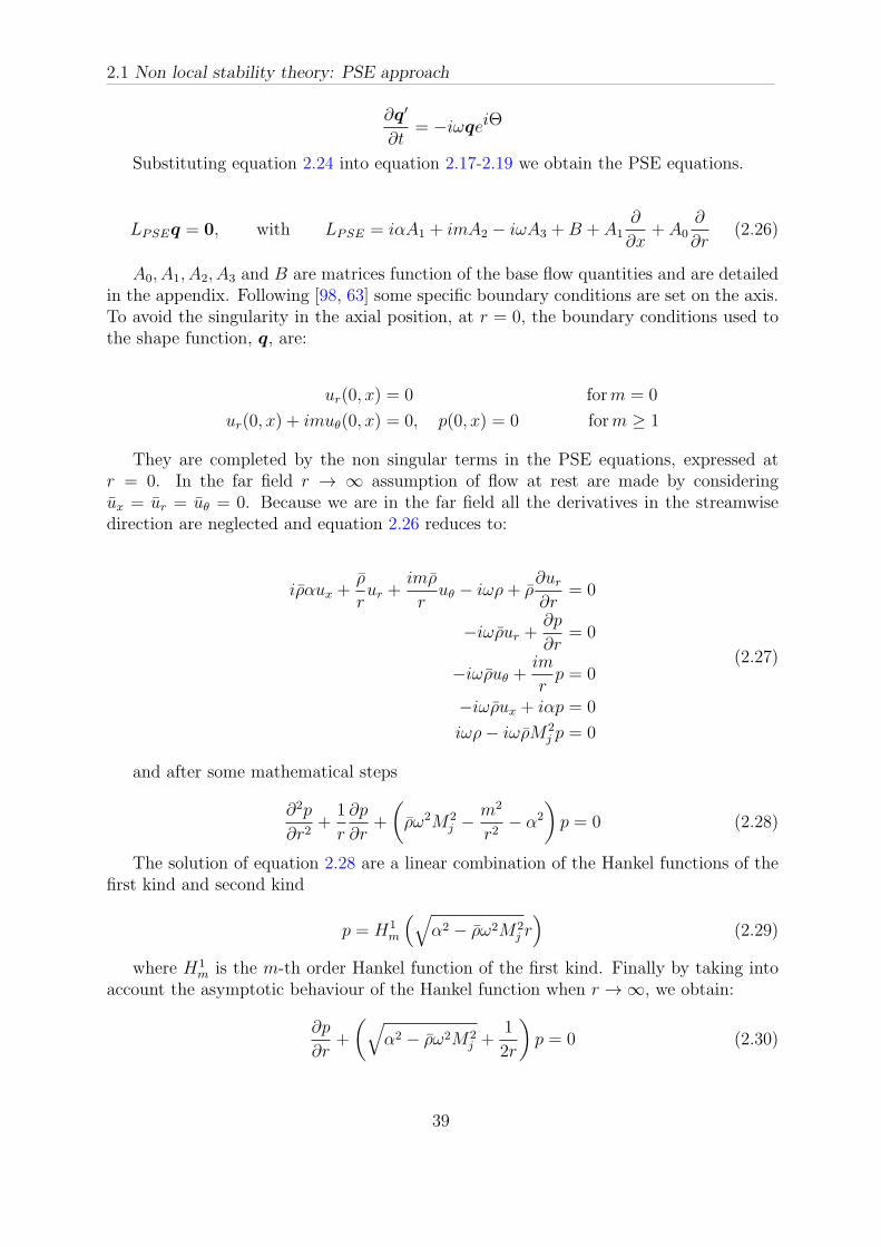
2.1 Non local stability theory: PSE approach
∂q′
∂t= −iωqeiΘ
Substituting equation 2.24 into equation 2.17-2.19 we obtain the PSE equations.
LPSEq = 0, with LPSE = iαA1 + imA2 − iωA3 +B + A1∂
∂x+ A0
∂
∂r(2.26)
A0, A1, A2, A3 and B are matrices function of the base flow quantities and are detailedin the appendix. Following [98, 63] some specific boundary conditions are set on the axis.To avoid the singularity in the axial position, at r = 0, the boundary conditions used tothe shape function, q, are:
ur(0, x) = 0 form = 0
ur(0, x) + imuθ(0, x) = 0, p(0, x) = 0 form ≥ 1
They are completed by the non singular terms in the PSE equations, expressed atr = 0. In the far field r → ∞ assumption of flow at rest are made by consideringux = ur = uθ = 0. Because we are in the far field all the derivatives in the streamwisedirection are neglected and equation 2.26 reduces to:
iραux +ρ
rur +
imρ
ruθ − iωρ+ ρ
∂ur
∂r= 0
−iωρur +∂p
∂r= 0
−iωρuθ +im
rp = 0
−iωρux + iαp = 0
iωρ− iωρM2j p = 0
(2.27)
and after some mathematical steps
∂2p
∂r2+
1
r
∂p
∂r+
(
ρω2M2j −
m2
r2− α2
)
p = 0 (2.28)
The solution of equation 2.28 are a linear combination of the Hankel functions of thefirst kind and second kind
p = H1m
(√
α2 − ρω2M2j r)
(2.29)
where H1m is the m-th order Hankel function of the first kind. Finally by taking into
account the asymptotic behaviour of the Hankel function when r → ∞, we obtain:
∂p
∂r+
(
√
α2 − ρω2M2j +
1
2r
)
p = 0 (2.30)
39
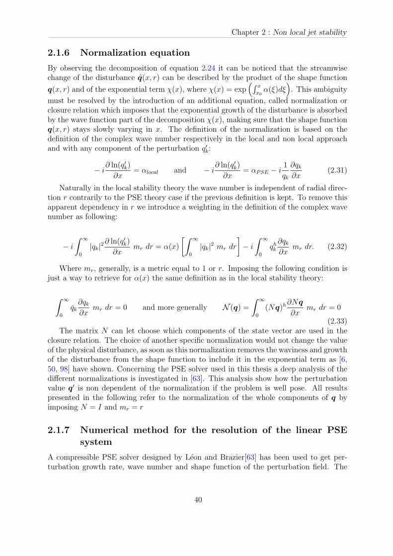
Chapter 2 : Non local jet stability
2.1.6 Normalization equation
By observing the decomposition of equation 2.24 it can be noticed that the streamwisechange of the disturbance q(x, r) can be described by the product of the shape function
q(x, r) and of the exponential term χ(x), where χ(x) = exp(
´ x
x0α(ξ)dξ
)
. This ambiguity
must be resolved by the introduction of an additional equation, called normalization orclosure relation which imposes that the exponential growth of the disturbance is absorbedby the wave function part of the decomposition χ(x), making sure that the shape functionq(x, r) stays slowly varying in x. The definition of the normalization is based on thedefinition of the complex wave number respectively in the local and non local approachand with any component of the perturbation q′k:
− i∂ ln(q′k)
∂x= αlocal and − i
∂ ln(q′k)
∂x= αPSE − i
1
qk
∂qk∂x
(2.31)
Naturally in the local stability theory the wave number is independent of radial direc-tion r contrarily to the PSE theory case if the previous definition is kept. To remove thisapparent dependency in r we introduce a weighting in the definition of the complex wavenumber as following:
− i
ˆ
∞
0
|qk|2∂ ln(q
′
k)
∂xmr dr = α(x)
[ˆ
∞
0
|qk|2 mr dr
]
− i
ˆ
∞
0
qhk∂qk∂x
mr dr. (2.32)
Where mr, generally, is a metric equal to 1 or r. Imposing the following condition isjust a way to retrieve for α(x) the same definition as in the local stability theory:
ˆ
∞
0
qk∂qk∂x
mr dr = 0 and more generally N (q) =
ˆ
∞
0
(Nq)h∂Nq
∂xmr dr = 0
(2.33)The matrix N can let choose which components of the state vector are used in the
closure relation. The choice of another specific normalization would not change the valueof the physical disturbance, as soon as this normalization removes the waviness and growthof the disturbance from the shape function to include it in the exponential term as [6,50, 98] have shown. Concerning the PSE solver used in this thesis a deep analysis of thedifferent normalizations is investigated in [63]. This analysis show how the perturbationvalue q′ is non dependent of the normalization if the problem is well pose. All resultspresented in the following refer to the normalization of the whole components of q byimposing N = I and mr = r
2.1.7 Numerical method for the resolution of the linear PSEsystem
A compressible PSE solver designed by Leon and Brazier[63] has been used to get per-turbation growth rate, wave number and shape function of the perturbation field. The
40
2.1 Non local stability theory: PSE approach
system of equations 2.26 and 2.33 are solved using a streamwise marching solution start-ing from the nozzle exit at x = x0 . The system is initialized by the solution of thelocal approach (LST). The radial direction is discretized using a multidomain spectralcollocation approach, or using a sixth order compact difference scheme with sectral-likeresolution, see Lele (1992)[62]. The mesh in the radial direction is discretized on a nonuniform grid. The first and second derivative of the metric are continuous in order toprovide a good accuracy when the radial derivatives of the parameters are computed:
∂q
∂r= Eq (2.34)
where the matrix E is different if using spectral collocation method or finite-differencecompact schemes.
The discretized problem is solved iteratively in the streamwise direction for the shapefunction q at each axial location. The wavenumber α is updated at each iteration usingthe classical scheme:
1. Advance x-position one step
2. Update the solution for q(x) equation 2.26 by solving a linear system.
3. Update α(x), α(p+1)j = α
(p)j + ∆α(p+1), where j refer to the position xj in the
discretized streamwise direction and p is the number of iteration
4. Check for convergence on α(x),
∣
∣
∣
∣
∆α(p)j
α(p)j
∣
∣
∣
∣
< ε. If not verified go to 2). Otherwise go
to 1)
An efficient method to compute ∆α(p)j can be obtained following the previous work of
Herbert (1993)[49] and Airiau (1994)[2]. The update value of α(p+1)j at the position xj is
given by
α(p+1)j = α
(p)j − i
N(q(p)j , q
(p)j−1)
A2(q(p)j )
, (2.35)
with
N(q(p)j , q
(p)j−1) =
ˆ
∞
0
(q(p)j )h ·
q(p)j − q
(p)j−1
∆xj
r dr (2.36)
A2(q(p)j ) =
ˆ
∞
0
(q(p)j )h · (q(p)
j )r dr (2.37)
In this thesis ε is fixed as, ε = 10−8 and needs around 6 − 8 iterations when computingclose to the exit nozzle and decay until 2− 3 after some diameters far to the nozzle.
The PSE system written in the discretized form leads to:
(α(x)A1 +mA2 + ωA3 +B) qj + A1
[
(qj − qj−1)
∆xj
]
+ A0 [Eq] (2.38)
41

Chapter 2 : Non local jet stability
finally, the shape function qj is computed by solving the following system:
(
α(x)A1 +mA2 + ωA3 +B +A1
∆x j+ A0E
)
qj =A1
∆xj
qj−1 (2.39)
Notice that the streamwise derivative, ∂q
∂x, is approximated by the backward finite differ-
ence form (qj − qj1)/∆xj. Figure 2.2, extracted by Leon (2012)[63] and Airiau (1994)[2],schematically represent the computational approach used to solve the PSE system:
Figure 2.2: Simple scheme of the PSE solver.
2.1.8 Stability of the PSE system
Are Parabolic Stability Equations parabolic? The answer is no. There exists a residualellipticity mainly of acoustic nature which means this system is only partially parabolic,Chang et al. (1991)[21]. Numerically instability would occur in attempting to use a toosmall marching stepsize in x, similar to that observed in applications of the ParabolizedNavier-Stokes equation formulation, PNS, Rubin and Tannehill (1992)[108]. Li and Mailik(1996)[65] used Fourier analysis to prove the existence of numerical instability and quantify
42
2.1 Non local stability theory: PSE approach
the bounds. It is demonstrated that the minimum step size, ∆xmin for numerical stabilityis, approximately, the inverse of the real part of the streamwise wavenumber:
∆xmin =1
αr
=λ
2π. (2.40)
This implies that a maximum of 2π steps per disturbance wavelength λ are allowedfor the marching. To reduce this step size we have at least two ways:
• drop out the ∂p
∂xterm. Li and Mailik (1996)[65] point out that since most of the
pressure gradient has been absorbed into the iαp term the ∂p
∂xterm is small in
comparison. They also demonstrate that the step-size restriction is reduced by atleast an order of magnitude.
• Introduce a stabilization term, Andersson et al. (1998)[8], that removes the ellip-ticity and leads to a well posed parabolic set of stability equations
Both approaches are good with minimal impact on the result. The weak ellipticityof the PSE was in addition analysed trough the Fourier and the characteristic theory byAiriau 1991[2]. If small steps of ∆x are required, as in presence of shock-cell in the baseflow, simply neglect the term ∂p
∂xmay not be enough. Following Andersson et al. [8] we
added a stabilizing term which is of the same order as the numerical errors. Since termsof this order were neglected in the original approximation of PSE, the addition of thisartificial term does not introduce any extra error at this order of approximation and wecan introduce the new set of equations:
A1∂q
∂x+ (iαA1 + imA2 − iωA3 +B + A0
∂
∂r)q =
−s(iαA1 + imA2 − iωA3 +B + A0∂
∂r)∂q
∂x
(2.41)
With this new configuration the critical step size is now defined as:
∆xmin >1
|αr|− 2s (2.42)
Equation 2.42 implies that the s value giving marginal stability approaches 0.5/ |αr|when ∆xmin → 0. Consequently, we can stably march PSEs downstream for any arbi-trarily small step size by using a suitable s. In our PSE code s has been setted as:
s = k
1
|αr|−∆x
2(2.43)
k is a constant value who must be grater then 1, in our computations its value is fixedto k = 3
4. The stabilization procedure has been validated performing the stability analysis
to an incompressible test case, Mj = 0.01, developed by Yen and Messersmith (1998)[133].In figure 2.3 the computation were performed for two different step sizes ∆x = 0.02, 0.05.
43
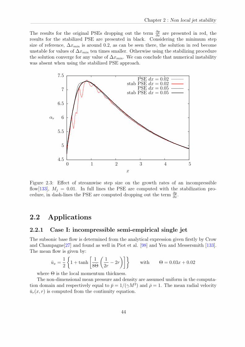
Chapter 2 : Non local jet stability
The results for the original PSEs dropping out the term ∂p
∂xare presented in red, the
results for the stabilized PSE are presented in black. Considering the minimum stepsize of reference, ∆xmin is around 0.2, as can be seen there, the solution in red becomeunstable for values of ∆xmin ten times smaller. Otherwise using the stabilizing procedurethe solution converge for any value of ∆xmin. We can conclude that numerical instabilitywas absent when using the stabilized PSE approach.
4.5
5
5.5
6
6.5
7
7.5
0 1 2 3 4 5
x
αr
PSE dx = 0.02stab PSE dx = 0.02
PSE dx = 0.05stab PSE dx = 0.05
Figure 2.3: Effect of streamwise step size on the growth rates of an incompressibleflow[133], Mj = 0.01. In full lines the PSE are computed with the stabilization pro-cedure, in dash-lines the PSE are computed dropping out the term ∂p
∂x.
2.2 Applications
2.2.1 Case I: incompressible semi-empirical single jet
The subsonic base flow is determined from the analytical expression given firstly by Crowand Champagne[27] and found as well in Piot et al. [98] and Yen and Messersmith [133].The mean flow is given by:
ux =1
2
1 + tanh
[
1
8Θ
(
1
2r− 2r
)]
with Θ = 0.03x+ 0.02
where Θ is the local momentum thickness.The non-dimensional mean pressure and density are assumed uniform in the computa-
tion domain and respectively equal to p = 1/(γM2) and ρ = 1. The mean radial velocityur(x, r) is computed from the continuity equation.
44

2.2 Applications
Figure 2.4 shows the computed axial velocity. The edge of the potential core and ofthe shear layer are identified by the two dash-dot lines. The computational domain, (Ω),is 10 diameters in the streamwise direction and 8 in the radial direction.
x
r
ux
Figure 2.4: Spatial distribution of the mean axial velocity, Mj = 0.01. In dash-dot linesthe boundary of potential core and the boundary of the shear layer.
The computations were performed for the axisymmetric instability mode, m = 0 anda Strouhal number of St = 0.6. In figure 2.5 the Local Stability Analysis is computed atthe initial position, x = x0. An unstable Kelvin-Helmholtz mode is clearly identified withα = 4.7− 4.0i. This value of α is used to initialize the PSE computation.
45
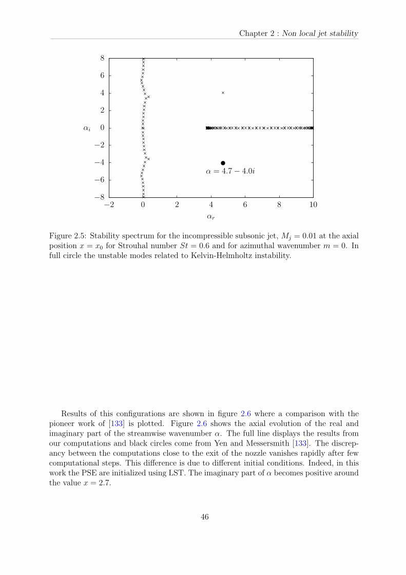
Chapter 2 : Non local jet stability
−8
−6
−4
−2
0
2
4
6
8
−2 0 2 4 6 8 10
αi
αr
α = 4.7− 4.0i
Figure 2.5: Stability spectrum for the incompressible subsonic jet, Mj = 0.01 at the axialposition x = x0 for Strouhal number St = 0.6 and for azimuthal wavenumber m = 0. Infull circle the unstable modes related to Kelvin-Helmholtz instability.
Results of this configurations are shown in figure 2.6 where a comparison with thepioneer work of [133] is plotted. Figure 2.6 shows the axial evolution of the real andimaginary part of the streamwise wavenumber α. The full line displays the results fromour computations and black circles come from Yen and Messersmith [133]. The discrep-ancy between the computations close to the exit of the nozzle vanishes rapidly after fewcomputational steps. This difference is due to different initial conditions. Indeed, in thiswork the PSE are initialized using LST. The imaginary part of α becomes positive aroundthe value x = 2.7.
46

2.2 Applications
x
Re(α)
Im(α)
b)
a)
Figure 2.6: Comparison between present PSE and Yen et Messersmith PSE(•), 1998. a)Real part of α, b) Imaginary part of α for a subsonic flow with ω = 1.2π and m = 0. Seealso [133].
Figure 2.7 shows the spatial distribution of the modulus of the pressure perturbationp′, |p′|. The perturbation increases in the unstable regions of the flow (Im(α(x)) < 0)until x = 2.7 and damp down when the flow becomes stable.
Figure 2.7: Spatial distribution of the modulus of the perturbation |p′| for the Strouhalnumber St = 0.6, and azimuthal wavenumber m = 0 the pressure growth in the unstableregions of the jet and fall-down for high values of the streamwise coordinates where theflow is stable.
47
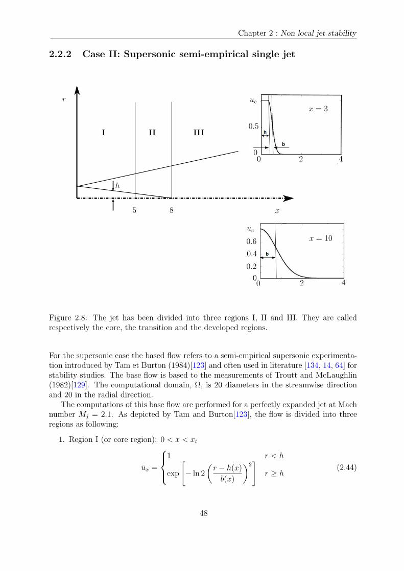
Chapter 2 : Non local jet stability
2.2.2 Case II: Supersonic semi-empirical single jet
r
x85
I II III
h
uc
0.5
00 2 4
x = 3
x = 10uc
0.4
0
0.2
0.6
2 40
Figure 2.8: The jet has been divided into three regions I, II and III. They are calledrespectively the core, the transition and the developed regions.
For the supersonic case the based flow refers to a semi-empirical supersonic experimenta-tion introduced by Tam et Burton (1984)[123] and often used in literature [134, 14, 64] forstability studies. The base flow is based to the measurements of Troutt and McLaughlin(1982)[129]. The computational domain, Ω, is 20 diameters in the streamwise directionand 20 in the radial direction.
The computations of this base flow are performed for a perfectly expanded jet at Machnumber Mj = 2.1. As depicted by Tam and Burton[123], the flow is divided into threeregions as following:
1. Region I (or core region): 0 < x < xt
ux =
1 r < h
exp
[
− ln 2
(
r − h(x)
b(x)
)2]
r ≥ h(2.44)
48
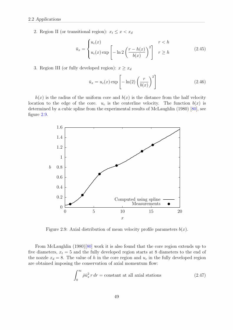
2.2 Applications
2. Region II (or transitional region): xt ≤ x < xd
ux =
uc(x) r < h
uc(x) exp
[
− ln 2
(
r − h(x)
b(x)
)2]
r ≥ h(2.45)
3. Region III (or fully developed region): x ≥ xd
ux = uc(x) exp
[
− ln(2)
(
r
b(x)
)2]
(2.46)
h(x) is the radius of the uniform core and b(x) is the distance from the half velocitylocation to the edge of the core. uc is the centerline velocity. The function b(x) isdetermined by a cubic spline from the experimental results of McLaughlin (1980) [80], seefigure 2.9.
0
0.2
0.4
0.6
0.8
1
1.2
1.4
1.6
0 5 10 15 20
b
x
Computed using splineMeasurements
Figure 2.9: Axial distribution of mean velocity profile parameters b(x).
From McLaughlin (1980)[80] work it is also found that the core region extends up tofive diameters, xt = 5 and the fully developed region starts at 8 diameters to the end ofthe nozzle xd = 8. The value of h in the core region and uc in the fully developed regionare obtained imposing the conservation of axial momentum flow:
ˆ
∞
0
ρu2x r dr = constant at all axial stations (2.47)
49

Chapter 2 : Non local jet stability
In region II h and b are determined by a cubic interpolation. The coefficients of the cubicpolynomial are chosen such that h and uc and their first derivatives in x are continuous.The density distribution ρ is obtained by solving Crocco-Busemann law:
ρ =[
−C1u2x + C3ux + C2
]
C1 =γ − 1
2M2
j , C2 =Ta
Tt
(1 +γ − 1
2M2
j )
C3 = C1 − C2 + 1.
(2.48)
Where Mj is the Mach jet number (Mj = 2.1), Tt the total temperature and Ta theambient temperature. The total temperature is set identical to the temperature of theambient air (Tt = Ta).
The radial velocity ur is obtained by solving continuity equation with integral ap-proach:
ur = −1
ρr
ˆ r
0
∂ρux
∂xrdr (2.49)
The corresponding distribution of centreline velocity uc, or ux(x, 0), of the three empiricalvelocity profiles eqs. 2.44-2.46, determined by the principle of conservation of momentumflux, is shown in figure 2.10. As can be seen, the calculated value of uc, agrees favourablywith the measurements of Troutt (1978)[128] for this particular configuration.
0.6
0.7
0.8
0.9
1
1.1
0 2 4 6 8 10 12 14
uc
x
ComputedMeasurements Troutt (1978)
Figure 2.10: Axial distribution of mean centerline velocity uc(x).
50
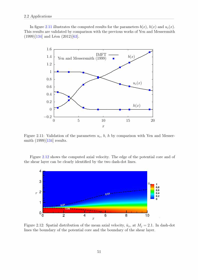
2.2 Applications
In figure 2.11 illustrates the computed results for the parameters b(x), h(x) and uc(x).This results are validated by comparison with the previous works of Yen and Messersmith(1999)[134] and Leon (2012)[63].
−0.2
0
0.2
0.4
0.6
0.8
1
1.2
1.4
1.6
0 5 10 15 20
x
b(x)
uc(x)
h(x)
IMFTYen and Messersmith (1999)
Figure 2.11: Validation of the parameters uc, b, h by comparison with Yen and Messer-smith (1999)[134] results.
Figure 2.12 shows the computed axial velocity. The edge of the potential core and ofthe shear layer can be clearly identified by the two dash-dot lines.
x
r
ux
Figure 2.12: Spatial distribution of the mean axial velocity, ux, at Mj = 2.1. In dash-dotlines the boundary of the potential core and the boundary of the shear layer.
51
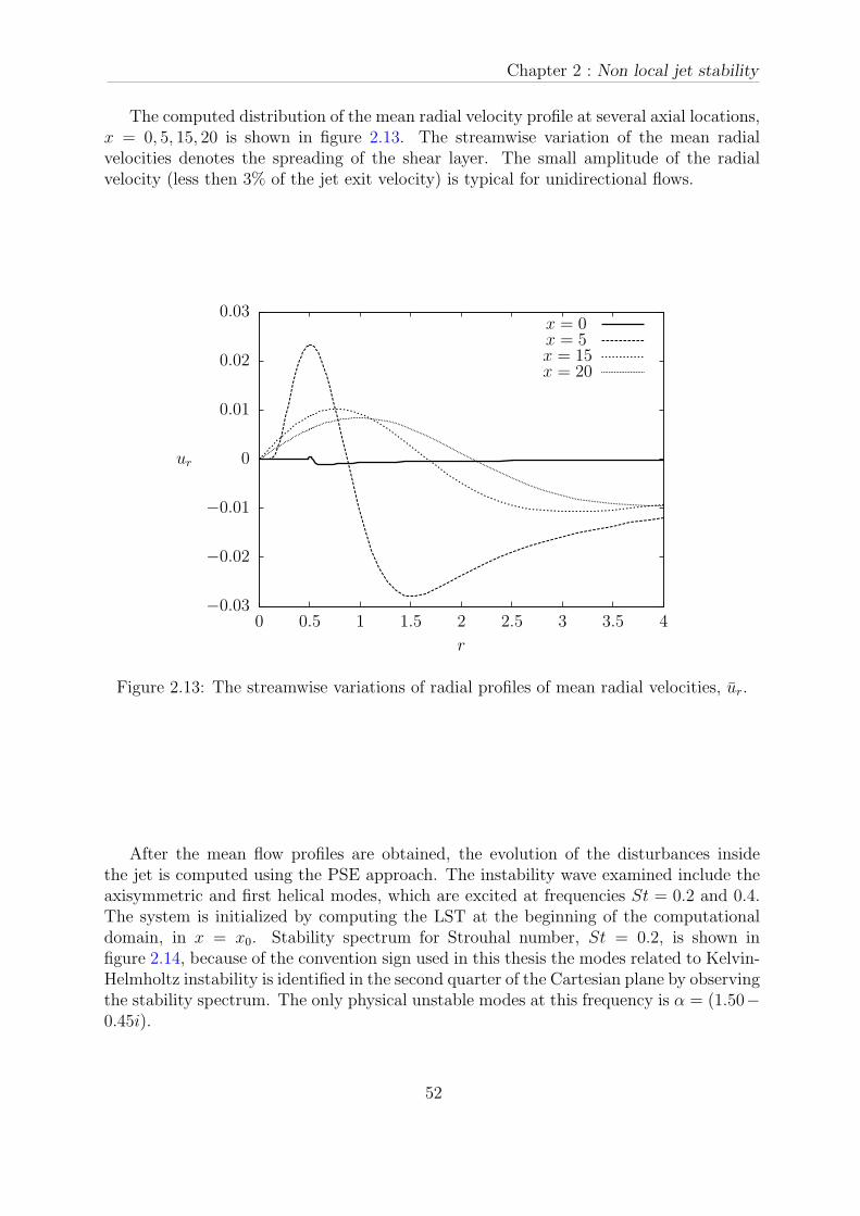
Chapter 2 : Non local jet stability
The computed distribution of the mean radial velocity profile at several axial locations,x = 0, 5, 15, 20 is shown in figure 2.13. The streamwise variation of the mean radialvelocities denotes the spreading of the shear layer. The small amplitude of the radialvelocity (less then 3% of the jet exit velocity) is typical for unidirectional flows.
−0.03
−0.02
−0.01
0
0.01
0.02
0.03
0 0.5 1 1.5 2 2.5 3 3.5 4
ur
r
x = 0x = 5x = 15x = 20
Figure 2.13: The streamwise variations of radial profiles of mean radial velocities, ur.
After the mean flow profiles are obtained, the evolution of the disturbances insidethe jet is computed using the PSE approach. The instability wave examined include theaxisymmetric and first helical modes, which are excited at frequencies St = 0.2 and 0.4.The system is initialized by computing the LST at the beginning of the computationaldomain, in x = x0. Stability spectrum for Strouhal number, St = 0.2, is shown infigure 2.14, because of the convention sign used in this thesis the modes related to Kelvin-Helmholtz instability is identified in the second quarter of the Cartesian plane by observingthe stability spectrum. The only physical unstable modes at this frequency is α = (1.50−0.45i).
52
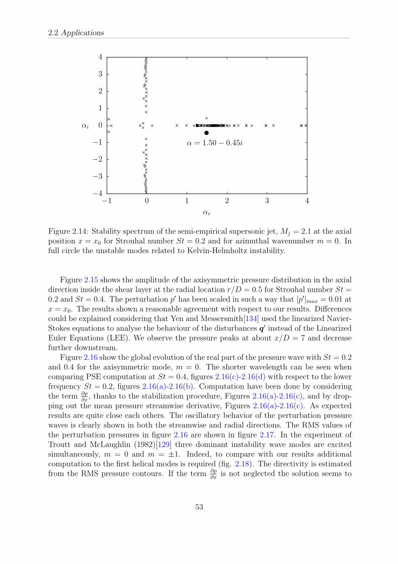
2.2 Applications
−4
−3
−2
−1
0
1
2
3
4
−1 0 1 2 3 4
αi
αr
α = 1.50− 0.45i
Figure 2.14: Stability spectrum of the semi-empirical supersonic jet, Mj = 2.1 at the axialposition x = x0 for Strouhal number St = 0.2 and for azimuthal wavenumber m = 0. Infull circle the unstable modes related to Kelvin-Helmholtz instability.
Figure 2.15 shows the amplitude of the axisymmetric pressure distribution in the axialdirection inside the shear layer at the radial location r/D = 0.5 for Strouhal number St =0.2 and St = 0.4. The perturbation p′ has been scaled in such a way that |p′|max = 0.01 atx = x0. The results shown a reasonable agreement with respect to our results. Differencescould be explained considering that Yen and Messersmith[134] used the linearized Navier-Stokes equations to analyse the behaviour of the disturbances q′ instead of the LinearizedEuler Equations (LEE). We observe the pressure peaks at about x/D = 7 and decreasefurther downstream.
Figure 2.16 show the global evolution of the real part of the pressure wave with St = 0.2and 0.4 for the axisymmetric mode, m = 0. The shorter wavelength can be seen whencomparing PSE computation at St = 0.4, figures 2.16(c)-2.16(d) with respect to the lowerfrequency St = 0.2, figures 2.16(a)-2.16(b). Computation have been done by consideringthe term ∂p
∂x, thanks to the stabilization procedure, Figures 2.16(a)-2.16(c), and by drop-
ping out the mean pressure streamwise derivative, Figures 2.16(a)-2.16(c). As expectedresults are quite close each others. The oscillatory behavior of the perturbation pressurewaves is clearly shown in both the streamwise and radial directions. The RMS values ofthe perturbation pressures in figure 2.16 are shown in figure 2.17. In the experiment ofTroutt and McLaughlin (1982)[129] three dominant instability wave modes are excitedsimultaneously, m = 0 and m = ±1. Indeed, to compare with our results additionalcomputation to the first helical modes is required (fig. 2.18). The directivity is estimatedfrom the RMS pressure contours. If the term ∂p
∂xis not neglected the solution seems to
53
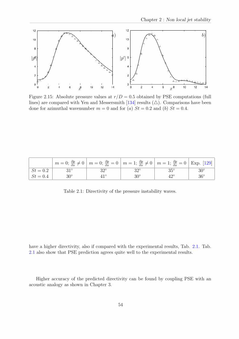
Chapter 2 : Non local jet stability
xx
|p′||p′|
a) b)
Figure 2.15: Absolute pressure values at r/D = 0.5 obtained by PSE computations (fulllines) are compared with Yen and Messersmith [134] results (). Comparisons have beendone for azimuthal wavenumber m = 0 and for (a) St = 0.2 and (b) St = 0.4.
∂p
∂x= 0 m = 0; ∂p
∂x6= 0 m = 0; ∂p
∂x= 0 m = 1; ∂p
∂x6= 0 m = 1; ∂p
∂x= 0 Exp. [129]
St = 0.2St = 0.4
31 32 32 35 30
30 41 30 42 36
Table 2.1: Directivity of the pressure instability waves.
have a higher directivity, also if compared with the experimental results, Tab. 2.1. Tab.2.1 also show that PSE prediction agrees quite well to the experimental results.
Higher accuracy of the predicted directivity can be found by coupling PSE with anacoustic analogy as shown in Chapter 3.
54

2.2 Applications
x
r
Re(p′)
(a) St = 0.2 and ∂p∂x
6= 0
x
r
(b) St = 0.2 and ∂p∂x
= 0
x
r
(c) St = 0.4 and ∂p∂x
6= 0
x
r
(d) St = 0.4 and ∂p∂x
= 0
Figure 2.16: Contour lines of the pressure waves for azimuthal wavenumber, m = 0. Samescale for each plots.
55
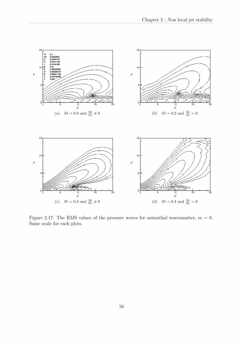
Chapter 2 : Non local jet stability
x
r
(a) St = 0.2 and ∂p∂x
6= 0
x
r
(b) St = 0.2 and ∂p∂x
= 0
x
r
(c) St = 0.4 and ∂p∂x
6= 0
x
r
(d) St = 0.4 and ∂p∂x
= 0
Figure 2.17: The RMS values of the pressure waves for azimuthal wavenumber, m = 0.Same scale for each plots.
56
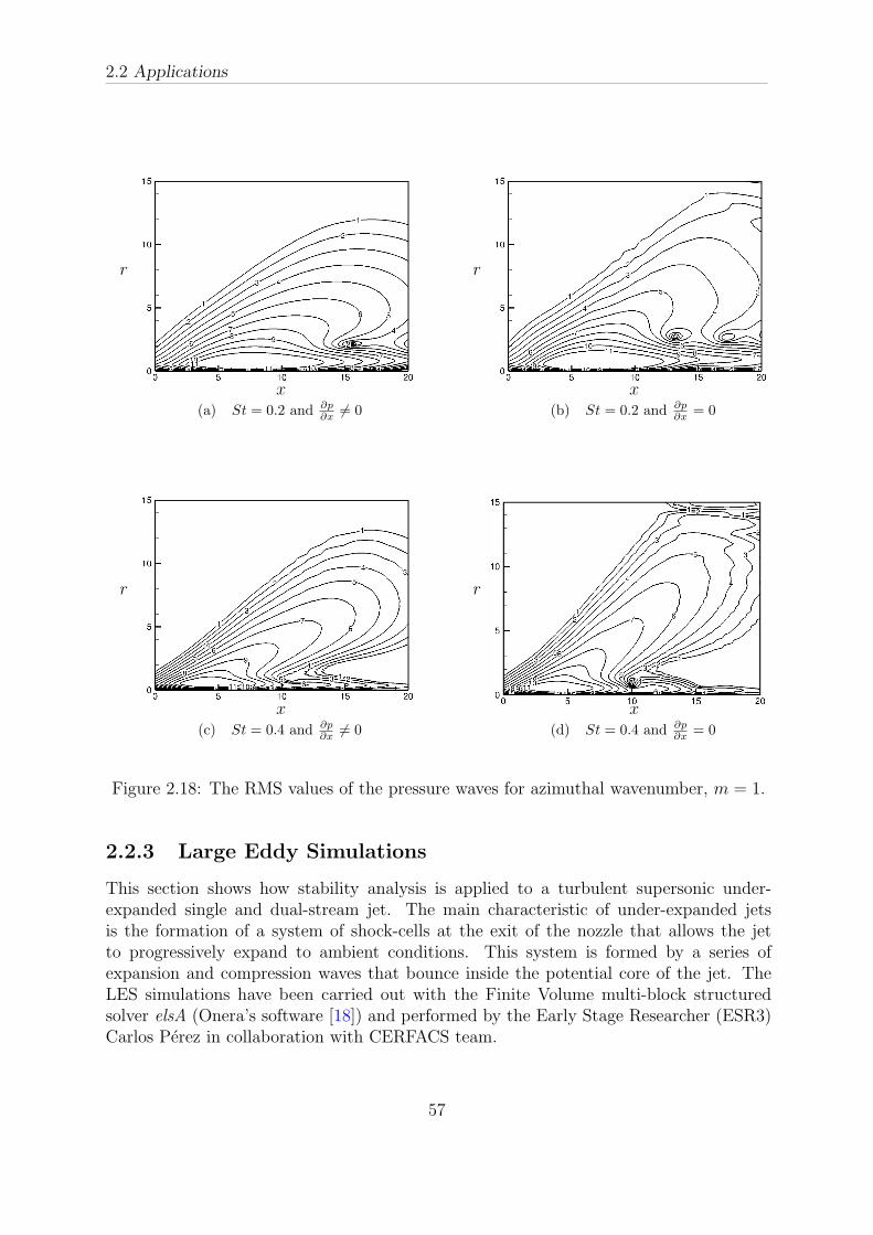
2.2 Applications
x
r
(a) St = 0.2 and ∂p∂x
6= 0
x
r
(b) St = 0.2 and ∂p∂x
= 0
x
r
(c) St = 0.4 and ∂p∂x
6= 0
x
r
(d) St = 0.4 and ∂p∂x
= 0
Figure 2.18: The RMS values of the pressure waves for azimuthal wavenumber, m = 1.
2.2.3 Large Eddy Simulations
This section shows how stability analysis is applied to a turbulent supersonic under-expanded single and dual-stream jet. The main characteristic of under-expanded jetsis the formation of a system of shock-cells at the exit of the nozzle that allows the jetto progressively expand to ambient conditions. This system is formed by a series ofexpansion and compression waves that bounce inside the potential core of the jet. TheLES simulations have been carried out with the Finite Volume multi-block structuredsolver elsA (Onera’s software [18]) and performed by the Early Stage Researcher (ESR3)Carlos Perez in collaboration with CERFACS team.
57
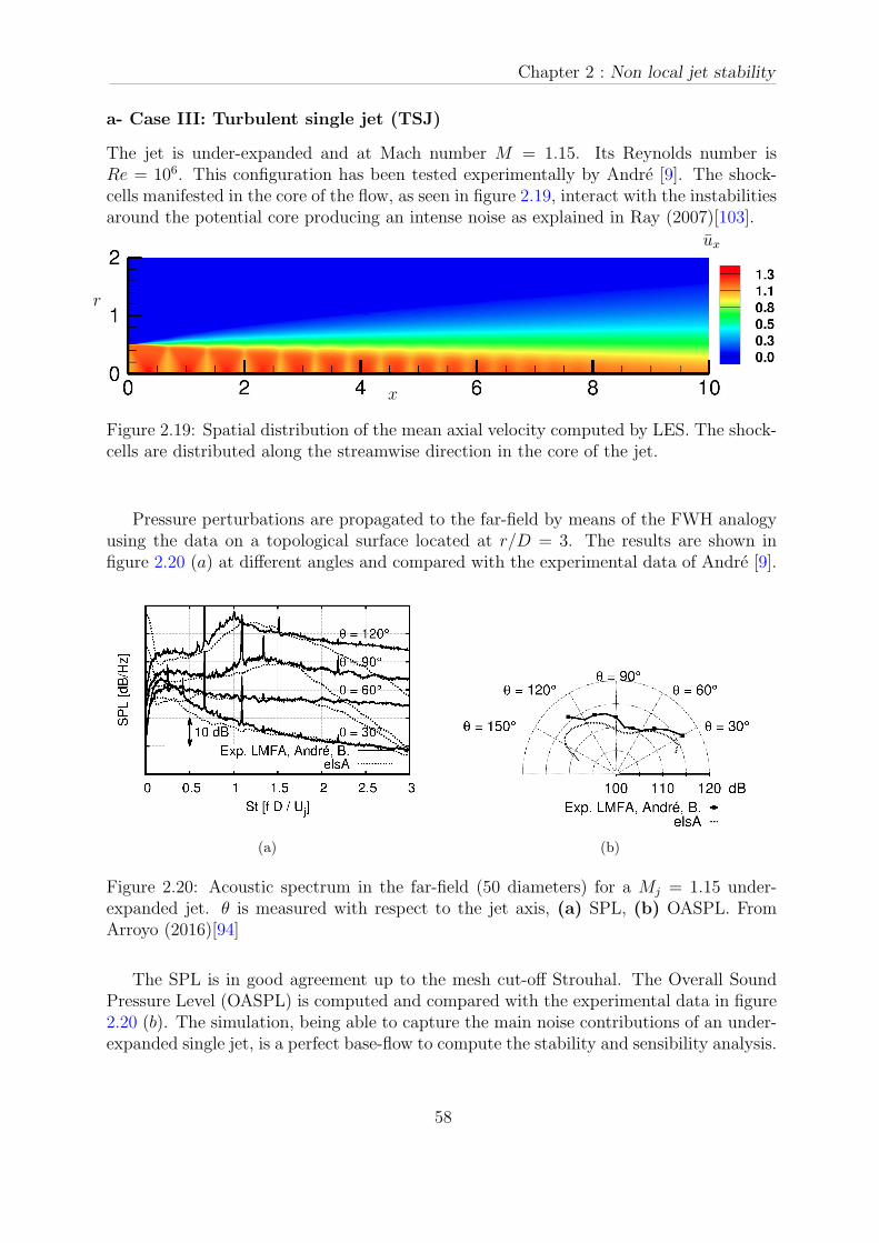
Chapter 2 : Non local jet stability
a- Case III: Turbulent single jet (TSJ)
The jet is under-expanded and at Mach number M = 1.15. Its Reynolds number isRe = 106. This configuration has been tested experimentally by Andre [9]. The shock-cells manifested in the core of the flow, as seen in figure 2.19, interact with the instabilitiesaround the potential core producing an intense noise as explained in Ray (2007)[103].
x
r
ux
Figure 2.19: Spatial distribution of the mean axial velocity computed by LES. The shock-cells are distributed along the streamwise direction in the core of the jet.
Pressure perturbations are propagated to the far-field by means of the FWH analogyusing the data on a topological surface located at r/D = 3. The results are shown infigure 2.20 (a) at different angles and compared with the experimental data of Andre [9].
(a) (b)
Figure 2.20: Acoustic spectrum in the far-field (50 diameters) for a Mj = 1.15 under-expanded jet. θ is measured with respect to the jet axis, (a) SPL, (b) OASPL. FromArroyo (2016)[94]
The SPL is in good agreement up to the mesh cut-off Strouhal. The Overall SoundPressure Level (OASPL) is computed and compared with the experimental data in figure2.20 (b). The simulation, being able to capture the main noise contributions of an under-expanded single jet, is a perfect base-flow to compute the stability and sensibility analysis.
58
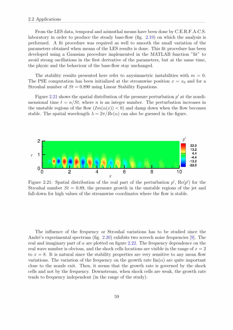
2.2 Applications
From the LES data, temporal and azimuthal means have been done by C.E.R.F.A.C.S.laboratory in order to produce the steady base-flow (fig. 2.19) on which the analysis isperformed. A fit procedure was required as well to smooth the small variation of theparameters obtained when means of the LES results is done. This fit procedure has beendeveloped using a Gaussian procedure implemented in the MATLAB function ”fit” toavoid strong oscillations in the first derivative of the parameters, but at the same time,the physic and the behaviour of the base-flow stay unchanged.
The stability results presented here refer to axysimmetric instabilities with m = 0.The PSE computation has been initialized at the streamwise position x = x0 and for aStrouhal number of St = 0.890 using Linear Stability Equations.
Figure 2.21 shows the spatial distribution of the pressure perturbation p′ at the nondi-mensional time t = n/St, where n is an integer number. The perturbation increases inthe unstable regions of the flow (Im(α(x)) < 0) and damp down when the flow becomesstable. The spatial wavelength λ = 2π/Re(α) can also be guessed in the figure.
x
r
p′
Figure 2.21: Spatial distribution of the real part of the perturbation p′, Re(p′) for theStrouhal number St = 0.89, the pressure growth in the unstable regions of the jet andfall-down for high values of the streamwise coordinates where the flow is stable.
The influence of the frequency or Strouhal variations has to be studied since theAndre’s experimental spectrum (fig. 2.20) exhibits two screech noise frequencies [9]. Thereal and imaginary part of α are plotted on figure 2.22. The frequency dependence on thereal wave number is obvious, and the shock cells locations are visible in the range of x = 2to x = 8. It is natural since the stability properties are very sensitive to any mean flowvariations. The variation of the frequency on the growth rate Im(α) are quite importantclose to the nozzle exit. Then, it seems that the growth rate is governed by the shockcells and not by the frequency. Downstream, when shock cells are weak, the growth ratetends to frequency independent (in the range of the study).
59
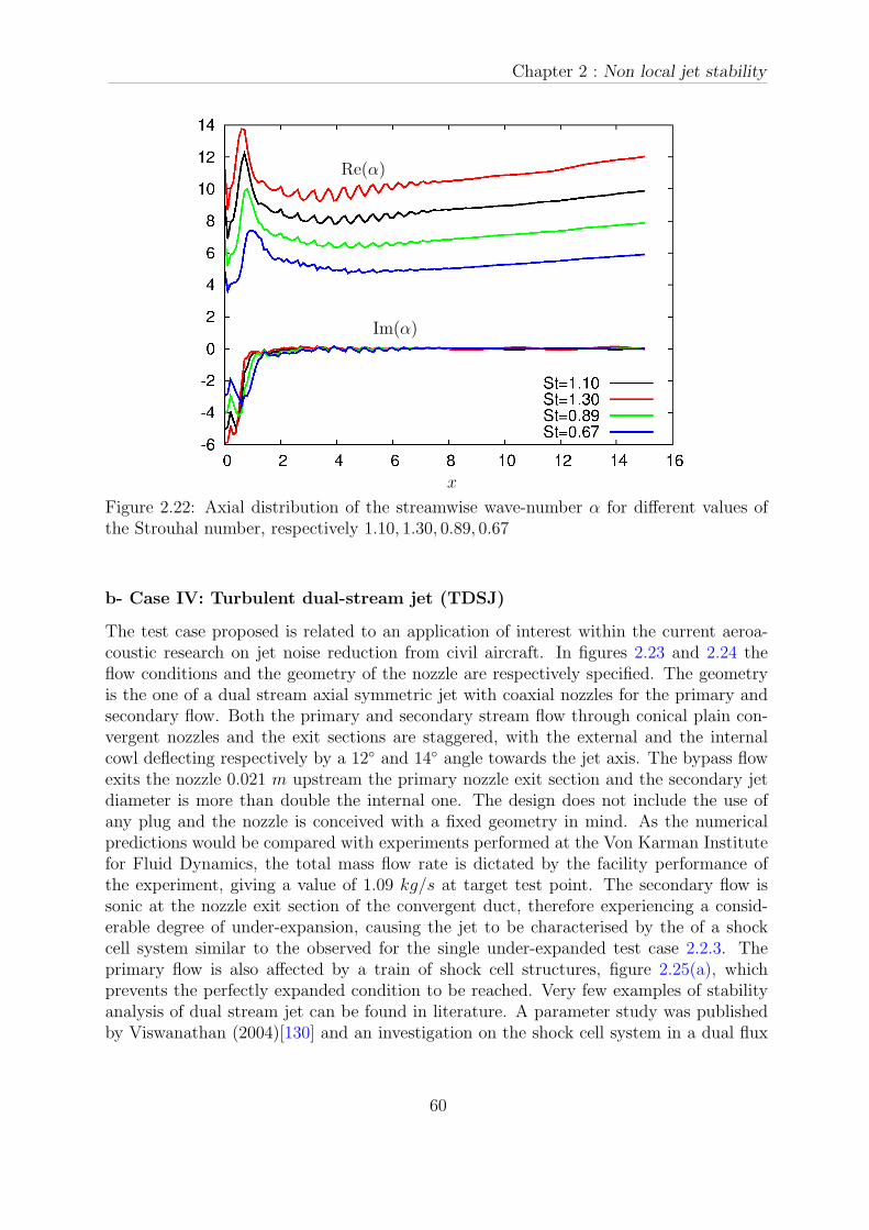
Chapter 2 : Non local jet stability
x
Re(α)
Im(α)
Figure 2.22: Axial distribution of the streamwise wave-number α for different values ofthe Strouhal number, respectively 1.10, 1.30, 0.89, 0.67
b- Case IV: Turbulent dual-stream jet (TDSJ)
The test case proposed is related to an application of interest within the current aeroa-coustic research on jet noise reduction from civil aircraft. In figures 2.23 and 2.24 theflow conditions and the geometry of the nozzle are respectively specified. The geometryis the one of a dual stream axial symmetric jet with coaxial nozzles for the primary andsecondary flow. Both the primary and secondary stream flow through conical plain con-vergent nozzles and the exit sections are staggered, with the external and the internalcowl deflecting respectively by a 12 and 14 angle towards the jet axis. The bypass flowexits the nozzle 0.021 m upstream the primary nozzle exit section and the secondary jetdiameter is more than double the internal one. The design does not include the use ofany plug and the nozzle is conceived with a fixed geometry in mind. As the numericalpredictions would be compared with experiments performed at the Von Karman Institutefor Fluid Dynamics, the total mass flow rate is dictated by the facility performance ofthe experiment, giving a value of 1.09 kg/s at target test point. The secondary flow issonic at the nozzle exit section of the convergent duct, therefore experiencing a consid-erable degree of under-expansion, causing the jet to be characterised by the of a shockcell system similar to the observed for the single under-expanded test case 2.2.3. Theprimary flow is also affected by a train of shock cell structures, figure 2.25(a), whichprevents the perfectly expanded condition to be reached. Very few examples of stabilityanalysis of dual stream jet can be found in literature. A parameter study was publishedby Viswanathan (2004)[130] and an investigation on the shock cell system in a dual flux
60
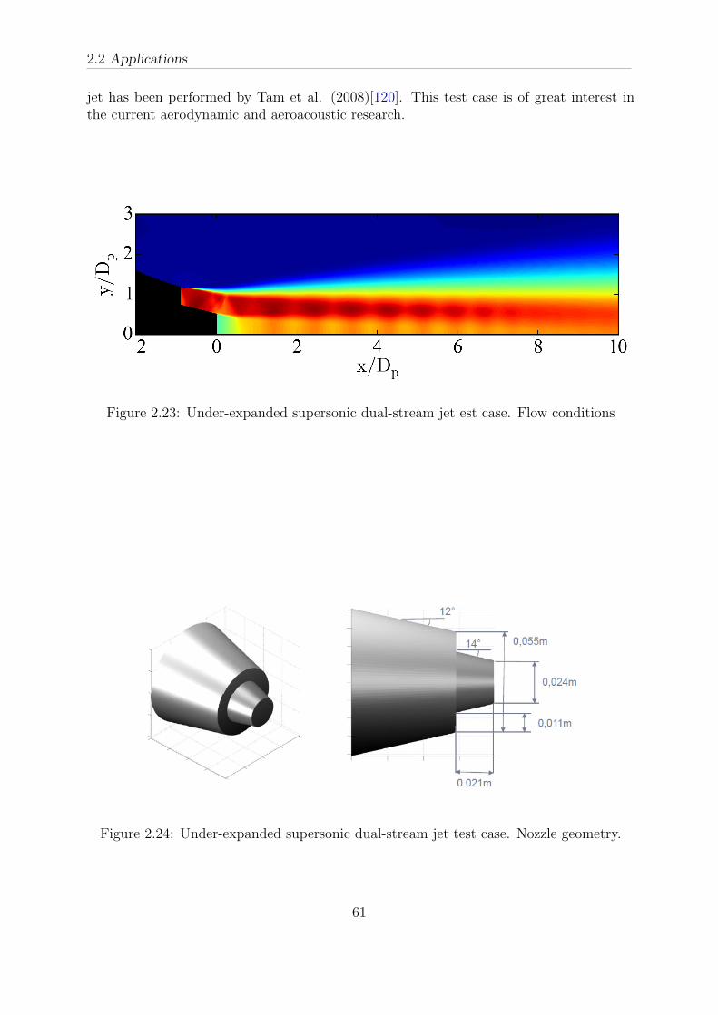
2.2 Applications
jet has been performed by Tam et al. (2008)[120]. This test case is of great interest inthe current aerodynamic and aeroacoustic research.
Figure 2.23: Under-expanded supersonic dual-stream jet est case. Flow conditions
Figure 2.24: Under-expanded supersonic dual-stream jet test case. Nozzle geometry.
61

Chapter 2 : Non local jet stability
(a)
(b)
Figure 2.25: Under-expanded supersonic dual-stream jet test case. Time and azimuthalaverage mean axial velocity ux.
The flow conditions of the co-axial jet are: the primary flow is cold and subsonic withan exit Mach number of Mp = 0.89 (CN P R = 1.675), the secondary stream is operatedat supersonic under-expanded conditions with a perfectly exit Mach number of Ms = 1.20(F N P R = 2.45). Here, CN P R and F N P R stand for Core and Fan Nozzle to PressureRatio respectively. The jets are established from two concentric convergent nozzles withprimary and secondary diameters of Dp = 23.4mm and Ds = 55.0mm respectively. Thethicknesses of the nozzles at the exit are of 0.5mm. The Reynolds numbers based on thejet exit diameters are Rep = 0.57 × 10⁶ and Res = 1.66 × 10⁶. The ambient conditionsused for this test case are a pressure Pamb = 101325 Pa and a temperature Tamb = 283 K.The stagnation pressure or total pressure Ptp = 1.6972 × 10⁵ Pa for the primary streamand Pts = 2.4825× 10⁵ Pa for the secondary stream. The total temperature Tt has beenkept equal to the ambient temperature Tamb for both streams.
62

2.2 Applications
The lengths are non-dimensionalized by the primary diameter Dp. As in the singlestream jet case 2.2.3, the steady base flow is obtained by temporal and azimuthal integralaverage in the whole computational domain (Ω) figure 2.26(a). The same fit procedure ofthe data implemented for the TSJ case was used. The computational domain (Ω) is 30diameters in the streamwise direction and 6 in the radial direction.
x
r
ux
(a)
x
r
ux
(b)
Figure 2.26: Test case under-expanded supersonic dual-stream jet. Time and azimuthalaverage mean axial velocity ux.
The PSE computation is initialized by a LST analysis. The choice of the initialstation x = x0 have been done, firstly, at the exit of the primary nozzle (test 1). Here,as example, we show the results of the eigenvalues problem obtained in the configurationof St = 1.0; two very distinct unstable modes are observed in the stability spectrum (fig.2.27-a). These two modes are the hydrodynamic Kelvin-Helmholtz modes (referred toas ”KH modes”) of the two mixing layers, KH1 and KH2 referring respectively to theinner and outer mixing regions. However, the strong shock that appears just at the end
63
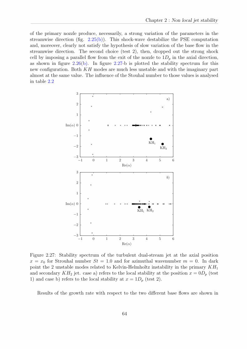
Chapter 2 : Non local jet stability
of the primary nozzle produce, necessarily, a strong variation of the parameters in thestreamwise direction (fig. 2.25(b)). This shock-wave destabilize the PSE computationand, moreover, clearly not satisfy the hypothesis of slow variation of the base flow in thestreamwise direction. The second choice (test 2), then, dropped out the strong shockcell by imposing a parallel flow from the exit of the nozzle to 1Dp in the axial direction,as shown in figure 2.26(b). In figure 2.27-b is plotted the stability spectrum for thisnew configuration. Both KH modes are much less unstable and with the imaginary partalmost at the same value. The influence of the Stouhal number to those values is analysedin table 2.2
−3
−2
−1
0
1
2
3
−1 0 1 2 3 4 5 6
Im(α)
Re(α)
KH2
KH1
a)
−3
−2
−1
0
1
2
3
−1 0 1 2 3 4 5 6
Im(α)
Re(α)
KH1 KH2
b)
Figure 2.27: Stability spectrum of the turbulent dual-stream jet at the axial positionx = x0 for Strouhal number St = 1.0 and for azimuthal wavenumber m = 0. In darkpoint the 2 unstable modes related to Kelvin-Helmholtz instability in the primary KH1
and secondary KH2 jet. case a) refers to the local stability at the position x = 0Dp (test1) and case b) refers to the local stability at x = 1Dp (test 2).
Results of the growth rate with respect to the two different base flows are shown in
64

2.2 Applications
figure 2.28. The instability behaviour of the flow and the point where the flow becomesstable, αi > 0 are not changing (x = 15Dp). Indeed, the solutions quickly converge tosame values after around 3Dp in the streamwise direction, showing that the choice ofoverpass the shock wave will not affect the physics of the instability waves.
−1
−0.8
−0.6
−0.4
−0.2
0
0.2
0 2 4 6 8 10 12 14
αi
x
Overpassing 1st shock-cellWithout overpassing 1st shock-cell
x*0
Figure 2.28: Growth rate computed for the two different baseflow. The two solutionsquickly converge to the same values.
By considering this new base flow configuration a parametric analysis of the pertur-bation waves with respect to different values of the Strouhal number, St, in the case ofaxisymmetric instabilities m = 0 has been done in the following. First conclusion can bepointed out observing Tab. 2.2, where the LST analysis is computed at the beginning ofthe computational domain, x = x0. The values of the streamwise wavenumber α functionof the Strouhal number, St, show that the local growth of the KH2 mode is larger than itsrelated to KH1 mode, which suggest a local dominance of the instability wave developingin the secondary jet. As expected, the real part αr, inversely proportional to the wave-length, decreases with the Strouhal number in the primary and in the secondary jet. Thelocal growth rate αi in the primary jet decrease with the Strouhal number and oppositebehaviour is observed for the unstable modes related to the secondary shear layer, KH2.This first results suggest a crucial role of the secondary jet, moreover, for small values ofthe Strouhal number.
65

Chapter 2 : Non local jet stability
∂p
∂x= 0 KH1 KH2
St = 1.0St = 0.8St = 0.6St = 0.4
3.46− 0.26i 4.18− 0.23i2.78− 0.22i 3.52− 0.33i2.10− 0.18i 2.79− 0.50i1.39− 0.12i 1.74− 0.63i
Table 2.2: Values of the initializing unstable Kelvin-Helmoltz modes in the inner and inthe outer shear-layer for different Strouhal numbers.
Clearly, this first trend, is not fully representative of the disturbances and a PSE anal-ysis is necessary to analyze the axial evolution of them. The frequency dependence of thereal and imaginary part of the streamwise wavenumber α(x) are plotted in figures 2.29and 2.30, respectively. As observed for the single stream case, the shock cells structures,clearly, influence the values of the wavenumber in particular the growth rate. The wavelength αr seems to be more affected by variations of the Strouhal number, St, if com-pared to the growth rate. The position where the flow becomes stable, however, changenoticeably varying the Strouhal number.
0
1
2
3
4
5
6
5 10 15 20 25 30
Im(α)
x
St = 1.0St = 0.8St = 0.6St = 0.4
Figure 2.29: Real part of the wavenumber α(x) for different Strouhal values.
66
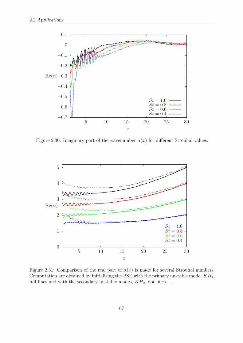
2.2 Applications
−0.7
−0.6
−0.5
−0.4
−0.3
−0.2
−0.1
0
0.1
5 10 15 20 25 30
Re(α)
x
St = 1.0St = 0.8St = 0.6St = 0.4
Figure 2.30: Imaginary part of the wavenumber α(x) for different Strouhal values.
0
1
2
3
4
5
5 10 15 20 25 30
Re(α)
x
St = 1.0St = 0.8St = 0.6St = 0.4
Figure 2.31: Comparison of the real part of α(x) is made for several Strouhal numbers.Computation are obtained by initialising the PSE with the primary unstable mode, KH1,full lines and with the secondary unstable modes, KH2, dot-lines. .
67

Chapter 2 : Non local jet stability
As explained in Leon (2012)[63] whereas the outcome is unambiguous when a singleunstable modes is present, the result is confused if the base flow supports multiple in-stabilities. It almost impossible to separate the two distinct unstable modes KH1 andKH2 computing the PSE without any kind of interaction between them. In particularthe modes related to the primary jet, KH1, probably due to his less unstable values,seems to quickly interact with the secondary jet. As observed in Sinha et al. (2016)[111]the instability waves referred to the two modes collapse downstream in the same wave.To elucidate this point, figure 2.31 shows the wavenumber αr(x) of the outer and innerPSE solutions for different Strouhal number in both cases, KH1 and KH2. The solutionsconverge into a same values when moving downstream in the streamwise direction.
Qualitatively this mechanism can be observed in figure 2.33 and 2.34. When computingthe PSE with respect to the secondary modes, KH2 the pressure perturbation p′ stay inthe secondary jet (r/Dp = 1.0 at the exit of the nozzle) at least, until this distinction canbe done (x = 10− 11Dp). The pressure perturbation p′ referred to the primary jet startto grow up in the inner shear layer, but then ”jump” to the more unstable outer shearlayer. This behaviour is exaggerate for St = 0.4, see figure 2.34, where the secondaryshear layer is much more unstable comparing to the primary one, 2.2.
These evidences demonstrates the coalescence of the outer and inner modes. Also ifthey start out as distinct instabilities near the nozzle, PSE cannot track them separately.These observations are representative of the range of frequencies studied (St = 0.4, 0.6,0.8, 1.0). The intrinsic interaction between the two modes, KH1 andKH2, put in evidencethree observations: (1) the primary and secondary shear layer merge downstream of thenozzle and at least this zone cannot support multiple unstable Kelvin-Helmholtz modes;(2) the more unstable secondary shear layer interact with the unstable modes even if thisperturbation is generated in the primary shear layer; (3) it seems that in the interval[6.5, 8] there is a natural exchange of stability. These Observations can be confirmed bya loacal stability analysis.
On figure 2.32 are plotted the most unstable eigen values obtained via the local stabilitytheory from x = 1 to x = 8. Inside blue circles are emphasized the first KH mode (KH1)at x = 6 and x = 8, and in red, the second KH modes, KH2, are plotted at the samepositions. It is clearly demonstrated that the KH1 becomes less amplified than the KH2
at x = 8, contrarily to the case x = 6. The αi axis ends on the figure at −0.01 to avoidthe numerous modes with neutral amplification. More deep conclusions will be pointedout when computing the sensitivity analysis in Chapter 3.
68
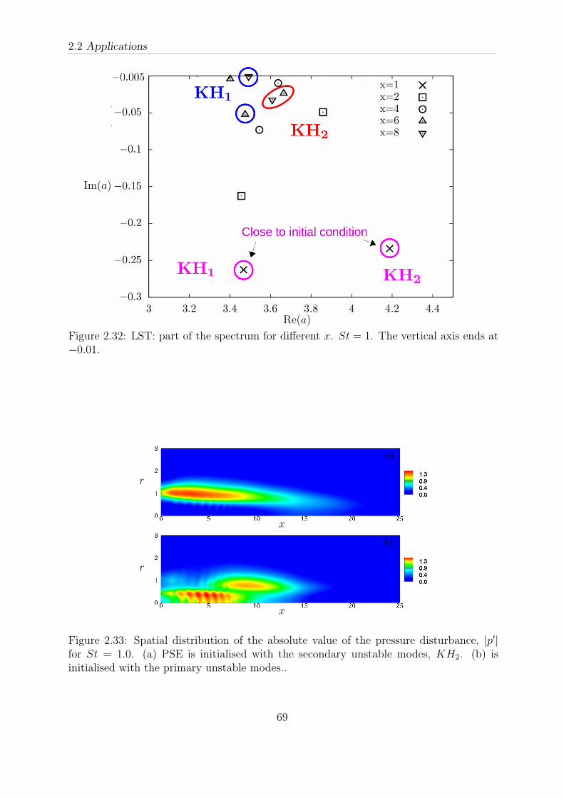
2.2 Applications
Im(a)
Re(a)
Figure 2.32: LST: part of the spectrum for different x. St = 1. The vertical axis ends at−0.01.
x
r
a)
x
r
b)
Figure 2.33: Spatial distribution of the absolute value of the pressure disturbance, |p′|for St = 1.0. (a) PSE is initialised with the secondary unstable modes, KH2. (b) isinitialised with the primary unstable modes..
69
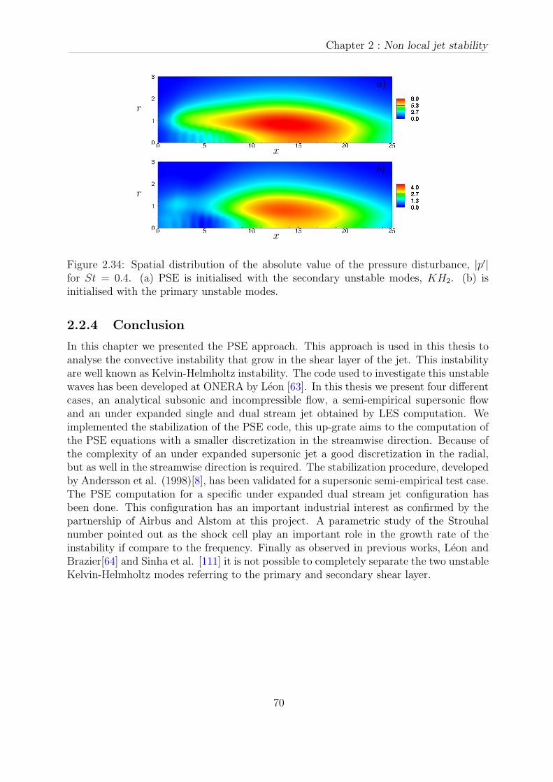
Chapter 2 : Non local jet stability
x
r
a)
x
r
b)
Figure 2.34: Spatial distribution of the absolute value of the pressure disturbance, |p′|for St = 0.4. (a) PSE is initialised with the secondary unstable modes, KH2. (b) isinitialised with the primary unstable modes.
2.2.4 Conclusion
In this chapter we presented the PSE approach. This approach is used in this thesis toanalyse the convective instability that grow in the shear layer of the jet. This instabilityare well known as Kelvin-Helmholtz instability. The code used to investigate this unstablewaves has been developed at ONERA by Leon [63]. In this thesis we present four differentcases, an analytical subsonic and incompressible flow, a semi-empirical supersonic flowand an under expanded single and dual stream jet obtained by LES computation. Weimplemented the stabilization of the PSE code, this up-grate aims to the computation ofthe PSE equations with a smaller discretization in the streamwise direction. Because ofthe complexity of an under expanded supersonic jet a good discretization in the radial,but as well in the streamwise direction is required. The stabilization procedure, developedby Andersson et al. (1998)[8], has been validated for a supersonic semi-empirical test case.The PSE computation for a specific under expanded dual stream jet configuration hasbeen done. This configuration has an important industrial interest as confirmed by thepartnership of Airbus and Alstom at this project. A parametric study of the Strouhalnumber pointed out as the shock cell play an important role in the growth rate of theinstability if compare to the frequency. Finally as observed in previous works, Leon andBrazier[64] and Sinha et al. [111] it is not possible to completely separate the two unstableKelvin-Helmholtz modes referring to the primary and secondary shear layer.
70
Chapter 3
Sensitivity analysis
Adjoint methods are based on the use of the adjoint operator of a given system of equa-tions. The adjoint equations have a form similar to the direct equations, and so the nu-merical method required for its implementation is of the same complexity as the methodused for the direct algorithm. However, some subtle differences exist which must be con-sidered, and are highlighted in this chapter. The aim of the present work is to derivethe adjoint of the Parabolized Stability Equations for a compressible jets in a consistentway, to validate it by performing some test cases as in the previous chapter and to applysensitivity to the complex case of dual-stream under-expanded jet. At the beginning ofthis chapter the principles of the adjoint methods are given. After that, the mathematicalformulation of the adjoint of the Parabolized Stability Equations is detailed. Then thenew code developed is validated and, finally, its numerical implementation is presented.Adjoint methods present a wide range of applications of interest in fluid dynamic prob-lems: sensitivity and receptivity analysis, computation of the optimal perturbation andoptimal control, and other optimization problems such as shape and grid optimizations,error minimization and optimal modification of the mean flow. In this thesis the adjointmethods is used to perform sensitivity analysis for compressible jets. Receptivity analysishas not been done in this thesis, but it is closely related to sensitivity analysis and so abrief description is included. The literature search reveals that the adjoint of the PSEfor compressible flow have never been applied to investigate external forcing perturbingthe system[10, 12]. We decided to perform this study because in our opinion sensitivityanalysis (SA) is one of the most successful ways to understand how external disturbancesevolve and create unstable waves into a jet.
3.1 Deeper knowledge of adjoint approach
This section is inspired by the review of Lucchini and Bottaro (2014)[71]. Adjoint equa-tions can be obtained, basically, in two ways that are intrinsically different:
• the adjoint equations are extracted by the direct equations in the continuous spaceand then both are discretized to be solved. This method is known as continuousadjoint
71
Chapter 3 : Sensitivity analysis
• the direct equations are discretized and the adjoint method is applied to this newsystem of equations to obtain the discretized adjoint.
The continuous equations are easier to implement because of the similarity with thedirect equations and easier to read and to interpret. On the other hand the discretizedapproach aims the adjoint solution to be non dependent to the discretization. In ourworks we always approach the first methodology that it is also, traditionally, the choiceof IMFT’s works.
In this chapter the inner product in the axial direction, radial direction and in thewhole computational domain are defined as follows:
〈u,v〉r =
ˆ
∞
0
uhv rdr, 〈u,v〉x =
ˆ xf
x0
uhv dx and 〈u,v〉Ω =
ˆ
Ω
uhv dΩ (3.1)
Where u and v stand for generals complex vectors and dΩ = rdrdx.
3.2 Pedagogical example of adjoint procedure
We considered the same problem illustrated by Airiau (2004)[4], we show the procedureto evaluate the adjoint equation based on the Lagrange multipliers.
Consider x and y the space variables and Ω the rectangular domain of our problem,(x, y) ∈ Ω, Ω = [x0, xf ]× [0,∞[.
We define the cost functional as:
E =1
2
(
ε0 〈q0, q0〉y + εf 〈qf , qf〉y + ε 〈q, q〉Ω
)
(3.2)
where 〈q0, q0〉y , 〈qf , qf〉y and 〈q, q〉Ω are respectively´
∞
0q20dy,
´
∞
0q2fdy and
´
Ωq2dΩ.
The cost function is weighted combination of the three terms and we can control it chang-ing the values of ε0, εf and ε.
The state equation is the well known Linear Burger’s equation:
∂q
∂x+ U (y)
∂q
∂y−
∂2q
∂y2= f (x, y) (3.3)
where U and f are known functions. In symbolic form the 3.3 reads:
Lq = f (3.4)
with:
L =
∂
∂x+ U (y)
∂
∂y−
∂2
∂y2
(3.5)
The initial condition and boundary conditions are respectively:
q (x0, y) = q0 (y) , (3.6)
72

3.3 Adjoint PSE theory
q (x, 0) = qw (x) , (3.7)
limy→∞
q (x, y) = 0 (3.8)
Arbitrary we calculate the sensitivity of E with respect to f :
Sf = ∇fE (3.9)
Writing the Lagrangian functional, the problem becomes unconstrained:
L = E − 〈q∗, Lq − f〉Ω (3.10)
where q∗ is the Lagrangian multiplier.The gradient ∇Lu of the functional with respect to a general variable u is defined as:
L(u+ δu)− L(u) = 〈∇uL, δu〉Ω (3.11)
All the theory of this approach is concentrated in the next two remarks:
1. because equation 3.4 is always verified L = E.
2. by definition the variation of the functional δL is equal to the sum of any directionalderivatives:
δL = 〈∇qL, δq〉Ω + 〈∇fL, δf〉Ω + 〈∇q∗L, δq∗〉Ω + 〈∇q0L, δq0〉y + 〈∇qwL, δqw〉x
.
Imposing to zero all the variations of the functional excepted δL = 〈∇fL, δf〉, consid-ering remark 1 and remark 2 and using integrations by parts rule we find:
L∗q∗ = εqq∗ (xf , y) = εfqf
q∗ (x, 0) = 0, limy→∞
q∗ (x, y) = 0
and the sensitivity Sf simply is:
Sf = q∗
To evaluate Sf we only need to solve ones the adjoint equations.
3.3 Adjoint PSE theory
This section has the purpose of illustrating a general adjoint based theory for the PSEapproach presented in the previous chapter that can be a powerful tool not only for thestudy of external forcing, but for any other parameter involved on the PSE computation.All the results presented here will refer to axisymmetric perturbations, m = 0 in a jet.
73
Chapter 3 : Sensitivity analysis
3.3.1 The cost functional
By definition [101] sensitivity is equivalent to a gradient of any functional for instancedescribed by a quadratic integral. This functional called E could be a physical energyassociated to the perturbed velocity, temperature and pressure. Mathematically it can bewritten as a quadratic function of the full disturbance vector. In addition the energy canbe defined globally, in the full computational domain or at a given x streamwise location.
So let define the local energy as :
Ex(x) =
ˆ
∞
0
q′hMq′mrdr.
mr is a metric and M is a diagonal positive matrix which weights the component ofthe disturbance vector and it allows some various energy definitions.
The global energy is defined from the local energy as:
E =1
2
ˆ xf
x0
Ex(x)dx
Inspired by the previous work of Walther et al. (2001)[131] the objective function isset as a quadratic function associated to the full disturbance vector. This function canbe defined locally in a given streamwise location:
Ex(x) =
ˆ
∞
0
qhq r dr where, q = χq
with
χ(x) = exp
[
i
ˆ x
x0
α(ξ)dξ
]
,
The new unknown term q(x, r) can be read as the spatial distribution of the disturbanceq′(x, r, t). In addition it can be defined globally, in the full computational domain:
E =1
2
ˆ xf
x0
Ex(x)dx
The Adjoint PSE theory is developed for the following general non dimensional costfunctional:
E = ℓ
ˆ xf
x0
Ex dx+ ℓfEf + ℓ0E0 (3.12)
Where Ef = Ex(xf ) and E0 = Ex(x0).
3.3.2 State equation (PSE)
Any perturbation q′ is assumed to have a wave-like exponential term χ(x) exp(i(mθ−ωt))and an amplitude function q(x, r) that varies slowly with x as:
74
3.3 Adjoint PSE theory
q′ = q(x, r)χ(x)ei (mθ − ωt), (3.13)
The idea is to explore flow response to external harmonic forcing f ′ directly acting inthe Linearized Euler Equations (LEE):
∂ρ′
∂t+ ρ(∇ · u′) + ρ′(∇ · u) + (u ·∇ρ′) + (u′ ·∇ρ) = f ′
1 (3.14)
ρ
(
∂u′
∂t+ (∇u′ · u) + (∇u · u′)
)
+∇p′ = f ′
m (3.15)
∂s′
∂t+ (∇s′ · u) + (∇s · u′) = f ′
5 (3.16)
where the source term f ′ = [f ′
1,f′
m, f ′
5] is applied in the LEE, while f ′
m is the momen-tum forcing with components: f ′
m = [f ′
2, f′
3, f′
4]Following the PSE approach modal decomposition of the perturbation q′ and of the
source term f ′ is applied.
q′ = q χ ei(mθ − ωt) and f ′ = f ei(mθ − ωt) (3.17)
Substituting equation 3.17 into equation 3.14-3.16 and using PSE assumption we getthe forced Parabolized Stability Equations for jet. In symbolic form reads:
χLPSEq = f (3.18)
LPSE is the same operator shown in equation 2.26.Normalization equation and the boundary conditions are the same of the unforced
PSE equations (Chapter 2).As the problem is ”quasi” parabolic (see previous chapter) we initialize the problem
with a known initial condition (i.e. from the local stability eigenvalue problem).
q(x0, r) = q0 and α(x0) = α0. (3.19)
3.3.3 Sensitivity analysis
a- Definitions
The sensitivity Svk is defined as the gradient of E with respect to any component of avector v, vk or any scalar variable b, Sb. Formally it can be written as:
Svk = ∇vkE(vk = vk0) =
[
∂E
∂vk
]
vk=vk0
or
Sb = ∇bE(b = b0) =
[
∂E
∂b
]
b
(3.20)
75

Chapter 3 : Sensitivity analysis
As shown in the previous example, in section 3.2, the technique adopted here tosolve the computational gradient is based on the Lagrange multipliers method. Theunconstrained Lagrangian functional, L, which operates on the real range, take directlyinto account of the PSE equations, the normalization equation, the boundary conditionsand the variables of the sensitivity. Here the theory is developed for external sources,f(x, r), for variations of the frequency ω and for variations of the initial condition q0(r).It is easy to demonstrate that an extension of any other variables is possible with fewmodifications of the adjoint equations. Under the hypothesis of small variations, allarguments of this new functional are assumed independent of each others. We have
L = E − 〈q∗, χLPSEq − f〉Ω −
ˆ xf
x0
n∗h〈q,∂q
∂x〉r dx− 〈p∗
0, q(x0, r)− q0〉r + c.c. (3.21)
where q∗, n∗ and p∗
0 are the complex Lagrangian multipliers.The variation of the functional schematically reads:
δL =∂L
∂qδq+
∂L
∂αδα+
∂L
∂q∗δq∗+
∂L
∂n∗δn∗+
∂L
∂q0
δq0+∂L
∂p∗0
δp∗
0+∂L
∂fδf+
∂L
∂ωδω+c.c. (3.22)
Where the two last terms refers to the sensitivity with respect to forcing, f(x, r) andto the frequency, ω. Because of the identity in equation 3.21, the Lagrangian L is the costfunction E by definition. Imposing all the different directional derivatives must vanishwith the exception of the gradient we are looking for, i.e. ∂L
∂fkδfk:
δL =∂L
∂fkδfk =
∂E
∂fkδfk (3.23)
In order to make the equations more readable is more convenient to write the La-grangian multipliers q∗ and p∗
0 in a way similar to the direct variables by the introductionof a wave-like part[3]:
q∗ = χ∗q∗ and p∗
0 = χ∗p∗
0 (3.24)
where χ∗ is such that χχ∗h = χ(xf ) = χf . After integrations by parts and severalmathematical steps detailed in the appendix we obtain the adjoint equation with therelated closing equation and the sensitivity.
a- Gradients resolution
1. Imposing equal to zero the gradient with respect to the state vector lead to theso-called adjoint PSE equations where the adjoint state q is solution of:
∂L
∂q= 0 : χh
f
[
(
Ah +Bh)
q∗ −∂Ah
1q∗
∂x−
1
r
∂Ah0q
∗
∂r
]
=∂ (n∗q)
∂x− n∗h∂q
∂x+ ℓχχhq
(3.25)
with boundary conditions:
76
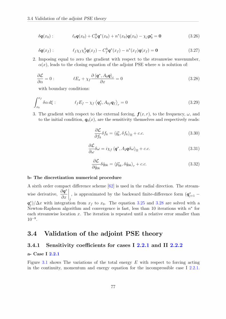
3.4 Validation of the adjoint PSE theory
δq(x0) : ℓ0q(x0) + Ch0 q
∗(x0) + n∗(x0)q(x0)− χfp∗
0 = 0 (3.26)
δq(xf ) : ℓfχfχhfq(xf )− Ch
f q∗(xf )− n∗(xf )q(xf ) = 0 (3.27)
2. Imposing equal to zero the gradient with respect to the streamwise wavenumber,α(x), leads to the closing equation of the adjoint PSE where n is solution of:
∂L
∂α= 0 : ℓEx + χf
∂ 〈q∗, A0q〉r∂x
= 0 (3.28)
with boundary conditions:
ˆ xf
x0
δα dξ : ℓfEf − χf
⟨
q∗
f , A0fqf
⟩
r= 0 (3.29)
3. The gradient with respect to the external forcing, f(x, r), to the frequency, ω, andto the initial condition, q0(x), are the sensitivity themselves and respectively reads:
∂L
∂fkδfk = 〈q∗k, δfk〉Ω + c.c. (3.30)
∂L
∂ωδω = iχf 〈q
∗, A2qδω〉Ω + c.c. (3.31)
∂L
∂q0kδq0k = 〈p∗0k, δq0k〉r + c.c. (3.32)
b- The discretization numerical procedure
A sixth order compact difference scheme [62] is used in the radial direction. The stream-
wise derivative,∂q∗
∂x
∣
∣
∣
∣
j
, is approximated by the backward finite-difference form (q∗
j+1 −
q∗
j )/∆x with integration from xf to x0. The equation 3.25 and 3.28 are solved with aNewton-Raphson algorithm and convergence is fast, less than 10 iterations with n∗ foreach streamwise location x. The iteration is repeated until a relative error smaller than10−8.
3.4 Validation of the adjoint PSE theory
3.4.1 Sensitivity coefficients for cases I 2.2.1 and II 2.2.2
a- Case I 2.2.1
Figure 3.1 shows The variations of the total energy E with respect to forcing actingin the continuity, momentum and energy equation for the incompressible case I 2.2.1.
77

Chapter 3 : Sensitivity analysis
The normalized sensitivity coefficients that the shape of the sensitivity functions and thelocation of their maximum are strongly related to the radial and the streamwise variationof the base flow. In particular the maximum of sensitivity is located along the border ofthe potential cone. In addition the sensitivity increases when the streamwise coordinatedecreases. That makes sense since it is natural to act as soon as possible on the noisegeneration mechanism if reduce noise emission is targeted. Another important point isthat sensitivity to axial momentum forcing is much higher than to radial momentumforcing.
rr
Sf1 Sf2
Sf4 Sf5
Figure 3.1: Sensitivity of the analytical incompressible jet. From the top to the bottomwe have respectively, the gradient of E with respect to the forcing acting in the continuity,r-momentum, x-momentum and energy equation at different fixed position in the stream-wise direction (x = 5.0, 2.5, 2.0, 1.5, 1.0)
78
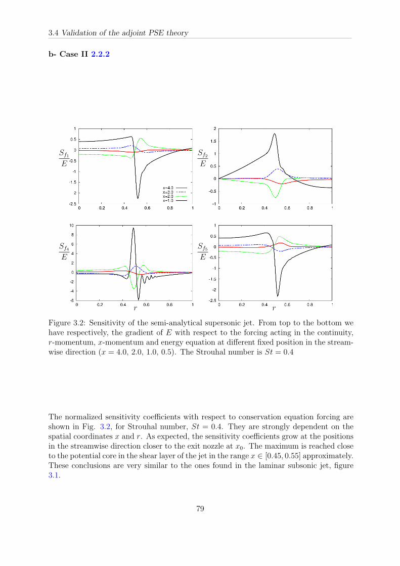
3.4 Validation of the adjoint PSE theory
b- Case II 2.2.2
rr
Sf1
E
Sf2
E
Sf4
E
Sf5
E
Figure 3.2: Sensitivity of the semi-analytical supersonic jet. From top to the bottom wehave respectively, the gradient of E with respect to the forcing acting in the continuity,r-momentum, x-momentum and energy equation at different fixed position in the stream-wise direction (x = 4.0, 2.0, 1.0, 0.5). The Strouhal number is St = 0.4
The normalized sensitivity coefficients with respect to conservation equation forcing areshown in Fig. 3.2, for Strouhal number, St = 0.4. They are strongly dependent on thespatial coordinates x and r. As expected, the sensitivity coefficients grow at the positionsin the streamwise direction closer to the exit nozzle at x0. The maximum is reached closeto the potential core in the shear layer of the jet in the range x ∈ [0.45, 0.55] approximately.These conclusions are very similar to the ones found in the laminar subsonic jet, figure3.1.
79
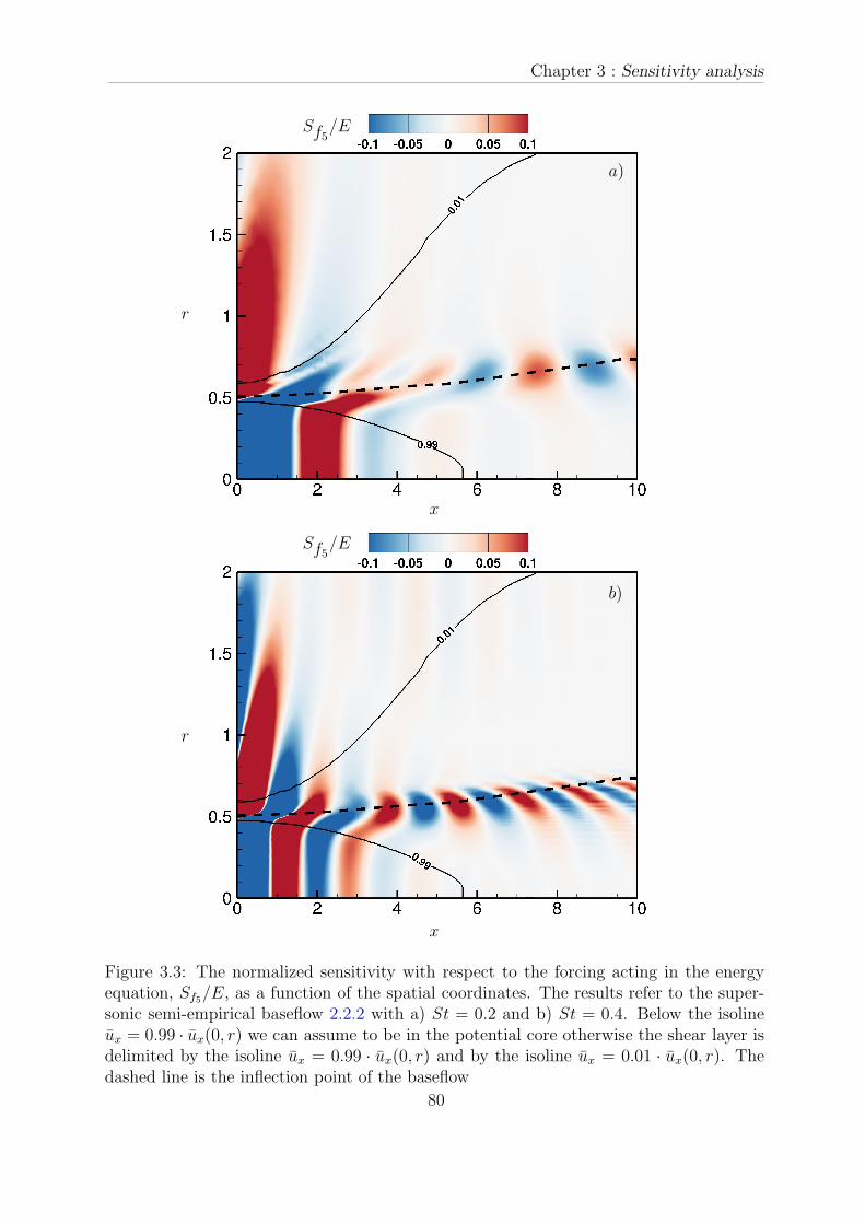
Chapter 3 : Sensitivity analysis
Sf5/E
Sf5/E
x
x
r
r
b)
a)
Figure 3.3: The normalized sensitivity with respect to the forcing acting in the energyequation, Sf5/E, as a function of the spatial coordinates. The results refer to the super-sonic semi-empirical baseflow 2.2.2 with a) St = 0.2 and b) St = 0.4. Below the isolineux = 0.99 · ux(0, r) we can assume to be in the potential core otherwise the shear layer isdelimited by the isoline ux = 0.99 · ux(0, r) and by the isoline ux = 0.01 · ux(0, r). Thedashed line is the inflection point of the baseflow
80
3.4 Validation of the adjoint PSE theory
In figure 3.3 can be observed the spatial distribution of the normalized sensitivity withrespect to forcing acting in the energy equation (for the other sensitivities conclusions arethe same). Two different Strouhal number are taking into account: a) St = 0.2 and b)
St = 0.4. The figure clearly shows the crucial role of the inflection point (∂2ux
∂r2=0) in
the evolution of the sensitivity. Moreover The maximum of the sensitivity max (|Sf/E|)is located along this line.
These results are well correlated with the location of the sound generation mechanismas seen in previous works [123, 64].
All these conclusions should be taken into account during the development of somenoise reduction strategies. However it is also important to observe that the maximumof sensitivity, for each fixed position in x, is located near to a region where sensitivity isalmost zero. Therefore the location of any control system must be very accurate to getsome good efficiency.
3.4.2 Validation procedure
The APSE computations have been validated for cases 2.2.1 and 2.2.2 by following thesteps outlined below:
• PSE code have been modified in order to solve:
χLPSEq = fk (3.33)
where fk is the vector with fk in the k-th components and zero otherwise.
• The variation of the quadratic function δE is computed as a difference betweenequation 3.33 and equation 2.26, after two PSE runs:
δE = E(δfk)− E(0) (3.34)
The small forcing δfk is chosen as:
δfk =ε
KF (x− x, r − r), with
F (x− x,r − r) = exp(−σx(x− x)2 − σr(r − r)2)(3.35)
where (x, r) is the central location of the forcing and K is a constant which nor-
malizes δfk such that
ˆ
Ω
δfkdΩ = ε. This Gaussian function, equation 3.35 is set
in the k-th line of the equation 2.26 and it acts in a restricted region of the domain(fig. 3.4). Several tests have been done and the range of the different coefficients todefine fk are given in Tab. 3.1.
• The variation of the quadratic function δE is computed following APSE theory:
δE =
ˆ
Ω
χ(xf )
χ(x)q∗k(x, r)δfk(x, r) dΩ + c.c. =
ˆ
Ω
q∗k(x, r)δfk(x, r) dΩ + c.c. (3.36)
81
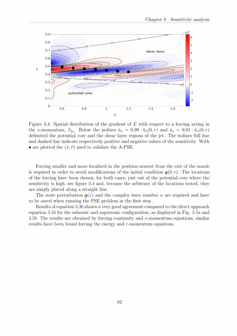
Chapter 3 : Sensitivity analysis
shear layer
potential cone
x
r
Figure 3.4: Spatial distribution of the gradient of E with respect to a forcing acting inthe x-momentum, Sf4 . Below the isolines ux = 0.99 · ux(0, r) and ux = 0.01 · ux(0, r)delimited the potential core and the shear layer regions of the jet. The isolines full lineand dashed line indicate respectively positive and negative values of the sensitivity. With• are plotted the (x, r) used to validate the A-PSE.
Forcing smaller and more localized in the position nearest from the exit of the nozzleis required in order to avoid modifications of the initial condition q(0, r). The locationsof the forcing have been chosen, for both cases, just out of the potential core where thesensitivity is high, see figure 3.4 and, because the arbitrary of the locations tested, theyare simply placed along a straight line.
The state perturbation q(x) and the complex wave number α are required and haveto be saved when running the PSE problem in the first step .
Results of equation 3.36 shown a very good agreement compared to the direct approachequation 3.34 for the subsonic and supersonic configuration, as displayed in Fig. 3.5a and3.5b. The results are obtained by forcing continuity and x-momentum equations, similarresults have been found forcing the energy and r-momentum equations.
82
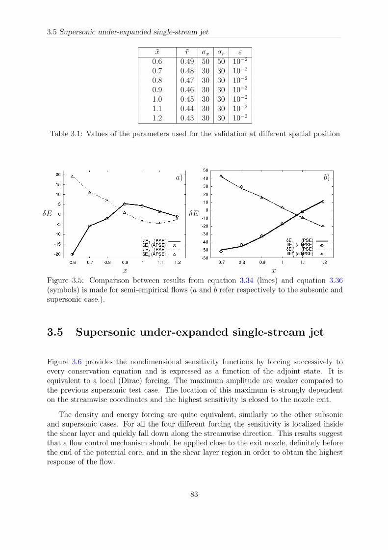
3.5 Supersonic under-expanded single-stream jet
x r σx σr ε0.60.70.80.91.01.11.2
0.49 50 50 10−2
0.48 30 30 10−2
0.47 30 30 10−2
0.46 30 30 10−2
0.45 30 30 10−2
0.44 30 30 10−2
0.43 30 30 10−2
Table 3.1: Values of the parameters used for the validation at different spatial position
xx
δEδE
a) b)
Figure 3.5: Comparison between results from equation 3.34 (lines) and equation 3.36(symbols) is made for semi-empirical flows (a and b refer respectively to the subsonic andsupersonic case.).
3.5 Supersonic under-expanded single-stream jet
Figure 3.6 provides the nondimensional sensitivity functions by forcing successively toevery conservation equation and is expressed as a function of the adjoint state. It isequivalent to a local (Dirac) forcing. The maximum amplitude are weaker compared tothe previous supersonic test case. The location of this maximum is strongly dependenton the streamwise coordinates and the highest sensitivity is closed to the nozzle exit.
The density and energy forcing are quite equivalent, similarly to the other subsonicand supersonic cases. For all the four different forcing the sensitivity is localized insidethe shear layer and quickly fall down along the streamwise direction. This results suggestthat a flow control mechanism should be applied close to the exit nozzle, definitely beforethe end of the potential core, and in the shear layer region in order to obtain the highestresponse of the flow.
83
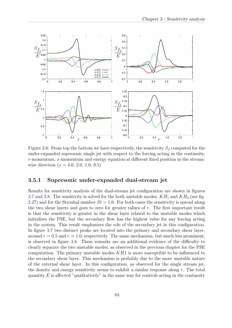
Chapter 3 : Sensitivity analysis
rr
Sf1E
Sf2E
Sf4E
Sf5E
Figure 3.6: From top the bottom we have respectively, the sensitivity Sf computed for theunder-expanded supersonic single jet with respect to the forcing acting in the continuity,r-momentum, x-momentum and energy equation at different fixed position in the stream-wise direction (x = 4.0, 2.0, 1.0, 0.5)
3.5.1 Supersonic under-expanded dual-stream jet
Results for sensitivity analysis of the dual-stream jet configuration are shown in figures3.7 and 3.8. The sensitivity is solved for the both unstable modes, KH1 and KH2 (see fig.2.27) and for the Strouhal number St = 1.0. For both cases the sensitivity is spread alongthe two shear layers and goes to zero for greater values of r. The first important resultis that the sensitivity is greater in the shear layer related to the unstable modes whichinitializes the PSE, but the secondary flow has the highest value for any forcing actingin the system. This result emphasizes the role of the secondary jet in this configuration.In figure 3.7 two distinct peaks are located into the primary and secondary shear layer,around r = 0.5 and r ≃ 1.0, respectively. The same mechanism, but much less prominent,is observed in figure 3.8. These remarks are an additional evidence of the difficulty toclearly separate the two unstable modes, as observed in the previous chapter for the PSEcomputation. The primary unstable modes KH1 is more susceptible to be influenced tothe secondary shear layer. This mechanism is probably due to the more unstable natureof the external shear layer. In this configuration, as observed for the single stream jet,the density and energy sensitivity seems to exhibit a similar response along r. The totalquantity E is affected ”qualitatively” in the same way for controls acting in the continuity
84
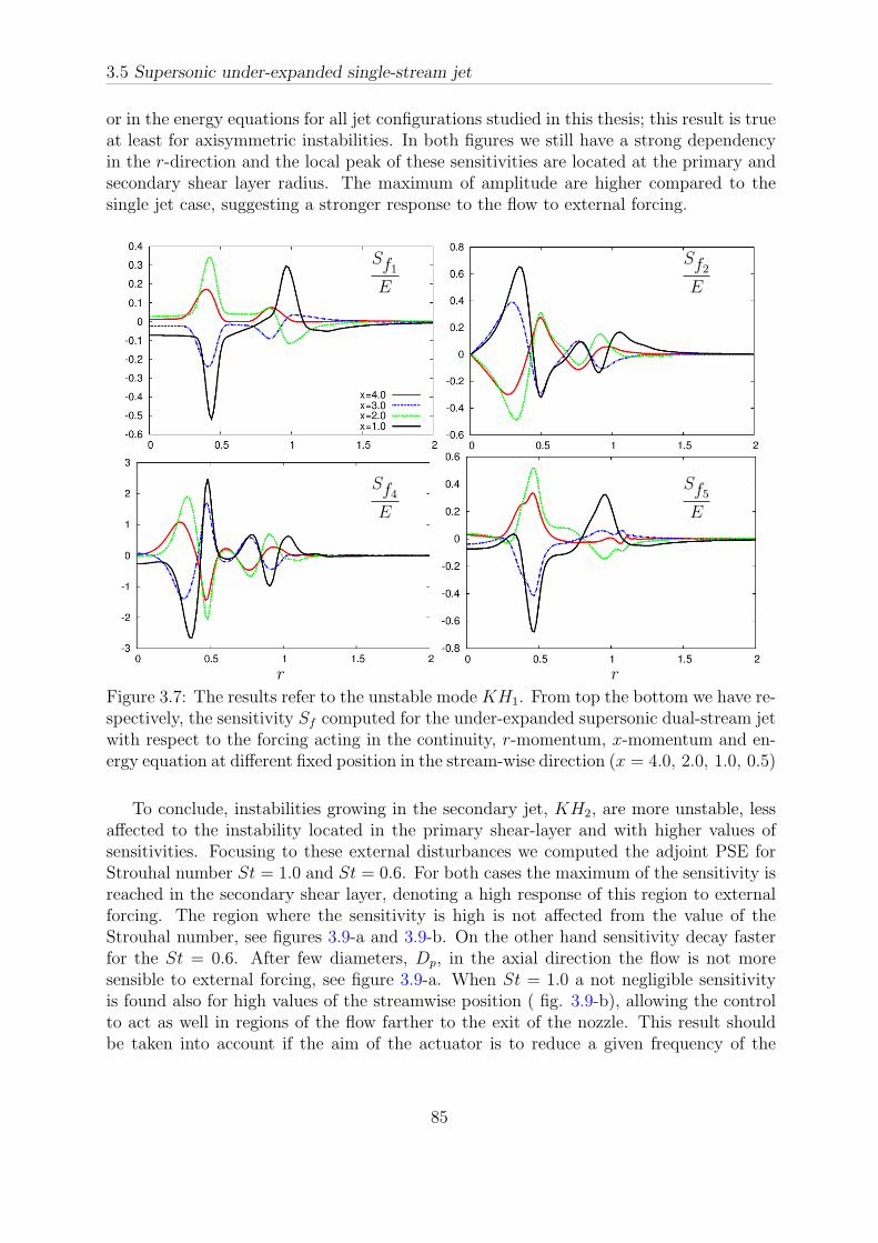
3.5 Supersonic under-expanded single-stream jet
or in the energy equations for all jet configurations studied in this thesis; this result is trueat least for axisymmetric instabilities. In both figures we still have a strong dependencyin the r-direction and the local peak of these sensitivities are located at the primary andsecondary shear layer radius. The maximum of amplitude are higher compared to thesingle jet case, suggesting a stronger response to the flow to external forcing.
rr
Sf1E
Sf2E
Sf4E
Sf5E
Figure 3.7: The results refer to the unstable mode KH1. From top the bottom we have re-spectively, the sensitivity Sf computed for the under-expanded supersonic dual-stream jetwith respect to the forcing acting in the continuity, r-momentum, x-momentum and en-ergy equation at different fixed position in the stream-wise direction (x = 4.0, 2.0, 1.0, 0.5)
To conclude, instabilities growing in the secondary jet, KH2, are more unstable, lessaffected to the instability located in the primary shear-layer and with higher values ofsensitivities. Focusing to these external disturbances we computed the adjoint PSE forStrouhal number St = 1.0 and St = 0.6. For both cases the maximum of the sensitivity isreached in the secondary shear layer, denoting a high response of this region to externalforcing. The region where the sensitivity is high is not affected from the value of theStrouhal number, see figures 3.9-a and 3.9-b. On the other hand sensitivity decay fasterfor the St = 0.6. After few diameters, Dp, in the axial direction the flow is not moresensible to external forcing, see figure 3.9-a. When St = 1.0 a not negligible sensitivityis found also for high values of the streamwise position ( fig. 3.9-b), allowing the controlto act as well in regions of the flow farther to the exit of the nozzle. This result shouldbe taken into account if the aim of the actuator is to reduce a given frequency of the
85
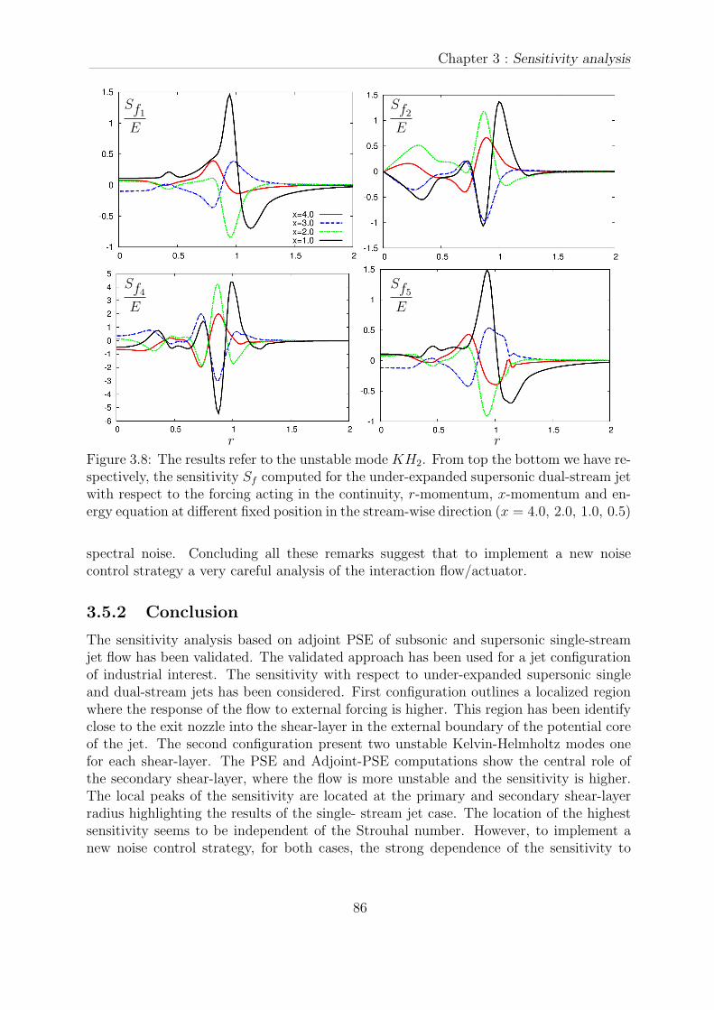
Chapter 3 : Sensitivity analysis
rr
Sf1E
Sf2E
Sf4E
Sf5E
Figure 3.8: The results refer to the unstable mode KH2. From top the bottom we have re-spectively, the sensitivity Sf computed for the under-expanded supersonic dual-stream jetwith respect to the forcing acting in the continuity, r-momentum, x-momentum and en-ergy equation at different fixed position in the stream-wise direction (x = 4.0, 2.0, 1.0, 0.5)
spectral noise. Concluding all these remarks suggest that to implement a new noisecontrol strategy a very careful analysis of the interaction flow/actuator.
3.5.2 Conclusion
The sensitivity analysis based on adjoint PSE of subsonic and supersonic single-streamjet flow has been validated. The validated approach has been used for a jet configurationof industrial interest. The sensitivity with respect to under-expanded supersonic singleand dual-stream jets has been considered. First configuration outlines a localized regionwhere the response of the flow to external forcing is higher. This region has been identifyclose to the exit nozzle into the shear-layer in the external boundary of the potential coreof the jet. The second configuration present two unstable Kelvin-Helmholtz modes onefor each shear-layer. The PSE and Adjoint-PSE computations show the central role ofthe secondary shear-layer, where the flow is more unstable and the sensitivity is higher.The local peaks of the sensitivity are located at the primary and secondary shear-layerradius highlighting the results of the single- stream jet case. The location of the highestsensitivity seems to be independent of the Strouhal number. However, to implement anew noise control strategy, for both cases, the strong dependence of the sensitivity to
86

3.5 Supersonic under-expanded single-stream jet
the spatial coordinates of the system suggest a very careful analysis of the interactionflow/actuator. This results have been obtained for both stability and sensitivity analysis,thanks to accurate LES computations from CERFACS. Focus our attention on the physicalexplanation of the highest sensitivity location we found that the inflection point and theshock-cell positions are crucial in the determination of such a zone.
87
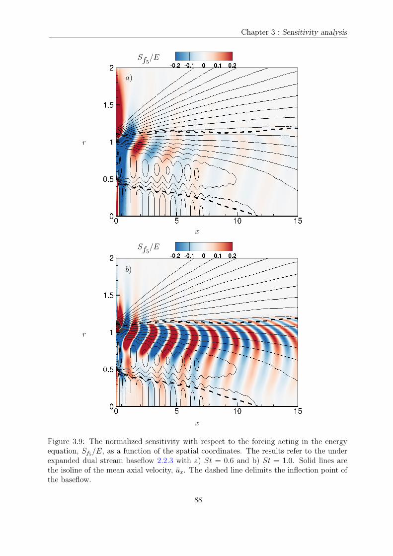
Chapter 3 : Sensitivity analysis
Sf5/E
Sf5/E
x
x
r
r
b)
a)
Figure 3.9: The normalized sensitivity with respect to the forcing acting in the energyequation, Sf5/E, as a function of the spatial coordinates. The results refer to the underexpanded dual stream baseflow 2.2.3 with a) St = 0.6 and b) St = 1.0. Solid lines arethe isoline of the mean axial velocity, ux. The dashed line delimits the inflection point ofthe baseflow.
88
Chapter 4
Uncertainty Quantifications andadjoint PSE
The first objective of this chapter is to validate and compare adjoint-based sensitivityand other sensitivity methods and their possible relation to Uncertainty Quantification(UQ) analysis. Inspired by a simple toy models we have shown how can be a lower costtool for mathematical analysis of complex problems of industrial interests. The secondobjective is to propose an Uncertainty Quantification of the incompressible single streamjet stability subjected to frequency variation. The governing equations are the low costPSE model. This objective is strongly related to the noise sensitivity and control studiessince it has been demonstrated that noise is originated from K-H instability in such aflow. Later, the adjoint PSE approach will be used, to make the link between sensitivityand UQ analysis as this quantification for Large Eddy Simulations or Reynolds AverageNavier-Stokes simulations can be considerably expensive. Envelope curves of the standarddeviation are determined and compared with good agreement for small variations of theinput parameters in the first toy model. For the jet stability, it has been found that thegrowth rate is almost insensitive to small frequency variations and, on the other hand, thephases of the amplitude functions of the disturbance are extremely sensitive to frequency.
This work have been done in collaboration with the University of Greenwich.
4.1 Introduction
The generation of noise has been demonstrated to originate from Kelvin-Helmholtz insta-bilities amplifying in the jet stream. Some noise reduction can not be achieved before adeep analysis of the sensitivity of this instability to any flow perturbations or variations.This work is based on the Linearized Parabolized Stability Equations (LPSE) and theiradjoint. Results are linked to uncertainty analysis. The base flow under consideration isthe incompressible semi-empirical single jet 2.2.1. An Uncertainty Quantification of thejet flow stability subjected to frequency variation is proposed since noise emission are re-lated to frequency. The remaining question is how sensitivity studies can be related to anUncertainty Quantification? To answer we first propose a toy model on which both sensi-tivity and UQ analysis are carried out. UQ analysis is about determining the ”reliability”
89
Chapter 4 : Uncertainty Quantifications and adjoint PSE
of the outputs of a problem under investigation when the inputs are not precise (inputcan varying or are uncertain). Such output uncertainties are represented by the standarddeviation. For cases where the determination of uncertainties is of a high interest it is rec-ommended to also look into the probabilistic or cumulate distribution functions. On theother hand, sensitivity analysis is about apportioning the uncertainty in the output withthe different input uncertainties (gradients). In the following the gradients are calculatedby four ways:
1. exactly calculating the sensitivity coefficients of the governing equations with theadjoint based approach
2. by integrating the standard deviation ratio from many direct computation
3. by a sensitivity indices
4. by a variance based sensitivity analysis.
The approach ii) and iii) can be qualified as One-factor-At-a-Time (OAT), just on com-ponent of the parameter vector is modified when the others are kept constant. In additionwe present a way to perform local sensitivity using gradient of the direct equations.
A toy model is proposed as a test where the input uncertainties are set arbitrarily.This simple example wants to manifest the relation between adjoint-based sensitivity andother sensitivity methods that can also include an uncertainty analysis. The next sectionis an application on the stability of compressible single jet flow.
4.2 A model toy problem
4.2.1 ODE direct equations
The toy model is a set of two coupled ODE formulated as a classical optimization problem.Given the state vector y = [y1, y2]
t ∈ C2 and the control or design parameter λ =
[λ1, λ2]t ∈ C
2 , where the exponent t always stands for transpose. The goal is to get,quantitatively or qualitatively, the variation of the cost function E(y, λ) with respect tothe variation of the control parameter λ. Moreover the state vector y and the controlparameter λ are directly related by the constrained state equation F (y, λ) = 0. The stateequation of the toy model, 4.1, includes its initial condition and is given by:
F (y, λ) = y(t, λ)− A(λ)y(t, λ)− b(λ)u(t) = 0, y(0) = y0 =
[
01
]
(4.1)
with
A =
[
−2i λ1
λ2λ21 −5
]
, b =
[
1 + λ2
λ1λ22
]
where i stands for the square root of −1 and u(t) can be any forcing or control fixedin this simple model as a cosine function, u(t) = cos(3t).
90
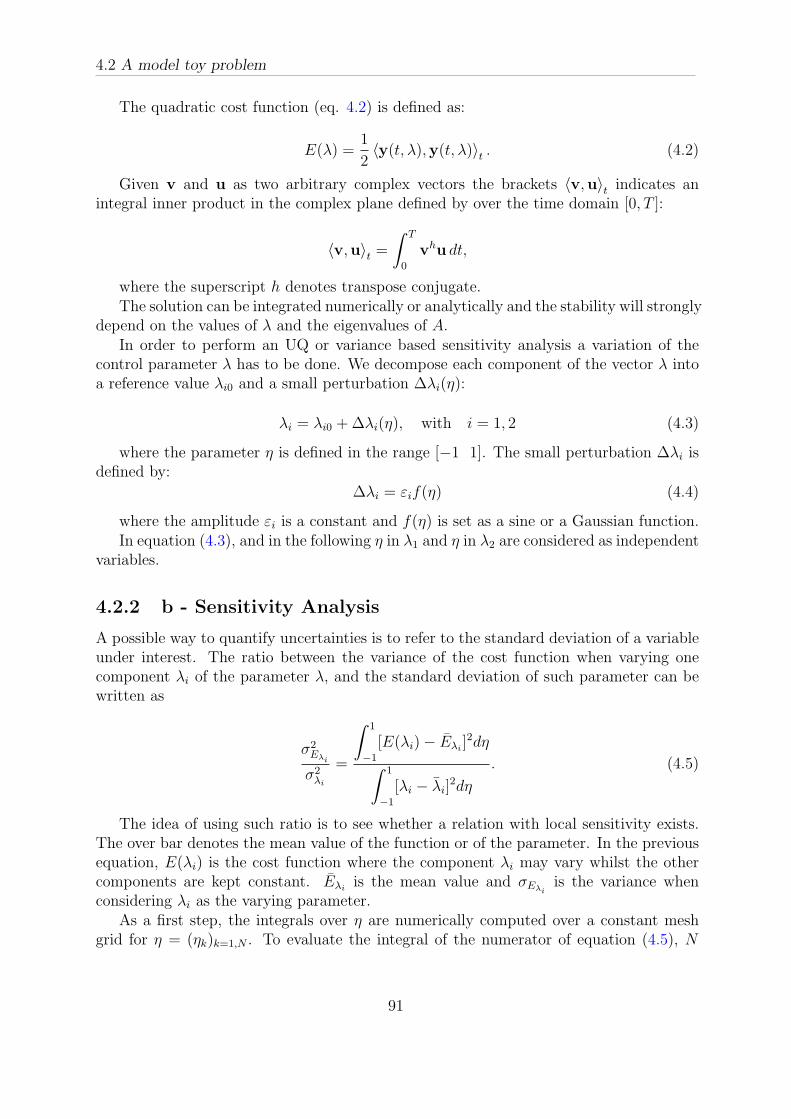
4.2 A model toy problem
The quadratic cost function (eq. 4.2) is defined as:
E(λ) =1
2〈y(t, λ),y(t, λ)〉t . (4.2)
Given v and u as two arbitrary complex vectors the brackets 〈v,u〉t indicates anintegral inner product in the complex plane defined by over the time domain [0, T ]:
〈v,u〉t =
ˆ T
0
vhu dt,
where the superscript h denotes transpose conjugate.The solution can be integrated numerically or analytically and the stability will strongly
depend on the values of λ and the eigenvalues of A.In order to perform an UQ or variance based sensitivity analysis a variation of the
control parameter λ has to be done. We decompose each component of the vector λ intoa reference value λi0 and a small perturbation ∆λi(η):
λi = λi0 +∆λi(η), with i = 1, 2 (4.3)
where the parameter η is defined in the range [−1 1]. The small perturbation ∆λi isdefined by:
∆λi = εif(η) (4.4)
where the amplitude εi is a constant and f(η) is set as a sine or a Gaussian function.In equation (4.3), and in the following η in λ1 and η in λ2 are considered as independent
variables.
4.2.2 b - Sensitivity Analysis
A possible way to quantify uncertainties is to refer to the standard deviation of a variableunder interest. The ratio between the variance of the cost function when varying onecomponent λi of the parameter λ, and the standard deviation of such parameter can bewritten as
σ2Eλi
σ2λi
=
ˆ 1
−1
[E(λi)− Eλi]2dη
ˆ 1
−1
[λi − λi]2dη
. (4.5)
The idea of using such ratio is to see whether a relation with local sensitivity exists.The over bar denotes the mean value of the function or of the parameter. In the previousequation, E(λi) is the cost function where the component λi may vary whilst the othercomponents are kept constant. Eλi
is the mean value and σEλiis the variance when
considering λi as the varying parameter.As a first step, the integrals over η are numerically computed over a constant mesh
grid for η = (ηk)k=1,N . To evaluate the integral of the numerator of equation (4.5), N
91
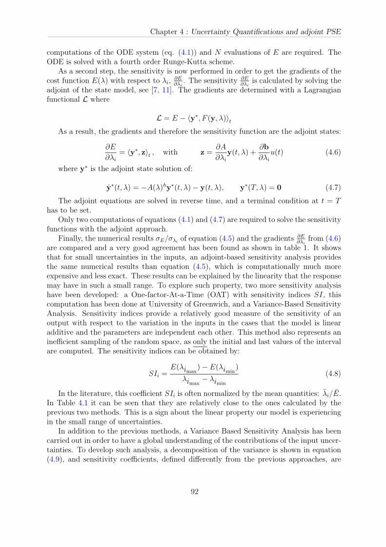
Chapter 4 : Uncertainty Quantifications and adjoint PSE
computations of the ODE system (eq. (4.1)) and N evaluations of E are required. TheODE is solved with a fourth order Runge-Kutta scheme.
As a second step, the sensitivity is now performed in order to get the gradients of thecost function E(λ) with respect to λi,
∂E∂λi
. The sensitivity ∂E∂λi
is calculated by solving theadjoint of the state model, see [7, 11]. The gradients are determined with a Lagrangianfunctional L where
L = E − 〈y∗, F (y, λ)〉t
As a result, the gradients and therefore the sensitivity function are the adjoint states:
∂E
∂λi
= 〈y∗, z〉t , with z =∂A
∂λi
y(t, λ) +∂b
∂λi
u(t) (4.6)
where y∗ is the adjoint state solution of:
y∗(t, λ) = −A(λ)hy∗(t, λ)− y(t, λ), y∗(T, λ) = 0 (4.7)
The adjoint equations are solved in reverse time, and a terminal condition at t = Thas to be set.
Only two computations of equations (4.1) and (4.7) are required to solve the sensitivityfunctions with the adjoint approach.
Finally, the numerical results σE/σλiof equation (4.5) and the gradients ∂E
∂λifrom (4.6)
are compared and a very good agreement has been found as shown in table 1. It showsthat for small uncertainties in the inputs, an adjoint-based sensitivity analysis providesthe same numerical results than equation (4.5), which is computationally much moreexpensive and less exact. These results can be explained by the linearity that the responsemay have in such a small range. To explore such property, two more sensitivity analysishave been developed: a One-factor-At-a-Time (OAT) with sensitivity indices SI, thiscomputation has been done at University of Greenwich, and a Variance-Based SensitivityAnalysis. Sensitivity indices provide a relatively good measure of the sensitivity of anoutput with respect to the variation in the inputs in the cases that the model is linearadditive and the parameters are independent each other. This method also represents aninefficient sampling of the random space, as only the initial and last values of the intervalare computed. The sensitivity indices can be obtained by:
SIi =E(λimax
)− E(λimin)
λimax− λimin
(4.8)
In the literature, this coefficient SIi is often normalized by the mean quantities: λi/E.In Table 4.1 it can be seen that they are relatively close to the ones calculated by theprevious two methods. This is a sign about the linear property our model is experiencingin the small range of uncertainties.
In addition to the previous methods, a Variance Based Sensitivity Analysis has beencarried out in order to have a global understanding of the contributions of the input uncer-tainties. To develop such analysis, a decomposition of the variance is shown in equation(4.9), and sensitivity coefficients, defined differently from the previous approaches, are
92

4.2 A model toy problem
Method∂E
∂λ1
∂E
∂λ2
Adjoint approach 0.27262 1.7992OAT σ-ratio 0.27084 1.8006
OAT SI 0.20670 1.3772
Table 4.1: Comparison among sensitivity methods.
λ1 λ2
√
S2/S1
S1 = 0.0224 S2 = 0.9776 6.606ST1 = 0.0228 ST2 = 0.9772 6.547
Table 4.2: Results from Variance Based Sensitivity Analysis.
computed in equation (4.10) from its proportion with respect to the total variance. Si
and STi, in equation (4.11), are the first order and total sensitivities index respectively.
In the following equations the multiple subscripts refer to second, third or higher orderinteractions, depending on the number of subscripts, see Saltelli et al. (2010)[109].
The results of such analysis are shown in table 2. Note thatm represents the dimensionof the stochastic space.
σ2E =
m∑
i=1
σ2Eλi
+m∑
i=1,j>i
σ2Eλij
+m∑
i=1,k>j>i
σ2Eλijk
+ ... (4.9)
1 =m∑
i=1
Si +m∑
i=1,j>i
Sij +m∑
i=1,k>j>i
Sijk + ...+ Sijk,...,m (4.10)
STi= Si + Sij + Sijk + ...+ Sijk,...,m (4.11)
The value of σ2E has been calculated by Latin Hypercube Sampling with a total of
5000 samples, as shown in Fig. 4.1, and it has been found that, by comparing with thedata from equation (4.5) and with the third columns of table 1 and 2, we get
σ2E ≈
2∑
i=1
σ2Eλi
or
√
S2
S1
≈∂E
∂λ2
/∂E
∂λ1
This is reflects the weak interaction of the higher order sensitivities, again due to thelinearised behaviour of the model.
93
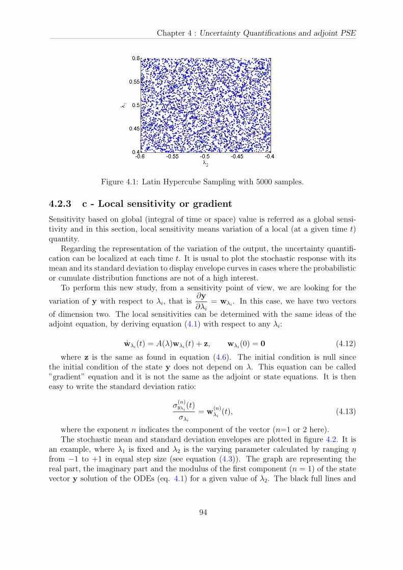
Chapter 4 : Uncertainty Quantifications and adjoint PSE
Figure 4.1: Latin Hypercube Sampling with 5000 samples.
4.2.3 c - Local sensitivity or gradient
Sensitivity based on global (integral of time or space) value is referred as a global sensi-tivity and in this section, local sensitivity means variation of a local (at a given time t)quantity.
Regarding the representation of the variation of the output, the uncertainty quantifi-cation can be localized at each time t. It is usual to plot the stochastic response with itsmean and its standard deviation to display envelope curves in cases where the probabilisticor cumulate distribution functions are not of a high interest.
To perform this new study, from a sensitivity point of view, we are looking for the
variation of y with respect to λi, that is∂y
∂λi
= wλi. In this case, we have two vectors
of dimension two. The local sensitivities can be determined with the same ideas of theadjoint equation, by deriving equation (4.1) with respect to any λi:
wλi(t) = A(λ)wλi
(t) + z, wλi(0) = 0 (4.12)
where z is the same as found in equation (4.6). The initial condition is null sincethe initial condition of the state y does not depend on λ. This equation can be called”gradient” equation and it is not the same as the adjoint or state equations. It is theneasy to write the standard deviation ratio:
σ(n)yλi
(t)
σλi
= w(n)λi
(t), (4.13)
where the exponent n indicates the component of the vector (n=1 or 2 here).The stochastic mean and standard deviation envelopes are plotted in figure 4.2. It is
an example, where λ1 is fixed and λ2 is the varying parameter calculated by ranging ηfrom −1 to +1 in equal step size (see equation (4.3)). The graph are representing thereal part, the imaginary part and the modulus of the first component (n = 1) of the statevector y solution of the ODEs (eq. 4.1) for a given value of λ2. The black full lines and
94
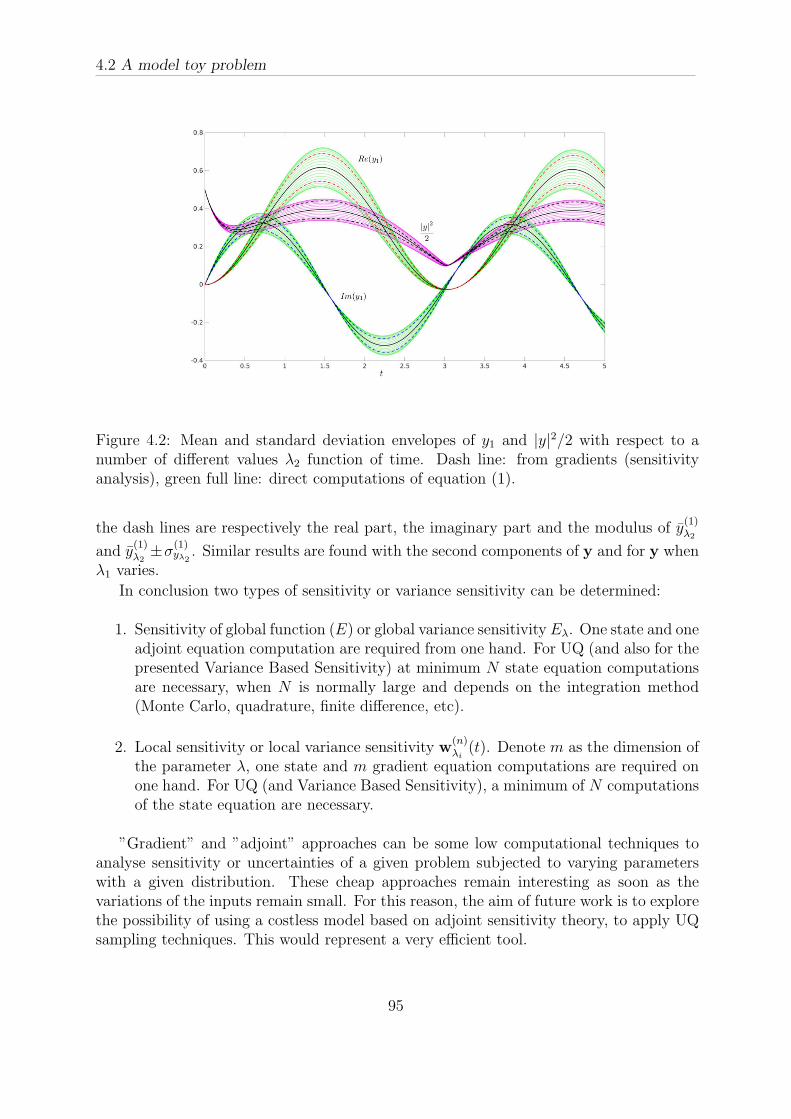
4.2 A model toy problem
Figure 4.2: Mean and standard deviation envelopes of y1 and |y|2/2 with respect to anumber of different values λ2 function of time. Dash line: from gradients (sensitivityanalysis), green full line: direct computations of equation (1).
the dash lines are respectively the real part, the imaginary part and the modulus of y(1)λ2
and y(1)λ2
±σ(1)yλ2
. Similar results are found with the second components of y and for y whenλ1 varies.
In conclusion two types of sensitivity or variance sensitivity can be determined:
1. Sensitivity of global function (E) or global variance sensitivity Eλ. One state and oneadjoint equation computation are required from one hand. For UQ (and also for thepresented Variance Based Sensitivity) at minimum N state equation computationsare necessary, when N is normally large and depends on the integration method(Monte Carlo, quadrature, finite difference, etc).
2. Local sensitivity or local variance sensitivity w(n)λi
(t). Denote m as the dimension ofthe parameter λ, one state and m gradient equation computations are required onone hand. For UQ (and Variance Based Sensitivity), a minimum of N computationsof the state equation are necessary.
”Gradient” and ”adjoint” approaches can be some low computational techniques toanalyse sensitivity or uncertainties of a given problem subjected to varying parameterswith a given distribution. These cheap approaches remain interesting as soon as thevariations of the inputs remain small. For this reason, the aim of future work is to explorethe possibility of using a costless model based on adjoint sensitivity theory, to apply UQsampling techniques. This would represent a very efficient tool.
95
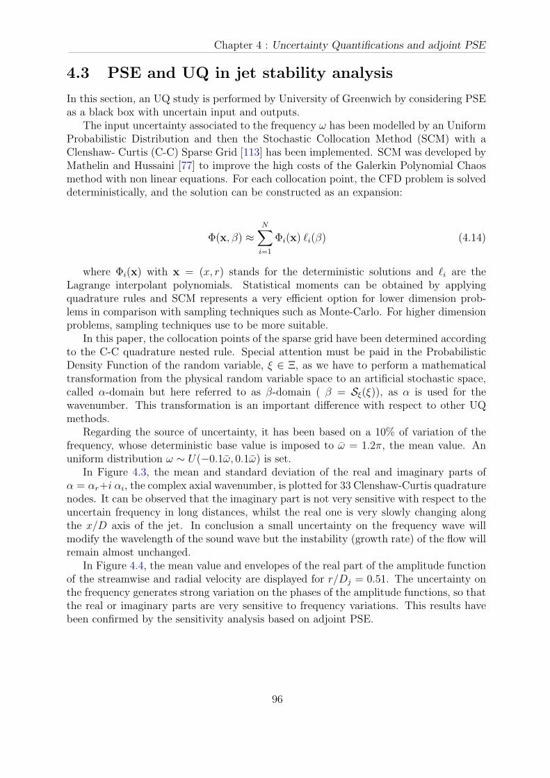
Chapter 4 : Uncertainty Quantifications and adjoint PSE
4.3 PSE and UQ in jet stability analysis
In this section, an UQ study is performed by University of Greenwich by considering PSEas a black box with uncertain input and outputs.
The input uncertainty associated to the frequency ω has been modelled by an UniformProbabilistic Distribution and then the Stochastic Collocation Method (SCM) with aClenshaw- Curtis (C-C) Sparse Grid [113] has been implemented. SCM was developed byMathelin and Hussaini [77] to improve the high costs of the Galerkin Polynomial Chaosmethod with non linear equations. For each collocation point, the CFD problem is solveddeterministically, and the solution can be constructed as an expansion:
Φ(x, β) ≈N∑
i=1
Φi(x) ℓi(β) (4.14)
where Φi(x) with x = (x, r) stands for the deterministic solutions and ℓi are theLagrange interpolant polynomials. Statistical moments can be obtained by applyingquadrature rules and SCM represents a very efficient option for lower dimension prob-lems in comparison with sampling techniques such as Monte-Carlo. For higher dimensionproblems, sampling techniques use to be more suitable.
In this paper, the collocation points of the sparse grid have been determined accordingto the C-C quadrature nested rule. Special attention must be paid in the ProbabilisticDensity Function of the random variable, ξ ∈ Ξ, as we have to perform a mathematicaltransformation from the physical random variable space to an artificial stochastic space,called α-domain but here referred to as β-domain ( β = Sξ(ξ)), as α is used for thewavenumber. This transformation is an important difference with respect to other UQmethods.
Regarding the source of uncertainty, it has been based on a 10% of variation of thefrequency, whose deterministic base value is imposed to ω = 1.2π, the mean value. Anuniform distribution ω ∼ U(−0.1ω, 0.1ω) is set.
In Figure 4.3, the mean and standard deviation of the real and imaginary parts ofα = αr+i αi, the complex axial wavenumber, is plotted for 33 Clenshaw-Curtis quadraturenodes. It can be observed that the imaginary part is not very sensitive with respect to theuncertain frequency in long distances, whilst the real one is very slowly changing alongthe x/D axis of the jet. In conclusion a small uncertainty on the frequency wave willmodify the wavelength of the sound wave but the instability (growth rate) of the flow willremain almost unchanged.
In Figure 4.4, the mean value and envelopes of the real part of the amplitude functionof the streamwise and radial velocity are displayed for r/Dj = 0.51. The uncertainty onthe frequency generates strong variation on the phases of the amplitude functions, so thatthe real or imaginary parts are very sensitive to frequency variations. This results havebeen confirmed by the sensitivity analysis based on adjoint PSE.
96
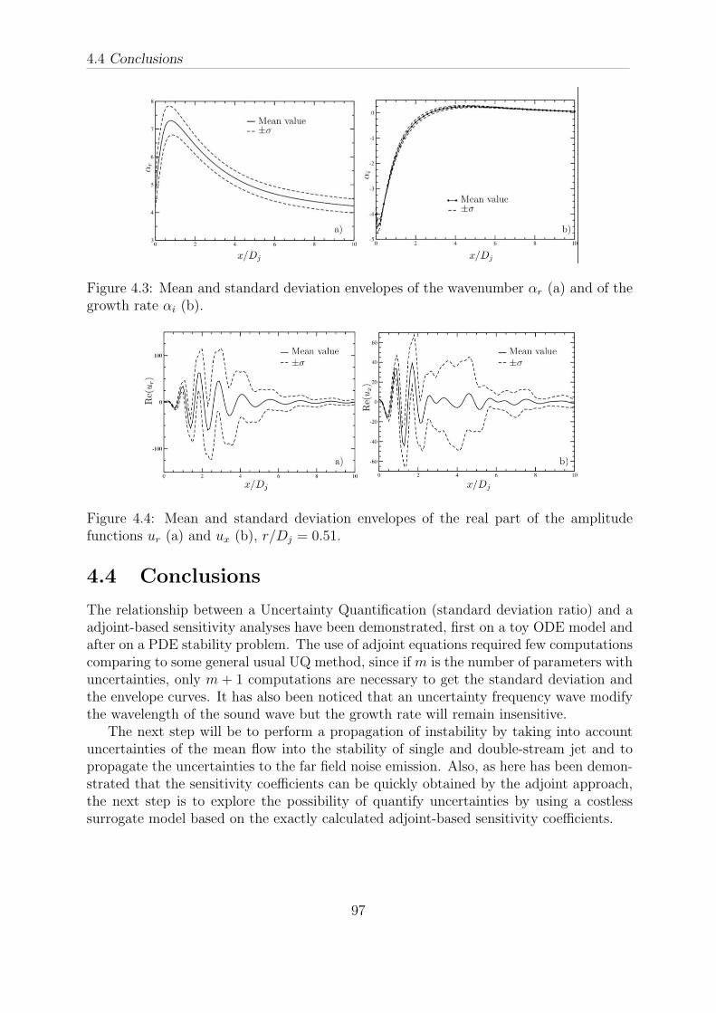
4.4 Conclusions
Figure 4.3: Mean and standard deviation envelopes of the wavenumber αr (a) and of thegrowth rate αi (b).
Figure 4.4: Mean and standard deviation envelopes of the real part of the amplitudefunctions ur (a) and ux (b), r/Dj = 0.51.
4.4 Conclusions
The relationship between a Uncertainty Quantification (standard deviation ratio) and aadjoint-based sensitivity analyses have been demonstrated, first on a toy ODE model andafter on a PDE stability problem. The use of adjoint equations required few computationscomparing to some general usual UQ method, since if m is the number of parameters withuncertainties, only m + 1 computations are necessary to get the standard deviation andthe envelope curves. It has also been noticed that an uncertainty frequency wave modifythe wavelength of the sound wave but the growth rate will remain insensitive.
The next step will be to perform a propagation of instability by taking into accountuncertainties of the mean flow into the stability of single and double-stream jet and topropagate the uncertainties to the far field noise emission. Also, as here has been demon-strated that the sensitivity coefficients can be quickly obtained by the adjoint approach,the next step is to explore the possibility of quantify uncertainties by using a costlesssurrogate model based on the exactly calculated adjoint-based sensitivity coefficients.
97

Chapter 4 : Uncertainty Quantifications and adjoint PSE
98

Chapter 5
Acoustic field analysis
5.1 Introduction
As explained in Section I, the acoustic analogy can be considered as a hybrid approach(Casalino (2003)[19]). In the current section the FW-H equation and integral solutionare reported (see appendix for details). The FW-H acoustic analogy represents a gener-alization of Lighthill’s acoustic analogy for flows including bodies in arbitrary motion. Inthis generalization the fluid is unbounded but partitioned into regions by an integrationsurface, as schematically shown in fig 5.1 . This surface does not need to coincide with aphysical body and can be permeable [16, 32]. The surface requirements are discussed indetails by Brentner and Farassat (1998)[16].
Figure 5.1: Radiation in an unbounded flow.
99

Chapter 5 : Acoustic field analysis
Let g(x, t) = 0 be the equation describing the moving control surface, whose pointsmove at velocity v(x, t)[19]. g is defined to satisfy the property ∇g = n on the surface,where n is the outward pointing unit normal vector. Following this procedure, the flowis partitioned into three regions according to the value of g. A point enclosed by theintegration surface satisfies g < 0 and this flow field portion can be replaced by a quiescentfluid. Mass and momentum sources are then distributed on the surface g(x, t) = 0,which allows the conservation laws across g(x, t) = 0 to be satisfied. This process iscarried out from the time-resolved estimates of pressure, density and velocity on theFW-H integration surface, obtained independently by CFD. The mass and momentumconservation equations are recast to obtain the FW-H equation. A more compact form ofthis equation is given by Casalino (2003)[19] and reported here:
(ρ− ρ0)c20H(g)
=∂2 TijH(g)
∂xi∂xj
−∂ Liδ(g)
∂xi
+∂ Qiδ(g)
∂t, (5.1)
where H(g) is the Heaviside function and in the first source term on the right hand sideTij is the Lighthill stress tensor [66]. The second and third contributions are, respectively,the surface source distributions of momentum (dipole) and mass (monopole). Expressionsfor these source terms are reported here:
Tij = ρuiuj + (p′ − c20ρ′)δij − τij, (5.2)
Li = Pijnj + ρui(un − vn), Pij = (p− p0)δij − τij, (5.3)
Q = ρ0Uini, (5.4)
with
Ui =
(
1−ρ
ρ0
)
vi +ρui
ρ0, (5.5)
where un and vn are the flow and surface velocity in the outward normal direction n.The three source terms in equation 5.1 are referred to respectively as quadrupole, dipoleand monopole sources. The monopole and dipole contributions are often referred to asrespectively thickness and loading noise for analogy with helicopter rotor applications.While the quadrupole term represents a volume distribution and is computationally themost expensive to estimate, the loading and thickness noise are surface distributions asindicated by the presence of the Dirac delta function multiplying these contributions,which shifts the value of the variables on the FW-H integration surface. The volumesource distribution accounts for all the non-linearities in the flow. The effects of convectionwith variable speed, non linear wave propagation and steepening, variable speed of sound,generation of noise by shocks, vorticity and turbulence in the flow field are all included inthis source term[16]. When the integration surface is taken coincident with a solid body, aphysical interpretation of loading and thickness noise is available. The loading noise takesinto account the effect of the interaction of the flow with vibrating surfaces, reproducing
100
5.1 Introduction
the net unsteady forcing acting on the fluid as a result of the presence of the body. Thethickness noise is originated by the motion of the surface in the normal direction[31] andit represents a displacement effect [35]. It is determined completely by the geometry andkinematics of the body[16]. The FW-H integral solution [35] is given by the followingintegral:
4πc20(ρ(x, t)− ρ0) =
ˆ
V
∇x · ∇x ·
[
TJ
r|1−Mr|
]
ret
dη−
ˆ
g=0
∇x ·
[
P · nA
r|1−Mr|
]
ret
dS(η)+
ˆ
g=0
∂
∂t
[
ρu · n
r|1−Mr|
]
ret
dS(η).
(5.6)
Expressions for the terms in equation 5.6 are given in equations 5.7-5.10.
y = η +
ˆ τe
∞
c0M (η, τ ′)dτ ′, n =∇xf
|∇xf |, (5.7)
J = exp
(ˆ τe
∞
∇ · c0M (η, τ ′)dτ ′)
, A =∇yf
|∇ηf |, (5.8)
P = pI − τ, Mr = M · r (5.9)
τe = t−r
c0(5.10)
WhereM is a vector with components the mach number in the three spatial directions.
5.1.1 Advanced time formulation AFW-H
Casalino [19] reports the integral solution of the FW-H equation in the advanced timeformulation, which is here referred to as AFW-H. In this solution, the acoustic pressurefluctuation p′ = p− p0 perceived by an observer located at the vector position x at timet is given by:
p′(x, t) = p′Q(x, t) + p′L(x, t) + p′T (x, t), (5.11)
where subscripts Q, L, and T are, respectively, the quadrupole, loading, and thicknessnoise contributions to p′ from the source field located at y generated at retarded timeτret = t − c−1
0 |x − y(τret)|. τret accounts for the time of flight of the noise propagatingfrom y to x at the constant speed of sound c0. Expressions for these contributions aregiven in Casalino[19] and are reported in the appendix.
101
Chapter 5 : Acoustic field analysis
5.1.2 Implementation of AFW-H analogy
A discretized form of equation 5.11 is implemented in a code developed at the University ofLeicester. The quadrupole source term is neglected. It is often possible in CAA to neglectthe volume source distribution of Tij, primarily due to the quadrupole term representingthe smallest contribution to noise radiation at low Mach numbers. One further advantageof this approach is the considerable decrease in the computational cost of the simulation,by reducing a three dimensional numerical integration to a two dimensional one. The FW-H algorithm is structured in the following way: at each discrete acoustic time τn, a loopover the observer positions xi is performed; for each xi, the contribution from the FW-Hsurface is estimated, by looping over the Sjs; finally, for each Sj, a loop is performed overthe surface elements dSk of Sj , on which the discretized form of the L and T terms isevaluated. The advanced time relative to the dSks is also estimated from the retardedtime equation [19] in order to save the p′ contribution at the correct observer time. Thisprocess is then repeated at different discrete acoustic times τn. Advancing in time, apressure fluctuation history is reconstructed and the final output of the tool is a matrixstoring, for each observer position, the pressure fluctuation p′(xi, t) as a discretised timearray. For each discrete acoustic time τn, the acoustic analogy post processor reads theCFD solution and retains the flow field data relative to the previous iteration τn1. Thisenables the estimation of the source time derivatives using the backward finite differenceapproximation
z =∂z
∂τ≈
zn − zn−1
∆τ(5.12)
where z is a source term variable. Considering the different characteristic time andlength scales between the hydrodynamic and the acoustic fields, the acoustic simulationusually requires a lower resolution in time. For this reason, the new tool is designed suchthat it can perform the numerical integration every m CFD time steps. For the jet testcase from Bogey and Bailly (2006)[15], the following relationship between the acousticand the CFD time steps is adopted:
∆τ = 10τCFD (5.13)
This choice allows the CAA simulation to use less computer time and memory.
5.2 PSE coupled with AFW-H analogy
as observed by Cheung et al. (2007)[22] PSE are accurately computed inside the jet,but fail to capture the acoustic radiation outside the mixing layer region. Acknowledgingthis limitation, several ways are possible to reconstruct the acoustic radiation outside thejet, i.e: techniques based to Kirchhoff surface strategy[64, 14, 123], by solving the LinearEuler Equation or by using an acoustic analogy. In the present study, the latter approachis employed, an AFW-H solver is used in this thesis. The solver has been developedat the University of Leicester and tested on noise source fields of increasing complexity(monopole, dipole and supersonic single stream jet). For the supersonic single stream
102
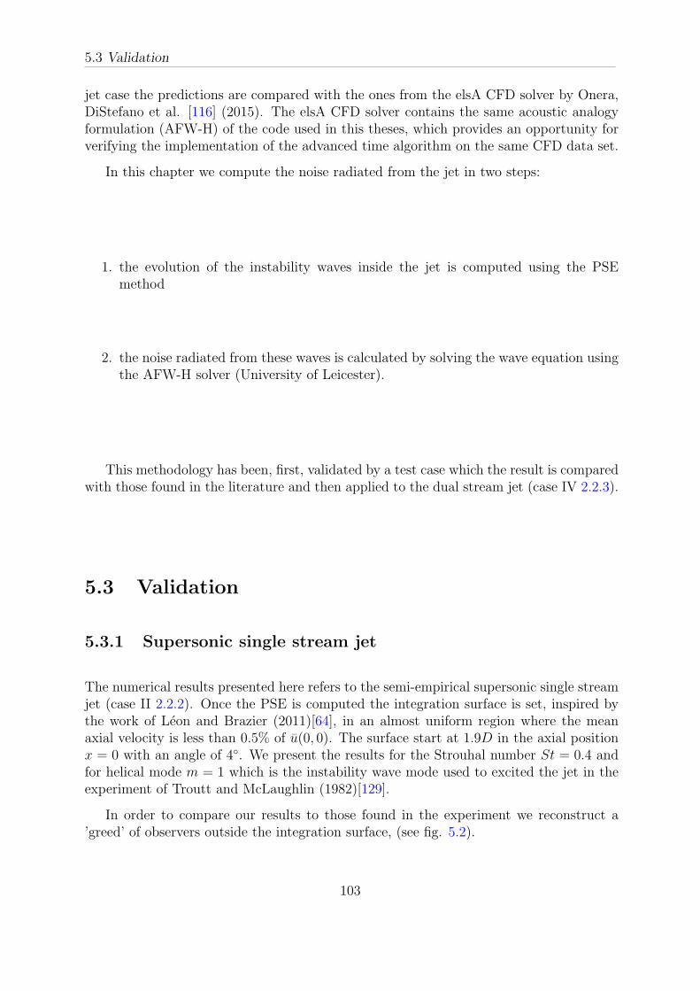
5.3 Validation
jet case the predictions are compared with the ones from the elsA CFD solver by Onera,DiStefano et al. [116] (2015). The elsA CFD solver contains the same acoustic analogyformulation (AFW-H) of the code used in this theses, which provides an opportunity forverifying the implementation of the advanced time algorithm on the same CFD data set.
In this chapter we compute the noise radiated from the jet in two steps:
1. the evolution of the instability waves inside the jet is computed using the PSEmethod
2. the noise radiated from these waves is calculated by solving the wave equation usingthe AFW-H solver (University of Leicester).
This methodology has been, first, validated by a test case which the result is comparedwith those found in the literature and then applied to the dual stream jet (case IV 2.2.3).
5.3 Validation
5.3.1 Supersonic single stream jet
The numerical results presented here refers to the semi-empirical supersonic single streamjet (case II 2.2.2). Once the PSE is computed the integration surface is set, inspired bythe work of Leon and Brazier (2011)[64], in an almost uniform region where the meanaxial velocity is less than 0.5% of u(0, 0). The surface start at 1.9D in the axial positionx = 0 with an angle of 4. We present the results for the Strouhal number St = 0.4 andfor helical mode m = 1 which is the instability wave mode used to excited the jet in theexperiment of Troutt and McLaughlin (1982)[129].
In order to compare our results to those found in the experiment we reconstruct a’greed’ of observers outside the integration surface, (see fig. 5.2).
103
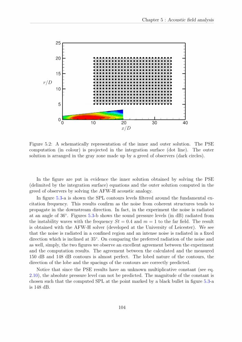
Chapter 5 : Acoustic field analysis
x/D
r/D
Figure 5.2: A schematically representation of the inner and outer solution. The PSEcomputation (in colour) is projected in the integration surface (dot line). The outersolution is arranged in the gray zone made up by a greed of observers (dark circles).
In the figure are put in evidence the inner solution obtained by solving the PSE(delimited by the integration surface) equations and the outer solution computed in thegreed of observers by solving the AFW-H acoustic analogy.
In figure 5.3-a is shown the SPL contours levels filtered around the fundamental ex-citation frequency. This results confirm as the noise from coherent structures tends topropagate in the downstream direction. In fact, in the experiment the noise is radiatedat an angle of 36. Figures 5.3-b shows the sound pressure levels (in dB) radiated fromthe instability waves with the frequency St = 0.4 and m = 1 to the far field. The resultis obtained with the AFW-H solver (developed at the University of Leicester). We seethat the noise is radiated in a confined region and an intense noise is radiated in a fixeddirection which is inclined at 35. On comparing the preferred radiation of the noise andas well, simply, the two figures we observe an excellent agreement between the experimentand the computation results. The agreement between the calculated and the measured150 dB and 148 dB contours is almost perfect. The lobed nature of the contours, thedirection of the lobe and the spacings of the contours are correctly predicted.
Notice that since the PSE results have an unknown multiplicative constant (see eq.2.10), the absolute pressure level can not be predicted. The magnitude of the constant ischosen such that the computed SPL at the point marked by a black bullet in figure 5.3-ais 148 dB.
104
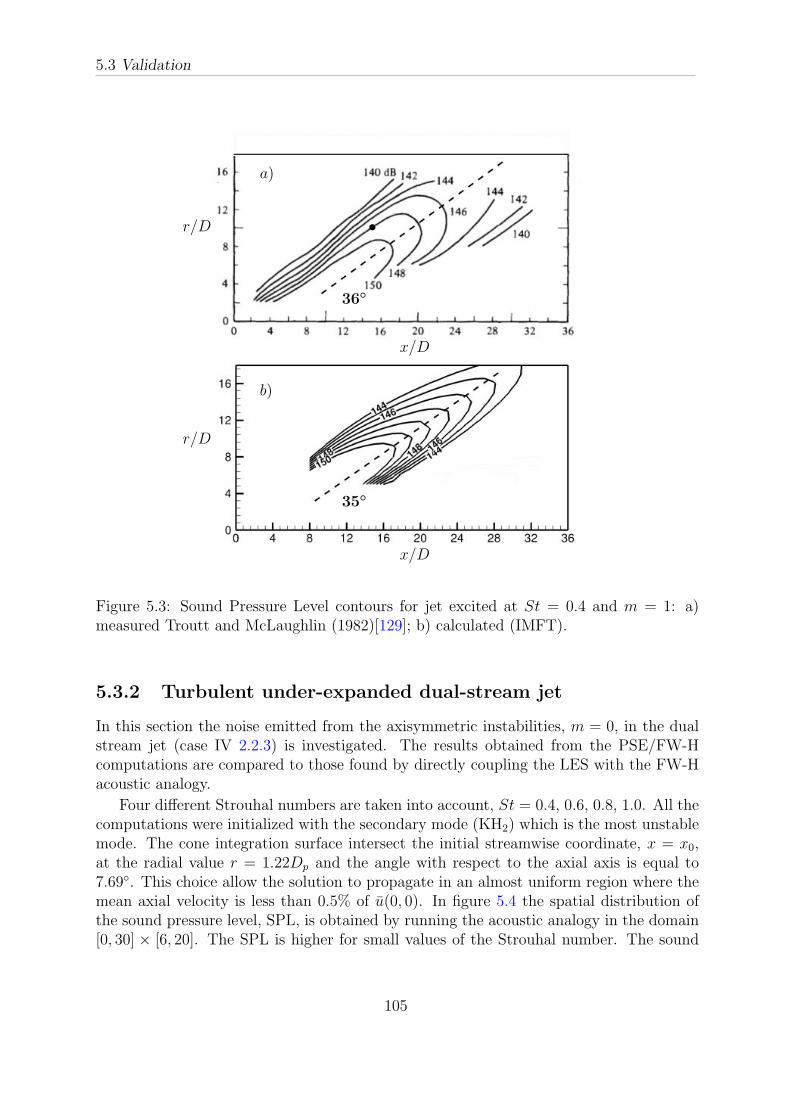
5.3 Validation
x/D
x/D
r/D
r/D
a)
b)
36
35
•
Figure 5.3: Sound Pressure Level contours for jet excited at St = 0.4 and m = 1: a)measured Troutt and McLaughlin (1982)[129]; b) calculated (IMFT).
5.3.2 Turbulent under-expanded dual-stream jet
In this section the noise emitted from the axisymmetric instabilities, m = 0, in the dualstream jet (case IV 2.2.3) is investigated. The results obtained from the PSE/FW-Hcomputations are compared to those found by directly coupling the LES with the FW-Hacoustic analogy.
Four different Strouhal numbers are taken into account, St = 0.4, 0.6, 0.8, 1.0. All thecomputations were initialized with the secondary mode (KH2) which is the most unstablemode. The cone integration surface intersect the initial streamwise coordinate, x = x0,at the radial value r = 1.22Dp and the angle with respect to the axial axis is equal to7.69. This choice allow the solution to propagate in an almost uniform region where themean axial velocity is less than 0.5% of u(0, 0). In figure 5.4 the spatial distribution ofthe sound pressure level, SPL, is obtained by running the acoustic analogy in the domain[0, 30] × [6, 20]. The SPL is higher for small values of the Strouhal number. The sound
105
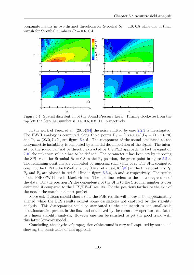
Chapter 5 : Acoustic field analysis
propagate mainly in two distinct directions for Strouhal St = 1.0, 0.8 while one of themvanish for Strouhal numbers St = 0.6, 0.4.
xx
r
r
r
r
c)d)
a) b)
Figure 5.4: Spatial distribution of the Sound Pressure Level. Turning clockwise from thetop left the Strouhal number is 0.4, 0.6, 0.8, 1.0, respectively.
In the work of Perez et al. (2016)[94] the noise emitted by case 2.2.3 is investigated.The FW-H analogy is computed along three points P1 = (13.4, 6.05),P2 = (18.0, 6.70)and P3 = (23.0, 7.42), see figure 5.4-d. The component of the sound associated to theaxisymmetric instability is computed by a modal decomposition of the signal. The inten-sity of the sound can not be directly extracted by the PSE approach, in fact in equation2.10 the unknown value ε has to be defined. The parameter ε has been set by imposingthe SPL value for Strouhal St = 0.8 in the P1 position, the green point in figure 5.5-a.The remaining positions are computed by imposing such value of ε. The SPL computedcoupling the LES to the FW-H analogy (Perez et al. (2016)[94]) in the three positions P1,P2 and P3 are plotted in red full line in figure 5.5-a, -b and -c respectively. The resultsof the PSE/FW-H are in black circles. The dot lines refers to the linear regression ofthe data. For the position P1 the dependence of the SPL to the Strouhal number is overestimated if compared to the LES/FW-H results. For the positions farther to the exit ofthe nozzle the match is almost perfect.
More calculations should shown that the PSE results will however be approximatelyaligned while the LES results exhibit some oscillations not captured by the stabilityanalysis. This discrepancies could be attributed to the nonlinearities and small-scaleinstationnarities present in the flow and not solved by the mean flow operator associatedto a linear stability analysis. However one can be satistied to get the good trend withthis latter low-cost model.
Concluding, the physics of propagation of the sound is very well captured by our modelshowing the consistence of this approach.
106

5.3 Validation
0 0.2 0.4 0.6 0.8 1 1.2 1.470
75
80
85
90
95
100
St
SP
L
SPL
SPL(PSE)
0 0.2 0.4 0.6 0.8 1 1.2 1.474
76
78
80
82
84
86
88
90
92
94
St
SP
L
SPL
SPL(PSE)
0 0.2 0.4 0.6 0.8 1 1.2 1.474
76
78
80
82
84
86
88
90
92
94
St
SP
L
SPL
SPL(PSE)
a)
b)
c)
Figure 5.5: The SPL is computed for the three different positions P1, P2 and P3 in figurea), b) and c) respectively. The red line refers to the SPL obtained by coupling the FW-Hacoustic analogy with the LES computation (see Perez et al. (2016)[94]). The dark bulletare the SPL estimated by our appraoch (developed in collaboration with the Universityof Leicester). The dot lines refers to the linear regression of the two computations.
107

Chapter 5 : Acoustic field analysis
5.4 Conclusion
In this chapter has been presented a low cost computational model able to predict thenoise emitted by the evolution of a small disturbance with a single frequency and a fixedazimuthal wavenumber. The solution is the results of a coupling between the PSE solverand the acoustic analogy solver; this development has been done in collaboration withthe University of Leicester. The model allows to a low cost study of the noise emission inturbulent jet and can be applied in future for many cases of industrial interest. The totalcomputations is very efficient and take about 20 minutes running in a normal laptop. Theapplication shown in this chapter a very good agreement is found between the computedand the measured Sound Pressure Level. The model predict very accurately the noiseemission also for jets with high complexity, like the turbulent under-expanded dual streamjet studied in this thesis work. This methodology leave open the possibility to investigatenoise in jet with high complexity efficiently.
108

Conclusions
Summary of main results
In this thesis many configurations are investigated. For PSE and the corresponding sen-sitivity of the jet flow to noise the main objective was to investigate the complex configu-ration of a dual stream under-expanded jet of industrial interest, obtained thanks to theaccurate LES computation from CERFACS[94].
In the first part of this work (chapter I and more in details in chapter II) the PSEapproach is presented. The PSE solver, developed by the ONERA’s team[63] was upgradeby a stabilization procedure in order to investigate more complex flows. A parametricstudy with respect to the Strouhal number pointed out that the shock cell play a crucialrole in the growth rate of the instability, otherwise variations in the frequency of theinstability seems to have a less effect in the growth rate. This study emphasize the roleof the two unstable Kelvin-Helmholtz modes. The K-H modes related to the secondaryshear-layer is the most unstable mode. The instabilities that grow in the secondary shearlayer present a weakly interaction to the primary shear layer. On the other hand theinstabilities that grow in the primary jet highly interact with the secondary jet, confirmingthat for PSE is very difficult to distinguish between the two unstable modes. This resultis in agreement with those found in the previous works of Leon and Brazier(2011) [64]and Sinha et al. (2016)[111].
Then, a sensitivity analysis of the instabilities is made in chapter III. Validation of thesensitivity analysis based on adjoint PSE for subsonic and supersonic single-stream jetflow has been carried out. Especially, the sensitivity obtained by adjoint-based approachand by Finite-Difference method are compared. The most sensitive region with respectto external forcing has been identified close to the exit nozzle into the shear-layer inthe external boundary of the potential core of the jet. For the dual stream jet case anew application about the interaction betweens the Kelvin-Helmholtz instabilities andthe shock-cells has been presented. During the identification of the highest sensitivitylocation a crucial role of the inflection point has been pointed out. Furthermore, theresults show a strong dependence of the sensitivity to the spatial coordinates. Theseremarks should be taken into account before proposing a new noise control strategy by avery deep analysis of the interaction flow/actuator.
In chapter IV the relationship between sensitivity and Uncertainty Quantification(UQ) has been investigated, firstly, by a toy model and then directly applied on the PSEstability problem in collaboration with the University of Greenwich. Make a link between
109
Chapter 5 : Acoustic field analysis
sensitivity and UQ could be an objective of industrial interest because, generally, thesensitivity solver are much less expensive in term of computational cost if compared withthe classical UQ approach. The UQ applied to the PSE model shows that the uncertaintyin the value of the instability frequency wave modifies the wavelength of the sound wave,but finally and astonishingly the growth rate will remain quite insensitive.
An important step of this work is to couple the stability and sensitivity solvers toa far-field sound propagation approach, Chapter V. Validation of this methodology forcases II 2.2.2 and IV 2.2.3 have been performed, in collaboration with the University ofLeicester, showing encouraging results for the prevision of the noise emission in jets.
Perspectives
A low computational cost model of the shear-layer instability modes in the co-axial jet,which takes into account the shock-cell system in the bypass stream, based on the Parab-olized Stability Equations has been developed. In addition, a far field acoustic simulationcoupled with PSE results has been validated for cases II 2.2.2 and IV 2.2.3 and can be useto deeper investigate the noise in the dual stream jet configuration. The next step willbe to develop a global sensitivity study for the full model (PSE + APSE + sound prop-agation) in the near and far field. Moreover, we should be able to provide in the base ofadjoint equations an extension to sensitivity of the noise to various possible perturbationsor forcing, related to aeroacoustic control. This numerically low-cost tool can be used forpredicting shock-cell noise. As discussed in [131, 23, 64] many questions remains relativeto the location and the quality of the coupling between the PSE pressure disturbance andthe far-field zone.
In parallel, the propagation of instability should be taken into account uncertainties ofthe mean flow variations. These uncertainties of the mean flow, probably, are propagatedinto the far field noise emission. Finally, the implementation of the ’gradient’ PSE solver(see eq. 4.12) could be a good alternative to investigate parameters dependences thatadjoint PSE are not able to solve efficiently (i.e. ∂α
∂ω). Because the sensitivity coefficients
can be quickly obtained by the adjoint approach, a future step is to explore the possi-bility of quantify uncertainties by using a costless surrogate model based on the exactlycalculated adjoint-based sensitivity coefficients, as done for the toy model in chapter IV.
110

List of Tables
1.1 Number of function evaluations to compute the gradient using Finite Dif-ference approximation (FD), Complex step derivative (CSD) and adjointequations (ADJ). First and second order FD approach are denoted FD1and FD2. . . . . . . . . . . . . . . . . . . . . . . . . . . . . . . . . . . . . 30
2.1 Directivity of the pressure instability waves. . . . . . . . . . . . . . . . . . 542.2 Values of the initializing unstable Kelvin-Helmoltz modes in the inner and
in the outer shear-layer for different Strouhal numbers. . . . . . . . . . . . 66
3.1 Values of the parameters used for the validation at different spatial position 83
4.1 Comparison among sensitivity methods. . . . . . . . . . . . . . . . . . . . 934.2 Results from Variance Based Sensitivity Analysis. . . . . . . . . . . . . . . 93
111

LIST OF TABLES
112

List of Figures
1.1 Shadowgraphs of a cold supersonic helium jet. Strong directional wavesare emitted from the shear layer close to the exit of the nozzle. . . . . . . . 5
1.2 Pulsed laser picture of the large turbulence structures in the mixing layer ofa Mach 1.3 jet (Thurow et al. 2003). Copyright 2003, American Instituteof Physics. . . . . . . . . . . . . . . . . . . . . . . . . . . . . . . . . . . . . 6
1.3 Acoustic power measurements of a heated M∞ = 1.5 jet. Azimuthal modem = 0 and frequency St = 0.25. Data obtained from measurements ofSuzuki and Colonius (2006)[117]. . . . . . . . . . . . . . . . . . . . . . . . 7
1.4 Noise radiation in a turbulent jet flow. . . . . . . . . . . . . . . . . . . . . 8
1.5 Typical far field jet noise spectrum, Tam (1995)[118]. . . . . . . . . . . . . 8
1.6 Schematic representation of the acoustic analogy approach. . . . . . . . . . 10
1.7 Linear and nonlinear behaviour of forced jets in (a) Crow and Champagne’s[27] and (b) Moore’s[86] experiment. Forcing Strouhal numbers are 0.3 forCrow and Champagne and ≃ 0.48 for Moore. The lines from bottom totop refer respectively to increasing forcing amplitudes at the nozzle exit.The triangles in Crow and Champagne’s experiment refer to the unforced jet 17
1.8 Comparison between SPL obtained by Balakumar (a) computing the waveequation for fixed Strouhal number, St, and azimuthal wavenumber m withexperimental results (b) measured by Troutt and McLaughlin[129]. . . . . 21
1.9 Shock noise test case, Mj = 1.22, m = 0. The curves represent the far fieldpressure amplitude, pff , computed by LEE solutions at different Strouhalnumber and symbols represent PSE/shock cell model solutions, Ray andLele (2007)[103]. . . . . . . . . . . . . . . . . . . . . . . . . . . . . . . . . . 22
1.10 Case a) the flow is stable. Case b) the perturbation is convected away fromx = 0 the flow is convectively unstable. Case c) the perturbation expandsaround x = 0 the flow is absolutely unstable. . . . . . . . . . . . . . . . . . 24
2.1 The coordinate system used in this thesis . . . . . . . . . . . . . . . . . . . 34
2.2 Simple scheme of the PSE solver. . . . . . . . . . . . . . . . . . . . . . . . 42
2.3 Effect of streamwise step size on the growth rates of an incompressibleflow[133], Mj = 0.01. In full lines the PSE are computed with the stabi-lization procedure, in dash-lines the PSE are computed dropping out theterm ∂p
∂x. . . . . . . . . . . . . . . . . . . . . . . . . . . . . . . . . . . . . . 44
113
LIST OF FIGURES
2.4 Spatial distribution of the mean axial velocity, Mj = 0.01. In dash-dotlines the boundary of potential core and the boundary of the shear layer. . 45
2.5 Stability spectrum for the incompressible subsonic jet, Mj = 0.01 at theaxial position x = x0 for Strouhal number St = 0.6 and for azimuthalwavenumber m = 0. In full circle the unstable modes related to Kelvin-Helmholtz instability. . . . . . . . . . . . . . . . . . . . . . . . . . . . . . . 46
2.6 Comparison between present PSE and Yen et Messersmith PSE(•), 1998.a) Real part of α, b) Imaginary part of α for a subsonic flow with ω = 1.2πand m = 0. See also [133]. . . . . . . . . . . . . . . . . . . . . . . . . . . . 47
2.7 Spatial distribution of the modulus of the perturbation |p′| for the Strouhalnumber St = 0.6, and azimuthal wavenumberm = 0 the pressure growth inthe unstable regions of the jet and fall-down for high values of the stream-wise coordinates where the flow is stable. . . . . . . . . . . . . . . . . . . . 47
2.8 The jet has been divided into three regions I, II and III. They are calledrespectively the core, the transition and the developed regions. . . . . . . . 48
2.9 Axial distribution of mean velocity profile parameters b(x). . . . . . . . . . 49
2.10 Axial distribution of mean centerline velocity uc(x). . . . . . . . . . . . . . 50
2.11 Validation of the parameters uc, b, h by comparison with Yen and Messer-smith (1999)[134] results. . . . . . . . . . . . . . . . . . . . . . . . . . . . . 51
2.12 Spatial distribution of the mean axial velocity, ux, at Mj = 2.1. In dash-dot lines the boundary of the potential core and the boundary of the shearlayer. . . . . . . . . . . . . . . . . . . . . . . . . . . . . . . . . . . . . . . . 51
2.13 The streamwise variations of radial profiles of mean radial velocities, ur. . . 52
2.14 Stability spectrum of the semi-empirical supersonic jet, Mj = 2.1 at theaxial position x = x0 for Strouhal number St = 0.2 and for azimuthalwavenumber m = 0. In full circle the unstable modes related to Kelvin-Helmholtz instability. . . . . . . . . . . . . . . . . . . . . . . . . . . . . . . 53
2.15 Absolute pressure values at r/D = 0.5 obtained by PSE computations (fulllines) are compared with Yen and Messersmith [134] results (). Compar-isons have been done for azimuthal wavenumber m = 0 and for (a) St = 0.2and (b) St = 0.4. . . . . . . . . . . . . . . . . . . . . . . . . . . . . . . . . 54
2.16 Contour lines of the pressure waves for azimuthal wavenumber, m = 0.Same scale for each plots. . . . . . . . . . . . . . . . . . . . . . . . . . . . 55
2.17 The RMS values of the pressure waves for azimuthal wavenumber, m = 0.Same scale for each plots. . . . . . . . . . . . . . . . . . . . . . . . . . . . 56
2.18 The RMS values of the pressure waves for azimuthal wavenumber, m = 1. . 57
2.19 Spatial distribution of the mean axial velocity computed by LES. Theshock-cells are distributed along the streamwise direction in the core ofthe jet. . . . . . . . . . . . . . . . . . . . . . . . . . . . . . . . . . . . . . . 58
2.20 Acoustic spectrum in the far-field (50 diameters) for a Mj = 1.15 under-expanded jet. θ is measured with respect to the jet axis, (a) SPL, (b)OASPL. From Arroyo (2016)[94] . . . . . . . . . . . . . . . . . . . . . . . . 58
114

LIST OF FIGURES
2.21 Spatial distribution of the real part of the perturbation p′, Re(p′) for theStrouhal number St = 0.89, the pressure growth in the unstable regions ofthe jet and fall-down for high values of the streamwise coordinates wherethe flow is stable. . . . . . . . . . . . . . . . . . . . . . . . . . . . . . . . . 59
2.22 Axial distribution of the streamwise wave-number α for different values ofthe Strouhal number, respectively 1.10, 1.30, 0.89, 0.67 . . . . . . . . . . . . 60
2.23 Under-expanded supersonic dual-stream jet est case. Flow conditions . . . 61
2.24 Under-expanded supersonic dual-stream jet test case. Nozzle geometry. . . 61
2.25 Under-expanded supersonic dual-stream jet test case. Time and azimuthalaverage mean axial velocity ux. . . . . . . . . . . . . . . . . . . . . . . . . 62
2.26 Test case under-expanded supersonic dual-stream jet. Time and azimuthalaverage mean axial velocity ux. . . . . . . . . . . . . . . . . . . . . . . . . 63
2.27 Stability spectrum of the turbulent dual-stream jet at the axial positionx = x0 for Strouhal number St = 1.0 and for azimuthal wavenumberm = 0. In dark point the 2 unstable modes related to Kelvin-Helmholtzinstability in the primary KH1 and secondary KH2 jet. case a) refers tothe local stability at the position x = 0Dp (test 1) and case b) refers to thelocal stability at x = 1Dp (test 2). . . . . . . . . . . . . . . . . . . . . . . . 64
2.28 Growth rate computed for the two different baseflow. The two solutionsquickly converge to the same values. . . . . . . . . . . . . . . . . . . . . . . 65
2.29 Real part of the wavenumber α(x) for different Strouhal values. . . . . . . 66
2.30 Imaginary part of the wavenumber α(x) for different Strouhal values. . . . 67
2.31 Comparison of the real part of α(x) is made for several Strouhal numbers.Computation are obtained by initialising the PSE with the primary unsta-ble mode, KH1, full lines and with the secondary unstable modes, KH2,dot-lines. . . . . . . . . . . . . . . . . . . . . . . . . . . . . . . . . . . . . . 67
2.32 LST: part of the spectrum for different x. St = 1. The vertical axis endsat −0.01. . . . . . . . . . . . . . . . . . . . . . . . . . . . . . . . . . . . . . 69
2.33 Spatial distribution of the absolute value of the pressure disturbance, |p′|for St = 1.0. (a) PSE is initialised with the secondary unstable modes,KH2. (b) is initialised with the primary unstable modes.. . . . . . . . . . . 69
2.34 Spatial distribution of the absolute value of the pressure disturbance, |p′|for St = 0.4. (a) PSE is initialised with the secondary unstable modes,KH2. (b) is initialised with the primary unstable modes. . . . . . . . . . . 70
3.1 Sensitivity of the analytical incompressible jet. From the top to the bottomwe have respectively, the gradient of E with respect to the forcing acting inthe continuity, r-momentum, x-momentum and energy equation at differentfixed position in the stream-wise direction (x = 5.0, 2.5, 2.0, 1.5, 1.0) . . . 78
3.2 Sensitivity of the semi-analytical supersonic jet. From top to the bottomwe have respectively, the gradient of E with respect to the forcing acting inthe continuity, r-momentum, x-momentum and energy equation at differentfixed position in the stream-wise direction (x = 4.0, 2.0, 1.0, 0.5). TheStrouhal number is St = 0.4 . . . . . . . . . . . . . . . . . . . . . . . . . . 79
115

LIST OF FIGURES
3.3 The normalized sensitivity with respect to the forcing acting in the energyequation, Sf5/E, as a function of the spatial coordinates. The results referto the supersonic semi-empirical baseflow 2.2.2 with a) St = 0.2 and b)St = 0.4. Below the isoline ux = 0.99 · ux(0, r) we can assume to bein the potential core otherwise the shear layer is delimited by the isolineux = 0.99 · ux(0, r) and by the isoline ux = 0.01 · ux(0, r). The dashed lineis the inflection point of the baseflow . . . . . . . . . . . . . . . . . . . . . 80
3.4 Spatial distribution of the gradient of E with respect to a forcing actingin the x-momentum, Sf4 . Below the isolines ux = 0.99 · ux(0, r) and ux =0.01 · ux(0, r) delimited the potential core and the shear layer regions ofthe jet. The isolines full line and dashed line indicate respectively positiveand negative values of the sensitivity. With • are plotted the (x, r) used tovalidate the A-PSE. . . . . . . . . . . . . . . . . . . . . . . . . . . . . . . . 82
3.5 Comparison between results from equation 3.34 (lines) and equation 3.36(symbols) is made for semi-empirical flows (a and b refer respectively tothe subsonic and supersonic case.). . . . . . . . . . . . . . . . . . . . . . . 83
3.6 From top the bottom we have respectively, the sensitivity Sf computedfor the under-expanded supersonic single jet with respect to the forcingacting in the continuity, r-momentum, x-momentum and energy equationat different fixed position in the stream-wise direction (x = 4.0, 2.0, 1.0, 0.5) 84
3.7 The results refer to the unstable mode KH1. From top the bottom we haverespectively, the sensitivity Sf computed for the under-expanded supersonicdual-stream jet with respect to the forcing acting in the continuity, r-momentum, x-momentum and energy equation at different fixed positionin the stream-wise direction (x = 4.0, 2.0, 1.0, 0.5) . . . . . . . . . . . . . . 85
3.8 The results refer to the unstable mode KH2. From top the bottom we haverespectively, the sensitivity Sf computed for the under-expanded supersonicdual-stream jet with respect to the forcing acting in the continuity, r-momentum, x-momentum and energy equation at different fixed positionin the stream-wise direction (x = 4.0, 2.0, 1.0, 0.5) . . . . . . . . . . . . . . 86
3.9 The normalized sensitivity with respect to the forcing acting in the energyequation, Sf5/E, as a function of the spatial coordinates. The results referto the under expanded dual stream baseflow 2.2.3 with a) St = 0.6 and b)St = 1.0. Solid lines are the isoline of the mean axial velocity, ux. Thedashed line delimits the inflection point of the baseflow. . . . . . . . . . . . 88
4.1 Latin Hypercube Sampling with 5000 samples. . . . . . . . . . . . . . . . . 94
4.2 Mean and standard deviation envelopes of y1 and |y|2/2 with respect to anumber of different values λ2 function of time. Dash line: from gradients(sensitivity analysis), green full line: direct computations of equation (1). . 95
4.3 Mean and standard deviation envelopes of the wavenumber αr (a) and ofthe growth rate αi (b). . . . . . . . . . . . . . . . . . . . . . . . . . . . . 97
4.4 Mean and standard deviation envelopes of the real part of the amplitudefunctions ur (a) and ux (b), r/Dj = 0.51. . . . . . . . . . . . . . . . . . . . 97
116
LIST OF FIGURES
5.1 Radiation in an unbounded flow. . . . . . . . . . . . . . . . . . . . . . . . 995.2 A schematically representation of the inner and outer solution. The PSE
computation (in colour) is projected in the integration surface (dot line).The outer solution is arranged in the gray zone made up by a greed ofobservers (dark circles). . . . . . . . . . . . . . . . . . . . . . . . . . . . . . 104
5.3 Sound Pressure Level contours for jet excited at St = 0.4 and m = 1: a)measured Troutt and McLaughlin (1982)[129]; b) calculated (IMFT). . . . 105
5.4 Spatial distribution of the Sound Pressure Level. Turning clockwise fromthe top left the Strouhal number is 0.4, 0.6, 0.8, 1.0, respectively. . . . . . 106
5.5 The SPL is computed for the three different positions P1, P2 and P3 infigure a), b) and c) respectively. The red line refers to the SPL obtained bycoupling the FW-H acoustic analogy with the LES computation (see Perezet al. (2016)[94]). The dark bullet are the SPL estimated by our appraoch(developed in collaboration with the University of Leicester). The dot linesrefers to the linear regression of the two computations. . . . . . . . . . . . 107
117

LIST OF FIGURES
118

Bibliography
[1] Abergel, F., and Temam, R. On some control problems in fluid mechanics.Theoret. Comput. Fluid Dyn. 1 (1990), 303–325.
[2] Airiau, C. Stabilite lineaire et faiblement non-lineaire d’une couche limite in-compressible par un systeme d’equations parabolique. PhD thesis, Ecole NationaleSuperieure de l’Aeronautique et de l’Espace, Toulouse, France, Juin 1994.
[3] Airiau, C. Non-parallel acoustic receptivity of a Blasius boundary layer using anadjoint approach. Flow Turbul. Combust. 65, 3/4 (2000), 347–367.
[4] Airiau, C. Stabilite, receptivite et controle optimal d’ecoulements cisailles: ap-proches adjointes. In Habilitation a diriger des recherches (Toulouse, France, 2004).
[5] Airiau, C., Bottaro, A., Walther, S., and Legendre, D. A methodologyfor optimal laminar flow control: Application to the damping of tollmien-schlichtingwaves in a boundary layer. Phys. Fluids 15, 5 (2003), 1131–1145.
[6] Airiau, C., and Casalis, G. Boundary layer linear stability using a system ofparabolic equations. Rech. Aerosp. 5 (1993), 57–68.
[7] Airiau, C., Walther, S., and Bottaro, A. Boundary layer sensitivity andreceptivity. C.R. Mecanique 330 (2002), 259–265.
[8] Andersson, P., Henningson, D., and Hanifi, A. On a stabilization procedurefor the parabolic stability equations. Journal of Engineering Mathematics 33 (1998),311.
[9] Andre, B., Castelain, T., and Bailly, C. Broadband shock-associated noisein screeching and non-screeching underexpanded supersonic jets. AIAA Journal 51(3) (2013), 665–673.
[10] Ansaldi, T., and Airiau, C. Non viscous sensitivity analysis of noise genera-tion mechanism in a low mach number jet. In 50th 3AF international conference(Toulouse, France, 2015), no. FP59.
[11] Ansaldi, T., and Airiau, C. Sensitivity analysis for subsonic jet using adjointof non local stability equations. No. AIAA 2015-2219.
119
BIBLIOGRAPHY
[12] Ansaldi, T., Airiau, C., Perez, C., and Puigt, G. PSE-based sensitivityanalysis of turbulent and supersonic single stream jet. No. 16-3052 in AIAA-paper.
[13] Bagheri, S., Schlatter, P., Schmid, P. J., and Henningson, D. S. Globalstability of a jet in crossflow. J. Fluid Mech. 624(1) (2009), 33–44.
[14] Balakumar, P. Prediction of supersonic jet noise. No. AIAA 98-1057.
[15] Bogey, C., and Bailly, C. Computation of a high Reynolds number jet and itsradiated noise using Large Eddy Simulation based on explicit filtering. Computersand Fluids 35(10) (2006), 1344–1358.
[16] Brentner, K. S., and Farassat, F. Analytical comparison of the acousticanalogy and Kirchhoff formulation for moving surfaces. AIAA Journal 36 (8) (1998),1379–1386.
[17] Brentner, K. S., and Holland, P. C. An efficient and robust method forpredicting helicopter rotor high-speed impulsive noise. J. Sound. Vib. 203 (1997),97–100.
[18] Cambier, L., Heib, S., and Plot, S. The Onera elsA CFD software: input fromresearch and feedback from industry. Mechanics and Industry 14 (2013), 159–174.
[19] Casalino, D. An advanced time approach for acoustic analogy predictions. J.Sound. Vib. 261 (4) (2003), 583–612.
[20] Cavalieri, A. V. G. Wavepackets as sound-source mechanisms in subsonic jets.PhD thesis, Ecole doctorale : Sciences et ingenierie en materiaux, mecanique,nergetique et aeronautique - SIMMEA, Poitiers, France, Juin 2012.
[21] Chang, C. L., Malik, M. R., Erlebacher, G., and Hussaini, M. Y. Com-pressible stability of growing boundary layers using parabolised stability equations.No. AIAA 1991-1636.
[22] Cheung, L. C., Bodony, D. J., and Lele, S. K. Noise radiation predictionsfrom jet instability waves using a hybrid nonlinear PSE-acoustic analogy approach.No. AIAA 2007-3638.
[23] Cheung, L. C., and Lele, S. K. Acoustic radiation from subsonic and supersonicmixing layers with nonlinear PSE. No. AIAA 2004-0363.
[24] Cheung, L. C., and Lele, S. K. Linear nd nonlinear precesses in two-dimensional mixing layer dynamics and sound radiation. J. Fluid Mech. 625 (2009),321–351.
[25] Chomaz, J. M. Linear and non-linear, local and global stability analysis of openflows. Turbulence in spatially extended systems 5 (1993), 245–257.
120
BIBLIOGRAPHY
[26] Colonius, T., and Lele, S. K. Computational aeroacoustics: progress on non-linear problems of sound generation. Prog. Aerosp. Sci. 40 (2004), 345–416.
[27] Crow, S. C., and Chamapagne, F. H. Orderly structure in jet turbulence. J.Fluid Mech. 48 (1971), 547–591.
[28] Curle, N. The influence of solid boundaries upon aerodynamic sound. vol. 231 ofProceedings of the Royal Society of London, pp. 505–514.
[29] Day, M., Mansour, N., and Reynolds, W. Nonlinear stability and structureof compressible reacting mixing layers. J. Fluid Mech. 446 (2001), 375–408.
[30] Farassat, F. Theory of noise generation from moving bodies with an applicationto helicopter rotors. In NASA technical report (1975), NASA.
[31] Farassat, F. Introduction to generalized functions with applications in aerody-namics and aeroacoustics. In NASA technical report (1994).
[32] Farassat, F. Derivation of formulations 1 and 1a of Farassat. In NASA technicalreport (2007), NASA.
[33] Farassat, F., and Myers, M. Extension of Kirchhoffs formula to radiation frommoving surfaces. J. Sound. Vib. 3 (1988), 451–460.
[34] Ffowcs Williams, J. The noise from turbulence convected at high speed. Philo-sophical Transactions of the Royal Society of London 255, 1061 (1963), 469–503.
[35] Ffowks williams, J., and Hawkings, D. Sound generetion by turbulenceand surfaces in arbitrary motion. Mathematical and Physical Sciences 264 (1969),321–342.
[36] Francescantonio, P. D. A new boundary integral formulation for the predictionof sound radiation. J. Sound. Vib. 202 (1997), 491–509.
[37] Giannetti, F., and Luchini, P. Structural sensitivity of the first instability ofthe cylinder wake. J. Fluid Mech. 581 (2007), 167–197.
[38] Glowinski, R. Finite element methods for the numerical solution of incompressibleviscous flow. introduction to the control of the Navier-Stokes equations. vol. 28 ofLectures in Appl. Math., pp. 219–301.
[39] Godreche, C., Menneville, P., and Castaing, B. Hydrodynamics and nonlinear istabilities. Cambrige University Press.
[40] Goldstein, G. A generalized acoustic analogy. J. Fluid Mech. 488 (2003), 315–333.
[41] Goldstein, M. A unified approach to some recent developments in jet noise theory.Int. J. Aeroacoustics 1, 1 (2002), 1–16.
121

BIBLIOGRAPHY
[42] Gudmundsson, K., and Colonius, T. Parabolized Stability Equation modelsfor turbulent jets and their radiated sound. No. AIAA 2009-3380.
[43] Gudmundsson, K., and Colonius, T. Instability wave models for the near-fieldfluctuations of turbulent jets. J. Fluid Mech. 689 (2011), 97–128.
[44] Gunzburger, M., Hou, L. S., and Svobodny, T. P. Numerical approximationof optimal control problem associated with the Navier-Stokes equations. vol. 2 ofAppl. Math. Lett., pp. 29–31.
[45] Gunzburger, M., Hou, L. S., and Svobodny, T. P. Boundary velocitycontrol in incompressible flow with an application to viscous drag reduction. SIAMJ. Control Optim 30 (1992), 167–181.
[46] Hardin, J. C., and Lamkin, S. L. Aeroacoustic computation of cylinder wakeflow. AIAA Journal 22(1) (1984), 51–57.
[47] Hawkings, D. L. Noise generation by transonic open rotors. Mechanics of SoundGeneration in Flows 1 (1979), 294–300.
[48] Herbert, T. Boundary-layer transition analysis and prediction revisited.No. AIAA 91-0737.
[49] Herbert, T. Parabolized Stability Equations. AGARD REPORT (1993).
[50] Herbert, T. Parabolized Stability Equations. Annu. Rev. Fluid Mech. 29 (1997),245–283.
[51] Herbert, T., and Bertolotti, F. Stability analysis of non-parallel boundarylayers. Bull. Am. Phys. Soc. 32 (1987).
[52] Hill, D. C. A theoretical approach for analyzing the re-stabilization of wakes. InNASA technical memorandum (1992), NASA.
[53] Hill, D. C. Adjoint systems and their role in the receptivity problem for boundarylayers. J. Fluid Mech. 292 (1995), 183–204.
[54] Howe, M. S. Contributions to the theory of aerodynamic sound, with applicationto excess jet noise and the theory of the flute. J. Fluid Mech. 71 (4) (1975), 625–673.
[55] Howe, M. S. Theory of vortex sound. vol. 33 of Cambridge University Press.
[56] Huerre, P., and Monkewitz, P. A. Local and global instabilities in spatiallydeveloping flows. Annu. Rev. Fluid Mech. 22 (1) (1990), 473–537.
[57] J. M. Seiner, T. R. S. B., and Ponton, M. K. Relationship between instabilitywaves and noise of high-speed jets. AIAA Journal 30 (1992), 1747–1767.
122

BIBLIOGRAPHY
[58] Joslin, R. D., Gunzburger, M. D., Nicolaides, R. A., Erlebacher, G.,
and Hussaini, M. Y. A self-contained, automated methodology for optimal flowcontrol validated for transition delay. AIAA Journal 35 (5) (1997), 816–824.
[59] Kim, J., Bodony, D. J., and Freund, J. B. Adoint-based control of loudevents in a turbulent jet. J. Fluid Mech. 741 (2014), 28–59.
[60] Kirchhoff, G. Zur theorie der lichtstrahlen. vol. 254 of Annalen der Physik,pp. 663–695.
[61] Ladeinde, F., Alabi, K., Colonius, T., Gudmundsson, K., Schlinker,
R., and Reba, R. An integrated RANS-PSE-wave packet tool for the predictionof subsonic and supersonic jet noise. No. AIAA 2010–4021.
[62] Lele, S. K. Compact finite difference schemes with spectral-like resolution. J.Comput. Phys. 103 (1992), 16–42.
[63] Leon, O. Etude du rayonnement acoustique des instabilites hydrodynamiques dejets double-flux avec les Equations de stabilite parabolisees (PSE). PhD thesis, Uni-versite de Toulouse, INPT, Toulouse, France, April 2012.
[64] Leon, O., and Brazier, J.-P. Application of linear Parabolized Stability Equa-tions to a subsonic coaxial jet. In AIAA/CEAS, 32nd Aeroacoustics Conference(2011).
[65] Li, F., and Malik, M. R. On the nature of PSE approximation. Int. J. Comput.Fluid D. 8 (1996), 253–273.
[66] Lighthill, M. On sound generated aerodynamically. I. General theory. Proc. R.Soc. Lond. A. 211 (1952), (1107),564–297.
[67] Lighthill, M. On sound generated aerodynamically. II. Turbulence as a sourceof sound. Proc. R. Soc. Lond. A. 222 (1954), (1148),1–32.
[68] Lilley, G. On the noise from jets. AGARD REPORT (1974).
[69] Lowson, M. The sound field for singularities in motion. vol. 286 of Proceedings ofthe Royal Society of London, pp. 559–572.
[70] Lowson, M. V., and Ollerhead, J. B. Visualization of noise from cold super-sonic jets. J. Acoustics Soc. Am. 44 (1968), 624.
[71] Luchini, P., and Bottaro, A. Adjoint equations in stabilty analysis. Annu.Rev. Fluid Mech. 46 (2014), 1–30.
[72] Lyrintzis, A. S. review: the use of Kirchhoffs method in computational aeroa-coustics. J. Fluid Eng. 116 (4) (1994), 665–676.
123

BIBLIOGRAPHY
[73] Lyrintzis, A. S. Surface integral methods in computational aeroacoustics. Fromthe (CFD) near-field to the (acoustic) far-field. Int. J. Aeroacoustics 2 (2003),95–128.
[74] Lyrintzis, A. S., and Mankbadi, R. R. Prediction of the far-field jet noiseusing Kirchhoffs formulation. AIAA Journal 34 (2) (1996), 413–416.
[75] Mankbadi, R. R., Hayder, M. E., and Povinelli, L. A. Structure of super-sonic jet flow and its radiated sound. J. Fluid Mech. 32 (5) (1994), 897–906.
[76] Marquet, O., Sipp, D., and Jaquin, L. Sensitivity analysis and passive controlof cylinder flow. J. Fluid Mech. 615 (2008), 221–252.
[77] Mathelin, L., and Hussaini, M. A stochastic collocation algorithm for uncer-tainty analysis. In NASA technical report/CR-2003-212153 (2003), NASA.
[78] McLaughlin, D. K., Morrison, G. L., and Toutt, T. R. Experiments onthe instability waves in a supersonic jet and their acoustic radiation. J. Fluid Mech.69 (1975), 73–95.
[79] McLaughlin, D. K., Morrison, G. L., and Toutt, T. R. Reynolds numberdependence in supersonic jet noise. AIAA Journal 15 (1977), 526–532.
[80] McLaughlin, D. K., Seiner, J. M., and Liu, H. On the noise generated bylarge scale instabilities in supersonic jets. No. 80-0964 in AIAA-paper.
[81] Michalke, A. Instability of a compressible circular free jet with consideration ofthe influence of the jet boundary layer thickness. In NASA technical memorandum,TM-75190 (1977).
[82] Mitchell, B. E., Lele, S. K., and Moin, P. Direct computation of the soundgenerated by vortex pairing in an axisymmetric jet. J. Fluid Mech. 383 (1999),113–142.
[83] Mollo-Cristensen, E., and Narashima, R. Sound emission from jets at highsubsonic velocities. J. Fluid Mech. 8(01) (1960), 49:60.
[84] Monkewitz, P. A., Bechert, D. W., Barsikow, B., and Lehmann, B.
Self-excited oscillations and mixing in a heated round jet. J. Fluid Mech. 213 (1)(1990), 611–639.
[85] Monkewitz, P. A., and Sohn, K. D. Absolute instability in hot jets. AIAAJournal 26 (1988), 911–916.
[86] Moore, C. J. The role of shear-layer instability waves in jet exhaust noise. J.Fluid Mech. 80 (2) (1977), 321–367.
124

BIBLIOGRAPHY
[87] Morgans, W. XIV. The Kirchhoff formula extended to a moving surface,. vol. 9 ofThe London, Edinburgh, and Dublin Philosophical Magazine and Journal of Science,pp. 141–161 1930.
[88] Morris, P. J. The spatial viscous instability of axisymmetric jets. J. Fluid Mech.77 (1976), 511–529.
[89] Morris, P. J., Long, L. N., Scheidegger, T. E., Wang, Q., and Pilon,
A. R. High speed jet noise simulations. No. AIAA 98-2290.
[90] Najafi-Yazdi, A., Bres, G. A., and Mongeau, L. An acoustic analogy for-mulation for moving sources in uniformly moving media. vol. 467 of Proceedings ofthe Royal Society of London, pp. 144–165.
[91] Nichols, J., and Lele, S. Global modes and transient response of a cold super-sonic jet. Annu. Rev. Fluid Mech. 669 (1) (2011), 225–241.
[92] Panda, J. Shock oscillation in underexpanded screeching jets. J. Fluid Mech. 363(1998), 173–198.
[93] Papamoschou, D. A new method for jet noise suppression in turbofan engines.No. 03-1053 in AIAA-paper.
[94] Perez, C., Puigt, G., Airiau, C., and Boussuge, J. F. Large Eddy Simula-tion of shock-cell noise from a dual stream jet. No. 16-2798 in AIAA-paper.
[95] Perrault-Joncas, D., and Maslowe, S. A. Linear stability of a compressiblecoaxial jet with continuous velocity and temperature profiles. Phys. Fluids 20(7),074102 (2008).
[96] Phillips, O. On the generation of sound by supersonic turbulent shear layers. J.Fluid Mech. 9 (1) (1960), 1–28.
[97] Pilon, A. R., and Lyrintzis, A. S. Development of an improved Kirchhoffmethod for jet aeroacoustics. AIAA Journal 36 (5) (1998), 783–790.
[98] Piot, E., Casalis, G., Muller, F., and Bailly, C. Investigation of the PSEapproach for subsonic and supersonic hot jets. detailed comparison with les andlinearized euler equations results. International Journal of Aeroacoustic 5-4 (2006),361–393.
[99] Powell, A. On the mechanism of choked jet noise. vol. 66 of Proceedings of thePhysical Society, pp. 1039–1057.
[100] Powell, A. Theory of vortex sound. Journal of the Acoustical Society of America36 (1) (1964), 177–195.
125
BIBLIOGRAPHY
[101] Pralits, J. O., Airiau, C., Hanifi, A., and Henningson, D. S. Sensitivityanalysis using adjoint parabolized stability equations for compressible flows. FlowTurbul. Combust. 65, 3/4 (2000), 321–346.
[102] Ray, P. K., Lawrence, C., Cheung, C., and Lele, S. K. On the growth andpropagation of linear instability waves in compressible turbulent jets. Phys. Fluids21 (2009).
[103] Ray, P. K., and Lele, S. K. Sound generated by instability wave/shock-cellinteraction in supersonic jets. J. Fluid Mech. 587 (2007), 173–215.
[104] Rayleigh, L. On the question of the stability of the flow of fluids. vol. 1892 ofPhilosophical Magazine, pp. 59–70.
[105] Reynolds, O. An experimental investigation of the circumstances which determinewhether the motion of water shall be direct or sinuous, and of the law of resistance inparallel channels. vol. 35 of Proceedings of the Royal Society of London, pp. 224–226.
[106] Rodrıguez, D., Samanta, A., Cavalieri, A. V. G., Colonius, T., and
Jordan, P. Parabolized Stability Equation models for predicting large-scale mixingnoise of turbulent round jets. No. AIAA 2011-2838.
[107] Rodrıguez, D., Sinha, A., bres, G. A., and Colonius, T. Acoustic fieldassociated with parabolized stability equation models in turbulent jets. No. AIAA2013-2279.
[108] S. G. Rubin, J. C. T. Parabolized/reduced Navier-Stokes computational techin-ques. Annu. Rev. Fluid Mech. 24 (1992), 117–144.
[109] Saltelli, A., Annoni, P., Azzini, I., Campolongo, F., Ratto, M., and
Tarantola, S. Variance based sensitivity analysis of model output. design andestimator for the total sensitivity index. Computer Physics Communications 181(2010), 259–279.
[110] Schmid, P. J. Nonmodal stability theory. Annu. Rev. Fluid Mech. 39 (2007),129–162.
[111] Sinha, A., Gaitonde, D. V., and Sohoni, N. Parabolized stability analysis ofdual-stream jets. No. 16-3057 in AIAA-paper.
[112] Sinha, A., Rodriguez, D., Bres, G. A., and Colonius, T. Wavepacketmodel for supersonic jet noise. J. Fluid Mech. 742 (2104), 71–95.
[113] Smolyak, S. Quadrature and interpolation formulas for tensor products of certainclasses of functions. Soviet Math. Dokl 4 (1963), 240–243.
[114] Spagnoli, B., and Airiau, C. Adjoint analysis for noise control in a two-dimensional compressible mixing layer. Computers and Fluids 37 (2008), 475–486.
126

BIBLIOGRAPHY
[115] Sritharan, S. Dynamic programming of Navier-Stokes equations. vol. 16 ofSystem Control Lett., pp. 299–307.
[116] Stefano, D. D., Rona, A., Hall, E., and Puigt, G. Implementing the ffowcswilliams and hawkings acoutic analogy in antares. In 22nd International Congresson Sound and Vibration (Florence, Italy, 2015).
[117] Suzuki, T., and Colonius, T. Instability waves in a subsonic round jet detectedusing a near- field phased microphone array. J. Fluid Mech. 565 (2006), 197–226.
[118] Tam, C. K. Computational aeroacoustics-issues and methods. AIAA Journal 33(1995), 1788–1796.
[119] Tam, C. K. Supersonic jet noise. Annu. Rev. Fluid Mech. 27(1) (1995), 17–43.
[120] Tam, C. K., Pastouchenko, N. N., and Viswanathan, K. Computation ofshock cell structure of dual-stream jets for noise prediction. AIAA Journal 46 (11)(2008), 2857–2867.
[121] Tam, C. K. W. Directional acoustic radiation from a supersonic jet generated byshear layer instability. J. Fluid Mech. 46, 4 (1971), 757–768.
[122] Tam, C. K. W., and Burton, D. E. Sound generated by instability waves ofsupersonic flows. part 1.. two-dimensional mixing layers. J. Fluid Mech. 138 (1984),249–271.
[123] Tam, C. K. W., and Burton, D. E. Sound generated by instability waves ofsupersonic flows. part 2. axisymmetric jets. J. Fluid Mech. 138 (1984), 273–295.
[124] Tam, C. K. W., and Chen, P. A statistical model of turbulence in two-dimensional mixing layers. J. Fluid Mech. 92 (1979), 303–326.
[125] Theofilis, V. Advances in global linear instability analysis of nonparallel andthree-dimensional flows. Progress in Aerospace Sciences 39 (4) (2003), 249–316.
[126] Thurow, B., Samimy, M., and Lempert, W. compressibility effects on turbu-lence structures of axisymmetric mixing layers. Phys. Fluids, 5 (2003), 1755–1765.
[127] Tissot, G., Zang, M., Lajus, F. J., Cavalieri, A., Jordan, P., and Colo-
nius, T. Sensitivity of wavepackets in jets to non-linear effects: the role of thecritical layer. No. AIAA 2015-2218.
[128] Troutt, T. R. Measurements on the flow and acoustic properties of a moderate-Reynolds number supersonic jet. PhD thesis, Oklahoma State University, 1978.
[129] Troutt, T. R., and McLaughlin, D. K. Experiments on the flow and acous-tic properties of a moderate Reynolds-number supersonic jet. J. Fluid Mech. 116(1982), 123–156.
127
Appendix
[130] Viswanathan, K. Parametric study of noise from dual-stream nozzles. J. FluidMech. 521 (2004), 35–68.
[131] Walther, S., Airiau, C., and Bottaro, A. Optimal control of Tollmien-Schlichting waves in a developing boundary layer. Phys. Fluids 13, 7 (2001), 2087–2096.
[132] Wei, M., and Freund, J. B. A noise-controlled free shear flow. J. Fluid Mech.546 (2006), 123–152.
[133] Yen, C. C., and Messersmith, N. L. Application of Parabolized StabilityEquations to the prediction of jet instabilities. In AIAA/ASME, 36th Conference(1998).
[134] Yen, C. C., and Messersmith, N. L. The use of compressible parabolizedstability equations for predicition of jet instabilities and noise. No. 99-1859 inAIAA-paper.
128
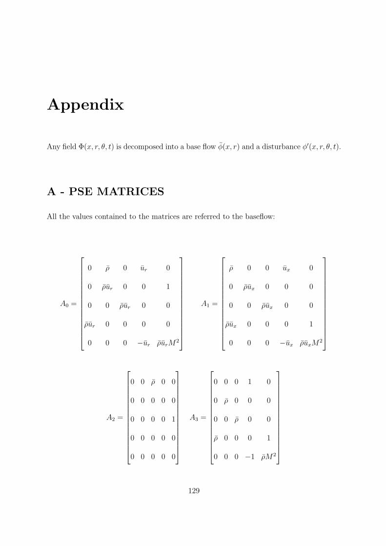
Appendix
Any field Φ(x, r, θ, t) is decomposed into a base flow φ(x, r) and a disturbance φ′(x, r, θ, t).
A - PSE MATRICES
All the values contained to the matrices are referred to the baseflow:
A0 =
0 ρ 0 ur 0
0 ρur 0 0 1
0 0 ρur 0 0
ρur 0 0 0 0
0 0 0 −ur ρurM2
A1 =
ρ 0 0 ux 0
0 ρux 0 0 0
0 0 ρux 0 0
ρux 0 0 0 1
0 0 0 −ux ρuxM2
A2 =
0 0 ρ 0 0
0 0 0 0 0
0 0 0 0 1
0 0 0 0 0
0 0 0 0 0
A3 =
0 0 0 1 0
0 ρ 0 0 0
0 0 ρ 0 0
ρ 0 0 0 1
0 0 0 −1 ρM2
129
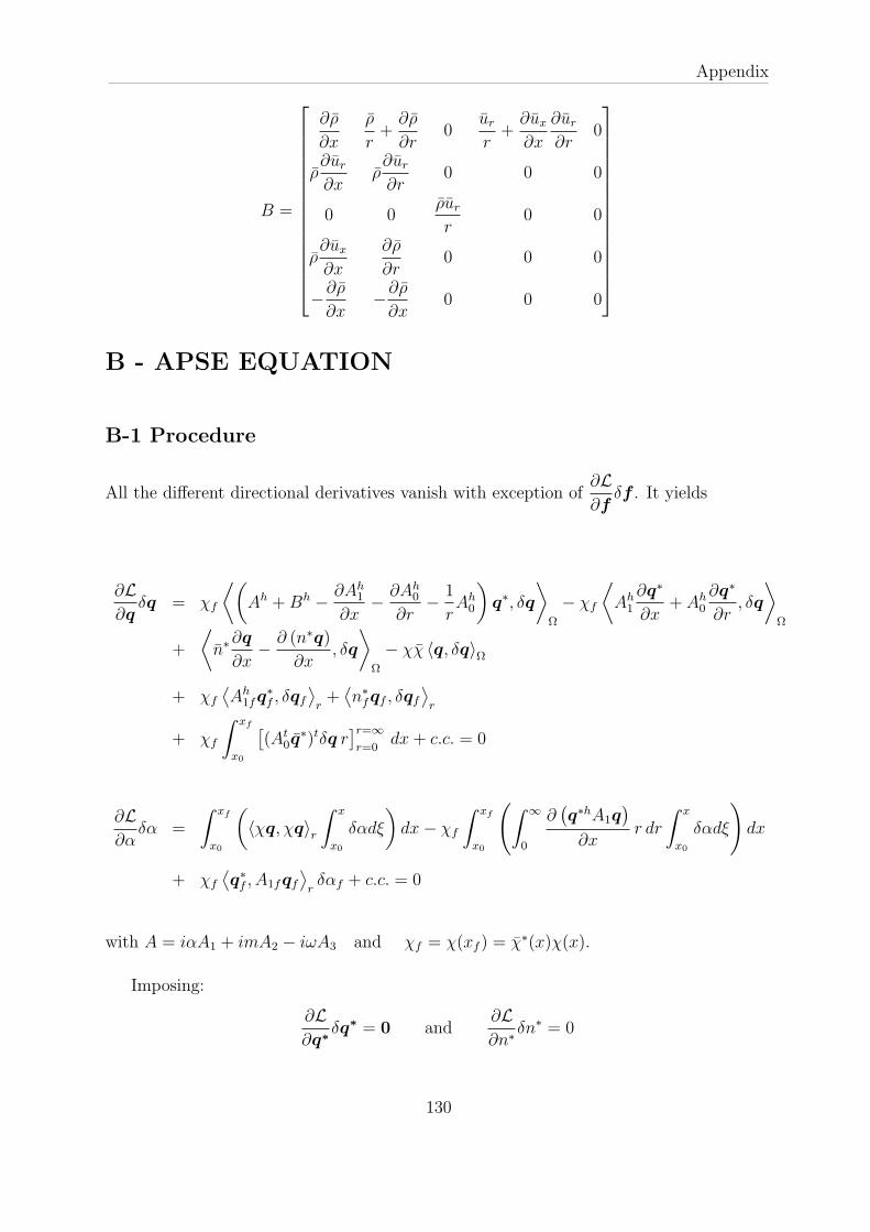
Appendix
B =
∂ρ
∂x
ρ
r+
∂ρ
∂r0
ur
r+
∂ux
∂x
∂ur
∂r0
ρ∂ur
∂xρ∂ur
∂r0 0 0
0 0ρur
r0 0
ρ∂ux
∂x
∂ρ
∂r0 0 0
−∂ρ
∂x−∂ρ
∂x0 0 0
B - APSE EQUATION
B-1 Procedure
All the different directional derivatives vanish with exception of∂L
∂fδf . It yields
∂L
∂qδq = χf
⟨(
Ah +Bh −∂Ah
1
∂x−
∂Ah0
∂r−
1
rAh
0
)
q∗, δq
⟩
Ω
− χf
⟨
Ah1
∂q∗
∂x+ Ah
0
∂q∗
∂r, δq
⟩
Ω
+
⟨
n∗∂q
∂x−
∂ (n∗q)
∂x, δq
⟩
Ω
− χχ 〈q, δq〉Ω
+ χf
⟨
Ah1fq
∗
f , δqf
⟩
r+⟨
n∗
fqf , δqf
⟩
r
+ χf
ˆ xf
x0
[
(At0q
∗)tδq r]r=∞
r=0dx+ c.c. = 0
∂L
∂αδα =
ˆ xf
x0
(
〈χq, χq〉r
ˆ x
x0
δαdξ
)
dx− χf
ˆ xf
x0
(
ˆ
∞
0
∂(
q∗hA1q)
∂xr dr
ˆ x
x0
δαdξ
)
dx
+ χf
⟨
q∗
f , A1fqf
⟩
rδαf + c.c. = 0
with A = iαA1 + imA2 − iωA3 and χf = χ(xf ) = χ∗(x)χ(x).
Imposing:
∂L
∂q∗δq∗ = 0 and
∂L
∂n∗δn∗ = 0
130

Appendix
we obtain respectively Eq. 2.26 and Eq. 2.33.
B-2 Adjoint Parabolized Stability Equations
Since all variations are arbitrary, except at boundaries where the conditions are fixed
(such as, for example, at x = x0).
• the different integrals vanish if the following Euler-Lagrange equations are satisfied:
L∗
PSEq∗ = g(q, n∗)
with
L∗
PSE = −1
rA0
h + Ah +Bh −∂Ah
1
∂x−
∂Ah0
∂r− Ah
1
∂
∂x− Ah
0
∂
∂r
and
g(q, n∗) =1
χf
[
(n∗ − n∗)∂q
∂x+
(
∂n∗
∂x+ χχ
)
q
]
• closing relation:
〈χq, χq〉r +
ˆ
∞
0
(
χf
∂(
q∗hA1q)
∂x
)
r dr + c.c. = 0
It is equation 3.28.
• terminal conditions:
χf
ˆ
∞
0
q∗hf A0fqf r dr + c.c. = 0 and χfA
h1fq
∗
f + n∗
fqf + c.c. = 0
131
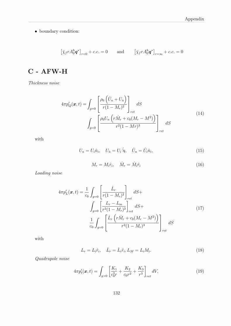
Appendix
• boundary condition:
[
χfrAh0q
∗]
r=0+ c.c. = 0 and
[
χfrAh0q
∗]
r=∞+ c.c. = 0
C - AFW-H
Thickness noise
4πp′Q(x, t) =
ˆ
g=0
ρ0
(
Un + Un
)
r(1−Mr)2
ret
dS
ˆ
g=0
ρ0Un
(
rMr + c0(Mr −M2))
r2(1−Mr)3
ret
dS
(14)
with
Un = Uini, Un = Ui˙in, Un = Uini, (15)
Mr = Miri, Mr = Miri (16)
Loading noise
4πp′L(x, t) =1
c0
ˆ
g=0
[
Lr
r(1−Mr)2
]
ret
dS+
ˆ
g=0
[
Lr − Lm
r2(1−Mr)2
]
ret
dS+
1
c0
ˆ
g=0
Lr
(
rMr + c0(Mr −M2))
r2(1−Mr)3
ret
dS
(17)
with
Lr = Liri, Lr = Liri, LM = LiMi. (18)
Quadrupole noise
4πp′t(x, t) =
ˆ
g>0
[
K1
c20r+
K2
c0r2+
K3
r3
]
ret
dV, (19)
132
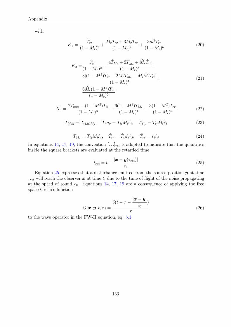
Appendix
with
K1 =Trr
(1−Mr)2+
MrTrr + 3MrTrr
(1−Mr)4+
3m2rTrr
(1−Mr)5(20)
K2 =Tii
(1−Mr)2−
4TMr+ 2TMr
+ MrTii
(1−Mr)3+
3[(1−M2)Trr − 2MrTMr−MiMrTrr]
(1−Mr)4+
6Mr(1−M2)Trr
(1−Mr)5
(21)
K3 =2Tmm − (1−M2)Tii
(1−Mr)3−
6(1−M2)TMr
(1−Mr)4+
3(1−M2)Trr
(1−Mr)5(22)
TMM = TijMiMj, Tmr = TijMirj, TMr
= TijMirj (23)
TMr= TijMirj, Trr = Tij rirj, Trr = rirj (24)
In equations 14, 17, 19, the convention [. . .]ret is adopted to indicate that the quantitiesinside the square brackets are evaluated at the retarded time
tret = t−|x− y(τret)|
c0(25)
Equation 25 expresses that a disturbance emitted from the source position y at timeτret will reach the observer x at time t, due to the time of flight of the noise propagatingat the speed of sound c0. Equations 14, 17, 19 are a consequence of applying the freespace Green’s function
G(x,y, t, τ) =δ(t− τ −
|x− y|
c0)
r(26)
to the wave operator in the FW-H equation, eq. 5.1.
133

Appendix
134