Embed Size (px)
Citation preview
Laboratoire d'Economie d'Orléans – UMR CNRS 6221 Faculté de Droit, d'Economie et de Gestion, Rue de Blois, B.P. 6739 – 45067 Orléans Cedex 2 - France
Tél : 33 (0)2 38 41 70 37 – 33 (0)2 38 49 48 19 – Fax : 33 (0)2 38 41 73 80 E-mail : [email protected] - http://www.univ-orleans.fr/DEG/LEO
Document de Recherche
n° 2008-24
« Regional Growth and Convergence : Heterogeneous Reaction Versus Interaction in Spatial Econometric
Approaches »
Cem ERTUR Julie LE GALLO
Regional growth and convergence: Heterogeneous reaction versus interaction in
spatial econometric approaches
Cem Ertur Laboratoire d'Economie d’Orléans, Faculté de Droit d’Economie et de Gestion, Rue de Blois, B.P. 6739, 45067 Orléans Cedex 2, France, [email protected]
Julie Le Gallo Centre de Recherche sur les Stratégies Economiques, Université de Franche-Comté, 45D, avenue de l’Observatoire, 25030 Besançon Cedex, France, [email protected] Abstract This paper presents various approaches dealing with heterogeneous reaction combined with interaction between neighboring units of observation developed in the spatial econometric literature, in the framework of cross-sectional models, and applied to the study of growth and convergence processes. We present the main econometric specifications capturing discrete or continuous spatial heterogeneity: the spatial regimes model and the locally linear, geographically weighted regression (GWR). We then examine how these specifications can be extended to further allow for spatial autocorrelation. Keywords: spatial econometrics, heterogeneity, spatial autocorrelation JEL: C21, O47, R11 Résumé La présence d'effets spatiaux, hétérogénéité et dépendance spatiales, dans les processus de croissance et de convergence régionales a récemment été mis en évidence dans la littérature. Cet article est une introduction aux différentes approches méthodologiques, développées en économétrie spatiale dans le contexte des modèles en coupe transversale et appliquées à l'étude des processus de croissance, dont l'objectif est de traiter le problème de l'hétérogénéité combinée à l'interaction entre unités d'observations voisines. Les spécifications d'économétrie spatiale intégrant l'hétérogénéité spatiale discrète ou continue, en particulier le modèle à régimes spatiaux et le modèle de régression localement linéaire, géographiquement pondéré (GWR) sont d'abord présentées. Deux approches alternatives permettant la prise en compte simultanée de l'hétérogénéité spatiale continue et de la dépendance spatiale sont ensuite développées. Mots-clés : Econométrie spatiale, hétérogénéité, autocorrélation spatiale JEL : C21, O47, R11
- - 1
Regional growth and convergence: Heterogeneous reaction versus interaction in
spatial econometric approaches
Cem Ertur Laboratoire d'Economie d’Orléans, Faculté de Droit d’Economie et de Gestion, Rue de Blois, B.P. 6739, 45067 Orléans Cedex 2, France, [email protected]
Julie Le Gallo Centre de Recherche sur les Stratégies Economiques, Université de Franche-Comté, 45D, avenue de l’Observatoire, 25030 Besançon Cedex, France, [email protected]
“Notwithstanding the general rule that ‘everything affects everything else’, it is often useful to assess whether
the dominant effects are caused by reaction to external forces or by interaction between (neighbouring)
individuals.”1 (Cliff and Ord, 1981, p.141)
1. Introduction Over the last few years, numerous studies have been carried out to analyze economic
convergence among countries or regions and recognizing at the same time the need to include
spatial effects (Abreu et al., 2005; Ertur et al., 2006; Fingleton and López-Bazo, 2006). For
example, a large number of contributions analyzing the β-convergence hypothesis impose
strong homogeneity assumptions on the cross-economy growth process, since each economy
is assumed to have an identical aggregate production function. However, modern growth
theory suggests that different economies should be described by distinct production functions.
In other words, β-convergence models should account for parameter heterogeneity (Brock
and Durlauf, 2001; Durlauf, 2001; Durlauf et al., 2005; Temple, 1999). Evidence of
parameter heterogeneity has been found in non-spatial models using different statistical
methodologies, such as in Canova (2004), Desdoigts (1999), Durlauf and Johnson (1995) and
Durlauf et al. (2001). Each of these studies suggests that the assumption of a single linear
statistical growth model applying to all countries or regions is incorrect.
Moreover, Ertur et al. (2007) argue that in a spatial context, similarities in legal and
social institutions, as well as culture and language might create spatially local uniformity in
economic structures, leading to situations where rates of convergence are similar for
1 The terms reaction and interaction are emphasised by the authors.
- - 2
observations located nearby in space. Parameter heterogeneity is then spatial in nature and
estimating a “global” relationship between growth rate and initial per capita income, which
applies in the same way over the whole study area, doesn’t allow capturing the important
convergence rate differences that might occur in space.
The instability in space of economic relationships illustrated by this example is called
spatial heterogeneity. This phenomenon can be observed at several spatial scales: behaviors
and economic phenomena are not similar in the center and in the periphery of a city, in an
urban region and in a rural region, in the “West” of the enlarged European Union and in the
“East”, etc. In an econometric regression, these differences may appear in two ways: with
space-varying coefficients and/or space-varying variances. The first case is labeled structural
instability of regression parameters, which vary systematically in space. The second case
pertains to heteroscedasticity, which is a frequent problem in cross-sections.
Spatial heterogeneity is one of the two spatial effects analyzed by the field of spatial
econometrics (Anselin, 1988). This effect operates through the specification of the reaction of
the variable of interest to explanatory variables or the specification of its variance. The other
is spatial autocorrelation, or the coincidence of value similarity and locational similarity. It is
aimed at capturing interaction between neighboring units of observation. This effect is also
highly relevant in growth and convergence analysis. Indeed, as pointed out by Easterly and
Levine (2001), there is a tendency for all factors of production to gather together, leading to a
geographic concentration of economic activities. As a consequence, any empirical study on
growth and convergence should explicitly acknowledge this phenomenon of spatial
interdependence between regions or countries. Moreover, as pointed out by Abreu et al.
(2005), this distinction between spatial heterogeneity and spatial dependence can be related to
two different ways of modeling spatial data in growth regressions: models of absolute
location and models of relative location. Absolute location refers to the impact of being
located at a particular point in space (continent, climate zone) and is usually captured through
dummy variables. Relative location refers to the effect of being located closer or further
away from other specific countries or regions.
While spatial autocorrelation has been the focus of several literature reviews (Anselin
and Bera, 1998; Anselin, 2006 for instance), spatial heterogeneity is much less presented per
se. In the convergence context, spatial effects have also already been the focus of several
literature reviews: Abreu et al. (2005), Rey and Janikas (2005) and Fingleton and López-Bazo
(2006). However, these studies focus more on the appropriate treatment and interpretation of
spatial autocorrelation in convergence models and/or distribution dynamic approaches. Abreu
- - 3

et al. (2005) present some models of absolute location but limit their discussion to models for
discrete spatial heterogeneity, while several recent studies extend these to models with
continuous space-varying coefficients (Bivand and Brunstad, 2005; Eckey et al., 2007; Ertur
et al., 2007).
In this context, this chapter is double-aimed. First, we present the main econometric
specifications capturing spatial heterogeneity, or models of absolute locations, in the
terminology of Abreu et al. (2005). Here, we focus on structural instability, as well as on
specific forms of heteroscedasticity and we provide examples of applications pertaining to
growth econometrics. Secondly, we examine how these specifications can be extended to
further allow for spatial autocorrelation in models of heterogeneous reaction. Concerning this
second point, it should be noted that spatial autocorrelation and spatial heterogeneity entertain
complex links. First, as pointed out by Anselin and Bera (1998) and Abreu et al. (2005), there
may be observational equivalence between these two effects in a cross-section. Indeed, a
cluster of high-growth regions may be the result of spillovers from one region to another or it
could be due to similarities in the variables affecting the regions' growth. Secondly,
heteroscedasticity and structural instability tests are not reliable in the presence of spatial
autocorrelation. For instance, Anselin and Griffith (1988) show that spatial autocorrelation
affects the size and power of the White and Breusch-Pagan tests of heteroscedasticity.
Anselin (1990a) also provides evidence that the Chow test for structural instability is not
reliable in the presence of spatial autocorrelation. Conversely, spatial autocorrelation tests are
affected by heteroscedasticity (Anselin, 1990b). Thirdly, spatial autocorrelation is sometimes
the result of an unmodelled parameter instability (Brunsdon et al., 1999a). In other words, if
space-varying relationships are modelled within a global regression, the error terms may be
spatially autocorrelated. We detail some of these issues in the growth and convergence
context in this chapter.
Note that heterogeneity can also be modeled using spatial panel data models.
However, this alternative approach will not be considered here as a complete survey is
provided by Anselin et al. (2008). Therefore, we focus here exclusively on the cross-sectional
approach. Also, due to space constraints, we do not review distribution dynamics approaches
to economic convergence and focus exclusively on spatial econometric modeling issues.2
Bearing these different elements in mind, this chapter is organized as follows. The next
section presents the specifications allowing for discrete heterogeneity, i.e. when different
parameters are estimated following spatial regimes. The following sections are devoted to
2 See Rey and Janikas (2005) and Rey and Le Gallo (2008) for such a review.
- - 4
continuous heterogeneity models: geographically-weighted regressions (section 3) and their
generalizations (section 4). Section 5 concludes and provides some research directions.
2. Discrete spatial heterogeneity Spatial instability of the parameters necessitates specifications in which the
characteristics of each spatial observation are taken into account. Therefore, we could specify
a different relationship for each zone i of the sample:
iiii xy εβ += ' Ni …,1= (1)
where iy represents the observation of the dependent variable for zone i; is the
vector including the observations for the K explanatory variables for zone i. It is associated to
'ix (1, )K
iβ , a vector of parameters to be estimated. Finally, in general, the variance differs with
i:
( ,K
i iid
1)
(0, 2 )iε σ∼ . Of course, given N observations, it is not possible to estimate consistently
NK parameters and N variances: this is the incidental parameter problem. Therefore, a spatial
structure for the data must be specified. The spatial variability of the mean of the coefficients
of a regression can be discrete, if systematic differences between regimes are observed, or it
can be continuous over the whole area. Note that, similarly to panel data models, a random
variation could also be specified, under the form of a random coefficients model. As this
possibility is not explicitly spatial, it will not be further considered in this chapter.3
Consider first the models for discrete spatial heterogeneity, which have been applied
extensively to study the club convergence hypothesis in a spatial context. Assume that the
area under study is divided into several regimes. If only one variable is under study, a spatial
ANOVA can be undertaken in order to investigate whether the mean of this variable is
different across the regimes. Spatial versions of ANOVA have also been suggested by
Griffith (1992).
3 See Anselin (1988) for further details on the random coefficients model in a cross-sectional context. See also Brunsdon et al. (1999b) for a comparison between random coefficients models and the GWR model, which is considered in section 3 of this chapter.
- - 5
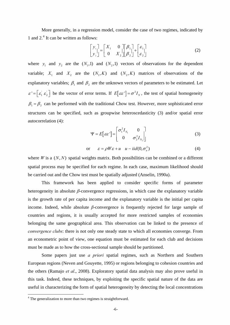
More generally, in a regression model, consider the case of two regimes, indicated by
1 and 2.4 It can be written as follows:
(2) ⎥⎦
⎤⎢⎣
⎡+⎥
⎦
⎤⎢⎣
⎡⎥⎦
⎤⎢⎣
⎡=⎥
⎦
⎤⎢⎣
⎡
2
1
2
1
2
1
00
2
1
εε
ββ
XX
yy
where 1y and 2y are the and vectors of observations for the dependent
variable; 1
1( ,1)N 2( ,1N )
X and 2 X are 1, ) 2( , )N K matrices of observations of the
explanatory variables; 1
the (N K and
β and 2β are the unknown vectors of parameters to be es t
' '1 2'
timated. Le
ε ε ε⎡ ⎤= ⎣ ⎦ be the vector of error terms. If [ ] 2' NE Iεε σ= , the test of spatia geneity
1 2
l homo
β β= can be performed with the traditional Chow test. However, more sophisticated error
structures can be specified, such as groupwise heteroscedasticity (3) and/or spatial error
autocorrelation (4):
[ ] 1
2
21
22
0'
0N
N
IE
I
σεε
σ
⎡ ⎤Ψ = = ⎢ ⎥
⎢ ⎥⎣ ⎦ (3)
or 2(0, )uW u u iidε ρ ε σ= + ∼ (4)
where W is a ( , )N N spatial weights matrix. Both possibilities can be combined or a different
spatial process may be specified for each regime. In each case, maximum likelihood should
be carr
ecisions
must b
ied out and the Chow test must be spatially adjusted (Anselin, 1990a).
This framework has been applied to consider specific forms of parameter
heterogeneity in absolute β-convergence regressions, in which case the explanatory variable
is the growth rate of per capita income and the explanatory variable is the initial per capita
income. Indeed, while absolute β-convergence is frequently rejected for large sample of
countries and regions, it is usually accepted for more restricted samples of economies
belonging the same geographical area. This observation can be linked to the presence of
convergence clubs: there is not only one steady state to which all economies converge. From
an econometric point of view, one equation must be estimated for each club and d
e made as to how the cross-sectional sample should be partitioned.
Some papers just use a priori spatial regimes, such as Northern and Southern
European regions (Neven and Gouyette, 1995) or regions belonging to cohesion countries and
the others (Ramajo et al., 2008). Exploratory spatial data analysis may also prove useful in
this task. Indeed, these techniques, by exploiting the specific spatial nature of the data are
useful in characterizing the form of spatial heterogeneity by detecting the local concentrations
4 The generalization to more than two regimes is straightforward.
- - 6
of similar values, by using Getis-Ord statistics (Ord and Getis, 1995) or LISA statistics
(Anselin, 1995). For example, Le Gallo and Ertur (2003) show that the spatial distribution of
per capita GDP in Europe before the recent enlargement is characterized by a strong North-
South polarization. More recently, Ertur and Koch (2006a) show that this polarization scheme
is replaced by a new West-East polarization scheme if the last enlargement of the European
Union to Central and Eastern European countries is taken into account. These polarization
schemes represent evidence in favor of the existence of at least two spatial regimes in the
European regions. This information is then used to estimate β-convergence models with
spatial regimes as in equation 2 (Fischer and Stirböck, 2006; Le Gallo and Dall’erba, 2006),
possibly associated with groupwise heteroscedasticity, and spatially autocorrelated error
terms as in equations 3 and 4 (Ertur et al., 2006), or a spatial lag of the form Wy (Dall’erba
and Le Gallo, 2008). However, as pointed out by Rey and Janikas (2005), the existing
specification search procedures should be extended to be able to distinguish between spatial
dependence and spatial heterogeneity while formal specification search strategies for spatial
heterog
(1999) non-parametric
specifi tion by allowing a spatial lag term or a spatial error process.
eneity have yet to be suggested.
While non-spatial papers use endogenous detection methods, such as regression trees
(Durlauf and Johnson, 1995), it should be emphasized that a technique allowing for an
endogenous estimation of regimes together with taking into account of spatial autocorrelation
stills needs to be developed (Anselin and Cho, 1998). A first step in this direction is the paper
by Basile and Gress (2005) who suggest a semi-parametric spatial autocovariance
specification that simultaneously takes into account the problems of non-linearities and
spatial dependence. In that purpose, they extend Liu and Stengo’s
ca
If no information is available on spatial regimes, or if one thinks that the mean of a
variable or that the regression coefficients do not change brutally between regimes, it is
preferable to use specifications allowing for continuous spatial variations across the whole
study area. The urban literature has frequently used trend surface analysis models and/or the
expansion method. In the first case, the coordinates of each location (such as latitude and
longitude) are added in the regression model so that the main characteristics of the regression
surface, such as simple “North-South” or “East-West” drifts or more complex drifts for
higher-order functions can be described (Agterberg, 1984). In the second case, the regression
coefficients are deterministic (Casetti, 1972) or stochastic (Anselin, 1988) functions of
expansion variables, such as the coordinates of each location. However, the expansion
- - 7
method suffers from two main drawbacks (Fotheringham et al., 2000, 2004). First, these
techniques only allow capturing trends in relations in space, the complexity of these trends
being determined by the complexity of the specified expansion equations. The estimates of
the parameters may therefore obscure important local variations to the broad trends
represented by the expansion equations. Secondly, the form of the expansion equations must
be specified a priori. To overcome these problems, Geographically Weighted Regression
(GWR) has been developed and applied in several papers focusing on economic convergence.
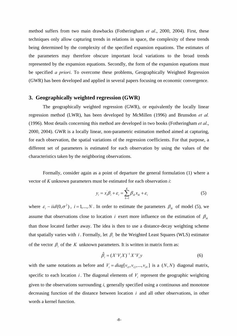
3. Ge
servation by using the values of the
characteristics taken by the neighboring observations.
ation (1) where a
K unknown parameters must be estimated for each observation
ographically weighted regression (GWR) The geographically weighted regression (GWR), or equivalently the locally linear
regression method (LWR), has been developed by McMillen (1996) and Brunsdon et al.
(1996). Most details concerning this method are developed in two books (Fotheringham et al.,
2000, 2004). GWR is a locally linear, non-parametric estimation method aimed at capturing,
for each observation, the spatial variations of the regression coefficients. For that purpose, a
different set of parameters is estimated for each ob
Formally, consider again as a point of departure the general formul
vector of i:
'K
y x x1
i i i i ik ik ik
β ε β ε=
= + = +∑ (5)
where 2(0, )i iidε σ∼ , 1,...,i N= . In order to estimate the parameters ikβ of model (5), we
assume that observations close to location i exert more influence on the estimation of ikβ
than those located farther away. The idea then to use a distance-decay weighting scheme
that spatially ries wit i . Formally, let i
h
is
va β be the Weighted Least Squares (WLS) estim
f the
ator
vector iβ of the K unknown para s. It is written
i
meter in matrix form as: o
ˆi
1( ' ) 'iX V X X V y−=β
with the same notations as before and 1 2[ , .., ]i i i iNV diag v v v
(6)
,.= is a ( , )N N diagonal matrix,
specific to each location i . The diagonal elements of iV represent the geographic weighting
given to the observations surrounding i, generally specified using a continuous and monotone
decreasing function of the distance between lo
words a kernel function.
cation i and all other observations, in other
- - 8
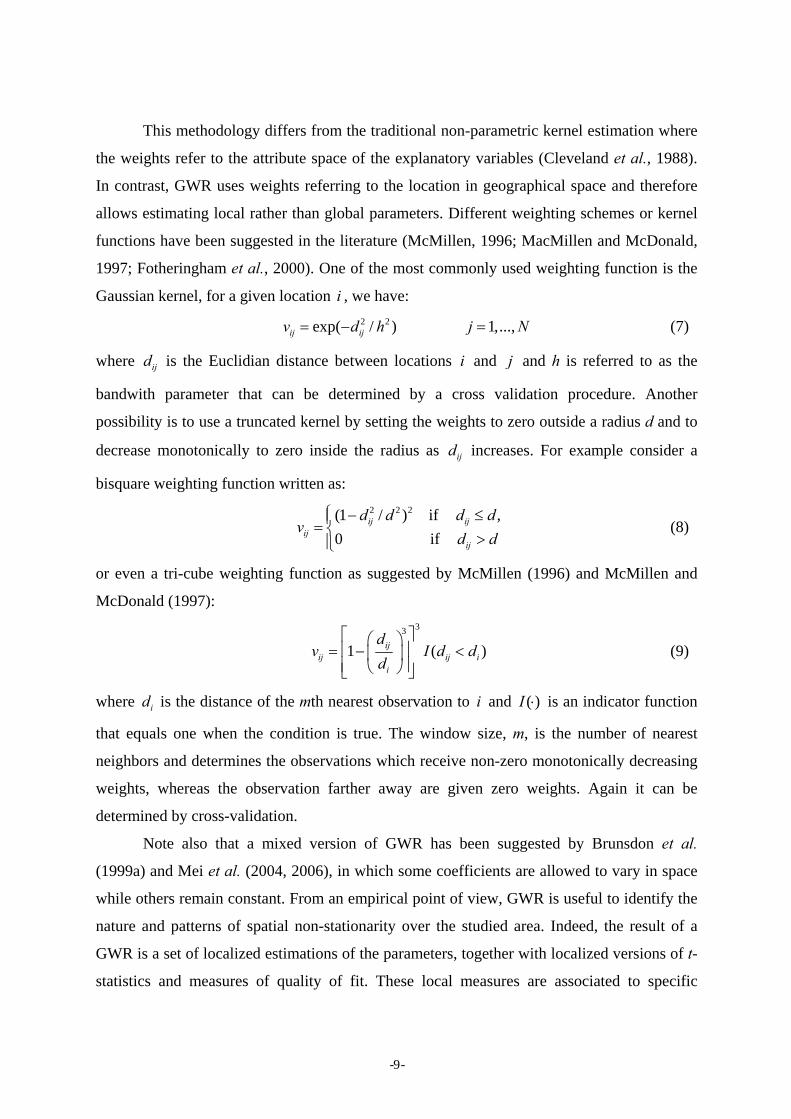
This methodology differs from the traditional non-parametric kernel estimation where
the weights refer to the attribute space of the explanatory variables (Cleveland et al., 1988).
In contrast, GWR uses weights referring to the location in geographical space and therefore
allows estimating local rather than global parameters. Different weighting schemes or kernel
functions have been suggested in the literature (McMillen, 1996; MacMillen and McDonald,
1997; Fotheringham et al., 2000). On of the mose t commonly used weighting function is the
aussian kernel, for a given location we havG e: i ,
2 2exp( / )ij ijv d h= − 1,...,j N= (7)
where ijd is the Euclidian distance between locations i and j and h is referred to as the
bandwith parameter that can be determined by a cross validation procedure. Another
possibility is to use a truncated kernel by setting the we hts to zero outside a radius d and to
decrease monotonically to zero inside
ig
ijthe radius as increases. For example consider a
bisquare weighting function written as:
(8)
eighting function as suggested by McMillen (1996) and McMillen and
McDonald (1997):
d
2 2 2(1 / ) if ,ij ijij
d d d dv
⎧ − ≤⎪= ⎨0 if ijd d>⎪⎩
or even a tri-cube w
33
1 (ijij ij i )
dv I d d
⎡ ⎤⎛ ⎞⎢ ⎥= − <⎜ ⎟ (9)
id⎢ ⎥⎝ ⎠⎣ ⎦
where id is the distance of the mth nearest observation to i and ( )I ⋅ is an indicator function
that equals one when the condition is true. The window size, m, is the number of nearest
neighbors and determines the observations which receive non-zero monotonically decreasing
weights, whereas the observation farther away are given zero weights. Again it can be
determined by cross-validation.
Note also that a mixed version of GWR has been suggested by Brunsdon et al.
(1999a) and Mei et al. (2004, 2006), in which some coefficients are allowed to vary in space
while others remain constant. From an empirical point of view, GWR is useful to identify the
nature and patterns of spatial non-stationarity over the studied area. Indeed, the result of a
GWR is a set of localized estimations of the parameters, together with localized versions of t-
statistics and measures of quality of fit. These local measures are associated to specific
- - 9
locations, so that they can be mapped to illustrate the spatial variations of the relationship
under s
traces of remaining spatial nonstationarity can be found. However,
they do
speed increases from south to north. The half-life period ranges
from le
ent
and percentage of fixed asset invested in State Owned Enterprises, show significant spatial
non-sta
tudy (Mennis, 2006).
We review here some of the most recent contributions related to regional growth and
development. Bivand and Brunstad (2005), in their paper focusing on the detection of spatial
misspecification in growth models using the R environment, estimate a conditional
convergence model including a spatially lagged endogenous variable and spatial regimes for
Western Europe over the period 1989-1999. They find support for the role of agricultural
subsidies in accounting for variations in regional growth. Higher levels of agricultural support
are associated with lower levels of growth, even after some measure of human capital has
been introduced. They also consider a GWR specification to essentially ascertain their results
by exploring whether any
not fully interpret their GWR results due to some methodological problems which
will be discussed below.
Another attempt to use GWR regressions in the regional growth context has been
made by Eckey et al. (2007) in a paper focusing on regional convergence in Germany over
the period 1995-2002 using disaggregated data on a sample of 180 labor market regions. They
estimate a model based on Mankiw et al. (1992) allowing all coefficients, especially the rate
of convergence, to vary across regions. Each region seems to converge using both absolute
and conditional convergence models as the local convergence parameters are all negative.
The value of the convergence
ss than 20 years for some regions in northern Germany to more than 50 years for
regions in southern Bavaria.
Finally, let us mention the contribution of Yu (2006) to the regional development
literature in his study of the development mechanisms in the Greater Beijing Area using
GWR. The analysis reveals two results: first, regional development mechanisms in the
Greater Beijing Area, such as Foreign Direct Investment, per capita fixed asset investm
tionarity; and second, development mechanisms have strong local characteristics.
From a methodological point of view, several problems plaguing GWR estimation and
inference must be mentioned here. First, concerning statistical inference, in order to know
whether the local estimations of parameters are significantly different between them and
compared to the OLS estimator, parametric tests have been suggested by Brunsdon et al.
- - 10
(1999a) and Leung et al. (2000a). Secondly, LeSage (2004) argues that the presence of
aberrant observations due to spatial enclave effects, shifts in regime or outliers can exert
undue influence on the GWR estimates. Therefore, he suggests a Bayesian estimation
approach that detects these observations and downweights them to lessen their influence on
the estimates. Thirdly, Wheeler and Tiefelsdorf (2005) point out that the local regression
estimates are potentially collinear even if the underlying exogenous variables in the data
generating process are uncorrelated. This collinearity can degrade coefficient precision in
GWR and lead to counter-intuitive signs for some regression coefficients. Using Monte-Carlo
simulations, Wheeler and Calder (2007) show that Bayesian models with spatially varying
coefficients (Gelfand et al., 2003) provide more accurate regression coefficients. Finally,
facing the various inference problems encountered by GWR, Páez et al. (2002a) place GWR
in a different statistical framework, interpreting GWR as a spatial model of error variance
heterogeneity, i.e. heteroscedasticity. The variance of the error term is defined as an
exponential function of the squared distance between two observations and has then a precise
geographical interpretation. While this approach is a special case of the well-known
multiplicative heteroscedasticity model developed by Harvey (1976), it nevertheless
represe
nally, Pace and LeSage (2004) introduce
nts a real breakthrough in the GWR literature and allows the derivation of formal
heterogeneity tests.
There still remains an important methodological problem pointed out by Páez et al.
(2002b) and Pace and LeSage (2004): spatial dependence may not be eliminated even at the
optimal bandwidth as it is often assumed in the related literature where it is considered that
spatial dependence is mainly due to inadequately modeled spatial heterogeneity. Actually,
this methodological problem is related to the complex links between spatial heterogeneity and
spatial dependence often underlined and more generally to the reaction versus interaction
debate first pointed out by Cliff and Ord (1981, p.141) in the spatial econometrics literature.
Even when heterogeneous reactions are taken into account as in the GWR framework, it
could be the case that there are also interactions between units of observation that should be
modeled with a spatially dependent covariance structure. Therefore, Brunsdon et al. (1998)
have proposed to include the spatially lagged endogenous variable in the GWR model and
Leung et al. (2000b) have suggested a test of spatial autocorrelation of the GWR residuals.
Moreover, Páez et al. (2002b) formulate a general model of spatial effects that includes as
special cases GWR with a spatially lagged endogenous variable (GWR-SL) and GWR with
spatially autocorrelated residuals (GWR-SEA). Fi
- - 11
spatial autoregressive local estimation (SALE) based on a computationally competitive
recursi
4. Generalized GWR We first consider here a straightforward generalization of the m
o added in the mo
ve maximum likelihood estimation method.
odel proposed by Páez
et al. (2002b) where the spatial lags of the explanatory variables are als del:
1
2
y W Y XW uρ β ε
ε λ ε⎧ = + +⎪⎨
= +⎪⎩ (10)
where (0, )u N Ω∼ is the vector of the dependant variable; ( ,1)N [ ]1X X W Xι=; y with
ι a s;( 1)N × vector of one X a ( , ( 1))N K − matrix of the explanatory variables excluding
the constant and 1W X its spatial lag; β is the ((2( 1) 1),1)K − + vector of the associated
parameters to be estimated; ρ and λ are the spatial autoregressive param 2W
ed spatial weights matrices;
eters; and 1W
are row-standardiz Ω is the diagonal covariance m the atrix of
error term u with elements denoted by iiω . More precisely, they adopt a specific form for
o
this
covariance matrix as f llows: 2GσΩ = and define its elements as 2ii i i
0ij
( ,g z )ω σ γ= and
ω = for i j≠ . Hence the variance of the error term u is a function of a ( ,1)p vector of
known variables iz , an unobservable parameter vector γ and an unknown constant 2σ . The
geographically weighted specification is then obtained by defining a variance model of the
exponential form as in Páez et al. (2002a):
oi o oi o oig a dγ γ= (11)
which is a special case of the previous form lation with 1
2( , ) exp( )
u p = and where the observable
variable oid is the distance between location o and observation i for 1,...,i N= . This
particular geographical specification locational heterogeneity
by Páez . (2002a, 2002b). The parameter
of the error variance is called
et al oγ is then th called kernel in the
tradition GWR literature. The generalized GWR model can therefore be defined in terms of
rameters as f lows:
e so- bandwidth
local pa ol
1o o o o oW y X A y X
2o o o o o o
oyW u B u
ρ β ε β ε⎧= + + = +⇒ ⎨
ε λ ε ε⎧⎨
= + =⎩ ⎩(12)
where 1o oA I Wρ= − ; 0 2oB I Wλ= − and . Note that and 2o o(0, )o ou N Gσ∼ oA B depend on
local parameters oρ and oλ respectively and oG depends on the local parameter oγ .
- - 12
If no spatial lags of the explanatory variab e allow . les ar ed, i.e [ ]X Xι= , it is easily
seen that when 0o oρ λ= = then o oA B I= = , and this model reduces to the standard GWR
model; when 0oλ = then oB I= , and we obtain a GWR model which includes the spatially
lagged endogenous variable (GWR-SL); when 0oρ = then oA I= , and we obtain a GWR
model with spatially autocorrelated errors (GWR-SEA). Páez et al. (2002b) propose to
estimate those two generalized GWR models by iterated maximum likelihood. They also
derive formal Lagrange multiplier tests against severa ication including a
and tests for locational heterogeneity in global models in presence of a spatially lagged
endogenous variable or in presence of spatial error autocorrelation. More flexibility is
allowed in the specification of the model by using
l form sspecif
test for om autocorrelation in GWR models
of mi
itted endogenous spatial lag, a test for spatial error
[ ]1X X W Xι= which also includes
spatial
eneity and spatial autocorrelation in an efficient way
sing recursive spatial maximum likelihood. Their appro
sequence of N spatial autoregressions, one for each observation, using a range of sub-sample
lags of the explanatory variables; the estimation method as well as all of the tests
proposed by Páez et al. (2002b) may then be straightforwardly generalized to such a model at
practically no cost.
An alternative approach to the generalization of the GWR model is proposed by Pace
and LeSage (2004): spatial autoregressive local estimation (SALE) allows to simultaneously
considering spatial parameter heterog
u ach is based on the estimation of a
sizes. Consider the spatial Durbin Model (SDM) where the spatial lags of the explanatory
variables are also added in the model:
y X Wyβ ρ ε= + + (13)
here the same notations as before and assuming that w 2 )NI . The concentrated log-(0,Nε σ∼
likelihood function for the global SDM model is then written as follows, for fixed ρ ,
omitting the constant term (Pace and Barry, 1997):
[ ]( ) ln ln ( )2NL I W SSEρ ρ ρ= − − (14)
where SSE denotes the sum of squared residuals. Since the maximum likelihood estimation of
the global SDM model relies on least squares estimates and the computation of the log-
determinant, a recursive spatial es method is conceivable. Pace and LeSage (2004,
ive spatial maximum likelihood approach based on recursive
timation
p. 35) develop such a recurs
- - 13
m bined with recursive least atrix decompositions used to compute log-determinants com
squares. More specifically, their approach to compute the log-determinant that appears in (14)
relies on the decomposition of ( )I Wρ− into two triangular matrices L and U , i.e.
( )I W LUρ− = , known as the LU decomposition. It is straightforward to show that:
1
ln ln lnN
jjj
I W U uρ=
− = =∑ (15)
ere jju is the diagonal element in position ( , )wh j j ix U . Pace and LeSage (2004)
underline ive nature of the LU decom on
of the matr
the recurs siti to de a spatial autoregressive
local estim
po sign
ation method for the SDM model. Indeed, the log-determinant of the successive
sub-matrices are the successive sums of the logarithms of the diagonal elements of the matrix
U , so that we have: 11u for the first sub-matrix, 11 22ln lnu u+ for the second one, and m
generally 1ln jjj
u=∑ for the mth sub-matrix with m n
ore
m≤ .
To implement the estimation procedure for observation i , note that the observations in
the sample are first ordered with respect to their distance to observation i . Also, the rows and
colum i . ns of the weights matrix are conse atrix by
Suppose now that we want to consider sub-samples of size equal to corresponding to the
ation . More specifically, the local profile log-likelihood
nction of Pace and LeSage (2004) is written as follows (omitting the constant term):
quently reordered. Denote that m W
m
im -nearest neighbors to observ
fu
[ ]( ) ln ln ( , )2i i i i iL I W SSE mmρ ρ ρ= − − (16
It can therefore be rewritten as:
)
[ ]1
( ) ln ( ) ln ( ) where2
m
i i i jj ij
mL u SSE m m nρ ρ ρ=
= − ≤∑ (17
sive method of Pace and Barry (1997) is then used
, )
The recur to estimate iρ , which may then
be interpreted as the local spatial autocorrelation parameter. We note th these
estimat
at as m N→
es approach the global estimates based on all N observations that would arise from
the global SDM model. The procedure is then repeated for all the observations in the sample
1,...,i N= yielding a sequence of N spatial autoregressions.
A Bayesian variant of this approach, labeled BSALE has been developed in Ertur et
al. (2007) in the empirical regional convergence framework and applied to a sample of 138
European regions over the period 1980-1995. On the one hand, regarding heterogeneity as
- - 14
with the standard GWR approach, the proposed locally linear spatial autoregressive model
partitions the cross-sectional sample observations by treating each location along with
neighboring locations as a sub-sample. This avoids arbitrary decisions regarding how to
partition the sample observations, but allows for variation in the parameter estimates across
all observations. On the other hand, it is assumed that similarities in legal and social
institutions as well as culture and language might give rise to local uniformity in economic
structures, leading to similar local schemes for convergence speeds and thus to a concept of
local convergence. In other words, there should exist spatial clustering in the magnitudes of
the β-convergence parameter estimates. However, the locally linear spatial estimation method
does not impose a priori similar convergence speeds for spatially neighboring observations.
Rather
ugal, Spain, some French regions), are
conver
interpretation of the results in a strict statistical sense.
One common criticism that can be made to most of the applications of GWR or SALE
presented in the growth and convergence literature is the lack of rigorous theoretical
, β-convergence parameters for each region in the sample are estimated based on the
sub-sample of neighboring regions. Furthermore, Bayesian techniques produce robust
estimates with regards to potential outliers and heteroscedasticity of unknown form. A
Markov Chain Monte Carlo (MCMC) estimation method is then developed to implement the
proposed approach.
The econometric results obtained using different sub-sample sizes show clear
evidence that indeed the spatially lagged endogenous variable should be included in the
specification. As the sub-sample size increases, they get larger positive modal values for the
local spatial autocorrelation coefficients. Individual estimates exhibit local spatial dependence
of a sufficiently large magnitude to create bias in standard GWR least-square estimates even
for relatively small sub-sample sizes. Estimated local spatial autocorrelation coefficients also
present a clear country dependent spatial pattern. Concerning the individual β-convergence
parameter estimates, it should be noted that country-level differences are apparent: estimates
change abruptly as one move from one country to another. In addition, there is also
substantial variation between regions within a country. Samples of draws generated during
MCMC sampling are then used to produce confidence intervals. It appears that only 31
regions, mainly located in south-western Europe (Port
ging. All other regions are characterized by non significant estimates. These
conclusions are similar for sub-sample sizes varying from roughly one-fourth to three-fourths
of the sample size. However, it should be noted that the estimates suffer from sample re-use
as in the case of other locally linear non-parametric estimation methods preventing
- - 15
foundations, as the estimated regressions are not derived as reduced forms from structural
theoretical models embedding both continuous spatial parameter heterogeneity and spatial
interaction.5 To our knowledge, Ertur and Koch (2007) is the first attempt to develop such a
theoretical growth model, which leads to the local SDM model as the relevant econometric
reduced form to be estimated. More precisely, their augmented Solow model includes both
physical capital externalities as suggested by the Frankel–Arrow–Romer model and spatial
externalities in knowledge to model technological interdependence. They suppose that
technical progress depends on the stock of physical capital per worker, which is
complementary with the stock of knowledge in the home country. It also depends on the stock
of knowledge in other countries which affects the technical progress of the home country. The
intensity of this spillover effect is assumed to be related to some concept of socio-economic
or institutional proximity, which is captured by exogenous geographical proximity. Their
model provides, as a reduced form, a conditional convergence equation, which is
characterized by complete parameter heterogeneity and which is therefore estimated using
SALE on a sample of 91 countries over the period 1960-1995. Their econometric results
support their model as all the coefficients have the predicted signs and underline spatially
varying
l scale, it would be interesting to figure out what modifications are needed to
adapt them at the regional scale to help to better understand regional growth and convergence
convergence speeds across countries as well as varying coefficients for all other
explanatory variables and their spatial lags as the saving rates and population growth rates.
Ertur and Koch (2006b) extend this model by including human capital as a production
factor following Mankiw et al. (1992) and propose to model human capital externalities along
the lines of Lucas (1988). Technological interdependence is still modeled in the form of
spatial externalities in order to take account of the worldwide diffusion of knowledge across
borders. The extended model also yields a spatial autoregressive conditional convergence
equation including both spatial autocorrelation and parameter heterogeneity as a reduced
form. However, in contrast to Mankiw et al. (1992), their results show that the coefficient of
human capital is low and not significant when it is used as a simple production factor. Further
research is therefore needed to investigate the role played by human capital in growth and
convergence processes. In addition, those models having been developed for countries at the
internationa
processes.
5 Until recently, this criticism was also valid for the simpler spatial specifications of convergence models. Some important contributions by Egger and Pfaffermayr (2006), López-Bazo et al. (2004), Vayá et al. (2004) fill the gap between theoretical and empirical models.
- - 16
5. Co
etric reduced forms that would be
estimated using the spatial econometric toolbox.
, Reidel, Boston.
Anselin L. (2006) Spatial econometrics, in: Mills T.C., Patterson K. (Eds.) Palgrave
Ans
onomics Statistics, Springer-Verlag, Berlin.
ncluding remarks This chapter aimed at presenting various approaches dealing with heterogeneous
reaction eventually combined with interaction between neighboring units of observation
developed in the spatial econometric literature, in the framework of cross-sectional models,
and applied to growth and convergence processes. Discrete and continuous forms of
heterogeneity allowing spatial variations in regressions coefficients have been studied.
Geographically Weighted Regressions have been used in the empirical growth and
convergence literature to model spatial heterogeneity in regression coefficients and their
generalizations taking into account spatial autocorrelation as well as spatial heterogeneity are
especially interesting. Further modeling strategies may include newly developed Bayesian
models with spatially varying coefficients (Gelfand et al., 2003) and neural networks
(Lebreton, 2005). The toolbox of the applied growth researcher is now very diverse and rich.
However, most importantly, we believe that, in further research, more efforts should be
oriented towards developing, especially at the regional scale, spatial structural theoretical
growth models, which would provide the basis of econom
References Abreu M., de Groot H.L.F., Florax R.J.G.M. (2005) Space and growth: a survey of empirical
evidence and methods, Région et Développement, 2005-21, 12-43. Agterberg F. (1984) Trend surface analysis, in: Gaile G.L, Wilmot C.J. (Eds.) Spatial
Statistics and ModelsAnselin L. (1988) Spatial Econometrics: Methods and Models, Kluwer Academic Publishers,
Dordrecht. Anselin L. (1990a) Spatial dependence and spatial structural instability in applied regression
analysis, Journal of Regional Science, 30, 185-207. Anselin L. (1990b) Some robust approach to testing and estimating in spatial econometrics,
Regional Science and Urban Economics, 20, 141-163. Anselin L. (1995) Local indicators of spatial association: LISA, Geographical Analysis, 27,
93-115.
Handbook of Econometrics: Volume 1, Econometric Theory, Palgrave MacMillan, Basingstoke. elin L., Bera A. (1998) Spatial dependence in linear regression models with an introduction to spatial econometrics, in: Ullah A., Giles D.E.A. (Eds.) Handbook of Applied Ec
Anselin L., Cho W.T. (2002) Spatial effects and ecological inference, Political Analysis, 10, 276-297.
Anselin L., Griffith D.A. (1988) Do spatial effects really matter in regression analysis? Papers of the Regional Science Association, 65, 11-34.
- - 17
Anselin L., Le Gallo J., Jayet H. (2008) Spatial panel econometrics, in: Matyas L., Sevestre P. (Eds.) The Econometrics of Panel Data, Kluwer Academic Publishers, Dordrecht,
Bas ional
Biv nstad R.J. (2005) Regional growth in Western Europe: detecting spatial
Bro eview,
Bru a
Brul Science, 39, 497-524.
spatially non-stationary regression
Canova F. (2004) Testing for convergence clubs in income per capita: a predictive density
Cas graphical
Cli . (1981) Spatial Processes: Models and Applications. Pion, London.
econometric analysis, Papers in Regional Science,
De pment and the formation of clubs, Journal
Duncan C., Jones K. (2000) Using multilevel models to model heterogeneity: potential and
Dur metrics, Journal of Econometrics, 100,
Dur -country growth behavior,
Dur J. (2005) Growth empirics, in Aghion P., Durlauf S.N.
Dur al Solow growth model, European
Eas owth
Eckey H.F., Kosfeld R., Turck M. (2007) Regional convergence in Germany: a
Egg
al data analysis, 1995-2000, Annals of Regional Science, 40,
Ertu l spillovers, LEG
Ertual of Applied Econometrics, 22, 1023-1062.
forthcoming. ile R., Gress B. (2005) Semi-parametric spatial auto-covariance models of reggrowth in Europe, Région et Développement, n°21-2005, 93-118. and R.S., Brumisspecification using the R environment, Papers in Regional Science, 85, 277-297. ck W., Durlauf S.N. (2001) Growth empirics and reality, World Bank Economic R15, 229-272. nsdon C., Fotheringham A.S., Charlton M. (1996) Geographically weighted regression:method for exploring spatial nonstationarity, Geographical Analysis, 28, 281-298. nsdon C., Fotheringham A.S., Charlton M. (1999a) Some notes on parametric significance tests for geographically weighted regression, Journal of Regiona
Brunsdon C., Fotheringham A.S., Charlton M. (1999b) A comparison of random coefficient modelling and geographically weighted regression forproblems, Geographical & Environmental Modelling, 3, 47-62.
approach, International Economic Review, 45, 49–77. etti E. (1972) Generating models by the expansion method: Applications to georesearch, Geographical Analysis, 4, 81-91.
Cleveland W.S., Devlin S.J., Grosse E. (1988) Regression by local fitting, methods, properties, and computational algorithms, Journal of Econometrics, 37, 87-114.
ff A.D., Ord J.KDall’erba S., Le Gallo J. (2008) Regional convergence and the impact of European structural
funds over 1989-1999: A spatialforthcoming.
sdoigts A. (1999) Patterns of economic develoof Economic Growth, 4, 305–330.
pitfalls, Geographical Analysis, 32, 279-305. lauf S.N. (2001) Manifesto for a growth econo65–69. lauf S.N., Johnson P.A. (1995) Multiple regimes and crossJournal of Applied Econometrics, 10, 365-384. lauf S.N., Johnson P.A., Temple(Eds.) Handbook of Economic Growth, Elsevier, Amsterdam. lauf S.N., Kourtellos A., Minkin A. (2001) The locEconomic Review, 45, 928-940. terly W., Levine R. (2001) It’s not factor accumulations: stylized facts and grmodels, World Bank Economic Review, 15, 177-219.
geographically weighted regression approach, Spatial Economic Analysis, 2, 45-64. er P., Pfaffermayr M. (2006) Spatial convergence, Papers in Regional Science, 85, 199-215.
Ertur C., Koch W. (2006a) Regional disparities in the European Union and the enlargement process: an exploratory spati723-765. r C., Koch W. (2006b) Convergence, human capital and internationaWorking Paper, n°2006-03. r C., Koch W. (2007) Growth, technological interdependence and spatial externalities: theory and evidence, Journ
- - 18
Ertur C., Le Gallo J., Baumont C. (2006) The European regional convergence process, 1980-1995: do spatial dependence and spatial heterogeneity matter? International Regional
Ert (2007) Local versus global convergence in Europe: A
Fin
Fis al growth and club-convergence;
Fot raphy, Perspectives
Fotying Relationships, Wiley, Chichester.
ing A, 30, 1905-1927.
urnal of the American Statistical Association, 98, 387-
Gri y adjusted N-way ANOVA model, Regional Science and
Ha y,
Le y of the
Le Gallo J., Ertur C. (2003) Exploratory spatial data analysis of the distribution of regional
Leb
Tools
Leu he
Leu among the residuals
Liu growth regressions: a semi-
López-Bazo E., Vayá E., Artis M. (2004) Regional externalities and growth: evidence from
Luc lopment, Journal of Monetary
Ma tion to the empirics of economic
Mc in Chicago: a nonparametric
Mc of employment density in a
Mesion model, Journal of Regional Science, 44, 143-157.
Science Review, 29, 2-34. ur C., Le Gallo J., LeSage J.P.bayesian spatial econometric approach, Review of Regional Studies, 37, 82-108. gleton B., López-Bazo E. (2006) Empirical growth models with spatial effects, Papers in Regional Science, 85, 177-198.
cher M.M., Stirböck C. (2006) Pan-European regionInsights from a spatial econometric perspective, Annals of Regional Science, 40, 693-721. heringham A.S., Brundson C., Charlton M. (2000) Quantitative Geogon Spatial Data Analysis, Sage Publications, London. heringham A.S., Brundson C., Charlton M. (2004) Geographically Weighted Regression: The Analysis of Spatially Var
Fotheringham A.S., Charlton M., Brunsdon C. (1998) Geographically weighted regression: a natural evolution of the expansion method for spatial data analysis, Environment and Plann
Gelfand A.E., Kim H., Sirmans C.F., Banerjee S. (2003) Spatial modelling with spatially varying coefficient processes, Jo396. ffith D.A. (1992) A spatiallUrban Economics, 22, 347-369.
rvey A.C. (1976) Estimating regression models with multiplicative heteroscedasticitEconometrica, 44, 461-465. Gallo J., Dall’erba S. (2006) Evaluating the temporal and spatial heterogeneitEuropean convergence process: 1980-1999, Journal of Regional Science, 46, 269-288.
per capita GDP in Europe, 1980-1995, Papers in Regional Science, 82, 175-201. reton M. (2005) The NCSTAR model as an alternative to the GWR model, Physica A, 355, 77-84.
LeSage J.P. (2004) A family of geographically weighted regression models, in: Anselin L., Florax R.J.G.M., Rey S.J. (Eds.) Advances in Spatial Econometrics: Methodology, and Applications, Springer, Berlin. ng Y., Mei C., Zhang W. (2000a) Statistical tests for spatial non-stationarity based on tgeographically weighted regression model, Environment and Planning A, 32, 9-32. ng Y., Mei C., Zhang W. (2000b) Testing for spatial autocorrelationof the geographically weighted regression, Environment and Planning A, 32, 871-890. Z., Stengos T. (1999) Non-linearities in cross-country parametric approach, Journal of Applied Econometrics¸14, 527-538.
European regions, Journal of Regional Science, 44, 43-73. as R.E. (1988) On the mechanics of economic deveEconomics, 22, 3–42. nkiw N.G., Romer D., Weil D.N. (1992) A contribugrowth, Quarterly Journal of Economics, 107, 407–437. Millen D.P. (1996) One hundred fifty years of land valuesapproach, Journal of Urban Economics, 40, 100-124. Millen D.P., McDonald J.F. (1997) A nonparametric analysispolycentric city, Journal of Regional Science, 37, 591-612. i C.-L., He S.-Y., Fang K.-T. (2004) A note on the mixed geographically weighted regres
- - 19
- - 20
regression, Environment and Planning A, 38, 587-
Me lts of geographically weighted regression, The
Nev in the European Community, Journal of
Ord s: distributional issues and an
Pacent variable, Geographical Analysis, 29, 232-247.
34, 733-754.
uropean Union: do cohesion policies encourage
Rey
n:
TemVayá E., López-Bazo E., Moreno R., Surinach J. (2004) Growth and externalities across
ns, Springer, Berlin.
7,
Whls with spatially varying coefficients, Journal of Geographical Systems, 145-166.
Yu D.-L. (2006) Spatially varying development mechanisms in the Greater Beijing Area: A geographically weighted regression investigation, Annals of Regional Science, 40, 173-190.
Mei C.-L., Wang N., Zhang W.X. (2006) Testing the importance of the explanatory variables in a mixed geographically weighted598. nnis J. (2006) Mapping the resuCartographic Journal, 43, 171-179. en D., Gouyette C. (1995) Regional convergence Common Market Studies, 33, 47-65. J.K, Getis A. (1995) Local spatial autocorrelation statisticapplication, Geographical Analysis, 27, 286-305. e R.K., Barry R. (1997) Quick computation of regressions with a spatially autoregressive depend
Pace R.K., LeSage J. (2004) Spatial auroregressive local estimation, in: Getis A., Mur J., Zoller H. (Eds.) Spatial Econometrics and Spatial Statistics, Palgrave MacMillan, New York.
Páez A., Uchida T., Miyamoto K. (2002a) A general framework for estimation and inference of geographically weighted regression models: 1. Location-specific kernel bandwith and a test for locational heterogeneity, Environment and Planning A,
Páez A., Uchida T., Miyamoto K. (2002b) A general framework for estimation and inference of geographically weighted regression models: 2. Spatial association and model specification tests, Environment and Planning A, 34, 883-904.
Ramajo J., Marquez M.A., Hewings G.J.D., Salinas M.M. (2008) Spatial heterogeneity and interregional spillovers in the Econvergence across regions? European Economic Review, forthcoming. S.J., Janikas M.V. (2005) Regional convergence, inequality, and space, Journal of Economic Geography, 5, 155-176.
Rey S.J., Le Gallo J. (2008) Spatial analysis of economic growth and convergence, iPalgrave Handbook of Econometrics: Volume 2, Applied Econometrics, Mills T.C., Patterson K. (Eds.), Palgrave MacMillan, Basingstoke, forthcoming. ple J. (1999) The new growth evidence, Journal of Economic Literature, 37, 112–156.
economies, an empirical analysis using spatial econometrics, in: Anselin L., Florax R.J.G.M., Rey S.J. (Eds.) Advances in Spatial Econometrics: Methodology, Tools and Applicatio
Wheeler D., Tiefelsdorf M. (2005) Multicollinearity and correlation among local regression coefficients in geographically weighted regression, Journal of Geographical Systems, 161-187. eeler D.C., Calder C.A. (2007) An assessment of coefficient accuracy in linear regression mode