AIX-MARSEILLE UNIVERSITÉÉCOLE DOCTORALE 352UFR SCIENCES

INSTITUT FRESNEL / ÉQUIPE CLARTÉ

Thèse présentée pour obtenir le grade universitaire de Docteur

Discipline : Physique et Sciences de la MatièreSpécialité : Optique, Photonique et Traitement d’Image

Emmanuel LASSALLE

Émissions quantiques spontanées : modifications induites parl’environnement

Environment induced modifications of spontaneous quantumemissions

Soutenue le 5 juillet 2019 devant le jury composé de :

Rémi CARMINATI Institut Langevin RapporteurChristophe SAUVAN Laboratoire Charles Fabry Rapporteur

Juan Jose SAENZ Donostia International Physics Center Examinateur

Patrice GENEVET CRHEA Examinateur

Anne SENTENAC Institut Fresnel Examinatrice

Brian STOUT Institut Fresnel Directeur de thèse

Thomas DURT Institut Fresnel Co-directeur de thèse

Cette œuvre est mise à disposition selon les termes de la Licence Creative CommonsAttribution - Pas d’Utilisation Commerciale - Pas de Modification 3.0 France.

Remerciements

Cette thèse a été réalisée en partie au sein de l’Institut Fresnel, à l’Université d’Aix-Marseille à Marseille (France), de novembre 2015 à juin 2018, puis au « Centre for Dis-ruptive Photonic Technologies » (CDPT), à Nanyang Technological University à Singapour,de juillet 2018 à juin 2019, dans le cadre d’une collaboration internationale. Pendant cestrois ans et huit mois, j’ai pu interagir avec beaucoup de personnes différentes, ce qui futextrêmement enrichissant, et, sans leur aide et leur soutien, cette thèse n’aurait pas pu sedérouler ainsi. Je tiens à les remercier ici, en commençant tout d’abord par mes soutiensfinanciers.

Soutiens financiers : École Doctorale « Physique et Sciences de la Matière » (ED 352)pour son soutien financier de trois ans ; Institut Fresnel (Fonds de la Science 2017-2018)et Nanyang Technological University pour leur co-financement de mon séjour d’un an àSingapour.

Membres du jury : Je désire remercier chaque membre du jury d’avoir accepté d’investirde leur temps et de leur énergie pour lire, corriger et critiquer cette thèse, et de m’avoirpermis d’améliorer ce travail de longue haleine. Je remercie ainsi Anne Sentenac,Rémi Carminati, Christophe Sauvan, Juan Jose Saenz et Patrice Genevet de m’avoir faitl’honneur d’être présents lors de ma défense de thèse.

Encadrants et collègues : Je veux exprimer ici toute ma reconnaissance envers BrianStout et Thomas Durt, qui ont co-encadré cette thèse pendant presque quatre ans. J’aiénormément apprécié l’autonomie et la confiance qu’ils m’ont accordées, et ce dès ledébut, tout en étant toujours ouverts à des discussions ou des questions. J’ai vraimenteu beaucoup de chance d’avoir de tels encadrants qui ont pris soin de moi et m’ont traitéde façon remarquable. Je tiens à remercier Nicolas Bonod, que j’ai considéré comme unmentor durant cette thèse, dont j’ai énormément apprécié le bon sens et les conseils, et quia également su me motiver lorsque j’en avais besoin. Mon quatrième encadrant pendantcette thèse a été David Wilkowski qui m’a reçu pour un séjour d’un an dans son groupeà Singapour, et avec qui j’ai beaucoup apprécié d’interagir et de travailler. Je le remercieinfiniment pour ce séjour, pour la confiance qu’il m’a donnée, et la qualité de son accom-pagnement. Je tiens à remercier chaleureusement Caroline Champenois avec qui j’ai biencollaboré, qui respire la motivation et la passion, et avec qui j’ai également énormémentapprécié de travailler. Je remercie également Jérôme Wenger, que j’ai côtoyé durant cettethèse à l’Institut Fresnel ou bien en conférences, pour tous ses conseils et son investisse-ment auprès des jeunes chercheurs que je trouve remarquable. Merci à Philippe Lalanneégalement qui m’a reçu pour un séjour de trois jours dans son laboratoire de Bordeauxpour me donner une véritable formation sur l’optique diffractive et les métasurfaces, ce

3

qui m’a fait gagner beaucoup de temps. Je suis ici reconnaissant pour les nombreusesdiscussions que l’on a eues, et pour sa générosité avec son temps et son énergie. Enfin, jeremercie le reste de l’équipe CLARTÉ de l’Institut Fresnel qui regroupe de belles personnes,qui contribuent à faire de cette thèse un très bon souvenir.

Personnel administratif : Sans les personnes que je vais présenter ici, le laboratoire etla recherche ne pourraient pas fonctionner. La première à qui j’ai eu à faire pour moninstallation administrative en tant que doctorant à l’Institut Fresnel a été Nelly Bardet,et je n’aurais pas pu espérer personne plus compétente, aidante, arrangeante et gen-tille qu’elle. Au sein de l’Institut Fresnel toujours, je suis extrêmement reconnaissantenvers Évelyne Santacroce dont le soutien a permis que la collaboration internationaleavec Singapour puisse avoir lieu. Dans la gestion de ce dossier délicat, j’ai eu l’aide et toutl’accompagnement d’une équipe très professionnelle et bienveillante : Fatima Kourourou,Cristina Pereira, Émilie Carlotti, ainsi qu’Aurore Piazzoli qui ont mené ce dossier avec brio.Concernant le déroulé de la thèse et la fin de thèse, je remercie Michèle Francia pour touteson aide au sujet de toutes les questions administratives de fin de thèse. À Singapour, j’aireçu l’aide précieuse de Sruthi Varier, qui est le cœur et le sourire du laboratoire CDPT.

Amis : Parmi les amis rencontrés pendant ces années, il y a Vincent Debierre qui est lapremière personne avec qui j’ai réellement commencé à travailler, et avec qui j’ai presquetout le temps été sur la même longueur d’onde, ce qui fut un plaisir ; mon collègue debureau pendant près de trois ans, Mahmoud Elsawy, avec qui j’ai partagé peines et joies ;Mauricio Garcia-Vergara, et les nombreuses et toujours intéressantes discussions pendantnos repas ; Nadège Rassem, son amitié et sa bienveillance envers « bébé Manu » ; RémiColom avec qui j’ai eu beaucoup d’affinité scientifique, et avec qui j’ai pu passer des heuresà parler de science ; Mohamed Hatifi, avec qui j’ai partagé le même encadrant et passé debons moments à parler et plaisanter. Je remercie également tous les gars de la « team foot» de l’Institut Fresnel, avec qui j’ai passé de merveilleux moments sportifs et de détente,ainsi que l’équipe « défi de Monte Cristo 2018 », composée de Marine Moussu et de CamilleScotté, pour tout son soutien pour relever ce défi. Je veux citer ici aussi mes colocataires,Alexis Devilez tout d’abord, pour nos nombreuses discussions enrichissantes et passion-nantes, que ce soit sur la science, sur Dieu ou sur le monde, puis Alexandre Beaudier, co-pain de longue date de l’équipe de football de l’École Centrale Marseille puis de l’InstitutFresnel, et avec qui j’ai partagé les temps merveilleux à la « villa », entourée de piscine,de centraliens et de lapins... À Singapour, je suis très reconnaissant d’avoir eu un collèguecomme Syed Aljunid, toujours disponible et pédagogue pour m’initier à la physique ex-périmentale, je n’aurais pas pu espérer mieux, et également Hubert Souquet-Basiège quim’a initié à mes tous débuts à Singapour avec beaucoup de passion et d’enthousiasme.

Famille : Enfin, je remercie et honore ma chère famille sans qui je ne serais pas là etqui est la base qui me permet d’être où je suis aujourd’hui, et à qui je dédie cette thèse :mon père Michel Lassalle, ma mère Manolita Lassalle, mon frère Micaël Lassalle, et monamour Meyi Ongsono. Merci enfin à mon Dieu, qui est l’ancre de ma foi.

4

Statement of contributions

This thesis, written in English, is composed of six chapters.

Chapter 1: The content of Chapter 1 corresponds to a large extent to the published re-search article mentionned in the publication list (listed number 3 in “List of publications”).In this work, Vincent Debierre and I have carried out all the derivations and calculationsin Section 1.3. I did all the numerical calculations in Section 1.3. Caroline Champenoishelped proposing the experiment in Section 1.4. This work was supervised by VincentDebierre and Thomas Durt.

Chapter 2: The content of Chapter 2 corresponds to a large extent to the published re-search article mentionned in the publication list (listed number 1 in “List of publications”).In this work, the derivation of the multipole formula in Section 2.4 is mostly based on pre-vious works of Brian Stout and co-workers about Mie theory and the T-Matrix formalism,which are cited in due form. I did all numerical computations presented in Section 2.5using an in-house code developed by Alexis Devilez. I did the calculations in Section 2.6on a system suggested by Jérôme Wenger. This work was supervised by Nicolas Bonodand Brian Stout.

Chapter 3: The content of Chapter 3 corresponds to a large extent to the publishedresearch article mentionned in the publication list (listed 2 in “List of publications”). Iderived all the analytical formulas using the quasi-normal mode formalism and carried onall the numerical calculations (the comparison with Mie theory was done using the home-made code developped by Alexis Devilez). I also beneficiated from fruitful discussionswith Rémi Colom and Xavier Zambrana-Puyalto. This work was supervised by NicolasBonod and Brian Stout.

Chapter 4: The Sections 4.2, 4.3 and 4.5 of Chapter 4 constitute a review of formalismsfound in the literature which are cited in due form. The original part of Chapter 4 is theSection 4.4, where I use the formalism of the quasi-normal modes in a quantum frame-work. The numerical calculations in Appendix 4.C were carried out by Mohamed Hatifi.This work was supervised by Thomas Durt.

Chapter 5: In Chapter 5, I did all the derivations and calculations in Section 5.2 usinga master-equation formalism. In Section 5.3, I carried out all the numerical computa-tions using an open-source code RETICOLO developped by Philippe Lalanne and Jean-Paul Hugonin, and I beneficiated from three days training with Philippe Lalanne at the“Laboratoire de Photonique, Numérique et Nanosciences” (LP2N) in Talence, France. This

5

project was initiated by David Wilkowski. This work was supervised by Thomas Durt andDavid Wilkowski.

Chapter 6: Chapter 6 is the only experimental chapter of this thesis and was carried outentirely in Singapore, in the CDPT, in the group of David Wilkowski. I contributed to allthe work presented in Sections 6.3 and 6.4 together with Syed Aljunid. The experimentalwork was supervised by Syed Aljunid and David Wilkowski.

6

List of publications

[1] E. Lassalle, A. Devilez, N. Bonod, T. Durt, and B. Stout, Lamb shift multipolar analy-sis, Journal of the Optical Society of America B 34, 1348 (2017).→ Editors’ Pick

Open-access (arXiv version): https://arxiv.org/abs/1804.02005

[2] E. Lassalle, N. Bonod, T. Durt, and B. Stout, Interplay between spontaneous decayrates and Lamb shifts in open photonic systems, Optics Letters 43, 1950 (2018).

Open-access (arXiv version): https://arxiv.org/abs/1804.08684

[3] E. Lassalle, C. Champenois, B. Stout, V. Debierre, and T. Durt, Conditions for anti-Zeno-effect observation in free-space atomic radiative decay, Physical Review A 97,062122 (2018).

Open-access (arXiv version): https://arxiv.org/abs/1804.01320

7

8

Résumé en français (long)

Le contrôle de l’émission spontanée d’émetteurs quantiques est d’une importance cap-itale dans le développement des futures technologies quantiques telles que la cryptogra-phie ou l’ordinateur quantiques. La base de ces applications consiste en la manipulationd’atomes, de molécules ou d’atomes « artificiels » comme sources élémentaires de lumière,et en l’exploitation de la nature quantique de la lumière émise, constituée de photonsuniques. Grâce au développement récent des techniques de nanofabrication et des nan-otechnologies, la modification de l’émission spontanée par l’environnement est en traind’être explorée au niveau de quelques émetteurs seulement, ce qui ouvre la voie versun contrôle et une manipulation de l’émission spontanée sans précédent. En parallèledes efforts expérimentaux, une compréhension théorique des mécanismes d’interactionfondamentaux entre émetteurs quantiques et leur environnement devient également in-dispensable.

Dans cette thèse, nous considérons l’émission spontanée dans trois paradigmes dif-férents traitant de la modification de ce processus due à l’environnement. Dans le premier,nous considèrons le problème du « monitorage » de l’émission spontanée, c’est-à-dire lefait qu’un observateur extérieur puisse modifier le processus d’émission par des mesuresfréquentes de l’état du système, ce qui est étroitement relié au problème de la mesureen mécanique quantique. Dans un deuxième temps, nous considèrons l’interactiond’émetteurs quantiques avec des résonances optiques supportées par des structuresnanométriques placées à proximité. Enfin, nous traitons de l’interaction lointaine entredes émetteurs et des surfaces gravées avec des nanostructures fabriquées et positionnéesselon un motif particulier, appelées métasurfaces.

Nous présentons et utilisons plusieurs formalismes pour modéliser ces différentes sit-uations, qui interfacent divers domaines de la physique comme l’optique quantique et lananophotonique. Nous illustrons chaque situation par des prédictions théoriques réalistessur la manière dont l’émission spontanée est modifiée : dans le premier cas, par une altéra-tion de la durée de vie de l’émetteur, dans le second, par une altération de la fréquence duphoton qui est émis, et, dans la dernière situation, comment l’environnement peut induireà longue distance une cohérence quantique chez l’émetteur. Pour chacune de ces prédic-tions, nous faisons des propositions expérimentales pour de futures confirmations de ceseffets, afin d’améliorer notre compréhension et le contrôle de ces processus fondamentauxd’interaction lumière-matière.

Mots clés : émetteurs quantiques, émission spontanée, effet Zénon quantique, effet anti-Zénon quantique, théorie de Mie, modes quasi-normaux, plasmonique, métasurfaces

9

Partie I : Émission spontanée monitorée

Dans la première partie (correspondant au chapitre 1), nous étudions l’effet anti-Zénonquantique sur des atomes hydrogénoïdes couplés au champ dans l’espace libre. Une desprédictions de la mécanique quantique concernant l’émission spontanée est que des ob-servations fréquentes de l’état du système — de notre émetteur quantique ici — peuventconduire à une modification de la dynamique. Il s’agit d’un effet propre aux systèmesquantiques et fortement lié au problème de la mesure en mécanique quantique, puisqu’enphysique classique on suppose en général que la mesure d’une grandeur physique ne mod-ifie pas l’état ou la dynamique du système. La dynamique libre de l’émission spontanéepeut être décrite par une décroissance exponentielle de la probabilité de survie dans l’étatexcité par1 :

Psurv(t) = e−γt (1)

où γ est appelé taux de décroissance ou taux d’émission et peut-être calculé par la fameuserègle d’or de Fermi, selon laquelle :

γ=2π

ħh2 | ⟨e, 0| HI |g,1k0⟩ |2ρ(ω0) (2)

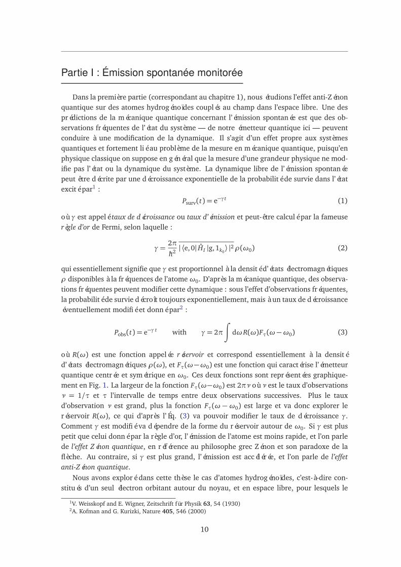
qui essentiellement signifie que γ est proportionnel à la densité d’états électromagnétiquesρ disponibles à la fréquences de l’atomeω0. D’après la mécanique quantique, des observa-tions fréquentes peuvent modifier cette dynamique : sous l’effet d’observations fréquentes,la probabilité de survie décroît toujours exponentiellement, mais à un taux de décroissanceéventuellement modifié et donné par2 :

Pobs(t) = e−γ t with γ= 2π

∫

dωR(ω)Fτ(ω−ω0) (3)

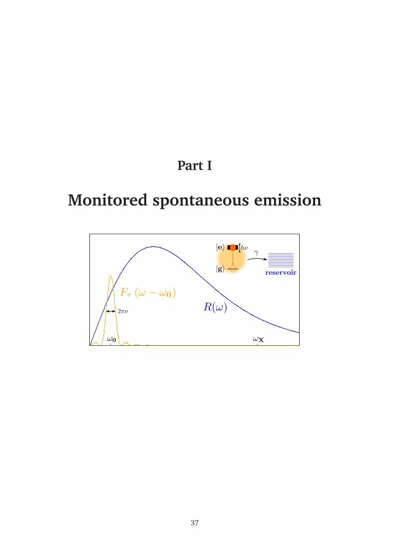
où R(ω) est une fonction appelée réservoir et correspond essentiellement à la densitéd’états électromagnétiques ρ(ω), et Fτ(ω−ω0) est une fonction qui caractérise l’émetteurquantique centrée et symétrique en ω0. Ces deux fonctions sont représentées graphique-ment en Fig. 1. La largeur de la fonction Fτ(ω−ω0) est 2πν où ν est le taux d’observationsν = 1/τ et τ l’intervalle de temps entre deux observations successives. Plus le tauxd’observation ν est grand, plus la fonction Fτ(ω − ω0) est large et va donc explorer leréservoir R(ω), ce qui d’après l’Éq. (3) va pouvoir modifier le taux de décroissance γ.Comment γ est modifié va dépendre de la forme du réservoir autour de ω0. Si γ est pluspetit que celui donné par la règle d’or, l’émission de l’atome est moins rapide, et l’on parlede l’effet Zénon quantique, en référence au philosophe grec Zénon et son paradoxe de laflèche. Au contraire, si γ est plus grand, l’émission est accélérée, et l’on parle de l’effetanti-Zénon quantique.

Nous avons exploré dans cette thèse le cas d’atomes hydrogénoïdes, c’est-à-dire con-stitués d’un seul électron orbitant autour du noyau, et en espace libre, pour lesquels le

1V. Weisskopf and E. Wigner, Zeitschrift für Physik 63, 54 (1930)2A. Kofman and G. Kurizki, Nature 405, 546 (2000)

10

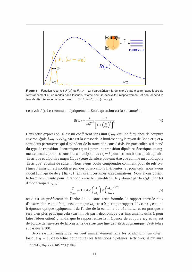
Figure 1 – Fonction réservoir R(ω) et Fτ (ω − ω0) caractérisant la densité d’états électromagnétiques del’environnement et les modes dans lesquels l’atome peut se désexciter, respectivement, et dont dépend letaux de décroissance par la formule γ = 2π

∫dω R(ω)Fτ (ω − ω0).

réservoir R(ω) est connu analytiquement. Son expression est la suivante3 :

R(ω) =D

ωη−1X

ωηh

1+

ωωX

2iµ(4)

Dans cette expression, D est un coefficient sans unité, ωX est une fréquence de coupureenviron égale à ωX ∼ c/a0, où c est la vitesse de la lumière et a0 le rayon de Bohr, et η et µsont deux paramètres qui dépendent de la transition considérée. En particulier, η dépenddu type de transition électronique : η= 1 pour une transition dipolaire électrique, et aug-mente ensuite pour les transitions multipolaires : η= 3 pour les transitions quadrupolaireélectrique et dipolaire magnétique (cette dernière pouvant être vue comme un quadrupoleélectrique) et ainsi de suite... Nous avons voulu comprendre comment pour de tels sys-tèmes l’émission est modifiée par des observations fréquentes, et pour cela, nous avonscalculé l’intégrale de γ [Éq. (3)] en faisant certaines approximations. Nous avons obtenula formule suivante pour le rapport entre le γ modifié et le γ donné par la règle d’or (etdénoté ci-après γROF):

γ

γROF

= 1+ A×

ν

ω0

×

ωX

ω0

η−1

(5)

où A est un pré-facteur de l’ordre de 1. Dans cette formule, le rapport entre le tauxd’observation ν et la fréquence atomique ω0 est très petit par rapport à 1, car ω0 est unefréquence optique typiquement de l’ordre de la centaine de téra-hertz, et en pratique νsera bien plus petit que cela (car limitée par l’électronique des instruments utilisés pourfaire l’observation) ; tandis que le rapport entre la fréquence de coupure ωX et ω0 estde l’ordre de l’inverse de la constante de structure fine de l’électrodynamique, c’est-à-diresupérieur à 100.

De ce résultat analytique, on peut immédiatement faire les prédictions suivantes :lorsque η = 1, c’est-à-dire pour toutes les transitions dipolaires électriques, il n’y aura

3J. Seke, Physica A 203, 269 (1994)

11

quasiment pas de modifications du taux d’émission, puisque le rapport ωX/ω0 disparaîtet le reste est très petit devant 1, tandis que pour tous les autres types de transitions, pourlesquelles η > 1, on peut s’attendre à avoir une accélération de l’émission (effet anti-Zénonquantique) si le taux d’observation est suffisamment élevé.

Une telle prédiction permet d’expliquer pourquoi l’effet anti-Zénon quantique, quiavait été prédit pour le processus d’émission spontanée dès les années 2000, n’a encore ja-mais été observé expérimentalement, à notre connaissance, dans des expériences d’atomesfroids ou d’ions piégés en espace libre. En effet, selon nos prédictions, cet effet n’est pasaccessible pour toutes les transitions dipolaires électriques qui sont les plus largementétudiées et utilisées lors des expériences.

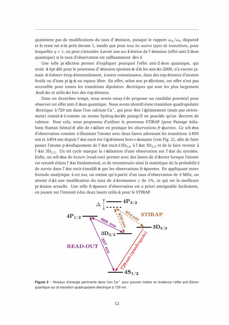
Dans un deuxième temps, nous avons essayé de proposer un candidat potentiel pourobserver cet effet anti-Zénon quantique. Nous avons identifié une transition quadrupolaireélectrique à 729 nm dans l’ion calcium Ca+, qui peut être légitimement (mais pas stricte-ment) considéré comme un atome hydrogénoïde puisqu’il ne possède qu’un électron devalence. Pour cela, nous proposons d’utiliser le processus STIRAP (pour Passage Adia-batic Raman Stimulé) afin de réaliser en pratique les observations fréquentes. Ce schémad’observation consiste à illuminer l’atome avec deux lasers adressant les transitions à 850nm et à 854 nm depuis l’état excité et légèrement hors-résonants (voir Fig. 2), afin de fairepasser l’atome périodiquement de l’état excité 3D5/2 à l’état 3D3/2 et de le faire revenir àl’état 3D5/2. Un tel cycle marque la réalisation d’une observation sur l’état du système.Enfin, un schéma de lecture (read-out) permet avec des lasers de détecter lorsque l’atomeest retombé dans l’état fondamental, et de reconstruire ainsi la statistique de la probabilitéde survie dans l’état excité modifiée par les observations fréquentes. En appliquant notreformule analytique à cet ion, on estime qu’à partir d’un taux d’observation de 4 MHz, onatteint déjà une modification du taux de décroissance γ de 1%, ce qui est la meilleureprécision actuelle. Une telle fréquence d’observation est a priori atteignable facilement,en jouant sur l’intensité des deux lasers utilisés pour le STIRAP.

Figure 2 – Niveaux d’énergie pertinents dans l’ion Ca+ pour pouvoir mettre en évidence l’effet anti-Zénonquantique sur la transition quadrupolaire électrique à 729 nm.

12

Partie II : Interactions en champs proche

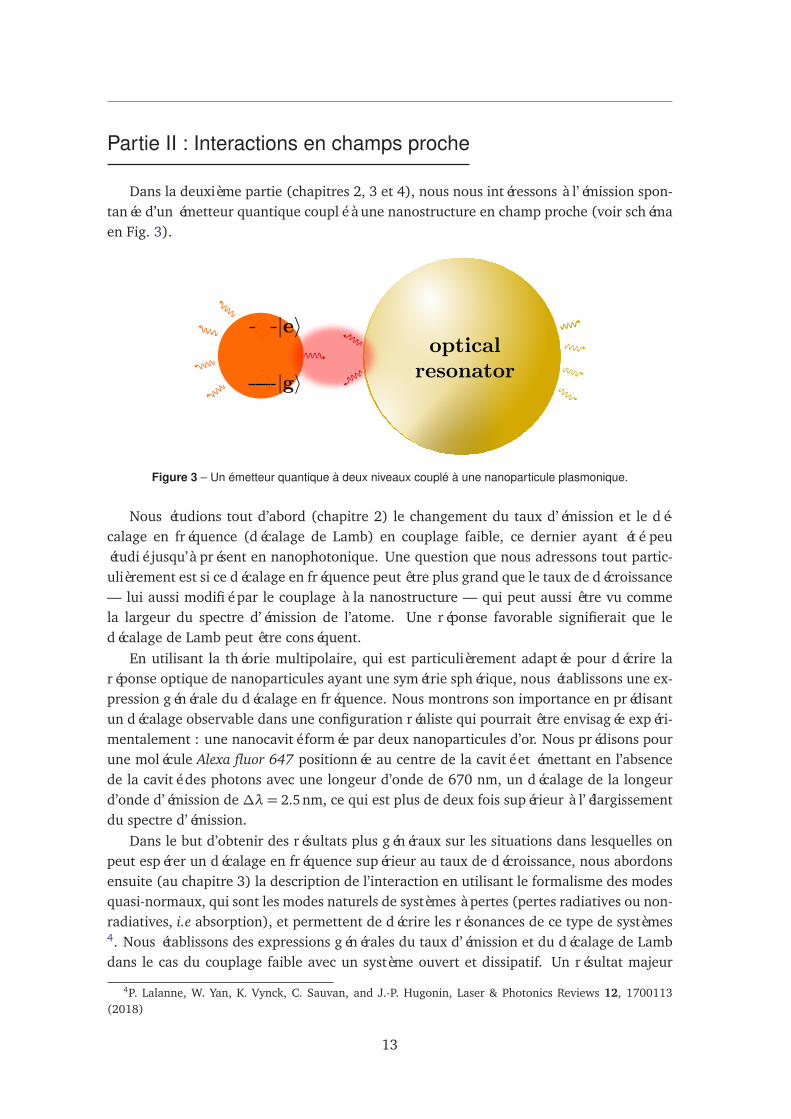
Dans la deuxième partie (chapitres 2, 3 et 4), nous nous intéressons à l’émission spon-tanée d’un émetteur quantique couplé à une nanostructure en champ proche (voir schémaen Fig. 3).

Figure 3 – Un émetteur quantique à deux niveaux couplé à une nanoparticule plasmonique.

Nous étudions tout d’abord (chapitre 2) le changement du taux d’émission et le dé-calage en fréquence (décalage de Lamb) en couplage faible, ce dernier ayant été peuétudié jusqu’à présent en nanophotonique. Une question que nous adressons tout partic-ulièrement est si ce décalage en fréquence peut être plus grand que le taux de décroissance— lui aussi modifié par le couplage à la nanostructure — qui peut aussi être vu commela largeur du spectre d’émission de l’atome. Une réponse favorable signifierait que ledécalage de Lamb peut être conséquent.

En utilisant la théorie multipolaire, qui est particulièrement adaptée pour décrire laréponse optique de nanoparticules ayant une symétrie sphérique, nous établissons une ex-pression générale du décalage en fréquence. Nous montrons son importance en prédisantun décalage observable dans une configuration réaliste qui pourrait être envisagée expéri-mentalement : une nanocavité formée par deux nanoparticules d’or. Nous prédisons pourune molécule Alexa fluor 647 positionnée au centre de la cavité et émettant en l’absencede la cavité des photons avec une longeur d’onde de 670 nm, un décalage de la longeurd’onde d’émission de ∆λ= 2.5nm, ce qui est plus de deux fois supérieur à l’élargissementdu spectre d’émission.

Dans le but d’obtenir des résultats plus généraux sur les situations dans lesquelles onpeut espérer un décalage en fréquence supérieur au taux de décroissance, nous abordonsensuite (au chapitre 3) la description de l’interaction en utilisant le formalisme des modesquasi-normaux, qui sont les modes naturels de systèmes à pertes (pertes radiatives ou non-radiatives, i.e absorption), et permettent de décrire les résonances de ce type de systèmes4. Nous établissons des expressions générales du taux d’émission et du décalage de Lambdans le cas du couplage faible avec un système ouvert et dissipatif. Un résultat majeur

4P. Lalanne, W. Yan, K. Vynck, C. Sauvan, and J.-P. Hugonin, Laser & Photonics Reviews 12, 1700113(2018)

13

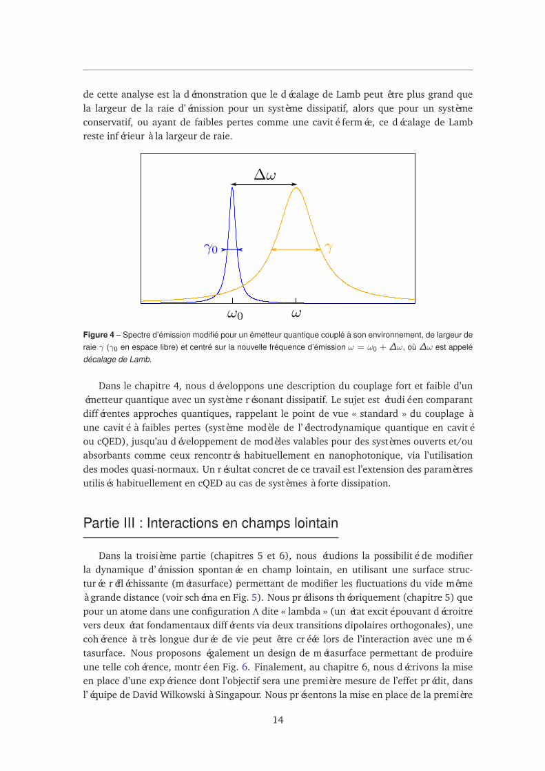
de cette analyse est la démonstration que le décalage de Lamb peut être plus grand quela largeur de la raie d’émission pour un système dissipatif, alors que pour un systèmeconservatif, ou ayant de faibles pertes comme une cavité fermée, ce décalage de Lambreste inférieur à la largeur de raie.

Figure 4 – Spectre d’émission modifié pour un émetteur quantique couplé à son environnement, de largeur deraie γ (γ0 en espace libre) et centré sur la nouvelle fréquence d’émission ω = ω0 + ∆ω, où ∆ω est appelédécalage de Lamb.

Dans le chapitre 4, nous développons une description du couplage fort et faible d’unémetteur quantique avec un système résonant dissipatif. Le sujet est étudié en comparantdifférentes approches quantiques, rappelant le point de vue « standard » du couplage àune cavité à faibles pertes (système modèle de l’électrodynamique quantique en cavitéou cQED), jusqu’au développement de modèles valables pour des systèmes ouverts et/ouabsorbants comme ceux rencontrés habituellement en nanophotonique, via l’utilisationdes modes quasi-normaux. Un résultat concret de ce travail est l’extension des paramètresutilisés habituellement en cQED au cas de systèmes à forte dissipation.

Partie III : Interactions en champs lointain

Dans la troisième partie (chapitres 5 et 6), nous étudions la possibilité de modifierla dynamique d’émission spontanée en champ lointain, en utilisant une surface struc-turée réfléchissante (métasurface) permettant de modifier les fluctuations du vide mêmeà grande distance (voir schéma en Fig. 5). Nous prédisons théoriquement (chapitre 5) quepour un atome dans une configuration Λ dite « lambda » (un état excité pouvant décroitrevers deux état fondamentaux différents via deux transitions dipolaires orthogonales), unecohérence à très longue durée de vie peut être créée lors de l’interaction avec une mé-tasurface. Nous proposons également un design de métasurface permettant de produireune telle cohérence, montré en Fig. 6. Finalement, au chapitre 6, nous décrivons la miseen place d’une expérience dont l’objectif sera une première mesure de l’effet prédit, dansl’équipe de David Wilkowski à Singapour. Nous présentons la mise en place de la première

14

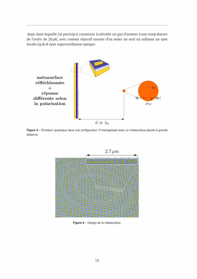
étape dans laquelle j’ai participé, consistant à refroidir un gaz d’atomes à une températurede l’ordre de 20µK, avec comme objectif ensuite d’en isoler un seul en utilisant un spotlocalisé généré par superoscillation optique.

Figure 5 – Émetteur quantique dans une configuration Λ interagissant avec un métasurface placée à grandedistance.

Figure 6 – Design de la métasurface.

15

16

Abstract in English (short)

The control of the spontaneous emission of quantum emitters is of fundamental impor-tance for the development of future quantum technologies, like quantum cryptography orquantum computing. Such applications rely on the manipulation of atoms, molecules, or"artificial" atoms, as elementary sources of light, and on the exploitation of the quantumnature of the emitted light, single photons. With the recent developments in nanofabri-cation techniques and nanotechnologies, the modification of the dynamics of the sponta-neous emission by the environment is being investigated at the level of a few emitters,allowing for unprecedented control and manipulation of the spontaneous emission. Inparallel to the experimental efforts, theoretical understanding of the fundamental inter-action mechanisms between quantum emitters and their environment also becomes moreand more essential.

In this thesis, we tackle three different paradigms of the spontaneous emission phe-nomenon, all dealing with modifications of the spontaneous emission induced the envi-ronment. Firstly, we tackle the problem of monitored spontaneous emission, that is howthe processus of emission is modified when the emitting system is being frequently moni-tored by an external observer, and which is closely related to the problem of measurementin quantum mechanics. Secondly, we consider the interaction between quantum emittersand optical resonances supported by nearby nanostructures. Finally, we study the remoteinteraction between quantum emitters and surfaces engraved with nanostructures whichare designed and arranged in specific patterns, so-called metasurfaces.

We present and deal with different formalisms to model such different situations, in-terfacing different fields of physics like quantum optics and nanophotonics. In each ofthese situations, we illustrate with realistic theoretical predictions how the spontaneousemission is modified: in the first case, how the lifetime of the quantum emitter is altered,in the second case how the frequency of the emitted photon is altered, and in the last situ-ation how the environment may induce quantum coherence in the emitter. For each case,for provide with experimental proposals for future confirmations of these predictions, tobring a better understanding and control over these fundamental processes.

Keywords: quantum emitters, spontaneous emission, quantum Zeno effect, anti-Zenoeffect, Mie theory, quasi-normal modes, plasmonics, metasurfaces

17

18

Contents

Remerciements 3

Statement of contributions 5

List of publications 7

Résumé en français (long) 9

Abstract in English (short) 17

Notations 23

General introduction 25

I Monitored spontaneous emission 37

1 Anti-Zeno Effect in hydrogen-like atoms 411.1 Introduction . . . . . . . . . . . . . . . . . . . . . . . . . . . . . . . . . . . . . . . . . 411.2 Monitored spontaneous emission: general analysis . . . . . . . . . . . . . . . . . 421.3 Quantum anti-Zeno effect in hydrogen-like atoms . . . . . . . . . . . . . . . . . 491.4 Experimental proposal . . . . . . . . . . . . . . . . . . . . . . . . . . . . . . . . . . 581.5 Conclusion . . . . . . . . . . . . . . . . . . . . . . . . . . . . . . . . . . . . . . . . . . 611.A Decay rate in free space . . . . . . . . . . . . . . . . . . . . . . . . . . . . . . . . . . 621.B Reservoir for hydrogen-like atoms in free space . . . . . . . . . . . . . . . . . . . 66

II Near-field interactions 73

2 Lamb shift multipolar analysis 772.1 Introduction . . . . . . . . . . . . . . . . . . . . . . . . . . . . . . . . . . . . . . . . . 772.2 Lamb shift and decay rate expressions . . . . . . . . . . . . . . . . . . . . . . . . . 782.3 Nanoparticle in the electric dipole approximation . . . . . . . . . . . . . . . . . 832.4 Multipolar formulation of the scattering problem . . . . . . . . . . . . . . . . . . 882.5 Multipolar analysis . . . . . . . . . . . . . . . . . . . . . . . . . . . . . . . . . . . . . 912.6 Calculation for a gold dimer nanoantenna . . . . . . . . . . . . . . . . . . . . . . 932.7 Conclusion . . . . . . . . . . . . . . . . . . . . . . . . . . . . . . . . . . . . . . . . . . 952.A Quantum derivation of the Lamb shift and decay rate . . . . . . . . . . . . . . . 962.B The multipolar basis . . . . . . . . . . . . . . . . . . . . . . . . . . . . . . . . . . . . 99

19

CONTENTS

2.C Analytical expressions of dipolar/quadrupolar Lamb shift . . . . . . . . . . . . 101

3 Quasi-Normal Mode analysis of the decay rate and Lamb shift 1073.1 Introduction . . . . . . . . . . . . . . . . . . . . . . . . . . . . . . . . . . . . . . . . . 1073.2 Definition of the Quasi-Normal Modes . . . . . . . . . . . . . . . . . . . . . . . . 1083.3 Lamb shift and decay rate expansions in terms of QNM . . . . . . . . . . . . . . 1103.4 Examples . . . . . . . . . . . . . . . . . . . . . . . . . . . . . . . . . . . . . . . . . . . 1113.5 Maximum Lamb shift in the single-resonance case . . . . . . . . . . . . . . . . . 1143.6 Conclusion . . . . . . . . . . . . . . . . . . . . . . . . . . . . . . . . . . . . . . . . . . 1173.A Derivation of Eqs. (3.9), (3.10), (3.11) and (3.12) . . . . . . . . . . . . . . . . . 1183.B Derivation of Eqs. (3.18), (3.19), (3.21) and (3.22) . . . . . . . . . . . . . . . . 120

4 Quantum descriptions of the weak and strong coupling regimes 1274.1 Introduction . . . . . . . . . . . . . . . . . . . . . . . . . . . . . . . . . . . . . . . . . 1274.2 cQED approach . . . . . . . . . . . . . . . . . . . . . . . . . . . . . . . . . . . . . . . 1304.3 “Continuum” approach . . . . . . . . . . . . . . . . . . . . . . . . . . . . . . . . . . 1384.4 Quasi-Normal Mode description . . . . . . . . . . . . . . . . . . . . . . . . . . . . 1454.5 Non-Hermitian Hamiltonian description . . . . . . . . . . . . . . . . . . . . . . . 1554.6 Conclusion . . . . . . . . . . . . . . . . . . . . . . . . . . . . . . . . . . . . . . . . . . 1584.A Jaynes-Cummings Hamiltonian . . . . . . . . . . . . . . . . . . . . . . . . . . . . . 1614.B Fermi golden rule . . . . . . . . . . . . . . . . . . . . . . . . . . . . . . . . . . . . . . 1634.C Discrete model . . . . . . . . . . . . . . . . . . . . . . . . . . . . . . . . . . . . . . . 1654.D Calculation of the kernels . . . . . . . . . . . . . . . . . . . . . . . . . . . . . . . . 1674.E QNM expressions of the decay rate and Lamb shift . . . . . . . . . . . . . . . . . 1694.F Second-order differential equation verified by α(t) . . . . . . . . . . . . . . . . . 171

III Far-field interactions 179

5 Anisotropic quantum vacuum induced by a metasurface 1835.1 Introduction . . . . . . . . . . . . . . . . . . . . . . . . . . . . . . . . . . . . . . . . . 1835.2 Theoretical predictions: long lifetime coherence . . . . . . . . . . . . . . . . . . 1845.3 Metasurface designs . . . . . . . . . . . . . . . . . . . . . . . . . . . . . . . . . . . . 1895.4 Discussions on the coherence and limitations . . . . . . . . . . . . . . . . . . . . 1985.5 Conclusion . . . . . . . . . . . . . . . . . . . . . . . . . . . . . . . . . . . . . . . . . . 2005.A Derivation of the Master Equation . . . . . . . . . . . . . . . . . . . . . . . . . . . 2015.B Metasurface design: super-cells . . . . . . . . . . . . . . . . . . . . . . . . . . . . . 2065.C Metasurface design: unit-cells . . . . . . . . . . . . . . . . . . . . . . . . . . . . . . 209

6 Cold atom experiment 2156.1 Introduction . . . . . . . . . . . . . . . . . . . . . . . . . . . . . . . . . . . . . . . . . 2156.2 Description of the experimental set-up . . . . . . . . . . . . . . . . . . . . . . . . 2166.3 Laser part . . . . . . . . . . . . . . . . . . . . . . . . . . . . . . . . . . . . . . . . . . . 2226.4 Temperature measurements . . . . . . . . . . . . . . . . . . . . . . . . . . . . . . . 2286.5 Conclusion . . . . . . . . . . . . . . . . . . . . . . . . . . . . . . . . . . . . . . . . . . 232

20

CONTENTS

6.A Lock drift with temperature . . . . . . . . . . . . . . . . . . . . . . . . . . . . . . . 233

General conclusion 237

Physical constants 239

21

CONTENTS

22

Notations

• The unitary vectors are marked with an arrow. Example: ~x .

• The other vectors are in bold. Example: X.

• The operators are marked with a hat. Example: X .

• The vectorial operators are in bold and marked with a hat. Example: X.

23

Chapter 0. General introduction

24

General introduction

Manipulating and controlling the spontaneous emission of quantum emitters is a fas-cinating domain of research. In a nutshell, it aims at using the most elementary sourceof light, an atom or a molecule, and how to exploit the quantum nature of the emittedlight, a single photon, for future “quantum telecommunications”, among them quantumcryptography or quantum computing.

A quantum emitter (QE), such as an atom, a molecule, or an “artificial atom” whichgenerally refers to a solid-state emitter like a quantum dot or color-center, is system withdiscrete energy levels. Spontaneous emission occurs in a QE, when it is in a state ofenergy (an excited state) higher than its lowest energy state (the ground state), whichdecays to the ground state by emitting a photon, whose energy corresponds to the energydifference between the two states. Other “non-radiative” desexcitation channels exist, likevibrationnal relaxation in molecules, or dephasing processes in solid-state emitters (likephonon-assisted mechanisms), but they will not be studied in this thesis [1]. Moreover, wewill interchangeably talk about quantum emitter or atom. The quantum emitters underinterest in the present work typically emit light in the visible or near-infrared (transitionfrequency ω0 ∼ 2π× 350THz or emission wavelength λ0 = 2πc/ω0 ∼ 800nm).

From a fundamental point of view, one cannot understand spontaneous emission ifone does not consider the coupling of the QE with the quantized electromagnetic (EM)field in the vacuum. A first clarification: the term “vacuum” in this thesis refers to theelectromagnetic vacuum, also called quantum vacuum, that is the absence of light (no pho-tons), and does not refer to the absence of matter — one can have an EM vacuum in thepresence of matter; to refer to the absence of matter, we will talk about “free space”.Einstein, who knew thanks to Bohr that there are discrete levels of energy in molecules,developped in 1917 his theory of radiation in which he introduced three elementary pro-cesses of exchange of energy between light and matter: absorption, stimulated emissionand spontaneous emission, characterized by the so-called Einstein’s coefficients [2]. Whilethe processes of absorption and stimulated emission could be explained in classical terms,he arrived at the conclusion that spontaneous emission cannot be explained by classicalelectromagnetism, showing the need for a quantum theory for radiation. The quantiza-tion of the EM field (refered to as the second quantization) is treated in the framework ofQuantum ElectroDynamics (QED), the most successful theory of light-matter interaction.According to this theory, in the quantum vacuum, the EM field is not null: it is null on aver-age, but presents fluctuations. Without taking into account the coupling between the atomand the quantized EM field in vacuum, one predicts that the atom would forever remainin the excited state and would never decay. Therefore, one can say that these vacuumfluctuations are responsible for the spontaneous emission, they “stimulate” or “trigger”the spontaneous decay of the QE.

25

Chapter 0. General introduction

One can study the dynamics of the spontaneous emission within the framework ofquantum optics, the non-relativistic counterpart of QED. Of course, when one speaks aboutspontaneous emission, there are always two steps: the preparation of the atom in the ex-cited state corresponds to a processus of absorption, and can be done for example usinga laser whose frequency is resonant with the transition considered, and the processus ofemission occurs through spontaneous decay. In this work, we assume that the absorptionprocess is much faster than the emission process, so that the two processes can be consid-ered as uncorrelated (for a treatment where both processes are taken into account, see e.g.Ref. [3]). Therefore, we will not consider the first step and we will always start the prob-lem with an atom in the excited state at time t = 0. Consistently throughout this thesis, thequantity which is chosen to investigate the temporal behavior of the QE is the probabilityof the atom to remain in its excited state, called the survival probability and denoted byPsurv(t) throughought this thesis. For a two-level atom in free-space, the Wigner-Weisskopftheory predicts that the survival probability decays exponentially in time at a rate γ0 [4]:

Psurv(t) = e−γ0 t , (6)

where the “decay rate in free-space” γ0, also called the Einstein A-coefficient, reads (in-troducing the electric dipole moment d of the atom):

γ0 =ω3

0d2

3πε0ħhc3. (7)

A second prediction of the theory is that the emitted spectrum has a Lorentzian distribu-tion, of full-width at half maximum (FWHM), also called radiative linewidth, and equalto the decay rate γ0. This can be seen as a time-energy uncertainty relation: by takingδE = ħhγ0 as a measure of the energy spread of the emitted photons, and defining τ= 1/γ0

the lifetime of the excited state, one has: δEτ = ħh. The meaning of the lifetime τ isthat after a delay significantly longer than τ, one is nearly sure that one photon has beenemitted. Typically for atoms or molecules τ∼ 10ns.

The influence of the environment of the QE on its spontaneous decay was pointed outby Purcell as early as in 1946 in the context of microcavities [5], and also predictions weremade about the spontaneous emission between mirrors in [6] and [7]: hence, this decayrate γ0 appears not to be an intrinsic property of the atom, but could be modified by theenvironment. This is contained in the famous Fermi golden rule, which is derived withinthe framework of the time-dependent perturbation theory, and states that the decay ratein an arbitrary environment reads (such expression is derived in Chapter 4, Section 4.3):

γ= 2πR(r0,ω0) . (8)

In this expression, we introduced a very important quantity used throughout this thesis,called the “reservoir coupling spectrum” R(r0,ω), where r0 emphasizes the dependenceon the QE location, which is the density of states ρ(ω), corresponding to the number ofEM states available per interval of frequency, weighted by the coupling strength g(r0,ω)(with the unit of a frequency), characterizing the coupling of the QE with the EM states offrequency ω [8]:

R(r0,ω) = |g(r0,ω)|2ρ(ω) . (9)

26

An important thing to note in the Fermi golden rule given by Eq. (8) is that the decayrate only depends on the density of states evaluated at the QE emission frequency ω0.The first experimental demonstration of the alteration of the spontaneous emission infinite geometries was done by Drexhage in the early 1970s with fluorescent organic dyesdeposited on top of a mirror, and whose distance from the mirror was precisely controlledusing dielectric film spacers [9]. Later, in 1985, the inhibition of the spontaneous emissionwas demonstrated experimentally for excited atoms between two mirrors separated by lessthan half the atomic transition wavelength λ0/2 [10].

In this thesis, we studied three facets of spontaneous emission. One of them is theproblem of monitored spontaneous emission, that is how spontaneous emission can bemodified when the QE is being frequently monitored in the excited state by an externalobserver. By “frequently monitored”, I mean that an observer experimentally asks veryfrequently the question: “Is the atom still in the excited state?” as long as the answeris “Yes”. This paradigm dates back to the work of Misra and Sudarshan in 1977 whoraised the fact that in principle, frequent enough measurements of a quantum system inits excited state should “freeze” the dynamics. This prediction is known as the QuantumZeno Effect [11]. This problem is related to the axioms of quantum mechanics about themeasurement, according to which, in this case, a measurement of the atom in its excitedstate will project the atom onto this state. By repeating this measurement very frequently(before the atom has time to decay), it was shown that the frequent projections into theexcited state are equivalent in effect to “dephasing” the excited state, which results ina broadening of its energy level [8]: if the time between each observation is δt = 1/ν,with ν the rate of the observations, then the broadening of the energy level is δE = ħhν,which leads, in agreement with the time-energy uncertainty relation, to δEδt = ħh. Due tothe broadening of its energy level, the atom will “see” a broader range of EM modes intowhich it can decay, which can modify its decay rate according to [8]:

γ= 2π

∫ ∞

0

dωR(r0,ω)Fν(ω−ω0) , (10)

where R(r0,ω) is the reservoir coupling spectrum, and Fν(ω−ω0) represents the broad-ening of the energy level of the excited state and is a function of width ν centered onω0. Therefore, depending on the range of R(r0,ω) (characterizing the environment) thatis probed by the atom through Fν(ω−ω0) in the integral, spontaneous emission may beeither frozen (γ < γ0), this is the Quantum Zeno Effect, or accelerated (γ > γ0), called theanti-Zeno effect (AZE). Note that in the limit where ν→ 0, then Fν(ω−ω0)→ δ(ω−ω0)and one recovers the Fermi golden rule decay rate: γ= 2πR(r0,ω0).

Another aspect of spontaneous emission is the coupling of the QE with resonances. Oneof the pioneering works is that of Purcell in 1946, who considered spontaneous emissionin a microcavity and calculated the maximum enhancement of the decay rate due to anideal coupling with the cavity resonance ωc in the resonant case (ωc = ω0), introducingthe so-called “Purcell factor” FP which quantifies the maximum enhancement of the decayrate γ compared to γ0 as [5]:

FP =3

4π2λ3

0QV

. (11)

27

Chapter 0. General introduction

In his equation, he introduced two figures-of-merit: the quality factor of the resonatorQ =ωc/γc, with γc representing the bandwidth of the cavity resonance; and the mode vol-ume V , which is the geometrical volume representing the spatial extent of the resonator.This Eq. (11) reveals two routes to increase the coupling: through increasing the qualityfactor Q of the resonator, or by decreasing the mode volume V . The first experiment ofthis type was performed in 1983 with atoms in a resonant microcavity [12], where thegroup of Haroche obtained an enhancement factor of approximately FP ≈ 500. For micro-cavities one usually has mode volumes limited by diffraction V ∼ λ3

0, such a milestone waspossible because of the high quality factor Q > 104 obtained by using very high qualitysuperconducting mirrors cooled to cryogenic temperatures. Such an experiment pavedthe way to the so-called cavity-Quantum ElectroDynamics (cQED), that is the study of theinteraction between atoms and photons in resonant cavities at the single photon level. Thephysics of such systems can be modelled by considering the atom coupled to a single EMmode of the cavity: this is the Jaynes-Cummings model [13]. In this model, the reservoircoupling spectrum R(r0,ω) of Eq. (9) is obtained by using the expression of the couplingconstant characterizing the coupling of the atom with the single mode in the case of aperfect matching in polarization and position (explained in Chapter 4, Section 4.2):

ħhg = d

√

√ ħhωc

2ε0V, (12)

and the density of states is phenomenologically assumed to be Lorentzian with full-widthat half maximum (FWHM) γc, so that at resonance (ω0 = ωc), it reads: ρ(ω0) = 2/πγc.The Purcell factor defined as FP = γ/γ0, reads: FP = 2πg2ρ(ω0)/γ0 (using Eqs. (8) and(9) to express γ). By replacing ρ(ω0) by 2/πγc, g by its expression given by Eq. (12), andγ0 by its expression given by Eq. (7), one can derive the Purcell factor originally given byPurcell [Eq. (11)]. This regime, where the irreversible decay of the excited QE happenslike in free space but at a rate which is modified by the resonance and quantified by thePurcell factor FP , is refered to as the weak-coupling regime, or also the low-Q cavity limit.In addition to this, the Jaynes-Cummings model [13] also predicts that when the couplingcharacterized by g is strong enough compared to the losses characterized by rate γc, spon-taneous emission displays reversibility features: the survival probability does not decreasemonotically anymore, and undergoes oscillations, called vacuum Rabi oscillations, reveal-ing that the QE can exchange the emitted photon periodically with the resonator. Such aregime, called the strong-coupling regime, was later achieved by the cQED community (see[14] and references therein, and also [15, 16]). Such an ultimate control of the spon-taneous emissiom of QE was remarkable, but however, these achievements require lowtemperatures, spectrally sharp QEs (such as atoms) and a fine tuning of the resonance ofthe cavity, rendering quantum applications difficult.

A more promising path towards applications began to be investigated in the 2000s bythe nanophotonics community, which results from the convergence of several communi-ties, notably by the near-field optics and plasmonics communities. One of the very firstexperiment coupling QEs (dye molecules) with surface plasmons was done in 1982 [17],where the authors already measured signatures of strong-coupling. In 2000, an exper-iment revealed that the presence of the so-called plasmon resonances in metallic nanos-

28

tructures could strongly modify the emission pattern of a fluorescent molecule [18]. Laterin 2006, two studies quantify how the emission of QE are modified by resonant metallicnanoparticles [19, 20], quantifying the decay rate enhancement as well as the modifica-tion of the radiation pattern. Therefore, plasmonic resonances, which adopt the role ofthe resonant cavity, can also strongly modify the decay of QEs with huge advantages as-sociated to the specificity of these systems at room temperature [21]. The first specificityis that plasmonic resonators present very broad resonances due to absorption in metals atoptical wavelengths, which is good to couple broad QEs, but has the drawback of present-ing very low quality factors Q ∼ 3−30 which does not favor strong coupling via the Purcellformula in Eq. (11). However, to compensate for this, one can exploit the subwavelengthconfinement of plasmonic resonances, whenever the atom is placed in the near-field of thenanostructure. By simply extrapolating the Purcell factor formula to the case of nanopho-tonics, despite small quality factors, the interaction volume could reach up to V ∼ λ3

0/104,allowing, according to the Purcell formula, efficient coupling between the atom and theresonator.

A final feature of plasmonic resonators is the quenching of the spontaneous emission(absorption of the emitted photon by the metal) which one would like to avoid. Therefore,one must quantify not only the decay rate enhancement, but also the radiative efficiencywhich is the ratio between the radiative decay rate and the total decay rate made of ra-diative plus non-radiative contributions. Using essentially nanogap devices, where the QEis embedded in the gap between two metallic structures, decay rate enhancement above1000 with a radiative efficiency above 50% have been demonstrated experimentally in theweak-coupling regime [22, 23]. Also, for these single-photon nanoantennas, which couplethe emission of the QE with the far-field, to be interesting for applications, the direction ofthe emission should be controlled, which is possible, by using structures of size of the orderof the wavelength, to induce constructive interferences in the desired direction. Moreover,the strong-coupling regime at the level of a few emitters at room temperature has beendemonstrated and is underway [23, 24]. Even though, such coupling requires positioningthe QE in very small volumes (which can be quite challenging due to surface-interactionslike Casimir-Polders interactions), these systems are very promising in terms of practicalimplementation in quantum applications. One of the goals is to exploit the very high de-cay rate enhancement of the spontaneous decay to build ultra fast integrated light sourcesemitting streams of single photons [22], with promising applications in quantum informa-tion technology.

A last aspect of spontaneous emission that we will discuss is the far-field control of thespontaneous emission of an atom with optical devices acting as mirrors, for atom-mirrordistances of many wavelengths typically z ∼ 10λ0. Firstly, it was demonstrated theo-retically in [25] that a spherical mirror could literally suppress the vacuum fluctuationswithin a volume of λ3

0 around the focus of the spherical mirror. Hence, the spontaneousemission of an excited atom located at this position can be fully suppressed, even if themirror covers only half of the atomic emission solid angle. Such a remote interaction is aninterferometric-like effect, in the sense that the QE must be located at a specific position(in this example in the focus of the spherical mirror), with a tolerance on the position of

29

Chapter 0. General introduction

about λ30, and if one moves the atom along the atom-mirror axis from half a wavelength,

one finds a two-fold increase of the decay rate [25]. In [26], the authors proposed touse instead of a simple spherical mirror a reflective surface engraved with subwavelengthstructures (nanoantennas), called a metasurface, to shape the quantum vacuum over re-mote distances. For instance, a metasurface that acts as a spherical mirror for a certainincident polarization, let us say linearly polarized along the x-axis, and as a planar mirrorfor the a polarization along the y-axis, would create an anisotropic quantum vacuum overremote distances. Such an anisotropic quantum vacuum is predicted to affect a multi-level atom: it would lead to the creation of a coherence between the two excited statesof a three-level atom in a V -configuration [27], located at the focus of this spherical mir-ror and initially prepared in one of the excited states (coherence which does not exist infree-space). While no experimental demonstration have been made so far of the effectof a mirror or metasurface over macroscopic distances z λ0/2π (experimental demon-strations exist in confined space, see e.g. [28]), this new paradigm could open the waytowards the creation of entanglement between QEs over remote distances mediated by ametasurface [29].

Outline of the thesis: This thesis is divided into three Parts, and is organized as follows:

In the first Part of this thesis (Chapter 1), we study the problem of the monitored spon-taneous emission. In a landmark article about monitored spontaneous emission [A. G. Kof-man and G. Kurizki, Nature (London) 405, 546 (2000)], Kofman and Kurizki concludedthat acceleration of the decay by frequent measurements, called the quantum anti-Zenoeffect (AZE), appears to be ubiquitous, while its counterpart, the quantum Zeno effect,is unattainable. However, up to now there have been no experimental observations ofthe AZE for atomic radiative decay (spontaneous emission) in free space. In Chapter 1,making use of the analytical results for the reservoir coupling spectrum R(r0,ω) avail-able for hydrogen-like atoms [30, 31], we theoretically demonstrate that, in free-space,only non-electric-dipolar transitions should present an observable AZE, revealing that thiseffect is consequently much less ubiquitous than firstly predicted. We then propose anexperimental scheme for AZE observation, involving the electric quadrupole transition inthe alkali-earth ions like Ca+ and Sr+. The proposed protocol is based on the stimulatedRaman adiabatic passage technique which acts like a dephasing quasi-measurement5.

The second Part (Chapters 2, 3 and 4), is dedicated to the study of the near-field inter-action between a single QE and resonant photonic nanostrutures. The near-field is definedas the region of space z λ0/2π, also called the non-retarded regime, which for opticalQE, is typically z 100nm; beyond this region, the coupling to the resonances is almostnull. In the weak-coupling regime, this coupling not only changes the decay rate of thespontaneous emission, but can also induce energy shifts of the energy levels of the atom,

5E. Lassalle, C. Champenois, B. Stout, V. Debierre, and T. Durt, Conditions for anti-Zeno-effect observationin free-space atomic radiative decay, Physical Review A 97, 062122 (2018)

30

resulting in a frequency-shift of the emitted photon frequency with respect to the baretransition frequency ω0. Such an effect is called the photonic Lamb shift, or simply Lambshift in this thesis. It is usually much less studied than the decay rate enhancement (Pur-cell effect) because the effect is considered as small. We start Chapter 2 by presenting inSection 2.2 the classical and quantum expressions of the decay rate and Lamb shift andshowing their equivalence. After recalling the electric dipole approximation commonlyuse to describe the optical response of nanoparticles of sizes a λ0 in Section 2.3, wenext study the photonic Lamb shift using the multipolar theory to describe the opticalresponse of plasmonic nanostructures presented in Section 2.4. We show in Section 2.5that this frequency-shift originates from the plasmon resonance coupling, illustrating thisin the case of a QE coupled to a single silver plasmonic nanoparticle. We also comparethe results obtained with the multipolar theory to the electric dipole approximation oftenused to describe nanoparticles of small size compared to the wavelength, and show thateven in the case where the radius of the nanoparticle is a λ0, the electric dipole approx-imation can fail and several multipoles are necessary to describe the Lamb shift. We finallycalculate in Section 2.6 the photonic Lamb shift in the case of an emitter embedded in thenanogap of a gold dimer, where we predict a significant shift of the emission frequencythat could be observed at room temperature6.

Next, in Chapter 3, we introduce the natural modes of photonic nanostructures, called“leaky modes”, Quasi-Normal Modes (QNMs) or Resonant States, which take into accountthe dissipative nature of these systems that are open (radiation losses), can be absorbing(absorption losses) and also dispersive. These modes, presented in Section 3.2, can beused to describe the optical resonances supported by nanostructures, which can be of adifferent nature: Mie resonances in dielectric structures or surface plasmons in metallicones. We use them to describe the Lamb shift and decay rate in Section 3.3, and weillustrate the obtained expressions in Section 3.4 for the canonical case of a sphere in twodifferent cases: a dielectric nanoparticle (silicon) and a plasmonic nanoparticle (silver).Also, the analyticity provided by this tool allows us to address the question: “Can theinduced shift of the emission frequency exceed the radiative linewidth?”. In Section 3.5,we provide an answer to this question in the single-resonance case7.

In Chapter 4, we make use of the previously introduced tools in a more general quan-tum treatment of the interaction between a single QE and resonant photonic or plasmonicnanostrutures, aiming at describing the weak and strong-coupling regimes. The usualcQED description considering the coupling to a resonant cavity, that we review in Sec-tion 4.2, most often deals with a single mode, and is valid for high-Q cavities, or in otherwords small losses. However, in nanophotonics, one deals with open and/or absorbingsystems and there are usually several resonances involved as shown in Chapters 2 and3, which goes well beyond the cQED description [32], and contains new physics beyondmerely repeating cQED physics. As shown in Chapter 3, a remarkable advantage of theQNMs is that they allow us to generalize the usual cQED figures of merit characterizing

6E. Lassalle, A. Devilez, N. Bonod, T. Durt, and B. Stout, Lamb shift multipolar analysis, Journal of theOptical Society of America B 34, 1348 (2017)

7E. Lassalle, N. Bonod, T. Durt, and B. Stout, Interplay between spontaneous decay rates and Lamb shifts inopen photonic systems, Optics Letters 43, 1950 (2018)

31

Chapter 0. General introduction

the interaction between a dipole source and a resonant cavity, such as the Purcell factor FP

or mode volume V , to the case of open and/or absorbing systems (that are almost alwaysfound in nanophotonics) and also taking into account material dispersion [33–35]. In Sec-tion 4.4, we incorporate this formalism into a fully quantum treatment of the interactionof a single QE with several resonances, which encompasses the weak and strong-couplingregime. A comparison with the figures-of-merit of cQED is also made in conclusion 4.6.Throughout this Part, we pay particular attention to the remarkable equivalence with aclassical description of the atom as a damped harmonic oscillator, in this situation whereonly one photon is involved (decay rate and Lamb shift in the weak-coupling regime, andvacuum Rabi splitting in the strong-coupling regime). Such an equivalence is establishedvia the Green tensor of the EM environment, and using the linear response theory and thequantum version of the fluctuation-dissipation theorem.

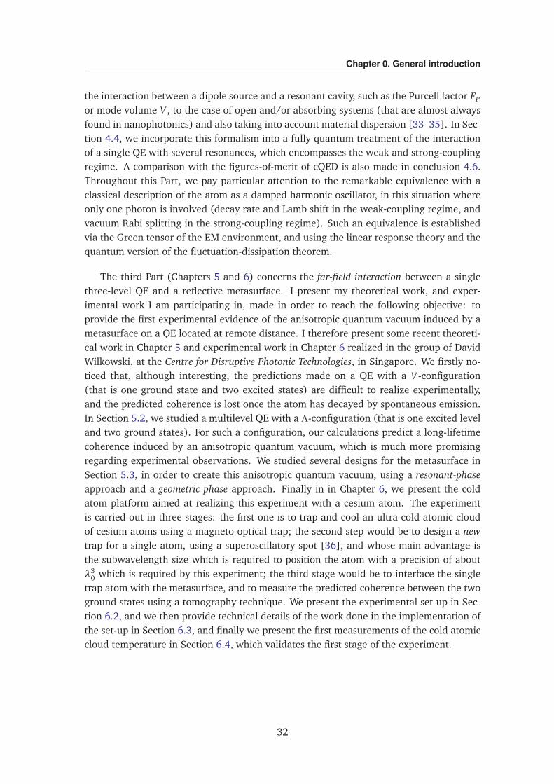
The third Part (Chapters 5 and 6) concerns the far-field interaction between a singlethree-level QE and a reflective metasurface. I present my theoretical work, and exper-imental work I am participating in, made in order to reach the following objective: toprovide the first experimental evidence of the anisotropic quantum vacuum induced by ametasurface on a QE located at remote distance. I therefore present some recent theoreti-cal work in Chapter 5 and experimental work in Chapter 6 realized in the group of DavidWilkowski, at the Centre for Disruptive Photonic Technologies, in Singapore. We firstly no-ticed that, although interesting, the predictions made on a QE with a V -configuration(that is one ground state and two excited states) are difficult to realize experimentally,and the predicted coherence is lost once the atom has decayed by spontaneous emission.In Section 5.2, we studied a multilevel QE with a Λ-configuration (that is one excited leveland two ground states). For such a configuration, our calculations predict a long-lifetimecoherence induced by an anisotropic quantum vacuum, which is much more promisingregarding experimental observations. We studied several designs for the metasurface inSection 5.3, in order to create this anisotropic quantum vacuum, using a resonant-phaseapproach and a geometric phase approach. Finally in in Chapter 6, we present the coldatom platform aimed at realizing this experiment with a cesium atom. The experimentis carried out in three stages: the first one is to trap and cool an ultra-cold atomic cloudof cesium atoms using a magneto-optical trap; the second step would be to design a newtrap for a single atom, using a superoscillatory spot [36], and whose main advantage isthe subwavelength size which is required to position the atom with a precision of aboutλ3

0 which is required by this experiment; the third stage would be to interface the singletrap atom with the metasurface, and to measure the predicted coherence between the twoground states using a tomography technique. We present the experimental set-up in Sec-tion 6.2, and we then provide technical details of the work done in the implementation ofthe set-up in Section 6.3, and finally we present the first measurements of the cold atomiccloud temperature in Section 6.4, which validates the first stage of the experiment.

32

Bibliography

[1] A. Auffèves, D. Gerace, J.-M. Gérard, M. F. Santos, L. Andreani, and J.-P. Poizat,Physical Review B 81, 245419 (2010).

[2] A. Einstein, Physikalische Zeitschrift 18, 121 (1917).

[3] D. Bouchet and R. Carminati, Journal of the Optical Society of America A 36, 186(2019).

[4] V. Weisskopf and E. Wigner, Zeitschrift für Physik 63, 54 (1930).

[5] E. M. Purcell, Physical Review 69, 681 (1946).

[6] P. W. Milonni and P. Knight, Optics Communications 9, 119 (1973).

[7] D. Kleppner, Physical Review Letters 47, 233 (1981).

[8] A. Kofman and G. Kurizki, Nature 405, 546 (2000).

[9] K. Drexhage, Journal of luminescence 1, 693 (1970).

[10] R. G. Hulet, E. S. Hilfer, and D. Kleppner, Physical Review Letters 55, 2137 (1985).

[11] B. Misra and E. Sudarshan, Journal of Mathematical Physics 18, 756 (1977).

[12] P. Goy, J. Raimond, M. Gross, and S. Haroche, Physical Review Letters 50, 1903(1983).

[13] E. T. Jaynes and F. W. Cummings, Proceedings of the IEEE 51, 89 (1963).

[14] S. Haroche and D. Kleppner, Physics Today 42, 24 (1989).

[15] R. Thompson, G. Rempe, and H. Kimble, Physical Review Letters 68, 1132 (1992).

[16] Y. Zhu, D. J. Gauthier, S. Morin, Q. Wu, H. Carmichael, and T. Mossberg, PhysicalReview Letters 64, 2499 (1990).

[17] I. Pockrand, A. Brillante, and D. Möbius, The Journal of Chemical Physics 77, 6289(1982).

[18] H. Gersen, M. F. García-Parajó, L. Novotny, J. Veerman, L. Kuipers, and N. F. vanHulst, Physical Review Letters 85, 5312 (2000).

[19] P. Anger, P. Bharadwaj, and L. Novotny, Physical Review Letters 96, 113002 (2006).

[20] S. Kühn, U. Håkanson, L. Rogobete, and V. Sandoghdar, Physical Review Letters 97,017402 (2006).

33

BIBLIOGRAPHY

[21] B. Kolaric, B. Maes, K. Clays, T. Durt, and Y. Caudano, Advanced Quantum Tech-nologies 1, 1800001 (2018).

[22] A. F. Koenderink, ACS Photonics 4, 710 (2017).

[23] F. Marquier, C. Sauvan, and J.-J. Greffet, ACS Photonics 4, 2091 (2017).

[24] D. G. Baranov, M. Wersall, J. Cuadra, T. J. Antosiewicz, and T. Shegai, ACS Photonics5, 24 (2017).

[25] G. Hétet, L. Slodicka, A. Glätzle, M. Hennrich, and R. Blatt, Physical Review A 82,063812 (2010).

[26] P. K. Jha, X. Ni, C. Wu, Y. Wang, and X. Zhang, Physical Review Letters 115, 025501(2015).

[27] G. Agarwal, Physical Review Letters 84, 5500 (2000).

[28] W. Jhe, A. Anderson, E. Hinds, D. Meschede, L. Moi, and S. Haroche, PhysicalReview Letters 58, 666 (1987).

[29] P. K. Jha, N. Shitrit, J. Kim, X. Ren, Y. Wang, and X. Zhang, ACS Photonics 5, 971(2017).

[30] H. Moses, Physical Review A 8, 1710 (1973).

[31] J. Seke, Physica A 203, 269 (1994).

[32] A. F. Koenderink, Optics Letters 35, 4208 (2010).

[33] P. T. Kristensen, C. Van Vlack, and S. Hughes, Optics Letters 37, 1649 (2012).

[34] C. Sauvan, J.-P. Hugonin, I. Maksymov, and P. Lalanne, Physical Review Letters 110,237401 (2013).

[35] E. Muljarov and W. Langbein, Physical Review B 94, 235438 (2016).

[36] J. Baumgartl, S. Kosmeier, M. Mazilu, E. T. Rogers, N. I. Zheludev, and K. Dholakia,Applied Physics Letters 98, 181109 (2011).

34

BIBLIOGRAPHY

35

BIBLIOGRAPHY

36

Part I

Monitored spontaneous emission

37

39

40

CHAPTER 1

Anti-Zeno Effect in hydrogen-like atoms

1.1 Introduction

One of the more peculiar features of quantum mechanics is that the measurement pro-cess can modify the evolution of a quantum system. The archetypes of this phenomenonare the quantum Zeno effect (QZE) and the quantum anti-Zeno effect (AZE) [1, 2]. TheQZE refers to the inhibition of the decay of an unstable quantum system due to frequentmeasurements [3], and was observed experimentally for the first time with trapped ions[4, 5] and more recently in cold neutral atoms [6]. The opposite effect, where the decayis accelerated by frequent measurements, was first called the AZE in Ref. [7], and wasdiscovered theoretically for spontaneous emission in cavities [8, 9], and first observed ina tunneling experiment with cold atoms (along with the QZE) [10], and recently with asingle superconducting qubit coupled to a waveguide cavity [11]. However, despite pre-dictions that the AZE should be much more ubiquitous than the QZE in radiative decayprocesses [1], it has never been observed to our knowledge for atomic radiative decay(spontaneous emission) in free space.

Here, we investigate the case of hydrogen-like atoms, for which the exact expression ofthe coupling between the atom and the free radiative field (cf. [12, 13]) allows us to derivean analytical expression for the measurement-modified decay rate. From this, we findthat only non-electric-dipole transitions can exhibit the AZE in free space (i.e. non-dipoleelectric transitions and magnetic transitions of any multipolar order), which drasticallylimits the experimental possibilities to observe this effect. We start with a presentation ofthe general formal results about the measurement-modified decay rate in Section 1.2, andwe then apply, in Section 1.3, this general framework to the case of electronic transitionsin hydrogen-like atoms to derive an analytical expression of the measurement-modifieddecay rate in free space. Then, we discuss the experimental realizability of the describedphenomenon in Section 1.4, and we identify a potential candidate: the electric quadrupoletransition between D5/2 and S1/2 in Ca+ or Sr+.

41

Chapter 1. Anti-Zeno Effect in hydrogen-like atoms

1.2 Monitored spontaneous emission: general analysis

We consider a two-level atom in free space with a lower level (ground state) and a upperlevel (excited state), initially prepared in the excited state. The atom will eventually decayto the ground state with the emission of a photon whose energy is equal to the difference ofenergy between the two atomic levels. To understand this phenomenon, called spontaneousemission, one must consider the coupling of the atom with the quantized radiation in thevacuum. We first briefly recall the formalism necessary to describe the interaction of anatom with the quantized radiation. Then, we examine how repeated observations (aimed atdetecting whether the atom has decayed or not) can modify the decay, and we present thetheory of monitored spontaneous emission.

1.2.1 Hamiltonians

Atomic Hamiltonian

The Hamiltonian of the two-level atomic system reads, in the second-quantized form(see [14], chapter 4.9):

HA = ħhωg |g⟩ ⟨g|+ħhωe |e⟩ ⟨e| (1.1)

where |g⟩ (for ground state) and |e⟩ (for excited state) are the eigen-states of HA withassociated eigen-energies ħhωg and ħhωe, respectively. The transition (Bohr) frequency isdefined as ω0 ≡ωe −ωg.

Radiation field Hamiltonian

To get the Hamiltonian of the electromagnetic (EM) field (or radiation field), we fol-low the standard canonical quantization procedure introducing a fictitious1 volume V . Inthis procedure, one expands the EM field onto EM modes (which are the most elemen-tary solution of the Maxwell’s equations), that we choose to be polarized travelling planemonochromatic wave (but other types of modes exist). Such a mode, labelled by j, is char-acterized by its frequency ωj, its wavevector kj whose modulus verifies |kj| = ωj/c, andits polarization vector ~εj such that ~εj ·kj = 0. The energy of a mode in the quantizationvolume V , taking periodic boundary conditions, has the same form as the one of a har-monic oscillator (see [15]). The total energy of the EM field is the sum of the energiesof all modes without any cross-terms (this result is not trivial). This decoupling allows toeasily perform the canonical quantization (a procedure elaborated by Dirac in his thesis in1925) of the total EM field, whose quantum Hamiltonian reads (see [16], chapter 4.5):

HR =∑

j

ħhωj

a†j aj +

12

where

aj, a†k

= δjk (1.2)

1The introduction of a finite quantization volume is not absolutely necessary for quantizing the EM field,but it is convenient because it simplifies the mathematics as we will see.

42

1.2 Monitored spontaneous emission: general analysis

where aj and a†j are, respectively, the photon annihilation and creation operators for the

mode j with frequency ωj, and δjk is the Kronecker delta. The subscript R stands for“radiation”. This remarkable result suggests that the quantized EM field, in the absence ofcharges, can be considered as a set of quantum harmonic oscillators independent of eachother, as shown by the fact that the radiation Hamiltonian is the sum of each individualHamiltonians Hj = ħhωj(a

†j aj +

12), and that the ladder operators aj and a†

k for differentoscillators do commute.

Interaction Hamiltonian

The interaction Hamiltonian which accounts for the coupling of the atom with thequantized EM field is given in the Coulomb gauge (and in SI units) by (see [16], chapter6):

HI =e

meA (r) · p , (1.3)

with e the elementary electric charge, me the electron mass, r and p are the positionand linear momentum operators of the electron, respectively, and A the vector potentialoperator of the quantized EM field. In writing Eq. (1.3), we consider only one-electronhydrogen-like atoms (in the sense that they have a single atomic electron orbiting aroundthe atomic nucleus). We also neglect the term relative to the nucleus (smaller by a factorme/M , where M is the mass of the nucleus), and finally we neglect the term ∝ A2 (seeEq. (6.69) in [16]). The interaction Hamiltonian (1.3) derives from the so-called minimal-coupling form of the total Hamiltonian, and is known as the A ·p form (see [14], chapter4.8). There exist other forms for the interaction Hamiltonian, and our choice is dictatedby the fact that (1.3) is more convenient for the multipolar treatment that will follow.

1.2.2 Time-dependent perturbation theory

General result

To study the interaction between the atom and the quantized EM field, one must con-sider the whole system atom + EM field. In particular, in order to describe the sponta-neous emission phenomenon, we restrict the Hilbert space of the atom and EM field statesto the subspace consisting of the atomic ground and excited states, and of the EM fieldvacuum state and one-photon states. In addition to this, we will make the rotating waveapproximation (RWA), which consists in dropping the terms in the interaction Hamilto-nian that couple the atomic excited state + one-photon state with the atomic groundstate + vacuum state. Mathematically, this means that the system is described by thestate:

|ψ (t)⟩= α (t)e−iω0 t |e, 0⟩+∑

j

βj (t)e−iωj t |g, 1j⟩ (1.4)

where |g,1j⟩ ≡ |g⟩ ⊗ |1j⟩ is the tensor product between the atomic state |g⟩ and the state ofthe EM field |1j⟩ containing one photon in the mode j and the vacuum in all other modes(this is called a one-photon state) and |e, 0⟩ ≡ |e⟩ ⊗ |0⟩ is the tensor product between the

43

Chapter 1. Anti-Zeno Effect in hydrogen-like atoms

atomic state |e⟩ and the vacuum state of the EM field |0⟩. In writing the state of the systemin this form, the zero of energy is taken at the level of the ground state |g⟩ (ħhωg = 0), andwe considered the energy associated to a one-photon state ħhωj by taking the infinite energyof the vacuum Ev =

∑

jħhωj/2 as a reference (this is called renormalization). Therefore,

HA reduces to HA = ħhω0 |e⟩ ⟨e| and HR is recast in the form HR =∑

jħhωja†j aj. To know

the dynamics, one must get the coefficients α (t) and βj (t) by solving the Schrödingerequation

iħhd |ψ (t)⟩

dt= H |ψ (t)⟩ (1.5)

with H = HA+ HR + HI and with the initial condition |ψ (0)⟩ = |e, 0⟩ (i.e., α(0) = 1 and ∀jβj(0) = 0) corresponding to the atom initially in the excited state |e⟩ and no photons in theEM field. One then obtains the following differential equations fullfilled by the coefficientsα (t) and βj (t) (taking into account the fact that as |0⟩ , |1j⟩ are eigen-states of HR — oftencalled Fock states, |e,0⟩ , |g,1j⟩ are eigen-states of the Hamiltonian HA+ HR):

iα (t) =∑

j

g∗j βj (t)ei(ω0−ωj)t , (1.6)

iβj (t) = gjα (t)e−i(ω0−ωj)t (1.7)

where we introduced the coupling constant gj defined by:

ħhgj ≡ ⟨g,1j| HI |e,0⟩ Unit:

gj

= s−1 . (1.8)

By formally integrating Eq. (1.7) together with the initial condition βj(0) = 0, one gets:

iβj (t) = gj

∫ t

0

dt ′α(t ′)e−i(ω0−ωj)t ′ (1.9)

and inserting this expression into Eq. (1.6) gives:

α (t) = −∑

j

|gj|2∫ t

0

dt ′α(t ′)ei(ω0−ωj)(t−t ′) . (1.10)

Up to now, no approximations have been made, and Eq. (1.10) is exact. We proceednow by using perturbation theory, which is motivated by the double fact that (i) we areinterested in the short-time behavior of the system (when α(t) ' α(0) = 1) and moreover(ii) we suppose that the coupling between the atom and the quantized EM field is weak(i.e., the coupling constants gj are small compared to the matrix elements of the non-interacting Hamiltonian H0 = HA + HR, with HA and HR given by Eqs. (1.1) and (1.2),respectively) (see [17], chapter 5.2). To get the first-order perturbative solution, we setα(t ′) = 1 in the right-hand side of Eq. (1.10) and get

α (t)' −∑

j

|gj|2∫ t

0

dt ′ ei(ω0−ωj)(t−t ′)

= −∑

j

|gj|2 ×ei(ω0−ωj)t − 1i(ω0 −ωj)

= −∑

j

|gj|2 × h

ω0 −ωj, t

× t

(1.11)

44

1.2 Monitored spontaneous emission: general analysis

where we introduced the function h(ω, t) defined by:

h(ω, t)≡1

iωt(eiωt − 1) . (1.12)

We proceed as previously by formally integrating Eq. (1.11) together with the initial con-dition α(0) = 1, to get:

α (t)' 1−∑

j

|gj|2∫ t

0

dt ′ h

ω0 −ωj, t ′

× t ′

= 1−∑

j

|gj|2 × i×1− h(ω0 −ωj, t)

ω0 −ωj× t .

(1.13)

To compute the survival probability Psurv (t) defined as

Psurv (t)≡ |⟨e, 0|ψ(t)⟩ |2

= |α (t) |2 ,(1.14)

we will ignore the second-order contributions (i.e., the term ∝

∑

j |gj|22

) because wealready neglected contributions of this order in obtaining Eq. (1.13) for α(t). Then thefirst order perturbative solution for the probability Psurv (t) is:

Psurv (t) = |α (t) |2

' 1− 2×Re

∑

j

|gj|2 × i×1− h(ω0 −ωj, t)

ω0 −ωj× t

!

= 1− 2×∑

j

|gj|2 ×Re

i×1− h(ω0 −ωj, t)

ω0 −ωj

× t

= 1− 2×∑

j

|gj|2 × Im

h(ω0 −ωj, t)

ω0 −ωj

× t

(1.15)

Moreover, one can easily show that

Im

h(ω0 −ωj, t)

ω0 −ωj

=12

t sinc2

(ω0 −ωj)t

2

(1.16)

with sinc(x)≡ sin(x)/x and thus:

Psurv (t) = 1−∑

j

|gj|2 × t sinc2

(ω0 −ωj)t

2

× t . (1.17)

Finally, Eq. (1.17) can be recast in the form

Psurv (t) = 1− 2π

∫ ∞

0

dωR (ω) Ft (ω−ω0)× t (1.18)

where

R (ω)≡∑

j

|gj|2δ(ω−ωj) Unit: [R (ω)] = s−1 (1.19)

and

Ft (ω−ω0)≡t

2πsinc2

(ω−ω0) t2

Unit: [Ft (ω−ω0)] = s . (1.20)

45

Chapter 1. Anti-Zeno Effect in hydrogen-like atoms

Quasi-continuum and density of states The one-photon states |1j⟩ in the fictitious boxof volume V (which is assumed to be large compared to λ3

0 where λ0 = 2πc/ω0) representa quasi-continuum, i.e. they form an ensemble of discrete states very close in frequency(and a real continuum when one allows the dimensions of the box to tend to infinity).Moreover, they form a degenerate quasi-continuum, which means that for a given fre-quency ωj, there are many one-photon states. Indeed, for a given frequency ωj, there aremany modes differing only by their polarization and propagation direction. It is conve-nient to introduce the concept of density of states ρ (ω), which is equal to the number ofquasi-continuum states in the frequency range from ω to ω+dω divided by the frequencywidth of this interval dω, and to replace the discrete sum in Eq. (1.19) by

R (ω) −→ |g(ω)|2ρ (ω) Unit: [ρ (ω)] = s (1.21)

where |g(ω)|2 corresponds to |gj|2 = ħh−2| ⟨g, 1j| HI |e, 0⟩ |2 averaged over all one-photonstates with ωj =ω (i.e. averaged over all emission directions and polarizations).

Therefore, the function R (ω), which is a property of the interaction Hamiltonian HI ,represents the density of states ρ(ω) weighted by the coupling strengths |g(ω)|2, and willbe called the reservoir coupling spectrum. The function Ft (ω−ω0) shows the broaden-ing of ω0 at very short times. In a sense, it represents the range of frequencies “seen” bythe atom in which it can decay. We will call it the atomic spectral profile.

First limiting case: the Zeno regime

Even if Eq. (1.18) has been derived for a two-level atom coupled to the EM field in freespace, it holds for any type of environment provided that the perturbation treatment stillholds. In practice, the reservoir R(ω) of the environment has a center of weight ωc and abandwidth ∆ωc which determines the effective range of integration in Eq. (1.18), and ismost conveniently described by the quality factor Qc ≡ ωc/∆ωc. For very short times forwhich

ωc t Qc and ωc t ωc

|ωc −ω0|(1.22)

the argument in the sinc(x) appearing in the function Ft (ω−ω0) is close to zero andsinc(x) can be approximated by 1. Thus, Ft (ω−ω0)∼ t/(2π) and Eq. (1.18) reduces to

Psurv (t)' 1− C × t2 where C ≡∫ ∞

0

R (ω) dω . (1.23)

This t2 dependence is characteristic of what is known as the quantum Zeno regime fora reason that will be explained later. The condition (1.22) can be easily met for a verypeaked and narrow reservoir centered on ω0 (Qc →∞, ωc = ω0) like a resonant cavityfor instance, whereas for the limit of an unbounded flat continuum (Qc → 0), this timeinterval shrinks to zero.

46

1.2 Monitored spontaneous emission: general analysis

Second limiting case: the Fermi golden rule regime

Very quickly, for

ωc t Qc and ωc t ωc

|ωc −ω0|(1.24)

(but not for too long times so that the perturbative treatment still holds), one has:

Ft (ω−ω0) =t

2πsinc2

(ω−ω0) t2

−→ δ (ω−ω0) (1.25)

and therefore Eq. (1.18) becomes

Psurv (t)' 1− γ0 t (1.26)

where the decay rate γ0 reads

γ0 ≡ 2πR(ω0) = 2π |g(ω0)|2ρ (ω0) Unit: [γ0] = s−1 (1.27)

This is the Fermi golden rule (FGR). Note that according to the FGR, only the one-photonstates of frequency ω0 contribute to the decay. In Appendix 1.A, we explicitely calculate|g(ω0)|2 and recover the well-known expression for the decay rate in vacuum. Moreover,when one goes beyond a perturbative treatment, the survival probability Psurv(t) decaysexponentially at a rate given by the FGR, and the present perturbative solution is simplythe short-time expansion of the exponential behavior Psurv(t) = e−γ0 t . The exponentialdecay is known as the Wigner-Weisskopf decay (see [17], chapter 5.3), in reference tothe method developped by Wigner and Weisskopf to calculate the non-perturbative long-time solution in 1930 [18]. Note that a secondary result of the calculation of Wigner andWeisskopf is that the atom emission spectrum is a Lorentzian curve of width γ0.

1.2.3 Monitored spontaneous emission: quantum Zeno and anti-Zeno effects

In this section, we want to know what happens when the unstable atom is being con-tinuously observed (monitored). According to one of the axioms of quantum mechanics, anobservation (measurement) corresponds to an ideal instantaneous projection onto an eigen-state of the system. We therefore study how the evolution of the system is modified if nfrequent projections onto the state |e⟩ are performed every time τ during a period t = nτ.The probability that no decay occurs during a period t = nτ is then defined as:

Pmoni (t = nτ)≡ Psurv (τ)× ...× Psurv (τ)︸ ︷︷ ︸

n times

= [Psurv (τ)]n . (1.28)

In the Zeno regime

In the Zeno regime for which the survival probability is given by Eq. (1.23), when nfrequent projections onto the state |e⟩ are performed every time τ during a period t = nτ,

47

Chapter 1. Anti-Zeno Effect in hydrogen-like atoms

the probability (1.28) reads:

Pmoni (t = nτ) =

1− C ×τ2n

=

1− C × t

n

2n

(τ=tn)

' 1− C ×t2

n(Taylor expansion to first order)

(1.29)

and in the limit of “continuous measurements” (limn→∞),

limn→∞

Pmoni (t = nτ) = 1 . (1.30)

This result means, according to Misra and Sudarshan [3] that: “[...] an unstable particlewhich is continuously observed to see whether it decays will never be found to decay!”.They called this phenomenon the “Zeno’s paradox in quantum theory”, also known as thequantum Zeno effect, in reference to the Greek philosopher Zeno and his arrow paradox.

In the Fermi regime

Contrary to the quantum Zeno effect, in the Fermi regime, where the survival proba-bility is given by Eq. (1.26), if n frequent projections onto the state |e⟩ are performed atevery time τ during a period t = nτ, then the probability (1.28) reads:

Pmoni (t = nτ) = (1− γ0τ)n

=

1− γ0tn

n(τ=

tn)

= exph

n log

1− γ0tn

i

' exph

n

−γ0tn

i

(n→ +∞)

= exp (−γ0 t)

(1.31)

and one can see that there is no modification of the decay under frequent measurements.

In the general case

We now come back to the more general result for the survival probability given byEq. (1.18) and we want to see what happens when the atom in the excited state is beingfrequently monitored at a rate ν= 1/τ (n measurements during the interval t = nτ). Theprobability (1.28) reads:

Pmoni (t = nτ) =

1− 2π

∫ ∞

0

dωR (ω) Fτ (ω−ω0)×τn

=

1− 2π

∫ ∞

0

dωR (ω) Fτ (ω−ω0)×tn

n

(τ=tn)

' exp (−γt)

(1.32)

48

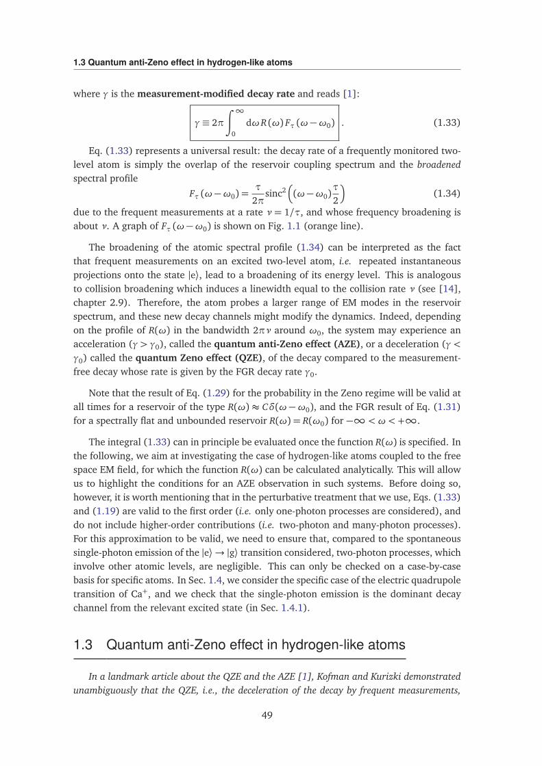
1.3 Quantum anti-Zeno effect in hydrogen-like atoms

where γ is the measurement-modified decay rate and reads [1]:

γ≡ 2π

∫ ∞

0

dωR (ω) Fτ (ω−ω0) . (1.33)

Eq. (1.33) represents a universal result: the decay rate of a frequently monitored two-level atom is simply the overlap of the reservoir coupling spectrum and the broadenedspectral profile

Fτ (ω−ω0) =τ

2πsinc2

(ω−ω0)τ

2

(1.34)

due to the frequent measurements at a rate ν = 1/τ, and whose frequency broadening isabout ν. A graph of Fτ (ω−ω0) is shown on Fig. 1.1 (orange line).

The broadening of the atomic spectral profile (1.34) can be interpreted as the factthat frequent measurements on an excited two-level atom, i.e. repeated instantaneousprojections onto the state |e⟩, lead to a broadening of its energy level. This is analogousto collision broadening which induces a linewidth equal to the collision rate ν (see [14],chapter 2.9). Therefore, the atom probes a larger range of EM modes in the reservoirspectrum, and these new decay channels might modify the dynamics. Indeed, dependingon the profile of R(ω) in the bandwidth 2πν around ω0, the system may experience anacceleration (γ > γ0), called the quantum anti-Zeno effect (AZE), or a deceleration (γ <γ0) called the quantum Zeno effect (QZE), of the decay compared to the measurement-free decay whose rate is given by the FGR decay rate γ0.

Note that the result of Eq. (1.29) for the probability in the Zeno regime will be valid atall times for a reservoir of the type R(ω) ≈ Cδ(ω−ω0), and the FGR result of Eq. (1.31)for a spectrally flat and unbounded reservoir R(ω) = R(ω0) for −∞<ω< +∞.

The integral (1.33) can in principle be evaluated once the function R(ω) is specified. Inthe following, we aim at investigating the case of hydrogen-like atoms coupled to the freespace EM field, for which the function R(ω) can be calculated analytically. This will allowus to highlight the conditions for an AZE observation in such systems. Before doing so,however, it is worth mentioning that in the perturbative treatment that we use, Eqs. (1.33)and (1.19) are valid to the first order (i.e. only one-photon processes are considered), anddo not include higher-order contributions (i.e. two-photon and many-photon processes).For this approximation to be valid, we need to ensure that, compared to the spontaneoussingle-photon emission of the |e⟩ → |g⟩ transition considered, two-photon processes, whichinvolve other atomic levels, are negligible. This can only be checked on a case-by-casebasis for specific atoms. In Sec. 1.4, we consider the specific case of the electric quadrupoletransition of Ca+, and we check that the single-photon emission is the dominant decaychannel from the relevant excited state (in Sec. 1.4.1).

1.3 Quantum anti-Zeno effect in hydrogen-like atoms

In a landmark article about the QZE and the AZE [1], Kofman and Kurizki demonstratedunambiguously that the QZE, i.e., the deceleration of the decay by frequent measurements,

49

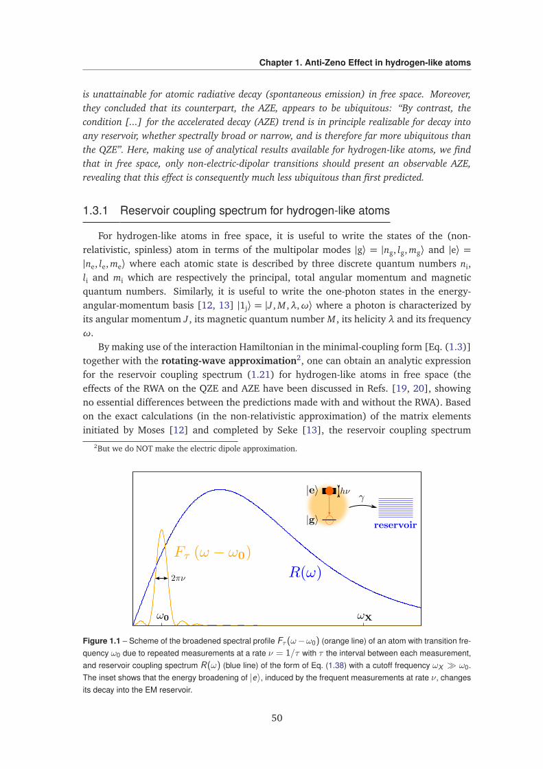
Chapter 1. Anti-Zeno Effect in hydrogen-like atoms

is unattainable for atomic radiative decay (spontaneous emission) in free space. Moreover,they concluded that its counterpart, the AZE, appears to be ubiquitous: “By contrast, thecondition [...] for the accelerated decay (AZE) trend is in principle realizable for decay intoany reservoir, whether spectrally broad or narrow, and is therefore far more ubiquitous thanthe QZE”. Here, making use of analytical results available for hydrogen-like atoms, we findthat in free space, only non-electric-dipolar transitions should present an observable AZE,revealing that this effect is consequently much less ubiquitous than first predicted.

1.3.1 Reservoir coupling spectrum for hydrogen-like atoms

For hydrogen-like atoms in free space, it is useful to write the states of the (non-relativistic, spinless) atom in terms of the multipolar modes |g⟩ = |ng, lg, mg⟩ and |e⟩ =|ne, le, me⟩ where each atomic state is described by three discrete quantum numbers ni,li and mi which are respectively the principal, total angular momentum and magneticquantum numbers. Similarly, it is useful to write the one-photon states in the energy-angular-momentum basis [12, 13] |1j⟩ = |J , M ,λ,ω⟩ where a photon is characterized byits angular momentum J , its magnetic quantum number M , its helicity λ and its frequencyω.

By making use of the interaction Hamiltonian in the minimal-coupling form [Eq. (1.3)]together with the rotating-wave approximation2, one can obtain an analytic expressionfor the reservoir coupling spectrum (1.21) for hydrogen-like atoms in free space (theeffects of the RWA on the QZE and AZE have been discussed in Refs. [19, 20], showingno essential differences between the predictions made with and without the RWA). Basedon the exact calculations (in the non-relativistic approximation) of the matrix elementsinitiated by Moses [12] and completed by Seke [13], the reservoir coupling spectrum

2But we do NOT make the electric dipole approximation.

Figure 1.1 – Scheme of the broadened spectral profile Fτ (ω−ω0) (orange line) of an atom with transition fre-quency ω0 due to repeated measurements at a rate ν = 1/τ with τ the interval between each measurement,and reservoir coupling spectrum R(ω) (blue line) of the form of Eq. (1.38) with a cutoff frequency ωX ω0.The inset shows that the energy broadening of |e〉, induced by the frequent measurements at rate ν, changesits decay into the EM reservoir.

50

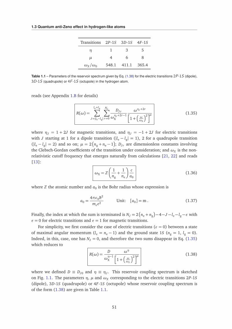
1.3 Quantum anti-Zeno effect in hydrogen-like atoms

Transitions 2P-1S 3D-1S 4F -1S

η 1 3 5

µ 4 6 8

ωX/ω0 548.1 411.1 365.4

Table 1.1 – Parameters of the reservoir spectrum given by Eq. (1.38) for the electric transitions 2P-1S (dipole),3D-1S (quadrupole) or 4F -1S (octupole) in the hydrogen atom.

reads (see Appendix 1.B for details)

R(ω) =le+lg∑

J=|le−lg|

NJ∑

r=0

DJ r

ωηJ+2r−1X

ωηJ+2r

h

1+

ωωX

2iµ(1.35)

where ηJ = 1 + 2J for magnetic transitions, and ηJ = −1 + 2J for electric transitionswith J starting at 1 for a dipole transition (|le − lg| = 1), 2 for a quadrupole transition(|le − lg| = 2) and so on; µ = 2

ng + ne − 1

; DJ r are dimensionless constants involvingthe Clebsch-Gordan coefficients of the transition under consideration; and ωX is the non-relativistic cutoff frequency that emerges naturally from calculations [21, 22] and reads[13]:

ωX = Z

1ng+

1ne

ca0

(1.36)

where Z the atomic number and a0 is the Bohr radius whose expression is

a0 =4πε0ħh2

mee2Unit: [a0] =m . (1.37)

Finally, the index at which the sum is terminated is NJ = 2

ne + ng

−4− J − le− lg−ε withε= 0 for electric transitions and ε= 1 for magnetic transitions.

For simplicity, we first consider the case of electric transitions (ε = 0) between a stateof maximal angular momentum (le = ne − 1) and the ground state 1S (ng = 1, lg = 0).Indeed, in this, case, one has NJ = 0, and therefore the two sums disappear in Eq. (1.35)which reduces to

R(ω) =D

ωη−1X

ωηh

1+

ωωX

2iµ(1.38)

where we defined D ≡ DJ0 and η ≡ ηJ . This reservoir coupling spectrum is sketchedon Fig. 1.1. The parameters η, µ and ωX corresponding to the electric transitions 2P-1S(dipole), 3D-1S (quadrupole) or 4F -1S (octupole) whose reservoir coupling spectrum isof the form (1.38) are given in Table 1.1.

51

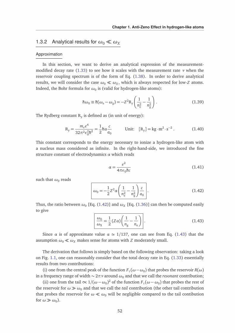
Chapter 1. Anti-Zeno Effect in hydrogen-like atoms

1.3.2 Analytical results for ω0ωX

Approximation

In this section, we want to derive an analytical expression of the measurement-modified decay rate (1.33) to see how it scales with the measurement rate ν when thereservoir coupling spectrum is of the form of Eq. (1.38). In order to derive analyticalresults, we will consider the case ω0 ωX , which is always respected for low-Z atoms.Indeed, the Bohr formula for ω0 is (valid for hydrogen-like atoms):

ħhω0 ≡ ħh(ωe −ωg) = −Z2Ry

1n2

e−

1n2

g

. (1.39)

The Rydberg constant Ry is defined as (in unit of energy):

Ry =mee4

32π2ε20ħh

2 =12ħhα

ca0

Unit: [Ry] = kg ·m2 · s−2 . (1.40)

This constant corresponds to the energy necessary to ionize a hydrogen-like atom witha nucleus mass considered as infinite. In the right-hand-side, we introduced the finestructure constant of electrodynamics α which reads

α=e2

4πε0ħhc(1.41)

such that ω0 reads

ω0 = −12

Z2α

1n2

e−

1n2

g

ca0

. (1.42)

Thus, the ratio between ω0 [Eq. (1.42)] and ωX [Eq. (1.36)] can then be computed easilyto give

ω0

ωX=

12(Zα)

1ng−

1ne

. (1.43)

Since α is of approximate value α ' 1/137, one can see from Eq. (1.43) that theassumption ω0ωX makes sense for atoms with Z moderately small.

The derivation that follows is simply based on the following observation: taking a lookon Fig. 1.1, one can reasonably consider that the total decay rate in Eq. (1.33) essentiallyresults from two contributions:

(i) one from the central peak of the function Fτ(ω−ω0) that probes the reservoir R(ω)in a frequency range of width ∼ 2πν aroundω0 and that we call the resonant contribution;

(ii) one from the tail∝ 1/(ω−ω0)2 of the function Fτ(ω−ω0) that probes the rest ofthe reservoir for ωω0 and that we call the tail contribution (the other tail contributionthat probes the reservoir for ω ω0 will be negligible compared to the tail contibutionfor ωω0).

52

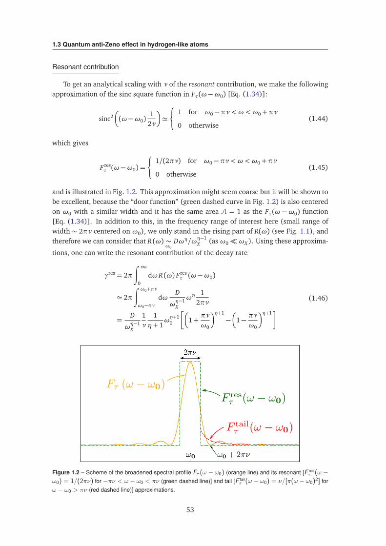
1.3 Quantum anti-Zeno effect in hydrogen-like atoms

Resonant contribution

To get an analytical scaling with ν of the resonant contribution, we make the followingapproximation of the sinc square function in Fτ(ω−ω0) [Eq. (1.34)]:

sinc2

(ω−ω0)1

2ν

'

(

1 for ω0 −πν <ω<ω0 +πν

0 otherwise(1.44)

which gives

F resτ (ω−ω0) =

(

1/(2πν) for ω0 −πν <ω<ω0 +πν

0 otherwise(1.45)

and is illustrated in Fig. 1.2. This approximation might seem coarse but it will be shown tobe excellent, because the “door function” (green dashed curve in Fig. 1.2) is also centeredon ω0 with a similar width and it has the same area A = 1 as the Fτ(ω −ω0) function[Eq. (1.34)]. In addition to this, in the frequency range of interest here (small range ofwidth ∼ 2πν centered on ω0), we only stand in the rising part of R(ω) (see Fig. 1.1), andtherefore we can consider that R (ω) ∼

ω0Dωη/ωη−1

X (as ω0ωX ). Using these approxima-

tions, one can write the resonant contribution of the decay rate

γres = 2π

∫ ∞

0

dωR (ω) F resτ (ω−ω0)

' 2π

∫ ω0+πν

ω0−πνdω

D

ωη−1X

ωη1

2πν

=D

ωη−1X

1ν

1η+ 1

ωη+10

1+πν

ω0

η+1

−

1−πν

ω0

η+1

(1.46)

Figure 1.2 – Scheme of the broadened spectral profile Fτ (ω − ω0) (orange line) and its resonant [F resτ (ω −

ω0) = 1/(2πν) for −πν < ω − ω0 < πν (green dashed line)] and tail [F tailτ (ω − ω0) = ν/[π(ω − ω0)2] for

ω − ω0 > πν (red dashed line)] approximations.

53

Chapter 1. Anti-Zeno Effect in hydrogen-like atoms

Furthermore, if we consider ν ω0 (this will be justified later), we can expand the twoterms in the bracket to third order in πν/ω0 to get

γres ' 2πD

ωη−1X

ωη0 (1.47)

which is nothing else than the FGR decay rate γ0 = 2πR(ω0) ' 2πDωη0/ωη−1X (as ω0

ωX ). Therefore the resonant contribution contains the FGR decay rate and nothing else:the effect of the frequent measurements will be contained in the second contribution: thetail contribution which will give the scaling of the measurement-modified decay rate interms of the measurement rate ν. Therefore:

γres ' γ0 (1.48)

Tail contribution

Now, we are interested in the contribution of the tail of Fτ(ω−ω0) far from ω0 (ωω0) which behaves as∝ 1/(ω−ω0)2 and probes the rest of the reservoir R(ω). To get ananalytical expression of this contribution, we replace the sin2 in Fτ(ω−ω0) by its meanvalue 1/2:

sinc2

(ω−ω0)1

2ν

'2ν2

(ω−ω0)2(1.49)

which givesF tailτ (ω−ω0) =

ν

π(ω−ω0)2(1.50)

and is illustrated in Fig. 1.2. Therefore the tail contribution reads:

γtail = 2π

∫ ω0−πν

0

dωR (ω) F tailτ (ω−ω0) +

∫ ∞

ω0+πνdωR (ω) F tail

τ (ω−ω0)

' 2π

∫ ∞

ω0ωωX

dωD

ωη−1X

ωηh

1+

ωωX

2iµν

π(ω−ω0)2

' 2π

∫ ∞

ω0ωωX

dωD

ωη−1X

ωηh

1+

ωωX

2iµν

πω2

'D

ωη−1X

× ν× Iηµ

(1.51)

where

Iηµ ≡ 2

∫ ∞

ω0ωωX

dωωη−2

h

1+

ωωX

2iµ(1.52)

To calculate the integral Iηµ, one can make the change of variable X = (ω/ωX )2. Thisleads to:

Iηµ =ωη−1X

∫ ∞

ε

dXXη2−

32

(1+ X )µ(1.53)

where (ω0/ωX )2 ε 1. One must now distinguish two cases.

54

1.3 Quantum anti-Zeno effect in hydrogen-like atoms

Case η= 1: electric dipole transitions In this case,

I1µ (ε) =

∫ ∞

ε

dX1

X (1+ X )µ. (1.54)

This integral is defined only if ε > 0, and we write I1µ(ε) to show the ε dependence, asthe numerical result will depend on the value of ε chosen. There is no analytical result forthis integral which must be computed numerically, and the most general result which onecan give for η= 1 is:

γtail = D× I1µ(ε)× ν (for η= 1) (1.55)

Case η > 1: non-electric-dipole transitions For η > 1, replacing ε by 0 is not prob-lematic as the integral is still well-defined when ε = 0 and moreover has an analyticalexpression in terms of the special “Euler’s Beta function”:

Iηµ =ωη−1X

∫ ∞

ε

dXXη2−

32

(1+ X )µ

'ωη−1X

∫ ∞

0

dXXη2−

32

(1+ X )µ(as ε 1)

=ωη−1X B

η

2−

12

,µ−η

2+

12

(1.56)

where B refers to Euler’s Beta function (well-defined for η > 1 and µ > (1/2)(η−1)). Thisyields the scaling (partially obtained in [1]):

γtail ' D× B

η

2−

12

,µ−η

2+

12

× ν (for η > 1) . (1.57)

Therefore, one can see that the tail contribution gives a scaling of the measurement-modified decay rate as∝ ν.

Final result and generalization

To sum up, the analytical expression of the decay rate γ= γres+γtail normalized by theFGR decay rate γ0 = 2πR(ω0)' 2πDωη0/ω

η−1X , reads [Eqs. (1.47), (1.55) and (1.57)]:

γ

γ0= 1+ A

ν

ω0

ωX

ω0

η−1

where A=

(

(2π)−1 I1µ(ε) for η= 1

(2π)−1 Bη

2 −12 ,µ− η

2 +12

for η > 1.

(1.58)Note that when the measurement rate ν→ 0, we recover the FGR decay rate γ0.

Now, we extend the previous result found for a reservoir of the simple form (1.38) tothe general form (1.35). We must sum over r, and then over J . In the general case, theFGR decay rate γ0 will be, for the reservoir coupling spectrum (1.35), given by

γ0 = 2πR(ω0)' 2πle+lg∑

J=|le−lg|

NJ∑

r=0

DJ r

ωηJ+2r−1X

ωηJ+2r0 . (1.59)

55

Chapter 1. Anti-Zeno Effect in hydrogen-like atoms

The hierarchy ω0 ωX ensures that the contribution from the smallest possible valueηJ +2r is dominant, that is for r = 0 and J =

le − lg

≡ Jmin. By writing ηmin ≡ ηJmin, the

FGR decay rate reduces to:

γ0 ' 2πDJmin0

ωηmin−1X

ωηmin0 . (1.60)

This is true if we assume that the coefficients DJ r have the same order of magnitudeand that DJmin0 does not vanish, which can occur for instance in the case of the electricdipole transitions (ε = 0, J = 1) between levels sharing the same principal quantumnumber (see Table 1.1 in Ref. [13]). However, we do not focus on this special case here.

The measurement-modified decay rate will be obtained as before as the sum of twocontributions γ= γres + γtail by separating two cases.

Case ηmin > 1: non-electric-dipole transitions For ηmin > 1, we just have to sum overr and over J:

γ' γ0 +le+lg∑

J=|le−lg|

NJ∑

r=0

DJ r × B

ηJ

2+ r −

12

,µ−ηJ

2− r +

12

× ν (1.61)

Case ηmin = 1: electric dipole transitions For ηmin = 1 (and Jmin = 1), the term in thedouble sum r = 0; J = 1 must be treated separately as previously

γ' γ0 + D10 × I1µ(ε)× ν︸ ︷︷ ︸

term r=0; J=1

+le+lg∑

J=2

DJ0 × B

ηJ

2−

12

,µ−ηJ

2+

12

× ν︸ ︷︷ ︸

terms r=0; J=2,...,le+lg

+le+lg∑

J=1

NJ∑

r=1

DJ r × B

ηJ

2+ r −

12

,µ−ηJ

2− r +

12

× ν︸ ︷︷ ︸

terms r=1,...,NJ ; J=1,...,le+lg

(1.62)

Finally, by dividing by the FGR decay rate (1.60) one gets

γ

γ0' 1+ A

ν

ω0

ωX

ω0

ηmin−1

(1.63)

where the coefficient A now reads:

A= (2π)−1 I1µ(ε) + (2π)−1

le+lg∑

J=2

DJ0

D10× B

ηJ

2−

12

,µ−ηJ

2+

12

+ (2π)−1le+lg∑

J=1

NJ∑

r=1

DJ r

D10× B

ηJ

2+ r −

12

,µ−ηJ

2− r +

12

for ηmin = 1 (1.64)

and

A= (2π)−1le+lg∑

J=|le−lg|

NJ∑

r=0

DJ r

DJmin0× B

ηJ

2+ r −

12

,µ−ηJ

2− r +

12

for ηmin > 1 (1.65)

56

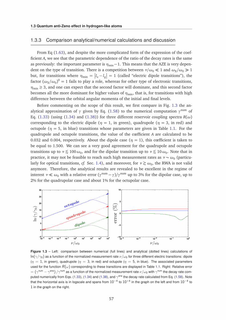
1.3 Quantum anti-Zeno effect in hydrogen-like atoms

1.3.3 Comparison analytical/numerical calculations and discussion

From Eq (1.63), and despite the more complicated form of the expression of the coef-ficient A, we see that the parametric dependence of the ratio of the decay rates is the sameas previously: the important parameter is ηmin−1. This means that the AZE is very depen-dent on the type of transition. There is a competition between ν/ω0 1 and ωX/ω0 1but, for transitions where ηmin =

le − lg

= 1 (called “electric dipole transitions”), thefactor (ωX/ω0)

0 = 1 fails to play a role, whereas for other type of electronic transitions,ηmin ≥ 3, and one can expect that the second factor will dominate, and this second factorbecomes all the more dominant for higher values of ηmin, that is, for transitions with highdifference between the orbital angular momenta of the initial and final levels.

Before commenting on the scope of this result, we first compare in Fig. 1.3 the an-alytical approximation of γ given by Eq. (1.58) to the numerical computation γnum ofEq. (1.33) (using (1.34) and (1.38)) for three different reservoir coupling spectra R(ω)corresponding to the electric dipole (η = 1, in green), quadrupole (η = 3, in red) andoctupole (η = 5, in blue) transitions whose parameters are given in Table 1.1. For thequadrupole and octupole transitions, the value of the cœfficient A are calculated to be0.032 and 0.004, respectively. About the dipole case (η = 1), this cœfficient is taken tobe equal to 1.500. We can see a very good agreement for the quadrupole and octupoletransitions up to ν ® 100ω0, and for the dipolar transition up to ν ® 10ω0. Note that inpractice, it may not be feasible to reach such high measurement rates as ν ∼ω0 (particu-larly for optical transitions, cf. Sec. 1.4), and moreover, for ν ¦ ω0, the RWA is not validanymore. Therefore, the analytical results are revealed to be excellent in the regime ofinterest ν ω0 with a relative error (γnum − γ)/γnum up to 3% for the dipolar case, up to2% for the quadrupolar case and about 1% for the octupolar case.

−5

0

5

10

15

20

25

30

10−4 10−3 10−2 10−1 100 101 102 103 104 −10

−5

0

5

10

10−4 10−3 10−2 10−1 100

Figure 1.3 – Left: comparison between numerical (full lines) and analytical (dotted lines) calculations ofln(γ/γ0) as a function of the normalized measurement rate ν/ω0 for three different electric transitions: dipole(η = 1, in green), quadrupole (η = 3, in red) and octupole (η = 5, in blue). The associated parametersused for the function R(ω) corresponding to these transitions are displayed in Table 1.1. Right: Relative error= (γnum − γana) /γnum as a function of the normalized measurement rate ν/ω0 with γnum the decay rate com-puted numerically from Eqs. (1.33), (1.34) and (1.38), and γana the decay rate calculated from Eq. (1.58). Notethat the horizontal axis is in logscale and spans from 10−4 to 10+4 in the graph on the left and from 10−4 to1 in the graph on the right.

57

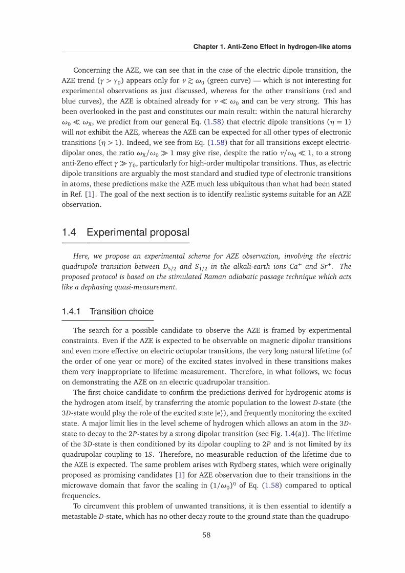
Chapter 1. Anti-Zeno Effect in hydrogen-like atoms

Concerning the AZE, we can see that in the case of the electric dipole transition, theAZE trend (γ > γ0) appears only for ν ¦ ω0 (green curve) — which is not interesting forexperimental observations as just discussed, whereas for the other transitions (red andblue curves), the AZE is obtained already for ν ω0 and can be very strong. This hasbeen overlooked in the past and constitutes our main result: within the natural hierarchyω0 ωX, we predict from our general Eq. (1.58) that electric dipole transitions (η = 1)will not exhibit the AZE, whereas the AZE can be expected for all other types of electronictransitions (η > 1). Indeed, we see from Eq. (1.58) that for all transitions except electric-dipolar ones, the ratio ωX/ω0 1 may give rise, despite the ratio ν/ω0 1, to a stronganti-Zeno effect γ γ0, particularly for high-order multipolar transitions. Thus, as electricdipole transitions are arguably the most standard and studied type of electronic transitionsin atoms, these predictions make the AZE much less ubiquitous than what had been statedin Ref. [1]. The goal of the next section is to identify realistic systems suitable for an AZEobservation.

1.4 Experimental proposal

Here, we propose an experimental scheme for AZE observation, involving the electricquadrupole transition between D5/2 and S1/2 in the alkali-earth ions Ca+ and Sr+. Theproposed protocol is based on the stimulated Raman adiabatic passage technique which actslike a dephasing quasi-measurement.

1.4.1 Transition choice

The search for a possible candidate to observe the AZE is framed by experimentalconstraints. Even if the AZE is expected to be observable on magnetic dipolar transitionsand even more effective on electric octupolar transitions, the very long natural lifetime (ofthe order of one year or more) of the excited states involved in these transitions makesthem very inappropriate to lifetime measurement. Therefore, in what follows, we focuson demonstrating the AZE on an electric quadrupolar transition.

The first choice candidate to confirm the predictions derived for hydrogenic atoms isthe hydrogen atom itself, by transferring the atomic population to the lowest D-state (the3D-state would play the role of the excited state |e⟩), and frequently monitoring the excitedstate. A major limit lies in the level scheme of hydrogen which allows an atom in the 3D-state to decay to the 2P-states by a strong dipolar transition (see Fig. 1.4(a)). The lifetimeof the 3D-state is then conditioned by its dipolar coupling to 2P and is not limited by itsquadrupolar coupling to 1S. Therefore, no measurable reduction of the lifetime due tothe AZE is expected. The same problem arises with Rydberg states, which were originallyproposed as promising candidates [1] for AZE observation due to their transitions in themicrowave domain that favor the scaling in (1/ω0)η of Eq. (1.58) compared to opticalfrequencies.

To circumvent this problem of unwanted transitions, it is then essential to identify ametastable D-state, which has no other decay route to the ground state than the quadrupo-

58

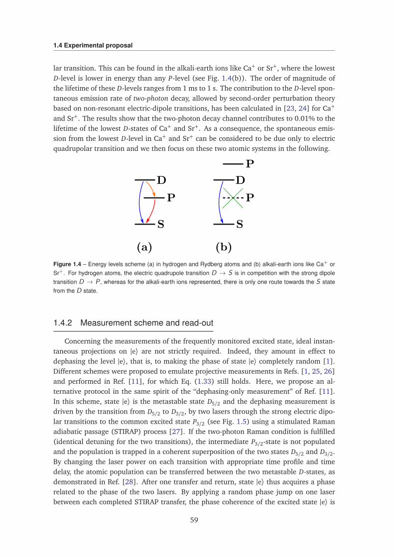
1.4 Experimental proposal

lar transition. This can be found in the alkali-earth ions like Ca+ or Sr+, where the lowestD-level is lower in energy than any P-level (see Fig. 1.4(b)). The order of magnitude ofthe lifetime of these D-levels ranges from 1 ms to 1 s. The contribution to the D-level spon-taneous emission rate of two-photon decay, allowed by second-order perturbation theorybased on non-resonant electric-dipole transitions, has been calculated in [23, 24] for Ca+

and Sr+. The results show that the two-photon decay channel contributes to 0.01% to thelifetime of the lowest D-states of Ca+ and Sr+. As a consequence, the spontaneous emis-sion from the lowest D-level in Ca+ and Sr+ can be considered to be due only to electricquadrupolar transition and we then focus on these two atomic systems in the following.

Figure 1.4 – Energy levels scheme (a) in hydrogen and Rydberg atoms and (b) alkali-earth ions like Ca+ orSr+. For hydrogen atoms, the electric quadrupole transition D → S is in competition with the strong dipoletransition D → P , whereas for the alkali-earth ions represented, there is only one route towards the S statefrom the D state.

1.4.2 Measurement scheme and read-out

Concerning the measurements of the frequently monitored excited state, ideal instan-taneous projections on |e⟩ are not strictly required. Indeed, they amount in effect todephasing the level |e⟩, that is, to making the phase of state |e⟩ completely random [1].Different schemes were proposed to emulate projective measurements in Refs. [1, 25, 26]and performed in Ref. [11], for which Eq. (1.33) still holds. Here, we propose an al-ternative protocol in the same spirit of the “dephasing-only measurement” of Ref. [11].In this scheme, state |e⟩ is the metastable state D5/2 and the dephasing measurement isdriven by the transition from D5/2 to D3/2, by two lasers through the strong electric dipo-lar transitions to the common excited state P3/2 (see Fig. 1.5) using a stimulated Ramanadiabatic passage (STIRAP) process [27]. If the two-photon Raman condition is fulfilled(identical detuning for the two transitions), the intermediate P3/2-state is not populatedand the population is trapped in a coherent superposition of the two states D5/2 and D3/2.By changing the laser power on each transition with appropriate time profile and timedelay, the atomic population can be transferred between the two metastable D-states, asdemonstrated in Ref. [28]. After one transfer and return, state |e⟩ thus acquires a phaserelated to the phase of the two lasers. By applying a random phase jump on one laserbetween each completed STIRAP transfer, the phase coherence of the excited state |e⟩ is

59

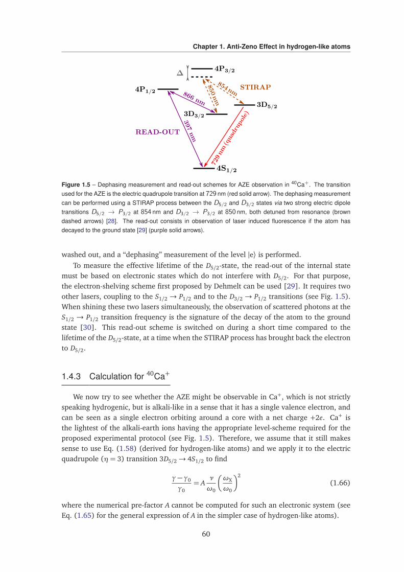
Chapter 1. Anti-Zeno Effect in hydrogen-like atoms

Figure 1.5 – Dephasing measurement and read-out schemes for AZE observation in 40Ca+. The transitionused for the AZE is the electric quadrupole transition at 729 nm (red solid arrow). The dephasing measurementcan be performed using a STIRAP process between the D5/2 and D3/2 states via two strong electric dipoletransitions D5/2 → P3/2 at 854 nm and D3/2 → P3/2 at 850 nm, both detuned from resonance (browndashed arrows) [28]. The read-out consists in observation of laser induced fluorescence if the atom hasdecayed to the ground state [29] (purple solid arrows).

washed out, and a “dephasing” measurement of the level |e⟩ is performed.To measure the effective lifetime of the D5/2-state, the read-out of the internal state

must be based on electronic states which do not interfere with D5/2. For that purpose,the electron-shelving scheme first proposed by Dehmelt can be used [29]. It requires twoother lasers, coupling to the S1/2 → P1/2 and to the D3/2 → P1/2 transitions (see Fig. 1.5).When shining these two lasers simultaneously, the observation of scattered photons at theS1/2 → P1/2 transition frequency is the signature of the decay of the atom to the groundstate [30]. This read-out scheme is switched on during a short time compared to thelifetime of the D5/2-state, at a time when the STIRAP process has brought back the electronto D5/2.

1.4.3 Calculation for 40Ca+

We now try to see whether the AZE might be observable in Ca+, which is not strictlyspeaking hydrogenic, but is alkali-like in a sense that it has a single valence electron, andcan be seen as a single electron orbiting around a core with a net charge +2e. Ca+ isthe lightest of the alkali-earth ions having the appropriate level-scheme required for theproposed experimental protocol (see Fig. 1.5). Therefore, we assume that it still makessense to use Eq. (1.58) (derived for hydrogen-like atoms) and we apply it to the electricquadrupole (η= 3) transition 3D5/2→ 4S1/2 to find

γ− γ0

γ0= A

ν

ω0

ωX

ω0

2

(1.66)

where the numerical pre-factor A cannot be computed for such an electronic system (seeEq. (1.65) for the general expression of A in the simpler case of hydrogen-like atoms).

60

1.5 Conclusion

To be observable, the AZE must induce a lifetime reduction larger than 1%, the bestprecision reached in recent 3D5/2-lifetime measurements in Ca+ [30]. We evaluate ωX

using Eq. (1.36) with ng = 4 and ne = 3 and by replacing the atomic number Z by theeffective number of charges Zeff = 2. Using the frequency of this transition ω0 = 2π ×411 THz, this gives a ratio (ωX/ω0)2 ' 6.6×106. If the unknown pre-factor A is assumed tobe of the order of unity, one would need ν∼ 4MHz to meet the observation requirement.

The transfer between the states D5/2 and D3/2 has been demonstrated in 40Ca+ with aSTIRAP process [28], where a complete one-way transfer duration of 5 µs was observedfor 420 mW/mm2 on the 850 nm 3D3/2 → 4P3/2 transition and 640 mW/mm2 on the854 nm 3D5/2 → 4P3/2 transition, with both lasers detuned by ∆ = 600 MHz from res-onance (see Fig. 1.5). To reduce the duration of the dephasing measurement to timescales smaller than 1 µs, one can increase the laser intensity by stronger focusing and/orlarger power, but we can also consider that a complete STIRAP transfer is not required toachieve a dephasing of the excited state. Furthermore, a close inspection of Tables I andII in Ref. [13] suggests that the pre-factor A could be much larger than unity, making theconstraint on a high measurement rate less stringent for AZE observation.

Even if the experimental requirements for AZE observation on quadrupole transitionin Ca+ are more demanding than today’s best achievements, realistic arguments show thatthey can be met in a dedicated experimental set-up. This experimental challenge wouldbenefit from theoretical insight concerning the still unknown pre-factor scaling the lifetimereduction.

1.5 Conclusion

Based on well-established results for hydrogen-like atoms, we derived in Section 1.3an analytical expression of the decay rate modified by frequent measurements which al-lows us to highlight the main condition for an observable AZE in atomic radiative decayin free space: all transitions except electric-dipole transitions will exhibit an AZE undersufficiently rapid repeated measurements. This analytical formula also indicates how theAZE scales with the measurement rate.

We then identified in Section 1.4 a suitable level scheme in the alkali-earth ions Ca+

and Sr+ for AZE observation, involving the electric quadrupole transition between D5/2 andS1/2, and using a new “dephasing” measurement protocol based on the STIRAP technique.Other suitable experimental schemes might exist, and we encourage further proposals inthis sense.

61

Chapter 1. Anti-Zeno Effect in hydrogen-like atoms

1.A Decay rate in free space

In this appendix, we follow more or less the chapter 6.4 in [16] to derive an analyticalexpression for the decay rate given by the FGR in Eq. (1.27) for a two-level atom in free space.We recall here its expression:

γ0 = 2π |g(ω0)|2ρ (ω0) (1.67)

Two things must be calculated: (i) the density of one-photon states |1j⟩, which corresponds tothe density of modes j in the fictitious volume V and (ii) the coupling constant |gj|2 averagedover all emission directions and polarizations.

1.A.1 Density of states in the volume V

The density of states ρ (ω) is equal to the number of quasi-continuum modes in thefrequency range from ω to ω + dω, divided by the frequency width of this interval dω:ρ(ω)≡ dN/dω. One must then find a way to count the number of modes dN in the widthdω. In vacuum and within the quantization volume V , the number of modes is easy tocount. First, we recall that here a mode j is referred to as a polarized travelling planemonochromatic wave, characterized by its frequency ωj, its wavevector kj whose modulusverifies |kj|=ωj/c and its polarization vector ~εj.

Moreover, we use periodic boundary conditions because they are well adapted for thequantization of freely propagating fields. They impose the quantization of the wavevectorsof the modes kj: kj = (2π/L)(nx ~x + ny ~y + nz~z) where L is the side of the cubic volume,and nx , ny , nz are integers. This has the advantage to make them countable, becauseeach wavevector can be represented by a point in the reciprocal space, and they constitutea cubic lattice with unit cell volume (2π/L)3. We now can count the number of pointsdN lying between spheres of radii k and k + dk in the reciprocal space. This is equalto the elementary volume between the two spheres 4πk2dk divided by the volume of aunit cell (2π/L)3. Moreover, taking into account that two modes are associated with eachwavevector, corresponding to two polarizations, the number of modes in this elementaryvolume is therefore:

dN = 24πk2

(2π/L)3dk

= Vk2

π2dk

(1.68)

Finally, because we want the number of modes in the bandwidth dω, we make the changeof variable k =ω/c to get

dN = Vω2

π2c3dω (1.69)

and one get the density of states ρ(ω) by dividing dN by dω:

ρ (ω) = Vω2

π2c3(1.70)

62

1.A Decay rate in free space

1.A.2 Coupling constant

We proceed by averaging the coupling constant |gj|2 over all emission directions andpolarizations. By noting |g(ω)|2 the quantity |gj|2 averaged over all modes with ωj = ω,that is over all polarizations and emission directions, one has:

|g(ω)|2 =12

14π

2∑

p=1

∫

dΩkj|gj|2 where ħhgj ≡ ⟨g,1j| HI |e,0⟩ (1.71)

where the sum is over the two orthogonal polarizations ~ε1 and ~ε2 forming a basis for thepolarization vector ~εj (and are chosen to form a direct triad with kj, see Fig. 1.6), and dΩkj

is the element of solid angle corresponding to the direction of kj. We want to calculate thisquantity. For that, we must express the coupling constant |gj|2. To get an expression for|gj|2, we first simplify the form of the interaction Hamiltonian HI of Eq. (1.3) by makingthe dipole approximation (also called long-wavelength approximation). This consistsin replacing the vector potential A(r) by its value at the position of the nucleus r = 0.The vector potential operator A can be expanded into travelling plane wave modes andexpressed in terms of the operators aj and a†

j according to (see [16], chapter 4):

A (r) =∑

j

~εj

E(1)j

ωj

ajeikj · r + a†

j e−ikj · r

(1.72)

with

E(1)j =

√

√

√ħhωj

2ε0VUnit: [E(1)j ] = V.m−1 (1.73)

where the volume V appearing in the expression of E(1)j is the quantization volume, and

we take r as a classical quantity. E(1)j is called the “one-photon amplitude of the mode j”

and comes from a freedom of choice of constant. It is chosen to be the amplitude of theclassical field with energy ħhωj corresponding to the energy of a single photon in the modej (see [16], chapter 4). By making the dipole approximation, the interaction Hamiltonianbecomes

HI =e

me

∑

j

√

√

√ħh

2ε0ωjV~εj · p

aj + a†j

(1.74)

Therefore, the coupling constant to the mode j reads:

ħh2|gj|2 = | ⟨g,1j| HI |e,0⟩ |2

=e2

m2e

ħh2ε0ωjV

| ⟨g| ~εj · p |e⟩ |2(1.75)

Now, we proceed to the calculation of the term ⟨g| ~εj · p |e⟩. To make a complete calcu-lation, we will consider the particular case of an electric dipole transition P → S betweenan excited state |e⟩ with orbital angular momentum le = 1, me = 0 and a ground state |g⟩with zero orbital angular momentum lg = 0, mg = 0. For a quantization axis taken along~z, one gets:

⟨g| ~εj · p |e⟩= ⟨g| pz |e⟩

~εj · ~z

(1.76)

63

Chapter 1. Anti-Zeno Effect in hydrogen-like atoms

Moreover, if we choose one polarization ~ε1 to be in the plane (~z,kj), one has ~ε1 · ~z = sinθ(see Fig. 1.6) and

⟨g| ~ε1 · p |e⟩= ⟨g| pz |e⟩ sinθ (1.77)

and then the other polarization ~ε2 is perpendicular to ~z: ~ε2 · ~z = 0 (see Fig. 1.6), andtherefore the matrix element is zero for this polarization. Thus, one gets

ħh2|gj|2 =e2

m2e

ħh2ε0ωjV

| ⟨g| pz |e⟩ |2sin2 θ (1.78)

Note: Note that this term ∝ sin2 θ gives the pattern of spontaneous emission for thisparticular transition, which is zero in the ~z direction (θ = 0) and maximal in the directionsperpendicular to ~z (θ = π/2). One can notice that it is the same pattern as the radiationdiagram obtained by a classical calculation of radiation from an electric dipole oscillatingin the ~z direction.

Therefore, by writing the element of solid angle as dΩ = sinθ dθ dϕ, in the integral,one gets for |g(ω)|2:

ħh2|g(ω)|2 =12

14π

e2

m2e

ħh2ε0ωV

| ⟨g| pz |e⟩ |2∫ 2π

0

dϕ

∫ π

0

dθ sin3 θ (1.79)

Moreover, taking into account that

∫ 2π

0

dϕ

∫ π

0

dθ sin3 θ =8π3

(1.80)

one gets

ħh2|g(ω)|2 =13

e2

m2e

ħh2ε0ωV

| ⟨g| pz |e⟩ |2 (1.81)

Finally, together with the density of states, one gets for the decay rate defined inEq. (1.67):

γ0 =1

3πε0

e2

m2e

ω0

ħhc3| ⟨g| pz |e⟩ |2 (1.82)

Note 1: The decay rate is independent of the quantization volume V .

Note 2: This matrix element is also related to the matrix element with the atomic dipoleoperator d = −er, that is3: ⟨g| ~εj · p |e⟩ = i(me/e)ω0 ⟨g| ~εj · d |e⟩, so that the decay rate alsotakes the form:

γ0 =1

3πε0

ω30

ħhc3| ⟨g| dz |e⟩ |2 (1.83)

3This identity directly results from p= −(ime/ħh)[r, HA].

64

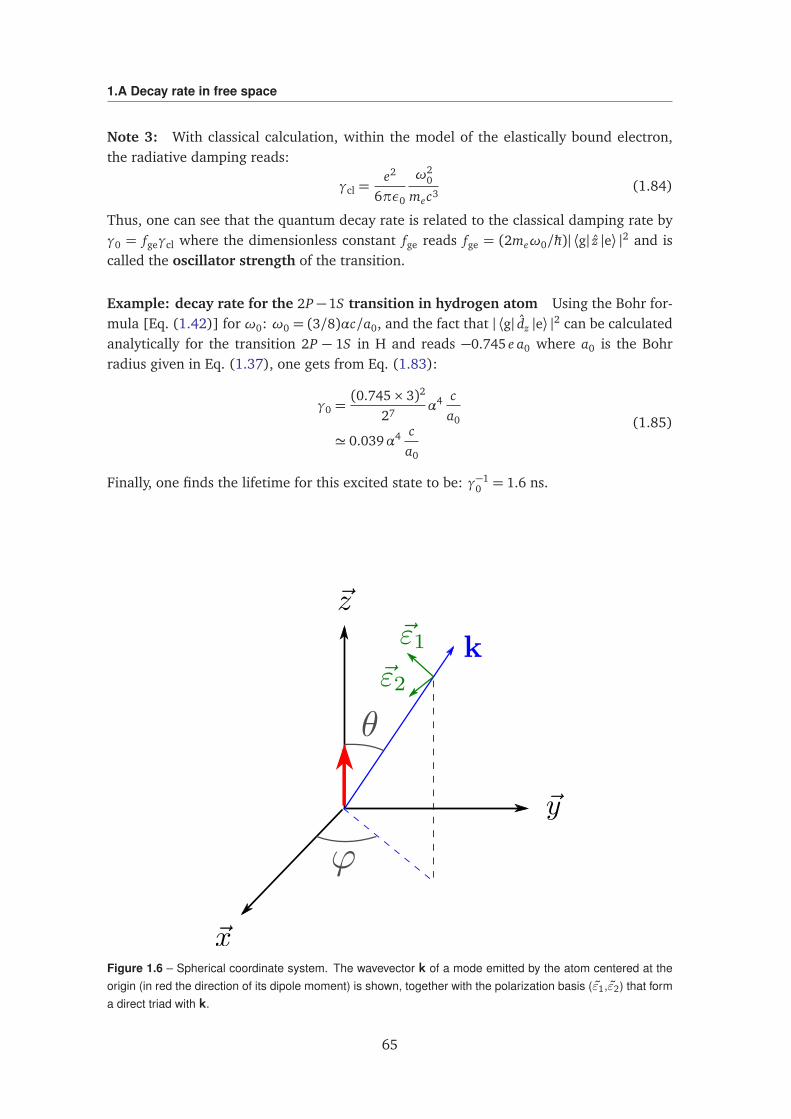
1.A Decay rate in free space

Note 3: With classical calculation, within the model of the elastically bound electron,the radiative damping reads:

γcl =e2

6πε0

ω20

mec3(1.84)

Thus, one can see that the quantum decay rate is related to the classical damping rate byγ0 = fgeγcl where the dimensionless constant fge reads fge = (2meω0/ħh)| ⟨g| z |e⟩ |2 and iscalled the oscillator strength of the transition.

Example: decay rate for the 2P −1S transition in hydrogen atom Using the Bohr for-mula [Eq. (1.42)] for ω0: ω0 = (3/8)αc/a0, and the fact that | ⟨g| dz |e⟩ |2 can be calculatedanalytically for the transition 2P − 1S in H and reads −0.745 e a0 where a0 is the Bohrradius given in Eq. (1.37), one gets from Eq. (1.83):

γ0 =(0.745× 3)2

27α4 c

a0

' 0.039α4 ca0

(1.85)

Finally, one finds the lifetime for this excited state to be: γ−10 = 1.6 ns.

Figure 1.6 – Spherical coordinate system. The wavevector k of a mode emitted by the atom centered at theorigin (in red the direction of its dipole moment) is shown, together with the polarization basis (ε1,ε2) that forma direct triad with k.

65

Chapter 1. Anti-Zeno Effect in hydrogen-like atoms

1.B Reservoir for hydrogen-like atoms in free space

In this Appendix, we sum up the results obtained by Moses [12] and Seke [13] and linkthem to our notations of the reservoirs Eqs. (1.35) and (1.38).

For hydrogen-like atoms in free space, it is useful to write the states of the (non-relativistic, spinless) atom in terms of the multipolar modes |g⟩ = |ng, lg, mg⟩ and |e⟩ =|ne, le, me⟩ where each atomic state is described by three discrete quantum numbers ni,li and mi which are respectively the principal, total angular momentum and magneticquantum numbers. Similarly, it is useful to write the one-photon states in the energy-angular-momentum basis |1j⟩= |J , M ,λ,ω⟩ where a photon is characterized by its angularmomentum J , its magnetic quantum number M , its helicity λ and its frequency ω, and thenormalization is such that (note that unfortunately the normalizations used in [12] and[13] are different and we follow here the one of Seke defined (not given explicitely)):

⟨J , M ,λ,ω | J ′, M ′,λ′,ω′⟩= δJJ ′δM M ′δλλ′δ

ω−ω′

(1.86)

The reservoir coupling spectrum (1.19) for given photon quantum numbers J , M ,λ,ω isthen given by

R(ω) =∑

J ,M ,λ

ħh−2| ⟨ng, lg, mg; J , M ,λ,ω| HI |ne, le, me; 0⟩ |2 (1.87)

because of the normalization in Eq. (1.86). Moreover, as a consequence of the conserva-tion of the angular momentum, the values of J and M must verify

(

J = |le − lg|, |le − lg|+ 1, ..., le + lg

M = me −mg ≡ M(1.88)

which are the exact selection rules. Therefore, the full reservoir takes the form

R(ω) =le+lg∑

J=|le−lg|

+J∑

M=−J

1∑

λ=0

ħh−2| ⟨ng, lg, mg; J , M ,λ,ω| HI |ne, le, me; 0⟩ |2δM M (1.89)

In the non-relativistic approximation, Seke calculated in [13] the exact matrix ele-ments ⟨ng, lg, mg; J , M ,λ,ω| HI |ne, le, me; 0⟩ for hydrogen-like atoms in free space, usingthe interaction Hamiltonian in the minimal-coupling form [Eq. (1.3)], by writing thevector potential operator A in the energy-angular-momentum representation (Eqs. (33a)and (33b) in [12]), and the linear momentum operator p in the position representationp= −iħh∇, he found that [Eqs. (17-19) in [13]]:

⟨ng, lg, mg; J , M ,λ,ω| HI |ne, le, me; 0⟩ ∝ λ ⟨lg, J , mg, M |lg, J , le, me⟩

×

ωωX

J+ε−1/2

h

1+

ωωX

2ing+ne−1

N ′J∑

r=0

d ′J r

ω

ωX

2r

(1.90)

66

1.B Reservoir for hydrogen-like atoms in free space

where ⟨lg, J , mg, M |lg, J , le, me⟩ are the Clebsch-Gordan coefficients of the transition of in-terest, and ωX is the non-relativistic cutoff frequency given by Eq. (1.36). The coeffi-cients d ′J r are numerical coefficients that have been calculated for certain transitions in[13] (note that the coefficients d ′J r here correspond to the coefficients d00dr in Eq. (18) inRef. [13]). The index at which the sum is terminated is N ′J = ne+ng−2−(1/2)(J−le−lg−ε)with ε = 0 for electric transitions and ε = 1 for magnetic transitions. The square of thisexpression that appears in Eq. (1.89) gives

| ⟨ng, lg, mg; J , M ,λ,ω| HI |ne, le, me; 0⟩ |2 ∝ λ2 ⟨lg, J , mg, M |lg, J , le, me⟩2

×

ωωX

2J+2ε−1

h

1+

ωωX

2i2(ng+ne−1)

N ′J∑

r=0

d ′J r

ω

ωX

2r

2

(1.91)

which can be recast in the form

| ⟨ng, lg, mg; J , M ,λ,ω| HI |ne, le, me; 0⟩ |2 ∝ λ2 ⟨lg, J , mg, M |lg, J , le, me⟩2

×NJ∑

r=0

dJ r

ωωX

2J+2ε−1+2r

h

1+

ωωX

2i2(ng+ne−1)(1.92)

where NJ = 2

ne + ng

− 4 − J − le − lg − ε and dJ r are combinations of the previous d ′J rcoefficients.

Finally, by plugging this expression into Eq. (1.89) one gets the reservoir shown inEq. (1.35), that is

R(ω) =le+lg∑

J=|le−lg|

NJ∑

r=0

DJ r

ωηJ+2r−1X

ωηJ+2r

h

1+

ωωX

2iµ(1.93)

where ηJ = 1 + 2J for magnetic transitions, and ηJ = −1 + 2J for electric transitionswith J = 1 for a dipole transition, J = 2 for a quadrupole transition and so on; µ =2

ng + ne − 1

and where the DJ r are dimensionless constants involving the previous dJ r

coefficients and the Clebsch-Gordan coefficients of the transition under consideration⟨lg, J , mg, M |lg, J , le, me⟩.

Note that this reservoir can take a much simpler form in the case of electric transitions(ε= 0) between a state of maximal angular momentum (le = ne−1) and the ground state1S (ng = 1, lg = 0). Indeed, in this, case, one has NJ = 0, and therefore the two sumsdisappear in the previous expression which reduces to the Eq. (1.38)

R(ω) =D

ωη−1X

ωηh

1+

ωωX

2iµ(1.94)

where we defined D ≡ DJ0 and η≡ ηJ .

Example: decay rate for the 2P − 1S transition in hydrogen atom For example, forthe 2P − 1S transition in hydrogen atom, η= 1 and µ= 4 and one has:

R(ω) = Dω

h

1+

ωωX

2i4 (1.95)

67

Chapter 1. Anti-Zeno Effect in hydrogen-like atoms

with D = (2/π)(2/3)9α3 (see [21] and [31], chapter 6). Taking into account that for thetransition 2P − 1S of H atom (ng = 1, ne = 2, Z = 1), ω0 = (3/8)αc/a0 [Eq. (1.42)] andωX = (3/2)(c/a0) [Eq. (1.36)] which gives a ratio ω0/ωX = α/4 [Eq. (1.43)], the decayrate reads:

γ0 = 2πR(ω0)

=

23

8

α4 ca0

1+α

4

2−4 (1.96)

Now, if one neglects the term [1+ (α/4)2]−4, the decay rate becomes

γ0 '

23

8

α4 ca0

' 0.039α4 ca0

(1.97)

which is fortunately the same result as the one found in the Appendix 1.A, Eq. (1.85).Therefore, as pointed out by Moses in [12], the dipole approximation used in Ap-pendix 1.A to calculate the decay rate is equivalent to neglect the “retardation term”[1 + (α/4)2]−4. The prediction for the lifetime doing the dipole approximation is quitegood, but one can increase the precision by keeping the retardation term.

68

Bibliography

[1] A. Kofman and G. Kurizki, Nature 405, 546 (2000).

[2] P. Facchi, H. Nakazato, and S. Pascazio, Physical Review Letters 86, 2699 (2001).

[3] B. Misra and E. Sudarshan, Journal of Mathematical Physics 18, 756 (1977).

[4] R. Cook, Physica Scripta 1988, 49 (1988).

[5] W. M. Itano, D. J. Heinzen, J. Bollinger, and D. Wineland, Physical Review A 41,2295 (1990).

[6] Y. Patil, S. Chakram, and M. Vengalattore, Physical Review Letters 115, 140402(2015).

[7] B. Kaulakys and V. Gontis, Physical Review A 56, 1131 (1997).

[8] A. Kofman and G. Kurizki, Physical Review A 54, R3750 (1996).

[9] M. Lewenstein and K. Rzazewski, Physical Review A 61, 022105 (2000).

[10] M. Fischer, B. Gutiérrez-Medina, and M. Raizen, Physical Review Letters 87, 040402(2001).

[11] P. Harrington, J. Monroe, and K. Murch, Physical Review Letters 118, 240401(2017).

[12] H. Moses, Physical Review A 8, 1710 (1973).

[13] J. Seke, Physica A 203, 269 (1994).

[14] R. Loudon, The quantum theory of light (Oxford University Press, 2000).

[15] L. Rayleigh, The London, Edinburgh, and Dublin Philosophical Magazine and Jour-nal of Science 49, 539 (1900).

[16] G. Grynberg, A. Aspect, and C. Fabre, Introduction to quantum optics: from the semi-classical approach to quantized light (Cambridge University Press, 2010).

[17] S. M. Barnett and P. M. Radmore, Methods in theoretical quantum optics, Vol. 15(Oxford University Press, 2002).

[18] V. Weisskopf and E. Wigner, Zeitschrift für Physik 63, 54 (1930).

[19] H. Zheng, S. Zhu, and M. Zubairy, Physical Review Letters 101, 200404 (2008).

69

BIBLIOGRAPHY

[20] Q. Ai, Y. Li, H. Zheng, and C. Sun, Physical Review A 81, 042116 (2010).

[21] P. Facchi and S. Pascazio, Physics Letters A 241, 139 (1998).

[22] V. Debierre, T. Durt, A. Nicolet, and F. Zolla, Physics Letters A 379, 2577 (2015).

[23] M. S. Safronova, W. R. Johnson, and U. I. Safronova, Journal of Physics B: Atomic,Molecular and Optical Physics 43, 074014 (2010).

[24] M. S. Safronova, W. R. Johnson, and U. I. Safronova, Journal of Physics B: Atomic,Molecular and Optical Physics 50, 189501 (2017).

[25] A. Kofman and G. Kurizki, Physical Review Letters 87, 270405 (2001).

[26] Q. Ai, D. Xu, S. Yi, A. G. Kofman, C. P. Sun, and F. Nori, Scientific Reports 3 (2013).

[27] J. R. Kuklinski, U. Gaubatz, F. T. Hioe, and K. Bergmann, Physical Review A 40,6741 (1989).

[28] J. L. Sørensen, D. Møller, T. Iversen, J. B. Thomsen, F. Jensen, P. Staanum, D. Voigt,and M. Drewsen, New Journal of Physics 8, 261 (2006).

[29] H. Dehmelt, in Bulletin of the American Physical Society, Vol. 20 (1975) p. 60.

[30] A. Kreuter, C. Becher, G. P. T. Lancaster, A. B. Mundt, C. Russo, H. Häffner, C. Roos,W. Hänsel, F. Schmidt-Kaler, R. Blatt, and M. S. Safronova, Physical Review A 71,032504 (2005).

[31] V. Debierre, La fonction d’onde du photon en principe et en pratique, Ph.D. thesis, EcoleCentrale de Marseille (2015).

70

BIBLIOGRAPHY

71

BIBLIOGRAPHY

72

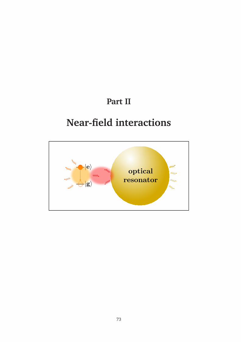
Part II

Near-field interactions

73

75

76

CHAPTER 2

Lamb shift multipolar analysis

2.1 Introduction

The coupling between quantum emitters (QEs) and optically resonant nanostructuresis at the heart of nanophotonics [1]. In the weak-coupling regime, the exponential decayin time of the excited state of the QE is characterized by the decay rate, which can beeither enhanced [2] or inhibited [3] by the local electromagnetic (EM) environment: thisis known as the Purcell effect. A less often discussed effect of spontaneous emission is thatthe surrounding environment also induces level shifts of the excited atomic states, result-ing in a frequency-shift for the emitted photons, in comparison with the bare resonancefrequency. This is the photonic Lamb shift, also called radiative frequency-shift or Casimir-Polder frequency-shift (historically it was called Lamb shift and referred to level shifts ofatoms in free space [4, 5]). In this Chapter, we will refer to it as photonic Lamb shiftor simply Lamb shift, and sometimes frequency-shift. This effect has been theoreticallystudied in the case of perfect reflectors [6], partially reflecting surfaces [7, 8], photoniccrystals [9–11], in the case of a dielectric microsphere without [12, 13] and with [14] ab-sorption, dielectric or metallic prolate spheroids [15], and in the case of two-dimensionalphotonic crystals [16]. However, there is a lack of experimental demonstration of such aneffect in quantum emitters.

In the present Chapter, we study the weak-coupling between a QE and its environment.We firstly start this Chapter with the Section 2.2, where we will justify the use of a clas-sical formalism to study the photonic Lamb shift and modified decay rate induced by thepresence of the environment by showing, in the weak-coupling regime, its equivalence tothe quantum result. We focus on the study of the photonic Lamb shift of a QE weakly1

coupled to optically resonant nanostructures, characterized by dielectric constants. Wedo not consider the extreme near-field (i.e. distances QE-object of z ∼ 1nm), where onmust take into account non-local effects in the nanostructure [17]. The resonances ofa given nanostructure characterize its optical response to an excitation electromagnetic(EM) field, and can be of different nature: for example Mie resonances in Mie resonators[18], or localized surface plasmon resonances in metallic nanoparticles [19]. After recall-ing in Section 2.3 a model commonly used to describe the optical response of a plasmonicnanoparticle, which consists in treating the particle as an electric dipole (known as the

1We refer here to the weak-coupling by opposition to the strong-coupling that will be studied in Chapter 4.

77

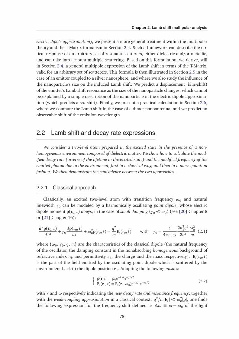
Chapter 2. Lamb shift multipolar analysis

electric dipole approximation), we present a more general treatment within the multipolartheory and the T-Matrix formalism in Section 2.4. Such a framework can describe the op-tical response of an arbitrary set of resonant scatterers, either dielectric and/or metallic,and can take into account multiple scattering. Based on this formulation, we derive, stillin Section 2.4, a general multipole expression of the Lamb shift in terms of the T-Matrix,valid for an arbitrary set of scatterers. This formula is then illustrated in Section 2.5 in thecase of an emitter coupled to a silver nanosphere, and where we also study the influence ofthe nanoparticle’s size on the induced Lamb shift. We predict a displacement (blue-shift)of the emitter’s Lamb shift resonance as the size of the nanoparticle changes, which cannotbe explained by a simple description of the nanoparticle in the electric dipole approxima-tion (which predicts a red-shift). Finally, we present a practical calculation in Section 2.6,where we compute the Lamb shift in the case of a dimer nanoantenna, and we predict anobservable shift of the emission wavelength.

2.2 Lamb shift and decay rate expressions

We consider a two-level atom prepared in the excited state in the presence of a non-homogeneous environment composed of dielectric matter. We show how to calculate the mod-ified decay rate (inverse of the lifetime in the excited state) and the modified frequency of theemitted photon due to the environment, first in a classical way, and then in a more quantumfashion. We then demonstrate the equivalence between the two approaches.

2.2.1 Classical approach

Classically, an excited two-level atom with transition frequency ω0 and naturallinewidth γ0 can be modeled by a harmonically oscillating point dipole, whose electricdipole moment p(r0, t) obeys, in the case of small damping (γ0ω0) (see [20] Chapter 8or [21] Chapter 16):

d2p(r0, t)d t2

+ γ0dp(r0, t)

d t+ω2

0p(r0, t) =q2

mEs(r0, t) with γ0 =

14πε0εb

2n3bq2

3c3

ω20

m(2.1)

where ω0, γ0, q, m are the characteristics of the classical dipole (the natural frequencyof the oscillator, the damping constant in the nonabsorbing homogeneous background ofrefractive index nb and permittivity εb, the charge and the mass respectively). Es(r0, t)is the part of the field emitted by the oscillating point dipole which is scattered by theenvironment back to the dipole position r0. Adopting the following ansatz:

p(r, t) = p0e−iωt e−γt/2

Es(r0, t) = Es(r0,ω0)e−iωt e−γt/2 (2.2)

with γ and ω respectively indicating the new decay rate and resonance frequency, togetherwith the weak-coupling approximation in a classical context: q2/m|Es| ω2

0|p|, one findsthe following expression for the frequency-shift defined as ∆ω ≡ ω − ω0 of the light

78

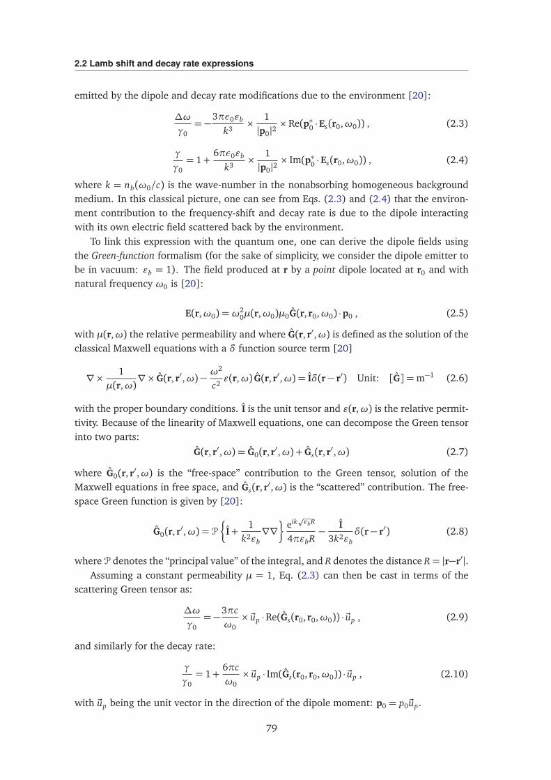
2.2 Lamb shift and decay rate expressions

emitted by the dipole and decay rate modifications due to the environment [20]:

∆ω

γ0= −

3πε0εb

k3×

1|p0|2

×Re(p∗0 ·Es(r0,ω0)) , (2.3)

γ

γ0= 1+

6πε0εb

k3×

1|p0|2

× Im(p∗0 ·Es(r0,ω0)) , (2.4)

where k = nb(ω0/c) is the wave-number in the nonabsorbing homogeneous backgroundmedium. In this classical picture, one can see from Eqs. (2.3) and (2.4) that the environ-ment contribution to the frequency-shift and decay rate is due to the dipole interactingwith its own electric field scattered back by the environment.

To link this expression with the quantum one, one can derive the dipole fields usingthe Green-function formalism (for the sake of simplicity, we consider the dipole emitter tobe in vacuum: εb = 1). The field produced at r by a point dipole located at r0 and withnatural frequency ω0 is [20]:

E(r,ω0) =ω20µ(r,ω0)µ0G(r, r0,ω0) ·p0 , (2.5)

with µ(r,ω) the relative permeability and where G(r, r′,ω) is defined as the solution of theclassical Maxwell equations with a δ function source term [20]

∇×1

µ(r,ω)∇× G(r, r′,ω)−

ω2

c2ε(r,ω) G(r, r′,ω) = Iδ(r− r′) Unit: [G] =m−1 (2.6)

with the proper boundary conditions. I is the unit tensor and ε(r,ω) is the relative permit-tivity. Because of the linearity of Maxwell equations, one can decompose the Green tensorinto two parts:

G(r, r′,ω) = G0(r, r′,ω) + Gs(r, r′,ω) (2.7)

where G0(r, r′,ω) is the “free-space” contribution to the Green tensor, solution of theMaxwell equations in free space, and Gs(r, r′,ω) is the “scattered” contribution. The free-space Green function is given by [20]:

G0(r, r′,ω) = P

§

I+1

k2εb∇∇

ª

eikpεbR

4πεbR−

I3k2εb

δ(r− r′) (2.8)

where P denotes the “principal value” of the integral, and R denotes the distance R= |r−r′|.Assuming a constant permeability µ = 1, Eq. (2.3) can then be cast in terms of the

scattering Green tensor as:

∆ω

γ0= −

3πcω0× ~up ·Re(Gs(r0, r0,ω0)) · ~up , (2.9)

and similarly for the decay rate:

γ

γ0= 1+

6πcω0× ~up · Im(Gs(r0, r0,ω0)) · ~up , (2.10)

with ~up being the unit vector in the direction of the dipole moment: p0 = p0~up.

79

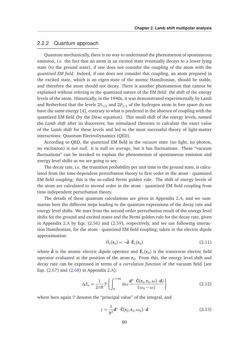
Chapter 2. Lamb shift multipolar analysis

2.2.2 Quantum approach

Quantum mechanically, there is no way to understand the phenomenon of spontaneousemission, i.e. the fact that an atom in an excited state eventually decays to a lower lyingstate (to the ground state), if one does not consider the coupling of the atom with thequantized EM field. Indeed, if one does not consider this coupling, an atom prepared inthe excited state, which is an eigen-state of the atomic Hamiltonian, should be stable,and therefore the atom should not decay. There is another phenomenon that cannot beexplained without refering to the quantized nature of the EM field: the shift of the energylevels of the atom. Historically, in the 1940s, it was demonstrated experimentally by Lamband Retherford that the levels 2S1/2 and 2P1/2 of the hydrogen atom in free space do nothave the same energy [4], contrary to what is predicted in the absence of coupling with thequantized EM field (by the Dirac equation). This small shift of the energy levels, namedthe Lamb shift after its discoverer, has stimulated theorists to calculate the exact valueof the Lamb shift for these levels and led to the most successful theory of light-matterinteractions: Quantum ElectroDynamics (QED).

According to QED, the quantized EM field in the vacuum state (no light, no photon,no excitation) is not null: it is null on average, but it has fluctuations. These “vacuumfluctuations” can be invoked to explain the phenomenon of spontaneous emission andenergy level shifts as we are going to see.

The decay rate, i.e. the transition probability per unit time to the ground state, is calcu-lated from the time-dependent perturbation theory to first order in the atom - quantizedEM field coupling; this is the so-called Fermi golden rule. The shift of energy levels ofthe atom are calculated to second order in the atom - quantized EM field coupling fromtime-independent perturbation theory.

The details of these quantum calculations are given in Appendix 2.A, and we sum-marize here the different steps leading to the quantum expressions of the decay rate andenergy level shifts. We start from the second-order perturbation result of the energy levelshifts for the ground and excited states and the Fermi golden rule for the decay rate, givenin Appendix 2.A by Eqs. (2.56) and (2.59), respectively, and we use following interac-tion Hamiltonian, for the atom - quantized EM field coupling, taken in the electric dipoleapproximation:

HI(r0) = −d · Ev(r0) (2.11)

where d is the atomic electric dipole operator and Ev(r0) is the transverse electric fieldoperator evaluated at the position of the atom r0. From this, the energy level shift anddecay rate can be expressed in terms of a correlation function of the vacuum field [seeEqs. (2.67) and (2.68) in Appendix 2.A]:

∆Ee =1

2πħhP

∫ +∞

0

dωd∗ · C(r0, r0,ω) ·d)

(ω0 −ω)

(2.12)

where here again P denotes the “principal value” of the integral, and

γ=1

ħh2 d∗ · C(r0, r0,ω0) ·d (2.13)

80

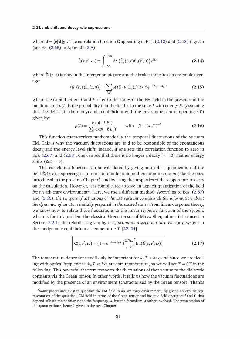
2.2 Lamb shift and decay rate expressions

where d= ⟨e| d |g⟩. The correlation function C appearing in Eqs. (2.12) and (2.13) is given(see Eq. (2.65) in Appendix 2.A):

C(r, r′,ω)≡∫ +∞

−∞dt

Ev(r, t)Ev(r′, 0)

eiωt (2.14)

where Ev(r, t) is now in the interaction picture and the braket indicates an ensemble aver-age:

Ev(r, t)Ev(r, 0)

=∑

I ,F

p(I)| ⟨F | Ev(r) |I⟩ |2 e−i(ωF−ωI )t (2.15)

where the capital letters I and F refer to the states of the EM field in the presence of themedium, and p(I) is the probability that the field is in the state I with energy EI (assumingthat the field is in thermodynamic equilibrium with the environment at temperature T)given by:

p(I) =exp(−βEI)

∑

k exp(−βEk)with β ≡ (kB T )−1 (2.16)

This function characterizes mathematically the temporal fluctuations of the vacuumEM. This is why the vacuum fluctuations are said to be responsible of the spontaneousdecay and the energy level shift; indeed, if one sets this correlation function to zero inEqs. (2.67) and (2.68), one can see that there is no longer a decay (γ= 0) neither energyshifts (∆Ei = 0).

This correlation function can be calculated by giving an explicit quantization of thefield Ev(r, t), expressing it in terms of annihilation and creation operators (like the onesintroduced in the previous Chapter), and by using the properties of these operators to carryon the calculation. However, it is complicated to give an explicit quantization of the fieldfor an arbitrary environment2. Here, we use a different method. According to Eqs. (2.67)and (2.68), the temporal fluctuations of the EM vacuum contains all the information aboutthe dynamics of an atom initially prepared in the excited state. From linear-response theory,we know how to relate these fluctuations to the linear-response function of the system,which is for this problem the classical Green tensor of Maxwell equations introduced inSection 2.2.1: the relation is given by the fluctuation-dissipation theorem for a system inthermodynamic equilibrium at temperature T [22–24]:

C(r, r′,ω) =

1− e−ħhω/kB T 2ħhω2

ε0c2Im(G(r, r′,ω)) (2.17)

The temperature dependence will only be important for kB T > ħhω, and since we are deal-ing with optical frequencies, kB T ħhω at room temperature, so we will set T = 0K in thefollowing. This powerful theorem connects the fluctuations of the vacuum to the dielectricconstants via the Green tensor. In other words, it tells us how the vacuum fluctuations aremodified by the presence of an environment (characterized by the Green tensor). Thanks

2Some procedures exist to quantize the EM field in an arbitrary environment, by giving an explicit rep-resentation of the quantized EM field in terms of the Green tensor and bosonic field operators f and f† thatdepend of both the position r and the frequency ω, but the formalism is rather involved. The presentation ofthis quantization scheme is given in the next Chapter.

81

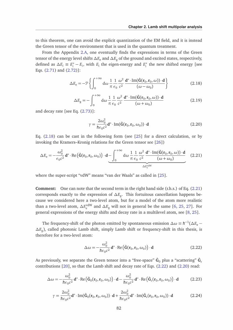
Chapter 2. Lamb shift multipolar analysis

to this theorem, one can avoid the explicit quantization of the EM field, and it is insteadthe Green tensor of the environment that is used in the quantum treatment.

From the Appendix 2.A, one eventually finds the expressions in terms of the Greentensor of the energy level shifts∆Ee and∆Eg of the ground and excited states, respectively,defined as ∆Ei ≡ E∗i − Ei, with Ei the eigen-energy and E∗i the new shifted energy [seeEqs. (2.71) and (2.72)]:

∆Ee = −P∫ +∞

0

dω1π

1ε0

ω2

c2

d∗ · Im(G(r0, r0,ω)) ·d(ω−ω0)

(2.18)

∆Eg = −∫ +∞

0

dω1π

1ε0

ω2

c2

d∗ · Im(G(r0, r0,ω)) ·d(ω+ω0)

(2.19)

and decay rate [see Eq. (2.73)]:

γ=2ω2

0

ħhε0c2d∗ · Im(G(r0, r0,ω0)) ·d (2.20)

Eq. (2.18) can be cast in the following form (see [25] for a direct calculation, or byinvoking the Kramers–Kronig relations for the Green tensor see [26])

∆Ee = −ω2

0

ε0c2d∗ ·Re

G(r0, r0,ω0)

·d−∫ +∞

0

dω1π

1ε0

ω2

c2

d∗ · Im(G(r0, r0,ω)) ·d(ω+ω0)

︸ ︷︷ ︸

∆EvdWe

(2.21)

where the super-script “vdW” means “van der Waals” as called in [25].

Comment: One can note that the second term in the right hand side (r.h.s.) of Eq. (2.21)corresponds exactly to the expression of ∆Eg. This fortuitous cancellation happens be-cause we considered here a two-level atom, but for a model of the atom more realisticthan a two-level atom, ∆EvdW

e and ∆Eg will not in general be the same [6, 25, 27]. Forgeneral expressions of the energy shifts and decay rate in a multilevel atom, see [8, 25].

The frequency-shift of the photon emitted by spontaneous emission ∆ω ≡ ħh−1(∆Ee −∆Eg), called photonic Lamb shift, simply Lamb shift or frequency-shift in this thesis, istherefore for a two-level atom:

∆ω= −ω2

0

ħhε0c2d∗ ·Re

G(r0, r0,ω0)

·d (2.22)

As previously, we separate the Green tensor into a “free-space” G0 plus a “scattering” Gs

contributions [20], so that the Lamb shift and decay rate of Eqs. (2.22) and (2.20) read:

∆ω= −ω2

0

ħhε0c2d∗ ·Re

G0(r0, r0,ω0)

·d−ω2

0

ħhε0c2d∗ ·Re

Gs(r0, r0,ω0)

·d (2.23)

γ=2ω2

0

ħhε0c2d∗ · Im(G0(r0, r0,ω0)) ·d+

2ω20

ħhε0c2d∗ · Im(Gs(r0, r0,ω0)) ·d (2.24)

82

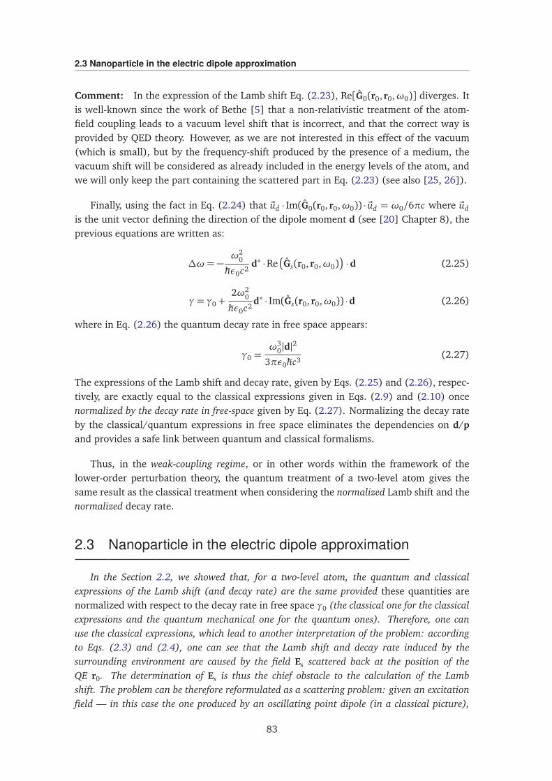
2.3 Nanoparticle in the electric dipole approximation

Comment: In the expression of the Lamb shift Eq. (2.23), Re[G0(r0, r0,ω0)] diverges. Itis well-known since the work of Bethe [5] that a non-relativistic treatment of the atom-field coupling leads to a vacuum level shift that is incorrect, and that the correct way isprovided by QED theory. However, as we are not interested in this effect of the vacuum(which is small), but by the frequency-shift produced by the presence of a medium, thevacuum shift will be considered as already included in the energy levels of the atom, andwe will only keep the part containing the scattered part in Eq. (2.23) (see also [25, 26]).

Finally, using the fact in Eq. (2.24) that ~ud · Im(G0(r0, r0,ω0)) · ~ud = ω0/6πc where ~ud

is the unit vector defining the direction of the dipole moment d (see [20] Chapter 8), theprevious equations are written as:

∆ω= −ω2

0

ħhε0c2d∗ ·Re

Gs(r0, r0,ω0)

·d (2.25)

γ= γ0 +2ω2

0

ħhε0c2d∗ · Im(Gs(r0, r0,ω0)) ·d (2.26)

where in Eq. (2.26) the quantum decay rate in free space appears:

γ0 =ω3

0|d|2

3πε0ħhc3(2.27)

The expressions of the Lamb shift and decay rate, given by Eqs. (2.25) and (2.26), respec-tively, are exactly equal to the classical expressions given in Eqs. (2.9) and (2.10) oncenormalized by the decay rate in free-space given by Eq. (2.27). Normalizing the decay rateby the classical/quantum expressions in free space eliminates the dependencies on d/pand provides a safe link between quantum and classical formalisms.

Thus, in the weak-coupling regime, or in other words within the framework of thelower-order perturbation theory, the quantum treatment of a two-level atom gives thesame result as the classical treatment when considering the normalized Lamb shift and thenormalized decay rate.

2.3 Nanoparticle in the electric dipole approximation

In the Section 2.2, we showed that, for a two-level atom, the quantum and classicalexpressions of the Lamb shift (and decay rate) are the same provided these quantities arenormalized with respect to the decay rate in free space γ0 (the classical one for the classicalexpressions and the quantum mechanical one for the quantum ones). Therefore, one canuse the classical expressions, which lead to another interpretation of the problem: accordingto Eqs. (2.3) and (2.4), one can see that the Lamb shift and decay rate induced by thesurrounding environment are caused by the field Es scattered back at the position of theQE r0. The determination of Es is thus the chief obstacle to the calculation of the Lambshift. The problem can be therefore reformulated as a scattering problem: given an excitationfield — in this case the one produced by an oscillating point dipole (in a classical picture),

83

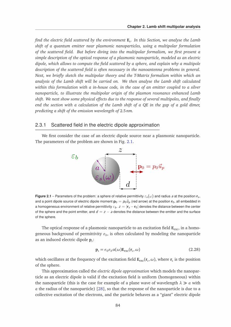
Chapter 2. Lamb shift multipolar analysis

find the electric field scattered by the environment Es. In this Section, we analyse the Lambshift of a quantum emitter near plasmonic nanoparticles, using a multipolar formulationof the scattered field. But before diving into the multipolar formalism, we first present asimple description of the optical response of a plasmonic nanoparticle, modeled as an electricdipole, which allows to compute the field scattered by a sphere, and explain why a multipoledescription of the scattered field is often necessary in the nanoantenna problems in general.Next, we briefly sketch the multipolar theory and the T-Matrix formalism within which ananalysis of the Lamb shift will be carried on. We then analyse the Lamb shift calculatedwithin this formulation with a in-house code, in the case of an emitter coupled to a silvernanoparticle, to illustrate the multipolar origin of the plasmon resonance enhanced Lambshift. We next show some physical effects due to the response of several multipoles, and finallyend the section with a calculation of the Lamb shift of a QE in the gap of a gold dimer,predicting a shift of the emission wavelength of 2.5nm.

2.3.1 Scattered field in the electric dipole approximation

We first consider the case of an electric dipole source near a plasmonic nanoparticle.The parameters of the problem are shown in Fig. 2.1.

Figure 2.1 – Parameters of the problem: a sphere of relative permittivity εs(ω) and radius a at the position rs ,and a point dipole source of electric dipole moment p0 = p0up (red arrow) at the position r0, all embedded ina homogeneous environment of relative permittivity εb. z = |rs − r0| denotes the distance between the centerof the sphere and the point emitter, and d = z − a denotes the distance between the emitter and the surfaceof the sphere.

The optical response of a plasmonic nanoparticle to an excitation field Eexc, in a homo-geneous background of permittivity εb, is often calculated by modeling the nanoparticleas an induced electric dipole ps:

ps = ε0εbα(ω)Eexc(rs,ω) (2.28)

which oscillates at the frequency of the excitation field Eexc(rs,ω), where rs is the positionof the sphere.

This approximation called the electric dipole approximation which models the nanopar-ticle as an electric dipole is valid if the excitation field is uniform (homogeneous) withinthe nanoparticle (this is the case for example of a plane wave of wavelength λ a witha the radius of the nanoparticle) [28], so that the response of the nanoparticle is due to acollective excitation of the electrons, and the particle behaves as a “giant” electric dipole

84

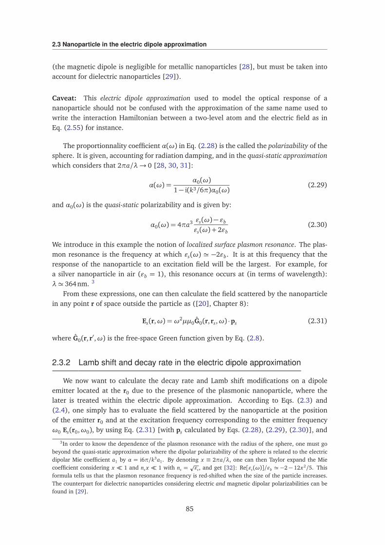
2.3 Nanoparticle in the electric dipole approximation

(the magnetic dipole is negligible for metallic nanoparticles [28], but must be taken intoaccount for dielectric nanoparticles [29]).

Caveat: This electric dipole approximation used to model the optical response of ananoparticle should not be confused with the approximation of the same name used towrite the interaction Hamiltonian between a two-level atom and the electric field as inEq. (2.55) for instance.

The proportionnality coefficient α(ω) in Eq. (2.28) is the called the polarizability of thesphere. It is given, accounting for radiation damping, and in the quasi-static approximationwhich considers that 2πa/λ→ 0 [28, 30, 31]:

α(ω) =α0(ω)

1− i(k3/6π)α0(ω)(2.29)

and α0(ω) is the quasi-static polarizability and is given by:

α0(ω) = 4πa3 εs(ω)− εb

εs(ω) + 2εb(2.30)

We introduce in this example the notion of localized surface plasmon resonance. The plas-mon resonance is the frequency at which εs(ω) ' −2εb. It is at this frequency that theresponse of the nanoparticle to an excitation field will be the largest. For example, fora silver nanoparticle in air (εb = 1), this resonance occurs at (in terms of wavelength):λ' 364nm. 3

From these expressions, one can then calculate the field scattered by the nanoparticlein any point r of space outside the particle as ([20], Chapter 8):

Es(r,ω) =ω2µµ0G0(r, rs,ω) ·ps (2.31)

where G0(r, r′,ω) is the free-space Green function given by Eq. (2.8).

2.3.2 Lamb shift and decay rate in the electric dipole approximation

We now want to calculate the decay rate and Lamb shift modifications on a dipoleemitter located at the r0 due to the presence of the plasmonic nanoparticle, where thelater is treated within the electric dipole approximation. According to Eqs. (2.3) and(2.4), one simply has to evaluate the field scattered by the nanoparticle at the positionof the emitter r0 and at the excitation frequency corresponding to the emitter frequencyω0 Es(r0,ω0), by using Eq. (2.31) [with ps calculated by Eqs. (2.28), (2.29), (2.30)], and

3In order to know the dependence of the plasmon resonance with the radius of the sphere, one must gobeyond the quasi-static approximation where the dipolar polarizability of the sphere is related to the electricdipolar Mie coefficient a1 by α = i6π/k3a1. By denoting x ≡ 2πa/λ, one can then Taylor expand the Miecoefficient considering x 1 and ns x 1 with ns =

pεs, and get [32]: Re[εs(ω)]/εb ' −2 − 12x2/5. This

formula tells us that the plasmon resonance frequency is red-shifted when the size of the particle increases.The counterpart for dielectric nanoparticles considering electric and magnetic dipolar polarizabilities can befound in [29].

85

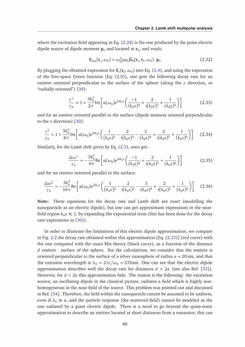
Chapter 2. Lamb shift multipolar analysis

where the excitation field appearing in Eq. (2.28) is the one produced by the point electricdipole source of dipole moment p0 and located at r0, and reads:

Eexc(rs,ω0) =ω20µµ0G0(rs, r0,ω0) ·p0 (2.32)

By plugging the obtained expression for Es(r0,ω0) into Eq. (2.4), and using the expressionof the free-space Green function [Eq. (2.8)], one gets the following decay rate for anemitter oriented perpendicular to the surface of the sphere (along the z direction, or“radially oriented”) [30]:

γ⊥

γ0= 1+

3k30

2πIm

α(ω0)e2ik0z

−1(k0z)4

+2

i(k0z)5+

1(k0z)6

(2.33)

and for an emitter oriented parallel to the surface (dipole moment oriented perpendicularto the z direction) [30]:

γ‖

γ0= 1+

3k30

8πIm

α(ω0)e2ik0z

1(k0z)2

−2

i(k0z)3−

3(k0z)4

+2

i(k0z)5+

1(k0z)6

(2.34)

Similarly, for the Lamb shift given by Eq. (2.3), ones get:

∆ω⊥

γ0= −

3k30

4πRe

α(ω0)e2ik0z

−1(k0z)4

+2

i(k0z)5+

1(k0z)6

(2.35)

and for an emitter oriented parallel to the surface:

∆ω‖

γ0= −

3k30

16πRe

α(ω0)e2ik0z

1(k0z)2

−2

i(k0z)3−

3(k0z)4

+2

i(k0z)5+

1(k0z)6

(2.36)

Note: These equations for the decay rate and Lamb shift are exact (modelling thenanoparticle as an electric dipole), but one can get approximate expressions in the near-field region k0z 1, by expanding the exponential term (this has been done for the decayrate expressions in [30]).

In order to illustrate the limitations of this electric dipole approximation, we comparein Fig. 2.2 the decay rate obtained within this approximation [Eq. (2.33)] (red curve) withthe one computed with the exact Mie theory (black curve), as a function of the distanced emitter - surface of the sphere. For the calculations, we consider that the emitter isoriented perpendicular to the surface of a silver nanosphere of radius a = 20nm, and thatthe emission wavelength is λ0 = 2πc/ω0 =335nm. One can see that the electric dipoleapproximation describes well the decay rate for distances d > 2a (see also Ref. [33]).However, for d < 2a this approximation fails. The reason is the following: the excitationsource, an oscillating dipole in the classical picture, radiates a field which is highly non-homogeneous in the near-field of the source. This problem was pointed out and discussedin Ref. [34]. Therefore, the field within the nanoparticle cannot be assumed to be uniform,even if λ0 a, and the particle response (the scattered field) cannot be modeled as theone radiated by a giant electric dipole. There is a need to go beyond the quais-staticapproximation to describe an emitter located at short distances from a resonator; this can

86

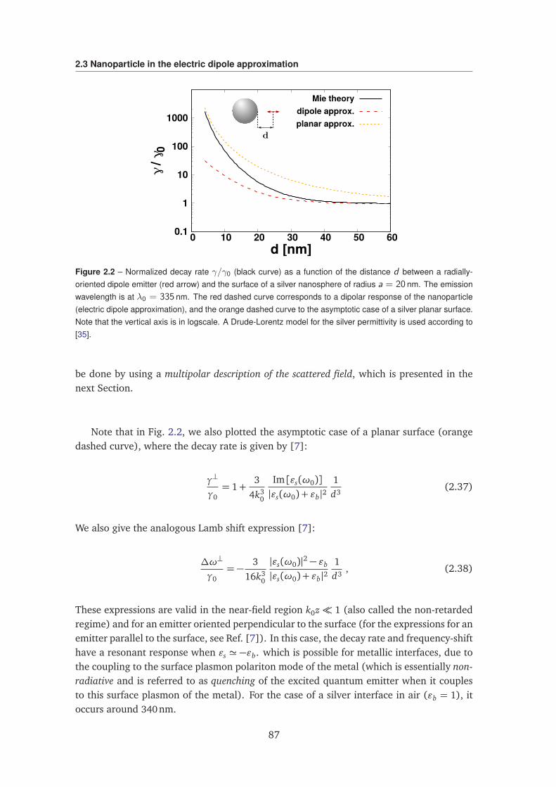
2.3 Nanoparticle in the electric dipole approximation

0.1

1

10

100

1000

0 10 20 30 40 50 60

γ/ γ

0

d [nm]

Mie theorydipole approx.planar approx.

Figure 2.2 – Normalized decay rate γ/γ0 (black curve) as a function of the distance d between a radially-oriented dipole emitter (red arrow) and the surface of a silver nanosphere of radius a = 20 nm. The emissionwavelength is at λ0 = 335 nm. The red dashed curve corresponds to a dipolar response of the nanoparticle(electric dipole approximation), and the orange dashed curve to the asymptotic case of a silver planar surface.Note that the vertical axis is in logscale. A Drude-Lorentz model for the silver permittivity is used according to[35].

be done by using a multipolar description of the scattered field, which is presented in thenext Section.

Note that in Fig. 2.2, we also plotted the asymptotic case of a planar surface (orangedashed curve), where the decay rate is given by [7]:

γ⊥

γ0= 1+

3

4k30

Im [εs(ω0)]|εs(ω0) + εb|2

1d3

(2.37)

We also give the analogous Lamb shift expression [7]:

∆ω⊥

γ0= −

3

16k30

|εs(ω0)|2 − εb

|εs(ω0) + εb|21d3

, (2.38)

These expressions are valid in the near-field region k0z 1 (also called the non-retardedregime) and for an emitter oriented perpendicular to the surface (for the expressions for anemitter parallel to the surface, see Ref. [7]). In this case, the decay rate and frequency-shifthave a resonant response when εs ' −εb. which is possible for metallic interfaces, due tothe coupling to the surface plasmon polariton mode of the metal (which is essentially non-radiative and is referred to as quenching of the excited quantum emitter when it couplesto this surface plasmon of the metal). For the case of a silver interface in air (εb = 1), itoccurs around 340nm.

87

Chapter 2. Lamb shift multipolar analysis

2.4 Multipolar formulation of the scattering problem

2.4.1 Multipolar basis

In order to calculate the field scattered by the environment Es, we will use the mul-tipolar theory, which is especially useful in describing EM scattering for particles withspherical symetries [18, 36], allowing an analytical formulation of the scattering problem(and avoid an integral formulation using the Green formalism). We will make use of themultipolar modes — also called Vector Partial Waves — which are a basis for EM fields,and that are by definition solutions of the vectorial Helmholtz equations in spherical co-ordinates. The construction of these modes and their explicit representations are given inAppendix 2.B. Importantly, each mode is specified by three discrete numbers: q accountsfor the parity of the field, and q = 1 for a magnetic mode and q = 2 for an electric mode;n = 1, 2, ...,∞ and will be called the ”multipolar order”; and m = −n, ..., n and will becalled the ”orbital number”. In the following, we will denote these modes by Mnm(kr) forthe magnetic modes (q = 1) and Nnm(kr) for the electric modes (q = 2), in the real spacerepresentation (k =ω/c).

2.4.2 T-Matrix formulation

A very fruitful method to calculate the scattered field Es knowing the excitation fieldEexc is the T-Matrix method [28]. In operator notation, the T-Matrix denoted T can bedefined as:

Es = T · Eexc (2.39)

The above expression traduces the fact that the scattered field Es has a linear relation withthe excitation field Eexc, and this linear dependence is embodied by the T-Matrix. TheT-Matrix is associated to a scatterer center and characterizes entirely its optical responseto an arbitrary excitation. Considering the case of a single scatterer first, its coefficientscan be defined from the following procedure:

1. One breaks the domain into two sub-domains separated by the surface of the scat-terer, defining the internal field Eint and outside field Eout = Eexc + Es;

2. One then expands all the EM fields (excitation, internal and scattered) on the mul-tipolar modes as (such expansions are particularly useful to describe the opticalresponse of spherical objects):

Eint(kr) = E0

∞∑

n=1

n∑

m=−n

s(1)nmMnm(kr) + s(2)nmNnm(kr) (2.40)

Eexc(kr) = E0

∞∑

n=1

n∑

m=−n

e(1)nmMnm(kr) + e(2)nmNnm(kr) (2.41)

Es(kr) = E0

∞∑

n=1

n∑

m=−n

f (1)nm M(+)nm(kr) + f (2)nm N(+)nm(kr) (2.42)

88

2.4 Multipolar formulation of the scattering problem

where E0 is the amplitude of the field, s(i)nm, e(i)nm and f (i)nm are the coefficients of themagnetic (i = 1) and electric (i = 2) modes of the internal, excitation and scatteredfield, respectively.

3. Finally, one uses the continuity of the tangential components of the fields inside andoutside the scatterer; as a consequence of the linearity of the Maxwell equations andof the continuity conditions, the coefficients of the scattered field are linearly relatedto those of the excitation field:

f (2)nm = −t(2)n e(2)nm (2.43)

f (1)nm = −t(1)n e(1)nm (2.44)

The T-Matrix coefficients are then defined as the coefficients of proportionnality betweenthe coefficients f (i)nm and e(i)nm. Note that this T-Matrix is infinite dimensional because themultipolar basis is infinite (the multipolar order n= 1, ...,∞), but in practice it is renderedfinite by truncating the multipolar order n to some finite dimension ncut (the choice of ncut

for which the summation with respect to the multipolar order n converges will depend onparticle size and interaction strengths).

Generalized Lorentz-Mie theory: In the case of a spherical Mie scatterer, T , is a diago-nal matrix composed of the Mie coefficients of the sphere (multiplied by −1). We now givethe expressions of the Mie coefficients in a slightly different way than in [28] (where theyare called the scattering coefficients). By introducing εs [µs] and εb [µb] as the relativepermittivity [permeability] of the sphere and the homogeneous background respectively,ks =

p

εs(ω)ω/c and k = pεbω/c, the Mie coefficients of a sphere of radius a take theform:

an =(εs/εb) jn(ksa)ψ′n(ka)−ψ′n(ksa) jn(ka)

(εs/εb) jn(ksa)ξ′n(ka)−ψ′n(ksa)hn(ka), (2.45)

for the electric Mie coefficient of order n, and

bn =(µs/µb) jn(ksa)ψ′n(ka)−ψ′n(ksa) jn(ka)

(µs/µb) jn(ksa)ξ′n(ka)−ψ′n(ksa)hn(ka), (2.46)

for the magnetic Mie coefficient of order n, where jn(x) and hn(x) are respectively thespherical Bessel functions and the first-type (outgoing) spherical Hankel functions, andψn(x) and ξn(x) are the Ricatti-Bessel functions defined as:

ψn(x)≡ x jn(x) (2.47)

ξn(x)≡ xhn(x) . (2.48)

2.4.3 Scattered field from a dipole source

We next apply this method to the scattering problem sketched in Fig. 2.1: we wantto compute the expression of the electric field Es(r,ω0) scattered by a single scatterer

89

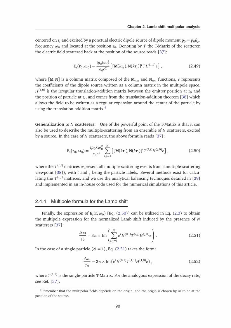
Chapter 2. Lamb shift multipolar analysis

centered on rs and excited by a ponctual electric dipole source of dipole moment p0 = p0~up,frequency ω0 and located at the position r0. Denoting by T the T-Matrix of the scatterer,the electric field scattered back at the position of the source reads [37]:

Es(r0,ω0) =ip0kω2

0

ε0c2

[M(krs),N(krs)]t T H(1,0)e

, (2.49)

where [M,N] is a column matrix composed of the Mnm and Nnm functions, e representsthe coefficients of the dipole source written as a column matrix in the multipole space.H(1,0) is the irregular translation-addition matrix between the emitter position at r0 andthe position of particle at rs, and comes from the translation-addition theorem [38] whichallows the field to be written as a regular expansion around the center of the particle byusing the translation-addition matrix 4.

Generalization to N scatterers: One of the powerful point of the T-Matrix is that it canalso be used to describe the multiple-scattering from an ensemble of N scatterers, excitedby a source. In the case of N scatterers, the above formula reads [37]:

Es(r0,ω0) =ip0kω2

0

ε0c2

N∑

i, j=1

[M(kri),N(kri)]t T (i, j)H( j,0)e

, (2.50)

where the T (i, j) matrices represent all multiple-scattering events from a multiple-scatteringviewpoint [38]), with i and j being the particle labels. Several methods exist for calcu-lating the T (i, j) matrices, and we use the analytical balancing techniques detailed in [39]and implemented in an in-house code used for the numerical simulations of this article.

2.4.4 Multipole formula for the Lamb shift

Finally, the expression of Es(r,ω0) [Eq. (2.50)] can be utilized in Eq. (2.3) to obtainthe multipole expression for the normalized Lamb shift induced by the presence of Nscatterers [37]:

∆ω

γ0= 3π× Im

N∑

i, j=1

et H(0,i)T (i, j)H( j,0)e

!

. (2.51)

In the case of a single particle (N = 1), Eq. (2.51) takes the form:

∆ω

γ0= 3π× Im

et H(0,1)T (1,1)H(1,0)e

, (2.52)

where T (1,1) is the single-particle T-Matrix. For the analogous expression of the decay rate,see Ref. [37].

4Remember that the multipolar fields depends on the origin, and the origin is chosen by us to be at theposition of the source.

90

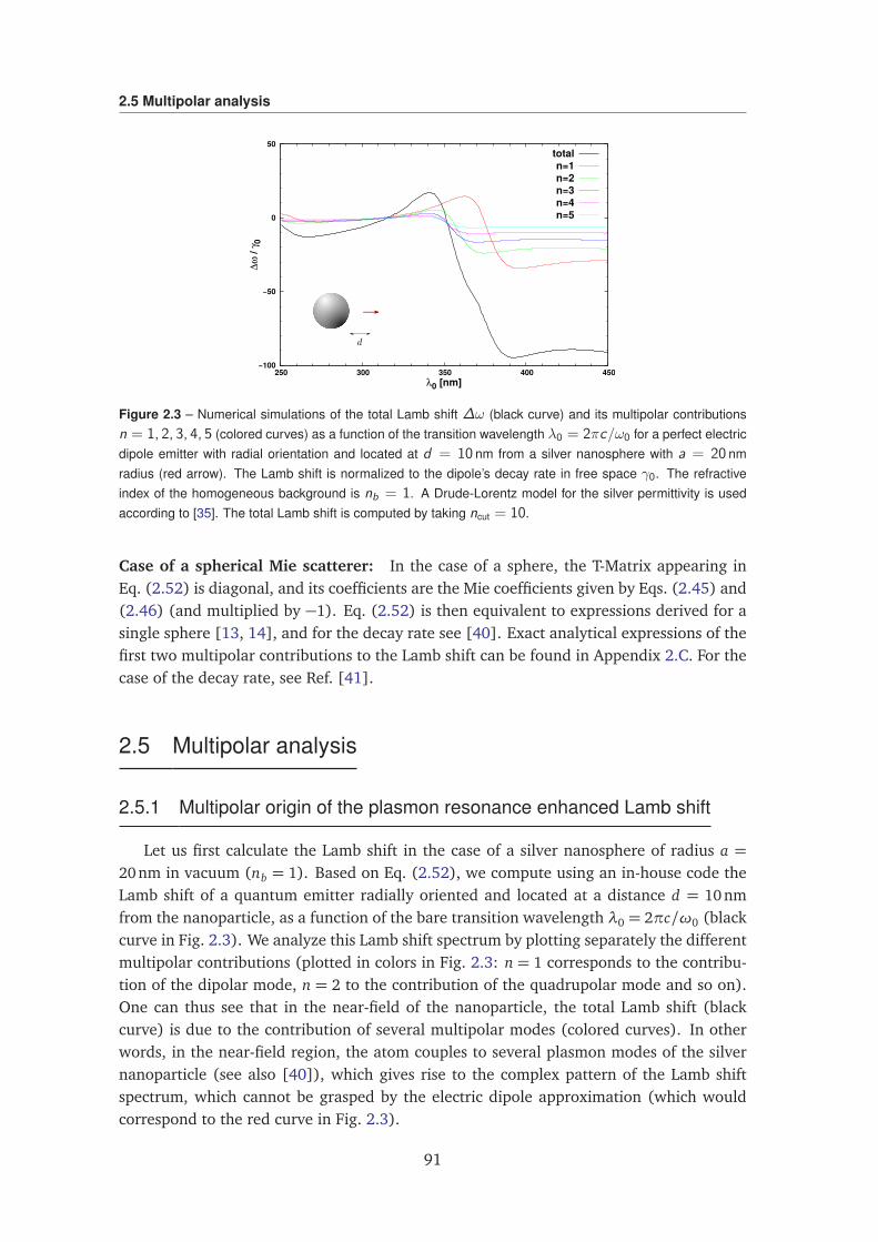
2.5 Multipolar analysis

−100

−50

0

50

250 300 350 400 450

∆ω

/ γ 0

λ0 [nm]

total

n=1

n=2

n=3

n=4

n=5

Figure 2.3 – Numerical simulations of the total Lamb shift ∆ω (black curve) and its multipolar contributionsn = 1, 2, 3, 4, 5 (colored curves) as a function of the transition wavelength λ0 = 2πc/ω0 for a perfect electricdipole emitter with radial orientation and located at d = 10 nm from a silver nanosphere with a = 20 nmradius (red arrow). The Lamb shift is normalized to the dipole’s decay rate in free space γ0. The refractiveindex of the homogeneous background is nb = 1. A Drude-Lorentz model for the silver permittivity is usedaccording to [35]. The total Lamb shift is computed by taking ncut = 10.

Case of a spherical Mie scatterer: In the case of a sphere, the T-Matrix appearing inEq. (2.52) is diagonal, and its coefficients are the Mie coefficients given by Eqs. (2.45) and(2.46) (and multiplied by −1). Eq. (2.52) is then equivalent to expressions derived for asingle sphere [13, 14], and for the decay rate see [40]. Exact analytical expressions of thefirst two multipolar contributions to the Lamb shift can be found in Appendix 2.C. For thecase of the decay rate, see Ref. [41].

2.5 Multipolar analysis

2.5.1 Multipolar origin of the plasmon resonance enhanced Lamb shift

Let us first calculate the Lamb shift in the case of a silver nanosphere of radius a =20nm in vacuum (nb = 1). Based on Eq. (2.52), we compute using an in-house code theLamb shift of a quantum emitter radially oriented and located at a distance d = 10nmfrom the nanoparticle, as a function of the bare transition wavelength λ0 = 2πc/ω0 (blackcurve in Fig. 2.3). We analyze this Lamb shift spectrum by plotting separately the differentmultipolar contributions (plotted in colors in Fig. 2.3: n = 1 corresponds to the contribu-tion of the dipolar mode, n = 2 to the contribution of the quadrupolar mode and so on).One can thus see that in the near-field of the nanoparticle, the total Lamb shift (blackcurve) is due to the contribution of several multipolar modes (colored curves). In otherwords, in the near-field region, the atom couples to several plasmon modes of the silvernanoparticle (see also [40]), which gives rise to the complex pattern of the Lamb shiftspectrum, which cannot be grasped by the electric dipole approximation (which wouldcorrespond to the red curve in Fig. 2.3).

91

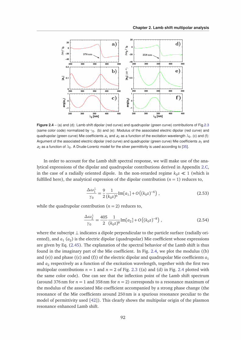
Chapter 2. Lamb shift multipolar analysis

−40

−20

0

20

250 300 350 400 450

∆ω

2/γ 0

0

0.5

1

250 300 350 400 450

|a2|

−1

0

1

250 300 350 400 450

arg

(a2)

λ0 [nm]

−40

−20

0

20

250 300 350 400 450∆ω

/γ 0

0

0.1

0.2

250 300 350 400 450

|a1|

−1

0

1

250 300 350 400 450

arg

(a1)

λ0 [nm]

Figure 2.4 – (a) and (d): Lamb shift dipolar (red curve) and quadrupolar (green curve) contributions of Fig.2.3(same color code) normalized by γ0. (b) and (e): Modulus of the associated electric dipolar (red curve) andquadrupolar (green curve) Mie coefficients a1 and a2 as a function of the excitation wavelength λ0. (c) and (f):Argument of the associated electric dipolar (red curve) and quadrupolar (green curve) Mie coefficients a1 anda2 as a function of λ0. A Drude-Lorentz model for the silver permittivity is used according to [35].

In order to account for the Lamb shift spectral response, we will make use of the ana-lytical expressions of the dipolar and quadrupolar contributions derived in Appendix 2.C,in the case of a radially oriented dipole. In the non-retarded regime k0z 1 (which isfulfilled here), the analytical expression of the dipolar contribution (n= 1) reduces to,

∆ω⊥1γ0

=92

1(k0z)6

Im[a1] +O

(k0z)−6

, (2.53)

while the quadrupolar contribution (n= 2) reduces to,

∆ω⊥2γ0

=4052

1(k0z)8

Im[a2] +O

(k0z)−8

, (2.54)

where the subscript ⊥ indicates a dipole perpendicular to the particle surface (radially ori-ented), and a1 (a2) is the electric dipolar (quadrupolar) Mie coefficient whose expressionsare given by Eq. (2.45). The explanation of the spectral behavior of the Lamb shift is thusfound in the imaginary part of the Mie coefficient. In Fig. 2.4, we plot the modulus ((b)and (e)) and phase ((c) and (f)) of the electric dipolar and quadrupolar Mie coefficients a1

and a2 respectively as a function of the excitation wavelength, together with the first twomultipolar contributions n = 1 and n = 2 of Fig. 2.3 ((a) and (d) in Fig. 2.4 plotted withthe same color code). One can see that the inflection point of the Lamb shift spectrum(around 376nm for n = 1 and 358nm for n = 2) corresponds to a resonance maximum ofthe modulus of the associated Mie coefficient accompanied by a strong phase change (theresonance of the Mie coefficients around 250nm is a spurious resonance peculiar to themodel of permittivity used [42]). This clearly shows the multipolar origin of the plasmonresonance enhanced Lamb shift.

92

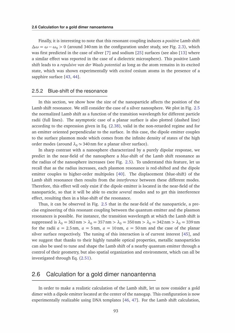
2.6 Calculation for a gold dimer nanoantenna

Finally, it is interesting to note that this resonant coupling induces a positive Lamb shift∆ω = ω−ω0 > 0 (around 340nm in the configuration under study, see Fig. 2.3), whichwas first predicted in the case of silver [7] and sodium [25] surfaces (see also [13] wherea similar effect was reported in the case of a dielectric microsphere). This positive Lambshift leads to a repulsive van der Waals potential as long as the atom remains in its excitedstate, which was shown experimentally with excited cesium atoms in the presence of asapphire surface [43, 44].

2.5.2 Blue-shift of the resonance

In this section, we show how the size of the nanoparticle affects the position of theLamb shift resonance. We still consider the case of a silver nanosphere. We plot in Fig. 2.5the normalized Lamb shift as a function of the transition wavelength for different particleradii (full lines). The asymptotic case of a planar surface is also plotted (dashed line)according to the expression given in Eq. (2.38), valid in the non-retarded regime and foran emitter oriented perpendicular to the surface. In this case, the dipole emitter couplesto the surface plasmon mode which comes from the infinite density of states of the highorder modes (around λ0 ' 340nm for a planar silver surface).

In sharp contrast with a nanosphere characterized by a purely dipolar response, wepredict in the near-field of the nanosphere a blue-shift of the Lamb shift resonance asthe radius of the nanosphere increases (see Fig. 2.5). To understand this feature, let usrecall that as the radius increases, each plasmon resonance is red-shifted and the dipoleemitter couples to higher-order multipoles [40]. The displacement (blue-shift) of theLamb shift resonance then results from the interference between these different modes.Therefore, this effect will only exist if the dipole emitter is located in the near-field of thenanoparticle, so that it will be able to excite several modes and to get this interferenceeffect, resulting then in a blue-shift of the resonance.

Thus, it can be observed in Fig. 2.5 that in the near-field of the nanoparticle, a pre-cise engineering of this resonant coupling between the quantum emitter and the plasmonresonances is possible. For instance, the transition wavelength at which the Lamb shift issuppressed is λ0 = 363nm > λ0 = 357nm > λ0 = 350nm > λ0 = 342nm > λ0 = 339nmfor the radii a = 2.5nm, a = 5nm, a = 10nm, a = 50nm and the case of the planarsilver surface respectively. The tuning of this interaction is of current interest [45], andwe suggest that thanks to their highly tunable optical properties, metallic nanoparticlescan also be used to tune and shape the Lamb shift of a nearby quantum emitter through acontrol of their geometry, but also spatial organization and environment, which can all beinvestigated through Eq. (2.51).

2.6 Calculation for a gold dimer nanoantenna

In order to make a realistic calculation of the Lamb shift, let us now consider a golddimer with a dipole emitter located at the center of the nanogap. This configuration is nowexperimentally realizable using DNA templates [46, 47]. For the Lamb shift calculation,

93

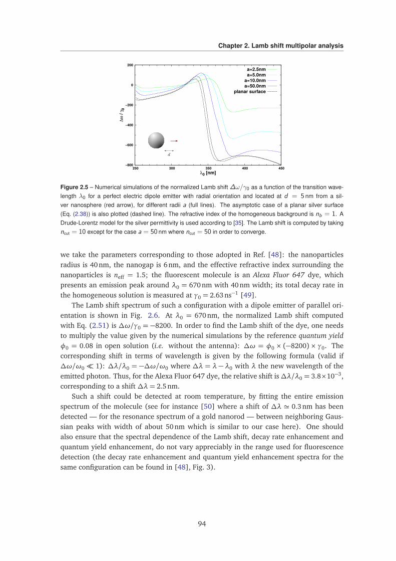
Chapter 2. Lamb shift multipolar analysis

−800

−600

−400

−200

0

200

250 300 350 400 450

∆ω

/ γ 0

λ0 [nm]

a=2.5nm

a=5.0nm

a=10.0nm

a=50.0nm

planar surface

Figure 2.5 – Numerical simulations of the normalized Lamb shift ∆ω/γ0 as a function of the transition wave-length λ0 for a perfect electric dipole emitter with radial orientation and located at d = 5 nm from a sil-ver nanosphere (red arrow), for different radii a (full lines). The asymptotic case of a planar silver surface(Eq. (2.38)) is also plotted (dashed line). The refractive index of the homogeneous background is nb = 1. ADrude-Lorentz model for the silver permittivity is used according to [35]. The Lamb shift is computed by takingncut = 10 except for the case a = 50 nm where ncut = 50 in order to converge.

we take the parameters corresponding to those adopted in Ref. [48]: the nanoparticlesradius is 40nm, the nanogap is 6nm, and the effective refractive index surrounding thenanoparticles is neff = 1.5; the fluorescent molecule is an Alexa Fluor 647 dye, whichpresents an emission peak around λ0 = 670nm with 40nm width; its total decay rate inthe homogeneous solution is measured at γ0 = 2.63ns−1 [49].

The Lamb shift spectrum of such a configuration with a dipole emitter of parallel ori-entation is shown in Fig. 2.6. At λ0 = 670nm, the normalized Lamb shift computedwith Eq. (2.51) is ∆ω/γ0 = −8200. In order to find the Lamb shift of the dye, one needsto multiply the value given by the numerical simulations by the reference quantum yieldφ0 = 0.08 in open solution (i.e. without the antenna): ∆ω = φ0 × (−8200) × γ0. Thecorresponding shift in terms of wavelength is given by the following formula (valid if∆ω/ω0 1): ∆λ/λ0 = −∆ω/ω0 where ∆λ = λ− λ0 with λ the new wavelength of theemitted photon. Thus, for the Alexa Fluor 647 dye, the relative shift is∆λ/λ0 = 3.8×10−3,corresponding to a shift ∆λ= 2.5nm.

Such a shift could be detected at room temperature, by fitting the entire emissionspectrum of the molecule (see for instance [50] where a shift of ∆λ ' 0.3nm has beendetected — for the resonance spectrum of a gold nanorod — between neighboring Gaus-sian peaks with width of about 50nm which is similar to our case here). One shouldalso ensure that the spectral dependence of the Lamb shift, decay rate enhancement andquantum yield enhancement, do not vary appreciably in the range used for fluorescencedetection (the decay rate enhancement and quantum yield enhancement spectra for thesame configuration can be found in [48], Fig. 3).

94

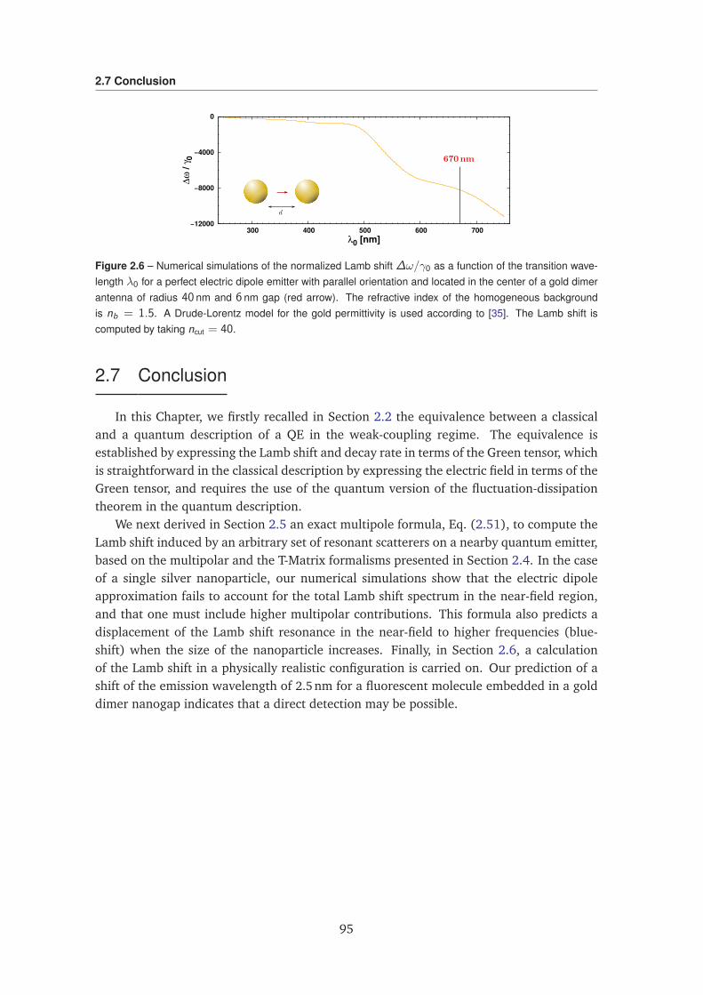
2.7 Conclusion

−12000

−8000

−4000

0

300 400 500 600 700

∆ω

/ γ 0

λ0 [nm]

Figure 2.6 – Numerical simulations of the normalized Lamb shift ∆ω/γ0 as a function of the transition wave-length λ0 for a perfect electric dipole emitter with parallel orientation and located in the center of a gold dimerantenna of radius 40 nm and 6 nm gap (red arrow). The refractive index of the homogeneous backgroundis nb = 1.5. A Drude-Lorentz model for the gold permittivity is used according to [35]. The Lamb shift iscomputed by taking ncut = 40.

2.7 Conclusion

In this Chapter, we firstly recalled in Section 2.2 the equivalence between a classicaland a quantum description of a QE in the weak-coupling regime. The equivalence isestablished by expressing the Lamb shift and decay rate in terms of the Green tensor, whichis straightforward in the classical description by expressing the electric field in terms of theGreen tensor, and requires the use of the quantum version of the fluctuation-dissipationtheorem in the quantum description.

We next derived in Section 2.5 an exact multipole formula, Eq. (2.51), to compute theLamb shift induced by an arbitrary set of resonant scatterers on a nearby quantum emitter,based on the multipolar and the T-Matrix formalisms presented in Section 2.4. In the caseof a single silver nanoparticle, our numerical simulations show that the electric dipoleapproximation fails to account for the total Lamb shift spectrum in the near-field region,and that one must include higher multipolar contributions. This formula also predicts adisplacement of the Lamb shift resonance in the near-field to higher frequencies (blue-shift) when the size of the nanoparticle increases. Finally, in Section 2.6, a calculationof the Lamb shift in a physically realistic configuration is carried on. Our prediction of ashift of the emission wavelength of 2.5nm for a fluorescent molecule embedded in a golddimer nanogap indicates that a direct detection may be possible.

95

Chapter 2. Lamb shift multipolar analysis

2.A Quantum derivation of the Lamb shift and decay rate

In this Appendix, we derive the quantum expressions of the decay rate and the energyshifts of a two-level atoms in terms of the Green tensor of Maxwell equations, followingclosely [8, 25].

System

One consider a two-level atom with ground state |g⟩ and excited state |e⟩ of eigen-energies Eg and Ee, respectively. When one introduces a coupling with the quantizedelectromagnetic field modeled by HI :

HI(r0) = −d · Ev(r0) (2.55)

where d is the atomic electric dipole operator and Ev(r0) is the transverse electric fieldoperator evaluated at the position of the atom r0, the energy level of the atom Eg and Ee

are shifted by a quantity ∆Ei.

Perturbation theory

By considering that the matrix elements of the interaction Hamiltonian are small com-pared to those of the non-interacting Hamiltonian (weak-coupling approximation in aquantum context), the energy-shifts ∆Ee = E∗e − Ee where E∗e is the new energy can cal-culated using time-independent perturbation theory to second order in the perturbationHI(r0):

∆Ee = E∗e − Ee =∑

I ,F

p(I)| ⟨g, F | HI(r0) |e, I⟩ |2

ħh(ωe −ωg)−ħh(ωF −ωI)(2.56)

where the capital letters I and F refer to the states of the EM field in the presence of themedium. We assume that the field is in thermodynamic equilibrium with the environmentat temperature T such that the probability p(I) that the field is in the state I with energyEI is given by:

p(I) =exp(−βEI)

∑

k exp(−βEk)with β ≡ (kB T )−1 (2.57)

Such expression can be put in an integral form as:

∆Ee = P

(

∫ +∞

0

dω∑

I ,F

p(I)| ⟨g, F | HI(r0) |e, I⟩ |2

ħh(ωe −ωg −ω)δ(ωF −ωI −ω)

)

(2.58)

where we introduce P as the “principal value” of the integral.The decay rate is given by the Fermi golden rule, which is derived using time-

dependent perturbation theory to first order in the perturbation HI(r0):

γ=2π

ħh2

∑

I ,F

p(I)| ⟨g, F | HI(r0) |e, I⟩ |2δ(ωF +ωg −ωI −ωe) (2.59)

96

2.A Quantum derivation of the Lamb shift and decay rate

Reservoir coupling spectrum

In these two expressions (2.58) and (2.59), we introduce the quantity called reservoircoupling spectrum:

R(r,ω)≡1

ħh2

∑

I ,F

p(I)| ⟨g, F | HI(r) |e, I⟩ |2δ(ωF −ωI −ω) (2.60)

so that these expressions are recast conveniently in terms of this function in the form:

∆Ee = P

∫ +∞

0

dωħhR(r0,ω)(ω0 −ω)

(2.61)

andγ= 2πR(r0,ω0) (2.62)

where we used the fact that ω0 =ωe −ωg.

Fluctuation-dissipation theorem

We now will use the fluctuation-dissipation theorem to show that the reservoir cou-pling spectrum R(r,ω) is related to the Green tensor G(r, r′,ω). We start from the expres-sion of R(r,ω) given in Eq. (2.60) and we proceed by expressing the δ function in integralform [see Ref. [8] passage from Eq. (2.2) to (2.3) for instance5]:

R(r,ω) =1

2πħh2

∫ +∞

−∞dt∑

I ,F

p(I)| ⟨g, F | HI(r) |e, I⟩ |2 e−i(ωF−ωI−ω)t

=1

2πħh2

∫ +∞

−∞dt d∗

Ev(r, t)Ev(r, 0)

deiωt

(2.63)

where Ev(r, t) is now in the interaction picture and the braket indicates an ensemble aver-age:

Ev(r, t)Ev(r, 0)

=∑

I ,F

p(I)| ⟨F | Ev(r) |I⟩ |2 e−i(ωF−ωI )t (2.64)

and d= ⟨e| d |g⟩. By introducing the correlation tensor C(r, r′,ω):

C(r, r′,ω)≡∫ +∞

−∞dt

Ev(r, t)Ev(r′, 0)

eiωt (2.65)

the expression of R(r,ω) is recast in the form:

R(r,ω) =1

2πħh2 d∗ · C(r, r,ω) ·d (2.66)

Therefore, the energy shift and decay rate given in Eqs. (2.61) and (2.62), respectively,can be written in terms of the correlation tensor C(r, r,ω):

∆Ee =1

2πħhP

∫ +∞

0

dωd∗ · C(r0, r0,ω) ·d)

(ω0 −ω)

(2.67)

5Do not be confused that the quantity ’R’ used in Ref. [8] is the decay rate, not like us.

97

Chapter 2. Lamb shift multipolar analysis

andγ=

1

ħh2 d∗ · C(r0, r0,ω0) ·d (2.68)

We next use the linear-response theory and the quantum form of the fluctuation-dissipation theorem to express the correlation tensor in terms of the Green tensorG(r, r′,ω) [22–24]:

C(r, r′,ω) =

1− e−ħhω/kB T 2ħhω2

ε0c2Im(G(r, r′,ω)) (2.69)

where G(r, r′,ω) is defined as the solution of Eq. (2.6) with the proper boundary condi-tions. One can see that the temperature dependence will only be important for kB T > ħhω.Since we are dealing with optical frequencies, one has kbT ħhω at room temperature, sothat one can set it to zero T = 0K.

Finally, employing expression (2.69) into Eq. (2.66) gives the following expression ofR(r,ω) in terms of the Green tensor at zero temperature:

R(r,ω) =1π

1ħhε0

ω2

c2d∗ · Im(G(r, r,ω)) ·d (2.70)

Expressions of energy shift and decay rate in terms of the Green tensor

Now, by plugging expression (2.70) of the reservoir into Eqs. (2.61) and (2.62), onegets:

∆Ee = −P∫ +∞

0

dω1π

1ε0

ω2

c2

d∗ · Im(G(r0, r0,ω)) ·d(ω−ω0)

(2.71)

One get the expression for the shift of the energy of the ground state ∆Eg by inverting ωe

and ωg in the above equation, which gives (we discard the principal value P which is notneeded anymore):

∆Eg = −∫ +∞

0

dω1π

1ε0

ω2

c2

d∗ · Im(G(r0, r0,ω)) ·d(ω+ω0)

(2.72)

The decay rate reads:

γ=2ω2

0

ħhε0c2d∗ · Im(G(r0, r0,ω0)) ·d (2.73)

98

2.B The multipolar basis

2.B The multipolar basis

In this Appendix, we present a particular basis of electromagnetic mode of the Maxwellequations without source particularly suitable to describe problems with spherical sym-metry: the multipolar modes, also called Vector Partial Waves, following the notations ofRef. [18] Chapter 3. The multipolar modes are a set of solutions of the Helmholtz equationin spherical coordinates:

∇ · (∇E) +ω

c

2ε(r,ω)E= 0

∇ · (∇H) +ω

c

2ε(r,ω)H= 0

(2.74)

They can be constructed from the solution of the scalar Helmholtz equation in sphericalcoordinates denoted by ϕ [18]:

M=∇× (~rϕ)p

n(n+ 1), (2.75)

N=∇×M

k(2.76)

The scalar Helmholtz equation is:

∇2ϕ + k2ϕ = 0 (2.77)

One can construct the following sets of solution of this equation in spherical ϕ(r,θ ,φ):

ϕnm (kr) = jn(kr)Ynm(θ ,φ)

ϕ(+)nm (kr) = hn(kr)Ynm(θ ,φ)(2.78)

where jn(kr) and hn(x) are respectively the spherical Bessel functions and the first-type(outgoing) spherical Hankel functions.

Ynm(θ ,φ) =

2n+ 14π

(n−m)!(n+m)!

eimφPmn (cos(θ )) (2.79)

where the functions Pmn are the Legendre polynomials for n = 0,1, 2.....∞ and m =

−n, ..., n. n is called the “multipolar order”, and m the “orbital number”. From thesetwo sets of solution of the scalar Helmholtz equation, two sets of solution for the M and Ncan be deduced.

However, it is more useful to express them in terms of the Vector Spherical Harmonics(VSH), defined as:

Ynm(θ ,φ) = Ynm(θ ,φ)~r

Znm(θ ,φ) =r∇Ynm(θ ,φ)p

n(n+ 1)

Xnm(θ ,φ) = Znm(θ ,φ)× ~r

(2.80)

which form a complete basis permitting to describe the angular variations of any vectorfields.

99

Chapter 2. Lamb shift multipolar analysis

The first set of basis is:

Mnm(kr) = jn(kr)Xnm(θ ,φ)

Nnm(kr) =1kr

Æ

n(n+ 1) jn(kr)Ynm(θ ,φ) + [kr jn(kr)]′Znm(θ ,φ) (2.81)

and the second set is:

M(+)nm(kr) = hn(kr)Xnm(θ ,φ)

N(+)nm(kr) =1kr

Æ

n(n+ 1)hn(kr)Ynm(θ ,φ) + [krhn(kr)]′Znm(θ ,φ) (2.82)

100

2.C Analytical expressions of dipolar/quadrupolar Lamb shift

2.C Analytical expressions of dipolar/quadrupolar Lamb shift

In this Appendix, we derive from Eq. (2.52) analytical expressions for the Lamb shiftdipolar and quadrupolar contributions for a sphere. We consider the sphere placed atthe position rs = (0, 0,+z) and an electric dipole emitter at the position r0 = (0, 0,0) andoriented either perpendicular to the surface of the sphere (orbital number m = 0, dipolemoment oriented along the z direction) or parallel to the surface (m = 1, dipole momentoriented perpendicularly to the z direction). Due to spherical symmetry, the T-Matrix ofthe single sphere is a diagonal matrix t composed of the Mie coefficients of the spheremultiplied by −1. With a quadrupolar assumption [41]:

t = −Diag(a1, a2, b1, b2) , (2.83)

with a1 (a2) the electric dipolar (quadrupolar) Mie coefficient and b1 (b2) the magneticdipolar (quadrupolar) Mie coefficient defined in Eqs. (2.45) and (2.46),

e = [e1, 0, 0, 0]t , (2.84)

with e1 the incident electric dipole coefficient, and

H(0,1) =

A1,m,1,m A1,m,2,m B1,m,1,m B1,m,2,m

A1,m,2,m A2,m,2,m B1,m,2,m B2,m,2,m

B1,m,1,m B1,m,2,m A1,m,1,m A1,m,2,m

B1,m,2,m B2,m,2,m A1,m,2,m A2,m,2,m

, (2.85)

where An,m,n′,m′ (Bn,m,n′,m′) the coupling coefficient from the electric (magnetic) multipoleorder n with orbital number m, to the multipole order n′ with orbital number m′. Notethat H(1,0) is the same as H(0,1) with all the B coefficients multiplied by −1. Employingthe expressions of the coefficients A and B calculated in [41] in Eq. (2.52), one gets for anelectric dipole oriented perpendicular to the particle surface (m= 0):

∆ω⊥1γ0

=92

Im

a1e2ik0z

(k0z)6(1− ik0z)2

(2.86)

for the dipolar contribution and

∆ω⊥2γ0

= −910

Im

a2e2ik0z

(k0z)8

−15i− 15(k0z)− 25(k0z)22

(2.87)

for the quadrupolar contribution. In the case of an electric dipole emitter oriented parallelto the particle surface (m = 1), the dipolar and quadrupolar contributions to the Lambshift read:

∆ω‖1

γ0=

98

Im

a1e2ik0z

(k0z)6

1− 2i(k0z)− 3(k0z)2 + 2i(k0z)3 + (k0z)4

−98

Im

b1e2ik0z

(k0z)4(i+ (k0z))2

(2.88)

101

Chapter 2. Lamb shift multipolar analysis

∆ω‖2

γ0=−

158

Im

a2e2ik0z

(k0z)8

6i+ 6(k0z)− 3i(k0z)2 − (k0z)32

+158

Im

b2e2ik0z

(k0z)6

3− 3i(k0z)− (k0z)22

(2.89)

Note that the Eq. (2.86) is the same as Eq. (2.35) using the fact that α = i(6π/k30)a1, and

Eq. (2.88) gives the same expression as Eq. (2.36) provided one sets b1 = 0. For plasmonicnanoparticles, the magnetic resonances can be neglected compared to the electric ones,and one can set all the bn = 0 in Eqs. (2.88) and (2.89). However, dielectric nanoparticlesupport magnetic resonances (see e.g. Ref. [41]), and one cannot set all the bn = 0. For di-electric nanoparticles, in the case of a dipole emitter with parallel orientation [Eqs. (2.88)and (2.89)], the presence of the magnetic Mie coefficients b1 and b2 traduces the couplingbetween the electric dipole emitter and the magnetic resonances. Note that it is not thecase for a dipole perpendicularly oriented [whose multipolar Lamb shift contributions onlydepends on the electric Mie coefficients, see Eqs. (2.86) and (2.87)] because the magneticfield produced by an electric dipole is null along the dipole axis, and therefore for thisspecific orientation the emitter only couples to electric resonances.

102

Bibliography

[1] A. F. Koenderink, ACS Photonics 4, 710 (2017).

[2] E. M. Purcell, Physical Review 69, 681 (1946).

[3] R. G. Hulet, E. S. Hilfer, and D. Kleppner, Physical Review Letters 55, 2137 (1985).

[4] W. E. Lamb and R. C. Retherford, Physcial Review 72, 241 (1947).

[5] H. A. Bethe, Physical Review 72, 339 (1947).

[6] G. Barton, Journal of Physics B: Atomic and Molecular Physics 7, 2134 (1974).

[7] R. R. Chance, A. Prock, and R. Silbey, Physical Review A 12, 1448 (1975).

[8] J. M. Wylie and J. Sipe, Physical Review A 30, 1185 (1984).

[9] A. Kofman, G. Kurizki, and B. Sherman, Journal of Modern Optics 41, 353 (1994).

[10] S.-Y. Zhu, Y. Yang, H. Chen, H. Zheng, and M. S. Zubairy, Physical Review Letters84, 2136 (2000).

[11] X.-H. Wang, Y. S. Kivshar, and B.-Y. Gu, Physical Review Letters 93, 073901 (2004).

[12] S. C. Ching, H. M. Lai, and K. Young, Journal of the Optical Society of America B 4,2004 (1987).

[13] V. V. Klimov, M. Ducloy, and V. S. Letokhov, Journal of Modern Optics 43, 2251(1996).

[14] H. T. Dung, L. Knöll, and D.-G. Welsch, Physical Review A 64, 013804 (2001).

[15] V. Klimov, M. Ducloy, and V. Letokhov, The European Physical Journal D-Atomic,Molecular, Optical and Plasma Physics 20, 133 (2002).

[16] A. Asatryan, L. Botten, N. Nicorovici, R. McPhedran, and C. M. de Sterke, Waves inRandom and Complex Media 16, 151 (2006).

[17] W. Zhu, R. Esteban, A. G. Borisov, J. J. Baumberg, P. Nordlander, H. J. Lezec,J. Aizpurua, and K. B. Crozier, Nature Communications 7 (2016).

[18] R. Colom, Etude théorique et expérimentale des résonances optiques des résonateursde Mie diélectriques pour exalter les interactions lumière-matière, Ph.D. thesis, Aix-Marseille Université (2018).

[19] F. Marquier, C. Sauvan, and J.-J. Greffet, ACS Photonics 4, 2091 (2017).

103

BIBLIOGRAPHY

[20] L. Novotny and B. Hecht, Principles of nano-optics (Cambridge University Press,2012).

[21] J. D. Jackson, Classical electrodynamics (AAPT, 1999).

[22] R. Kubo and K. Tomita, Journal of the Physical Society of Japan 9, 888 (1954).

[23] A. McLachlan, Proceedings of the Royal Society of London A 271, 387 (1963).

[24] G. Agarwal, Physical Review A 11, 230 (1975).

[25] J. Wylie and J. Sipe, Physical Review A 32, 2030 (1985).

[26] D. Dzsotjan, J. Kästel, and M. Fleischhauer, Physical Review B 84, 075419 (2011).

[27] E. Hinds and V. Sandoghdar, Physical Review A 43, 398 (1991).

[28] C. F. Bohren and D. R. Huffman, Absorption and scattering of light by small particles(John Wiley & Sons, 2008).

[29] R. Colom, A. Devilez, N. Bonod, and B. Stout, Physical Review B 93, 045427 (2016).

[30] R. Carminati, J.-J. Greffet, C. Henkel, and J. Vigoureux, Optics Communications261, 368 (2006).

[31] S. Albaladejo, M. I. Marqués, M. Laroche, and J. J. Sáenz, Physical Review Letters102, 113602 (2009).

[32] A. Moroz, Journal of the Optical Society of America B 26, 517 (2009).

[33] E. Castanié, M. Boffety, and R. Carminati, Optics Letters 35, 291 (2010).

[34] P. C. Chaumet, A. Rahmani, F. de Fornel, and J.-P. Dufour, Physical Review B 58,2310 (1998).

[35] A. D. Rakic, A. B. Djurišic, J. M. Elazar, and M. L. Majewski, Applied Optics 37, 5271(1998).

[36] X. Zambrana-Puyalto, Control and characterization of nano-structures with the sym-metries of light, Ph.D. thesis, Macquarie University (2014).

[37] B. Stout, A. Devilez, B. Rolly, and N. Bonod, Journal of the Optical Society of AmericaB 28, 1213 (2011).

[38] B. Stout, J.-C. Auger, and J. Lafait, Journal of Modern Optics 49, 2129 (2002).

[39] B. Stout, J.-C. Auger, and A. Devilez, Journal of the Optical Society of America A25, 2549 (2008).

[40] G. C. des Francs, A. Bouhelier, E. Finot, J. C. Weeber, A. Dereux, C. Girard, andE. Dujardin, Optics Express 16, 17654 (2008).

104

BIBLIOGRAPHY

[41] B. Rolly, B. Bebey, S. Bidault, B. Stout, and N. Bonod, Physical Review B 85, 245432(2012).

[42] F. Hao and P. Nordlander, Chemical Physics Letters 446, 115 (2007).

[43] M. Fichet, F. Schuller, D. Bloch, and M. Ducloy, Physical Review A 51, 1553 (1995).

[44] H. Failache, S. Saltiel, M. Fichet, D. Bloch, and M. Ducloy, Physical Review Letters83, 5467 (1999).

[45] S. A. Aljunid, E. A. Chan, G. Adamo, M. Ducloy, D. Wilkowski, and N. I. Zheludev,Nano Letters 16, 3137 (2016).

[46] M. P. Busson, B. Rolly, B. Stout, N. Bonod, and S. Bidault, Nature Communications3, 962 (2012).

[47] S. Bidault, A. Devilez, V. Maillard, L. Lermusiaux, J.-M. Guigner, N. Bonod, andJ. Wenger, ACS Nano 10, 4806 (2016).

[48] D. Punj, R. Regmi, A. Devilez, R. Plauchu, S. B. Moparthi, B. Stout, N. Bonod,H. Rigneault, and J. Wenger, ACS Photonics 2, 1099 (2015).

[49] R. Regmi, A. A. Al Balushi, H. Rigneault, R. Gordon, and J. Wenger, Scientific Reports5 (2015).

[50] I. Ament, J. Prasad, A. Henkel, S. Schmachtel, and C. Sönnichsen, Nano Letters 12,1092 (2012).

105

BIBLIOGRAPHY

106

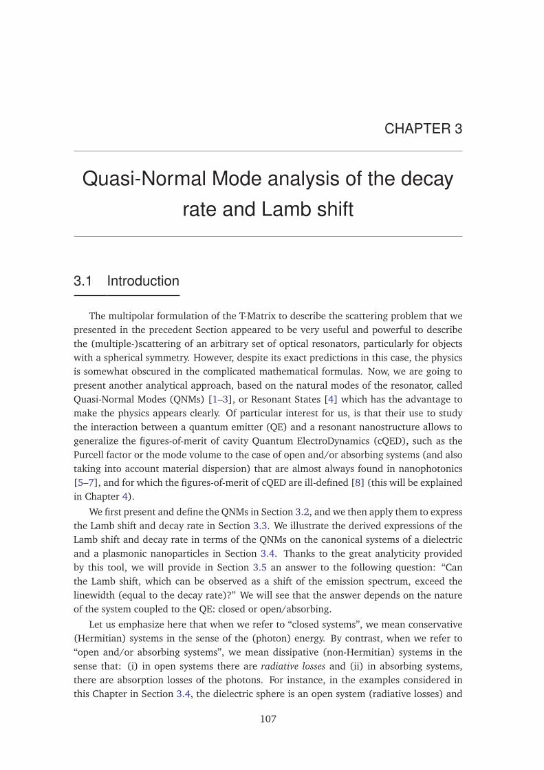
CHAPTER 3

Quasi-Normal Mode analysis of the decayrate and Lamb shift

3.1 Introduction

The multipolar formulation of the T-Matrix to describe the scattering problem that wepresented in the precedent Section appeared to be very useful and powerful to describethe (multiple-)scattering of an arbitrary set of optical resonators, particularly for objectswith a spherical symmetry. However, despite its exact predictions in this case, the physicsis somewhat obscured in the complicated mathematical formulas. Now, we are going topresent another analytical approach, based on the natural modes of the resonator, calledQuasi-Normal Modes (QNMs) [1–3], or Resonant States [4] which has the advantage tomake the physics appears clearly. Of particular interest for us, is that their use to studythe interaction between a quantum emitter (QE) and a resonant nanostructure allows togeneralize the figures-of-merit of cavity Quantum ElectroDynamics (cQED), such as thePurcell factor or the mode volume to the case of open and/or absorbing systems (and alsotaking into account material dispersion) that are almost always found in nanophotonics[5–7], and for which the figures-of-merit of cQED are ill-defined [8] (this will be explainedin Chapter 4).

We first present and define the QNMs in Section 3.2, and we then apply them to expressthe Lamb shift and decay rate in Section 3.3. We illustrate the derived expressions of theLamb shift and decay rate in terms of the QNMs on the canonical systems of a dielectricand a plasmonic nanoparticles in Section 3.4. Thanks to the great analyticity providedby this tool, we will provide in Section 3.5 an answer to the following question: “Canthe Lamb shift, which can be observed as a shift of the emission spectrum, exceed thelinewidth (equal to the decay rate)?” We will see that the answer depends on the natureof the system coupled to the QE: closed or open/absorbing.

Let us emphasize here that when we refer to “closed systems”, we mean conservative(Hermitian) systems in the sense of the (photon) energy. By contrast, when we refer to“open and/or absorbing systems”, we mean dissipative (non-Hermitian) systems in thesense that: (i) in open systems there are radiative losses and (ii) in absorbing systems,there are absorption losses of the photons. For instance, in the examples considered inthis Chapter in Section 3.4, the dielectric sphere is an open system (radiative losses) and

107

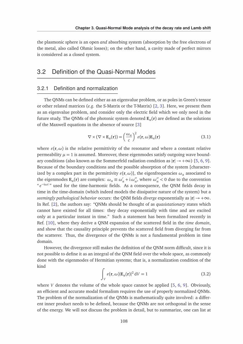
Chapter 3. Quasi-Normal Mode analysis of the decay rate and Lamb shift

the plasmonic sphere is an open and absorbing system (absorption by the free electrons ofthe metal, also called Ohmic losses); on the other hand, a cavity made of perfect mirrorsis considered as a closed system.

3.2 Definition of the Quasi-Normal Modes

3.2.1 Definition and normalization

The QNMs can be defined either as an eigenvalue problem, or as poles in Green’s tensoror other related matrices (e.g. the S-Matrix or the T-Matrix) [2, 3]. Here, we present themas an eigenvalue problem, and consider only the electric field which we only need in thefuture study. The QNMs of the photonic system denoted Eα(r) are defined as the solutionsof the Maxwell equations in the absence of source [3]

∇× (∇× Eα(r)) =ωα

c

2ε(r,ω)Eα(r) (3.1)

where ε(r,ω) is the relative permittivity of the resonator and where a constant relativepermeability µ= 1 is assumed. Moreover, these eigenmodes satisfy outgoing wave bound-ary conditions (also known as the Sommerfeld radiation condition as |r| → +∞) [5, 6, 9].Because of the boundary conditions and the possible absorption of the system [character-ized by a complex part in the permittivity ε(r,ω)], the eigenfrequencies ωα associated tothe eigenmodes Eα(r) are complex: ωα ≡ ω′α + iω′′α, where ω′′α < 0 due to the convention“ e−iωt ” used for the time-harmonic fields. As a consequence, the QNM fields decay intime in the time-domain (which indeed models the dissipative nature of the system) but aseemingly pathological behavior occurs: the QNM fields diverge exponentially as |r| → +∞.In Ref. [2], the authors say: “QNMs should be thought of as quasistationary states whichcannot have existed for all times: they decay exponentially with time and are excitedonly at a particular instant in time.” Such a statement has been formalized recently inRef. [10], where they derive a QNM expansion of the scattered field in the time domain,and show that the causality principle prevents the scattered field from diverging far fromthe scatterer. Thus, the divergence of the QNMs is not a fundamental problem in timedomain.

However, the divergence still makes the definition of the QNM norm difficult, since it isnot possible to define it as an integral of the QNM field over the whole space, as commonlydone with the eigenmodes of Hermitian systems; that is, a normalization condition of thekind

∫

Vε(r,ω)|Eα(r)|2 dV = 1 (3.2)

where V denotes the volume of the whole space cannot be applied [5, 6, 9]. Obviously,an efficient and accurate modal formalism requires the use of properly normalized QNMs.The problem of the normalization of the QNMs is mathematically quite involved: a differ-ent inner product needs to be defined, because the QNMs are not orthogonal in the senseof the energy. We will not discuss the problem in detail, but to summarize, one can list at

108

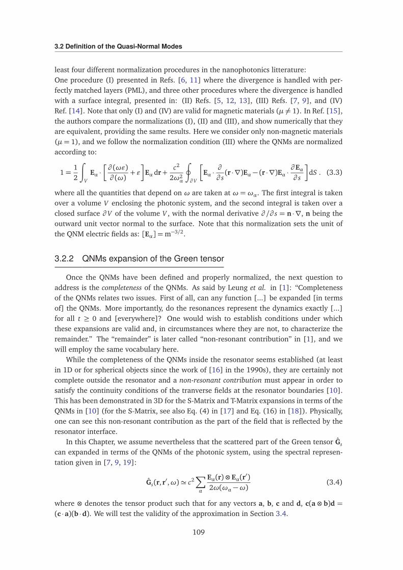
3.2 Definition of the Quasi-Normal Modes

least four different normalization procedures in the nanophotonics litterature:One procedure (I) presented in Refs. [6, 11] where the divergence is handled with per-fectly matched layers (PML), and three other procedures where the divergence is handledwith a surface integral, presented in: (II) Refs. [5, 12, 13], (III) Refs. [7, 9], and (IV)Ref. [14]. Note that only (I) and (IV) are valid for magnetic materials (µ 6= 1). In Ref. [15],the authors compare the normalizations (I), (II) and (III), and show numerically that theyare equivalent, providing the same results. Here we consider only non-magnetic materials(µ= 1), and we follow the normalization condition (III) where the QNMs are normalizedaccording to:

1=12

∫

VEα ·

∂ (ωε)∂ (ω)

+ ε

Eα dr+c2

2ω2α

∮

∂ V

Eα ·∂

∂ s(r ·∇)Eα − (r ·∇)Eα ·

∂ Eα∂ s

dS . (3.3)

where all the quantities that depend on ω are taken at ω =ωα. The first integral is takenover a volume V enclosing the photonic system, and the second integral is taken over aclosed surface ∂ V of the volume V , with the normal derivative ∂ /∂ s = n ·∇, n being theoutward unit vector normal to the surface. Note that this normalization sets the unit ofthe QNM electric fields as: [Eα] =m−3/2.

3.2.2 QNMs expansion of the Green tensor

Once the QNMs have been defined and properly normalized, the next question toaddress is the completeness of the QNMs. As said by Leung et al. in [1]: “Completenessof the QNMs relates two issues. First of all, can any function [...] be expanded [in termsof] the QNMs. More importantly, do the resonances represent the dynamics exactly [...]for all t ≥ 0 and [everywhere]? One would wish to establish conditions under whichthese expansions are valid and, in circumstances where they are not, to characterize theremainder.” The “remainder” is later called “non-resonant contribution” in [1], and wewill employ the same vocabulary here.

While the completeness of the QNMs inside the resonator seems established (at leastin 1D or for spherical objects since the work of [16] in the 1990s), they are certainly notcomplete outside the resonator and a non-resonant contribution must appear in order tosatisfy the continuity conditions of the tranverse fields at the resonator boundaries [10].This has been demonstrated in 3D for the S-Matrix and T-Matrix expansions in terms of theQNMs in [10] (for the S-Matrix, see also Eq. (4) in [17] and Eq. (16) in [18]). Physically,one can see this non-resonant contribution as the part of the field that is reflected by theresonator interface.

In this Chapter, we assume nevertheless that the scattered part of the Green tensor Gs

can expanded in terms of the QNMs of the photonic system, using the spectral represen-tation given in [7, 9, 19]:

Gs(r, r′,ω)' c2∑

α

Eα(r)⊗ Eα(r′)2ω(ωα −ω)

(3.4)

where ⊗ denotes the tensor product such that for any vectors a, b, c and d, c(a ⊗ b)d =(c ·a)(b ·d). We will test the validity of the approximation in Section 3.4.

109

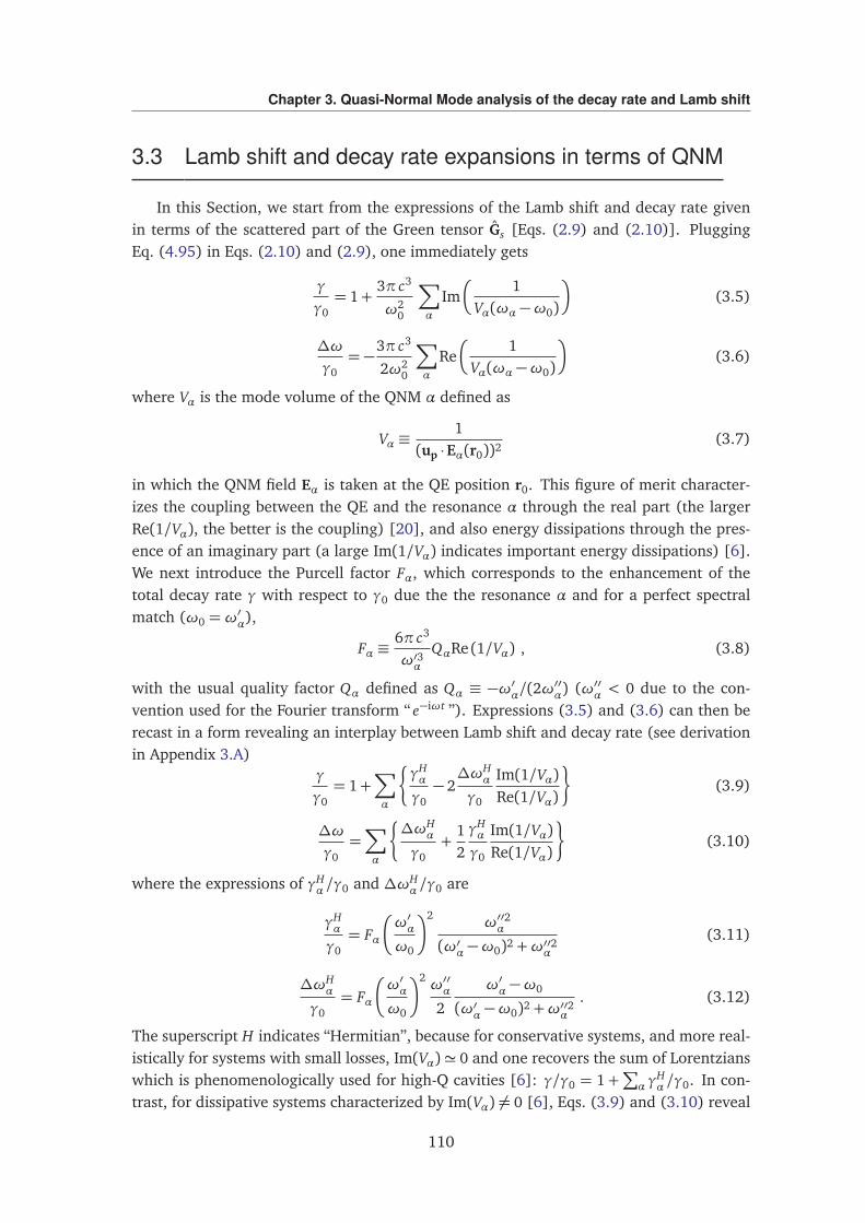
Chapter 3. Quasi-Normal Mode analysis of the decay rate and Lamb shift

3.3 Lamb shift and decay rate expansions in terms of QNM

In this Section, we start from the expressions of the Lamb shift and decay rate givenin terms of the scattered part of the Green tensor Gs [Eqs. (2.9) and (2.10)]. PluggingEq. (4.95) in Eqs. (2.10) and (2.9), one immediately gets

γ

γ0= 1+

3π c3

ω20

∑

α

Im

1Vα(ωα −ω0)

(3.5)

∆ω

γ0= −

3π c3

2ω20

∑

α

Re

1Vα(ωα −ω0)

(3.6)

where Vα is the mode volume of the QNM α defined as

Vα ≡1

(up ·Eα(r0))2(3.7)

in which the QNM field Eα is taken at the QE position r0. This figure of merit character-izes the coupling between the QE and the resonance α through the real part (the largerRe(1/Vα), the better is the coupling) [20], and also energy dissipations through the pres-ence of an imaginary part (a large Im(1/Vα) indicates important energy dissipations) [6].We next introduce the Purcell factor Fα, which corresponds to the enhancement of thetotal decay rate γ with respect to γ0 due the the resonance α and for a perfect spectralmatch (ω0 =ω′α),

Fα ≡6π c3

ω′3αQαRe (1/Vα) , (3.8)

with the usual quality factor Qα defined as Qα ≡ −ω′α/(2ω′′α) (ω′′α < 0 due to the con-

vention used for the Fourier transform “ e−iωt ”). Expressions (3.5) and (3.6) can then berecast in a form revealing an interplay between Lamb shift and decay rate (see derivationin Appendix 3.A)

γ

γ0= 1+

∑

α

γHα

γ0− 2∆ωH

α

γ0

Im(1/Vα)Re(1/Vα)

(3.9)

∆ω

γ0=∑

α

∆ωHα

γ0+

12

γHα

γ0

Im(1/Vα)Re(1/Vα)

(3.10)

where the expressions of γHα /γ0 and ∆ωH

α /γ0 are

γHα

γ0= Fα

ω′αω0

2ω′′2α

(ω′α −ω0)2 +ω′′2α(3.11)

∆ωHα

γ0= Fα

ω′αω0

2ω′′α2

ω′α −ω0

(ω′α −ω0)2 +ω′′2α. (3.12)

The superscript H indicates “Hermitian”, because for conservative systems, and more real-istically for systems with small losses, Im(Vα)' 0 and one recovers the sum of Lorentzianswhich is phenomenologically used for high-Q cavities [6]: γ/γ0 = 1+

∑

α γHα /γ0. In con-

trast, for dissipative systems characterized by Im(Vα) 6= 0 [6], Eqs. (3.9) and (3.10) reveal

110

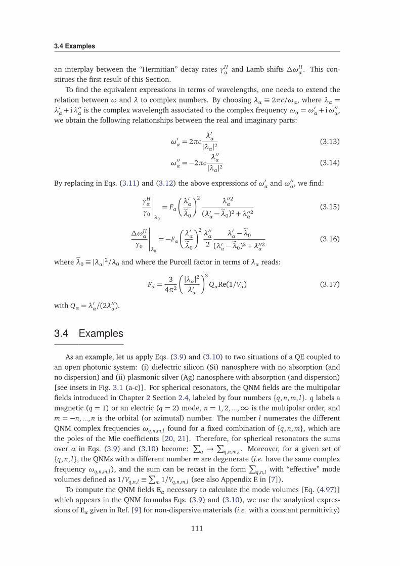
3.4 Examples

an interplay between the “Hermitian” decay rates γHα and Lamb shifts ∆ωH

α . This con-stitues the first result of this Section.

To find the equivalent expressions in terms of wavelengths, one needs to extend therelation between ω and λ to complex numbers. By choosing λα ≡ 2πc/ωα, where λα =λ′α + iλ′′α is the complex wavelength associated to the complex frequency ωα =ω′α + iω′′α,we obtain the following relationships between the real and imaginary parts:

ω′α = 2πcλ′α|λα|2

(3.13)

ω′′α = −2πcλ′′α|λα|2

(3.14)

By replacing in Eqs. (3.11) and (3.12) the above expressions of ω′α and ω′′α, we find:

γHα

γ0

λ0

= Fα

λ′αeλ0

2λ′′2α

(λ′α − eλ0)2 +λ′′2α(3.15)

∆ωHα

γ0

λ0

= −Fα

λ′αeλ0

2λ′′α2

λ′α − eλ0

(λ′α − eλ0)2 +λ′′2α(3.16)

where eλ0 ≡ |λα|2/λ0 and where the Purcell factor in terms of λα reads:

Fα =3

4π2

|λα|2

λ′α

3

QαRe(1/Vα) (3.17)

with Qα = λ′α/(2λ′′α).

3.4 Examples

As an example, let us apply Eqs. (3.9) and (3.10) to two situations of a QE coupled toan open photonic system: (i) dielectric silicon (Si) nanosphere with no absorption (andno dispersion) and (ii) plasmonic silver (Ag) nanosphere with absorption (and dispersion)[see insets in Fig. 3.1 (a-c)]. For spherical resonators, the QNM fields are the multipolarfields introduced in Chapter 2 Section 2.4, labeled by four numbers q, n, m, l. q labels amagnetic (q = 1) or an electric (q = 2) mode, n = 1, 2, ...,∞ is the multipolar order, andm = −n, ..., n is the orbital (or azimutal) number. The number l numerates the differentQNM complex frequencies ωq,n,m,l found for a fixed combination of q, n, m, which arethe poles of the Mie coefficients [20, 21]. Therefore, for spherical resonators the sumsover α in Eqs. (3.9) and (3.10) become:

∑

α →∑

q,n,m,l . Moreover, for a given set ofq, n, l, the QNMs with a different number m are degenerate (i.e. have the same complexfrequency ωq,n,m,l), and the sum can be recast in the form

∑

q,n,l with “effective” modevolumes defined as 1/Vq,n,l ≡

∑

m 1/Vq,n,m,l (see also Appendix E in [7]).To compute the QNM fields Eα necessary to calculate the mode volumes [Eq. (4.97)]

which appears in the QNM formulas Eqs. (3.9) and (3.10), we use the analytical expres-sions of Eα given in Ref. [9] for non-dispersive materials (i.e. with a constant permittivity)

111

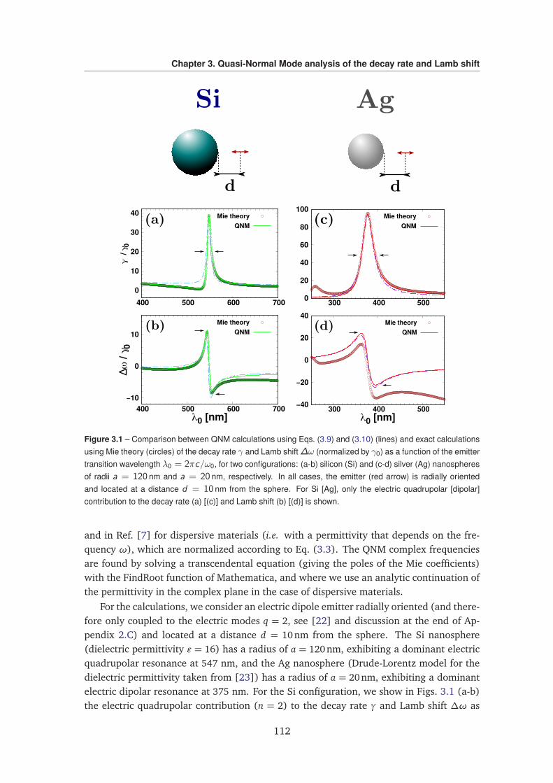
Chapter 3. Quasi-Normal Mode analysis of the decay rate and Lamb shift

0

10

20

30

40

400 500 600 700

γ* /

γ 0

Mie theoryQNM

−10

0

10

400 500 600 700

∆ω

/γ0

λ0 [nm]

Mie theoryQNM

0

20

40

60

80

100

300 400 500

Mie theoryQNM

−40

−20

0

20

40

300 400 500λ0 [nm]

Mie theoryQNM

Figure 3.1 – Comparison between QNM calculations using Eqs. (3.9) and (3.10) (lines) and exact calculationsusing Mie theory (circles) of the decay rate γ and Lamb shift ∆ω (normalized by γ0) as a function of the emittertransition wavelength λ0 = 2πc/ω0, for two configurations: (a-b) silicon (Si) and (c-d) silver (Ag) nanospheresof radii a = 120 nm and a = 20 nm, respectively. In all cases, the emitter (red arrow) is radially orientedand located at a distance d = 10 nm from the sphere. For Si [Ag], only the electric quadrupolar [dipolar]contribution to the decay rate (a) [(c)] and Lamb shift (b) [(d)] is shown.

and in Ref. [7] for dispersive materials (i.e. with a permittivity that depends on the fre-quency ω), which are normalized according to Eq. (3.3). The QNM complex frequenciesare found by solving a transcendental equation (giving the poles of the Mie coefficients)with the FindRoot function of Mathematica, and where we use an analytic continuation ofthe permittivity in the complex plane in the case of dispersive materials.

For the calculations, we consider an electric dipole emitter radially oriented (and there-fore only coupled to the electric modes q = 2, see [22] and discussion at the end of Ap-pendix 2.C) and located at a distance d = 10nm from the sphere. The Si nanosphere(dielectric permittivity ε = 16) has a radius of a = 120nm, exhibiting a dominant electricquadrupolar resonance at 547 nm, and the Ag nanosphere (Drude-Lorentz model for thedielectric permittivity taken from [23]) has a radius of a = 20nm, exhibiting a dominantelectric dipolar resonance at 375 nm. For the Si configuration, we show in Figs. 3.1 (a-b)the electric quadrupolar contribution (n = 2) to the decay rate γ and Lamb shift ∆ω as

112

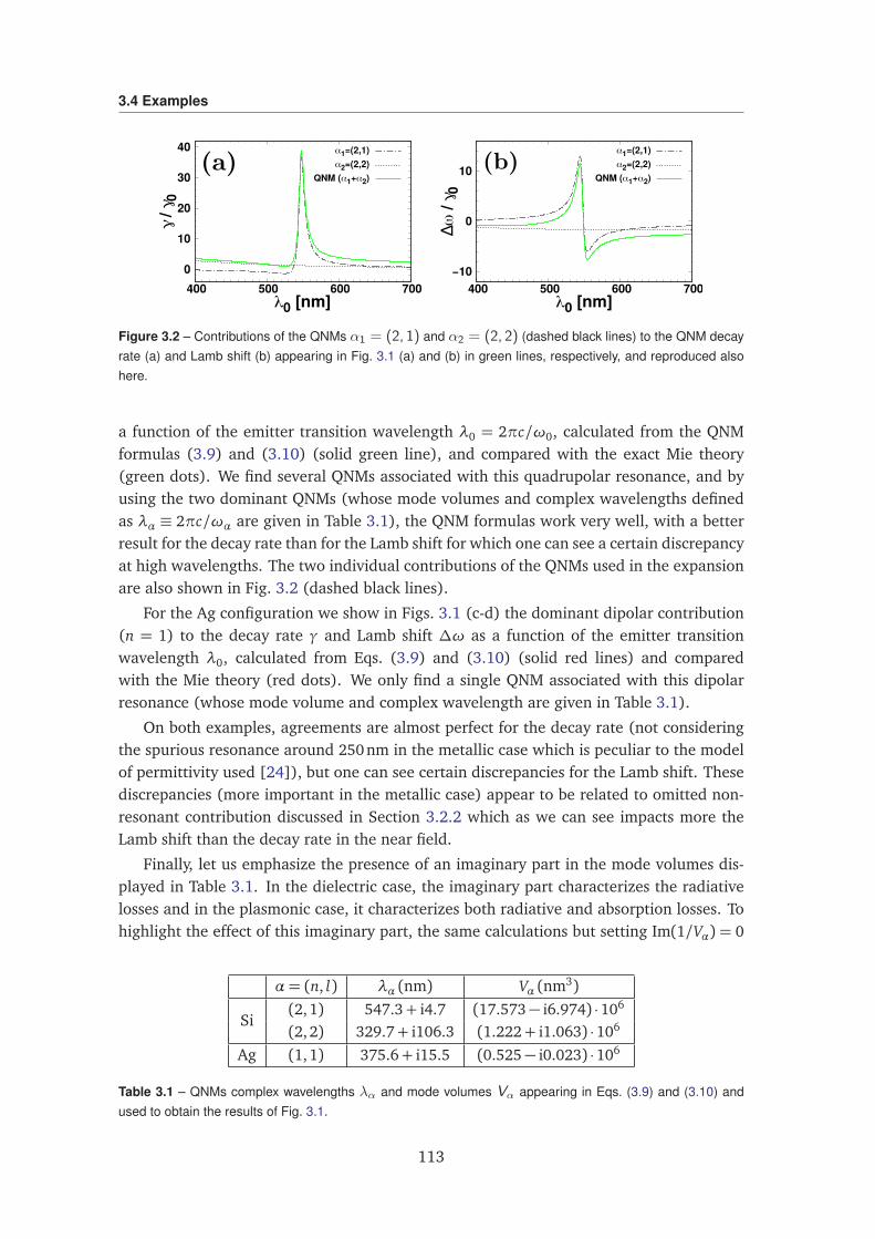
3.4 Examples

0

10

20

30

40

400 500 600 700

γ/γ

0

λ0 [nm]

α1=(2,1)α2=(2,2)

QNM (α1+α2)

−10

0

10

400 500 600 700

∆ω

/γ0

λ0 [nm]

α1=(2,1)α2=(2,2)

QNM (α1+α2)

Figure 3.2 – Contributions of the QNMs α1 = (2, 1) and α2 = (2, 2) (dashed black lines) to the QNM decayrate (a) and Lamb shift (b) appearing in Fig. 3.1 (a) and (b) in green lines, respectively, and reproduced alsohere.

a function of the emitter transition wavelength λ0 = 2πc/ω0, calculated from the QNMformulas (3.9) and (3.10) (solid green line), and compared with the exact Mie theory(green dots). We find several QNMs associated with this quadrupolar resonance, and byusing the two dominant QNMs (whose mode volumes and complex wavelengths definedas λα ≡ 2πc/ωα are given in Table 3.1), the QNM formulas work very well, with a betterresult for the decay rate than for the Lamb shift for which one can see a certain discrepancyat high wavelengths. The two individual contributions of the QNMs used in the expansionare also shown in Fig. 3.2 (dashed black lines).

For the Ag configuration we show in Figs. 3.1 (c-d) the dominant dipolar contribution(n = 1) to the decay rate γ and Lamb shift ∆ω as a function of the emitter transitionwavelength λ0, calculated from Eqs. (3.9) and (3.10) (solid red lines) and comparedwith the Mie theory (red dots). We only find a single QNM associated with this dipolarresonance (whose mode volume and complex wavelength are given in Table 3.1).

On both examples, agreements are almost perfect for the decay rate (not consideringthe spurious resonance around 250nm in the metallic case which is peculiar to the modelof permittivity used [24]), but one can see certain discrepancies for the Lamb shift. Thesediscrepancies (more important in the metallic case) appear to be related to omitted non-resonant contribution discussed in Section 3.2.2 which as we can see impacts more theLamb shift than the decay rate in the near field.

Finally, let us emphasize the presence of an imaginary part in the mode volumes dis-played in Table 3.1. In the dielectric case, the imaginary part characterizes the radiativelosses and in the plasmonic case, it characterizes both radiative and absorption losses. Tohighlight the effect of this imaginary part, the same calculations but setting Im(1/Vα) = 0

α= (n, l) λα (nm) Vα (nm3)

Si(2, 1) 547.3+ i4.7 (17.573− i6.974) ·106

(2, 2) 329.7+ i106.3 (1.222+ i1.063) ·106

Ag (1, 1) 375.6+ i15.5 (0.525− i0.023) ·106

Table 3.1 – QNMs complex wavelengths λα and mode volumes Vα appearing in Eqs. (3.9) and (3.10) andused to obtain the results of Fig. 3.1.

113

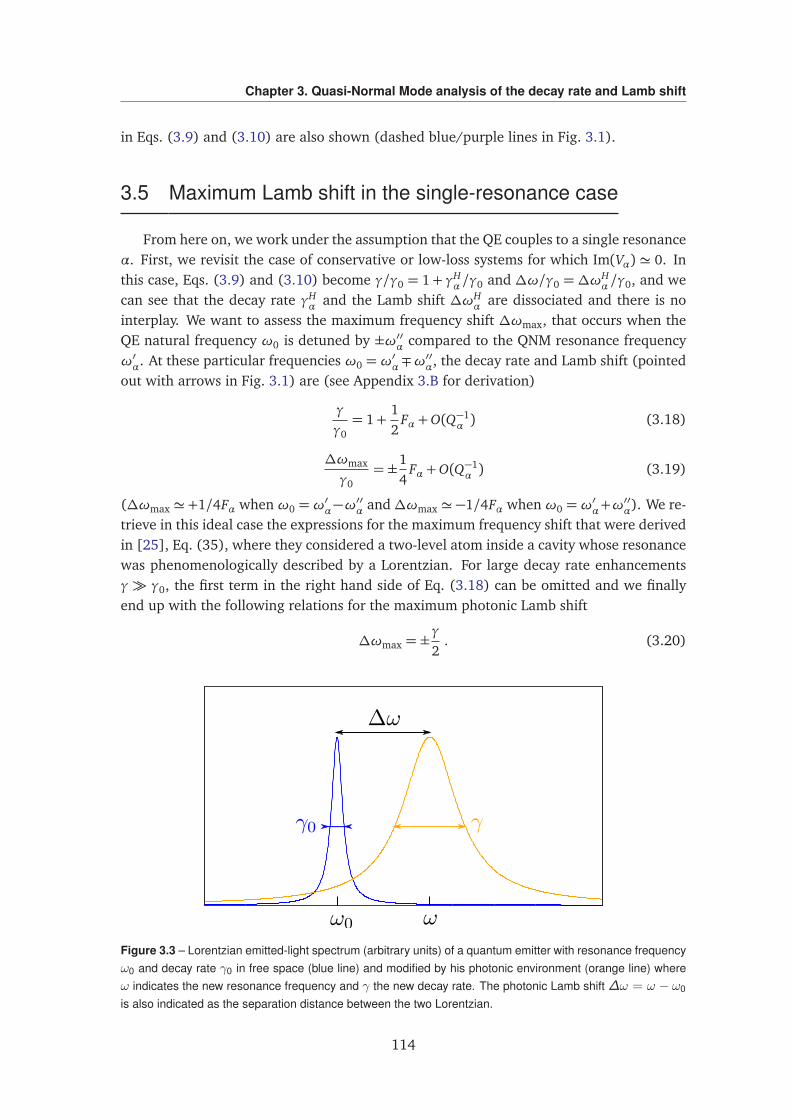
Chapter 3. Quasi-Normal Mode analysis of the decay rate and Lamb shift

in Eqs. (3.9) and (3.10) are also shown (dashed blue/purple lines in Fig. 3.1).

3.5 Maximum Lamb shift in the single-resonance case

From here on, we work under the assumption that the QE couples to a single resonanceα. First, we revisit the case of conservative or low-loss systems for which Im(Vα) ' 0. Inthis case, Eqs. (3.9) and (3.10) become γ/γ0 = 1+ γH

α /γ0 and ∆ω/γ0 = ∆ωHα /γ0, and we

can see that the decay rate γHα and the Lamb shift ∆ωH

α are dissociated and there is nointerplay. We want to assess the maximum frequency shift ∆ωmax, that occurs when theQE natural frequency ω0 is detuned by ±ω′′α compared to the QNM resonance frequencyω′α. At these particular frequencies ω0 =ω′α∓ω

′′α, the decay rate and Lamb shift (pointed

out with arrows in Fig. 3.1) are (see Appendix 3.B for derivation)

γ

γ0= 1+

12

Fα +O(Q−1α ) (3.18)

∆ωmax

γ0= ±

14

Fα +O(Q−1α ) (3.19)

(∆ωmax ' +1/4Fα whenω0 =ω′α−ω′′α and∆ωmax ' −1/4Fα whenω0 =ω′α+ω

′′α). We re-

trieve in this ideal case the expressions for the maximum frequency shift that were derivedin [25], Eq. (35), where they considered a two-level atom inside a cavity whose resonancewas phenomenologically described by a Lorentzian. For large decay rate enhancementsγ γ0, the first term in the right hand side of Eq. (3.18) can be omitted and we finallyend up with the following relations for the maximum photonic Lamb shift

∆ωmax = ±γ

2. (3.20)

Figure 3.3 – Lorentzian emitted-light spectrum (arbitrary units) of a quantum emitter with resonance frequencyω0 and decay rate γ0 in free space (blue line) and modified by his photonic environment (orange line) whereω indicates the new resonance frequency and γ the new decay rate. The photonic Lamb shift ∆ω = ω − ω0

is also indicated as the separation distance between the two Lorentzian.

114

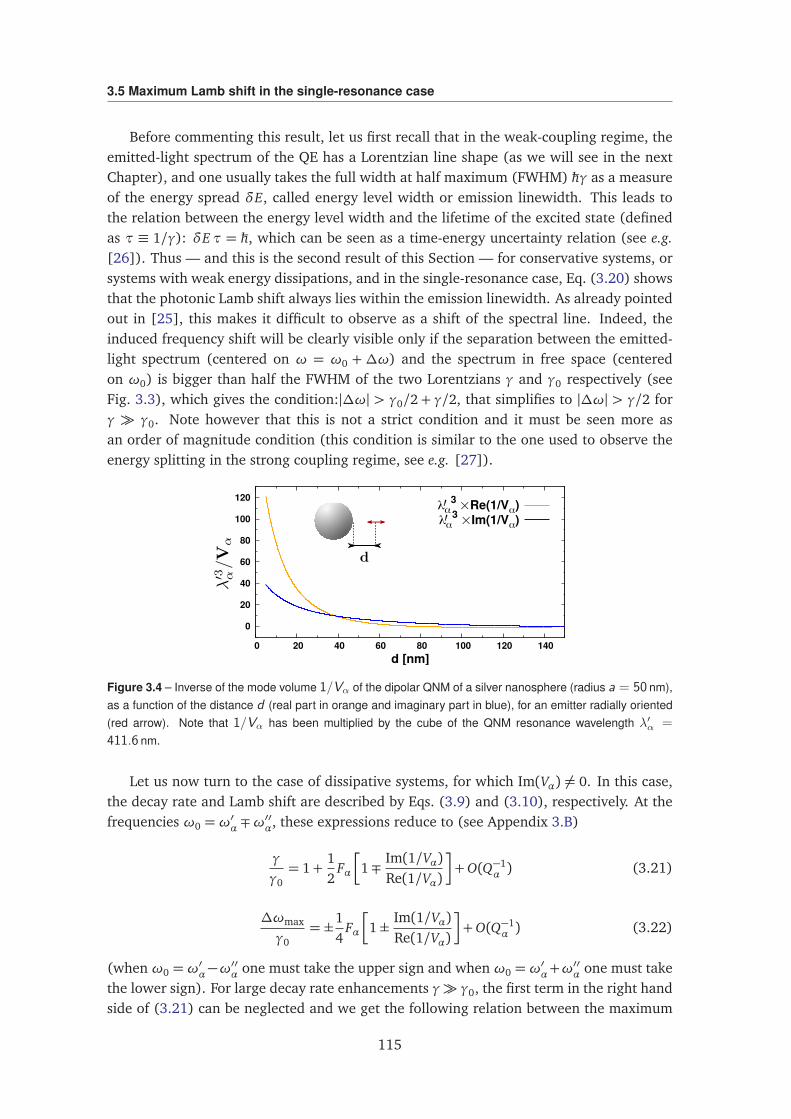
3.5 Maximum Lamb shift in the single-resonance case

Before commenting this result, let us first recall that in the weak-coupling regime, theemitted-light spectrum of the QE has a Lorentzian line shape (as we will see in the nextChapter), and one usually takes the full width at half maximum (FWHM) ħhγ as a measureof the energy spread δE, called energy level width or emission linewidth. This leads tothe relation between the energy level width and the lifetime of the excited state (definedas τ ≡ 1/γ): δE τ = ħh, which can be seen as a time-energy uncertainty relation (see e.g.[26]). Thus — and this is the second result of this Section — for conservative systems, orsystems with weak energy dissipations, and in the single-resonance case, Eq. (3.20) showsthat the photonic Lamb shift always lies within the emission linewidth. As already pointedout in [25], this makes it difficult to observe as a shift of the spectral line. Indeed, theinduced frequency shift will be clearly visible only if the separation between the emitted-light spectrum (centered on ω = ω0 + ∆ω) and the spectrum in free space (centeredon ω0) is bigger than half the FWHM of the two Lorentzians γ and γ0 respectively (seeFig. 3.3), which gives the condition:|∆ω| > γ0/2+ γ/2, that simplifies to |∆ω| > γ/2 forγ γ0. Note however that this is not a strict condition and it must be seen more asan order of magnitude condition (this condition is similar to the one used to observe theenergy splitting in the strong coupling regime, see e.g. [27]).

0

20

40

60

80

100

120

0 20 40 60 80 100 120 140d [nm]

λα3×Re(1/Vα)

λα3×Im(1/Vα)

Figure 3.4 – Inverse of the mode volume 1/Vα of the dipolar QNM of a silver nanosphere (radius a = 50 nm),as a function of the distance d (real part in orange and imaginary part in blue), for an emitter radially oriented(red arrow). Note that 1/Vα has been multiplied by the cube of the QNM resonance wavelength λ′α =

411.6 nm.

Let us now turn to the case of dissipative systems, for which Im(Vα) 6= 0. In this case,the decay rate and Lamb shift are described by Eqs. (3.9) and (3.10), respectively. At thefrequencies ω0 =ω′α ∓ω

′′α, these expressions reduce to (see Appendix 3.B)

γ

γ0= 1+

12

Fα

1∓Im(1/Vα)Re(1/Vα)

+O(Q−1α ) (3.21)

∆ωmax

γ0= ±

14

Fα

1±Im(1/Vα)Re(1/Vα)

+O(Q−1α ) (3.22)

(when ω0 =ω′α−ω′′α one must take the upper sign and when ω0 =ω′α+ω

′′α one must take

the lower sign). For large decay rate enhancements γ γ0, the first term in the right handside of (3.21) can be neglected and we get the following relation between the maximum

115

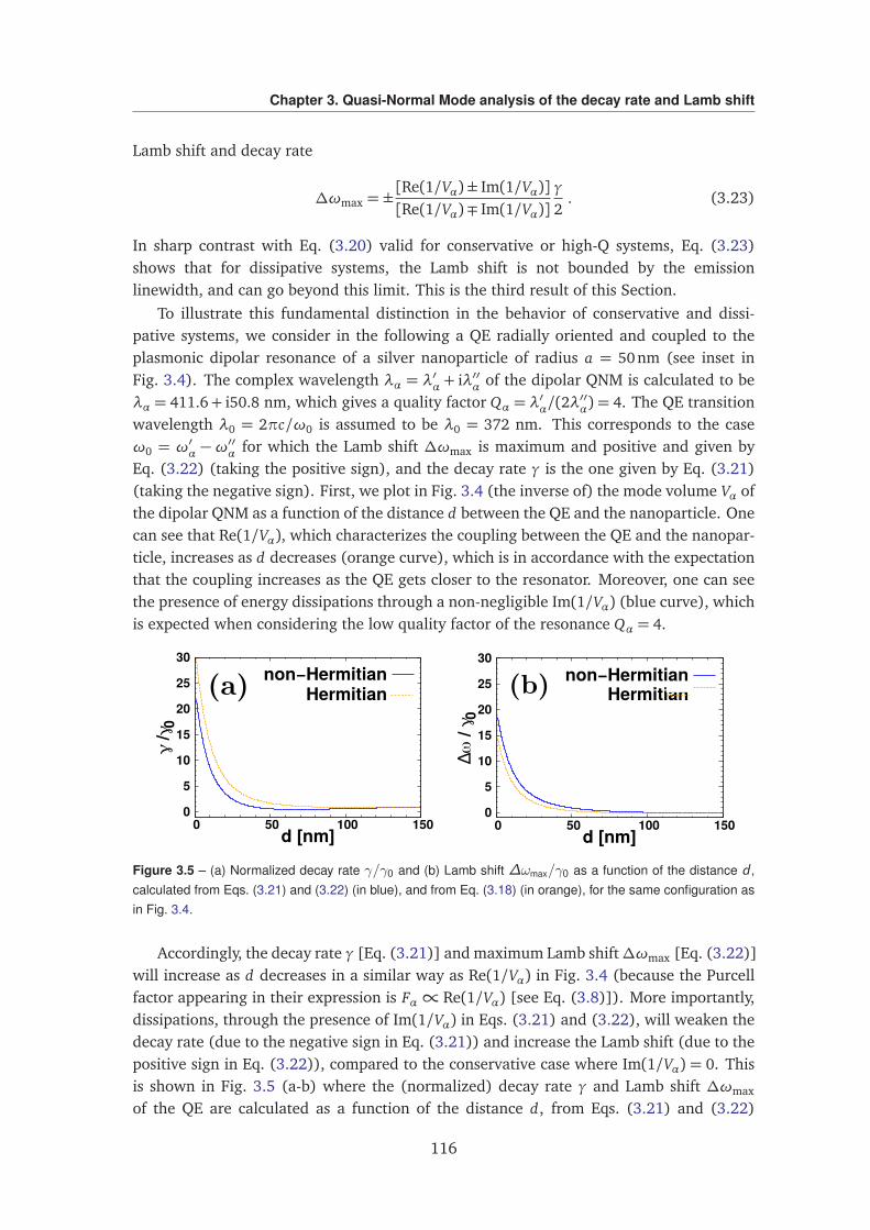
Chapter 3. Quasi-Normal Mode analysis of the decay rate and Lamb shift

Lamb shift and decay rate

∆ωmax = ±[Re(1/Vα)± Im(1/Vα)][Re(1/Vα)∓ Im(1/Vα)]

γ

2. (3.23)

In sharp contrast with Eq. (3.20) valid for conservative or high-Q systems, Eq. (3.23)shows that for dissipative systems, the Lamb shift is not bounded by the emissionlinewidth, and can go beyond this limit. This is the third result of this Section.

To illustrate this fundamental distinction in the behavior of conservative and dissi-pative systems, we consider in the following a QE radially oriented and coupled to theplasmonic dipolar resonance of a silver nanoparticle of radius a = 50nm (see inset inFig. 3.4). The complex wavelength λα = λ′α + iλ′′α of the dipolar QNM is calculated to beλα = 411.6+ i50.8 nm, which gives a quality factor Qα = λ′α/(2λ

′′α) = 4. The QE transition

wavelength λ0 = 2πc/ω0 is assumed to be λ0 = 372 nm. This corresponds to the caseω0 = ω′α −ω

′′α for which the Lamb shift ∆ωmax is maximum and positive and given by

Eq. (3.22) (taking the positive sign), and the decay rate γ is the one given by Eq. (3.21)(taking the negative sign). First, we plot in Fig. 3.4 (the inverse of) the mode volume Vα ofthe dipolar QNM as a function of the distance d between the QE and the nanoparticle. Onecan see that Re(1/Vα), which characterizes the coupling between the QE and the nanopar-ticle, increases as d decreases (orange curve), which is in accordance with the expectationthat the coupling increases as the QE gets closer to the resonator. Moreover, one can seethe presence of energy dissipations through a non-negligible Im(1/Vα) (blue curve), whichis expected when considering the low quality factor of the resonance Qα = 4.

0

5

10

15

20

25

30

0 50 100 150

γ*/γ 0

d [nm]

non−HermitianHermitian

0

5

10

15

20

25

30

0 50 100 150

∆ω

/γ0

d [nm]

non−HermitianHermitian

Figure 3.5 – (a) Normalized decay rate γ/γ0 and (b) Lamb shift ∆ωmax/γ0 as a function of the distance d ,calculated from Eqs. (3.21) and (3.22) (in blue), and from Eq. (3.18) (in orange), for the same configuration asin Fig. 3.4.

Accordingly, the decay rate γ [Eq. (3.21)] and maximum Lamb shift∆ωmax [Eq. (3.22)]will increase as d decreases in a similar way as Re(1/Vα) in Fig. 3.4 (because the Purcellfactor appearing in their expression is Fα∝ Re(1/Vα) [see Eq. (3.8)]). More importantly,dissipations, through the presence of Im(1/Vα) in Eqs. (3.21) and (3.22), will weaken thedecay rate (due to the negative sign in Eq. (3.21)) and increase the Lamb shift (due to thepositive sign in Eq. (3.22)), compared to the conservative case where Im(1/Vα) = 0. Thisis shown in Fig. 3.5 (a-b) where the (normalized) decay rate γ and Lamb shift ∆ωmax

of the QE are calculated as a function of the distance d, from Eqs. (3.21) and (3.22)

116

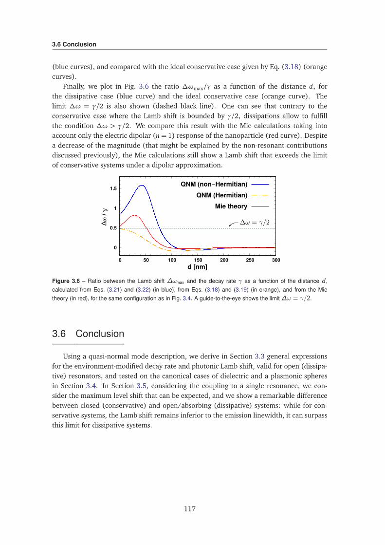
3.6 Conclusion

(blue curves), and compared with the ideal conservative case given by Eq. (3.18) (orangecurves).

Finally, we plot in Fig. 3.6 the ratio ∆ωmax/γ as a function of the distance d, forthe dissipative case (blue curve) and the ideal conservative case (orange curve). Thelimit ∆ω = γ/2 is also shown (dashed black line). One can see that contrary to theconservative case where the Lamb shift is bounded by γ/2, dissipations allow to fulfillthe condition ∆ω > γ/2. We compare this result with the Mie calculations taking intoaccount only the electric dipolar (n= 1) response of the nanoparticle (red curve). Despitea decrease of the magnitude (that might be explained by the non-resonant contributionsdiscussed previously), the Mie calculations still show a Lamb shift that exceeds the limitof conservative systems under a dipolar approximation.

0

0.5

1

1.5

0 50 100 150 200 250 300

∆ω

/ γ*

d [nm]

QNM (non−Hermitian)QNM (Hermitian)

Mie theory

Figure 3.6 – Ratio between the Lamb shift ∆ωmax and the decay rate γ as a function of the distance d ,calculated from Eqs. (3.21) and (3.22) (in blue), from Eqs. (3.18) and (3.19) (in orange), and from the Mietheory (in red), for the same configuration as in Fig. 3.4. A guide-to-the-eye shows the limit ∆ω = γ/2.

3.6 Conclusion

Using a quasi-normal mode description, we derive in Section 3.3 general expressionsfor the environment-modified decay rate and photonic Lamb shift, valid for open (dissipa-tive) resonators, and tested on the canonical cases of dielectric and a plasmonic spheresin Section 3.4. In Section 3.5, considering the coupling to a single resonance, we con-sider the maximum level shift that can be expected, and we show a remarkable differencebetween closed (conservative) and open/absorbing (dissipative) systems: while for con-servative systems, the Lamb shift remains inferior to the emission linewidth, it can surpassthis limit for dissipative systems.

117

Chapter 3. Quasi-Normal Mode analysis of the decay rate and Lamb shift

3.A Derivation of Eqs. (3.9), (3.10), (3.11) and (3.12)

Here we derive the interplay relations between the decay rate and Lamb shift[Eqs. (3.9), (3.10), (3.11) and (3.12)] obtained in Section 3.3. For Hermitian systems,Im(1/Vα) = 0. In this case, Eqs. (3.5) and (3.6) (main text) can be written as

γ

γ0= 1+

3π c3

ω20

∑

α

Re

1Vα

Im

1ωα −ω0

(3.24)

∆ω

γ0= −

3π c3

2ω20

∑

α

Re

1Vα

Re

1ωα −ω0

. (3.25)

We then define the Hermitian decay rate and Lamb shift associated to the resonance α as

γHα

γ0≡

3π c3

ω20

Re

1Vα

Im

1ωα −ω0

(3.26)

∆ωHα

γ0≡ −

3π c3

2ω20

Re

1Vα

Re

1ωα −ω0

, (3.27)

so that the total decay rate and Lamb shift read γ∗ = γ0 +∑

α γHα and ∆ω =

∑

α∆ωHα

respectively.For non-Hermitian systems, Im(1/Vα) 6= 0. In this case, Eqs. (3.5) and (3.6) present an

extra term compared to the Hermitian case

γ

γ0= 1+

3π c3

ω20

∑

α

Re

1Vα

Im

1ωα −ω0

+3π c3

ω20

∑

α

Im

1Vα

Re

1ωα −ω0

(3.28)

∆ω

γ0= −

3π c3

2ω20

∑

α

Re

1Vα

Re

1ωα −ω0

+3π c3

2ω20

∑

α

Im

1Vα

Im

1ωα −ω0

. (3.29)

By making use of (3.26) and (3.27), these expressions can be recast in the form

γ

γ0= 1+

∑

α

γHα

γ0− 2∆ωH

α

γ0

Im(1/Vα)Re(1/Vα)

(3.30)

∆ω

γ0=∑

α

∆ωHα

γ0+

12

γHα

γ0

Im(1/Vα)Re(1/Vα)

(3.31)

which are the expressions (3.9) and (3.10) of the main text.Now, we show how the expressions (3.26) and (3.27) for γH

α and∆ωHα respectively can

be rewritten in the form of Eqs. (3.11) and (3.12) (main text). First, by multiplying by thecomplex conjugate, we can explicitely write (we recall that we defined ωα ≡ω′α + iω′′α)

Re

1ωα −ω0

=ω′α −ω0

|ωα −ω0|2=

ω′α −ω0

(ω′α −ω0)2 +ω′′2α(3.32)

Im

1ωα −ω0

=−ω′′α

|ωα −ω0|2=

−ω′′α(ω′α −ω0)2 +ω′′2α

(3.33)

118

3.A Derivation of Eqs. (3.9), (3.10), (3.11) and (3.12)

By reporting these expressions into Eqs. (3.26) and (3.27), we get

γHα

γ0=

3π c3

ω20

Re

1Vα

−ω′′α(ω′α −ω0)2 +ω′′2α

(3.34)

∆ωHα

γ0= −

3π c3

2ω20

Re

1Vα

ω′α −ω0

(ω′α −ω0)2 +ω′′2α(3.35)

Finally, by introducing the Purcell factor defined in Eq. (3.8) (main text), we end up withthe Eqs. (3.11) and (3.12) of the main text, that is

γHα

γ0= Fα

ω′αω0

2ω′′2α

(ω′α −ω0)2 +ω′′2α(3.36)

∆ωHα

γ0= Fα

ω′αω0

2ω′′α2

ω′α −ω0

(ω′α −ω0)2 +ω′′2α. (3.37)

119

Chapter 3. Quasi-Normal Mode analysis of the decay rate and Lamb shift

3.B Derivation of Eqs. (3.18), (3.19), (3.21) and (3.22)

Here we derive the expressions of the decay rate and Lamb shift obtained in Section 3.5in the single-resonance case [Eqs. (3.18), (3.19), (3.21) and (3.22)].

We consider for that two particular detunings of the natural QE frequency ω0 com-pared to the QNM resonance frequency ω′α: ω0 = ω′α ∓ ω

′′α, for which the Lamb shift

presents an extremum (indicated by arrows in Fig. 3.1 (b) and (d) in the main text). Westart with the detuning ω0 = ω′α +ω

′′α. By replacing ω0 by ω′α +ω

′′α in Eqs. (3.11) and

(3.12), one gets

γHα

γ0=

12

Fα

ω′αω′α +ω′′α

2

=12

Fα

1

1− 12Qα

!2

(3.38)

∆ωHα

γ0= −

14

Fα

ω′αω′α +ω′′α

2

= −14

Fα

1

1− 12Qα

!2

(3.39)

where we used the fact that Qα = −ω′α/(2ω′′α). In the single-resonance case, Eqs. (3.9)

and (3.10) thus reduce to

γ

γ0= 1+

γHα

γ0− 2∆ωH

α

γ0

Im(1/Vα)Re(1/Vα)

(3.40)

∆ω

γ0=∆ωH

α

γ0+

12

γHα

γ0

Im(1/Vα)Re(1/Vα)

, (3.41)

and by employing the previous expressions of γHα and ∆ωH

α , one gets

γ

γ0= 1+

12

Fα

1

1− 12Qα

!2

1+Im(1/Vα)Re(1/Vα)

(3.42)

∆ω−

γ0= −

14

Fα

1

1− 12Qα

!2

1−Im(1/Vα)Re(1/Vα)

. (3.43)

Similarly, for the detuning ω0 =ω′α−ω′′α, replacing ω0 in Eqs. (3.11) and (3.12) yields

γHα

γ0=

12

Fα

ω′αω′α −ω′′α

2

=12

Fα

1

1+ 12Qα

!2

(3.44)

∆ωHα

γ0=

14

Fα

ω′αω′α −ω′′α

2

=14

Fα

1

1+ 12Qα

!2

. (3.45)

Then, by plugging these equations in the expressions of the decay rate and Lamb shift inthe single-resonance case as previously, one gets

γ

γ0= 1+

12

Fα

1

1+ 12Qα

!2

1−Im(1/Vα)Re(1/Vα)

(3.46)

120

3.B Derivation of Eqs. (3.18), (3.19), (3.21) and (3.22)

∆ω+

γ0=

14

Fα

1

1+ 12Qα

!2

1+Im(1/Vα)Re(1/Vα)

. (3.47)

Note that for the Hermitian systems, the decay rate and Lamb shift for these two particulardetunings are given by Eqs. (3.42), (3.43), (3.46) and (3.47) with Im(1/Vα) = 0, and oneends up with the Eqs. (3.18) and (3.19) of the main text.

121

Chapter 3. Quasi-Normal Mode analysis of the decay rate and Lamb shift

122

Bibliography

[1] E. Ching, P. Leung, A. M. van den Brink, W. Suen, S. Tong, and K. Young, Reviewsof Modern Physics 70, 1545 (1998).

[2] E. Berti, V. Cardoso, and A. O. Starinets, Classical and Quantum Gravity 26, 163001(2009).

[3] P. Lalanne, W. Yan, K. Vynck, C. Sauvan, and J.-P. Hugonin, Laser & PhotonicsReviews 12, 1700113 (2018).

[4] G. García-Calderón, in Unstable States in the Continuous Spectra, Part I: Analysis,Concepts, Methods, and Results, Advances in Quantum Chemistry, Vol. 60, edited byC. A. Nicolaides and E. Brändas (Academic Press, 2010) pp. 407 – 455.

[5] P. T. Kristensen, C. Van Vlack, and S. Hughes, Optics Letters 37, 1649 (2012).

[6] C. Sauvan, J.-P. Hugonin, I. Maksymov, and P. Lalanne, Physical Review Letters 110,237401 (2013).

[7] E. Muljarov and W. Langbein, Physical Review B 94, 235438 (2016).

[8] A. F. Koenderink, Optics Letters 35, 4208 (2010).

[9] M. Doost, W. Langbein, and E. A. Muljarov, Physical Review A 90, 013834 (2014).

[10] R. Colom, R. McPhedran, B. Stout, and N. Bonod, Physical Review B 98, 085418(2018).

[11] B. Vial, F. Zolla, A. Nicolet, and M. Commandré, Physical Review A 89, 023829(2014).

[12] H. M. Lai, P. T. Leung, K. Young, P. W. Barber, and S. C. Hill, Physical Review A 41,5187 (1990).

[13] P. T. Kristensen and S. Hughes, ACS Photonics 1, 2 (2013).

[14] B. Stout, R. Colom, N. Bonod, and R. McPhedran, arXiv:1903.07183 [physics](2019).

[15] P. T. Kristensen, R.-C. Ge, and S. Hughes, Physical Review A 92, 053810 (2015).

[16] P. Leung, S. Liu, and K. Young, Physical Review A 49, 3057 (1994).

[17] V. Grigoriev, A. Tahri, S. Varault, B. Rolly, B. Stout, J. Wenger, and N. Bonod, PhysicalReview A 88, 011803 (2013).

123

BIBLIOGRAPHY

[18] T. Zhan and S. Chui, Physical Review A 90, 023802 (2014).

[19] C. Sauvan, J.-P. Hugonin, R. Carminati, and P. Lalanne, Physical Review A 89,043825 (2014).

[20] X. Zambrana-Puyalto and N. Bonod, Physical Review B 91, 195422 (2015).

[21] B. Stout, A. Devilez, B. Rolly, and N. Bonod, Journal of the Optical Society of AmericaB 28, 1213 (2011).

[22] B. Rolly, B. Bebey, S. Bidault, B. Stout, and N. Bonod, Physical Review B 85, 245432(2012).

[23] A. D. Rakic, A. B. Djurišic, J. M. Elazar, and M. L. Majewski, Applied Optics 37, 5271(1998).

[24] F. Hao and P. Nordlander, Chemical Physics Letters 446, 115 (2007).

[25] S. C. Ching, H. M. Lai, and K. Young, Journal of the Optical Society of America B 4,2004 (1987).

[26] V. Dodonov and A. Dodonov, Physica Scripta 90, 074049 (2015).

[27] P. Törmä and W. L. Barnes, Reports on Progress in Physics 78, 013901 (2014).

124

BIBLIOGRAPHY

125

BIBLIOGRAPHY

126

CHAPTER 4

Quantum descriptions of the weak andstrong coupling regimes

4.1 Introduction

In Chapters 2 and 3, we mostly talked about the weak-coupling regime of interactionbetween a quantum emitter (QE) and photonic/plasmonic resonators. In this regime, thedecay rate of the QE and the emitted frequency are modified compared to their valuesin free space, and such modifications can be calculated by perturbative treatments aspresented in Section 2.2. In this introduction, we therefore focus on the strong-couplingregime, and we do a short review of the experimental work carried in relation with strong-coupling.

In the 1980s, Serge Haroche popularized the picture of atoms coupled to a single(resonant) mode in a cavity, known as cavity-quantum electrodynamics (cQED) [1]. Thequality factor of the cavity was so high that he was even able to explore the strong-couplingregime in which the atom exchanges several times a single photon with the mode of thecavity [2, 3]. These experiments were carried out in the microwave frequency range andinvolved several Rydberg atoms. However, similar experiments were also realized at thelevel of a single Rydberg atom by another group [4, 5]. A bit later, the strong-couplingwas realized at optical frequencies [6–8], and achieved with a single atom [9, 10]. Therealization of an efficient coupling between the quantum emitter (QE) and the cavityrelies on the high cavity quality factor obtained at low temperature, spectrally sharp QEsand a fine tuning of the cavity resonance.

Due to the progress in micro and nanotechnologies, strong-coupling was observed inthe 1990s at optical frequencies with solid-state quantum emitters (semiconductor quan-tum dots) in integrated microcavities cooled at cryogenic temperatures, and was achievedwith single solid-state QEs in 2004 [11, 12]. A review concerning single solid-state QEscan be found in [13].

The generic term “cavity” has evolved and taken different forms over the years, andin general refers to a resonant system. In the nanophotonics community for instance,optically resonant nanostructures take the role of open cavities. In such systems, importantcoupling can be achieved at room temperature with QEs with broader linewidths. In2004, the strong-coupling regime was clearly observed with J-aggregates in the group of

127

Chapter 4. Quantum descriptions of the weak and strong coupling regimes

J. Bellessa [14, 15] and in the group of T. Ebbesen [16, 17], and later with other varioustypes of QEs like dye molecules and quantum dots (for more references, see the recentreview [18] and references therein). Note however that signatures of strong-couplingwere already observed with dye molecules in 1982 [19]. More exhaustive overviews onthe strong-coupling between QEs and photonic/plasmonic resonators are presented inthree recent reviews on the topic [18, 20, 21]. Very recently, some groups claimed therealization of strong-coupling in plasmonic structures at room temperatures at the singleemitter level [22–26]. These papers are compared and discussed in [20].

In the present Chapter, we aim at first summarizing the quantum theoretical ap-proaches and models which were developed to deal with the problem of the spontaneousemission of a two-level atom interacting with a resonant system. In a quantum treatment,the quantity which is chosen to investigate the temporal behavior of the system is theprobability of the atom to remain in its excited state, called the survival probability anddenoted Psurv(t) hereafter. We aim at understanding the transition between the weak andstrong-coupling regimes. In the weak-coupling regime, Psurv(t) decays monotically in timeto zero, but with a decay rate modified compared to the free-space decay rate. On theother hand, in the strong-coupling regime, Psurv(t) undergoes oscillations, called vacuumRabi oscillations, before decaying to zero. These oscillations represent a coherent andreversible exchange of energy (photon) between the quantum emitter and the photonicsystem.

There is also an other facet of the interaction between an atom and the resonatorwhen one looks at the emission spectrum. In the weak-coupling regime, the distributionin frequency of the emitted photons is essentially one peak whereas in the strong-couplingone can distinguish two distinct peaks: this is called the vacuum Rabi splitting, and theseparation between the peaks depends on the strength of the coupling. Note that thetheories presented here are not suitable as such to investigate the ultra-strong-couplingregime, because we systematically make the rotating-wave approximation when writingthe interaction Hamiltonian, which is valid unless the atom-cavity coupling rate becomescomparable to the atomic resonance frequency. In this case, one enters the ultra strong-coupling regime which can be found in [27–32].

We first present in Section 4.2 a powerful model to describe an atom in a closed cavityextensively used in cQED. It is based on the Jaynes-Cummings Hamiltonian [33], with thefigures-of-merit such as the coupling constant g characterizing the coupling between theQE and the mode, or the effective volume V , which is essentially the volume of the cavityand characterizes the confinement of the field, and the cavity losses are introduced eitherphenomenologically by a cavity decay rate γα, or more rigorously by coupling the mode ofthe cavity to a continuum of modes outside of the cavity, which leads to a master equation(see e.g. [34] chapter 5 or [35] chapter 6). Such a description is part of a larger paradigmdeveloped to deal with dissipative quantum systems (see e.g. [36]), but is valid only in thelimit of small leakages, which is most often verified for closed cavities with high qualityfactors Q, and has been very successful to describe cQED experiments, and later in opticalmicrocavities in the 1990s.

128

4.1 Introduction

An equivalent model is then presented in Section 4.3 but providing a different physicalinterpretation of the interaction, where the atom is this time coupled to a continuumof modes with a Lorentzian density of states of linewidth γα — the full width at halfmaximum (FWHM).

Such models were very successful in cQED where the systems considered usually sufferfrom small losses. However, these models are not a priori valid in nanophotonics whereopen, strongly absorbing and dispersive systems are usually considered (for example plas-monics in the visible).

Therefore, we present in Sections 4.4 and 4.5 two approaches to transpose the cQEDformalism in nanophotonics. These approaches are based on a Green tensor description ofthe electromagnetic environment, and on the natural modes of the photonic or plasmonicresonator, which are the resonant states [or quasi-normal modes (QNMs)] presented inthe Chapter 3. Such an approach based on the natural modes of the system was alreadypointed out in [37], where they wrote: “A more natural way of stating these ideas is touse the QNMs of the open system alone, rather than the modes of the universe — inother words, to eliminate the bath degrees of freedom. This would be possible as an exactstatement only if the QNMs are complete.”

In the approach presented in Section 4.4, we show how the QNM framework allowsus to generalize the usual cQED figure-of-merit characterizing the interaction betweendipole sources and a resonance of a cavity, such as the mode volume V . Moreover, itallows to revisit notions such as the density of states and the coupling constants in thecase of nanophotonics.

In the approach presented in Section 4.5 and based on [38, 39], we derive a non-Hermitian “effective” Hamiltonian for the subsystem atom + QNMs of the resonator.However, the Lorentzian density of states of the resonant modes is introduced in a morephenomenologically way than in Section 4.4.

Finally, in conclusion we compare the figures-of-merit derived within the QNM frame-work in Section 4.4 with the cQED ones presented in Section 4.2.

129

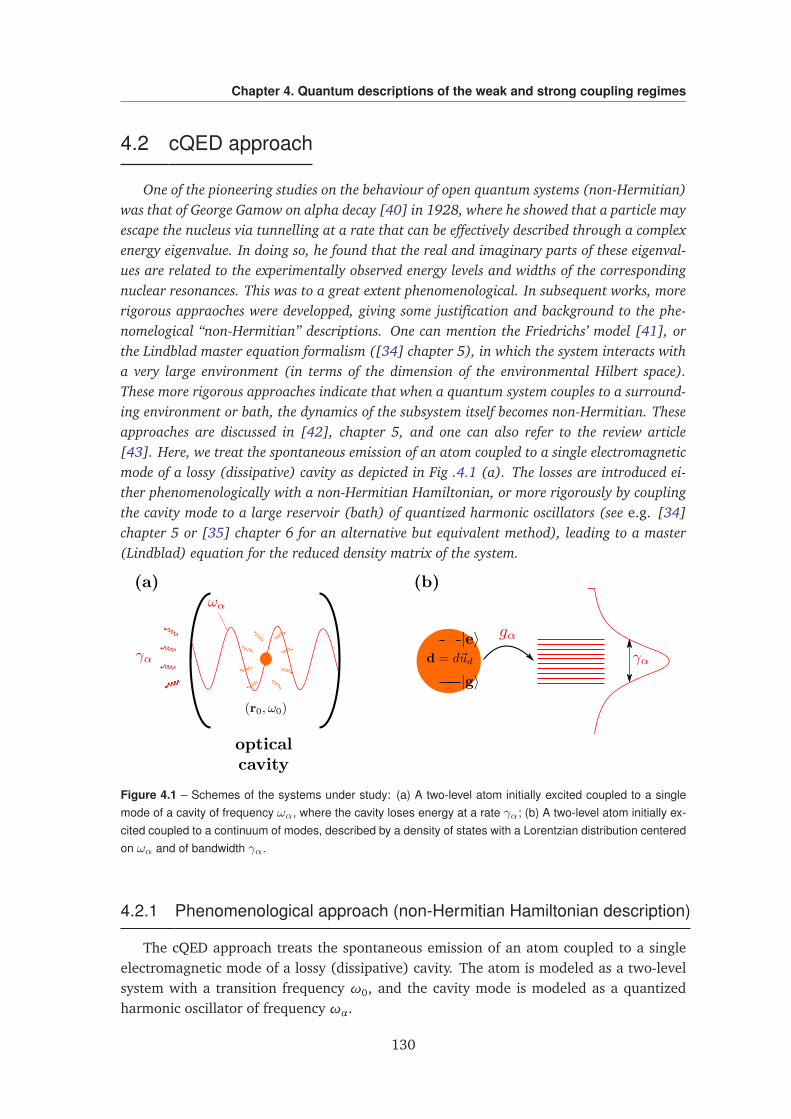
Chapter 4. Quantum descriptions of the weak and strong coupling regimes

4.2 cQED approach

One of the pioneering studies on the behaviour of open quantum systems (non-Hermitian)was that of George Gamow on alpha decay [40] in 1928, where he showed that a particle mayescape the nucleus via tunnelling at a rate that can be effectively described through a complexenergy eigenvalue. In doing so, he found that the real and imaginary parts of these eigenval-ues are related to the experimentally observed energy levels and widths of the correspondingnuclear resonances. This was to a great extent phenomenological. In subsequent works, morerigorous appraoches were developped, giving some justification and background to the phe-nomelogical “non-Hermitian” descriptions. One can mention the Friedrichs’ model [41], orthe Lindblad master equation formalism ([34] chapter 5), in which the system interacts witha very large environment (in terms of the dimension of the environmental Hilbert space).These more rigorous approaches indicate that when a quantum system couples to a surround-ing environment or bath, the dynamics of the subsystem itself becomes non-Hermitian. Theseapproaches are discussed in [42], chapter 5, and one can also refer to the review article[43]. Here, we treat the spontaneous emission of an atom coupled to a single electromagneticmode of a lossy (dissipative) cavity as depicted in Fig .4.1 (a). The losses are introduced ei-ther phenomenologically with a non-Hermitian Hamiltonian, or more rigorously by couplingthe cavity mode to a large reservoir (bath) of quantized harmonic oscillators (see e.g. [34]chapter 5 or [35] chapter 6 for an alternative but equivalent method), leading to a master(Lindblad) equation for the reduced density matrix of the system.

Figure 4.1 – Schemes of the systems under study: (a) A two-level atom initially excited coupled to a singlemode of a cavity of frequency ωα, where the cavity loses energy at a rate γα; (b) A two-level atom initially ex-cited coupled to a continuum of modes, described by a density of states with a Lorentzian distribution centeredon ωα and of bandwidth γα.

4.2.1 Phenomenological approach (non-Hermitian Hamiltonian description)

The cQED approach treats the spontaneous emission of an atom coupled to a singleelectromagnetic mode of a lossy (dissipative) cavity. The atom is modeled as a two-levelsystem with a transition frequency ω0, and the cavity mode is modeled as a quantizedharmonic oscillator of frequency ωα.

130

4.2 cQED approach

The total Hamiltonian of the system two-level atom + single cavity mode (not takinginto account the losses) obtained within the electric dipole and rotating wave approxima-tions is given by (for a derivation, see Appendix 4.A, where the rotating-wave approxima-tion is also clarified):

HJC = ħhω0σ†σ+ħhωαa†a+ħhg

σa† + σ†a

(4.1)

where we give the expression of the coupling constant g (for an atom dipole moment d=d~ud and a perfect polarization and position matching with the mode, see Appendix 4.A):

ħhg = d

√

√ ħhωα2ε0V

(4.2)

with V the volume of the cavity. g is a real quantity with the dimensions of frequency. Allthe other notations are introduced in Appendix 4.A. The parameters of this Hamiltonianare the atomic transition frequency ω0, the cavity mode frequency ωα, and the couplingconstant g. Such Hamiltonian is known as the Jaynes-Cummings Hamiltonian [33], hencethe subscript “JC”. It is worth noting that it is Hermitian.

This system two-level atom + single cavity mode can exchange energy with its en-vironment, and therefore the dynamics becomes non-Hermitian. Such a dynamics can bedescribe by the non-Hermitian evolution of a pure state of the type:

|ψ (t)⟩= α (t) |e, 0⟩+ β (t) |g, 1⟩ (4.3)

where the state |e,0⟩ stands for atom in the excited state and no photon in the cavityand |g, 1⟩ stands for atom in the ground state and one photon in the cavity, which obeysthe Schrödinger equation with the non-Hermitian “effective” Hamiltonian H = HJC + Hloss

where Hloss is phenomenologically introduced and reads in the basis |e, 0⟩ , |g, 1⟩:

Hloss = ħh

0 00 −iγα2

(4.4)

where the parameter γα is called the cavity decay rate.

The coefficients α (t) and β (t) are obtained by solving the Schrödinger equation withthe non-Hermitian Hamiltonian H = HJC + Hloss:

iħh∂

∂ t

α(t)β(t)

= ħh

ω0 gg ωα − iγα2

α(t)β(t)

(4.5)

One way to solve the dynamics of such a system is to diagonalize the above matrix.Upon diagonalization, one gets the following eigenvalues:

ω± =ω0 +ωα

2− iγα4±Ω

2(4.6)

where we defined the quantity:

Ω≡

√

√

4g2 +

δ+ iγα2

2(4.7)

131

Chapter 4. Quantum descriptions of the weak and strong coupling regimes

and where δ ≡ω0 −ωα is the detuning. We are first of all interested in the probability tofind the atom in the excited state, the survival probability defined as Psurv(t) ≡ |α(t)|2, sowe want to find the expression of α(t). Its general expression reads:

α(t) = A+e−iω+ t + A−e−iω− t (4.8)

where the constants A+ and A− are determined by the initial conditions α(0) = 1 andα(0) = −iω0 (coming from the fact that β(0) = 0 in Eq. (4.5)):

A± =12±δ+ iγα/2

2Ω(4.9)

Weak and strong coupling regimes in the resonant case ω0 =ωα:

In the resonant case ω0 =ωα, the eigen-frequencies in Eq. (4.6) become:

ω± =ωα − iγα4±Ω

2(4.10)

where Ω now reads:

Ω=

√

√

4g2 −γα

2

2(4.11)

One can clearly see that two different regimes in the time-domain are possible dependingon the values of g and γα:(i) for small coupling constant g < 1

4γα, Ω becomes purely imaginary, and the eigen-frequencies ω± [Eq. (4.10)] are now complex, leading to a monotonic decay of theamplitude α(t) in time [Eq. (4.8)], known as the weak-coupling regime;(ii) for large coupling constant g > 1

4γα, Ω is real, and the eigen-frequencies ω±[Eq. (4.10)] show a different real part, leading to oscillations of the amplitude α(t)in the time-domain, known as the strong-coupling regime. The oscillations, known asvacuum Rabi oscillations, can be seen physically as a coherent and reversible exchange ofenergy between the quantum emitter and the photonic system.

The general solution will not be derived explicitely. Only the two following limitingcases will be studied: the (very) weak-coupling regime, i.e. when g γα, and the (very)strong-coupling regime, i.e. when g γα. In fact, a very good approximate of the solutionmay be derived in these two cases by means of power series expansion. These two regimesare separated by the critical regime, i.e. when g = γα/4.

Critical regime: g = γα/4

Exactly at the transition between the two regimes, when g = γα/4, one has Ω = 0. Atthis sometimes called “exceptional point” [43], the eigenfrequencies in Eq. (4.10) coalesceand the eigenvectors become completely parallel giving for the amplitude α(t):

α(t) =h

1+γα2

t2

i

e−γα2

t2 (4.12)

132

4.2 cQED approach

Very weak-coupling regime: g γα

To get more insight about what is going on in this regime, we will derive an analyticalsolution in the case of huge losses due to the photonic system g γα. We can then do thefollowing power series expansion:

Ω' iγα2− i

4g2

γα(4.13)

Then, from Eq. (4.11), the eigen-frequencies become:

ω+ 'ωα − i2g2

γα(4.14)

ω− 'ωα − iγα2+ i

2g2

γα(4.15)

and the constants A± [Eq. (4.9)] become:

A+ ' 1+4g2

γ2α

(4.16)

A− ' −4g2

γ2α

(4.17)

By defining the decay rate γ as:

γ≡4g2

γα(4.18)

the expression of α(t) becomes:

α(t)'

1+γ

γα

e−iωα te−γt2 −

γ

γαe−iωα te−γα

t2 eγ

t2 (4.19)

Very quickly when t 1/γα, and considering that γ γα, one gets the asymptotic result:

α(t)' e−γ2 t (4.20)

which gives a survival probability

Psurv(t) = |α(t)|2 ' e−γt (4.21)

This behavior is the one expected in the case of weak-coupling [35].

Purcell factor: We now introduce the Purcell factor Fp, which is a figure-of-merit com-monly used when studying the weak-coupling between a QE and a resonance, defined bythe equation Fp ≡ γ/γ0 [where γ0 is the atomic decay rate in free-space whose expressionhas been given in Chapter 2, Eq. (2.27)]:

Fp =4g2

γ0γα(4.22)

By using the expression of the coupling constant g given by Eq. (4.2) and the expressionof the free-space decay rate given in Chapter 2, Eq. (2.27), one recovers the usual formsof the Purcell factor [44]:

Fp =6πc3

ω3α

QV

⇔ FP =3

4π2λ3α

QV

(4.23)

where λα = 2πc/ωα and we introduced the quality factor of the resonance as: Q ≡ωα/γα.

133

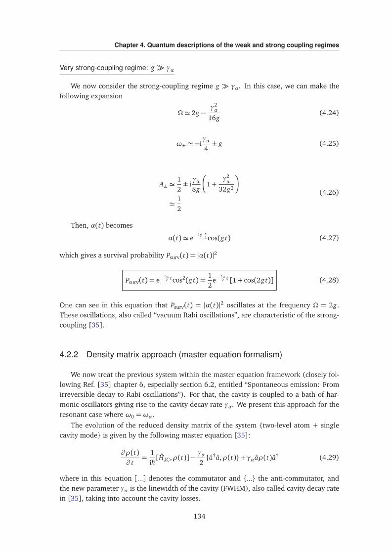
Chapter 4. Quantum descriptions of the weak and strong coupling regimes

Very strong-coupling regime: g γα

We now consider the strong-coupling regime g γα. In this case, we can make thefollowing expansion

Ω' 2g −γ2α

16g(4.24)

ω± ' −iγα4± g (4.25)

A± '12± iγα8g

1+γ2α

32g2

'12

(4.26)

Then, α(t) becomes

α(t)' e−γα2

t2 cos(g t) (4.27)

which gives a survival probability Psurv(t) = |α(t)|2

Psurv(t) = e−γα2 tcos2(g t) =

12

e−γα2 t [1+ cos(2g t)] (4.28)

One can see in this equation that Psurv(t) = |α(t)|2 oscillates at the frequency Ω = 2g.These oscillations, also called “vacuum Rabi oscillations”, are characteristic of the strong-coupling [35].

4.2.2 Density matrix approach (master equation formalism)

We now treat the previous system within the master equation framework (closely fol-lowing Ref. [35] chapter 6, especially section 6.2, entitled “Spontaneous emission: Fromirreversible decay to Rabi oscillations”). For that, the cavity is coupled to a bath of har-monic oscillators giving rise to the cavity decay rate γα. We present this approach for theresonant case where ω0 =ωα.

The evolution of the reduced density matrix of the system two-level atom + singlecavity mode is given by the following master equation [35]:

∂ ρ(t)∂ t

=1iħh[HJC,ρ(t)]−

γα2a†a,ρ(t)+ γαaρ(t)a† (4.29)

where in this equation [...] denotes the commutator and ... the anti-commutator, andthe new parameter γα is the linewidth of the cavity (FWHM), also called cavity decay ratein [35], taking into account the cavity losses.

134

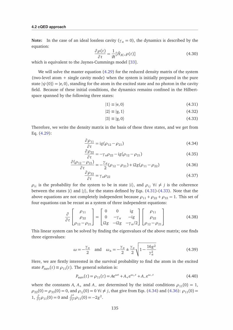
4.2 cQED approach

Note: In the case of an ideal lossless cavity (γα = 0), the dynamics is described by theequation:

∂ ρ(t)∂ t

=1iħh[HJC,ρ(t)] (4.30)

which is equivalent to the Jaynes-Cummings model [33].

We will solve the master equation (4.29) for the reduced density matrix of the systemtwo-level atom + single cavity mode when the system is initially prepared in the purestate |ψ (0)⟩= |e, 0⟩, standing for the atom in the excited state and no photon in the cavityfield. Because of these initial conditions, the dynamics remains confined in the Hilbert-space spanned by the following three states:

|1⟩ ≡ |e, 0⟩ (4.31)

|2⟩ ≡ |g, 1⟩ (4.32)

|3⟩ ≡ |g, 0⟩ (4.33)

Therefore, we write the density matrix in the basis of these three states, and we get fromEq. (4.29):

∂ ρ11

∂ t= ig(ρ12 −ρ21) (4.34)

∂ ρ22

∂ t= −γαρ22 − ig(ρ12 −ρ21) (4.35)

∂ (ρ12 −ρ21)∂ t

= −γα2(ρ12 −ρ21) + i2g(ρ11 −ρ22) (4.36)

∂ ρ33

∂ t= γαρ22 (4.37)

ρii is the probability for the system to be in state |i⟩, and ρi j ∀i 6= j is the coherencebetween the states |i⟩ and | j⟩, for the states defined by Eqs. (4.31)-(4.33). Note that theabove equations are not completely independent because ρ11 +ρ22 +ρ33 = 1. This set offour equations can be recast as a system of three independent equations:

∂

∂ t

ρ11

ρ22

ρ12 −ρ21

=

0 0 ig0 −γα −ig

i2g −i2g −γα/2

ρ11

ρ22

ρ12 −ρ21

(4.38)

This linear system can be solved by finding the eigenvalues of the above matrix; one findsthree eigenvalues:

ω= −γα2

and ω± = −γα2±γα2

√

√

√

1−16g2

γ2α

(4.39)

Here, we are firstly interested in the survival probability to find the atom in the excitedstate Psurv(t)≡ ρ11(t). The general solution is:

Psurv(t) = ρ11(t) = Aeωt + A+eω+ t + A−eω− t (4.40)

where the constants A, A+ and A− are determined by the initial conditions ρ11(0) = 1,ρ22(0) = ρ33(0) = 0, and ρi j(0) = 0 ∀i 6= j, that give from Eqs. (4.34) and (4.36): ρ11(0) =

1, ∂∂ tρ11(0) = 0 and ∂ 2

∂ t2ρ11(0) = −2g2.

135

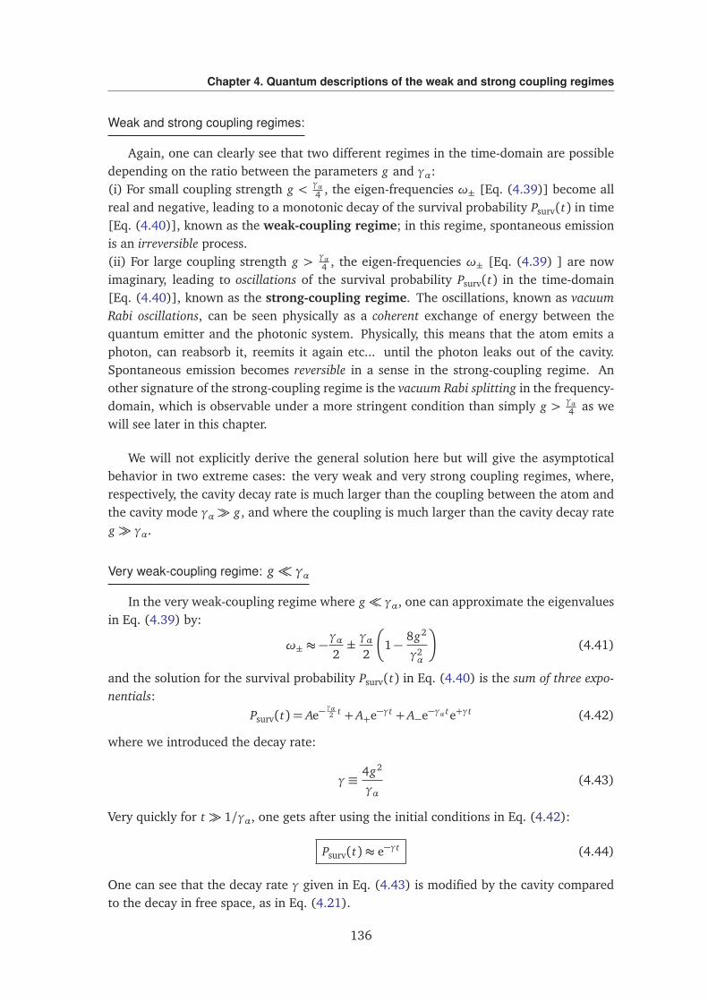
Chapter 4. Quantum descriptions of the weak and strong coupling regimes

Weak and strong coupling regimes:

Again, one can clearly see that two different regimes in the time-domain are possibledepending on the ratio between the parameters g and γα:(i) For small coupling strength g < γα

4 , the eigen-frequencies ω± [Eq. (4.39)] become allreal and negative, leading to a monotonic decay of the survival probability Psurv(t) in time[Eq. (4.40)], known as the weak-coupling regime; in this regime, spontaneous emissionis an irreversible process.(ii) For large coupling strength g > γα

4 , the eigen-frequencies ω± [Eq. (4.39) ] are nowimaginary, leading to oscillations of the survival probability Psurv(t) in the time-domain[Eq. (4.40)], known as the strong-coupling regime. The oscillations, known as vacuumRabi oscillations, can be seen physically as a coherent exchange of energy between thequantum emitter and the photonic system. Physically, this means that the atom emits aphoton, can reabsorb it, reemits it again etc... until the photon leaks out of the cavity.Spontaneous emission becomes reversible in a sense in the strong-coupling regime. Another signature of the strong-coupling regime is the vacuum Rabi splitting in the frequency-domain, which is observable under a more stringent condition than simply g > γα

4 as wewill see later in this chapter.

We will not explicitly derive the general solution here but will give the asymptoticalbehavior in two extreme cases: the very weak and very strong coupling regimes, where,respectively, the cavity decay rate is much larger than the coupling between the atom andthe cavity mode γα g, and where the coupling is much larger than the cavity decay rateg γα.

Very weak-coupling regime: g γα

In the very weak-coupling regime where g γα, one can approximate the eigenvaluesin Eq. (4.39) by:

ω± ≈ −γα2±γα2

1−8g2

γ2α

(4.41)

and the solution for the survival probability Psurv(t) in Eq. (4.40) is the sum of three expo-nentials:

Psurv(t) = Ae−γα2 t + A+e−γt + A−e−γα te+γt (4.42)

where we introduced the decay rate:

γ≡4g2

γα(4.43)

Very quickly for t 1/γα, one gets after using the initial conditions in Eq. (4.42):

Psurv(t)≈ e−γt (4.44)

One can see that the decay rate γ given in Eq. (4.43) is modified by the cavity comparedto the decay in free space, as in Eq. (4.21).

136

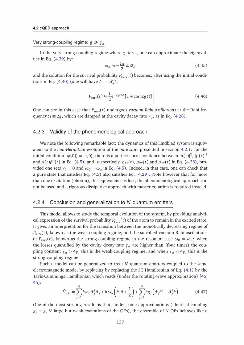
4.2 cQED approach

Very strong-coupling regime: g γα

In the very strong-coupling regime where g γα, one can approximate the eigenval-ues in Eq. (4.39) by:

ω± ≈ −γα2± i2g (4.45)

and the solution for the survival probability Psurv(t) becomes, after using the initial condi-tions in Eq. (4.40) (one will have A− = A∗+):

Psurv(t)≈12

e−γα t/2 [1+ cos(2g t)] (4.46)

One can see in this case that Psurv(t) undergoes vacuum Rabi oscillations at the Rabi fre-quency Ω≡ 2g, which are damped at the cavity decay rate γα, as in Eq. (4.28).

4.2.3 Validity of the phenomenological approach

We note the following remarkable fact: the dynamics of this Lindblad system is equiv-alent to the non-Hermitian evolution of the pure state presented in section 4.2.1: for theinitial condition |ψ(0)⟩ = |e, 0⟩, there is a perfect correspondance between |α(t)|2, |β(t)|2

and α(t)β∗(t) in Eq. (4.5), and, respectively, ρ11(t), ρ22(t) and ρ12(t) in Eq. (4.38), pro-vided one sets γ0 = 0 and ω0 = ωα in Eq. (4.5). Indeed, in that case, one can check thata pure state that satisfies Eq. (4.5) also satisfies Eq. (4.29). Note however that for morethan one excitation (photon), this equivalence is lost; the phenomenological approach cannot be used and a rigorous dissipative approach with master equation is required instead.

4.2.4 Conclusion and generalization to N quantum emitters

This model allows to study the temporal evolution of the system, by providing analyti-cal expression of the survival probability Psurv(t) of the atom to remain in the excited state.It gives an interpretation for the transition between the monotically decreasing regime ofPsurv(t), known as the weak-coupling regime, and the so-called vacuum Rabi oscillationsof Psurv(t), known as the strong-coupling regime in the resonant case ω0 = ωα: whenthe losses quantified by the cavity decay rate γα are higher than (four times) the cou-pling constant γα > 4g, this is the weak-coupling regime, and when γα < 4g, this is thestrong-coupling regime.

Such a model can be generalized to treat N quantum emitters coupled to the sameelectromagnetic mode, by replacing by replacing the JC Hamiltonian of Eq. (4.1) by theTavis-Cummings Hamiltonian which reads (under the rotating-wave approximation) [45,46]:

HT C =N∑

j=1

ħhω0σ†j σ j +ħhωα

a†a+12

+N∑

j=1

ħhg j

σ j a† + σ†

j a

(4.47)

One of the most striking results is that, under some approximations (identical couplingg j ≡ g, N large but weak excitations of the QEs), the ensemble of N QEs behaves like a

137

Chapter 4. Quantum descriptions of the weak and strong coupling regimes

giant harmonic oscillator coupled to the EM mode by a coupling constantp

N g [18, 20].From this scaling, one can conclude that one way to enter the strong-coupling regime issimply to increases the number of QEs N as one has a favorable scaling of the couplingconstant∝

pN .

4.3 “Continuum” approach

We now present a model which is conceptually quite different from the ones presented inthe previous section. This model treats the spontaneous emission of an atom coupled to abounded continuum of electromagnetic modes, with a bandwidth γα. As previously, the atomis modeled as a two-level system with transition frequency ω0, and the continuum is assumedto have a “Lorentzian” density of states (modes) centered on a frequency ωα and with abandwidth γα (FWHM) as depicted in Fig. 4.1 (b). In particular, while conceptually verydifferent, this model predicts the same temporal behavior as the previous ones. This rathersimple approach will allow us to introduce different concepts that we will use in the followingchapter, where we will give foundation and improve this phenomenological approach. Also,this model provides a different interpretation of the transition between the weak and strongcoupling regimes in the resonant case ω0 = ωα: the transition occurs when the bandwidthof the continuum is equal to γ, where γ is the modified atomic decay rate given by the Fermigolden rule. When γ < γα/4, Psurv(t) has a monotically decreasing behavior, and whenγ > γα/4, Psurv(t) shows an oscillatory behavior (the vacuum Rabi oscillations). Finally,the interest of this model is that it predicts the distribution in energy of the emitted photonsin the continuum which is an observable that one can measure in practice: the so-calledvacuum Rabi splitting. We present here this model, following and readapting [47], chapter1, Complement 1A.

4.3.1 Description of the model

We consider a two-level atom of transition frequency ω0 and a discrete1 continuum ofelectromagnetic states labeled by j and of frequency ωj. This corresponds to the state:

|ψ (t)⟩= α (t)e−iω0 t |e, 0⟩+∑

j

βj (t)e−iωj t |g, 1j⟩ (4.48)

where |g,1j⟩ ≡ |g⟩ ⊗ |1j⟩ is the tensor product between the atomic ground state |g⟩ and thestate of the EM field |1j⟩ containing one photon in the mode j and |e,0⟩ ≡ |e⟩ ⊗ |0⟩ is thetensor product between the atomic excited state |e⟩ and the vacuum state of the EM field|0⟩. Note that by writing the state like this, we do not consider states like |e,1j⟩ (atomin the excited state and one photon in the mode j) or |g,0⟩ (atom in the ground stateand no photon), in the spirit of the rotating-wave approximation (which neglects in theinteraction Hamiltonian the terms that couple the states |e,1j⟩ and |g,0⟩).

1The discretization of the continuum in j distinct states of frequency ωj is for pure mathematical conve-nience, and one recovers a real continuum in the limit where the separation in the frequencies ωj tends to benull.

138

4.3 “Continuum” approach

The total Hamiltonian of the system is written in the general form:

H = H0 + HI(r0) (4.49)

where H0 is the Hamiltonian of the non-interacting system atom + EM field with eigen-states |g,1j⟩ ; |e,0⟩ and associated eigenenergies ħhωj;ħhω0, and HI(r0) is the interactionHamiltonian taken here in the electric dipole approximation form:

HI(r0) = −d · E⊥(r0) (4.50)

where d is the atomic electric dipole operator and E⊥(r0) is the transverse electric fieldoperator evaluated at the position of the atom r0.

To know the dynamics of the spontaneous emission, one must get the coefficients α (t)and βj (t) by solving the Schrödinger equation with the initial condition |ψ (0)⟩ = |e,0⟩(i.e., α(0) = 1 and βj(0) = 0) corresponding to the atom initially in the excited stateand no photon in the electromagnetic field. One then obtains the following differentialequations fullfilled by the coefficients α (t) and βj (t):

iα (t) =∑

j

g∗j (r0)βj (t)ei(ω0−ωj)t , (4.51)

iβj (t) = gj(r0)α (t)e−i(ω0−ωj)t . (4.52)

where we introduced the coupling strength gj(r) (also called coupling rate) defined by:

ħhgj(r)≡ ⟨g, 1j| HI(r) |e,0⟩ Unit:

gj

= s−1 (4.53)

By formally integrating Eq. (4.52) together with the initial condition βj(0) = 0, one gets:

iβj (t) = gj(r0)

∫ t

0

dt ′α(t ′)e−i(ω0−ωj)t ′ (4.54)

and inserting this expression into Eq. (4.51) gives:

α (t) = −∑

j

|gj(r0)|2∫ t

0

dt ′α(t ′)ei(ω0−ωj)(t−t ′) (4.55)

that is conveniently recast in the form

α (t) = −∫ t

0

dt ′α(t ′)

∫ ∞

0

dωR(r0,ω)ei(ω0−ω)(t−t ′) (4.56)

where we introduced the reservoir coupling spectrum R(r,ω) defined as:

R(r,ω) =∑

j

|gj(r)|2δ(ω−ωj) Unit: [R(r,ω)] = s−1 (4.57)

139

Chapter 4. Quantum descriptions of the weak and strong coupling regimes

4.3.2 Fermi golden rule and density of states

We now introduce the Fermi golden rule that we will use in the following. It is obtainedas a first-order perturbative solution of Eq. (4.56) with initial condition α(0) = 1. To firstorder in R(r0,ω), one gets (see Appendix 4.B):

Psurv(t) = 1− γt (4.58)

where γ is given by the following expression, known as the Fermi golden rule (FGR):

γ= 2πR(r0,ω0) (4.59)

In reality, the one-photon states |1j⟩ form a continuum, and one can therefore write R(r,ω)in terms of the density of states (DOS) ρ(ω) as:

R(r,ω) −→ |g(r,ω)|2ρ(ω) (4.60)

where ħhg(r,ω) ≡ ⟨g,1ω| HI(r) |e,0⟩ with |1ω⟩ representing the one-photon state with fre-quency ω, and the DOS ρ(ω) represents the number of electromagnetic modes per unitfrequency. One then recovers a more common form of the FGR:

γ= 2π|g(r,ω0)|2ρ(ω0) (4.61)

in terms of the density of states2.

4.3.3 Temporal evolution

The formalism presented so far is quite general, valid for any reservoir coupling spec-trum R(r,ω). We will develop further the analytical model by assuming a simple form forthe reservoir. In this model, we first assume that the coupling strength g(r,ω) is a constantof the position and frequency g(r,ω) ≡ g. On the other hand, we assume a “Lorentzian”distribution for the DOS ρ(ω) centered on the frequency ωα and of FWHM ∆ω= γα:

ρ(ω) =1π

γα/2(ωα −ω)2 + (γα/2)2

(4.62)

These assumptions lead to the following reservoir coupling spectrum:

R(r,ω) = g2 1π

γα/2(ωα −ω)2 + (γα/2)2

(4.63)

With the expression Eq. (4.63) of the reservoir coupling spectrum, the frequency in-tegral in Eq. (4.56) can be calculated exactly (see [47], chapter 1, Complement 1A). By

2As already discussed in Chapter 1, Section 1.2.2, in the case of a degenerate continuum (i.e., for agiven frequency ω, there are many one-photon states |1k⟩ with ωk = ω, differing for instance from thepropagation direction and polarization, when these quantities are defined), R(r,ω) must be written as:R(r,ω) = |g(r,ω)|2ρ(ω) where |g(r,ω)|2 denotes |g(r,ω)|2 averaged over all one-photon states |1k⟩ withfrequency ωk =ω.

140

4.3 “Continuum” approach

letting the lower limit of the integral tends to −∞, one gets3:

α (t) = −γγα4

∫ t

0

dt ′α(t ′)e(t−t ′)[i(ω0−ωα)−γα2 ] (4.64)

where one introduces the decay rate:

γ≡4g2

γα(4.65)

Note: This decay rate is the one given by the Fermi golden rule (4.59): γ= 2πR(r0,ω0) =2πg2ρ(ω0), with ρ(ω0) = 2/(πγα) in the resonant case where ω0 =ωα.

By differentiating this expression, one gets a second-order differential equation for theamplitude α(t) (see [47], chapter 1, Complement 1A):

α(t)−h

i(ω0 −ωα)−γα2

i

α(t) +γγα4α(t) = 0 (4.66)

One can then solve exactly this differential equation and get the general expression:

α(t) =

e−iΩ t2 + eiΩ t

2

2

+(ω0 −ωα) + iγα2

Ω

e−iΩ t2 − eiΩ t

2

2

ei(ω0−ωα)t2 e−

γα2

t2 (4.67)

where Ω reads:

Ω=

√

√

γγα +

ω0 −ωα + iγα2

2(4.68)

Weak and strong coupling regimes in the resonant case ω0 =ωα:

In the resonant case, Ω becomes:

Ω=

√

√

γγα −γα

2

2(4.69)

Again, one can see two different regimes depending on the values of γ and γα:

• If γ < γα/4, then Ω is purely imaginary and the exponentials in Eq. (4.67) do notoscillate, and one has a monotical behavior of α(t) which decreases with time. Thisis the weak-coupling regime.

• If γ > γα/4, then Ω is real and the exponentials in Eq. (4.67) do oscillate, and onehas an oscillating behavior of α(t), damped by the last exponential. This is thestrong-coupling regime.

3Taking into account the truncation at 0 in the integral leads to some mathematical subtleties. The effectsof such a truncation, also known as threshold effects, were studied in Ref. [48]. In letting the integral go from−∞ to +∞, we neglect these threshold effects (like in the Wigner-Weisskopf theory for instance [49]). Thisconsiderably simplifies the integral calculations, and one can check numerically that it is a good approxima-tion when the width of the Lorentzian γα is much smaller than ωα: γαωα (in other words for a mode witha quality factor Q =ωα/γα large compared to 1).

141

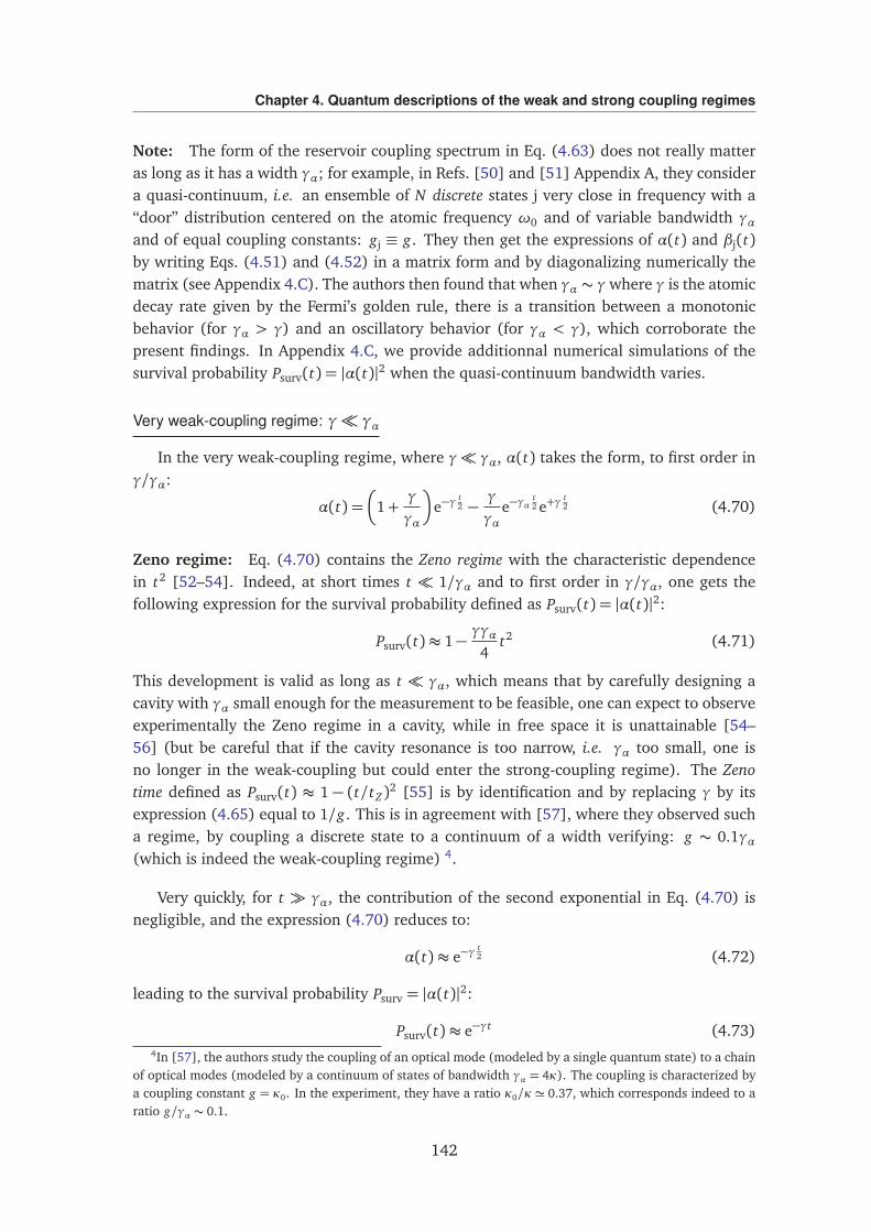
Chapter 4. Quantum descriptions of the weak and strong coupling regimes

Note: The form of the reservoir coupling spectrum in Eq. (4.63) does not really matteras long as it has a width γα; for example, in Refs. [50] and [51] Appendix A, they considera quasi-continuum, i.e. an ensemble of N discrete states j very close in frequency with a“door” distribution centered on the atomic frequency ω0 and of variable bandwidth γαand of equal coupling constants: gj ≡ g. They then get the expressions of α(t) and βj(t)by writing Eqs. (4.51) and (4.52) in a matrix form and by diagonalizing numerically thematrix (see Appendix 4.C). The authors then found that when γα ∼ γwhere γ is the atomicdecay rate given by the Fermi’s golden rule, there is a transition between a monotonicbehavior (for γα > γ) and an oscillatory behavior (for γα < γ), which corroborate thepresent findings. In Appendix 4.C, we provide additionnal numerical simulations of thesurvival probability Psurv(t) = |α(t)|2 when the quasi-continuum bandwidth varies.

Very weak-coupling regime: γ γα

In the very weak-coupling regime, where γ γα, α(t) takes the form, to first order inγ/γα:

α(t) =

1+γ

γα

e−γt2 −

γ

γαe−γα

t2 e+γ

t2 (4.70)

Zeno regime: Eq. (4.70) contains the Zeno regime with the characteristic dependencein t2 [52–54]. Indeed, at short times t 1/γα and to first order in γ/γα, one gets thefollowing expression for the survival probability defined as Psurv(t) = |α(t)|2:

Psurv(t)≈ 1−γγα4

t2 (4.71)

This development is valid as long as t γα, which means that by carefully designing acavity with γα small enough for the measurement to be feasible, one can expect to observeexperimentally the Zeno regime in a cavity, while in free space it is unattainable [54–56] (but be careful that if the cavity resonance is too narrow, i.e. γα too small, one isno longer in the weak-coupling but could enter the strong-coupling regime). The Zenotime defined as Psurv(t) ≈ 1 − (t/tZ)2 [55] is by identification and by replacing γ by itsexpression (4.65) equal to 1/g. This is in agreement with [57], where they observed sucha regime, by coupling a discrete state to a continuum of a width verifying: g ∼ 0.1γα(which is indeed the weak-coupling regime) 4.

Very quickly, for t γα, the contribution of the second exponential in Eq. (4.70) isnegligible, and the expression (4.70) reduces to:

α(t)≈ e−γt2 (4.72)

leading to the survival probability Psurv = |α(t)|2:

Psurv(t)≈ e−γt (4.73)4In [57], the authors study the coupling of an optical mode (modeled by a single quantum state) to a chain

of optical modes (modeled by a continuum of states of bandwidth γα = 4κ). The coupling is characterized bya coupling constant g = κ0. In the experiment, they have a ratio κ0/κ ' 0.37, which corresponds indeed to aratio g/γα ∼ 0.1.

142

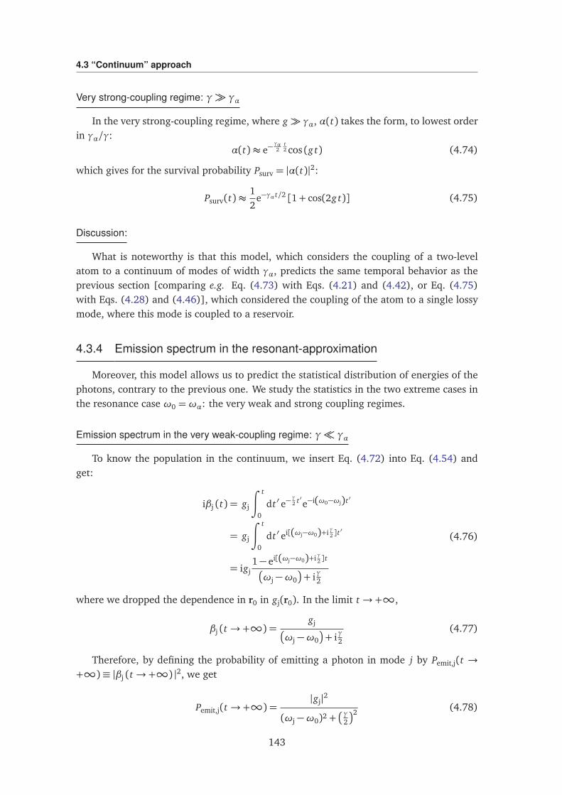
4.3 “Continuum” approach

Very strong-coupling regime: γ γα

In the very strong-coupling regime, where g γα, α(t) takes the form, to lowest orderin γα/γ:

α(t)≈ e−γα2

t2 cos (g t) (4.74)

which gives for the survival probability Psurv = |α(t)|2:

Psurv(t)≈12

e−γα t/2 [1+ cos(2g t)] (4.75)

Discussion:

What is noteworthy is that this model, which considers the coupling of a two-levelatom to a continuum of modes of width γα, predicts the same temporal behavior as theprevious section [comparing e.g. Eq. (4.73) with Eqs. (4.21) and (4.42), or Eq. (4.75)with Eqs. (4.28) and (4.46)], which considered the coupling of the atom to a single lossymode, where this mode is coupled to a reservoir.

4.3.4 Emission spectrum in the resonant-approximation

Moreover, this model allows us to predict the statistical distribution of energies of thephotons, contrary to the previous one. We study the statistics in the two extreme cases inthe resonance case ω0 =ωα: the very weak and strong coupling regimes.

Emission spectrum in the very weak-coupling regime: γ γα

To know the population in the continuum, we insert Eq. (4.72) into Eq. (4.54) andget:

iβj (t) = gj

∫ t

0

dt ′ e−γ2 t ′e−i(ω0−ωj)t ′

= gj

∫ t

0

dt ′ ei[(ωj−ω0)+i γ2 ]t′

= igj1− ei[(ωj−ω0)+i γ2 ]t

ωj −ω0

+ iγ2

(4.76)

where we dropped the dependence in r0 in gj(r0). In the limit t → +∞,

βj (t → +∞) =gj

ωj −ω0

+ iγ2(4.77)

Therefore, by defining the probability of emitting a photon in mode j by Pemit,j(t →+∞)≡ |βj (t → +∞) |2, we get

Pemit,j(t → +∞) =|gj|2

(ωj −ω0)2 +γ

2

2 (4.78)

143

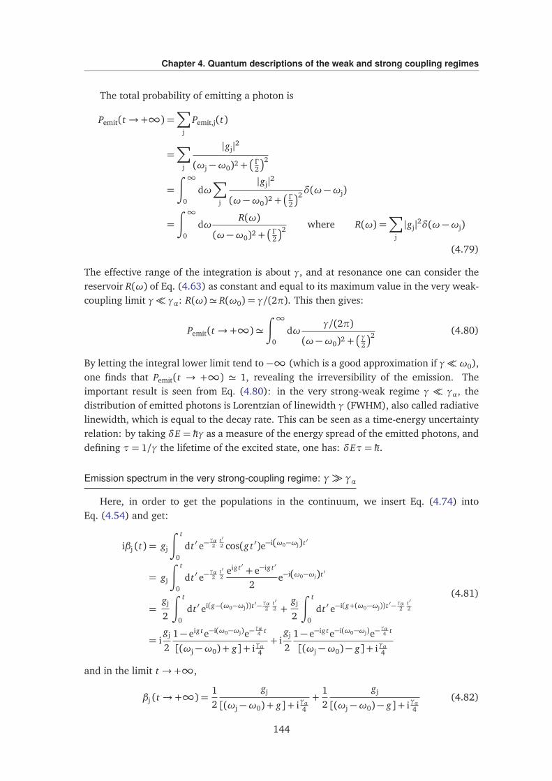
Chapter 4. Quantum descriptions of the weak and strong coupling regimes

The total probability of emitting a photon is

Pemit(t → +∞) =∑

j

Pemit,j(t)

=∑

j

|gj|2

(ωj −ω0)2 +

Γ2

2

=

∫ ∞

0

dω∑

j

|gj|2

(ω−ω0)2 +

Γ2

2δ(ω−ωj)

=

∫ ∞

0

dωR(ω)

(ω−ω0)2 +

Γ2

2 where R(ω) =∑

j

|gj|2δ(ω−ωj)

(4.79)

The effective range of the integration is about γ, and at resonance one can consider thereservoir R(ω) of Eq. (4.63) as constant and equal to its maximum value in the very weak-coupling limit γ γα: R(ω)' R(ω0) = γ/(2π). This then gives:

Pemit(t → +∞)'∫ ∞

0

dωγ/(2π)

(ω−ω0)2 +γ

2

2 (4.80)

By letting the integral lower limit tend to −∞ (which is a good approximation if γω0),one finds that Pemit(t → +∞) ' 1, revealing the irreversibility of the emission. Theimportant result is seen from Eq. (4.80): in the very strong-weak regime γ γα, thedistribution of emitted photons is Lorentzian of linewidth γ (FWHM), also called radiativelinewidth, which is equal to the decay rate. This can be seen as a time-energy uncertaintyrelation: by taking δE = ħhγ as a measure of the energy spread of the emitted photons, anddefining τ= 1/γ the lifetime of the excited state, one has: δEτ= ħh.

Emission spectrum in the very strong-coupling regime: γ γα

Here, in order to get the populations in the continuum, we insert Eq. (4.74) intoEq. (4.54) and get:

iβj (t) = gj

∫ t

0

dt ′ e−γα2

t′2 cos(g t ′)e−i(ω0−ωj)t ′

= gj

∫ t

0

dt ′ e−γα2

t′2

eig t ′ + e−ig t ′

2e−i(ω0−ωj)t ′

=gj

2

∫ t

0

dt ′ ei(g−(ω0−ωj))t ′−γα2

t′2 +

gj

2

∫ t

0

dt ′ e−i(g+(ω0−ωj))t ′−γα2

t′2

= igj

21− eig te−i(ω0−ωj)e−

γα4 t

[(ωj −ω0) + g] + iγα4+ i

gj

21− e−ig te−i(ω0−ωj)e−

γα4 t

[(ωj −ω0)− g] + iγα4

(4.81)

and in the limit t → +∞,

βj (t → +∞) =12

gj

[(ωj −ω0) + g] + iγα4+

12

gj

[(ωj −ω0)− g] + iγα4(4.82)

144

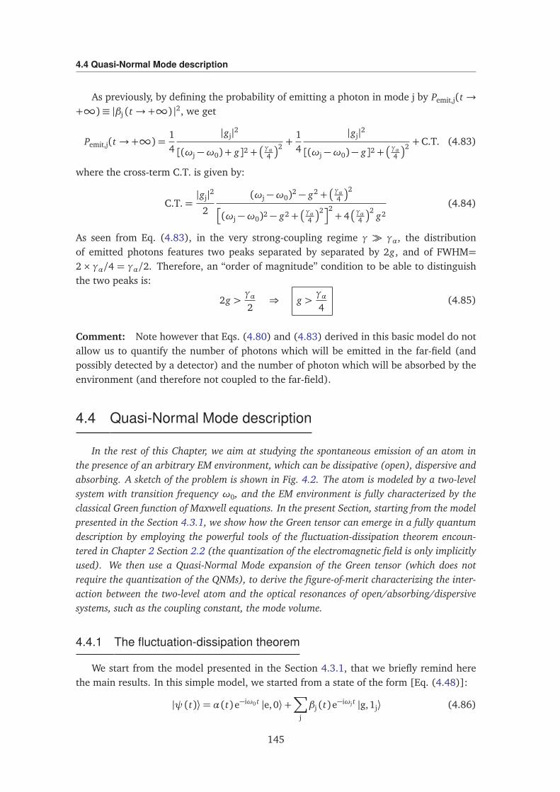
4.4 Quasi-Normal Mode description

As previously, by defining the probability of emitting a photon in mode j by Pemit,j(t →+∞)≡ |βj (t → +∞) |2, we get

Pemit,j(t → +∞) =14

|gj|2

[(ωj −ω0) + g]2 +γα

4

2 +14

|gj|2

[(ωj −ω0)− g]2 +γα

4

2 +C.T. (4.83)

where the cross-term C.T. is given by:

C.T.=|gj|2

2

(ωj −ω0)2 − g2 +γα

4

2

(ωj −ω0)2 − g2 +γα

4

22+ 4

γα4

2g2

(4.84)

As seen from Eq. (4.83), in the very strong-coupling regime γ γα, the distributionof emitted photons features two peaks separated by separated by 2g, and of FWHM=2× γα/4 = γα/2. Therefore, an “order of magnitude” condition to be able to distinguishthe two peaks is:

2g >γα2

⇒ g >γα4

(4.85)

Comment: Note however that Eqs. (4.80) and (4.83) derived in this basic model do notallow us to quantify the number of photons which will be emitted in the far-field (andpossibly detected by a detector) and the number of photon which will be absorbed by theenvironment (and therefore not coupled to the far-field).

4.4 Quasi-Normal Mode description

In the rest of this Chapter, we aim at studying the spontaneous emission of an atom inthe presence of an arbitrary EM environment, which can be dissipative (open), dispersive andabsorbing. A sketch of the problem is shown in Fig. 4.2. The atom is modeled by a two-levelsystem with transition frequency ω0, and the EM environment is fully characterized by theclassical Green function of Maxwell equations. In the present Section, starting from the modelpresented in the Section 4.3.1, we show how the Green tensor can emerge in a fully quantumdescription by employing the powerful tools of the fluctuation-dissipation theorem encoun-tered in Chapter 2 Section 2.2 (the quantization of the electromagnetic field is only implicitlyused). We then use a Quasi-Normal Mode expansion of the Green tensor (which does notrequire the quantization of the QNMs), to derive the figure-of-merit characterizing the inter-action between the two-level atom and the optical resonances of open/absorbing/dispersivesystems, such as the coupling constant, the mode volume.

4.4.1 The fluctuation-dissipation theorem

We start from the model presented in the Section 4.3.1, that we briefly remind herethe main results. In this simple model, we started from a state of the form [Eq. (4.48)]:

|ψ (t)⟩= α (t)e−iω0 t |e, 0⟩+∑

j

βj (t)e−iωj t |g, 1j⟩ (4.86)

145

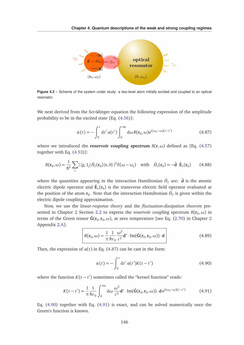
Chapter 4. Quantum descriptions of the weak and strong coupling regimes

Figure 4.2 – Scheme of the system under study: a two-level atom initially excited and coupled to an opticalresonator.

We next derived from the Scrödinger equation the following expression of the amplitudeprobability to be in the excited state [Eq. (4.56)]:

α (t) = −∫ t

0

dt ′α(t ′)

∫ ∞

0

dωR(r0,ω)ei(ω0−ω)(t−t ′) (4.87)

where we introduced the reservoir coupling spectrum R(r,ω) defined as [Eq. (4.57)together with Eq. (4.53)]:

R(r0,ω) =1

ħh2

∑

j

| ⟨g,1j| HI(r0) |e,0⟩ |2δ(ω−ωj) with HI(r0) = −d · Ev(r0) (4.88)

where the quantities appearing in the interaction Hamiltonian HI are: d is the atomicelectric dipole operator and Ev(r0) is the transverse electric field operator evaluated atthe position of the atom r0. Note that the interaction Hamiltonian HI is given within theelectric dipole coupling approximation.

Now, we use the linear-response theory and the fluctuation-dissipation theorem pre-sented in Chapter 2 Section 2.2 to express the reservoir coupling spectrum R(r0,ω) interms of the Green tensor G(r0, r0,ω), at zero temperature [see Eq. (2.70) in Chapter 2Appendix 2.A]:

R(r0,ω) =1π

1ħhε0

ω2

c2d∗ · Im(G(r0, r0,ω)) ·d (4.89)

Then, the expression of α(t) in Eq. (4.87) can be cast in the form:

α (t) = −∫ t

0

dt ′α(t ′)K(t − t ′) (4.90)

where the function K(t − t ′) sometimes called the “kernel function” reads:

K(t − t ′) =1π

1ħhε0

∫ ∞

0

dωω2

c2d∗ · Im(G(r0, r0,ω)) ·dei(ω0−ω)(t−t ′) (4.91)

Eq. (4.90) together with Eq. (4.91) is exact, and can be solved numerically once theGreen’s function is known.

146

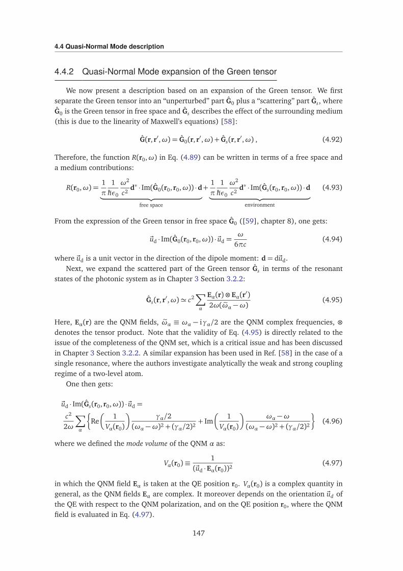
4.4 Quasi-Normal Mode description

4.4.2 Quasi-Normal Mode expansion of the Green tensor

We now present a description based on an expansion of the Green tensor. We firstseparate the Green tensor into an “unperturbed” part G0 plus a “scattering” part Gs, whereG0 is the Green tensor in free space and Gs describes the effect of the surrounding medium(this is due to the linearity of Maxwell’s equations) [58]:

G(r, r′,ω) = G0(r, r′,ω) + Gs(r, r′,ω) , (4.92)

Therefore, the function R(r0,ω) in Eq. (4.89) can be written in terms of a free space anda medium contributions:

R(r0,ω) =1π

1ħhε0

ω2

c2d∗ · Im(G0(r0, r0,ω)) ·d

︸ ︷︷ ︸

free space

+1π

1ħhε0

ω2

c2d∗ · Im(Gs(r0, r0,ω)) ·d

︸ ︷︷ ︸

environment

(4.93)

From the expression of the Green tensor in free space G0 ([59], chapter 8), one gets:

~ud · Im(G0(r0, r0,ω)) · ~ud =ω

6πc(4.94)

where ~ud is a unit vector in the direction of the dipole moment: d= d~ud.Next, we expand the scattered part of the Green tensor Gs in terms of the resonant

states of the photonic system as in Chapter 3 Section 3.2.2:

Gs(r, r′,ω)' c2∑

α

Eα(r)⊗ Eα(r′)2ω( eωα −ω)

(4.95)

Here, Eα(r) are the QNM fields, eωα ≡ ωα − iγα/2 are the QNM complex frequencies, ⊗denotes the tensor product. Note that the validity of Eq. (4.95) is directly related to theissue of the completeness of the QNM set, which is a critical issue and has been discussedin Chapter 3 Section 3.2.2. A similar expansion has been used in Ref. [58] in the case of asingle resonance, where the authors investigate analytically the weak and strong couplingregime of a two-level atom.

One then gets:

~ud · Im(Gs(r0, r0,ω)) · ~ud =

c2

2ω

∑

α

§

Re

1Vα(r0)

γα/2(ωα −ω)2 + (γα/2)2

+ Im

1Vα(r0)

ωα −ω(ωα −ω)2 + (γα/2)2

ª

(4.96)

where we defined the mode volume of the QNM α as:

Vα(r0)≡1

(~ud ·Eα(r0))2(4.97)

in which the QNM field Eα is taken at the QE position r0. Vα(r0) is a complex quantity ingeneral, as the QNM fields Eα are complex. It moreover depends on the orientation ~ud ofthe QE with respect to the QNM polarization, and on the QE position r0, where the QNMfield is evaluated in Eq. (4.97).

147

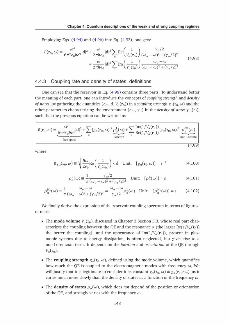
Chapter 4. Quantum descriptions of the weak and strong coupling regimes

Employing Eqs. (4.94) and (4.96) into Eq. (4.93), one gets:

R(r0,ω) =ω3

6π2ε0ħhc3|d|2 +

ω

2πħhε0|d|2

∑

α

Re

1Vα(r0)

γα/2(ωα −ω)2 + (γα/2)2

+ω

2πħhε0|d|2

∑

α

Im

1Vα(r0)

ωα −ω(ωα −ω)2 + (γα/2)2

(4.98)

4.4.3 Coupling rate and density of states: definitions

One can see that the reservoir in Eq. (4.98) contains three parts. To understand betterthe meaning of each part, one can introduce the concepts of coupling strength and densityof states, by gathering the quantities (ω0, d, Vα(r0)) in a coupling strentgh gα(r0,ω) and theother parameters characterizing the environment (ωα, γα) in the density of states ρα(ω),such that the previous equation can be written as

R(r0,ω) =ω3

6π2ε0ħhc3|d|2

︸ ︷︷ ︸

free space

+∑

α

|gα(r0,ω)|2ρLα(ω)︸ ︷︷ ︸

Lorentz

+∑

α

Im(1/Vα(r0))Re(1/Vα(r0))

|gα(r0,ω)|2 ρNLα (ω)︸ ︷︷ ︸

non-Lorentz

(4.99)where

ħhgα(r0,ω)≡√

√ ħhω2ε0

Re

1Vα(r0)

× d Unit: [gα(r0,ω)] = s−1 (4.100)

ρLα(ω)≡

1π

γα/2(ωα −ω)2 + (γα/2)2

Unit: [ρLα(ω)] = s (4.101)

ρNLα (ω)≡

1π

ωα −ω(ωα −ω)2 + (γα/2)2

=ωα −ωγα/2

ρLα(ω) Unit: [ρNL

α (ω)] = s (4.102)

We finally derive the expression of the reservoir coupling spectrum in terms of figures-of-merit

• The mode volume Vα(r0), discussed in Chapter 3 Section 3.3, whose real part char-acterizes the coupling between the QE and the resonance α (the larger Re(1/Vα(r0))the better the coupling), and the appearance of Im(1/Vα(r0)), present in plas-monic systems due to energy dissipation, is often neglected, but gives rise to anon-Lorentzian term. It depends on the location and orientation of the QE throughVα(r0).

• The coupling strength gα(r0,ω), defined using the mode volume, which quantifieshow much the QE is coupled to the electromagnetic modes with frequency ω, Wewill justify that it is legitimate to consider it as constant gα(r0,ω) ' gα(r0,ωα), as itvaries much more slowly than the density of states as a function of the frequency ω.

• The density of states ρα(ω), which does not depend of the position or orientationof the QE, and strongly varies with the frequency ω.

148

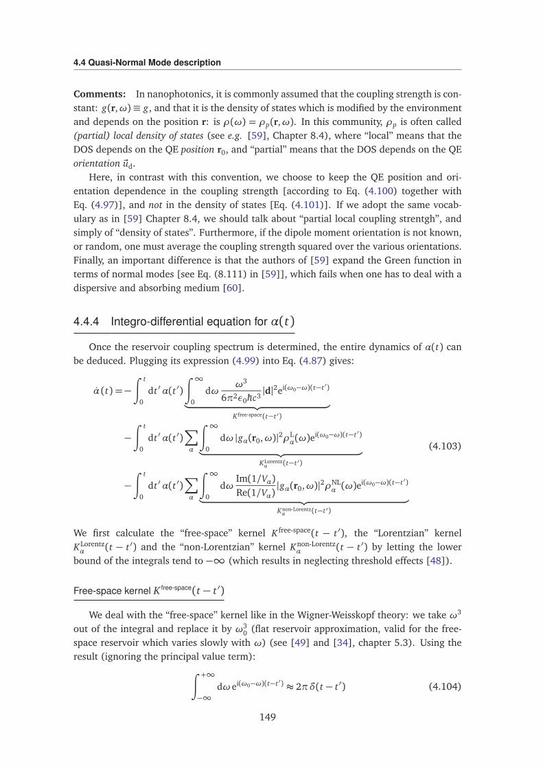
4.4 Quasi-Normal Mode description

Comments: In nanophotonics, it is commonly assumed that the coupling strength is con-stant: g(r,ω)≡ g, and that it is the density of states which is modified by the environmentand depends on the position r: is ρ(ω) = ρp(r,ω). In this community, ρp is often called(partial) local density of states (see e.g. [59], Chapter 8.4), where “local” means that theDOS depends on the QE position r0, and “partial” means that the DOS depends on the QEorientation ~ud.

Here, in contrast with this convention, we choose to keep the QE position and ori-entation dependence in the coupling strength [according to Eq. (4.100) together withEq. (4.97)], and not in the density of states [Eq. (4.101)]. If we adopt the same vocab-ulary as in [59] Chapter 8.4, we should talk about “partial local coupling strentgh”, andsimply of “density of states”. Furthermore, if the dipole moment orientation is not known,or random, one must average the coupling strength squared over the various orientations.Finally, an important difference is that the authors of [59] expand the Green function interms of normal modes [see Eq. (8.111) in [59]], which fails when one has to deal with adispersive and absorbing medium [60].

4.4.4 Integro-differential equation for α(t)

Once the reservoir coupling spectrum is determined, the entire dynamics of α(t) canbe deduced. Plugging its expression (4.99) into Eq. (4.87) gives:

α (t) =−∫ t

0

dt ′α(t ′)

∫ ∞

0

dωω3

6π2ε0ħhc3|d|2ei(ω0−ω)(t−t ′)

︸ ︷︷ ︸

K free-space(t−t ′)

−∫ t

0

dt ′α(t ′)∑

α

∫ ∞

0

dω |gα(r0,ω)|2ρLα(ω)e

i(ω0−ω)(t−t ′)

︸ ︷︷ ︸

KLorentzα (t−t ′)

−∫ t

0

dt ′α(t ′)∑

α

∫ ∞

0

dωIm(1/Vα)Re(1/Vα)

|gα(r0,ω)|2ρNLα (ω)e

i(ω0−ω)(t−t ′)

︸ ︷︷ ︸

Knon-Lorentzα (t−t ′)

(4.103)

We first calculate the “free-space” kernel K free-space(t − t ′), the “Lorentzian” kernelKLorentzα (t − t ′) and the “non-Lorentzian” kernel Knon-Lorentz

α (t − t ′) by letting the lowerbound of the integrals tend to −∞ (which results in neglecting threshold effects [48]).

Free-space kernel K free-space(t − t ′)

We deal with the “free-space” kernel like in the Wigner-Weisskopf theory: we take ω3

out of the integral and replace it by ω30 (flat reservoir approximation, valid for the free-

space reservoir which varies slowly with ω) (see [49] and [34], chapter 5.3). Using theresult (ignoring the principal value term):

∫ +∞

−∞dωei(ω0−ω)(t−t ′) ≈ 2πδ(t − t ′) (4.104)

149

Chapter 4. Quantum descriptions of the weak and strong coupling regimes

one gets:

K free-space(t − t ′)≡∫ +∞

−∞dω

ω3

6π2ε0ħhc3|d|2ei(ω0−ω)(t−t ′)

'ω3

0

6π2ε0ħhc3|d|2

∫ +∞

−∞dωei(ω0−ω)(t−t ′)

'ω3

0

3πε0ħhc3|d|2δ(t − t ′)

= γ0δ(t − t ′)

(4.105)

where

γ0 ≡ω3

0

3πε0ħhc3|d|2 (4.106)

which is the expression of the free-space decay rate γ0.

Lorentzian kernel KLorentzα

(t − t ′)

We now deal with the “Lorentzian” kernel. Similarly, to make the integration, wewill consider that the quantity gα(r0,ω) is constant as a function of the frequency ω andwe will take it out from the integral replacing it by gα(r0,ω0). This is the equivalent innanophotonics to assume that the coupling strength is constant and that only the densityof states changes, but often said without justifications. Here we justify why it is legitimateto do that, as |gα(r0,ω)|2∝ω [Eq. (4.100)] slowly varies compared to the variation of theDOS ρL

α(ω) [Eq. (4.101)]. Therefore, the only thing is to calculate the Fourier transformof a Lorentzian function, which can be determined analytically, and it is why the case of aLorentzian reservoir is interesting.

We can then calculate the “Lorentzian” kernel analytically, by using the Fourier trans-form of a Lorentzian function (see Appendix 4.D):

KLorentzα (t − t ′)≡

∫ +∞

−∞dω |gα(r0,ω)|2ρL

α(ω)ei(ω0−ω)(t−t ′)

' |gα(r0,ω0)|2∫ +∞

−∞dωρL

α(ω)ei(ω0−ω)(t−t ′)

= |gα(r0,ω0)|2ei(ω0−ωα)(t−t ′)e−γα2 |t−t ′|

(4.107)

150

4.4 Quasi-Normal Mode description

Non-Lorentzian kernel Knon-Lorentzα

(t − t ′)

Similarly, we can then calculate the “non-Lorentzian” kernel analytically (see Ap-pendix 4.D):

Knon-Lorentzα (t − t ′) =

∫ +∞

−∞dω

Im(1/Vα)Re(1/Vα)

|gα(r0,ω)|2ρNLα (ω)e

i(ω0−ω)(t−t ′)

'Im(1/Vα)Re(1/Vα)

|gα(r0,ω0)|2∫ +∞

−∞dωρNL

α (ω)ei(ω0−ω)(t−t ′)

= iIm(1/Vα)Re(1/Vα)

|gα(r0,ω0)|2ei(ω0−ωα)(t−t ′)e−γα2 |t−t ′|

︸ ︷︷ ︸

KLorentzα (t−t ′)

= iIm(1/Vα)Re(1/Vα)

KLorentzα (t − t ′)

(4.108)

Finally, by plugging these previous expressions into Eq. (4.103), one gets:

α (t) = −γ0

∫ t

0

dt ′α(t ′)δ(t − t ′)︸ ︷︷ ︸

=α(t)/2

−∑

α

|gα(r0,ω0)|2

1+ iIm(1/Vα)Re(1/Vα)

∫ t

0

dt ′α(t ′)ei(ω0−ωα)(t−t ′)e−γα2 |t−t ′| (4.109)

which gives

α(t) = −γ0

2α(t)−

∑

α

|gα(r0,ω0)|2

1+ iIm(1/Vα)Re(1/Vα)

∫ t

0

dt ′α(t ′)e[i(ω0−ωα)−γα2 ](t−t ′)

(4.110)

Note: From the integro-differential Eq. (4.87) for α(t), we end-up with this integro-differential Eq. (4.110), after using the fluctuation-dissipations theorem and the resonantstate tools. It is necessary to employ numerical methods to solve and study this equationin the general case. An analytical treatment may however be carried out in the single-resonance case.

The weak-coupling regime: In the weak-coupling regime, one can do the followingMarkov approximations in the above integral: one replaces α(t ′) by α(t) and one makestend to infinity the upper integral limit. Then, the above integro-differential equation canbe calculated analytically. The solution becomes (see Appendix 4.E):

α(t) = exp

−hγ

2+ i∆ω

i

t

(4.111)

where

γ= γ0+∑

α

|gα(r0,ω0)|2γα

(ω0 −ωα)2 +γα

2

2−∑

α

2|gα(r0,ω0)|2ω0 −ωα

(ω0 −ωα)2 +γα

2

2

Im(1/Vα)Re(1/Vα)

(4.112)

151

Chapter 4. Quantum descriptions of the weak and strong coupling regimes

∆ω=∑

α

|gα(r0,ω0)|2ω0 −ωα

(ω0 −ωα)2 +γα

2

2 +∑

α

12|gα(r0,ω0)|2

γα

(ω0 −ωα)2 +γα

2

2

Im(1/Vα)Re(1/Vα)

(4.113)

Note: The decay rate γ and the Lamb shift ∆ω are exactly the same as the ones de-rived in Chapter 3 Section 3.3 once normalized by the decay rate in free space γ0 (seeAppendix 4.E).

4.4.5 Temporal evolution in the single-resonance case

We are going to derive an exact solution for the amplitude α(t) obeying Eq. (4.110) inthe single-resonance case.

Single-resonance case: We consider the coupling between the atom and a single pho-tonic or plasmonic resonance α. In this case, one can get a closed-form solution of theamplitude α(t). First, the integro-differential equation for α(t) reduces to:

α (t) = −γ0

2α(t)− g2

∫ t

0

dt ′α(t ′)e[i(ω0−ωα)−γα2 ](t−t ′) (4.114)

with

g2 ≡ |gα(r0,ω0)|2

1+ iIm(1/Vα)Re(1/Vα)

(4.115)

which we will call the “generalized” coupling constant. By differentiating this equation,one gets the second order differential equation verified by α(t) (see Appendix 4.F):

α(t)−h

i(ω0 −ωα)−γ0

2−γα2

i

α(t) +h

g2 − iγ0

2(ω0 −ωα) +

γ0

2γα2

i

α(t) = 0 (4.116)

Note: This equation is the same as Eq. (4.66) if we do not consider the emission of theatom in free space, i.e., set γ0 = 0 in Eq. (4.116), and if we neglect Im(1/Vα(r0)) in theexpression of g in Eq. (4.116), provided g in Eq. (4.66) verifies g = |gα(r0,ω0)|.

This second order differential equation can be solved rigorously by writting the char-acteristic polynomial of this equation or equivalently by making the following ansatz forthe solution:

α(t) = e−iωt (4.117)

By plugging this expression of α(t), we get two eigen-frequencies:

ω± =ωα −ω0

2− iγ0

4− iγα4±Ω

2with Ω=

√

√h

ω0 −ωα + iγα

2−γ0

2

i2+ 4g2

(4.118)

152

4.4 Quasi-Normal Mode description

Note: These are the eigen-frequencies as in Section 4.2.1, taking into account that inwriting the state of the system [Eq. (4.86)], we add the phase factor “e−iω0 t”, so thetotal amplitude in front of the state |e, 0⟩ gets an additional frequency ω0, such that thefrequency of the total amplitude is indeed:

ω± =ωα +ω0

2− iγ0

4− iγα4±Ω

2(4.119)

Therefore, α(t) can be written as:

α(t) = A+e−iω+ t + A−e−iω− t (4.120)

where the constants A± are obtained with the initial conditions α(t = 0) = 1 and α(t =0) = 0 [as seen from Eq. (4.51) where βj(t = 0) = 0]:

A± =12±(ω0 −ωα) + i

γ02 +

γα2

2Ω(4.121)

The solution Eq. (4.120) together with the Eqs. (4.118) and (4.121) gives the exactsolution for α(t):

α(t) =

e−iΩ t2 + eiΩ t

2

2

+(ω0 −ωα) + i

γ02 +

γα2

Ω

e−iΩ t2 − eiΩ t

2

2

ei(ω0−ωα)t2 e−(

γ02 +

γα2 ) t

2

(4.122)From this expression, one can numerically study the survival probability Psurv(t) =

|α(t)|2 as a function of the time t, the detuningω0−ωα 6= 0, the magnitude of the couplingstrength g appearing in the expression of Ω [Eq. (4.118)], and the losses quantified by γ0

and γα.

4.4.6 Emission spectrum in the resonant-approximation

We are going to give an “order-of-magnitude condition” for the vacuum Rabi splittingobservation in the resonant case and in the strong-coupling regime.

Perfect Lorentzian case: To recover results found in the literature, we neglect theIm(1/Vα(r0)) (i.e. Vα is real) in the expression of g in Eq. (4.115), such that togetherwith Eq. (4.100), g reads:

g = |gα(ω0)|=√

√ ω0

2ħhε0Vαd (4.123)

This is equivalent to consider only a DOS which is perfectly Lorentzian.

Resonant-approximation: We make the resonant-approximation ω0 =ωα, to get:

α(t) = A+e−iω+ t + A−e−iω− t (4.124)

withA± =

12± iγ0 + γα

4Ω(4.125)

153

Chapter 4. Quantum descriptions of the weak and strong coupling regimes

ω± =ωα − iγ0 + γα

4±Ω

2(4.126)

and

Ω≡ω+(ω0 =ωα)−ω−(ω0 =ωα) =

√

√

4g2 −γα

2−γ0

2

2(4.127)

For our qualitative discussion, we consider the strong-coupling regime g γ0,γα so thatA± in Eq. (4.125) can be approximated by A± ≈ 1/2. By plugging the expression of α(t)into the expression of β(t) [from Eq. (4.86)], one gets:

iβj(t)≈gj

2

∫ t

0

dt ′

e−iω+ t ′ + e−iω− t ′

e−(ω0−ωj)t ′ (4.128)

which gives:

β(t → +∞) =gj

21

(ωj −ω0)−ω++

gj

21

(ωj −ω0)−ω−

=gj

21

(ωj −ω0)−Ω2 + iγ0+γα

4

+gj

21

(ωj −ω0) +Ω2 + iγ0+γα

4

(4.129)

and

Pemit,j(t → +∞) =14

|gj|2

[(ωj −ω0) +Ω2 ]2 +

γ0+γα4

2 +14

|gj|2

[(ωj −ω0)−Ω2 ]2 +

γ0+γα4

2 +C.T.

(4.130)In addition to a cross-term “C.T.”, one gets two peaks separated by Ω, each one havinga full width at half maximum (FWHM) of (γ0 + γα)/2. This gives the following “order ofmagnitude” condition to observe the splitting:

Ω=

√

√

4g2 −γα

2−γ0

2

2>γ0 + γα

2(4.131)

The above condition can also be rewritten as

4g2 >γ2

0 + γ2α

2⇒ g >

12

√

√

√γ20 + γ2

α

2(4.132)

The quantity Ω is as before called the vacuum Rabi splitting, and in case of equalloss (γ0 = γα), or very strong-coupling g |γα − γ0|, corresponds to 2g. In this case, thesplitting reads:

2g >(γ0 + γα)

2⇒ g >

(γ0 + γα)4

(4.133)

This condition above is the condition to observe the splitting in the frequency domain,in the limit case where g |γα − γ0| where we obtained an analytical solution accurateto first order in g/|γα − γ0| only, and we got a splitting of 2g. However, this is the max-imum splitting one can get, and usually the splitting will be smaller than 2g. It is thesame condition as the one found in Section 4.3, Eq. (4.85), provided one sets γ0 = 0 inEq. (4.133).

154

4.5 Non-Hermitian Hamiltonian description

Discussion: These equations (4.131), (4.132) and (4.133) are the same as the onesknown in the literature [18, 20, 61]. What is particularly amazing is that this conditionis identical as the one obtained with a completely classical treatment [18]. However, thepresence of Im(1/Vα(r0)) appearing in the coupling constant g [Eq. (4.115)] complicatessomewhat the discussion but has been discussed in the weak and strong coupling regimesin [62], showing that in the weak-coupling regime the decay rate is no longer Lorentzian,and that in the strong coupling regime it results in a blurring of the usual strong-couplingcondition. Furthermore, it seems that the presence of Im(1/Vα(r0)) reduces the necessarycoupling strength to observe the splitting [62].

4.5 Non-Hermitian Hamiltonian description

In this Section, we present a second quantization scheme for the EM field in the presenceof a general medium — sometimes called “macroscopic QED”, which was developped by a fewgroups [63–65] and [66, 67], and used to develop a formalism for the spontaneous emissionproblem of a two-level quantum emitter in terms of the Green tensor in [60] and [68], forinstance. We briefly recall hereafter the quantization scheme, and we derive Hamiltonianallowing us to treat the problem of spontaneous emission, and we present an analytical ap-proach developed in [69, 70] based on a phenomenological expansion of the Green tensor interms of Lorentzians, each Lorentzian corresponding to a resonance.

4.5.1 Quantization scheme

The quantization procedure presented here is sometimes also called “macroscopicQED”. The EM field in the presence of a general environment (dispersive and absorb-ing) is described by an electric-field operator E(r,ω), function of the spatial positionr and the frequency ω. The environment is characterized by a relative permittivity:ε(r′,ω) = ε′(r′,ω) + iε′′(r′,ω) and a constant relative permeability is assumed (µ = 1).They show that this operator can be expressed in terms of the classical Green’s functionG(r, r′,ω) of the Maxwell’s equations as:

E(r,ω) = i

√

√ ħhπε0

ω2

c2

∫

dr′Æ

ε′′(r′,ω) G(r, r′,ω) · f(r′,ω) (4.134)

where they introduced the bosonic field operators f and f† which are the equivalent ofthe annihilation and creation operators a and a† but for the EM field in the presence ofthe medium. f and f† depend on the position r and the frequency ω. Their cartesiancomponents verify the following commutation relations:

fi(r,ω), f j(r′,ω′)

= 0 (4.135)

f †i (r,ω), f †

j (r′,ω′)

= 0 (4.136)

fi(r,ω), f †j (r′,ω′)

= δi jδ(r− r′)δ(ω−ω′) (4.137)

155

Chapter 4. Quantum descriptions of the weak and strong coupling regimes

The Hamiltonian of the radiation reads:

HR =

∫

dr

∫ +∞

0

dωħhω f†(r,ω) · f(r,ω) (4.138)

4.5.2 Temporal evolution

Employing this quantization scheme, one can study the dynamics of the excited two-level atom in terms of the Green tensor, which fully contains all the properties of the EMenvironment of the emitter.

The Hamiltonian of the two-level atom is:

HA = ħhω0σ†σ (4.139)

with ω0 the transition frequency (defining the energy ground state as the zero of energy).The interaction Hamiltonian reads, in the electric-dipole and rotating-wave approxi-

mations:

HI = −

σ†

∫ +∞

0

dωd · E(r0,ω) +H.c.

(4.140)

where d is the dipole moment and r0 is the position of the atom.They then solve the Shrödinger equation with the total Hamiltonian H = HA+ HR + HI

considering that the system is described by the state:

|ψ(t)⟩= α(t)e−iω0 t |e,0⟩+∫

dr

∫ +∞

0

dωβω(r, t)e−iωt |g, 1ω(r)⟩ (4.141)

and get for the excited state amplitude α(t):

α (t) =

∫ t

0

dt ′ K(t − t ′)α(t ′) (4.142)

where the function K(t − t ′) called the “kernel function” in [60] reads:

K(t − t ′) = −1π

1ħhε0

∫ +∞

0

dωω2

c2d∗ · Im(G(r0, r0,ω)) ·dei(ω0−ω)(t−t ′) (4.143)

Comment: The Eqs. (4.142) and (4.143) are the same as the Eqs. (4.90) and (4.91)derived using the fluctuation-dissipation theorem.

Note: Note that these equations are exact, within the approximations made, and can beused to study both the weak and strong coupling. To further study the dynamics containedin Eqs. (4.142) and (4.143), one must know the Green tensor of the problem. We presentnext an analytical approach based on a phenomenological expansion of the Green tensor.

156

4.5 Non-Hermitian Hamiltonian description

4.5.3 Derivation of an effective non-Hermitian Hamiltonian

Starting from this second quantization formalism, we briefly present here an analyti-cal approach developed in [69, 70]. In these works, the authors study the problem of atwo-level atom coupled to metallic nanoparticle, which is the archetype of a plasmonicresonator supporting plasmon resonances, refered to as localized surface plasmons res-onances (LSP). The authors aimed at deriving an effective non-Hermitian Hamiltonianfor the sub-system QE + N LSP modes, based on a phenomenological expansion of theGreen tensor as a sum of Lorentzians, each Lorentzian corresponding to a plasmon res-onance. Note that such an expansion is commonly used to go further analytically (see[71–73]), but one must be careful as it was shown not to be always accurate in nanopho-tonics [74]. In [69, 70], the authors start from the previous Hamiltonian H = HA+ HR+ HI

[Eqs. (4.138), (4.139) and (4.140), where the emitter losses characterized by the rate γ0

is introduced phenomenologically]:

H = ħhω0σ†σ−iħh

γ0

2σ†σ+

∫

dr

∫ +∞

0

dωħhω f†(r,ω) · f(r,ω)−

σ†

∫ +∞

0

dωd · E(r0,ω) +H.c.

(4.144)Similarly to what has been done in Section 4.3 [Eq. (4.63)], they then express in

a phenomenological way the Green tensor projection onto the dipole moment (that wecalled the reservoir coupling spectrum in Section 4.3) as a sum of Lorentzians through 5:

R(r,ω) =1π

ω2

ħhε0c2d∗ · Im

G(r, r′,ω)

·d≈N∑

α=1

|gα(r0)|21π

γα/2(ωα −ω)2 + (γα/2)2

(4.145)

where ωα and γα are the resonance frequency and width of the resonances labeled α,respectively, and gα(r0) are the coupling constants. They are considered as free parametersand gα(r0,ω) as independent of ω and only dependent on r0. By integrating over allfrequencies, or in other words, by tracing out the continuous degrees of freedom of themodes, they derive an effective Hamiltonian for the sub-system QE + N LSP modes[69, 70]:

Heff = HA+ HR,eff + HI ,eff (4.146)

which reads, in the new basis |e, 0⟩ , |g, 1α⟩, with |e⟩ and |g⟩ the eigenstates of HA, and|0⟩ and |1α⟩ eigenstates of HR,eff:

Heff = ħh

ω0 − iγ02 g1 g2 ... gN

g1 ω1 − iγ12 0 ... 0

g2 0 ω2 − iγ22 ... 0

... ... ... ... 0gN 0 ... 0 ωN − iγN

2

(4.147)

5In [69, 70] or [47] Chapter 1 Complement 1A, the authors talk about a Lorentzian coupling constantg which is misleading. The relevant quantity is actually the reservoir coupling spectrum R(r,ω) introducedhere, which corresponds to the density of states weighted by the coupling strength (see Section 4.3.2). It is thisreservoir that is Lorentzian. The confusion comes from the fact that R(r,ω) and g have the same unit.

157

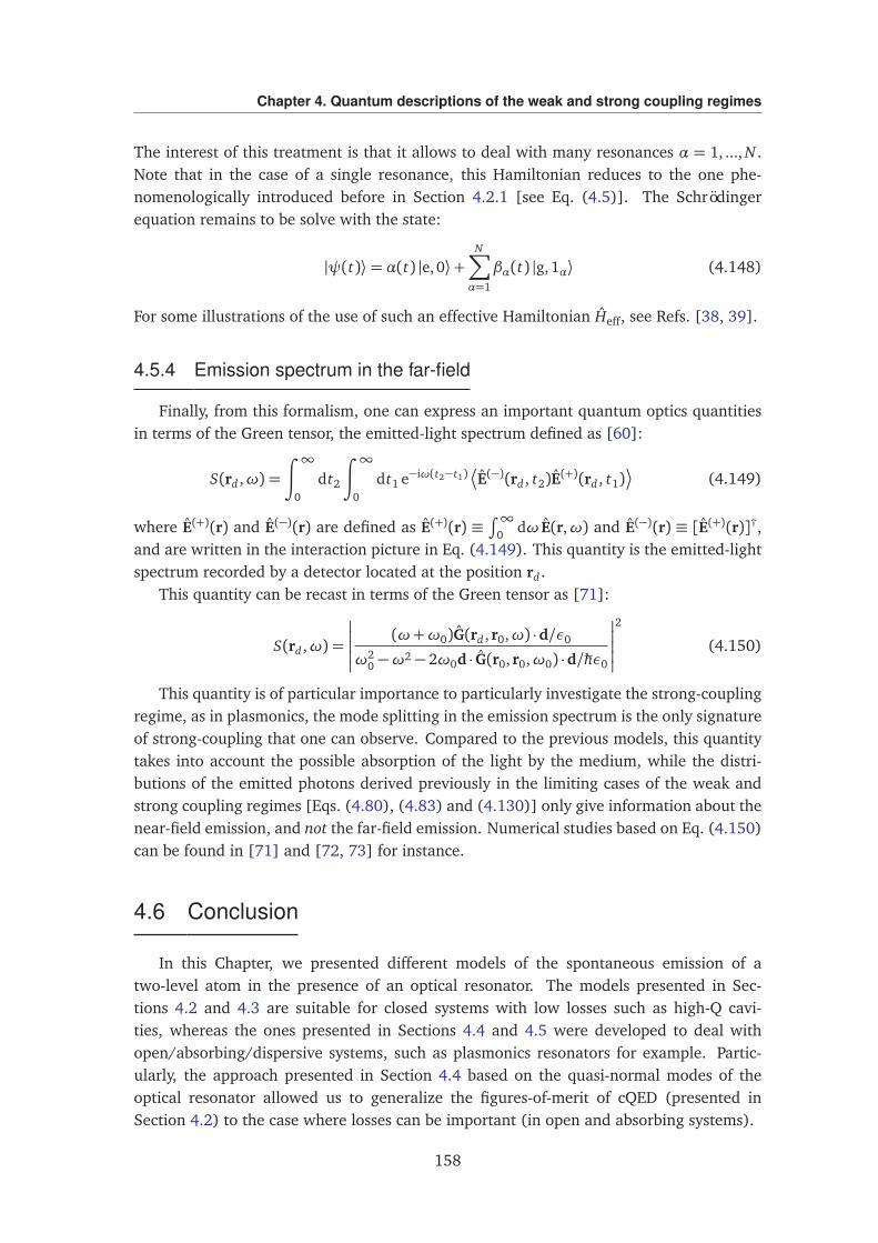
Chapter 4. Quantum descriptions of the weak and strong coupling regimes

The interest of this treatment is that it allows to deal with many resonances α = 1, ..., N .Note that in the case of a single resonance, this Hamiltonian reduces to the one phe-nomenologically introduced before in Section 4.2.1 [see Eq. (4.5)]. The Schrödingerequation remains to be solve with the state:

|ψ(t)⟩= α(t) |e, 0⟩+N∑

α=1

βα(t) |g, 1α⟩ (4.148)

For some illustrations of the use of such an effective Hamiltonian Heff, see Refs. [38, 39].

4.5.4 Emission spectrum in the far-field

Finally, from this formalism, one can express an important quantum optics quantitiesin terms of the Green tensor, the emitted-light spectrum defined as [60]:

S(rd ,ω) =

∫ ∞

0

dt2

∫ ∞

0

dt1 e−iω(t2−t1)

E(−)(rd , t2)E(+)(rd , t1)

(4.149)

where E(+)(r) and E(−)(r) are defined as E(+)(r) ≡∫∞

0 dω E(r,ω) and E(−)(r) ≡ [E(+)(r)]†,and are written in the interaction picture in Eq. (4.149). This quantity is the emitted-lightspectrum recorded by a detector located at the position rd .

This quantity can be recast in terms of the Green tensor as [71]:

S(rd ,ω) =

(ω+ω0)G(rd , r0,ω) ·d/ε0

ω20 −ω2 − 2ω0d · G(r0, r0,ω0) ·d/ħhε0

2

(4.150)

This quantity is of particular importance to particularly investigate the strong-couplingregime, as in plasmonics, the mode splitting in the emission spectrum is the only signatureof strong-coupling that one can observe. Compared to the previous models, this quantitytakes into account the possible absorption of the light by the medium, while the distri-butions of the emitted photons derived previously in the limiting cases of the weak andstrong coupling regimes [Eqs. (4.80), (4.83) and (4.130)] only give information about thenear-field emission, and not the far-field emission. Numerical studies based on Eq. (4.150)can be found in [71] and [72, 73] for instance.

4.6 Conclusion

In this Chapter, we presented different models of the spontaneous emission of atwo-level atom in the presence of an optical resonator. The models presented in Sec-tions 4.2 and 4.3 are suitable for closed systems with low losses such as high-Q cavi-ties, whereas the ones presented in Sections 4.4 and 4.5 were developed to deal withopen/absorbing/dispersive systems, such as plasmonics resonators for example. Partic-ularly, the approach presented in Section 4.4 based on the quasi-normal modes of theoptical resonator allowed us to generalize the figures-of-merit of cQED (presented inSection 4.2) to the case where losses can be important (in open and absorbing systems).

158

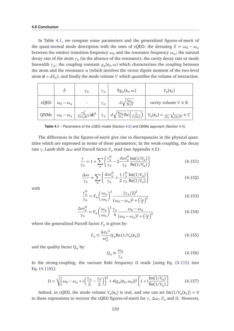
4.6 Conclusion

In Table 4.1, we compare some parameters and the generalized figures-of-merit ofthe quasi-normal mode description with the ones of cQED: the detuning δ = ω0 − ωαbetween the emitter transition frequency ω0 and the resonator frequency ωα; the naturaldecay rate of the atom γ0 (in the absence of the resonator); the cavity decay rate or modelinewidth γα; the coupling constant gα(r0,ω) which characterizes the coupling betweenthe atom and the resonance α (which involves the vector dipole moment of the two-levelatom d= d~ud), and finally the mode volume V which quantifies the volume of interaction.

δ γ0 γα ħhgα(r0,ω) Vα(r0)

cQED ω0 −ωα - γα dr

ħhωα2ε0V cavity volume V ∈ R

QNMs ω0 −ωαω3

03πε0ħhc3 |d|2 γα d

r

ħhωα2ε0

Re

1Vα(r0)

Vα(r0) =1

(~ud ·Eα(r0))2∈ C

Table 4.1 – Parameters of the cQED model (Section 4.2) and QNMs approach (Section 4.4).

The differences in the figures-of-merit give rise to discrepancies in the physical quan-tities which are expressed in terms of these parameters; In the weak-coupling, the decayrate γ, Lamb shift ∆ω and Purcell factor Fα read (see Appendix 4.E):

γ

γ0= 1+

∑

α

γHα

γ0− 2∆ωH

α

γ0

Im(1/Vα)Re(1/Vα)

(4.151)

∆ω

γ0=∑

α

∆ωHα

γ0+

12

γHα

γ0

Im(1/Vα)Re(1/Vα)

(4.152)

withγHα

γ0= Fα

ωαω0

2 (γα/2)2

(ω0 −ωα)2 +γα

2

2 (4.153)

∆ωHα

γ0= Fα

ωαω0

2 γα4

ω0 −ωα(ω0 −ωα)2 +

γα2

2 (4.154)

where the generalized Purcell factor Fα is given by:

Fα ≡6πc3

ω3α

QαRe (1/Vα(r0)) (4.155)

and the quality factor Qα by:Qα ≡

ωαγα

(4.156)

In the strong-coupling, the vacuum Rabi frequency Ω reads [using Eq. (4.115) intoEq. (4.118)]:

Ω=

√

√

h

ω0 −ωα + iγα

2−γ0

2

i2+ 4|gα(r0,ω0)|2

1+ iIm(1/Vα)Re(1/Vα)

(4.157)

Indeed, in cQED, the mode volume Vα(r0) is real, and one can set Im (1/Vα(r0)) = 0in these expressions to recover the cQED figures-of-merit for γ, ∆ω, Fα and Ω. However,

159

Chapter 4. Quantum descriptions of the weak and strong coupling regimes

for systems with important losses, Vα(r0) is in general characterized by an imaginary part,which was illustrated in Chapter 3 Section 3.4 in the case of a dielectric (no absorption butradiation losses) and a plasmonic (absorption and radiation losses) spheres, which bothconstitute “open” cavities. Therefore, as pointed out by Koenderink in [75], the modevolume is a crucial parameter which has different meanings in closed or open cavities,and finds its proper definition in open cavities within the framework of the quasi-normalmodes (see Chapter 3 and also [74, 76, 77]).

Moreover, while we discussed here only quantum formalisms, it is remarkable to pointout that the Purcell factor Fα [Eq. (4.155)], the decay rate γ and Lamb shift∆ω normalizedby the free space decay rate γ0 [Eqs. (4.151), (4.152), (4.153) and (4.154)], as well asthe vacuum Rabi splitting Ω [Eq. (4.157)], have the same expressions as the ones derivedusing a fully classical treatment. About the classical treatment, the interested reader couldrefer for instance to [18] when one does not consider Im [1/Vα(r0)] and [62] in the generalcase.

160

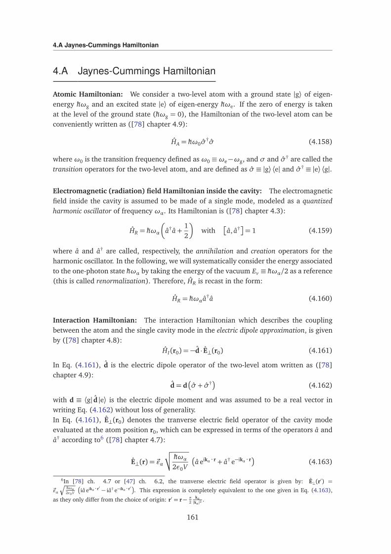
4.A Jaynes-Cummings Hamiltonian

4.A Jaynes-Cummings Hamiltonian

Atomic Hamiltonian: We consider a two-level atom with a ground state |g⟩ of eigen-energy ħhωg and an excited state |e⟩ of eigen-energy ħhωe. If the zero of energy is takenat the level of the ground state (ħhωg = 0), the Hamiltonian of the two-level atom can beconveniently written as ([78] chapter 4.9):

HA = ħhω0σ†σ (4.158)

where ω0 is the transition frequency defined as ω0 ≡ωe−ωg, and σ and σ† are called thetransition operators for the two-level atom, and are defined as σ ≡ |g⟩ ⟨e| and σ† ≡ |e⟩ ⟨g|.

Electromagnetic (radiation) field Hamiltonian inside the cavity: The electromagneticfield inside the cavity is assumed to be made of a single mode, modeled as a quantizedharmonic oscillator of frequency ωα. Its Hamiltonian is ([78] chapter 4.3):

HR = ħhωα

a†a+12

with

a, a†

= 1 (4.159)

where a and a† are called, respectively, the annihilation and creation operators for theharmonic oscillator. In the following, we will systematically consider the energy associatedto the one-photon state ħhωα by taking the energy of the vacuum Ev ≡ ħhωα/2 as a reference(this is called renormalization). Therefore, HR is recast in the form:

HR = ħhωαa†a (4.160)

Interaction Hamiltonian: The interaction Hamiltonian which describes the couplingbetween the atom and the single cavity mode in the electric dipole approximation, is givenby ([78] chapter 4.8):

HI(r0) = −d · E⊥(r0) (4.161)

In Eq. (4.161), d is the electric dipole operator of the two-level atom written as ([78]chapter 4.9):

d= d

σ+ σ†

(4.162)

with d ≡ ⟨g| d |e⟩ is the electric dipole moment and was assumed to be a real vector inwriting Eq. (4.162) without loss of generality.In Eq. (4.161), E⊥(r0) denotes the tranverse electric field operator of the cavity modeevaluated at the atom position r0, which can be expressed in terms of the operators a anda† according to6 ([78] chapter 4.7):

E⊥(r) = ~εα

√

√ ħhωα2ε0V

a eikα · r + a† e−ikα · r (4.163)

6In [78] ch. 4.7 or [47] ch. 6.2, the tranverse electric field operator is given by: E⊥(r′) =

~εα

Ç

ħhωα2ε0V

ia eikα · r′ − ia† e−ikα · r′

. This expression is completely equivalent to the one given in Eq. (4.163),

as they only differ from the choice of origin: r′ = r− π2

kα|kα |2

.

161

Chapter 4. Quantum descriptions of the weak and strong coupling regimes

where V denotes the physical volume of the cavity, kα is the wavevector of the modeverifying |kα|=ωα/c, and ~εα is the polarization polarization vector of the mode such that~εα ·kα = 0.By taking the origin such that the position of the atom is r0 = 0, and making use ofEqs. (4.162) and (4.163), the interaction Hamiltonian of Eq. (4.161) simplifies to:

HI = ħhg

σ+ σ†

a+ a†

(4.164)

where we defined the coupling constant g as:

ħhg ≡ − (d · ~εα )√

√ ħhωα2ε0V

(4.165)

g is a real quantity with the dimensions of frequency. Finally, we make the rotating waveapproximation by dropping the terms “σa” and “σ†a†” in Eq. (4.164) to get ([78] chapter4.9):

HI = ħhg

σ†a+ a†σ

(4.166)

Jaynes-Cummings Hamiltonian: The full Jaynes-Cummings Hamiltonian is the totalHamiltonian obtained within this model HJC = HA+ HR + HI :

HJC = ħhω0σ†σ+ħhωαa†a+ħhg

σ†a+ a†σ

(4.167)

162

4.B Fermi golden rule

4.B Fermi golden rule

The Fermi golden rule is derived from time-dependent perturbation theory, which isvalid (see [34], chapter 5.2):(i) to describe short-time behavior (when α(t)' α(0) = 1)(ii) if the coupling between the two-level system and the reservoir is weak (i.e., the cou-pling strengths gj are small).

To get the first-order perturbative solution in g2j , we set α(t ′) = 1 in the right-hand

side of Eq. (4.56):

α (t)' −∫ ∞

0

dωR(r0,ω)

∫ t

0

dt ′ ei(ω0−ω)(t−t ′) (4.168)

One can first calculate the time integral:

∫ t

0

dt ′ ei(ω0−ω)(t−t ′) =ei(ω0−ω)t − 1

i(ω0 −ω)

= h(ω0 −ω, t)× t

(4.169)

to get

α (t)' −∫ ∞

0

dωR(r0,ω)× h(ω0 −ω, t)× t (4.170)

where we introduced the function h(ω, t) defined by:

h(ω, t)≡eiωt − 1

iωt(4.171)

We then proceed by formally integrating Eq. (4.169) together with the initial conditionα(0) = 1 to get

α(t) = 1−∫ ∞

0

dωR(r0,ω)

∫ t

0

dt ′ h(ω0 −ω, t ′)× t ′

= 1−∫ ∞

0

dωR(r0,ω) i

1− h(ω0 −ω, t)ω0 −ω

t

(4.172)

To compute the survival probability Psurv (t) defined as

Psurv (t)≡ |⟨e, 0|ψ(t)⟩ |2

= |α (t) |2(4.173)

we will ignore the second-order contributions (i.e., the term ∝

∑

j |gj|22

) because wealready neglected contributions of this order in obtaining Eq. (4.168) for α(t). Then the

163

Chapter 4. Quantum descriptions of the weak and strong coupling regimes

first order perturbative solution for the probability Psurv (t) is:

Psurv (t) = |α (t) |2

' 1− 2×Re

∫ ∞

0

dωR(r0,ω) i

1− h(ω0 −ω, t)ω0 −ω

t

= 1− 2×∫ ∞

0

dωR(r0,ω)×Re§

i×1− h(ω0 −ω, t)

ω0 −ω

ª

× t

= 1− 2×∫ ∞

0

dωR(r0,ω)× Im§

h(ω0 −ω, t)ω0 −ω

ª

× t

(4.174)

Moreover, one can easily show that

Im§

h(ω0 −ω, t)ω0 −ω

ª

=12

t sinc2

(ω0 −ω)t2

(4.175)

with sinc(x)≡ sin(x)/x . Thus,

Psurv (t) = 1−∫ ∞

0

dωR(r0,ω)× t sinc2

(ω0 −ωj)t

2

× t (4.176)

Finally, Eq. (4.176) can be recast in the form

Psurv (t) = 1− 2π

∫ ∞

0

dωR (r0,ω) Ft (ω−ω0)× t (4.177)

where

R (r0,ω)≡∑

j

|gj(r0)|2δ(ω−ωj) Unit: [R (ω)] = s−1 (4.178)

and

Ft (ω−ω0)≡t

2πsinc2

(ω−ω0) t2

Unit: [Ft (ω−ω0)] = s (4.179)

The Fermi golden rule is then obtained by noting that for t 1/∆ω where∆ω is the widthof the reservoir which determines the effective range of integration (but t sufficiently smallfor the perturbative solution to hold):

Ft (ω−ω0)→ δ (ω−ω0) (4.180)

and one therefore gets:Psurv (t) = 1− γ× t (4.181)

where γ is the decay rate given by the Fermi golden rule:

γ≡ 2πR(r0,ω0) (4.182)

164

4.C Discrete model

4.C Discrete model

We recall here the discrete model from Refs. [50] and [51] Appendix A. In this model,one considers N states j with a “door” distribution centered on the atomic frequency ω0

and of variable bandwidth γα. One can then write Eqs. (4.51) and (4.52) in a matrix form:

iħh∂

∂ t

α(t)β1(t)

...βN (t)

= ħh

ω0 g∗1(r0) . . . g∗N (r0)g1(r0) ω1

.... . . 0

gN (r0) 0 ωN

︸ ︷︷ ︸

M

·

α(t)β1(t)

...βN (t)

, (4.183)

Moreover, one assumes equal and real coupling constants: g j(r0)≡ g for all modes j.

The square matrix M can be diagonalised using Mathematica. The program gives backthe eigenvalues κn and eigenvectors |κn⟩ of M , that can be used to solve for α(t) and β j(t)using the general expression of their solution

α(t)β1(t)

...βN (t)

=N+1∑

n=1

cn|κn⟩e−iκn t . (4.184)

where the cn are given by the initial conditions:

α(t = 0) = 1 (4.185)

β j(t = 0) = 0 (4.186)

In Figs. 4.3 and 4.4, we plot the survival probability Psurv(t) = |α(t)|2 obtained withthis numerical method when the continuum bandwidth γα varies. As the value of thebandwidth decreases, one can see the transition from the weak (Fig. 4.3) to the strong(Fig. 4.4) coupling regime, where, respectively, Psurv(t) decays monotically, and Psurv(t)undergoes oscillations.

Note that the large “revival” peaks in the first two plots are an artefact peculiar to thediscretization [51]. It is a manifestation of partial Poincaré recurrence due to the factthat when the Hilbert space of the quantum system is of finite dimension, the Poincarérecurrence time is finite (and its value is the smallest common multiple of all the eigenfre-quencies of the Hamiltonian in Eq. (4.183)).

165

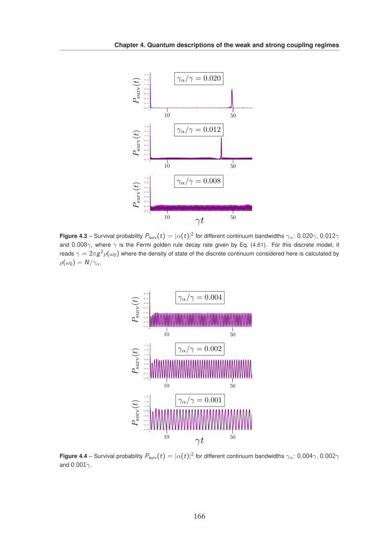
Chapter 4. Quantum descriptions of the weak and strong coupling regimes

Figure 4.3 – Survival probability Psurv(t) = |α(t)|2 for different continuum bandwidths γα: 0.020γ, 0.012γand 0.008γ, where γ is the Fermi golden rule decay rate given by Eq. (4.61). For this discrete model, itreads γ = 2πg2ρ(ω0) where the density of state of the discrete continuum considered here is calculated byρ(ω0) = N/γα.

Figure 4.4 – Survival probability Psurv(t) = |α(t)|2 for different continuum bandwidths γα: 0.004γ, 0.002γand 0.001γ.

166

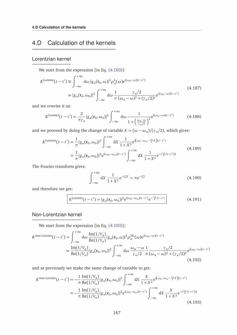
4.D Calculation of the kernels

4.D Calculation of the kernels

Lorentzian kernel

We start from the expression [in Eq. (4.103)]

KLorentz(t − t ′)≡∫ +∞

−∞dω |gα(r0,ω)|2ρL

α(ω)ei(ω0−ω)(t−t ′)

' |gα(r0,ω0)|2∫ +∞

−∞dω

1π

γα/2(ωα −ω)2 + (γα/2)2

ei(ω0−ω)(t−t ′)

(4.187)

and we rewrite it as:

KLorentz(t − t ′) =2πγα|gα(r0,ω0)|2

∫ +∞

−∞dω

1

1+

ωα−ωγα/2

2 ei(ω0−ω)(t−t ′) (4.188)

and we proceed by doing the change of variable X = (ω−ωα)/(γα/2), which gives:

KLorentz(t − t ′) =1π|gα(r0,ω0)|2

∫ +∞

−∞dX

11+ X 2

ei(ω0−ωα−γα2 X)(t−t ′)

=1π|gα(r0,ω0)|2ei(ω0−ωα)(t−t ′)

∫ +∞

−∞dX

11+ X 2

e−i γα2 (t−t ′)X

(4.189)

The Fourier transform gives:∫ +∞

−∞dX

11+ X 2

e−iξX = πe−|ξ| (4.190)

and therefore we get:

KLorentz(t − t ′) = |gα(r0,ω0)|2ei(ω0−ωα)(t−t ′)e−γα2 |t−t ′| (4.191)

Non-Lorentzian kernel

We start from the expression [in Eq. (4.103)]:

Knon-Lorentz(t − t ′) =

∫ +∞

−∞dω

Im(1/Vα)Re(1/Vα)

|gα(r0,ω)|2ρNLα (ω)e

i(ω0−ω)(t−t ′)

'Im(1/Vα)Re(1/Vα)

|gα(r0,ω0)|2∫ +∞

−∞dωωα −ωγα/2

1π

γα/2(ωα −ω)2 + (γα/2)2

ei(ω0−ω)(t−t ′)

(4.192)

and as previously we make the same change of variable to get:

Knon-Lorentz(t − t ′) = −1π

Im(1/Vα)Re(1/Vα)

|gα(r0,ω0)|2∫ +∞

−∞dX

X1+ X 2

ei(ω0−ωα−γα2 X)(t−t ′)

= −1π

Im(1/Vα)Re(1/Vα)

|gα(r0,ω0)|2ei(ω0−ωα)(t−t ′)

∫ +∞

−∞dX

X1+ X 2

e−i γα2 (t−t ′)X

(4.193)

167

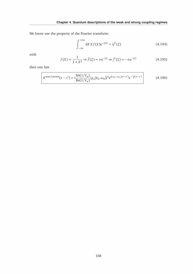
Chapter 4. Quantum descriptions of the weak and strong coupling regimes

We know use the property of the Fourier transform:∫ +∞

−∞dX X f (X )e−iξX = i f ′(ξ) (4.194)

withf (X ) =

11+ X 2

⇒ f (ξ) = πe−|ξ|⇒ f ′(ξ) = −πe−|ξ| (4.195)

then one has

Knon-Lorentz(t − t ′) = iIm(1/Vα)Re(1/Vα)

|gα(r0,ω0)|2ei(ω0−ωα)(t−t ′)e−γα2 |t−t ′| (4.196)

168

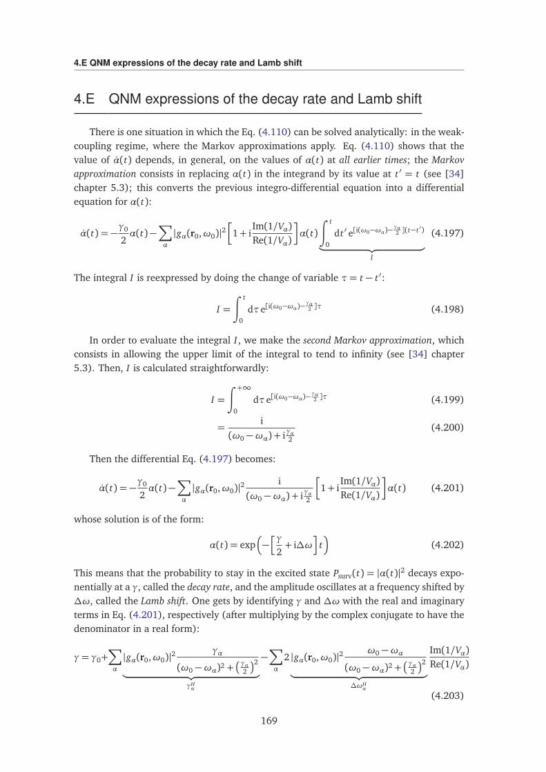
4.E QNM expressions of the decay rate and Lamb shift

4.E QNM expressions of the decay rate and Lamb shift

There is one situation in which the Eq. (4.110) can be solved analytically: in the weak-coupling regime, where the Markov approximations apply. Eq. (4.110) shows that thevalue of α(t) depends, in general, on the values of α(t) at all earlier times; the Markovapproximation consists in replacing α(t) in the integrand by its value at t ′ = t (see [34]chapter 5.3); this converts the previous integro-differential equation into a differentialequation for α(t):

α(t) = −γ0

2α(t)−

∑

α

|gα(r0,ω0)|2

1+ iIm(1/Vα)Re(1/Vα)

α(t)

∫ t

0

dt ′ e[i(ω0−ωα)−γα2 ](t−t ′)

︸ ︷︷ ︸

I

(4.197)

The integral I is reexpressed by doing the change of variable τ= t − t ′:

I =

∫ t

0

dτe[i(ω0−ωα)−γα2 ]τ (4.198)

In order to evaluate the integral I , we make the second Markov approximation, whichconsists in allowing the upper limit of the integral to tend to infinity (see [34] chapter5.3). Then, I is calculated straightforwardly:

I =

∫ +∞

0

dτe[i(ω0−ωα)−γα2 ]τ (4.199)

=i

(ω0 −ωα) + iγα2(4.200)

Then the differential Eq. (4.197) becomes:

α(t) = −γ0

2α(t)−

∑

α

|gα(r0,ω0)|2i

(ω0 −ωα) + iγα2

1+ iIm(1/Vα)Re(1/Vα)

α(t) (4.201)

whose solution is of the form:

α(t) = exp

−hγ

2+ i∆ω

i

t

(4.202)

This means that the probability to stay in the excited state Psurv(t) = |α(t)|2 decays expo-nentially at a γ, called the decay rate, and the amplitude oscillates at a frequency shifted by∆ω, called the Lamb shift. One gets by identifying γ and ∆ω with the real and imaginaryterms in Eq. (4.201), respectively (after multiplying by the complex conjugate to have thedenominator in a real form):

γ= γ0+∑

α

|gα(r0,ω0)|2γα

(ω0 −ωα)2 +γα

2

2

︸ ︷︷ ︸

γHα

−∑

α

2 |gα(r0,ω0)|2ω0 −ωα

(ω0 −ωα)2 +γα

2

2

︸ ︷︷ ︸

∆ωHα

Im(1/Vα)Re(1/Vα)

(4.203)

169

Chapter 4. Quantum descriptions of the weak and strong coupling regimes

∆ω=∑

α

|gα(r0,ω0)|2ω0 −ωα

(ω0 −ωα)2 +γα

2

2

︸ ︷︷ ︸

∆ωHα

+∑

α

12|gα(r0,ω0)|2

γα

(ω0 −ωα)2 +γα

2

2

︸ ︷︷ ︸

γHα

Im(1/Vα)Re(1/Vα)

(4.204)By normalizing these quantities by the free space decay rate γ0 given by Eq. (4.106)

and using the expression of gα(r0,ω0) given by Eq. (4.100), one gets:

γ

γ0= 1+

∑

α

γHα

γ0− 2∆ωH

α

γ0

Im(1/Vα)Re(1/Vα)

(4.205)

∆ω

γ0=∑

α

∆ωHα

γ0+

12

γHα

γ0

Im(1/Vα)Re(1/Vα)

(4.206)

withγHα

γ0= Fα

ωαω0

2 (γα/2)2

(ω0 −ωα)2 +γα

2

2 (4.207)

∆ωHα

γ0= Fα

ωαω0

2 γα4

ω0 −ωα(ω0 −ωα)2 +

γα2

2 (4.208)

where we defined the generalized Purcell factor as:

Fα ≡6πc3

ω3α

QαRe (1/Vα(r0)) (4.209)

and the quality factor Qα:Qα ≡

ωαγα

(4.210)

These expressions are exactly the ones derived in chapter 2, where we used the com-plex frequency notation ωα ≡ω′α+ iω′′α, where one has the correspondance ω′α↔ωα andω′′α↔−γα/2.

170

4.F Second-order differential equation verified by α(t)

4.F Second-order differential equation verified by α(t)

We start from Eq. (4.115):

α(t) = −γ0

2α(t)− g2

∫ t

0

dt ′α(t ′)e[i(ω0−ωα)−γα2 ](t−t ′)

= −γ0

2α(t)− g2e[i(ω0−ωα)−

γα2 ]t

∫ t

0

dt ′α(t ′)e−[i(ω0−ωα)−γα2 ]t

′

(4.211)

By calling¨

I(t) =∫ t

0 dt ′α(t ′)e−[i(ω0−ωα)−γα2 ]t

′

I ′(t) = α(t)e−[i(ω0−ωα)−γα2 ]t

(4.212)

we get by differentiating the previous equation:

α(t) = −γ0

2α(t)− g2[i(ω0 −ωα)−

γα2]e[i(ω0−ωα)−

γα2 ]t × I(t)− g2 e[i(ω0−ωα)−

γα2 ]t × I ′(t)

︸ ︷︷ ︸

α(t)

= −γ0

2α(t)− g2[i(ω0 −ωα)−

γα2]e[i(ω0−ωα)−

γα2 ]t × I(t)− g2α(t)

(4.213)

Moreover, by noticing from Eq. (4.211) that

− g2e[i(ω0−ωα)−γα2 ]t × I(t) = α(t) +

γ0

2α(t) (4.214)

one gets

α(t) = −γ0

2α(t) + [i(ω0 −ωα)−

γα2][α(t) +

γ0

2α(t)]− g2α(t) (4.215)

which is rearranged into the Eq. (4.116) in the main text:

α(t)− [i(ω0 −ωα)−γ0

2−γα2]α(t) + [g2 − i

γ0

2(ω0 −ωα) +

γ0

2γα2]α(t) = 0 (4.216)

171

Chapter 4. Quantum descriptions of the weak and strong coupling regimes

172

Bibliography

[1] S. Haroche and D. Kleppner, Physics Today 42, 24 (1989).

[2] Y. Kaluzny, P. Goy, M. Gross, J. M. Raimond, and S. Haroche, Physical Review Letters51, 1175 (1983).

[3] M. Brune, J. Raimond, P. Goy, L. Davidovich, and S. Haroche, Physical ReviewLetters 59, 1899 (1987).

[4] D. Meschede, H. Walther, and G. Müller, Physical Review Letters 54, 551 (1985).

[5] G. Rempe, H. Walther, and N. Klein, Physical Review Letters 58, 353 (1987).

[6] M. Raizen, R. Thompson, R. Brecha, H. Kimble, and H. Carmichael, Physical ReviewLetters 63, 240 (1989).

[7] Y. Zhu, D. J. Gauthier, S. Morin, Q. Wu, H. Carmichael, and T. Mossberg, PhysicalReview Letters 64, 2499 (1990).

[8] G. Rempe, R. Thompson, R. Brecha, W. Lee, and H. Kimble, Physical Review Letters67, 1727 (1991).

[9] R. Thompson, G. Rempe, and H. Kimble, Physical Review Letters 68, 1132 (1992).

[10] C. J. Hood, M. S. Chapman, T. W. Lynn, and H. J. Kimble, Physical Review Letters80, 4157 (1998).

[11] J. P. Reithmaier, G. Sek, A. Löffler, C. Hofmann, S. Kuhn, S. Reitzenstein, L. Keldysh,V. Kulakovskii, T. Reinecke, and A. Forchel, Nature 432, 197 (2004).

[12] T. Yoshie, A. Scherer, J. Hendrickson, G. Khitrova, H. Gibbs, G. Rupper, C. Ell,O. Shchekin, and D. Deppe, Nature 432, 200 (2004).

[13] P. Lodahl, S. Mahmoodian, and S. Stobbe, Reviews of Modern Physics 87, 347(2015).

[14] J. Bellessa, C. Bonnand, J. Plenet, and J. Mugnier, Physical Review Letters 93,036404 (2004).

[15] J. Bellessa, C. Symonds, K. Vynck, A. Lemaitre, A. Brioude, L. Beaur, J. C. Plenet,P. Viste, D. Felbacq, E. Cambril, and P. Valvin, Physical Review B 80, 033303 (2009).

[16] J. Dintinger, S. Klein, F. Bustos, W. L. Barnes, and T. W. Ebbesen, Physical Review B71, 035424 (2005).

173

BIBLIOGRAPHY

[17] J. Dintinger, S. Klein, and T. W. Ebbesen, Advanced Materials 18, 1267 (2006).

[18] P. Törmä and W. L. Barnes, Reports on Progress in Physics 78, 013901 (2014).

[19] I. Pockrand, A. Brillante, and D. Möbius, The Journal of Chemical Physics 77, 6289(1982).

[20] D. G. Baranov, M. Wersall, J. Cuadra, T. J. Antosiewicz, and T. Shegai, ACS Photonics5, 24 (2017).

[21] F. Marquier, C. Sauvan, and J.-J. Greffet, ACS Photonics 4, 2091 (2017).

[22] T. Itoh, Y. S. Yamamoto, H. Tamaru, V. Biju, S.-i. Wakida, and Y. Ozaki, PhysicalReview B 89, 195436 (2014).

[23] T. Hartsfield, W.-S. Chang, S.-C. Yang, T. Ma, J. Shi, L. Sun, G. Shvets, S. Link, andX. Li, Proceedings of the National Academy of Sciences 112, 12288 (2015).

[24] K. Santhosh, O. Bitton, L. Chuntonov, and G. Haran, Nature Communications 7,11823 (2016).

[25] R. Chikkaraddy, B. de Nijs, F. Benz, S. J. Barrow, O. A. Scherman, E. Rosta, A. Deme-triadou, P. Fox, O. Hess, and J. J. Baumberg, Nature 535, 127 (2016).

[26] R. Liu, Z.-K. Zhou, Y.-C. Yu, T. Zhang, H. Wang, G. Liu, Y. Wei, H. Chen, and X.-H.Wang, Physical Review Letters 118, 237401 (2017).

[27] A. Ridolfo, M. Leib, S. Savasta, and M. J. Hartmann, Physical Review Letters 109,193602 (2012).

[28] A. Ridolfo, S. Savasta, and M. J. Hartmann, Physical Review Letters 110, 163601(2013).

[29] R. Stassi, A. Ridolfo, O. Di Stefano, M. J. Hartmann, and S. Savasta, Physical ReviewLetters 110, 243601 (2013).

[30] S. De Liberato, Physical Review Letters 112, 016401 (2014).

[31] A. Cacciola, O. Di Stefano, R. Stassi, R. Saija, and S. Savasta, ACS Nano 8, 11483(2014).

[32] F. Todisco, M. De Giorgi, M. Esposito, L. De Marco, A. Zizzari, M. Bianco, L. Dominici,D. Ballarini, V. Arima, G. Gigli, et al., ACS Photonics 5, 143 (2017).

[33] E. T. Jaynes and F. W. Cummings, Proceedings of the IEEE 51, 89 (1963).

[34] S. M. Barnett and P. M. Radmore, Methods in theoretical quantum optics, Vol. 15(Oxford University Press, 2002).

[35] S. M. Dutra, Cavity quantum electrodynamics: the strange theory of light in a box(John Wiley & Sons, 2005).

174

BIBLIOGRAPHY

[36] R. P. Feynman and F. Vernon Jr, Annals of Physics 281, 547 (2000).

[37] P. Leung, S. Liu, and K. Young, Physical Review A 49, 3057 (1994).

[38] H. Varguet, B. Rousseaux, D. Dzsotjan, H. Jauslin, S. Guérin, and G. C. des Francs,Optics Letters 41, 4480 (2016).

[39] H. Varguet, B. Rousseaux, D. Dzsotjan, H. R. Jauslin, S. Guérin, and G. C. des Francs,Journal of Physics B: Atomic, Molecular and Optical Physics 52, 055404 (2019).

[40] G. Gamow, Zeitschrift für Physik 51, 204 (1928).

[41] K. Friedrichs, Communications on Pure and Applied Mathematics 1, 361 (1948).

[42] V. Debierre, La fonction d’onde du photon en principe et en pratique, Ph.D. thesis, EcoleCentrale Marseille (2015).

[43] R. El-Ganainy, K. G. Makris, M. Khajavikhan, Z. H. Musslimani, S. Rotter, and D. N.Christodoulides, Nature Physics 14, 11 (2018).

[44] E. M. Purcell, Physical Review 69, 681 (1946).

[45] M. Tavis and F. Cummings, Physics Letters A 25, 714 (1967).

[46] B. M. Garraway, Philosophical Transactions of the Royal Society A: Mathematical,Physical and Engineering Sciences 369, 1137 (2011).

[47] G. Grynberg, A. Aspect, and C. Fabre, Introduction to quantum optics: from the semi-classical approach to quantized light (Cambridge University Press, 2010).

[48] B. Piraux, R. Bhatt, and P. Knight, Physical Review A 41, 6296 (1990).

[49] V. Weisskopf and E. Wigner, Zeitschrift für Physik 63, 54 (1930).

[50] V. Debierre, I. Goessens, E. Brainis, and T. Durt, Physical Review A 92, 023825(2015).

[51] B. Kolaric, B. Maes, K. Clays, T. Durt, and Y. Caudano, Advanced Quantum Tech-nologies 1, 1800001 (2018).

[52] B. Misra and E. Sudarshan, Journal of Mathematical Physics 18, 756 (1977).

[53] P. Facchi, H. Nakazato, and S. Pascazio, Physical Review Letters 86, 2699 (2001).

[54] A. Kofman and G. Kurizki, Nature 405, 546 (2000).

[55] P. Facchi and S. Pascazio, Physics Letters A 241, 139 (1998).

[56] V. Debierre, T. Durt, A. Nicolet, and F. Zolla, Physics Letters A 379, 2577 (2015).

[57] A. Crespi, F. V. Pepe, P. Facchi, F. Sciarrino, P. Mataloni, H. Nakazato, S. Pascazio,and R. Osellame, Physical Review Letters 122, 130401 (2019).

175

BIBLIOGRAPHY

[58] D. Bouchet and R. Carminati, Journal of the Optical Society of America A 36, 186(2019).

[59] L. Novotny and B. Hecht, Principles of nano-optics (Cambridge University Press,2012).

[60] H. T. Dung, L. Knöll, and D.-G. Welsch, Physical Review A 62, 053804 (2000).

[61] G. Khitrova, H. Gibbs, M. Kira, S. W. Koch, and A. Scherer, Nature Physics 2, 81(2006).

[62] P. Lalanne, W. Yan, K. Vynck, C. Sauvan, and J.-P. Hugonin, Laser & PhotonicsReviews 12, 1700113 (2018).

[63] T. Gruner and D.-G. Welsch, Physical Review A 53, 1818 (1996).

[64] H. T. Dung, L. Knöll, and D.-G. Welsch, Physical Review A 57, 3931 (1998).

[65] S. Scheel, L. Knöll, and D.-G. Welsch, Physical Review A 58, 700 (1998).

[66] R. Matloob, R. Loudon, S. M. Barnett, and J. Jeffers, Physical Review A 52, 4823(1995).

[67] R. Matloob and R. Loudon, Physical Review A 53, 4567 (1996).

[68] P. Yao, C. Van Vlack, A. Reza, M. Patterson, M. Dignam, and S. Hughes, PhysicalReview B 80, 195106 (2009).

[69] B. Rousseaux, D. Dzsotjan, G. C. des Francs, H. Jauslin, C. Couteau, and S. Guérin,Physical Review B 93, 045422 (2016).

[70] D. Dzsotjan, B. Rousseaux, H. Jauslin, G. C. des Francs, C. Couteau, and S. Guérin,Physical Review A 94, 023818 (2016).

[71] C. Van Vlack, P. T. Kristensen, and S. Hughes, Physical Review B 85, 075303 (2012).

[72] A. González-Tudela, P. Huidobro, L. Martín-Moreno, C. Tejedor, and F. García-Vidal,Physical Review Letters 110, 126801 (2013).

[73] A. Delga, J. Feist, J. Bravo-Abad, and F. Garcia-Vidal, Physical Review Letters 112,253601 (2014).

[74] C. Sauvan, J.-P. Hugonin, I. Maksymov, and P. Lalanne, Physical Review Letters 110,237401 (2013).

[75] A. F. Koenderink, Optics Letters 35, 4208 (2010).

[76] P. T. Kristensen, C. Van Vlack, and S. Hughes, Optics Letters 37, 1649 (2012).

[77] E. Muljarov and W. Langbein, Physical Review B 94, 235438 (2016).

[78] R. Loudon, The quantum theory of light (Oxford University Press, 2000).

176

BIBLIOGRAPHY

177

BIBLIOGRAPHY

178

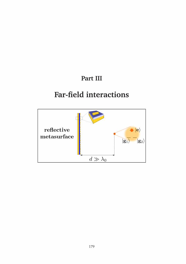
Part III

Far-field interactions

179

181

182

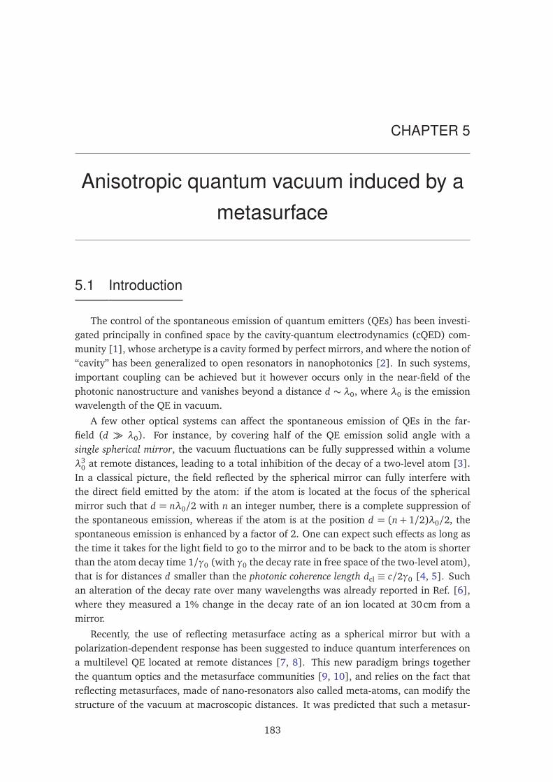
CHAPTER 5

Anisotropic quantum vacuum induced by ametasurface

5.1 Introduction

The control of the spontaneous emission of quantum emitters (QEs) has been investi-gated principally in confined space by the cavity-quantum electrodynamics (cQED) com-munity [1], whose archetype is a cavity formed by perfect mirrors, and where the notion of“cavity” has been generalized to open resonators in nanophotonics [2]. In such systems,important coupling can be achieved but it however occurs only in the near-field of thephotonic nanostructure and vanishes beyond a distance d ∼ λ0, where λ0 is the emissionwavelength of the QE in vacuum.

A few other optical systems can affect the spontaneous emission of QEs in the far-field (d λ0). For instance, by covering half of the QE emission solid angle with asingle spherical mirror, the vacuum fluctuations can be fully suppressed within a volumeλ3

0 at remote distances, leading to a total inhibition of the decay of a two-level atom [3].In a classical picture, the field reflected by the spherical mirror can fully interfere withthe direct field emitted by the atom: if the atom is located at the focus of the sphericalmirror such that d = nλ0/2 with n an integer number, there is a complete suppression ofthe spontaneous emission, whereas if the atom is at the position d = (n + 1/2)λ0/2, thespontaneous emission is enhanced by a factor of 2. One can expect such effects as long asthe time it takes for the light field to go to the mirror and to be back to the atom is shorterthan the atom decay time 1/γ0 (with γ0 the decay rate in free space of the two-level atom),that is for distances d smaller than the photonic coherence length dcl ≡ c/2γ0 [4, 5]. Suchan alteration of the decay rate over many wavelengths was already reported in Ref. [6],where they measured a 1% change in the decay rate of an ion located at 30cm from amirror.

Recently, the use of reflecting metasurface acting as a spherical mirror but with apolarization-dependent response has been suggested to induce quantum interferences ona multilevel QE located at remote distances [7, 8]. This new paradigm brings togetherthe quantum optics and the metasurface communities [9, 10], and relies on the fact thatreflecting metasurfaces, made of nano-resonators also called meta-atoms, can modify thestructure of the vacuum at macroscopic distances. It was predicted that such a metasur-

183

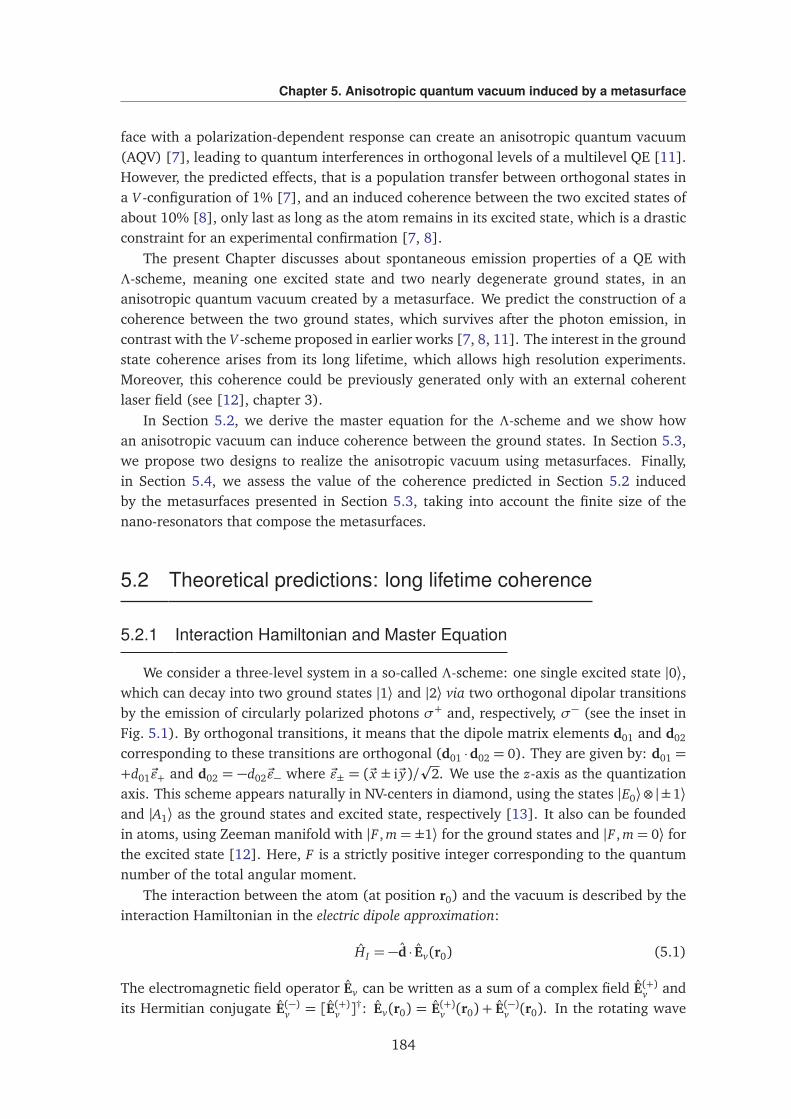
Chapter 5. Anisotropic quantum vacuum induced by a metasurface

face with a polarization-dependent response can create an anisotropic quantum vacuum(AQV) [7], leading to quantum interferences in orthogonal levels of a multilevel QE [11].However, the predicted effects, that is a population transfer between orthogonal states ina V -configuration of 1% [7], and an induced coherence between the two excited states ofabout 10% [8], only last as long as the atom remains in its excited state, which is a drasticconstraint for an experimental confirmation [7, 8].

The present Chapter discusses about spontaneous emission properties of a QE withΛ-scheme, meaning one excited state and two nearly degenerate ground states, in ananisotropic quantum vacuum created by a metasurface. We predict the construction of acoherence between the two ground states, which survives after the photon emission, incontrast with the V -scheme proposed in earlier works [7, 8, 11]. The interest in the groundstate coherence arises from its long lifetime, which allows high resolution experiments.Moreover, this coherence could be previously generated only with an external coherentlaser field (see [12], chapter 3).

In Section 5.2, we derive the master equation for the Λ-scheme and we show howan anisotropic vacuum can induce coherence between the ground states. In Section 5.3,we propose two designs to realize the anisotropic vacuum using metasurfaces. Finally,in Section 5.4, we assess the value of the coherence predicted in Section 5.2 inducedby the metasurfaces presented in Section 5.3, taking into account the finite size of thenano-resonators that compose the metasurfaces.

5.2 Theoretical predictions: long lifetime coherence

5.2.1 Interaction Hamiltonian and Master Equation

We consider a three-level system in a so-called Λ-scheme: one single excited state |0⟩,which can decay into two ground states |1⟩ and |2⟩ via two orthogonal dipolar transitionsby the emission of circularly polarized photons σ+ and, respectively, σ− (see the inset inFig. 5.1). By orthogonal transitions, it means that the dipole matrix elements d01 and d02

corresponding to these transitions are orthogonal (d01 ·d02 = 0). They are given by: d01 =+d01~ε+ and d02 = −d02~ε− where ~ε± = (~x ± i~y)/

p2. We use the z-axis as the quantization

axis. This scheme appears naturally in NV-centers in diamond, using the states |E0⟩⊗ |±1⟩and |A1⟩ as the ground states and excited state, respectively [13]. It also can be foundedin atoms, using Zeeman manifold with |F , m= ±1⟩ for the ground states and |F , m= 0⟩ forthe excited state [12]. Here, F is a strictly positive integer corresponding to the quantumnumber of the total angular moment.

The interaction between the atom (at position r0) and the vacuum is described by theinteraction Hamiltonian in the electric dipole approximation:

HI = −d · Ev(r0) (5.1)

The electromagnetic field operator Ev can be written as a sum of a complex field E(+)v andits Hermitian conjugate E(−)v = [E(+)v ]

†: Ev(r0) = E(+)v (r0) + E(−)v (r0). In the rotating wave

184

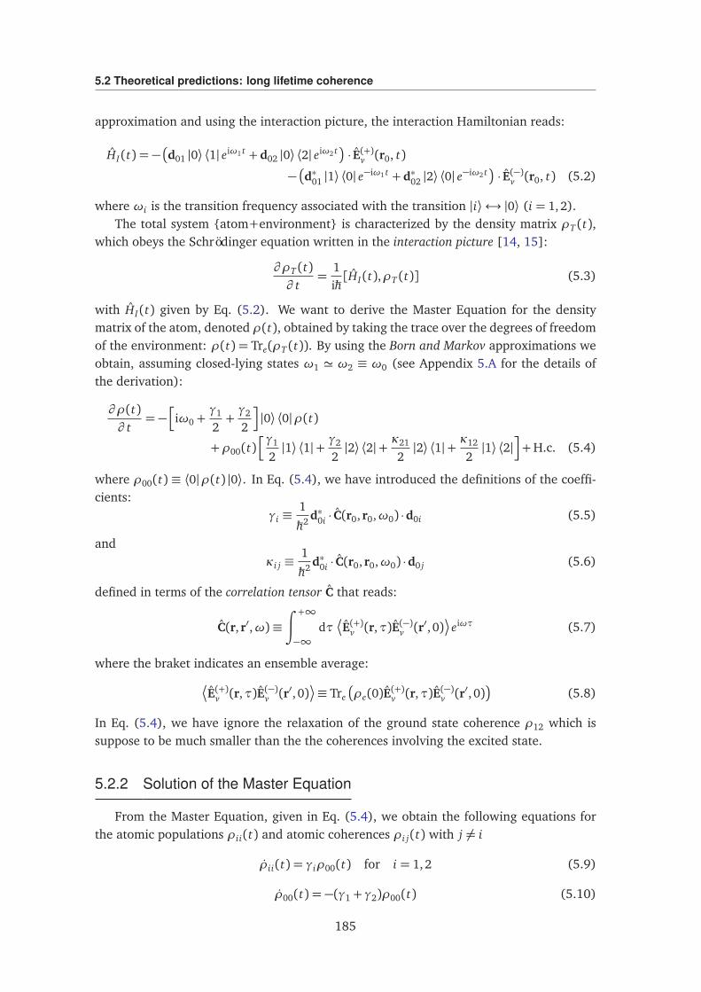
5.2 Theoretical predictions: long lifetime coherence

approximation and using the interaction picture, the interaction Hamiltonian reads:

HI(t) = −

d01 |0⟩ ⟨1| eiω1 t + d02 |0⟩ ⟨2| eiω2 t

· E(+)v (r0, t)

−

d∗01 |1⟩ ⟨0| e−iω1 t + d∗02 |2⟩ ⟨0| e

−iω2 t

· E(−)v (r0, t) (5.2)

where ωi is the transition frequency associated with the transition |i⟩↔ |0⟩ (i = 1, 2).The total system atom+environment is characterized by the density matrix ρT (t),

which obeys the Schrödinger equation written in the interaction picture [14, 15]:

∂ ρT (t)∂ t

=1iħh[HI(t),ρT (t)] (5.3)

with HI(t) given by Eq. (5.2). We want to derive the Master Equation for the densitymatrix of the atom, denoted ρ(t), obtained by taking the trace over the degrees of freedomof the environment: ρ(t) = Tre(ρT (t)). By using the Born and Markov approximations weobtain, assuming closed-lying states ω1 ' ω2 ≡ ω0 (see Appendix 5.A for the details ofthe derivation):

∂ ρ(t)∂ t

= −h

iω0 +γ1

2+γ2

2

i

|0⟩ ⟨0|ρ(t)

+ρ00(t)hγ1

2|1⟩ ⟨1|+

γ2

2|2⟩ ⟨2|+

κ21

2|2⟩ ⟨1|+

κ12

2|1⟩ ⟨2|

i

+H.c. (5.4)

where ρ00(t) ≡ ⟨0|ρ(t) |0⟩. In Eq. (5.4), we have introduced the definitions of the coeffi-cients:

γi ≡1

ħh2 d∗0i · C(r0, r0,ω0) ·d0i (5.5)

andκi j ≡

1

ħh2 d∗0i · C(r0, r0,ω0) ·d0 j (5.6)

defined in terms of the correlation tensor C that reads:

C(r, r′,ω)≡∫ +∞

−∞dτ

E(+)v (r,τ)E(−)v (r′, 0)

eiωτ (5.7)

where the braket indicates an ensemble average:

E(+)v (r,τ)E(−)v (r′, 0)

≡ Tre

ρe(0)E(+)v (r,τ)E(−)v (r

′, 0)

(5.8)

In Eq. (5.4), we have ignore the relaxation of the ground state coherence ρ12 which issuppose to be much smaller than the the coherences involving the excited state.

5.2.2 Solution of the Master Equation

From the Master Equation, given in Eq. (5.4), we obtain the following equations forthe atomic populations ρii(t) and atomic coherences ρi j(t) with j 6= i

ρii(t) = γiρ00(t) for i = 1,2 (5.9)

ρ00(t) = −(γ1 + γ2)ρ00(t) (5.10)

185

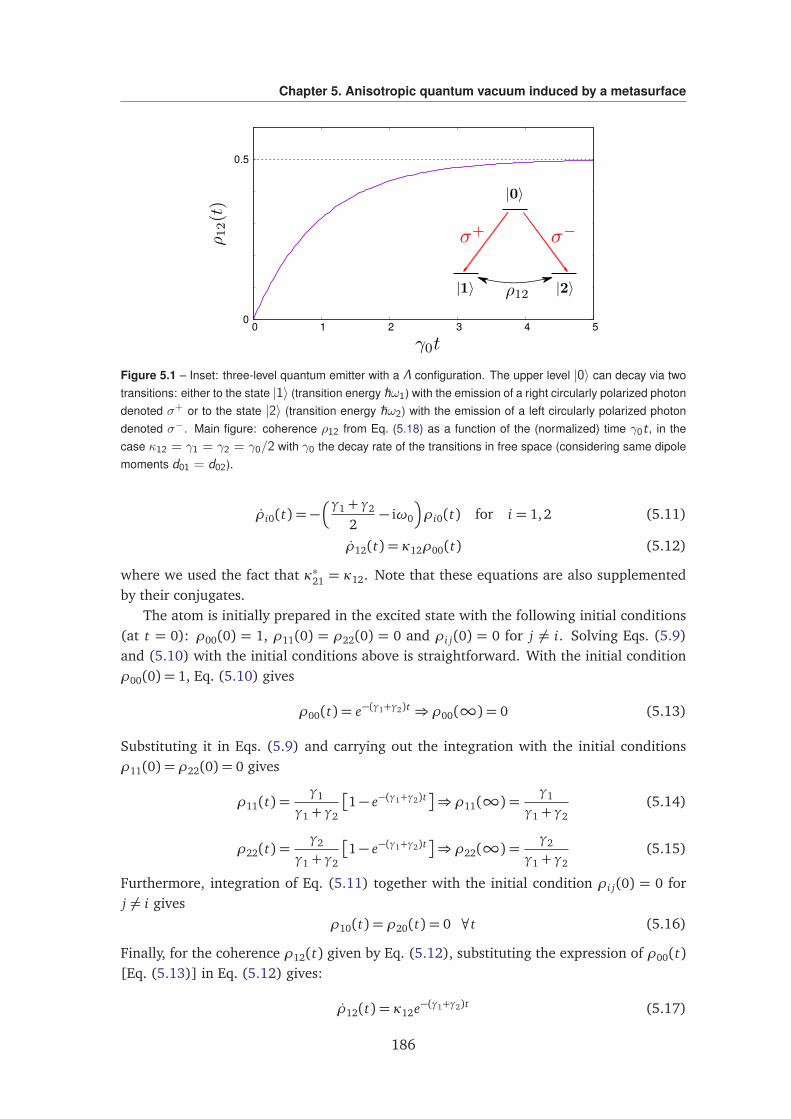
Chapter 5. Anisotropic quantum vacuum induced by a metasurface

0

0.5

0 1 2 3 4 5

Figure 5.1 – Inset: three-level quantum emitter with a Λ configuration. The upper level |0〉 can decay via twotransitions: either to the state |1〉 (transition energy ħhω1) with the emission of a right circularly polarized photondenoted σ+ or to the state |2〉 (transition energy ħhω2) with the emission of a left circularly polarized photondenoted σ−. Main figure: coherence ρ12 from Eq. (5.18) as a function of the (normalized) time γ0t , in thecase κ12 = γ1 = γ2 = γ0/2 with γ0 the decay rate of the transitions in free space (considering same dipolemoments d01 = d02).

ρi0(t) = −γ1 + γ2

2− iω0

ρi0(t) for i = 1,2 (5.11)

ρ12(t) = κ12ρ00(t) (5.12)

where we used the fact that κ∗21 = κ12. Note that these equations are also supplementedby their conjugates.

The atom is initially prepared in the excited state with the following initial conditions(at t = 0): ρ00(0) = 1, ρ11(0) = ρ22(0) = 0 and ρi j(0) = 0 for j 6= i. Solving Eqs. (5.9)and (5.10) with the initial conditions above is straightforward. With the initial conditionρ00(0) = 1, Eq. (5.10) gives

ρ00(t) = e−(γ1+γ2)t ⇒ ρ00(∞) = 0 (5.13)

Substituting it in Eqs. (5.9) and carrying out the integration with the initial conditionsρ11(0) = ρ22(0) = 0 gives

ρ11(t) =γ1

γ1 + γ2

1− e−(γ1+γ2)t

⇒ ρ11(∞) =γ1

γ1 + γ2(5.14)

ρ22(t) =γ2

γ1 + γ2

1− e−(γ1+γ2)t

⇒ ρ22(∞) =γ2

γ1 + γ2(5.15)

Furthermore, integration of Eq. (5.11) together with the initial condition ρi j(0) = 0 forj 6= i gives

ρ10(t) = ρ20(t) = 0 ∀t (5.16)

Finally, for the coherence ρ12(t) given by Eq. (5.12), substituting the expression of ρ00(t)[Eq. (5.13)] in Eq. (5.12) gives:

ρ12(t) = κ12e−(γ1+γ2)t (5.17)

186

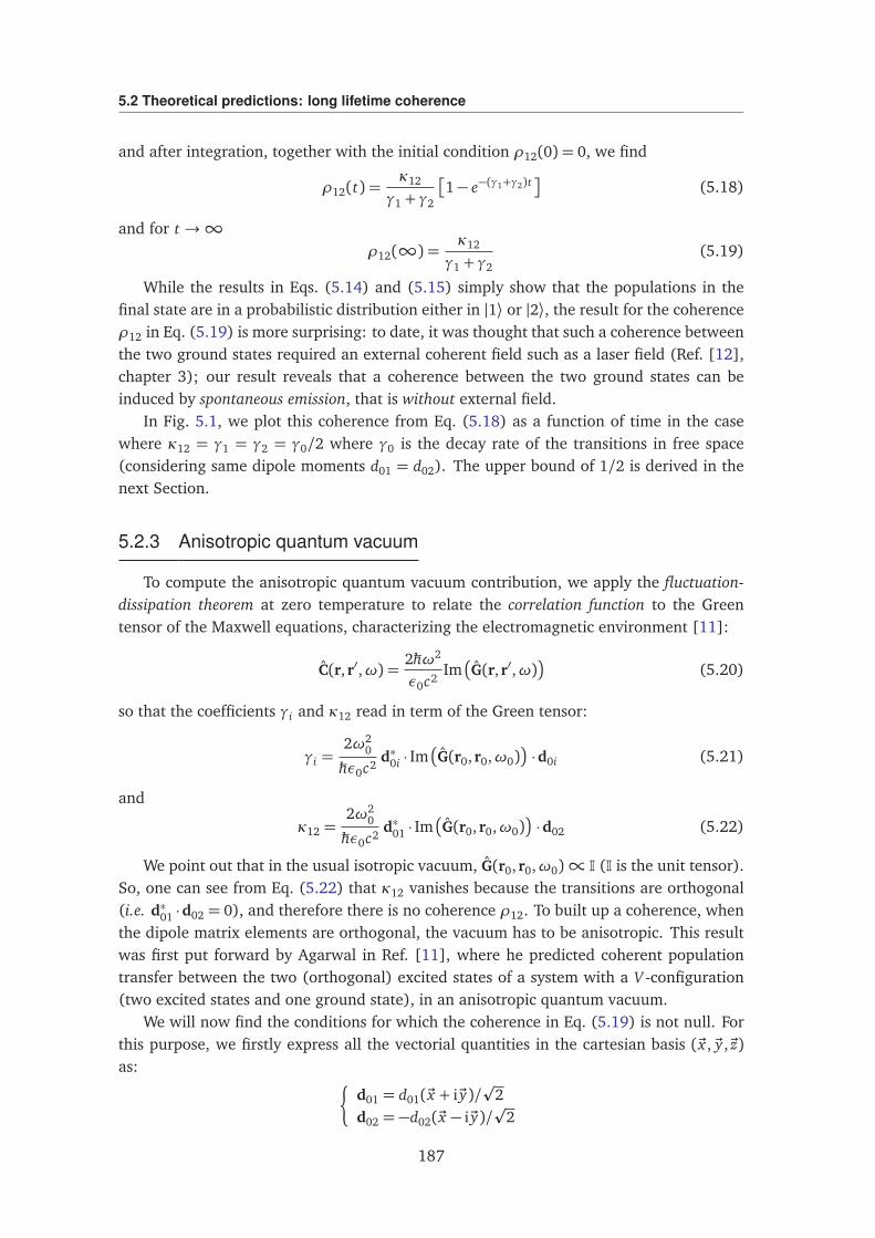
5.2 Theoretical predictions: long lifetime coherence

and after integration, together with the initial condition ρ12(0) = 0, we find

ρ12(t) =κ12

γ1 + γ2

1− e−(γ1+γ2)t

(5.18)

and for t →∞ρ12(∞) =

κ12

γ1 + γ2(5.19)

While the results in Eqs. (5.14) and (5.15) simply show that the populations in thefinal state are in a probabilistic distribution either in |1⟩ or |2⟩, the result for the coherenceρ12 in Eq. (5.19) is more surprising: to date, it was thought that such a coherence betweenthe two ground states required an external coherent field such as a laser field (Ref. [12],chapter 3); our result reveals that a coherence between the two ground states can beinduced by spontaneous emission, that is without external field.

In Fig. 5.1, we plot this coherence from Eq. (5.18) as a function of time in the casewhere κ12 = γ1 = γ2 = γ0/2 where γ0 is the decay rate of the transitions in free space(considering same dipole moments d01 = d02). The upper bound of 1/2 is derived in thenext Section.

5.2.3 Anisotropic quantum vacuum

To compute the anisotropic quantum vacuum contribution, we apply the fluctuation-dissipation theorem at zero temperature to relate the correlation function to the Greentensor of the Maxwell equations, characterizing the electromagnetic environment [11]:

C(r, r′,ω) =2ħhω2

ε0c2Im

G(r, r′,ω)

(5.20)

so that the coefficients γi and κ12 read in term of the Green tensor:

γi =2ω2

0

ħhε0c2d∗0i · Im

G(r0, r0,ω0)

·d0i (5.21)

and

κ12 =2ω2

0

ħhε0c2d∗01 · Im

G(r0, r0,ω0)

·d02 (5.22)

We point out that in the usual isotropic vacuum, G(r0, r0,ω0)∝ I (I is the unit tensor).So, one can see from Eq. (5.22) that κ12 vanishes because the transitions are orthogonal(i.e. d∗01 ·d02 = 0), and therefore there is no coherence ρ12. To built up a coherence, whenthe dipole matrix elements are orthogonal, the vacuum has to be anisotropic. This resultwas first put forward by Agarwal in Ref. [11], where he predicted coherent populationtransfer between the two (orthogonal) excited states of a system with a V -configuration(two excited states and one ground state), in an anisotropic quantum vacuum.

We will now find the conditions for which the coherence in Eq. (5.19) is not null. Forthis purpose, we firstly express all the vectorial quantities in the cartesian basis (~x , ~y , ~z)as:

d01 = d01(~x + i~y)/p

2d02 = −d02(~x − i~y)/

p2

187

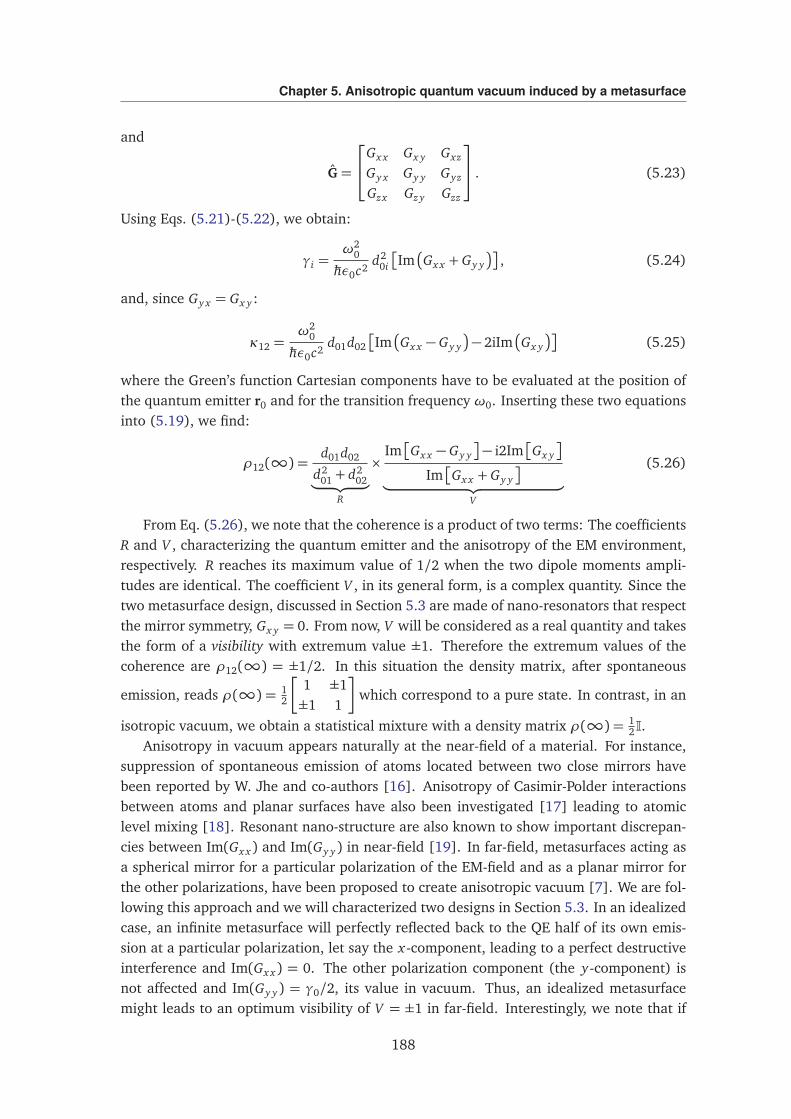
Chapter 5. Anisotropic quantum vacuum induced by a metasurface

and

G=

Gx x Gx y Gxz

Gy x Gy y Gyz

Gzx Gz y Gzz

. (5.23)

Using Eqs. (5.21)-(5.22), we obtain:

γi =ω2

0

ħhε0c2d2

0i

Im

Gx x + Gy y

, (5.24)

and, since Gy x = Gx y :

κ12 =ω2

0

ħhε0c2d01d02

Im

Gx x − Gy y

− 2iIm

Gx y

(5.25)

where the Green’s function Cartesian components have to be evaluated at the position ofthe quantum emitter r0 and for the transition frequency ω0. Inserting these two equationsinto (5.19), we find:

ρ12(∞) =d01d02

d201 + d2

02︸ ︷︷ ︸

R

×Im

Gx x − Gy y

− i2Im

Gx y

Im

Gx x + Gy y

︸ ︷︷ ︸

V

(5.26)

From Eq. (5.26), we note that the coherence is a product of two terms: The coefficientsR and V , characterizing the quantum emitter and the anisotropy of the EM environment,respectively. R reaches its maximum value of 1/2 when the two dipole moments ampli-tudes are identical. The coefficient V , in its general form, is a complex quantity. Since thetwo metasurface design, discussed in Section 5.3 are made of nano-resonators that respectthe mirror symmetry, Gx y = 0. From now, V will be considered as a real quantity and takesthe form of a visibility with extremum value ±1. Therefore the extremum values of thecoherence are ρ12(∞) = ±1/2. In this situation the density matrix, after spontaneous

emission, reads ρ(∞) = 12

1 ±1±1 1

which correspond to a pure state. In contrast, in an

isotropic vacuum, we obtain a statistical mixture with a density matrix ρ(∞) = 12I.

Anisotropy in vacuum appears naturally at the near-field of a material. For instance,suppression of spontaneous emission of atoms located between two close mirrors havebeen reported by W. Jhe and co-authors [16]. Anisotropy of Casimir-Polder interactionsbetween atoms and planar surfaces have also been investigated [17] leading to atomiclevel mixing [18]. Resonant nano-structure are also known to show important discrepan-cies between Im(Gx x) and Im(Gy y) in near-field [19]. In far-field, metasurfaces acting asa spherical mirror for a particular polarization of the EM-field and as a planar mirror forthe other polarizations, have been proposed to create anisotropic vacuum [7]. We are fol-lowing this approach and we will characterized two designs in Section 5.3. In an idealizedcase, an infinite metasurface will perfectly reflected back to the QE half of its own emis-sion at a particular polarization, let say the x-component, leading to a perfect destructiveinterference and Im(Gx x) = 0. The other polarization component (the y-component) isnot affected and Im(Gy y) = γ0/2, its value in vacuum. Thus, an idealized metasurfacemight leads to an optimum visibility of V = ±1 in far-field. Interestingly, we note that if

188

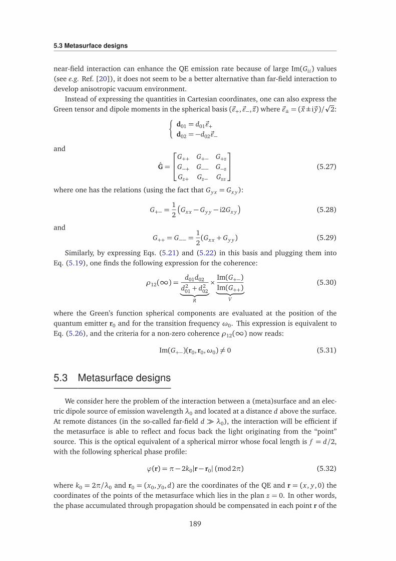
5.3 Metasurface designs

near-field interaction can enhance the QE emission rate because of large Im(Gii) values(see e.g. Ref. [20]), it does not seem to be a better alternative than far-field interaction todevelop anisotropic vacuum environment.

Instead of expressing the quantities in Cartesian coordinates, one can also express theGreen tensor and dipole moments in the spherical basis (~ε+, ~ε−, ~z) where ~ε± = (~x± i~y)/

p2:

d01 = d01~ε+d02 = −d02~ε−

and

G=

G++ G+− G+z

G−+ G−− G−z

Gz+ Gz− Gzz

(5.27)

where one has the relations (using the fact that Gy x = Gx y):

G+− =12

Gx x − Gy y − i2Gx y

(5.28)

andG++ = G−− =

12(Gx x + Gy y) (5.29)

Similarly, by expressing Eqs. (5.21) and (5.22) in this basis and plugging them intoEq. (5.19), one finds the following expression for the coherence:

ρ12(∞) =d01d02

d201 + d2

02︸ ︷︷ ︸

R

×Im(G+−)Im(G++)︸ ︷︷ ︸

V

(5.30)

where the Green’s function spherical components are evaluated at the position of thequantum emitter r0 and for the transition frequency ω0. This expression is equivalent toEq. (5.26), and the criteria for a non-zero coherence ρ12(∞) now reads:

Im(G+−)(r0, r0,ω0) 6= 0 (5.31)

5.3 Metasurface designs

We consider here the problem of the interaction between a (meta)surface and an elec-tric dipole source of emission wavelength λ0 and located at a distance d above the surface.At remote distances (in the so-called far-field d λ0), the interaction will be efficient ifthe metasurface is able to reflect and focus back the light originating from the “point”source. This is the optical equivalent of a spherical mirror whose focal length is f = d/2,with the following spherical phase profile:

ϕ(r) = π− 2k0|r− r0| (mod2π) (5.32)

where k0 = 2π/λ0 and r0 = (x0, y0, d) are the coordinates of the QE and r = (x , y , 0) thecoordinates of the points of the metasurface which lies in the plan z = 0. In other words,the phase accumulated through propagation should be compensated in each point r of the

189

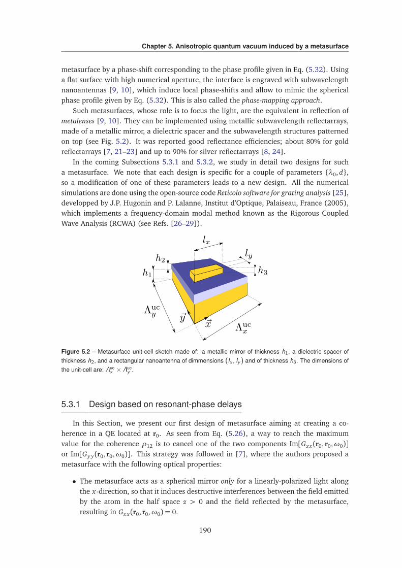
Chapter 5. Anisotropic quantum vacuum induced by a metasurface

metasurface by a phase-shift corresponding to the phase profile given in Eq. (5.32). Usinga flat surface with high numerical aperture, the interface is engraved with subwavelengthnanoantennas [9, 10], which induce local phase-shifts and allow to mimic the sphericalphase profile given by Eq. (5.32). This is also called the phase-mapping approach.

Such metasurfaces, whose role is to focus the light, are the equivalent in reflection ofmetalenses [9, 10]. They can be implemented using metallic subwavelength reflectarrays,made of a metallic mirror, a dielectric spacer and the subwavelength structures patternedon top (see Fig. 5.2). It was reported good reflectance efficiencies; about 80% for goldreflectarrays [7, 21–23] and up to 90% for silver reflectarrays [8, 24].

In the coming Subsections 5.3.1 and 5.3.2, we study in detail two designs for sucha metasurface. We note that each design is specific for a couple of parameters λ0, d,so a modification of one of these parameters leads to a new design. All the numericalsimulations are done using the open-source code Reticolo software for grating analysis [25],developped by J.P. Hugonin and P. Lalanne, Institut d’Optique, Palaiseau, France (2005),which implements a frequency-domain modal method known as the Rigorous CoupledWave Analysis (RCWA) (see Refs. [26–29]).

Figure 5.2 – Metasurface unit-cell sketch made of: a metallic mirror of thickness h1, a dielectric spacer ofthickness h2, and a rectangular nanoantenna of dimmensions (lx , ly ) and of thickness h3. The dimensions ofthe unit-cell are: Λuc

x × Λucy .

5.3.1 Design based on resonant-phase delays

In this Section, we present our first design of metasurface aiming at creating a co-herence in a QE located at r0. As seen from Eq. (5.26), a way to reach the maximumvalue for the coherence ρ12 is to cancel one of the two components Im[Gx x(r0, r0,ω0)]or Im[Gy y(r0, r0,ω0)]. This strategy was followed in [7], where the authors proposed ametasurface with the following optical properties:

• The metasurface acts as a spherical mirror only for a linearly-polarized light alongthe x-direction, so that it induces destructive interferences between the field emittedby the atom in the half space z > 0 and the field reflected by the metasurface,resulting in Gx x(r0, r0,ω0) = 0.

190

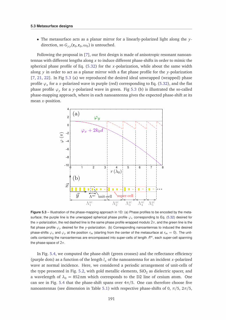
5.3 Metasurface designs

• The metasurface acts as a planar mirror for a linearly-polarized light along the y-direction, so Gy y(r0, r0,ω0) is untouched.

Following the proposal in [7], our first design is made of anisotropic resonant nanoan-tennas with different lengths along x to induce different phase-shifts in order to mimic thespherical phase profile of Eq. (5.32) for the x-polarization, while about the same widthalong y in order to act as a planar mirror with a flat phase profile for the y-polarization[7, 21, 22]. In Fig 5.3 (a) we reproduced the desired ideal unwrapped (wrapped) phaseprofile ϕx for a x-polarized wave in purple (red) corresponding to Eq. (5.32), and the flatphase profile ϕy for a y-polarized wave in green. Fig 5.3 (b) is illustrated the so-calledphase-mapping approach, where in each nanoantenna gives the expected phase-shift at itsmean x-position.

−10

−8

−6

−4

−2

0

2

4

0 1 2 3 4 5 6 7 8

Figure 5.3 – Illustration of the phase-mapping approach in 1D: (a) Phase profiles to be encoded by the meta-surface; the purple line is the unwrapped spherical phase profile ϕx corresponding to Eq. (5.32) desired forthe x -polarization, the red dashed line is the same phase profile wrapped modulo 2π, and the green line is theflat phase profile ϕy desired for the y -polarization. (b) Corresponding nanoantennas to induced the desiredphase-shifts ϕx and ϕy at the position rm (starting from the center of the metasurface at rm = 0). The unit-cells containing the nanoantennas are encompassed into super-cells of length Λsc, each super-cell spanningthe phase-space of 2π.

In Fig. 5.4, we computed the phase-shift (green crosses) and the reflectance efficiency(purple dots) as a function of the length lx of the nanoantenna for an incident x-polarizedwave at normal incidence. Here, we considered a periodic arrangement of unit-cells ofthe type presented in Fig. 5.2, with gold metallic elements, SiO2 as dielectric spacer, anda wavelength of λ0 = 852nm which corresponds to the D2 line of cesium atom. Onecan see in Fig. 5.4 that the phase-shift spans over 4π/5. One can therefore choose fivenanoantennas (see dimension in Table 5.1) with respective phase-shifts of 0, π/5, 2π/5,

191

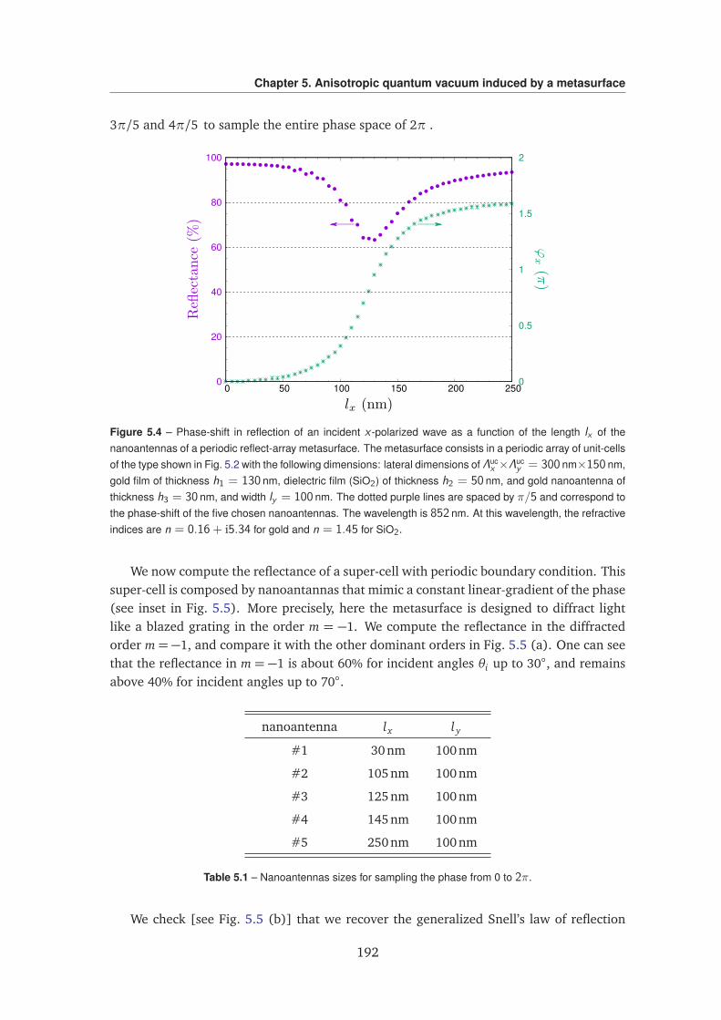
Chapter 5. Anisotropic quantum vacuum induced by a metasurface

3π/5 and 4π/5 to sample the entire phase space of 2π .

0

20

40

60

80

100

0 50 100 150 200 2500

0.5

1

1.5

2

Figure 5.4 – Phase-shift in reflection of an incident x -polarized wave as a function of the length lx of thenanoantennas of a periodic reflect-array metasurface. The metasurface consists in a periodic array of unit-cellsof the type shown in Fig. 5.2 with the following dimensions: lateral dimensions of Λuc

x ×Λucy = 300 nm×150 nm,

gold film of thickness h1 = 130 nm, dielectric film (SiO2) of thickness h2 = 50 nm, and gold nanoantenna ofthickness h3 = 30 nm, and width ly = 100 nm. The dotted purple lines are spaced by π/5 and correspond tothe phase-shift of the five chosen nanoantennas. The wavelength is 852 nm. At this wavelength, the refractiveindices are n = 0.16 + i5.34 for gold and n = 1.45 for SiO2.

We now compute the reflectance of a super-cell with periodic boundary condition. Thissuper-cell is composed by nanoantannas that mimic a constant linear-gradient of the phase(see inset in Fig. 5.5). More precisely, here the metasurface is designed to diffract lightlike a blazed grating in the order m = −1. We compute the reflectance in the diffractedorder m= −1, and compare it with the other dominant orders in Fig. 5.5 (a). One can seethat the reflectance in m = −1 is about 60% for incident angles θi up to 30, and remainsabove 40% for incident angles up to 70.

nanoantenna lx l y

#1 30nm 100nm

#2 105nm 100nm

#3 125nm 100nm

#4 145nm 100nm

#5 250nm 100nm

Table 5.1 – Nanoantennas sizes for sampling the phase from 0 to 2π.

We check [see Fig. 5.5 (b)] that we recover the generalized Snell’s law of reflection

192

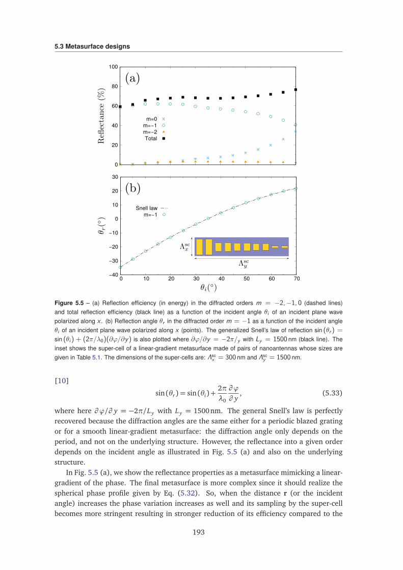
5.3 Metasurface designs

−40

−30

−20

−10

0

10

20

30

0 10 20 30 40 50 60 70

Snell lawm=−1

0

20

40

60

80

100

0 10 20 30 40 50 60 70

m=0m=−1m=−2Total

Figure 5.5 – (a) Reflection efficiency (in energy) in the diffracted orders m = −2,−1, 0 (dashed lines)and total reflection efficiency (black line) as a function of the incident angle θi of an incident plane wavepolarized along x . (b) Reflection angle θr in the diffracted order m = −1 as a function of the incident angleθi of an incident plane wave polarized along x (points). The generalized Snell’s law of reflection sin (θr ) =

sin (θi ) + (2π/λ0)(∂ϕ/∂y) is also plotted where ∂ϕ/∂y = −2π/y with Ly = 1500 nm (black line). Theinset shows the super-cell of a linear-gradient metasurface made of pairs of nanoantennas whose sizes aregiven in Table 5.1. The dimensions of the super-cells are: Λsc

x = 300 nm and Λscy = 1500 nm.

[10]

sin (θr) = sin (θi) +2πλ0

∂ ϕ

∂ y, (5.33)

where here ∂ ϕ/∂ y = −2π/L y with L y = 1500nm. The general Snell’s law is perfectlyrecovered because the diffraction angles are the same either for a periodic blazed gratingor for a smooth linear-gradient metasurface: the diffraction angle only depends on theperiod, and not on the underlying structure. However, the reflectance into a given orderdepends on the incident angle as illustrated in Fig. 5.5 (a) and also on the underlyingstructure.

In Fig. 5.5 (a), we show the reflectance properties as a metasurface mimicking a linear-gradient of the phase. The final metasurface is more complex since it should realize thespherical phase profile given by Eq. (5.32). So, when the distance r (or the incidentangle) increases the phase variation increases as well and its sampling by the super-cellbecomes more stringent resulting in stronger reduction of its efficiency compared to the

193

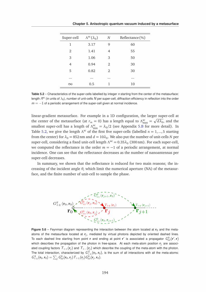
Chapter 5. Anisotropic quantum vacuum induced by a metasurface

Super-cell Λsc (λ0) N Reflectance (%)

1 3.17 9 60

2 1.41 4 55

3 1.06 3 50

4 0.94 2 30

5 0.82 2 30

... ... ... ...

∞ 0.5 1 10

Table 5.2 – Characteristics of the super-cells labelled by integer n starting from the center of the metasurface:length Λsc (in units of λ0), number of unit-cells N per super-cell, diffraction efficiency in reflection into the orderm = −1 of a periodic arrangement of the super-cell given at normal incidence.

linear-gradient metasurface. For example in a 1D configuration, the larger super-cell atthe center of the metasurface (at rm = 0) has a length equal to Λsc

max =p

dλ0, and thesmallest super-cell has a length of Λsc

min = λ0/2 (see Appendix 5.B for more detail). InTable 5.2, we give the length Λsc of the first five super-cells (labelled n = 1, ..., 5 startingfrom the center) for λ0 = 852nm and d = 10λ0. We also put the number of unit-cells N persuper-cell, considering a fixed unit-cell length Λuc = 0.35λ0 (300nm). For each super-cell,we computed the reflectance in the order m = −1 of a periodic arrangement, at normalincidence. One can see that the reflectance decreases as the number of nanoantennas persuper-cell decreases.

In summary, we shown that the reflectance is reduced for two main reasons; the in-creasing of the incident angle θi which limit the numerical aperture (NA) of the metasur-face, and the finite number of unit-cell to sample the phase.

Figure 5.6 – Feynman diagram representing the interaction between the atom located at r0 and the meta-atoms of the metasurface located at rj , mediated by virtual photons depicted by oriented dashed lines.To each dashed line starting from point r and ending at point r′ is associated a propagator G 0

zz(r′, r)

which describes the propagation of the photon in free-space. At each meta-atom position rj are associ-ated coupling factors T++(rj) and T+−(rj) which describe the coupling of the meta-atom with the photon.The total interaction, characterized by GS

+±(r0, r0), is the sum of all interactions with all the meta-atoms:GS+±(r0, r0) =

∑j G 0

zz(r0, rj)T+±(rj)G 0zz(rj , r0).

194

5.3 Metasurface designs

5.3.2 Design based on geometric-phases

The second design is based on a geometric Pancharatnam–Berry phase rotation assuggested in Ref. [8]. Here, the design is made of an unique nanoantenna with a position-dependent orientation.

The design should be such that Re[V ] in Eq. (5.30) is maximum (in absolute value).We then write G as a free-space contribution G0 plus a “scattered” contribution GS due tothe metasurface so that the components G++ and G+− in Eq. (5.30) can be written as:

G++ = G0++ + GS

++ (5.34)

G+− = G0+− + GS

+− = GS+− (5.35)

Eq. (5.35) simplifies because the free-space components G0+− = 0. Moreover, G0

++ = G0−− =

G0zz and in the following we replace G0

++ and G0−− by G0

zz. According to Eq. (5.30, Re[V ] ismaximal if the following criteria are fulfilled:

(i) GS++(r0, r0,ω0) = 0

(ii) GS+−(r0, r0,ω0) is maximum.

Using a T-Matrix-like formalism [30], one can write GS in the form [31, 32]:

GS = G0 T G0 (5.36)

where T ≡∑

j T ( j) and T ( j) is the T-Matrix describing the field scattered by the nanoan-tenna j. Moreover, we suppose that the spacing between nanoantennas is large enough sothat they are not coupled (single scattering approximation) [9]. In the position represen-tation, GS reads (dropping the variable ω0 for concision):

GS(r0, r0) =∑

j

G0(r0, r j)T (r j)G0(r j , r0) (5.37)

In Fig. 5.6 we give a representation of Eq. (5.37) using a Feynman diagram. Such arepresentation allows us to reinterpret the conditions that will satisfy the criteria (i) and(ii). The criteria (i) is achieved when T++(r j) is null for each point r j:

|T++(r j)|= 0 ∀ j (5.38)

where T++ is the component ++ of the T-Matrix in the spherical basis. The criteria (ii) isachieved when the coupling T+−(r j) is maximum (that is |T+−(r j)|maximum). In addition,the following phase condition should be satisfied:

arg[G0zz(r0, r j)] + arg[T+−(r j)] + arg[G0

zz(r j , r0)] = 2π, (5.39)

so that the contributions of all nanoantennas add-on constructively. T+− is the component+− of the T-Matrix in the spherical basis. In the far-field approximation, we expand thefree-space Green function so that:

arg

G0zz(r0, r j)

= arg

G0zz(r j , r0)

' k0|r0 − r j| . (5.40)

195

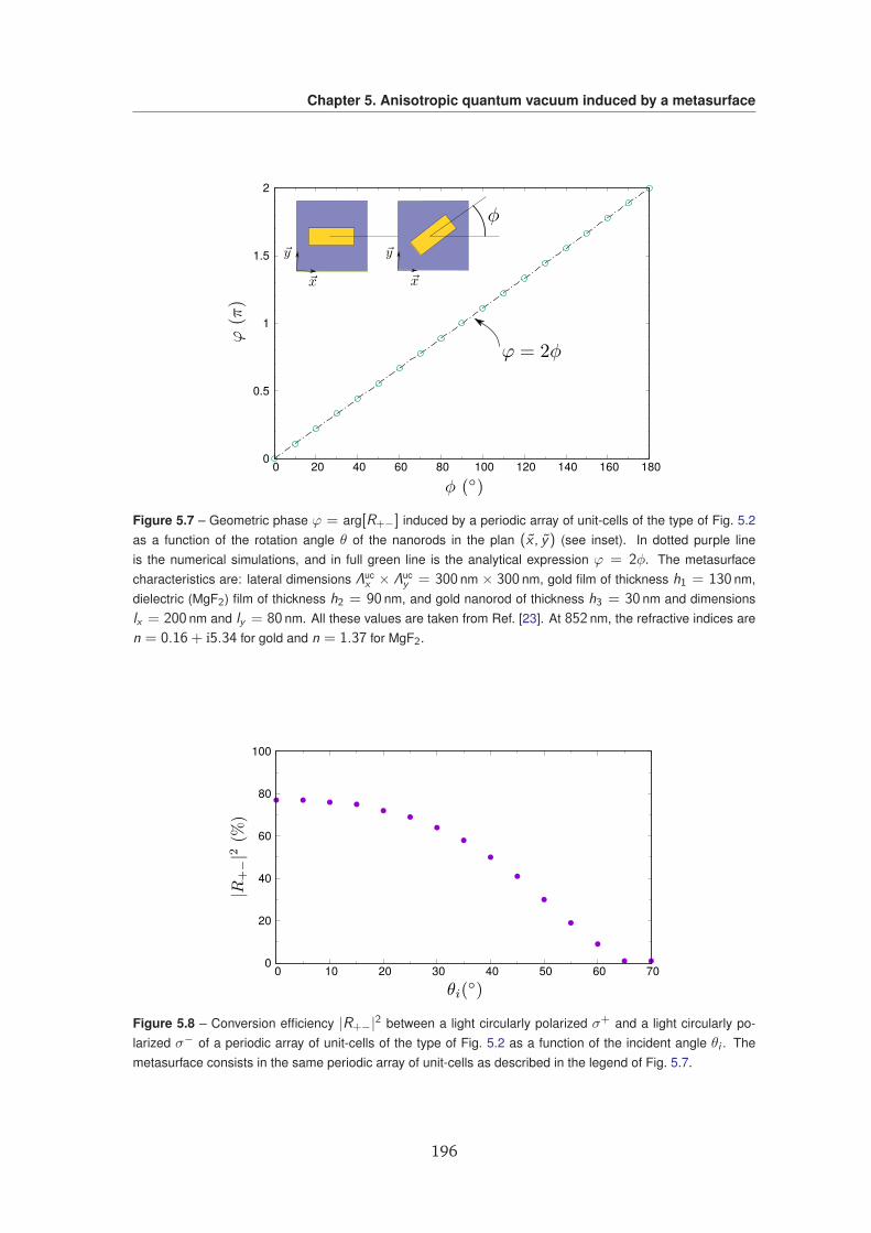
Chapter 5. Anisotropic quantum vacuum induced by a metasurface

0

0.5

1

1.5

2

0 20 40 60 80 100 120 140 160 180

Figure 5.7 – Geometric phase ϕ = arg[R+−] induced by a periodic array of unit-cells of the type of Fig. 5.2as a function of the rotation angle θ of the nanorods in the plan (x , y) (see inset). In dotted purple lineis the numerical simulations, and in full green line is the analytical expression ϕ = 2φ. The metasurfacecharacteristics are: lateral dimensions Λuc

x × Λucy = 300 nm × 300 nm, gold film of thickness h1 = 130 nm,

dielectric (MgF2) film of thickness h2 = 90 nm, and gold nanorod of thickness h3 = 30 nm and dimensionslx = 200 nm and ly = 80 nm. All these values are taken from Ref. [23]. At 852 nm, the refractive indices aren = 0.16 + i5.34 for gold and n = 1.37 for MgF2.

0

20

40

60

80

100

0 10 20 30 40 50 60 70

Figure 5.8 – Conversion efficiency |R+−|2 between a light circularly polarized σ+ and a light circularly po-larized σ− of a periodic array of unit-cells of the type of Fig. 5.2 as a function of the incident angle θi . Themetasurface consists in the same periodic array of unit-cells as described in the legend of Fig. 5.7.

196

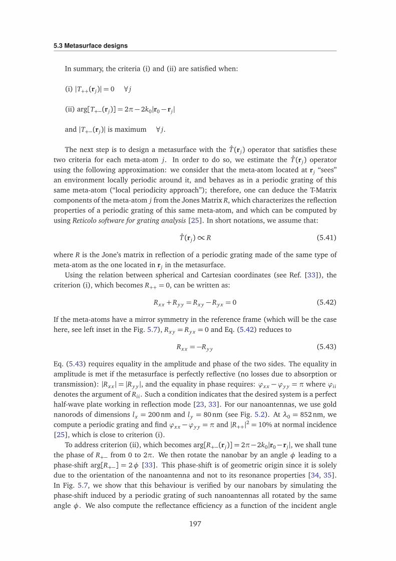
5.3 Metasurface designs

In summary, the criteria (i) and (ii) are satisfied when:

(i) |T++(r j)|= 0 ∀ j

(ii) arg[T+−(r j)] = 2π− 2k0|r0 − r j|

and |T+−(r j)| is maximum ∀ j.

The next step is to design a metasurface with the T (r j) operator that satisfies thesetwo criteria for each meta-atom j. In order to do so, we estimate the T (r j) operatorusing the following approximation: we consider that the meta-atom located at r j “sees”an environment locally periodic around it, and behaves as in a periodic grating of thissame meta-atom (“local periodicity approach”); therefore, one can deduce the T-Matrixcomponents of the meta-atom j from the Jones Matrix R, which characterizes the reflectionproperties of a periodic grating of this same meta-atom, and which can be computed byusing Reticolo software for grating analysis [25]. In short notations, we assume that:

T (r j)∝ R (5.41)

where R is the Jone’s matrix in reflection of a periodic grating made of the same type ofmeta-atom as the one located in r j in the metasurface.

Using the relation between spherical and Cartesian coordinates (see Ref. [33]), thecriterion (i), which becomes R++ = 0, can be written as:

Rx x + R y y = Rx y − R y x = 0 (5.42)

If the meta-atoms have a mirror symmetry in the reference frame (which will be the casehere, see left inset in the Fig. 5.7), Rx y = R y x = 0 and Eq. (5.42) reduces to

Rx x = −R y y (5.43)

Eq. (5.43) requires equality in the amplitude and phase of the two sides. The equality inamplitude is met if the metasurface is perfectly reflective (no losses due to absorption ortransmission): |Rx x | = |R y y |, and the equality in phase requires: ϕx x −ϕy y = π where ϕii

denotes the argument of Rii. Such a condition indicates that the desired system is a perfecthalf-wave plate working in reflection mode [23, 33]. For our nanoantennas, we use goldnanorods of dimensions lx = 200nm and l y = 80nm (see Fig. 5.2). At λ0 = 852nm, wecompute a periodic grating and find ϕx x −ϕy y = π and |R++|2 = 10% at normal incidence[25], which is close to criterion (i).

To address criterion (ii), which becomes arg[R+−(r j)] = 2π−2k0|r0− r j|, we shall tunethe phase of R+− from 0 to 2π. We then rotate the nanobar by an angle φ leading to aphase-shift arg[R+−] = 2φ [33]. This phase-shift is of geometric origin since it is solelydue to the orientation of the nanoantenna and not to its resonance properties [34, 35].In Fig. 5.7, we show that this behaviour is verified by our nanobars by simulating thephase-shift induced by a periodic grating of such nanoantennas all rotated by the sameangle φ. We also compute the reflectance efficiency as a function of the incident angle

197

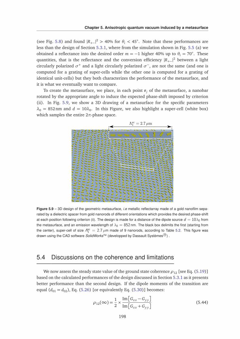
Chapter 5. Anisotropic quantum vacuum induced by a metasurface

(see Fig. 5.8) and found |R+−|2 > 40% for θi < 45. Note that these performances areless than the design of Section 5.3.1, where from the simulation shown in Fig. 5.5 (a) weobtained a reflectance into the desired order m = −1 higher 40% up to θi = 70. Thesequantities, that is the reflectance and the conversion efficiency |R+−|2 between a lightcircularly polarized σ+ and a light circularly polarized σ−, are not the same (and one iscomputed for a grating of super-cells while the other one is computed for a grating ofidentical unit-cells) but they both characterizes the performance of the metasurface, andit is what we eventually want to compare.

To create the metasurface, we place, in each point r j of the metasurface, a nanobarrotated by the appropriate angle to induce the expected phase-shift imposed by criterion(ii). In Fig. 5.9, we show a 3D drawing of a metasurface for the specific parametersλ0 = 852nm and d = 10λ0. In this Figure, we also highlight a super-cell (white box)which samples the entire 2π-phase space.

Figure 5.9 – 3D design of the geometric metasurface, i.e metallic reflectarray made of a gold nanofilm sepa-rated by a dielectric spacer from gold nanorods of different orientations which provides the desired phase-shiftat each position following criterion (ii). The design is made for a distance of the dipole source d = 10λ0 fromthe metasurface, and an emission wavelength of λ0 = 852 nm. The black box delimits the first (starting fromthe center), super-cell of size Λsc

1 = 2.7µm made of 9 nanorods, according to Table 5.2. This figure wasdrawn using the CAD software SolidWorksTM (developped by Dassault Systèmes R©) .

5.4 Discussions on the coherence and limitations

We now assess the steady state value of the ground state coherence ρ12 [see Eq. (5.19)]based on the calculated performances of the design discussed in Section 5.3.1 as it presentsbetter performance than the second design. If the dipole moments of the transition areequal (d01 = d02), Eq. (5.26) [or equivalently Eq. (5.30)] becomes:

ρ12(∞) =12×

Im

Gx x − Gy y

Im

Gx x + Gy y

(5.44)

198

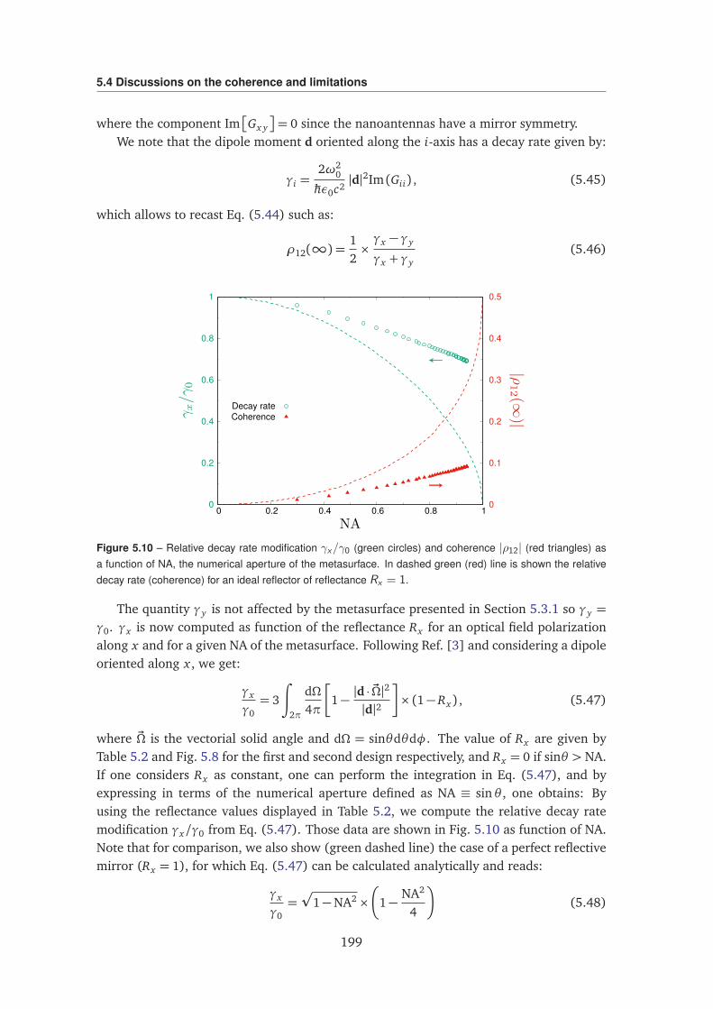
5.4 Discussions on the coherence and limitations

where the component Im

Gx y

= 0 since the nanoantennas have a mirror symmetry.We note that the dipole moment d oriented along the i-axis has a decay rate given by:

γi =2ω2

0

ħhε0c2|d|2Im (Gii) , (5.45)

which allows to recast Eq. (5.44) such as:

ρ12(∞) =12×γx − γy

γx + γy(5.46)

0

0.2

0.4

0.6

0.8

1

0 0.2 0.4 0.6 0.8 1 0

0.1

0.2

0.3

0.4

0.5

Decay rateCoherence

Figure 5.10 – Relative decay rate modification γx/γ0 (green circles) and coherence |ρ12| (red triangles) asa function of NA, the numerical aperture of the metasurface. In dashed green (red) line is shown the relativedecay rate (coherence) for an ideal reflector of reflectance Rx = 1.

The quantity γy is not affected by the metasurface presented in Section 5.3.1 so γy =γ0. γx is now computed as function of the reflectance Rx for an optical field polarizationalong x and for a given NA of the metasurface. Following Ref. [3] and considering a dipoleoriented along x , we get:

γx

γ0= 3

∫

2π

dΩ4π

1−|d · ~Ω|2

|d|2

× (1− Rx) , (5.47)

where ~Ω is the vectorial solid angle and dΩ = sinθdθdφ. The value of Rx are given byTable 5.2 and Fig. 5.8 for the first and second design respectively, and Rx = 0 if sinθ > NA.If one considers Rx as constant, one can perform the integration in Eq. (5.47), and byexpressing in terms of the numerical aperture defined as NA ≡ sinθ , one obtains: Byusing the reflectance values displayed in Table 5.2, we compute the relative decay ratemodification γx/γ0 from Eq. (5.47). Those data are shown in Fig. 5.10 as function of NA.Note that for comparison, we also show (green dashed line) the case of a perfect reflectivemirror (Rx = 1), for which Eq. (5.47) can be calculated analytically and reads:

γx

γ0=p

1−NA2 ×

1−NA2

4

(5.48)

199

Chapter 5. Anisotropic quantum vacuum induced by a metasurface

For a metasurface of NA = 0.7, we get a reduction of the decay rate γx of 20% com-pared to γ0. We note that larger NA results in a very moderate improvement because ofthe rapid drop of the Reflectance. We finally plug the γx values into Eq. (5.46), and geta coherence ∼ 0.05 at NA= 0.7 (see Fig. 5.10). Similarly, we show the ideal case (reddashed line) when plugging Eq. (5.48) into Eq. (5.46). This value is about one order ofmagnitude smaller that the 0.5 value expected for a ideal reflector with NA= 1. Neverthe-less this coherence, which is a direct consequence of AQV, should be observable using thecurrent state-of-art NV-center experimental platform [13].

5.5 Conclusion

In this work, we predicted the creation of a long-lifetime coherence between thetwo ground states of a quantum emitter with a Λ-configuration, induced by a quantumanisotropic vacuum. We proposed two metasurface designs, based on two different ap-proaches, a resonant phase-delay approach and a geometric phase approach to create theanisotropic vacuum. We quantify the efficiency of such metasurfaces to redirect light onthe quantum emitter, located at macroscopic distances taking into account the limitationson the numerical aperture due to the phase-mapping approach. Based on the exact resultsavailable for a perfect spherical mirror, we estimate an redirection of the light of about20% at NA= 0.7, leading to a coherence of 0.05. Due to the in-principle infinite lifetime ofthe coherence, this system allows for high resolution experiments, which is necessary todetect the effect of the metasurface on the atom predicted here.

Detecting this coherence would be, to our knowledge, the first experimental demon-stration of the effect of the anisotropy of vacuum at remote distances on quantum emit-ters. In addition this experiment will be a new test of quantum electrodynamics, in acounter-intuitive regime where coherence is driven by relaxation processes and vacuumfluctuation. Such an experimental demonstration will also pave the way for controlledinteractions between several quantum emitters by the means of a metasurface [24, 36],which ultimately can be used to perform entanglement of the emitter for quantum tech-nology applications in a new paradigm.

200

5.A Derivation of the Master Equation

5.A Derivation of the Master Equation

In this Appendix, we present the Master Equation framework, closely followingRefs. [14] Chapter 5.6 and [15] Chapter 1, that we used to derive the master equation[Eq. (5.4)] in Section 5.2.

Short notations: It will be convenient for the following calculations to rewrite HI(t) ofEq. (5.2) in a more compact form:

HI(t) = d†(t) · E(+)v (t) + d(t) · E(−)v (t) (5.49)

where d(t) and d†(t) are defined by:

d(t)≡ −

d∗01 |1⟩ ⟨0| e−iω1 t + d∗02 |2⟩ ⟨0| e

−iω2 t

(5.50)

d†(t)≡ −

d01 |0⟩ ⟨1| eiω1 t + d02 |0⟩ ⟨2| eiω2 t

(5.51)

Note that for clarity we dropped the label r0 appearing in E(+)v (r0, t) and E(−)v (r0, t), but onemust remember that the fields are evaluated at the position of the atom r0. Remember thatthis Hamiltonian is written in the electric dipole and rotating-wave approximations.

In the interaction picture, the density matrix ρT (t) of the total system atom+environmentobeys the Schrödinger equation [14, 15]:

∂ ρT (t)∂ t

=1iħh[HI(t),ρT (t)] (5.52)

The atomic density matrix ρ(t) is obtained by taking the trace over the degrees of freedomof the environment: ρ(t) = Tre(ρT (t)), and therefore obeys:

∂ ρ(t)∂ t

=1iħh

Tre[HI(t),ρT (t)] (5.53)

We formally integrate Eq. (5.52):

ρT (t) = ρT (0) +1iħh

∫ t

0

dt ′ [HI(t′),ρT (t

′)] (5.54)

and substitute this expression in Eq. (5.53):

∂ ρ(t)∂ t

=1iħh

Tre[HI(t),ρT (0)]−1

ħh2

∫ t

0

dt ′ Tre

HI(t), [HI(t′),ρT (t

′)]

(5.55)

Approximations 1 and 2:

• We assume that the environment has a large number of degrees of freedom andtherefore is little changed by the coupling with the atom: therefore we write ρT (t) =ρ(t)⊗ ρe(0), where ρe(t) is the reduced density matrix of the environment (this iscalled the Born approximation).

• Moreover, we assume that Tre([HI(t),ρT (0)]) = 0, which is guaranteed since theelectric field operators E(+)v (r0, t) and E(−)v (r0, t) have zero mean in the vacuum state.

201

Chapter 5. Anisotropic quantum vacuum induced by a metasurface

Under these approximations, Eq. (5.55) reduces to:

∂ ρ(t)∂ t

= −1

ħh2

∫ t

0

dt ′ Tre

HI(t), [HI(t′),ρe(0)⊗ρ(t ′)]

(5.56)

Approximation 3: We make the Markov approximation and replace ρ(t ′) by ρ(t) in theintegrand.

Therefore, we get a Master Equation for the atomic density matrix ρ(t) in the Born-Markov approximation:

∂ ρ(t)∂ t

= −1

ħh2

∫ t

0

dt ′ Tre

HI(t), [HI(t′),ρe(0)⊗ρ(t)]

(5.57)

It is now time to write HI(t) explicitely and to expand the commutators. Using thecompact form Eq. (5.49) into Eq. (5.57) one gets:

∂ ρ(t)∂ t

=

−1

ħh2

∫ t

0

dt ′ Tre

d†(t) · E(+)v (t) + d(t) · E(−)v (t), [d†(t ′) · E(+)v (t

′) + d(t ′) · E(−)v (t′),ρe(0)⊗ρ(t)]

(5.58)

Expanding the commutators in Eq. (5.58) gives 16 terms. Noting that the trace only actson the field operators and on ρe(0), and using the cyclic property of the trace operationand the fact that for instance Tre

ρe(0))E(+)v (t)E(−)v (t

′)

=

E(+)v (t)E(−)v (t

′)

, we get

∂ ρ(t)∂ t

= −1

ħh2

∫ t

0

dt ′

E(+)v (t)E(−)v (t

′)

d†(t)d(t ′)ρ(t)− d(t ′)ρ(t)d†(t)

+

E(+)v (t′)E(−)v (t)

ρ(t)d†(t ′)d(t)− d(t)ρ(t)d†(t ′)

+

E(−)v (t)E(+)v (t

′)

d(t)d†(t ′)ρ(t)− d†(t ′)ρ(t)d(t)

+

E(−)v (t′)E(+)v (t)

ρ(t)d(t ′)d†(t)− d†(t)ρ(t)d(t ′)

+

E(+)v (t)E(+)v (t

′)

d†(t)d†(t ′)ρ(t)− d†(t ′)ρ(t)d†(t)

+

E(+)v (t′)E(+)v (t)

ρ(t)d†(t ′)d†(t)− d†(t)ρ(t)d†(t ′)

+

E(−)v (t)E(−)v (t

′)

d(t)d(t ′)ρ(t)− d(t ′)ρ(t)d(t)

+

E(−)v (t′)E(−)v (t)

ρ(t)d(t ′)d(t)− d(t)ρ(t)d(t ′)

(5.59)

Approximations 4 and 5:

• We assume that the correlation functions

E(+)v (t)E(+)v (t

′)

,

E(+)v (t′)E(+)v (t)

,

E(−)v (t)E(−)v (t

′)

and

E(−)v (t′)E(−)v (t)

are all null, which is justified if the electromagnetic environ-ment is in thermodynamic equilibrium.

• We also neglect the correlation functions

E(−)v (t)E(+)v (t

′)

and

E(−)v (t′)E(+)v (t)

,which is justified is one considers an atom emitting at optical frequencies.

202

5.A Derivation of the Master Equation

Thus, only the first 2 terms remain in Eq. (5.59) which reduces to

∂ ρ(t)∂ t

= −1

ħh2

∫ t

0

dt ′

E(+)v (t)E(−)v (t

′)

d†(t)d(t ′)ρ(t)− d(t ′)ρ(t)d†(t)

+

E(+)v (t′)E(−)v (t)

ρ(t)d†(t ′)d(t)− d(t)ρ(t)d†(t ′)

(5.60)

Note: By using the property of the correlation function

E(+)v (t′)E(−)v (t)

=

E(+)v (t)E(−)v (t

′)∗

,

and noting the fact that

ρ(t)d†(t ′)d(t)− d(t)ρ(t)d†(t ′)

=

d†(t)d(t ′)ρ(t)− d(t ′)ρ(t)d†(t)†

,one can see that the second term in Eq. (5.60) is actually the Hermitian conjugate (H.c.)of the first one. Therefore, we simply write Eq. (5.60) as

∂ ρ(t)∂ t

= −1

ħh2

∫ t

0

dt ′

E(+)v (t)E(−)v (t

′)

d†(t)d(t ′)ρ(t)− d(t ′)ρ(t)d†(t)

+H.c. (5.61)

Eq. (5.61) is the starting point to calculate the dynamical evolution of any multilevelatom. Here, we proceed by writing explicitely the terms in the integrand using the ex-pressions for d(t) and d†(t) from Eqs. (5.50) and (5.51), which corresponds to the Λ-configuration with orthogonal transitions:

d†(t)d(t ′)ρ(t) = eiω1(t−t ′)d01 |0⟩ ⟨0|d∗01ρ(t) + eiω2(t−t ′)d02 |0⟩ ⟨0|d∗02ρ(t) (5.62)

and by defining ρ00(t)≡ ⟨0|ρ(t) |0⟩ to simplify the expressions:

d(t ′)ρ(t)d†(t) = +eiω1(t−t ′)ρ00(t)d∗01 |1⟩ ⟨1|d01 + eiω2(t−t ′)ρ00(t)d

∗02 |2⟩ ⟨2|d02

+ eiω1 t e−iω2 t ′ρ00(t)d∗02 |2⟩ ⟨1|d01 + eiω2 t e−iω1 t ′ρ00(t)d

∗01 |1⟩ ⟨2|d02 (5.63)

Substituting these expressions in Eq. (5.61) and by factorizing the exponential terms,we get:

∂ ρ(t)∂ t

= −1

ħh2

∫ t

0

dt ′

E(+)v (t)E(−)v (t

′)

×[eiω1(t−t ′)

d01 |0⟩ ⟨0|d∗01ρ(t)−ρ00(t)d∗01 |1⟩ ⟨1|d01

+ eiω2(t−t ′)

d02 |0⟩ ⟨0|d∗02ρ(t)−ρ00(t)d∗02 |2⟩ ⟨2|d02

− eiω1 t e−iω2 t ′ρ00(t)d∗02 |2⟩ ⟨1|d01 − eiω2 t e−iω1 t ′ρ00(t)d

∗01 |1⟩ ⟨2|d02]

+H.c.

(5.64)

Change of variable:

E(+)v (t)E(−)v (t

′)

=

E(+)v (t − t ′)E(−)v (0)

(the correlation functiononly depends on the time difference). Making the change of variable τ= t − t ′, and:

Approximation 6: We make the upper limit tend to infinity. Eq. (5.64) becomes

∂ ρ(t)∂ t

= −1

ħh2

∫ ∞

0

dτ

E(+)v (τ)E(−)v (0)

× [eiω1τ

d01 |0⟩ ⟨0|d∗01ρ(t)−ρ00(t)d∗01 |1⟩ ⟨1|d01

+ eiω2τ

d02 |0⟩ ⟨0|d∗02ρ(t)−ρ00(t)d∗02 |2⟩ ⟨2|d02

− ei(ω1−ω2)t eiω2τρ00(t)d∗02 |2⟩ ⟨1|d01 − ei(ω2−ω1)t eiω1τρ00(t)d

∗01 |1⟩ ⟨2|d02]

+H.c.

(5.65)

203

Chapter 5. Anisotropic quantum vacuum induced by a metasurface

We finally introduce the positive part of the correlation tensor as:

C(+)(ω)≡∫ ∞

0

dτ

E(+)v (τ)E(−)v (0)

eiωτ (5.66)

to get:

∂ ρ(t)∂ t

= −Γ1 (|0⟩ ⟨0|ρ(t)−ρ00(t) |1⟩ ⟨1|)− Γ2 (|0⟩ ⟨0|ρ(t)−ρ00(t) |2⟩ ⟨2|)

+ Γ21ei(ω1−ω2)tρ00(t) |2⟩ ⟨1|+ Γ12ei(ω2−ω1)tρ00(t) |1⟩ ⟨2|+H.c.

(5.67)

with the following definitions of the coefficients:

Γi ≡1

ħh2 d∗0i · C(+)(ω1) ·d0i (5.68)

andΓi j ≡

1

ħh2 d∗0i · C(+)(ω1) ·d0 j (5.69)

Remember that in the Master Equation above ρ(t) is still in the interaction picture,and we come back to the Schrödinger picture assuming furthermore that the transitionenergies are about the same ω1 'ω2 ≡ω0

∂ ρ(t)∂ t

= −iω0 |0⟩ ⟨0|ρ(t)− Γ1 (|0⟩ ⟨0|ρ(t)−ρ00(t) |1⟩ ⟨1|)− Γ2 (|0⟩ ⟨0|ρ(t)−ρ00(t) |2⟩ ⟨2|)

+ Γ21ρ00(t) |2⟩ ⟨1|+ Γ12ρ00(t) |1⟩ ⟨2|+H.c.

(5.70)

In Eq. (5.70), we have introduced the definitions of the coefficients:

Γi ≡1

ħh2 d∗0i · C(+)(r0, r0,ω0) ·d0i (5.71)

andΓi j ≡

1

ħh2 d∗0i · C(+)(r0, r0,ω0) ·d0 j (5.72)

defined in terms of the positive part of the correlation tensor C(+) that reads:

C(+)(r, r′,ω) =

∫ +∞

0

dτ

E(+)v (r,τ)E(−)v (r′, 0)

eiωτ (5.73)

where the braket indicates an ensemble average:

E(+)v (r,τ)E(−)v (r′, 0)

≡ Tre

ρe(0)E(+)v (r,τ)E(−)v (r

′, 0)

(5.74)

Using the mathematical relation:

P

1x

=1

x + iε+ iπδ(x) with ε→ 0 (5.75)

204

5.A Derivation of the Master Equation

one can demonstrate that:

C(+)(r, r′,ω0) =12

C(r, r′,ω0) +i

2πP

∫ +∞

0

dωC(r, r′,ω)ω0 −ω

(5.76)

where C is the correlation tensor defined as:

C(r, r′,ω)≡∫ +∞

−∞dτ

E(+)v (r,τ)E(−)v (r′, 0)

eiωτ (5.77)

Therefore, the coefficients Γi become:

Γi =γi

2+ i∆ωi (5.78)

withγi =

1

ħh2 d∗0i · C(r0, r0,ω0) ·d0i (5.79)

and

∆ωi =1

2πħh2P

¨

∫ +∞

0

dωd∗0i · C(r0, r0,ω) ·d0i

ω0 −ω

«

(5.80)

where γi can be interpreted as the decay rate on the transition |0⟩ → |i⟩, and ∆ωi is theLamb shift of the level |i⟩.

In the following, we recast the Lamb shift into the transition frequency and reduceC(+)(r, r′,ω0) as:

C(+)(r, r′,ω0)≡12

C(r, r′,ω0) (5.81)

Therefore, the coefficients become:

Γi ≈γi

2with γi =

1

ħh2 d∗0i · C(r0, r0,ω0) ·d0i (5.82)

andΓi j ≈

κi j

2with κi j =

1

ħh2 d∗0i · C(r0, r0,ω0) ·d0 j . (5.83)

205

Chapter 5. Anisotropic quantum vacuum induced by a metasurface

5.B Metasurface design: super-cells

Here, we answer the following questions:

• Is there a minimum size for a super-cell (other than the practical limitation comingfrom the nanoantennas which have a finite size in practice, which will constraineven more the minimum size of a super-cell that one can design, as we will see inthe next section)?

• Is there a maximum size? For a given configuration (that is a point source at distanced from the metasurface), what super-cell sizes must be used to impart the desiredphase-shift? Where to place them on the metasurface?

To answer these questions, we derive the expression of the lengths of the super-cells as a function of the parameters d and λ0 in 1D. For that, let us first denote by rn

the position at which ends the super-cell labelled by n, starting from the center of themetasurface (n = 1 corresponds to the first super-cell, n = 2 corresponds to the secondsuper-cell etc...). This corresponds to the positions of the phase discontinuities of thered dashed curve in Fig. 5.3 (a). The positions rn are obtained by solving the followingequation:

|ϕx(rn)−ϕy(0)|= 2πn (5.84)

with ϕx(0) = π− 2k0d [see Eq. (5.32)]. A simple algebric calculation leads to the result:

rn =

√

√

√

n(λ0d) + n2

λ0

2

2

(5.85)

One can now deduce the length Λscn of a super-cell n. It simply reads:

Λscn = rn − rn−1 (5.86)

In Fig. 5.11, we show the length Λscn for the first 50 super-cells (green dots). One can see

that the length decreases monotically: the first super-cells have the larger sizes, and as nincreases the length of the super-cells dimishes.

Maximum and minimum lengths: One can derive approximate expressions for Λscn for

small n (that is for the first super-cells) and for large n (that is for the more distant super-cells). Indeed, in Eq. (5.85) one can see two terms: the first term is (λ0d), weighted by n,and the second term is (λ0/2)2, weighted by n2.

For small n, the second term can be neglected, because for the source distance d con-sidered here, (λ0d) (λ0/2)2 (d is several wavelengths, like d ∼ 10λ0). Then Eq. (5.85)can be approximated by:

rn 'Æ

n(λ0d) (5.87)

which leads to the following approximated length:

Λscn ' (

pn−p

n− 1)Æ

λ0d (5.88)

206

5.B Metasurface design: super-cells

This expression is shown in Fig. 5.11 (blue dashed line) and works well until n = 3 forthis specific case where d = 10λ0. Moreover, from this formula one can get the maximumlength of a super-cell, which is the length of the super-cell n= 1:

Λscmax =

Æ

λ0d (5.89)

For n large enough, the first term can be neglected and Eq. (5.85) can be approximatedby:

rn ' nλ0

2(5.90)

which leads to the following approximated length:

Λscn '

λ0

2(5.91)

This limit is shown in Fig. 5.11 (black dashed line) and one can see that the convergenceis fast. This formula therefore gives the minimum length of a super-cell

Λscmin =

λ0

2(5.92)

Note: It is noteworthy to point out that these 2 extreme quantities Λscmin and Λsc

maxcan be deduced from the grating equation for a Littrow configuration (where θr = θi, θi

incident angle, θr diffracted angle into the first order):

2Λ sinθi = λ0 (5.93)

with Λ the grating period. In the very limit of large incident angle θi = 90, one getsΛmin = λ0/2 for the grating period, and for the limit of very small incident angles, let’ssay when the light impinges on the edge of the first period of the grating θi ' (Λ/2)/d.Note that Λ/2 is because the grating is symmetric in 0 and the first period extends from[−Λ/2;+Λ/2]; moreover, it does not really make sense to consider smaller angle than thatas the light would not see any period and would be reflected specularly. One then getsΛmax =

p

λ0d.Example: Let us calculate the size of a metasurface we could fabricate. Let us consider

we use 40 super-cells. The extremity of the metasurface from the origin is therefore r40.For d = 10λ0 and λ0 = 852nm, this corresponds to r40 ' 24µm (which gives a metasurfaceof cross-section 48µm×48µm). This corresponds to a NA defined as NA= sinθi ' 0.94(that is an incident angle θi = 70). So in summary, for the configuration d = 10λ0 andλ0 = 852nm, a metasurface with a NA= 0.94 will have a cross-section 48µm×48µm, andwill be made of 40 different super-cells (differing by their length Λsc

n ), whose lengths varyfrom Λsc

min < Λscn < Λ

scmax, with Λsc

max =p

10λ0 ' 3.16λ0 ' 2.694µm, and Λscmin ' 0.426µm.

207

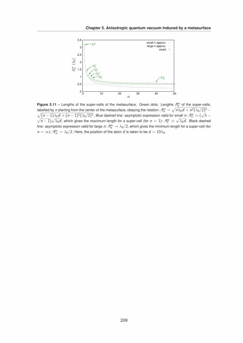
Chapter 5. Anisotropic quantum vacuum induced by a metasurface

0

0.5

1

1.5

2

2.5

3

3.5

0 10 20 30 40 50

small n approx.large n approx.

exact

Figure 5.11 – Lengths of the super-cells of the metasurface. Green dots: Lengths Λscn of the super-cells,

labelled by n starting from the center of the metasurface, obeying the relation: Λscn =

√nλ0d + n2(λ0/2)2−√

(n − 1)λ0d + (n − 1)2(λ0/2)2. Blue dashed line: asymptotic expression valid for small n: Λscn ' (

√n −√

n − 1)√λ0d , which gives the maximum length for a super-cell (for n = 1): Λsc

1 '√λ0d . Black dashed

line: asymptotic expression valid for large n: Λscn → λ0/2, which gives the minimum length for a super-cell (for

n =∞): Λsc∞ = λ0/2. Here, the position of the atom d is taken to be d = 10λ0.

208

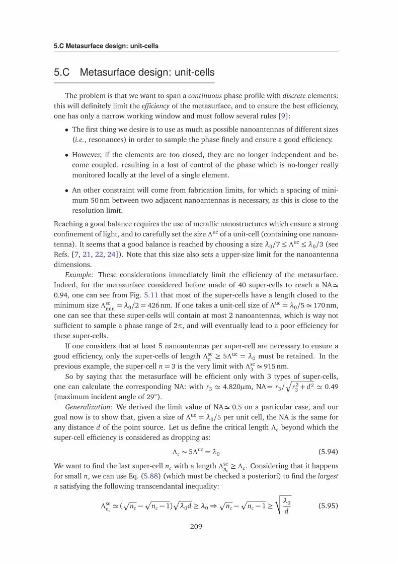
5.C Metasurface design: unit-cells

5.C Metasurface design: unit-cells

The problem is that we want to span a continuous phase profile with discrete elements:this will definitely limit the efficiency of the metasurface, and to ensure the best efficiency,one has only a narrow working window and must follow several rules [9]:

• The first thing we desire is to use as much as possible nanoantennas of different sizes(i.e., resonances) in order to sample the phase finely and ensure a good efficiency.

• However, if the elements are too closed, they are no longer independent and be-come coupled, resulting in a lost of control of the phase which is no-longer reallymonitored locally at the level of a single element.

• An other constraint will come from fabrication limits, for which a spacing of mini-mum 50nm between two adjacent nanoantennas is necessary, as this is close to theresolution limit.

Reaching a good balance requires the use of metallic nanostructures which ensure a strongconfinement of light, and to carefully set the size Λuc of a unit-cell (containing one nanoan-tenna). It seems that a good balance is reached by choosing a size λ0/7≤ Λuc ≤ λ0/3 (seeRefs. [7, 21, 22, 24]). Note that this size also sets a upper-size limit for the nanoantennadimensions.

Example: These considerations immediately limit the efficiency of the metasurface.Indeed, for the metasurface considered before made of 40 super-cells to reach a NA'0.94, one can see from Fig. 5.11 that most of the super-cells have a length closed to theminimum size Λsc

min = λ0/2= 426nm. If one takes a unit-cell size of Λuc = λ0/5' 170nm,one can see that these super-cells will contain at most 2 nanoantennas, which is way notsufficient to sample a phase range of 2π, and will eventually lead to a poor efficiency forthese super-cells.

If one considers that at least 5 nanoantennas per super-cell are necessary to ensure agood efficiency, only the super-cells of length Λsc

n ≥ 5Λuc = λ0 must be retained. In theprevious example, the super-cell n= 3 is the very limit with Λsc

3 ' 915nm.So by saying that the metasurface will be efficient only with 3 types of super-cells,

one can calculate the corresponding NA: with r3 ' 4.820µm, NA= r3/q

r23 + d2 ' 0.49

(maximum incident angle of 29).Generalization: We derived the limit value of NA' 0.5 on a particular case, and our

goal now is to show that, given a size of Λuc = λ0/5 per unit cell, the NA is the same forany distance d of the point source. Let us define the critical length Λc beyond which thesuper-cell efficiency is considered as dropping as:

Λc ∼ 5Λuc = λ0 (5.94)

We want to find the last super-cell nc with a length Λscnc≥ Λc. Considering that it happens

for small n, we can use Eq. (5.88) (which must be checked a posteriori) to find the largestn satisfying the following transcendantal inequality:

Λscnc' (p

nc −p

nc − 1)Æ

λ0d ≥ λ0⇒p

nc −p

nc − 1≥

√

√λ0

d(5.95)

209

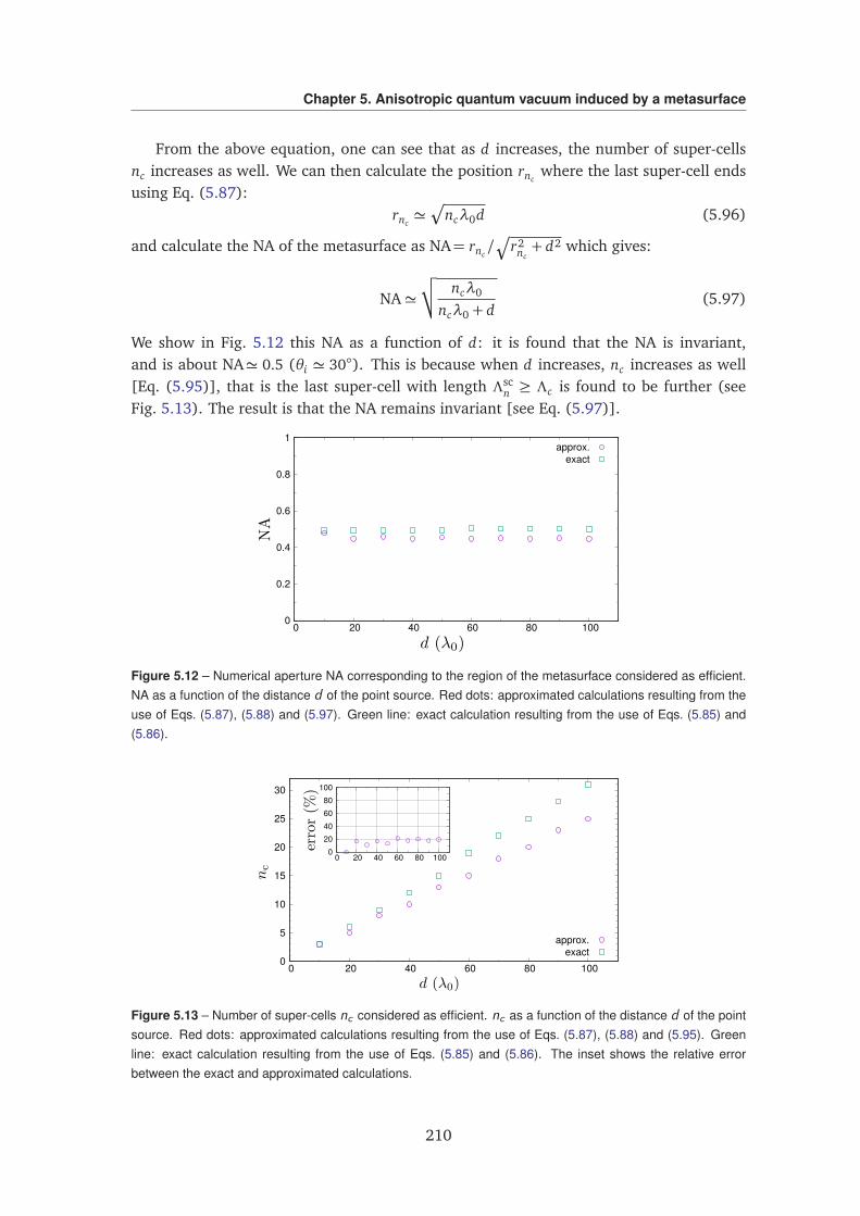
Chapter 5. Anisotropic quantum vacuum induced by a metasurface

From the above equation, one can see that as d increases, the number of super-cellsnc increases as well. We can then calculate the position rnc

where the last super-cell endsusing Eq. (5.87):

rnc'Æ

ncλ0d (5.96)

and calculate the NA of the metasurface as NA= rnc/q

r2nc+ d2 which gives:

NA'√

√ ncλ0

ncλ0 + d(5.97)

We show in Fig. 5.12 this NA as a function of d: it is found that the NA is invariant,and is about NA' 0.5 (θi ' 30). This is because when d increases, nc increases as well[Eq. (5.95)], that is the last super-cell with length Λsc

n ≥ Λc is found to be further (seeFig. 5.13). The result is that the NA remains invariant [see Eq. (5.97)].

0

0.2

0.4

0.6

0.8

1

0 20 40 60 80 100

approx.exact

Figure 5.12 – Numerical aperture NA corresponding to the region of the metasurface considered as efficient.NA as a function of the distance d of the point source. Red dots: approximated calculations resulting from theuse of Eqs. (5.87), (5.88) and (5.97). Green line: exact calculation resulting from the use of Eqs. (5.85) and(5.86).

0

5

10

15

20

25

30

0 20 40 60 80 100

approx.exact

020406080

100

0 20 40 60 80 100

Figure 5.13 – Number of super-cells nc considered as efficient. nc as a function of the distance d of the pointsource. Red dots: approximated calculations resulting from the use of Eqs. (5.87), (5.88) and (5.95). Greenline: exact calculation resulting from the use of Eqs. (5.85) and (5.86). The inset shows the relative errorbetween the exact and approximated calculations.

210

Bibliography

[1] J.-M. Raimond and S. Haroche, Exploring the quantum (Oxford University Press,Oxford, 2006).

[2] D. G. Baranov, M. Wersall, J. Cuadra, T. J. Antosiewicz, and T. Shegai, ACS Photonics5, 24 (2017).

[3] G. Hétet, L. Slodicka, A. Glätzle, M. Hennrich, and R. Blatt, Physical Review A 82,063812 (2010).

[4] U. Dorner and P. Zoller, Physical Review A 66, 023816 (2002).

[5] J. Kästel and M. Fleischhauer, Physical Review A 71, 011804 (2005).

[6] J. Eschner, C. Raab, F. Schmidt-Kaler, and R. Blatt, Nature 413, 495 (2001).

[7] P. K. Jha, X. Ni, C. Wu, Y. Wang, and X. Zhang, Physical Review Letters 115, 025501(2015).

[8] P. K. Jha, N. Shitrit, X. Ren, Y. Wang, and X. Zhang, Physical Review Letters 121,116102 (2018).

[9] P. Lalanne and P. Chavel, Laser & Photonics Reviews 11, 1600295 (2017).

[10] P. Genevet, F. Capasso, F. Aieta, M. Khorasaninejad, and R. Devlin, Optica 4, 139(2017).

[11] G. Agarwal, Physical Review Letters 84, 5500 (2000).

[12] D. Suter, The physics of laser-atom interactions, Vol. 19 (Cambridge University Press,1997).

[13] E. Togan, Y. Chu, A. Trifonov, L. Jiang, J. Maze, L. Childress, M. G. Dutt, A. S.Sørensen, P. Hemmer, A. S. Zibrov, et al., Nature 466, 730 (2010).

[14] S. M. Barnett and P. M. Radmore, Methods in theoretical quantum optics, Vol. 15(Oxford University Press, 2002).

[15] H. J. Carmichael, Statistical methods in quantum optics 1: master equations andFokker-Planck equations (Springer Science & Business Media, 2013).

[16] W. Jhe, A. Anderson, E. Hinds, D. Meschede, L. Moi, and S. Haroche, PhysicalReview Letters 58, 666 (1987).

211

BIBLIOGRAPHY

[17] T. Taillandier-Loize, J. Baudon, G. Dutier, F. Perales, M. Boustimi, and M. Ducloy,Physical Review A 89, 052514 (2014).

[18] M. Boustimi, B. V. De Lesegno, J. Baudon, J. Robert, and M. Ducloy, Physical ReviewLetters 86, 2766 (2001).

[19] G. C. Des Francs, A. Bouhelier, E. Finot, J.-C. Weeber, A. Dereux, C. Girard, andE. Dujardin, Optics Express 16, 17654 (2008).

[20] E. Lassalle, N. Bonod, T. Durt, and B. Stout, Optics Letters 43, 1950 (2018).

[21] S. Sun, K.-Y. Yang, C.-M. Wang, T.-K. Juan, W. T. Chen, C. Y. Liao, Q. He, S. Xiao,W.-T. Kung, G.-Y. Guo, et al., Nano Letters 12, 6223 (2012).

[22] A. Pors, O. Albrektsen, I. P. Radko, and S. I. Bozhevolnyi, Scientific Reports 3, 2155(2013).

[23] G. Zheng, H. Mühlenbernd, M. Kenney, G. Li, T. Zentgraf, and S. Zhang, NatureNanotechnology 10, 308 (2015).

[24] P. K. Jha, N. Shitrit, J. Kim, X. Ren, Y. Wang, and X. Zhang, ACS Photonics 5, 971(2017).

[25] J. Hugonin and P. Lalanne, Reticolo software for grating analysis (Institute d’Optique,Palaiseau, France, 2005).

[26] M. Moharam, E. B. Grann, D. A. Pommet, and T. Gaylord, Journal of the OpticalSociety of America A 12, 1068 (1995).

[27] L. Li, Journal of the Optical Society of America A 14, 2758 (1997).

[28] P. Lalanne and M. P. Jurek, Journal of Modern Optics 45, 1357 (1998).

[29] E. Popov and M. Nevière, Journal of the Optical Society of America A 17, 1773(2000).

[30] B. Stout, J.-C. Auger, and J. Lafait, Journal of Modern Optics 49, 2129 (2002).

[31] B. Stout, A. Devilez, B. Rolly, and N. Bonod, Journal of the Optical Society of AmericaB 28, 1213 (2011).

[32] E. Lassalle, A. Devilez, N. Bonod, T. Durt, and B. Stout, Journal of the OpticalSociety of America B 34, 1348 (2017).

[33] W. Luo, S. Xiao, Q. He, S. Sun, and L. Zhou, Advanced Optical Materials 3, 1102(2015).

[34] S. Pancharatnam, in Proceedings of the Indian Academy of Sciences-Section A, Vol. 44(Springer, 1956) pp. 398–417.

[35] M. V. Berry, Journal of Modern Optics 34, 1401 (1987).

212

BIBLIOGRAPHY

[36] S. Hughes and G. S. Agarwal, Physical Review Letters 118, 063601 (2017).

213

BIBLIOGRAPHY

214

CHAPTER 6

Cold atom experiment

6.1 Introduction

This Chapter is the only “experimental” Chapter of this thesis. It aims at presentingthe experimental platform dedicated to observe the coherence induced by a metasurface,as predicted in the previous Chapter. The experiment is a cold atom experiment, withcesium atoms, which contain the three-level structure in Λ-configuration necessary to geta long-lifetime coherence, or more precisely a tripod structure with one excited state andthree ground states.

The experimental project is threefold. Firstly, we want to start by cooling and trappinga cloud of cesium atoms, using a magneto-optical trap (MOT); this is a well-known tech-nique in atomic physics [1], and the starting point of many quantum experiments withatoms. The ingredients of MOT are an ultra high vacuum cell, strong magnetic field gra-dients, and three pairs of orthogonal counter-propagating laser beams circularly polarizedand overlapped at the trapping region, where the magnetic-field gradient is null.

The second objective is to build a new technique to trap a single atom, by using asuperoscillatory spot, and to study it as a new tool to trap and cool a single atom. Its par-ticularity is to be able to localize the light field below the diffraction limit, and therefore totrap an atom with subwavelength precision, which is one of the experimental constraintsdiscussed in the previous Chapter (the coherence is induced only if the atom is in a welldefined position). Such a superoscillatory spot can be generated by focusing a far red-detuned laser beam with a super-oscillatory lens (SOL), because a SOL allows to focuslight on a spot of arbitrary size, below the diffraction limit. Such a technique was usedrecently to trap nanoparticles [2], and our goal here is to extend this technique to thetrapping of single atoms. For a brief history about this promising technique, the discoveryof super-oscillations was done in Ref. [3], and first observed in Refs. [4, 5]. Note thatthere are different techniques to create the super-oscillations [6]. Here, we want to usethe technique developped recently and experimentally demonstrated in Ref. [7], wherethe spot is created by using two spatial light modulators (SLM), which presents the ad-vantage that the spot can be created and imaged at remote distances; this is crucial forus to make the experiment easier since the SOL can now be located outside of the highvacuum cell which contain the atoms.

Eventually, the last step would be to interface the single atom trapped in the super-

215

Chapter 6. Cold atom experiment

oscillatory spot with the fabricated metasurface, and to observe the predicted coherenceinduced by spontaneous emission. The coherence can be measured by implementing a to-mography technique, which consists in reading the atomic populations in different basis,in order to reconstruct the entire density matrix of the atom.

I participated to the first aspect of this project, that is the obtention and characteriza-tion of the MOT, and I present in this Chapter the results that we obtained. We first startin Section 6.2 by presenting the cesium atoms and giving some of its spectroscopic prop-erties that will be used for cooling and trapping, and we then explain the principle of aMOT. In Section 6.3, we present the laser part of the MOT, in particular how we control itsfrequency with very high precision, which is absolutely necessary in order to trap and coolefficiently. At last, in Section 6.4, we present the first measurements of the temperature ofthe atoms in the MOT, which is one of the most important characteristics of a cold atomiccloud. For that we use the “time-of-flight” method, that we also explain briefly.

6.2 Description of the experimental set-up

The experimental set-up presented here is dedicated to cool down and trap cesium (Cs)atoms. We present first some physical and optical properties of the Cs atoms, and then webriefly explain the technique used to cool and trap the atoms.

6.2.1 Cesium atom

The cesium atom is an alkali-metal atom. It has 55 electrons (atomic number Z = 55),and only one in the outermost shell. Its electron configuration is:

[Xe]6s1 (6.1)

where [Xe] denotes the electron configuration of the Xenon noble gas (atomic numberZ = 54). The isotope considered here is 133Cs, as it is the only stable isotope of cesium. Itsmass is [8]:

m= 2.2× 10−25 kg (6.2)

The first excited state of Cs, labelled 6P-state, has a fine-structure doublet labelled6P1/2 and 6P3/2, which results from the coupling between the orbital angular momentumof the outer electron (commonly denoted LLL) and its spin angular momentum (commonlydenoted SSS). The total angular momentum of the electron is then denoted JJJ = LLL + SSS, andthe corresponding quantum number J lies in the range |L−S| ≤ J ≤ L+S. For the groundstate 6S, S = 1/2 and L = 0 so J = 1/2, and for the first excited state 6P, S = 1/2 andL = 1 so J = 1/2 or J = 3/2, resulting into two states of different energy (the energy levelis shifted according to the value of J).

Nomenclature: The nomenclature of the energy levels now becomes obvious: the firstnumber is the principal quantum number of the outer electron, the letter corresponds tothe orbital angular quantum number L (with the following correspondance: L = 0 →

216

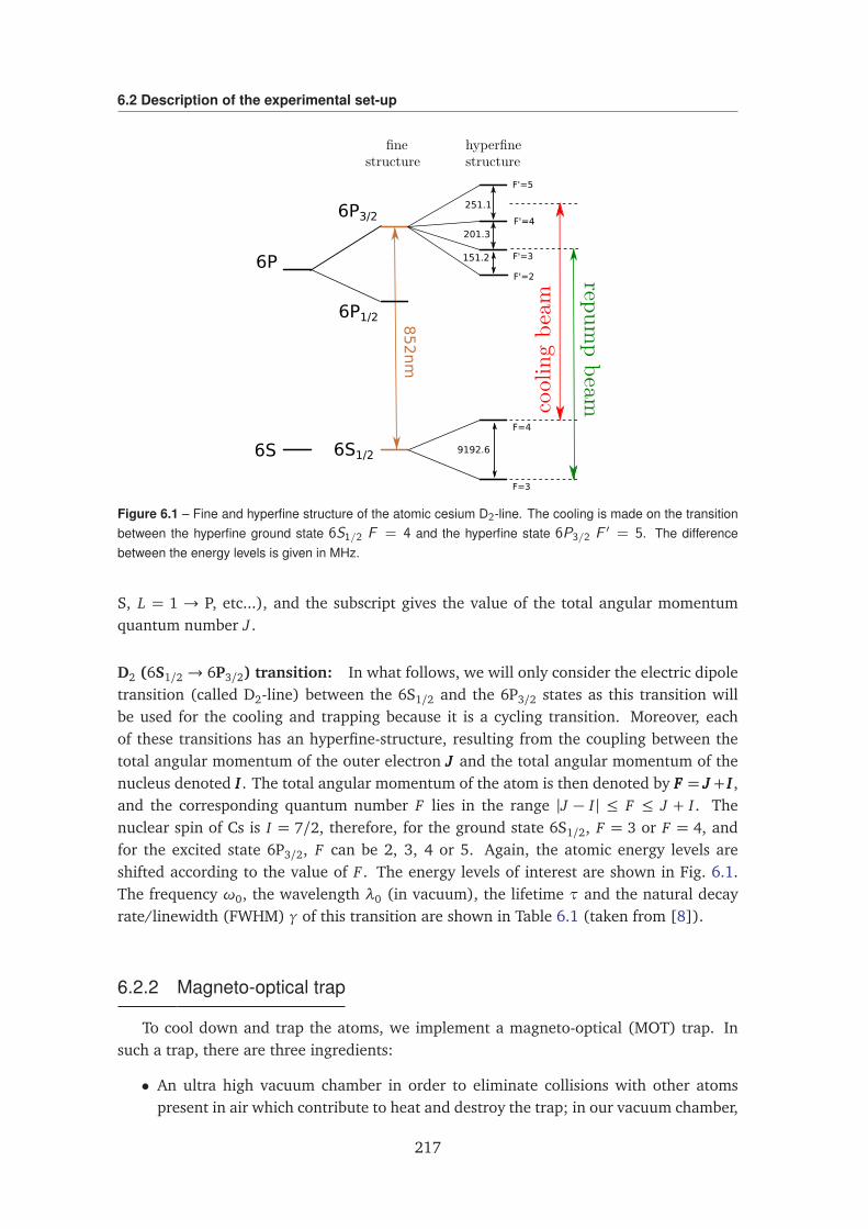
6.2 Description of the experimental set-up

6S1/2

6P3/2

852nm

F=4

F=3

151.2

201.3

251.1

9192.6

F'=5

F'=4

F'=3

F'=2

6P1/2

6S

6P

Figure 6.1 – Fine and hyperfine structure of the atomic cesium D2-line. The cooling is made on the transitionbetween the hyperfine ground state 6S1/2 F = 4 and the hyperfine state 6P3/2 F ′ = 5. The differencebetween the energy levels is given in MHz.

S, L = 1 → P, etc...), and the subscript gives the value of the total angular momentumquantum number J .

D2 (6S1/2 → 6P3/2) transition: In what follows, we will only consider the electric dipoletransition (called D2-line) between the 6S1/2 and the 6P3/2 states as this transition willbe used for the cooling and trapping because it is a cycling transition. Moreover, eachof these transitions has an hyperfine-structure, resulting from the coupling between thetotal angular momentum of the outer electron JJJ and the total angular momentum of thenucleus denoted III . The total angular momentum of the atom is then denoted by FFF = JJJ+ III ,and the corresponding quantum number F lies in the range |J − I | ≤ F ≤ J + I . Thenuclear spin of Cs is I = 7/2, therefore, for the ground state 6S1/2, F = 3 or F = 4, andfor the excited state 6P3/2, F can be 2, 3, 4 or 5. Again, the atomic energy levels areshifted according to the value of F . The energy levels of interest are shown in Fig. 6.1.The frequency ω0, the wavelength λ0 (in vacuum), the lifetime τ and the natural decayrate/linewidth (FWHM) γ of this transition are shown in Table 6.1 (taken from [8]).

6.2.2 Magneto-optical trap

To cool down and trap the atoms, we implement a magneto-optical (MOT) trap. Insuch a trap, there are three ingredients:

• An ultra high vacuum chamber in order to eliminate collisions with other atomspresent in air which contribute to heat and destroy the trap; in our vacuum chamber,

217

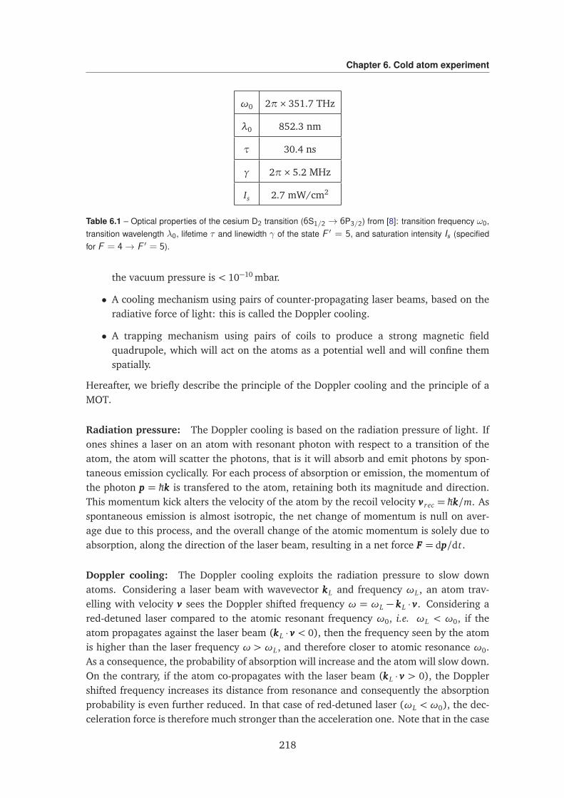
Chapter 6. Cold atom experiment

ω0 2π× 351.7 THz

λ0 852.3 nm

τ 30.4 ns

γ 2π× 5.2 MHz

Is 2.7 mW/cm2

Table 6.1 – Optical properties of the cesium D2 transition (6S1/2 → 6P3/2) from [8]: transition frequency ω0,transition wavelength λ0, lifetime τ and linewidth γ of the state F ′ = 5, and saturation intensity Is (specifiedfor F = 4→ F ′ = 5).

the vacuum pressure is < 10−10 mbar.

• A cooling mechanism using pairs of counter-propagating laser beams, based on theradiative force of light: this is called the Doppler cooling.

• A trapping mechanism using pairs of coils to produce a strong magnetic fieldquadrupole, which will act on the atoms as a potential well and will confine themspatially.

Hereafter, we briefly describe the principle of the Doppler cooling and the principle of aMOT.

Radiation pressure: The Doppler cooling is based on the radiation pressure of light. Ifones shines a laser on an atom with resonant photon with respect to a transition of theatom, the atom will scatter the photons, that is it will absorb and emit photons by spon-taneous emission cyclically. For each process of absorption or emission, the momentum ofthe photon ppp = ħhkkk is transfered to the atom, retaining both its magnitude and direction.This momentum kick alters the velocity of the atom by the recoil velocity vvvrec = ħhkkk/m. Asspontaneous emission is almost isotropic, the net change of momentum is null on aver-age due to this process, and the overall change of the atomic momentum is solely due toabsorption, along the direction of the laser beam, resulting in a net force FFF = dppp/dt.

Doppler cooling: The Doppler cooling exploits the radiation pressure to slow downatoms. Considering a laser beam with wavevector kkkL and frequency ωL, an atom trav-elling with velocity vvv sees the Doppler shifted frequency ω = ωL − kkkL · vvv. Considering ared-detuned laser compared to the atomic resonant frequency ω0, i.e. ωL < ω0, if theatom propagates against the laser beam (kkkL · vvv < 0), then the frequency seen by the atomis higher than the laser frequency ω > ωL, and therefore closer to atomic resonance ω0.As a consequence, the probability of absorption will increase and the atom will slow down.On the contrary, if the atom co-propagates with the laser beam (kkkL · vvv > 0), the Dopplershifted frequency increases its distance from resonance and consequently the absorptionprobability is even further reduced. In that case of red-detuned laser (ωL < ω0), the dec-celeration force is therefore much stronger than the acceleration one. Note that in the case

218

6.2 Description of the experimental set-up

of a blue-detuned laser (ωL > ω0), the contrary effect happens, and the acceleration ismuch stronger than the decceleration. Therefore, to cool down atoms, only a red-detunedlaser is relevant.

Optical molasses: One can use appropriately this assymetry to cool down the atoms byusing pairs of counter-propagating laser beams. In such a configuration, each atom movingin this field will be acted by a decceleration force much stronger than the acceleration one(both forces equalize only if the atom is not moving). Such an environment is calledoptical molasse.

Doppler limit: With this kind of cooling technique, one reaches a limit for the tempera-ture. This limit is due to heating process arising from the scattering of photons (absorptionand emission cycles). This heating can be seen as a Brownian motion in the momentumspace. As well described in Ref. [9], “the temperature results from an equilibrium be-tween laser cooling and the heating process arising from the random nature of both theabsorption and emission of photons”. At equilibrium, the effective temperature reads [1]:

T =ħhγ2

8kBδ

1+ 4δ2

γ2+

IIs

(6.3)

where I is the intensity of the laser, Is is the saturation intensity of the transition consideredand reads: Is = ħhω3γ/12πc2, δ = ωL −ω0 is the laser detuning, and we remind that γ−1

is the lifetime of the excited state used for the cooling. From this expression, one can seethat the minimum temperature that can reach using this cooling technique, for a detuningδ = −γ/2 and in the low-intensity limit, called the Doppler limit, is [1]:

TD 'ħhγ2kB

(6.4)

For us, we realize the cooling on the 6S1/2 → 6P3/2 transition of cesium, which gives aDoppler limit of TD ' 125µK.

Sub-Doppler cooling: As seen from Eq. (6.3), the minimum temperature one expectsfrom the Doppler cooling is obtained for the parameters: δ = −γ/2 and I → 0. However,it is now well-known that one can reach much lower temperatures by taking into accountthe multilevel structure of the atom and the polarization gradient of the light in a MOT[10, 11]. These mechanisms are known as polarization gradient cooling mechanisms, andone of them is the Sisyphus cooling. In real 3D optical molasses, both mechanisms occur,and can produce ultra-low temperatures, closed to the recoil temperature given by:

Trec =ħh2k2

2mkB(6.5)

In principle, under some conditions, the temperature should be linear in I and 1/δ. Thetheory of sub-Doppler cooling tells us that for |δ| γ and Ω |δ| [10]:

kB T ∝ħhΩ2

|δ|(6.6)

∝ ħhγ×γ

|δ|×

IIs

(6.7)

219

Chapter 6. Cold atom experiment

where Ω is the Rabi frequency of the laser characterizing the coupling between the atomicdipole moment and the laser field.

Magneto-optical trap: The radiation pressure itself does not allow for spatial confine-ment of the atoms. Indeed, the atoms are still able to move slowly in any direction andeventually they can diffuse out of the overlap region between the laser beams. In orderto both cool and confine the atoms, the force has to be additionally position-dependent.This dependence is provided by the MOT configuration. Operation of the MOT is based onmanipulations of the external and internal degrees of freedom of atoms by means of care-fully prepared optical and magnetic fields. The optical molasse is modified by selectingthe proper circular polarizations for the beams and applying a weak quadrupole magneticfield.

To understand the functionment of a MOT, let’s consider a 1D model as in Ref. [1]. Thesituation is the following. We consider the following simple level structure for the atom:hyperfine components F = 0 and F ′ = 1 for the ground and excited state respectively.The structure is shown on Fig. 6.2 (a). Then, we consider our atom moving in two laserbeams counterpropagating along the z-axis, in a coaxial inhomogeneous magnetic field BBBof quadrupole symmetry [Fig. 6.2 (b)]. There are two things to note now:

• A first key point is that the two laser beam are of opposite circular polarization (rightσ+ and left σ−), and are red-detuned from resonance. Therefore, by conservationof the angular momentum, we have some selection rules and the σ+ [resp. σ−]circularly polarized beam causes only transitions with ∆mF = +1 [resp. ∆mF = −1],as shown on figure 6.2.

• A second key point is that the magnetic field changes linearly with z, its sign alteringin the trap center [Fig. 6.2 (c)]. The role of the magnefic field in to lift the degener-acy (Zeeman effect) of the upper states. Besides, since the inhomogeneous magneticfield has a constant gradient ∂ B/∂ z, this splitting changes linearly with z [Fig. 6.2(c)]. The Zeeman shift of these levels is proportional to the magnetic field BBB and tothe magnetic quantum number mF of the state:

∆E = gµBmF B (6.8)

where g is the Landé factor and µB the Bohr magneton.

Now, after having introduced the configuration, we can discuss how it allows us toeffectively cool and trap the atoms. Let’s for instance consider that the atom is situated tothe left of the reference frame, where the magnetic field is negative. In that case, the σ+beam is significantly closer to resonance than the σ− beam. Therefore, the momentumtransfer induced by the σ+ beam pushing the atom to the centre is higher than the oneinduced by the σ− beam repelling the atom out of the trap centre. The opposite situationhappens to the right of the trap. As a result, the atom is pushed towards the field freeregion B = 0, where the two forces cancel each other.

220

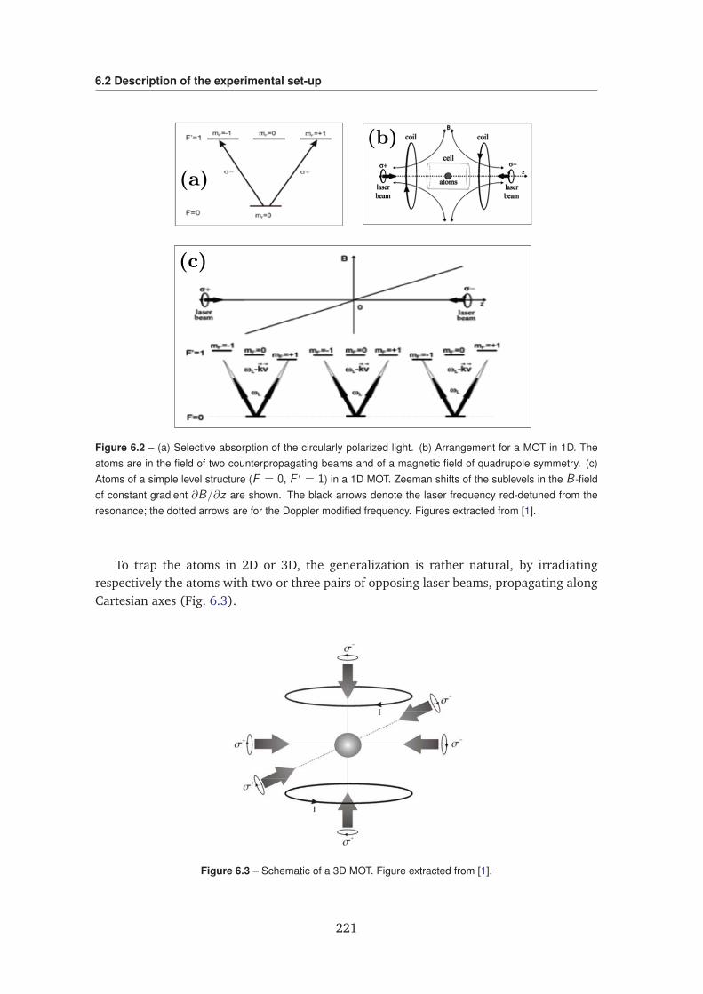
6.2 Description of the experimental set-up

Figure 6.2 – (a) Selective absorption of the circularly polarized light. (b) Arrangement for a MOT in 1D. Theatoms are in the field of two counterpropagating beams and of a magnetic field of quadrupole symmetry. (c)Atoms of a simple level structure (F = 0, F ′ = 1) in a 1D MOT. Zeeman shifts of the sublevels in the B-fieldof constant gradient ∂B/∂z are shown. The black arrows denote the laser frequency red-detuned from theresonance; the dotted arrows are for the Doppler modified frequency. Figures extracted from [1].

To trap the atoms in 2D or 3D, the generalization is rather natural, by irradiatingrespectively the atoms with two or three pairs of opposing laser beams, propagating alongCartesian axes (Fig. 6.3).

Figure 6.3 – Schematic of a 3D MOT. Figure extracted from [1].

221

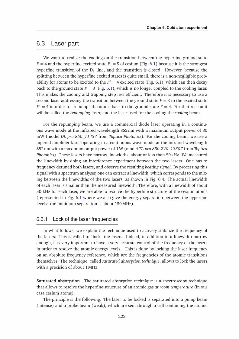
Chapter 6. Cold atom experiment

6.3 Laser part

We want to realize the cooling on the transition between the hyperfine ground stateF = 4 and the hyperfine excited state F ′ = 5 of cesium (Fig. 6.1) because it is the strongesthyperfine transition of the D2 line, and the transition is closed. However, because thesplitting between the hyperfine excited states is quite small, there is a non-negligible prob-ability for atoms to be excited to the F ′ = 4 excited state (Fig. 6.1), which can then decayback to the ground state F = 3 (Fig. 6.1), which is no longer coupled to the cooling laser.This makes the cooling and trapping step less efficient. Therefore it is necessary to use asecond laser addressing the transition between the ground state F = 3 to the excited stateF ′ = 4 in order to “repump” the atoms back to the ground state F = 4. For that reason itwill be called the repumping laser, and the laser used for the cooling the cooling beam.

For the repumping beam, we use a commercial diode laser operating in a continu-ous wave mode at the infrared wavelength 852nm with a maximum output power of 80mW (model DL pro 850_11457 from Toptica Photonics). For the cooling beam, we use atapered amplifier laser operating in a continuous wave mode at the infrared wavelength852nm with a maximum output power of 1W (model TA pro 850-2V0_13307 from TopticaPhotonics). These lasers have narrow linewidths, about or less than 50kHz. We measuredthe linewidth by doing an interference experiment between the two lasers. One has tofrequency detuned both lasers, and observe the resulting beating signal. By processing thissignal with a spectrum analyser, one can extract a linewidth, which corresponds to the mix-ing between the linewidths of the two lasers, as shown in Fig. 6.4. The actual linewidthof each laser is smaller than the measured linewidth. Therefore, with a linewidth of about50 kHz for each laser, we are able to resolve the hyperfine structure of the cesium atoms(represented in Fig. 6.1 where we also give the energy separation between the hyperfinelevels: the minimum separation is about 150MHz).

6.3.1 Lock of the laser frequencies

In what follows, we explain the technique used to actively stabilize the frequency ofthe lasers. This is called to “lock” the lasers. Indeed, in addition to a linewidth narrowenough, it is very important to have a very accurate control of the frequency of the lasersin order to resolve the atomic energy levels . This is done by locking the laser frequencyon an absolute frequency reference, which are the frequencies of the atomic transitionsthemselves. The technique, called saturated absorption technique, allows to lock the laserswith a precision of about 1MHz.

Saturated absorption The saturated absorption technique is a spectroscopy techniquethat allows to resolve the hyperfine structure of an atomic gas at room temperature (in ourcase cesium atoms).

The principle is the following: The laser to be locked is separated into a pump beam(intense) and a probe beam (weak), which are sent through a cell containing the atomic

222

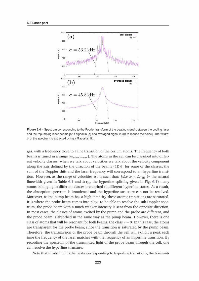
6.3 Laser part

0

200

400

600

800

1000

160 165 170 175

sign

al (a

. u.)

brut signalfit

0

200

400

600

800

1000

160 165 170 175

sign

al (a

. u.)

frequency (MHz)

averaged signalfit

Figure 6.4 – Spectrum corresponding to the Fourier transform of the beating signal between the cooling laserand the repumping laser beams [brut signal in (a) and averaged signal in (b) to reduce the noise]. The “width”σ of the spectrum is extracted using a Gaussian fit.

gas, with a frequency close to a fine transition of the cesium atoms. The frequency of bothbeams is tuned in a range [ωmin;ωmax]. The atoms in the cell can be classified into differ-ent velocity classes [when we talk about velocities we talk about the velocity componentalong the axis defined by the direction of the beams (1D)]: for some of the classes, thesum of the Doppler shift and the laser frequency will correspond to an hyperfine transi-tion. However, as the range of velocities ∆v is such that: k∆v γ,∆νHF (γ the naturallinewidth given in Table 6.1 and ∆νHF the hyperfine splitting given in Fig. 6.1) manyatoms belonging to different classes are excited to different hyperfine states. As a result,the absorption spectrum is broadened and the hyperfine structure can not be resolved.Moreover, as the pump beam has a high intensity, these atomic transitions are saturated.It is where the probe beam comes into play: to be able to resolve the sub-Doppler spec-trum, the probe beam with a much weaker intensity is sent from the opposite direction.In most cases, the classes of atoms excited by the pump and the probe are different, andthe probe beam is absorbed in the same way as the pump beam. However, there is oneclass of atoms that will be resonant for both beams, the class v = 0. In this case, the atomsare transparent for the probe beam, since the transition is saturated by the pump beam.Therefore, the transmission of the probe beam through the cell will exhibit a peak eachtime the frequency of the laser matches with the frequency of an hyperfine transition. Byrecording the spectrum of the transmitted light of the probe beam through the cell, onecan resolve the hyperfine structure.

Note that in addition to the peaks corresponding to hyperfine transitions, the transmit-

223

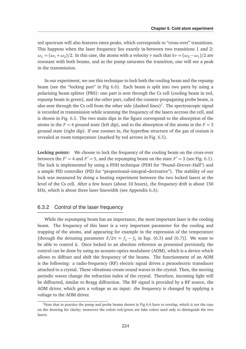
Chapter 6. Cold atom experiment

ted spectrum will also features extra peaks, which corresponds to “cross-over” transitions.This happens when the laser frequency lies exactly in-between two transitions 1 and 2:ωL = (ω1+ω2)/2. In this case, the atoms with a velocity v such that kv = (ω2−ω1)/2 areresonant with both beams, and as the pump saturates the transition, one will see a peakin the transmission.

In our experiment, we use this technique to lock both the cooling beam and the repumpbeam (see the “locking part” in Fig 6.6). Each beam is split into two parts by using apolarizing beam splitter (PBS): one part is sent through the Cs cell (cooling beam in red,repump beam in green), and the other part, called the counter-propagating probe beam, isalso sent through the Cs cell from the other side (dashed lines)1. The spectroscopic signalis recorded in transmission while scanning the frequency of the lasers accross the cell, andis shown in Fig. 6.5. The two main dips in the figure correspond to the absorption of theatoms in the F = 4 ground state (left dip), and to the absorption of the atoms in the F = 3ground state (right dip). If one zoomes in, the hyperfine structure of the gas of cesium isrevealed at room temperature (marked by red arrows in Fig. 6.5).

Locking points: We choose to lock the frequency of the cooling beam on the cross-overbetween the F ′ = 4 and F ′ = 5, and the repumping beam on the state F ′ = 3 (see Fig. 6.1).The lock is implemented by using a PDH technique (PDH for “Pound–Drever–Hall”) anda simple PID controller (PID for “proportional–integral–derivative”). The stability of ourlock was measured by doing a beating experiment between the two locked lasers at thelevel of the Cs cell. After a few hours (about 10 hours), the frequency drift is about 150kHz, which is about three laser linewidth (see Appendix 6.A).

6.3.2 Control of the laser frequency

While the repumping beam has an importance, the most important laser is the coolingbeam. The frequency of this laser is a very important parameter for the cooling andtrapping of the atoms, and appearing for example in the expression of the temperature[through the detuning parameter δ/2π = fL − f0 in Eqs. (6.3) and (6.7)]. We want tobe able to control it. Once locked to an absolute reference as presented previously, thecontrol can be done by using an acousto-optics modulator (AOM), which is a device whichallows to diffract and shift the frequency of the beams. The functionment of an AOMis the following: a radio-frequency (RF) electric signal drives a piezoelectric transducerattached to a crystal. These vibrations create sound waves in the crystal. Then, the movingperiodic waves change the refraction index of the crystal. Therefore, incoming light willbe diffracted, similar to Bragg diffraction. The RF signal is provided by a RF source, theAOM driver, which gets a voltage as an input: the frequency is changed by applying avoltage to the AOM driver.

1Note that in practice the pump and probe beams shown in Fig 6.6 have to overlap, which is not the caseon the drawing for clarity; moreover the colors red/green are fake colors used only to distinguish the twolasers.

224

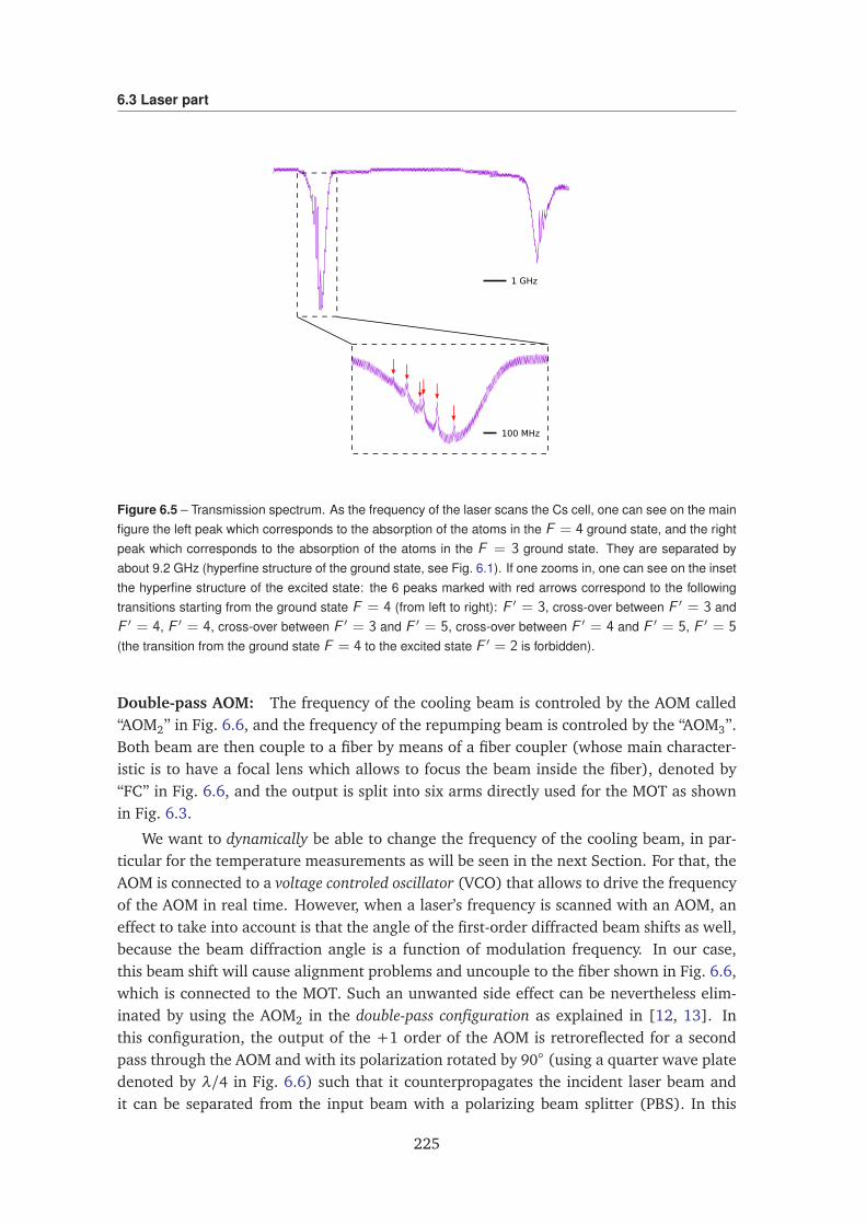
6.3 Laser part

1 GHz

100 MHz

Figure 6.5 – Transmission spectrum. As the frequency of the laser scans the Cs cell, one can see on the mainfigure the left peak which corresponds to the absorption of the atoms in the F = 4 ground state, and the rightpeak which corresponds to the absorption of the atoms in the F = 3 ground state. They are separated byabout 9.2 GHz (hyperfine structure of the ground state, see Fig. 6.1). If one zooms in, one can see on the insetthe hyperfine structure of the excited state: the 6 peaks marked with red arrows correspond to the followingtransitions starting from the ground state F = 4 (from left to right): F ′ = 3, cross-over between F ′ = 3 andF ′ = 4, F ′ = 4, cross-over between F ′ = 3 and F ′ = 5, cross-over between F ′ = 4 and F ′ = 5, F ′ = 5

(the transition from the ground state F = 4 to the excited state F ′ = 2 is forbidden).

Double-pass AOM: The frequency of the cooling beam is controled by the AOM called“AOM2” in Fig. 6.6, and the frequency of the repumping beam is controled by the “AOM3”.Both beam are then couple to a fiber by means of a fiber coupler (whose main character-istic is to have a focal lens which allows to focus the beam inside the fiber), denoted by“FC” in Fig. 6.6, and the output is split into six arms directly used for the MOT as shownin Fig. 6.3.

We want to dynamically be able to change the frequency of the cooling beam, in par-ticular for the temperature measurements as will be seen in the next Section. For that, theAOM is connected to a voltage controled oscillator (VCO) that allows to drive the frequencyof the AOM in real time. However, when a laser’s frequency is scanned with an AOM, aneffect to take into account is that the angle of the first-order diffracted beam shifts as well,because the beam diffraction angle is a function of modulation frequency. In our case,this beam shift will cause alignment problems and uncouple to the fiber shown in Fig. 6.6,which is connected to the MOT. Such an unwanted side effect can be nevertheless elim-inated by using the AOM2 in the double-pass configuration as explained in [12, 13]. Inthis configuration, the output of the +1 order of the AOM is retroreflected for a secondpass through the AOM and with its polarization rotated by 90 (using a quarter wave platedenoted by λ/4 in Fig. 6.6) such that it counterpropagates the incident laser beam andit can be separated from the input beam with a polarizing beam splitter (PBS). In this

225

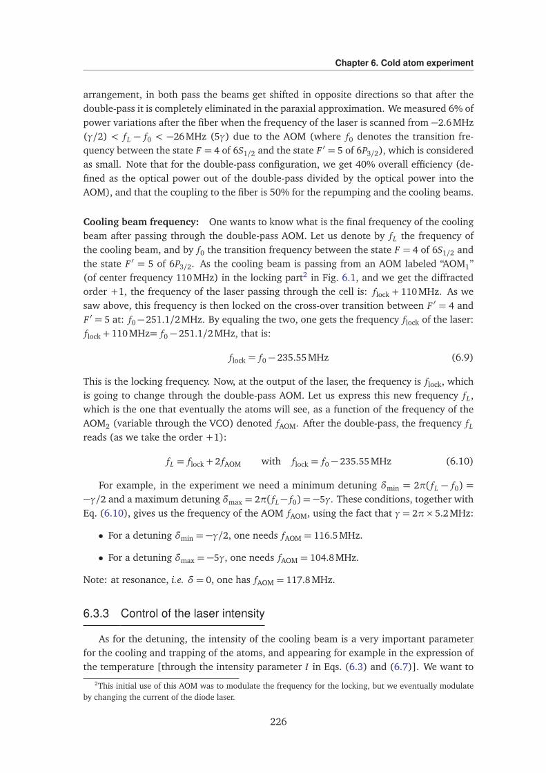
Chapter 6. Cold atom experiment

arrangement, in both pass the beams get shifted in opposite directions so that after thedouble-pass it is completely eliminated in the paraxial approximation. We measured 6% ofpower variations after the fiber when the frequency of the laser is scanned from −2.6MHz(γ/2) < fL − f0 < −26MHz (5γ) due to the AOM (where f0 denotes the transition fre-quency between the state F = 4 of 6S1/2 and the state F ′ = 5 of 6P3/2), which is consideredas small. Note that for the double-pass configuration, we get 40% overall efficiency (de-fined as the optical power out of the double-pass divided by the optical power into theAOM), and that the coupling to the fiber is 50% for the repumping and the cooling beams.

Cooling beam frequency: One wants to know what is the final frequency of the coolingbeam after passing through the double-pass AOM. Let us denote by fL the frequency ofthe cooling beam, and by f0 the transition frequency between the state F = 4 of 6S1/2 andthe state F ′ = 5 of 6P3/2. As the cooling beam is passing from an AOM labeled “AOM1”(of center frequency 110MHz) in the locking part2 in Fig. 6.1, and we get the diffractedorder +1, the frequency of the laser passing through the cell is: flock + 110MHz. As wesaw above, this frequency is then locked on the cross-over transition between F ′ = 4 andF ′ = 5 at: f0−251.1/2MHz. By equaling the two, one gets the frequency flock of the laser:flock + 110MHz= f0 − 251.1/2MHz, that is:

flock = f0 − 235.55MHz (6.9)

This is the locking frequency. Now, at the output of the laser, the frequency is flock, whichis going to change through the double-pass AOM. Let us express this new frequency fL,which is the one that eventually the atoms will see, as a function of the frequency of theAOM2 (variable through the VCO) denoted fAOM. After the double-pass, the frequency fL

reads (as we take the order +1):

fL = flock + 2 fAOM with flock = f0 − 235.55MHz (6.10)

For example, in the experiment we need a minimum detuning δmin = 2π( fL − f0) =−γ/2 and a maximum detuning δmax = 2π( fL− f0) = −5γ. These conditions, together withEq. (6.10), gives us the frequency of the AOM fAOM, using the fact that γ= 2π× 5.2MHz:

• For a detuning δmin = −γ/2, one needs fAOM = 116.5MHz.

• For a detuning δmax = −5γ, one needs fAOM = 104.8MHz.

Note: at resonance, i.e. δ = 0, one has fAOM = 117.8MHz.

6.3.3 Control of the laser intensity

As for the detuning, the intensity of the cooling beam is a very important parameterfor the cooling and trapping of the atoms, and appearing for example in the expression ofthe temperature [through the intensity parameter I in Eqs. (6.3) and (6.7)]. We want to

2This initial use of this AOM was to modulate the frequency for the locking, but we eventually modulateby changing the current of the diode laser.

226

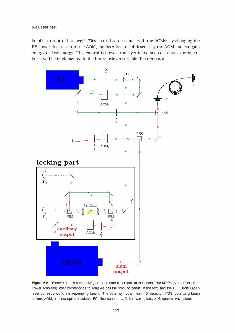
6.3 Laser part

be able to control it as well. This control can be done with the AOMs: by changing theRF power that is sent to the AOM, the laser beam is diffracted by the AOM and can gainenergy or lose energy. This control is however not yet implemented in our experiment,but it will be implemented in the future using a variable RF attenuator.

Figure 6.6 – Experimental setup: locking part and modulation part of the lasers. The MOPA (Master OscillatorPower Amplifier) laser corresponds to what we call the “cooling beam” in the text, and the DL (Diode Laser)laser corresponds to the repumping beam. The other symbols mean: D, detector; PBS, polarizing beamsplitter; AOM, acousto-optic modulator; FC, fiber coupler; λ/2, half-wave plate; λ/4, quarter-wave plate.

227

Chapter 6. Cold atom experiment

6.4 Temperature measurements

The temperature of a cold atomic cloud is one of its most important characteristics. Wepresent here our measurements of the temperature of the cloud of cold cesium atoms usingthe time-of-flight (TOF) method. We did not implement the shadow imaging method toextract the atom number density, but roughly speaking the atom density in the MOT is about109 − 1010 atoms/cm3.

6.4.1 Time-of-flight method

The time-of-flight method starts from a cold atomic cloud confined in a trap. At timet0, one releases the atomic cloud from the trap, and lets it expands. At a later time t1, onemeasures the fluorescence of the atoms using a resonant probe light to get an image of theexpanded cloud using a CMOS camera (model DCC3240N from Thorlabs). By measuringthe expansion of the cloud during the time ∆t = t1 − t0, one can deduce its temperature.Note that this method is destructive: the cloud is destroyed after each measurement bythe resonant probe which scatters the atoms away.

We now explain more quantitatively how to deduce the temperature of the cloud fromits expansion. Taking z as the vertical direction, we consider only the plan (x , z) (as ourCCD camera will image a section of this plan only), we start from an initial Gaussian po-sition and velocity distributions of the atoms in the trap (assuming the classical behaviourof a gas), and assume that the cloud of cold atoms is initially spherically symmetric witha Gaussian radius σ0. After a time t, the probability distribution of finding an atom atposition (x , z) is given by [14]:

g (x , z, t) =1

2πσ2(t)exp

−x2 + z2(t)

2σ2(t)

with z(t) = z −12

g t2 (6.11)

with

σ(t) =

√

√

σ20 +

kB Tm

t2 (6.12)

Finally, considering a probe light with a section much larger than the atomic cloud size,one can consider the intensity seen by the atoms as constant and equal to I . Assumingthat the fluorescence signal is directly proportionnal to the number of atoms in the beam,the fluorescence intensity distribution reads:

Ifluo (x , z, t)∝ I ×1

2πσ2(t)exp

−x2 + z2(t)

2σ2(t)

(6.13)

with I the intensity of the resonant probe light. We get some fluorescence image in Fig. 6.7.The sequence is as following: all the lasers were switched off at time t = 0, and switchedon again after various TOFs t for fluorescence imaging.

Fitting procedure: In order to extract the expanded Gaussian radius σ(t) of the cloud,we fitted the fluorescence images obtained for different expansion times t (see Fig. 6.7)

228

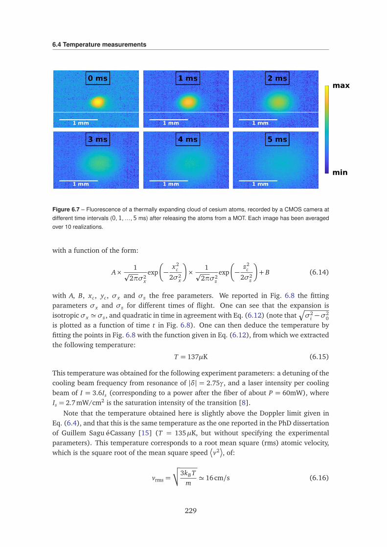
6.4 Temperature measurements

min

max

Figure 6.7 – Fluorescence of a thermally expanding cloud of cesium atoms, recorded by a CMOS camera atdifferent time intervals (0, 1, ..., 5 ms) after releasing the atoms from a MOT. Each image has been averagedover 10 realizations.

with a function of the form:

A×1

p2πσ2

x

exp

−x2

c

2σ2x

×1

p2πσ2

z

exp

−z2

c

2σ2z

+ B (6.14)

with A, B, xc, yc, σx and σz the free parameters. We reported in Fig. 6.8 the fittingparameters σx and σz for different times of flight. One can see that the expansion isisotropic σx ' σz, and quadratic in time in agreement with Eq. (6.12) (note that

q

σ2i −σ

20

is plotted as a function of time t in Fig. 6.8). One can then deduce the temperature byfitting the points in Fig. 6.8 with the function given in Eq. (6.12), from which we extractedthe following temperature:

T = 137µK (6.15)

This temperature was obtained for the following experiment parameters: a detuning of thecooling beam frequency from resonance of |δ| = 2.75γ, and a laser intensity per coolingbeam of I = 3.6Is (corresponding to a power after the fiber of about P = 60mW), whereIs = 2.7mW/cm2 is the saturation intensity of the transition [8].

Note that the temperature obtained here is slightly above the Doppler limit given inEq. (6.4), and that this is the same temperature as the one reported in the PhD dissertationof Guillem Sagué-Cassany [15] (T = 135µK, but without specifying the experimentalparameters). This temperature corresponds to a root mean square (rms) atomic velocity,which is the square root of the mean square speed

v2

, of:

vrms =

√

√3kB Tm' 16 cm/s (6.16)

229

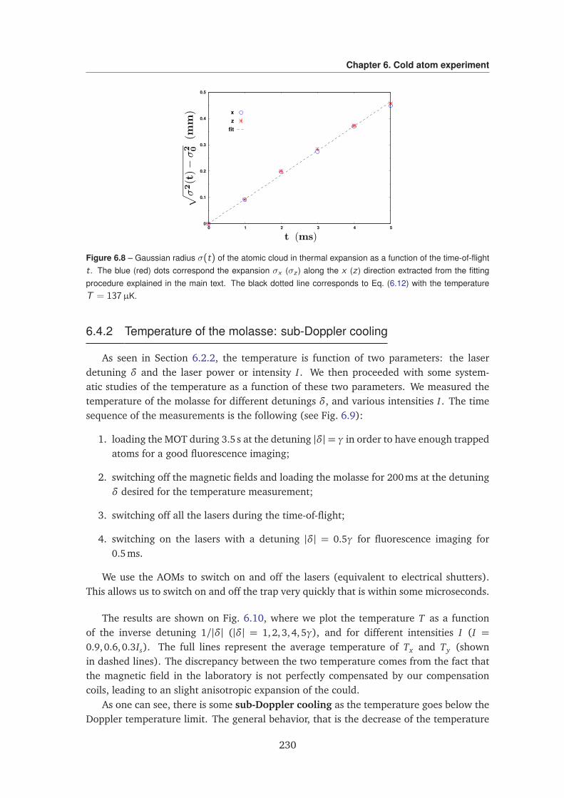
Chapter 6. Cold atom experiment

0

0.1

0.2

0.3

0.4

0.5

0 1 2 3 4 5

xz

fit

Figure 6.8 – Gaussian radius σ(t) of the atomic cloud in thermal expansion as a function of the time-of-flightt . The blue (red) dots correspond the expansion σx (σz ) along the x (z ) direction extracted from the fittingprocedure explained in the main text. The black dotted line corresponds to Eq. (6.12) with the temperatureT = 137µK.

6.4.2 Temperature of the molasse: sub-Doppler cooling

As seen in Section 6.2.2, the temperature is function of two parameters: the laserdetuning δ and the laser power or intensity I . We then proceeded with some system-atic studies of the temperature as a function of these two parameters. We measured thetemperature of the molasse for different detunings δ, and various intensities I . The timesequence of the measurements is the following (see Fig. 6.9):

1. loading the MOT during 3.5 s at the detuning |δ|= γ in order to have enough trappedatoms for a good fluorescence imaging;

2. switching off the magnetic fields and loading the molasse for 200ms at the detuningδ desired for the temperature measurement;

3. switching off all the lasers during the time-of-flight;

4. switching on the lasers with a detuning |δ| = 0.5γ for fluorescence imaging for0.5ms.

We use the AOMs to switch on and off the lasers (equivalent to electrical shutters).This allows us to switch on and off the trap very quickly that is within some microseconds.

The results are shown on Fig. 6.10, where we plot the temperature T as a functionof the inverse detuning 1/|δ| (|δ| = 1,2, 3,4, 5γ), and for different intensities I (I =0.9,0.6, 0.3Is). The full lines represent the average temperature of Tx and Ty (shownin dashed lines). The discrepancy between the two temperature comes from the fact thatthe magnetic field in the laboratory is not perfectly compensated by our compensationcoils, leading to an slight anisotropic expansion of the could.

As one can see, there is some sub-Doppler cooling as the temperature goes below theDoppler temperature limit. The general behavior, that is the decrease of the temperature

230

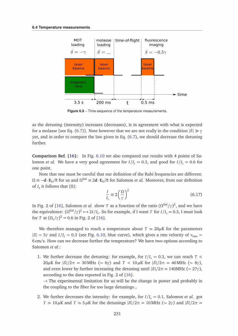
6.4 Temperature measurements

laserbeams

laserbeams

MOTloading

molasseloading

time-of-flight fluorescenceimaging

time

magneticfield

3.5 s 200 ms t 0.5 ms

laserbeams

Figure 6.9 – Time-sequence of the temperature measurements.

as the detuning (intensity) increases (decreases), is in agreement with what is expectedfor a molasse [see Eq. (6.7)]. Note however that we are not really in the condition |δ| γyet, and in order to compare the law given in Eq. (6.7), we should decrease the detuningfurther.

Comparison Ref. [16]: In Fig. 6.10 we also compared our results with 4 points of Sa-lomon et al. We have a very good agreement for I/Is = 0.3, and good for I/Is = 0.6 forone point.

Note that one must be careful that our definition of the Rabi frequencies are different:Ω ≡ −d ·E0/ħh for us and ΩSal ≡ 2d ·E0/ħh for Salomon et al. Moreover, from our definitionof Is it follows that [8]:

IIs≡ 2

Ω

γ

2

(6.17)

In Fig. 2 of [16], Salomon et al. show T as a function of the ratio (ΩSal/γ)2, and we havethe equivalence: (ΩSal/γ)2↔ 2I/Is. So for example, if I want T for I/Is = 0.3, I must lookfor T at (Ωs/γ)2 = 0.6 in Fig. 2 of [16].

We therefore managed to reach a temperature about T ' 20µK for the parameters|δ| = 5γ and I/Is = 0.3 (see Fig. 6.10, blue curve), which gives a rms velocity of vrms =6 cm/s. How can we decrease further the temperature? We have two options according toSalomon et al.:

1. We further decrease the detuning: for example, for I/Is = 0.3, we can reach T <20µK for |δ|/2π = 30MHz (∼ 6γ) and T < 10µK for |δ|/2π = 40MHz (∼ 8γ),and even lower by further increasing the detuning until |δ|/2π = 140MHz (∼ 27γ),according to the data reported in Fig. 2 of [16].→ The experimental limitation for us will be the change in power and probably inthe coupling to the fiber for too large detunings...

2. We further decreases the intensity: for example, for I/Is = 0.1, Salomon et al. gotT ' 10µK and T ' 5µK for the detunings |δ|/2π = 10MHz (∼ 2γ) and |δ|/2π =

231

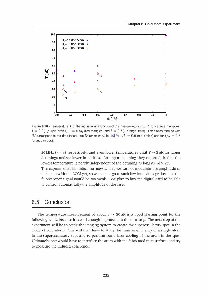
Chapter 6. Cold atom experiment

0

10

20

30

40

50

60

70

80

90

100

0.2 0.3 0.4 0.5 0.6 0.7 0.8 0.9 1

T (µ

K)

1/δ (1/γ)

I/Is=0.9 (P=15mW)I/Is=0.6 (P=10mW)I/Is=0.3 (P= 5mW)

Figure 6.10 – Temperature T of the molasse as a function of the inverse detuning 1/|δ| for various intensities:I = 0.9Is (purple circles), I = 0.6Is (red triangles) and I = 0.3Is (orange stars). The circles marked with“S” correspond to the data taken from Salomon et al. in [16] for I/Is = 0.6 (red circles) and for I/Is = 0.3

(orange circles).

20MHz (∼ 4γ) respectively, and even lower temperatures until T ' 3µK for largerdetunings and/or lower intensities. An important thing they reported, is that thelowest temperature is nearly independent of the detuning as long as |δ|> 2γ.The experimental limitation for now is that we cannot modulate the amplitude ofthe beam with the AOM yet, so we cannot go to such low intensities yet because thefluorescence signal would be too weak... We plan to buy the digital card to be ableto control automatically the amplitude of the laser.

6.5 Conclusion

The temperature measurement of about T ' 20µK is a good starting point for thefollowing work, because it is cool enough to proceed to the next step. The next step of theexperiment will be to settle the imaging system to create the superoscillatory spot in thecloud of cold atoms. One will then have to study the transfer efficiency of a single atomin the superoscillatory spot and to perform some laser cooling of the atom in the spot.Ultimately, one would have to interface the atom with the fabricated metasurface, and tryto measure the induced coherence.

232

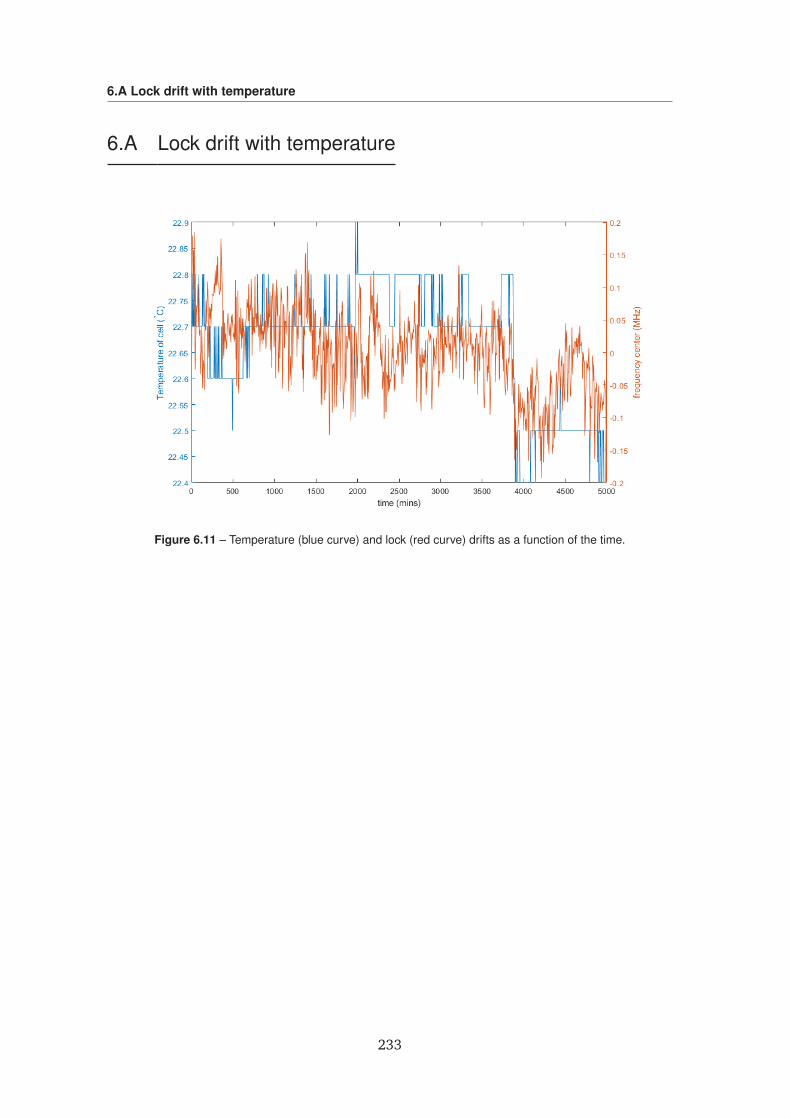
6.A Lock drift with temperature

6.A Lock drift with temperature

Figure 6.11 – Temperature (blue curve) and lock (red curve) drifts as a function of the time.

233

Chapter 6. Cold atom experiment

234

Bibliography

[1] K. Kowalski, V. Cao Long, K. Dinh Xuan, M. Głódz, B. Nguyen Huy, and J. Szonert,Computational Methods in Science and Technology Special Issue (2), 115 (2010).

[2] B. K. Singh, H. Nagar, Y. Roichman, and A. Arie, Light: Science & Applications 6,17050 (2017).

[3] G. T. Di Francia, Il Nuovo Cimento (1943-1954) 9, 426 (1952).

[4] F. M. Huang, Y. Chen, F. J. G. de Abajo, and N. I. Zheludev, Journal of Optics A:Pure and Applied Optics 9, S285 (2007).

[5] F. M. Huang, N. Zheludev, Y. Chen, and F. Javier Garcia de Abajo, Applied PhysicsLetters 90, 091119 (2007).

[6] E. T. Rogers and N. I. Zheludev, Journal of Optics 15, 094008 (2013).

[7] J. Baumgartl, S. Kosmeier, M. Mazilu, E. T. Rogers, N. I. Zheludev, and K. Dholakia,Applied Physics Letters 98, 181109 (2011).

[8] D. A. Steck, https://steck.us/alkalidata/cesiumnumbers.pdf (2007).

[9] W. D. Phillips, Reviews of Modern Physics 70, 721 (1998).

[10] J. Dalibard and C. Cohen-Tannoudji, Journal of the Optical Society of America B 6,2023 (1989).

[11] P. J. Ungar, D. S. Weiss, E. Riis, and S. Chu, Journal of the Optical Society of AmericaB 6, 2058 (1989).

[12] E. A. Donley, T. P. Heavner, F. Levi, M. Tataw, and S. R. Jefferts, Review of ScientificInstruments 76, 063112 (2005).

[13] D. McCarron, http://massey.dur.ac.uk/resources/slcornish/AOMGuide.pdf (2007).

[14] T. M. Brzozowski, M. Maczynska, M. Zawada, J. Zachorowski, and W. Gawlik, Jour-nal of Optics B: Quantum and Semiclassical Optics 4, 62 (2002).

[15] G. S. Cassany, Cold atom physics using ultra-thin optical fibres, Ph.D. thesis, Rheinis-chen Freidrich-Wilhelms-Universität Bonn (2008).

[16] C. Salomon, J. Dalibard, W. Phillips, A. Clairon, and S. Guellati, EPL (EurophysicsLetters) 12, 683 (1990).

235

BIBLIOGRAPHY

236

General conclusion

In this thesis, we studied different facets of the spontaneous emission phenomenon.This requires interfacing the following scientific domains: quantum optics, nanophotonics(plasmonics, metasurfaces), and atomic physics. To investigate such a broad spectrumsubject, I benefited from interactions and collaborations within the Institut Fresnel, withother French laboratories like the PIIM in Marseille or the LP2N in Bordeaux, as well asin the context of an international collaboration with the CDPT in Singapore. Thanks tothis dynamic environment, I was able to carry out new theoretical predictions for eachphenomenon studied in this thesis. Here is a brief summary of the main theoretical resultsof this thesis as well as some personal outlook.

Part I was devoted to the study of monitored spontaneous emission. Our main result isa theoretical prediction about the anti-Zeno effect (AZE) in hydrogen-like atoms in free-space. We show that the AZE is impossible for the most commonly studied electric-dipolartransitions, which drastically limits the candidates and explains why this effect has neverbeen demonstrated experimentally for atoms in free space since its theoretical predictionabout twenty years ago. We proposed an experimental test feasible with alkali-earth ionssuch as Ca+ or Sr+. This result has been published in: E. Lassalle, C. Champenois, B. Stout,V. Debierre, and T. Durt, Conditions for anti-Zeno-effect observation in free-space atomicradiative decay, Physical Review A 97, 062122 (2018). This paves the way for a futureexperiment which would be the first experimental demonstration of the AZE in atoms infree-pace, and would be a further test of quantum optics predictions about the effect ofmeasurement on quantum systems, which is one of the most striking quantum signaturescompared to classical measurements.

Part II was dedicated to the study of the near-field interaction between a quantumemitter (QE) and optically resonant nanostructures. We particularly studied the frequencyshift (Lamb shift) of the emitted photon induced by the resonances. Using the multipolartheory, we predicted a shift of the emission wavelength of ∆λ = 2.5nm for a molecule(Alexa fluor) located in the nanogap of a gold dimer (Chapter 2). The overall study hasbeen published in: E. Lassalle, A. Devilez, N. Bonod, T. Durt, and B. Stout, Lamb shiftmultipolar analysis, Journal of the Optical Society of America B 34, 1348 (2017).

The most important novelty in my eyes was the use of a quantum optics formalismbased on a Quasi-Normal Mode description of the resonances of the resonator, whichare the natural EM modes of the structure (Chapter 4). In particular, this descriptionallowed us to demonstrate in the specific case of the photonic Lamb shift a fundamentaldistinction between closed and open systems in the presence of a single resonance. Whilefor closed systems, the Lamb shift remains within the emission linewidth, it can go beyondthis fundamental range for dissipative (open) systems (Chapter 3). This result has been

237

Chapter 7. General conclusion

published in: E. Lassalle, N. Bonod, T. Durt, and B. Stout, Interplay between spontaneousdecay rates and Lamb shifts in open photonic systems, Optics Letters 43, 1950 (2018). Ipersonally found the QNM formalism of great value for analytical analysis. In the future,I would like to investigate further the differences emphasized by this description withcQED-like descriptions. Moreover, I would like to see how this formalism generalizes totreat two QEs whose interactions are mediated by resonances.

In Part III, we addressed a new paradigm, which consists in the far-field interactionbetween QE and a metasurface. We predicted an effect on a quantum emitter by ananisotropic metasurface over a distance d ∼ 10λ, far beyond the near-field region. Notably,we predicted the creation by spontaneous emission of a long-lifetime coherence betweenthe two ground states of a Λ atom, and we conceived some metasurface designs, basedon the phase-mapping approach, suitable for the creation of the anisotropic quantum vac-uum (Chapter 5): E. Lassalle, P. Lalanne, S. Aljunid, B. Stout, T. Durt, and D. Wilkowski,Long-lifetime coherence in a quantum emitter induced by a metasurface (in preparation).The experimental set-up built to carry on such experiments with cesium atoms was alsopresented, along with our first characterization of the cold atomic cloud by the measure-ment of the temperature (Chapter 6). In the future, I hope that such an experiment wouldreveal the effect of the metasurface on a QE over macroscopic distances, opening the waytowards the possibility of entangling atoms over remotes distances. Looking ahead, withthe very dynamical field of metasurfaces, one could imagine a dynamically reconfigurablemetasurface, and a regular array of atoms, to dynamically entangle atoms, and performquantum processing.

Last but not least, in collaboration with B. Kolaric, M. Hatifi, B. Stout, and T. Durt,we are presently conceiving an experiment aimed at revealing the quantum signature ofthe dynamics underlying spontaneous emission of fluorophores put into a resonant cavity,through the temporal statistics of the emitted photons. Preliminary computations showthat certain effects (like the Zeno regime) are intimately linked to the quantum natureof the process: B. Kolaric, E. Lassalle, M. Hatifi, B. Stout, T. Durt: Quantum signature inthe weak and strong coupling regimes revealed through temporal statistics of spontaneouslyemitted photons (in preparation).

238

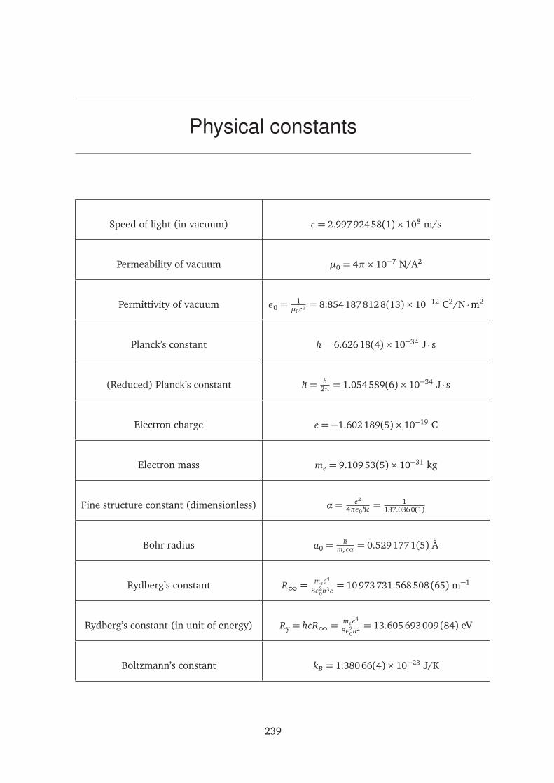
Physical constants

Speed of light (in vacuum) c = 2.997924 58(1)× 108 m/s

Permeability of vacuum µ0 = 4π× 10−7 N/A2

Permittivity of vacuum ε0 =1µ0c2 = 8.854 187812 8(13)× 10−12 C2/N ·m2

Planck’s constant h= 6.626 18(4)× 10−34 J · s

(Reduced) Planck’s constant ħh= h2π = 1.054589(6)× 10−34 J · s

Electron charge e = −1.602189(5)× 10−19 C

Electron mass me = 9.10953(5)× 10−31 kg

Fine structure constant (dimensionless) α= e2

4πε0ħhc =1

137.0360(1)

Bohr radius a0 =ħh

mecα = 0.529 1771(5) Å

Rydberg’s constant R∞ =mee4

8ε20h3c= 10973 731.568508 (65) m−1

Rydberg’s constant (in unit of energy) Ry = hcR∞ =mee4

8ε20h2 = 13.605693 009 (84) eV

Boltzmann’s constant kB = 1.38066(4)× 10−23 J/K

239