Embed Size (px)
DESCRIPTION
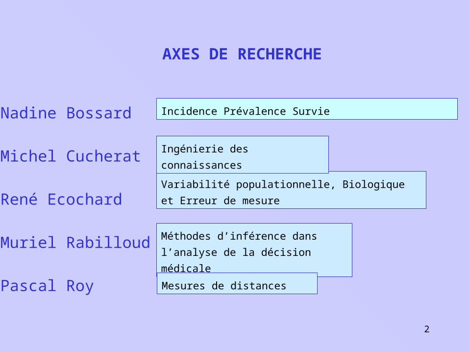
Equipe BioStatistique-Santé (BSS) Pascal ROY PU-PH. AXES DE RECHERCHE. Nadine Bossard Michel Cucherat René Ecochard Muriel Rabilloud Pascal Roy. Incidence Prévalence Survie. Ingénierie des connaissances. Variabilité populationnelle, Biologique et Erreur de mesure. - PowerPoint PPT Presentation
Citation preview

1
Equipe BioStatistique-Santé (BSS)
Pascal ROY PU-PH
2
Incidence Prévalence Survie
Variabilité populationnelle, Biologique
et Erreur de mesure
Méthodes d’inférence dans l’analyse de
la décision médicale
Mesures de distances
Ingénierie des connaissances
AXES DE RECHERCHE
Nadine Bossard
Michel Cucherat
René Ecochard
Muriel Rabilloud
Pascal Roy
3
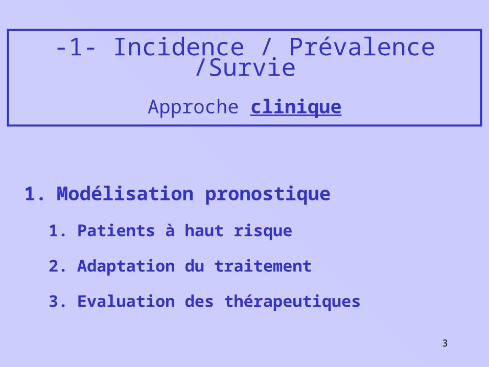
1. Modélisation pronostique
1. Patients à haut risque
2. Adaptation du traitement
3. Evaluation des thérapeutiques
-1- Incidence / Prévalence /Survie
Approche clinique
4
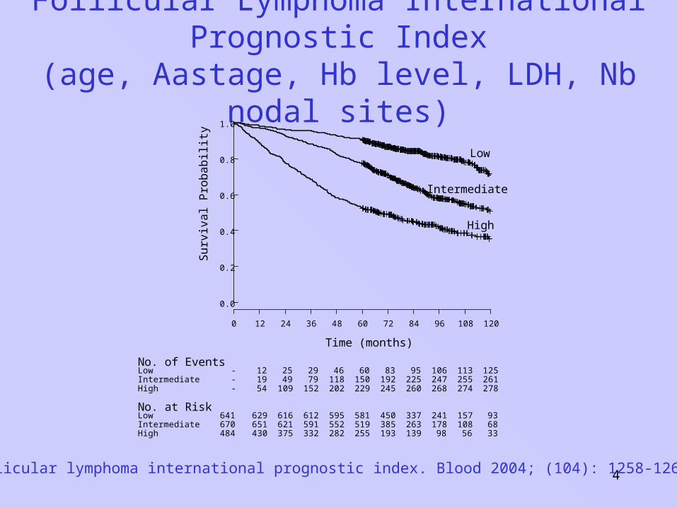
Follicular Lymphoma International Prognostic Index(age, Aastage, Hb level, LDH, Nb nodal sites)
0 12 24 36 48 60 72 84 96 108 120
0.0
0.2
0.4
0.6
0.8
1.0
Time (months)
Sur
viva
l Pro
babi
lity
Low
Intermediate
High
No. of EventsLowIntermediateHigh
No. at RiskLowIntermediateHigh
- 12 25 29 46 60 83 95 106 113 125- 19 49 79 118 150 192 225 247 255 261- 54 109 152 202 229 245 260 268 274 278
641 629 616 612 595 581 450 337 241 157 93670 651 621 591 552 519 385 263 178 108 68484 430 375 332 282 255 193 139 98 56 33
Follicular lymphoma international prognostic index. Blood 2004; (104): 1258-1265.
5
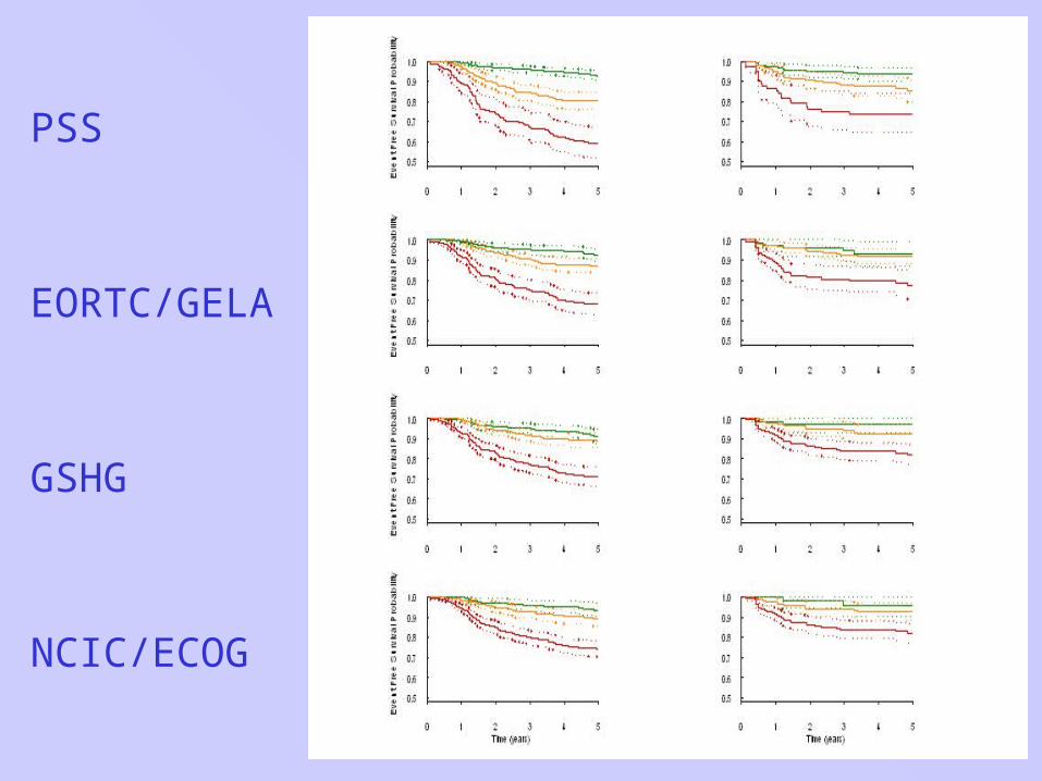
PSS
EORTC/GELA
GSHG
NCIC/ECOG
6
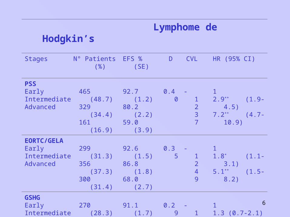
Lymphome de Hodgkin’s
Stages N° Patients (%) EFS % (SE) D CVL HR (95% CI)
PSS EarlyIntermediateAdvanced
465 (48.7)329 (34.4)161 (16.9)
92.7 (1.2)80.2 (2.2)59.0 (3.9)
0.40 -1237 12.9** (1.9-4.5)7.2** (4.7-10.9)
EORTC/GELA EarlyIntermediateAdvanced
299 (31.3)356 (37.3)300 (31.4)
92.6 (1.5)86.8 (1.8)68.0 (2.7)
0.35 -1249 11.8* (1.1-3.1)5.1** (1.5-8.2)
GSHG EarlyIntermediateAdvanced
270 (28.3)318 (33.3)367 (38.4)
91.1 (1.7)89.0 (1.7)71.1 (2.4)
0.29 -1255 11.3 (0.7-2.1)3.7** (2.4-5.9)
NCIC/ECOG EarlyIntermediateAdvanced
205 (21.5)271 (28.4)479 (50.1)
93.7 (1.7)89.3 (1.9)74.3 (2.0)
0.29 -1257 11.7 (0.9-3.4)4.6** (2.5-8.2)
7
1. Evaluer les propriétés prédictives des modèles
2. Estimer la part du pronostic attribuable
1. aux caractéristiques cliniques et biologiques classiques
2. aux caractéristiques transcriptomique ou protéomique des
tumeurs
Perspectives
8
1. Estimation de l’incidence et de la survie du cancer en France.Cancer incidence and mortality in France over the period 1978-2000. Rev Epidemiol
Sante Publique 2003; (51): 3-30.
Evolution de l'incidence et de la mortalité par cancer en France de 1978 à 2000. INVS,
1-217. 2003. Ref Type: Serial (Book,Monograph)
2. Estimation of relative survival in cancer patients The FRANCIM
population based study
-1- Incidence / Prévalence /Survie
Approche épidémiologique
9
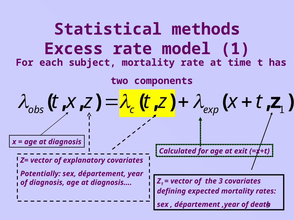
Statistical methodsExcess rate model (1)
For each subject, mortality rate at time t has two components
)z,(),(),,( 1txztzxt expcobs
Z= vector of explanatory covariates
Potentially: sex, département, year of diagnosis, age at diagnosis…. Z1 = vector of the 3 covariates
defining expected mortality rates:
sex , département ,year of death
x = age at diagnosisCalculated for age at exit (=x+t)
10
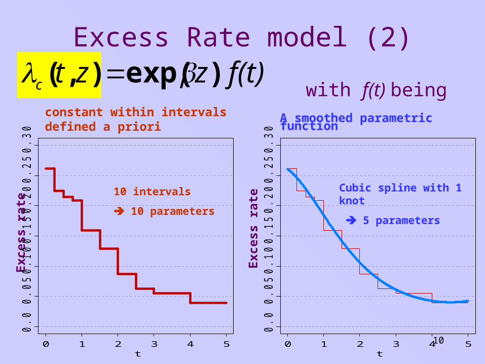
Excess Rate model (2)f(t) zztc )exp(),(
with f(t) beingconstant within intervals defined a priori
A smoothed parametric function
Exc
ess
rate
Exc
ess
rate
t0 1 2 3 4 5
0.0
0.0
50
.10
0.1
50
.20
0.2
50
.30
t0 1 2 3 4 5
0.0
0.0
50
.10
0.1
50
.20
0.2
50
.30
10 intervals
10 parameters
Cubic spline with 1 knot
5 parameters
11
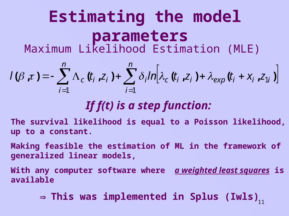
Estimating the model parameters Maximum Likelihood Estimation (MLE)
n
iiiiexpiic
n
iiiic zxtztlnztl
11
1
),(),(),(),(
If f(t) is a step function:The survival likelihood is equal to a Poisson likelihood, up to a constant.
Making feasible the estimation of ML in the framework of generalized linear models,
With any computer software where a weighted least squares is available
This was implemented in Splus (Iwls)
12
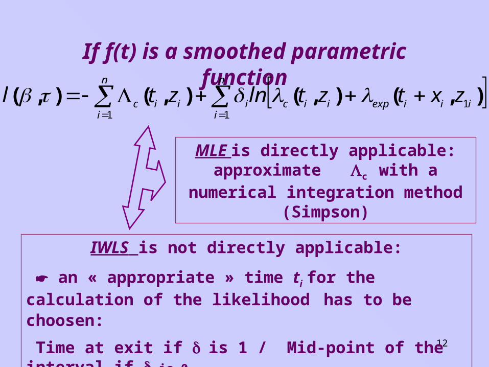
If f(t) is a smoothed parametric function
n
iiiiexpiic
n
iiiic zxtztlnztl
11
1
),(),(),(),(
MLE is directly applicable: approximate c with a numerical
integration method (Simpson)
IWLS is not directly applicable:
an « appropriate » time ti for the calculation of the likelihood has to be choosen:
Time at exit if is 1 / Mid-point of the interval if is 0
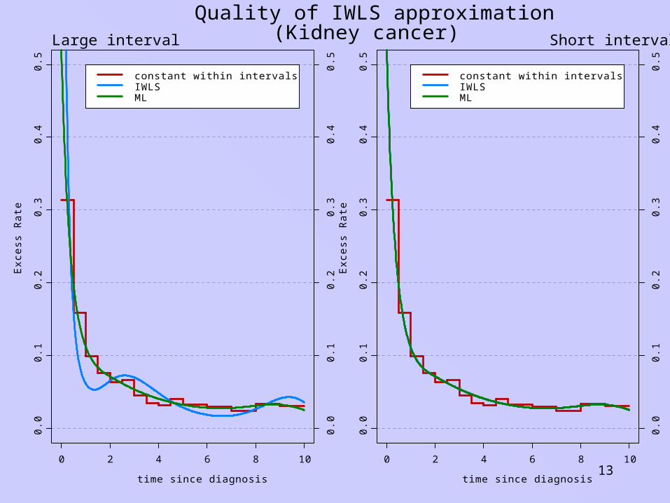
13time since diagnosis
Exc
ess
Ra
te
0 2 4 6 8 10
0.0
0.1
0.2
0.3
0.4
0.5
0.0
0.1
0.2
0.3
0.4
0.5
Large interval
constant within intervalsIWLSML
time since diagnosis
Exc
ess
Ra
te
0 2 4 6 8 10
0.0
0.1
0.2
0.3
0.4
0.5
0.0
0.1
0.2
0.3
0.4
0.5
Short interval
constant within intervalsIWLSML
Quality of IWLS approximation (Kidney cancer)
14
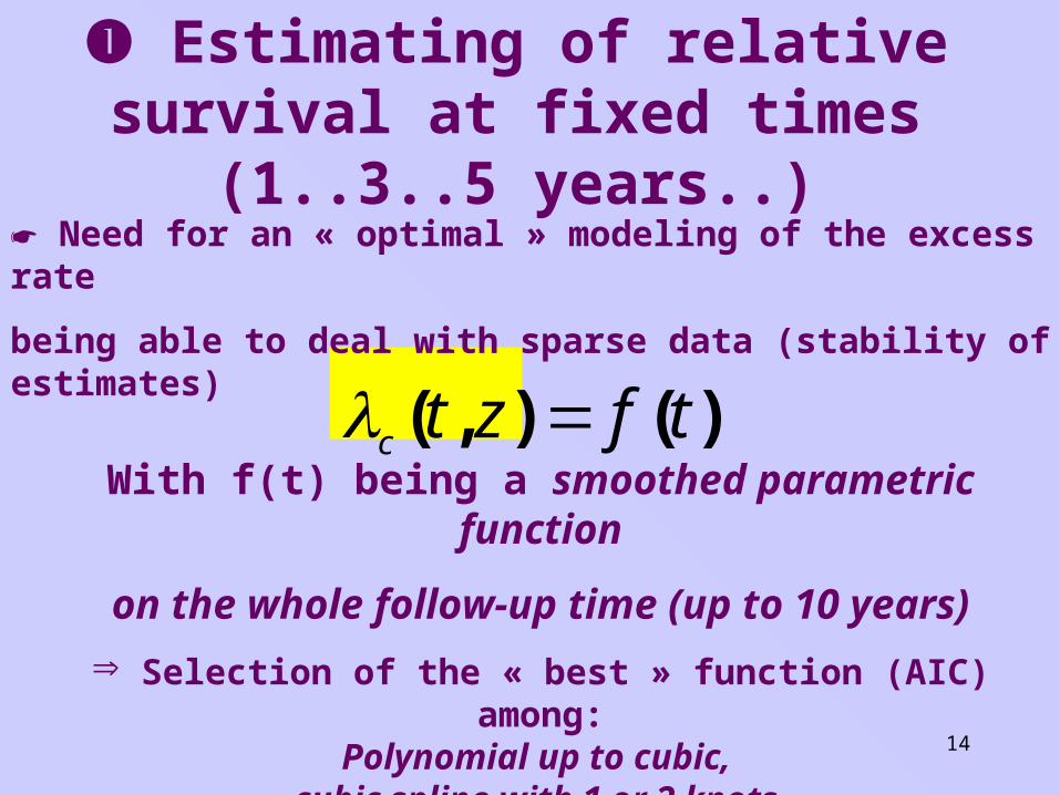
Estimating of relative survival at fixed times (1..3..5 years..)
)(),( tfztc With f(t) being a smoothed parametric
function
on the whole follow-up time (up to 10 years)
Selection of the « best » function (AIC) among:Polynomial up to cubic,
cubic spline with 1 or 2 knots.
Need for an « optimal » modeling of the excess rate
being able to deal with sparse data (stability of estimates)
15
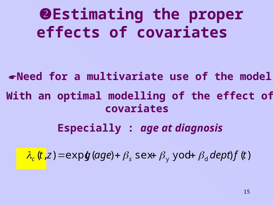
Estimating the proper effects of covariates
)() yod sex )(exp(),( dy tfdeptagegzt sc
Need for a multivariate use of the model
With an optimal modelling of the effect of covariates
Especially : age at diagnosis
16
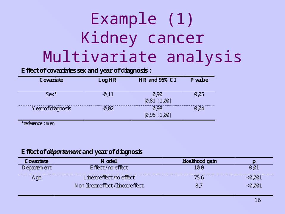
Example (1)Kidney cancer
Multivariate analysis
Effect of covariates sex and year of diagnosis : Covariate Log HR HR and 95%CI
P value
Sex* -0,11 0,90 [0,81 ; 1,00]
0,05
Year of diagnosis -0,02 0,98 [0,96 ; 1,00]
0,04
*reference : men
Effect of département and year of diagnosis Covariate Model likelihood gain p
Département Effect / no effect 10,0 0,01
Age Linear effect /no effect 75,6 <0,001
Non linear effect / linear effect 8,7 <0,001
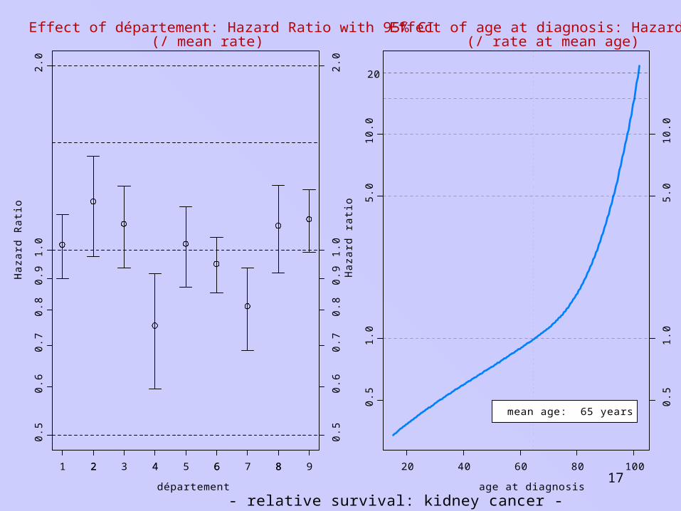
17département
Ha
zard
Ra
tio
2 4 6 8
0.5
0.6
0.7
0.8
0.9
1.0
2.0
1 2 3 4 5 6 7 8 9
0.5
0.6
0.7
0.8
0.9
1.0
2.0
Effect of département: Hazard Ratio with 95% CI (/ mean rate)
age at diagnosis
Ha
zard
ra
tio
20 40 60 80 100
0.5
1.0
5.0
10
.0
Effect of age at diagnosis: Hazard Ratio (/ rate at mean age)
20
mean age: 65 years
0.5
1.0
5.0
10
.0
- relative survival: kidney cancer -
18
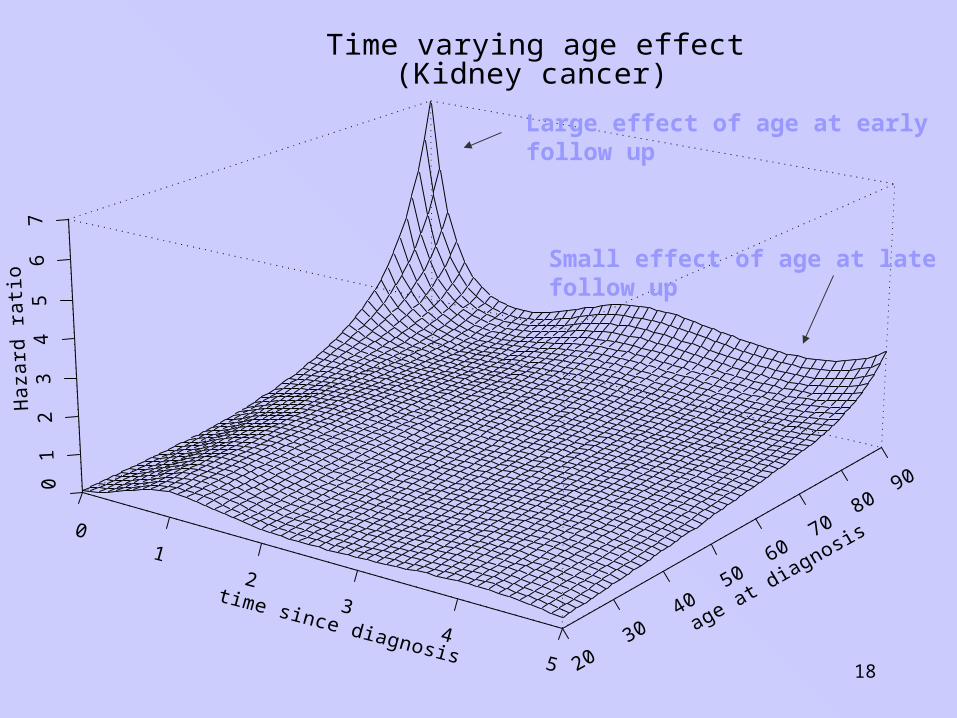
Time varying age effect (Kidney cancer)
Large effect of age at early follow up
Small effect of age at late follow up