Etude numérique et empirique de l’atténuation haute ... · time windows of 5 s for the pre-event noise and direct S-wave were used to compute the Fourier spectra. ... Etude numérique

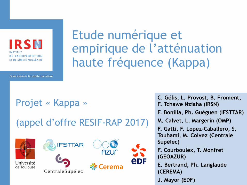
Etude numérique et empirique de l’atténuation haute fréquence (Kappa)

Projet « Kappa »

(appel d’offre RESIF-RAP 2017)

C. Gélis, L. Provost, B. Froment, F. Tchawe Nziaha (IRSN)

F. Bonilla, Ph. Guéguen (IFSTTAR)

M. Calvet, L. Margerin (OMP)

F. Gatti, F. Lopez-Caballero, S. Touhami, M. Colvez (Centrale Supélec)

F. Courboulex, T. Monfret (GEOAZUR)

E. Bertrand, Ph. Langlaude (CEREMA)

J. Mayor (EDF)

Etude numérique et empirique de l’atténuation haute fréquence (Kappa) – Journées RESIF – 29-31 janvier 2018, Montpellier 2/9

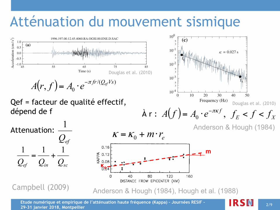
Atténuation du mouvement sismique

( ) )/(0, VsQfr efeAfrA π−⋅=

Qef = facteur de qualité effectif, dépend de f Attenuation:

scinef QQQ111

+=

Campbell (2009)

efQ1

different views on the selection of the pre-event, P-

wave and S-wave portions of the record and on the

selection of fE and fX, which can lead to some vari-

ations in j between analysts. We found that

differences in picking of the pre-event, P-wave and

S-wave portions did not significantly affect the jsobtained.

A semi-automatic procedure to choose the inter-

vals used to compute the direct shear-wave spectra

and noise spectra was also applied. Since both P- and

S-wave arrival times had been previously picked,

time windows of 5 s for the pre-event noise and direct

S-wave were used to compute the Fourier spectra.

Various lengths of time windows from 1 to 10 s were

also tested with similar results, so a standard length of

5 s was finally chosen. The time series were pro-

cessed using a Hanning taper of 5%. The resulting

Fourier spectra were then smoothed by a KONNO and

OHMACHI (1998) filter (filter bandwidth of 40), and

only data having a signal-to-noise ratio greater than

three were used to compute j. The values of fX and fEused to compute j in this procedure were chosen by

the analyst, as in the completely manual approach

described above. In the next section we present the

approach we took to quantify the subjectivity and

precision of the obtained js.In the absence of the high-frequency decay

quantified here by j Fourier amplitude spectra should

be flat above the corner frequency, fc, of the source.

When fitting the best-fit lines to determine j it is

necessary that fE (the frequency chosen as the start of

the best-fit line) is greater than fc otherwise the jestimates can be biased. When using strong-motion

data from moderate and large earthquakes (Mw C 5.5)

as done by ANDERSON and HOUGH (1984) fc is gener-ally lower than 1 Hz hence bias in j due to fc is not aproblem. However, in this study where we are using

data from earthquakes with 3.4 B M B 5.3 fc is

generally between 1 and 6 Hz, using Fig. 8 of DRO-

UET et al. (2008) showing the relation between

magnitude and fc. The fE values are selected here to

be above fc based on visual inspection (Figs. 2, 3)

and, therefore, most best-fit lines will be minimally

affected by fc, especially since fX (the frequency up to

which the line is fitted) is usually greater than 30 Hz.

Site amplification curves, relative to reference

sites displaying little amplification, for some of the

stations considered here are provided by DROUET

45 55 65 75 85Time (s)

-1.0

-0.5

0.0

0.5

1.0

Acc

eler

atio

n (c

m/s

2 )

(a)

1996.197.00.12.45.4060.RA.OGSI.00.ENE.D.SAC

0 10 20 30 40 50Frequency (Hz)

10-6

10-5

10-4

10-3

10-2

10-1

100

Acc

eler

atio

n Sp

ectr

a (c

m/s

)

35

35

35

35

35

35

Noise S-wave

(b)

0 10 20 30 40 50Frequency (Hz)

10-4

10-3

10-2

10-1

100

35

35

35

35

= 0.027 s

(c)

fE

fX

Figure 2Example of direct shear-wave and noise spectra computed from a record that shows a clear high-frequency linear trend. Also shown are the

intervals used to estimate the pre-event noise and the direct shear-wave spectra (black parts of acceleration time-history) and the frequencies fEand fX chosen by one of the analysts (the other analysts chose similar fE and fX for records such as this)

1308 J. Douglas et al. Pure Appl. Geophys.

κo

m

Anderson & Hough (1984), Hough et al. (1988)

erm ⋅+= 0κκ

Douglas et al. (2010)

( ) XEf fffeAfA <<⋅= − ,0

κπ

different views on the selection of the pre-event, P-

wave and S-wave portions of the record and on the

selection of fE and fX, which can lead to some vari-

ations in j between analysts. We found that

differences in picking of the pre-event, P-wave and

S-wave portions did not significantly affect the jsobtained.

A semi-automatic procedure to choose the inter-

vals used to compute the direct shear-wave spectra

and noise spectra was also applied. Since both P- and

S-wave arrival times had been previously picked,

time windows of 5 s for the pre-event noise and direct

S-wave were used to compute the Fourier spectra.

Various lengths of time windows from 1 to 10 s were

also tested with similar results, so a standard length of

5 s was finally chosen. The time series were pro-

cessed using a Hanning taper of 5%. The resulting

Fourier spectra were then smoothed by a KONNO and

OHMACHI (1998) filter (filter bandwidth of 40), and

only data having a signal-to-noise ratio greater than

three were used to compute j. The values of fX and fEused to compute j in this procedure were chosen by

the analyst, as in the completely manual approach

described above. In the next section we present the

approach we took to quantify the subjectivity and

precision of the obtained js.In the absence of the high-frequency decay

quantified here by j Fourier amplitude spectra should

be flat above the corner frequency, fc, of the source.

When fitting the best-fit lines to determine j it is

necessary that fE (the frequency chosen as the start of

the best-fit line) is greater than fc otherwise the jestimates can be biased. When using strong-motion

data from moderate and large earthquakes (Mw C 5.5)

as done by ANDERSON and HOUGH (1984) fc is gener-ally lower than 1 Hz hence bias in j due to fc is not aproblem. However, in this study where we are using

data from earthquakes with 3.4 B M B 5.3 fc is

generally between 1 and 6 Hz, using Fig. 8 of DRO-

UET et al. (2008) showing the relation between

magnitude and fc. The fE values are selected here to

be above fc based on visual inspection (Figs. 2, 3)

and, therefore, most best-fit lines will be minimally

affected by fc, especially since fX (the frequency up to

which the line is fitted) is usually greater than 30 Hz.

Site amplification curves, relative to reference

sites displaying little amplification, for some of the

stations considered here are provided by DROUET

45 55 65 75 85Time (s)

-1.0

-0.5

0.0

0.5

1.0

Acc

eler

atio

n (c

m/s

2 )

(a)

1996.197.00.12.45.4060.RA.OGSI.00.ENE.D.SAC

0 10 20 30 40 50Frequency (Hz)

10-6

10-5

10-4

10-3

10-2

10-1

100

Acc

eler

atio

n Sp

ectr

a (c

m/s

)

35

35

35

35

35

35

Noise S-wave

(b)

0 10 20 30 40 50Frequency (Hz)

10-4

10-3

10-2

10-1

100

35

35

35

35

= 0.027 s

(c)

fE

fX

Figure 2Example of direct shear-wave and noise spectra computed from a record that shows a clear high-frequency linear trend. Also shown are the

intervals used to estimate the pre-event noise and the direct shear-wave spectra (black parts of acceleration time-history) and the frequencies fEand fX chosen by one of the analysts (the other analysts chose similar fE and fX for records such as this)


Anderson & Hough (1984)

Douglas et al. (2010)

À r :


Utilisation de Kappa

GMPEs

Zones de sismicité faible à modérée

Zones actives

Kappa

ì Aléa sismique (« host-to-target ») Campbell, 2003 ; Cotton et al., 2006

ì  Prédiction du mouvement sismique (effet de site)

Boore, 2003

equation, the slope of the spectral decay d lnA!f"=df is#πκ. Anderson and Hough (1984) noted that if Qef!r"and thus t$ is independent of frequency, the effect of attenua-tion on a Brune (1970, 1971) source displacement spectrum,for which the high-frequency decay is proportional to f#2,will yield the spectral shape given by both Cormier(1982) and equation (5). These authors further found thatκ was dependent on distance with a nonzero intercept thatthey interpreted to be the attenuation due to the propagationof S waves through the subsurface geological structure and aslope that they interpreted to be the incremental attenuationdue to the horizontal propagation of S waves through thecrust. They also showed that the spectral decay of the loga-rithm of the Fourier acceleration spectrum with frequency,assuming an ω-square source spectrum, is flat (i.e., κ % 0)when Qef % ∞ and Qef ∝ f and is negative (i.e., κ > 0)when Qef % Q0 and Qef ∝ fη!η < 1". However, only whenQef % Q0 (a constant) is the spectral decay described exactlyby equation (5). Fitting equation (5) to a model with a frac-tional frequency dependence ofQef will yield a smaller valueof κ than a model in which Qef is assumed to be constant,which emphasizes the importance of the standard assumption

that Qef is independent of frequency when interpreting κas a site parameter. Otherwise, the true value of Qef will beunderestimated.

Hough et al. (1988) and Hough and Anderson (1988)performed a thorough study of κ using the recordings ofsmall earthquakes from the Anza seismic array in southernCalifornia. Based on this analysis, Hough and Anderson(1988) proposed a general model for κ given by the equation

κ!r" %Z

pathQi!z"#1VS!z"#1dr; (6)

where Qi is the frequency-independent component of Qef atdepth z within the profile. They used this model to infer theattenuation structure at Anza from a regional crustal velocitymodel. They noted that their proposed model for κ!r" wasthe same as that given by Cormier (1982) for t$ in equa-tion (4), except that it used only the frequency-independentcomponent of Qef . Hough et al. (1988) concluded that thesimilarity of the distance-dependence of κ!r" in the Anzaand Imperial Valley regions of southern California, areasin which the intercepts at r % 0 were very different presum-ably due to the vastly different subsurface geology, supportedthe earlier assumption by Anderson and Hough (1984) thatthe intercept of κ!r" represents the attenuation of seismicwaves within the geological structure beneath the site andthat the distance-dependence of κ!r" represents the attenua-tion due to the horizontal propagation of seismic waves with-in the crust. Hough et al. (1988) referred to this site com-ponent of κ!r" as κ0. Anderson (1991) generalized the linearκ!r" model of Hough and Anderson (1988) and Hough et al.(1988) by proposing a mathematical formulation of the ob-served behavior of κ that regarded this parameter to be anarbitrary function of distance that he defined by the equation

κ!r" % κ0 & ~κ!r"; (7)

where κ0 is the intercept at r % 0.Since being introduced, κ0 has become the preferred

parameter for incorporating site attenuation in the calculationof amplification factors using the quarter-wavelength methodof Joyner et al. (1981). A summary of κ0 estimates for a vari-ety of geological conditions throughout the United States hasbeen compiled by Anderson (1986, 1991) and Silva andDarragh (1995). Even Halldorsson and Papageorgiou (2005)have adopted it as their high-frequency filter parameter in therevision of the specific barrier model of the earthquakesource (Papageorgiou and Aki, 1983) because of its betterfit to strong-motion data. However, these latter authors con-tinue to suggest that it could be a source parameter ratherthan a site parameter.

In the quarter-wavelength method, the site amplificationof the Fourier amplitude spectrumof acceleration is calculatedfrom the equation (Boore, 2003)

Amp!f" % !ρSβS=!ρ !β"1=2 exp!#πκ0f"; (8)

Figure 3. Fourier amplitude spectrum of the N85° E componentof ground acceleration recorded at Cucapah during the MexicaliValley earthquake of 9 June 1980 (ML 6.2). The accelerographwas a digital recorder that samples at a rate of 200=sec. (A) log-log axes; (B) linear-log axes (after Anderson and Hough, 1984).

2368 K. W. Campbell

Campbell (2009)

Extraits USGS, M>5

Contenu du projet RESIF-RAP « Kappa » Approche empirique ▌ Données (françaises RESIF) ▌ Calcul de Kappa et Q

Approche numérique ▌ Milieu connu (Q) ▌ Tests de sensibilité

4/9 Etude numérique et empirique de l’atténuation haute fréquence (Kappa) – Journées RESIF – 29-31 janvier 2018, Montpellier

Application au contexte français (Nice) ▌ Vers l’estimation du mouvement pour un site spécifique

Participants : C. Gélis, L. Provost, B. Froment, F. Tchawe Nziaha (IRSN) F. Bonilla, Ph. Guéguen (IFSTTAR) M. Calvet, L. Margerin (OMP) F. Gatti, F. Lopez-Caballero, S. Touhami, M. Colvez (Centrale Supélec) F. Courboulex, T. Monfret (GEOAZUR) E. Bertrand, Ph. Langlaude (CEREMA) J. Mayor (EDF) Objectifs: Publications communes (1 résumé soumis à SSA 2018)


Contenu du projet – approche empirique ì  Estimation de Kappa sur quelques stations sismologiques

françaises à l’aide des données les plus récentes (et autres stations)

A non-automatic procedure for estimating j was

adopted because we noted that the frequency, fE, atwhich the acceleration spectral amplitudes show a

decline varied significantly from record to record and

therefore assuming a constant fE, such as has been

done in some previous studies, could lead to biased

estimates for j. Similarly, due to varying signal-to-

noise ratios (visually inspected), fX shows large

variations and therefore it was not possible to use a

constant value for all records. Since the procedure

followed here is non-automatic, it is quite time-con-

suming and also subjective because analysts can have

-5˚ 0˚ 5˚ 10˚

45˚

50˚

12

4˚ 5˚ 6˚ 7˚ 8˚ 9˚41˚

42˚

43˚

44˚

45˚

46˚

47˚

48˚

49˚

0 50 100

km

Besancon

ColmarEpinal

NancyStrasbourg

Lons-le-Saunier

MaconBourg-en-Bresse

Lyon

St.-Etienne

Valence

Privas

Gap

Grenoble

AvignonNimes

Le-Puy-en-Velay

Montpellier

MarseilleToulon

Digne-les-Bains

Nice

(1)

-2˚ -1˚ 0˚ 1˚ 2˚ 3˚

42˚

43˚

0 50 100

km

Biarritz

Pau

Lourdes St-Gaudens

Pamplona

Huesca

Gerona

Narbonne

Beziers

Carcassonne

Perpignan

(2)

Figure 1Earthquake (circles) and station (triangles) locations and travel paths (lines) of the records used for this study. 1 Alps and Cote d’Azur

(southern part of map) and 2 Pyrenees

Vol. 167, (2010) A j Model for Mainland France 1307

Douglas, Bonilla, Gehl et Gélis (2010)

This may be explained by the fact that some of the

stations are located in the sedimentary Grenoble

basin where the deep soil layer could lead to large

attenuation.

Figures 7 and 8 show j estimates and fitted linear

relations for 11 stations located in the Alps and

the Pyrenees. Two sets of fits were made: one in

which the slope (mj) and the intercept (j0) were

0 50 100 150 200 250 300 350 4000.000.020.040.060.080.100.120.140.160.18

Soil

(s)

Standard: 0 = 0.0350 s, m = 0.000156 s / kmWeighted: 0 = 0.0347 s, m = 0.000161 s / km

Alps

0 50 100 150 200 250 300 350 400Distance (km)

0.000.020.040.060.080.100.120.140.160.18

Roc

k(s

)


0 50 100 150 200 250 300 350 4000.000.020.040.060.080.100.120.140.160.18


Côte d’Azur

0 50 100 150 200 250 300 350 400Distance (km)

0.000.020.040.060.080.100.120.140.160.18


0 50 100 150 200 250 300 350 4000.000.020.040.060.080.100.120.140.160.18


Pyrenees

0 50 100 150 200 250 300 350 400Distance (km)

0.000.020.040.060.080.100.120.140.160.18


Figure 6Distance dependence of j values for three regions in mainland France. The top plots present the results for stations located on soil. The bottom

plots show the results for stations located on rock

0 50 100 150 200 250 300 350 4000.000.020.040.060.080.100.120.140.160.18

(s)

Unc. standard: 0 = 0.023 s, m = 0.000125 s / kmUnc. weighted: 0 = 0.022 s, m = 0.000126 s / kmCon. standard: 0 = 0.0174 s, m = 0.000156 s / kmCon. weighted: 0 = 0.0164 s, m = 0.000161 s / km

OGAN (Rock)

0 50 100 150 200 250 300 350 4000.000.020.040.060.080.100.120.140.160.18


OGMO (Rock)

0 50 100 150 200 250 300 350 400

Distance (km)

0.000.020.040.060.080.100.120.140.160.18

(s)


OGMU (Rock)

0 50 100 150 200 250 300 350 400

Distance (km)

0.000.020.040.060.080.100.120.140.160.18


OGSI (Rock)

Figure 7j estimates and their ±1 standard deviations for stations located in the Alps. Also shown are the fitted linear relations. Four best-fit lines werefitted for each station: two (using standard and weighted regression) in which mj was allowed to vary (black) and two (using standard and

weighted regression) in which mj was constrained to the value from the regional analysis shown in Fig. 6 (grey)



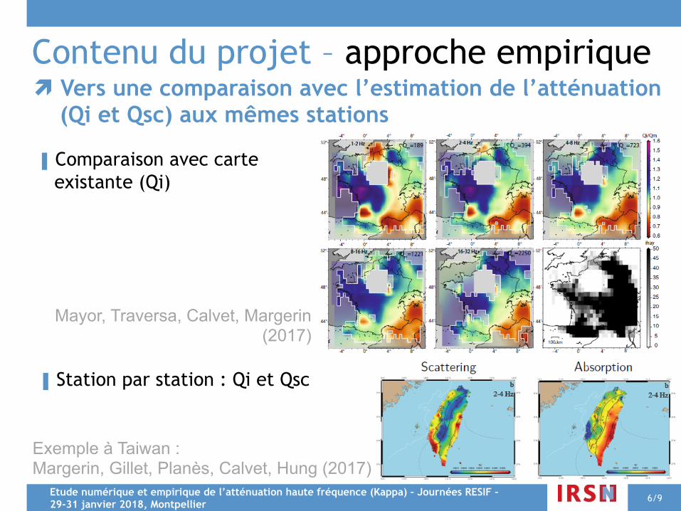
Contenu du projet – approche empirique ì Vers une comparaison avec l’estimation de l’atténuation

(Qi et Qsc) aux mêmes stations

Mayor, Traversa, Calvet, Margerin (2017)

Exemple à Taiwan : Margerin, Gillet, Planès, Calvet, Hung (2017)

▌ Comparaison avec carte existante (Qi)

▌ Station par station : Qi et Qsc

Etude numérique et empirique de l’atténuation haute fréquence (Kappa) – Journées RESIF – 29-31 janvier 2018, Montpellier

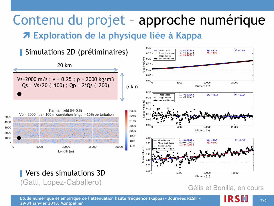
Vs=2000 m/s ; ν = 0.25 ; ρ = 2000 kg/m3 Qs = Vs/20 (=100) ; Qp = 2*Qs (=200)

7/9

Contenu du projet – approche numérique ì  Exploration de la physique liée à Kappa

20 km

5 km

Gélis et Bonilla, en cours

▌ Simulations 2D (préliminaires)

▌ Vers des simulations 3D (Gatti, Lopez-Caballero)


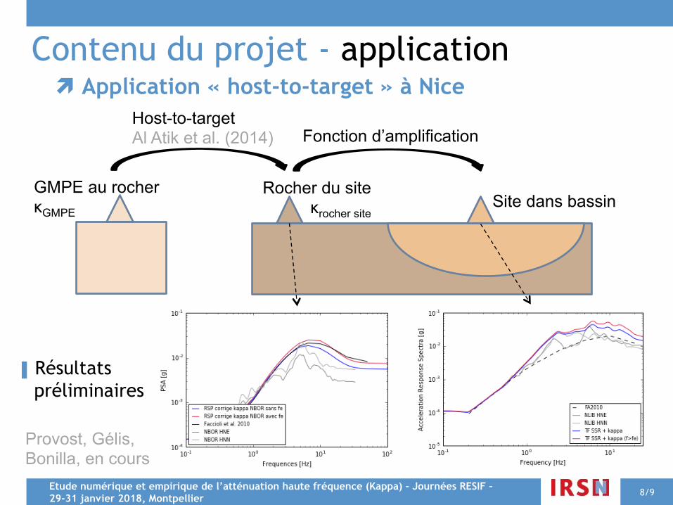
Contenu du projet - application ì Application « host-to-target » à Nice

Provost, Gélis, Bonilla, en cours

GMPE au rocher κGMPE

Rocher du site κrocher site

Site dans bassin

Host-to-target Al Atik et al. (2014) Fonction d’amplification

▌ Résultats préliminaires


Etat des lieux ì  Projet d’un an (début 1er juillet 2017), soumis en réponse à un

appel d’offre dans le cadre du GIS-RAP, possibilité de prolongation (sans budget supplémentaire)

ì  6 000 € budget (+ 4 650 € autres ressources) ì Cofinancement M2 ì Ressources informatiques ì Réunions

ì  2 réunions en visio depuis début projet (autres planifiées)

ì  Différents objectifs et approches autour d’une même thématique dans un groupe avec des compétences et connaissances très complémentaires

ì  Utilisation des données du réseau sismologique français

ì  Comment pérenniser ce groupe ?



Documents

Etude numérique et empirique de l’atténuation haute ... · time windows of 5 s for the pre-event noise and direct S-wave were used to compute the Fourier spectra. ... Etude numérique