Fiscal interactions and spillover effects of a federal

Maio de 2015 Working Paper

388

Fiscal interactions and spillover effects of

a federal grant to Brazilian municipalities

Marcelo Castro

Enlinson Mattos

Rebeca Regatieri

TEXTO PARA DISCUSSÃO 388 • MAIO DE 2015 • 1

Os artigos dos Textos para Discussão da Escola de Economia de São Paulo da Fundação Getulio

Vargas são de inteira responsabilidade dos autores e não refletem necessariamente a opinião da

FGV-EESP. É permitida a reprodução total ou parcial dos artigos, desde que creditada a fonte.

Escola de Economia de São Paulo da Fundação Getulio Vargas FGV-EESP www.eesp.fgv.br

Fiscal interactions and spillover effects of a federal grant to

Brazilian municipalities

Marcelo Castro∗ Enlinson Mattos† Rebeca Regatieri‡

May, 2015

Abstract

What is the impact of an unconditional transfer to a municipality when the municipality’sneighbor also receives the transfer? In this paper, we test whether a federal governmentgrant, the Municipalities’ Participation Fund (Fundo de Participacao dos Municıpios - FPM),differently affects municipal expenditures depending on neighbor cities. We use cities nearone of the four points of discontinuity in the FPM transfers according to population bracketsand with neighbors near different thresholds. We estimate the impacts of own and neighborFPM using the method of Regression Discontinuity Design (RDD). The results indicatethat part of the flypaper effect of FPM on local economies that has been estimated inthe literature can be explained by increased spending in neighboring municipalities. Thespillover is generally positive, with the exception of spending on health and sanitation insome population groups. We also consider a sample of neighbors that are more distant fromthe thresholds, and we show that in these cases the differences on estimations when we controlfor the neighbors’ FPM are not substantial. Ultimately, we find an effect on the neighborpopulations that helps clarify the observed FPM correlation in neighboring municipalities.

Keywords: fiscal federalism, program evaluation, flypaper effect, fiscal spillover.

Resumo

Qual o impacto de uma transferencia incondicional a um municıpio quando seu vizinhotambem recebe a transferencia? Nesse artigo nos testamos se uma transferencia do governofederal, o Fundo de Participacao dos Municıpios (FPM), afeta os gastos municipais de formadiferente dependendo dos municıpios vizinhos. Nos utilizamos municıpios proximos a um dosquatro pontos de descontinuidade no repasse do FPM de acordo com faixas de populacaoe que possuıam vizinhos proximos a pontos de descontinuidade diferentes. Nos estimamoso impacto do FPM recebido pelo proprio municıpio e pelo vizinho usando o metodo deRegressoes em Descontinuidade (RDD). Os resultados indicam que parte do efeito flypaper doFPM sobre a economia local estimado na literatura pode ser explicado pelo aumento de gastosnos municıpios vizinhos. O spillover e em geral positivo, com excecao dos gastos em saudee saneamento em algumas faixas populacionais. Nos tambem consideramos uma amostrade vizinhos mais distantes dos pontos de descontinuidade, e mostramos que nesse caso asdiferencas nas estimativas quando controlamos pelo FPM do vizinho nao sao substanciais.Por ultimo, encontramos um efeito positivo do FPM sobre a populacao dos municıpiosvizinhos, o que ajuda a esclarecer a correlacao observada entre o FPM de cidades vizinhas.

∗Corresponding author. Sao Paulo School of Economics (EESP / FGV-SP). Email:[email protected].†Sao Paulo School of Economics (EESP / FGV-SP). Email: [email protected]‡Master in Economics at Sao Paulo School of Economics (EESP / FGV-SP) and Finance and Control Analyst

at National Treasury. Email: [email protected]. The opinions expressed in this paper are solely theresponsibility of the authors and do not necessarily express the views of the National Treasury.

1

1 Introduction

In federalist economies, it is fundamental to investigate the extent of strategic interactions among

jurisdictions to determine the distribution of government resources to subnational entities.

In addition, fiscal spillovers help predict better tax and expenditure responsibilities in those

jurisdictions. Although a large body of empirical literature has emerged in recent years that has

documented the existence of fiscal spillovers, such studies generally lack identification issues in

their estimation.

The aim of this article is to identify the causal effect of a federal grant to a municipality on its

own expenditures, separating from the effect of neighbors’ grants, the grant spillover effect. We

consider an unconditional and involuntary transfer rule from the federal government to Brazilian

municipalities, the Participation Fund of Municipalities (Fundo de Participacao dos Municıpos

- FPM), as a source of exogenous variation in local spending. FPM grants are distributed

according to well-defined population brackets, thereby allowing us to use municipalities that

are close to discontinuity thresholds to identify exogenous variation in the transfers to those

jurisdictions. The method of Regression Discontinuity Design (RDD) allows us to work around

a central problem in the empirical literature, the endogeneity of neighbors’ fiscal responses.

Unobserved determinants of fiscal decisions are usually correlated across neighbors, whereas

in a federalist economy, those jurisdictions’ decisions can be simultaneously determined in

equilibrium. The previous empirical literature that aimed to test for fiscal spillover used

instruments for neighbors’ fiscal behavior based on neighbors’ idiosyncratic characteristics or

lags in the variables of interest (Case, Rosen and Hines, 1993; Figlio, Kolplin and Reid, 1999;

Saavedra, 2000; Brueckner and Saavedra, 2001; Deveraux, Lockwood and Redoano, 2007, 2008;

Bordignon, Cerniglia and Revelli, 2003; Buettner, 2003). More recently, the empirical literature

has addressed the identification problem using a more robust strategy (Baicker, 2004, 2005;

Knight and Schiff, 2010; Isen, 2014), and our paper aims to contribute to this recent literature.

In particular, our paper is more closely related to Isen (2014) in that we also attempt to

identify exogenous variation in neighbors’ fiscal variables using RDD. However, our strategy of

identification is similar to that of Brollo et al (2013), Litshcig and Morrison (2013), Arvate et al

(2013), and Castro and Regatieri (2014) in that we exploit a key feature of FPM distribution: this

federal transfer increases exogenously and discontinuously at the population bracket thresholds

to municipalities in a given state. We estimate RDD impacts of FPM in cities with population

2

near the thresholds. Thus, we consider cities with similar populations, some of which receive

a large amount of additional federal funds because of small increases in population beyond the

thresholds.

In theoretical terms, there are three general ways in which a city’s expenses could spill over

onto its neighbors (Wilson, 1999). When the number of jurisdictions is small, the local taxes are

chosen in strategic fashion, taking into account the inverse relationship between a jurisdiction’s

tax rate and its base. A related body of literature focuses on welfare competition, specifically

on income redistribution by local governments when the poor migrate in response to differing

welfare benefits. A third body of literature analyzes the strategic interactions caused by benefit

spillovers. However, according to Brueckner (2000), these theoretical models can be classified

into two main categories: spillover models and resource-flow models. The former category

incorporates cases in which local public expenditures can be correlated among neighbors when a

good’s production can be exploited by people from neighboring municipalities, as with highway

construction, environmental models, and efforts to reduce crime. The latter category includes

tax and welfare competition models as well as the yardstick competition model (Besley and

Case, 1995), in which voters can observe and compare the taxes and public service delivery in

neighboring municipalities before legitimize mayors’ second terms.

Our results confirm the existence of the spillover effect, in contrast to the most recent findings

by Isen (2014), that found no significant fiscal spillover effect for a sample of American counties,

municipalities and school districts. More importantly, our estimation suggests a larger spillover

effect than those previously found in the literature, and our identification strategy allows to

control for the neighbor’s fiscal policy variation to estimate the local response to federal grant.

We find a reduction in the flypaper estimates compared with those found in the literature.

The paper is divided as follows. In the next Section, we present our database and the FPM

institutional evolution. Section 3 explains econometric methodology to empirical implementation

and hypothesis that guarantee the causal identification of our instrument. In Section 4 we

analyze carefully the validation of the hypothesis in our data, while in Section 5 we present our

main results. Section 5 presents the results using a different sample of neighbors and Section 6

the results for extra robustness checks implemented in the Appendix. We make the final remarks

in Section 7.

3

2 Data and institutional background

FPM grants are the federal government’s most important transfer to municipalities and the main

revenue sources of small municipalities. In our sample, FPM grants account for an average of

45% of local budget revenues, which comprise tax revenues and transfers. The fund was created

in the 1947 Constitution, but the rule’s actual legal basis is outlined in the 1988 Constitution,

from Article 159 on, which sets the rule for allocating the fund’s resources. Article 160 of the

Constitution prohibits any constraints on the destination of these resources and restricts the

possibility of conditioning the transfer itself.

Transferring the FPM grants by population bracket was first established in 1966 with Law

No. 5,172 and the Complementary Act 35 of 1967, and the current thresholds were defined in the

1981 Decree Law No. 1,881, approved by Legislative Decree 19 of 1982. Complementary Law No.

59 of 1988 determined that FPM population coefficients should be reviewed annually according

to population estimates released by the National Statistics Institute (Instituto Brasileiro de

Geografia e Estatıstica - IBGE). Complementary Law No. 62, from 1989, postponed this change,

as did successive laws, such that this transition was only completed in 2007. Complementary Law

No. 62 also defined the Court of Audit (Tribunal de Contas da Uniao - TCU) as the responsible

body for monitoring and calculating the coefficients and creating additional legislation to regulate

the infra-constitutional background.

During the initial years of the 1990s, the transfers were still made based on 1981 decree law

coefficients. Beginning in 1993, the 1991 Census population was considered for cities that were

created after this census. Complementary Law No. 91 from 1997 determined the convergence

of the annual FPM grants to municipalities based on previous year population estimated by

IBGE over a transition period of four years, that was subsequently extended until 2007. This

transition aimed to help cities avoid drastically reductions in budget revenues, especially for

cities that had lost population because of migration or emancipation. In these cases, the annual

extra FPM, compared with the values under the 1995 coefficients, was discounted annually until

2007 (TCU Normative Decision No. 14, 1996).

We use data regarding the FPM transfers and expenditures of municipalities with fewer

than 30,000 inhabitants from 2002 to 2012, taken from the Finance of Brazil system (Financas

do Brasil - FINBRA) of the National Treasury Secretariat (Secretaria do Tesouro Nacional -

STN). The values of municipal expenditures and FPM shares available in FINBRA are reported

4

directly by the municipalities. We separately analyze the main municipal expenditures according

to the function in public administration: health, education, urbanization and basic sanitation1.

Nominal values (in reais, R$) were updated to January 2014 using the official Consumer Price

Index (Indice de Precos ao Consumidor Amplo - IPCA), calculated by IBGE2. Additionally, we

use information about local populations estimates released by IBGE.

The preparation of FINBRA stems from Law No. 4,320, from 1964, Articles 111 and 112,

and Complementary Law No. 101, from 2000, Article 51. Each municipality sends the Table of

Consolidated Municipal Financial Data to a public national bank, and the National Treasury

compiles the information. We have an unbalanced panel with approximately 4,000 municipalities

that had fewer than 30,000 inhabitants between 2002 and 2012. There is an attrition rate of

approximately 5% caused by municipalities that did not send their information in different years,

generally, small towns with fewer than 10,000 inhabitants.

The data regarding local populations derive from population censuses that were conducted

every ten years by the IBGE and the census population counts conducted at halftime. In the

period considered, there were population censuses in 2000 and 2010 and a population count in

2007, that are used to FPM distribution during the period 2003-2012. In the period between

population censuses, IBGE provides population estimates calculated from the growth rates

between the previous two censuses, weighted by country and state growth (IBGE, 2008). IBGE

publishes annual estimates until August 31 of each year, and by October 31, the final estimates

are sent to TCU (Article 102, Law No. 8443 of July 16, 1992). These estimates refer to July 1 of

each year (t) and are used to calculate FPM transfers in the following year (t + 1) (Ministerio

da Fazenda, 2005; 2012a).

We calculate the amounts that should have been transferred in accordance with the law,

which we call theoretical FPM, to determine whether the values reported to FINBRA by the

mayors are correct3. Now, we explain the calculation of the financial reducer to the period

2002-2007. First, we define the Additional Gain (AGit), a an auxiliary variable, for each

municipality as the difference between the tabulated population coefficient in 1995 and the

coefficient of the previous year, t-1:

1Considering the municipalities in our sample, the main types of expenditures in each function are: health -primary care and hospital assistance; education - elementary and childhood education; urbanization - constructionof roads and public works; sanitation - urban sanitation. More information about this expenditure classificationis available in Rezende (2007).

2US$1 was approximately equal to R$2.35 during this period at the official exchange rate.3More details on calculating the theoretical FPM coefficients can be found in Gasparini and Miranda (2006).

5

AGit = k(popi,1995)− k(popi,t−1) if AGit > 0 ; 0 otherwise

Where k is the coefficient of population used as a source of exogenous variation on FPM

transfer in our sample of cities. In fact, k is a step function of previous year local population

estimated by IBGE and tabulated by the law, as shown in Table 1 of appendix E.

There is a percentual reduction in (AGit), 1−Rt, where Rt is defined by law and increases

along the years, in such a way that there is a convergence of all cities by 20084. We use the

variable Additional Adjusted Gain, AAGit:

AAGit = AGit × (1−Rt) if AGit > 0 ; 0 otherwise

We define the Non-Supported Cities Coefficient, NSCit, as:

NSCit = k(popi,t−1) if AGit ≤ 0 ; 0 otherwise

The percentage, Rt, that is not used for cities which coefficients decreased is redistributed

to the Non Supported Cities. The total Share to Redistribute, SRit,can be written as:

SRit =Σj,t,SAGjt − Σj,t,SAAGjt

Σj,t,SNSCjt×NSCit if AGit ≤ 0 ; 0 otherwise

That is, SR is the value reduced from cities that receive additional gain (AG > 0) that are

distributed each city that are not supported by additional gain (AG ≤ 0), according to the

weight of each non supported city given all cities in the same situation in a given state and year.

The Final City Coefficient, FCit, is defined as:

FCit = k(popi,t−1) +AAGit if AGit > 0 and year ≤ 2007

FCit = k(popi,t−1) + SRit if AGit ≤ 0 and year ≤ 2007

FCit = k(popi,t−1) if year > 2007

Finally, theoretical FPM can be described by Equation (1):

theoreticalFPMit =FCit

Σj|SFCjt× ei ×Mt × 0.864 (1)

We divide the final coefficient of each city, FC, which is a direct function of the previous

year’s population coefficient, for the state total. Then, we multiply this percentage by the total

destined to city i’s state, ei, which follows a tabulation defined by the FPM law (TCU Resolution

4Financial reducer (Rt) values were: 40% in 2002, 50% in 2003, 60% in 2004, 70% in 2005, 80% in 2006 and90% in 2007, according to Complementary Law No. 91 of 1997.

6

242/1990) and presented in Table 2 of Appendix E. Mt e the national amount allocated to the

FPM each year, determined as 23.5% of the income tax and the tax on industrialized products

collected by the union. 86.4% of this amount is destined for interior cities with fewer than

140,000 inhabitants, which applies to all the cities in our sample.

We calculate in Equation (2) the increase in the theoretical FPM due to the previous year

population variation, for the period 2008-2012:

∆theoreticalFPMit

∆popi,t−1=

∆kit(∆popi,t−1)Σj 6=i|Skjt(popj,t−1)

(Σj|Skjt(popj,t−1))2× ei ×Mt × 0.864 (2)

The effect of population growth on theoretical FPM is heterogeneous among cities because

FPM distribution for interior cities also depends on the state. This effect is positive when

the population grows beyond the FPM thresholds, but it is decreasing because the coefficient

variation between the brackets is always the same (as shown in Table 1 of Appendix E). The

derivatives for supported and non supported cities during the years that the reducer was applied

follow a similar pattern.

3 Empirical strategy

We want to analyze the effect of extra FPM transfers received by municipalities on their budget

expenditures considering the spillover effects from neighboring cities, which could also have

received extra transfers. An Ordinary Least Squares (OLS) regression using all cities would

likely be spurious given that per capita local spending and FPM are both correlated with local

population. Also, similar neighboring municipalities are affected by similar cost shocks to local

public goods provision and prices as well as by national trends in the economy, situations that

could wrongly suggest a spillover effect (Revelli, 2005).

The methodology commonly used to estimate causal FPM impacts is based on this grant

distribution law, which determines that part of the amount is transferred according to specific

population segments. Hence, causal identification relies on the assumption that per capita FPM

variation can be considered a random experiment near the thresholds. There is a small or null

probability that a municipality receives a different value from the one established by this legal

criterion of city population, because the transfers are automatically made monthly following

accounting rules of apportionment.

RDD instrument validity entails that population thresholds cannot be correlated with other

7

local characteristics that are correlated with local spending to ensure causal impacts identification

(Lee, Lemieux, 2010), for example, political-administrative conditions and voters’ preferences

for public goods. This means that the population brackets that are used to transfer funds

to cities cannot be correlated with other factors that influence local expenditures, at least in

small regions near the thresholds. Additionally, the method implies that it is not possible to

complete manipulate population, what could result in nonrandom variation between control and

treatment groups, but we do allow for some non-prohibitive marginal manipulation.

Many papers have used this methodology and have found a positive impact of FPM on local

expenditures (for example, Arvate et al, 2013, and Castro and Regatieri, 2014). In this paper,

we argue that part of the estimated FPM effect on local expenditures may occur because of

spillover effects from the FPM grants that were transferred to neighbor municipalities. The

correlation between the population growth in neighboring municipalities leads to correlations

among received FPM, even if we control for local fixed effects. Thus, we show that the FPM

impact estimated by RDD are sensitive to the choice of neighbor cities.

There are three types of spillover or spatial interactions due to FPM that we are concerned.

First, the estimated impact using FPM population rule ignores general equilibrium effects

caused by the transfer. In particular, the estimated effect is the result of fiscal interactions

between municipalities that receive the resource and their neighbors. Additionally, depending

on the complementarity of neighbors’ spending, prices and demand can be impacted. General

equilibrium effects are difficult to distinguish, but their presence does not invalidate the estimates

if our interest is on the final effect of the experiment.

Two other types of spillover can lead to bias in the estimates, even if the goal is to measure

the total effect of the program. First, municipalities with a higher FPM population coefficient

occasionally have neighbors that are in the control group (i.e., immediately left of the thresholds),

which is likely to occur because of population correlation between neighboring municipalities.

Thus, controlling for this type of spillover prevents the treatment from contaminating the

control group, which can lead to underestimating the treatment effect (if the FPM grants

and neighbors’ expenditures are complementary) or overestimating it (if the FPM grants and

neighbors’ expenditures are substitutes). Our solution involves the assumption that city i and

neighbor j necessarily receive different instruments that do not coincide, that is, they are in

different RDD estimation windows. We ensure that, for example, if city i is considered treated

as crossing threshold 1, for example, its neighbors j do not appear as controls at threshold 1,

8

and neighbors j are necessarily in either the treatment or the control groups at any of the other

thresholds.

Finally, the third and more challenging possibility of spillover occurs even when we control

for city i and neigbor j at different thresholds. Municipalities that surpass one threshold

during the period may probably have neighbors that also surpass different thresholds because

of the population growth correlation of neighboring municipalities. The formula for the annual

population growth estimated by the IBGE, as will be made clear in Section 4, depends on the

growth in each city, region and country, between the two previous censuses. This generates

treatment correlation among neighbors that are close to different thresholds. We control for this

type of spillover adding the cities i and j’s FPM grants simultaneously in the regressions.

Our empirical strategy finds support in the empirical literature that seeks to estimate the

spillover effect of social experiments. For example, Acemoglu and Angrist (2000) use two

endogenous variables to estimate school peer effects. They control for student’s measured

ability, as for the school mean ability, as there is a common thought that students’ abilities

are correlated within a school. There is a literature that also considered double randomization

as the best way to estimate spillover effect (Angelucci, De Giorgi, 2009; Angelucci, Di March,

2010). Thus, we simultaneously control for own and neighbor j’s populations as two different

instruments, possibly correlated, to identify a own and neighbor’s FPM effects, as it equivalent

to take random cities i that are eligible for the treatment and then randomize their neighbors j.

We detail our strategy considering cities i and j with populations pi and pj in small windows

around different thresholds with no intersection among them. We consider for now 2 population

thresholds (we use four thresholds in our estimates), p1 and p2, and that FPMi is a function

of p1 and FPMj is a function of p2, as the only variable considered affecting FPM transfers

and local expenditures in the windows. We consider that city i’s budget spending depends on

whether city i or its neighbor j receive the FPM grants. We assume for simplicity that treatment

can be represented by a binary variable, as the effect of an additional R$1 transferred. Actually,

local population is just one variable of the formula used for the distribution of FPM, as we made

clear in Section 2, which means that treatment is heterogeneous even among cities at the same

threshold. However, we consider sufficiently small estimation windows around the thresholds to

capture the specific impact of the population rule. Based on Imbens and Lemieux (2008), we

formalize city i’s potential spending as a funtion of the i and j’s FPM transfers and population

size:

9

E(Gi|Ti, Tj , pi, pj) = g0(pi) + [g1(pi)− g0(pi)]Ti + w0(pj) + [w1(pj)− w0(pj)]Tj

where

Ti = 1(pi ≥ p1)

and

Tj = 1(pj ≥ p2)

Gi is city i’s spending, which depends on its population and that of its neighbor. Ti is a

binary treatment that indicates whether municipality i receives an additional transfer, which

occurs when the population, pi, is greater than the cutoff, p1. g1(pi) is the potential expenditure

of municipalities with population pi because of a R$1 per capita of transfer, while g0(pi) is the

potential expenditures of these cities when the mayors do not have that additional income. The

same is true for Tj , which is 1 when the population of city j, pj , is bigger than a given threshold,

p2, with p1 6= p2. Also, w1(pj) is the potential spillover of city j onto city i spending when city j

receives the extra FPM grant and w0(pj) is the potential spillover of city j onto city i en when

city j does not receive the extra amount.

Thus, the total impact of the city i’s FPM grant on local spending is equal to the potential

direct impact of receiving an extra money plus the additional spillover of neighbors receiving

the extra money. The identification problem is that we do not observe g0 and g1 for the same

municipality with population pi, in the same way that we do not observe w0 and w1 for the

same city with population pj .

We consider that transfers follow a continuous distribution based on the population, except

at the thresholds, and that potential expenditures g0 and g1 are continuous at p1 as w0 and

w1 are continuous at p2. Theoretical identification of treatment effect using RDD relies on

the distribution limits of dependent and independent variables at the thresholds (Imbens and

Lemieux, 2008). We define the Local Average Treatment Effect (LATE) as the effect of a

marginal population variation near the thresholds on city i’s expenditures:

LATEi(p1) = limpi→(p1)+

E(Gi|Ti, Tj , pj)− limpi→(p1)−

E(Gi|Ti, Tj , pj) =

limpi→(p1)+

E(Gi|Ti = 1, Tj , pj)− limpi→(p1)−

E(Gi|Ti = 0, Tj , pj) =

10

g1(p1)− g0(p1) + (w1(pj)− w0(pj))[E(Tj |pi → p+1 , pj)− E(Tj |pi → p−1 , pj)] =

g1(p1)− g0(p1) + (w1(pj)− w0(pj))[P (pj > p2|pi → p+1 )− P (pj ≤ p2|pi → p−1 )]

The causal effect of the city i’s FPM grant on own expenditures, g1(pi) − g0(pi), can be

consistently identified without considering spillover effects if there is no correlation between

neighbor’s populations. In this case, the impact of FPMi on city i’s expenditures could be

estimated by regressing expenditures on FPM transfers in a vicinity of the cutoff p1. Nonetheless,

the spillover effect is nonzero if there is correlation between neighbor’s populations:

P (pj > p2|pi → p+1 ) 6= P (pj ≤ p2|pi → p−1 )

In this case, not controlling for neighbor j’s FPM spillover biases the estimated treatment

impact. There are arguments that support this possibility, as neighbor’s populations are

correlated, because local population growth estimates are highly influenced by regional conditions

(IBGE, 2008), as we explain in Section 4. Therefore, as we approximate the potential values

exactly at the thresholds for observations close to them, the possibility of population correlation

among neighbors should not be ignored. Estimates using fixed effects can also be biased because

of the same source of correlation between neighbors’ population growth.

Again, the spillover identification problem is that we can not estimate w1 e w2 for the same

city j. Again, we explore the FPM law discontinuities and we consider neighbors j around the

population thresholds, in such a way that cities i and j are in different threshold windows. In

the case of non-zero spillover effects, we can identify the total effect of the cities i and j’s FPM

grants on i’s expenditures as:

LATEij(p1, p2) = limpj→(p2)+

LATEi − limpj→(p2)−

LATEi

= (g1(p1)− g0(p1)) + (w1(p2)− w0(p2)) (3)

We formalize the regressions to be estimated. Our objective is to estimate the LATE given

cities i and j’s population at different thresholds. The option adopted in this paper for the RDD

implementation follows Angrist and Lavy (1999), who also used a Two-Stage Least Squares

11

(2SLS) approach, but for only one endogenous variable. Indeed, RDD estimation can be

consistently generated by 2SLS (Imbens and Lemieux, 2008; Angrist and Lavy, 1999). The

first stage consists of regressing cities i and j’s declared FPM per capita on i and j’s theoretical

FPM per capita, the calculated amount that should have been transferred strictly under the

law. In the second stage we estimate the impacts of i and j’s FPM per capita predicted in the

first stage on i’s budget expenditure. 2SLS estimates Intended To Treat effects, which means

the average effect on the population of compliers (Angrist, Imbens and Rubin, 1996), but as

there are no deviations from the rule, 2SLS regression estimates equation (3).

The first stage specification is:

FPM = λ0 + λ1theoreticalFPM + λ2g2(p) + v (4)

where FPM is the vector of cities i and j’s declared per capita FPM and theoreticalFPM

is the vector of cities i and j’s theoretical per capita FPM, g2(p) is the vector of i’s and j’s

population polynomials of order 2. The second stage regression is:

Gi = α0 + τFPM∗ + α1g2(p) + ϑi (5)

where Gi is city i’s municipal budget expenditures and FPM∗ are the cities i and j’s FPM

per capita estimated in the first stage. τ is the vector of the coefficients of interest. ϑi is the city

i’s idiosyncratic error term, which we cluster by city i to control the variance of each city over

time (Wooldrigde, 2002). We also estimate regressions using the variable logarithms, except for

the populations terms. Estimation using panel data to control for local fixed effects guarantees

the robustness of results as local population growth is a continuous function of population, in

such a way that politicians can not manipulate population growth, as we demonstrate in Section

4.

The regression model that we present is a local linear regression, so that the results are valid

only for the municipalities located near the thresholds5. Nevertheless, we analyze the effects at

different population thresholds - 10,188, 13,584, 16,980 and 23,772 inhabitants. This guarantees

a degree of external validity for the average effect estimation in municipalities with up to 30,000

inhabitants, which account for approximately 80% of Brazilian municipalities and nearly 25%

5We present maps for treatment and control cities of the southeast states, the most populated region in Brazil,in Appendix D. The colored cities are in one of the RDD windows. We consider both city i and neighbors j coloredin our main regressions, but each one with a different color.

12

of the national population.

The fact that the treatment variable is not binary suggests the use of a fuzzy RDD, which

allows for the heterogeneity of treatment among the participants. The hypotheses of identification

are the same as those used in the sharp design that have been presented so far. The complete

discontinuity of the treatment variable is not strictly necessary for the RDD given that there

is some exogenous variation in the treatment caused by the instrument (Imbens and Lemieux,

2008).

4 Instrument validity

4.1 First stage impacts of FPM discontinuity rule

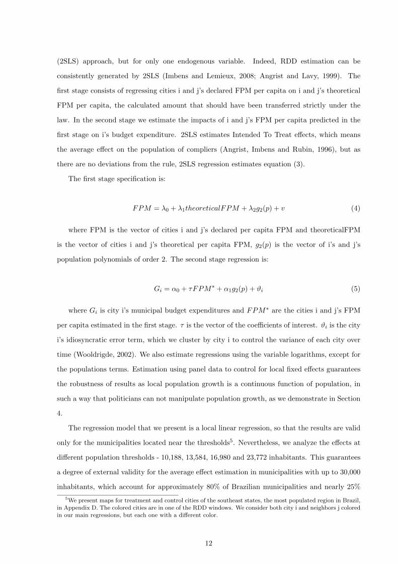
We present evidences of exogenous shocks at the population thresholds due to the FPM rule.

Figure 1 compares the average per capita FPM transferred according to data from FINBRA,

which are reported by city halls, and theoretical FPM, the value that should be transferred

strictly following FPM law, as functions of the previous year’s estimated population. In general,

municipalities report amounts that exceed what should be transferred by the fund, possibly

because this resource is distributed along with others, thereby creating difficulties in separating

resources. The peaks in Figure 1 are the effects of the population coefficient variation at the

thresholds. Increases in per capita FPM occur only in regions close to the thresholds, whereas

in other regions, the correlation between per capita FPM and population is negative.

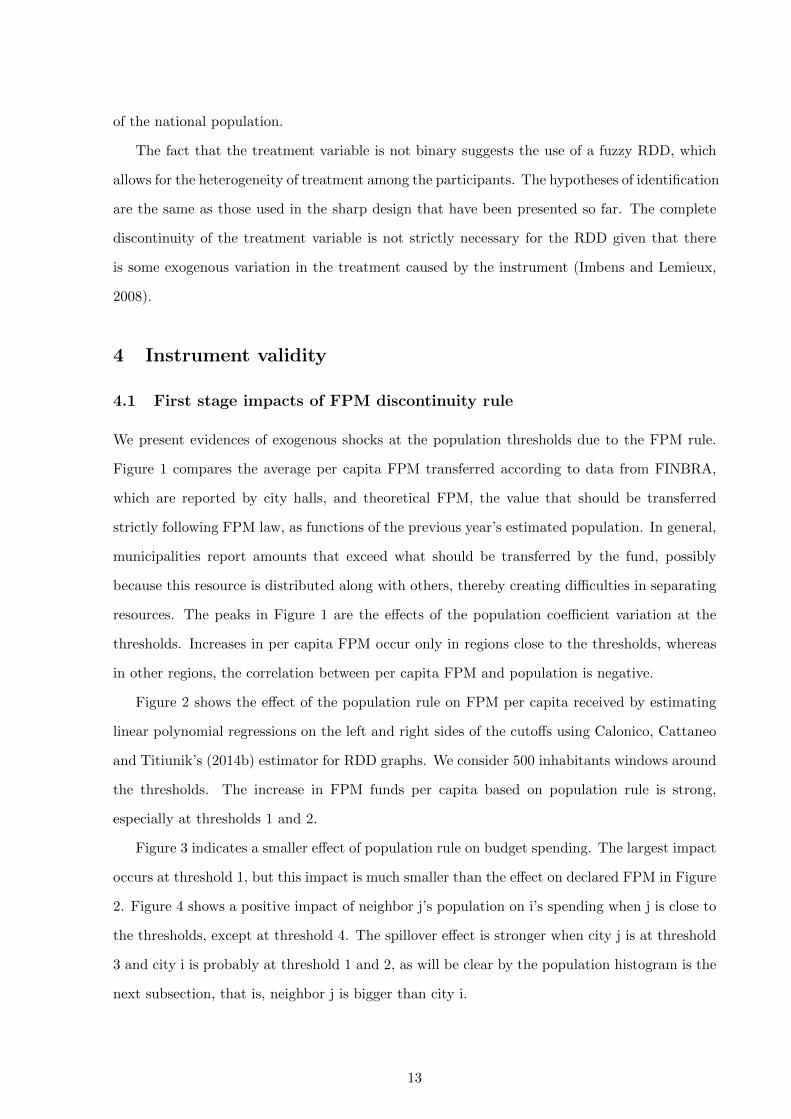
Figure 2 shows the effect of the population rule on FPM per capita received by estimating

linear polynomial regressions on the left and right sides of the cutoffs using Calonico, Cattaneo

and Titiunik’s (2014b) estimator for RDD graphs. We consider 500 inhabitants windows around

the thresholds. The increase in FPM funds per capita based on population rule is strong,

especially at thresholds 1 and 2.

Figure 3 indicates a smaller effect of population rule on budget spending. The largest impact

occurs at threshold 1, but this impact is much smaller than the effect on declared FPM in Figure

2. Figure 4 shows a positive impact of neighbor j’s population on i’s spending when j is close to

the thresholds, except at threshold 4. The spillover effect is stronger when city j is at threshold

3 and city i is probably at threshold 1 and 2, as will be clear by the population histogram is the

next subsection, that is, neighbor j is bigger than city i.

13

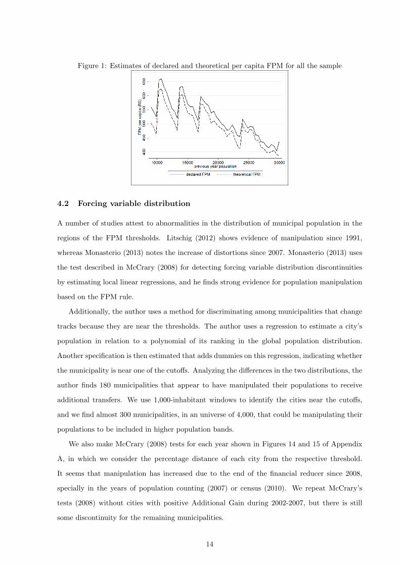
Figure 1: Estimates of declared and theoretical per capita FPM for all the sample

4.2 Forcing variable distribution

A number of studies attest to abnormalities in the distribution of municipal population in the

regions of the FPM thresholds. Litschig (2012) shows evidence of manipulation since 1991,

whereas Monasterio (2013) notes the increase of distortions since 2007. Monasterio (2013) uses

the test described in McCrary (2008) for detecting forcing variable distribution discontinuities

by estimating local linear regressions, and he finds strong evidence for population manipulation

based on the FPM rule.

Additionally, the author uses a method for discriminating among municipalities that change

tracks because they are near the thresholds. The author uses a regression to estimate a city’s

population in relation to a polynomial of its ranking in the global population distribution.

Another specification is then estimated that adds dummies on this regression, indicating whether

the municipality is near one of the cutoffs. Analyzing the differences in the two distributions, the

author finds 180 municipalities that appear to have manipulated their populations to receive

additional transfers. We use 1,000-inhabitant windows to identify the cities near the cutoffs,

and we find almost 300 municipalities, in an universe of 4,000, that could be manipulating their

populations to be included in higher population bands.

We also make McCrary (2008) tests for each year shown in Figures 14 and 15 of Appendix

A, in which we consider the percentage distance of each city from the respective threshold.

It seems that manipulation has increased due to the end of the financial reducer since 2008,

specially in the years of population counting (2007) or census (2010). We repeat McCrary’s

tests (2008) without cities with positive Additional Gain during 2002-2007, but there is still

some discontinuity for the remaining municipalities.

14

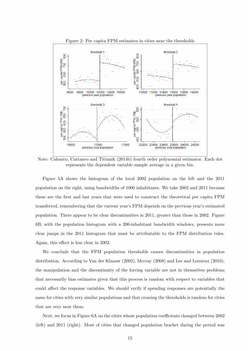
Figure 2: Per capita FPM estimates in cities near the thresholds

Note: Calonico, Cattaneo and Titiunik (2014b) fourth order polynomial estimator. Each dotrepresents the dependent variable sample average in a given bin.

Figure 5A shows the histogram of the local 2002 population on the left and the 2011

population on the right, using bandwidths of 1000 inhabitants. We take 2002 and 2011 because

these are the first and last years that were used to construct the theoretical per capita FPM

transferred, remembering that the current year’s FPM depends on the previous year’s estimated

population. There appear to be clear discontinuities in 2011, greater than those in 2002. Figure

6B, with the population histogram with a 200-inhabitant bandwidth windows, presents more

clear jumps in the 2011 histogram that must be attributable to the FPM distribution rules.

Again, this effect is less clear in 2002.

We conclude that the FPM population thresholds causes discontinuities in population

distribution. According to Van der Klaauw (2002), Mccray (2008) and Lee and Lemieux (2010),

the manipulation and the discontinuity of the forcing variable are not in themselves problems

that necessarily bias estimates given that this process is random with respect to variables that

could affect the response variables. We should verify if spending responses are potentially the

same for cities with very similar populations and that crossing the thresholds is random for cities

that are very near them.

Next, we focus in Figure 6A on the cities whose population coefficients changed between 2002

(left) and 2011 (right). Most of cities that changed population bracket during the period was

15

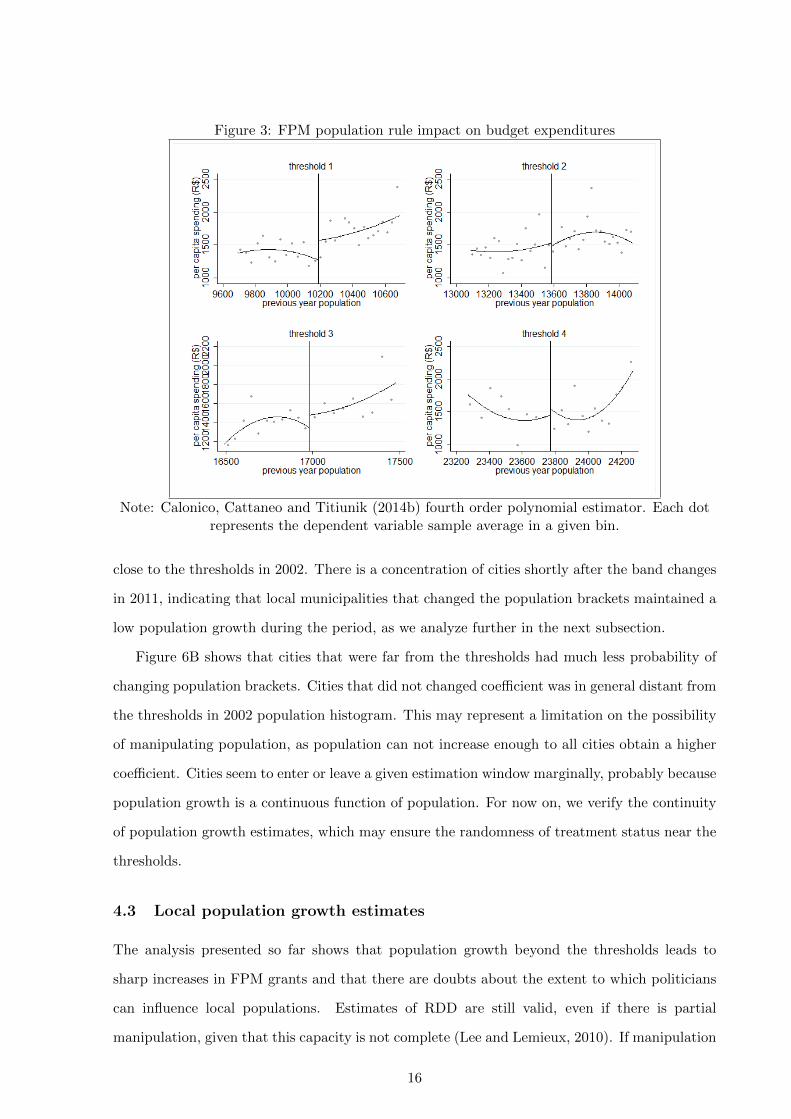
Figure 3: FPM population rule impact on budget expenditures


close to the thresholds in 2002. There is a concentration of cities shortly after the band changes

in 2011, indicating that local municipalities that changed the population brackets maintained a

low population growth during the period, as we analyze further in the next subsection.

Figure 6B shows that cities that were far from the thresholds had much less probability of

changing population brackets. Cities that did not changed coefficient was in general distant from

the thresholds in 2002 population histogram. This may represent a limitation on the possibility

of manipulating population, as population can not increase enough to all cities obtain a higher

coefficient. Cities seem to enter or leave a given estimation window marginally, probably because

population growth is a continuous function of population. For now on, we verify the continuity

of population growth estimates, which may ensure the randomness of treatment status near the

thresholds.

4.3 Local population growth estimates

The analysis presented so far shows that population growth beyond the thresholds leads to

sharp increases in FPM grants and that there are doubts about the extent to which politicians

can influence local populations. Estimates of RDD are still valid, even if there is partial

manipulation, given that this capacity is not complete (Lee and Lemieux, 2010). If manipulation

16

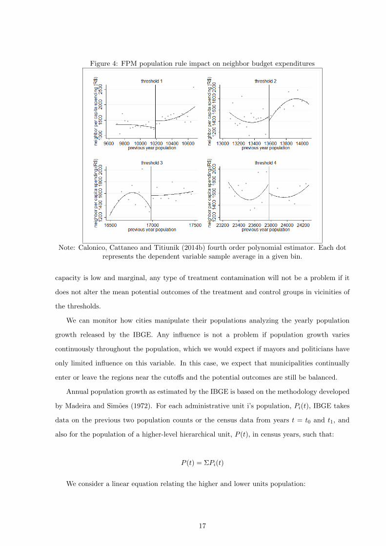
Figure 4: FPM population rule impact on neighbor budget expenditures


capacity is low and marginal, any type of treatment contamination will not be a problem if it

does not alter the mean potential outcomes of the treatment and control groups in vicinities of

the thresholds.

We can monitor how cities manipulate their populations analyzing the yearly population

growth released by the IBGE. Any influence is not a problem if population growth varies

continuously throughout the population, which we would expect if mayors and politicians have

only limited influence on this variable. In this case, we expect that municipalities continually

enter or leave the regions near the cutoffs and the potential outcomes are still be balanced.

Annual population growth as estimated by the IBGE is based on the methodology developed

by Madeira and Simoes (1972). For each administrative unit i’s population, Pi(t), IBGE takes

data on the previous two population counts or the census data from years t = t0 and t1, and

also for the population of a higher-level hierarchical unit, P (t), in census years, such that:

P (t) = ΣPi(t)

We consider a linear equation relating the higher and lower units population:

17

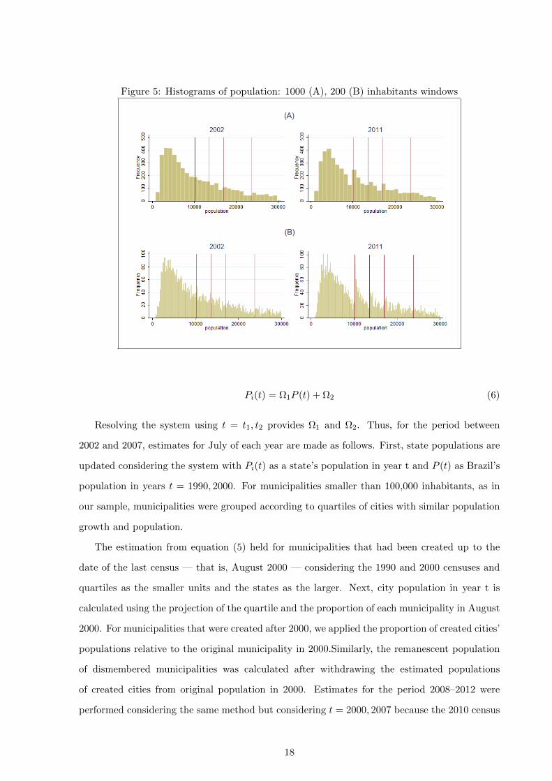
Figure 5: Histograms of population: 1000 (A), 200 (B) inhabitants windows

Pi(t) = Ω1P (t) + Ω2 (6)

Resolving the system using t = t1, t2 provides Ω1 and Ω2. Thus, for the period between

2002 and 2007, estimates for July of each year are made as follows. First, state populations are

updated considering the system with Pi(t) as a state’s population in year t and P (t) as Brazil’s

population in years t = 1990, 2000. For municipalities smaller than 100,000 inhabitants, as in

our sample, municipalities were grouped according to quartiles of cities with similar population

growth and population.

The estimation from equation (5) held for municipalities that had been created up to the

date of the last census — that is, August 2000 — considering the 1990 and 2000 censuses and

quartiles as the smaller units and the states as the larger. Next, city population in year t is

calculated using the projection of the quartile and the proportion of each municipality in August

2000. For municipalities that were created after 2000, we applied the proportion of created cities’

populations relative to the original municipality in 2000.Similarly, the remanescent population

of dismembered municipalities was calculated after withdrawing the estimated populations

of created cities from original population in 2000. Estimates for the period 2008–2012 were

performed considering the same method but considering t = 2000, 2007 because the 2010 census

18

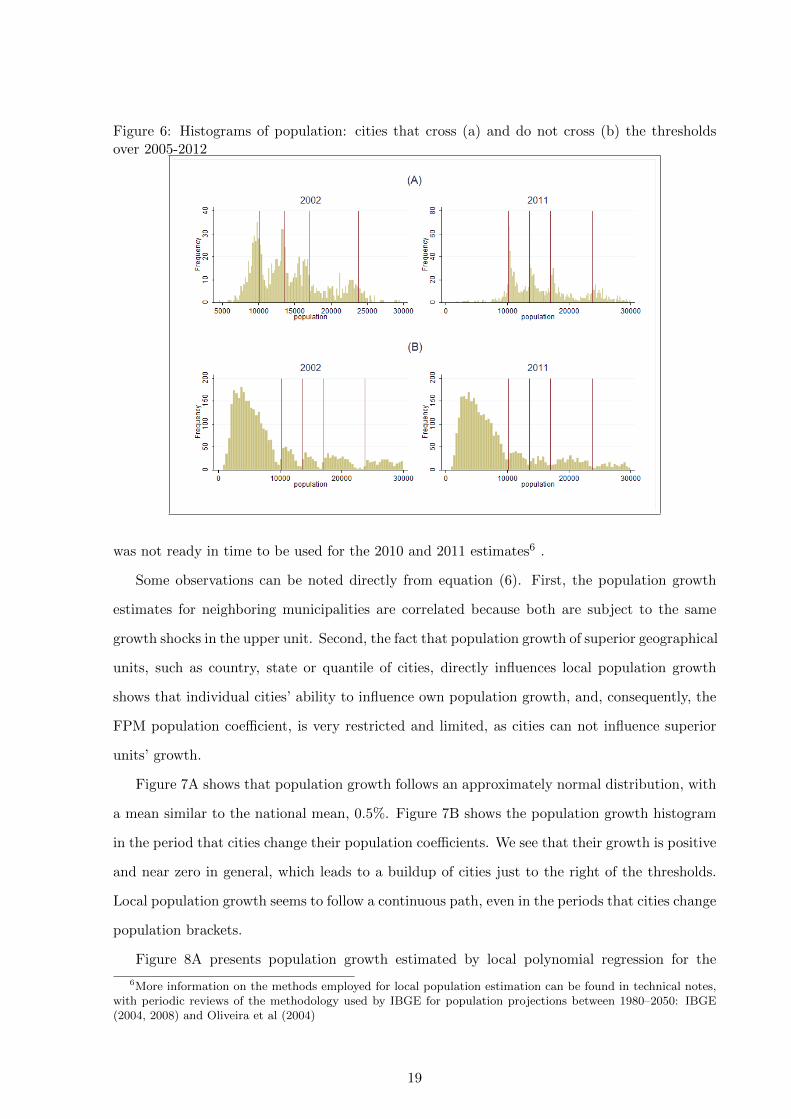
Figure 6: Histograms of population: cities that cross (a) and do not cross (b) the thresholdsover 2005-2012

was not ready in time to be used for the 2010 and 2011 estimates6 .

Some observations can be noted directly from equation (6). First, the population growth

estimates for neighboring municipalities are correlated because both are subject to the same

growth shocks in the upper unit. Second, the fact that population growth of superior geographical

units, such as country, state or quantile of cities, directly influences local population growth

shows that individual cities’ ability to influence own population growth, and, consequently, the

FPM population coefficient, is very restricted and limited, as cities can not influence superior

units’ growth.

Figure 7A shows that population growth follows an approximately normal distribution, with

a mean similar to the national mean, 0.5%. Figure 7B shows the population growth histogram

in the period that cities change their population coefficients. We see that their growth is positive

and near zero in general, which leads to a buildup of cities just to the right of the thresholds.

Local population growth seems to follow a continuous path, even in the periods that cities change

population brackets.

Figure 8A presents population growth estimated by local polynomial regression for the

6More information on the methods employed for local population estimation can be found in technical notes,with periodic reviews of the methodology used by IBGE for population projections between 1980–2050: IBGE(2004, 2008) and Oliveira et al (2004)

19

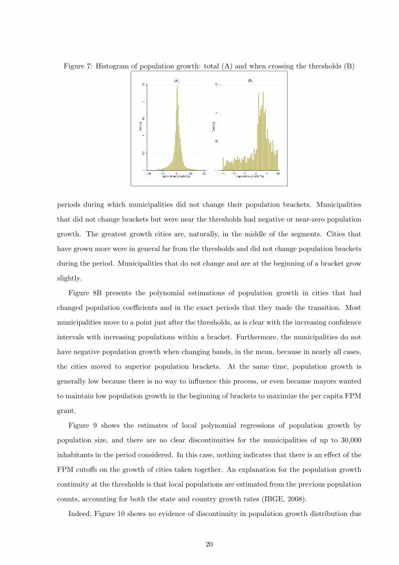
Figure 7: Histogram of population growth: total (A) and when crossing the thresholds (B)

periods during which municipalities did not change their population brackets. Municipalities

that did not change brackets but were near the thresholds had negative or near-zero population

growth. The greatest growth cities are, naturally, in the middle of the segments. Cities that

have grown more were in general far from the thresholds and did not change population brackets

during the period. Municipalities that do not change and are at the beginning of a bracket grow

slightly.

Figure 8B presents the polynomial estimations of population growth in cities that had

changed population coefficients and in the exact periods that they made the transition. Most

municipalities move to a point just after the thresholds, as is clear with the increasing confidence

intervals with increasing populations within a bracket. Furthermore, the municipalities do not

have negative population growth when changing bands, in the mean, because in nearly all cases,

the cities moved to superior population brackets. At the same time, population growth is

generally low because there is no way to influence this process, or even because mayors wanted

to maintain low population growth in the beginning of brackets to maximize the per capita FPM

grant.

Figure 9 shows the estimates of local polynomial regressions of population growth by

population size, and there are no clear discontinuities for the municipalities of up to 30,000

inhabitants in the period considered. In this case, nothing indicates that there is an effect of the

FPM cutoffs on the growth of cities taken together. An explanation for the population growth

continuity at the thresholds is that local populations are estimated from the previous population

counts, accounting for both the state and country growth rates (IBGE, 2008).

Indeed, Figure 10 shows no evidence of discontinuity in population growth distribution due

20

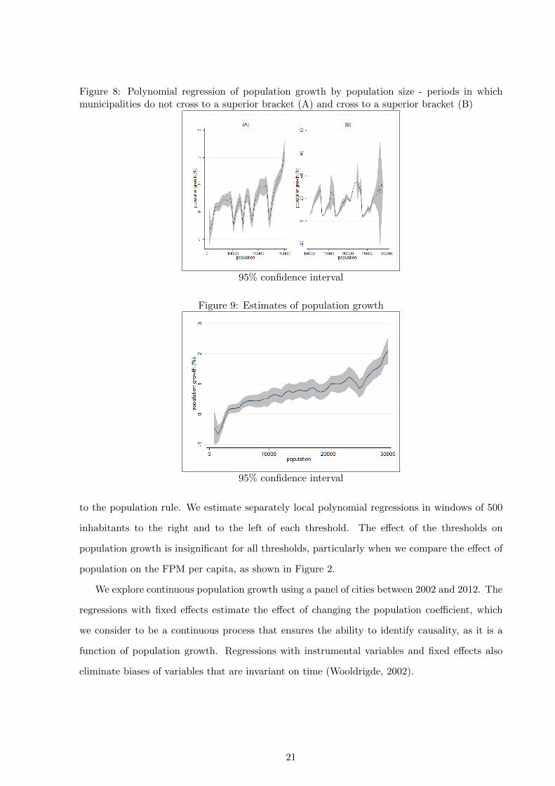
Figure 8: Polynomial regression of population growth by population size - periods in whichmunicipalities do not cross to a superior bracket (A) and cross to a superior bracket (B)

95% confidence interval

Figure 9: Estimates of population growth

95% confidence interval

to the population rule. We estimate separately local polynomial regressions in windows of 500

inhabitants to the right and to the left of each threshold. The effect of the thresholds on

population growth is insignificant for all thresholds, particularly when we compare the effect of

population on the FPM per capita, as shown in Figure 2.

We explore continuous population growth using a panel of cities between 2002 and 2012. The

regressions with fixed effects estimate the effect of changing the population coefficient, which

we consider to be a continuous process that ensures the ability to identify causality, as it is a

function of population growth. Regressions with instrumental variables and fixed effects also

eliminate biases of variables that are invariant on time (Wooldrigde, 2002).

21

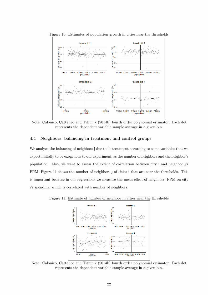
Figure 10: Estimates of population growth in cities near the thresholds


4.4 Neighbors’ balancing in treatment and control groups

We analyze the balancing of neighbors j due to i’s treatment according to some variables that we

expect initially to be exogenous to our experiment, as the number of neighbors and the neighbor’s

population. Also, we want to assess the extent of correlation between city i and neighbor j’s

FPM. Figure 11 shows the number of neighbors j of cities i that are near the thresholds. This

is important because in our regressions we measure the mean effect of neighbors’ FPM on city

i’s spending, which is correlated with number of neighbors.

Figure 11: Estimate of number of neighbor in cities near the thresholds


22

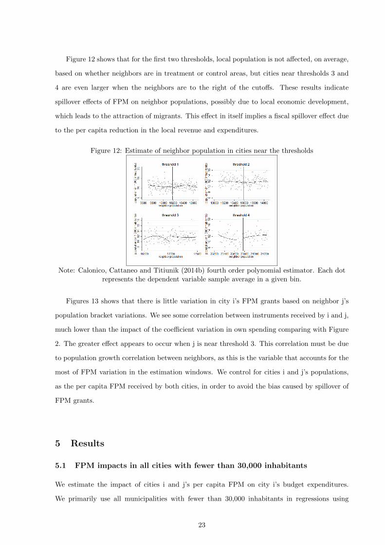
Figure 12 shows that for the first two thresholds, local population is not affected, on average,

based on whether neighbors are in treatment or control areas, but cities near thresholds 3 and

4 are even larger when the neighbors are to the right of the cutoffs. These results indicate

spillover effects of FPM on neighbor populations, possibly due to local economic development,

which leads to the attraction of migrants. This effect in itself implies a fiscal spillover effect due

to the per capita reduction in the local revenue and expenditures.

Figure 12: Estimate of neighbor population in cities near the thresholds


Figures 13 shows that there is little variation in city i’s FPM grants based on neighbor j’s

population bracket variations. We see some correlation between instruments received by i and j,

much lower than the impact of the coefficient variation in own spending comparing with Figure

2. The greater effect appears to occur when j is near threshold 3. This correlation must be due

to population growth correlation between neighbors, as this is the variable that accounts for the

most of FPM variation in the estimation windows. We control for cities i and j’s populations,

as the per capita FPM received by both cities, in order to avoid the bias caused by spillover of

FPM grants.

5 Results

5.1 FPM impacts in all cities with fewer than 30,000 inhabitants

We estimate the impact of cities i and j’s per capita FPM on city i’s budget expenditures.

We primarily use all municipalities with fewer than 30,000 inhabitants in regressions using

23

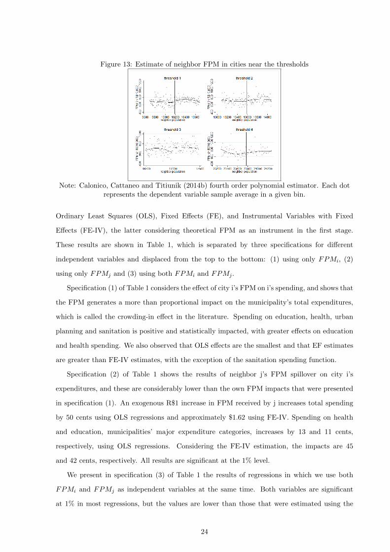
Figure 13: Estimate of neighbor FPM in cities near the thresholds


Ordinary Least Squares (OLS), Fixed Effects (FE), and Instrumental Variables with Fixed

Effects (FE-IV), the latter considering theoretical FPM as an instrument in the first stage.

These results are shown in Table 1, which is separated by three specifications for different

independent variables and displaced from the top to the bottom: (1) using only FPMi, (2)

using only FPMj and (3) using both FPMi and FPMj .

Specification (1) of Table 1 considers the effect of city i’s FPM on i’s spending, and shows that

the FPM generates a more than proportional impact on the municipality’s total expenditures,

which is called the crowding-in effect in the literature. Spending on education, health, urban

planning and sanitation is positive and statistically impacted, with greater effects on education

and health spending. We also observed that OLS effects are the smallest and that EF estimates

are greater than FE-IV estimates, with the exception of the sanitation spending function.

Specification (2) of Table 1 shows the results of neighbor j’s FPM spillover on city i’s

expenditures, and these are considerably lower than the own FPM impacts that were presented

in specification (1). An exogenous R$1 increase in FPM received by j increases total spending

by 50 cents using OLS regressions and approximately $1.62 using FE-IV. Spending on health

and education, municipalities’ major expenditure categories, increases by 13 and 11 cents,

respectively, using OLS regressions. Considering the FE-IV estimation, the impacts are 45

and 42 cents, respectively. All results are significant at the 1% level.

We present in specification (3) of Table 1 the results of regressions in which we use both

FPMi and FPMj as independent variables at the same time. Both variables are significant

at 1% in most regressions, but the values are lower than those that were estimated using the

24

variables separately. Specially, spillover estimates are much lower than before. The effect on

spending using FE is 10 cents lower, whereas the FE-IV estimates were 45 cents lower, less than

one-third of the estimates from part (2).

Estimates of the impact of i’s FPM on its own expenditures are much closer to the coefficients

that were estimated in specification (1). This shows that the correlation between a municipality’s

own FPM grant and its spending is very high, whereas the additional explanation of the variable

FPMj is very low, which is clear from the observation of R2 of OLS regressions. FPMj alone

appears to explain 4 % of i’s expenditures, but adding FPMj to specification (1) does not

increase regression R2.

[Table 1]

5.2 Impacts of FPM using the discontinuity rule

Next, we estimate the effect of FPMi and FPMj on city i’s expenditures using RDD regressions,

considering that i and j have populations within 500 inhabitants of the thresholds. We consider

for all of the following regressions in this subsection that cities i and neighbors j are in windows

around different thresholds, even in the regressions that control for only one FPM. We use 2SLS

in Fixed Effects (FE-IV), including theoretical FPM as instruments for i and j’s declared FPM

grants.

Table 2 shows the effects of FPMi and FPMj , estimated separately and together, on city

i’s budget expenditures. The first 4 columns show the results for the variables by level, and the

last 4 columns present elasticities estimated by regressions with the variables transformed into

logarithms, with the exception of population and its quadratic term. In each column, we control

for population i in one of the four discontinuity windows at the top or for population j at the

bottom. Controlling only for FPMi, the effect of R$1 extra FPM on spending is significantly

higher than R$1, R$1.81 at the first threshold and R$3.25 at the last. A municipality’s own

FPM effects are reduced when we add neighbor j’s FPM. The largest reductions occur at the

first threshold, with the effect reduced to R$1.13; the reductions at thresholds 2 and 3 are

smaller, and the estimates at threshold 4 are now insignificant. The trend is similar when we

use logarithms of variables. A municipality’s maximum own FPM grant’s estimated elasticity

is 1.14% at threshold 2. Effects are reduced with the addition of neighbors’ FPM grants; in

25

particular, the effect at threshold 1 decreases from 0.88% to 0.57%. At the same time, the

spillover effect of FPMj is only significant and positive when city i is at threshold 1, and so j’s

population is greater than i’s.

We present at the bottom of Table 2 spillover estimates in which we control for neighbors j

near each of the thresholds. The coefficient of FPMj , the spillover effect of the grant, without

controlling for FPMi, is in general similar to the estimated effect of FPMi alone in the first

part of the table, maybe due to the correlation of FPM between cities i and j. These effects

are R$1.66 when neighbor j is near the first thresholds, R$2.75 and R$2.28 at thresholds 2

and 3, and R$3.19 when neighbor j is at the last threshold. Controlling for FPMi reduces the

FPMj spillover effect, which is no longer significant at 10% at thresholds 1 and 4. Additionally,

the FPMi impacts are lower when city i is not at these thresholds. FPMj elasticity, without

controlling for log FPMj , on expenditures per capita is 0.79% at the first threshold, whereas at

the other thresholds, the values are statistically very close to 1%. There is again a reduction in

the magnitude and significance of FPMj effects with the addition of the log FPMi. The spillover

effect remains only in the intermediate tracks, and both FPMi and FPMj are insignificant when

j is at threshold 4.

[Table 2]

In Table 3, we repeat the procedures from the previous table, replacing budget spending

with health spending as the dependent variable. The effects of a municipality’s own FPM grant,

without controlling for FPMj , are positive and significant. The impacts estimated with level

variables show an increasing effect from the first to the third population thresholds, ranging from

R$0.55 to R$0.78. The effects estimated with level variables and with FPMj as the control are

lower, especially at threshold 1, and are insignificant for the municipalities at threshold 4. The

effects continue to increase with population increases up to the third threshold, ranging from

R$0.29 to R$1.02.

The effects with log variables without controlling for FPMj are generally close to 1% except

for the third threshold, where the estimated impact is 2.16%. By controlling for FPMj , the

estimated effects of a municipality’s own FPM grant are insignificant at the second and fourth

thresholds and close to 1% at threshold 1, but the estimation at threshold 3 shows a significant

effect of 4.07%. The main change in the previously observed trends is a negative FPMj spillover

26

effect of 2.28% on health spending when i is at threshold (3), that is, municipalities would spend

more on health if there were no FPM spillover effect received by neighbors j. In this case, j

usually has a lower population than i, according to population distribution in Section 4, which

shows that city i spends less on health when their neighbors are smaller and receive larger FPM

grants.

Table 3 also presents estimates of j’s FPM spillover effects on city i’s health spending,

controlling for the neighbor j’s threshold, first without controlling for the FPM received by i.

The estimates are small, ranging from R$0.45 to R$0.81 for level regressions, values statistically

lower than R$1. Adding FPMi, the spillover effect is R$0.53 at threshold 3, whereas becomes

insignificant at the others. The impact of FPMi is significant only when j is near the first or

second thresholds, when i’s population is usually larger than j’s. Regressions with log variables

show that the spillover effect on health spending, without controlling for FPMi, is statistically

equal to 1%, except at the first threshold, where the effect is 0.7%. Controlling for FPMi,

the elasticities of FPMj when j is near the first or second population thresholds are -0.72%

and -2.59%, respectively, and elasticity is positive on the third threshold, 0.75%. These results,

significant at 1%, confirm that the estimated j’s FPM spillover effect on i’s health spending is

negative when neighbor j is smaller than i, and positive otherwise. In this situation, neighbor

j’s population benefits more from city i’s spending on health than the opposite, so an increase

in neighbor j’s health spending may decrease total demand for health services in city i.

[Table 3]

The impacts of FPM grants on education spending are shown in Table 4. The first part

shows that the impact of a municipality’s own FPM grant, without controlling for neighbors’

grants, increases with the municipality’s own population from R$0.53 to R$0.98 for each R$1 per

capita transferred from thresholds 1 to 4. The level effects range from R$0.37 to R$0.83 between

the first and third thresholds when we add FPMj , and spillover effects are not significant at

5%.

The results using log variables are statistically close to 1%, except at the first threshold,

0.76%. Again, the impacts increase with population and reach 1.23% at threshold 4. The

elasticities of FPMi when we add the log FPMj do not change statistically at thresholds 2 and

3, but they become insignificant at threshold 4 and less than 1% at the first threshold, 0.44%.

27

The spillover effect is 0.43% when city i is on the first threshold and j is bigger, value significant

at 5%.

The lower part shows the regression results in which we control population j in each of four

RDD estimation windows. The level spillover effect, without controlling for i’s FPM, is R$0.57

for the smallest population group and R$1.02 for the largest group. The spillover effects, when

we add city i’s FPM, remain significant only at the second and third thresholds, R$0.61 and

R$0.46. The spillover elasticities, without controlling for FPMi, on education spending are

statistically close to 1%. When we add the log of city i’s FPM grant, the estimates become

insignificant at the 5% confidence level.

[Table 4]

The estimated effects of FPM on urbanization spending are in Table 5. The effects by level

are lower than those estimated for education and health spending and very lower than R$1, but

are still significant at 1%, ranging from R$0.15 to R$0.56 when we do not control for neighbors’

FPM . The effects of a municipality’s own FPM are reduced when we include neighbors’ FPM

grants and are insignificant on the second and fourth tracks. The effects are only significant at

1% for municipalities at threshold 3, a increase of R$0.35.

The FPMi elasticity in urban spending, without controlling for FPMj , is greater than 1%

for municipalities on the third and fourth RDD windows, with values of 1.74% and 1.88%, and

close to 1% when i is in the first or second estimation windows. By adding the log of FPMj , the

elasticity of FPMi is 2.62% at threshold 3, significant at 1%, 1.42% at threshold 1, significant

at 5%, while insignificant at 10% at the other thresholds. The effect of the log FPMj is only

significant at 10% when i is at threshold 3, -1.26%.

The bottom part of Table 5 shows the results after controlling for population j in each of the

four RDD estimation windows. The results are generally positive and significant at 1% when

we do not control for FPMi, ranging from R$0.23 to R$0.42. By adding FPMi, most of the

estimated effects of FPMj lose significance at 5%, except when neighbors j are in estimation

window 3, R$0.22.

The estimated elasticities follows the same trend of regressions using level variables. The

effects of FPMj without controlling for FPMi are positive and statistically close to 1%, except

for threshold 4, which value is 1.96%. Adding FPMi removes the significance of FPMj at all

28

the thresholds, whereas the effect of FPMi is significant at 5% when j is in the first or second

windows, increasing urban spending by 1.67% and 1.85% respectively.

[Table 5]

Finally, Table 6 shows the results for spending on basic sanitation - the function of budget

spending with the lowest amount applied in our sample. The estimated effects for a municipality’s

own FPM, using level variables and without considering neighbors’ FPM grants, are insignificant

at 5% at thresholds 1 and 2 and significant at this value at thresholds 3 and 4, although the

effects are very small, R$0.08 and R$0.07 respectively. The level effect of FPMi when we control

for FPMj only remains significant at 5% when i is at threshold 3, R$0.23, as well as FPMj

spillover impact, -R$0.15 in this case.

The effect of log FPMi without controlling for log FPMj is only significant at 5% at

threshold 3, 4.38%, which increases to 16.12% when we control for FPMj . At the same time,

there is a strong negative spillover at this threshold of -9.59%. The elasticities of FPMi and

FPMj are insignificant at 1% in the other groups.

The effect of neighbor j’s FPM grants, without controlling for city i’s FPM grant, on

sanitation spending are only significant at threshold 3, R$0.12 for the level regression and

6.91% for log estimates. Spillover effects on sanitation are more significant when we include

i’s FPM. The effect level is significant at 5% when j is close to threshold 1, - R$0.12, and in

the log estimation, -5.96%. At the same time, the values are positive and significant at 5% for

municipalities at threshold 3, R$0.21 for level variables and 13.79% for log variables.

These results show a substitution effect between neighbors’ FPM grants and spending on

sanitation, as happens with health expenditures. Basic sanitation is very deficient in Brazilian

small cities, which is one of the most important causes of diseases and demanding public health

system. the spillover effect of FPMj is greater when j is in the first estimation window, that is,

when j is smaller than i. Increasing sanitation spending in neighbor j, when j is smaller than i,

may decrease demand for i’s health services and even decrease i’s health spending. Moreover,

the decrease on health demand may lead to city i’s mayor invest less in sanitation.

[Table 6]

29

6 Alternative sample of neighbors

The developed analysis shows that thinking about a municipality’s own FPM per capita as a

quasi-experiment to measure the impacts of transference on expenditures may be misleading if

we do not consider neighbors’ conditions, due to correlations between neighbors’ FPM grants.

In experiment design literature, we should say that increasing i’s probability of being treated

increases the probability of j’s being treated, so not controlling for both cities’s treatment status

may lead to bias in the estimates.

Another way to avoid FPM interactions between municipalities and their neighbors is to

select an appropriate sample of neighbors j that lie outside of any of the RDD windows, in

which case the probability of both cities i and j changing population coefficient simultaneously

is considerably reduced7. In this case, small population growth may change the treatment status

of i but not that of j, so we can identify a given municipality’s own FPM impacts. Conversely,

we can measure spillover effects controlling for neighbors j in one of the RDD window and cities

i out of them.

Table 7 shows FPMi impacts on i’s spending by function. We perform 2SLS-FE regressions

using level variables and considering the FPM grant received by municipality i at each of the

thresholds; initially, we consider all of the thresholds together. On the left side of the table, we

consider regressions without controlling for FPMj . Overall, the estimates are relatively close to

those that were previously calculated. On the right side of the table, we repeat the regressions

with the addition of FPMj . We consider the aggregate FPM grant received by neighbor j in

place of the per capita values because population can be influenced by spillover effects.

The changes are much smaller than those found in Tables 2–6 . Estimated variances increase

when we control for j’s FPM, but they are much smaller than those that are exposed in Tables

2–6, indicating a bigger sample and weaker correlations between the cities i and j’s FPM. The

total budget spending shows the greater difference in the estimated values with the inclusion of

FPMj , although this difference is not statistically significant except when we consider all the

thresholds together.

[Table 7]

The estimates for neighbor j’s FPM spillover effect, with j in the RDD windows, on city i,

7Consider cities i that are colored and neighbors j that are white on maps of Appendix D.

30

outside of the windows, are shown in Table 8. The results of 2SLS regressions without adding

the aggregate FPM grants received by i as controls are on the left side. The estimates are larger

than those that we found previously. In this case, as is clear by the histogram in Figure 5, most

cities i have fewer than 10,000 inhabitants and so are smaller than i, showing again that the

spillover effect of neighbor j on city i is greater when j is larger than i.

The right side repeats the estimation spillover with the addition of the FPM grant received

by i as the control. Spillover effects on overall expenditures decrease with the addition of

municipality i’s FPM grant. Estimates are significant in all specifications. The effects estimated

for the FPM amounts that were added as controls are null to two decimal places, for all

regressions performed in this Section, which is further evidence of the validity of the instrument

in this sample.

[Table 8]

Finally, we estimate the spillover effect on city i’s population when j is within the RDD

windows and i is not. The upper part of table 9 shows the results for level variables. The

estimated effects without controlling for i’s FPM are significant for all thresholds and increase

with j’s population, and there is an increase of one person for each R$1 per capita FPMj when

j is close to threshold 4. The right side shows that the level spillover effect when controlling

for FPMi becomes statistically null for all thresholds considered together and for the first and

second thresholds, whereas the effects are positive for thresholds 3 and 4. The estimated effects

with the variables in logs show an elasticity between the thresholds that varies from 0.03% to

0.06%, except for cities j that are at the first threshold, 0.01%, and the results are similar when

we control for i’s FPM. Spillover effects of neighbor j’s FPM on city i’s population may be one

cause of the FPM correlations between neighbors.

These results indicate that population mobility is an important variable for fiscal interaction

in Brazilian cities, as population is the only variable that can increase local FPM over the short

term. Moreover, correlation among populations may be due to FPM itself. One possibility is

that cities compete with each other attracting population for receiving extra grants. Also, local

development due to the extra grant may lead to migration from other regions.

[Table 9]

31

7 Extra robustness checks

We conduct additional tests to assess the robustness of our results to different specifications.

Table 10 of Appendix A presents RDD estimations excluding the years in which there are

population discontinuities, based on the McCrary (2008) tests in Figures 14 and 15. We take

logarithms of the variables, with the exception of population, and we exclude the years 2008,

2011 and 2012, remembering that a given year’s population is used to estimate the following

year’s FPM. The left-hand table shows the results without controlling for neighbor j’s FPM

and an elasticity on expenditures usually slightly above the previously calculated - especially for

cities near the first threshold.

Controlling for FPMj on the right side, a municipality’s own FPM effects are typically

reduced, and neighbor spillover is insignificant in nearly all cases; the exception is FPM spillover

on health spending at threshold 3, for which there is a reduction of 2.4% for each 1% increase in

neighbor FPM. Two factors explain the general loss of significance: first, a reduction of nearly

one-third of the sample size, and second, the reduction on treatment status variation, which

reduces the sensitivity of the fixed-effects estimator. Discontinuities in population distribution

are attributable to the population count in 2007 and the population census in 2010. In this

years, the parameters that are used to estimate population growth in the inter census years

changed. The exclusion of these years implies excluding most of the exogenous FPM variation

that is not correlated through time and between cities i and j.

Appendix B presents the RDD regressions in which we considered alternative windows around

the thresholds, with the dependent variables and the theoretical and declared FPM transformed

into logarithms. Table 11 shows the results for windows with 1,000 inhabitants to the right

and to the left of the thresholds. The effects remain statistically significant, with values similar

to those found using a 500-inhabitant window, although the sample size increases. Table 12

shows the results with a window of 250 inhabitants. The effects are generally smaller and less

significant than those found previously. We expect that the impact of exogenous FPM variation

is best captured the closer municipalities are to the thresholds. In contrast, a smaller estimation

window implies a smaller sample and possibly a higher correlation in population growth between

municipalities, due to competition to change population bracket.

32

We present in Table 13 of Appendix C the results when we control for neighbor j’s spending,

considering the variables in logarithms, in which that we do (the right side) or do not (the

left side) control for neighbor j’s FPM. The effects of a municipality’s own FPM are generally

statistically smaller than those that were previously estimated in both specifications. The effect

is nearly always less than 1% for each 1% additional FPM per capita received. This result

indicates that budget expenditure spillover accounts for part of a municipality’s own FPM

impacts. Spillover effects of neighbor j’s FPM grants on city i’s expenditures decrease, as

observed on the right side of the table, which is explained by the high correlation between FPM

and per capita spending. FPMj spillover effects on health and sanitation spending are still

negative and significant at 1% when city i is close to the third threshold.

8 Conclusions

To what extent the impacts of an unconditional grant to a municipality i will be affected if i’s

neighbor also receives the transfer? We estimate the effects of a federal grant, the Municipalities’s

Paticipation Fund, the FPM, on municipal expenditures, also considering the spillover impacts

of the neighbor’s grant. We use a rule of transfer that is based on population brackets, which

creates discontinuities at the 4 thresholds considered for the Regression Discontinuity Design

(RDD). Thus, we can estimate the extent to which the response to FPM grant that is received

by city i in window ni is related to j’s FPM grant in window nj , with ni 6= nj . In these

municipalities, receiving the FPM grant should be correlated given that the probability of

treatment is influenced by population growth, which is correlated among neighbor cities. We

estimate own and spillover effects separately by controlling for i and j’s FPM in the same time.

Effects of i’s FPM on i’s spending are in general positive and significant, but the values are

reduced when we control for FPMj , as there is a positive spillover in most of the cases. The

effects on municipalities that are close to threshold 4 are not significant when we control for

j’s FPM, indicating a high correlation between cities i and j’s treatment status, possible due

to population correlation. Elasticity of j’s FPM on i’s education and urbanism spending are

positive, indicating a complementary of these expenditures between neighbors i and j, but the

elasticities of FPMj on city i’s health and sanitation expenditures are negative when j is smaller

than i. It is well known that small cities’ populations are highly dependent on the health care

provisions in larger nearby cities. In this situation, if a small city j spends more on health,

33

the demand of city j’s population for city i’s public health provision may decrease, and city i’s

spending on health may decrease as well.

We perform alternative estimations of FPM spillover impacts using neighboring municipalities

that are outside of the RDD windows. The estimates for this sample are less affected by the

inclusion of neighbors’ FPM, and they generally retain their significance, because in this case the

city has much more chance of being treated than its neighbor. These results indicate that the

estimates of the FPM impacts may change due to the chosen sample of neighbors. Finally, we

estimate the spillover effect on neighbor population, which is positive and significant, specially

at thresholds 3 and 4. FPM spillover effects on population mobility may explain part of the

population correlation and fiscal interaction among Brazilian municipalities.

References

[1] Acemoglu, D. and Angrist, J. (2000). How large are human-capitalexternalities? Evidence from compulsory-schooling laws. NBER Chapters, NBERMacroeconomics Annual, National Bureau of Economic Research, 15, 9-74.

[2] Angelucci, M. and De Giorgi, G. (2009). Indirect effects of an aid program: howdo cash transfers affect ineligibles’ consumption? American Economic Review,99(1), 486–508.

[3] Angelucci, M. and Di Maro, V. (2010). Program evaluation and spillover effects.Impact-Evaluation Guidelines, Technical Notes, Inter-American DevelopmentBank, No. IDB-TN-136.

[4] Angrist, J., Imbens, G. and Rubin, D. (1996). Identification of causal effects usinginstrumental variables. Journal of the American Statistical Association, 91(434),444–472.

[5] Angrist, J. and Lavy, V. (1999). Using Maimonides’ Rule to estimate the effect ofclass size on scholastic achievement. The Quarterly Journal of Economics, 114(2),533-575.

[6] Arvate, P. , Mattos, E. and Rocha, F. (2013). Conditional versus unconditionalgrants and local public spending in Brazilian municipalities. 35th Meeting of theBrazilian Econometric Society, Foz do Iguacu, Brazil, December.

[7] Besley, T. and Case, A. (1995). American Economic Review, 85, 25-45.

[8] Bordignon, M., Cerniglia, F. and Revelli, F. (2003). In search of yardstickcompetition: a spatial analysis of Italian municipality property tax setting.Journal of Urban Economics, 54(2), 199-217.

[9] Brollo, F., Nannicini, T., Perotti, R. and Tabellini,G. (2013). The PoliticalResource Curse. American Economic Review, 103(5), 1759-1796.

[10] Brueckner, J. (2000). A Tiebout/Tax-competition Model. Journal of PublicEconomics, 77(2), 285-306.

34

[11] Brueckner, J. and Saavedra, L. (2001). Do local overnments engage in strategicproperty-tax competition? National Tax Journal, 54(2), 203-230.

[12] Buettner, T. (2003). Tax base effects and fiscal externalities of local capitaltaxation: evidence from a panel of German jurisdictions. Journal of UrbanEconomics, 54(1), 110-128.

[13] Calonico, S., Cattaneo, M. and Titiunik, R. (2014a). Robust nonparametricconfidence intervals for Regression-Discontinuity Designs. Econometrica, 82(6),2295–2326.

[14] Calonico, S., Cattaneo, M. and Titiunik, R. (2014b). Robust data-driven inferencein the Regression-Discontinuity Design. Stata Journal, 14(4), 909-946.

[15] Case, A., Rosen, H. and Hines, J. (1993). Budget spillovers and fiscal policyinterdependence: evidence from the states.Journal of Public Economics, 52(3),285-307.

[16] Castro, M. and Regatieri, R. (2014). Impacto do Fundo de Participacao dosMunicıpios sobre os gastos publicos por funcao e subfuncao: analise atraves deuma regressao em descontinuidade. 42 Encontro Nacional de Economia, Natal,Brasil, December.

[17] Devereux, M., Lockwood, B., Redoano, M. (2007). Horizontal and vertical indirecttax competition: Theory and some evidence from the USA. Journal of PublicEconomics, 91(3-4), 451-479.

[18] Devereux, M., Lockwood, B., Redoano, M. (2008). Do countries compete overcorporate tax rates? Journal of Public Economics, 92(5-6), 1210-1235.

[19] Figlio, D., Kolpin, V. and Reid,W. (1999). Do states play welfare games? Journalof Urban economics, 46(3), 437-454.

[20] Gadenne, L. (2011). Tax Me, But Spend Wisely: The Political Economy of Taxes,Theory and Evidence from Brazilian Local Governments. Northeast UniversitiesDevelopment Consortium Conference 2011, Yale University, New Haven, USA.

[21] IBGE - Instituto Brasileiro de Geografia e Estatıstica (2004). Projecao dapopulacao do Brasil por sexo e idade – 1980-2050: Revisao 2004. Rio de Janeiro,RJ: IBGE.

[22] IBGE - Instituto Brasileiro de Geografia e Estatıstica (2008). Projecao dapopulacao do Brasil por sexo e idade – 1980-2050: Revisao 2008. Rio de Janeiro,RJ: IBGE.

[23] Imbens, G. and Lemieux, T. (2008). Regression Discontinuity Designs: A Guideto Practice. Journal of Econometrics, 142, 615–635.

[24] Imbens, G. and Wooldridge, J. (2009). Recent developments in the econometricsof Program Evaluation. Journal of Economic Literature, 47(1), 5-86.

[25] Isen, A. (2014). Do local government fiscal spillovers exist? Evidence fromcounties, municipalities, and school districts. Journal of Public Economics,110(C), 57-73.

[26] Kling, J., Liebman, J. and Katz, L. (2007). Experimental analysis of neighborhoodeffects. Econometrica, 75(1), 83–119.

35

[27] Knight, B. and Schiff, N. (2010). Spatial competition and cross-border shopping:Evidence from State Lotteries [Working Paper No 15713]. National Bureau ofEconomic Research, Cambridge, MA.

[28] Lee, D. and Lemieux, T. (2010). Regression Discontinuity Designs in Economics.Journal of Economic Literature, 48(2), 281-355.

[29] Litschig, S. (2012). Are rules-based government programs shielded fromspecial-interest politics? Evidence from revenue-sharing transfers in Brazil.Journal of Public Economics, 96(11-12), 1047-1060.

[30] Litschig, S. and Morrison, K. (2012). Government spending and re-election:Quasi-Experimental evidence from Brazilian municipalities [Working Paper No

515]. Barcelona Graduate School of Economics, Barcelona, BA.

[31] Litschig, S. and Morrison, K. (2013). The impact of intergovernmental transfers oneducation outcomes and poverty reduction. American Economic Journal: AppliedEconomics, 5(4), 206-240.

[32] Madeira, J. L.and Simoes, C. (1972). Estimativas preliminares da populacaourbana e rural segundo as Unidades da Federacao, de 1960/1980 por uma novametodologia. Revista Brasileira de Estatıstica, 33(129), 3-11.

[33] Mccrary, J. (2008). Manipulation of the running variable in the regressiondiscontinuity design: a density test. Journal of Econometrics, 142(2), 698-714.

[34] Mendes, C. and Sousa, M. (2006). Demand for locally provided public serviceswithin the median voter’s framework: the case of the Brazilian municipalities.Applied Economics, 38(3), 239-251.

[35] Miguel, E. and Kremer, M. (2004). Worms: identifying impacts on education andhealth in the presence of treatment externalities. Econometrica, 72(1), 159–217.

[36] Ministerio da Fazenda (2005). O que voce precisa saber sobre transferenciasconstitucionais. Brasılia: Ministerio da Fazenda, Secretaria do Tesouro Nacional.

[37] Ministerio da Fazenda (2012a). O que voce precisa saber sobre transferenciasconstitucionais e legais: Fundo de Participacao dos Municıpios - FPM. Brasılia:Ministerio da Fazenda, Secretaria do Tesouro Nacional.

[38] Ministerio da Fazenda (2012b). Manual de contabilidade aplicada ao setorpublico: aplicado a Uniao, aos Estados, ao Distrito Federal e aos Municıpios- procedimentos contabeis orcamentarios. Brasılia: Ministerio da Fazenda,Secretaria do Tesouro Nacional.

[39] Monasterio, L. (2013). O FPM e a estranha distribuicao da populacao dospequenos municıpios brasileiros. [Texto para discussao No. 1818]. Brasılia, DF:IPEA.

[40] Nickerson, D. W. (2008). Is voting contagious? Evidence from two fieldexperiments. American Political Science Review, 102(1), 49–57.

[41] Persson, T. and Tabellini, G. (1996). Federal Fiscal Constitutions: Risk sharingand moral hazard. Econometrica, 64(3), 623–646.

[42] Revelli, F. (2005). On spatial public finance empirics. International Tax and PublicFinance, 12, 475-492.

36

[43] Rezende, F. (2007). Financas Publicas. Sao Paulo: Editora Atlas.

[44] Saavedra, L. (2000). A Model of Welfare competition with evidence from AFDC.Journal Urban Economics, 47, 248-279.

[45] Samuelson, P. (1954). The Pure Theory of Public Expenditure. Review ofEconomics and Statistics, 36(4), 387–389.

[46] Slack, E. (1980). Local fiscal response to intergovernmental transfers. The Reviewof Economics and Statistics, 62(3), 364-370.

[47] TCU - Tribunal de Contas da Uniao (2008). Transferencias governamentaisconstitucionais. Brasılia: TCU, Secretaria de Macroavaliacao Governamental.

[48] Tiebout, C. (1956). A pure theory of local expenditures. Journal of PoliticalEconomy, 64(5), 416–424.

[49] Van der Klaauw, W. (2002). Estimating the effect of financial aid offerson college enrollment: A Regression–Discontinuity Approach. InternationalEconomic Review, 43(4), 1249–1287.

[50] Wilson, J. (1999). Theories of tax competition. National Tax Journal, 52(2),269-304.

[51] Wooldridge, J. (2002). Econometric Analysis of Cross Section and Panel Data.MA: MIT Press.

37

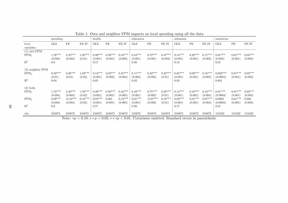
Table 1: Own and neighbor FPM impacts on local spending using all the data

spending health education urbanism sanitation

level OLS FE FE IV OLS FE FE IV OLS FE FE IV OLS FE FE IV OLS FE FE IVvariables

(1) own FPMFPMi 1.76*** 2.45*** 1.95*** 0.39*** 0.56*** 0.54*** 0.44*** 0.72*** 0.47*** 0.14*** 0.20*** 0.17*** 0.01*** 0.01*** 0.03***

(0.004) (0.004) (0.01) (0.001) (0.001) (0.002) (0.001) (0.001) (0.003) (0.001) (0.001) (0.002) (0.004) (0.001) (0.002)R2 0.6 0.57 0.39 0.16 0.01

(2) neighbor FPMFPMj 0.50*** 0.86*** 1.62*** 0.13*** 0.22*** 0.45*** 0.11*** 0.22*** 0.42*** 0.05*** 0.09*** 0.16*** 0.002*** 0.01*** 0.02***

(0.01) (0.01) (0.02) (0.001) (0.002) (0.004) (0.002) (0.002) (0.01) (0.001) (0.001) (0.002) (0.0004) (0.001) (0.002)R2 0.04 0.05 0.02 0.02 0.001

(3) bothFPMi 1.74*** 2.48*** 1.59*** 0.38*** 0.56*** 0.44*** 0.43*** 0.75*** 0.32*** 0.14*** 0.19*** 0.12*** 0.01*** 0.01*** 0.03***

(0.004) (0.004) (0.02) (0.001) (0.001) (0.005) (0.001) (0.002) (0.01) (0.001) (0.001) (0.004) (0.0004) (0.001) (0.003)FPMj 0.09*** -0.10*** 0.45*** 0.04*** 0.001 0.13*** 0.01*** -0.07*** 0.18*** 0.02*** 0.01*** 0.07*** 0.0003 0.01*** 0.003

(0.004) (0.004) (0.02) (0.001) (0.001) (0.005) (0.001) (0.002) (0.01) (0.001) (0.001) (0.004) (0.0004) (0.001) (0.003)R2 0.6 0.57 0.39 0.17 0.01

obs 210872 210872 210872 210872 210872 210872 210872 210872 210872 210872 210872 210872 151822 151822 151822

Note: ∗p < 0.10, ∗ ∗ p < 0.05, ∗ ∗ ∗p < 0.01. Covariates omitted. Standard errors in parenthesis.

38

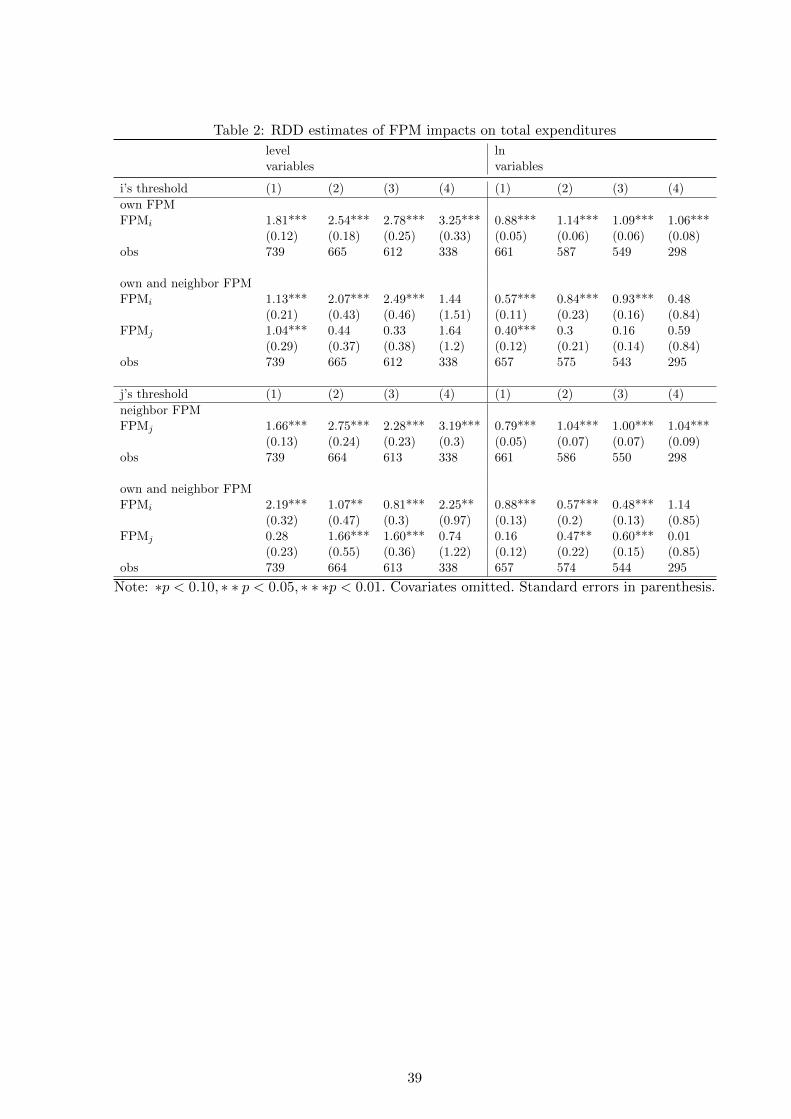
Table 2: RDD estimates of FPM impacts on total expenditures

level lnvariables variables

i’s threshold (1) (2) (3) (4) (1) (2) (3) (4)

own FPMFPMi 1.81*** 2.54*** 2.78*** 3.25*** 0.88*** 1.14*** 1.09*** 1.06***

(0.12) (0.18) (0.25) (0.33) (0.05) (0.06) (0.06) (0.08)obs 739 665 612 338 661 587 549 298

own and neighbor FPMFPMi 1.13*** 2.07*** 2.49*** 1.44 0.57*** 0.84*** 0.93*** 0.48

(0.21) (0.43) (0.46) (1.51) (0.11) (0.23) (0.16) (0.84)FPMj 1.04*** 0.44 0.33 1.64 0.40*** 0.3 0.16 0.59

(0.29) (0.37) (0.38) (1.2) (0.12) (0.21) (0.14) (0.84)obs 739 665 612 338 657 575 543 295

j’s threshold (1) (2) (3) (4) (1) (2) (3) (4)

neighbor FPMFPMj 1.66*** 2.75*** 2.28*** 3.19*** 0.79*** 1.04*** 1.00*** 1.04***

(0.13) (0.24) (0.23) (0.3) (0.05) (0.07) (0.07) (0.09)obs 739 664 613 338 661 586 550 298

own and neighbor FPMFPMi 2.19*** 1.07** 0.81*** 2.25** 0.88*** 0.57*** 0.48*** 1.14

(0.32) (0.47) (0.3) (0.97) (0.13) (0.2) (0.13) (0.85)FPMj 0.28 1.66*** 1.60*** 0.74 0.16 0.47** 0.60*** 0.01

(0.23) (0.55) (0.36) (1.22) (0.12) (0.22) (0.15) (0.85)obs 739 664 613 338 657 574 544 295


39

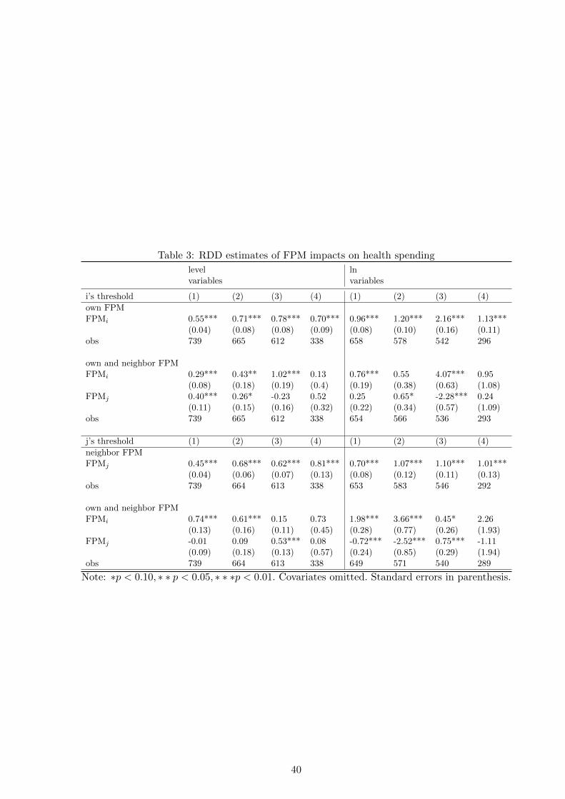
Table 3: RDD estimates of FPM impacts on health spending


i’s threshold (1) (2) (3) (4) (1) (2) (3) (4)

own FPMFPMi 0.55*** 0.71*** 0.78*** 0.70*** 0.96*** 1.20*** 2.16*** 1.13***

(0.04) (0.08) (0.08) (0.09) (0.08) (0.10) (0.16) (0.11)obs 739 665 612 338 658 578 542 296

own and neighbor FPMFPMi 0.29*** 0.43** 1.02*** 0.13 0.76*** 0.55 4.07*** 0.95

(0.08) (0.18) (0.19) (0.4) (0.19) (0.38) (0.63) (1.08)FPMj 0.40*** 0.26* -0.23 0.52 0.25 0.65* -2.28*** 0.24

(0.11) (0.15) (0.16) (0.32) (0.22) (0.34) (0.57) (1.09)obs 739 665 612 338 654 566 536 293

j’s threshold (1) (2) (3) (4) (1) (2) (3) (4)


(0.04) (0.06) (0.07) (0.13) (0.08) (0.12) (0.11) (0.13)obs 739 664 613 338 653 583 546 292

own and neighbor FPMFPMi 0.74*** 0.61*** 0.15 0.73 1.98*** 3.66*** 0.45* 2.26

(0.13) (0.16) (0.11) (0.45) (0.28) (0.77) (0.26) (1.93)FPMj -0.01 0.09 0.53*** 0.08 -0.72*** -2.52*** 0.75*** -1.11

(0.09) (0.18) (0.13) (0.57) (0.24) (0.85) (0.29) (1.94)obs 739 664 613 338 649 571 540 289


40

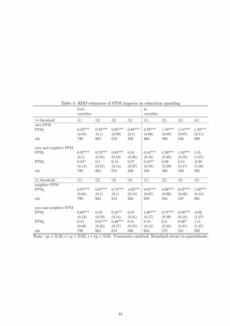
Table 4: RDD estimates of FPM impacts on education spending


i’s threshold (1) (2) (3) (4) (1) (2) (3) (4)

own FPMFPMi 0.53*** 0.94*** 0.95*** 0.98*** 0.76*** 1.19*** 1.14*** 1.23***

(0.05) (0.1) (0.09) (0.1) (0.06) (0.09) (0.07) (0.11)obs 739 665 612 338 660 580 546 298

own and neighbor FPMFPMi 0.37*** 0.73*** 0.83*** 0.34 0.44*** 1.09*** 1.02*** 1.45

(0.1) (0.25) (0.16) (0.46) (0.16) (0.32) (0.19) (1.07)FPMj 0.24* 0.2 0.14 0.57 0.43** 0.08 0.14 -0.22

(0.14) (0.21) (0.14) (0.37) (0.18) (0.29) (0.17) (1.08)obs 739 665 612 338 656 568 540 295

j’s threshold (1) (2) (3) (4) (1) (2) (3) (4)


(0.05) (0.1) (0.1) (0.14) (0.07) (0.09) (0.08) (0.12)obs 739 664 613 338 658 584 547 295

own and neighbor FPMFPMi 0.69*** 0.23 0.34** 0.57 1.00*** 0.77*** 0.59*** -0.02

(0.13) (0.19) (0.14) (0.41) (0.17) (0.29) (0.18) (1.27)FPMj 0.13 0.61*** 0.46*** 0.51 0.18 0.2 0.36* 1.11

(0.09) (0.22) (0.17) (0.52) (0.15) (0.32) (0.21) (1.27)obs 739 664 613 338 654 572 541 292


41

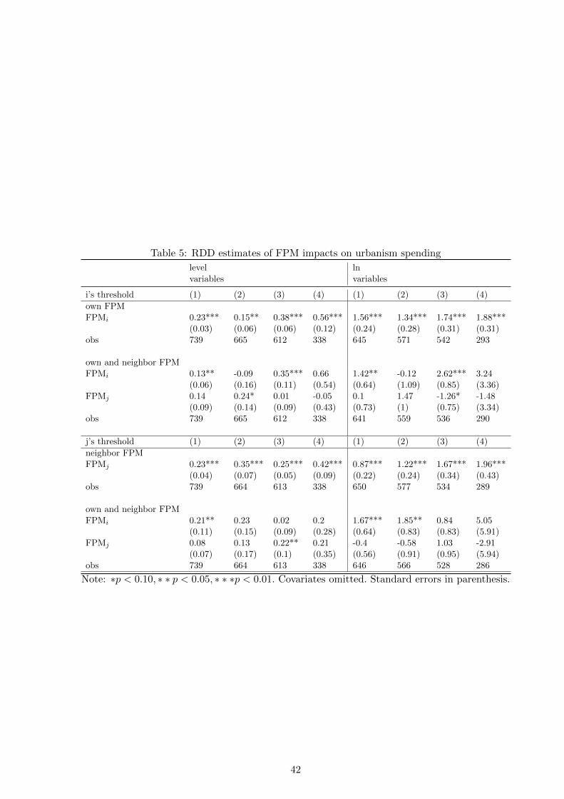
Table 5: RDD estimates of FPM impacts on urbanism spending


i’s threshold (1) (2) (3) (4) (1) (2) (3) (4)

own FPMFPMi 0.23*** 0.15** 0.38*** 0.56*** 1.56*** 1.34*** 1.74*** 1.88***

(0.03) (0.06) (0.06) (0.12) (0.24) (0.28) (0.31) (0.31)obs 739 665 612 338 645 571 542 293

own and neighbor FPMFPMi 0.13** -0.09 0.35*** 0.66 1.42** -0.12 2.62*** 3.24

(0.06) (0.16) (0.11) (0.54) (0.64) (1.09) (0.85) (3.36)FPMj 0.14 0.24* 0.01 -0.05 0.1 1.47 -1.26* -1.48

(0.09) (0.14) (0.09) (0.43) (0.73) (1) (0.75) (3.34)obs 739 665 612 338 641 559 536 290

j’s threshold (1) (2) (3) (4) (1) (2) (3) (4)


(0.04) (0.07) (0.05) (0.09) (0.22) (0.24) (0.34) (0.43)obs 739 664 613 338 650 577 534 289

own and neighbor FPMFPMi 0.21** 0.23 0.02 0.2 1.67*** 1.85** 0.84 5.05

(0.11) (0.15) (0.09) (0.28) (0.64) (0.83) (0.83) (5.91)FPMj 0.08 0.13 0.22** 0.21 -0.4 -0.58 1.03 -2.91

(0.07) (0.17) (0.1) (0.35) (0.56) (0.91) (0.95) (5.94)obs 739 664 613 338 646 566 528 286


42

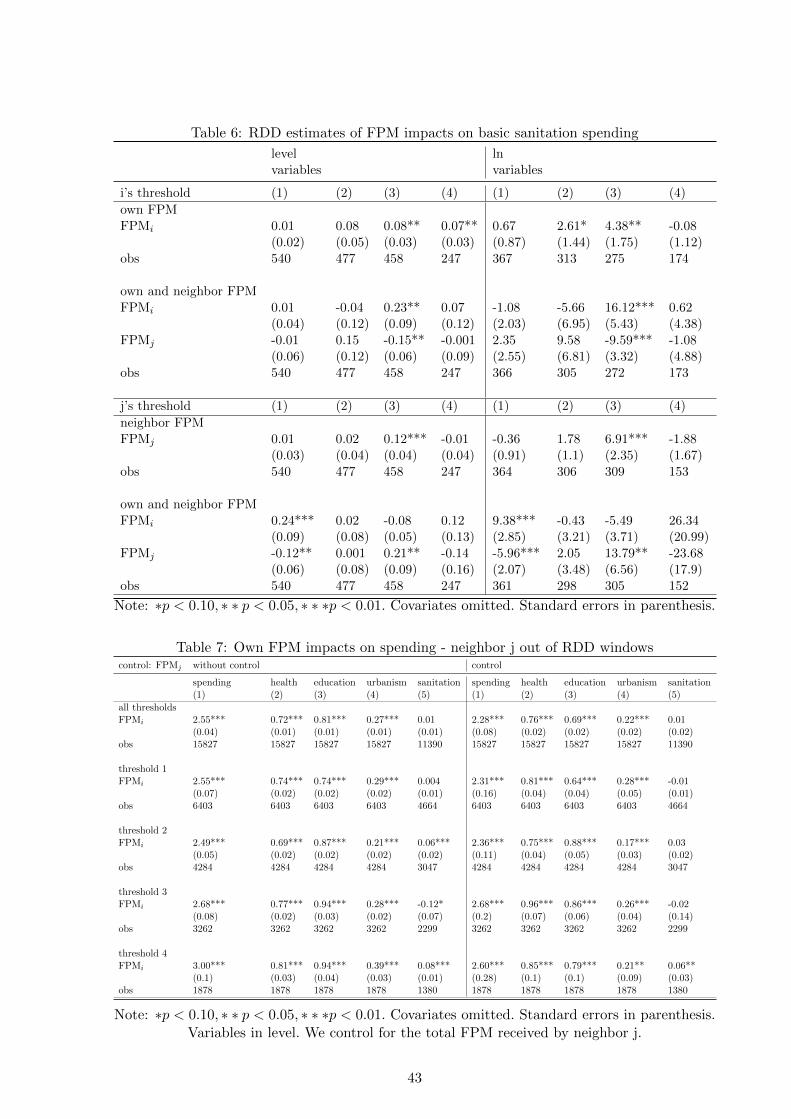
Table 6: RDD estimates of FPM impacts on basic sanitation spending


i’s threshold (1) (2) (3) (4) (1) (2) (3) (4)

own FPMFPMi 0.01 0.08 0.08** 0.07** 0.67 2.61* 4.38** -0.08

(0.02) (0.05) (0.03) (0.03) (0.87) (1.44) (1.75) (1.12)obs 540 477 458 247 367 313 275 174

own and neighbor FPMFPMi 0.01 -0.04 0.23** 0.07 -1.08 -5.66 16.12*** 0.62

(0.04) (0.12) (0.09) (0.12) (2.03) (6.95) (5.43) (4.38)FPMj -0.01 0.15 -0.15** -0.001 2.35 9.58 -9.59*** -1.08

(0.06) (0.12) (0.06) (0.09) (2.55) (6.81) (3.32) (4.88)obs 540 477 458 247 366 305 272 173

j’s threshold (1) (2) (3) (4) (1) (2) (3) (4)

neighbor FPMFPMj 0.01 0.02 0.12*** -0.01 -0.36 1.78 6.91*** -1.88

(0.03) (0.04) (0.04) (0.04) (0.91) (1.1) (2.35) (1.67)obs 540 477 458 247 364 306 309 153

own and neighbor FPMFPMi 0.24*** 0.02 -0.08 0.12 9.38*** -0.43 -5.49 26.34

(0.09) (0.08) (0.05) (0.13) (2.85) (3.21) (3.71) (20.99)FPMj -0.12** 0.001 0.21** -0.14 -5.96*** 2.05 13.79** -23.68

(0.06) (0.08) (0.09) (0.16) (2.07) (3.48) (6.56) (17.9)obs 540 477 458 247 361 298 305 152


Table 7: Own FPM impacts on spending - neighbor j out of RDD windowscontrol: FPMj without control control

spending health education urbanism sanitation spending health education urbanism sanitation(1) (2) (3) (4) (5) (1) (2) (3) (4) (5)

all thresholdsFPMi 2.55*** 0.72*** 0.81*** 0.27*** 0.01 2.28*** 0.76*** 0.69*** 0.22*** 0.01

(0.04) (0.01) (0.01) (0.01) (0.01) (0.08) (0.02) (0.02) (0.02) (0.02)obs 15827 15827 15827 15827 11390 15827 15827 15827 15827 11390

threshold 1FPMi 2.55*** 0.74*** 0.74*** 0.29*** 0.004 2.31*** 0.81*** 0.64*** 0.28*** -0.01

(0.07) (0.02) (0.02) (0.02) (0.01) (0.16) (0.04) (0.04) (0.05) (0.01)obs 6403 6403 6403 6403 4664 6403 6403 6403 6403 4664

threshold 2FPMi 2.49*** 0.69*** 0.87*** 0.21*** 0.06*** 2.36*** 0.75*** 0.88*** 0.17*** 0.03

(0.05) (0.02) (0.02) (0.02) (0.02) (0.11) (0.04) (0.05) (0.03) (0.02)obs 4284 4284 4284 4284 3047 4284 4284 4284 4284 3047

threshold 3FPMi 2.68*** 0.77*** 0.94*** 0.28*** -0.12* 2.68*** 0.96*** 0.86*** 0.26*** -0.02

(0.08) (0.02) (0.03) (0.02) (0.07) (0.2) (0.07) (0.06) (0.04) (0.14)obs 3262 3262 3262 3262 2299 3262 3262 3262 3262 2299

threshold 4FPMi 3.00*** 0.81*** 0.94*** 0.39*** 0.08*** 2.60*** 0.85*** 0.79*** 0.21** 0.06**

(0.1) (0.03) (0.04) (0.03) (0.01) (0.28) (0.1) (0.1) (0.09) (0.03)obs 1878 1878 1878 1878 1380 1878 1878 1878 1878 1380

Note: ∗p < 0.10, ∗ ∗ p < 0.05, ∗ ∗ ∗p < 0.01. Covariates omitted. Standard errors in parenthesis.Variables in level. We control for the total FPM received by neighbor j.

43

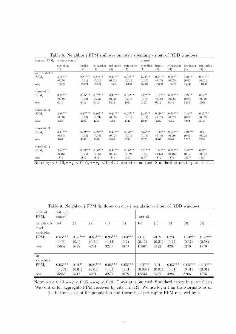
Table 8: Neighbor j FPM spillover on city i spending - i out of RDD windowscontrol: FPMi without control control


all thresholdsFPMj 3.09*** 0.87*** 0.84*** 0.30*** 0.04*** 2.72*** 0.94*** 0.66*** 0.21*** 0.04***

(0.05) (0.01) (0.01) (0.01) (0.01) (0.10) (0.03) (0.03) (0.03) (0.01)obs 15839 15839 15839 15839 11390 15839 15839 15839 15839 11390

threshold 1FPMj 3.33*** 0.95*** 0.82*** 0.33*** 0.04*** 3.17*** 1.04*** 0.69*** 0.27*** 0.04**

(0.09) (0.02) (0.03) (0.02) (0.01) (0.19) (0.06) (0.06) (0.05) (0.02)obs 6413 6413 6413 6413 4664 6413 6413 6413 6413 4664

threshold 2FPMj 2.89*** 0.87*** 0.86*** 0.24*** 0.05*** 2.49*** 0.99*** 0.70*** 0.13** 0.05***

(0.09) (0.03) (0.03) (0.03) (0.01) (0.19) (0.07) (0.07) (0.06) (0.02)obs 4282 4282 4282 4282 3047 4282 4282 4282 4282 3047

threshold 3FPMj 3.41*** 0.92*** 0.89*** 0.33*** 0.03** 3.25*** 1.08*** 0.71*** 0.24*** -0.01

(0.14) (0.03) (0.04) (0.03) (0.01) (0.35) (0.08) (0.09) (0.07) (0.02)obs 3267 3267 3267 3267 2299 3267 3267 3267 3267 2299

threshold 4FPMj 3.84*** 0.98*** 0.96*** 0.48*** 0.06*** 3.31*** 1.14*** 0.69*** 0.47*** 0.07*

(0.16) (0.05) (0.06) (0.05) (0.02) (0.46) (0.15) (0.16) (0.13) (0.04)obs 1877 1877 1877 1877 1380 1877 1877 1877 1877 1380


Table 9: Neighbor j FPM Spillover on city i population - i out of RDD windows

control: withoutFPMi control control

thresholds 1-4 (1) (2) (3) (4) 1-4 (1) (2) (3) (4)

levelvariablesFPMj 0.55*** 0.32*** 0.63*** 0.93*** 1.03*** -0.05 -0.24 0.23 1.13*** 1.55***

(0.06) (0.1) (0.11) (0.14) (0.2) (0.13) (0.21) (0.24) (0.37) (0.58)obs 15867 6422 4291 3276 1878 15867 6422 4291 3276 1878

lnvariablesFPMj 0.03*** 0.01** 0.03*** 0.06*** 0.05*** 0.03*** 0.01 0.03*** 0.05*** 0.04***

(0.003) (0.01) (0.01) (0.01) (0.01) (0.004) (0.01) (0.01) (0.01) (0.01)obs 15856 6417 4291 3270 1878 15834 6409 4284 3266 1875

Note: ∗p < 0.10, ∗ ∗ p < 0.05, ∗ ∗ ∗p < 0.01. Covariates omitted. Standard errors in parenthesis.We control for aggregate FPM received by city i, in R$. We use logarithm transformations on

the bottom, except for population and theoretical per capita FPM received by i.

44

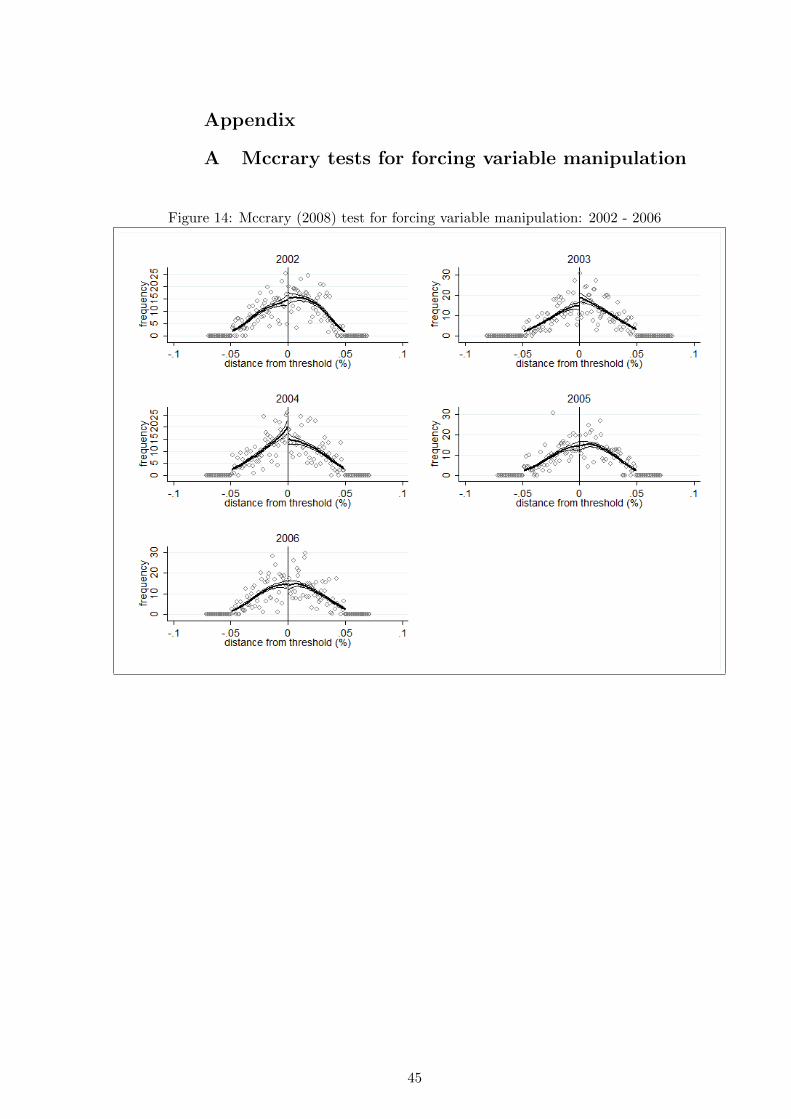
Appendix

A Mccrary tests for forcing variable manipulation

Figure 14: Mccrary (2008) test for forcing variable manipulation: 2002 - 2006

45

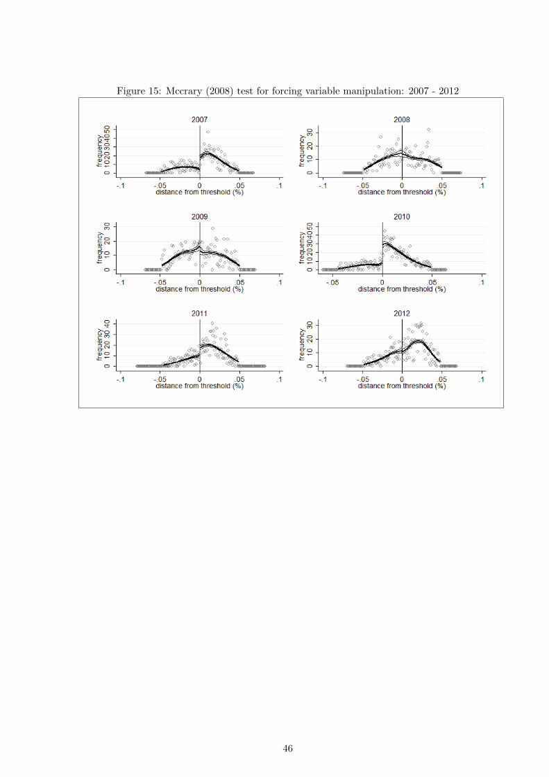
Figure 15: Mccrary (2008) test for forcing variable manipulation: 2007 - 2012

46

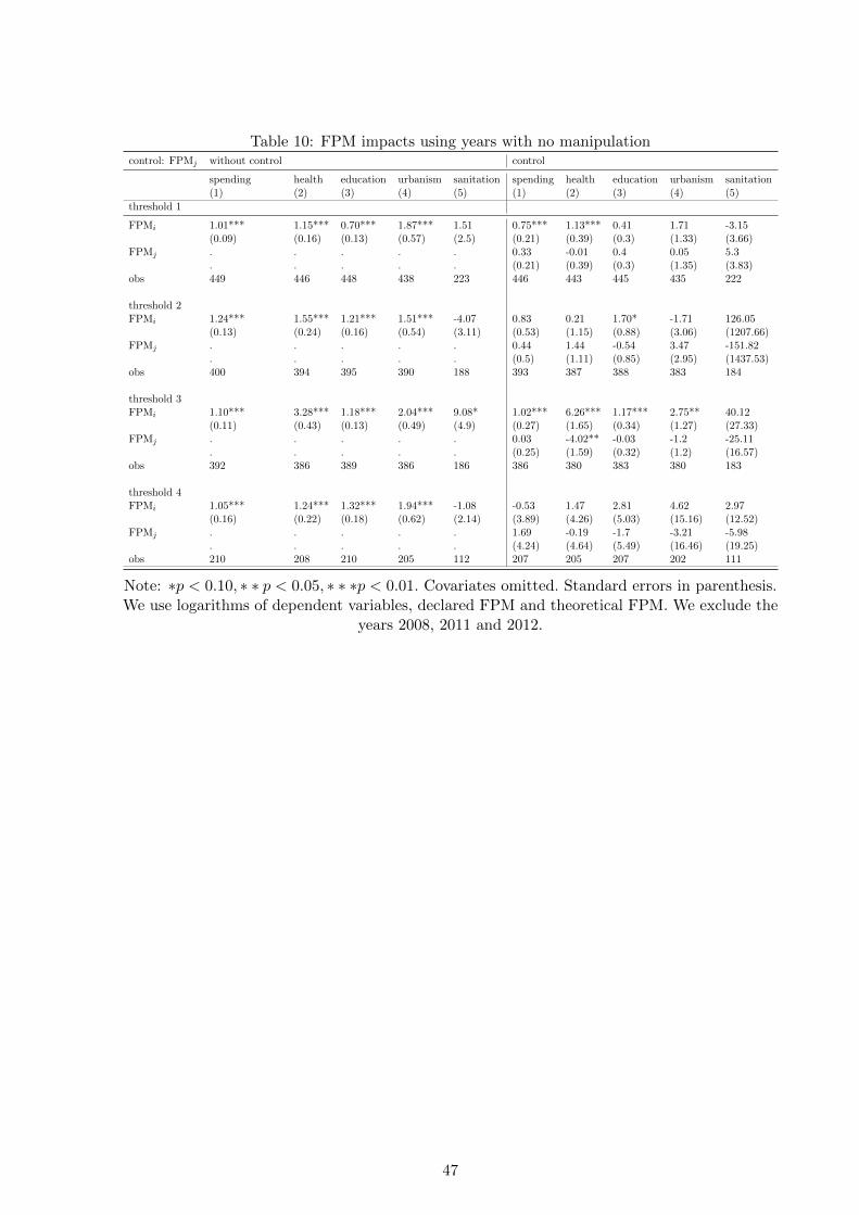
Table 10: FPM impacts using years with no manipulationcontrol: FPMj without control control


threshold 1

FPMi 1.01*** 1.15*** 0.70*** 1.87*** 1.51 0.75*** 1.13*** 0.41 1.71 -3.15(0.09) (0.16) (0.13) (0.57) (2.5) (0.21) (0.39) (0.3) (1.33) (3.66)

FPMj . . . . . 0.33 -0.01 0.4 0.05 5.3. . . . . (0.21) (0.39) (0.3) (1.35) (3.83)

obs 449 446 448 438 223 446 443 445 435 222

threshold 2FPMi 1.24*** 1.55*** 1.21*** 1.51*** -4.07 0.83 0.21 1.70* -1.71 126.05

(0.13) (0.24) (0.16) (0.54) (3.11) (0.53) (1.15) (0.88) (3.06) (1207.66)FPMj . . . . . 0.44 1.44 -0.54 3.47 -151.82

. . . . . (0.5) (1.11) (0.85) (2.95) (1437.53)obs 400 394 395 390 188 393 387 388 383 184

threshold 3FPMi 1.10*** 3.28*** 1.18*** 2.04*** 9.08* 1.02*** 6.26*** 1.17*** 2.75** 40.12

(0.11) (0.43) (0.13) (0.49) (4.9) (0.27) (1.65) (0.34) (1.27) (27.33)FPMj . . . . . 0.03 -4.02** -0.03 -1.2 -25.11

. . . . . (0.25) (1.59) (0.32) (1.2) (16.57)obs 392 386 389 386 186 386 380 383 380 183

threshold 4FPMi 1.05*** 1.24*** 1.32*** 1.94*** -1.08 -0.53 1.47 2.81 4.62 2.97

(0.16) (0.22) (0.18) (0.62) (2.14) (3.89) (4.26) (5.03) (15.16) (12.52)FPMj . . . . . 1.69 -0.19 -1.7 -3.21 -5.98

. . . . . (4.24) (4.64) (5.49) (16.46) (19.25)obs 210 208 210 205 112 207 205 207 202 111

Note: ∗p < 0.10, ∗ ∗ p < 0.05, ∗ ∗ ∗p < 0.01. Covariates omitted. Standard errors in parenthesis.We use logarithms of dependent variables, declared FPM and theoretical FPM. We exclude the

years 2008, 2011 and 2012.

47

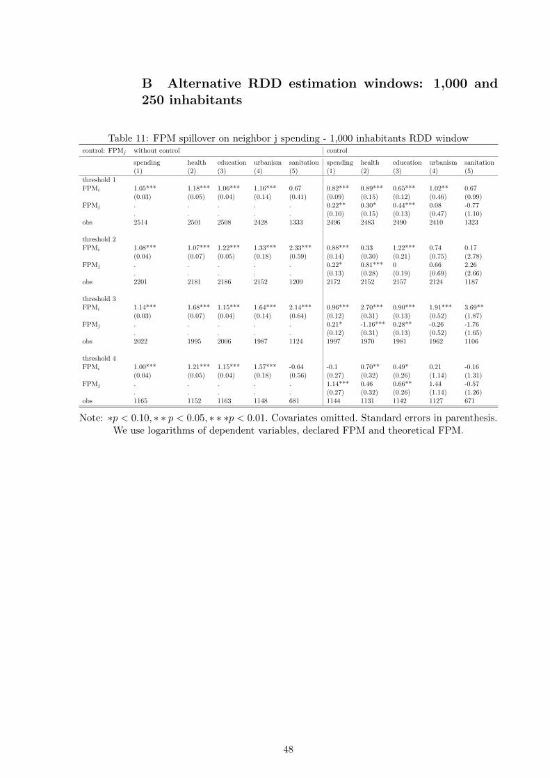
B Alternative RDD estimation windows: 1,000 and250 inhabitants

Table 11: FPM spillover on neighbor j spending - 1,000 inhabitants RDD windowcontrol: FPMj without control control


threshold 1FPMi 1.05*** 1.18*** 1.06*** 1.16*** 0.67 0.82*** 0.89*** 0.65*** 1.02** 0.67

(0.03) (0.05) (0.04) (0.14) (0.41) (0.09) (0.15) (0.12) (0.46) (0.99)FPMj . . . . . 0.22** 0.30* 0.44*** 0.08 -0.77

. . . . . (0.10) (0.15) (0.13) (0.47) (1.10)obs 2514 2501 2508 2428 1333 2496 2483 2490 2410 1323

threshold 2FPMi 1.08*** 1.07*** 1.22*** 1.33*** 2.33*** 0.88*** 0.33 1.22*** 0.74 0.17

(0.04) (0.07) (0.05) (0.18) (0.59) (0.14) (0.30) (0.21) (0.75) (2.78)FPMj . . . . . 0.22* 0.81*** 0 0.66 2.26

. . . . . (0.13) (0.28) (0.19) (0.69) (2.66)obs 2201 2181 2186 2152 1209 2172 2152 2157 2124 1187

threshold 3FPMi 1.14*** 1.68*** 1.15*** 1.64*** 2.14*** 0.96*** 2.70*** 0.90*** 1.91*** 3.69**

(0.03) (0.07) (0.04) (0.14) (0.64) (0.12) (0.31) (0.13) (0.52) (1.87)FPMj . . . . . 0.21* -1.16*** 0.28** -0.26 -1.76

. . . . . (0.12) (0.31) (0.13) (0.52) (1.65)obs 2022 1995 2006 1987 1124 1997 1970 1981 1962 1106

threshold 4FPMi 1.00*** 1.21*** 1.15*** 1.57*** -0.64 -0.1 0.70** 0.49* 0.21 -0.16

(0.04) (0.05) (0.04) (0.18) (0.56) (0.27) (0.32) (0.26) (1.14) (1.31)FPMj . . . . . 1.14*** 0.46 0.66** 1.44 -0.57

. . . . . (0.27) (0.32) (0.26) (1.14) (1.26)obs 1165 1152 1163 1148 681 1144 1131 1142 1127 671

Note: ∗p < 0.10, ∗ ∗ p < 0.05, ∗ ∗ ∗p < 0.01. Covariates omitted. Standard errors in parenthesis.We use logarithms of dependent variables, declared FPM and theoretical FPM.

48

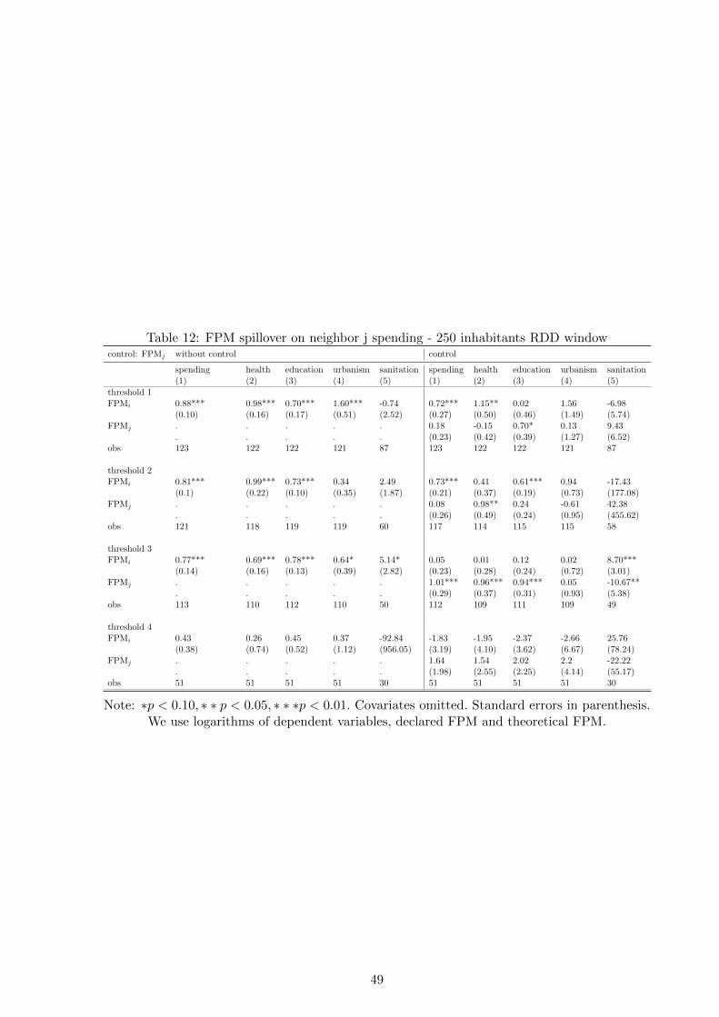
Table 12: FPM spillover on neighbor j spending - 250 inhabitants RDD windowcontrol: FPMj without control control


threshold 1FPMi 0.88*** 0.98*** 0.70*** 1.60*** -0.74 0.72*** 1.15** 0.02 1.56 -6.98

(0.10) (0.16) (0.17) (0.51) (2.52) (0.27) (0.50) (0.46) (1.49) (5.74)FPMj . . . . . 0.18 -0.15 0.70* 0.13 9.43

. . . . . (0.23) (0.42) (0.39) (1.27) (6.52)obs 123 122 122 121 87 123 122 122 121 87

threshold 2FPMi 0.81*** 0.99*** 0.73*** 0.34 2.49 0.73*** 0.41 0.61*** 0.94 -17.43

(0.1) (0.22) (0.10) (0.35) (1.87) (0.21) (0.37) (0.19) (0.73) (177.08)FPMj . . . . . 0.08 0.98** 0.24 -0.61 42.38

. . . . . (0.26) (0.49) (0.24) (0.95) (455.62)obs 121 118 119 119 60 117 114 115 115 58

threshold 3FPMi 0.77*** 0.69*** 0.78*** 0.64* 5.14* 0.05 0.01 0.12 0.02 8.70***

(0.14) (0.16) (0.13) (0.39) (2.82) (0.23) (0.28) (0.24) (0.72) (3.01)FPMj . . . . . 1.01*** 0.96*** 0.94*** 0.05 -10.67**

. . . . . (0.29) (0.37) (0.31) (0.93) (5.38)obs 113 110 112 110 50 112 109 111 109 49

threshold 4FPMi 0.43 0.26 0.45 0.37 -92.84 -1.83 -1.95 -2.37 -2.66 25.76

(0.38) (0.74) (0.52) (1.12) (956.05) (3.19) (4.10) (3.62) (6.67) (78.24)FPMj . . . . . 1.64 1.54 2.02 2.2 -22.22

. . . . . (1.98) (2.55) (2.25) (4.14) (55.17)obs 51 51 51 51 30 51 51 51 51 30

Note: ∗p < 0.10, ∗ ∗ p < 0.05, ∗ ∗ ∗p < 0.01. Covariates omitted. Standard errors in parenthesis.We use logarithms of dependent variables, declared FPM and theoretical FPM.

49

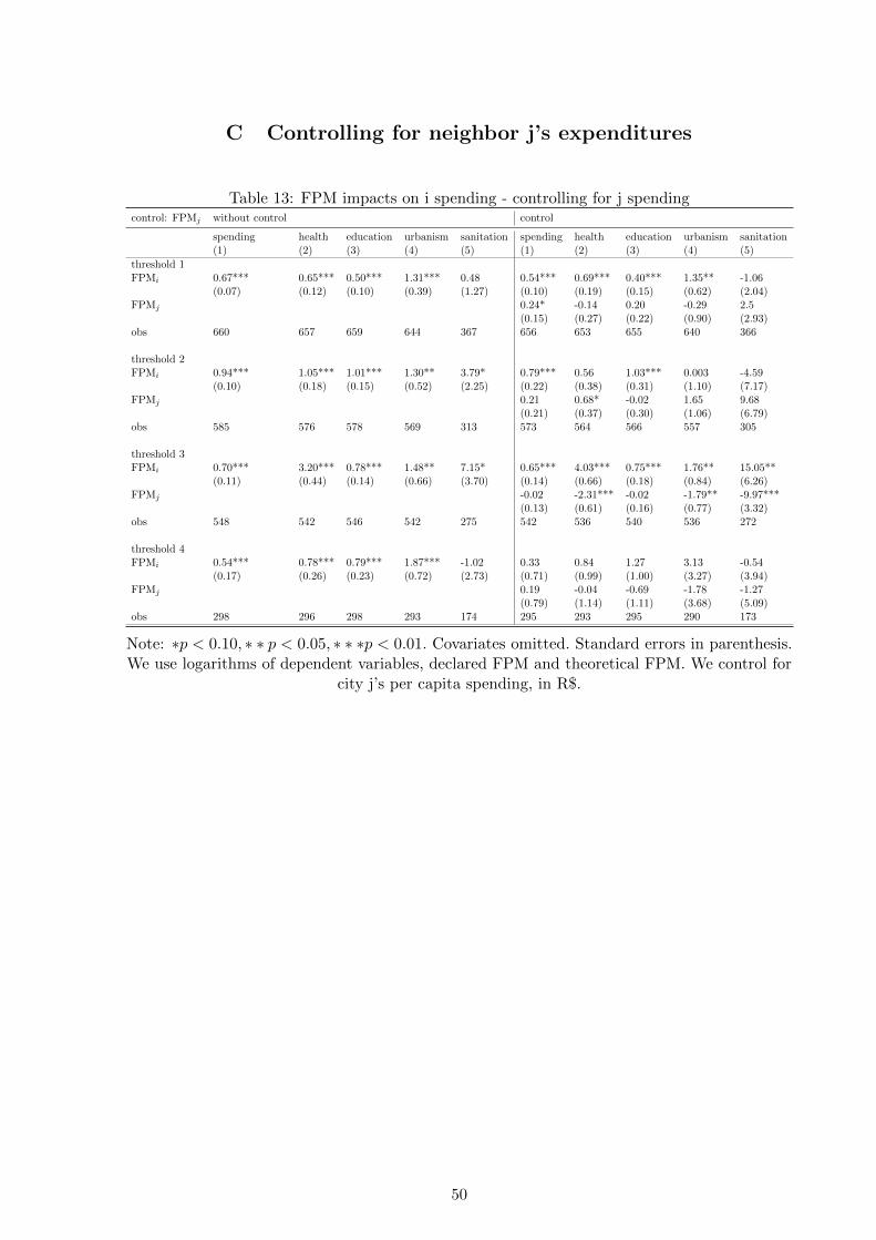
C Controlling for neighbor j’s expenditures

Table 13: FPM impacts on i spending - controlling for j spendingcontrol: FPMj without control control


threshold 1FPMi 0.67*** 0.65*** 0.50*** 1.31*** 0.48 0.54*** 0.69*** 0.40*** 1.35** -1.06

(0.07) (0.12) (0.10) (0.39) (1.27) (0.10) (0.19) (0.15) (0.62) (2.04)FPMj 0.24* -0.14 0.20 -0.29 2.5

(0.15) (0.27) (0.22) (0.90) (2.93)obs 660 657 659 644 367 656 653 655 640 366

threshold 2FPMi 0.94*** 1.05*** 1.01*** 1.30** 3.79* 0.79*** 0.56 1.03*** 0.003 -4.59

(0.10) (0.18) (0.15) (0.52) (2.25) (0.22) (0.38) (0.31) (1.10) (7.17)FPMj 0.21 0.68* -0.02 1.65 9.68

(0.21) (0.37) (0.30) (1.06) (6.79)obs 585 576 578 569 313 573 564 566 557 305

threshold 3FPMi 0.70*** 3.20*** 0.78*** 1.48** 7.15* 0.65*** 4.03*** 0.75*** 1.76** 15.05**

(0.11) (0.44) (0.14) (0.66) (3.70) (0.14) (0.66) (0.18) (0.84) (6.26)FPMj -0.02 -2.31*** -0.02 -1.79** -9.97***

(0.13) (0.61) (0.16) (0.77) (3.32)obs 548 542 546 542 275 542 536 540 536 272

threshold 4FPMi 0.54*** 0.78*** 0.79*** 1.87*** -1.02 0.33 0.84 1.27 3.13 -0.54

(0.17) (0.26) (0.23) (0.72) (2.73) (0.71) (0.99) (1.00) (3.27) (3.94)FPMj 0.19 -0.04 -0.69 -1.78 -1.27

(0.79) (1.14) (1.11) (3.68) (5.09)obs 298 296 298 293 174 295 293 295 290 173

Note: ∗p < 0.10, ∗ ∗ p < 0.05, ∗ ∗ ∗p < 0.01. Covariates omitted. Standard errors in parenthesis.We use logarithms of dependent variables, declared FPM and theoretical FPM. We control for

city j’s per capita spending, in R$.

50

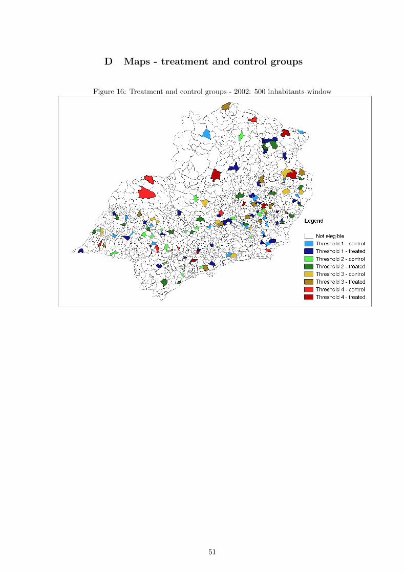
D Maps - treatment and control groups

Figure 16: Treatment and control groups - 2002: 500 inhabitants window

51

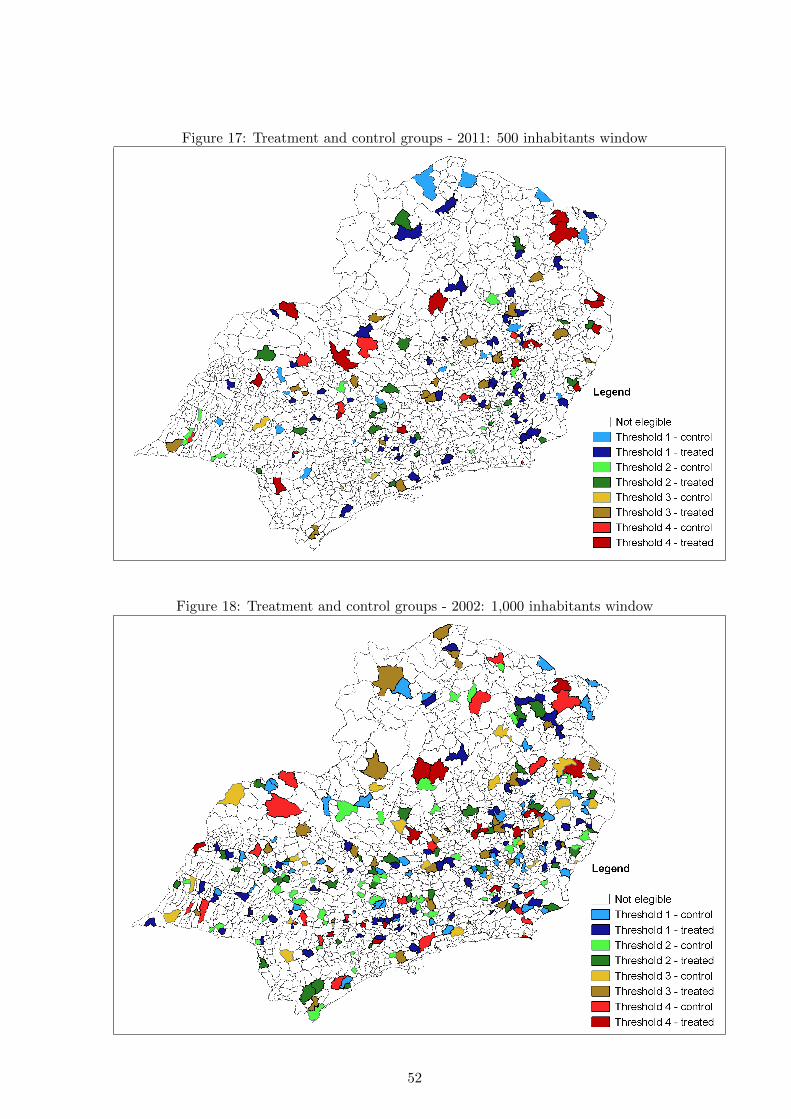
Figure 17: Treatment and control groups - 2011: 500 inhabitants window

Figure 18: Treatment and control groups - 2002: 1,000 inhabitants window

52

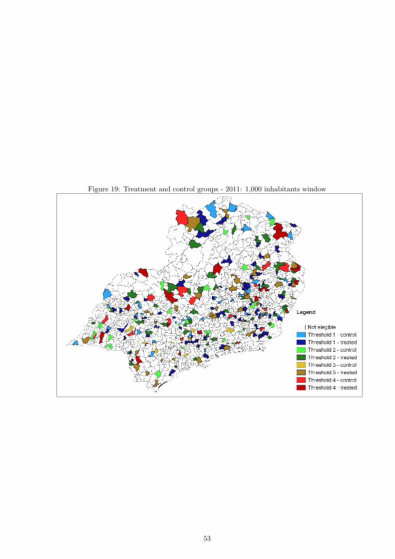
Figure 19: Treatment and control groups - 2011: 1,000 inhabitants window

53

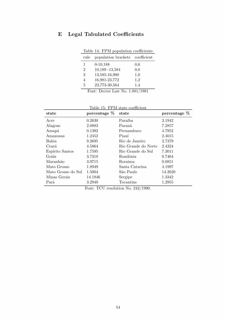
E Legal Tabulated Coefficients

Table 14: FPM population coefficients

rule population brackets coefficient

1 0-10,188 0,62 10,189 -13,584 0,83 13,585-16,980 1,04 16,981-23,772 1,25 23,773-30,564 1,4

Font: Decree Law No. 1.881/1981

Table 15: FPM state coefficient

state percentage % state percentage %

Acre 0.2630 Paraıba 3.1942Alagoas 2.0883 Parana 7.2857Amapa 0.1392 Pernambuco 4.7952Amazonas 1.2452 Piauı 2.4015Bahia 9.2695 Rio de Janeiro 2.7379Ceara 4.5864 Rio Grande do Norte 2.4324Espırito Santos 1.7595 Rio Grande do Sul 7.3011Goias 3.7318 Rondonia 0.7464Maranhao 3.9715 Roraima 0.0851Mato Grosso 1.8949 Santa Catarina 4.1997Mato Grosso do Sul 1.5004 Sao Paulo 14.2620Minas Gerais 14.1846 Sergipe 1.3342Para 3.2948 Tocantins 1.2955

Font: TCU resolution No. 242/1990.

54

Documents

Fiscal interactions and spillover effects of a federal