Embed Size (px)
Citation preview
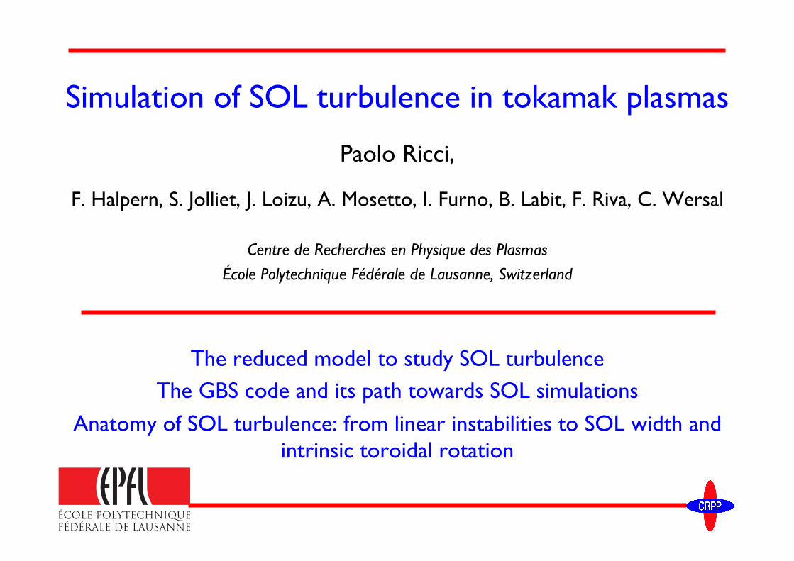
Simulation of SOL turbulence in tokamak plasmas ������
Paolo Ricci,
F. Halpern, S. Jolliet, J. Loizu, A. Mosetto, I. Furno, B. Labit, F. Riva, C. Wersal
Centre de Recherches en Physique des Plasmas
École Polytechnique Fédérale de Lausanne, Switzerland
The reduced model to study SOL turbulence The GBS code and its path towards SOL simulations
Anatomy of SOL turbulence: from linear instabilities to SOL width and intrinsic toroidal rotation
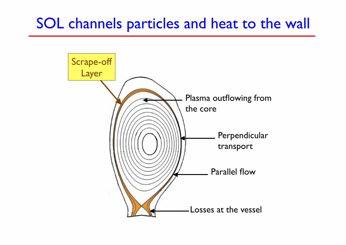
SOL channels particles and heat to the wall
Plasma outflowing from the core
Scrape-off Layer
Perpendicular transport
Losses at the vessel
Parallel flow
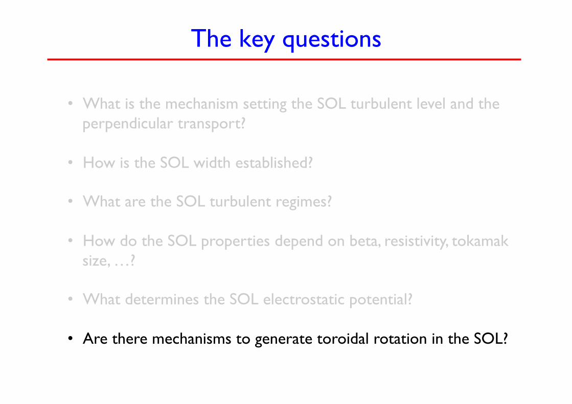
The key questions
• What is the mechanism setting the SOL turbulent level and the
perpendicular transport?
• How is the SOL width established?
• What are the SOL turbulent regimes?
• How do the SOL properties depend on beta, resistivity, tokamak size, …?
• What determines the SOL electrostatic potential?
• Are there mechanisms to generate toroidal rotation in the SOL?
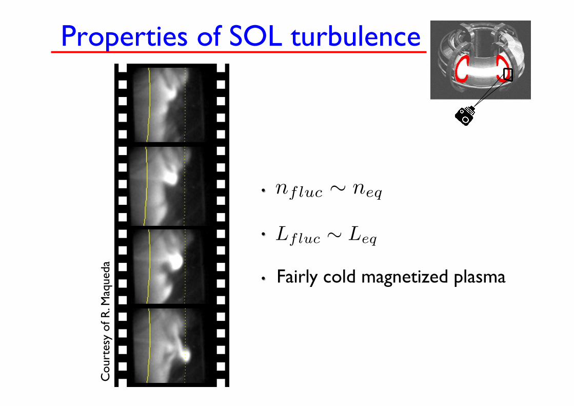
Properties of SOL turbulence
Cou
rtes
y of
R. M
aque
da
nfluc ∼ neq
Lfluc ∼ Leq
Fairly cold magnetized plasma
•
•
•
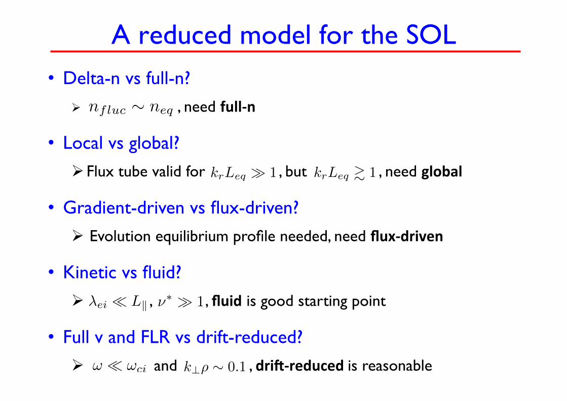
A reduced model for the SOL • Delta-n vs full-n?
Ø , need full-‐n
• Local vs global?
Ø Flux tube valid for , but , need global
• Gradient-driven vs flux-driven?
Ø Evolution equilibrium profile needed, need flux-‐driven
• Kinetic vs fluid?
Ø , , fluid is good starting point
• Full v and FLR vs drift-reduced?
Ø and , dri2-‐reduced is reasonable
nfluc ∼ neq
k⊥ρ ∼ 0.1ω � ωci
λei � L� ν∗ � 1
krLeq � 1 krLeq � 1
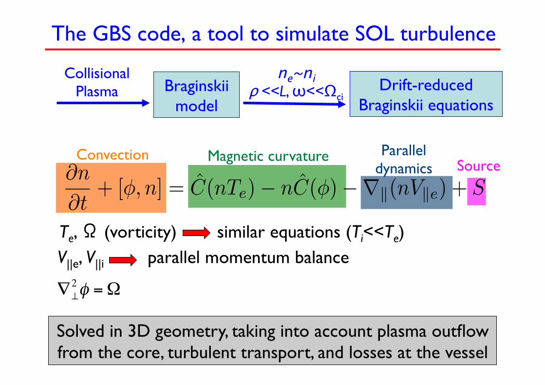
The GBS code, a tool to simulate SOL turbulence
ne~ni ρ <<L, ω<<Ωci
Braginskii model
Drift-reduced Braginskii equations
Collisional Plasma
Te, Ω (vorticity) similar equations (Ti<<Te) V||e, V||i parallel momentum balance
!
"#2$ =%
Solved in 3D geometry, taking into account plasma outflow from the core, turbulent transport, and losses at the vessel
Parallel dynamics
Magnetic curvature Source
Convection ∂n
∂t+ [φ, n] = C(nTe)− nC(φ)−∇�(nV�e) + S
0
1
2
3
4
Totalpotentialdrop
0
0.5
1
1.5
2
0
0.5
1
1.5
2
0
0.5
1
1.5
2
0
0.2
0.4
0.6
0
1
2
3
4
Totalpotentialdrop
0
0.5
1
1.5
2
0
0.5
1
1.5
2
0
0.5
1
1.5
2
0
0.2
0.4
0.6
0
1
2
3
4
Totalpotentialdrop
0
0.5
1
1.5
2
0
0.5
1
1.5
2
0
0.5
1
1.5
2
0
0.2
0.4
0.6
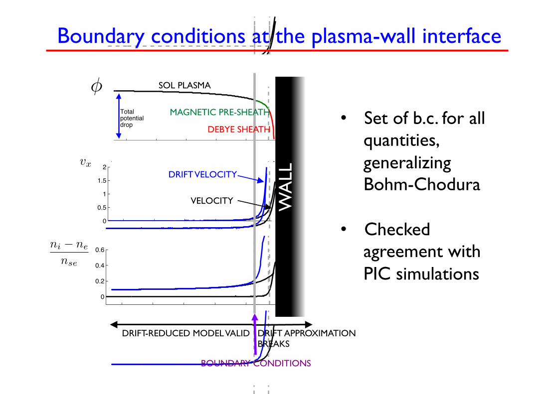
Boundary conditions at the plasma-wall interface
φ
ni − ne
nse
SOL PLASMA
vx
DRIFT-REDUCED MODEL VALID DRIFT APPROXIMATION BREAKS
DRIFT VELOCITY
WA
LL
• Set of b.c. for all quantities, generalizing Bohm-Chodura
• Checked agreement with PIC simulations
BOUNDARY CONDITIONS
VELOCITY
MAGNETIC PRE-SHEATH
DEBYE SHEATH
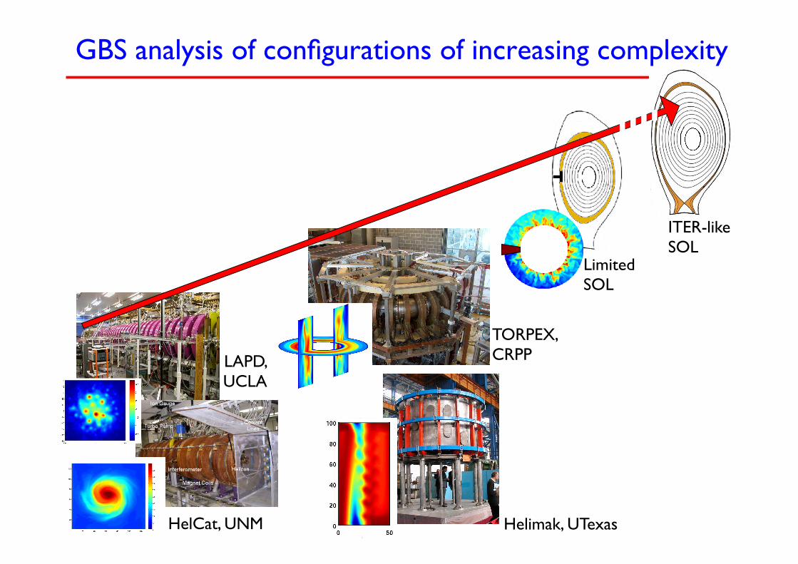
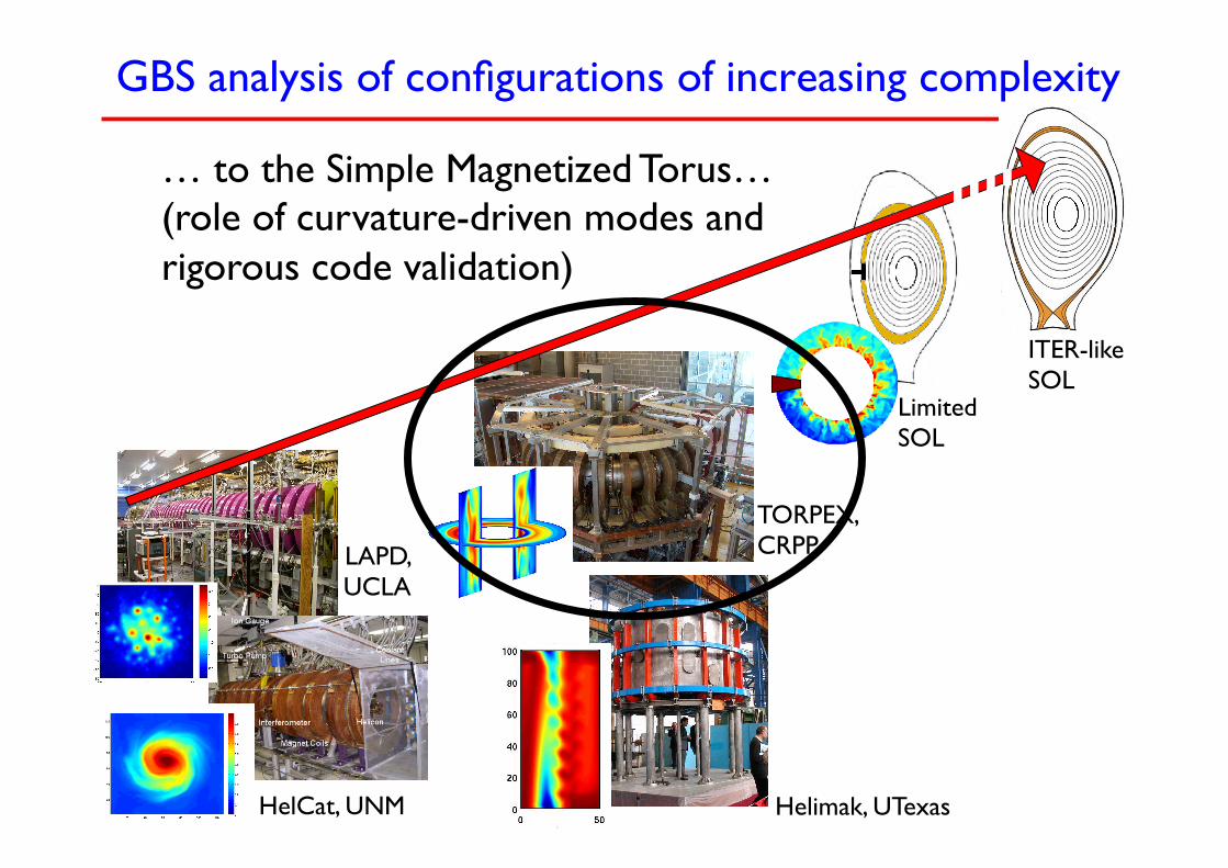
GBS analysis of configurations of increasing complexity
LAPD, UCLA
HelCat, UNM Helimak, UTexas
TORPEX, CRPP
ITER-like SOL Limited
SOL
MotivationThe plasma-wall transitionGBS turbulence simulationsSheath effects on turbulence
Conclusions
The GBS codeExamples of 3D simulations
The GBS code, a tool to simulate open field line turbulence
� Developed by steps of increasing complexity
� Drift-reduced Braginskii equations
� Global, 3D, Flux-driven, Full-n [Ricci et al PPCF 2012]
J. Loizu et al. 13 / 24 The role of the sheath in magnetized plasma fluid turbulence
Limited SOL
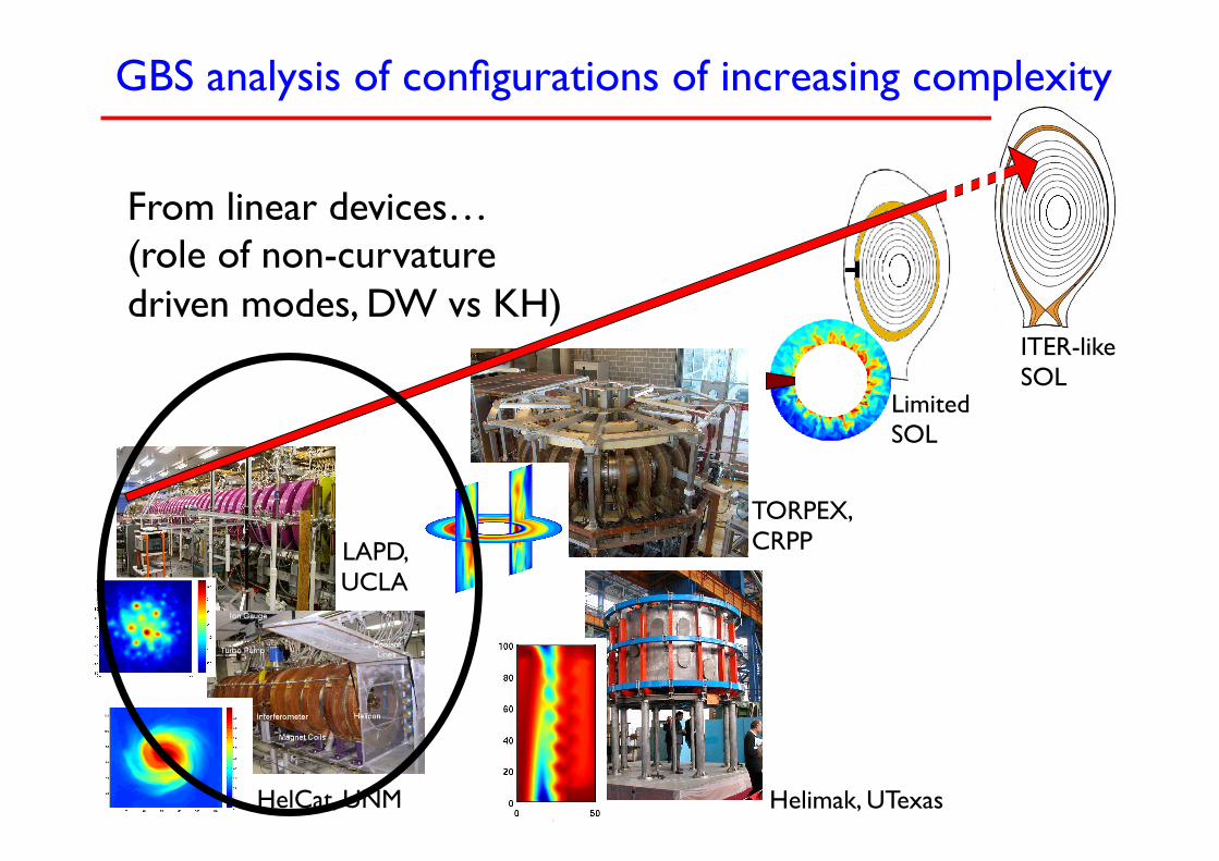
From linear devices… (role of non-curvature driven modes, DW vs KH)
GBS analysis of configurations of increasing complexity
LAPD, UCLA
HelCat, UNM Helimak, UTexas
TORPEX, CRPP
ITER-like SOL Limited
SOL
MotivationThe plasma-wall transitionGBS turbulence simulationsSheath effects on turbulence
Conclusions
The GBS codeExamples of 3D simulations
The GBS code, a tool to simulate open field line turbulence
� Developed by steps of increasing complexity
� Drift-reduced Braginskii equations
� Global, 3D, Flux-driven, Full-n [Ricci et al PPCF 2012]
J. Loizu et al. 13 / 24 The role of the sheath in magnetized plasma fluid turbulence
Limited SOL
… to the Simple Magnetized Torus… (role of curvature-driven modes and rigorous code validation)
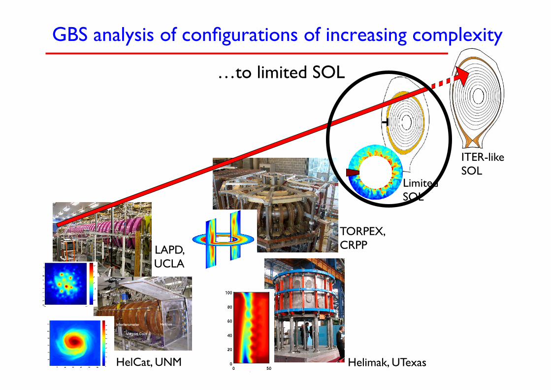
GBS analysis of configurations of increasing complexity
LAPD, UCLA
HelCat, UNM Helimak, UTexas
TORPEX, CRPP
ITER-like SOL Limited
SOL
…to limited SOL
MotivationThe plasma-wall transitionGBS turbulence simulationsSheath effects on turbulence
Conclusions
The GBS codeExamples of 3D simulations
The GBS code, a tool to simulate open field line turbulence
� Developed by steps of increasing complexity
� Drift-reduced Braginskii equations
� Global, 3D, Flux-driven, Full-n [Ricci et al PPCF 2012]
J. Loizu et al. 13 / 24 The role of the sheath in magnetized plasma fluid turbulence
Limited SOL
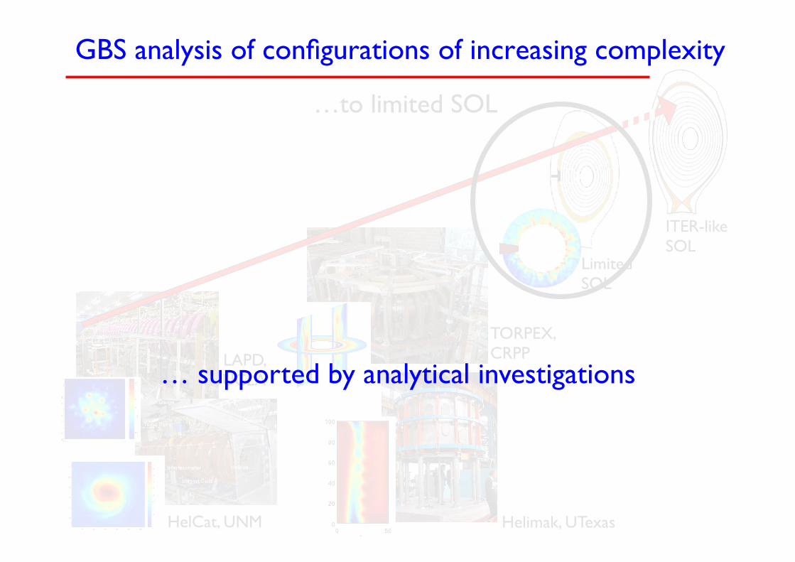
… supported by analytical investigations
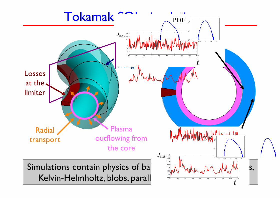
Tokamak SOL simulations
Simulations contain physics of ballooning modes, drift waves, Kelvin-Helmholtz, blobs, parallel flows, sheath losses…
Losses at the limiter
Radial transport
Flow along B
Plasma outflowing from
the core
φ20 30 40 50 60 70 80 90 100 110
0.2
0.4
0.6
0.8
1
1.2
1.4
1.6
20 30 40 50 60 70 80 90 100 1100.15
0.2
0.25
0.3
0.35
0.4
0.45
0.5
1 0.5 0 0.5 110 4
10 2
100
1 0.5 0 0.5 110 4
10 2
100
t
Jsat
20 30 40 50 60 70 80 90 100 1100.2
0.4
0.6
0.8
1
1.2
1.4
1.6
20 30 40 50 60 70 80 90 100 1100.15
0.2
0.25
0.3
0.35
0.4
0.45
0.5
1 0.5 0 0.5 110 4
10 2
100
1 0.5 0 0.5 110 4
10 2
100
t
Jsat
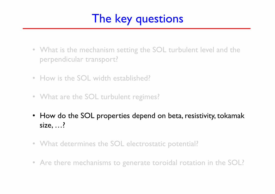
The key questions
• What is the mechanism setting the SOL turbulent level and the
perpendicular transport?
• How is the SOL width established?
• What are the SOL turbulent regimes?
• How do the SOL properties depend on beta, resistivity, tokamak size, …?
• What determines the SOL electrostatic potential?
• Are there mechanisms to generate toroidal rotation in the SOL?
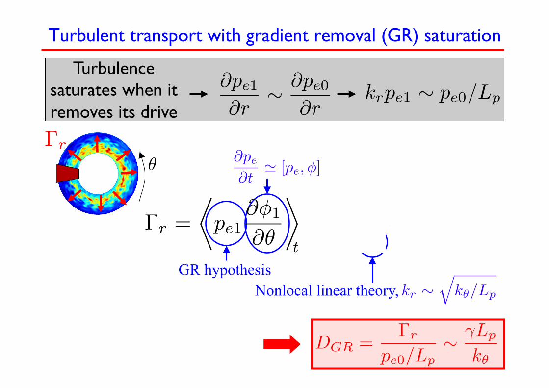
Turbulent transport with gradient removal (GR) saturation
Turbulence saturates when it removes its drive
∂pe1∂r
∼ ∂pe0∂r
krpe1 ∼ pe0/Lp
GR hypothesis
∂pe∂t
� [pe,φ]
Nonlocal linear theory, kr ∼�
kθ/Lp
DGR =Γr
pe0/Lp∼ γLp
kθ
Γr =
�pe1
∂φ1
∂θ
�∼ γpe0
Lpk2r∼ γpe0
kθ
θ
Γr
t
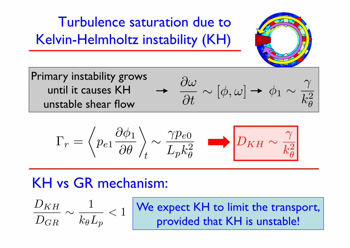
Turbulence saturation due to Kelvin-Helmholtz instability (KH)
Primary instability grows until it causes KH
unstable shear flow
∂ω
∂t∼ [φ,ω] φ1 ∼ γ
k2θ
We expect KH to limit the transport, provided that KH is unstable!
KH vs GR mechanism:
DKH ∼ γ
k2θ
DKH
DGR
∼ 1
kθLp
< 1
Γr =
�pe1
∂φ1
∂θ
�∼ γpe0
Lpk2θt
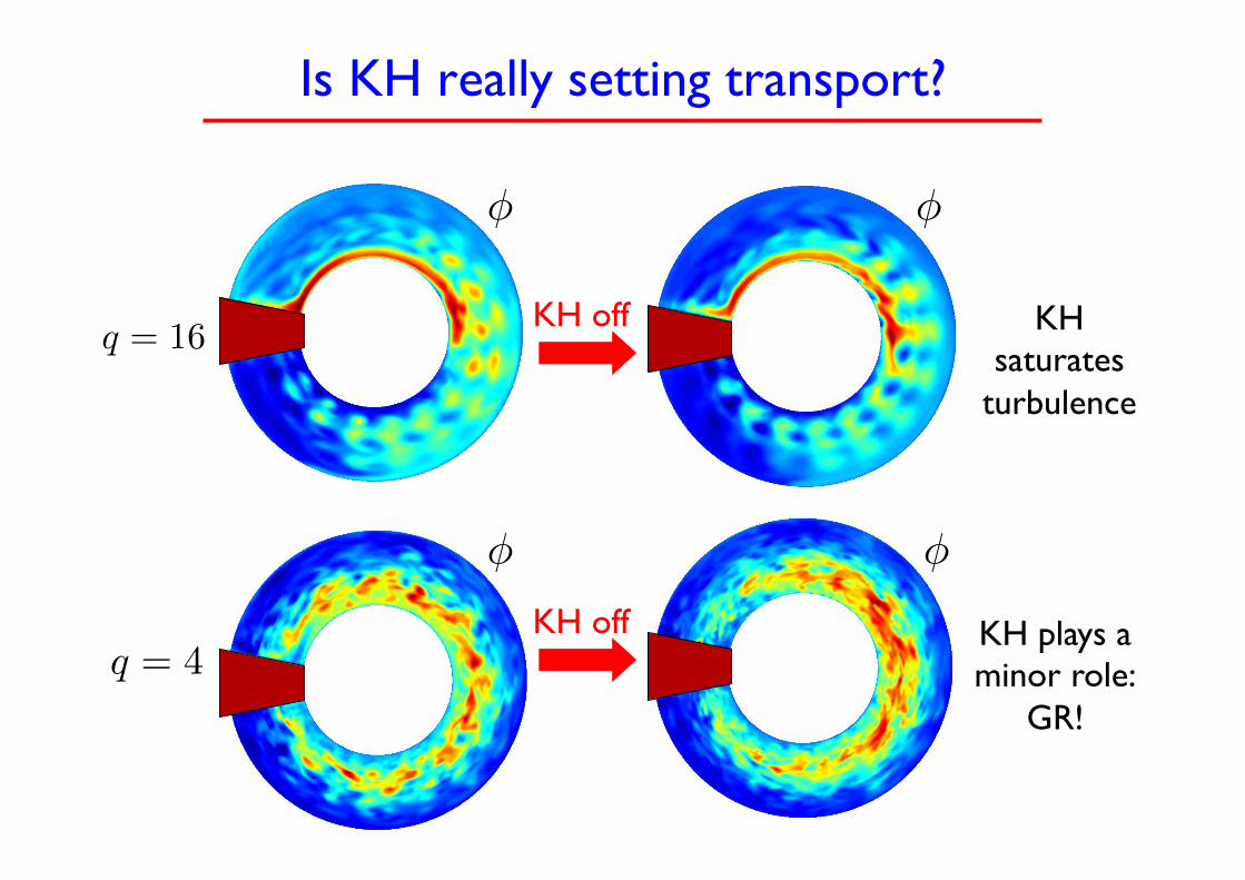
Is KH really setting transport?
q = 16KH off KH
saturates turbulence
q = 4KH off KH plays a
minor role: GR!
φφ
φ φ
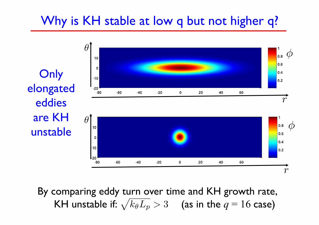
Why is KH stable at low q but not higher q?
Only elongated
eddies are KH unstable
By comparing eddy turn over time and KH growth rate, KH unstable if: (as in the q = 16 case)
�kθLp > 3
φ
r
θ
φ
r
θ
The key questions
• What is the mechanism setting the SOL turbulent level and
the perpendicular transport?
• How is the SOL width established?
• What are the SOL turbulent regimes?
• How do the SOL properties depend on beta, resistivity, tokamak size, …?
• What determines the SOL electrostatic potential?
• Is toroidal rotation generated in the SOL?
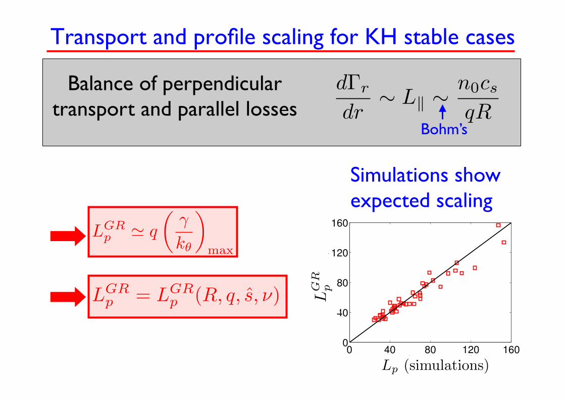
Transport and profile scaling for KH stable cases
Simulations show expected scaling
Balance of perpendicular transport and parallel losses
dΓr
dr∼ L� ∼ n0cs
qRBohm’s
LGRp � q
�γ
kθ
�
max
IntroductionGlobal model for SOL turbulence
What have we learnt so far ?Conclusions
Saturation mechanismDominant instabilitiesElectromagnetic effectsScrape-off layer width scalingIntrinsic rotation
Good agreement between theory and simulationsLp predicted using self-consistent procedure
0 40 80 120 1600
40
80
120
160
Lp (simulation)
Lp(theory)
GBS simulations : R = 500–2000, q = 3–6, ν = 0.01–1, β = 0–3× 10⁻³
F.D. Halpern et al. 15 / 36 Global EM simulations of tokamak SOL turbulence
LGRp = LGR
p (R, q, s, ν)
Lp (simulations)
LGR
p
The key questions
• What is the mechanism setting the SOL turbulent level and the
perpendicular transport?
• How is the SOL width established?
• What are the SOL turbulent regimes?
• How do the SOL properties depend on beta, resistivity, tokamak size, …?
• What determines the SOL electrostatic potential?
• Are there mechanisms to generate toroidal rotation in the SOL?
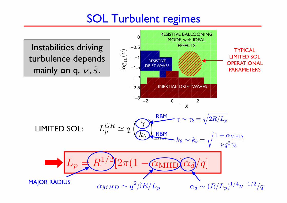
Lp = R1/2[2π(1− αMHD)αd/q]
2 0 23
2.5
2
1.5
1
0.5
0
s
log 1
0(!)
SOL Turbulent regimes RESISTIVE BALLOONING
MODE, with IDEAL EFFECTS
INERTIAL DRIFT WAVES
RESISTIVE DRIFT WAVES
log 1
0(ν)
s
Instabilities driving turbulence depends mainly on q, , . sν
TYPICAL LIMITED SOL
OPERATIONAL PARAMETERS
MAJOR RADIUS αd ∼ (R/Lp)
1/4ν−1/2/qαMHD ∼ q2βR/Lp
LGRp � q
�γ
kθ
�
max
LIMITED SOL: γ ∼ γb =
�2R/Lp
RBM
kθ ∼ kb =
�1− αMHD
νq2γb
RBM
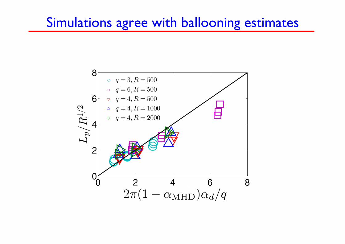
Simulations agree with ballooning estimates
IntroductionGlobal model for SOL turbulence
What have we learnt so far ?Conclusions
Saturation mechanismDominant instabilitiesElectromagnetic effectsScrape-off layer width scalingIntrinsic rotation
Scaling follows GBS simulation dataComparison carried out over wide range of parameters (R, q, β, ν)
0 2 4 6 80
2
4
6
8
!
2!"d(1! ")1/2/q"
!1/2
Lp/R
1/2
q = 3,R = 500
q = 6,R = 500
q = 4,R = 500
q = 4,R = 1000
q = 4,R = 2000
F.D. Halpern et al. 27 / 36 Global EM simulations of tokamak SOL turbulence
2π(1− αMHD)αd/q
The key questions
• What is the mechanism setting the SOL turbulent level and the
perpendicular transport?
• How is the SOL width established?
• What are the SOL turbulent regimes?
• How do the SOL properties depend on beta, resistivity, tokamak size, …?
• What determines the SOL electrostatic potential?
• Are there mechanisms to generate toroidal rotation in the SOL?
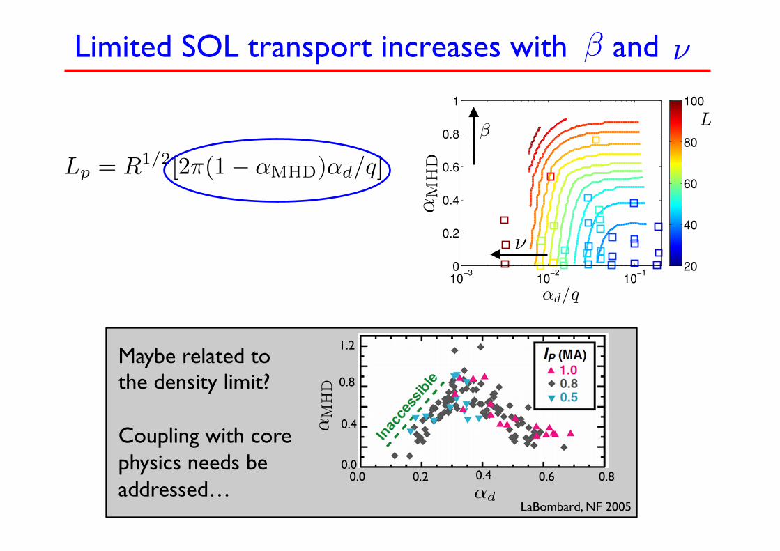
Limited SOL transport increases with and
IntroductionGlobal model for SOL turbulence
What have we learnt so far ?Conclusions
Saturation mechanismDominant instabilitiesElectromagnetic effectsScrape-off layer width scalingIntrinsic rotation
Electromagnetic phase space� Build dimensionless phase space with full linear system...� Verify turbulent saturation theory with GBS simulations
� R = 500, βe = 0 to 3× 10⁻³, ν = 0.01, 0.1, 1, q = 3, 4, 6
!d/q
!
10!3
10!2
10!1
0
0.2
0.4
0.6
0.8
1
20
40
60
80
100
(Contours of Lp given by theory, squares are GBS simulations)
F.D. Halpern et al. 23 / 36 Global EM simulations of tokamak SOL turbulence
Lβ
ν
Lp = R1/2[2π(1− αMHD)αd/q]
αM
HD
β ν
IntroductionGlobal model for SOL turbulence
What have we learnt so far ?Conclusions
Saturation mechanismDominant instabilitiesElectromagnetic effectsScrape-off layer width scalingIntrinsic rotation
SOL turbulence : interplay between β, ν, and ω∗
[LaBombard et al., Nucl Fusion (2005), lower-null L-mode discharges]
Important to understand resistive → ideal ballooning mode transition
F.D. Halpern et al. 20 / 36 Global EM simulations of tokamak SOL turbulence
Maybe related to the density limit? Coupling with core physics needs be addressed…
αM
HD
αdLaBombard, NF 2005
0.0
0.4
0.8
1.2
0.0 0.2 0.4 0.6 0.8
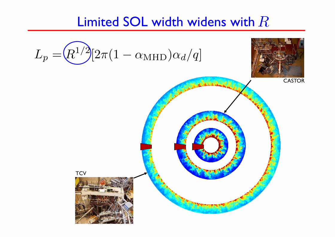
Limited SOL width widens with
CASTOR
TCV
Lp = R1/2[2π(1− αMHD)αd/q]
R
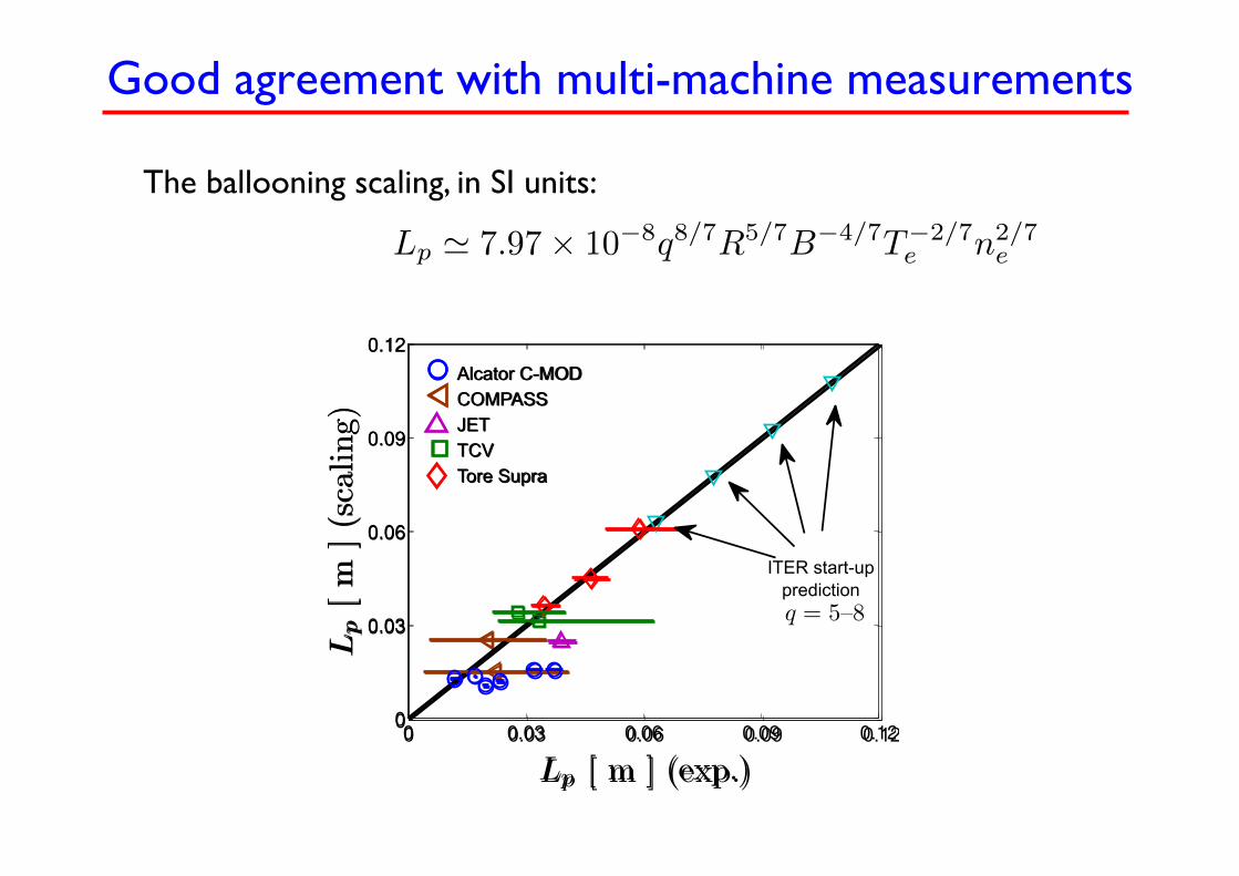
Good agreement with multi-machine measurements
Lp � 7.97× 10⁻⁸q8/7R5/7B−4/7T−2/7e n2/7
e
The ballooning scaling, in SI units:
0 0.03 0.06 0.09 0.120
0.03
0.06
0.09
0.12
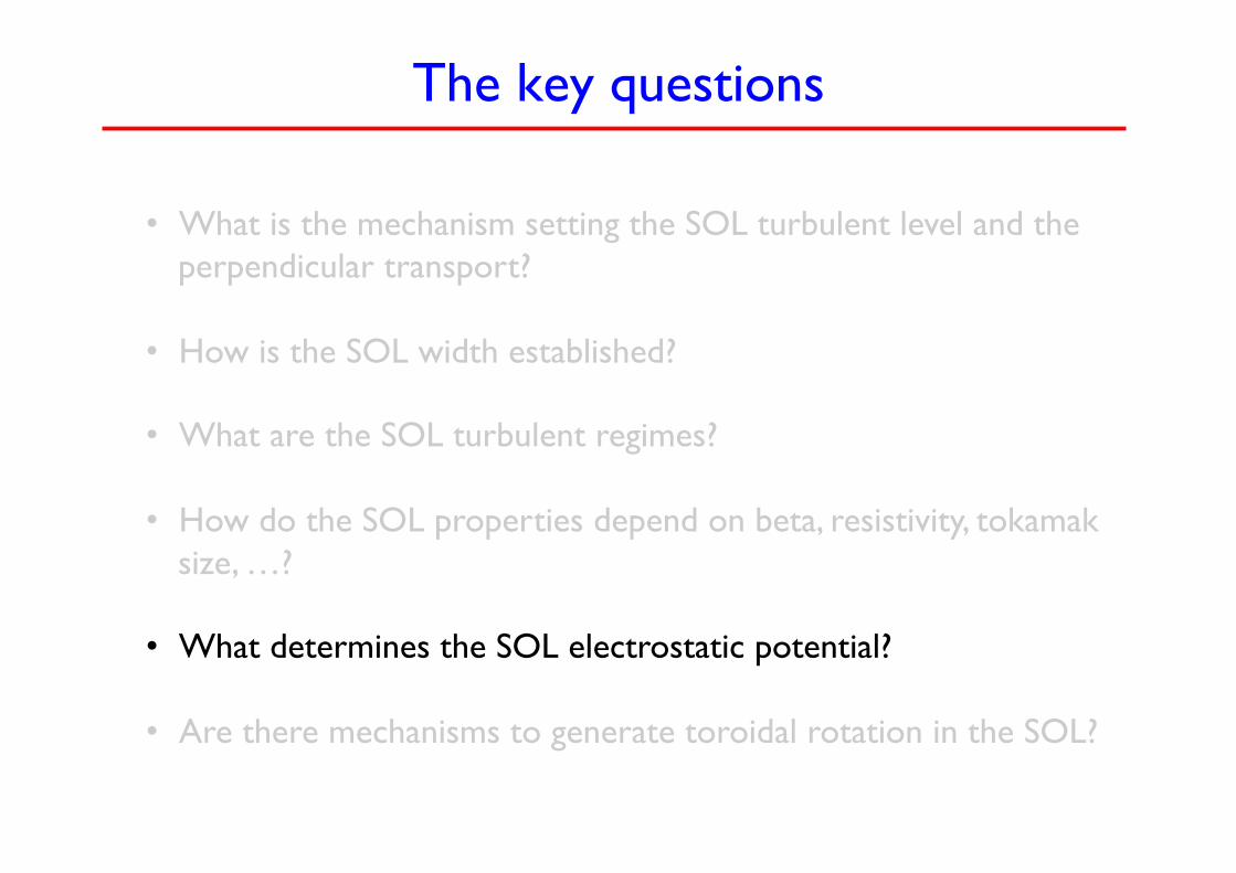
The key questions
• What is the mechanism setting the SOL turbulent level and the
perpendicular transport?
• How is the SOL width established?
• What are the SOL turbulent regimes?
• How do the SOL properties depend on beta, resistivity, tokamak size, …?
• What determines the SOL electrostatic potential?
• Are there mechanisms to generate toroidal rotation in the SOL?
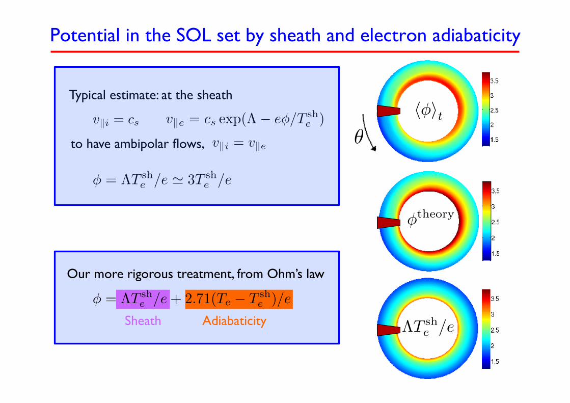
Potential in the SOL set by sheath and electron adiabaticity On the electrostatic potential in the scrape-off-layer of magnetic confinement devices13
Figure 3. Equilibrium profile of the electrostatic potential φ in a poloidal cross-section
as given from GBS simulations (top row), from Eq. (11) (middle row), and from the
widely used estimate φ = ΛT0 (bottom row) with T0 = (T+e +T−e )/2. Here Λ = 3 (left
column), Λ = 6 (middle column), and Λ = 10 (right column).
Typical estimate: at the sheath
to have ambipolar flows, Our more rigorous treatment, from Ohm’s law
v�i = cs v�e = cs exp(Λ− eφ/T she )
φ = ΛT she /e � 3T sh
e /e
v�i = v�e
φ = ΛT she /e+ 2.71(Te − T sh
e )/e
Sheath Adiabaticity ΛT she /e
�φ�t
φtheory
θ
The key questions
• What is the mechanism setting the SOL turbulent level and the
perpendicular transport?
• How is the SOL width established?
• What are the SOL turbulent regimes?
• How do the SOL properties depend on beta, resistivity, tokamak size, …?
• What determines the SOL electrostatic potential?
• Are there mechanisms to generate toroidal rotation in the SOL?
IntroductionGlobal model for SOL turbulence
What have we learnt so far ?Conclusions
Saturation mechanismDominant instabilitiesElectromagnetic effectsScrape-off layer width scalingIntrinsic rotation
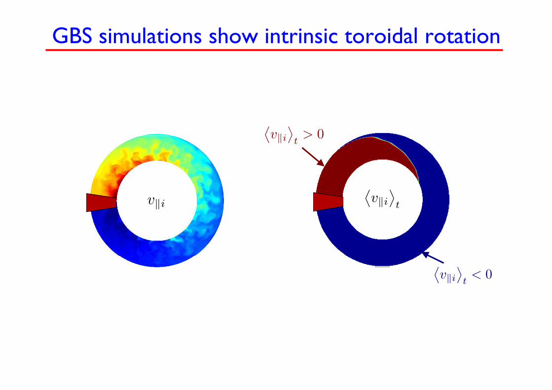
GBS simulations show intrinsic toroidal rotation
Snapshot Time-average
F.D. Halpern et al. 31 / 36 Global EM simulations of tokamak SOL turbulence
GBS simulations show intrinsic toroidal rotation Introduction
Global model for SOL turbulenceWhat have we learnt so far ?
Conclusions
Saturation mechanismDominant instabilitiesElectromagnetic effectsScrape-off layer width scalingIntrinsic rotation
GBS simulations show intrinsic toroidal rotation
Snapshot Time-average
F.D. Halpern et al. 31 / 36 Global EM simulations of tokamak SOL turbulence
v�i
IntroductionGlobal model for SOL turbulence
What have we learnt so far ?Conclusions
Saturation mechanismDominant instabilitiesElectromagnetic effectsScrape-off layer width scalingIntrinsic rotation
GBS simulations show intrinsic toroidal rotation
Snapshot Time-average +/-
� There is a finite volume-averaged toroidal rotation (∼ 0.3cs)
F.D. Halpern et al. 32 / 36 Global EM simulations of tokamak SOL turbulence
�v�i
�t< 0
�v�i
�t> 0
�v�i
�t
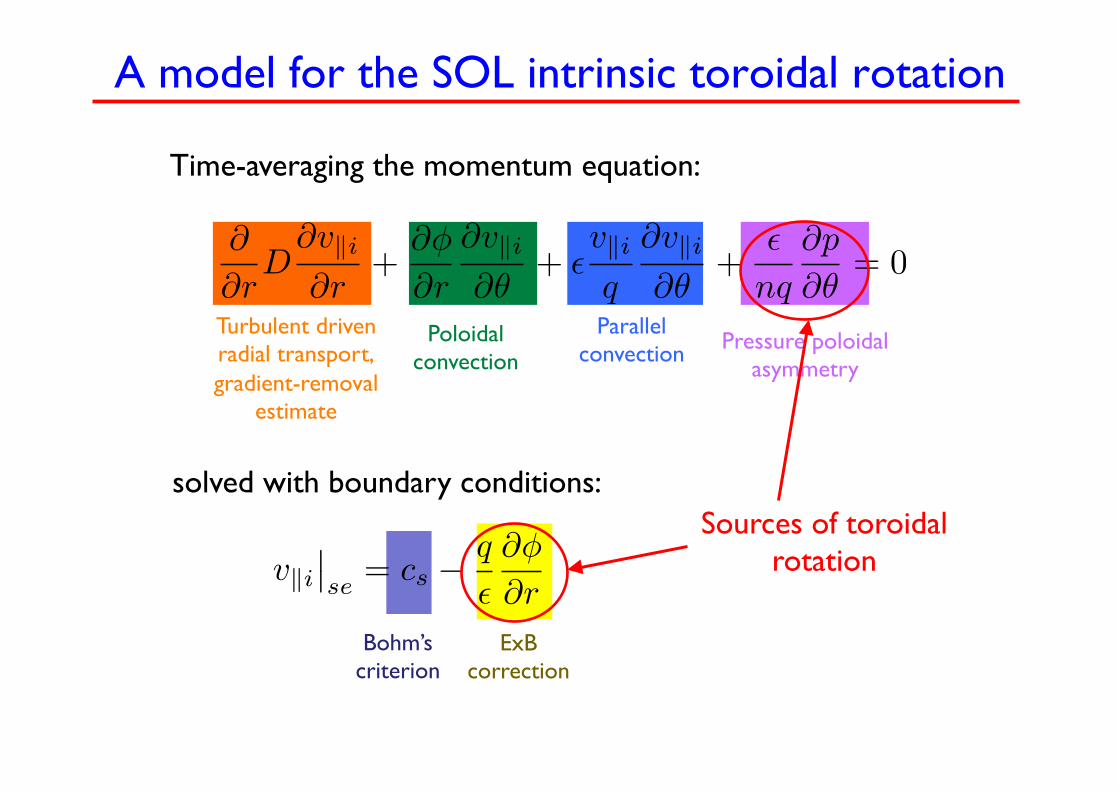
A model for the SOL intrinsic toroidal rotation
Time-averaging the momentum equation:
∂
∂rD∂v�i∂r
+∂φ
∂r
∂v�i∂θ
+ �v�iq
∂v�i∂θ
+�
nq
∂p
∂θ= 0
Turbulent driven radial transport, gradient-removal
estimate
Poloidal convection
Parallel convection
solved with boundary conditions:
Pressure poloidal asymmetry
v�i��se
= cs −q
�
∂φ
∂r
Bohm’s criterion
ExB correction
Sources of toroidal rotation
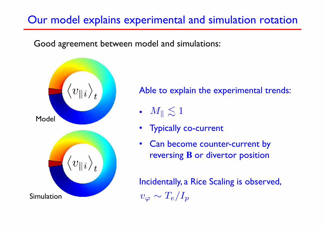
Our model explains experimental and simulation rotation
Good agreement between model and simulations:
IntroductionGlobal model for SOL turbulence
What have we learnt so far ?Conclusions
Saturation mechanismDominant instabilitiesElectromagnetic effectsScrape-off layer width scalingIntrinsic rotation
GBS simulations agree with the theory�v�i
�tfrom GBS simulations
�v�i
�tfrom Theory
(limiter position → HFS, down, LFS, up)
F.D. Halpern et al. 34 / 36 Global EM simulations of tokamak SOL turbulence
Able to explain the experimental trends:
•
• Typically co-current
• Can become counter-current by reversing B or divertor position
Incidentally, a Rice Scaling is observed,
M� � 1
vϕ ∼ Te/Ip
Model
Simulation
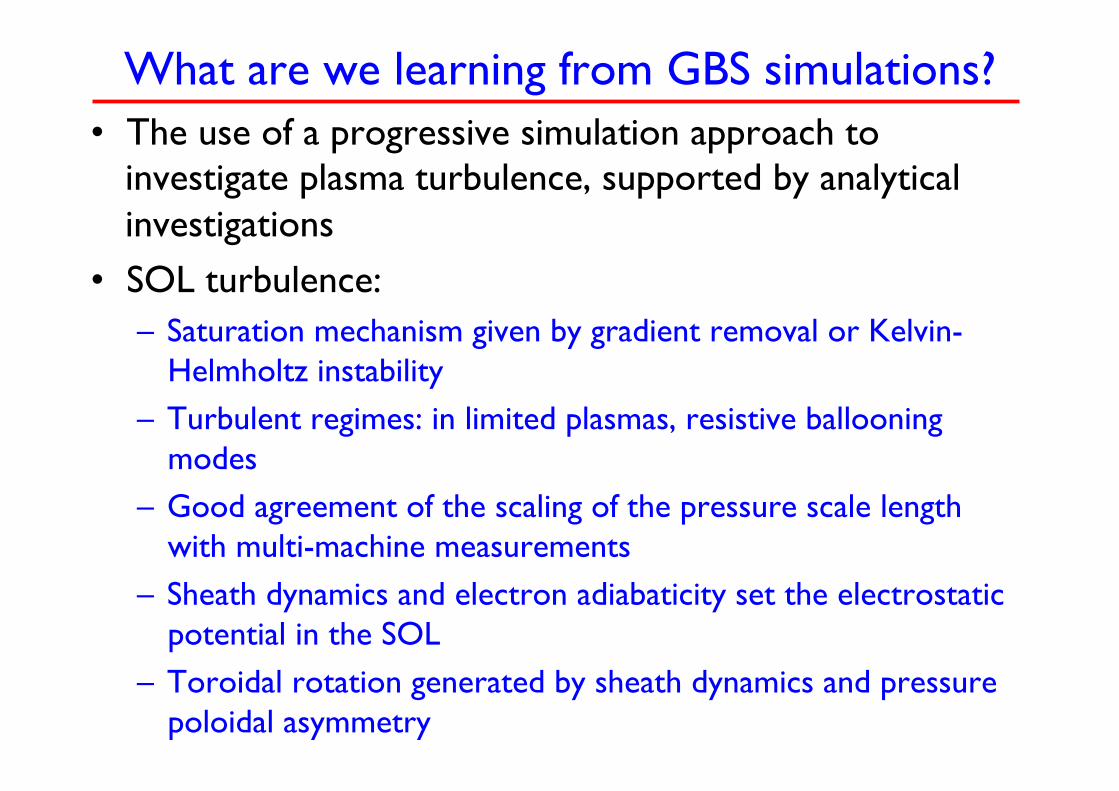
What are we learning from GBS simulations? • The use of a progressive simulation approach to
investigate plasma turbulence, supported by analytical investigations
• SOL turbulence: – Saturation mechanism given by gradient removal or Kelvin-
Helmholtz instability – Turbulent regimes: in limited plasmas, resistive ballooning
modes – Good agreement of the scaling of the pressure scale length
with multi-machine measurements – Sheath dynamics and electron adiabaticity set the electrostatic
potential in the SOL – Toroidal rotation generated by sheath dynamics and pressure
poloidal asymmetry


![Infections bactériennes des muqueuses - érosions syphilitiquescochlea.iurc.montp.inserm.fr/enseignement/cycle_2/MIB/Ressources... · [dermo-hypodermite] Infections bactériennes](https://img.pdfslide.fr/doc/110x75/5fd2700fcc816f59bc461057/infections-bactriennes-des-muqueuses-rosions-dermo-hypodermite-infections.jpg)