Embed Size (px)
Citation preview
Thèse de doctorat
Pour obtenir le grade de Docteur de l’Université
POLYTECHNIQUE HAUTS-DE-FRANCE
Spécialité micro et nanotechnologies, acoustiques et télécommunications
Présentée et soutenue par Doan LE ANH.
Le 01/03/2019, à Valenciennes
Ecole doctorale :
Sciences Pour l’Ingénieur (SPI)
Equipe de recherche, Laboratoire :
Institut d’Electronique, de Micro-Electronique et de Nanotechnologie/Département d’Opto-Acousto-Electronique (IEMN/DOAE)
Du micro véhicule aérien au nano véhicule aérien : études théoriques et expérimentales sur un insecte artificiel à ailes battantes
Composition du jury
Président du jury
M. André PREUMONT, Professeur des Universités, ULB / Active Structures Laboratory, Bruxelles
Rapporteurs
M. Bruno ALLARD, Professeur des Universités, INSA de Lyon / Laboratoire Ampère, Lyon M. Ramiro GODOY-DIANA, Chargé de recherches CNRS HDR, ESPCI / PMMH, Paris
Examinateur
Mme Guylaine POULIN-VITTRANT, Chargé de recherches CNRS, INSA-CVL GREMAN, Blois
Directeurs de thèse
M. Éric CATTAN, Professeur des Universités, UPHF / IEMN, Valenciennes M. Sébastien GRONDEL, Professeur des Universités, UPHF / IEMN, Valenciennes
Membre invité
M. Olivier Thomas, Professeur des Universités, ENSAM/ LSIS, Lille

i
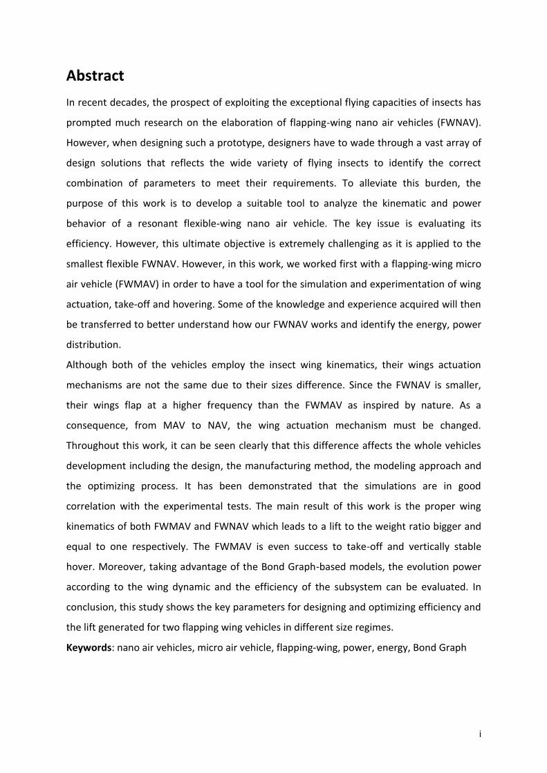
Abstract
In recent decades, the prospect of exploiting the exceptional flying capacities of insects has
prompted much research on the elaboration of flapping-wing nano air vehicles (FWNAV).
However, when designing such a prototype, designers have to wade through a vast array of
design solutions that reflects the wide variety of flying insects to identify the correct
combination of parameters to meet their requirements. To alleviate this burden, the
purpose of this work is to develop a suitable tool to analyze the kinematic and power
behavior of a resonant flexible-wing nano air vehicle. The key issue is evaluating its
efficiency. However, this ultimate objective is extremely challenging as it is applied to the
smallest flexible FWNAV. However, in this work, we worked first with a flapping-wing micro
air vehicle (FWMAV) in order to have a tool for the simulation and experimentation of wing
actuation, take-off and hovering. Some of the knowledge and experience acquired will then
be transferred to better understand how our FWNAV works and identify the energy, power
distribution.
Although both of the vehicles employ the insect wing kinematics, their wings actuation
mechanisms are not the same due to their sizes difference. Since the FWNAV is smaller,
their wings flap at a higher frequency than the FWMAV as inspired by nature. As a
consequence, from MAV to NAV, the wing actuation mechanism must be changed.
Throughout this work, it can be seen clearly that this difference affects the whole vehicles
development including the design, the manufacturing method, the modeling approach and
the optimizing process. It has been demonstrated that the simulations are in good
correlation with the experimental tests. The main result of this work is the proper wing
kinematics of both FWMAV and FWNAV which leads to a lift to the weight ratio bigger and
equal to one respectively. The FWMAV is even success to take-off and vertically stable
hover. Moreover, taking advantage of the Bond Graph-based models, the evolution power
according to the wing dynamic and the efficiency of the subsystem can be evaluated. In
conclusion, this study shows the key parameters for designing and optimizing efficiency and
the lift generated for two flapping wing vehicles in different size regimes.
Keywords: nano air vehicles, micro air vehicle, flapping-wing, power, energy, Bond Graph

iii
Résumé
Au cours des dernières décennies, la possibilité d’exploiter les capacités de vol exceptionnelles des
insectes a été à l’origine de nombreuses recherches sur l’élaboration de nano-véhicules aériens
(NAVs) à ailes battantes. Cependant, lors de la conception de tels prototypes, les chercheurs doivent
analyser une vaste gamme de solutions liées à la grande diversité des insectes volants pour identifier
les fonctionnalités et les paramètres adaptés à leurs besoins. Afin d’alléger cette tâche, le but de ce
travail est de développer un outil permettant à la fois d’examiner le comportement cinématique et
énergétique d’un nano-véhicule aérien à ailes flexibles résonantes, et donc d'évaluer son efficacité.
Cet objectif reste néanmoins extrêmement difficile à atteindre car il concerne des objets de très
petites tailles. Aussi, nous avons choisi tout d’abord de travailler sur un micro-véhicule aérien (MAV)
à ailes battantes. Il s’agit avant tout de valider l’outil de modélisation à travers une comparaison
systématique des simulations avec des résultats expérimentaux effectués lors de l’actionnement des
ailes, puis au cours du décollage et du vol stationnaire du prototype. Une partie des connaissances et
expériences acquises pourra ensuite être utilisée afin de mieux comprendre le fonctionnement et
identifier la distribution d'énergie au sein du NAV.
Bien que les deux véhicules s’inspirent directement de la cinématique des ailes d'insectes, les
mécanismes d'actionnement des ailes artificielles des deux prototypes ne sont pas les mêmes en
raison de la différence de taille. Comme le NAV est plus petit, ces ailes ont un mouvement de
battement à une fréquence plus élevée que celles du MAV, à l’instar de ce qui existe dans la nature.
En conséquence, lorsque l’on passe du MAV au NAV, le mécanisme d’actionnement des ailes doit
être adapté et cette différence nécessite d’une part, de revoir la conception, l'approche de
modélisation et le processus d'optimisation, et d’autre part, de modifier le procédé de fabrication.
Une fois ces améliorations apportées, nous avons obtenu des résultats de simulations en accord
avec les tests expérimentaux. Le principal résultat de ce travail concerne l’obtention pour les deux
prototypes, le MAV et le NAV, d’une cinématique appropriée des ailes, qui conduit à une force de
portance équivalente au poids. Nous avons d’ailleurs démontré que le MAV était capable de décoller
et d’avoir un vol stationnaire stable selon l’axe vertical. En tirant parti des modèles basés sur le
langage Bond Graph, il est également possible d'évaluer les performances énergétiques de ces
prototypes en fonction de la dynamique de l'aile. En conclusion, cette étude contribue à la définition
des paramètres essentiels à prendre en compte lors de la conception et l'optimisation énergétique
de micro et nano-véhicules à ailes battantes.
Mots clés: nano-véhicules aérien, micro-véhicule aérien, ailes battantes, puissance, énergie, Bond
Graph

v
Preface
This dissertation is formatted in accordance with the regulations of the University of
Polytechnique Haut-de-France and submitted in partial fulfillment of the requirements for a
PhD degree awarded jointly by the University of Polytechnique Haut-de-France. Versions of
this dissertation will exist in the institutional repositories of this university.
All aspects of the material appearing in this thesis have been originally written by the author
unless otherwise stated.
This work has been done in the IEMN-DOAE laboratory under the supervision of Prof.
Sébastien Grondel, and Prof. Eric Cattan.
A version of chapter 4 has been submitted. [A.L. DOAN], D. Faux, O. Thomas, S. Grondel, E.
Cattan, Kinematic and power behavior analysis of a resonant flexible-wing nano air vehicle
using a Bond Graph approach, January 2019. All the experiments and simulations were
conducted by the author under the supervision of Prof. Sébastien Grondel, and Prof. Eric
Cattan.
A version of chapter 3 was presented at the International Micro Air Vehicle conference and
Flight Competition on the flapping wing MAV, 2017 (A.L. DOAN, C. Delebarre, S. Grondel, E.
Cattan, Bond Graph based design tool for a passive rotation flapping wing IMAV2017, p.
242).
A version of chapter 4 was presented at the International Mechatronics conference on the
flapping wing MAV, 2017 (A.L. DOAN, D. Faux, S. Dupont, S. Grondel, E. Cattan, Modeling
and simulation of the vertical takeoff and energy consumption of a vibrating wing nano air
vehicle REM2016, p. 123).

vii
Table of Contents
Abstract ....................................................................................................................................... i
Résumé...................................................................................................................................... iii
Preface ....................................................................................................................................... v
Table of Contents ..................................................................................................................... vii
List of Figures ............................................................................................................................ xi
List of Tables .......................................................................................................................... xvii
Abbreviations .......................................................................................................................... xix
Acknowledgements ................................................................................................................. xxi
Dedication .............................................................................................................................. xxiii
General introduction ..................................................................................................................1
Chapter 1: Literature reviews..................................................................................................5
1.1 Current and potential applications of UAVs and small UAVs .......................................... 6
1.2 MAV and NAV specifications ............................................................................................ 7
1.3 Classification of MAVs and NAVs ..................................................................................... 8
1.3.1 Fixed-wing ...................................................................................................................9
1.3.2 Rotary-wing ..............................................................................................................10
1.3.3 Flapping-wing ...........................................................................................................12
1.4 Flapping flight ................................................................................................................. 14
1.4.1 Flapping flyer kinematics ..........................................................................................16
1.4.2 Wing actuation mechanisms ....................................................................................18
1.4.3 Unsteady mechanisms in flapping flight ..................................................................19
1.4.3.1 Wagner effect .....................................................................................................20
1.4.3.2 Kramer effect (rotational forces) .......................................................................21
1.4.3.3 Added mass ........................................................................................................21
1.5 Flying modes................................................................................................................... 22
1.5.1 Gliding flight ..............................................................................................................22
1.5.2 Flapping forward flight .............................................................................................24
1.5.3 Hovering flight ..........................................................................................................26
1.6 Review of component selection of flapping MAVs and NAVs ....................................... 27
1.6.1 Flapping-wing actuators ...........................................................................................28
1.6.2 Tail, sail, and tailless .................................................................................................29
1.6.3 Control scheme for flapping-wing vehicles ..............................................................31
1.6.4 Number of wings ......................................................................................................33
1.6.5 Wing rotational principle ..........................................................................................34
1.7 Summarization and motivation ...................................................................................... 34
Chapter 2: FWMAV model and design...................................................................................39
2.1 Introduction .................................................................................................................... 40
2.2 FWMAV dynamic model ................................................................................................. 40
2.2.1 Flapping and rotating kinetics ..................................................................................42
2.2.2 Modeling of the submodels ......................................................................................43
2.2.2.1 Motor Driver and geared motor ........................................................................43
2.2.2.2 Modeling of the aerodynamic forces .................................................................45
2.2.2.3 Dynamic equation of FWMAV wing motion ......................................................49
2.2.2.4 Complete Bond Graph model .............................................................................55
2.2.3 FWMAV parameters .................................................................................................57
2.2.3.1 Wing parameters ................................................................................................57
2.2.3.2 Geared motor parameters .................................................................................57
2.2.3.3 Helical spring stiffness ........................................................................................58
2.3 Optimization ................................................................................................................... 59
2.3.1 Initial prototype ........................................................................................................59
2.3.2 Parameter optimization............................................................................................62
2.3.2.1 Sensitivity to spring stiffness and driving frequency .........................................62
2.3.2.2 Sensitivity to the input voltage ..........................................................................64
2.3.2.3 Sensitivity to wing flexural stiffness ...................................................................65
2.3.2.4 Sensitivity to wing offset ( ) ...........................................................................68
2.3.3 Final prototype .........................................................................................................70
2.4 Conclusion of the MAV design ....................................................................................... 71
Chapter 3: Towards the construction of a FWMAV able to take off and to
stabilize...................................................................................................................................73
3.1 Material preparation and assembly work ...................................................................... 74
3.1.1 Motor and motor driver selections ..........................................................................74
3.1.2 Wing fabrication .......................................................................................................76
3.1.3 Wing’s stiffness determination ................................................................................76
3.1.4 Wing’s damping coefficient. .....................................................................................79
ix
3.1.5 Torsional spring ........................................................................................................82
3.1.6 Assembly step ...........................................................................................................82
3.2 Experimental analysis of the wing movement and generated lift ................................. 83
3.3 Validation ....................................................................................................................... 85
3.3.1 Frequency response .................................................................................................85
3.3.2 Input voltage response .............................................................................................87
3.3.3 Wing kinematic in desired working condition ..........................................................88
3.3.4 Take-off demonstration ............................................................................................89
3.4 Altitude control .............................................................................................................. 90
3.4.1 Image processing ......................................................................................................96
3.4.2 Manual tuning PID ....................................................................................................97
3.5 Development of an electronic circuit: .......................................................................... 100
3.5.1 Electronic components: ......................................................................................... 101
3.6 Analysis of power and energy consumption ................................................................ 102
3.6.1 MAV power consumption analysis ........................................................................ 103
3.6.2 Energy analysis ...................................................................................................... 106
3.6.3 Efficiency of the FWMAV ....................................................................................... 107
3.7 Conclusion .................................................................................................................... 108
Chapter 4: Kinematic and power behavior analysis of OVMI.............................................109
4.1 Introduction .................................................................................................................. 110
4.2 OVMI Dynamic Bond Graph model .............................................................................. 111
4.2.1 Prototype description ............................................................................................ 111
4.2.2 OVMI Word Bond Graph ....................................................................................... 112
4.2.3 Bond Graph model ................................................................................................. 113
4.2.3.1 Generator Bond Graph model ......................................................................... 113
4.2.3.2 Electromagnetic actuator Bond Graph model ................................................ 113
4.2.3.3 “Wings”Bond Graph model ............................................................................. 115
4.2.3.4 Global system modeling .................................................................................. 117
4.2.4 Parameter estimation ............................................................................................ 118
4.2.4.1 Generator and electromagnetic actuator ....................................................... 118
4.2.4.2 “Wings” ............................................................................................................ 119
4.3 Kinematic simulation and dynamic power analysis ..................................................... 120
4.3.1 Kinematic simulation ............................................................................................. 120
4.3.2 Wing kinematic concept validation ....................................................................... 122
4.3.3 Dynamic power analysis ........................................................................................ 124
4.3.3.1 Power partition versus working mode ............................................................ 125
4.3.3.2 Kinetic and potential energy versus wing movement ..................................... 125
4.3.3.3 . Power distribution versus aeroelastic effect ................................................ 128
4.4 Conclusion .................................................................................................................... 128
Conclusion and perspective .................................................................................................. 131
References ............................................................................................................................. 135
Appendix ................................................................................................................................ 147
A.1.Chapter1:Literature reviews ......................................................................................... 147
A.1.1: Selection criteria for different rotary-wing typologies ....................................... 147
A.1.2 Unsteady aerodynamics ....................................................................................... 148
A.2.Chapter2: FWMAV model and design .......................................................................... 152
A.2.1: Aerodynamic models of insect-like flapping wings .............................................. 152
A.2.2: Bond Graph presentation for FWMAV wings ....................................................... 155
A.2.3: Derive dynamic euqation of the wing from the Bond Graph presentation. ........ 155
A.3.Chapter 3: Towards the construction of a FWMAV able to take off and to stabilize .. 157
A.3.1: Schematic and layouts of electronic circuit developed for the FWMAV ............. 157
A.4 Chapter 4: Kinematic and power behavior analysis of OVMI ...................................... 160
A.4.1: Fabrication process .............................................................................................. 160
xi
List of Figures
Figure 1.1: MAV and NAV flight range compared to existing flying vehicles and species [38] ..8
Figure 1.2: Fixed, rigid, and flexible wings, (a) transparent Black Widow by AeroVironment
[39], (b) a flexible-wing design developed at the University of Florida [40]. .............................9
Figure 1.3: Graphic representation of rotary-wing configurations: a) conventional, b) ducted
coaxial, c) conventional coaxial, d) side-by-side rotors, e) synchropter, f) conventional
tandem, g) quadrotor [48], [49]. ...............................................................................................10
Figure 1.4: Examples of rotary-wing MAVs and NAVs, (a) the Black Hornet, (b) Crazyflie, (c)
Mesicopter, (d) Picoflyer. ..........................................................................................................11
Figure 1.5: Reynolds number range for flying bio-systems and flying vehicles adapted from
[56]. The NAV does not have the lower limit, it should be any vehicle with Re number and
weight smaller than those of the MAV. ....................................................................................12
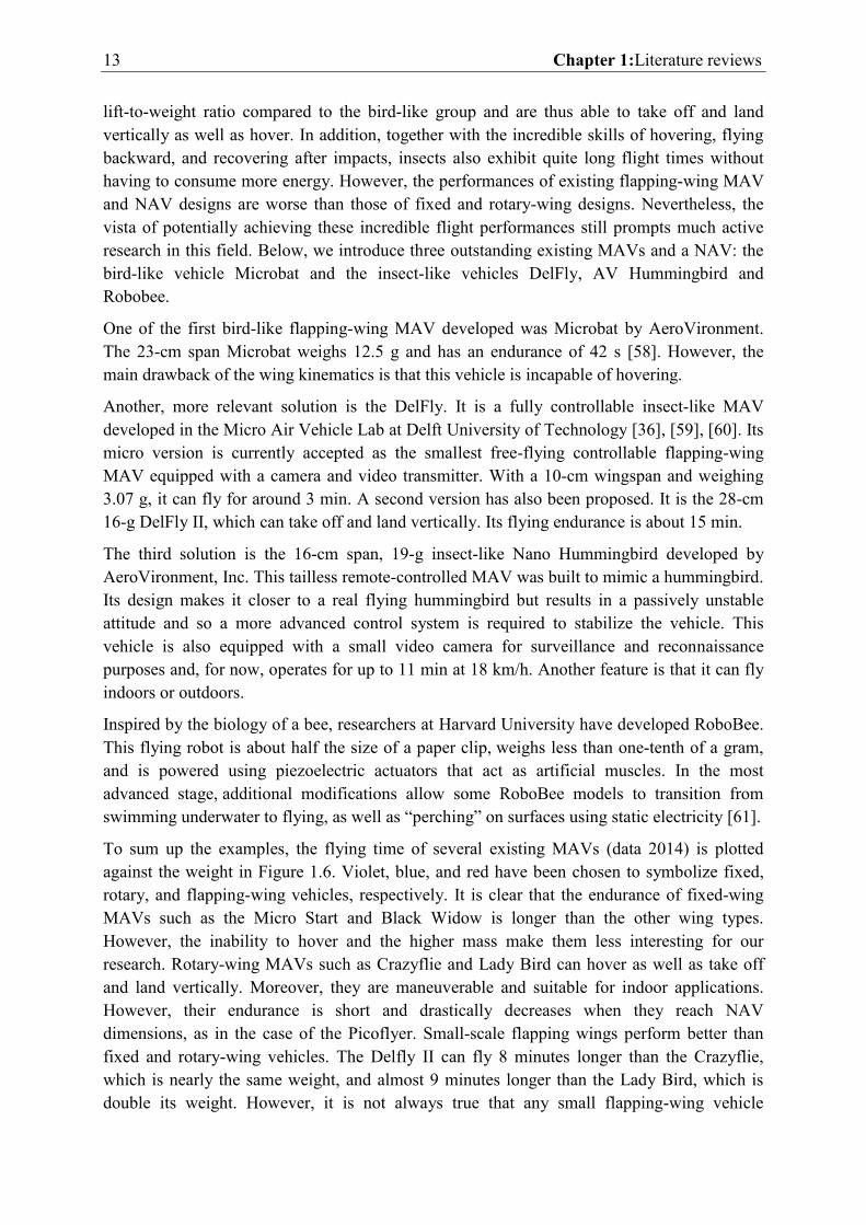
Figure 1.6: Relationship between weight and flying time of existing MAVs (2014 data).
Names of fixed, rotary, and flapping-wing vehicles are in violet, blue, and red, respectively.
Only crucial dimensions corresponding to each wing category are displayed to indicate the
vehicle size. For instance, wingspan depicts the size of flapping and fixed-wing MAVs, while
the 3D dimensions of quadrotor and rotor diameter are used for other rotary-wing vehicles.14
Figure 1.7: Superimposed frames showing typical landing maneuvers of a honeybee [63]. ..15
Figure 1.8: Video sequence using the prism platform showing a typical escape. White dots
on the image mark the points on the head and abdomen used to determine the center of
mass of the fly (black and white circle) at three time points: stimulus onset ( ), immediately
before the jump ( ), and the moment of takeoff ( ). The red dot marks the contact
point of the tarsus (final segment of legs of insects) with the surface at [64]. ...................15
Figure 1.9: Wing movement cycle of a gull during normal flight [66]. .....................................16
Figure 1.10: Basic flapping wing kinematics: a) Wing path described by the trajectory of a
particular wing chord; b) Snapshots of this wing chord during upstroke and downstroke
demonstrating its translational motion and stroke reversal including supination and
pronation; c) Evolution of flapping and rotating in quadrature over time [68] [10] ...............17
Figure 1.11: a) bird flight apparatus [69], insects and their flight apparatus: b) direct and c)
indirect muscles [70] [71]. ........................................................................................................18
Figure 1.12: Vortex system and development of bound circulation around an airfoil starting
from rest [74] ............................................................................................................................20
Figure 1.13: High-lift devices used in aircraft and their equivalents in flying animals, [85],
[86]. ...........................................................................................................................................23
Figure 1.14: Vortex generators used in aircraft (left) and their equivalents in flying animals,
a) Protruding digit on a bat wing, b) Serrated leading-edge feather of an owl, c) Corrugated
dragonfly wing, adapted from [85], [86]. .................................................................................23
Figure 1.15: Lateral view of flapping motions illustrating the path of the wingtip (filled
circles) and wrist (open circles) adapting to steady-speed flight [89]. .....................................24
Figure 1.16: Wingtip paths relative to the body – indicated by arrows – for a variety of flyers.
a) albatross, fast gait; b) pigeon, slow gait; c) horseshoe bat, fast flight; d) horseshoe bat,
slow gait; e) blowfly; f) locust; g) June Beetle; h) fruit fly [90]. ................................................25
Figure 1.17: Flow structures for a) slow and b) fast forward flapping flight [89]. ...................25
Figure 1.18: Three-dimensional vortex structures in the flow during a stroke cycle of a ruby-
throated hummingbird, where the time stamp from (a) to (d) is 0.37, 0.51, 0.58, and 0.78T (T
is the stroke cycle). The dashed lines mark the vortex loop from the downstroke. The thick
arrow in (d) indicates the location where the LEV is pinched off [93]. ....................................26
Figure 1.19: Different tail designs: a) conventional airplane tail [114], b) DelFly I V-tail, and c)
DelFly II Inverted V-tail [36] ......................................................................................................30
Figure 1.20: MAV Sails: a) Mentor [2007]; b) Richter and Lipson [2011]; c) Jellyfish robot
[2014]. .......................................................................................................................................30
Figure 1.21: Periodic wing motion parameters: a) stroke amplitude, symmetric or
asymmetric wingbeat frequency, and wing stroke bias angle, b) stroke-plane tilt angle, c)
and d) angle of attack between downstroke and upstroke. ....................................................32
Figure 1.22: Split-cycle constant-period frequency modulation, control strategies of flapping
MAV: a) Vertical translation, b) Horizontal translation, c) Yawing motion, and d) Rolling
motion from Doman and Oppenheimer [2014]. ......................................................................32
Figure 1.23: Different wing configurations: (I) Conventional wing, Robo Raven; (II)
BionicOpter Dragonfly; unconventional wing including DelFly II with a single clap-and-fling
mechanism (IIIa), Delfly Micro with a double clap-and-fling mechanism (IIIb), and Mentor
with a multiple clap-and-fling mechanism [36]. .......................................................................33
Figure 1.24: Relationship between a) wing length and total mass, b) wing length and flapping
frequency, adapted from [124] ................................................................................................37
Figure 2.1: MAV structure definition ........................................................................................40
Figure 2.2: FWMAV Word Bond Graph .....................................................................................41
Figure 2.3: Prototype with a mass-spring-damper system adapted from [95] ........................41
Figure 2.4: Schematic of the passive rigid wing. .......................................................................42
Figure 2.5: Anterior and distal views of the wing .....................................................................43
Figure 2.6: Mechanical model of a DC torque motor connected through gearing to an inertial
load [125]. .................................................................................................................................43
Figure 2.7: Bond Graph representation of the motor driver and geared motor. ....................44
Figure 2.8: Wing geometry .......................................................................................................47
Figure 2.9: Translational and rotational forces on each wing strip ..........................................47
Figure 2.10: Wing section and parameters for calculating the added mass forces adapted
from [86]. ..................................................................................................................................48
Figure 2.11: 1-junction arrangement. .......................................................................................52
xiii
Figure 2.12: Flow connections ..................................................................................................53
Figure 2.13: Bond Graph representation of the FWMAV wing and the corresponding
aerodynamics ............................................................................................................................54
Figure 2.14: FWMAV Bond Graph representation. Several power and energy sensors are
added for the power and energy analysis in Chapter 3 (Section 3.6). .....................................56
Figure 2.15: a) The trajectory and b) corresponding aerodynamic forces of one wing ...........60
Figure 2.16: Aerodynamic forces of the lift and drag components ..........................................61
Figure 2.17: The added mass force helps wing rotation. Lift component (red arrow), drag
component (blue arrow), (black arrow). ..........................................................................62
Figure 2.18: Effect of spring stiffness and excitation frequency on flapping amplitude (a) and
mean lift (b). Thirty springs of different stiffness were tested over a driving frequency range
of 0 Hz to 40 Hz. Each spring represents a system portrayed by a unique color. Only the first
five and last three systems are plotted in full for clarity. The dashed blue lines represent the
maximum flapping and lift values for the others. The first seven springs are provided in the
figure legend for detailed discussions. .....................................................................................63
Figure 2.19: Flapping amplitude (a) and mean lift force (b) as a function of the input voltage
A simulation with a sweep of the input voltage from [0.5 5] V was conducted on the first
seven systems discussed in section 2.3.2.1. Each system was excited at the frequency where
maximum mean lift occurs. ......................................................................................................65
Figure 2.20: Average translational force coefficients as a function of the angle of attack [79].66
Figure 2.21: Sensitivity to variations in wing flexural stiffness. The FWMAV system with a
spring stiffness of 2.95e3 mN.mm/rad was stimulated using an input voltage of 4.5 V at 10
Hz. The wing bending stiffness ranged from 1e-4 N.m/rad to 4e-4 N.m/rad. .........................67
Figure 2.22: Effect of variation of wing offset. The FWMAV system with a spring stiffness of
2.95e3 mN.mm/rad was stimulated using an input voltage of 4.5 V at 10 Hz. The wing offset
dw ranged from 0 m to 0.06 m. .................................................................................................69
Figure 2.23: Wing kinematics a) and lift components of aerodynamic forces (b). ..................70
Figure 3.1: a) Motor GM15A, b) planetary gearhead of GM15A, c) Pololu DRV8835 dual
motors driver shield for Arduino [141] .....................................................................................74
Figure 3.2 : PWM approximated sinusoidal voltage .................................................................75
Figure 3.3 : a) asymmetric flapping wing movement caused by b) input voltage offset. ........75
Figure 3.4 : Picture of FWMAV’s wing configuration. ...............................................................76
Figure 3.5 : Diagram and experimental setup for measuring the rubber stiffness. .................77
Figure 3.6 : Wing’s stiffness with the rubber part (9mm). Each measurement is repeated
three times (colored circles). The stiffness value of the rubber is a value within the range
of minimum stiffness and maximum stiffness . ....................................................78
Figure 3.7 : Set-up of damping coefficient determination experiment and its diagram..........80
Figure 3.8 : Variation in rotational angle as a function of time. Local maximum and minimum
of free oscillation are represented by red and yellow stars, respectively. ..............................81
Figure 3.9 : First FWMAV prototype : a) Designed prototype and b) Fabricated one. ............83
Figure 3.10 : Level arm configuration for lift measurement experiment. ................................84
Figure 3.11 : Diagram of wing observation: experimental setup .............................................85
Figure 3.12 : Wing movement and lift observations experimental setup ................................85
Figure 3.13 : Measured lift versus driving frequency. Frequency is change for every two
second from 1 to 20 Hz. ............................................................................................................86
Figure 3.14: a) Amplitude of flapping angle, b) average lift for various input voltage
frequencies. The experimental and simulation data are represented by continuous and
dashed lines, respectively. ........................................................................................................86
Figure 3.15 : Generated lift versus driving voltage. Voltage is changed every two second
from 0.5 to 5.5V. .......................................................................................................................87
Figure 3.16 : Amplitude of a) flapping angle, b) mean lift for various input voltages.
Experiment and simulation data are plotted in continuous and dashed lines respectively. ...88
Figure 3.17 : Wing kinematic at V. Flapping and rotation curves are in red
and blue, respectively. The dashed lines represent the corresponding simulation data. .......89
Figure 3.18 : Demonstration of take-off. The white and red dots are the initial and current
position of the FWMAV, respectively. After 7 s the vehicle was 6.5 cm above its initial
position. ....................................................................................................................................90
Figure 3.19 : Basic close loop control plan. The controller adjusts the system behavior to
reach the designed reference (error = 0). ................................................................................91
Figure 3.20 : Different sensors for the altitude control plans and their corresponding setups.
From left to right, inertial measurement unit (IMU), IR distance sensor and video tracking
camera. .....................................................................................................................................95
Figure 3.21 : Red spot tracking process: a) real-time snapshot frame, b) gray image from RGB
frame, c) subtraction of red component and filtering out unwanted noise using median
filter, d) conversion of resulting grayscale image into a binary image, e) removal of all spots
smaller than 100 pixels, f) outlining of the red object with a rectangular box. .......................97
Figure 3.22 : Altitude control experiment setup. .....................................................................99
Figure 3.23 : Performance of manual PID tuning to control the altitude of flapping flight. a)
Vehicle position in pixels, b) controlled voltage. A is the voltage amplitude, Amax is the
maximum voltage without wing collision (4.87 V) ...................................................................99
Figure 3.24 : Design of the electronic board a) principle, b) main components and their
interfaces with the microcontroller. ...................................................................................... 100
Figure 3.25 : An electronic circuit fabricated by Thurmelec (2 g and 3 mm x 3.8 mm), a) front,
b) back. ................................................................................................................................... 102
Figure 3.26 : Power distribution in the FWMAV developed. Red rectangles represent
dissipated power and green rectangles represent storage power. Pin and Pmechanic are in
yellow rectangles. Arrow directions represent the direction of power. ............................... 103
xv
Figure 3.27 : General power analysis. The simulation and experimental input power (Pinexp
and Pin) are plotted on the same graph to highlight the coherence. PD is defined as the sum
of the dissipated power (PR0, Pbm, and Peff) and PS is the sum of Pmechanic and PJm. Pmax and Pmin
are found for PS but can be applied to the other power sources. ......................................... 104
Figure 3.28 : Dissipated power at the motor. The power dissipates more at the motor coil;
only a small portion is due to motor efficiency. .................................................................... 105
Figure 3.29 : Power distribution at the wing. is the sum of and . ............. 106
Figure 3.30: Relationship between the kinetic and potential energy and the flapping and
rotation movements. ............................................................................................................. 107
Figure 3.31 : Efficiencies of the motor, the wing and the whole system. ............................. 108
Figure 4.1: OVMI prototype with wings and electromagnetic actuator with a total mass of 22
mg and a wingspan of 22 mm. ............................................................................................... 111
Figure 4.2: a) diagram of a flexible wing with two degrees of freedom, b) simulated bending
mode, c) simulated twisting mode. ....................................................................................... 112
Figure 4.3: Word Bond Graph of the prototype. ................................................................... 112
Figure 4.4: Generator Bond Graph model. ............................................................................ 113
Figure 4.5: Representation of an electromagnetic actuator, a) through an equivalent
electrical circuit b) through a Bond Graph formalism. .......................................................... 114
Figure 4.6: Presentation of the average magnetic field. ....................................................... 114
Figure 4.7: Diagram of the “Wings” skeleton; the colors are used to distinguish between
vicinal beams. ......................................................................................................................... 115
Figure 4.8: Bond Graph representation of OVMI “Wings”. ................................................... 117
Figure 4.9: Global OVMI Bond Graph model. ........................................................................ 118
Figure 4.10: Photograph of a prototype placed in a vacuum chamber used to quantify the
influence of the surrounding pressure on its dynamic behavior........................................... 119
Figure 4.11: Evolution of the quality factor according to the surrounding pressure. ........... 120
Figure 4.12: Simulated Bond Graph amplitude and frequency response phase of the
prototype. a) amplitude of free end of beam 2 (1) and its corresponding portions including
bending (2) and twisting (3) modal coordinates; b) bending (2) and twisting (3) phases and
the difference (4). .................................................................................................................. 121
Figure 4.13: Wing kinematics in a) bending mode (f = 132.5 Hz), b) twisting mode (f = 151.4
Hz), c) quadrature mode 1 (f = 135.5 Hz) and d) quadrature mode 2 (f = 148.0 Hz). ........... 122
Figure 4.14: Experimental deflection shape at resonance: (a) flapping mode; (b) twisting
mode. (c) FRF of the prototype taken at the magnet and leading edge left wing, zoomed
over the frequency range of interest. (d) Average lift force over one period for several
excitation frequencies. Polynomial curve fit [10]. ................................................................. 123
Figure 4.15: Several frames captures using high-speed camera at the second quadrature
actuation frequency (190.8 Hz). Blue dashed line: initial chord position; Orange dashed line:
current chord position. Slope inversion occures around frame 4 [10]. ................................ 124

Figure 4.16: Reactive energy (1st row), wing displacement at the tip of the leading edge (2nd
row), and evolution of lift (3rd row) ...................................................................................... 127
Figure 4.17: FRF of the free end of the leading edge in a vacuum and in the air. ................ 128
xvii
List of Tables
Table 1.1: Actuator categories adapted from [100] [101] ........................................................28
Table 2.1: Polynomial coefficients ............................................................................................57
Table 2.2: Motor parameters ....................................................................................................58
Table 2.3: Wing parameters......................................................................................................58
Table 2.4: Summarization of optimized parameters ................................................................71
Table 3.1 : Stiffnesses of rubbers according to their lengths. ..................................................79
Table 3.2 : Springs characteristic ..............................................................................................82
Table 3.3 : Mass of components of the FWMAV ......................................................................89
Table 3.4 : Review of control plans from numerous studies. ...................................................93
Table 3.5 : Effect of increasing gains separately .......................................................................98
Table 4.1: “Wings” parameters .............................................................................................. 120
Table 4.2: Power distribution, power is in Watts. % and % are percentages of
. ........................................................................................................................... 125
Table 4.3: Comparison of power (in Watts) calculated in air (At) and in vacuum
(Vac)...........................................................................................................................128

xix
Abbreviations
UAVs Unmanned aerial vehicles
DC Direct Current
MAV Micro Air Vehicles
NAV Nano Air Vehicles
FWMAV Flapping Wing Micro Air Vehicles
FWNAV Flapping Wing Nano Air Vehicles
SNCF Society of French railways
Re Reynold number
CDF Computational Fluid Dynamics
LEV Leading edge vortex
TEV Trailling edge vortex
BEM Blade Element Method
ASIC Application Specific Integrated Circuit
IC Integrated circuit


xxi
Acknowledgements
I wish to express my deepest gratitude to two Professors, Sébastien Grondel and Eric Cattan, my
advisors, for his guidance, patience and careful supervision towards my academic program. My study
in the laboratory IEMN-DOAE and this thesis would not be done and completed without his
persistent support and encouragement. He showed me how to be an intelligent scholar who
rigorously pursues the truth. He made me know that I can do things that I thought to be beyond my
capacity.
I would like to express thanks to Associate Professor Thi Muoi Le. She was the first person who
helped, encouraged me to come to Valenciennes to study.
I gratefully acknowledge and would like to express special thanks to my friend Damien Faux, who
allowed me to use a part of his research for my work. He has given me also a lot of constructive
comments and valuable suggestions all the way long.
I am especially indebted to the Polytechnic University of Hauts-de-France for granting me study
leave and supporting me during my stay.
I would like to express thanks to my all friends in France who bring me so much fun!
Finally, I owe an immeasurable indebtedness to my family who has always stayed beside me. Their
continuous support and encouragement have been my sources of confidence that my study and my
work in France would eventually be completed!
Best regards, THANKS ALL!!!


xxiii
Dedication
I dedicate this thesis
To the memory of my late grandparent

General introduction 1
General introduction
Humans have always been fascinated by nature which is defined collectively as plants, animals, the landscape, and other features and products of the earth [1]. In particular, the exceptional skills used by species to adapt perfectly to the environment have gained a lot of attention. It is not surprising that many human developments and innovations are inspired by the incredible diversity and efficiency of nature. The work presented here contributes to this trend and deals with drones.
The rising sector of drones [2], also called unmanned aerial vehicles (UAVs), is enriched by bio-inspired concepts to help improve efficiency. Faced with the need for flying vehicles capable of operating in enclosed and confined environments, UAVs have become much smaller. Furthermore, the flying mechanisms have evolved from fixed-wing or rotary-wing to flapping-wing and vibrating-wing mimicking small birds and insects, respectively. Depending on their size and weight, these miniaturized UAVs are usually classified into two categories: MAV1 and NAV2.
Though much progress has been made [3], [4], there is still significant disparity in performance between existing MAV and NAV and their natural sources of inspiration in terms of payload capacity, maneuverability, and most importantly, flight endurance. There are three main reasons for these limitations. First, copying the wing motions of natural flyers is not an easy task. In fact, the wing kinematics of insects and small birds are very complex. By timing the stroke reversals of the wings independently or in unison, these creatures can control their direction as well as improve lift and thrust [5]. Second, considered as the most difficult challenge, low Reynolds numbers (Re) result in unsteady aerodynamics affecting the flight of small-size flying vehicles [6], [7]. Lastly, due to the smaller size, faster and more energetic wing beating is required to maintain flight, which also requires a higher energy density. There is still a lot of room for improvement and so, for this thesis, it was decided to develop a MAV the size of a small bird and a NAV the size of an insect. The two prototypes were primarily developed at the Institute of Electronics, Microelectronics, and Nanotechnology (IEMN) [8] where the microelectromechanical systems (MEMS) and the electronic circuit could be fabricated using the facilities available. The MAV mimics a Hummingbird [9], which is the only bird that can hover. Its wings are driven by a Direct Current (DC) motor powered by reciprocal voltage to generate a flapping motion. The NAV comprises a three-dimensional flexible structure fabricated using MEMS technology coupled with an electromagnetic actuator that allows the whole vehicle to vibrate at a higher frequency than the MAV.
The aim of this work undertaken within the ANR CLEAR-Flight project 13-0012-001 (Controlled Lift for Efficient flight of an Artificial Insect) was to develop an autonomous, bio-inspired flapping-wing Nano-Air-Vehicle. However, the ultimate objective of reducing the vehicle size and producing a NAV is extremely challenging as it is the first fully flexible NAV [10]. It was, therefore, decided to work with a MAV first in order to understand the
2
flight, develop the electronic board, and ensure stable flight. Some of the knowledge and experience acquired could then be transferred to developing a NAV.
This dissertation is organized around four chapters as follows.
Chapter 1 introduces past and current research on UAVs but focuses more particularly on MAVs and NAVs. Through the comparison of different design concepts, we show that the flapping-wing design is best suited to our application. We then present the fundamentals of flapping flight, including wing kinematics and unsteady aerodynamic mechanisms. We propose wing kinematics for our vehicles close to those of hummingbirds and insects and find some lift enhancing aerodynamic mechanisms such as the Wagner effect and the added mass effect. Finally, a review of existing flapping MAVs and NAVs according to their actuators and structures helps us to choose the design of our MAV and NAV.
Chapter 2 describes the modeling and optimization steps in the development of the target MAV. Based on the design found in chapter 1, we developed and optimized a mathematical model for our MAV to select the best parameters with regard to some criteria relating to wing motion.
Chapter 3 details the validation step. This step starts with the fabrication of the MAV using the recommended parameters determined from previous analyses. The prototype is then characterized and compared with the simulation results to validate the model. This chapter also includes the power analysis, a demonstration of open loop take-off, and closed-loop vertical position stable flight. The development of an electronic circuit with all the functions needed for autonomous flight is also included. Taking advantage of the Bond Graph formalism, a novel analysis on the power distribution in the MAV has been conducted.
Chapter 4 returns to the flapping NAV. First, the new lift enhancement concept developed by D. Faux and his coworkers is introduced [10]. Next, the Bond Graph approach is adapted to this concept and used to reproduce the system dynamics and evaluate power distribution during lift production as well as vehicle efficiency. After that, the system efficiency and power flows can be exploited.
Finally, the conclusion of this dissertation exposes the main contributions of this work and provides some recommendations for future lines of research.
This work was financed by the Hauts-de-France Region, the French Directorate General of Armaments, the ANR Clear-Flight project (ANR-13-ASTR-0012), and the RENATECH program. It was carried out in close collaboration with the IEMN [8], Lille Arts and Métiers ParisTech (ENSAM) [11], the National Office of Aerospace Studies and Research (ONERA) [12], Thurmelec [13], and the French National School of Computer Science, Automation, Energetics, Mechanical, and Electronic engineering (ENSIAME) [14].
1. MAV: Micro Air Vehicles, initiated by the Defense Advanced Research Projects Agency (DARPA) in the 1990s, are a class of miniature UAVs with a maximum dimension of 15 cm and weighing up to 100 g, as well as a range of 10 km and an autonomy of between 20 and 60 min.
General introduction 3
2. NAV: Nano Air Vehicles (NAV), program initiated by the Defense Advanced Research Projects Agency (DARPA) in 2005, are a class of miniature UAVs with a maximum dimension of 7.5 cm and a gross takeoff weight of below 10 g.

4
5 Chapter 1:Literature reviews
Chapter 1: Literature reviews
Contents 1.1 Current and potential applications of UAVs and small UAVs ... . . . . . . . . . . . . 6
1.2 MAV and NAV specifications .. . . . . . . . . . . . . . . . . . . . . . . . . . . . . . . . . . . . . . . . . . . . . . . . . . . . . . . . . . . 7
1.3 Classification of MAVs and NAVs ... . . . . . . . . . . . . . . . . . . . . . . . . . . . . . . . . . . . . . . . . . . . . . . . . . . 8
1.3.1 Fixed-wing ................................................................................................................ 9
1.3.2 Rotary-wing ............................................................................................................. 10
1.3.3 Flapping-wing ......................................................................................................... 12
1.4 Flapping flight . . . . . . . . . . . . . . . . . . . . . . . . . . . . . . . . . . . . . . . . . . . . . . . . . . . . . . . . . . . . . . . . . . . . . . . . . . . . . . . 14
1.4.1 Flapping flyer kinematics ........................................................................................ 16
1.4.2 Wing actuation mechanisms .................................................................................... 18
1.4.3 Unsteady mechanisms in flapping flight ................................................................. 19
1.5 Flying modes .. . . . . . . . . . . . . . . . . . . . . . . . . . . . . . . . . . . . . . . . . . . . . . . . . . . . . . . . . . . . . . . . . . . . . . . . . . . . . . . . 22
1.5.1 Gliding flight ........................................................................................................... 22
1.5.2 Flapping forward flight ........................................................................................... 24
1.5.3 Hovering flight ........................................................................................................ 26
1.6 Review of component selection of flapping MAVs and NAVs ... . . . . . . . . . 27
1.6.1 Flapping-wing actuators .......................................................................................... 28
1.6.2 Tail, sail, and tailless ............................................................................................... 29
1.6.3 Control scheme for flapping-wing vehicles ............................................................ 31
1.6.4 Number of wings ..................................................................................................... 33
1.6.5 Wing rotational principle ........................................................................................ 34
1.7 Summarization and motivation .. . . . . . . . . . . . . . . . . . . . . . . . . . . . . . . . . . . . . . . . . . . . . . . . . . . . . . . 34
1.1 Current and potential applications of UAVs and small UAVs 6
1.1 Current and potential applications of UAVs and small UAVs
A question that naturally arises is how to identify current and potential applications of UAVs that correspond to the chosen size, i.e., small UAVs or MAVs or NAVs. UAVs have been almost exclusively used by the military [15]–[17] for almost 20 years. Nowadays, technological advances have made them more accessible and they are becoming a part of our daily lives. Their use, including commercial, scientific, and recreational, has rapidly expanded: policing and peacekeeping [18], smuggling and drugs [19], precision agriculture [20]–[23], forestry vegetation and species monitoring [21], [24], surveying and mapping of sites and man-made structures [25]–[27], managing emergencies and traffic monitoring [28], [29], drone racing and toys for children and/or model lovers [30]. Some of the relevant applications are discussed in detail below.
In agriculture, uses can be divided into two main categories: treatment (spraying in general), and diagnosis (geo-referenced data collection on the state of the crops). For treatment, the UAVs must be capable of stable flight with a high payload while avoiding obstacles close to the ground. This is possible with rotary-wing drones ("multi-rotor" type). For diagnosis, the device must carry sensors at a fairly high altitude to avoid all obstacles and cover large areas quickly. Fixed-wing drones are the most suitable for this ("mini-plane" type). The image obtained with a drone does not differ structurally from a satellite image but approaches centimeter-scale precision due to its lower flight altitude. The most advanced drone manufacturers in the agricultural sector offer dedicated sensors: advanced imaging systems, infrared, multi-spectral reflectance or thermal cameras. The onboard sensor selected depends on the type of measurement: biomass, chlorophyll rate, foliar density, water stress or imaging (e.g., estimating damage caused by pests).
In surveying and mapping, i.e., managing emergencies and traffic monitoring, the National Society of French railways (SNCF) also exploits the agility of UAVs to improve its network surveillance methods [31]. UAVs can collect information without affecting traffic, thus offering prospects in many fields:
Prevention and detection of all kinds of intrusions in railway rights-of-way, more particularly to combat metal theft
Inspection of civil engineering structures (bridges, viaducts), railway stations (roofs, canopies), industrial workshops or trains (roofs), and rock faces (prevention of rock falls)
Inspection of electrical installations to detect defective components (hotspots), for example
Rapid detection of obstacles or damage to the track in the event of inclement weather or malice
Follow-up of worksites, from the exploratory phases to acceptance of the works
Monitoring and control of vegetation around railway tracks
The Hardis Group proposes a system embedded in a small-size UAV intended to automate inventory and control operations conducted in warehouses to identify and correct storage errors [32]. This innovation comprises a device allowing the drone to move autonomously around a warehouse according to a predetermined flight plan. The drone is coupled with a
7 Chapter 1:Literature reviews
system capable of identifying and capturing the stocktaking information using an onboard camera, associating the image with its position in the warehouse, and automatically converting it into storage.
Scientists at the University of Bristol have successfully mapped radiation levels around a Japanese nuclear power plant using a UAV [33]. They argue that it is the surest way of monitoring levels after the tsunami triggered a nuclear disaster in Fukushima in 2011. Helicopters and other remote-controlled mobile equipment are unable to get close enough to provide a clear picture of what is happening.
Drone Adventures have conducted post-disaster mapping missions in locations such as Haiti, where up-to-date maps can be critical to facilitate distribution (short-term) and infrastructure management and repair (long-term) [34]. They have also joined forces with the space science information center at the University of Tokyo to explore how areas devastated by the Fukushima Daiichi disaster are evolving [35]. UAV have mapped three different towns around Fukushima.
To stabilize flight and handle the desired applications, every UAV needs onboard mechanisms, electronic circuits, and sensors. These require a certain amount of space and weight, and even with the modern technology available, most UAVs currently employed for real tasks are unable to reach the scale of MAV and NAV. Until now, these small-size UAVs were used mainly in research laboratories to improve their performance. Fortunately, the new materials are becoming increasingly lighter, the electronic parts are getting smaller, and the batteries have a higher energy density. In addition, the civilian UAV market could be worth billions of dollars in the long term. This market is attracting avionics manufacturers such as Dassault, Thales, and EADS that benefit from their experience in the military. UAVs will undoubtedly soon be pushing new boundaries. With this vista, some potential applications of small-size UAVs are listed below.
The small size of UAVs means they can be used in confined spaces, i.e., inside buildings where their larger cousin would be unsuitable. A possible application would be monitoring sensitive industrial environments (chemical, nuclear, etc.). In addition, the acoustic discretion is perfect for monitoring patient health in hospitals or spy missions for the military. The final suggestion mimics the swarming behavior of small birds or insects. UAVs work together in a group and each one is assigned a mini task as part of a global objective.
1.2 MAV and NAV specifications
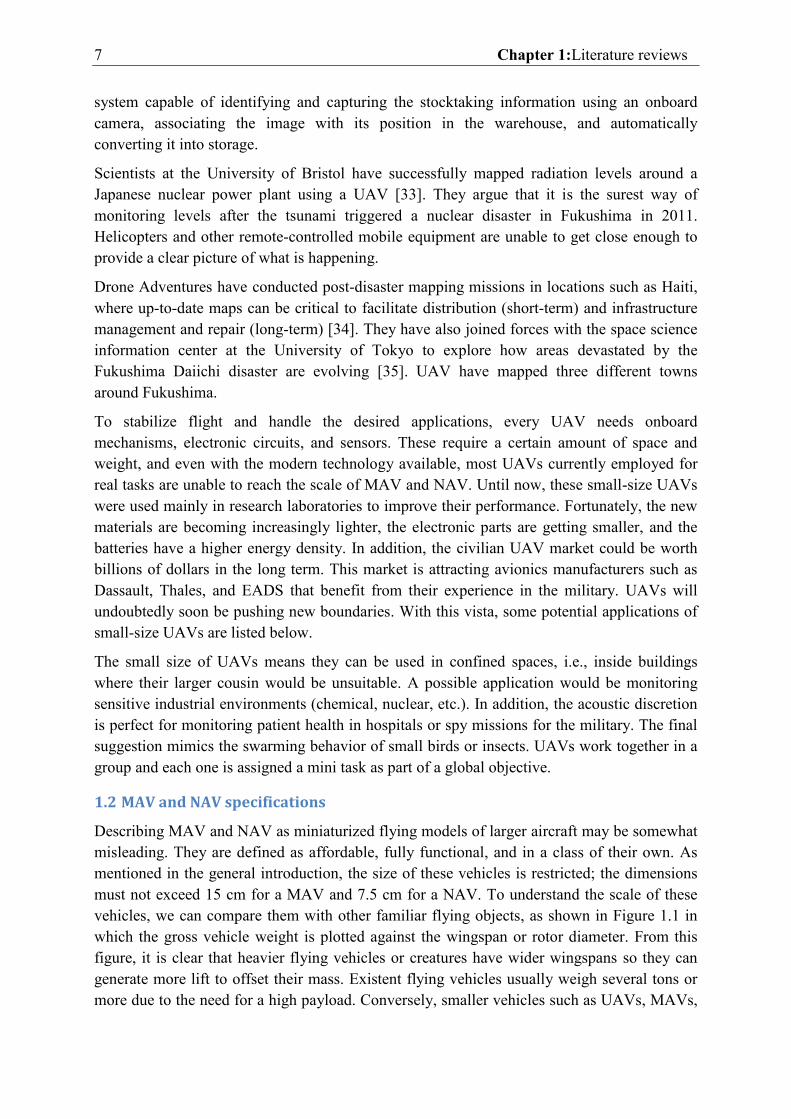
Describing MAV and NAV as miniaturized flying models of larger aircraft may be somewhat misleading. They are defined as affordable, fully functional, and in a class of their own. As mentioned in the general introduction, the size of these vehicles is restricted; the dimensions must not exceed 15 cm for a MAV and 7.5 cm for a NAV. To understand the scale of these vehicles, we can compare them with other familiar flying objects, as shown in Figure 1.1 in which the gross vehicle weight is plotted against the wingspan or rotor diameter. From this figure, it is clear that heavier flying vehicles or creatures have wider wingspans so they can generate more lift to offset their mass. Existent flying vehicles usually weigh several tons or more due to the need for a high payload. Conversely, smaller vehicles such as UAVs, MAVs,
1.3 Classification of MAVs and NAVs 8
and NAVs are commonly used for data collection and so the payload is not a key criterion. The lower bounds of weight and wingspan of man-made vehicles are nowadays limited by technology. The DelFly Micro [36] (3 g, 10-cm wingspan) is considered the world's smallest autonomous MAV while the Robobee [37] (80 mg, 3.5-cm wingspan) is the world‟s smallest NAV that can hover. Without even considering the duration of flight, this small size is nowhere near that of natural flyers such as flies or mosquitoes. The nano devices we are currently able to fabricate cannot rival natural flyers such as insects. As can be seen in Figure 1.1, MAVs are on the same scale as the largest insects and the smallest birds, and NAVs can be any smaller and lighter vehicles.
These small-size flyers have high surface-to-volume ratios and the mass is highly constrained by the volume and inversely. Consequently, much work has been undertaken on propulsion and navigation systems, flight controllers, electronics, and onboard payloads to develop miniaturized structures. These micro-drones now benefit from the latest technology. Another issue resulting from their tiny size is the extreme reduction in Reynolds number (Re), which drastically shifts the aerodynamic behavior. Fortunately, nature has already provided designers with the answer. As MAV and NAV are of a similar size to birds and insects, the flapping-wing concept is more suitable for MAV and NAV than the more traditional fixed- and rotary-wing concepts [4].
Figure 1.1: MAV and NAV flight range compared to existing flying vehicles and species [38]
1.3 Classification of MAVs and NAVs
Existing MAVs and NAVs can be divided into three main categories based on the way they create lift: fixed-wing, rotary-wing, and flapping-wing, and are described in the following paragraphs.
NAV Design space
9 Chapter 1:Literature reviews
1.3.1 Fixed-wing
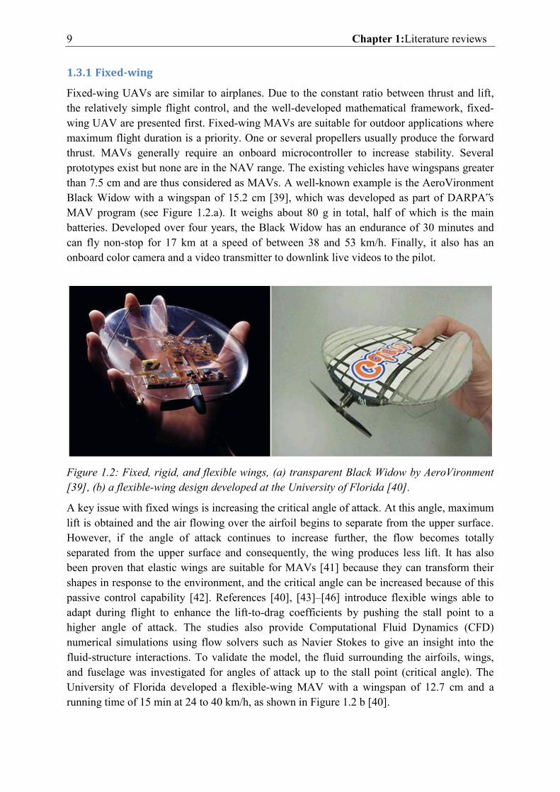
Fixed-wing UAVs are similar to airplanes. Due to the constant ratio between thrust and lift, the relatively simple flight control, and the well-developed mathematical framework, fixed-wing UAV are presented first. Fixed-wing MAVs are suitable for outdoor applications where maximum flight duration is a priority. One or several propellers usually produce the forward thrust. MAVs generally require an onboard microcontroller to increase stability. Several prototypes exist but none are in the NAV range. The existing vehicles have wingspans greater than 7.5 cm and are thus considered as MAVs. A well-known example is the AeroVironment Black Widow with a wingspan of 15.2 cm [39], which was developed as part of DARPA‟s MAV program (see Figure 1.2.a). It weighs about 80 g in total, half of which is the main batteries. Developed over four years, the Black Widow has an endurance of 30 minutes and can fly non-stop for 17 km at a speed of between 38 and 53 km/h. Finally, it also has an onboard color camera and a video transmitter to downlink live videos to the pilot.
Figure 1.2: Fixed, rigid, and flexible wings, (a) transparent Black Widow by AeroVironment [39], (b) a flexible-wing design developed at the University of Florida [40].
A key issue with fixed wings is increasing the critical angle of attack. At this angle, maximum lift is obtained and the air flowing over the airfoil begins to separate from the upper surface. However, if the angle of attack continues to increase further, the flow becomes totally separated from the upper surface and consequently, the wing produces less lift. It has also been proven that elastic wings are suitable for MAVs [41] because they can transform their shapes in response to the environment, and the critical angle can be increased because of this passive control capability [42]. References [40], [43]–[46] introduce flexible wings able to adapt during flight to enhance the lift-to-drag coefficients by pushing the stall point to a higher angle of attack. The studies also provide Computational Fluid Dynamics (CFD) numerical simulations using flow solvers such as Navier Stokes to give an insight into the fluid-structure interactions. To validate the model, the fluid surrounding the airfoils, wings, and fuselage was investigated for angles of attack up to the stall point (critical angle). The University of Florida developed a flexible-wing MAV with a wingspan of 12.7 cm and a running time of 15 min at 24 to 40 km/h, as shown in Figure 1.2 b [40].
1.3 Classification of MAVs and NAVs 10
According to DARPA, fixed-wing vehicles are the best with regard to size and weight [47]. However, their wings need to keep moving forward to generate lift and the vehicles cannot hover and maneuver in tight spaces. Consequently, they are not suitable for our goal defined in the General Introduction. The wing type presented in the next section may be the solution for a more maneuverable MAV.
1.3.2 Rotary-wing
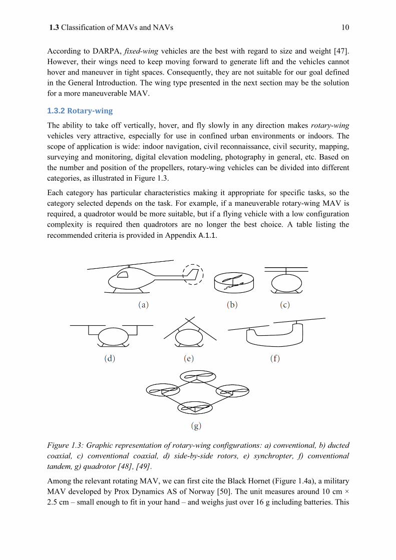
The ability to take off vertically, hover, and fly slowly in any direction makes rotary-wing vehicles very attractive, especially for use in confined urban environments or indoors. The scope of application is wide: indoor navigation, civil reconnaissance, civil security, mapping, surveying and monitoring, digital elevation modeling, photography in general, etc. Based on the number and position of the propellers, rotary-wing vehicles can be divided into different categories, as illustrated in Figure 1.3.
Each category has particular characteristics making it appropriate for specific tasks, so the category selected depends on the task. For example, if a maneuverable rotary-wing MAV is required, a quadrotor would be more suitable, but if a flying vehicle with a low configuration complexity is required then quadrotors are no longer the best choice. A table listing the recommended criteria is provided in Appendix A.1.1.
Figure 1.3: Graphic representation of rotary-wing configurations: a) conventional, b) ducted coaxial, c) conventional coaxial, d) side-by-side rotors, e) synchropter, f) conventional tandem, g) quadrotor [48], [49].
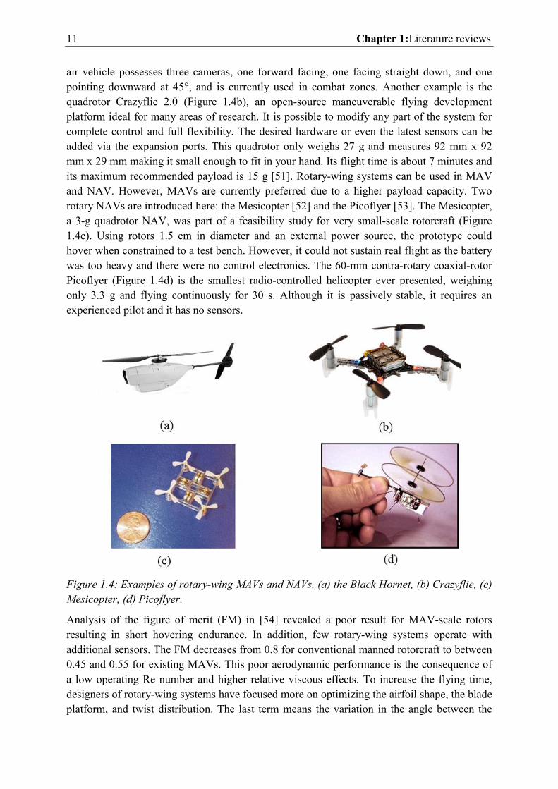
Among the relevant rotating MAV, we can first cite the Black Hornet (Figure 1.4a), a military MAV developed by Prox Dynamics AS of Norway [50]. The unit measures around 10 cm × 2.5 cm – small enough to fit in your hand – and weighs just over 16 g including batteries. This
11 Chapter 1:Literature reviews
air vehicle possesses three cameras, one forward facing, one facing straight down, and one pointing downward at 45°, and is currently used in combat zones. Another example is the quadrotor Crazyflie 2.0 (Figure 1.4b), an open-source maneuverable flying development platform ideal for many areas of research. It is possible to modify any part of the system for complete control and full flexibility. The desired hardware or even the latest sensors can be added via the expansion ports. This quadrotor only weighs 27 g and measures 92 mm x 92 mm x 29 mm making it small enough to fit in your hand. Its flight time is about 7 minutes and its maximum recommended payload is 15 g [51]. Rotary-wing systems can be used in MAV and NAV. However, MAVs are currently preferred due to a higher payload capacity. Two rotary NAVs are introduced here: the Mesicopter [52] and the Picoflyer [53]. The Mesicopter, a 3-g quadrotor NAV, was part of a feasibility study for very small-scale rotorcraft (Figure 1.4c). Using rotors 1.5 cm in diameter and an external power source, the prototype could hover when constrained to a test bench. However, it could not sustain real flight as the battery was too heavy and there were no control electronics. The 60-mm contra-rotary coaxial-rotor Picoflyer (Figure 1.4d) is the smallest radio-controlled helicopter ever presented, weighing only 3.3 g and flying continuously for 30 s. Although it is passively stable, it requires an experienced pilot and it has no sensors.
Figure 1.4: Examples of rotary-wing MAVs and NAVs, (a) the Black Hornet, (b) Crazyflie, (c) Mesicopter, (d) Picoflyer.
Analysis of the figure of merit (FM) in [54] revealed a poor result for MAV-scale rotors resulting in short hovering endurance. In addition, few rotary-wing systems operate with additional sensors. The FM decreases from 0.8 for conventional manned rotorcraft to between 0.45 and 0.55 for existing MAVs. This poor aerodynamic performance is the consequence of a low operating Re number and higher relative viscous effects. To increase the flying time, designers of rotary-wing systems have focused more on optimizing the airfoil shape, the blade platform, and twist distribution. The last term means the variation in the angle between the
1.3 Classification of MAVs and NAVs 12
profile chord of the blade tip and the profile chord of the blade root [55]. Last but not least, the noise due to the single actuation frequency of the propellers or rotors cannot be neglected.
In conclusion, both fixed and rotary wings have been studied for many years. However, they all have problems linked to the reduction in vehicle size and Re number. This has motivated researchers to investigate flapping wings.
1.3.3 Flapping-wing
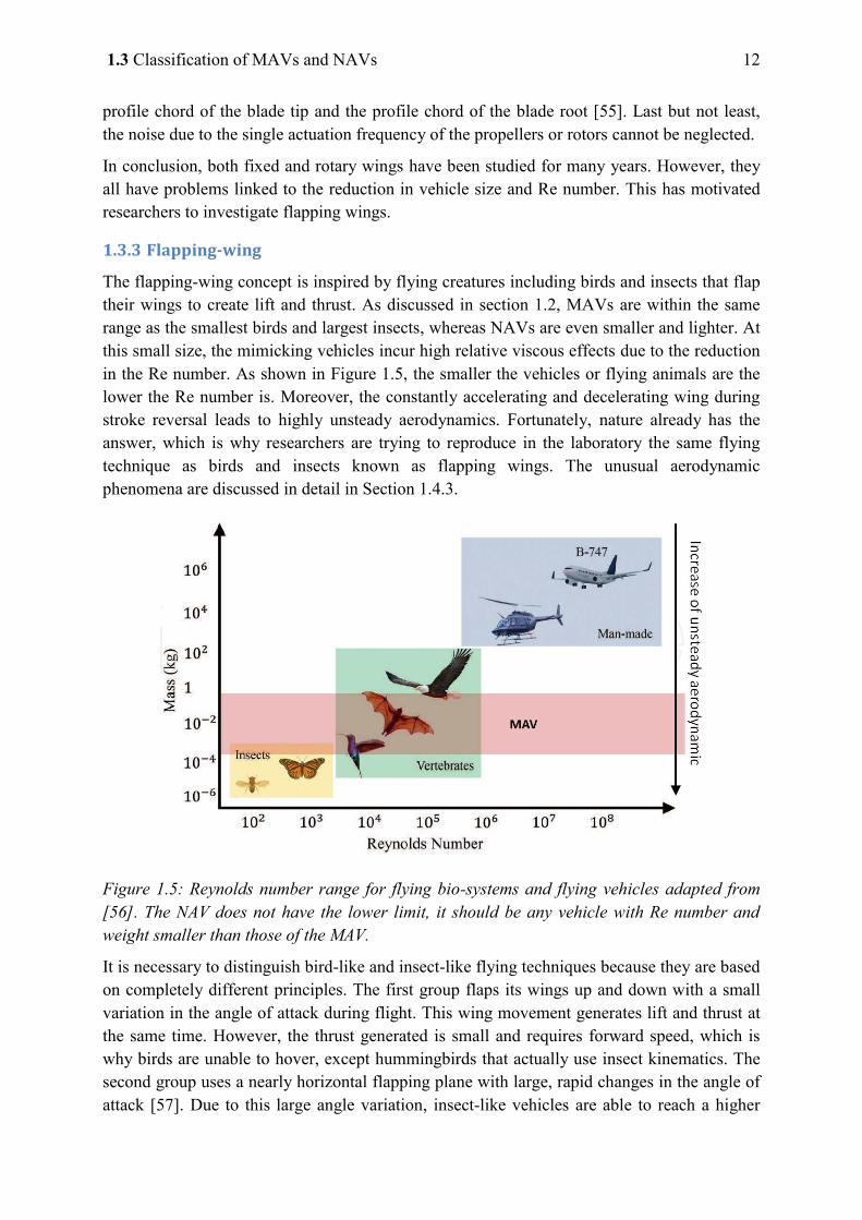
The flapping-wing concept is inspired by flying creatures including birds and insects that flap their wings to create lift and thrust. As discussed in section 1.2, MAVs are within the same range as the smallest birds and largest insects, whereas NAVs are even smaller and lighter. At this small size, the mimicking vehicles incur high relative viscous effects due to the reduction in the Re number. As shown in Figure 1.5, the smaller the vehicles or flying animals are the lower the Re number is. Moreover, the constantly accelerating and decelerating wing during stroke reversal leads to highly unsteady aerodynamics. Fortunately, nature already has the answer, which is why researchers are trying to reproduce in the laboratory the same flying technique as birds and insects known as flapping wings. The unusual aerodynamic phenomena are discussed in detail in Section 1.4.3.
Figure 1.5: Reynolds number range for flying bio-systems and flying vehicles adapted from [56]. The NAV does not have the lower limit, it should be any vehicle with Re number and weight smaller than those of the MAV.
It is necessary to distinguish bird-like and insect-like flying techniques because they are based on completely different principles. The first group flaps its wings up and down with a small variation in the angle of attack during flight. This wing movement generates lift and thrust at the same time. However, the thrust generated is small and requires forward speed, which is why birds are unable to hover, except hummingbirds that actually use insect kinematics. The second group uses a nearly horizontal flapping plane with large, rapid changes in the angle of attack [57]. Due to this large angle variation, insect-like vehicles are able to reach a higher
13 Chapter 1:Literature reviews
lift-to-weight ratio compared to the bird-like group and are thus able to take off and land vertically as well as hover. In addition, together with the incredible skills of hovering, flying backward, and recovering after impacts, insects also exhibit quite long flight times without having to consume more energy. However, the performances of existing flapping-wing MAV and NAV designs are worse than those of fixed and rotary-wing designs. Nevertheless, the vista of potentially achieving these incredible flight performances still prompts much active research in this field. Below, we introduce three outstanding existing MAVs and a NAV: the bird-like vehicle Microbat and the insect-like vehicles DelFly, AV Hummingbird and Robobee.
One of the first bird-like flapping-wing MAV developed was Microbat by AeroVironment. The 23-cm span Microbat weighs 12.5 g and has an endurance of 42 s [58]. However, the main drawback of the wing kinematics is that this vehicle is incapable of hovering.
Another, more relevant solution is the DelFly. It is a fully controllable insect-like MAV developed in the Micro Air Vehicle Lab at Delft University of Technology [36], [59], [60]. Its micro version is currently accepted as the smallest free-flying controllable flapping-wing MAV equipped with a camera and video transmitter. With a 10-cm wingspan and weighing 3.07 g, it can fly for around 3 min. A second version has also been proposed. It is the 28-cm 16-g DelFly II, which can take off and land vertically. Its flying endurance is about 15 min.
The third solution is the 16-cm span, 19-g insect-like Nano Hummingbird developed by AeroVironment, Inc. This tailless remote-controlled MAV was built to mimic a hummingbird. Its design makes it closer to a real flying hummingbird but results in a passively unstable attitude and so a more advanced control system is required to stabilize the vehicle. This vehicle is also equipped with a small video camera for surveillance and reconnaissance purposes and, for now, operates for up to 11 min at 18 km/h. Another feature is that it can fly indoors or outdoors.
Inspired by the biology of a bee, researchers at Harvard University have developed RoboBee. This flying robot is about half the size of a paper clip, weighs less than one-tenth of a gram, and is powered using piezoelectric actuators that act as artificial muscles. In the most advanced stage, additional modifications allow some RoboBee models to transition from swimming underwater to flying, as well as “perching” on surfaces using static electricity [61].
To sum up the examples, the flying time of several existing MAVs (data 2014) is plotted against the weight in Figure 1.6. Violet, blue, and red have been chosen to symbolize fixed, rotary, and flapping-wing vehicles, respectively. It is clear that the endurance of fixed-wing MAVs such as the Micro Start and Black Widow is longer than the other wing types. However, the inability to hover and the higher mass make them less interesting for our research. Rotary-wing MAVs such as Crazyflie and Lady Bird can hover as well as take off and land vertically. Moreover, they are maneuverable and suitable for indoor applications. However, their endurance is short and drastically decreases when they reach NAV dimensions, as in the case of the Picoflyer. Small-scale flapping wings perform better than fixed and rotary-wing vehicles. The Delfly II can fly 8 minutes longer than the Crazyflie, which is nearly the same weight, and almost 9 minutes longer than the Lady Bird, which is double its weight. However, it is not always true that any small flapping-wing vehicle
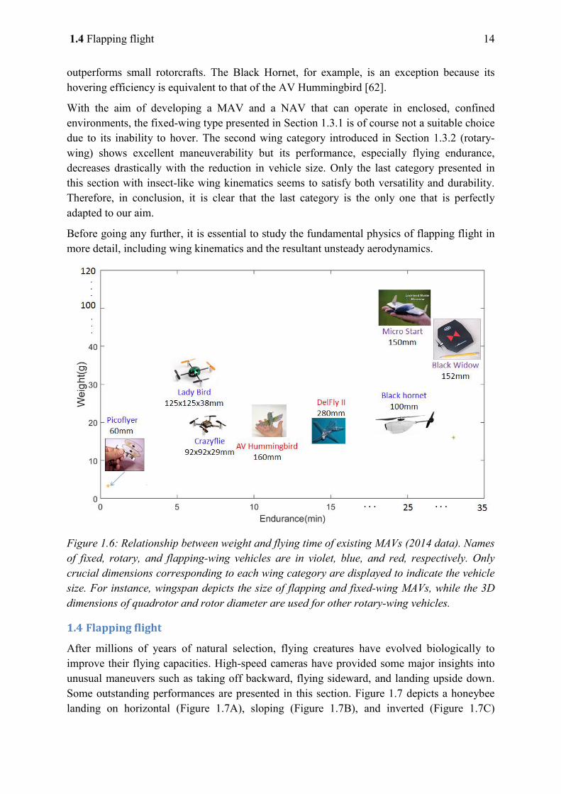
1.4 Flapping flight 14
outperforms small rotorcrafts. The Black Hornet, for example, is an exception because its hovering efficiency is equivalent to that of the AV Hummingbird [62].
With the aim of developing a MAV and a NAV that can operate in enclosed, confined environments, the fixed-wing type presented in Section 1.3.1 is of course not a suitable choice due to its inability to hover. The second wing category introduced in Section 1.3.2 (rotary-wing) shows excellent maneuverability but its performance, especially flying endurance, decreases drastically with the reduction in vehicle size. Only the last category presented in this section with insect-like wing kinematics seems to satisfy both versatility and durability. Therefore, in conclusion, it is clear that the last category is the only one that is perfectly adapted to our aim.
Before going any further, it is essential to study the fundamental physics of flapping flight in more detail, including wing kinematics and the resultant unsteady aerodynamics.
Figure 1.6: Relationship between weight and flying time of existing MAVs (2014 data). Names of fixed, rotary, and flapping-wing vehicles are in violet, blue, and red, respectively. Only crucial dimensions corresponding to each wing category are displayed to indicate the vehicle size. For instance, wingspan depicts the size of flapping and fixed-wing MAVs, while the 3D dimensions of quadrotor and rotor diameter are used for other rotary-wing vehicles.
1.4 Flapping flight
After millions of years of natural selection, flying creatures have evolved biologically to improve their flying capacities. High-speed cameras have provided some major insights into unusual maneuvers such as taking off backward, flying sideward, and landing upside down. Some outstanding performances are presented in this section. Figure 1.7 depicts a honeybee landing on horizontal (Figure 1.7A), sloping (Figure 1.7B), and inverted (Figure 1.7C)
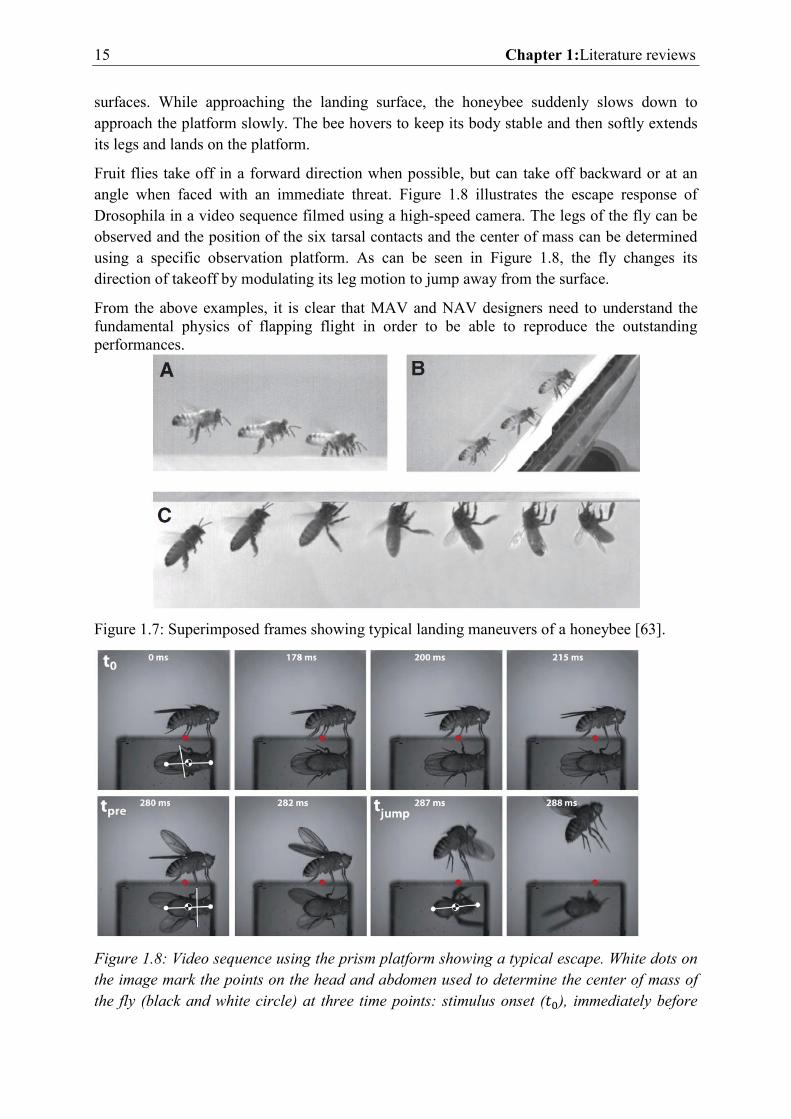
15 Chapter 1:Literature reviews
surfaces. While approaching the landing surface, the honeybee suddenly slows down to approach the platform slowly. The bee hovers to keep its body stable and then softly extends its legs and lands on the platform.
Fruit flies take off in a forward direction when possible, but can take off backward or at an angle when faced with an immediate threat. Figure 1.8 illustrates the escape response of Drosophila in a video sequence filmed using a high-speed camera. The legs of the fly can be observed and the position of the six tarsal contacts and the center of mass can be determined using a specific observation platform. As can be seen in Figure 1.8, the fly changes its direction of takeoff by modulating its leg motion to jump away from the surface.
From the above examples, it is clear that MAV and NAV designers need to understand the fundamental physics of flapping flight in order to be able to reproduce the outstanding performances.
Figure 1.7: Superimposed frames showing typical landing maneuvers of a honeybee [63].
Figure 1.8: Video sequence using the prism platform showing a typical escape. White dots on the image mark the points on the head and abdomen used to determine the center of mass of the fly (black and white circle) at three time points: stimulus onset ( ), immediately before
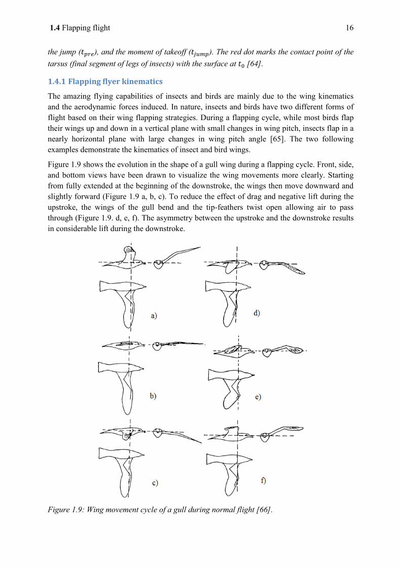
1.4 Flapping flight 16
the jump ( ), and the moment of takeoff ( ). The red dot marks the contact point of the tarsus (final segment of legs of insects) with the surface at [64].
1.4.1 Flapping flyer kinematics
The amazing flying capabilities of insects and birds are mainly due to the wing kinematics and the aerodynamic forces induced. In nature, insects and birds have two different forms of flight based on their wing flapping strategies. During a flapping cycle, while most birds flap their wings up and down in a vertical plane with small changes in wing pitch, insects flap in a nearly horizontal plane with large changes in wing pitch angle [65]. The two following examples demonstrate the kinematics of insect and bird wings.
Figure 1.9 shows the evolution in the shape of a gull wing during a flapping cycle. Front, side, and bottom views have been drawn to visualize the wing movements more clearly. Starting from fully extended at the beginning of the downstroke, the wings then move downward and slightly forward (Figure 1.9 a, b, c). To reduce the effect of drag and negative lift during the upstroke, the wings of the gull bend and the tip-feathers twist open allowing air to pass through (Figure 1.9. d, e, f). The asymmetry between the upstroke and the downstroke results in considerable lift during the downstroke.
Figure 1.9: Wing movement cycle of a gull during normal flight [66].
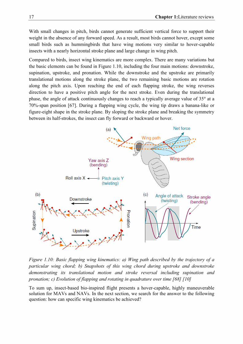
17 Chapter 1:Literature reviews
With small changes in pitch, birds cannot generate sufficient vertical force to support their weight in the absence of any forward speed. As a result, most birds cannot hover, except some small birds such as hummingbirds that have wing motions very similar to hover-capable insects with a nearly horizontal stroke plane and large change in wing pitch.
Compared to birds, insect wing kinematics are more complex. There are many variations but the basic elements can be found in Figure 1.10, including the four main motions: downstroke, supination, upstroke, and pronation. While the downstroke and the upstroke are primarily translational motions along the stroke plane, the two remaining basic motions are rotation along the pitch axis. Upon reaching the end of each flapping stroke, the wing reverses direction to have a positive pitch angle for the next stroke. Even during the translational phase, the angle of attack continuously changes to reach a typically average value of 35 at a 70%-span position [67]. During a flapping wing cycle, the wing tip draws a banana-like or figure-eight shape in the stroke plane. By sloping the stroke plane and breaking the symmetry between its half-strokes, the insect can fly forward or backward or hover.
Figure 1.10: Basic flapping wing kinematics: a) Wing path described by the trajectory of a particular wing chord; b) Snapshots of this wing chord during upstroke and downstroke demonstrating its translational motion and stroke reversal including supination and pronation; c) Evolution of flapping and rotating in quadrature over time [68] [10]
To sum up, insect-based bio-inspired flight presents a hover-capable, highly maneuverable solution for MAVs and NAVs. In the next section, we search for the answer to the following question: how can specific wing kinematics be achieved?
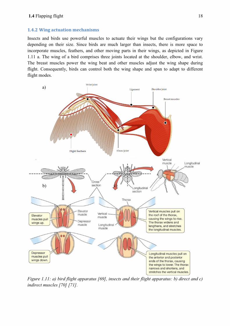
1.4 Flapping flight 18
1.4.2 Wing actuation mechanisms
Insects and birds use powerful muscles to actuate their wings but the configurations vary depending on their size. Since birds are much larger than insects, there is more space to incorporate muscles, feathers, and other moving parts in their wings, as depicted in Figure 1.11 a. The wing of a bird comprises three joints located at the shoulder, elbow, and wrist. The breast muscles power the wing beat and other muscles adjust the wing shape during flight. Consequently, birds can control both the wing shape and span to adapt to different flight modes.
Figure 1.11: a) bird flight apparatus [69], insects and their flight apparatus: b) direct and c) indirect muscles [70] [71].
a)
b) c)
19 Chapter 1:Literature reviews
Conversely, insect wings are relatively simple with only a membrane and veins, and the wing shape remains almost unchanged during the stroke. The originality, however, arises from the way in which the flight muscles are connected to the wings. In nature, the flapping motion is generated in two ways [70]. The first comprises insects using muscles that directly drive the wings, as shown in Figure 1.11 b). This is typical of four-wing insects such as dragonflies and damselflies. The simplicity of direct drive enables agile flight but limits the flapping frequency. The second group uses indirect flight muscles [72], which are found in more advanced insects such as bees or flies, as shown in Figure 1.11 c). With this configuration, the flight muscles coupled with the thorax act as a resonant structure. The insects can, therefore, flap at much higher frequencies, with greater amplitudes, and the wings are always synchronized.
The wing kinematics and their actuation mechanisms are discussed in Section 1.4.1 and in this section. Next, the basic and advanced aerodynamic concepts of a flapping-wing flyer are considered.
1.4.3 Unsteady mechanisms in flapping flight
Although a traditional steady state approach has been successfully applied to explain bird flight, it usually underestimates the capacity of insects to generate lift. In simulations, some of the flying insects even failed to take off [73]. This discrepancy can be explained, as the traditional theory does not consider the lift enhancement mechanisms arising from the size reduction of flying creatures. To understand this phenomenon better, a dimensionless factor named Reynolds number (Re) is introduced [6]:
Re
(1.1)
where is the fluid density, is the velocity of the fluid relative to the moving object, is a characteristic length, and is the dynamic viscosity of the fluid medium. From this equation, it is clear that bigger flying creatures (higher and ) operate at a higher Re number. Consequently, the inertial effect is dominant and the viscous effect can be neglected. Conversely, since both size and speed are reduced, the viscous effect becomes more important with small creatures (lower Re number). Therefore, the corresponding unsteady aerodynamics caused by the interaction between the wing movement and the surrounding viscous fluid must be considered. Although sophisticated, the unsteady aerodynamics conceal the relevant lift enhancement mechanisms for small flyers such as clap-and-fling, delayed stall, and wing–wake interactions. To understand the production of these mechanisms, more powerful concepts must be introduced including circulation and vorticity. While vorticity depicts the rotation of a fluid element at a specific point, circulation is the sum of the vorticity around the wing within a flow field. Furthermore, viscosity is necessary to generate lift [74] since the effects of viscosity lead to the formation of the vortex, which is responsible for producing the right conditions for lift.
Given the problems with investigating real insects first-hand, mechanical models have been employed to study insect wing kinematics. To conserve the underlying fluid dynamics phenomena, it is necessary to match the Reynolds number and reduced frequency parameters (body velocity/wing velocity) of the model with those of an insect. With the help of flow
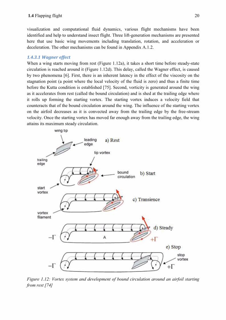
1.4 Flapping flight 20
visualization and computational fluid dynamics, various flight mechanisms have been identified and help to understand insect flight. Three lift-generation mechanisms are presented here that use basic wing movements including translation, rotation, and acceleration or deceleration. The other mechanisms can be found in Appendix A.1.2.
1.4.3.1 Wagner effect
When a wing starts moving from rest (Figure 1.12a), it takes a short time before steady-state circulation is reached around it (Figure 1.12d). This delay, called the Wagner effect, is caused by two phenomena [6]. First, there is an inherent latency in the effect of the viscosity on the stagnation point (a point where the local velocity of the fluid is zero) and thus a finite time before the Kutta condition is established [75]. Second, vorticity is generated around the wing as it accelerates from rest (called the bound circulation) and is shed at the trailing edge where it rolls up forming the starting vortex. The starting vortex induces a velocity field that counteracts that of the bound circulation around the wing. The influence of the starting vortex on the airfoil decreases as it is convected away from the trailing edge by the free-stream velocity. Once the starting vortex has moved far enough away from the trailing edge, the wing attains its maximum steady circulation.
Figure 1.12: Vortex system and development of bound circulation around an airfoil starting from rest [74]
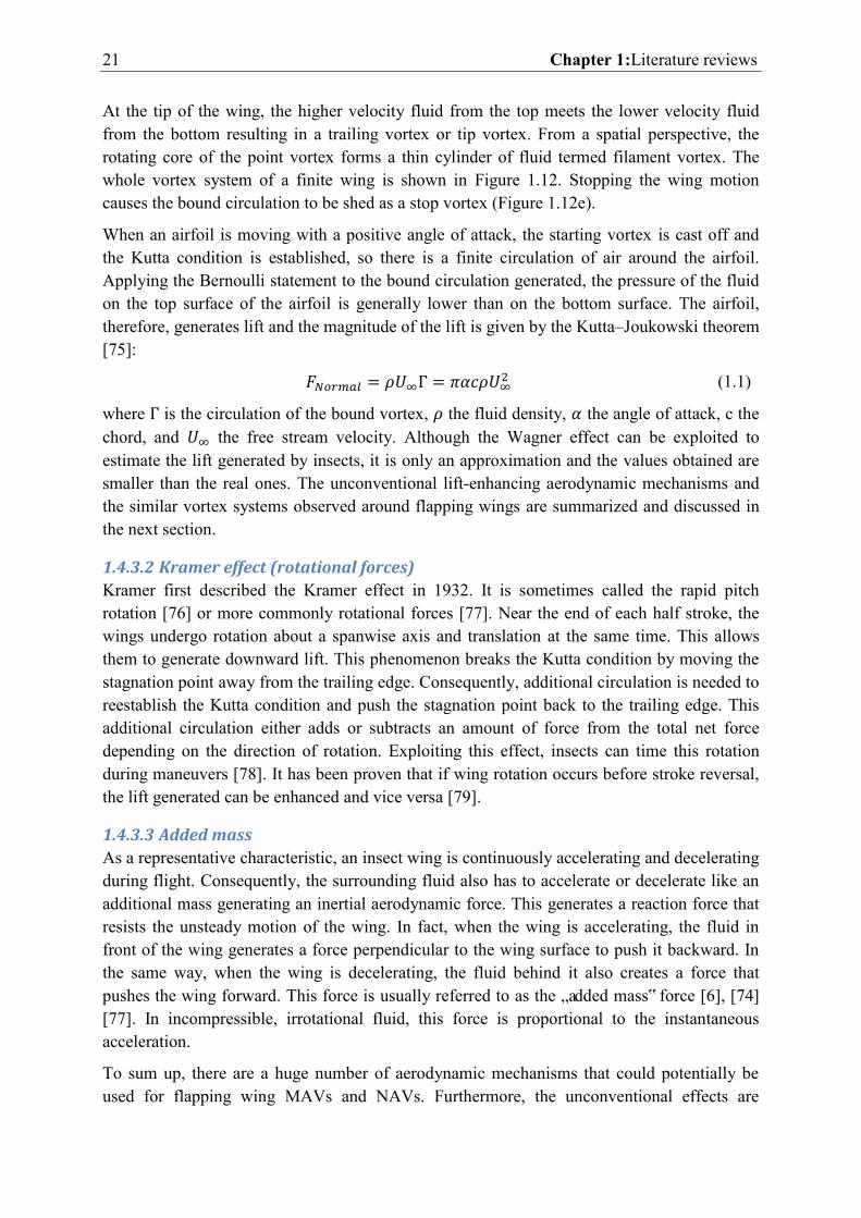
21 Chapter 1:Literature reviews
At the tip of the wing, the higher velocity fluid from the top meets the lower velocity fluid from the bottom resulting in a trailing vortex or tip vortex. From a spatial perspective, the rotating core of the point vortex forms a thin cylinder of fluid termed filament vortex. The whole vortex system of a finite wing is shown in Figure 1.12. Stopping the wing motion causes the bound circulation to be shed as a stop vortex (Figure 1.12e).
When an airfoil is moving with a positive angle of attack, the starting vortex is cast off and the Kutta condition is established, so there is a finite circulation of air around the airfoil. Applying the Bernoulli statement to the bound circulation generated, the pressure of the fluid on the top surface of the airfoil is generally lower than on the bottom surface. The airfoil, therefore, generates lift and the magnitude of the lift is given by the Kutta–Joukowski theorem [75]:
(1.1)
where is the circulation of the bound vortex, the fluid density, the angle of attack, c the chord, and the free stream velocity. Although the Wagner effect can be exploited to estimate the lift generated by insects, it is only an approximation and the values obtained are smaller than the real ones. The unconventional lift-enhancing aerodynamic mechanisms and the similar vortex systems observed around flapping wings are summarized and discussed in the next section.
1.4.3.2 Kramer effect (rotational forces)
Kramer first described the Kramer effect in 1932. It is sometimes called the rapid pitch rotation [76] or more commonly rotational forces [77]. Near the end of each half stroke, the wings undergo rotation about a spanwise axis and translation at the same time. This allows them to generate downward lift. This phenomenon breaks the Kutta condition by moving the stagnation point away from the trailing edge. Consequently, additional circulation is needed to reestablish the Kutta condition and push the stagnation point back to the trailing edge. This additional circulation either adds or subtracts an amount of force from the total net force depending on the direction of rotation. Exploiting this effect, insects can time this rotation during maneuvers [78]. It has been proven that if wing rotation occurs before stroke reversal, the lift generated can be enhanced and vice versa [79].
1.4.3.3 Added mass
As a representative characteristic, an insect wing is continuously accelerating and decelerating during flight. Consequently, the surrounding fluid also has to accelerate or decelerate like an additional mass generating an inertial aerodynamic force. This generates a reaction force that resists the unsteady motion of the wing. In fact, when the wing is accelerating, the fluid in front of the wing generates a force perpendicular to the wing surface to push it backward. In the same way, when the wing is decelerating, the fluid behind it also creates a force that pushes the wing forward. This force is usually referred to as the „added mass‟ force [6], [74] [77]. In incompressible, irrotational fluid, this force is proportional to the instantaneous acceleration.
To sum up, there are a huge number of aerodynamic mechanisms that could potentially be used for flapping wing MAVs and NAVs. Furthermore, the unconventional effects are
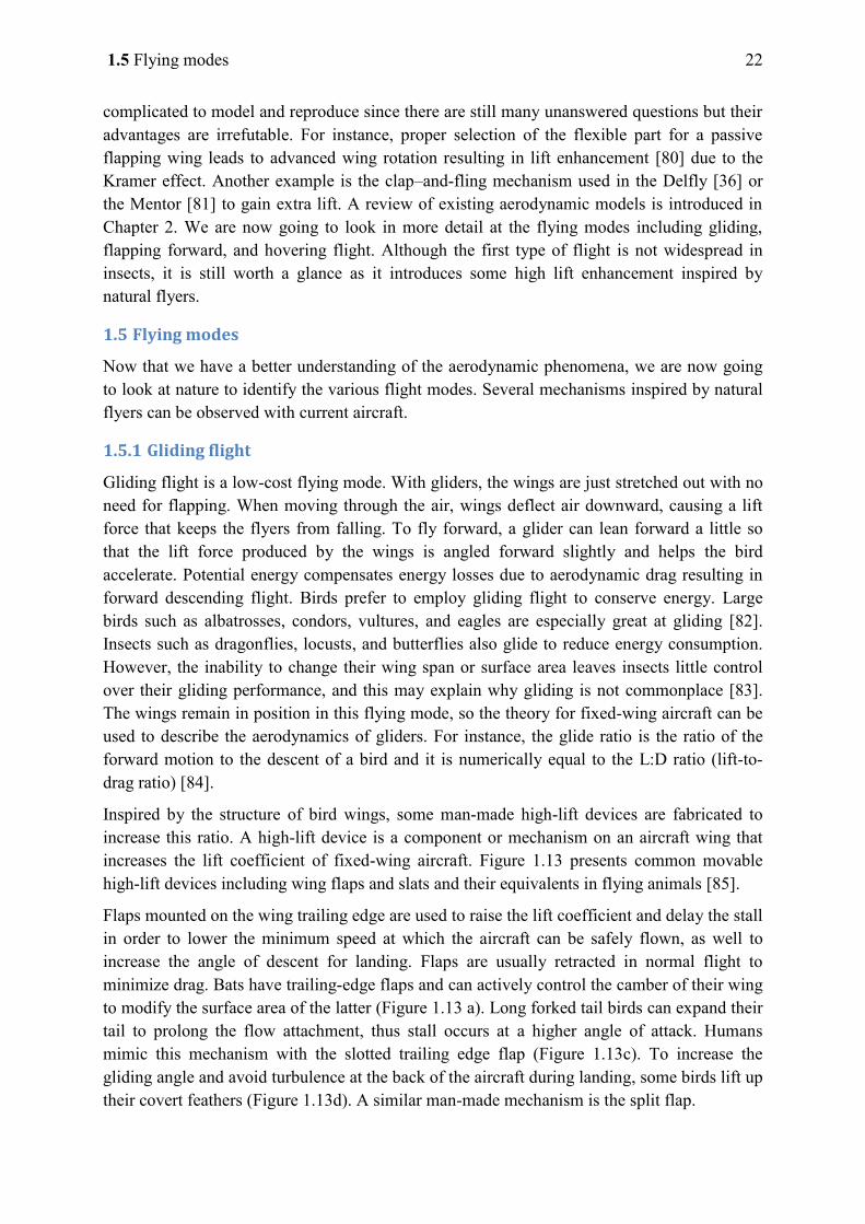
1.5 Flying modes 22
complicated to model and reproduce since there are still many unanswered questions but their advantages are irrefutable. For instance, proper selection of the flexible part for a passive flapping wing leads to advanced wing rotation resulting in lift enhancement [80] due to the Kramer effect. Another example is the clap–and-fling mechanism used in the Delfly [36] or the Mentor [81] to gain extra lift. A review of existing aerodynamic models is introduced in Chapter 2. We are now going to look in more detail at the flying modes including gliding, flapping forward, and hovering flight. Although the first type of flight is not widespread in insects, it is still worth a glance as it introduces some high lift enhancement inspired by natural flyers.
1.5 Flying modes
Now that we have a better understanding of the aerodynamic phenomena, we are now going to look at nature to identify the various flight modes. Several mechanisms inspired by natural flyers can be observed with current aircraft.
1.5.1 Gliding flight
Gliding flight is a low-cost flying mode. With gliders, the wings are just stretched out with no need for flapping. When moving through the air, wings deflect air downward, causing a lift force that keeps the flyers from falling. To fly forward, a glider can lean forward a little so that the lift force produced by the wings is angled forward slightly and helps the bird accelerate. Potential energy compensates energy losses due to aerodynamic drag resulting in forward descending flight. Birds prefer to employ gliding flight to conserve energy. Large birds such as albatrosses, condors, vultures, and eagles are especially great at gliding [82]. Insects such as dragonflies, locusts, and butterflies also glide to reduce energy consumption. However, the inability to change their wing span or surface area leaves insects little control over their gliding performance, and this may explain why gliding is not commonplace [83]. The wings remain in position in this flying mode, so the theory for fixed-wing aircraft can be used to describe the aerodynamics of gliders. For instance, the glide ratio is the ratio of the forward motion to the descent of a bird and it is numerically equal to the L:D ratio (lift-to-drag ratio) [84].
Inspired by the structure of bird wings, some man-made high-lift devices are fabricated to increase this ratio. A high-lift device is a component or mechanism on an aircraft wing that increases the lift coefficient of fixed-wing aircraft. Figure 1.13 presents common movable high-lift devices including wing flaps and slats and their equivalents in flying animals [85].
Flaps mounted on the wing trailing edge are used to raise the lift coefficient and delay the stall in order to lower the minimum speed at which the aircraft can be safely flown, as well to increase the angle of descent for landing. Flaps are usually retracted in normal flight to minimize drag. Bats have trailing-edge flaps and can actively control the camber of their wing to modify the surface area of the latter (Figure 1.13 a). Long forked tail birds can expand their tail to prolong the flow attachment, thus stall occurs at a higher angle of attack. Humans mimic this mechanism with the slotted trailing edge flap (Figure 1.13c). To increase the gliding angle and avoid turbulence at the back of the aircraft during landing, some birds lift up their covert feathers (Figure 1.13d). A similar man-made mechanism is the split flap.
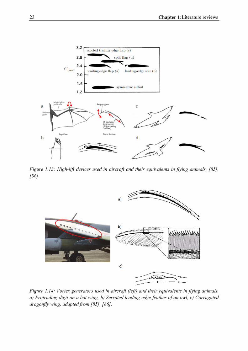
23 Chapter 1:Literature reviews
Figure 1.13: High-lift devices used in aircraft and their equivalents in flying animals, [85], [86].
Figure 1.14: Vortex generators used in aircraft (left) and their equivalents in flying animals, a) Protruding digit on a bat wing, b) Serrated leading-edge feather of an owl, c) Corrugated dragonfly wing, adapted from [85], [86].
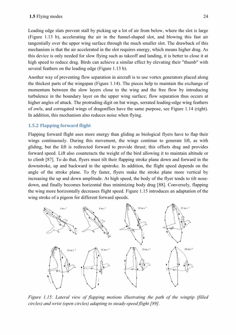
1.5 Flying modes 24
Leading edge slats prevent stall by picking up a lot of air from below, where the slot is large (Figure 1.13 b), accelerating the air in the funnel-shaped slot, and blowing this fast air tangentially over the upper wing surface through the much smaller slot. The drawback of this mechanism is that the air accelerated in the slot requires energy, which means higher drag. As this device is only needed for slow flying such as takeoff and landing, it is better to close it at high speed to reduce drag. Birds can achieve a similar effect by elevating their "thumb" with several feathers on the leading edge (Figure 1.13 b).
Another way of preventing flow separation in aircraft is to use vortex generators placed along the thickest parts of the wingspan (Figure 1.14). The pieces help to maintain the exchange of momentum between the slow layers close to the wing and the free flow by introducing turbulence in the boundary layer on the upper wing surface; flow separation thus occurs at higher angles of attack. The protruding digit on bat wings, serrated leading-edge wing feathers of owls, and corrugated wings of dragonflies have the same purpose, see Figure 1.14 (right). In addition, this mechanism also reduces noise when flying.
1.5.2 Flapping forward flight
Flapping forward flight uses more energy than gliding as biological flyers have to flap their wings continuously. During this movement, the wings continue to generate lift, as with gliding, but the lift is redirected forward to provide thrust; this offsets drag and provides forward speed. Lift also counteracts the weight of the bird allowing it to maintain altitude or to climb [87]. To do that, flyers must tilt their flapping stroke plane down and forward in the downstroke, up and backward in the upstroke. In addition, the flight speed depends on the angle of the stroke plane. To fly faster, flyers make the stroke plane more vertical by increasing the up and down amplitude. At high speed, the body of the flyer tends to tilt nose-down, and finally becomes horizontal thus minimizing body drag [88]. Conversely, flapping the wing more horizontally decreases flight speed. Figure 1.15 introduces an adaptation of the wing stroke of a pigeon for different forward speeds.
Figure 1.15: Lateral view of flapping motions illustrating the path of the wingtip (filled circles) and wrist (open circles) adapting to steady-speed flight [89].
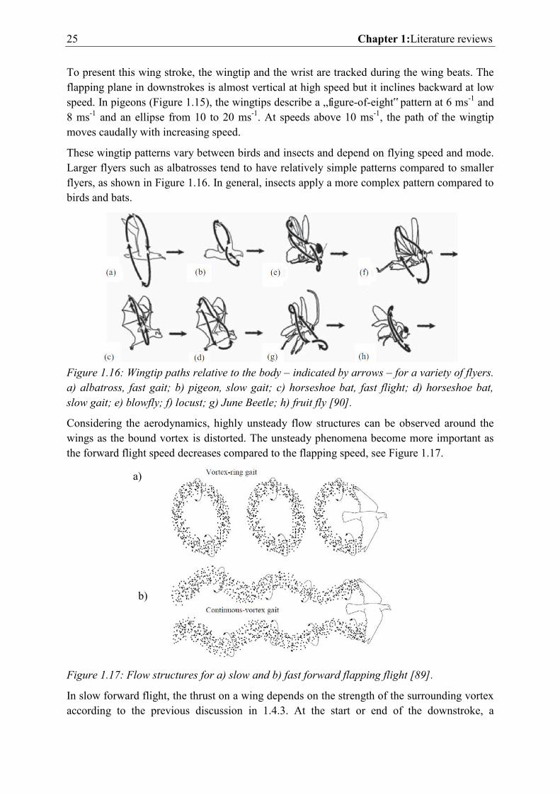
25 Chapter 1:Literature reviews
To present this wing stroke, the wingtip and the wrist are tracked during the wing beats. The flapping plane in downstrokes is almost vertical at high speed but it inclines backward at low speed. In pigeons (Figure 1.15), the wingtips describe a „figure-of-eight‟ pattern at 6 ms-1 and 8 ms-1 and an ellipse from 10 to 20 ms-1. At speeds above 10 ms-1, the path of the wingtip moves caudally with increasing speed.
These wingtip patterns vary between birds and insects and depend on flying speed and mode. Larger flyers such as albatrosses tend to have relatively simple patterns compared to smaller flyers, as shown in Figure 1.16. In general, insects apply a more complex pattern compared to birds and bats.
Figure 1.16: Wingtip paths relative to the body – indicated by arrows – for a variety of flyers. a) albatross, fast gait; b) pigeon, slow gait; c) horseshoe bat, fast flight; d) horseshoe bat, slow gait; e) blowfly; f) locust; g) June Beetle; h) fruit fly [90].
Considering the aerodynamics, highly unsteady flow structures can be observed around the wings as the bound vortex is distorted. The unsteady phenomena become more important as the forward flight speed decreases compared to the flapping speed, see Figure 1.17.
Figure 1.17: Flow structures for a) slow and b) fast forward flapping flight [89].
In slow forward flight, the thrust on a wing depends on the strength of the surrounding vortex according to the previous discussion in 1.4.3. At the start or end of the downstroke, a
a)
b)
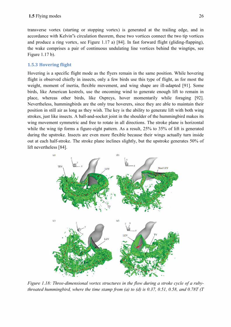
1.5 Flying modes 26
transverse vortex (starting or stopping vortex) is generated at the trailing edge, and in accordance with Kelvin‟s circulation theorem, these two vortices connect the two tip vortices and produce a ring vortex, see Figure 1.17 a) [84]. In fast forward flight (gliding-flapping), the wake comprises a pair of continuous undulating line vortices behind the wingtips, see Figure 1.17 b).
1.5.3 Hovering flight
Hovering is a specific flight mode as the flyers remain in the same position. While hovering flight is observed chiefly in insects, only a few birds use this type of flight, as for most the weight, moment of inertia, flexible movement, and wing shape are ill-adapted [91]. Some birds, like American kestrels, use the oncoming wind to generate enough lift to remain in place, whereas other birds, like Ospreys, hover momentarily while foraging [92]. Nevertheless, hummingbirds are the only true hoverers, since they are able to maintain their position in still air as long as they wish. The key is the ability to generate lift with both wing strokes, just like insects. A ball-and-socket joint in the shoulder of the hummingbird makes its wing movement symmetric and free to rotate in all directions. The stroke plane is horizontal while the wing tip forms a figure-eight pattern. As a result, 25% to 35% of lift is generated during the upstroke. Insects are even more flexible because their wings actually turn inside out at each half-stroke. The stroke plane inclines slightly, but the upstroke generates 50% of lift nevertheless [84].
Figure 1.18: Three-dimensional vortex structures in the flow during a stroke cycle of a ruby-throated hummingbird, where the time stamp from (a) to (d) is 0.37, 0.51, 0.58, and 0.78T (T
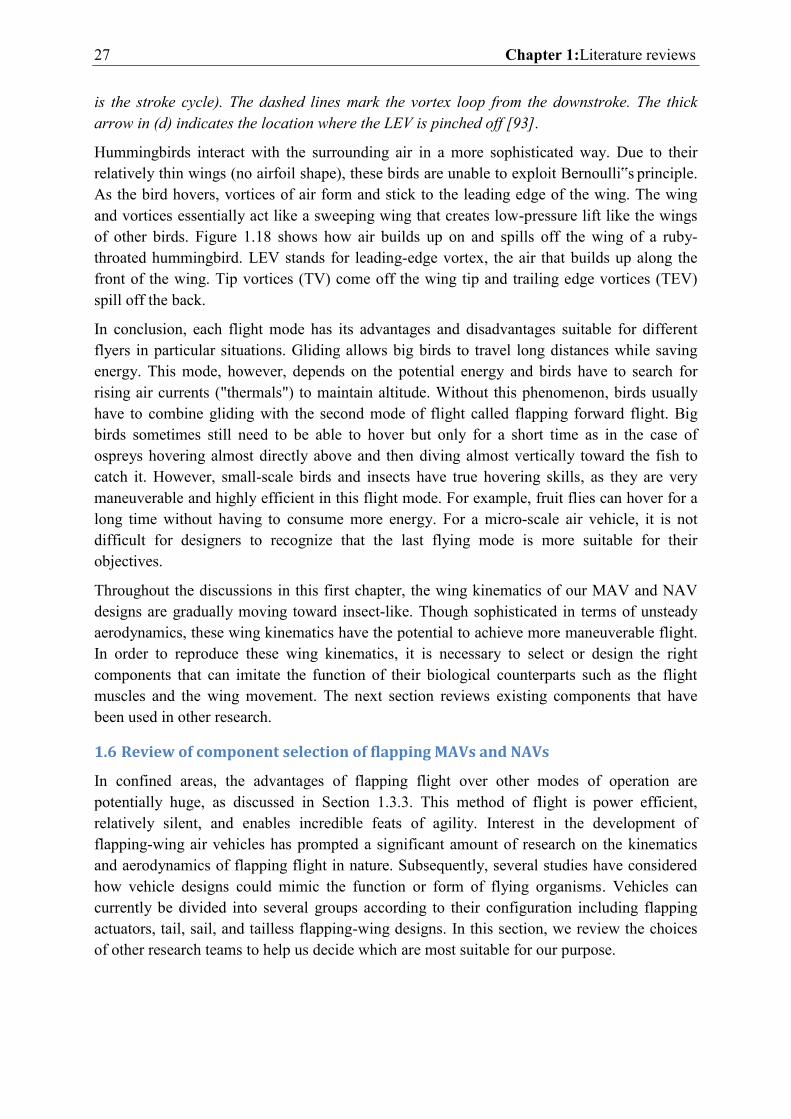
27 Chapter 1:Literature reviews
is the stroke cycle). The dashed lines mark the vortex loop from the downstroke. The thick arrow in (d) indicates the location where the LEV is pinched off [93].
Hummingbirds interact with the surrounding air in a more sophisticated way. Due to their relatively thin wings (no airfoil shape), these birds are unable to exploit Bernoulli‟s principle. As the bird hovers, vortices of air form and stick to the leading edge of the wing. The wing and vortices essentially act like a sweeping wing that creates low-pressure lift like the wings of other birds. Figure 1.18 shows how air builds up on and spills off the wing of a ruby-throated hummingbird. LEV stands for leading-edge vortex, the air that builds up along the front of the wing. Tip vortices (TV) come off the wing tip and trailing edge vortices (TEV) spill off the back.
In conclusion, each flight mode has its advantages and disadvantages suitable for different flyers in particular situations. Gliding allows big birds to travel long distances while saving energy. This mode, however, depends on the potential energy and birds have to search for rising air currents ("thermals") to maintain altitude. Without this phenomenon, birds usually have to combine gliding with the second mode of flight called flapping forward flight. Big birds sometimes still need to be able to hover but only for a short time as in the case of ospreys hovering almost directly above and then diving almost vertically toward the fish to catch it. However, small-scale birds and insects have true hovering skills, as they are very maneuverable and highly efficient in this flight mode. For example, fruit flies can hover for a long time without having to consume more energy. For a micro-scale air vehicle, it is not difficult for designers to recognize that the last flying mode is more suitable for their objectives.
Throughout the discussions in this first chapter, the wing kinematics of our MAV and NAV designs are gradually moving toward insect-like. Though sophisticated in terms of unsteady aerodynamics, these wing kinematics have the potential to achieve more maneuverable flight. In order to reproduce these wing kinematics, it is necessary to select or design the right components that can imitate the function of their biological counterparts such as the flight muscles and the wing movement. The next section reviews existing components that have been used in other research.
1.6 Review of component selection of flapping MAVs and NAVs
In confined areas, the advantages of flapping flight over other modes of operation are potentially huge, as discussed in Section 1.3.3. This method of flight is power efficient, relatively silent, and enables incredible feats of agility. Interest in the development of flapping-wing air vehicles has prompted a significant amount of research on the kinematics and aerodynamics of flapping flight in nature. Subsequently, several studies have considered how vehicle designs could mimic the function or form of flying organisms. Vehicles can currently be divided into several groups according to their configuration including flapping actuators, tail, sail, and tailless flapping-wing designs. In this section, we review the choices of other research teams to help us decide which are most suitable for our purpose.
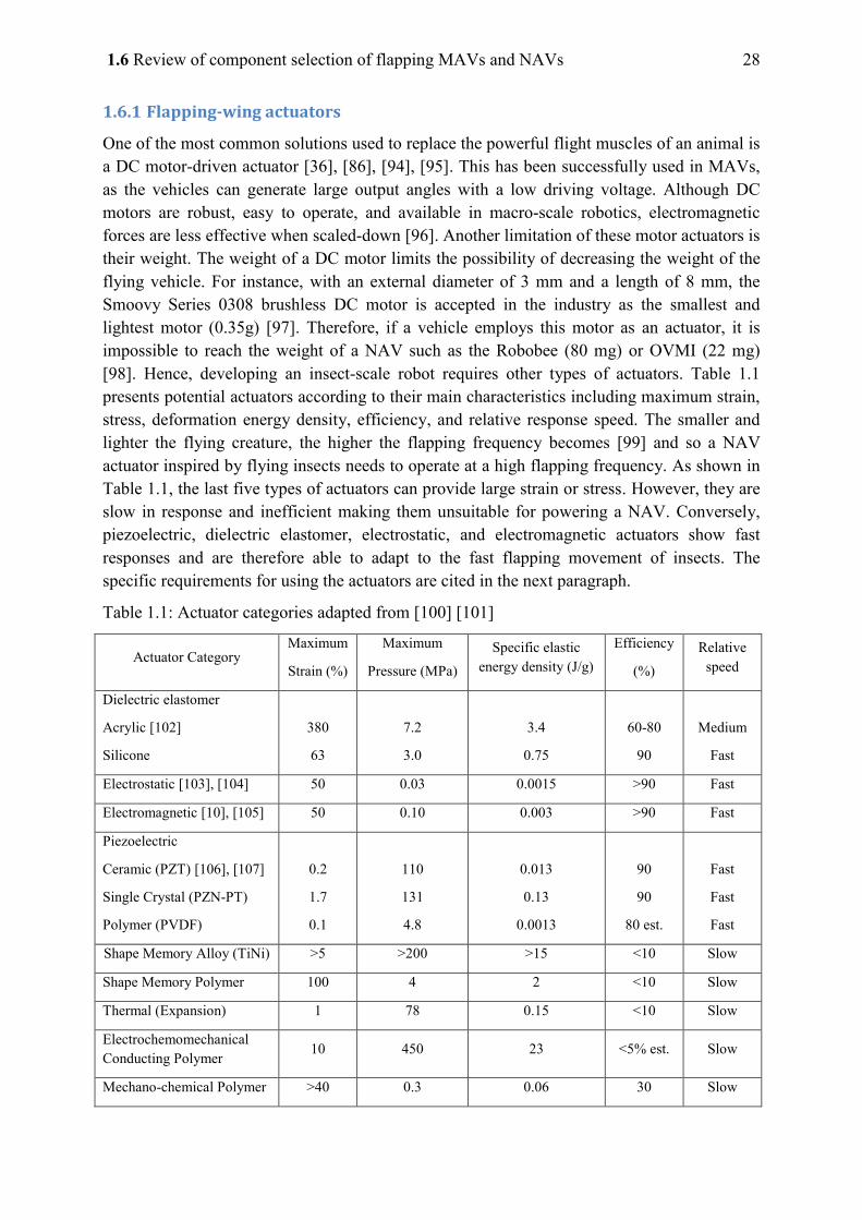
1.6 Review of component selection of flapping MAVs and NAVs 28
1.6.1 Flapping-wing actuators
One of the most common solutions used to replace the powerful flight muscles of an animal is a DC motor-driven actuator [36], [86], [94], [95]. This has been successfully used in MAVs, as the vehicles can generate large output angles with a low driving voltage. Although DC motors are robust, easy to operate, and available in macro-scale robotics, electromagnetic forces are less effective when scaled-down [96]. Another limitation of these motor actuators is their weight. The weight of a DC motor limits the possibility of decreasing the weight of the flying vehicle. For instance, with an external diameter of 3 mm and a length of 8 mm, the Smoovy Series 0308 brushless DC motor is accepted in the industry as the smallest and lightest motor (0.35g) [97]. Therefore, if a vehicle employs this motor as an actuator, it is impossible to reach the weight of a NAV such as the Robobee (80 mg) or OVMI (22 mg) [98]. Hence, developing an insect-scale robot requires other types of actuators. Table 1.1 presents potential actuators according to their main characteristics including maximum strain, stress, deformation energy density, efficiency, and relative response speed. The smaller and lighter the flying creature, the higher the flapping frequency becomes [99] and so a NAV actuator inspired by flying insects needs to operate at a high flapping frequency. As shown in Table 1.1, the last five types of actuators can provide large strain or stress. However, they are slow in response and inefficient making them unsuitable for powering a NAV. Conversely, piezoelectric, dielectric elastomer, electrostatic, and electromagnetic actuators show fast responses and are therefore able to adapt to the fast flapping movement of insects. The specific requirements for using the actuators are cited in the next paragraph.
Table 1.1: Actuator categories adapted from [100] [101]
Actuator Category Maximum
Strain (%)
Maximum
Pressure (MPa) Specific elastic
energy density (J/g) Efficiency
(%) Relative
speed
Dielectric elastomer
Acrylic [102]
Silicone
380
63
7.2
3.0
3.4
0.75
60-80
90
Medium
Fast
Electrostatic [103], [104] 50 0.03 0.0015 >90 Fast
Electromagnetic [10], [105] 50 0.10 0.003 >90 Fast
Piezoelectric
Ceramic (PZT) [106], [107]
Single Crystal (PZN-PT)
Polymer (PVDF)
0.2
1.7
0.1
110
131
4.8
0.013
0.13
0.0013
90
90
80 est.
Fast
Fast
Fast
Shape Memory Alloy (TiNi) >5 >200 >15 <10 Slow
Shape Memory Polymer 100 4 2 <10 Slow
Thermal (Expansion) 1 78 0.15 <10 Slow
Electrochemomechanical Conducting Polymer
10 450 23 <5% est. Slow
Mechano-chemical Polymer >40 0.3 0.06 30 Slow
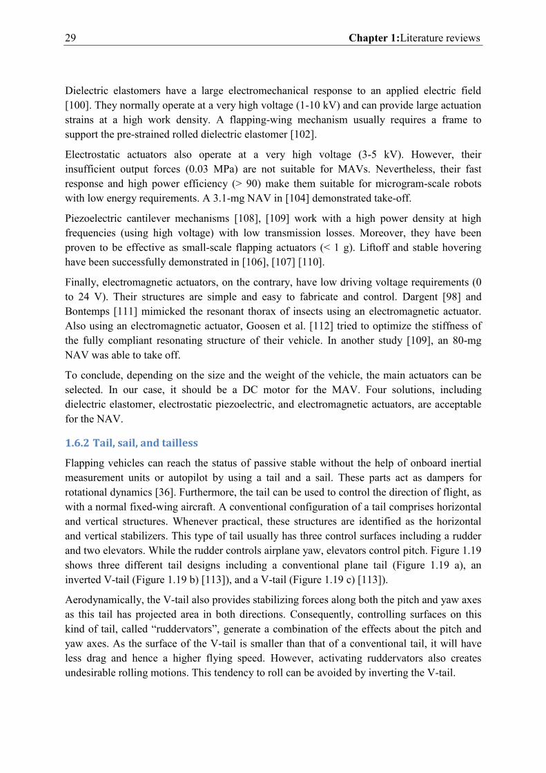
29 Chapter 1:Literature reviews
Dielectric elastomers have a large electromechanical response to an applied electric field [100]. They normally operate at a very high voltage (1-10 kV) and can provide large actuation strains at a high work density. A flapping-wing mechanism usually requires a frame to support the pre-strained rolled dielectric elastomer [102].
Electrostatic actuators also operate at a very high voltage (3-5 kV). However, their insufficient output forces (0.03 MPa) are not suitable for MAVs. Nevertheless, their fast response and high power efficiency (> 90) make them suitable for microgram-scale robots with low energy requirements. A 3.1-mg NAV in [104] demonstrated take-off.
Piezoelectric cantilever mechanisms [108], [109] work with a high power density at high frequencies (using high voltage) with low transmission losses. Moreover, they have been proven to be effective as small-scale flapping actuators (< 1 g). Liftoff and stable hovering have been successfully demonstrated in [106], [107] [110].
Finally, electromagnetic actuators, on the contrary, have low driving voltage requirements (0 to 24 V). Their structures are simple and easy to fabricate and control. Dargent [98] and Bontemps [111] mimicked the resonant thorax of insects using an electromagnetic actuator. Also using an electromagnetic actuator, Goosen et al. [112] tried to optimize the stiffness of the fully compliant resonating structure of their vehicle. In another study [109], an 80-mg NAV was able to take off.
To conclude, depending on the size and the weight of the vehicle, the main actuators can be selected. In our case, it should be a DC motor for the MAV. Four solutions, including dielectric elastomer, electrostatic piezoelectric, and electromagnetic actuators, are acceptable for the NAV.
1.6.2 Tail, sail, and tailless
Flapping vehicles can reach the status of passive stable without the help of onboard inertial measurement units or autopilot by using a tail and a sail. These parts act as dampers for rotational dynamics [36]. Furthermore, the tail can be used to control the direction of flight, as with a normal fixed-wing aircraft. A conventional configuration of a tail comprises horizontal and vertical structures. Whenever practical, these structures are identified as the horizontal and vertical stabilizers. This type of tail usually has three control surfaces including a rudder and two elevators. While the rudder controls airplane yaw, elevators control pitch. Figure 1.19 shows three different tail designs including a conventional plane tail (Figure 1.19 a), an inverted V-tail (Figure 1.19 b) [113]), and a V-tail (Figure 1.19 c) [113]).
Aerodynamically, the V-tail also provides stabilizing forces along both the pitch and yaw axes as this tail has projected area in both directions. Consequently, controlling surfaces on this kind of tail, called “ruddervators”, generate a combination of the effects about the pitch and yaw axes. As the surface of the V-tail is smaller than that of a conventional tail, it will have less drag and hence a higher flying speed. However, activating ruddervators also creates undesirable rolling motions. This tendency to roll can be avoided by inverting the V-tail.
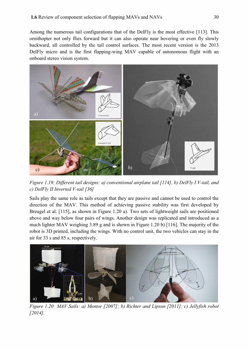
1.6 Review of component selection of flapping MAVs and NAVs 30
Among the numerous tail configurations that of the DelFly is the most effective [113]. This ornithopter not only flies forward but it can also operate near hovering or even fly slowly backward, all controlled by the tail control surfaces. The most recent version is the 2013 DelFly micro and is the first flapping-wing MAV capable of autonomous flight with an onboard stereo vision system.
Figure 1.19: Different tail designs: a) conventional airplane tail [114], b) DelFly I V-tail, and c) DelFly II Inverted V-tail [36]
Sails play the same role as tails except that they are passive and cannot be used to control the direction of the MAV. This method of achieving passive stability was first developed by Breugel et al. [115], as shown in Figure 1.20 a). Two sets of lightweight sails are positioned above and way below four pairs of wings. Another design was replicated and introduced as a much lighter MAV weighing 3.89 g and is shown in Figure 1.20 b) [116]. The majority of the robot is 3D printed, including the wings. With no control unit, the two vehicles can stay in the air for 33 s and 85 s, respectively.
Figure 1.20: MAV Sails: a) Mentor [2007]; b) Richter and Lipson [2011]; c) Jellyfish robot [2014].
a)
c) b)
a) b) c)
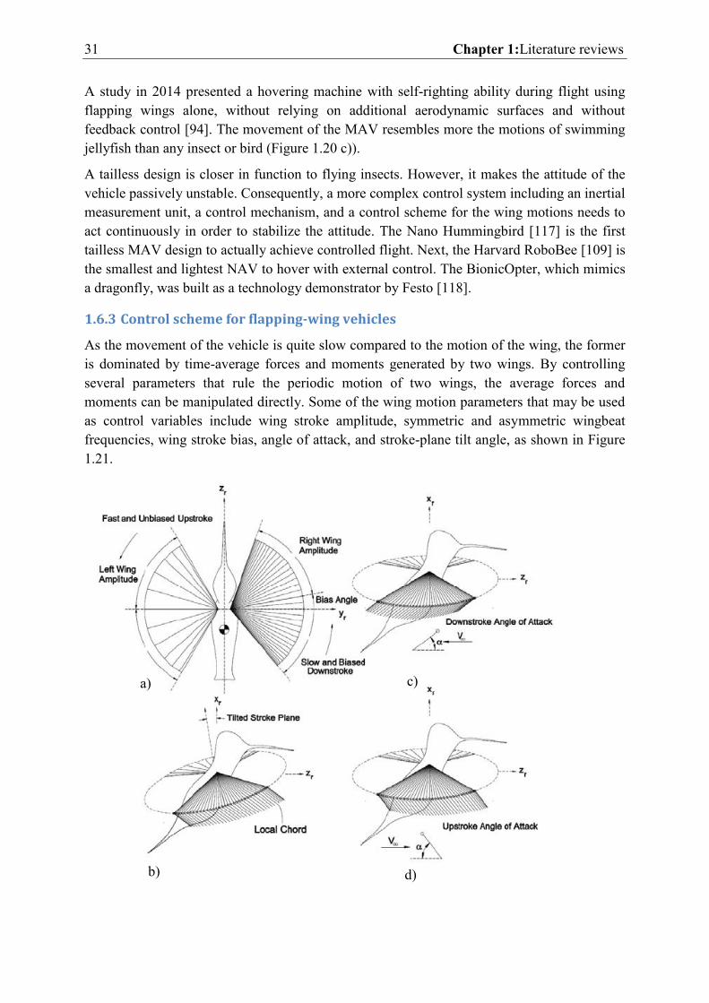
31 Chapter 1:Literature reviews
A study in 2014 presented a hovering machine with self-righting ability during flight using flapping wings alone, without relying on additional aerodynamic surfaces and without feedback control [94]. The movement of the MAV resembles more the motions of swimming jellyfish than any insect or bird (Figure 1.20 c)).
A tailless design is closer in function to flying insects. However, it makes the attitude of the vehicle passively unstable. Consequently, a more complex control system including an inertial measurement unit, a control mechanism, and a control scheme for the wing motions needs to act continuously in order to stabilize the attitude. The Nano Hummingbird [117] is the first tailless MAV design to actually achieve controlled flight. Next, the Harvard RoboBee [109] is the smallest and lightest NAV to hover with external control. The BionicOpter, which mimics a dragonfly, was built as a technology demonstrator by Festo [118].
1.6.3 Control scheme for flapping-wing vehicles
As the movement of the vehicle is quite slow compared to the motion of the wing, the former is dominated by time-average forces and moments generated by two wings. By controlling several parameters that rule the periodic motion of two wings, the average forces and moments can be manipulated directly. Some of the wing motion parameters that may be used as control variables include wing stroke amplitude, symmetric and asymmetric wingbeat frequencies, wing stroke bias, angle of attack, and stroke-plane tilt angle, as shown in Figure 1.21.
a) c)
b) d)
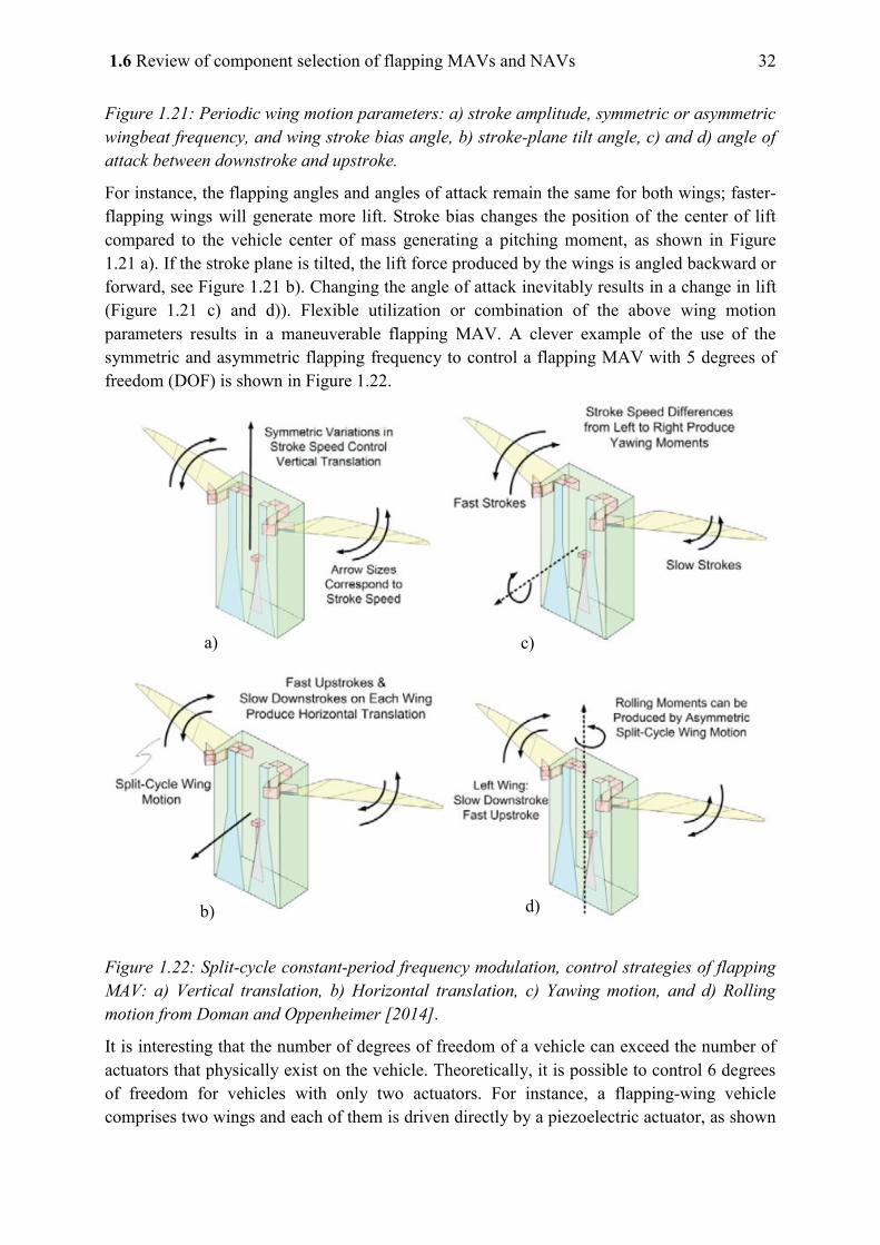
1.6 Review of component selection of flapping MAVs and NAVs 32
Figure 1.21: Periodic wing motion parameters: a) stroke amplitude, symmetric or asymmetric wingbeat frequency, and wing stroke bias angle, b) stroke-plane tilt angle, c) and d) angle of attack between downstroke and upstroke.
For instance, the flapping angles and angles of attack remain the same for both wings; faster-flapping wings will generate more lift. Stroke bias changes the position of the center of lift compared to the vehicle center of mass generating a pitching moment, as shown in Figure 1.21 a). If the stroke plane is tilted, the lift force produced by the wings is angled backward or forward, see Figure 1.21 b). Changing the angle of attack inevitably results in a change in lift (Figure 1.21 c) and d)). Flexible utilization or combination of the above wing motion parameters results in a maneuverable flapping MAV. A clever example of the use of the symmetric and asymmetric flapping frequency to control a flapping MAV with 5 degrees of freedom (DOF) is shown in Figure 1.22.
Figure 1.22: Split-cycle constant-period frequency modulation, control strategies of flapping MAV: a) Vertical translation, b) Horizontal translation, c) Yawing motion, and d) Rolling motion from Doman and Oppenheimer [2014].
It is interesting that the number of degrees of freedom of a vehicle can exceed the number of actuators that physically exist on the vehicle. Theoretically, it is possible to control 6 degrees of freedom for vehicles with only two actuators. For instance, a flapping-wing vehicle comprises two wings and each of them is driven directly by a piezoelectric actuator, as shown
a) c)
b) d)
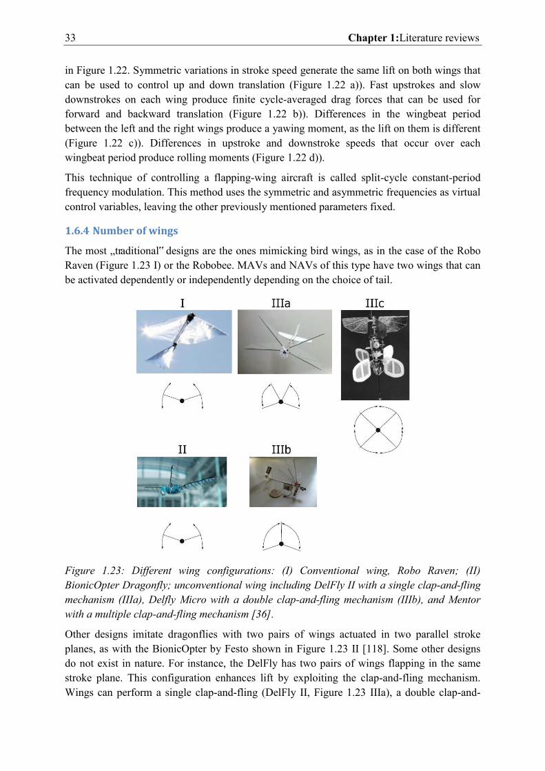
33 Chapter 1:Literature reviews
in Figure 1.22. Symmetric variations in stroke speed generate the same lift on both wings that can be used to control up and down translation (Figure 1.22 a)). Fast upstrokes and slow downstrokes on each wing produce finite cycle-averaged drag forces that can be used for forward and backward translation (Figure 1.22 b)). Differences in the wingbeat period between the left and the right wings produce a yawing moment, as the lift on them is different (Figure 1.22 c)). Differences in upstroke and downstroke speeds that occur over each wingbeat period produce rolling moments (Figure 1.22 d)).
This technique of controlling a flapping-wing aircraft is called split-cycle constant-period frequency modulation. This method uses the symmetric and asymmetric frequencies as virtual control variables, leaving the other previously mentioned parameters fixed.
1.6.4 Number of wings
The most „traditional‟ designs are the ones mimicking bird wings, as in the case of the Robo Raven (Figure 1.23 I) or the Robobee. MAVs and NAVs of this type have two wings that can be activated dependently or independently depending on the choice of tail.
Figure 1.23: Different wing configurations: (I) Conventional wing, Robo Raven; (II) BionicOpter Dragonfly; unconventional wing including DelFly II with a single clap-and-fling mechanism (IIIa), Delfly Micro with a double clap-and-fling mechanism (IIIb), and Mentor with a multiple clap-and-fling mechanism [36].
Other designs imitate dragonflies with two pairs of wings actuated in two parallel stroke planes, as with the BionicOpter by Festo shown in Figure 1.23 II [118]. Some other designs do not exist in nature. For instance, the DelFly has two pairs of wings flapping in the same stroke plane. This configuration enhances lift by exploiting the clap-and-fling mechanism. Wings can perform a single clap-and-fling (DelFly II, Figure 1.23 IIIa), a double clap-and-
1.7 Summarization and motivation 34
fling (DelFly Micro, Figure 1.23 IIIb) or multiple clap-and-fling simultaneously (Mentor, Figure 1.23 IIIb). A sketch under the corresponding vehicles in Figure 1.23 depicts the clap-and-fling mechanism. For example, double clap-and-fling means the lower wings touch the upper wings and the upper wings meet each other. Obviously, the wing configuration has a considerable effect on the forces generated by the flapping and on the way in which the MAV can be controlled. However, a two-wing design was chosen, as the aim was to develop a vehicle mimicking a natural flyer.
1.6.5 Wing rotational principle
Next, there is still the question of the principle of wing rotation. Varying the angle of attack changes the lift produced. In nature, the wing structure of birds and insects allows them to actively manipulate their wing rotation. In [86], [117], the researchers successfully imitated this mechanically by controlling not only the angle of attack but also wing membrane twisting. However, existing mechanisms are complicated and require skillful mechanical engineers to fabricate them. Moreover, this mechanism considerably increases the vehicle mass. Therefore, another principle called passive wing pitch was introduced to overcome this problem. This mechanism is observed in the wing motions of a tethered dragonfly, Libellula pulchella, a hovering fruit fly, and a hovering hawkmoth [119]. Although these insects have the musculature to control the wing pitch during flight, the aerodynamics and wing inertial forces are sufficient to pitch the wing without the aid of the muscles. This mechanism is successfully applied in many existing flapping wing MAVs [37], [95], [116], [120]–[123]. In most cases, a flexible part is added to the wing to contribute to the rotational movement of the wing. Another choice exploits the flexibility of the leading edge to produce the twisting movement of the wing, as in [116]. In some cases, the wing can rotate passively at a specific angle limited by a stopper fixed to one end of the wing leading-edge spar [122], [121]. In the last approach, the wings collide with the stopper and are, therefore, vulnerable to vibrational flaws and breaking. To sum up, active wing pitch brings more control but significantly increases the vehicle mass. Therefore, until now, this concept is applied majorly on MAVs with the higher payload. On the contrary, lightweight passive wing pitch could be found on both MAV and NAV.
In conclusion, a DC motor is preferred as the main actuator for MAV while both piezoelectric and electromagnetic actuators are more suitable for NAV. Next, the choice of tail, tailless or sail depends on the designer. Sail simplifies control, but the vehicle is less versatile and it also looks unnatural. Tail with active control results in higher maneuverability but it also increases the complexity of the linkage mechanisms and consequently increases the vehicle mass. Tailless designs with two or four wings are closest to biological flyers. Their flight, however, is very unstable thus requiring a more complex electronic circuit and control scheme. Finally, the passive wing pitch is more suitable for our MAV.
1.7 Summarization and motivation
From the earlier comparison of three types of MAV and NAV based on the wing configuration in Section 1.3, we found that flapping-wing vehicles have the potential to outpace other types in terms of flying performance, especially small-size vehicles. Section 1.4
35 Chapter 1:Literature reviews
emphasizes this statement by introducing some representative flapping flyers in nature and their highly maneuverable flight. The tremendous difficulties of unsteady aerodynamic phenomena encountered by researchers when designing small-size flying vehicles are also highlighted. The obstacles, however, uncover many possibilities of lift enhancement such as exploiting the clap-and-fling mechanism or delaying the stall. In Section 1.5, we took a quick glance at the flying mode of flyers in nature and hovering mode drew our attention. Section 1.6 reviews existing MAVs and NAVs. By dividing them into groups depending on their actuators and geometric configurations, we acquired more information from other research. Now, we synthesize all our accumulated knowledge to deduce the final design of our MAV and NAV.
Regarding the MAV, as mentioned in the general introduction, the final goal is to develop a NAV. However, this is a challenge. Therefore, it was decided to initially work with a MAV to gain understanding of the flying dynamics of a flapping wing vehicle. Some of the knowledge acquired could then be transferred to the development of the NAV. For this reason, the MAV developed had to be close to the OVMI, the target NAV, in terms of physical phenomena. Consequently, an insect-like MAV is no doubt the perfect choice. This choice is clearly linked to the Hummingbird, as the size and weight of this bird fall within the MAV range. In addition, this is the only bird that can hover with insect-like wing kinematics. Furthermore, this inspiring flyer is found in the transitional area between birds and insects to which its flying dynamics are therefore closely related. Consequently, more knowledge acquired during the development of the MAV can be transferred to developing the NAV.
With the idea of developing a flapping-wing MAV inspired by the hummingbird, it is now necessary to establish two important, closely related specifications of the flying vehicle: wingspan and total mass. As can be seen in Figure 1.24 a), the relationship between the weight and the wing length of natural flyers is linear. A heavier flyer has longer wings and inversely. From this correlation, the appropriate wing length can be chosen according to the total mass of the bio-inspired vehicle. Considering existing materials available, the total mass of the vehicle including the electrical circuit and the battery would close to 10 g. Taking Hummingbirds (red dashed line) as a benchmark, this mass corresponds to a wing length of 8 cm.
Next, in Figure 1.24 b) the wing length is plotted against the flapping frequency of natural flyers and is used to predict the flapping frequency. It can be seen that insects always flap their wings faster than birds and the flapping frequency increases as the wing length decreases. Several successful FWMAVs are presented in this plot to validate this bio-inspired choice. While RoboBee and OVMI are within the range of insects, DelFly Micro and Nano Hummingbird are in the same range as birds and more precisely hummingbirds. With a wing length of 8 cm, our 10-g target is in the range of the hummingbird, so according to nature its flapping frequency should be close to 20 Hz.
From this information about the driving frequency and the desired vehicle mass, it is possible to pick a suitable actuator. As discussed in Section 1.6.1, a motor is a good choice for a flapping MAV. In addition, there are possibilities on the market that have a wide range of input power. Furthermore, using a motor as an actuator saves time and reduces issues linked
1.7 Summarization and motivation 36
to the fabrication and assembly of MAV, as with piezoelectric or electromagnetic actuators. So, it was decided to employ an electrical DC motor to flap the wings of our MAV. To sum up, the MAV is inspired by the hummingbird, which has a mass of 10 g, a wing length of about 8 cm, and a flapping frequency of 20 Hz.
Considering the NAV approach, it is not the same with the MAV from the conception and fabrication point of view. The MAV relies on the micromechanical technology which allows fabricating fastly and easily the components of the vehicle. However, with this technique, the vehicle size cannot be smaller than a certain value. Therefore the solution of the MAV is inspired by the hummingbird. Heretofore, most of the existing MAVs and NAVs are fabricated by this technology and the Robobee could be considered as the most successful one. On the other hand, the NAV developed in this work has to reproduce the behaviour of the small insects. Consequently the only solution in that case is the OVMI since its fabrication uses the Microelectromechanical systems (MEMS) which allows to further reduce the vehicle scale. To sum up, the NAV prototype studied here comprises a 3D flexible skeleton fabricated by MEMS technology and powers by an electromagnetic actuator. More detail on this prototype will be discussed in Chapter 4. From this moment, the “flapping wing MAV” and “flapping wing MAV” are abbreviated to “FWMAV” and “FWNAV” respectively.
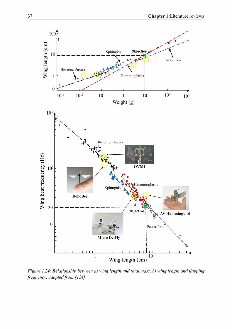
37 Chapter 1:Literature reviews
Figure 1.24: Relationship between a) wing length and total mass, b) wing length and flapping frequency, adapted from [124]
a)
b)

1.7 Summarization and motivation 38
39 Chapter 2:FWMAV model and design
Chapter 2: FWMAV model and design
Contents
2.1 Introduction .. . . . . . . . . . . . . . . . . . . . . . . . . . . . . . . . . . . . . . . . . . . . . . . . . . . . . . . . . . . . . . . . . . . . . . . . . . . . . . . . . . 40
2.2 FWMAV dynamic model . . . . . . . . . . . . . . . . . . . . . . . . . . . . . . . . . . . . . . . . . . . . . . . . . . . . . . . . . . . . . . . . . 40
2.2.1 Flapping and rotating kinetics ................................................................................. 42
2.2.2 Modeling of the submodels ..................................................................................... 43
2.2.2.4 Complete Bond Graph model ........................................................................... 55
2.2.3 FWMAV parameters ............................................................................................... 57
2.3 Optimization .. . . . . . . . . . . . . . . . . . . . . . . . . . . . . . . . . . . . . . . . . . . . . . . . . . . . . . . . . . . . . . . . . . . . . . . . . . . . . . . . . 59
2.3.1 Initial prototype ....................................................................................................... 59
2.3.2 Parameter optimization ........................................................................................... 62
2.3.3 Final prototype ........................................................................................................ 70
2.4 Conclusion of the MAV design .. . . . . . . . . . . . . . . . . . . . . . . . . . . . . . . . . . . . . . . . . . . . . . . . . . . . . . . 71
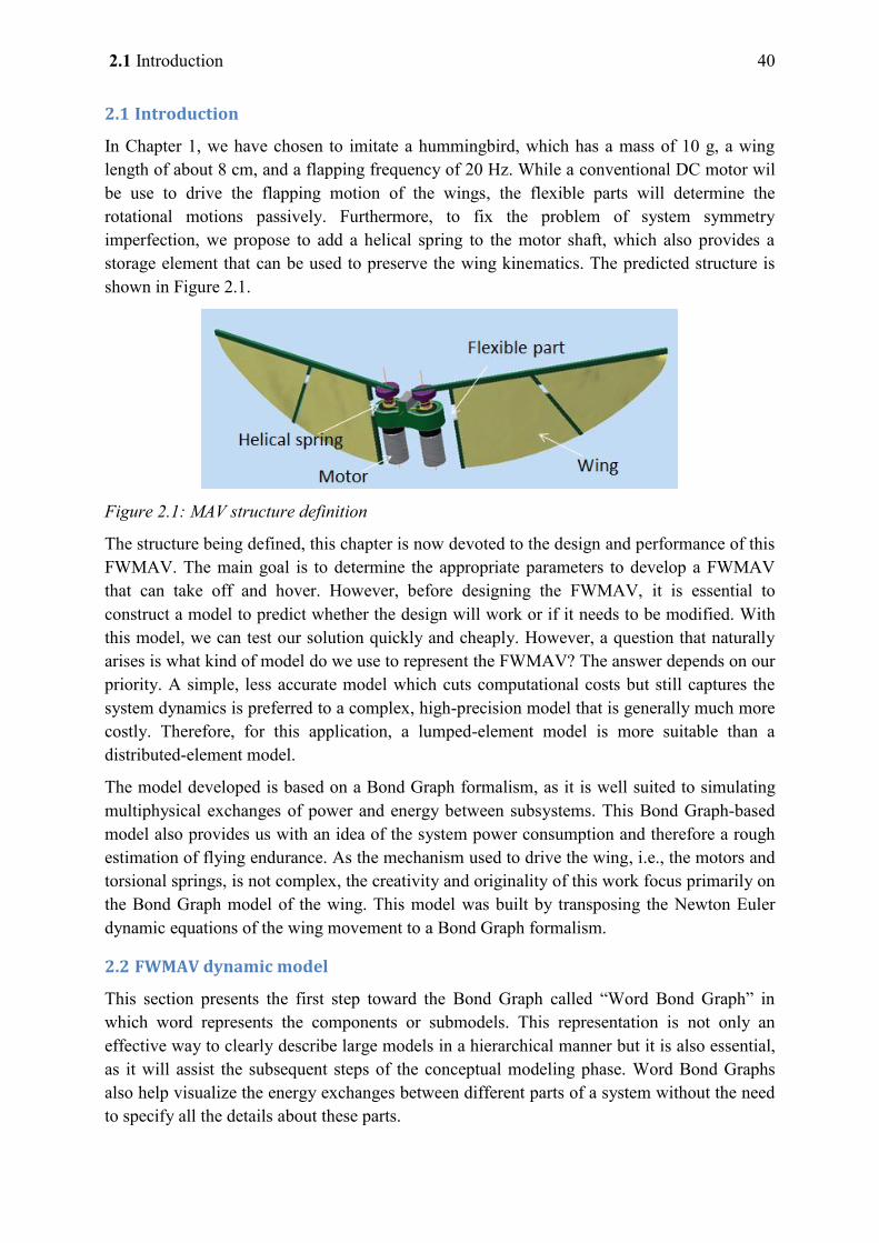
2.1 Introduction 40
2.1 Introduction
In Chapter 1, we have chosen to imitate a hummingbird, which has a mass of 10 g, a wing length of about 8 cm, and a flapping frequency of 20 Hz. While a conventional DC motor wil be use to drive the flapping motion of the wings, the flexible parts will determine the rotational motions passively. Furthermore, to fix the problem of system symmetry imperfection, we propose to add a helical spring to the motor shaft, which also provides a storage element that can be used to preserve the wing kinematics. The predicted structure is shown in Figure 2.1.
Figure 2.1: MAV structure definition
The structure being defined, this chapter is now devoted to the design and performance of this FWMAV. The main goal is to determine the appropriate parameters to develop a FWMAV that can take off and hover. However, before designing the FWMAV, it is essential to construct a model to predict whether the design will work or if it needs to be modified. With this model, we can test our solution quickly and cheaply. However, a question that naturally arises is what kind of model do we use to represent the FWMAV? The answer depends on our priority. A simple, less accurate model which cuts computational costs but still captures the system dynamics is preferred to a complex, high-precision model that is generally much more costly. Therefore, for this application, a lumped-element model is more suitable than a distributed-element model.
The model developed is based on a Bond Graph formalism, as it is well suited to simulating multiphysical exchanges of power and energy between subsystems. This Bond Graph-based model also provides us with an idea of the system power consumption and therefore a rough estimation of flying endurance. As the mechanism used to drive the wing, i.e., the motors and torsional springs, is not complex, the creativity and originality of this work focus primarily on the Bond Graph model of the wing. This model was built by transposing the Newton Euler dynamic equations of the wing movement to a Bond Graph formalism.
2.2 FWMAV dynamic model
This section presents the first step toward the Bond Graph called “Word Bond Graph” in which word represents the components or submodels. This representation is not only an effective way to clearly describe large models in a hierarchical manner but it is also essential, as it will assist the subsequent steps of the conceptual modeling phase. Word Bond Graphs also help visualize the energy exchanges between different parts of a system without the need to specify all the details about these parts.
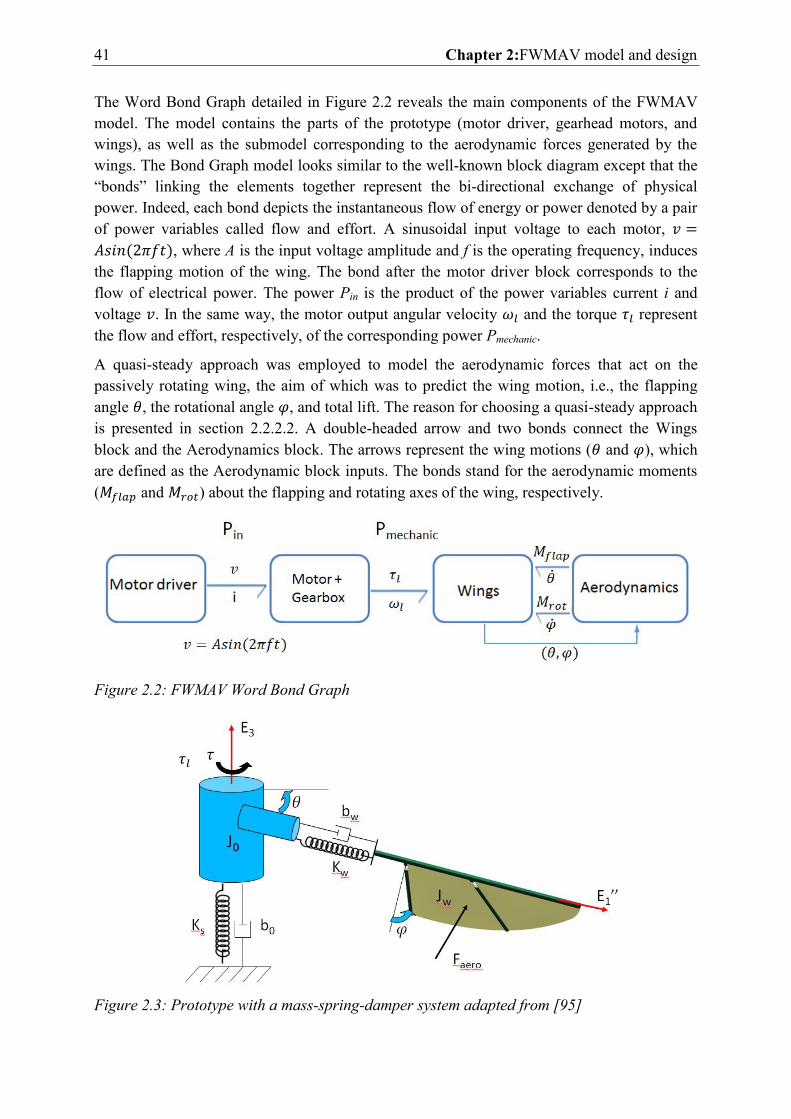
41 Chapter 2:FWMAV model and design
The Word Bond Graph detailed in Figure 2.2 reveals the main components of the FWMAV model. The model contains the parts of the prototype (motor driver, gearhead motors, and wings), as well as the submodel corresponding to the aerodynamic forces generated by the wings. The Bond Graph model looks similar to the well-known block diagram except that the “bonds” linking the elements together represent the bi-directional exchange of physical power. Indeed, each bond depicts the instantaneous flow of energy or power denoted by a pair of power variables called flow and effort. A sinusoidal input voltage to each motor,
, where A is the input voltage amplitude and f is the operating frequency, induces the flapping motion of the wing. The bond after the motor driver block corresponds to the flow of electrical power. The power Pin is the product of the power variables current i and voltage . In the same way, the motor output angular velocity and the torque represent the flow and effort, respectively, of the corresponding power Pmechanic.
A quasi-steady approach was employed to model the aerodynamic forces that act on the passively rotating wing, the aim of which was to predict the wing motion, i.e., the flapping angle , the rotational angle , and total lift. The reason for choosing a quasi-steady approach is presented in section 2.2.2.2. A double-headed arrow and two bonds connect the Wings block and the Aerodynamics block. The arrows represent the wing motions ( and ), which are defined as the Aerodynamic block inputs. The bonds stand for the aerodynamic moments ( and ) about the flapping and rotating axes of the wing, respectively.
Figure 2.2: FWMAV Word Bond Graph
Figure 2.3: Prototype with a mass-spring-damper system adapted from [95]
𝜏𝑙
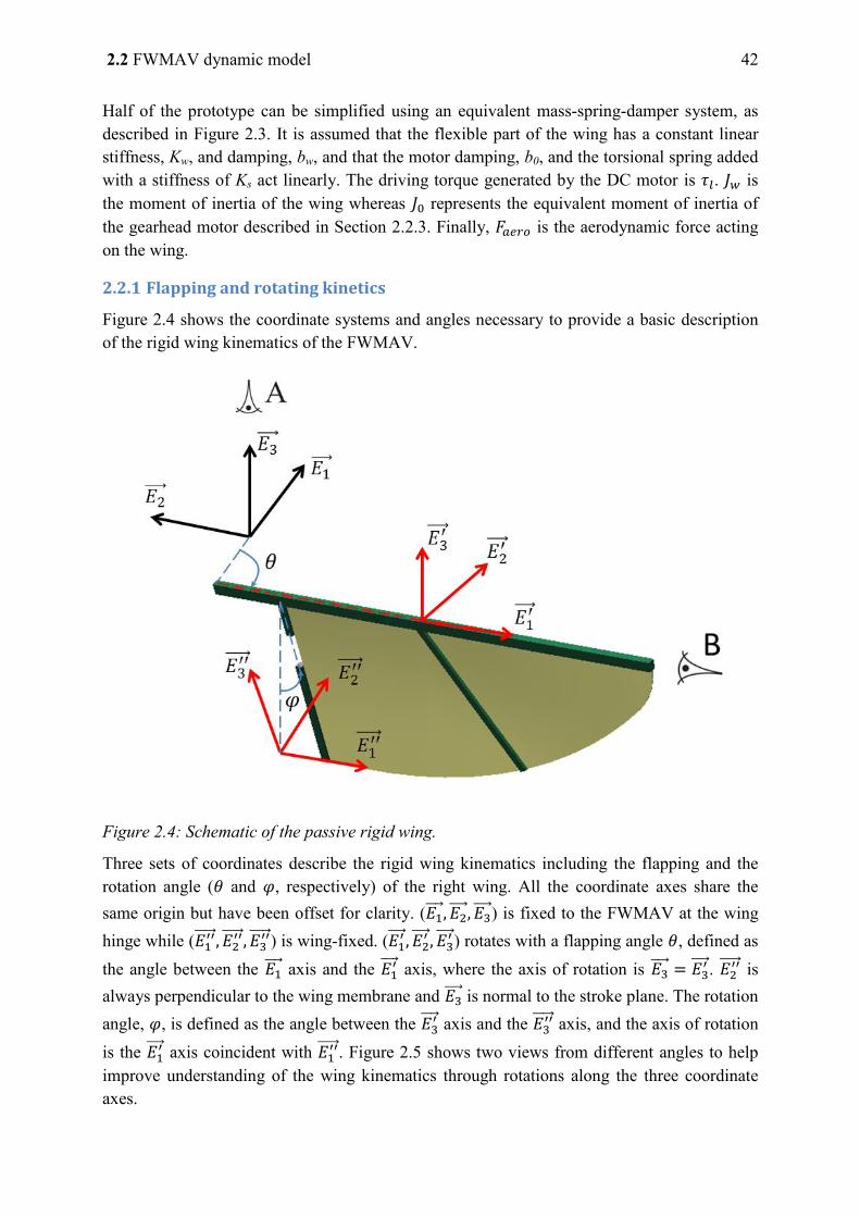
2.2 FWMAV dynamic model 42
Half of the prototype can be simplified using an equivalent mass-spring-damper system, as described in Figure 2.3. It is assumed that the flexible part of the wing has a constant linear stiffness, Kw, and damping, bw, and that the motor damping, b0, and the torsional spring added with a stiffness of Ks act linearly. The driving torque generated by the DC motor is . is the moment of inertia of the wing whereas represents the equivalent moment of inertia of the gearhead motor described in Section 2.2.3. Finally, is the aerodynamic force acting on the wing.
2.2.1 Flapping and rotating kinetics
Figure 2.4 shows the coordinate systems and angles necessary to provide a basic description of the rigid wing kinematics of the FWMAV.
Figure 2.4: Schematic of the passive rigid wing.
Three sets of coordinates describe the rigid wing kinematics including the flapping and the rotation angle ( and , respectively) of the right wing. All the coordinate axes share the same origin but have been offset for clarity. (
) is fixed to the FWMAV at the wing hinge while (
) is wing-fixed. (
) rotates with a flapping angle , defined as
the angle between the axis and the
axis, where the axis of rotation is
. is
always perpendicular to the wing membrane and is normal to the stroke plane. The rotation
angle, , is defined as the angle between the axis and the
axis, and the axis of rotation is the
axis coincident with . Figure 2.5 shows two views from different angles to help
improve understanding of the wing kinematics through rotations along the three coordinate axes.
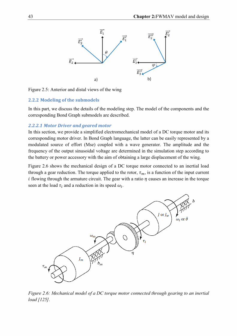
43 Chapter 2:FWMAV model and design
Figure 2.5: Anterior and distal views of the wing
2.2.2 Modeling of the submodels
In this part, we discuss the details of the modeling step. The model of the components and the corresponding Bond Graph submodels are described.
2.2.2.1 Motor Driver and geared motor
In this section, we provide a simplified electromechanical model of a DC torque motor and its corresponding motor driver. In Bond Graph language, the latter can be easily represented by a modulated source of effort (Mse) coupled with a wave generator. The amplitude and the frequency of the output sinusoidal voltage are determined in the simulation step according to the battery or power accessory with the aim of obtaining a large displacement of the wing.
Figure 2.6 shows the mechanical design of a DC torque motor connected to an inertial load through a gear reduction. The torque applied to the rotor, , is a function of the input current flowing through the armature circuit. The gear with a ratio causes an increase in the torque seen at the load and a reduction in its speed .
Figure 2.6: Mechanical model of a DC torque motor connected through gearing to an inertial load [125].
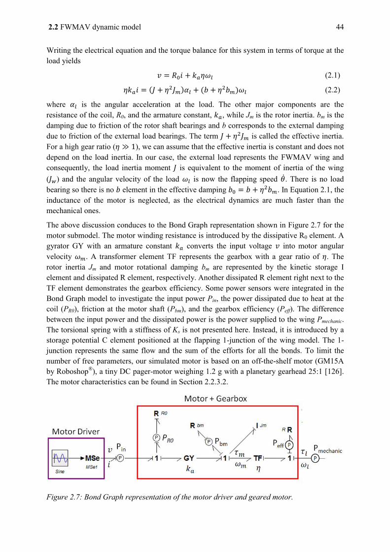
2.2 FWMAV dynamic model 44
Writing the electrical equation and the torque balance for this system in terms of torque at the load yields
(2.1)
(2.2)
where is the angular acceleration at the load. The other major components are the resistance of the coil, R0, and the armature constant, , while Jm is the rotor inertia. bm is the damping due to friction of the rotor shaft bearings and b corresponds to the external damping due to friction of the external load bearings. The term is called the effective inertia. For a high gear ratio ( ), we can assume that the effective inertia is constant and does not depend on the load inertia. In our case, the external load represents the FWMAV wing and consequently, the load inertia moment is equivalent to the moment of inertia of the wing ( ) and the angular velocity of the load is now the flapping speed . There is no load bearing so there is no element in the effective damping . In Equation 2.1, the inductance of the motor is neglected, as the electrical dynamics are much faster than the mechanical ones.
The above discussion conduces to the Bond Graph representation shown in Figure 2.7 for the motor submodel. The motor winding resistance is introduced by the dissipative R0 element. A gyrator GY with an armature constant converts the input voltage into motor angular velocity . A transformer element TF represents the gearbox with a gear ratio of . The rotor inertia Jm and motor rotational damping bm are represented by the kinetic storage I element and dissipated R element, respectively. Another dissipated R element right next to the TF element demonstrates the gearbox efficiency. Some power sensors were integrated in the Bond Graph model to investigate the input power Pin, the power dissipated due to heat at the coil (PR0), friction at the motor shaft (Pbm), and the gearbox efficiency (Peff). The difference between the input power and the dissipated power is the power supplied to the wing Pmechanic. The torsional spring with a stiffness of Ks is not presented here. Instead, it is introduced by a storage potential C element positioned at the flapping 1-junction of the wing model. The 1-junction represents the same flow and the sum of the efforts for all the bonds. To limit the number of free parameters, our simulated motor is based on an off-the-shelf motor (GM15A by Roboshop®), a tiny DC pager-motor weighing 1.2 g with a planetary gearhead 25:1 [126]. The motor characteristics can be found in Section 2.2.3.2.
Figure 2.7: Bond Graph representation of the motor driver and geared motor.
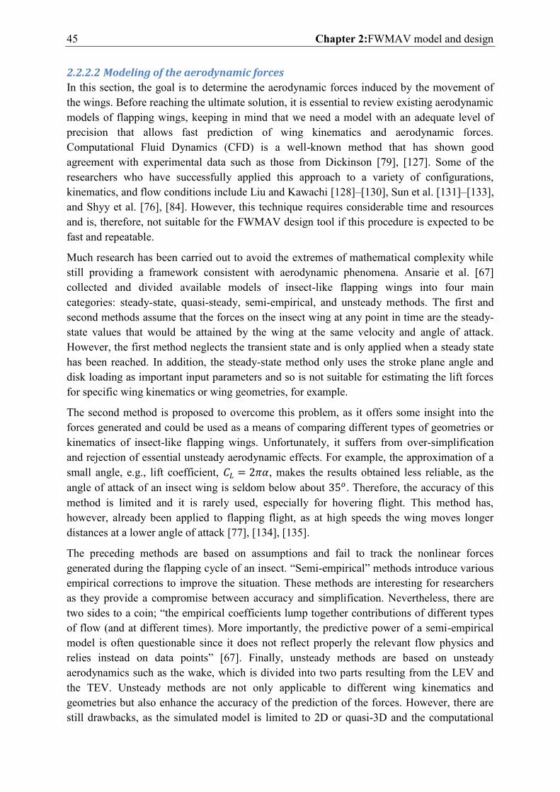
45 Chapter 2:FWMAV model and design
2.2.2.2 Modeling of the aerodynamic forces
In this section, the goal is to determine the aerodynamic forces induced by the movement of the wings. Before reaching the ultimate solution, it is essential to review existing aerodynamic models of flapping wings, keeping in mind that we need a model with an adequate level of precision that allows fast prediction of wing kinematics and aerodynamic forces. Computational Fluid Dynamics (CFD) is a well-known method that has shown good agreement with experimental data such as those from Dickinson [79], [127]. Some of the researchers who have successfully applied this approach to a variety of configurations, kinematics, and flow conditions include Liu and Kawachi [128]–[130], Sun et al. [131]–[133], and Shyy et al. [76], [84]. However, this technique requires considerable time and resources and is, therefore, not suitable for the FWMAV design tool if this procedure is expected to be fast and repeatable.
Much research has been carried out to avoid the extremes of mathematical complexity while still providing a framework consistent with aerodynamic phenomena. Ansarie et al. [67] collected and divided available models of insect-like flapping wings into four main categories: steady-state, quasi-steady, semi-empirical, and unsteady methods. The first and second methods assume that the forces on the insect wing at any point in time are the steady-state values that would be attained by the wing at the same velocity and angle of attack. However, the first method neglects the transient state and is only applied when a steady state has been reached. In addition, the steady-state method only uses the stroke plane angle and disk loading as important input parameters and so is not suitable for estimating the lift forces for specific wing kinematics or wing geometries, for example.
The second method is proposed to overcome this problem, as it offers some insight into the forces generated and could be used as a means of comparing different types of geometries or kinematics of insect-like flapping wings. Unfortunately, it suffers from over-simplification and rejection of essential unsteady aerodynamic effects. For example, the approximation of a small angle, e.g., lift coefficient, , makes the results obtained less reliable, as the angle of attack of an insect wing is seldom below about . Therefore, the accuracy of this method is limited and it is rarely used, especially for hovering flight. This method has, however, already been applied to flapping flight, as at high speeds the wing moves longer distances at a lower angle of attack [77], [134], [135].
The preceding methods are based on assumptions and fail to track the nonlinear forces generated during the flapping cycle of an insect. “Semi-empirical” methods introduce various empirical corrections to improve the situation. These methods are interesting for researchers as they provide a compromise between accuracy and simplification. Nevertheless, there are two sides to a coin; “the empirical coefficients lump together contributions of different types of flow (and at different times). More importantly, the predictive power of a semi-empirical model is often questionable since it does not reflect properly the relevant flow physics and relies instead on data points” [67]. Finally, unsteady methods are based on unsteady aerodynamics such as the wake, which is divided into two parts resulting from the LEV and the TEV. Unsteady methods are not only applicable to different wing kinematics and geometries but also enhance the accuracy of the prediction of the forces. However, there are still drawbacks, as the simulated model is limited to 2D or quasi-3D and the computational
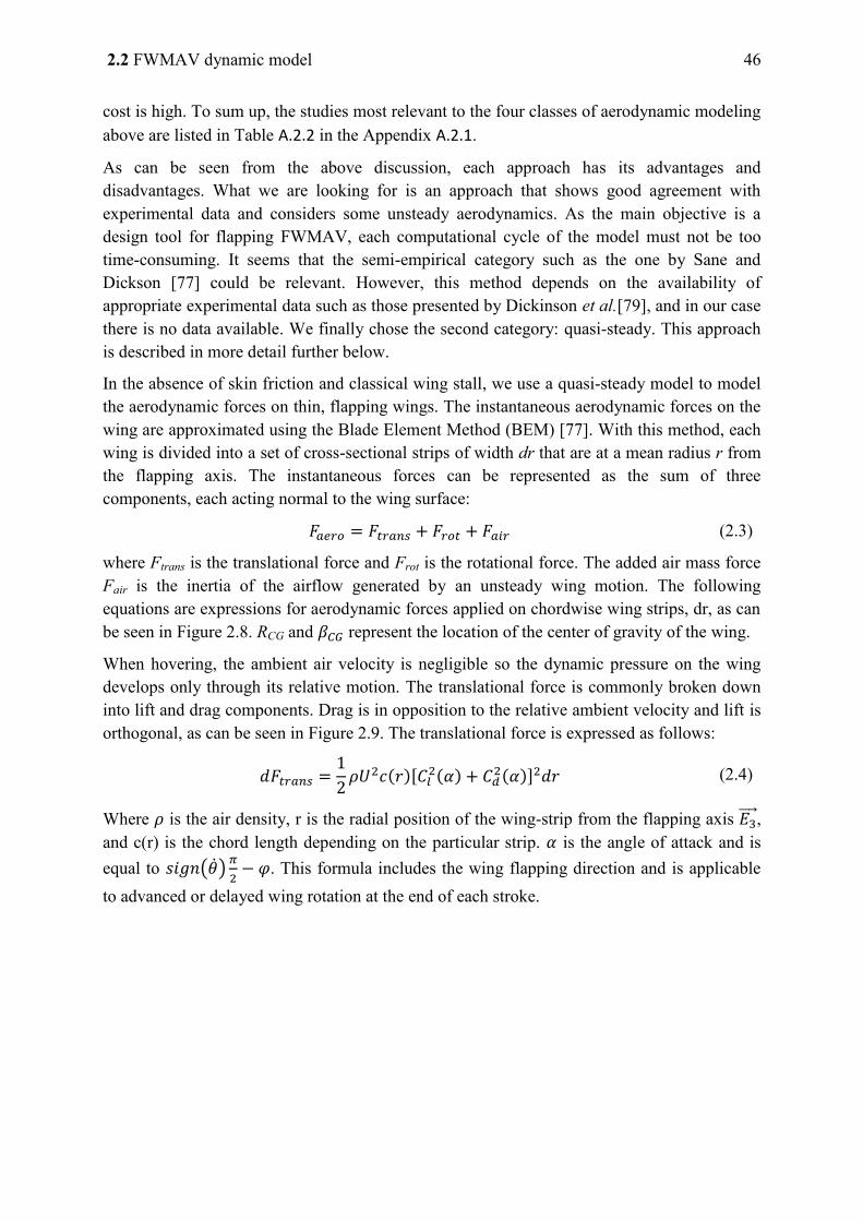
2.2 FWMAV dynamic model 46
cost is high. To sum up, the studies most relevant to the four classes of aerodynamic modeling above are listed in Table A.2.2 in the Appendix A.2.1.
As can be seen from the above discussion, each approach has its advantages and disadvantages. What we are looking for is an approach that shows good agreement with experimental data and considers some unsteady aerodynamics. As the main objective is a design tool for flapping FWMAV, each computational cycle of the model must not be too time-consuming. It seems that the semi-empirical category such as the one by Sane and Dickson [77] could be relevant. However, this method depends on the availability of appropriate experimental data such as those presented by Dickinson et al.[79], and in our case there is no data available. We finally chose the second category: quasi-steady. This approach is described in more detail further below.
In the absence of skin friction and classical wing stall, we use a quasi-steady model to model the aerodynamic forces on thin, flapping wings. The instantaneous aerodynamic forces on the wing are approximated using the Blade Element Method (BEM) [77]. With this method, each wing is divided into a set of cross-sectional strips of width dr that are at a mean radius r from the flapping axis. The instantaneous forces can be represented as the sum of three components, each acting normal to the wing surface:
(2.3)
where Ftrans is the translational force and Frot is the rotational force. The added air mass force Fair is the inertia of the airflow generated by an unsteady wing motion. The following equations are expressions for aerodynamic forces applied on chordwise wing strips, dr, as can be seen in Figure 2.8. RCG and represent the location of the center of gravity of the wing.
When hovering, the ambient air velocity is negligible so the dynamic pressure on the wing develops only through its relative motion. The translational force is commonly broken down into lift and drag components. Drag is in opposition to the relative ambient velocity and lift is orthogonal, as can be seen in Figure 2.9. The translational force is expressed as follows:
[
] (2.4)
Where is the air density, r is the radial position of the wing-strip from the flapping axis ,
and c(r) is the chord length depending on the particular strip. is the angle of attack and is equal to ( )
. This formula includes the wing flapping direction and is applicable
to advanced or delayed wing rotation at the end of each stroke.
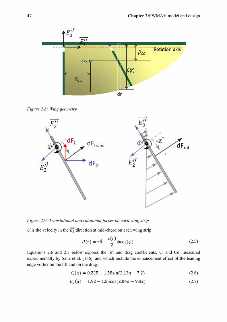
47 Chapter 2:FWMAV model and design
Figure 2.8: Wing geometry
Figure 2.9: Translational and rotational forces on each wing strip
U is the velocity in the direction at mid-chord on each wing strip:
(2.5)
Equations 2.6 and 2.7 below express the lift and drag coefficients, Cl and Cd, measured experimentally by Sane et al. [136], and which include the enhancement effect of the leading edge vortex on the lift and on the drag.
(2.6)
(2.7)
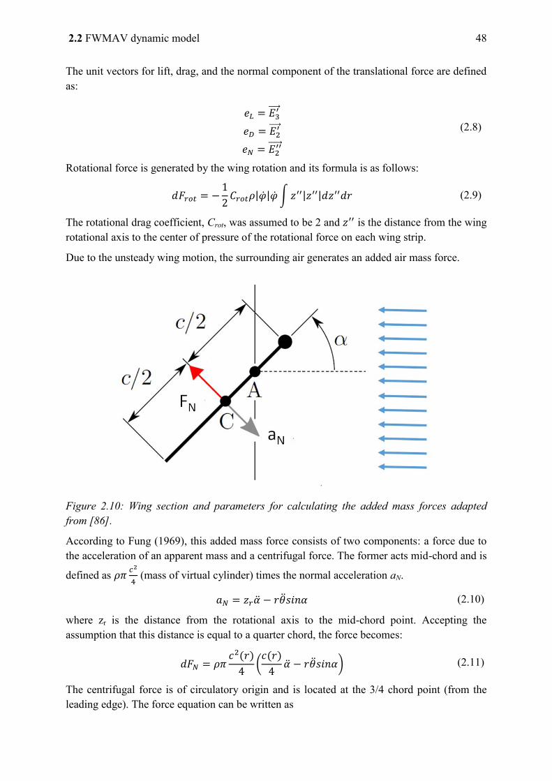
2.2 FWMAV dynamic model 48
The unit vectors for lift, drag, and the normal component of the translational force are defined as:
(2.8)
Rotational force is generated by the wing rotation and its formula is as follows:
| | ∫ | | (2.9)
The rotational drag coefficient, Crot, was assumed to be 2 and is the distance from the wing rotational axis to the center of pressure of the rotational force on each wing strip.
Due to the unsteady wing motion, the surrounding air generates an added air mass force.
Figure 2.10: Wing section and parameters for calculating the added mass forces adapted from [86].
According to Fung (1969), this added mass force consists of two components: a force due to the acceleration of an apparent mass and a centrifugal force. The former acts mid-chord and is
defined as
(mass of virtual cylinder) times the normal acceleration aN.
(2.10)
where zr is the distance from the rotational axis to the mid-chord point. Accepting the assumption that this distance is equal to a quarter chord, the force becomes:
(
) (2.11)
The centrifugal force is of circulatory origin and is located at the 3/4 chord point (from the leading edge). The force equation can be written as
49 Chapter 2:FWMAV model and design
( ) (2.12)
and therefore the total force that acts on each wing strip becomes
(2.13)
(
)
( ) (2.14)
The above equations need to be integrated numerically to obtain the aerodynamic forces on the entire wing.
This quasi-steady model is really promising with respect to its simplicity and accuracy with experimental data. A set of very simple equations dependent on the basic kinematics and geometric parameters of the wing will drastically limit the computational load. These advantages are relevant for a straightforward and efficient model of a rotational passive flapping wing. The aerodynamic forces act as moments about the flapping and rotating axes.
2.2.2.3 Dynamic equation of FWMAV wing motion
There are many approaches to derive the dynamic equations of a mechanical system. All of them produce equivalent sets of equations; however, some forms of the equations may be better suited for computation or analysis. As we wish to understand better the dynamics of the system, we used a Lagrangian approach [137]. This method is based on the energy properties of mechanical systems, and provides a much more elegant and direct way of solving complicated systems, especially if you start adding damping or driving mechanisms. In fact, one of the attractive aspects is that Lagrangian mechanics can solve systems much more easily and quickly than Newtonian mechanics. In Newtonian mechanics, for example, constraints must be explicitly considered, whereas they can be bypassed in Lagrangian mechanics.
In our case, the dynamic equations of the wing are formulated in Lagrangian form with two coordinates for the flapping and rotational angles, as in Equation 2.15. This approach draws on the work of Lindsey Hines et al. [95].
(2.15)
T is the total kinetic energy of the system, equaling the sum of the kinetic energy of the wing including translational and rotational movement, and P is the potential energy of the system due to the added spring and the flexible part. is the wing angular velocity, m is the wing mass augmented with the added air mass defined in Equation 2.25, and is the velocity at the wing center of gravity, as in Figure 2.8. The wing angular velocity and the velocity at the wing center of gravity are formulated as follows:
(2.16)
(2.17)
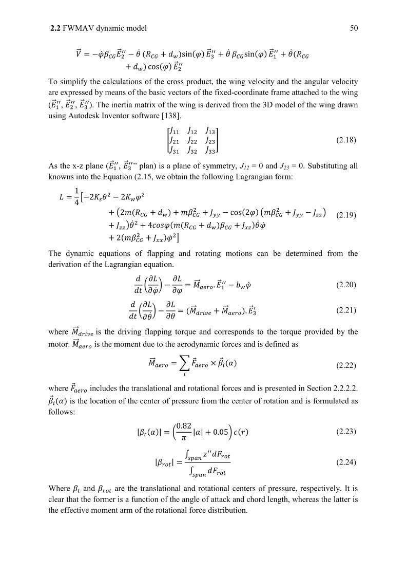
2.2 FWMAV dynamic model 50
To simplify the calculations of the cross product, the wing velocity and the angular velocity are expressed by means of the basic vectors of the fixed-coordinate frame attached to the wing ( , , ). The inertia matrix of the wing is derived from the 3D model of the wing drawn using Autodesk Inventor software [138].
[
] (2.18)
As the x-z plane ( , ” plan) is a plane of symmetry, J12 = 0 and J23 = 0. Substituting all knowns into the Equation (2.15, we obtain the following Lagrangian form:
[
( (
)
)
]
(2.19)
The dynamic equations of flapping and rotating motions can be determined from the derivation of the Lagrangian equation.
(
)
(2.20)
(
)
(2.21)
where is the driving flapping torque and corresponds to the torque provided by the motor. is the moment due to the aerodynamic forces and is defined as
∑
(2.22)
where includes the translational and rotational forces and is presented in Section 2.2.2.2. is the location of the center of pressure from the center of rotation and is formulated as follows:
| | (
| | ) (2.23)
| | ∫
∫
(2.24)
Where and are the translational and rotational centers of pressure, respectively. It is clear that the former is a function of the angle of attack and chord length, whereas the latter is the effective moment arm of the rotational force distribution.
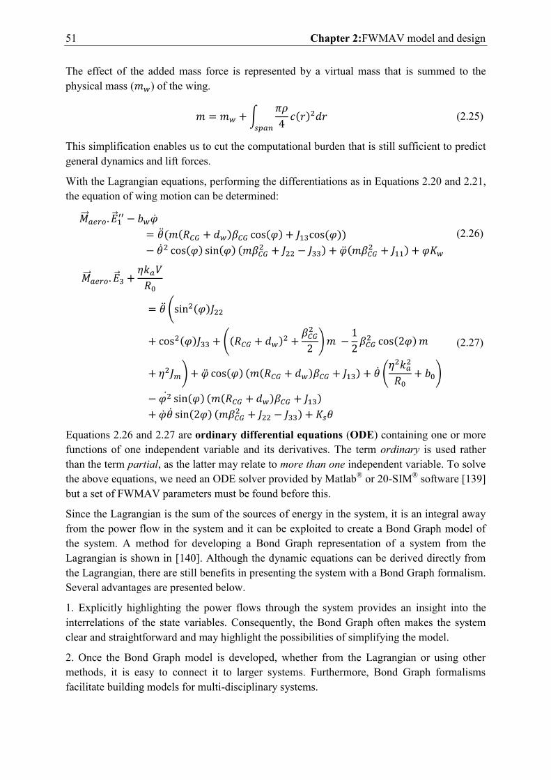
51 Chapter 2:FWMAV model and design
The effect of the added mass force is represented by a virtual mass that is summed to the physical mass ( ) of the wing.
∫
(2.25)
This simplification enables us to cut the computational burden that is still sufficient to predict general dynamics and lift forces.
With the Lagrangian equations, performing the differentiations as in Equations 2.20 and 2.21, the equation of wing motion can be determined:
(2.26)
(
(
)
) (
)
(2.27)
Equations 2.26 and 2.27 are ordinary differential equations (ODE) containing one or more functions of one independent variable and its derivatives. The term ordinary is used rather than the term partial, as the latter may relate to more than one independent variable. To solve the above equations, we need an ODE solver provided by Matlab® or 20-SIM® software [139] but a set of FWMAV parameters must be found before this.
Since the Lagrangian is the sum of the sources of energy in the system, it is an integral away from the power flow in the system and it can be exploited to create a Bond Graph model of the system. A method for developing a Bond Graph representation of a system from the Lagrangian is shown in [140]. Although the dynamic equations can be derived directly from the Lagrangian, there are still benefits in presenting the system with a Bond Graph formalism. Several advantages are presented below.
1. Explicitly highlighting the power flows through the system provides an insight into the interrelations of the state variables. Consequently, the Bond Graph often makes the system clear and straightforward and may highlight the possibilities of simplifying the model.
2. Once the Bond Graph model is developed, whether from the Lagrangian or using other methods, it is easy to connect it to larger systems. Furthermore, Bond Graph formalisms facilitate building models for multi-disciplinary systems.
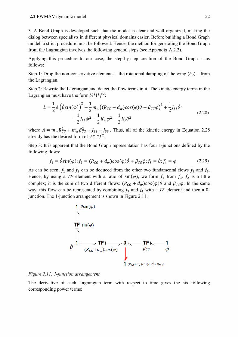
2.2 FWMAV dynamic model 52
3. A Bond Graph is developed such that the model is clear and well organized, making the dialog between specialists in different physical domains easier. Before building a Bond Graph model, a strict procedure must be followed. Hence, the method for generating the Bond Graph from the Lagrangian involves the following general steps (see Appendix A.2.2).
Applying this procedure to our case, the step-by-step creation of the Bond Graph is as follows:
Step 1: Drop the non-conservative elements – the rotational damping of the wing (bw) – from the Lagrangian.
Step 2: Rewrite the Lagrangian and detect the flow terms in it. The kinetic energy terms in the Lagrangian must have the form ½*I* :
( )
( )
(2.28)
where
. Thus, all of the kinetic energy in Equation 2.28 already has the desired form of ½*I* .
Step 3: It is apparent that the Bond Graph representation has four 1-junctions defined by the following flows:
(2.29)
As can be seen, and can be deduced from the other two fundamental flows and . Hence, by using a TF element with a ratio of , we form from . is a little complex; it is the sum of two different flows: and . In the same way, this flow can be represented by combining and with a TF element and then a 0-junction. The 1-junction arrangement is shown in Figure 2.11.
Figure 2.11: 1-junction arrangement.
The derivative of each Lagrangian term with respect to time gives the six following corresponding power terms:
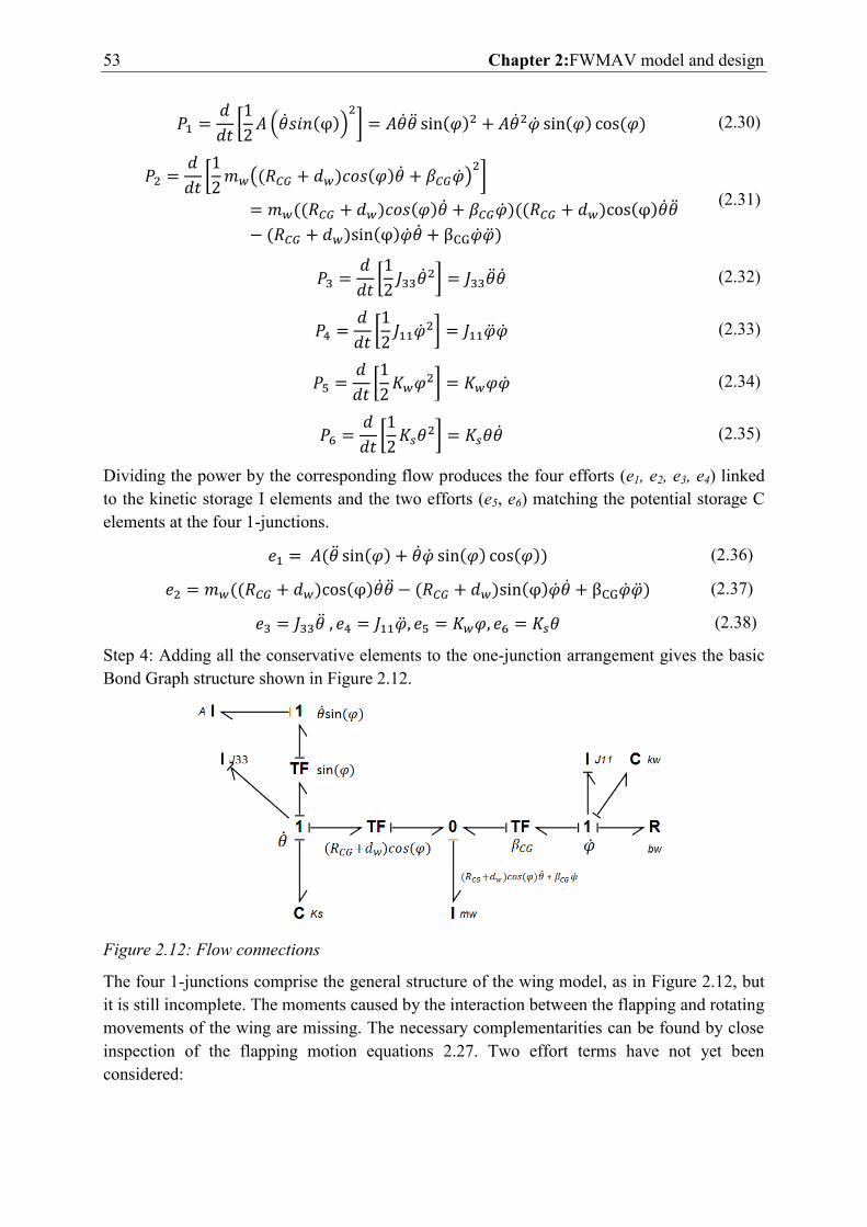
53 Chapter 2:FWMAV model and design
[
( )
] (2.30)
[
( )
]
(2.31)
[
] (2.32)
[
] (2.33)
[
] (2.34)
[
] (2.35)
Dividing the power by the corresponding flow produces the four efforts (e1, e2, e3, e4) linked to the kinetic storage I elements and the two efforts (e5, e6) matching the potential storage C elements at the four 1-junctions.
(2.36)
(2.37)
(2.38)
Step 4: Adding all the conservative elements to the one-junction arrangement gives the basic Bond Graph structure shown in Figure 2.12.
Figure 2.12: Flow connections
The four 1-junctions comprise the general structure of the wing model, as in Figure 2.12, but it is still incomplete. The moments caused by the interaction between the flapping and rotating movements of the wing are missing. The necessary complementarities can be found by close inspection of the flapping motion equations 2.27. Two effort terms have not yet been considered:
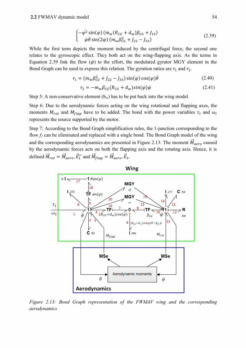
2.2 FWMAV dynamic model 54
{
(2.39)
While the first term depicts the moment induced by the centrifugal force, the second one relates to the gyroscopic effect. They both act on the wing-flapping axis. As the terms in Equation 2.39 link the flow ( ) to the effort, the modulated gyrator MGY element in the Bond Graph can be used to express this relation. The gyration ratios are and .
(2.40)
(2.41)
Step 5: A non-conservative element (bw) has to be put back into the wing model.
Step 6: Due to the aerodynamic forces acting on the wing rotational and flapping axes, the moments and have to be added. The bond with the power variables and represents the source supported by the motor.
Step 7: According to the Bond Graph simplification rules, the 1-junction corresponding to the flow f2 can be eliminated and replaced with a single bond. The Bond Graph model of the wing and the corresponding aerodynamics are presented in Figure 2.13. The moment caused by the aerodynamic forces acts on both the flapping axis and the rotating axis. Hence, it is defined
and .
Figure 2.13: Bond Graph representation of the FWMAV wing and the corresponding aerodynamics
55 Chapter 2:FWMAV model and design
To verify the model, it is possible to retrieve the same dynamic Lagrangian equations from the Bond Graph model of the wing, see the Appendix A.2.2.To conclude, we demonstrate that the Bond Graph representation of the wing is well adapted to represent the Lagrangian wing kinematics.
2.2.2.4 Complete Bond Graph model
To constitute the FWMAV model, all the submodels presented in the preceding sections were linked together by connecting the common bonds representing the power transfer. Based on this model, a non-linear optimization of the main component parameters is carried out in section 2.7.
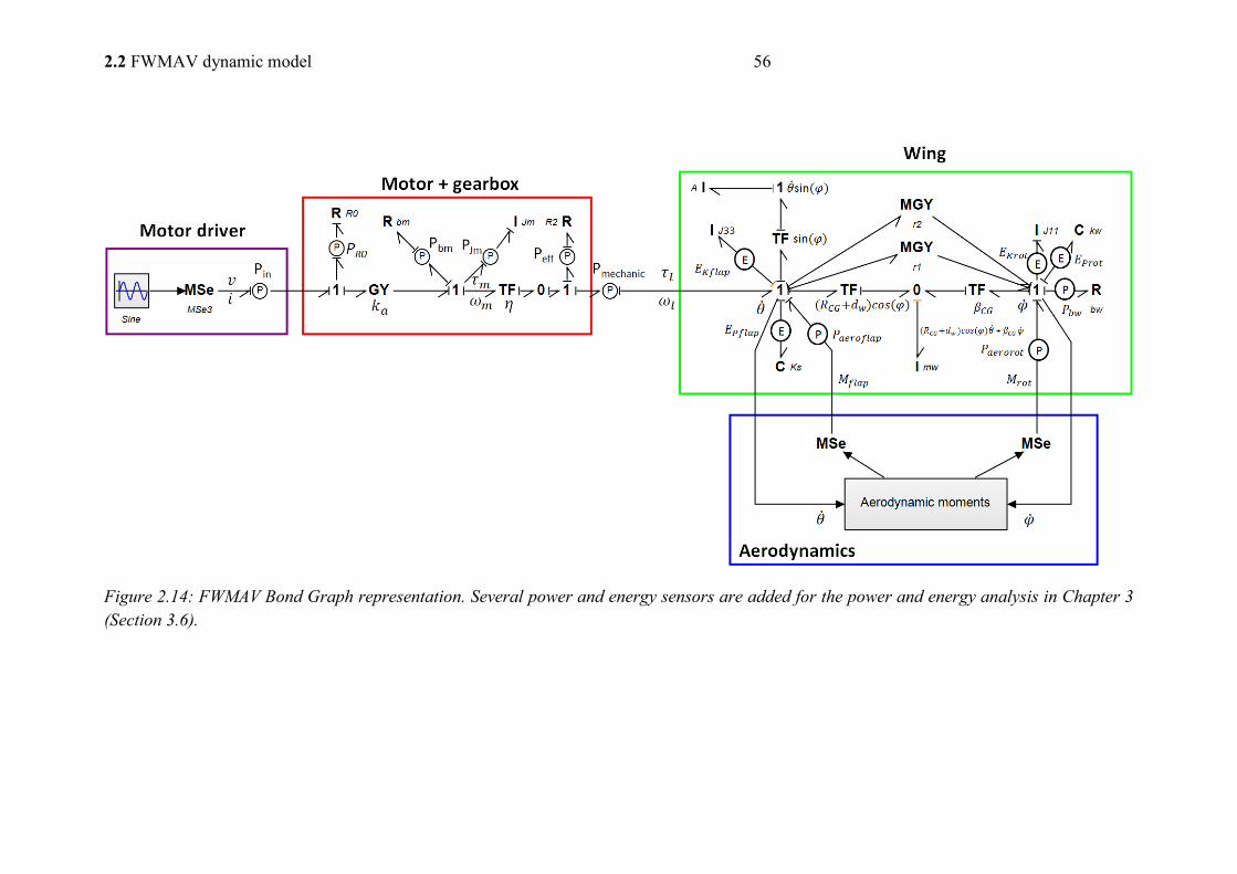
2.2 FWMAV dynamic model 56
Figure 2.14: FWMAV Bond Graph representation. Several power and energy sensors are added for the power and energy analysis in Chapter 3 (Section 3.6).
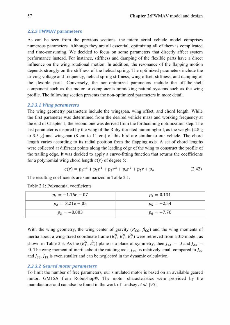
57 Chapter 2:FWMAV model and design
2.2.3 FWMAV parameters
As can be seen from the previous sections, the micro aerial vehicle model comprises numerous parameters. Although they are all essential, optimizing all of them is complicated and time-consuming. We decided to focus on some parameters that directly affect system performance instead. For instance, stiffness and damping of the flexible parts have a direct influence on the wing rotational motion. In addition, the resonance of the flapping motion depends strongly on the stiffness of the helical spring. The optimized parameters include the driving voltage and frequency, helical spring stiffness, wing offset, stiffness, and damping of the flexible parts. Conversely, the non-optimized parameters include the off-the-shelf component such as the motor or components mimicking natural systems such as the wing profile. The following section presents the non-optimized parameters in more detail.
2.2.3.1 Wing parameters
The wing geometry parameters include the wingspan, wing offset, and chord length. While the first parameter was determined from the desired vehicle mass and working frequency at the end of Chapter 1, the second one was derived from the forthcoming optimization step. The last parameter is inspired by the wing of the Ruby-throated hummingbird, as the weight (2.8 g to 3.5 g) and wingspan (8 cm to 11 cm) of this bird are similar to our vehicle. The chord length varies according to its radial position from the flapping axis. A set of chord lengths were collected at different points along the leading edge of the wing to construct the profile of the trailing edge. It was decided to apply a curve-fitting function that returns the coefficients for a polynomial wing chord length of degree 5:
(2.42)
The resulting coefficients are summarized in Table 2.1.
Table 2.1: Polynomial coefficients
With the wing geometry, the wing center of gravity ( , ) and the wing moments of inertia about a wing-fixed coordinate frame ( , , ) were retrieved from a 3D model, as shown in Table 2.3. As the ( , ) plane is a plane of symmetry, then and
. The wing moment of inertia about the rotating axis, , is relatively small compared to and . is even smaller and can be neglected in the dynamic calculation.
2.2.3.2 Geared motor parameters
To limit the number of free parameters, our simulated motor is based on an available geared motor: GM15A from Robotshop®. The motor characteristics were provided by the manufacturer and can also be found in the work of Lindsey et al. [95].
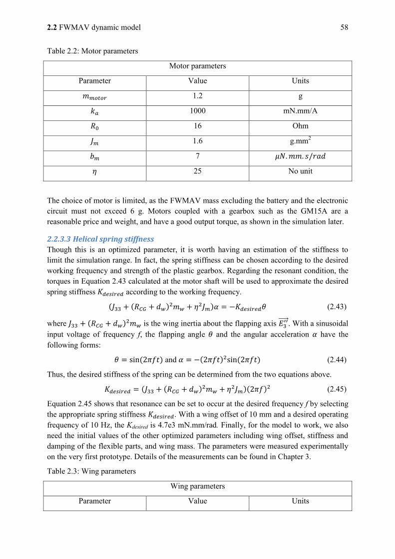
2.2 FWMAV dynamic model 58
Table 2.2: Motor parameters
Motor parameters
Parameter Value Units
1.2 g
1000 mN.mm/A
16 Ohm
1.6 g.mm2
7
25 No unit
The choice of motor is limited, as the FWMAV mass excluding the battery and the electronic circuit must not exceed 6 g. Motors coupled with a gearbox such as the GM15A are a reasonable price and weight, and have a good output torque, as shown in the simulation later.
2.2.3.3 Helical spring stiffness
Though this is an optimized parameter, it is worth having an estimation of the stiffness to limit the simulation range. In fact, the spring stiffness can be chosen according to the desired working frequency and strength of the plastic gearbox. Regarding the resonant condition, the torques in Equation 2.43 calculated at the motor shaft will be used to approximate the desired spring stiffness according to the working frequency.
(2.43)
where is the wing inertia about the flapping axis . With a sinusoidal
input voltage of frequency f, the flapping angle and the angular acceleration have the following forms:
and (2.44)
Thus, the desired stiffness of the spring can be determined from the two equations above.
(2.45)
Equation 2.45 shows that resonance can be set to occur at the desired frequency f by selecting the appropriate spring stiffness . With a wing offset of 10 mm and a desired operating frequency of 10 Hz, the Kdesired is 4.7e3 mN.mm/rad. Finally, for the model to work, we also need the initial values of the other optimized parameters including wing offset, stiffness and damping of the flexible parts, and wing mass. The parameters were measured experimentally on the very first prototype. Details of the measurements can be found in Chapter 3.
Table 2.3: Wing parameters
Wing parameters
Parameter Value Units
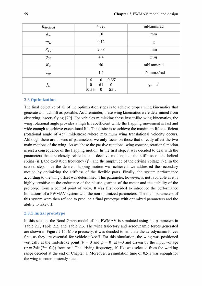
59 Chapter 2:FWMAV model and design
4.7e3 mN.mm/rad
10 mm
0.12 g
20.8 mm
4.4
50 mN.mm/rad
1.5 mN.mm.s/rad
[
] g.mm2
2.3 Optimization
The final objective of all of the optimization steps is to achieve proper wing kinematics that generate as much lift as possible. As a reminder, these wing kinematics were determined from observing insects flying [79]. For vehicles mimicking these insect-like wing kinematics, the wing rotational angle provides a high lift coefficient while the flapping movement is fast and wide enough to achieve exceptional lift. The desire is to achieve the maximum lift coefficient (rotational angle of 45°) mid-stroke where maximum wing translational velocity occurs. Although there are dozens of parameters, we only focus on those that directly affect the two main motions of the wing. As we chose the passive rotational wing concept, rotational motion is just a consequence of the flapping motion. In the first step, it was decided to deal with the parameters that are closely related to the decisive motion, i.e., the stiffness of the helical spring (Ks), the excitation frequency ( ), and the amplitude of the driving voltage ( ). In the second step, once the desired flapping motion was achieved, we addressed the secondary motion by optimizing the stiffness of the flexible parts. Finally, the system performance according to the wing offset was determined. This parameter, however, is not favorable as it is highly sensitive to the endurance of the plastic gearbox of the motor and the stability of the prototype from a control point of view. It was first decided to introduce the performance limitations of a FWMAV system with the non-optimized parameters. The main parameters of this system were then refined to produce a final prototype with optimized parameters and the ability to take off.
2.3.1 Initial prototype
In this section, the Bond Graph model of the FWMAV is simulated using the parameters in Table 2.1, Table 2.2, and Table 2.3. The wing trajectory and aerodynamic forces generated are shown in Figure 2.15. More precisely, it was decided to simulate the aerodynamic forces first, as they are essential for vehicle takeoff. For this simulation, the wing was positioned vertically at the mid-stroke point ( and ) at t=0 and driven by the input voltage ( ) from rest. The driving frequency, 10 Hz, was selected from the working range decided at the end of Chapter 1. Moreover, a simulation time of 0.5 s was enough for the wing to enter its steady state.
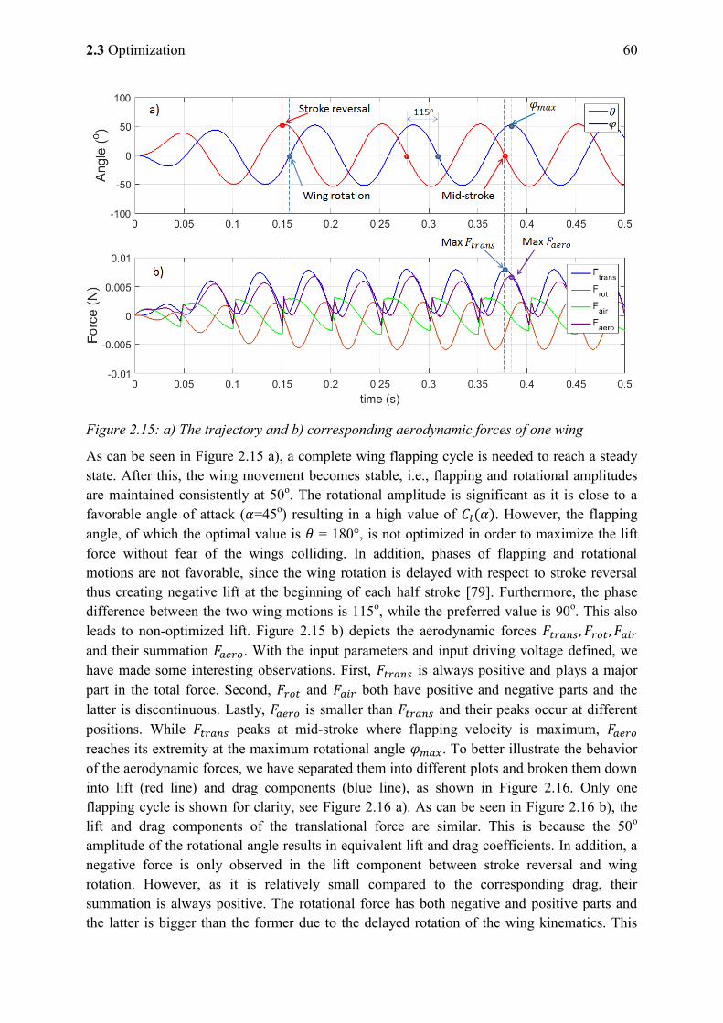
2.3 Optimization 60
Figure 2.15: a) The trajectory and b) corresponding aerodynamic forces of one wing
As can be seen in Figure 2.15 a), a complete wing flapping cycle is needed to reach a steady state. After this, the wing movement becomes stable, i.e., flapping and rotational amplitudes are maintained consistently at 50o. The rotational amplitude is significant as it is close to a favorable angle of attack ( =45o) resulting in a high value of . However, the flapping angle, of which the optimal value is = 180°, is not optimized in order to maximize the lift force without fear of the wings colliding. In addition, phases of flapping and rotational motions are not favorable, since the wing rotation is delayed with respect to stroke reversal thus creating negative lift at the beginning of each half stroke [79]. Furthermore, the phase difference between the two wing motions is 115o, while the preferred value is 90o. This also leads to non-optimized lift. Figure 2.15 b) depicts the aerodynamic forces and their summation . With the input parameters and input driving voltage defined, we have made some interesting observations. First, is always positive and plays a major part in the total force. Second, and both have positive and negative parts and the latter is discontinuous. Lastly, is smaller than and their peaks occur at different positions. While peaks at mid-stroke where flapping velocity is maximum, reaches its extremity at the maximum rotational angle . To better illustrate the behavior of the aerodynamic forces, we have separated them into different plots and broken them down into lift (red line) and drag components (blue line), as shown in Figure 2.16. Only one flapping cycle is shown for clarity, see Figure 2.16 a). As can be seen in Figure 2.16 b), the lift and drag components of the translational force are similar. This is because the 50o amplitude of the rotational angle results in equivalent lift and drag coefficients. In addition, a negative force is only observed in the lift component between stroke reversal and wing rotation. However, as it is relatively small compared to the corresponding drag, their summation is always positive. The rotational force has both negative and positive parts and the latter is bigger than the former due to the delayed rotation of the wing kinematics. This
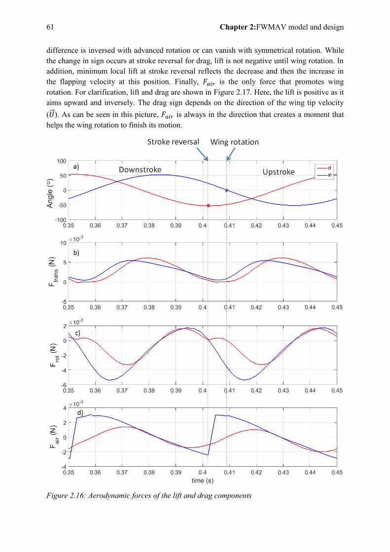
61 Chapter 2:FWMAV model and design
difference is inversed with advanced rotation or can vanish with symmetrical rotation. While the change in sign occurs at stroke reversal for drag, lift is not negative until wing rotation. In addition, minimum local lift at stroke reversal reflects the decrease and then the increase in the flapping velocity at this position. Finally, is the only force that promotes wing rotation. For clarification, lift and drag are shown in Figure 2.17. Here, the lift is positive as it aims upward and inversely. The drag sign depends on the direction of the wing tip velocity ( ). As can be seen in this picture, is always in the direction that creates a moment that helps the wing rotation to finish its motion.
Figure 2.16: Aerodynamic forces of the lift and drag components
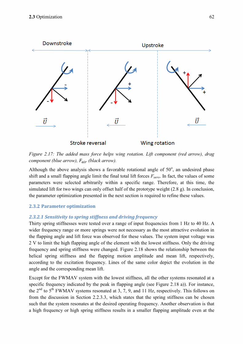
2.3 Optimization 62
Figure 2.17: The added mass force helps wing rotation. Lift component (red arrow), drag component (blue arrow), (black arrow).
Although the above analysis shows a favorable rotational angle of 50o, an undesired phase shift and a small flapping angle limit the final total lift forces Faero. In fact, the values of some parameters were selected arbitrarily within a specific range. Therefore, at this time, the simulated lift for two wings can only offset half of the prototype weight (2.8 g). In conclusion, the parameter optimization presented in the next section is required to refine these values.
2.3.2 Parameter optimization
2.3.2.1 Sensitivity to spring stiffness and driving frequency
Thirty spring stiffnesses were tested over a range of input frequencies from 1 Hz to 40 Hz. A wider frequency range or more springs were not necessary as the most attractive evolution in the flapping angle and lift force was observed for these values. The system input voltage was 2 V to limit the high flapping angle of the element with the lowest stiffness. Only the driving frequency and spring stiffness were changed. Figure 2.18 shows the relationship between the helical spring stiffness and the flapping motion amplitude and mean lift, respectively, according to the excitation frequency. Lines of the same color depict the evolution in the angle and the corresponding mean lift.
Except for the FWMAV system with the lowest stiffness, all the other systems resonated at a specific frequency indicated by the peak in flapping angle (see Figure 2.18 a)). For instance, the 2nd to 5th FWMAV systems resonated at 3, 7, 9, and 11 Hz, respectively. This follows on from the discussion in Section 2.2.3.3, which states that the spring stiffness can be chosen such that the system resonates at the desired operating frequency. Another observation is that a high frequency or high spring stiffness results in a smaller flapping amplitude even at the
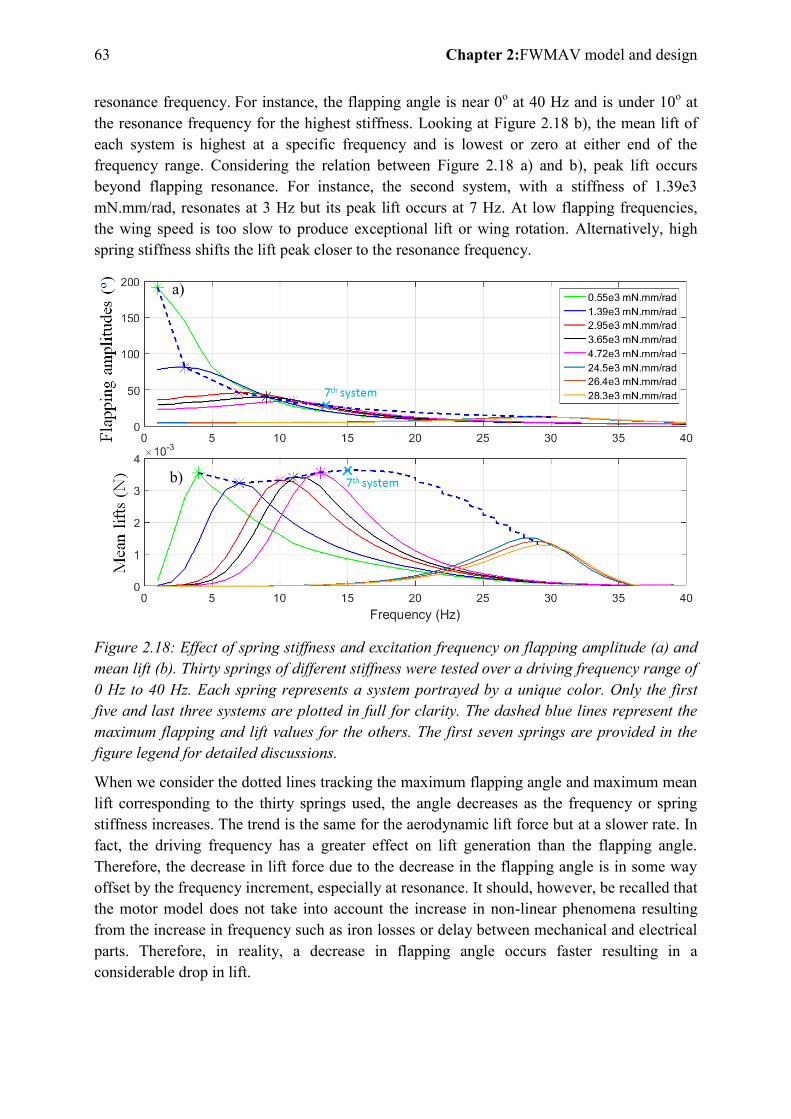
63 Chapter 2:FWMAV model and design
resonance frequency. For instance, the flapping angle is near 0o at 40 Hz and is under 10o at the resonance frequency for the highest stiffness. Looking at Figure 2.18 b), the mean lift of each system is highest at a specific frequency and is lowest or zero at either end of the frequency range. Considering the relation between Figure 2.18 a) and b), peak lift occurs beyond flapping resonance. For instance, the second system, with a stiffness of 1.39e3 mN.mm/rad, resonates at 3 Hz but its peak lift occurs at 7 Hz. At low flapping frequencies, the wing speed is too slow to produce exceptional lift or wing rotation. Alternatively, high spring stiffness shifts the lift peak closer to the resonance frequency.
Figure 2.18: Effect of spring stiffness and excitation frequency on flapping amplitude (a) and mean lift (b). Thirty springs of different stiffness were tested over a driving frequency range of 0 Hz to 40 Hz. Each spring represents a system portrayed by a unique color. Only the first five and last three systems are plotted in full for clarity. The dashed blue lines represent the maximum flapping and lift values for the others. The first seven springs are provided in the figure legend for detailed discussions.
When we consider the dotted lines tracking the maximum flapping angle and maximum mean lift corresponding to the thirty springs used, the angle decreases as the frequency or spring stiffness increases. The trend is the same for the aerodynamic lift force but at a slower rate. In fact, the driving frequency has a greater effect on lift generation than the flapping angle. Therefore, the decrease in lift force due to the decrease in the flapping angle is in some way offset by the frequency increment, especially at resonance. It should, however, be recalled that the motor model does not take into account the increase in non-linear phenomena resulting from the increase in frequency such as iron losses or delay between mechanical and electrical parts. Therefore, in reality, a decrease in flapping angle occurs faster resulting in a considerable drop in lift.
a)
b)
2.3 Optimization 64
In general, if the mean lift is considered as the priority criterion, the FWMAV system should be excited at the peak lift frequency rather than at the resonance frequency. The system with the lowest spring stiffness produces the highest lift at 3 Hz. However, its flapping angle is too high with an input voltage of 2 V and results in the wings colliding. Finally, the 7th FWMAV system working at 15 Hz seems the best choice, as it produces the highest lift force while avoiding the problem of the 1st system. However, a compromise between wing speed, flapping amplitude, and system endurance can provide other solutions. Another remark is on the choice at the end of Chapter 1 of the flapping frequency which is 20 Hz. As shown in Figure 2.18, it seems that there is no advantage to work at this frequency with the proposed system. This is due to the fact that the flapping angle reduces drastically as the driving frequency increases. With the selected motor (GM15A), at 20 Hz, the flapping angle is about 25o. Another motor with higher torque could improve this situation.
2.3.2.2 Sensitivity to the input voltage
The aim of this section is to analyze the effect of the input voltage on system performance. To this end, a sweep of the input voltages was simulated. The nominal operation of this motor is 3.3 V or equivalent to a 4.6 V amplitude sinusoidal driving signal. A maximum increase in 10% provides an inspection range of 0 V to 5 V. Only the first seven springs from the previous section were used, as any further increase in spring stiffness did not produce more lift and could potentially damage the plastic gearbox. Depending on the spring, the motor frequency was set to the optimal lift value determined in Section 2.3.2.1.
Figure 2.19 clearly illustrates a linear relationship between the input voltage and the flapping amplitude or mean lift within the inspection range. As the voltage increases, the flapping amplitude and the mean lift also increase. It is clear that FWMAV systems with lower stiffness excited at a lower frequency produce higher flapping amplitudes.
However, in reality, this angle should not exceed 90o to avoid the wings colliding. With this constraint, only the first four FWMAV systems could reach the maximum flapping amplitude (90o) within the voltage inspection range. The 1st and 2nd FWMAV systems reached this limit at input voltages of 1.5 V and 3.25 V, respectively. Unfortunately, the corresponding lift generated (0.0018 N and 0.0105 N, respectively) is still far from the values that can handle half the vehicle mass (0.015 N). Regarding the 3rd and 4th FWMAV systems, both achieved a lift-to-weight ratio of greater than one at maximum flapping amplitude. However, the former system is preferred as it reaches 90o at 4.9 V. This voltage is higher than the recommended driving voltage (4.6 V).
There is also another solution that uses the 5th and 6th FWMAV systems but at the recommended voltage. The lift generated is slightly higher than with the 3rd system. However, the plastic gearbox of the motor has to endure a higher driving frequency and higher spring stiffness, which affects vehicle endurance. In general, the 3rd FWMAV system activated at 10 Hz and 4.5 V is the better solution.
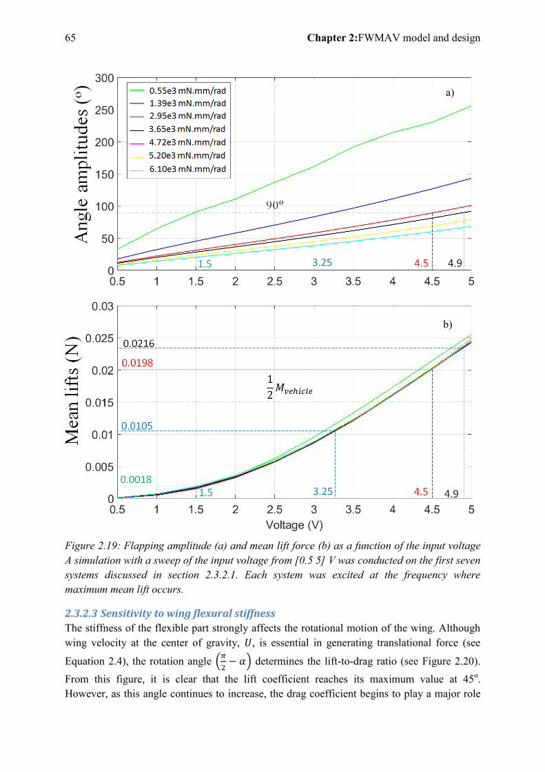
65 Chapter 2:FWMAV model and design
Figure 2.19: Flapping amplitude (a) and mean lift force (b) as a function of the input voltage A simulation with a sweep of the input voltage from [0.5 5] V was conducted on the first seven systems discussed in section 2.3.2.1. Each system was excited at the frequency where maximum mean lift occurs.
2.3.2.3 Sensitivity to wing flexural stiffness
The stiffness of the flexible part strongly affects the rotational motion of the wing. Although wing velocity at the center of gravity, , is essential in generating translational force (see
Equation 2.4), the rotation angle (
) determines the lift-to-drag ratio (see Figure 2.20).
From this figure, it is clear that the lift coefficient reaches its maximum value at 45o. However, as this angle continues to increase, the drag coefficient begins to play a major role
a)
b)
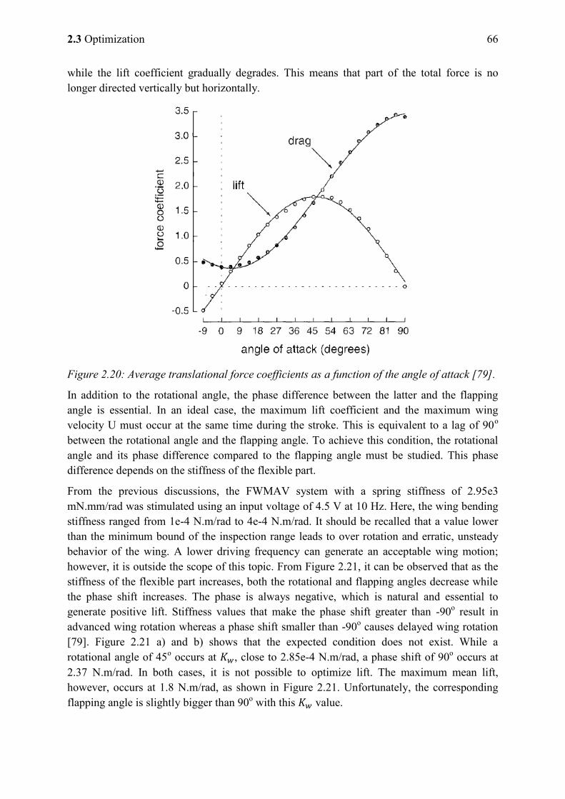
2.3 Optimization 66
while the lift coefficient gradually degrades. This means that part of the total force is no longer directed vertically but horizontally.
Figure 2.20: Average translational force coefficients as a function of the angle of attack [79].
In addition to the rotational angle, the phase difference between the latter and the flapping angle is essential. In an ideal case, the maximum lift coefficient and the maximum wing velocity U must occur at the same time during the stroke. This is equivalent to a lag of 90o between the rotational angle and the flapping angle. To achieve this condition, the rotational angle and its phase difference compared to the flapping angle must be studied. This phase difference depends on the stiffness of the flexible part.
From the previous discussions, the FWMAV system with a spring stiffness of 2.95e3 mN.mm/rad was stimulated using an input voltage of 4.5 V at 10 Hz. Here, the wing bending stiffness ranged from 1e-4 N.m/rad to 4e-4 N.m/rad. It should be recalled that a value lower than the minimum bound of the inspection range leads to over rotation and erratic, unsteady behavior of the wing. A lower driving frequency can generate an acceptable wing motion; however, it is outside the scope of this topic. From Figure 2.21, it can be observed that as the stiffness of the flexible part increases, both the rotational and flapping angles decrease while the phase shift increases. The phase is always negative, which is natural and essential to generate positive lift. Stiffness values that make the phase shift greater than -90o result in advanced wing rotation whereas a phase shift smaller than -90o causes delayed wing rotation [79]. Figure 2.21 a) and b) shows that the expected condition does not exist. While a rotational angle of 45o occurs at , close to 2.85e-4 N.m/rad, a phase shift of 90o occurs at 2.37 N.m/rad. In both cases, it is not possible to optimize lift. The maximum mean lift, however, occurs at 1.8 N.m/rad, as shown in Figure 2.21. Unfortunately, the corresponding flapping angle is slightly bigger than 90o with this value.
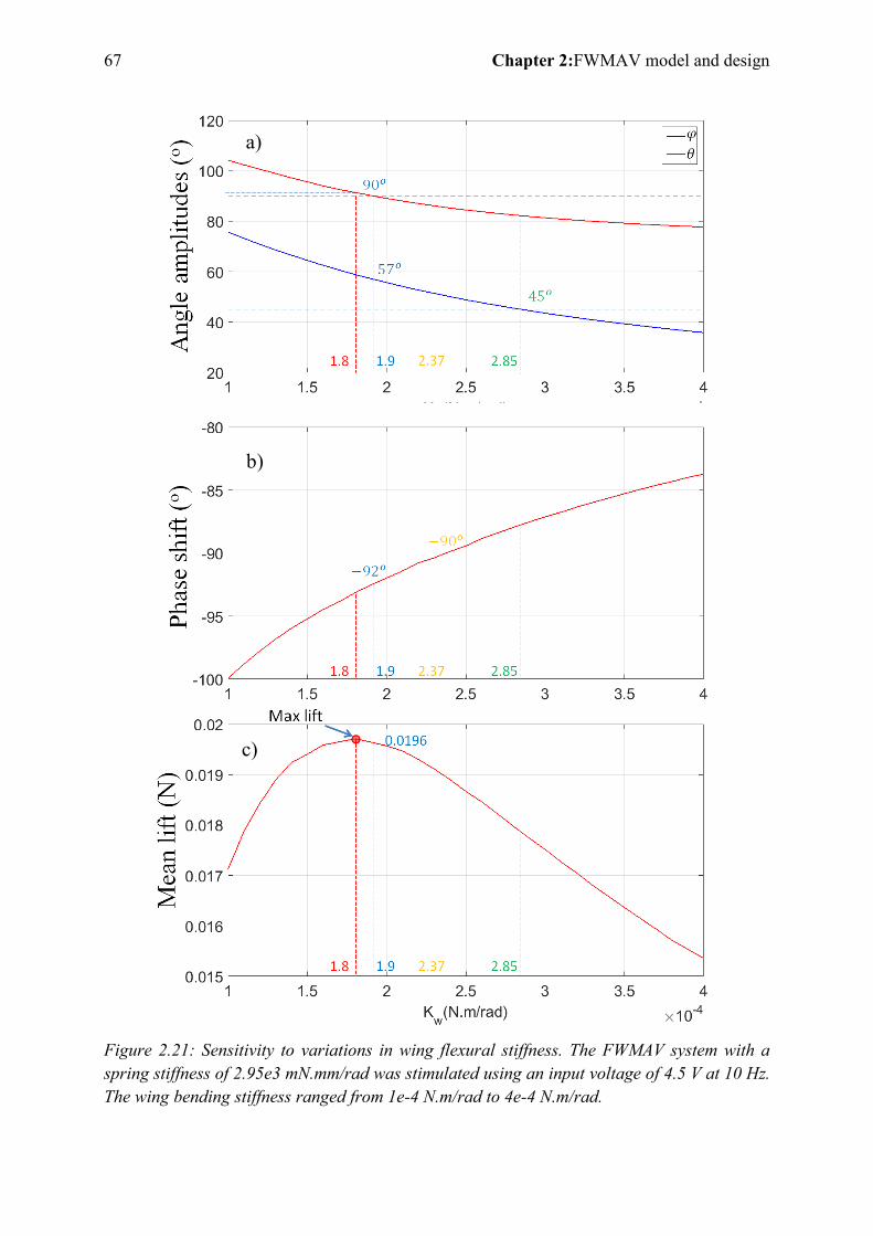
67 Chapter 2:FWMAV model and design
Figure 2.21: Sensitivity to variations in wing flexural stiffness. The FWMAV system with a spring stiffness of 2.95e3 mN.mm/rad was stimulated using an input voltage of 4.5 V at 10 Hz. The wing bending stiffness ranged from 1e-4 N.m/rad to 4e-4 N.m/rad.
a)
b)
c)
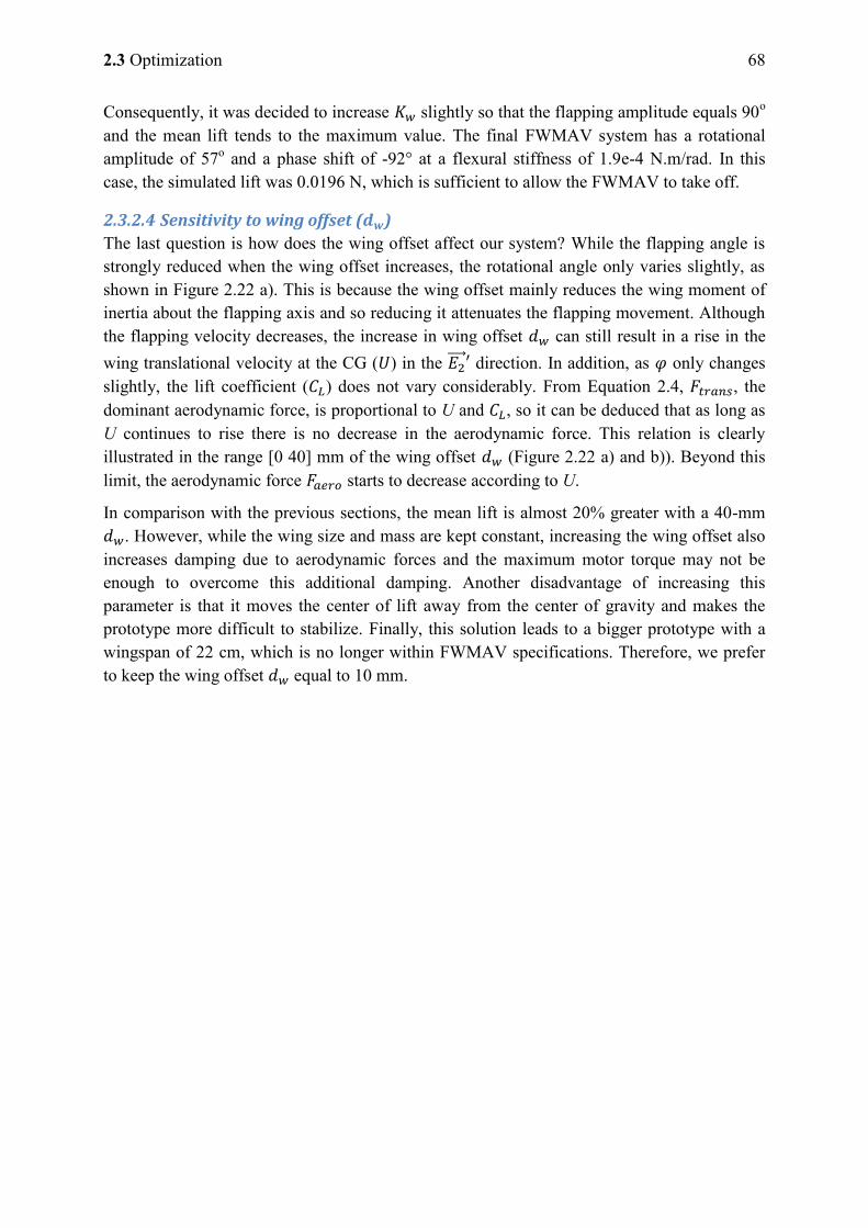
2.3 Optimization 68
Consequently, it was decided to increase slightly so that the flapping amplitude equals 90o and the mean lift tends to the maximum value. The final FWMAV system has a rotational amplitude of 57o and a phase shift of -92° at a flexural stiffness of 1.9e-4 N.m/rad. In this case, the simulated lift was 0.0196 N, which is sufficient to allow the FWMAV to take off.
2.3.2.4 Sensitivity to wing offset ( )
The last question is how does the wing offset affect our system? While the flapping angle is strongly reduced when the wing offset increases, the rotational angle only varies slightly, as shown in Figure 2.22 a). This is because the wing offset mainly reduces the wing moment of inertia about the flapping axis and so reducing it attenuates the flapping movement. Although the flapping velocity decreases, the increase in wing offset can still result in a rise in the wing translational velocity at the CG ( ) in the
direction. In addition, as only changes slightly, the lift coefficient ( ) does not vary considerably. From Equation 2.4, , the dominant aerodynamic force, is proportional to U and , so it can be deduced that as long as U continues to rise there is no decrease in the aerodynamic force. This relation is clearly illustrated in the range [0 40] mm of the wing offset (Figure 2.22 a) and b)). Beyond this limit, the aerodynamic force starts to decrease according to U.
In comparison with the previous sections, the mean lift is almost 20% greater with a 40-mm . However, while the wing size and mass are kept constant, increasing the wing offset also increases damping due to aerodynamic forces and the maximum motor torque may not be enough to overcome this additional damping. Another disadvantage of increasing this parameter is that it moves the center of lift away from the center of gravity and makes the prototype more difficult to stabilize. Finally, this solution leads to a bigger prototype with a wingspan of 22 cm, which is no longer within FWMAV specifications. Therefore, we prefer to keep the wing offset equal to 10 mm.
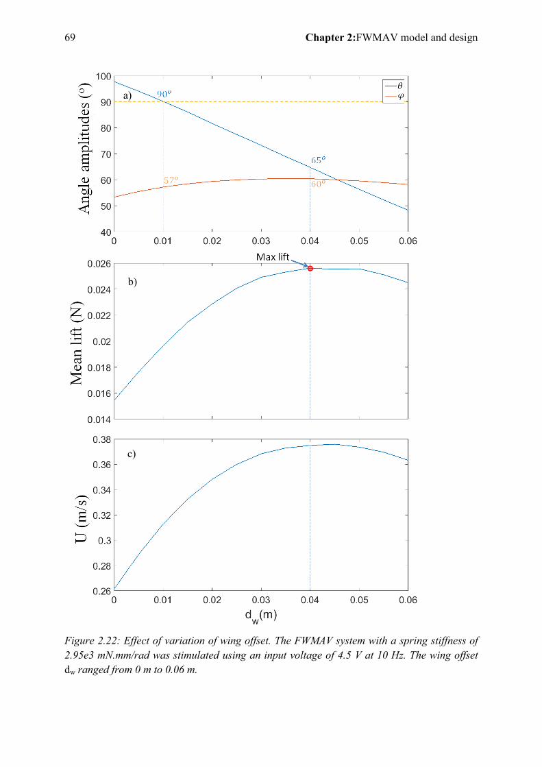
69 Chapter 2:FWMAV model and design
Figure 2.22: Effect of variation of wing offset. The FWMAV system with a spring stiffness of 2.95e3 mN.mm/rad was stimulated using an input voltage of 4.5 V at 10 Hz. The wing offset dw ranged from 0 m to 0.06 m.
a)
b)
c)
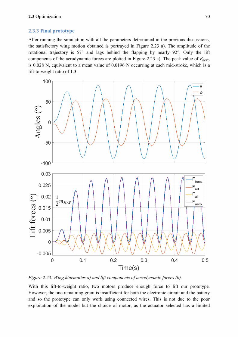
2.3 Optimization 70
2.3.3 Final prototype
After running the simulation with all the parameters determined in the previous discussions, the satisfactory wing motion obtained is portrayed in Figure 2.23 a). The amplitude of the rotational trajectory is 57° and lags behind the flapping by nearly 92°. Only the lift components of the aerodynamic forces are plotted in Figure 2.23 a). The peak value of is 0.028 N, equivalent to a mean value of 0.0196 N occurring at each mid-stroke, which is a lift-to-weight ratio of 1.3.
Figure 2.23: Wing kinematics a) and lift components of aerodynamic forces (b).
With this lift-to-weight ratio, two motors produce enough force to lift our prototype. However, the one remaining gram is insufficient for both the electronic circuit and the battery and so the prototype can only work using connected wires. This is not due to the poor exploitation of the model but the choice of motor, as the actuator selected has a limited
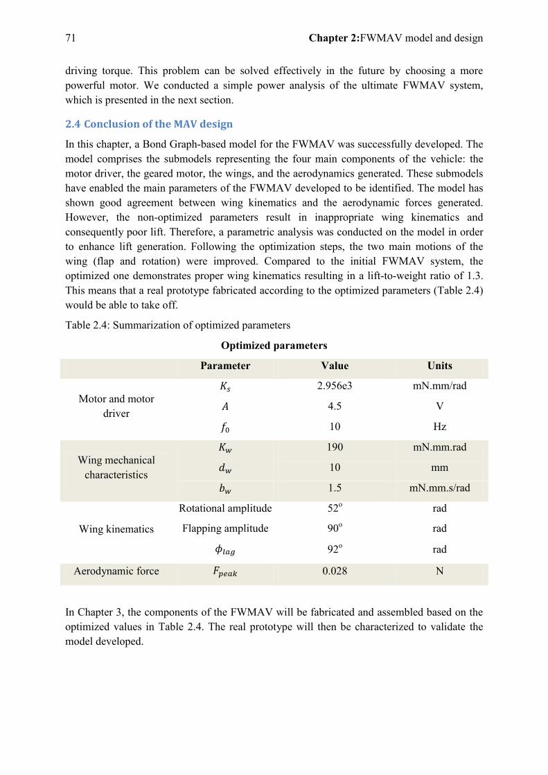
71 Chapter 2:FWMAV model and design
driving torque. This problem can be solved effectively in the future by choosing a more powerful motor. We conducted a simple power analysis of the ultimate FWMAV system, which is presented in the next section.
2.4 Conclusion of the MAV design
In this chapter, a Bond Graph-based model for the FWMAV was successfully developed. The model comprises the submodels representing the four main components of the vehicle: the motor driver, the geared motor, the wings, and the aerodynamics generated. These submodels have enabled the main parameters of the FWMAV developed to be identified. The model has shown good agreement between wing kinematics and the aerodynamic forces generated. However, the non-optimized parameters result in inappropriate wing kinematics and consequently poor lift. Therefore, a parametric analysis was conducted on the model in order to enhance lift generation. Following the optimization steps, the two main motions of the wing (flap and rotation) were improved. Compared to the initial FWMAV system, the optimized one demonstrates proper wing kinematics resulting in a lift-to-weight ratio of 1.3. This means that a real prototype fabricated according to the optimized parameters (Table 2.4) would be able to take off.
Table 2.4: Summarization of optimized parameters
Optimized parameters
Parameter Value Units
Motor and motor driver
2.956e3 mN.mm/rad
4.5 V
10 Hz
Wing mechanical characteristics
190 mN.mm.rad
10 mm
1.5 mN.mm.s/rad
Wing kinematics
Rotational amplitude 52o rad
Flapping amplitude 90o rad
92o rad
Aerodynamic force 0.028 N
In Chapter 3, the components of the FWMAV will be fabricated and assembled based on the optimized values in Table 2.4. The real prototype will then be characterized to validate the model developed.

2.4 Conclusion of the MAV design 72
73 Chapter 3:Towards the construction of a FWMAV able to take off and to stabilize
Chapter 3: Towards the construction of a FWMAV able
to take off and to stabilize
Contents
3.1 Material preparation and assembly work .. . . . . . . . . . . . . . . . . . . . . . . . . . . . . . . . . . . . . . . . . 74
3.1.1 Motor and motor driver selections .......................................................................... 74
3.1.2 Wing fabrication ...................................................................................................... 76
3.1.3 Wing‟s stiffness determination ................................................................................ 76
3.1.4 Wing‟s damping coefficient. ................................................................................... 79
3.1.5 Torsional spring ....................................................................................................... 82
3.1.6 Assembly step ......................................................................................................... 82
3.2 Experimental analysis of the wing movement and generated lift . . . . . . . . . 83
3.3 Validation .. . . . . . . . . . . . . . . . . . . . . . . . . . . . . . . . . . . . . . . . . . . . . . . . . . . . . . . . . . . . . . . . . . . . . . . . . . . . . . . . . . . . . 85
3.3.1 Frequency response ................................................................................................. 85
3.3.2 Input voltage response ............................................................................................. 87
3.3.3 Wing kinematic in desired working condition ........................................................ 88
3.3.4 Take-off demonstration ........................................................................................... 89
3.4 Altitude control . . . . . . . . . . . . . . . . . . . . . . . . . . . . . . . . . . . . . . . . . . . . . . . . . . . . . . . . . . . . . . . . . . . . . . . . . . . . . . 90
3.4.1 Image processing ..................................................................................................... 96
3.4.2 Manual tuning PID .................................................................................................. 97
3.5 Development of an electronic circuit: . . . . . . . . . . . . . . . . . . . . . . . . . . . . . . . . . . . . . . . . . . . . .100
3.5.1 Electronic components: ......................................................................................... 101
3.6 Analysis of power and energy consumption .. . . . . . . . . . . . . . . . . . . . . . . . . . . . . . . . . . . .102
3.6.1 MAV power consumption analysis ....................................................................... 103
3.6.2 Energy analysis ..................................................................................................... 106
3.6.3 Efficiency of the FWMAV .................................................................................... 107
3.7 Conclusion .. . . . . . . . . . . . . . . . . . . . . . . . . . . . . . . . . . . . . . . . . . . . . . . . . . . . . . . . . . . . . . . . . . . . . . . . . . . . . . . . . . .108
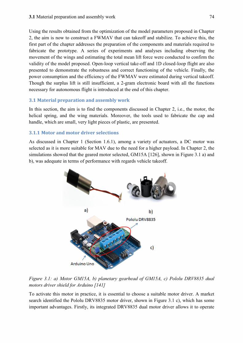
3.1 Material preparation and assembly work 74
Using the results obtained from the optimization of the model parameters proposed in Chapter 2, the aim is now to construct a FWMAV that can takeoff and stabilize. To achieve this, the first part of the chapter addresses the preparation of the components and materials required to fabricate the prototype. A series of experiments and analyses including observing the movement of the wings and estimating the total mean lift force were conducted to confirm the validity of the model proposed. Open-loop vertical take-off and 1D closed-loop flight are also presented to demonstrate the robustness and correct functioning of the vehicle. Finally, the power consumption and the efficiency of the FWMAV were estimated during vertical takeoff. Though the surplus lift is still insufficient, a 2-gram electronic board with all the functions necessary for autonomous flight is introduced at the end of this chapter.
3.1 Material preparation and assembly work
In this section, the aim is to find the components discussed in Chapter 2, i.e., the motor, the helical spring, and the wing materials. Moreover, the tools used to fabricate the cap and handle, which are small, very light pieces of plastic, are presented.
3.1.1 Motor and motor driver selections
As discussed in Chapter 1 (Section 1.6.1), among a variety of actuators, a DC motor was selected as it is more suitable for MAV due to the need for a higher payload. In Chapter 2, the simulations showed that the geared motor selected, GM15A [126], shown in Figure 3.1 a) and b), was adequate in terms of performance with regards vehicle takeoff.
Figure 3.1: a) Motor GM15A, b) planetary gearhead of GM15A, c) Pololu DRV8835 dual motors driver shield for Arduino [141]
To activate this motor in practice, it is essential to choose a suitable motor driver. A market search identified the Pololu DRV8835 motor driver, shown in Figure 3.1 c), which has some important advantages. Firstly, its integrated DRV8835 dual motor driver allows it to operate
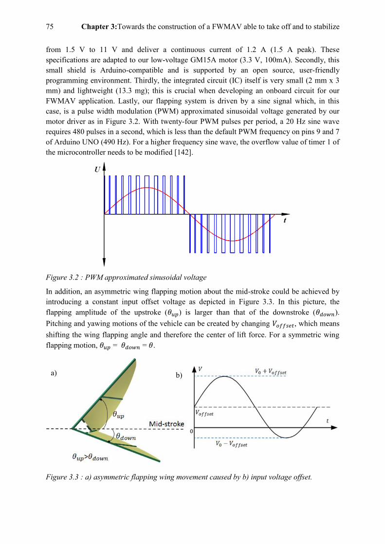
75 Chapter 3:Towards the construction of a FWMAV able to take off and to stabilize
from 1.5 V to 11 V and deliver a continuous current of 1.2 A (1.5 A peak). These specifications are adapted to our low-voltage GM15A motor (3.3 V, 100mA). Secondly, this small shield is Arduino-compatible and is supported by an open source, user-friendly programming environment. Thirdly, the integrated circuit (IC) itself is very small (2 mm x 3 mm) and lightweight (13.3 mg); this is crucial when developing an onboard circuit for our FWMAV application. Lastly, our flapping system is driven by a sine signal which, in this case, is a pulse width modulation (PWM) approximated sinusoidal voltage generated by our motor driver as in Figure 3.2. With twenty-four PWM pulses per period, a 20 Hz sine wave requires 480 pulses in a second, which is less than the default PWM frequency on pins 9 and 7 of Arduino UNO (490 Hz). For a higher frequency sine wave, the overflow value of timer 1 of the microcontroller needs to be modified [142].
Figure 3.2 : PWM approximated sinusoidal voltage
In addition, an asymmetric wing flapping motion about the mid-stroke could be achieved by introducing a constant input offset voltage as depicted in Figure 3.3. In this picture, the flapping amplitude of the upstroke ( ) is larger than that of the downstroke ( ). Pitching and yawing motions of the vehicle can be created by changing , which means shifting the wing flapping angle and therefore the center of lift force. For a symmetric wing flapping motion, = = .
Figure 3.3 : a) asymmetric flapping wing movement caused by b) input voltage offset.
a) b)
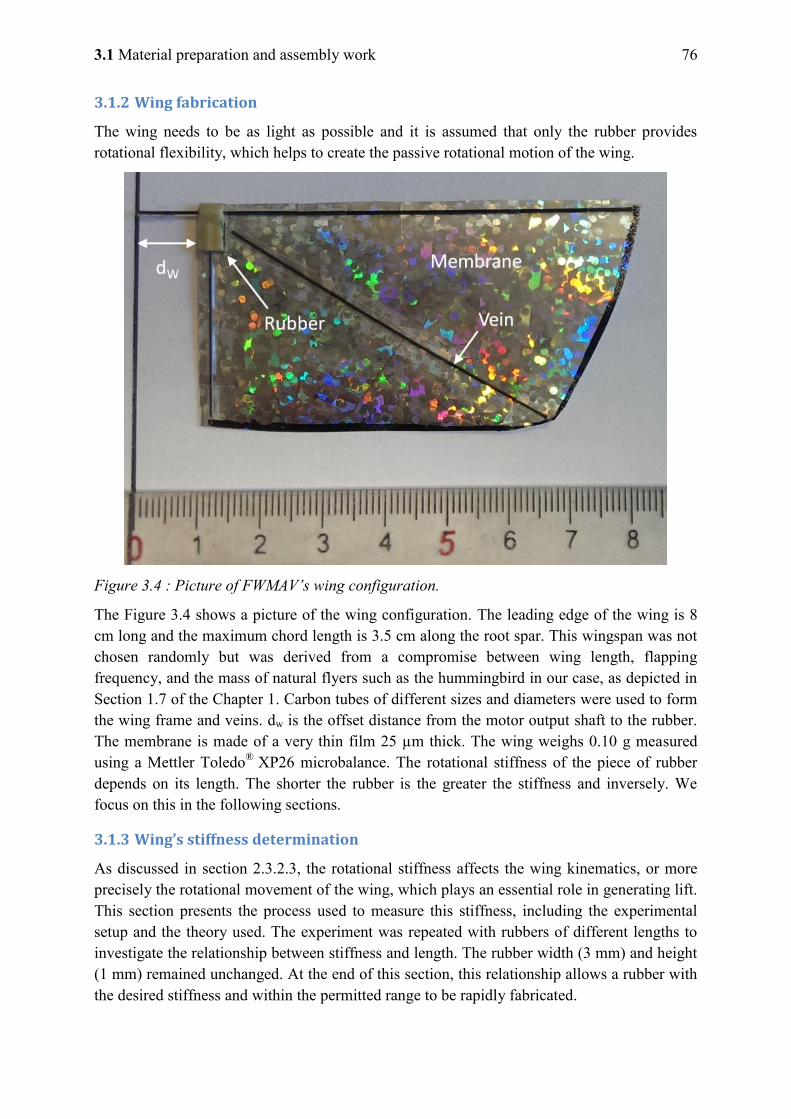
3.1 Material preparation and assembly work 76
3.1.2 Wing fabrication
The wing needs to be as light as possible and it is assumed that only the rubber provides rotational flexibility, which helps to create the passive rotational motion of the wing.
Figure 3.4 : Picture of FWMAV’s wing configuration.
The Figure 3.4 shows a picture of the wing configuration. The leading edge of the wing is 8 cm long and the maximum chord length is 3.5 cm along the root spar. This wingspan was not chosen randomly but was derived from a compromise between wing length, flapping frequency, and the mass of natural flyers such as the hummingbird in our case, as depicted in Section 1.7 of the Chapter 1. Carbon tubes of different sizes and diameters were used to form the wing frame and veins. dw is the offset distance from the motor output shaft to the rubber. The membrane is made of a very thin film 25 µm thick. The wing weighs 0.10 g measured using a Mettler Toledo® XP26 microbalance. The rotational stiffness of the piece of rubber depends on its length. The shorter the rubber is the greater the stiffness and inversely. We focus on this in the following sections.
3.1.3 Wing’s stiffness determination
As discussed in section 2.3.2.3, the rotational stiffness affects the wing kinematics, or more precisely the rotational movement of the wing, which plays an essential role in generating lift. This section presents the process used to measure this stiffness, including the experimental setup and the theory used. The experiment was repeated with rubbers of different lengths to investigate the relationship between stiffness and length. The rubber width (3 mm) and height (1 mm) remained unchanged. At the end of this section, this relationship allows a rubber with the desired stiffness and within the permitted range to be rapidly fabricated.
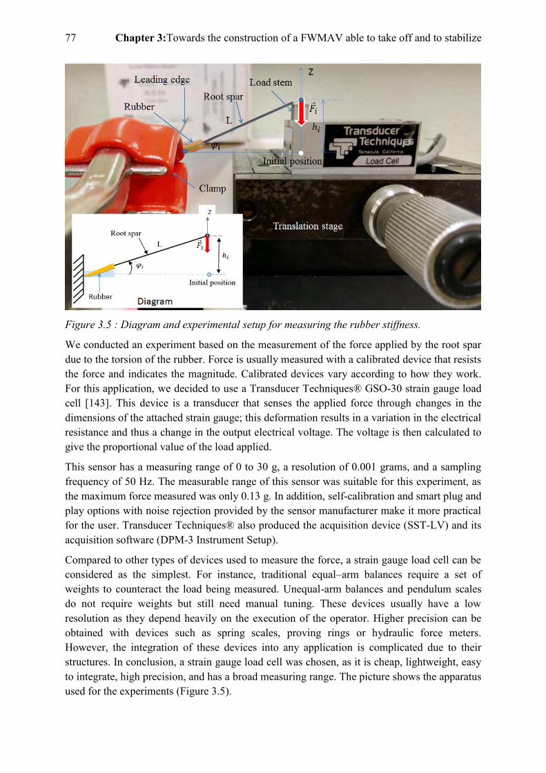
77 Chapter 3:Towards the construction of a FWMAV able to take off and to stabilize
Figure 3.5 : Diagram and experimental setup for measuring the rubber stiffness.
We conducted an experiment based on the measurement of the force applied by the root spar due to the torsion of the rubber. Force is usually measured with a calibrated device that resists the force and indicates the magnitude. Calibrated devices vary according to how they work. For this application, we decided to use a Transducer Techniques® GSO-30 strain gauge load cell [143]. This device is a transducer that senses the applied force through changes in the dimensions of the attached strain gauge; this deformation results in a variation in the electrical resistance and thus a change in the output electrical voltage. The voltage is then calculated to give the proportional value of the load applied.
This sensor has a measuring range of 0 to 30 g, a resolution of 0.001 grams, and a sampling frequency of 50 Hz. The measurable range of this sensor was suitable for this experiment, as the maximum force measured was only 0.13 g. In addition, self-calibration and smart plug and play options with noise rejection provided by the sensor manufacturer make it more practical for the user. Transducer Techniques® also produced the acquisition device (SST-LV) and its acquisition software (DPM-3 Instrument Setup).
Compared to other types of devices used to measure the force, a strain gauge load cell can be considered as the simplest. For instance, traditional equal–arm balances require a set of weights to counteract the load being measured. Unequal-arm balances and pendulum scales do not require weights but still need manual tuning. These devices usually have a low resolution as they depend heavily on the execution of the operator. Higher precision can be obtained with devices such as spring scales, proving rings or hydraulic force meters. However, the integration of these devices into any application is complicated due to their structures. In conclusion, a strain gauge load cell was chosen, as it is cheap, lightweight, easy to integrate, high precision, and has a broad measuring range. The picture shows the apparatus used for the experiments (Figure 3.5).
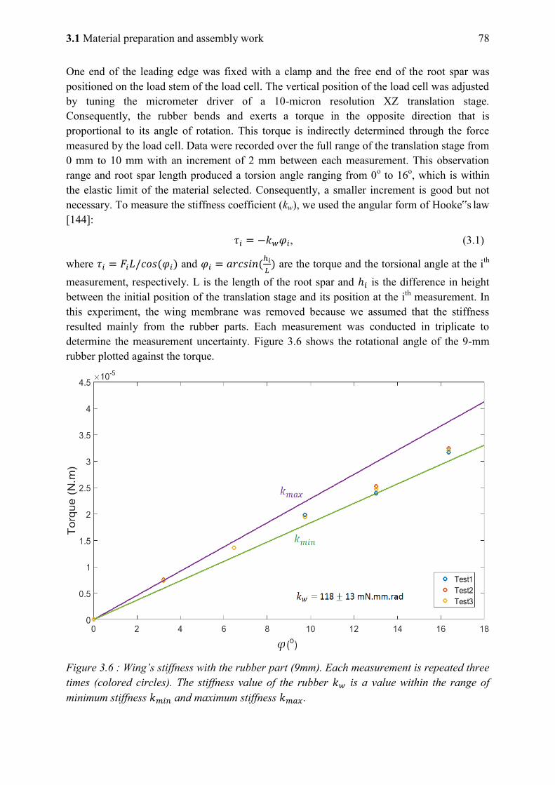
3.1 Material preparation and assembly work 78
One end of the leading edge was fixed with a clamp and the free end of the root spar was positioned on the load stem of the load cell. The vertical position of the load cell was adjusted by tuning the micrometer driver of a 10-micron resolution XZ translation stage. Consequently, the rubber bends and exerts a torque in the opposite direction that is proportional to its angle of rotation. This torque is indirectly determined through the force measured by the load cell. Data were recorded over the full range of the translation stage from 0 mm to 10 mm with an increment of 2 mm between each measurement. This observation range and root spar length produced a torsion angle ranging from 0o to 16o, which is within the elastic limit of the material selected. Consequently, a smaller increment is good but not necessary. To measure the stiffness coefficient (kw), we used the angular form of Hooke‟s law [144]:
, (3.1)
where and
are the torque and the torsional angle at the ith
measurement, respectively. L is the length of the root spar and is the difference in height between the initial position of the translation stage and its position at the ith measurement. In this experiment, the wing membrane was removed because we assumed that the stiffness resulted mainly from the rubber parts. Each measurement was conducted in triplicate to determine the measurement uncertainty. Figure 3.6 shows the rotational angle of the 9-mm rubber plotted against the torque.
Figure 3.6 : Wing’s stiffness with the rubber part (9mm). Each measurement is repeated three times (colored circles). The stiffness value of the rubber is a value within the range of minimum stiffness and maximum stiffness .
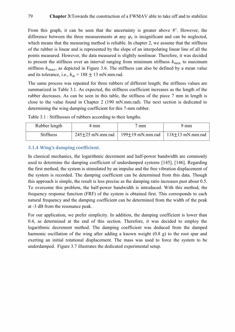
79 Chapter 3:Towards the construction of a FWMAV able to take off and to stabilize
From this graph, it can be seen that the uncertainty is greater above 8°. However, the difference between the three measurements at any is insignificant and can be neglected, which means that the measuring method is reliable. In chapter 2, we assume that the stiffness of the rubber is linear and is represented by the slope of an interpolating linear line of all the points measured. However, the data measured is slightly nonlinear. Therefore, it was decided to present the stiffness over an interval ranging from minimum stiffness to maximum stiffness , as depicted in Figure 3.6. The stiffness can also be defined by a mean value and its tolerance, i.e., = 188 13 mN.mm.rad.
The same process was repeated for three rubbers of different length; the stiffness values are summarized in Table 3.1. As expected, the stiffness coefficient increases as the length of the rubber decreases. As can be seen in this table, the stiffness of the piece 7 mm in length is close to the value found in Chapter 2 (190 mN.mm.rad). The next section is dedicated to determining the wing damping coefficient for this 7-mm rubber.
Table 3.1 : Stiffnesses of rubbers according to their lengths.
Rubber length 4 mm 7 mm 9 mm
Stiffness 245 25 mN.mm.rad 199 19 mN.mm.rad 118 13 mN.mm.rad
3.1.4 Wing’s damping coefficient.
In classical mechanics, the logarithmic decrement and half-power bandwidth are commonly used to determine the damping coefficient of underdamped systems [145], [146]. Regarding the first method, the system is stimulated by an impulse and the free vibration displacement of the system is recorded. The damping coefficient can be determined from this data. Though this approach is simple, the result is less precise as the damping ratio increases past about 0.5. To overcome this problem, the half-power bandwidth is introduced. With this method, the frequency response function (FRF) of the system is obtained first. This corresponds to each natural frequency and the damping coefficient can be determined from the width of the peak at -3 dB from the resonance peak.
For our application, we prefer simplicity. In addition, the damping coefficient is lower than 0.4, as determined at the end of this section. Therefore, it was decided to employ the logarithmic decrement method. The damping coefficient was deduced from the damped harmonic oscillation of the wing after adding a known weight (0.8 g) to the root spar and exerting an initial rotational displacement. The mass was used to force the system to be underdamped. Figure 3.7 illustrates the dedicated experimental setup.
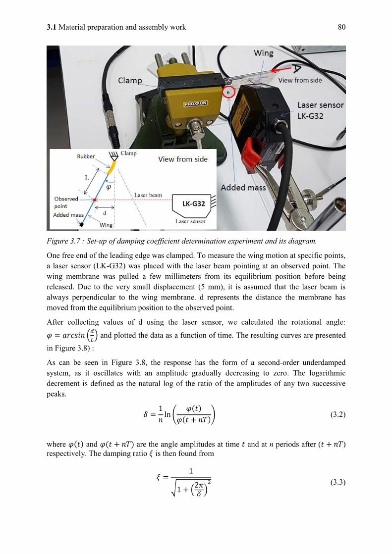
3.1 Material preparation and assembly work 80
Figure 3.7 : Set-up of damping coefficient determination experiment and its diagram.
One free end of the leading edge was clamped. To measure the wing motion at specific points, a laser sensor (LK-G32) was placed with the laser beam pointing at an observed point. The wing membrane was pulled a few millimeters from its equilibrium position before being released. Due to the very small displacement (5 mm), it is assumed that the laser beam is always perpendicular to the wing membrane. d represents the distance the membrane has moved from the equilibrium position to the observed point.
After collecting values of d using the laser sensor, we calculated the rotational angle:
(
) and plotted the data as a function of time. The resulting curves are presented
in Figure 3.8) :
As can be seen in Figure 3.8, the response has the form of a second-order underdamped system, as it oscillates with an amplitude gradually decreasing to zero. The logarithmic decrement is defined as the natural log of the ratio of the amplitudes of any two successive peaks.
(
) (3.2)
where and are the angle amplitudes at time and at n periods after ( ) respectively. The damping ratio is then found from
√ (
) (3.3)
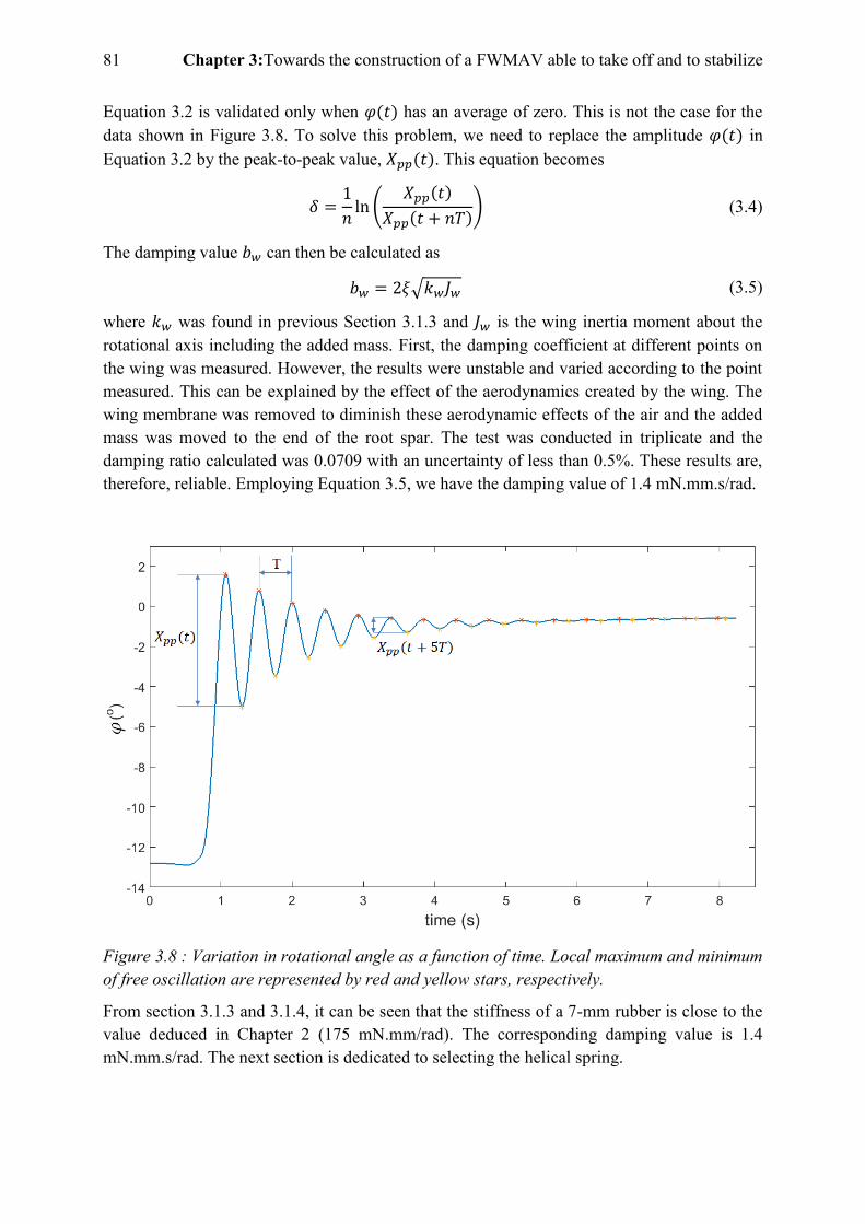
81 Chapter 3:Towards the construction of a FWMAV able to take off and to stabilize
Equation 3.2 is validated only when has an average of zero. This is not the case for the data shown in Figure 3.8. To solve this problem, we need to replace the amplitude in Equation 3.2 by the peak-to-peak value, . This equation becomes
(
) (3.4)
The damping value can then be calculated as
√ (3.5)
where was found in previous Section 3.1.3 and is the wing inertia moment about the rotational axis including the added mass. First, the damping coefficient at different points on the wing was measured. However, the results were unstable and varied according to the point measured. This can be explained by the effect of the aerodynamics created by the wing. The wing membrane was removed to diminish these aerodynamic effects of the air and the added mass was moved to the end of the root spar. The test was conducted in triplicate and the damping ratio calculated was 0.0709 with an uncertainty of less than 0.5%. These results are, therefore, reliable. Employing Equation 3.5, we have the damping value of 1.4 mN.mm.s/rad.
Figure 3.8 : Variation in rotational angle as a function of time. Local maximum and minimum of free oscillation are represented by red and yellow stars, respectively.
From section 3.1.3 and 3.1.4, it can be seen that the stiffness of a 7-mm rubber is close to the value deduced in Chapter 2 (175 mN.mm/rad). The corresponding damping value is 1.4 mN.mm.s/rad. The next section is dedicated to selecting the helical spring.
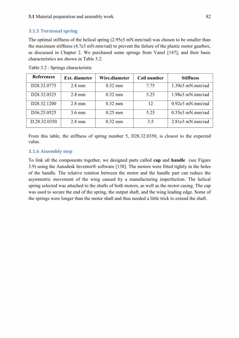
3.1 Material preparation and assembly work 82
3.1.5 Torsional spring
The optimal stiffness of the helical spring (2.95e3 mN.mm/rad) was chosen to be smaller than the maximum stiffness (4.7e3 mN.mm/rad) to prevent the failure of the plastic motor gearbox, as discussed in Chapter 2. We purchased some springs from Vanel [147], and their basic characteristics are shown in Table 3.2.
Table 3.2 : Springs characteristic
References Ext. diameter Wire.diameter Coil number Stiffness D28.32.0775 2.8 mm 0.32 mm 7.75 1.39e3 mN.mm/rad
D28.32.0525 2.8 mm 0.32 mm 5.25 1.98e3 mN.mm/rad
D28.32.1200 2.8 mm 0.32 mm 12 0.92e3 mN.mm/rad
D36.25.0525 3.6 mm 0.25 mm 5.25 0.55e3 mN.mm/rad
D.28.32.0350 2.8 mm 0.32 mm 3.5 2.81e3 mN.mm/rad
From this table, the stiffness of spring number 5, D28.32.0350, is closest to the expected value.
3.1.6 Assembly step
To link all the components together, we designed parts called cap and handle (see Figure 3.9) using the Autodesk Inventor® software [138]. The motors were fitted tightly in the holes of the handle. The relative rotation between the motor and the handle part can reduce the asymmetric movement of the wing caused by a manufacturing imperfection. The helical spring selected was attached to the shafts of both motors, as well as the motor casing. The cap was used to secure the end of the spring, the output shaft, and the wing leading edge. Some of the springs were longer than the motor shaft and thus needed a little trick to extend the shaft.
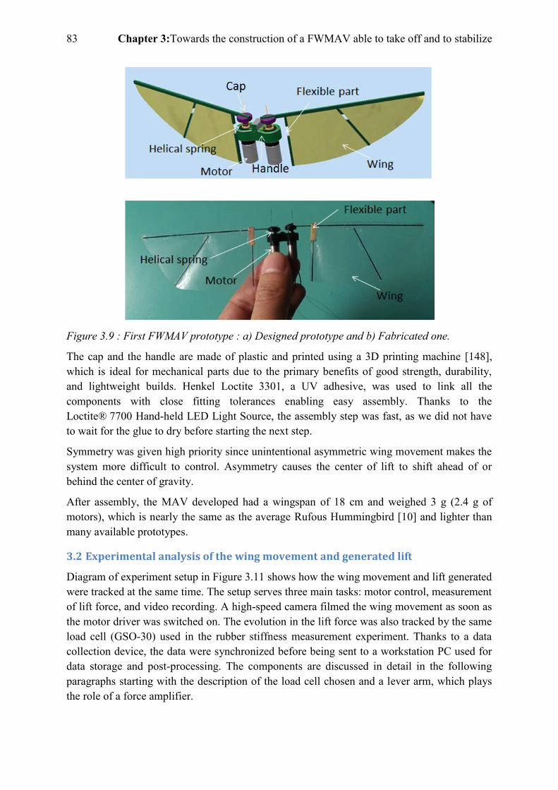
83 Chapter 3:Towards the construction of a FWMAV able to take off and to stabilize
Figure 3.9 : First FWMAV prototype : a) Designed prototype and b) Fabricated one.
The cap and the handle are made of plastic and printed using a 3D printing machine [148], which is ideal for mechanical parts due to the primary benefits of good strength, durability, and lightweight builds. Henkel Loctite 3301, a UV adhesive, was used to link all the components with close fitting tolerances enabling easy assembly. Thanks to the Loctite® 7700 Hand-held LED Light Source, the assembly step was fast, as we did not have to wait for the glue to dry before starting the next step.
Symmetry was given high priority since unintentional asymmetric wing movement makes the system more difficult to control. Asymmetry causes the center of lift to shift ahead of or behind the center of gravity.
After assembly, the MAV developed had a wingspan of 18 cm and weighed 3 g (2.4 g of motors), which is nearly the same as the average Rufous Hummingbird [10] and lighter than many available prototypes.
3.2 Experimental analysis of the wing movement and generated lift
Diagram of experiment setup in Figure 3.11 shows how the wing movement and lift generated were tracked at the same time. The setup serves three main tasks: motor control, measurement of lift force, and video recording. A high-speed camera filmed the wing movement as soon as the motor driver was switched on. The evolution in the lift force was also tracked by the same load cell (GSO-30) used in the rubber stiffness measurement experiment. Thanks to a data collection device, the data were synchronized before being sent to a workstation PC used for data storage and post-processing. The components are discussed in detail in the following paragraphs starting with the description of the load cell chosen and a lever arm, which plays the role of a force amplifier.
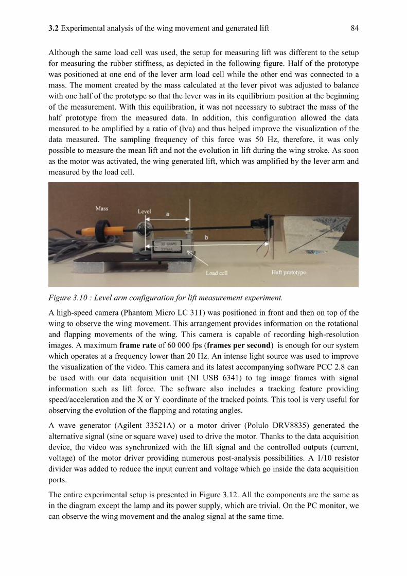
3.2 Experimental analysis of the wing movement and generated lift 84
Although the same load cell was used, the setup for measuring lift was different to the setup for measuring the rubber stiffness, as depicted in the following figure. Half of the prototype was positioned at one end of the lever arm load cell while the other end was connected to a mass. The moment created by the mass calculated at the lever pivot was adjusted to balance with one half of the prototype so that the lever was in its equilibrium position at the beginning of the measurement. With this equilibration, it was not necessary to subtract the mass of the half prototype from the measured data. In addition, this configuration allowed the data measured to be amplified by a ratio of (b/a) and thus helped improve the visualization of the data measured. The sampling frequency of this force was 50 Hz, therefore, it was only possible to measure the mean lift and not the evolution in lift during the wing stroke. As soon as the motor was activated, the wing generated lift, which was amplified by the lever arm and measured by the load cell.
Figure 3.10 : Level arm configuration for lift measurement experiment.
A high-speed camera (Phantom Micro LC 311) was positioned in front and then on top of the wing to observe the wing movement. This arrangement provides information on the rotational and flapping movements of the wing. This camera is capable of recording high-resolution images. A maximum frame rate of 60 000 fps (frames per second) is enough for our system which operates at a frequency lower than 20 Hz. An intense light source was used to improve the visualization of the video. This camera and its latest accompanying software PCC 2.8 can be used with our data acquisition unit (NI USB 6341) to tag image frames with signal information such as lift force. The software also includes a tracking feature providing speed/acceleration and the X or Y coordinate of the tracked points. This tool is very useful for observing the evolution of the flapping and rotating angles.
A wave generator (Agilent 33521A) or a motor driver (Polulo DRV8835) generated the alternative signal (sine or square wave) used to drive the motor. Thanks to the data acquisition device, the video was synchronized with the lift signal and the controlled outputs (current, voltage) of the motor driver providing numerous post-analysis possibilities. A 1/10 resistor divider was added to reduce the input current and voltage which go inside the data acquisition ports.
The entire experimental setup is presented in Figure 3.12. All the components are the same as in the diagram except the lamp and its power supply, which are trivial. On the PC monitor, we can observe the wing movement and the analog signal at the same time.
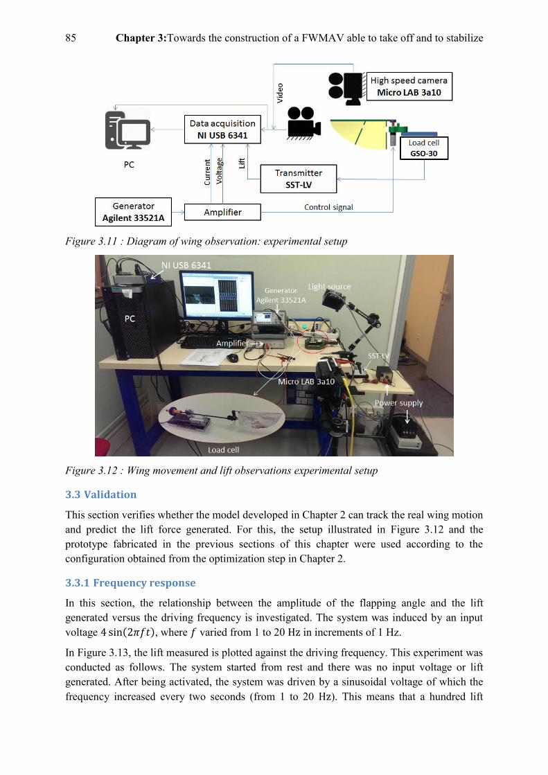
85 Chapter 3:Towards the construction of a FWMAV able to take off and to stabilize
Figure 3.11 : Diagram of wing observation: experimental setup
Figure 3.12 : Wing movement and lift observations experimental setup
3.3 Validation
This section verifies whether the model developed in Chapter 2 can track the real wing motion and predict the lift force generated. For this, the setup illustrated in Figure 3.12 and the prototype fabricated in the previous sections of this chapter were used according to the configuration obtained from the optimization step in Chapter 2.
3.3.1 Frequency response
In this section, the relationship between the amplitude of the flapping angle and the lift generated versus the driving frequency is investigated. The system was induced by an input voltage , where varied from 1 to 20 in increments of 1 Hz.
In Figure 3.13, the lift measured is plotted against the driving frequency. This experiment was conducted as follows. The system started from rest and there was no input voltage or lift generated. After being activated, the system was driven by a sinusoidal voltage of which the frequency increased every two seconds (from 1 to 20 ). This means that a hundred lift
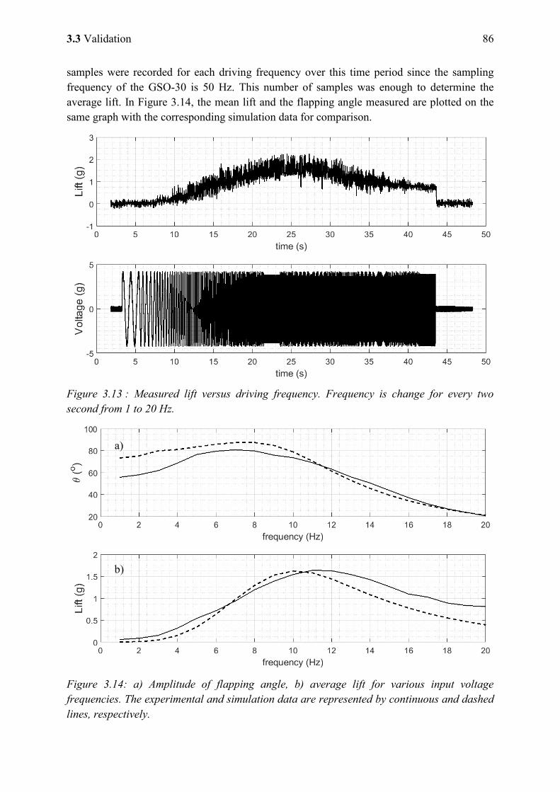
3.3 Validation 86
samples were recorded for each driving frequency over this time period since the sampling frequency of the GSO-30 is 50 Hz. This number of samples was enough to determine the average lift. In Figure 3.14, the mean lift and the flapping angle measured are plotted on the same graph with the corresponding simulation data for comparison.
Figure 3.13 : Measured lift versus driving frequency. Frequency is change for every two second from 1 to 20 Hz.
Figure 3.14: a) Amplitude of flapping angle, b) average lift for various input voltage frequencies. The experimental and simulation data are represented by continuous and dashed lines, respectively.
a)
b)
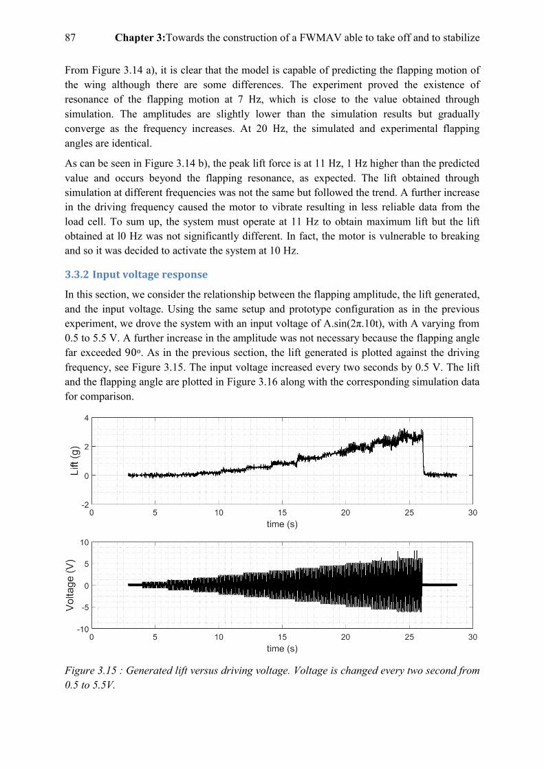
87 Chapter 3:Towards the construction of a FWMAV able to take off and to stabilize
From Figure 3.14 a), it is clear that the model is capable of predicting the flapping motion of the wing although there are some differences. The experiment proved the existence of resonance of the flapping motion at 7 , which is close to the value obtained through simulation. The amplitudes are slightly lower than the simulation results but gradually converge as the frequency increases. At 20 , the simulated and experimental flapping angles are identical.
As can be seen in Figure 3.14 b), the peak lift force is at 11 , 1 higher than the predicted value and occurs beyond the flapping resonance, as expected. The lift obtained through simulation at different frequencies was not the same but followed the trend. A further increase in the driving frequency caused the motor to vibrate resulting in less reliable data from the load cell. To sum up, the system must operate at 11 Hz to obtain maximum lift but the lift obtained at l0 Hz was not significantly different. In fact, the motor is vulnerable to breaking and so it was decided to activate the system at 10 Hz.
3.3.2 Input voltage response
In this section, we consider the relationship between the flapping amplitude, the lift generated, and the input voltage. Using the same setup and prototype configuration as in the previous experiment, we drove the system with an input voltage of A.sin(2π.10t), with A varying from 0.5 to 5.5 V. A further increase in the amplitude was not necessary because the flapping angle far exceeded 90o. As in the previous section, the lift generated is plotted against the driving frequency, see Figure 3.15. The input voltage increased every two seconds by 0.5 V. The lift and the flapping angle are plotted in Figure 3.16 along with the corresponding simulation data for comparison.
Figure 3.15 : Generated lift versus driving voltage. Voltage is changed every two second from 0.5 to 5.5V.
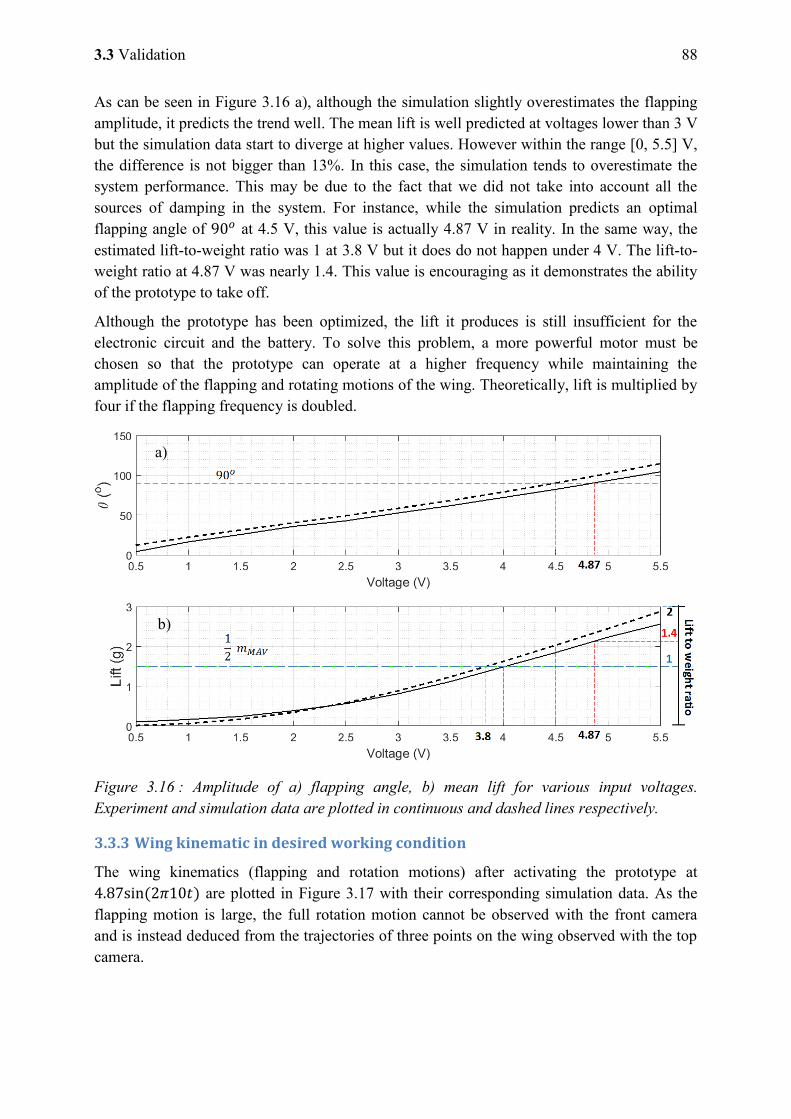
3.3 Validation 88
As can be seen in Figure 3.16 a), although the simulation slightly overestimates the flapping amplitude, it predicts the trend well. The mean lift is well predicted at voltages lower than 3 V but the simulation data start to diverge at higher values. However within the range [0, 5.5] V, the difference is not bigger than 13%. In this case, the simulation tends to overestimate the system performance. This may be due to the fact that we did not take into account all the sources of damping in the system. For instance, while the simulation predicts an optimal flapping angle of at 4.5 V, this value is actually 4.87 V in reality. In the same way, the estimated lift-to-weight ratio was 1 at 3.8 V but it does do not happen under 4 V. The lift-to-weight ratio at 4.87 V was nearly 1.4. This value is encouraging as it demonstrates the ability of the prototype to take off.
Although the prototype has been optimized, the lift it produces is still insufficient for the electronic circuit and the battery. To solve this problem, a more powerful motor must be chosen so that the prototype can operate at a higher frequency while maintaining the amplitude of the flapping and rotating motions of the wing. Theoretically, lift is multiplied by four if the flapping frequency is doubled.
Figure 3.16 : Amplitude of a) flapping angle, b) mean lift for various input voltages. Experiment and simulation data are plotted in continuous and dashed lines respectively.
3.3.3 Wing kinematic in desired working condition
The wing kinematics (flapping and rotation motions) after activating the prototype at are plotted in Figure 3.17 with their corresponding simulation data. As the flapping motion is large, the full rotation motion cannot be observed with the front camera and is instead deduced from the trajectories of three points on the wing observed with the top camera.
b)
a)
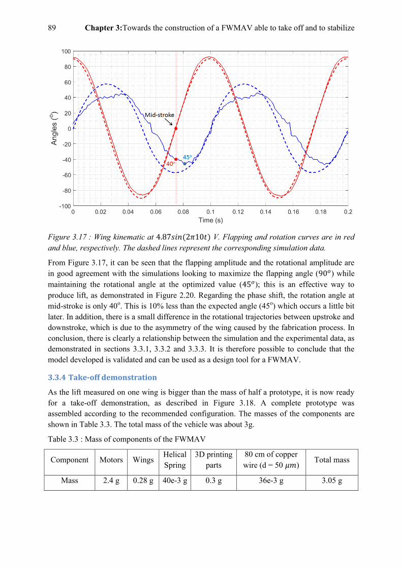
89 Chapter 3:Towards the construction of a FWMAV able to take off and to stabilize
Figure 3.17 : Wing kinematic at V. Flapping and rotation curves are in red and blue, respectively. The dashed lines represent the corresponding simulation data.
From Figure 3.17, it can be seen that the flapping amplitude and the rotational amplitude are in good agreement with the simulations looking to maximize the flapping angle ( ) while maintaining the rotational angle at the optimized value ( ); this is an effective way to produce lift, as demonstrated in Figure 2.20. Regarding the phase shift, the rotation angle at mid-stroke is only 40o. This is 10% less than the expected angle (45o) which occurs a little bit later. In addition, there is a small difference in the rotational trajectories between upstroke and downstroke, which is due to the asymmetry of the wing caused by the fabrication process. In conclusion, there is clearly a relationship between the simulation and the experimental data, as demonstrated in sections 3.3.1, 3.3.2 and 3.3.3. It is therefore possible to conclude that the model developed is validated and can be used as a design tool for a FWMAV.
3.3.4 Take-off demonstration
As the lift measured on one wing is bigger than the mass of half a prototype, it is now ready for a take-off demonstration, as described in Figure 3.18. A complete prototype was assembled according to the recommended configuration. The masses of the components are shown in Table 3.3. The total mass of the vehicle was about 3g.
Table 3.3 : Mass of components of the FWMAV
Component Motors Wings Helical Spring
3D printing parts
80 cm of copper wire (d = 50 )
Total mass
Mass 2.4 g 0.28 g 40e-3 g 0.3 g 36e-3 g 3.05 g
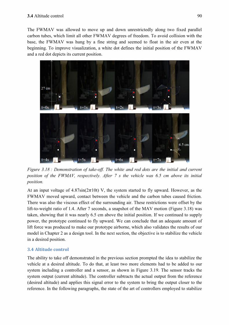
3.4 Altitude control 90
The FWMAV was allowed to move up and down unrestrictedly along two fixed parallel carbon tubes, which limit all other FWMAV degrees of freedom. To avoid collision with the base, the FWMAV was hung by a fine string and seemed to float in the air even at the beginning. To improve visualization, a white dot defines the initial position of the FWMAV and a red dot depicts its current position.
Figure 3.18 : Demonstration of take-off. The white and red dots are the initial and current position of the FWMAV, respectively. After 7 s the vehicle was 6.5 cm above its initial position.
At an input voltage of 4.87sin(2 10t) V, the system started to fly upward. However, as the FWMAV moved upward, contact between the vehicle and the carbon tubes caused friction. There was also the viscous effect of the surrounding air. These restrictions were offset by the lift-to-weight ratio of 1.4. After 7 seconds, a snapshot of the MAV motion (Figure 3.18) was taken, showing that it was nearly 6.5 cm above the initial position. If we continued to supply power, the prototype continued to fly upward. We can conclude that an adequate amount of lift force was produced to make our prototype airborne, which also validates the results of our model in Chapter 2 as a design tool. In the next section, the objective is to stabilize the vehicle in a desired position.
3.4 Altitude control
The ability to take off demonstrated in the previous section prompted the idea to stabilize the vehicle at a desired altitude. To do that, at least two more elements had to be added to our system including a controller and a sensor, as shown in Figure 3.19. The sensor tracks the system output (current altitude). The controller subtracts the actual output from the reference (desired altitude) and applies this signal error to the system to bring the output closer to the reference. In the following paragraphs, the state of the art of controllers employed to stabilize
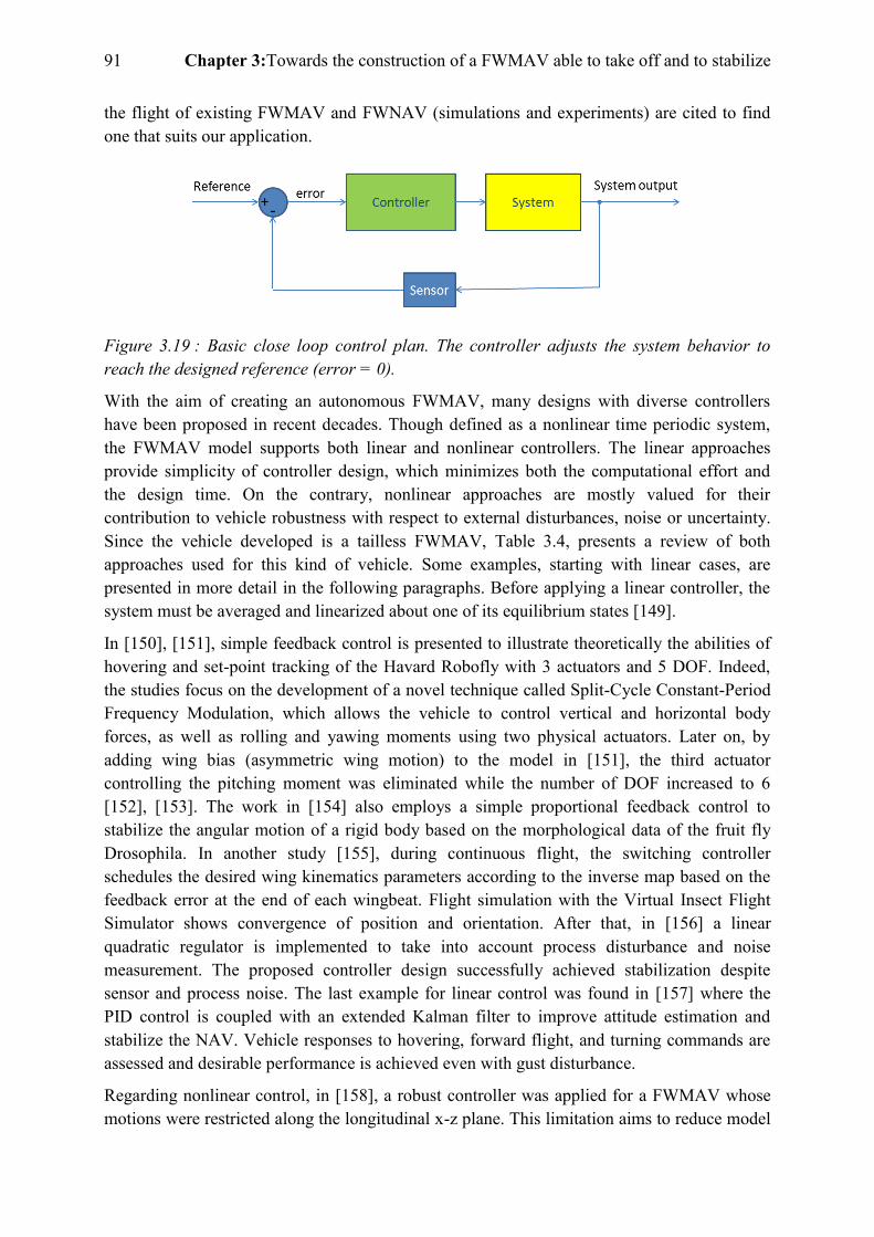
91 Chapter 3:Towards the construction of a FWMAV able to take off and to stabilize
the flight of existing FWMAV and FWNAV (simulations and experiments) are cited to find one that suits our application.
Figure 3.19 : Basic close loop control plan. The controller adjusts the system behavior to reach the designed reference (error = 0).
With the aim of creating an autonomous FWMAV, many designs with diverse controllers have been proposed in recent decades. Though defined as a nonlinear time periodic system, the FWMAV model supports both linear and nonlinear controllers. The linear approaches provide simplicity of controller design, which minimizes both the computational effort and the design time. On the contrary, nonlinear approaches are mostly valued for their contribution to vehicle robustness with respect to external disturbances, noise or uncertainty. Since the vehicle developed is a tailless FWMAV, Table 3.4, presents a review of both approaches used for this kind of vehicle. Some examples, starting with linear cases, are presented in more detail in the following paragraphs. Before applying a linear controller, the system must be averaged and linearized about one of its equilibrium states [149].
In [150], [151], simple feedback control is presented to illustrate theoretically the abilities of hovering and set-point tracking of the Havard Robofly with 3 actuators and 5 DOF. Indeed, the studies focus on the development of a novel technique called Split-Cycle Constant-Period Frequency Modulation, which allows the vehicle to control vertical and horizontal body forces, as well as rolling and yawing moments using two physical actuators. Later on, by adding wing bias (asymmetric wing motion) to the model in [151], the third actuator controlling the pitching moment was eliminated while the number of DOF increased to 6 [152], [153]. The work in [154] also employs a simple proportional feedback control to stabilize the angular motion of a rigid body based on the morphological data of the fruit fly Drosophila. In another study [155], during continuous flight, the switching controller schedules the desired wing kinematics parameters according to the inverse map based on the feedback error at the end of each wingbeat. Flight simulation with the Virtual Insect Flight Simulator shows convergence of position and orientation. After that, in [156] a linear quadratic regulator is implemented to take into account process disturbance and noise measurement. The proposed controller design successfully achieved stabilization despite sensor and process noise. The last example for linear control was found in [157] where the PID control is coupled with an extended Kalman filter to improve attitude estimation and stabilize the NAV. Vehicle responses to hovering, forward flight, and turning commands are assessed and desirable performance is achieved even with gust disturbance.
Regarding nonlinear control, in [158], a robust controller was applied for a FWMAV whose motions were restricted along the longitudinal x-z plane. This limitation aims to reduce model
3.4 Altitude control 92
complexity to illustrate issues relating to wing flapping control that stem from the peculiar characteristics of the actuation mechanism control. The controller enables the vehicle to follow a set of points in about one minute. In [159], the study introduces bounded state feedback nonlinear control laws applied to stabilize a FWMAV in the desired hovering position. The robustness of this control is proved with tests which take into account the aerodynamic coefficients and external disturbance. In [160], the authors push the control methodology further by decomposing the system into a nominal model, and structured and unstructured uncertainties, and then designing three corresponding controllers: direct feedback, adaptive, and robust. The Lyapunov theorem and numerical simulations confirmed the validity of such an advanced controller in which the conversion of flight attitudes can be carried out by adjusting the relevant parameters of the dynamic models. Likewise, for a class of uncertain nonlinear systems whose threshold value of lumped disturbance is difficult to measure in practice, a recurrent cerebellar model articulation controller is proposed as an observer to approximate this disturbance in real time [161]. As in [160], the system is divided into a nominal model and a lumped disturbance term comprising modeling error, parameter uncertainties, disturbances, and unmodeled dynamics. Adaptive control, robust control, and sliding mode control were adopted to handle these system components. The asymptotic stability was proved based on the Lyapunov stability theory, and simulation results of micro flying robot attitude control indicated that the algorithm proposed improves transient performance and robustness. While the control strategies listed above are all theoretically proven through simulations, adaptive control in [162] is applied directly to a real FWNAV called Robobee from Havard Microrobotics Laboratory. In the experiment, eight high-speed cameras were used to provide position and orientation feedback for the controller. Although there is a delay of 0.2 s after the controller is activated, the vehicle successfully reaches a set position and achieves vertical take-off and landing.
Regarding our application, which is similar to the case of Hines at al. [163], five out of six DOF were blocked and only the vertical translation was free. The experiments were always conducted in a closed room; there were no disturbances such as gusts of wind or raindrops. Furthermore, the stroke amplitude, the unique control parameter, was directly manipulated by the input voltage amplitude generated by a high-quality motor driver. Consequently, there was no issue with input noise. In such a simple situation, a linear controller such as a PID is sufficient.
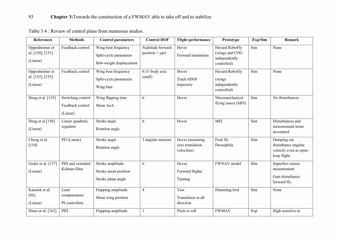
93 Chapter 3:Towards the construction of a FWMAV able to take off and to stabilize
Table 3.4 : Review of control plans from numerous studies.
References Methods Control parameters Control DOF Flight performance Prototype Exp/Sim Remark
Oppenheimer et al. [150], [151]
(Linear)
Feedback control Wing beat frequency
Split-cycle parameters
Bob-weight displacement
5(altitude forward position + ypr)
Hover
Forward translation
Havard RoboFly (wings and COG independently controlled)
Sim None
Oppenheimer et al. [152], [153]
(Linear)
Feedback control Wing beat frequency
Split-cycle parameters
Wing bias
6 (Y-body axis small)
Hover
Track 6DOF trajectory
Havard RoboFly
(wings independently controlled)
Sim None
Deng et al. [155] Switching control
Feedback control
(Linear)
Wing flipping time
Mean AoA
6 Hover Micromechanical flying insect (MFI)
Sim No disturbances
Deng et al.[156]
(Linear)
Linear quadratic regulator
Stroke angle
Rotation angle
6 Hover MFI Sim Disturbances and measurement noise accounted
Cheng et al. [154]
PD (Linear) Stroke angle
Rotation angle
3 angular motions Hover (assuming zero translation velocities)
Fruit fly Drosophila
Sim Damping out disturbance angular velocity even in open-loop flight.
Geder et al. [157]
(Linear)
PID and extended Kalman filter
Stroke amplitude
Stroke mean position
Stroke plane angle
6 Hover
Forward flights
Turning
FWNAV model Sim Imperfect sensor measurement
Gust disturbance forward fly.
Karasek et al. [86]
(Linear)
Lead compensators
PI controllers
Flapping amplitude
Mean wing position
4 Yaw
Translation in all direction
Humming bird Sim None
Hines at al. [163] PID Flapping amplitude 1 Pitch or roll FWMAV Exp High sensitive to
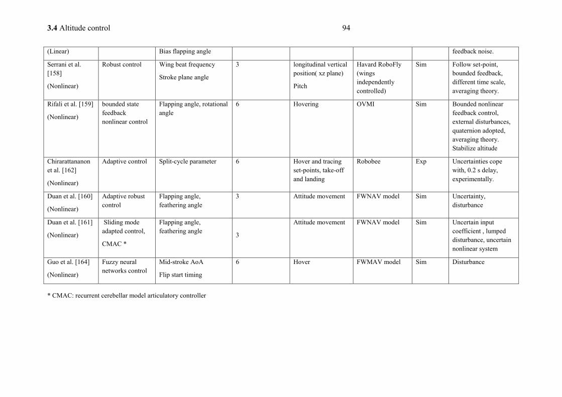
3.4 Altitude control 94
(Linear) Bias flapping angle feedback noise.
Serrani et al. [158]
(Nonlinear)
Robust control Wing beat frequency
Stroke plane angle
3 longitudinal vertical position( xz plane)
Pitch
Havard RoboFly (wings independently controlled)
Sim Follow set-point, bounded feedback, different time scale, averaging theory.
Rifali et al. [159]
(Nonlinear)
bounded state feedback nonlinear control
Flapping angle, rotational angle
6 Hovering OVMI Sim Bounded nonlinear feedback control, external disturbances, quaternion adopted, averaging theory. Stabilize altitude
Chirarattananon et al. [162]
(Nonlinear)
Adaptive control Split-cycle parameter 6 Hover and tracing set-points, take-off and landing
Robobee Exp Uncertainties cope with, 0.2 s delay, experimentally.
Duan et al. [160]
(Nonlinear)
Adaptive robust control
Flapping angle, feathering angle
3 Attitude movement FWNAV model Sim Uncertainty, disturbance
Duan et al. [161]
(Nonlinear)
Sliding mode adapted control,
CMAC *
Flapping angle, feathering angle
3
Attitude movement FWNAV model Sim Uncertain input coefficient , lumped disturbance, uncertain nonlinear system
Guo et al. [164]
(Nonlinear)
Fuzzy neural networks control
Mid-stroke AoA
Flip start timing
6 Hover FWMAV model Sim Disturbance
* CMAC: recurrent cerebellar model articulatory controller
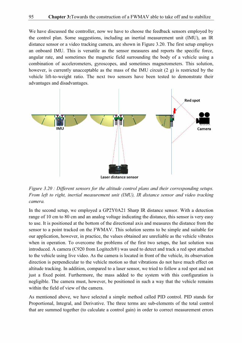
95 Chapter 3:Towards the construction of a FWMAV able to take off and to stabilize
We have discussed the controller, now we have to choose the feedback sensors employed by the control plan. Some suggestions, including an inertial measurement unit (IMU), an IR distance sensor or a video tracking camera, are shown in Figure 3.20. The first setup employs an onboard IMU. This is versatile as the sensor measures and reports the specific force, angular rate, and sometimes the magnetic field surrounding the body of a vehicle using a combination of accelerometers, gyroscopes, and sometimes magnetometers. This solution, however, is currently unacceptable as the mass of the IMU circuit (2 g) is restricted by the vehicle lift-to-weight ratio. The next two sensors have been tested to demonstrate their advantages and disadvantages.
Figure 3.20 : Different sensors for the altitude control plans and their corresponding setups. From left to right, inertial measurement unit (IMU), IR distance sensor and video tracking camera.
In the second setup, we employed a GP2Y0A21 Sharp IR distance sensor. With a detection range of 10 cm to 80 cm and an analog voltage indicating the distance, this sensor is very easy to use. It is positioned at the bottom of the directional axis and measures the distance from the sensor to a point tracked on the FWMAV. This solution seems to be simple and suitable for our application, however, in practice, the values obtained are unreliable as the vehicle vibrates when in operation. To overcome the problems of the first two setups, the last solution was introduced. A camera (C920 from Logitech®) was used to detect and track a red spot attached to the vehicle using live video. As the camera is located in front of the vehicle, its observation direction is perpendicular to the vehicle motion so that vibrations do not have much effect on altitude tracking. In addition, compared to a laser sensor, we tried to follow a red spot and not just a fixed point. Furthermore, the mass added to the system with this configuration is negligible. The camera must, however, be positioned in such a way that the vehicle remains within the field of view of the camera.
As mentioned above, we have selected a simple method called PID control. PID stands for Proportional, Integral, and Derivative. The three terms are sub-elements of the total control that are summed together (to calculate a control gain) in order to correct measurement errors
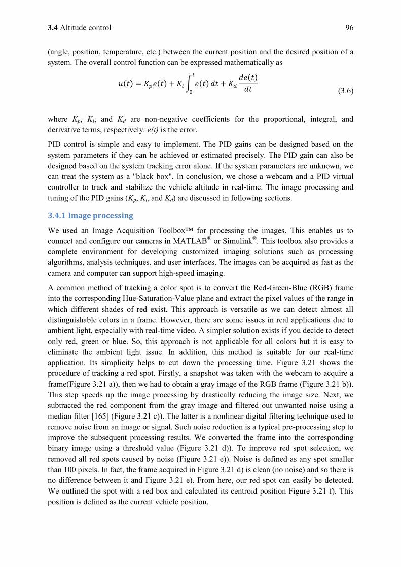
3.4 Altitude control 96
(angle, position, temperature, etc.) between the current position and the desired position of a system. The overall control function can be expressed mathematically as
∫
(3.6)
where Kp, Ki, and Kd are non-negative coefficients for the proportional, integral, and derivative terms, respectively. e(t) is the error.
PID control is simple and easy to implement. The PID gains can be designed based on the system parameters if they can be achieved or estimated precisely. The PID gain can also be designed based on the system tracking error alone. If the system parameters are unknown, we can treat the system as a "black box". In conclusion, we chose a webcam and a PID virtual controller to track and stabilize the vehicle altitude in real-time. The image processing and tuning of the PID gains (Kp, Ki, and Kd) are discussed in following sections.
3.4.1 Image processing
We used an Image Acquisition Toolbox™ for processing the images. This enables us to connect and configure our cameras in MATLAB® or Simulink®. This toolbox also provides a complete environment for developing customized imaging solutions such as processing algorithms, analysis techniques, and user interfaces. The images can be acquired as fast as the camera and computer can support high-speed imaging.
A common method of tracking a color spot is to convert the Red-Green-Blue (RGB) frame into the corresponding Hue-Saturation-Value plane and extract the pixel values of the range in which different shades of red exist. This approach is versatile as we can detect almost all distinguishable colors in a frame. However, there are some issues in real applications due to ambient light, especially with real-time video. A simpler solution exists if you decide to detect only red, green or blue. So, this approach is not applicable for all colors but it is easy to eliminate the ambient light issue. In addition, this method is suitable for our real-time application. Its simplicity helps to cut down the processing time. Figure 3.21 shows the procedure of tracking a red spot. Firstly, a snapshot was taken with the webcam to acquire a frame(Figure 3.21 a)), then we had to obtain a gray image of the RGB frame (Figure 3.21 b)). This step speeds up the image processing by drastically reducing the image size. Next, we subtracted the red component from the gray image and filtered out unwanted noise using a median filter [165] (Figure 3.21 c)). The latter is a nonlinear digital filtering technique used to remove noise from an image or signal. Such noise reduction is a typical pre-processing step to improve the subsequent processing results. We converted the frame into the corresponding binary image using a threshold value (Figure 3.21 d)). To improve red spot selection, we removed all red spots caused by noise (Figure 3.21 e)). Noise is defined as any spot smaller than 100 pixels. In fact, the frame acquired in Figure 3.21 d) is clean (no noise) and so there is no difference between it and Figure 3.21 e). From here, our red spot can easily be detected. We outlined the spot with a red box and calculated its centroid position Figure 3.21 f). This position is defined as the current vehicle position.
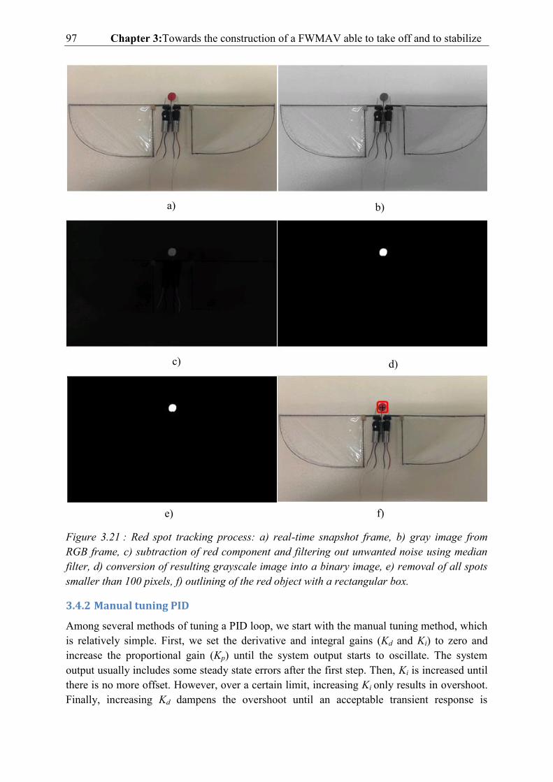
97 Chapter 3:Towards the construction of a FWMAV able to take off and to stabilize
Figure 3.21 : Red spot tracking process: a) real-time snapshot frame, b) gray image from RGB frame, c) subtraction of red component and filtering out unwanted noise using median filter, d) conversion of resulting grayscale image into a binary image, e) removal of all spots smaller than 100 pixels, f) outlining of the red object with a rectangular box.
3.4.2 Manual tuning PID
Among several methods of tuning a PID loop, we start with the manual tuning method, which is relatively simple. First, we set the derivative and integral gains (Kd and Ki) to zero and increase the proportional gain (Kp) until the system output starts to oscillate. The system output usually includes some steady state errors after the first step. Then, Ki is increased until there is no more offset. However, over a certain limit, increasing Ki only results in overshoot. Finally, increasing Kd dampens the overshoot until an acceptable transient response is
a) b)
c) d)
e) f)
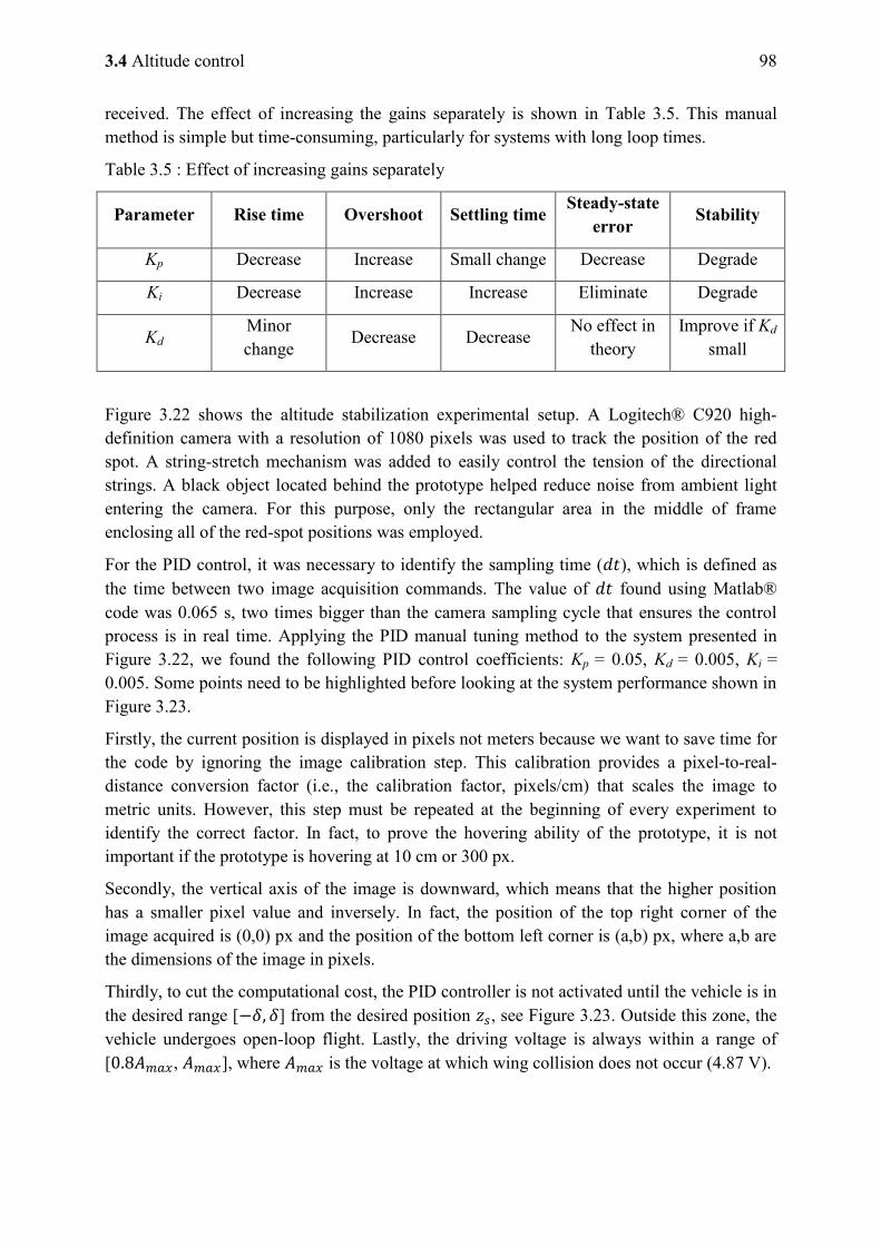
3.4 Altitude control 98
received. The effect of increasing the gains separately is shown in Table 3.5. This manual method is simple but time-consuming, particularly for systems with long loop times.
Table 3.5 : Effect of increasing gains separately
Parameter Rise time Overshoot Settling time Steady-state error
Stability
Kp Decrease Increase Small change Decrease Degrade
Ki Decrease Increase Increase Eliminate Degrade
Kd Minor change
Decrease Decrease No effect in
theory Improve if Kd
small
Figure 3.22 shows the altitude stabilization experimental setup. A Logitech® C920 high-definition camera with a resolution of 1080 pixels was used to track the position of the red spot. A string-stretch mechanism was added to easily control the tension of the directional strings. A black object located behind the prototype helped reduce noise from ambient light entering the camera. For this purpose, only the rectangular area in the middle of frame enclosing all of the red-spot positions was employed.
For the PID control, it was necessary to identify the sampling time ( ), which is defined as the time between two image acquisition commands. The value of found using Matlab® code was 0.065 s, two times bigger than the camera sampling cycle that ensures the control process is in real time. Applying the PID manual tuning method to the system presented in Figure 3.22, we found the following PID control coefficients: Kp = 0.05, Kd = 0.005, Ki = 0.005. Some points need to be highlighted before looking at the system performance shown in Figure 3.23.
Firstly, the current position is displayed in pixels not meters because we want to save time for the code by ignoring the image calibration step. This calibration provides a pixel-to-real-distance conversion factor (i.e., the calibration factor, pixels/cm) that scales the image to metric units. However, this step must be repeated at the beginning of every experiment to identify the correct factor. In fact, to prove the hovering ability of the prototype, it is not important if the prototype is hovering at 10 cm or 300 px.
Secondly, the vertical axis of the image is downward, which means that the higher position has a smaller pixel value and inversely. In fact, the position of the top right corner of the image acquired is (0,0) px and the position of the bottom left corner is (a,b) px, where a,b are the dimensions of the image in pixels.
Thirdly, to cut the computational cost, the PID controller is not activated until the vehicle is in the desired range [ ] from the desired position , see Figure 3.23. Outside this zone, the vehicle undergoes open-loop flight. Lastly, the driving voltage is always within a range of [ , ], where is the voltage at which wing collision does not occur (4.87 V).
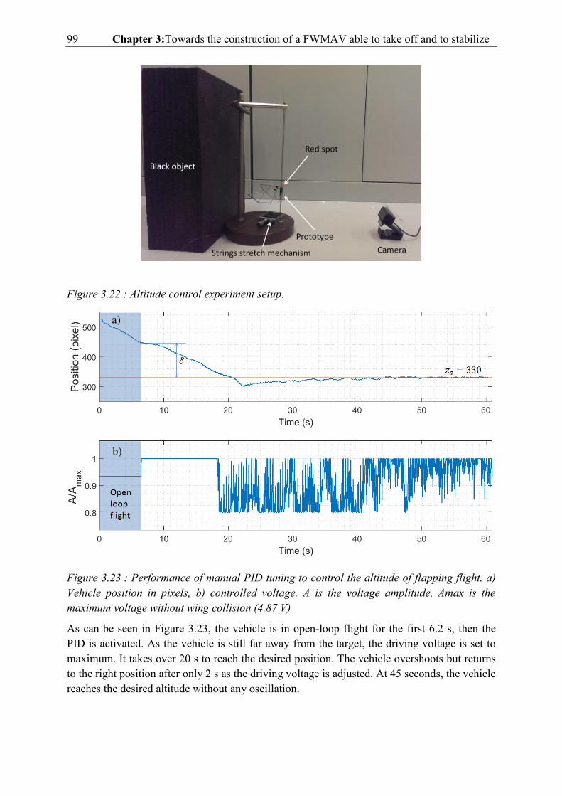
99 Chapter 3:Towards the construction of a FWMAV able to take off and to stabilize
Figure 3.22 : Altitude control experiment setup.
Figure 3.23 : Performance of manual PID tuning to control the altitude of flapping flight. a) Vehicle position in pixels, b) controlled voltage. A is the voltage amplitude, Amax is the maximum voltage without wing collision (4.87 V)
As can be seen in Figure 3.23, the vehicle is in open-loop flight for the first 6.2 s, then the PID is activated. As the vehicle is still far away from the target, the driving voltage is set to maximum. It takes over 20 s to reach the desired position. The vehicle overshoots but returns to the right position after only 2 s as the driving voltage is adjusted. At 45 seconds, the vehicle reaches the desired altitude without any oscillation.
a)
b)
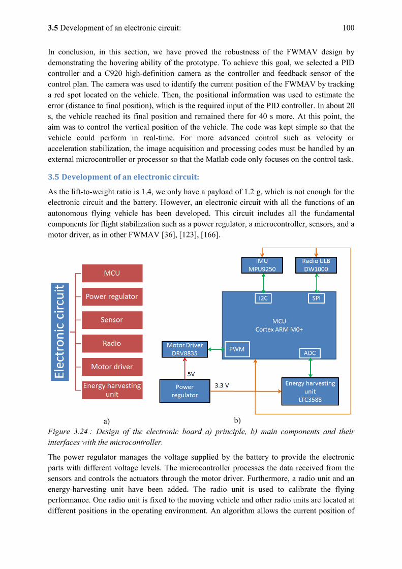
3.5 Development of an electronic circuit: 100
In conclusion, in this section, we have proved the robustness of the FWMAV design by demonstrating the hovering ability of the prototype. To achieve this goal, we selected a PID controller and a C920 high-definition camera as the controller and feedback sensor of the control plan. The camera was used to identify the current position of the FWMAV by tracking a red spot located on the vehicle. Then, the positional information was used to estimate the error (distance to final position), which is the required input of the PID controller. In about 20 s, the vehicle reached its final position and remained there for 40 s more. At this point, the aim was to control the vertical position of the vehicle. The code was kept simple so that the vehicle could perform in real-time. For more advanced control such as velocity or acceleration stabilization, the image acquisition and processing codes must be handled by an external microcontroller or processor so that the Matlab code only focuses on the control task.
3.5 Development of an electronic circuit:
As the lift-to-weight ratio is 1.4, we only have a payload of 1.2 g, which is not enough for the electronic circuit and the battery. However, an electronic circuit with all the functions of an autonomous flying vehicle has been developed. This circuit includes all the fundamental components for flight stabilization such as a power regulator, a microcontroller, sensors, and a motor driver, as in other FWMAV [36], [123], [166].
Figure 3.24 : Design of the electronic board a) principle, b) main components and their interfaces with the microcontroller.
The power regulator manages the voltage supplied by the battery to provide the electronic parts with different voltage levels. The microcontroller processes the data received from the sensors and controls the actuators through the motor driver. Furthermore, a radio unit and an energy-harvesting unit have been added. The radio unit is used to calibrate the flying performance. One radio unit is fixed to the moving vehicle and other radio units are located at different positions in the operating environment. An algorithm allows the current position of
a) b)
101 Chapter 3:Towards the construction of a FWMAV able to take off and to stabilize
the vehicle to be estimated based on the relative distances from the onboard radio unit with the other ones. This estimated location can then be compared with the real position of the vehicle to evaluate its performance. Concerning the energy-harvesting unit, as the power issue is crucial for the endurance of a micro-size flying vehicle, this unit must be able to collect free energy. Within the Clear flight project, work has been conducted on collecting energy from the ambient light or the deformation of the wing membrane.
Principle of the electronic circuit is shown in Figure 3.24 a). As the available weight and space on a FWMAV is always limited, the electronic parts selected need to be small, lightweight, and have a low power consumption but still satisfy the high accuracy and fast response requirements. The next section introduces all the components selected in detail.
3.5.1 Electronic components:
As mentioned above, the mass of the circuit is limited by the ability of the prototype to generate lift. In a recent, quick test, by changing the actuator and the plastic gearbox, the flapping frequency was doubled while maintaining the flapping angle. Theoretically, four times more lift could be achieved compared with the previous prototype. The new prototype is, of course, heavier but we do have extra weight for the electronic circuit and the battery (less than 6 g). To sum up, the mass of the electronic circuit must not exceed 6 g and the lighter it is the longer the flight endurance as there is more weight for the battery.
This microcontroller was selected, as the programmers are familiar with the programming platform, which is the Arduino environment. In fact, this platform significantly increases the ease of use for software coding and debugging. Among many existing cards, Arduino Genuino Zero powered by a 32-bit ARM Cortex M0+ (ATSAMD21G18A-MU) was selected as suitable for wearable high-tech applications [167]. This microcontroller is small in size (10 mm x 10 mm) and weighs only 300 mg. Even though it is tiny, this microcontroller has a fairly high computer processing unit frequency (48 MHz) and numerous interface types such as USB, SPI, I2C, I2S, U SART. In addition, the 256 kb of program memory and 32 kb of RAM are also suitable for our application.
To stabilize the flight of a FWMAV, an IMU that provides a linear rate of acceleration and rotation using accelerometers and gyroscopes is necessary. Depending on the application, it is possible to choose between IMU sensors with six or nine axes. For instance, MPU 6050 is a 6-axis IMU [168]. However, a side effect of using the gyroscopes of this sensor is the unavoidable yaw drift due to a limitation of the technology when used over an extended period of time. To solve this problem, some IMU also include a magnetometer, which is commonly used as a heading reference. In our application, we decided to employ a 9-axis IMU sensor, the MPU 9250, which also provides access to a magnetometer and allows us to determine magnetic north [169]. Besides the advantages of size, weight, and power consumption, software for this sensor is well developed within the Arduino community. This sensor has been employed in a mission of the Clear flight project, which aims to improve the estimation of the trajectory of mobile devices [170].
Concerning the calibration unit, the selected radio, DW1000, uses Ultra Wideband (UWB) technology in order to have decimeter-level positioning [171]. Unlike traditional radio
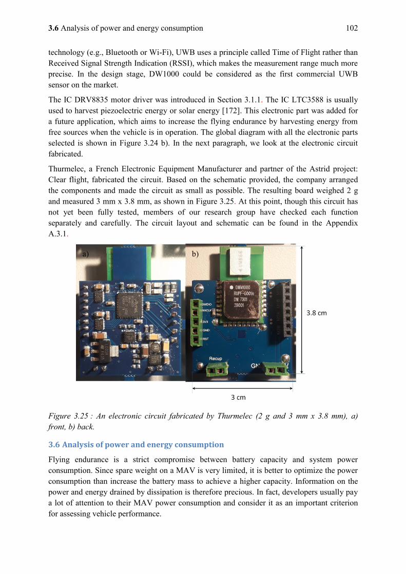
3.6 Analysis of power and energy consumption 102
technology (e.g., Bluetooth or Wi-Fi), UWB uses a principle called Time of Flight rather than Received Signal Strength Indication (RSSI), which makes the measurement range much more precise. In the design stage, DW1000 could be considered as the first commercial UWB sensor on the market.
The IC DRV8835 motor driver was introduced in Section 3.1.1. The IC LTC3588 is usually used to harvest piezoelectric energy or solar energy [172]. This electronic part was added for a future application, which aims to increase the flying endurance by harvesting energy from free sources when the vehicle is in operation. The global diagram with all the electronic parts selected is shown in Figure 3.24 b). In the next paragraph, we look at the electronic circuit fabricated.
Thurmelec, a French Electronic Equipment Manufacturer and partner of the Astrid project: Clear flight, fabricated the circuit. Based on the schematic provided, the company arranged the components and made the circuit as small as possible. The resulting board weighed 2 g and measured 3 mm x 3.8 mm, as shown in Figure 3.25. At this point, though this circuit has not yet been fully tested, members of our research group have checked each function separately and carefully. The circuit layout and schematic can be found in the Appendix A.3.1.
Figure 3.25 : An electronic circuit fabricated by Thurmelec (2 g and 3 mm x 3.8 mm), a) front, b) back.
3.6 Analysis of power and energy consumption
Flying endurance is a strict compromise between battery capacity and system power consumption. Since spare weight on a MAV is very limited, it is better to optimize the power consumption than increase the battery mass to achieve a higher capacity. Information on the power and energy drained by dissipation is therefore precious. In fact, developers usually pay a lot of attention to their MAV power consumption and consider it as an important criterion for assessing vehicle performance.
a) b)
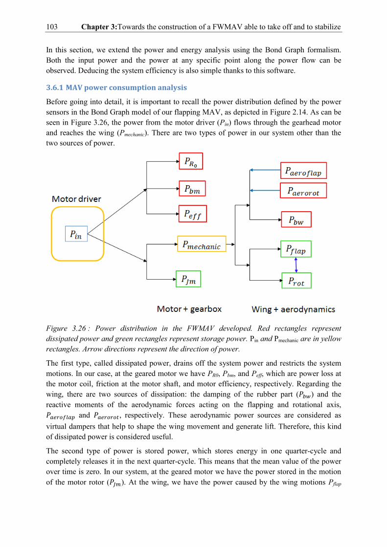
103 Chapter 3:Towards the construction of a FWMAV able to take off and to stabilize
In this section, we extend the power and energy analysis using the Bond Graph formalism. Both the input power and the power at any specific point along the power flow can be observed. Deducing the system efficiency is also simple thanks to this software.
3.6.1 MAV power consumption analysis
Before going into detail, it is important to recall the power distribution defined by the power sensors in the Bond Graph model of our flapping MAV, as depicted in Figure 2.14. As can be seen in Figure 3.26, the power from the motor driver (Pin) flows through the gearhead motor and reaches the wing (Pmechanic). There are two types of power in our system other than the two sources of power.
Figure 3.26 : Power distribution in the FWMAV developed. Red rectangles represent dissipated power and green rectangles represent storage power. Pin and Pmechanic are in yellow rectangles. Arrow directions represent the direction of power.
The first type, called dissipated power, drains off the system power and restricts the system motions. In our case, at the geared motor we have PR0, Pbm, and Peff, which are power loss at the motor coil, friction at the motor shaft, and motor efficiency, respectively. Regarding the wing, there are two sources of dissipation: the damping of the rubber part ( ) and the reactive moments of the aerodynamic forces acting on the flapping and rotational axis, and , respectively. These aerodynamic power sources are considered as virtual dampers that help to shape the wing movement and generate lift. Therefore, this kind of dissipated power is considered useful.
The second type of power is stored power, which stores energy in one quarter-cycle and completely releases it in the next quarter-cycle. This means that the mean value of the power over time is zero. In our system, at the geared motor we have the power stored in the motion of the motor rotor ( ). At the wing, we have the power caused by the wing motions Pflap
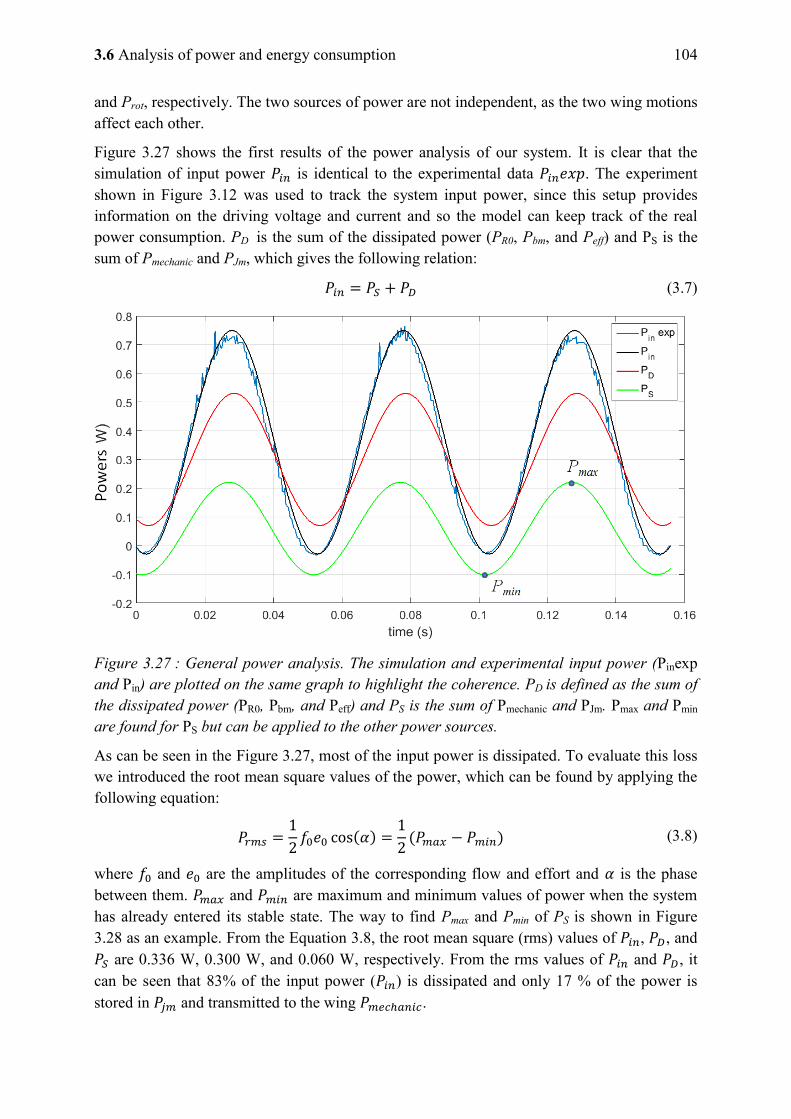
3.6 Analysis of power and energy consumption 104
and Prot, respectively. The two sources of power are not independent, as the two wing motions affect each other.
Figure 3.27 shows the first results of the power analysis of our system. It is clear that the simulation of input power is identical to the experimental data . The experiment shown in Figure 3.12 was used to track the system input power, since this setup provides information on the driving voltage and current and so the model can keep track of the real power consumption. PD is the sum of the dissipated power (PR0, Pbm, and Peff) and PS is the sum of Pmechanic and PJm, which gives the following relation:
(3.7)
Figure 3.27 : General power analysis. The simulation and experimental input power (Pinexp and Pin) are plotted on the same graph to highlight the coherence. PD is defined as the sum of the dissipated power (PR0, Pbm, and Peff) and PS is the sum of Pmechanic and PJm. Pmax and Pmin are found for PS but can be applied to the other power sources.
As can be seen in the Figure 3.27, most of the input power is dissipated. To evaluate this loss we introduced the root mean square values of the power, which can be found by applying the following equation:
(3.8)
where and are the amplitudes of the corresponding flow and effort and is the phase between them. and are maximum and minimum values of power when the system has already entered its stable state. The way to find Pmax and Pmin of PS is shown in Figure 3.28 as an example. From the Equation 3.8, the root mean square (rms) values of , , and are 0.336 W, 0.300 W, and 0.060 W, respectively. From the rms values of and , it can be seen that 83% of the input power ( ) is dissipated and only 17 % of the power is stored in and transmitted to the wing .
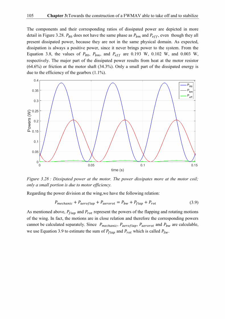
105 Chapter 3:Towards the construction of a FWMAV able to take off and to stabilize
The components and their corresponding ratios of dissipated power are depicted in more detail in Figure 3.28. does not have the same phase as and , even though they all present dissipated power, because they are not in the same physical domain. As expected, dissipation is always a positive power, since it never brings power to the system. From the Equation 3.8, the values of , , and are 0.193 W, 0.102 W, and 0.003 W, respectively. The major part of the dissipated power results from heat at the motor resistor (64.6%) or friction at the motor shaft (34.3%). Only a small part of the dissipated energy is due to the efficiency of the gearbox (1.1%).
Figure 3.28 : Dissipated power at the motor. The power dissipates more at the motor coil; only a small portion is due to motor efficiency.
Regarding the power division at the wing,we have the following relation:
(3.9)
As mentioned above, and represent the powers of the flapping and rotating motions of the wing. In fact, the motions are in close relation and therefore the corresponding powers cannot be calculated separately. Since , , and are calculable, we use Equation 3.9 to estimate the sum of and which is called .
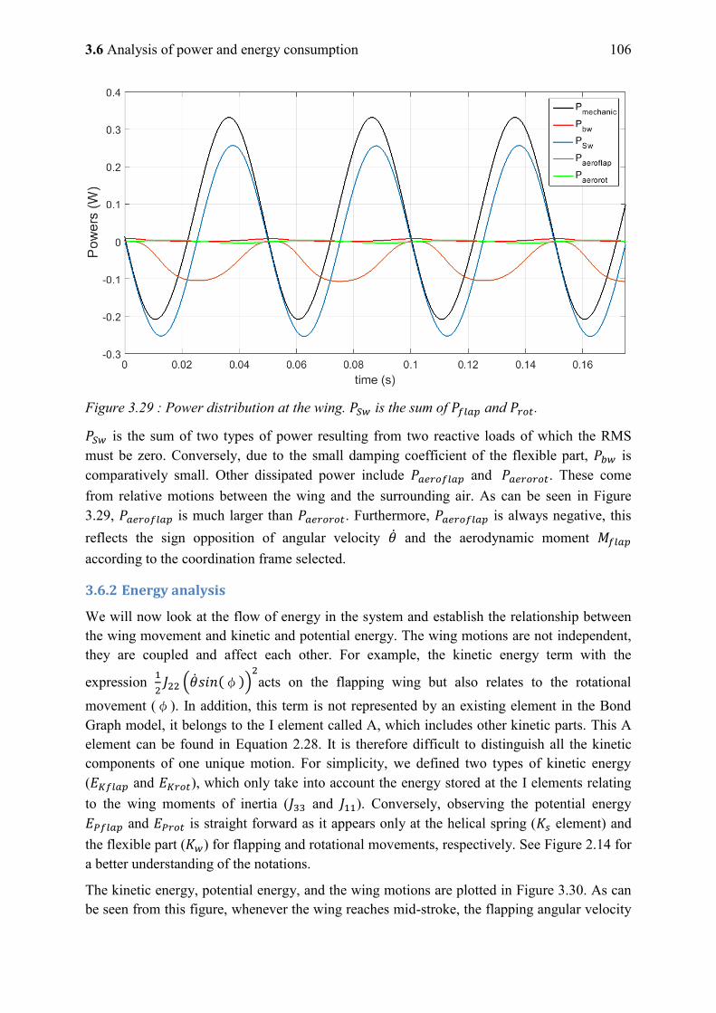
3.6 Analysis of power and energy consumption 106
Figure 3.29 : Power distribution at the wing. is the sum of and .
is the sum of two types of power resulting from two reactive loads of which the RMS must be zero. Conversely, due to the small damping coefficient of the flexible part, is comparatively small. Other dissipated power include and . These come from relative motions between the wing and the surrounding air. As can be seen in Figure 3.29, is much larger than . Furthermore, is always negative, this reflects the sign opposition of angular velocity and the aerodynamic moment according to the coordination frame selected.
3.6.2 Energy analysis
We will now look at the flow of energy in the system and establish the relationship between the wing movement and kinetic and potential energy. The wing motions are not independent, they are coupled and affect each other. For example, the kinetic energy term with the
expression
( )
acts on the flapping wing but also relates to the rotational movement ( ). In addition, this term is not represented by an existing element in the Bond Graph model, it belongs to the I element called A, which includes other kinetic parts. This A element can be found in Equation 2.28. It is therefore difficult to distinguish all the kinetic components of one unique motion. For simplicity, we defined two types of kinetic energy ( and ), which only take into account the energy stored at the I elements relating to the wing moments of inertia ( and ). Conversely, observing the potential energy and is straight forward as it appears only at the helical spring ( element) and the flexible part ( ) for flapping and rotational movements, respectively. See Figure 2.14 for a better understanding of the notations.
The kinetic energy, potential energy, and the wing motions are plotted in Figure 3.30. As can be seen from this figure, whenever the wing reaches mid-stroke, the flapping angular velocity
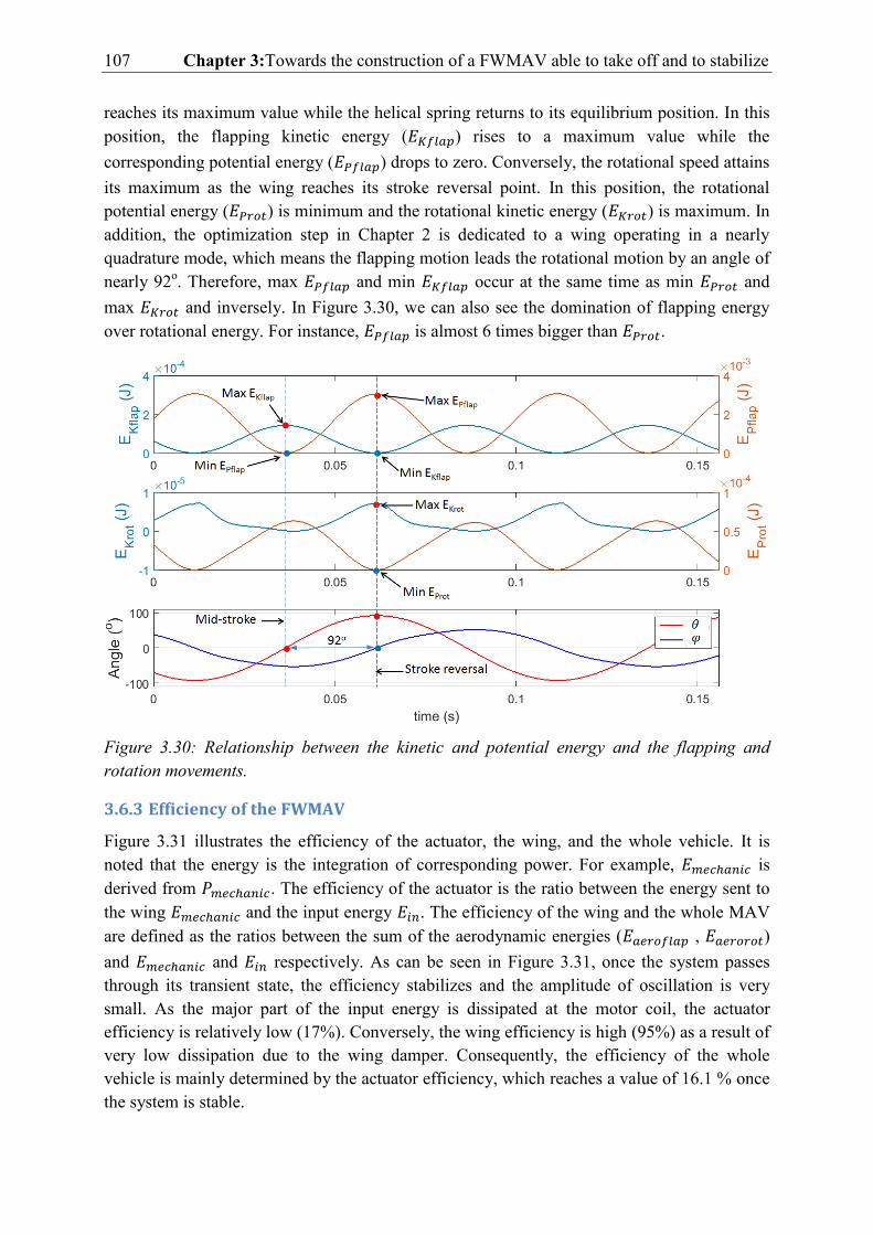
107 Chapter 3:Towards the construction of a FWMAV able to take off and to stabilize
reaches its maximum value while the helical spring returns to its equilibrium position. In this position, the flapping kinetic energy ( ) rises to a maximum value while the corresponding potential energy ( ) drops to zero. Conversely, the rotational speed attains its maximum as the wing reaches its stroke reversal point. In this position, the rotational potential energy ( ) is minimum and the rotational kinetic energy ( ) is maximum. In addition, the optimization step in Chapter 2 is dedicated to a wing operating in a nearly quadrature mode, which means the flapping motion leads the rotational motion by an angle of nearly 92o. Therefore, max and min occur at the same time as min and max and inversely. In Figure 3.30, we can also see the domination of flapping energy over rotational energy. For instance, is almost 6 times bigger than .
Figure 3.30: Relationship between the kinetic and potential energy and the flapping and rotation movements.
3.6.3 Efficiency of the FWMAV
Figure 3.31 illustrates the efficiency of the actuator, the wing, and the whole vehicle. It is noted that the energy is the integration of corresponding power. For example, is derived from . The efficiency of the actuator is the ratio between the energy sent to the wing and the input energy . The efficiency of the wing and the whole MAV are defined as the ratios between the sum of the aerodynamic energies ( , ) and and respectively. As can be seen in Figure 3.31, once the system passes through its transient state, the efficiency stabilizes and the amplitude of oscillation is very small. As the major part of the input energy is dissipated at the motor coil, the actuator efficiency is relatively low (17%). Conversely, the wing efficiency is high (95%) as a result of very low dissipation due to the wing damper. Consequently, the efficiency of the whole vehicle is mainly determined by the actuator efficiency, which reaches a value of 16.1 % once the system is stable.
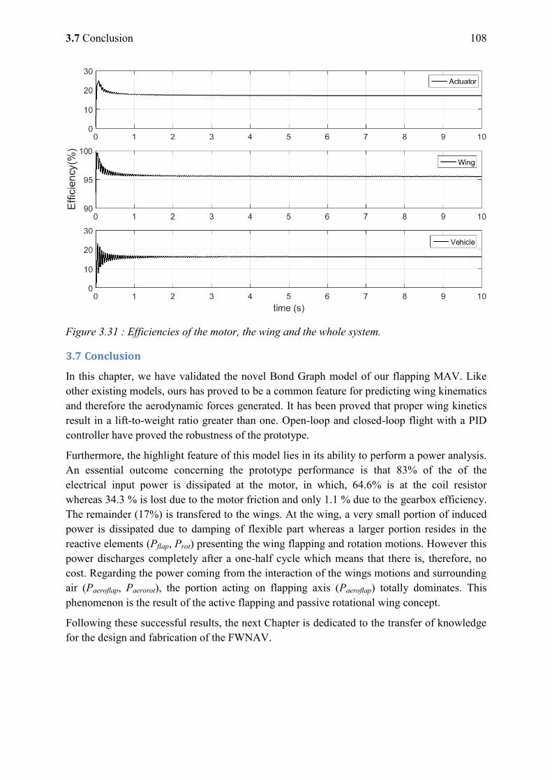
3.7 Conclusion 108
Figure 3.31 : Efficiencies of the motor, the wing and the whole system.
3.7 Conclusion
In this chapter, we have validated the novel Bond Graph model of our flapping MAV. Like other existing models, ours has proved to be a common feature for predicting wing kinematics and therefore the aerodynamic forces generated. It has been proved that proper wing kinetics result in a lift-to-weight ratio greater than one. Open-loop and closed-loop flight with a PID controller have proved the robustness of the prototype.
Furthermore, the highlight feature of this model lies in its ability to perform a power analysis. An essential outcome concerning the prototype performance is that 83% of the of the electrical input power is dissipated at the motor, in which, 64.6% is at the coil resistor whereas 34.3 % is lost due to the motor friction and only 1.1 % due to the gearbox efficiency. The remainder (17%) is transfered to the wings. At the wing, a very small portion of induced power is dissipated due to damping of flexible part whereas a larger portion resides in the reactive elements (Pflap, Prot) presenting the wing flapping and rotation motions. However this power discharges completely after a one-half cycle which means that there is, therefore, no cost. Regarding the power coming from the interaction of the wings motions and surrounding air (Paeroflap, Paerorot), the portion acting on flapping axis (Paeroflap) totally dominates. This phenomenon is the result of the active flapping and passive rotational wing concept.
Following these successful results, the next Chapter is dedicated to the transfer of knowledge for the design and fabrication of the FWNAV.
109 Chapter 4:Kinematic and power behavior analysis of OVMI
Chapter 4: Kinematic and power behavior analysis of
OVMI
Contents
4.1 Introduction .. . . . . . . . . . . . . . . . . . . . . . . . . . . . . . . . . . . . . . . . . . . . . . . . . . . . . . . . . . . . . . . . . . . . . . . . . . . . . . . . .110
4.2 OVMI Dynamic Bond Graph model . . . . . . . . . . . . . . . . . . . . . . . . . . . . . . . . . . . . . . . . . . . . . . . . .111
4.2.1 Prototype description ............................................................................................. 111
4.2.2 OVMI Word Bond Graph ..................................................................................... 112
4.2.3 Bond Graph model ................................................................................................ 113
4.2.4 Parameter estimation ............................................................................................. 118
4.3 Kinematic simulation and dynamic power analysis . . . . . . . . . . . . . . . . . . . . . . . . . . .120
4.3.1 Kinematic simulation ............................................................................................ 120
4.3.2 Wing kinematic concept validation ....................................................................... 122
4.3.3 Dynamic power analysis ....................................................................................... 124
4.4 Conclusion .. . . . . . . . . . . . . . . . . . . . . . . . . . . . . . . . . . . . . . . . . . . . . . . . . . . . . . . . . . . . . . . . . . . . . . . . . . . . . . . . . . .128
4.1 Introduction 110
4.1 Introduction
As already explained in the Chapter 1, developing a flying vehicle with a wingspan of just a few millimeters and a very low weight of a few milligrams is a challenge. The weight and size limits imposed are in contrast to the huge amount of power required to overcome aerodynamic drag, and the inertia of the constantly oscillating wing and accompanying mechanisms. Fortunately, the solution exists in nature, since insects such as flies, bees, wasps, and beetles use, among others, mechanical resonance to counteract these problems [70]. This design concept – inspired by the resonant thorax of these dipteran insects – is usually achieved by introducing elasticity into the micro and nano air vehicle structures.
The elastic element can be any of the following components: helical spring [173]–[175], virtual spring [176], compliant link [177], vehicle frame [178], or even the main actuator [102], [179]. The aim, therefore, is to develop a model to analyze the performance of these flexible vehicles in terms of power and energy.
There are a variety of tools and methods for this purpose ranging from the maximum power theorem coupled with impedance matching condition to energy methods applied to hovering flight. For example, the maximum power theorem and impedance matching condition is used , in [95], [180], for a simple platform coupling a DC motor and linear stiffness. A motor was chosen to enable the system to resonate with the highest overall efficiency at a specific flapping angle. The model also proves the advantages of operating at resonance, as this system is capable of converting the inertial energy of the wing into elastic energy. Consequently, minimum input power and maximum aerodynamic power are achieved simultaneously.
The same approach was applied for a vehicle with a non-linear elastic thoracic mechanism based on polyimide film hinges [177]. Though the effect of resonance in reducing the electrical power input was not clear, this mechanism successfully conserved mechanical power during wing movement. Thrust per unit power was also assessed to prove the advantage of this compliant mechanism compared to an equivalent rigid-body mechanism. In another study [181], the vehicle was powered by piezoelectric actuators. Given the vehicle mass and wing length, an energy method was employed to determine the mass ratio between the actuator and the battery which would be necessary to hover. The maximum hovering endurance, flight speed, and distance covered were then deduced from this ratio.
Another potential solution would be like in Chapters 2 and 3 to use the Bond Graph-based model to analyse the power efficiency of the electromagnetic actuator of a resonant FWNAV. This is the preferred solution here, since we want to develop a similar analyze than those used successfully for the FWMAV.
Consequently, the main objective of this chapter is to develop a Bond Graph-based model for an FWNAV that will be used to estimate the vehicle performance by considering its dynamic power behavior. The model itself is original as it is a distributed-parameter model and is based on a flexible micro-structure. The vehicle studied is a micromachined FWNAV – named “object volant mimant l‟insecte” (OVMI) or insect-mimicking flying object – powered
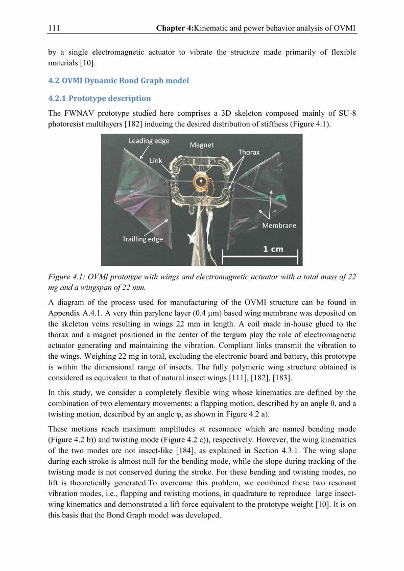
111 Chapter 4:Kinematic and power behavior analysis of OVMI
by a single electromagnetic actuator to vibrate the structure made primarily of flexible materials [10].
4.2 OVMI Dynamic Bond Graph model
4.2.1 Prototype description
The FWNAV prototype studied here comprises a 3D skeleton composed mainly of SU-8 photoresist multilayers [182] inducing the desired distribution of stiffness (Figure 4.1).
Figure 4.1: OVMI prototype with wings and electromagnetic actuator with a total mass of 22 mg and a wingspan of 22 mm.
A diagram of the process used for manufacturing of the OVMI structure can be found in Appendix A.4.1. A very thin parylene layer (0.4 µm) based wing membrane was deposited on the skeleton veins resulting in wings 22 mm in length. A coil made in-house glued to the thorax and a magnet positioned in the center of the tergum play the role of electromagnetic actuator generating and maintaining the vibration. Compliant links transmit the vibration to the wings. Weighing 22 mg in total, excluding the electronic board and battery, this prototype is within the dimensional range of insects. The fully polymeric wing structure obtained is considered as equivalent to that of natural insect wings [111], [182], [183].
In this study, we consider a completely flexible wing whose kinematics are defined by the combination of two elementary movements: a flapping motion, described by an angle θ, and a twisting motion, described by an angle φ, as shown in Figure 4.2 a).
These motions reach maximum amplitudes at resonance which are named bending mode (Figure 4.2 b)) and twisting mode (Figure 4.2 c)), respectively. However, the wing kinematics of the two modes are not insect-like [184], as explained in Section 4.3.1. The wing slope during each stroke is almost null for the bending mode, while the slope during tracking of the twisting mode is not conserved during the stroke. For these bending and twisting modes, no lift is theoretically generated.To overcome this problem, we combined these two resonant vibration modes, i.e., flapping and twisting motions, in quadrature to reproduce large insect-wing kinematics and demonstrated a lift force equivalent to the prototype weight [10]. It is on this basis that the Bond Graph model was developed.
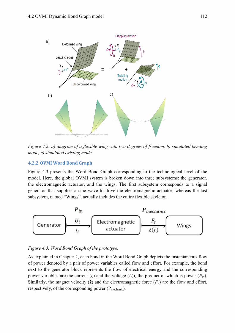
4.2 OVMI Dynamic Bond Graph model 112
Figure 4.2: a) diagram of a flexible wing with two degrees of freedom, b) simulated bending mode, c) simulated twisting mode.
4.2.2 OVMI Word Bond Graph
Figure 4.3 presents the Word Bond Graph corresponding to the technological level of the model. Here, the global OVMI system is broken down into three subsystems: the generator, the electromagnetic actuator, and the wings. The first subsystem corresponds to a signal generator that supplies a sine wave to drive the electromagnetic actuator, whereas the last subsystem, named “Wings”, actually includes the entire flexible skeleton.
Figure 4.3: Word Bond Graph of the prototype.
As explained in Chapter 2, each bond in the Word Bond Graph depicts the instantaneous flow of power denoted by a pair of power variables called flow and effort. For example, the bond next to the generator block represents the flow of electrical energy and the corresponding power variables are the current (ii) and the voltage (Ui), the product of which is power (Pin). Similarly, the magnet velocity ( ) and the electromagnetic force (Fe) are the flow and effort, respectively, of the corresponding power (Pmechanic).
a)
b) c)
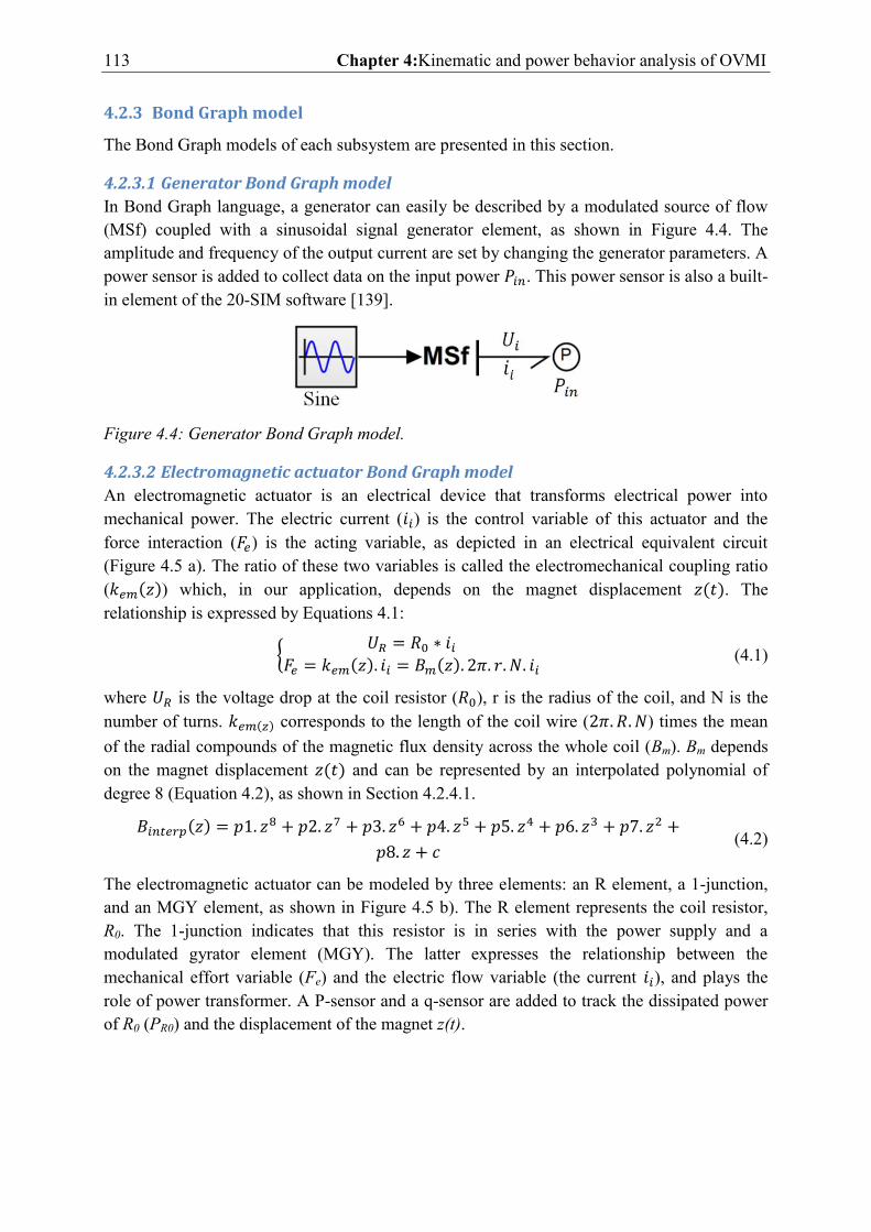
113 Chapter 4:Kinematic and power behavior analysis of OVMI
4.2.3 Bond Graph model
The Bond Graph models of each subsystem are presented in this section.
4.2.3.1 Generator Bond Graph model
In Bond Graph language, a generator can easily be described by a modulated source of flow (MSf) coupled with a sinusoidal signal generator element, as shown in Figure 4.4. The amplitude and frequency of the output current are set by changing the generator parameters. A power sensor is added to collect data on the input power . This power sensor is also a built-in element of the 20-SIM software [139].
Figure 4.4: Generator Bond Graph model.
4.2.3.2 Electromagnetic actuator Bond Graph model
An electromagnetic actuator is an electrical device that transforms electrical power into mechanical power. The electric current ( ) is the control variable of this actuator and the force interaction ( ) is the acting variable, as depicted in an electrical equivalent circuit (Figure 4.5 a). The ratio of these two variables is called the electromechanical coupling ratio ( ) which, in our application, depends on the magnet displacement . The relationship is expressed by Equations 4.1:
{
(4.1)
where is the voltage drop at the coil resistor ( ), r is the radius of the coil, and N is the number of turns. corresponds to the length of the coil wire ( ) times the mean of the radial compounds of the magnetic flux density across the whole coil (Bm). Bm depends on the magnet displacement and can be represented by an interpolated polynomial of degree 8 (Equation 4.2), as shown in Section 4.2.4.1.
(4.2)
The electromagnetic actuator can be modeled by three elements: an R element, a 1-junction, and an MGY element, as shown in Figure 4.5 b). The R element represents the coil resistor, R0. The 1-junction indicates that this resistor is in series with the power supply and a modulated gyrator element (MGY). The latter expresses the relationship between the mechanical effort variable (Fe) and the electric flow variable (the current ), and plays the role of power transformer. A P-sensor and a q-sensor are added to track the dissipated power of R0 (PR0) and the displacement of the magnet z(t).

4.2 OVMI Dynamic Bond Graph model 114
Figure 4.5: Representation of an electromagnetic actuator, a) through an equivalent electrical circuit b) through a Bond Graph formalism.
Finally, the modulated gyration ratio, , is represented by the block diagram, as shown in Figure 4.6 and according to Equation 4.2.
Figure 4.6: Presentation of the average magnetic field.
a)
b)
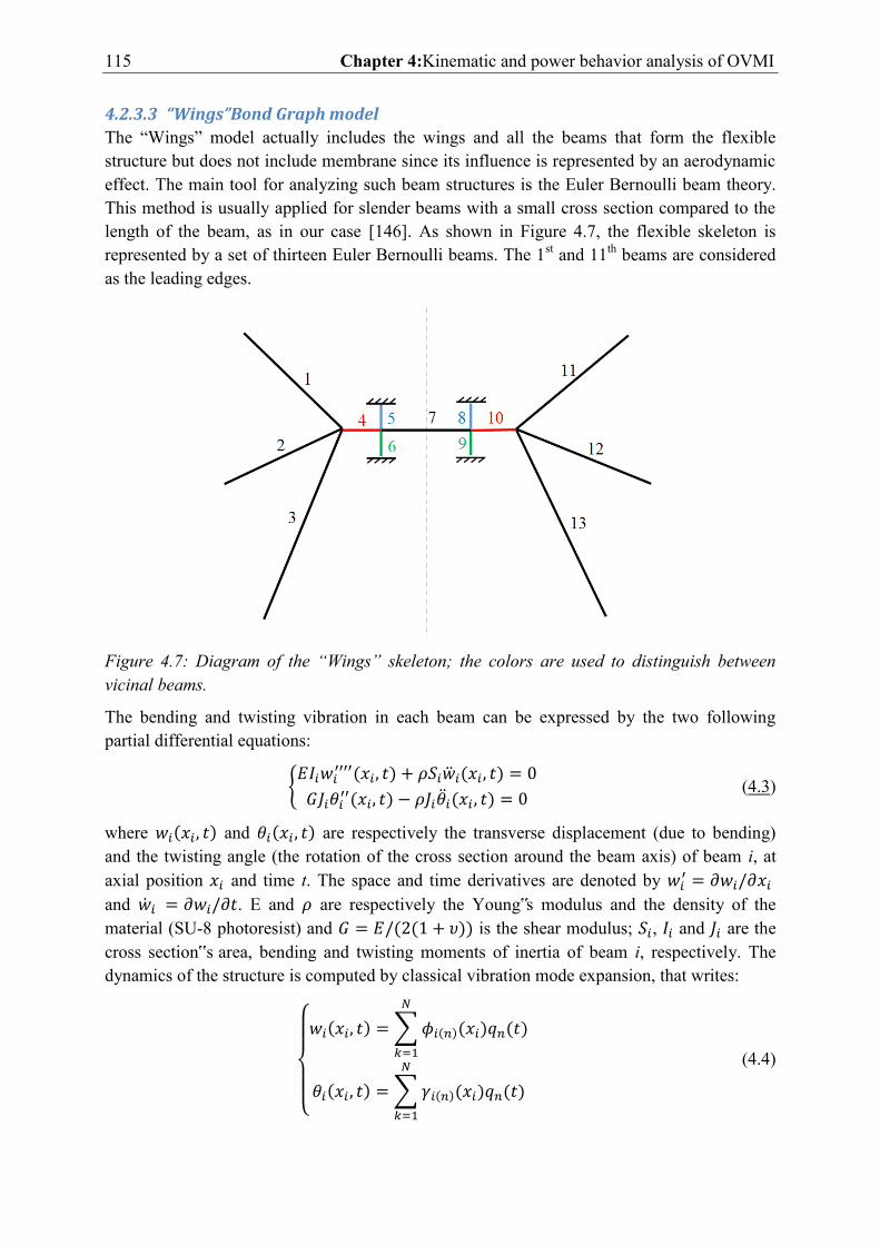
115 Chapter 4:Kinematic and power behavior analysis of OVMI
4.2.3.3 “Wings”Bond Graph model
The “Wings” model actually includes the wings and all the beams that form the flexible structure but does not include membrane since its influence is represented by an aerodynamic effect. The main tool for analyzing such beam structures is the Euler Bernoulli beam theory. This method is usually applied for slender beams with a small cross section compared to the length of the beam, as in our case [146]. As shown in Figure 4.7, the flexible skeleton is represented by a set of thirteen Euler Bernoulli beams. The 1st and 11th beams are considered as the leading edges.
Figure 4.7: Diagram of the “Wings” skeleton; the colors are used to distinguish between vicinal beams.
The bending and twisting vibration in each beam can be expressed by the two following partial differential equations:
{
(4.3)
where and are respectively the transverse displacement (due to bending) and the twisting angle (the rotation of the cross section around the beam axis) of beam i, at axial position and time t. The space and time derivatives are denoted by
and . E and are respectively the Young‟s modulus and the density of the material (SU-8 photoresist) and is the shear modulus; , and are the cross section‟s area, bending and twisting moments of inertia of beam i, respectively. The dynamics of the structure is computed by classical vibration mode expansion, that writes:
{
∑
∑
(4.4)
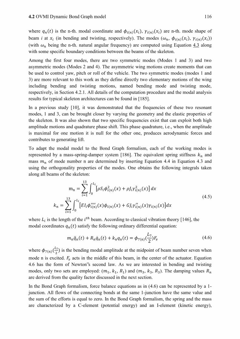
4.2 OVMI Dynamic Bond Graph model 116
where is the n-th. modal coordinate and , are n-th. mode shape of beam i at (in bending and twisting, respectively). The modes ( , , ) (with being the n-th. natural angular frequency) are computed using Equation 4.3 along with some specific boundary conditions between the beams of the skeleton.
Among the first four modes, there are two symmetric modes (Modes 1 and 3) and two asymmetric modes (Modes 2 and 4). The asymmetric wing motions create moments that can be used to control yaw, pitch or roll of the vehicle. The two symmetric modes (modes 1 and 3) are more relevant to this work as they define directly two elementary motions of the wing including bending and twisting motions, named bending mode and twisting mode, respectively, in Section 4.2.1. All details of the computation procedure and the modal analysis results for typical skeleton architectures can be found in [185].
In a previous study [10], it was demonstrated that the frequencies of these two resonant modes, 1 and 3, can be brought closer by varying the geometry and the elastic properties of the skeleton. It was also shown that two specific frequencies exist that can exploit both high amplitude motions and quadrature phase shift. This phase quadrature, i.e., when the amplitude is maximal for one motion it is null for the other one, produces aerodynamic forces and contributes to generating lift.
To adapt the modal model to the Bond Graph formalism, each of the working modes is represented by a mass-spring-damper system [186]. The equivalent spring stiffness and mass of mode number n are determined by inserting Equation 4.4 in Equation 4.3 and using the orthogonality properties of the modes. One obtains the following integrals taken along all beams of the skeleton:
∑∫ [
]
∑∫ [
]
(4.5)
where is the length of the beam. According to classical vibration theory [146], the modal coordinates satisfy the following ordinary differential equation:
(4.6)
where
is the bending modal amplitude at the midpoint of beam number seven when
mode n is excited. acts in the middle of this beam, in the center of the actuator. Equation 4.6 has the form of Newton‟s second law. As we are interested in bending and twisting modes, only two sets are employed: ( , , ) and ( , , ). The damping values are derived from the quality factor discussed in the next section.
In the Bond Graph formalism, force balance equations as in (4.6) can be represented by a 1-junction. All flows of the connecting bonds at the same 1-junction have the same value and the sum of the efforts is equal to zero. In the Bond Graph formalism, the spring and the mass are characterized by a C-element (potential energy) and an I-element (kinetic energy),
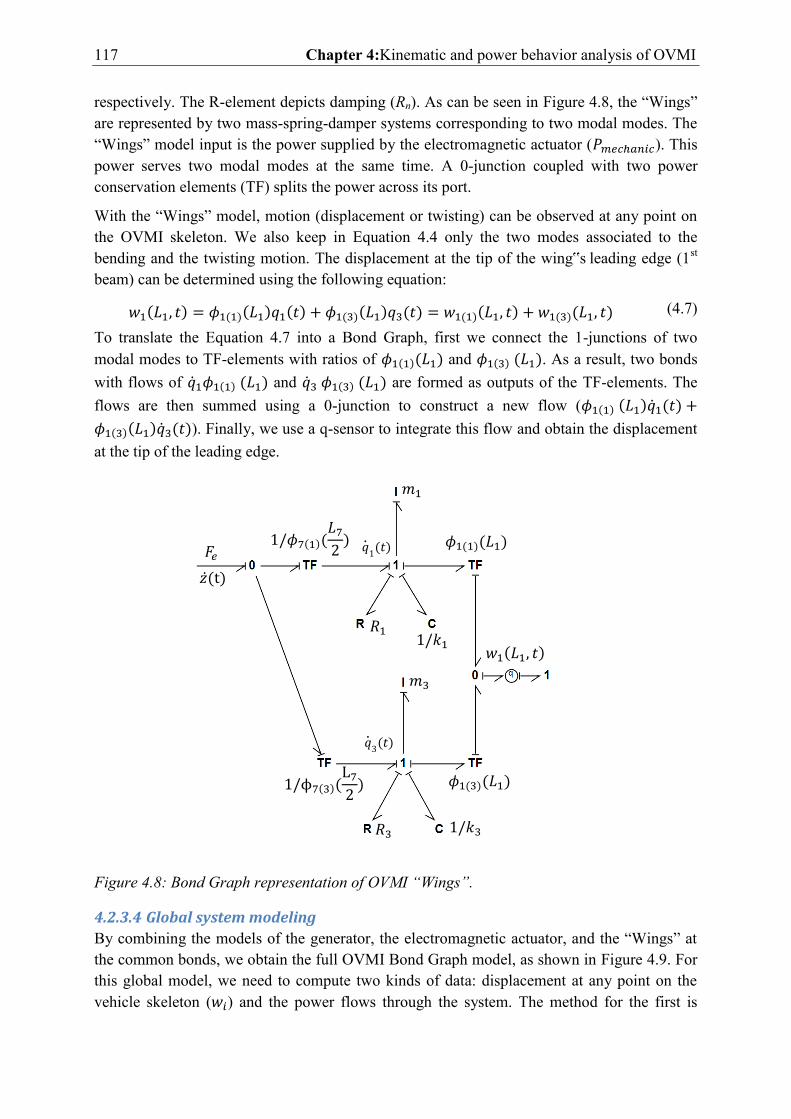
117 Chapter 4:Kinematic and power behavior analysis of OVMI
respectively. The R-element depicts damping (Rn). As can be seen in Figure 4.8, the “Wings” are represented by two mass-spring-damper systems corresponding to two modal modes. The “Wings” model input is the power supplied by the electromagnetic actuator ( ). This power serves two modal modes at the same time. A 0-junction coupled with two power conservation elements (TF) splits the power across its port.
With the “Wings” model, motion (displacement or twisting) can be observed at any point on the OVMI skeleton. We also keep in Equation 4.4 only the two modes associated to the bending and the twisting motion. The displacement at the tip of the wing‟s leading edge (1st beam) can be determined using the following equation:
(4.7)
To translate the Equation 4.7 into a Bond Graph, first we connect the 1-junctions of two modal modes to TF-elements with ratios of and . As a result, two bonds with flows of and are formed as outputs of the TF-elements. The flows are then summed using a 0-junction to construct a new flow (
). Finally, we use a q-sensor to integrate this flow and obtain the displacement at the tip of the leading edge.
Figure 4.8: Bond Graph representation of OVMI “Wings”.
4.2.3.4 Global system modeling
By combining the models of the generator, the electromagnetic actuator, and the “Wings” at the common bonds, we obtain the full OVMI Bond Graph model, as shown in Figure 4.9. For this global model, we need to compute two kinds of data: displacement at any point on the vehicle skeleton ( ) and the power flows through the system. The method for the first is
𝐹𝑒 �� t
𝜙 𝐿
ϕ L
𝑚
𝑘 𝑅
𝑅
𝜙 𝐿
𝜙 𝐿
𝑘
𝑚
�� 𝑡
�� 𝑡
𝑤 𝐿 𝑡
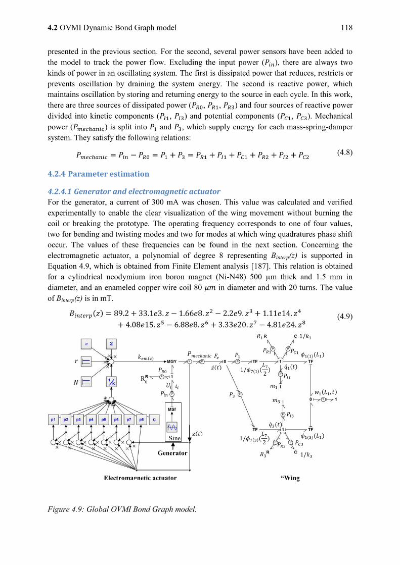
4.2 OVMI Dynamic Bond Graph model 118
presented in the previous section. For the second, several power sensors have been added to the model to track the power flow. Excluding the input power ( ), there are always two kinds of power in an oscillating system. The first is dissipated power that reduces, restricts or prevents oscillation by draining the system energy. The second is reactive power, which maintains oscillation by storing and returning energy to the source in each cycle. In this work, there are three sources of dissipated power ( , , ) and four sources of reactive power divided into kinetic components ( , ) and potential components ( , ). Mechanical power ( ) is split into and , which supply energy for each mass-spring-damper system. They satisfy the following relations:
(4.8)
4.2.4 Parameter estimation
4.2.4.1 Generator and electromagnetic actuator
For the generator, a current of 300 mA was chosen. This value was calculated and verified experimentally to enable the clear visualization of the wing movement without burning the coil or breaking the prototype. The operating frequency corresponds to one of four values, two for bending and twisting modes and two for modes at which wing quadratures phase shift occur. The values of these frequencies can be found in the next section. Concerning the electromagnetic actuator, a polynomial of degree 8 representing Binterp(z) is supported in Equation 4.9, which is obtained from Finite Element analysis [187]. This relation is obtained for a cylindrical neodymium iron boron magnet (Ni-N48) 500 µm thick and 1.5 mm in diameter, and an enameled copper wire coil 80 in diameter and with 20 turns. The value of Binterp(z) is in mT.
(4.9)
Figure 4.9: Global OVMI Bond Graph model.
Sine
𝑃𝑖𝑛 𝑈𝑖 𝑖𝑖
R0 𝑃𝑅
𝑘𝑒𝑚 𝑧
𝑧 𝑡
𝐹𝑒 �� 𝑡 𝜙
𝐿
𝜙 𝐿
𝑚
𝑘 𝑅
𝑅
𝜙 𝐿
𝜙 𝐿
𝑘
𝑚
�� 𝑡
�� 𝑡
𝑤 𝐿 𝑡
Generator
Electromagnetic actuator “Wings”
𝑃𝑚𝑒𝑐 𝑎𝑛𝑖𝑐 𝑃
𝑃
𝑟
𝑁
𝑃𝑅 𝑃𝐶
𝑃𝐼
𝑃𝐼
𝑃𝑅 𝑃𝐶
119 Chapter 4:Kinematic and power behavior analysis of OVMI
4.2.4.2 “Wings”
The equivalent stiffness and mass corresponding to each resonant mode could be theoretically derived from Equation 4.5. The corresponding operating frequency is thus determined by
√ . The equivalent damping, including the damping effect of the aeroelastic
forces, is however evaluated experimentally through the impact of air pressure on the dynamic behavior of the prototypes. The experiments were conducted by placing the prototype in a vacuum chamber, as shown in Figure 4.10, to control the surrounding pressure. The vacuum chamber used consists of an airtight chamber connected to a primary vacuum pump to reach a vacuum pressure of mbar. The prototype is positioned on a support inside this airtight enclosure in front of a transparent porthole to measure the displacement at the center of the skeleton on the electromagnetic actuator using a laser vibrometer. The frequency response functions (FRFs) at specific points on the “Wings” prototype can thus be established for different pressures. These FRFs make it possible to evaluate aerodynamic damping at different pressures by identifying the bandwidth at -3 dB below the resonant peak level. We can thus obtain the quality factor ( ) of the wing according to the pressure inside the vacuum chamber, as shown in Figure 4.11.
Figure 4.10: Photograph of a prototype placed in a vacuum chamber used to quantify the influence of the surrounding pressure on its dynamic behavior.
A logical decrease in the quality factor with the elevation in pressure is observed that corresponds to the increase in damping as . At atmospheric pressure, the quality factor is and , whereas at a pressure of mbar, and
. The damping value is then estimated as √ for each mode under the desired pressure conditions. The results are summarized in the Table 4.1 for the sake of clarity.
Prototype
Support Porthole
Laser spot
Vacuum chamber
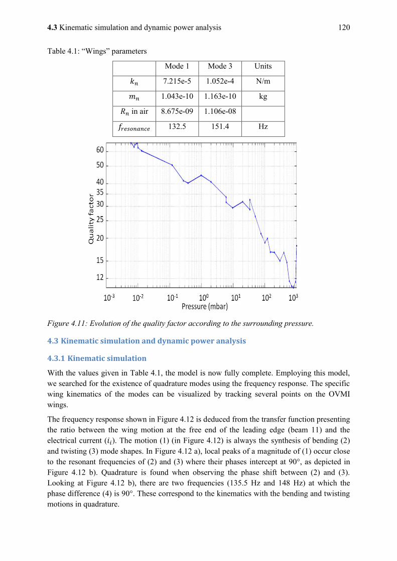
4.3 Kinematic simulation and dynamic power analysis 120
Table 4.1: “Wings” parameters
Mode 1 Mode 3 Units
7.215e-5 1.052e-4 N/m
1.043e-10 1.163e-10 kg
in air 8.675e-09 1.106e-08
132.5 151.4 Hz
Figure 4.11: Evolution of the quality factor according to the surrounding pressure.
4.3 Kinematic simulation and dynamic power analysis
4.3.1 Kinematic simulation
With the values given in Table 4.1, the model is now fully complete. Employing this model, we searched for the existence of quadrature modes using the frequency response. The specific wing kinematics of the modes can be visualized by tracking several points on the OVMI wings.
The frequency response shown in Figure 4.12 is deduced from the transfer function presenting the ratio between the wing motion at the free end of the leading edge (beam 11) and the electrical current ( ). The motion (1) (in Figure 4.12) is always the synthesis of bending (2) and twisting (3) mode shapes. In Figure 4.12 a), local peaks of a magnitude of (1) occur close to the resonant frequencies of (2) and (3) where their phases intercept at 90°, as depicted in Figure 4.12 b). Quadrature is found when observing the phase shift between (2) and (3). Looking at Figure 4.12 b), there are two frequencies (135.5 Hz and 148 Hz) at which the phase difference (4) is 90°. These correspond to the kinematics with the bending and twisting motions in quadrature.
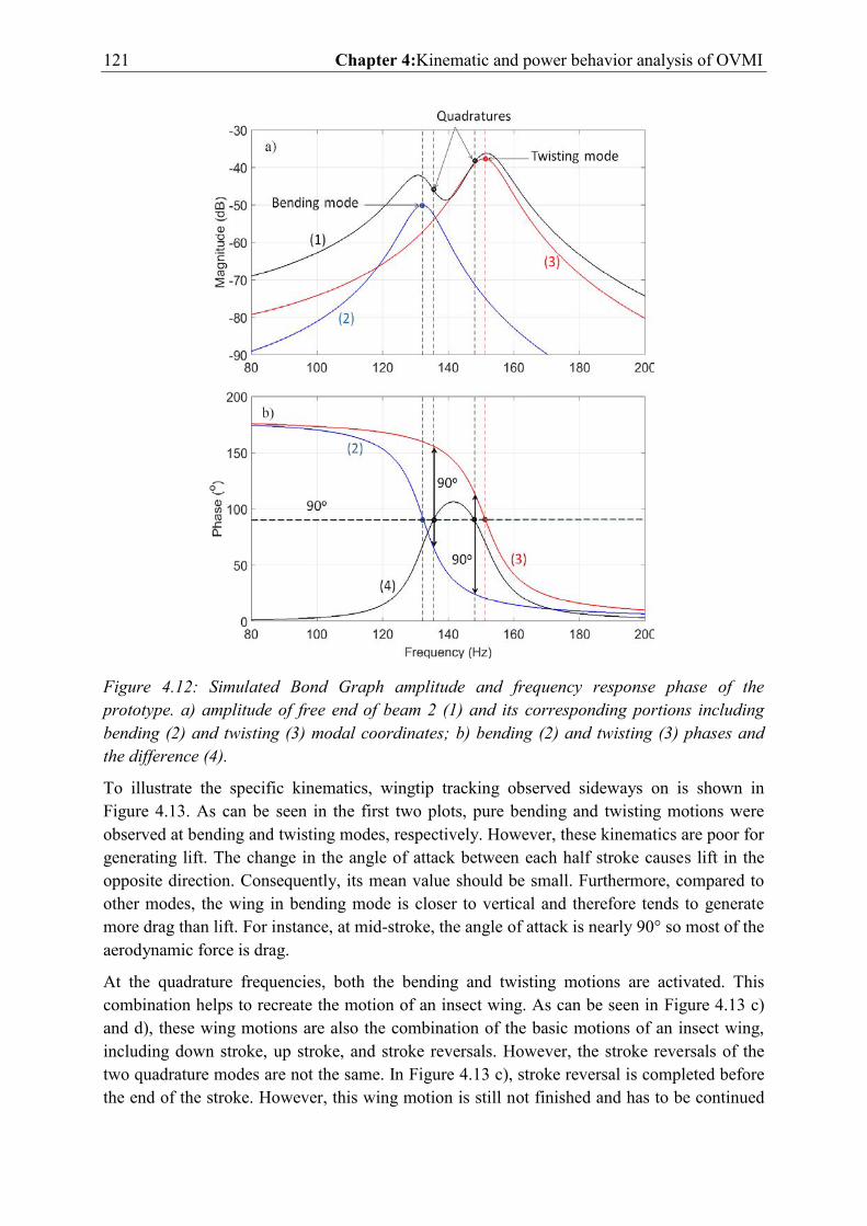
121 Chapter 4:Kinematic and power behavior analysis of OVMI
Figure 4.12: Simulated Bond Graph amplitude and frequency response phase of the prototype. a) amplitude of free end of beam 2 (1) and its corresponding portions including bending (2) and twisting (3) modal coordinates; b) bending (2) and twisting (3) phases and the difference (4).
To illustrate the specific kinematics, wingtip tracking observed sideways on is shown in Figure 4.13. As can be seen in the first two plots, pure bending and twisting motions were observed at bending and twisting modes, respectively. However, these kinematics are poor for generating lift. The change in the angle of attack between each half stroke causes lift in the opposite direction. Consequently, its mean value should be small. Furthermore, compared to other modes, the wing in bending mode is closer to vertical and therefore tends to generate more drag than lift. For instance, at mid-stroke, the angle of attack is nearly 90° so most of the aerodynamic force is drag.
At the quadrature frequencies, both the bending and twisting motions are activated. This combination helps to recreate the motion of an insect wing. As can be seen in Figure 4.13 c) and d), these wing motions are also the combination of the basic motions of an insect wing, including down stroke, up stroke, and stroke reversals. However, the stroke reversals of the two quadrature modes are not the same. In Figure 4.13 c), stroke reversal is completed before the end of the stroke. However, this wing motion is still not finished and has to be continued
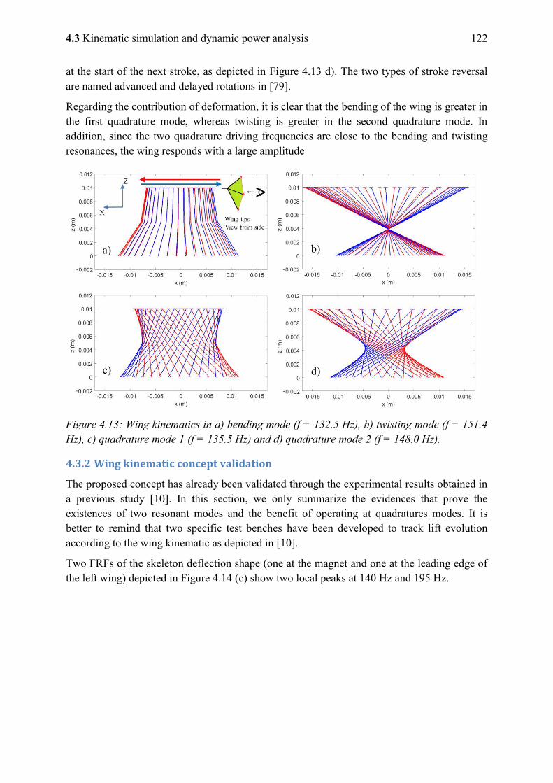
4.3 Kinematic simulation and dynamic power analysis 122
at the start of the next stroke, as depicted in Figure 4.13 d). The two types of stroke reversal are named advanced and delayed rotations in [79].
Regarding the contribution of deformation, it is clear that the bending of the wing is greater in the first quadrature mode, whereas twisting is greater in the second quadrature mode. In addition, since the two quadrature driving frequencies are close to the bending and twisting resonances, the wing responds with a large amplitude
Figure 4.13: Wing kinematics in a) bending mode (f = 132.5 Hz), b) twisting mode (f = 151.4 Hz), c) quadrature mode 1 (f = 135.5 Hz) and d) quadrature mode 2 (f = 148.0 Hz).
4.3.2 Wing kinematic concept validation
The proposed concept has already been validated through the experimental results obtained in a previous study [10]. In this section, we only summarize the evidences that prove the existences of two resonant modes and the benefit of operating at quadratures modes. It is better to remind that two specific test benches have been developed to track lift evolution according to the wing kinematic as depicted in [10].
Two FRFs of the skeleton deflection shape (one at the magnet and one at the leading edge of the left wing) depicted in Figure 4.14 (c) show two local peaks at 140 Hz and 195 Hz.
a) b)
c) d)
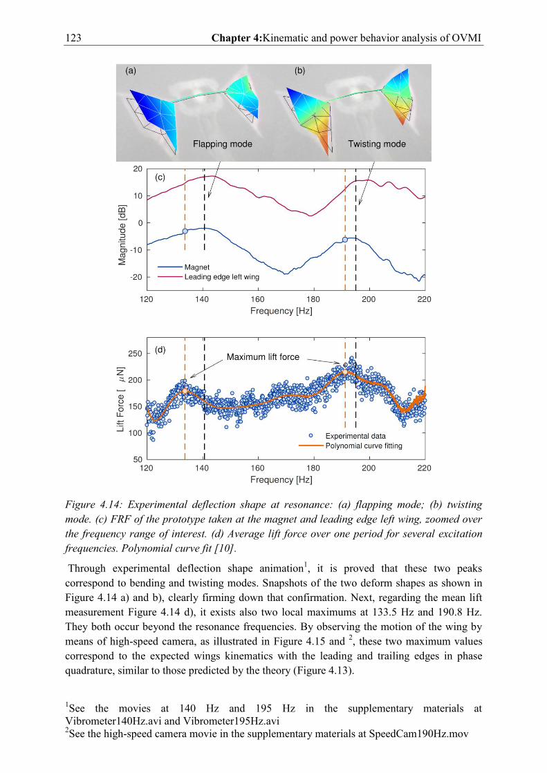
123 Chapter 4:Kinematic and power behavior analysis of OVMI
1See the movies at 140 Hz and 195 Hz in the supplementary materials at Vibrometer140Hz.avi and Vibrometer195Hz.avi 2See the high-speed camera movie in the supplementary materials at SpeedCam190Hz.mov
Figure 4.14: Experimental deflection shape at resonance: (a) flapping mode; (b) twisting mode. (c) FRF of the prototype taken at the magnet and leading edge left wing, zoomed over the frequency range of interest. (d) Average lift force over one period for several excitation frequencies. Polynomial curve fit [10].
Through experimental deflection shape animation1, it is proved that these two peaks correspond to bending and twisting modes. Snapshots of the two deform shapes as shown in Figure 4.14 a) and b), clearly firming down that confirmation. Next, regarding the mean lift measurement Figure 4.14 d), it exists also two local maximums at 133.5 Hz and 190.8 Hz. They both occur beyond the resonance frequencies. By observing the motion of the wing by means of high-speed camera, as illustrated in Figure 4.15 and 2, these two maximum values correspond to the expected wings kinematics with the leading and trailing edges in phase quadrature, similar to those predicted by the theory (Figure 4.13).
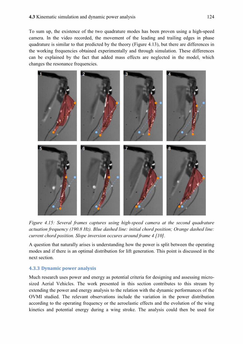
4.3 Kinematic simulation and dynamic power analysis 124
To sum up, the existence of the two quadrature modes has been proven using a high-speed camera. In the video recorded, the movement of the leading and trailing edges in phase quadrature is similar to that predicted by the theory (Figure 4.13), but there are differences in the working frequencies obtained experimentally and through simulation. These differences can be explained by the fact that added mass effects are neglected in the model, which changes the resonance frequencies.
Figure 4.15: Several frames captures using high-speed camera at the second quadrature actuation frequency (190.8 Hz). Blue dashed line: initial chord position; Orange dashed line: current chord position. Slope inversion occures around frame 4 [10].
A question that naturally arises is understanding how the power is split between the operating modes and if there is an optimal distribution for lift generation. This point is discussed in the next section.
4.3.3 Dynamic power analysis
Much research uses power and energy as potential criteria for designing and assessing micro-sized Aerial Vehicles. The work presented in this section contributes to this stream by extending the power and energy analysis to the relation with the dynamic performances of the OVMI studied. The relevant observations include the variation in the power distribution according to the operating frequency or the aeroelastic effects and the evolution of the wing kinetics and potential energy during a wing stroke. The analysis could then be used for
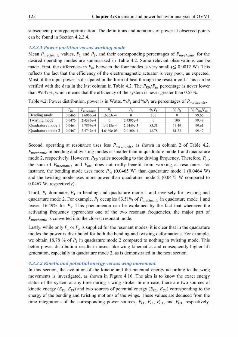
125 Chapter 4:Kinematic and power behavior analysis of OVMI
subsequent prototype optimization. The definitions and notations of power at observed points can be found in Section 4.2.3.4.
4.3.3.1 Power partition versus working mode
Mean values, and , and their corresponding percentages of for the desired operating modes are summarized in Table 4.2. Some relevant observations can be made. First, the differences in between the four modes is very small ( 0.0012 W). This reflects the fact that the efficiency of the electromagnetic actuator is very poor, as expected. Most of the input power is dissipated in the form of heat through the resistor coil. This can be verified with the data in the last column in Table 4.2. The percentage is never lower than 99.47%, which means that the efficiency of the system is never greater than 0.53%.
Table 4.2: Power distribution, power is in Watts. % and % are percentages of .
Bending mode 0.0465 1.6063e-4 1.6063e-4 0 100 0 99.65 Twisting mode 0.0476 2.4395e-4 0 2.4395e-4 0 100 99.49 Quadrature mode 1 0.0464 1.7863e-4 1.4918e-4 2.9449e-5 83.51 16.49 99.61 Quadrature mode 2 0.0467 2.4747e-4 4.6469e-05 2.0100e-4 18.78 81.22 99.47
Second, operating at resonance uses less , as shown in column 2 of Table 4.2. in bending and twisting modes is smaller than in quadrature mode 1 and quadrature mode 2, respectively. However, varies according to the driving frequency. Therefore, the sum of and , does not really benefit from working at resonance. For instance, the bending mode uses more (0.0465 W) than quadrature mode 1 (0.0464 W) and the twisting mode uses more power than quadrature mode 2 (0.0475 W compared to 0.0467 W, respectively).
Third, dominates in bending and quadrature mode 1 and inversely for twisting and quadrature mode 2. For example, occupies 83.51% of in quadrature mode 1 and leaves 16.49% for . This phenomenon can be explained by the fact that whenever the activating frequency approaches one of the two resonant frequencies, the major part of is converted into the closest resonant mode.
Lastly, while only or is supplied for the resonant modes, it is clear that in the quadrature modes the power is distributed for both the bending and twisting deformations. For example, we obtain 18.78 % of in quadrature mode 2 compared to nothing in twisting mode. This better power distribution results in insect-like wing kinematics and consequently higher lift generation, especially in quadrature mode 2, as is demonstrated in the next section.
4.3.3.2 Kinetic and potential energy versus wing movement
In this section, the evolution of the kinetic and the potential energy according to the wing movements is investigated, as shown in Figure 4.16. The aim is to know the exact energy status of the system at any time during a wing stroke. In our case, there are two sources of kinetic energy ( , ) and two sources of potential energy ( , ) corresponding to the energy of the bending and twisting motions of the wings. These values are deduced from the time integrations of the corresponding power sources, , , , and , respectively.
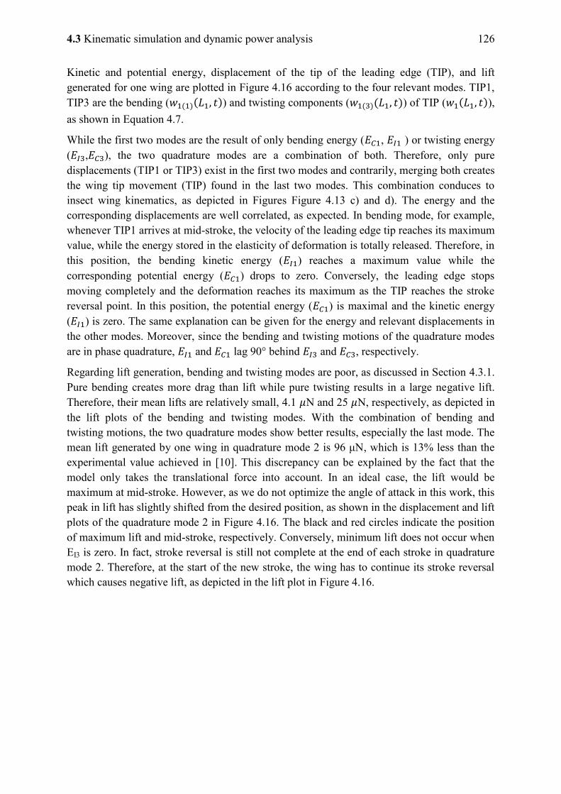
4.3 Kinematic simulation and dynamic power analysis 126
Kinetic and potential energy, displacement of the tip of the leading edge (TIP), and lift generated for one wing are plotted in Figure 4.16 according to the four relevant modes. TIP1, TIP3 are the bending ( ) and twisting components ( ) of TIP ( ), as shown in Equation 4.7.
While the first two modes are the result of only bending energy ( , ) or twisting energy ( , ), the two quadrature modes are a combination of both. Therefore, only pure displacements (TIP1 or TIP3) exist in the first two modes and contrarily, merging both creates the wing tip movement (TIP) found in the last two modes. This combination conduces to insect wing kinematics, as depicted in Figures Figure 4.13 c) and d). The energy and the corresponding displacements are well correlated, as expected. In bending mode, for example, whenever TIP1 arrives at mid-stroke, the velocity of the leading edge tip reaches its maximum value, while the energy stored in the elasticity of deformation is totally released. Therefore, in this position, the bending kinetic energy ( ) reaches a maximum value while the corresponding potential energy ( ) drops to zero. Conversely, the leading edge stops moving completely and the deformation reaches its maximum as the TIP reaches the stroke reversal point. In this position, the potential energy ( ) is maximal and the kinetic energy ( ) is zero. The same explanation can be given for the energy and relevant displacements in the other modes. Moreover, since the bending and twisting motions of the quadrature modes are in phase quadrature, and lag 90° behind and , respectively.
Regarding lift generation, bending and twisting modes are poor, as discussed in Section 4.3.1. Pure bending creates more drag than lift while pure twisting results in a large negative lift. Therefore, their mean lifts are relatively small, 4.1 N and 25 N, respectively, as depicted in the lift plots of the bending and twisting modes. With the combination of bending and twisting motions, the two quadrature modes show better results, especially the last mode. The mean lift generated by one wing in quadrature mode 2 is 96 μN, which is 13% less than the experimental value achieved in [10]. This discrepancy can be explained by the fact that the model only takes the translational force into account. In an ideal case, the lift would be maximum at mid-stroke. However, as we do not optimize the angle of attack in this work, this peak in lift has slightly shifted from the desired position, as shown in the displacement and lift plots of the quadrature mode 2 in Figure 4.16. The black and red circles indicate the position of maximum lift and mid-stroke, respectively. Conversely, minimum lift does not occur when EI3 is zero. In fact, stroke reversal is still not complete at the end of each stroke in quadrature mode 2. Therefore, at the start of the new stroke, the wing has to continue its stroke reversal which causes negative lift, as depicted in the lift plot in Figure 4.16.
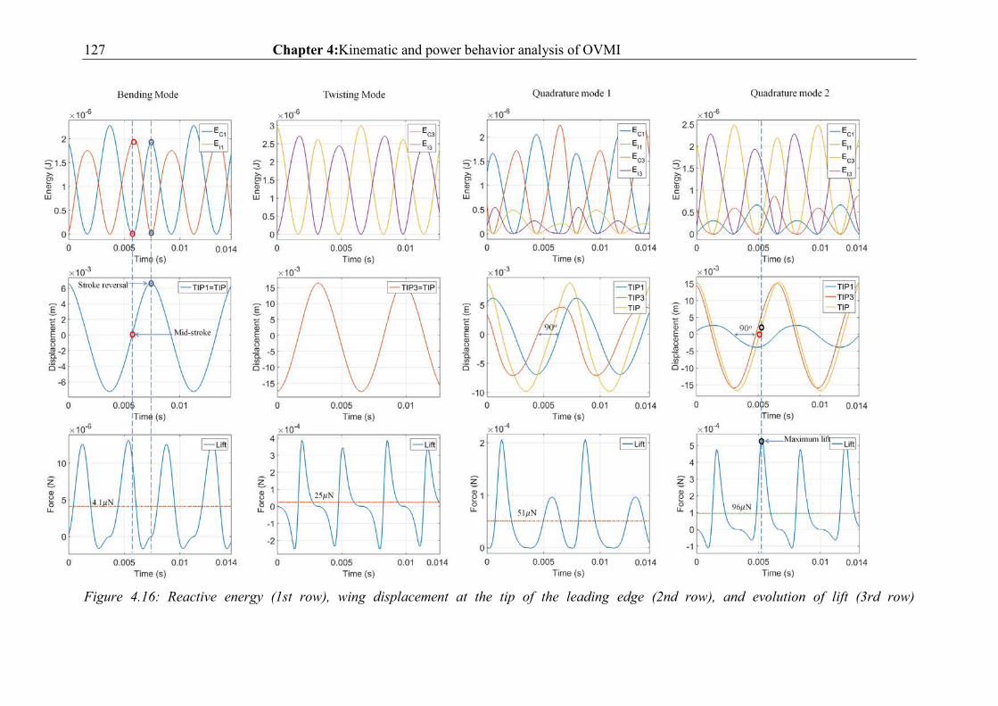
127 Chapter 4:Kinematic and power behavior analysis of OVMI
Figure 4.16: Reactive energy (1st row), wing displacement at the tip of the leading edge (2nd row), and evolution of lift (3rd row)
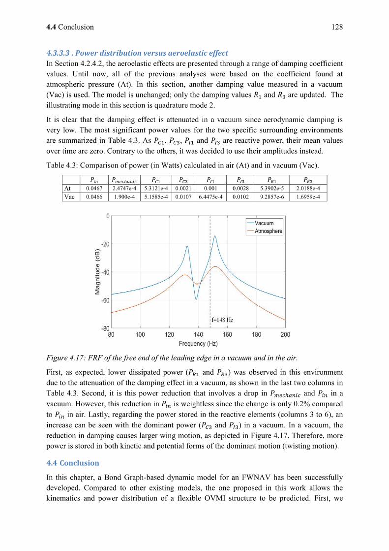
4.4 Conclusion 128
4.3.3.3 . Power distribution versus aeroelastic effect
In Section 4.2.4.2, the aeroelastic effects are presented through a range of damping coefficient values. Until now, all of the previous analyses were based on the coefficient found at atmospheric pressure (At). In this section, another damping value measured in a vacuum (Vac) is used. The model is unchanged; only the damping values and are updated. The illustrating mode in this section is quadrature mode 2.
It is clear that the damping effect is attenuated in a vacuum since aerodynamic damping is very low. The most significant power values for the two specific surrounding environments are summarized in Table 4.3. As , , and are reactive power, their mean values over time are zero. Contrary to the others, it was decided to use their amplitudes instead.
Table 4.3: Comparison of power (in Watts) calculated in air (At) and in vacuum (Vac).
At 0.0467 2.4747e-4 5.3121e-4 0.0021 0.001 0.0028 5.3902e-5 2.0188e-4 Vac 0.0466 1.900e-4 5.1585e-4 0.0107 6.4475e-4 0.0102 9.2857e-6 1.6959e-4
Figure 4.17: FRF of the free end of the leading edge in a vacuum and in the air.
First, as expected, lower dissipated power ( and ) was observed in this environment due to the attenuation of the damping effect in a vacuum, as shown in the last two columns in Table 4.3. Second, it is this power reduction that involves a drop in and in a vacuum. However, this reduction in is weightless since the change is only 0.2% compared to in air. Lastly, regarding the power stored in the reactive elements (columns 3 to 6), an increase can be seen with the dominant power ( and ) in a vacuum. In a vacuum, the reduction in damping causes larger wing motion, as depicted in Figure 4.17. Therefore, more power is stored in both kinetic and potential forms of the dominant motion (twisting motion).
4.4 Conclusion
In this chapter, a Bond Graph-based dynamic model for an FWNAV has been successfully developed. Compared to other existing models, the one proposed in this work allows the kinematics and power distribution of a flexible OVMI structure to be predicted. First, we
129 Chapter 4:Kinematic and power behavior analysis of OVMI
simulate four working modes: pure bending mode, pure twisting mode, quadrature mode 1, and quadrature mode 2. The simulated kinematics and lift are impressively close to the experimental values. Second, taking advantage of the Bond Graph formalism, energy and power distributions between subsystems of the OVMI were easily tracked. The results first show a heavy loss found at the electromagnetic actuator resulting in less than 0.53 % of the electric power input actually serving the wing motion.
Then, through the analyses of the dynamic performance in relation to the power and energy, some key conclusions can be drawn. First, there is a strong correlation between the evolution in energy and the wing kinematics and lift generated, i.e., the lift reaches its peak close to mid-stroke where the wing kinetic energy is at its maximum. Second, the model can adapt to the variation in aeroelastic effect. The decrease in damping caused by aerodynamic forces in a vacuum leads to a larger wing amplitude and greater stored kinetic power. Third, insect wing kinematics can be achieved with proper power distribution, i.e., 18.87% for or 81.22% for results in quadrature mode 2. Finally, this last mode is considered as the most efficient, as it could create more lift than the other modes. In conclusion, this Bond Graph-based model is essential to analyze the dynamic performance of the vehicle from a power and energy point of view. Future work could include the optimization of the structure to enhance the lift force. Besides this ultimate structure, we will also obtain new information on the power distribution between bending and twisting motions. This knowledge will help to form a new power criterion which could be applied to the next prototype.

4.4 Conclusion 130
131 Conclusion and perspective
Conclusion and perspective
Conclusion The aim of this work was to develop an autonomous, bio-inspired flapping-wing Nano-Air-Vehicle (NAV). This PhD was undertaken within the ANR CLEAR-Flight project 13-0012-001 (Controlled Lift for Efficient flight of an Artificial Insect). As the ultimate objective of reducing the vehicle size and producing a NAV is extremely challenging, it has been, therefore, decided to work with a MAV. The first step is to acquire knowledge in the design and fabrication of a small flying vehicle. The second step is to have a tool for the simulation and experimentation of wing actuation, take-off and hovering. The last step is to develop the electronic board and ensure stable flight. Some of the experience obtained could then be transferred for the NAV development. The main contributions of this work are presented as follows.
Chapter 1 is a literature review of fundamental theories related to the flapping wing. First, it has been demonstrated that compared to fixed and rotating wings, vehicles employing flapping wing have a crucial advantage when working in the restricted and confined environment. Next, in order to apply this wing type on the MAV or NAV, it has been necessary to understand the relevant bio-inspired concepts such as the wing actuation mechanisms, the wing kinematics, the aerodynamics and the flying modes. As a result, the insect-like wing kinematic inspired by the small birds and insects has been selected. Although governed by the unsteady aerodynamics, this wing kinematic has been proved as an appropriate solution especially for hovering flight of the small size vehicles. In addition, it has been found that MAV can employ both direct and indirect wing actuation mechanisms, but the indirect type is more adapted to NAV since this mechanism allows the vehicle to flap their wings at higher frequencies. The above discussions have converged to a MAV inspired by the hummingbird since this small bird is the only bird that can truly hover with an insect-like wing kinematic and indirect wing actuation mechanism. In the final step, the components of the MAV are bio-inspired. As a consequence, conventional DC motors coupled with helical springs replace flight muscles and have been used to drive the MAV flapping motion, while a rubber determines the wing rotation passively. Although some of the knowledge acquired could be transferred to develop the NAV, some components better adapted to the smaller scale would have to be replaced as for example the DC actuator by an electromagnetic actuator. Furthermore, the wing design is also a key issue and should be reconsidered for the NAV.
In Chapter 2, a Bond Graph-based model of the MAV has been developed. For simplicity, this model uses a lumped parameter approach. It is noted that the Bond Graph formalism has been employed since it is well suited to simulate multi-physical exchanges of power and energy between subsystems. It helps not only to predict the wing kinematic and the generated aerodynamic forces but also to optimize the key parameters of the MAV. These key parameters are the following: the input voltage, the frequency, the stiffness of the helical
132
spring, the stiffness of the rubber and the wing offset. Throughout an optimizing process, a proper wing kinematic which results in a lift greater than the vehicle weight has been found.
In Chapter 3, based on the optimized parameters, a prototype was fabricated and characterized to validate the dimensioning results of the model. Both wing motions and generated lift measured on different frequencies and input voltage were impressively close to the corresponding simulation results. Moreover, one of the major results is that the prototype is now able to take-off since a lift-to-weight ratio around 1.4 has been simulated and demonstrated experimentally. A PID controller has been included to prove the robustness and stability of the prototype vertical flight. In addition, taking the advantage of the Bond Graph formalism, the power evolution at any point on the power flow in the MAV could be observed. Some key conclusions can be drawn. Firstly, 83% of the electrical input power (Pin) is dissipated at the motor coil (PR0). This leads to an overall electromechanical efficiency of 17 % for the MAV. This mechanical power is transferred to the wings (Pmechanic). Secondly, at the wing, the dissipated power caused by the damping of the rubber (Pbw) is inconsiderable. A larger portion resides in the reactive elements (Pflap, Prot) presenting the wing flapping and rotation motions but discharges completely after a one-half cycle which means that there is, therefore, no cost of power. Thirdly, regarding the power coming from the interaction of the wings motions and surrounding air (Paeroflap, Paerorot), the portion acting on flapping axis (Paeroflap) totally dominates. Regarding the electronic circuit development, with the lift to weight ratio of 1.4, we have only 1.2 g for the payload. It is however not enough to integrate currently the electronic circuit and the battery. Nevertheless, an electronic circuit with full functions of an autonomy flying vehicle has been developed. This circuit already includes all fundamental components for flight stabilization such as power regulator, microcontroller, sensors and motor driver. The circuit has the weight of 2 g and a size of 3x3.8 cm2.
Chapter 4 was dedicated to the development of the NAV. Since the NAV is smaller so their wings must operate at a higher frequency than the MAV. Therefore, while remaining the insect-wing kinematic as the MAV, the wing actuation mechanism changes from direct to indirect to achieve higher flapping frequency. To realize that, it was decided to vibrate the whole flexible skeleton of the NAV including the thorax, wings and links by an electromagnetic actuator. Regarding the development of the NAV, a Bond Graph-based dynamic model for this vehicle has been successfully developed. Compared to the MAV, the NAV is modeled using a distributed parameter approach, since we take into account the motion at every point on the flexible structure. As a consequence, in the case of NAV, it is not possible to use the same methodology than those applied to the MAV in order to obtain the insect-wing kinematic. Instead, we played with the geometry and the elastic properties of the structure. As a result, the prototype studied reproduces insect wing kinematics by combining two resonant vibration modes – bending and twisting modes of the structure respectively. Once again, the simulated kinematics and lift at the working modes are impressively close to the experimental values. The existences of the two resonant modes and the benefit of operating at quadratures modes have been proved. Also taking advantage of the Bond Graph formalism, energy and power distributions between subsystems of the NAV were also easily tracked. The results first show a heavy loss found at the electromagnetic actuator resulting in less than 0.53 % of the electric power input serving the wing motion. This value is much
133 Conclusion and perspective
smaller than the one (17%) found in MAV. Secondly, an insect wing kinematics can be achieved with proper power distribution: for example, in quadrature mode 2 we obtained 18.78% for the power in charge of bending motion or 81.22% for the power in charge of twisting motion results. Compared to the MAV, the power division between the two main motions of NAV is not fixed, it depends on the working frequency. For instance, at the quadrature mode 1 (135.5 Hz), more power (83.51%) is divided for the flapping motion comparing to only 18.78% in the quadrature mode 2. Finally, the quadrature mode 2 is considered as the most efficient, as it could create more lift than the other modes and produces enough lift to take-off. However, since the weight of electrical wires is even heavier than the prototype, the NAV is still on the ground.
Perspectives In order to achieve the goal to have a MAV and a NAV which are able to fly autonomously, the work should be continued on the following points:
1. Considering the work presented here, the main conclusion is that both MAV and NAV are not able yet to generate enough lift to take-off with electronic board and payload. Therefore the first perspective is to enhance the lift generation. For the MAV, a solution which is directly inspired by flying creatures is to increase the flapping frequency. For instance, if the flapping frequency is double while the amplitudes of the wing motions remain, the prototype can produce theoretically four times of lift, and therefore the electronic circuit and the battery could be onboard. In this case, we have to find a new motor better adapted to fulfil such an objective. Regarding the NAV, it is more complex since the generated lift was mainly limited by the small wing movements. In fact, both angles of flapping and twisting ranges are approximate of 20°. Therefore it is necessary to optimize the wing geometry and material so that the amplitudes of wing motions would be larger while remaining the same wing kinematic as in case of the quadrature mode 2.
Other possibilities for future works come from the advantages of the Bond Graph formalism in power and energy analysis that allows optimizing the wing actuation from the power point of view Firstly, it is possible to apply the same power analysis on the existing MAVs and NAVs. By comparing the efficiencies of the subsystems of the flying vehicles, we can find better solutions. Secondly, by observing the wings movements of real insects and birds, it is expected to have a figure of the power distribution between the flapping and rotating or twisting motions. This information could help to form a new dynamic power criterion which can be applied for our next prototypes.
2. After having a higher lift to weight ratio, the second perspective is to control and stabilize the flight. In the case of MAV, it is necessary to integrate and program the electronic board developed in Chapter 3 so that the vehicle can perform a directional flight. On the other hand, another challenge is to equip a few milligrams NAV with an electronic circuit with today‟s technology. The objective is to integrate all the electronic components needed for an autonomous flight into an application specific integrated circuit (ASIC).
3. In the next step, for an autonomous flight, both the MAV and NAV need to integrate the batteries and the sensors such as a camera which help to recognize the surrounding
134
environment. Thanks to the sensor, the vehicles can identify the characteristics of the operating environment and make the decision by themselves.
Furthermore, to extend the endurance of the vehicles, the energy harvesting unit integrated into the electronic circuit could play a crucial role. Light, wind or deformation of the wing membrane are all possible sources of free energy. Another solution is to make the vehicles lighter so that they spend less energy and can operate longer. The new materials are becoming increasingly lighter, the electronic parts are getting smaller, and the batteries have a higher energy density. In addition, as the avionics manufacturers such as Dassault, Thales, and European Aeronautic Defence and Space company (EADS now Airbus) have already participated into the development of MAV and NAV, we could benefit from their experience in aeronautics and spatial civil and military. MAV and NAV weights will undoubtedly soon be pushing new boundaries.
Finally, when the NAV succeeds to be autonomous with proper endurance, it is possible to assign them to the different tasks. The small size of vehicles means they can be used in confined spaces, i.e., inside buildings. A possible application would be monitoring sensitive industrial environments (chemical, nuclear, etc.). In addition, the acoustic discretion is perfect for monitoring patient health in hospitals or spy missions for the military. The final suggestion mimics the swarming behaviour of small birds or insects i.e, the flapping vehicles work together in a group and each one is assigned a mini task as part of a global objective.
135 References
References
[1] “nature | Definition of nature in English by Oxford Dictionaries,” Oxford Dictionaries | English. [Online]. Available: https://en.oxforddictionaries.com/definition/nature. [Accessed: 26-Sep-2018].
[2] Unmanned aircraft systems: (UAS). Montréal: International Civil Aviation Organization, 2011.
[3] J. W. Gerdes and S. K. Gupta, “A REVIEW OF BIRD-INSPIRED FLAPPING WING MINIATURE AIR VEHICLE DESIGNS,” p. 16.
[4] L. Petricca, P. Ohlckers, and C. Grinde, “Micro- and Nano-Air Vehicles: State of the Art,” Int. J. Aerosp. Eng., vol. 2011, pp. 1–17, 2011.
[5] S. K. Banala, Y. Karakaya, S. McIntosh, Z. Khan, and S. K. Agrawal, “Design and Optimization of a Mechanism for Out of Plane Insect Wing Like Motion With Twist,” p. 7, 2004.
[6] S. P. Sane, “The aerodynamics of insect flight,” J. Exp. Biol., vol. 206, no. 23, pp. 4191–4208, Dec. 2003.
[7] M. H. Dickinson and K. G. Götz, “Unsteady aerodynamic performance of model wings at low reynolds numbers,” p. 21.
[8] “IEMN – Institut d‟Electronique, de Microélectronique et de Nanotechnologie.” . [9] C. H. Greenewalt, Hummingbirds. Dover Publication, INC., New York, 1990. [10] D. Faux, O. Thomas, E. Cattan, S. Grondel, and L. A. Doan, “Two modes resonant
combined motion for insect wings kinematics reproduction and lift generation,” EPL Europhys. Lett., vol. 121, no. 6, p. 66001, Mar. 2018.
[11] “Accueil | Arts et métiers.” [Online]. Available: https://artsetmetiers.fr/fr. [Accessed: 23-Oct-2018].
[12] “ONERA, le centre français de recherche aérospatiale.” [Online]. Available: https://www.onera.fr/. [Accessed: 23-Oct-2018].
[13] “Conception et Intégration de produits électroniques - Thurmelec à Pulversheim,” Thurmelec. [Online]. Available: https://www.thurmelec.fr/. [Accessed: 23-Oct-2018].
[14] “Page d‟accueil ENSIAME | ENSIAME | Université de Valenciennes.” [Online]. Available: http://www.uphf.fr/ensiame/page-daccueil-ensiame. [Accessed: 23-Oct-2018].
[15] “History of U.S. Drones,” Understanding Empire: Technology, Power, Politics, 21-May-2012. .
[16] “Remote Piloted Aerial Vehicles.” [Online]. Available: http://www.ctie.monash.edu.au/hargrave/rpav_home.html. [Accessed: 18-Jun-2017].
[17] V. K. Saxena, The Amazing Growth and Journey of UAV’s and Ballastic Missile Defence Capabilities: Where the Technology is Leading to? Vij Books India Pvt Ltd, 2013.
[18] C. Kennedy and J. I. Rogers, “Virtuous drones?,” Int. J. Hum. Rights, vol. 19, no. 2, pp. 211–227, Feb. 2015.
[19] “Drones smuggling porn, drugs to inmates around the world | Fox News.” [Online]. Available: http://www.foxnews.com/us/2017/04/17/drones-smuggling-porn-drugs-to-inmates-around-world.html. [Accessed: 18-Jun-2017].
[20] C. Zhang and J. M. Kovacs, “The application of small unmanned aerial systems for precision agriculture: a review,” Precis. Agric., vol. 13, no. 6, pp. 693–712, Dec. 2012.
[21] G. J. Grenzdörffer, A. Engel, and B. Teichert, “The photogrammetric potential of low-cost UAVs in forestry and agriculture,” Int. Arch. Photogramm. Remote Sens. Spat. Inf. Sci., vol. 31, no. B3, pp. 1207–1214, 2008.
136
[22] F. G. Costa, J. Ueyama, T. Braun, G. Pessin, F. S. Osório, and P. A. Vargas, “The use of unmanned aerial vehicles and wireless sensor network in agricultural applications,” in Geoscience and Remote Sensing Symposium (IGARSS), 2012 IEEE International, 2012, pp. 5045–5048.
[23] L. Hassan-Esfahani, A. Torres-Rua, A. M. Ticlavilca, A. Jensen, and M. McKee, “Topsoil moisture estimation for precision agriculture using unmmaned aerial vehicle multispectral imagery,” in Geoscience and Remote Sensing Symposium (IGARSS), 2014 IEEE International, 2014, pp. 3263–3266.
[24] J. Berni, P. J. Zarco-Tejada, L. Suarez, and E. Fereres, “Thermal and Narrowband Multispectral Remote Sensing for Vegetation Monitoring From an Unmanned Aerial Vehicle,” IEEE Trans. Geosci. Remote Sens., vol. 47, no. 3, pp. 722–738, Mar. 2009.
[25] G. J. J. Verhoeven, “Providing an archaeological bird‟s-eye view – an overall picture of ground-based means to execute low-altitude aerial photography (LAAP) in Archaeology,” Archaeol. Prospect., vol. 16, no. 4, pp. 233–249, Oct. 2009.
[26] F. Chiabrando, F. Nex, D. Piatti, and F. Rinaudo, “UAV and RPV systems for photogrammetric surveys in archaelogical areas: two tests in the Piedmont region (Italy),” J. Archaeol. Sci., vol. 38, no. 3, pp. 697–710, Mar. 2011.
[27] F. Rinaudo, F. Chiabrando, A. M. Lingua, and A. T. Spanò, “Archaeological site monitoring: UAV photogrammetry can be an answer,” Int. Arch. Photogramm. Remote Sens. Spat. Inf. Sci., vol. 39, no. B5, pp. 583–588, 2012.
[28] U. Niethammer, M. R. James, S. Rothmund, J. Travelletti, and M. Joswig, “UAV-based remote sensing of the Super-Sauze landslide: Evaluation and results,” Eng. Geol., vol. 128, pp. 2–11, Mar. 2012.
[29] W. Hartmann, S. Tilch, H. Eisenbeiss, and K. Schindler, “Determination of the UAV position by automatic processing of thermal images,” Int. Arch. Photogramm. Remote Sens. Spat. Inf. Sci., vol. 39, p. B6, 2012.
[30] “Shrediquette BOLT.” . [31] “Les drones au service des entreprises | SNCF Réseau.” [Online]. Available:
https://www.sncf-reseau.fr/fr/a-propos/notre-strategie/drones-et-entreprises. [Accessed: 25-Oct-2018].
[32] “Eyesee : le drone pour automatiser les inventaires des entrepôts logistiques,” Hardis Group, 16-Jul-2015. [Online]. Available: https://www.hardis-group.com/nos-activites/solutions-logistiques/Eyesee-drone-pour-automatiser-les-inventaires-des-entrepots-logistiques. [Accessed: 25-Oct-2018].
[33] U. of Bristol, “2014: Drone helps Fukushima clean-up | Cabot Institute for the Environment | University of Bristol.” [Online]. Available: http://www.bristol.ac.uk/cabot/news/2014/487.html. [Accessed: 25-Oct-2018].
[34] “Drone Adventures in Haiti | Robohub.” . [35] “Fukushima – a Drones Eye View – Drone Adventures.” . [36] G. C. H. E. de Croon, M. Perçin, B. D. W. Remes, R. Ruijsink, and C. De Wagter, The
DelFly. Dordrecht: Springer Netherlands, 2016. [37] R. J. Wood, “The First Takeoff of a Biologically Inspired At-Scale Robotic Insect,”
IEEE Trans. Robot., vol. 24, no. 2, pp. 341–347, Apr. 2008. [38] B. Singh, “Dynamics and aeroelasticity of hover-capable flapping wings: Experiments
and analysis,” University of Maryland, College Park, 2007. [39] J. Grasmeyer and M. Keennon, “Development of the Black Widow Micro Air
Vehicle,” 2001. [40] D. Gyllhem, K. Mohseni, D. Lawrence, and P. Geuzaine, “Numerical simulation of
flow around the Colorado micro aerial vehicle,” in AIAA Fluid Dynamics Conference and Exhibit, 2005, pp. 6–9.
137 References
[41] W. Shyy, B. Mats, and L. Daniel, “Flapping and fexible wings for biological and micro air vehicles,” Prog. Aerosp. Sci., vol. 35, no. 5, pp. 455–506, 1999.
[42] M. R. Waszak, L. N. Jenkins, and P. Ifju, “Stability and control properties of an aeroelastic fixed wing micro aerial vehicle,” AIAA Pap., vol. 4005, p. 2001, 2001.
[43] V. Brion, M. Aki, and S. Shkarayev, “Numerical simulation of low Reynolds number flows around micro air vehicles and comparison against wind tunnel data,” in AIAA Applied Aerodynamics Conference, 2006, pp. 5–8.
[44] Y. Lian and W. Shyy, “Numerical Simulations of Membrane Wing Aerodynamics for Micro Air Vehicle Applications,” J. Aircr., vol. 42, no. 4, pp. 865–873, Jul. 2005.
[45] B. Stanford, D. Viieru, R. Albertani, W. Shyy, and P. Ifju, “A numerical and experimental investigation of flexible micro air vehicle wing deformation,” 2006.
[46] D. Viieru, R. Albertani, W. Shyy, and P. G. Ifju, “Effect of Tip Vortex on Wing Aerodynamics of Micro Air Vehicles,” J. Aircr., vol. 42, no. 6, pp. 1530–1536, Nov. 2005.
[47] B. Singh, “Dynamics and Aeroelasticity of Hover-Capable Flapping Wings: Experiments and Analysis. PhD thesis,” 2006.
[48] A. Datta, “The martian autonomous rotary-wing vehicle (MARV).” Tech. Rep., University of Maryland, College Park, Md, USA, 2000.
[49] L. Petricca, P. Ohlckers, and C. Grinde, “Micro- and Nano-Air Vehicles: State of the Art,” Int. J. Aerosp. Eng., vol. 2011, pp. 1–17, 2011.
[50] “Black Hornet Nano,” Wikipedia. 23-Aug-2018. [51] “Crazyflie 2.0.” [Online]. Available: https://www.seeedstudio.com/Crazyflie-2.0-p-
2103.html. [Accessed: 11-Jul-2017]. [52] I. Kroo et al., “The Mesicopter: A Miniature Rotorcraft Concept Phase II Final
Report,” p. 138. [53] P. Muren, “Picoflyer description,” 2005. [Online]. Available:
http://www.proxflyer.com/pi_meny.htm. [54] F. Bohorquez and D. Pines, “Hover performance of rotor blades at low reynolds
numbers for rotary wing micro air vehicles,” AIAA Pap., vol. 6567, no. 2, 2003. [55] “Twisting blade propeller and profile pitch.” [Online]. Available:
https://heliciel.com/en/helice/Vrillage%20calage%20pale%20helice.htm. [Accessed: 11-Sep-2018].
[56] H. Dong, A. T. Bode-Oke, and C. Li, “Learning from Nature: Unsteady Flow Physics in Bioinspired Flapping Flight,” in Flight Physics - Models, Techniques and Technologies, K. Volkov, Ed. InTech, 2018.
[57] C. Galiński and R. Żbikowski, “Some problems of micro air vehicles development,” Bull. Pol. Acad. Sci. Tech. Sci., vol. 55, no. 1, 2007.
[58] T. N. Pornsin-Sirirak, Y.-C. Tai, C.-M. Ho, and M. Keennon, “Microbat: A palm-sized electrically powered ornithopter,” in Proceedings of NASA/JPL Workshop on Biomorphic Robotics, 2001, pp. 14–17.
[59] M. Groen, B. Bruggeman, B. Remes, R. Ruijsink, B. W. Van Oudheusden, and H. Bijl, “Improving flight performance of the flapping wing MAV DelFly II,” in Int. Micro Air Vehicle Conf. and Competition (IMAV 2010)(Braunschweig, Germany), 2010.
[60] G. C. de Croon, M. A. Groen, C. De Wagter, B. Remes, R. Ruijsink, and B. W. van Oudheusden, “Design, aerodynamics and autonomy of the DelFly,” Bioinspir. Biomim., vol. 7, no. 2, p. 025003, 2012.
[61] “New RoboBee flies, dives, swims, and explodes out the of water,” Wyss Institute, 25-Oct-2017. [Online]. Available: https://wyss.harvard.edu/new-robobee-flies-dives-swims-and-explodes-out-the-of-water/. [Accessed: 24-Sep-2018].
138
[62] J. W. Kruyt, E. M. Quicazan-Rubio, G. F. van Heijst, D. L. Altshuler, and D. Lentink, “Hummingbird wing efficacy depends on aspect ratio and compares with helicopter rotors,” J. R. Soc. Interface, vol. 11, no. 99, pp. 20140585–20140585, Jul. 2014.
[63] C. Evangelista, P. Kraft, M. Dacke, J. Reinhard, and M. V. Srinivasan, “The moment before touchdown: landing manoeuvres of the honeybee Apis mellifera,” J. Exp. Biol., vol. 213, no. 2, pp. 262–270, Jan. 2010.
[64] G. Card and M. H. Dickinson, “Visually Mediated Motor Planning in the Escape Response of Drosophila,” Curr. Biol., vol. 18, no. 17, pp. 1300–1307, Sep. 2008.
[65] B. Singh, M. Ramasamy, I. Chopra, and J. G. Leishman, “Experimental studies on insect-based flapping wings for micro hovering air vehicles,” AIAA Pap., vol. 2293, p. 2005, 2005.
[66] R. H. J. Brown, “The flight of birds,” J. Exp. Biol., vol. 30, no. 1, pp. 90–103, 1953. [67] S. A. Ansari, R. Żbikowski, and K. Knowles, “Aerodynamic modelling of insect-like
flapping flight for micro air vehicles,” Prog. Aerosp. Sci., vol. 42, no. 2, pp. 129–172, Feb. 2006.
[68] P. Seshadri, M. Benedict, and I. Chopra, “A novel mechanism for emulating insect wing kinematics,” Bioinspir. Biomim., vol. 7, no. 3, p. 036017, Sep. 2012.
[69] “Inside a wing,” DK Find Out! [Online]. Available: https://www.dkfindout.com/us/animals-and-nature/birds/inside-wing/. [Accessed: 01-Nov-2018].
[70] C. T. Bolsman, B. Palsson, H. Goosen, R. Schmidt, and F. van Keulen, “The use of resonant structures for miniaturizing FMAVs,” in 3rd US-European Competition and Workshop on Micro Air Vehicle & European Micro Air Vehicle Conference and Flight Competition, Toulouse, France, 2007.
[71] “Animal Physiology 4e.” [Online]. Available: https://animalphys4e.sinauer.com/boxex2002.html. [Accessed: 01-Nov-2018].
[72] S. M. Walker et al., “In Vivo Time-Resolved Microtomography Reveals the Mechanics of the Blowfly Flight Motor,” PLoS Biol., vol. 12, no. 3, p. e1001823, Mar. 2014.
[73] C. P. Ellington, “The Aerodynamics of Hovering Insect Flight. I. The Quasi-Steady Analysis,” Philos. Trans. R. Soc. B Biol. Sci., vol. 305, no. 1122, pp. 1–15, Feb. 1984.
[74] F.-O. Lehmann, “The mechanisms of lift enhancement in insect flight,” Naturwissenschaften, vol. 91, no. 3, pp. 101–122, Mar. 2004.
[75] “Kutta condition,” Wikipedia. 19-Jan-2017. [76] W. Shyy et al., “Recent progress in flapping wing aerodynamics and aeroelasticity,”
Prog. Aerosp. Sci., vol. 46, no. 7, pp. 284–327, Oct. 2010. [77] S. P. Sane and M. H. Dickinson, “The aerodynamic effects of wing rotation and a
revised quasi-steady model of flapping flight,” J. Exp. Biol., vol. 205, no. 8, pp. 1087–1096, 2002.
[78] M. H. Dickinson, F.-O. Lehmann, and K. G. Gotz, “The active control of wing rotation by Drosophila,” J. Exp. Biol., vol. 182, no. 1, pp. 173–189, 1993.
[79] M. H. Dickinson, “Wing Rotation and the Aerodynamic Basis of Insect Flight,” Science, vol. 284, no. 5422, pp. 1954–1960, Jun. 1999.
[80] V. Arabagi and M. Sitti, “Simulation and analysis of a passive pitch reversal flapping wing mechanism for an aerial robotic platform,” in Intelligent Robots and Systems, 2008. IROS 2008. IEEE/RSJ International Conference on, 2008, pp. 1260–1265.
[81] P. Zdunich et al., “Development and Testing of the Mentor Flapping-Wing Micro Air Vehicle,” J. Aircr., vol. 44, no. 5, pp. 1701–1711, Sep. 2007.
[82] “Gliding flight,” Wikipedia. 15-Sep-2018.
139 References
[83] J. M. Wakeling and C. P. Ellington, “Dragonfly flight i. Gliding flight and steady-state aerodynamic forces,” p. 14.
[84] W. Shyy, H. Aono, C. Kang, and H. Liu, An introduction to flapping wing aerodynamics. Cambridge ; New York: Cambridge University Press, 2013.
[85] U. M. Lindhe Norberg, “Structure, form, and function of flight in engineering and the living world,” J. Morphol., vol. 252, no. 1, pp. 52–81, Apr. 2002.
[86] M. Karasek and A. Preumont, “Robotic hummingbird: Design of a control mechanism for a hovering flapping wing micro air vehicle,” PhD Thesis Univ., 2014.
[87] “Bird flight,” Wikipedia. 02-Jul-2017. [88] C. P. Ellington, “the novel aerodynamics of insect flight: applications to micro-air
vehicles,” p. 10. [89] B. Tobalske and K. Dial, “Flight kinematics of black-billed magpies and pigeons over
a wide range of speeds,” J. Exp. Biol., vol. 199, no. 2, pp. 263–280, 1996. [90] Alexander, “Nature‟s flyers: birds, insects, and the biomechanics of flight,” Choice
Rev. Online, vol. 40, no. 02, pp. 40-0906-40–0906, Oct. 2002. [91] W. Shyy, Y. Lian, J. Tang, D. Viieru, and H. Liu, “Aerodynamics of Low Reynolds
Number Flyers,” p. 213, 2007. [92] Wild West Nature, Osprey hovers like a hummingbird hunting in Yellowstone National
Park. 2013. [93] J. Song, H. Luo, and T. L. Hedrick, “Three-dimensional flow and lift characteristics of
a hovering ruby-throated hummingbird,” J. R. Soc. Interface, vol. 11, no. 98, pp. 20140541–20140541, Jul. 2014.
[94] L. Ristroph and S. Childress, “Stable hovering of a jellyfish-like flying machine,” J. R. Soc. Interface, vol. 11, no. 92, pp. 20130992–20130992, Jan. 2014.
[95] L. Hines, D. Campolo, and M. Sitti, “Liftoff of a motor-driven, flapping-wing microaerial vehicle capable of resonance,” Robot. IEEE Trans. On, vol. 30, no. 1, pp. 220–232, 2014.
[96] W. Trimmer and R. Jebens, “Actuators for micro robots,” Proc. 1989 Int. Conf. Robot. Autom. Scottsdale AZ, vol. 3, pp. 1547–1552, 1989.
[97] “Servomoteurs C.C. sans balais 0308...B.” [Online]. Available: https://www.faulhaber.com/fr/produits/series/0308b/. [Accessed: 22-Oct-2017].
[98] A. Bontemps, F. Valenciennes, S. Grondel, S. Dupont, T. Vanneste, and E. Cattan, “Modeling and evaluation of power transmission of flapping wing nano air vehicle,” in 2014 IEEE/ASME 10th International Conference on Mechatronic and Embedded Systems and Applications (MESA), 2014, pp. 1–6.
[99] W. Shyy, C. Kang, P. Chirarattananon, S. Ravi, and H. Liu, “Aerodynamics, sensing and control of insect-scale flapping-wing flight,” Proc. R. Soc. Math. Phys. Eng. Sci., vol. 472, no. 2186, p. 20150712, Feb. 2016.
[100] R. D. Kornbluh et al., “Electroelastomers: applications of dielectric elastomer transducers for actuation, generation, and smart structures,” presented at the SPIE‟s 9th Annual International Symposium on Smart Structures and Materials, San Diego, CA, 2002, pp. 254–270.
[101] C. Zhang, “Design and Control of Flapping Wing Micro Air Vehicles,” Technical University of Mandrid, 2016.
[102] G.-K. Lau, H.-T. Lim, J.-Y. Teo, and Y.-W. Chin, “Lightweight mechanical amplifiers for rolled dielectric elastomer actuators and their integration with bio-inspired wing flappers,” Smart Mater. Struct., vol. 23, no. 2, p. 025021, Feb. 2014.
[103] Z. Liu, X. Yan, M. Qi, and L. Lin, “Electrostatic flapping wings with pivot-spar brackets for high lift force,” 2016, pp. 1133–1136.
140
[104] X. Yan, M. Qi, and L. Lin, “Self-lifting artificial insect wings via electrostatic flapping actuators,” 2015, pp. 22–25.
[105] Y. Zou, W. Zhang, and Z. Zhang, “Liftoff of an Electromagnetically Driven Insect-Inspired Flapping-Wing Robot,” IEEE Trans. Robot., vol. 32, no. 5, pp. 1285–1289, Oct. 2016.
[106] Z. E. Teoh and R. J. Wood, “A bioinspired approach to torque control in an insect-sized flapping-wing robot,” in 5th IEEE RAS/EMBS International Conference on Biomedical Robotics and Biomechatronics, Sao Paulo, Brazil, 2014, pp. 911–917.
[107] K. Y. Ma, P. Chirarattananon, and R. J. Wood, “Design and fabrication of an insect-scale flying robot for control autonomy,” in 2015 IEEE/RSJ International Conference on Intelligent Robots and Systems (IROS), Hamburg, Germany, 2015, pp. 1558–1564.
[108] B. M. Finio and R. J. Wood, “Distributed power and control actuation in the thoracic mechanics of a robotic insect,” Bioinspir. Biomim., vol. 5, no. 4, p. 045006, Dec. 2010.
[109] K. Y. Ma, P. Chirarattananon, S. B. Fuller, and R. J. Wood, “Controlled Flight of a Biologically Inspired, Insect-Scale Robot,” Science, vol. 340, no. 6132, pp. 603–607, May 2013.
[110] Z. E. Teoh, S. B. Fuller, P. Chirarattananon, N. O. Prez-Arancibia, J. D. Greenberg, and R. J. Wood, “A hovering flapping-wing microrobot with altitude control and passive upright stability,” in 2012 IEEE/RSJ International Conference on Intelligent Robots and Systems, Vilamoura-Algarve, Portugal, 2012, pp. 3209–3216.
[111] T. Dargent et al., “Micromachining of an SU-8 flapping-wing flying micro-electro-mechanical system,” J. Micromechanics Microengineering, vol. 19, no. 8, p. 085028, Aug. 2009.
[112] J. F. Goosen, H. J. Peters12, Q. Wang, P. Tiso, and F. van Keulen, “Resonance B Resonance Based Flapping Wing Micro Air Vehicle.”
[113] G. De Croon, K. M. E. De Clercq, R. Ruijsink, B. Remes, and C. de Wagter, “Design, aerodynamics, and vision-based control of the DelFly,” Int. J. Micro Air Veh., vol. 1, no. 2, pp. 71–97, 2009.
[114] C.-K. Hsu, J. Evans, S. Vytla, and P. G. Huang, “Development of flapping wing micro air vehicles-design, CFD, experiment and actual flight,” in 48th AIAA Aerospace Sciences Meeting Including the New Horizons Forum and Aerospace Exposition, 2010, p. 1018.
[115] F. van Breugel, W. Regan, and H. Lipson, “From insects to machines,” IEEE Robot. Autom. Mag., vol. 15, no. 4, pp. 68–74, Dec. 2008.
[116] C. Richter and H. Lipson, “Untethered hovering flapping flight of a 3D-printed mechanical insect,” Artif. Life, vol. 17, no. 2, pp. 73–86, 2011.
[117] M. Keennon, K. Klingebiel, and H. Won, “Development of the Nano Hummingbird: A Tailless Flapping Wing Micro Air Vehicle,” 2012.
[118] “BionicOpter | Festo Corporate.” [Online]. Available: https://www.festo.com/group/en/cms/10224.htm. [Accessed: 20-Jul-2017].
[119] A. J. Bergou, S. Xu, and Z. J. Wang, “Passive wing pitch reversal in insect flight,” J. Fluid Mech., vol. 591, Nov. 2007.
[120] H. V. Phan et al., “Stable Vertical Takeoff of an Insect-Mimicking Flapping-Wing System Without Guide Implementing Inherent Pitching Stability,” J. Bionic Eng., vol. 9, no. 4, pp. 391–401, Dec. 2012.
[121] F. Leys, D. Reynaerts, and D. Vandepitte, “Outperforming hummingbirds‟ load-lifting capability with a lightweight hummingbird-like flapping-wing mechanism,” Biol. Open, vol. 5, no. 8, pp. 1052–1060, Aug. 2016.
[122] J. Zhang, B. Cheng, J. A. Roll, X. Deng, and B. Yao, “Direct drive of flapping wings under resonance with instantaneous wing trajectory control,” in Robotics and Automation (ICRA), 2013 IEEE International Conference on, 2013, pp. 4029–4034.
141 References
[123] D. Coleman and M. Benedict, “On the Development of a Robotic Hummingbird,” 2016.
[124] C. H. Greenewalt, “The Flight of Birds: The Significant Dimensions, Their Departure from the Requirements for Dimensional Similarity, and the Effect on Flight Aerodynamics of That Departure,” Trans. Am. Philos. Soc., vol. 65, no. 4, p. 1, 1975.
[125] J. J. Craig, “Introduction to Robotics,” 2005. [126] “Gear Motor :: Solarbotics.” [Online]. Available:
https://solarbotics.com/product/gm15a/. [Accessed: 08-Aug-2017]. [127] S. P. Sane and M. H. Dickinson, “The control of flight force by a flapping wing: lift
and drag production,” J. Exp. Biol., vol. 204, no. 15, pp. 2607–2626, 2001. [128] H. Liu and K. Kawachi, “A Numerical Study of Insect Flight,” J. Comput. Phys., vol.
146, no. 1, pp. 124–156, Oct. 1998. [129] H. Liu, C. P. Ellington, K. Kawachi, C. Van Den Berg, and A. P. Willmott, “A
computational fluid dynamic study of hawkmoth hovering,” J. Exp. Biol., vol. 201, no. 4, pp. 461–477, 1998.
[130] H. Liu, T. Nakata, N. Gao, M. Maeda, H. Aono, and W. Shyy, “Micro air vehicle-motivated computational biomechanics in bio-flights: aerodynamics, flight dynamics and maneuvering stability,” Acta Mech. Sin., vol. 26, no. 6, pp. 863–879, Dec. 2010.
[131] M. Sun, J. Wang, and Y. Xiong, “Dynamic flight stability of hovering insects,” Acta Mech. Sin., vol. 23, no. 3, pp. 231–246, Jun. 2007.
[132] M. Sun, “Dynamic flight stability of a hovering bumblebee,” J. Exp. Biol., vol. 208, no. 3, pp. 447–459, Feb. 2005.
[133] M. Sun, “High-lift generation and power requirements of insect flight,” Fluid Dyn. Res., vol. 37, no. 1–2, pp. 21–39, Jul. 2005.
[134] A. K. Brodsky, “Vortex formation in the tethered flight of the peacock butterfly Inachis io L.(Lepidoptera, Nymphalidae) and some aspects of insect flight evolution,” J. Exp. Biol., vol. 161, no. 1, pp. 77–95, 1991.
[135] A. P. Willmott and C. P. Ellington, “The mechanics of flight in the hawkmoth Manduca sexta. II. Aerodynamic consequences of kinematic and morphological variation.,” J. Exp. Biol., vol. 200, no. 21, pp. 2723–2745, 1997.
[136] S. P. Sane and M. H. Dickinson, “Quasi-steady model of flapping flight,” p. 10. [137] “Lagrangian mechanics,” Wikipedia. 15-Jul-2017. [138] “Inventor | Mechanical Design & 3D CAD Software | Autodesk.” [Online]. Available:
https://www.autodesk.com/products/inventor/overview#. [Accessed: 15-Aug-2017]. [139] “20-sim home page.” [Online]. Available: http://www.20sim.com/. [Accessed: 11-Oct-
2018]. [140] R. T. McBride, System analysis through bond graph modeling. Citeseer, 2005. [141] “Pololu DRV8835 Dual Motor Driver Shield for Arduino.” [Online]. Available:
https://www.pololu.com/product/2511. [Accessed: 28-Jul-2017]. [142] “Arduino Playground - Timer1.” [Online]. Available:
https://playground.arduino.cc/code/timer1. [Accessed: 10-Sep-2018]. [143] “Transducer Technique.” [Online]. Available: https://www.transducertechniques.com/.
[Accessed: 08-Aug-2017]. [144] “Hooke‟s Law.” [Online]. Available: https://en.wikipedia.org/wiki/Hooke%27s_law.
[Accessed: 08-Aug-2017]. [145] J. Wijker, Mechanical Vibrations in Spacecraft Design. Berlin, Heidelberg: Springer
Berlin Heidelberg, 2004. [146] B. Balachandran and E. B. Magrab, Vibrations. Australia; [Clifton Park, N.Y.]:
Cengage Learning, 2009.
142
[147] “Lò xo xoắn - vanel.com.” [Online]. Available: https://www.vanel.com/torsion.php. [Accessed: 01-Aug-2017].
[148] “XD Series Desktop 3D printers – Mass Portal 3D Printers.” . [149] H. E. Taha, M. R. Hajj, and A. H. Nayfeh, “Flight dynamics and control of flapping-
wing MAVs: a review,” Nonlinear Dyn., vol. 70, no. 2, pp. 907–939, Oct. 2012. [150] M. Oppenheimer, D. Doman, and D. Sigthorsson, “Dynamics and Control of a
Minimally Actuated Biomimetic Vehicle: Part II-Control,” in AIAA Guidance, Navigation, and Control Conference, Chicago, Illinois, 2009.
[151] D. B. Doman, M. W. Oppenheimer, and D. O. Sigthorsson, “Wingbeat Shape Modulation for Flapping-Wing Micro-Air-Vehicle Control During Hover (Postprint),” p. 18.
[152] D. Doman, M. Oppenheimer, and D. Sigthorsson, “Dynamics and Control of a Biomimetic Vehicle Using Biased Wingbeat Forcing Functions: Part II - Controller,” in 48th AIAA Aerospace Sciences Meeting Including the New Horizons Forum and Aerospace Exposition, Orlando, Florida, 2010.
[153] M. Oppenheimer, D. Doman, and D. Sigthorsson, “Dynamics and Control of a Biomimetic Vehicle Using Biased Wingbeat Forcing Functions: Part I - Aerodynamic Model,” in 48th AIAA Aerospace Sciences Meeting Including the New Horizons Forum and Aerospace Exposition, Orlando, Florida, 2010.
[154] B. Cheng and X. Deng, “Near-hover dynamics and attitude stabilization of an insect model,” in Proceedings of the 2010 American Control Conference, Baltimore, MD, 2010, pp. 39–44.
[155] X. Deng, L. Schenato, and S. Sastry, “Hovering Flight Control of a Micromechanical Flying Insect,” p. 6.
[156] Xinyan Deng, L. Schenato, and S. S. Sastry, “Flapping flight for biomimetic robotic insects: part II-flight control design,” IEEE Trans. Robot., vol. 22, no. 4, pp. 789–803, Aug. 2006.
[157] J. Geder, R. Ramamurti, W. Sandberg, and A. Flynn, “Modeling and Control Design for a Flapping-Wing Nano Air Vehicle,” in AIAA Guidance, Navigation, and Control Conference, Toronto, Ontario, Canada, 2010.
[158] A. Serrani, B. Keller, M. Bolender, and D. Doman, “Robust Control of a 3-DOF Flapping Wing Micro Air Vehicle*,” in AIAA Guidance, Navigation, and Control Conference, Toronto, Ontario, Canada, 2010.
[159] H. Rifai, N. Marchand, and G. Poulin, “Bounded control of a flapping wing micro drone in three dimensions,” in 2008 IEEE International Conference on Robotics and Automation, Pasadena, CA, USA, 2008, pp. 164–169.
[160] H. Duan and Q. Li, “Dynamic model and attitude control of Flapping Wing Micro Aerial Vehicle,” in 2009 IEEE International Conference on Robotics and Biomimetics (ROBIO), Guilin, China, 2009, pp. 451–456.
[161] H. Duan and D. Gu, “Sliding mode adaptive control for flying robot based on recurrent CMAC algorithm,” in 2011 IEEE International Conference on Mechatronics and Automation, Beijing, China, 2011, pp. 440–445.
[162] P. Chirarattananon, K. Y. Ma, and R. J. Wood, “Adaptive control for takeoff, hovering, and landing of a robotic fly,” in 2013 IEEE/RSJ International Conference on Intelligent Robots and Systems, Tokyo, 2013, pp. 3808–3815.
[163] L. L. Hines, V. Arabagi, and M. Sitti, “Free flight simulations and pitch and roll control experiments of a sub-gram flapping-flight micro aerial vehicle,” in Robotics and Automation (ICRA), 2011 IEEE International Conference on, 2011, pp. 1–7.
143 References
[164] Qing Guo, Minglang Hu, Ruixuan Wei, Jie Xu, and Hongfei Song, “Hovering control based on fuzzy neural networks for biomimetic flying robotic,” in 2008 International Conference on Information and Automation, Changsha, China, 2008, pp. 504–508.
[165] “Median filter,” Wikipedia. 30-Sep-2018. [166] M. Keennon, K. Klingebiel, and H. Won, “Development of the Nano Hummingbird: A
Tailless Flapping Wing Micro Air Vehicle,” 2012. [167] “Arduino Zero.” [Online]. Available: https://store.arduino.cc/usa/arduino-zero.
[Accessed: 10-Sep-2018]. [168] “MPU-6050 | TDK.” [Online]. Available:
https://www.invensense.com/products/motion-tracking/6-axis/mpu-6050/. [Accessed: 10-Sep-2018].
[169] “MPU-9250 | TDK.” [Online]. Available: https://www.invensense.com/products/motion-tracking/9-axis/mpu-9250/. [Accessed: 10-Sep-2018].
[170] K. Saidi, M. Zwingelstein, A. Khanafer, M. Asmani, and S. Grondel, “A practical method for improving mobile devices trajectory estimation via MEMs accelerometers,” in 2016 11th France-Japan & 9th Europe-Asia Congress on Mechatronics (MECATRONICS) /17th International Conference on Research and Education in Mechatronics (REM), Compiègne, France, 2016, pp. 103–110.
[171] “ScenSor DW1000 Chip - RTLS | DecaWave.” [Online]. Available: http://www.decawave.com/products/dw1000. [Accessed: 10-Sep-2018].
[172] “SparkFun Energy Harvester Breakout - LTC3588 - BOB-09946 - SparkFun Electronics.” [Online]. Available: https://www.sparkfun.com/products/9946. [Accessed: 10-Sep-2018].
[173] L. Hines, D. Colmenares, and M. Sitti, “Platform design and tethered flight of a motor-driven flapping-wing system,” in Robotics and Automation (ICRA), 2015 IEEE International Conference on, 2015, pp. 5838–5845.
[174] S. S. Baek, K. Y. Ma, and R. S. Fearing, “Efficient resonant drive of flapping-wing robots,” in 2009 IEEE/RSJ International Conference on Intelligent Robots and Systems, St. Louis, MO, USA, 2009, pp. 2854–2860.
[175] J. Zhang, B. Cheng, J. A. Roll, X. Deng, and B. Yao, “Direct drive of flapping wings under resonance with instantaneous wing trajectory control,” in Robotics and Automation (ICRA), 2013 IEEE International Conference on, 2013, pp. 4029–4034.
[176] J. A. Roll, B. Cheng, and X. Deng, “An Electromagnetic Actuator for High-Frequency Flapping-Wing Microair Vehicles,” IEEE Trans. Robot., vol. 31, no. 2, pp. 400–414, Apr. 2015.
[177] G.-K. Lau, Y.-W. Chin, J. T.-W. Goh, and R. J. Wood, “Dipteran-Insect-Inspired Thoracic Mechanism With Nonlinear Stiffness to Save Inertial Power of Flapping-Wing Flight,” IEEE Trans. Robot., vol. 30, no. 5, pp. 1187–1197, Oct. 2014.
[178] C. T. Bolsman, J. F. L. Goosen, and F. van Keulen, “Design Overview of a Resonant Wing Actuation Mechanism for Application in Flapping Wing MAVs,” Int. J. Micro Air Veh., vol. 1, no. 4, pp. 263–272, Dec. 2009.
[179] G.-K. Lau, Y.-W. Chin, and T.-G. La, “Development of elastomeric flight muscles for flapping wing micro air vehicles,” 2017, p. 1016320.
[180] D. Campolo, M. Azhar, G.-K. Lau, and M. Sitti, “Can DC Motors Directly Drive Flapping Wings at High Frequency and Large Wing Strokes?,” IEEE ASME Trans. Mechatron., vol. 19, no. 1, pp. 109–120, Feb. 2014.
[181] J. P. Whitney and R. J. Wood, “Conceptual design of flapping-wing micro air vehicles,” Bioinspir. Biomim., vol. 7, no. 3, p. 036001, Sep. 2012.
144
[182] X. Q. Bao, A. Bontemps, S. Grondel, and E. Cattan, “Design and fabrication of insect-inspired composite wings for MAV application using MEMS technology,” J. Micromechanics Microengineering, vol. 21, no. 12, p. 125020, Dec. 2011.
[183] A. Bontemps, T. Vanneste, J.-B. Paquet, T. Dietsch, S. Grondel, and E. Cattan, “Design and performance of an insect-inspired nano air vehicle,” Smart Mater. Struct., vol. 22, no. 1, p. 014008, Jan. 2013.
[184] S. N. Fry, R. Sayaman, and M. H. Dickinson, “The Aerodynamics of Free-Flight Maneuvers in Drosophila,” vol. 300, p. 5, 2003.
[185] D. Faux, O. Thomas, S. Grondel, and E. Cattan, “Dynamic Optimization of Artificial Insect-Sized Flapping Wings for a Bioinspired Kinematics Using a Two Resonant Vibration Modes Combination,” Submitt. J. Sound Vib. 13 Dec. 2018.
[186] W. Borutzky, Bond Graph Methodology. London: Springer London, 2010. [187] A. Bontemps, “Prototypage d‟un Objet Volant Mimant l‟Insecte,” PhD thesis
University of Valenciennes, 2012. [188] T. Weis-Fogh, “Quick estimates of flight fitness in hovering animals, including novel
mechanisms for lift production,” J. Exp. Biol., vol. 59, no. 1, pp. 169–230, 1973. [189] M. Le, “An Unconventional Lift-Enhancing Mechanism: Clap and Fling | Bio-Aerial
Locomotion.” . [190] J. M. Birch, “The influence of wing-wake interactions on the production of
aerodynamic forces in flapping flight,” J. Exp. Biol., vol. 206, no. 13, pp. 2257–2272, Jul. 2003.
[191] G. Bagan, “Algorithmes et complexité des problèmes d‟énumération pour l‟évaluation de requêtes logiques,” Université de Caen, 2009.
[192] T. Weis-Fogh, “Energetics of hovering flight in hummingbirds and in Drosophila,” J. Exp. Biol., vol. 56, no. 1, pp. 79–104, 1972.
[193] J. M. V. Rayner, “A vortex theory of animal flight. Part 1. The vortex wake of a hovering animal,” J. Fluid Mech., vol. 91, no. 4, pp. 697–730, 1979.
[194] C. P. Ellington, “The aerodynamics of hovering insect flight-The aerodynamics of hovering insect flight. V. A vortex theory,” Phil Trans R Soc Lond B, vol. 305, no. 1122, pp. 115–144, 1984.
[195] S. Sunada and C. P. Ellington, “A new method for explaining the generation of aerodynamic forces in flapping flight,” Math. Methods Appl. Sci., vol. 24, no. 17–18, pp. 1377–1386, 2001.
[196] M. F. M. Osborne, “Aerodynamics of flapping flight with application to insects,” J. Exp. Biol., vol. 28, no. 2, pp. 221–245, 1951.
[197] C. P. Ellington, “The Aerodynamics of Hovering Insect Flight. IV. Aeorodynamic Mechanisms,” Philos. Trans. R. Soc. B Biol. Sci., vol. 305, no. 1122, pp. 79–113, Feb. 1984.
[198] A. Azuma, The Biokinetics of Flying and Swimming. Tokyo: Springer Japan, 1992. [199] S. A. Ansari, “A Nonlinear, Unsteady, aerodynamic model for insect-like flapping
wings in the hover with micro air vehicle applications,” Cranfield University (RMCS Shrivenham), 2004.
[200] J. A. Walker and M. W. Westneat, “Mechanical performance of aquatic rowing and flying,” Proc. R. Soc. B Biol. Sci., vol. 267, no. 1455, pp. 1875–1881, Sep. 2000.
[201] L. W. Traub, “Analysis and Estimation of the Lift Components of Hovering Insects,” J. Aircr., vol. 41, no. 2, pp. 284–289, Mar. 2004.
[202] M. J. Tarascio, M. Ramasamy, I. Chopra, and J. G. Leishman, “Flow Visualization of Micro Air Vehicle Scaled Insect-Based Flapping Wings.,” J. Aircr., vol. 42, no. 2, pp. 385–390, Mar. 2005.
145 References
[203] G. J. Berman and Z. J. Wang, “Energy-minimizing kinematics in hovering insect flight,” J. Fluid Mech., vol. 582, p. 153, Jul. 2007.
[204] F. O. Minotti, “Unsteady two-dimensional theory of a flapping wing,” Phys. Rev. E, vol. 66, no. 5, Nov. 2002.
[205] C. B. Pedersen, “An indicial-polhamus model of aerodynamics of insect-like flapping wings in hover,” Cranfield University, 2003.
[206] Y. Yongliang, T. Binggang, and M. Huiyang, “An analytic approach to theoretical modeling of highly unsteady viscous flow excited by wing flapping in small insects,” Acta Mech. Sin., vol. 19, no. 6, pp. 508–516, Dec. 2003.
[207] D. I. Pullin and Z. J. Wang, “Unsteady forces on an accelerating plate and application to hovering insect flight,” p. 21.
[208] S. A. Ansari and K. Knowles, “A nonlinear unsteady aerodynamic model for insect-like flapping wings in the hover: Part I. Methodology and analysis,” p. 52.
[209] S. A. Ansari, R. Żbikowski, and K. Knowles, “Non-linear unsteady aerodynamic model for insect-like flapping wings in the hover. Part 2: Implementation and validation,” Proc. Inst. Mech. Eng. Part G J. Aerosp. Eng., vol. 220, no. 3, pp. 169–186, Mar. 2006.
[210] A. Gogulapati, “Nonlinear Approximate Aeroelastic Analysis of Flapping Wings in Hover and Forward Flight. PhD thesis,” University of Michigan, 2011.
[211] H. Taha and M. Hajj, “Unsteady Nonlinear Aerodynamics of Hovering MAVs/Insects,” 2013.
[212] D. Faux, “Couplage modal pour la reproduction de la cinématique d‟une aile d‟insecte et la génération de portance d‟un nano-drone bio-inspiré,” VALENCIENNES ET DU HAINAUT-CAMBRESIS, 2017.
[213] T. Vanneste, “Développement d‟un outil de modélisation aéroélastique du vol battu de l‟insecte appliqué à la conception d‟un nano-drone résonant,” VALENCIENNES ET DU HAINAUT-CAMBRESIS, 2017.

146
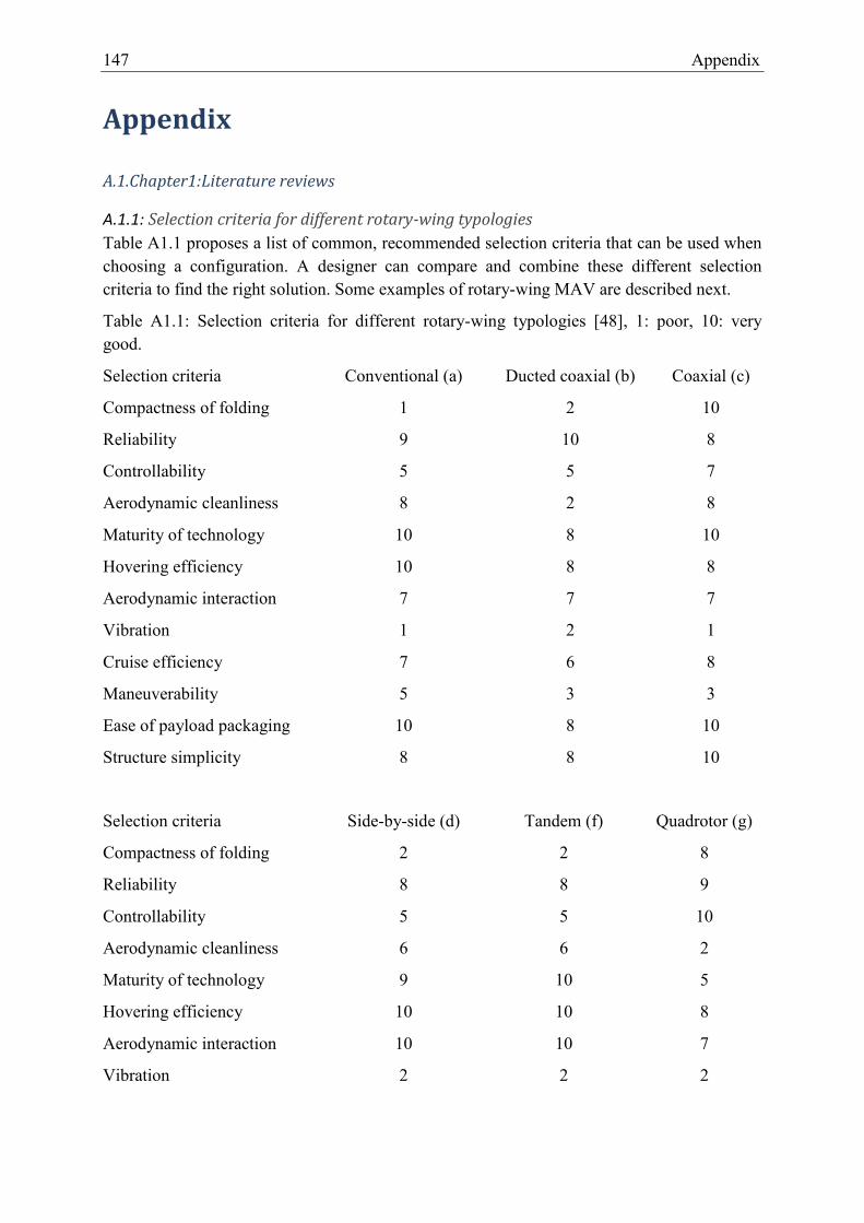
147 Appendix
Appendix
A.1.Chapter1:Literature reviews
A.1.1: Selection criteria for different rotary-wing typologies
Table A1.1 proposes a list of common, recommended selection criteria that can be used when choosing a configuration. A designer can compare and combine these different selection criteria to find the right solution. Some examples of rotary-wing MAV are described next.
Table A1.1: Selection criteria for different rotary-wing typologies [48], 1: poor, 10: very good.
Selection criteria Conventional (a) Ducted coaxial (b) Coaxial (c)
Compactness of folding 1 2 10
Reliability 9 10 8
Controllability 5 5 7
Aerodynamic cleanliness 8 2 8
Maturity of technology 10 8 10
Hovering efficiency 10 8 8
Aerodynamic interaction 7 7 7
Vibration 1 2 1
Cruise efficiency 7 6 8
Maneuverability 5 3 3
Ease of payload packaging 10 8 10
Structure simplicity 8 8 10
Selection criteria Side-by-side (d) Tandem (f) Quadrotor (g)
Compactness of folding 2 2 8
Reliability 8 8 9
Controllability 5 5 10
Aerodynamic cleanliness 6 6 2
Maturity of technology 9 10 5
Hovering efficiency 10 10 8
Aerodynamic interaction 10 10 7
Vibration 2 2 2
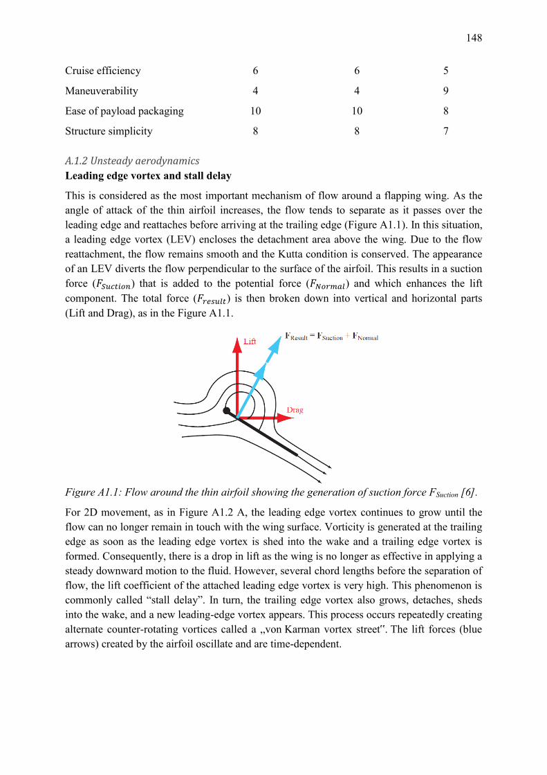
148
Cruise efficiency 6 6 5
Maneuverability 4 4 9
Ease of payload packaging 10 10 8
Structure simplicity 8 8 7
A.1.2 Unsteady aerodynamics
Leading edge vortex and stall delay
This is considered as the most important mechanism of flow around a flapping wing. As the angle of attack of the thin airfoil increases, the flow tends to separate as it passes over the leading edge and reattaches before arriving at the trailing edge (Figure A1.1). In this situation, a leading edge vortex (LEV) encloses the detachment area above the wing. Due to the flow reattachment, the flow remains smooth and the Kutta condition is conserved. The appearance of an LEV diverts the flow perpendicular to the surface of the airfoil. This results in a suction force ( ) that is added to the potential force ( ) and which enhances the lift component. The total force ( ) is then broken down into vertical and horizontal parts (Lift and Drag), as in the Figure A1.1.
Figure A1.1: Flow around the thin airfoil showing the generation of suction force FSuction [6].
For 2D movement, as in Figure A1.2 A, the leading edge vortex continues to grow until the flow can no longer remain in touch with the wing surface. Vorticity is generated at the trailing edge as soon as the leading edge vortex is shed into the wake and a trailing edge vortex is formed. Consequently, there is a drop in lift as the wing is no longer as effective in applying a steady downward motion to the fluid. However, several chord lengths before the separation of flow, the lift coefficient of the attached leading edge vortex is very high. This phenomenon is commonly called “stall delay”. In turn, the trailing edge vortex also grows, detaches, sheds into the wake, and a new leading-edge vortex appears. This process occurs repeatedly creating alternate counter-rotating vortices called a „von Karman vortex street‟. The lift forces (blue arrows) created by the airfoil oscillate and are time-dependent.
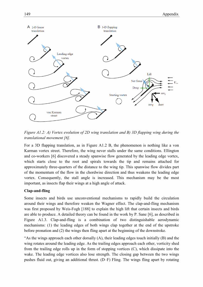
149 Appendix
Figure A1.2: A) Vortex evolution of 2D wing translation and B) 3D flapping wing during the translational movement [6].
For a 3D flapping translation, as in Figure A1.2 B, the phenomenon is nothing like a von Karman vortex street. Therefore, the wing never stalls under the same conditions. Ellington and co-workers [6] discovered a steady spanwise flow generated by the leading edge vortex, which starts close to the root and spirals towards the tip and remains attached for approximately three-quarters of the distance to the wing tip. This spanwise flow divides part of the momentum of the flow in the chordwise direction and thus weakens the leading edge vortex. Consequently, the stall angle is increased. This mechanism may be the most important, as insects flap their wings at a high angle of attack.
Clap-and-fling
Some insects and birds use unconventional mechanisms to rapidly build the circulation around their wings and therefore weaken the Wagner effect. The clap-and-fling mechanism was first proposed by Weis-Fogh [188] to explain the high lift that certain insects and birds are able to produce. A detailed theory can be found in the work by P. Sane [6], as described in Figure A1.3. Clap-and-fling is a combination of two distinguishable aerodynamic mechanisms: (1) the leading edges of both wings clap together at the end of the upstroke before pronation and (2) the wings then fling apart at the beginning of the downstroke.
“As the wings approach each other dorsally (A), their leading edges touch initially (B) and the wing rotates around the leading edge. As the trailing edges approach each other, vorticity shed from the trailing edge rolls up in the form of stopping vortices (C), which dissipate into the wake. The leading edge vortices also lose strength. The closing gap between the two wings pushes fluid out, giving an additional thrust. (D–F) Fling. The wings fling apart by rotating
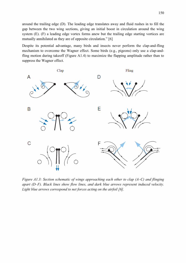
150
around the trailing edge (D). The leading edge translates away and fluid rushes in to fill the gap between the two wing sections, giving an initial boost in circulation around the wing system (E). (F) a leading edge vortex forms anew but the trailing edge starting vortices are mutually annihilated as they are of opposite circulation.” [6]
Despite its potential advantage, many birds and insects never perform the clap-and-fling mechanism to overcome the Wagner effect. Some birds (e.g., pigeons) only use a clap-and-fling motion during takeoff (Figure A1.4) to maximize the flapping amplitude rather than to suppress the Wagner effect.
Figure A1.3: Section schematic of wings approaching each other to clap (A–C) and flinging apart (D–F). Black lines show flow lines, and dark blue arrows represent induced velocity. Light blue arrows correspond to net forces acting on the airfoil [6].
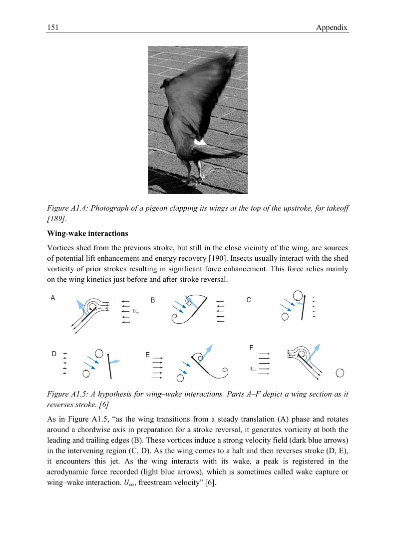
151 Appendix
Figure A1.4: Photograph of a pigeon clapping its wings at the top of the upstroke, for takeoff [189].
Wing-wake interactions
Vortices shed from the previous stroke, but still in the close vicinity of the wing, are sources of potential lift enhancement and energy recovery [190]. Insects usually interact with the shed vorticity of prior strokes resulting in significant force enhancement. This force relies mainly on the wing kinetics just before and after stroke reversal.
Figure A1.5: A hypothesis for wing–wake interactions. Parts A–F depict a wing section as it reverses stroke. [6]
As in Figure A1.5, “as the wing transitions from a steady translation (A) phase and rotates around a chordwise axis in preparation for a stroke reversal, it generates vorticity at both the leading and trailing edges (B). These vortices induce a strong velocity field (dark blue arrows) in the intervening region (C, D). As the wing comes to a halt and then reverses stroke (D, E), it encounters this jet. As the wing interacts with its wake, a peak is registered in the aerodynamic force recorded (light blue arrows), which is sometimes called wake capture or wing–wake interaction. , freestream velocity” [6].
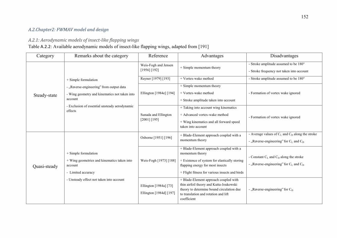
152 A.2.Chapter2: FWMAV model and design
A.2.1: Aerodynamic models of insect-like flapping wings
Table A.2.2: Available aerodynamic models of insect-like flapping wings, adapted from [191]
Category Remarks about the category Reference Advantages Disadvantages
Steady-state
+ Simple formulation
- „Reverse-engineering‟ from output data
- Wing geometry and kinematics not taken into account
- Exclusion of essential unsteady aerodynamic effects
Weis-Fogh and Jensen [1956] [192] + Simple momentum theory
- Stroke amplitude assumed to be 180°
- Stroke frequency not taken into account
Rayner [1979] [193] + Vortex-wake method - Stroke amplitude assumed to be 180°
Ellington [1984e] [194]
+ Simple momentum theory
+ Vortex-wake method
+ Stroke amplitude taken into account
- Formation of vortex wake ignored
Sunada and Ellington [2001] [195]
+ Taking into account wing kinematics
+ Advanced vortex-wake method
+ Wing kinematics and all forward speed taken into account
- Formation of vortex wake ignored
Quasi-steady
+ Simple formulation
+ Wing geometries and kinematics taken into account
- Limited accuracy
- Unsteady effect not taken into account
Osborne [1951] [196] + Blade-Element approach coupled with a momentum theory
- Average values of CL and CD along the stroke
- „Reverse-engineering‟ for CL and CD
Weis-Fogh [1973] [188]
+ Blade-Element approach coupled with a momentum theory
+ Existence of system for elastically storing flapping energy for most insects
+ Flight fitness for various insects and birds
- Constant CL and CD along the stroke
- „Reverse-engineering‟ for CL and CD
Ellington [1984a] [73]
Ellington [1984d] [197]
+ Blade-Element approach coupled with thin airfoil theory and Kutta-Joukowski theory to determine bound circulation due to translation and rotation and lift coefficient
- „Reverse-engineering‟ for CD

153 Appendix
Azuma [1992] [198]
+ Blade-Element approach coupled with a Theodorsen function
+ Power requirements analysis
- Based on a flat plate
- Limited treatment of drag
Ansari [2004] [199] + Blade-Element approach coupled with a Glauert-type analysis
- Limited treatment of drag
Semi-empirical
+ Simple formulation
+ Wing geometry and kinematics taken into account
+ Experimental correction factor
- Different types of flow lumped together
- Wake interaction generally not modeled
Walker and Westneat [2000] [200]
+ Blade-Element approach
+ Use of Wagner‟s function
+ Added-mass and skin-friction effects
- Wing as a rectangular plate
Sane and Dickinson [2002][77]
+ Blade-element approach
+ Added-mass
- Based partially on a flat plate
- Wake capture component unclear
Traub [2004] [201] + Simple actuator disk theory
+ Polhamus‟ leading-edge suction analogy
- Devised for time-averaged data
- Small angle approximations
Tarascio et al. [2005] [202]
+ Free vortex blob method
+ Modeling of the wake
- Limited to 2D-plate and to the wake
- Based on a flat plate
Berman and Wang [2007] [203]
+ Blade element
+ Added-mass
- Based partially on a flat plate
Unsteady
+ Unsteady phenomena taken into account
+ Wing kinematics taken into account
+ Wing geometry taken into account (except for 2D wing)
+ Accuracy without resorting to experiments
+ Flows physics
- More complex formulation
- Computational cost
- Limited to 2d or quasi-3D
Minotti [2002] [204] + Conformal mapping
+ Potential methods
- 2D resolution of the wing
- Based on a thin flat plate
Pedersen [2003] [205]
+ Blade-element method
+ Circulatory and non-circulatory forces
+ Wagner and Kussner function
- 2D resolution of the wing
- Based on a thin flat plate
Yongliang et al. [2003] [206]
+ Conformal mapping
+ Potential methods
- 2D resolution of the wing
- Based on a thin flat plate
Pullin and Wang [2004] [207]
+ Conformal mapping
+ Similarity approach (spiral vortex sheet)
- 2D resolution of the wing
- Based on a thin flat plate
Ansari et al. [2006] + Radial Blade-Element method - 2D resolution on each blade
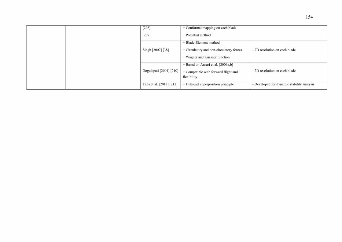
154
[208]
[209]
+ Conformal mapping on each blade
+ Potential method
Singh [2007] [38]
+ Blade-Element method
+ Circulatory and non-circulatory forces
+ Wagner and Kussner function
- 2D resolution on each blade
Gogulapati [2001] [210]
+ Based on Ansari et al. [2006a,b]
+ Compatible with forward flight and flexibility
- 2D resolution on each blade
Taha et al. [2013] [211] + Duhamel superposition principle - Developed for dynamic stability analysis
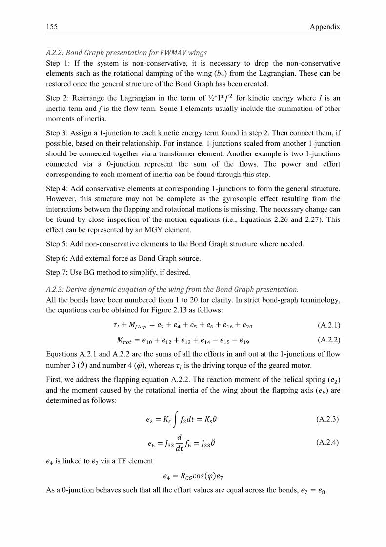
155 Appendix
A.2.2: Bond Graph presentation for FWMAV wings
Step 1: If the system is non-conservative, it is necessary to drop the non-conservative elements such as the rotational damping of the wing (bw) from the Lagrangian. These can be restored once the general structure of the Bond Graph has been created.
Step 2: Rearrange the Lagrangian in the form of ½*I* for kinetic energy where I is an inertia term and f is the flow term. Some I elements usually include the summation of other moments of inertia.
Step 3: Assign a 1-junction to each kinetic energy term found in step 2. Then connect them, if possible, based on their relationship. For instance, 1-junctions scaled from another 1-junction should be connected together via a transformer element. Another example is two 1-junctions connected via a 0-junction represent the sum of the flows. The power and effort corresponding to each moment of inertia can be found through this step.
Step 4: Add conservative elements at corresponding 1-junctions to form the general structure. However, this structure may not be complete as the gyroscopic effect resulting from the interactions between the flapping and rotational motions is missing. The necessary change can be found by close inspection of the motion equations (i.e., Equations 2.26 and 2.27). This effect can be represented by an MGY element.
Step 5: Add non-conservative elements to the Bond Graph structure where needed.
Step 6: Add external force as Bond Graph source.
Step 7: Use BG method to simplify, if desired.
A.2.3: Derive dynamic euqation of the wing from the Bond Graph presentation.
All the bonds have been numbered from 1 to 20 for clarity. In strict bond-graph terminology, the equations can be obtained for Figure 2.13 as follows:
(A.2.1)
(A.2.2)
Equations A.2.1 and A.2.2 are the sums of all the efforts in and out at the 1-junctions of flow number 3 ( ) and number 4 ( ), whereas is the driving torque of the geared motor.
First, we address the flapping equation A.2.2. The reaction moment of the helical spring ( ) and the moment caused by the rotational inertia of the wing about the flapping axis ( ) are determined as follows:
∫ (A.2.3)
(A.2.4)
is linked to via a TF element
As a 0-junction behaves such that all the effort values are equal across the bonds, .
156
where
therefore,
(A.2.5)
As and are also linked by a TF element with a ratio of
where , i.e.,
(A.2.6)
and are easily deduced from the relation between the input flows and the output effort of the two MGY elements.
(A.2.7)
(A.2.8)
Where r1 and r2 can be found in equations 2.40 and 2.41. Substituting the results of equation A.2.3 through A.2.8 into equation A.2.1, we reestablish the flapping equation as in Equation 2.27.
Next, we recover the Lagrangian rotational equation from equation A.2.2. The efforts are expressed as follows.
Through the relationship between the input and output efforts of the transformer TF element, we have
where , i.e.,
(A.2.9)
Moments caused by wing damping and the reaction force of the wing rotational stiffness are determined such that
,
(A.2.10)
The moment due to rotational inertia is
(A.2.11)
Then, the two outputs of the modulated gyrator MGY element are determined such that
(A.2.12)
157 Appendix
(A.2.13)
Substituting the results of equation A.2.9 through 2.54 A.2.13 into equation A.2.2, we obtain the rotational equation written in 2.26.
A.3.Chapter 3: Towards the construction of a FWMAV able to take off and to stabilize
A.3.1: Schematic and layouts of electronic circuit developed for the FWMAV
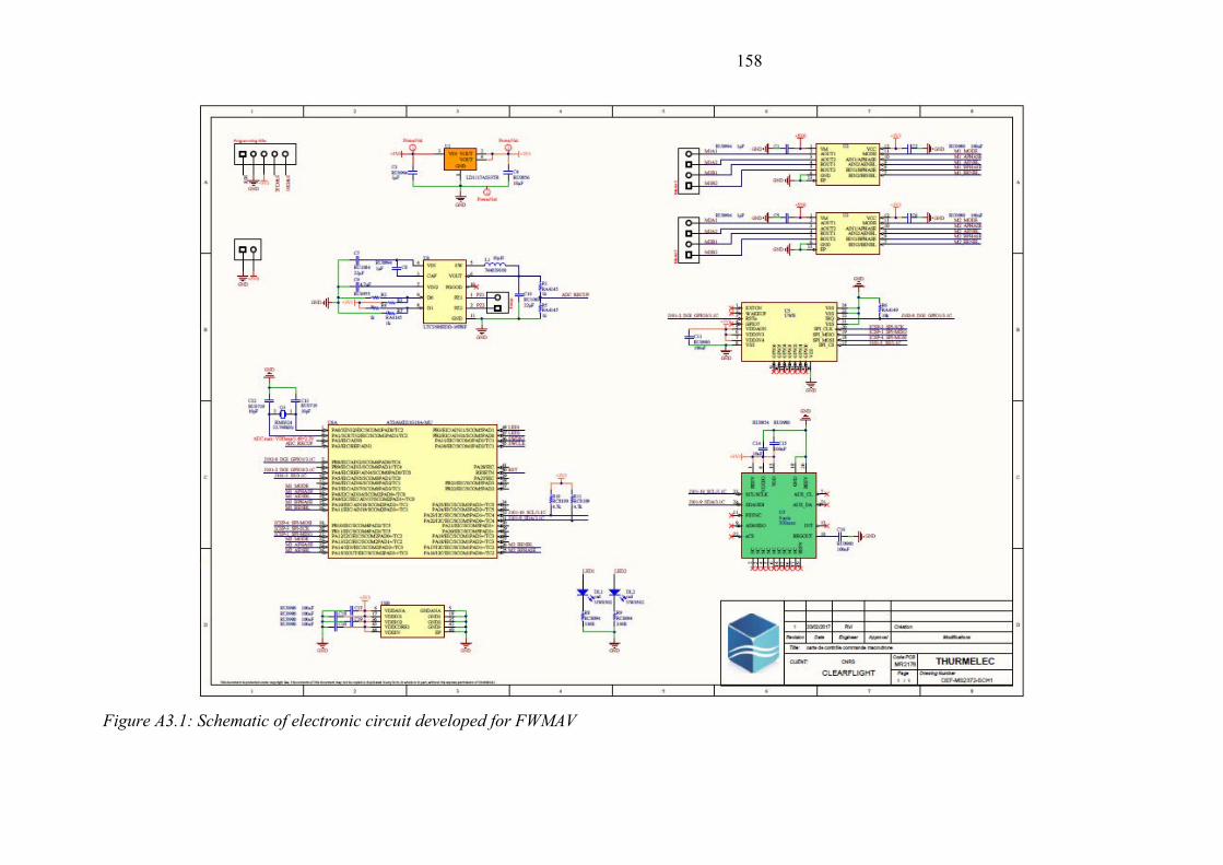
158
Figure A3.1: Schematic of electronic circuit developed for FWMAV
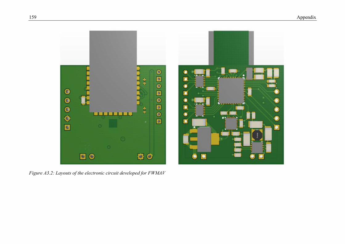
159 Appendix
Figure A3.2: Layouts of the electronic circuit developed for FWMAV
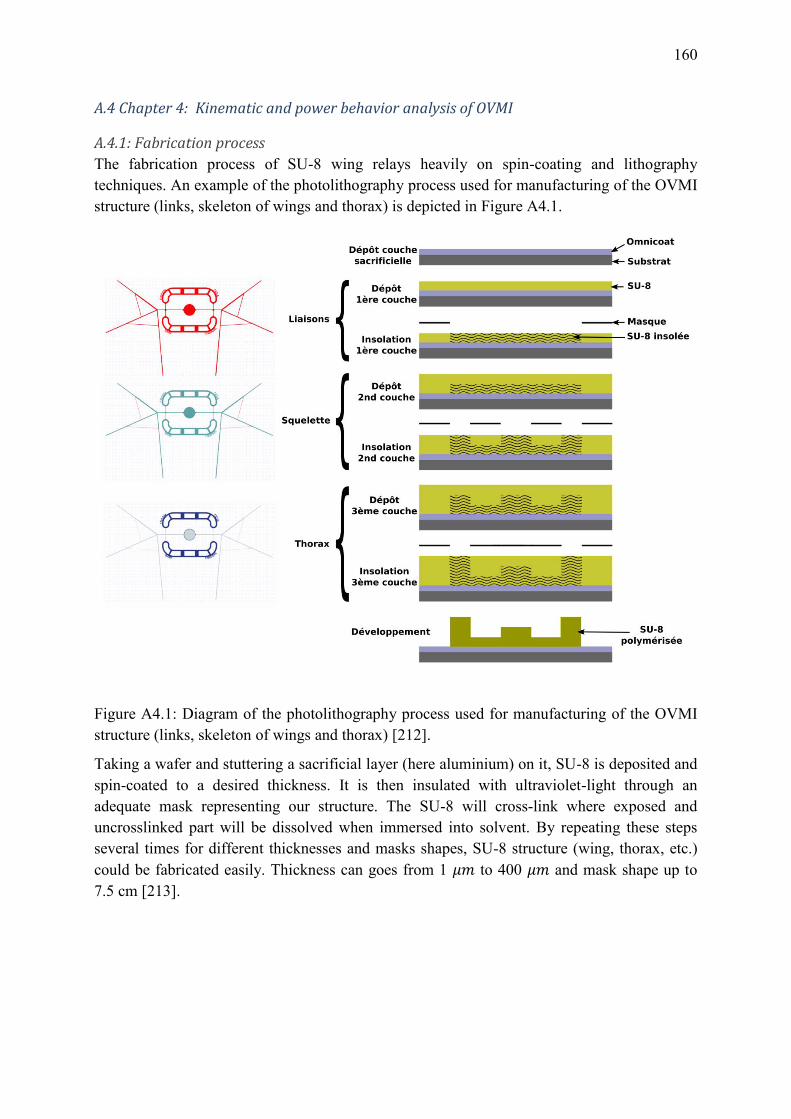
160
A.4 Chapter 4: Kinematic and power behavior analysis of OVMI
A.4.1: Fabrication process
The fabrication process of SU-8 wing relays heavily on spin-coating and lithography techniques. An example of the photolithography process used for manufacturing of the OVMI structure (links, skeleton of wings and thorax) is depicted in Figure A4.1.
Figure A4.1: Diagram of the photolithography process used for manufacturing of the OVMI structure (links, skeleton of wings and thorax) [212].
Taking a wafer and stuttering a sacrificial layer (here aluminium) on it, SU-8 is deposited and spin-coated to a desired thickness. It is then insulated with ultraviolet-light through an adequate mask representing our structure. The SU-8 will cross-link where exposed and uncrosslinked part will be dissolved when immersed into solvent. By repeating these steps several times for different thicknesses and masks shapes, SU-8 structure (wing, thorax, etc.) could be fabricated easily. Thickness can goes from 1 to 400 and mask shape up to 7.5 cm [213].