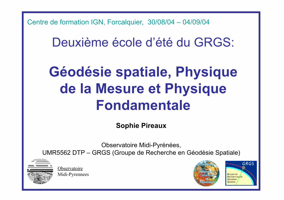
Deuxième école d’été du GRGS:

Géodésie spatiale, Physique de la Mesure et Physique

Fondamentale Sophie Pireaux

Observatoire Midi-Pyrénées, UMR5562 DTP – GRGS (Groupe de Recherche en Géodésie Spatiale)

Observatoire Midi-Pyrennees

Centre de formation IGN, Forcalquier, 30/08/04 – 04/09/04

Session I. Space Geodesy and relativity

•  Mathematical introduction to relativistic theories

•  General relativity and scalar-tensor theories •  Key tools for relativistic gravitational effects •  Introduction to relativistic celestial mechanics •  Geodesy and tests of relativistic theories of

gravitation •  Light propagation in curved space-time

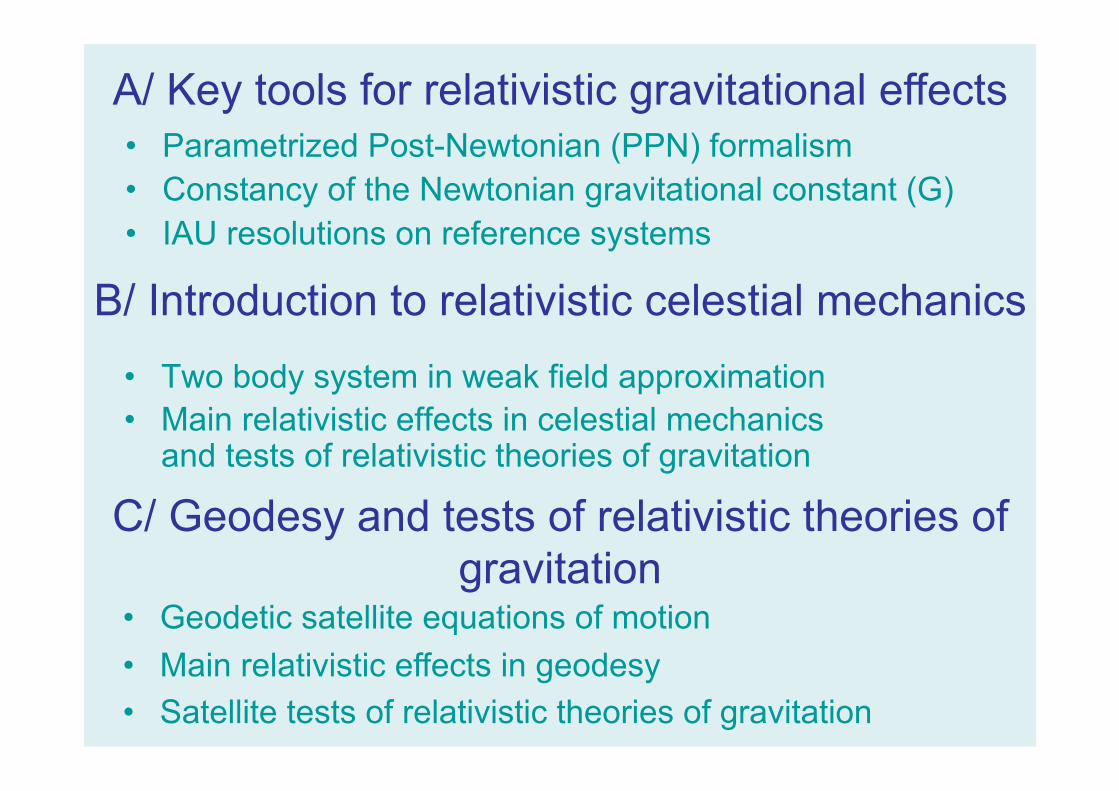
B/ Introduction to relativistic celestial mechanics •  Two body system in weak field approximation •  Main relativistic effects in celestial mechanics

and tests of relativistic theories of gravitation

C/ Geodesy and tests of relativistic theories of gravitation

•  Geodetic satellite equations of motion •  Main relativistic effects in geodesy •  Satellite tests of relativistic theories of gravitation

A/ Key tools for relativistic gravitational effects •  Parametrized Post-Newtonian (PPN) formalism •  Constancy of the Newtonian gravitational constant (G) •  IAU resolutions on reference systems

RELATIVISTIC THEORIES OF GRAVITATION

A/ Key tools for relativistic gravitational effects

IAU metric conventions

PPN formalism

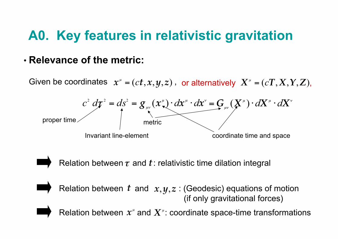
Given be coordinates ,

proper time metric

coordinate time and space Invariant line-element

Relation between and : (Geodesic) equations of motion (if only gravitational forces)

Relation between and : relativistic time dilation integral

Relation between and : coordinate space-time transformations

or alternatively ,

A0. Key features in relativistic gravitation

•  Relevance of the metric:

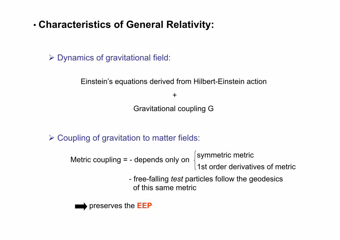
•  Characteristics of General Relativity:

  Dynamics of gravitational field:

  Coupling of gravitation to matter fields:

Einstein’s equations derived from Hilbert-Einstein action

+

Gravitational coupling G

Metric coupling = - depends only on

- free-falling test particles follow the geodesics of this same metric

preserves the EEP

symmetric metric 1st order derivatives of metric

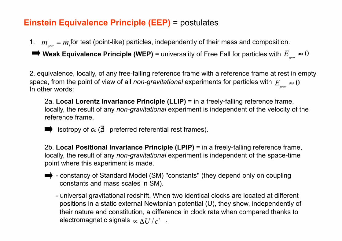
1. for test (point-like) particles, independently of their mass and composition.

Weak Equivalence Principle (WEP) = universality of Free Fall for particles with

2. equivalence, locally, of any free-falling reference frame with a reference frame at rest in empty space, from the point of view of all non-gravitational experiments for particles with

Einstein Equivalence Principle (EEP) = postulates

In other words:

2a. Local Lorentz Invariance Principle (LLIP) = in a freely-falling reference frame, locally, the result of any non-gravitational experiment is independent of the velocity of the reference frame.

isotropy of c0 ( preferred referential rest frames).

2b. Local Positional Invariance Principle (LPIP) = in a freely-falling reference frame, locally, the result of any non-gravitational experiment is independent of the space-time point where this experiment is made.

- constancy of Standard Model (SM) ''constants'' (they depend only on coupling constants and mass scales in SM).

- universal gravitational redshift. When two identical clocks are located at different positions in a static external Newtonian potential (U), they show, independently of their nature and constitution, a difference in clock rate when compared thanks to electromagnetic signals .

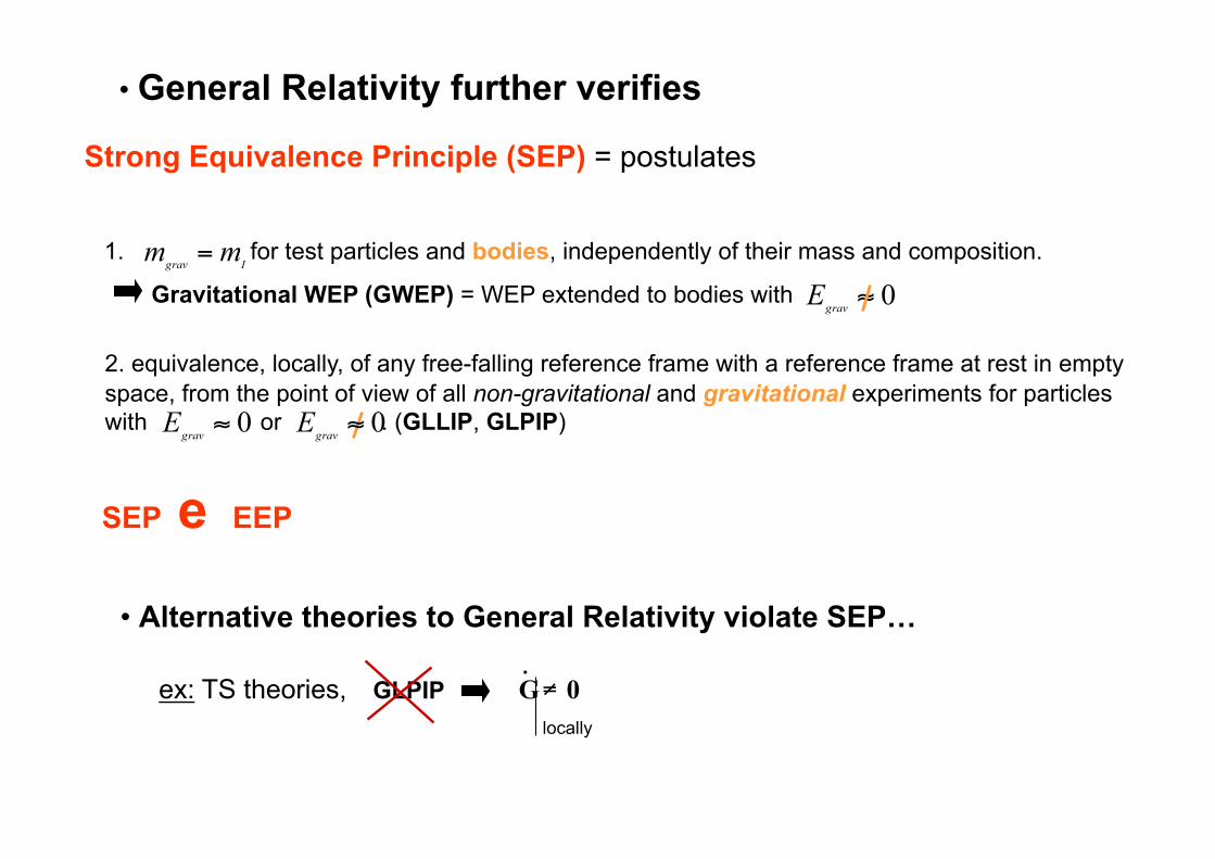
•  General Relativity further verifies

Strong Equivalence Principle (SEP) = postulates

1. for test particles and bodies, independently of their mass and composition.

Gravitational WEP (GWEP) = WEP extended to bodies with

2. equivalence, locally, of any free-falling reference frame with a reference frame at rest in empty space, from the point of view of all non-gravitational and gravitational experiments for particles with or . (GLLIP, GLPIP)

SEP e EEP

•  Alternative theories to General Relativity violate SEP…

ex: TS theories, G 0 GLPIP .

locally

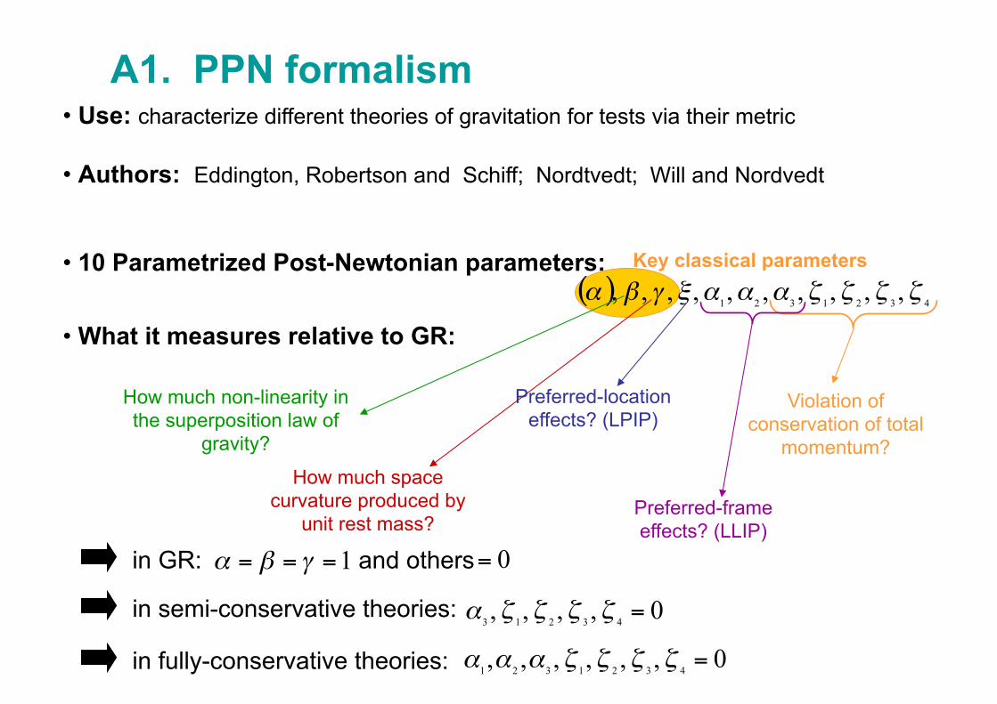
•  Use: characterize different theories of gravitation for tests via their metric

•  Authors: Eddington, Robertson and Schiff; Nordtvedt; Will and Nordvedt

•  10 Parametrized Post-Newtonian parameters:

•  What it measures relative to GR:

Key classical parameters

A1. PPN formalism

in GR: and others

How much space curvature produced by

unit rest mass?

How much non-linearity in the superposition law of

gravity?

Preferred-location effects? (LPIP)

Violation of conservation of total

momentum?

Preferred-frame effects? (LLIP)

in semi-conservative theories:

in fully-conservative theories:

Key classical parameters

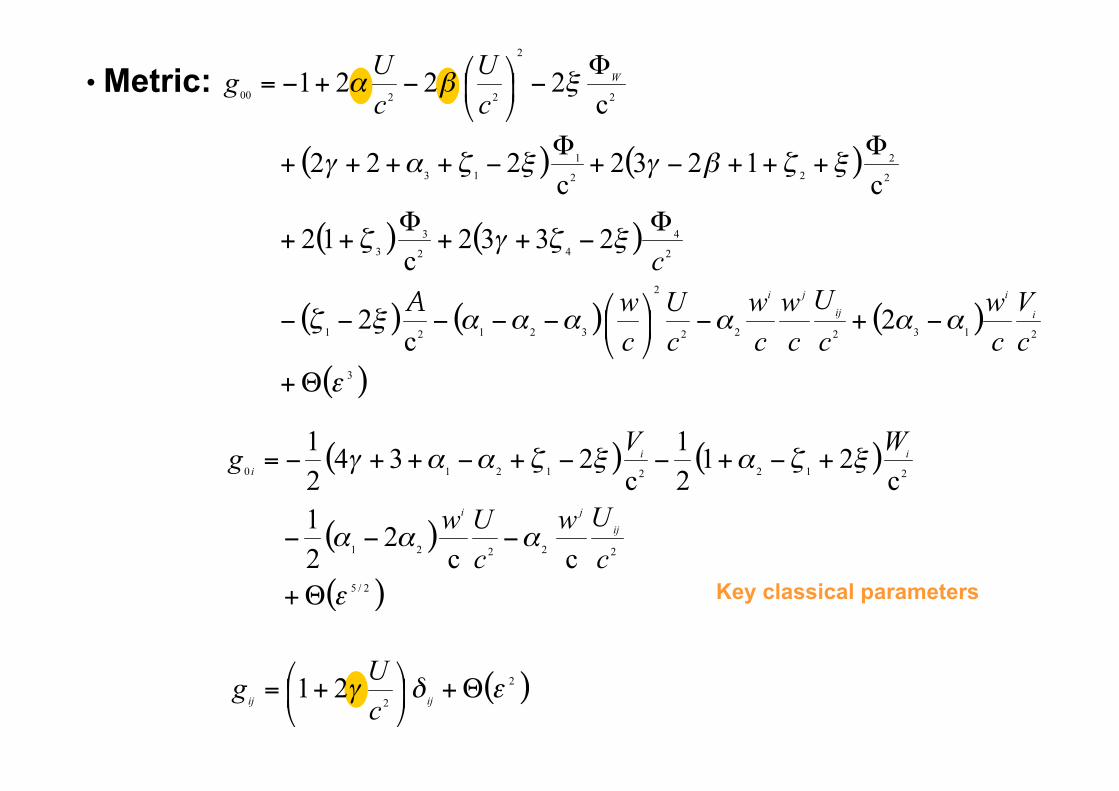
•  Metric:

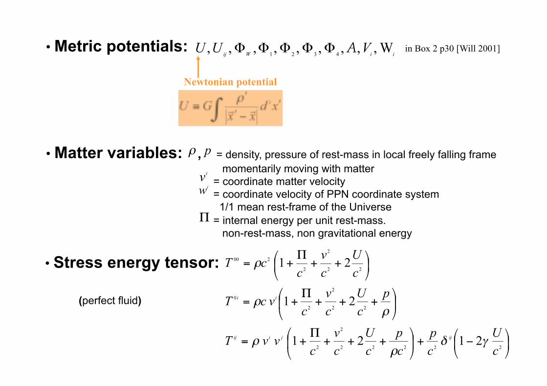
•  Metric potentials: in Box 2 p30 [Will 2001]

Newtonian potential

•  Matter variables: , = density, pressure of rest-mass in local freely falling frame momentarily moving with matter = coordinate matter velocity = coordinate velocity of PPN coordinate system 1/1 mean rest-frame of the Universe = internal energy per unit rest-mass. non-rest-mass, non gravitational energy

•  Stress energy tensor:

(perfect fluid)

•  PPN metric Gauge: PPN standard gauge

! ***en cours***

Present best

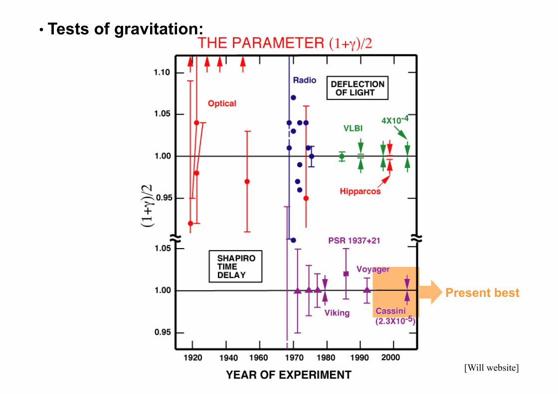
•  Tests of gravitation:

[Will website]

Present best

[Will website]

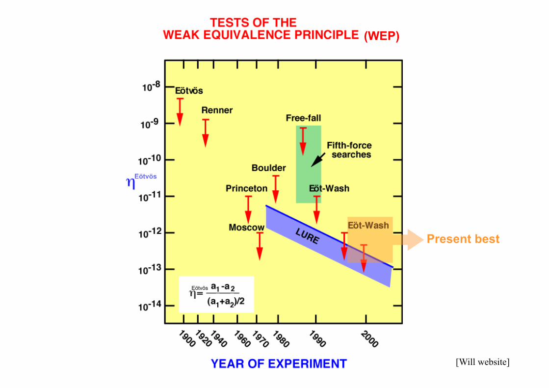
(WEP)

Eötvös

Eötvös

Present best

[Will website]

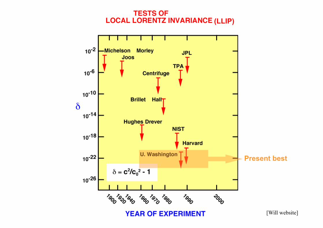
(LLIP)

Present best

[Will website]

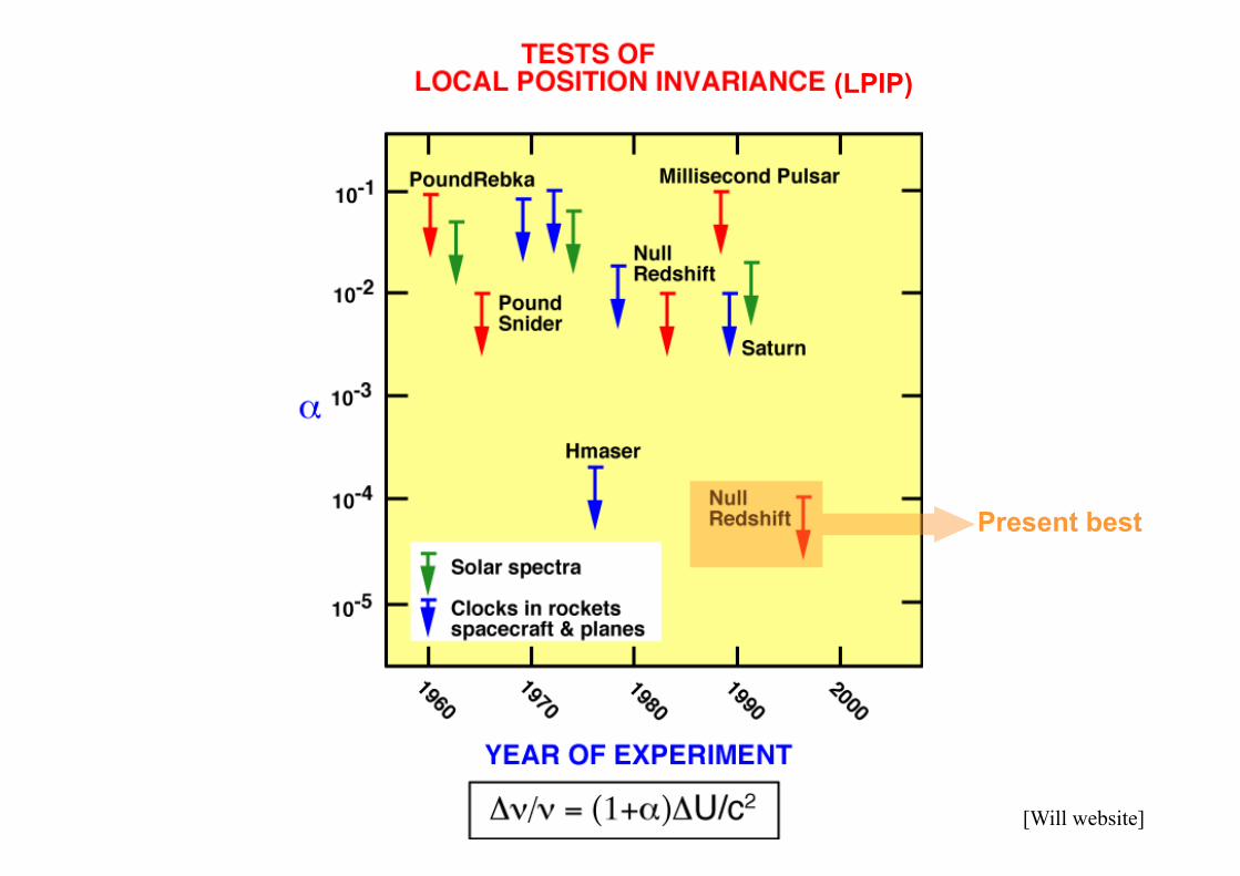
(LPIP)

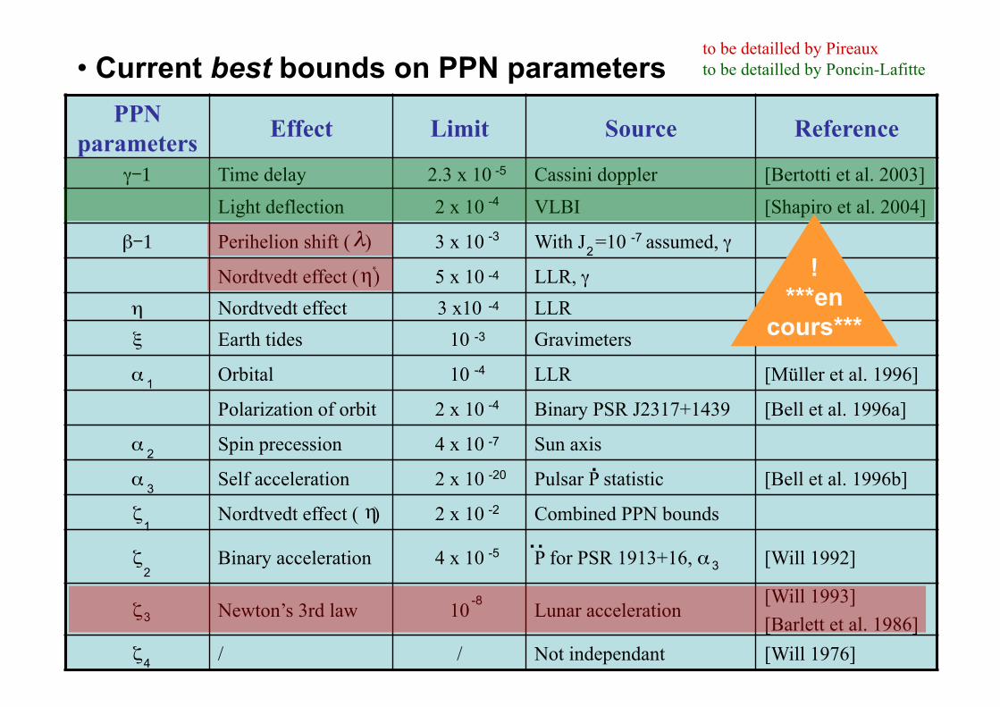
•  Current best bounds on PPN parameters PPN

parameters Effect Limit Source Reference

γ-1 Time delay 2.3 x 10 Cassini doppler [Bertotti et al. 2003] Light deflection 2 x 10 VLBI [Shapiro et al. 2004]

β-1 Perihelion shift ( ) 3 x 10 With J =10 assumed, γ

Nordtvedt effect ( ) 5 x 10 LLR, γ η Nordtvedt effect 3 x10 LLR ξ Earth tides 10 Gravimeters

α Orbital 10 LLR [Müller et al. 1996]

Polarization of orbit 2 x 10 Binary PSR J2317+1439 [Bell et al. 1996a]

α Spin precession 4 x 10 Sun axis

α Self acceleration 2 x 10 Pulsar P statistic [Bell et al. 1996b]

ζ Nordtvedt effect ( ) 2 x 10 Combined PPN bounds

ζ Binary acceleration 4 x 10 P for PSR 1913+16, α [Will 1992]

ζ Newton’s 3rd law 10 Lunar acceleration [Will 1993] [Barlett et al. 1986]

ζ / / Not independant [Will 1976]

-5

-4

-3

-4

-4

3

-3

-4

-4

-7

-20

-2

-5

-8

1

2

3

4

2

1

.

..

2 -7

3

to be detailled by Pireaux to be detailled by Poncin-Lafitte

! ***en

cours***

fully conservative theory

no preferred location effect

less deflection, time-delay than GR

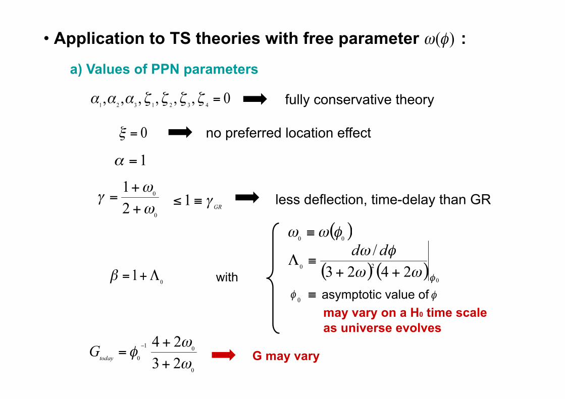
•  Application to TS theories with free parameter :

a) Values of PPN parameters

with

may vary on a H0 time scale as universe evolves

G may vary

asymptotic value of

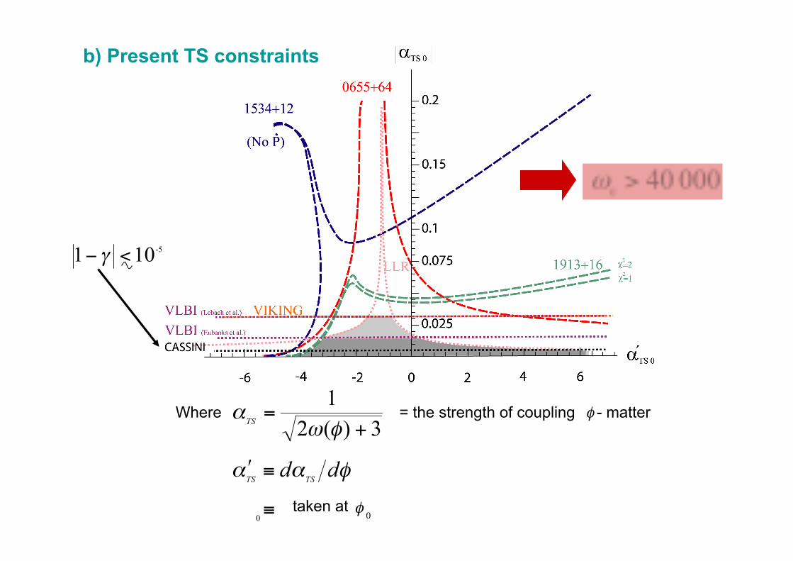
b) Present TS constraints

Where = the strength of coupling - matter

taken at

CASSINI

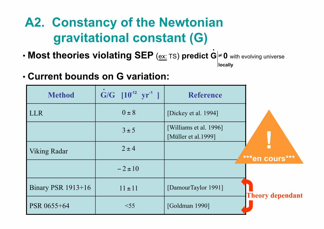
A2. Constancy of the Newtonian gravitational constant (G)

Method G/G [10 yr ] Reference

LLR [Dickey et al. 1994]

[Williams et al. 1996] [Müller et al.1999]

Viking Radar

Binary PSR 1913+16 [DamourTaylor 1991]

PSR 0655+64 <55 [Goldman 1990]

. -12 -1

•  Most theories violating SEP (ex: TS) predict G 0 with evolving universe

•  Current bounds on G variation:

.

locally

Theory dependant

! ***en cours***

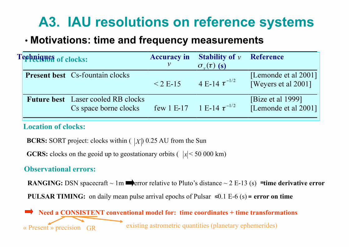
A3. IAU resolutions on reference systems •  Motivations: time and frequency measurements

Location of clocks:

BCRS: SORT project: clocks within ( ) 0.25 AU from the Sun

GCRS: clocks on the geoid up to geostationary orbits ( < 50 000 km)

Observational errors:

RANGING: DSN spacecraft ~ 1m error relative to Pluto’s distance ~ 2 E-13 (s) time derivative error

PULSAR TIMING: on daily mean pulse arrival epochs of Pulsar 0.1 E-6 (s) error on time

Need a CONSISTENT conventional model for: time coordinates + time transformations

GR existing astrometric quantities (planetary ephemerides) « Present » precision

Precision of clocks:

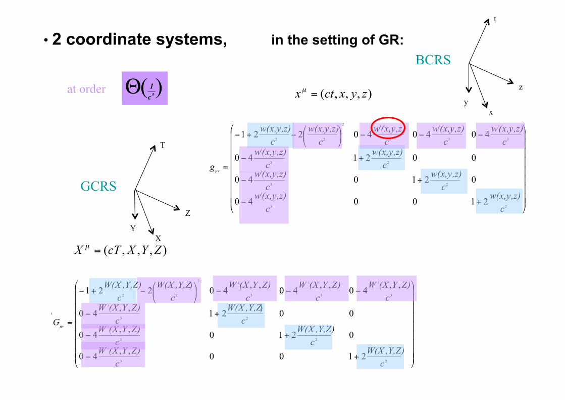
GCRS

BCRS

y x

t

z

Y X

T

Z

at order at order at order

•  2 coordinate systems, in the setting of GR:

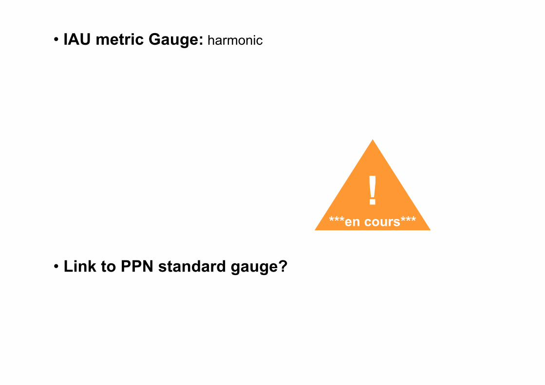
•  IAU metric Gauge: harmonic

•  Link to PPN standard gauge?

! ***en cours***

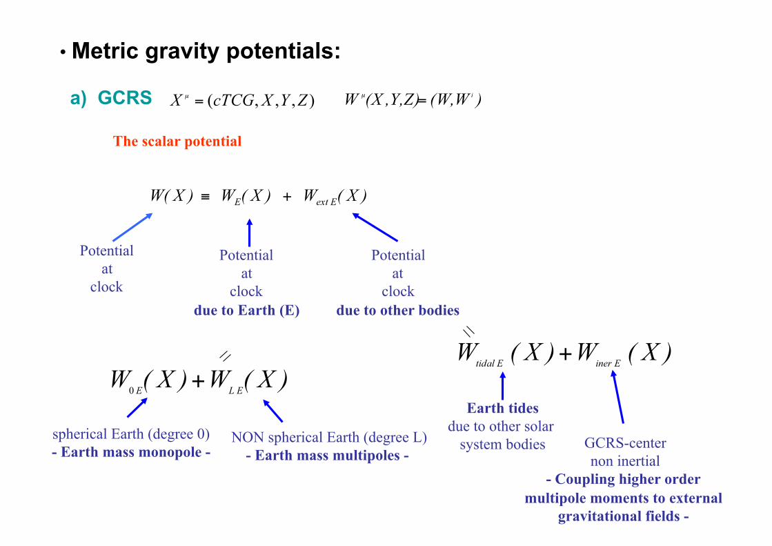
•  Metric gravity potentials:

Potential at

clock

Potential at

clock due to Earth (E)

Potential at

clock due to other bodies

Earth tides due to other solar

system bodies GCRS-center non inertial

- Coupling higher order multipole moments to external

gravitational fields -

spherical Earth (degree 0) - Earth mass monopole -

NON spherical Earth (degree L) - Earth mass multipoles -

The scalar potential

a) GCRS

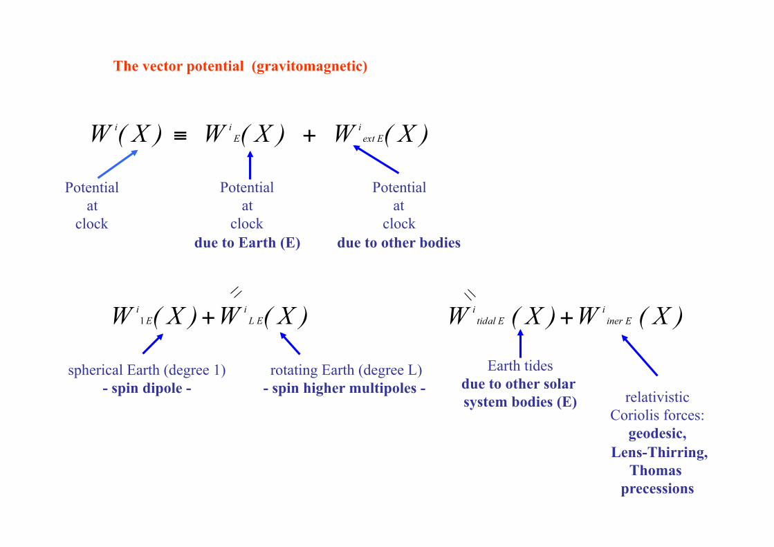
Potential at

clock

Potential at

clock due to Earth (E)

Potential at

clock due to other bodies

Earth tides due to other solar system bodies (E) relativistic

Coriolis forces: geodesic,

Lens-Thirring, Thomas

precessions

spherical Earth (degree 1) - spin dipole -

rotating Earth (degree L) - spin higher multipoles -

The vector potential (gravitomagnetic)

Potential at

clock

Potential at

clock due to body « n »

spherical body « n » (degree 0)

- « n » mass monopole -

NON spherical « n » (degree L) - « n » mass multipoles -

The scalar potential

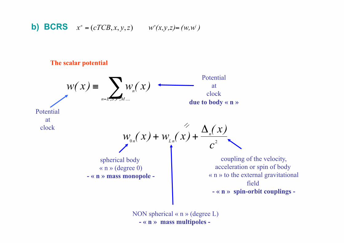
b) BCRS

coupling of the velocity, acceleration or spin of body

« n » to the external gravitational field

- « n » spin-orbit couplings -

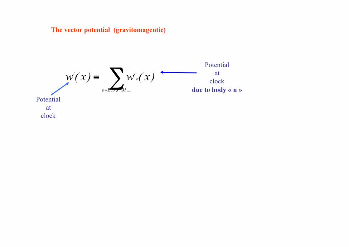
The vector potential (gravitomagentic)

Potential at

clock

Potential at

clock due to body « n »

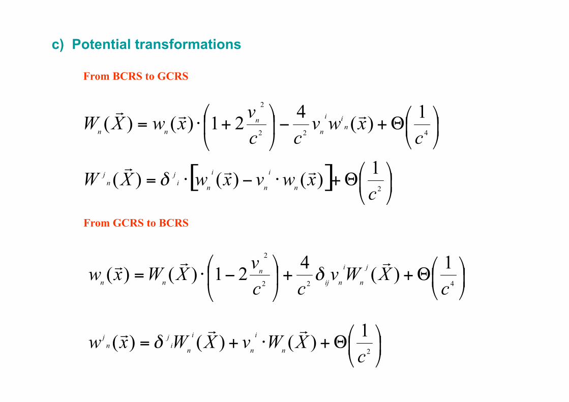
c) Potential transformations

From BCRS to GCRS

From GCRS to BCRS

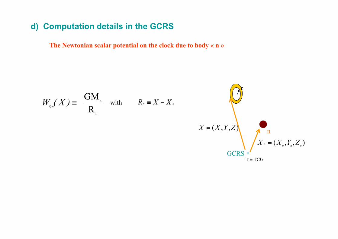
The Newtonian scalar potential on the clock due to body « n »

d) Computation details in the GCRS

with

n

GCRS

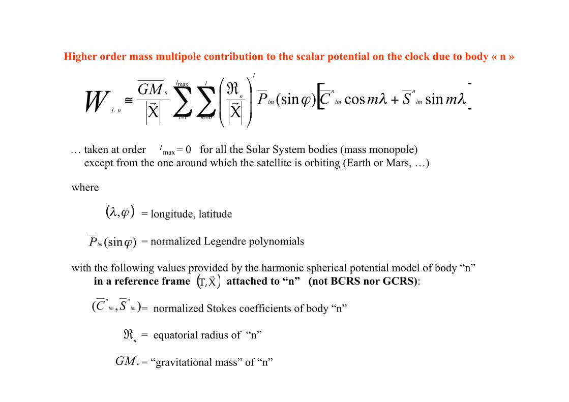
Higher order mass multipole contribution to the scalar potential on the clock due to body « n »

… taken at order = 0 for all the Solar System bodies (mass monopole) except from the one around which the satellite is orbiting (Earth or Mars, …)

where

= longitude, latitude

= normalized Legendre polynomials

with the following values provided by the harmonic spherical potential model of body “n” in a reference frame attached to “n” (not BCRS nor GCRS):

= normalized Stokes coefficients of body “n”

= equatorial radius of “n”

= “gravitational mass” of “n”

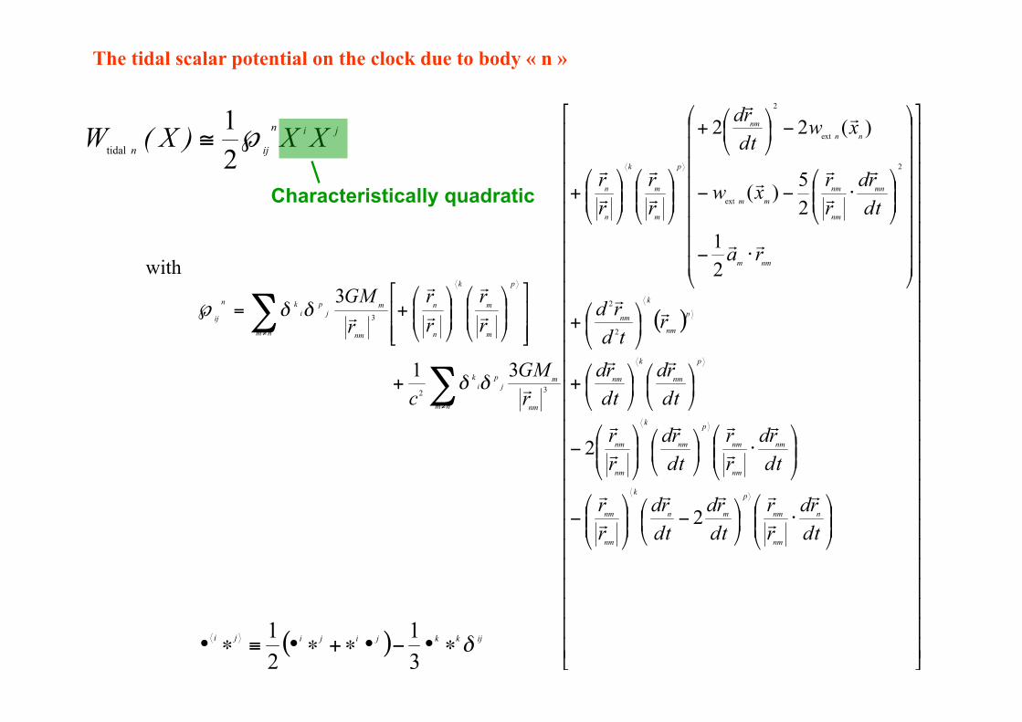
The tidal scalar potential on the clock due to body « n »

with

Characteristically quadratic

The tidal vector potential on the clock due to body « n »

! ***en cours***

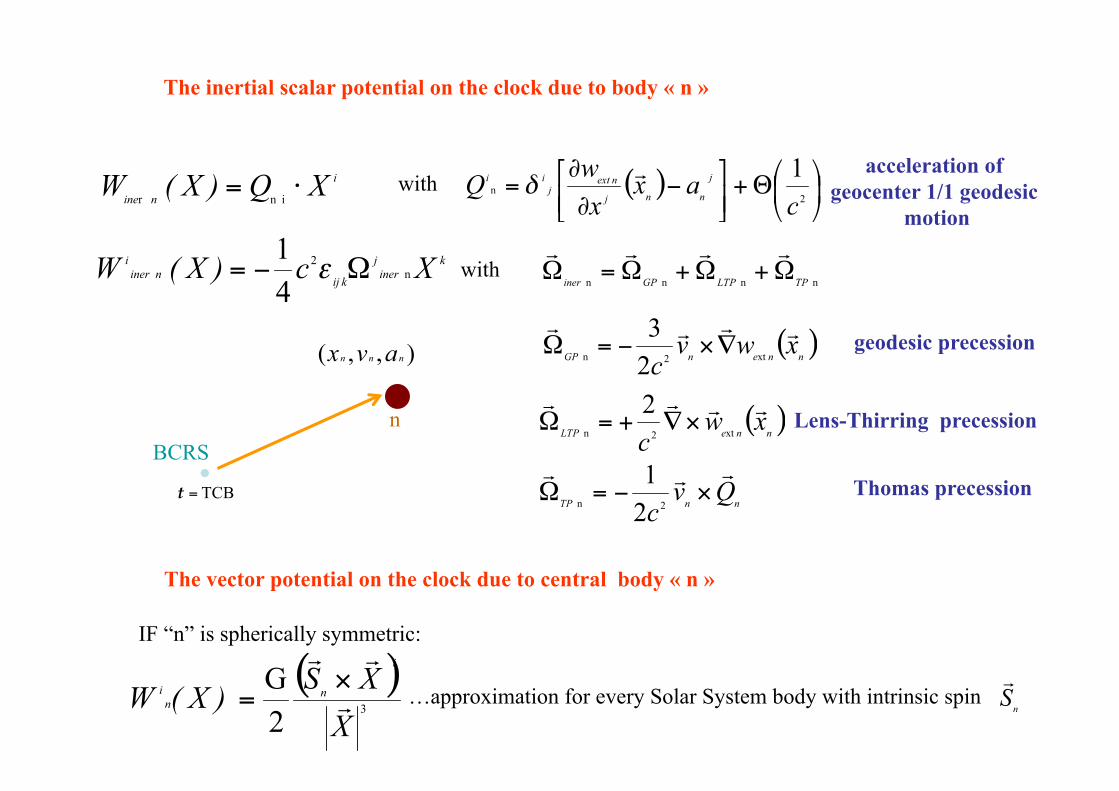
The inertial scalar potential on the clock due to body « n »

with

with

Lens-Thirring precession

geodesic precession

Thomas precession

The vector potential on the clock due to central body « n »

IF “n” is spherically symmetric:

…approximation for every Solar System body with intrinsic spin

acceleration of geocenter 1/1 geodesic

motion

n BCRS

with

n BCRS

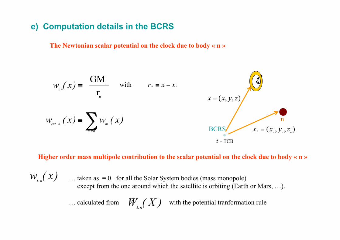
e) Computation details in the BCRS

The Newtonian scalar potential on the clock due to body « n »

Higher order mass multipole contribution to the scalar potential on the clock due to body « n »

… taken as = 0 for all the Solar System bodies (mass monopole) except from the one around which the satellite is orbiting (Earth or Mars, …).

… calculated from with the potential tranformation rule

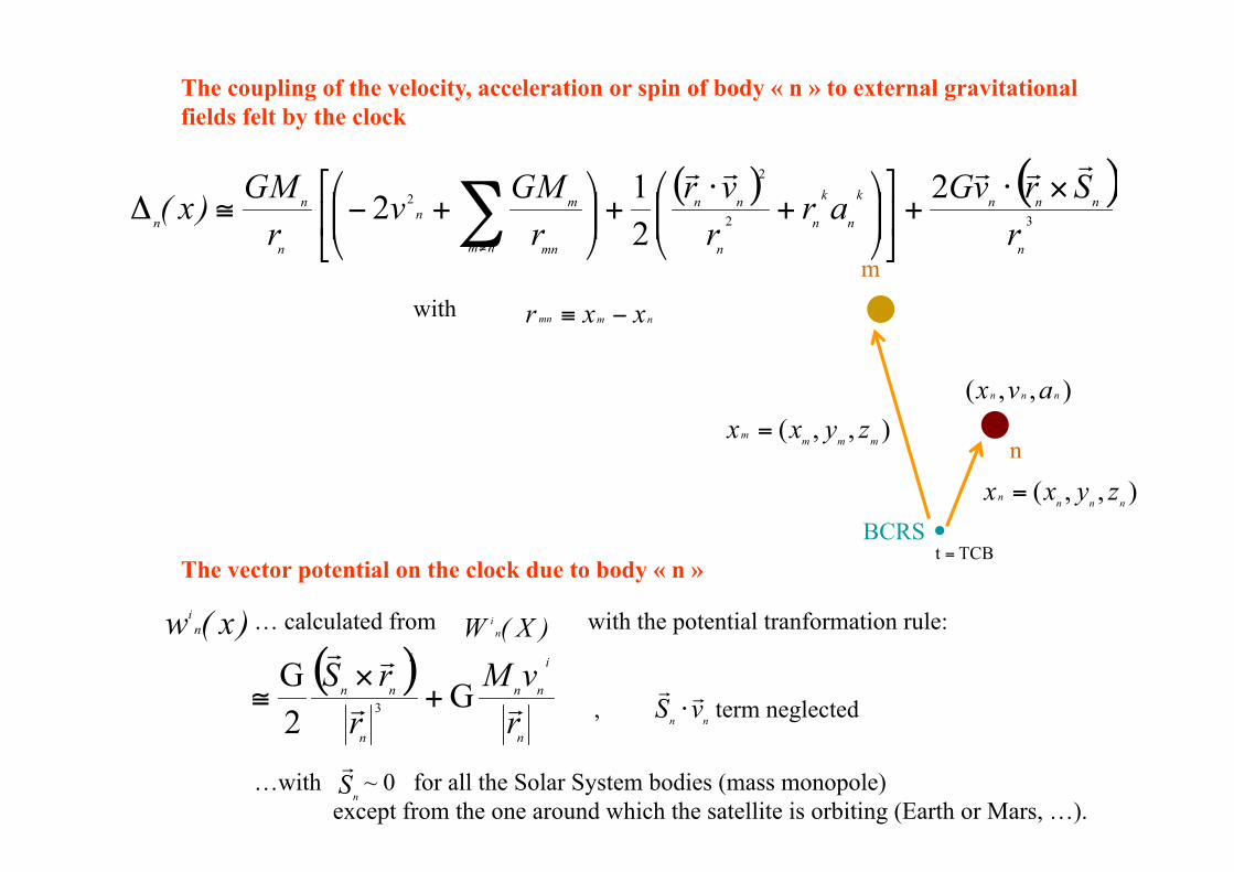
The coupling of the velocity, acceleration or spin of body « n » to external gravitational fields felt by the clock

with

n

BCRS

m

The vector potential on the clock due to body « n »

… calculated from with the potential tranformation rule:

, term neglected

…with ~ 0 for all the Solar System bodies (mass monopole) except from the one around which the satellite is orbiting (Earth or Mars, …).

B/ Introduction to relativistic celestial mechanics

RELATIVISTIC THEORIES OF GRAVITATION

PPN formalism, n-body weak field approximation

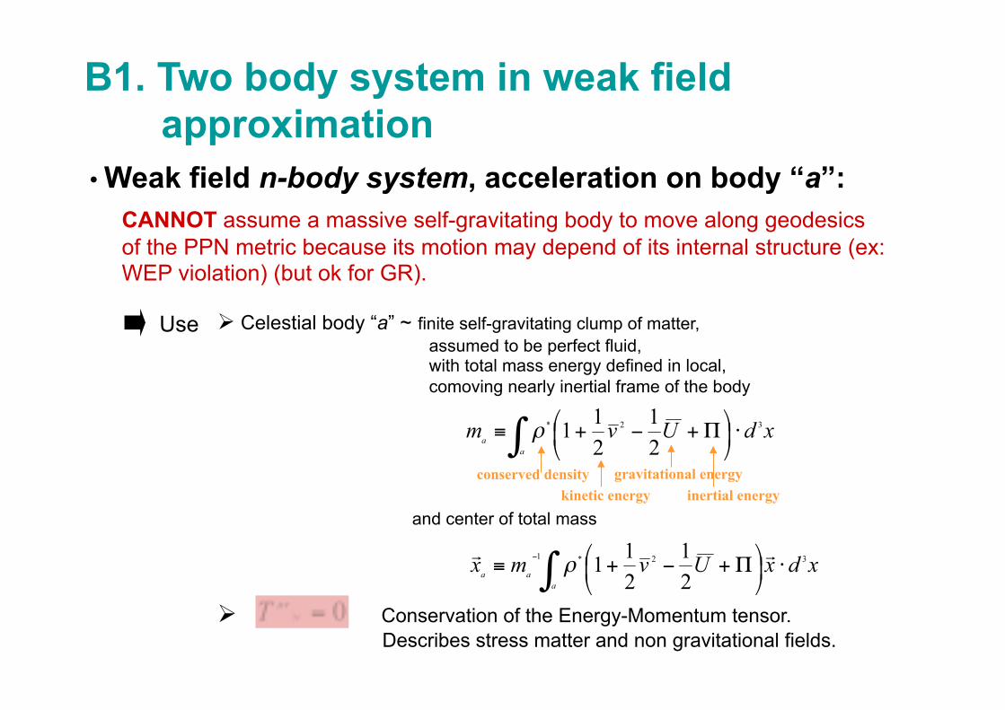
B1. Two body system in weak field approximation •  Weak field n-body system, acceleration on body “a”:

CANNOT assume a massive self-gravitating body to move along geodesics of the PPN metric because its motion may depend of its internal structure (ex: WEP violation) (but ok for GR).

  Celestial body “a” ~ finite self-gravitating clump of matter, assumed to be perfect fluid, with total mass energy defined in local, comoving nearly inertial frame of the body

and center of total mass

  Conservation of the Energy-Momentum tensor. Describes stress matter and non gravitational fields.

Use

conserved density kinetic energy

gravitational energy inertial energy

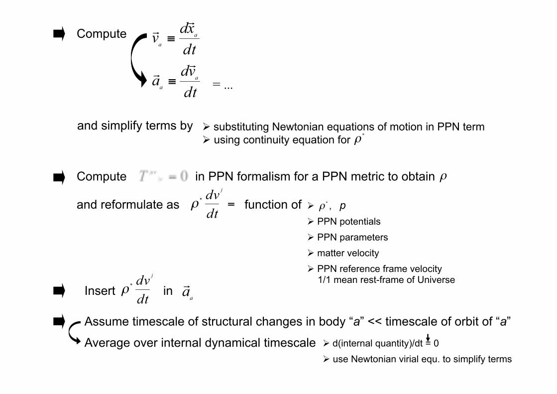
Compute

= ...

and simplify terms by   substituting Newtonian equations of motion in PPN term   using continuity equation for

Compute in PPN formalism for a PPN metric to obtain

and reformulate as function of   , p   PPN potentials   PPN parameters

  matter velocity   PPN reference frame velocity 1/1 mean rest-frame of Universe

Insert in

Assume timescale of structural changes in body “a” << timescale of orbit of “a”

Average over internal dynamical timescale   d(internal quantity)/dt = 0   use Newtonian virial equ. to simplify terms

with vector/tensor integrals

over , , , in “a” [Will 1993, table 6.2]

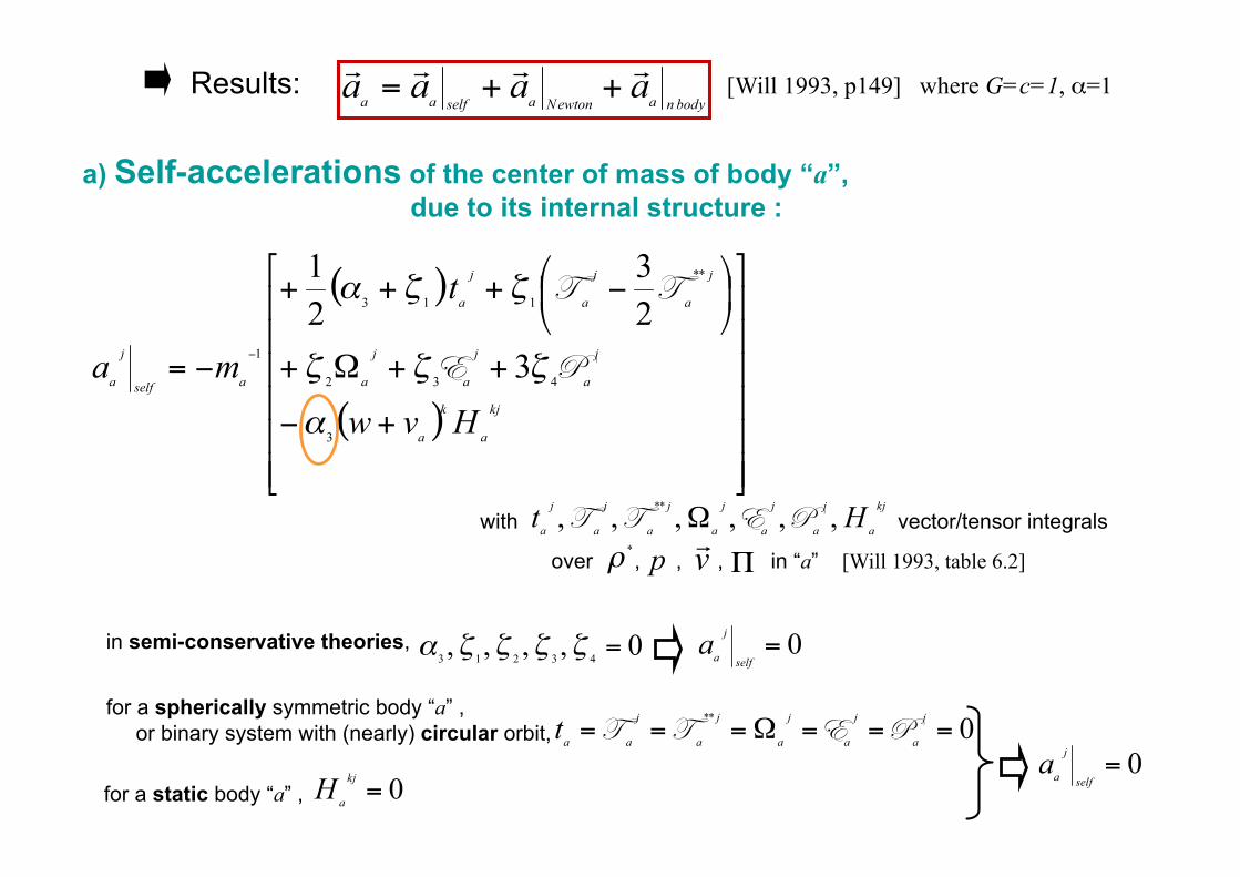
a) Self-accelerations of the center of mass of body “a”, due to its internal structure :

[Will 1993, p149] where G=c=1, α=1 Results:

in semi-conservative theories,

for a spherically symmetric body “a” , or binary system with (nearly) circular orbit,

for a static body “a” ,

…or, more convenient with a mass independent from direction:

[Will 1993, table 6.2, 151]

Inertial mass tensor of body “a”

Active gravitational mass tensor of body “b”

Passive gravitational mass tensor of body “a”

with

where

with

given in [Will 1993, p150]

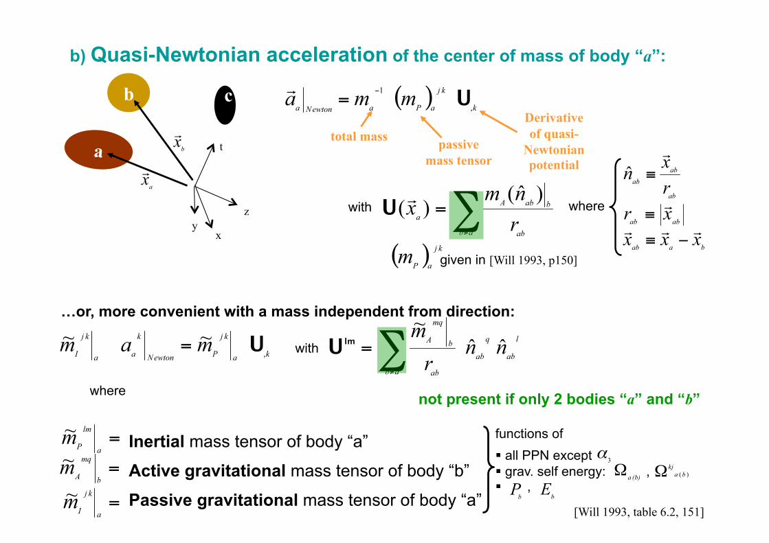
b) Quasi-Newtonian acceleration of the center of mass of body “a”:

total mass passive mass tensor

Derivative of quasi-

Newtonian potential

not present if only 2 bodies “a” and “b”

a

b c

y x

t

z where

functions of   all PPN except   grav. self energy: ,   ,

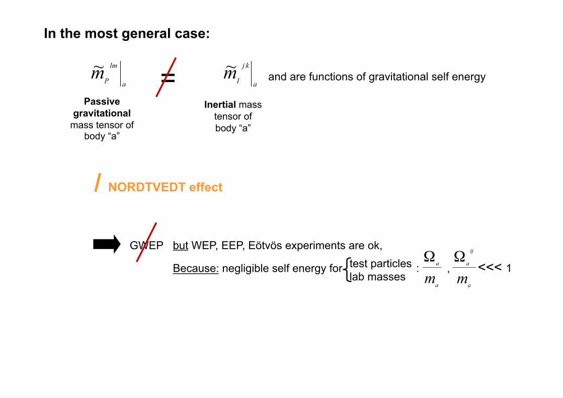
In the most general case:

Passive gravitational

mass tensor of body “a”

Inertial mass tensor of body “a”

= and are functions of gravitational self energy

GWEP

/ NORDTVEDT effect

but WEP, EEP, Eötvös experiments are ok,

Because: negligible self energy for : , <<< 1 test particles lab masses

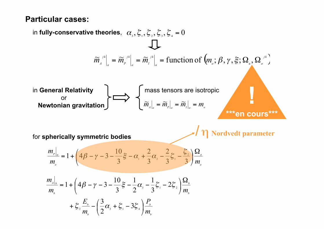
in General Relativity mass tensors are isotropic or Newtonian gravitation !

***en cours***

for spherically symmetric bodies / η Nordvedt parameter

in fully-conservative theories,

Particular cases:

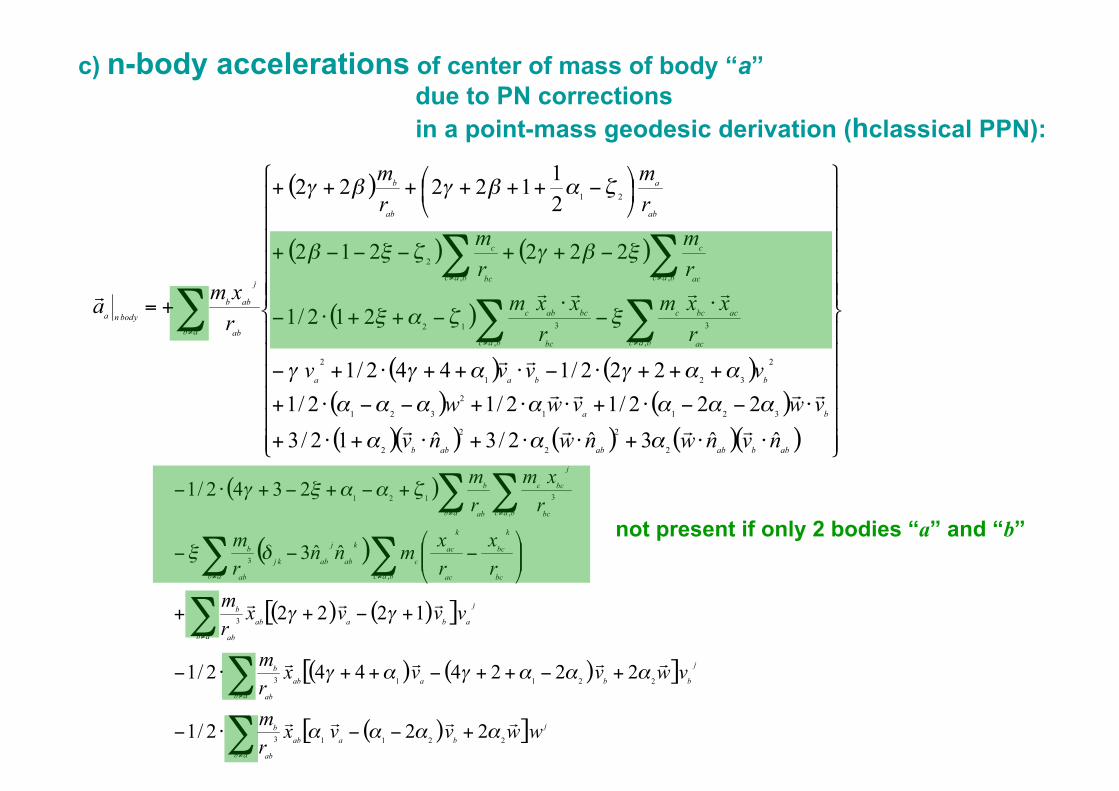
c) n-body accelerations of center of mass of body “a” due to PN corrections in a point-mass geodesic derivation (hclassical PPN):

not present if only 2 bodies “a” and “b”

ecliptic plane

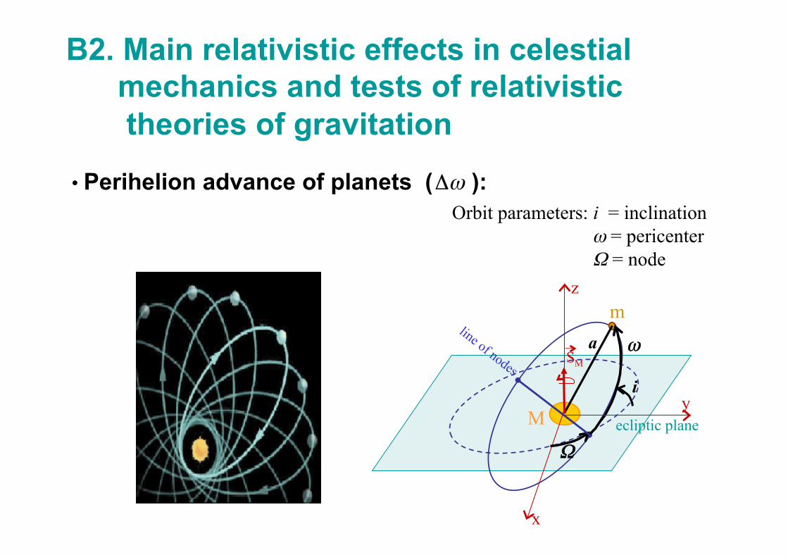
B2. Main relativistic effects in celestial mechanics and tests of relativistic theories of gravitation

•  Perihelion advance of planets ( ):

M

m a

S M

i

ω

Orbit parameters: i = inclination ω = pericenter Ω = node

x

y

z

Ω

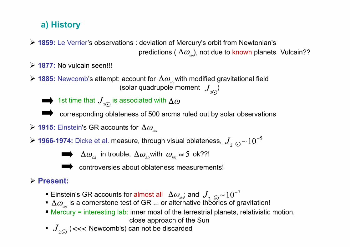
a) History

  1859: Le Verrier’s observations : deviation of Mercury's orbit from Newtonian's predictions ( ), not due to known planets Vulcain??

  1877: No vulcain seen!!!

  1885: Newcomb’s attempt: account for with modified gravitational field (solar quadrupole moment )

1st time that is associated with

corresponding oblateness of 500 arcms ruled out by solar observations

  1915: Einstein's GR accounts for

  1966-1974: Dicke et al. measure, through visual oblateness,

in trouble, with ok??!

controversies about oblateness measurements!

  Present:   Einstein's GR accounts for almost all ; and   is a cornerstone test of GR ... or alternative theories of gravitation!   Mercury = interesting lab: inner most of the terrestrial planets, relativistic motion, close approach of the Sun   ( Newcomb's) can not be discarded

. .

.

.

.

b) Theoretical calculation

. . Schwarzschild radius of Sun

orbital parameters of m

.

. gravitational quadrupole moment of Sun

with

~ 3 x 10 (J /10 ) -4 -7 2

. .

~ 2 x 10 for m = Mercury -7

~ 10 owing to PPN constraints on β (from η) and γ

-4

= 0 if fully conservative theory

neglect

mean radius of the Sun .

. .

. .

.

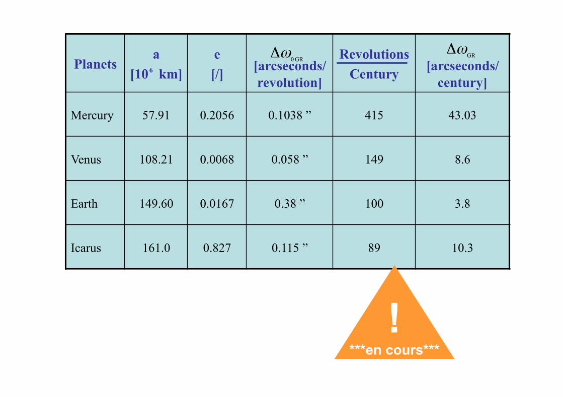
Planets a

[10 km] e [/] [arcseconds/

revolution]

Revolutions Century [arcseconds/

century]

Mercury 57.91 0.2056 0.1038 ” 415 43.03

Venus 108.21 0.0068 0.058 ” 149 8.6

Earth 149.60 0.0167 0.38 ” 100 3.8

Icarus 161.0 0.827 0.115 ” 89 10.3

6

! ***en cours***

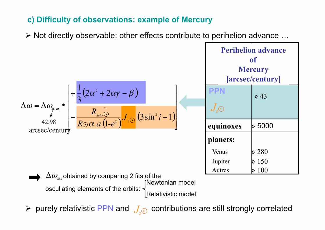
  Not directly observable: other effects contribute to perihelion advance …

  purely relativistic PPN and contributions are still strongly correlated

42,98 arcsec/century

. . . J 2

c) Difficulty of observations: example of Mercury

obtained by comparing 2 fits of the

oscullating elements of the orbits: Newtonian model

Relativistic model

. J 2

.

PPN » 43

equinoxes » 5000

planets: Venus » 280 Jupiter » 150 Autres » 100

Perihelion advance of

Mercury [arcsec/century]

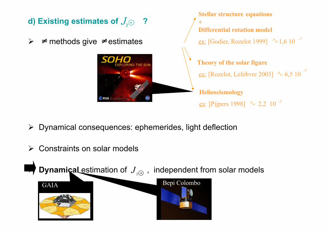
d) Existing estimates of ?

  methods give estimates

  Dynamical consequences: ephemerides, light deflection

  Constraints on solar models

  Dynamical estimation of , independent from solar models

Stellar structure equations + Differential rotation model

ex: [Godier, Rozelot 1999] 1,6 10 -7

Helioseismology

ex: [Pijpers 1998] 2,2 10 -7

GAIA Bepi Colombo

.

. J 2

Theory of the solar figure

ex: [Rozelot, Lefebvre 2003] 6,5 10 -7

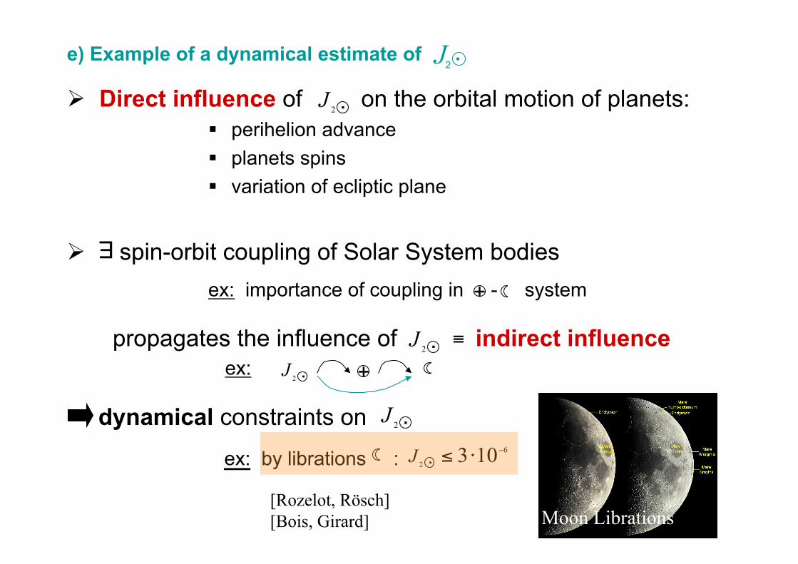
e) Example of a dynamical estimate of

  Direct influence of on the orbital motion of planets:   perihelion advance   planets spins   variation of ecliptic plane

  spin-orbit coupling of Solar System bodies ex: importance of coupling in - system

propagates the influence of indirect influence ex:

dynamical constraints on

ex: by librations :

[Rozelot, Rösch] [Bois, Girard]

..

E +

.

.

+

.

Moon Librations

. J 2

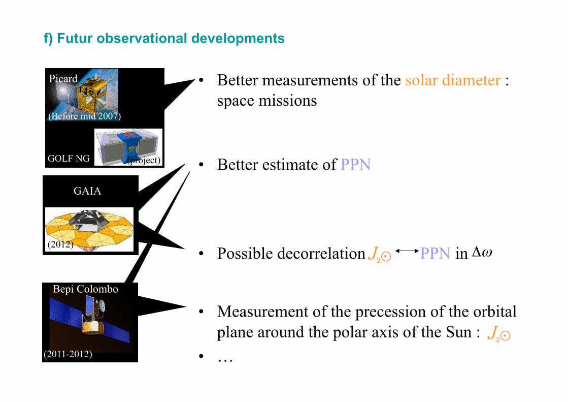
•  Better measurements of the solar diameter : space missions

•  Better estimate of PPN

•  Possible decorrelation PPN in

•  Measurement of the precession of the orbital plane around the polar axis of the Sun :

•  …

f) Futur observational developments

Picard

Bepi Colombo

GAIA

GOLF NG

(Before mid 2007)

(project)

(2012)

(2011-2012)

. J 2

. J 2

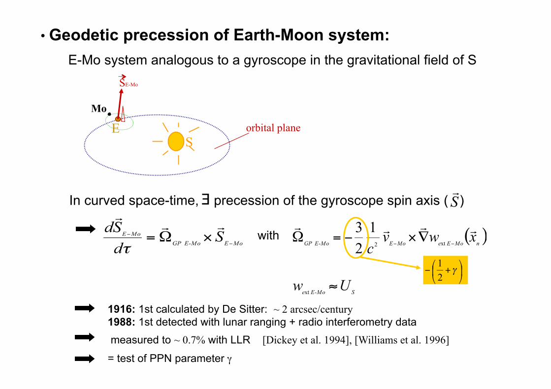
•  Geodetic precession of Earth-Moon system: E-Mo system analogous to a gyroscope in the gravitational field of S

E S

Mo

orbital plane

SE-Mo

1916: 1st calculated by De Sitter: ~ 2 arcsec/century 1988: 1st detected with lunar ranging + radio interferometry data measured to ~ 0.7% with LLR [Dickey et al. 1994], [Williams et al. 1996]

with

In curved space-time, precession of the gyroscope spin axis ( )

= test of PPN parameter γ

with

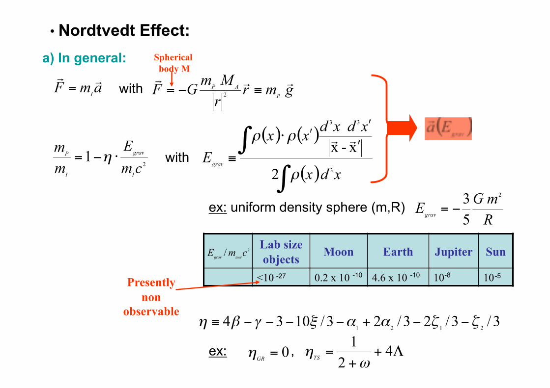
•  Nordtvedt Effect:

with

ex: uniform density sphere (m,R)

Lab size objects Moon Earth Jupiter Sun

<10 0.2 x 10 4.6 x 10 10 10 -5 -8 -10 -10 -27

ex: ,

Presently non

observable

a) In general: Spherical body M

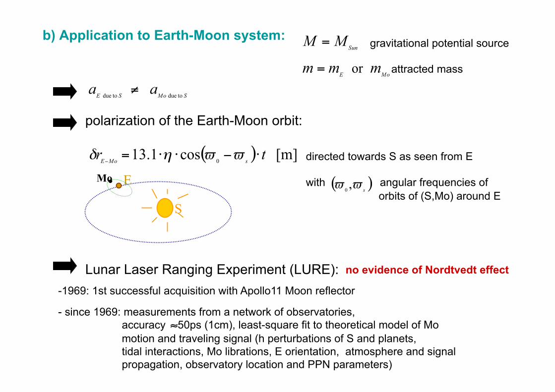
b) Application to Earth-Moon system:

E

S

Mo

attracted mass

gravitational potential source

polarization of the Earth-Moon orbit:

directed towards S as seen from E

with angular frequencies of orbits of (S,Mo) around E

Lunar Laser Ranging Experiment (LURE): - 1969: 1st successful acquisition with Apollo11 Moon reflector

-  since 1969: measurements from a network of observatories, accuracy 50ps (1cm), least-square fit to theoretical model of Mo motion and traveling signal (h perturbations of S and planets, tidal interactions, Mo librations, E orientation, atmosphere and signal propagation, observatory location and PPN parameters)

no evidence of Nordtvedt effect

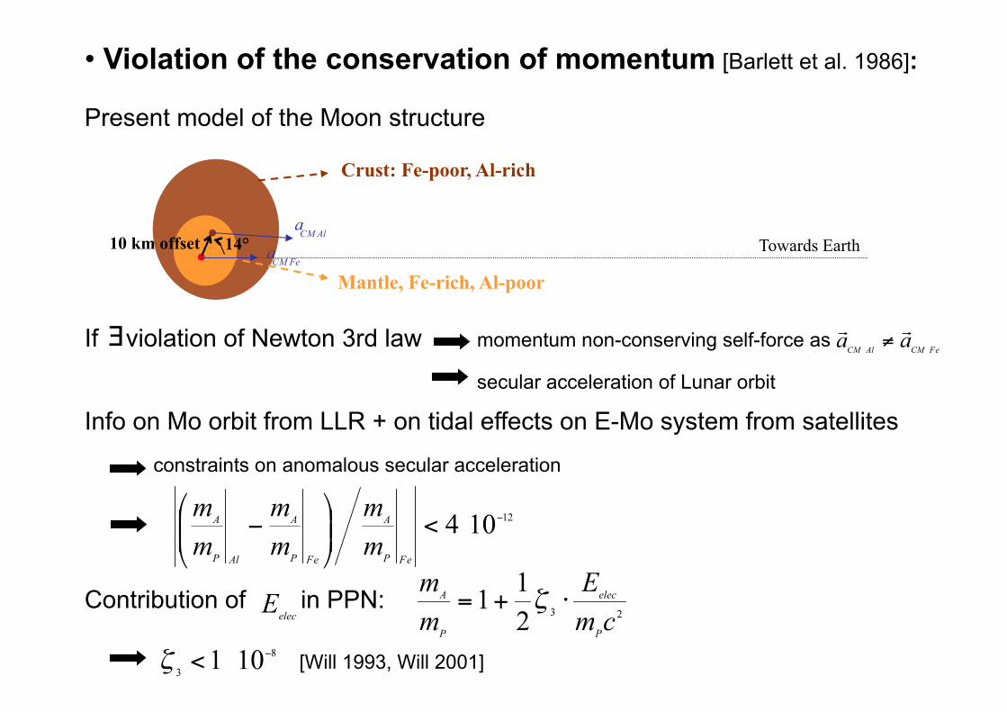
•  Violation of the conservation of momentum [Barlett et al. 1986]:

Present model of the Moon structure

If violation of Newton 3rd law momentum non-conserving self-force as

secular acceleration of Lunar orbit

Info on Mo orbit from LLR + on tidal effects on E-Mo system from satellites

constraints on anomalous secular acceleration

Contribution of in PPN:

[Will 1993, Will 2001]

Towards Earth 10 km offset

Mantle, Fe-rich, Al-poor

Crust: Fe-poor, Al-rich

14° a CM Fe

a CM Al

C/ Geodesy and tests of relativistic theories of gravitation

RELATIVISTIC THEORIES OF GRAVITATION

IAU metric conventions, Geodesic equation

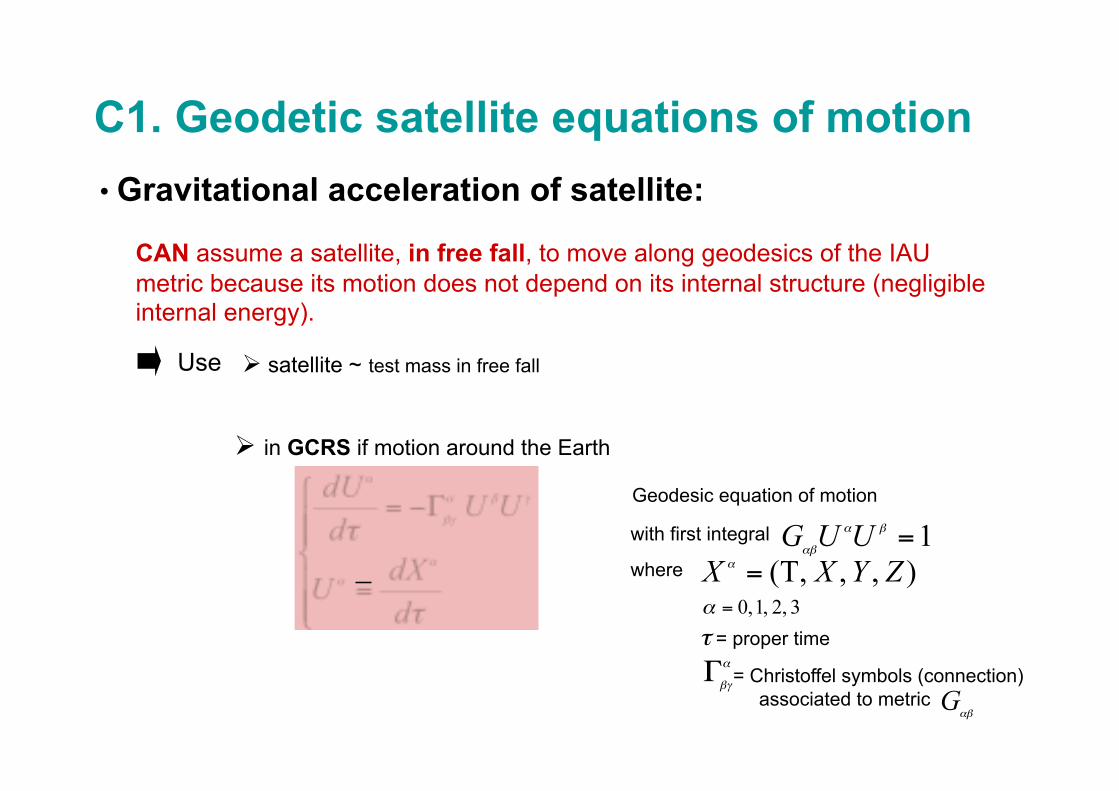
C1. Geodetic satellite equations of motion •  Gravitational acceleration of satellite:

CAN assume a satellite, in free fall, to move along geodesics of the IAU metric because its motion does not depend on its internal structure (negligible internal energy).

  satellite ~ test mass in free fall Use

  in BCRS if motion in the solar system

Geodesic equation of motion

with first integral

where

τ = proper time

= Christoffel symbols (connection) associated to metric

  in GCRS if motion around the Earth

Geodesic equation of motion

with first integral

where

τ = proper time

= Christoffel symbols (connection) associated to metric

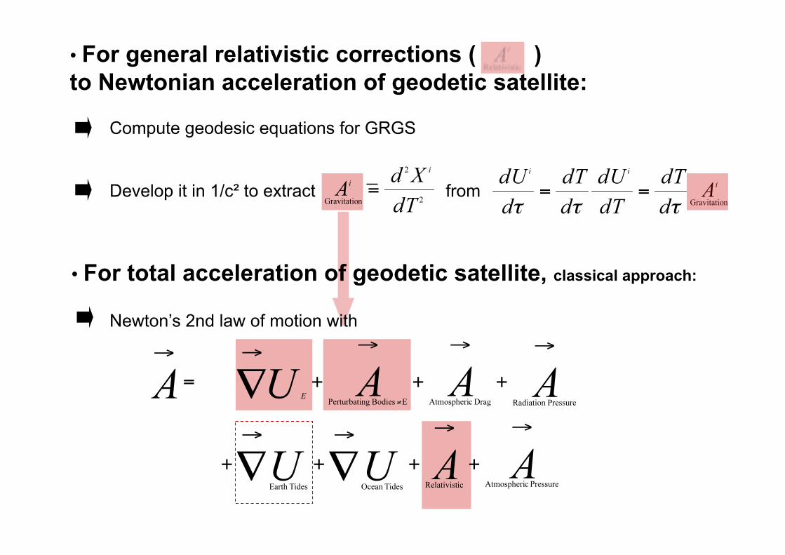
Newton’s 2nd law of motion with

•  For total acceleration of geodetic satellite, classical approach:

•  For general relativistic corrections ( ) to Newtonian acceleration of geodetic satellite:

Compute geodesic equations for GRGS

Develop it in 1/c² to extract from

C2. Main relativistic effects in Geodesy

LAGEOS 1

SEASAT

Laser GEOdymics Satellite 1 Aims: - calculate station positions (1-3cm) - monitor tectonic-plate motion - measure Earth gravitational field - measure Earth rotation Design: - spherical with laser reflectors - no onboard sensors/electronic - no attitude control Orbit: 5858x5958km, i = 52.6° Mission: 1976, ~50 years (USA)

SEA SATellite Aims: -test oceanic sensors (to measure sea surface heights ) Design: Orbit: 800km Mission: June-October 1978

•  Examples: a high-, or respectively low-altitude satellite…

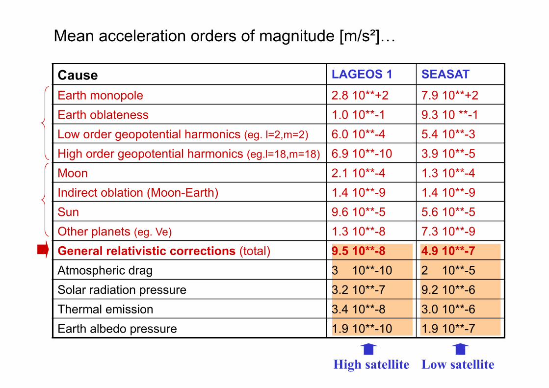
Cause LAGEOS 1 SEASAT Earth monopole 2.8 10**+2 7.9 10**+2 Earth oblateness 1.0 10**-1 9.3 10 **-1 Low order geopotential harmonics (eg. l=2,m=2) 6.0 10**-4 5.4 10**-3 High order geopotential harmonics (eg.l=18,m=18) 6.9 10**-10 3.9 10**-5 Moon 2.1 10**-4 1.3 10**-4 Indirect oblation (Moon-Earth) 1.4 10**-9 1.4 10**-9 Sun 9.6 10**-5 5.6 10**-5 Other planets (eg. Ve) 1.3 10**-8 7.3 10**-9 General relativistic corrections (total) 9.5 10**-8 4.9 10**-7 Atmospheric drag 3 10**-10 2 10**-5 Solar radiation pressure 3.2 10**-7 9.2 10**-6 Thermal emission 3.4 10**-8 3.0 10**-6 Earth albedo pressure 1.9 10**-10 1.9 10**-7

Mean acceleration orders of magnitude [m/s²]…

High satellite Low satellite

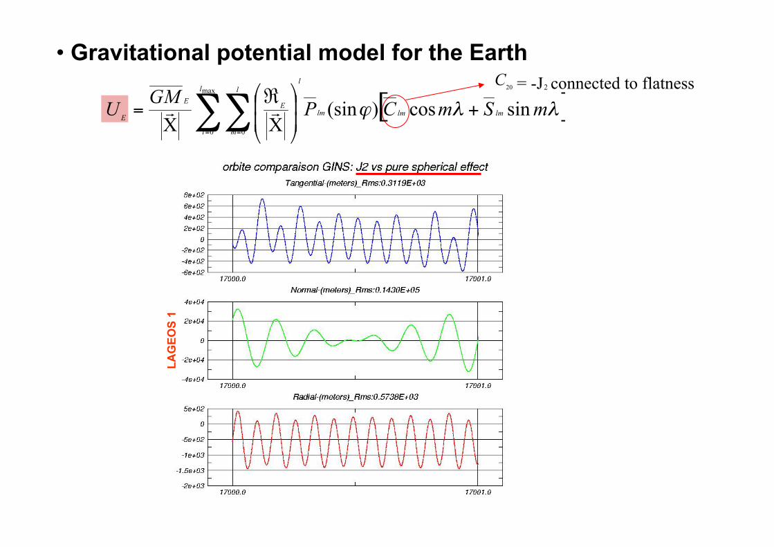
•  Gravitational potential model for the Earth = -J 2 connected to flatness

LAG

EOS

1 LA

GEO

S 1

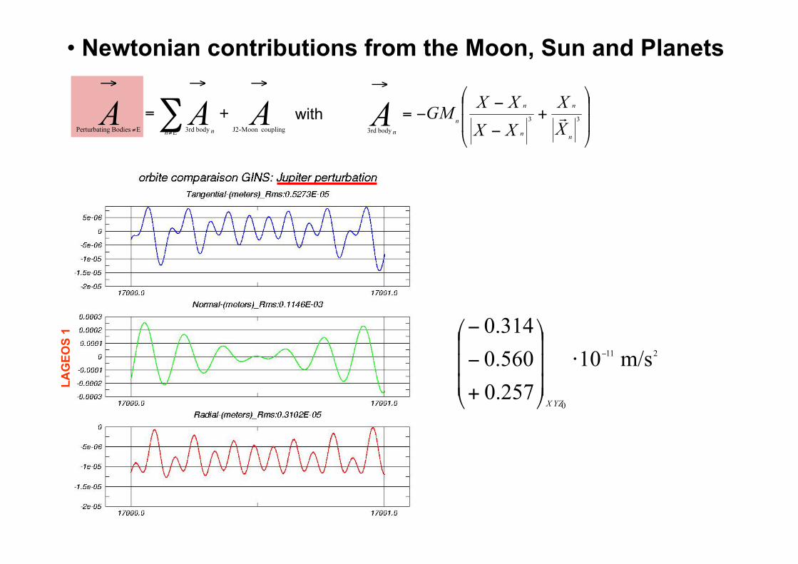
•  Newtonian contributions from the Moon, Sun and Planets

and

LAG

EOS

1 LA

GEO

S 1

with

LAG

EOS

1

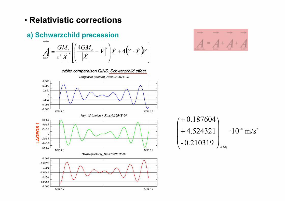
•  Relativistic corrections a) Schwarzchild precession

LAG

EOS

1

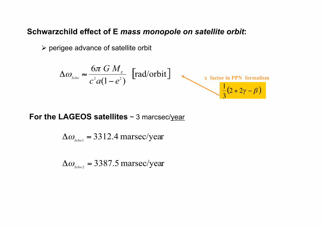
Schwarzchild effect of E mass monopole on satellite orbit:

  perigee advance of satellite orbit

For the LAGEOS satellites ~ 3 marcsec/year

x factor in PPN formalism

,

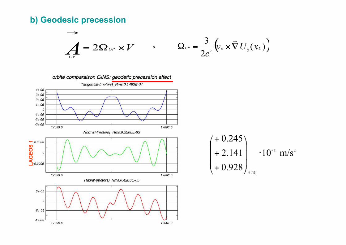
b) Geodesic precession LA

GEO

S 1

with

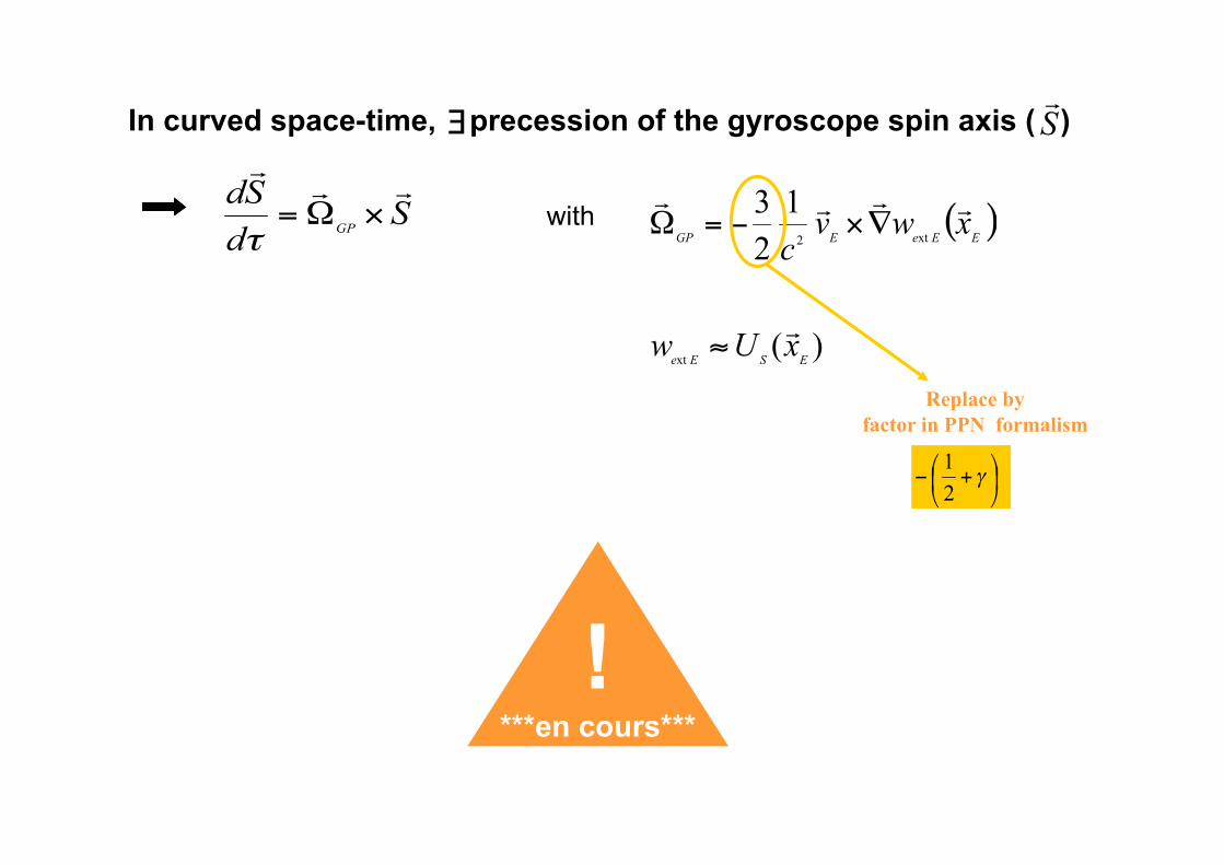
In curved space-time, precession of the gyroscope spin axis ( )

! ***en cours***

Replace by factor in PPN formalism

,

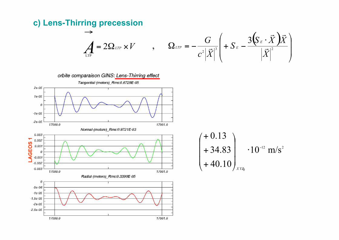
c) Lens-Thirring precession LA

GEO

S 1

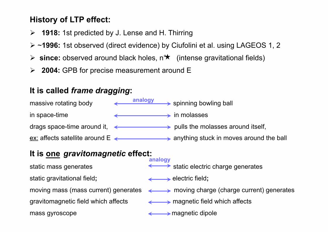
History of LTP effect:   1918: 1st predicted by J. Lense and H. Thirring

  ~1996: 1st observed (direct evidence) by Ciufolini et al. using LAGEOS 1, 2

  since: observed around black holes, n° (intense gravitational fields)

  2004: GPB for precise measurement around E

It is called frame dragging: massive rotating body spinning bowling ball

in space-time in molasses

drags space-time around it, pulls the molasses around itself,

ex: affects satellite around E anything stuck in moves around the ball

analogy

It is one gravitomagnetic effect: static mass generates static electric charge generates

static gravitational field; electric field;

moving mass (mass current) generates moving charge (charge current) generates

gravitomagnetic field which affects magnetic field which affects

mass gyroscope magnetic dipole

analogy

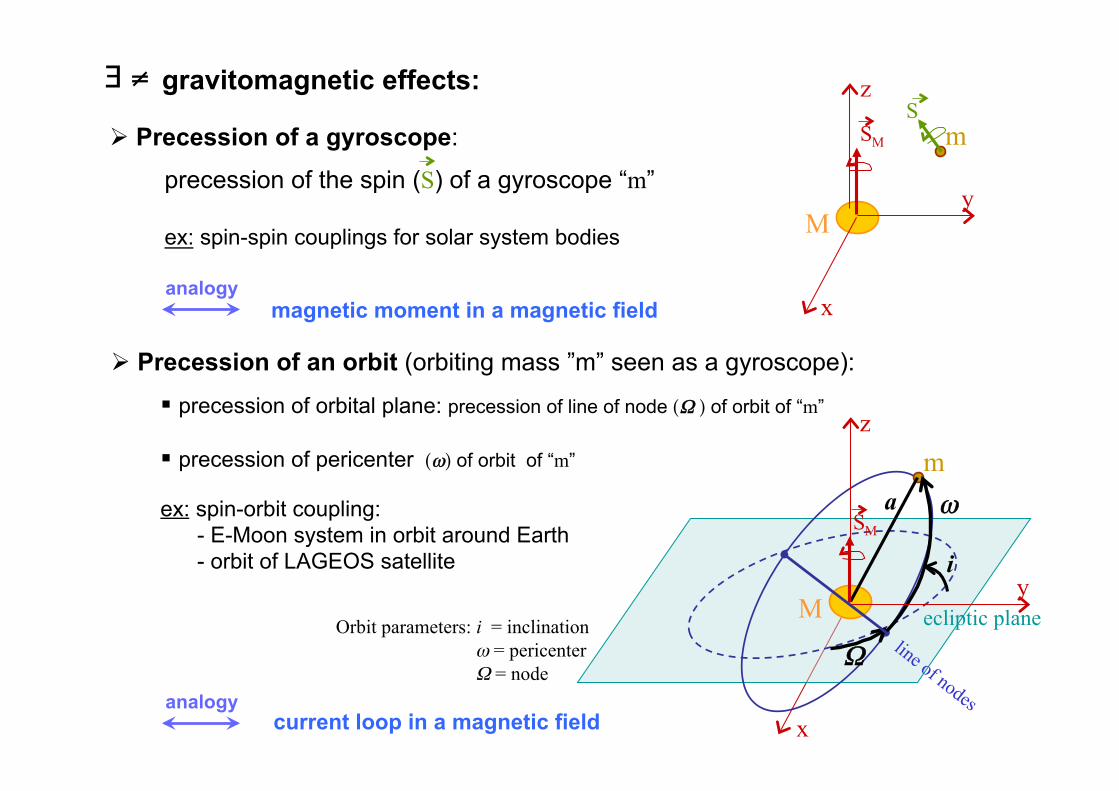
  Precession of a gyroscope:

precession of the spin (S) of a gyroscope “m”

ex: spin-spin couplings for solar system bodies

gravitomagnetic effects:

M y

m S M

x

z S

analogy

analogy

magnetic moment in a magnetic field

current loop in a magnetic field x

ecliptic plane M

m a

S M

i

ω

Orbit parameters: i = inclination ω = pericenter Ω = node

y

z

Ω

  Precession of an orbit (orbiting mass ”m” seen as a gyroscope):

  precession of orbital plane: precession of line of node (Ω ) of orbit of “m”

  precession of pericenter (ω) of orbit of “m”

ex: spin-orbit coupling: - E-Moon system in orbit around Earth - orbit of LAGEOS satellite

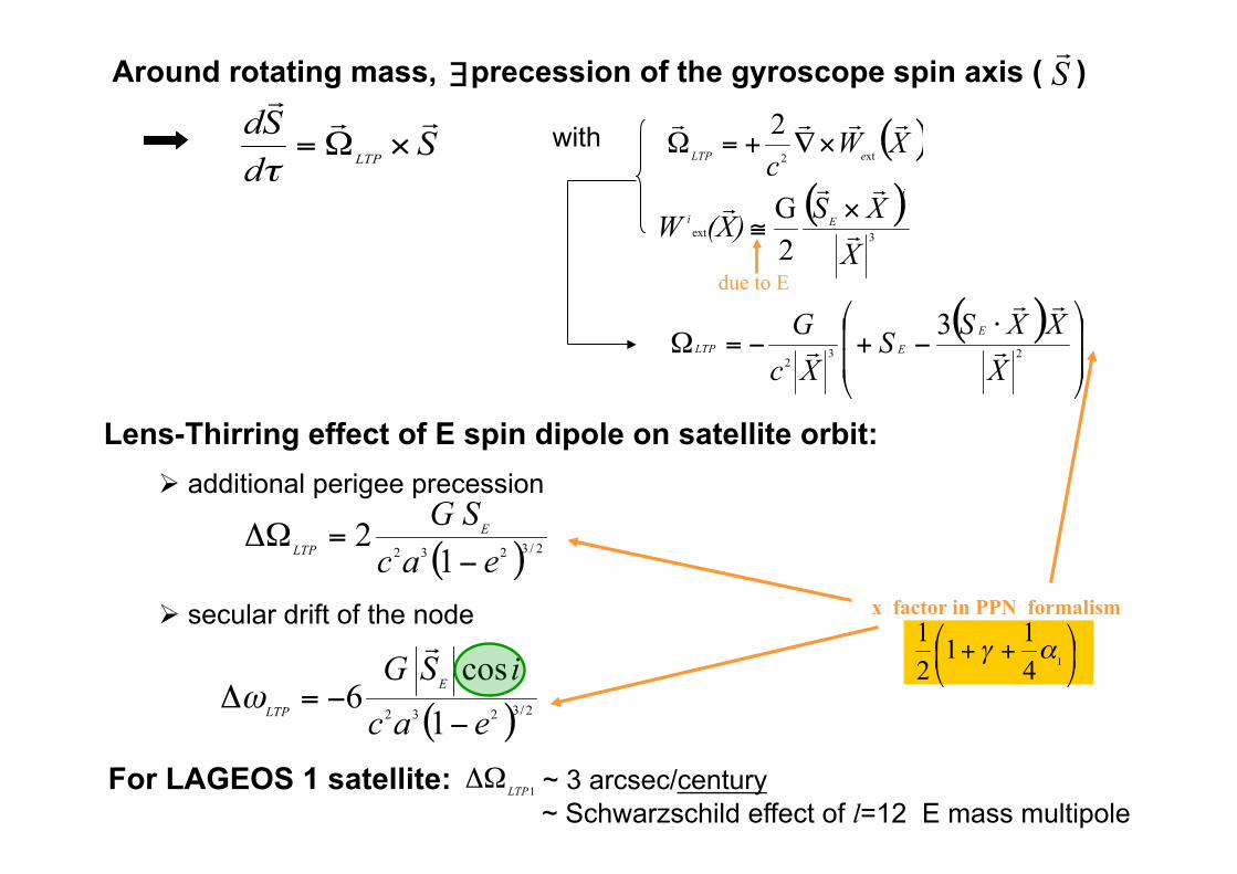
Lens-Thirring effect of E spin dipole on satellite orbit:   additional perigee precession

  secular drift of the node

with

due to E

For LAGEOS 1 satellite: ~ 3 arcsec/century ~ Schwarzschild effect of l=12 E mass multipole

Around rotating mass, precession of the gyroscope spin axis ( )

x factor in PPN formalism

LAGEOS 1

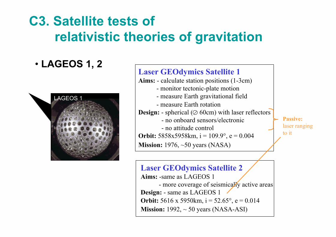
Laser GEOdymics Satellite 1 Aims: - calculate station positions (1-3cm) - monitor tectonic-plate motion - measure Earth gravitational field - measure Earth rotation Design: - spherical ( 60cm) with laser reflectors - no onboard sensors/electronic - no attitude control Orbit: 5858x5958km, i = 109.9°, e = 0.004 Mission: 1976, ~50 years (NASA)

Laser GEOdymics Satellite 2 Aims: -same as LAGEOS 1 - more coverage of seismically active areas Design: - same as LAGEOS 1 Orbit: 5616 x 5950km, i = 52.65°, e = 0.014 Mission: 1992, ~ 50 years (NASA-ASI)

C3. Satellite tests of relativistic theories of gravitation

•  LAGEOS 1, 2

Passive: laser ranging to it

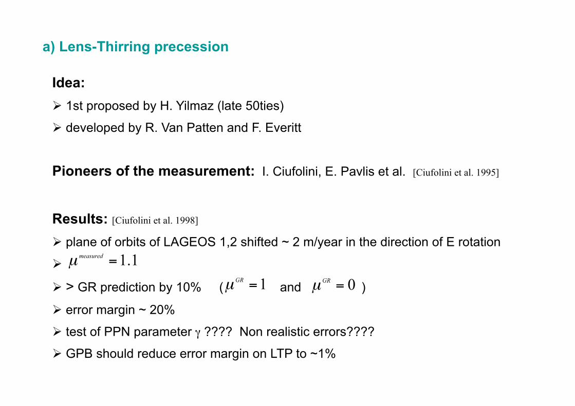
Idea:   1st proposed by H. Yilmaz (late 50ties)

  developed by R. Van Patten and F. Everitt

Pioneers of the measurement: I. Ciufolini, E. Pavlis et al. [Ciufolini et al. 1995]

a) Lens-Thirring precession

Results: [Ciufolini et al. 1998]   plane of orbits of LAGEOS 1,2 shifted ~ 2 m/year in the direction of E rotation

 

  > GR prediction by 10% ( and )

  error margin ~ 20%

  test of PPN parameter γ ???? Non realistic errors????

  GPB should reduce error margin on LTP to ~1%

observables: , ,

unknowns: , ,

errors on Jn: ,

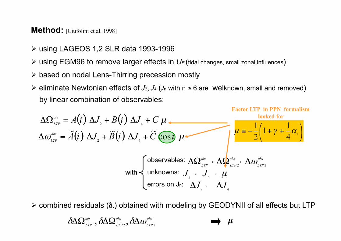
Method: [Ciufolini et al. 1998]

  using LAGEOS 1,2 SLR data 1993-1996

  using EGM96 to remove larger effects in UE (tidal changes, small zonal influences)

  based on nodal Lens-Thirring precession mostly

  eliminate Newtonian effects of J2, J4 (Jn with n 6 are welknown, small and removed) by linear combination of observables:

with

  combined residuals (δ.) obtained with modeling by GEODYNII of all effects but LTP

Factor LTP in PPN formalism looked for

µ

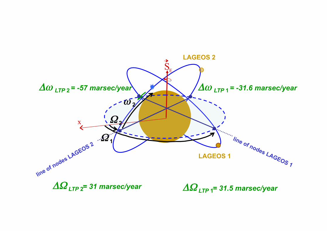
LAGEOS 2

LAGEOS 1

S E

x Ω 2

Ω 1

ω 2

Δω = -57 marsec/year LTP 2

ΔΩ = 31 marsec/year LTP 2 ΔΩ = 31.5 marsec/year LTP 1

Δω = -31.6 marsec/year LTP 1

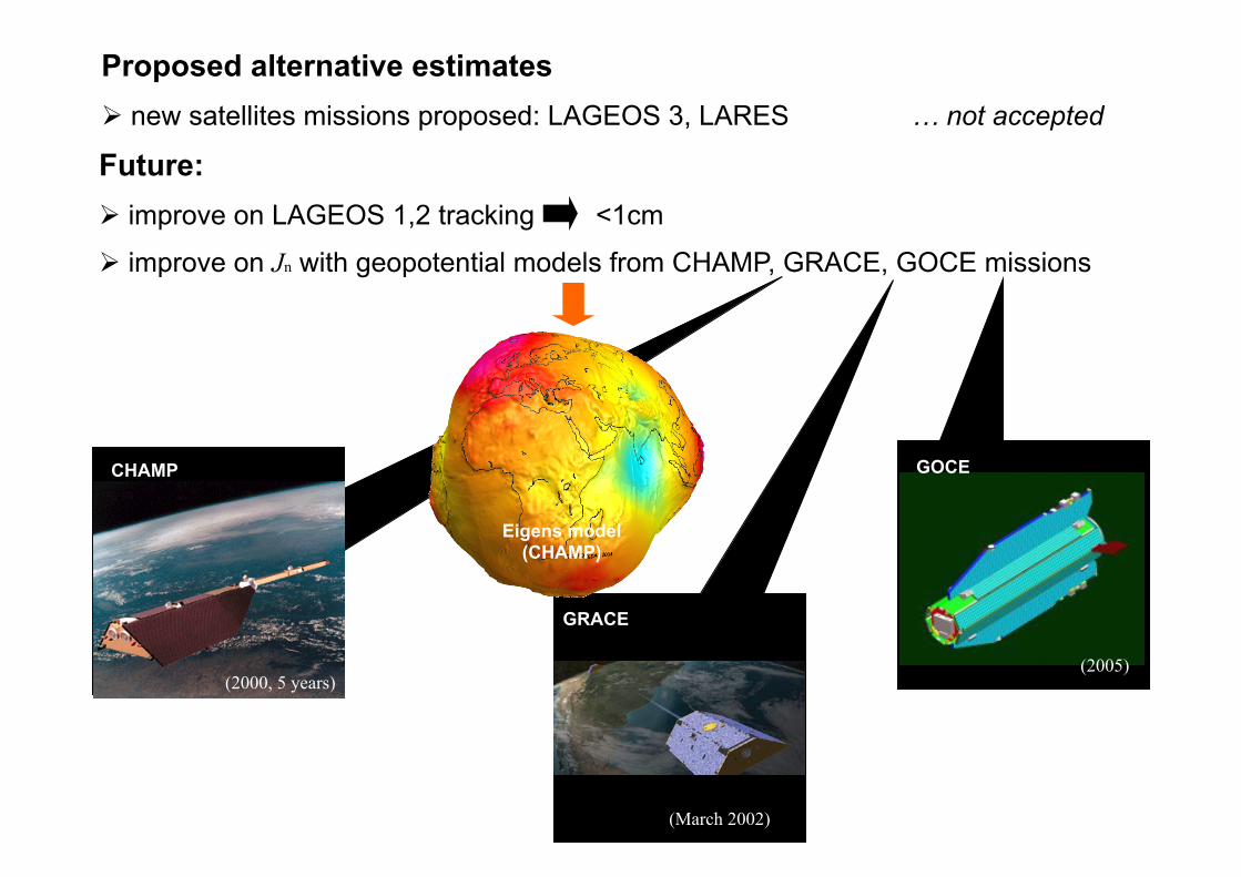
GRACE

(March 2002)

CHAMP

(2000, 5 years)

Eigens model (CHAMP)

Future:

  improve on LAGEOS 1,2 tracking <1cm

  improve on Jn with geopotential models from CHAMP, GRACE, GOCE missions

GOCE

(2005)

Proposed alternative estimates   new satellites missions proposed: LAGEOS 3, LARES … not accepted

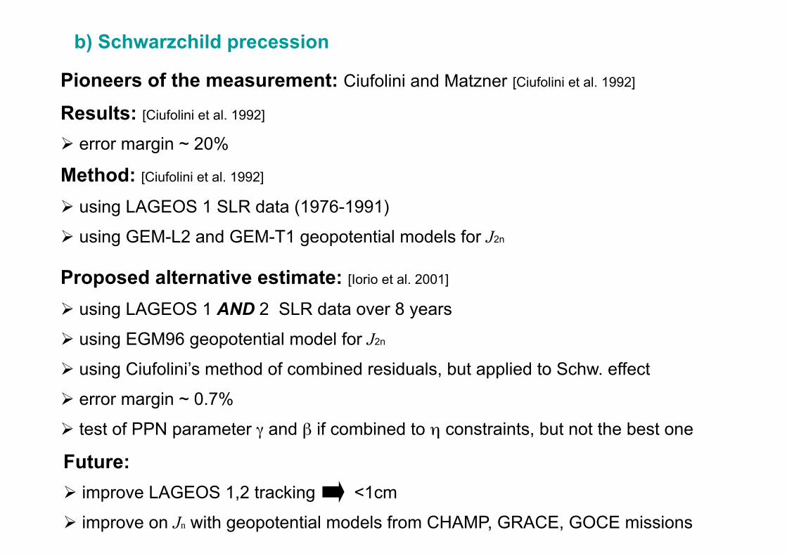
Pioneers of the measurement: Ciufolini and Matzner [Ciufolini et al. 1992]

Results: [Ciufolini et al. 1992]   error margin ~ 20%

Method: [Ciufolini et al. 1992]   using LAGEOS 1 SLR data (1976-1991)

  using GEM-L2 and GEM-T1 geopotential models for J2n

b) Schwarzchild precession

Proposed alternative estimate: [Iorio et al. 2001]   using LAGEOS 1 AND 2 SLR data over 8 years

  using EGM96 geopotential model for J2n

  using Ciufolini’s method of combined residuals, but applied to Schw. effect

  error margin ~ 0.7%

  test of PPN parameter γ and β if combined to η constraints, but not the best one

Future:

  improve LAGEOS 1,2 tracking <1cm

  improve on Jn with geopotential models from CHAMP, GRACE, GOCE missions

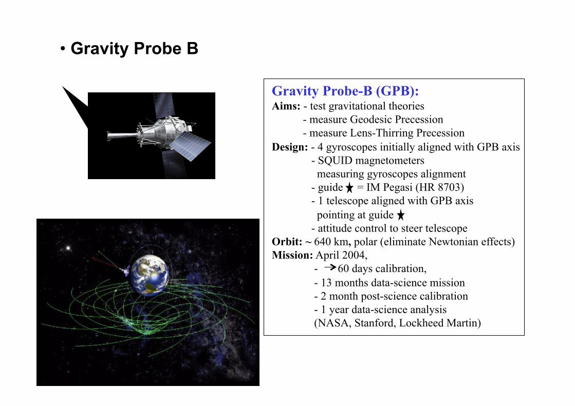
Gravity Probe-B (GPB): Aims: - test gravitational theories - measure Geodesic Precession - measure Lens-Thirring Precession Design: - 4 gyroscopes initially aligned with GPB axis - SQUID magnetometers measuring gyroscopes alignment - guide = IM Pegasi (HR 8703) - 1 telescope aligned with GPB axis pointing at guide - attitude control to steer telescope Orbit: ~ 640 km, polar (eliminate Newtonian effects) Mission: April 2004, - 60 days calibration, - 13 months data-science mission - 2 month post-science calibration - 1 year data-science analysis (NASA, Stanford, Lockheed Martin)

•  Gravity Probe B

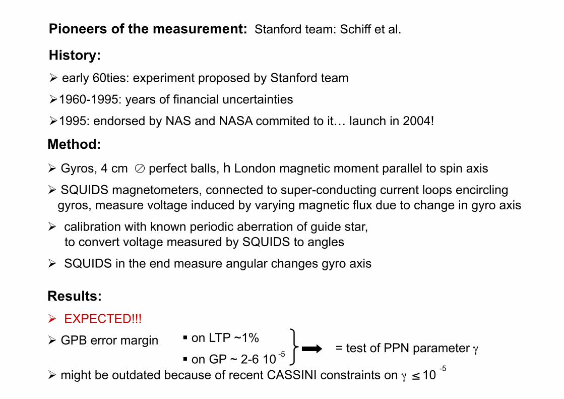
Pioneers of the measurement: Stanford team: Schiff et al.

History:   early 60ties: experiment proposed by Stanford team

 1960-1995: years of financial uncertainties

 1995: endorsed by NAS and NASA commited to it… launch in 2004!

-5

-5

  on LTP ~1%

  on GP ~ 2-6 10 = test of PPN parameter γ

Method:   Gyros, 4 cm perfect balls, h London magnetic moment parallel to spin axis

  SQUIDS magnetometers, connected to super-conducting current loops encircling gyros, measure voltage induced by varying magnetic flux due to change in gyro axis

  calibration with known periodic aberration of guide star, to convert voltage measured by SQUIDS to angles

  SQUIDS in the end measure angular changes gyro axis

Results:   EXPECTED!!!

  GPB error margin

  might be outdated because of recent CASSINI constraints on γ 10

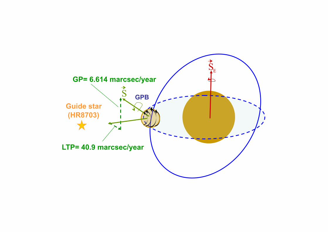
GPB

S E

Guide star (HR8703)

S GP= 6.614 marcsec/year

LTP= 40.9 marcsec/year

BIBLIOGRAPHY [Barlett et al. 1986] Phys. Rev., Lett., 57, 21-24 [Bell et al. 1996a] Astrophys.J., 464, 857. astro-ph/9512100 [Bell et al. 1996b] Class. Quantum Grav., 13, 3121-3128. gr-qc/9606062 [Bertotti et al. 2003] Nature, 425, 374-376 [Bize et al 1999] Europhysics Letters C, 45, 558 [W. Cui et al. 1998] Astrophys. J., 492, L53 [Ciufolini 1986] Phys. Rev. Lett., 56, 278 [Ciufolini et al. 1992] Int. J. Mod. Phys. A, 7(4), 843-852 [Ciufolini et al. 1996] Nuovo Cimento A, 109, 579 [Ciufolini et al. 1997a] gr-qc/9704065 [Ciufolini et al. 1997b] Class. Quantum Grav., 14, 2701 [Ciufolini et al. 1998] Science, 279, 2100 [Chiba et al.1998] Nuclear Phys. B, 530, 304-324. gr-qc/9708030 v2 May 1998. [Counselman et al.1974] Phys. Rev. Let., 33, 1621-1623 [DamourTaylor 1991] Astrophys. J., 366, 501-511 [Damour et al. 1996a] Phys. Rev. D, 54, 1474-1491 [Damour et al. 1996b] Phys. Rev. D, 53, 5541-5578. gr-qc/9506063. [Damour et al. 1998] Phys. Rev. D, 58, 042001 [Dickey et al. 1994] Science, 265, 482-490 [Eubanks et al.1999] ftp://casa.usno.navy.mil/navnet/postscript/prd\_15.ps [Fomalont et al. 1976] Phys. Rev. Let., 36, 1475-1478 [Goldman 1990] Mon. Not. R. Astron. Soc, 244, 184-187

[IAU 1992] IAU 1991 resolutions. IAU Information Bulletin 67 [IAU 2001a] IAU 2000 resolutions. IAU Information Bulletin 88 [IAU 2001b] Erratum on resolution B1.3. Information Bulletin 89 [IAU 2003] IAU Division 1, ICRS Working Group Task 5: SOFA libraries

http://www.iau-sofa.rl.ac.uk/product.html [IERS 2003] IERS website http://www.iers.org/map [Iorio et al. 2001] gr-qc/0103088 v10 July 2002 [Iorio et al. 2002a] La Revista del Nuovo Cimento, 25(5) [Iorio et al. 2002b] J. of Geodetic Soc. of Japan, 48 (1), 13-20 [Lebach et al.1995] Phys. Rev. Let., 75, 8, 1439-1442 [Lemonde et al 2001] Ed. A.N.Luiten, Berlin (Springer) [Lens et al. 1918] Phys. Z. 19,156. English translation [Mashhoon et al. 1984] Gen. Relativ. Gravitation 16, 711 [Müller et al. 1996] Phys. Rev. D, 54, R5927-5930 [Müller et al.1999] Proc. 8th M. Grossman Meeting on GR, 1151-1153, World Sc. Singapore [Nordtvedt 1988] Int. J. Theor. Phys., 27, 1395 [Reasenberg et al. 1979] Astrophys. J., 234, L219-L221 [Ries et al. 2003] The Lens-Thirring effect. Ed. Ruffini & Sigismondi, World Scientific, Singapore, p201 [Robertson et al. 1984] Nature, 310, 572-574 [Robertson et al.1991a] Nature, 349, 768-770 [Robertson et al.1991b] Proc. of AGU Chapman Conference, Washington, 22-26, 203-212 [Seielstad et al.1970] Phys. Rev. Let., 24, 1373-1376 [Shapiro et al. 2004] Phys. Rev. Let., 92, 121101

[Soffel et al 2003] prepared for the Astronomical Journal, astro-ph/0303376v1 [Weyers et al 2001] Metrologia A, 38, 4, 343 [Will website] http://wugrav.wustl.edu/People/CLIFF/index.html [Will 1976] Astrophys. J., 204, 224-234 [Will 1992] Astrophys. J. Lett., 393, L59-L61 [Will 1993] Cambridge University Press [Will 2001] http://www.livingreviews.org/Articles/Volume4/2001-will/ [Will 2002] gr-qc/0212069 v1 [Williams et al. 1996] Phys. Rev. D,53, 6730-6739 [Williams et al. 2001] Proc. 9th Marcel Grossmann 2000. Ed. World Scientific.

Other transparencies…

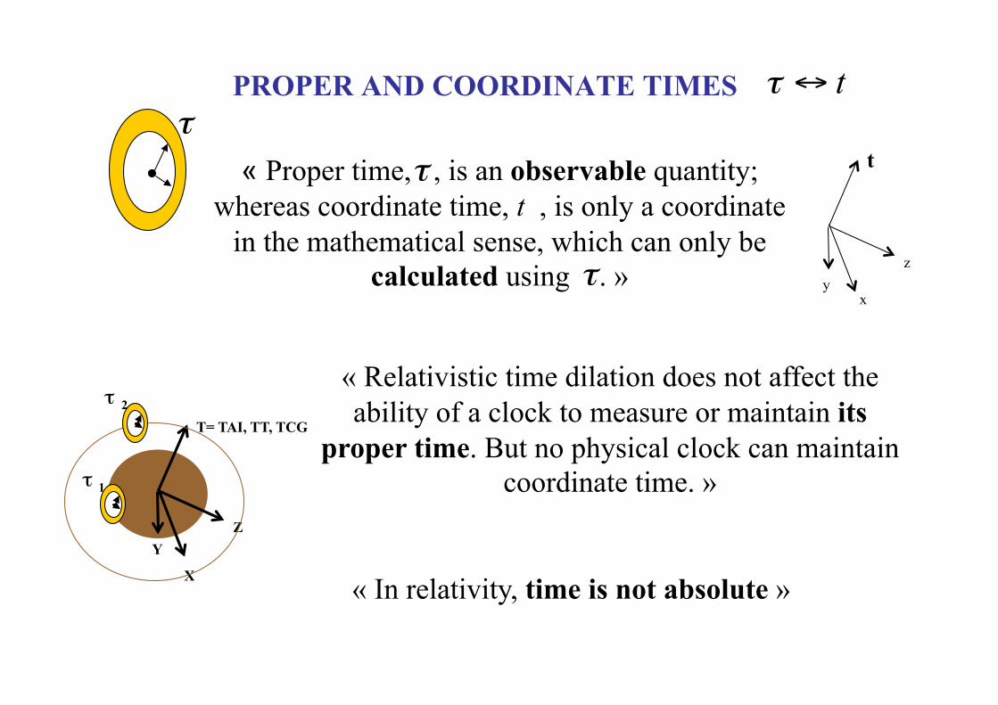
PROPER AND COORDINATE TIMES

« Proper time, , is an observable quantity; whereas coordinate time, t , is only a coordinate

in the mathematical sense, which can only be calculated using . »

« Relativistic time dilation does not affect the ability of a clock to measure or maintain its

proper time. But no physical clock can maintain coordinate time. »

X

Y

T= TAI, TT, TCG

Z

y x

t

z

« In relativity, time is not absolute »

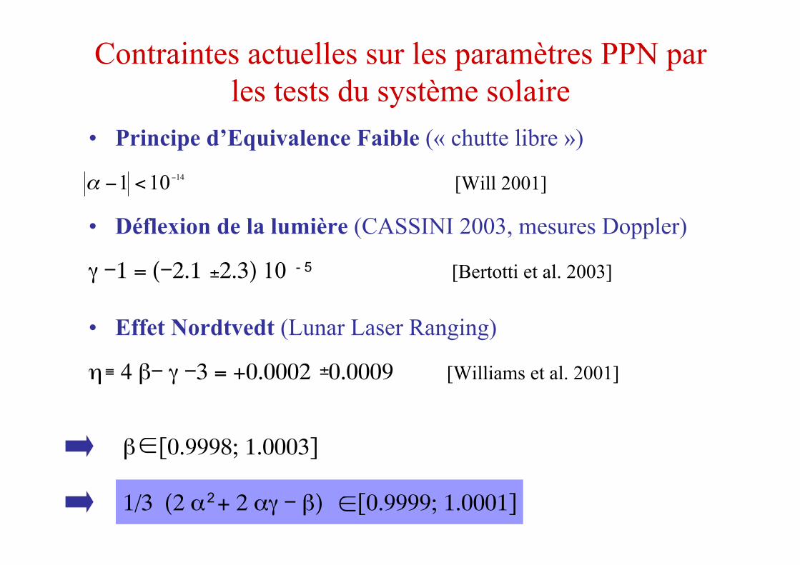
Contraintes actuelles sur les paramètres PPN par les tests du système solaire

•  Principe d’Equivalence Faible (« chutte libre »)

[Will 2001]

•  Déflexion de la lumière (CASSINI 2003, mesures Doppler)

γ -1 = (-2.1 2.3) 10 [Bertotti et al. 2003]

•  Effet Nordtvedt (Lunar Laser Ranging)

η 4 β- γ -3 = +0.0002 0.0009 [Williams et al. 2001]

- 5

β [0.9998; 1.0003]

1/3 (2 α + 2 αγ - β) [0.9999; 1.0001] 2

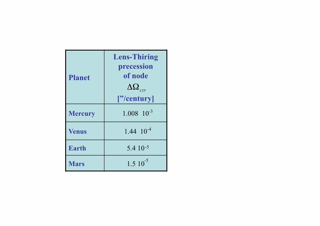
Planet

Lens-Thiring precession

of node

[”/century]

Mercury 1.008 10

Venus 1.44 10

Earth 5.4 10

Mars 1.5 10

-3

-4

-5

-5