Embed Size (px)
Citation preview
Habilitation à Diriger des RecherchesDossier de candidature
Alexandre Krupa
Université de Rennes 1Ecole Doctorale MATISSE
Spécialité : Traitement du signal
14 septembre 2012

Habilitation à Diriger des RecherchesCV détaillé - Document de synthèse
Alexandre Krupa
14 septembre 2012


Table des matières
1 Curriculum vitæ et synthèse de l’activité professionnelle 71.1 Parcours professionnel . . . . . . . . . . . . . . . . . . . . . . . . . . . . . . . . . . . 81.2 Diplômes universitaires et formation initiale . . . . . . . . . . . . . . . . . . . . . . . . 81.3 Spécialités scientifiques . . . . . . . . . . . . . . . . . . . . . . . . . . . . . . . . . . . 91.4 Synthèse des activités de recherche . . . . . . . . . . . . . . . . . . . . . . . . . . . . 91.5 Responsabilités scientifiques . . . . . . . . . . . . . . . . . . . . . . . . . . . . . . . . 111.6 Distinctions . . . . . . . . . . . . . . . . . . . . . . . . . . . . . . . . . . . . . . . . . 121.7 Activités d’enseignement . . . . . . . . . . . . . . . . . . . . . . . . . . . . . . . . . . 121.8 Charges collectives . . . . . . . . . . . . . . . . . . . . . . . . . . . . . . . . . . . . . 13
2 Activités de recherche 152.1 Asservissement visuel échographique utilisant des informations géométriques . . . . . . 162.2 Asservissement visuel échographique utilisant l’information dense . . . . . . . . . . . . 172.3 Encadrement d’activités de recherche . . . . . . . . . . . . . . . . . . . . . . . . . . . 172.4 Actions contractuelles, coopérations . . . . . . . . . . . . . . . . . . . . . . . . . . . . 192.5 Réalisation de logiciels . . . . . . . . . . . . . . . . . . . . . . . . . . . . . . . . . . . 20
3 Liste des publications 23
4 Travaux joints 29

6 TABLE DES MATIÈRES

CHAPITRE 1
Curriculum vitæ et synthèse de l’activité professionnelle
Alexandre KRUPANé le 20 avril 1976 à Strasbourg (67)Marié, deux enfants
FonctionChargé de recherche INRIA (CR1)Equipe-projet LagadicCentre de recherche INRIA Rennes-Bretagne Atlantique / IRISA
Adresse professionnelleINRIA Rennes-Bretagne Atlantique / IRISACampus Universitaire de Beaulieu35042 Rennes CedexTel : 02 99 84 25 85Fax : 02 99 84 71 71E-mail : [email protected] : http://www.irisa.fr/lagadic/
8 Parcours professionnel
1.1 Parcours professionnel
[2007 −→] Chargé de recherche INRIA 1ère classe, équipe-projet Lagadic commune au centre derecherche INRIA Rennes-Bretagne Atlantique et à l’IRISA (UMR 6074).
[2004–2007] Chargé de recherche INRIA 2ème classe, équipe-projet Lagadic commune au centre derecherche INRIA Rennes-Bretagne Atlantique et à l’IRISA.
[2006–2007] Chargé de recherche INRIA mis à disposition de l’université de Johns Hopkins (Balti-more, USA), Department of Computer Science. Computer-Integrated Surgical Systems and Tech-nology Engineering Research Center (Prof. Russell H. Taylor). Cadre du programme sabbatiquerecherche de l’INRIA.
[2003–2004] Attaché temporaire d’enseignement et de recherche, IUT de Schiltigheim, départe-ment Génie Industriel et Maintenance, université Louis Pasteur à Strasbourg.
[2002–2003] Attaché temporaire d’enseignement et de recherche, IUT de Schiltigheim (antenne deHaguenau), département Génie Electrique et Informatique Industrielle, université Louis Pasteur àStrasbourg.
[2000–2002] Moniteur de l’enseignement supérieur, UFR de Sciences Physiques, université LouisPasteur à Strasbourg.
[1999–2000] Moniteur de l’enseignement supérieur, Ecole Nationale Supérieure de Physique deStrasbourg, université Louis Pasteur.
[1999–2002] Allocataire de recherche MENRT, Institut National Polytechnique de Lorraine.
1.2 Diplômes universitaires et formation initiale
[2003] Doctorat en Automatique et Traitement du Signal, Institut National Polytechnique de Lor-raine.
Laboratoire des Sciences de l’Image, de l’Informatique et de la Télédétection (UMR 7005),équipe Automatique, Vision et Robotique, Strasbourg.Sujet : Commande par vision d’un robot de chirurgie laparoscopique.Directeur et co-directeur de thèse : Didier Wolf et Michel de Mathelin.Date de soutenance : 4 juillet 2003.Composition du jury :– Président : Jocelyne Troccaz (Directeur de Recherche CNRS à l’université Joseph Fourier,
Grenoble) ;– Rapporteurs : Jocelyne Troccaz et Philippe Martinet (Professeur à l’université Blaise Pascal,
Clermont-Ferrand) ;– Examinateurs : Didier Wolf (Professeur à l’Institut National Polytechnique de Lorraine,
Nancy), Michel de Mathelin (Professeur à l’université de Strasbourg), Jacques Gangloff(Professeur à l’université de Strasbourg) et Christophe Doignon (Professeur à l’universitéde Strasbourg) ;
– Invités : Guillaume Morel (Professeur à l’université Pierre et Marie Curie, Paris), Luc Soler(Docteur en Informatique à l’IRCAD et Professeur associé au CHU de Strasbourg) et DidierMutter (Professeur chirurgien à l’IRCAD).
[1999] DEA Automatique et Traitement Numérique du Signal option automatique, Institut NationalPolytechnique de Lorraine, Nancy.Sujet du stage : Asservissement visuel d’une tête endoscopique constituée de fibres en alliage àmémoire de forme. Laboratoire des Sciences de l’Image, de l’Informatique et de la Télédétection,équipe Automatique, Vision et Robotique, Strasbourg.
Curriculum vitæ et synthèse de l’activité professionnelle 9
[1998] Maîtrise Electronique Electrotechnique Automatique option signaux stochastiques, bruit etsystème de communication numérique, Université Louis Pasteur de Strasbourg.Sujet de stage : Modélisation virtuelle d’un synthétiseur sonore analogique.
[1997] Licence Electronique Electrotechnique Automatique, Université Louis Pasteur de Stras-bourg.
[1996] Diplôme Universitaire de Technologie en Génie Electrique et Informatique Industrielle,option électronique, Université de Haute Alsace, Mulhouse.Sujet de stage : Développement et mise en en œuvre d’une carte électronique permettant de piloterdifférents appareils audio-visuels, France 3 Alsace, Strasbourg.
[1994] Baccalauréat série E, Lycée Freppel, Obernai (67).
1.3 Spécialités scientifiques
– Asservissement visuel utilisant l’imagerie échographique,– Commande de robots médicaux par retour visuel,– Vision par ordinateur et traitement d’images échographiques temps réel.
1.4 Synthèse des activités de recherche
Encadrement
– Thèse en cours :– 1 thèse co-encadrée à 70% (Tao Li), 3ème année.
– Thèses soutenues :– 1 thèse encadrée à 100% (Caroline Nadeau),– 1 thèse co-encadrée à 90% (Rafik Mebarki).
– Post-doctorants :– 2 post-doctorants encadrés à 100% (Caroline Nadeau, Deukhee Lee),– 1 post-doctorant encadré à 30% (Jan Petr).
– Stages :– 5 stages de master recherche (Wael Bachta, Pauline Giard, Frederic Monge, Petar Palasek,
Pierre Chatelain),– 1 stage de master professionnel (Julien Charreyron),– 2 stages ingénieur niveau master 1 (Emilio Roth, Luis Parada).
Diffusion des résultats
Publications
La liste complète des publications est donnée dans le chapitre 3.– 5 articles dans des revues à comité de lecture
– IEEE trans. on Robotics, précédemment IEEE trans. on Robotics and Automation (2003)– Advanced Robotics (2004, 2006)– The Int. Journal of Robotics Research (2009)– IEEE trans. on Robotics (2010)
– 28 articles dans des conférences internationales à comité de lecture– Robotiques : IEEE Int. Conf. on Robotics and Automation (ICRA’02’02’03’06’06’07’08’09’11’12),
IEEE/RSJ Int. Conf. on Intelligent Robots and Systems (IROS’02’05’10’11’11), Int. Symp. on
10 Synthèse des activités de recherche
Experimental Robotics (ISER’00’02), Int. Symp. on Measurement and Control in Robotics(ISMCR’02).
– Imagerie médicale et gestes médico-chirurgicaux assistés par ordinateur : Hamlyn Symp. onMedical Robotics (Hamlyn’10’12), Int. Conf. on Medical Image Computing and Computer-Assisted Intervention (MICCAI’01’02’07’08’11), Computer Assisted Medical and Surgical In-terventions (SURGETICA’02).
– Traitement d’images : IEEE Int. Conf. on Image Processing(ICIP’11)– 3 articles dans des workshops internationaux
– Workshop at the IEEE Int. Conf. on Robotics and Automation (ICRA’07’09)– IARP Int. Workshop on Micro Robots, Micro Machines and Systems (’99)
– 4 articles dans des conférences nationales– Conférence sur la Recherche en Imagerie et Technologies pour la Santé (RITS’11)– Journées francophones des jeunes chercheurs en vision par ordinateur (ORASIS’11)– Conférence sur l’Imagerie pour les Sciences du Vivant et de la Médecine (IMVIE’03)– Conférence on Modelling and Simulation for Computer aided Medicine and Surgery (MS4CMS’02)
– 1 article dans un ouvrage de vulgarisation– Magazine DocSciences, à paraître
Conférences invitées
– GMSI 2010 (2nd International Symposium of the Global Center of Excellence for MechanicalSystems Innovation, organisé par l’université de Tokyo, mai 2010). Exposé invité en session plé-nière : Two approaches for the complete guidance of a robotized ultrasound probe using visualservoing.
– JNRR 2009 (7èmes journées nationales de la recherche en robotique, Neuvy-sur-Barangeon, Nov.2009). Exposé invité en session plénière : Asservissement visuel par imagerie médicale.
– Rencontre Franco-Japonaise 2009 (Journées de rencontre franco-Japonaises réunissant les cher-cheurs en robotique médicale organisées par l’ambassade de France au Japon, mai 2009). Exposéinvité en session plénière : Automatic guidance of robotized ultrasound probe by visual servoing.
Présentations de travaux lors de séminaires nationaux
– Présentation orale des résultats du projet ANR USComp, Compensation temps réel du mouve-ment physiologique sous imagerie ultrasonore, au Grand Colloque STIC organisé par L’AgenceNationale de la Recherche (ANR), 2012.
– Présentation orale au séminaire du département informatique et télécommunications de l’ENSCACHAN - Antenne de Bretagne, 2011.
– Présentation du poster Compensation temps réel du mouvement physiologique sous imagerie ul-trasonore au Grand Colloque STIC organisé par L’Agence Nationale de la Recherche (ANR),2010.
– Présentation orale au GT Robotique médicale du GDR Robotique, 2007.– Présentation orale au GT SYStèmes MEcatroniques du GDR MACS, 2006.– Démonstration de robotique aux Journées Nationales de Recherche en Robotique, 2003.– Présentations orales aux Journées des Jeunes Chercheurs en Robotique, 2010, 2012.– Présentation orale aux Journées du Pôle Micro-robotique, 2000.– Présentation orale au GT5 du PCR-GDR ISIS, 2000.
Curriculum vitæ et synthèse de l’activité professionnelle 11
1.5 Responsabilités scientifiques
Organisation de conférences, séminaires
[2007–2009] Co-responsable (avec Eric Marchand) de l’organisation du congrès ORASIS 2009 (dou-zième congrès francophone des jeunes chercheurs en vision par ordinateur) qui a eu lieu à Trégas-tel du 8 au 12 juin 2009.
[2001–2002] Membre du comité local d’organisation des JJCR15 (15èmes Journées des Jeunes Cher-cheurs en Robotique), Strasbourg, Janvier 2002.
Responsabilités éditoriales : membre de comité de programme
– ORASIS 2011 : 13èmes congrès francophone de vision par ordinateur, Praz-sur-Arly, juin 2011.
Projets collaboratifs
– [2008–2012] Porteur du projet ANR Contint USComp (description à la section 2.4).– [2008–2012] Responsable scientifique du partenaire INRIA dans le projet ANR Contint PROSIT
(description à la section 2.4).
Évaluation d’articles dans des revues et conférences à comité de lecture
Évaluation d’articles pour :– Revues : Int. Journal on Robotics Research (03, 04, 08, 09, 10), IEEE Trans. on Robotics (05, 10),
Int. Journal of Computer Vision (06), Journal of Medical Image Analysis (07, 08, 09, 10), Int.Journal of Optomechatronics (08, 10), IEEE/ASME Trans. on Mechatronics (08), IEEE Trans. onControl Systems Technology (10), IEEE Transactions on Medical Imaging (07).
– Conférences : IEEE Int. Conf on Robotics and Automation (06, 07, 08, 10, 11, 12), IEEE/RSJInt. Conf. on Intelligent Robots and Systems (05, 07, 09, 11, 12), Int. Conf. on Medical ImageComputing and Computer-Assisted Intervention (07, 11), IEEE/ASME Int. Conf. on AdvancedIntelligent Mechatronics (09), IEEE Int. Conf. on Engineering in Medicine and Biology Society(09).
Expertises de projets
– [2009] Evaluation scientifique d’un projet soumis à l’agence nationale de la recherche (ANR)dans le cadre du programme TecSan.
– [2011] Evaluation à mis-parcours de 3 projets ARC (Actions de recherche collaboratives) de l’IN-RIA.
Participations à des jurys de thèse de doctorat
En tant qu’examinateur :– Ahmed Ayadi, Université Louis Pasteur de Strasbourg, juillet 2008.En tant qu’encadrant :– Rafik Mebarki, Automatic guidance of robotized 2D ultrasound probes with visual servoing based
on image moments, thèse de l’Université de Rennes 1, mention traitement du signal, mars 2010.– Caroline Nadeau, Asservissement visuel échographique : Application au positionnement et au
suivi de coupes anatomiques, thèse de l’Université de Rennes 1, mention traitement du signal,novembre 2011.
12 Distinctions
Participations à des jurys de Master
– Benoît Combès, étudiant en Master2 STI de l’IFSIC, Université de Rennes 1, juin 2007.– Frédéric Monge, étudiant en Master 2 SISEA-IMAGE, Université de Rennes 1, UFR ISTIC, juillet
2011.
Participations à des comités de sélection
– Poste MCF 61, Télécom Physique Strasbourg, Université de Strasbourg, mai 2012.– Poste MCF 61, ENSMM - Ecole Nationale Supérieure de Mécanique et des Microtechniques,
Besançon, mai 2012.
1.6 Distinctions
– L’article Control of an Ultrasound Probe by Adaptive Visual Servoing a été sélectionné commeétant l’un des 10 finalistes pour le prix du meilleur papier de la conférence internationale IROS’05(IEEE/RSJ Int. Conf. on Intelligent Robots and Systems, Edmonton, Canada, août 2005).
– L’article Image moments-based ultrasound visual servoing a été sélectionné comme étant l’un des5 finalistes pour le prix du “Best Vision Paper Award” de la conférence internationale ICRA’08(IEEE Int. Conf. on Robotics and Automation, Pasadena, Californie, mai 2008).
– L’article Automatic guidance of an ultrasound probe by visual servoing based on B-mode imagemoments a été sélectionné comme étant l’un des 3 finalistes pour le prix du “Young ScientistAward in Robotics and Interventions” de la conférence internationale MICCAI’08 (Int. Conf. onMedical Image Computing and Computer-Assisted Intervention, New York, Septembre 2008).
– L’article Automatic tracking of an organ section with an ultrasound probe: compensation of res-piratory Motion a obtenu un prix “MICCAI Student Travel Award” à la conférence internationaleMICCAI’11 (Int. Conf. on Medical Image Computing and Computer-Assisted Intervention, To-ronto, Septembre 2011).
– L’article Target tracking in 3D ultrasound volumes by direct visual servoing a été sélectionnécomme étant l’un des 3 finalistes pour le prix du “Best Oral Presentation Award” à la conférenceHamlyn Symposium 2012.
1.7 Activités d’enseignement
2007−→ Activités d’enseignement en troisième cycle universitaire
2002-2004 Attaché temporaire d’enseignement et de recherche à l’université Louis Pasteur de Stras-bourg
1999-2002 Moniteur de l’enseignement supérieur à l’université Louis Pasteur de Strasbourg
Enseignements réalisés en troisème cycle
[2007−→] Master recherche Signaux et Images en Biologie et Médecine, Universités de Brest,Rennes 1 et Angers– 3 heures de cours annuel « Robotique chirurgicale guidée par l’image » dans l’UE « Chirurgie
guidée par l’image »
Curriculum vitæ et synthèse de l’activité professionnelle 13
Enseignements réalisés en second cycle
[1999–2000] Ecole Nationale Supérieure de Physique de Strasbourg (ENSPS)– 40 heures de TP en électronique analogique (1ère année d’école d’ingénieur)– 12 heures de TP en électronique numérique (1ère année d’école d’ingénieur)– 28 heures de TD en programmation en assembleur (2ème année d’école d’ingénieur)
Enseignements réalisés en premier cycle
[2000-2001] UFR de physiques, Université Strasbourg 1– 24 heures de TP en électronique et optique (1ère année DEUG MIAS)– 72 heures de TP en sciences physiques (1ère année DEUG Science de la Vie)
[2001-2002] UFR de physiques, Université Strasbourg 1– 96 heures de TP en sciences physiques (1ère année DEUG MIAS)
[2002-2003] IUT de Génie Electrique et Informatique Industrielle, Université Strasbourg 1– 40 heures de TP en automatique (2ème année)– 48 heures de TP en génie électrique (1ère année)– 56 heures de TP en informatique industrielle (1ère année)
[2003-2004] IUT de Génie Industriel et Maintenance, Université Strasbourg 1– 12 heures de TD en programmation assembleur (2ème année)– 80 heures de TP en programmation assembleur (2ème année)– 32 heures de TP en programmation sous LabView (2ème année)– 48 heures de TP en électronique de puissance (2ème année)– 48 heures de TP en projet électronique (2ème année)– 40 heures de TP en projet informatique industrielle (2ème année)– 16 heures de TD en électronique numérique et informatique industrielle (1ère année)
1.8 Charges collectives
[2011−→] Membre du groupe de Travail des Actions Incitatives (GTAI) du COST (Conseil d’Orienta-tion Scientifique et Technologique) de l’INRIA.
[2010−→] Membre de la CUMIR (Commission des Utilisateurs des Moyens Informatiques) du Centrede Recherche INRIA Rennes-Bretagne Atlantique.
[2001–2002] Trésorier adjoint de l’AJCR (Association des Jeunes Chercheurs en Robotique de France).
[1999–2001] Membre du conseil scientifique du Laboratoire des Sciences de l’Image, de l’Informatiqueet de la Télédétection (LSIIT) de Strasbourg.

14 Charges collectives
CHAPITRE 2
Activités de recherche
Mots-Clés : Asservissement visuel, imagerie échographique, robotique médicale, vision par ordina-teur.
La liste des publications est donnée dans le chapitre 3 du CV. La description de mes travaux de rechercheprésentés succinctement ci-après n’est pas exhaustive. Le mémoire d’habilitation constitue une synthèseplus complète de mes travaux jusqu’en juillet 2012.
Mes travaux de recherche se situent principalement dans le domaine de la robotique médicale ettraitent en particulier de la commande de robots médicaux par asservissement visuel. L’asservissementvisuel consiste à commander les mouvements d’un système dynamique, généralement un robot, à partird’informations visuelles extraites de l’image fournie par un capteur embarqué ou observant le système.
Historiquement, j’ai débuté mes activités de recherche lors de mon stage de DEA au LSIIT à Stras-bourg, où j’ai développé et mis en œuvre un système de commande par vision permettant d’actionnerune tête endoscopique constituée de fibres en alliage à mémoire de forme [W4]. Par la suite, mon travailde thèse a été d’augmenter les fonctionnalités des robots de chirurgie laparascopique, en y intégrant desmodes de commandes automatiques ou semi-automatiques par asservissement visuel [T1]. Le principeest d’assister le geste chirurgical en commandant totalement ou partiellement les déplacements des ou-tils chirurgicaux à partir de l’information contenue dans l’image per-opératoire fournie par la caméraendoscopique [R5].
Dès mon recrutement en septembre 2004 à l’INRIA dans l’équipe-projet Lagadic, j’ai démarré unenouvelle thématique de recherche portant sur l’étude et l’élaboration de méthodes d’asservissement vi-suel utilisant les images échographiques. Dans ce contexte, très peu de travaux avaient été menés surl’utilisation de l’image fournie par un capteur échographique et les méthodes existantes permettaientuniquement de contrôler les mouvements de la sonde dans le plan de coupe. En effet, il est importantde noter qu’une sonde échographique 2D a la particularité de fournir une information complète dans leplan d’observation du capteur mais de ne fournir aucune information en dehors de ce plan. A la diffé-rence, une caméra fournit une projection de la scène 3D vers une image 2D. De ce fait, les méthodesd’asservissement visuel fondées sur l’utilisation d’une caméra ne peuvent être appliquées directement àla modalité échographique. Il faut également noter qu’une problématique importante est l’extraction entemps réel des informations visuelles, nécessaires à la commande d’un système robotique, à partir des
16 Asservissement visuel échographique utilisant des informations géométriques
images échographiques qui sont par nature très fortement bruitées.
J’ai par conséquent orienté mon activité de recherche sur la modélisation de l’interaction entre lecapteur échographique et son environnement en vue de réaliser des asservissements visuels échogra-phiques. Les applications qui en découlent se situent principalement dans le contexte de la robotiquemédicale. J’ai proposé deux catégories d’approches qui se différencient principalement par la nature desinformations visuelles considérées en entrée de la commande du système.
2.1 Asservissement visuel échographique utilisant des informations géo-métriques
La première catégorie d’approches utilise en entrée de l’asservissement visuel des informations géo-métriques extraites des images échographiques 2D. Mes travaux de recherche ont porté sur la détermi-nation et la modélisation de primitives visuelles qui sont pertinentes pour la réalisation de tâches depositionnement de la sonde vis-à-vis d’un objet d’intérêt observé dans l’image. Les modèles d’inter-action reliant la variation des primitives visuelles retenues, au déplacement complet de la sonde, ontété déterminés analytiquement. Afin de prendre en compte les variations des primitives induites par lemouvement de la sonde en-dehors du plan d’observation, j’ai proposé d’utiliser des modèles simplifiésou estimés en ligne de la surface des objets observés. Cette modélisation a permis par la suite de mettreen œuvre les lois de commande cinématique pour contrôler les 6 degrés de liberté de la sonde en vued’atteindre une section désirée de l’objet d’intérêt. J’ai conduit cette étude pour différents types de pri-mitives visuelles.
– Information visuelle de type « point ». Une étude a porté sur l’utilisation de primitives visuellesde type point afin de positionner la sonde par rapport à un objet constitué de droites intersectantle plan d’observation [R3]. L’image observée correspond dans ce cas à des points dont les co-ordonnées 2D ont été considérées en tant qu’informations visuelles. En pratique ces droites ontété matérialisées par des fils de nylons tendus et immergés dans un bac d’eau. Un asservissementvisuel a été mis en œuvre pour positionner la sonde de manière à observer l’intersection d’unobjet en forme de croix à différentes positions dans l’image en vue d’automatiser une procédured’étalonnage de la sonde [C16].
– Information visuelle de type « contour ». Afin de positionner la sonde par rapport à un objetovoïdal représentant la forme d’une tumeur ou d’un kyste, j’ai considéré le contour de la sectionobservée et plus particulièrement les coefficients du polynôme décrivant ce contour en entrée dela commande [C15]. Le modèle d’interaction a été déterminé à partir d’un modèle géométrique3D de l’objet obtenu à partir d’une imagerie pré-opératoire.
– Information visuelle de type « moments ». Pour augmenter le domaine de stabilité de l’asservis-sement visuel, j’ai considéré les moments de la section observée en tant qu’informations visuelles(thèse soutenue en mars 2010 - Rafik Mebarki) [C12][C11]. Cette méthode a été par la suite cou-plée à une estimation en ligne du vecteur normal à la surface de l’organe pour s’affranchir dela connaissance d’un modèle pré-opératoire [C10][R1]. Cette approche basée sur les moments aété intégrée sur le dispositif de télé-échographie du projet ANR PROSIT, en vue de fournir aumédecin des fonctionnalités d’assistance au diagnostic. Entre autres, une tâche de récupération desection et un mode de maintien de la visibilité lors de la télé-opération ont été proposés (thèsedébutée en octobre 2009 - Tao Li) [C2]. En outre, une méthode de segmentation robuste a étédéveloppée et intégrée au dispositif pour extraire la section de l’élément anatomique d’intérêt en
Activités de recherche 17
temps réel [C6]. Cette approche basée sur les moments a également été étendue à l’utilisation decapteurs multi-plans [C8] (thèse soutenue en novembre 2011 - Caroline Nadeau).
2.2 Asservissement visuel échographique utilisant l’information dense
La seconde catégorie d’approches utilise l’information dense de l’image échographique. Elle per-met de s’affranchir de l’étape de segmentation et de considérer des images très faiblement structuréesne présentant pas forcément des contours de sections décelables. J’ai initié mes travaux dans cette voie,lors de ma mise à disposition à l’université de Johns Hopkins à Baltimore en 2006. J’y ai développéune méthode permettant de synchroniser les déplacements d’une sonde échographique actionnée par unrobot médical afin de suivre une cible anatomique mobile. L’intérêt pratique est de pouvoir par la suitesynchroniser les gestes médicaux assistés par robot avec le mouvement physiologique du patient.
– Information de type « speckle ». J’ai proposé d’utiliser l’information de speckle présente dansles images échographiques pour réaliser des tâches de poursuite d’organe en mouvement par unesonde échographique robotisée [C14][C13][R2]. En fait, le speckle n’est pas un bruit car il résultedes réflexions multiples de l’onde ultrasonore dans les micro-structures des tissus. Une techniquede décorrélation du speckle a été proposée pour obtenir une estimation de la position relative entreune coupe de référence évoluant avec le mouvement des tissus et la coupe courante observée parla sonde 2D. L’approche consiste alors à minimiser cette position relative par un asservissementvisuel hybride 2D/3D.
– Information de type « intensité des pixels ». J’ai également considéré l’intensité des pixelsd’une région d’intérêt directement en entrée de l’asservissement visuel (thèse de Caroline Na-deau)[C7]. Dans ce cas, le modèle d’interaction reliant la variation de la valeur d’intensité audéplacement complet de la sonde est déterminé à partir de la connaissance du gradient 3D del’image. Ce dernier peut être soit calculé à partir d’un ensemble de coupes acquises au démarragede la tâche autour de la coupe courante ou estimé en ligne durant l’asservissement visuel à partirde l’image observée et de l’odométrie du robot porteur de sonde. Cette information d’intensité aété particulièrement considérée dans le cadre du projet ANR USComp pour réaliser des tâches decompensation du mouvement physiologique du patient en vue de stabiliser l’image observée [C5].L’approche a également été étendue à l’utilisation d’un capteur échographique bi-plans [C4] et àl’usage d’une sonde 3D [C1].
– Prise en compte des déformations. Afin de prendre en compte le mouvement non rigide destissus organiques, j’ai également travaillé au développement d’une méthode capable de suivreles déformations des tissus dans une séquence de volumes échographiques fournis par une sonde3D (post-doctorat de Deukhee Lee, 2010-2011) [C3]. Cette méthode est basée sur un modèle dedéformation dont les paramètres sont mis à jour à partir de la mesure de différence d’intensité desvoxels entre volumes successifs. Un asservissement visuel a été mis en œuvre pour compenser lacomposante rigide de la déformation estimée en vue de poursuivre une région d’intérêt par unesonde 3D.
2.3 Encadrement d’activités de recherche
Encadrement de thèses
[2009−→] TAO LI (co-encadrement à 70 %). Commande d’un robot de télé-échographie par asser-vissement visuel, thèse de l’université de Rennes 1, mention Traitement du Signal (financement
18 Encadrement d’activités de recherche
INRIA sur ANR PROSIT). Soutenance prévue fin 2012.
[2008–2011] CAROLINE NADEAU (encadrement à 100 %). Asservissement visuel échographique : Ap-plication au positionnement et au suivi de coupes anatomiques, thèse de l’université de Rennes 1,mention Traitement du Signal (financement MENRT). Président : Christian Barillot (CNRS), Rap-porteurs : Jocelyne Troccaz (CNRS, TIMC-IMAG, Grenoble), Etienne Dombre (CNRS, LIRMM,Montpellier), Examinateurs : Jacque Gangloff (Université Strasbourg), François Chaumette (IN-RIA Rennes, directeur de thèse), Alexandre Krupa (INRIA Rennes). Caroline Nadeau a été post-doctorant dans l’équipe Lagadic de janvier à septembre 2012. Elle est actuellement ingénieur auCEA.
[2006–2010] RAFIK MEBARKI (co-encadrement à 90 %). Automatic guidance of robotized 2D ultra-sound probes with visual servoing based on image moments, thèse de l’université de Rennes 1,mention Traitement du Signal (financement MENRT). Président : Christian Barillot (CNRS), Rap-porteurs : Guillaume Morel (Université Pierre et Marie Curie - Paris 6), Philippe Poignet (Univer-sité de Montpellier), Examinateurs : Pierre Dupont (Harvard Medical School, Boston University),François Chaumette (INRIA Rennes, directeur de thèse), Alexandre Krupa (INRIA Rennes). Ra-fik Mebarki a été post-doctorant à Khalifa University of Science, Abu Dhabi, de 2011 à 2012. Ilest actuellement post-doctorant à l’université de Naples dans le groupe de recherche en robotiquePRISMA dirigé par Bruno Siciliano.
Encadrement de post-doctorants ou ingénieurs experts
[2011–2012] CAROLINE NADEAU (Docteur de l’université de Rennes 1), ingénieur expert post-doctorantdans le cadre du projet ANR PROSIT. Développement d’outils logiciels pour la mise en œuvre detâches d’asservissement visuel d’assistance à la télé-échographie robotisée. (encadrement à 100%)
[2010–2011] DEUKHEE LEE (PhD in Engineering Synthesis, The University of Tokyo, Tokyo, Ja-pan), post-doctorant dans le cadre du projet ANR USComp. Suivi des déformations dans uneséquence de volumes échographiques. Deukhee Lee est actuellement chercheur au Korea Instituteof Science and Technology (KIST), Seoul, Korea. (encadrement à 100 %)
[2010–2011] JAN PETR (PhD in Medical Imaging, Czech Technical University in Pragues, CzechRepublic), post-doctorant dans le cadre du projet ANR USComp. Segmentation temps réel desimages échographiques par technique de graph-cut. Jan est actuellement post-doctorant au “PET-Center at Helmholt-Zentrum Dresden-Rossendorf” en Allemagne. (co-encadrement à 30 %)
Encadrement de stages de Master2 ou DEA
[2012] PIERRE CHATELAIN, étudiant en Master 2 Mathématiques - Vision - Apprentissage, EcoleNormale Supérieure de Cachan. Guidage automatique d’une sonde échographique robotisée pourle maintien de la visibilité d’une aiguille de biopsie (avril à juillet).
[2012] PETAR PALASEK, étudiant au “Master Of Science in Computing à University of Zagreb” enCroatie. Improving soft tissue target visual tracking in 4D ultrasound (mars à juin).
[2011] FREDERIC MONGE, étudiant en Master 2 SISEA-IMAGE (Signal, Image, Systèmes Embarquéset Automatique, parcours Image), Université de Rennes 1, UFR ISTIC. Estimation de paramètresmécaniques par simulation des déformations des tissus mous (mars à juillet).
[2010] PAULINE GIARD, étudiante en Master Recherche MSIR (Modèles, Systèmes, Imagerie, Robo-tique) de l’Université Blaise Pascal et en formation d’ingénieur à l’Institut Français de MécaniqueAvancée (IFMA) de Clermont-Ferrand. Conception d’un modèle déformable pour la simulationdes déformations des tissus mous dans des images échographiques (février à juin).
Activités de recherche 19
[2007] JULIEN CHARREYRON, étudiant en Master Professionnel Compétences Complémentaires enInformatique à L’IFSIC, Université de Rennes 1. Etude et développement d’un simulateur logicielpermettant de générer des images échographiques avec prise en compte de déformations en tempsréel (avril à septembre).
[2005] WAEL BACHTA, étudiant en DEA Photonique, Image et Cybernétique à l’Université Louis-Pasteur de Strasbourg. Asservissements visuels à partir d’images échographiques (mars à juillet).Wael Bachta est maître de conférence à l’Université Pierre et Marie Curie - Paris 6 depuis sep-tembre 2009.
Encadrement de stages d’ingénieur
[2009] EMILIO ROTH, étudiant ingénieur en robotique et électronique à “Universidad Autónoma deMéxico”. Mise en oeuvre d’un algorithme de segmentation d’images sans information de contours(février à juin).
[2005] LUIS PARADA, étudiant en 4ème année de cycle d’ingénieur à l’école Supélec de Rennes. Réa-lisation d’une démonstration de robotique appliquée à l’échographie 3D (juillet à août).
2.4 Actions contractuelles, coopérations
Actions contractuelles
[2008–2012] Porteur du projet ANR USComp (Compensation temps réel du mouvement physiologiquesous imagerie ultrasonore) qui a été sélectionné par l’Agence Nationale de Recherche (ANR) dansle cadre de l’appel à projets 2008 du programme Contenus et Interactions. Les partenaires impli-qués dans ce projet sont l’INRIA Rennes-Bretagne Atlantique, le LIRMM de Montpellier et leLSIIT de Strasbourg. Le projet ANR USComp se situe dans le contexte de la robotique médicale.Il se focalise principalement sur un travail de recherche en amont qui a pour objectif de lever plu-sieurs verrous scientifiques en matière de commande multi-capteurs d’un robot porteur de sondeultrasonore interagissant avec des tissus mous. La problématique concerne plus particulièrementl’utilisation dans la commande de l’image échographique per-opératoire, de l’effort d’interactionavec les tissus mous et de la mesure de signaux externes de type débit respiratoire du patient.L’objectif est de réaliser une compensation automatique du mouvement physiologique du patienten stabilisant l’image échographique par un système robotique manipulant la sonde.Montant partenaire INRIA : 286KContrat : Financement complet des post-doctorants Deukhee Lee et Jan Petr.Site web : http://uscomp.inria.fr/
[2008–2012] Responsable scientifique et technique du partenaire INRIA dans le cadre du projet ANRPROSIT (Plate-forme Robotique pour un Système Interactif en Télé-échographie). Ce projet a étésélectionné par l’ANR dans le cadre de l’appel à projets 2008 du programme Contenus et Interac-tions. Il regroupe les partenaires PRISME, Pprime, CHU de Tours, INRIA et l’industriel Robosoftdans le but de développer une plate-forme robotisée permettant d’effectuer l’examen échogra-phique de patients à distance (télé-échographie). Le rôle du partenaire INRIA est de développerde nouvelles fonctionnalités permettant de commander les déplacements de la sonde par asservis-sement visuel afin d’assister le médecin lors de l’examen. Ces modes automatiques concernentd’une part une tâche de récupération de section anatomique permettant au médecin qui télé-opèrede naviguer automatiquement parmi un ensemble de coupes échographiques apprises au préalable,et d’autre part, une tâche de maintien de visibilité de la section anatomique d’intérêt lors de la télé-opération.Montant partenaire INRIA : 173K

20 Réalisation de logiciels
Contrat : Financement complet de la thèse de Tao Li.Site web : http://www.anr-prosit.fr/
Collaborations internationales
[2011−→] Collaboration scientifique avec Prof. Pierre Dupont, Harvard Medical School and Children’sHospital Boston, USA.
[2006-2007] Mise à disposition à The Johns Hopkins University, Computer-Integrated Surgical Sys-tems and Technology Engineering Research Center (Prof. Russell H. Taylor, Prof. Gabor Fichtin-ger), Baltimore, USA.
2.5 Réalisation de logiciels
La liste des logiciels créés et présentés ci-après n’est pas exhaustive.
Logiciels déposés à l’agence pour la protection des programmes (APP)
– USSPECKLESERVO
Auteur : A. KrupaCertificat : IDDN.FR.001.190012.000.S.P.2009.000.21000Le logiciel UsSpeckleServo correspond à une librairie qui permet de déterminer la commande àappliquer à une sonde échographique 2D robotisée afin de suivre le déplacement, selon 6 degrésde liberté, d’une maquette simulant un volume de tissu organique. La méthode mise en œuvreutilise le bruit de type « speckle » contenu dans l’image échographique en tant qu’informationvisuelle pour estimer, par une technique de décorrélation du « speckle », la position relativeentre la coupe courante fournie par la sonde échographique 2D et une coupe de référence, situéedans le volume de la maquette, apprise à un instant donné et évoluant avec le déplacement de lamaquette. Cette information de position est ensuite utilisée par un asservissement visuel pourcommander les déplacements de la sonde échographique de manière à minimiser la positionrelative entre les deux coupes et réaliser ainsi le suivi de la coupe de référence.
– USSIMULATOR
Auteur : A. KrupaCertificat : IDDN.FR.001.190014.000.S.P.2009.000.21000Le logiciel UsSimulator est une librairie fournissant un simulateur d’images échographiques.Il permet de positionner une sonde échographique 2D virtuelle dans un volume échographique3D préalablement acquis. Ce simulateur logiciel d’images échographiques permet de validerles méthodes d’asservissement visuel et le traitement d’images associé.
– USMOMENTSERVO
Auteurs : R. Mebarki, A. Krupa, F. ChaumetteCertificat : IDDN.FR.001.410016.000.S.P.2009.000.21000Le logiciel UsMomentServo correspond à une librairie qui permet de déterminer la commande àappliquer à une sonde échographique 2D robotisée afin de la positionner de manière à atteindreet maintenir la section désirée d’un objet observé. La technique de commande mise en œuvres’appuie sur un asservissement visuel utilisant les moments de la section de l’objet observé. Celogiciel permet d’extraire les moments de la section observée de l’objet, de calculer la loi decommande permettant de contrôler les 6 degrés de liberté de la sonde, incluant les mouvementsdans le plan et ceux en-dehors du plan d’observation de la sonde, avec ou sans connaissance apriori de la forme de l’objet considéré.

Activités de recherche 21
– USGRAPHCUT
Auteurs : J. Petr, A. Krupa, C. BarillotLe logiciel UsGraphCut permet de segmenter en temps réel une séquence d’images échogra-phiques 2D ou 3D. L’algorithme réalise la coupe minimale d’un graphe à deux nœuds termi-naux, où les nœuds des graphes correspondent aux pixels (ou voxels) et les arêtes expriment lesrelations entre pixels (ou voxels) voisins. Une initialisation interactive permet de définir deuxrégions à différencier dans l’image (les nœuds source et les nœuds puits). La coupe de poidsminimale est celle dont la somme de la valeur des arêtes est minimale et séparant au mieux lesrégions les plus similaires de la source (resp. du puits). Une parallélisation de l’algorithme surmultiprocesseurs graphiques (GPU) a permis de réduire considérablement le temps de calculafin de permettre une segmentation en temps réel des images 2D ou 3D.UsGraphCut a fait l’objet d’un dépôt à l’APP en septembre 2011.

22 Réalisation de logiciels
CHAPITRE 3
Liste des publications
Thèse
[T1] A. Krupa. – Commande par vision d’un robot de chirurgie laparoscopique. – Thèse de doc-torat, mention automatique et traitement du signal, Institut National Polytechnique de Lorraine,juin 2003.
Revues internationales avec comité de lecture
[R1] R. Mebarki, A. Krupa, F. Chaumette. – 2D ultrasound probe complete guidance by visual ser-voing using image moments. – IEEE Trans. on Robotics, 26(2) :296-306, avril, 2010.
[R2] A. Krupa, G. Fichtinger, G.D. Hager. – Real-time motion stabilization with B-mode ultrasoundusing image speckle information and visual servoing. – The International Journal of RoboticsResearch, IJRR, Special Issue on Medical Robotics, 28(10) :1334-1354, 2009.
[R3] A. Krupa, F. Chaumette. – Guidance of an ultrasound probe by visual servoing. – AdvancedRobotics, Special Issue on ”selected paper from IROS’05”, 20(11) :1203-1218, novembre 2006.
[R4] A. Krupa, G. Morel, M. de Mathelin. – Achieving high precision laparoscopic manipulationthrough adaptive force control. – Advanced Robotics, 8(9) :905-926, septembre 2004.
[R5] A. Krupa, J. Gangloff, C. Doignon, M. de Mathelin, G. Morel, J. Leroy, L. Soler, J. Marescaux. –Autonomous 3-D positioning of surgical instruments in robotized laparoscopic surgery usingvisual servoing. – IEEE Trans. on Robotics and Automation, Special Issue on Medical Robotics,19(5) :842-853, octobre 2003.
Actes
[Ch1] E. Marchand, L. Morin, A. Krupa. – Actes des 12ème édition des Journées ORASIS, Congrèsdes jeunes chercheurs en vision par ordinateur. – Trégastel, France, juin, 2009.
Chapitre de livre
[Ch2] C. Doignon, F. Nageotte, B. Maurin, A. Krupa. – Pose estimation and feature tracking for robotassisted surgery with medical imaging. – in Unifying Perspectives in Computational and RobotVision, D. Kragic and V.M. Kyrki (Eds.), Springer Verlag, Lecture Notes on Electrical Enginee-ring, Chapitre. 8, p. 79-102, Mai 2008.
24
Conférences internationales avec comité de lecture
[C1] C. Nadeau, H. Ren, A. Krupa, P.E. Dupont. – Target tracking in 3D ultrasound volumes by directvisual servoing. in Hamlyn Symposium on Medical robotics, Londres, Royaume-Uni, Juillet2012.
[C2] T. Li, O. Kermorgant, A. Krupa. – Maintaining visibility constraints during tele-echographywith ultrasound visual servoing. – in IEEE Int. Conf. on Robotics and Automation, ICRA’12,Saint Paul, USA, Mai 2012.
[C3] D. Lee, A. Krupa. – Intensity-based visual servoing for non-rigid motion compensation of softtissue structures due to physiological motion using 4D ultrasound. – in IEEE/RSJ Int. Conf. onIntelligent Robots and Systems, IROS’11, p. 2831-2836, San Francisco, USA, septembre 2011.
[C4] C. Nadeau, A. Krupa. – Improving ultrasound intensity-based visual servoing : tracking andpositioning tasks with 2D and bi-plane probes. – in IEEE/RSJ Int. Conf. on Intelligent Robotsand Systems, IROS’11, p. 2837-2842, San Francisco, USA, septembre 2011.
[C5] C. Nadeau, A. Krupa, J. Gangloff. – Automatic tracking of an organ section with an ultrasoundprobe : compensation of respiratory motion. – in Int. Conf. on Medical Image Computing andComputer-Assisted Intervention, MICCAI’11, Toronto, Canada, septembre 2011.
[C6] T. Li, A. Krupa, C. Collewet. – A robust parametric active contour based on Fourier descrip-tors. – in IEEE Int. Conf. on Image Processing, ICIP’11, Bruxelles, Belgique, septembre 2011.
[C7] C. Nadeau, A. Krupa. – Intensity-based direct visual servoing of an ultrasound probe. – in IEEEInt. Conf. on Robotics and Automation, ICRA’11, p. 5677-5682, Shanghai, Chine, mai 2011.
[C8] C. Nadeau, A. Krupa. – A multi-plane approach for ultrasound visual servoing : applicationto a registration task. – in IEEE/RSJ Int. Conf. on Intelligent Robots and Systems, IROS’10,p. 5706-5711, Tapei, Taiwan, octobre 2010.
[C9] G. Charron, N. Morette, T. Essomba, P. Vieyres, J. Canou, P. Fraisse, S. Zeghloul, A. Krupa,P. Arbeille. – Robotic platform for an interactive tele-echographic system : The PROSIT ANR-2008 project. – in Hamlyn Symposium on medical robotics, Londres, Royaume-Uni, Mai 2010.
[C10] R. Mebarki, A. Krupa, F. Chaumette. – Modeling and 3D local estimation for in-plane andout-of-plane motion guidance by 2D ultrasound-based visual servoing. – in IEEE Int. Conf. onRobotics and Automation, ICRA’09, p. 319-325, Kobe, Japan, mai 2009.
[C11] R. Mebarki, A. Krupa, C. Collewet. – Automatic guidance of an ultrasound probe by visualservoing based on B-mode image moments. – in Int. Conf. on Medical Image Computing andComputer-Assisted Intervention, MICCAI’08, D. Metaxas, L. Axel, G. Fichtinger, G. Szekely(eds.), p. 339-346, New York, Septembre 2008.
[C12] R. Mebarki, A. Krupa, F. Chaumette. – Image moments-based ultrasound visual servoing. – inIEEE Int. Conf. on Robotics and Automation, ICRA’08, p. 113-119, Pasadena, Californie, mai2008.
[C13] A. Krupa, G. Fichtinger, G.D. Hager. – Real-time tissue tracking with B-mode ultrasound usingspeckle and visual servoing. – in Int. Conf. on Medical Image Computing and Computer-AssistedIntervention, MICCAI’07, N. Ayache, S. Ourselin, A. Maeder (eds.), p. 1-8, Brisbane, Australie,octobre 2007.
[C14] A. Krupa, G. Fichtinger, G.D. Hager. – Full motion tracking in ultrasound using image speckleinformation and visual servoing. – in IEEE Int. Conf. on Robotics and Automation, ICRA’07,p. 2458-2464, Rome, Italie, avril 2007.
[C15] W. Bachta, A. Krupa. – Towards ultrasound image-based visual servoing. – in IEEE Int. Conf.on Robotics and Automation, ICRA’06, p. 4112-4117, Orlando, Florida, mai 2006.
Liste des publications 25
[C16] A. Krupa. – Automatic calibration of a robotized 3D ultrasound imaging system by visualservoing. – in IEEE Int. Conf. on Robotics and Automation, ICRA’06, p. 4136-4141, Orlando,Florida, mai 2006.
[C17] A. Krupa, F. Chaumette. – Control of an ultrasound probe by adaptive visual servoing. – inIEEE/RSJ Int. Conf. on Intelligent Robots and Systems, IROS’05, vol. 2, p. 2007-2012, Edmon-ton, Canada, août 2005.
[C18] S. Boudjabi, A. Ferreira, A. Krupa. – Modeling and vision-based control of a micro catheterhead for teleoperated in-pipe inspection. – in IEEE Int. Conf. on Robotics and Automation,ICRA’03, p. 4282-4287, Taipei, Taiwan, mai 2003.
[C19] A. Krupa, C. Doignon, J. Gangloff, M. de Mathelin. – Combined image-based and depth vi-sual servoing applied to robotized laparoscopic surgery. – in IEEE/RSJ Int. Conf. on IntelligentRobots and Systems, IROS’02, Lausanne, Suisse, octobre 2002.
[C20] R. Ginhoux, A. Krupa, J. Gangloff, M. de Mathelin, L. Soler. – Active mechanical filteringof breathing-induced motion in robotized laparoscopy. – in Surgetica’2002 : Computer-AidedMedical Interventions : tools and applications, Sauramps Medical (Eds.) Grenoble, France, Sep-tembre 2002.
[C21] A. Krupa, M. de Mathelin, C. Doignon, J. Gangloff, G. Morel, L. Soler, J. Leroy, J. Ma-rescaux. – Automatic 3-D positioning of surgical instruments during robotized laparoscopicsurgery using automatic visual feedback. – in Int. Conf. on Medical Image Computing andComputer-Assisted Intervention, MICCAI’02, T. Dohi, R. Kikinis (eds.), Lecture Notes in Com-puter Science, vol. 2488, p. 9-16, Tokyo, Japon, Septembre 2002.
[C22] A. Krupa, M. de Mathelin, C. Doignon, J. Gangloff, G. Morel, L. Soler, J. Leroy, J. Mares-caux. – Towards semi-autonomy in laparoscopic surgery : first live experiments. – in Int. Symp.on Experimental Robotics, ISER’02, Sant’Angelo d’Ischia, Italie, juillet 2002.
[C23] A. Krupa, M. de Mathelin, J. Gangloff, C. Doignon, G. Morel. – A vision system for automatic3D positioning of surgical instruments for laparoscopic surgery with robot. – in Int Symp. onMeasurement and Control in Robotics , Bourges, France, juin 2002.
[C24] A. Krupa, G. Morel, M. de Mathelin. – Achieving high precision laparoscopic manipulationthrough adaptive force control. – in IEEE Int. Conf. on Robotics and Automation, ICRA’02,p. 1864-1869, Washington DC, USA, mai 2002.
[C25] A. Krupa, J. Gangloff, M. de Mathelin, C. Doignon, G. Morel, L. Soler, J. Leroy, J. Mares-ceaux. – Autonomous retrieval and positioning of surgical instruments in robotized laparoscopicsurgery using visual servoing and laser pointers. – in IEEE Int. Conf. on Robotics and Automa-tion, ICRA’02, p. 3769-3774, Washington DC, USA, mai 2002.
[C26] A. Krupa, C. Doignon, J. Gangloff, M. de Mathelin and G. Morel. – Autonomous retrievaland positioning of surgical instruments in robotized laparoscopic surgery using visual servoingand laser pointers. – in Video session of IEEE Int. Conf. on Robotics and Automation, ICRA’02,Washington DC, USA, mai 2002.
[C27] A. Krupa, M. de Mathelin, C. Doignon, J. Gangloff, G. Morel, L. Soler, J. Maresceaux. – Deve-lopment of semi-autonomous control modes in laparoscopic surgery using visual servoing. – inInt. Conf. on Medical Image Computing and Computer-Assisted Intervention, MICCAI’01, W.J.Niessen, M.A. Viergever (eds.), Lecture Notes in Computer Science, vol. 2208, p. 1306-1307,Utrecht, Pays-Bas, octobre 2001.
[C28] A. Krupa, C. Doignon, J. Gangloff, M. de Mathelin, L. Soler, G. Morel. – Towards semi-autonomy in laparoscopic surgery through vision and force feedback control. – in Int. Symp. onExperimental Robotics, ISER’00, Lecture Notes in Control and Information Sciences, vol. 271,p. 189-198, Hawaii,USA, décembre 2000.
26
Workshops internationaux avec comité de lecture
[W1] A. Krupa, G. Fichtinger, G.D. Hager. – Rigid motion compensation with a robotized 2D ultra-sound probe using speckle information and visual servoing. – in Advanced Sensing and SensorIntegration in Medical Robotics, Workshop at the IEEE Int. Conf. on Robotics and Automation,D. Burschka, G.D. Hager, R. Konietschke, A. M. Okamura (ed.), Kobe, Japan, mai 2009.
[W2] A. Krupa. – Automatic guidance of robotized ultrasound probe by visual servoing. – in France-Japan Research Workshop on Medical and Surgical Robotics, JPMRW’09, Organized by theEmbassy of France in Japan and the University of Tokyo, Tokyo, Japon, mai 2009.
[W3] C. Doignon, F. Nageotte, B. Maurin, A. Krupa. – Model-based 3-D pose estimation and featuretracking for robot assisted surgery with medical imaging. – in From features to actions - Unifyingperspectives in computational and robot vision, Workshop at the IEEE Int. Conf. on Roboticsand Automation, D. Kragic (ed.), Rome, Italie, avril 2007.
[W4] A. Krupa, G. Morel, M. de Mathelin. – Vision based control of a micro-endoscope head actuatedwith shape memory alloy wires. – in IARP Workshop on Micro Robots, Micro Machines andSystems, p. 122-127, Moscou, Russie, Novembre 1999.
Conférences nationales avec comité de lecture
[CN1] T. Li, A. Krupa, C. Collewet. – Un contour actif robuste basé sur les descripteurs de Fourier. –ORASIS’11, journées francophones des jeunes chercheurs en vision par ordinateur, Praz-sur-Arly, France, juin 2011.
[CN2] C. Nadeau, A. Krupa. – Asservissement visuel direct d’une sonde échographique. – Conférencesur la Recherche en Imagerie et Technologies pour la Santé, RITS’11, Rennes, France, avril 2011.
[CN3] A. Krupa, M. de Mathelin. – Aide au geste chirurgical par asservissement visuel en chirurgielaparoscopique robotisée. – Colloque IMVIE - Imagerie pour les Sciences du Vivant et de laMédecine, Strasbourg, France, Septembre 2003.
[CN4] A. Krupa, M. de Mathelin, C. Doignon, J. Gangloff, G. Morel, L. Soler, J. Leroy, J. Mares-caux. – Automatic positioning of surgical instruments during laparoscopic surgery with robotsusing automatic visual feedback. – in Conference on Modelling and Simulation for Computer ai-ded Medicine and Surgery, MS4CMS’02, Ed. ESAIM-Proceedings, Rocquencourt, France, 2002.
Ouvrages de vulgarisation
[M1] S. Charbonnier, A. Krupa. – La santé révolutionnée par les nouvelles technologies, MagazineDocSciences, à paraître.
Conférences invitées
[M2] A. Krupa. – Two approaches for the complete guidance of a robotized ultrasound probe usingvisual servoing. – in International Symposium of the Global Center of Excellence for MechanicalSystems Innovation, GMSI 2010, Tokyo, Japon, mai 2010.
[M3] A. Krupa. – Asservissement visuel par imagerie médicale. – in Journées Nationales de la Re-cherche en Robotique, JNRR’09, Neuvy-sur-Barangeon, France, novembre 2009.
Divers (articles dans des conférences sans comité de lecture, démonstrations, posters )
[M4] A. Krupa. – Résultats du projet ANR USComp : Compensation temps réel du mouvement phy-siologique sous imagerie ultrasonore. – Présentation orale au Grand Colloque STIC organisé parl’Agence Nationale de la Recherche (ANR), Centre des congrès de Lyon, 4-6 janvier 2012.
Liste des publications 27
[M5] A. Krupa. – Compensation temps réel du mouvement physiologique sous imagerie ultrasonore. –Session de poster au Grand Colloque STIC organisé par l’Agence Nationale de la Recherche(ANR), Centre des congrès de la Cité des Sciences et de l’Industrie à Paris, 5-7 janvier 2010.
[M6] A. Krupa. – Asservissement visuel utilisant le speckle contenu dans l’image échographique. –Journée du GT Robotique médicale du GDR Robotique, Paris, France, mars 2007.
[M7] A. Krupa. – Calibrage automatique par asservissement visuel d’un système robotique dédié àl’échographie 3D. – Journée du GT SYStèmes MEcatroniques du GDR MACS, Bourges, France,janvier 2006.
[M8] A. Krupa. – Récupération et positionnement automatique d’un instrument chirurgical en lapa-roscopie. – Session de démonstration robotique aux Journées Nationales de Recherche en Robo-tique, JNRR’03, Clermont-Ferrand, France, octobre 2003.
[M9] A. Krupa. – Récupération et positionnement automatique de l’outil chirurgical en chirugie mini-invasive robotisée par asservissement visuel et pointage laser. – 15ème édition des Journées desjeunes chercheurs en robotique, JJCR’02, Strasbourg, France, janvier 2002.
[M10] A. Krupa, C. Doignon, J. Gangloff, M. de Mathelin, G. Morel, L. Soler. – Réalisation de tâchessemi-autonomes avec un robot de chirugie laparoscopique par retour d’effort et asservissementvisuel. – Journée du GT5 du PRC-GDR ISIS, Rennes, France, Décembre 2000.
[M11] A. Krupa, G. Morel, M. de Mathelin. – Asservissement visuel d’une micro-caméra actionnée parfibres à mémoire de forme. – Troisièmes journées du Pôle Micro-robotique, Paris, France, juin2000.
[M12] A. Krupa, G. Morel, M. de Mathelin. – Commande dans l’image d’une tête de caméra endosco-pique actionnée par fils à mémoire de forme. – 12ème édition des Journées des jeunes chercheursen robotique, JJCR’00, Bourges, France, février 2000.
Rapports de recherche[RR1] A. Krupa. – Asservissement visuel d’un micro-système constitué de fibres en alliage à mémoire
de forme. – Rapport de stage, Institut National Polytechnique de Lorraine, DEA Automatique etTraitement Numérique du Signal, septembre 1999.

28
CHAPITRE 4
Travaux joints
Le mémoire d’Habilitation à Diriger des Recherches ainsi qu’une copie de 6 articles significatifs demes travaux post thèse, dont les références sont indiquées ci-dessous, sont fournis en complément du CV.
– R. Mebarki, A. Krupa, F. Chaumette. – 2D ultrasound probe complete guidance by visual ser-voing using image moments. – IEEE Trans. on Robotics, 26(2) :296-306, avril, 2010.
– A. Krupa, G. Fichtinger, G.D. Hager. – Real-time motion stabilization with B-mode ultrasoundusing image speckle information and visual servoing. – The International Journal of RoboticsResearch, IJRR, Special Issue on Medical Robotics, 28(10) :1334-1354, 2009.
– A. Krupa, F. Chaumette. – Guidance of an Ultrasound Probe by Visual Servoing. – AdvancedRobotics, 20(11) :1203-1218, novembre 2006.
– C. Nadeau, A. Krupa. – Intensity-based direct visual servoing of an ultrasound probe. – in IEEEInt. Conf. on Robotics and Automation, ICRA’11, p. 5677-5682, Shanghai, Chine, mai 2011.
– D. Lee, A. Krupa. – Intensity-based visual servoing for non-rigid motion compensation of softtissue structures due to physiological motion using 4D ultrasound. – in IEEE/RSJ Int. Conf. onIntelligent Robots and Systems, IROS’11, p. 2831-2836, San Francisco, USA, septembre 2011.
– C. Nadeau, A. Krupa. – A multi-plane approach for ultrasound visual servoing : application to aregistration task. – in IEEE/RSJ Int. Conf. on Intelligent Robots and Systems, IROS’10, p. 5706-5711, Tapei, Taiwan, octobre 2010.

30

296 IEEE TRANSACTIONS ON ROBOTICS, VOL. 26, NO. 2, APRIL 2010
2-D Ultrasound Probe Complete Guidance by VisualServoing Using Image Moments
Rafik Mebarki, Alexandre Krupa, and Francois Chaumette
Abstract—This paper presents a visual-servoing method that isbased on 2-D ultrasound (US) images. The main goal is to guidea robot actuating a 2-D US probe in order to reach a desiredcross-section image of an object of interest. The method we pro-pose allows the control of both in-plane and out-of-plane probemotions. Its feedback visual features are combinations of momentsextracted from the observed image. The exact analytical form ofthe interaction matrix that relates the image-moments time varia-tion to the probe velocity is developed, and six independent visualfeatures are proposed to control the six degrees of freedom of therobot. In order to endow the system with the capability of auto-matically interacting with objects of unknown shape, a model-freevisual servoing is developed. For that, we propose an efficient on-line estimation method to identify the parameters involved in theinteraction matrix. Results obtained in both simulations and ex-periments validate the methods presented in this paper and showtheir robustness to different errors and perturbations, especiallythose inherent to the noisy US images.
Index Terms—Medical robotics, model-free servoing, modeling,ultrasound (US) imaging, visual servoing.
I. INTRODUCTION
IMAGE-BASED guidance is a promising approach toperforming a wide range of applications. Especially, in
medicine, different imaging modalities have been used to assisteither surgical or diagnosis interventions. Among these modal-ities, ultrasound (US) imaging presents relevant advantages ofnoninvasiveness, safety, and portability. In particular, conven-tional 2-D US imaging affords noticeably more advantages, i.e.,its real-time streaming with high pixel resolution, its widespreadin medical centers, and its low cost. In this paper, we presenta visual-servoing method to fully and automatically position a2-D US probe actuated by a medical robot in order to reach adesired cross-section image of an object of interest. The methodwe propose makes direct use of the US images that are providedby the probe in the servo control scheme. Potential applications
Manuscript received May 16, 2009; revised December 3, 2009 and January29, 2010. Current version published April 7, 2010. This paper was recom-mended for publication by Associate Editor K. Yamane and Editor G. Orioloupon evaluation of the reviewers’ comments. This work was supported by theANR project US-Comp of the French National Research Agency. This paperwas presented in part at the IEEE International Conference on Robotics andAutomation, Kobe, Japan, May 2009.
The authors are with the INRIA, Centre Rennes-Bretagne Atlantique,and IRISA 35 042 Rennes Cedex, France (e-mail: [email protected];[email protected]; [email protected]).
This paper has supplementary downloadable material available athttp://ieeexplore.ieee.org, provided by the author. This material includes onevideo. Its size is 19 M. Contact [email protected] for further questionsabout this work.
Color versions of one or more of the figures in this paper are available onlineat http://ieeexplore.ieee.org.
Digital Object Identifier 10.1109/TRO.2010.2042533
are numerous. For instance, in pathology analysis, it can beused to accurately position the 2-D US probe, in order to ob-tain a 2-D cross-sectional image having a maximum similaritywith one previously obtained with the same or other imagingmodalities, like magnetic resonance imaging (MRI) and com-puted tomography scan (CT-SCAN). Also, during a biopsy or aradio-frequency ablation, it could assist the surgeon for needleinsertion by positioning the probe on an appropriate soft-tissuecross-section image. However, up until now, few works havedealt with the direct use of US images in visual servoing.
The first work in this area has been presented in [1]. Therobotic task was to automatically center the section of the aortaartery in the US image, while an operator was telemanipulatingthe robot. Visual servoing was thus limited to control only thethree degrees of freedom (DOFs) of the in-plane motions ofthe US probe. An US-image-based visual-servoing method toposition a needle for percutaneous cholecystostomy has beenproposed in [2]. The needle was mechanically constrained to liein the observation plane of an eye-to-hand 2-D US probe, andonly two in-plane motions were controlled by visual servoing.In fact, the ability to control out-of-plane motions directly fromthe observed 2-D US images is a real challenge. The main prob-lem is related to the manner by which a 2-D US probe interactswith its environment. Indeed, such a sensor provides full infor-mation in its observation plane but none outside of it. Anotheralternative consists of using 3-D US imaging system. In [3],a motionless 3-D US probe allows guiding of a laparoscopicsurgical instrument actuated by a robot arm. The robotic taskwas to position the instrument tip at a 3-D target location. Theproposed approach is a position-based technique that requiresan estimation of the instrument pose. Currently, 3-D US imag-ing systems, however, suffer from low pixel resolution, theyare time-consuming, present significant cost, and, furthermore,provide only limited spatial perception. Therefore, in the workpresented in this paper, we focus solely on the use of the 2-DUS modality.
Recently, few investigations have dealt with the issue of con-trolling the out-of-plane motions from the observed 2-D USimages. A 2-D US-image-based servoing of a robotized laparo-scopic surgical instrument that aimed at intracardiac surgery hasbeen presented in [4] and [5]. In those works, a static 2-D USprobe observed forceps connected to the tip of the instrument.The intersection of the US probe beam with the forceps resultsin two image points that were selected as the visual featuresin the servo scheme, in order to control the 4 DOFs of thatinstrument. The robotic task was to automatically position theforceps in such a manner that they intersect the US beam atdesired image-points positions. However, those servoing meth-ods deal with images of instruments with known geometry,
1552-3098/$26.00 © 2010 IEEE
MEBARKI et al.: 2-D ULTRASOUND PROBE COMPLETE GUIDANCE BY VISUAL SERVOING USING IMAGE MOMENTS 297
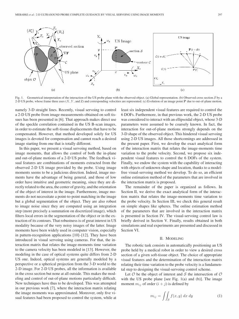
Fig. 1. Geometrical interpretation of the interaction of the US probe plane with the observed object. (a) Global representation. (b) Observed cross section S by a2-D US probe, whose frame three axes (X , Y , and Z) and corresponding velocities are represented. (c) Evolution of an image point P due to out-of-plane motion.
namely 3-D straight lines. Recently, visual servoing to controla 2-D US probe from image measurements obtained on soft tis-sues has been presented in [6]. That approach makes direct useof the speckle correlation contained in the US B-scan images,in order to estimate the soft-tissue displacements that have to becompensated. However, that method developed solely for USimages is devoted for compensation and cannot reach a desiredimage starting from one that is totally different.
In this paper, we present a visual servoing method, based onimage moments, that allows the control of both the in-planeand out-of-plane motions of a 2-D US probe. The feedback vi-sual features are combinations of moments extracted from theobserved 2-D US image provided by the probe. Using imagemoments seems to be a judicious direction. Indeed, image mo-ments have the advantage of being general, and those of loworder have intuitive and geometric meaning, since they are di-rectly related to the area, the center of gravity, and the orientationof the object of interest in the image. Furthermore, image mo-ments do not necessitate a point-to-point matching in the imagebut a global segmentation of the object. They are also robustto image noise since they are computed using an integrationstep (more precisely a summation on discretized image), whichfilters local errors in the segmentation of the object or in the ex-traction of its contours. That robustness is of great interest in USmodality because of the very noisy images of the latter. Imagemoments have been widely used in computer vision, especiallyin pattern-recognition applications [10]–[12]. They have beenintroduced in visual servoing using cameras. For that, the in-teraction matrix that relates the image-moments time variationto the camera velocity has been modeled in [13]. However, themodeling in the case of optical systems quite differs from 2-DUS one. Indeed, optical systems are generally modeled by aperspective or a spherical projection from the 3-D world to the2-D image. For 2-D US probes, all the information is availablein the cross section but none at all outside. This makes the mod-eling and control of out-of-plane motions particularly difficult.New techniques have thus to be developed. This was attemptedin our previous work [7], where the interaction matrix relatingthe image moments was approximated. Moreover, only five vi-sual features had been proposed to control the system, while at
least six independent visual features are required to control the6 DOFs. Furthermore, in that previous work, the 2-D US probewas considered to interact with an ellipsoidal object, whose 3-Dparameters were assumed to be coarsely known. In fact, theinteraction for out-of-plane motions strongly depends on the3-D shape of the observed object. This hindered visual servoingusing 2-D US images. All those shortcomings are addressed inthe present paper. First, we develop the exact analytical formof the interaction matrix that relates the image-moments timevariation to the probe velocity. Second, we propose six inde-pendent visual features to control the 6 DOFs of the system.Finally, we endow the system with the capability of interactingwith objects of unknown shape and location, thanks to a model-free visual-servoing method we develop. To do so, an efficientonline estimation method of the parameters that are involved inthe interaction matrix is proposed.
The remainder of the paper is organized as follows. InSection II, we derive the exact analytical form of the interac-tion matrix that relates the image-moments time variation tothe probe velocity. In Section III, we check this general resulton simple shapes like spheres. The online estimation methodof the parameters that are involved in the interaction matrixis presented in Section IV. The visual-servoing control law isbriefly derived in Section V. Finally, results obtained in bothsimulations and real experiments are presented and discussed inSection VI.
II. MODELING
The robotic task consists in automatically positioning an USprobe held by a medical robot in order to view a desired crosssection of a given soft-tissue object. The choice of appropriatevisual features and the determination of the interaction matrixrelating their time variation to the probe velocity is a fundamen-tal step to designing the visual-servoing control scheme.
Let O be the object of interest and S the intersection of Owith the US probe plane [see Fig. 1(a) and (b)]. The imagemoment mij of order (i + j) is defined by
mij =∫ ∫
Sf(x, y) dx dy (1)
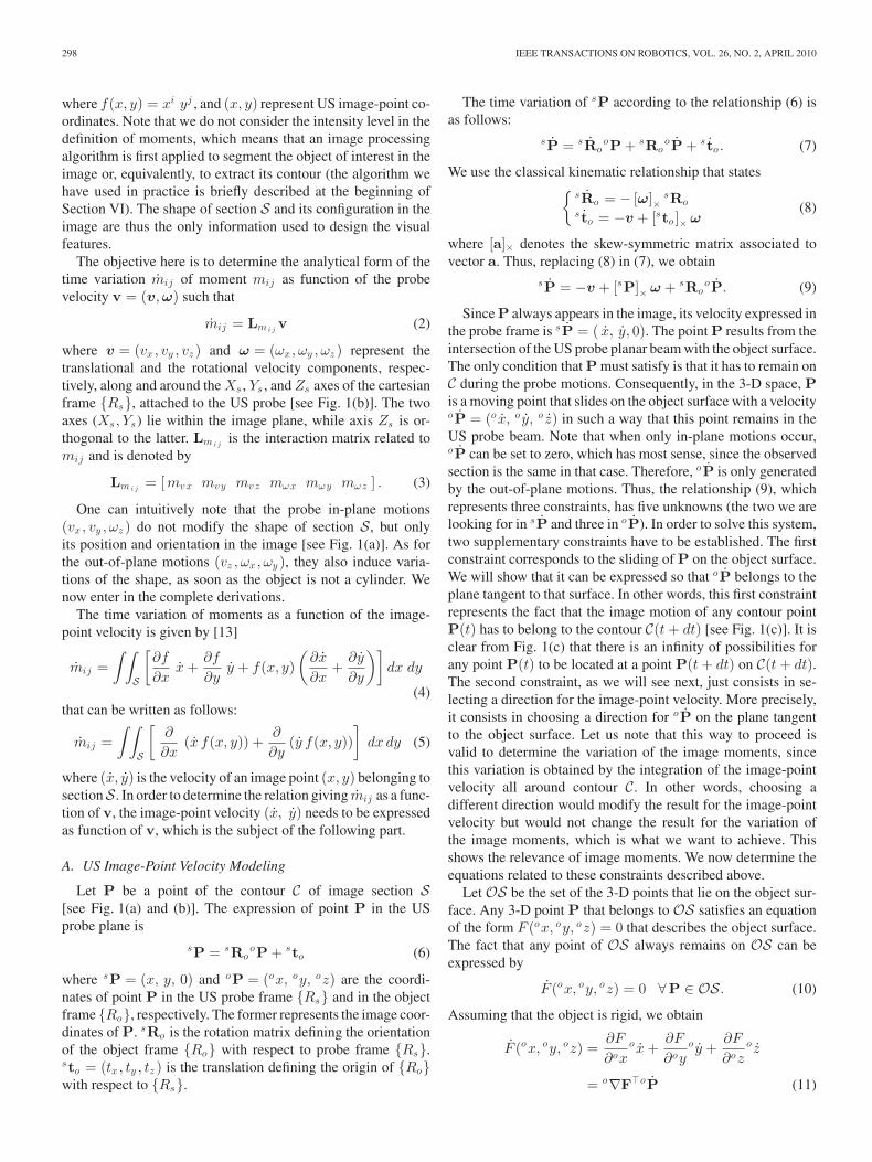
298 IEEE TRANSACTIONS ON ROBOTICS, VOL. 26, NO. 2, APRIL 2010
where f(x, y) = xi yj , and (x, y) represent US image-point co-ordinates. Note that we do not consider the intensity level in thedefinition of moments, which means that an image processingalgorithm is first applied to segment the object of interest in theimage or, equivalently, to extract its contour (the algorithm wehave used in practice is briefly described at the beginning ofSection VI). The shape of section S and its configuration in theimage are thus the only information used to design the visualfeatures.
The objective here is to determine the analytical form of thetime variation mij of moment mij as function of the probevelocity v = (v,ω) such that
mij = Lmi jv (2)
where v = (vx, vy , vz ) and ω = (ωx, ωy , ωz ) represent thetranslational and the rotational velocity components, respec-tively, along and around the Xs , Ys , and Zs axes of the cartesianframe {Rs}, attached to the US probe [see Fig. 1(b)]. The twoaxes (Xs, Ys) lie within the image plane, while axis Zs is or-thogonal to the latter. Lmi j
is the interaction matrix related tomij and is denoted by
Lmi j= [mvx mvy mvz mωx mωy mωz ] . (3)
One can intuitively note that the probe in-plane motions(vx, vy , ωz ) do not modify the shape of section S, but onlyits position and orientation in the image [see Fig. 1(a)]. As forthe out-of-plane motions (vz , ωx, ωy ), they also induce varia-tions of the shape, as soon as the object is not a cylinder. Wenow enter in the complete derivations.
The time variation of moments as a function of the image-point velocity is given by [13]
mij =∫ ∫
S
[∂f
∂xx +
∂f
∂yy + f(x, y)
(∂x
∂x+
∂y
∂y
)]dx dy
(4)that can be written as follows:
mij =∫ ∫
S
[∂
∂x(x f(x, y)) +
∂
∂y(y f(x, y))
]dx dy (5)
where (x, y) is the velocity of an image point (x, y) belonging tosectionS. In order to determine the relation giving mij as a func-tion of v, the image-point velocity (x, y) needs to be expressedas function of v, which is the subject of the following part.
A. US Image-Point Velocity Modeling
Let P be a point of the contour C of image section S[see Fig. 1(a) and (b)]. The expression of point P in the USprobe plane is
sP = sRooP + sto (6)
where sP = (x, y, 0) and oP = (ox, oy, oz) are the coordi-nates of point P in the US probe frame {Rs} and in the objectframe {Ro}, respectively. The former represents the image coor-dinates of P. sRo is the rotation matrix defining the orientationof the object frame {Ro} with respect to probe frame {Rs}.sto = (tx , ty , tz ) is the translation defining the origin of {Ro}with respect to {Rs}.
The time variation of sP according to the relationship (6) isas follows:
sP = sRooP + sRo
oP + s to . (7)
We use the classical kinematic relationship that states{sRo = − [ω]×
sRos to = −v + [sto ]× ω
(8)
where [a]× denotes the skew-symmetric matrix associated tovector a. Thus, replacing (8) in (7), we obtain
sP = −v + [sP]× ω + sRooP. (9)
Since P always appears in the image, its velocity expressed inthe probe frame is sP = ( x, y, 0). The point P results from theintersection of the US probe planar beam with the object surface.The only condition that P must satisfy is that it has to remain onC during the probe motions. Consequently, in the 3-D space, Pis a moving point that slides on the object surface with a velocityoP = (o x, o y, o z) in such a way that this point remains in theUS probe beam. Note that when only in-plane motions occur,oP can be set to zero, which has most sense, since the observedsection is the same in that case. Therefore, oP is only generatedby the out-of-plane motions. Thus, the relationship (9), whichrepresents three constraints, has five unknowns (the two we arelooking for in sP and three in oP). In order to solve this system,two supplementary constraints have to be established. The firstconstraint corresponds to the sliding of P on the object surface.We will show that it can be expressed so that oP belongs to theplane tangent to that surface. In other words, this first constraintrepresents the fact that the image motion of any contour pointP(t) has to belong to the contour C(t + dt) [see Fig. 1(c)]. It isclear from Fig. 1(c) that there is an infinity of possibilities forany point P(t) to be located at a point P(t + dt) on C(t + dt).The second constraint, as we will see next, just consists in se-lecting a direction for the image-point velocity. More precisely,it consists in choosing a direction for oP on the plane tangentto the object surface. Let us note that this way to proceed isvalid to determine the variation of the image moments, sincethis variation is obtained by the integration of the image-pointvelocity all around contour C. In other words, choosing adifferent direction would modify the result for the image-pointvelocity but would not change the result for the variation ofthe image moments, which is what we want to achieve. Thisshows the relevance of image moments. We now determine theequations related to these constraints described above.
Let OS be the set of the 3-D points that lie on the object sur-face. Any 3-D point P that belongs to OS satisfies an equationof the form F (ox, oy, oz) = 0 that describes the object surface.The fact that any point of OS always remains on OS can beexpressed by
F (ox, oy, oz) = 0 ∀P ∈ OS. (10)
Assuming that the object is rigid, we obtain
F (ox, oy, oz) =∂F
∂oxox +
∂F
∂oyo y +
∂F
∂ozo z
= o∇F�oP (11)
MEBARKI et al.: 2-D ULTRASOUND PROBE COMPLETE GUIDANCE BY VISUAL SERVOING USING IMAGE MOMENTS 299
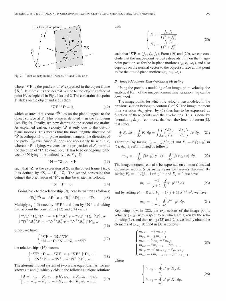
Fig. 2. Point velocity in the 3-D space. o P and N lie on π .
where o∇F is the gradient of F expressed in the object frame{Ro}. It represents the normal vector to the object surface atpoint P, as depicted in Figs. 1(a) and 2. The constraint that pointP slides on the object surface is then
o∇F� oP = 0, (12)
which ensures that vector oP lies on the plane tangent to theobject surface at P. This plane is denoted π in the following(see Fig. 2). Finally, we now determine the second constraint.As explained earlier, velocity oP is only due to the out-of-plane motions. This means that the most tangible direction ofoP is orthogonal to in-plane motions, namely, the direction ofthe probe Zs-axis. Since Zs does not necessarily lie within π,wherein oP is lying, we consider the projection of Zs on π asthe direction of oP. To conclude, oP has to be orthogonal to thevector oN lying on π defined by (see Fig. 2)
oN = oZs × o∇F (13)
such that oZs is the expression of Zs in the object frame {Ro}.It is defined by oZs = sR�
osZs . The second constraint that
defines the orientation of oP can thus be written as follows:oN� oP = 0. (14)
Going back to the relationship (9), it can be written as follows:sR�
osP = −sR�
o v + sR�o [sP]× ω + oP. (15)
Multiplying (15) once by o∇F� and then by oN� and takinginto account the constraints (12) and (14) yields{
o∇F�sR�o
sP = −o∇F�sR�o v + o∇F�sR�
o [sP]× ωoN�sR�
osP = −oN�sR�
o v + oN�sR�o [sP]× ω.
(16)Since, we have{
s∇F = sRoo∇F
sN = sRooN = sZs × s∇F
(17)
the relationships (16) become{s∇F�sP = −s∇F� v + s∇F� [sP]× ω
sN�sP = −sN� v + sN� [sP]× ω.(18)
The aforementioned system of two scalar equations has two un-knowns x and y, which yields to the following unique solution:{
x = −vx − Kx vz − y Kx ωx + xKx ωy + y ωz
y = −vy − Ky vz − y Ky ωx + xKy ωy − xωz(19)
with
Kx =fx fz(
f 2x + f 2
y
)Ky =
fy fz(f 2
x + f 2y
) (20)
such that s∇F = (fx, fy , fz ). From (19) and (20), we can con-clude that the image-point velocity depends only on the image-point position, as for the in-plane motions (vx , vy , ωz ), and alsodepends on the normal vector to the object surface at that pointas for the out-of-plane motions (vz , ωx , ωy ).
B. Image-Moments Time-Variation Modeling
Using the previous modeling of an image-point velocity, theanalytical form of the image-moment time variation mij can bedeveloped.
The image points for which the velocity was modeled in theprevious section belong to contour C of S. The image-momenttime variation mij given by (5) thus has to be expressed asfunction of these points and their velocities. This is done byformulating mij on contour C, thanks to the Green’s theorem [8],that states∮
CFx dx +
∮CFy dy =
∫ ∫S
(∂Fy
∂x− ∂Fx
∂y
)dx dy. (21)
Therefore, by taking Fx = −y f(x, y) and Fy = x f(x, y) in(5), mij is reformulated as follows:
mij = −∮C[f(x, y) y] dx +
∮C[f(x, y) x] dy. (22)
The image moments can also be expressed on contour C insteadon image section S by using again the Green’s theorem. Bysetting Fx = −1/(j + 1)xi yj+1 and Fy = 0, we have
mij =−1
j + 1
∮Cxi yj+1 dx (23)
and by setting Fx = 0 and Fy = 1/(i + 1) xi+1 yj , we have
mij =1
i + 1
∮Cxi+1 yj dy. (24)
Replacing now, in (22), the expressions of the image-pointsvelocity (x, y) with respect to v, which are given by the rela-tionship (19), and then using (23) and (24), we finally obtain theelements of Lmi j
defined in (3) as follows:
mvx = −imi−1,j
mvy = −j mi,j−1mvz = xmij − ymij
mωx = xmi,j+1 − ymi,j+1mωy = −xmi+1,j + ymi+1,j
mωz = imi−1,j+1 − j mi+1,j−1
(25)
where
xmij =∮Cxi yj Ky dx
ymij =∮Cxi yj Kx dy.
(26)
300 IEEE TRANSACTIONS ON ROBOTICS, VOL. 26, NO. 2, APRIL 2010
Similar to the image-point velocity, we can note that the termscorresponding to the in-plane motions (vx , vy , ωz ) only dependon the measurements in the image, while the terms correspond-ing to the out-of-plane motions (vz , ωx , ωy ) also require theknowledge of the normal vector to the object surface for eachpoint of the observed contour.
III. INTERPRETATION FOR SIMPLE SHAPES
In this section, we analytically verify the validity of the gen-eral modeling step on spheres. The case of cylindrical objects isanalyzed in [17].
A. Image-Point Velocity
The 3-D points lying on the object surface satisfy the follow-ing relationship:
F (ox, oy, oz) =(
ox
R
)2
+(
oy
R
)2
+(
oz
R
)2
− 1 = 0 (27)
where R is the radius of the sphere. The gradient vector o∇F isthus obtained by o∇F = 2/R2 (ox, oy, oz)� = 2/R2 oP.
The point oP is expressed as function of its coordinates inthe US image using (6)
oP = sR�o (sP − sto) . (28)
Substituting (28) into the expression of o∇F, which was givenearlier, we obtain the normal vector as function of the image-point coordinates
o∇F =2
R2sR�
o (sP − sto) (29)
that we express in the probe frame
s∇F =2
R2sRo
sR�o (sP − sto)
=2
R2 (sP − sto) . (30)
Remembering the expression of sP and sto given inSection II-A, we obtain
s∇F =2
R2 (x − tx , y − ty ,−tz )� . (31)
The coefficients Kx and Ky , which are involved in the image-point velocity (19), are calculated according to the relation (20)as follows:
Kx =
−tz (x − tx)(x − tx)2 + (y − ty )2
Ky =−tz (y − ty )
(x − tx)2 + (y − ty )2 .(32)
We can note that the US image-point velocity does not dependon the rotation matrix sRo between the object frame and theprobe frame. This can be explained by the fact that a sphere hasno orientation in the 3-D space.
We now write the coefficients Kx and Ky in a more compactform. The constraint (27) is formulated as follows:
F (ox, oy, oz) =1
R2oP�oP − 1 = 0. (33)
Replacing oP given by (28) in (33), we have
(sP − sto)� (sP − sto) − R2 = 0. (34)
Then, remembering the expressions of sP and sto given inSection II-A yields
(x − tx)2 + (y − ty )2 + t2z − R2 = 0 (35)
that represents the equation of a circle of center (tx , ty ) andof radius ρ =
√R2 − t2z . Thus, the area of the image section is
a = πρ2 = π (R2 − t2z ). Replacing (35) in (32), the coefficientsKx and Ky are finally obtained as follows:
Kx =
−π tz (x − tx)a
Ky =−π tz (y − ty )
a.
(36)
B. Interaction Matrix
The terms xmij and ymij involved in (25) are calculated bysubstituting (36) in (26), where the moments mij , mi,j−1 , andmi−1,j are identified according to (23) and (24). We obtain
xmij =
πtz [(j + 1)mij − j ty mi,j−1 ]a
ymij =πtz [−(i + 1)mij + i tx mi−1,j ]
a
(37)
which yields
xmij − ymij =π tz
a[k mij − itx mi−1,j − jty mi,j−1 ] (38)
with k = i + j + 2. We can note that the image-moment timevariation, in the case of a sphere-shaped object, depends only onthe image moments and the position of the sphere center withrespect to {Rs}.
Since the intersection of a plane with a sphere is a circle[given by (35)], we can define only three independent featuresfrom the image. The simplest choice is obviously the area a ofthe circle S, and the coordinates (xg , yg ) of its center of gravity.They are defined in terms of the image moments as follows:
a = m00
xg =m10
m00
yg =m01
m00.
(39)
The interaction matrices of these features are derived by replac-ing (38) in (25). We obtain after some developments
La = 2π tz [ 0 0 1 yg −xg 0 ]
Lxg= [−1 0 0 0 −tz yg ]
Lyg= [ 0 −1 0 tz 0 −xg ]. (40)
As expected, the area a does not vary with the in-plane mo-tions. Also, the coordinates (xg , yg ) of the center of gravity donot change in response to translational motion in the direction ofthe probe z-axis. Finally, we can note that when tz = 0, all thecoefficients, of the aforementioned interaction matrices, whichare involved in the probe out-of-plane motions (vz , ωx , ωy ),are equal to zero. This can be explained by the fact that, when
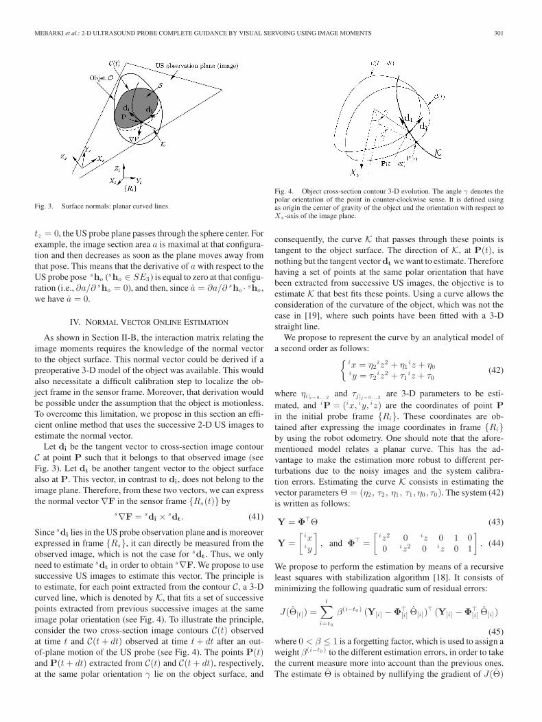
MEBARKI et al.: 2-D ULTRASOUND PROBE COMPLETE GUIDANCE BY VISUAL SERVOING USING IMAGE MOMENTS 301
Fig. 3. Surface normals: planar curved lines.
tz = 0, the US probe plane passes through the sphere center. Forexample, the image section area a is maximal at that configura-tion and then decreases as soon as the plane moves away fromthat pose. This means that the derivative of a with respect to theUS probe pose sho (sho ∈ SE3) is equal to zero at that configu-ration (i.e., ∂a/∂ sho = 0), and then, since a = ∂a/∂ sho · ˙sho ,we have a = 0.
IV. NORMAL VECTOR ONLINE ESTIMATION
As shown in Section II-B, the interaction matrix relating theimage moments requires the knowledge of the normal vectorto the object surface. This normal vector could be derived if apreoperative 3-D model of the object was available. This wouldalso necessitate a difficult calibration step to localize the ob-ject frame in the sensor frame. Moreover, that derivation wouldbe possible under the assumption that the object is motionless.To overcome this limitation, we propose in this section an effi-cient online method that uses the successive 2-D US images toestimate the normal vector.
Let di be the tangent vector to cross-section image contourC at point P such that it belongs to that observed image (seeFig. 3). Let dt be another tangent vector to the object surfacealso at P. This vector, in contrast to di , does not belong to theimage plane. Therefore, from these two vectors, we can expressthe normal vector ∇F in the sensor frame {Rs(t)} by
s∇F = sdi × sdt . (41)
Since sdi lies in the US probe observation plane and is moreoverexpressed in frame {Rs}, it can directly be measured from theobserved image, which is not the case for sdt . Thus, we onlyneed to estimate sdt in order to obtain s∇F. We propose to usesuccessive US images to estimate this vector. The principle isto estimate, for each point extracted from the contour C, a 3-Dcurved line, which is denoted by K, that fits a set of successivepoints extracted from previous successive images at the sameimage polar orientation (see Fig. 4). To illustrate the principle,consider the two cross-section image contours C(t) observedat time t and C(t + dt) observed at time t + dt after an out-of-plane motion of the US probe (see Fig. 4). The points P(t)and P(t + dt) extracted from C(t) and C(t + dt), respectively,at the same polar orientation γ lie on the object surface, and
Fig. 4. Object cross-section contour 3-D evolution. The angle γ denotes thepolar orientation of the point in counter-clockwise sense. It is defined usingas origin the center of gravity of the object and the orientation with respect toXs -axis of the image plane.
consequently, the curve K that passes through these points istangent to the object surface. The direction of K, at P(t), isnothing but the tangent vector dt we want to estimate. Thereforehaving a set of points at the same polar orientation that havebeen extracted from successive US images, the objective is toestimate K that best fits these points. Using a curve allows theconsideration of the curvature of the object, which was not thecase in [19], where such points have been fitted with a 3-Dstraight line.
We propose to represent the curve by an analytical model ofa second order as follows:{
ix = η2iz2 + η1
iz + η0iy = τ2
iz2 + τ1iz + τ0
(42)
where ηi|i = 0 . . . 2 and τj |j = 0 . . . 2 are 3-D parameters to be esti-mated, and iP = (ix, iy, iz) are the coordinates of point Pin the initial probe frame {Ri}. These coordinates are ob-tained after expressing the image coordinates in frame {Ri}by using the robot odometry. One should note that the afore-mentioned model relates a planar curve. This has the ad-vantage to make the estimation more robust to different per-turbations due to the noisy images and the system calibra-tion errors. Estimating the curve K consists in estimating thevector parameters Θ = (η2 , τ2 , η1 , τ1 , η0 , τ0). The system (42)is written as follows:
Y = Φ�Θ (43)
Y =[
ixiy
], and Φ� =
[iz2 0 iz 0 1 00 iz2 0 iz 0 1
]. (44)
We propose to perform the estimation by means of a recursiveleast squares with stabilization algorithm [18]. It consists ofminimizing the following quadratic sum of residual errors:
J(Θ[t]) =t∑
i=t0
β(i−t0 ) (Y[i] − Φ�[i] Θ[i])� (Y[i] − Φ�
[i] Θ[i])
(45)where 0 < β ≤ 1 is a forgetting factor, which is used to assign aweight β(i−t0 ) to the different estimation errors, in order to takethe current measure more into account than the previous ones.The estimate Θ is obtained by nullifying the gradient of J(Θ)
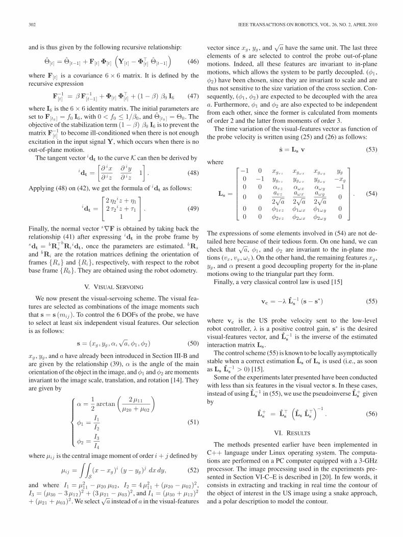
302 IEEE TRANSACTIONS ON ROBOTICS, VOL. 26, NO. 2, APRIL 2010
and is thus given by the following recursive relationship:
Θ[t] = Θ[t−1] + F[t] Φ[t]
(Y[t] − Φ�
[t] Θ[t−1]
)(46)
where F[t] is a covariance 6 × 6 matrix. It is defined by therecursive expression
F−1[t] = β F−1
[t−1] + Φ[t] Φ�[t] + (1 − β) β0 I6 (47)
where I6 is the 6 × 6 identity matrix. The initial parameters areset to F[t0 ] = f0 I6 , with 0 < f0 ≤ 1/β0 , and Θ[t0 ] = Θ0 . Theobjective of the stabilization term (1 − β) β0 I6 is to prevent thematrix F−1
[t] to become ill-conditioned when there is not enoughexcitation in the input signal Y, which occurs when there is noout-of-plane motion.
The tangent vector idt to the curve K can then be derived by
idt =[∂ ix
∂ iz
∂ iy
∂ iz1]
. (48)
Applying (48) on (42), we get the formula of idt as follows:
idt =
2 η2
iz + η12 τ2
iz + τ11
. (49)
Finally, the normal vector s∇F is obtained by taking back therelationship (41) after expressing idt in the probe frame bysdt = bR�
sbRi
idt , once the parameters are estimated. bRs
and bRi are the rotation matrices defining the orientation offrames {Rs} and {Ri}, respectively, with respect to the robotbase frame {Rb}. They are obtained using the robot odometry.
V. VISUAL SERVOING
We now present the visual-servoing scheme. The visual fea-tures are selected as combinations of the image moments suchthat s = s (mij ). To control the 6 DOFs of the probe, we haveto select at least six independent visual features. Our selectionis as follows:
s = (xg , yg , α,√
a, φ1 , φ2) (50)
xg , yg , and a have already been introduced in Section III-B andare given by the relationship (39), α is the angle of the mainorientation of the object in the image, and φ1 and φ2 are momentsinvariant to the image scale, translation, and rotation [14]. Theyare given by
α =12
arctan(
2µ11
µ20 + µ02
)
φ1 =I1
I2
φ2 =I3
I4
(51)
where µij is the central image moment of order i + j defined by
µij =∫ ∫
S(x − xg )i (y − yg )j dx dy, (52)
and where I1 = µ211 − µ20 µ02 , I2 = 4µ2
11 + (µ20 − µ02)2 ,I3 = (µ30 − 3µ12)2 + (3µ21 − µ03)2 , and I4 = (µ30 + µ12)2
+ (µ21 + µ03)2 . We select√
a instead of a in the visual-features
vector since xg , yg , and√
a have the same unit. The last threeelements of s are selected to control the probe out-of-planemotions. Indeed, all these features are invariant to in-planemotions, which allows the system to be partly decoupled. (φ1 ,φ2) have been chosen, since they are invariant to scale and arethus not sensitive to the size variation of the cross section. Con-sequently, (φ1 , φ2) are expected to be decoupled with the areaa. Furthermore, φ1 and φ2 are also expected to be independentfrom each other, since the former is calculated from momentsof order 2 and the latter from moments of order 3.
The time variation of the visual-features vector as function ofthe probe velocity is written using (25) and (26) as follows:
s = Ls v (53)
where
Ls =
−1 0 xgv zxgω x
xgω yyg
0 −1 ygv zygω x
ygω y−xg
0 0 αvz αωx αωy −10 0
avz
2√
a
aωx
2√
a
aωy
2√
a0
0 0 φ1vz φ1ωx φ1ωy 00 0 φ2vz φ2ωx φ2ωy 0
. (54)
The expressions of some elements involved in (54) are not de-tailed here because of their tedious form. On one hand, we cancheck that
√a, φ1 , and φ2 are invariant to the in-plane mo-
tions (vx , vy , ωz ). On the other hand, the remaining features xg ,yg , and α present a good decoupling property for the in-planemotions owing to the triangular part they form.
Finally, a very classical control law is used [15]
vc = −λ L−1s (s − s∗) (55)
where vc is the US probe velocity sent to the low-levelrobot controller, λ is a positive control gain, s∗ is the desiredvisual-features vector, and L−1
s is the inverse of the estimatedinteraction matrix Ls .
The control scheme (55) is known to be locally asymptoticallystable when a correct estimation Ls of Ls is used (i.e., as soonas Ls L−1
s > 0) [15].Some of the experiments later presented have been conducted
with less than six features in the visual vector s. In these cases,instead of using L−1
s in (55), we use the pseudoinverse L+s given
by
L+s = L�
s
(Ls L�
s
)−1. (56)
VI. RESULTS
The methods presented earlier have been implemented inC++ language under Linux operating system. The computa-tions are performed on a PC computer equipped with a 3-GHzprocessor. The image processing used in the experiments pre-sented in Section VI-C–E is described in [20]. In few words, itconsists in extracting and tracking in real time the contour ofthe object of interest in the US image using a snake approach,and a polar description to model the contour.
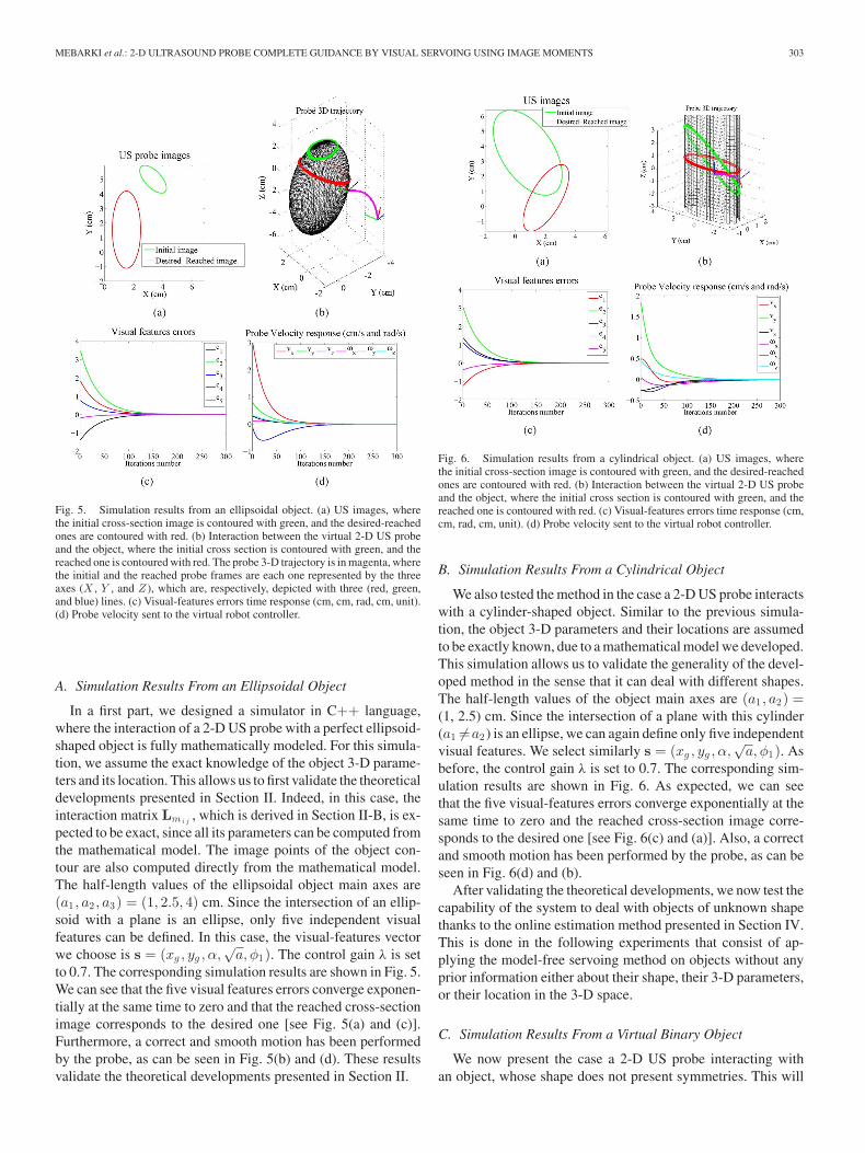
MEBARKI et al.: 2-D ULTRASOUND PROBE COMPLETE GUIDANCE BY VISUAL SERVOING USING IMAGE MOMENTS 303
Fig. 5. Simulation results from an ellipsoidal object. (a) US images, wherethe initial cross-section image is contoured with green, and the desired-reachedones are contoured with red. (b) Interaction between the virtual 2-D US probeand the object, where the initial cross section is contoured with green, and thereached one is contoured with red. The probe 3-D trajectory is in magenta, wherethe initial and the reached probe frames are each one represented by the threeaxes (X , Y , and Z ), which are, respectively, depicted with three (red, green,and blue) lines. (c) Visual-features errors time response (cm, cm, rad, cm, unit).(d) Probe velocity sent to the virtual robot controller.
A. Simulation Results From an Ellipsoidal Object
In a first part, we designed a simulator in C++ language,where the interaction of a 2-D US probe with a perfect ellipsoid-shaped object is fully mathematically modeled. For this simula-tion, we assume the exact knowledge of the object 3-D parame-ters and its location. This allows us to first validate the theoreticaldevelopments presented in Section II. Indeed, in this case, theinteraction matrix Lmi j
, which is derived in Section II-B, is ex-pected to be exact, since all its parameters can be computed fromthe mathematical model. The image points of the object con-tour are also computed directly from the mathematical model.The half-length values of the ellipsoidal object main axes are(a1 , a2 , a3) = (1, 2.5, 4) cm. Since the intersection of an ellip-soid with a plane is an ellipse, only five independent visualfeatures can be defined. In this case, the visual-features vectorwe choose is s = (xg , yg , α,
√a, φ1). The control gain λ is set
to 0.7. The corresponding simulation results are shown in Fig. 5.We can see that the five visual features errors converge exponen-tially at the same time to zero and that the reached cross-sectionimage corresponds to the desired one [see Fig. 5(a) and (c)].Furthermore, a correct and smooth motion has been performedby the probe, as can be seen in Fig. 5(b) and (d). These resultsvalidate the theoretical developments presented in Section II.
Fig. 6. Simulation results from a cylindrical object. (a) US images, wherethe initial cross-section image is contoured with green, and the desired-reachedones are contoured with red. (b) Interaction between the virtual 2-D US probeand the object, where the initial cross section is contoured with green, and thereached one is contoured with red. (c) Visual-features errors time response (cm,cm, rad, cm, unit). (d) Probe velocity sent to the virtual robot controller.
B. Simulation Results From a Cylindrical Object
We also tested the method in the case a 2-D US probe interactswith a cylinder-shaped object. Similar to the previous simula-tion, the object 3-D parameters and their locations are assumedto be exactly known, due to a mathematical model we developed.This simulation allows us to validate the generality of the devel-oped method in the sense that it can deal with different shapes.The half-length values of the object main axes are (a1 , a2) =(1, 2.5) cm. Since the intersection of a plane with this cylinder(a1 �=a2) is an ellipse, we can again define only five independentvisual features. We select similarly s = (xg , yg , α,
√a, φ1). As
before, the control gain λ is set to 0.7. The corresponding sim-ulation results are shown in Fig. 6. As expected, we can seethat the five visual-features errors converge exponentially at thesame time to zero and the reached cross-section image corre-sponds to the desired one [see Fig. 6(c) and (a)]. Also, a correctand smooth motion has been performed by the probe, as can beseen in Fig. 6(d) and (b).
After validating the theoretical developments, we now test thecapability of the system to deal with objects of unknown shapethanks to the online estimation method presented in Section IV.This is done in the following experiments that consist of ap-plying the model-free servoing method on objects without anyprior information either about their shape, their 3-D parameters,or their location in the 3-D space.
C. Simulation Results From a Virtual Binary Object
We now present the case a 2-D US probe interacting withan object, whose shape does not present symmetries. This will
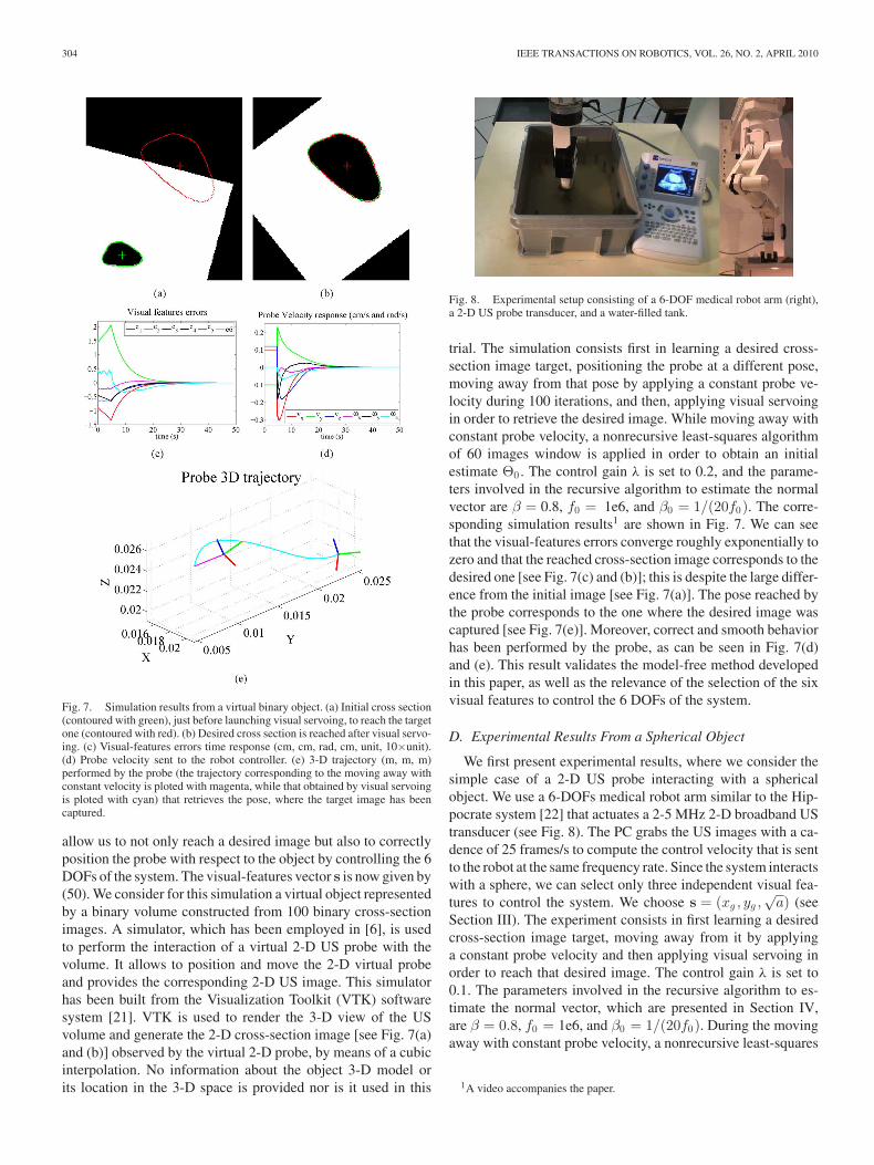
304 IEEE TRANSACTIONS ON ROBOTICS, VOL. 26, NO. 2, APRIL 2010
Fig. 7. Simulation results from a virtual binary object. (a) Initial cross section(contoured with green), just before launching visual servoing, to reach the targetone (contoured with red). (b) Desired cross section is reached after visual servo-ing. (c) Visual-features errors time response (cm, cm, rad, cm, unit, 10×unit).(d) Probe velocity sent to the robot controller. (e) 3-D trajectory (m, m, m)performed by the probe (the trajectory corresponding to the moving away withconstant velocity is ploted with magenta, while that obtained by visual servoingis ploted with cyan) that retrieves the pose, where the target image has beencaptured.
allow us to not only reach a desired image but also to correctlyposition the probe with respect to the object by controlling the 6DOFs of the system. The visual-features vector s is now given by(50). We consider for this simulation a virtual object representedby a binary volume constructed from 100 binary cross-sectionimages. A simulator, which has been employed in [6], is usedto perform the interaction of a virtual 2-D US probe with thevolume. It allows to position and move the 2-D virtual probeand provides the corresponding 2-D US image. This simulatorhas been built from the Visualization Toolkit (VTK) softwaresystem [21]. VTK is used to render the 3-D view of the USvolume and generate the 2-D cross-section image [see Fig. 7(a)and (b)] observed by the virtual 2-D probe, by means of a cubicinterpolation. No information about the object 3-D model orits location in the 3-D space is provided nor is it used in this
Fig. 8. Experimental setup consisting of a 6-DOF medical robot arm (right),a 2-D US probe transducer, and a water-filled tank.
trial. The simulation consists first in learning a desired cross-section image target, positioning the probe at a different pose,moving away from that pose by applying a constant probe ve-locity during 100 iterations, and then, applying visual servoingin order to retrieve the desired image. While moving away withconstant probe velocity, a nonrecursive least-squares algorithmof 60 images window is applied in order to obtain an initialestimate Θ0 . The control gain λ is set to 0.2, and the parame-ters involved in the recursive algorithm to estimate the normalvector are β = 0.8, f0 = 1e6, and β0 = 1/(20f0). The corre-sponding simulation results1 are shown in Fig. 7. We can seethat the visual-features errors converge roughly exponentially tozero and that the reached cross-section image corresponds to thedesired one [see Fig. 7(c) and (b)]; this is despite the large differ-ence from the initial image [see Fig. 7(a)]. The pose reached bythe probe corresponds to the one where the desired image wascaptured [see Fig. 7(e)]. Moreover, correct and smooth behaviorhas been performed by the probe, as can be seen in Fig. 7(d)and (e). This result validates the model-free method developedin this paper, as well as the relevance of the selection of the sixvisual features to control the 6 DOFs of the system.
D. Experimental Results From a Spherical Object
We first present experimental results, where we consider thesimple case of a 2-D US probe interacting with a sphericalobject. We use a 6-DOFs medical robot arm similar to the Hip-pocrate system [22] that actuates a 2-5 MHz 2-D broadband UStransducer (see Fig. 8). The PC grabs the US images with a ca-dence of 25 frames/s to compute the control velocity that is sentto the robot at the same frequency rate. Since the system interactswith a sphere, we can select only three independent visual fea-tures to control the system. We choose s = (xg , yg ,
√a) (see
Section III). The experiment consists in first learning a desiredcross-section image target, moving away from it by applyinga constant probe velocity and then applying visual servoing inorder to reach that desired image. The control gain λ is set to0.1. The parameters involved in the recursive algorithm to es-timate the normal vector, which are presented in Section IV,are β = 0.8, f0 = 1e6, and β0 = 1/(20f0). During the movingaway with constant probe velocity, a nonrecursive least-squares
1A video accompanies the paper.
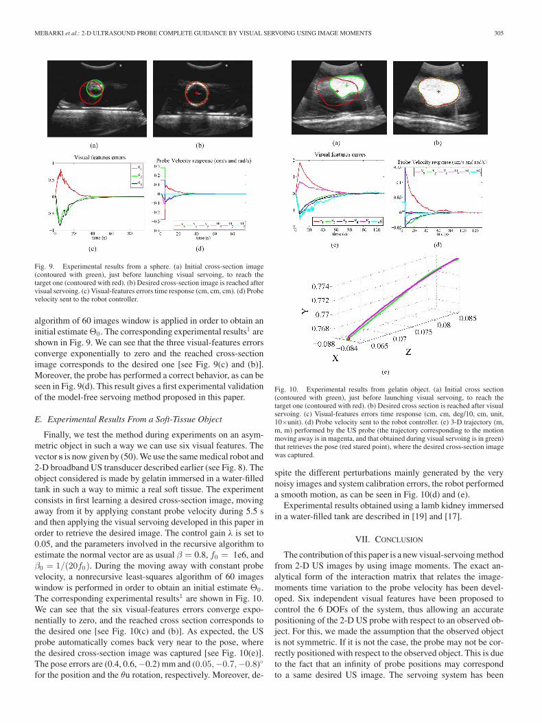
MEBARKI et al.: 2-D ULTRASOUND PROBE COMPLETE GUIDANCE BY VISUAL SERVOING USING IMAGE MOMENTS 305
Fig. 9. Experimental results from a sphere. (a) Initial cross-section image(contoured with green), just before launching visual servoing, to reach thetarget one (contoured with red). (b) Desired cross-section image is reached aftervisual servoing. (c) Visual-features errors time response (cm, cm, cm). (d) Probevelocity sent to the robot controller.
algorithm of 60 images window is applied in order to obtain aninitial estimate Θ0 . The corresponding experimental results1 areshown in Fig. 9. We can see that the three visual-features errorsconverge exponentially to zero and the reached cross-sectionimage corresponds to the desired one [see Fig. 9(c) and (b)].Moreover, the probe has performed a correct behavior, as can beseen in Fig. 9(d). This result gives a first experimental validationof the model-free servoing method proposed in this paper.
E. Experimental Results From a Soft-Tissue Object
Finally, we test the method during experiments on an asym-metric object in such a way we can use six visual features. Thevector s is now given by (50). We use the same medical robot and2-D broadband US transducer described earlier (see Fig. 8). Theobject considered is made by gelatin immersed in a water-filledtank in such a way to mimic a real soft tissue. The experimentconsists in first learning a desired cross-section image, movingaway from it by applying constant probe velocity during 5.5 sand then applying the visual servoing developed in this paper inorder to retrieve the desired image. The control gain λ is set to0.05, and the parameters involved in the recursive algorithm toestimate the normal vector are as usual β = 0.8, f0 = 1e6, andβ0 = 1/(20f0). During the moving away with constant probevelocity, a nonrecursive least-squares algorithm of 60 imageswindow is performed in order to obtain an initial estimate Θ0 .The corresponding experimental results1 are shown in Fig. 10.We can see that the six visual-features errors converge expo-nentially to zero, and the reached cross section corresponds tothe desired one [see Fig. 10(c) and (b)]. As expected, the USprobe automatically comes back very near to the pose, wherethe desired cross-section image was captured [see Fig. 10(e)].The pose errors are (0.4, 0.6, −0.2) mm and (0.05,−0.7,−0.8)◦
for the position and the θu rotation, respectively. Moreover, de-
Fig. 10. Experimental results from gelatin object. (a) Initial cross section(contoured with green), just before launching visual servoing, to reach thetarget one (contoured with red). (b) Desired cross section is reached after visualservoing. (c) Visual-features errors time response (cm, cm, deg/10, cm, unit,10×unit). (d) Probe velocity sent to the robot controller. (e) 3-D trajectory (m,m, m) performed by the US probe (the trajectory corresponding to the motionmoving away is in magenta, and that obtained during visual servoing is in green)that retrieves the pose (red stared point), where the desired cross-section imagewas captured.
spite the different perturbations mainly generated by the verynoisy images and system calibration errors, the robot performeda smooth motion, as can be seen in Fig. 10(d) and (e).
Experimental results obtained using a lamb kidney immersedin a water-filled tank are described in [19] and [17].
VII. CONCLUSION
The contribution of this paper is a new visual-servoing methodfrom 2-D US images by using image moments. The exact an-alytical form of the interaction matrix that relates the image-moments time variation to the probe velocity has been devel-oped. Six independent visual features have been proposed tocontrol the 6 DOFs of the system, thus allowing an accuratepositioning of the 2-D US probe with respect to an observed ob-ject. For this, we made the assumption that the observed objectis not symmetric. If it is not the case, the probe may not be cor-rectly positioned with respect to the observed object. This is dueto the fact that an infinity of probe positions may correspondto a same desired US image. The servoing system has been
306 IEEE TRANSACTIONS ON ROBOTICS, VOL. 26, NO. 2, APRIL 2010
endowed with the capability of automatically interacting withobjects of unknown shapes without any prior knowledge of their3-D parameters nor their 3-D location, by developing a model-free visual-servoing method. For that, we proposed an efficientonline estimation technique of the 3-D parameters involved inthe servo scheme. The results obtained in both simulations andexperiments have shown the validity of the developed methodand its robustness with respect to the noisy images. The methodwe proposed is general in the sense that it can be applied to dif-ferent imaging modalities that, like US, provide full informationin their observation plane, as for instance, MRI and CT-SCAN.The presented model-free visual servoing method is howevercurrently devoted for motionless objects. Considering movingobjects can be technically addressed by using a high sampling-rate frequency in the online estimation algorithm and the visualservoing in such a way that they become insensitive to thesemotions. Nevertheless, if the object moves with a high veloc-ity, the online estimation algorithm may fail. That is the reasonwhy it will be necessary to theoretically improve the model-freeservoing method in the future to take into account such motion.
REFERENCES
[1] P. Abolmaesumi, S. E. Salcudean, W.-H. Zhu, M. R. Sirouspour, andS. P. DiMaio, “Image-guided control of a robot for medical ultrasound,”IEEE Trans. Robot. Autom., vol. 18, no. 1, pp. 11–23, Feb. 2002.
[2] J. Hong, T. Dohi, M. Hashizume, K. Konishi, and N. Hata, “An ulrasound-driven needle insertion robot for percutaneous cholecystostomy,” Phys.Med. Biol., vol. 49, no. 3, pp. 441–445, 2004.
[3] P. M. Novotny, J. A. Stoll, P. E. Dupont, and R. D. Howe, “Real-timevisual servoing of a robot using three-dimensional ultrasound,” in Proc.IEEE Int. Conf. Robot. Autom., Roma, Italy, May 2007, pp. 2655–2660.
[4] M. A. Vitrani, H. Mitterhofer, N. Bonnet, and G. Morel, “Robustultrasound-based visual servoing for beating heart intracardiac surgery,”in Proc. IEEE Int. Conf. Robot. Autom., Roma, Italy, Apr. 2007, pp. 3021–3027.
[5] M. Sauvee, P. Poignet, and E. Dombre, “Ultrasound image-based visualservoing of a surgical instrument through nonlinear model predictive con-trol,” Int. J. Robot. Res., vol. 27, no. 1, pp. 25–40, Jan. 2008.
[6] A. Krupa, G. Fichtinger, and G. D. Hager, “Real-time motion stabiliza-tion with B-mode ultrasound using image speckle information and visualservoing,” Int. J. Robot. Res., vol. 28, no. 10, pp. 1334–1354, 2009.
[7] R. Mebarki, A. Krupa, and F. Chaumette, “Image moments-based ultra-sound visual servoing,” in Proc. IEEE Int. Conf. Robot. Autom., Pasadena,CA, May 2008, pp. 113–119.
[8] J. Stewart, Calculus, 2nd ed. Pacific Grove, CA: Brooks/Cole, 1991.[9] A. G. Mamistvalov, “N-dimensional invariants and conceptual mathemat-
ical theory of recognition n-dimentional solids,” IEEE Trans. PatternAnal. Mach. Intell., vol. 20, no. 8, pp. 819–831, Aug. 1998.
[10] M. K. Hu, “Visual pattern recognition by moment invariants,” IRE Trans.Inf. Theory, vol. 8, pp. 179–187, 1962.
[11] R. Mukundan and K. R. Ramakrishman, Moment Functions in ImageAnalysis: Theory and Application. Singapore: World Scientific, 1998.
[12] R. J. Prokop and A. P. Reeves, “A survey of moment-based techniques forunoccluded object representation and recognition,” Comput. Vis., Graph.,Image Process. Conf., vol. 54, pp. 438–460, Sep. 1992.
[13] F. Chaumette, “Image moments: A general and useful set of features forvisual servoing,” IEEE Trans. Robot., vol. 20, no. 4, pp. 713–723, Aug.2004.
[14] O. Tahri and F. Chaumette, “Point-based and region-based image momentsfor visual servoing of planar objects,” IEEE Trans. Robot., vol. 21, no. 6,pp. 1116–1127, Dec. 2005.
[15] B. Espiau, F. Chaumette, and P. Rives, “A new approach to visual servoingin robotics,” IEEE Trans. Robot. Autom., vol. 8, no. 6, pp. 313–326, Jun.1992.
[16] S. Hutchinson, G. Hager, and P. Corke, “A tutorial on visual servo control,”IEEE Trans. Robot. Autom., vol. 12, no. 5, pp. 651–670, Oct. 1996.
[17] R. Mebarki, “Automatic guidance of robotized 2D ultrasound probes withvisual servoing based on image moments,” Ph.D. dissertation, IRISA,Rennes, Mar. 2010.
[18] G. Kreisselmeier, “Stabilized least-squares type adaptive identifiers,”IEEE Trans. Automat. Control, vol. 35, no. 3, pp. 306–309, Mar. 1990.
[19] R. Mebarki, A. Krupa, and F. Chaumette, “Modeling and 3D local esti-mation for in-plane and out-of-plane motion guidance by 2D ultrasoundvisual servoing,” in Proc. IEEE Int. Conf. Robot. Autom., Kobe, Japan,May 2009, pp. 1206–1212.
[20] C. Collewet, “Polar snakes: A fast and robust parametric active contourmodel,” presented at IEEE Int. Conf. Image Process., Cairo, Egypt, Nov.2009.
[21] W. Schroeder, K. Martin, and B. Lorensen The Visualization Toolkit: AnObject Oriented Approach to 3D Graphics, 4th ed., Kitware, Dec. 1, 2006,ISBN: 193093419X.
[22] F. Pierrot, E. Dombre, E. Degoulange, L. Urbain, P. Caron, S. Boudet,J. Gariepy, and J. Megnien, “Hippocrate: A safe robot arm for medi-cal applications with force feedback,” Med. Image Anal., vol. 3, no. 3,pp. 285–300, 1999.
Rafik Mebarki was born in Algeria in April 1983.He graduated with the Engineer degree in auto-matic control from the National Polytechnic School,Algiers, Algeria, in 2005. He received the M.S. de-gree in automatic systems from Paul Sabatier Uni-versity, Toulouse, France, in 2006. He is currentlyworking toward the Ph.D. degree with the Lagadicteam at IRISA/INRIA, Rennes-Bretagne Atlantique,Rennes, France.
His current research interests include robotics andvisual servoing, especially servoing from ultrasound
images.Mr. Mebarki was a Finalist for the Best Vision Paper Award at the 2008 IEEE
International Conference on Robotics and Automation and the 2008 MedicalImage Computing and Computer-Assisted Intervention Young Scientist Awardsin the Robotics and Interventions category.
Alexandre Krupa received the M.S. and Ph.D. de-grees in control systems and signal processing fromthe National Polytechnic Institute of Lorraine, Nancy,France, in 1999 and 2003, respectively. His Ph.D. re-search work was carried out with the eAVR team(Control Vision and Robotics) with the Laboratoiredes Sciences de l’Image de l’Informatique et de laTeledetection, Strasbourg, France.
From 2002 to 2004, he was an Assistant Asso-ciate Professor for undergraduate student lectures inelectronics, control, and computer programming with
Strasbourg University, Strasbourg, France. Since 2004, he has been a ResearchScientist with INRIA, Rennes, France, where he is currently a Member of theLagadic group. In 2006, he was a Postdoctoral Associate with the Computer-Integrated Surgical Systems and Technology Engineering Research Center,Johns Hopkins University, Baltimore, MD. His current research interests in-clude medical robotics, computer-assisted systems in the medical and surgicalfields, and, most specifically, the control of medical robots by visual servoingusing medical images.
Francois Chaumette received the M.Sc. degree fromEcole Nationale Superieure de Mecanique, Nantes,France, in 1987, and the Ph.D. degree in computer sci-ence from the University of Rennes, Rennes, France,in 1990.
Since 1990, he has been with INRIA, Rennes,where he is currently “Directeur de Recherches” andHead of the Lagadic group. He is currently on the Ed-itorial Board of the International Journal of RoboticsResearch. His research interests include robotics andcomputer vision, especially visual servoing and active
perception.Dr. Chaumette was an Associate Editor of the IEEE TRANSACTIONS ON
ROBOTICS from 2001 to 2005. He was the recipient of the AFCET/CNRS Prizefor the best French thesis in automatic control in 1991 and the 2002 King-SunFu Memorial Best IEEE TRANSACTIONS ON ROBOTICS AND AUTOMATION PaperAward.

Alexandre KrupaIRISA,INRIA Rennes-Bretagne Atlantique,Lagadic,F-35042 Rennes,[email protected]
Gabor FichtingerSchool of Computing,Queen’s University,Kingston, ON,[email protected] Research Center,Johns Hopkins University,Baltimore, MD 21218,USA
Gregory D. HagerEngineering Research Center,Johns Hopkins University,Baltimore, MD 21218,[email protected]
Real-time MotionStabilization withB-mode UltrasoundUsing Image SpeckleInformation and VisualServoing
Abstract
We develop visual servo control to stabilize the image of moving softtissue in B-mode ultrasound (US) imaging. We define the target regionin a B-mode US image, and automatically control a robot to manip-ulate an US probe by minimizing the difference between the targetand the most recently acquired US image. We exploit tissue speckleinformation to compute the relative pose between the probe and thetarget region. In-plane motion is handled by image region trackingand out-of-plane motion recovered by speckle tracking using speckledecorrelation. A visual servo control scheme is then applied to manip-ulate the US probe to stabilize the target region in the live US image.In a first experiment involving only translational motion, an US phan-tom was moved by one robot while stabilizing the target with a secondrobot holding the US probe. In a second experiment, large six-degree-
The International Journal of Robotics ResearchVol. 28, No. 10, October 2009, pp. 1334–1354DOI: 10.1177/0278364909104066c! The Author(s), 2009. Reprints and permissions:http://www.sagepub.co.uk/journalsPermissions.nav
of-freedom (DOF) motions were manually applied to an US phan-tom while a six-DOF medical robot was controlled automatically tocompensate for the probe displacement. The obtained results supportthe hypothesis that automated motion stabilization shows promise fora variety of US-guided medical procedures such as prostate cancerbrachytherapy.
KEY WORDS—medical robotics, ultrasound, speckle corre-lation, visual servoing, motion compensation
1. Introduction
Quantitative ultrasound (US) guidance has great potential insupporting a wide range of diagnostic procedures and mini-mally invasive interventions. However, one of the barriers towider application is the challenge of locating and maintainingtargets of interest within the US scan-plane, particularly whenthe underlying tissue is in motion. Conventional wisdom mightsuggest that this problem could be effectively solved by apply-ing known motion tracking techniques to 3D US images. How-ever, current 3D US systems are prohibitively expensive, suffer
1334
at INRIA RENNES on September 18, 2012ijr.sagepub.comDownloaded from
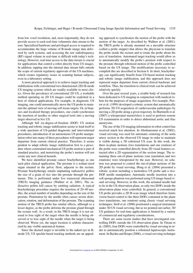
Krupa, Fichtinger, and Hager / B-mode Ultrasound Using Image Speckle Information and Visual Servoing 1335
from low voxel resolution, and, most importantly, they do notprovide access to each real-time volumetric data stream to theuser. Specialized hardware and privileged access is required toaccommodate the huge volume of B-mode image data deliv-ered by such systems, and accessing the raw radiofrequency(RF) signal volume in real-time is difficult with today’s tech-nology. However, real-time access to the data stream is crucialfor applications that control a robot directly from US images.In addition, tapping into the internal data stream falls outsidethe scope of current regulatory approvals of the US machines,which creates regulatory issues in scanning human subjects,even in a laboratory setting.
A more practical approach is to achieve target tracking andstabilization with conventional two-dimensional (2D) B-modeUS imaging systems which are readily available in most clin-ics. Given the prevalence of conventional 2D US, a workablemethod operating on 2D US images could be exploited in ahost of clinical applications. For example, in diagnostic USimaging, one could automatically move the US probe to main-tain the optimal view of moving soft tissue targets. Or, in biop-sies and localized therapy procedures, one could synchronizethe insertion of needles or other surgical tools into a movingtarget observed in live US.
Although full six-degree-of-freedom (DOF) US motiontracking and robotic image stabilization seems to lend itself toa wide spectrum of US-guided diagnostic and interventionalprocedures, introduction of an autonomous US probe manipu-lation robot into many of these procedures will represent majordeparture from current clinical practice. Therefore, it seemsprudent to adapt robotic image stabilization first to a proce-dure where constrained mechanical US probe motion is part ofstandard practice, and motorizing the probe’s motion will notcreate any new clinical hazards.
We have identified prostate cancer brachytherapy as onesuch pilot clinical application. The prostate is a walnut-sizedorgan situated in the pelvic floor, adjacent to the rectum.Prostate brachytherapy entails implanting radioactive pelletsthe size of a grain of rice into the prostate through the per-ineum. This is performed under live transrectal ultrasound(TRUS) imaging guidance (Wallner et al. 2001). The ra-dioactive pellets kill cancer by emitting radiation. A typicalbrachytherapy procedure requires the insertion of 20–40 nee-dles, the actual number of needles depending on the size of theprostate. Penetration by the needle often causes severe dislo-cation, rotation, and deformation of the prostate. The scanningmotion of the TRUS probe has similar effects, although to alesser degree, as the probe deforms the prostate gland throughthe rectum wall. As a result, in the TRUS image it is not un-usual to lose sight of the target when the needle is being ob-served or to lose sight of the needle when the target is beingobserved. Worse yet, the target location is seldom character-ized by any visible anatomical feature.
Since the desired target is invisible to the naked eye in B-mode US, US speckle-based tracking methods are an appeal-
ing approach to synchronize the motion of the probe with themotion of the target. As described by Wallner et al. (2001),the TRUS probe is already mounted on a movable structure(called a probe stepper) that allows the physician to translatethe probe inside the rectum and to rotate the probe about theaxis of translation. Automated target tracking would allow usto automatically modify the probe’s position with respect tothe prostate through robotized motion of the probe controlledbased on the US image. The modifications necessary to ac-complish this are described in Section 6. In short, brachyther-apy can significantly benefit from US-based motion trackingand robotic image stabilization, and this approach does notrepresent major departure from current clinical hardware andworkflow. Thus, the transition to clinical trials can be achievedrelatively quickly.
Over the past several years, a sizable body of research hasbeen dedicated to US imaging in conjunction with medical ro-bots for the purposes of image acquisition. For example, Pier-rot et al. (1999) developed a robotic system that automaticallyperforms 3D US acquisition of cardiovascular pathologies bymoving a 2D probe along a given trajectory. In Martinelli et al.(2007) a teleoperated master/slave is used to perform remoteUS examination in order to detect abdominal aortic and iliacaneurysms.
The use of the US imaging information in robot control hasreceived much less attention. In Abolmaesumi et al. (2002),visual servoing was used for automatic centering of the aortaartery section in the observed US image in order to maintainit visible during a 3D robotized US scan. In this work, thethree in-plane motions (two translations and one rotation) ofthe probe were controlled directly from 2D visual features ex-tracted after a 2D segmentation of the section image. The re-maining three out-of-plane motions (one translation and tworotations) were teleoperated by the user. However, no solu-tion was proposed to control the out-of-plane motions of the2D probe by visual servoing. Hong et al. (2004) presented arobotic system including a motionless US probe and a two-DOF needle manipulator. Automatic needle insertion into asoft sponge phantom was performed using US image-based vi-sual servoing. However, in this work, the actuated needle hadto lie in the US observation plane, as only two DOFs inside theobservation plane were controlled. In general, a conventionalUS probe provides a 2D B-scan image which therefore limitsvision-based control to the three DOFs contained in the plane(two translations, one rotation) using classic visual servoingtechniques. Stoll et al. (2006) positioned a surgical instrumentunder 3D US visual servoing, but as we pointed out earlier, 3DUS guidance for real-time applications is limited by a varietyof commercial and regulatory considerations.
There are some recent studies that have investigated con-trolling DOFs outside the US observation plane. In Vitrani etal. (2005), four DOFs were controlled by visual servoing in or-der to automatically position a robotized laparoscopic instru-ment. In Bachta and Krupa (2006), a visual servoing technique
at INRIA RENNES on September 18, 2012ijr.sagepub.comDownloaded from
1336 THE INTERNATIONAL JOURNAL OF ROBOTICS RESEARCH / October 2009
was used to control six-DOF motion of the US probe to targeta targeted section of a tumor. These methods, however, de-pended on geometrical models of the objects of interests, i.e.the tool forceps in Vitrani et al. (2005) and a pre-operative tu-mor model in Bachta and Krupa (2006), as well as on exten-sive image processing to segment the objects in B-mode USimages.
Our stabilization methods rely heavily on the properties ofUS speckle. Traditionally, US speckle has been considered tobe noise, and much effort has been devoted to eliminating orreducing speckle in US images. Speckle, however, is not ran-dom noise. It results from coherent reflection of very smallcells contained in soft tissue. As a result, it is spatially coher-ent and remains highly correlated over small motions of theUS probe. In practice, focusing of the US beam is never per-fect, especially in the elevation direction, i.e. orthogonal to theimaging plane, and so the US beam has a thickness of severalmillimeters. Thus, for small motions of the US probe, consec-utive beams overlap in space. Perfect, or “fully developed”,speckle created by the region of tissue in the intersection oftwo beams appears to be fixed in space. In principle, it followsthat just three regions of perfect speckle are sufficient to locatethe full six-DOF pose of the US beam relative to the tissue. Un-fortunately, in biological tissue speckle is seldom perfect and itis further diminished during the formation of B-mode images.Nonetheless, as we show in the following, B-mode images stillpossess enough coherence that we can exploit it to recover thefull six-DOF relative pose of B-mode US images, even in theelevation direction.
In prior work, speckle information was used to estimatemulti-dimensional flow of 2D US images (Bohs et al. 2000).Recently several authors (Chang et al. 2003! Gee et al. 2006)have published speckle decorrelation techniques for perform-ing freehand 3D US imaging without the need for a positionsensor to provide the location of the 2D US probe. A prob-abilistic framework was also proposed by Laporte and Arbel(2007) to estimate elevational separation between US imagesover large image sequences from speckle information. Thesetechniques depend on experimental pre-calibration of speckledecorrelation curves in real soft tissues and/or speckle mimick-ing phantoms. In Boctor et al. (2005), a method using speckletracking was used for real-time intra-operative calibration of atracked 2D B-mode probe used in image-guided surgery appli-cations. Speckle correlation is also widely used in sonoelastog-raphy imaging, to estimate the displacement field of biologicalscatterers caused by physical pressure (Boctor et al. 2006).
In contrast to the motion tracking methods enumeratedabove, we present a method for fully automatic, real-timetracking and motion compensation of a moving soft tissue tar-get, using a sequence of 2D B-mode US images. We track bothin-plane and out-of plane motions by making direct use of thespeckle information contained in the US images. This is fun-damentally different from prior techniques that relied on seg-menting structures of interest, such as in Abolmaesumi et al.
Fig. 1. Decomposition of the target plane position by succes-sive in-plane and out-of-plane homogeneous transformations.
(2002) and Hong et al. (2004). Much abridged descriptions ofparticular aspects of this project have appeared in Krupa etal. (2007a,b). Here we provide a wider survey of prior art, in-depth description of the tracking method, and extensive sim-ulation and experimental results accompanied by an in-depthdiscussion and analysis.
The remainder of this paper is organized as follows. Sec-tion 2 presents the overall tracking problem and the motiondecomposition we use to describe the full motion of the softtissue target. Sections 2.1 and 2.2 present the methods usedto extract the in-plane and out-of-plane motion, respectively,of the target B-scan image. A hybrid servo control approachis developed in Section 3 to control the displacement of anUS probe held by a robot in order to stabilize a moving B-scan target of soft tissue. Results obtained from simulationsand ex vivo experiments are then presented and discussed inSections 4 and 5.
2. Motion Estimation
Our problem is to control the motion of an US probe so asto minimize the relative offset between the observed B-scandenoted by a Cartesian frame "p# and a target B-scan denotedby a Cartesian frame "t#. Since this relative offset will be closeto zero during the active stabilization process that we presentin this paper, we propose to approximate the six-DOF targetplane pose relative to the probe from the combination of twohomogeneous transformations: pHt $ pHc
cHt where pHc andcHt describe the in-plane and out-of-plane displacement of thetarget, respectively, as illustrated in Figure 1.
at INRIA RENNES on September 18, 2012ijr.sagepub.comDownloaded from
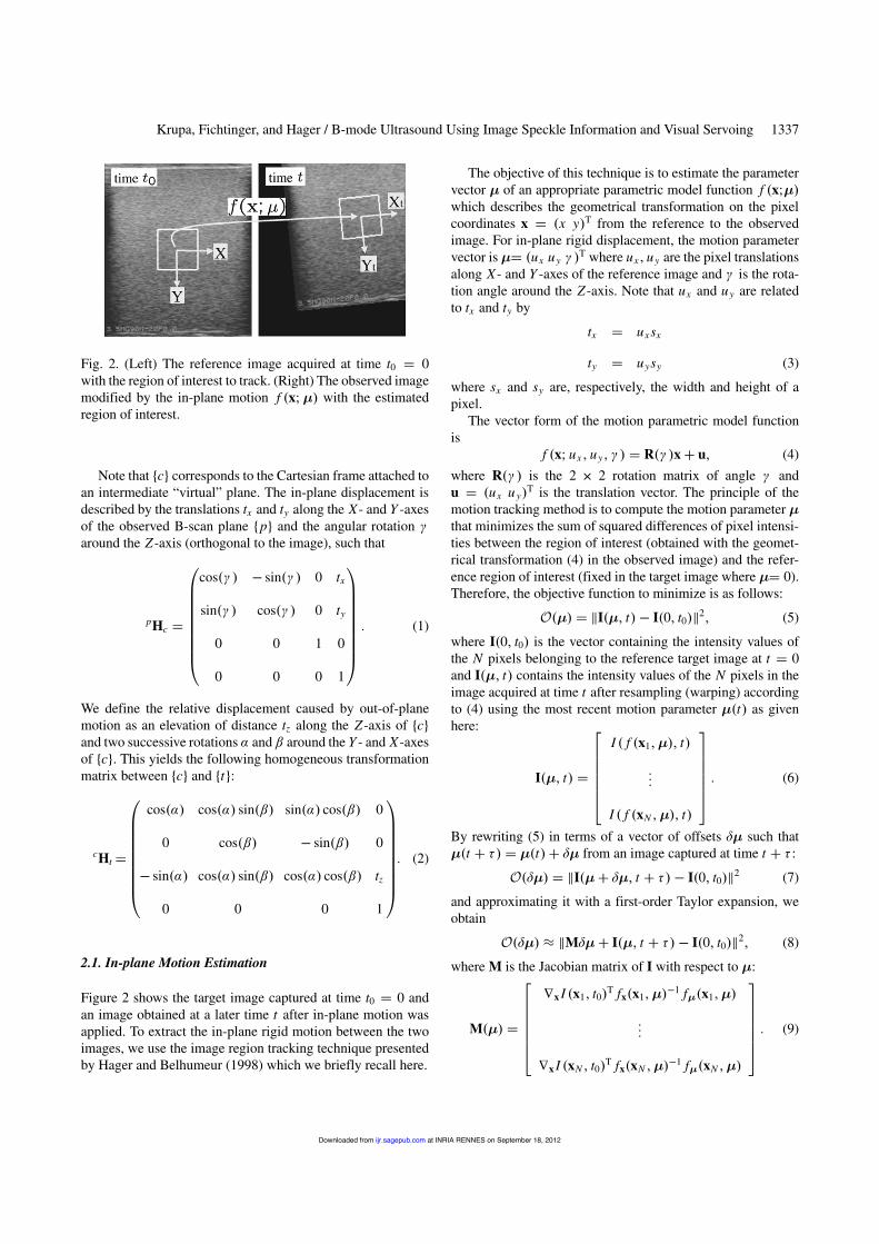
Krupa, Fichtinger, and Hager / B-mode Ultrasound Using Image Speckle Information and Visual Servoing 1337
Fig. 2. (Left) The reference image acquired at time t0 % 0with the region of interest to track. (Right) The observed imagemodified by the in-plane motion f !x& !" with the estimatedregion of interest.
Note that "c# corresponds to the Cartesian frame attached toan intermediate “virtual” plane. The in-plane displacement isdescribed by the translations tx and ty along the X- and Y -axesof the observed B-scan plane "p# and the angular rotation #around the Z -axis (orthogonal to the image), such that
pHc %
!
""""""""#
cos!# " ' sin!# " 0 tx
sin!# " cos!# " 0 ty
0 0 1 0
0 0 0 1
$
%%%%%%%%&
$ (1)
We define the relative displacement caused by out-of-planemotion as an elevation of distance tz along the Z -axis of "c#and two successive rotations % and & around the Y - and X -axesof "c#. This yields the following homogeneous transformationmatrix between "c# and "t#:
cHt %
!
""""""""#
cos!%" cos!%" sin!&" sin!%" cos!&" 0
0 cos!&" ' sin!&" 0
' sin!%" cos!%" sin!&" cos!%" cos!&" tz
0 0 0 1
$
%%%%%%%%&
$ (2)
2.1. In-plane Motion Estimation
Figure 2 shows the target image captured at time t0 % 0 andan image obtained at a later time t after in-plane motion wasapplied. To extract the in-plane rigid motion between the twoimages, we use the image region tracking technique presentedby Hager and Belhumeur (1998) which we briefly recall here.
The objective of this technique is to estimate the parametervector ! of an appropriate parametric model function f !x&!"which describes the geometrical transformation on the pixelcoordinates x % !x y"T from the reference to the observedimage. For in-plane rigid displacement, the motion parametervector is!% !ux uy # "
T where ux , uy are the pixel translationsalong X- and Y -axes of the reference image and # is the rota-tion angle around the Z -axis. Note that ux and uy are relatedto tx and ty by
tx % ux sx
ty % uysy (3)
where sx and sy are, respectively, the width and height of apixel.
The vector form of the motion parametric model functionis
f !x& ux ' uy' # " % R!# "x( u' (4)
where R!# " is the 2 ) 2 rotation matrix of angle # andu % !ux uy"
T is the translation vector. The principle of themotion tracking method is to compute the motion parameter !that minimizes the sum of squared differences of pixel intensi-ties between the region of interest (obtained with the geomet-rical transformation (4) in the observed image) and the refer-ence region of interest (fixed in the target image where !% 0).Therefore, the objective function to minimize is as follows:
!!!" % *I!!' t"' I!0' t0"*2' (5)
where I!0' t0" is the vector containing the intensity values ofthe N pixels belonging to the reference target image at t % 0and I!!' t" contains the intensity values of the N pixels in theimage acquired at time t after resampling (warping) accordingto (4) using the most recent motion parameter !!t" as givenhere:
I!!' t" %
'
((((()
I ! f !x1'!"' t"
$$$
I ! f !xN '!"' t"
*
+++++,$ (6)
By rewriting (5) in terms of a vector of offsets (! such that!!t ( )" % !!t"( (! from an image captured at time t ( ) :
!!(!" % *I!!( (!' t ( )"' I!0' t0"*2 (7)
and approximating it with a first-order Taylor expansion, weobtain
!!(!" $ *M(!( I!!' t ( )"' I!0' t0"*2' (8)
where M is the Jacobian matrix of I with respect to !:
M!!" %
'
((((()
+x I !x1' t0"T fx!x1'!"'1 f!!x1'!"
$$$
+x I !xN ' t0"T fx!xN '!"'1 f!!xN '!"
*
+++++,$ (9)
at INRIA RENNES on September 18, 2012ijr.sagepub.comDownloaded from
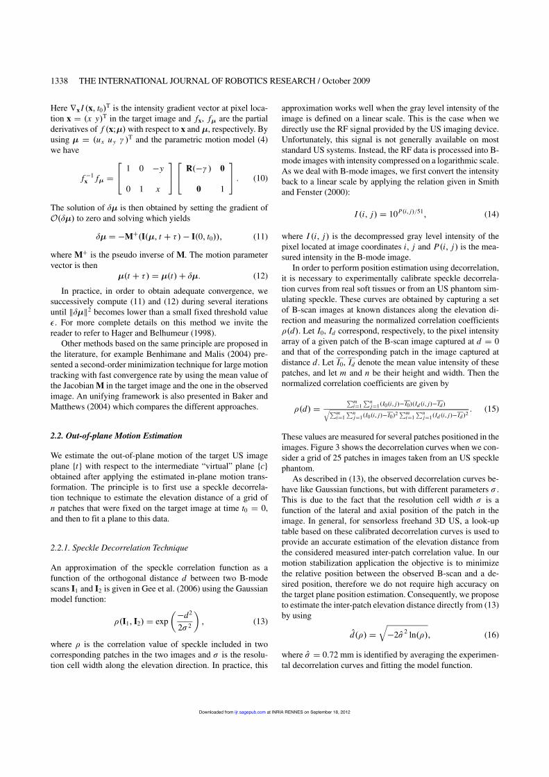
1338 THE INTERNATIONAL JOURNAL OF ROBOTICS RESEARCH / October 2009
Here +x I !x' t0"T is the intensity gradient vector at pixel loca-tion x % !x y"T in the target image and fx, f! are the partialderivatives of f !x&!" with respect to x and !, respectively. Byusing ! % !ux uy # "
T and the parametric motion model (4)we have
f '1x f! %
'
)1 0 'y
0 1 x
*
,
'
)R!'# " 0
0 1
*
, $ (10)
The solution of (! is then obtained by setting the gradient of!!(!" to zero and solving which yields
(! % 'M(!I!!' t ( )"' I!0' t0""' (11)
where M( is the pseudo inverse of M. The motion parametervector is then
!!t ( )" % !!t"( (!$ (12)
In practice, in order to obtain adequate convergence, wesuccessively compute (11) and (12) during several iterationsuntil *(!*2 becomes lower than a small fixed threshold value*. For more complete details on this method we invite thereader to refer to Hager and Belhumeur (1998).
Other methods based on the same principle are proposed inthe literature, for example Benhimane and Malis (2004) pre-sented a second-order minimization technique for large motiontracking with fast convergence rate by using the mean value ofthe Jacobian M in the target image and the one in the observedimage. An unifying framework is also presented in Baker andMatthews (2004) which compares the different approaches.
2.2. Out-of-plane Motion Estimation
We estimate the out-of-plane motion of the target US imageplane "t# with respect to the intermediate “virtual” plane "c#obtained after applying the estimated in-plane motion trans-formation. The principle is to first use a speckle decorrela-tion technique to estimate the elevation distance of a grid ofn patches that were fixed on the target image at time t0 % 0,and then to fit a plane to this data.
2.2.1. Speckle Decorrelation Technique
An approximation of the speckle correlation function as afunction of the orthogonal distance d between two B-modescans I1 and I2 is given in Gee et al. (2006) using the Gaussianmodel function:
+!I1' I2" % exp-'d2
2, 2
.' (13)
where + is the correlation value of speckle included in twocorresponding patches in the two images and , is the resolu-tion cell width along the elevation direction. In practice, this
approximation works well when the gray level intensity of theimage is defined on a linear scale. This is the case when wedirectly use the RF signal provided by the US imaging device.Unfortunately, this signal is not generally available on moststandard US systems. Instead, the RF data is processed into B-mode images with intensity compressed on a logarithmic scale.As we deal with B-mode images, we first convert the intensityback to a linear scale by applying the relation given in Smithand Fenster (2000):
I !i' j" % 10P!i' j"-51' (14)
where I !i' j" is the decompressed gray level intensity of thepixel located at image coordinates i' j and P!i' j" is the mea-sured intensity in the B-mode image.
In order to perform position estimation using decorrelation,it is necessary to experimentally calibrate speckle decorrela-tion curves from real soft tissues or from an US phantom sim-ulating speckle. These curves are obtained by capturing a setof B-scan images at known distances along the elevation di-rection and measuring the normalized correlation coefficients+!d". Let I0, Id correspond, respectively, to the pixel intensityarray of a given patch of the B-scan image captured at d % 0and that of the corresponding patch in the image captured atdistance d. Let I0, Id denote the mean value intensity of thesepatches, and let m and n be their height and width. Then thenormalized correlation coefficients are given by
+!d" %/m
i%1/n
j%1!I0!i' j"'I0"!Id !i' j"'Id "0/mi%1
/nj%1!I0!i' j"'I0"2
/mi%1
/nj%1!Id !i' j"'Id "2
$ (15)
These values are measured for several patches positioned in theimages. Figure 3 shows the decorrelation curves when we con-sider a grid of 25 patches in images taken from an US specklephantom.
As described in (13), the observed decorrelation curves be-have like Gaussian functions, but with different parameters , .This is due to the fact that the resolution cell width , is afunction of the lateral and axial position of the patch in theimage. In general, for sensorless freehand 3D US, a look-uptable based on these calibrated decorrelation curves is used toprovide an accurate estimation of the elevation distance fromthe considered measured inter-patch correlation value. In ourmotion stabilization application the objective is to minimizethe relative position between the observed B-scan and a de-sired position, therefore we do not require high accuracy onthe target plane position estimation. Consequently, we proposeto estimate the inter-patch elevation distance directly from (13)by using
,d!+" %0'2 ,, 2 ln!+"' (16)
where ,, % 0$72 mm is identified by averaging the experimen-tal decorrelation curves and fitting the model function.
at INRIA RENNES on September 18, 2012ijr.sagepub.comDownloaded from
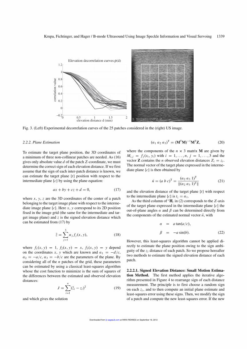
Krupa, Fichtinger, and Hager / B-mode Ultrasound Using Image Speckle Information and Visual Servoing 1339
Fig. 3. (Left) Experimental decorrelation curves of the 25 patches considered in the (right) US image.
2.2.2. Plane Estimation
To estimate the target plane position, the 3D coordinates ofa minimum of three non-collinear patches are needed. As (16)gives only absolute value d of the patch Z-coordinate, we mustdetermine the correct sign of each elevation distance. If we firstassume that the sign of each inter-patch distance is known, wecan estimate the target plane "t# position with respect to theintermediate plane "c# by using the plane equation:
ax ( by ( cz ( d % 0' (17)
where x , y, z are the 3D coordinates of the center of a patchbelonging to the target image plane with respect to the interme-diate image plane "c#. Here x , y correspond to its 2D positionfixed in the image grid (the same for the intermediate and tar-get image plane) and z is the signed elevation distance whichcan be estimated from (17) by
,z %31
j%1
% j f j !x' y"' (18)
where f1!x' y" % 1, f2!x' y" % x , f3!x' y" % y dependon the coordinates x , y which are known and %1 % 'd-c,%2 % 'a-c, %3 % 'b-c are the parameters of the plane. Byconsidering all of the n patches of the grid, these parameterscan be estimated by using a classical least-squares algorithmwhose the cost function to minimize is the sum of squares ofthe differences between the estimated and observed elevationdistances:
J %n1
i%1
!,zi ' zi "2 (19)
and which gives the solution
!%1 %2 %3"T % !MTM"'1MTZ' (20)
where the components of the n ) 3 matrix M are given byMi' j % f j !xi ' yi " with i % 1' $ $ $ ' n, j % 1' $ $ $ ' 3 and thevector Z contains the n observed elevation distances Zi % zi .The normal vector of the target plane expressed in the interme-diate plane "c# is then obtained by
-n % !a b c"T % !%2 %3 1"T
*!%2 %3 1"T* (21)
and the elevation distance of the target plane "t# with respectto the intermediate plane "c# is tz % %1.
As the third column of cHt in (2) corresponds to the Z -axisof the target plane expressed in the intermediate plane "c# theout-of-plane angles % and & can be determined directly fromthe components of the estimated normal vector -n, with
% % a tan!a-c"'
& % 'a sin!b"$ (22)
However, this least-squares algorithm cannot be applied di-rectly to estimate the plane position owing to the sign ambi-guity of the zi distance of each patch. So we propose hereaftertwo methods to estimate the signed elevation distance of eachpatch.
2.2.2.1. Signed Elevation Distance: Small Motion Estima-tion Method. The first method applies the iterative algo-rithm presented in Figure 4 to rearrange sign of each distancemeasurement. The principle is to first choose a random signon each zi ' and to then compute an initial plane estimate andleast-squares error using these signs. Then, we modify the signof a patch and compute the new least-squares error. If the new
at INRIA RENNES on September 18, 2012ijr.sagepub.comDownloaded from
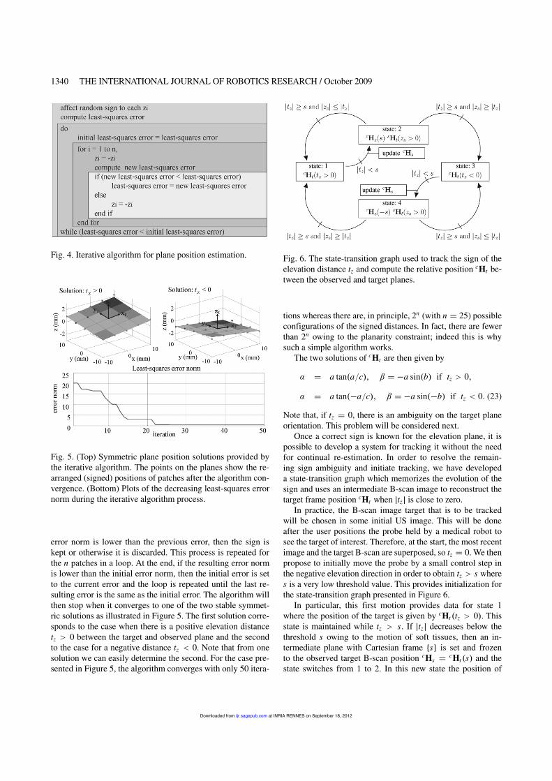
1340 THE INTERNATIONAL JOURNAL OF ROBOTICS RESEARCH / October 2009
Fig. 4. Iterative algorithm for plane position estimation.
Fig. 5. (Top) Symmetric plane position solutions provided bythe iterative algorithm. The points on the planes show the re-arranged (signed) positions of patches after the algorithm con-vergence. (Bottom) Plots of the decreasing least-squares errornorm during the iterative algorithm process.
error norm is lower than the previous error, then the sign iskept or otherwise it is discarded. This process is repeated forthe n patches in a loop. At the end, if the resulting error normis lower than the initial error norm, then the initial error is setto the current error and the loop is repeated until the last re-sulting error is the same as the initial error. The algorithm willthen stop when it converges to one of the two stable symmet-ric solutions as illustrated in Figure 5. The first solution corre-sponds to the case when there is a positive elevation distancetz . 0 between the target and observed plane and the secondto the case for a negative distance tz / 0. Note that from onesolution we can easily determine the second. For the case pre-sented in Figure 5, the algorithm converges with only 50 itera-
Fig. 6. The state-transition graph used to track the sign of theelevation distance tz and compute the relative position cHt be-tween the observed and target planes.
tions whereas there are, in principle, 2n (with n % 25) possibleconfigurations of the signed distances. In fact, there are fewerthan 2n owing to the planarity constraint! indeed this is whysuch a simple algorithm works.
The two solutions of cHt are then given by
% % a tan!a-c"' & % 'a sin!b" if tz . 0'
% % a tan!'a-c"' & % 'a sin!'b" if tz / 0$ (23)
Note that, if tz % 0, there is an ambiguity on the target planeorientation. This problem will be considered next.
Once a correct sign is known for the elevation plane, it ispossible to develop a system for tracking it without the needfor continual re-estimation. In order to resolve the remain-ing sign ambiguity and initiate tracking, we have developeda state-transition graph which memorizes the evolution of thesign and uses an intermediate B-scan image to reconstruct thetarget frame position cHt when .tz . is close to zero.
In practice, the B-scan image target that is to be trackedwill be chosen in some initial US image. This will be doneafter the user positions the probe held by a medical robot tosee the target of interest. Therefore, at the start, the most recentimage and the target B-scan are superposed, so tz % 0. We thenpropose to initially move the probe by a small control step inthe negative elevation direction in order to obtain tz . s wheres is a very low threshold value. This provides initialization forthe state-transition graph presented in Figure 6.
In particular, this first motion provides data for state 1where the position of the target is given by cHt !tz . 0". Thisstate is maintained while tz . s. If .tz. decreases below thethreshold s owing to the motion of soft tissues, then an in-termediate plane with Cartesian frame "s# is set and frozento the observed target B-scan position cHs % cHt!s" and thestate switches from 1 to 2. In this new state the position of
at INRIA RENNES on September 18, 2012ijr.sagepub.comDownloaded from
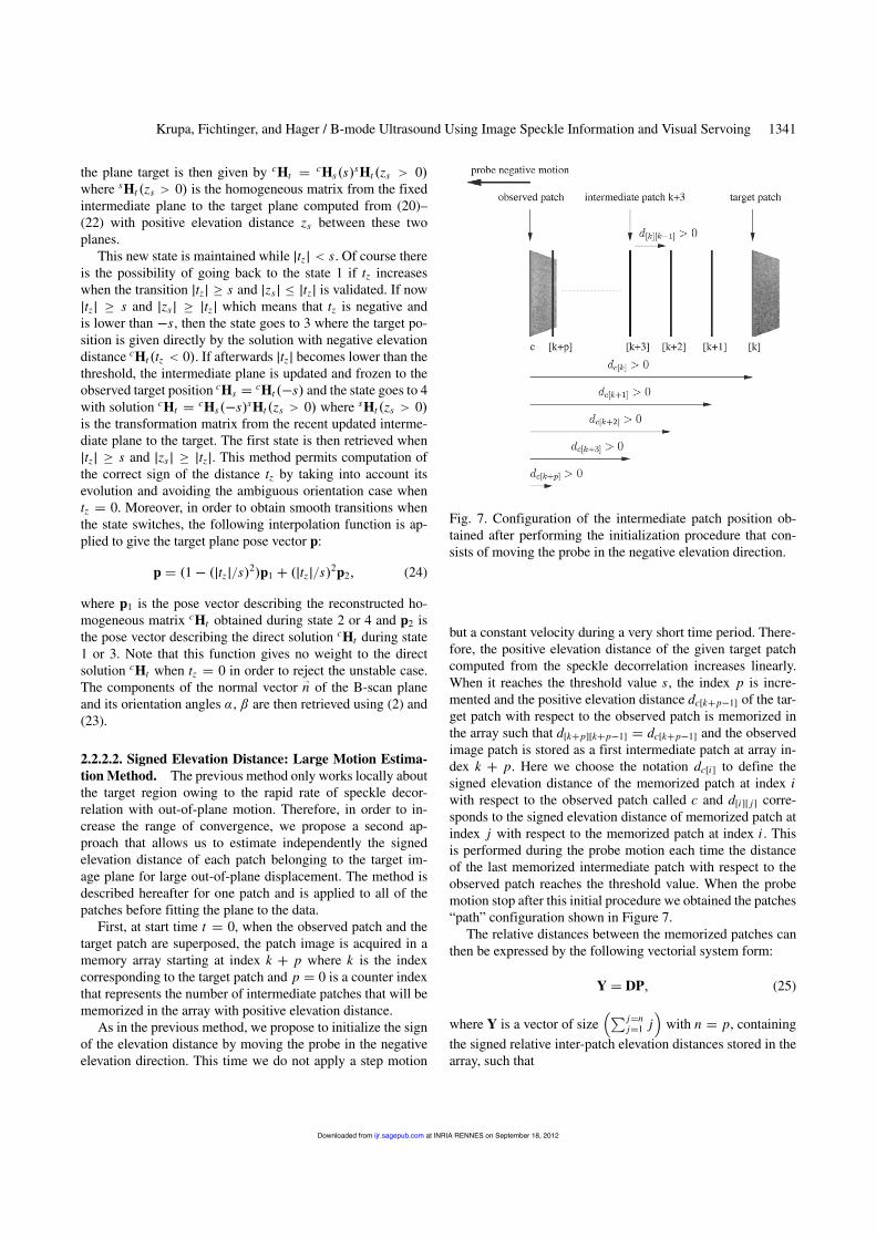
Krupa, Fichtinger, and Hager / B-mode Ultrasound Using Image Speckle Information and Visual Servoing 1341
the plane target is then given by cHt % cHs!s"sHt!zs . 0"where sHt !zs . 0" is the homogeneous matrix from the fixedintermediate plane to the target plane computed from (20)–(22) with positive elevation distance zs between these twoplanes.
This new state is maintained while .tz. / s. Of course thereis the possibility of going back to the state 1 if tz increaseswhen the transition .tz. / s and .zs . 0 .tz. is validated. If now.tz. / s and .zs . / .tz. which means that tz is negative andis lower than 's, then the state goes to 3 where the target po-sition is given directly by the solution with negative elevationdistance cHt!tz / 0". If afterwards .tz. becomes lower than thethreshold, the intermediate plane is updated and frozen to theobserved target position cHs % cHt!'s" and the state goes to 4with solution cHt % cHs!'s"sHt!zs . 0" where sHt!zs . 0"is the transformation matrix from the recent updated interme-diate plane to the target. The first state is then retrieved when.tz. / s and .zs . / .tz.. This method permits computation ofthe correct sign of the distance tz by taking into account itsevolution and avoiding the ambiguous orientation case whentz % 0. Moreover, in order to obtain smooth transitions whenthe state switches, the following interpolation function is ap-plied to give the target plane pose vector p:
p % !1' !.tz .-s"2"p1 ( !.tz.-s"2p2' (24)
where p1 is the pose vector describing the reconstructed ho-mogeneous matrix cHt obtained during state 2 or 4 and p2 isthe pose vector describing the direct solution cHt during state1 or 3. Note that this function gives no weight to the directsolution cHt when tz % 0 in order to reject the unstable case.The components of the normal vector -n of the B-scan planeand its orientation angles %, & are then retrieved using (2) and(23).
2.2.2.2. Signed Elevation Distance: Large Motion Estima-tion Method. The previous method only works locally aboutthe target region owing to the rapid rate of speckle decor-relation with out-of-plane motion. Therefore, in order to in-crease the range of convergence, we propose a second ap-proach that allows us to estimate independently the signedelevation distance of each patch belonging to the target im-age plane for large out-of-plane displacement. The method isdescribed hereafter for one patch and is applied to all of thepatches before fitting the plane to the data.
First, at start time t % 0, when the observed patch and thetarget patch are superposed, the patch image is acquired in amemory array starting at index k ( p where k is the indexcorresponding to the target patch and p % 0 is a counter indexthat represents the number of intermediate patches that will bememorized in the array with positive elevation distance.
As in the previous method, we propose to initialize the signof the elevation distance by moving the probe in the negativeelevation direction. This time we do not apply a step motion
Fig. 7. Configuration of the intermediate patch position ob-tained after performing the initialization procedure that con-sists of moving the probe in the negative elevation direction.
but a constant velocity during a very short time period. There-fore, the positive elevation distance of the given target patchcomputed from the speckle decorrelation increases linearly.When it reaches the threshold value s, the index p is incre-mented and the positive elevation distance dc[k(p'1] of the tar-get patch with respect to the observed patch is memorized inthe array such that d[k(p][k(p'1] % dc[k(p'1] and the observedimage patch is stored as a first intermediate patch at array in-dex k ( p. Here we choose the notation dc[i] to define thesigned elevation distance of the memorized patch at index iwith respect to the observed patch called c and d[i][ j] corre-sponds to the signed elevation distance of memorized patch atindex j with respect to the memorized patch at index i . Thisis performed during the probe motion each time the distanceof the last memorized intermediate patch with respect to theobserved patch reaches the threshold value. When the probemotion stop after this initial procedure we obtained the patches“path” configuration shown in Figure 7.
The relative distances between the memorized patches canthen be expressed by the following vectorial system form:
Y % DP' (25)
where Y is a vector of size2/ j%n
j%1 j3
with n % p, containingthe signed relative inter-patch elevation distances stored in thearray, such that
at INRIA RENNES on September 18, 2012ijr.sagepub.comDownloaded from
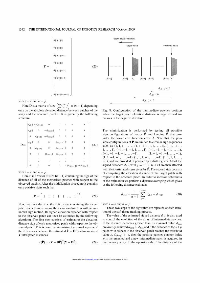
1342 THE INTERNATIONAL JOURNAL OF ROBOTICS RESEARCH / October 2009
Y %
'
(((((((((((((((((((((((()
d[i(1][i]
d[i(2][i]
d[i(2][i(1]
d[i(3][i]
d[i(3][i(1]
d[i(3][i(2]
$$$
d[i(n][i(n'1]
*
++++++++++++++++++++++++,
(26)
with i % k and n % p.Here D is a matrix of size
2/ j%nj%1 j
3) !n ( 1" depending
only on the absolute elevation distance between patches of thearray and the observed patch c. It is given by the followingstructure:
D%
'
((((((((((((((((()
.dc[i ]. '.dc[i(1]. 0 0 0 0 0
.dc[i ]. 0 '.dc[i(2]. 0 0 0 0
0 .dc[i(1]. '.dc[i(2]. 0 0 0 0
.dc[i ]. 0 0 '.dc[i(3]. 0 0 0
0 .dc[i(1]. 0 '.dc[i(3]. 0 0 0
0 0 .dc[i(2]. '.dc[i(3]. 0 0 0
$$$
$$$
$$$
$$$
$$$
$$$
$$$
0 0 0 0 0 .dc[i(n'1]. '.dc[i(n].
*
+++++++++++++++++,
(27)
with i % k and n % p.Here P is a vector of size !n ( 1" containing the sign of the
distance of all of the memorized patches with respect to theobserved patch c. After the initialization procedure it containsonly positive signs such that
P %4
1 1 1 1 1 $ $ $ 15T$ (28)
Now, we consider that the soft tissue containing the targetpatch starts to move along the elevation direction with an un-known sign motion. Its signed elevation distance with respectto the observed patch can then be estimated by the followingalgorithm. The first step consists of estimating the elevationdistance sign of each memorized patch with respect to the ob-served patch. This is done by minimizing the sum of squares ofthe differences between the estimated ,Y % D ,P and memorizedY inter-patch distances:
J ! ,P" % !Y'D ,P"T!Y' D ,P"$ (29)
Fig. 8. Configuration of the intermediate patches positionwhen the target patch elevation distance is negative and in-creases in the negative direction.
The minimization is performed by testing all possiblesign configurations of vector ,P and keeping ,P that pro-vides the lower cost function error J . Note that the pos-sible configurations of ,P are limited to circular sign sequencessuch as !1' 1' 1' 1' $ $ $ ' 1", !'1' 1' 1' 1' $ $ $ ' 1", !'1''1' 1'1' $ $ $ ' 1", !'1''1''1' 1' $ $ $ ' 1", !'1''1''1''1' $ $ $ ' 1",!'1''1''1''1' $ $ $ ''1", !1''1''1''1' $ $ $ ''1",!1' 1''1''1' $ $ $ ''1", !1' 1' 1''1' $ $ $ ''1", !1' 1' 1' 1' $ $ $ ''1", and are provided in practice by a shift register. All of thesigned distances dc[ j] with j % i' $ $ $ ' !i ( n" are then affectedwith their estimated signs given by ,P. The second step consistsof computing the elevation distance of the target patch withrespect to the observed patch. In order to increase robustnessof the estimation we perform a distance averaging which givesus the following distance estimate:
dc[k] %1
n ( 1
j%i(n1
j%i
dc[ j] ( d[ j][k] (30)
with i % k and n % p.These two steps of the algorithm are repeated at each itera-
tion of the soft tissue tracking process.The value of the estimated signed distance dc[k] is also used
to control the evolution of the array of intermediate patches.If the distance becomes greater than its maximal value dmax
previously achieved dc[k] . dmax and if the distance of the k(ppatch with respect to the observed patch reaches the thresholdvalue s, dc[k(p] . s, then the positive patches counter indexp is incremented and a new intermediate patch is acquired inthe memory array. In the opposite side if the distance of the
at INRIA RENNES on September 18, 2012ijr.sagepub.comDownloaded from
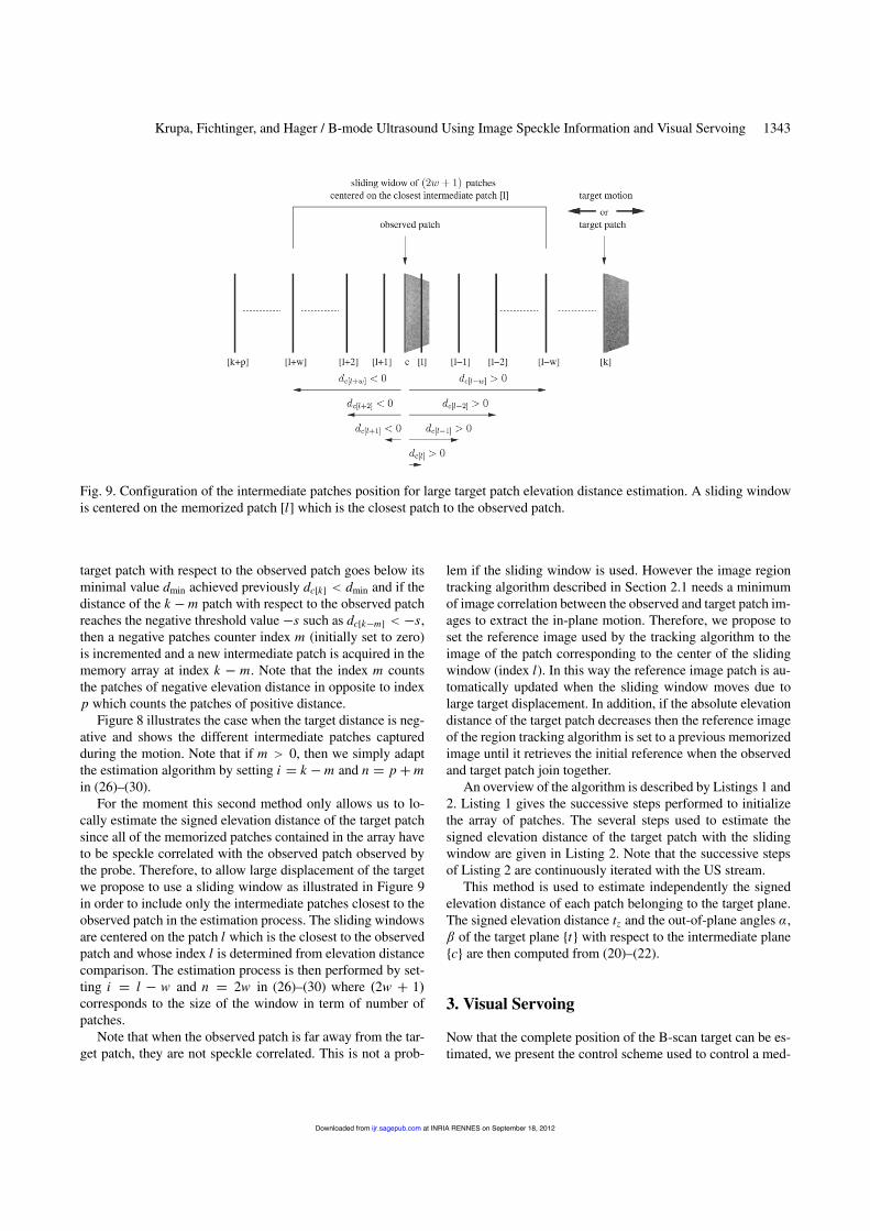
Krupa, Fichtinger, and Hager / B-mode Ultrasound Using Image Speckle Information and Visual Servoing 1343
Fig. 9. Configuration of the intermediate patches position for large target patch elevation distance estimation. A sliding windowis centered on the memorized patch [l] which is the closest patch to the observed patch.
target patch with respect to the observed patch goes below itsminimal value dmin achieved previously dc[k] / dmin and if thedistance of the k 'm patch with respect to the observed patchreaches the negative threshold value 's such as dc[k'm] / 's,then a negative patches counter index m (initially set to zero)is incremented and a new intermediate patch is acquired in thememory array at index k ' m. Note that the index m countsthe patches of negative elevation distance in opposite to indexp which counts the patches of positive distance.
Figure 8 illustrates the case when the target distance is neg-ative and shows the different intermediate patches capturedduring the motion. Note that if m . 0, then we simply adaptthe estimation algorithm by setting i % k 'm and n % p (min (26)–(30).
For the moment this second method only allows us to lo-cally estimate the signed elevation distance of the target patchsince all of the memorized patches contained in the array haveto be speckle correlated with the observed patch observed bythe probe. Therefore, to allow large displacement of the targetwe propose to use a sliding window as illustrated in Figure 9in order to include only the intermediate patches closest to theobserved patch in the estimation process. The sliding windowsare centered on the patch l which is the closest to the observedpatch and whose index l is determined from elevation distancecomparison. The estimation process is then performed by set-ting i % l ' 0 and n % 20 in (26)–(30) where !20 ( 1"corresponds to the size of the window in term of number ofpatches.
Note that when the observed patch is far away from the tar-get patch, they are not speckle correlated. This is not a prob-
lem if the sliding window is used. However the image regiontracking algorithm described in Section 2.1 needs a minimumof image correlation between the observed and target patch im-ages to extract the in-plane motion. Therefore, we propose toset the reference image used by the tracking algorithm to theimage of the patch corresponding to the center of the slidingwindow (index l). In this way the reference image patch is au-tomatically updated when the sliding window moves due tolarge target displacement. In addition, if the absolute elevationdistance of the target patch decreases then the reference imageof the region tracking algorithm is set to a previous memorizedimage until it retrieves the initial reference when the observedand target patch join together.
An overview of the algorithm is described by Listings 1 and2. Listing 1 gives the successive steps performed to initializethe array of patches. The several steps used to estimate thesigned elevation distance of the target patch with the slidingwindow are given in Listing 2. Note that the successive stepsof Listing 2 are continuously iterated with the US stream.
This method is used to estimate independently the signedelevation distance of each patch belonging to the target plane.The signed elevation distance tz and the out-of-plane angles %,& of the target plane "t# with respect to the intermediate plane"c# are then computed from (20)–(22).
3. Visual Servoing
Now that the complete position of the B-scan target can be es-timated, we present the control scheme used to control a med-
at INRIA RENNES on September 18, 2012ijr.sagepub.comDownloaded from
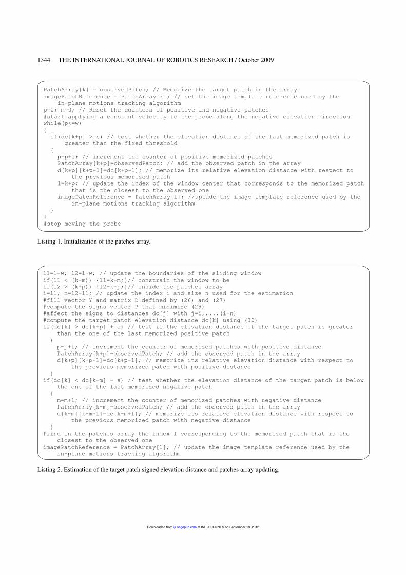
1344 THE INTERNATIONAL JOURNAL OF ROBOTICS RESEARCH / October 2009
Listing 1. Initialization of the patches array.
Listing 2. Estimation of the target patch signed elevation distance and patches array updating.
at INRIA RENNES on September 18, 2012ijr.sagepub.comDownloaded from
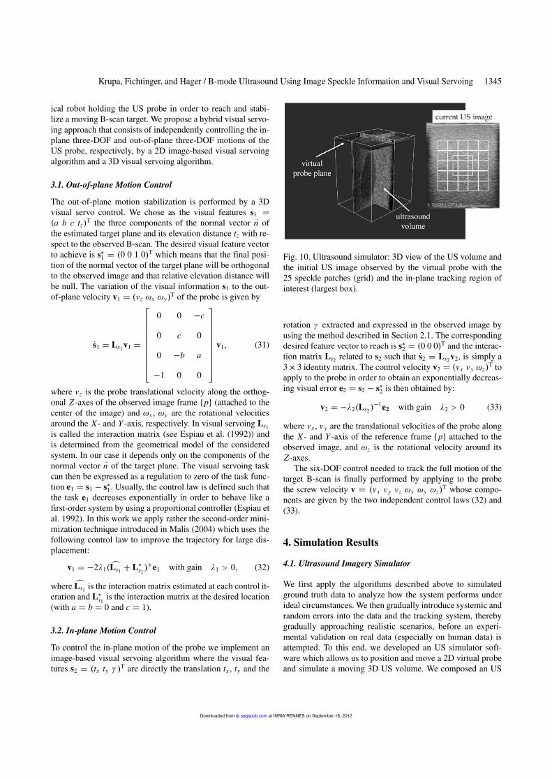
Krupa, Fichtinger, and Hager / B-mode Ultrasound Using Image Speckle Information and Visual Servoing 1345
ical robot holding the US probe in order to reach and stabi-lize a moving B-scan target. We propose a hybrid visual servo-ing approach that consists of independently controlling the in-plane three-DOF and out-of-plane three-DOF motions of theUS probe, respectively, by a 2D image-based visual servoingalgorithm and a 3D visual servoing algorithm.
3.1. Out-of-plane Motion Control
The out-of-plane motion stabilization is performed by a 3Dvisual servo control. We chose as the visual features s1 %!a b c tz"
T the three components of the normal vector -n ofthe estimated target plane and its elevation distance tz with re-spect to the observed B-scan. The desired visual feature vectorto achieve is s11 % !0 0 1 0"T which means that the final posi-tion of the normal vector of the target plane will be orthogonalto the observed image and that relative elevation distance willbe null. The variation of the visual information s1 to the out-of-plane velocity v1 % !1z 2x 2y"
T of the probe is given by
2s1 % Ls1v1 %
'
(((((((()
0 0 'c
0 c 0
0 'b a
'1 0 0
*
++++++++,
v1' (31)
where 1z is the probe translational velocity along the orthog-onal Z -axes of the observed image frame "p# (attached to thecenter of the image) and 2x , 2y are the rotational velocitiesaround the X - and Y -axis, respectively. In visual servoing Ls1
is called the interaction matrix (see Espiau et al. (1992)) andis determined from the geometrical model of the consideredsystem. In our case it depends only on the components of thenormal vector -n of the target plane. The visual servoing taskcan then be expressed as a regulation to zero of the task func-tion e1 % s1 ' s11. Usually, the control law is defined such thatthe task e1 decreases exponentially in order to behave like afirst-order system by using a proportional controller (Espiau etal. 1992). In this work we apply rather the second-order mini-mization technique introduced in Malis (2004) which uses thefollowing control law to improve the trajectory for large dis-placement:
v1 % '231!6Ls1 ( L1s1"(e1 with gain 31 . 0' (32)
where 6Ls1 is the interaction matrix estimated at each control it-eration and L1s1
is the interaction matrix at the desired location(with a % b % 0 and c % 1).
3.2. In-plane Motion Control
To control the in-plane motion of the probe we implement animage-based visual servoing algorithm where the visual fea-tures s2 % !tx ty # "
T are directly the translation tx , ty and the
Fig. 10. Ultrasound simulator: 3D view of the US volume andthe initial US image observed by the virtual probe with the25 speckle patches (grid) and the in-plane tracking region ofinterest (largest box).
rotation # extracted and expressed in the observed image byusing the method described in Section 2.1. The correspondingdesired feature vector to reach is s12 % !0 0 0"T and the interac-tion matrix Ls2 related to s2 such that 2s2 % Ls2 v2, is simply a3)3 identity matrix. The control velocity v2 % !1x 1y 2z"
T toapply to the probe in order to obtain an exponentially decreas-ing visual error e2 % s2 ' s12 is then obtained by:
v2 % '32!Ls2"'1e2 with gain 32 . 0 (33)
where 1x , 1y are the translational velocities of the probe alongthe X - and Y -axis of the reference frame "p# attached to theobserved image, and 2z is the rotational velocity around itsZ-axes.
The six-DOF control needed to track the full motion of thetarget B-scan is finally performed by applying to the probethe screw velocity v % !1x 1y 1z 2x 2y 2z"
T whose compo-nents are given by the two independent control laws (32) and(33).
4. Simulation Results
4.1. Ultrasound Imagery Simulator
We first apply the algorithms described above to simulatedground truth data to analyze how the system performs underideal circumstances. We then gradually introduce systemic andrandom errors into the data and the tracking system, therebygradually approaching realistic scenarios, before an experi-mental validation on real data (especially on human data) isattempted. To this end, we developed an US simulator soft-ware which allows us to position and move a 2D virtual probeand simulate a moving 3D US volume. We composed an US
at INRIA RENNES on September 18, 2012ijr.sagepub.comDownloaded from
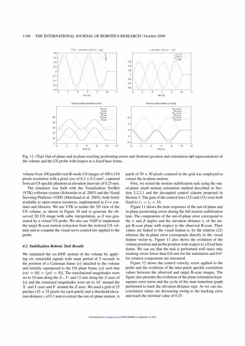
1346 THE INTERNATIONAL JOURNAL OF ROBOTICS RESEARCH / October 2009
Fig. 11. (Top) Out-of-plane and in-plane tracking positioning errors and (bottom) position and orientation (u4 representation) ofthe volume and the US probe with respect to a fixed base frame.
volume from 100 parallel real B-mode US images of 180)210pixels resolution with a pixel size of 0$2) 0$2 mm2, capturedfrom an US speckle phantom at elevation intervals of 0.25 mm.
The simulator was built with the Visualization ToolKit(VTK) software system (Schroeder et al. 2003) and the VisualServoing Platform (ViSP) (Marchand et al. 2005), both freelyavailable as open-source resources, implemented as C++ rou-tines and libraries. We use VTK to render the 3D view of theUS volume, as shown in Figure 10 and to generate the ob-served 2D US image with cubic interpolation, as if was gen-erated by a virtual US probe. We also use ViSP to implementthe target B-scan motion extraction from the resliced US vol-ume and to compute the visual servo control law applied to theprobe.
4.2. Stabilization Robotic Task Results
We simulated the six-DOF motion of the volume by apply-ing six sinusoidal signals with same period of 5 seconds tothe position of a Cartesian frame "o# attached to the volumeand initially superposed to the US plane frame "p# such that"o!t % 0"# % "p!t % 0"#. The translational magnitudes wereset to 10 mm along the X -, Y - and 12 mm along the Z -axes of"o# and the rotational magnitudes were set to 103 around theX - and Y -axes and 83 around the Z-axes. We used a grid of 25patches (25) 25 pixels for each patch) and a threshold eleva-tion distance s of 0.1 mm to extract the out-of-plane motion. A
patch of 50 ) 50 pixels centered in the grid was employed toextract the in-plane motion.
First, we tested the motion stabilization task using the out-of-plane small motion estimation method described in Sec-tion 2.2.2.1 and the decoupled control scheme proposed inSection 3. The gain of the control laws (32) and (33) were bothfixed to 31 % 32 % 10.
Figure 11 shows the time responses of the out-of-plane andin-plane positioning errors during the full motion stabilizationtask. The components of the out-of-plane error correspond tothe % and & angles and the elevation distance tz of the tar-get B-scan plane with respect to the observed B-scan. Theirvalues are linked to the visual feature s1 by the relation (22)whereas the in-plane error corresponds directly to the visualfeature vector s2. Figure 11 also shows the evolution of thevolume position and probe position with respect to a fixed baseframe. We can see that the task is performed well since onlytracking errors lower than 0.8 mm for the translation and 0$63
for rotation components are measured.Figure 12 shows the control velocity screw applied to the
probe and the evolution of the inter-patch speckle correlationvalues between the observed and target B-scan images. Thefigure also presents the evolution of the plane estimation least-squares error norm and the cycle of the state-transition graphperformed to track the elevation distance sign. As we can see,correlation values are decreasing owing to the tracking errorand reach the minimal value of 0.25.
at INRIA RENNES on September 18, 2012ijr.sagepub.comDownloaded from
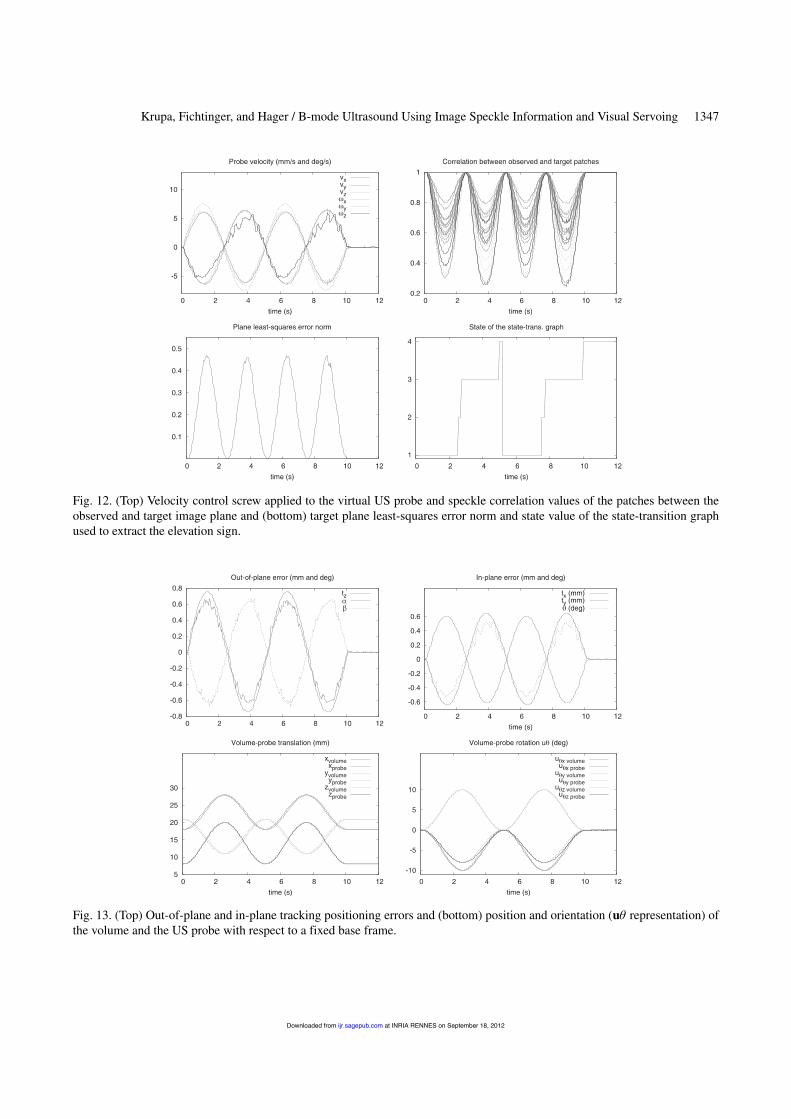
Krupa, Fichtinger, and Hager / B-mode Ultrasound Using Image Speckle Information and Visual Servoing 1347
Fig. 12. (Top) Velocity control screw applied to the virtual US probe and speckle correlation values of the patches between theobserved and target image plane and (bottom) target plane least-squares error norm and state value of the state-transition graphused to extract the elevation sign.
Fig. 13. (Top) Out-of-plane and in-plane tracking positioning errors and (bottom) position and orientation (u4 representation) ofthe volume and the US probe with respect to a fixed base frame.
at INRIA RENNES on September 18, 2012ijr.sagepub.comDownloaded from
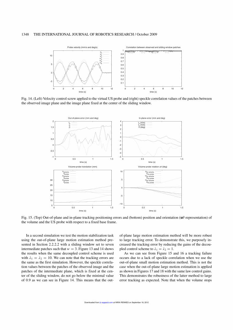
1348 THE INTERNATIONAL JOURNAL OF ROBOTICS RESEARCH / October 2009
Fig. 14. (Left) Velocity control screw applied to the virtual US probe and (right) speckle correlation values of the patches betweenthe observed image plane and the image plane fixed at the center of the sliding window.
Fig. 15. (Top) Out-of-plane and in-plane tracking positioning errors and (bottom) position and orientation (u4 representation) ofthe volume and the US probe with respect to a fixed base frame.
In a second simulation we test the motion stabilization taskusing the out-of-plane large motion estimation method pre-sented in Section 2.2.2.2 with a sliding window set to sevenintermediate patches such that 0 % 3. Figure 13 and 14 showsthe results when the same decoupled control scheme is usedwith 31 % 32 % 10. We can note that the tracking errors arethe same as the first simulation. However, the speckle correla-tion values between the patches of the observed image and thepatches of the intermediate plane, which is fixed at the cen-ter of the sliding window, do not go below the minimal valueof 0$9 as we can see in Figure 14. This means that the out-
of-plane large motion estimation method will be more robustto large tracking error. To demonstrate this, we purposely in-creased the tracking error by reducing the gains of the decou-pled control scheme to 31 % 32 % 1.
As we can see from Figure 15 and 16 a tracking failureoccurs due to a lack of speckle correlation when we use theout-of-plane small motion estimation method. This is not thecase when the out-of-plane large motion estimation is appliedas shown in Figures 17 and 18 with the same law control gains.This demonstrates the robustness of the latter method to largeerror tracking as expected. Note that when the volume stops
at INRIA RENNES on September 18, 2012ijr.sagepub.comDownloaded from
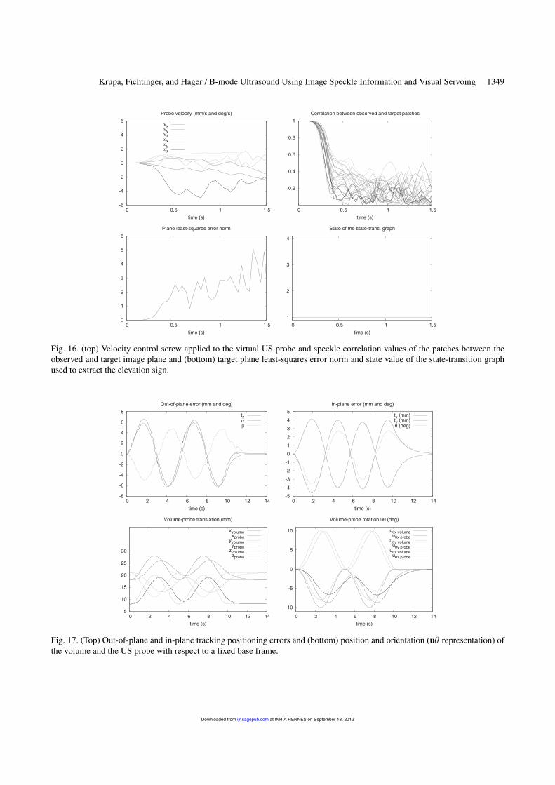
Krupa, Fichtinger, and Hager / B-mode Ultrasound Using Image Speckle Information and Visual Servoing 1349
Fig. 16. (top) Velocity control screw applied to the virtual US probe and speckle correlation values of the patches between theobserved and target image plane and (bottom) target plane least-squares error norm and state value of the state-transition graphused to extract the elevation sign.
Fig. 17. (Top) Out-of-plane and in-plane tracking positioning errors and (bottom) position and orientation (u4 representation) ofthe volume and the US probe with respect to a fixed base frame.
at INRIA RENNES on September 18, 2012ijr.sagepub.comDownloaded from
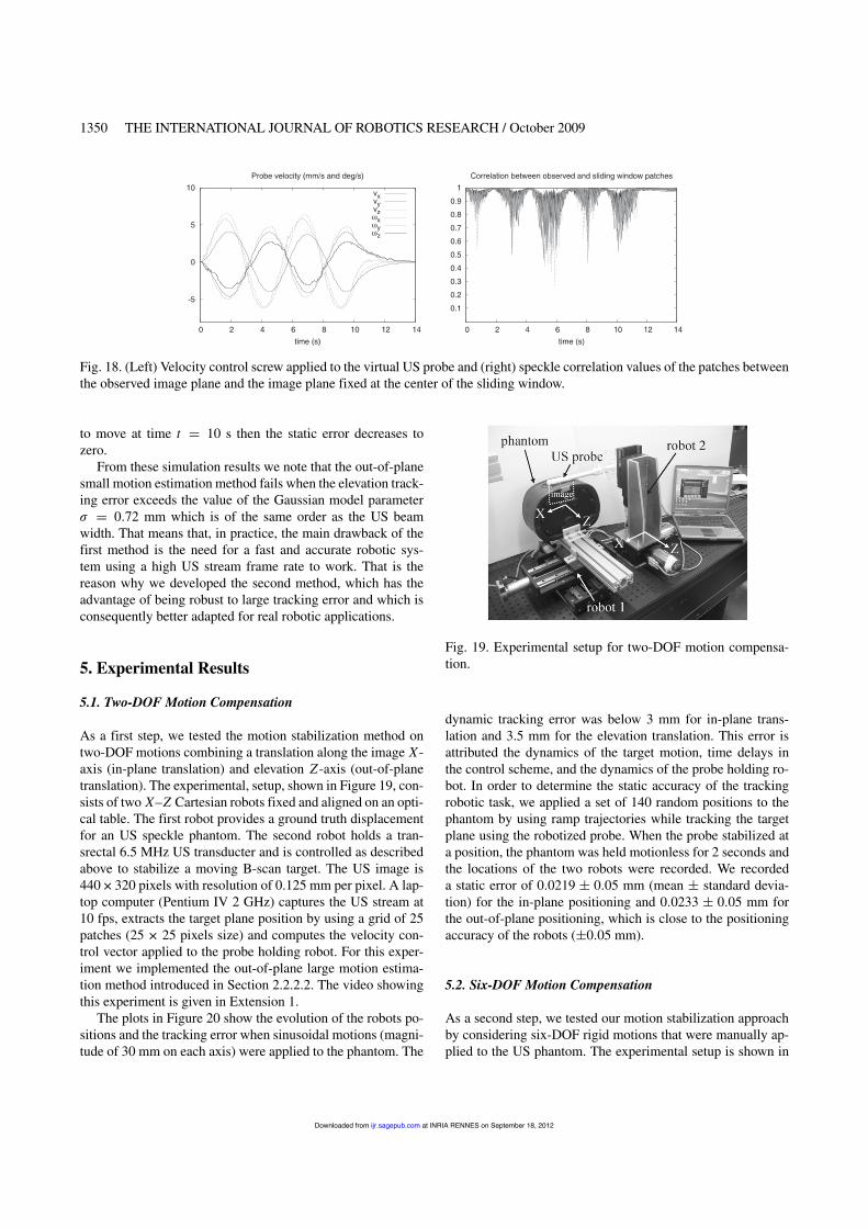
1350 THE INTERNATIONAL JOURNAL OF ROBOTICS RESEARCH / October 2009
Fig. 18. (Left) Velocity control screw applied to the virtual US probe and (right) speckle correlation values of the patches betweenthe observed image plane and the image plane fixed at the center of the sliding window.
to move at time t % 10 s then the static error decreases tozero.
From these simulation results we note that the out-of-planesmall motion estimation method fails when the elevation track-ing error exceeds the value of the Gaussian model parameter, % 0$72 mm which is of the same order as the US beamwidth. That means that, in practice, the main drawback of thefirst method is the need for a fast and accurate robotic sys-tem using a high US stream frame rate to work. That is thereason why we developed the second method, which has theadvantage of being robust to large tracking error and which isconsequently better adapted for real robotic applications.
5. Experimental Results
5.1. Two-DOF Motion Compensation
As a first step, we tested the motion stabilization method ontwo-DOF motions combining a translation along the image X-axis (in-plane translation) and elevation Z -axis (out-of-planetranslation). The experimental, setup, shown in Figure 19, con-sists of two X–Z Cartesian robots fixed and aligned on an opti-cal table. The first robot provides a ground truth displacementfor an US speckle phantom. The second robot holds a tran-srectal 6.5 MHz US transducter and is controlled as describedabove to stabilize a moving B-scan target. The US image is440)320 pixels with resolution of 0.125 mm per pixel. A lap-top computer (Pentium IV 2 GHz) captures the US stream at10 fps, extracts the target plane position by using a grid of 25patches (25 ) 25 pixels size) and computes the velocity con-trol vector applied to the probe holding robot. For this exper-iment we implemented the out-of-plane large motion estima-tion method introduced in Section 2.2.2.2. The video showingthis experiment is given in Extension 1.
The plots in Figure 20 show the evolution of the robots po-sitions and the tracking error when sinusoidal motions (magni-tude of 30 mm on each axis) were applied to the phantom. The
Fig. 19. Experimental setup for two-DOF motion compensa-tion.
dynamic tracking error was below 3 mm for in-plane trans-lation and 3.5 mm for the elevation translation. This error isattributed the dynamics of the target motion, time delays inthe control scheme, and the dynamics of the probe holding ro-bot. In order to determine the static accuracy of the trackingrobotic task, we applied a set of 140 random positions to thephantom by using ramp trajectories while tracking the targetplane using the robotized probe. When the probe stabilized ata position, the phantom was held motionless for 2 seconds andthe locations of the two robots were recorded. We recordeda static error of 0$0219 4 0$05 mm (mean 4 standard devia-tion) for the in-plane positioning and 0$0233 4 0$05 mm forthe out-of-plane positioning, which is close to the positioningaccuracy of the robots (40$05 mm).
5.2. Six-DOF Motion Compensation
As a second step, we tested our motion stabilization approachby considering six-DOF rigid motions that were manually ap-plied to the US phantom. The experimental setup is shown in
at INRIA RENNES on September 18, 2012ijr.sagepub.comDownloaded from
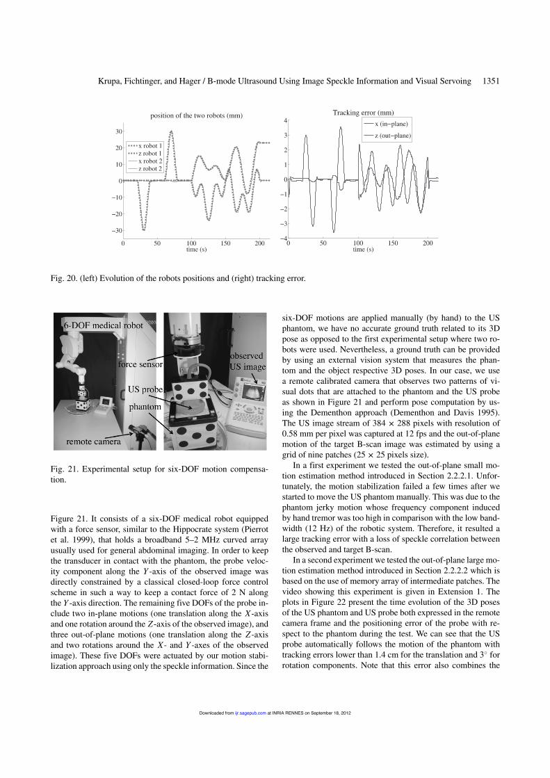
Krupa, Fichtinger, and Hager / B-mode Ultrasound Using Image Speckle Information and Visual Servoing 1351
Fig. 20. (left) Evolution of the robots positions and (right) tracking error.
Fig. 21. Experimental setup for six-DOF motion compensa-tion.
Figure 21. It consists of a six-DOF medical robot equippedwith a force sensor, similar to the Hippocrate system (Pierrotet al. 1999), that holds a broadband 5–2 MHz curved arrayusually used for general abdominal imaging. In order to keepthe transducer in contact with the phantom, the probe veloc-ity component along the Y -axis of the observed image wasdirectly constrained by a classical closed-loop force controlscheme in such a way to keep a contact force of 2 N alongthe Y -axis direction. The remaining five DOFs of the probe in-clude two in-plane motions (one translation along the X-axisand one rotation around the Z -axis of the observed image), andthree out-of-plane motions (one translation along the Z -axisand two rotations around the X- and Y -axes of the observedimage). These five DOFs were actuated by our motion stabi-lization approach using only the speckle information. Since the
six-DOF motions are applied manually (by hand) to the USphantom, we have no accurate ground truth related to its 3Dpose as opposed to the first experimental setup where two ro-bots were used. Nevertheless, a ground truth can be providedby using an external vision system that measures the phan-tom and the object respective 3D poses. In our case, we usea remote calibrated camera that observes two patterns of vi-sual dots that are attached to the phantom and the US probeas shown in Figure 21 and perform pose computation by us-ing the Dementhon approach (Dementhon and Davis 1995).The US image stream of 384 ) 288 pixels with resolution of0.58 mm per pixel was captured at 12 fps and the out-of-planemotion of the target B-scan image was estimated by using agrid of nine patches (25) 25 pixels size).
In a first experiment we tested the out-of-plane small mo-tion estimation method introduced in Section 2.2.2.1. Unfor-tunately, the motion stabilization failed a few times after westarted to move the US phantom manually. This was due to thephantom jerky motion whose frequency component inducedby hand tremor was too high in comparison with the low band-width (12 Hz) of the robotic system. Therefore, it resulted alarge tracking error with a loss of speckle correlation betweenthe observed and target B-scan.
In a second experiment we tested the out-of-plane large mo-tion estimation method introduced in Section 2.2.2.2 which isbased on the use of memory array of intermediate patches. Thevideo showing this experiment is given in Extension 1. Theplots in Figure 22 present the time evolution of the 3D posesof the US phantom and US probe both expressed in the remotecamera frame and the positioning error of the probe with re-spect to the phantom during the test. We can see that the USprobe automatically follows the motion of the phantom withtracking errors lower than 1.4 cm for the translation and 33 forrotation components. Note that this error also combines the
at INRIA RENNES on September 18, 2012ijr.sagepub.comDownloaded from
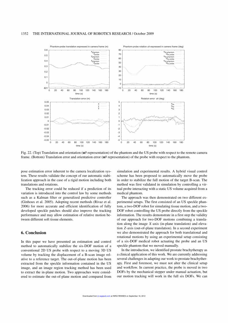
1352 THE INTERNATIONAL JOURNAL OF ROBOTICS RESEARCH / October 2009
Fig. 22. (Top) Translation and orientation (u4 representation) of the phantom and the US probe with respect to the remote cameraframe. (Bottom) Translation error and orientation error (u4 representation) of the probe with respect to the phantom.
pose estimation error inherent to the camera localization sys-tem. These results validate the concept of our automatic stabi-lization approach in the case of a rigid motion including bothtranslations and rotations.
The tracking error could be reduced if a prediction of itsvariation is introduced into the control law by some methodssuch as a Kalman filter or generalized predictive controller(Ginhoux et al. 2005). Adopting recent methods (Rivaz et al.2006) for more accurate and efficient identification of fullydeveloped speckle patches should also improve the trackingperformance and may allow estimation of relative motion be-tween different soft tissue elements.
6. Conclusion
In this paper we have presented an estimation and controlmethod to automatically stabilize the six-DOF motion of aconventional 2D US probe with respect to a moving 3D USvolume by tracking the displacement of a B-scan image rel-ative to a reference target. The out-of-plane motion has beenextracted from the speckle information contained in the USimage, and an image region tracking method has been usedto extract the in-plane motion. Two approaches were consid-ered to estimate the out-of-plane motion and compared from
simulation and experimental results. A hybrid visual controlscheme has been proposed to automatically move the probein order to stabilize the full motion of the target B-scan. Themethod was first validated in simulation by controlling a vir-tual probe interacting with a static US volume acquired from amedical phantom.
The approach was then demonstrated on two different ex-perimental setups. The first consisted of an US speckle phan-tom, a two-DOF robot for simulating tissue motion, and a two-DOF robot controlling the US probe directly from the speckleinformation. The results demonstrate in a first step the validityof our approach for two-DOF motions combining a transla-tion along the image X-axis (in-plane translation) and eleva-tion Z -axis (out-of-plane translation). In a second experimentwe also demonstrated the approach for both translational androtational motions by using an experimental setup consistingof a six-DOF medical robot actuating the probe and an USspeckle phantom that we moved manually.
In the introduction, we identified prostate brachytherapy asa clinical application of this work. We are currently addressingseveral challenges in adapting our work to prostate brachyther-apy. First and foremost, we must not alter the clinical setupand workflow. In current practice, the probe is moved in twoDOFs by the mechanical stepper under manual actuation, butour motion tracking will work in the full six DOFs. We can
at INRIA RENNES on September 18, 2012ijr.sagepub.comDownloaded from
Krupa, Fichtinger, and Hager / B-mode Ultrasound Using Image Speckle Information and Visual Servoing 1353
encode and actuate existing DOFs of the stepper, but furthermodifications are prohibitive. To this end, several extensionswill be necessary to our current tracking and servoing tech-niques. Most contemporary TRUS probes have two perpen-dicularly arranged transducers: one crystal provides a trans-verse image perpendicular to the translation axis and a sec-ond crystal gives a sagittal image across the rotation axis. Inessence, the transverse crystal maps the prostate in Cartesianspace while the sagittal crystal works in a cylindrical frameof reference. Therefore, we will adapt our automatic stabiliza-tion approach to the mixed Cartesian–cylindrical scheme usedin TRUS imaging. Second, we will attempt to track the tar-get and needle at the same time with a single TRUS probe.We expect that some target and needle motions can be com-pensated for, and the remaining misalignments will have to berepresented visually. Such a mixed scheme will undoubtedlylead to an extensive investigation of human–machine interfacetechniques as well. Finally, in a later phase, we will integratethe resulting six-DOF motion tracking and two-DOF TRUSimage stabilization with an existing needle placement roboticsystem (Fichtinger et al. 2008). Altogether, the work presentedhere has launched us on a challenging and clinically importanttrajectory of research.
Acknowledgments
The authors acknowledge the support of the National ScienceFoundation under Engineering Research Center grant EEC-9731748 and the French INRIA Institute. The authors thankDr Emad Boctor for providing the 3DUS data needed bythe US imagery simulator and Dr Ankur Kapoor and Dr Iu-lian Iordachita for assistance in designing of the first experi-mental setup at the Johns Hopkins University. We also thankDr Danny Y. Song (Johns Hopkins University Hospital) andDr Everette C. Burdette (Acoustic MedSystems, Inc.) for as-sistance in systems concept development and expert advice inclinical brachytherapy instrumentation.
Appendix: Index to Multimedia Extensions
The multimedia extension page is found at http://www.ijrr.org
Table of Multimedia Extensions.
Extension Type Description
1 Video Video showing simulations andexperiments.
References
Abolmaesumi, P., Salcudean, S. E., Zhu, W. H., Sirouspour,M. and DiMaio, S. (2002). Image-guided control of a robot
for medical ultrasound. IEEE Transactions on Robotics andAutomation, 18(1): 11–23.
Bachta, W. and Krupa, A. (2006). Towards ultrasound image-based visual servoing. IEEE International Conferenceon Robotics and Automation (ICRA’2006), Orlando, FL,pp. 4112–4117.
Baker, S. and Matthews, I. (2004). Lucas-kanade 20 years on:a unifying framework. International Journal of ComputerVision, 56(3): 221–255.
Benhimane, S. and Malis, E. (2004). Real-time image-basedtracking of planes using efficient second-order minimiza-tion. IEEE/RSJ International Conference on Intelligent Ro-bots and Systems (IROS’04), Sendai, Japan, pp. 943–948.
Boctor, E., deOliveira, M., Choti, M., Ghanem, R., Taylor,R. H., Hager, G. D. and Fichtinger, G. (2006). Ultrasoundmonitoring of tissue ablation via deformation model andshape priors. 9th International Conference on Medical Im-age Computing and Computer-Assisted Intervention (MIC-CAI’2006), Copenhagen, Denmark, pp. 405–412.
Boctor, E., Iordachita, I., Fichtinger, G. and Hager, G. D.(2005). Real-time quality control of tracked ultrasound.8th International Conference on Medical Image Computingand Computer-Assisted Intervention (MICCAI’2005), PalmSprings, CA, pp. 621–630.
Bohs, L. N., Geiman, B. J., Anderson, M. E., Gebhart, S. C.and Trahey, G. E. (2000). Speckle tracking for multi-dimensional flow estimation. Ultrasonics, 28(1): 369–375.
Chang, R. F., Wu, W. J., Chen, D. R., Chen, W. M., Shu, W.,Lee, J. H. and Jeng, L. B. (2003). 3-D US frame positioningusing speckle decorrelation and image registration. Ultra-sound in Medicine and Biology, 29(6): 801–812.
Dementhon, D. and Davis, L. (1995). Model-based object posein 25 lines of code. International Journal of Computer Vi-sion, 15: 123–141.
Espiau, B., Chaumette, F. and Rives, P. (1992). A new ap-proach to visual servoing in robotics. IEEE Transactionson Robotics and Automation, 8(3): 313–326.
Fichtinger, G., Fiene, J., Kennedy, C., Kronreif, G., Iordachita,I., Song, D., Burdette, E. and Kazanzides, P. (2008). Ro-botic assistance for ultrasound-guided prostate brachyther-apy. Medical Image Analysis, 12(5): 535–545.
Gee, A. H., Housden, R. J., Hassenpflug, P., Treece, G. M. andPrager, R. W. (2006). Sensorless freehand 3d ultrasound inreal tissues: speckle decorrelation without fully developedspeckle. Medical Image Analysis, 10(2): 137–149.
Ginhoux, R., Gangloff, J., de Mathelin, M., Soler, L., Sanchez,M. M. A. and Marescaux, J. (2005). Active filtering ofphysiological motion in robotized surgery using predictivecontrol. IEEE Transactions on Robotics, 21(1): 67–79.
Hager, G. D. and Belhumeur, P. N. (1998). Efficient regiontracking with parametric models of geometry and illumina-tion. IEEE Transactions on Pattern Analysis and MachineIntelligence, 20(10): 1025–1039.
at INRIA RENNES on September 18, 2012ijr.sagepub.comDownloaded from
1354 THE INTERNATIONAL JOURNAL OF ROBOTICS RESEARCH / October 2009
Hong, J., Dohi, T., Hashizume, M., Konishi, K. and Hata, N.(2004). An ultrasound-driven needle insertion robot for per-cutaneous cholecystostomy. Physics in Medicine and Biol-ogy, 49(3): 441–455.
Krupa, A., Fichtinger, G. and Hager, G. D. (2007a). Full mo-tion tracking in ultrasound using image speckle informa-tion and visual servoing. IEEE International Conference onRobotics and Automation (ICRA’2007), Rome, pp. 2458–2464.
Krupa, A., Fichtinger, G. and Hager, G. D. (2007b). Real-time tissue tracking with B-mode ultrasound using speckleand visual servoing. 10th International Conference on Med-ical Image Computing and Computer-Assisted Interven-tion (MICCAI’2007), Volume 2, Brisbane, Australia, pp. 1–8.
Laporte, C. and Arbel, T. (2007). Probabilistic speckle decor-relation for 3D ultrasound. 10th International Conferenceon Medical Image Computing and Computer-Assisted In-tervention (MICCAI’2007), Volume 1, Brisbane, Australia,pp. 925–932.
Malis, E. (2004). Improving vision-based control usingefficient second-order minimization techniques. IEEEInternational Conference on Robotics and Automation(ICRA’2004), New Orleans, LA.
Marchand, E., Spindler, F. and Chaumette, F. (2005). ViSP forvisual servoing: a generic software platform with a wideclass of robot control skills. IEEE Robotics and AutomationMagazine, 12(4): 40–52.
Martinelli, T., Bosson, J., Bressollette, L., Pelissier, F.,Boidard, E., Troccaz, J. and Cinquin, P. (2007). Robot-based tele-echography! clinical evaluation of the TER sys-tem in abdominal aortic exploration. Journal of Ultrasoundin Medicine, 26(11): 1611–1616.
Pierrot, F., Dombre, E., Degoulange, E., Urbain, L., Caron, P.,Boudet, S., Gariepy, J. and Megnien, J. (1999). Hippocrate:a safe robot arm for medical applications with force feed-back. Medical Image Analysis (MedIA), 3(3): 285–300.
Rivaz, H., Boctor, E. and Fichtinger, G. (2006). Ultrasoundspeckle detection using low order moments. IEEE Interna-tional Ultrasonics Symposium, Vancouver, Canada.
Schroeder, W., Martin, K. and Lorensen, B. (2003). The Vi-sualization Toolkit: An Object-Oriented Approach to 3DGraphics, 3rd edition. Kitware.
Smith, W. L. and Fenster, A. (2000). Optimum scan spacingfor three-dimensional ultrasound by speckle statistics. Ul-trasound in Medicine and Biology, 26(4): 551–562.
Stoll, J., Novotny, P., Howe, R. and Dupont, P. (2006). Real-time 3D ultrasound-based servoing of a surgical instrument.IEEE International Conference on Robotics and Automa-tion (ICRA’2006), Orlando, FL.
Vitrani, M. A., Morel, G. and Ortmaier, T. (2005). Automaticguidance of a surgical instrument with ultrasound based vi-sual servoing. IEEE International Conference on Roboticsand Automation (ICRA’2005), Barcelona, Spain, pp. 510–515.
Wallner, K., Blasko, J. and Dattoli, M. (2001). ProstateBrachytherapy Made Complicated, 2nd edition. Smart-Medicine Press, Seattle, WA.
at INRIA RENNES on September 18, 2012ijr.sagepub.comDownloaded from

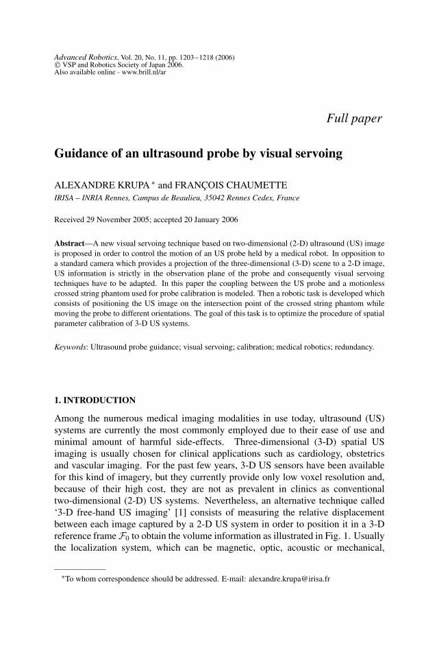
Advanced Robotics, Vol. 20, No. 11, pp. 1203–1218 (2006) VSP and Robotics Society of Japan 2006.Also available online - www.brill.nl/ar
Full paper
Guidance of an ultrasound probe by visual servoing
ALEXANDRE KRUPA ∗ and FRANÇOIS CHAUMETTEIRISA – INRIA Rennes, Campus de Beaulieu, 35042 Rennes Cedex, France
Received 29 November 2005; accepted 20 January 2006
Abstract—A new visual servoing technique based on two-dimensional (2-D) ultrasound (US) imageis proposed in order to control the motion of an US probe held by a medical robot. In opposition toa standard camera which provides a projection of the three-dimensional (3-D) scene to a 2-D image,US information is strictly in the observation plane of the probe and consequently visual servoingtechniques have to be adapted. In this paper the coupling between the US probe and a motionlesscrossed string phantom used for probe calibration is modeled. Then a robotic task is developed whichconsists of positioning the US image on the intersection point of the crossed string phantom whilemoving the probe to different orientations. The goal of this task is to optimize the procedure of spatialparameter calibration of 3-D US systems.
Keywords: Ultrasound probe guidance; visual servoing; calibration; medical robotics; redundancy.
1. INTRODUCTION
Among the numerous medical imaging modalities in use today, ultrasound (US)systems are currently the most commonly employed due to their ease of use andminimal amount of harmful side-effects. Three-dimensional (3-D) spatial USimaging is usually chosen for clinical applications such as cardiology, obstetricsand vascular imaging. For the past few years, 3-D US sensors have been availablefor this kind of imagery, but they currently provide only low voxel resolution and,because of their high cost, they are not as prevalent in clinics as conventionaltwo-dimensional (2-D) US systems. Nevertheless, an alternative technique called‘3-D free-hand US imaging’ [1] consists of measuring the relative displacementbetween each image captured by a 2-D US system in order to position it in a 3-Dreference frame F0 to obtain the volume information as illustrated in Fig. 1. Usuallythe localization system, which can be magnetic, optic, acoustic or mechanical,
∗To whom correspondence should be addressed. E-mail: [email protected]
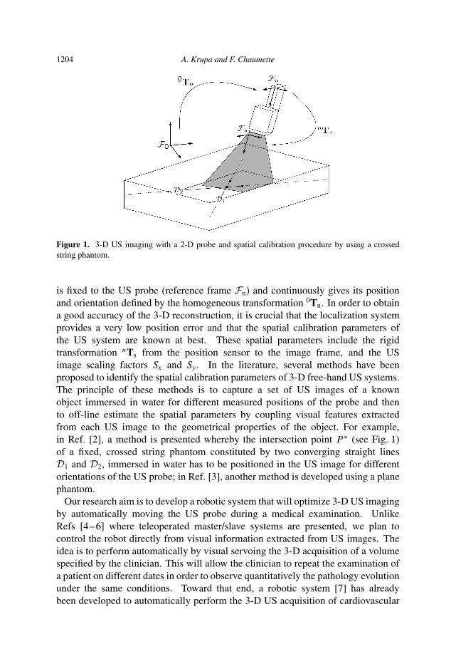
1204 A. Krupa and F. Chaumette
Figure 1. 3-D US imaging with a 2-D probe and spatial calibration procedure by using a crossedstring phantom.
is fixed to the US probe (reference frame Fn) and continuously gives its positionand orientation defined by the homogeneous transformation 0Tn. In order to obtaina good accuracy of the 3-D reconstruction, it is crucial that the localization systemprovides a very low position error and that the spatial calibration parameters ofthe US system are known at best. These spatial parameters include the rigidtransformation nTs from the position sensor to the image frame, and the USimage scaling factors Sx and Sy . In the literature, several methods have beenproposed to identify the spatial calibration parameters of 3-D free-hand US systems.The principle of these methods is to capture a set of US images of a knownobject immersed in water for different measured positions of the probe and thento off-line estimate the spatial parameters by coupling visual features extractedfrom each US image to the geometrical properties of the object. For example,in Ref. [2], a method is presented whereby the intersection point P ∗ (see Fig. 1)of a fixed, crossed string phantom constituted by two converging straight linesD1 and D2, immersed in water has to be positioned in the US image for differentorientations of the US probe; in Ref. [3], another method is developed using a planephantom.
Our research aim is to develop a robotic system that will optimize 3-D US imagingby automatically moving the US probe during a medical examination. UnlikeRefs [4–6] where teleoperated master/slave systems are presented, we plan tocontrol the robot directly from visual information extracted from US images. Theidea is to perform automatically by visual servoing the 3-D acquisition of a volumespecified by the clinician. This will allow the clinician to repeat the examination ofa patient on different dates in order to observe quantitatively the pathology evolutionunder the same conditions. Toward that end, a robotic system [7] has alreadybeen developed to automatically perform the 3-D US acquisition of cardiovascular
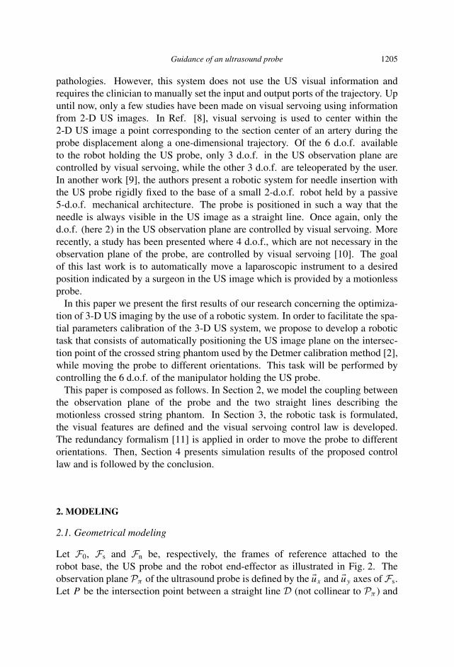
Guidance of an ultrasound probe 1205
pathologies. However, this system does not use the US visual information andrequires the clinician to manually set the input and output ports of the trajectory. Upuntil now, only a few studies have been made on visual servoing using informationfrom 2-D US images. In Ref. [8], visual servoing is used to center within the2-D US image a point corresponding to the section center of an artery during theprobe displacement along a one-dimensional trajectory. Of the 6 d.o.f. availableto the robot holding the US probe, only 3 d.o.f. in the US observation plane arecontrolled by visual servoing, while the other 3 d.o.f. are teleoperated by the user.In another work [9], the authors present a robotic system for needle insertion withthe US probe rigidly fixed to the base of a small 2-d.o.f. robot held by a passive5-d.o.f. mechanical architecture. The probe is positioned in such a way that theneedle is always visible in the US image as a straight line. Once again, only thed.o.f. (here 2) in the US observation plane are controlled by visual servoing. Morerecently, a study has been presented where 4 d.o.f., which are not necessary in theobservation plane of the probe, are controlled by visual servoing [10]. The goalof this last work is to automatically move a laparoscopic instrument to a desiredposition indicated by a surgeon in the US image which is provided by a motionlessprobe.
In this paper we present the first results of our research concerning the optimiza-tion of 3-D US imaging by the use of a robotic system. In order to facilitate the spa-tial parameters calibration of the 3-D US system, we propose to develop a robotictask that consists of automatically positioning the US image plane on the intersec-tion point of the crossed string phantom used by the Detmer calibration method [2],while moving the probe to different orientations. This task will be performed bycontrolling the 6 d.o.f. of the manipulator holding the US probe.
This paper is composed as follows. In Section 2, we model the coupling betweenthe observation plane of the probe and the two straight lines describing themotionless crossed string phantom. In Section 3, the robotic task is formulated,the visual features are defined and the visual servoing control law is developed.The redundancy formalism [11] is applied in order to move the probe to differentorientations. Then, Section 4 presents simulation results of the proposed controllaw and is followed by the conclusion.
2. MODELING
2.1. Geometrical modeling
Let F0, Fs and Fn be, respectively, the frames of reference attached to therobot base, the US probe and the robot end-effector as illustrated in Fig. 2. Theobservation plane Pπ of the ultrasound probe is defined by the �ux and �uy axes of Fs.Let P be the intersection point between a straight line D (not collinear to Pπ ) and
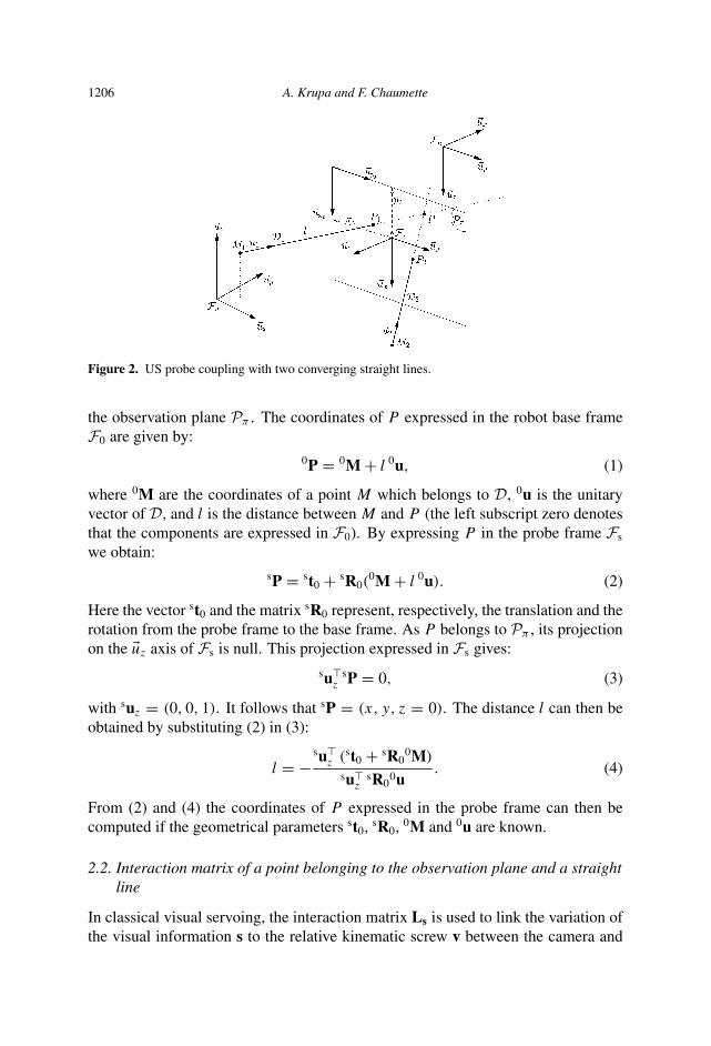
1206 A. Krupa and F. Chaumette
Figure 2. US probe coupling with two converging straight lines.
the observation plane Pπ . The coordinates of P expressed in the robot base frameF0 are given by:
0P = 0M + l 0u, (1)
where 0M are the coordinates of a point M which belongs to D, 0u is the unitaryvector of D, and l is the distance between M and P (the left subscript zero denotesthat the components are expressed in F0). By expressing P in the probe frame Fs
we obtain:sP = st0 + sR0(
0M + l 0u). (2)
Here the vector st0 and the matrix sR0 represent, respectively, the translation and therotation from the probe frame to the base frame. As P belongs to Pπ , its projectionon the �uz axis of Fs is null. This projection expressed in Fs gives:
su�z
sP = 0, (3)
with suz = (0, 0, 1). It follows that sP = (x, y, z = 0). The distance l can then beobtained by substituting (2) in (3):
l = −su�
z (st0 + sR00M)
su�z
sR00u
. (4)
From (2) and (4) the coordinates of P expressed in the probe frame can then becomputed if the geometrical parameters st0, sR0, 0M and 0u are known.
2.2. Interaction matrix of a point belonging to the observation plane and a straightline
In classical visual servoing, the interaction matrix Ls is used to link the variation ofthe visual information s to the relative kinematic screw v between the camera and
Guidance of an ultrasound probe 1207
the scene:
s = Lsv. (5)
In our system, the visual information associated to the point P are its 2-Dcoordinates p = (x, y) expressed in the US probe frame. Since the imagecoordinates are measured in pixels in the 2-D image frame {�uxp, �uyp} attached atthe left-top corner of the image plane, the following variable transformation has tobe made to obtain p = (x, y) which is expressed in m:
x = (xp − xc)Sx and y = (yp − yc)Sy, (6)
where (xp, yp) are the pixel coordinates of P , (xc, yc) are the pixel coordinates of theimage center, and Sx and Sy are, respectively, the height and width of a pixel. Theanalytical form of the interaction matrix related to p is determined by calculatingthe time derivative of (2):
sP = st0 + sR0(0M + l 0u) + sR0(
0M + l 0u). (7)
As the point M is fixed with respect to F0, we have:
sP = st0 + sR0(0M + l 0u) + sR0 l 0u. (8)
Let us define v = (υ, ω) as the velocity screw of the probe expressed in Fs
with υ = (υx, υy, υz) the translational velocity vector and ω = (ωx, ωy, ωz) theangular velocity vector of the probe frame with respect to the base frame. The timederivative of the rotational matrix is linked to ω by [11]:
sR0 = −[ω]×sR0, (9)
with [ω]× being the skew symmetric matrix associated with the angular velocityvector ω. The term st0 is the velocity of the base frame origin with respect to theprobe frame. It is related to the velocity screw v of the probe by the followingfundamental equation of kinematics:
st0 = −υ + [st0]×ω = [−I3 [st0]×]v, (10)
where [st0]× is the skew symmetric matrix associated with st0. By substituting (2),(9) and (10) in (8), we obtain:
sP = [sP]×ω + l sR00u − υ. (11)
By applying the projection relation su�z
sP = 0, the time derivative of the distance l
can then be extracted:
l =su�
z υ − su�z [sP]×ω
su�z
sR00u
, (12)
1208 A. Krupa and F. Chaumette
which after substitution in (11) gives the following expression:
sP =(
[sP]× −susu�
z
su�z
su[sP]×
)ω
+( susu�
z
su�z
su− I3
)υ, (13)
where su = sR00u = (ux, uy, uz) is the unitary vector of D expressed in the
probe frame. Finally, we can determine the interaction matrix Lp related to p bydeveloping the two first rows of (13):
p = (x, y) = Lpv, (14)
with
Lp =
−1 0ux
uz
ux
uz
y −ux
uz
x y
0 −1uy
uz
uy
uz
y −uy
uz
x −x
. (15)
This matrix depends on the components of the unitary vector su of the straight lineD and the 2-D coordinates p, all expressed in the probe frame. The condition tocompute Lp is that uz �= 0. This is verified when D is not collinear to the observationplan Pπ . Note that if P coincides with the origin of Fs then p is invariant to therotational motion of the US probe and if D is orthogonal to Pπ (ux = 0 and uy = 0)then p is invariant to the translational motion along �uz.
3. VISUAL SERVOING
First, let us formulate the robotic task to achieve. The goal is to position theintersection point P ∗ between two converging straight lines D1 and D2 not collinearto the US observation plan Pπ (see Fig. 2) on a target point defined in the US imagewith a set of different orientations of the probe. For each orientation, the end-effector pose will be recorded once the point is positioned in the image in order toestimate the spatial calibration parameters of the US system by the use of the off-line Detmer method [2]. The visual task consists in centering the points P1 and P2
on a target indicated in the image.
3.1. Vision-based task function
The visual features s we chose are the 2-D coordinates p1 = (x1, y1) and p2 =(x2, y2) of points P1 and P2 expressed in the probe frame:
s = (x1, y1, x2, y2). (16)
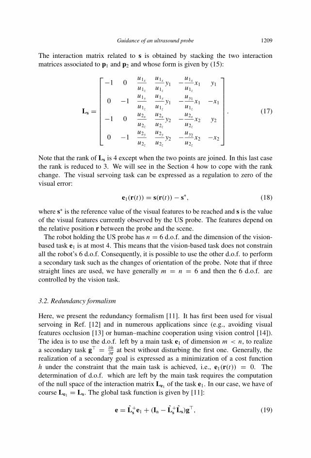
Guidance of an ultrasound probe 1209
The interaction matrix related to s is obtained by stacking the two interactionmatrices associated to p1 and p2 and whose form is given by (15):
Ls =
−1 0u1x
u1z
u1x
u1z
y1 −u1x
u1z
x1 y1
0 −1u1y
u1z
u1y
u1z
y1 −uy1
u1z
x1 −x1
−1 0u2x
u2z
u2x
u2z
y2 −u2x
u2z
x2 y2
0 −1u2y
u2z
u2y
u2z
y2 −uy2
u2z
x2 −x2
. (17)
Note that the rank of Ls is 4 except when the two points are joined. In this last casethe rank is reduced to 3. We will see in the Section 4 how to cope with the rankchange. The visual servoing task can be expressed as a regulation to zero of thevisual error:
e1(r(t)) = s(r(t)) − s∗, (18)
where s∗ is the reference value of the visual features to be reached and s is the valueof the visual features currently observed by the US probe. The features depend onthe relative position r between the probe and the scene.
The robot holding the US probe has n = 6 d.o.f. and the dimension of the vision-based task e1 is at most 4. This means that the vision-based task does not constrainall the robot’s 6 d.o.f. Consequently, it is possible to use the other d.o.f. to performa secondary task such as the changes of orientation of the probe. Note that if threestraight lines are used, we have generally m = n = 6 and then the 6 d.o.f. arecontrolled by the vision task.
3.2. Redundancy formalism
Here, we present the redundancy formalism [11]. It has first been used for visualservoing in Ref. [12] and in numerous applications since (e.g., avoiding visualfeatures occlusion [13] or human–machine cooperation using vision control [14]).The idea is to use the d.o.f. left by a main task e1 of dimension m < n, to realizea secondary task g� = ∂h
∂r at best without disturbing the first one. Generally, therealization of a secondary goal is expressed as a minimization of a cost functionh under the constraint that the main task is achieved, i.e., e1(r(t)) = 0. Thedetermination of d.o.f. which are left by the main task requires the computationof the null space of the interaction matrix Le1 of the task e1. In our case, we have ofcourse Le1 = Ls. The global task function is given by [11]:
e = L+s e1 + (In − L+
s Ls)g�, (19)
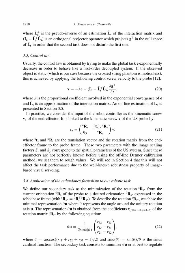
1210 A. Krupa and F. Chaumette
where L+s is the pseudo-inverse of an estimation Ls of the interaction matrix and
(In − L+s Ls) is an orthogonal projector operator which projects g� in the null space
of Ls in order that the second task does not disturb the first one.
3.3. Control law
Usually, the control law is obtained by trying to make the global task e exponentiallydecrease in order to behave like a first-order decoupled system. If the observedobject is static (which is our case because the crossed string phantom is motionless),this is achieved by applying the following control screw velocity to the probe [12]:
v = −λe − (In − L+s Ls)
∂g�
∂t, (20)
where λ is the proportional coefficient involved in the exponential convergence of eand Ls is an approximation of the interaction matrix. An on-line estimation of Ls ispresented in Section 3.5.
In practice, we consider the input of the robot controller as the kinematic screwvn of the end-effector. It is linked to the kinematic screw v of the US probe by:
vn =( nRs [nts]×nRs
03nRs
)v, (21)
where nts and nRs are the translation vector and the rotation matrix from the end-effector frame to the probe frame. These two parameters with the image scalingfactors Sx and Sy correspond to the spatial parameters of the US system. Since theseparameters are not perfectly known before using the off-line Detmer calibrationmethod, we set them to rough values. We will see in Section 4 that this will notaffect the task performance due to the well-known robustness property of image-based visual servoing.
3.4. Application of the redundancy formalism to our robotic task
We define our secondary task as the minimization of the rotation sRs∗ from thecurrent orientation 0Rs of the probe to a desired orientation 0Rs∗ expressed in therobot base frame (with sRs∗ = 0R�
s0Rs∗). To describe the rotation sRs∗ , we chose the
minimal representation θu where θ represents the angle around the unitary rotationaxis u. The representation θu is obtained from the coefficients rij (i=1..3,j=1..3) of therotation matrix sRs∗ by the following equation:
θu = 1
2sinc(θ)
r32 − r23
r13 − r31
r21 − r12
, (22)
where θ = arccos((r11 + r22 + r33 − 1)/2) and sinc(θ) = sin(θ)/θ is the sinuscardinal function. The secondary task consists to minimize θu or at best to regulate
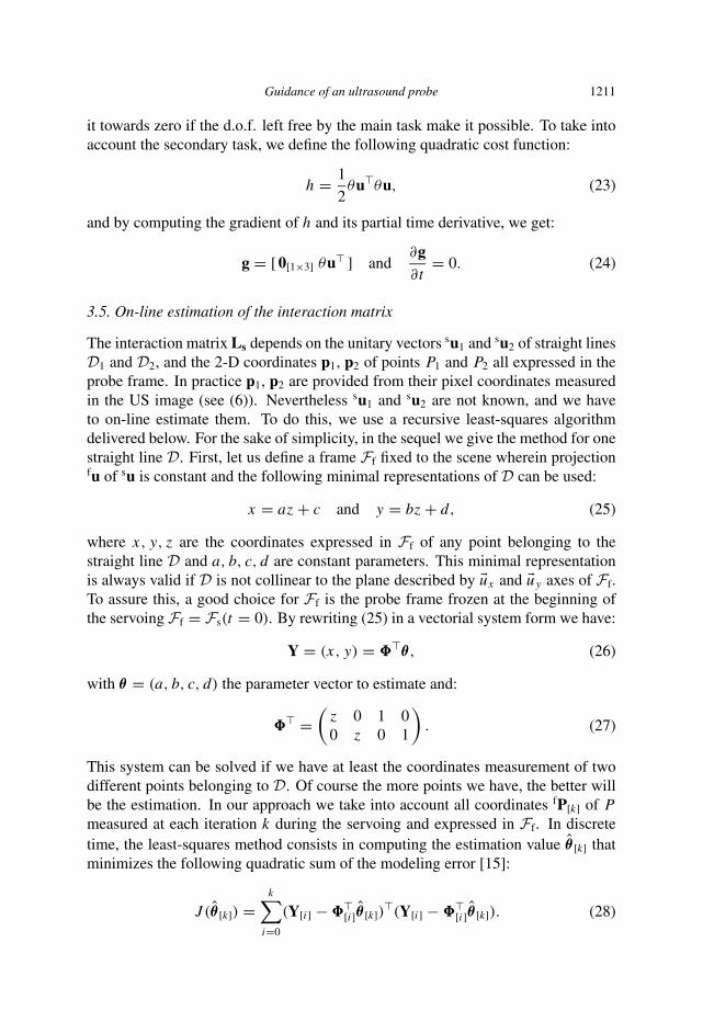
Guidance of an ultrasound probe 1211
it towards zero if the d.o.f. left free by the main task make it possible. To take intoaccount the secondary task, we define the following quadratic cost function:
h = 1
2θu�θu, (23)
and by computing the gradient of h and its partial time derivative, we get:
g = [0[1×3] θu� ] and∂g∂t
= 0. (24)
3.5. On-line estimation of the interaction matrix
The interaction matrix Ls depends on the unitary vectors su1 and su2 of straight linesD1 and D2, and the 2-D coordinates p1, p2 of points P1 and P2 all expressed in theprobe frame. In practice p1, p2 are provided from their pixel coordinates measuredin the US image (see (6)). Nevertheless su1 and su2 are not known, and we haveto on-line estimate them. To do this, we use a recursive least-squares algorithmdelivered below. For the sake of simplicity, in the sequel we give the method for onestraight line D. First, let us define a frame Ff fixed to the scene wherein projectionfu of su is constant and the following minimal representations of D can be used:
x = az + c and y = bz + d, (25)
where x, y, z are the coordinates expressed in Ff of any point belonging to thestraight line D and a, b, c, d are constant parameters. This minimal representationis always valid if D is not collinear to the plane described by �ux and �uy axes of Ff.To assure this, a good choice for Ff is the probe frame frozen at the beginning ofthe servoing Ff = Fs(t = 0). By rewriting (25) in a vectorial system form we have:
Y = (x, y) = ��θ , (26)
with θ = (a, b, c, d) the parameter vector to estimate and:
�� =(
z 0 1 00 z 0 1
). (27)
This system can be solved if we have at least the coordinates measurement of twodifferent points belonging to D. Of course the more points we have, the better willbe the estimation. In our approach we take into account all coordinates fP[k] of P
measured at each iteration k during the servoing and expressed in Ff. In discretetime, the least-squares method consists in computing the estimation value θ [k] thatminimizes the following quadratic sum of the modeling error [15]:
J (θ [k]) =k∑
i=0
(Y[i] − ��[i]θ [k])�(Y[i] − ��
[i]θ [k]). (28)
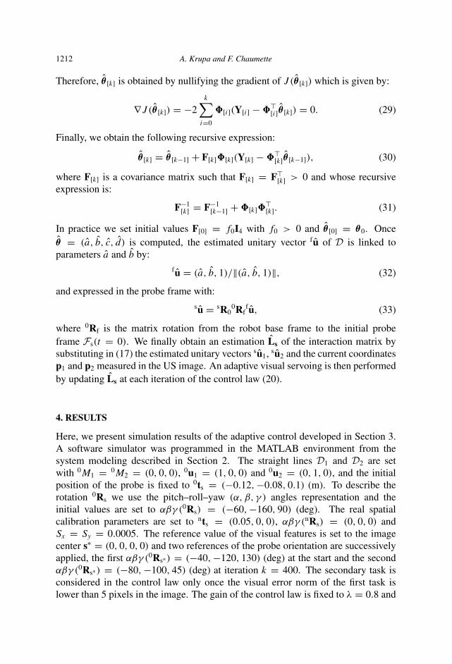
1212 A. Krupa and F. Chaumette
Therefore, θ [k] is obtained by nullifying the gradient of J (θ [k]) which is given by:
∇J (θ [k]) = −2k∑
i=0
�[i](Y[i] − ��[i]θ [k]) = 0. (29)
Finally, we obtain the following recursive expression:
θ [k] = θ [k−1] + F[k]�[k](Y[k] − ��[k]θ [k−1]), (30)
where F[k] is a covariance matrix such that F[k] = F�[k] > 0 and whose recursive
expression is:
F−1[k] = F−1
[k−1] + �[k]��[k]. (31)
In practice we set initial values F[0] = f0I4 with f0 > 0 and θ [0] = θ0. Onceθ = (a, b, c, d) is computed, the estimated unitary vector fu of D is linked toparameters a and b by:
fu = (a, b, 1)/‖(a, b, 1)‖, (32)
and expressed in the probe frame with:
su = sR00Rf
fu, (33)
where 0Rf is the matrix rotation from the robot base frame to the initial probeframe Fs(t = 0). We finally obtain an estimation Ls of the interaction matrix bysubstituting in (17) the estimated unitary vectors su1, su2 and the current coordinatesp1 and p2 measured in the US image. An adaptive visual servoing is then performedby updating Ls at each iteration of the control law (20).
4. RESULTS
Here, we present simulation results of the adaptive control developed in Section 3.A software simulator was programmed in the MATLAB environment from thesystem modeling described in Section 2. The straight lines D1 and D2 are setwith 0M1 = 0M2 = (0, 0, 0), 0u1 = (1, 0, 0) and 0u2 = (0, 1, 0), and the initialposition of the probe is fixed to 0ts = (−0.12, −0.08, 0.1) (m). To describe therotation 0Rs we use the pitch–roll–yaw (α, β, γ ) angles representation and theinitial values are set to αβγ (0Rs) = (−60, −160, 90) (deg). The real spatialcalibration parameters are set to nts = (0.05, 0, 0), αβγ (nRs) = (0, 0, 0) andSx = Sy = 0.0005. The reference value of the visual features is set to the imagecenter s∗ = (0, 0, 0, 0) and two references of the probe orientation are successivelyapplied, the first αβγ (0Rs∗) = (−40, −120, 130) (deg) at the start and the secondαβγ (0Rs∗) = (−80, −100, 45) (deg) at iteration k = 400. The secondary task isconsidered in the control law only once the visual error norm of the first task islower than 5 pixels in the image. The gain of the control law is fixed to λ = 0.8 and
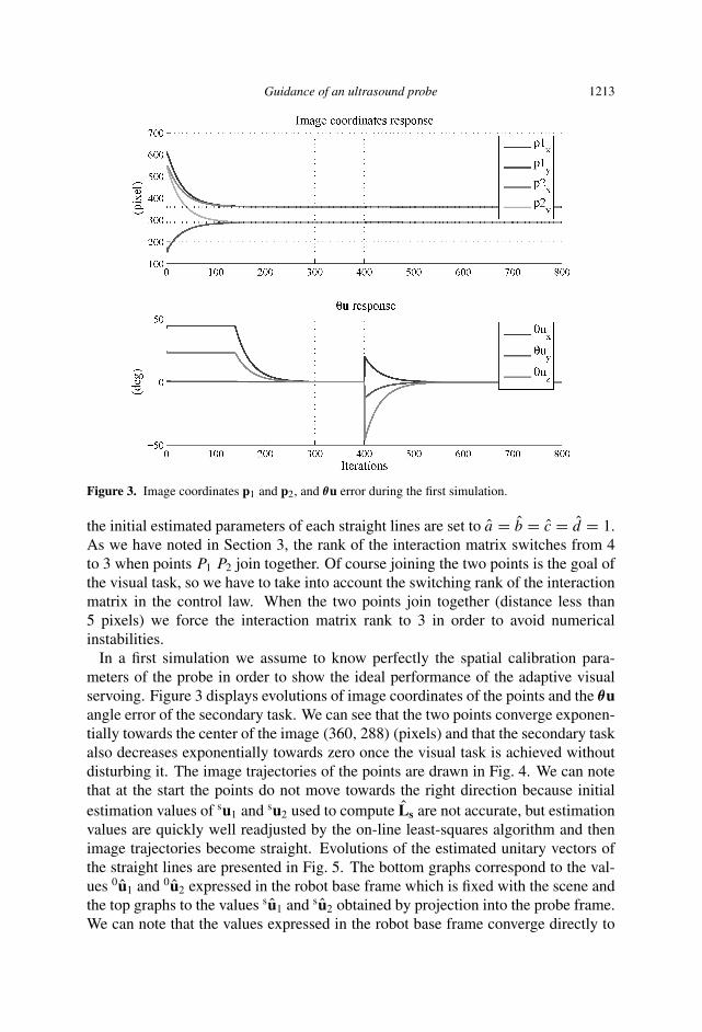
Guidance of an ultrasound probe 1213
Figure 3. Image coordinates p1 and p2, and θu error during the first simulation.
the initial estimated parameters of each straight lines are set to a = b = c = d = 1.As we have noted in Section 3, the rank of the interaction matrix switches from 4to 3 when points P1 P2 join together. Of course joining the two points is the goal ofthe visual task, so we have to take into account the switching rank of the interactionmatrix in the control law. When the two points join together (distance less than5 pixels) we force the interaction matrix rank to 3 in order to avoid numericalinstabilities.
In a first simulation we assume to know perfectly the spatial calibration para-meters of the probe in order to show the ideal performance of the adaptive visualservoing. Figure 3 displays evolutions of image coordinates of the points and the θuangle error of the secondary task. We can see that the two points converge exponen-tially towards the center of the image (360, 288) (pixels) and that the secondary taskalso decreases exponentially towards zero once the visual task is achieved withoutdisturbing it. The image trajectories of the points are drawn in Fig. 4. We can notethat at the start the points do not move towards the right direction because initialestimation values of su1 and su2 used to compute Ls are not accurate, but estimationvalues are quickly well readjusted by the on-line least-squares algorithm and thenimage trajectories become straight. Evolutions of the estimated unitary vectors ofthe straight lines are presented in Fig. 5. The bottom graphs correspond to the val-ues 0u1 and 0u2 expressed in the robot base frame which is fixed with the scene andthe top graphs to the values su1 and su2 obtained by projection into the probe frame.We can note that the values expressed in the robot base frame converge directly to
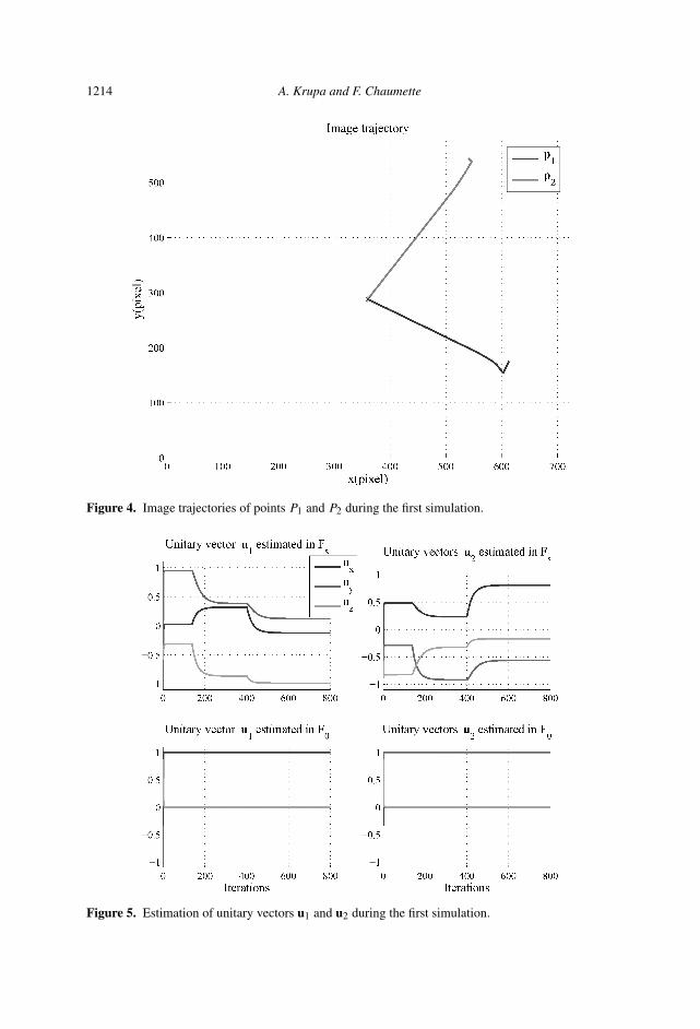
1214 A. Krupa and F. Chaumette
Figure 4. Image trajectories of points P1 and P2 during the first simulation.
Figure 5. Estimation of unitary vectors u1 and u2 during the first simulation.
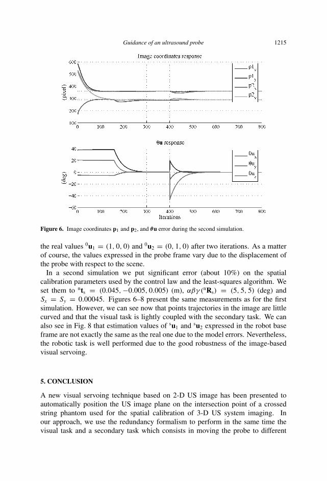
Guidance of an ultrasound probe 1215
Figure 6. Image coordinates p1 and p2, and θu error during the second simulation.
the real values 0u1 = (1, 0, 0) and 0u2 = (0, 1, 0) after two iterations. As a matterof course, the values expressed in the probe frame vary due to the displacement ofthe probe with respect to the scene.
In a second simulation we put significant error (about 10%) on the spatialcalibration parameters used by the control law and the least-squares algorithm. Weset them to nts = (0.045, −0.005, 0.005) (m), αβγ (nRs) = (5, 5, 5) (deg) andSx = Sy = 0.00045. Figures 6–8 present the same measurements as for the firstsimulation. However, we can see now that points trajectories in the image are littlecurved and that the visual task is lightly coupled with the secondary task. We canalso see in Fig. 8 that estimation values of su1 and su2 expressed in the robot baseframe are not exactly the same as the real one due to the model errors. Nevertheless,the robotic task is well performed due to the good robustness of the image-basedvisual servoing.
5. CONCLUSION
A new visual servoing technique based on 2-D US image has been presented toautomatically position the US image plane on the intersection point of a crossedstring phantom used for the spatial calibration of 3-D US system imaging. Inour approach, we use the redundancy formalism to perform in the same time thevisual task and a secondary task which consists in moving the probe to different
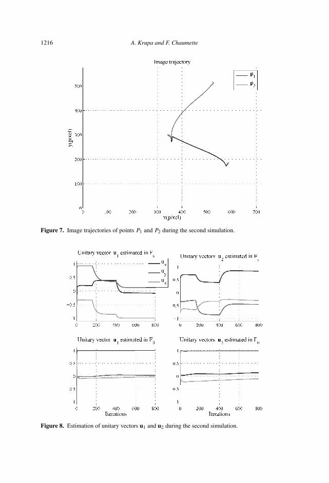
1216 A. Krupa and F. Chaumette
Figure 7. Image trajectories of points P1 and P2 during the second simulation.
Figure 8. Estimation of unitary vectors u1 and u2 during the second simulation.
Guidance of an ultrasound probe 1217
orientations. An adaptive control law has been proposed by updating the interactionmatrix related to the visual features thanks to an estimation algorithm. For themoment, results are obtained from simulation, but we plan to perform our taskwith a 6-d.o.f. medical manipulator specially designed for 3-D US imaging whichwill soon be available in our laboratory. Simulation results showed that the visualservoing is robust to large errors on the spatial calibration parameters.
REFERENCES
1. T. R. Nelson and D. H. Pretorius, Three-dimensional ultrasound imaging, Ultrasound Med. Biol.24, 1243–1270 (1998).
2. P. R. Detmer, G. Basheim, T. Hodges, K. W. Beach, E. P. Filer, D. H. Burns and D. E. StrandnessJr, 3D ultrasonic image feature localization based on magnetic scanhead tracking: in vitrocalibration and validation, Ultrasound Med. Biol. 20, 923–936 (1994).
3. F. Rousseau, P. Hellier and C. Barillot, Robust and automatic calibration method for 3Dfreehand ultrasound, in: Proc. Int. Conf. on Medical Image Computing and Computer AssistedIntervention, Montreal, pp. 440–448 (2003).
4. K. Masuda, E. Kimura, N. Tateishi and K. Ishihara, Three-dimensional motion mechanism ofultrasound probe and its application for tele-echography system, in: Proc. IEEE/RSJ Int. Conf.on Intelligent Robots and Systems, Maui, HI, pp. 1112–1116 (2001).
5. A. Vilchis, J. Troccaz, P. Cinquin, K. Masuda and F. Pellisier, A new robot architecture forteleechography, IEEE Trans. Robotics Automat. 19, 922–926 (2003).
6. M. Mitsuishi, S. Warisawa, T. Tsuda, T. Higuchi, N. Koizumi, H. Hashizume and K. Fujiwara,Remote ultrasound diagnostic system, in: Proc. IEEE Int. Conf. on Robotics and Automation,Seoul, pp. 1567–1574 (2001).
7. F. Pierrot, E. Dombre, E. Degoulange, L. Urbain, P. Caron, S. Boudet, J. Gariepy and J. Megnien,Hippocrate: a safe robot arm for medical applications with force feedback, Med. Image Analysis3, 285–300 (1999).
8. P. Abolmaesumi, S. E. Salcudean, W. H. Zhu, M. Sirouspour and S. P. DiMaio, Image-guidedcontrol of a robot for medical ultrasound, IEEE Trans. Robotics Automat. 18, 11–23 (2002).
9. J. Hong, T. Dohi, M. Hashizume, K. Konishi and N. Hata, An ultrasound-driven needle insertionrobot for percutaneous cholecystostomy, Phys. Med. Biol. 49, 441–455 (2004).
10. M. A. Vitrani, G. Morel and T. Ortmaier, Automatic guidance of a surgical instrument withultrasound based visual servoing, in: Proc. IEEE Int. Conf. on Robotics and Automation,Barcelona, pp. 510–515 (2005).
11. C. Samson, M. Le Borgne and B. Espiau, Robot Control: The Task Function Approach.Clarendon Press, Oxford (1991).
12. B. Espiau, F. Chaumette and P. Rives, A new approach to visual servoing in robotics, IEEETrans. Robotics Automat. 8, 313–326 (1992).
13. E. Marchand and G.-D. Hager, Dynamic sensor planning in visual servoing, in: Proc. IEEE/RSJInt. Conf. on Intelligent Robots and Systems, Leuven, Vol. 3, pp. 1988–1993 (1998).
14. G. D. Hager, Human-machine cooperative manipulation with vision-based motion constraints,presented at: Workshop on Visual Servoing (IROS’02), Lausanne (2002).
15. R. Johansson, System Modeling and Identification. Prentice-Hall, Englewood Cliffs, NJ (1993).
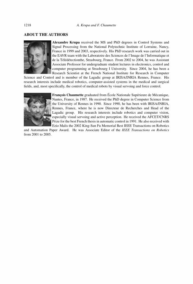
1218 A. Krupa and F. Chaumette
ABOUT THE AUTHORS
Alexandre Krupa received the MS and PhD degrees in Control Systems andSignal Processing from the National Polytechnic Institute of Lorraine, Nancy,France in 1999 and 2003, respectively. His PhD research work was carried out inthe EAVR team with the Laboratoire des Sciences de l’Image de l’Informatique etde la Télédétectionthe, Strasbourg, France. From 2002 to 2004, he was AssistantAssociate Professor for undergraduate student lectures in electronics, control andcomputer programming at Strasbourg I University. Since 2004, he has been aResearch Scientist at the French National Institute for Research in Computer
Science and Control and is member of the Lagadic group at IRISA/INRIA Rennes, France. Hisresearch interests include medical robotics, computer-assisted systems in the medical and surgicalfields, and, most specifically, the control of medical robots by visual servoing and force control.
François Chaumette graduated from École Nationale Supérieure de Mécanique,Nantes, France, in 1987. He received the PhD degree in Computer Science fromthe University of Rennes in 1990. Since 1990, he has been with IRISA/INRIA,Rennes, France, where he is now Directeur de Recherches and Head of theLagadic group. His research interests include robotics and computer vision,especially visual servoing and active perception. He received the AFCET/CNRSPrize for the best French thesis in automatic control in 1991. He also received withEzio Malis the 2002 King-Sun Fu Memorial Best IEEE Transactions on Robotics
and Automation Paper Award. He was Associate Editor of the IEEE Transactions on Roboticsfrom 2001 to 2005.
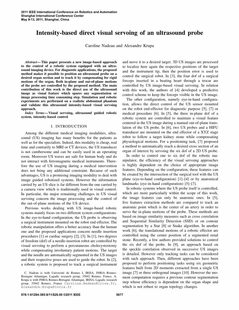
Intensity-based direct visual servoing of an ultrasound probe
Caroline Nadeau and Alexandre Krupa
Abstract— This paper presents a new image-based approachto the control of a robotic system equipped with an ultra-sound imaging device. For diagnostic applications, the proposedmethod makes it possible to position an ultrasound probe on adesired organ section and to track it by compensating for rigidmotions of the organ. Both in-plane and out-of-plane motionsof the probe are controlled by the proposed method. The maincontribution of this work is the direct use of the ultrasoundimage as visual feature which spares any segmentation orimage processing time consuming step. Simulation and roboticexperiments are performed on a realistic abdominal phantomand validate this ultrasound intensity-based visual servoingapproach.
Index Terms— Visual servoing, ultrasound guided roboticsystem, intensity-based control
I. INTRODUCTION
Among the different medical imaging modalities, ultra-sound (US) imaging has many benefits for the patients aswell as for the specialists. Indeed, this modality is cheap, realtime and contrarily to MRI or CT devices, the US transduceris not cumbersome and can be easily used in an operatingroom. Moreover US waves are safe for human body and donot interact with ferromagnetic medical instruments. There-fore the use of US imaging during a medical interventiondoes not bring any additional constraint. Because of suchadvantages, US is a promising imaging modality to deal withimage guided robotized systems. However the informationcarried by an US slice is far different from the one carried bya camera view which is traditionally used in visual control.In particular, the major remaining challenges in US visualservoing concern the image processing and the control ofthe out-of-plane motions of the US device.
Previous works dealing with US image-based roboticsystems mainly focus on two different system configurations.In the eye-to-hand configuration, the US probe is observinga surgical instrument mounted on the robot end-effector. Therobotic manipulation offers a better accuracy than the humanone and the proposed applications concern needle insertionprocedures [1] or cardiac surgery [2], [3]. In [1], two degreesof freedom (dof) of a needle-insertion robot are controlled byvisual servoing to perform a percutaneous cholecystostomywhile compensating involuntary patient motions. The targetand the needle are automatically segmented in the US imagesand their respective poses are used to guide the robot. In [2],a robotic system is proposed to track a surgical instrument
C. Nadeau is with Universite de Rennes I, IRISA, INRIA Rennes-Bretagne Atlantique, Lagadic research group, 35042 Rennes, France. A.Krupa is with INRIA Rennes-Bretagne Atlantique, IRISA, Lagadic researchgroup, 35042 Rennes, France [email protected],[email protected]
and move it to a desired target. 3D US images are processedto localize here again the respective positions of the targetand the instrument tip, then the position error is used tocontrol the surgical robot. In [3], the four dof of a surgicalforceps inserted in a beating heart through a trocar arecontrolled by US image-based visual servoing. In relationwith this work, the authors of [4] developed a predictivecontrol scheme to keep the forceps visible in the US image.
The other configuration, namely eye-in-hand configura-tion, allows the direct control of the US sensor mountedon the robot end-effector for diagnostic purpose [5], [7] ormedical procedure [6]. In [5], the three in-plane dof of arobotic system are controlled to maintain a visual featurecentered in the US image during a manual out-of-plane trans-lation of the US probe. In [6], two US probes and a HIFUtransducer are mounted on the end effector of a XYZ stagerobot to follow a target kidney stone while compensatingphysiological motions. For a positioning task, [7] proposeda method to automatically reach a desired cross section of anorgan of interest by servoing the six dof of a 2D US probe.
In order to control one to six dof of the robotic ma-nipulator, the efficiency of the visual servoing approachesis highly dependent on the choice of appropriate imagefeatures. Depending on the configuration, these features canbe created by the intersection of the surgical tool with the USplane (eye-to-hand configuration) [1]–[4] or by anatomicallandmarks (eye-in-hand configuration) [5]–[7].
In robotic systems where the US probe itself is controlled,which are more particularly within the scope of this work,the image features can only be anatomic ones. In [5],five features extraction methods are compared to track ananatomic point which is the center of an artery in order toservo the in-plane motions of the probe. These methods arebased on image similarity measures such as cross correlationand Sequential Similarity Detection (SSD) or on contoursegmentation by a Star [8] or Snake algorithm. In anotherwork [6], the translational motions of a robotic effector arecontrolled using the center position of a segmented renalstone. Recently, a few authors provided solutions to controlthe six dof of the probe. In [9], an approach based onthe speckle correlation observed in successive US imagesis detailed. However only tracking tasks can be consideredwith such approach. Then, different approaches have beenproposed to perform positioning tasks using six geometricfeatures built from 2D moments extracted from a single USimage [7] or three orthogonal images [10]. However the mo-ment computation requires a previous contour segmentationstep whose efficiency is dependent on the organ shape andwhich is not robust to organ topology changes.
2011 IEEE International Conference on Robotics and AutomationShanghai International Conference CenterMay 9-13, 2011, Shanghai, China
978-1-61284-385-8/11/$26.00 ©2011 IEEE 5677
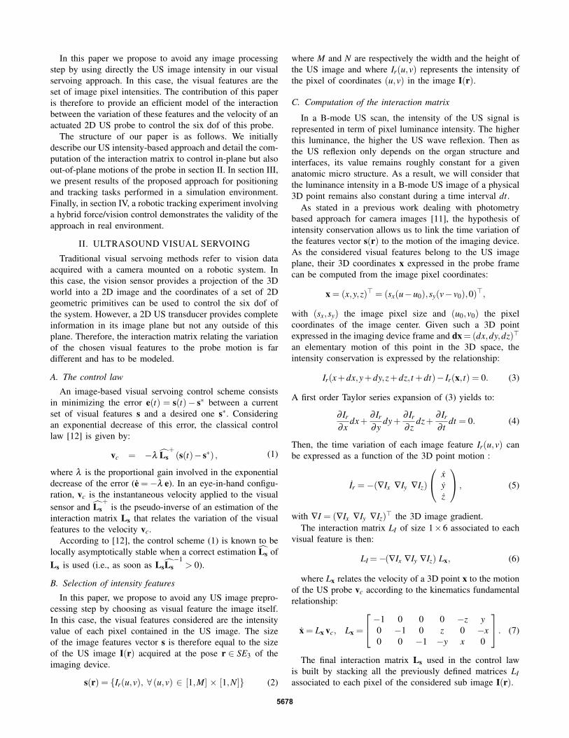
In this paper we propose to avoid any image processingstep by using directly the US image intensity in our visualservoing approach. In this case, the visual features are theset of image pixel intensities. The contribution of this paperis therefore to provide an efficient model of the interactionbetween the variation of these features and the velocity of anactuated 2D US probe to control the six dof of this probe.
The structure of our paper is as follows. We initiallydescribe our US intensity-based approach and detail the com-putation of the interaction matrix to control in-plane but alsoout-of-plane motions of the probe in section II. In section III,we present results of the proposed approach for positioningand tracking tasks performed in a simulation environment.Finally, in section IV, a robotic tracking experiment involvinga hybrid force/vision control demonstrates the validity of theapproach in real environment.
II. ULTRASOUND VISUAL SERVOING
Traditional visual servoing methods refer to vision dataacquired with a camera mounted on a robotic system. Inthis case, the vision sensor provides a projection of the 3Dworld into a 2D image and the coordinates of a set of 2Dgeometric primitives can be used to control the six dof ofthe system. However, a 2D US transducer provides completeinformation in its image plane but not any outside of thisplane. Therefore, the interaction matrix relating the variationof the chosen visual features to the probe motion is fardifferent and has to be modeled.
A. The control law
An image-based visual servoing control scheme consistsin minimizing the error e(t) = s(t)− s∗ between a currentset of visual features s and a desired one s∗. Consideringan exponential decrease of this error, the classical controllaw [12] is given by:
vc = −λ Ls+
(s(t)− s∗) , (1)
where λ is the proportional gain involved in the exponentialdecrease of the error (e =−λ e). In an eye-in-hand configu-ration, vc is the instantaneous velocity applied to the visualsensor and Ls
+is the pseudo-inverse of an estimation of the
interaction matrix Ls that relates the variation of the visualfeatures to the velocity vc.
According to [12], the control scheme (1) is known to belocally asymptotically stable when a correct estimation Ls ofLs is used (i.e., as soon as LsLs
−1> 0).
B. Selection of intensity features
In this paper, we propose to avoid any US image prepro-cessing step by choosing as visual feature the image itself.In this case, the visual features considered are the intensityvalue of each pixel contained in the US image. The sizeof the image features vector s is therefore equal to the sizeof the US image I(r) acquired at the pose r ∈ SE3 of theimaging device.
s(r) = {Ir(u,v), ∀ (u,v) ∈ [1,M] × [1,N]} (2)
where M and N are respectively the width and the height ofthe US image and where Ir(u,v) represents the intensity ofthe pixel of coordinates (u,v) in the image I(r).
C. Computation of the interaction matrix
In a B-mode US scan, the intensity of the US signal isrepresented in term of pixel luminance intensity. The higherthis luminance, the higher the US wave reflexion. Then asthe US reflexion only depends on the organ structure andinterfaces, its value remains roughly constant for a givenanatomic micro structure. As a result, we will consider thatthe luminance intensity in a B-mode US image of a physical3D point remains also constant during a time interval dt.
As stated in a previous work dealing with photometrybased approach for camera images [11], the hypothesis ofintensity conservation allows us to link the time variation ofthe features vector s(r) to the motion of the imaging device.As the considered visual features belong to the US imageplane, their 3D coordinates x expressed in the probe framecan be computed from the image pixel coordinates:
x = (x,y,z)> = (sx(u−u0),sy(v− v0),0)>,
with (sx,sy) the image pixel size and (u0,v0) the pixelcoordinates of the image center. Given such a 3D pointexpressed in the imaging device frame and dx = (dx,dy,dz)>
an elementary motion of this point in the 3D space, theintensity conservation is expressed by the relationship:
Ir(x+dx,y+dy,z+dz, t +dt)− Ir(x, t) = 0. (3)
A first order Taylor series expansion of (3) yields to:
∂ Ir
∂xdx+
∂ Ir
∂ydy+
∂ Ir
∂ zdz+
∂ Ir
∂ tdt = 0. (4)
Then, the time variation of each image feature Ir(u,v) canbe expressed as a function of the 3D point motion :
Ir =−(∇Ix ∇Iy ∇Iz)
xyz
, (5)
with ∇I = (∇Ix ∇Iy ∇Iz)> the 3D image gradient.The interaction matrix LI of size 1×6 associated to each
visual feature is then:
LI =−(∇Ix ∇Iy ∇Iz) Lx, (6)
where Lx relates the velocity of a 3D point x to the motionof the US probe vc according to the kinematics fundamentalrelationship:
x = Lx vc, Lx =
−1 0 0 0 −z y0 −1 0 z 0 −x0 0 −1 −y x 0
. (7)
The final interaction matrix Ls used in the control lawis built by stacking all the previously defined matrices LIassociated to each pixel of the considered sub image I(r).
5678
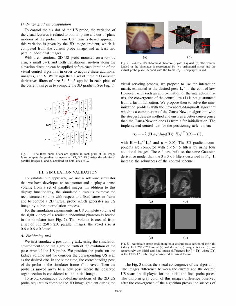
D. Image gradient computation
To control the six dof of the US probe, the variation ofthe visual features is related to both in-plane and out-of-planemotions of the probe. In our US intensity-based approach,this variation is given by the 3D image gradient, which iscomputed from the current probe image and at least twoparallel additional images.
With a conventional 2D US probe mounted on a roboticarm, a small back and forth translational motion along theelevation direction can be applied before each iteration of thevisual control algorithm in order to acquire these additionalimages Ia and Ib. We design then a set of three 3D Gaussianderivatives filters of size 3× 3× 3 applied in each pixel ofthe current image I0 to compute the 3D gradient (see Fig. 1).
Fig. 1. The three cubic filters are applied in each pixel of the imageI0 to compute the gradient components (∇Ix,∇Iy,∇Iz) using the additionalparallel images Ia and Ib acquired on both sides of I0.
III. SIMULATION VALIDATIONTo validate our approach, we use a software simulator
that we have developed to reconstruct and display a densevolume from a set of parallel images. In addition to thisdisplay functionality, the simulator allows us to move thereconstructed volume with respect to a fixed cartesian frameand to control a 2D virtual probe which generates an USimage by cubic interpolation process.
For the simulation experiments, an US complete volume ofthe right kidney of a realistic abdominal phantom is loadedin the simulator (see Fig. 2). This volume is created froma set of 335 250× 250 parallel images, the voxel size is0.6×0.6×0.3mm3.
A. Positioning task
We first simulate a positioning task, using the simulationenvironment to obtain a ground truth of the evolution of thepose error of the US probe. We position the probe on thekidney volume and we consider the corresponding US scanas the desired one. In the same time, the corresponding poseof the probe in the simulator frame r∗ is saved. Then theprobe is moved away to a new pose where the observedorgan section is considered as the initial image.
To avoid continuous out-of-plane motions of the 2D USprobe required to compute the 3D image gradient during the
(a) (b)Fig. 2. (a) The US abdominal phantom (Kyoto Kagaku). (b) The volumeloaded in the simulator is represented by two orthogonal slices and thevirtual probe plane, defined with the frame Fp, is displayed in red.
visual servoing process, we propose to use the interactionmatrix estimated at the desired pose Ls
∗ in the control law.However, with such an approximation of the interaction ma-trix, the convergence of the control law (1) is not guaranteedfrom a far initialization. We propose then to solve the min-imization problem with the Levenberg-Marquardt algorithmwhich is a combination of the Gauss-Newton algorithm withthe steepest descent method and ensures a better convergencethan the Gauss-Newton one (1) from a far initialization. Theimplemented control law for the positioning task is then:
vc =−λ (H+ µdiag(H))−1Ls∗> (s(t)− s∗) ,
with H = Ls∗>Ls
∗ and µ = 0.05. The 3D gradient com-ponents are computed with 5× 5× 5 filters by using fouradditional images. These filters, built on the same Gaussianderivative model than the 3×3×3 filters described in Fig. 1,increase the robustness of the control scheme.
(a) (b)
(c) (d)Fig. 3. Automatic probe positioning on a desired cross section of the rightkidney. Full 250× 250 initial (a) and desired (b) images. (c) and (d) arerespectively the initial and final image differences I(r∗)− I(r) where I(r)is the 170×170 sub image considered as visual feature.
The Fig. 3 shows the visual convergence of the algorithm.The images difference between the current and the desiredUS scans are displayed for the initial and final probe poses.The uniform gray color of this images difference observedafter the convergence of the algorithm proves the success of
5679
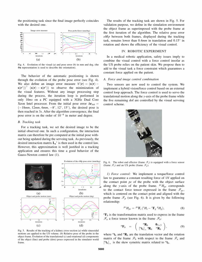
the positioning task since the final image perfectly coincideswith the desired one.
(a) (b)Fig. 4. Evolution of the visual (a) and pose error (b) in mm and deg, (theθu representation is used to describe the orientation).
The behavior of the automatic positioning is shownthrough the evolution of the probe pose error (see Fig. 4).We also define an image error measure C (r) = (s(r)−s(r∗))> (s(r) − s(r∗)) to observe the minimization ofthe visual features. Without any image processing stepduring the process, the iteration loop is performed inonly 10ms on a PC equipped with a 3GHz Dual CoreXeon Intel processor. From the initial pose error ∆rinit =(−18mm, 12mm, 6mm, −8◦, 12◦, 15◦), the desired pose isthen reached in 3s. After the algorithm convergence, the finalpose error is on the order of 10−6 in meter and degree.
B. Tracking task
For a tracking task, we set the desired image to be theinitial observed one. In such a configuration, the interactionmatrix can therefore be pre computed at the initial pose with-out being updated during the servoing task. As previously, thedesired interaction matrix Ls
∗ is then used in the control law.However, this approximation is well justified in a trackingapplication and ensures this time a good behavior of theGauss-Newton control law (1).
(a) (b)
(c) (d)Fig. 5. Results of the tracking of a kidney cross-section (a) while sinusoidalmotions are applied to the US volume. (b) Relative pose of the probe in theobject frame. Evolution of the translational (c) and rotational (d) componentsof the object (line) and probe (dots) poses expressed in the simulator worldframe.
The results of the tracking task are shown in Fig. 5. Forvalidation purpose, we define in the simulation environmentthe object frame as superimposed with the probe frame atthe first iteration of the algorithm. The relative pose erroroMp between both frames, displayed during the trackingtask, remains lower than 0.4mm in translation and 0.15◦ inrotation and shows the efficiency of the visual control.
IV. ROBOTIC EXPERIMENT
In a medical robotic application, safety issues imply tocombine the visual control with a force control insofar asthe US probe relies on the patient skin. We propose then toadd to the visual task a force constraint which guarantees aconstant force applied on the patient.
A. Force and image control combination
Two sensors are now used to control the system. Weimplement a hybrid vision/force control based on an externalcontrol loop approach. The force control is used to servo thetranslational motion along the y-axis of the probe frame whilethe five remaining dof are controlled by the visual servoingcontrol scheme.
Fig. 6. The robot end effector (frame Fe) is equipped with a force sensor(frame Fs) and an US probe (frame Fp).
1) Force control: We implement a torque/force controllaw to guarantee a constant resulting force of 1N applied onthe contact point pc of the probe with the object surfacealong the y-axis of the probe frame. pcHpc correspondsto the contact force tensor expressed in the frame Fpc,which is centered on the contact point and aligned with theprobe frame Fp (see Fig. 6). It is given by the followingrelationship:
pcHpc = pcFs (sHs− sFggHg), (8)
aFb is the transformation matrix used to express in the frameFa a force tensor known in the frame Fb:
aFb =( aRb 03×3
[atb]×aRb
aRb
), (9)
where atb and aRb are the translation vector and the rotationmatrix of the frame Fb with respect to the frame Fa and[atb]× is the skew symetric matrix related to atb.
5680
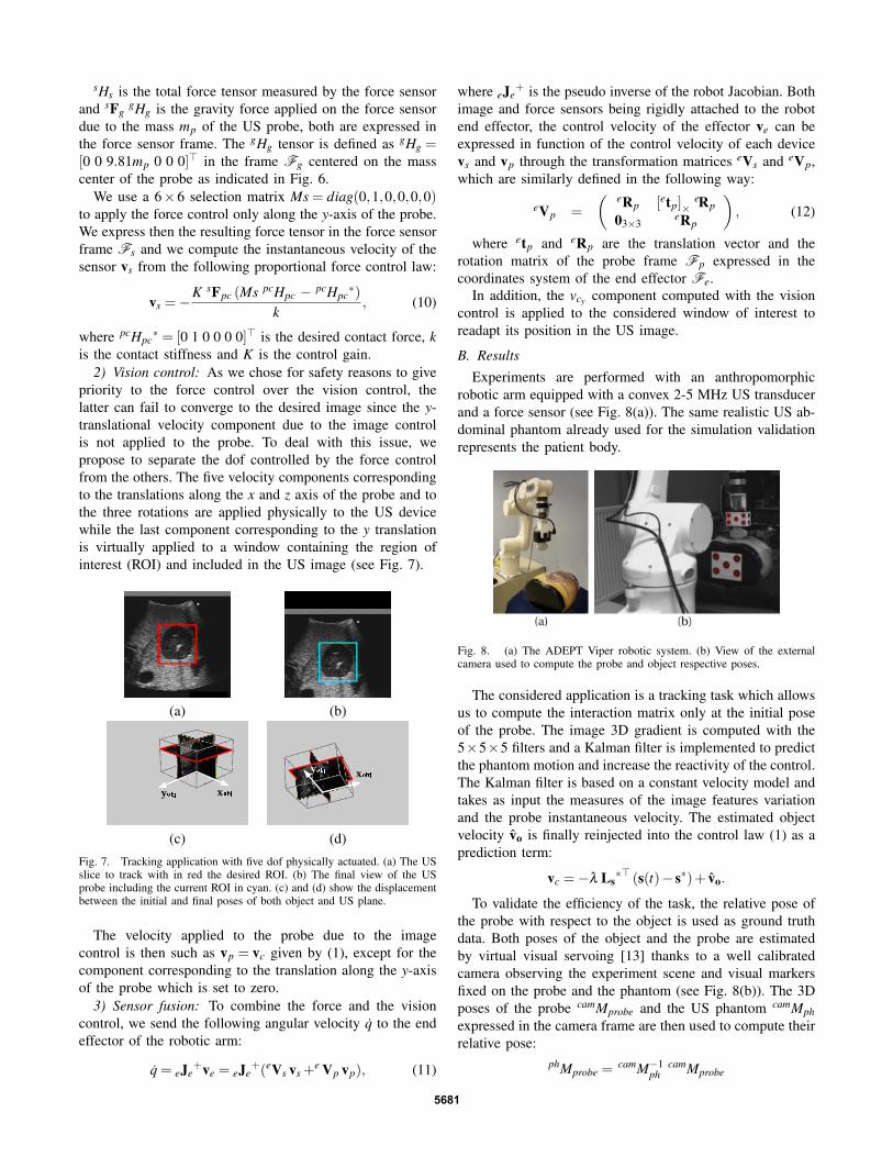
sHs is the total force tensor measured by the force sensorand sFg
gHg is the gravity force applied on the force sensordue to the mass mp of the US probe, both are expressed inthe force sensor frame. The gHg tensor is defined as gHg =[0 0 9.81mp 0 0 0]> in the frame Fg centered on the masscenter of the probe as indicated in Fig. 6.
We use a 6×6 selection matrix Ms = diag(0,1,0,0,0,0)to apply the force control only along the y-axis of the probe.We express then the resulting force tensor in the force sensorframe Fs and we compute the instantaneous velocity of thesensor vs from the following proportional force control law:
vs =−K sFpc (Ms pcHpc − pcHpc
∗)k
, (10)
where pcHpc∗ = [0 1 0 0 0 0]> is the desired contact force, k
is the contact stiffness and K is the control gain.2) Vision control: As we chose for safety reasons to give
priority to the force control over the vision control, thelatter can fail to converge to the desired image since the y-translational velocity component due to the image controlis not applied to the probe. To deal with this issue, wepropose to separate the dof controlled by the force controlfrom the others. The five velocity components correspondingto the translations along the x and z axis of the probe and tothe three rotations are applied physically to the US devicewhile the last component corresponding to the y translationis virtually applied to a window containing the region ofinterest (ROI) and included in the US image (see Fig. 7).
(a) (b)
(c) (d)Fig. 7. Tracking application with five dof physically actuated. (a) The USslice to track with in red the desired ROI. (b) The final view of the USprobe including the current ROI in cyan. (c) and (d) show the displacementbetween the initial and final poses of both object and US plane.
The velocity applied to the probe due to the imagecontrol is then such as vp = vc given by (1), except for thecomponent corresponding to the translation along the y-axisof the probe which is set to zero.
3) Sensor fusion: To combine the force and the visioncontrol, we send the following angular velocity q to the endeffector of the robotic arm:
q = eJe+ve = eJe
+(eVs vs +e Vp vp), (11)
where eJe+ is the pseudo inverse of the robot Jacobian. Both
image and force sensors being rigidly attached to the robotend effector, the control velocity of the effector ve can beexpressed in function of the control velocity of each devicevs and vp through the transformation matrices eVs and eVp,which are similarly defined in the following way:
eVp =( eRp [etp]×
eRp03×3
eRp
), (12)
where etp and eRp are the translation vector and therotation matrix of the probe frame Fp expressed in thecoordinates system of the end effector Fe.
In addition, the vcy component computed with the visioncontrol is applied to the considered window of interest toreadapt its position in the US image.
B. ResultsExperiments are performed with an anthropomorphic
robotic arm equipped with a convex 2-5 MHz US transducerand a force sensor (see Fig. 8(a)). The same realistic US ab-dominal phantom already used for the simulation validationrepresents the patient body.
Fig. 8. (a) The ADEPT Viper robotic system. (b) View of the externalcamera used to compute the probe and object respective poses.
The considered application is a tracking task which allowsus to compute the interaction matrix only at the initial poseof the probe. The image 3D gradient is computed with the5×5×5 filters and a Kalman filter is implemented to predictthe phantom motion and increase the reactivity of the control.The Kalman filter is based on a constant velocity model andtakes as input the measures of the image features variationand the probe instantaneous velocity. The estimated objectvelocity vo is finally reinjected into the control law (1) as aprediction term:
vc =−λ Ls∗> (s(t)− s∗)+ vo.
To validate the efficiency of the task, the relative pose ofthe probe with respect to the object is used as ground truthdata. Both poses of the object and the probe are estimatedby virtual visual servoing [13] thanks to a well calibratedcamera observing the experiment scene and visual markersfixed on the probe and the phantom (see Fig. 8(b)). The 3Dposes of the probe camMprobe and the US phantom camMphexpressed in the camera frame are then used to compute theirrelative pose:
phMprobe = camM−1ph
camMprobe
5681
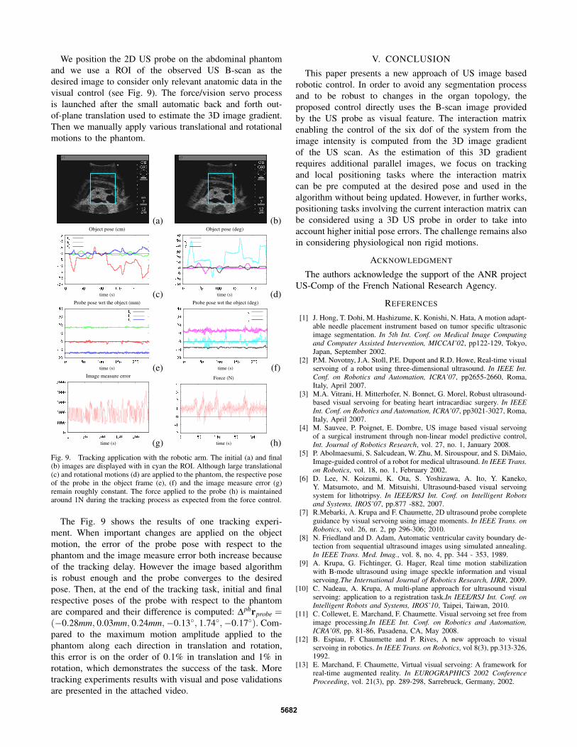
We position the 2D US probe on the abdominal phantomand we use a ROI of the observed US B-scan as thedesired image to consider only relevant anatomic data in thevisual control (see Fig. 9). The force/vision servo processis launched after the small automatic back and forth out-of-plane translation used to estimate the 3D image gradient.Then we manually apply various translational and rotationalmotions to the phantom.
(a) (b)
(c) (d)
(e) (f)
(g) (h)Fig. 9. Tracking application with the robotic arm. The initial (a) and final(b) images are displayed with in cyan the ROI. Although large translational(c) and rotational motions (d) are applied to the phantom, the respective poseof the probe in the object frame (e), (f) and the image measure error (g)remain roughly constant. The force applied to the probe (h) is maintainedaround 1N during the tracking process as expected from the force control.
The Fig. 9 shows the results of one tracking experi-ment. When important changes are applied on the objectmotion, the error of the probe pose with respect to thephantom and the image measure error both increase becauseof the tracking delay. However the image based algorithmis robust enough and the probe converges to the desiredpose. Then, at the end of the tracking task, initial and finalrespective poses of the probe with respect to the phantomare compared and their difference is computed: ∆phrprobe =(−0.28mm, 0.03mm, 0.24mm,−0.13◦, 1.74◦,−0.17◦). Com-pared to the maximum motion amplitude applied to thephantom along each direction in translation and rotation,this error is on the order of 0.1% in translation and 1% inrotation, which demonstrates the success of the task. Moretracking experiments results with visual and pose validationsare presented in the attached video.
V. CONCLUSION
This paper presents a new approach of US image basedrobotic control. In order to avoid any segmentation processand to be robust to changes in the organ topology, theproposed control directly uses the B-scan image providedby the US probe as visual feature. The interaction matrixenabling the control of the six dof of the system from theimage intensity is computed from the 3D image gradientof the US scan. As the estimation of this 3D gradientrequires additional parallel images, we focus on trackingand local positioning tasks where the interaction matrixcan be pre computed at the desired pose and used in thealgorithm without being updated. However, in further works,positioning tasks involving the current interaction matrix canbe considered using a 3D US probe in order to take intoaccount higher initial pose errors. The challenge remains alsoin considering physiological non rigid motions.
ACKNOWLEDGMENT
The authors acknowledge the support of the ANR projectUS-Comp of the French National Research Agency.
REFERENCES
[1] J. Hong, T. Dohi, M. Hashizume, K. Konishi, N. Hata, A motion adapt-able needle placement instrument based on tumor specific ultrasonicimage segmentation. In 5th Int. Conf. on Medical Image Computingand Computer Assisted Intervention, MICCAI’02, pp122-129, Tokyo,Japan, September 2002.
[2] P.M. Novotny, J.A. Stoll, P.E. Dupont and R.D. Howe, Real-time visualservoing of a robot using three-dimensional ultrasound. In IEEE Int.Conf. on Robotics and Automation, ICRA’07, pp2655-2660, Roma,Italy, April 2007.
[3] M.A. Vitrani, H. Mitterhofer, N. Bonnet, G. Morel, Robust ultrasound-based visual servoing for beating heart intracardiac surgery. In IEEEInt. Conf. on Robotics and Automation, ICRA’07, pp3021-3027, Roma,Italy, April 2007.
[4] M. Sauvee, P. Poignet, E. Dombre, US image based visual servoingof a surgical instrument through non-linear model predictive control,Int. Journal of Robotics Research, vol. 27, no. 1, January 2008.
[5] P. Abolmaesumi, S. Salcudean, W. Zhu, M. Sirouspour, and S. DiMaio,Image-guided control of a robot for medical ultrasound. In IEEE Trans.on Robotics, vol. 18, no. 1, February 2002.
[6] D. Lee, N. Koizumi, K. Ota, S. Yoshizawa, A. Ito, Y. Kaneko,Y. Matsumoto, and M. Mitsuishi, Ultrasound-based visual servoingsystem for lithotripsy. In IEEE/RSJ Int. Conf. on Intelligent Robotsand Systems, IROS’07, pp.877 -882, 2007.
[7] R.Mebarki, A. Krupa and F. Chaumette, 2D ultrasound probe completeguidance by visual servoing using image moments. In IEEE Trans. onRobotics, vol. 26, nr. 2, pp 296-306; 2010.
[8] N. Friedland and D. Adam, Automatic ventricular cavity boundary de-tection from sequential ultrasound images using simulated annealing.In IEEE Trans. Med. Imag., vol. 8, no. 4, pp. 344 - 353, 1989.
[9] A. Krupa, G. Fichtinger, G. Hager, Real time motion stabilizationwith B-mode ultrasound using image speckle information and visualservoing.The International Journal of Robotics Research, IJRR, 2009.
[10] C. Nadeau, A. Krupa, A multi-plane approach for ultrasound visualservoing: application to a registration task.In IEEE/RSJ Int. Conf. onIntelligent Robots and Systems, IROS’10, Taipei, Taiwan, 2010.
[11] C. Collewet, E. Marchand, F. Chaumette. Visual servoing set free fromimage processing.In IEEE Int. Conf. on Robotics and Automation,ICRA’08, pp. 81-86, Pasadena, CA, May 2008.
[12] B. Espiau, F. Chaumette and P. Rives, A new approach to visualservoing in robotics. In IEEE Trans. on Robotics, vol 8(3), pp.313-326,1992.
[13] E. Marchand, F. Chaumette, Virtual visual servoing: A framework forreal-time augmented reality. In EUROGRAPHICS 2002 ConferenceProceeding, vol. 21(3), pp. 289-298, Sarrebruck, Germany, 2002.
5682
Intensity-based visual servoing for non-rigid motion compensation ofsoft tissue structures due to physiological motion using 4D ultrasound
Deukhee Lee and Alexandre Krupa
Abstract— This paper presents a visual-servoing method forcompensating motion of soft tissue structures using 4D ultra-sound. The motion of soft tissue structures caused by physiologi-cal and external motion makes it difficult to investigate them fordiagnostic and therapeutic purposes. The main goal is to tracknon-rigidly moving soft tissue structures and compensate themotion in order to keep a lesion on its target position during atreatment. We define a 3D non-rigid motion model by extendingthe Thin-Plate Spline (TPS) algorithm. The motion parametersare estimated with intensity-value changes of a points set in atracking soft tissue structure. Finally, the global rigid motionis compensated with a 6-DOF robot according to the motionparameters of the tracking structure. Simulation experimentsare performed with recorded 3D US images of in-vivo soft tissuestructures and validate the effectiveness of the non-rigid motiontracking method. Robotic experiments demonstrated the successof our method with a deformable phantom.
I. INTRODUCTION
Medical imaging modalities make it possible to observesoft tissue structures non-invasively. Among them, ultrasound(US) imaging has many benefits. It is cheap, real-time,safe for human body, and non-interactive with ferromagneticmaterials. For these reasons, US is the most widespreadmedical imaging modality.
Physiological motions such as respiration and heartbeatmove soft tissue structures globally and deform them locally.Therefore this motion of soft tissue structures makes itdifficult to investigate them for diagnostic and therapeuticpurposes. Especially the target position of non-invasive ther-apy should follow the physiological motion of a movinglesion.
There are some literatures to deal with motion compensa-tion using US imaging. In [1] and [2], speckle decorrelationis used to estimate elevational motion of 2D US probe,and Krupa et al.[2] successfully compensate the soft tissuerigid motion with a 2D probe attached to a robot. In [3],an US image-based visual servoing method is presented toposition a 2D probe on a desired organ section and track itthanks to the use of image moments obtained from contoursegmentation. Nadeau tracks 3D rigid motion using a virtual3D US probe in [4]. In [5], 3D translational motions areestimated using 4D US. However, non-rigid motion is notconsidered in the above methods.
The contributions of this paper are to track 3D non-rigid motion using 4D US in real time and to compensatethe motion. At our best knowledge, unlike other non-rigid
The authors are with INRIA Rennes-Bretagne Atlantique, IRISA,Campus de Beaulieu, 35042 Rennes cedex, France Deukhee.Lee,[email protected]
registration procedures, our method is processed in realtime. In the rest of this paper, a non-rigid motion modelis defined using 3D Thin-Plate Spline (TPS). Then, anintensity-based tracking method is described to estimatethe parameters of the motion model. Global rigid motionsuch as 3 translations and 3 rotations are extracted fromnon-rigid motion parameters. Finally, a 6 degree-of-freedom(DOF) robot equipped with a 4D US probe is controlled tocompensate the rigid motion. Tracking accuracy is discussedfrom simulation experiments using in-vivo US images andthe effectiveness of the proposed method is also verified fromrobotic experiments with a deformable tissue-mimicking(TM) phantom.
II. NON-RIGID MOTION TRACKING
Before compensating the 3D motion of soft tissue struc-tures, a new method to estimate 3D motion of deformablesoft tissue is proposed in this section.
A. 3D Scan Conversion
We use a SonixTOUCH Research 4D US scanner (Ul-trasonix Medical Corporation, Canada) and a motorizedUS 3D transducer (Model: 4DC7-3/40, Ultrasonix MedicalCorporation, Canada). Since the 4D US scanner is designedfor the purpose of research works, we can access digital databefore the conversion into an image. Afterwards, a set ofvolume data is converted into a volumetric image, called as3D scan conversion.
For scan conversion, geometries of the probe (the 2D UStransducer’s radius Rprobe and the motor’s radius Rmotor) andimaging parameters (the number of sample data in a A-lineNsamples, the number of A-lines in a frame Nlines, and thenumber of frames in a scan volume N f rames, angle betweenneighboring A-lines αline, and angle between neighboringframes α f rame) are considered in (1). In Fig. 1, a samples(i, j,k), which is the i-th datum along the j-th A-linein the k-th frame, is relocated into a point p(r,ϕ,θ) ina volumetric image, which is represented as p(x,y,z) inCartesian coordinates according to (1) and (2).
Note that our 3D US probe continuously scans volumeswhile its motor is sweeping the volume in forward and back-ward directions. Additionally, sweeping direction d (whichis 1 in the forward direction and 0 in the backward directionin (1c)) and motor’s rotating motion should be considered.In (1c), we assumed that the motor stops during the time toscan A-line so that scan lines are straight.
2011 IEEE/RSJ International Conference onIntelligent Robots and SystemsSeptember 25-30, 2011. San Francisco, CA, USA
978-1-61284-456-5/11/$26.00 ©2011 IEEE 2831
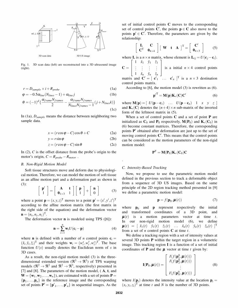
φ θ
RprobeRmotor
X X
YZ
p(x, y, z)r
p
JK
I
s(i, j, k)
3D scan data 3D US image
r
OO
…
Fig. 1. 3D scan data (left) are reconstructed into a 3D ultrasound image(right).
r = Dsample× i+Rprobe (1a)ϕ =−0.5αline(Nlines−1)+αline j (1b)
θ = (−1)d{α f rameN f rames
2−
α f rameN f rames
NlinesN f rames−1( j+Nlinesk)}
(1c)
In (1a), Dsample means the distance between neighboring twosample data.
x = (r cosϕ−C)cosθ +C (2a)y = r sinϕ (2b)z = (r cosϕ−C)sinθ (2c)
In (2), C is the offset distance from the probe’s origin to themotor’s origin, C = Rprobe−Rmotor .
B. Non-Rigid Motion Model
Soft tissue structures move and deform due to physiologi-cal motion. Therefore, we can model the motion of soft tissueas an affine motion part and a deformation part as shown in(3): [
p′1
]=
[A t
01×3 1
][p1
]+
[n0
](3)
where a point p = (x,y,z)T moves to a point p′ = (x′,y′,z′)T
according to the affine motion matrix (the first matrix inthe right side of the equation) and the deformation vectorn = (nx,ny,nz)
T.The deformation vector n is modeled using TPS ([6]):
n =n
∑i=1
wiU(ci−p) (4)
where n is defined with a number of n control points ci =(xi, yi, zi)
T and their weights wi = (wxi ,w
yi ,w
zi )
T. The basefunction U(s) usually denotes the Euclidean norm of s in3D cases.
As a result, the non-rigid motion model (3) is the three-dimensional extended version (ℜ3 → ℜ3) of TPS warpingmodels (ℜ2→ℜ2 and ℜ2→ℜ3, respectively) presented in[7] and [8]. The parameters of the motion model, ( A, t, andW= {w1,w2, . . . ,wn}), are estimated with a set of points P={p1, . . . ,pn} in the reference image and the correspondingset of points P′ = {p′1, . . . ,p′n} in sequential images. As the
set of initial control points C moves to the correspondingset of control points C′, the points p ∈ C also move to thepoints p′ ∈ C′. Therefore, the parameters are given by therelationship:[
L CCT 04×4
][W t A
]T=
[C′
04×3
](5)
where L is a n×n matrix, whose element is Li j =U(c j−ci).
C =
1 x1 y1 z1...
......
...1 xn yn zn
is a initial n× 4 control points
matrix and C′ = [ c′1 . . . c′n ]T is a n× 3 destinationcontrol points matrix.
According to [6], the motion model (3) is rewritten as (6).
p′T = M(p)K∗(C)C′ (6)
where M(p) = [ U(p− c1) . . . U(p− cn) 1 x y z ]and K∗(C) denotes the (n+4)×n sub-matrix of the invertedform of the leftmost matrix in (5).
When a set of control points C and a set of point P areinitialized as C0 and P0 respectively, M(P0) and K∗(C0) in(6) become constant matrices. Therefore, the correspondingpoints P′ obtained after deformation are just up to the set ofmoving control points C′. This means that the control pointscan be considered as the motion parameters of the non-rigidmotion model:
PT = M(P0)K∗(C0)C
.
C. Intensity-Based Tracking
Now, we propose to use the parametric motion modeldefined in the previous section to track a deformable objectfrom a sequence of 3D US images. Based on the sameprinciple of the 2D region tracking method presented in [9]we define a parametric motion model:
p = f (p0,µµµ(t)) (7)
where p0 and p represent respectively the initialand transformed coordinates of a 3D point, andµµµ(t) is a motion parameters vector at time t.In our non-rigid motion model (6), we defineµµµ(t) = [ x1(t) y1(t) z1(t) . . . xn(t) yn(t) zn(t) ]T
from a set of n control points C at time t.We define a tracking region with a set of intensity values at
several 3D points P within the target region in a volumetricimage. This tracking region I is a function of a set of initialcoordinates of P and the µµµ vector at time t given by:
I(P0,µµµ(t)) =
I( f (p0
1,µµµ(t)))I( f (p0
2,µµµ(t)))...
I( f (p0N ,µµµ(t)))
(8)
where I(pi) denotes the intensity value at the location pi =(xi,yi,zi)
T at time t and N is the number of 3D points.
2832
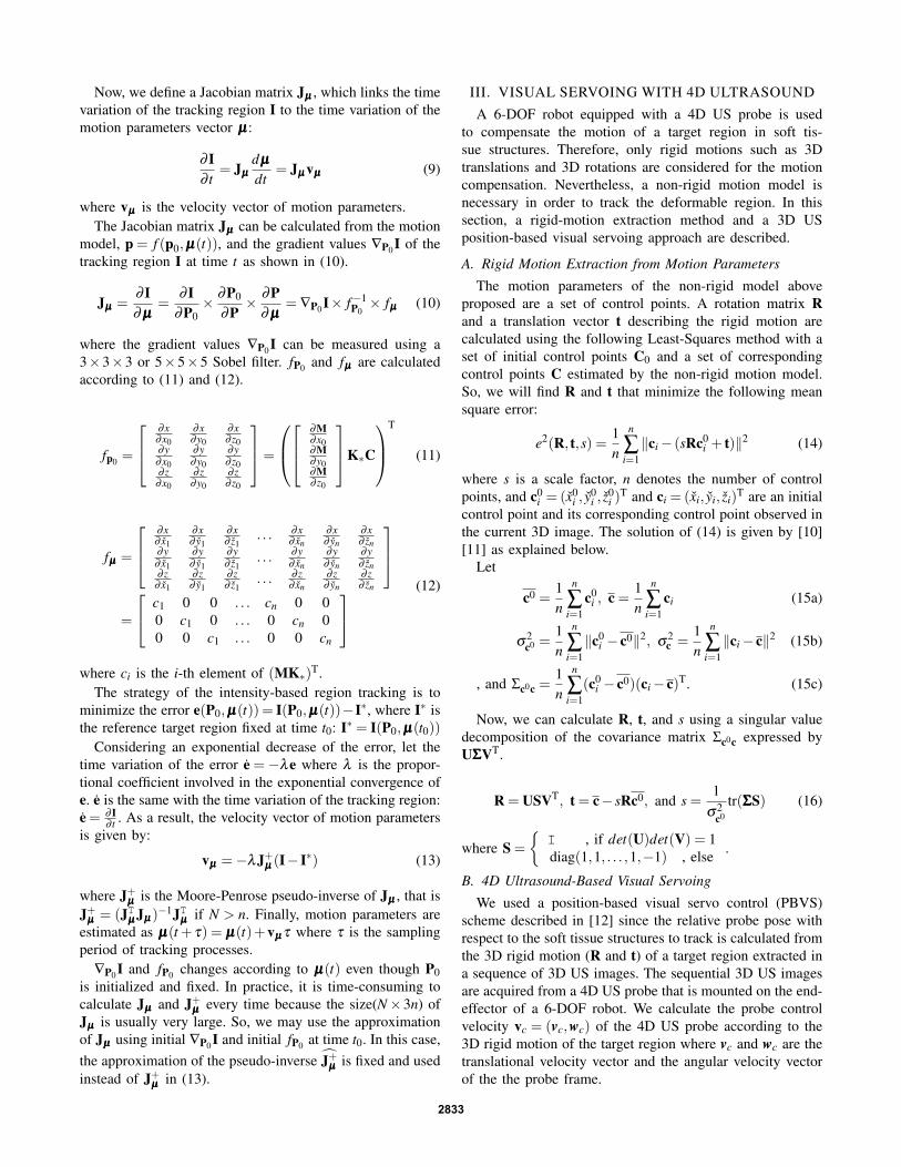
Now, we define a Jacobian matrix Jµµµ , which links the timevariation of the tracking region I to the time variation of themotion parameters vector µµµ:
∂ I∂ t
= Jµµµ
dµµµ
dt= Jµµµ vµµµ (9)
where vµµµ is the velocity vector of motion parameters.The Jacobian matrix Jµµµ can be calculated from the motion
model, p = f (p0,µµµ(t)), and the gradient values ∇P0I of thetracking region I at time t as shown in (10).
Jµµµ =∂ I∂ µµµ
=∂ I
∂P0× ∂P0
∂P× ∂P
∂ µµµ= ∇P0I× f−1
P0× fµµµ (10)
where the gradient values ∇P0 I can be measured using a3×3×3 or 5×5×5 Sobel filter. fP0 and fµµµ are calculatedaccording to (11) and (12).
fp0 =
∂x∂x0
∂x∂y0
∂x∂ z0
∂y∂x0
∂y∂y0
∂y∂ z0
∂ z∂x0
∂ z∂y0
∂ z∂ z0
=
∂M∂x0∂M∂y0∂M∂ z0
K∗C
T
(11)
fµµµ =
∂x∂ x1
∂x∂ y1
∂x∂ z1
. . . ∂x∂ xn
∂x∂ yn
∂x∂ zn
∂y∂ x1
∂y∂ y1
∂y∂ z1
. . . ∂y∂ xn
∂y∂ yn
∂y∂ zn
∂ z∂ x1
∂ z∂ y1
∂ z∂ z1
. . . ∂ z∂ xn
∂ z∂ yn
∂ z∂ zn
=
c1 0 0 . . . cn 0 00 c1 0 . . . 0 cn 00 0 c1 . . . 0 0 cn
(12)
where ci is the i-th element of (MK∗)T.The strategy of the intensity-based region tracking is to
minimize the error e(P0,µµµ(t)) = I(P0,µµµ(t))−I∗, where I∗ isthe reference target region fixed at time t0: I∗ = I(P0,µµµ(t0))
Considering an exponential decrease of the error, let thetime variation of the error e =−λe where λ is the propor-tional coefficient involved in the exponential convergence ofe. e is the same with the time variation of the tracking region:e = ∂ I
∂ t . As a result, the velocity vector of motion parametersis given by:
vµµµ =−λJ+µµµ (I− I∗) (13)
where J+µµµ is the Moore-Penrose pseudo-inverse of Jµµµ , that isJ+µµµ = (JTµµµ Jµµµ)
−1JTµµµ if N > n. Finally, motion parameters areestimated as µµµ(t +τ) = µµµ(t)+vµµµ τ where τ is the samplingperiod of tracking processes.
∇P0I and fP0 changes according to µµµ(t) even though P0is initialized and fixed. In practice, it is time-consuming tocalculate Jµµµ and J+µµµ every time because the size(N×3n) ofJµµµ is usually very large. So, we may use the approximationof Jµµµ using initial ∇P0I and initial fP0 at time t0. In this case,the approximation of the pseudo-inverse J+µµµ is fixed and usedinstead of J+µµµ in (13).
III. VISUAL SERVOING WITH 4D ULTRASOUNDA 6-DOF robot equipped with a 4D US probe is used
to compensate the motion of a target region in soft tis-sue structures. Therefore, only rigid motions such as 3Dtranslations and 3D rotations are considered for the motioncompensation. Nevertheless, a non-rigid motion model isnecessary in order to track the deformable region. In thissection, a rigid-motion extraction method and a 3D USposition-based visual servoing approach are described.
A. Rigid Motion Extraction from Motion Parameters
The motion parameters of the non-rigid model aboveproposed are a set of control points. A rotation matrix Rand a translation vector t describing the rigid motion arecalculated using the following Least-Squares method with aset of initial control points C0 and a set of correspondingcontrol points C estimated by the non-rigid motion model.So, we will find R and t that minimize the following meansquare error:
e2(R, t,s) =1n
n
∑i=1‖ci− (sRc0
i + t)‖2 (14)
where s is a scale factor, n denotes the number of controlpoints, and c0
i = (x0i , y
0i , z
0i )
T and ci = (xi, yi, zi)T are an initial
control point and its corresponding control point observed inthe current 3D image. The solution of (14) is given by [10][11] as explained below.
Let
c0 =1n
n
∑i=1
c0i , c =
1n
n
∑i=1
ci (15a)
σ2c0 =
1n
n
∑i=1‖c0
i − c0‖2, σ2c =
1n
n
∑i=1‖ci− c‖2 (15b)
, and Σc0c =1n
n
∑i=1
(c0i − c0)(ci− c)T. (15c)
Now, we can calculate R, t, and s using a singular valuedecomposition of the covariance matrix Σc0c expressed byUΣΣΣVT.
R = USVT, t = c− sRc0, and s =1
σ2c0
tr(ΣΣΣS) (16)
where S =
{I , if det(U)det(V) = 1diag(1,1, . . . ,1,−1) , else .
B. 4D Ultrasound-Based Visual Servoing
We used a position-based visual servo control (PBVS)scheme described in [12] since the relative probe pose withrespect to the soft tissue structures to track is calculated fromthe 3D rigid motion (R and t) of a target region extracted ina sequence of 3D US images. The sequential 3D US imagesare acquired from a 4D US probe that is mounted on the end-effector of a 6-DOF robot. We calculate the probe controlvelocity vc = (vc,wc) of the 4D US probe according to the3D rigid motion of the target region where vc and wc are thetranslational velocity vector and the angular velocity vectorof the the probe frame.
2833
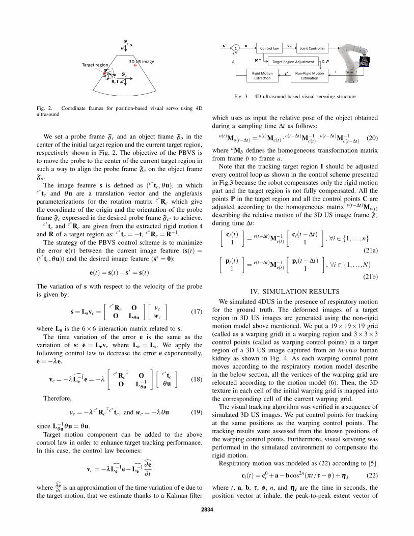
!""
#"
!"#$#
$""
!"#$%#&'()*#+(,)*-#,*)&./#
Fig. 2. Coordinate frames for position-based visual servo using 4Dultrasound
We set a probe frame Fc and an object frame Fo in thecenter of the initial target region and the current target region,respectively shown in Fig. 2. The objective of the PBVS isto move the probe to the center of the current target region insuch a way to align the probe frame Fc on the object frameFo.
The image feature s is defined as (c∗ tc,θu), in whichc∗ tc and θu are a translation vector and the angle/axisparameterizations for the rotation matrix c∗Rc which givethe coordinate of the origin and the orientation of the probeframe Fc expressed in the desired probe frame Fc∗ to achieve.
c∗ tc and c∗Rc are given from the extracted rigid motion tand R of a target region as: c∗ tc =−t, c∗Rc = R−1.
The strategy of the PBVS control scheme is to minimizethe error e(t) between the current image feature (s(t) =(c∗ tc,θu)) and the desired image feature (s∗ = 0):
e(t) = s(t)− s∗ = s(t)
The variation of s with respect to the velocity of the probeis given by:
s = Lsvc =
[c∗Rc O
O Lθu
][vcwc
](17)
where Ls is the 6×6 interaction matrix related to s.The time variation of the error e is the same as the
variation of s: e = Levc where Le = Ls. We apply thefollowing control law to decrease the error e exponentially,e =−λe.
vc =−λ L−1e e =−λ
[c∗Rc
T OO L−1
θu
][c∗ tcθu
](18)
Therefore,
vc =−λc∗Rc
Tc∗ tc, and wc =−λθu (19)
since L−1θu θu = θu.
Target motion component can be added to the abovecontrol law in order to enhance target tracking performance.In this case, the control law becomes:
vc =−λ L−1e e− L−1
e∂e∂ t
where ∂e∂ t is an approximation of the time variation of e due to
the target motion, that we estimate thanks to a Kalman filter
!"#$%&'"$%("))*(&+& '"$%(")&),-&
."$/0#1#2&3"4"$&5647,4"$&
0#1#2&3"4"$&58%(,94"$&
:,(1*%&0*1#"$&;2<=6%7*$%&
>&
/& vc
Fig. 3. 4D ultrasound-based visual servoing structure
which uses as input the relative pose of the object obtainedduring a sampling time ∆t as follows:
o(t)Mo(t−∆t) =o(t)Mc(t) · c(t−∆t)M−1
c(t) ·o(t−∆t)M−1
c(t−∆t) (20)
where aMb defines the homogeneous transformation matrixfrom frame b to frame a.
Note that the tracking target region I should be adjustedevery control loop as shown in the control scheme presentedin Fig.3 because the robot compensates only the rigid motionpart and the target region is not fully compensated. All thepoints P in the target region and all the control points C areadjusted according to the homogeneous matrix v(t−∆t)Mv(t)describing the relative motion of the 3D US image frame Fvduring time ∆t:[
ci(t)1
]= v(t−∆t)M−1
v(t)
[ci(t−∆t)
1
], ∀i ∈ {1, . . . ,n}
(21a)[pi(t)
1
]= v(t−∆t)M−1
v(t)
[pi(t−∆t)
1
], ∀i ∈ {1, . . . ,N}
(21b)
IV. SIMULATION RESULTSWe simulated 4DUS in the presence of respiratory motion
for the ground truth. The deformed images of a targetregion in 3D US images are generated using the non-rigidmotion model above mentioned. We put a 19×19×19 grid(called as a warping grid) in a warping region and 3×3×3control points (called as warping control points) in a targetregion of a 3D US image captured from an in-vivo humankidney as shown in Fig. 4. As each warping control pointmoves according to the respiratory motion model describein the below section, all the vertices of the warping grid arerelocated according to the motion model (6). Then, the 3Dtexture in each cell of the initial warping grid is mapped intothe corresponding cell of the current warping grid.
The visual tracking algorithm was verified in a sequence ofsimulated 3D US images. We put control points for trackingat the same positions as the warping control points. Thetracking results were assessed from the known positions ofthe warping control points. Furthermore, visual servoing wasperformed in the simulated environment to compensate therigid motion.
Respiratory motion was modeled as (22) according to [5].
ci(t) = c0i +a−bcos2n(πt/τ−φ)+ηηη iii (22)
where t, a, b, τ , φ , n, and ηηη iii are the time in seconds, theposition vector at inhale, the peak-to-peak extent vector of
2834
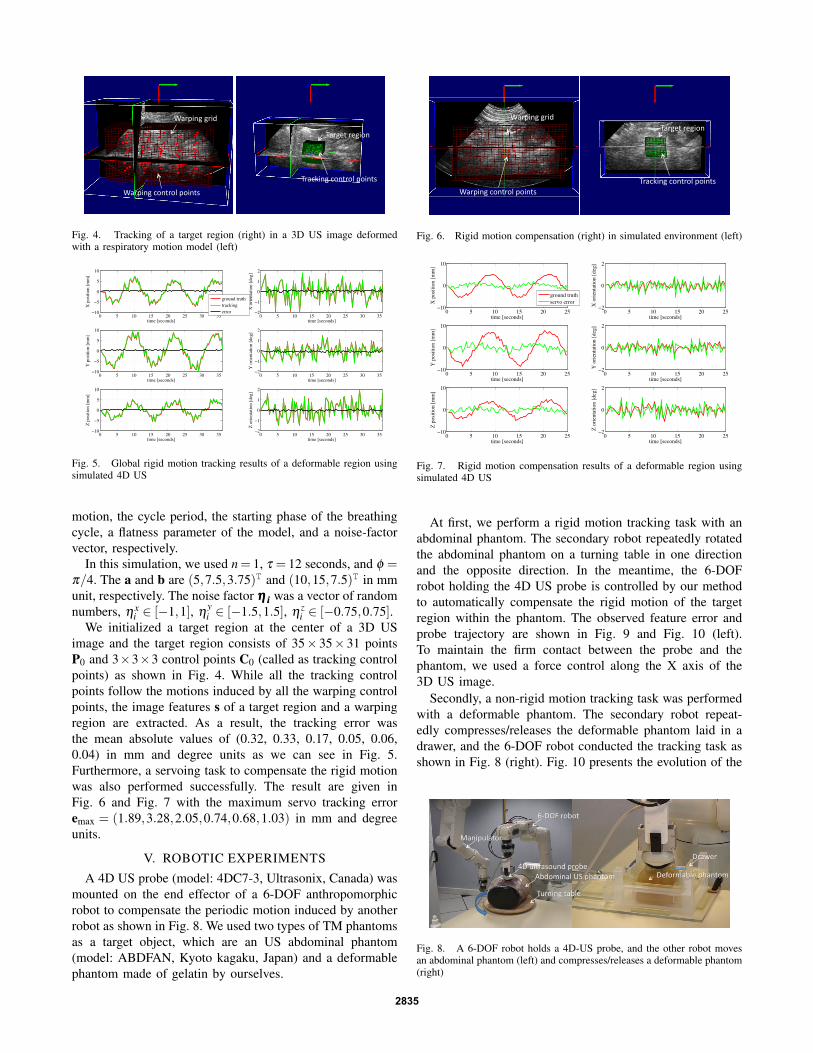
!"#$%&'()$*'+"*,)-*&'+.)
!#"(/+)"/(&*')
0#"-&'()("&1)
0#"-&'()$*'+"*,)-*&'+.)
Fig. 4. Tracking of a target region (right) in a 3D US image deformedwith a respiratory motion model (left)
! " #! #" $! $" %! %"#!
"
!
"
#!
&'()*+,)-./0,1
2*3.,'&'./*+((1
! " #! #" $! $" %! %"#!
"
!
"
#!
&'()*+,)-./0,1
4*3.,'&'./*+((1
! " #! #" $! $" %! %"#!
"
!
"
#!
&'()*+,)-./0,1
5*3.,'&'./*+((1
! " #! #" $! $" %! %"$
#
!
#
$
&'()*+,)-./0,1
2*.6')/&7&'./*+0)81
! " #! #" $! $" %! %"$
#
!
#
$
&'()*+,)-./0,1
4*.6')/&7&'./*+0)81
! " #! #" $! $" %! %"$
#
!
#
$
&'()*+,)-./0,1
5*.6')/&7&'./*+0)81
86.9/0*&69&:&67-;'/8)66.6
Fig. 5. Global rigid motion tracking results of a deformable region usingsimulated 4D US
motion, the cycle period, the starting phase of the breathingcycle, a flatness parameter of the model, and a noise-factorvector, respectively.
In this simulation, we used n= 1, τ = 12 seconds, and φ =π/4. The a and b are (5,7.5,3.75)T and (10,15,7.5)T in mmunit, respectively. The noise factor ηηη iii was a vector of randomnumbers, ηx
i ∈ [−1,1], ηyi ∈ [−1.5,1.5], η
zi ∈ [−0.75,0.75].
We initialized a target region at the center of a 3D USimage and the target region consists of 35× 35× 31 pointsP0 and 3×3×3 control points C0 (called as tracking controlpoints) as shown in Fig. 4. While all the tracking controlpoints follow the motions induced by all the warping controlpoints, the image features s of a target region and a warpingregion are extracted. As a result, the tracking error wasthe mean absolute values of (0.32, 0.33, 0.17, 0.05, 0.06,0.04) in mm and degree units as we can see in Fig. 5.Furthermore, a servoing task to compensate the rigid motionwas also performed successfully. The result are given inFig. 6 and Fig. 7 with the maximum servo tracking erroremax = (1.89,3.28,2.05,0.74,0.68,1.03) in mm and degreeunits.
V. ROBOTIC EXPERIMENTS
A 4D US probe (model: 4DC7-3, Ultrasonix, Canada) wasmounted on the end effector of a 6-DOF anthropomorphicrobot to compensate the periodic motion induced by anotherrobot as shown in Fig. 8. We used two types of TM phantomsas a target object, which are an US abdominal phantom(model: ABDFAN, Kyoto kagaku, Japan) and a deformablephantom made of gelatin by ourselves.
!"#$%&'('#%)(
!"#$%&'(*+&,#+-($+%&,.(/#"*0%&'(*+&,#+-($+%&,.(
/"#'1,(#1'%+&(
Fig. 6. Rigid motion compensation (right) in simulated environment (left)
! " #! #" $! $"#!
!
#!
%&'()*+(,-./+0
1)2-+&%&-.)*''0
! " #! #" $! $"#!
!
#!
%&'()*+(,-./+0
3)2-+&%&-.)*''0
! " #! #" $! $"#!
!
#!
%&'()*+(,-./+04)2-+&%&-.)*''0
! " #! #" $! $"$
!
$
%&'()*+(,-./+0
1)-5&(.%6%&-.)*/(70
! " #! #" $! $"$
!
$
%&'()*+(,-./+0
3)-5&(.%6%&-.)*/(70
! " #! #" $! $"$
!
$
%&'()*+(,-./+0
4)-5&(.%6%&-.)*/(70
75-8./)%58%9+(5:-)(55-5
Fig. 7. Rigid motion compensation results of a deformable region usingsimulated 4D US
At first, we perform a rigid motion tracking task with anabdominal phantom. The secondary robot repeatedly rotatedthe abdominal phantom on a turning table in one directionand the opposite direction. In the meantime, the 6-DOFrobot holding the 4D US probe is controlled by our methodto automatically compensate the rigid motion of the targetregion within the phantom. The observed feature error andprobe trajectory are shown in Fig. 9 and Fig. 10 (left).To maintain the firm contact between the probe and thephantom, we used a force control along the X axis of the3D US image.
Secondly, a non-rigid motion tracking task was performedwith a deformable phantom. The secondary robot repeat-edly compresses/releases the deformable phantom laid in adrawer, and the 6-DOF robot conducted the tracking task asshown in Fig. 8 (right). Fig. 10 presents the evolution of the
Fig. 8. A 6-DOF robot holds a 4D-US probe, and the other robot movesan abdominal phantom (left) and compresses/releases a deformable phantom(right)
2835
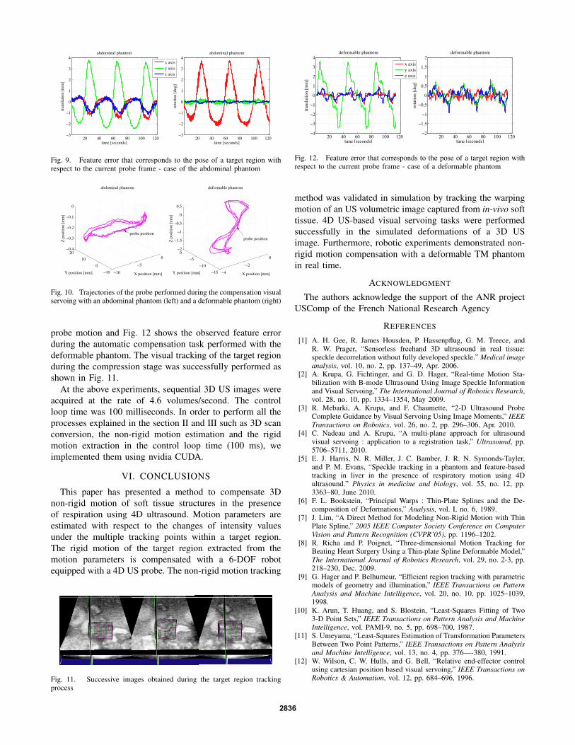
!" #" $" %" &"" &!"'
!
&
"
&
!
'
#()*+,-.(/012(.3+,
3-,405647+.*68
39(.6/(3-+.05,,8
!" #" $" %" &"" &!"'
!
&
"
&
!
'
#()*+,-.(/012(.3+,
3-,405647+.*68
9+3(3-+.05*4:8
;0(;-6<0(;-6=0(;-6
Fig. 9. Feature error that corresponds to the pose of a target region withrespect to the current probe frame - case of the abdominal phantom
!
"
#
$%$#
%#"
$&%
$
#&%
#
#&%
'()*+,-,*.(/001
234*506783()96.-*0
:()*+,-,*.(/001
;()*+,-,*.(/001
)5*73()*+,-,*.
!"
#
"
!""
!"$""%&
"%'
"%$
"%!
"
()*+,-.-+/)0112
345+1-/36)*73/.+1
8)*+,-.-+/)0112
9)*+,-.-+/)0112
*:+4;)*+,-.-+/
Fig. 10. Trajectories of the probe performed during the compensation visualservoing with an abdominal phantom (left) and a deformable phantom (right)
probe motion and Fig. 12 shows the observed feature errorduring the automatic compensation task performed with thedeformable phantom. The visual tracking of the target regionduring the compression stage was successfully performed asshown in Fig. 11.
At the above experiments, sequential 3D US images wereacquired at the rate of 4.6 volumes/second. The controlloop time was 100 milliseconds. In order to perform all theprocesses explained in the section II and III such as 3D scanconversion, the non-rigid motion estimation and the rigidmotion extraction in the control loop time (100 ms), weimplemented them using nvidia CUDA.
VI. CONCLUSIONS
This paper has presented a method to compensate 3Dnon-rigid motion of soft tissue structures in the presenceof respiration using 4D ultrasound. Motion parameters areestimated with respect to the changes of intensity valuesunder the multiple tracking points within a target region.The rigid motion of the target region extracted from themotion parameters is compensated with a 6-DOF robotequipped with a 4D US probe. The non-rigid motion tracking
Fig. 11. Successive images obtained during the target region trackingprocess
!" #" $" %" &"" &!"#
'
!
&
"
&
!
'
#()*+,-./0)123.45+-
56-)178)9+4(8:
5,.480.56+417--:
!" #" $" %" &"" &!"!
&;<
&
";<
"
";<
&
&;<
!()*+,-./0)123.45+-
56-)178)9+4(8:
,+5.56+417()=:
>1.>68?1.>68@1.>68
Fig. 12. Feature error that corresponds to the pose of a target region withrespect to the current probe frame - case of a deformable phantom
method was validated in simulation by tracking the warpingmotion of an US volumetric image captured from in-vivo softtissue. 4D US-based visual servoing tasks were performedsuccessfully in the simulated deformations of a 3D USimage. Furthermore, robotic experiments demonstrated non-rigid motion compensation with a deformable TM phantomin real time.
ACKNOWLEDGMENT
The authors acknowledge the support of the ANR projectUSComp of the French National Research Agency
REFERENCES
[1] A. H. Gee, R. James Housden, P. Hassenpflug, G. M. Treece, andR. W. Prager, “Sensorless freehand 3D ultrasound in real tissue:speckle decorrelation without fully developed speckle.” Medical imageanalysis, vol. 10, no. 2, pp. 137–49, Apr. 2006.
[2] A. Krupa, G. Fichtinger, and G. D. Hager, “Real-time Motion Sta-bilization with B-mode Ultrasound Using Image Speckle Informationand Visual Servoing,” The International Journal of Robotics Research,vol. 28, no. 10, pp. 1334–1354, May 2009.
[3] R. Mebarki, A. Krupa, and F. Chaumette, “2-D Ultrasound ProbeComplete Guidance by Visual Servoing Using Image Moments,” IEEETransactions on Robotics, vol. 26, no. 2, pp. 296–306, Apr. 2010.
[4] C. Nadeau and A. Krupa, “A multi-plane approach for ultrasoundvisual servoing : application to a registration task,” Ultrasound, pp.5706–5711, 2010.
[5] E. J. Harris, N. R. Miller, J. C. Bamber, J. R. N. Symonds-Tayler,and P. M. Evans, “Speckle tracking in a phantom and feature-basedtracking in liver in the presence of respiratory motion using 4Dultrasound.” Physics in medicine and biology, vol. 55, no. 12, pp.3363–80, June 2010.
[6] F. L. Bookstein, “Principal Warps : Thin-Plate Splines and the De-composition of Deformations,” Analysis, vol. I, no. 6, 1989.
[7] J. Lim, “A Direct Method for Modeling Non-Rigid Motion with ThinPlate Spline,” 2005 IEEE Computer Society Conference on ComputerVision and Pattern Recognition (CVPR’05), pp. 1196–1202.
[8] R. Richa and P. Poignet, “Three-dimensional Motion Tracking forBeating Heart Surgery Using a Thin-plate Spline Deformable Model,”The International Journal of Robotics Research, vol. 29, no. 2-3, pp.218–230, Dec. 2009.
[9] G. Hager and P. Belhumeur, “Efficient region tracking with parametricmodels of geometry and illumination,” IEEE Transactions on PatternAnalysis and Machine Intelligence, vol. 20, no. 10, pp. 1025–1039,1998.
[10] K. Arun, T. Huang, and S. Blostein, “Least-Squares Fitting of Two3-D Point Sets,” IEEE Transactions on Pattern Analysis and MachineIntelligence, vol. PAMI-9, no. 5, pp. 698–700, 1987.
[11] S. Umeyama, “Least-Squares Estimation of Transformation ParametersBetween Two Point Patterns,” IEEE Transactions on Pattern Analysisand Machine Intelligence, vol. 13, no. 4, pp. 376—-380, 1991.
[12] W. Wilson, C. W. Hulls, and G. Bell, “Relative end-effector controlusing cartesian position based visual servoing,” IEEE Transactions onRobotics & Automation, vol. 12, pp. 684–696, 1996.
2836
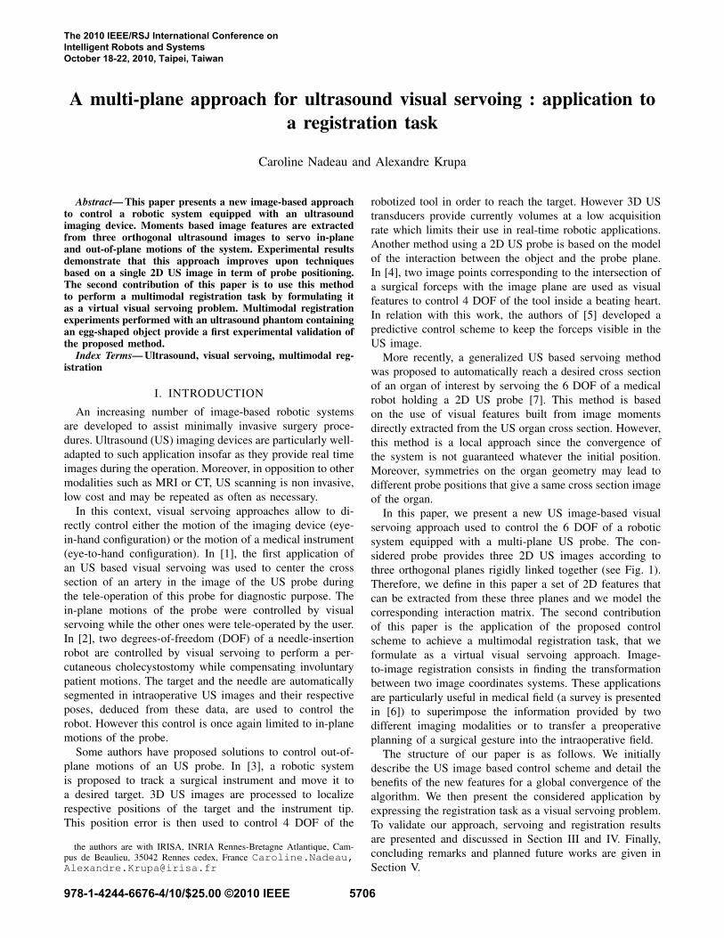
A multi-plane approach for ultrasound visual servoing : application toa registration task
Caroline Nadeau and Alexandre Krupa
Abstract— This paper presents a new image-based approachto control a robotic system equipped with an ultrasoundimaging device. Moments based image features are extractedfrom three orthogonal ultrasound images to servo in-planeand out-of-plane motions of the system. Experimental resultsdemonstrate that this approach improves upon techniquesbased on a single 2D US image in term of probe positioning.The second contribution of this paper is to use this methodto perform a multimodal registration task by formulating itas a virtual visual servoing problem. Multimodal registrationexperiments performed with an ultrasound phantom containingan egg-shaped object provide a first experimental validation ofthe proposed method.
Index Terms— Ultrasound, visual servoing, multimodal reg-istration
I. INTRODUCTION
An increasing number of image-based robotic systemsare developed to assist minimally invasive surgery proce-dures. Ultrasound (US) imaging devices are particularly well-adapted to such application insofar as they provide real timeimages during the operation. Moreover, in opposition to othermodalities such as MRI or CT, US scanning is non invasive,low cost and may be repeated as often as necessary.
In this context, visual servoing approaches allow to di-rectly control either the motion of the imaging device (eye-in-hand configuration) or the motion of a medical instrument(eye-to-hand configuration). In [1], the first application ofan US based visual servoing was used to center the crosssection of an artery in the image of the US probe duringthe tele-operation of this probe for diagnostic purpose. Thein-plane motions of the probe were controlled by visualservoing while the other ones were tele-operated by the user.In [2], two degrees-of-freedom (DOF) of a needle-insertionrobot are controlled by visual servoing to perform a per-cutaneous cholecystostomy while compensating involuntarypatient motions. The target and the needle are automaticallysegmented in intraoperative US images and their respectiveposes, deduced from these data, are used to control therobot. However this control is once again limited to in-planemotions of the probe.
Some authors have proposed solutions to control out-of-plane motions of an US probe. In [3], a robotic systemis proposed to track a surgical instrument and move it toa desired target. 3D US images are processed to localizerespective positions of the target and the instrument tip.This position error is then used to control 4 DOF of the
the authors are with IRISA, INRIA Rennes-Bretagne Atlantique, Cam-pus de Beaulieu, 35042 Rennes cedex, France Caroline.Nadeau,[email protected]
robotized tool in order to reach the target. However 3D UStransducers provide currently volumes at a low acquisitionrate which limits their use in real-time robotic applications.Another method using a 2D US probe is based on the modelof the interaction between the object and the probe plane.In [4], two image points corresponding to the intersection ofa surgical forceps with the image plane are used as visualfeatures to control 4 DOF of the tool inside a beating heart.In relation with this work, the authors of [5] developed apredictive control scheme to keep the forceps visible in theUS image.
More recently, a generalized US based servoing methodwas proposed to automatically reach a desired cross sectionof an organ of interest by servoing the 6 DOF of a medicalrobot holding a 2D US probe [7]. This method is basedon the use of visual features built from image momentsdirectly extracted from the US organ cross section. However,this method is a local approach since the convergence ofthe system is not guaranteed whatever the initial position.Moreover, symmetries on the organ geometry may lead todifferent probe positions that give a same cross section imageof the organ.
In this paper, we present a new US image-based visualservoing approach used to control the 6 DOF of a roboticsystem equipped with a multi-plane US probe. The con-sidered probe provides three 2D US images according tothree orthogonal planes rigidly linked together (see Fig. 1).Therefore, we define in this paper a set of 2D features thatcan be extracted from these three planes and we model thecorresponding interaction matrix. The second contributionof this paper is the application of the proposed controlscheme to achieve a multimodal registration task, that weformulate as a virtual visual servoing approach. Image-to-image registration consists in finding the transformationbetween two image coordinates systems. These applicationsare particularly useful in medical field (a survey is presentedin [6]) to superimpose the information provided by twodifferent imaging modalities or to transfer a preoperativeplanning of a surgical gesture into the intraoperative field.
The structure of our paper is as follows. We initiallydescribe the US image based control scheme and detail thebenefits of the new features for a global convergence of thealgorithm. We then present the considered application byexpressing the registration task as a visual servoing problem.To validate our approach, servoing and registration resultsare presented and discussed in Section III and IV. Finally,concluding remarks and planned future works are given inSection V.
The 2010 IEEE/RSJ International Conference on Intelligent Robots and Systems October 18-22, 2010, Taipei, Taiwan
978-1-4244-6676-4/10/$25.00 ©2010 IEEE 5706
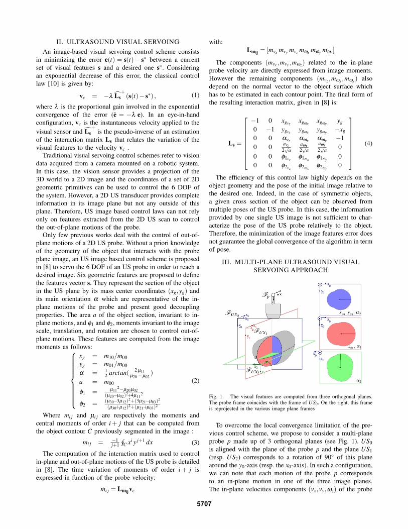
II. ULTRASOUND VISUAL SERVOINGAn image-based visual servoing control scheme consists
in minimizing the error e(t) = s(t)− s∗ between a currentset of visual features s and a desired one s∗. Consideringan exponential decrease of this error, the classical controllaw [10] is given by:
vc = −λ Ls+
(s(t)− s∗) , (1)
where λ is the proportional gain involved in the exponentialconvergence of the error (e = −λ e). In an eye-in-handconfiguration, vc is the instantaneous velocity applied to thevisual sensor and Ls
+is the pseudo-inverse of an estimation
of the interaction matrix Ls that relates the variation of thevisual features to the velocity vc .
Traditional visual servoing control schemes refer to visiondata acquired from a camera mounted on a robotic system.In this case, the vision sensor provides a projection of the3D world to a 2D image and the coordinates of a set of 2Dgeometric primitives can be used to control the 6 DOF ofthe system. However, a 2D US transducer provides completeinformation in its image plane but not any outside of thisplane. Therefore, US image based control laws can not relyonly on features extracted from the 2D US scan to controlthe out-of-plane motions of the probe.
Only few previous works deal with the control of out-of-plane motions of a 2D US probe. Without a priori knowledgeof the geometry of the object that interacts with the probeplane image, an US image based control scheme is proposedin [8] to servo the 6 DOF of an US probe in order to reach adesired image. Six geometric features are proposed to definethe features vector s. They represent the section of the objectin the US plane by its mass center coordinates (xg,yg) andits main orientation α which are representative of the in-plane motions of the probe and present good decouplingproperties. The area a of the object section, invariant to in-plane motions, and φ1 and φ2, moments invariant to the imagescale, translation, and rotation are chosen to control out-of-plane motions. These features are computed from the imagemoments as follows:
xg = m10/m00yg = m01/m00
α = 12 arctan( 2 µ11
µ20−µ02)
a = m00
φ1 = µ112−µ20µ02
(µ20−µ02)2+4µ112
φ2 = (µ30−3µ12)2+(3µ21−µ03)2
(µ30+µ12)2+(µ21+µ03)2
(2)
Where mi j and µi j are respectively the moments andcentral moments of order i + j that can be computed fromthe object contour C previously segmented in the image :
mi j = −1j+1
∮C xi y j+1 dx (3)
The computation of the interaction matrix used to controlin-plane and out-of-plane motions of the US probe is detailedin [8]. The time variation of moments of order i + j isexpressed in function of the probe velocity:
mi j = Lmijvc
with:Lmij = [mvx mvy mvz mωx mωy mωz ]
The components (mvx ,mvy ,mωz) related to the in-planeprobe velocity are directly expressed from image moments.However the remaining components (mvz ,mωx ,mωy) alsodepend on the normal vector to the object surface whichhas to be estimated in each contour point. The final form ofthe resulting interaction matrix, given in [8] is:
Ls =
−1 0 xgvz xgωx xgωy yg
0 −1 ygvz ygωx ygωy −xg
0 0 αvz αωx αωy −10 0 avz
2√
aaωx2√
aaωy2√
a 00 0 φ1vz φ1ωx φ1ωy 00 0 φ2vz φ2ωx φ2ωy 0
(4)
The efficiency of this control law highly depends on theobject geometry and the pose of the initial image relative tothe desired one. Indeed, in the case of symmetric objects,a given cross section of the object can be observed frommultiple poses of the US probe. In this case, the informationprovided by one single US image is not sufficient to char-acterize the pose of the US probe relatively to the object.Therefore, the minimization of the image features error doesnot guarantee the global convergence of the algorithm in termof pose.
III. MULTI-PLANE ULTRASOUND VISUALSERVOING APPROACH
Fig. 1. The visual features are computed from three orthogonal planes.The probe frame coincides with the frame of US0. On the right, this frameis reprojected in the various image plane frames
To overcome the local convergence limitation of the pre-vious control scheme, we propose to consider a multi-planeprobe p made up of 3 orthogonal planes (see Fig. 1). US0is aligned with the plane of the probe p and the plane US1(resp. US2) corresponds to a rotation of 90◦ of this planearound the y0-axis (resp. the x0-axis). In such a configuration,we can note that each motion of the probe p correspondsto an in-plane motion in one of the three image planes.The in-plane velocities components (vx,vy,ωz) of the probe
5707
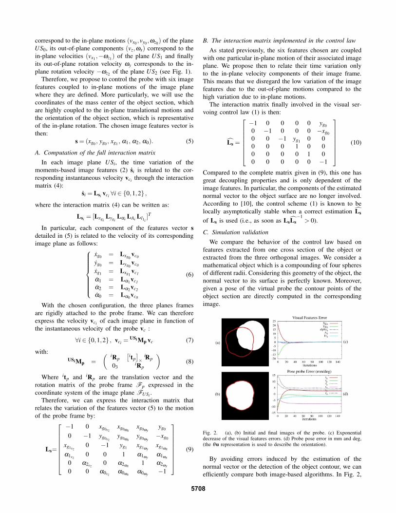
correspond to the in-plane motions (vx0 ,vy0 ,ωz0) of the planeUS0, its out-of-plane components (vz,ωx) correspond to thein-plane velocities (vx1 ,−ωz1) of the plane US1 and finallyits out-of-plane rotation velocity ωy corresponds to the in-plane rotation velocity −ωz2 of the plane US2 (see Fig. 1).
Therefore, we propose to control the probe with six imagefeatures coupled to in-plane motions of the image planewhere they are defined. More particularly, we will use thecoordinates of the mass center of the object section, whichare highly coupled to the in-plane translational motions andthe orientation of the object section, which is representativeof the in-plane rotation. The chosen image features vector isthen:
s = (xg0 , yg0 , xg1 , α1, α2, α0). (5)
A. Computation of the full interaction matrix
In each image plane USi, the time variation of themoments-based image features (2) si is related to the cor-responding instantaneous velocity vci through the interactionmatrix (4):
si = Lsi vci ∀i ∈ {0,1,2} ,
where the interaction matrix (4) can be written as:
Lsi = [LxgiLygi
Lαi LAi Ll1i]T
In particular, each component of the features vector sdetailed in (5) is related to the velocity of its correspondingimage plane as follows:
xg0 = Lxg0vc0
yg0 = Lyg0vc0
xg1 = Lxg1vc1
α1 = Lα1vc1
α2 = Lα2vc2
α0 = Lα0vc0
(6)
With the chosen configuration, the three planes framesare rigidly attached to the probe frame. We can thereforeexpress the velocity vci of each image plane in function ofthe instantaneous velocity of the probe vc :
∀i ∈ {0,1,2} , vci = USiMp vc (7)
with:USiMp =
( iRp[
itp]×
iRp
03iRp
)(8)
Where itp and iRp are the translation vector and therotation matrix of the probe frame Fp expressed in thecoordinate system of the image plane FUSi .
Therefore, we can express the interaction matrix thatrelates the variation of the features vector (5) to the motionof the probe frame by:
Ls=
−1 0 xg0vzxg0ωx
xg0ωyyg0
0 −1 yg0vzyg0ωx
yg0ωy−xg0
xg1vz0 −1 yg1 xg1ωy
xg1ωx
α1vz 0 0 1 α1ωy α1ωx
0 α2vz 0 α2ωx 1 α2ωy
0 0 α0vz α0ωx α0ωy −1
(9)
B. The interaction matrix implemented in the control law
As stated previously, the six features chosen are coupledwith one particular in-plane motion of their associated imageplane. We propose then to relate their time variation onlyto the in-plane velocity components of their image frame.This means that we disregard the low variation of the imagefeatures due to the out-of-plane motions compared to thehigh variation due to in-plane motions.
The interaction matrix finally involved in the visual ser-voing control law (1) is then:
Ls =
−1 0 0 0 0 yg00 −1 0 0 0 −xg00 0 −1 yg1 0 00 0 0 1 0 00 0 0 0 1 00 0 0 0 0 −1
(10)
Compared to the complete matrix given in (9), this one hasgreat decoupling properties and is only dependent of theimage features. In particular, the components of the estimatednormal vector to the object surface are no longer involved.According to [10], the control scheme (1) is known to belocally asymptotically stable when a correct estimation Ls
of Ls is used (i.e., as soon as LsLs−1
> 0).
C. Simulation validation
We compare the behavior of the control law based onfeatures extracted from one cross section of the object orextracted from the three orthogonal images. We consider amathematical object which is a compounding of four spheresof different radii. Considering this geometry of the object, thenormal vector to its surface is perfectly known. Moreover,given a pose of the virtual probe the contour points of theobject section are directly computed in the correspondingimage.
Fig. 2. (a), (b) Initial and final images of the probe. (c) Exponentialdecrease of the visual features errors. (d) Probe pose error in mm and deg,(the θu representation is used to describe the orientation).
By avoiding errors induced by the estimation of thenormal vector or the detection of the object contour, we canefficiently compare both image-based algorithms. In Fig. 2,
5708
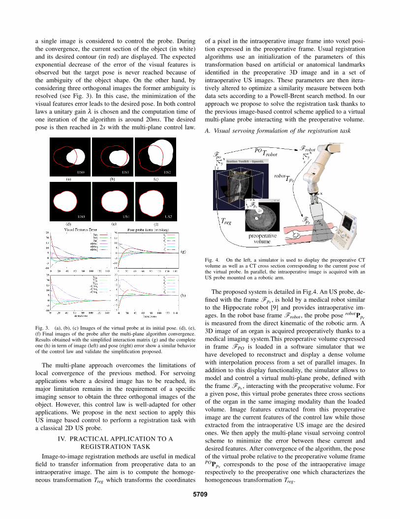
a single image is considered to control the probe. Duringthe convergence, the current section of the object (in white)and its desired contour (in red) are displayed. The expectedexponential decrease of the error of the visual features isobserved but the target pose is never reached because ofthe ambiguity of the object shape. On the other hand, byconsidering three orthogonal images the former ambiguity isresolved (see Fig. 3). In this case, the minimization of thevisual features error leads to the desired pose. In both controllaws a unitary gain λ is chosen and the computation time ofone iteration of the algorithm is around 20ms. The desiredpose is then reached in 2s with the multi-plane control law.
Fig. 3. (a), (b), (c) Images of the virtual probe at its initial pose. (d), (e),(f) Final images of the probe after the multi-plane algorithm convergence.Results obtained with the simplified interaction matrix (g) and the completeone (h) in term of image (left) and pose (right) error show a similar behaviorof the control law and validate the simplification proposed.
The multi-plane approach overcomes the limitations oflocal convergence of the previous method. For servoingapplications where a desired image has to be reached, itsmajor limitation remains in the requirement of a specificimaging sensor to obtain the three orthogonal images of theobject. However, this control law is well-adapted for otherapplications. We propose in the next section to apply thisUS image based control to perform a registration task witha classical 2D US probe.
IV. PRACTICAL APPLICATION TO AREGISTRATION TASK
Image-to-image registration methods are useful in medicalfield to transfer information from preoperative data to anintraoperative image. The aim is to compute the homoge-neous transformation Treg which transforms the coordinates
of a pixel in the intraoperative image frame into voxel posi-tion expressed in the preoperative frame. Usual registrationalgorithms use an initialization of the parameters of thistransformation based on artificial or anatomical landmarksidentified in the preoperative 3D image and in a set ofintraoperative US images. These parameters are then itera-tively altered to optimize a similarity measure between bothdata sets according to a Powell-Brent search method. In ourapproach we propose to solve the registration task thanks tothe previous image-based control scheme applied to a virtualmulti-plane probe interacting with the preoperative volume.
A. Visual servoing formulation of the registration task
Fig. 4. On the left, a simulator is used to display the preoperative CTvolume as well as a CT cross section corresponding to the current pose ofthe virtual probe. In parallel, the intraoperative image is acquired with anUS probe mounted on a robotic arm.
The proposed system is detailed in Fig.4. An US probe, de-fined with the frame Fpr , is hold by a medical robot similarto the Hippocrate robot [9] and provides intraoperative im-ages. In the robot base frame Frobot , the probe pose robotPpr
is measured from the direct kinematic of the robotic arm. A3D image of an organ is acquired preoperatively thanks to amedical imaging system.This preoperative volume expressedin frame FPO is loaded in a software simulator that wehave developed to reconstruct and display a dense volumewith interpolation process from a set of parallel images. Inaddition to this display functionality, the simulator allows tomodel and control a virtual multi-plane probe, defined withthe frame Fpv , interacting with the preoperative volume. Fora given pose, this virtual probe generates three cross sectionsof the organ in the same imaging modality than the loadedvolume. Image features extracted from this preoperativeimage are the current features of the control law while thoseextracted from the intraoperative US image are the desiredones. We then apply the multi-plane visual servoing controlscheme to minimize the error between these current anddesired features. After convergence of the algorithm, the poseof the virtual probe relative to the preoperative volume framePOPpv corresponds to the pose of the intraoperative imagerespectively to the preoperative one which characterizes thehomogeneous transformation Treg.
5709
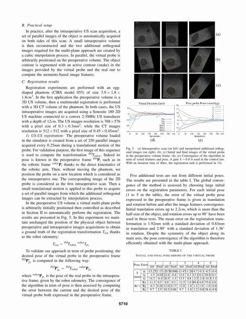
B. Practical setup
In practice, after the intraoperative US scan acquisition, aset of parallel images of the object is automatically acquiredon both sides of this scan. A small intraoperative volumeis then reconstructed and the two additional orthogonalimages required for the multi-plane approach are created bya cubic interpolation process. In parallel, the virtual probe isarbitrarily positioned on the preoperative volume. The objectcontour is segmented with an active contour (snake) in theimages provided by the virtual probe and the real one tocompute the moments-based image features.
C. Registration results
Registration experiments are performed with an egg-shaped phantom (CIRS model 055) of size 3.9 × 1.8 ×1.8cm3. In the first application the preoperative volume is a3D US volume, then a multimodal registration is performedwith a 3D CT volume of the phantom. In both cases, the USintraoperative images are acquired using a Sonosite 180 2DUS machine connected to a convex 2-5MHz US transducerwith a depth of 12cm. The US images resolution is 768×576with a pixel size of 0.3× 0.3mm2, while the CT imagesresolution is 512×512 with a pixel size of 0.45×0.45mm2.
1) US-US registration: The preoperative volume loadedin the simulator is created from a set of 250 parallel imagesacquired every 0.25mm during a translational motion of theprobe. For validation purpose, the first image of this sequenceis used to compute the transformation POTrobot . Indeed itspose is known in the preoperative frame POPi such as inthe robotic frame robotPi thanks to the direct kinematics ofthe robotic arm. Then, without moving the phantom, weposition the probe on a new location which is considered asthe intraoperative one. The corresponding image of the 2Dprobe is considered as the first intraoperative scan. Then asmall translational motion is applied to this probe to acquirea set of parallel images from which the additional orthogonalimages can be extracted by interpolation process.
In the preoperative US volume a virtual multi-plane probeis arbitrarily initially positioned then controlled as describedin Section II to automatically perform the registration. Theresults are presented in Fig. 5. In this experiment we main-tain unchanged the position of the physical object betweenpreoperative and intraoperative images acquisitions to obtaina ground truth of the registration transformation Treg thanksto the robot odometry:
Treg = POTrobotrobotTpr
To validate our approach in term of probe positioning, thedesired pose of the virtual probe in the preoperative framePOP∗pv is computed in the following way:
POP∗pv = POTrobotrobotPpr
where robotPpr is the pose of the real probe in the intraopera-tive frame, given by the robot odometry. The convergence ofthe algorithm in term of pose is then assessed by computingthe error between the current and the desired pose of thevirtual probe both expressed in the preoperative frame.
Fig. 5. (a) Intraoperative scan (on left) and interpolated additional orthog-onal images (on right). (b), (c) Initial and final images of the virtual probein the preoperative volume frame. (d), (e) Convergence of the algorithm interm of visual features and pose. A gain λ = 0.8 is used in the control law.With an iteration time of 40ms, the registration task is performed in 12s.
Five additional tests are run from different initial poses.The results are presented in the table I. The global conver-gence of the method is assessed by choosing large initialerrors on the registration parameters. For each initial pose(1 to 5 in the table), the error of the virtual probe poseexpressed in the preoperative frame is given in translationand rotation before and after the image features convergence.Initial translation errors up to 2.2cm, which is more than thehalf-size of the object, and rotation errors up to 90◦ have beenused in these tests. The mean error on the registration trans-formation is 1.92mm with a standard deviation of 0.83mmin translation and 2.90◦ with a standard deviation of 1.36◦
in rotation. Despite the symmetry of the object along itsmain axis, the pose convergence of the algorithm is thereforeefficiently obtained with the multi-plane approach.
TABLE IINITIAL AND FINAL POSE ERRORS OF THE VIRTUAL PROBE
Pose Error 1 2 3 4 5init final init final init final init final init final
T tx -13.25 1.13 -20.50.006-13.47-1.20 4.7 -0.3 -6.5 -0.4
(mm) ty -1.5 -0.02 22.6 -0.4 12.6 0.3 13.2 0.2 20.8 0.1tz 14.2 -0.4 20.5 -1.3 13.5 0.8 -2.5 -2.4 -14.5 -3.1
R(◦)Rx -11.5 0.5 8.0 0.3 -11.5 1.0 89.4 4.0 75.6 4.0Ry -6.3 0.26 12.0 0.17 -12.0 -1.8 1.4 1.0 -1.0 -0.6Rz 9.7 2.9 10.3 0.86 9.7 -1.0 1.2 -0.8 38.4 -0.8
5710
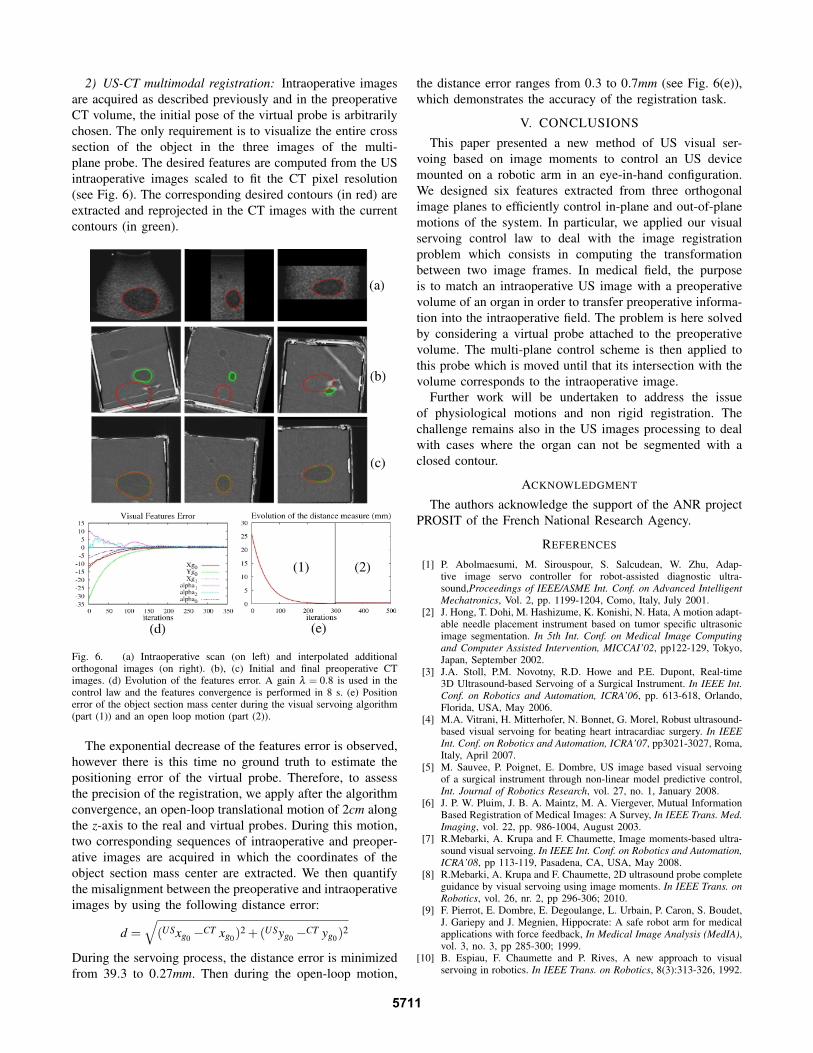
2) US-CT multimodal registration: Intraoperative imagesare acquired as described previously and in the preoperativeCT volume, the initial pose of the virtual probe is arbitrarilychosen. The only requirement is to visualize the entire crosssection of the object in the three images of the multi-plane probe. The desired features are computed from the USintraoperative images scaled to fit the CT pixel resolution(see Fig. 6). The corresponding desired contours (in red) areextracted and reprojected in the CT images with the currentcontours (in green).
Fig. 6. (a) Intraoperative scan (on left) and interpolated additionalorthogonal images (on right). (b), (c) Initial and final preoperative CTimages. (d) Evolution of the features error. A gain λ = 0.8 is used in thecontrol law and the features convergence is performed in 8 s. (e) Positionerror of the object section mass center during the visual servoing algorithm(part (1)) and an open loop motion (part (2)).
The exponential decrease of the features error is observed,however there is this time no ground truth to estimate thepositioning error of the virtual probe. Therefore, to assessthe precision of the registration, we apply after the algorithmconvergence, an open-loop translational motion of 2cm alongthe z-axis to the real and virtual probes. During this motion,two corresponding sequences of intraoperative and preoper-ative images are acquired in which the coordinates of theobject section mass center are extracted. We then quantifythe misalignment between the preoperative and intraoperativeimages by using the following distance error:
d =√
(USxg0 −CT xg0)2 +(USyg0 −CT yg0)2
During the servoing process, the distance error is minimizedfrom 39.3 to 0.27mm. Then during the open-loop motion,
the distance error ranges from 0.3 to 0.7mm (see Fig. 6(e)),which demonstrates the accuracy of the registration task.
V. CONCLUSIONSThis paper presented a new method of US visual ser-
voing based on image moments to control an US devicemounted on a robotic arm in an eye-in-hand configuration.We designed six features extracted from three orthogonalimage planes to efficiently control in-plane and out-of-planemotions of the system. In particular, we applied our visualservoing control law to deal with the image registrationproblem which consists in computing the transformationbetween two image frames. In medical field, the purposeis to match an intraoperative US image with a preoperativevolume of an organ in order to transfer preoperative informa-tion into the intraoperative field. The problem is here solvedby considering a virtual probe attached to the preoperativevolume. The multi-plane control scheme is then applied tothis probe which is moved until that its intersection with thevolume corresponds to the intraoperative image.
Further work will be undertaken to address the issueof physiological motions and non rigid registration. Thechallenge remains also in the US images processing to dealwith cases where the organ can not be segmented with aclosed contour.
ACKNOWLEDGMENT
The authors acknowledge the support of the ANR projectPROSIT of the French National Research Agency.
REFERENCES
[1] P. Abolmaesumi, M. Sirouspour, S. Salcudean, W. Zhu, Adap-tive image servo controller for robot-assisted diagnostic ultra-sound,Proceedings of IEEE/ASME Int. Conf. on Advanced IntelligentMechatronics, Vol. 2, pp. 1199-1204, Como, Italy, July 2001.
[2] J. Hong, T. Dohi, M. Hashizume, K. Konishi, N. Hata, A motion adapt-able needle placement instrument based on tumor specific ultrasonicimage segmentation. In 5th Int. Conf. on Medical Image Computingand Computer Assisted Intervention, MICCAI’02, pp122-129, Tokyo,Japan, September 2002.
[3] J.A. Stoll, P.M. Novotny, R.D. Howe and P.E. Dupont, Real-time3D Ultrasound-based Servoing of a Surgical Instrument. In IEEE Int.Conf. on Robotics and Automation, ICRA’06, pp. 613-618, Orlando,Florida, USA, May 2006.
[4] M.A. Vitrani, H. Mitterhofer, N. Bonnet, G. Morel, Robust ultrasound-based visual servoing for beating heart intracardiac surgery. In IEEEInt. Conf. on Robotics and Automation, ICRA’07, pp3021-3027, Roma,Italy, April 2007.
[5] M. Sauvee, P. Poignet, E. Dombre, US image based visual servoingof a surgical instrument through non-linear model predictive control,Int. Journal of Robotics Research, vol. 27, no. 1, January 2008.
[6] J. P. W. Pluim, J. B. A. Maintz, M. A. Viergever, Mutual InformationBased Registration of Medical Images: A Survey, In IEEE Trans. Med.Imaging, vol. 22, pp. 986-1004, August 2003.
[7] R.Mebarki, A. Krupa and F. Chaumette, Image moments-based ultra-sound visual servoing. In IEEE Int. Conf. on Robotics and Automation,ICRA’08, pp 113-119, Pasadena, CA, USA, May 2008.
[8] R.Mebarki, A. Krupa and F. Chaumette, 2D ultrasound probe completeguidance by visual servoing using image moments. In IEEE Trans. onRobotics, vol. 26, nr. 2, pp 296-306; 2010.
[9] F. Pierrot, E. Dombre, E. Degoulange, L. Urbain, P. Caron, S. Boudet,J. Gariepy and J. Megnien, Hippocrate: A safe robot arm for medicalapplications with force feedback, In Medical Image Analysis (MedIA),vol. 3, no. 3, pp 285-300; 1999.
[10] B. Espiau, F. Chaumette and P. Rives, A new approach to visualservoing in robotics. In IEEE Trans. on Robotics, 8(3):313-326, 1992.
5711


![LETTRE N° 1 Octobre 2012 - [TIMC-IMAG] · Parution d'un ouvrage de synthèse en robotique médicale édité par Jocelyne Troccaz. Parce que ce ... ("Medical robotics") publiée par](https://img.pdfslide.fr/doc/110x75/5b83b9a17f8b9a23668da337/lettre-n-1-octobre-2012-timc-imag-parution-dun-ouvrage-de-synthese-en.jpg)