Harmonisation of physical and chemical methods for soil

Vol. 7(6), pp. 386-401, June 2013

DOI: 10.5897/AJEST12.101

ISSN 1996-0786 © 2013 Academic Journals

http://www.academicjournals.org/AJEST

African Journal of Environmental Science and Technology

Full Length Research Paper

Harmonisation of physical and chemical methods for soil management in Cork Oak forests - Lessons from

collaborative investigations

Iain McLellan1, Adélia Varela2, Mohamed Blahgen3, Maria Daria Fumi4, Abdennaceur Hassen5, Nejla Hechminet5, Atef Jaouani5, Amel Khessairi5, Karim Lyamlouli3, Hadda-Imene Ouzari5, Valeria Mazzoleni4, Elisa Novelli4, Agostino Pintus6, Càtia Rodrigues2, Pino Angelo Ruiu6,

Cristina Silva Pereira2 and Andrew Hursthouse1*

1Institute of Biomedical and Environmental Health Research, School of Science, University of the West of Scotland,

Paisley, United Kingdom. 2Instituto de Biologia Experimental e Tecnológica (IBET), Oeiras, Portugal.

3Faculty of Science, University Hassan II- Aïn Chock, Casablanca, Morocco.

4Instituto di Enologia e Ingegneria agro-alimentare, Università Cattolica del Sacro Cuore, Piacenza, Italy.

5Centre de Recherche en Sciences et Technolgies de l’Eau, Solimnen, Tunisia.

6AGRIS Sargena, Dipartimento della Ricerca per il Sughero e la Silvicoltura, Tempo Pausania, Italy.

Accepted 4 June, 2013

As part of a collaborative project to investigate human impacts on Quercus suber L. (cork oak) forests, five research groups from countries in Europe and North Africa undertook a survey of soil quality (physical properties, potentially toxic elements) at sites in NW Tunisia and NW Sardinia. All groups performed the analysis of soil samples after agreeing prescribed methodologies to ensure harmonisation and the production of a robust and reliable data set. The data produced were compared using basic statistical methods and revealed strong positive correlation despite minor operational variation. The data indicates that inter and intra laboratory variability differed from parameter to parameter and that good agreement was obtained where methodology was common. Collaborative research introduced the need for common communication plans and exchange of information not normally supplied in analytical reporting. Key words: Forest soil quality, inter-comparison, Quercus suber L., cork oak, Tunisia, Sardinia, chemical analysis, potentially toxic elements.

INTRODUCTION Whilst accepted standards for soil quality exist, such as the International Standard for sample collection (ISO, 2002) or pH determination (ISO, 1994), it is common for laboratories to use methods based on accepted local (national) practice or modifications of methodologies for basic soil parameters due to the experience of laboratory staff. Whilst this approach is often adequate for local survey activity, where project require tests to be carried

out at different locations on common samples, the project goals can only be met with a fuller understanding of comparability between laboratory groups. Inter-laboratory comparison has traditionally been used to reveal the extent of the variability of results between laboratories in collaborative projects (Rust and Fenton, 1983; Quevauviller et al., 1996), the quality assurance proce-dures used in a laboratory (Kong et al., 2007) and analy-

*Corresponding author. E-mail: [email protected].

tical method reproducibility (Rauret et al., 1999; Kleinmann et al., 2001; Rahman et al., 2005). For example, in a pan-European study of urban soil quality, analysis of shared samples for Potentially Toxic Elements (PTEs) by experienced laboratories, revealed that 20% of the results differed from the target values by 25% as a result of values being close to the detection limits and calculation errors and lack of quality assurance proce-dures (Davidson et al., 2007).

Additional issues which should be considered, and are exacerbated within a multi-national and multi-disciplinary project, surround the complexity of data management, definition of roles and responsibility, particularly when changes in personnel and changes in research direc-tion/detail occur as natural components of the research investigation (Hunnes, 2010; Horner and Minifie, 2011). Changes in personnel within a team, raises the possibility that new team members and their approach can result in significant inter-laboratory variation (Cools et al., 2004). Communication between project teams and particularly in projects studying locations directly affected by environmental pollutants, has been identified as an important factor in successful inter-disciplinary projects (Huby and Adams, 2009).

This paper presents an assessment of work carried out as part of a wider NATO Science for Peace (SfP) project entitled “preventative and remediation strategies for conti-nuous elimination of poly-chlorinated phenols from forest soils and ground waters”. It focused on the evaluation of human impacts on sensitive forest ecosystem to improved assessment methods for locations undergoing rapid exploitation and affecting the quality of forest products. The project involved five different laboratories: three from NATO member countries and two from NATO border countries, which had expertise in a wide range of topics covering environmental microbiology, cork science and environmental geochemistry, with some participants having little or no experience in soil chemical analysis. An overarching aim of SfP projects is to contribute to solidarity among nations, by applying the best technical expertise to problem solving. It was agreed from the project kick off, that a set of prescribed methodologies and protocols would be used for basic soil characterisation to ensure harmonisation and reproduce-bility of analytical results across the project network and with added benefits to improve the experience of laboratories in sharing good analytical practice and in training early career researchers. This is an important aspect for any collaborative project as it has been found that laboratories which establish good quality assurance (QA) procedures obtain results which are less variable than laboratories without robust QA procedures (Kong et al., 2007).

The work presented in this paper demonstrates the impact of adopting QA approach in collaborative environ-mental assessment. In particular, it provides evidence to show the value of common and agreed methodologies

McLellan et al. 387 across partner teams. The strategic value of robust and systematic investigation in a multi-national and inter-disciplinary project is particularly critical for the cork oak forests. They span many geographical and cultural boundaries, and their productivity is acutely sensitive to their management (Silva Pereira et al, 2000; Mazzoleni et al, 2005; Urbieta et al, 2008). All data presented has been anonymised and individual laboratory contributions are indicated using simple notation. MATERIALS AND METHODS Soil samples were collected from three Tunisian Quercus suber L. (cork oak) forests in June 2007 and February 2009 and from a Sardinian forest in June 2008 and March 2009, following international standards (ISO, 2002). The geology of northern Tunisia where the samples were collected comprised marine sediments from the Neogene and Oligocene periods and agrilliceous-sandy-fluviatile sediments from the Triassic period (Shlüter, 2006) specifically - aeolian sand (Ras Rajel), clays and sandstones (Ain Hamraia) and partially decarbonated limestone and marls (Fej Errih) (Dimanche, 1971). The Sardinian sample locations were based on an unequigranular monzogranite pluton from the carboniferous, upper permian period (Pintus and Ruiu, 1996), at an experimental forest station, located close to the town of Tempio Pausiana. Soil samples were collected following the International Standard (ISO, 2002). Within each forest, three locations were chosen; from each location, a composite sample was prepared from five sub-samples, homogenised in the field and collected from the arms and centre of an X (each arm was 1 m in length). The samples were sieved in the field to remove leaf litter and large pebbles before transportation to the local host laboratory where they were refrigerated, further homogenised and separated using cone and quartering technique prior to the distribution of ~200 g aliquots by courier to the participating laboratories. Once samples were received at the participating laboratory, they were air dried and sieved to <2 mm for analysis.

Samples were collected from 0 to 10 cm (SF) and 10 to 20 cm (SB) depths at individual sites (Table 1), for the 2007 Tunisian samples, samples were collected from 0 to 20 cm. For each sampling period, total sample numbers sent to participants were: Tunisia 2007 n = 6; Tunisia 2009 n = 18, Sardinia 2008 n = 18 and Sardinia 2009 n = 18. A number of the participating laboratories were subject to import licence and soil quarantine procedures which meant that soils could not immediately be prepared for analysis and were subject to strict handling procedures (Scottish Government, 2012). All laboratories undertook to determine soil pH (in H2O and KCl) and organic carbon (oxidation), particle size determination (except laboratory C) and a suite of potentially toxic elements (PTEs) (laboratories A, C and E) (Table 2). The methodologies used are referenced in Table 2 and laboratories reported the mean ± standard deviation of each sample analysis. All data was collated and managed by laboratory E who provided a standard data reporting format, which was circulated to the participant laboratories. Data comparison was carried out on the mean values using statistics package for social scientists (SPSS, 2006). All data sets were found to have normal distribution using the Kolmogorov-Smirnov test (p<0.05). Correlation was determined using Pearson’s correlation coefficient (r) with two-tailed significance.

Analysis of variance (ANOVA) with Tukey post-hoc analysis was used to determine which laboratories had significantly different values; these have previously been used for inter-laboratory analysis (Rust and Fenton, 1983; Kong et al., 2007). Principal component analysis (PCA) is a method which related variables are

388 Afr. J. Environ. Sci. Technol.

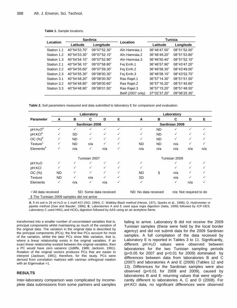
Table 1. Sample locations.

Location Sardinia

Location Tunisia

Latitude Longitude Latitude Longitude

Station 1.1 40°54’53.70” 09°07’52.30” Aîn Hamraia.1 36°46’47.50” 08°51’52.00”



Station 2.1 40°54’56.10” 09°07‘58.80” Fej Errih.1 36°46’57.90” 08°43’47.20”

Station 2.2 40°54’55.60” 09°07’59.30” Fej Errih.2 36°46’58.30” 08°43’49.00”

Station 2.3 40°54’55.30” 09°08’00.30” Fej Errih.3 36°46’58.10” 08°43’52.70”

Station 3.1 40°54’48.20” 09°08’00.50” Ras Rajel.1 36°57’14.30” 08°51’51.50”



Belif (2007 only) 37°02’37.20” 09°06’25.30”

Table 2. Soil parameters measured and data submitted to laboratory E for comparison and evaluation.

Parameter

Laboratory Laboratory

A B C D E A B C D E

Sardinian 2008 Sardinian 2009

pH:H2Oa ND

pH:KCla SD ND

OC (%)b ND ND

Texturec ND n/a ND ND n/a

Elementsd n/a n/a n/a n/a n/a n/a n/a

Tunisian 2007 Tunisian 2009

pH:H2O

§

pH:KCl

OC (%) ND ND n/a

Texture ND n/a SD n/a

Elements n/a n/a n/a

All data received SD: Some data received ND: No data received n/a: Not required to do

§ The Tunisian 2009 samples did not arrive

A. 5 ml soil in 25 ml H2O or 1 mol/l KCl (ISO, 1994); C. Walkley Black method (Hesse, 1971; Sparks et al., 1996); D, Hydrometer or pipette method (Gee and Bauder, 1986); E. Laboratories A and E used aqua regia digestion (Italia, 1999) followed by ICP-OES. Laboratory C used HNO3 and HClO4 digestion followed by AAS using an air-acetylene flame.

transformed into a smaller number of uncorrelated variables that is, principal components whilst maintaining as much of the variation of the original data. The variation in the original data is described by the principal components (PCs); the first few PCs account for most of the variation, whilst the later PCs show little variation, that is, where a linear relationship exists in the original variables. If an exact linear relationship existed between the original variables, then a PC would have zero variance (Jolliffe, 1986; Jackson, 1991). Rotation of the original vectors produces PCs that are easier to interpret (Jackson, 1991); therefore, for this study, PCs were derived from correlation matrices with varimax orthogonal rotation with an Eigenvalue >1.

RESULTS

Inter-laboratory comparison was complicated by income-plete data submissions from some partners and samples

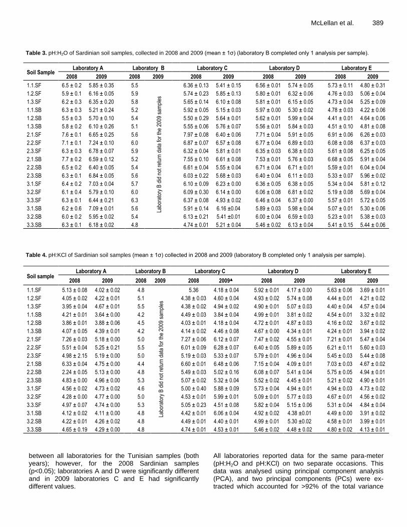
failing to arrive. Laboratory B did not receive the 2009 Tunisian samples (these were held by the local border agency) and did not submit data for the 2009 Sardinian samples. A full compilation of the data received by Laboratory E is reported in Tables 3 to 11. Significantly, different pH:H2O values were observed between laboratories for the two Tunisian sampling periods (p<0.05 for 2007 and p<0.01 for 2009) dominated by differences between data from laboratories B and C (2007) and laboratories A and E (2009) (Tables 12 and 13). Differences for the Sardinian samples were also observed (p<0.01 for 2008 and 2009), caused by laboratories B and E returning values that were signify-cantly different to laboratories A, C and D (2008). For pH:KCl data, no significant differences were observed

McLellan et al. 389

Table 3. pH:H2O of Sardinian soil samples, collected in 2008 and 2009 (mean ± 1σ) (laboratory B completed only 1 analysis per sample).

Soil Sample Laboratory A Laboratory B Laboratory C Laboratory D Laboratory E

2008 2009 2008 2009 2008 2009 2008 2009 2008 2009

1.1.SF 6.5 ± 0.2 5.85 ± 0.35 5.5

Labo

rato

ry B

did

not

ret

urn

data

for

the

2009

sam

ples

6.36 ± 0.13 5.41 ± 0.15 6.56 ± 0.01 5.74 ± 0.05 5.73 ± 0.11 4.80 ± 0.31

1.2.SF 5.9 ± 0.1 6.16 ± 0.05 5.9 5.74 ± 0.23 5.85 ± 0.13 5.80 ± 0.01 6.32 ± 0.06 4.76 ± 0.03 5.06 ± 0.04

1.3.SF 6.2 ± 0.3 6.35 ± 0.20 5.8 5.65 ± 0.14 6.10 ± 0.08 5.81 ± 0.01 6.15 ± 0.05 4.73 ± 0.04 5.25 ± 0.09

1.1.SB 6.3 ± 0.3 5.21 ± 0.24 5.2 5.92 ± 0.05 5.15 ± 0.03 5.97 ± 0.00 5.30 ± 0.02 4.78 ± 0.03 4.22 ± 0.06

1.2.SB 5.5 ± 0.3 5.70 ± 0.10 5.4 5.50 ± 0.29 5.64 ± 0.01 5.62 ± 0.01 5.99 ± 0.04 4.41 ± 0.01 4.64 ± 0.06

1.3.SB 5.8 ± 0.2 6.10 ± 0.26 5.1 5.55 ± 0.06 5.76 ± 0.07 5.56 ± 0.01 5.84 ± 0.03 4.51 ± 0.10 4.81 ± 0.08

2.1.SF 7.6 ± 0.1 6.65 ± 0.25 5.6 7.97 ± 0.08 6.40 ± 0.06 7.71 ± 0.04 5.91 ± 0.05 6.91 ± 0.06 6.26 ± 0.03

2.2.SF 7.1 ± 0.1 7.24 ± 0.10 6.0 6.87 ± 0.07 6.57 ± 0.08 6.77 ± 0.04 6.89 ± 0.03 6.08 ± 0.08 6.37 ± 0.03

2.3.SF 6.3 ± 0.3 6.78 ± 0.07 5.9 6.32 ± 0.04 5.81 ± 0.01 6.35 ± 0.03 6.38 ± 0.03 5.61 ± 0.08 6.25 ± 0.05

2.1.SB 7.7 ± 0.2 6.59 ± 0.12 5.2 7.55 ± 0.10 6.61 ± 0.08 7.53 ± 0.01 5.76 ± 0.03 6.68 ± 0.05 5.91 ± 0.04

2.2.SB 6.5 ± 0.2 6.40 ± 0.05 5.4 6.61 ± 0.04 5.55 ± 0.04 6.71 ± 0.04 6.71 ± 0.01 5.59 ± 0.01 6.04 ± 0.04

2.3.SB 6.3 ± 0.1 6.84 ± 0.05 5.6 6.03 ± 0.22 5.68 ± 0.03 6.40 ± 0.04 6.11 ± 0.03 5.33 ± 0.07 5.96 ± 0.02

3.1.SF 6.4 ± 0.2 7.03 ± 0.04 5.7 6.10 ± 0.09 6.23 ± 0.00 6.36 ± 0.05 6.38 ± 0.05 5.34 ± 0.04 5.81 ± 0.12

3.2.SF 6.1 ± 0.4 5.79 ± 0.10 6.0 6.09 ± 0.30 6.14 ± 0.00 6.06 ± 0.08 6.81 ± 0.02 5.19 ± 0.08 5.69 ± 0.04

3.3.SF 6.3 ± 0.1 6.44 ± 0.21 6.3 6.37 ± 0.08 4.93 ± 0.02 6.46 ± 0.04 6.37 ± 0.00 5.57 ± 0.01 5.72 ± 0.05

3.1.SB 6.2 ± 0.6 7.09 ± 0.01 5.6 5.91 ± 0.14 6.16 ±0.04 5.89 ± 0.03 5.98 ± 0.04 5.07 ± 0.01 5.30 ± 0.06

3.2.SB 6.0 ± 0.2 5.95 ± 0.02 5.4 6.13 ± 0.21 5.41 ±0.01 6.00 ± 0.04 6.59 ± 0.03 5.23 ± 0.01 5.38 ± 0.03

3.3.SB 6.3 ± 0.1 6.18 ± 0.02 4.8 4.74 ± 0.01 5.21 ± 0.04 5.46 ± 0.02 6.13 ± 0.04 5.41 ± 0.15 5.44 ± 0.06

Table 4. pH:KCl of Sardinian soil samples (mean ± 1σ) collected in 2008 and 2009 (laboratory B completed only 1 analysis per sample).

Soil sample Laboratory A Laboratory B Laboratory C Laboratory D Laboratory E

2008 2009 2008 2009 2008 2009▲ 2008 2009 2008 2009

1.1.SF 5.13 ± 0.08 4.02 ± 0.02 4.8

Labo

rato

ry B

did

not

ret

urn

data

for

the

2009

sam

ples

5.36 4.18 ± 0.04 5.92 ± 0.01 4.17 ± 0.00 5.63 ± 0.06 3.69 ± 0.01

1.2.SF 4.05 ± 0.02 4.22 ± 0.01 5.1 4.38 ± 0.03 4.60 ± 0.04 4.93 ± 0.02 5.74 ± 0.08 4.44 ± 0.01 4.21 ± 0.02

1.3.SF 3.95 ± 0.04 4.67 ± 0.01 5.5 4.38 ± 0.02 4.94 ± 0.02 4.90 ± 0.01 5.07 ± 0.03 4.40 ± 0.04 4.57 ± 0.04

1.1.SB 4.21 ± 0.01 3.64 ± 0.00 4.2 4.49 ± 0.03 3.84 ± 0.04 4.99 ± 0.01 3.81 ± 0.02 4.54 ± 0.01 3.32 ± 0.02

1.2.SB 3.86 ± 0.01 3.88 ± 0.06 4.5 4.03 ± 0.01 4.18 ± 0.04 4.72 ± 0.01 4.87 ± 0.03 4.16 ± 0.02 3.67 ± 0.02

1.3.SB 4.07 ± 0.05 4.39 ± 0.01 4.2 4.14 ± 0.02 4.46 ± 0.08 4.67 ± 0.00 4.34 ± 0.01 4.24 ± 0.01 3.94 ± 0.02

2.1.SF 7.26 ± 0.03 5.18 ± 0.00 5.0 7.27 ± 0.06 6.12 ± 0.07 7.47 ± 0.02 4.55 ± 0.01 7.21 ± 0.01 5.47 ± 0.04

2.2.SF 5.51 ± 0.04 5.25 ± 0.21 5.5 6.01 ± 0.09 6.28 ± 0.07 6.40 ± 0.05 5.89 ± 0.05 6.21 ± 0.11 5.60 ± 0.03

2.3.SF 4.98 ± 2.15 5.19 ± 0.00 5.0 5.19 ± 0.03 5.33 ± 0.07 5.79 ± 0.01 4.96 ± 0.04 5.45 ± 0.03 5.44 ± 0.08

2.1.SB 6.33 ± 0.04 4.75 ± 0.00 4.4 6.60 ± 0.01 6.48 ± 0.06 7.15 ± 0.04 4.09 ± 0.01 7.03 ± 0.03 4.67 ± 0.02

2.2.SB 2.24 ± 0.05 5.13 ± 0.00 4.8 5.49 ± 0.03 5.02 ± 0.16 6.08 ± 0.07 5.41 ± 0.04 5.75 ± 0.05 4.94 ± 0.01

2.3.SB 4.83 ± 0.00 4.96 ± 0.00 5.3 5.07 ± 0.02 5.32 ± 0.04 5.52 ± 0.02 4.45 ± 0.01 5.21 ± 0.02 4.90 ± 0.01

3.1.SF 4.56 ± 0.02 4.73 ± 0.02 4.6 5.00 ± 0.40 5.88 ± 0.09 5.73 ± 0.04 4.94 ± 0.01 4.94 ± 0.03 4.73 ± 0.02

3.2.SF 4.28 ± 0.00 4.77 ± 0.00 5.0 4.53 ± 0.01 5.99 ± 0.01 5.09 ± 0.01 5.77 ± 0.03 4.67 ± 0.01 4.56 ± 0.02

3.3.SF 4.97 ± 0.07 4.74 ± 0.00 5.3 5.05 ± 0.23 4.51 ± 0.08 5.82 ± 0.04 5.15 ± 0.06 5.31 ± 0.04 4.84 ± 0.04

3.1.SB 4.12 ± 0.02 4.11 ± 0.00 4.8 4.42 ± 0.01 6.06 ± 0.04 4.92 ± 0.02 4.38 ±0.01 4.49 ± 0.00 3.91 ± 0.02

3.2.SB 4.22 ± 0.01 4.26 ± 0.02 4.8 4.49 ± 0.01 4.40 ± 0.01 4.99 ± 0.01 5.30 ±0.02 4.58 ± 0.01 3.99 ± 0.01

3.3.SB 4.65 ± 0.19 4.29 ± 0.00 4.8 4.74 ± 0.01 4.53 ± 0.01 5.46 ± 0.02 4.48 ± 0.02 4.80 ± 0.02 4.13 ± 0.01

between all laboratories for the Tunisian samples (both years); however, for the 2008 Sardinian samples (p<0.05); laboratories A and D were significantly different and in 2009 laboratories C and E had significantly different values.

All laboratories reported data for the same para-meter (pH:H2O and pH:KCl) on two separate occasions. This data was analysed using principal component analysis (PCA), and two principal components (PCs) were ex-tracted which accounted for >92% of the total variance


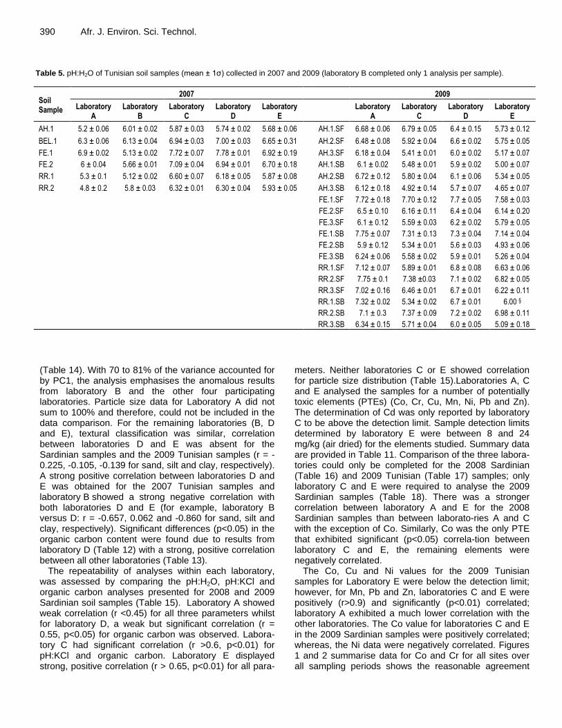
Table 5. pH:H2O of Tunisian soil samples (mean ± 1σ) collected in 2007 and 2009 (laboratory B completed only 1 analysis per sample).

Soil Sample

2007 2009

Laboratory A

Laboratory B

Laboratory C

Laboratory D

Laboratory E

Laboratory

A Laboratory

C Laboratory

D Laboratory

E

AH.1 5.2 ± 0.06 6.01 ± 0.02 5.87 ± 0.03 5.74 ± 0.02 5.68 ± 0.06 AH.1.SF 6.68 ± 0.06 6.79 ± 0.05 6.4 ± 0.15 5.73 ± 0.12

BEL.1 6.3 ± 0.06 6.13 ± 0.04 6.94 ± 0.03 7.00 ± 0.03 6.65 ± 0.31 AH.2.SF 6.48 ± 0.08 5.92 ± 0.04 6.6 ± 0.02 5.75 ± 0.05

FE.1 6.9 ± 0.02 5.13 ± 0.02 7.72 ± 0.07 7.78 ± 0.01 6.92 ± 0.19 AH.3.SF 6.18 ± 0.04 5.41 ± 0.01 6.0 ± 0.02 5.17 ± 0.07

FE.2 6 ± 0.04 5.66 ± 0.01 7.09 ± 0.04 6.94 ± 0.01 6.70 ± 0.18 AH.1.SB 6.1 ± 0.02 5.48 ± 0.01 5.9 ± 0.02 5.00 ± 0.07

RR.1 5.3 ± 0.1 5.12 ± 0.02 6.60 ± 0.07 6.18 ± 0.05 5.87 ± 0.08 AH.2.SB 6.72 ± 0.12 5.80 ± 0.04 6.1 ± 0.06 5.34 ± 0.05

RR.2 4.8 ± 0.2 5.8 ± 0.03 6.32 ± 0.01 6.30 ± 0.04 5.93 ± 0.05 AH.3.SB 6.12 ± 0.18 4.92 ± 0.14 5.7 ± 0.07 4.65 ± 0.07

FE.1.SF 7.72 ± 0.18 7.70 ± 0.12 7.7 ± 0.05 7.58 ± 0.03

FE.2.SF 6.5 ± 0.10 6.16 ± 0.11 6.4 ± 0.04 6.14 ± 0.20

FE.3.SF 6.1 ± 0.12 5.59 ± 0.03 6.2 ± 0.02 5.79 ± 0.05

FE.1.SB 7.75 ± 0.07 7.31 ± 0.13 7.3 ± 0.04 7.14 ± 0.04

FE.2.SB 5.9 ± 0.12 5.34 ± 0.01 5.6 ± 0.03 4.93 ± 0.06

FE.3.SB 6.24 ± 0.06 5.58 ± 0.02 5.9 ± 0.01 5.26 ± 0.04

RR.1.SF 7.12 ± 0.07 5.89 ± 0.01 6.8 ± 0.08 6.63 ± 0.06

RR.2.SF 7.75 ± 0.1 7.38 ±0.03 7.1 ± 0.02 6.82 ± 0.05

RR.3.SF 7.02 ± 0.16 6.46 ± 0.01 6.7 ± 0.01 6.22 ± 0.11

RR.1.SB 7.32 ± 0.02 5.34 ± 0.02 6.7 ± 0.01 6.00 §

RR.2.SB 7.1 ± 0.3 7.37 ± 0.09 7.2 ± 0.02 6.98 ± 0.11

RR.3.SB 6.34 ± 0.15 5.71 ± 0.04 6.0 ± 0.05 5.09 ± 0.18

(Table 14). With 70 to 81% of the variance accounted for by PC1, the analysis emphasises the anomalous results from laboratory B and the other four participating laboratories. Particle size data for Laboratory A did not sum to 100% and therefore, could not be included in the data comparison. For the remaining laboratories (B, D and E), textural classification was similar, correlation between laboratories D and E was absent for the Sardinian samples and the 2009 Tunisian samples (r = -0.225, -0.105, -0.139 for sand, silt and clay, respectively). A strong positive correlation between laboratories D and E was obtained for the 2007 Tunisian samples and laboratory B showed a strong negative correlation with both laboratories D and E (for example, laboratory B versus D: r = -0.657, 0.062 and -0.860 for sand, silt and clay, respectively). Significant differences (p<0.05) in the organic carbon content were found due to results from laboratory D (Table 12) with a strong, positive correlation between all other laboratories (Table 13).

The repeatability of analyses within each laboratory, was assessed by comparing the pH:H2O, pH:KCl and organic carbon analyses presented for 2008 and 2009 Sardinian soil samples (Table 15). Laboratory A showed weak correlation (r <0.45) for all three parameters whilst for laboratory D, a weak but significant correlation (r = 0.55, p<0.05) for organic carbon was observed. Labora-tory C had significant correlation (r >0.6, p<0.01) for pH:KCl and organic carbon. Laboratory E displayed strong, positive correlation (r > 0.65, p<0.01) for all para-

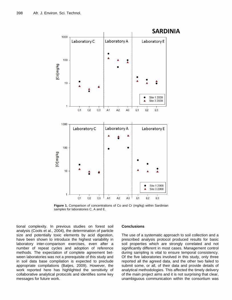
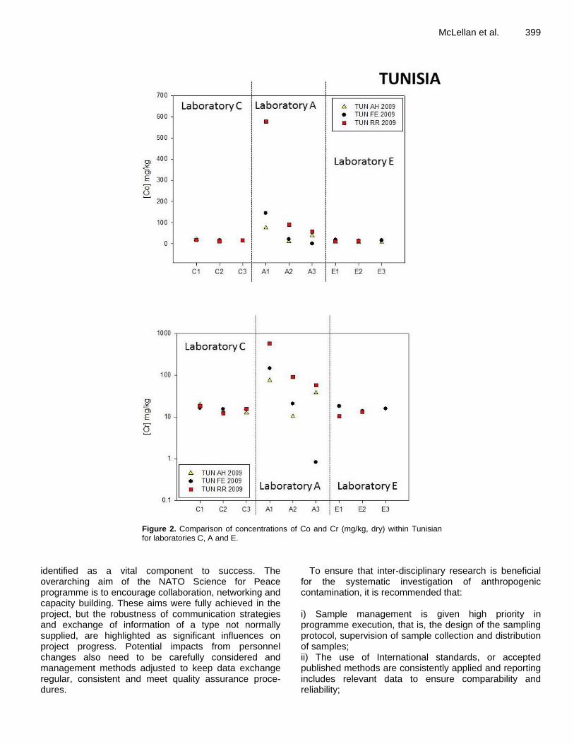
meters. Neither laboratories C or E showed correlation for particle size distribution (Table 15).Laboratories A, C and E analysed the samples for a number of potentially toxic elements (PTEs) (Co, Cr, Cu, Mn, Ni, Pb and Zn). The determination of Cd was only reported by laboratory C to be above the detection limit. Sample detection limits determined by laboratory E were between 8 and 24 mg/kg (air dried) for the elements studied. Summary data are provided in Table 11. Comparison of the three labora-tories could only be completed for the 2008 Sardinian (Table 16) and 2009 Tunisian (Table 17) samples; only laboratory C and E were required to analyse the 2009 Sardinian samples (Table 18). There was a stronger correlation between laboratory A and E for the 2008 Sardinian samples than between laborato-ries A and C with the exception of Co. Similarly, Co was the only PTE that exhibited significant (p<0.05) correla-tion between laboratory C and E, the remaining elements were negatively correlated.

The Co, Cu and Ni values for the 2009 Tunisian samples for Laboratory E were below the detection limit; however, for Mn, Pb and Zn, laboratories C and E were positively (r>0.9) and significantly (p<0.01) correlated; laboratory A exhibited a much lower correlation with the other laboratories. The Co value for laboratories C and E in the 2009 Sardinian samples were positively correlated; whereas, the Ni data were negatively correlated. Figures 1 and 2 summarise data for Co and Cr for all sites over all sampling periods shows the reasonable agreement

McLellan et al. 391

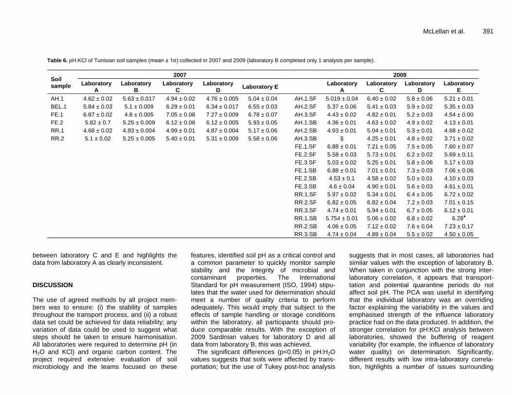
Table 6. pH:KCl of Tunisian soil samples (mean ± 1σ) collected in 2007 and 2009 (laboratory B completed only 1 analysis per sample).

Soil sample

2007 2009

Laboratory A

Laboratory B

Laboratory C

Laboratory D

Laboratory E Laboratory

A Laboratory

C Laboratory

D Laboratory

E

AH.1 4.62 ± 0.02 5.63 ± 0.017 4.94 ± 0.02 4.76 ± 0.005 5.04 ± 0.04 AH.1.SF 5.019 ± 0.04 6.40 ± 0.02 5.8 ± 0.06 5.21 ± 0.01

BEL.1 5.84 ± 0.03 5.1 ± 0.009 6.29 ± 0.01 6.34 ± 0.017 6.55 ± 0.03 AH.2.SF 5.37 ± 0.06 5.41 ± 0.03 5.9 ± 0.02 5.35 ± 0.03

FE.1 6.87 ± 0.02 4.8 ± 0.005 7.05 ± 0.08 7.27 ± 0.009 6.78 ± 0.07 AH.3.SF 4.43 ± 0.02 4.82 ± 0.01 5.2 ± 0.03 4.54 ± 0.00

FE.2 5.82 ± 0.7 5.25 ± 0.009 6.12 ± 0.08 6.12 ± 0.005 5.93 ± 0.05 AH.1.SB 4.36 ± 0.01 4.63 ± 0.02 4.9 ± 0.02 4.13 ± 0.01

RR.1 4.68 ± 0.02 4.93 ± 0.004 4.99 ± 0.01 4.87 ± 0.004 5.17 ± 0.06 AH.2.SB 4.93 ± 0.01 5.04 ± 0.01 5.3 ± 0.01 4.68 ± 0.02

RR.2 5.1 ± 0.02 5.25 ± 0.005 5.40 ± 0.01 5.31 ± 0.009 5.58 ± 0.06 AH.3.SB § 4.25 ± 0.01 4.8 ± 0.02 3.71 ± 0.02

FE.1.SF 6.88 ± 0.01 7.21 ± 0.05 7.5 ± 0.05 7.60 ± 0.07

FE.2.SF 5.58 ± 0.03 5.73 ± 0.01 6.2 ± 0.02 5.69 ± 0.11

FE.3.SF 5.03 ± 0.02 5.25 ± 0.01 5.8 ± 0.06 5.17 ± 0.03

FE.1.SB 6.88 ± 0.01 7.01 ± 0.01 7.3 ± 0.03 7.06 ± 0.06

FE.2.SB 4.53 ± 0.1 4.58 ± 0.02 5.0 ± 0.01 4.10 ± 0.03

FE.3.SB 4.6 ± 0.04 4.90 ± 0.01 5.6 ± 0.03 4.61 ± 0.01

RR.1.SF 5.97 ± 0.02 5.34 ± 0.01 6.4 ± 0.05 6.72 ± 0.02

RR.2.SF 6.82 ± 0.05 6.82 ± 0.04 7.2 ± 0.03 7.01 ± 0.15

RR.3.SF 4.74 ± 0.01 5.94 ± 0.01 6.7 ± 0.05 6.12 ± 0.01

RR.1.SB 5.754 ± 0.01 5.06 ± 0.02 6.8 ± 0.02 6.28●

RR.2.SB 4.06 ± 0.05 7.12 ± 0.02 7.6 ± 0.04 7.23 ± 0.17

RR.3.SB 4.74 ± 0.04 4.89 ± 0.04 5.5 ± 0.02 4.50 ± 0.05

between laboratory C and E and highlights the data from laboratory A as clearly inconsistent. DISCUSSION The use of agreed methods by all project mem-bers was to ensure: (i) the stability of samples throughout the transport process, and (ii) a robust data set could be achieved for data reliability; any variation of data could be used to suggest what steps should be taken to ensure harmonisation. All laboratories were required to determine pH (in H2O and KCl) and organic carbon content. The project required extensive evaluation of soil microbiology and the teams focused on these

features, identified soil pH as a critical control and a common parameter to quickly monitor sample stability and the integrity of microbial and contaminant properties. The International Standard for pH measurement (ISO, 1994) stipu-lates that the water used for determination should meet a number of quality criteria to perform adequately. This would imply that subject to the effects of sample handling or storage conditions within the laboratory, all participants should pro-duce comparable results. With the exception of 2009 Sardinian values for laboratory D and all data from laboratory B, this was achieved.

The significant differences (p<0.05) in pH:H2O values suggests that soils were affected by trans-portation; but the use of Tukey post-hoc analysis

suggests that in most cases, all laboratories had similar values with the exception of laboratory B. When taken in conjunction with the strong inter-laboratory correlation, it appears that transport-tation and potential quarantine periods do not affect soil pH. The PCA was useful in identifying that the individual laboratory was an overriding factor explaining the variability in the values and emphasised strength of the influence laboratory practice had on the data produced. In addition, the stronger correlation for pH:KCl analysis between laboratories, showed the buffering of reagent variability (for example, the influence of laboratory water quality) on determination. Significantly, different results with low intra-laboratory correla-tion, highlights a number of issues surrounding


Table 7. Organic carbon content (%w/w, mean ± 1σ) of Sardinian soil samples collected in 2008 and 2009.

Soil Sample Laboratory A Laboratory C Laboratory D Laboratory E

2008 2009 2008 2009 2008 2009 2008 2009

1.1.SF 4.93 ± 0.29 6.34 ± 1.20 3.16 ± 0.226 3.84 ± 0.105 2.62 ± 0.14 3.79 ± 0.16 3.49 ± 0.60 4.62 ± 0.36

1.2.SF 6.56 ± 0.86 4.47 ± 0.52 2.86 ± 0.120 3.76 ± 0.195 2.00 ± 0.07 4.44 ± 0.17 3.33 ± 0.20 3.59 ± 0.31

1.3.SF 5.92 ± 0.40 5.76 ± 1.29 2.83 ± 0.226 3.59 ± 0.594 2.46 ± 0.29 4.83 ± 0.40 2.60 ± 0.29 3.30 ± 0.12

1.1.SB 6.55 ± 0.66 5.29 ± 0.45 2.39 ± 0.173 3.00 ± 0.000 1.75 ± 0.17 3.38 ± 0.35 2.52 ± 0.21 3.70 ± 0.06

1.2.SB 9.20 ± 0.96 3.62 ± 0.86 2.43 ± 0.248 2.41 ± 0.120 1.83 ± 0.13 2.01 ± 0.09 2.18 ± 0.25 2.91 ± 0.25

1.3.SB 8.50 ± 1.05 4.78 ± 1.74 1.88 ± 0.173 1.86 ± 0.195 1.46 ± 0.11 3.96 ± 0.48 1.97 ± 0.14 2.59 ± 0.12

2.1.SF 4.45 ± 0.70 5.62 ± 0.41 3.52 ± 0.481 3.33 ± 0.113 2.74 ± 0.31 3.00 ± 0.07 2.72 ± 0.84 3.25 ± 0.24

2.2.SF 5.97 ± 1.10 5.91 ± 0.77 5.29 ± 0.699 4.93 ± 0.180 5.02 ± 0.47 4.09 ± 0.44 6.53 ± 0.43 4.47 ± 0.18

2.3.SF 5.07 ± 1.10 6.26 ± 0.45 3.68 ± 0.692 3.80 ± 0.970 3.29 ± 0.38 5.06 ± 0.17 4.20 ± 0.95 5.70 ± 0.31

2.1.SB 5.21 ± 0.82 4.77 ± 1.06 1.71 ± 0.128 2.50 ± 0.338 1.42 ± 0.05 2.59 ± 0.08 1.85 ± 0.19 2.75 ± 0.14

2.2.SB 7.98 ± 1.32 5.85 ± 0.76 2.69 ± 0.353 2.62 ± 0.038 2.77 ± 0.24 3.31 ± 0.22 3.44 ± 0.29 3.41 ± 0.27

2.3.SB 10.24 ± 2.02 6.06 ± 0.85 2.60 ± 0.323 3.55 ± 0.353 2.61 ± 0.28 4.02 ± 0.11 2.48 ± 0.25 3.70 ± 0.21

3.1.SF 10.36 ± 1.42 6.47 ± 0.75 3.52 ± 0.421 4.53 ± 0.083 3.11 ± 0.17 2.96 ± 0.25 4.28 ± 0.28 5.65 ± 0.06

3.2.SF 12.22 ± 1.64 5.54 ± 1.47 5.93 ± 0.526 6.22 ± 0.541 4.55 ± 0.26 6.03 ± 0.34 6.49 ± 0.30 6.80 ± 0.36

3.3.SF 7.66 ± 0.05 6.54 ± 0.74 4.23 ± 0.459 4.92 ± 0.218 3.41 ± 0.20 6.10 ± 0.51 4.13 ± 0.17 5.21 ± 0.27

3.1.SB 8.04 ± 1.13 6.05 ± 1.26 3.34 ± 0.241 3.08 ± 0.098 2.53 ± 0.08 2.98 ± 0.42 3.63 ± 0.11 3.68 ± 0.07

3.2.SB 10.08 ± 1.22 6.91 ± 0.46 4.80 ± 0.256 3.66 ± 0.143 3.38 ± 0.23 4.82 ± 0.22 4.82 ± 0.15 5.13 ± 0.26

3.3.SB 5.84 ± 0.81 6.22 ± 0.78 2.98 ±0.549 2.88 ± 0.241 2.75 ± 0.11 4.49 ± 0.23 3.15 ± 0.19 3.19 ± 0.11

Table 8. Organic carbon content (%w/w, mean ± 1σ) of Tunisian soil samples collected in 2007 and 2009, laboratory C did not report replicates.

Soil Sample

2007 2009

Laboratory B▲

Laboratory

C▲

Laboratory

D▲

Laboratory

E▲

Laboratory A▲

Laboratory

D▲

Laboratory

E▲

AH.1 2.37 ± 0.26 2.96 3.52 ± 0.13 2.90 ± 0.15 AH.1.SF 4.02 ± 0.53 3.71 ± 0.20 3.85 ± 0.25

BEL.1 1.46 ± 0.20 6.17 5.33 ± 0.59 4.41 ± 0.14 AH.2.SF 5.53 ± 0.66 5.16 ± 0.12 4.04 ± 0.32

FE.1 2.01 ± 0.13 3.09 3.67 ± 0.03 3.11 ± 0.08 AH.3.SF 8.05 ± 0.86 5.04 ± 0.16 4.09 ± 0.04

FE.2 1.38 ± 0.81 2.56 3.17 ± 0.65 2.52 ± 0.15 AH.1.SB 1.75 ± 0.14 1.58 ± 0.07 2.04 ± 0.11

RR.1 2.41 ± 0.36 1.87 2.47 ± 0.25 2.07 ± 0.01 AH.2.SB 1.32 ± 0.15 1.56 ± 0.12 1.35 ± 0.07

RR.2 1.50 ± 0.17 1.41 1.67 ± 0.16 1.61 ± 0.14 AH.3.SB 6.56 ± 0.65 2.06 ± 0.12 1.90 ± 0.05

FE.1.SF 7.38 ± 0.66 3.57 ± 0.03 3.16 ± 0.28

FE.2.SF 9.82 ± 1.14 6.57 ± 0.50 5.03 ± 0.35

FE.3.SF 7.67 ± 0.11 4.90 ± 0.27 4.39 ± 0.27

FE.1.SB 7.17 ± 0.60 2.11 ± 0.10 2.19 ± 0.03

FE.2.SB 7.14 ± 1.17 3.34 ± 0.17 3.33 ± 0.06

FE.3.SB 7.35 ± 0.90 3.55 ± 0.32 3.90 ± 0.25

RR.1.SF 4.96 ± 0.14 4.92 ± 0.47 4.68 ± 0.51

RR.2.SF 3.85 ± 0.09 2.67 ± 0.37 1.21 ± 0.04

RR.3.SF 3.55 ± 0.24 3.22 ± 0.45 2.62 ± 0.35

RR.1.SB 0.78 ± 0.05 1.34 ± 0.10 2.11 ± 0.10

RR.2.SB 1.80 ± 0.08 1.82 ± 0.28 1.34 ± 0.15

RR.3.SB 2.33 ± 0.24 1.08 ± 0.19 0.98 ± 0.07

McLellan et al. 393 Table 9. Particle size analysis (%) of Sardinian soil samples.

Soil Sample

Laboratory A Laboratory D Laboratory E

2008 2008 2009 2008 2009

Sand Silt Clay Sand Silt Clay Sand Silt Clay Sand Silt Clay Sand Silt Clay

1.1.SF 72.1 21.7 4.4 64.91 17.80 17.29 64.91 17.80 17.29 60.92 32.65 6.43 60.92 32.65 6.43

1.2.SF 70.9 21.3 2.8 69.76 14.45 15.79 69.76 14.45 15.79 63.04 33.25 3.71 63.04 33.25 3.71

1.3.SF 69.6 11.5 15.8 69.17 14.31 16.52 69.17 14.31 16.52 67.62 27.86 4.52 67.62 27.86 4.52

1.1.SB 81.6 12.5 3.8 70.27 14.40 15.33 70.27 14.40 15.33 69.90 18.93 11.17 69.90 18.93 11.17

1.2.SB 65.4 16.2 3.5 69.90 14.67 15.43 69.90 14.67 15.43 62.36 33.57 4.07 62.36 33.57 4.07

1.3.SB 61.7 14.6 15.0 69.63 14.04 16.33 69.63 14.04 16.33 58.92 35.51 5.57 58.92 35.51 5.57

2.1.SF 64.0 26.2 2.7 70.33 15.69 13.98 70.33 15.69 13.98 70.23 22.48 7.29 70.23 22.48 7.29

2.2.SF 69.5 16.2 3.8 61.85 17.98 20.17 61.85 17.98 20.17 61.05 32.95 6.01 61.05 32.95 6.01

2.3.SF 71.0 15.0 4.6 65.90 16.33 17.77 65.90 16.33 17.77 67.94 28.77 3.29 67.94 28.77 3.29

2.1.SB 77.9 16.8 2.6 71.87 14.34 13.79 71.87 14.34 13.79 61.78 32.14 6.08 61.78 32.14 6.08

2.2.SB 72.1 10.3 14.6 67.02 15.30 17.68 67.02 15.30 17.68 66.02 28.84 5.14 66.02 28.84 5.14

2.3.SB 69.8 12.3 15.6 69.53 14.60 15.87 69.53 14.60 15.87 71.38 23.54 5.09 71.38 23.54 5.09

3.1.SF 88.6 6.3 2.9 62.23 17.16 20.61 62.23 17.16 20.61 67.33 29.36 3.31 67.33 29.36 3.31

3.2.SF 67.7 21.2 3.9 65.28 18.90 15.82 65.28 18.90 15.82 71.21 26.11 2.68 71.21 26.11 2.68

3.3.SF 64.4 27.3 2.7 64.62 15.61 19.77 64.62 15.61 19.77 71.57 24.71 3.72 71.57 24.71 3.72

3.1.SB 61.8 29.2 4.3 65.10 15.54 19.36 65.10 15.54 19.36 68.56 23.77 7.68 68.56 23.77 7.68

3.2.SB 67.6 22.7 4.6 68.69 14.88 16.43 68.69 14.88 16.43 69.64 29.18 1.19 69.64 29.18 1.19

3.3.SB 65.1 20.7 5.4 62.23 17.16 20.61 62.23 17.16 20.61 66.85 30.10 3.04 66.85 30.10 3.04

Table 10. Particle size analysis (%) of Tunisian soil samples.

Soil Sample

2008 2009

Laboratory B Laboratory D Laboratory E Laboratory A Laboratory D Laboratory E

Sand Silt Clay Sand Silt Clay Sand Silt Clay Sand Silt Clay Sand Silt Clay Sand Silt Clay

AH.1 24.9 51.1 24.0 75.30 10.20 14.50 62.87 28.53 8.60 AH.1.SF 62.86 28.54 8.6 68.43 18.45 13.12 57.04 30.07 12.89

BEL.1 37.9 42.4 19.7 ● 63.87 29.44 6.70 AH.2.SF 63.83 29.44 6.7 71.16 16.10 12.74 64.06 27.06 8.88

FE.1 44.5 34.9 20.6 61.60 14.60 23.80 51.65 37.53 10.82 AH.3.SF 62.2 29.03 6.12 75.75 9.46 14.79 57.52 35.00 7.47

FE.2 34.8 41.8 23.4 64.50 19.30 16.20 55.99 31.60 12.41 AH.1.SB 68.88 11.51 19.61 47.78 31.12 21.10

RR.1 30.3 39.3 30.4 75.90 10.30 13.80 66.04 24.73 9.23 AH.2.SB 65.16 13.44 21.40 66.03 29.44 4.53

RR.2 32.1 36.3 31.6 85.60 4.70 9.70 76.52 16.92 6.55 AH.3.SB 59.88 16.72 23.40 59.52 30.71 9.77

FE.1.SF 51.65 37.53 10.82 75.50 8.95 15.55 53.69 38.03 8.29

FE.2.SF 55.98 31.61 11.81 84.10 5.54 10.36 56.68 37.35 5.97


Table 10. Contd

FE.3.SF 52.03 33.06 11.1 82.22 4.94 12.84 49.99 45.28 4.73

FE.1.SB 64.60 23.49 11.91 46.81 41.95 11.24

FE.2.SB 81.65 8.26 10.09 49.43 39.95 10.62

FE.3.SB 73.38 14.76 11.86 41.45 49.42 9.13

RR.1.SF 66.04 24.73 8.83 62.82 15.30 21.88 56.47 35.10 8.43

RR.2.SF 76.52 16.93 6.35 60.49 18.11 21.40 61.69 35.46 2.85

RR.3.SF 69.23 22.23 6.03 56.34 17.30 26.36 72.77 24.38 2.85

RR.1.SB 63.60 22.84 13.56 ●

RR.2.SB 80.08 8.83 11.09 70.48 24.18 5.34

RR.3.SB 79.68 9.37 10.95 67.09 24.86 8.04

● Not determined.

Table 11. Summary of potentially toxic element concentrations for Tunisian and Sardinian soils reported for laboratory A, C and E.

Sampling period Laboratory (no. of samples) Element [mean (standard deviation)] (mg/kg, air dry)

Co Cr Cu Mn Ni Pb Zn

Sardinia 2008

C (9) 3.0 (2.1) 15.0 (2.5) 7.2 (3.6) 441.2 (415) 17.9 (10.1) 31.8 (17.7) 39.2 (28.5)

A (18) 102.8 (54.1) 210 (156) 106 (18.5) nd 121.7 (28.1) 171.8 (109) Nd

E (18) 12.4 (4.4) 18.5 (8.6) <dl 1494 (448) 10.1 (5.1) 21.9 (5.4) 67.3 (31.6)

Tunisia 2009

C (8) 7.0 (2.3) 10.7 (4.0) 5.41 (2.6) 772 (97) 5.70 (2.5) 16.9 (1.7) 54.0 (11.0)

A (16) 47.8 (38.3) 91.6 (142) 26.3 (18.7) Nd 53.7 (25.9) nd nd

E (18) <dl 13.2 (2.9) <dl 819 (1,697) <dl 131.2 (317) 120.6 (252)

Sardinia 2009 A (18) 1.9 (1.5) 0.5 (0.3) 0.1 (0.1) nd 12.44 (49.31) nd nd

E (18) 9.6 (3.2) 16.0 (7.0) 10.7 (5.8) 1,110 (177) 9.3 (3.3) 19.5 (4.2) 73.4 (14.7)

surrounding laboratory procedures and practice. Following a single method for organic carbon determination produced results which had strong, positive correlation with the exception of labora-tory A. The poor correlation for particle size analy-sis can be explained by the use of four different methodologies. Laboratories A and B used a modified hydrometer method (removal of organic

carbon using H2O2); however, did not communi-cate their complete methodology. The failure to communicate detailed methodologies and subse-quent results led to confusion in interpretation and delays in processing outputs. Values for laborato-ry A failed to sum to 100%, and the missing percentage was attributed to the removal of orga-nic material; thus, the data had to be excluded

from comparison. Laboratory D followed the pipette method and

laboratory E followed the hydrometer method (Table 2); with, laboratory E consistently reporting greater silt content. The two methodologies used different concentrations of sodium hexametapho-sphate (Na-HMP): Laboratory D - 0.075 g HMP/g soil, laboratory E - 0.125 g HMP/g soil. The higher

McLellan et al. 395

Table 12. ANOVA with Tukey post-hoc analysis of pH:H2O, pH:KCl and organic carbon content in soil samples from Tunisia and Sardinia.

Laboratory

pH:H2O pH:KCl Organic carbon (%)

Tunisia Sardinia Tunisia Sardinia Tunisia Sardinia

2007 2009 2008 2009 2007 2009 2008 2009 2007 2009 2008 2009

n = 7 n = 18 n = 18 n = 18 n = 7 n = 18 n = 18 n = 18 n = 7 n = 18 n = 18 n = 18

A 5.75 ± 0.79

ab

6.73 ± 0.62

b

6.39 ± 0.57

a

6.35 ± 0.54

b

5.49 ± 0.86

a

5.28 ± 0.91

a

4.62 ± 1.06

b

4.57 ± 0.49

ab

§ 5.06 ± 2.73

b

7.49 ± 2.24

b

5.69 ± 0.83

b

B 5.64 ± 0.43

b

▲ 5.63 ± 0.32

b

§ 5.16 ± 0.29

a

▲ 4.87 ± 0.39

ab

§ 1.86 ± 0.47

a

▲ § §

C 6.76 ± 0.64

a

6.12 ± 0.84

ab

6.26 ± 0.65

a

5.81 ± 0.49

ab

5.80 ± 0.83

a

5.58 ± 0.95

a

5.04 ± 0.86

ab

5.12 ± 0.84

a

3.01 ± 1.68

a

§ 3.32 ± 1.13

a

3.58 ± 1.06

a

D 6.66 ± 0.73

ab

6.46 ± 0.60

ab

6.32 ± 0.60

a

6.19 ± 0.41

b

5.78 ± 0.97

a

6.08 ± 0.92

a

5.59 ± 0.81

a

4.85 ± 0.61

ab

3.31 ± 1.24

a

3.23 ± 1.59

a

2.76 ± 0.96

a

3.99 ± 1.12

a

E 6.29 ± 0.52

ab

5.90 ± 0.85

a

5.39 ± 0.68

b

5.50 ± 0.61

a

5.84 ± 0.71

a

5.54 ± 1.22

a

5.17 ± 0.91

ab

4.48 ± 0.66

b

2.77 ± 0.97

a

2.90 ± 1.31

a

3.55 ± 1.37

a

4.09 ± 1.19

a

F-ratio 3.84* 4.42** 11.38** 9.88** 0.84 1.97 3.32* 3.49* 1.71 6.24* 37.08** 13.79**

Values are mean ± σ; ▲ Samples were not received; § No values were reported; p<0.05; **<p0.01; Column values followed by different letters (a, b) indicate significant differences (p<0.05).

Table 13. Pearson correlation (r) matrix of organic carbon content for soil samples collected in Tunisia and Sardinia.

Sardinia

2008 (n = 18) 2009 (n = 18)

Laboratory A C D E Laboratory A C D E

A 1.000 A 1.000

C 0.322 1.000 C 0.429 1.000

D 0.236 0.938** 1.000 D 0.455 0.641** 1.000

E 0.312 0.948** 0.944** 1.000 E 0.554** 0.862** 0.603** 1.000

Tunisia

2007 (n = 6) 2009 (n = 18)

B C D E A D E

B 1.000 A 1.000

C -0.282 1.000 D 0.622** 1.000

D -0.155 0.968** 1.000 E 0.701** 0.925** 1.000

E -0.169 0.978** 0.995** 1.000

* p<0.05; ** p<0.01.


Table 14. Principal component analysis of cork forest soil (0 to 20 cm) pH:H2O and pH:KCl values as reported by all laboratories.

Laboratory pH 2007 Tunisia (n = 6) 2008 Sardinia (n = 18)

PC 1 PC 2 PC 1 PC 2

A H2O 0.912 0.227 0.968 -0.006

B H2O -0.018 -0.976 -0.012 0.951

C H2O 0.855 0.504 0.985 0.007

D H2O 0.939 0.337 0.988 0.026

E H2O 0.965 0.164 0.981 0.110

A KCl 0.961 0.225 0.779 0.107

B KCl -0.465 -0.820 0.108 0.938

C KCl 0.981 0.171 0.991 0.046

D KCl 0.976 0.194 0.986 0.056

E KCl 0.974 0.098 0.987 0.038

Variance (%) 81.7 14.0 74.3 17.8

Values highlighted in bold represent values which show a strong relationship within that component.

Table 15. Repeatability of physico-chemical measurements using Pearson correlation (r) comparison of Sardinian 2008 and 2009 soil samples for pH, organic carbon and particle size analysis.

Parameter A C D E

pH:H2O 0.441 0.448 0.002 0.712**

pH:KCl 0.305 0.601** -0.090 0.652**

Organic Carbon 0.035 0.863** 0.547* 0.809**

Sand

Did not submit 2009 values Not required to determine

-0.083 -0.244

Silt -0.131 -0.312

Clay 0.030 0.232

n = 18; **p<0.01; *p<0.05.

Table 16. Pearson correlation (r) of laboratory A, C and E elemental analysis for the Sardinian 2008 soil samples.

Element Laboratories A v C Laboratory C v E Laboratory A v E

r n r n r n

Co 0.819** 9 0.693 6 0.641* 12

Cr -0.096 9 0.696 6 -0.613 9

Cu 0.138 9 ▲ ▲

Mn § 0.176 9

§

Ni 0.107 9 0.741 6 -0.443 9

Pb -0.226 9 0.253 5 -0.380 9

Zn § 0.105 9

§

▲ Laboratory E values were below detection limits; § Laboratory A did not determine.

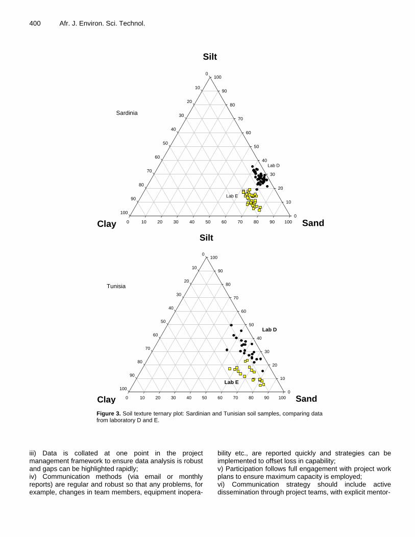
Na-HMP concentration could explain lower silt content results, with coarser fractions remaining in solution for long. Figure 3 show that whilst this difference is clear, it does not influence the final textural classification of

samples (USDA sandy-loam to loam). Slight differences in calculations and temperature correction factors have also been reported to explain difference in data achieved when using the hydrometer method (Keller and Gee, 2006);

McLellan et al. 397

Table 17. Pearson correlation (r) of laboratory A, C and E elemental analysis for the Tunisian 2009 soil samples.

Element Laboratories A v C Laboratory C v E Laboratory A v E

r n r n r n

Co -0.112 8 ▲ ▲

Cr 0.257 8 0.845 8 0.320 6

Cu 0.360 8 ▲ ▲

Mn § 0.989** 8 §

Ni -0.053 8 ▲ ▲

Pb § 0.918** 5 §

Zn § 0.974** 8 §

▲ Laboratory E values were below detection limits; § laboratory A did not determine; **p<0.01.

Table 18. Pearson correlation (r) of laboratory A and E elemental analysis for the Sardinian 2009 soil samples.

Element r n

Co 0.537* 15

Cr -0.223 12

Cu 0.398 6

Ni -0.835* 6

*p<0.05.

however, the most probable factor is the lack of detailed replication. Each hydrometer determination requires 40 g of soil (10 g for a pipette determination) and due to the amount of soil supplied for each sample, a full set of replicates could not be completed for all tests. Given the influence of even minor modification of common metho-dology, detailed information including precise calculation method is required as well as logistical planning for sample exchange. The greatest inter-laboratory variation for soil quality parameters has previously been attributed to particle size determination (Rust and Fenton, 1983) and the results of this study support this parameter to be highly sensitive to the detail of analytical methodology.

The determination of a suite of PTEs including Co, Cr, Mn, Ni and Pb by laboratories A, C and E produced limited agreement. The use of standard quality assurance and quality control procedures were reported by laboratories C and E through the use of replicates, blanks and certified reference materials, and for laboratory E data, the use of more than one wavelength for ICPOES (inductively coupled plasma - optical emission spectro-metry) determinations. Good recoveries and detection limits are reflected in the close correlation between C and E. The lack of correlation with laboratory A appears to be due to the differences in analytical techniques and soil

grain size chosen for digestion. Laboratories C and E both used sieved (<250 μm) and crushed soil whilst laboratory A used soil <2 mm; the smaller particle size making samples easier to digest and sub sampling less variable. The flame-AAS (atomic absorption spectro-metry) technique used by laboratory A, whilst a recom-mended national standard method, is much less sensitive than the ICP-OES analysis used by the other two laboratories and can be more strongly affected by matrix-based interferences. Other practical aspects of a multi-national project are likely to have affected data corre-lation. During the time of this study, laboratory A was subject to personnel changes at a number of levels, affecting project deliverables (for example, sample collec-tion), in addition, laboratories A and B did not complete a number of key project tasks which were never fully explained; although, communication between groups was good and inter-institutional exchange of PhD students had a strong positive effect on awareness of methodologies and training in new techniques. At some stages during the course of the project communication, either formal or informal, of critical project details and incomplete information supply, were of concern and caused delays in delivering outputs. Overall, the project produced reasonable agreement, given the organisational


Figure 1. Comparison of concentrations of Co and Cr (mg/kg) within Sardinian samples for laboratories C, A and E.

tional complexity. In previous studies on forest soil analysis (Cools et al., 2004), the determination of particle size and potentially toxic elements by acid digestion, have been shown to introduce the highest variability in laboratory inter-comparison exercises, even after a number of repeat cycles and adoption of reference methods. The expectation of complete agreement bet-ween laboratories was not a prerequisite of this study and in soil data base compilation is expected to preclude appropriate compilations (Batjes, 2009). However, the work reported here has highlighted the sensitivity of collaborative analytical protocols and identifies some key messages for future work.

Conclusions The use of a systematic approach to soil collection and a prescribed analysis protocol produced results for basic soil properties which are strongly correlated and not significantly different in most cases. Management control during sampling is vital to ensure temporal consistency. Of the five laboratories involved in this study, only three reported all the agreed data, and the other two failed to submit some, or all, of their data and provide details of analytical methodologies. This affected the timely delivery of the main project aims and it is not surprising that clear, unambiguous communication within the consortium was

McLellan et al. 399

Figure 2. Comparison of concentrations of Co and Cr (mg/kg, dry) within Tunisian for laboratories C, A and E.

identified as a vital component to success. The overarching aim of the NATO Science for Peace programme is to encourage collaboration, networking and capacity building. These aims were fully achieved in the project, but the robustness of communication strategies and exchange of information of a type not normally supplied, are highlighted as significant influences on project progress. Potential impacts from personnel changes also need to be carefully considered and management methods adjusted to keep data exchange regular, consistent and meet quality assurance proce-dures.

To ensure that inter-disciplinary research is beneficial for the systematic investigation of anthropogenic contamination, it is recommended that: i) Sample management is given high priority in programme execution, that is, the design of the sampling protocol, supervision of sample collection and distribution of samples; ii) The use of International standards, or accepted published methods are consistently applied and reporting includes relevant data to ensure comparability and reliability;


Figure 3. Soil texture ternary plot: Sardinian and Tunisian soil samples, comparing data from laboratory D and E.

iii) Data is collated at one point in the project management framework to ensure data analysis is robust and gaps can be highlighted rapidly; iv) Communication methods (via email or monthly reports) are regular and robust so that any problems, for example, changes in team members, equipment inopera-

bility etc., are reported quickly and strategies can be implemented to offset loss in capability; v) Participation follows full engagement with project work plans to ensure maximum capacity is employed; vi) Communication strategy should include active dissemination through project teams, with explicit mentor-

Sand0 10 20 30 40 50 60 70 80 90 100

Silt

0

10

20

30

40

50

60

70

80

90

100

Clay

0

10

20

30

40

50

60

70

80

90

100

Lab E

Lab D

Sand0 10 20 30 40 50 60 70 80 90 100

Silt

0

10

20

30

40

50

60

70

80

90

100

Clay

0

10

20

30

40

50

60

70

80

90

100

Lab D

Lab E

Sardinia

Tunisia

ing roles by those with more extensive experience, supporting those with less. ACKNOWLEDGEMENTS The authors would like to thank the University of the West of Scotland for granting a PhD studentship to I. M. This research was part funded by NATO, Science for Peace, Project ESP. MD. SFPP981674. With thanks to Sylvo-pastoral Institute of Tabarka, Tunisia and AGRIS Sardegna, Sardinia for granting permission to sample. REFERENCES Batjes NH (2009) Harmonized soil profile data for applications at global

and continental scales: updates to the WISE database. Soil Use Manage. 25:124-127.

Cools N, Delanote V, Scheldeman X, Quataert P, De Vos B, Roskams P (2004). Quality assurance and quality control in forest soil analyses: A comparison between European soil laboratories. Accred. Qual. Assur. 9:688-694.

Davidson CM, Nordon A, Urquhart GJ, Ajmone-Marsan F, Biasioli M, Duartes AC, Diaz-Barrientos E, Grčman H, Hodnik A, Hossack I, Hursthouse AS, Ljung K, Madrid F, Otabbong E, Rodrigues S (2007). Quality and comparability of measurement of potentially toxic elements in urban soils by a group of European laboratories. Int. J. Environ. Anal. Chem. 87(8):589-601.

Dimanche P (1971). Cartes des roches - meres de sols. Tunis, Institute National de Recherches Forestieres: Tunisian Soil Map.

Gee GW, Bauder JW (1986). Particle-size analysis, p383-411 in A Klute (Ed.) Methods of soil analysis, Part 1: Physical and mineralogical methods 2nd Edn. Agron. Monogr. 9 Soil Science Society of America, Inc., American Society of Agronomy, Inc.: Madison, Wisconsin. pp. 383-411.

Hesse PR (1971). A Textbook of Soil Chemical Analysis, John Murray, London. p. 520.

Horner J, Minifie FD (2011). Research ethics II: Mentoring, collaboration, peer review, and data management and ownership. J. Speech Lang. Hear. Res. 54:S330-S345.

Huby M, Adams R (2009) Interdisciplinarity and participatory approaches to environmental health. Environ. Geochem. Health 31:219-226.

Hunnes OD (2010). Partnership South - North: reporting from a project. Volda University College.

ISO (1994). Soil Quality - Part 3: Chemical methods - Section 3.2 Determination of pH. International Organisation for Standardisation (ISO).

ISO (2002). Soil quality - Part 1: Guidance on the design of sampling procedures. International Organisation for Standarisation (ISO).

Italia (1999). Approvazione dei Metodi ufficiali di analisi chimica del suolo. Decreto Ministeriale, 13 settembre 1999. Supplemento ordinario no. 185. Gazzetta Ufficiale no. 248 serie generale, 21 ottobre 1999.

Jackson JE (1991). A User's Guide to Principal Components. Chichester, John Wiley & Sons Inc.

Jolliffe IT (1986). Principal Component Analysis. New York, Springer-Verlag Inc.

McLellan et al. 401 Keller JM, Gee GW (2006). Comparison of American Society of Testing

Materials and Soil Science Society of America Hydrometer Methods for Particle-Size Analysis. Soil Sci. Soc. Am. J. 70:1094-1100.

Kleinmann PJA, Sharpley AN, Gartley K, Jarrell WM, Kuo S, Menon RG, Myers R, Reddy KR, Skogley EO (2001). Interlaboratory comparison of soil phosphorus extracted by various soil test methods. Commun. Soil Sci. Plant Anal. 32:2325-2345.

Kong MF, Chan S, Wong YC, Wong SK, Sin DWM (2007). Interlaboratory comparison for the determination of five residual organochlorine pesticides in ginseng root samples by gas chromatography. J. AOAC Int. 90:1133-1141.

Mazzoleni V, Dallagiovanna L, Trevisan M, Nicelli M (2005). Persistent organic pollutants in cork used for production of wine stoppers. Chemosphere 58:1547-1552.

Pintus A, Ruiu PA (1996). (Unpublished). "Piano di gestione della Sughereta Sperimentale di 'Cusseddu - Miali - Parapinta'." Stazione Sperimental del Sughero

Quevauviller P, Lachica M, Barahona E, Rauret G, Ure A, Gomez A, Muntau H (1996). Interlaboratory comparison of EDTA and DTPA procedures prior to certification of extractable trace elements in calcareous soil. Sci. Total Environ. 178:127-132.

Rahman GMM, Kingston HM, Kern JC, Hartwell SW, Anderson RF, Yang SY (2005). Inter-laboratory validation of EPA method 3200 for mercury speciation analysis using prepared soil reference materials. Appl. Organomet. Chem. 19:301-307.

Rauret G, López-Sánchez JF, Sahuquillo A, Rubio R, Davidson C, Ure A, Quevauviller P (1999). Improvement of the BCR three step sequential extraction procedure prior to the certification of new sediment and soil reference materials. J. Environ. Monit. 1: 57-61.

Rust RH, Fenton TE (1983). Inter laboratoy comparison of soil characterisation data - north central States. Soil Sci. Soc. Am. J. 47:566-569.

Scottish Government (2012) Plant Health Licensing regulations. Accessed from http://www.sasa.gov.uk/plant-health/plant-health-licensing.

Shlüter T (2006). Tunisia. Geological Atlas of Africa: With Notes on Stratigraphy, Tectonics, Economic Geology, Geohazards and Geosites of Each Country, Springer Berlin Heidelberg.

Silva Pereira C, Figueiredo Marques JJ, San Romão MV (2000). Cork taint: Scientific knowledge and public perception - a critical review. Crit. Reviews Microbiol. 26:147-162.

Sparks DL, Page AL, Helmke PA, Loeppert RH, Soltanpour PN, Tabatabai MA, Johnston CT, Sumner ME (eds.) (1996). Methods of Soil Analysis: Part 3 Chemical Methods. Soil Science Society of America, Inc., American Society of Agronomy, Inc.: Madison, Wisconsin. p. 1390.

SPSS (2006). SPSS 15.0 for Windows. Urbieta IT, Zavala MA, Marañón T (2008). Human and non-human

determinants of forest composition in southern Spain: evidence of shifts towards cork oak dominance as a result of management over the past century. J. Biogeography 35:1688-1700.

Documents

Harmonisation of physical and chemical methods for soil