Limite hydrodynamique de quelques modèles de la théorie cinétique discrète

C. R. Acad. Sci. Paris, t. 330, Série I, p. 951–956, 2000Problèmes mathématiques de la mécanique/Mathematical Problems in Mechanics(Mécanique des fluides/Fluid Mechanics)

Limite hydrodynamique de quelques modèlesde la théorie cinétique discrèteAbdelghani BELLOUQUID

Département de mathématiques, Université d’Evry, boulevard des coquibus 91025 Evry, France

École normale supérieure de Cachan, 61, avenue du Président-Wilson, 94235 Cachan, FranceCourriel : [email protected]

(Reçu le 17 avril 2000, accepté le 27 avril 2000)

Résumé. Nous présentons la limite fluide de quelques modèles à répartition discrète des vitesses,modèle de Broadwell et modèle de Cabannes. Nous montrons l’existence locale uniforme(en ε) et la convergence forte de la solution vers la solution de l’équation de la chaleur. 2000 Académie des sciences/Éditions scientifiques et médicales Elsevier SAS

The hydrodynamical limit of discrete kinetic equations

Abstract. The Broadwell model and the Cabannes model of the Boltzmann equation for a simplediscrete velocity gas are investigated in the hydrodynamical limit to the level of the heatequation locally in time as the mean free pathε→ 0. We prove the uniform (inε) existenceof local strong solutions and their strong convergence asε→ 0. 2000 Académie dessciences/Éditions scientifiques et médicales Elsevier SAS

Abridged English version

We consider here the Broadwell [7] and the Cabannes [8] model of the Boltzmann equation. The Cauchyproblem with initial data for the Broadwell and the Cabannes model is considered in [8] and [10] in thelarge time. In [9] the limit theorem of Broadwell model to its hydrodynamical equations asε→ 0 is shownin the compressible Euler level in some finite time for the locally Maxwellian analytic initial data. In [9]the proof is based on the assumed existence of smooth solutions to the fluid equations, they cannot showthe validity of the fluid approximation beyond the first time shock discontinuities appear.

Here we concern the asymptotic problem for the Broadwell and the Cabannes model (1), (6) asε→ 0.Our main result is an existence theorem that holds for allε sufficiently small and a proof of the validity ofthe fluid—dynamical approximation. We wish to show that system (1) and (6) have a unique solution insome suitable class, forε sufficiently small, and to find the asymptotic behavior of solution asε tends tozero. The strong convergence of the solution of the Broadwell and the Cabannes equation asε→ 0 is provedby the uniform estimate and the equicontinuity int ∈ [0, T ] of the solution with respect toε ∈ (0, ε0] for

Note présentée par Carlo CERCIGNANI .

S0764-4442(00)00301-3/FLA 2000 Académie des sciences/Éditions scientifiques et médicales Elsevier SAS. Tous droits réservés. 951

A. Bellouquid

initial data satisfying hypotheses (4), (8). Thus it is shown that the Broadwell and the Cabannes model withsmall initial data can be approximated locally in time asε→ 0 by the heat equation (5), (7). An analogousasymptotic problem was considered in [1–5] and [6].

1. The Broadwell model

In order to linearize the Broadwell model (1) near the absolute Maxwellian state(1,1,1,1) we substitueNεi = 1 + εϕ(ε)nεi ,N

0i = 1 + εϕ(ε)ni0 in (1) (ϕ(ε)→ 0 asε→ 0). We get the system (2) fornεi .

Our results are as follows:

THEOREM 1.1. –There existα > 0 such that for any(n00, n10, n20, n30) ∈H1 with‖n00, n10, n20, n30‖1< α, there existε0, Tε, such that for anyε ∈ (0, ε0], and anyt ∈ [0, Tε] there exist a unique solution(nε0, n

ε1, n

ε2, n

ε3) to (2) satisfying:(

nε0, nε1, n

ε2, n

ε3

)∈ L∞

([0, Tε],H1

)∩C

([0, Tε],L

2(x)),∥∥nε0, nε1, nε2, nε3∥∥1

<α.

THEOREM 1.2. –Let (nε0, nε1, n

ε2, n

ε3) as in Theorem1.1. Then(

nε0, nε1, n

ε2, n

ε3

)−→

(n0

0, n01, n

02, n

03

)weakly?L∞

([0, T ],H1

), asε→ 0,

and the limit satisfies the heat equation(3).

If, in addition,ϕ(ε) = O(ε) and the initial data satisfy (4) we have:

THEOREM 1.3. –Let (nε0, nε1, n

ε2, n


nε0, nε1, n

ε2, n

ε3

)−→

(n0

0, n01, n

02, n

03

)strongly inC

([0, T ],L2(x)

), asε→ 0,


2. The Cabannes model

The purpose of this section is to extend to those models (with triple collisions), results similar to thoseobtained for Broadwell’s equations. We wish to show that system (6) has a unique solution in some suitableclass, forε sufficiently small, and to find the asymptotic behavior of solution asε tends to zero. we considerthe system (6) in a neighbourhood of the absolute Maxwelliann state:

Nεi = 1 + εϕ(ε)nεi , i= 1,3,

M εj = 1 + εϕ(ε)mε

j , j = 2,5.

THEOREM 2.1. –There existα > 0 such that for any(n10, n30,m20,m50) ∈H1 with ‖n00, n10, n20, n30‖1< α, there existε0, Tε, such that for anyε ∈ (0, ε0], and anyt ∈ [0, Tε] there exist a unique solution(nε1, n

ε3,m

ε2,m

ε5) to (6) satisfying:(

nε1, nε3,m

ε2,m

ε5

)∈ L∞

([0, Tε],H1

)∩C

([0, Tε],L

2(x)),∥∥nε1, nε3,mε

2,mε5

∥∥1<α.

THEOREM 2.2. –Let (nε1, nε3,m

ε2,m


nε1, nε3,m

ε2,m

ε5

)−→

(n0

1, n03,m

02,m

05

)weakly?L∞

([0, T ],H1

), asε→ 0,


952

Limite hydrodynamique de quelques modèles de la théorie cinétique discrète

If, in addition,ϕ(ε) = O(ε) and the initial data satisfy (8) we obtain:

THEOREM 2.3. –Let (nε1, nε3,m

ε2,m


nε1, nε3,m

ε2,m

ε5

)−→

(n0

1, n03,m

02,m

05

)strongly inC

([0, T ],L2(x)

), asε→ 0,


Remark1. – We haveTε→+∞ asε→ 0.

1. Modèle de Broadwell

On s’intéresse ici au modèle plan régulier à six vitesses. Ce modèle a été initialement proposé parBroadwell [7]. L’existence globale et le comportement asymptotique pour des temps grands du modèlede Broadwell ont été prouvés dans [10]. Dans [9], R. Caflish, G. Papanicolaou ont établi l’approximationde ce modèle par le système des équations d’Euler. On considère les équations cinétiques pour le modèlede Broadwell paramètrées parε sous la forme :

εdNε

0

dt+

dNε0

dx=

2B

3ε(Nε

1Nε2 −Nε

0Nε3 ),

εdNε

1

dt+

1

2

dNε1

dx=B

3ε(Nε

0Nε3 −Nε

1Nε2 ),

εdNε

2

dt− 1

2

dNε2

dx=B

3ε(Nε

0Nε3 −Nε

1Nε2 ),

εdNε

3

dt− dNε

3

dx=

2B

3ε(Nε

1Nε2 −Nε

0Nε3 ),

Nεi (t= 0, x) =N0

i , i= 0, . . . ,3.

(1)

Le système (1) peut être résolu en développant la solution au voisinage d’une MaxwellienneNεi =

1 + εϕ(ε)nεi (i= 0, . . . ,3). On obtient le système pournεi :

dnε0dt

+1

ε

dnε0dx

=2B

3ε2(nε1 + nε2 − nε0 − nε3) +

2B

3εϕ(ε)(nε1n

ε2 − nε0nε3),

dnε1dt

+1

2ε

dnε1dx

=− B

3ε2(nε1 + nε2 − nε0 − nε3)− 2B

3εϕ(ε)(nε1n

ε2 − nε0nε3),

dnε2dt− 1

2ε

dnε2dx

=− B

3ε2(nε1 + nε2 − nε0 − nε3)− 2B

3εϕ(ε)(nε1n

ε2 − nε0nε3),

dnε3dt− 1

ε

dnε3dx

=2B

3ε2(nε1 + nε2 − nε0 − nε3) +

2B

3εϕ(ε)(nε1n

ε2 − nε0nε3),

nεi (0) = ni0, i= 0, . . . ,3.

(2)

Dans cette Note, nous prouvons que le problème (2) admet une solution locale dans un intervalle de temps[0, Tε](Tε→ +∞ lorsqueε tend vers0) pour une donnée initiale régulière et petite et que cette solutionconverge vers la solution de l’équation de la chaleur. La convergence forte de la solution est établie sousl’hypothése (4) sur la donnée initiale. Pour la preuve des théorèmes, nous renvoyons à [6].

953

A. Bellouquid

THÉORÈME 1.1. –Il existeα> 0 telle que, pour tout(n00, n10, n20, n30) ∈H1 vérifiant

‖n00, n10, n20, n30‖1 <α,

il existeε0, Tε, tels que∀ ε < ε0, pour toutt ∈ [0, Tε], il existe une unique solution régulière(nε0, nε1, n

ε2, n

ε3)

de(2) vérifiant: (nε0, n

ε1, n

ε2, n

ε3

)∈ L∞

([0, Tε],H1

)∩C

([0, Tε],L

2(x)),∥∥nε0, nε1, nε2, nε3∥∥1

<α.

THÉORÈME 1.2. –Quandε tend vers0, on a:– (nε0, n

ε1, n

ε2, n

ε3) converge vers(n0

0, n01, n

02, n

03) pour la topologie faible?L∞([0, T ],H1).

– (n00, n

01, n

02, n

03) est solution de:

∂tn

00 =

1

4B∂2xn

00,

n01 = n0

3 =−n00, n0

2 = n00,

n00(0) =

n00 − n30 − 2n10 + 2n20

6.

(3)

Si on suppose de plusϕ(ε) = O(ε) et la donnée initiale vérifie :

∥∥∂xnεi (0)

∥∥26Cε, i= 0, . . . ,3,∥∥nε1(0) + nε2(0)− nε0(0)− nε3(0)

∥∥26Cε2,

limε→0

∥∥nε0(0)− nε3(0)− 2nε1(0) + 2nε2(0)−W∥∥

2= 0.

(4)

On obtient alors :

THÉORÈME 1.3. –Quandε tend vers 0, on a:– (nε0, n

ε1, n

ε2, n


0, n01, n

02, n

03) dansC([0, T ],L2(x)).

– (n00, n

01, n

02, n


∂tn

00 =

1

4B∂2xn

00,

n01 = n0

3 =−n00, n0

2 = n00,

n00(0) =

W

6.

(5)

2. Modèle de Cabannes

On s’intéresse ici au modèle à dix vitesses avec des collisions ternaires. Ce modèle a été introduit parCabannes, nous renvoyons à [8]. Les densités de molécules de vitessesui sont notéesNi, les densitésde molécules de vitessesvj sont notéesMj . Nous supposons que les densités dépendent seulement desvariablesx et t, nous supposerons aussi que les densités correspondant a des vitesses de même composantesur l’axe desx sont égales :N1 = N2 = N7 = N8, N3 = N4 = N5 = N6. Si on considère les collisions

954

Limite hydrodynamique de quelques modèles de la théorie cinétique discrète

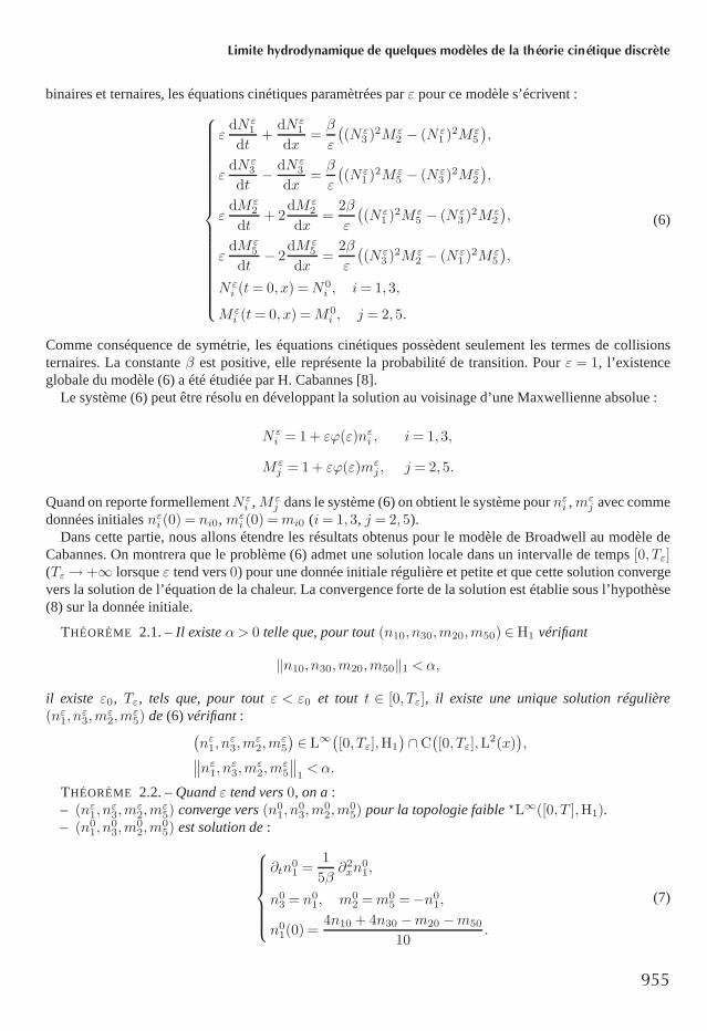
binaires et ternaires, les équations cinétiques paramètrées parε pour ce modèle s’écrivent :

εdNε

1

dt+

dNε1

dx=β

ε

((Nε

3 )2M ε2 − (Nε

1 )2M ε5

),

εdNε

3

dt− dNε

3

dx=β

ε

((Nε

1 )2M ε5 − (Nε

3 )2M ε2

),

εdM ε

2

dt+ 2

dM ε2

dx=

2β

ε

((Nε

1 )2M ε5 − (Nε

3 )2M ε2

),

εdM ε

5

dt− 2

dM ε5

dx=

2β

ε

((Nε

3 )2M ε2 − (Nε

1 )2M ε5

),

Nεi (t= 0, x) =N0

i , i= 1,3,

M εi (t= 0, x) =M0

i , j = 2,5.

(6)

Comme conséquence de symétrie, les équations cinétiques possèdent seulement les termes de collisionsternaires. La constanteβ est positive, elle représente la probabilité de transition. Pourε = 1, l’existenceglobale du modèle (6) a été étudiée par H. Cabannes [8].

Le système (6) peut être résolu en développant la solution au voisinage d’une Maxwellienne absolue :

Nεi = 1 + εϕ(ε)nεi , i= 1,3,

M εj = 1 + εϕ(ε)mε

j , j = 2,5.

Quand on reporte formellementNεi ,M ε

j dans le système (6) on obtient le système pournεi ,mεj avec comme

données initialesnεi (0) = ni0,mεi (0) =mi0 (i= 1,3, j = 2,5).

Dans cette partie, nous allons étendre les résultats obtenus pour le modèle de Broadwell au modèle deCabannes. On montrera que le problème (6) admet une solution locale dans un intervalle de temps[0, Tε](Tε→+∞ lorsqueε tend vers0) pour une donnée initiale régulière et petite et que cette solution convergevers la solution de l’équation de la chaleur. La convergence forte de la solution est établie sous l’hypothèse(8) sur la donnée initiale.

THÉORÈME 2.1. –Il existeα> 0 telle que, pour tout(n10, n30,m20,m50) ∈H1 vérifiant

‖n10, n30,m20,m50‖1 <α,

il existe ε0, Tε, tels que, pour toutε < ε0 et tout t ∈ [0, Tε], il existe une unique solution régulière(nε1, n

ε3,m

ε2,m

ε5) de(6) vérifiant:(

nε1, nε3,m

ε2,m

ε5

)∈ L∞

([0, Tε],H1

)∩C

([0, Tε],L

2(x)),∥∥nε1, nε3,mε

2,mε5

∥∥1<α.


ε3,m

ε2,m


1, n03,m

02,m

05) pour la topologie faible?L∞([0, T ],H1).

– (n01, n

03,m

02,m


∂tn01 =

1

5β∂2xn

01,

n03 = n0

1, m02 =m0

5 =−n01,

n01(0) =

4n10 + 4n30 −m20 −m50

10.

(7)

955

A. Bellouquid

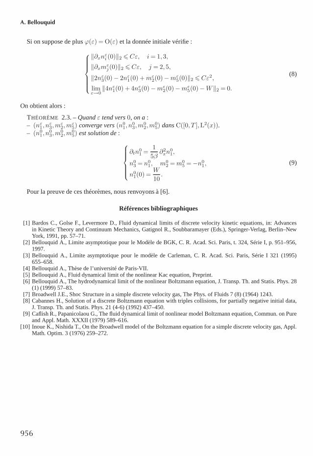
Si on suppose de plusϕ(ε) = O(ε) et la donnée initiale vérifie :‖∂xnεi (0)‖2 6Cε, i= 1,3,

‖∂xmεj(0)‖2 6Cε, j = 2,5,

‖2nε3(0)− 2nε1(0) +mε2(0)−mε

5(0)‖2 6Cε2,

limε→0‖4nε1(0) + 4nε3(0)−mε

2(0)−mε5(0)−W‖2 = 0.

(8)

On obtient alors :


ε3,m

ε2,m


1, n03,m

02,m

05) dansC([0, T ],L2(x)).

– (n01, n

03,m

02,m


∂tn01 =

1

5β∂2xn

01,

n03 = n0

1, m02 =m0

5 =−n01,

n01(0) =

W

10.

(9)

Pour la preuve de ces théorèmes, nous renvoyons à [6].

Références bibliographiques

[1] Bardos C., Golse F., Levermore D., Fluid dynamical limits of discrete velocity kinetic equations, in: Advancesin Kinetic Theory and Continuum Mechanics, Gatignol R., Soubbaramayer (Eds.), Springer-Verlag, Berlin–NewYork, 1991, pp. 57–71.

[2] Bellouquid A., Limite asymptotique pour le Modèle de BGK, C. R. Acad. Sci. Paris, t. 324, Série I, p. 951–956,1997.

[3] Bellouquid A., Limite asymptotique pour le modèle de Carleman, C. R. Acad. Sci. Paris, Série I 321 (1995)655–658.

[4] Bellouquid A., Thèse de l’université de Paris-VII.[5] Bellouquid A., Fluid dynamical limit of the nonlinear Kac equation, Preprint.[6] Bellouquid A., The hydrodynamical limit of the nonlinear Boltzmann equation, J. Transp. Th. and Statis. Phys. 28

(1) (1999) 57–83.[7] Broadwell J.E., Shoc Structure in a simple discrete velocity gas, The Phys. of Fluids 7 (8) (1964) 1243.[8] Cabannes H., Solution of a discrete Boltzmann equation with triples collisions, for partially negative initial data,

J. Transp. Th. and Statis. Phys. 21 (4-6) (1992) 437–450.[9] Caflish R., Papanicolaou G., The fluid dynamical limit of nonlinear model Boltzmann equation, Commun. on Pure

and Appl. Math. XXXII (1979) 589–616.[10] Inoue K., Nishida T., On the Broadwell model of the Boltzmann equation for a simple discrete velocity gas, Appl.

Math. Optim. 3 (1976) 259–272.

956

Documents

Limite hydrodynamique de quelques modèles de la théorie cinétique discrète