Embed Size (px)
Citation preview
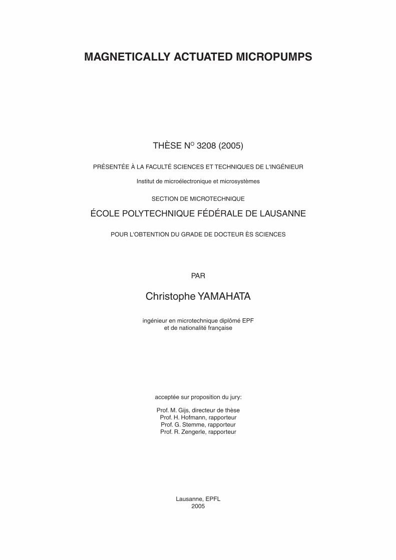
THÈSE NO 3208 (2005)
ÉCOLE POLYTECHNIQUE FÉDÉRALE DE LAUSANNE
PRÉSENTÉE À LA FACULTÉ SCIENCES ET TECHNIQUES DE L'INGÉNIEUR
Institut de microélectronique et microsystèmes
SECTION DE MICROTECHNIQUE
POUR L'OBTENTION DU GRADE DE DOCTEUR ÈS SCIENCES
PAR
ingénieur en microtechnique diplômé EPFet de nationalité française
acceptée sur proposition du jury:
Prof. M. Gijs, directeur de thèseProf. H. Hofmann, rapporteurProf. G. Stemme, rapporteurProf. R. Zengerle, rapporteur
Lausanne, EPFL2005
MAGNETICALLY ACTUATED MICROPUMPS
Christophe YAMAHATA

© Christophe Yamahata, 2005
. . . . .
. . . . . . . . . . . . . . . . . . . . . . . . . . . . . . . . . . .ABSTRACT
“Lab-On-a-Chip” (LOC) systems are intended to transpose complete laboratory instrumentations on the few square centimetres of a single microfluidic chip. With such devices the objective is to minimize the time and cost associated with routine biological analysis while improving reproducibility. At the heart of these systems, a fluid delivery unit controls and transfers tiny quantities of liquids enabling the biological assays. This explains the need for robust integrated micropumps as a precondition for the development of many LOC devices.
In this context, we have developed a rapid prototyping method for the fabrication of microfluidic chips in plastic and glass materials. The microfabrication principle, which is based on the powder blasting microstructuring process, was used to build devices in either polymethylmethacrylate (PMMA) or borosilicate glass.
Various types of micropumps have been developed which were all based on external magnetic actuation. The use of ferrofluids (or magnetic liquids) has been the subject of the first part of the research. A piston pump using a ferrofluid plug moved by an external magnet has been studied. The integration of a rare-earth material (NdFeB) in a flexible polydimethylsiloxane (PDMS) membrane, in the form of a powder or as a classical permanent magnet, has then been proposed. An external electromagnet was used to actuate the magnet-containing diaphragm of a reciprocating micropump.
Different types of valves, which constitute the critical element in reciprocating micropumps, have also been investigated. We have studied silicone membrane valves, nozzle-diffuser elements and ball valves. While nozzle-diffuser elements present the simplest valving solution from a manufacturing point of view, ball valves have been proposed as a very promising alternative due to their high efficiency.
Together with the detailed characterization of the prototypes, we have proposed analytical models that predict the hydrodynamic behaviour of the micropumps.
The performances of our micropumps indicate that magnetic actuation is well adapted for LOC microsystems. While we have demonstrated that our proposed microfabrication technique is an excellent rapid prototyping method for disposable plastic devices, our glass micropumps present a competitive low-cost alternative satisfying criteria of biocompatibility and high temperature (130 °C) resistance.
iii

. . . . .
. . . . . . . . . . . . . . . . . . . . . . . . . . . . . . . . . . .VERSION ABRÉGÉE
Les systèmes de type “Laboratoire intégré sur une puce” (en anglais, Lab-on-a-Chip ou LOC) ont pour ambition de transposer des instrumentations complètes de laboratoire sur les quelques centimètres carrés d’une puce microfluidique. Avec de tels dispositifs, l’objectif est de réduire au minimum le temps et le coût associés aux analyses biologiques les plus courantes, tout en améliorant leur reproductibilité. Au coeur de ces systèmes, une unité de distribution de fluide commande et transfère des quantités minuscules de liquides pour permettre les analyses biologiques. L’intégration de micropompes robustes apparaît ainsi comme une condition préalable au développement ultérieur pour de nombreux dispositifs LOC.
Dans ce contexte, nous avons développé une méthode de prototypage rapide permettant la fabrication de microsystèmes fluidiques en plastique et en verre. Le procédé de fabrication est basé sur la technique de structuration par microsablage. Cette technique a été employée pour réaliser des pièces intégralement en poly(méthyle methacrylate) (PMMA) ou en verre borosilicaté.
Au moyen de ce procédé de fabrication, nous avons pu développer différents types de micropompes, toutes étant basées sur le principe d’un actionnement magnétique externe. L’utilisation de ferrofluides (ou ‘liquides magnétiques’) a fait l’objet de la première partie de cette recherche. Nous avons ainsi proposé une pompe à ferrofluide (déplacé par un aimant externe) inspirée du principe de la pompe à piston. Par la suite, nous avons opté pour l’intégration d’un aimant en terres rare (en NdFeB) dans une membrane flexible en poly(diméthyle siloxane) (PDMS): soit sous la forme de poudres ou simplement en introduisant un aimant fritté classique. Nous avons utilisé un électro-aimant externe pour l’actionnement de l’aimant contenu dans le diaphragme de la micropompe.
Nous nous sommes par ailleurs concentrés sur le choix des valves car elles constituent l’élément critique des pompes. Nous avons étudié les valves à membrane flexible en silicone, les éléments de type ‘diffuseur’ et les valves à billes. Du point de vue de leur construction, les diffuseurs constituent la solution
v
VE R S I O N A B R É G É E
vi
la plus simple pour produire un effet de directivité du flux. Les valves à billes, quant à elles, peuvent être une alternative prometteuse en raison de leur grande efficacité.
Tout en présentant une caractérisation détaillée des divers prototypes, nous avons établi des modèles analytiques simples qui permettent de prévoir le comportement hydrodynamique de ces micropompes.
Les performances de nos différentes pompes indiquent que les actionneurs magnétiques sont bien adaptés pour les microsystèmes de type LOC. Enfin, nous avons pu démontrer que notre méthode de prototypage rapide est une excellente solution pour la fabrication d’échantillons jetables; tandis que les pompes en verres sont une alternative peu coûteuse et répondent aux critères de biocompatibilité et de résistance à haute température (130 °C).

«Il vaut mieux pomper même s’il ne se passe rien que risquer qu’il se passe
quelque chose de pire en ne pompant pas.»(Shadok motto)

. . . . .
. . . . . . . . . . . . . . . . . . . . . . . . . . . . . . . . . . .ACKNOWLEDGEMENTS
This thesis work was carried out at the Laboratory for Microsystems, Institute of Microelectronics and Microsystems, Swiss Federal Institute of Technology, Lausanne (EPFL). The work was done in collaboration with Dr. Alain Donzel and was supported by the Swiss Commission for Technology and Innovation under the MedTech program (project CTI-MedTech 4960.1 MTS), an initiative that supports research in the field of biomedical technologies.
I acknowledge the members of the jury, Prof. Martin Gijs, Prof. Hannes Bleuler, Prof. Heinrich Hofmann, Prof. Göran Stemme, and Prof. Roland Zengerle, for reviewing this work.
I want to thank my supervisor, Prof. Martin Gijs, who gave me the opportunity to do this Ph.D. thesis at the Laboratory for Microsystems. I had great pleasure to work in the pleasant atmosphere of his laboratory. I am also grateful to my colleagues for their encouragement and many discussions we had together that guided me during this thesis. In particular, the development of plastic microfluidic chips has benefited from the experience of Dr. Virendra Parashar; and the fabrication of micropumps by fusion bonding of glass has been possible thanks to the know-how of Frédéric Lacharme and Dr. Dominique Solignac.
The ferrofluidic micropump was developed in partnership with Dr. Mathieu Chastellain and Prof. Heinrich Hofmann (Powder Technology Laboratory, EPFL) who worked on the synthesis of the water-based ferrofluid.
All through the thesis, I also had the chance to train students who significantly contributed to this work during their semester project. Christian Lotto, Eyad Al-Assaf and Silvan Schnydrig have worked on the development of the valveless micropump. Jan Matter, Yves Burri and Emilie Kernen have worked on the development of the ball valve micropump.
I express my gratitude to Prof. Yves Perriard, Dr. Miroslav Markovic, Dr. Patrik Hoffman, Dr. Trong-Vien Truong, Dr. Alain Donzel, and Harald van Lintel for their scientific advice.
I am thankful to Dr. Bernd Grieb (Magnequench Europe) for the technical informations on magnetic powders; and to Mr. Bertrand Reuse from Gotec SA (Sion, Switzerland) for the fruitful discussions we had together as well as for the pump prototypes he gave me.
Finally, I especially thank André Mercanzini and Sophie Moiroux who have kindly helped me in the correction of different articles during this thesis.
All these people have contributed to this work and I am grateful towards them.
Lausanne, February 2005. Christophe Yamahata
ix

. . . . .
. . . . . . . . . . . . . . . . . . . . . . . . . . . . . . . . . . .TABLE OF CONTENTS
Abstract . . . . . . . . . . . . . . . . . . . . . . . . . . . . . . . . . . . . . . . . . . . . . . . . . . iii
Version Abrégée . . . . . . . . . . . . . . . . . . . . . . . . . . . . . . . . . . . . . . . . . . . v
Acknowledgements . . . . . . . . . . . . . . . . . . . . . . . . . . . . . . . . . . . . . . . . . ix
Table of Contents . . . . . . . . . . . . . . . . . . . . . . . . . . . . . . . . . . . . . . . . . . xi
Nomenclature . . . . . . . . . . . . . . . . . . . . . . . . . . . . . . . . . . . . . . . . . . . . . xvAbbreviations and acronyms .................................................................................. xvSymbols .................................................................................................................... xvii
1 Introduction . . . . . . . . . . . . . . . . . . . . . . . . . . . . . . . . . . . . . . . . . . . . . . . . 11.1 Microfluidics and Lab-On-a-Chip .................................................................... 31.2 Scope of the thesis .......................................................................................... 5
2 Theory of Fluid Mechanics . . . . . . . . . . . . . . . . . . . . . . . . . . . . . . . . . . . . . 72.1 Definitions ......................................................................................................... 72.2 Fluidic laws ....................................................................................................... 11
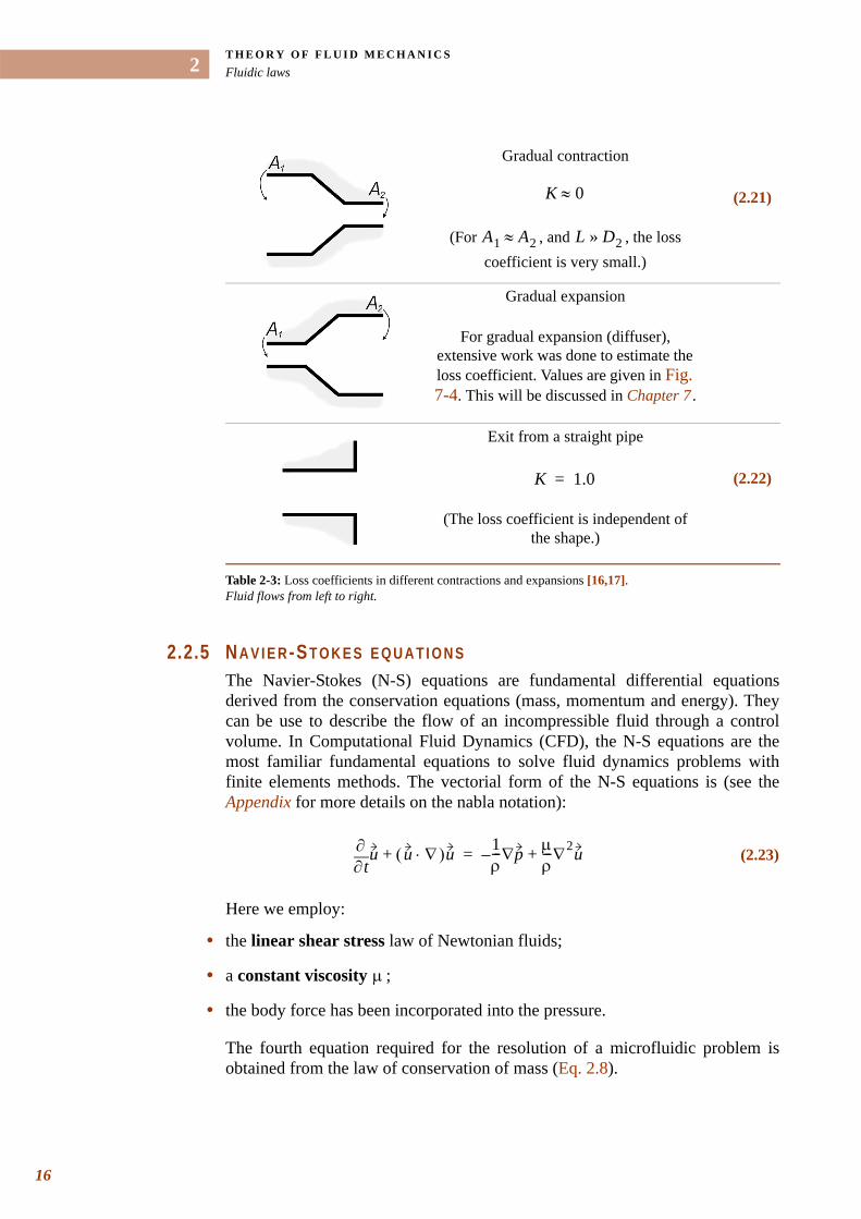
2.2.1 Conservation laws ......................................................................................... 112.2.2 Frictionless flow: the Bernoulli equation ...................................................... 142.2.3 Hagen-Poiseuille law ..................................................................................... 142.2.4 Minor losses ................................................................................................... 152.2.5 Navier-Stokes equations ................................................................................ 162.2.6 Numerical analysis ........................................................................................ 172.2.7 Microfluidics and macrofluidics .................................................................... 17
2.3 Hydraulic system analysis .............................................................................. 182.3.1 RLC equivalent model .................................................................................... 182.3.2 Damped oscillator model ............................................................................... 202.3.3 RLC electrical equivalent model of the reciprocating pump ......................... 23
3 Theory of Magnetic Actuation . . . . . . . . . . . . . . . . . . . . . . . . . . . . . . . . . . 273.1 Basics of magnetism ....................................................................................... 27
3.1.1 Magnetic materials ........................................................................................ 273.1.2 Magnetic moment ........................................................................................... 283.1.3 Soft and hard magnetic materials .................................................................. 30
3.2 Ferrofluids and magnetic liquids .................................................................... 303.2.1 Ferrofluids ..................................................................................................... 313.2.2 Generalized Bernoulli equation ..................................................................... 31
3.3 Permanent magnets ......................................................................................... 333.3.1 Magnets classification ................................................................................... 33
xi
TA B L E O F C O N T E N T S
xii
3.3.2 Chemical resistance of rare-earth magnets ................................................... 333.3.3 Energy density of magnetic materials ............................................................ 34
3.4 Electromechanical systems ............................................................................. 343.4.1 Lorentz force .................................................................................................. 353.4.2 Classification ................................................................................................. 353.4.3 Magnetic membrane and electromagnet ........................................................ 363.4.4 Improved electromagnetic system .................................................................. 38
4 State-of-the-art on Micropumps . . . . . . . . . . . . . . . . . . . . . . . . . . . . . . . . . 394.1 Actuators ........................................................................................................... 40
4.1.1 Microactuators ............................................................................................... 404.1.2 Comparison of actuation methods ................................................................. 43
4.2 Micropumps ...................................................................................................... 454.2.1 Classification of micropumps ......................................................................... 454.2.2 Basic pump parameters .................................................................................. 474.2.3 Design rules for reciprocating pumps ............................................................ 484.2.4 Literature review of micropumps ................................................................... 484.2.5 Some examples of micropumps ...................................................................... 50
4.3 Valves ................................................................................................................. 564.3.1 Classification of microvalves ......................................................................... 564.3.2 Main parameters of valves ............................................................................. 584.3.3 Some examples of valving principles ............................................................. 58
4.4 Conclusion ........................................................................................................ 63
5 Microfabrication Technology . . . . . . . . . . . . . . . . . . . . . . . . . . . . . . . . . . . 655.1 Review of microfabrication techniques used in microsystems ................... 65
5.1.1 Silicon micromachining ................................................................................. 655.1.2 Other processes .............................................................................................. 67
5.2 Powder blasting erosion process ................................................................... 685.2.1 Equipment ...................................................................................................... 695.2.2 Mechanical etching by powder blasting ........................................................ 705.2.3 Microchannels fabrication ............................................................................. 72
5.3 PMMA microchips fabricated by powder blasting ......................................... 745.3.1 Advantage of PMMA ...................................................................................... 745.3.2 Fabrication process ....................................................................................... 745.3.3 Check-valve integration ................................................................................. 75
5.4 Glass microchips fabricated by powder blasting .......................................... 765.4.1 Glass fusion bonding ...................................................................................... 775.4.2 Final assembly of the glass chips ................................................................... 77
5.5 Magnetic membrane fabrication ...................................................................... 785.5.1 Integrated permanent magnet ........................................................................ 795.5.2 Integrated polymer magnet ............................................................................ 79
5.6 Conclusion ........................................................................................................ 81
6 Ferrofluidic Micropump . . . . . . . . . . . . . . . . . . . . . . . . . . . . . . . . . . . . . . . 836.1 Ferrofluids and their applications ................................................................... 83
6.1.1 Composition of ferrofluids ............................................................................. 83
. . .
. .TA B L E O F C O N T E N T S
6.1.2 Magnetic properties of ferrofluids ................................................................. 846.1.3 Applications of ferrofluids ............................................................................. 846.1.4 Use of ferrofluids in microfluidics ................................................................. 86
6.2 Synthesis and characterization of the water-based ferrofluid ..................... 886.2.1 Synthesis of the ferrofluid .............................................................................. 886.2.2 Characterization of the ferrofluid .................................................................. 89
6.3 Working principle and design of the micropump ......................................... 926.3.1 Working principle .......................................................................................... 926.3.2 Microfabrication of the micropump ............................................................... 93
6.4 Characterization of the ferrofluidic micropump ............................................ 956.4.1 Check-valve characterization ........................................................................ 956.4.2 Pump performance ......................................................................................... 95
6.5 Conclusion ........................................................................................................ 98
7 Diffuser Micropump . . . . . . . . . . . . . . . . . . . . . . . . . . . . . . . . . . . . . . . . . . 997.1 Design of a diffuser micropump in plastic (PMMA) ...................................... 997.2 Working principle of the diffuser micropump ............................................... 1017.3 Nozzle/diffuser element ................................................................................... 102
7.3.1 Determination of diffuser performance with minor losses theory ................. 1037.3.2 Numerical simulation ..................................................................................... 1077.3.3 Steady flow characteristics of the diffuser ..................................................... 109
7.4 Microfabrication of the PMMA diffuser micropump ...................................... 1107.4.1 Magnetic membrane ...................................................................................... 1107.4.2 PMMA microfluidic chip ................................................................................ 111
7.5 Characterization and analysis of the PMMA diffuser micropump ............... 1137.5.1 Magnetic membrane and electromagnet ........................................................ 1137.5.2 Flow rate – back-pressure measurement ....................................................... 1137.5.3 Resonant frequency ........................................................................................ 1147.5.4 Frequency-dependent flow rate ..................................................................... 117
7.6 Glass diffuser micropump ............................................................................... 1197.7 Conclusion ........................................................................................................ 121
8 Ball Valve Micropump . . . . . . . . . . . . . . . . . . . . . . . . . . . . . . . . . . . . . . . . 1238.1 Working principle of the ball valve micropump in glass .............................. 1248.2 Powder blasting holes in glass material ........................................................ 1258.3 Characterization of the ball valve micropumps ............................................ 128
8.3.1 Characterization of the ball valve in glass .................................................... 1288.3.2 PMMA and glass micropumps characterization ............................................ 129
8.4 Damped oscillator model of the ball valve micropump ................................ 1318.5 Conclusion ........................................................................................................ 133
9 Conclusion and Outlook . . . . . . . . . . . . . . . . . . . . . . . . . . . . . . . . . . . . . . . 1359.1 Discussion ........................................................................................................ 136
xiii
TA B L E O F C O N T E N T S
xiv
9.2 Future work ....................................................................................................... 138
Appendix . . . . . . . . . . . . . . . . . . . . . . . . . . . . . . . . . . . . . . . . . . . . . . . . . 141A.1 Complements on fluids mechanics ................................................................ 141A.2 Vector relations using nabla notation ............................................................. 144A.3 Magnetic beads manipulation ......................................................................... 147A.4 Mohs’ hardness scale ...................................................................................... 148
References . . . . . . . . . . . . . . . . . . . . . . . . . . . . . . . . . . . . . . . . . . . . . . . 149
Publications . . . . . . . . . . . . . . . . . . . . . . . . . . . . . . . . . . . . . . . . . . . . . . . 157Journal articles .......................................................................................................... 157Conferences ............................................................................................................... 157
Curriculum Vitae . . . . . . . . . . . . . . . . . . . . . . . . . . . . . . . . . . . . . . . . . . . 159
. . . . .
. . . . . . . . . . . . . . . . . . . . . . . . . . . . . . . . . . .NOMENCLATURE
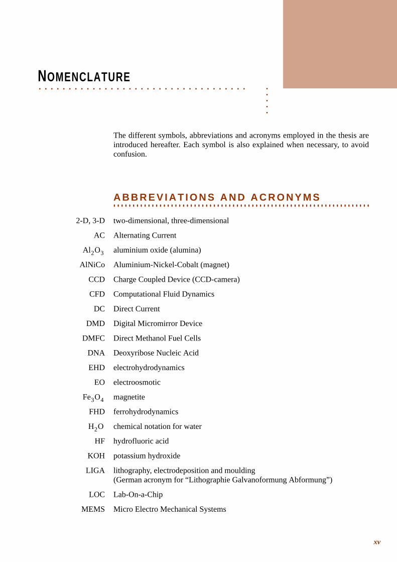
The different symbols, abbreviations and acronyms employed in the thesis are introduced hereafter. Each symbol is also explained when necessary, to avoid confusion.
. . . . . . . . . . . . . . . . . . . . . . . . . . . . . . . . . . . . . . . . . . . . . . . . . . . . . . . . . . . . . . . . . . .A B B R E V I A T I O N S A N D A C R O N Y M S
2-D, 3-D two-dimensional, three-dimensional
AC Alternating Current
aluminium oxide (alumina)
AlNiCo Aluminium-Nickel-Cobalt (magnet)
CCD Charge Coupled Device (CCD-camera)
CFD Computational Fluid Dynamics
DC Direct Current
DMD Digital Micromirror Device
DMFC Direct Methanol Fuel Cells
DNA Deoxyribose Nucleic Acid
EHD electrohydrodynamics
EO electroosmotic
magnetite
FHD ferrohydrodynamics
chemical notation for water
HF hydrofluoric acid
KOH potassium hydroxide
LIGA lithography, electrodeposition and moulding (German acronym for “Lithographie Galvanoformung Abformung”)
LOC Lab-On-a-Chip
MEMS Micro Electro Mechanical Systems
Al2O3
Fe3O4
H2O
xv
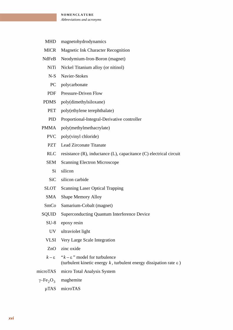
N O M E N C L A T U R EAbbreviations and acronyms
xvi
MHD magnetohydrodynamics
MICR Magnetic Ink Character Recognition
NdFeB Neodymium-Iron-Boron (magnet)
NiTi Nickel Titanium alloy (or nitinol)
N-S Navier-Stokes
PC polycarbonate
PDF Pressure-Driven Flow
PDMS poly(dimethylsiloxane)
PET poly(ethylene terephthalate)
PID Proportional-Integral-Derivative controller
PMMA poly(methylmethacrylate)
PVC poly(vinyl chloride)
PZT Lead Zirconate Titanate
RLC resistance (R), inductance (L), capacitance (C) electrical circuit
SEM Scanning Electron Microscope
Si silicon
SiC silicon carbide
SLOT Scanning Laser Optical Trapping
SMA Shape Memory Alloy
SmCo Samarium-Cobalt (magnet)
SQUID Superconducting Quantum Interference Device
SU-8 epoxy resin
UV ultraviolet light
VLSI Very Large Scale Integration
ZnO zinc oxide
“ ” model for turbulence (turbulent kinetic energy , turbulent energy dissipation rate )
microTAS micro Total Analysis System
maghemite
µTAS microTAS
k ε– k ε–k ε
γ-Fe2O3
. . .
. .N O M E N C L A T U R ESymbols
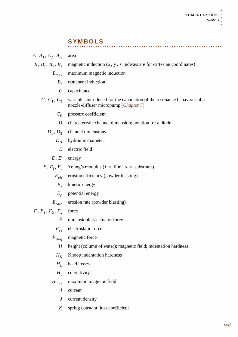
. . . . . . . . . . . . . . . . . . . . . . . . . . . . . . . . . . . . . . . . . . . . . . . . . . . . . . . . . . . . . . . . . . .S Y M B O L S
, , , area
, , , magnetic induction ( , , indexes are for cartesian coordinates)
maximum magnetic induction
remanent induction
capacitance
, , variables introduced for the calculation of the resonance behaviour of a nozzle-diffuser micropump (Chapter 7 )
pressure coefficient
characteristic channel dimension; notation for a diode
, channel dimensions
hydraulic diameter
electric field
, energy
, , Young’s modulus ( , )
erosion efficiency (powder blasting)
kinetic energy
potential energy
erosion rate (powder blasting)
, , , force
dimensionless actuator force
electrostatic force
magnetic force
height (column of water); magnetic field; indentation hardness
Knoop indentation hardness
head losses
coercitivity
maximum magnetic field
current
current density
spring constant; loss coefficient
A A1 A2 Am
B Bx By Bz x y z
Bmax
Br
C
C C1 C3
CP
D
D1 D2
DH
E
E E'
E Ef Es f film= s substrate=
Eeff
Ek
Ep
Erate
F F1 F2 Fx
F
Fes
Fmag
H
HK
HL
Hc
Hmax
I
J
K
xvii
N O M E N C L A T U R ESymbols
xviii
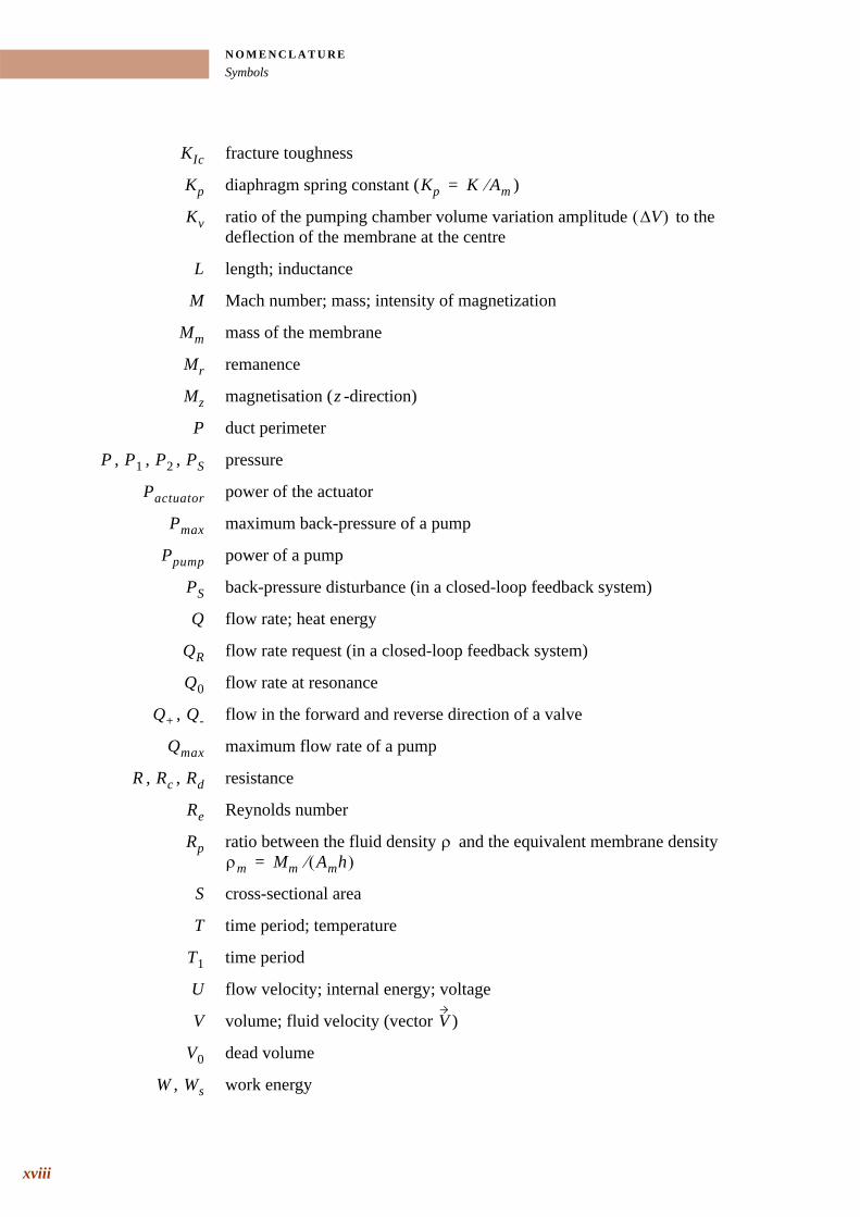
fracture toughness
diaphragm spring constant ( )
ratio of the pumping chamber volume variation amplitude to the deflection of the membrane at the centre
length; inductance
Mach number; mass; intensity of magnetization
mass of the membrane
remanence
magnetisation ( -direction)
duct perimeter
, , , pressure
power of the actuator
maximum back-pressure of a pump
power of a pump
back-pressure disturbance (in a closed-loop feedback system)
flow rate; heat energy
flow rate request (in a closed-loop feedback system)
flow rate at resonance
, flow in the forward and reverse direction of a valve
maximum flow rate of a pump
, , resistance
Reynolds number
ratio between the fluid density and the equivalent membrane density
cross-sectional area
time period; temperature
time period
flow velocity; internal energy; voltage
volume; fluid velocity (vector )
dead volume
, work energy
KIc
Kp Kp K Am⁄=
Kv V∆( )
L
M
Mm
Mr
Mz z
P
P P1 P2 PS
Pactuator
Pmax
Ppump
PS
Q
QR
Q0
Q+ Q-
Qmax
R Rc Rd
Re
Rp ρρm Mm Amh( )⁄=
S
T
T1
U
V V
V0
W Ws
. . .
. .N O M E N C L A T U R ESymbols
deflection amplitude of the membrane
impedance (complex)
area; major radius of an ellipse
minor radius of an ellipse
speed of sound
piezoelectrics coupling coefficient
frequency
resonant frequency
earth gravitational acceleration ( )
channel height
(complex number)
length
mass; magnetic moment
, , , pressure
energy per unit of mass ( ); charge of a particle
circular duct radius
scaling factor (dimensional analysis)
time
, , flow velocities in the , , cartesian coordinates
, , flow velocity
average fluid velocity
particle velocity (powder blasting)
, , channel width
work per unit of mass ( )
, , cartesian coordinates; lengths
, channel inlet (1) and outlet (2) height
pump stroke efficiency (diffuser micropump)
, thermal expansion coefficient ( , )
variable introduced for the calculation of the resonance behaviour of a nozzle-diffuser micropump (Chapter 7 )
X
Z
a
b
c
d33
f
f0
g g 9.8 m s 2–⋅=
h
j 1–=
l
m
p p0 p1 p2
q q Q m⁄=
r
s
t
u v w x y z
u1 v1 v2
v
vparticle
w w1 w2
ws ws Ws m⁄=
x y z
z1 z2
α
αf αsf film= s substrate=
β
xix
N O M E N C L A T U R ESymbols
xx
distance of the air gap
average static deflection of the membrane
roughness; relative elongation in a material; compression ratio of a pump
permittivity of vacuum ( )
valve efficiency
efficiency of a nozzle/diffuser element
efficiency of a pump
angle (diffuser)
( , ) fluid dynamic viscosity (dynamic viscosity of air, water)
permeability of vacuum ( )
relative permeability
fluid kinematic viscosity ( )
damping coefficient
, loss coefficients in the diffuser and nozzle directions
density
normal stress in a material
pulsation
resonance pulsation
flow rate
, flow rate in the diffuser and nozzle directions
(relative) magnetic susceptibility
torque
diameter
a change or difference of; symbol for the Laplacian operator
nabla operator
γ γ ρg=
δ
δstatic
ε
ε0 ε0 8.85 12–×10 F m 1–⋅=
η
η'
ηpump
θ
µ µair µwater
µ0 µ0 4π 7–×10 H m 1–⋅=
µr
ν ν µ ρ⁄=
ξ
ξd ξn
ρ
σ
ω
ω0
φ
φd φn
χ
Γ
∅
∆
∇
CHAPTER
1. . . . .
. . . . . . . . . . . . . . . . . . . . . . . . . . . . . . . . . . .INTRODUCTION
he production, in 1971, of the first commercial microprocessors in silicon (4004 Microprocessor, Intel Corporation) was an important milestone for the semiconductors industry. Inspired by the technologies
used in microelectronics, early efforts in microsystems focused on silicon fabrication technology. Since then, silicon has been an intensively used material in microsystems. In this context, the development of the first micropump dates back to 1988 when H. T. G. Van Lintel et al. presented for the first time a micropump based on the micromachining of silicon [1,2]. Later, with the emergence of microfluidic systems, glass and plastics became the privileged materials [3].
From an economic point of view, we can distinguish three principal advantages of microfabricated systems: their potentially low-cost, reduced size, and the availability of highly automated and reproducible production processes. We know now a number of successful microelectromechanical devices.
T
a
bc
b
bd
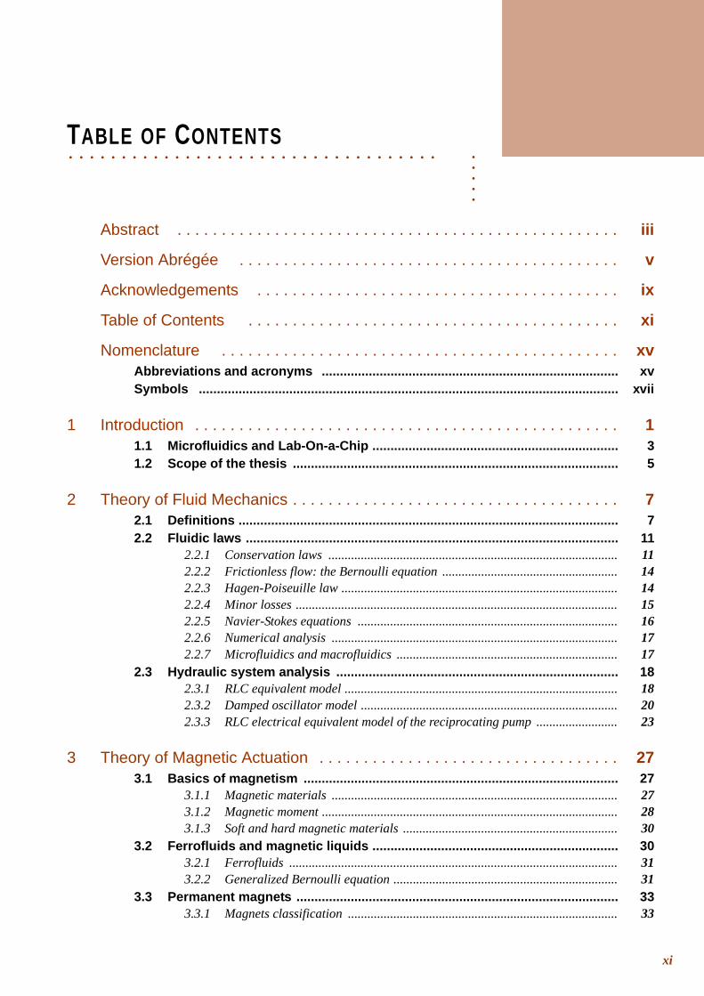
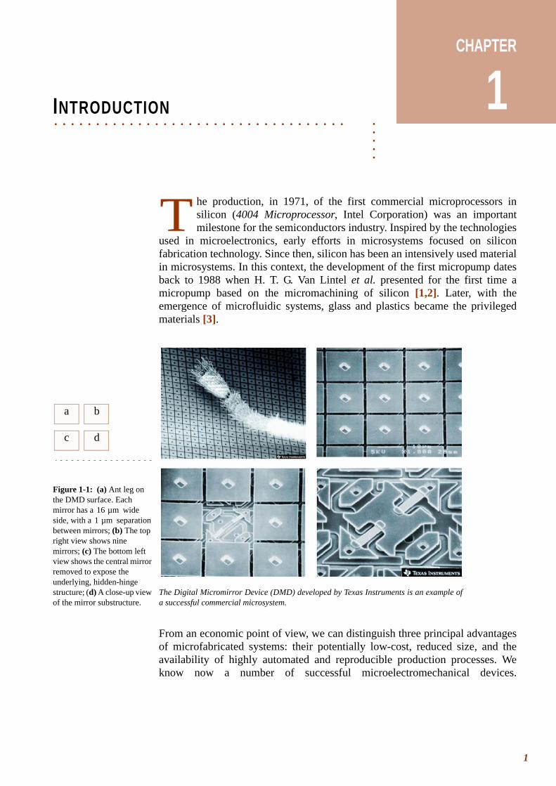
Figure 1-1: (a) Ant leg on the DMD surface. Each mirror has a wide side, with a separation between mirrors; (b) The top right view shows nine mirrors; (c) The bottom left view shows the central mirror removed to expose the underlying, hidden-hinge structure; (d) A close-up view of the mirror substructure.
The Digital Micromirror Device (DMD) developed by Texas Instruments is an example of a successful commercial microsystem.
16 µm1 µm
1
I N T R O D U C T I O N
2
1
Well-known and representative mass market products that have pushed the research in the field of microsystems are:
• Digital Micromirror Device A major technological innovation which emerged from optical microsystems appeared in 1987 when Texas Instruments produced the Digital Micromirror Device (DMD)1 microchip invented by L. J. Hornbeck [4]. The DMD is an array of fast digital light switches integrated on a silicon addressing circuit (see Fig. 1-1).
• Acceleration SensorIn 1993, Analog Devices was the first company to commercialize accelerometers, when the first crash detection sensors were introduced for air bag deployment in automobiles. In 2002, the semiconductor company announced that it had shipped its 100 millionth acceleration sensor.
• Inkjet Printer NozzleInkjet printing nozzles etched in silicon were initially developed at IBM [5]. A market study established by NEXUS in 1996 estimated the production of inkjet print heads to 500 million pieces for the year 2002, raising the product as a prominent microfluidic device derived from micromachining technology [6].
1. Digital Light Processing (Texas Instruments), http://www.dlp.com/
. . .
. .I N T R O D U C T I O NMicrofluidics and Lab-On-a-Chip
. . . . . . . . . . . . . . . . . . . . . . . . . . . . . . . . . . . . . . . . . . . . . . . . . . . . . . . . . . . . . . . . . . . 1 . 1 M I C R O F L U I D I C S A N D L A B - O N - A - C H I P
Recent breakthroughs in life sciences are to a large extent based on advances in biotechnologies. One reason for the success of this research field is related to the miniaturization of biochemical analysis systems. The concept of Lab-On-a-Chip (LOC) – also known as Micro Total Analysis System (microTAS, µTAS) [7,8,9] – well illustrates this approach. Many laboratory techniques in biology and chemistry need fluid handling and involve time-consuming and repetitive fluid manipulation tasks. Beyond the objective of integrating several laboratory processes into a single chip, microTAS devices are aiming to drastically reduce the volume of analysed samples, to shorten analysis times, to automate and improve the quality of experiments, and finally to lower the costs of many standard processes [3,10].
The technological progress in the fabrication of microsystems has rendered microTAS an affordable approach. The possibilities envisaged by using microfluidic systems have interested not only scientists but also industries, especially in the Life Sciences and fine chemistry field. As a consequence, bio-MEMS has become a major research area for many laboratories during the past decade. Two different approaches are observed in microTAS research: they
a
b
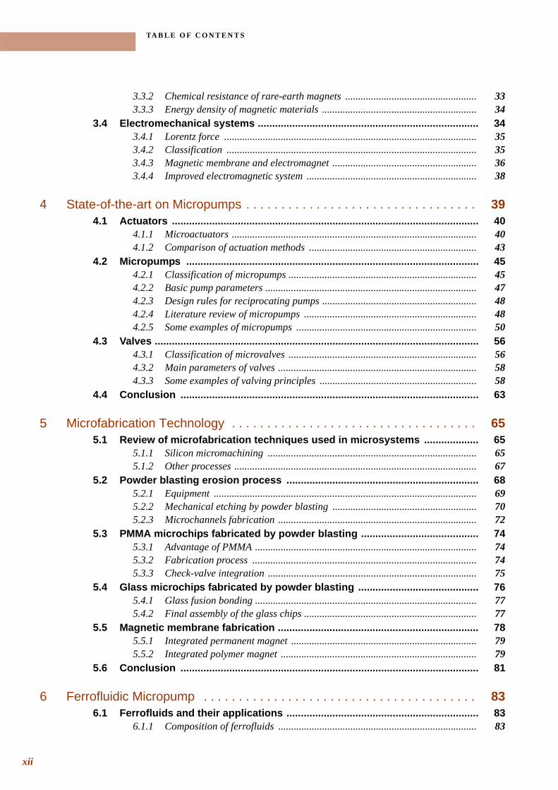
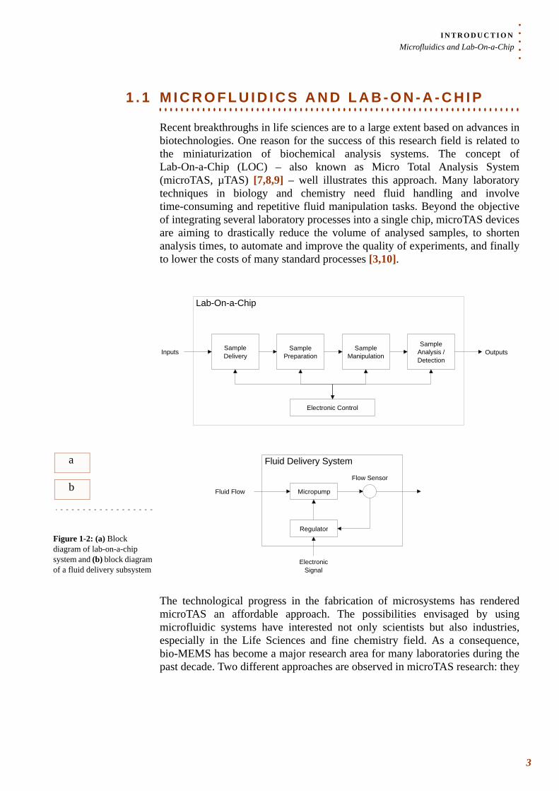
Figure 1-2: (a) Block diagram of lab-on-a-chip system and (b) block diagram of a fluid delivery subsystem
Lab-On-a-Chip
SampleDelivery
SamplePreparation
SampleManipulation
SampleAnalysis / Detection
Inputs Outputs
Electronic Control
Fluid Delivery System
Micropump
Flow Sensor
Regulator
Fluid Flow
ElectronicSignal
3
I N T R O D U C T I O NMicrofluidics and Lab-On-a-Chip
4
1
are either based on microarrays or on microfluidic systems. The latter type of microTAS can be represented in a block diagram with subsystems that include fluid sample dispensing, appropriate preparation before analysis, and different handling steps (see Fig. 1-2 (a)).
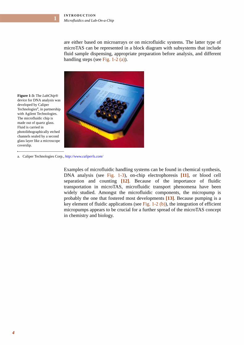
Examples of microfluidic handling systems can be found in chemical synthesis, DNA analysis (see Fig. 1-3), on-chip electrophoresis [11], or blood cell separation and counting [12]. Because of the importance of fluidic transportation in microTAS, microfluidic transport phenomena have been widely studied. Amongst the microfluidic components, the micropump is probably the one that fostered most developments [13]. Because pumping is a key element of fluidic applications (see Fig. 1-2 (b)), the integration of efficient micropumps appears to be crucial for a further spread of the microTAS concept in chemistry and biology.
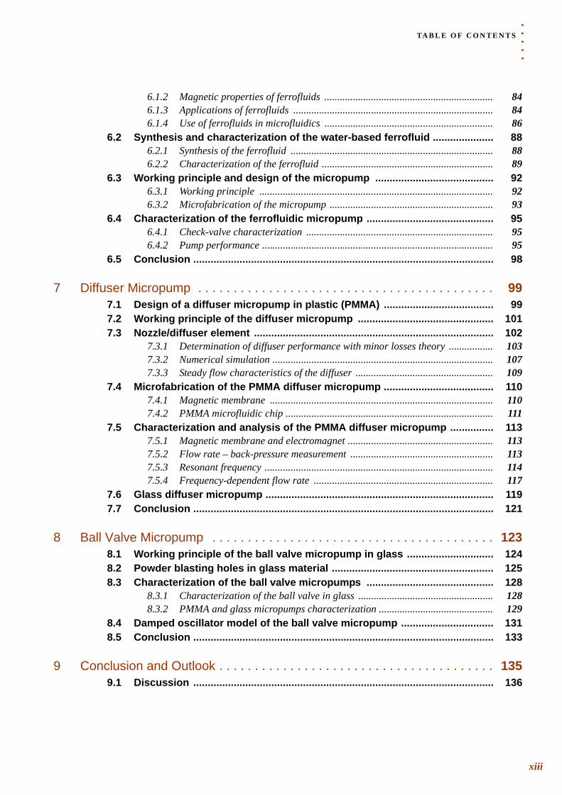
Figure 1-3: The LabChip® device for DNA analysis was developed by Caliper Technologiesa, in partnership with Agilent Technologies. The microfluidic chip is made out of quartz glass. Fluid is carried in photolithographically etched channels sealed by a second glass layer like a microscope coverslip.
a. Caliper Technologies Corp., http://www.caliperls.com/
. . .
. .I N T R O D U C T I O NScope of the thesis
. . . . . . . . . . . . . . . . . . . . . . . . . . . . . . . . . . . . . . . . . . . . . . . . . . . . . . . . . . . . . . . . . . . 1 . 2 S C O P E O F T H E T H E S I S
Liquid transport is most commonly a result of applied pressure. It can be achieved for example by using a syringe pump, a peristaltic pump, or simply by applying a vacuum at the outlet of a microchannel. Although manual pipetting or external (syringe or peristaltic) pumps are generally used in laboratory experiments for the precise dispensing of fluids, the realization of miniaturized pumps has attracted great attention in the development of integrated systems. In this context, our research is focused on the study of magnetically and electromagnetically actuated micropumps.
We realized various types of pumps keeping in mind, as an important factor, their suitability for LOC devices. The theoretical background of microfluidics is given in Chapter 2 and the basics of magnetism in Chapter 3 for magnetism. The state-of-the-art of micropumps is reviewed in Chapter 4 . In this chapter, the principle of reciprocating pumps is explained; and the potential of magnetic actuation revealed. We finally study different options for the valving effect. In Chapter 5 , the most commonly used microsystem fabrication processes are reviewed before we introduce our simple and low-cost technology based on the powder blasting micro-erosion process which was developed for the fabrication of our microfluidic chips. Our work on a ferrofluidic piston micropump is described in Chapter 6 and the development of a valveless electromagnetic micropump is studied in Chapter 7 . Finally, a ball valve electromagnetic micropump is presented in Chapter 8 . We conclude the thesis with an outlook on future developments of the project and show its potential for microfluidic applications (Chapter 9 ).
5

CHAPTER
2. . . . .
. . . . . . . . . . . . . . . . . . . . . . . . . . . . . . . . . . .THEORY OF FLUID MECHANICS
he aim of this chapter is to give the theoretical background on Fluid Mechanics necessary to understand the behaviour of pressure-driven flow in microfluidic systems. We will first introduce some basic
definitions. We will then present the main laws of fluidics which will be used all through this thesis and explain the specific matters to take care about in Microfluidics. We will also present different complementary methods which can be used to theoretically predict the behaviour of pressure-driven flow obtained with reciprocating micropumps. In particular, since the pumping methods of concern in this work are based on reciprocating actuation, the last part of the chapter will provide a general analysis of dynamic hydraulic systems for the modelling of oscillating micropumps. The latter part will be useful for the analysis of the diffuser micropump in Chapter 7 where a theoretical model for the resonant frequency of the pump will be presented. The model will also be used in Chapter 8 where the frequency-dependent behaviour of ball valve micropumps will be discussed.
. . . . . . . . . . . . . . . . . . . . . . . . . . . . . . . . . . . . . . . . . . . . . . . . . . . . . . . . . . . . . . . . . . . 2 . 1 D E F I N I T I O N S
Cont ro l vo lume and cont ro l
su r face
A control volume is a volume in space which contains the system of interest. In like manner, the surface of the control volume is defined as the control surface. All inputs and outputs from the system must pass through the control surface.
Steady f low A steady flow is a flow in which velocity components and thermodynamic properties at every point in space do not change with time. Individual fluid particles may move, but at any particular point in space, such particle behaves just as any other fluid particle when it was at that place. There is no time dependent parameter in steady flow equations ( ). Time dependent flow is said to be unsteady.
T
∂ t∂⁄ 0=
7
T H E O R Y O F F L U I D M E C H A N I C SDefinitions
8
2
Flow reg ime The flow is laminar when all fluid elements move deterministically along distinct and traceable stream lines. At sufficiently high Reynolds number (defined hereafter), the flow becomes unstable and evolves to a turbulentregime. Turbulence is characterized by a random motion of fluid particles, transverse to the main flow direction. A chaotic mixing of viscous fluid occurs. Viscous forces dominate in a laminar flow regime, while inertial forces dominate in a turbulent flow regime.
Reyno lds number
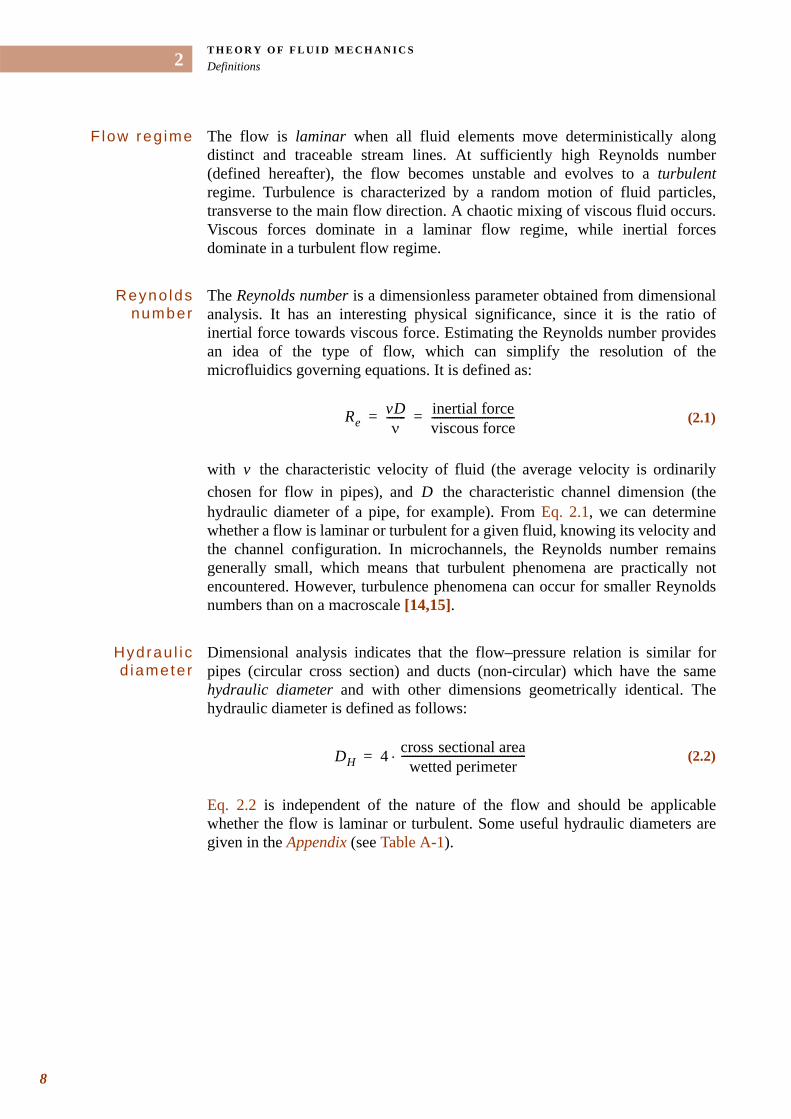
The Reynolds number is a dimensionless parameter obtained from dimensional analysis. It has an interesting physical significance, since it is the ratio of inertial force towards viscous force. Estimating the Reynolds number provides an idea of the type of flow, which can simplify the resolution of the microfluidics governing equations. It is defined as:
with the characteristic velocity of fluid (the average velocity is ordinarily chosen for flow in pipes), and the characteristic channel dimension (the hydraulic diameter of a pipe, for example). From Eq. 2.1, we can determine whether a flow is laminar or turbulent for a given fluid, knowing its velocity and the channel configuration. In microchannels, the Reynolds number remains generally small, which means that turbulent phenomena are practically not encountered. However, turbulence phenomena can occur for smaller Reynolds numbers than on a macroscale [14,15].
Hydrau l i c d iameter
Dimensional analysis indicates that the flow–pressure relation is similar for pipes (circular cross section) and ducts (non-circular) which have the same hydraulic diameter and with other dimensions geometrically identical. The hydraulic diameter is defined as follows:
Eq. 2.2 is independent of the nature of the flow and should be applicable whether the flow is laminar or turbulent. Some useful hydraulic diameters are given in the Appendix (see Table A-1).
(2.1)RevDν
------- inertial forceviscous force-------------------------------= =
vD
(2.2)DH 4 cross sectional areawetted perimeter
-----------------------------------------------⋅=
. . .
. .T H E O R Y O F F L U I D M E C H A N I C SDefinitions
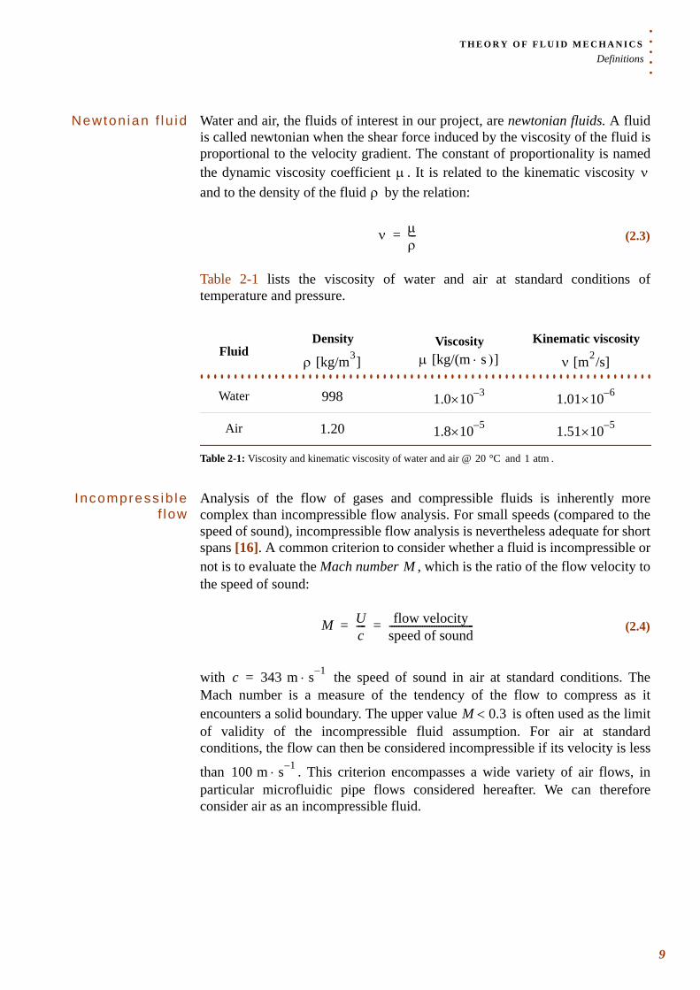
Newton ian f lu id Water and air, the fluids of interest in our project, are newtonian fluids. A fluid is called newtonian when the shear force induced by the viscosity of the fluid is proportional to the velocity gradient. The constant of proportionality is named the dynamic viscosity coefficient . It is related to the kinematic viscosity and to the density of the fluid by the relation:
Table 2-1 lists the viscosity of water and air at standard conditions of temperature and pressure.
Incompress ib le f low
Analysis of the flow of gases and compressible fluids is inherently more complex than incompressible flow analysis. For small speeds (compared to the speed of sound), incompressible flow analysis is nevertheless adequate for short spans [16]. A common criterion to consider whether a fluid is incompressible or not is to evaluate the Mach number , which is the ratio of the flow velocity to the speed of sound:
with the speed of sound in air at standard conditions. The Mach number is a measure of the tendency of the flow to compress as it encounters a solid boundary. The upper value is often used as the limit of validity of the incompressible fluid assumption. For air at standard conditions, the flow can then be considered incompressible if its velocity is less
than . This criterion encompasses a wide variety of air flows, in particular microfluidic pipe flows considered hereafter. We can therefore consider air as an incompressible fluid.
µ νρ
(2.3)ν µρ---=
FluidDensity Viscosity Kinematic viscosity
. . . . . . . . . . . . . . . . . . . . . . . . . . . . . . . . . . . . . . . . . . . . . . . . . . . . . . . . . . . . . . . . . . . Water
Air
Table 2-1: Viscosity and kinematic viscosity of water and air @ and .
ρ [kg/m3] µ [kg/(m s⋅ )] ν [m2/s]
998 1.0 3–×10 1.01 6–×10
1.20 1.8 5–×10 1.51 5–×10
20 °C 1 atm
M
(2.4)M Uc---- flow velocity
speed of sound------------------------------------= =
c 343 m s 1–⋅=
M 0.3<
100 m s 1–⋅
9
T H E O R Y O F F L U I D M E C H A N I C SDefinitions
10
2
Hydros ta t ic p ressure
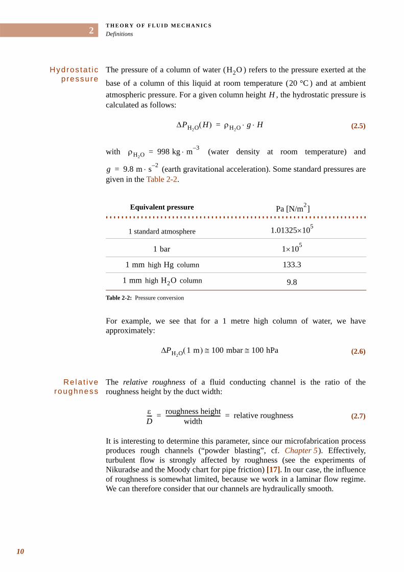
The pressure of a column of water ( ) refers to the pressure exerted at the
base of a column of this liquid at room temperature ( ) and at ambient atmospheric pressure. For a given column height , the hydrostatic pressure is calculated as follows:
with (water density at room temperature) and
(earth gravitational acceleration). Some standard pressures are given in the Table 2-2.
For example, we see that for a 1 metre high column of water, we have approximately:
Rela t i ve roughness
The relative roughness of a fluid conducting channel is the ratio of the roughness height by the duct width:
It is interesting to determine this parameter, since our microfabrication process produces rough channels (“powder blasting”, cf. Chapter 5 ). Effectively, turbulent flow is strongly affected by roughness (see the experiments of Nikuradse and the Moody chart for pipe friction) [17]. In our case, the influence of roughness is somewhat limited, because we work in a laminar flow regime. We can therefore consider that our channels are hydraulically smooth.
H2O
20 °CH
(2.5)∆PH2O H( ) ρH2O g H⋅ ⋅=
Equivalent pressure . . . . . . . . . . . . . . . . . . . . . . . . . . . . . . . . . . . . . . . . . . . . . . . . . . . . . . . . . . . . . . . . . . . 1 standard atmosphere
high column
high column
Table 2-2: Pressure conversion
ρH2O 998 kg m 3–⋅=
g 9.8 m s 2–⋅=
Pa [N/m2]
1.01325 5×10
1 bar 1 5×10
1 mm Hg 133.3
1 mm H2O 9.8
(2.6)PH2O 1 m( ) 100≅∆ mbar 100 hPa≅
(2.7)εD---- roughness height
width---------------------------------------- relative roughness= =
. . .
. .T H E O R Y O F F L U I D M E C H A N I C SFluidic laws
Nozz les , d i f fusers and
ventur is
Nozzles and diffusers interchange fluid velocity and fluid static pressure. The nozzle (converging walls) transforms a high-pressure, low-velocity flow into a high-velocity, low-pressure jet. The diffuser (diverging walls) transforms a high-velocity, low-pressure jet into a low-velocity, high pressure flow. The evaluation of the performance of these elements is obtained from the calculation of minor losses. These elements will be studied in detail in Chapter 7 .
The venturi is an interesting application which takes advantage of the properties of these elements. A venturi is made of the combination of a nozzle and a diffuser. The purpose of a venturi tube is to create a region of low static pressure at the venturi throat which can be used to draw in a second fluid, as in a venturi carburettor, or to generate a pressure differential between the throat and the contiguous pipe line, as in a venturi flowmeter [16].
. . . . . . . . . . . . . . . . . . . . . . . . . . . . . . . . . . . . . . . . . . . . . . . . . . . . . . . . . . . . . . . . . . . 2 . 2 F L U I D I C L A W S
In this section, we introduce the theory of fluid dynamics for fluids flowing in pipes and ducts, assuming the following hypothesis for the fluid:
• Steady flow ( )
• Newtonian fluid (viscosity )
• Incompressible (constant density )
Our pumping applications are devoted to the pumping of water-based fluids. We therefore focus our analysis to water and extend it to gases (air), which are both newtonian fluids. As described in the previous paragraph, the assumption of incompressible flow remains valid in our applications. Steady flow assumption is more restrictive, since reciprocating pumps intrinsically produce a pulsed flow (unsteady). However, we will see in next paragraph a method for the study of oscillating flows.
2.2.1 C O N S E R V A T I O N L A W SWith the general hypothesis formulated above, and in the case of an incompressible laminar flow for isotropic fluids, the fluid flow problem can be solved from three differential equations resulting from conservation laws: the
∂ t∂⁄ 0=
µ
ρ
11
T H E O R Y O F F L U I D M E C H A N I C SFluidic laws
12
2
conservation of mass, momentum and energy. Applying the set of equations to a region of interest, a control volume, it reduces to [17]:
• Conservation of mass The law of continuity says that matter can be neither created nor destroyed. The incoming mass equals outgoing mass. For incompressible fluids (constant density ), this can be expressed in terms of the vector fluid velocity:
which reads:
where are the velocity values in the cartesian coordinates, respectively.
• Conservation of momentumThe conservation of linear and rotational momentum lead to the well-known fluidic newtonian equations. We limit the discussion here to the linear momentum relation, which reads: the sum of all external forces acting on the control volume is equal to the sum of the total rate of change of momentum. In a mathematical notation:
The left-hand side of Eq. 2.10 represents inertial forces and the right-hand side represents the forces due to the applied pressure , the gravity force (or any body force), and the viscosity. The Navier-Stokes equation (see further) is obtained from the law of conservation of momentum.
• Conservation of energy The first law of thermodynamics describes the conservation of energy. The accumulation of energy in the control volume is the difference between incoming and outgoing energy. This equality can be written as:
ρ
(2.8)∇ V⋅ 0=
(2.9)x∂
∂uy∂
∂vz∂
∂w+ + 0=
u, v, w x, y, z
(2.10)ρdVdt------- ∇p– ρg µ∇2V+ +=
p
(2.11)Q W– ∆E=
. . .
. .T H E O R Y O F F L U I D M E C H A N I C SFluidic laws
with the heat added on the system (temperature transition), the work done by the system, and the change in energy of the system. We adopt the convention that the work done by the system is positive, while the work transferred to the system is negative. Notice that the distinction between the different forms of energy is arbitrary. The energy term can also be separated into:
where is the internal energy (molecular motion), is the kinetic energy,
is the potential energy and are other forms of energy such as external magnetic energy for example. We omit the latter type of external energy which will be introduced in the study of ferrohydrodynamics (Chapter 3 ).
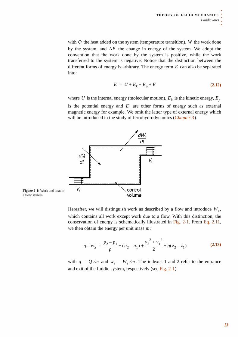
Hereafter, we will distinguish work as described by a flow and introduce , which contains all work except work due to a flow. With this distinction, the conservation of energy is schematically illustrated in Fig. 2-1. From Eq. 2.11, we then obtain the energy per unit mass :
with and . The indexes 1 and 2 refer to the entrance and exit of the fluidic system, respectively (see Fig. 2-1).
Q W∆E
E
(2.12)E U Ek Ep E'+ + +=
U Ek Ep
E'
Figure 2-1: Work and heat in a flow system.
Ws
m
(2.13)q wS–p2 p1–
ρ---------------- u2 u1–( )
v22 v1
2+2
--------------------- g z2 z1–( )+ + +=
q Q m⁄= ws Ws m⁄=
13
T H E O R Y O F F L U I D M E C H A N I C SFluidic laws
14
2
2.2.2 FR I C T I O N L E S S F L O W: T H E B E R N O U L L I E Q U A T I O NThe Bernoulli equation interrelates the dynamic properties of a fluid flow at two separate points in a fluid volume at the same moment in time. It is available along the stream line of a steady flow for incompressible fluids having a negligible viscosity (frictionless flow). Under these hypotheses, the Bernoulli equation is deduced from the energy equation (Eq. 2.13):
where . Eq. 2.14 has length as its unit and is expressed in terms of “head”: pressure head, velocity head and potential head (from left to right). This equation is somewhat limited, since all fluids have friction. In actual flow situations, losses occurring in real fluids must be taken into account by the introduction of “head losses” (notation ). Introducing an irreversible loss
coefficient , Eq. 2.14 can be modified as:
The velocity is assumed to be uniform over the cross section of the fluidic circuit where the loss coefficient applies to. The loss coefficient is a function of the Reynolds number and of the geometry of the component. It will be discussed in detail in the section describing minor losses and in Chapter 7 where diffusers will be studied.
2.2.3 H A G E N-PO I S E U I L L E L A WFriction losses in a pipe can be estimated from the Hagen-Poiseuille law. In a channel of length with a hydraulic diameter , where the flow is laminar
and the fluid is incompressible and flows steadily, the variation of pressure is related to the flow rate by:
This equation can be easily demonstrated from the Poiseuille parabolic flow theory given in the Appendix (see Eq. A.4). It has been verified that the Hagen-Poiseuille law describes very accurately the experimental results. Note that the pressure drop in a laminar flow is independent of the roughness of the pipe wall.
(2.14)p1γ-----
v12
2g------- z1+ +
p2γ-----
v22
2g------- z2+ +=
γ ρg=
HL
K
(2.15)p1γ-----
v12
2g------- z1+ +
p2γ-----
v22
2g------- z2 K v2
2g------+ + +=
vK
∆x DH
∆pQ
(2.16)∆p 128µ∆xQπDH
4------------------------–=
. . .
. .T H E O R Y O F F L U I D M E C H A N I C SFluidic laws
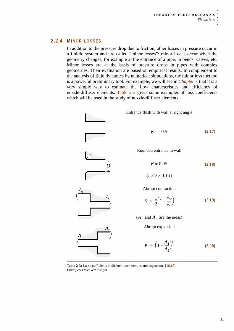
2.2.4 M I N O R L O S S E SIn addition to the pressure drop due to friction, other losses in pressure occur in a fluidic system and are called “minor losses”: minor losses occur when the geometry changes, for example at the entrance of a pipe, in bends, valves, etc. Minor losses are at the basis of pressure drops in pipes with complex geometries. Their evaluation are based on empirical results. In complement to the analysis of fluid dynamics by numerical simulations, the minor loss method is a powerful preliminary tool. For example, we will see in Chapter 7 that it is a very simple way to estimate the flow characteristics and efficiency of nozzle-diffuser elements. Table 2-3 gives some examples of loss coefficients which will be used in the study of nozzle-diffuser elements.
Entrance flush with wall at right angle
(2.17)
Rounded entrance in wall
( )
(2.18)
Abrupt contraction
( and are the areas)
(2.19)
Abrupt expansion
(2.20)
Table 2-3: Loss coefficients in different contractions and expansions [16,17]. Fluid flows from left to right.
K 0.5=
K 0.05≈
r D⁄ 0.16>
K 12--- 1
A2A1------–⎝ ⎠
⎛ ⎞=
A1 A2
K 1A1A2------–⎝ ⎠
⎛ ⎞ 2=
15
T H E O R Y O F F L U I D M E C H A N I C SFluidic laws
16
2
2.2.5 N A V I E R-S T O K E S E Q U A T I O N SThe Navier-Stokes (N-S) equations are fundamental differential equations derived from the conservation equations (mass, momentum and energy). They can be use to describe the flow of an incompressible fluid through a control volume. In Computational Fluid Dynamics (CFD), the N-S equations are the most familiar fundamental equations to solve fluid dynamics problems with finite elements methods. The vectorial form of the N-S equations is (see the Appendix for more details on the nabla notation):
Here we employ:
• the linear shear stress law of Newtonian fluids;
• a constant viscosity ;
• the body force has been incorporated into the pressure.
The fourth equation required for the resolution of a microfluidic problem is obtained from the law of conservation of mass (Eq. 2.8).
Gradual contraction
(For , and , the loss coefficient is very small.)
(2.21)
Gradual expansion
For gradual expansion (diffuser), extensive work was done to estimate the loss coefficient. Values are given in Fig. 7-4. This will be discussed in Chapter 7 .
Exit from a straight pipe
(The loss coefficient is independent of the shape.)
(2.22)
Table 2-3: Loss coefficients in different contractions and expansions [16,17]. Fluid flows from left to right.
K 0≈
A1 A2≈ L D2»
K 1.0=
(2.23)t∂
∂ u u ∇⋅( )u+ 1ρ--- p µ
ρ---∇2u+∇–=
µ
. . .
. .T H E O R Y O F F L U I D M E C H A N I C SFluidic laws
2.2.6 N U M E R I C A L A N A L Y S I SA general solution for Eq. 2.9 and Eq. 2.23 has not been found, due to the non-linear and second-order nature of this set of differential equations. Therefore, CFD can be attractive for the study of fluid flow in complex geometries where simple solutions can not be given [18]. The finite-element method can be applied for the solution of the N-S equations in a defined geometry where boundary conditions are known. The principle of the finite-element method consists in dividing the domain of interest in subdomains of defined size (mesh). N-S differential equations are then applied to each of these elements and are solved in an iterative process (with Newton-Raphson or Runge-Kutta algorithms, for example). For unsteady flow, the continuous time is also divided in discrete steps. Because of the high time consumption involved in a three-dimensional (3-D simulation) study, we limited the numerical simulation in this thesis to the two-dimensional (2-D) case and extrapolated it to 3-D.
One of the major methodologies employed for the numerical simulation of turbulence effects is called “ modelling.” The standard model simulates the transport of both turbulent kinetic energy ( ), and turbulent energy dissipation rate ( ). This method uses time-averaged hydrodynamic equations and transport equations for turbulence characteristics. This model was included with the simulation software Femlab 2.2 [19] that we used for the simulation of the nozzle-diffuser element (see Chapter 7 ).
2.2.7 M I C R O F L U I D I C S A N D M A C R O F L U I D I C SThe theory of fluid mechanics provides an analytical model which is valid for macroscopic flow and remains valid for most microchannels of more than
in size [14]. In our case, all dimensions being wider or equal to , macroscopic laws are valid although the influence of miniaturization on fluid motion has to be taken into account in the study of fluid dynamics. In microfluidics, the main scaling effect to consider for the pressure-driven flow is its influence on the flow regime. The Reynolds number is therefore an important parameter to determine. It was observed that the transition from laminar to turbulent flow was obtained at lower Reynolds numbers in microchannels than in larger scale channels [15]. For this reason, although laminar flow might dominate in microfluidics, it is important to consider the possible presence of a transitional flow regime. For this reason, our simulations included a “ model” of the turbulence.
k ε–k
ε
1 µm 100 µm
k ε–
17
T H E O R Y O F F L U I D M E C H A N I C SHydraulic system analysis
18
2
. . . . . . . . . . . . . . . . . . . . . . . . . . . . . . . . . . . . . . . . . . . . . . . . . . . . . . . . . . . . . . . . . . . 2 . 3 H Y D R A U L I C S Y S T E M A N A L Y S I S
In a reciprocating micropump, we are intrinsically faced with flow-induced vibrations since pumping is obtained from the oscillations of a piston/plunger or a diaphragm. In this paragraph, we will provide a simple model of the hydraulic system in order to predict the frequency-dependence of the pumping system [20,21]. The calculation presented is based on the method of linear analysis.
2.3.1 RLC E Q U I V A L E N T M O D E LThe equivalence of hydraulic systems with RLC circuits (resistance, inductance, capacitance) can be used to schematically describe the fluidic system with lumped elements that simplify the calculations.
Pure f lu id conductor
Viscous fluid flow through a channel gives rise to a pressure drop between the inlet and the outlet. For incompressible newtonian fluids, the behaviour is governed by the Hagen-Poiseuille law and the relation between the fluid flow and pressure drop across the physical element is linear. From Eq. 2.16, we can therefore consider a channel of hydraulic diameter and length as a pure
fluid conductor having a fluidic resistance defined as:
The ideal fluid conductor is applicable if the tube is long enough in comparison to its hydraulic diameter, so that the effects of non-uniform flow near the entrance can be neglected (“fully developed flow”).
Pure f lu id induc tor
Inertial effects encountered in accelerating a fluid in a pipe or passage can be modelled by a fluid inductor. In an ideal fluid inductor there is a linear relation between the inductor pressure differential and the inductor flow derivative
. Introducing the fluid inductance , this relation is written:
Let us consider the unsteady frictionless flow of an incompressible fluid in a duct of constant cross-section area and length . The force necessary to
produce an acceleration of the fluid mass in the pipe is, according to
Newton’s law:
DH l
R
(2.24)R 128µlπDH
4--------------=
p t( )
Q· t( ) L
(2.25)p t( ) L Q· t( )⋅=
S l F
tddv
(2.26)F ρlS tddv=
. . .
. .T H E O R Y O F F L U I D M E C H A N I C SHydraulic system analysis
With , the average velocity of the fluid in the pipe, the combination of Eq. 2.25 and Eq. 2.26 gives the relation for the fluid inductance:
A pipe can then be modelled as the combination of a pure fluidic resistance and a pure fluid inductance.
Pure f lu id capac i to r
A fluid capacitor is a physical element in which the energy stored is a function of fluid pressure and is defined as:
where is the fluid flow rate through the capacitor and is the pressure in the capacitor. The parameter is the fluid capacitance. From Eq. 2.28, we can evaluate this parameter as:
where is the volume variation in the capacitor when it is subjected to a pressure differential . In a diaphragm reciprocating pump, the membrane deflection affects the chamber volume and plays the role of the capacitor.
v
(2.27)L ρlS-----=
(2.28)Q C tddp=
Q p t( )C
(2.29)C V∆p∆
-------=
V∆p∆
19
T H E O R Y O F F L U I D M E C H A N I C SHydraulic system analysis
20
2
Table 2-4 summarizes the equivalence between hydraulic and electrical models. From this table, we deduce that, under certain conditions, any fluidic element of an hydraulic system can be replaced by a lumped fluidic element. This attractive simplification can be helpful if the studied system is easily transformable. We will see below that this can be the case for reciprocating pumps.
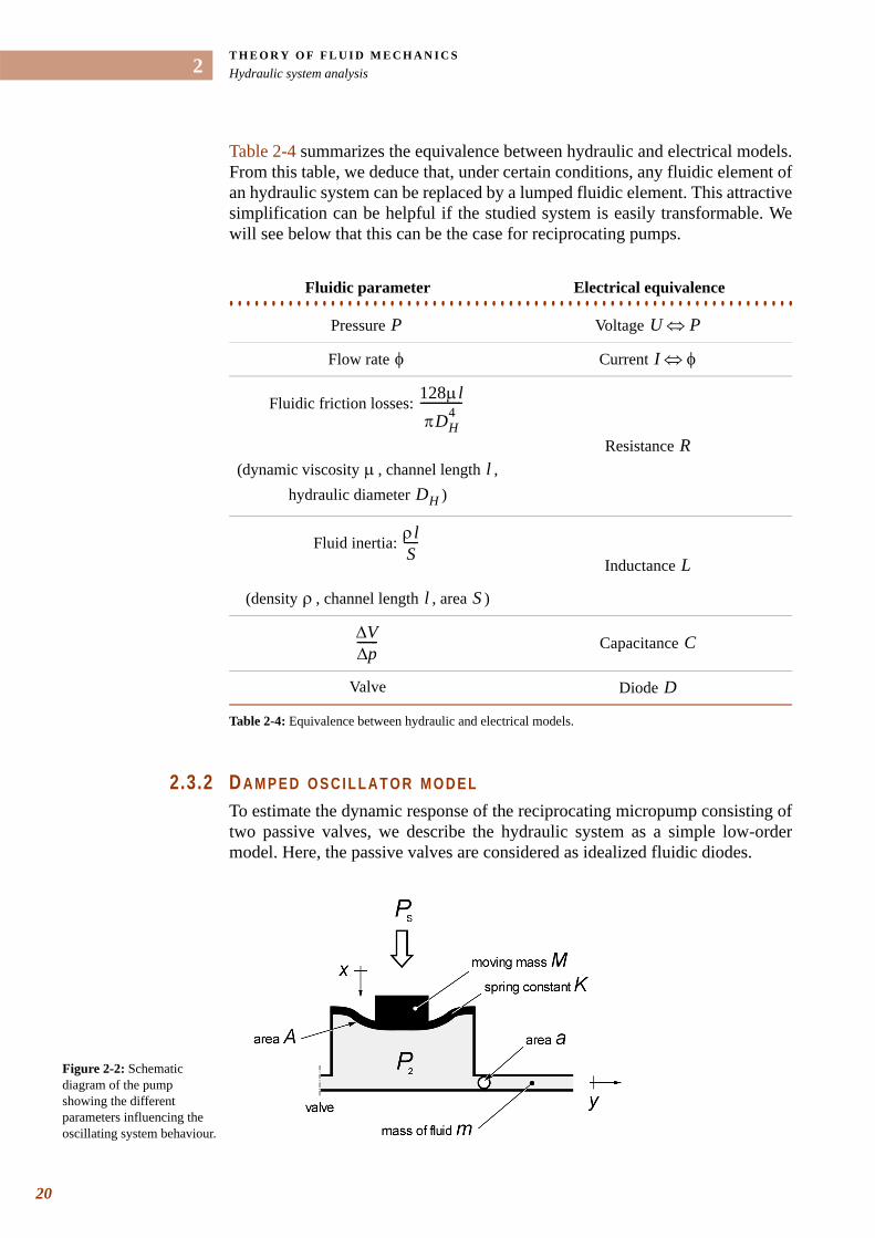
2.3.2 D A M P E D O S C I L L A T O R M O D E LTo estimate the dynamic response of the reciprocating micropump consisting of two passive valves, we describe the hydraulic system as a simple low-order model. Here, the passive valves are considered as idealized fluidic diodes.
Fluidic parameter Electrical equivalence. . . . . . . . . . . . . . . . . . . . . . . . . . . . . . . . . . . . . . . . . . . . . . . . . . . . . . . . . . . . . . . . . . .Pressure Voltage
Flow rate Current
Fluidic friction losses:
(dynamic viscosity , channel length , hydraulic diameter )
Resistance
Fluid inertia:
(density , channel length , area )
Inductance
Capacitance
Valve Diode
Table 2-4: Equivalence between hydraulic and electrical models.
P U P⇔
φ I φ⇔
128µlπDH
4--------------
µ lDH
R
ρlS-----
ρ l S
L
V∆p∆
------- C
D
Figure 2-2: Schematic diagram of the pump showing the different parameters influencing the oscillating system behaviour.
. . .
. .T H E O R Y O F F L U I D M E C H A N I C SHydraulic system analysis
Let us consider a diaphragm pump working in the pumping mode, as illustrated in Fig. 2-2. In this mode, the inlet valve is closed while the outlet valve is opened. If the outlet microchannel has a small section , high rates of fluid acceleration may be involved and, although the mass of the fluid is small compared to the mass of the membrane, its effect is high. Let the actuator apply a constant pressure (above atmospheric pressure) on the flexible
membrane of spring constant to predict the acceleration of the fluid in the outlet microchannel. Without leakage or friction losses, and assuming the pressure in the chamber is atmospheric, we find [21]:
In order to withstand an applied pressure in the microchannel, the pressure in the chamber must be higher than atmospheric pressure and the equation is rewritten as:
Neglecting fluid friction, an approximate value for can be obtained by
assuming the fluid in the channel to move as a solid. For a channel of area
containing a total mass of fluid accelerated at rate , we have:
Neglecting friction, leakage and compressibility effects, the volume of fluid displaced by the membrane is equal to the volume that flows in the outlet channel, so that:
and
am
MPs
K
(2.30)PsA Kx– Mt2
2
dd x=
P2
(2.31)Ps P2–( )A Kx– Mt2
2
dd x=
P2
a
m d2y dt2⁄
(2.32)P2a mt2
2
dd y=
(2.33)Ax ay=
(2.34)t2
2
dd y A
a---
t2
2
dd x=
21
T H E O R Y O F F L U I D M E C H A N I C SHydraulic system analysis
22
2
Hence
or
The term which appears in Eq. 2.31 can be substituted with this previous expression:
which is rewritten:
The effective moving mass is and the factor may be very
high.
From this second order equation, we determine the resonant frequency of the hydraulic system:
(2.35)P2a mAa---
t2
2
dd x=
(2.36)P2A m Aa---⎝ ⎠
⎛ ⎞ 2
t2
2
dd x=
P2A
(2.37)PSA m Aa---⎝ ⎠
⎛ ⎞ 2
t2
2
dd x Kx–– M
t2
2
dd x=
(2.38)PSA M Aa---⎝ ⎠
⎛ ⎞ 2m+
⎩ ⎭⎨ ⎬⎧ ⎫
t2
2
dd x Kx+=
M m Aa---⎝ ⎠
⎛ ⎞ 2+
⎩ ⎭⎨ ⎬⎧ ⎫ A
a---⎝ ⎠
⎛ ⎞ 2
f0
(2.39)f0
12π------ K
M Aa---⎝ ⎠
⎛ ⎞ 2m+
---------------------------=
. . .
. .T H E O R Y O F F L U I D M E C H A N I C SHydraulic system analysis
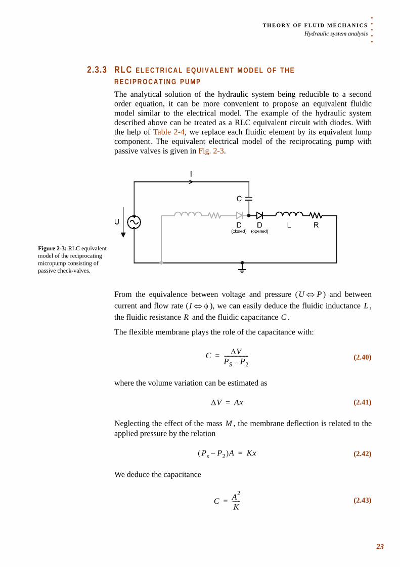
2.3.3 RLC E L E C T R I C A L E Q U I V A L E N T M O D E L O F T H E R E C I P R O C A T I N G P U M PThe analytical solution of the hydraulic system being reducible to a second order equation, it can be more convenient to propose an equivalent fluidic model similar to the electrical model. The example of the hydraulic system described above can be treated as a RLC equivalent circuit with diodes. With the help of Table 2-4, we replace each fluidic element by its equivalent lump component. The equivalent electrical model of the reciprocating pump with passive valves is given in Fig. 2-3.
From the equivalence between voltage and pressure ( ) and between current and flow rate ( ), we can easily deduce the fluidic inductance , the fluidic resistance and the fluidic capacitance .
The flexible membrane plays the role of the capacitance with:
where the volume variation can be estimated as
Neglecting the effect of the mass , the membrane deflection is related to the applied pressure by the relation
We deduce the capacitance
Figure 2-3: RLC equivalent model of the reciprocating micropump consisting of passive check-valves.
U P⇔I φ⇔ L
R C
(2.40)C ∆VPS P2–------------------=
(2.41)∆V Ax=
M
(2.42)Ps P2–( )A Kx=
(2.43)C A2
K------=
23
T H E O R Y O F F L U I D M E C H A N I C SHydraulic system analysis
24
2
The fluid inertia in the microchannel (section , length ) is:
Rewriting the density as
we obtain for the inertia of the fluid in the microchannel
Friction losses also occur in this microchannel. In the case of a laminar incompressible flow, the losses in a channel of hydraulic diameter can be approximated by the Hagen-Poiseuille law:
Although losses occurring in the flexible membrane were not taken into consideration, our simplified RLC equivalent model is already sufficient to correctly predict the behaviour of the pump. In the pumping mode ( in Fig. 2-3), the left side of the circuit is closed (left diode does not conduct current) and we have the following relation for the tension:
which can be rewritten in an equivalent form for fluidics;
The complex impedance of this system is
a l
(2.44)L ρla-----=
(2.45)ρ mla-----=
(2.46)L ma2-----=
DH
(2.47)R 128µlπDH
4--------------=
U 0>
(2.48)U t( ) 1C---- I t( ) td
T1
∫ Ltd
d I t( ) RI t( )+ +=
(2.49)Ps t( ) KA2------ φ t( ) td
T1
∫ma2-----
tdd φ t( ) Rφ t( )+ +=
(2.50)Z R j ma2-----ω K
A2------ 1
ω----–⎝ ⎠
⎛ ⎞+=
. . .
. .T H E O R Y O F F L U I D M E C H A N I C SHydraulic system analysis
and the resonant frequency is
or
Here, we have not considered the mass of the membrane , otherwise we would have obtained exactly the same results as in the previous development (Eq. 2.39). Another interesting aspect in this model is that we can easily deduce the flow rate of the pump as a function of the applied pressure. For a sinusoidal excitation (pulsation ) of the actuator, we have
We can deduce the normalized average flow rate :
where is the average flow rate at the resonant frequency.
Introducing a damping term and the resonance pulsation
, Eq. 2.54 can also be written:
(2.51)f01
2π------ 1
LC-------=
(2.52)f0
12π------ 1
ma2-----A2
K------
------------ 12π------ K
Aa---⎝ ⎠
⎛ ⎞ 2m
----------------= =
M
ω 2π T⁄=
(2.53)Ps t( ) Ps ωtsin=
Q Q0⁄
(2.54)QQ0------ ω2
ω2 LR---ω2 1
RC--------–⎝ ⎠
⎛ ⎞ 2+
----------------------------------------------=
Q0
ξ R2--- C
L----=
ω01LC
-----------=
(2.55)QQ0------ 2ξ
ωω0------⎝ ⎠
⎛ ⎞ 2
1 ωω0------⎝ ⎠
⎛ ⎞ 2–⎝ ⎠
⎛ ⎞ 22ξ ω
ω0------⎝ ⎠
⎛ ⎞ 2+
-----------------------------------------------------------=
25
T H E O R Y O F F L U I D M E C H A N I C SHydraulic system analysis
26
2
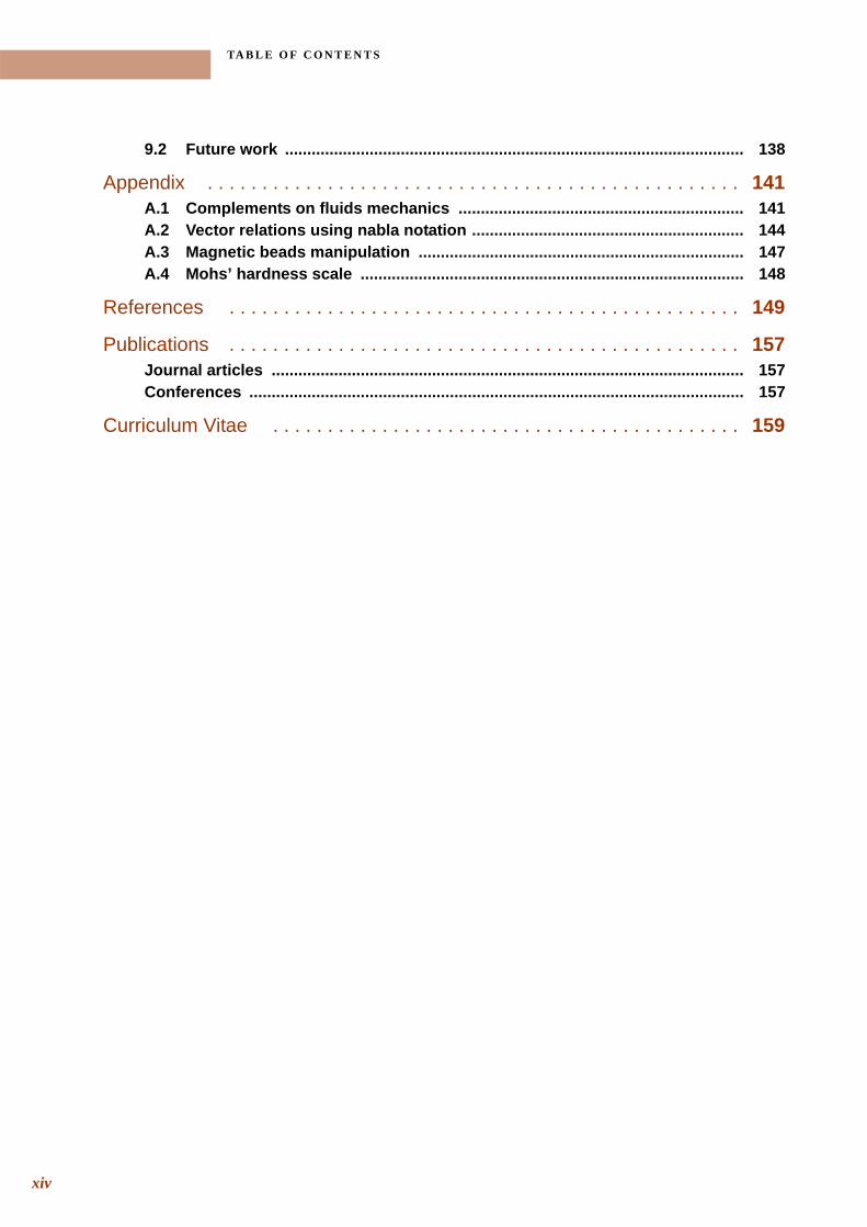
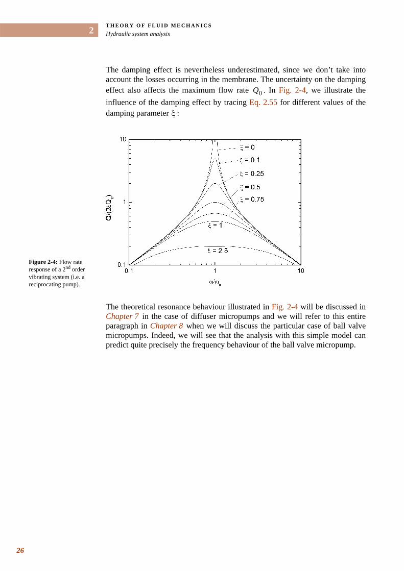
The damping effect is nevertheless underestimated, since we don’t take into account the losses occurring in the membrane. The uncertainty on the damping effect also affects the maximum flow rate . In Fig. 2-4, we illustrate the influence of the damping effect by tracing Eq. 2.55 for different values of the damping parameter :
The theoretical resonance behaviour illustrated in Fig. 2-4 will be discussed in Chapter 7 in the case of diffuser micropumps and we will refer to this entire paragraph in Chapter 8 when we will discuss the particular case of ball valve micropumps. Indeed, we will see that the analysis with this simple model can predict quite precisely the frequency behaviour of the ball valve micropump.
Q0
ξ
Figure 2-4: Flow rate response of a 2nd order vibrating system (i.e. a reciprocating pump).
CHAPTER
3. . . . .
. . . . . . . . . . . . . . . . . . . . . . . . . . . . . . . . . . .THEORY OF MAGNETIC ACTUATION
he theoretical background on Magnetic Actuation will be given in this chapter in order to provide the necessary tools for the understanding of magnetic concepts introduced with ferrofluids (magnetic liquids) and
electromagnetic systems used for the actuation of our developed micropumps. The first paragraph will present the basic theory of magnetism. In the second paragraph, we will give an overview of the theory of ferrohydrodynamics (fluidics and magnetism) to treat the manipulation of ferrofluids in channels. The performances and some material aspects of permanent magnets will then be presented and we will close this chapter by considering the case of electromagnetic actuation.
. . . . . . . . . . . . . . . . . . . . . . . . . . . . . . . . . . . . . . . . . . . . . . . . . . . . . . . . . . . . . . . . . . .3 . 1 B A S I C S O F M A G N E T I S M
For a detailed theory on magnetism, we refer to reference books on magnetism and electromagnetism. The references [22,23,24], for example, provide a theory on electricity and magnetism; whereas in reference [25], the physical aspects of magnetism are investigated.
3.1.1 M A G N E T I C M A T E R I A L S
Substances which can be magnetized by a magnetic field are called magnetic materials. The intensity of magnetization denotes the state of polarization of magnetized matter. We also introduce the definition of the magnetic induction
which is defined such that in vacuum , where is the permeability of vacuum:
Magnetic induction, magnetic field and magnetization are related by:
T
HM
B B µ0H= µ0
(3.1)µ0 4π 7–×10 H m 1–⋅=
(3.2)B µ0 H M+( )=
27
T H E O R Y O F M A G N E T I C A C T U A T I O NBasics of magnetism
28
3
For media considered in the present study, is more or less proportional to , so that we can assume:
We can rewrite Eq. 3.2 as:
The dimensionless constants and are known as the magnetic susceptibilityand the relative permeability, respectively.
3.1.2 M A G N E T I C M O M E N TTo study the magnetic forces acting on a magnetic dipole, we define the magnetic moment through the following equation:
The magnetization is the magnetic moment per unit volume .
With this definition, we can calculate the energy due to magnetic interaction:
The torque can be determined by:
And the force is obtained from Eq. 3.6:
By introducing the nabla ( ) notation, we write:
M H
(3.3)M χH=
(3.4)B µ0H 1 χ+( ) µ0µrH= =
χ µr
m
(3.5)m VM VχH= =
M m V
(3.6)U m B⋅–=
(3.7)Γ m B∧=
(3.8)F ∇U– ∇ m– B⋅( )–= =
∇
(3.9)∇ x∂∂ x y∂
∂ y z∂∂ z+ +=
. . .
. .T H E O R Y O F M A G N E T I C A C T U A T I O NBasics of magnetism
and we can substitute:
Using the vector identity (see Appendix), Eq. 3.8 can be developed as follows:
Noting that is constant and , the translational force on a magnetic material in an inhomogeneous magnetic field can be written as:
In the -direction (cartesian coordinates), the force exerted on a dipole
subjected to the gradient of an external magnetic field is therefore:
with similar relations for the other force components.
If , it follows that , etc. (see Appendix). Thus Eq. 3.13
can be written:
In the case of collinear vectors, Eq. 3.13 can be simplified by:
(3.10)m ∇⋅ mx x∂∂ my y∂
∂ mz z∂∂+ +=
(3.11)∇ m B⋅( ) m ∇⋅⎝ ⎠⎛ ⎞ B B ∇⋅⎝ ⎠
⎛ ⎞ m m ∇ B×⎝ ⎠⎛ ⎞× B ∇ m×⎝ ⎠
⎛ ⎞×+ + +=
m ∇ B× 0=
(3.12)F m ∇⋅⎝ ⎠⎛ ⎞ B=
x
H
(3.13)Fx mx x∂∂Bx my y∂
∂Bx mz z∂∂Bx+ +=
∇ B× 0=y∂
∂Bxx∂
∂By=
(3.14)Fx mx x∂∂Bx my x∂
∂By mz x∂∂Bz+ +=
(3.15)Fx mx x∂∂Bx=
29
T H E O R Y O F M A G N E T I C A C T U A T I O NFerrofluids and magnetic liquids
30
3
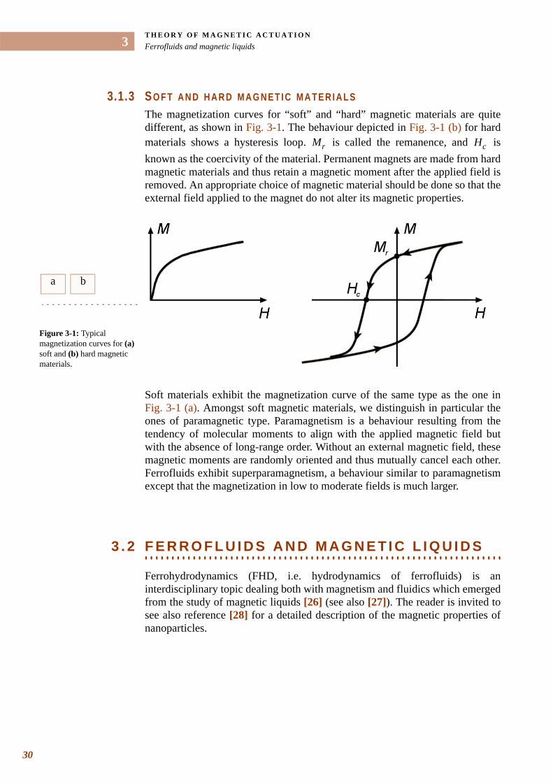
3.1.3 S O F T A N D H A R D M A G N E T I C M A T E R I A L SThe magnetization curves for “soft” and “hard” magnetic materials are quite different, as shown in Fig. 3-1. The behaviour depicted in Fig. 3-1 (b) for hard materials shows a hysteresis loop. is called the remanence, and is known as the coercivity of the material. Permanent magnets are made from hard magnetic materials and thus retain a magnetic moment after the applied field is removed. An appropriate choice of magnetic material should be done so that the external field applied to the magnet do not alter its magnetic properties.
Soft materials exhibit the magnetization curve of the same type as the one in Fig. 3-1 (a). Amongst soft magnetic materials, we distinguish in particular the ones of paramagnetic type. Paramagnetism is a behaviour resulting from the tendency of molecular moments to align with the applied magnetic field but with the absence of long-range order. Without an external magnetic field, these magnetic moments are randomly oriented and thus mutually cancel each other. Ferrofluids exhibit superparamagnetism, a behaviour similar to paramagnetism except that the magnetization in low to moderate fields is much larger.
. . . . . . . . . . . . . . . . . . . . . . . . . . . . . . . . . . . . . . . . . . . . . . . . . . . . . . . . . . . . . . . . . . .3 . 2 F E R R O F L U I D S A N D M A G N E T I C L I Q U I D S
Ferrohydrodynamics (FHD, i.e. hydrodynamics of ferrofluids) is an interdisciplinary topic dealing both with magnetism and fluidics which emerged from the study of magnetic liquids [26] (see also [27]). The reader is invited to see also reference [28] for a detailed description of the magnetic properties of nanoparticles.
Mr Hc
a b
Figure 3-1: Typical magnetization curves for (a) soft and (b) hard magnetic materials.
. . .
. .T H E O R Y O F M A G N E T I C A C T U A T I O NFerrofluids and magnetic liquids
3.2.1 F E R R O F L U I D S Ferrofluids are colloidal magnetic fluids. A colloid is a suspension of finely divided particles (nanoparticles) in a continuous medium. Ferrofluids are composed of small particles of solids (typically ), magnetic, single-domain particles coated with a molecular layer and a dispersant (surfactant) and suspended in a liquid carrier. The colloidal ferrofluid must be synthesized, for it is not found in nature. The three primary constituents of these magnetic liquids are:
• The liquid carrier in which the particles are suspended. Ferrofluids can be water- or oil-based. We employed water-based ferrofluids fabricated at the Powder Technology Laboratory of the EPFL [29].
• The suspended superparamagnetic particles are made from materials such as iron oxide, and have a diameter of the order of . The small size is necessary to maintain stability of the colloidal suspension, as particles significantly larger than this would precipitate.
• The surfactant coats the ferrofluid particles to help maintain the consistency of the colloidal suspension. The surfactant prevents interactions and agglomeration of particles.
The particles are sufficiently small so that the ferrofluid retains its liquid characteristics even in the presence of a magnetic field, and substantial magnetic forces can be induced which results in fluid motion. The magnetic liquid can then be considered as an ultrafine particle system with interparticle spacing large enough to approximate the particles as non-interacting.
3.2.2 G E N E R A L I Z E D B E R N O U L L I E Q U A T I O N The Bernoulli equation which was presented in Chapter 2 (Eq. 2.14) can be generalized to the case of ferrofluids (which are incompressible fluids) to include the effect of magnetic forces acting on the magnetic liquid [26]:
3 15 nm–
10 20 nm–
(3.16)12---ρv2 ρgz p µ0 M Hd
0
H
∫–+ + cste=
31
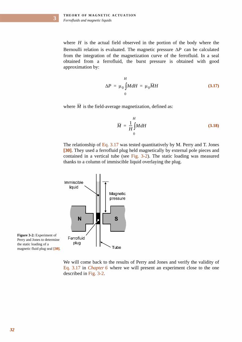
T H E O R Y O F M A G N E T I C A C T U A T I O NFerrofluids and magnetic liquids
32
3
where is the actual field observed in the portion of the body where the Bernoulli relation is evaluated. The magnetic pressure can be calculated from the integration of the magnetization curve of the ferrofluid. In a seal obtained from a ferrofluid, the burst pressure is obtained with good approximation by:
where is the field-average magnetization, defined as:
The relationship of Eq. 3.17 was tested quantitatively by M. Perry and T. Jones [30]. They used a ferrofluid plug held magnetically by external pole pieces and contained in a vertical tube (see Fig. 3-2). The static loading was measured thanks to a column of immiscible liquid overlaying the plug.
We will come back to the results of Perry and Jones and verify the validity of Eq. 3.17 in Chapter 6 where we will present an experiment close to the one described in Fig. 3-2.
HP∆
(3.17)P∆ µ0 M Hd0
H
∫ µ0MH= =
M
(3.18)M 1H---- M Hd
0
H
∫=
Figure 3-2: Experiment of Perry and Jones to determine the static loading of a magnetic fluid plug seal [30].
. . .
. .T H E O R Y O F M A G N E T I C A C T U A T I O NPermanent magnets
. . . . . . . . . . . . . . . . . . . . . . . . . . . . . . . . . . . . . . . . . . . . . . . . . . . . . . . . . . . . . . . . . . .3 . 3 P E R M A N E N T M A G N E T S
In this paragraph, we discuss permanent magnets which are composed of hard magnetic material. A good permanent magnet should produce a high magnetic field while having a low mass, and should be stable against demagnetization effects. The desired properties of such magnets are typically formulated in terms of magnetic energy density, remanence and coercivity of the magnetic materials.
3.3.1 M A G N E T S C L A S S I F I C A T I O N Among commercially available magnets, we can distinguish two types of magnets:
• Hard ferrite magnets Hard ferrite magnets are reliable and efficient components having a very good price to performance ratio. One of their main characteristics is their high resistance against humidity, solvents, alkalis and weak acids.
• Rare-earth magnets Rare-earth magnets in Samarium-Cobalt (SmCo) and Neodymium-Iron-Boron (NdFeB) have a very high energy density ( magnetic energy density product). Using these magnets in permanent magnet motors, very high performances with an excellent efficiency can be achieved.
3.3.2 C H E M I C A L R E S I S T A N C E O F R A R E-E A R T H M A G N E T S
• SmCo Samarium-Cobalt magnets are relatively resistant to humidity, solvents, alkaline solutions, lubricants and neutral poisonous gases. Acids and salt solutions, however, affect them. In the longer term, hydrogen gas leads to decomposition and a loss of magnetic properties. These chemical attacks can be reduced or avoided completely by metallic or plastic coatings.
• NdFeB The microstructure of neodymium magnets can show free Nd depending on their type and quality. Neodymium is extremely corrodible in its free form, and spontaneously forms neodymium oxide or hydroxide powder by increasing its volume. Normal NdFeB magnets are even affected by atmospheric humidity. However, the material is relatively resistant to most solvents, whereas in the presence of salts and acids it suffers from extreme corrosion. In commercial plastic bonded NdFeB magnets, free neodymium occurs only in small proportions, thus they are clearly more resistant than the comparable sintered material.
B H⋅
33
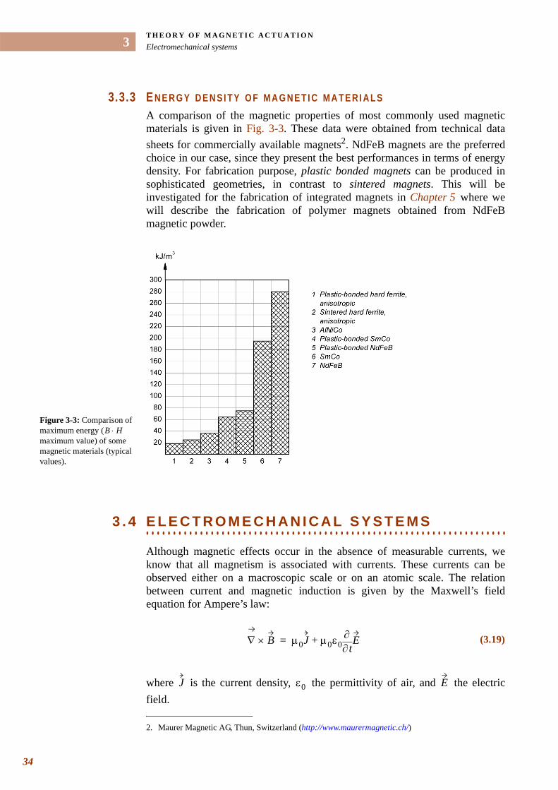
T H E O R Y O F M A G N E T I C A C T U A T I O NElectromechanical systems
34
3
3.3.3 E N E R G Y D E N S I T Y O F M A G N E T I C M A T E R I A L S A comparison of the magnetic properties of most commonly used magnetic materials is given in Fig. 3-3. These data were obtained from technical data sheets for commercially available magnets2. NdFeB magnets are the preferred choice in our case, since they present the best performances in terms of energy density. For fabrication purpose, plastic bonded magnets can be produced in sophisticated geometries, in contrast to sintered magnets. This will be investigated for the fabrication of integrated magnets in Chapter 5 where we will describe the fabrication of polymer magnets obtained from NdFeB magnetic powder.
. . . . . . . . . . . . . . . . . . . . . . . . . . . . . . . . . . . . . . . . . . . . . . . . . . . . . . . . . . . . . . . . . . .3 . 4 E L E C T R O M E C H A N I C A L S Y S T E M S
Although magnetic effects occur in the absence of measurable currents, we know that all magnetism is associated with currents. These currents can be observed either on a macroscopic scale or on an atomic scale. The relation between current and magnetic induction is given by the Maxwell’s field equation for Ampere’s law:
where is the current density, the permittivity of air, and the electric field.
2. Maurer Magnetic AG, Thun, Switzerland (http://www.maurermagnetic.ch/)
Figure 3-3: Comparison of maximum energy ( maximum value) of some magnetic materials (typical values).
B H⋅
(3.19)∇ B× µ0J µ0ε0 t∂∂ E+=
J ε0 E
. . .
. .T H E O R Y O F M A G N E T I C A C T U A T I O NElectromechanical systems
3.4.1 L O R E N T Z F O R C E
The electromagnetic fields and exert a force on a particle of charge
and velocity according to the Lorentz law:
The force acting on a current flowing in an element of a magnet
induction is obtained from the Lorentz force law:
3.4.2 C L A S S I F I C A T I O N Depending on the elements constituting the magnetic circuit, we distinguish different types of electromechanical systems. They are all characterized by the presence of a magnetic field generated by a coil. Most electrical machines (motors) are characterized by a moment resulting from the interaction between two or more coils (placed at the stator and at the rotor). The following list presents the cases which appear to be the most suitable for electromechanical actuation of a reciprocating pump. A complete classification can be found in the specialized literature (see for example reference [31]):
• Reluctant systemA reluctant system does not contain any permanent magnet. The force is associated with the modification of the inductance in the ferromagnetic circuit. These systems are simple but have a low efficiency for small dimensions. They are found in electromagnets and in stepper motors, for example. The solution is also adapted for reciprocating pumps (the piston being the soft ferromagnetic core). Electromechanical pumps developed by Gotec3 are of this type.
• Electrodynamic systemAn electrodynamic system contains a magnet and a magnetic circuit which are fixed, and one (or more) moving coil(s). It has a good dynamic characteristic (small inertia) and is for example found in voice coils. However, electrical connection is the main difficulty with such systems. In the case of our micropump, the integration of a moving coil was not desired since it would have involved the supplementary development of an adapted microfabrication technique for the electrical connection.
E H F q
v
(3.20)F qE qv B×+=
Fd I ld
B
(3.21)Fmag I ld B×=
3. Gotec SA, Sion, Switzerland (http://www.gotec.ch/)
35

T H E O R Y O F M A G N E T I C A C T U A T I O NElectromechanical systems
36
3
• Electromagnetic systemIn an electromagnetic system, the magnetic circuit and the coils are fixed, while the permanent magnets are mobile. Such systems have a higher mechanical inertia compared to equivalent electrodynamic systems. This solution was chosen in our electromechanically actuated reciprocating pumps for its ease of implementation: the moving diaphragm has a permanent magnet and is actuated with a coil external to the pump. The case of such an electromagnetic system is treated in next sections.
3.4.3 M A G N E T I C M E M B R A N E A N D E L E C T R O M A G N E TIn the case treated below, we used a NdFeB composite magnet which was fabricated from a polydimethylsiloxane (PDMS)4 matrix melt with an isotropic magnetic powder MQP-S-115. The fabrication procedure will be explained in more details in Chapter 5 . The magnetic membrane was externally actuated by a coil supplied with a sinusoidal current of amplitude (see schematic diagram in the insert of Fig. 3-4). The electromagnet had a soft magnetic iron core for magnetic field concentration and amplification.
Fig. 3-4 shows the magnetic induction along the symmetry line ( -axis) of the electromagnet with and without the presence of the soft iron core, as measured with a Hall probe6. We clearly observe the amplification of the induction by a factor of about 8 when using the soft core.
4. Dow Corning Corp., Midland, USA (http://www.dowcorning.com/)5. Magnequench GmbH, Essen, Germany (http://www.magnequench.com/)
1500 turns 150 mA
Figure 3-4: Magnetic field generated by the electromagnet for a continuous current.
150 mA
6. Teslameter model 6010, F.W. Bell, Orlando, USA
z
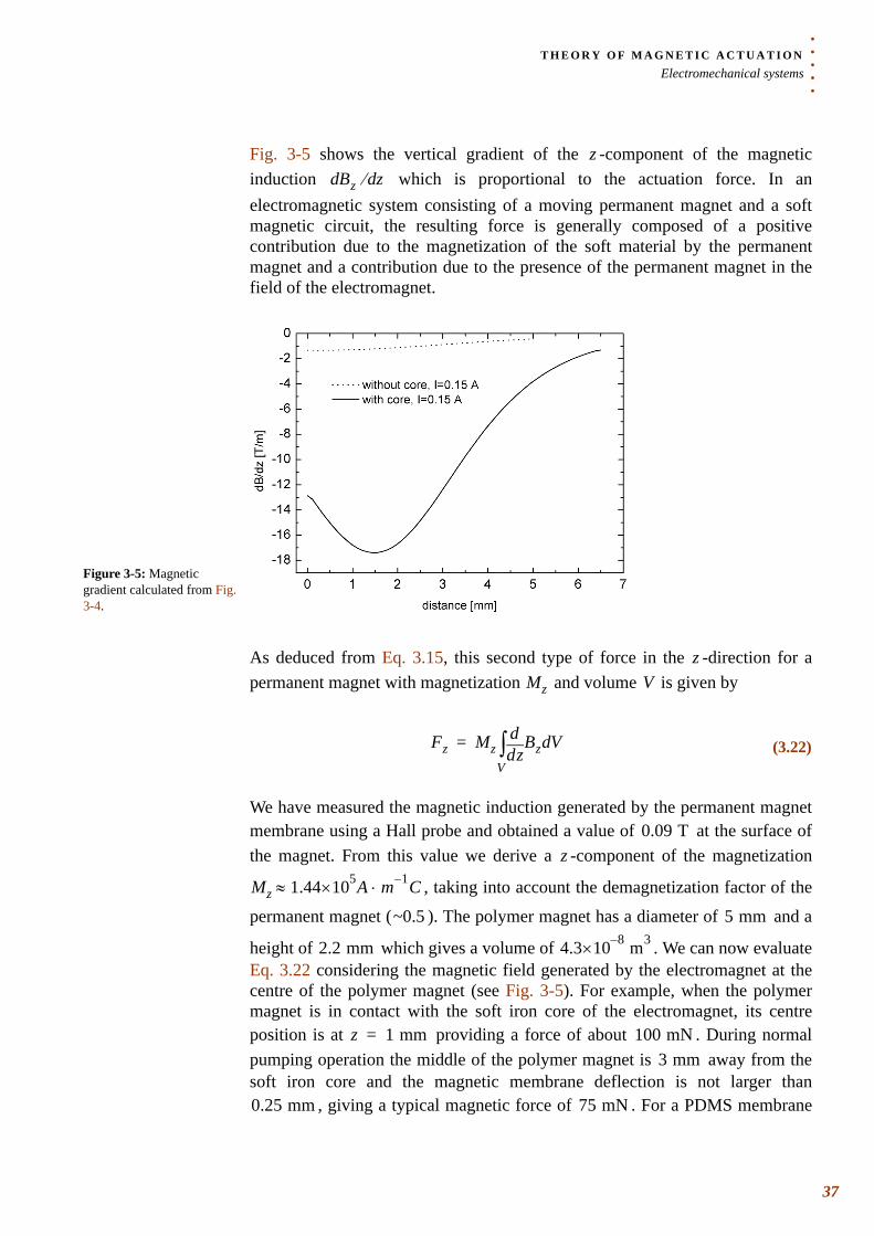
. . .
. .T H E O R Y O F M A G N E T I C A C T U A T I O NElectromechanical systems
Fig. 3-5 shows the vertical gradient of the -component of the magnetic induction which is proportional to the actuation force. In an electromagnetic system consisting of a moving permanent magnet and a soft magnetic circuit, the resulting force is generally composed of a positive contribution due to the magnetization of the soft material by the permanent magnet and a contribution due to the presence of the permanent magnet in the field of the electromagnet.
As deduced from Eq. 3.15, this second type of force in the -direction for a permanent magnet with magnetization and volume is given by
We have measured the magnetic induction generated by the permanent magnet membrane using a Hall probe and obtained a value of at the surface of the magnet. From this value we derive a -component of the magnetization
, taking into account the demagnetization factor of the
permanent magnet ( ). The polymer magnet has a diameter of and a
height of which gives a volume of . We can now evaluate Eq. 3.22 considering the magnetic field generated by the electromagnet at the centre of the polymer magnet (see Fig. 3-5). For example, when the polymer magnet is in contact with the soft iron core of the electromagnet, its centre position is at providing a force of about . During normal pumping operation the middle of the polymer magnet is away from the soft iron core and the magnetic membrane deflection is not larger than
, giving a typical magnetic force of . For a PDMS membrane
zBz zd⁄d
Figure 3-5: Magnetic gradient calculated from Fig. 3-4.
zMz V
(3.22)Fz Mz zdd Bz Vd
V∫=
0.09 Tz
Mz 1.44 5×10 A m 1–⋅≈ C
~0.5 5 mm
2.2 mm 4.3 8–×10 m3
z 1 mm= 100 mN3 mm
0.25 mm 75 mN
37
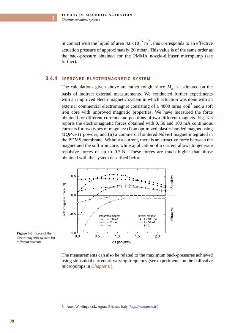
T H E O R Y O F M A G N E T I C A C T U A T I O NElectromechanical systems
38
3
in contact with the liquid of area , this corresponds to an effective actuation pressure of approximately . This value is of the same order as the back-pressure obtained for the PMMA nozzle-diffuser micropump (see further).
3.4.4 IM P R O V E D E L E C T R O M A G N E T I C S Y S T E M
The calculations given above are rather rough, since is estimated on the basis of indirect external measurements. We conducted further experiments with an improved electromagnetic system in which actuation was done with an external commercial electromagnet consisting of a coil7 and a soft iron core with improved magnetic properties. We have measured the force obtained for different currents and positions of two different magnets. Fig. 3-6reports the electromagnetic forces obtained with 0, 50 and 100 mA continuous currents for two types of magnets: (i) an optimized plastic-bonded magnet using MQP-S-11 powder; and (ii) a commercial sintered NdFeB magnet integrated in the PDMS membrane. Without a current, there is an attractive force between the magnet and the soft iron core, while application of a current allows to generate repulsive forces of up to . These forces are much higher than those obtained with the system described before.
The measurements can also be related to the maximum back-pressures achieved using sinusoidal current of varying frequency (see experiments on the ball valve micropumps in Chapter 8 ).
3.8 5–×10 m2
20 mbar
7. Atam Windings s.r.l., Agrate Brianza, Italy (http://www.atam.it/)
Mz
4800 turns
0.5 N
Figure 3-6: Force of the electromagnetic system for different currents.
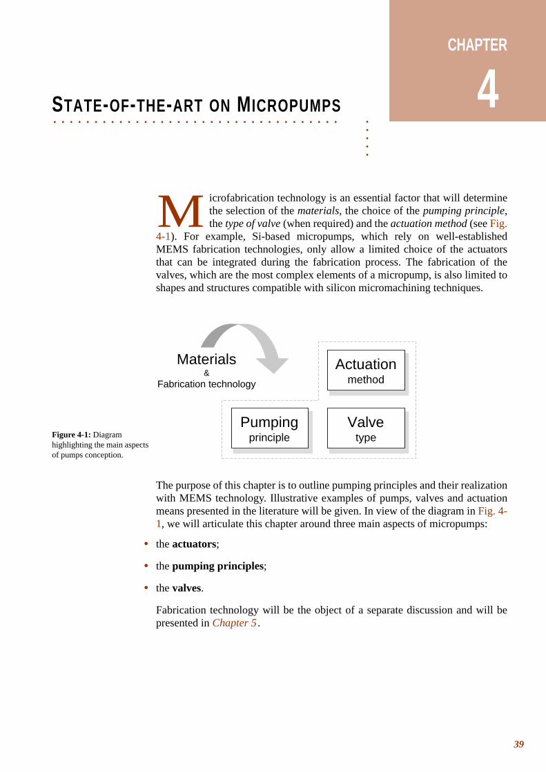
CHAPTER
4. . . . .
. . . . . . . . . . . . . . . . . . . . . . . . . . . . . . . . . . .STATE-OF-THE-ART ON MICROPUMPS
icrofabrication technology is an essential factor that will determine the selection of the materials, the choice of the pumping principle, the type of valve (when required) and the actuation method (see Fig.
4-1). For example, Si-based micropumps, which rely on well-established MEMS fabrication technologies, only allow a limited choice of the actuators that can be integrated during the fabrication process. The fabrication of the valves, which are the most complex elements of a micropump, is also limited to shapes and structures compatible with silicon micromachining techniques.
The purpose of this chapter is to outline pumping principles and their realization with MEMS technology. Illustrative examples of pumps, valves and actuation means presented in the literature will be given. In view of the diagram in Fig. 4-1, we will articulate this chapter around three main aspects of micropumps:
• the actuators;
• the pumping principles;
• the valves.
Fabrication technology will be the object of a separate discussion and will be presented in Chapter 5 .
M
Figure 4-1: Diagram highlighting the main aspects of pumps conception.
Valvetype
Materials&
Fabrication technology
Actuationmethod
Pumpingprinciple
39
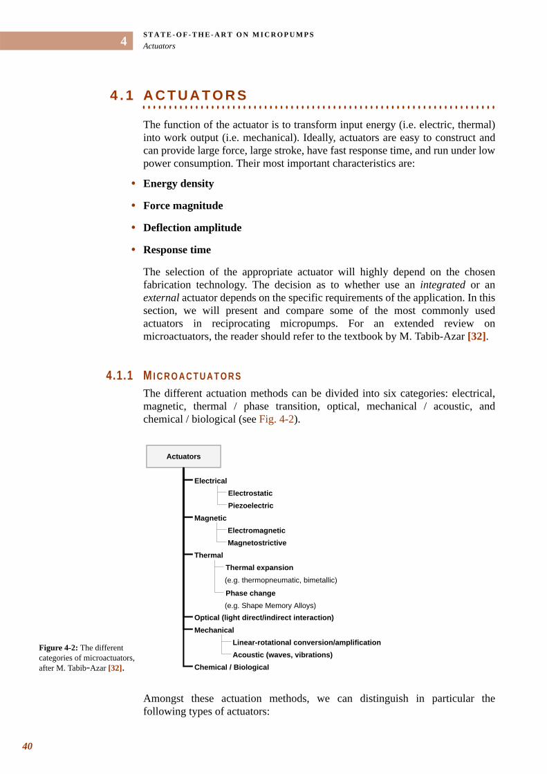
ST A T E - O F - T H E - A R T O N M I C R O P U M P SActuators
40
4
. . . . . . . . . . . . . . . . . . . . . . . . . . . . . . . . . . . . . . . . . . . . . . . . . . . . . . . . . . . . . . . . . . . 4 . 1 A C T U A T O R S
The function of the actuator is to transform input energy (i.e. electric, thermal) into work output (i.e. mechanical). Ideally, actuators are easy to construct and can provide large force, large stroke, have fast response time, and run under low power consumption. Their most important characteristics are:
• Energy density
• Force magnitude
• Deflection amplitude
• Response time
The selection of the appropriate actuator will highly depend on the chosen fabrication technology. The decision as to whether use an integrated or an external actuator depends on the specific requirements of the application. In this section, we will present and compare some of the most commonly used actuators in reciprocating micropumps. For an extended review on microactuators, the reader should refer to the textbook by M. Tabib-Azar [32].
4.1.1 M I C R O A C T U A T O R S The different actuation methods can be divided into six categories: electrical, magnetic, thermal / phase transition, optical, mechanical / acoustic, and chemical / biological (see Fig. 4-2).
Amongst these actuation methods, we can distinguish in particular the following types of actuators:
Figure 4-2: The different categories of microactuators, after M. Tabib-Azar [32].
Actuators
Electrical
Magnetic
Electrostatic
Piezoelectric
Thermal
Thermal expansion
Phase change
Optical (light direct/indirect interaction)
Mechanical
Linear-rotational conversion/amplification
Chemical / Biological
Electromagnetic
Magnetostrictive
Acoustic (waves, vibrations)
(e.g. thermopneumatic, bimetallic)
(e.g. Shape Memory Alloys)
. . .
. .ST A T E - O F - T H E - A R T O N M I C R O P U M P SActuators
Bimeta l l i c Bimetallic actuation is obtained through temperature changes and results from the difference in thermal expansion coefficient between two materials bonded together. Large deflections are only achievable at high temperature changes since thermal expansion coefficients of popular MEMS materials are close and small. This limits the usefulness of such actuators in the case of reciprocating micropumps.
Shape Memory E f fec t
Shape memory alloys (SMA), especially NiTi alloys (Nitinol) can be used to produce very high energy storage. In the “shape memory effect” mode, these actuators undergo a reversible temperature-dependent material phase transition from the Austenitic to the Martensitic phase. These phase transitions result in mechanical deformations that can be used to produce large displacement actuators. However, the response time is slow, and the memory effect requires the “education” of the actuators so that they can recover their different “memorized” shapes for the two phases.
Pneumat ic Pneumatic actuation is obtained using an external source. Such an actuation source is therefore not transportable. However, on-chip pressure sources (obtained thermopneumatically, for example) can make this actuation method practical for portable devices. In a thermopneumatic microactuator, it is the volume expansion of a fluid which is used for actuation. The fluid may be a liquid that turns into a gas or simply a gas that expands upon heating.
Elec t ros ta t i c Electrostatic actuation is based on Coulombic attraction forces between charged surfaces. When a voltage is applied between two plates of area separated by an air gap , the electrostatic force is:
where is the permittivity of free space and is the electric field. The gap distance between the electrodes should be as small as possible. Therefore, small strokes are typical of electrostatic actuation. On the other hand, it benefits from a fast response time and a low power consumption.
Another important aspect can be deduced from Eq. 4.1: the electrostatic force is a surface force that scales down favourably with size [33,34,35]. Assuming that all dimensions are scaled with the same factor , the electrostatic force will scale as:
• if the electrical field scales as ;
• if the voltage scales as .
This shows that electrostatic actuators can be favourably used in miniaturized systems.
V Aδ Fes
, (4.1)Fes12---ε0AE2= E V
δ---=
ε0 E
s Fes
s2 E s0
s0 V s0
41
ST A T E - O F - T H E - A R T O N M I C R O P U M P SActuators
42
4
Piezoe lec t r i c Piezoelectric actuation (or the electrostrictive effect) is obtained by means of the strain induced in a piezoelectric material (e.g. lead zirconate titanate or PZT, zinc oxide or ZnO) by an applied electric field. A fast response time and a high energy density are typical for piezoelectrics. However, the fabrication of integrated piezoelectric microactuators in Si-based microsystems requires the deposition of an additional thin film of piezoelectric material onto the silicon. This process is complex, which explains why most of the Si-based reciprocating micropumps generally rather have a piezoelectric disc glued on the actuation membrane of the micropump.
Magnetos t r i c t i ve Similarly to the electrostrictive effect, magnetostriction is induced by an external magnetic field but deformation strokes are much lower. Magnetostrictive materials are excellent candidates as sensors and find applications as displacement, magnetic field sensors or magnetic memories.
Elec t romagnet ic Electromagnetic actuation has been described earlier in Chapter 3 . From Eq.
3.21, we can deduce the magnetic force between a current carrying wire
(length , current ) and a permanent magnet (magnetic induction ):
Electromagnetic actuation generally requires the use of a permanent magnet to generate a sufficient force for the microactuators. Furthermore, coil integration is difficult and current requirements can result in heating issues. The maximum current is therefore an important factor. In the case of a wire and a permanent magnet ( is an insensitive variable that depends upon materials properties, and
thus scales as ), the electromagnetic force scales as [33,34]:
• if the current density scales as ;
• if the current scales as .
The assumption of a constant current density leads to an underestimation of the maximum achievable force, because a better cooling can be obtained with smaller components. W. Trimmer and R. Jebens [33] only considered the conduction effect to estimate the cooling in microactuators, while J. Peirs et al.[34] also studied convective cooling. Their conclusion is that, in general,
maximal current in microactuators will scale as for a constant heat flow.
Fmag
l I B
(4.2)Fmag I ld B×l∫=
B
s0 Fmag
s3 J s0
s2 I s1
s1
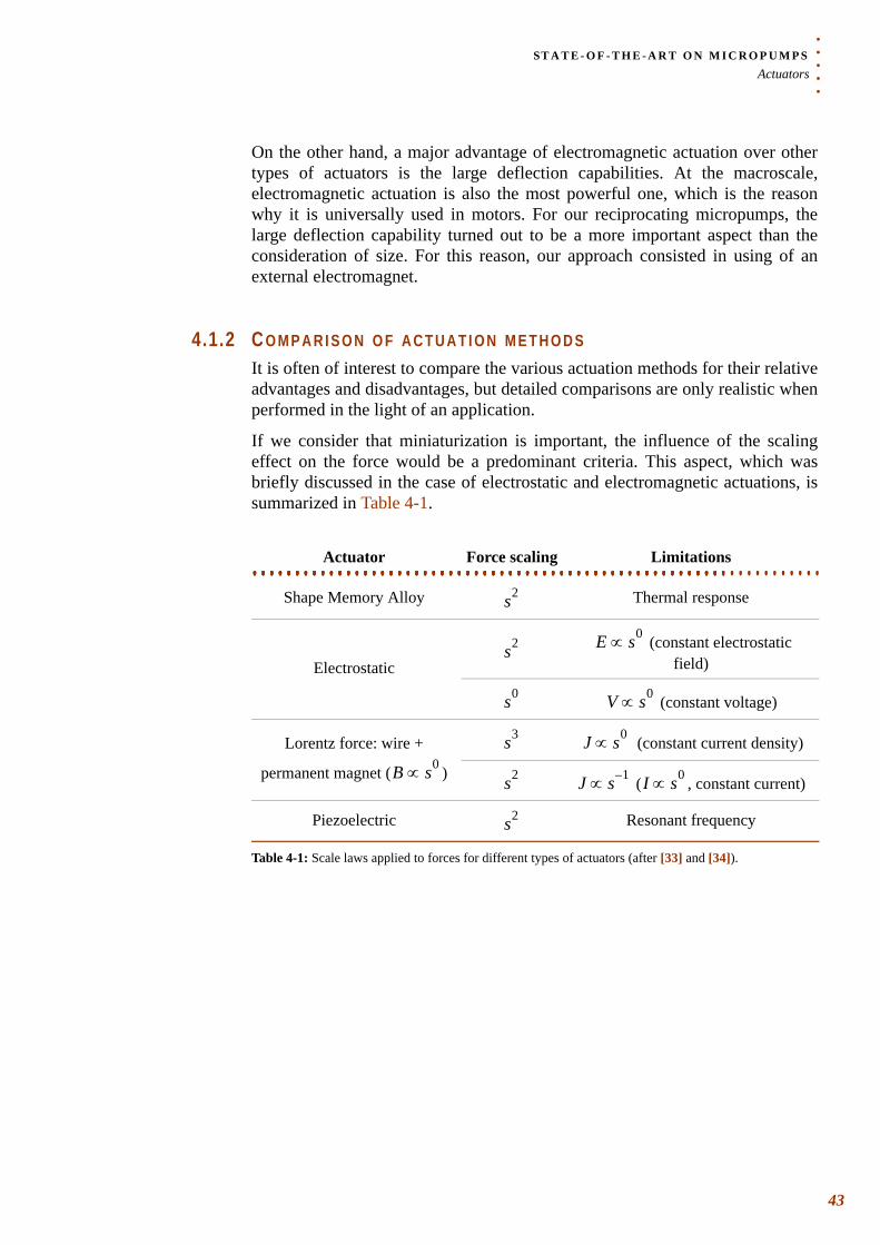
. . .
. .ST A T E - O F - T H E - A R T O N M I C R O P U M P SActuators
On the other hand, a major advantage of electromagnetic actuation over other types of actuators is the large deflection capabilities. At the macroscale, electromagnetic actuation is also the most powerful one, which is the reason why it is universally used in motors. For our reciprocating micropumps, the large deflection capability turned out to be a more important aspect than the consideration of size. For this reason, our approach consisted in using of an external electromagnet.
4.1.2 C O M P A R I S O N O F A C T U A T I O N M E T H O D S It is often of interest to compare the various actuation methods for their relative advantages and disadvantages, but detailed comparisons are only realistic when performed in the light of an application.
If we consider that miniaturization is important, the influence of the scaling effect on the force would be a predominant criteria. This aspect, which was briefly discussed in the case of electrostatic and electromagnetic actuations, is summarized in Table 4-1.
Actuator Force scaling Limitations. . . . . . . . . . . . . . . . . . . . . . . . . . . . . . . . . . . . . . . . . . . . . . . . . . . . . . . . . . . . . . . . . . . . . . . . . . . . . . . . . . . . . . . . . . . . . . . . . . . . . . . . . . . . . . . . . . . . . . . . . . .. . . . . . . . . . . . . . . . . . . . . . . . . . . . . . . . . . . . . . . . . . . . . . . . . . . . . . . .. . . . . . . . . . . . . . . . . . . . . . . . . . . . . . . . . . . . . . . . . . . . . . . . . . . . . . . .Shape Memory Alloy Thermal response
Electrostatic (constant electrostatic
field)
(constant voltage)
Lorentz force: wire +
permanent magnet ( )
(constant current density)
( , constant current)
Piezoelectric Resonant frequency
Table 4-1: Scale laws applied to forces for different types of actuators (after [33] and [34]).
s2
s2 E s0∝
s0 V s0∝
B s0∝
s3 J s0∝
s2 J s 1–∝ I s0∝
s2
43
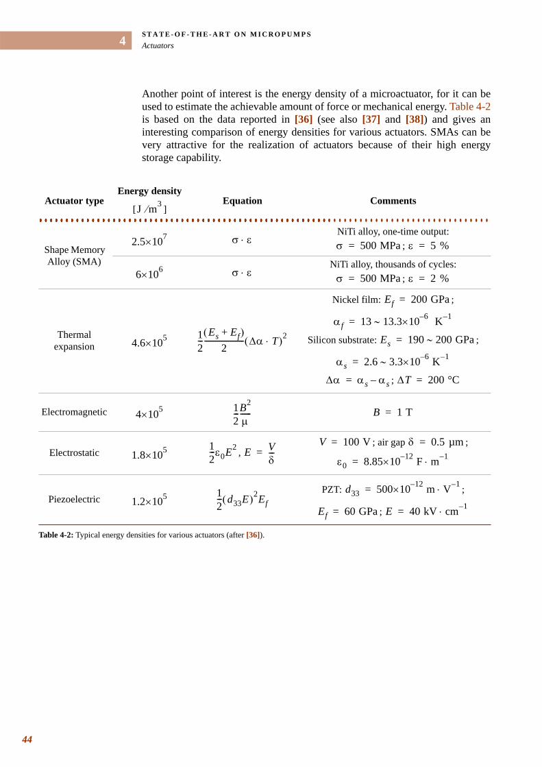
ST A T E - O F - T H E - A R T O N M I C R O P U M P SActuators
44
4
Another point of interest is the energy density of a microactuator, for it can be used to estimate the achievable amount of force or mechanical energy. Table 4-2is based on the data reported in [36] (see also [37] and [38]) and gives an interesting comparison of energy densities for various actuators. SMAs can be very attractive for the realization of actuators because of their high energy storage capability.
Actuator typeEnergy density
[ ]Equation Comments
. . . . . . . . . . . . . . . . . . . . . . . . . . . . . . . . . . . . . . . . . . . . . . . . . . . . . . . . . . . . . . . . . . . . . . . . . . . . . . . . . . . . . . . . . . . . . . . . . . . . . . . . . . . . . . . . . . . . . . . . . . . . . . . . . . . . . . . . . . . . . .. . . . . . . . . . . . . . . . . . . . . . . . . . . . . . . . . . . . . . . . . . . . . . . . . . . . . . . .. . . . . . . . . . . . . . . . . . . . . . . . . . . . . . . . . . . . . . . . . . . . . . . . . . . . . . . . Shape Memory
Alloy (SMA)
NiTi alloy, one-time output: ;
NiTi alloy, thousands of cycles: ;
Thermal expansion
Nickel film: ;
Silicon substrate: ;
;
Electromagnetic
Electrostatic , ; air gap ;
PiezoelectricPZT: ;
;
Table 4-2: Typical energy densities for various actuators (after [36]).
J m3⁄
2.5 7×10 σ ε⋅ σ 500 MPa= ε 5 %=
6 6×10 σ ε⋅ σ 500 MPa= ε 2 %=
4.6 5×10¹²---
Es Ef+( )2
---------------------- ∆α T⋅( )2
Ef 200 GPa=
αf 13 13.3∼ 6–×10 K 1–=
Es 190 200 GPa∼=
αs 2.6 3.3 6–×10 K 1–∼=
∆α αs αs–= ∆T 200 °C=
4 5×10 12---B2
µ------ B 1 T=
1.8 5×10¹²---ε0E2 E V
δ---=
V 100 V= δ 0.5 µm=
ε0 8.85 12–×10 F m 1–⋅=
1.2 5×10¹²--- d33E( )2Ef
d33 500 12–×10 m V 1–⋅=
Ef 60 GPa= E 40 kV cm 1–⋅=
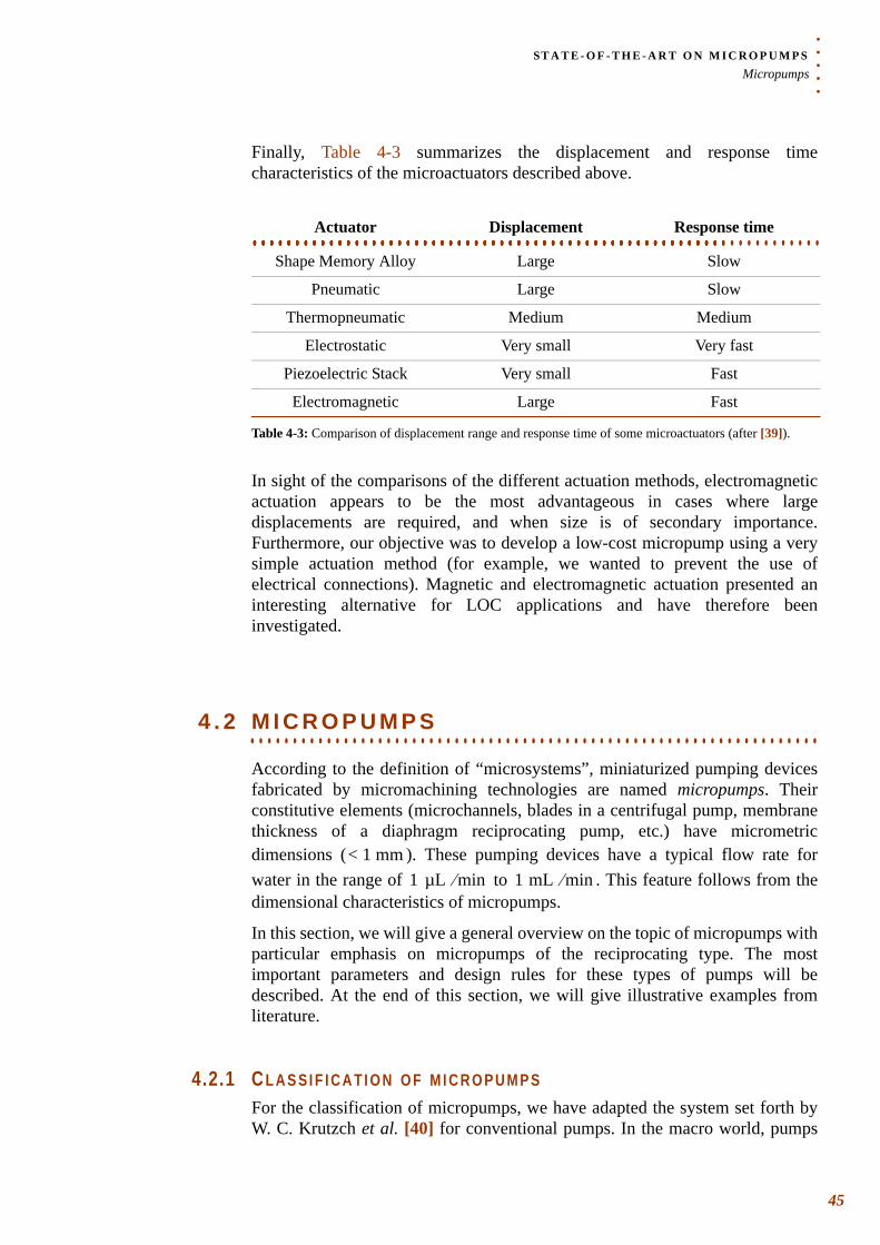
. . .
. .ST A T E - O F - T H E - A R T O N M I C R O P U M P SMicropumps
Finally, Table 4-3 summarizes the displacement and response time characteristics of the microactuators described above.
In sight of the comparisons of the different actuation methods, electromagnetic actuation appears to be the most advantageous in cases where large displacements are required, and when size is of secondary importance. Furthermore, our objective was to develop a low-cost micropump using a very simple actuation method (for example, we wanted to prevent the use of electrical connections). Magnetic and electromagnetic actuation presented an interesting alternative for LOC applications and have therefore been investigated.
. . . . . . . . . . . . . . . . . . . . . . . . . . . . . . . . . . . . . . . . . . . . . . . . . . . . . . . . . . . . . . . . . . . 4 . 2 M I C R O P U M P S
According to the definition of “microsystems”, miniaturized pumping devices fabricated by micromachining technologies are named micropumps. Their constitutive elements (microchannels, blades in a centrifugal pump, membrane thickness of a diaphragm reciprocating pump, etc.) have micrometric dimensions ( ). These pumping devices have a typical flow rate for water in the range of to . This feature follows from the dimensional characteristics of micropumps.
In this section, we will give a general overview on the topic of micropumps with particular emphasis on micropumps of the reciprocating type. The most important parameters and design rules for these types of pumps will be described. At the end of this section, we will give illustrative examples from literature.
4.2.1 C L A S S I F I C A T I O N O F M I C R O P U M P SFor the classification of micropumps, we have adapted the system set forth by W. C. Krutzch et al. [40] for conventional pumps. In the macro world, pumps
Actuator Displacement Response time. . . . . . . . . . . . . . . . . . . . . . . . . . . . . . . . . . . . . . . . . . . . . . . . . . . . . . . . . . . . . . . . . . . . . . . . . . . . . . . . . . . . . . . . . . . . . . . . . . . . . . . . . . . . . . . . . . . . . . . . . . .. . . . . . . . . . . . . . . . . . . . . . . . . . . . . . . . . . . . . . . . . . . . . . . . . . . . . . . .. . . . . . . . . . . . . . . . . . . . . . . . . . . . . . . . . . . . . . . . . . . . . . . . . . . . . . . .Shape Memory Alloy Large Slow
Pneumatic Large Slow
Thermopneumatic Medium Medium
Electrostatic Very small Very fast
Piezoelectric Stack Very small Fast
Electromagnetic Large Fast
Table 4-3: Comparison of displacement range and response time of some microactuators (after [39]).
< 1 mm1 µL min⁄ 1 mL min⁄
45

ST A T E - O F - T H E - A R T O N M I C R O P U M P SMicropumps
46
4
are divided into two main categories, according to the way the fluid is displaced:
• Hydrodynamic pumpsHere energy is continuously added to increase the fluid velocities within the pump. Centrifugal pumps are the most common type of traditional hydrodynamic pumps. Electrohydrodynamic (EHD), magnetohydrodynamic (MHD) and electroosmotic (EO) pumps are all based on interactions between the working fluid and an electromagnetic field. MHD based pumping, for example uses the Lorentz force and requires the fluid to be electrically conducting. Another type of pumps found in this category is the acoustic pump which generates flow through sound wave effects (e.g. ultrasonic).
• Positive displacement pumpsEnergy is periodically added by applying a force to one or more movable boundaries of fluid-containing volumes. Volume changes resulting from this action produce a direct pressure increase up to the value required to move the fluid through the valves and into the outlet line. These pumps produce a pulsating flow.
Figure 4-3: Classification of pumps (adapted from [40] and [41]).
Pumps
HydrodynamicPositive
displacement
Reciprocating
Aperiodic
Rotary
Piston, plunger
Diaphragm
Simplex
Multiplex
Single rotor
Multiple rotor
Centrifugal
Axial flow
Mixed flow, radial flow
Peripheral
Electrohydrodynamic (EHD)
Electroosmotic
Magnetohydrodynamic (MHD)
Acoustic, ultrasonic
Gear
Lobe
Circumferential piston
Screw
Syringe pump
Vane
Piston
Flexible member
Screw
Peristaltic
AC
DC
Parallel
Serial (peristaltic)
Electrowetting / thermocapillary
Injection
Induction
Conduction
. . .
. .ST A T E - O F - T H E - A R T O N M I C R O P U M P SMicropumps
Dynamic pumps (also referred to as “continuous flow pumps”) provide a higher and much steadier flow rate than positive displacement pumps, but they are not suitable for the handling of high-viscosity liquids. The choice of a pumping principle will depend on the required specifications and will be made on the basis of the application they serve.
4.2.2 B A S I C P U M P P A R A M E T E R SThe performance of a pump, which highly depends on its working principle, is mainly characterized by the following parameters:
• the operating frequency range and/or resonant frequency;
• the maximum flow rate (obtained in the absence of back-pressure);
• the maximum back-pressure : The back-pressure opposes the work done by the pump. At the maximum back-pressure, the flow rate falls to zero.
• the power of the pump: The power delivered by the pump to the fluid, , can be expressed as:
where is the volume rate of the flow and is the pressure increase produced by the pump. The pumps developed in this thesis, demonstrate a linear decrease of the flow rate versus an increasing back-pressure. Under this assumption, Eq. 4.3 can also be expressed as [41]:
• the efficiency of the pump:The efficiency of the pump, , is expressed as:
with , the power required to drive the pump actuator. Many factors affect the pump efficiency: friction losses (mechanical efficiency), fluid leakage losses (in particular limited valve efficiency), losses due to imperfect construction (presence of bubbles), etc.
These different criteria were used in the review of D. J. Laser and J. G. Santiago [41] and more particularly in that of N. T. Nguyen et al. [38] to compare pumping principles and designs.
Qmax
Pmax
Ppump
(4.3)Ppump P∆ Q⋅=
Q P∆
(4.4)Ppump∆Pmax Q⋅ max
4---------------------------------=
ηpump
(4.5)ηpumpPpump
Pactuator---------------------=
Pactuator
47
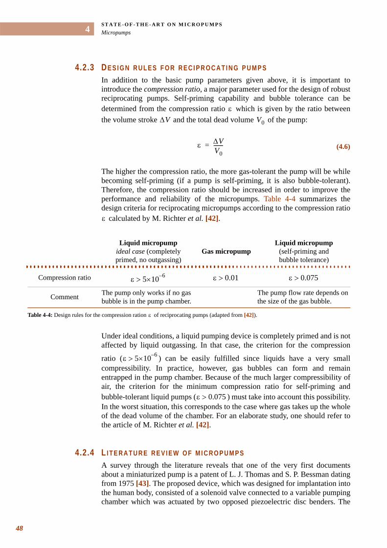
ST A T E - O F - T H E - A R T O N M I C R O P U M P SMicropumps
48
4
4.2.3 D E S I G N R U L E S F O R R E C I P R O C A T I N G P U M P SIn addition to the basic pump parameters given above, it is important to introduce the compression ratio, a major parameter used for the design of robust reciprocating pumps. Self-priming capability and bubble tolerance can be determined from the compression ratio which is given by the ratio between the volume stroke and the total dead volume of the pump:
The higher the compression ratio, the more gas-tolerant the pump will be while becoming self-priming (if a pump is self-priming, it is also bubble-tolerant). Therefore, the compression ratio should be increased in order to improve the performance and reliability of the micropumps. Table 4-4 summarizes the design criteria for reciprocating micropumps according to the compression ratio
calculated by M. Richter et al. [42].
Under ideal conditions, a liquid pumping device is completely primed and is not affected by liquid outgassing. In that case, the criterion for the compression
ratio ( ) can be easily fulfilled since liquids have a very small compressibility. In practice, however, gas bubbles can form and remain entrapped in the pump chamber. Because of the much larger compressibility of air, the criterion for the minimum compression ratio for self-priming and bubble-tolerant liquid pumps ( ) must take into account this possibility. In the worst situation, this corresponds to the case where gas takes up the whole of the dead volume of the chamber. For an elaborate study, one should refer to the article of M. Richter et al. [42].
4.2.4 L I T E R A T U R E R E V I E W O F M I C R O P U M P SA survey through the literature reveals that one of the very first documents about a miniaturized pump is a patent of L. J. Thomas and S. P. Bessman dating from 1975 [43]. The proposed device, which was designed for implantation into the human body, consisted of a solenoid valve connected to a variable pumping chamber which was actuated by two opposed piezoelectric disc benders. The
ε∆V V0
(4.6)ε ∆VV0-------=
ε
Liquid micropump ideal case (completely primed, no outgassing)
Gas micropump Liquid micropump
(self-priming and bubble tolerance). . . . . . . . . . . . . . . . . . . . . . . . . . . . . . . . . . . . . . . . . . . . . . . . . . . . . . . . . . . . . . . . . . . . . . . . . . . . . . . . . . . . . . .. . . . . . . . . . . . . . . . . . . . . . . . . . . . . . . . . . . . . . . . . . . . . . . . . . . . . . . .. . . . . . . . . . . . . . . . . . . . . . . . . . . . . . . . . . . . . . . . . . . . . . . . . . . . . . . .. . . . . . . . . . . . . . . . . . . . . . . . . . . . . . . . . . . . . . . . . . . . . . . . . . . . . . . .
Compression ratio
Comment The pump only works if no gas bubble is in the pump chamber.
The pump flow rate depends on the size of the gas bubble.
Table 4-4: Design rules for the compression ration of reciprocating pumps (adapted from [42]).
ε 5 6–×10> ε 0.01> ε 0.075>
ε
ε 5 6–×10>
ε 0.075>
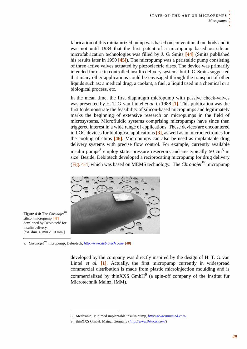
. . .
. .ST A T E - O F - T H E - A R T O N M I C R O P U M P SMicropumps
fabrication of this miniaturized pump was based on conventional methods and it was not until 1984 that the first patent of a micropump based on silicon microfabrication technologies was filled by J. G. Smits [44] (Smits published his results later in 1990 [45]). The micropump was a peristaltic pump consisting of three active valves actuated by piezoelectric discs. The device was primarily intended for use in controlled insulin delivery systems but J. G. Smits suggested that many other applications could be envisaged through the transport of other liquids such as: a medical drug, a coolant, a fuel, a liquid used in a chemical or a biological process, etc.
In the mean time, the first diaphragm micropump with passive check-valves was presented by H. T. G. van Lintel et al. in 1988 [1]. This publication was the first to demonstrate the feasibility of silicon-based micropumps and legitimately marks the beginning of extensive research on micropumps in the field of microsystems. Microfluidic systems comprising micropumps have since then triggered interest in a wide range of applications. These devices are encountered in LOC devices for biological applications [3], as well as in microelectronics for the cooling of chips [46]. Micropumps can also be used as implantable drug delivery systems with precise flow control. For example, currently available insulin pumps8 employ static pressure reservoirs and are typically 50 cm3 in size. Beside, Debiotech developed a reciprocating micropump for drug delivery (Fig. 4-4) which was based on MEMS technology. The Chronojet™ micropump
developed by the company was directly inspired by the design of H. T. G. van Lintel et al. [1]. Actually, the first micropump currently in widespread commercial distribution is made from plastic microinjection moulding and is commercialized by thinXXS GmbH9 (a spin-off company of the Institut für Microtechnik Mainz, IMM).
8. Medtronic, Minimed implantable insulin pump, http://www.minimed.com/
Figure 4-4: The Chronojet™ silicon micropump [47] developed by Debiotecha for insulin delivery. [ext. dim. ]
a. Chronojet™ micropump, Debiotech, http://www.debiotech.com/ [48]
6 mm 10 mm×
9. thinXXS GmbH, Mainz, Germany (http://www.thinxxs.com/)
49
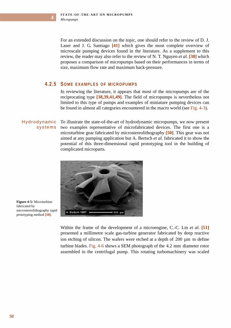
ST A T E - O F - T H E - A R T O N M I C R O P U M P SMicropumps
50
4
For an extended discussion on the topic, one should refer to the review of D. J. Laser and J. G. Santiago [41] which gives the most complete overview of microscale pumping devices found in the literature. As a supplement to this review, the reader may also refer to the review of N. T. Nguyen et al. [38] which proposes a comparison of micropumps based on their performances in terms of size, maximum flow rate and maximum back-pressure.
4.2.5 S O M E E X A M P L E S O F M I C R O P U M P SIn reviewing the literature, it appears that most of the micropumps are of the reciprocating type [38,39,41,49]. The field of micropumps is nevertheless not limited to this type of pumps and examples of miniature pumping devices can be found in almost all categories encountered in the macro world (see Fig. 4-3).
Hydrodynamic sys tems
To illustrate the state-of-the-art of hydrodynamic micropumps, we now present two examples representative of microfabricated devices. The first one is a microturbine gear fabricated by microstereolithography [50]. This gear was not aimed at any pumping application but A. Bertsch et al. fabricated it to show the potential of this three-dimensional rapid prototyping tool in the building of complicated microparts.
Within the frame of the development of a microengine, C.-C. Lin et al. [51] presented a millimetre scale gas-turbine generator fabricated by deep reactive ion etching of silicon. The wafers were etched at a depth of to define turbine blades. Fig. 4-6 shows a SEM photograph of the diameter rotor assembled in the centrifugal pump. This rotating turbomachinery was scaled
Figure 4-5: Microturbine fabricated by microstereolithography rapid prototyping method [50].
200 µm4.2 mm
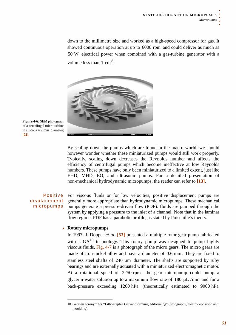
. . .
. .ST A T E - O F - T H E - A R T O N M I C R O P U M P SMicropumps
down to the millimetre size and worked as a high-speed compressor for gas. It showed continuous operation at up to and could deliver as much as
electrical power when combined with a gas-turbine generator with a
volume less than .
By scaling down the pumps which are found in the macro world, we should however wonder whether these miniaturized pumps would still work properly. Typically, scaling down decreases the Reynolds number and affects the efficiency of centrifugal pumps which become ineffective at low Reynolds numbers. These pumps have only been miniaturized to a limited extent, just like EHD, MHD, EO, and ultrasonic pumps. For a detailed presentation of non-mechanical hydrodynamic micropumps, the reader can refer to [13].
Pos i t i ve d isp lacement
m ic ropumps
For viscous fluids or for low velocities, positive displacement pumps are generally more appropriate than hydrodynamic micropumps. These mechanical pumps generate a pressure-driven flow (PDF): fluids are pumped through the system by applying a pressure to the inlet of a channel. Note that in the laminar flow regime, PDF has a parabolic profile, as stated by Poiseuille’s theory.
Rotary micropumpsIn 1997, J. Döpper et al. [53] presented a multiple rotor gear pump fabricated with LIGA10 technology. This rotary pump was designed to pump highly viscous fluids. Fig. 4-7 is a photograph of the micro gears. The micro gears are made of iron-nickel alloy and have a diameter of . They are fixed to stainless steel shafts of diameter. The shafts are supported by ruby bearings and are externally actuated with a miniaturized electromagnetic motor. At a rotational speed of , the gear micropump could pump a glycerin-water solution up to a maximum flow rate of and for a back-pressure exceeding (theoretically estimated to
6000 rpm50 W
1 cm3
Figure 4-6: SEM photograph of a centrifugal microturbine in silicon ( diameter) [52].
4.2 mm
10. German acronym for “Lithographie Galvanoformung Abformung” (lithography, electrodeposition and moulding).
0.6 mm240 µm
2250 rpm180 µL min⁄
1200 hPa 9000 hPa
51
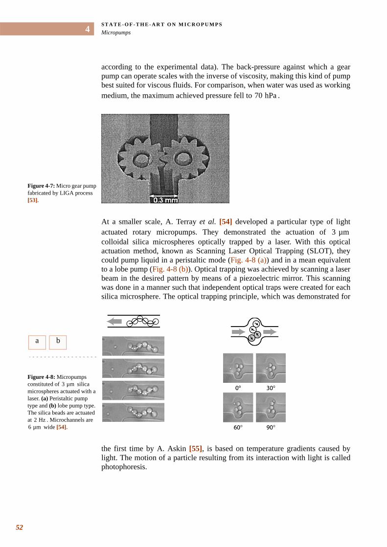
ST A T E - O F - T H E - A R T O N M I C R O P U M P SMicropumps
52
4
according to the experimental data). The back-pressure against which a gear pump can operate scales with the inverse of viscosity, making this kind of pump best suited for viscous fluids. For comparison, when water was used as working medium, the maximum achieved pressure fell to .
At a smaller scale, A. Terray et al. [54] developed a particular type of light actuated rotary micropumps. They demonstrated the actuation of colloidal silica microspheres optically trapped by a laser. With this optical actuation method, known as Scanning Laser Optical Trapping (SLOT), they could pump liquid in a peristaltic mode (Fig. 4-8 (a)) and in a mean equivalent to a lobe pump (Fig. 4-8 (b)). Optical trapping was achieved by scanning a laser beam in the desired pattern by means of a piezoelectric mirror. This scanning was done in a manner such that independent optical traps were created for each silica microsphere. The optical trapping principle, which was demonstrated for
the first time by A. Askin [55], is based on temperature gradients caused by light. The motion of a particle resulting from its interaction with light is called photophoresis.
70 hPa
Figure 4-7: Micro gear pump fabricated by LIGA process [53].
3 µm
a b
Figure 4-8: Micropumps constituted of silica microspheres actuated with a laser. (a) Peristaltic pump type and (b) lobe pump type. The silica beads are actuated at . Microchannels are
wide [54].
3 µm
2 Hz6 µm
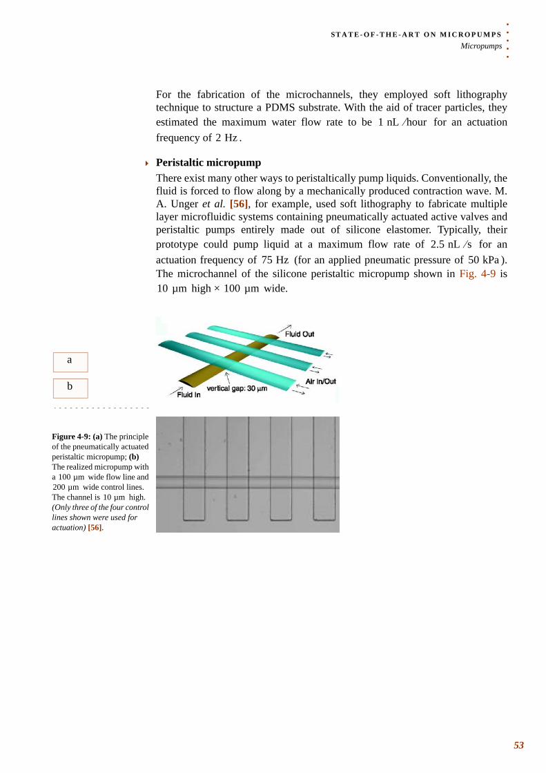
. . .
. .ST A T E - O F - T H E - A R T O N M I C R O P U M P SMicropumps
For the fabrication of the microchannels, they employed soft lithography technique to structure a PDMS substrate. With the aid of tracer particles, they estimated the maximum water flow rate to be for an actuation frequency of .
Peristaltic micropumpThere exist many other ways to peristaltically pump liquids. Conventionally, the fluid is forced to flow along by a mechanically produced contraction wave. M. A. Unger et al. [56], for example, used soft lithography to fabricate multiple layer microfluidic systems containing pneumatically actuated active valves and peristaltic pumps entirely made out of silicone elastomer. Typically, their prototype could pump liquid at a maximum flow rate of for an actuation frequency of (for an applied pneumatic pressure of ). The microchannel of the silicone peristaltic micropump shown in Fig. 4-9 is
high × wide.
1 nL hour⁄2 Hz
2.5 nL s⁄75 Hz 50 kPa
10 µm 100 µm
a
b
Figure 4-9: (a) The principle of the pneumatically actuated peristaltic micropump; (b) The realized micropump with a wide flow line and
wide control lines. The channel is high. (Only three of the four control lines shown were used for actuation) [56].
100 µm200 µm
10 µm
53
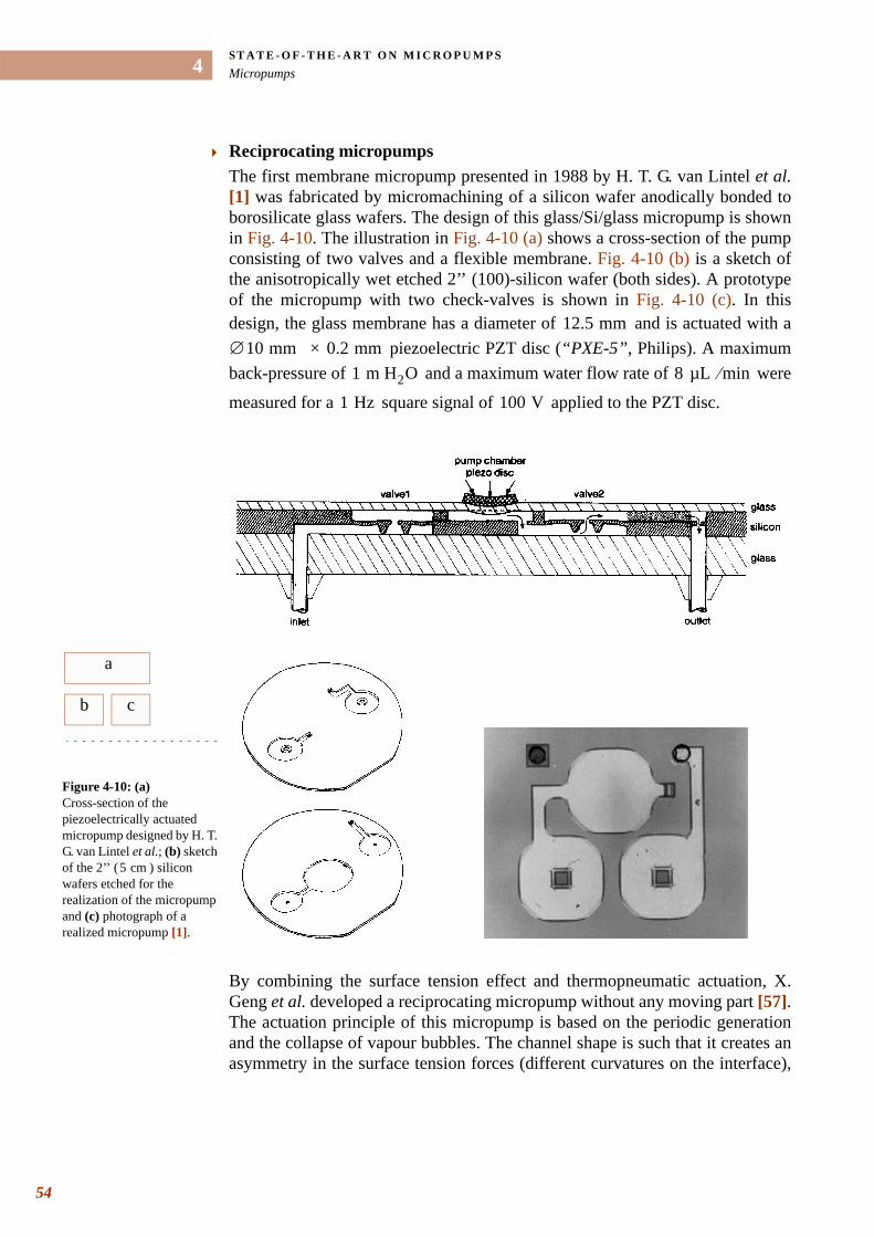
ST A T E - O F - T H E - A R T O N M I C R O P U M P SMicropumps
54
4
Reciprocating micropumpsThe first membrane micropump presented in 1988 by H. T. G. van Lintel et al.[1] was fabricated by micromachining of a silicon wafer anodically bonded to borosilicate glass wafers. The design of this glass/Si/glass micropump is shown in Fig. 4-10. The illustration in Fig. 4-10 (a) shows a cross-section of the pump consisting of two valves and a flexible membrane. Fig. 4-10 (b) is a sketch of the anisotropically wet etched 2’’ (100)-silicon wafer (both sides). A prototype of the micropump with two check-valves is shown in Fig. 4-10 (c). In this design, the glass membrane has a diameter of and is actuated with a
× piezoelectric PZT disc (“PXE-5”, Philips). A maximum back-pressure of and a maximum water flow rate of were
measured for a square signal of applied to the PZT disc.
By combining the surface tension effect and thermopneumatic actuation, X. Geng et al. developed a reciprocating micropump without any moving part [57]. The actuation principle of this micropump is based on the periodic generation and the collapse of vapour bubbles. The channel shape is such that it creates an asymmetry in the surface tension forces (different curvatures on the interface),
12.5 mm∅10 mm 0.2 mm
1 m H2O 8 µL min⁄
1 Hz 100 V
a
bb bc
Figure 4-10: (a) Cross-section of the piezoelectrically actuated micropump designed by H. T. G. van Lintel et al.; (b) sketch of the 2’’ ( ) silicon wafers etched for the realization of the micropump and (c) photograph of a realized micropump [1].
5 cm
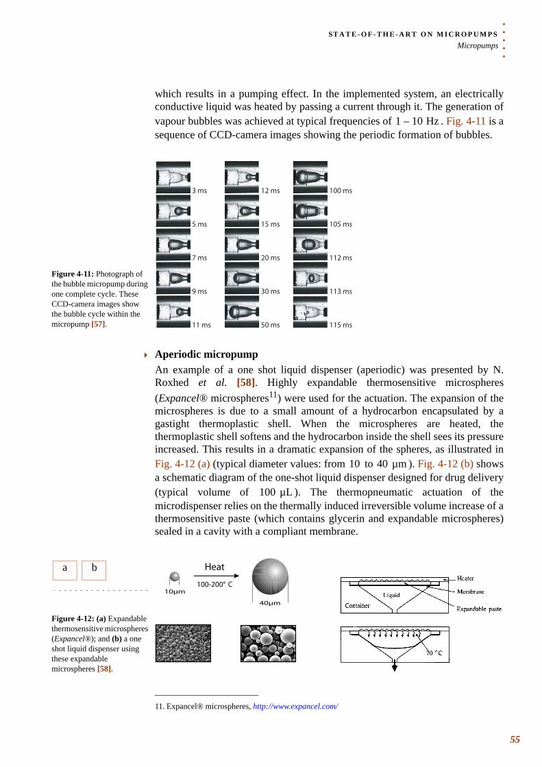
. . .
. .ST A T E - O F - T H E - A R T O N M I C R O P U M P SMicropumps
which results in a pumping effect. In the implemented system, an electrically conductive liquid was heated by passing a current through it. The generation of vapour bubbles was achieved at typical frequencies of . Fig. 4-11 is a sequence of CCD-camera images showing the periodic formation of bubbles.
Aperiodic micropumpAn example of a one shot liquid dispenser (aperiodic) was presented by N. Roxhed et al. [58]. Highly expandable thermosensitive microspheres (Expancel® microspheres11) were used for the actuation. The expansion of the microspheres is due to a small amount of a hydrocarbon encapsulated by a gastight thermoplastic shell. When the microspheres are heated, the thermoplastic shell softens and the hydrocarbon inside the shell sees its pressure increased. This results in a dramatic expansion of the spheres, as illustrated in Fig. 4-12 (a) (typical diameter values: from to ). Fig. 4-12 (b) shows a schematic diagram of the one-shot liquid dispenser designed for drug delivery (typical volume of ). The thermopneumatic actuation of the microdispenser relies on the thermally induced irreversible volume increase of a thermosensitive paste (which contains glycerin and expandable microspheres) sealed in a cavity with a compliant membrane.
1 10 Hz–
Figure 4-11: Photograph of the bubble micropump during one complete cycle. These CCD-camera images show the bubble cycle within the micropump [57].
3 ms
5 ms
7 ms
9 ms
11 ms
12 ms
15 ms
20 ms
30 ms
50 ms
100 ms
105 ms
112 ms
113 ms
115 ms
11. Expancel® microspheres, http://www.expancel.com/
10 40 µm
100 µL
a b
Figure 4-12: (a) Expandable thermosensitive microspheres (Expancel®); and (b) a one shot liquid dispenser using these expandable microspheres [58].
Heat
100-200° C
40µm
10µm
55
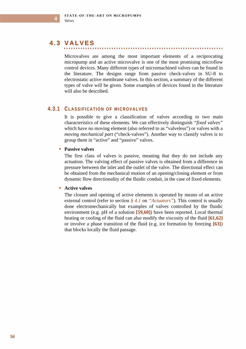
ST A T E - O F - T H E - A R T O N M I C R O P U M P SValves
56
4
. . . . . . . . . . . . . . . . . . . . . . . . . . . . . . . . . . . . . . . . . . . . . . . . . . . . . . . . . . . . . . . . . . . 4 . 3 V A L V E S
Microvalves are among the most important elements of a reciprocating micropump and an active microvalve is one of the most promising microflow control devices. Many different types of micromachined valves can be found in the literature. The designs range from passive check-valves in SU-8 to electrostatic active membrane valves. In this section, a summary of the different types of valve will be given. Some examples of devices found in the literature will also be described.
4.3.1 C L A S S I F I C A T I O N O F M I C R O V A L V E SIt is possible to give a classification of valves according to two main characteristics of these elements. We can effectively distinguish “fixed valves”which have no moving element (also referred to as “valveless”) or valves with a moving mechanical part (“check-valves”). Another way to classify valves is to group them in “active” and “passive” valves.
• Passive valvesThe first class of valves is passive, meaning that they do not include any actuation. The valving effect of passive valves is obtained from a difference in pressure between the inlet and the outlet of the valve. The directional effect can be obtained from the mechanical motion of an opening/closing element or from dynamic flow directionality of the fluidic conduit, in the case of fixed elements.
• Active valvesThe closure and opening of active elements is operated by means of an active external control (refer to section § 4.1 on “Actuators”). This control is usually done electromechanically but examples of valves controlled by the fluidic environment (e.g. pH of a solution [59,60]) have been reported. Local thermal heating or cooling of the fluid can also modify the viscosity of the fluid [61,62]or involve a phase transition of the fluid (e.g. ice formation by freezing [63]) that blocks locally the fluid passage.
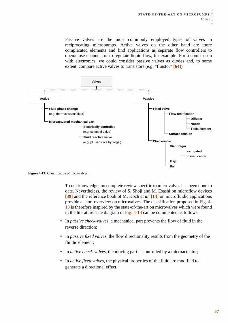
. . .
. .ST A T E - O F - T H E - A R T O N M I C R O P U M P SValves
Passive valves are the most commonly employed types of valves in reciprocating micropumps. Active valves on the other hand are more complicated elements and find applications as separate flow controllers to open/close channels or to regulate liquid flow, for example. For a comparison with electronics, we could consider passive valves as diodes and, to some extent, compare active valves to transistors (e.g. “fluistor” [64]).
To our knowledge, no complete review specific to microvalves has been done to date. Nevertheless, the review of S. Shoji and M. Esashi on microflow devices [39] and the reference book of M. Koch et al. [14] on microfluidic applications provide a short overview on microvalves. The classification proposed in Fig. 4-13 is therefore inspired by the state-of-the-art on microvalves which were found in the literature. The diagram of Fig. 4-13 can be commented as follows:
• In passive check-valves, a mechanical part prevents the flow of fluid in the reverse direction;
• In passive fixed valves, the flow directionality results from the geometry of the fluidic element;
• In active check-valves, the moving part is controlled by a microactuator;
• In active fixed valves, the physical properties of the fluid are modified to generate a directional effect.
Figure 4-13: Classification of microvalves.
Valves
Active Passive
Check-valve
Microactuated mechanical part
Diaphragm
Flap
Ball
corrugated
bossed center
Electrically controlled
Fluid reactive valve
Fluid phase change Fixed valve
Flow rectification
Diffuser
Nozzle
Surface tension
Tesla element
(e.g. thermoviscous fluid)
(e.g. pH sensitive hydrogel)
(e.g. solenoid valve)
57
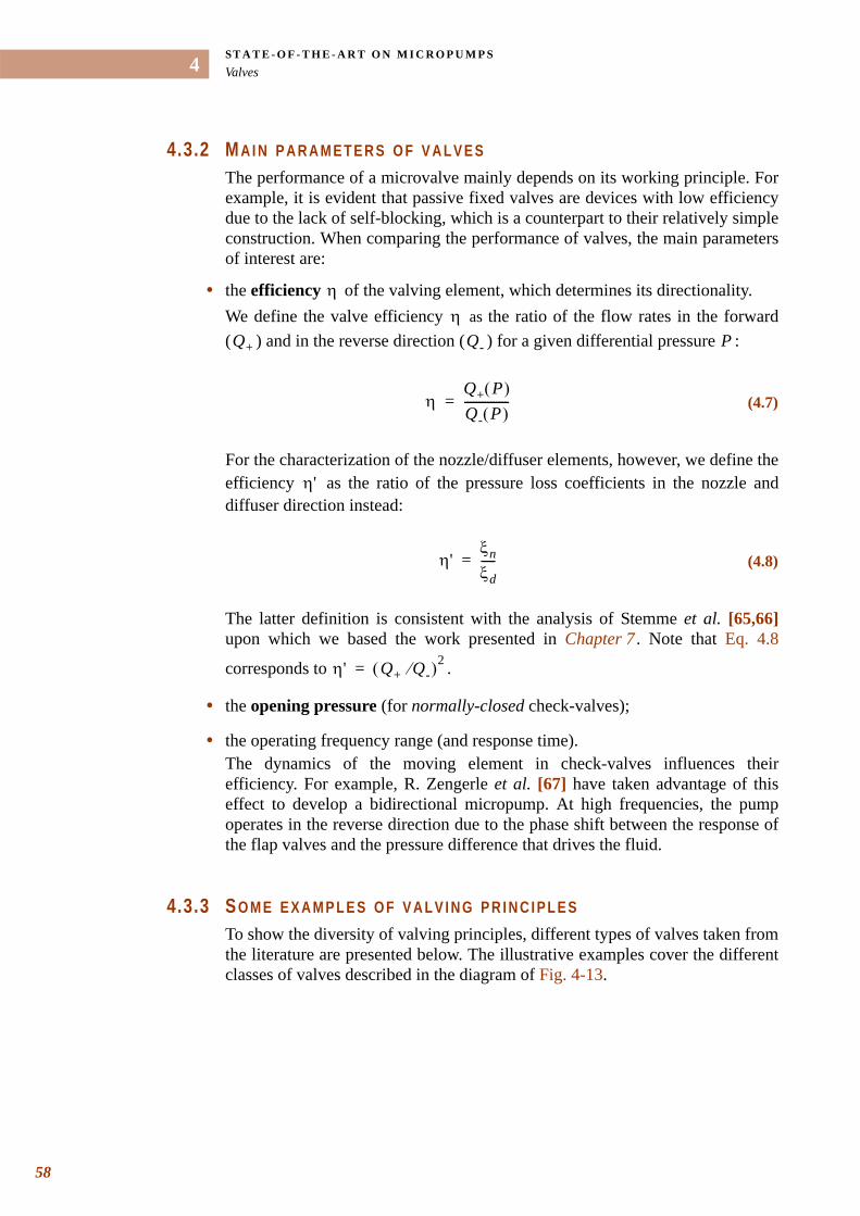
ST A T E - O F - T H E - A R T O N M I C R O P U M P SValves
58
4
4.3.2 M A I N P A R A M E T E R S O F V A L V E SThe performance of a microvalve mainly depends on its working principle. For example, it is evident that passive fixed valves are devices with low efficiency due to the lack of self-blocking, which is a counterpart to their relatively simple construction. When comparing the performance of valves, the main parameters of interest are:
• the efficiency of the valving element, which determines its directionality. We define the valve efficiency as the ratio of the flow rates in the forward ( ) and in the reverse direction ( ) for a given differential pressure :
For the characterization of the nozzle/diffuser elements, however, we define the efficiency as the ratio of the pressure loss coefficients in the nozzle and diffuser direction instead:
The latter definition is consistent with the analysis of Stemme et al. [65,66]upon which we based the work presented in Chapter 7 . Note that Eq. 4.8
corresponds to .
• the opening pressure (for normally-closed check-valves);
• the operating frequency range (and response time).The dynamics of the moving element in check-valves influences their efficiency. For example, R. Zengerle et al. [67] have taken advantage of this effect to develop a bidirectional micropump. At high frequencies, the pump operates in the reverse direction due to the phase shift between the response of the flap valves and the pressure difference that drives the fluid.
4.3.3 S O M E E X A M P L E S O F V A L V I N G P R I N C I P L E STo show the diversity of valving principles, different types of valves taken from the literature are presented below. The illustrative examples cover the different classes of valves described in the diagram of Fig. 4-13.
ηη
Q+ Q- P
(4.7)ηQ+ P( )Q- P( )---------------=
η'
(4.8)η'ξnξd-----=
η' Q+ Q-⁄( )2=
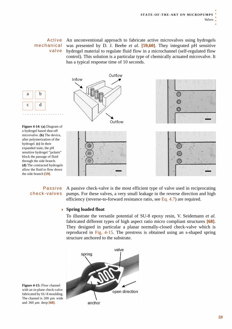
. . .
. .ST A T E - O F - T H E - A R T O N M I C R O P U M P SValves
Act ive mechan ica l
va lve
An unconventional approach to fabricate active microvalves using hydrogels was presented by D. J. Beebe et al. [59,60]. They integrated pH sensitive hydrogel material to regulate fluid flow in a microchannel (self-regulated flow control). This solution is a particular type of chemically actuated microvalve. It has a typical response time of 10 seconds.
Pass ive check-va lves
A passive check-valve is the most efficient type of valve used in reciprocating pumps. For these valves, a very small leakage in the reverse direction and high efficiency (reverse-to-forward resistance ratio, see Eq. 4.7) are required.
Spring loaded floatTo illustrate the versatile potential of SU-8 epoxy resin, V. Seidemann et al.fabricated different types of high aspect ratio micro compliant structures [68]. They designed in particular a planar normally-closed check-valve which is reproduced in Fig. 4-15. The prestress is obtained using an s-shaped spring structure anchored to the substrate.
a
bc
b
bd
Figure 4-14: (a) Diagram of a hydrogel based shut-off microvalve. (b) The device, after polymerization of the hydrogel. (c) In their expanded state, the pH sensitive hydrogel “jackets” block the passage of fluid through the side branch. (d) The contracted hydrogels allow the fluid to flow down the side branch [59].
Figure 4-15: Flow channel with an in-plane check-valve fabricated by SU-8 moulding. The channel is wide and deep [68].
200 µm360 µm
59
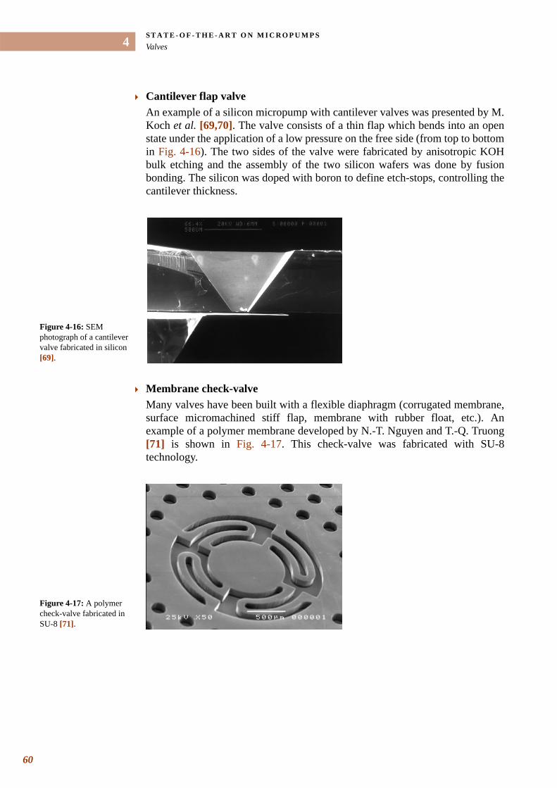
ST A T E - O F - T H E - A R T O N M I C R O P U M P SValves
60
4
Cantilever flap valveAn example of a silicon micropump with cantilever valves was presented by M. Koch et al. [69,70]. The valve consists of a thin flap which bends into an open state under the application of a low pressure on the free side (from top to bottom in Fig. 4-16). The two sides of the valve were fabricated by anisotropic KOH bulk etching and the assembly of the two silicon wafers was done by fusion bonding. The silicon was doped with boron to define etch-stops, controlling the cantilever thickness.
Membrane check-valveMany valves have been built with a flexible diaphragm (corrugated membrane, surface micromachined stiff flap, membrane with rubber float, etc.). An example of a polymer membrane developed by N.-T. Nguyen and T.-Q. Truong [71] is shown in Fig. 4-17. This check-valve was fabricated with SU-8 technology.
Figure 4-16: SEM photograph of a cantilever valve fabricated in silicon [69].
Figure 4-17: A polymer check-valve fabricated in SU-8 [71].
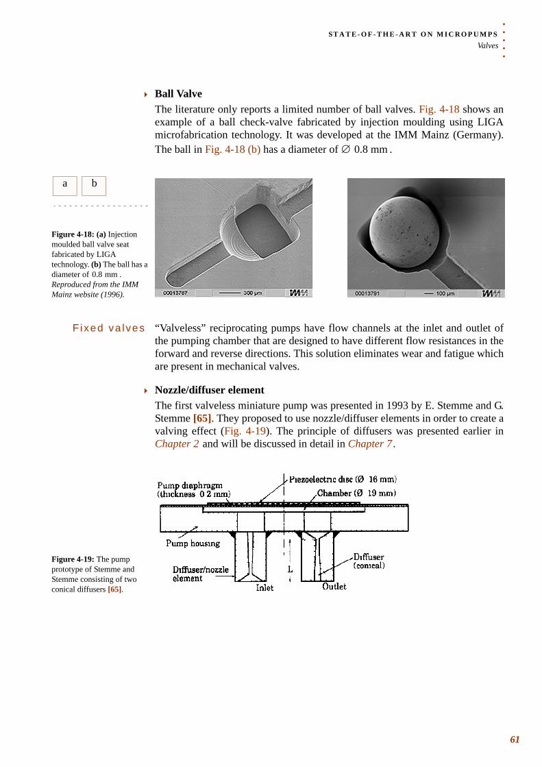
. . .
. .ST A T E - O F - T H E - A R T O N M I C R O P U M P SValves
Ball ValveThe literature only reports a limited number of ball valves. Fig. 4-18 shows an example of a ball check-valve fabricated by injection moulding using LIGA microfabrication technology. It was developed at the IMM Mainz (Germany). The ball in Fig. 4-18 (b) has a diameter of .
Fixed va lves “Valveless” reciprocating pumps have flow channels at the inlet and outlet of the pumping chamber that are designed to have different flow resistances in the forward and reverse directions. This solution eliminates wear and fatigue which are present in mechanical valves.
Nozzle/diffuser elementThe first valveless miniature pump was presented in 1993 by E. Stemme and G. Stemme [65]. They proposed to use nozzle/diffuser elements in order to create a valving effect (Fig. 4-19). The principle of diffusers was presented earlier in Chapter 2 and will be discussed in detail in Chapter 7 .
∅ 0.8 mm
a b
Figure 4-18: (a) Injection moulded ball valve seat fabricated by LIGA technology. (b) The ball has a diameter of . Reproduced from the IMM Mainz website (1996).
0.8 mm
Figure 4-19: The pump prototype of Stemme and Stemme consisting of two conical diffusers [65].
61
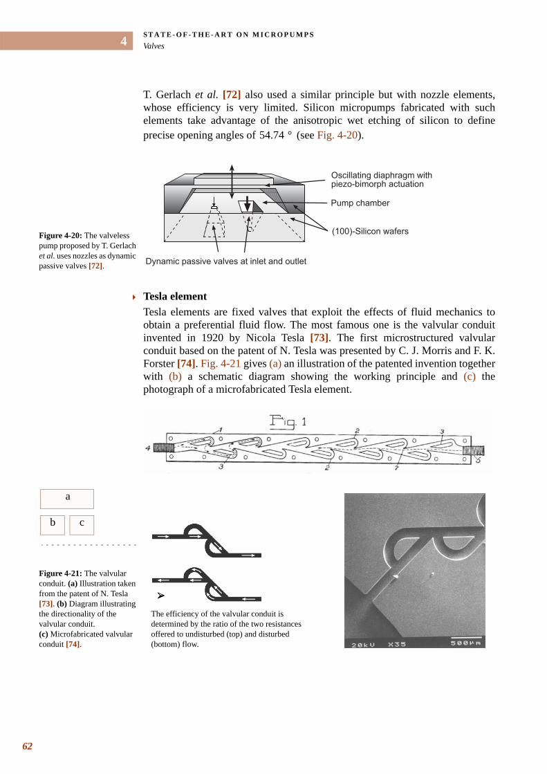
ST A T E - O F - T H E - A R T O N M I C R O P U M P SValves
62
4
T. Gerlach et al. [72] also used a similar principle but with nozzle elements, whose efficiency is very limited. Silicon micropumps fabricated with such elements take advantage of the anisotropic wet etching of silicon to define precise opening angles of (see Fig. 4-20).
Tesla elementTesla elements are fixed valves that exploit the effects of fluid mechanics to obtain a preferential fluid flow. The most famous one is the valvular conduit invented in 1920 by Nicola Tesla [73]. The first microstructured valvular conduit based on the patent of N. Tesla was presented by C. J. Morris and F. K. Forster [74]. Fig. 4-21 gives (a) an illustration of the patented invention together with (b) a schematic diagram showing the working principle and (c) the photograph of a microfabricated Tesla element.
54.74 °
Figure 4-20: The valveless pump proposed by T. Gerlach et al. uses nozzles as dynamic passive valves [72].
Oscillating diaphragm withpiezo-bimorph actuation
Pump chamber
(100)-Silicon wafers
Dynamic passive valves at inlet and outlet
a
bb bc
Figure 4-21: The valvular conduit. (a) Illustration taken from the patent of N. Tesla [73]. (b) Diagram illustrating the directionality of the valvular conduit. (c) Microfabricated valvular conduit [74].
The efficiency of the valvular conduit is determined by the ratio of the two resistances offered to undisturbed (top) and disturbed (bottom) flow.
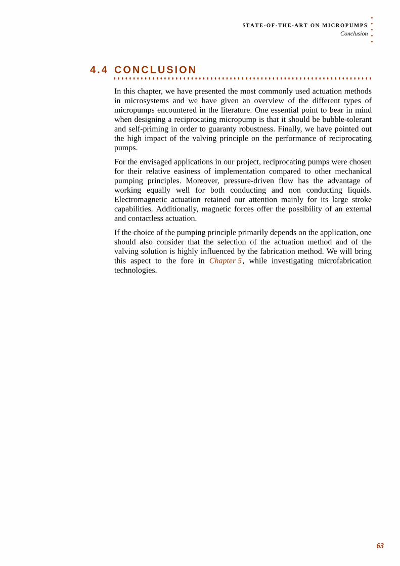
. . .
. .ST A T E - O F - T H E - A R T O N M I C R O P U M P SConclusion
. . . . . . . . . . . . . . . . . . . . . . . . . . . . . . . . . . . . . . . . . . . . . . . . . . . . . . . . . . . . . . . . . . . 4 . 4 C O N C L U S I O N
In this chapter, we have presented the most commonly used actuation methods in microsystems and we have given an overview of the different types of micropumps encountered in the literature. One essential point to bear in mind when designing a reciprocating micropump is that it should be bubble-tolerant and self-priming in order to guaranty robustness. Finally, we have pointed out the high impact of the valving principle on the performance of reciprocating pumps.
For the envisaged applications in our project, reciprocating pumps were chosen for their relative easiness of implementation compared to other mechanical pumping principles. Moreover, pressure-driven flow has the advantage of working equally well for both conducting and non conducting liquids. Electromagnetic actuation retained our attention mainly for its large stroke capabilities. Additionally, magnetic forces offer the possibility of an external and contactless actuation.
If the choice of the pumping principle primarily depends on the application, one should also consider that the selection of the actuation method and of the valving solution is highly influenced by the fabrication method. We will bring this aspect to the fore in Chapter 5 , while investigating microfabrication technologies.
63

CHAPTER
5. . . . .
. . . . . . . . . . . . . . . . . . . . . . . . . . . . . . . . . . .MICROFABRICATION TECHNOLOGY
evelopments in MicroElectroMechanical Systems (MEMS) technology have enabled a strong miniaturization of biochemical analysis systems and have led to the lab-on-a-chip concept. While an
important part of MEMS is based on silicon and fabrication techniques similar to those used in microelectronics, the need for low-cost and disposable materials explains why plastic MEMS devices are particularly attractive. Beside, for the further industrial development of microfluidic systems, it is necessary to produce them in an economic way and possibly out of the clean-room. In this chapter, we will present a simple fabrication technology that we have developed for the realization of our microfluidic chips. The fabrication method is based on powder blasting erosion process and enabled the fabrication of PMMA (polymethylmethacrylate) plastic and glass chips. We believe this fabrication method is particularly convenient for the rapid prototyping of microfluidic devices.
5 . 1 R E V I E W O F M I C R O F A B R I C A T I O N
. . . . . . . . . . . . . . . . . . . . . . . . . . . . . . . . . . . . . . . . . . . . . . . . . . . . . . . . . . . . . . . . . . .T E C H N I Q U E S U S E D I N M I C R O S Y S T E M S
Numerous processes are used in micromachining. Many processing techniques have originated from microelectronics, and most of the early microelectromechanical systems have been fabricated using silicon-based techniques. However, also a lot of other materials and microfabrication technologies have been investigated and developed. In this section, we will present some of the microfabrication techniques used in microfluidics. For an extended overview on microfabrication techniques, we invite the reader to read the reference book of M. J. Madou [75] and the book of M. Koch et al.dedicated to microfluidic technology [70].
5.1.1 S I L I C O N M I C R O M A C H I N I N GHistorically, silicon has been the most commonly used material in microsystems. A lot of devices are still fabricated in silicon because of its well-known electrical and mechanical properties. This material is also attractive
D
65
M I C R O F A B R I C A T I O N TE C H N O L O G YReview of microfabrication techniques used in microsystems
66
5
because of the possible integration of MEMS devices on substrates including electronics. Silicon micromachining can be divided into:
• Bulk micromachining
• Surface micromachining
In bulk micromachining the whole thickness of the silicon wafer is structured, while in surface micromachining all the fabrication is done on the surface. This micromachining technique generally consists of the following sequences:
L i thography First, a mask defining the pattern to be etched is defined on the surface of the silicon wafer using a photolithographic process. Silicon dioxide and silicon nitride are often used as mask materials, but it is also common to use directly photoresist or a deposited metal. The basic steps for lithography involve either positive or negative resists. Photolithography is the most common technology; and for high resolution, X-ray, electron beam and ion beam lithography have been developed.
Etch ing Next, silicon etching is done using either wet or dry etching. A variety of physical and chemical etching methods are possible. In addition, the crystalline nature of silicon substrate can be advantageously utilized in certain wet etches. For example, anisotropic KOH wet etching of a silicon wafer12 was used by T. Gerlach et al. to produce nozzles with precisely defined angles (see Fig. 4-20): in silicon crystal, the angle between and planes is .
Bond ing Bonding is used in order to join wafers processed using both bulk and surface micromachining to obtain multi-level complex devices. The most common forms of bonding are fusion bonding (Si/Si) and anodic bonding (Si/Glass).
• Si fusion bondingHere, two silicon wafers with hydrophilic surfaces are pressed together at room temperature after cleansing. This pre-bonding step is followed by an annealing treatment above to achieve a permanent chemical bond.
• Anodic bondingThe bonding of a pyrex (sodium silicate glass) wafer to a Si wafer is achieved by applying a voltage difference of around between the two wafers and heating to about .
12. In solid state physics, directions and surface within a surface can be expressed by Miller indices. The planes (100),(110) and (111) are most used in silicon. 1 indicates an intersection of the plane with x, y, z axis at the unit length and 0 indicates that the plane and the axis are parallel.
100( )
100( ) 111( ) 54.74 °
800 °C
50 V350 500 °C–
. . .
. .M I C R O F A B R I C A T I O N TE C H N O L O G YReview of microfabrication techniques used in microsystems
5.1.2 O T H E R P R O C E S S E SIn addition to silicon, alternative materials such as glass (for example fused silica), ceramics, plastics, silicone rubber (i.e. PDMS) are becoming popular, especially thanks to the growth of the importance of microfluidics. Main factors that have motivated these developments are: biocompatibility aspects, the use of cheaper materials and/or micromachining processes (avoiding for example the clean-room infrastructure).
Thermop las t ic rep l i ca t ion
Plastic is the material of choice for the production of high volumes at low cost. The standard processes which are used in the industry are hot embossing and injection moulding. These production methods have also triggered interest for microreplication. The production of the replication master in that case requires the use of high precision micromachining techniques.
LIGA LIGA was initially developed in Germany in the 1980s and has since become a standard microfabrication process. LIGA is the acronym for “X-ray Lithographie Galvanoformung Abformung,” which means X-ray lithography, electrodeposition and moulding. A thick X-ray sensitive resist is exposed and used as a mould for electroplating. The formed metal mould can then be used for injection moulding of plastic parts or to produce plastic moulds. This technique produces high aspect ratio structures.
SU-8 SU-8 is a negative, epoxy-type, near-UV photoresist based on EPON SU-8epoxy resin which was originally developed at IBM. The very high aspect ratio (>20) which has been demonstrated with standard contact lithography equipment renders this material very attractive for MEMS applications. While LIGA yields better results, low-cost applications can benefit from this resist which is well suited for acting as a mould, for example.
Microstereolithography A number of non-conventional micromachining techniques have been developed over the years to overcome the limitation of standard processes. Microstereolithography is an example of a technology which has been intensively studied at the Laboratory for Microsystems (EPFL) by A. Bertsch et al. (cf. illustration in Fig. 4-5 and reference [50]). This fabrication method has developed from the rapid prototyping industry, and is based on a layer-by-layer light-induced polymerization of a liquid resin.
Powder b las t ing While the processes just presented are based on photosensitive and chemical etching processes, powder blasting microstructuring results from the mechanical erosion of a mask-protected substrate by a high-velocity powder
67
M I C R O F A B R I C A T I O N TE C H N O L O G YPowder blasting erosion process
68
5
beam. Powder blasting is a very common industrial method which is used in a wide range of applications such as:
• Cleaning of dental crowns and bridges
• Finishing and texturing injection mould cavities
• Semiconductor wafer drilling and cutting
In the latter case, powder blasting can be used to cut slots, holes and apertures in thin, fragile substrates. The use of this erosion process for microstructuring has initially been studied by P. J. Slikkerveer [76] who developed a model for the erosion process of holes in glass substrates. Its use for MEMS applications was further investigated in our laboratory [77,78]. In particular, powder blasting has been shown to be a promising tool for microfluidics [11,79]. In next paragraph, we describe an application of this technique for the microfabrication of microfluidic chips in plastic and in glass materials.
. . . . . . . . . . . . . . . . . . . . . . . . . . . . . . . . . . . . . . . . . . . . . . . . . . . . . . . . . . . . . . . . . . .5 . 2 P O W D E R B L A S T I N G E R O S I O N P R O C E S S
A typical powder blasting machine is schematically described in Fig. 5-1. The set-up consists of the powder blaster which regulates the flow of abrasive powder accelerated to the nozzle. An air dryer is connected to the powder reservoir to avoid moisture issues. To obtain an homogeneous scan of its surface, the sample is placed on a - translation stage. A dust collector recovers the used alumina powder.
x y
Figure 5-1: A typical powder blasting system.
. . .
. .M I C R O F A B R I C A T I O N TE C H N O L O G YPowder blasting erosion process
5.2.1 E Q U I P M E N TThe powder blasting machine which was used in our experiments is an Airsonics HP-213. The applied pressure can be regulated between 1 and 5 bars. A schematic diagram showing the principle of powder blasting micro-erosion process is given in Fig. 5-2. The different elements are described below.
Nozz le The nozzle provides the focusing and acceleration of the abrasive stream generated by the blaster. The round nozzle we used was in tungsten for its increased resistance to wear.
Mask The protective mask must have an erosion rate much smaller than that of the substrate. We used metallic masks fabricated by laser cutting. Other solutions including PDMS (which is a soft, ductile material) protective layers were also tested at the laboratory. For large productions, we would suggest the use of a micro patterned Ordyl mask, as described by P. J. Slikkerveer [76].
Subst ra te PMMA and glass materials were the two types of substrates used for our microfabrication. Powder blasting has also been shown to be an appropriate micromachining technique for other hard, brittle materials and was for example recently used for the fabrication of miniaturized ferrite E-cores [80].
Powder The erosion process is due to the impact of accelerated particles on brittle materials which create cracks. Depending on the application aimed for, different types of abrasive powders with various shapes and hardness can be used. Most common powders are:
• Silicon carbide Silicon carbide (SiC), due to its hardness and high density (see Table 5-1), is the most efficient media used for micro-abrasive blasting. It has a hardness of over 9 on Mohs’ scale, just below diamond14.
• Crushed glass It is a mild abrasive media (Mohs’ hardness = ) which is employed when only a slight degree of abrasion is desired.
• Glass beads The spherical shape of a glass bead keeps it from cutting into the surface of the part. It is typically used to perform light deburring or to apply a satin-like finish on a work piece.
13. Texas Airsonics Inc., Corpus Christi, Texas, USA14. Mohs’ hardness is defined by how well a substance will resist scratching by another substance. The
scale consists of 10 minerals ranging from 1 for the softest (talc) to 10 for the hardest (diamond). See also the Appendix.
5 6–
69
M I C R O F A B R I C A T I O N TE C H N O L O G YPowder blasting erosion process
70
5
• Aluminium oxide Aluminium oxide is the most commonly used cutting abrasive because of the sharp shape of the particles and good hardness (Mohs’ hardness = 9).
In our experiments, aluminium oxide ( or alumina) powders were used as abrasive powders. The sharp alumina particles employed have a mean size of
. They are ejected from the nozzle at high velocities (particle velocity
), as measured by E. Belloy et al. in [78].
5.2.2 M E C H A N I C A L E T C H I N G B Y P O W D E R B L A S T I N GThe rate of material removal is one of the important parameters to characterize etching techniques. It is commonly evaluated from the erosion rate , which is defined as:
The mechanical etching process of powder blasting was studied in details by P. J. Slikkerveer [76]. In his analysis, he introduced the erosion efficiency :
Al2O3
30 µm
vparticle 100 300 m s 1–⋅÷=
Figure 5-2: Schematic diagram showing the principle of powder blasting etching.
Erate
(5.1)Erateweight of removed material
weight of impacting particles----------------------------------------------------------------------=
Eeff
(5.2)Eeffweight of removed material
Ek------------------------------------------------------------------=
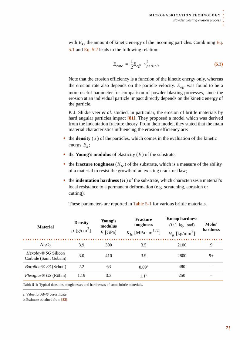
. . .
. .M I C R O F A B R I C A T I O N TE C H N O L O G YPowder blasting erosion process
with , the amount of kinetic energy of the incoming particles. Combining Eq. 5.1 and Eq. 5.2 leads to the following relation:
Note that the erosion efficiency is a function of the kinetic energy only, whereas the erosion rate also depends on the particle velocity. was found to be a more useful parameter for comparison of powder blasting processes, since the erosion at an individual particle impact directly depends on the kinetic energy of the particle.
P. J. Slikkerveer et al. studied, in particular, the erosion of brittle materials by hard angular particles impact [81]. They proposed a model which was derived from the indentation fracture theory. From their model, they stated that the main material characteristics influencing the erosion efficiency are:
• the density ( ) of the particles, which comes in the evaluation of the kinetic energy ;
• the Young’s modulus of elasticity ( ) of the substrate;
• the fracture toughness ( ) of the substrate, which is a measure of the ability of a material to resist the growth of an existing crack or flaw;
• the indentation hardness ( ) of the substrate, which characterizes a material’s local resistance to a permanent deformation (e.g. scratching, abrasion or cutting).
These parameters are reported in Table 5-1 for various brittle materials.
Ek
(5.3)Erate12---Eeff vparticle
2⋅=
Eeff
ρEk
E
KIc
H
MaterialDensity
Young’s modulus
Fracturetoughness
Knoop hardness ( load) Mohs’
hardness
. . . . . . . . . . . . . . . . . . . . . . . . . . . . . . . . . . . . . . . . . . . . . . . . . . . . . . . . . . . . . . . . . . . . . . . . . . . . . . . . . . . . . . Al2O3 3.9 390 3.5 2100 9
Hexoloy® SG Silicon Carbide (Saint Gobain) 3.0 410 3.9 2800 9+
Borofloat® 33 (Schott) 2.2 63 0.89a 480 –
Plexiglas® GS (Röhm) 1.19 3.3 1.1b 250 –
Table 5-1: Typical densities, toughnesses and hardnesses of some brittle materials.
a. Value for AF45 borosilicateb. Estimate obtained from [82]
ρ [g/cm3] E [GPa] KIc [MPa m1 2⁄ ]⋅
0.1 kg
HK [kg/mm2]
71
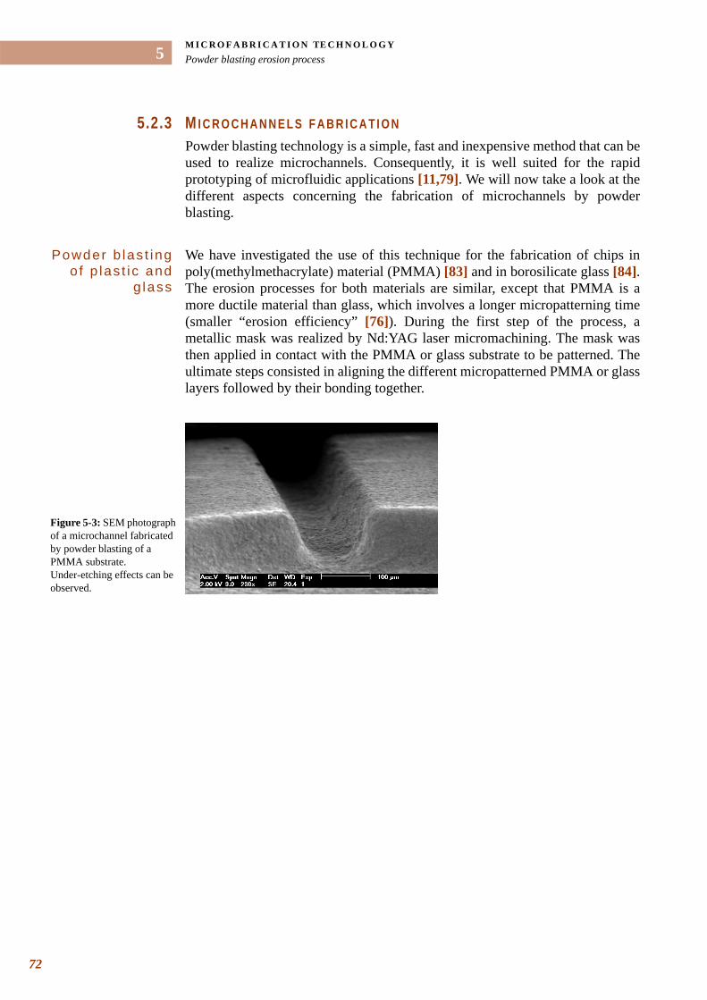
M I C R O F A B R I C A T I O N TE C H N O L O G YPowder blasting erosion process
72
5
5.2.3 M I C R O C H A N N E L S F A B R I C A T I O NPowder blasting technology is a simple, fast and inexpensive method that can be used to realize microchannels. Consequently, it is well suited for the rapid prototyping of microfluidic applications [11,79]. We will now take a look at the different aspects concerning the fabrication of microchannels by powder blasting.
Powder b las t ing o f p las t i c and
g lass
We have investigated the use of this technique for the fabrication of chips in poly(methylmethacrylate) material (PMMA) [83] and in borosilicate glass [84]. The erosion processes for both materials are similar, except that PMMA is a more ductile material than glass, which involves a longer micropatterning time (smaller “erosion efficiency” [76]). During the first step of the process, a metallic mask was realized by Nd:YAG laser micromachining. The mask was then applied in contact with the PMMA or glass substrate to be patterned. The ultimate steps consisted in aligning the different micropatterned PMMA or glass layers followed by their bonding together.
Figure 5-3: SEM photograph of a microchannel fabricated by powder blasting of a PMMA substrate. Under-etching effects can be observed.
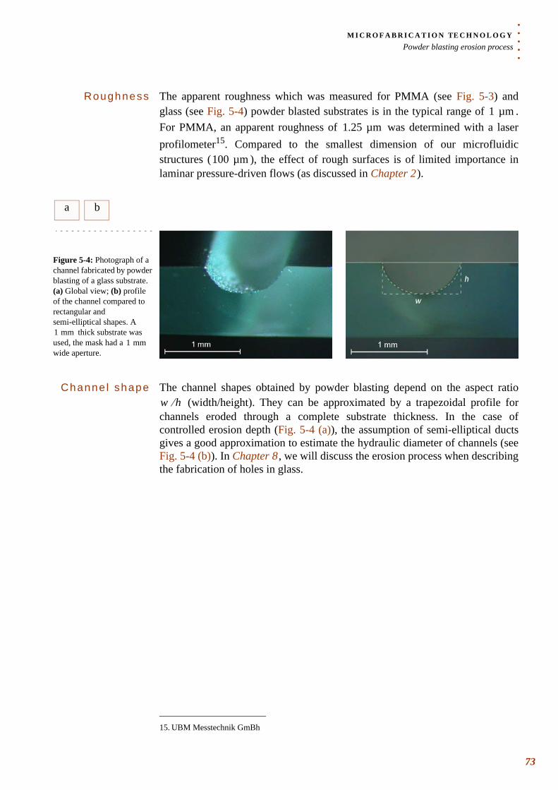
. . .
. .M I C R O F A B R I C A T I O N TE C H N O L O G YPowder blasting erosion process
Roughness The apparent roughness which was measured for PMMA (see Fig. 5-3) and glass (see Fig. 5-4) powder blasted substrates is in the typical range of . For PMMA, an apparent roughness of was determined with a laser profilometer15. Compared to the smallest dimension of our microfluidic structures ( ), the effect of rough surfaces is of limited importance in laminar pressure-driven flows (as discussed in Chapter 2 ).
Channe l shape The channel shapes obtained by powder blasting depend on the aspect ratio (width/height). They can be approximated by a trapezoidal profile for
channels eroded through a complete substrate thickness. In the case of controlled erosion depth (Fig. 5-4 (a)), the assumption of semi-elliptical ducts gives a good approximation to estimate the hydraulic diameter of channels (see Fig. 5-4 (b)). In Chapter 8 , we will discuss the erosion process when describing the fabrication of holes in glass.
15. UBM Messtechnik GmBh
1 µm1.25 µm
100 µm
a b
Figure 5-4: Photograph of a channel fabricated by powder blasting of a glass substrate. (a) Global view; (b) profile of the channel compared to rectangular and semi-elliptical shapes. A
thick substrate was used, the mask had a wide aperture.
1 mm1 mm
w h⁄
73
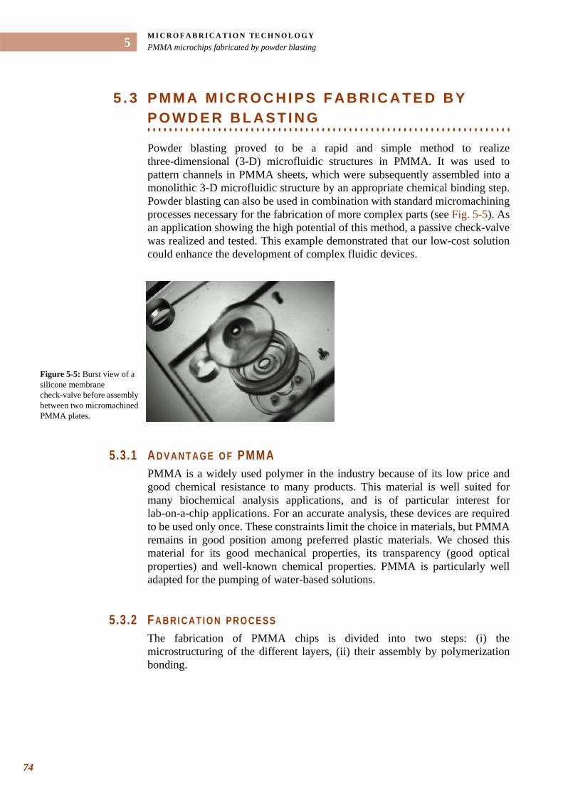
M I C R O F A B R I C A T I O N TE C H N O L O G YPMMA microchips fabricated by powder blasting
74
5
5 . 3 P M M A M I C R O C H I P S F A B R I C A T E D B Y
. . . . . . . . . . . . . . . . . . . . . . . . . . . . . . . . . . . . . . . . . . . . . . . . . . . . . . . . . . . . . . . . . . .P O W D E R B L A S T I N G
Powder blasting proved to be a rapid and simple method to realize three-dimensional (3-D) microfluidic structures in PMMA. It was used to pattern channels in PMMA sheets, which were subsequently assembled into a monolithic 3-D microfluidic structure by an appropriate chemical binding step. Powder blasting can also be used in combination with standard micromachining processes necessary for the fabrication of more complex parts (see Fig. 5-5). As an application showing the high potential of this method, a passive check-valve was realized and tested. This example demonstrated that our low-cost solution could enhance the development of complex fluidic devices.
5.3.1 A D V A N T A G E O F PMMA PMMA is a widely used polymer in the industry because of its low price and good chemical resistance to many products. This material is well suited for many biochemical analysis applications, and is of particular interest for lab-on-a-chip applications. For an accurate analysis, these devices are required to be used only once. These constraints limit the choice in materials, but PMMA remains in good position among preferred plastic materials. We chosed this material for its good mechanical properties, its transparency (good optical properties) and well-known chemical properties. PMMA is particularly well adapted for the pumping of water-based solutions.
5.3.2 FA B R I C A T I O N P R O C E S SThe fabrication of PMMA chips is divided into two steps: (i) the microstructuring of the different layers, (ii) their assembly by polymerization bonding.
Figure 5-5: Burst view of a silicone membrane check-valve before assembly between two micromachined PMMA plates.
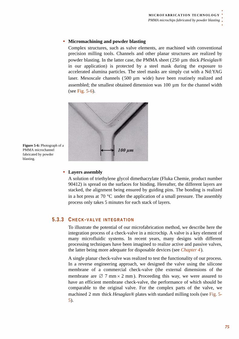
. . .
. .M I C R O F A B R I C A T I O N TE C H N O L O G YPMMA microchips fabricated by powder blasting
• Micromachining and powder blasting Complex structures, such as valve elements, are machined with conventional precision milling tools. Channels and other planar structures are realized by powder blasting. In the latter case, the PMMA sheet ( thick Plexiglas®in our application) is protected by a steel mask during the exposure to accelerated alumina particles. The steel masks are simply cut with a Nd:YAG laser. Mesoscale channels ( wide) have been routinely realized and assembled; the smallest obtained dimension was for the channel width (see Fig. 5-6).
• Layers assembly A solution of triethylene glycol dimethacrylate (Fluka Chemie, product number 90412) is spread on the surfaces for binding. Hereafter, the different layers are stacked, the alignment being ensured by guiding pins. The bonding is realized in a hot press at under the application of a small pressure. The assembly process only takes 5 minutes for each stack of layers.
5.3.3 C H E C K- V A L V E I N T E G R A T I O NTo illustrate the potential of our microfabrication method, we describe here the integration process of a check-valve in a microchip. A valve is a key element of many microfluidic systems. In recent years, many designs with different processing techniques have been imagined to realize active and passive valves, the latter being more adequate for disposable devices (see Chapter 4 ).
A single planar check-valve was realized to test the functionality of our process. In a reverse engineering approach, we designed the valve using the silicone membrane of a commercial check-valve (the external dimensions of the membrane are ). Proceeding this way, we were assured to have an efficient membrane check-valve, the performance of which should be comparable to the original valve. For the complex parts of the valve, we machined thick Hesaglas® plates with standard milling tools (see Fig. 5-5).
250 µm
500 µm100 µm
Figure 5-6: Photograph of a PMMA microchannel fabricated by powder blasting.
70 °C
∅ 7 mm 2 mm×
2 mm
75
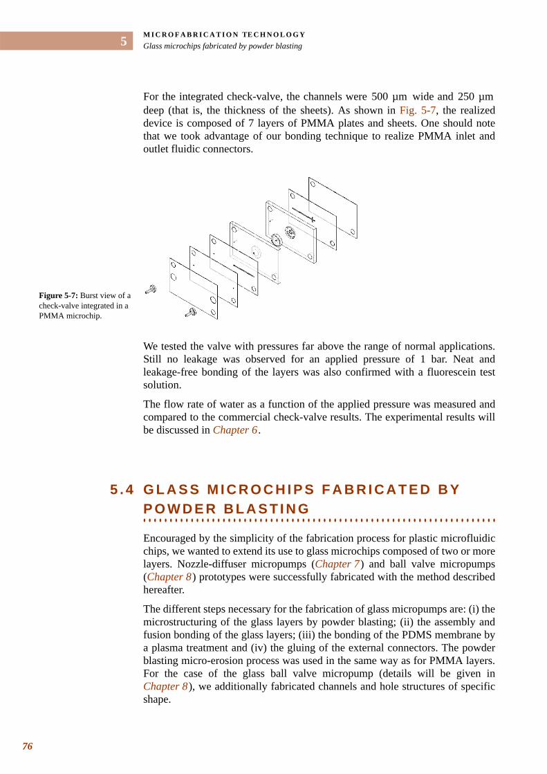
M I C R O F A B R I C A T I O N TE C H N O L O G YGlass microchips fabricated by powder blasting
76
5
For the integrated check-valve, the channels were wide and deep (that is, the thickness of the sheets). As shown in Fig. 5-7, the realized device is composed of 7 layers of PMMA plates and sheets. One should note that we took advantage of our bonding technique to realize PMMA inlet and outlet fluidic connectors.
We tested the valve with pressures far above the range of normal applications. Still no leakage was observed for an applied pressure of 1 bar. Neat and leakage-free bonding of the layers was also confirmed with a fluorescein test solution.
The flow rate of water as a function of the applied pressure was measured and compared to the commercial check-valve results. The experimental results will be discussed in Chapter 6 .
5 . 4 G L A S S M I C R O C H I P S F A B R I C A T E D B Y
. . . . . . . . . . . . . . . . . . . . . . . . . . . . . . . . . . . . . . . . . . . . . . . . . . . . . . . . . . . . . . . . . . .P O W D E R B L A S T I N G
Encouraged by the simplicity of the fabrication process for plastic microfluidic chips, we wanted to extend its use to glass microchips composed of two or more layers. Nozzle-diffuser micropumps (Chapter 7 ) and ball valve micropumps (Chapter 8 ) prototypes were successfully fabricated with the method described hereafter.
The different steps necessary for the fabrication of glass micropumps are: (i) the microstructuring of the glass layers by powder blasting; (ii) the assembly and fusion bonding of the glass layers; (iii) the bonding of the PDMS membrane by a plasma treatment and (iv) the gluing of the external connectors. The powder blasting micro-erosion process was used in the same way as for PMMA layers. For the case of the glass ball valve micropump (details will be given in Chapter 8 ), we additionally fabricated channels and hole structures of specific shape.
500 µm 250 µm
Figure 5-7: Burst view of a check-valve integrated in a PMMA microchip.
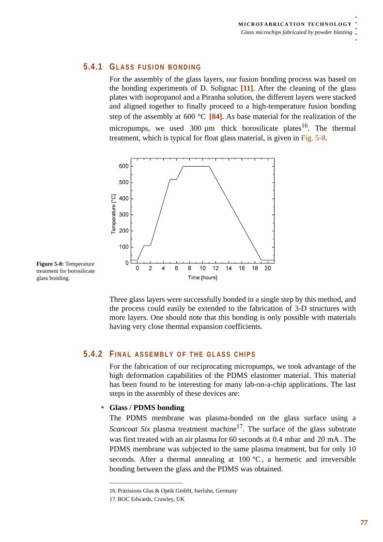
. . .
. .M I C R O F A B R I C A T I O N TE C H N O L O G YGlass microchips fabricated by powder blasting
5.4.1 G L A S S F U S I O N B O N D I N GFor the assembly of the glass layers, our fusion bonding process was based on the bonding experiments of D. Solignac [11]. After the cleaning of the glass plates with isopropanol and a Piranha solution, the different layers were stacked and aligned together to finally proceed to a high-temperature fusion bonding step of the assembly at [84]. As base material for the realization of the micropumps, we used thick borosilicate plates16. The thermal treatment, which is typical for float glass material, is given in Fig. 5-8.
Three glass layers were successfully bonded in a single step by this method, and the process could easily be extended to the fabrication of 3-D structures with more layers. One should note that this bonding is only possible with materials having very close thermal expansion coefficients.
5.4.2 F I N A L A S S E M B L Y O F T H E G L A S S C H I P SFor the fabrication of our reciprocating micropumps, we took advantage of the high deformation capabilities of the PDMS elastomer material. This material has been found to be interesting for many lab-on-a-chip applications. The last steps in the assembly of these devices are:
• Glass / PDMS bondingThe PDMS membrane was plasma-bonded on the glass surface using a Scancoat Six plasma treatment machine17. The surface of the glass substrate was first treated with an air plasma for 60 seconds at and . The PDMS membrane was subjected to the same plasma treatment, but for only 10 seconds. After a thermal annealing at , a hermetic and irreversible bonding between the glass and the PDMS was obtained.
16. Präzisions Glas & Optik GmbH, Iserlahn, Germany
600 °C300 µm
Figure 5-8: Temperature treatment for borosilicate glass bonding.
17. BOC Edwards, Crawley, UK
0.4 mbar 20 mA
100 °C
77
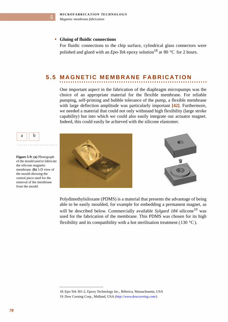
M I C R O F A B R I C A T I O N TE C H N O L O G YMagnetic membrane fabrication
78
5
• Gluing of fluidic connectionsFor fluidic connections to the chip surface, cylindrical glass connectors were polished and glued with an Epo-Tek epoxy solution18 at for 2 hours.
. . . . . . . . . . . . . . . . . . . . . . . . . . . . . . . . . . . . . . . . . . . . . . . . . . . . . . . . . . . . . . . . . . .5 . 5 M A G N E T I C M E M B R A N E F A B R I C A T I O N
One important aspect in the fabrication of the diaphragm micropumps was the choice of an appropriate material for the flexible membrane. For reliable pumping, self-priming and bubble tolerance of the pump, a flexible membrane with large deflection amplitude was particularly important [42]. Furthermore, we needed a material that could not only withstand high flexibility (large stroke capability) but into which we could also easily integrate our actuator magnet. Indeed, this could easily be achieved with the silicone elastomer.
Polydimethylsiloxane (PDMS) is a material that presents the advantage of being able to be easily moulded, for example for embedding a permanent magnet, as will be described below. Commercially available Sylgard 184 silicone19 was used for the fabrication of the membrane. This PDMS was chosen for its high flexibility and its compatibility with a hot sterilisation treatment ( ).
18. Epo-Tek 301-2, Epoxy Technology Inc., Billerica, Massachusetts, USA
80 °C
a b
Figure 5-9: (a) Photograph of the mould used to fabricate the silicone magnetic membrane. (b) 3-D view of the mould showing the central piece used for the removal of the membrane from the mould.
19. Dow Corning Corp., Midland, USA (http://www.dowcorning.com/)
130 °C
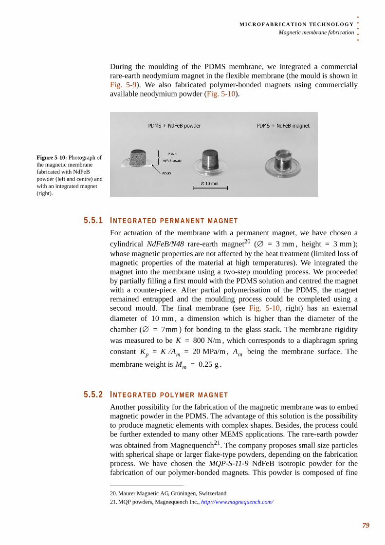
. . .
. .M I C R O F A B R I C A T I O N TE C H N O L O G YMagnetic membrane fabrication
During the moulding of the PDMS membrane, we integrated a commercial rare-earth neodymium magnet in the flexible membrane (the mould is shown in Fig. 5-9). We also fabricated polymer-bonded magnets using commercially available neodymium powder (Fig. 5-10).
5.5.1 I N T E G R A T E D P E R M A N E N T M A G N E TFor actuation of the membrane with a permanent magnet, we have chosen a cylindrical NdFeB/N48 rare-earth magnet20 ( , ); whose magnetic properties are not affected by the heat treatment (limited loss of magnetic properties of the material at high temperatures). We integrated the magnet into the membrane using a two-step moulding process. We proceeded by partially filling a first mould with the PDMS solution and centred the magnet with a counter-piece. After partial polymerisation of the PDMS, the magnet remained entrapped and the moulding process could be completed using a second mould. The final membrane (see Fig. 5-10, right) has an external diameter of , a dimension which is higher than the diameter of the chamber ( ) for bonding to the glass stack. The membrane rigidity was measured to be , which corresponds to a diaphragm spring constant , being the membrane surface. The
membrane weight is .
5.5.2 I N T E G R A T E D P O L Y M E R M A G N E TAnother possibility for the fabrication of the magnetic membrane was to embed magnetic powder in the PDMS. The advantage of this solution is the possibility to produce magnetic elements with complex shapes. Besides, the process could be further extended to many other MEMS applications. The rare-earth powder was obtained from Magnequench21. The company proposes small size particles with spherical shape or larger flake-type powders, depending on the fabrication process. We have chosen the MQP-S-11-9 NdFeB isotropic powder for the fabrication of our polymer-bonded magnets. This powder is composed of fine
Figure 5-10: Photograph of the magnetic membrane fabricated with NdFeB powder (left and centre) and with an integrated magnet (right).
20. Maurer Magnetic AG, Grüningen, Switzerland
∅ 3 mm= height 3 mm=
10 mm∅ 7mm=
K 800 N/m=Kp K Am⁄ 20 MPa/m= = Am
Mm 0.25 g=
21. MQP powders, Magnequench Inc., http://www.magnequench.com/
79
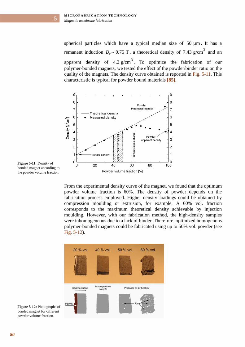
M I C R O F A B R I C A T I O N TE C H N O L O G YMagnetic membrane fabrication
80
5
spherical particles which have a typical median size of . It has a
remanent induction , a theoretical density of and an
apparent density of . To optimize the fabrication of our polymer-bonded magnets, we tested the effect of the powder/binder ratio on the quality of the magnets. The density curve obtained is reported in Fig. 5-11. This characteristic is typical for powder bound materials [85].
From the experimental density curve of the magnet, we found that the optimum powder volume fraction is 60%. The density of powder depends on the fabrication process employed. Higher density loadings could be obtained by compression moulding or extrusion, for example. A 60% vol. fraction corresponds to the maximum theoretical density achievable by injection moulding. However, with our fabrication method, the high-density samples were inhomogeneous due to a lack of binder. Therefore, optimized homogenous polymer-bonded magnets could be fabricated using up to 50% vol. powder (see Fig. 5-12).
50 µm
Br 0.75 T∼ 7.43 g/cm3
4.2 g/cm3
Figure 5-11: Density of bonded magnet according to the powder volume fraction.
Figure 5-12: Photographs of bonded magnet for different powder volume fraction.
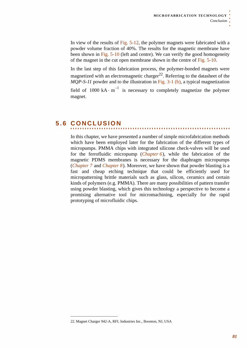
. . .
. .M I C R O F A B R I C A T I O N TE C H N O L O G YConclusion
In view of the results of Fig. 5-12, the polymer magnets were fabricated with a powder volume fraction of 40%. The results for the magnetic membrane have been shown in Fig. 5-10 (left and centre). We can verify the good homogeneity of the magnet in the cut open membrane shown in the centre of Fig. 5-10.
In the last step of this fabrication process, the polymer-bonded magnets were magnetized with an electromagnetic charger22. Referring to the datasheet of the MQP-S-11 powder and to the illustration in Fig. 3-1 (b), a typical magnetization
field of is necessary to completely magnetize the polymer magnet.
. . . . . . . . . . . . . . . . . . . . . . . . . . . . . . . . . . . . . . . . . . . . . . . . . . . . . . . . . . . . . . . . . . .5 . 6 C O N C L U S I O N
In this chapter, we have presented a number of simple microfabrication methods which have been employed later for the fabrication of the different types of micropumps. PMMA chips with integrated silicone check-valves will be used for the ferrofluidic micropump (Chapter 6 ), while the fabrication of the magnetic PDMS membranes is necessary for the diaphragm micropumps (Chapter 7 and Chapter 8 ). Moreover, we have shown that powder blasting is a fast and cheap etching technique that could be efficiently used for micropatterning brittle materials such as glass, silicon, ceramics and certain kinds of polymers (e.g. PMMA). There are many possibilities of pattern transfer using powder blasting, which gives this technology a perspective to become a promising alternative tool for micromachining, especially for the rapid prototyping of microfluidic chips.
22. Magnet Charger 942-A, RFL Industries Inc., Boonton, NJ, USA
1000 kA m 1–⋅
81

CHAPTER
6. . . . .
. . . . . . . . . . . . . . . . . . . . . . . . . . . . . . . . . . .FERROFLUIDIC MICROPUMP *
* Adapted version of: C. Yamahata, M. Chastellain, V. K. Parashar, A. Petri, H. Hofmann, and M. A. M. Gijs, «Plastic micropump with ferrofluidic actuation», Journal of Microelectromechanical Systems 14 (1), pp. 96-102. 2005. DOI: 10.1109/JMEMS.2004.839007
n this chapter, we present the realization and characterization of a new type of plastic micropump based on the magnetic actuation of a magnetic liquid. The pump consists of two serial check-valves that convert the periodic
motion of a ferrofluidic plug into a pulsed quasi-continuous flow. The ferrofluid is actuated by the mechanical motion of an external NdFeB permanent magnet. The water-based ferrofluid is synthesized in-house using a co-precipitation method and has a saturation magnetization of . The micropump consists of various layers of polymethylmethacrylate (PMMA), which are microstructured by powder blasting or by standard mechanical micromachining techniques, and are assembled in a single plastic structure using a monomer gluing solution. Two soft silicone membranes are integrated in the microfluidic structure to form two check-valves. Water has been successfully pumped at flow rates of up to and pumping is achieved at back-pressures of up to .
6 . 1 F E R R O F L U I D S A N D T H E I R
. . . . . . . . . . . . . . . . . . . . . . . . . . . . . . . . . . . . . . . . . . . . . . . . . . . . . . . . . . . . . . . . . . .A P P L I C A T I O N S
A comprehensive description of ferrofluids can be found in [86] of the Encyclopedia of Materials. We summarize hereafter the main aspects as regard to the purpose of our work.
6.1.1 C O M P O S I T I O N O F F E R R O F L U I D SA ferrofluid, or magnetic fluid, consists of a stable suspension of sub-domain magnetic particles colloidally dispersed in a liquid carrier (usually hydrocarbon or a water-based solution). The typical size of particles in a ferrofluid is about
, a dimension which is smaller than a magnetic domain. The colloidal
I32 mT
30 µL min⁄25 mbar
10 nm
83
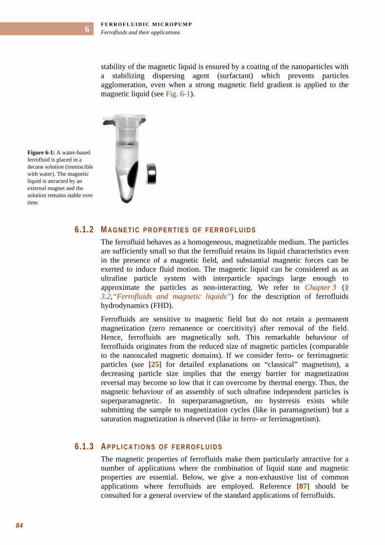
F E R R O F L U I D I C M I C R O P U M PFerrofluids and their applications
84
6
stability of the magnetic liquid is ensured by a coating of the nanoparticles with a stabilizing dispersing agent (surfactant) which prevents particles agglomeration, even when a strong magnetic field gradient is applied to the magnetic liquid (see Fig. 6-1).
6.1.2 M A G N E T I C P R O P E R T I E S O F F E R R O F L U I D SThe ferrofluid behaves as a homogeneous, magnetizable medium. The particles are sufficiently small so that the ferrofluid retains its liquid characteristics even in the presence of a magnetic field, and substantial magnetic forces can be exerted to induce fluid motion. The magnetic liquid can be considered as an ultrafine particle system with interparticle spacings large enough to approximate the particles as non-interacting. We refer to Chapter 3 (§ 3.2,“Ferrofluids and magnetic liquids”) for the description of ferrofluids hydrodynamics (FHD).
Ferrofluids are sensitive to magnetic field but do not retain a permanent magnetization (zero remanence or coercitivity) after removal of the field. Hence, ferrofluids are magnetically soft. This remarkable behaviour of ferrofluids originates from the reduced size of magnetic particles (comparable to the nanoscaled magnetic domains). If we consider ferro- or ferrimagnetic particles (see [25] for detailed explanations on “classical” magnetism), a decreasing particle size implies that the energy barrier for magnetization reversal may become so low that it can overcome by thermal energy. Thus, the magnetic behaviour of an assembly of such ultrafine independent particles is superparamagnetic. In superparamagnetism, no hysteresis exists while submitting the sample to magnetization cycles (like in paramagnetism) but a saturation magnetization is observed (like in ferro- or ferrimagnetism).
6.1.3 A P P L I C A T I O N S O F F E R R O F L U I D SThe magnetic properties of ferrofluids make them particularly attractive for a number of applications where the combination of liquid state and magnetic properties are essential. Below, we give a non-exhaustive list of common applications where ferrofluids are employed. Reference [87] should be consulted for a general overview of the standard applications of ferrofluids.
Figure 6-1: A water-based ferrofluid is placed in a decane solution (immiscible with water). The magnetic liquid is attracted by an external magnet and the solution remains stable over time.

. . .
. .F E R R O F L U I D I C M I C R O P U M PFerrofluids and their applications
• Ferrofluid sealA ferrofluid is used in rotary shaft seals where it is retained in place between the rotating and fixed members under the action of magnetic forces. The magnetic flux is concentrated in the gap between the magnetically permeable shaft and permanent magnets. The ferrofluid assumes the shape of a liquid O-ring and produces a hermetic seal. In typical commercial vacuum feedthroughs, a single stage can sustain a differential pressure of . The working principle of a ferrofluid rotary shaft seal is shown in Fig. 6-2.
A direct application of the rotary shaft seal is found in the machinery used for the manufacturing of integrated circuits, which requires an environment free of any particulate contaminants. As an example, a robot arm with a ferrofluid seal can be used for wafer transportation.
• Loudspeaker application (see for example [88])Placed into the air gap between the pole piece and the coil, the ferrofluid plays three roles in a loudspeaker system:
– It conducts heat away from the voice coil;
– It keeps the voice coil concentric with the magnet (ferrofluid is naturally retained in the gap.);
– It is used as a medium for damping.
• Printing with magnetic inksBy incorporating nano-sized magnetic particles into ink, the resulting liquid is capable of generating a magnetic signal and can subsequently be read by very simple and inexpensive magnetic recording technology. For example, Magnetic Ink Character Recognition (MICR) technology is used by banks to print details on cheques to enable automatic processing. When a document that contains this ink needs to be read, it passes through a machine which magnetizes the ink and then translates the magnetic information into characters.
200 mbar
Figure 6-2: Components of a magnetic fluid rotary seal.
85
F E R R O F L U I D I C M I C R O P U M PFerrofluids and their applications
86
6
• Magnetic particles for biomedical applicationsM. Chastellain [29], who provided us with the water-based ferrofluids employed in our experiments, synthesized nanoparticles for applications in hyperthermia (controlled heating in a well defined body area for cancer therapy), drug delivery (targeted drug release to the exact target tissue by electromagnetic trigger action) an DNA in vitro separation. All these applications deal with using iron oxide nanoparticles in physiological media (either in vitro or in vivo), i.e. water-based liquid media.
In reference [89], M. Shinkai summarizes the main fields where ferrofluids among others, and more generally magnetic particles, are used in medical applications. The review of M. A. M. Gijs [90] relates most recent advances in the handling and manipulation of magnetic particles (micro- and nano-sized) in microfluidic systems and gives the basic physics of magnetism for magnetic beads manipulation.
6.1.4 U S E O F F E R R O F L U I D S I N M I C R O F L U I D I C SSince the concept of micro Total Analysis Systems or µTAS was introduced in 1990 [7,10], fluidic microchip technologies have overcome multiple experimental hurdles opening the field for numerous pharmaceutical and biological applications. References [8] and [9] give recent and comprehensive overviews of all the important developments in technology, theoretical understanding and applications in the field. During these developments, a continuous challenge has been the transport and pumping of small quantities of biological fluids on the order of a few microlitres per minute. The first development of a micropump dates from the 1980s with the emergence of the field of MicroElectroMechanical Systems (MEMS). H. T. G. van Lintel et al.[1,2] presented the first silicon micropump based on the piezoelectric or thermopneumatic actuation of a thin membrane. Since then, many other integrated silicon-based micropumps, mostly based on piezoelectric actuation, were proposed [13,38]. Silicon fluidic MEMS devices have found several commercial applications. They are used for insulin delivery [48], in gas control as active fluidic valving [64] and in inkjet technology [91]. However, for many µTAS applications, microfluidic systems need to be disposable and low-cost, offering plastic materials a competitive edge for the fabrication of micropumps. Plastics have been used in a variety of microfluidic systems [9] and plastic micropumps have already been shown to be of great potential [92,93,94,95]. Innovative actuation methods for fluid handling were simultaneously developed, for example the use of magnetically actuated magnetic liquids or ferrofluids. Ferrofluids are used in a variety of applications, such as in loudspeaker systems [88], where they improve mechanical performances (they conduct heat away from the voice coil, keep the voice coil concentric with the magnet, play the role of a medium for damping) or in rotary vacuum feedthroughs [96], where they play the role of sealing fluids. B. Wagner et al.[97] demonstrated the surface displacement of drops of a ferrofluid based on the linear translation of miniaturized magnets in a hybrid system. The first ferrofluidic piston pump was presented in 1991 in [98]. N. E. Greivell and B. Hannaford [99] realized an electromagnetically actuated ferrofluid
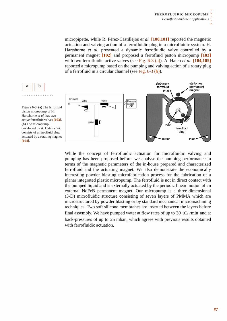
. . .
. .F E R R O F L U I D I C M I C R O P U M PFerrofluids and their applications
micropipette, while R. Pérez-Castillejos et al. [100,101] reported the magnetic actuation and valving action of a ferrofluidic plug in a microfluidic system. H. Hartshorne et al. presented a dynamic ferrofluidic valve controlled by a permanent magnet [102] and proposed a ferrofluid piston micropump [103] with two ferrofluidic active valves (see Fig. 6-3 (a)). A. Hatch et al. [104,105]reported a micropump based on the pumping and valving action of a rotary plug of a ferrofluid in a circular channel (see Fig. 6-3 (b)).
While the concept of ferrofluidic actuation for microfluidic valving and pumping has been proposed before, we analyse the pumping performance in terms of the magnetic parameters of the in-house prepared and characterized ferrofluid and the actuating magnet. We also demonstrate the economically interesting powder blasting microfabrication process for the fabrication of a planar integrated plastic micropump. The ferrofluid is not in direct contact with the pumped liquid and is externally actuated by the periodic linear motion of an external NdFeB permanent magnet. Our micropump is a three-dimensional (3-D) microfluidic structure consisting of seven layers of PMMA which are microstructured by powder blasting or by standard mechanical micromachining techniques. Two soft silicone membranes are inserted between the layers before final assembly. We have pumped water at flow rates of up to and at back-pressures of up to , which agrees with previous results obtained with ferrofluidic actuation.
a b
Figure 6-3: (a) The ferrofluid piston micropump of H. Hartshorne et al. has two active ferrofluid valves [103]. (b) The micropump developed by A. Hatch et al. consists of a ferrofluid plug actuated by a rotating magnet [104].
30 µL min⁄25 mbar
87
F E R R O F L U I D I C M I C R O P U M PSynthesis and characterization of the water-based ferrofluid
88
6
6 . 2 S Y N T H E S I S A N D C H A R A C T E R I Z A T I O N O F
. . . . . . . . . . . . . . . . . . . . . . . . . . . . . . . . . . . . . . . . . . . . . . . . . . . . . . . . . . . . . . . . . . .T H E W A T E R - B A S E D F E R R O F L U I D
The water-based ferrofluid used in our experiments was developed at the Powder Technology Laboratory (EPFL). We refer to the thesis of M. Chastellain [29] for more extensive details on the subject of ferrofluids synthesis and applications of superparamagnetic particles.
6.2.1 S Y N T H E S I S O F T H E F E R R O F L U I DMagnetic nanoparticles are prepared by a classical co-precipitation method [106]. A mixture of a solution containing ferric and ferrous chloride is precipitated with concentrated ammonia. This yields a black precipitate which is washed several times with ultra-pure water. The remaining solid is refluxed in a mixture of diluted nitric acid in the presence of a solution. This treatment results in an aqueous suspension which is reddish brown in
colour. The thus obtained suspension is dialysed against to get
rid of un-reacted precursor ions and centrifuged at for 30 minutes. The
supernatant is discarded and a few millilitres of is added to the solid part to get a highly concentrated suspension. The water-based ferrofluid remains stable for a pH between 2 and 3. The iron oxide content of the suspensions is determined by redox titration with a standard solution of potassium permanganate.
The dynamic viscosity of the ferrofluid was measured using an ARES setup from Rheometric Scientific equipped with a plane–plane geometry. A viscosity
of for a shear rate of is obtained at room temperature, about ten times higher than the viscosity of water.
A comprehensive characterization of the synthesized ferrofluid can be found in [107]. Briefly, the ferrofluid consists of iron oxide particles in a crystalline non-stoichiometric phase with a lattice parameter in between pure magnetite ( ) and pure maghemite ( ). Primary particles have a size in the
range. The iron content is measured after titration to be of per litre suspension. Assuming that only one solid phase is present and that no free iron is in solution (which is ensured by the dialysis step) the iron oxide content can be calculated. Depending on the phase formed we get and
per litre suspension for and , respectively.
Fe(NO3)3 9H2O⋅
HNO3 10 2– M
30000 g
HNO3 10 2– M
10 mPa s⋅ 100 s 1–
Fe3O4 γ-Fe2O3
10 nm 226.1 g Fe2+
323.3 g312.5 g γ-Fe2O3 Fe3O4
. . .
. .F E R R O F L U I D I C M I C R O P U M PSynthesis and characterization of the water-based ferrofluid
6.2.2 C H A R A C T E R I Z A T I O N O F T H E F E R R O F L U I DThe magnetic characterization of the ferrofluid (Fig. 6-4) was carried out by Prof. K. V. Rao and A. Gupta, Department of Materials Science Tmfy-MSE, Royal Institute of Technology, Stockholm, Sweden.
Magnet iza t ion curve
A Quantum Design MPMS2 SQUID magnetometer is used for magnetic characterization of liquid samples at . The magnetization curve of the ferrofluid is obtained by subjecting the sample to a magnetic field cycle ranging between and as shown in Fig. 6-4.
The absence of hysteresis is a clear signature of the superparamagnetic behaviour of the ferrofluid particles at this temperature. Of particular interest is the relatively large saturation magnetization, which will enable the generation of an appreciable magnetic force (see below). The initial magnetic susceptibility is also determined from Fig. 6-4 and found to be .
The measured value of the saturation magnetic field ( ) of our ferrofluid is higher than that of commercial water-based ferrofluids, but is a factor smaller than the saturation field for commercial hydrocarbon-based ferrofluids [96]. In-house developed water-based ferrofluids are obtained as a side product of a synthesis devoted to in vitro and in vivo applications. They were mainly chosen for their good stability in time.
Magnet ic p ressure
The magnetic pressure that a ferrofluidic plug in a channel can withstand is measured experimentally as shown in Fig. 6-5. A rare-earth NdFeB magnet is placed at a controlled position under a tube (external diameter of , internal diameter of ) containing a long ferrofluidic plug. A
300 K
800 kA/m 800 kA/m–
χ 0.83≈
Figure 6-4: Magnetic characteristic of the synthesized ferrofluids.
32 mT2 3–
0.7 mm0.3 mm 10 mm
89
F E R R O F L U I D I C M I C R O P U M PSynthesis and characterization of the water-based ferrofluid
90
6
vertical column is filled with water at a low flow rate using a peristaltic pump. The hydrostatic loading, generated this way, determines the hydrostatic pressure that the ferrofluidic plug can withstand. We obtain magnetic sealing for hydrostatic pressures of up to .
From the ferrohydrodynamic Bernoulli equation (Eq. 3.16 in Chapter 3 ) [26]one can theoretically calculate the magnetic pressure that a static magnetic liquid seal can withstand if one side of the ferrofluid is magnetized (situated in the high field region of the magnet) and the other side is outside of the magnetic field. The magnetic pressure is given, with good approximation, by (see Eq. 3.17 in Chapter 3 ):
70 mbar
Figure 6-5: Measurement method of the hydrostatic pressure sustained by the plug of ferrofluid.
(6.1)∆P µ0 M Hd0
Hmax
∫=
. . .
. .F E R R O F L U I D I C M I C R O P U M PSynthesis and characterization of the water-based ferrofluid
To calculate this magnetic pressure, we need to know the maximum field generated by the permanent magnet. We present the magnetic characteristics of the permanent magnet in Fig. 6-6, as measured by a miniature Hall probe. From this figure, we observe the nearly-linear behaviour of in the range
.
The maximum magnetic field at the position of the ferrofluidic plug ( ) is taken directly from Fig. 6-6. Its value is used in the integration of the magnetization curve of the magnetic liquid (Fig. 6-4) to calculate the theoretical magnetic pressure, according to Eq. 6.1. The calculated magnetic pressure is given in Fig. 6-7 for different positions of the ferrofluidic channel with respect to the magnet and is in good agreement with experimental results. For each position, we give the minimum and maximum measured pressure obtained from different experiments, thus giving an idea of the reproducibility of the experiment.
Hmax
Bx
5 mm x 5 mm< <–
Figure 6-6: Magnetic field measured on the symmetry axis of the magnet.
Hmax Bmax µ0⁄=
z
z
Figure 6-7: Magnetic pressure sustained by the plug of ferrofluid as a function of the distance between the ferrofluid and the permanent magnet.
91
F E R R O F L U I D I C M I C R O P U M PWorking principle and design of the micropump
92
6
6 . 3 W O R K I N G P R I N C I P L E A N D D E S I G N O F
. . . . . . . . . . . . . . . . . . . . . . . . . . . . . . . . . . . . . . . . . . . . . . . . . . . . . . . . . . . . . . . . . . .T H E M I C R O P U M P
6.3.1 W O R K I N G P R I N C I P L EOur micropump is based on the oscillatory motion of a ferrofluidic piston in a microfluidic channel. Two check-valves convert the motion of the ferrofluidic plug to a quasi-continuous flow from the input to the output reservoir, as schematically shown in Fig. 6-8. The valves are passive, normally-closed, and open simply under the pressure generated by the ferrofluidic piston. The ferrofluid serves both as an actuator and seal. The periodic linear motion of the ferrofluidic plug ( ) is induced by a mechanically moving cylindrical rare-earth magnet (DSC-10/4 A-RES350 magnet23: NdFeB, diameter , height , coercitive field , magnetic
remanence ). The magnet is mounted on a computer-controlled
motorized stage and is translated with velocities of up to over a range of up to . The magnet used has a relatively low displacement speed, resulting in a pulsed flow, originating from the periodic opening/closing of the two check-valves. By controlling the speed and the displacement amplitude of the magnet, it is possible to vary the frequency and stroke volume. In our design, the total dead volume (volume between the two valves) is about 80 microlitres. With a translation amplitude of the external magnet of , the stroke volume is approximately 100 microlitres. These values result in a relatively large compression ratio of , which is sufficient for the self-priming of the pump (cf. § 4.2.3). A separation plug of low-viscosity oil (length ) is used to separate the pumped liquid from the water-based ferrofluid and to prevent mixing between water and ferrofluid.
23.Megatron AG
1 mm 1 mm 10 mm××
10 mm 4 mm Hc 830 kA/m=
Br 1200 mT=
100 mm/min10 mm
10 mm
ε 1.25=
5 mm
Figure 6-8: Working principle of the ferrofluidic micropump.
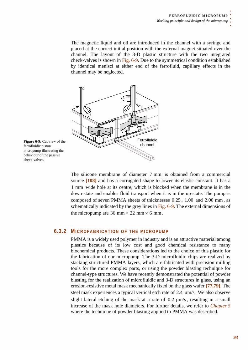
. . .
. .F E R R O F L U I D I C M I C R O P U M PWorking principle and design of the micropump
The magnetic liquid and oil are introduced in the channel with a syringe and placed at the correct initial position with the external magnet situated over the channel. The layout of the 3-D plastic structure with the two integrated check-valves is shown in Fig. 6-9. Due to the symmetrical condition established by identical menisci at either end of the ferrofluid, capillary effects in the channel may be neglected.
The silicone membrane of diameter is obtained from a commercial source [108] and has a corrugated shape to lower its elastic constant. It has a
wide hole at its centre, which is blocked when the membrane is in the down-state and enables fluid transport when it is in the up-state. The pump is composed of seven PMMA sheets of thicknesses , and , as schematically indicated by the grey lines in Fig. 6-9. The external dimensions of the micropump are .
6.3.2 M I C R O F A B R I C A T I O N O F T H E M I C R O P U M PPMMA is a widely used polymer in industry and is an attractive material among plastics because of its low cost and good chemical resistance to many biochemical products. These considerations led to the choice of this plastic for the fabrication of our micropump. The 3-D microfluidic chips are realized by stacking structured PMMA layers, which are fabricated with precision milling tools for the more complex parts, or using the powder blasting technique for channel-type structures. We have recently demonstrated the potential of powder blasting for the realization of microfluidic and 3-D structures in glass, using an erosion-resistive metal mask mechanically fixed on the glass wafer [77,79]. The steel mask experiences a typical vertical etch rate of . We also observe slight lateral etching of the mask at a rate of , resulting in a small increase of the mask hole diameters. For further details, we refer to Chapter 5 where the technique of powder blasting applied to PMMA was described.
Figure 6-9: Cut view of the ferrofluidic piston micropump illustrating the behaviour of the passive check-valves.
7 mm
1 mm
0.25 1.00 2.00 mm
36 mm 22 mm 6 mm××
2.4 µm/s0.2 µm/s
93
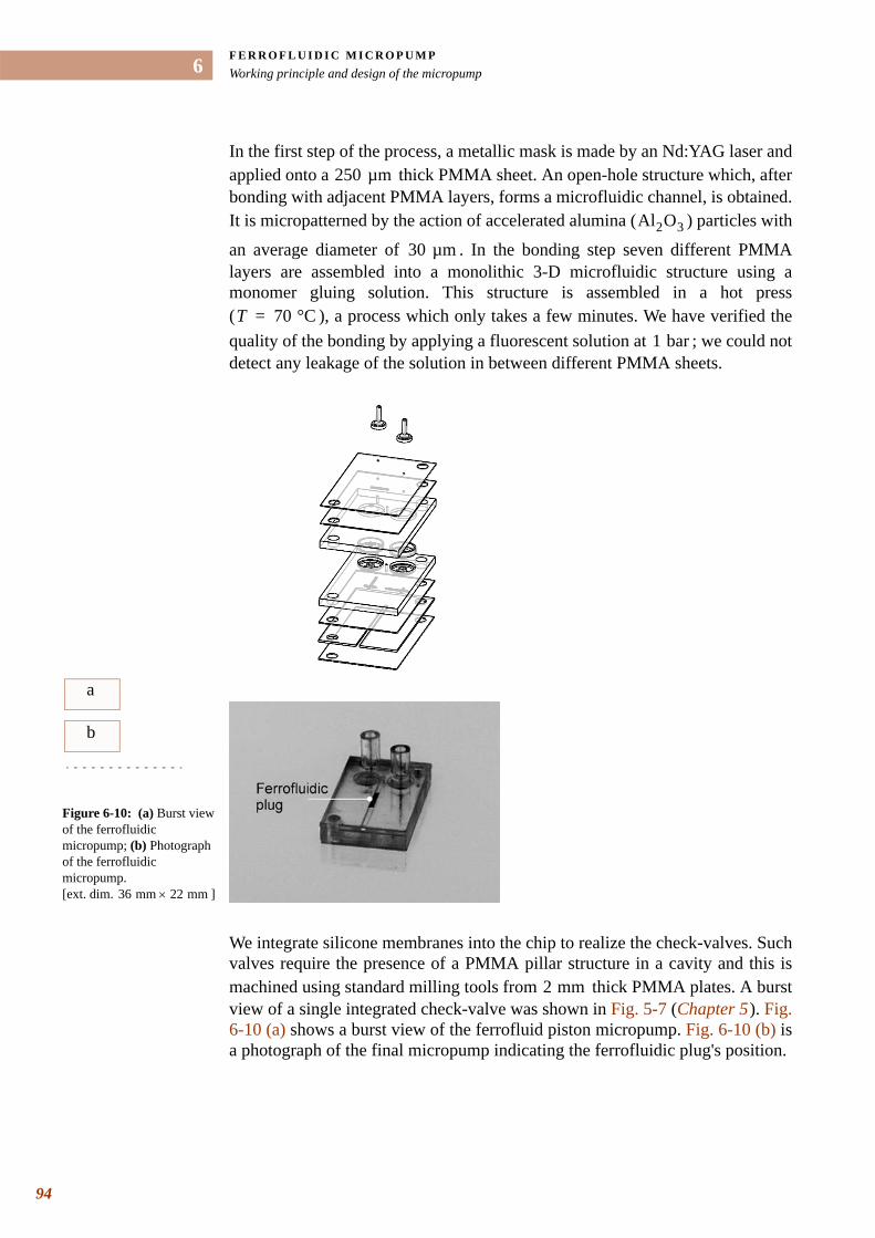
F E R R O F L U I D I C M I C R O P U M PWorking principle and design of the micropump
94
6
In the first step of the process, a metallic mask is made by an Nd:YAG laser and applied onto a thick PMMA sheet. An open-hole structure which, after bonding with adjacent PMMA layers, forms a microfluidic channel, is obtained. It is micropatterned by the action of accelerated alumina ( ) particles with
an average diameter of . In the bonding step seven different PMMA layers are assembled into a monolithic 3-D microfluidic structure using a monomer gluing solution. This structure is assembled in a hot press ( ), a process which only takes a few minutes. We have verified the quality of the bonding by applying a fluorescent solution at ; we could not detect any leakage of the solution in between different PMMA sheets.
We integrate silicone membranes into the chip to realize the check-valves. Such valves require the presence of a PMMA pillar structure in a cavity and this is machined using standard milling tools from thick PMMA plates. A burst view of a single integrated check-valve was shown in Fig. 5-7 (Chapter 5 ). Fig. 6-10 (a) shows a burst view of the ferrofluid piston micropump. Fig. 6-10 (b) is a photograph of the final micropump indicating the ferrofluidic plug's position.
250 µm
Al2O3
30 µm
T 70 °C=1 bar
a
b
Figure 6-10: (a) Burst view of the ferrofluidic micropump; (b) Photograph of the ferrofluidic micropump. [ext. dim. ]36 mm 22 mm×
2 mm
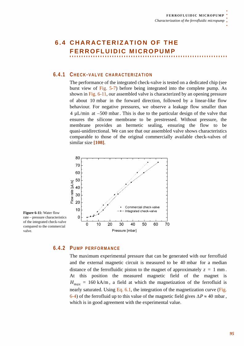
. . .
. .F E R R O F L U I D I C M I C R O P U M PCharacterization of the ferrofluidic micropump
6 . 4 C H A R A C T E R I Z A T I O N O F T H E
. . . . . . . . . . . . . . . . . . . . . . . . . . . . . . . . . . . . . . . . . . . . . . . . . . . . . . . . . . . . . . . . . . .F E R R O F L U I D I C M I C R O P U M P
6.4.1 C H E C K- V A L V E C H A R A C T E R I Z A T I O NThe performance of the integrated check-valve is tested on a dedicated chip (see burst view of Fig. 5-7) before being integrated into the complete pump. As shown in Fig. 6-11, our assembled valve is characterized by an opening pressure of about in the forward direction, followed by a linear-like flow behaviour. For negative pressures, we observe a leakage flow smaller than
at . This is due to the particular design of the valve that ensures the silicone membrane to be prestressed. Without pressure, the membrane provides an hermetic sealing, ensuring the flow to be quasi-unidirectional. We can see that our assembled valve shows characteristics comparable to those of the original commercially available check-valves of similar size [108].
6.4.2 P U M P P E R F O R M A N C EThe maximum experimental pressure that can be generated with our ferrofluid and the external magnetic circuit is measured to be for a median distance of the ferrofluidic piston to the magnet of approximately . At this position the measured magnetic field of the magnet is
, a field at which the magnetization of the ferrofluid is nearly saturated. Using Eq. 6.1, the integration of the magnetization curve (Fig. 6-4) of the ferrofluid up to this value of the magnetic field gives , which is in good agreement with the experimental value.
10 mbar
4 µL/min 500 mbar–
Figure 6-11: Water flow rate – pressure characteristics of the integrated check-valve compared to the commercial valve.
40 mbarz 1 mm=
Hmax 160 kA/m=
∆P 40 mbar≈
95
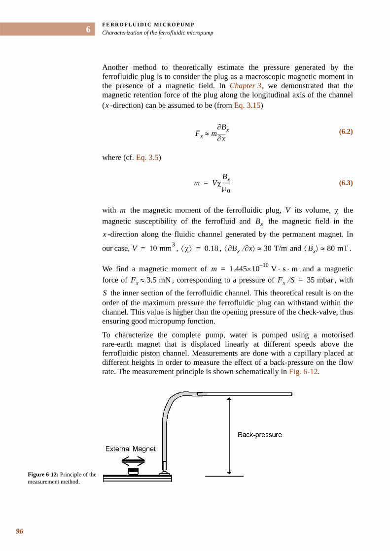
F E R R O F L U I D I C M I C R O P U M PCharacterization of the ferrofluidic micropump
96
6
Another method to theoretically estimate the pressure generated by the ferrofluidic plug is to consider the plug as a macroscopic magnetic moment in the presence of a magnetic field. In Chapter 3 , we demonstrated that the magnetic retention force of the plug along the longitudinal axis of the channel ( -direction) can be assumed to be (from Eq. 3.15)
where (cf. Eq. 3.5)
with the magnetic moment of the ferrofluidic plug, its volume, the magnetic susceptibility of the ferrofluid and the magnetic field in the
-direction along the fluidic channel generated by the permanent magnet. In
our case, , , and .
We find a magnetic moment of and a magnetic force of , corresponding to a pressure of , with
the inner section of the ferrofluidic channel. This theoretical result is on the order of the maximum pressure the ferrofluidic plug can withstand within the channel. This value is higher than the opening pressure of the check-valve, thus ensuring good micropump function.
To characterize the complete pump, water is pumped using a motorised rare-earth magnet that is displaced linearly at different speeds above the ferrofluidic piston channel. Measurements are done with a capillary placed at different heights in order to measure the effect of a back-pressure on the flow rate. The measurement principle is shown schematically in Fig. 6-12.
x
(6.2)Fx m x∂∂Bx≈
(6.3)m VχBxµ0-----=
m V χBx
x
V 10 mm3= χ⟨ ⟩ 0.18= Bx∂ x∂⁄⟨ ⟩ 30 T/m≈ Bx⟨ ⟩ 80 mT≈
m 1.445 10–×10 V s m⋅ ⋅=Fx 3.5 mN≈ Fx S⁄ 35 mbar=
S
Figure 6-12: Principle of the measurement method.
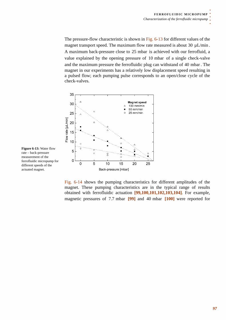
. . .
. .F E R R O F L U I D I C M I C R O P U M PCharacterization of the ferrofluidic micropump
The pressure-flow characteristic is shown in Fig. 6-13 for different values of the magnet transport speed. The maximum flow rate measured is about . A maximum back-pressure close to is achieved with our ferrofluid, a value explained by the opening pressure of of a single check-valve and the maximum pressure the ferrofluidic plug can withstand of . The magnet in our experiments has a relatively low displacement speed resulting in a pulsed flow; each pumping pulse corresponds to an open/close cycle of the check-valves.
Fig. 6-14 shows the pumping characteristics for different amplitudes of the magnet. These pumping characteristics are in the typical range of results obtained with ferrofluidic actuation [99,100,101,102,103,104]. For example, magnetic pressures of [99] and [100] were reported for
30 µL/min25 mbar
10 mbar40 mbar
Figure 6-13: Water flow rate – back-pressure measurement of the ferrofluidic micropump for different speeds of the actuated magnet.
7.7 mbar 40 mbar
97
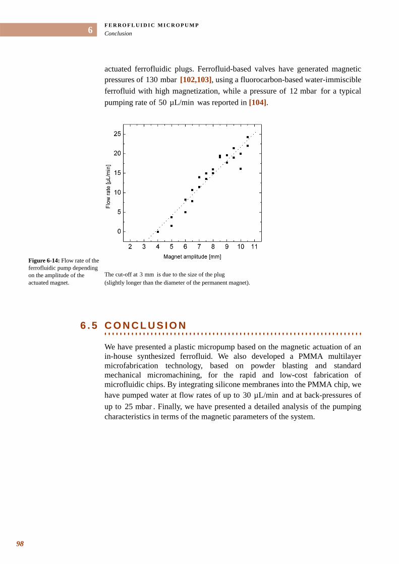
F E R R O F L U I D I C M I C R O P U M PConclusion
98
6
actuated ferrofluidic plugs. Ferrofluid-based valves have generated magnetic pressures of [102,103], using a fluorocarbon-based water-immiscible ferrofluid with high magnetization, while a pressure of for a typical pumping rate of was reported in [104].
. . . . . . . . . . . . . . . . . . . . . . . . . . . . . . . . . . . . . . . . . . . . . . . . . . . . . . . . . . . . . . . . . . .6 . 5 C O N C L U S I O N
We have presented a plastic micropump based on the magnetic actuation of an in-house synthesized ferrofluid. We also developed a PMMA multilayer microfabrication technology, based on powder blasting and standard mechanical micromachining, for the rapid and low-cost fabrication of microfluidic chips. By integrating silicone membranes into the PMMA chip, we have pumped water at flow rates of up to and at back-pressures of up to . Finally, we have presented a detailed analysis of the pumping characteristics in terms of the magnetic parameters of the system.
130 mbar12 mbar
50 µL/min
Figure 6-14: Flow rate of the ferrofluidic pump depending on the amplitude of the actuated magnet.
The cut-off at is due to the size of the plug (slightly longer than the diameter of the permanent magnet).
3 mm
30 µL/min25 mbar
CHAPTER
7. . . . .
. . . . . . . . . . . . . . . . . . . . . . . . . . . . . . . . . . .DIFFUSER MICROPUMP *
* Adapted version of: C. Yamahata, C. Lotto, E. Al-Assaf, and M. A. M. Gijs, «A PMMA valveless micropump using electromagnetic actuation», Microfluidics and Nanofluidics (in press). DOI: 10.1007/s10404-004-0007-6 C. Yamahata, F. Lacharme, and M. A. M. Gijs, «Glass valveless micropump using electromagnetic actuation», Microelectronic Engineering (in press). DOI: 10.1016/j.mee.2004.12.018
n this chapter, we first describe the fabrication and characterization of an electromagnetically actuated polymethylmethacrylate (PMMA) valveless micropump. The pump consists of two diffuser elements and a
polydimethylsiloxane (PDMS) membrane with an integrated composite magnet made of NdFeB magnetic powder. Diffuser theory is combined with numerical simulation tools to correctly dimension the micropump. Water was pumped at flow rates of up to and back-pressures of up to . We determined a resonant frequency of and for pumping of water and air, respectively. We present a detailed analysis of the frequency-dependent flow rate of the micropump and analyse our experimental data using the theoretical models of A. Olsson et al. [109] and L. S. Pan et al. [110].
As an alternative, we propose in § 7.6 the fabrication of a similar micropump in glass material. This solution has the advantage of being compatible with applications where sterilization and chemical inertness are issues. The glass micropump shows a behaviour comparable to the PMMA prototype but with enhanced performance. Water was pumped at flow rates of up to and maximum achieved back-pressure was increased up to , thanks to the use of an improved electromagnetic actuation. The theoretical model of A. Olsson et al. [109] also correctly predicts the resonant frequency of the glass diffuser micropump.
7 . 1 D E S I G N O F A D I F F U S E R M I C R O P U M P I N
. . . . . . . . . . . . . . . . . . . . . . . . . . . . . . . . . . . . . . . . . . . . . . . . . . . . . . . . . . . . . . . . . . .P L A S T I C ( P M M A )
Since the introduction of the concept of micro Total Analysis Systems or µTAS in 1990 [7,10], multiple fluidic microchip technologies have been developed. A continuous challenge has been the transport and pumping of small quantities of biological fluids, of the order of a few microlitres per minute. The first development of a micropump dates from the 1980s with the emergence of the field of MicroElectroMechanical Systems (MEMS). H. T. G. van Lintel et al.
I400 µL/min 12 mbar
12 Hz 200 Hz
1 mL/min50 mbar
99
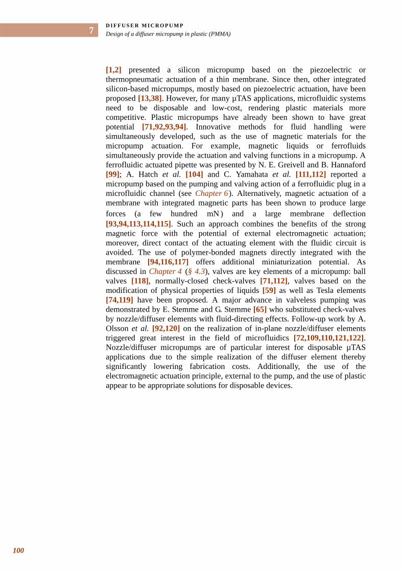
D I F F U S E R M I C R O P U M PDesign of a diffuser micropump in plastic (PMMA)
100
7
[1,2] presented a silicon micropump based on the piezoelectric or thermopneumatic actuation of a thin membrane. Since then, other integrated silicon-based micropumps, mostly based on piezoelectric actuation, have been proposed [13,38]. However, for many µTAS applications, microfluidic systems need to be disposable and low-cost, rendering plastic materials more competitive. Plastic micropumps have already been shown to have great potential [71,92,93,94]. Innovative methods for fluid handling were simultaneously developed, such as the use of magnetic materials for the micropump actuation. For example, magnetic liquids or ferrofluids simultaneously provide the actuation and valving functions in a micropump. A ferrofluidic actuated pipette was presented by N. E. Greivell and B. Hannaford [99]; A. Hatch et al. [104] and C. Yamahata et al. [111,112] reported a micropump based on the pumping and valving action of a ferrofluidic plug in a microfluidic channel (see Chapter 6 ). Alternatively, magnetic actuation of a membrane with integrated magnetic parts has been shown to produce large forces (a few hundred ) and a large membrane deflection [93,94,113,114,115]. Such an approach combines the benefits of the strong magnetic force with the potential of external electromagnetic actuation; moreover, direct contact of the actuating element with the fluidic circuit is avoided. The use of polymer-bonded magnets directly integrated with the membrane [94,116,117] offers additional miniaturization potential. As discussed in Chapter 4 (§ 4.3), valves are key elements of a micropump: ball valves [118], normally-closed check-valves [71,112], valves based on the modification of physical properties of liquids [59] as well as Tesla elements [74,119] have been proposed. A major advance in valveless pumping was demonstrated by E. Stemme and G. Stemme [65] who substituted check-valves by nozzle/diffuser elements with fluid-directing effects. Follow-up work by A. Olsson et al. [92,120] on the realization of in-plane nozzle/diffuser elements triggered great interest in the field of microfluidics [72,109,110,121,122]. Nozzle/diffuser micropumps are of particular interest for disposable µTAS applications due to the simple realization of the diffuser element thereby significantly lowering fabrication costs. Additionally, the use of the electromagnetic actuation principle, external to the pump, and the use of plastic appear to be appropriate solutions for disposable devices.
mN
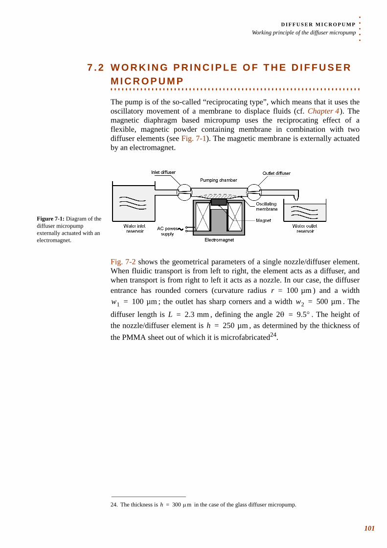
. . .
. .D I F F U S E R M I C R O P U M PWorking principle of the diffuser micropump
7 . 2 W O R K I N G P R I N C I P L E O F T H E D I F F U S E R
. . . . . . . . . . . . . . . . . . . . . . . . . . . . . . . . . . . . . . . . . . . . . . . . . . . . . . . . . . . . . . . . . . .M I C R O P U M P
The pump is of the so-called “reciprocating type”, which means that it uses the oscillatory movement of a membrane to displace fluids (cf. Chapter 4 ). The magnetic diaphragm based micropump uses the reciprocating effect of a flexible, magnetic powder containing membrane in combination with two diffuser elements (see Fig. 7-1). The magnetic membrane is externally actuated by an electromagnet.
Fig. 7-2 shows the geometrical parameters of a single nozzle/diffuser element. When fluidic transport is from left to right, the element acts as a diffuser, and when transport is from right to left it acts as a nozzle. In our case, the diffuser entrance has rounded corners (curvature radius ) and a width
; the outlet has sharp corners and a width . The
diffuser length is , defining the angle . The height of the nozzle/diffuser element is , as determined by the thickness of the PMMA sheet out of which it is microfabricated24.
Figure 7-1: Diagram of the diffuser micropump externally actuated with an electromagnet.
24. The thickness is in the case of the glass diffuser micropump.
r 100 µm=w1 100 µm= w2 500 µm=
L 2.3 mm= 2θ 9.5°=h 250 µm=
h 300 µm=
101
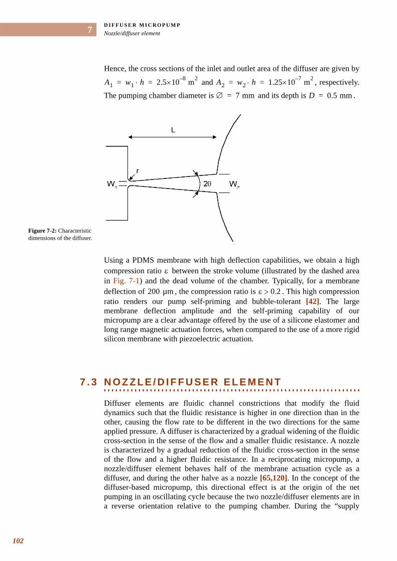
D I F F U S E R M I C R O P U M PNozzle/diffuser element
102
7
Hence, the cross sections of the inlet and outlet area of the diffuser are given by
and , respectively.
The pumping chamber diameter is and its depth is .
Using a PDMS membrane with high deflection capabilities, we obtain a high compression ratio between the stroke volume (illustrated by the dashed area in Fig. 7-1) and the dead volume of the chamber. Typically, for a membrane deflection of , the compression ratio is . This high compression ratio renders our pump self-priming and bubble-tolerant [42]. The large membrane deflection amplitude and the self-priming capability of our micropump are a clear advantage offered by the use of a silicone elastomer and long range magnetic actuation forces, when compared to the use of a more rigid silicon membrane with piezoelectric actuation.
. . . . . . . . . . . . . . . . . . . . . . . . . . . . . . . . . . . . . . . . . . . . . . . . . . . . . . . . . . . . . . . . . . .7 . 3 N O Z Z L E / D I F F U S E R E L E M E N T
Diffuser elements are fluidic channel constrictions that modify the fluid dynamics such that the fluidic resistance is higher in one direction than in the other, causing the flow rate to be different in the two directions for the same applied pressure. A diffuser is characterized by a gradual widening of the fluidic cross-section in the sense of the flow and a smaller fluidic resistance. A nozzle is characterized by a gradual reduction of the fluidic cross-section in the sense of the flow and a higher fluidic resistance. In a reciprocating micropump, a nozzle/diffuser element behaves half of the membrane actuation cycle as a diffuser, and during the other halve as a nozzle [65,120]. In the concept of the diffuser-based micropump, this directional effect is at the origin of the net pumping in an oscillating cycle because the two nozzle/diffuser elements are in a reverse orientation relative to the pumping chamber. During the “supply
A1 w1 h⋅ 2.5 8–×10 m2= = A2 w2 h⋅ 1.25 7–×10 m2= =
∅ 7 mm= D 0.5 mm=
Figure 7-2: Characteristic dimensions of the diffuser.
ε
200 µm ε 0.2>
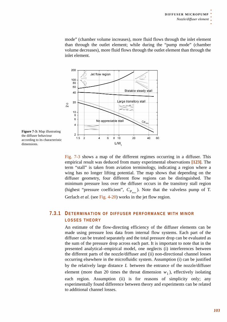
. . .
. .D I F F U S E R M I C R O P U M PNozzle/diffuser element
mode” (chamber volume increases), more fluid flows through the inlet element than through the outlet element; while during the “pump mode” (chamber volume decreases), more fluid flows through the outlet element than through the inlet element.
Fig. 7-3 shows a map of the different regimes occurring in a diffuser. This empirical result was deduced from many experimental observations [123]. The term “stall” is taken from aviation terminology, indicating a region where a wing has no longer lifting potential. The map shows that depending on the diffuser geometry, four different flow regions can be distinguished. The minimum pressure loss over the diffuser occurs in the transitory stall region (highest “pressure coefficient”, ). Note that the valveless pump of T. Gerlach et al. (see Fig. 4-20) works in the jet flow region.
7.3.1 D E T E R M I N A T I O N O F D I F F U S E R P E R F O R M A N C E W I T H M I N O R L O S S E S T H E O R YAn estimate of the flow-directing efficiency of the diffuser elements can be made using pressure loss data from internal flow systems. Each part of the diffuser can be treated separately and the total pressure drop can be evaluated as the sum of the pressure drop across each part. It is important to note that in the presented analytical–empirical model, one neglects (i) interferences between the different parts of the nozzle/diffuser and (ii) non-directional channel losses occurring elsewhere in the microfluidic system. Assumption (i) can be justified by the relatively large distance between the entrance of the nozzle/diffuser element (more than 20 times the throat dimension ), effectively isolating each region. Assumption (ii) is for reasons of simplicity only; any experimentally found difference between theory and experiments can be related to additional channel losses.
Figure 7-3: Map illustrating the diffuser behaviour according to its characteristic dimensions.
CPmax
Lw1
103
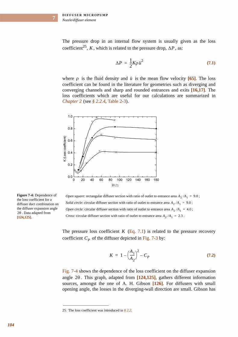
D I F F U S E R M I C R O P U M PNozzle/diffuser element
104
7
The pressure drop in an internal flow system is usually given as the loss coefficient25, , which is related to the pressure drop, , as:
where is the fluid density and is the mean flow velocity [65]. The loss coefficient can be found in the literature for geometries such as diverging and converging channels and sharp and rounded entrances and exits [16,17]. The loss coefficients which are useful for our calculations are summarized in Chapter 2 (see § 2.2.4, Table 2-3).
The pressure loss coefficient (Eq. 7.1) is related to the pressure recovery coefficient of the diffuser depicted in Fig. 7-3 by:
Fig. 7-4 shows the dependence of the loss coefficient on the diffuser expansion angle . This graph, adapted from [124,125], gathers different information sources, amongst the one of A. H. Gibson [126]. For diffusers with small opening angle, the losses in the diverging-wall direction are small. Gibson has
25. The loss coefficient was introduced in § 2.2.
K ∆P
(7.1)∆P 12---Kρu2=
ρ u
Figure 7-4: Dependence of the loss coefficient for a diffuser duct combination on the diffuser expansion angle
. Data adapted from [124,125].
Open square: rectangular diffuser section with ratio of outlet to entrance area ;
Solid circle: circular diffuser section with ratio of outlet to entrance area ;
Open circle: circular diffuser section with ratio of outlet to entrance area ;
Cross: circular diffuser section with ratio of outlet to entrance area .2θ
A2 A1⁄ 9.0=
A2 A1⁄ 9.0=
A2 A1⁄ 4.0=
A2 A1⁄ 2.3=
KCP
(7.2)K 1A1A2------⎝ ⎠
⎛ ⎞2
– CP–=
2θ
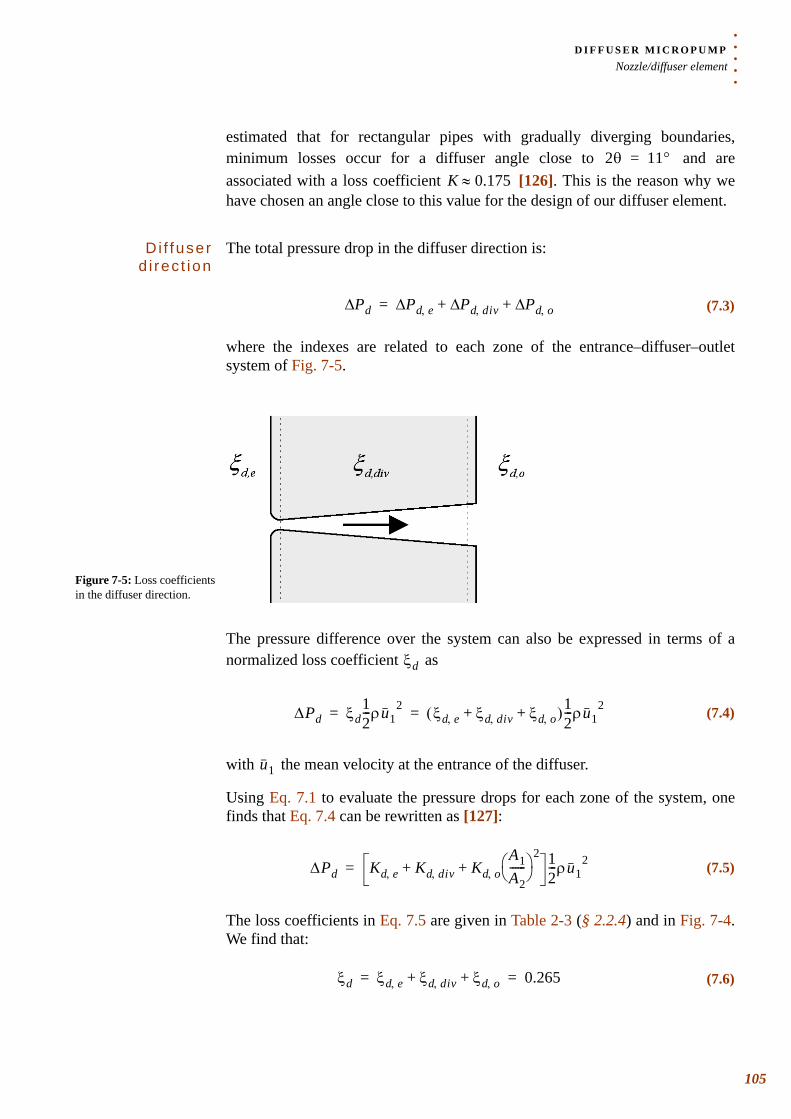
. . .
. .D I F F U S E R M I C R O P U M PNozzle/diffuser element
estimated that for rectangular pipes with gradually diverging boundaries, minimum losses occur for a diffuser angle close to and are associated with a loss coefficient [126]. This is the reason why we have chosen an angle close to this value for the design of our diffuser element.
Di f fuser d i rec t ion
The total pressure drop in the diffuser direction is:
where the indexes are related to each zone of the entrance–diffuser–outlet system of Fig. 7-5.
The pressure difference over the system can also be expressed in terms of a normalized loss coefficient as
with the mean velocity at the entrance of the diffuser.
Using Eq. 7.1 to evaluate the pressure drops for each zone of the system, one finds that Eq. 7.4 can be rewritten as [127]:
The loss coefficients in Eq. 7.5 are given in Table 2-3 (§ 2.2.4) and in Fig. 7-4. We find that:
2θ 11°=K 0.175≈
(7.3)Pd∆ Pd e, Pd div, Pd o,∆+∆+∆=
Figure 7-5: Loss coefficients in the diffuser direction.
ξd
(7.4)∆Pd ξd12---ρu1
2 ξd e, ξd div, ξd o,+ +( )12---ρu1
2= =
u1
(7.5)∆Pd Kd e, Kd div, Kd o,A1A2------⎝ ⎠
⎛ ⎞2
+ + 12---ρu1
2=
(7.6)ξd ξd e, ξd div, ξd o,+ + 0.265= =
105
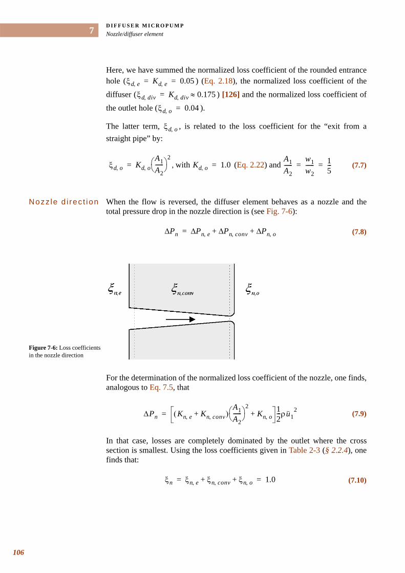
D I F F U S E R M I C R O P U M PNozzle/diffuser element
106
7
Here, we have summed the normalized loss coefficient of the rounded entrance hole ( ) (Eq. 2.18), the normalized loss coefficient of the
diffuser ( ) [126] and the normalized loss coefficient of
the outlet hole ( ).
The latter term, , is related to the loss coefficient for the “exit from a straight pipe” by:
Nozz le d i rec t ion When the flow is reversed, the diffuser element behaves as a nozzle and the total pressure drop in the nozzle direction is (see Fig. 7-6):
For the determination of the normalized loss coefficient of the nozzle, one finds, analogous to Eq. 7.5, that
In that case, losses are completely dominated by the outlet where the cross section is smallest. Using the loss coefficients given in Table 2-3 (§ 2.2.4), one finds that:
ξd e, Kd e, 0.05= =
ξd div, Kd div, 0.175≈=
ξd o, 0.04=
ξd o,
, with (Eq. 2.22) and (7.7)ξd o, Kd o,A1A2------⎝ ⎠
⎛ ⎞2
= Kd o, 1.0=A1A2------
w1w2------ 1
5---= =
(7.8)
Figure 7-6: Loss coefficients in the nozzle direction
Pn∆ Pn e, Pn conv, Pn o,∆+∆+∆=
(7.9)∆Pn Kn e, Kn conv,+( )A1A2------⎝ ⎠
⎛ ⎞2
Kn o,+ 12---ρu1
2=
(7.10)ξn ξn e, ξn conv, ξn o,+ + 1.0= =
. . .
. .D I F F U S E R M I C R O P U M PNozzle/diffuser element
Here, we have summed the normalized loss coefficient of the entrance hole
( ) (Eq. 2.17), the normalized loss coefficient of the
nozzle ( ) (Eq. 2.21), and the normalized loss
coefficient of the outlet hole ( ) (Eq. 2.22).
Di f fuser e f f i c iency
The resulting diffuser element efficiency ratio is defined as [65]:
with and , the volume flows in the diffuser and in the nozzle direction,
respectively. The higher , the higher the flow-directing efficiency. This efficiency ratio is the theoretically achievable one, and is higher than the experimental parameter, as will be shown later. This may be due to the presence of direction-independent losses of the flow in the microfluidic circuit.
7.3.2 N U M E R I C A L S I M U L A T I O N The commercial software package Femlab® 2.2. was used to simulate the nozzle/diffuser element. The program solves the Navier-Stokes equation using a two-equation turbulence model referred to as the “ turbulence model” (cf. § 2.2.6). All simulations were done in two dimensions using water as the fluid
( ; kinematic viscosity ). Defining the Reynolds number for a diffuser as
one finds that for typical flow velocities through the small section of the diffuser which is indicative of the development of a laminar flow regime. V. Singhal et al. [128] have recently presented numerical simulations demonstrating that the flow rectification effect in nozzle/diffuser elements not only occurs in the turbulent flow regime, but can also take place for laminar flows.
ξn e, Kn e, A1 A2⁄( )2 0≈=
ξn conv, Kn conv, A1 A2⁄( )2 0≈=
ξn o, Kn o, 1.0≈=
(7.11)η'ξnξd-----
φdφn-----⎝ ⎠
⎛ ⎞2
3.8= = =
φd φn
η'
k ε–
ρ 1000 kg m 3–⋅= ν 1.0 6–×10 m2 s 1–⋅=Re
(7.12)Reu1w1
ν------------=
Re 100= u1 1 m s 1–⋅=
107
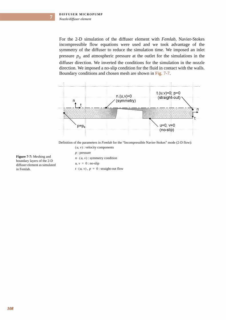
D I F F U S E R M I C R O P U M PNozzle/diffuser element
108
7
For the 2-D simulation of the diffuser element with Femlab, Navier-Stokes incompressible flow equations were used and we took advantage of the symmetry of the diffuser to reduce the simulation time. We imposed an inlet pressure and atmospheric pressure at the outlet for the simulations in the diffuser direction. We inverted the conditions for the simulation in the nozzle direction. We imposed a no-slip condition for the fluid in contact with the walls. Boundary conditions and chosen mesh are shown in Fig. 7-7.
p0
Figure 7-7: Meshing and boundary layers of the 2-D diffuser element as simulated in Femlab.
Definition of the parameters in Femlab for the “Incompressible Navier-Stokes” mode (2-D flow):: velocity components
: pressure: symmetry condition: no-slip, : straight-out flow
u v,( )
pn u v,( )⋅
u v, 0=t u v,( )⋅ p 0=
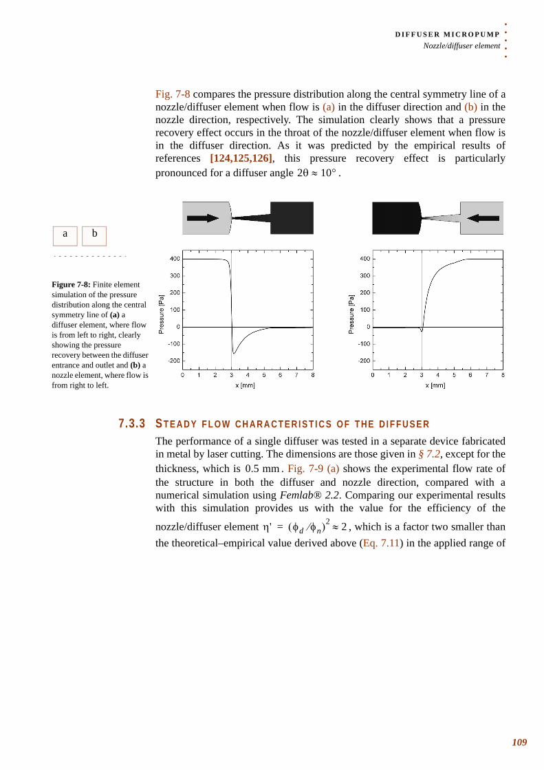
. . .
. .D I F F U S E R M I C R O P U M PNozzle/diffuser element
Fig. 7-8 compares the pressure distribution along the central symmetry line of a nozzle/diffuser element when flow is (a) in the diffuser direction and (b) in the nozzle direction, respectively. The simulation clearly shows that a pressure recovery effect occurs in the throat of the nozzle/diffuser element when flow is in the diffuser direction. As it was predicted by the empirical results of references [124,125,126], this pressure recovery effect is particularly pronounced for a diffuser angle .
7.3.3 S T E A D Y F L O W C H A R A C T E R I S T I C S O F T H E D I F F U S E RThe performance of a single diffuser was tested in a separate device fabricated in metal by laser cutting. The dimensions are those given in § 7.2, except for the thickness, which is . Fig. 7-9 (a) shows the experimental flow rate of the structure in both the diffuser and nozzle direction, compared with a numerical simulation using Femlab® 2.2. Comparing our experimental results with this simulation provides us with the value for the efficiency of the
nozzle/diffuser element , which is a factor two smaller than the theoretical–empirical value derived above (Eq. 7.11) in the applied range of
2θ 10°≈
a b
Figure 7-8: Finite element simulation of the pressure distribution along the central symmetry line of (a) a diffuser element, where flow is from left to right, clearly showing the pressure recovery between the diffuser entrance and outlet and (b) a nozzle element, where flow is from right to left.
0.5 mm
η' φd φn⁄( )2 2≈=
109
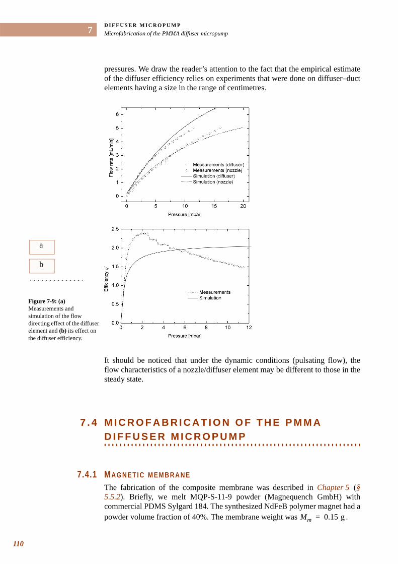
D I F F U S E R M I C R O P U M PMicrofabrication of the PMMA diffuser micropump
110
7
pressures. We draw the reader’s attention to the fact that the empirical estimate of the diffuser efficiency relies on experiments that were done on diffuser–duct elements having a size in the range of centimetres.
It should be noticed that under the dynamic conditions (pulsating flow), the flow characteristics of a nozzle/diffuser element may be different to those in the steady state.
7 . 4 M I C R O F A B R I C A T I O N O F T H E P M M A
. . . . . . . . . . . . . . . . . . . . . . . . . . . . . . . . . . . . . . . . . . . . . . . . . . . . . . . . . . . . . . . . . . .D I F F U S E R M I C R O P U M P
7.4.1 M A G N E T I C M E M B R A N EThe fabrication of the composite membrane was described in Chapter 5 (§ 5.5.2). Briefly, we melt MQP-S-11-9 powder (Magnequench GmbH) with commercial PDMS Sylgard 184. The synthesized NdFeB polymer magnet had a powder volume fraction of 40%. The membrane weight was .
a
b
Figure 7-9: (a) Measurements and simulation of the flow directing effect of the diffuser element and (b) its effect on the diffuser efficiency.
Mm 0.15 g=
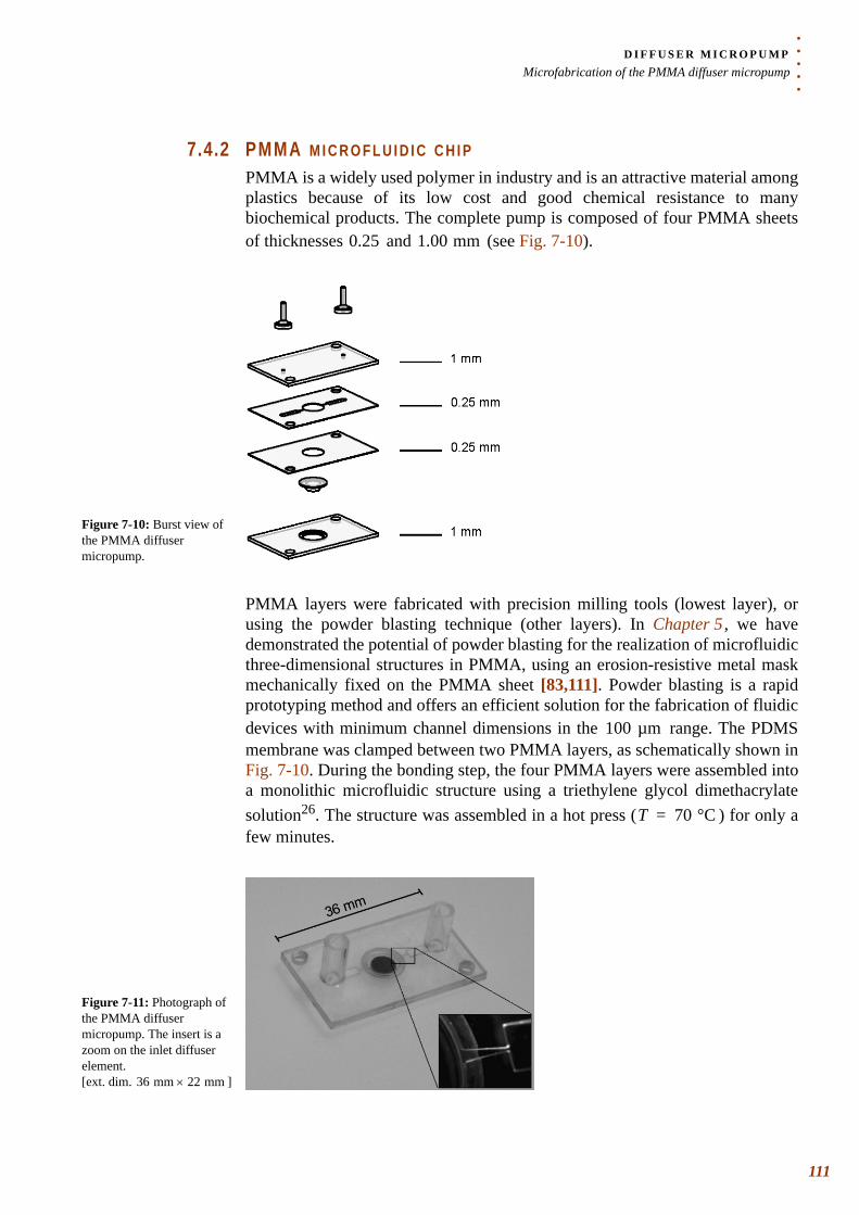
. . .
. .D I F F U S E R M I C R O P U M PMicrofabrication of the PMMA diffuser micropump
7.4.2 PMMA M I C R O F L U I D I C C H I PPMMA is a widely used polymer in industry and is an attractive material among plastics because of its low cost and good chemical resistance to many biochemical products. The complete pump is composed of four PMMA sheets of thicknesses and (see Fig. 7-10).
PMMA layers were fabricated with precision milling tools (lowest layer), or using the powder blasting technique (other layers). In Chapter 5 , we have demonstrated the potential of powder blasting for the realization of microfluidic three-dimensional structures in PMMA, using an erosion-resistive metal mask mechanically fixed on the PMMA sheet [83,111]. Powder blasting is a rapid prototyping method and offers an efficient solution for the fabrication of fluidic devices with minimum channel dimensions in the range. The PDMS membrane was clamped between two PMMA layers, as schematically shown in Fig. 7-10. During the bonding step, the four PMMA layers were assembled into a monolithic microfluidic structure using a triethylene glycol dimethacrylate solution26. The structure was assembled in a hot press ( ) for only a few minutes.
0.25 1.00 mm
Figure 7-10: Burst view of the PMMA diffuser micropump.
100 µm
T 70 °C=
Figure 7-11: Photograph of the PMMA diffuser micropump. The insert is a zoom on the inlet diffuser element. [ext. dim. ]36 mm 22 mm×
111
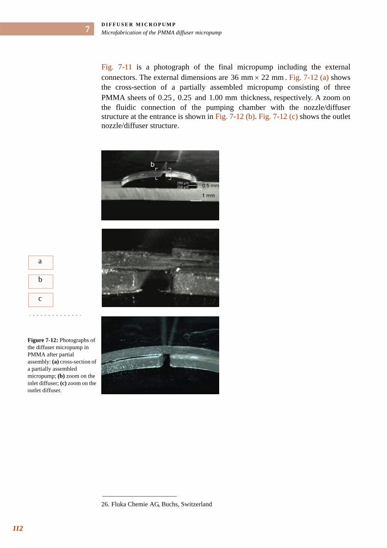
D I F F U S E R M I C R O P U M PMicrofabrication of the PMMA diffuser micropump
112
7
Fig. 7-11 is a photograph of the final micropump including the external connectors. The external dimensions are . Fig. 7-12 (a) shows the cross-section of a partially assembled micropump consisting of three PMMA sheets of , and thickness, respectively. A zoom on the fluidic connection of the pumping chamber with the nozzle/diffuser structure at the entrance is shown in Fig. 7-12 (b). Fig. 7-12 (c) shows the outlet nozzle/diffuser structure.
26. Fluka Chemie AG, Buchs, Switzerland
36 mm 22 mm×
0.25 0.25 1.00 mm
a
b
c
Figure 7-12: Photographs of the diffuser micropump in PMMA after partial assembly: (a) cross-section of a partially assembled micropump; (b) zoom on the inlet diffuser; (c) zoom on the outlet diffuser.
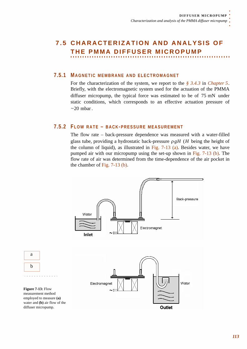
. . .
. .D I F F U S E R M I C R O P U M PCharacterization and analysis of the PMMA diffuser micropump
7 . 5 C H A R A C T E R I Z A T I O N A N D A N A L Y S I S O F
. . . . . . . . . . . . . . . . . . . . . . . . . . . . . . . . . . . . . . . . . . . . . . . . . . . . . . . . . . . . . . . . . . .T H E P M M A D I F F U S E R M I C R O P U M P
7.5.1 M A G N E T I C M E M B R A N E A N D E L E C T R O M A G N E T For the characterization of the system, we report to the § 3.4.3 in Chapter 5 . Briefly, with the electromagnetic system used for the actuation of the PMMA diffuser micropump, the typical force was estimated to be of under static conditions, which corresponds to an effective actuation pressure of
.
7.5.2 F L O W R A T E – B A C K- P R E S S U R E M E A S U R E M E N T The flow rate – back-pressure dependence was measured with a water-filled glass tube, providing a hydrostatic back-pressure ( being the height of the column of liquid), as illustrated in Fig. 7-13 (a). Besides water, we have pumped air with our micropump using the set-up shown in Fig. 7-13 (b). The flow rate of air was determined from the time-dependence of the air pocket in the chamber of Fig. 7-13 (b).
75 mN
~20 mbar
ρgH H
a
b
Figure 7-13: Flow measurement method employed to measure (a) water and (b) air flow of the diffuser micropump.
113
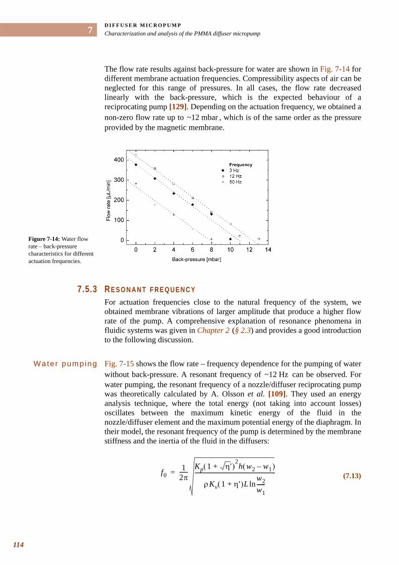
D I F F U S E R M I C R O P U M PCharacterization and analysis of the PMMA diffuser micropump
114
7
The flow rate results against back-pressure for water are shown in Fig. 7-14 for different membrane actuation frequencies. Compressibility aspects of air can be neglected for this range of pressures. In all cases, the flow rate decreased linearly with the back-pressure, which is the expected behaviour of a reciprocating pump [129]. Depending on the actuation frequency, we obtained a non-zero flow rate up to , which is of the same order as the pressure provided by the magnetic membrane.
7.5.3 R E S O N A N T F R E Q U E N C YFor actuation frequencies close to the natural frequency of the system, we obtained membrane vibrations of larger amplitude that produce a higher flow rate of the pump. A comprehensive explanation of resonance phenomena in fluidic systems was given in Chapter 2 (§ 2.3) and provides a good introduction to the following discussion.
Water pumping Fig. 7-15 shows the flow rate – frequency dependence for the pumping of water without back-pressure. A resonant frequency of can be observed. For water pumping, the resonant frequency of a nozzle/diffuser reciprocating pump was theoretically calculated by A. Olsson et al. [109]. They used an energy analysis technique, where the total energy (not taking into account losses) oscillates between the maximum kinetic energy of the fluid in the nozzle/diffuser element and the maximum potential energy of the diaphragm. In their model, the resonant frequency of the pump is determined by the membrane stiffness and the inertia of the fluid in the diffusers:
~12 mbar
Figure 7-14: Water flow rate – back-pressure characteristics for different actuation frequencies.
~12 Hz
(7.13)f01
2π------
Kp 1 η'+( )2h w2 w1–( )
ρKv 1 η'+( )Lw2w1------ln
------------------------------------------------------------=
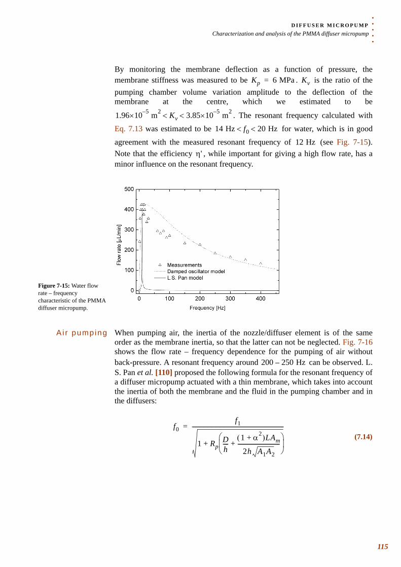
. . .
. .D I F F U S E R M I C R O P U M PCharacterization and analysis of the PMMA diffuser micropump
By monitoring the membrane deflection as a function of pressure, the membrane stiffness was measured to be . is the ratio of the pumping chamber volume variation amplitude to the deflection of the membrane at the centre, which we estimated to be
. The resonant frequency calculated with
Eq. 7.13 was estimated to be for water, which is in good
agreement with the measured resonant frequency of (see Fig. 7-15). Note that the efficiency , while important for giving a high flow rate, has a minor influence on the resonant frequency.
Ai r pumping When pumping air, the inertia of the nozzle/diffuser element is of the same order as the membrane inertia, so that the latter can not be neglected. Fig. 7-16shows the flow rate – frequency dependence for the pumping of air without back-pressure. A resonant frequency around can be observed. L. S. Pan et al. [110] proposed the following formula for the resonant frequency of a diffuser micropump actuated with a thin membrane, which takes into account the inertia of both the membrane and the fluid in the pumping chamber and in the diffusers:
Kp 6 MPa= Kv
1.96 5–×10 m2 Kv 3.85 5–×10 m2< <
14 Hz f0 20 Hz< <
12 Hzη'
Figure 7-15: Water flow rate – frequency characteristic of the PMMA diffuser micropump.
200 250 Hz–
(7.14)f0
f1
1 RpDh----
1 α2+( )LAm
2h A1A2
-------------------------------+⎝ ⎠⎜ ⎟⎛ ⎞
+
--------------------------------------------------------------------=
115
D I F F U S E R M I C R O P U M PCharacterization and analysis of the PMMA diffuser micropump
116
7
where is the membrane surface, is the ratio between the fluid density
and the equivalent membrane density . The resonant
frequency of the membrane is determined by its elastic constant and mass
:
The pump stroke efficiency is calculated from Eq. 7.6 and Eq. 7.10:
From Eq. 7.16, we find that:
For , and neglecting the inertia of the fluid in the chamber (term ), Eq. 7.14 can be rewritten as:
Am Rp ρ
ρm Mm Amh( )⁄=
f1
Mm
(7.15)f11
2π------
KpAmMm
-------------=
α
(7.16)αξn ξd–
ξn ξd+------------------------- η' 1–
η' 1+------------------= =
(7.17)1 α2+
2--------------- 1 η'+
1 η'+( )2
-------------------------=
Rp 1» D h⁄
(7.18)f0
f1
Rp1 α2+( )LAm
2h A1A2
-------------------------------⎝ ⎠⎜ ⎟⎛ ⎞
------------------------------------------------=
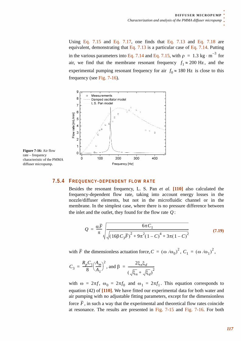
. . .
. .D I F F U S E R M I C R O P U M PCharacterization and analysis of the PMMA diffuser micropump
Using Eq. 7.15 and Eq. 7.17, one finds that Eq. 7.13 and Eq. 7.18 are equivalent, demonstrating that Eq. 7.13 is a particular case of Eq. 7.14. Putting
in the various parameters into Eq. 7.14 and Eq. 7.15, with for air, we find that the membrane resonant frequency , and the
experimental pumping resonant frequency for air is close to this frequency (see Fig. 7-16).
7.5.4 F R E Q U E N C Y- D E P E N D E N T F L O W R A T EBesides the resonant frequency, L. S. Pan et al. [110] also calculated the frequency-dependent flow rate, taking into account energy losses in the nozzle/diffuser elements, but not in the microfluidic channel or in the membrane. In the simplest case, where there is no pressure difference between the inlet and the outlet, they found for the flow rate :
with the dimensionless actuation force, , ,
, and
with , and . This equation corresponds to equation (42) of [110]. We have fitted our experimental data for both water and air pumping with no adjustable fitting parameters, except for the dimensionless force , in such a way that the experimental and theoretical flow rates coincide at resonance. The results are presented in Fig. 7-15 and Fig. 7-16. For both
ρ 1.3 kg m 3–⋅=f1 200 Hz≈
f0 180 Hz≈
Figure 7-16: Air flow rate – frequency characteristic of the PMMA diffuser micropump.
Q
(7.19)Q αFπ
-------6πC1
16βC3F( )2 9π2 1 C–( )4 3π 1 C–( )2+ +
------------------------------------------------------------------------------------------------------=
F C ω ω0⁄( )2= C1 ω ω1⁄( )2=
C3RpC1
8------------
AmA1-------⎝ ⎠
⎛ ⎞2
= β2ξnξd
ξn ξd+( )2
---------------------------------=
ω 2πf= ω0 2πf0= ω1 2πf1=
F
117
D I F F U S E R M I C R O P U M PCharacterization and analysis of the PMMA diffuser micropump
118
7
cases, the theory of L. S. Pan et al. predicts a very narrow resonance peak due to an underestimation of the losses in the fluidic circuit. In the case of a forced oscillating system with damping the dependence of the membrane deflection amplitude on pulsation is given by [20]:
with a dimensionless damping coefficient, and the average static
deflection of the membrane for the applied force , which can be written as:
The flow rate of the pump can be estimated from the average membrane deflection amplitude times the pulsation , corrected by the pump stroke efficiency , giving the following equation:
Rewriting Eq. 7.22 results in:
For our micropump losses take place in the diffusers, in the channels, and in the membrane. These multiple sources complicate the estimation of the parameter
. The following values were used for the fitting curve of Fig. 7-15: , , , , ; while for the curve
of Fig. 7-16, we find that , , , ,
; in good agreement with the geometrical parameters of the micropump. We note that the damping effect is more important for water than for air, which can be related to the higher dynamic viscosity of water
( @ ) compared to air
( @ ). For comparison, if we fit the theoretical curves of L. S. Pan et al. with the damped forced oscillator model, we find for the dimensionless damping coefficient and
X ω
(7.20)X
δstatic
2ξ ωω0------⎝ ⎠
⎛ ⎞ 21 ω
ω0------⎝ ⎠
⎛ ⎞ 2–⎝ ⎠
⎛ ⎞ 2+
---------------------------------------------------------------=
ξ δstatic
F
(7.21)δstaticF
KpAm-------------=
QX ω
α
(7.22)Q απ---AmXω≈
(7.23)Q απ---Amδstaticω1
ωω1------⎝ ⎠
⎛ ⎞ 2
2ξ ωω0------⎝ ⎠
⎛ ⎞ 21 ω
ω0------⎝ ⎠
⎛ ⎞ 2–⎝ ⎠
⎛ ⎞ 2+
-----------------------------------------------------------≈
ξ α 0.2=δstatic 170 µm= ξ 35= f0 12 Hz= f1 200 Hz=
α 0.2= δstatic 55 µm= ξ 0.7= f0 180 Hz=
f1 200 Hz=
µwater 1.0 3–×10 N m 2– s⋅ ⋅= 20 °C
µair 1.8 5–×10 N m 2– s⋅ ⋅= 20 °C
ξ 0.35= ξ 0.007=
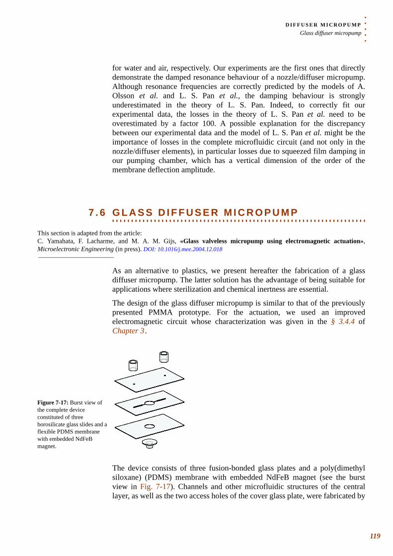
. . .
. .D I F F U S E R M I C R O P U M PGlass diffuser micropump
for water and air, respectively. Our experiments are the first ones that directly demonstrate the damped resonance behaviour of a nozzle/diffuser micropump. Although resonance frequencies are correctly predicted by the models of A. Olsson et al. and L. S. Pan et al., the damping behaviour is strongly underestimated in the theory of L. S. Pan. Indeed, to correctly fit our experimental data, the losses in the theory of L. S. Pan et al. need to be overestimated by a factor 100. A possible explanation for the discrepancy between our experimental data and the model of L. S. Pan et al. might be the importance of losses in the complete microfluidic circuit (and not only in the nozzle/diffuser elements), in particular losses due to squeezed film damping in our pumping chamber, which has a vertical dimension of the order of the membrane deflection amplitude.
. . . . . . . . . . . . . . . . . . . . . . . . . . . . . . . . . . . . . . . . . . . . . . . . . . . . . . . . . . . . . . . . . . .7 . 6 G L A S S D I F F U S E R M I C R O P U M P
This section is adapted from the article: C. Yamahata, F. Lacharme, and M. A. M. Gijs, «Glass valveless micropump using electromagnetic actuation», Microelectronic Engineering (in press). DOI: 10.1016/j.mee.2004.12.018
As an alternative to plastics, we present hereafter the fabrication of a glass diffuser micropump. The latter solution has the advantage of being suitable for applications where sterilization and chemical inertness are essential.
The design of the glass diffuser micropump is similar to that of the previously presented PMMA prototype. For the actuation, we used an improved electromagnetic circuit whose characterization was given in the § 3.4.4 of Chapter 3 .
The device consists of three fusion-bonded glass plates and a poly(dimethyl siloxane) (PDMS) membrane with embedded NdFeB magnet (see the burst view in Fig. 7-17). Channels and other microfluidic structures of the central layer, as well as the two access holes of the cover glass plate, were fabricated by
Figure 7-17: Burst view of the complete device constituted of three borosilicate glass slides and a flexible PDMS membrane with embedded NdFeB magnet.
119
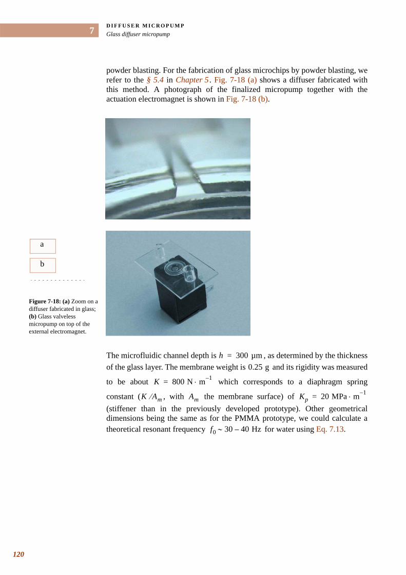
D I F F U S E R M I C R O P U M PGlass diffuser micropump
120
7
powder blasting. For the fabrication of glass microchips by powder blasting, we refer to the § 5.4 in Chapter 5 . Fig. 7-18 (a) shows a diffuser fabricated with this method. A photograph of the finalized micropump together with the actuation electromagnet is shown in Fig. 7-18 (b).
The microfluidic channel depth is , as determined by the thickness of the glass layer. The membrane weight is and its rigidity was measured
to be about which corresponds to a diaphragm spring
constant ( , with the membrane surface) of (stiffener than in the previously developed prototype). Other geometrical dimensions being the same as for the PMMA prototype, we could calculate a theoretical resonant frequency for water using Eq. 7.13.
a
b
Figure 7-18: (a) Zoom on a diffuser fabricated in glass; (b) Glass valveless micropump on top of the external electromagnet.
h 300 µm=0.25 g
K 800 N m 1–⋅=
K Am⁄ Am Kp 20 MPa m 1–⋅=
f0 30 40 Hz–∼
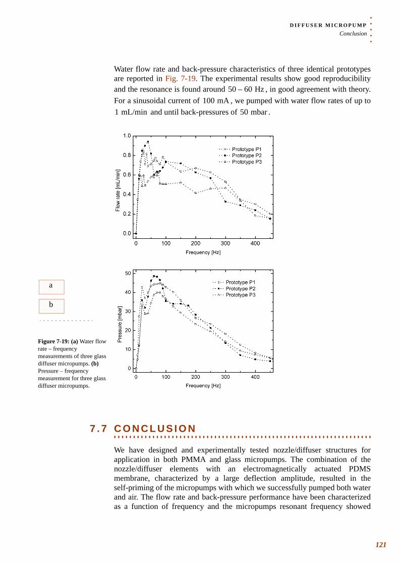
. . .
. .D I F F U S E R M I C R O P U M PConclusion
Water flow rate and back-pressure characteristics of three identical prototypes are reported in Fig. 7-19. The experimental results show good reproducibility and the resonance is found around , in good agreement with theory. For a sinusoidal current of , we pumped with water flow rates of up to
and until back-pressures of .
. . . . . . . . . . . . . . . . . . . . . . . . . . . . . . . . . . . . . . . . . . . . . . . . . . . . . . . . . . . . . . . . . . .7 . 7 C O N C L U S I O N
We have designed and experimentally tested nozzle/diffuser structures for application in both PMMA and glass micropumps. The combination of the nozzle/diffuser elements with an electromagnetically actuated PDMS membrane, characterized by a large deflection amplitude, resulted in the self-priming of the micropumps with which we successfully pumped both water and air. The flow rate and back-pressure performance have been characterized as a function of frequency and the micropumps resonant frequency showed
50 60 Hz–100 mA
1 mL/min 50 mbar
a
b
Figure 7-19: (a) Water flow rate – frequency measurements of three glass diffuser micropumps. (b) Pressure – frequency measurement for three glass diffuser micropumps.
121
D I F F U S E R M I C R O P U M PConclusion
122
7
good agreement with the theoretical models of A. Olsson et al. [109] and L. S. Pan et al. [110]. We verified in particular that the frequency-dependent flow rate of the nozzle-diffuser micropump can be well understood by a fluidic damped oscillator model.
CHAPTER
8. . . . .
. . . . . . . . . . . . . . . . . . . . . . . . . . . . . . . . . . .BALL VALVE MICROPUMP *
* Adapted version of: C. Yamahata, F. Lacharme, Y. Burri, and M. A. M. Gijs, «A ball valve micropump in glass fabricated by powder blasting», Sensors and actuators B: Chemical (in press). DOI: 10.1016/j.snb.2005.01.005
all-valves, consisting of spheres contained within a conical chamber, are commonly used in the macroworld of reciprocating pumps. Although ball valves are excellent candidates for the generation of
unidirectional pumping flows, they have been rarely used in micropumps. This might be because of their non-trivial combination with classical 2-D technologies.
A first type of ball valve micropump fabricated by stereolithography was presented by M. C. Carrozza et al. [130] in 1995. They used the stereolithography fabrication technique to build complex 3-D hemispherical ball chambers. The micropump was piezoelectrically actuated with a PZT disc glued on its membrane. For a sinusoidal of , the maximum water flow rate was and a maximum back-pressure of was obtained. A second type of ball valve micropump was presented by O. Krusemark et al. in 1998 [131]. It was made in silicon/glass and had one active electromagnetically actuated ball valve. Alternately, the ball valve could also work in the passive mode [132]. More recently, A. Sin et al. [133] reported a polymethylmethacrylate (PMMA) ball valve micropump with a pneumatically actuated membrane.
In this chapter, we will present two types of ball valve micropumps which were developed using the powder blasting micro-erosion technology. A first type of disposable micropump is made out of polymethylmethacrylate (PMMA), while a second type of re-usable micropump is made out of borosilicate glass; the latter has the advantage of being sterilizable at high temperature ( ). The flexible magnetic actuation membranes were fabricated in polydimethylsiloxane (PDMS) with embedded NdFeB magnetic powder (polymer-bonded magnet) for the plastic micropump, and with a cylindrical NdFeB magnet for the glass micropump.
B
300 V 75 Hz2.7 mL/min 250 mbar
120 °C
123
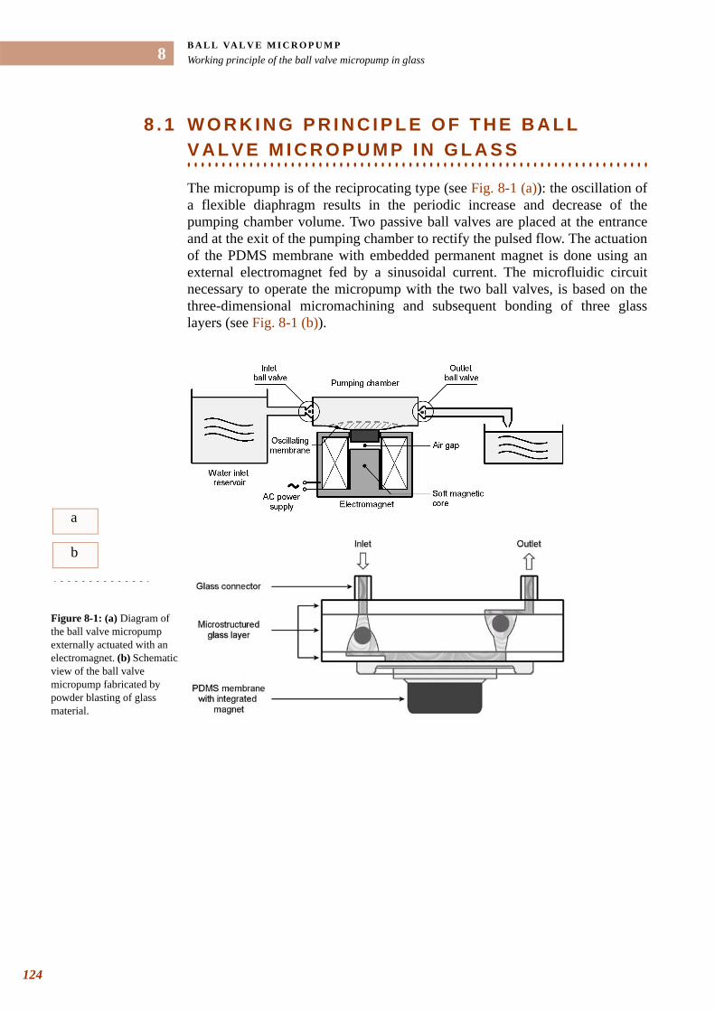
B A L L VA L V E M I C R O P U M PWorking principle of the ball valve micropump in glass
124
8
8 . 1 W O R K I N G P R I N C I P L E O F T H E B A L L
. . . . . . . . . . . . . . . . . . . . . . . . . . . . . . . . . . . . . . . . . . . . . . . . . . . . . . . . . . . . . . . . . . .V A L V E M I C R O P U M P I N G L A S S
The micropump is of the reciprocating type (see Fig. 8-1 (a)): the oscillation of a flexible diaphragm results in the periodic increase and decrease of the pumping chamber volume. Two passive ball valves are placed at the entrance and at the exit of the pumping chamber to rectify the pulsed flow. The actuation of the PDMS membrane with embedded permanent magnet is done using an external electromagnet fed by a sinusoidal current. The microfluidic circuit necessary to operate the micropump with the two ball valves, is based on the three-dimensional micromachining and subsequent bonding of three glass layers (see Fig. 8-1 (b)).
a
b
Figure 8-1: (a) Diagram of the ball valve micropump externally actuated with an electromagnet. (b) Schematic view of the ball valve micropump fabricated by powder blasting of glass material.
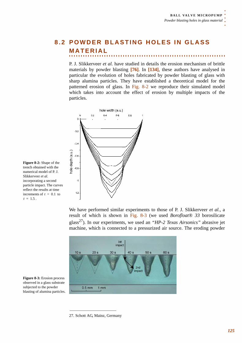
. . .
. .B A L L VA L V E M I C R O P U M PPowder blasting holes in glass material
8 . 2 P O W D E R B L A S T I N G H O L E S I N G L A S S
. . . . . . . . . . . . . . . . . . . . . . . . . . . . . . . . . . . . . . . . . . . . . . . . . . . . . . . . . . . . . . . . . . .M A T E R I A L
P. J. Slikkerveer et al. have studied in details the erosion mechanism of brittle materials by powder blasting [76]. In [134], these authors have analysed in particular the evolution of holes fabricated by powder blasting of glass with sharp alumina particles. They have established a theoretical model for the patterned erosion of glass. In Fig. 8-2 we reproduce their simulated model which takes into account the effect of erosion by multiple impacts of the particles.
We have performed similar experiments to those of P. J. Slikkerveer et al., a result of which is shown in Fig. 8-3 (we used Borofloat® 33 borosilicate glass27). In our experiments, we used an “HP-2 Texas Airsonics” abrasive jet machine, which is connected to a pressurized air source. The eroding powder
Figure 8-2: Shape of the trench obtained with the numerical model of P. J. Slikkerveer et al. incorporating a second particle impact. The curves reflect the results at time increments of to
.t 0.1=
t 1.5=
27. Schott AG, Mainz, Germany
Figure 8-3: Erosion process observed in a glass substrate subjected to the powder blasting of alumina particles.
125
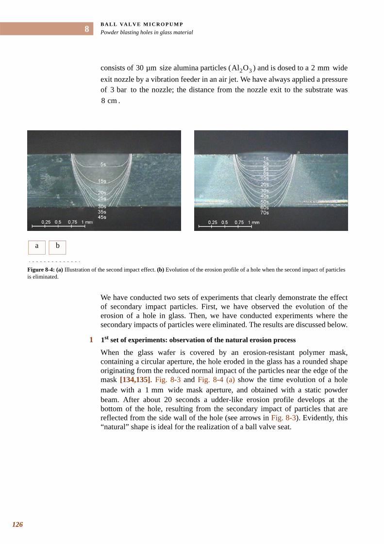
B A L L VA L V E M I C R O P U M PPowder blasting holes in glass material
126
8
consists of size alumina particles ( ) and is dosed to a wide exit nozzle by a vibration feeder in an air jet. We have always applied a pressure of to the nozzle; the distance from the nozzle exit to the substrate was
.
We have conducted two sets of experiments that clearly demonstrate the effect of secondary impact particles. First, we have observed the evolution of the erosion of a hole in glass. Then, we have conducted experiments where the secondary impacts of particles were eliminated. The results are discussed below.
1 1st set of experiments: observation of the natural erosion process
When the glass wafer is covered by an erosion-resistant polymer mask, containing a circular aperture, the hole eroded in the glass has a rounded shape originating from the reduced normal impact of the particles near the edge of the mask [134,135]. Fig. 8-3 and Fig. 8-4 (a) show the time evolution of a hole made with a wide mask aperture, and obtained with a static powder beam. After about 20 seconds a udder-like erosion profile develops at the bottom of the hole, resulting from the secondary impact of particles that are reflected from the side wall of the hole (see arrows in Fig. 8-3). Evidently, this “natural” shape is ideal for the realization of a ball valve seat.
30 µm Al2O3 2 mm
3 bar8 cm
a b
Figure 8-4: (a) Illustration of the second impact effect. (b) Evolution of the erosion profile of a hole when the second impact of particles is eliminated.
1 mm
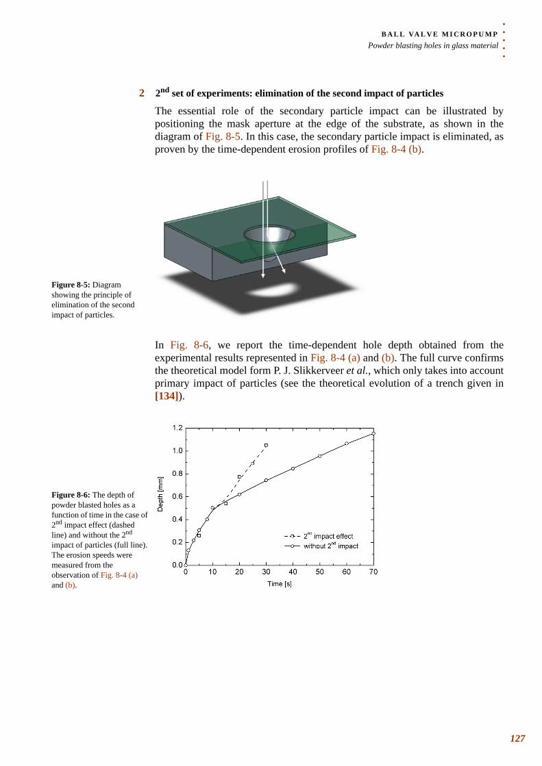
. . .
. .B A L L VA L V E M I C R O P U M PPowder blasting holes in glass material
2 2nd set of experiments: elimination of the second impact of particles
The essential role of the secondary particle impact can be illustrated by positioning the mask aperture at the edge of the substrate, as shown in the diagram of Fig. 8-5. In this case, the secondary particle impact is eliminated, as proven by the time-dependent erosion profiles of Fig. 8-4 (b).
In Fig. 8-6, we report the time-dependent hole depth obtained from the experimental results represented in Fig. 8-4 (a) and (b). The full curve confirms the theoretical model form P. J. Slikkerveer et al., which only takes into account primary impact of particles (see the theoretical evolution of a trench given in [134]).
Figure 8-5: Diagram showing the principle of elimination of the second impact of particles.
Figure 8-6: The depth of powder blasted holes as a function of time in the case of 2nd impact effect (dashed line) and without the 2nd impact of particles (full line). The erosion speeds were measured from the observation of Fig. 8-4 (a) and (b).
127
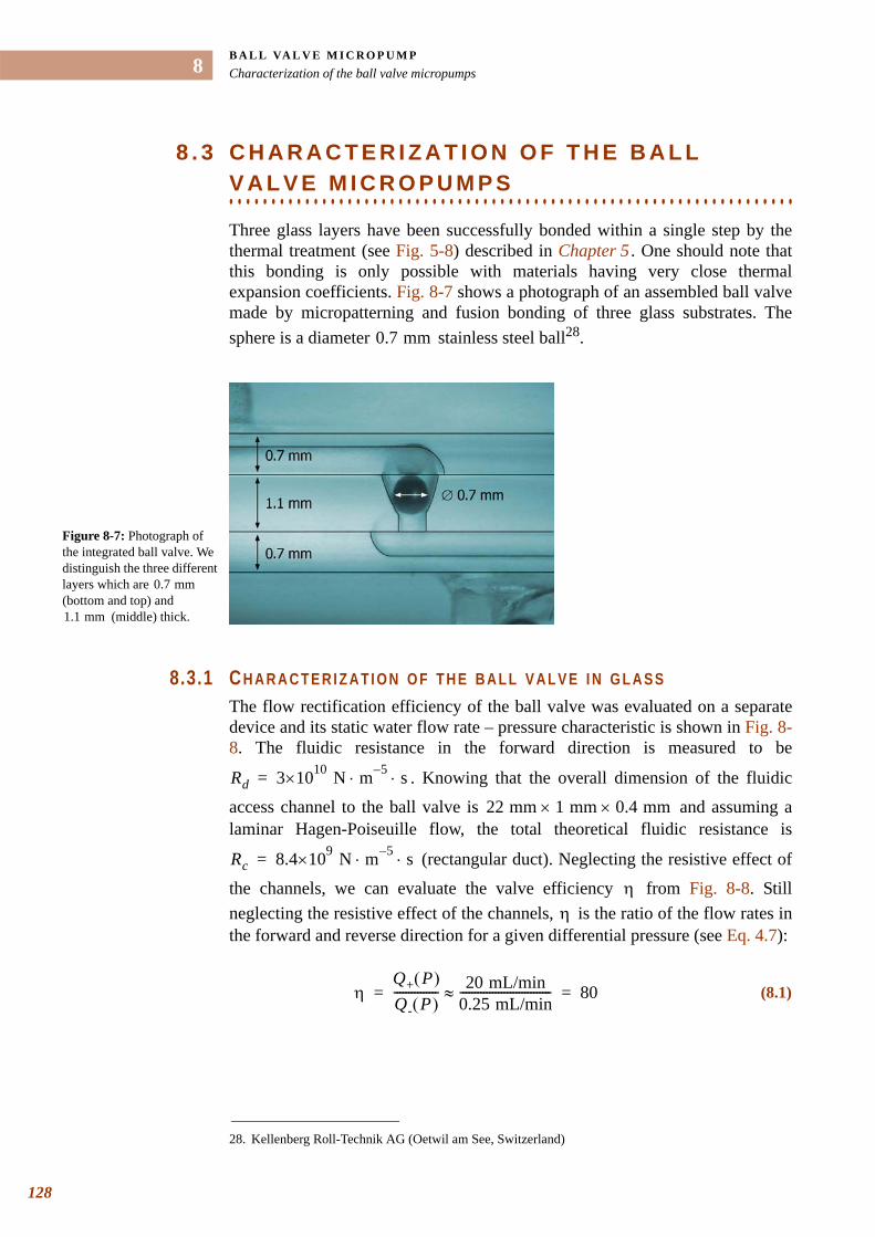
B A L L VA L V E M I C R O P U M PCharacterization of the ball valve micropumps
128
8
8 . 3 C H A R A C T E R I Z A T I O N O F T H E B A L L
. . . . . . . . . . . . . . . . . . . . . . . . . . . . . . . . . . . . . . . . . . . . . . . . . . . . . . . . . . . . . . . . . . .V A L V E M I C R O P U M P S
Three glass layers have been successfully bonded within a single step by the thermal treatment (see Fig. 5-8) described in Chapter 5 . One should note that this bonding is only possible with materials having very close thermal expansion coefficients. Fig. 8-7 shows a photograph of an assembled ball valve made by micropatterning and fusion bonding of three glass substrates. The sphere is a diameter stainless steel ball28.
8.3.1 C H A R A C T E R I Z A T I O N O F T H E B A L L V A L V E I N G L A S SThe flow rectification efficiency of the ball valve was evaluated on a separate device and its static water flow rate – pressure characteristic is shown in Fig. 8-8. The fluidic resistance in the forward direction is measured to be
. Knowing that the overall dimension of the fluidic
access channel to the ball valve is and assuming a laminar Hagen-Poiseuille flow, the total theoretical fluidic resistance is
(rectangular duct). Neglecting the resistive effect of
the channels, we can evaluate the valve efficiency from Fig. 8-8. Still neglecting the resistive effect of the channels, is the ratio of the flow rates in the forward and reverse direction for a given differential pressure (see Eq. 4.7):
28. Kellenberg Roll-Technik AG (Oetwil am See, Switzerland)
0.7 mm
Figure 8-7: Photograph of the integrated ball valve. We distinguish the three different layers which are (bottom and top) and
(middle) thick.
0.7 mm
1.1 mm
Rd 3 10×10 N m 5– s⋅ ⋅=
22 mm 1 mm 0.4 mm××
Rc 8.4 9×10 N m 5– s⋅ ⋅=
ηη
(8.1)ηQ+ P( )Q- P( )--------------- 20 mL/min
0.25 mL/min-------------------------------≈ 80= =
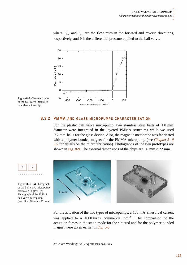
. . .
. .B A L L VA L V E M I C R O P U M PCharacterization of the ball valve micropumps
where and are the flow rates in the forward and reverse directions, respectively, and P is the differential pressure applied to the ball valve.
8.3.2 PMMA A N D G L A S S M I C R O P U M P S C H A R A C T E R I Z A T I O N
For the plastic ball valve micropump, two stainless steel balls of diameter were integrated in the layered PMMA structures while we used
balls for the glass device. Also, the magnetic membrane was fabricated with a polymer-bonded magnet for the PMMA micropump (see Chapter 5 , § 5.5 for details on the microfabrication). Photographs of the two prototypes are shown in Fig. 8-9. The external dimensions of the chips are .
For the actuation of the two types of micropumps, a sinusoidal current was applied to a commercial coil29. The comparison of the actuation forces in the static mode for the sintered and for the polymer-bonded magnet were given earlier in Fig. 3-6.
Q+ Q-
Figure 8-8: Characterization of the ball valve integrated in a glass microchip.
1.0 mm
0.7 mm
36 mm 22 mm×
a b
Figure 8-9: (a) Photograph of the ball valve micropump fabricated in glass. (b) Photograph of the PMMA ball valve micropump. [ext. dim. ]36 mm 22 mm×
29. Atam Windings s.r.l., Agrate Brianza, Italy
100 mA4800 turns
129
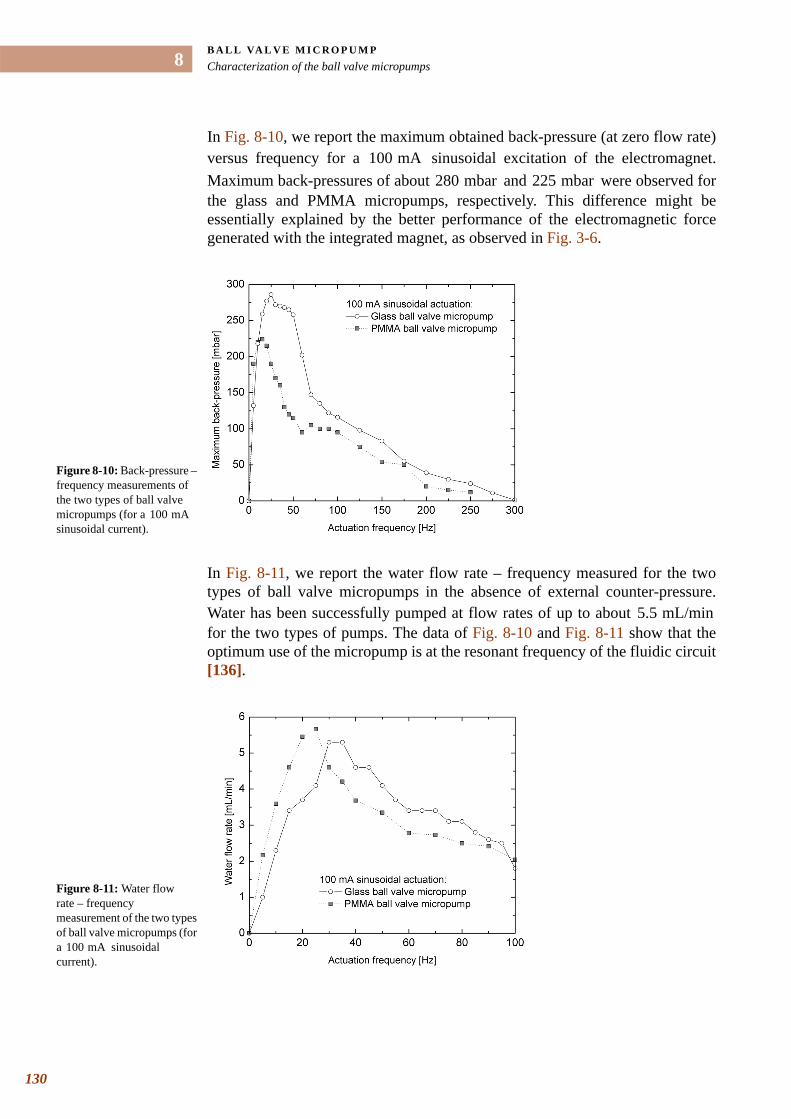
B A L L VA L V E M I C R O P U M PCharacterization of the ball valve micropumps
130
8
In Fig. 8-10, we report the maximum obtained back-pressure (at zero flow rate) versus frequency for a sinusoidal excitation of the electromagnet. Maximum back-pressures of about and were observed for the glass and PMMA micropumps, respectively. This difference might be essentially explained by the better performance of the electromagnetic force generated with the integrated magnet, as observed in Fig. 3-6.
In Fig. 8-11, we report the water flow rate – frequency measured for the two types of ball valve micropumps in the absence of external counter-pressure. Water has been successfully pumped at flow rates of up to about for the two types of pumps. The data of Fig. 8-10 and Fig. 8-11 show that the optimum use of the micropump is at the resonant frequency of the fluidic circuit [136].
100 mA280 mbar 225 mbar
Figure 8-10: Back-pressure – frequency measurements of the two types of ball valve micropumps (for a sinusoidal current).
100 mA
5.5 mL/min
Figure 8-11: Water flow rate – frequency measurement of the two types of ball valve micropumps (for a sinusoidal current).
100 mA
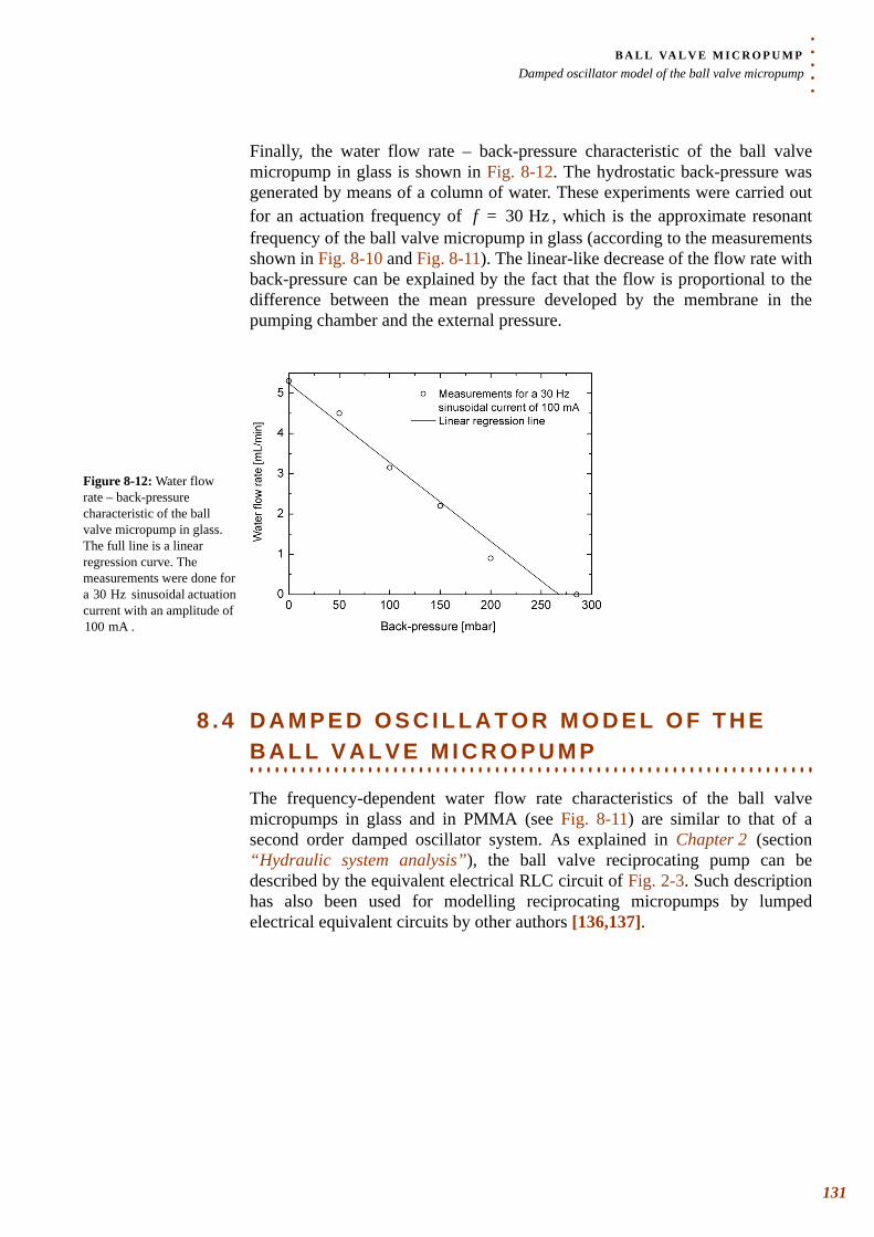
. . .
. .B A L L VA L V E M I C R O P U M PDamped oscillator model of the ball valve micropump
Finally, the water flow rate – back-pressure characteristic of the ball valve micropump in glass is shown in Fig. 8-12. The hydrostatic back-pressure was generated by means of a column of water. These experiments were carried out for an actuation frequency of , which is the approximate resonant frequency of the ball valve micropump in glass (according to the measurements shown in Fig. 8-10 and Fig. 8-11). The linear-like decrease of the flow rate with back-pressure can be explained by the fact that the flow is proportional to the difference between the mean pressure developed by the membrane in the pumping chamber and the external pressure.
8 . 4 D A M P E D O S C I L L A T O R M O D E L O F T H E
. . . . . . . . . . . . . . . . . . . . . . . . . . . . . . . . . . . . . . . . . . . . . . . . . . . . . . . . . . . . . . . . . . .B A L L V A L V E M I C R O P U M P
The frequency-dependent water flow rate characteristics of the ball valve micropumps in glass and in PMMA (see Fig. 8-11) are similar to that of a second order damped oscillator system. As explained in Chapter 2 (section “Hydraulic system analysis”), the ball valve reciprocating pump can be described by the equivalent electrical RLC circuit of Fig. 2-3. Such description has also been used for modelling reciprocating micropumps by lumped electrical equivalent circuits by other authors [136,137].
f 30 Hz=
Figure 8-12: Water flow rate – back-pressure characteristic of the ball valve micropump in glass. The full line is a linear regression curve. The measurements were done for a sinusoidal actuation current with an amplitude of
.
30 Hz
100 mA
131
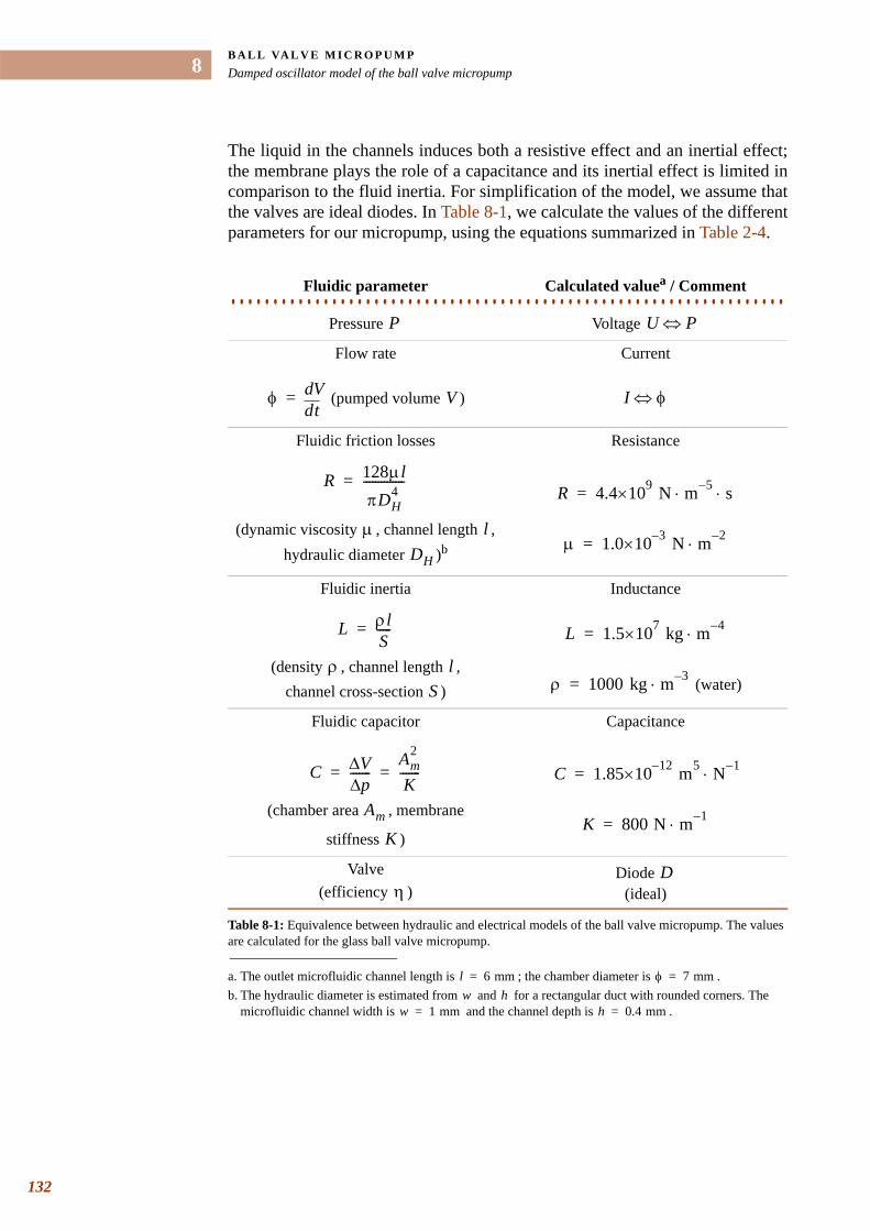
B A L L VA L V E M I C R O P U M PDamped oscillator model of the ball valve micropump
132
8
The liquid in the channels induces both a resistive effect and an inertial effect; the membrane plays the role of a capacitance and its inertial effect is limited in comparison to the fluid inertia. For simplification of the model, we assume that the valves are ideal diodes. In Table 8-1, we calculate the values of the different parameters for our micropump, using the equations summarized in Table 2-4.
Fluidic parameter Calculated valuea / Comment. . . . . . . . . . . . . . . . . . . . . . . . . . . . . . . . . . . . . . . . . . . . . . . . . . . . . . . . . . . . . . . . . . Pressure Voltage
Flow rate Current
(pumped volume )
Fluidic friction losses Resistance
(dynamic viscosity , channel length , hydraulic diameter )b
Fluidic inertia Inductance
(density , channel length ,channel cross-section ) (water)
Fluidic capacitor Capacitance
(chamber area , membrane
stiffness )
Valve (efficiency )
Diode (ideal)
Table 8-1: Equivalence between hydraulic and electrical models of the ball valve micropump. The values are calculated for the glass ball valve micropump.
a. The outlet microfluidic channel length is ; the chamber diameter is .b. The hydraulic diameter is estimated from and for a rectangular duct with rounded corners. The
microfluidic channel width is and the channel depth is .
P U P⇔
φtd
dV= V I φ⇔
R 128µlπDH
4--------------=
µ lDH
R 4.4 9×10 N m 5– s⋅ ⋅=
µ 1.0 3–×10 N m 2–⋅=
L ρlS-----=
ρ lS
L 1.5 7×10 kg m 4–⋅=
ρ 1000 kg m 3–⋅=
C V∆p∆
-------Am
2
K-------= =
Am
K
C 1.85 12–×10 m5 N 1–⋅=
K 800 N m 1–⋅=
ηD
l 6 mm= φ 7 mm=w h
w 1 mm= h 0.4 mm=
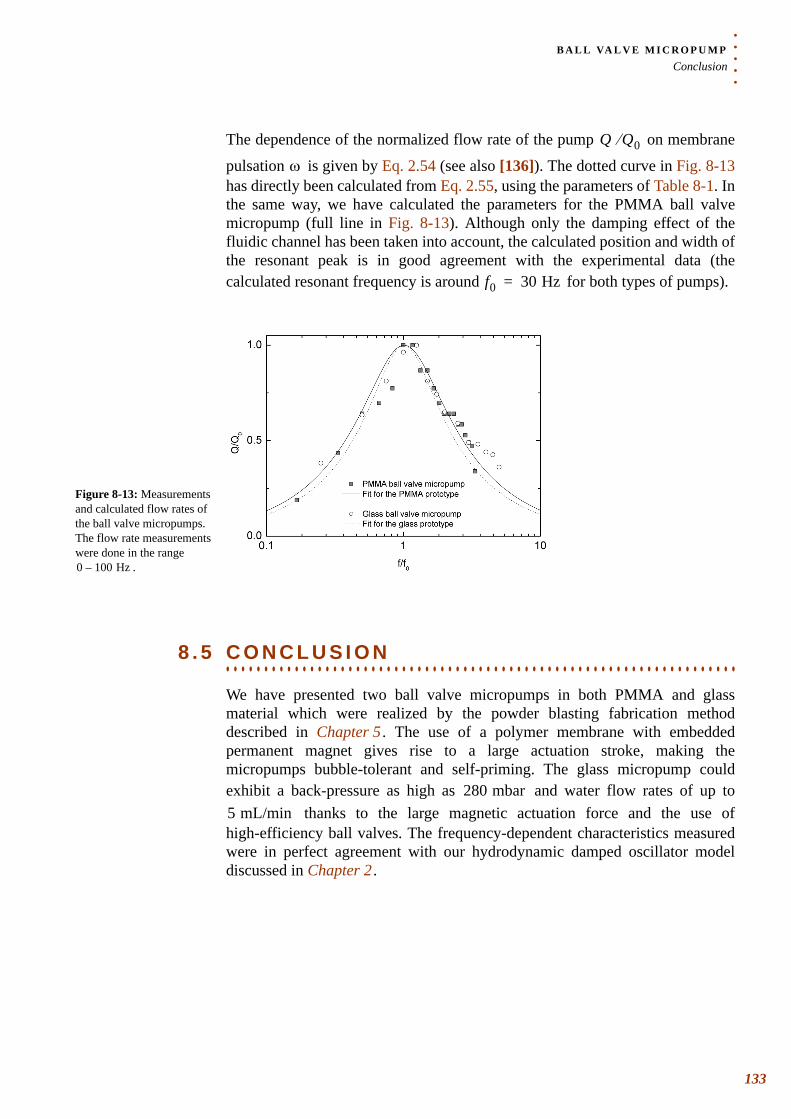
. . .
. .B A L L VA L V E M I C R O P U M PConclusion
The dependence of the normalized flow rate of the pump on membrane
pulsation is given by Eq. 2.54 (see also [136]). The dotted curve in Fig. 8-13has directly been calculated from Eq. 2.55, using the parameters of Table 8-1. In the same way, we have calculated the parameters for the PMMA ball valve micropump (full line in Fig. 8-13). Although only the damping effect of the fluidic channel has been taken into account, the calculated position and width of the resonant peak is in good agreement with the experimental data (the calculated resonant frequency is around for both types of pumps).
. . . . . . . . . . . . . . . . . . . . . . . . . . . . . . . . . . . . . . . . . . . . . . . . . . . . . . . . . . . . . . . . . . .8 . 5 C O N C L U S I O N
We have presented two ball valve micropumps in both PMMA and glass material which were realized by the powder blasting fabrication method described in Chapter 5 . The use of a polymer membrane with embedded permanent magnet gives rise to a large actuation stroke, making the micropumps bubble-tolerant and self-priming. The glass micropump could exhibit a back-pressure as high as and water flow rates of up to
thanks to the large magnetic actuation force and the use of high-efficiency ball valves. The frequency-dependent characteristics measured were in perfect agreement with our hydrodynamic damped oscillator model discussed in Chapter 2 .
Q Q0⁄
ω
f0 30 Hz=
Figure 8-13: Measurements and calculated flow rates of the ball valve micropumps. The flow rate measurements were done in the range
.0 100 Hz–
280 mbar5 mL/min
133

CHAPTER
9. . . . .
. . . . . . . . . . . . . . . . . . . . . . . . . . . . . . . . . . .CONCLUSION AND OUTLOOK
udging from the hundreds of publications that have been reported in recent literature reviews [38,41,49], the micropump is undeniably one of the microsystems that has known most interest among the large number of
microfluidic components realized until now. Evidently, this stems from the essential role that the pumping function plays in fluid delivery microsystems in general, and in lab-on-a-chip (LOC) devices in particular (cf. Fig. 1-2). It was emphasized [3] that the integration of efficient and low-cost pumps and valves, compatible with biochemical analysis in LOC devices, was one of the key challenges for the further spread of this technology.
The approach we have chosen consisted in only integrating the inexpensive parts of a micropump into the LOC device. This led us to choose external actuation for our pumps, thus eliminating the difficulties inherent to connections. Magnetic actuation – although unfavourable when downsizing – turned out to be the best compromise among the different actuator mechanisms due to the large displacement capabilities, the high forces, the fast response time, and the ease of implementation of this kind of actuators (Chapter 4 ). In this scope, we have investigated both the use of ferrofluids, or magnetic liquids, and the electromagnetic actuation of permanent magnets. • Secondly, the need for simple and low-cost methods for the fabrication of microfluidic chips has encouraged us to develop a microfabrication process based on powder blastingtechnology (Chapter 5 ). This rapid prototyping technique could be applied to the fabrication of 3-D microfluidic chips either in polymethylmethacrylate (PMMA) or in glass (borosilicate) material, depending on the targeted application field. Actually, plastics are generally preferred for disposable devices, while glass is an appropriate material for the applications that demand chemical inertness or require a sterilization procedure. • Thirdly, we have proposed different approaches for “positive displacement” pumps using three types of valves. We have developed (i) a ferrofluid piston micropump with silicone check-valves (Chapter 6 ); (ii) a reciprocating diaphragm micropump with nozzle-diffuser elements (Chapter 7 ); and (iii) a reciprocating diaphragm micropump with ball valves (Chapter 8 ).
J
135
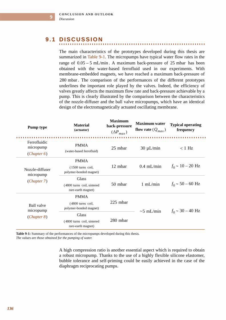
C O N C L U S I O N A N D O U T L O O KDiscussion
136
9
. . . . . . . . . . . . . . . . . . . . . . . . . . . . . . . . . . . . . . . . . . . . . . . . . . . . . . . . . . . . . . . . . . .9 . 1 D I S C U S S I O N
The main characteristics of the prototypes developed during this thesis are summarized in Table 9-1. The micropumps have typical water flow rates in the range of . A maximum back-pressure of has been obtained with the water-based ferrofluid used in our experiments. With membrane-embedded magnets, we have reached a maximum back-pressure of
. The comparison of the performances of the different prototypes underlines the important role played by the valves. Indeed, the efficiency of valves greatly affects the maximum flow rate and back-pressure achievable by a pump. This is clearly illustrated by the comparison between the characteristics of the nozzle-diffuser and the ball valve micropumps, which have an identical design of the electromagnetically actuated oscillating membrane.
A high compression ratio is another essential aspect which is required to obtain a robust micropump. Thanks to the use of a highly flexible silicone elastomer, bubble tolerance and self-priming could be easily achieved in the case of the diaphragm reciprocating pumps.
0.05 5 mL/min– 25 mbar
280 mbar
Pump type Material(actuator)
Maximum back-pressure
( )
Maximum water flow rate ( )
Typical operating frequency
. . . . . . . . . . . . . . . . . . . . . . . . . . . . . . . . . . . . . . . . . . . . . . . . . . . . . . . . . . . . . . . . . . . . . . . . . . . . . . . . . . . . . . . Ferrofluidic micropump(Chapter 6 )
PMMA (water-based ferrofluid)
Nozzle-diffuser micropump(Chapter 7 )
PMMA( coil,
polymer-bonded magnet)
Glass( coil, sintered
rare-earth magnet)
Ball valve micropump(Chapter 8 )
PMMA( coil,
polymer-bonded magnet)
Glass( coil, sintered
rare-earth magnet)
Table 9-1: Summary of the performances of the micropumps developed during this thesis. The values are those obtained for the pumping of water.
Pmax∆ Qmax
25 mbar 30 µL/min 1 Hz<
1500 turns 12 mbar 0.4 mL/min f0 10 20 Hz–∼
4800 turns 50 mbar 1 mL/min f0 50 60 Hz–∼
4800 turns 225 mbar
~5 mL/min f0 30 40 Hz–∼
4800 turns 280 mbar
. . .
. .C O N C L U S I O N A N D O U T L O O KDiscussion
In view of the results obtained during this thesis, we finally conclude for each type of micropump.
• Ferrofluidic micropumpThe magnetic manipulation of ferrofluids is an interesting option for microfluidic applications but the development of the magnetic liquid must be done in sight of a well-defined application. That is, oil-based ferrofluids non-contaminating and immiscible with water would trigger further interest for pumping in microchannels.
• Nozzle-diffuser micropumpAlthough it has a limited efficiency and suffers from back-flow limitations, the nozzle-diffuser micropump has the outstanding advantage of being simple in fabrication. Not only the absence of moving parts in the valves eliminates the risk of wear or clogging, but also prevents damage to biological cells potentially in the pump flow [138]. Thus, this certainly is one of the most promising pumping techniques for microfluidic systems, as proven by the large number of papers related to this microfluidic component.
• Ball valve micropumpThe high efficiency and the robustness of ball valves, together with their relative simplicity represent the main advantages of these elements compared to other check-valves. In particular, the ball valve micropump has shown its potential for applications demanding high flow rates and high back-pressures.
137
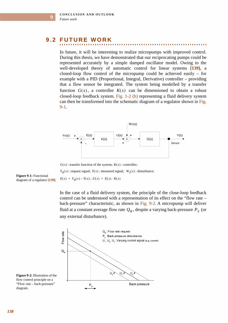
C O N C L U S I O N A N D O U T L O O KFuture work
138
9
. . . . . . . . . . . . . . . . . . . . . . . . . . . . . . . . . . . . . . . . . . . . . . . . . . . . . . . . . . . . . . . . . . .9 . 2 F U T U R E W O R K
In future, it will be interesting to realize micropumps with improved control. During this thesis, we have demonstrated that our reciprocating pumps could be represented accurately by a simple damped oscillator model. Owing to the well-developed theory of automatic control for linear systems [139], a closed-loop flow control of the micropump could be achieved easily – for example with a PID (Proportional, Integral, Derivative) controller – providing that a flow sensor be integrated. The system being modelled by a transfer function , a controller can be dimensioned to obtain a robust closed-loop feedback system. Fig. 1-2 (b) representing a fluid delivery system can then be transformed into the schematic diagram of a regulator shown in Fig. 9-1.
In the case of a fluid delivery system, the principle of the close-loop feedback control can be understood with a representation of its effect on the “flow rate – back-pressure” characteristic, as shown in Fig. 9-2. A micropump will deliver fluid at a constant average flow rate , despite a varying back-pressure (or any external disturbance).
G s( ) K s( )
Figure 9-1: Functional diagram of a regulator [139].
: transfer function of the system; : controller;
: request signal; : measured signal; : disturbance;
;
Σ G(s)Sensor
K(s)ΣYR(s) +
+
WS(s)
+ Y(s)U(s)
-
E(s)
G s( ) K s( )
YR s( ) Y s( ) WS s( )
E s( ) YR s( ) Y s( )–= U s( ) E s( ) K s( )⋅=
QR PS
Figure 9-2: Illustration of the flow control principle on a “Flow rate – back-pressure” diagram.
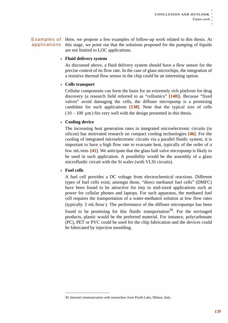
. . .
. .C O N C L U S I O N A N D O U T L O O KFuture work
Examples o f app l ica t ions
Here, we propose a few examples of follow-up work related to this thesis. At this stage, we point out that the solutions proposed for the pumping of liquids are not limited to LOC applications.
Fluid delivery systemAs discussed above, a fluid delivery system should have a flow sensor for the precise control of its flow rate. In the case of glass microchips, the integration of a resistive thermal flow sensor in the chip could be an interesting option.
Cells transportCellular components can form the basis for an extremely rich platform for drug discovery (a research field referred to as “cellomics” [140]). Because “fixed valves” avoid damaging the cells, the diffuser micropump is a promising candidate for such applications [138]. Note that the typical size of cells ( ) fits very well with the design presented in this thesis.
Cooling deviceThe increasing heat generation rates in integrated microelectronic circuits (in silicon) has motivated research on compact cooling technologies [46]. For the cooling of integrated microelectronic circuits via a parallel fluidic system, it is important to have a high flow rate to evacuate heat, typically of the order of a few [41]. We anticipate that the glass ball valve micropump is likely to be used in such application. A possibility would be the assembly of a glass microfluidic circuit with the Si wafer (with VLSI circuits).
Fuel cellsA fuel cell provides a DC voltage from electrochemical reactions. Different types of fuel cells exist; amongst those, “direct methanol fuel cells” (DMFC) have been found to be attractive for tiny to mid-sized applications such as power for cellular phones and laptops. For such apparatus, the methanol fuel cell requires the transportation of a water-methanol solution at low flow rates (typically ). The performance of the diffuser micropumps has been found to be promising for this fluidic transportation30. For the envisaged products, plastic would be the preferred material. For instance, polycarbonate (PC), PET or PVC could be used for the chip fabrication and the devices could be fabricated by injection moulding.
10 100 µm–
mL/min
30. Internal communication with researchers from Pirelli Labs, Milano, Italy.
2 mL/hour
139
VANOLI, «L’Usine Électrique». L’Association (2000).
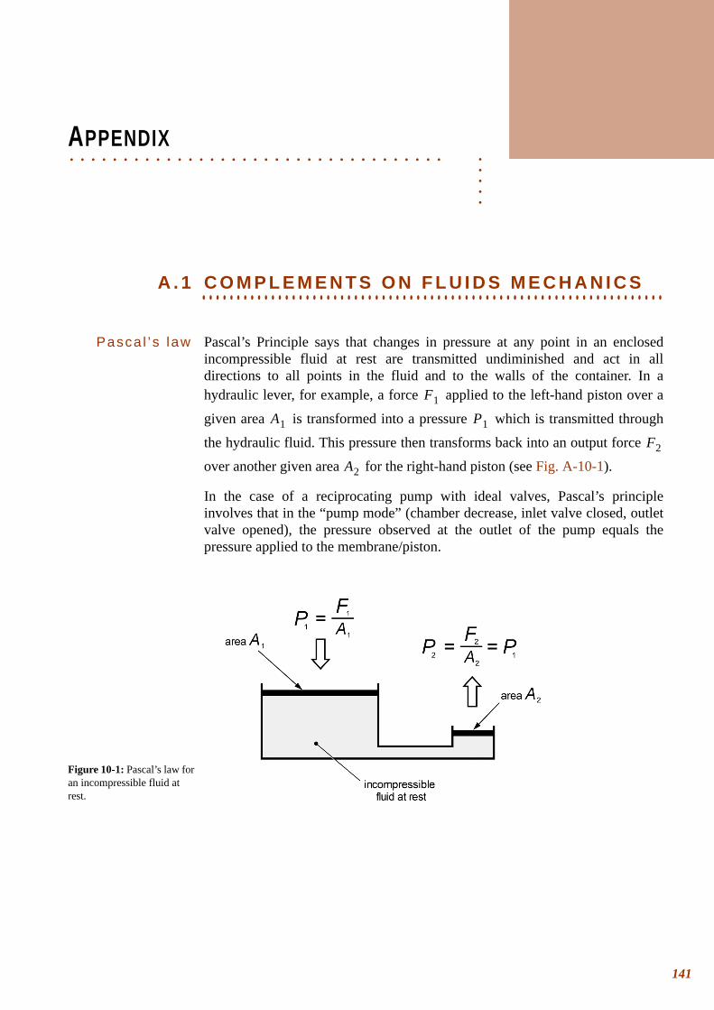
. . . . .
. . . . . . . . . . . . . . . . . . . . . . . . . . . . . . . . . . .APPENDIX
. . . . . . . . . . . . . . . . . . . . . . . . . . . . . . . . . . . . . . . . . . . . . . . . . . . . . . . . . . . . . . . . . . . A . 1 C O M P L E M E N T S O N F L U I D S M E C H A N I C S
Pasca l ’ s law Pascal’s Principle says that changes in pressure at any point in an enclosed incompressible fluid at rest are transmitted undiminished and act in all directions to all points in the fluid and to the walls of the container. In a hydraulic lever, for example, a force applied to the left-hand piston over a
given area is transformed into a pressure which is transmitted through
the hydraulic fluid. This pressure then transforms back into an output force
over another given area for the right-hand piston (see Fig. A-10-1).
In the case of a reciprocating pump with ideal valves, Pascal’s principle involves that in the “pump mode” (chamber decrease, inlet valve closed, outlet valve opened), the pressure observed at the outlet of the pump equals the pressure applied to the membrane/piston.
F1
A1 P1
F2
A2
Figure 10-1: Pascal’s law for an incompressible fluid at rest.
141
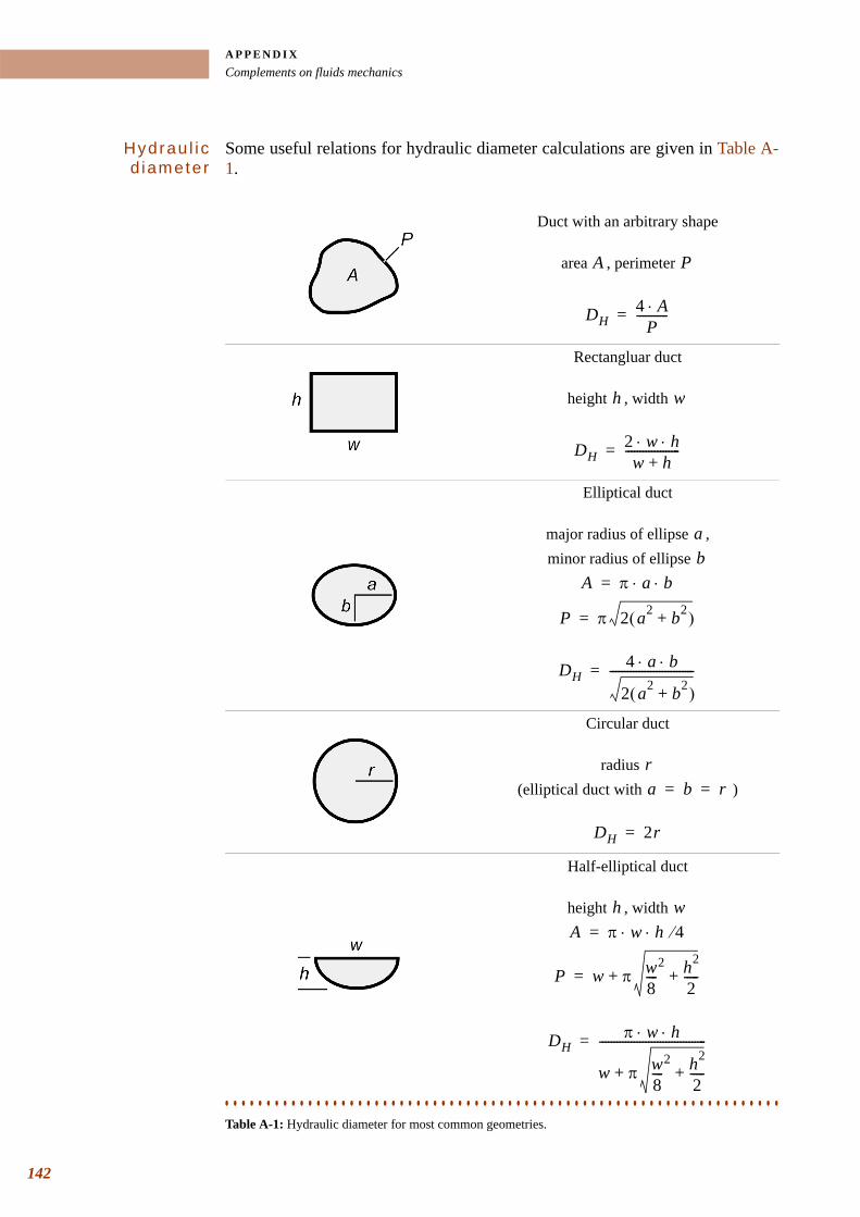
A P P E N D I XComplements on fluids mechanics
142
Hydrau l i c d iameter
Some useful relations for hydraulic diameter calculations are given in Table A-1.
Duct with an arbitrary shape
area , perimeter
Rectangluar duct
height , width
Elliptical duct
major radius of ellipse , minor radius of ellipse
Circular duct
radius (elliptical duct with )
Half-elliptical duct
height , width
. . . . . . . . . . . . . . . . . . . . . . . . . . . . . . . . . . . . . . . . . . . . . . . . . . . . . . . . . . . . . . . . . . . Table A-1: Hydraulic diameter for most common geometries.
A P
DH4 A⋅
P-----------=
h w
DH2 w h⋅ ⋅w h+
-------------------=
ab
A π a b⋅ ⋅=
P π 2 a2 b2+( )=
DH4 a b⋅ ⋅
2 a2 b2+( )-----------------------------=
ra b r= =
DH 2r=
h wA π w h 4⁄⋅ ⋅=
P w π w8----
2 h2
2-----++=
DHπ w h⋅ ⋅
w π w8----
2 h2
2-----++
-------------------------------------=
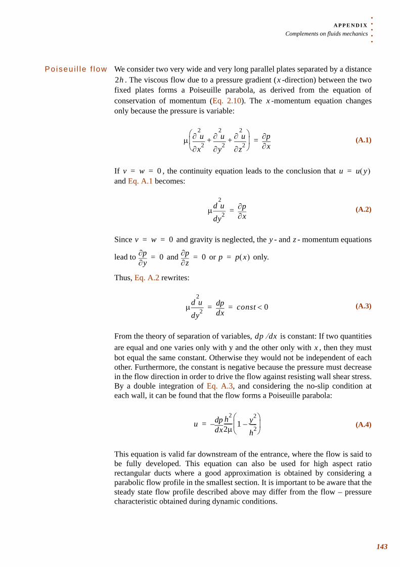
. . .
. .A P P E N D I XComplements on fluids mechanics
Poiseu i l le f low We consider two very wide and very long parallel plates separated by a distance . The viscous flow due to a pressure gradient ( -direction) between the two
fixed plates forms a Poiseuille parabola, as derived from the equation of conservation of momentum (Eq. 2.10). The -momentum equation changes only because the pressure is variable:
If , the continuity equation leads to the conclusion that and Eq. A.1 becomes:
Since and gravity is neglected, the - and - momentum equations
lead to and or only.
Thus, Eq. A.2 rewrites:
From the theory of separation of variables, is constant: If two quantities are equal and one varies only with y and the other only with , then they must bot equal the same constant. Otherwise they would not be independent of each other. Furthermore, the constant is negative because the pressure must decrease in the flow direction in order to drive the flow against resisting wall shear stress. By a double integration of Eq. A.3, and considering the no-slip condition at each wall, it can be found that the flow forms a Poiseuille parabola:
This equation is valid far downstream of the entrance, where the flow is said to be fully developed. This equation can also be used for high aspect ratio rectangular ducts where a good approximation is obtained by considering a parabolic flow profile in the smallest section. It is important to be aware that the steady state flow profile described above may differ from the flow – pressure characteristic obtained during dynamic conditions.
2h x
x
(A.1)µx2
2
∂
∂ uy2
2
∂
∂ uz2
2
∂
∂ u+ +⎝ ⎠⎜ ⎟⎛ ⎞
x∂∂p=
v w 0= = u u y( )=
(A.2)µy2
2
dd u
x∂∂p=
v w 0= = y z
y∂∂p 0=
z∂∂p 0= p p x( )=
(A.3)µy2
2
dd u
xddp const 0<= =
dp dx⁄x
(A.4)uxd
dp– h2
2µ------ 1 y2
h2-----–
⎝ ⎠⎜ ⎟⎛ ⎞
=
143
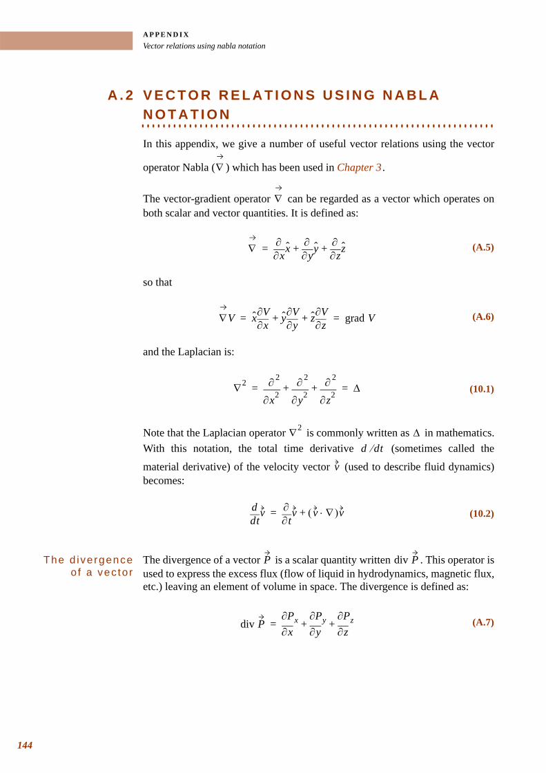
A P P E N D I XVector relations using nabla notation
144
A . 2 V E C T O R R E L A T I O N S U S I N G N A B L A
. . . . . . . . . . . . . . . . . . . . . . . . . . . . . . . . . . . . . . . . . . . . . . . . . . . . . . . . . . . . . . . . . . . N O T A T I O N
In this appendix, we give a number of useful vector relations using the vector
operator Nabla ( ) which has been used in Chapter 3 .
The vector-gradient operator can be regarded as a vector which operates on both scalar and vector quantities. It is defined as:
so that
and the Laplacian is:
Note that the Laplacian operator is commonly written as in mathematics. With this notation, the total time derivative (sometimes called the
material derivative) of the velocity vector (used to describe fluid dynamics) becomes:
The d ivergence o f a vec tor
The divergence of a vector is a scalar quantity written . This operator is used to express the excess flux (flow of liquid in hydrodynamics, magnetic flux, etc.) leaving an element of volume in space. The divergence is defined as:
∇
∇
(A.5)∇ x∂∂ x y∂
∂ y z∂∂ z+ +=
(A.6)∇V x x∂∂V y y∂
∂V z z∂∂V+ + grad V= =
(10.1)∇2
x2
2
∂
∂
y2
2
∂
∂
z2
2
∂
∂+ + ∆= =
∇2 ∆d dt⁄
v
(10.2)td
d vt∂
∂ v v ∇⋅( )+ v=
P div P
(A.7)div Px∂
∂Pxy∂
∂Pyz∂
∂Pz+ +=
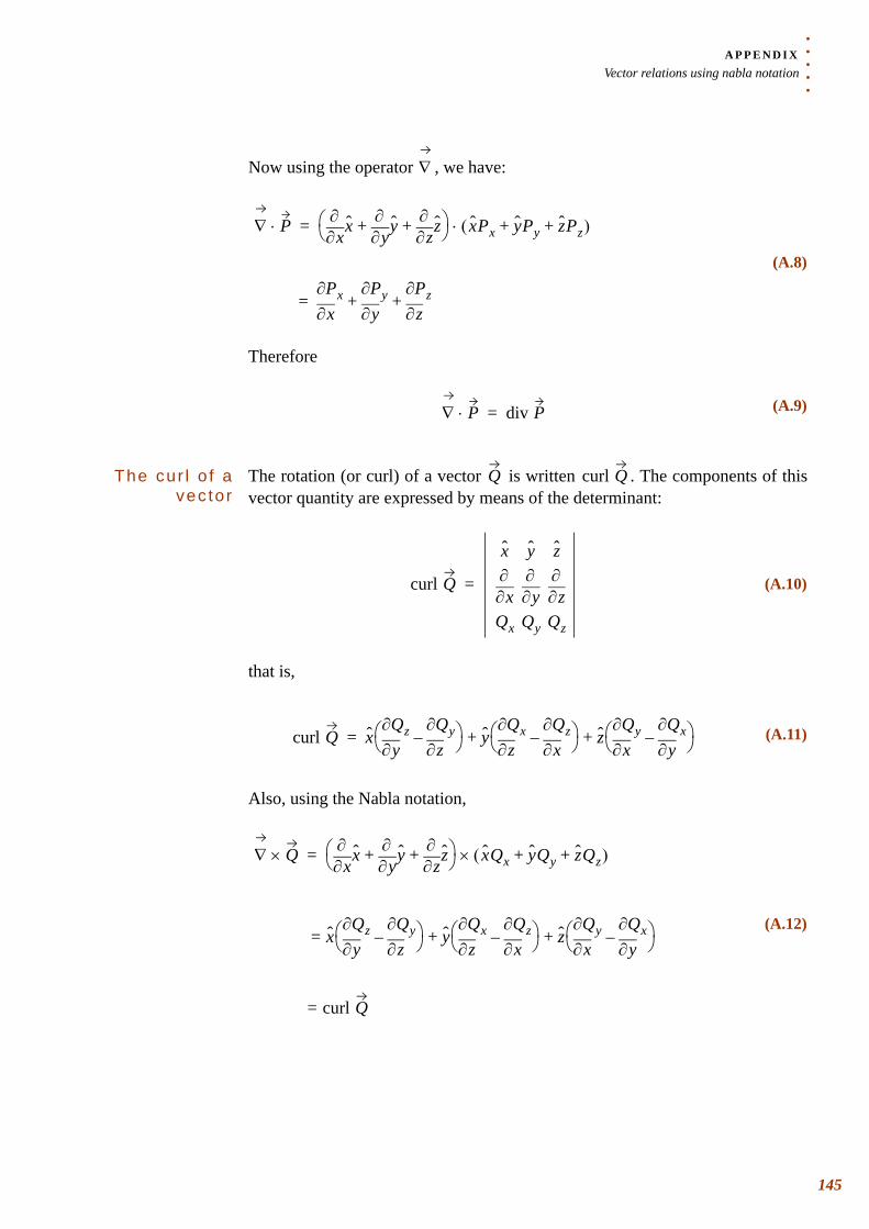
. . .
. .A P P E N D I XVector relations using nabla notation
Now using the operator , we have:
Therefore
The cur l o f a vec tor
The rotation (or curl) of a vector is written . The components of this vector quantity are expressed by means of the determinant:
that is,
Also, using the Nabla notation,
∇
(A.8)
∇ P⋅ x∂∂ x y∂
∂ y z∂∂ z+ +⎝ ⎠
⎛ ⎞ xPx yPy zPz+ +( )⋅=
x∂
∂Pxy∂
∂Pyz∂
∂Pz+ +=
(A.9)∇ P⋅ div P=
Q curl Q
(A.10)curl Q
x y z
x∂∂
y∂∂
z∂∂
Qx Qy Qz
=
(A.11)curl Q xy∂
∂Qzz∂
∂Qy–⎝ ⎠⎛ ⎞ y
z∂∂Qx
x∂∂Qz–⎝ ⎠
⎛ ⎞ zx∂
∂Qyy∂
∂Qx–⎝ ⎠⎛ ⎞+ +=
(A.12)
∇ Q× x∂∂ x y∂
∂ y z∂∂ z+ +⎝ ⎠
⎛ ⎞ xQx yQy zQz+ +( )×=
= xy∂
∂Qzz∂
∂Qy–⎝ ⎠⎛ ⎞ y
z∂∂Qx
x∂∂Qz–⎝ ⎠
⎛ ⎞ zx∂
∂Qyy∂
∂Qx–⎝ ⎠⎛ ⎞+ +
= curl Q
145
A P P E N D I XVector relations using nabla notation
146
Some use fu l vec tor re la t ions
The operator may operate on a product of two quantities:
Another useful operator has the form ; it operates on a vector:
With this notation, we develop Eq. A.13 and it can be easily demonstrated that:
The first term in Eq. A.15 can be developed using Eq. A.14:
If satisfies , then , etc. and Eq. A.16 can be written
with components
, etc. This type of vector can be used to represent
the force on a dipole in a non-uniform field (cf. Eq. 3.13 and Eq. 3.14)
∇
(A.13)grad P Q⋅( ) ∇ P Q⋅( )=
P grad⋅( ) P ∇⋅=
(A.14)P ∇⋅ Px x∂∂ Py y∂
∂ Pz z∂∂+ +=
(A.15)∇ P Q⋅( ) P ∇⋅⎝ ⎠⎛ ⎞ Q Q ∇⋅⎝ ⎠
⎛ ⎞ P P ∇ Q×⎝ ⎠⎛ ⎞ Q ∇ P×⎝ ⎠
⎛ ⎞×+×+ +=
(A.16)
P ∇⋅⎝ ⎠⎛ ⎞ Q Px x∂
∂ Py y∂∂ Pz z∂
∂+ +⎝ ⎠⎛ ⎞ Q=
x Px x∂∂Qx Py y∂
∂Qx Pz z∂∂Qx+ +⎝ ⎠
⎛ ⎞
+ y Px x∂∂Qy Py y∂
∂Qy Pz z∂∂Qy+ +⎝ ⎠
⎛ ⎞
+ z Px x∂∂Qz Py y∂
∂Qz Pz z∂∂Qz+ +⎝ ⎠
⎛ ⎞
=
Q ∇ Q× 0=y∂
∂Qxx∂
∂Qy=
x Px x∂∂Qx Py x∂
∂Qy Pz x∂∂Qz+ +⎝ ⎠
⎛ ⎞
. . .
. .A P P E N D I XMagnetic beads manipulation
. . . . . . . . . . . . . . . . . . . . . . . . . . . . . . . . . . . . . . . . . . . . . . . . . . . . . . . . . . . . . . . . . . . A . 3 M A G N E T I C B E A D S M A N I P U L A T I O N
A. Rida et al. have demonstrated the linear transport of superparamagnetic microbeads using planar coils placed in a uniform magnetostatic field [141]. This application is very close to the ferrofluid manipulation, which is the reason why we present this example in the Appendix.
A uniform static magnetic field is created with permanent magnets in a
direction orthogonal to the displacement of the microbeads (channel direction
). The role of is to impose a permanent magnetic moment to the
microbeads. is high enough to saturate the superparamagnetic beads with a
constant magnetization . The additional use of planar coils generates a magnetic field gradient which is then sufficient to displace the microbeads.
The magnetic moment on a microbead of volume can be considered as constant and, from Eq. 3.5, we have:
with the magnetic susceptibility of the magnetic particle. We have seen
earlier that the force on a constant magnetic dipole placed in a
non-uniform magnetic induction field is:
where is a combination of the constant induction field and the contribution of the coils. From Eq. A.16, Eq. A.18 can be we rewritten, for the contribution in the direction, as:
Since is satisfied, we have and .
Therefore Eq. A.19 can be rewritten:
H0
z
x H0
H0
Ms
m V
(A.17)m VMs VχH0 zVχH0= = =
χ
F m
B
(A.18)F ∇ m B⋅( ) m ∇⋅⎝ ⎠⎛ ⎞ B≅=
B B0
x
(A.19)Fx mx x∂∂Bx my y∂
∂Bx mz z∂∂Bx+ +=
∇ B× 0=y∂
∂Bxx∂
∂By=z∂
∂Bxx∂
∂Bz=
(A.20)Fx mx x∂∂Bx my x∂
∂By mz x∂∂Bz+ +=
147
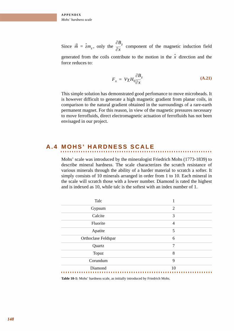
A P P E N D I XMohs’ hardness scale
148
Since , only the component of the magnetic induction field
generated from the coils contribute to the motion in the direction and the force reduces to:
This simple solution has demonstrated good perfomance to move microbeads. It is however difficult to generate a high magnetic gradient from planar coils, in comparison to the natural gradient obtained in the surroundings of a rare-earth permanent magnet. For this reason, in view of the magnetic pressures necessary to move ferrofluids, direct electromagnetic actuation of ferrofluids has not been envisaged in our project.
. . . . . . . . . . . . . . . . . . . . . . . . . . . . . . . . . . . . . . . . . . . . . . . . . . . . . . . . . . . . . . . . . . . A . 4 M O H S ’ H A R D N E S S S C A L E
Mohs’ scale was introduced by the mineralogist Friedrich Mohs (1773-1839) to describe mineral hardness. The scale characterizes the scratch resistance of various minerals through the ability of a harder material to scratch a softer. It simply consists of 10 minerals arranged in order from 1 to 10. Each mineral in the scale will scratch those with a lower number. Diamond is rated the highest and is indexed as 10, while talc is the softest with an index number of 1.
m zmz= x∂∂Bz
x
(A.21)Fx VχH0 x∂∂Bz=
Talc 1
Gypsum 2
Calcite 3
Fluorite 4
Apatite 5
Orthoclase Feldspar 6
Quartz 7
Topaz 8
Corundum 9
Diamond 10. . . . . . . . . . . . . . . . . . . . . . . . . . . . . . . . . . . . . . . . . . . . . . . . . . . . . . . . . . . . . . . . . . .Table 10-1: Mohs’ hardness scale, as initially introduced by Friedrich Mohs.
. . . . .
. . . . . . . . . . . . . . . . . . . . . . . . . . . . . . . . . . .REFERENCES
[1] H. T. G. van Lintel, F. C. M. van De Pol, and S. Bouwstra, "A piezoelectric micropump based on micromachining of silicon," Sensors and Actuators 15 (2), pp. 153-167, 1988. DOI: 10.1016/0250-6874(88)87005-7
[2] F. C. M. Van de Pol, H. T. G. Van Lintel, M. Elwenspoek, and J. H. J. Fluitman, "A thermopneumatic micropump based on micro-engineering techniques," Sensors and Actuators A: Physical 21 (1-3), pp. 198-202, 1990. DOI: 10.1016/0924-4247(90)85038-6
[3] P. Mitchell, "Microfluidics—downsizing large-scale biology," Nature biotechnology 19 (8), pp. 717-721, 2001. DOI: 10.1038/90754
[4] L. J. Hornbeck, "Digital Light Processing and MEMS: an overview," Proc. IEEE/LEOS 1996 Summer Topical Meetings, Keystone, CO, USA, 1996.
[5] E. Bassous, H. H. Taub, and L. Kuhn, "Ink Jet Printing Nozzle Arrays Etched in Silicon," Applied Physics Letters 31, pp. 135-137, 1977. DOI: 10.1063/1.89587
[6] D. Estève and J. Simonne, "Microsystèmes," in traité Electronique, vol. E2305: Techniques de l'Ingénieur, 2000.
[7] A. Manz, N. Graber, and H. M. Widmer, "Miniaturized Total Chemical-Analysis Systems - A Novel Concept for Chemical Sensing," Sensors and Actuators B: Chemical 1 (1-6), pp. 244-248, 1990.DOI: 10.1016/0925-4005(90)80209-I
[8] D. R. Reyes, D. Iossifidis, P. A. Auroux, and A. Manz, "Micro total analysis systems. 1. Introduction, theory, and technology," Analytical Chemistry 74 (12), pp. 2623-2636, 2002. DOI: 10.1021/ac0202435
[9] P. A. Auroux, D. Iossifidis, D. R. Reyes, and A. Manz, "Micro total analysis systems. 2. Analytical standard operations and applications," Analytical Chemistry 74 (12), pp. 2637-2652, 2002. DOI: 10.1021/ac020239t
[10] A. Manz, J. C. Fettinger, E. Verpoorte, H. Ludi, H. M. Widmer, and D. J. Harrison, "Micromachining of monocrystalline silicon and glass for chemical analysis systems A look into next century's technology or just a fashionable craze?," TrAC Trends in Analytical Chemistry 10 (5), pp. 144-149, 1991.DOI: 10.1016/0165-9936(91)85116-9
[11] D. Solignac, "Glass Microchips for Bio-Chemical Analysis: Technologies and Applications." Lausanne, Switzerland: Swiss Federal Institute of Technology Lausanne (EPFL), 2003.
[12] S. D. Gawad, "Dielectric spectroscopy in a microfabricated flow cytometer." Lausanne, Switzerland: Swiss Federal Institute of Technology Lausanne (EPFL), 2004.
[13] F. E. H. Tay and W. O. Choong, "Literature Review for Micropumps," in Microfluidics and BioMEMS Applications, pp. 3-140, F. E. H. Tay, Ed. Boston: Kluwer Academic Publishers, 2002.
[14] M. Koch, A. Evans, and A. Brunnschweiler, "Theory of microfluidic flow," in Microfluidic technology and applications. Baldock (England): Research studies press ltd., 2000.
[15] P. Gravesen, J. Branebjerg, and O. S. Jensen, "Microfluidics-a review," Journal of Micromechanics and Microengineering (4), pp. 168-182, 1993. DOI: 10.1088/0960-1317/3/4/002
[16] R. D. Blevins, Applied fluid dynamics handbook. New York: Van Norstrand Reinhold company Inc., 1984.
[17] F. M. White, Fluid Mechanics, 4th ed. New York: The McGraw-Hill Companies, 1998.
[18] M. B. Abbott and D. R. Basco, Computational Fluid Dynamics: An introduction for engineers. Harlow, UK: Longman Scientific & Technical, 1989.
149
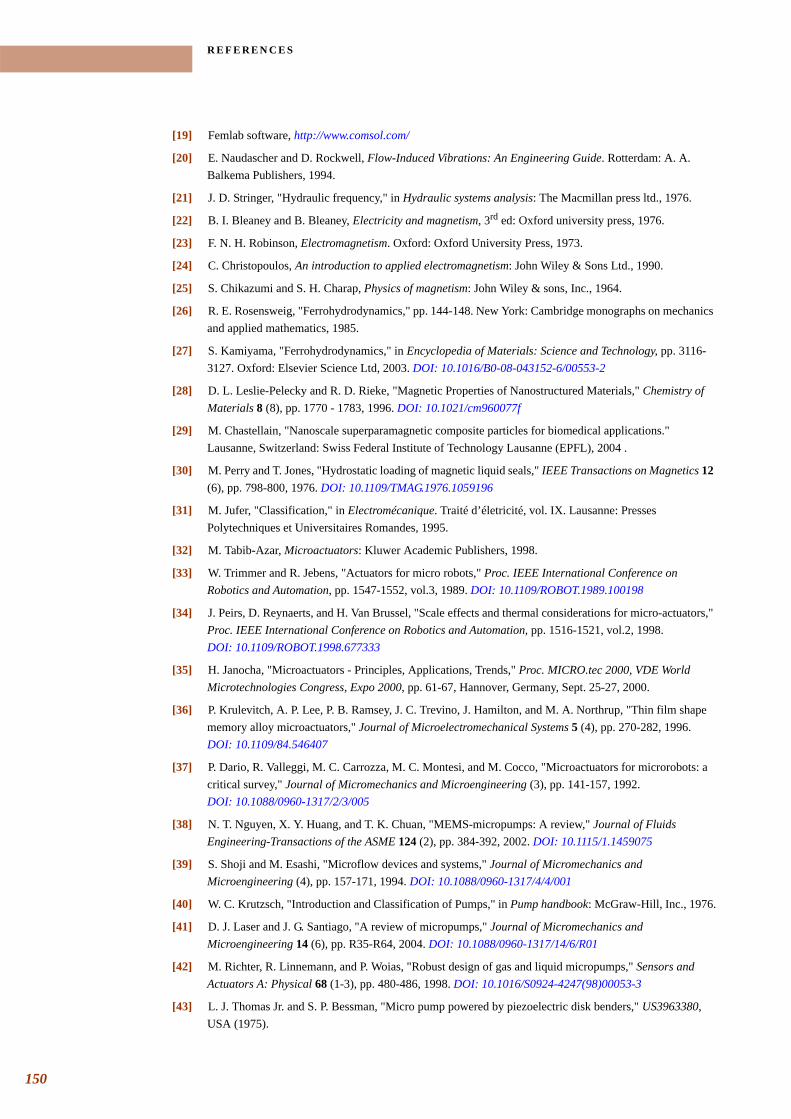
R E F E R E N C E S
150
[19] Femlab software, http://www.comsol.com/
[20] E. Naudascher and D. Rockwell, Flow-Induced Vibrations: An Engineering Guide. Rotterdam: A. A. Balkema Publishers, 1994.
[21] J. D. Stringer, "Hydraulic frequency," in Hydraulic systems analysis: The Macmillan press ltd., 1976.
[22] B. I. Bleaney and B. Bleaney, Electricity and magnetism, 3rd ed: Oxford university press, 1976.
[23] F. N. H. Robinson, Electromagnetism. Oxford: Oxford University Press, 1973.
[24] C. Christopoulos, An introduction to applied electromagnetism: John Wiley & Sons Ltd., 1990.
[25] S. Chikazumi and S. H. Charap, Physics of magnetism: John Wiley & sons, Inc., 1964.
[26] R. E. Rosensweig, "Ferrohydrodynamics," pp. 144-148. New York: Cambridge monographs on mechanics and applied mathematics, 1985.
[27] S. Kamiyama, "Ferrohydrodynamics," in Encyclopedia of Materials: Science and Technology, pp. 3116-3127. Oxford: Elsevier Science Ltd, 2003. DOI: 10.1016/B0-08-043152-6/00553-2
[28] D. L. Leslie-Pelecky and R. D. Rieke, "Magnetic Properties of Nanostructured Materials," Chemistry of Materials 8 (8), pp. 1770 - 1783, 1996. DOI: 10.1021/cm960077f
[29] M. Chastellain, "Nanoscale superparamagnetic composite particles for biomedical applications." Lausanne, Switzerland: Swiss Federal Institute of Technology Lausanne (EPFL), 2004 .
[30] M. Perry and T. Jones, "Hydrostatic loading of magnetic liquid seals," IEEE Transactions on Magnetics 12 (6), pp. 798-800, 1976. DOI: 10.1109/TMAG.1976.1059196
[31] M. Jufer, "Classification," in Electromécanique. Traité d’életricité, vol. IX. Lausanne: Presses Polytechniques et Universitaires Romandes, 1995.
[32] M. Tabib-Azar, Microactuators: Kluwer Academic Publishers, 1998.
[33] W. Trimmer and R. Jebens, "Actuators for micro robots," Proc. IEEE International Conference on Robotics and Automation, pp. 1547-1552, vol.3, 1989. DOI: 10.1109/ROBOT.1989.100198
[34] J. Peirs, D. Reynaerts, and H. Van Brussel, "Scale effects and thermal considerations for micro-actuators," Proc. IEEE International Conference on Robotics and Automation, pp. 1516-1521, vol.2, 1998.DOI: 10.1109/ROBOT.1998.677333
[35] H. Janocha, "Microactuators - Principles, Applications, Trends," Proc. MICRO.tec 2000, VDE World Microtechnologies Congress, Expo 2000, pp. 61-67, Hannover, Germany, Sept. 25-27, 2000.
[36] P. Krulevitch, A. P. Lee, P. B. Ramsey, J. C. Trevino, J. Hamilton, and M. A. Northrup, "Thin film shape memory alloy microactuators," Journal of Microelectromechanical Systems 5 (4), pp. 270-282, 1996.DOI: 10.1109/84.546407
[37] P. Dario, R. Valleggi, M. C. Carrozza, M. C. Montesi, and M. Cocco, "Microactuators for microrobots: a critical survey," Journal of Micromechanics and Microengineering (3), pp. 141-157, 1992.DOI: 10.1088/0960-1317/2/3/005
[38] N. T. Nguyen, X. Y. Huang, and T. K. Chuan, "MEMS-micropumps: A review," Journal of Fluids Engineering-Transactions of the ASME 124 (2), pp. 384-392, 2002. DOI: 10.1115/1.1459075
[39] S. Shoji and M. Esashi, "Microflow devices and systems," Journal of Micromechanics and Microengineering (4), pp. 157-171, 1994. DOI: 10.1088/0960-1317/4/4/001
[40] W. C. Krutzsch, "Introduction and Classification of Pumps," in Pump handbook: McGraw-Hill, Inc., 1976.
[41] D. J. Laser and J. G. Santiago, "A review of micropumps," Journal of Micromechanics and Microengineering 14 (6), pp. R35-R64, 2004. DOI: 10.1088/0960-1317/14/6/R01
[42] M. Richter, R. Linnemann, and P. Woias, "Robust design of gas and liquid micropumps," Sensors and Actuators A: Physical 68 (1-3), pp. 480-486, 1998. DOI: 10.1016/S0924-4247(98)00053-3
[43] L. J. Thomas Jr. and S. P. Bessman, "Micro pump powered by piezoelectric disk benders," US3963380, USA (1975).
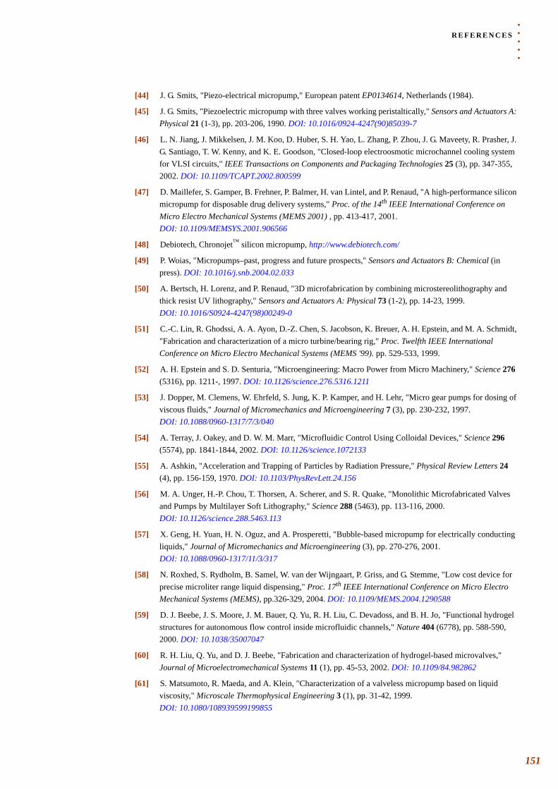
. . .
. .R E F E R E N C E S
[44] J. G. Smits, "Piezo-electrical micropump," European patent EP0134614, Netherlands (1984).
[45] J. G. Smits, "Piezoelectric micropump with three valves working peristaltically," Sensors and Actuators A: Physical 21 (1-3), pp. 203-206, 1990. DOI: 10.1016/0924-4247(90)85039-7
[46] L. N. Jiang, J. Mikkelsen, J. M. Koo, D. Huber, S. H. Yao, L. Zhang, P. Zhou, J. G. Maveety, R. Prasher, J. G. Santiago, T. W. Kenny, and K. E. Goodson, "Closed-loop electroosmotic microchannel cooling system for VLSI circuits," IEEE Transactions on Components and Packaging Technologies 25 (3), pp. 347-355, 2002. DOI: 10.1109/TCAPT.2002.800599
[47] D. Maillefer, S. Gamper, B. Frehner, P. Balmer, H. van Lintel, and P. Renaud, "A high-performance silicon micropump for disposable drug delivery systems," Proc. of the 14th IEEE International Conference on Micro Electro Mechanical Systems (MEMS 2001) , pp. 413-417, 2001. DOI: 10.1109/MEMSYS.2001.906566
[48] Debiotech, Chronojet™ silicon micropump, http://www.debiotech.com/
[49] P. Woias, "Micropumps–past, progress and future prospects," Sensors and Actuators B: Chemical (in press). DOI: 10.1016/j.snb.2004.02.033
[50] A. Bertsch, H. Lorenz, and P. Renaud, "3D microfabrication by combining microstereolithography and thick resist UV lithography," Sensors and Actuators A: Physical 73 (1-2), pp. 14-23, 1999.DOI: 10.1016/S0924-4247(98)00249-0
[51] C.-C. Lin, R. Ghodssi, A. A. Ayon, D.-Z. Chen, S. Jacobson, K. Breuer, A. H. Epstein, and M. A. Schmidt, "Fabrication and characterization of a micro turbine/bearing rig," Proc. Twelfth IEEE International Conference on Micro Electro Mechanical Systems (MEMS '99). pp. 529-533, 1999.
[52] A. H. Epstein and S. D. Senturia, "Microengineering: Macro Power from Micro Machinery," Science 276 (5316), pp. 1211-, 1997. DOI: 10.1126/science.276.5316.1211
[53] J. Dopper, M. Clemens, W. Ehrfeld, S. Jung, K. P. Kamper, and H. Lehr, "Micro gear pumps for dosing of viscous fluids," Journal of Micromechanics and Microengineering 7 (3), pp. 230-232, 1997. DOI: 10.1088/0960-1317/7/3/040
[54] A. Terray, J. Oakey, and D. W. M. Marr, "Microfluidic Control Using Colloidal Devices," Science 296 (5574), pp. 1841-1844, 2002. DOI: 10.1126/science.1072133
[55] A. Ashkin, "Acceleration and Trapping of Particles by Radiation Pressure," Physical Review Letters 24 (4), pp. 156-159, 1970. DOI: 10.1103/PhysRevLett.24.156
[56] M. A. Unger, H.-P. Chou, T. Thorsen, A. Scherer, and S. R. Quake, "Monolithic Microfabricated Valves and Pumps by Multilayer Soft Lithography," Science 288 (5463), pp. 113-116, 2000. DOI: 10.1126/science.288.5463.113
[57] X. Geng, H. Yuan, H. N. Oguz, and A. Prosperetti, "Bubble-based micropump for electrically conducting liquids," Journal of Micromechanics and Microengineering (3), pp. 270-276, 2001.DOI: 10.1088/0960-1317/11/3/317
[58] N. Roxhed, S. Rydholm, B. Samel, W. van der Wijngaart, P. Griss, and G. Stemme, "Low cost device for precise microliter range liquid dispensing," Proc. 17th IEEE International Conference on Micro Electro Mechanical Systems (MEMS), pp.326-329, 2004. DOI: 10.1109/MEMS.2004.1290588
[59] D. J. Beebe, J. S. Moore, J. M. Bauer, Q. Yu, R. H. Liu, C. Devadoss, and B. H. Jo, "Functional hydrogel structures for autonomous flow control inside microfluidic channels," Nature 404 (6778), pp. 588-590, 2000. DOI: 10.1038/35007047
[60] R. H. Liu, Q. Yu, and D. J. Beebe, "Fabrication and characterization of hydrogel-based microvalves," Journal of Microelectromechanical Systems 11 (1), pp. 45-53, 2002. DOI: 10.1109/84.982862
[61] S. Matsumoto, R. Maeda, and A. Klein, "Characterization of a valveless micropump based on liquid viscosity," Microscale Thermophysical Engineering 3 (1), pp. 31-42, 1999. DOI: 10.1080/108939599199855
151
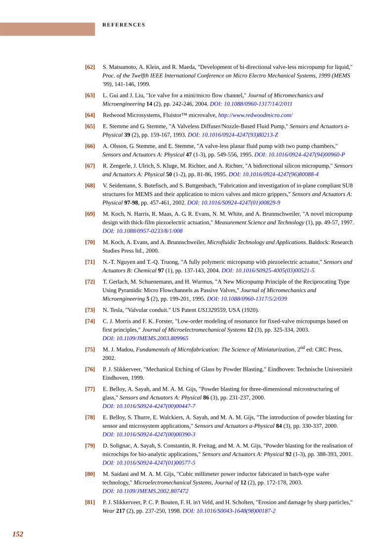
R E F E R E N C E S
152
[62] S. Matsumoto, A. Klein, and R. Maeda, "Development of bi-directional valve-less micropump for liquid," Proc. of the Twelfth IEEE International Conference on Micro Electro Mechanical Systems, 1999 (MEMS '99), 141-146, 1999.
[63] L. Gui and J. Liu, "Ice valve for a mini/micro flow channel," Journal of Micromechanics and Microengineering 14 (2), pp. 242-246, 2004. DOI: 10.1088/0960-1317/14/2/011
[64] Redwood Microsystems, Fluistor™ microvalve, http://www.redwoodmicro.com/
[65] E. Stemme and G. Stemme, "A Valveless Diffuser/Nozzle-Based Fluid Pump," Sensors and Actuators a-Physical 39 (2), pp. 159-167, 1993. DOI: 10.1016/0924-4247(93)80213-Z
[66] A. Olsson, G. Stemme, and E. Stemme, "A valve-less planar fluid pump with two pump chambers," Sensors and Actuators A: Physical 47 (1-3), pp. 549-556, 1995. DOI: 10.1016/0924-4247(94)00960-P
[67] R. Zengerle, J. Ulrich, S. Kluge, M. Richter, and A. Richter, "A bidirectional silicon micropump," Sensors and Actuators A: Physical 50 (1-2), pp. 81-86, 1995. DOI: 10.1016/0924-4247(96)80088-4
[68] V. Seidemann, S. Butefisch, and S. Buttgenbach, "Fabrication and investigation of in-plane compliant SU8 structures for MEMS and their application to micro valves and micro grippers," Sensors and Actuators A: Physical 97-98, pp. 457-461, 2002. DOI: 10.1016/S0924-4247(01)00829-9
[69] M. Koch, N. Harris, R. Maas, A. G. R. Evans, N. M. White, and A. Brunnschweiler, "A novel micropump design with thick-film piezoelectric actuation," Measurement Science and Technology (1), pp. 49-57, 1997.DOI: 10.1088/0957-0233/8/1/008
[70] M. Koch, A. Evans, and A. Brunnschweiler, Microfluidic Technology and Applications. Baldock: Research Studies Press ltd., 2000.
[71] N.-T. Nguyen and T.-Q. Truong, "A fully polymeric micropump with piezoelectric actuator," Sensors and Actuators B: Chemical 97 (1), pp. 137-143, 2004. DOI: 10.1016/S0925-4005(03)00521-5
[72] T. Gerlach, M. Schuenemann, and H. Wurmus, "A New Micropump Principle of the Reciprocating Type Using Pyramidic Micro Flowchannels as Passive Valves," Journal of Micromechanics and Microengineering 5 (2), pp. 199-201, 1995. DOI: 10.1088/0960-1317/5/2/039
[73] N. Tesla, "Valvular conduit." US Patent US1329559, USA (1920).
[74] C. J. Morris and F. K. Forster, "Low-order modeling of resonance for fixed-valve micropumps based on first principles," Journal of Microelectromechanical Systems 12 (3), pp. 325-334, 2003. DOI: 10.1109/JMEMS.2003.809965
[75] M. J. Madou, Fundamentals of Microfabrication: The Science of Miniaturization, 2nd ed: CRC Press, 2002.
[76] P. J. Slikkerveer, "Mechanical Etching of Glass by Powder Blasting." Eindhoven: Technische Universiteit Eindhoven, 1999.
[77] E. Belloy, A. Sayah, and M. A. M. Gijs, "Powder blasting for three-dimensional microstructuring of glass," Sensors and Actuators A: Physical 86 (3), pp. 231-237, 2000. DOI: 10.1016/S0924-4247(00)00447-7
[78] E. Belloy, S. Thurre, E. Walckiers, A. Sayah, and M. A. M. Gijs, "The introduction of powder blasting for sensor and microsystem applications," Sensors and Actuators a-Physical 84 (3), pp. 330-337, 2000. DOI: 10.1016/S0924-4247(00)00390-3
[79] D. Solignac, A. Sayah, S. Constantin, R. Freitag, and M. A. M. Gijs, "Powder blasting for the realisation of microchips for bio-analytic applications," Sensors and Actuators A: Physical 92 (1-3), pp. 388-393, 2001.DOI: 10.1016/S0924-4247(01)00577-5
[80] M. Saidani and M. A. M. Gijs, "Cubic millimeter power inductor fabricated in batch-type wafer technology," Microelectromechanical Systems, Journal of 12 (2), pp. 172-178, 2003. DOI: 10.1109/JMEMS.2002.807472
[81] P. J. Slikkerveer, P. C. P. Bouten, F. H. in't Veld, and H. Scholten, "Erosion and damage by sharp particles," Wear 217 (2), pp. 237-250, 1998. DOI: 10.1016/S0043-1648(98)00187-2
. . .
. .R E F E R E N C E S
[82] S. R. Choi and J. A. Salem, "Fracture toughness of PMMA as measured with indentation cracks," Journal of Materials Research 8 (12), pp. 3210-3217, 1993.
[83] C. Yamahata, C. Lotto, E. Al-Assaf, and M. A. M. Gijs, "A PMMA valveless micropump using electromagnetic actuation," Microfluidics and Nanofluidics, 2005 (in press). DOI: 10.1007/s10404-004-0007-6
[84] C. Yamahata, F. Lacharme, and M. A. M. Gijs, "Glass valveless micropump using electromagnetic actuation," Microelectronic Engineering, 2005 (in press). DOI: 10.1016/j.mee.2004.12.018
[85] F. Weber and P. Scheibner, "Herstellung von Formteilen durch Metallpulverspritzgiessen unter besonderer Beachtung spezieller Probleme des Formgebungsprozesses und der Rheologie von Metallpulver-Binder-Mischungen," Technischen Universität Chemnitz-Zwickau, 1994.
[86] R. E. Rosensweig, "Ferrofluids: Introduction," in Encyclopedia of Materials: Science and Technology, pp. 3093-3102. Oxford: Elsevier Science Ltd, 2003. DOI: 10.1016/B0-08-043152-6/00550-7
[87] K. Raj, "Ferrofluids: Applications," in Encyclopedia of Materials: Science and Technology, pp. 3083-3087. Oxford: Elsevier Science Ltd, 2003. DOI: 10.1016/B0-08-043152-6/00548-9
[88] K. Raj, J. Bonvouloir, and R. Moskowitz, "Loudspeaker." US patent US5461677 (1995).
[89] M. Shinkai, "Functional magnetic particles for medical application," Journal of Bioscience and Bioengineering 94 (6), pp. 606-613, 2002. DOI: 10.1016/S1389-1723(02)80202-X
[90] M. A. M. Gijs, "Magnetic bead handling on-chip: new opportunities for analytical applications," Microfluidics and Nanofluidics 1 (1), pp. 22-40, 2004. DOI: 10.1007/s10404-004-0010-y
[91] Olivetti I-Jet, Silicon ink-jet technology, http://www.olivettii-jet.it/
[92] A. Olsson, G. Stemme, O. Larsson, J. Holm, L. Lundbladh, and O. Ohman, "Valve-less diffuser micropumps fabricated using thermoplastic replication," Sensors and Actuators A: Physical 64 (1), pp. 63-68, 1998. DOI: 10.1016/S0924-4247(98)80059-9
[93] S. Böhm, W. Olthuis, and P. Bergveld, "A plastic micropump constructed with conventional techniques and materials," Sensors and Actuators A: Physical 77 (3), pp. 223-228, 1999. DOI: 10.1016/S0924-4247(99)00192-2
[94] S. Santra, P. Holloway, and C. D. Batich, "Fabrication and testing of a magnetically actuated micropump," Sensors and Actuators B: Chemical 87 (2), pp. 358-364, 2002. DOI: 10.1016/S0925-4005(02)00272-1
[95] T. Merkel, M. Graeber, and L. Pagel, "A new technology for fluidic microsystems based on PCB technology," Sensors and Actuators A: Physical 77 (2), pp. 98-105, 1999. DOI: 10.1016/S0924-4247(99)00062-X
[96] Ferrotec, Vacuum feedthroughs, http://www.ferrotec.com/
[97] B. Wagner, M. Kreutzer, and W. Benecke, "Permanent magnet micromotors on silicon substrates," Journal of Microelectromechanical Systems 2 (1), pp. 23-29, 1993. DOI: 10.1109/84.232591
[98] J. E. Leland, "Ferrofluid piston pump for use with heat pipes or the like." US patent US5005639 (1991).
[99] N. E. Greivell and B. Hannaford, "The design of a ferrofluid magnetic pipette," IEEE Transactions on Biomedical Engineering 44 (3), pp. 129-135, 1997. DOI: 10.1109/10.554759
[100] R. Pérez-Castillejos, J. A. Plaza, J. Esteve, P. Losantos, M. C. Acero, C. Cane, and F. Serra-Mestres, "The use of ferrofluids in micromechanics," Sensors and Actuators A: Physical 84 (1-2), pp. 176-180, 2000.DOI: 10.1016/S0924-4247(99)00318-0
[101] R. Pérez-Castillejos et al., "Smart passive microfluidic systems based on ferrofluids for microTAS applications," Proc. Transducers ’01, Munich, Germany, 2001.
[102] H. Hartshorne, "Development of Microfabricated Valves for uTAS," Proc. microTAS ’98, Banff, Canada, Kluwer Academic Publishers, pp. 379-381, 1998.
[103] H. Hartshorne, C. J. Backhouse, and W. E. Lee, "Ferrofluid-based microchip pump and valve," Sensors and Actuators B: Chemical 99 (2-3), pp. 592-600, 2004. DOI: 10.1016/j.snb.2004.01.016
153
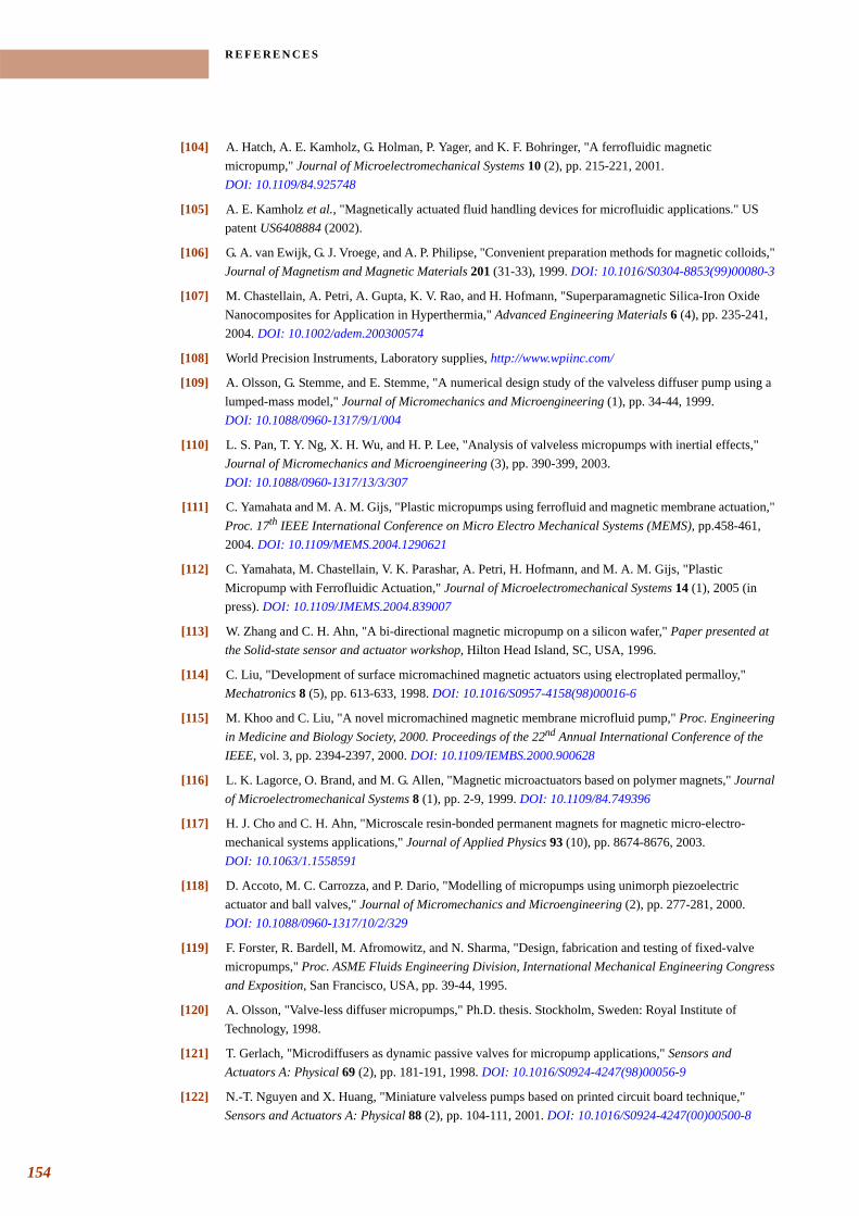
R E F E R E N C E S
154
[104] A. Hatch, A. E. Kamholz, G. Holman, P. Yager, and K. F. Bohringer, "A ferrofluidic magnetic micropump," Journal of Microelectromechanical Systems 10 (2), pp. 215-221, 2001. DOI: 10.1109/84.925748
[105] A. E. Kamholz et al., "Magnetically actuated fluid handling devices for microfluidic applications." US patent US6408884 (2002).
[106] G. A. van Ewijk, G. J. Vroege, and A. P. Philipse, "Convenient preparation methods for magnetic colloids," Journal of Magnetism and Magnetic Materials 201 (31-33), 1999. DOI: 10.1016/S0304-8853(99)00080-3
[107] M. Chastellain, A. Petri, A. Gupta, K. V. Rao, and H. Hofmann, "Superparamagnetic Silica-Iron Oxide Nanocomposites for Application in Hyperthermia," Advanced Engineering Materials 6 (4), pp. 235-241, 2004. DOI: 10.1002/adem.200300574
[108] World Precision Instruments, Laboratory supplies, http://www.wpiinc.com/
[109] A. Olsson, G. Stemme, and E. Stemme, "A numerical design study of the valveless diffuser pump using a lumped-mass model," Journal of Micromechanics and Microengineering (1), pp. 34-44, 1999. DOI: 10.1088/0960-1317/9/1/004
[110] L. S. Pan, T. Y. Ng, X. H. Wu, and H. P. Lee, "Analysis of valveless micropumps with inertial effects," Journal of Micromechanics and Microengineering (3), pp. 390-399, 2003. DOI: 10.1088/0960-1317/13/3/307
[111] C. Yamahata and M. A. M. Gijs, "Plastic micropumps using ferrofluid and magnetic membrane actuation," Proc. 17th IEEE International Conference on Micro Electro Mechanical Systems (MEMS), pp.458-461, 2004. DOI: 10.1109/MEMS.2004.1290621
[112] C. Yamahata, M. Chastellain, V. K. Parashar, A. Petri, H. Hofmann, and M. A. M. Gijs, "Plastic Micropump with Ferrofluidic Actuation," Journal of Microelectromechanical Systems 14 (1), 2005 (in press). DOI: 10.1109/JMEMS.2004.839007
[113] W. Zhang and C. H. Ahn, "A bi-directional magnetic micropump on a silicon wafer," Paper presented at the Solid-state sensor and actuator workshop, Hilton Head Island, SC, USA, 1996.
[114] C. Liu, "Development of surface micromachined magnetic actuators using electroplated permalloy," Mechatronics 8 (5), pp. 613-633, 1998. DOI: 10.1016/S0957-4158(98)00016-6
[115] M. Khoo and C. Liu, "A novel micromachined magnetic membrane microfluid pump," Proc. Engineering in Medicine and Biology Society, 2000. Proceedings of the 22nd Annual International Conference of the IEEE, vol. 3, pp. 2394-2397, 2000. DOI: 10.1109/IEMBS.2000.900628
[116] L. K. Lagorce, O. Brand, and M. G. Allen, "Magnetic microactuators based on polymer magnets," Journal of Microelectromechanical Systems 8 (1), pp. 2-9, 1999. DOI: 10.1109/84.749396
[117] H. J. Cho and C. H. Ahn, "Microscale resin-bonded permanent magnets for magnetic micro-electro-mechanical systems applications," Journal of Applied Physics 93 (10), pp. 8674-8676, 2003. DOI: 10.1063/1.1558591
[118] D. Accoto, M. C. Carrozza, and P. Dario, "Modelling of micropumps using unimorph piezoelectric actuator and ball valves," Journal of Micromechanics and Microengineering (2), pp. 277-281, 2000. DOI: 10.1088/0960-1317/10/2/329
[119] F. Forster, R. Bardell, M. Afromowitz, and N. Sharma, "Design, fabrication and testing of fixed-valve micropumps," Proc. ASME Fluids Engineering Division, International Mechanical Engineering Congress and Exposition, San Francisco, USA, pp. 39-44, 1995.
[120] A. Olsson, "Valve-less diffuser micropumps," Ph.D. thesis. Stockholm, Sweden: Royal Institute of Technology, 1998.
[121] T. Gerlach, "Microdiffusers as dynamic passive valves for micropump applications," Sensors and Actuators A: Physical 69 (2), pp. 181-191, 1998. DOI: 10.1016/S0924-4247(98)00056-9
[122] N.-T. Nguyen and X. Huang, "Miniature valveless pumps based on printed circuit board technique," Sensors and Actuators A: Physical 88 (2), pp. 104-111, 2001. DOI: 10.1016/S0924-4247(00)00500-8
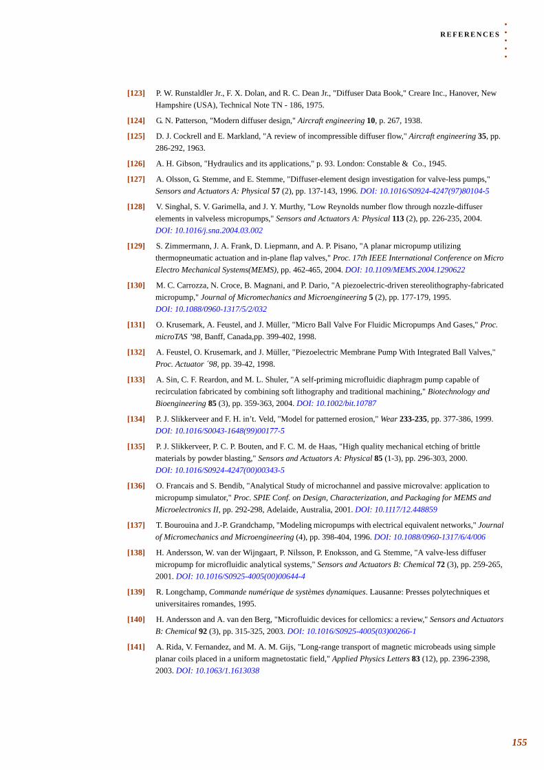
. . .
. .R E F E R E N C E S
[123] P. W. Runstaldler Jr., F. X. Dolan, and R. C. Dean Jr., "Diffuser Data Book," Creare Inc., Hanover, New Hampshire (USA), Technical Note TN - 186, 1975.
[124] G. N. Patterson, "Modern diffuser design," Aircraft engineering 10, p. 267, 1938.
[125] D. J. Cockrell and E. Markland, "A review of incompressible diffuser flow," Aircraft engineering 35, pp. 286-292, 1963.
[126] A. H. Gibson, "Hydraulics and its applications," p. 93. London: Constable & Co., 1945.
[127] A. Olsson, G. Stemme, and E. Stemme, "Diffuser-element design investigation for valve-less pumps," Sensors and Actuators A: Physical 57 (2), pp. 137-143, 1996. DOI: 10.1016/S0924-4247(97)80104-5
[128] V. Singhal, S. V. Garimella, and J. Y. Murthy, "Low Reynolds number flow through nozzle-diffuser elements in valveless micropumps," Sensors and Actuators A: Physical 113 (2), pp. 226-235, 2004. DOI: 10.1016/j.sna.2004.03.002
[129] S. Zimmermann, J. A. Frank, D. Liepmann, and A. P. Pisano, "A planar micropump utilizing thermopneumatic actuation and in-plane flap valves," Proc. 17th IEEE International Conference on Micro Electro Mechanical Systems(MEMS), pp. 462-465, 2004. DOI: 10.1109/MEMS.2004.1290622
[130] M. C. Carrozza, N. Croce, B. Magnani, and P. Dario, "A piezoelectric-driven stereolithography-fabricated micropump," Journal of Micromechanics and Microengineering 5 (2), pp. 177-179, 1995. DOI: 10.1088/0960-1317/5/2/032
[131] O. Krusemark, A. Feustel, and J. Müller, "Micro Ball Valve For Fluidic Micropumps And Gases," Proc. microTAS ’98, Banff, Canada,pp. 399-402, 1998.
[132] A. Feustel, O. Krusemark, and J. Müller, "Piezoelectric Membrane Pump With Integrated Ball Valves," Proc. Actuator ´98, pp. 39-42, 1998.
[133] A. Sin, C. F. Reardon, and M. L. Shuler, "A self-priming microfluidic diaphragm pump capable of recirculation fabricated by combining soft lithography and traditional machining," Biotechnology and Bioengineering 85 (3), pp. 359-363, 2004. DOI: 10.1002/bit.10787
[134] P. J. Slikkerveer and F. H. in’t. Veld, "Model for patterned erosion," Wear 233-235, pp. 377-386, 1999. DOI: 10.1016/S0043-1648(99)00177-5
[135] P. J. Slikkerveer, P. C. P. Bouten, and F. C. M. de Haas, "High quality mechanical etching of brittle materials by powder blasting," Sensors and Actuators A: Physical 85 (1-3), pp. 296-303, 2000. DOI: 10.1016/S0924-4247(00)00343-5
[136] O. Francais and S. Bendib, "Analytical Study of microchannel and passive microvalve: application to micropump simulator," Proc. SPIE Conf. on Design, Characterization, and Packaging for MEMS and Microelectronics II, pp. 292-298, Adelaide, Australia, 2001. DOI: 10.1117/12.448859
[137] T. Bourouina and J.-P. Grandchamp, "Modeling micropumps with electrical equivalent networks," Journal of Micromechanics and Microengineering (4), pp. 398-404, 1996. DOI: 10.1088/0960-1317/6/4/006
[138] H. Andersson, W. van der Wijngaart, P. Nilsson, P. Enoksson, and G. Stemme, "A valve-less diffuser micropump for microfluidic analytical systems," Sensors and Actuators B: Chemical 72 (3), pp. 259-265, 2001. DOI: 10.1016/S0925-4005(00)00644-4
[139] R. Longchamp, Commande numérique de systèmes dynamiques. Lausanne: Presses polytechniques et universitaires romandes, 1995.
[140] H. Andersson and A. van den Berg, "Microfluidic devices for cellomics: a review," Sensors and Actuators B: Chemical 92 (3), pp. 315-325, 2003. DOI: 10.1016/S0925-4005(03)00266-1
[141] A. Rida, V. Fernandez, and M. A. M. Gijs, "Long-range transport of magnetic microbeads using simple planar coils placed in a uniform magnetostatic field," Applied Physics Letters 83 (12), pp. 2396-2398, 2003. DOI: 10.1063/1.1613038
155

. . . . .
. . . . . . . . . . . . . . . . . . . . . . . . . . . . . . . . . . .PUBLICATIONS
J O U R N A L A R T I C L E S Part of the work presented in this thesis has been published in the following journals:
• C. Yamahata, M. Chastellain, V. K. Parashar, A. Petri, H. Hofmann, and M. A. M. Gijs, «Plastic micropump with ferrofluidic actuation», Journal of Microelectromechanical Systems 14 (1), pp. 96-102, 2005. DOI: 10.1109/JMEMS.2004.839007
• C. Yamahata, C. Lotto, E. Al-Assaf, and M. A. M. Gijs, «A PMMA valveless micropump using electromagnetic actuation», Microfluidics and Nanofluidics, 2005 (in press). DOI: 10.1007/s10404-004-0007-6
• C. Yamahata, F. Lacharme, and M. A. M. Gijs, «Glass valveless micropump using electromagnetic actuation», Microelectronic Engineering, 2005 (in press). DOI: 10.1016/j.mee.2004.12.018
• C. Yamahata, F. Lacharme, Y. Burri, and M. A. M. Gijs, «A ball valve micropump in glass fabricated by powder blasting», Sensors and Actuators B: Chemical, 2005 (in press). DOI: 10.1016/j.snb.2005.01.005
C O N F E R E N C E S The work has also been presented at the following conferences:
• C. Yamahata, F. Lacharme, J. Matter, S. Schnydrig, Y. Burri, M. A. M. Gijs, «Electromagnetically actuated ball valve micropumps», Technical digest of the 13th International Conference on Solid-State Sensors, Actuators and Microsystems (Transducers’05), Seoul, Korea, June 5-9, 2005.
• C. Yamahata, F. Lacharme, M. A. M. Gijs, «Glass valveless micropump using electromagnetic actuation», Proceeding of the 30th International Conference on Micro- and Nano- Engineering (MNE 2004), Rotterdam, The Netherlands, September 19-22, 2004.
157
P U B L I C A T I O N S
158
• C. Yamahata, M. A. M. Gijs, «Plastic micropumps using ferrofluid and magnetic membrane actuation», Proceeding of the 17th IEEE Inernational Conference on Micro Electro Mechanical Systems (MEMS 2004), pp. 458-461, Maastricht, The Netherlands, January 25-29, 2004.DOI: 10.1109/MEMS.2004.1290621
• C. Yamahata and M. A. M. Gijs, «Integrated plastic micropumps with magnetic actuation», Nanotech, the 7th Annual European Conference on Micro & Nanoscale Technologies for the Biosciences, Montreux, Switzerland, November 25-27, 2003.
• C. Yamahata, M. Chastellain, H. Hofmann, and M.A.M. Gijs, «A Ferrofluid Micropump for Biochemical Applications», 22ème journée des Matériaux, EPFL, Lausanne, Switzerland, October 16-17, 2003.
• C. Yamahata, M. Chastellain, H. Hofmann, and M. A. M. Gijs, «A ferrofluid micropump for lab-on-a-chip applications», Technical Digest of the 17th European Conference on Solid State Transducers (Eurosensors XVII), pp. 26-27, Guimarães, Portugal, September 21-24, 2003.
• C. Yamahata and M.A.M. Gijs, «A plastic prototyping technology for microfluidics», Nanotech, the 6th Annual European Conference on Micro & Nanoscale Technologies for the Biosciences, Montreux, Switzerland, November 26-28, 2002.

. . . . .
. . . . . . . . . . . . . . . . . . . . . . . . . . . . . . . . . . .CURRICULUM VITAE
. . . . . . . . . . . . . . . . . . . . . . . . . . . . . . . . . . . . . . . . . . . . . . . . . . . . . . . . . . . . . . . . . . . . . . . . . . . . . . . . . . . . . . E D U C A T I O N
. . . . . . . . . . . . . . . . . . . . . . . . . . . . . . . . . . . . . . . . . . . . . . . . . . . . . . . . . . . . . . . . . . . . . . . . . . . . . . . . . . . . . . P R O F E S S I O N A L A C T I V I T I E S
. . . . . . . . . . . . . . . . . . . . . . . . . . . . . . . . . . . . . . . . . . . . . . . . . . . . . . . . . . . . . . . . . . . . . . . . . . . . . . . . . . . . . . O T H E R A C T I V I T I E S
. . . . . . . . . . . . . . . . . . . . . . . . . . . . . . . . . . . . . . . . . . . . . . . . . . . . . . . . . . . . . . . . . . . . . . . . . . . . . . . . . . . . . . P A R T I C U L A R S K I L L S
Christophe YamahataDecember 28th, 1977French citizenship (Clamart, France)
2001 – 2005 (February) Doctoral thesis at the Swiss Federal Institute of Technology Lausanne (EPFL). Thesis entitled: «Magnetically Actuated Micropumps.»
1995 – 2000 Dipl.-Eng. in Microengineering, graduated from the Swiss Federal Institute of Technology Lausanne (EPFL).Diploma work: «Study of the mechanical behavior of linear guidings based on the superelastic properties of Shape Memory Alloys.»
2005 (since April) Postdoctoral position at the Laboratory for Integrated Micro-Mechatronic Systems, University of Tokyo.
2001 – 2004 Research assistant at the Laboratory for Microsystems, Institute of Microelectronics and Microsystems, EPFL. < http://lmis2.epfl.ch/ >
2000 Mediapolis Sàrl (Lausanne, Switzerland).Development of Internet tools for the management of interactive kiosks.
1999 Internship at Nouvelle Lemania SA (L’Orient, Switzerland).
1998 Internship at Medtronic Europe SA (Tolochenaz, Switzerland).
Member of the committee board of the association of research scientists of the EPFL (ACIDE), 2001. < http://acide.epfl.ch/ >Webmaster and responsible for the attribution of student's grants at Ingénieurs du Monde, a student association of the EPFL. Member of the committee board during years 2001-2003. < http://idm.epfl.ch/ >Webmaster and graphic designer at Fréquence Banane, the student radio station in Lausanne, Switzerland (2001-2004). < http://www.frequencebanane.ch/ >
Languages French (mother tongue), English (fluent), Spanish (good level), German (beginer).
Computer knowledge
MySQL, PHP, HTML, Pascal, C, SolidWorks, Femlab, Matlab, Dreamweawer, Photoshop, Paint Shop Pro, FrameMaker, Word, Excel, PowerPoint.
159