Embed Size (px)
Citation preview
UNIVERSITÉ PAUL CEZANNE (AIX-MARSEILLE III)
N̊ attribué par la bibliothèque2007AIX30051
Titre :
MÉTHODES PAR SOUS-ESPACES ET D’OPTIMISATION :APPLICATION AU TRAITEMENT D’ANTENNE, A
L’ANALYSE D’IMAGES,ET AU TRAITEMENT DE DONNÉES TENSORIELLES
THÈSEpour obtenir le grade de
DOCTEURDE L’UNIVERSITÉ PAUL CEZANNE
Faculté des Sciences et Techniques
Discipline : Optique, Image et Signal
Présentée et soutenue publiquement par :
Julien MAROT
Directeur de thèse : Pr. Salah Bourennane
École Doctorale : Physique et Sciences de la Matière
JURY :
Rapporteurs : Pr. Eric Moreau Univ. de Toulon et du VarPr. Yide Wang Univ. de Nantes
Examinateurs : Pr. Jean-Pierre Sessarego Lab. de Mécanique et d’Acoustique - CNRSM. Hamid Aghajan Stanford University, CA, USAM. Jacques Blanc-Talon DGA, MRIS
Directeur de thèse : Pr. Salah Bourennane Ecole Centrale Marseille, Institut Fresnel, Marseille
ANNEE : 2007

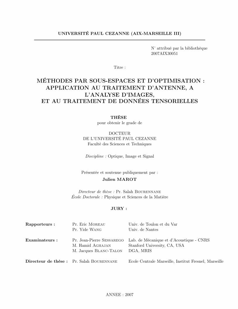
Abstract
THIS thesis is devoted to subspace-based and optimization methods. The methods pro-posed in this dissertation are developed and adapted in three contexts : for applications
in array processing, that is, for one-dimensional signal processing, for image understandingpurposes, that is, for two-dimensional signal processing, and for tensor signal processing, thatis, for multidimensional signal processing.The first part of the manuscript deals with array processing methods and applications. Basicdefinitions which are relevant in array processing are presented. The interest of second orderstatistics is emphasized : within the measurement space spanned by the eigenvectors of a co-variance matrix, one distinguishes signal subspace eigenvectors associated with the dominanteigenvalues, and noise subspace eigenvectors. High-resolution methods of array processing,such as MUSIC (MUltiple SIgnal Characterization) and TLS-ESPRIT (Total-Least-SquaresEstimation of Signal Parameters via Rotational Invariance Techniques) methods, are based onthe orthogonality between signal and noise subspaces. A novel optimization method is presen-ted. It combines either gradient or DIRECT (DIviding RECTangles) algorithms with splineinterpolation. An array processing application is considered : We propose a novel method forsource localization in presence of phase distortions. Especially, a novel algorithm handles adistorted antenna composed of a large number of sensors, keeping a small computational load.The second part of the manuscript considers image understanding applications. We reviewSLIDE method which adapts array processing methods to straight line retrieval. We proposenovel fast subspace-based methods for the estimation of straight line orientations and offsets.We consider several optimization methods for nearly straight distorted contour retrieval. Es-pecially, we propose a novel optimization method which is fast and handles distortions withhigh curvature. Then, we consider star-shaped contour retrieval. For this, we adapt a virtualcircular antenna to the processed image. The corresponding signal generation scheme yieldslinear phase signals from concentric circles. This enables the use of high-resolution methodswhich distinguish between possibly close radius values. We consider various contour shapessuch as distorted circles or ellipses.The third part of the manuscript is concerned with tensor signal processing. We remind thedefinitions concerning tensors, and review several multiway signal processing methods, whichrely on data projection upon signal subspace : the lower rank-(K1, . . . ,KN ) truncation ofthe HOSVD, the rank-(K1, . . . ,KN ) tensor approximation, in particular its version based onfourth order cumulants, which handles the case of correlated Gaussian noise. We present amultiway version of Wiener filtering. Both rank-(K1, . . . ,KN ) tensor approximation and mul-tiway Wiener filtering rely on an optimization algorithm named Alternating Least Squares(ALS) loop. We propose a nonorthogonal tensor flattening method to improve denoising re-sults. For this we use the straight line detection method proposed in the first part.

iv ABSTRACT
Key words : Array, second order statistics, subspace-based method, high-resolution me-thod, distorted wavefront, estimation, array processing, optimization, spline interpolation,image, contour, linear antenna, circular antenna, multilinear algebra, tensor decomposition,multiway array, lower-rank approximation, filtering.
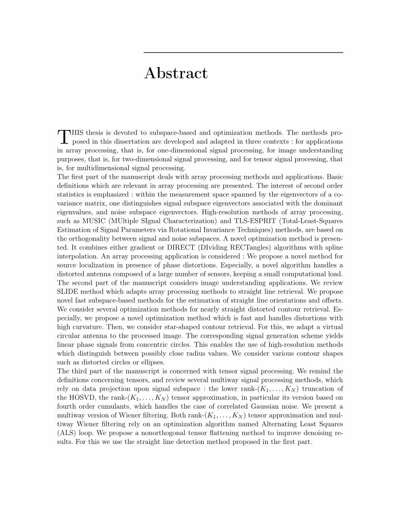
Résumé
CETTE thèse est consacrée aux méthodes par sous-espaces et d’optimisation. Les mé-thodes proposées dans ce manuscrit sont développées et adaptées dans trois contextes :
pour des applications en traitement d’antenne, c’est-à-dire pour le traitement de signauxunidimensionnels, pour l’analyse d’images, c’est-à-dire de signaux bidimensionnels, pour letraitement du signal tensoriel, c’est-à-dire de signaux multidimensionnels. La première partiede ce manuscrit traite de méthodes par sous-espaces et d’optimisation et de leurs applicationsen traitement d’antenne. Des définitions concernant un problème de traitement d’antennesont présentées, l’intérêt de statistiques d’ordre deux est mis en valeur : dans l’espace des me-sures couvert par les vecteurs propres d’une matrice de covariance, l’on distingue les vecteurspropres du sous espace signal associés aux valeurs propres dominantes, et les vecteurs propresdu sous-espace bruit. Les méthodes haute résolution du traitement d’antenne, telles que MU-SIC (MUltiple SIgnal Characterization) et TLS-ESPRIT (Total-Least-Squares Estimation ofSignal Parameters via Rotational Invariance Techniques), sont fondées sur l’orthogonalitéentre sous-espace bruit et sous-espace signal. On présente une nouvelle méthode d’optimisa-tion combinant les méthodes du gradient ou DIRECT (DIviding RECTangles) et une méthoded’interpolation par splines. On propose une application pour la résolution d’un problème entraitement d’antenne : Une nouvelle méthode est proposée pour la localisation de sources enprésence de distortions de phase, tout en conservant une charge de calcul faible. Ceci permetde faire face au cas d’antennes distordues à grand nombre de capteurs.La seconde partie de ce manuscrit concerne des applications en analyse d’images. Nous rap-pelons les principes de la méthode SLIDE (subspace-based LIne DEtection) qui adapte desméthodes de traitement d’antenne à l’estimation de contours rectilignes. Nous proposons desméthodes par sous-espaces rapides pour l’estimation de l’orientation et de l’offset de contoursrectilignes. Nous présentons plusieurs méthodes d’optimisation pour l’estimation de contoursapproximativement rectilignes et distordus. En particulier, nous proposons une nouvelle mé-thode d’optimisation qui est rapide et permet d’estimer des distortions de courbure impor-tante. Nous proposons aussi d’estimer des contours étoilés. Pour cela, nous adaptons uneantenne circulaire virtuelle à l’image à traiter. Le schéma de génération de signal correspon-dant conduit à des signaux à phase linéaire à partir de cercles concentriques. Cela permetd’appliquer des méthodes haute résolution du traitement d’antenne, et de distinguer des va-leurs de rayon pouvant être très proches. Nous nous intéressons à des formes de contour variéestelles que des cercles distordus, ou des ellipses.La troisième partie du manuscrit concerne le traitement du signal tensoriel. Nous rappelonsles principales définitions concernant les tenseurs, et donnons un état de l’art sur les méthodesde traitement du signal multidimensionel, qui reposent sur la projection des données sur lesous-espace signal : la troncature de rang-(K1, . . . ,KN ) de la HOSVD, l’approximation derang-(K1, . . . ,KN ) inférieur d’un tenseur, en particulier la version de cette méthode utilisantles cumulants d’ordre quatre, qui traite le cas d’un bruit Gaussien corrélé. Nous présentons
vi RÉSUMÉ
une version multidimensionelle du filtrage de Wiener. L’approximation de rang-(K1, . . . ,KN )inférieur d’un tenseur et le filtrage de Wiener multidimensionel reposent sur un algorithmed’optimisation nommé moindres carrés alternés ou Alternating Least Squares (ALS). Nousproposons une procédure de déploiement de tenseur qui est nonorthogonale : le déploiementest effectué selon la direction des contours rectilignes dans l’image et pas dans la direction deslignes ou des colonnes. Ceci a pour but d’améliorer les résultats de débruitage. Pour estimerles directions de déploiement appropriées, nous utilisons la méthode d’estimation de contourprésentée dans la première partie du manuscrit.
Mots clé : Antenne, statistiques d’ordre deux, méthodes par sous-espaces, méthodes hauterésolution, front d’onde distordu, estimation, traitement d’antenne, optimisation, interpola-tion par splines, image, contour, antenne linéaire, antenne circulaire, algèbre multilinéaire,décomposition tensorielle, tableau multidimensionnel, approximation de rang inférieur, fil-trage.
Acknowledgements
This PhD has been performed in the "Groupe Signaux Multidimensionnels" (GSM) teamof the Fresnel Institute, in Marseille, France.
I am very grateful to Professor Salah Bourennane, head of GSM team, and headof the research department in the Ecole Centrale de Marseille, for his supervision. SalahBourennane managed to sustain my initiatives at all opportune moments, his unmatchedenthusiasm and above all his unfailing trust made me feel confident about my work. Hisrigorous way of considering theoretical issues were very profitable. Salah Bourennane alwaysincited me to concretize my ideas and initiatives by submitting articles for publication injournal or conference papers. Salah Bourennane’s meticulous readings of the articles that wejointly published greatly improved their quality. Moreover he permitted me to participate inseveral international conferences and thereby to meet researchers and share the knowledgeand experience I acquired during my PhD.I was honored by all members of the jury who examined this dissertation :
– M. J.-P. Sessarego,– M. Y. Wang,– M. H. Aghajan,– M. E. Moreau,– M. J. Blanc-Talon.
It was a privilege for me to be inserted in GSM group. During my three years of PhD, Ihave constantly been working with talented people. Especially, I thank all PhD students whomaintained a pleasant atmosphere. In particular, I thank Damien, Cyril, Jean-Michel, Simon,William, Damien, Alexis and of course Nadine. I wish to express my sincere appreciationto all researchers of GSM group, in particular Stéphane Derrode, Thierry Gaidon, MireilleGuillaume, Mouloud Adel. They provided me with valuable advice and practical help, concer-ning my research investigations or for teaching purposes.Special gratitude is also due to my friends from sport training who participated with me innumerous lessons or competitions, that is, my swimming coach Didier, cyclists Roger, Robert,Daniel, Eric, Christian, triathletes Ludovic and Jean-Jacques, swimmers Eric, Pierre, Chris-telle, Adeline and Julie. Thanks for their support to my family, to Francois and Anne, and toAlbert and Lluis for their constant welcoming in my home country Andorra. Thanks to myparents and grandparents for their support.

Table des matières
Abstract iii
Résumé v
Acknowledgements vii
Introduction 1
I Principles of array processing and optimization, estimation ofdirections-of-arrival in the case of a distorted antenna with large numberof sensors 7
1 Principles of array processing and optimization methods 9
1.1 Basics of array processing . . . . . . . . . . . . . . . . . . . . . . . . . . . . . 9
1.1.1 Definitions . . . . . . . . . . . . . . . . . . . . . . . . . . . . . . . . . 10
1.1.2 Signal model . . . . . . . . . . . . . . . . . . . . . . . . . . . . . . . . 10
1.2 Second order statistics : cross-spectral matrix and distinction between signalsubspace and noise subspace . . . . . . . . . . . . . . . . . . . . . . . . . . . . 11
1.2.1 Cross-spectral matrix . . . . . . . . . . . . . . . . . . . . . . . . . . . 12
1.2.2 Distinction between signal and noise subspaces . . . . . . . . . . . . . 13
1.2.3 Orthogonality between signal and noise subspaces . . . . . . . . . . . . 14
1.3 High-resolution methods . . . . . . . . . . . . . . . . . . . . . . . . . . . . . . 15
1.3.1 MUSIC method . . . . . . . . . . . . . . . . . . . . . . . . . . . . . . . 15
1.3.2 TLS-ESPRIT method . . . . . . . . . . . . . . . . . . . . . . . . . . . 16
1.3.3 Propagator method . . . . . . . . . . . . . . . . . . . . . . . . . . . . . 17
1.3.4 Propagator method applied to signal . . . . . . . . . . . . . . . . . . . 18
1.3.5 Balance on high-resolution methods . . . . . . . . . . . . . . . . . . . 19
x TABLE DES MATIÈRES
1.4 Optimization method : combination of gradient or DIRECT algorithm withspline interpolation . . . . . . . . . . . . . . . . . . . . . . . . . . . . . . . . . 19
1.5 Conclusion of chapter 1 . . . . . . . . . . . . . . . . . . . . . . . . . . . . . . 21
2 Phase distortion estimation by DIRECT and spline interpolation algo-rithms 23
2.1 Introduction . . . . . . . . . . . . . . . . . . . . . . . . . . . . . . . . . . . . . 23
2.2 Problem statement . . . . . . . . . . . . . . . . . . . . . . . . . . . . . . . . . 24
2.3 Retrieval and cancellation of phase distortions . . . . . . . . . . . . . . . . . . 24
2.3.1 Phase shift retrieval . . . . . . . . . . . . . . . . . . . . . . . . . . . . 24
2.3.2 Cancel the phase shifts in the received signals . . . . . . . . . . . . . . 25
2.3.3 Proposed algorithm . . . . . . . . . . . . . . . . . . . . . . . . . . . . . 26
2.4 Simulation results . . . . . . . . . . . . . . . . . . . . . . . . . . . . . . . . . . 26
2.5 Conclusion of chapter 2 . . . . . . . . . . . . . . . . . . . . . . . . . . . . . . 28
II Array processing and optimization methods applied to image un-derstanding 29
3 Straight line and nearly straight contour retrieval, by high-resolution me-thods of array processing and optimization methods 31
3.1 Introduction . . . . . . . . . . . . . . . . . . . . . . . . . . . . . . . . . . . . . 32
3.2 Data model, signal generation out of the image data . . . . . . . . . . . . . . 33
3.3 Straight contour estimation . . . . . . . . . . . . . . . . . . . . . . . . . . . . 35
3.3.1 Angle estimation, overview of the SLIDE method . . . . . . . . . . . . 35
3.3.2 Angle estimation by Propagator method . . . . . . . . . . . . . . . . . 36
3.3.3 Offset estimation . . . . . . . . . . . . . . . . . . . . . . . . . . . . . . 37
3.3.3.1 Extension of the Hough Transform . . . . . . . . . . . . . . . 37
3.3.3.2 Proposed method : MFBLP . . . . . . . . . . . . . . . . . . . 38
3.4 Straight line estimation : results obtained . . . . . . . . . . . . . . . . . . . . 40
3.4.1 Straight line estimation by SLIDE method, and MFBLP . . . . . . . . 40
3.4.2 Close-valued offset estimation . . . . . . . . . . . . . . . . . . . . . . . 42
3.4.3 Computational complexity of the proposed method for offset estimationand Hough transform . . . . . . . . . . . . . . . . . . . . . . . . . . . . 43
3.4.4 Balance on straight contour retrieval . . . . . . . . . . . . . . . . . . . 44
3.5 Region-based contour retrieval . . . . . . . . . . . . . . . . . . . . . . . . . . . 44
3.5.1 Proposed method . . . . . . . . . . . . . . . . . . . . . . . . . . . . . . 45
3.5.2 Application of the proposed method to pectoral muscle segmentation . 46
TABLE DES MATIÈRES xi
3.5.3 Balance on region-based segmentation . . . . . . . . . . . . . . . . . . 48
3.6 Estimation of non rectilinear contours in an image as an inverse problem :principles of the proposed optimization method and gradient algorithm . . . . 48
3.6.1 Retrieval of a general phase model . . . . . . . . . . . . . . . . . . . . 48
3.6.2 Initialization of the proposed algorithm . . . . . . . . . . . . . . . . . 49
3.6.3 Distorted curve : proposed algorithm . . . . . . . . . . . . . . . . . . . 49
3.6.4 Convergence of the gradient method . . . . . . . . . . . . . . . . . . . 51
3.6.5 Summary of the proposed algorithm . . . . . . . . . . . . . . . . . . . 52
3.6.6 Numerical complexity of the method . . . . . . . . . . . . . . . . . . . 52
3.7 Generalization of distorted contour estimation to the estimation of several curves 53
3.8 Simulations on non rectilinear contours . . . . . . . . . . . . . . . . . . . . . . 54
3.9 Estimation of non rectilinear contours in an image by means of Propagator andoptimization methods . . . . . . . . . . . . . . . . . . . . . . . . . . . . . . . 59
3.9.1 Formulation of a phase model . . . . . . . . . . . . . . . . . . . . . . . 59
3.9.2 Propagator method for phase shift estimation . . . . . . . . . . . . . . 59
3.10 Propagator applied to the covariance matrix associated with gradient algo-rithm : Experimental results, computational times . . . . . . . . . . . . . . . 60
3.10.1 Real-world images . . . . . . . . . . . . . . . . . . . . . . . . . . . . . 60
3.10.2 Statistical results . . . . . . . . . . . . . . . . . . . . . . . . . . . . . . 62
3.11 Distorted contour retrieval by the combination of gradient and spline interpolation 63
3.11.1 Formulation of a signal model . . . . . . . . . . . . . . . . . . . . . . . 63
3.11.2 Optimization algorithm : combination of gradient and spline interpolation 64
3.12 Distorted contour retrieval by gradient algorithm combined with spline inter-polation : results and discussion . . . . . . . . . . . . . . . . . . . . . . . . . . 65
3.12.1 Hand-made images . . . . . . . . . . . . . . . . . . . . . . . . . . . . . 66
3.12.2 Distorted contour retrieval in real-world grey level images . . . . . . . 70
3.13 Conclusion of chapter 3 . . . . . . . . . . . . . . . . . . . . . . . . . . . . . . 71
4 Subspace-Based and DIRECT algorithms for distorted circular contour es-timation 73
4.1 Introduction . . . . . . . . . . . . . . . . . . . . . . . . . . . . . . . . . . . . . 74
4.2 Problem statement and signal generation . . . . . . . . . . . . . . . . . . . . . 75
4.2.1 Problem statement . . . . . . . . . . . . . . . . . . . . . . . . . . . . . 75
4.2.2 Virtual signal generation . . . . . . . . . . . . . . . . . . . . . . . . . . 76
4.3 Proposed method for radius and center estimation . . . . . . . . . . . . . . . 78
4.4 Optimization method for the estimation of nearly circular contours . . . . . . 80
4.4.1 Proposed optimization method . . . . . . . . . . . . . . . . . . . . . . 81
xii TABLE DES MATIÈRES
4.4.2 Summary of the proposed method . . . . . . . . . . . . . . . . . . . . 81
4.5 Results and discussion . . . . . . . . . . . . . . . . . . . . . . . . . . . . . . . 82
4.5.1 Hand-made images . . . . . . . . . . . . . . . . . . . . . . . . . . . . . 82
4.5.2 Real-world images . . . . . . . . . . . . . . . . . . . . . . . . . . . . . 89
4.6 Conclusion of chapter 4 . . . . . . . . . . . . . . . . . . . . . . . . . . . . . . 92
III Tensor approach of image processing, nonorthogonal tensor flatte-ning via main direction detection 93
5 Lower-rank tensor approximation and multiway filtering 95
5.1 Introduction . . . . . . . . . . . . . . . . . . . . . . . . . . . . . . . . . . . . . 96
5.2 Tensor representation and properties . . . . . . . . . . . . . . . . . . . . . . . 98
5.3 Tensor filtering problem formulation . . . . . . . . . . . . . . . . . . . . . . . 99
5.3.1 Channel-by-channel SVD-based filtering . . . . . . . . . . . . . . . . . 100
5.3.2 Tensor filtering based on multimode PCA . . . . . . . . . . . . . . . . 101
5.3.2.1 White decorrelated Gaussian noise and second order statisticsbased method . . . . . . . . . . . . . . . . . . . . . . . . . . 101
5.3.2.2 Correlated Gaussian noise and higher-order statistics basedmethod . . . . . . . . . . . . . . . . . . . . . . . . . . . . . . 102
5.3.3 Multiway Wiener filtering . . . . . . . . . . . . . . . . . . . . . . . . . 104
5.4 Simulation results . . . . . . . . . . . . . . . . . . . . . . . . . . . . . . . . . . 106
5.4.1 Performance criterion . . . . . . . . . . . . . . . . . . . . . . . . . . . 106
5.4.2 Denoising of color images . . . . . . . . . . . . . . . . . . . . . . . . . 107
5.4.2.1 Denoising of a color image impaired by additive Gaussian noise107
5.4.2.2 HOSVD-(K1,K2,K3), rank-(K1,K2,K3) approximation ba-sed on second order and higher-order statistics, applied to animage impaired by an additive correlated Gaussian noise . . . 111
5.4.3 Denoising of multispectral images . . . . . . . . . . . . . . . . . . . . . 113
5.4.4 Statistical performances . . . . . . . . . . . . . . . . . . . . . . . . . . 114
5.4.5 Filtering of a multicomponent seismic type signal . . . . . . . . . . . . 115
5.4.5.1 Filtering of a multicomponent seismic type signal impaired byan additive white Gaussian noise . . . . . . . . . . . . . . . . 115
5.4.5.2 Filtering of a multicomponent seismic type signal impaired byan additive correlated Gaussian noise . . . . . . . . . . . . . 117
5.5 Nonorthogonal tensor flattening for hyperspectral image filtering . . . . . . . 119
5.5.1 Influence of nth-mode ranks on SNR . . . . . . . . . . . . . . . . . . . 120
5.5.2 Main directions of tensors and MWFR algorithm . . . . . . . . . . . 121
TABLE DES MATIÈRES xiii
5.5.3 Real-world data : HYDICE HSI . . . . . . . . . . . . . . . . . . . . . . 122
5.5.3.1 Noise level in HYDICE images . . . . . . . . . . . . . . . . . 122
5.5.3.2 HSI02 image . . . . . . . . . . . . . . . . . . . . . . . . . . . 123
5.5.4 Balance about nonorthogonal tensor flattening . . . . . . . . . . . . . 123
5.6 Conclusion of chapter 5 . . . . . . . . . . . . . . . . . . . . . . . . . . . . . . 124
Concluding remarks 125
A Appendix A : mathematical considerations about multiway filtering 129
A.1 Appendix : Alternating Least Squares algorithms . . . . . . . . . . . . . . . . 129
A.1.1 ALS algorithm in Rank-(K1, . . . ,KN ) approximation - TUCKALS3 al-gorithm . . . . . . . . . . . . . . . . . . . . . . . . . . . . . . . . . . . 129
A.1.2 Fourth order cumulant slice matrix-based multimode PCA-based filtering130
A.1.3 ALS algorithm in multiway Wiener filtering . . . . . . . . . . . . . . . 131
A.2 Appendix : nth-mode Wiener filter analytical expression . . . . . . . . . . . . 132
A.3 Appendix : Assumptions and related expression of the nth-mode Wiener filter 134
B Appendix B : Synthèse du manuscrit 139
B.1 Introduction générale . . . . . . . . . . . . . . . . . . . . . . . . . . . . . . . . 139
B.2 Corps du manuscrit . . . . . . . . . . . . . . . . . . . . . . . . . . . . . . . . . 142
B.2.1 Résumé du chapitre 1 : Principes des méthodes de traitement d’antenneet d’optimisation . . . . . . . . . . . . . . . . . . . . . . . . . . . . . . 142
B.2.1.1 Bases de traitement d’antenne . . . . . . . . . . . . . . . . . 143
B.2.1.2 Statistiques d’ordre deux : matrice interspectrale et distinctionentre sous-espace signal et sous-espace bruit . . . . . . . . . . 144
B.2.1.3 Méthodes haute résolution . . . . . . . . . . . . . . . . . . . 145
B.2.1.4 Méthode MUSIC . . . . . . . . . . . . . . . . . . . . . . . . . 145
B.2.1.5 Méthode TLS-ESPRIT . . . . . . . . . . . . . . . . . . . . . 145
B.2.1.6 Méthode du Propagateur . . . . . . . . . . . . . . . . . . . . 145
B.2.1.7 Algorithme d’optimisation associé à une méthode d’interpola-tion par splines . . . . . . . . . . . . . . . . . . . . . . . . . . 146
B.2.1.8 Conclusion du chapitre 1 . . . . . . . . . . . . . . . . . . . . 146
B.2.2 Résumé du chapitre 2 : Estimation de distortions de phase par DIRECTassocié à l’interpolation par splines . . . . . . . . . . . . . . . . . . . . 146
B.2.2.1 Position du problème . . . . . . . . . . . . . . . . . . . . . . 147
B.2.2.2 Résultats : Caractérisation de trois sources . . . . . . . . . . 147
B.2.2.3 Conclusion du chapitre 2 . . . . . . . . . . . . . . . . . . . . 147
xiv TABLE DES MATIÈRES
B.2.3 Résumé du chapitre 3 : Estimation de contours rectilignes et approxi-mativement rectilignes . . . . . . . . . . . . . . . . . . . . . . . . . . . 148
B.2.3.1 Modèle de données, génération de signal à partir de l’image . 149
B.2.3.2 Estimation de contours distordus . . . . . . . . . . . . . . . . 149
B.2.3.3 Quelques résultats : estimation de contours rectilignes et ap-proximativement rectilignes . . . . . . . . . . . . . . . . . . . 150
B.2.3.4 Conclusion du chapitre 3 . . . . . . . . . . . . . . . . . . . . 152
B.2.4 Résumé du chapitre 4 : Estimation de contours circulaires et approxi-mativement circulaires . . . . . . . . . . . . . . . . . . . . . . . . . . . 152
B.2.4.1 Position du problème et génération de signal . . . . . . . . . 153
B.2.4.2 Estimation de cercles multiples avec des centres et des rayonsdifférents . . . . . . . . . . . . . . . . . . . . . . . . . . . . . 155
B.2.4.3 Quelques résultats . . . . . . . . . . . . . . . . . . . . . . . . 155
B.2.4.4 Conclusion du chapitre 4 . . . . . . . . . . . . . . . . . . . . 158
B.2.5 Résumé du chapitre 5 : Approximation de tenseur de rang inférieur etfiltrage multimodal . . . . . . . . . . . . . . . . . . . . . . . . . . . . . 159
B.2.5.1 Les données tensorielles . . . . . . . . . . . . . . . . . . . . . 159
B.2.5.2 Quelques résultats de débruitage de données tensorielles . . . 160
B.2.5.3 Conclusion du chapitre 5 . . . . . . . . . . . . . . . . . . . . 161
B.3 Conclusion générale . . . . . . . . . . . . . . . . . . . . . . . . . . . . . . . . . 161
Liste des figures 165
Liste des tableaux 171
Bibliographie 173
Introduction
DATA processing and analysis have been developed and encouraged by the progress innumerical computing, video, and acquisition systems such as sensors. A set of sensors
forms an antenna, or array. When an array processing problem is considered, one generallyassumes that signals received on each sensor are centered around one frequency. So, for eachsensor, one chooses the signal Fourier transform component corresponding to this frequencyof interest. One obtains then a unidimensional signal : one component per sensor. Anantenna is used for source localization, and gets various shapes. Circular antennas are used intelecommunications, linear antennas are used for instance for object detection. In particular,antennas with large number of sensors have been used to improve localisation results. Objectdetection and localization is of great interest for civilian and military applications, forthe detection of mines, pipe-lines, cables. Solving an array processing problem consists indetermining the origin of waves emitted by possibly close sources. Important fundings weredevoted to array processing techniques to solve difficult cases such as the case of sources withclose directions-of-arrival, correlated sources, and the case where correlated noise impairs thedata.The approach adopted during this thesis comes from the following remark : Array processingmethods have been widely improved, and could profit to image processing and multidimen-sional signal processing fields. It appeared then of great interest, during this thesis, to setanalogies between array processing methods, which are unidimensional signal methods, andimage processing problems. Now, images are either bidimensional images, when binary or greylevel images are considered, either multidimensional when color or multispectral images areconsidered. We considered the problem of contour estimation in binary or grey level images.A first issue is to transcript the image content into a signal. For this, a particular signalgeneration method consists of adapting an antenna to the processed image. This antennais either linear or circular, depending on the shape of the expected object. To apply arrayprocessing methods to multidimensional data processing, and in particular to data denoising,it is possible to choose another formalism. We chose, to enable the application of algebraicmethods of array processing to such a problem, to consider each vector of a multidimensionalentity as a signal realization. We provide in the remainder of this introduction some detailsconcerning the issues of processings applied to signals, images, or multidimensional data.
Data are bidimensional when image acquisition is performed. Image processing consistsin producing new images which are in some way more desirable. Recovering from blur ornoise impairment is required in the case of noisy or moving sensors. The purpose of imageunderstanding is to extract desired information from two-dimensional images. Locating andmeasurement of features and patterns is a typical image understanding task. Such a task is ea-sily performed by the human brain which possesses the ability to extract pertinent informationand interpret a small number of parameters from images. The output of image understanding
2 INTRODUCTION
is either a number of parameter values or a description of the objects present in the image. Nu-merous phenomena depend on several physical variables such as those associated with space(three dimensions), time, wavelength, color or wave polarisation. In this context data acquisi-tion yields multidimensional data. To record, study and extract useful information from thesephenomena, several multidimensional or multicomponent sensors have appeared for the lastfifty years. The data provided by multicomponent sensors are called multiway data. Multiwaydata are modeled by arrays, and each array entry is associated with a physical parameter,such as time, space or wavelength. Such an array is denominated tensor [92, 38], and eachdimension of a tensor is called nth-mode ; the number of nth-modes is called the order of thetensor.Data are sampled such that a signal is a set of samples, an image is a set of pixels, and a tensoris a multiway array. Therefore, signal, image and tensor processing are performed by algebraicmethods. This type of data processing relies, in general, on second order [133, 114, 90, 5, 3]or higher-order statistics [80, 89, 108] computation. The most common processing which isapplied to a covariance matrix is the Singular Value Decomposition (SVD [43, 51]), or theeigendecomposition. Efficient techniques for extracting the desired parameters from the arraydata are based on the so-called signal subspace concept [115, 114, 90, 3]. All eigenvectors of thecovariance matrix of the collected signals form the measurement space. The key observationwhile computing second order or higher-order statistics is that a low-dimensional subspacepermits to extract useful information, in particular expected parameters [5, 3]. The know-ledge, or the estimation by statistical criteria [132], of the useful signal subspace dimensionpermits to partition the measurement space into a signal subspace that contains the desiredinformation, and a noise subspace, that contains all undesired contributions.Optimization methods mean to retrieve a set of unknown parameters, by minimizing a crite-rion, generally squared distance between data model and measurements. They distinguish intwo categories : global and local methods. Global methods retrieve the global minimum of afunction, they are not supposed to converge on a local minimum, at the expense of a gene-rally high computational cost. For instance, DIviding RECTangles (DIRECT) method [64],or the genetic algorithms [50] are global optimization methods. Local methods are gene-rally faster than global methods. A classical local method for the resolution of nonlinear andnon-constrained optimization problems is the gradient or Newton [48] method, which can beaccelerated as a variable step gradient method.There is great interest in combining subspace-based and optimization methods to obtain anoptimal estimation of either a set of parameters or expected features from signal, image ortensor data. In array processing, subspace-based Propagator method was associated withan optimization method to improve direction-of-arrival (DOA) estimation in the presence ofphase distortion [90]. In the field of image processing, DIRECT method [64] was adaptedto image registration, especially for medical images [130]. In the field of tensor processing,an Alternating Least Squares (ALS) algorithm that yields a particular tensor decompositionwas proposed in [76, 77]. An ALS algorithm was also proposed in [96] to solve a tensor datafiltering problem, for a denoising application.The purpose of this manuscript is to propose and associate several methods, either subspace-based ones, or optimization ones, for data processing and (or) understanding, in the fields ofarray processing for one-dimensional signals, image processing for two-dimensional signals, andtensor processing for multidimensional signals. The background and proposed improvements,in array processing, image processing, and tensor processing respectively are as follows :
INTRODUCTION 3
• In an array processing problem, several signal realizations are usually available, they arecollected upon the array at several instants. The signal subspace dimension is equal to thenumber of emitting sources. In practice, if the number of sources is not a priori known,this number can be estimated from the data by statistical criteria such as MinimumDescription Length (MDL) [132]. In this framework we introduce novel optimization al-gorithms in an array processing problem concerning distorted antennas with large numberof sensors.
• Two major types of image problems are processing and understanding. Many applicationshave been developed and encouraged thanks to revolutionary trends in computer andvideo technologies. The purpose of image understanding is to extract desired informationfrom an image or a set of images. Image processing is concerned with transforming imagesto produce new images which exhibit a better quality, with respect to any criterion.Some image processing applications are, among others, deblurring and denoising (imagerestoration), improving the appearance (image enhancement), and reducing the storagerequirements.An original approach of contour estimation consists in placing the processed image in awave propagation context. More precisely, a contour is considered as a frozen wavefront,and the image background is considered as a propagation medium [5]. However, in thisframework, when one image is processed, there are no time-dependent signals. So thequestion arises as how a sample covariance matrix can be formed. In [3, 5], Aghajanproposed a specific formalism that permits to transcript the content of an image intoseveral signal realizations. This enables the application of subspace-based methods [114].In this frame we adapt array processing and optimization algorithms to an understandingproblem, especially to retrieve linear contours, nearly linear distorted contours, circularcontours, and nearly circular distorted contours.
• In a tensor processing problem, it is possible to extend the subspace approach, with someprior assumption about the dimension of the signal subspace [92]. The projection of theprocessed data on the signal subspace along each mode yields efficient denoising [96].Recent studies have shown that denoising results are improved when the multiway struc-ture of the data is taken into account, and multilinear algebra is applied [41, 96, 97]. Thesubspace-based methods which are applied in the core of these algorithms require theavailability of signal realizations. With a stationarity and ergodicity assumption, eachcolumn-vector of a processed tensor is considered as a signal realization, and second orhigher-order statistics are computed from these signal realizations. Then, assuming thatthe nth-mode rank is smaller than the nth-mode dimension, whatever the nth-mode, asignal subspace and a noise subspace can be distinguished from this data space. In thisframe we present the last advances in multiway tensor processing relying on subspace-based and optimization methods, and prove the interest of straight line retrieval for theimprovement of tensor signal processing.
This manuscript falls into five chapters :Chapter 1 states the problem of source localization in array processing, to introduce the rea-der with the physical elements that compose this framework, and with the array processingsignal model. The interest of second order statistics is presented, in particular we emphasizethe distinction between signal and noise subspaces in the set of eigenvectors of a covariancematrix computed from signal realizations. The principles of the high-resolution methods MU-
4 INTRODUCTION
SIC (MUltiple SIgnal Characterization) and TLS-ESPRIT (Total-Least-Squares Estimationof Signal Parameters via Rotational Invariance Techniques) are explained. We present an op-timization method that will be adapted for several purposes in the manuscript.Chapter 2 solves a source localization problem in a particular case, namely when wavefrontsare impinging on a distorted antenna composed of a large number of sensors. We show thatit is necessary to cancel the phase errors resulting from the antenna distortions, to resolveall possibly close directions-of-arrival. We propose to estimate phase distortions by a robustoptimization algorithm that combines DIRECT (DIviding RECTangles) algorithm and splineinterpolation.Chapter 3 is devoted first to the estimation of rectilinear and nearly rectilinear contours inimages by high-resolution methods. In the case of rectilinear contours it has been shown thatit is possible to transpose this image processing problem to an array processing problem. Theexisting straight line characterization method called Subspace-based Line Detection (SLIDE)leads to models with orientations and offsets of straight lines as the desired parameters. Wepropose several fast high-resolution methods to estimate straight line parameters. The signalgeneration process devoted to straight line retrieval is retained for the case of nearly rectili-near distorted contour estimation. This issue is handled for the first time thanks to an inverseproblem formulation and a phase model fitting. We propose several optimization algorithms toretrieve the contour distortions, from the phase of the generated signal. The whole proposedcontour estimation algorithm works blindly, as the optimization method is initialized by theestimated straight line parameters.Chapter 4 adapts array processing methods to circular and nearly circular contour estima-tion. We show how to adapt subspace-based high-resolution methods of array processing tothe estimation of several radii while extending the circle estimation to retrieve circular-likedistorted contours. Especially, we develop and validate a new model for virtual signal genera-tion by simulating a circular antenna. A variable speed propagation scheme toward circularantenna yields a linear phase signal. Therefore, a high-resolution method provides the possiblyclose radii. Either the gradient method or the more robust combination of DIRECT (DIvidingRECTangles) and spline interpolation can extend this method for free-form object segmenta-tion. The retrieval of multiple non concentric circles and rotated ellipses is also considered. Toevaluate the performance of the proposed nearly linear and nearly circular contour retrievalmethods, we compare them with a least-squares method, Hough transform and GVF (Gra-dient Vector Flow). We apply the proposed method to hand-made images while consideringsome real-world ones.Chapter 5 presents some recent filtering methods based on the lower-rank tensor approxi-mation approach for denoising tensor signals. In this approach, multicomponent data arerepresented by tensors, that is, multiway arrays. The classical channel-by-channel SVD-basedfiltering method is overviewed. This method processes successively all slice matrices of theconsidered tensor. In particular, and contrary to channel-by-channel SVD-based filtering, mul-tiway filtering methods include a flattening step, that is, the reorganization of the tensor dataas a bidimensional entity. This permits to consider the processed tensor as a whole, insteadof splitting the data. We present the lower rank-(K1, . . . ,KN ) truncation of the HOSVD,which performs a multimode Principal Component Analysis (PCA). Then, a refined versionof lower rank-(K1, . . . ,KN ) truncation of the HOSVD is emphasized, namely the lower rank-(K1, . . . ,KN ) tensor approximation. This method is initialized by the truncation of HOSVD,and includes an optimization stage, that is, an Alternating Least Squares (ALS) loop. Thecriterion which is thereby minimized is the mean squared difference between estimated and
INTRODUCTION 5
processed tensors, for a set of lower ranks. Then, two recently developed tensor filteringmethods are overviewed. The first method consists of an improvement of the lower rank-(K1, . . . ,KN ) tensor approximation in the case of an additive correlated Gaussian noise. Thisimprovement is especially done thanks to the fourth order cumulant slice matrix. The secondmethod consists of an extension of Wiener filtering for tensor data. The criterion which isminimized by this multiway Wiener filtering is the squared difference between estimated andexpected tensors, for a set of lower ranks. The performance and comparative results betweenall these tensor filtering methods are presented for the cases of noise reduction in color images,multispectral images, and multicomponent seismic data. Chapter 5 also proves the interestof straight line retrieval methods in multiway filtering. In particular, the straight line retrievalmethods proposed in Chapter 3 retrieve major orientations which are possibly present insome bidimensional slice matrices of the data tensor. Then, we prove that performing flatte-ning along these major orientations improves multiway tensor denoising methods. Appendix Aconcerns mathematical details about the presented methods. Appendix B provides a summaryof the manuscript in french.

First part
Principles of array processing and
optimization, estimation of
directions-of-arrival in the case of a
distorted antenna with large number
of sensors

CHAPITRE
1 Principles of array
processing and
optimization methods
In this chapter, we state an array processing problem and describe some high-resolutionmethods of array processing. We also propose a novel optimization method. The purpose ofsection 1.1 is to introduce the reader with the definition of the elements that compose an arrayprocessing problem, with the signal model that is derived as a function of the parameters of theconsidered array processing issue, such as the number of sensors and sources, the directions-of-arrival (DOA). In section 1.2, we introduce the reader with second order statistics, in particularwith the estimation of a covariance matrix. We distinguish between signal and noise subspaces,and emphasize the orthogonality between signal and noise subspaces. In section 1.3.1, we detailthe MUSIC (MUltiple SIgnal Characterization) method, which is a parametric method basedon the orthogonality hypothesis between a signal subspace vector model and noise subspacevectors. In section 1.3.2, we present briefly TLS-ESPRIT (Total-Least-Squares - Estimationof Signal Parameters via Rotational Invariance Techniques) method which is based on thearray partitioning into two identical sub-arrays. These methods solve close-valued directions-of-arrival. In section 1.4, we present an optimization method that will be adapted further, tosolve several problems in array processing and image understanding.
1.1 Basics of array processing
In several application fields such as acoustics, geophysics, astronomy, telecommunicationsand medical imagery, signals provided by an array of sensors are used to characterize oneor several emitting sources. Array processing considers the issue of time and space sampledsignals, which are collected by an array of sensors. Collected signals contain information aboutthe expected sources. Beamforming [75] is the first developed method for source localization.Its principle is to compute the energy received in all directions via rotating the antenna.This method is a low resolution one, because its spatial resolution depends on the width ofthe reception diagram, which depends on the number of sensors of the antenna. This preventsthis method from distinguishing between close sources. The so-called high-resolution methods,such as MUltiple SIgnal Characterization (MUSIC) have been developed to cope with closesources. These methods are based on the orthogonality between signal and noise subspaces.
10CHAPITRE 1. PRINCIPLES OF ARRAY PROCESSING AND OPTIMIZATION
METHODS
1.1.1 Definitions
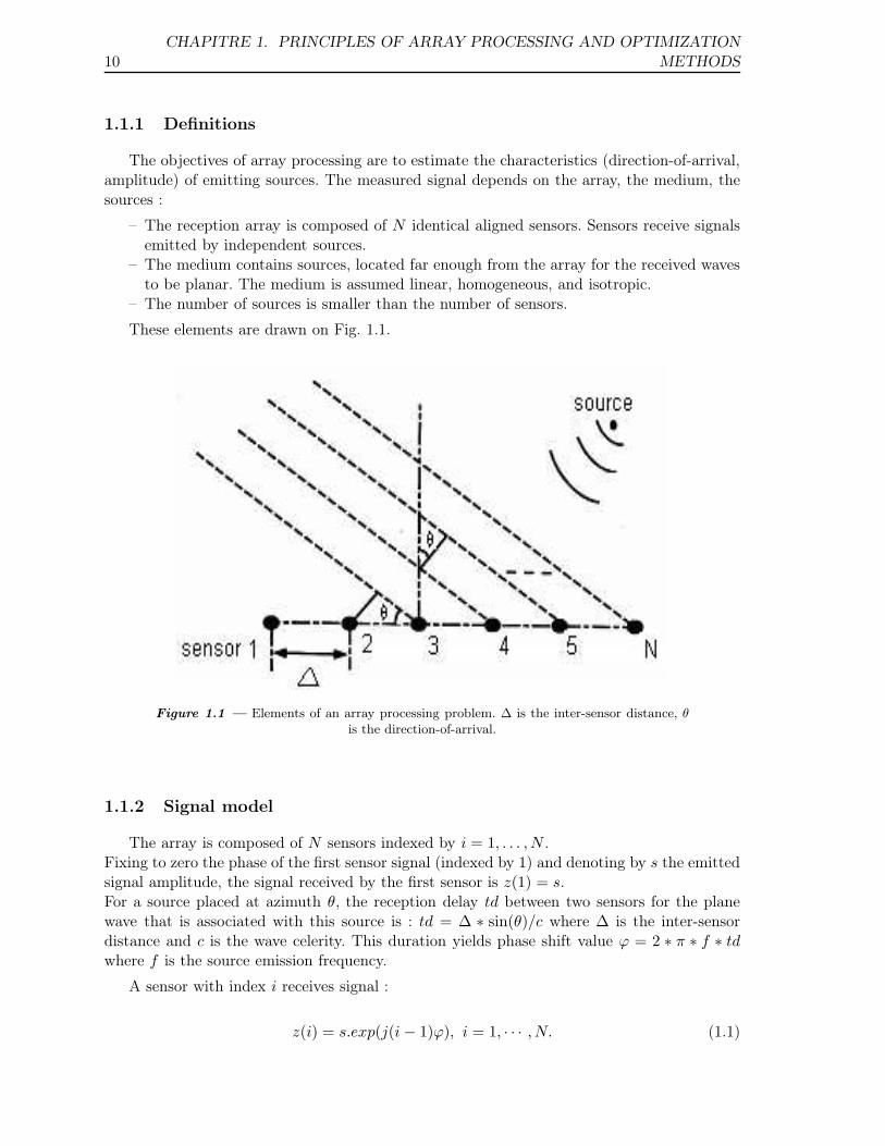
The objectives of array processing are to estimate the characteristics (direction-of-arrival,amplitude) of emitting sources. The measured signal depends on the array, the medium, thesources :
– The reception array is composed of N identical aligned sensors. Sensors receive signalsemitted by independent sources.
– The medium contains sources, located far enough from the array for the received wavesto be planar. The medium is assumed linear, homogeneous, and isotropic.
– The number of sources is smaller than the number of sensors.
These elements are drawn on Fig. 1.1.
Figure 1.1 — Elements of an array processing problem. ∆ is the inter-sensor distance, θ
is the direction-of-arrival.
1.1.2 Signal model
The array is composed of N sensors indexed by i = 1, . . . , N .Fixing to zero the phase of the first sensor signal (indexed by 1) and denoting by s the emittedsignal amplitude, the signal received by the first sensor is z(1) = s.For a source placed at azimuth θ, the reception delay td between two sensors for the planewave that is associated with this source is : td = ∆ ∗ sin(θ)/c where ∆ is the inter-sensordistance and c is the wave celerity. This duration yields phase shift value ϕ = 2 ∗ π ∗ f ∗ tdwhere f is the source emission frequency.
A sensor with index i receives signal :
z(i) = s.exp(j(i − 1)ϕ), i = 1, · · · , N. (1.1)
1.2. SECOND ORDER STATISTICS : CROSS-SPECTRAL MATRIX ANDDISTINCTION BETWEEN SIGNAL SUBSPACE AND NOISE SUBSPACE 11
When d sources are considered, in an additive noise environment, the received signal isexpressed as :
z =
1 1 . . . 1exp(jϕ1) exp(jϕ2) . . . exp(jϕd)
. . . . . . . . . . . .exp(j(N − 1) ∗ ϕ1) exp(j(N − 1) ∗ ϕ2) . . . exp(j(N − 1) ∗ ϕd)
s1
s2
. . .sd
+
n(1)n(2). . .
n(N)
(1.2)where z = [z(1), . . . , z(N)]T , T denoting transpose, is a vector containing all signal compo-nents, [s1, . . . , sd]
T is a vector containing all source amplitudes, and [n(1), . . . , n(N)]T is avector containing all noise components. Defining ai(ϕk) = exp(j(i− 1) ∗ϕk), each componentz(i) of z is expressed as :
z(i) =d∑
k=1
ai(ϕk)sk + n(i), i = 1, . . . , N. (1.3)
We obtain a model for the signal which is received by an array of N sensors, when d sourcesare expected.We set a(ϕk) = [a1(ϕk), a2(ϕk), . . . , aN (ϕk)]T .
Signals can be expressed in a vector form :
z = A(Φ).s + n, (1.4)
where s = [s1, . . . , sd]T is a source amplitude vector, n = [n(1), . . . , n(N)]T , and A(Φ) =
[a(ϕ1), · · · ,a(ϕd)] is an N × d Vandermonde matrix, called transfer matrix or directionalmatrix.
Considering a set of K realizations z1, z2, . . . , zK of received signals, a set s1, s2, . . . , sK ofsource amplitudes, a set of noise realizations n1,n2, . . . ,nK , and by storing each realizationas a column vector of matrices Z, S, N respectively, we obtain in matrix form :
Z = A(Φ)S + N (1.5)
Equation (1.5) contains the whole information provided by the signals received on thearray of sensors.
1.2 Second order statistics : cross-spectral matrix and distinc-tion between signal subspace and noise subspace
From the signals received on the array of sensors, it is of great interest to exploit secondorder statistics. In particular, the eigendecomposition of the cross-spectral matrix yields adistinction between signal and noise subspaces.
12CHAPITRE 1. PRINCIPLES OF ARRAY PROCESSING AND OPTIMIZATION
METHODS
1.2.1 Cross-spectral matrix
We consider a set of K realizations {zl, l = 1, . . . ,K}. A cross-spectral matrix is a cova-riance matrix which is computed in the Fourier space. It can be expressed as follows, for thesignal realizations quoted above :
Rzz = E[zlz
Hl
](1.6)
where H denotes transpose conjugate. An estimate of the covariance matrix is given by :
Rzz =1
K
K∑
l=1
zlzHl , (1.7)
or, by considering the forward and backward (indicated by subscript r) versions of the signalrealizations :
Rzz =1
2K
K∑
l=1
zlzHl + zr
l zrHl (1.8)
where zrl denotes the lth backward sub-vector : [zr
l = zl(N), zl(N − 1), . . . , zl(1)].Matrix form of Eq. (1.7) is the following :
Rzz =1
KZZH (1.9)
The signal is assumed independent from noise ; realizations of noise vector nl are uncorrelated,so the noise covariance matrix is diagonal. All noise realizations have identical variance σ2,so the noise realization covariance matrix is σ2I.
Useful signal part is assumed independent from noise part of the data, so the covariancematrix of the received signals is the summation of the covariance matrix of the useful signalpart of the data and the covariance matrix of noise realizations. By using Eq. (1.4) in Eq. (1.7),we get :
Rzz = A(Φ)RssAH(Φ) + σ2I (1.10)
with
Rss = E[sls
Hl
], (1.11)
and
E[nln
Hl
]= σ2I (1.12)
Using backward and forward versions of the signals yields a better estimation of thecovariance matrix [133].The eigen-decomposition of the covariance matrix is used in general to characterize sources bysubspace (signal and noise subspaces)-based methods [115, 107, 114]. The covariance matrixeigendecomposition is expressed as follows :
Rzz = ΣNi=1λieie
Hi (1.13)
where {λi, i = 1, . . . , N} are the eigenvalues of the covariance matrix, and {ei, i = 1, . . . , N}are the eigenvectors of the covariance matrix.
1.2. SECOND ORDER STATISTICS : CROSS-SPECTRAL MATRIX ANDDISTINCTION BETWEEN SIGNAL SUBSPACE AND NOISE SUBSPACE 13
1.2.2 Distinction between signal and noise subspaces
The eigenvectors of the covariance matrix span the measurement space. Within the mea-surement space, we distinguish between a signal and a noise subspace. When the dimensionof the signal subspace is d, that is, when there are d sources in the considered problem, thisdistinction between subspaces is expressed by :
Rzz = Σdi=1λieie
Hi + ΣN
i=d+1λieieHi = EsΛsE
Hs + EnΛnE
Hn (1.14)
where Es contains the useful signal eigenvectors and En contains the noise eigenvectors.Λs is a diagonal matrix that contains the d largest eigenvalues, Λn is a diagonal matrix thatcontains the eigenvalues associated with the noise subspace.
One can prove that the d largest eigenvalues are associated with the signal subspace. Forthis, we consider the case where noise is null. Then one can express a realization of the receivedsignal as :
z = A(Φ).s (1.15)
The covariance matrix is then :
Rzz = A(Φ)RssAH(Φ) (1.16)
We assume that sources are uncorrelated. Therefore, matrix Rss is diagonal and expressedas :
Rss = diag {α1, α2, . . . , αd} where α1, α2, . . . , αd are the powers of sources 1, 2, . . . , d res-pectively.
Matrix Rss has rank d, matrices A(Φ) and AH(Φ) have rank d. Therefore matrix Rzz
resulting from the product of these three matrices has rank d when noise is null. Then thecovariance matrix can be expressed as :
Rzz = Σdi=1γieie
Hi (1.17)
Equation (1.17) shows that matrix Rzz exhibits d non-zero eigenvalues. These eigenvalues are{γi, i = 1, . . . , d}. As Rzz is positive definite, all γi values are strictly positive. We notice thatif sources are correlated, matrix Rzz may not have rank d when noise is null. Then we usespatial smoothing to decorrelate the sources. In the case where noise is not null, and assumingthat noise is decorrelated and white, the covariance matrix is expressed as :
Rzz = Σdi=1γieie
Hi + σ2I (1.18)
Completely correlated sources
Two sources are completely correlated if they are related by a time shift. The source vectoris then :
s(t) = [s(t), s(t − τ0)]T where τ0 is the time shift between two sources. In the frequency
domain, the source vector is expressed as : s = [s, s exp(−j2πf0τ)]T .The covariance matrix of the useful signal part is expressed as : A(Φ)RssA
H(Φ) with
14CHAPITRE 1. PRINCIPLES OF ARRAY PROCESSING AND OPTIMIZATION
METHODS
Rss =
[|s|2 |s|2 exp(j2π f0τ)
|s|2 exp(−j2π f0τ) |s|2]
(1.19)
The determinant of matrix Rss is null, so there exists only one non-zero eigenvalue. Onecannot distinguish between the two sources although two sources are actually expected.In this case we use a spatial smoothing procedure : A sub-array of length M is translatedalong the array. The new directional matrix is denoted by AM (Φ) and is composed of M rowsand d columns. The M rows of AM (Φ) are equal to the M first rows of A(Φ). The signalcorresponding to the position of the sub-array of index l is :
zl = AM (Φ)Dl−1s + nl (1.20)
where D = diag {ζ1, · · · , ζd}, with ζk = exp(jϕk), ∀ k = 1, . . . , d. By considering the noise vec-tor components : n = [n(1), . . . , n(N)]T one can express vector nl = [n(l), . . . , n(l + M − 1)]T .
The covariance matrices of the signal realizations zl, l = 1, . . . ,K, received on each sub-array are expressed as :
AM (Φ)RssAHM (Φ) + σ2I
...
AM (Φ)Dl−1Rss(DH)l−1AH
M (Φ) + σ2I
...
AM (Φ)DK−1Rss(DH)K−1AH
M (Φ) + σ2I
A covariance matrix with rank K is obtained by computing the mean of the covariancematrices calculated from the signals received on each sub-array.
Rzz =1
K
K∑
l=1
(AM (Φ)Dl−1Rss(DH)l−1AH
M (Φ) + σ2I) (1.21)
Rzz = AM (Φ)1
K(
K∑
l=1
Dl−1Rss(DH)l−1)AH
M (Φ) + σ2I (1.22)
This summation of K different matrices of rank 1 leads to a rank K matrix.Turning to the case of non correlated sources, from Eq. (1.18) we notice that the d lar-gest eigenvalues of the covariance matrix are expressed as
{λi = γi + σ2, i = 1, . . . , d
}. Indeed
{γi, i = 1, . . . , d} are strictly positive, then γi + σ2 > σ2, ∀ i = 1, . . . , d. The N − d smallesteigenvalues of the covariance matrix are
{λi = σ2, i = d + 1, . . . , N
}. We define all eigenvec-
tors associated with the d largest eigenvalues of the covariance matrix as the vectors of thesignal subspace and the eigenvectors associated with the N − d smallest eigenvalues of thecovariance matrix as the vectors of the noise subspace.
1.2.3 Orthogonality between signal and noise subspaces
Referring to Eq. (1.9) and to the expression of the covariance matrix, we note that thecovariance matrix is hermitian, that is, it is equal to its transpose conjugate. Therefore,
1.3. HIGH-RESOLUTION METHODS 15
its eigenvalues are positive or null, and its eigenvectors are orthonormal. Thus, each noisesubspace vector is orthogonal to the signal subspace vectors. We draw the same conclusion inthis way :In the case where noise is decorrelated from the signal, and noise is uncorrelated and white,the covariance matrix can be expressed as :
Rzz = A(Φ)RssAH(Φ) + σ2I (1.23)
Let ei be an eigenvector of Rzz. A(Φ)RssAH(Φ)ei = (λi − σ2)ei.
We have shown that if λi = σ2, ei can only be a vector that belongs to the noise subspace.Therefore, if ei is a noise subspace vector, A(Φ)RssA
H(Φ)ei = 0 then AH(Φ)ei = 0. Thisproves that a noise subspace vector is orthogonal to the subspace that is spanned by thecolumns of A(Φ), that is, the vectors that span the signal subspace.
1.3 High-resolution methods
In this section we present three high-resolution methods. The main property of thesemethods is that they distinguish between close direction-of-arrival values.
1.3.1 MUSIC method
We have shown in section 1.2 that the d largest eigenvalues of the cross-spectral matrixare associated with the signal subspace vectors, and that the noise subspace vectors are or-thogonal to the signal subspace vectors.MUSIC (MUltiple SIgnal Characterization) method selects the eigenvectors that are not asso-ciated with the dominant eigenvalues, that is, the noise subspace eigenvectors. MUSIC methodtakes into account the fact that noise subspace vectors are orthogonal to the signal subspacevectors. MUSIC is a parametric method : it calculates the scalar product between noisesubspace vectors and a signal subspace vector model, which includes the direction-of-arrivalparameter value.
We build a model vector which is convenient for all directional vectors :
a(ϕ) = [1, exp(jϕ), exp(j2ϕ), . . . , exp(j(N − 1) ∗ ϕ)]T
Thus, the scalar product EHn a(ϕ) is null for all parameter values ϕ which are equal to the
source directions-of-arrival :EH
n a(ϕ) = 0 if ϕ = ϕk, (1.24)
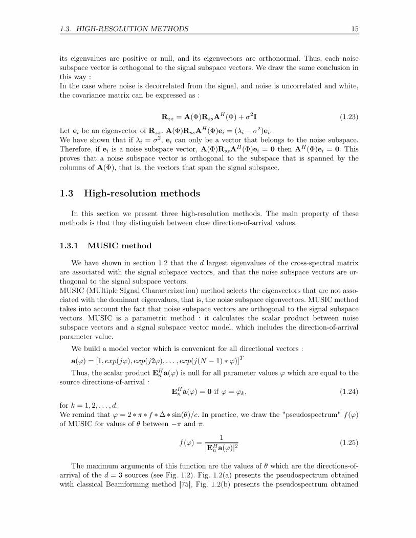
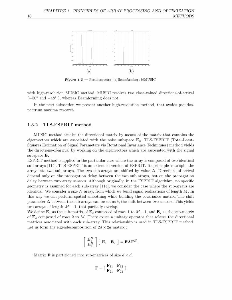
for k = 1, 2, . . . , d.We remind that ϕ = 2 ∗ π ∗ f ∗∆ ∗ sin(θ)/c. In practice, we draw the "pseudospectrum" f(ϕ)of MUSIC for values of θ between −π and π.
f(ϕ) =1
|EHn a(ϕ)|2 (1.25)
The maximum arguments of this function are the values of θ which are the directions-of-arrival of the d = 3 sources (see Fig. 1.2). Fig. 1.2(a) presents the pseudospectrum obtainedwith classical Beamforming method [75], Fig. 1.2(b) presents the pseudospectrum obtained
16CHAPITRE 1. PRINCIPLES OF ARRAY PROCESSING AND OPTIMIZATION
METHODS
−100 −80 −60 −40 −20 0 20 40 60 80 1000
0.05
0.1
0.15
0.2
0.25
0.3
0.35
0.4Beamforming
DOA(°)
Pse
ud
osp
ectr
um
−100 −80 −60 −40 −20 0 20 40 60 80 1000
2
4
6
8
10
12
14
16x 10
28 MUSIC
DOA (°)
Pse
ud
osp
ectr
um
(a) (b)
Figure 1.2 — Pseudospectra : a)Beamforming ; b)MUSIC
with high-resolution MUSIC method. MUSIC resolves two close-valued directions-of-arrival(−50◦ and −48◦ ), whereas Beamforming does not.
In the next subsection we present another high-resolution method, that avoids pseudos-pectrum maxima research.
1.3.2 TLS-ESPRIT method
MUSIC method studies the directional matrix by means of the matrix that contains theeigenvectors which are associated with the noise subspace En. TLS-ESPRIT (Total-Least-Squares Estimation of Signal Parameters via Rotational Invariance Techniques) method yieldsthe directions-of-arrival by working on the eigenvectors which are associated with the signalsubspace Es.ESPRIT method is applied in the particular case where the array is composed of two identicalsub-arrays [114]. TLS-ESPRIT is an extended version of ESPRIT. Its principle is to split thearray into two sub-arrays. The two sub-arrays are shifted by value ∆. Directions-of-arrivaldepend only on the propagation delay between the two sub-arrays, not on the propagationdelay between two array sensors. Although originally, in the ESPRIT algorithm, no specificgeometry is assumed for each sub-array [114], we consider the case where the sub-arrays areidentical. We consider a size N array, from which we build signal realizations of length M . Inthis way we can perform spatial smoothing while building the covariance matrix. The shiftparameter ∆ between the sub-arrays can be set as δ, the shift between two sensors. This yieldstwo arrays of length M − 1, that partially overlap.We define E1 as the sub-matrix of Es composed of rows 1 to M −1, and E2 as the sub-matrixof Es composed of rows 2 to M . There exists a unitary operator that relates the directionalmatrices associated with each sub-array. This relationship is used in TLS-ESPRIT method.Let us form the eigendecomposition of 2d × 2d matrix :
[EH
1
EH2
] [E1 E2
]= FΛFH .
Matrix F is partitioned into sub-matrices of size d × d,
F = [F11 F12
F21 F22]
1.3. HIGH-RESOLUTION METHODS 17
By setting as βk, k = 1, 2, · · · , d, the eigenvalues of matrix −F12F−122 , the directions-of-
arrival are given by [114] :
θ̂k = sin−1[c
(2 π f ∆)Im(ln(
βk
|βk|))], k = 1, . . . , d (1.26)
where Im denotes imaginary part. Therefore, we obtained the estimated values θ̂k of thesource directions-of-arrival.In this framework, the covariance matrix eigenvalues lead to an estimation of the value of d,the number of sources. This estimate is the minimum argument of the "Minimum DescriptionLength" statistical criterion :
MDL(k) = − log
(GM(k)
AM(k)
)(M−k)P
+k
2(2M − k)log(P ) (1.27)
where GM(k) and AM(k) are respectively the geometric and arithmetic means of the (M−k)smallest eigenvalues, given by :
GM(k) =
M∏
i=k+1
λ1
M−k
i (1.28)
and
AM(k) =1
M − k
M∑
i=k+1
λi (1.29)
TLS-ESPRIT method, as well as MUSIC method, relies on the covariance matrix eigen-decomposition. In the next subsection, we present a method which does not rely on eigende-composition, namely the propagator.
1.3.3 Propagator method
The main property of Propagator method is that it does not rely on the eigendecompositionof the covariance matrix. From the data vector z = [z(1), · · · , z(N)]T we perform spatialsmoothing while estimating the covariance matrix : we build K vectors zl = [z(l), · · · , z(M +l− 1)]T , l = 1, · · · ,K of length M with d < M ≤ N − d+ 1. The transfer matrix AM (Φ) hassize M × d. Propagator exploits the linear dependence between the lines of transfer matrixAM (Φ) (see Eq. (1.4)) : AM (Φ) has d independent columns and M > d lines. With Propagatormethod [90], we estimate the phase shift values {ϕk, k = 1, . . . , d}. Propagator method [90]relies on the partition of matrix AM (Φ) :
AHM (Φ) =
[AH
1 | AH2
](1.30)
A1 is a (d×d) matrix and A2 is a (M −d)×d matrix. Matrix AM (Φ) has d columns and thenits rank is up to d. If we suppose that the rows (or columns) of A1 are linearly independent,there exists a linear relationship between matrix A1 and matrix A2 :
A2 = ΠHA1, (1.31)
18CHAPITRE 1. PRINCIPLES OF ARRAY PROCESSING AND OPTIMIZATION
METHODS
where Π is a matrix of size (d × (M − d)).Defining as the "propagator operator" an (M × (M − d)) matrix Q such that :
QH =[ΠH | −I
](1.32)
where I is the ((M − d) × (M − d)) identity matrix, we get :
QHAM (Φ) = ΠHA1 − A2 = 0. (1.33)
The operator Π has to be estimated in order to build the propagator matrix Q. Let Rzz bethe covariance matrix of signals {zl, l = 1, . . . ,K}. We partition the covariance matrix of thereceived signals as follows :
Rzz = [G | H] (1.34)
where G is of size M × (M − d). Matrix Π is obtained from G and H by minimizing theFrobenius norm of (H − G Π), which results in [90, 23] :
Π = [GHG]−1GHH. (1.35)
The expected values for ϕ are such that they lead to the d strongest local maxima of functionf defined as : f(ϕ) = (
∣∣QHa(ϕ)∣∣2)−1 for values of θ between −π and π. Propagator then
yields an estimate of the directions-of-arrival, by partitionning the covariance matrix, andwithout performing its eigendecomposition, contrary to more commonly used methods suchas MUSIC or TLS-ESPRIT. We propose in the following a version of this method which iseven faster, namely the Propagator applied to the generated signals.
1.3.4 Propagator method applied to signal
This version differs from the original Propagator method that partitions the covariancematrix in the sense that operator Π is estimated by partitioning the data vector z. We firstselect the M first components of vector z. This yields a vector which has same length as thesignal realizations which are employed to compute the covariance matrix in the methods thatwere previously presented. Length M vector z is partitioned as follows :
z =[zT1 zT
2
]T(1.36)
where z1 is a length d vector and z2 is a length M − d vector. Using Eq. (3.8) and Eq. (1.30),we obtain the following expression for signal z as a function of A1(Φ) :
z =
A1(Φ)s + n1
−−−A2(Φ)s + n2
Using Eq. (1.31), we obtain :
z =
A1(Φ)s + n1
−−−ΠHA1(Φ)s + n2
(1.37)
where n1 (respectively n2) is a length d (respectively M − d) vector.To obtain a stable estimate for ΠH , we reformulate the problem as a regularized unconstrainedminimization problem, so that the proposed solution for ΠH minimizes [56] :
g(Π) = |z2 − ΠHz1|2 + ς|ΠH |2 (1.38)
1.4. OPTIMIZATION METHOD : COMBINATION OF GRADIENT OR DIRECTALGORITHM WITH SPLINE INTERPOLATION 19
where ς is a Lagrange multiplier [56]. First term in Eq. (1.38) ensures that the estimatedsolution has small residuals, while the second favors "well-behaved solutions" [56].g(Π) is minimum when its derivative with respect to Π is null. The optimal solution is :
ΠH = z2zH1 (z1z
H1 + ςI)−1 (1.39)
where I is the identity matrix.Matrix Q is computed from matrix Π as in Eq. (1.32).From Eq. (1.39), we notice that, if ς > 0, matrix (z1z
H1 + ςI) is invertible. Regularization
constant ς then turns the problem into a well-conditionned one. By avoiding the estimationof a covariance matrix, we expect a faster algorithm.We notice that ΠH is a rank 1 matrix and cannot yield a correct estimate of several parametervalues.To cope with it, we adapt a spatial smoothing procedure, using all signal realizations zl, l =1, . . . ,K. We use the signals zl1, zl2, l = 1, . . . ,K that result from the partition in a lengthd signal and a length M − d signal of each signal realization.
ΠH =1
K
K∑
l=1
(zl2zHl1 (zl1z
Hl1 + ςI)−1) (1.40)
In Eq. (1.40), ΠH is a rank K > d matrix and may yield d parameter values.
1.3.5 Balance on high-resolution methods
The main advantage of TLS-ESPRIT method is that it avoids the research procedure ofthe maxima of a pseudospectrum, inherent in MUSIC method, and it yields the parameterestimates in terms of eigenvalues [114]. Then TLS-ESPRIT method exhibits a low computatio-nal load compared to MUSIC algorithm. Propagator method either estimates the covariancematrix without performing eigendecomposition, or works directly on a single signal realiza-tion. This yields a fast algorithm. High-resolution performances will be exemplified in nextchapters of this manuscript. In the next section, we present an optimization method which willbe adapted in parts 1 and 2 of the manuscript for array processing and image understandingapplications.
1.4 Optimization method : combination of gradient or DIRECTalgorithm with spline interpolation
We propose here an optimization method that aims at fitting a data vector by a priormodel. This optimization method finds a set of N unknown parameters, starting from aset of N initialization values. The components of the complex-valued data vector are deno-ted by zinput(1), . . . , zinput(N) and stored in vector zinput = [zinput(1), . . . , zinput(N)]T . Theunknown values are denoted by ρ(1), . . . , ρ(N), and stored in vector ρ = [ρ(1), . . . , ρ(N)]T .The components of the model vector which is supposed to fit the data are denoted byzρ(1), . . . , zρ(N) and stored in vector zρ = [zρ(1), . . . , zρ(N)]T . The initialization values aredenoted by ρ0(1), . . . , ρ0(N) and stored in vector ρ0 = [ρ0(1), . . . , ρ0(N)]T . The proposed op-timization method minimizes a criterion denoted by J , which is expressed as a function of all
20CHAPITRE 1. PRINCIPLES OF ARRAY PROCESSING AND OPTIMIZATION
METHODS
unknown values ρ(1), . . . , ρ(N) and depends on the processed data. The proposed optimiza-tion algorithm is iterative and recursive, that is, a coordinate vector ρl+1 computed at stepl + 1 of the algorithm depends on coordinate vector ρl computed at step l. At step l of therecursive procedure, a coordinate vector ρl is computed from criterion J defined by :
J(ρl) = ||zinput − zρl||2 (1.41)
where ||.|| represents the norm induced by the usual scalar product of CN .
To minimize the criterion of previous equation, we can use gradient method, with eitherconstant or variable step size. The vectors of the series are obtained by the relation :
∀l ∈ N : ρl+1 = ρl − λ∇(J(ρl)), (1.42)
where λ is the step for the descent. The recurrence loop is ρl → zestimated for ρl→ J(ρl).
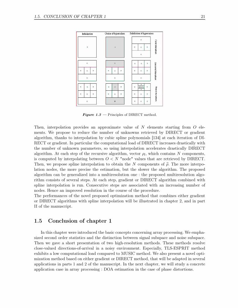
We stop when the gradient becomes lower than a threshold.A variable step gradient method is such that the step λ depends on the iteration index l. Forinstance we can choose λl+1 = 1.05λl for instance.Another optimization method that may be used to minimize the criterion of previous equationis DIRECT (DIviding RECTangles). The main property of DIRECT is that it obtains theglobal minimum of a function. DIRECT does not require the knowledge of the criterion to beminimized. Few parameters are needed in the optimization procedure. DIRECT normalizesthe research space and obtains hypercubes from this research space. Then DIRECT evaluatesthe solution which is at the center of each hypercube. Hypercubes are divided into smallercubes : The smaller the evaluation at the center of a cube, the smaller the cube. In this way,the algorithm favors the regions of the initial research space where the evaluations are small.The division process is performed recursively as is shown in Fig. 1.3. The selection of optimalblocks is based on a compromise between the size and the evaluation at the center of theblock. Thus, DIRECT selects small blocks that provide an interesting (small) evaluation inthe sense of the criterion which is minimized, and DIRECT selects large blocks which are lessinteresting in the sense of the minimized criterion. The main drawback of DIRECT algorithmis that it exhibits an elevated computational load.
A more elaborated optimization algorithm consists in combining either gradient or DI-RECT algorithms with spline interpolation. The main purpose of this method is to reducethe computational load of DIRECT method and to obtain a solution vector that exhibitssome continuity properties.Let O be an integer smaller than N . A cubic spline f interpolating on the partition{y(1), . . . , y(O)} of {1, . . . , N} that we call "node points", to the elements ρ(1), . . . , ρ(N),is a function for which f(y(o)) = ρ(y(o)) for o = 1, . . . , O. It is a piecewise polynomialfunction that consists of O − 1 cubic (third order) polynomials fo defined on the interval[ρ(y(o)), ρ(y(o + 1))]. Furthermore, each fo is joined at y(o), for o = 2, . . . , O − 1, so thatρ′
(y(o)) = f′
(y(o)) and ρ′′
(y(o)) = f′′
(y(o)) are continuous. The oth polynomial curve, fo, isdefined over the fixed interval [y(o), y(o + 1)] and is a third order polynomial. Function fo isthe one that minimizes the integral E of Eq. (1.43).
E =
∫ u=y(o+1)
u=y(o)
f ′′(u)2
(1 + f ′(u)2)5/2du (1.43)
1.5. CONCLUSION OF CHAPTER 1 21
Figure 1.3 — Principles of DIRECT method.
Then, interpolation provides an approximate value of N elements starting from O ele-ments. We propose to reduce the number of unknowns retrieved by DIRECT or gradientalgorithm, thanks to interpolation by cubic spline polynomials [134] at each iteration of DI-RECT or gradient. In particular the computational load of DIRECT increases drastically withthe number of unknown parameters, so using interpolation accelerates drastically DIRECTalgorithm. At each step of the recursive algorithm, vector ρl, which contains N components,is computed by interpolating between O < N "node" values that are retrieved by DIRECT.Then, we propose spline interpolation to obtain the N components of ρ̂. The more interpo-lation nodes, the more precise the estimation, but the slower the algorithm. The proposedalgorithm can be generalized into a multiresolution one : the proposed multiresolution algo-rithm consists of several steps. At each step, gradient or DIRECT algorithm combined withspline interpolation is run. Consecutive steps are associated with an increasing number ofnodes. Hence an improved resolution in the course of the procedure.The performances of the novel proposed optimization method that combines either gradientor DIRECT algorithms with spline interpolation will be illustrated in chapter 2, and in partII of the manuscript.
1.5 Conclusion of chapter 1
In this chapter were introduced the basic concepts concerning array processing. We empha-sized second order statistics and the distinction between signal subspace and noise subspace.Then we gave a short presentation of two high-resolution methods. These methods resolveclose-valued directions-of-arrival in a noisy environment. Especially, TLS-ESPRIT methodexhibits a low computational load compared to MUSIC method. We also present a novel opti-mization method based on either gradient or DIRECT method, that will be adapted in severalapplications in parts 1 and 2 of the manuscript. In the next chapter, we will study a concreteapplication case in array processing : DOA estimation in the case of phase distortions.

CHAPITRE
2 Phase distortion
estimation by DIRECT
and spline interpolation
algorithms
An important cause of performance loss in source localization in underwater acoustics isthat towed flexible antennas deviate from the assumed rectilinear shape. In this work thelocalization of sources in presence of phase errors is studied. Cancellation of phase errors isnecessary to solve the source localization problem. A previous work led to interesting resultsfor antennas composed of a few sensors. We propose here a novel algorithm which is adaptedto the antennas composed of a large number of sensors, keeping a small computational load.Our method is based on an orthogonality property between signal and noise subspaces anda novel optimization method : the robust DIRECT (DIviding RECTangles) algorithm acce-lerated by spline interpolation [85]. The performances of the proposed method are illustratedby applying it to the characterization of three sources.Section 2.1 emphasizes the interest of this work, with respect to existing methods. Section 2.2presents the problem statement. The method proposed is described in Section 2.3, where weestimate phase distortions by an optimization method. In Section 2.4, we evaluate the perfor-mances of the proposed method by an example with three wavefronts and a statistical study.Concluding remarks about this chapter are provided in section 2.5.This work has been published inJ. Marot and S. Bourennane, "Phase Distortion Estimation by DIRECT and spline interpo-lation algorithms", IEEE Signal Processing Letters, Vol. 14, no. 7, pp : 461-464, July 2007.
2.1 Introduction
Finding the parameters of wavefronts impinging on a distorted antenna has been thepurpose of various previous studies [100, 63, 91]. In this chapter, we consider a distortedantenna and wavefronts that are distorted because of the inhomogeneity of the propagationmedium [63]. Previous works considered antennas with a relatively low number of sensors [63,91, 115]. Contrary to these works, we consider antennas composed of a large number of sensors.The proposed method must still lead to small computational times, to permit an easy realtime implementation. The proposed method is particularly useful when the number of sensors
24CHAPITRE 2. PHASE DISTORTION ESTIMATION BY DIRECT AND SPLINE
INTERPOLATION ALGORITHMS
is much greater than the number of sources, which is usually the case in practice [91].
2.2 Problem statement
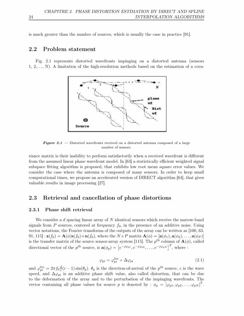
Fig. 2.1 represents distorted wavefronts impinging on a distorted antenna (sensors1, 2,. . ., N). A limitation of the high-resolution methods based on the estimation of a cova-
Figure 2.1 — Distorted wavefronts received on a distorted antenna composed of a largenumber of sensors.
riance matrix is their inability to perform satisfactorily when a received wavefront is differentfrom the assumed linear phase wavefront model. In [63] a statistically efficient weighted signalsubspace fitting algorithm is proposed, that exhibits low root mean square error values. Weconsider the case where the antenna is composed of many sensors. In order to keep smallcomputational times, we propose an accelerated version of DIRECT algorithm [64], that givesvaluable results in image processing [27].
2.3 Retrieval and cancellation of phase distortions
2.3.1 Phase shift retrieval
We consider a d spacing linear array of N identical sensors which receive the narrow-bandsignals from P sources, centered at frequency f0, in the presence of an additive noise. Usingvector notations, the Fourier transforms of the outputs of the array can be written as [100, 63,91, 115] : z(f0) = A(φ)s(f0)+n(f0), where the N×P matrix A(φ) = [a(φ1),a(φ2), . . . ,a(φP )]is the transfer matrix of the source sensor-array system [115]. The pth column of A(φ), called
directional vector of the pth source, is a(φp) =[e−jϕp1, e−jϕp2 , . . . , e−jϕpN
]T, where :
ϕpi = ϕlinpi + ∆ϕpi (2.1)
and ϕlinpi = 2πf0
dc (i − 1) sin(θp). θp is the direction-of-arrival of the pth source, c is the wave
speed, and ∆ϕpi is an additive phase shift value, also called distortion, that can be dueto the deformation of the array and to the perturbation of the impinging wavefronts. Thevector containing all phase values for source p is denoted by : φp = [ϕp1, ϕp2, . . . , ϕpN ]T .
2.3. RETRIEVAL AND CANCELLATION OF PHASE DISTORTIONS 25
z(f0) = [z1(f0), z2(f0), . . . , zN (f0)]T , s(f0) = [s1(f0), s2(f0), . . . , sP (f0)]
T and n(f0) =[n1(f0), n2(f0), . . . , nN (f0)]
T are the Fourier transforms of the array outputs, the source si-gnals and noise vectors, respectively. We consider that K snapshots are available :{z1(f0), z2(f0), . . . , zK(f0)}. The high-resolution method proposed in [115] uses the ei-gendecomposition of the cross-spectral matrix of the received signals : Γzz(f0) =1K ΣK
l=1zl(f0)zHl (f0), where H denotes transpose conjugate. By denoting V(f0) the matrix
containing the vectors of the noise subspace [115] associated with the (N−P ) smallest eigenva-lues, we get [115] : V(f0)
HA(φ) = 0. In the rest of the chapter the frequency f0 is omitted. Thisorthogonality property is used in MUSIC algorithm [115]. The inverse of |V(f0)
Ha(φ)|F , where|.|F denotes Frobenius norm, is called pseudospectrum. Firstly, using MUSIC algorithm, initialvalues of directions-of-arrival are estimated. Secondly, we calculate for each initial direction-
of-arrival θ̂0p, p = 1, . . . , P0 (P0 ≤ P ) a vector of phase values φ̂0p =
[ϕ̂lin
p1 , ϕ̂linp2 , . . . , ϕ̂lin
pN
]T,
where :
ϕ̂linpi = 2πf0
d
c(i − 1) sin(θ̂0p) (2.2)
We use DIRECT algorithm initialized by vector φp0, in order to calculate the expected phase
values :φp = argmin(|VHa(φp)|F ), (2.3)
DIRECT performs global optimization [64]. The computational load of DIRECT algorithmgrows rapidly when the number of sensors, or equivalently the number of unknown phasevalues, increases. At any iteration m, we accelerate DIRECT algorithm by reducing the num-ber of retrieved unknowns and then we propose spline interpolation [27] to obtain the Nphase values of φ̂m
p : we interpolate a subset of values of φ̂mp , which are retrieved by DIRECT
algorithm. The more interpolation nodes, the more accurate the estimation. See 1.4 for de-tails about this optimization method. The series of vectors φ̂m
p converges when m tends to
infinity [64], towards a vector φ̂p such that |VHa(φ̂p)|F is minimum.
2.3.2 Cancel the phase shifts in the received signals
Then for each wavefront the optimization method is run anew and initialized by the ap-proximate value of the corresponding direction-of-arrival. For each source p, phase distortionsof the received signals are canceled to obtain signals z
pl,processed, l = 1 . . . ,K that suit per-
fectly the method based on the orthogonality between signal and noise subspaces [115]. Forone wavefront, phase distortions do not depend only on the physical shape of the antennabut also on the orientation of the wavefront. At this point an approximate value of severaldirections-of-arrival is available. We get the vector of estimated phase distortions :
∆̂φp =[∆̂ϕp1, ∆̂ϕp2, . . . , ∆̂ϕpN
]T(2.4)
corresponding to the current wavefront using Eq. (2.1). We can cancel the phase distortionsand compute the signals to be processed defined by :
zpl,processed = Dp(∆̂φp) zl, l = 1, . . . ,K (2.5)
whereDp(∆̂φp) = diag[ej∆̂ϕp1 , ej∆̂ϕp2, . . . , ej∆̂ϕpN ] (2.6)
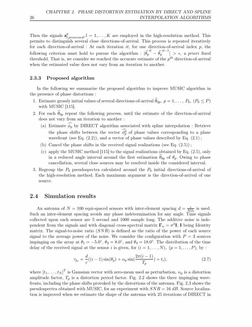
26CHAPITRE 2. PHASE DISTORTION ESTIMATION BY DIRECT AND SPLINE
INTERPOLATION ALGORITHMS
Then the signals zpl,processed, l = 1, . . . ,K are employed in the high-resolution method. This
permits to distinguish several close directions-of-arrival. This process is repeated iterativelyfor each direction-of-arrival : At each iteration it, for one direction-of-arrival index p, the
following criterion must hold to pursue the algorithm : |θ̂pit − θ̂p
it−1| > ǫ, a priori fixedthreshold. That is, we consider we reached the accurate estimate of the pth direction-of-arrivalwhen the estimated value does not vary from an iteration to another.
2.3.3 Proposed algorithm
In the following we summarize the proposed algorithm to improve MUSIC algorithm inthe presence of phase distortions :
1. Estimate grossly initial values of several directions-of-arrival θ̂0p, p = 1, . . . , P0, (P0 ≤ P )with MUSIC [115].
2. For each θ̂0p repeat the following process, until the estimate of the direction-of-arrivaldoes not vary from an iteration to another :
(a) Estimate φ̂p by DIRECT algorithm associated with spline interpolation : Retrieve
the phase shifts between the vector φ̂0p of phase values corresponding to a plane
wavefront (see Eq. (2.2)), and a vector of phase values described by Eq. (2.1) ;
(b) Cancel the phase shifts in the received signal realizations (see Eq. (2.5)) ;
(c) apply the MUSIC method [115] to the signal realizations obtained by Eq. (2.5), onlyin a reduced angle interval around the first estimation θ̂0p of θp. Owing to phasecancellation, several close sources may be resolved inside the considered interval.
3. Regroup the P0 pseudospectra calculated around the P0 initial directions-of-arrival ofthe high-resolution method. Each maximum argument is the direction-of-arrival of onesource.
2.4 Simulation results
An antenna of N = 100 equi-spaced sensors with inter-element spacing d = c32f0
is used.Such an inter-element spacing avoids any phase indetermination for any angle. Time signalscollected upon each sensor are 5 second and 1000 sample long. The additive noise is inde-pendent from the signals and with diagonal cross-spectral matrix Γn = σ2I, I being Identitymatrix. The signal-to-noise ratio (SNR) is defined as the ratio of the power of each sourcesignal to the average power of the noise. We consider the configuration with P = 3 sourcesimpinging on the array at θ1 = −5.0◦, θ2 = 8.0◦, and θ3 = 18.0◦. The distribution of the timedelay of the received signal at the sensor i is given, for (i = 1, . . . , N), (p = 1, . . . , P ), by :
τpi=
d
c((i − 1) sin(θp) + αp sin(
2π(i − 1)
Tp) + ti), (2.7)
where [t1, . . . , tN ]T is Gaussian vector with zero-mean used as perturbation, αp is a distortionamplitude factor, Tp is a distortion period factor. Fig. 2.2 shows the three impinging wave-fronts, including the phase shifts provoked by the distortions of the antenna. Fig. 2.3 shows thepseudospectra obtained with MUSIC, for an experiment with SNR = 16 dB. Source localiza-tion is improved when we estimate the shape of the antenna with 25 iterations of DIRECT in
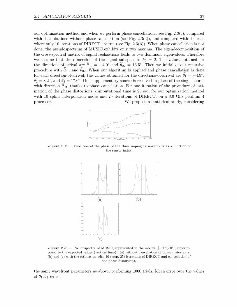
2.4. SIMULATION RESULTS 27
our optimization method and when we perform phase cancellation : see Fig. 2.3(c), comparedwith that obtained without phase cancellation (see Fig. 2.3(a)), and compared with the casewhere only 10 iterations of DIRECT are run (see Fig. 2.3(b)). When phase cancellation is notdone, the pseudospectrum of MUSIC exhibits only two maxima. The eigendecomposition ofthe cross-spectral matrix of signal realizations leads to two dominant eigenvalues. Thereforewe assume that the dimension of the signal subspace is P0 = 2. The values obtained forthe directions-of-arrival are θ̂01 = −4.0◦ and θ̂02 = 16.5◦. Then we initialize our recursiveprocedure with θ̂01, and θ̂02. When our algorithm is applied and phase cancellation is donefor each direction-of-arrival, the values obtained for the directions-of-arrival are θ̂1 = −4.9◦,θ̂2 = 8.2◦, and θ̂3 = 17.6◦. One supplementary source is resolved in place of the single sourcewith direction θ̂02, thanks to phase cancellation. For one iteration of the procedure of esti-mation of the phase distortions, computational time is 25 sec. for our optimization methodwith 10 spline interpolation nodes and 25 iterations of DIRECT, on a 3.0 Ghz pentium 4processor. We propose a statistical study, considering
0 10 20 30 40 50 60 70 80 90 100−50
0
50
100
150
sensor index
phas
e valu
e (°)
Figure 2.2 — Evolution of the phase of the three impinging wavefronts as a function ofthe sensor index.
−50 −40 −30 −20 −10 0 10 20 30 40 500
5
10
15
−50 −40 −30 −20 −10 0 10 20 30 40 500
5
10
15
20
25
(a) (b)
−50 −40 −30 −20 −10 0 10 20 30 40 500
2000
4000
6000
8000
10000
12000
14000
16000
18000
(c)
Figure 2.3 — Pseudospectra of MUSIC, represented in the interval [−50◦, 50◦], superim-posed to the expected values (vertical lines) : (a) without cancellation of phase distortions ;(b) and (c) with the estimation with 10 (resp. 25) iterations of DIRECT and cancellation of
the phase distortions.
the same wavefront parameters as above, performing 1000 trials. Mean error over the valuesof θ1, θ2, θ3 is :
28CHAPITRE 2. PHASE DISTORTION ESTIMATION BY DIRECT AND SPLINE
INTERPOLATION ALGORITHMS
ME = 13000
∑3p=1(
∑1000j=1
(θ̂pj
− θp
)), where j indexes the trials and θ̂pj
is the estimation
obtained at the jth trial for the pth direction-of-arrival. Root mean square error is defined by :
RMSE =√
13000
∑3p=1
∑1000j=1 (θ̂pj
− θp)2.
The statistical results obtained are always acceptable (see Table 2.1).
SNR (dB) 30 34 38 42 46ME (◦) 0.13 0.08 0.06 0.04 0.02
RMSE (◦) 0.09 0.06 0.03 0.01 0.005
Tableau 2.1 — ME and RMSE values over angle estimation for several SNR values.
2.5 Conclusion of chapter 2
A novel algorithm for the characterization of distorted wavefronts and the improvement ofresolution in the presence of phase distortions is proposed. We focused on the case of antennaswith many sensors. To keep low computational times, we proposed a version of "DIRECT"algorithm accelerated by spline interpolation to retrieve distorted wavefronts impinging on adistorted antenna. We have shown that, taking into account phase distortions and cancelingthem, the estimation of the directions-of-arrival of several wavefronts is possible and accurate.In the next chapter, we show that array processing methods can be transposed to an imageprocessing problem. In particular, we show that subspace-based methods of array processingyield close-valued feature parameters.
Second part
Array processing and optimization
methods applied to image
understanding

CHAPITRE
3 Straight line and nearly
straight contour retrieval,
by high-resolution
methods of array
processing and
optimization methods
This chapter is devoted to the estimation of rectilinear and distorted contours in images byHigh Resolution and optimization methods. In the case of rectilinear contours it has beenshown that it is possible to transpose this image processing problem to an array processingproblem. The existing straight line characterization method called Subspace-based Line De-tection (SLIDE) leads to models with orientations and offsets of straight lines as the desiredparameters. In this part, we propose several high-resolution methods which are adapted tothe retrieval of the orientations of straight lines. In particular, we propose a high-resolutionmethod named Propagator which does not rely on the eigendecomposition of the covariancematrix, and which is then faster than other high-resolution methods such as MUSIC or TLS-ESPRIT. We adapt several optimization algorithms : we illustrate the performances of gra-dient algorithm with images which are noise-free or only slightly impaired. Then we adapta more robust optimization method, that combines DIRECT (DIviding RECTangles) withspline interpolation. DIRECT is a global optimization method and is then robust to noise im-pairment, and spline interpolation yields a continuous contour with continuity and curvatureconstraints. This method will be exemplified in particular on real-world or noisy images. Thischapter is organized as follows :In section 3.1, we present an overview of the last advances in contour retrieval methods, andmention the SLIDE method that was proposed to cope with the retrieval of straight lines withclose-valued orientations in a noisy environment. In section 3.2, we state the model which isadopted for a processed image, and we remind the signal generation scheme which is usedin SLIDE method to generate signals out of the image data. In section 3.3, we review TLS-ESPRIT method adapted to the estimation of the orientations of straight lines, we propose toadapt Propagator method, which either relies on the partition of the covariance matrix andnot on its eigendecomposition, or works directly on the generated signal. Propagator type
32
CHAPITRE 3. STRAIGHT LINE AND NEARLY STRAIGHT CONTOURRETRIEVAL, BY HIGH-RESOLUTION METHODS OF ARRAY PROCESSING AND
OPTIMIZATION METHODS
methods are faster than TLS-ESPRIT method. We also propose a novel method for offsetestimation, which is based on a high-resolution method and is faster than the extension of theHough transform. In section 3.4, we present some results obtained on hand-made and real-world images with the proposed straight line estimation methods. In section 3.5, we proposean automatic threshold procedure : a squared criterion compares the signal generated from thethreshold image with an image containing a straight line that fits an expected contour. Thethreshold image that minimizes the chosen criterion contains a selected region aside the fittingstraight line. In section 3.6, we present the principles of the proposed optimization methodfor distorted contour retrieval, and we adapt the gradient optimization algorithm : we solvean inverse problem to retrieve contour distortions from the phase of the generated signal. Insection 3.7, we propose a generalization of the proposed method to the retrieval of severalcontours. In section 3.8, we present some simulation results obtained with gradient algorithm.In section 3.9, we propose to associate gradient method with Propagator to retrieve severaldistorted contours. Section 3.10 presents the results obtained with this particular method.Section 3.11 presents a robust optimization method which associates gradient with spline in-terpolation, which copes with noisy images. In section 3.12 we present the results obtainedby the combination of gradient with spline interpolation, especially on real-world images, andcompared with Gradient Vector Flow (GVF).
This work has been published in :S. Bourennane and J. Marot, "Estimation of straight line offsets by a high-resolution method",IEE Vision Image and Signal Processing, vol. 153, pp. 224-229, 2006., inS. Bourennane and J. Marot, "Contour estimation by array processing methods", Applied si-gnal processing, article ID 95634, 15 pages, 2006., inJ. Marot and S. Bourennane, Propagator method for an application to contour estimation,Pattern recognition letters, vol. 28, no. 12, pp. 1556-1562, sept. 2007., inS. Bourennane and J. Marot, "Line parameters estimation by array processing methods",IEEE ICASSP’05, Vol. 4, pp. 965-968, Mar. 2005, and inS. Bourennane and J. Marot, "Optimization and interpolation for distorted contour estima-tion", IEEE ICASSP’06, Vol. 2, pp. 717-20, April 2006.
3.1 Introduction
Shape description is an important goal of computational vision and image processing.Giving the characteristics of lines or distorted contours is faced in robotic way scree-ning, measuring of wafer track width in microelectronics, aerial image analysis, vehicletrajectory and particle detection. Distorted contour retrieval is also encountered in medi-cal imaging. To solve this problem, active contour or "snakes" segmentation was propo-sed [69, 141, 103, 105, 15, 66, 88, 137, 135, 34, 29]. The idea behind active contour seg-mentation methods is to evolve a parametric curve in the image domain. The curve evolutionis described by a partial differential equation that drives the active contour to a minimum ofa functional. Approaches to active contour segmentation can be either region or edge-based.Among region-based methods, level set methods in particular, introduced in [103] performtexture segmentation. The key idea of level set methods is to represent the evolving curvewith an implicit function which takes positive values inside an image domain with some tex-ture properties, negative values outside this image domain, and null values on the boundariesof this domain. Level set methods allow for automatic change of topology, such as merging
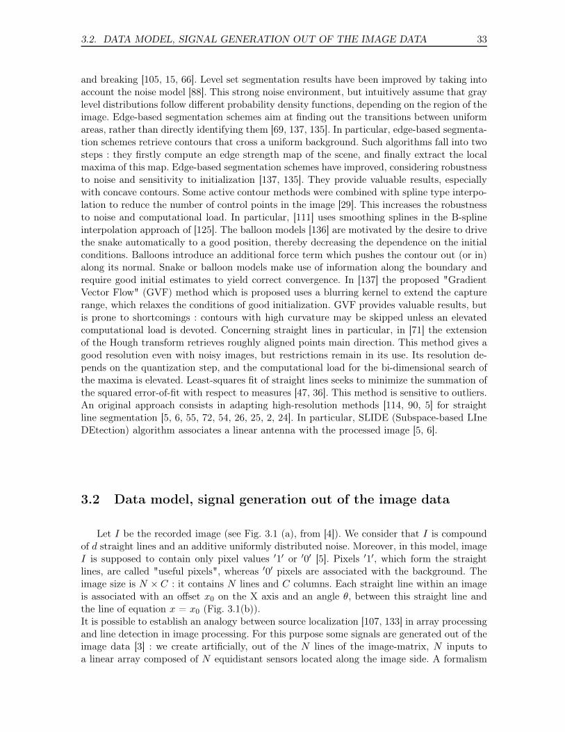
3.2. DATA MODEL, SIGNAL GENERATION OUT OF THE IMAGE DATA 33
and breaking [105, 15, 66]. Level set segmentation results have been improved by taking intoaccount the noise model [88]. This strong noise environment, but intuitively assume that graylevel distributions follow different probability density functions, depending on the region of theimage. Edge-based segmentation schemes aim at finding out the transitions between uniformareas, rather than directly identifying them [69, 137, 135]. In particular, edge-based segmenta-tion schemes retrieve contours that cross a uniform background. Such algorithms fall into twosteps : they firstly compute an edge strength map of the scene, and finally extract the localmaxima of this map. Edge-based segmentation schemes have improved, considering robustnessto noise and sensitivity to initialization [137, 135]. They provide valuable results, especiallywith concave contours. Some active contour methods were combined with spline type interpo-lation to reduce the number of control points in the image [29]. This increases the robustnessto noise and computational load. In particular, [111] uses smoothing splines in the B-splineinterpolation approach of [125]. The balloon models [136] are motivated by the desire to drivethe snake automatically to a good position, thereby decreasing the dependence on the initialconditions. Balloons introduce an additional force term which pushes the contour out (or in)along its normal. Snake or balloon models make use of information along the boundary andrequire good initial estimates to yield correct convergence. In [137] the proposed "GradientVector Flow" (GVF) method which is proposed uses a blurring kernel to extend the capturerange, which relaxes the conditions of good initialization. GVF provides valuable results, butis prone to shortcomings : contours with high curvature may be skipped unless an elevatedcomputational load is devoted. Concerning straight lines in particular, in [71] the extensionof the Hough transform retrieves roughly aligned points main direction. This method gives agood resolution even with noisy images, but restrictions remain in its use. Its resolution de-pends on the quantization step, and the computational load for the bi-dimensional search ofthe maxima is elevated. Least-squares fit of straight lines seeks to minimize the summation ofthe squared error-of-fit with respect to measures [47, 36]. This method is sensitive to outliers.An original approach consists in adapting high-resolution methods [114, 90, 5] for straightline segmentation [5, 6, 55, 72, 54, 26, 25, 2, 24]. In particular, SLIDE (Subspace-based LIneDEtection) algorithm associates a linear antenna with the processed image [5, 6].
3.2 Data model, signal generation out of the image data
Let I be the recorded image (see Fig. 3.1 (a), from [4]). We consider that I is compoundof d straight lines and an additive uniformly distributed noise. Moreover, in this model, imageI is supposed to contain only pixel values ′1′ or ′0′ [5]. Pixels ′1′, which form the straightlines, are called "useful pixels", whereas ′0′ pixels are associated with the background. Theimage size is N × C : it contains N lines and C columns. Each straight line within an imageis associated with an offset x0 on the X axis and an angle θ, between this straight line andthe line of equation x = x0 (Fig. 3.1(b)).It is possible to establish an analogy between source localization [107, 133] in array processingand line detection in image processing. For this purpose some signals are generated out of theimage data [3] : we create artificially, out of the N lines of the image-matrix, N inputs toa linear array composed of N equidistant sensors located along the image side. A formalism
34
CHAPITRE 3. STRAIGHT LINE AND NEARLY STRAIGHT CONTOURRETRIEVAL, BY HIGH-RESOLUTION METHODS OF ARRAY PROCESSING AND
OPTIMIZATION METHODS
adopted in [5] allows signal generation, by the following computation :
z(i) =
C∑
k=1
I(i, k)exp(−jµk), i = 1, ..., N (3.1)
where {I(i, k); i ∈ {1, ..., N}; k ∈ {1, ..., C}} denote the image pixels, and where µ is apropagation parameter [7, 3] that can be constant or variable : we can consider a constant orvariable parameter propagation scheme. We focus in the following on the case where a binaryimage is considered. The contours are composed of 1-valued pixels also called "edge pixels",whereas 0-valued pixels compose the background. When d lines are present in the image, thereare d non zero pixels on the ith line of the image-matrix, localized on the columns x1, · · · , xd
respectively. The signal received by the sensor in front of the ith line, when no noise is presentin the image, is written [4] :
z(i) =
d∑
k=1
exp(−jµxk(i)), i = 1, .., N (3.2)
First we consider the case of only one line with angle θ and offset x0, as it is shown onFig. 3.1 b). Supposing that the width, along the X axis, of each line is equal to one pixel, thehorizontal coordinate of a straight line pixel in front of the ith sensor is :
x(i) = x0 − (i − 1) tan(θ) (3.3)
Hence the signal received on the ith sensor is written :
z(i) = exp(−jµx(i))
z(i) = exp(−jµx0)exp(jµ(i − 1) tan(θ)) (3.4)
In this expression we took into account the possible values of each pixel ′1′ or ′0′. In thepresence of d different straight lines in the image and an additive noise, the signal receivedon the sensor i is :
z(i) =d∑
k=1
exp(jµ(i − 1) tan(θk))exp(−jµx0k) + n(i), (3.5)
where n(i) is the noise on the ith line, that can be due to several noise pixels. As a consequenceof the presence of noisy non zero pixels, the linear variation of the phase in Eq. (3.5) is nolonger verified.Defining :
ai(θk) = exp(jµ(i − 1) tan(θk)), sk = exp(−jµx0k), (3.6)
Equation (3.5) becomes
z(i) =d∑
k=1
ai(θk)sk + n(i), i = 1, · · · , N. (3.7)
Equation (3.15) gives the signal model that will be employed in the following, and that fullycharacterizes the d lines within the noisy image. Grouping all terms in a single vector, Eq. (3.7)becomes :
z = A(θ)s + n (3.8)
with A(θ) = [a(θ1), · · · ,a(θd)] where a(θk) = [a1(θk), a2(θk), · · · , aN (θk)]T , with ai(θk) =
exp(jµ(i − 1)tan(θk)), i = 1, . . . , N , superscript T denoting transpose.
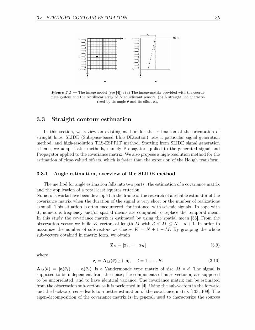
3.3. STRAIGHT CONTOUR ESTIMATION 35
a) b)
Figure 3.1 — The image model (see [4]) : (a) The image-matrix provided with the coordi-nate system and the rectilinear array of N equidistant sensors. (b) A straight line characte-
rized by its angle θ and its offset x0.
3.3 Straight contour estimation
In this section, we review an existing method for the estimation of the orientation ofstraight lines. SLIDE (Subspace-based LIne DEtection) uses a particular signal generationmethod, and high-resolution TLS-ESPRIT method. Starting from SLIDE signal generationscheme, we adapt faster methods, namely Propagator applied to the generated signal andPropagator applied to the covariance matrix. We also propose a high-resolution method for theestimation of close-valued offsets, which is faster than the extension of the Hough transform.
3.3.1 Angle estimation, overview of the SLIDE method
The method for angle estimation falls into two parts : the estimation of a covariance matrixand the application of a total least squares criterion.Numerous works have been developed in the frame of the research of a reliable estimator of thecovariance matrix when the duration of the signal is very short or the number of realizationsis small. This situation is often encountered, for instance, with seismic signals. To cope withit, numerous frequency and/or spatial means are computed to replace the temporal mean.In this study the covariance matrix is estimated by using the spatial mean [55]. From theobservation vector we build K vectors of length M with d < M ≤ N − d + 1. In order tomaximize the number of sub-vectors we choose K = N + 1 − M . By grouping the wholesub-vectors obtained in matrix form, we obtain
ZK = [z1, · · · , zK ] (3.9)
wherezl = AM (θ)sl + nl, l = 1, · · · ,K. (3.10)
AM (θ) = [a(θ1), · · · ,a(θd)] is a Vandermonde type matrix of size M × d. The signal issupposed to be independent from the noise ; the components of noise vector nl are supposedto be uncorrelated, and to have identical variance. The covariance matrix can be estimatedfrom the observation sub-vectors as it is performed in [4]. Using the sub-vectors in the forwardand the backward sense leads to a better estimation of the covariance matrix [133, 109]. Theeigen-decomposition of the covariance matrix is, in general, used to characterize the sources
36
CHAPITRE 3. STRAIGHT LINE AND NEARLY STRAIGHT CONTOURRETRIEVAL, BY HIGH-RESOLUTION METHODS OF ARRAY PROCESSING AND
OPTIMIZATION METHODS
by subspace techniques in array processing. In the frame of image processing the aim is toestimate the angle θ of the d straight lines. Several high-resolution methods that solve thisproblem have been proposed in the literature [115, 107, 114]. SLIDE algorithm is applied toa particular case of an array consisting of two identical sub-arrays [7]. Through TLS-ESPRITmethod, which is detailed in section 1.3.2, SLIDE leads to the following estimated angles [7] :
θ̂k = tan−1[1
(µ ∗ ∆)Im(ln(
βk
|βk|))], (3.11)
where {βk, k = 1, . . . , d} are the eigenvalues of a diagonal unitary matrix that relates themeasurements from the first sub-array to the measurements resulting from the second sub-array. Parameter µ is the propagation constant, and ∆ is the distance between two sensors.TLS-ESPRIT yields an accurate estimation of the orientations of the expected straight lines.We propose in the following to adapt high-resolution methods that do not require eigende-composition of the covariance matrix, and predict that they are faster than TLS-ESPRIT.
3.3.2 Angle estimation by Propagator method
The high-resolution method called "Propagator" [90, 23], which led good results in arrayprocessing, is used for the first time in the field of image processing. This fast high-resolutionmethod estimates the orientation of straight lines, and we further adapt it to the retrieval ofseveral distorted contours.First, we consider one contour which is strictly a straight line, with angle θ and offset x0 (seeFig. 3.1). The horizontal coordinate of a pixel in front of the ith sensor is :
x(i) = x0 − (i − 1)tan(θ) (3.12)
Hence the signal received on the ith sensor reads :
z(i) = exp(−jµx(i)) = exp(−jµx0)exp(jµ(i − 1)tan(θ)). (3.13)
If d straight lines are expected and additive noise is present, the signal received on sensor ireads :
z(i) =
d∑
k=1
exp(jµ(i − 1)tan(θk))exp(−jµx0k) + n(i) (3.14)
where n(i) is the noise due to random edge pixels on the ith row.Setting ai(θk) = exp(jµ(i − 1)tan(θk)), sk = exp(−jµx0k), Eq. (3.14) becomes :
z(i) =d∑
k=1
ai(θk)sk + n(i). (3.15)
From the data vector z = [z(1), · · · , z(N)]T we build K vectors zl = [z(l), · · · , z(M + l −1)]T , l = 1, · · · ,K, of length M with d < M ≤ N − d + 1. We define matrix AM (θ) as :
AM (θ) = [a(θ1), · · · ,a(θd)] (3.16)
where a(θk) = [1, ζk, · · · , ζM−1k ]T , with ζk = exp(jµtan(θk)). With Propagator method [90]
(see subsection 1.3.3), we estimate the orientations {θk} of the straight lines. The angle
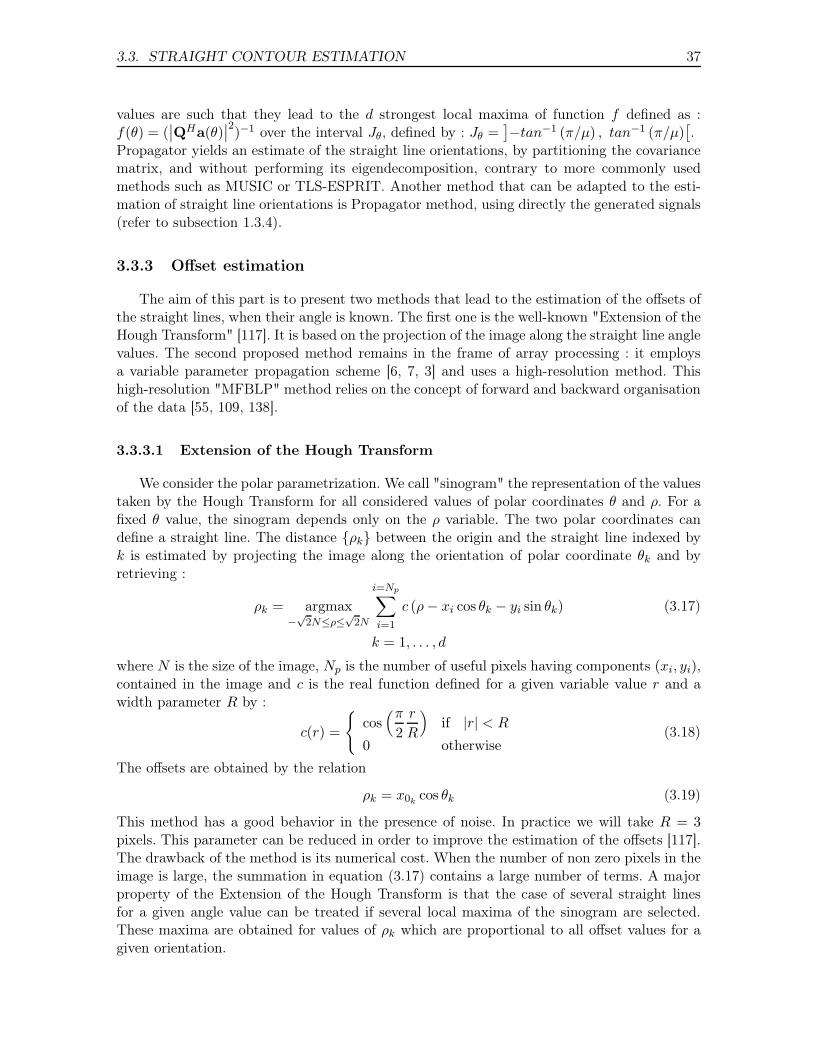
3.3. STRAIGHT CONTOUR ESTIMATION 37
values are such that they lead to the d strongest local maxima of function f defined as :f(θ) = (
∣∣QHa(θ)∣∣2)−1 over the interval Jθ, defined by : Jθ =
]−tan−1 (π/µ) , tan−1 (π/µ)
[.
Propagator yields an estimate of the straight line orientations, by partitioning the covariancematrix, and without performing its eigendecomposition, contrary to more commonly usedmethods such as MUSIC or TLS-ESPRIT. Another method that can be adapted to the esti-mation of straight line orientations is Propagator method, using directly the generated signals(refer to subsection 1.3.4).
3.3.3 Offset estimation
The aim of this part is to present two methods that lead to the estimation of the offsets ofthe straight lines, when their angle is known. The first one is the well-known "Extension of theHough Transform" [117]. It is based on the projection of the image along the straight line anglevalues. The second proposed method remains in the frame of array processing : it employsa variable parameter propagation scheme [6, 7, 3] and uses a high-resolution method. Thishigh-resolution "MFBLP" method relies on the concept of forward and backward organisationof the data [55, 109, 138].
3.3.3.1 Extension of the Hough Transform
We consider the polar parametrization. We call "sinogram" the representation of the valuestaken by the Hough Transform for all considered values of polar coordinates θ and ρ. For afixed θ value, the sinogram depends only on the ρ variable. The two polar coordinates candefine a straight line. The distance {ρk} between the origin and the straight line indexed byk is estimated by projecting the image along the orientation of polar coordinate θk and byretrieving :
ρk = argmax−√
2N≤ρ≤√
2N
i=Np∑
i=1
c (ρ − xi cos θk − yi sin θk) (3.17)
k = 1, . . . , d
where N is the size of the image, Np is the number of useful pixels having components (xi, yi),contained in the image and c is the real function defined for a given variable value r and awidth parameter R by :
c(r) =
{cos
(π
2
r
R
)if |r| < R
0 otherwise(3.18)
The offsets are obtained by the relation
ρk = x0kcos θk (3.19)
This method has a good behavior in the presence of noise. In practice we will take R = 3pixels. This parameter can be reduced in order to improve the estimation of the offsets [117].The drawback of the method is its numerical cost. When the number of non zero pixels in theimage is large, the summation in equation (3.17) contains a large number of terms. A majorproperty of the Extension of the Hough Transform is that the case of several straight linesfor a given angle value can be treated if several local maxima of the sinogram are selected.These maxima are obtained for values of ρk which are proportional to all offset values for agiven orientation.
38
CHAPITRE 3. STRAIGHT LINE AND NEARLY STRAIGHT CONTOURRETRIEVAL, BY HIGH-RESOLUTION METHODS OF ARRAY PROCESSING AND
OPTIMIZATION METHODS
3.3.3.2 Proposed method : MFBLP
The variable speed propagation scheme method [6, 7] enables the estimation of the offsetswith a lower computational load than the Extension of the Hough Transform. We associateto this specific signal generation scheme a high-resolution method called "MFBLP" (ModifiedForward Backward Linear Prediction). In a previous work (see [55]), the concept of usingforward-backward averaging led to effective results when it was applied to the SLIDE algo-rithm.The basic idea in this method is to associate a propagation speed which is different for eachline in the image. By setting artificially a propagation speed that linearly depends on theindex of the lines in the matrix, we will be able to apply a frequency retrieval method tocompute the offset values. When the first orientation value is considered, the signal receivedon sensor i (i = 1, · · · , N) is then :
z(i) =
d1∑
k=1
exp(−jτx0k)exp(jτ(i − 1)tan(θ1)) + n(i) (3.20)
d1 is the number of lines with angle θ1. When τ varies linearly as a function of the line indexthe measure vector z contains a modulated frequency term. Indeed we set τ = α(i − 1).
z(i) =
d1∑
k=1
exp(−jα(i − 1)x0k)exp(jα(i − 1)2tan(θ1)) + n(i) (3.21)
This is a sum of d1 signals that have a common quadratic phase term but different linear phaseterms. The first treatment consists in obtaining an expression containing only linear terms.This goal is reached by dividing z(i) by the non zero term ai(θ1) = exp(jα(i − 1)2tan(θ1)).We obtain then :
w(i) =
d1∑
k=1
exp(−jα(i − 1)x0k) + n′
(i), (3.22)
i = 1, · · · , N.
The resulting signal appears as a combination of d1 sinusoids with frequencies :
fk =αx0k
2π, k = 1, · · · , d1. (3.23)
Consequently, the estimation of the offsets can be transposed to a frequency estimation pro-blem. Estimation of frequencies from sources having the same amplitude was considered in[124]. In the following a high-resolution algorithm, initially introduced in spectral analysis[124], is proposed for the estimation of the offsets.After adopting our signal model we adapt it to the spectral analysis method called modifiedforward backward linear prediction (MFBLP) [124] for estimating the offsets :We consider dk straight lines with given angle θk, and apply the MFBLP method. We considerdk straight lines with given angle θk, and apply the MFBLP method, to the vector w. For aconvenient representation the components of w will be written [w1, w2, ..., wN ].1) For a N-data vector w, form the matrix Q of size 2 · (N −L)×L -where the subscript "∗"indicates conjugate- :
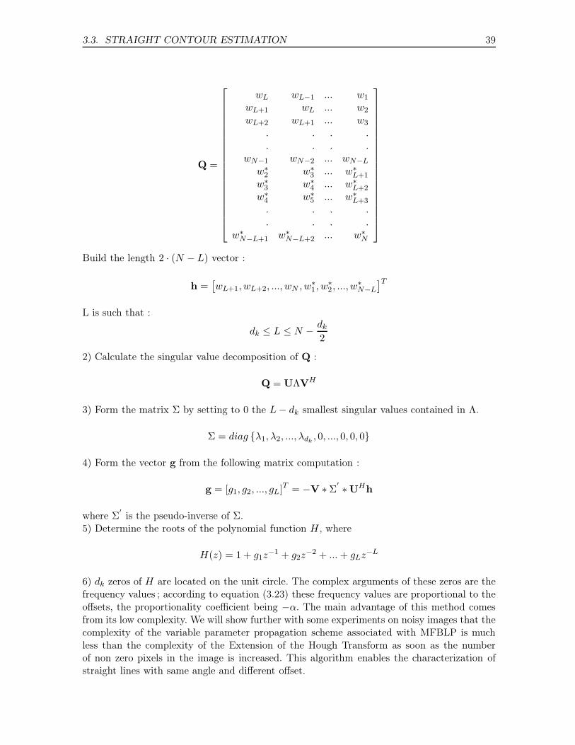
3.3. STRAIGHT CONTOUR ESTIMATION 39
Q =
wL wL−1 ... w1
wL+1 wL ... w2
wL+2 wL+1 ... w3
. . . .
. . . .wN−1 wN−2 ... wN−L
w∗2 w∗
3 ... w∗L+1
w∗3 w∗
4 ... w∗L+2
w∗4 w∗
5 ... w∗L+3
. . . .
. . . .w∗
N−L+1 w∗N−L+2 ... w∗
N
Build the length 2 · (N − L) vector :
h =[wL+1, wL+2, ..., wN , w∗
1, w∗2, ..., w
∗N−L
]T
L is such that :
dk ≤ L ≤ N − dk
2
2) Calculate the singular value decomposition of Q :
Q = UΛVH
3) Form the matrix Σ by setting to 0 the L − dk smallest singular values contained in Λ.
Σ = diag {λ1, λ2, ..., λdk, 0, ..., 0, 0, 0}
4) Form the vector g from the following matrix computation :
g = [g1, g2, ..., gL]T = −V ∗ Σ′ ∗UHh
where Σ′
is the pseudo-inverse of Σ.5) Determine the roots of the polynomial function H, where
H(z) = 1 + g1z−1 + g2z
−2 + ... + gLz−L
6) dk zeros of H are located on the unit circle. The complex arguments of these zeros are thefrequency values ; according to equation (3.23) these frequency values are proportional to theoffsets, the proportionality coefficient being −α. The main advantage of this method comesfrom its low complexity. We will show further with some experiments on noisy images that thecomplexity of the variable parameter propagation scheme associated with MFBLP is muchless than the complexity of the Extension of the Hough Transform as soon as the numberof non zero pixels in the image is increased. This algorithm enables the characterization ofstraight lines with same angle and different offset.
40
CHAPITRE 3. STRAIGHT LINE AND NEARLY STRAIGHT CONTOURRETRIEVAL, BY HIGH-RESOLUTION METHODS OF ARRAY PROCESSING AND
OPTIMIZATION METHODS
3.4 Straight line estimation : results obtained
This section falls into three subsections dedicated to the efficiency of the presented straightline estimation methods. The first subsection concerns the estimation of rectilinear curves bySLIDE method and MFBLP. The second subsection emphasizes the ability of MFBLP toresolve close-valued offsets. The third subsection compares MFBLP and the extension of theHough transform in terms of computational load.
3.4.1 Straight line estimation by SLIDE method, and MFBLP
As a first example, we propose an application of our method in the case of robotic vision.Fig. 3.2(a) is a photography taken by a camera and transmitted to the automatic command ofa vehicle moving on the railway. This vehicle is used in particular for servicing of railways, i.e.for the replacement of the parallel crosspieces. The vehicle, when moving along the railway,determines first the position of the rails from the obtained picture. Then, the position of thenearest crosspiece is detected. It places itself over the detected crosspiece and the replacementof this one is performed by an auxiliary engine. The iterative replacement of the crosspiecesis realized step by step. First, the position of the rails is determined. The array processingmethods of "SLIDE" and variable propagation scheme associated with MFBLP are employed.The result of this determination is presented on Fig. 3.2 (b) Referring to the retrieved positionof the rails, the vehicle decides about the correction to give to its progression. Once therails are retrieved, the image is processed once again, the localization of the first crosspieceis performed and presented on Fig. 3.2(c) The crosspiece can be detected by changing theposition of the antenna (this technique is described in [3]). The process is repeated and thecrosspieces are retrieved iteratively. For this grey level image, the computational time whichis required to retrieve the two rails by means of SLIDE algorithm, when MFBLP method isassociated with the variable speed generation scheme, is the following : the estimation of thetwo orientation values, including signal generation and running TLS-ESPRIT method, needs0.063 sec. The estimation of the offsets needs 1.1 sec. As a comparison, the Extension of theHough Transform, employed with the a priori knowledge of the angles, needs 47 sec. to findthe offsets of the two lines that fit the rails.We exemplify now the estimation of convex object contours with polygonal geometry, as asecond application case. Our method is employed to retrieve the characteristics of a polygon,namely the number of sides and the coordinates of the summits. For this purpose, the straightlines that fit the sides of the polygon are determined by the proposed method. The number andthe parameters (angles, offsets) of the straight lines allow respectively to estimate the numberof sides and the summits. The summits are fitted by considering the polygon as the smallestconvex of the image, corresponding to the common intersection of the half-plans associatedrespectively with the support straight lines. Fig. 3.3(a) presents the case of a polygon includedin a noisy image. This image contains 15% of randomly distributed noisy pixels. The straightlines that fit the sides are given on Fig. 3.3(b) and are determined in spite of the presence ofnoise in the image. For an image with more noisy pixels, a bias on the values of angle andoffset can appear. It is difficult to obtain a valuable result from images with more than 20%of randomly distributed noisy pixels.Fig. 3.4 presents the result obtained on an image containing a set of roughly aligned points.Like images containing dashed lines, this kind of images leads to generated signals that are
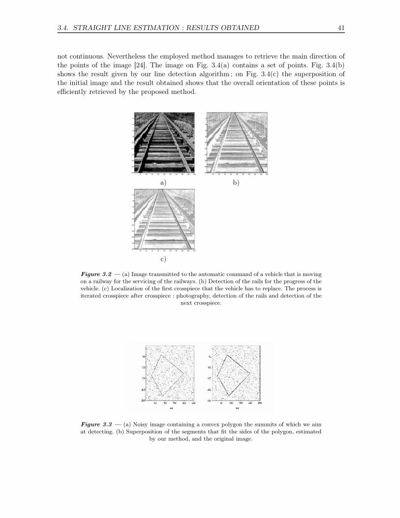
3.4. STRAIGHT LINE ESTIMATION : RESULTS OBTAINED 41
not continuous. Nevertheless the employed method manages to retrieve the main direction ofthe points of the image [24]. The image on Fig. 3.4(a) contains a set of points. Fig. 3.4(b)shows the result given by our line detection algorithm ; on Fig. 3.4(c) the superposition ofthe initial image and the result obtained shows that the overall orientation of these points isefficiently retrieved by the proposed method.
20 40 60 80 100 120 140 160 180 200
20
40
60
80
100
120
140
160
180
20020 40 60 80 100 120 140 160 180 200
20
40
60
80
100
120
140
160
180
200
a) b)
20 40 60 80 100 120 140 160 180 200
20
40
60
80
100
120
140
160
180
200
c)
Figure 3.2 — (a) Image transmitted to the automatic command of a vehicle that is movingon a railway for the servicing of the railways. (b) Detection of the rails for the progress of thevehicle. (c) Localization of the first crosspiece that the vehicle has to replace. The process isiterated crosspiece after crosspiece : photography, detection of the rails and detection of the
next crosspiece.
a) b)
Figure 3.3 — (a) Noisy image containing a convex polygon the summits of which we aimat detecting. (b) Superposition of the segments that fit the sides of the polygon, estimated
by our method, and the original image.
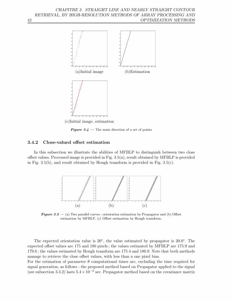
42
CHAPITRE 3. STRAIGHT LINE AND NEARLY STRAIGHT CONTOURRETRIEVAL, BY HIGH-RESOLUTION METHODS OF ARRAY PROCESSING AND
OPTIMIZATION METHODS
20 40 60 80 100 120 140 160 180 200
20
40
60
80
100
120
140
160
180
20020 40 60 80 100 120 140 160 180 200
20
40
60
80
100
120
140
160
180
200
(a)Initial image (b)Estimation
20 40 60 80 100 120 140 160 180 200
20
40
60
80
100
120
140
160
180
200
(c)Initial image, estimation
Figure 3.4 — The main direction of a set of points
3.4.2 Close-valued offset estimation
In this subsection we illustrate the abilities of MFBLP to distinguish between two closeoffset values. Processed image is provided in Fig. 3.5(a), result obtained by MFBLP is providedin Fig. 3.5(b), and result obtained by Hough transform is provided in Fig. 3.5(c).
20 40 60 80 100 120 140 160 180 200
20
40
60
80
100
120
140
160
180
20020 40 60 80 100 120 140 160 180 200
20
40
60
80
100
120
140
160
180
20020 40 60 80 100 120 140 160 180 200
20
40
60
80
100
120
140
160
180
200
(a) (b) (c)
Figure 3.5 — (a) Two parallel curves : orientation estimation by Propagator and (b) Offsetestimation by MFBLP, (c) Offset estimation by Hough transform.
The expected orientation value is 20◦, the value estimated by propagator is 20.0◦. Theexpected offset values are 175 and 180 pixels ; the values estimated by MFBLP are 175.9 and179.8 ; the values estimated by Hough transform are 175.4 and 180.9. Note that both methodsmanage to retrieve the close offset values, with less than a one pixel bias.For the estimation of parameter θ computational times are, excluding the time required forsignal generation, as follows : the proposed method based on Propagator applied to the signal(see subsection 3.3.2) lasts 5.4×10⁻⁴ sec. Propagator method based on the covariance matrix
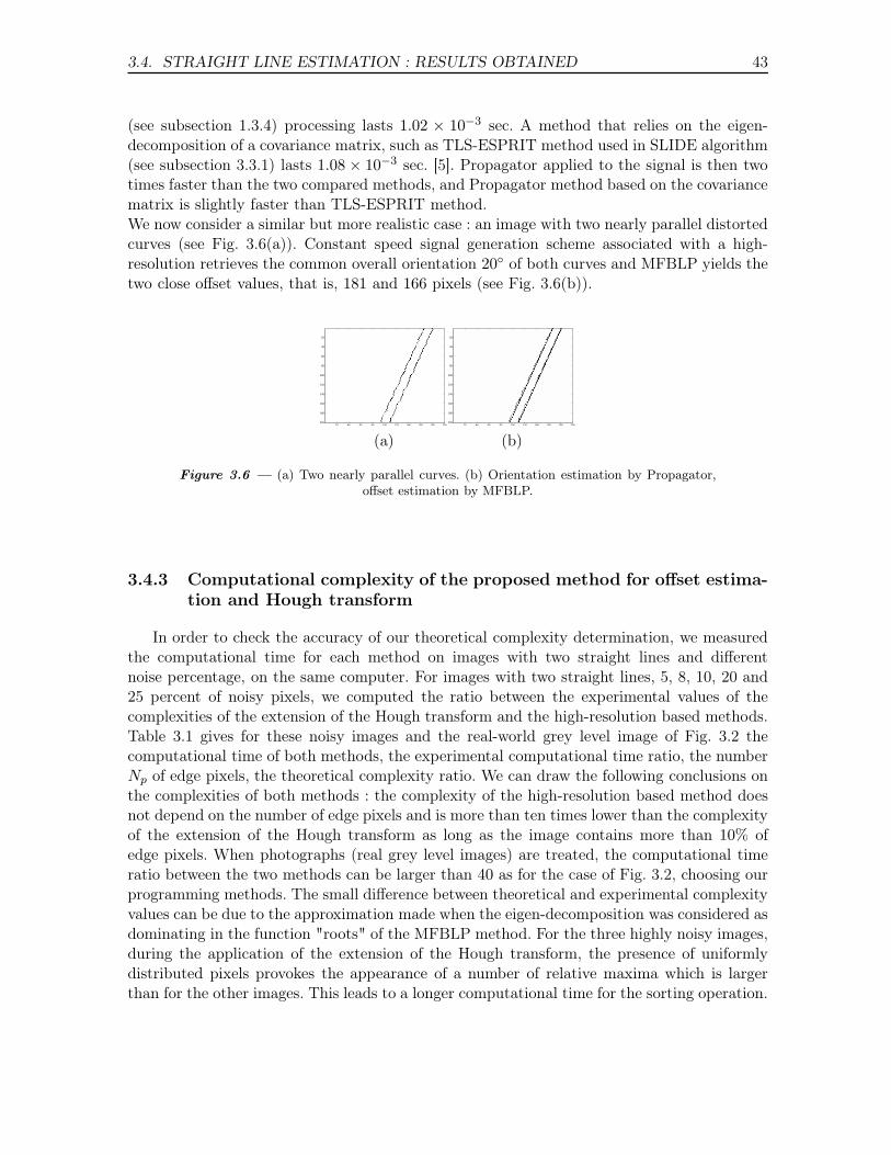
3.4. STRAIGHT LINE ESTIMATION : RESULTS OBTAINED 43
(see subsection 1.3.4) processing lasts 1.02 × 10⁻³ sec. A method that relies on the eigen-decomposition of a covariance matrix, such as TLS-ESPRIT method used in SLIDE algorithm(see subsection 3.3.1) lasts 1.08 × 10⁻³ sec. [5]. Propagator applied to the signal is then twotimes faster than the two compared methods, and Propagator method based on the covariancematrix is slightly faster than TLS-ESPRIT method.We now consider a similar but more realistic case : an image with two nearly parallel distortedcurves (see Fig. 3.6(a)). Constant speed signal generation scheme associated with a high-resolution retrieves the common overall orientation 20◦ of both curves and MFBLP yields thetwo close offset values, that is, 181 and 166 pixels (see Fig. 3.6(b)).
20 40 60 80 100 120 140 160 180 200
20
40
60
80
100
120
140
160
180
20020 40 60 80 100 120 140 160 180 200
20
40
60
80
100
120
140
160
180
200
(a) (b)
Figure 3.6 — (a) Two nearly parallel curves. (b) Orientation estimation by Propagator,offset estimation by MFBLP.
3.4.3 Computational complexity of the proposed method for offset estima-tion and Hough transform
In order to check the accuracy of our theoretical complexity determination, we measuredthe computational time for each method on images with two straight lines and differentnoise percentage, on the same computer. For images with two straight lines, 5, 8, 10, 20 and25 percent of noisy pixels, we computed the ratio between the experimental values of thecomplexities of the extension of the Hough transform and the high-resolution based methods.Table 3.1 gives for these noisy images and the real-world grey level image of Fig. 3.2 thecomputational time of both methods, the experimental computational time ratio, the numberNp of edge pixels, the theoretical complexity ratio. We can draw the following conclusions onthe complexities of both methods : the complexity of the high-resolution based method doesnot depend on the number of edge pixels and is more than ten times lower than the complexityof the extension of the Hough transform as long as the image contains more than 10% ofedge pixels. When photographs (real grey level images) are treated, the computational timeratio between the two methods can be larger than 40 as for the case of Fig. 3.2, choosing ourprogramming methods. The small difference between theoretical and experimental complexityvalues can be due to the approximation made when the eigen-decomposition was considered asdominating in the function "roots" of the MFBLP method. For the three highly noisy images,during the application of the extension of the Hough transform, the presence of uniformlydistributed pixels provokes the appearance of a number of relative maxima which is largerthan for the other images. This leads to a longer computational time for the sorting operation.
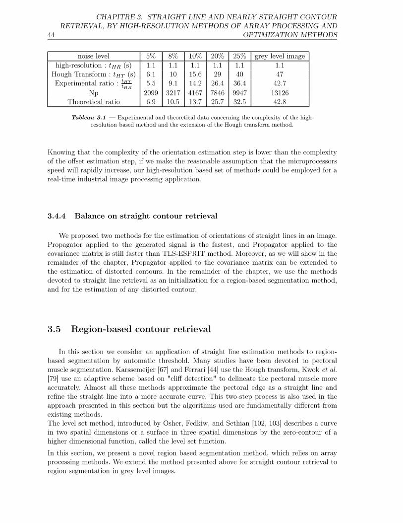
44
CHAPITRE 3. STRAIGHT LINE AND NEARLY STRAIGHT CONTOURRETRIEVAL, BY HIGH-RESOLUTION METHODS OF ARRAY PROCESSING AND
OPTIMIZATION METHODS
noise level 5% 8% 10% 20% 25% grey level imagehigh-resolution : tHR (s) 1.1 1.1 1.1 1.1 1.1 1.1
Hough Transform : tHT (s) 6.1 10 15.6 29 40 47Experimental ratio : tHT
tHR5.5 9.1 14.2 26.4 36.4 42.7
Np 2099 3217 4167 7846 9947 13126Theoretical ratio 6.9 10.5 13.7 25.7 32.5 42.8
Tableau 3.1 — Experimental and theoretical data concerning the complexity of the high-resolution based method and the extension of the Hough transform method.
Knowing that the complexity of the orientation estimation step is lower than the complexityof the offset estimation step, if we make the reasonable assumption that the microprocessorsspeed will rapidly increase, our high-resolution based set of methods could be employed for areal-time industrial image processing application.
3.4.4 Balance on straight contour retrieval
We proposed two methods for the estimation of orientations of straight lines in an image.Propagator applied to the generated signal is the fastest, and Propagator applied to thecovariance matrix is still faster than TLS-ESPRIT method. Moreover, as we will show in theremainder of the chapter, Propagator applied to the covariance matrix can be extended tothe estimation of distorted contours. In the remainder of the chapter, we use the methodsdevoted to straight line retrieval as an initialization for a region-based segmentation method,and for the estimation of any distorted contour.
3.5 Region-based contour retrieval
In this section we consider an application of straight line estimation methods to region-based segmentation by automatic threshold. Many studies have been devoted to pectoralmuscle segmentation. Karssemeijer [67] and Ferrari [44] use the Hough transform, Kwok et al.[79] use an adaptive scheme based on "cliff detection" to delineate the pectoral muscle moreaccurately. Almost all these methods approximate the pectoral edge as a straight line andrefine the straight line into a more accurate curve. This two-step process is also used in theapproach presented in this section but the algorithms used are fundamentally different fromexisting methods.The level set method, introduced by Osher, Fedkiw, and Sethian [102, 103] describes a curvein two spatial dimensions or a surface in three spatial dimensions by the zero-contour of ahigher dimensional function, called the level set function.
In this section, we present a novel region based segmentation method, which relies on arrayprocessing methods. We extend the method presented above for straight contour retrieval toregion segmentation in grey level images.
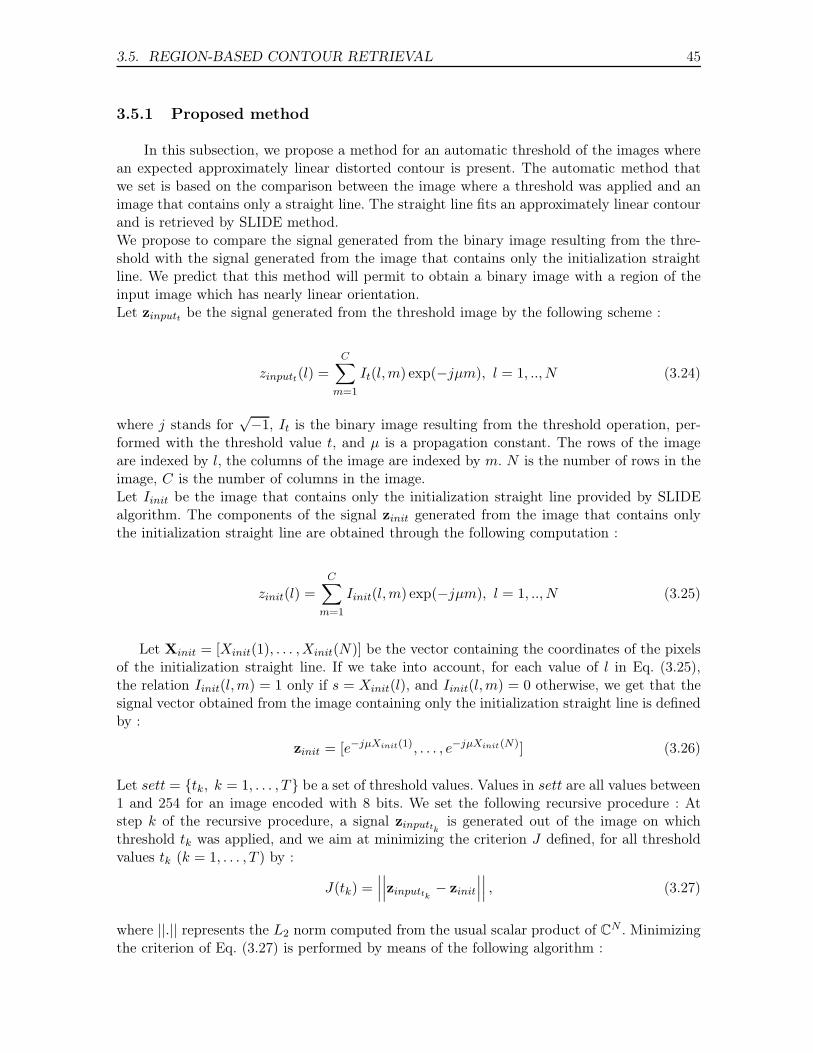
3.5. REGION-BASED CONTOUR RETRIEVAL 45
3.5.1 Proposed method
In this subsection, we propose a method for an automatic threshold of the images wherean expected approximately linear distorted contour is present. The automatic method thatwe set is based on the comparison between the image where a threshold was applied and animage that contains only a straight line. The straight line fits an approximately linear contourand is retrieved by SLIDE method.We propose to compare the signal generated from the binary image resulting from the thre-shold with the signal generated from the image that contains only the initialization straightline. We predict that this method will permit to obtain a binary image with a region of theinput image which has nearly linear orientation.Let zinputt be the signal generated from the threshold image by the following scheme :
zinputt(l) =
C∑
m=1
It(l,m) exp(−jµm), l = 1, .., N (3.24)
where j stands for√−1, It is the binary image resulting from the threshold operation, per-
formed with the threshold value t, and µ is a propagation constant. The rows of the imageare indexed by l, the columns of the image are indexed by m. N is the number of rows in theimage, C is the number of columns in the image.Let Iinit be the image that contains only the initialization straight line provided by SLIDEalgorithm. The components of the signal zinit generated from the image that contains onlythe initialization straight line are obtained through the following computation :
zinit(l) =C∑
m=1
Iinit(l,m) exp(−jµm), l = 1, .., N (3.25)
Let Xinit = [Xinit(1), . . . ,Xinit(N)] be the vector containing the coordinates of the pixelsof the initialization straight line. If we take into account, for each value of l in Eq. (3.25),the relation Iinit(l,m) = 1 only if s = Xinit(l), and Iinit(l,m) = 0 otherwise, we get that thesignal vector obtained from the image containing only the initialization straight line is definedby :
zinit = [e−jµXinit(1), . . . , e−jµXinit(N)] (3.26)
Let sett = {tk, k = 1, . . . , T} be a set of threshold values. Values in sett are all values between1 and 254 for an image encoded with 8 bits. We set the following recursive procedure : Atstep k of the recursive procedure, a signal zinputtk
is generated out of the image on whichthreshold tk was applied, and we aim at minimizing the criterion J defined, for all thresholdvalues tk (k = 1, . . . , T ) by :
J(tk) =∣∣∣∣∣∣zinputtk
− zinit
∣∣∣∣∣∣ , (3.27)
where ||.|| represents the L2 norm computed from the usual scalar product of CN . Minimizingthe criterion of Eq. (3.27) is performed by means of the following algorithm :
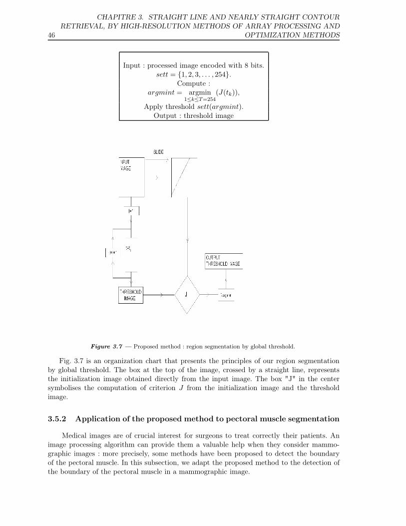
46
CHAPITRE 3. STRAIGHT LINE AND NEARLY STRAIGHT CONTOURRETRIEVAL, BY HIGH-RESOLUTION METHODS OF ARRAY PROCESSING AND
OPTIMIZATION METHODS
Input : processed image encoded with 8 bits.sett = {1, 2, 3, . . . , 254}.
Compute :argmint = argmin
1≤k≤T=254(J(tk)),
Apply threshold sett(argmint).Output : threshold image
Figure 3.7 — Proposed method : region segmentation by global threshold.
Fig. 3.7 is an organization chart that presents the principles of our region segmentationby global threshold. The box at the top of the image, crossed by a straight line, representsthe initialization image obtained directly from the input image. The box "J" in the centersymbolises the computation of criterion J from the initialization image and the thresholdimage.
3.5.2 Application of the proposed method to pectoral muscle segmentation
Medical images are of crucial interest for surgeons to treat correctly their patients. Animage processing algorithm can provide them a valuable help when they consider mammo-graphic images : more precisely, some methods have been proposed to detect the boundaryof the pectoral muscle. In this subsection, we adapt the proposed method to the detection ofthe boundary of the pectoral muscle in a mammographic image.
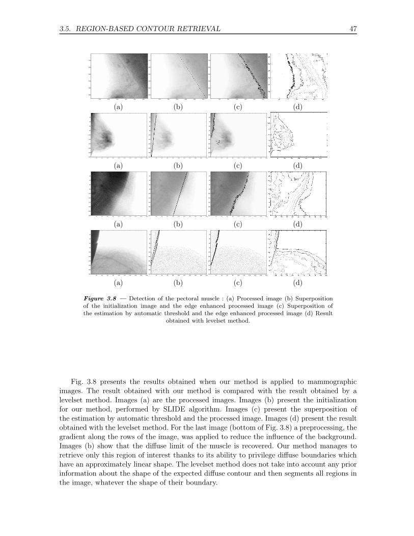
3.5. REGION-BASED CONTOUR RETRIEVAL 47
100 200 300 400 500 600
100
200
300
400
500
600
100 200 300 400 500 600
100
200
300
400
500
600
100 200 300 400 500 600
100
200
300
400
500
600
(a) (b) (c) (d)
20 40 60 80 100 120 140 160 180 200
20
40
60
80
100
120
140
160
180
20020 40 60 80 100 120 140 160 180 200
20
40
60
80
100
120
140
160
180
20020 40 60 80 100 120 140 160 180 200
20
40
60
80
100
120
140
160
180
200
(a) (b) (c) (d)
20 40 60 80 100 120 140 160 180 200
20
40
60
80
100
120
140
160
180
20020 40 60 80 100 120 140 160 180 200
20
40
60
80
100
120
140
160
180
20020 40 60 80 100 120 140 160 180 200
20
40
60
80
100
120
140
160
180
200
(a) (b) (c) (d)
20 40 60 80 100 120 140 160 180 200
20
40
60
80
100
120
140
160
180
20020 40 60 80 100 120 140 160 180 200
20
40
60
80
100
120
140
160
180
20020 40 60 80 100 120 140 160 180 200
20
40
60
80
100
120
140
160
180
200
(a) (b) (c) (d)
Figure 3.8 — Detection of the pectoral muscle : (a) Processed image (b) Superpositionof the initialization image and the edge enhanced processed image (c) Superposition ofthe estimation by automatic threshold and the edge enhanced processed image (d) Result
obtained with levelset method.
Fig. 3.8 presents the results obtained when our method is applied to mammographicimages. The result obtained with our method is compared with the result obtained by alevelset method. Images (a) are the processed images. Images (b) present the initializationfor our method, performed by SLIDE algorithm. Images (c) present the superposition ofthe estimation by automatic threshold and the processed image. Images (d) present the resultobtained with the levelset method. For the last image (bottom of Fig. 3.8) a preprocessing, thegradient along the rows of the image, was applied to reduce the influence of the background.Images (b) show that the diffuse limit of the muscle is recovered. Our method manages toretrieve only this region of interest thanks to its ability to privilege diffuse boundaries whichhave an approximately linear shape. The levelset method does not take into account any priorinformation about the shape of the expected diffuse contour and then segments all regions inthe image, whatever the shape of their boundary.
48
CHAPITRE 3. STRAIGHT LINE AND NEARLY STRAIGHT CONTOURRETRIEVAL, BY HIGH-RESOLUTION METHODS OF ARRAY PROCESSING AND
OPTIMIZATION METHODS
3.5.3 Balance on region-based segmentation
In this section, we propose a distorted contour retrieval method which is based on athreshold. The first step of this contour retrieval method consists in an initialization by meansof a straight line. The second step consists in finding the binary image which results from athreshold and is the closest to the image that contains only the initialization straight line. Ourcriterion is based on a signal generated from the image containing the initialization straightline and a signal generated from the threshold image. The threshold image only contains aregion which is selected from the processed image. This region is, in the original image, asmooth transition with overall straight orientation, between two homogeneous parts of theimage.In order to exemplify the efficiency of the proposed method, we consider an application tomedical images : we have shown that our method is able to retrieve the limits of the pectoralmuscle in a mammographic image. In the remainder of the chapter, we no longer considerregion but contour retrieval.
3.6 Estimation of non rectilinear contours in an image as aninverse problem : principles of the proposed optimizationmethod and gradient algorithm
In the previous sections we recalled a specific formalism for image representation, andpresented an application of the high-resolution methods of array processing to the retrievalof straight lines in an image.In this section, we keep the formalism retained for straight lines retrieval. The more generalcase of distorted contour estimation is proposed. As well as in the previous sections, thisproblem can be considered as an array processing problem in which a wave front has tobe estimated. It is possible to make an analogy with a physical phenomenon that can beobserved in wave physics. We suppose that the distorted curve actually contained in theimage can be assimilated to a distorted wave front. Such a distorted front can be observedwhen the propagation medium is not isotropic. In order to estimate the wave front distortion,we propose to apply a recursive algorithm. In [23], a similar problem is solved, in the case ofa plane wave received by a distorted antenna.We propose a new method called ECAPMO (Estimation of Contours by Array ProcessingMethods and Optimization) for the estimation of continuous non rectilinear contours. It relieson the formulation of an inverse problem over the generated signals and the determination ofphase fluctuations.
3.6.1 Retrieval of a general phase model
The ECAPMO method relies on the idea of a continuous phase model. We propose toextend the formalism proposed in [5], that sets the analogy between the phase model used inarray processing and a contour in image processing. Instead of assuming that the phase modelis known, i.e. that there exists a predefined model for the contour that we aim at retrieving,we create an artificial evolution of the wave front and of the corresponding received signal. Bysetting a recursive algorithm, we modify the phase of a current signal until it is equal to the
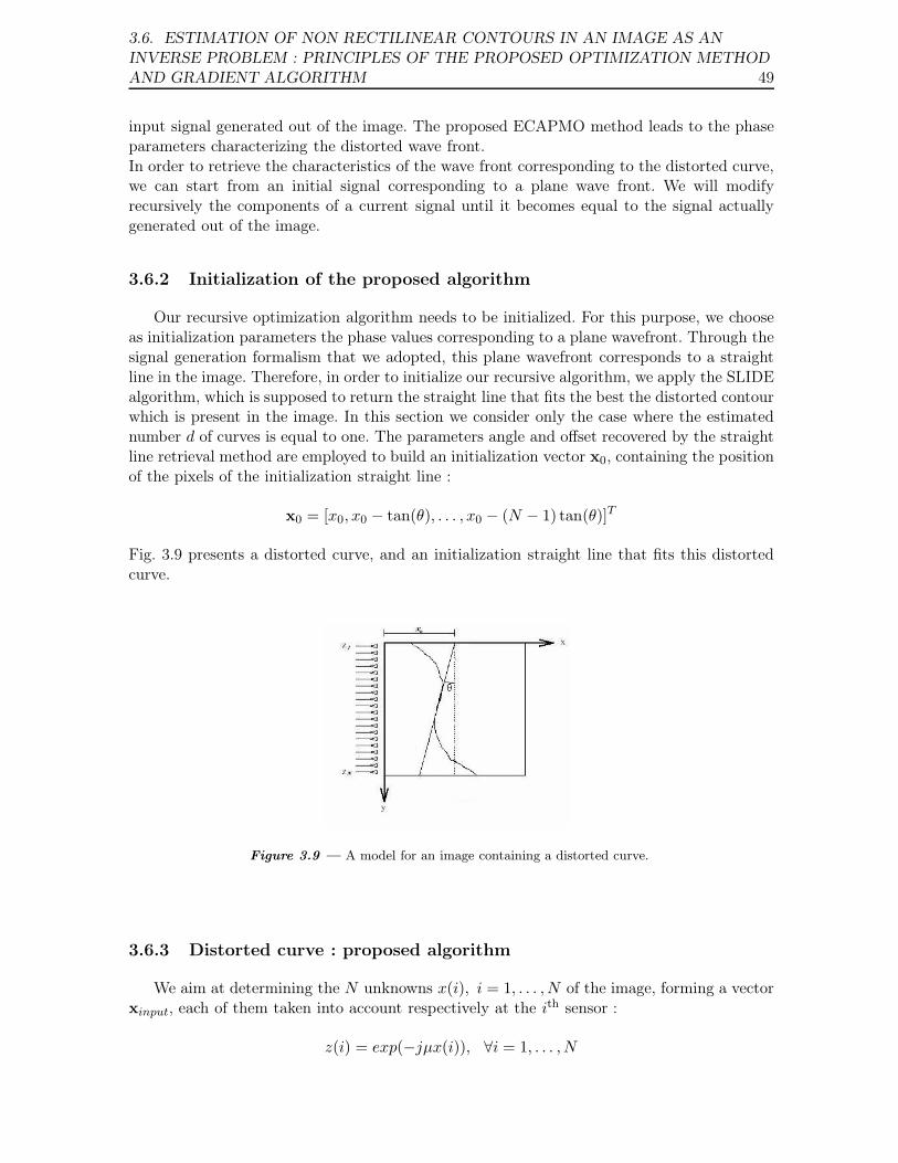
3.6. ESTIMATION OF NON RECTILINEAR CONTOURS IN AN IMAGE AS ANINVERSE PROBLEM : PRINCIPLES OF THE PROPOSED OPTIMIZATION METHODAND GRADIENT ALGORITHM 49
input signal generated out of the image. The proposed ECAPMO method leads to the phaseparameters characterizing the distorted wave front.In order to retrieve the characteristics of the wave front corresponding to the distorted curve,we can start from an initial signal corresponding to a plane wave front. We will modifyrecursively the components of a current signal until it becomes equal to the signal actuallygenerated out of the image.
3.6.2 Initialization of the proposed algorithm
Our recursive optimization algorithm needs to be initialized. For this purpose, we chooseas initialization parameters the phase values corresponding to a plane wavefront. Through thesignal generation formalism that we adopted, this plane wavefront corresponds to a straightline in the image. Therefore, in order to initialize our recursive algorithm, we apply the SLIDEalgorithm, which is supposed to return the straight line that fits the best the distorted contourwhich is present in the image. In this section we consider only the case where the estimatednumber d of curves is equal to one. The parameters angle and offset recovered by the straightline retrieval method are employed to build an initialization vector x0, containing the positionof the pixels of the initialization straight line :
x0 = [x0, x0 − tan(θ), . . . , x0 − (N − 1) tan(θ)]T
Fig. 3.9 presents a distorted curve, and an initialization straight line that fits this distortedcurve.
Figure 3.9 — A model for an image containing a distorted curve.
3.6.3 Distorted curve : proposed algorithm
We aim at determining the N unknowns x(i), i = 1, . . . , N of the image, forming a vectorxinput, each of them taken into account respectively at the ith sensor :
z(i) = exp(−jµx(i)), ∀i = 1, . . . , N
50
CHAPITRE 3. STRAIGHT LINE AND NEARLY STRAIGHT CONTOURRETRIEVAL, BY HIGH-RESOLUTION METHODS OF ARRAY PROCESSING AND
OPTIMIZATION METHODS
The observation vector is
zinput = [exp(jϕ1), . . . , exp(jϕN )]T (3.28)
with ϕi = −µx(i), representing the phase of sensor i. So we try to recreate the signal fromwhich we ignore the N parameters. We start from the initialization vector x0, characterizinga straight line that fits a locally rectilinear portion of the curve to be studied. Then, with kindexing the steps of this recursive algorithm, we aim at minimizing
J(xk) = ||zinput − zestimated for xk||2 (3.29)
where ||.|| represents the norm induced by the usual scalar product of CN . For this purpose
we use gradient methods with fixed step type. The vectors of the series are obtained by therelation
∀k ∈ N : xk+1 = xk − λ∇(J(xk)) (3.30)
where 0 < λ < 1 is the step for the descent. The recurrence loop is
xk → zestimated for xk→ J(xk)
The gradient is estimated using finite differences. We stop when the gradient becomes lowerthan a threshold.At this point, by minimizing the function J , we find the components of vector x leading tothe signal z which is the closest to the input signal. Nevertheless, by employing the criterionof minimum square error between signals, a phase indetermination over the input signal isremaining. Therefore, we propose an algorithm that aims at canceling the phase indetermi-nation induced by the criterion that we chose. This algorithm is based upon the continuity ofthe phase of the signal which is actually generated out of the image. Moreover we prove thatthe series (xk)k∈N
actually converges towards a local minimum argument of the criterion J .By defining as x̂l the components of x̂ and starting from the following relation
∀p ∈ Z, exp(jϕl) = exp(−jµxl) = exp(−jµx̂l)
= exp(−jµ(x̂l +2pπ
µ)),
we deduce that there exists an N -uplet of relative integers denoted by pl such that xinput =x̂ + 2π
µ [p1, p2, . . . , pN ]T .
This relation is equivalent to a shift which is proportional to 2πµ between xl and x̂l for
each line l of the image, or to a phase delay appearing on the signals obtained on the lines ofthe image-matrix.The general formulation of the N-components vectors which minimize the cost function J aredefined by
Argmin J = x̂ +2π
µZ
N =
(x̂1 +
2πp1
µ, . . . , x̂N +
2πpN
µ
),
(p1, . . . , pN ) ∈ ZN
3.6. ESTIMATION OF NON RECTILINEAR CONTOURS IN AN IMAGE AS ANINVERSE PROBLEM : PRINCIPLES OF THE PROPOSED OPTIMIZATION METHODAND GRADIENT ALGORITHM 51
The choice of the descent method towards such a minimum x̂ is such that
x̂ ∈ Argminy
{|y − x0|}
where |.| symbolises here the norm induced by the scalar product in RN , and y ∈ Argmin J .
This implies that the main characteristics of x̂ are
1. to minimize the criterion J ,
2. to guarantee that its distance to x0, i.e. |x̂ − x0| is minimum with respect to the distancesof x0 to the other solutions x of J .
The next step concerns the determination of the actual values of the vector xinput. Theuniqueness of the correct N -uplet for the reconstruction of the distorted wave requires todetermine at least one of the components xl of x. At this stage of the method the choice ofan initialization by a convenient straight line and the interest of the work presented aboutthe determination of the curves step in. The hypotheses of curve continuity is exploited forthis purpose. A reconstruction method (going successively forward and backward over thelines) of the curve is proposed starting from a fixed point. Before going further, we chooseas an arbitrary point imax, the maximum value of the set {i = 1, . . . , N} such that x̂i =x0 − (i − 1) tan θ, determined from the data x0 and x̂. We obtain
pimax = 0 and ximax = x̂imax
We set δ(µ) = Max {|x̂l − x̂l−1|, l = 2, . . . , N}. For the forward part over the remaining linesof the image-matrix, for each line l = imax, . . . , N , we determine successively ml ∈ N such
that∣∣∣x̂l − x̂l−1 − 2π
µ sign(x̂l − x̂l−1)ml
∣∣∣ < δ(µ) and we set pl−1 = sign(x̂l − x̂l−1)ml. For the
descent method over the lines we start anew for l = imax + 1, . . . , N − 1 by increasing theindex l for the two relations above.
3.6.4 Convergence of the gradient method
For k → +∞ the series xk converges towards a vector x̂ such that :
zinput = zx̂
That is to say x̂ is the argument of a local minimum of J contained in the neighborhood (inthe sense of topology) of x0. Indeed, let us denote for all k ∈ N, Rk = λ ||∇J(xk)||. The orderone Taylor series of J over the Rk radius ball centered on xk allows to write
∀ω ∈ RN , |ω| ≤ Rk :
J(xk + ω) = J(xk)+ < ∇J(xk), ω > + |ω| ε(ω)
Thus for ω = −λ∇J(xk), with λ small enough so that ω have negligible norm, we obtain
J(xk − λ∇J(xk)︸ ︷︷ ︸xk+1
) = J(xk) − λ ||∇J(xk)||2 ≤ J(xk).
That is to say,∀k ≥ 0, J(xk+1) ≤ J(xk).
The series (xk)k∈Ninduces the decrease of J with
limk→+∞
∇J(xk) = 0
This proves the convergence of the proposed optimization algorithm.
52
CHAPITRE 3. STRAIGHT LINE AND NEARLY STRAIGHT CONTOURRETRIEVAL, BY HIGH-RESOLUTION METHODS OF ARRAY PROCESSING AND
OPTIMIZATION METHODS
3.6.5 Summary of the proposed algorithm
An outline of the proposed distorted contour estimation method is given as follows :
1. Derive artificial signals using Equation (3.43) ;
2. Apply SLIDE algorithm : estimate line angle and offset that fit the best the distortedcontour (see subsections 2.2 and 2.3) ;
3. Initialize the ECAPMO method using the straight line parameters obtained after applyingthe straight line retrieval method ;
4. Estimate the fluctuations of the position of the pixels around the initialization straightline, by using the gradient algorithm ;
5. Solve the phase indetermination problem, by using the hypothesis of continuity of thecurve.
3.6.6 Numerical complexity of the method
We previously defined Np as the number of non zero pixels, and d as the number of straightlines. With given values of these parameters and of the image size parameter N , the order ofmagnitude of the complexity of the angle estimation method is Np + N · (
√N + d) [7, 117].
As concerns the algorithm of offset estimation, let us remind that L is a parameter chosenclose to N , and dk is the number of parallel lines with a given orientation index k. In practiceL is the integer part of (N − dk
2 ).For signal generation, 7 · Np operations are needed to obtain the signal z of Equation (3.20).For each of the d orientations found through constant parameter propagation, the signal w
of Equation (3.22) is obtained from the signal z with 4 + 3 · N operations. For the MFBLPmethod, we consider the case when one offset is expected for each orientation value. We chosefor the parameter L the value N − 1. The procedure "roots" employed at step 5) in order tofind the zeros of the polynomial function H is based on an eigen-decomposition of an L × Lmatrix. This eigen-decomposition dominates the other operations realized by the MFBLPalgorithm in terms of complexity. Thus the complexity of this dominant step is L3 or equiva-lently (N − 1)3.Therefore, the order of magnitude of the computational complexity of the offset determinationalgorithm is 7 · Np + d · (4 + 3 · N + (N − 1)3).The complexity dominating part of our algorithm for curve distortion estimation is the itera-tive algorithm. Let ”Niter” be the number of iterations, necessary for the convergence of thealgorithm.We count the number of operations, neglecting the time required by the additions, and in-cluding one storage operation for the current value of the estimated vector xk of a currentiteration k. Computing and storing the vector x0 from the parameters angle and offset givenby the initialisation step, requires N +1 operations. For each iteration k, including one storageoperation for each computed value of ∇J(xk), we obtain the following results :
1. The numerical derivative ∇J(xk) requires the computation of two values of the functionJ , computed for vector xk and an incremented version of xk, and one division by theincremental vector. Then, 10·N operations are needed for the computation of the functionJ . The substraction of two successive values of the function J and a division by the size
3.7. GENERALIZATION OF DISTORTED CONTOUR ESTIMATION TO THEESTIMATION OF SEVERAL CURVES 53
N incremental vector needs N operations. So, 2 · (10 ·N) + N + 1 operations are neededfor the computation and storage of the derivative ∇J(xk).
2. N operations are needed for the multiplication of ∇J(xk) by λ, so the computation ofxk+1 from Equation (3.30) and the storage of xk+1 needs N + 1 operations.
So N + 1 operations are needed for the computation of x0, and 22 · N + 2 operations for thecomputations of all iterations. In total, N +1+Niter ·(22·N +2) operations are needed. Someexperimental results about the computational time required for the distorted curve retrievalmethod will be presented in the Section 5.
3.7 Generalization of distorted contour estimation to the esti-mation of several curves
In this section we consider the case where the estimated number of curves d is larger thanone. We will suppose that each curve is composed of a single pixel per line in the image.Therefore the model for the input signal zinput = [z(1), z(2), . . . , z(N)]T is :
z =
z(1)z(2)...z(N)
=
d∑
k=1
exp(jϕ1k)exp(jϕ2k)...exp(jϕNk)
+
n(1)n(2)...n(N)
=
exp(jϕ11) . . . exp(jϕ1d)exp(jϕ21) . . . exp(jϕ2d)...
. . ....
exp(jϕN1) . . . exp(jϕNd)
11...1
+ n
= A(ϕ) s + n
where A(ϕ) is a matrix of size N × d taken as a model for the matrix of the directionalvectors of the sources and s is the vector of sources amplitudes, all equal to 1.
So the term ϕik ∈ ]−π, π] represents the phase of the transfer function of the systemsource k and sensor i having an amplitude equal to 1. The source-vector related to source kis
a(ϕk) = [exp(jϕ1k), exp(jϕ2k), . . . , exp(jϕNk)]T (3.31)
Referring to matrix notations, we obtain thus
A(ϕ) = [a(ϕ1),a(ϕ2), . . . ,a(ϕd)] (3.32)
So that we can define an application written z, such that to every matrix variable
ϕ = [ϕ1, ϕ2, . . . , ϕd] =
ϕ11 . . . ϕ1d
ϕ21 . . . ϕ2d...
. . ....
ϕN1 . . . ϕNd
(3.33)
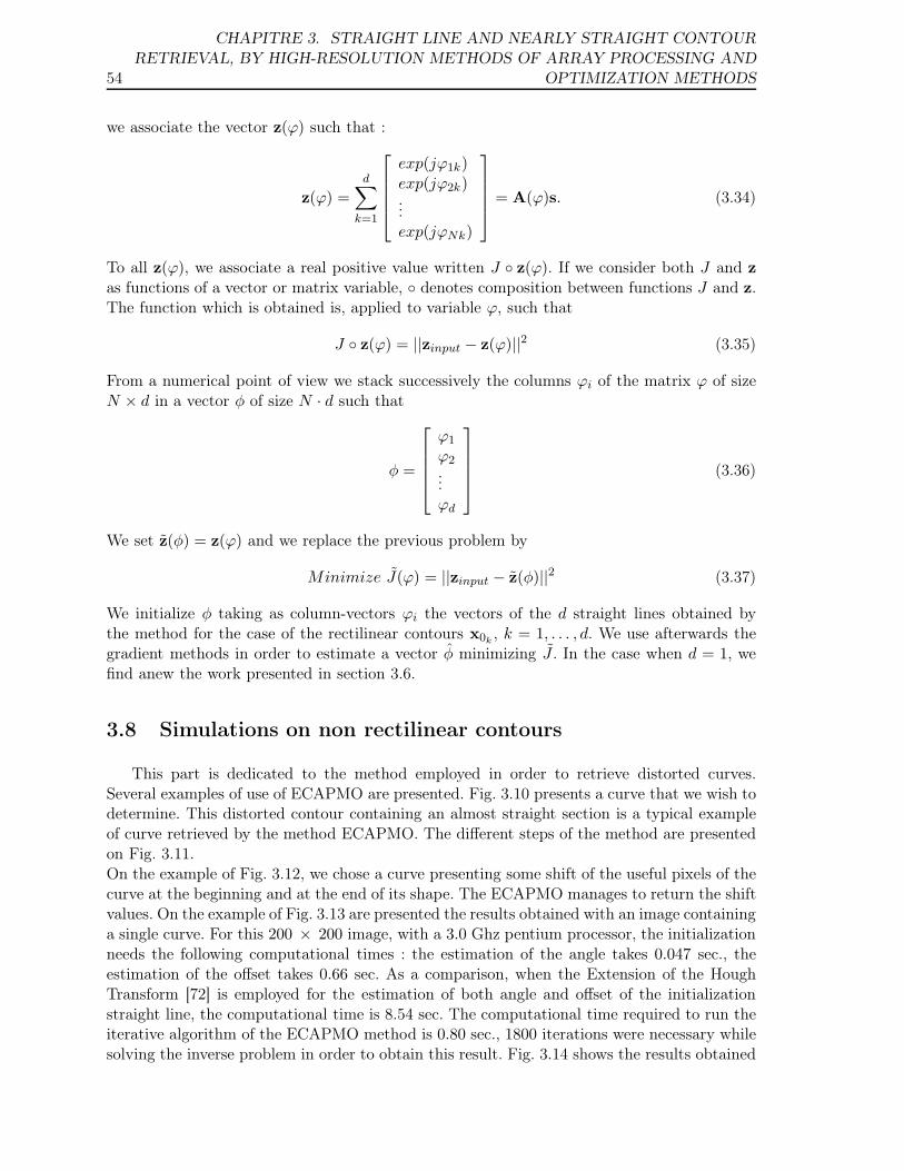
54
CHAPITRE 3. STRAIGHT LINE AND NEARLY STRAIGHT CONTOURRETRIEVAL, BY HIGH-RESOLUTION METHODS OF ARRAY PROCESSING AND
OPTIMIZATION METHODS
we associate the vector z(ϕ) such that :
z(ϕ) =
d∑
k=1
exp(jϕ1k)exp(jϕ2k)...exp(jϕNk)
= A(ϕ)s. (3.34)
To all z(ϕ), we associate a real positive value written J ◦ z(ϕ). If we consider both J and z
as functions of a vector or matrix variable, ◦ denotes composition between functions J and z.The function which is obtained is, applied to variable ϕ, such that
J ◦ z(ϕ) = ||zinput − z(ϕ)||2 (3.35)
From a numerical point of view we stack successively the columns ϕi of the matrix ϕ of sizeN × d in a vector φ of size N · d such that
φ =
ϕ1
ϕ2...ϕd
(3.36)
We set z̃(φ) = z(ϕ) and we replace the previous problem by
Minimize J̃(ϕ) = ||zinput − z̃(φ)||2 (3.37)
We initialize φ taking as column-vectors ϕi the vectors of the d straight lines obtained bythe method for the case of the rectilinear contours x0k
, k = 1, . . . , d. We use afterwards thegradient methods in order to estimate a vector φ̂ minimizing J̃ . In the case when d = 1, wefind anew the work presented in section 3.6.
3.8 Simulations on non rectilinear contours
This part is dedicated to the method employed in order to retrieve distorted curves.Several examples of use of ECAPMO are presented. Fig. 3.10 presents a curve that we wish todetermine. This distorted contour containing an almost straight section is a typical exampleof curve retrieved by the method ECAPMO. The different steps of the method are presentedon Fig. 3.11.On the example of Fig. 3.12, we chose a curve presenting some shift of the useful pixels of thecurve at the beginning and at the end of its shape. The ECAPMO manages to return the shiftvalues. On the example of Fig. 3.13 are presented the results obtained with an image containinga single curve. For this 200 × 200 image, with a 3.0 Ghz pentium processor, the initializationneeds the following computational times : the estimation of the angle takes 0.047 sec., theestimation of the offset takes 0.66 sec. As a comparison, when the Extension of the HoughTransform [72] is employed for the estimation of both angle and offset of the initializationstraight line, the computational time is 8.54 sec. The computational time required to run theiterative algorithm of the ECAPMO method is 0.80 sec., 1800 iterations were necessary whilesolving the inverse problem in order to obtain this result. Fig. 3.14 shows the results obtained
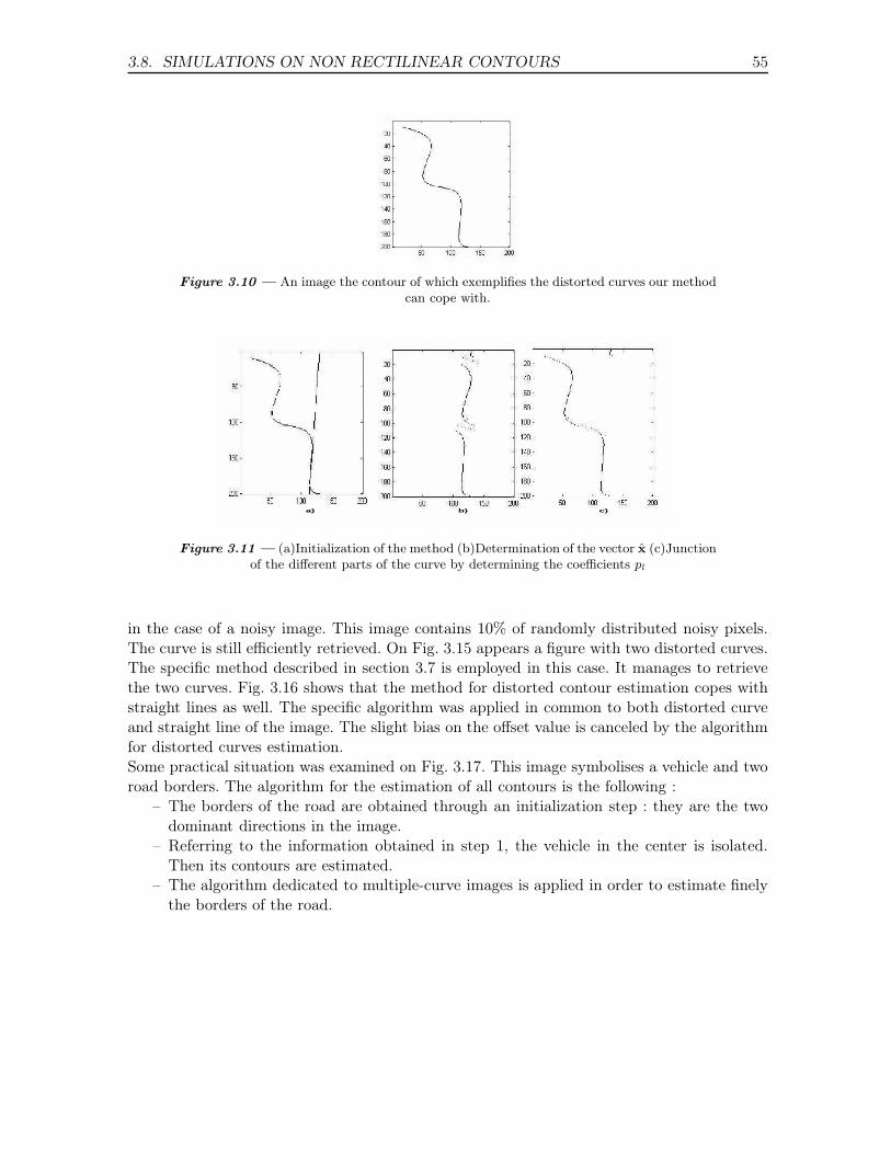
3.8. SIMULATIONS ON NON RECTILINEAR CONTOURS 55
Figure 3.10 — An image the contour of which exemplifies the distorted curves our methodcan cope with.
a) b) c)
Figure 3.11 — (a)Initialization of the method (b)Determination of the vector x̂ (c)Junctionof the different parts of the curve by determining the coefficients pl
in the case of a noisy image. This image contains 10% of randomly distributed noisy pixels.The curve is still efficiently retrieved. On Fig. 3.15 appears a figure with two distorted curves.The specific method described in section 3.7 is employed in this case. It manages to retrievethe two curves. Fig. 3.16 shows that the method for distorted contour estimation copes withstraight lines as well. The specific algorithm was applied in common to both distorted curveand straight line of the image. The slight bias on the offset value is canceled by the algorithmfor distorted curves estimation.Some practical situation was examined on Fig. 3.17. This image symbolises a vehicle and tworoad borders. The algorithm for the estimation of all contours is the following :
– The borders of the road are obtained through an initialization step : they are the twodominant directions in the image.
– Referring to the information obtained in step 1, the vehicle in the center is isolated.Then its contours are estimated.
– The algorithm dedicated to multiple-curve images is applied in order to estimate finelythe borders of the road.
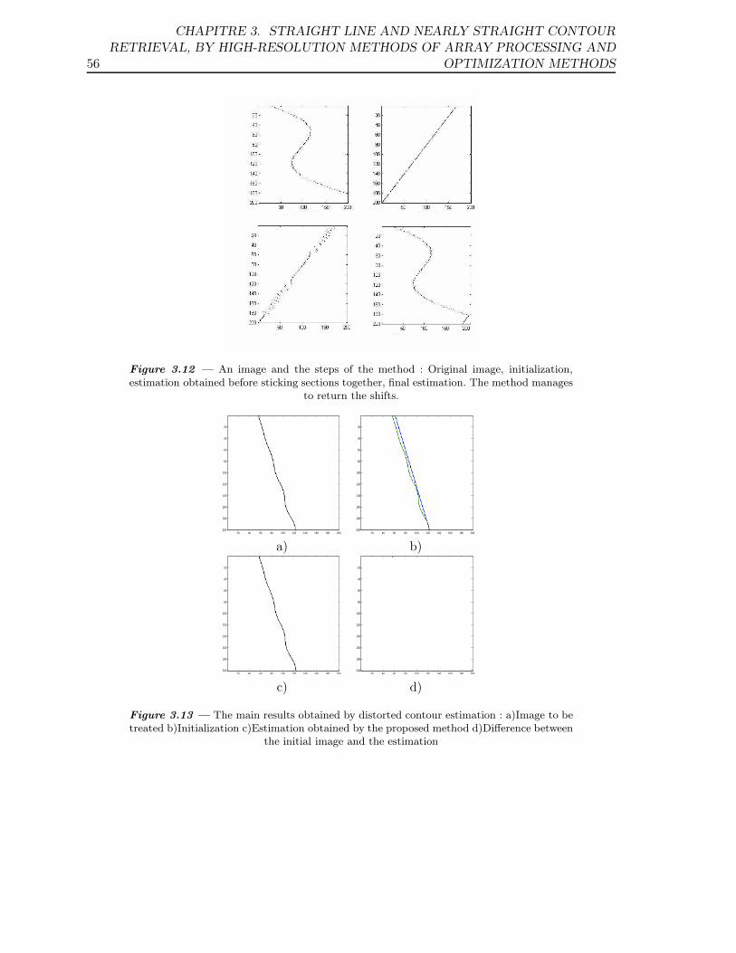
56
CHAPITRE 3. STRAIGHT LINE AND NEARLY STRAIGHT CONTOURRETRIEVAL, BY HIGH-RESOLUTION METHODS OF ARRAY PROCESSING AND
OPTIMIZATION METHODS
Figure 3.12 — An image and the steps of the method : Original image, initialization,estimation obtained before sticking sections together, final estimation. The method manages
to return the shifts.
20 40 60 80 100 120 140 160 180 200
20
40
60
80
100
120
140
160
180
20020 40 60 80 100 120 140 160 180 200
20
40
60
80
100
120
140
160
180
200
a) b)
20 40 60 80 100 120 140 160 180 200
20
40
60
80
100
120
140
160
180
20020 40 60 80 100 120 140 160 180 200
20
40
60
80
100
120
140
160
180
200
c) d)
Figure 3.13 — The main results obtained by distorted contour estimation : a)Image to betreated b)Initialization c)Estimation obtained by the proposed method d)Difference between
the initial image and the estimation
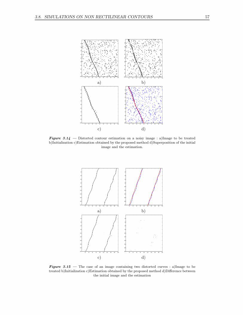
3.8. SIMULATIONS ON NON RECTILINEAR CONTOURS 57
10 20 30 40 50 60 70 80 90 100
10
20
30
40
50
60
70
80
90
100
10 20 30 40 50 60 70 80 90 100
10
20
30
40
50
60
70
80
90
100
a) b)
10 20 30 40 50 60 70 80 90 100
10
20
30
40
50
60
70
80
90
10010 20 30 40 50 60 70 80 90 100
10
20
30
40
50
60
70
80
90
100
c) d)
Figure 3.14 — Distorted contour estimation on a noisy image : a)Image to be treatedb)Initialization c)Estimation obtained by the proposed method d)Superposition of the initial
image and the estimation.
20 40 60 80 100 120 140 160 180 200
20
40
60
80
100
120
140
160
180
20020 40 60 80 100 120 140 160 180 200
20
40
60
80
100
120
140
160
180
200
a) b)
20 40 60 80 100 120 140 160 180 200
20
40
60
80
100
120
140
160
180
20020 40 60 80 100 120 140 160 180 200
20
40
60
80
100
120
140
160
180
200
c) d)
Figure 3.15 — The case of an image containing two distorted curves : a)Image to betreated b)Initialization c)Estimation obtained by the proposed method d)Difference between
the initial image and the estimation
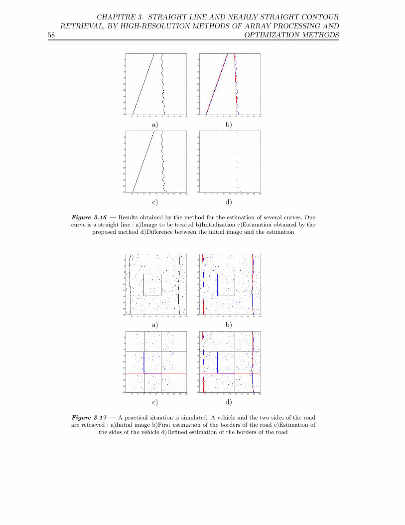
58
CHAPITRE 3. STRAIGHT LINE AND NEARLY STRAIGHT CONTOURRETRIEVAL, BY HIGH-RESOLUTION METHODS OF ARRAY PROCESSING AND
OPTIMIZATION METHODS
20 40 60 80 100 120 140 160 180 200
20
40
60
80
100
120
140
160
180
20020 40 60 80 100 120 140 160 180 200
20
40
60
80
100
120
140
160
180
200
a) b)
20 40 60 80 100 120 140 160 180 200
20
40
60
80
100
120
140
160
180
20020 40 60 80 100 120 140 160 180 200
20
40
60
80
100
120
140
160
180
200
c) d)
Figure 3.16 — Results obtained by the method for the estimation of several curves. Onecurve is a straight line : a)Image to be treated b)Initialization c)Estimation obtained by the
proposed method d)Difference between the initial image and the estimation
20 40 60 80 100 120 140 160 180 200
20
40
60
80
100
120
140
160
180
20020 40 60 80 100 120 140 160 180 200
20
40
60
80
100
120
140
160
180
200
a) b)
20 40 60 80 100 120 140 160 180 200
20
40
60
80
100
120
140
160
180
20020 40 60 80 100 120 140 160 180 200
20
40
60
80
100
120
140
160
180
200
c) d)
Figure 3.17 — A practical situation is simulated. A vehicle and the two sides of the roadare retrieved : a)Initial image b)First estimation of the borders of the road c)Estimation of
the sides of the vehicle d)Refined estimation of the borders of the road
3.9. ESTIMATION OF NON RECTILINEAR CONTOURS IN AN IMAGE BY MEANSOF PROPAGATOR AND OPTIMIZATION METHODS 59
3.9 Estimation of non rectilinear contours in an image bymeans of Propagator and optimization methods
3.9.1 Formulation of a phase model
The adopted approach for signal generation permits to obtain a general phase model whendistorted contours are expected. Let us consider the generated signal z. Each component of z
is as follows :
z(i) = exp(−jµx(i)) = exp(jµ(i − 1)tan(θ) − jµ∆x(i))exp(−jµx0) (3.38)
This expression contains, for one curve and the ith row of the image, the value ∆x(i) ofthe shift between the position of the pixel belonging to a straight line fitting the curve,and the pixel of the curve itself. Equation (3.38) is equivalent to : z(i) = ai(θ)s, whereai(θ) = exp(jµ(i − 1)tan(θ) − jµ∆x(i)) and s = exp(−jµx0). It is possible to set toge-ther in a vector model the components ai(θ) of all rows of the image. If several orien-tation values are considered, the vector model concerning the orientation k is : a(θk) =[e−jµ∆x(1), ej(µtan(θk)−µ∆x(2)), . . . , ej(µ(N−1)tan(θk)−µ∆x(N))
]T. The purpose of the next subsec-
tion is to estimate the values ∆x(1), . . . ,∆x(N) of the pixel shifts.
3.9.2 Propagator method for phase shift estimation
Referring to Equation (1.32), matrix Q has M lines and M − d columns. Therefore, thevector that will be estimated will be of length M . We remind that the value of M can bechosen up to M = N − d + 1 ≤ N . In practice, the images to be treated are not supposed tocontain a large number of curves, so that M can be fixed to a value close to N . The techniquethat we use is the following : an initialization vector holding for the N rows of the imageis computed. This initialization vector fits the distorted curve by a dominant straight line.Then, starting from this initialization vector, M phase values of the signals are computed.We proposed a method for this purpose in [28]. The last N − M phases are supposed todiffer from the N − M phases of the initialization vector by a phase shift which is equalto the last computed phase shift. In the general case where several curves with parametersθk, k = 1, . . . , d are present, we have to find the vector a(θk), for k = 1, . . . , d, such that :
|QHa(θk)|2 = 0 (3.39)
where |.| denotes the L2 norm. Let a(θk)o =[1, ejµtan(θk), . . . , ejµ(N−1)tan(θk)
]Tbe a vector
obtained by using the initial estimate of the orientation of the straight lines fitting the kthcontour. We use the conjugated gradient method, initialized by the vector a(θk)o, to estimatea(θk) by minimizing the criterion of Eq. (3.39). The sequence of vectors of the recurrence loopare obtained by the relation :
∀q ∈ N : a(θk)q+1 = a(θk)q − 2λQQHa(θk)q, 0 ≤ q ≤ niter (3.40)
where q indexes the elements of the sequence of the recurrence loop, 0 < λ < 1 is the stepsize, niter is the number of iterations. We stop the recursion when the criterion is under afixed threshold.From the complex argument of the components of vector a(θk), we get the values of ∆x(i).
60
CHAPITRE 3. STRAIGHT LINE AND NEARLY STRAIGHT CONTOURRETRIEVAL, BY HIGH-RESOLUTION METHODS OF ARRAY PROCESSING AND
OPTIMIZATION METHODS
At this point, the values of θk for each curve indexed by k, each offset x0 and ∆x(i) fori = 1, . . . ,M , have been calculated. The last N − M pixels are supposed to be straightlyaligned along the orientation of the initialization straight line, from the Mth pixel to thebottom of the image. Thus, the position of the pixels of each distorted curve are known atthis point.
3.10 Propagator applied to the covariance matrix associatedwith gradient algorithm : Experimental results, computa-tional times
3.10.1 Real-world images
This subsection is divided into two parts : one is devoted to straight line reconstruction,and the other concerns distorted contour retrieval.When the procedure for straight lines retrieval is run, the values of parameters µ and α haveto be chosen. As concerns parameter µ, [5] provides a study that gives the maximum valueof an estimated orientation, with a value of µ equal to 1. This maximum value is 73◦ andis enough, considering that if the image is rotated by 90◦, all orientation values present inthe image can be computed. We applied such a rotation to the image of Fig. 2, in order todetect the crosspieces which are supposed to have an orientation of 90◦. This is equivalent toplace the antenna at the bottom side of the image. If µ is smaller, the maximum orientationvalue is higher, but it was empirically shown that the value 1 gives the best results. If µ ishigher the maximum value of an estimated orientation is lower. That is why we chose to usevalue 1 for µ. As concerns α, it must be such that the value of α multiplied by the maximumoffset value remains in an interval of length 2π. Indeed MFBLP method leads to the frequencyvalue −αx0. This frequency value must be in the interval [0, 2π[ in order to avoid any phaseindetermination. Therefore we can choose for instance the value 2.5 × 10⁻³ for an imagecontaining 200 columns. As concerns parameter M , it can be chosen up to N − d + 1, whered is the number of expected contours. As the number of estimated phase shift values betweenthe initialization straight line and the expected contour is equal to M , we decided to fix Mto an elevated value, close to the number of rows in the image. The research step angle is 0.3̊in interval Jθ, otherwise it is specified.Gradient Vector Flow [137] is well-suited for a comparison with our method. Its popularity isdue to its ability of attracting an active contour toward object boundary from a sufficientlylarge distance and its ability of moving the contour into object cavities. This enables aninitialization by any contour -for instance a rectilinear one- whatever the curvature of theexpected contour. GVF is based on a recursive optimization method. We may perform anynumber of iterations and thus control its computational load. In the following, we denoteby ǫ the mean bias over the position of the pixels, computed over all pixels of the curve :ǫ = 1
N
∑Ni=1 |x̂(i) − x(i)|, where x̂(i) is the estimation obtained for the position of the pixel
of row i. Fig. 3.18(a) presents an aerial image containing a road. One side of the image hassize N = 470. An edge enhancement and a threshold are applied (see Fig. 3.18(b)). When theproposed methods are applied, parameter M was chosen equal to 468 to maximize the numberof pixel shift values which are actually estimated. One initialization straight line is obtained,which has the same overall orientation as the road. The angle value is −3.3̊ and the offset value
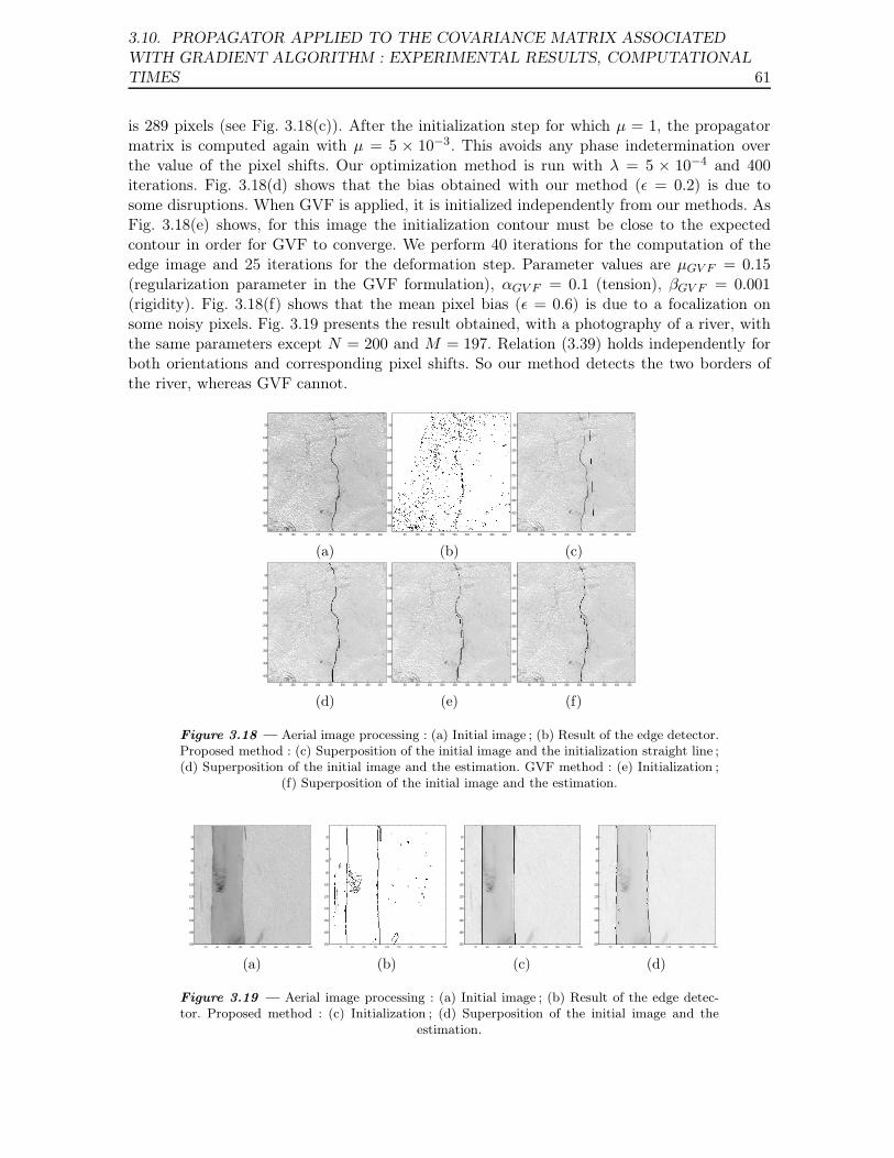
3.10. PROPAGATOR APPLIED TO THE COVARIANCE MATRIX ASSOCIATEDWITH GRADIENT ALGORITHM : EXPERIMENTAL RESULTS, COMPUTATIONALTIMES 61
is 289 pixels (see Fig. 3.18(c)). After the initialization step for which µ = 1, the propagatormatrix is computed again with µ = 5 × 10⁻³. This avoids any phase indetermination overthe value of the pixel shifts. Our optimization method is run with λ = 5 × 10⁻⁴ and 400iterations. Fig. 3.18(d) shows that the bias obtained with our method (ǫ = 0.2) is due tosome disruptions. When GVF is applied, it is initialized independently from our methods. AsFig. 3.18(e) shows, for this image the initialization contour must be close to the expectedcontour in order for GVF to converge. We perform 40 iterations for the computation of theedge image and 25 iterations for the deformation step. Parameter values are µGV F = 0.15(regularization parameter in the GVF formulation), αGV F = 0.1 (tension), βGV F = 0.001(rigidity). Fig. 3.18(f) shows that the mean pixel bias (ǫ = 0.6) is due to a focalization onsome noisy pixels. Fig. 3.19 presents the result obtained, with a photography of a river, withthe same parameters except N = 200 and M = 197. Relation (3.39) holds independently forboth orientations and corresponding pixel shifts. So our method detects the two borders ofthe river, whereas GVF cannot.
50 100 150 200 250 300 350 400 450
50
100
150
200
250
300
350
400
450
50 100 150 200 250 300 350 400 450
50
100
150
200
250
300
350
400
450
50 100 150 200 250 300 350 400 450
50
100
150
200
250
300
350
400
450
(a) (b) (c)
50 100 150 200 250 300 350 400 450
50
100
150
200
250
300
350
400
450
50 100 150 200 250 300 350 400 450
50
100
150
200
250
300
350
400
450
50 100 150 200 250 300 350 400 450
50
100
150
200
250
300
350
400
450
(d) (e) (f)
Figure 3.18 — Aerial image processing : (a) Initial image ; (b) Result of the edge detector.Proposed method : (c) Superposition of the initial image and the initialization straight line ;(d) Superposition of the initial image and the estimation. GVF method : (e) Initialization ;
(f) Superposition of the initial image and the estimation.
20 40 60 80 100 120 140 160 180 200
20
40
60
80
100
120
140
160
180
20020 40 60 80 100 120 140 160 180 200
20
40
60
80
100
120
140
160
180
20020 40 60 80 100 120 140 160 180 200
20
40
60
80
100
120
140
160
180
20020 40 60 80 100 120 140 160 180 200
20
40
60
80
100
120
140
160
180
200
(a) (b) (c) (d)
Figure 3.19 — Aerial image processing : (a) Initial image ; (b) Result of the edge detec-tor. Proposed method : (c) Initialization ; (d) Superposition of the initial image and the
estimation.
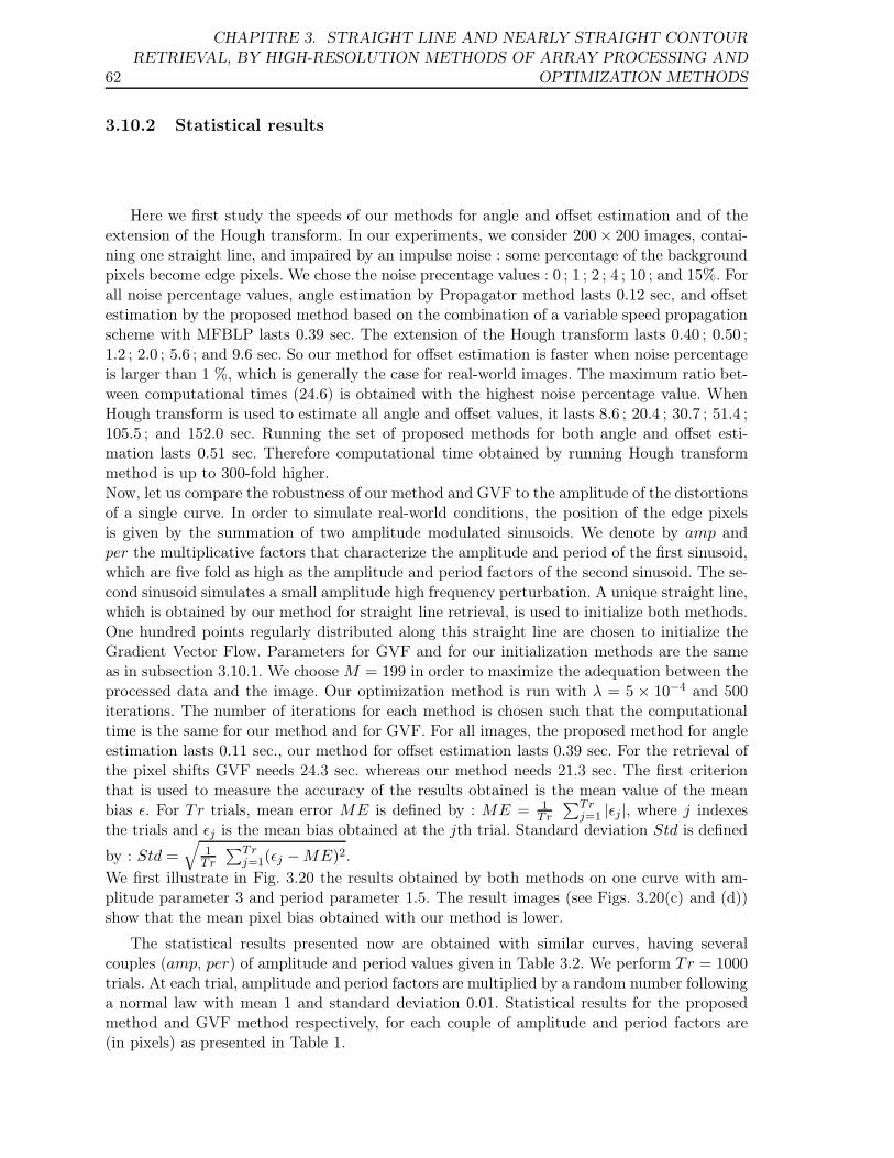
62
CHAPITRE 3. STRAIGHT LINE AND NEARLY STRAIGHT CONTOURRETRIEVAL, BY HIGH-RESOLUTION METHODS OF ARRAY PROCESSING AND
OPTIMIZATION METHODS
3.10.2 Statistical results
Here we first study the speeds of our methods for angle and offset estimation and of theextension of the Hough transform. In our experiments, we consider 200× 200 images, contai-ning one straight line, and impaired by an impulse noise : some percentage of the backgroundpixels become edge pixels. We chose the noise precentage values : 0 ; 1 ; 2 ; 4 ; 10 ; and 15%. Forall noise percentage values, angle estimation by Propagator method lasts 0.12 sec, and offsetestimation by the proposed method based on the combination of a variable speed propagationscheme with MFBLP lasts 0.39 sec. The extension of the Hough transform lasts 0.40 ; 0.50 ;1.2 ; 2.0 ; 5.6 ; and 9.6 sec. So our method for offset estimation is faster when noise percentageis larger than 1 %, which is generally the case for real-world images. The maximum ratio bet-ween computational times (24.6) is obtained with the highest noise percentage value. WhenHough transform is used to estimate all angle and offset values, it lasts 8.6 ; 20.4 ; 30.7 ; 51.4 ;105.5 ; and 152.0 sec. Running the set of proposed methods for both angle and offset esti-mation lasts 0.51 sec. Therefore computational time obtained by running Hough transformmethod is up to 300-fold higher.Now, let us compare the robustness of our method and GVF to the amplitude of the distortionsof a single curve. In order to simulate real-world conditions, the position of the edge pixelsis given by the summation of two amplitude modulated sinusoids. We denote by amp andper the multiplicative factors that characterize the amplitude and period of the first sinusoid,which are five fold as high as the amplitude and period factors of the second sinusoid. The se-cond sinusoid simulates a small amplitude high frequency perturbation. A unique straight line,which is obtained by our method for straight line retrieval, is used to initialize both methods.One hundred points regularly distributed along this straight line are chosen to initialize theGradient Vector Flow. Parameters for GVF and for our initialization methods are the sameas in subsection 3.10.1. We choose M = 199 in order to maximize the adequation between theprocessed data and the image. Our optimization method is run with λ = 5 × 10⁻⁴ and 500iterations. The number of iterations for each method is chosen such that the computationaltime is the same for our method and for GVF. For all images, the proposed method for angleestimation lasts 0.11 sec., our method for offset estimation lasts 0.39 sec. For the retrieval ofthe pixel shifts GVF needs 24.3 sec. whereas our method needs 21.3 sec. The first criterionthat is used to measure the accuracy of the results obtained is the mean value of the meanbias ǫ. For Tr trials, mean error ME is defined by : ME = 1
Tr
∑Trj=1 |ǫj |, where j indexes
the trials and ǫj is the mean bias obtained at the jth trial. Standard deviation Std is defined
by : Std =√
1Tr
∑Trj=1(ǫj − ME)2.
We first illustrate in Fig. 3.20 the results obtained by both methods on one curve with am-plitude parameter 3 and period parameter 1.5. The result images (see Figs. 3.20(c) and (d))show that the mean pixel bias obtained with our method is lower.
The statistical results presented now are obtained with similar curves, having severalcouples (amp, per) of amplitude and period values given in Table 3.2. We perform Tr = 1000trials. At each trial, amplitude and period factors are multiplied by a random number followinga normal law with mean 1 and standard deviation 0.01. Statistical results for the proposedmethod and GVF method respectively, for each couple of amplitude and period factors are(in pixels) as presented in Table 1.
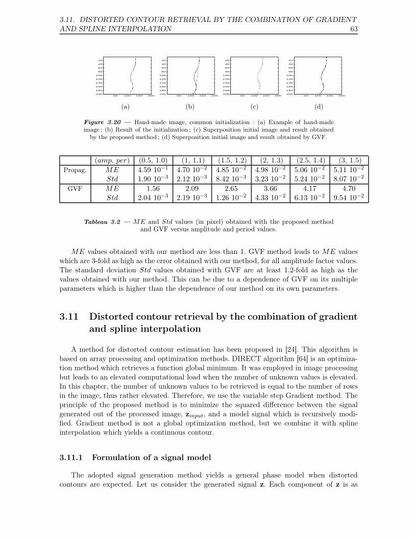
3.11. DISTORTED CONTOUR RETRIEVAL BY THE COMBINATION OF GRADIENTAND SPLINE INTERPOLATION 63
50 100 150 200
20
40
60
80
100
120
140
160
180
20050 100 150 200
20
40
60
80
100
120
140
160
180
20050 100 150 200
20
40
60
80
100
120
140
160
180
20050 100 150 200
20
40
60
80
100
120
140
160
180
200
(a) (b) (c) (d)
Figure 3.20 — Hand-made image, common initialization : (a) Example of hand-madeimage ; (b) Result of the initialization ; (c) Superposition initial image and result obtained
by the proposed method ; (d) Superposition initial image and result obtained by GVF.
(amp, per) (0.5, 1.0) (1, 1.1) (1.5, 1.2) (2, 1.3) (2.5, 1.4) (3, 1.5)Propag. ME 4.59 10−1 4.70 10−2 4.85 10−2 4.98 10−2 5.06 10−2 5.11 10−2
Std 1.90 10−3 2.12 10−3 8.42 10−3 3.23 10−2 5.24 10−2 8.07 10−2
GVF ME 1.56 2.09 2.65 3.66 4.17 4.70Std 2.04 10−3 2.19 10−3 1.26 10−2 4.33 10−2 6.13 10−2 9.54 10−2
Tableau 3.2 — ME and Std values (in pixel) obtained with the proposed methodand GVF versus amplitude and period values.
ME values obtained with our method are less than 1. GVF method leads to ME valueswhich are 3-fold as high as the error obtained with our method, for all amplitude factor values.The standard deviation Std values obtained with GVF are at least 1.2-fold as high as thevalues obtained with our method. This can be due to a dependence of GVF on its multipleparameters which is higher than the dependence of our method on its own parameters.
3.11 Distorted contour retrieval by the combination of gradientand spline interpolation
A method for distorted contour estimation has been proposed in [24]. This algorithm isbased on array processing and optimization methods. DIRECT algorithm [64] is an optimiza-tion method which retrieves a function global minimum. It was employed in image processingbut leads to an elevated computational load when the number of unknown values is elevated.In this chapter, the number of unknown values to be retrieved is equal to the number of rowsin the image, thus rather elevated. Therefore, we use the variable step Gradient method. Theprinciple of the proposed method is to minimize the squared difference between the signalgenerated out of the processed image, zinput, and a model signal which is recursively modi-fied. Gradient method is not a global optimization method, but we combine it with splineinterpolation which yields a continuous contour.
3.11.1 Formulation of a signal model
The adopted signal generation method yields a general phase model when distortedcontours are expected. Let us consider the generated signal z. Each component of z is as
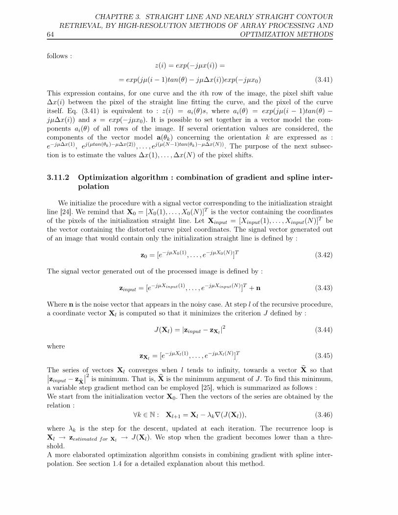
64
CHAPITRE 3. STRAIGHT LINE AND NEARLY STRAIGHT CONTOURRETRIEVAL, BY HIGH-RESOLUTION METHODS OF ARRAY PROCESSING AND
OPTIMIZATION METHODS
follows :z(i) = exp(−jµx(i)) =
= exp(jµ(i − 1)tan(θ) − jµ∆x(i))exp(−jµx0) (3.41)
This expression contains, for one curve and the ith row of the image, the pixel shift value∆x(i) between the pixel of the straight line fitting the curve, and the pixel of the curveitself. Eq. (3.41) is equivalent to : z(i) = ai(θ)s, where ai(θ) = exp(jµ(i − 1)tan(θ) −jµ∆x(i)) and s = exp(−jµx0). It is possible to set together in a vector model the com-ponents ai(θ) of all rows of the image. If several orientation values are considered, thecomponents of the vector model a(θk) concerning the orientation k are expressed as :e−jµ∆x(1), ej(µtan(θk)−µ∆x(2)), . . . , ej(µ(N−1)tan(θk)−µ∆x(N)). The purpose of the next subsec-tion is to estimate the values ∆x(1), . . . ,∆x(N) of the pixel shifts.
3.11.2 Optimization algorithm : combination of gradient and spline inter-polation
We initialize the procedure with a signal vector corresponding to the initialization straightline [24]. We remind that X0 = [X0(1), . . . ,X0(N)]T is the vector containing the coordinatesof the pixels of the initialization straight line. Let Xinput = [Xinput(1), . . . ,Xinput(N)]T bethe vector containing the distorted curve pixel coordinates. The signal vector generated outof an image that would contain only the initialization straight line is defined by :
z0 = [e−jµX0(1), . . . , e−jµX0(N)]T (3.42)
The signal vector generated out of the processed image is defined by :
zinput = [e−jµXinput(1), . . . , e−jµXinput(N)]T + n (3.43)
Where n is the noise vector that appears in the noisy case. At step l of the recursive procedure,a coordinate vector Xl is computed so that it minimizes the criterion J defined by :
J(Xl) = |zinput − zXl|2 (3.44)
wherezXl
= [e−jµXl(1), . . . , e−jµXl(N)]T (3.45)
The series of vectors Xl converges when l tends to infinity, towards a vector X̂ so that∣∣zinput − zX̂
∣∣2 is minimum. That is, X̂ is the minimum argument of J . To find this minimum,a variable step gradient method can be employed [25], which is summarized as follows :We start from the initialization vector X0. Then the vectors of the series are obtained by therelation :
∀k ∈ N : Xl+1 = Xl − λk∇(J(Xl)), (3.46)
where λk is the step for the descent, updated at each iteration. The recurrence loop isXl → zestimated for Xl
→ J(Xl). We stop when the gradient becomes lower than a thre-shold.A more elaborated optimization algorithm consists in combining gradient with spline inter-polation. See section 1.4 for a detailed explanation about this method.
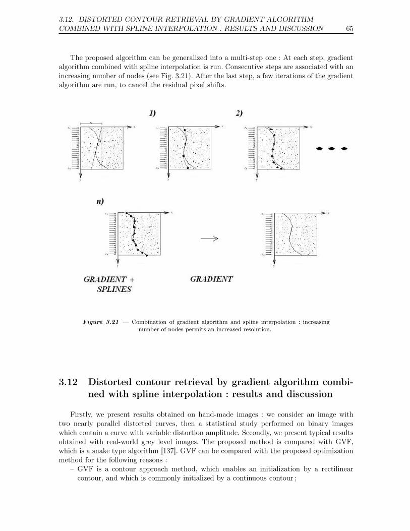
3.12. DISTORTED CONTOUR RETRIEVAL BY GRADIENT ALGORITHMCOMBINED WITH SPLINE INTERPOLATION : RESULTS AND DISCUSSION 65
The proposed algorithm can be generalized into a multi-step one : At each step, gradientalgorithm combined with spline interpolation is run. Consecutive steps are associated with anincreasing number of nodes (see Fig. 3.21). After the last step, a few iterations of the gradientalgorithm are run, to cancel the residual pixel shifts.
Figure 3.21 — Combination of gradient algorithm and spline interpolation : increasingnumber of nodes permits an increased resolution.
3.12 Distorted contour retrieval by gradient algorithm combi-ned with spline interpolation : results and discussion
Firstly, we present results obtained on hand-made images : we consider an image withtwo nearly parallel distorted curves, then a statistical study performed on binary imageswhich contain a curve with variable distortion amplitude. Secondly, we present typical resultsobtained with real-world grey level images. The proposed method is compared with GVF,which is a snake type algorithm [137]. GVF can be compared with the proposed optimizationmethod for the following reasons :
– GVF is a contour approach method, which enables an initialization by a rectilinearcontour, and which is commonly initialized by a continuous contour ;
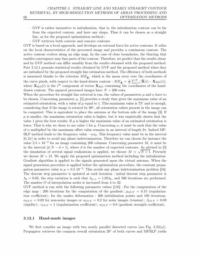
66
CHAPITRE 3. STRAIGHT LINE AND NEARLY STRAIGHT CONTOURRETRIEVAL, BY HIGH-RESOLUTION METHODS OF ARRAY PROCESSING AND
OPTIMIZATION METHODS
– GVF is rather insensitive to initialization, that is, the initialization contour can be farfrom the expected contour, and have any shape. Thus it can be chosen as a straightline, as for the proposed optimization method ;
– GVF retrieves both convexe and concave contours.GVF is based on a local approach, and develops an external force for active contours. It relieson the local characteristics of the processed image and provides a continuous contour. Theactive contour evolves along an edge map. In the case of close boundaries, the blurring thatenables convergence may fuse parts of the contour. Therefore, we predict that the results obtai-ned by GVF method can differ sensibly from the results obtained with the proposed method.Part 3.12.1 presents statistical results obtained by GVF and the proposed method when theyare initialized by the proposed straight line estimation method. The efficiency of both methodsis measured thanks to the criterion ME
X̂, which is the mean error over the coordinates of
the curve pixels, with respect to the hand-drawn contour : MEX̂
= 1N
∑Ni=1 |X̂(i)−XHD(i)|,
where XHD(i) is the ith component of vector XHD containing the coordinates of the hand-drawn contour. The squared processed images have N = 200 rows.When the procedure for straight line retrieval is run, the values of parameters µ and α have tobe chosen. Concerning parameter µ, [5] provides a study that gives the maximum value of anestimated orientation, with a value of µ equal to 1. This maximum value is 73◦ and is enough,considering that if the image is rotated by 90◦, all orientation values present in the image canbe computed. This is equivalent to place the antenna at the bottom side of the image [3]. Ifµ is smaller, the maximum orientation value is higher, but it was empirically shown that thevalue 1 gives the best results. If µ is higher the maximum value of an estimated orientation islower. That is why we chose to use value 1 for µ. Concerning α, it must be such that the valueof α multiplied by the maximum offset value remains in an interval of length 2π. Indeed MF-BLP method leads to the frequency value −αx0. This frequency value must be in the interval[0, 2π[ in order to avoid any phase indetermination. Therefore we can choose for instance thevalue 2.5 × 10⁻³ for an image containing 200 columns. Concerning parameter M , it must bein the interval [d,N − d + 1], where d is the number of expected contours. As advised in [5]the simulation of several signal realizations is applied, we choose M ≃
√N + 1. Precisely
we choose M = 15. We apply the proposed optimization method including the initialization.Gradient algorithm is applied to the signals generated upon the virtual antenna. When thesignal generation procedure is applied before the optimization procedure, the constant propa-gation parameter value is µ = 0.5 10−3. This avoids any phase indetermination problem [24].The descent step parameter is updated at each iteration : initial descent step parameter isλ0 = 0.05, the step variation is such that λk+1 = 1.05λk , and 500 iterations are performed.The number O of interpolation nodes is increased from 4 to 32.GVF method is run with the following parameter values [135] : For the computation of theedge map : 200 iterations for the computation of the gradient ; µGV F = 0.15 (regulariza-tion coefficient) ; for the snakes deformation : 200 initialization points and 100 iterations.αGV F = 0.02 for non-noisy images or αGV F = 0.2 for noisy images (tension) ; βGV F = 0.03(rigidity) ; γGV F = 1 (regularization coefficient) ; κGV F = 0.8 (gradient strength coefficient).
3.12.1 Hand-made images
We first consider an image with two nearly parallel distorted curves (see Fig. 3.22(a)).Propagator retrieves the common overall orientation 20◦ of both curves and MFBLP yields
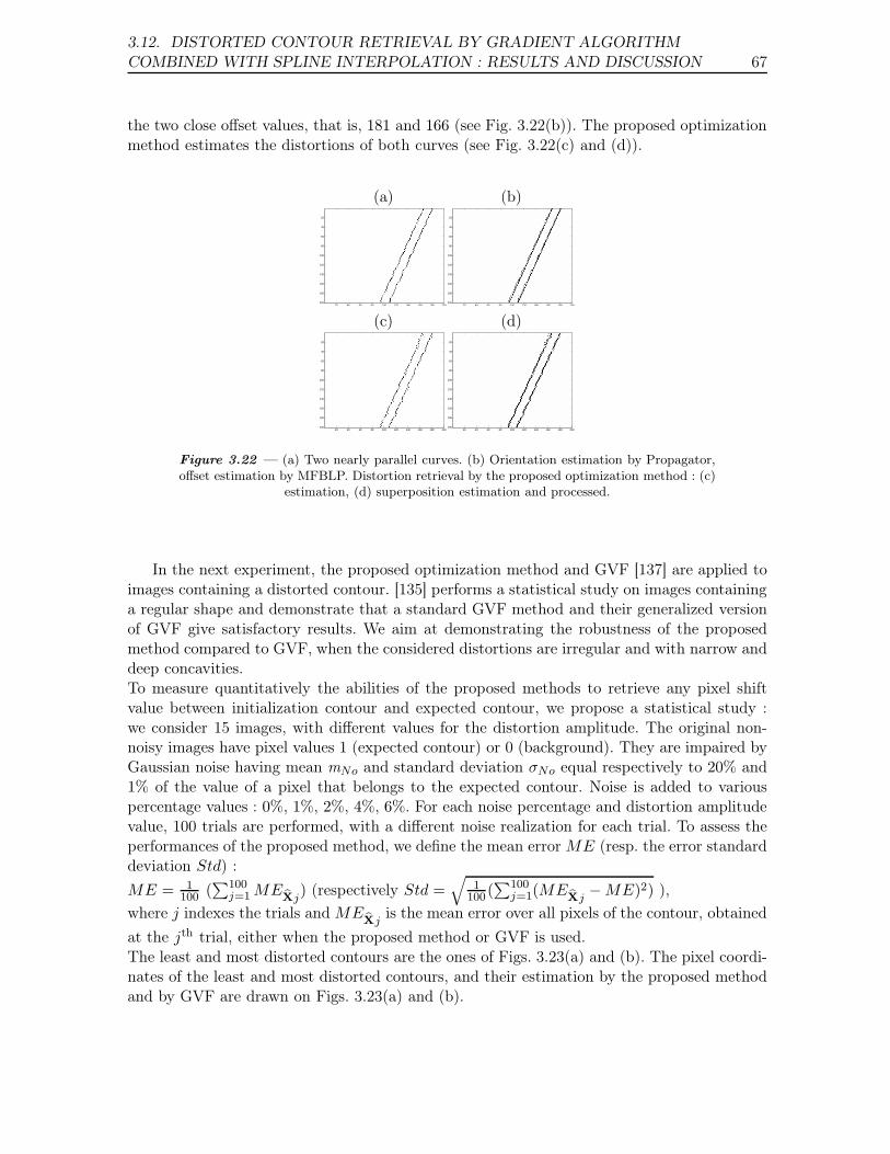
3.12. DISTORTED CONTOUR RETRIEVAL BY GRADIENT ALGORITHMCOMBINED WITH SPLINE INTERPOLATION : RESULTS AND DISCUSSION 67
the two close offset values, that is, 181 and 166 (see Fig. 3.22(b)). The proposed optimizationmethod estimates the distortions of both curves (see Fig. 3.22(c) and (d)).
(a) (b)
20 40 60 80 100 120 140 160 180 200
20
40
60
80
100
120
140
160
180
20020 40 60 80 100 120 140 160 180 200
20
40
60
80
100
120
140
160
180
200
(c) (d)
20 40 60 80 100 120 140 160 180 200
20
40
60
80
100
120
140
160
180
20020 40 60 80 100 120 140 160 180 200
20
40
60
80
100
120
140
160
180
200
Figure 3.22 — (a) Two nearly parallel curves. (b) Orientation estimation by Propagator,offset estimation by MFBLP. Distortion retrieval by the proposed optimization method : (c)
estimation, (d) superposition estimation and processed.
In the next experiment, the proposed optimization method and GVF [137] are applied toimages containing a distorted contour. [135] performs a statistical study on images containinga regular shape and demonstrate that a standard GVF method and their generalized versionof GVF give satisfactory results. We aim at demonstrating the robustness of the proposedmethod compared to GVF, when the considered distortions are irregular and with narrow anddeep concavities.To measure quantitatively the abilities of the proposed methods to retrieve any pixel shiftvalue between initialization contour and expected contour, we propose a statistical study :we consider 15 images, with different values for the distortion amplitude. The original non-noisy images have pixel values 1 (expected contour) or 0 (background). They are impaired byGaussian noise having mean mNo and standard deviation σNo equal respectively to 20% and1% of the value of a pixel that belongs to the expected contour. Noise is added to variouspercentage values : 0%, 1%, 2%, 4%, 6%. For each noise percentage and distortion amplitudevalue, 100 trials are performed, with a different noise realization for each trial. To assess theperformances of the proposed method, we define the mean error ME (resp. the error standarddeviation Std) :
ME = 1100 (
∑100j=1 ME
X̂j) (respectively Std =
√1
100 (∑100
j=1(MEX̂j
− ME)2) ),
where j indexes the trials and MEX̂j
is the mean error over all pixels of the contour, obtained
at the jth trial, either when the proposed method or GVF is used.The least and most distorted contours are the ones of Figs. 3.23(a) and (b). The pixel coordi-nates of the least and most distorted contours, and their estimation by the proposed methodand by GVF are drawn on Figs. 3.23(a) and (b).
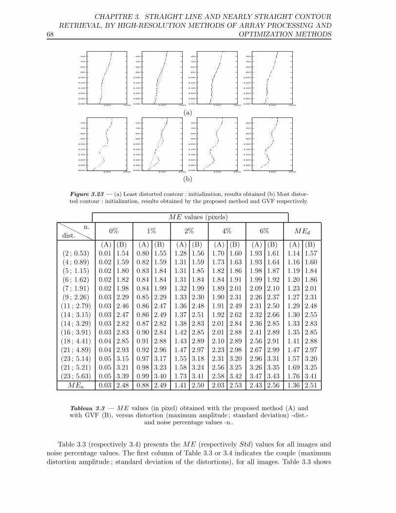
68
CHAPITRE 3. STRAIGHT LINE AND NEARLY STRAIGHT CONTOURRETRIEVAL, BY HIGH-RESOLUTION METHODS OF ARRAY PROCESSING AND
OPTIMIZATION METHODS
100 200
20
40
60
80
100
120
140
160
180
200100 200
20
40
60
80
100
120
140
160
180
200100 200
20
40
60
80
100
120
140
160
180
200100 200
20
40
60
80
100
120
140
160
180
200
(a)
100 200
20
40
60
80
100
120
140
160
180
200100 200
20
40
60
80
100
120
140
160
180
200100 200
20
40
60
80
100
120
140
160
180
200100 200
20
40
60
80
100
120
140
160
180
200
(b)
Figure 3.23 — (a) Least distorted contour : initialization, results obtained (b) Most distor-ted contour : initialization, results obtained by the proposed method and GVF respectively.
ME values (pixels)H
HH
HHH
dist.n.
0% 1% 2% 4% 6% MEd
(A) (B) (A) (B) (A) (B) (A) (B) (A) (B) (A) (B)(2 ; 0.53) 0.01 1.54 0.80 1.55 1.28 1.56 1.70 1.60 1.93 1.61 1.14 1.57(4 ; 0.89) 0.02 1.59 0.82 1.59 1.31 1.59 1.73 1.63 1.93 1.64 1.16 1.60(5 ; 1.15) 0.02 1.80 0.83 1.84 1.31 1.85 1.82 1.86 1.98 1.87 1.19 1.84(6 ; 1.62) 0.02 1.82 0.84 1.84 1.31 1.84 1.84 1.91 1.99 1.92 1.20 1.86(7 ; 1.91) 0.02 1.98 0.84 1.99 1.32 1.99 1.89 2.01 2.09 2.10 1.23 2.01(9 ; 2.26) 0.03 2.29 0.85 2.29 1.33 2.30 1.90 2.31 2.26 2.37 1.27 2.31(11 ; 2.79) 0.03 2.46 0.86 2.47 1.36 2.48 1.91 2.49 2.31 2.50 1.29 2.48(14 ; 3.15) 0.03 2.47 0.86 2.49 1.37 2.51 1.92 2.62 2.32 2.66 1.30 2.55(14 ; 3.29) 0.03 2.82 0.87 2.82 1.38 2.83 2.01 2.84 2.36 2.85 1.33 2.83(16 ; 3.91) 0.03 2.83 0.90 2.84 1.42 2.85 2.01 2.88 2.41 2.89 1.35 2.85(18 ; 4.41) 0.04 2.85 0.91 2.88 1.43 2.89 2.10 2.89 2.56 2.91 1.41 2.88(21 ; 4.89) 0.04 2.93 0.92 2.96 1.47 2.97 2.23 2.98 2.67 2.99 1.47 2.97(23 ; 5.14) 0.05 3.15 0.97 3.17 1.55 3.18 2.31 3.20 2.96 3.31 1.57 3.20(21 ; 5.21) 0.05 3.21 0.98 3.23 1.58 3.24 2.56 3.25 3.26 3.35 1.69 3.25(23 ; 5.63) 0.05 3.39 0.99 3.40 1.73 3.41 2.58 3.42 3.47 3.43 1.76 3.41
MEn 0.03 2.48 0.88 2.49 1.41 2.50 2.03 2.53 2.43 2.56 1.36 2.51
Tableau 3.3 — ME values (in pixel) obtained with the proposed method (A) andwith GVF (B), versus distortion (maximum amplitude ; standard deviation) -dist.-
and noise percentage values -n..
Table 3.3 (respectively 3.4) presents the ME (respectively Std) values for all images andnoise percentage values. The first column of Table 3.3 or 3.4 indicates the couple (maximumdistortion amplitude ; standard deviation of the distortions), for all images. Table 3.3 shows
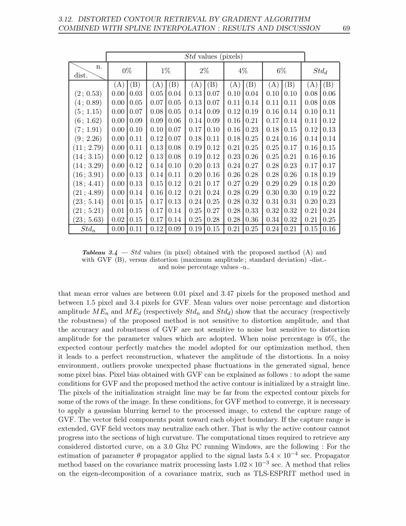
3.12. DISTORTED CONTOUR RETRIEVAL BY GRADIENT ALGORITHMCOMBINED WITH SPLINE INTERPOLATION : RESULTS AND DISCUSSION 69
Std values (pixels)H
HH
HHH
dist.n.
0% 1% 2% 4% 6% Stdd
(A) (B) (A) (B) (A) (B) (A) (B) (A) (B) (A) (B)(2 ; 0.53) 0.00 0.03 0.05 0.04 0.13 0.07 0.10 0.04 0.10 0.10 0.08 0.06(4 ; 0.89) 0.00 0.05 0.07 0.05 0.13 0.07 0.11 0.14 0.11 0.11 0.08 0.08(5 ; 1.15) 0.00 0.07 0.08 0.05 0.14 0.09 0.12 0.19 0.16 0.14 0.10 0.11(6 ; 1.62) 0.00 0.09 0.09 0.06 0.14 0.09 0.16 0.21 0.17 0.14 0.11 0.12(7 ; 1.91) 0.00 0.10 0.10 0.07 0.17 0.10 0.16 0.23 0.18 0.15 0.12 0.13(9 ; 2.26) 0.00 0.11 0.12 0.07 0.18 0.11 0.18 0.25 0.24 0.16 0.14 0.14(11 ; 2.79) 0.00 0.11 0.13 0.08 0.19 0.12 0.21 0.25 0.25 0.17 0.16 0.15(14 ; 3.15) 0.00 0.12 0.13 0.08 0.19 0.12 0.23 0.26 0.25 0.21 0.16 0.16(14 ; 3.29) 0.00 0.12 0.14 0.10 0.20 0.13 0.24 0.27 0.28 0.23 0.17 0.17(16 ; 3.91) 0.00 0.13 0.14 0.11 0.20 0.16 0.26 0.28 0.28 0.26 0.18 0.19(18 ; 4.41) 0.00 0.13 0.15 0.12 0.21 0.17 0.27 0.29 0.29 0.29 0.18 0.20(21 ; 4.89) 0.00 0.14 0.16 0.12 0.21 0.24 0.28 0.29 0.30 0.30 0.19 0.22(23 ; 5.14) 0.01 0.15 0.17 0.13 0.24 0.25 0.28 0.32 0.31 0.31 0.20 0.23(21 ; 5.21) 0.01 0.15 0.17 0.14 0.25 0.27 0.28 0.33 0.32 0.32 0.21 0.24(23 ; 5.63) 0.02 0.15 0.17 0.14 0.25 0.28 0.28 0.36 0.34 0.32 0.21 0.25
Stdn 0.00 0.11 0.12 0.09 0.19 0.15 0.21 0.25 0.24 0.21 0.15 0.16
Tableau 3.4 — Std values (in pixel) obtained with the proposed method (A) andwith GVF (B), versus distortion (maximum amplitude ; standard deviation) -dist.-
and noise percentage values -n..
that mean error values are between 0.01 pixel and 3.47 pixels for the proposed method andbetween 1.5 pixel and 3.4 pixels for GVF. Mean values over noise percentage and distortionamplitude MEn and MEd (respectively Stdn and Stdd) show that the accuracy (respectivelythe robustness) of the proposed method is not sensitive to distortion amplitude, and thatthe accuracy and robustness of GVF are not sensitive to noise but sensitive to distortionamplitude for the parameter values which are adopted. When noise percentage is 0%, theexpected contour perfectly matches the model adopted for our optimization method, thenit leads to a perfect reconstruction, whatever the amplitude of the distortions. In a noisyenvironment, outliers provoke unexpected phase fluctuations in the generated signal, hencesome pixel bias. Pixel bias obtained with GVF can be explained as follows : to adopt the sameconditions for GVF and the proposed method the active contour is initialized by a straight line.The pixels of the initialization straight line may be far from the expected contour pixels forsome of the rows of the image. In these conditions, for GVF method to converge, it is necessaryto apply a gaussian blurring kernel to the processed image, to extend the capture range ofGVF. The vector field components point toward each object boundary. If the capture range isextended, GVF field vectors may neutralize each other. That is why the active contour cannotprogress into the sections of high curvature. The computational times required to retrieve anyconsidered distorted curve, on a 3.0 Ghz PC running Windows, are the following : For theestimation of parameter θ propagator applied to the signal lasts 5.4 × 10⁻⁴ sec. Propagatormethod based on the covariance matrix processing lasts 1.02×10⁻³ sec. A method that relieson the eigen-decomposition of a covariance matrix, such as TLS-ESPRIT method used in

70
CHAPITRE 3. STRAIGHT LINE AND NEARLY STRAIGHT CONTOURRETRIEVAL, BY HIGH-RESOLUTION METHODS OF ARRAY PROCESSING AND
OPTIMIZATION METHODS
SLIDE algorithm lasts 1.08× 10⁻³ sec. [5]. Propagator applied to the signal is then two timesfaster than the two compared methods. The proposed method for offset estimation usingMFBLP last 0.592 sec. The proposed optimization method, for which 30 interpolation nodesand 3000 iterations are necessary, lasts 26.5 sec. GVF method lasts 28.1 sec.
3.12.2 Distorted contour retrieval in real-world grey level images
The proposed optimization method is initialized by means of the straight line detectionmethod presented in subsection 3.3.1. When grey level images are considered, an edge en-hancing procedure attenuates the contribution of the continuous background, which eases theprocedure of signal generation [7]. Figs. 3.24, 3.25 and 3.26 present the results obtained on se-veral images acquired in the context of aerial imaging and of an industrial application -defaultdetection in tissue. Initialization contour and final result are superimposed to the processedimage. Column (a) contains the processed image, column (b) contains the initialization by theproposed method, column (c) contains the result obtained with the proposed method, column(d) contains the initialization for GVF algorithm, column (e) contains the result obtainedwith GVF.
(a) (b) (c) (d) (e)
20 40 60 80 100 120 140 160 180 200
20
40
60
80
100
120
140
160
180
20020 40 60 80 100 120 140 160 180 200
20
40
60
80
100
120
140
160
180
20020 40 60 80 100 120 140 160 180 200
20
40
60
80
100
120
140
160
180
20020 40 60 80 100 120 140 160 180 200
20
40
60
80
100
120
140
160
180
20 40 60 80 100 120 140 160 180 200
20
40
60
80
100
120
140
160
180
20 40 60 80 100 120 140 160 180 200
20
40
60
80
100
120
140
160
180
20020 40 60 80 100 120 140 160 180 200
20
40
60
80
100
120
140
160
180
20020 40 60 80 100 120 140 160 180 200
20
40
60
80
100
120
140
160
180
20020 40 60 80 100 120 140 160 180 200
20
40
60
80
100
120
140
160
180
20 40 60 80 100 120 140 160 180 200
20
40
60
80
100
120
140
160
180
20 40 60 80 100 120 140 160 180 200
20
40
60
80
100
120
140
160
180
20020 40 60 80 100 120 140 160 180 200
20
40
60
80
100
120
140
160
180
20020 40 60 80 100 120 140 160 180 200
20
40
60
80
100
120
140
160
180
20020 40 60 80 100 120 140 160 180 200
20
40
60
80
100
120
140
160
180
20 40 60 80 100 120 140 160 180 200
20
40
60
80
100
120
140
160
180
Figure 3.24 — Aerial image analysis : coast detection. (a) processed image, (b) initia-lization, (c) result with the proposed method, (d) initialization for GVF, (e) result with
GVF.
when the active contour performs well, namely when it is initialized close to the expectedcontour, and when it converges, its result is close to the result obtained with the proposed
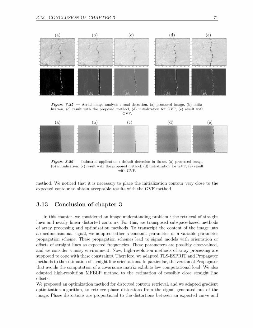
3.13. CONCLUSION OF CHAPTER 3 71
(a) (b) (c) (d) (e)
50 100 150 200 250 300 350 400 450
50
100
150
200
250
300
350
400
450
50 100 150 200 250 300 350 400 450
50
100
150
200
250
300
350
400
450
50 100 150 200 250 300 350 400 450
50
100
150
200
250
300
350
400
450
50 100 150 200 250 300 350 400 450
50
100
150
200
250
300
350
400
450
50 100 150 200 250 300 350 400 450
50
100
150
200
250
300
350
400
450
20 40 60 80 100 120 140 160 180 200
20
40
60
80
100
120
140
160
180
20020 40 60 80 100 120 140 160 180 200
20
40
60
80
100
120
140
160
180
20020 40 60 80 100 120 140 160 180 200
20
40
60
80
100
120
140
160
180
20020 40 60 80 100 120 140 160 180 200
20
40
60
80
100
120
140
160
180
20 40 60 80 100 120 140 160 180 200
20
40
60
80
100
120
140
160
180
Figure 3.25 — Aerial image analysis : road detection. (a) processed image, (b) initia-lization, (c) result with the proposed method, (d) initialization for GVF, (e) result with
GVF.
(a) (b) (c) (d) (e)
20 40 60 80 100 120 140 160 180 200
20
40
60
80
100
120
140
160
180
20020 40 60 80 100 120 140 160 180 200
20
40
60
80
100
120
140
160
180
20020 40 60 80 100 120 140 160 180 200
20
40
60
80
100
120
140
160
180
20020 40 60 80 100 120 140 160 180 200
20
40
60
80
100
120
140
160
180
20 40 60 80 100 120 140 160 180 200
20
40
60
80
100
120
140
160
180
Figure 3.26 — Industrial application : default detection in tissue. (a) processed image,(b) initialization, (c) result with the proposed method, (d) initialization for GVF, (e) result
with GVF.
method. We noticed that it is necessary to place the initialization contour very close to theexpected contour to obtain acceptable results with the GVF method.
3.13 Conclusion of chapter 3
In this chapter, we considered an image understanding problem : the retrieval of straightlines and nearly linear distorted contours. For this, we transposed subspace-based methodsof array processing and optimization methods. To transcript the content of the image intoa onedimensionnal signal, we adopted either a constant parameter or a variable parameterpropagation scheme. These propagation schemes lead to signal models with orientation oroffsets of straight lines as expected frequencies. These parameters are possibly close-valued,and we consider a noisy environment. Now, high-resolution methods of array processing aresupposed to cope with these constraints. Therefore, we adapted TLS-ESPRIT and Propagatormethods to the estimation of straight line orientations. In particular, the version of Propagatorthat avoids the computation of a covariance matrix exhibits low computational load. We alsoadapted high-resolution MFBLP method to the estimation of possibly close straight lineoffsets.We proposed an optimization method for distorted contour retrieval, and we adapted gradientoptimization algorithm, to retrieve phase distortions from the signal generated out of theimage. Phase distortions are proportional to the distortions between an expected curve and

72
CHAPITRE 3. STRAIGHT LINE AND NEARLY STRAIGHT CONTOURRETRIEVAL, BY HIGH-RESOLUTION METHODS OF ARRAY PROCESSING AND
OPTIMIZATION METHODS
a fitting straight line. This procedure is generalized to the retrieval of several contours byan association of Propagator with gradient method. We also propose a novel optimizationmethod which is still fast, and yields a continuous contour. We compared the results obtainedwith this method with those obtained with gradient vector flow. Especially, the proposedmethod retrieves contours with high curvature, and leads to good results when real-worldimages are processed. These methods rely on signal generation upon a linear antenna. In thenext chapter, we consider contours which are no longer linear or nearly linear but circular ornearly circular. For this, we adapt a circular antenna to the processed image.
CHAPITRE
4 Subspace-Based and
DIRECT algorithms for
distorted circular contour
estimation
Circular features are commonly sought in digital image processing. SLIDE (subspace-basedLIne DEtection) method proposed to estimate the center and the radius of a single circle. Inthis chapter, we introduce a novel method for estimating several radii while extending thecircle estimation to retrieve circular-like distorted contours. Especially, we develop and vali-date a new model for virtual signal generation by simulating a circular antenna.This circular antenna yields linear phase signals which suit high-resolution methods whichwere applied to straight or nearly straight contour estimation. Therefore, the same high-resolution and optimization methods as those used for straight or nearly straight contourestimation can be adapted to the retrieval of circular or nearly circular contour retrieval.The circle center is estimated by the SLIDE method. A variable speed propagation schemetoward the circular antenna yields a linear phase signal. Therefore, a high-resolution methodprovides the radius. Either the gradient method or the more robust combination of DIRECT(DIviding RECTangles) and spline interpolation can extend this method for free form ob-ject segmentation. The retrieval of multiple non concentric circles and rotated ellipses is alsoconsidered. To evaluate the performance of the proposed methods, we compare them witha least-squares method, Hough transform and GVF (Gradient Vector Flow). We apply theproposed method to hand-made images while considering some real-world images.This chapter is organized as follows. In Section 4.1, we review the existing methods for contourretrieval, and emphasize the interest of array processing methods applied to image unders-tanding. In Section 4.2, the problem of circle retrieval is highlighted, while explaining how togenerate a signal from the image, upon a circular antenna. In Section 4.3, a signal model isderived. We will show that a linear phase signal is obtained when circles are expected andeither variable [7] or constant propagation parameter is adopted for signal generation. Byusing the MDL (Minimum Description Length) criterion [132, 5], the number of concentricfeatures is detected ; then a high-resolution method [114] estimates the possibly close radiusvalues of the expected concentric circles. Then, the proposed approach is generalized to re-trieve several circles or ellipses with different centers and radii. In Section 4.4, the retrieval ofcircular contours is extended to any closed contour fitted by a circle. Optimization methodsare investigated for this purpose. The fast variable step gradient method and the robust
74CHAPITRE 4. SUBSPACE-BASED AND DIRECT ALGORITHMS FOR
DISTORTED CIRCULAR CONTOUR ESTIMATION
DIRECT (DIviding RECTangles) method [64] are accelerated using spline interpolation. InSection 4.5, we discuss the results obtained by the proposed approach when it is applied tohand-made and real-world images. The proposed radius estimation method is compared withleast-squares fitting and Hough transform applied to radius estimation [122]. Our optimiza-tion method is compared with GVF [137], in particular concerning the robustness to noiseand contour curvature. Concluding remarks about the methods presented in this chapter areprovided in section 4.6.
This work has been published in :Julien Marot and Salah Bourennane, "Subspace-Based and DIRECT Algorithms for DistortedCircular Contour Estimation", IEEE trans. on Image Processing, vol. 16, no. 9, pp. 2369-2378, september 2007, inJ. Marot and S. Bourennane, "Array processing and fast Optimization Algorithms for Distor-ted Circular Contour Retrieval", Advances on signal processing, article ID 57354, 13 pages,july 2007, and inJ. Marot and S. Bourennane, "Array processing approach for object segmentation in images",IEEE ICASSP’07, Vol. 1, pp. 621-24, April 2007.
4.1 Introduction
Circular features are commonly sought in digital image processing. Circle fitting is suitablein several domains such as quality inspection for food industry, mechanical parts [81] and par-ticle trajectories [37, 65]. Circle fitting has been applied in microwave engineering [68] and balldetection for robotic vision systems [35]. Nearly circular features are sought in character recog-nition. [36, 45] proposed a template-based system for online character recognition, where therepresentative templates are automatically counted. These templates are viewed as differentwriting styles for any character. Ordinary or total least-squares methods for circle fitting seekto minimize the squares sum of error-of-fit with respect to measures [16, 47, 20, 101]. Usinggeometric fitting [16], error distances are defined with the orthogonal, or shortest, distancesfrom given points to the geometric feature to be fitted. In [20], a least-squares fitting approachis proposed. It is based on the hypothesis that a set of circular arcs extracted from the imageis related to a set of circles contained in a model by translation, rotation and scaling. [20]presents an analytical solution based on least-squares fitting to obtain an optimal geometrictransformation for the alignment of the circular arcs with circles. For a single circular arc, thismethod is easy to implement. For multiple arcs with different center, this method relies on thestrong hypothesis that all model circles should be transformed by the same translation, rota-tion and scaling operations to fit the arcs in the image. One of the major limitations of mostof least-squares approaches is their sensitivity to outliers [20]. [9, 10] focused on planar splineinterpolation between control-points by quadratic rational Bézier curves, to retrieve circulararcs. Compared to [20], this method does not take into account the prior knowledge of modelsor templates. It is based on interpolation between control-points. Other methods support circleretrieval, even in a noisy environment. The generalized Hough transform (GHT) provides esti-mation of the circle center coordinates when their radius is known [61, 19]. Its main drawbackis the computational load, although fast versions have been proposed [122]. Contour-basedsnakes methods [69], such as Gradient Vector Flow (GVF), were largely used [137, 135], toretrieve concavities and weak edges with blurred boundaries. GVF limitations can be ob-served when the expected contour exhibits a high curvature. Levelset type methods [15, 66]
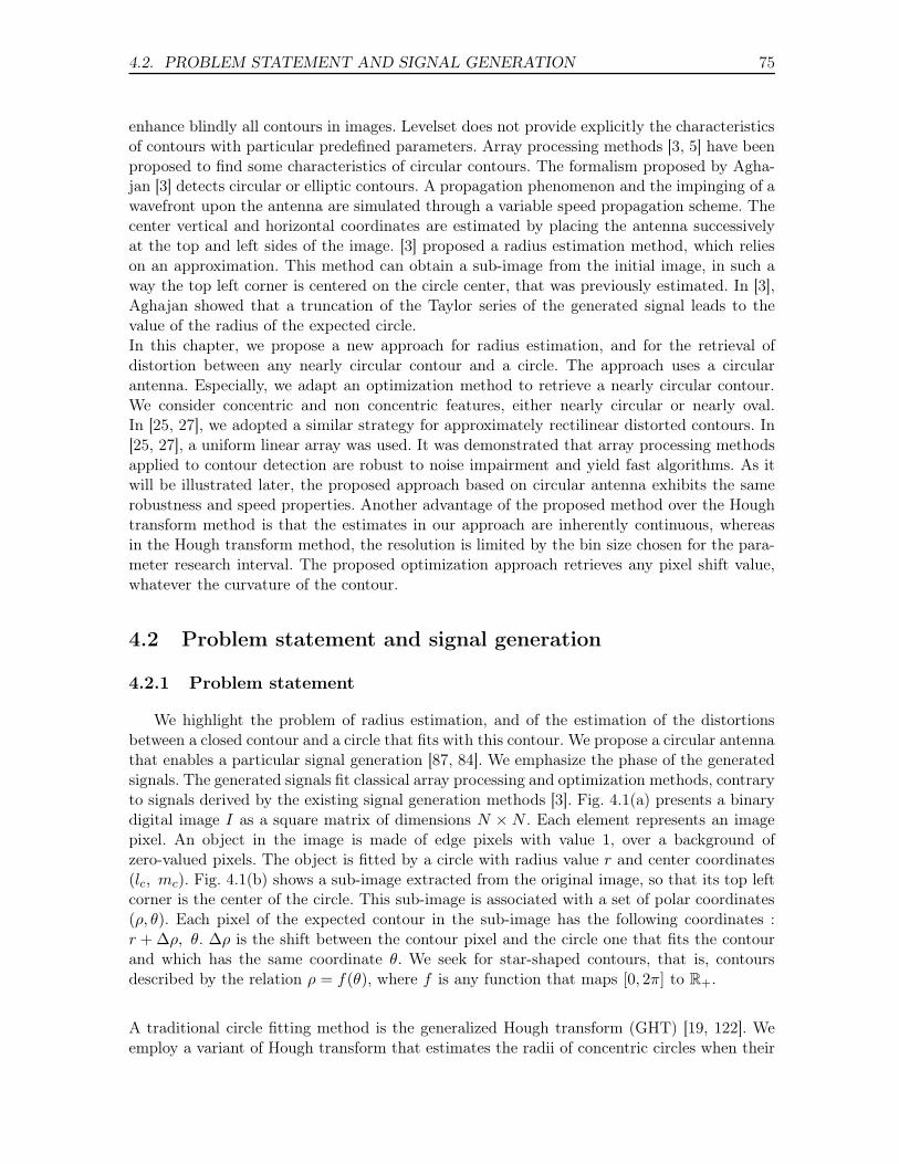
4.2. PROBLEM STATEMENT AND SIGNAL GENERATION 75
enhance blindly all contours in images. Levelset does not provide explicitly the characteristicsof contours with particular predefined parameters. Array processing methods [3, 5] have beenproposed to find some characteristics of circular contours. The formalism proposed by Agha-jan [3] detects circular or elliptic contours. A propagation phenomenon and the impinging of awavefront upon the antenna are simulated through a variable speed propagation scheme. Thecenter vertical and horizontal coordinates are estimated by placing the antenna successivelyat the top and left sides of the image. [3] proposed a radius estimation method, which relieson an approximation. This method can obtain a sub-image from the initial image, in such away the top left corner is centered on the circle center, that was previously estimated. In [3],Aghajan showed that a truncation of the Taylor series of the generated signal leads to thevalue of the radius of the expected circle.In this chapter, we propose a new approach for radius estimation, and for the retrieval ofdistortion between any nearly circular contour and a circle. The approach uses a circularantenna. Especially, we adapt an optimization method to retrieve a nearly circular contour.We consider concentric and non concentric features, either nearly circular or nearly oval.In [25, 27], we adopted a similar strategy for approximately rectilinear distorted contours. In[25, 27], a uniform linear array was used. It was demonstrated that array processing methodsapplied to contour detection are robust to noise impairment and yield fast algorithms. As itwill be illustrated later, the proposed approach based on circular antenna exhibits the samerobustness and speed properties. Another advantage of the proposed method over the Houghtransform method is that the estimates in our approach are inherently continuous, whereasin the Hough transform method, the resolution is limited by the bin size chosen for the para-meter research interval. The proposed optimization approach retrieves any pixel shift value,whatever the curvature of the contour.
4.2 Problem statement and signal generation
4.2.1 Problem statement
We highlight the problem of radius estimation, and of the estimation of the distortionsbetween a closed contour and a circle that fits with this contour. We propose a circular antennathat enables a particular signal generation [87, 84]. We emphasize the phase of the generatedsignals. The generated signals fit classical array processing and optimization methods, contraryto signals derived by the existing signal generation methods [3]. Fig. 4.1(a) presents a binarydigital image I as a square matrix of dimensions N × N . Each element represents an imagepixel. An object in the image is made of edge pixels with value 1, over a background ofzero-valued pixels. The object is fitted by a circle with radius value r and center coordinates(lc, mc). Fig. 4.1(b) shows a sub-image extracted from the original image, so that its top leftcorner is the center of the circle. This sub-image is associated with a set of polar coordinates(ρ, θ). Each pixel of the expected contour in the sub-image has the following coordinates :r + ∆ρ, θ. ∆ρ is the shift between the contour pixel and the circle one that fits the contourand which has the same coordinate θ. We seek for star-shaped contours, that is, contoursdescribed by the relation ρ = f(θ), where f is any function that maps [0, 2π] to R+.
A traditional circle fitting method is the generalized Hough transform (GHT) [19, 122]. Weemploy a variant of Hough transform that estimates the radii of concentric circles when their
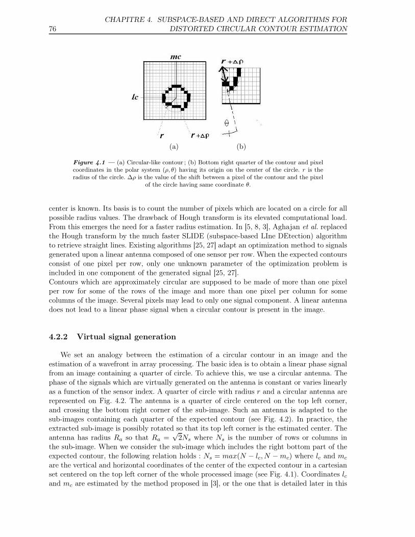
76CHAPITRE 4. SUBSPACE-BASED AND DIRECT ALGORITHMS FOR
DISTORTED CIRCULAR CONTOUR ESTIMATION
(a) (b)
Figure 4.1 — (a) Circular-like contour ; (b) Bottom right quarter of the contour and pixelcoordinates in the polar system (ρ, θ) having its origin on the center of the circle. r is theradius of the circle. ∆ρ is the value of the shift between a pixel of the contour and the pixel
of the circle having same coordinate θ.
center is known. Its basis is to count the number of pixels which are located on a circle for allpossible radius values. The drawback of Hough transform is its elevated computational load.From this emerges the need for a faster radius estimation. In [5, 8, 3], Aghajan et al. replacedthe Hough transform by the much faster SLIDE (subspace-based LIne DEtection) algorithmto retrieve straight lines. Existing algorithms [25, 27] adapt an optimization method to signalsgenerated upon a linear antenna composed of one sensor per row. When the expected contoursconsist of one pixel per row, only one unknown parameter of the optimization problem isincluded in one component of the generated signal [25, 27].Contours which are approximately circular are supposed to be made of more than one pixelper row for some of the rows of the image and more than one pixel per column for somecolumns of the image. Several pixels may lead to only one signal component. A linear antennadoes not lead to a linear phase signal when a circular contour is present in the image.
4.2.2 Virtual signal generation
We set an analogy between the estimation of a circular contour in an image and theestimation of a wavefront in array processing. The basic idea is to obtain a linear phase signalfrom an image containing a quarter of circle. To achieve this, we use a circular antenna. Thephase of the signals which are virtually generated on the antenna is constant or varies linearlyas a function of the sensor index. A quarter of circle with radius r and a circular antenna arerepresented on Fig. 4.2. The antenna is a quarter of circle centered on the top left corner,and crossing the bottom right corner of the sub-image. Such an antenna is adapted to thesub-images containing each quarter of the expected contour (see Fig. 4.2). In practice, theextracted sub-image is possibly rotated so that its top left corner is the estimated center. Theantenna has radius Ra so that Ra =
√2Ns where Ns is the number of rows or columns in
the sub-image. When we consider the sub-image which includes the right bottom part of theexpected contour, the following relation holds : Ns = max(N − lc, N − mc) where lc and mc
are the vertical and horizontal coordinates of the center of the expected contour in a cartesianset centered on the top left corner of the whole processed image (see Fig. 4.1). Coordinates lcand mc are estimated by the method proposed in [3], or the one that is detailed later in this
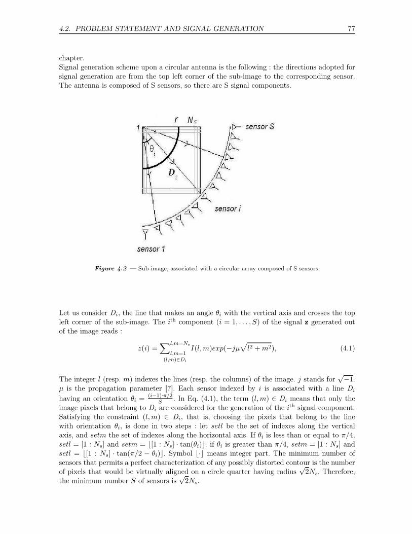
4.2. PROBLEM STATEMENT AND SIGNAL GENERATION 77
chapter.Signal generation scheme upon a circular antenna is the following : the directions adopted forsignal generation are from the top left corner of the sub-image to the corresponding sensor.The antenna is composed of S sensors, so there are S signal components.
Figure 4.2 — Sub-image, associated with a circular array composed of S sensors.
Let us consider Di , the line that makes an angle θi with the vertical axis and crosses the topleft corner of the sub-image. The ith component (i = 1, . . . , S) of the signal z generated outof the image reads :
z(i) =∑l,m=Ns
l,m=1(l,m)∈Di
I(l,m)exp(−jµ√
l2 + m2), (4.1)
The integer l (resp. m) indexes the lines (resp. the columns) of the image. j stands for√−1.
µ is the propagation parameter [7]. Each sensor indexed by i is associated with a line Di
having an orientation θi = (i−1)·π/2S . In Eq. (4.1), the term (l,m) ∈ Di means that only the
image pixels that belong to Di are considered for the generation of the ith signal component.Satisfying the constraint (l,m) ∈ Di , that is, choosing the pixels that belong to the linewith orientation θi, is done in two steps : let setl be the set of indexes along the verticalaxis, and setm the set of indexes along the horizontal axis. If θi is less than or equal to π/4,setl = [1 : Ns] and setm = ⌊[1 : Ns] · tan(θi)⌋. if θi is greater than π/4, setm = [1 : Ns] andsetl = ⌊[1 : Ns] · tan(π/2 − θi)⌋. Symbol ⌊·⌋ means integer part. The minimum number ofsensors that permits a perfect characterization of any possibly distorted contour is the numberof pixels that would be virtually aligned on a circle quarter having radius
√2Ns. Therefore,
the minimum number S of sensors is√
2Ns.
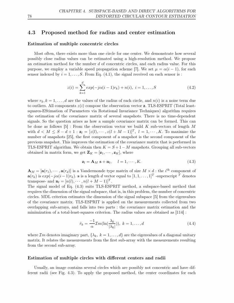
78CHAPITRE 4. SUBSPACE-BASED AND DIRECT ALGORITHMS FOR
DISTORTED CIRCULAR CONTOUR ESTIMATION
4.3 Proposed method for radius and center estimation
Estimation of multiple concentric circles
Most often, there exists more than one circle for one center. We demonstrate how severalpossibly close radius values can be estimated using a high-resolution method. We proposean estimation method for the number d of concentric circles, and each radius value. For thispurpose, we employ a variable speed propagation scheme [7]. We set µ = α(i − 1), for eachsensor indexed by i = 1, . . . , S. From Eq. (4.1), the signal received on each sensor is :
z(i) =
d∑
k=1
exp(−jα(i − 1)rk) + n(i), i = 1, . . . , S (4.2)
where rk, k = 1, . . . , d are the values of the radius of each circle, and n(i) is a noise term dueto outliers. All components z(i) compose the observation vector z. TLS-ESPRIT (Total least-squares-EStimation of Parameters via Rotational Invariance Techniques) algorithm requiresthe estimation of the covariance matrix of several snapshots. There is no time-dependentsignals. So the question arises as how a sample covariance matrix can be formed. This canbe done as follows [5] : From the observation vector we build K sub-vectors of length Mwith d < M ≤ S − d + 1 : zl = [z(l), · · · , z(l + M − 1)]T , l = 1, · · · ,K. To maximize thenumber of snapshots [25], the first component of a snapshot is the second component of theprevious snapshot. This improves the estimation of the covariance matrix that is performed inTLS-ESPRIT algorithm. We obtain then K = S +1−M snapshots. Grouping all sub-vectorsobtained in matrix form, we get ZK = [z1, · · · , zK ], where
zl = AM s + nl, l = 1, · · · ,K. (4.3)
AM = [a(r1), · · · ,a(rd)] is a Vandermonde type matrix of size M × d : the ith component ofa(rk) is exp(−jα(i− 1)rk). s is a length d vector equal to [1, 1, . . . , 1]T -superscript T denotestranspose- and nl = [n(l), · · · , n(l + M − 1)]T .The signal model of Eq. (4.3) suits TLS-ESPRIT method, a subspace-based method thatrequires the dimension of the signal subspace, that is, in this problem, the number of concentriccircles. MDL criterion estimates the dimension of the signal subspace [5] from the eigenvaluesof the covariance matrix. TLS-ESPRIT is applied on the measurements collected from twooverlapping sub-arrays, and falls into two parts : the covariance matrix estimation and theminimization of a total-least-squares criterion. The radius values are obtained as [114] :
r̂k =−1
αIm(ln(
λk
|λk|)), k = 1, . . . , d (4.4)
where Im denotes imaginary part, {λk, k = 1, . . . , d} are the eigenvalues of a diagonal unitarymatrix. It relates the measurements from the first sub-array with the measurements resultingfrom the second sub-array.
Estimation of multiple circles with different centers and radii
Usually, an image contains several circles which are possibly not concentric and have dif-ferent radii (see Fig. 4.3). To apply the proposed method, the center coordinates for each
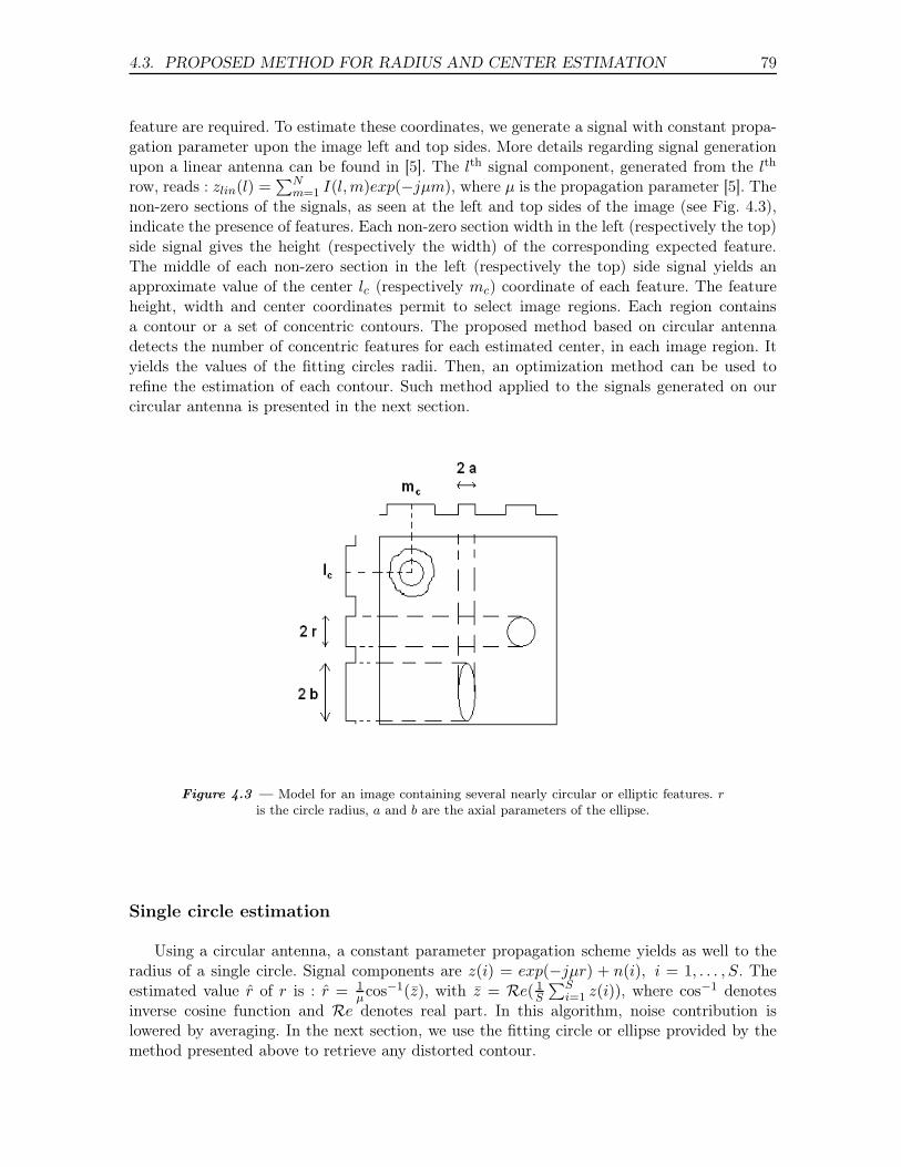
4.3. PROPOSED METHOD FOR RADIUS AND CENTER ESTIMATION 79
feature are required. To estimate these coordinates, we generate a signal with constant propa-gation parameter upon the image left and top sides. More details regarding signal generationupon a linear antenna can be found in [5]. The lth signal component, generated from the lth
row, reads : zlin(l) =∑N
m=1 I(l,m)exp(−jµm), where µ is the propagation parameter [5]. Thenon-zero sections of the signals, as seen at the left and top sides of the image (see Fig. 4.3),indicate the presence of features. Each non-zero section width in the left (respectively the top)side signal gives the height (respectively the width) of the corresponding expected feature.The middle of each non-zero section in the left (respectively the top) side signal yields anapproximate value of the center lc (respectively mc) coordinate of each feature. The featureheight, width and center coordinates permit to select image regions. Each region containsa contour or a set of concentric contours. The proposed method based on circular antennadetects the number of concentric features for each estimated center, in each image region. Ityields the values of the fitting circles radii. Then, an optimization method can be used torefine the estimation of each contour. Such method applied to the signals generated on ourcircular antenna is presented in the next section.
Figure 4.3 — Model for an image containing several nearly circular or elliptic features. r
is the circle radius, a and b are the axial parameters of the ellipse.
Single circle estimation
Using a circular antenna, a constant parameter propagation scheme yields as well to theradius of a single circle. Signal components are z(i) = exp(−jµr) + n(i), i = 1, . . . , S. Theestimated value r̂ of r is : r̂ = 1
µcos−1(z̄), with z̄ = Re( 1S
∑Si=1 z(i)), where cos−1 denotes
inverse cosine function and Re denotes real part. In this algorithm, noise contribution islowered by averaging. In the next section, we use the fitting circle or ellipse provided by themethod presented above to retrieve any distorted contour.
80CHAPITRE 4. SUBSPACE-BASED AND DIRECT ALGORITHMS FOR
DISTORTED CIRCULAR CONTOUR ESTIMATION
Numerical complexity of the circle fitting method
In the general case the image contains outlier pixels and several concentric circles. First, asconcerns the estimation of the coordinates of the center [3] : it is performed by signal generationupon a linear antenna located on one horizontal and then one vertical side of the image,followed by TLS-ESPRIT method. This antenna contains N sensors, each corresponding toone row or column. The estimation of the coordinate of the center requires the followingoperations and computational complexity, for each coordinate along horizontal and verticalaxes [3] :
– Variable speed propagation scheme upon a linear antenna aside the image : N2 opera-tions [5] ;
– Application of TLS-ESPRIT to the covariance matrix of the generated signals : for theestimation, and respectively the fast eigendecomposition, of the covariance matrix inTLS-ESPRIT method [117, 7] : N · M , and respectively M2 ;
We choose M =√
N , as recommended in [7]. The computational complexity for center retrie-val is then N2 + N · (
√N + 1).
As concerns the estimation of the radius values, we remind that d is the number of concentriccircles and the dimension of the signal subspace in the covariance matrix in TLS-ESPRITmethod. The computational complexity of the steps of our method for radius estimation is :
– For signal generation [117, 5] : the number of sensors multiplied by the number of pixelsthat are crossed by each line Di, that is : S · Nsubimage or equivalently S · N ;
– For the estimation, and respectively the fast eigendecomposition, of the covariance ma-trix in TLS-ESPRIT method [117, 7] : S · M , and respectively d · M2 ;
We choose M =√
S, as recommended in [7]. The computational complexity of the angleestimation method is then S ·N +S · (
√S + d). In practice, the order of magnitude of S is N ,
and the computational load of the proposed method for center and radius estimation is N2.As concerns the generalized Hough transform we discretize the ρ axis to the minimum requirednumber of values, that is,
√2 ·N for the computation of the accumulator. Also, the θ axis for
counting the edge pixels is discretized to√
2 · N values (√
2 · N is the minimum number oforientations that permits to characterize any contour in the image, see subsection 4.2.2). Inthese conditions the order of magnitude of the computational load of the generalized Houghtransform, for the estimation of the center and the radius of the circles, is N3 [122]. Toconclude, the computational complexity of the proposed method is N2, as compared to N3
for the generalized Hough transform. The same order of magnitude of computational loadswere obtained in [5] when SLIDE algorithm was compared with the Hough transform forstraight line retrieval.
4.4 Optimization method for the estimation of nearly circularcontours
The optimization methods proposed in [25, 27] estimate the pixel shift values betweena straight line and a nearly linear contour. These methods rely on the assumption that onecomponent of the generated signal is associated with only one unknown pixel shift value inone image row (or column). The proposed circular antenna adapts optimization methods toretrieve distorted star-shaped contours.
4.4. OPTIMIZATION METHOD FOR THE ESTIMATION OF NEARLY CIRCULARCONTOURS 81
4.4.1 Proposed optimization method
We employ a circular antenna to retrieve the shift values between an initialization circleand the expected contour. We process successively each quarter of the circle, and retrievethe distortions between one quarter of the initialization circle and the expected contour partthat is located in the same quarter of the image. As an example, in Fig. 4.1, the right bottomquarter of the considered image is represented in Fig. 4.1(b). An optimization method inspiredfrom [25] is defined as follows :A contour in the considered sub-image is described with a set of polar coordinates by :{ρ(i), θ(i), i = 1, . . . , S}. We estimate the S unknowns ρ(i) that characterize the contour,forming a vector :
ρ = [ρ(1), ρ(2), . . . , ρ(S)]T , (4.5)
The basic idea is to consider that ρ can be written as : ρ = [r + ∆ρ(1), r + ∆ρ(2), . . . , r +∆ρ(S)]T (see Fig. 4.1), where r is the radius of a circle that fits the expected contour. Theoptimization method that we adapt to this problem estimates {∆ρ(i), i = 1, . . . , S}, that is,the shift values between the initialization circle and the expected contour.If we take into account the position given by ρ of all edge pixels in Eq. (4.1), the componentsof signal z generated out of the image containing the expected contour read :
z(i) = exp(−jµρ(i)), ∀i = 1, . . . , S (4.6)
We try to recreate the signal z, whose components are defined by Eq. (4.6), and in which weignore the S parameters. We start with an initialization vector ρ0, characterizing a quarter ofcircle that fits the expected distorted contour in the considered sub-image. The S componentsof ρ0 are equal to r, the radius value that was previously estimated : ρ0 = [r, r, . . . , r]T . Then,with k indexing this recursive algorithm steps, we aim to minimize :
J(ρk) = ||z− zestimated for ρk||2 (4.7)
where ||.|| represents the norm induced by the usual scalar product of CS . The components of
zestimated for ρkare defined similarly to the components of z (see Eq. (4.6)) as a function of
the components of ρk, and the components of ρk are obtained from the components of ρ0 byadding a shift : ρk = [r + ∆ρk(1), r + ∆ρk(2), . . . , r + ∆ρk(S)]T . To estimate ρ, we use eitherthe variable step gradient method or the more robust combination of DIRECT and splineinterpolation methods, which is detailed in section 1.4. We denote by ρ̂ the vector includingall the estimated values ρk(i), i = 1, . . . , S
4.4.2 Summary of the proposed method
The proposed method for distorted contour estimation is summarized as follows :– Generation of a signal with constant parameter, on a linear antenna placed at the top
of and aside the image ;– Estimation of the centers of the circles or ellipses that fit the expected contours ;– Variable speed propagation scheme upon the proposed circular antenna : Estimation of
the number of circles by MDL criterion, estimation of the radius of each circle fittingany expected contour (see Eqs. (4.1) and (4.2)) or the axial parameters of the ellipse ;
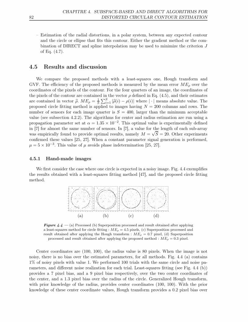
82CHAPITRE 4. SUBSPACE-BASED AND DIRECT ALGORITHMS FOR
DISTORTED CIRCULAR CONTOUR ESTIMATION
– Estimation of the radial distortions, in a polar system, between any expected contourand the circle or ellipse that fits this contour. Either the gradient method or the com-bination of DIRECT and spline interpolation may be used to minimize the criterion Jof Eq. (4.7).
4.5 Results and discussion
We compare the proposed methods with a least-squares one, Hough transform andGVF. The efficiency of the proposed methods is measured by the mean error MEρ over thecoordinates of the pixels of the contour. For the four quarters of an image, the coordinates ofthe pixels of the contour are contained in the vector ρ defined in Eq. (4.5), and their estimatesare contained in vector ρ̂. MEρ = 1
S
∑Si=1 |ρ̂(i) − ρ(i)| where | · | means absolute value. The
proposed circle fitting method is applied to images having N = 200 columns and rows. Thenumber of sensors for each image quarter is S = 400, larger than the minimum acceptablevalue (see subsection 4.2.2). The algorithms for center and radius estimation are run using apropagation parameter set at α = 1.35 × 10⁻². This optimal value is experimentally definedin [7] for almost the same number of sensors. In [7], a value for the length of each sub-arraywas empirically found to provide optimal results, namely M =
√S = 20. Other experiments
confirmed these values [25, 27]. When a constant parameter signal generation is performed,µ = 5 × 10⁻³. This value of µ avoids phase indetermination [25, 27].
4.5.1 Hand-made images
We first consider the case where one circle is expected in a noisy image. Fig. 4.4 exemplifiesthe results obtained with a least-squares fitting method [47], and the proposed circle fittingmethod.
20 40 60 80 100 120 140 160 180 200
20
40
60
80
100
120
140
160
180
20020 40 60 80 100 120 140 160 180 200
20
40
60
80
100
120
140
160
180
20020 40 60 80 100 120 140 160 180 200
20
40
60
80
100
120
140
160
180
20020 40 60 80 100 120 140 160 180 200
20
40
60
80
100
120
140
160
180
200
(a) (b) (c) (d)
Figure 4.4 — (a) Processed (b) Superposition processed and result obtained after applyinga least-squares method for circle fitting : MEρ = 4.5 pixels, (c) Superposition processed andresult obtained after applying the Hough transform : MEρ = 0.7 pixel, (d) Superposition
processed and result obtained after applying the proposed method : MEρ = 0.3 pixel.
Center coordinates are (100, 100), the radius value is 80 pixels. When the image is notnoisy, there is no bias over the estimated parameters, for all methods. Fig. 4.4 (a) contains1% of noisy pixels with value 1. We performed 100 trials with the same circle and noise pa-rameters, and different noise realization for each trial. Least-squares fitting (see Fig. 4.4 (b))provides a 7 pixel bias, and a 9 pixel bias respectively, over the two center coordinates ofthe center, and a 1.3 pixel bias over the radius of the circle. Generalized Hough transform,with prior knowledge of the radius, provides center coordinates (100, 100). With the priorknowledge of these center coordinate values, Hough transform provides a 0.2 pixel bias over
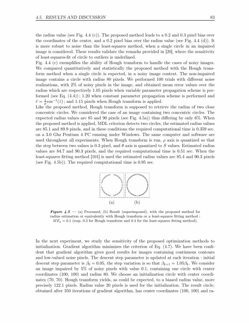
4.5. RESULTS AND DISCUSSION 83
the radius value (see Fig. 4.4 (c)). The proposed method leads to a 0.2 and 0.3 pixel bias overthe coordinates of the center, and a 0.2 pixel bias over the radius value (see Fig. 4.4 (d)). Itis more robust to noise than the least-squares method, when a single circle in an impairedimage is considered. These results validate the remarks provided in [20], where the sensitivityof least-squares-fit of circle to outliers is underlined.Fig. 4.4 (c) exemplifies the ability of Hough transform to handle the cases of noisy images.We compared quantitatively and statistically the proposed method with the Hough trans-form method when a single circle is expected, in a noisy image context. The non-impairedimage contains a circle with radius 80 pixels. We performed 100 trials with different noiserealizations, with 2% of noisy pixels in the image, and obtained mean error values over theradius which are respectively 1.05 pixels when variable parameter propagation scheme is per-formed (see Eq. (4.4)) ; 1.20 when constant parameter propagation scheme is performed andr̂ = 1
µcos−1(z̄) ; and 1.15 pixels when Hough transform is applied.Like the proposed method, Hough transform is supposed to retrieve the radius of two closeconcentric circles. We considered the case of an image containing two concentric circles. Theexpected radius values are 85 and 90 pixels (see Fig. 4.5a)) thus differing by only 6%. Whenthe proposed method is applied, MDL criterion detects two circles, the estimated radius valuesare 85.1 and 89.9 pixels, and in these conditions the required computational time is 0.359 sec.on a 3.0 Ghz Pentium 4 PC running under Windows. The same computer and software areused throughout all experiments. When Hough transform is run, ρ axis is quantized so thatthe step between two values is 0.3 pixel, and θ axis is quantized to S values. Estimated radiusvalues are 84.7 and 90.3 pixels, and the required computational time is 0.51 sec. When theleast-squares fitting method [101] is used the estimated radius values are 85.4 and 90.3 pixels(see Fig. 4.5b)). The required computational time is 0.95 sec.
20 40 60 80 100 120 140 160 180 200
20
40
60
80
100
120
140
160
180
20020 40 60 80 100 120 140 160 180 200
20
40
60
80
100
120
140
160
180
200
(a) (b)
Figure 4.5 — (a) Processed, (b) Result (superimposed), with the proposed method forradius estimation or equivalently with Hough transform or a least-squares fitting method :
MEρ = 0.1 (resp. 0.3 for Hough transform and 0.4 for the least-squares fitting method).
In the next experiment, we study the sensitivity of the proposed optimization methods toinitialization. Gradient algorithm minimizes the criterion of Eq. (4.7). We have been confi-dent that gradient algorithm gives good results for images containing continuous contoursand low-valued noise pixels. The descent step parameter is updated at each iteration : initialdescent step parameter is β0 = 0.05, the step variation is so that βk+1 = 1.05βk. We consideran image impaired by 5% of noisy pixels with value 0.1, containing one circle with centercoordinates (100, 100) and radius 80. We choose an initialization circle with center coordi-nates (70, 70). Hough transform yields, as could be expected, to a biased radius value, moreprecisely 122.1 pixels. Radius value 20 pixels is used for the initialization. The result circle,obtained after 350 iterations of gradient algorithm, has center coordinates (100, 100) and ra-
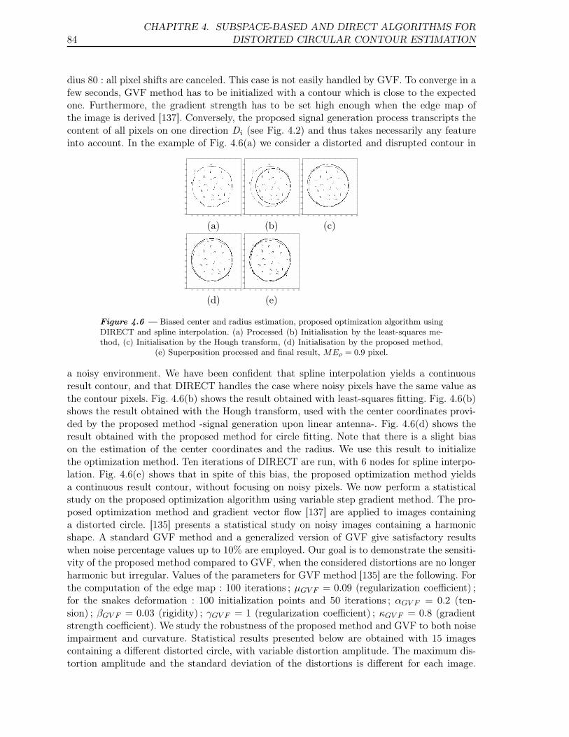
84CHAPITRE 4. SUBSPACE-BASED AND DIRECT ALGORITHMS FOR
DISTORTED CIRCULAR CONTOUR ESTIMATION
dius 80 : all pixel shifts are canceled. This case is not easily handled by GVF. To converge in afew seconds, GVF method has to be initialized with a contour which is close to the expectedone. Furthermore, the gradient strength has to be set high enough when the edge map ofthe image is derived [137]. Conversely, the proposed signal generation process transcripts thecontent of all pixels on one direction Di (see Fig. 4.2) and thus takes necessarily any featureinto account. In the example of Fig. 4.6(a) we consider a distorted and disrupted contour in
20 40 60 80 100 120 140 160 180 200
20
40
60
80
100
120
140
160
180
20020 40 60 80 100 120 140 160 180 200
20
40
60
80
100
120
140
160
180
20020 40 60 80 100 120 140 160 180 200
20
40
60
80
100
120
140
160
180
200
(a) (b) (c)
20 40 60 80 100 120 140 160 180 200
20
40
60
80
100
120
140
160
180
20020 40 60 80 100 120 140 160 180 200
20
40
60
80
100
120
140
160
180
200
(d) (e)
Figure 4.6 — Biased center and radius estimation, proposed optimization algorithm usingDIRECT and spline interpolation. (a) Processed (b) Initialisation by the least-squares me-thod, (c) Initialisation by the Hough transform, (d) Initialisation by the proposed method,
(e) Superposition processed and final result, MEρ = 0.9 pixel.
a noisy environment. We have been confident that spline interpolation yields a continuousresult contour, and that DIRECT handles the case where noisy pixels have the same value asthe contour pixels. Fig. 4.6(b) shows the result obtained with least-squares fitting. Fig. 4.6(b)shows the result obtained with the Hough transform, used with the center coordinates provi-ded by the proposed method -signal generation upon linear antenna-. Fig. 4.6(d) shows theresult obtained with the proposed method for circle fitting. Note that there is a slight biason the estimation of the center coordinates and the radius. We use this result to initializethe optimization method. Ten iterations of DIRECT are run, with 6 nodes for spline interpo-lation. Fig. 4.6(e) shows that in spite of this bias, the proposed optimization method yieldsa continuous result contour, without focusing on noisy pixels. We now perform a statisticalstudy on the proposed optimization algorithm using variable step gradient method. The pro-posed optimization method and gradient vector flow [137] are applied to images containinga distorted circle. [135] presents a statistical study on noisy images containing a harmonicshape. A standard GVF method and a generalized version of GVF give satisfactory resultswhen noise percentage values up to 10% are employed. Our goal is to demonstrate the sensiti-vity of the proposed method compared to GVF, when the considered distortions are no longerharmonic but irregular. Values of the parameters for GVF method [135] are the following. Forthe computation of the edge map : 100 iterations ; µGV F = 0.09 (regularization coefficient) ;for the snakes deformation : 100 initialization points and 50 iterations ; αGV F = 0.2 (ten-sion) ; βGV F = 0.03 (rigidity) ; γGV F = 1 (regularization coefficient) ; κGV F = 0.8 (gradientstrength coefficient). We study the robustness of the proposed method and GVF to both noiseimpairment and curvature. Statistical results presented below are obtained with 15 imagescontaining a different distorted circle, with variable distortion amplitude. The maximum dis-tortion amplitude and the standard deviation of the distortions is different for each image.
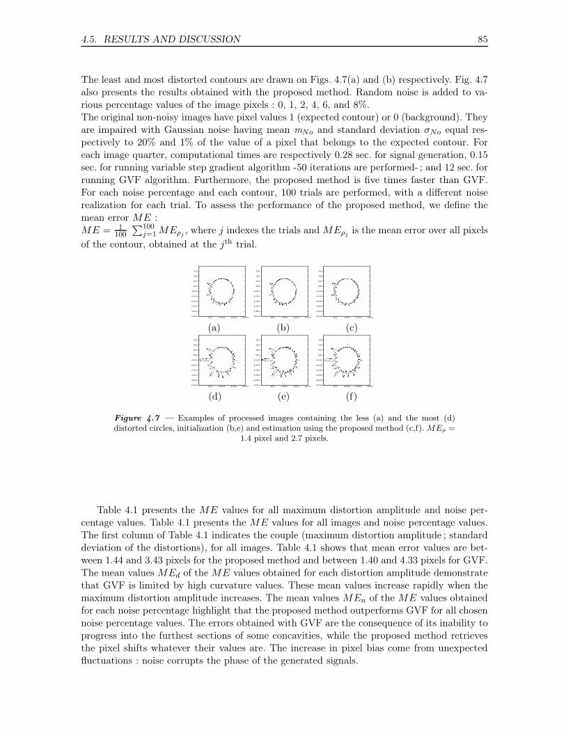
4.5. RESULTS AND DISCUSSION 85
The least and most distorted contours are drawn on Figs. 4.7(a) and (b) respectively. Fig. 4.7also presents the results obtained with the proposed method. Random noise is added to va-rious percentage values of the image pixels : 0, 1, 2, 4, 6, and 8%.The original non-noisy images have pixel values 1 (expected contour) or 0 (background). Theyare impaired with Gaussian noise having mean mNo and standard deviation σNo equal res-pectively to 20% and 1% of the value of a pixel that belongs to the expected contour. Foreach image quarter, computational times are respectively 0.28 sec. for signal generation, 0.15sec. for running variable step gradient algorithm -50 iterations are performed- ; and 12 sec. forrunning GVF algorithm. Furthermore, the proposed method is five times faster than GVF.For each noise percentage and each contour, 100 trials are performed, with a different noiserealization for each trial. To assess the performance of the proposed method, we define themean error ME :ME = 1
100
∑100j=1 MEρj
, where j indexes the trials and MEρjis the mean error over all pixels
of the contour, obtained at the jth trial.
50 100 150 200
20
40
60
80
100
120
140
160
180
20050 100 150 200
20
40
60
80
100
120
140
160
180
20050 100 150 200
20
40
60
80
100
120
140
160
180
200
(a) (b) (c)
50 100 150 200
20
40
60
80
100
120
140
160
180
20050 100 150 200
20
40
60
80
100
120
140
160
180
20050 100 150 200
20
40
60
80
100
120
140
160
180
200
(d) (e) (f)
Figure 4.7 — Examples of processed images containing the less (a) and the most (d)distorted circles, initialization (b,e) and estimation using the proposed method (c,f). MEρ =
1.4 pixel and 2.7 pixels.
Table 4.1 presents the ME values for all maximum distortion amplitude and noise per-centage values. Table 4.1 presents the ME values for all images and noise percentage values.The first column of Table 4.1 indicates the couple (maximum distortion amplitude ; standarddeviation of the distortions), for all images. Table 4.1 shows that mean error values are bet-ween 1.44 and 3.43 pixels for the proposed method and between 1.40 and 4.33 pixels for GVF.The mean values MEd of the ME values obtained for each distortion amplitude demonstratethat GVF is limited by high curvature values. These mean values increase rapidly when themaximum distortion amplitude increases. The mean values MEn of the ME values obtainedfor each noise percentage highlight that the proposed method outperforms GVF for all chosennoise percentage values. The errors obtained with GVF are the consequence of its inability toprogress into the furthest sections of some concavities, while the proposed method retrievesthe pixel shifts whatever their values are. The increase in pixel bias come from unexpectedfluctuations : noise corrupts the phase of the generated signals.
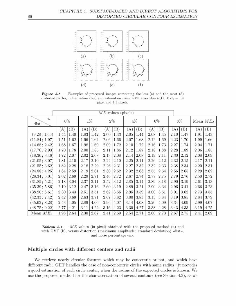
86CHAPITRE 4. SUBSPACE-BASED AND DIRECT ALGORITHMS FOR
DISTORTED CIRCULAR CONTOUR ESTIMATION
50 100 150 200
20
40
60
80
100
120
140
160
180
20050 100 150 200
20
40
60
80
100
120
140
160
180
20050 100 150 200
20
40
60
80
100
120
140
160
180
200
(a) (b) (c)
50 100 150 200
20
40
60
80
100
120
140
160
180
20050 100 150 200
20
40
60
80
100
120
140
160
180
20050 100 150 200
20
40
60
80
100
120
140
160
180
200
(d) (e) (f)
Figure 4.8 — Examples of processed images containing the less (a) and the most (d)distorted circles, initialization (b,e) and estimation using GVF algorithm (c,f). MEρ = 1.4
pixel and 4.1 pixels.
ME values (pixels)H
HH
HHH
dist.n.
0% 1% 2% 4% 6% 8% Mean MEd
(A) (B) (A) (B) (A) (B) (A) (B) (A) (B) (A) (B) (A) (B)(9.28 ; 1.66) 1.44 1.40 1.83 1.42 2.00 1.43 2.05 1.44 2.08 1.45 2.10 1.47 1.91 1.43
(11.84 ; 1.97) 1.51 1.62 1.96 1.64 2.06 1.66 2.07 1.68 2.12 1.69 2.23 1.70 1.99 1.66(14.68 ; 2.42) 1.68 1.67 1.98 1.69 2.09 1.72 2.10 1.72 2.16 1.73 2.27 1.74 2.04 1.71(17.76 ; 2.93) 1.70 1.78 2.00 1.85 2.11 1.86 2.12 1.87 2.18 1.88 2.28 1.89 2.06 1.85(18.36 ; 3.46) 1.72 2.07 2.02 2.08 2.13 2.08 2.14 2.08 2.19 2.11 2.30 2.12 2.08 2.09(21.05 ; 3.07) 1.81 2.10 2.17 2.10 2.24 2.10 2.25 2.11 2.26 2.12 2.32 2.15 2.17 2.11(21.55 ; 3.62) 1.82 2.28 2.18 2.29 2.26 2.31 2.27 2.32 2.32 2.33 2.38 2.34 2.20 2.31(24.88 ; 4.25) 1.84 2.59 2.19 2.61 2.30 2.62 2.32 2.63 2.55 2.64 2.56 2.65 2.29 2.62(28.34 ; 5.01) 2.02 2.69 2.29 2.71 2.46 2.72 2.67 2.74 2.77 2.75 2.79 2.76 2.50 2.72(31.85 ; 5.21) 2.18 3.04 2.37 3.11 2.52 3.12 2.85 3.14 2.89 3.18 2.90 3.19 2.61 3.13(35.39 ; 5.86) 2.19 3.12 2.47 3.16 2.60 3.19 2.89 3.21 2.90 3.34 2.96 3.41 2.66 3.23(38.90 ; 6.61) 2.30 3.43 2.51 3.51 2.62 3.55 2.95 3.59 3.00 3.61 3.01 3.62 2.73 3.55(42.33 ; 7.42) 2.42 3.69 2.63 3.71 2.67 3.82 3.00 3.83 3.13 3.84 3.19 3.85 2.84 3.79(45.63 ; 8.28) 2.43 4.05 2.89 4.06 2.96 4.07 3.14 4.08 3.20 4.09 3.34 4.09 2.99 4.07(48.75 ; 9.22) 2.77 4.21 3.11 4.22 3.16 4.23 3.30 4.27 3.38 4.28 3.43 4.33 3.19 4.25Mean MEn 1.98 2.64 2.30 2.67 2.41 2.69 2.54 2.71 2.60 2.73 2.67 2.75 2.41 2.69
Tableau 4.1 — ME values (in pixel) obtained with the proposed method (a) andwith GVF (b), versus distortion (maximum amplitude ; standard deviation) -dist.-,
and noise percentage -n.-.
Multiple circles with different centers and radii
We retrieve nearly circular features which may be concentric or not, and which havedifferent radii. GHT handles the case of non-concentric circles with same radius : it providesa good estimation of each circle center, when the radius of the expected circles is known. Weuse the proposed method for the characterization of several contours (see Section 4.3), as we
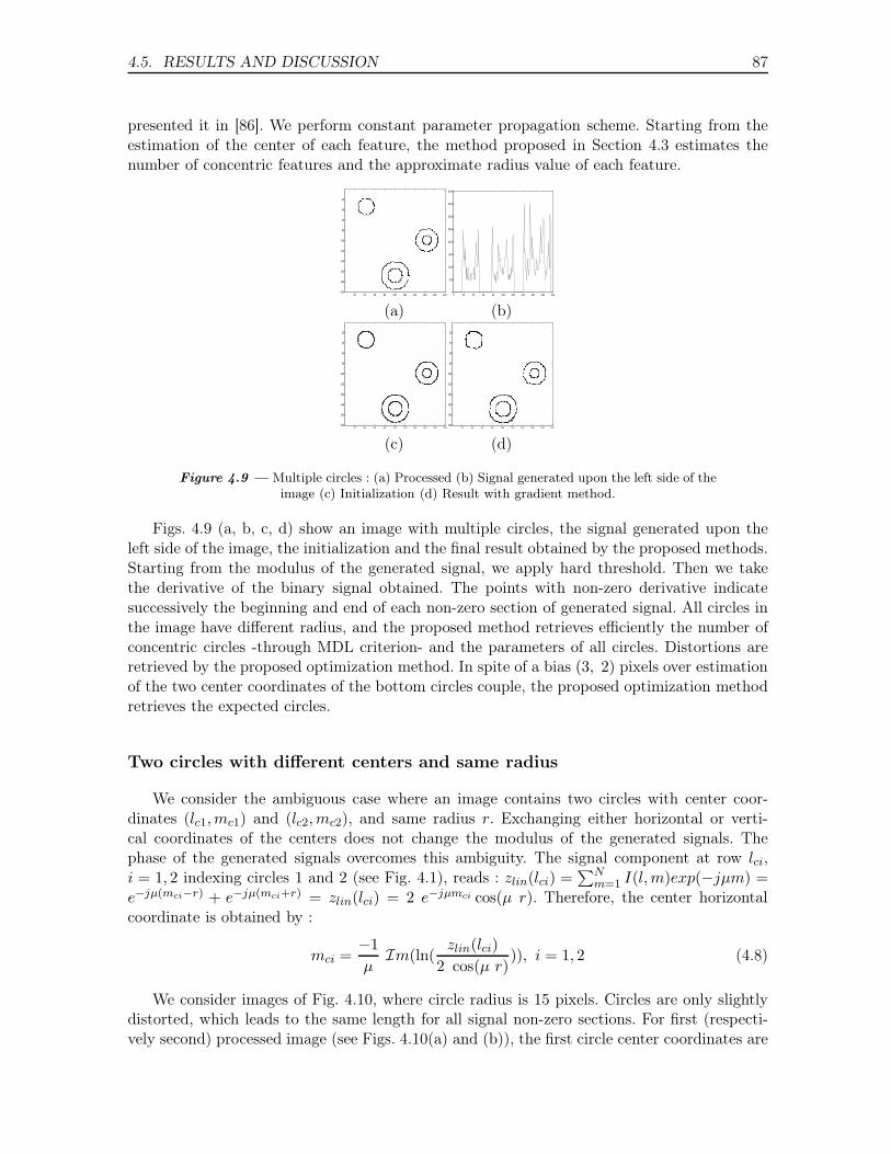
4.5. RESULTS AND DISCUSSION 87
presented it in [86]. We perform constant parameter propagation scheme. Starting from theestimation of the center of each feature, the method proposed in Section 4.3 estimates thenumber of concentric features and the approximate radius value of each feature.
20 40 60 80 100 120 140 160 180 200
20
40
60
80
100
120
140
160
180
2000 20 40 60 80 100 120 140 160 180 200
0
500
1000
1500
2000
2500
3000
3500
4000
(a) (b)
20 40 60 80 100 120 140 160 180 200
20
40
60
80
100
120
140
160
180
20020 40 60 80 100 120 140 160 180 200
20
40
60
80
100
120
140
160
180
200
(c) (d)
Figure 4.9 — Multiple circles : (a) Processed (b) Signal generated upon the left side of theimage (c) Initialization (d) Result with gradient method.
Figs. 4.9 (a, b, c, d) show an image with multiple circles, the signal generated upon theleft side of the image, the initialization and the final result obtained by the proposed methods.Starting from the modulus of the generated signal, we apply hard threshold. Then we takethe derivative of the binary signal obtained. The points with non-zero derivative indicatesuccessively the beginning and end of each non-zero section of generated signal. All circles inthe image have different radius, and the proposed method retrieves efficiently the number ofconcentric circles -through MDL criterion- and the parameters of all circles. Distortions areretrieved by the proposed optimization method. In spite of a bias (3, 2) pixels over estimationof the two center coordinates of the bottom circles couple, the proposed optimization methodretrieves the expected circles.
Two circles with different centers and same radius
We consider the ambiguous case where an image contains two circles with center coor-dinates (lc1,mc1) and (lc2,mc2), and same radius r. Exchanging either horizontal or verti-cal coordinates of the centers does not change the modulus of the generated signals. Thephase of the generated signals overcomes this ambiguity. The signal component at row lci,i = 1, 2 indexing circles 1 and 2 (see Fig. 4.1), reads : zlin(lci) =
∑Nm=1 I(l,m)exp(−jµm) =
e−jµ(mci−r) + e−jµ(mci+r) = zlin(lci) = 2 e−jµmci cos(µ r). Therefore, the center horizontalcoordinate is obtained by :
mci =−1
µIm(ln(
zlin(lci)
2 cos(µ r))), i = 1, 2 (4.8)
We consider images of Fig. 4.10, where circle radius is 15 pixels. Circles are only slightlydistorted, which leads to the same length for all signal non-zero sections. For first (respecti-vely second) processed image (see Figs. 4.10(a) and (b)), the first circle center coordinates are
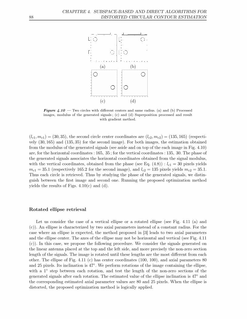
88CHAPITRE 4. SUBSPACE-BASED AND DIRECT ALGORITHMS FOR
DISTORTED CIRCULAR CONTOUR ESTIMATION
(a) (b)
20 40 60 80 100 120 140 160 180 200
20
40
60
80
100
120
140
160
180
20020 40 60 80 100 120 140 160 180 200
20
40
60
80
100
120
140
160
180
200
(c) (d)
Figure 4.10 — Two circles with different centers and same radius. (a) and (b) Processedimages, modulus of the generated signals ; (c) and (d) Superposition processed and result
with gradient method.
(lc1,mc1) = (30, 35), the second circle center coordinates are (lc2,mc2) = (135, 165) (respecti-vely (30, 165) and (135, 35) for the second image). For both images, the estimation obtainedfrom the modulus of the generated signals (see aside and on top of the each image in Fig. 4.10)are, for the horizontal coordinates : 165, 35 ; for the vertical coordinates : 135, 30. The phase ofthe generated signals associates the horizontal coordinates obtained from the signal modulus,with the vertical coordinates, obtained from the phase (see Eq. (4.8)) : lc1 = 30 pixels yieldsmc1 = 35.1 (respectively 165.2 for the second image), and lc2 = 135 pixels yields mc2 = 35.1.Thus each circle is retrieved. Thus by studying the phase of the generated signals, we distin-guish between the first image and second one. Running the proposed optimization methodyields the results of Figs. 4.10(c) and (d).
Rotated ellipse retrieval
Let us consider the case of a vertical ellipse or a rotated ellipse (see Fig. 4.11 (a) and(c)). An ellipse is characterized by two axial parameters instead of a constant radius. For thecase where an ellipse is expected, the method proposed in [3] leads to two axial parametersand the ellipse center. The axes of the ellipse may not be horizontal and vertical (see Fig. 4.11(c)). In this case, we propose the following procedure. We consider the signals generated onthe linear antenna placed at the top and the left side, and more precisely the non-zero sectionlength of the signals. The image is rotated until these lengths are the most different from eachother. The ellipse of Fig. 4.11 (c) has center coordinates (100, 100), and axial parameters 80and 25 pixels. Its inclination is 47◦. We perform rotations of the image containing the ellipse,with a 1◦ step between each rotation, and test the length of the non-zero sections of thegenerated signals after each rotation. The estimated value of the ellipse inclination is 47◦ andthe corresponding estimated axial parameter values are 80 and 25 pixels. When the ellipse isdistorted, the proposed optimization method is logically applied.
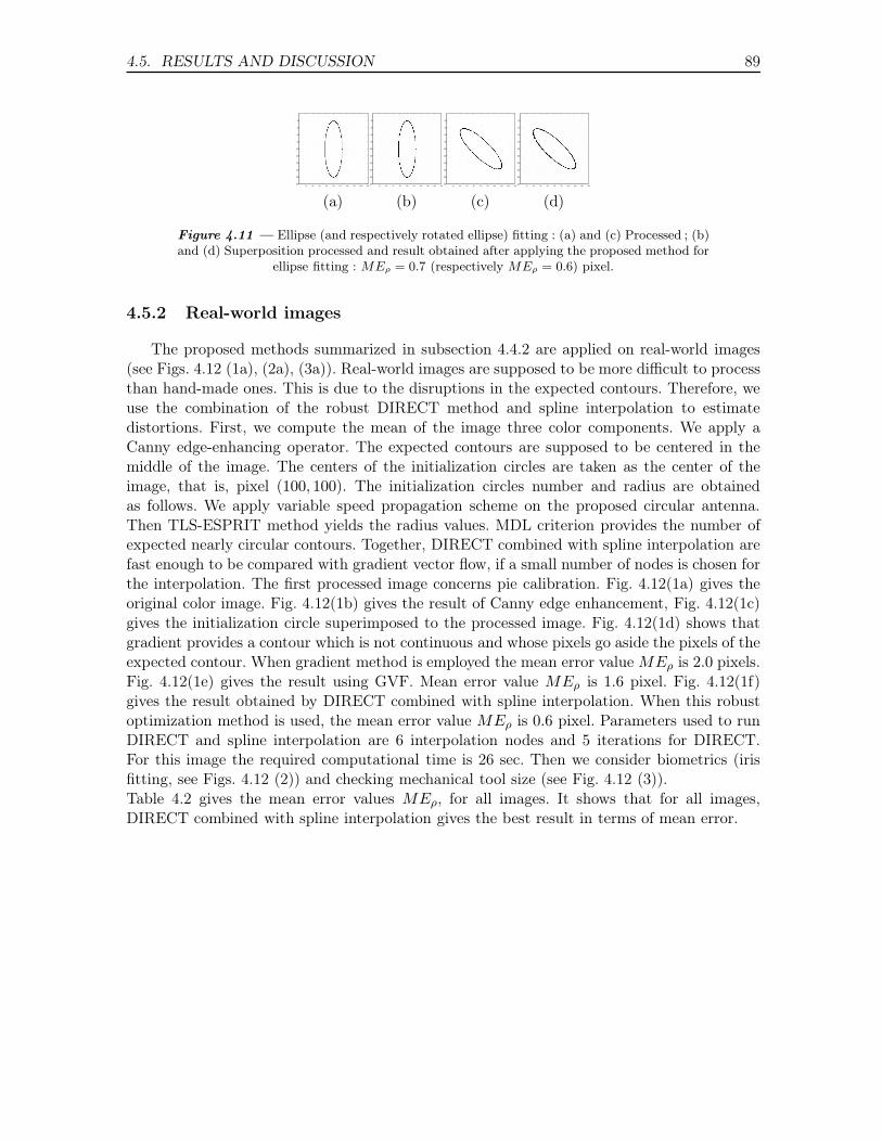
4.5. RESULTS AND DISCUSSION 89
20 40 60 80 100 120 140 160 180 200
20
40
60
80
100
120
140
160
180
20020 40 60 80 100 120 140 160 180 200
20
40
60
80
100
120
140
160
180
20020 40 60 80 100 120 140 160 180 200
20
40
60
80
100
120
140
160
180
20020 40 60 80 100 120 140 160 180 200
20
40
60
80
100
120
140
160
180
200
(a) (b) (c) (d)
Figure 4.11 — Ellipse (and respectively rotated ellipse) fitting : (a) and (c) Processed ; (b)and (d) Superposition processed and result obtained after applying the proposed method for
ellipse fitting : MEρ = 0.7 (respectively MEρ = 0.6) pixel.
4.5.2 Real-world images
The proposed methods summarized in subsection 4.4.2 are applied on real-world images(see Figs. 4.12 (1a), (2a), (3a)). Real-world images are supposed to be more difficult to processthan hand-made ones. This is due to the disruptions in the expected contours. Therefore, weuse the combination of the robust DIRECT method and spline interpolation to estimatedistortions. First, we compute the mean of the image three color components. We apply aCanny edge-enhancing operator. The expected contours are supposed to be centered in themiddle of the image. The centers of the initialization circles are taken as the center of theimage, that is, pixel (100, 100). The initialization circles number and radius are obtainedas follows. We apply variable speed propagation scheme on the proposed circular antenna.Then TLS-ESPRIT method yields the radius values. MDL criterion provides the number ofexpected nearly circular contours. Together, DIRECT combined with spline interpolation arefast enough to be compared with gradient vector flow, if a small number of nodes is chosen forthe interpolation. The first processed image concerns pie calibration. Fig. 4.12(1a) gives theoriginal color image. Fig. 4.12(1b) gives the result of Canny edge enhancement, Fig. 4.12(1c)gives the initialization circle superimposed to the processed image. Fig. 4.12(1d) shows thatgradient provides a contour which is not continuous and whose pixels go aside the pixels of theexpected contour. When gradient method is employed the mean error value MEρ is 2.0 pixels.Fig. 4.12(1e) gives the result using GVF. Mean error value MEρ is 1.6 pixel. Fig. 4.12(1f)gives the result obtained by DIRECT combined with spline interpolation. When this robustoptimization method is used, the mean error value MEρ is 0.6 pixel. Parameters used to runDIRECT and spline interpolation are 6 interpolation nodes and 5 iterations for DIRECT.For this image the required computational time is 26 sec. Then we consider biometrics (irisfitting, see Figs. 4.12 (2)) and checking mechanical tool size (see Fig. 4.12 (3)).Table 4.2 gives the mean error values MEρ, for all images. It shows that for all images,DIRECT combined with spline interpolation gives the best result in terms of mean error.
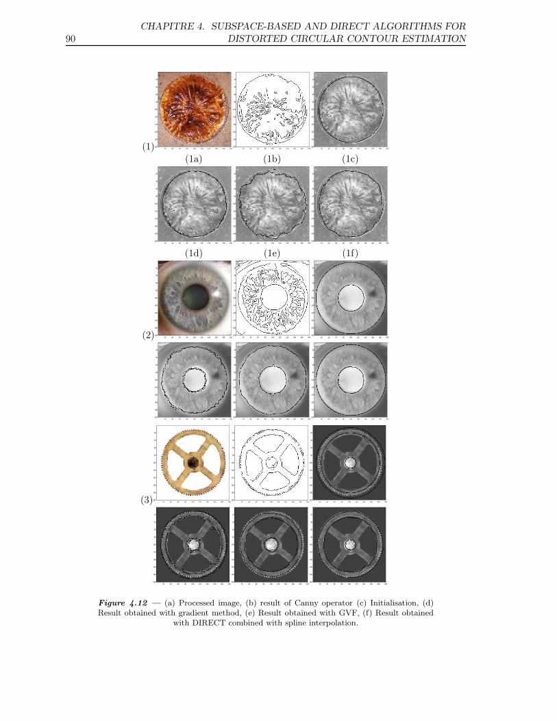
90CHAPITRE 4. SUBSPACE-BASED AND DIRECT ALGORITHMS FOR
DISTORTED CIRCULAR CONTOUR ESTIMATION
(1) 20 40 60 80 100 120 140 160 180 200
20
40
60
80
100
120
140
160
180
20020 40 60 80 100 120 140 160 180 200
20
40
60
80
100
120
140
160
180
20020 40 60 80 100 120 140 160 180 200
20
40
60
80
100
120
140
160
180
200
(1a) (1b) (1c)
20 40 60 80 100 120 140 160 180 200
20
40
60
80
100
120
140
160
180
20020 40 60 80 100 120 140 160 180 200
20
40
60
80
100
120
140
160
180
20020 40 60 80 100 120 140 160 180 200
20
40
60
80
100
120
140
160
180
200
(1d) (1e) (1f)
(2) 20 40 60 80 100 120 140 160 180 200
20
40
60
80
100
120
140
160
180
20020 40 60 80 100 120 140 160 180 200
20
40
60
80
100
120
140
160
180
20020 40 60 80 100 120 140 160 180 200
20
40
60
80
100
120
140
160
180
200
20 40 60 80 100 120 140 160 180 200
20
40
60
80
100
120
140
160
180
20020 40 60 80 100 120 140 160 180 200
20
40
60
80
100
120
140
160
180
20020 40 60 80 100 120 140 160 180 200
20
40
60
80
100
120
140
160
180
200
(3) 20 40 60 80 100 120 140 160 180 200
20
40
60
80
100
120
140
160
180
20020 40 60 80 100 120 140 160 180 200
20
40
60
80
100
120
140
160
180
20020 40 60 80 100 120 140 160 180 200
20
40
60
80
100
120
140
160
180
200
20 40 60 80 100 120 140 160 180 200
20
40
60
80
100
120
140
160
180
20020 40 60 80 100 120 140 160 180 200
20
40
60
80
100
120
140
160
180
20020 40 60 80 100 120 140 160 180 200
20
40
60
80
100
120
140
160
180
200
Figure 4.12 — (a) Processed image, (b) result of Canny operator (c) Initialisation, (d)Result obtained with gradient method, (e) Result obtained with GVF, (f) Result obtained
with DIRECT combined with spline interpolation.
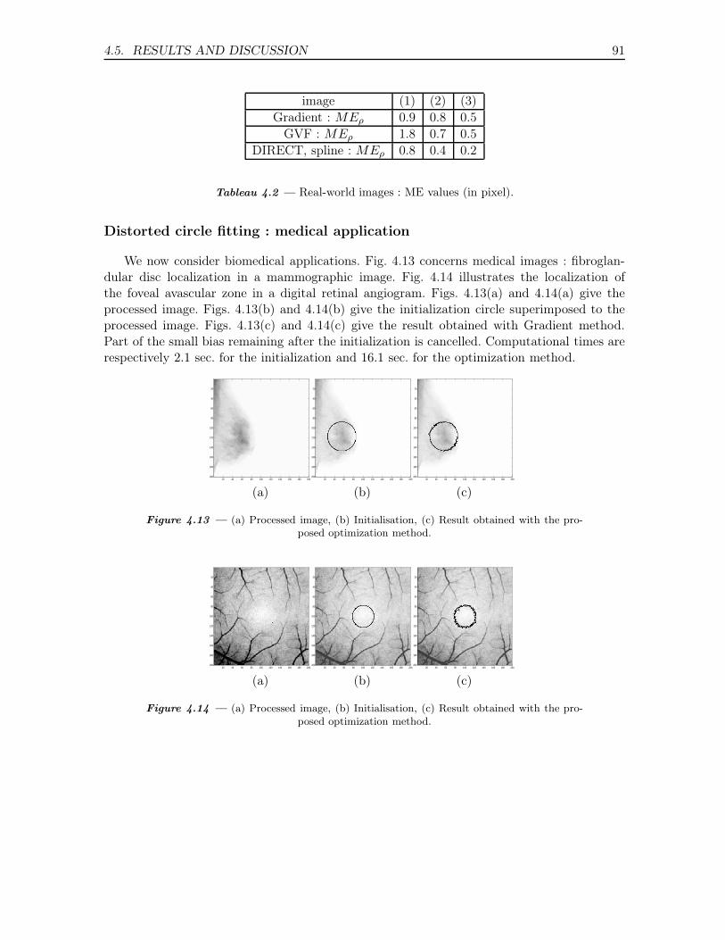
4.5. RESULTS AND DISCUSSION 91
image (1) (2) (3)Gradient : MEρ 0.9 0.8 0.5
GVF : MEρ 1.8 0.7 0.5DIRECT, spline : MEρ 0.8 0.4 0.2
Tableau 4.2 — Real-world images : ME values (in pixel).
Distorted circle fitting : medical application
We now consider biomedical applications. Fig. 4.13 concerns medical images : fibroglan-dular disc localization in a mammographic image. Fig. 4.14 illustrates the localization ofthe foveal avascular zone in a digital retinal angiogram. Figs. 4.13(a) and 4.14(a) give theprocessed image. Figs. 4.13(b) and 4.14(b) give the initialization circle superimposed to theprocessed image. Figs. 4.13(c) and 4.14(c) give the result obtained with Gradient method.Part of the small bias remaining after the initialization is cancelled. Computational times arerespectively 2.1 sec. for the initialization and 16.1 sec. for the optimization method.
20 40 60 80 100 120 140 160 180 200
20
40
60
80
100
120
140
160
180
20020 40 60 80 100 120 140 160 180 200
20
40
60
80
100
120
140
160
180
20020 40 60 80 100 120 140 160 180 200
20
40
60
80
100
120
140
160
180
200
(a) (b) (c)
Figure 4.13 — (a) Processed image, (b) Initialisation, (c) Result obtained with the pro-posed optimization method.
20 40 60 80 100 120 140 160 180 200
20
40
60
80
100
120
140
160
180
20020 40 60 80 100 120 140 160 180 200
20
40
60
80
100
120
140
160
180
20020 40 60 80 100 120 140 160 180 200
20
40
60
80
100
120
140
160
180
200
(a) (b) (c)
Figure 4.14 — (a) Processed image, (b) Initialisation, (c) Result obtained with the pro-posed optimization method.
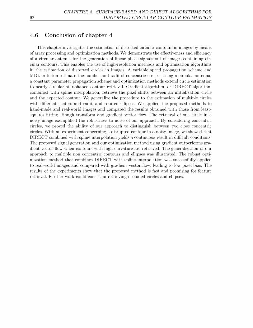
92CHAPITRE 4. SUBSPACE-BASED AND DIRECT ALGORITHMS FOR
DISTORTED CIRCULAR CONTOUR ESTIMATION
4.6 Conclusion of chapter 4
This chapter investigates the estimation of distorted circular contours in images by meansof array processing and optimization methods. We demonstrate the effectiveness and efficiencyof a circular antenna for the generation of linear phase signals out of images containing cir-cular contours. This enables the use of high-resolution methods and optimization algorithmsin the estimation of distorted circles in images. A variable speed propagation scheme andMDL criterion estimate the number and radii of concentric circles. Using a circular antenna,a constant parameter propagation scheme and optimization methods extend circle estimationto nearly circular star-shaped contour retrieval. Gradient algorithm, or DIRECT algorithmcombined with spline interpolation, retrieve the pixel shifts between an initialization circleand the expected contour. We generalize the procedure to the estimation of multiple circleswith different centers and radii, and rotated ellipses. We applied the proposed methods tohand-made and real-world images and compared the results obtained with those from least-squares fitting, Hough transform and gradient vector flow. The retrieval of one circle in anoisy image exemplified the robustness to noise of our approach. By considering concentriccircles, we proved the ability of our approach to distinguish between two close concentriccircles. With an experiment concerning a disrupted contour in a noisy image, we showed thatDIRECT combined with spline interpolation yields a continuous result in difficult conditions.The proposed signal generation and our optimization method using gradient outperforms gra-dient vector flow when contours with high curvature are retrieved. The generalization of ourapproach to multiple non concentric contours and ellipses was illustrated. The robust opti-mization method that combines DIRECT with spline interpolation was successfully appliedto real-world images and compared with gradient vector flow, leading to low pixel bias. Theresults of the experiments show that the proposed method is fast and promising for featureretrieval. Further work could consist in retrieving occluded circles and ellipses.
Third part
Tensor approach of image processing,
nonorthogonal tensor flattening via
main direction detection

CHAPITRE
5 Lower-rank tensor
approximation and
multiway filtering
This chapter presents some recent filtering methods based on the lower-rank tensorapproximation approach for denoising tensor signals. In this approach, multicomponentdata are represented by tensors, that is, multiway arrays, and the presented tensor filteringmethods rely on multilinear algebra. The chapter is organized as follows : In section 5.1,we present application fields of the presented methods, and provide definitions of tensordecomposition models. Section 5.2 presents the tensor data and a short overview of itsmain properties. Section 5.3 introduces the tensor formulation of the classical noise-removalproblem as well as some new tensor filtering notations. Firstly, we explain how the channel-by-channel SVD-based method processes successively each component of the data tensor.Secondly, we consider two methods that take into account the relationships between eachcomponent of the considered tensor. These two methods are based on the nth-mode signalsubspace. The first method for signal tensor estimation is based on multimode PCA achievedby rank-(K1, . . . ,KN ) approximation. The second method is a new tensor version of Wienerfiltering. Section 5.4 presents some comparative results where the overviewed multiwayfiltering methods are applied to noise reduction in color images, denoising of multispectralimages, and denoising of multicomponent seismic waves. Section 5.5 presents a nonorthogonaltensor flattening method, that aims at improving the result of tensor data denoisingwhen main directions are expected in the processed tensor. We consider an application tohyperspectral imagery. Finally, section 5.6 concludes the chapter.Appendices A.1, A.2, and A.3 concern mathematical details about the Alternating LeastSquares (ALS) optimization algorithms used in the presented multiway algorithms, and somedetails about multiway Wiener filtering.
This work has been accepted in :D. Muti, S. Bourennane and J. Marot, "Lower-Rank Tensor Approximation and MultiwayFiltering", SIAM Journal on Matrix Analysis and Applications (SIMAX), accepted september12, 2007
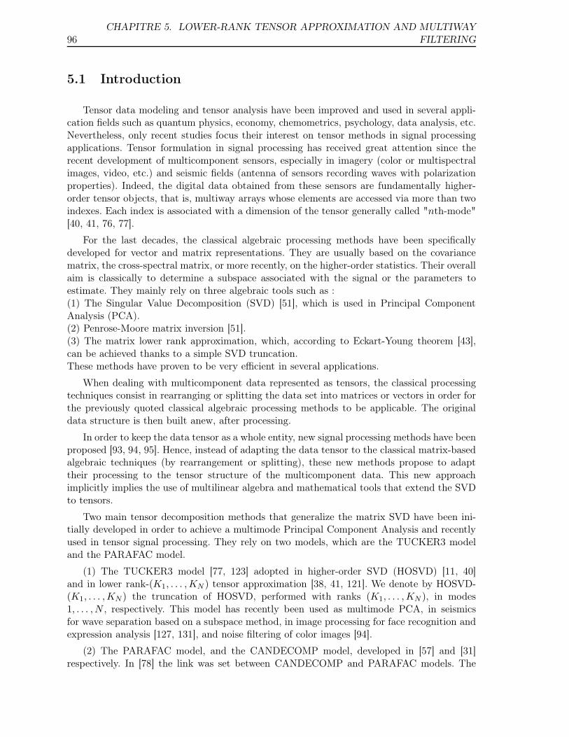
96CHAPITRE 5. LOWER-RANK TENSOR APPROXIMATION AND MULTIWAY
FILTERING
5.1 Introduction
Tensor data modeling and tensor analysis have been improved and used in several appli-cation fields such as quantum physics, economy, chemometrics, psychology, data analysis, etc.Nevertheless, only recent studies focus their interest on tensor methods in signal processingapplications. Tensor formulation in signal processing has received great attention since therecent development of multicomponent sensors, especially in imagery (color or multispectralimages, video, etc.) and seismic fields (antenna of sensors recording waves with polarizationproperties). Indeed, the digital data obtained from these sensors are fundamentally higher-order tensor objects, that is, multiway arrays whose elements are accessed via more than twoindexes. Each index is associated with a dimension of the tensor generally called "nth-mode"[40, 41, 76, 77].
For the last decades, the classical algebraic processing methods have been specificallydeveloped for vector and matrix representations. They are usually based on the covariancematrix, the cross-spectral matrix, or more recently, on the higher-order statistics. Their overallaim is classically to determine a subspace associated with the signal or the parameters toestimate. They mainly rely on three algebraic tools such as :(1) The Singular Value Decomposition (SVD) [51], which is used in Principal ComponentAnalysis (PCA).(2) Penrose-Moore matrix inversion [51].(3) The matrix lower rank approximation, which, according to Eckart-Young theorem [43],can be achieved thanks to a simple SVD truncation.These methods have proven to be very efficient in several applications.
When dealing with multicomponent data represented as tensors, the classical processingtechniques consist in rearranging or splitting the data set into matrices or vectors in order forthe previously quoted classical algebraic processing methods to be applicable. The originaldata structure is then built anew, after processing.
In order to keep the data tensor as a whole entity, new signal processing methods have beenproposed [93, 94, 95]. Hence, instead of adapting the data tensor to the classical matrix-basedalgebraic techniques (by rearrangement or splitting), these new methods propose to adapttheir processing to the tensor structure of the multicomponent data. This new approachimplicitly implies the use of multilinear algebra and mathematical tools that extend the SVDto tensors.
Two main tensor decomposition methods that generalize the matrix SVD have been ini-tially developed in order to achieve a multimode Principal Component Analysis and recentlyused in tensor signal processing. They rely on two models, which are the TUCKER3 modeland the PARAFAC model.
(1) The TUCKER3 model [77, 123] adopted in higher-order SVD (HOSVD) [11, 40]and in lower rank-(K1, . . . ,KN ) tensor approximation [38, 41, 121]. We denote by HOSVD-(K1, . . . ,KN ) the truncation of HOSVD, performed with ranks (K1, . . . ,KN ), in modes1, . . . , N , respectively. This model has recently been used as multimode PCA, in seismicsfor wave separation based on a subspace method, in image processing for face recognition andexpression analysis [127, 131], and noise filtering of color images [94].
(2) The PARAFAC model, and the CANDECOMP model, developed in [57] and [31]respectively. In [78] the link was set between CANDECOMP and PARAFAC models. The
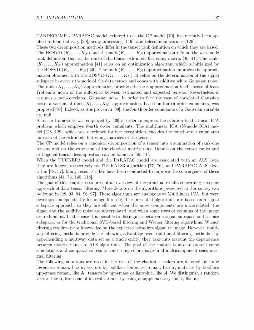
5.1. INTRODUCTION 97
CANDECOMP / PARAFAC model, referred to as the CP model [70], has recently been ap-plied to food industry [30], array processing [119], and telecommunications [120].These two decomposition methods differ in the tensor rank definition on which they are based.The HOSVD-(K1, . . . ,KN ) and the rank-(K1, . . . ,KN ) approximation rely on the nth-moderank definition, that is, the rank of the tensor nth-mode flattening matrix [40, 41]. The rank-(K1, . . . ,KN ) approximation [41] relies on an optimization algorithm which is initialized bythe HOSVD-(K1, . . . ,KN ) [40]. The rank-(K1, . . . ,KN ) approximation improves the approxi-mation obtained with the HOSVD-(K1, . . . ,KN ). It relies on the determination of the signalsubspace in every nth-mode of the data tensor and copes with additive white Gaussian noise.The rank-(K1, . . . ,KN ) approximation provides the best approximation in the sense of leastFrobenius norm of the difference between estimated and expected tensors. Nevertheless itassumes a non-correlated Gaussian noise. In order to face the case of correlated Gaussiannoise, a variant of rank-(K1, . . . ,KN ) approximation, based on fourth order cumulants, wasproposed [97]. Indeed, as it is proven in [89], the fourth order cumulants of a Gaussian variableare null.A tensor framework was employed by [39] in order to express the solution to the linear ICAproblem which employs fourth order cumulants. The multilinear ICA (N-mode ICA) mo-del [128, 129], which was developed for face recognition, encodes the fourth-order cumulantsfor each of the nth-mode flattening matrices of the tensor.The CP model relies on a canonical decomposition of a tensor into a summation of rank-onetensors and on the extension of the classical matrix rank. Details on the tensor ranks andorthogonal tensor decomposition can be found in [59, 74].When the TUCKER3 model and the PARAFAC model are associated with an ALS loop,they are known respectively as TUCKALS3 algorithm [77, 76], and PARAFAC ALS algo-rithm [78, 57]. Many recent studies have been conducted to improve the convergence of thesealgorithms [41, 73, 140, 118].The goal of this chapter is to present an overview of the principal results concerning this newapproach of data tensor filtering. More details on the algorithms presented in this survey canbe found in [98, 93, 94, 96, 97]. These algorithms are analogous to Multilinear ICA, but weredeveloped independently for image filtering. The presented algorithms are based on a signalsubspace approach, so they are efficient when the noise components are uncorrelated, thesignal and the additive noise are uncorrelated, and when some rows or columns of the imageare redundant. In this case it is possible to distinguish between a signal subspace and a noisesubspace, as for the traditional SVD-based filtering and Wiener filtering algorithms. Wienerfiltering requires prior knowledge on the expected noise-free signal or image. However, multi-way filtering methods provide the following advantage over traditional filtering methods : byapprehending a multiway data set as a whole entity, they take into account the dependencebetween modes thanks to ALS algorithms. The goal of the chapter is also to present somesimulations and comparative results concerning color images and multicomponent seismic si-gnal filtering.The following notations are used in the rest of the chapter : scalars are denoted by italiclowercase roman, like a ; vectors by boldface lowercase roman, like a ; matrices by boldfaceuppercase roman, like A ; tensors by uppercase calligraphic, like A. We distinguish a randomvector, like a, from one of its realizations, by using a supplementary index, like ai.
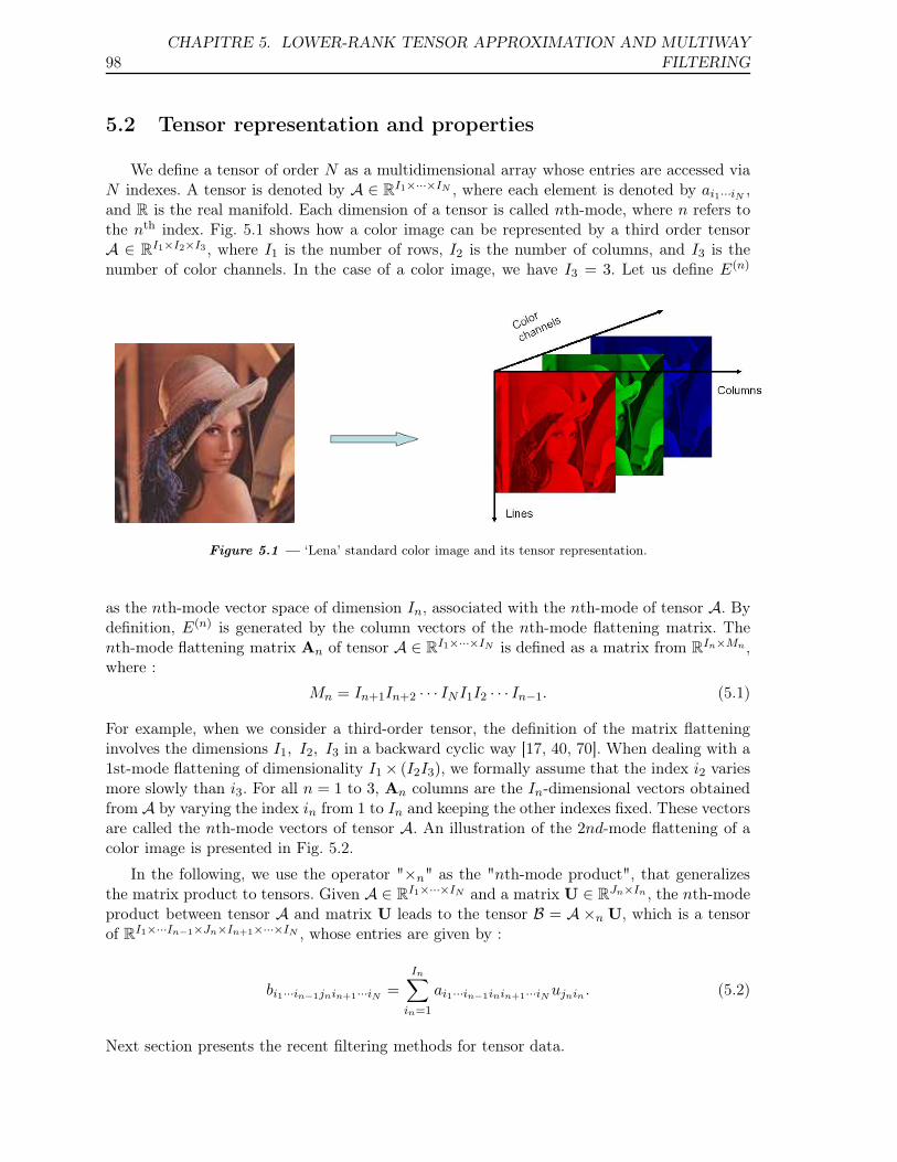
98CHAPITRE 5. LOWER-RANK TENSOR APPROXIMATION AND MULTIWAY
FILTERING
5.2 Tensor representation and properties
We define a tensor of order N as a multidimensional array whose entries are accessed viaN indexes. A tensor is denoted by A ∈ R
I1×···×IN , where each element is denoted by ai1···iN ,and R is the real manifold. Each dimension of a tensor is called nth-mode, where n refers tothe nth index. Fig. 5.1 shows how a color image can be represented by a third order tensorA ∈ R
I1×I2×I3 , where I1 is the number of rows, I2 is the number of columns, and I3 is thenumber of color channels. In the case of a color image, we have I3 = 3. Let us define E(n)
Figure 5.1 — ‘Lena’ standard color image and its tensor representation.
as the nth-mode vector space of dimension In, associated with the nth-mode of tensor A. Bydefinition, E(n) is generated by the column vectors of the nth-mode flattening matrix. Thenth-mode flattening matrix An of tensor A ∈ R
I1×···×IN is defined as a matrix from RIn×Mn ,
where :
Mn = In+1In+2 · · · INI1I2 · · · In−1. (5.1)
For example, when we consider a third-order tensor, the definition of the matrix flatteninginvolves the dimensions I1, I2, I3 in a backward cyclic way [17, 40, 70]. When dealing with a1st-mode flattening of dimensionality I1 × (I2I3), we formally assume that the index i2 variesmore slowly than i3. For all n = 1 to 3, An columns are the In-dimensional vectors obtainedfrom A by varying the index in from 1 to In and keeping the other indexes fixed. These vectorsare called the nth-mode vectors of tensor A. An illustration of the 2nd-mode flattening of acolor image is presented in Fig. 5.2.
In the following, we use the operator "×n" as the "nth-mode product", that generalizesthe matrix product to tensors. Given A ∈ R
I1×···×IN and a matrix U ∈ RJn×In , the nth-mode
product between tensor A and matrix U leads to the tensor B = A×n U, which is a tensorof R
I1×···In−1×Jn×In+1×···×IN , whose entries are given by :
bi1···in−1jnin+1···iN =
In∑
in=1
ai1···in−1inin+1···iN ujnin . (5.2)
Next section presents the recent filtering methods for tensor data.
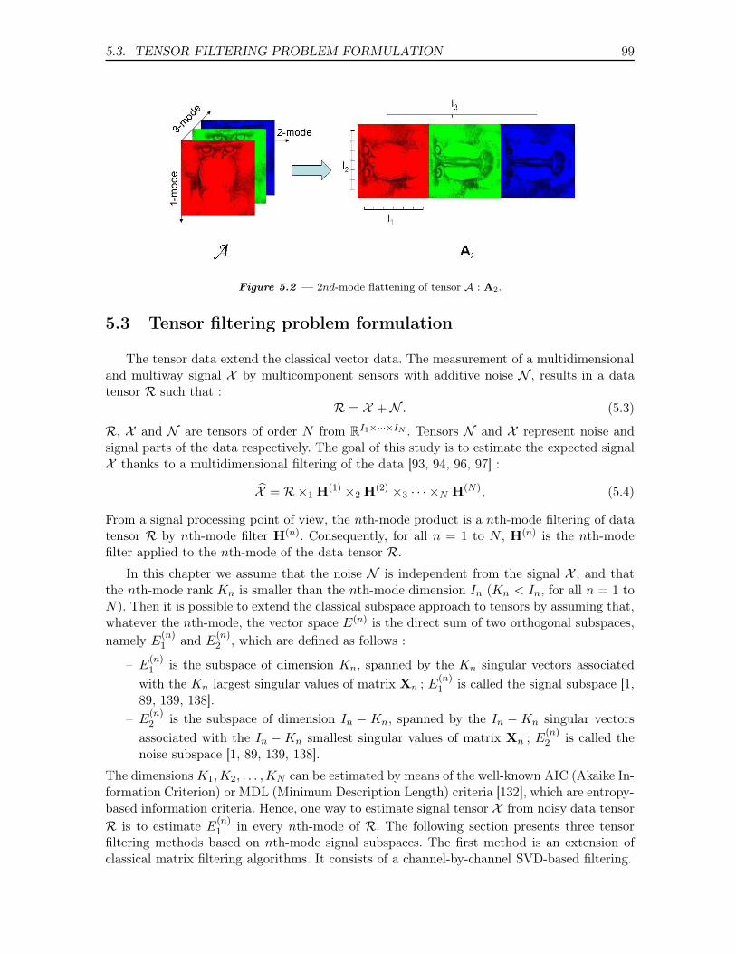
5.3. TENSOR FILTERING PROBLEM FORMULATION 99
Figure 5.2 — 2nd-mode flattening of tensor A : A2.
5.3 Tensor filtering problem formulation
The tensor data extend the classical vector data. The measurement of a multidimensionaland multiway signal X by multicomponent sensors with additive noise N , results in a datatensor R such that :
R = X + N . (5.3)
R, X and N are tensors of order N from RI1×···×IN . Tensors N and X represent noise and
signal parts of the data respectively. The goal of this study is to estimate the expected signalX thanks to a multidimensional filtering of the data [93, 94, 96, 97] :
X̂ = R×1 H(1) ×2 H(2) ×3 · · · ×N H(N), (5.4)
From a signal processing point of view, the nth-mode product is a nth-mode filtering of datatensor R by nth-mode filter H(n). Consequently, for all n = 1 to N , H(n) is the nth-modefilter applied to the nth-mode of the data tensor R.
In this chapter we assume that the noise N is independent from the signal X , and thatthe nth-mode rank Kn is smaller than the nth-mode dimension In (Kn < In, for all n = 1 toN). Then it is possible to extend the classical subspace approach to tensors by assuming that,whatever the nth-mode, the vector space E(n) is the direct sum of two orthogonal subspaces,namely E
(n)1 and E
(n)2 , which are defined as follows :
– E(n)1 is the subspace of dimension Kn, spanned by the Kn singular vectors associated
with the Kn largest singular values of matrix Xn ; E(n)1 is called the signal subspace [1,
89, 139, 138].
– E(n)2 is the subspace of dimension In − Kn, spanned by the In − Kn singular vectors
associated with the In − Kn smallest singular values of matrix Xn ; E(n)2 is called the
noise subspace [1, 89, 139, 138].
The dimensions K1,K2, . . . ,KN can be estimated by means of the well-known AIC (Akaike In-formation Criterion) or MDL (Minimum Description Length) criteria [132], which are entropy-based information criteria. Hence, one way to estimate signal tensor X from noisy data tensorR is to estimate E
(n)1 in every nth-mode of R. The following section presents three tensor
filtering methods based on nth-mode signal subspaces. The first method is an extension ofclassical matrix filtering algorithms. It consists of a channel-by-channel SVD-based filtering.
100CHAPITRE 5. LOWER-RANK TENSOR APPROXIMATION AND MULTIWAY
FILTERING
The second filtering method is based on multimode PCA achieved by rank-(K1, . . . ,KN )approximation. Two algorithms are presented for this case. The first algorithm is implicitlydeveloped for an additive white and Gaussian noise assumption, whereas the second algorithmrepresents an improvement of the first one in the case of a correlated Gaussian noise. Thisimprovement is achieved thanks to higher-order statistics.The third method, the multiway Wiener filtering (Wmm-(K1, . . . ,KN )), is an algorithm thatextends the classical two-dimensional Wiener filtering to tensor data.
5.3.1 Channel-by-channel SVD-based filtering
The classical algebraical methods operate on two-dimensional data matrices and are ba-sed on the Singular Value Decomposition (SVD) [1, 12, 13], and on Eckart-Young theoremconcerning the best lower rank approximation of a matrix [43] in the least-squares sense.
In the first method, a preprocessing is applied to the multidimensional and multiway data.It consists in splitting data tensor R, representing the noisy multicomponent image into two-dimensional "slice matrices" of data, each representing a specific channel. According to theclassical signal subspace methods [22], the left and right signal subspaces, corresponding torespectively the column and the row vectors of each slice matrix, are simultaneously determi-ned by processing the SVD of the matrix associated with the data of the slice matrix. Let usconsider the slice matrix R(:, :, i3, . . . , ij , . . . , iN ) of data tensor R. Projectors P on the leftsignal subspace, and Q on the right signal subspace are built from respectively the left and theright singular vectors associated with the K largest singular values of R(:, :, i3, . . . , ij , . . . , iN ).The parameter K simultaneously defines the dimensions of the left and right signal subspaces.Applying the projectors P and Q on the slice R(:, :, i3, . . . , ij , . . . , iN ) amounts to computeits best lower rank-K matrix approximation [43] in the least-squares sense.
The filtering of each slice matrix of data tensor R separately is called in the following"channel-by-channel" SVD-based filtering of R. It consists of a first way to estimate thesignal tensor X and can be summarized by the following steps :
1. input : data tensor R, left and right signal subspace dimension K.for iN = 1 to IN :for iN−1 = 1 to IN−1 :...for i4 = 1 to I4 :for i3 = 1 to I3 :
(a) calculate matrix R(:, :, i3, . . . , ij , . . . , iN ) SVD :
R(:, :, i3, . . . , ij , . . . , iN ) = U ·Σ · VT ,
where Σ is the core matrix regrouping the singular values of the matrix R(:, :, i3, . . . , ij , . . . , iN ), and U = [u1 . . .uI1] and V = [v1 . . . vI2] are the matrices contai-ning the left and right singular vectors defined respectively by ui1 and vi2 .
(b) construct matrices UK = [u1 . . .uK ] and VK = [v1 . . .vK ] containing the K largestleft and right eigenvectors of R(:, :, i3, . . . , ij , . . . , iN ) ;
(c) compute the projector P = UKUTK on the column signal subspace, and projector
Q = VKVTK on the row signal subspace.
5.3. TENSOR FILTERING PROBLEM FORMULATION 101
(d) compute the two-dimensional slice matrices of the estimated expected signal X̂ :
X̂ (:, :, i3, . . . , ij , . . . , iN ) = PR(:, :, i3, . . . , ij , . . . , iN )Q
2. output : estimated expected signal : X̂ .
Channel-by-channel SVD-based filtering is based on a common efficient method, but exhibitsa major drawback : it does not take into account the relationships between the components ofthe processed tensor. Moreover, channel-by-channel SVD-based filtering is appropriate onlyon some conditions. For example, applying SVD-based filtering to an image is generally ap-propriate when the rows or columns of an image are redundant, that is, linearly dependent.In this case, the rank K of the image is equal to the number of linearly independent rows orcolumns. It is only in this case that it would be safe to throw out eigenvectors from K + 1on. It is only in this special case that the noise subspace is orthogonal to the signal subspace.Otherwise, the noise simply increases the variance of the signal subspace and underestimatingthe signal subspace dimension would result in throwing out both signal and noise information.Thus, one would lose spatial resolution.The next subsection presents a multiway filtering method that processes jointly, and notsuccessively, each component of the data tensor.
5.3.2 Tensor filtering based on multimode PCA
5.3.2.1 White decorrelated Gaussian noise and second order statistics based me-thod
Assuming that the dimension Kn of the signal subspace is known for all n = 1 to N , oneway to estimate the expected signal tensor X from the noisy data tensor R = X + N , isto orthogonally project, for every nth-mode, the vectors of tensor R on the nth-mode signalsubspace E
(n)1 , for all n = 1 to N . This statement is equivalent to replace in (5.4) the filters
H(n) by the projectors P(n) on the nth-mode signal subspace :
X̂ = R×1 P(1) ×2 · · · ×N P(N). (5.5)
In this last formulation, projectors P(n) are estimated thanks to a multimode PCA appliedto data tensor R. This multimode PCA-based filtering generalizes the classical matrix filteringmethods [46, 49, 58, 60, 62, 82], and implicitly supposes that the additive noise is white andGaussian.
In the vector or matrix formulation, the definition of the projector on the signal subspaceis based on the eigenvectors associated with the largest eigenvalues of the covariance matrixof the set of observation vectors. Hence, the determination of the signal subspace amounts todetermine the best approximation (in the least-squares sense) of the observation matrix orthe covariance matrix.
As an extension to the vector and matrix cases, in the tensor formulation, the projectors onthe nth-mode vector spaces are determined by computing the rank-(K1, . . . ,KN ) approxima-tion of R in the least-squares sense. From a mathematical point of view, the rank-(K1, . . . ,KN )
102CHAPITRE 5. LOWER-RANK TENSOR APPROXIMATION AND MULTIWAY
FILTERING
approximation of R is represented by tensor RK1,...,KN which minimizes the quadratic tensorFrobenius norm ‖R−B‖2 subject to the condition that B ∈ R
I1×...×IN is a rank-(K1, . . . ,KN )tensor. The description of TUCKALS3 algorithm, used in rank-(K1, . . . ,KN ) approximationis provided in subsection A.1.1.A good approximation of the rank-(K1, . . . ,KN ) approximation can simply be achieved bycomputing the HOSVD-(K1, . . . ,KN ) of tensor R [41, 92]. Indeed, the HOSVD-(K1, . . . ,KN )of R consists of the initialization step of TUCKALS3 algorithm, and hence can be conside-red as a suboptimal solution for the rank-(K1, . . . ,KN ) approximation of tensor R [41]. ThisHOSVD-based technique has recently been used in [97] for denoising and source separationof multicomponent seismic waves.
5.3.2.2 Correlated Gaussian noise and higher-order statistics based method
In practice, the condition of noise whiteness is not always fulfilled. Hence, in the caseof an additive correlated Gaussian noise, TUCKALS3 algorithm is theoretically incapable ofproviding a good estimation of the nth-mode signal subspaces since it is based on secondorder moments. A classical means to remove the Gaussian (noise) components is to use thehigher-order statistics, and especially the higher-order cumulants. The tensor framework hasbeen used to compute the fourth order cumulants as a means of solving the ICA problem [39].Vasilescu and Terzopoulos introduced a multilinear ICA (N-mode ICA) for face recognition,which encodes the higher-order statistics associated with each mode of the tensor [128, 129].The related methods are based on the well-known cumulant property stating that the higher-order cumulants of a Gaussian variable are null [80, 89].
As a consequence, in the case of an additive correlated Gaussian noise, a recent study[97] has proposed to improve the multimode PCA-based filtering, by incorporating into TU-CKALS3 algorithm the fourth order cumulants instead of the second order moments.
From a practical point of view, second order matrices C(n),0 and C(n),k at steps 2b and3(a)iii of TUCKALS3 algorithm are replaced with the corresponding fourth order cumulants.In the following, we only present the details of the procedure for matrix C(n),k. Obtaining thedetails concerning C(n),0 is straightforward.
We assume that {r(n)p , p = 1, . . . ,Mn}, and {b(n),k
p , p = 1, . . . ,Mn} are the Mn realizationsof two random vectors r(n) and b(n),k. In practice, we take as the realizations of these tworandom vectors the nth-mode vectors of data tensors R and B(n),k. Matrix C(n),k reads :
C(n),k =Mn∑
p=1
b(n),kp r(n)T
p . (5.6)
The fourth order cumulants associated with vectors r(n) and b(n),k are denoted by :
C(n),k = Cum(b(n),k,b(n),kT
, r(n), r(n)T
), (5.7)
where Cum(·) denotes the cumulant operator. C(n),k is a fourth order super-symmetric tensorfrom R
In×In×In×In , whose generic term for indexes (i1, i2, j1, j2), for centered variables, isgiven by [52, 80] :
(C(n),k)i1,i2,j1,j2 = E[b(n),ki1
b(n),ki2
r(n)j1
r(n)j2
]
−E[b(n),ki1
r(n)j1
]E[b(n),ki2
r(n)j2
] − E[b(n),ki1
r(n)j2
]E[b(n),ki2
r(n)j1
](5.8)
5.3. TENSOR FILTERING PROBLEM FORMULATION 103
where b(n),ki and r
(n)j are the ith and jth components of random vectors b(n),k and r(n), and
E[·] is the expectation operator. The practical estimation of (C(n),k)i1,i2,j1,j2 is given by :
(C(n),k)i1,i2,j1,j2 = 1Mn
(∑Mn
p=1
(b(n),ki1p b
(n),ki2p r
(n)j1pr
(n)j2p
))
− 1Mn
2
(∑Mn
p=1
(b(n),ki1p r
(n)j1p
)) (∑Mn
p=1
(b(n),ki2p r
(n)j2p
))
− 1Mn
2
(∑Mn
p=1
(b(n),ki1p r
(n)j2p
))(∑Mn
p=1
(b(n),ki2p r
(n)j1p
)).
(5.9)
Here, b(n),kij and r
(n)ij are the elements at position (i, j) of tensors B(n),k and R nth-mode
flattening matrices B(n),kn and Rn.
In the classical TUCKALS3 algorithm, the Kn nth-mode signal subspace basis vectors,given by matrix U(n),k, are estimated by computing, at step 3a, the eigenvectors associatedwith the Kn largest eigenvalues of matrix C(n),k. This amounts to computing the best lowerrank-Kn approximation of C(n),k. In [110] fourth order cumulants are used instead of thecovariance matrix because of their ability to remove Gaussian noise. Indeed, the fourth ordercumulants of Gaussian variables are null. Therefore, when dealing with an additive correlatedGaussian noise, we also use fourth order cumulants [97].
The main drawback of fourth order cumulants is the high computational load to buildevery fourth order cumulant tensor associated with the nth-mode of the data tensor. Thiscomputational load depends on the size of the data tensor R, that is, the values of In, forall n = 1 to N . One way to reduce the computational load has recently been proposed in[97] and consists in using the fourth order cumulant slice matrix. The cumulant slice matrixhas initially been introduced in array processing for source localisation or directions-of-arrival(DOA) estimation [21, 139, 138]. In [52, 139, 138], it is proven that the signal subspace spannedby the eigenvectors associated with the largest eigenvalues of a cumulant slice matrix is thesame as signal subspace obtained from the whole cumulant tensor defined in (5.7) [139, 138].Therefore, we use only the eigenvectors of one cumulant slice matrix in our algorithm (seestep 2(a)iii) because the other cumulant slice matrices provide redundant information. Theuse of the fourth order cumulant slice matrix provides a much faster algorithm [138]. In our
application, the fourth order cumulant slice matrix C(n),kq can be defined, from (5.8), by fixing
the qth component of vector b(n),k as follows :(C(n),k
q
)ij
= E[(b(n),k
q )2r(n)i r
(n)j
]− 2E
[b(n),kq r
(n)i
]E
[b(n),kq r
(n)j
]. (5.10)
The practical estimation of(C
(n),kq
)ij
can be given by :
(C(n),k
q
)ij
=1
Mn
Mn∑
p=1
(b(n),kqp
)2r(n)ip r
(n)jp
− 2
M2n
Mn∑
p=1
b(n),kqp r
(n)ip
Mn∑
p=1
b(n),kqp r
(n)jp
, (5.11)
where b(n),kij and r
(n)ij are respectively the elements at position (i, j) in the nth-mode flattening
matrices B(n),kn and Rn of tensors B(n),k and R.
As a consequence, in the case of an additive correlated Gaussian noise, the Kn nth-modesignal subspace basis vectors can now be estimated by computing matrix C
(n),kq lower rank-
Kn approximation. Then, the fourth order cumulant slice matrix-based multimode PCA-basedfiltering is summarized in subsection A.1.2.
104CHAPITRE 5. LOWER-RANK TENSOR APPROXIMATION AND MULTIWAY
FILTERING
It was experimentally shown in [97], that when the parameter q involved in C(n),kq
is chosen properly, multimode PCA filtering based on fourth order cumulants (deno-ted by rank−C(K1, . . . ,KN )) and on fourth order cumulant slice matrix (denoted byrank−C1(K1, . . . ,KN )) give sensibly the same performances in regard to noise reductionin color images and multicomponent seismic waves.
5.3.3 Multiway Wiener filtering
Let Rn, Xn and Nn be the nth-mode flattening matrices of tensors R, X and N , respec-tively.
In the previous subsection, the estimation of signal tensor X has been performed byprojecting noisy data tensor R on each nth-mode signal subspace. The nth-mode projectorshave been estimated thanks to the use of multimode PCA achieved by rank-(K1, . . . ,KN )approximation. In spite of the good results given by this method, it is possible to improvethe tensor filtering quality by determining nth-mode filters H(n), n = 1 to N , in (5.4), whichoptimize an estimation criterion. The most classical method is to minimize the mean squarederror between the expected signal tensor X and the estimated signal tensor X̂ given in (5.4) :
e(H(1), . . . ,H(N)) = E[‖X −R×1 H(1) ×2 · · · ×N H(N)‖2]. (5.12)
Due to the criterion which is minimized, filters H(n), n = 1 to N , can be called "nth-modeWiener filters" [96].According to the calculations presented in Appendix A.2, especially from (A.1) to (A.15),the minimization of (5.12) with respect to filter H(n), for fixed H(m), m 6= n, leads to thefollowing expression of nth-mode Wiener filter :
H(n) = γ(n)XRΓ
(n)RR
−1, (5.13)
whereγ
(n)XR = E
[XnT
(n)RTn
](5.14)
is the T(n)-weighted covariance matrix between the random column vectors of signal Xn anddata Rn, with :
T(n) = H(1) ⊗ · · · ⊗ H(n−1) ⊗ H(n+1) ⊗ · · · ⊗ H(N), (5.15)
where ⊗ stands for Kronecker product, and :
Γ(n)RR = E
[RnQ
(n)RTn
], (5.16)
is the Q(n)-weighted covariance matrix of the data Rn, with :
Q(n) = T(n)TT(n). (5.17)
In order to obtain H(n) through (5.13), we suppose that the filters {H(m),m = 1 to N,m 6= n}are known. Data tensor R is available, but signal tensor X is unknown. So, only the termΓ
(n)RR can be derived, and not the term γ
(n)XR. Hence, some more assumptions on X have to
be made in order to overcome the indetermination over γ(n)XR [93, 96]. In the one-dimensional
case, a classical assumption is to consider that a signal vector is a weighted combination of
5.3. TENSOR FILTERING PROBLEM FORMULATION 105
the signal subspace basis vectors. In extension to the tensor case, [93, 96] have proposed toconsider that the nth-mode flattening matrix Xn can be expressed as a weighted combinationof Kn vectors from the nth-mode signal subspace E
(n)1 :
Xn = V(n)s O(n), (5.18)
with Xn ∈ RIn×Mn , and V
(n)s ∈ R
In×Kn being the matrix containing the Kn orthonormalbasis vectors of nth-mode signal subspace E
(n)1 . Matrix O(n) ∈ RKn×Mn is a weight matrix
and contains the whole information on expected signal tensor X . This model implies thatsignal nth-mode flattening matrix Xn is orthogonal to nth-mode noise flattening matrix Nn,since signal subspace E
(n)1 and noise subspace E
(n)2 are supposed mutually orthogonal.
Supposing that noise N in (5.3) is white, Gaussian and independent from signal X , andintroducing the signal model (5.18) in (5.13) leads to a computable expression of nth-modeWiener filter H(n) (see Appendix A.3) :
H(n) = V(n)s γ
(n)OOΛ
(n)−1
Γs V(n)T
s , (5.19)
where γ(n)OOΛ
(n)−1
Γs is a diagonal weight matrix given by :
γ(n)OOΛ
(n)−1
Γs = diag
[β1
λΓ1
, · · · ,βKn
λΓKn
], (5.20)
where λΓ1 , . . . , λΓ
Knare the Kn largest eigenvalues of Q(n)-weighted covariance matrix Γ
(n)RR (see
(5.16)). Parameters β1, . . . , βKn depend on λγ1 , . . . , λγ
Knwhich are the Kn largest eigenvalues
of T(n)-weighted covariance matrixγ
(n)RR = E[RnT
(n)RTn ], according to the following relation :
βkn= λγ
kn− σ
(n)2
Γ , ∀ kn = 1, . . . ,Kn (5.21)
Superscript γ refers to the T(n)-weighted covariance, and subscript Γ to the Q(n)-weighted
covariance. σ(n)2
Γ is the degenerated eigenvalue of noise T(n)-weighted covariance matrix
γ(n)NN = E
[NnT
(n)NTn
]. Thanks to the additive noise and the signal independence assump-
tions, the In −Kn smallest eigenvalues of γ(n)RR are equal to σ
(n)2
Γ , and thus, can be estimatedby the following relation :
σ̂(n)2
Γ =1
In − Kn
In∑
kn=Kn+1
λγkn
. (5.22)
In order to determine the nth-mode Wiener filters H(n) that minimize the mean squarederror (5.12), the Alternating Least Squares (ALS) algorithm has been proposed in [93, 96].It is detailed in subsection A.1.3.
In subsection 5.3.2, we presented the adaptation of multimode PCA to the case of a noncorrelated Gaussian noise, by using higher-order statistics. In the same way, it is possible touse higher-order statistics for multiway Wiener filtering. For this, one should replace step 2aii-B by step 2aii of the ALS loop in subsection 5.3.2, and replace step 2aii-E by the computationof the cumulant slice C
(n),kq associated with the fourth order cumulants of matrix R
(n),kn and
matrix (R(n),kn )T . Elements of C
(n),kq are given in (5.11).
106CHAPITRE 5. LOWER-RANK TENSOR APPROXIMATION AND MULTIWAY
FILTERING
5.4 Simulation results
In the following simulations, the channel-by-channel SVD-based filtering defined in subsec-tion 5.3.1 and the rank-(K1, . . . ,KN ) approximation based multiway and multidimensionalfiltering are applied to the denoising of color images and multispectral images, and to thedenoising of seismic signals. Color images, multispectral images, and seismic signals can berepresented by a third order tensor from R
I1×I2×I3 , where I1, I2, and I3 take different values.In all these applications, the efficiency of denoising is tested in the presence of an additiveGaussian noise, either correlated or not.A multidimensional and multiway white Gaussian noise N which is added to signal tensor Xcan be expressed as :
N = α · G, (5.23)
where every element of G ∈ RI1×I2×I3 is an independent realization of a normalized centered
Gaussian law, and where α is a coefficient that permits to set the SNR in noisy data tensorR.When we process images impaired by correlated Gaussian noise, the noise which is added isa third order tensor defined by :
N c = N ×1 W(1) ×2 W(2) ×3 W(3), (5.24)
where every element of N represents an independent realization of a white Gaussian noise,and W(n) is a weight matrix in the nth-mode, n = 1, 2, 3.
In order to evaluate the performances of the overviewed tensor signal processing methods,a particular performance criterion is employed as proposed in [96, 97].
5.4.1 Performance criterion
Following the representation of (5.3), the multiway noisy data tensor is expressed as R =X +N , where X is the expected signal tensor and N is the additive noise tensor. Let us definethe Signal to Noise Ratio (SNR, in dB) in the noisy data tensor by :
SNR = 10log(‖X‖2
‖N‖2). (5.25)
In order to a posteriori verify the quality of the estimated signal tensor, we use theNormalized Quadratic Error criterion (NQE) defined as follows :
NQE(X̂ ) =‖X̂ − X‖2
‖X‖2. (5.26)
The NQE criterion permits a quantitative comparison of the channel-by-channel SVD-basedfiltering and the rank-(K1,K2,K3) approximation multiway and multidimensional filtering.Considering this criterion, we expect the rank-(K1,K2,K3) approximation to give betterresults than the channel-by-channel SVD-based filtering method.
5.4. SIMULATION RESULTS 107
5.4.2 Denoising of color images
Denoising of color images has already been studied in several works [18, 99, 116]. Somesolutions have been brought from the field of wavelet processing, exhibiting good results interms of output SNR. These studies only concern bidimensional data, whereas the methodsthat we compare are adapted to the processing of third order tensors as a whole, and inparticular to three-channel images. We focus on subspace-based methods. We first considerthe channel-by-channel SVD-based filtering, the rank-(K1,K2,K3) approximation and multi-way Wiener filtering (Wmm-(K1,K2,K3)), applied to images impaired by an additive whiteGaussian noise.Then we present the results obtained with rank-(K1,K2,K3) based on second order andhigher-order statistics, applied to images impaired by an additive correlated Gaussian noise.We compare the performances of the methods applied in this subsection in terms of denoisingefficiency and computational load.
5.4.2.1 Denoising of a color image impaired by additive Gaussian noise
Let us consider the "Sailboat" standard color image of Fig. 5.3(a) represented as a thirdorder tensor X ∈ R
256×256×3. The ranks of the signal subspace for each mode are 30 for the1st-mode, 30 for the 2nd-mode, and 2 for the 3rd-mode. This is fixed thanks to the followingprocess : For Fig. 5.3(a), we took the standard non-noisy "sailboat" image and we artificiallyreduced the ranks of the non-noisy image, that is, we set the parameters (K1,K2,K3) to(30,30,2), thanks to the truncation of HOSVD. This permits to ensure that, for each mode,the rank of the signal subspace is lower than the corresponding dimension. This also permits toevaluate the performances of the filtering methods applied, independently from the accuracyof the estimation of the values of the ranks by MDL or AIC criterion.Fig. 5.3(b) shows the noisy image resulting from the impairment of Fig. 5.3(a) and representedas R = X + N . Third-order noise tensor N is defined by relation (5.23) by choosing α suchthat, considering previous definition of (5.25), the SNR in the noisy image of Fig. 5.3(b) is8.1dB. In these simulations, the value of the parameter K of channel-by-channel SVD-basedfiltering, the values of the dimensions of the row and column signal subspace are supposedto be known and fixed to 30. In the same way, parameters (K1,K2,K3) of rank-(K1,K2,K3)approximation are fixed to (30, 30, 2).The channel-by-channel SVD-based filtering of noisy image R (see Fig. 5.3(b)) yields theimage of Fig. 5.3(c), and rank-(30, 30, 2) approximation of noisy data tensor R yields theimage of Fig. 5.3(d). The NQE, defined in (5.26), permits a quantitative comparison betweenchannel-by-channel SVD-based filtering and rank-(30, 30, 2) approximation. Figure 5.4, whichpresents the evolution of the NQE with respect to SNR varying from 3dB to 18dB, shows theNQE obtained with Wmm-(30, 30, 2) is lower than the NQE obtained with the filtering withrank-(30, 30, 2) approximation. For this simulation, the rank-(K1,K2,K3) approximation givesbetter results than channel-by-channel SVD-based filtering according to the NQE criterion.From the resulting image, presented on Fig. 5.3(d), we notice that dimension reduction leadsto a loss of spatial resolution. However the choice of a set of values K1,K2,K3 which are smallenough is the condition for an efficient noise reduction effect.Therefore, a tradeoff should be considered between noise reduction and detail preservation.This tradeoff was discussed in [112]. We were interested in using the Minimum DescriptionLength criterion [132], applied to the left singular values of the flattening matrices computed
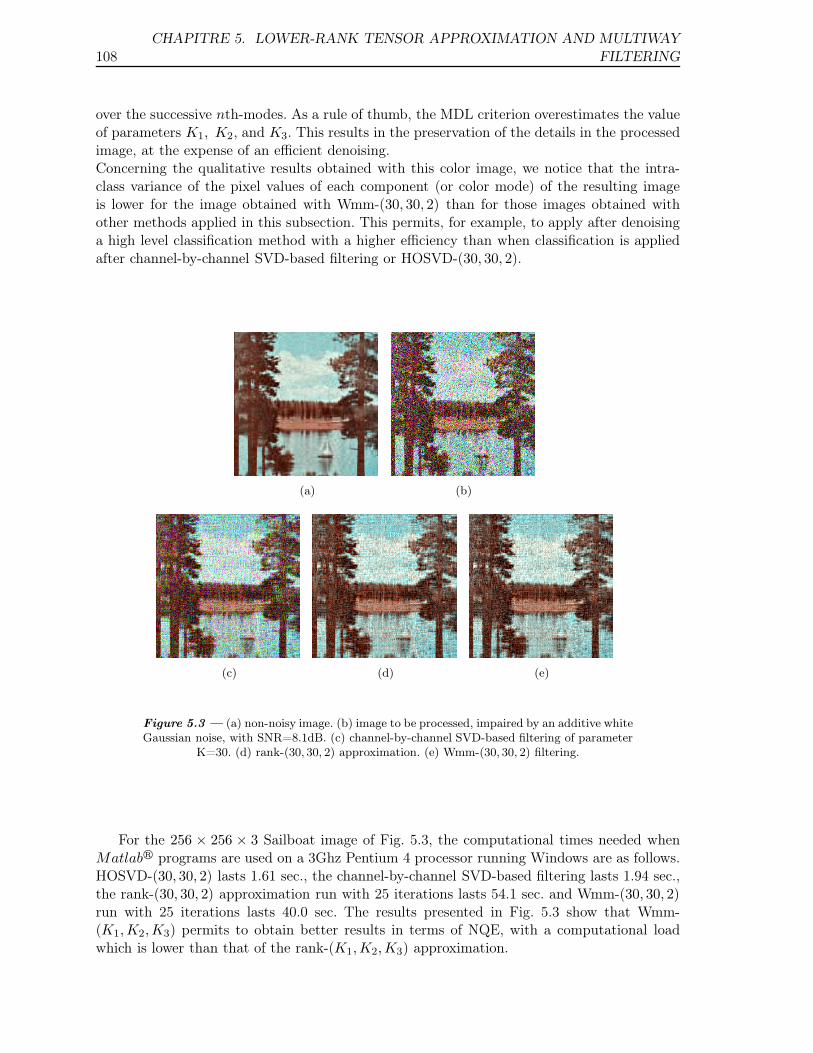
108CHAPITRE 5. LOWER-RANK TENSOR APPROXIMATION AND MULTIWAY
FILTERING
over the successive nth-modes. As a rule of thumb, the MDL criterion overestimates the valueof parameters K1, K2, and K3. This results in the preservation of the details in the processedimage, at the expense of an efficient denoising.Concerning the qualitative results obtained with this color image, we notice that the intra-class variance of the pixel values of each component (or color mode) of the resulting imageis lower for the image obtained with Wmm-(30, 30, 2) than for those images obtained withother methods applied in this subsection. This permits, for example, to apply after denoisinga high level classification method with a higher efficiency than when classification is appliedafter channel-by-channel SVD-based filtering or HOSVD-(30, 30, 2).
(a) (b)
(c) (d) (e)
Figure 5.3 — (a) non-noisy image. (b) image to be processed, impaired by an additive whiteGaussian noise, with SNR=8.1dB. (c) channel-by-channel SVD-based filtering of parameter
K=30. (d) rank-(30, 30, 2) approximation. (e) Wmm-(30, 30, 2) filtering.
For the 256 × 256 × 3 Sailboat image of Fig. 5.3, the computational times needed whenMatlabr programs are used on a 3Ghz Pentium 4 processor running Windows are as follows.HOSVD-(30, 30, 2) lasts 1.61 sec., the channel-by-channel SVD-based filtering lasts 1.94 sec.,the rank-(30, 30, 2) approximation run with 25 iterations lasts 54.1 sec. and Wmm-(30, 30, 2)run with 25 iterations lasts 40.0 sec. The results presented in Fig. 5.3 show that Wmm-(K1,K2,K3) permits to obtain better results in terms of NQE, with a computational loadwhich is lower than that of the rank-(K1,K2,K3) approximation.
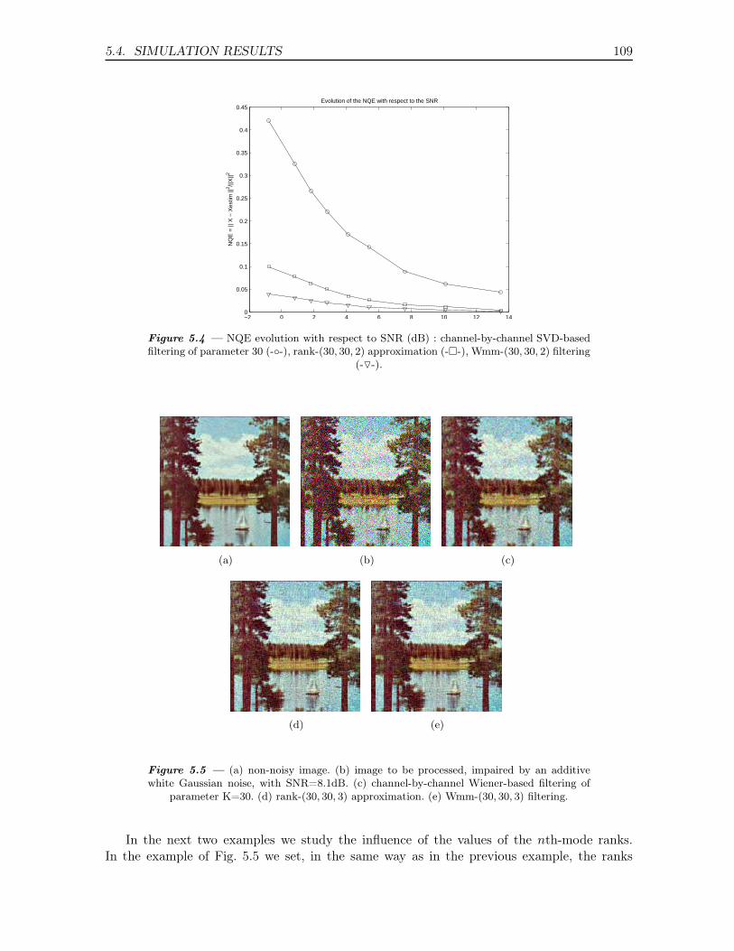
5.4. SIMULATION RESULTS 109
−2 0 2 4 6 8 10 12 140
0.05
0.1
0.15
0.2
0.25
0.3
0.35
0.4
0.45Evolution of the NQE with respect to the SNR
NQ
E =
|| X
− X
estim
||2 /||
X||2
Figure 5.4 — NQE evolution with respect to SNR (dB) : channel-by-channel SVD-basedfiltering of parameter 30 (-◦-), rank-(30, 30, 2) approximation (-�-), Wmm-(30, 30, 2) filtering
(-▽-).
(a) (b) (c)
(d) (e)
Figure 5.5 — (a) non-noisy image. (b) image to be processed, impaired by an additivewhite Gaussian noise, with SNR=8.1dB. (c) channel-by-channel Wiener-based filtering of
parameter K=30. (d) rank-(30, 30, 3) approximation. (e) Wmm-(30, 30, 3) filtering.
In the next two examples we study the influence of the values of the nth-mode ranks.In the example of Fig. 5.5 we set, in the same way as in the previous example, the ranks
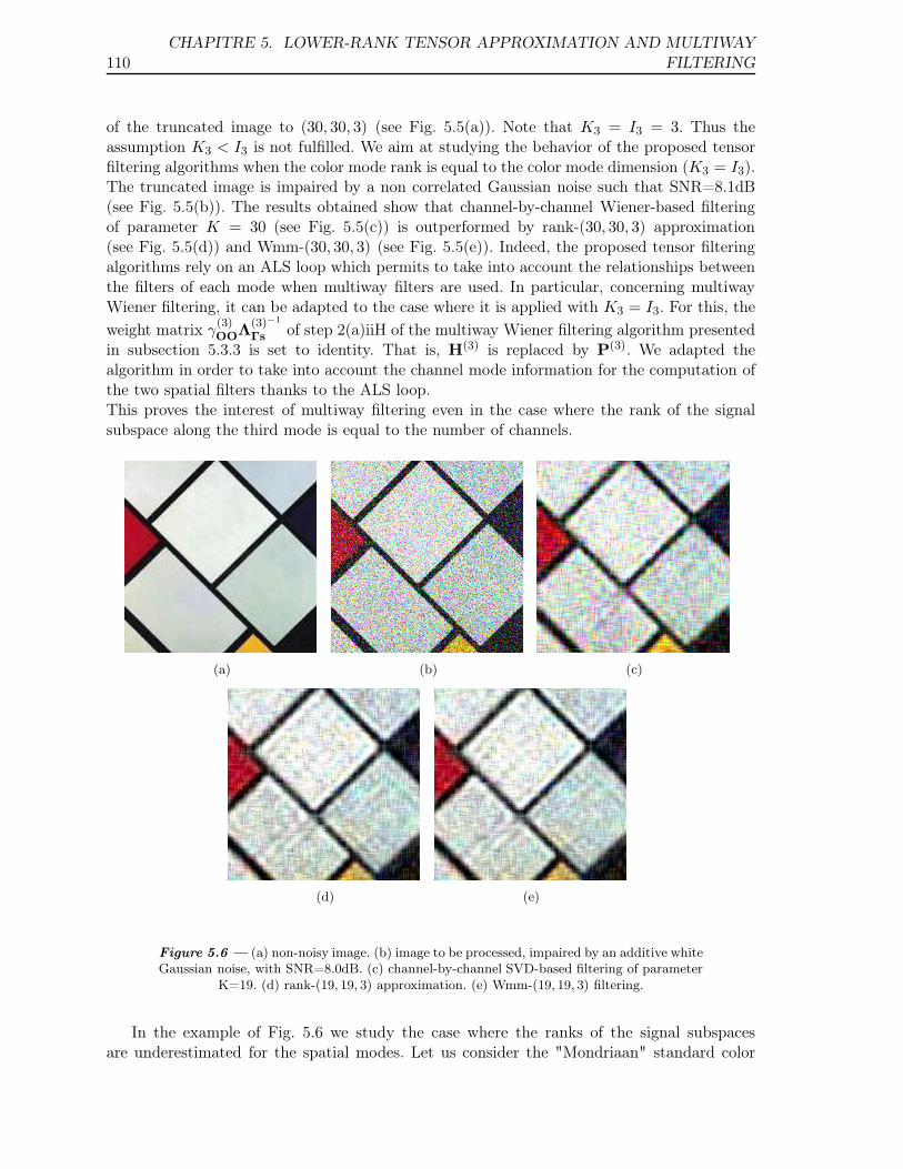
110CHAPITRE 5. LOWER-RANK TENSOR APPROXIMATION AND MULTIWAY
FILTERING
of the truncated image to (30, 30, 3) (see Fig. 5.5(a)). Note that K3 = I3 = 3. Thus theassumption K3 < I3 is not fulfilled. We aim at studying the behavior of the proposed tensorfiltering algorithms when the color mode rank is equal to the color mode dimension (K3 = I3).The truncated image is impaired by a non correlated Gaussian noise such that SNR=8.1dB(see Fig. 5.5(b)). The results obtained show that channel-by-channel Wiener-based filteringof parameter K = 30 (see Fig. 5.5(c)) is outperformed by rank-(30, 30, 3) approximation(see Fig. 5.5(d)) and Wmm-(30, 30, 3) (see Fig. 5.5(e)). Indeed, the proposed tensor filteringalgorithms rely on an ALS loop which permits to take into account the relationships betweenthe filters of each mode when multiway filters are used. In particular, concerning multiwayWiener filtering, it can be adapted to the case where it is applied with K3 = I3. For this, the
weight matrix γ(3)OOΛ
(3)−1
Γs of step 2(a)iiH of the multiway Wiener filtering algorithm presentedin subsection 5.3.3 is set to identity. That is, H(3) is replaced by P(3). We adapted thealgorithm in order to take into account the channel mode information for the computation ofthe two spatial filters thanks to the ALS loop.This proves the interest of multiway filtering even in the case where the rank of the signalsubspace along the third mode is equal to the number of channels.
(a) (b) (c)
(d) (e)
Figure 5.6 — (a) non-noisy image. (b) image to be processed, impaired by an additive whiteGaussian noise, with SNR=8.0dB. (c) channel-by-channel SVD-based filtering of parameter
K=19. (d) rank-(19, 19, 3) approximation. (e) Wmm-(19, 19, 3) filtering.
In the example of Fig. 5.6 we study the case where the ranks of the signal subspacesare underestimated for the spatial modes. Let us consider the "Mondriaan" standard color
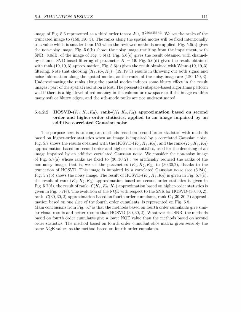
5.4. SIMULATION RESULTS 111
image of Fig. 5.6 represented as a third order tensor X ∈ R256×256×3. We set the ranks of the
truncated image to (150, 150, 3). The ranks along the spatial modes will be fixed intentionallyto a value which is smaller than 150 when the reviewed methods are applied. Fig. 5.6(a) givesthe non-noisy image, Fig. 5.6(b) shows the noisy image resulting from the impairment, withSNR=8.0dB, of the image of Fig. 5.6(a). Fig. 5.6(c) gives the result obtained with channel-by-channel SVD-based filtering of parameter K = 19. Fig. 5.6(d) gives the result obtainedwith rank-(19, 19, 3) approximation, Fig. 5.6(e) gives the result obtained with Wmm-(19, 19, 3)filtering. Note that choosing (K1,K2,K3)=(19, 19, 3) results in throwing out both signal andnoise information along the spatial modes, as the ranks of the noisy image are (150, 150, 3).Underestimating the ranks along the spatial modes induces some blurry effect in the resultimages : part of the spatial resolution is lost. The presented subspace-based algorithms performwell if there is a high level of redundancy in the column or row space or if the image exhibitsmany soft or blurry edges, and the nth-mode ranks are not underestimated.
5.4.2.2 HOSVD-(K1,K2,K3), rank-(K1,K2,K3) approximation based on secondorder and higher-order statistics, applied to an image impaired by anadditive correlated Gaussian noise
The purpose here is to compare methods based on second order statistics with methodsbased on higher-order statistics when an image is impaired by a correlated Gaussian noise.Fig. 5.7 shows the results obtained with the HOSVD-(K1,K2,K3), and the rank-(K1,K2,K3)approximation based on second order and higher-order statistics, used for the denoising of animage impaired by an additive correlated Gaussian noise. We consider the non-noisy imageof Fig. 5.7(a) whose ranks are fixed to (30, 30, 2) : we artificially reduced the ranks of thenon-noisy image, that is, we set the parameters (K1,K2,K3) to (30,30,2), thanks to thetruncation of HOSVD. This image is impaired by a correlated Gaussian noise (see (5.24)).Fig. 5.7(b) shows the noisy image. The result of HOSVD-(K1,K2,K3) is given in Fig. 5.7(c),the result of rank-(K1,K2,K3) approximation based on second order statistics is given inFig. 5.7(d), the result of rank−C(K1,K2,K3) approximation based on higher-order statistics isgiven in Fig. 5.7(e). The evolution of the NQE with respect to the SNR for HOSVD-(30, 30, 2),rank−C(30, 30, 2) approximation based on fourth order cumulants, rank-C1(30, 30, 2) approxi-mation based on one slice of the fourth order cumulants, is represented on Fig. 5.8.Main conclusions from Fig. 5.7 is that the methods based on fourth order cumulants give simi-lar visual results and better results than HOSVD-(30, 30, 2). Whatever the SNR, the methodsbased on fourth order cumulants give a lower NQE value than the methods based on secondorder statistics. The method based on fourth order cumulant slice matrix gives sensibly thesame NQE values as the method based on fourth order cumulants.
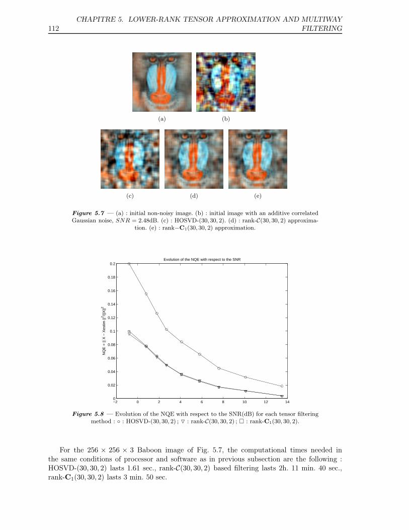
112CHAPITRE 5. LOWER-RANK TENSOR APPROXIMATION AND MULTIWAY
FILTERING
(a) (b)
(c) (d) (e)
Figure 5.7 — (a) : initial non-noisy image. (b) : initial image with an additive correlatedGaussian noise, SNR = 2.48dB. (c) : HOSVD-(30,30, 2). (d) : rank-C(30, 30, 2) approxima-
tion. (e) : rank−C1(30, 30, 2) approximation.
−2 0 2 4 6 8 10 12 140
0.02
0.04
0.06
0.08
0.1
0.12
0.14
0.16
0.18
0.2Evolution of the NQE with respect to the SNR
NQ
E =
|| X
− X
estim
||2 /||
X||2
Figure 5.8 — Evolution of the NQE with respect to the SNR(dB) for each tensor filteringmethod : ◦ : HOSVD-(30,30, 2) ; ▽ : rank-C(30, 30, 2) ; � : rank-C1(30, 30, 2).
For the 256 × 256 × 3 Baboon image of Fig. 5.7, the computational times needed inthe same conditions of processor and software as in previous subsection are the following :HOSVD-(30, 30, 2) lasts 1.61 sec., rank-C(30, 30, 2) based filtering lasts 2h. 11 min. 40 sec.,rank-C1(30, 30, 2) lasts 3 min. 50 sec.
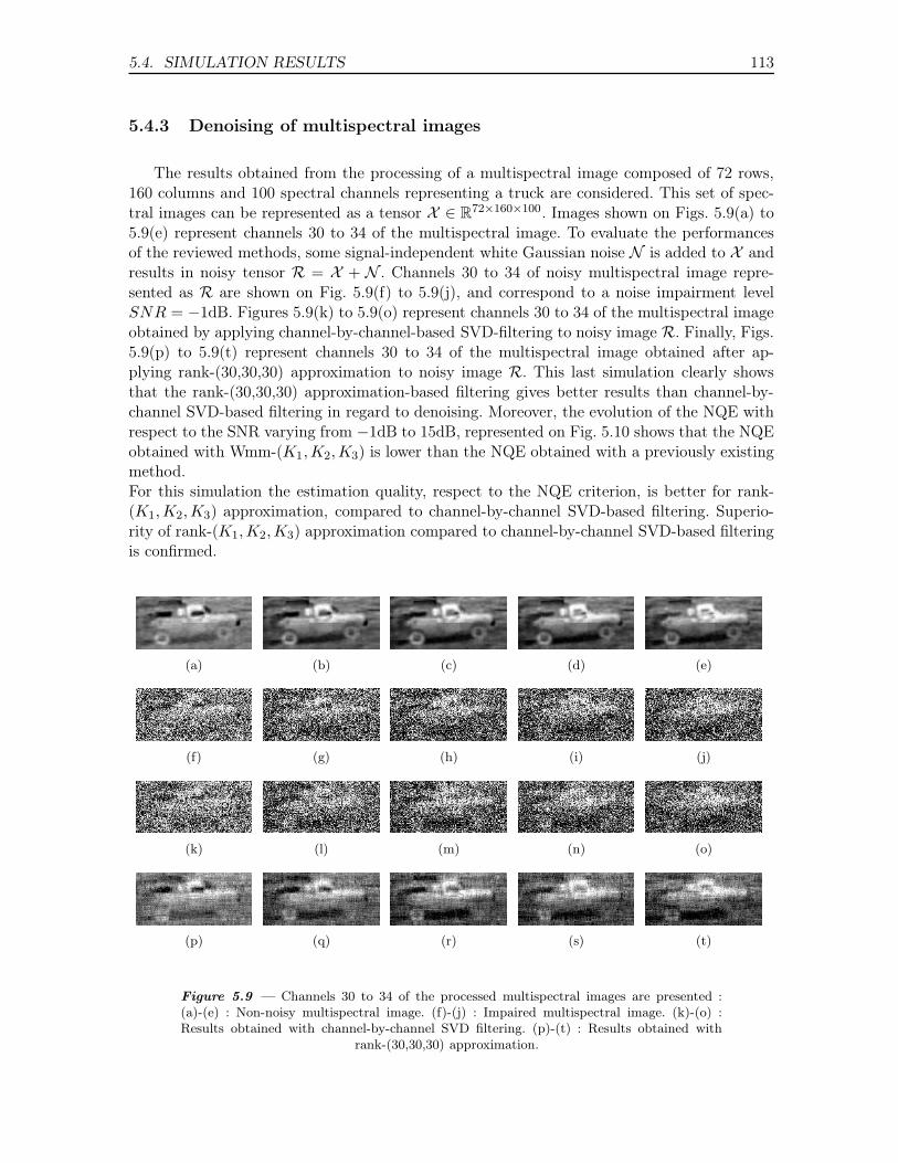
5.4. SIMULATION RESULTS 113
5.4.3 Denoising of multispectral images
The results obtained from the processing of a multispectral image composed of 72 rows,160 columns and 100 spectral channels representing a truck are considered. This set of spec-tral images can be represented as a tensor X ∈ R
72×160×100. Images shown on Figs. 5.9(a) to5.9(e) represent channels 30 to 34 of the multispectral image. To evaluate the performancesof the reviewed methods, some signal-independent white Gaussian noise N is added to X andresults in noisy tensor R = X + N . Channels 30 to 34 of noisy multispectral image repre-sented as R are shown on Fig. 5.9(f) to 5.9(j), and correspond to a noise impairment levelSNR = −1dB. Figures 5.9(k) to 5.9(o) represent channels 30 to 34 of the multispectral imageobtained by applying channel-by-channel-based SVD-filtering to noisy image R. Finally, Figs.5.9(p) to 5.9(t) represent channels 30 to 34 of the multispectral image obtained after ap-plying rank-(30,30,30) approximation to noisy image R. This last simulation clearly showsthat the rank-(30,30,30) approximation-based filtering gives better results than channel-by-channel SVD-based filtering in regard to denoising. Moreover, the evolution of the NQE withrespect to the SNR varying from −1dB to 15dB, represented on Fig. 5.10 shows that the NQEobtained with Wmm-(K1,K2,K3) is lower than the NQE obtained with a previously existingmethod.For this simulation the estimation quality, respect to the NQE criterion, is better for rank-(K1,K2,K3) approximation, compared to channel-by-channel SVD-based filtering. Superio-rity of rank-(K1,K2,K3) approximation compared to channel-by-channel SVD-based filteringis confirmed.
(a) (b) (c) (d) (e)
(f) (g) (h) (i) (j)
(k) (l) (m) (n) (o)
(p) (q) (r) (s) (t)
Figure 5.9 — Channels 30 to 34 of the processed multispectral images are presented :(a)-(e) : Non-noisy multispectral image. (f)-(j) : Impaired multispectral image. (k)-(o) :Results obtained with channel-by-channel SVD filtering. (p)-(t) : Results obtained with
rank-(30,30,30) approximation.
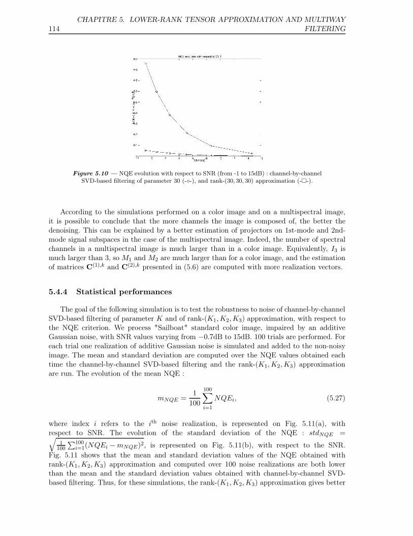
114CHAPITRE 5. LOWER-RANK TENSOR APPROXIMATION AND MULTIWAY
FILTERING
Figure 5.10 — NQE evolution with respect to SNR (from -1 to 15dB) : channel-by-channelSVD-based filtering of parameter 30 (-◦-), and rank-(30, 30, 30) approximation (-�-).
According to the simulations performed on a color image and on a multispectral image,it is possible to conclude that the more channels the image is composed of, the better thedenoising. This can be explained by a better estimation of projectors on 1st-mode and 2nd-mode signal subspaces in the case of the multispectral image. Indeed, the number of spectralchannels in a multispectral image is much larger than in a color image. Equivalently, I3 ismuch larger than 3, so M1 and M2 are much larger than for a color image, and the estimationof matrices C(1),k and C(2),k presented in (5.6) are computed with more realization vectors.
5.4.4 Statistical performances
The goal of the following simulation is to test the robustness to noise of channel-by-channelSVD-based filtering of parameter K and of rank-(K1,K2,K3) approximation, with respect tothe NQE criterion. We process "Sailboat" standard color image, impaired by an additiveGaussian noise, with SNR values varying from −0.7dB to 15dB. 100 trials are performed. Foreach trial one realization of additive Gaussian noise is simulated and added to the non-noisyimage. The mean and standard deviation are computed over the NQE values obtained eachtime the channel-by-channel SVD-based filtering and the rank-(K1,K2,K3) approximationare run. The evolution of the mean NQE :
mNQE =1
100
100∑
i=1
NQEi, (5.27)
where index i refers to the ith noise realization, is represented on Fig. 5.11(a), withrespect to SNR. The evolution of the standard deviation of the NQE : stdNQE =√
1100
∑100i=1(NQEi − mNQE)2, is represented on Fig. 5.11(b), with respect to the SNR.
Fig. 5.11 shows that the mean and standard deviation values of the NQE obtained withrank-(K1,K2,K3) approximation and computed over 100 noise realizations are both lowerthan the mean and the standard deviation values obtained with channel-by-channel SVD-based filtering. Thus, for these simulations, the rank-(K1,K2,K3) approximation gives better
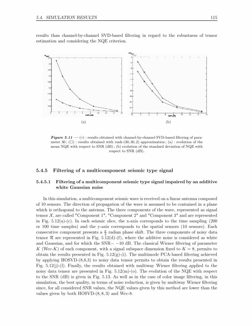
5.4. SIMULATION RESULTS 115
results than channel-by-channel SVD-based filtering in regard to the robustness of tensorestimation and considering the NQE criterion.
(a) (b)
Figure 5.11 — (◦) : results obtained with channel-by-channel SVD-based filtering of para-meter 30 ; (�) : results obtained with rank-(30, 30, 2) approximation ; (a) : evolution of themean NQE with respect to SNR (dB) ; (b) evolution of the standard deviation of NQE with
respect to SNR (dB).
5.4.5 Filtering of a multicomponent seismic type signal
5.4.5.1 Filtering of a multicomponent seismic type signal impaired by an additivewhite Gaussian noise
In this simulation, a multicomponent seismic wave is received on a linear antenna composedof 10 sensors. The direction of propagation of the wave is assumed to be contained in a planewhich is orthogonal to the antenna. The three components of the wave, represented as signaltensor X , are called "Component 1", "Component 2" and "Component 3" and are representedin Fig. 5.12(a)-(c). In each seismic slice, the x-axis corresponds to the time sampling (200or 100 time samples) and the y-axis corresponds to the spatial sensors (10 sensors). Eachconsecutive component presents a π
2 radian phase shift. The three components of noisy datatensor R are represented in Fig. 5.12(d)-(f), where the additive noise is considered as whiteand Gaussian, and for which the SNR= −10 dB. The classical Wiener filtering of parameterK (Wcc-K) of each component, with a signal subspace dimension fixed to K = 8, permits toobtain the results presented in Fig. 5.12(g)-(i). The multimode PCA-based filtering achievedby applying HOSVD-(8,8,3) to noisy data tensor permits to obtain the results presented inFig. 5.12(j)-(l). Finally, the results obtained with multiway Wiener filtering applied to thenoisy data tensor are presented in Fig. 5.12(m)-(o). The evolution of the NQE with respectto the SNR (dB) is given in Fig. 5.13. As well as in the case of color image filtering, in thissimulation, the best quality, in terms of noise reduction, is given by multiway Wiener filteringsince, for all considered SNR values, the NQE values given by this method are lower than thevalues given by both HOSVD-(8, 8, 3) and Wcc-8.
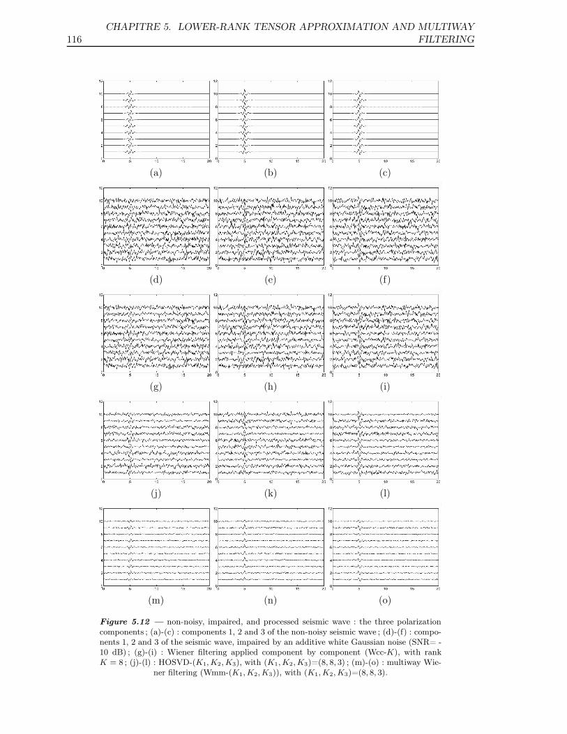
116CHAPITRE 5. LOWER-RANK TENSOR APPROXIMATION AND MULTIWAY
FILTERING
(a) (b) (c)
(d) (e) (f)
(g) (h) (i)
(j) (k) (l)
(m) (n) (o)
Figure 5.12 — non-noisy, impaired, and processed seismic wave : the three polarizationcomponents ; (a)-(c) : components 1, 2 and 3 of the non-noisy seismic wave ; (d)-(f) : compo-nents 1, 2 and 3 of the seismic wave, impaired by an additive white Gaussian noise (SNR= -10 dB) ; (g)-(i) : Wiener filtering applied component by component (Wcc-K), with rankK = 8 ; (j)-(l) : HOSVD-(K1, K2, K3), with (K1, K2, K3)=(8, 8, 3) ; (m)-(o) : multiway Wie-
ner filtering (Wmm-(K1, K2, K3)), with (K1, K2, K3)=(8, 8, 3).
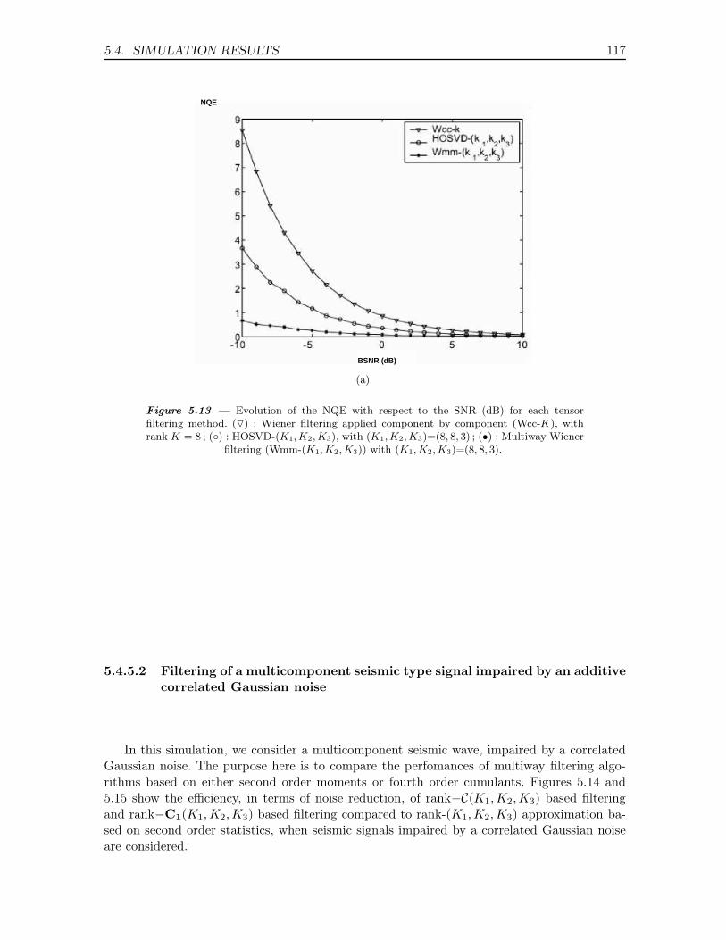
5.4. SIMULATION RESULTS 117
NQE
BSNR (dB)
(a)
Figure 5.13 — Evolution of the NQE with respect to the SNR (dB) for each tensorfiltering method. (▽) : Wiener filtering applied component by component (Wcc-K), withrank K = 8 ; (◦) : HOSVD-(K1, K2, K3), with (K1, K2, K3)=(8, 8, 3) ; (•) : Multiway Wiener
filtering (Wmm-(K1, K2, K3)) with (K1, K2, K3)=(8, 8, 3).
5.4.5.2 Filtering of a multicomponent seismic type signal impaired by an additivecorrelated Gaussian noise
In this simulation, we consider a multicomponent seismic wave, impaired by a correlatedGaussian noise. The purpose here is to compare the perfomances of multiway filtering algo-rithms based on either second order moments or fourth order cumulants. Figures 5.14 and5.15 show the efficiency, in terms of noise reduction, of rank−C(K1,K2,K3) based filteringand rank−C1(K1,K2,K3) based filtering compared to rank-(K1,K2,K3) approximation ba-sed on second order statistics, when seismic signals impaired by a correlated Gaussian noiseare considered.
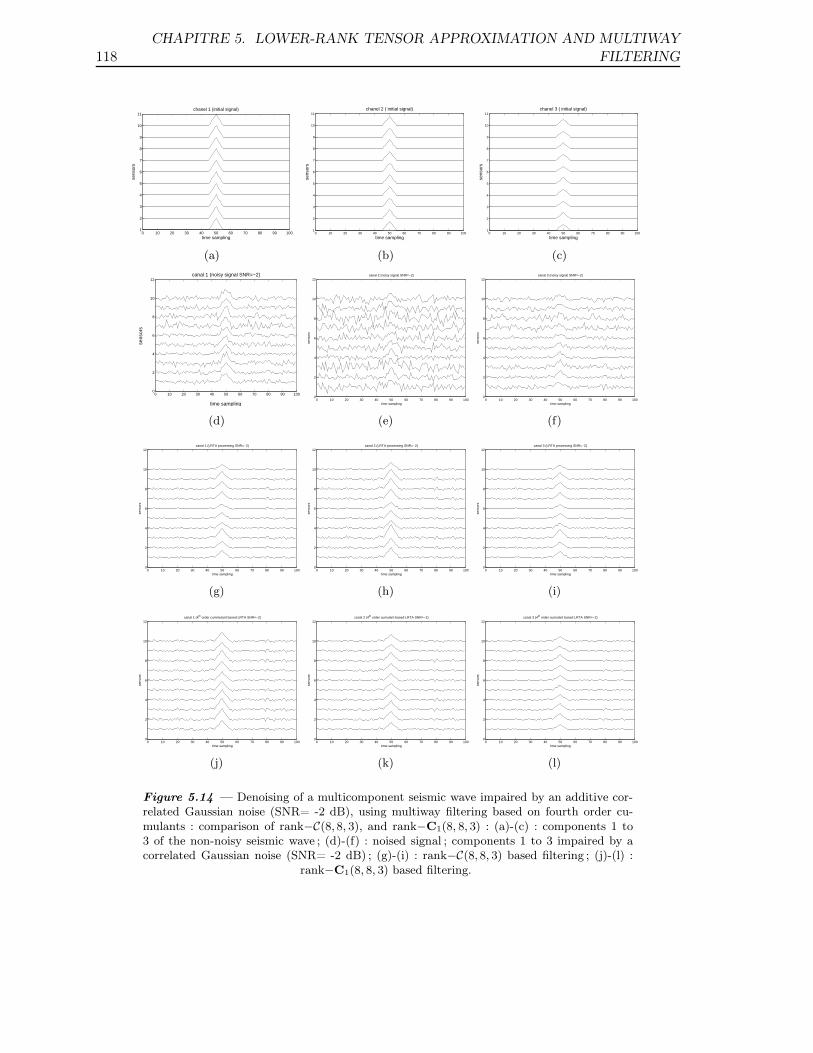
118CHAPITRE 5. LOWER-RANK TENSOR APPROXIMATION AND MULTIWAY
FILTERING
0 10 20 30 40 50 60 70 80 90 1001
2
3
4
5
6
7
8
9
10
11chanel 1 (initial signal)
time sampling
sens
ors
(a)
0 10 20 30 40 50 60 70 80 90 1001
2
3
4
5
6
7
8
9
10
11chanel 2 ( initial signal)
time sampling
sens
ors
(b)
0 10 20 30 40 50 60 70 80 90 1001
2
3
4
5
6
7
8
9
10
11chanel 3 ( initial signal)
time sampling
sens
ors
(c)
0 10 20 30 40 50 60 70 80 90 1000
2
4
6
8
10
12canal 1 (noisy signal SNR=−2)
time sampling
sens
ors
(d)
0 10 20 30 40 50 60 70 80 90 1000
2
4
6
8
10
12canal 2 (noisy signal SNR=−2)
time sampling
sens
ors
(e)
0 10 20 30 40 50 60 70 80 90 1000
2
4
6
8
10
12canal 3 (noisy signal SNR=−2)
time sampling
sens
ors
(f)
0 10 20 30 40 50 60 70 80 90 1000
2
4
6
8
10
12canal 1 (LRTA processing SNR=−2)
time sampling
sens
ors
(g)
0 10 20 30 40 50 60 70 80 90 1000
2
4
6
8
10
12canal 2 (LRTA processing SNR=−2)
time sampling
sens
ors
(h)
0 10 20 30 40 50 60 70 80 90 1000
2
4
6
8
10
12canal 3 (LRTA processing SNR=−2)
time sampling
sens
ors
(i)
0 10 20 30 40 50 60 70 80 90 1000
2
4
6
8
10
12canal 1 (4th order cummulant based LRTA SNR=−2)
time sampling
sens
ors
(j)
0 10 20 30 40 50 60 70 80 90 1000
2
4
6
8
10
12canal 2 (4th order cumulant based LRTA SNR=−2)
time sampling
sens
ors
(k)
0 10 20 30 40 50 60 70 80 90 1000
2
4
6
8
10
12canal 3 (4th order cumulant based LRTA SNR=−2)
time sampling
sens
ors
(l)
Figure 5.14 — Denoising of a multicomponent seismic wave impaired by an additive cor-related Gaussian noise (SNR= -2 dB), using multiway filtering based on fourth order cu-mulants : comparison of rank−C(8, 8, 3), and rank−C1(8, 8, 3) : (a)-(c) : components 1 to3 of the non-noisy seismic wave ; (d)-(f) : noised signal ; components 1 to 3 impaired by acorrelated Gaussian noise (SNR= -2 dB) ; (g)-(i) : rank−C(8, 8, 3) based filtering ; (j)-(l) :
rank−C1(8, 8, 3) based filtering.
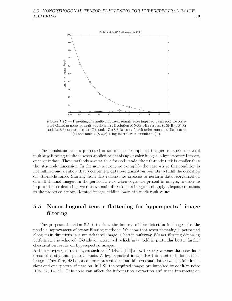
5.5. NONORTHOGONAL TENSOR FLATTENING FOR HYPERSPECTRAL IMAGEFILTERING 119
−10 −8 −6 −4 −2 0 2 4 6 8 100
1
2
3
4
5
6
7
8
9
10Evolution of the NQE with respect to SNR
NQ
E =
|| X
− X
estim
||2 /||
X||2
Figure 5.15 — Denoising of a multicomponent seismic wave impaired by an additive corre-lated Gaussian noise, by multiway filtering : Evolution of NQE with respect to SNR (dB) forrank-(8, 8, 3) approximation (�), rank−C1(8, 8, 3) using fourth order cumulant slice matrix
(◦) and rank−C(8, 8, 3) using fourth order cumulants (+).
The simulation results presented in section 5.4 exemplified the performance of severalmultiway filtering methods when applied to denoising of color images, a hyperspectral image,or seismic data. These methods assume that for each mode, the nth-mode rank is smaller thanthe nth-mode dimension. In the next section, we exemplify the case where this condition isnot fulfilled and we show that a convenient data reorganization permits to fulfill the conditionon nth-mode ranks. Starting from this remark, we propose to perform data reorganizationof multichannel images. In the particular case when edges are present in images, in order toimprove tensor denoising, we retrieve main directions in images and apply adequate rotationsto the processed tensor. Rotated images exhibit lower nth-mode rank values.
5.5 Nonorthogonal tensor flattening for hyperspectral imagefiltering
The purpose of section 5.5 is to show the interest of line detection in images, for thepossible improvement of tensor filtering methods. We show that when flattening is performedalong main directions in a multichannel image, a better multiway Wiener filtering denoisingperformance is achieved. Details are preserved, which may yield in particular better furtherclassification results on hyperspectral images.Airborne hyperspectral imagers such as HYDICE [113] allow to study a scene that uses hun-dreds of contiguous spectral bands. A hyperspectral image (HSI) is a set of bidimensionalimages. Therefore, HSI data can be represented as multidimensional data : two spatial dimen-sions and one spectral dimension. In HSI, the acquired images are impaired by additive noise[106, 32, 14, 53]. This noise can affect the information extraction and scene interpretation
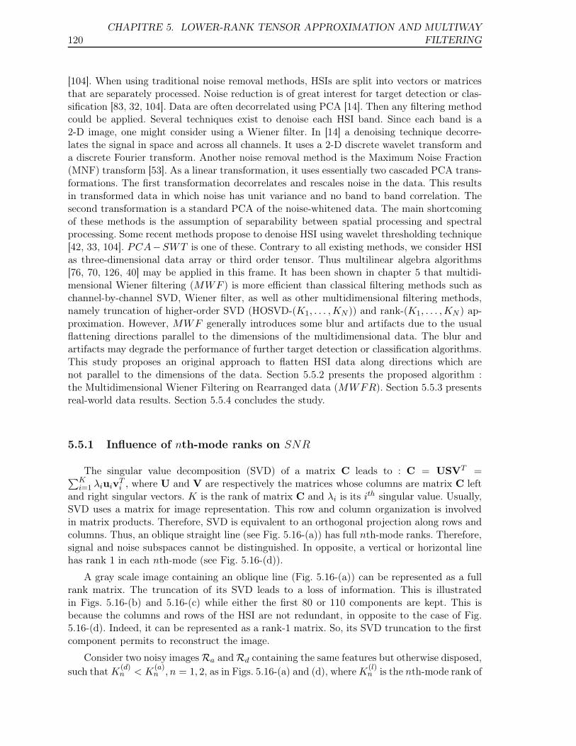
120CHAPITRE 5. LOWER-RANK TENSOR APPROXIMATION AND MULTIWAY
FILTERING
[104]. When using traditional noise removal methods, HSIs are split into vectors or matricesthat are separately processed. Noise reduction is of great interest for target detection or clas-sification [83, 32, 104]. Data are often decorrelated using PCA [14]. Then any filtering methodcould be applied. Several techniques exist to denoise each HSI band. Since each band is a2-D image, one might consider using a Wiener filter. In [14] a denoising technique decorre-lates the signal in space and across all channels. It uses a 2-D discrete wavelet transform anda discrete Fourier transform. Another noise removal method is the Maximum Noise Fraction(MNF) transform [53]. As a linear transformation, it uses essentially two cascaded PCA trans-formations. The first transformation decorrelates and rescales noise in the data. This resultsin transformed data in which noise has unit variance and no band to band correlation. Thesecond transformation is a standard PCA of the noise-whitened data. The main shortcomingof these methods is the assumption of separability between spatial processing and spectralprocessing. Some recent methods propose to denoise HSI using wavelet thresholding technique[42, 33, 104]. PCA−SWT is one of these. Contrary to all existing methods, we consider HSIas three-dimensional data array or third order tensor. Thus multilinear algebra algorithms[76, 70, 126, 40] may be applied in this frame. It has been shown in chapter 5 that multidi-mensional Wiener filtering (MWF ) is more efficient than classical filtering methods such aschannel-by-channel SVD, Wiener filter, as well as other multidimensional filtering methods,namely truncation of higher-order SVD (HOSVD-(K1, . . . ,KN )) and rank-(K1, . . . ,KN ) ap-proximation. However, MWF generally introduces some blur and artifacts due to the usualflattening directions parallel to the dimensions of the multidimensional data. The blur andartifacts may degrade the performance of further target detection or classification algorithms.This study proposes an original approach to flatten HSI data along directions which arenot parallel to the dimensions of the data. Section 5.5.2 presents the proposed algorithm :the Multidimensional Wiener Filtering on Rearranged data (MWFR). Section 5.5.3 presentsreal-world data results. Section 5.5.4 concludes the study.
5.5.1 Influence of nth-mode ranks on SNR
The singular value decomposition (SVD) of a matrix C leads to : C = USVT =∑Ki=1 λiuiv
Ti , where U and V are respectively the matrices whose columns are matrix C left
and right singular vectors. K is the rank of matrix C and λi is its ith singular value. Usually,SVD uses a matrix for image representation. This row and column organization is involvedin matrix products. Therefore, SVD is equivalent to an orthogonal projection along rows andcolumns. Thus, an oblique straight line (see Fig. 5.16-(a)) has full nth-mode ranks. Therefore,signal and noise subspaces cannot be distinguished. In opposite, a vertical or horizontal linehas rank 1 in each nth-mode (see Fig. 5.16-(d)).
A gray scale image containing an oblique line (Fig. 5.16-(a)) can be represented as a fullrank matrix. The truncation of its SVD leads to a loss of information. This is illustratedin Figs. 5.16-(b) and 5.16-(c) while either the first 80 or 110 components are kept. This isbecause the columns and rows of the HSI are not redundant, in opposite to the case of Fig.5.16-(d). Indeed, it can be represented as a rank-1 matrix. So, its SVD truncation to the firstcomponent permits to reconstruct the image.
Consider two noisy images Ra and Rd containing the same features but otherwise disposed,such that K
(d)n < K
(a)n , n = 1, 2, as in Figs. 5.16-(a) and (d), where K
(l)n is the nth-mode rank of
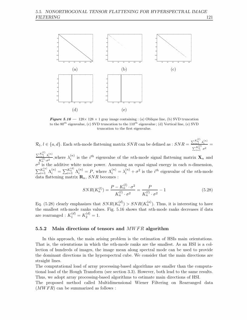
5.5. NONORTHOGONAL TENSOR FLATTENING FOR HYPERSPECTRAL IMAGEFILTERING 121
20 40 60 80 100 120
20
40
60
80
100
120
20 40 60 80 100 120
20
40
60
80
100
120
20 40 60 80 100 120
20
40
60
80
100
120
(a) (b) (c)
20 40 60 80 100 120
20
40
60
80
100
120
20 40 60 80 100 120
20
40
60
80
100
120
(d) (e)
Figure 5.16 — 128× 128 × 1 gray image containing : (a) Oblique line, (b) SVD truncation
to the 80th eigenvalue, (c) SVD truncation to the 110th eigenvalue ; (d) Vertical line, (e) SVDtruncation to the first eigenvalue.
Rl, l ∈ {a, d}. Each nth-mode flattening matrix SNR can be defined as : SNR =∑K
(l)n
i=1 λ(n)i
∑K(l)n
i=1 σ2
=
∑K(l)n
i=1 λ(n)i
K(l)n ·σ2
,where λ(n)i is the ith eigenvalue of the nth-mode signal flattening matrix Xn and
σ2 is the additive white noise power. Assuming an equal signal energy in each n-dimension,∑K
(a)n
i=1 Λ(n)i =
∑K(d)n
i=1 Λ(n)i = P , where Λ
(n)i = λ
(n)i + σ2 is the ith eigenvalue of the nth-mode
data flattening matrix Rn, SNR becomes :
SNR(K(l)n ) =
P − K(l)n · σ2
K(l)n · σ2
=P
K(l)n · σ2
− 1 (5.28)
Eq. (5.28) clearly emphasizes that SNR(K(d)n ) > SNR(K
(a)n ). Thus, it is interesting to have
the smallest nth-mode ranks values. Fig. 5.16 shows that nth-mode ranks decreases if dataare rearranged : K
(d)1 = K
(d)2 = 1.
5.5.2 Main directions of tensors and MWFR algorithm
In this approach, the main arising problem is the estimation of HSIs main orientations.That is, the orientations in which the nth-mode ranks are the smallest. As an HSI is a col-lection of hundreds of images, the image mean along spectral mode can be used to providethe dominant directions in the hyperspectral cube. We consider that the main directions arestraight lines.The computational load of array processing-based algorithms are smaller than the computa-tional load of the Hough Transform (see section 3.3). However, both lead to the same results.Thus, we adopt array processing-based algorithms to estimate main directions of HSI.The proposed method called Multidimensional Wiener Filtering on Rearranged data(MWFR) can be summarized as follows :
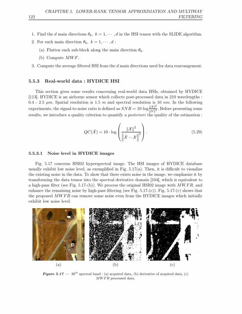
122CHAPITRE 5. LOWER-RANK TENSOR APPROXIMATION AND MULTIWAY
FILTERING
1. Find the d main directions θk, k = 1, · · · , d in the HSI tensor with the SLIDE algorithm.
2. For each main direction θk, k = 1, · · · , d :
(a) Flatten each sub-block along the main direction θk.
(b) Compute MWF .
3. Compute the average filtered HSI from the d main directions used for data rearrangement.
5.5.3 Real-world data : HYDICE HSI
This section gives some results concerning real-world data HSIs, obtained by HYDICE[113]. HYDICE is an airborne sensor which collects post-processed data in 210 wavelengths :0.4 - 2.5 µm. Spatial resolution is 1.5 m and spectral resolution is 10 nm. In the following
experiments, the signal-to-noise ratio is defined as SNR = 10·log ‖X‖2
‖N‖2 . Before presenting some
results, we introduce a quality criterion to quantify a posteriori the quality of the estimation :
QC(X̂ ) = 10 · log
‖X‖2
∥∥∥X̂ − X∥∥∥
2
. (5.29)
5.5.3.1 Noise level in HYDICE images
Fig. 5.17 concerns HSI02 hyperspectral image. The HSI images of HYDICE databaseusually exhibit low noise level, as exemplified in Fig. 5.17(a). Then, it is difficult to visualizethe existing noise in the data. To show that there exists noise in the image, we emphasize it bytransforming the data tensor into the spectral derivative domain [104], which is equivalent toa high-pass filter (see Fig. 5.17-(b)). We process the original HSI02 image with MWFR, andenhance the remaining noise by high-pass filtering (see Fig. 5.17-(c)). Fig. 5.17-(c) shows thatthe proposed MWFR can remove some noise even from the HYDICE images which initiallyexhibit low noise level.
(a) (b) (c)
Figure 5.17 — 30th spectral band : (a) acquired data, (b) derivative of acquired data, (c)MWFR processed data.
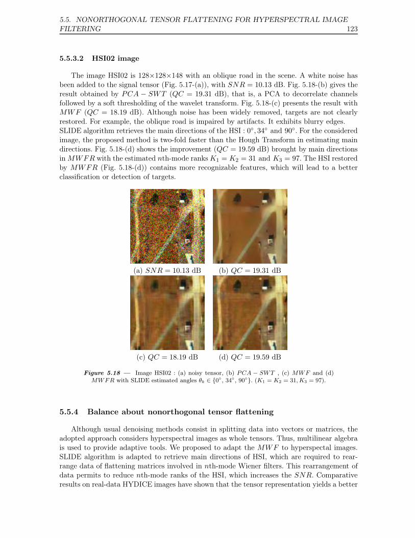
5.5. NONORTHOGONAL TENSOR FLATTENING FOR HYPERSPECTRAL IMAGEFILTERING 123
5.5.3.2 HSI02 image
The image HSI02 is 128×128×148 with an oblique road in the scene. A white noise hasbeen added to the signal tensor (Fig. 5.17-(a)), with SNR = 10.13 dB. Fig. 5.18-(b) gives theresult obtained by PCA − SWT (QC = 19.31 dB), that is, a PCA to decorrelate channelsfollowed by a soft thresholding of the wavelet transform. Fig. 5.18-(c) presents the result withMWF (QC = 18.19 dB). Although noise has been widely removed, targets are not clearlyrestored. For example, the oblique road is impaired by artifacts. It exhibits blurry edges.SLIDE algorithm retrieves the main directions of the HSI : 0◦, 34◦ and 90◦. For the consideredimage, the proposed method is two-fold faster than the Hough Transform in estimating maindirections. Fig. 5.18-(d) shows the improvement (QC = 19.59 dB) brought by main directionsin MWFR with the estimated nth-mode ranks K1 = K2 = 31 and K3 = 97. The HSI restoredby MWFR (Fig. 5.18-(d)) contains more recognizable features, which will lead to a betterclassification or detection of targets.
(a) SNR = 10.13 dB (b) QC = 19.31 dB
(c) QC = 18.19 dB (d) QC = 19.59 dB
Figure 5.18 — Image HSI02 : (a) noisy tensor, (b) PCA − SWT , (c) MWF and (d)MWFR with SLIDE estimated angles θk ∈ {0◦, 34◦, 90◦}. (K1 = K2 = 31, K3 = 97).
5.5.4 Balance about nonorthogonal tensor flattening
Although usual denoising methods consist in splitting data into vectors or matrices, theadopted approach considers hyperspectral images as whole tensors. Thus, multilinear algebrais used to provide adaptive tools. We proposed to adapt the MWF to hyperspectal images.SLIDE algorithm is adapted to retrieve main directions of HSI, which are required to rear-range data of flattening matrices involved in nth-mode Wiener filters. This rearrangement ofdata permits to reduce nth-mode ranks of the HSI, which increases the SNR. Comparativeresults on real-data HYDICE images have shown that the tensor representation yields a better
124CHAPITRE 5. LOWER-RANK TENSOR APPROXIMATION AND MULTIWAY
FILTERING
restoration compared to channel-by-channel denoising or to PCA − SWT , wavelet threshol-ding technique. MWFR clearly outperforms MWF , especially for small targets which arenot parallel to rows or columns. The MWFR can be seen as a noise removal method forfurther applications such as classification or target detection in HSI.
5.6 Conclusion of chapter 5
In this chapter, an overview on new mathematical methods dedicated to multicomponentdata is presented. Multicomponent data are represented as tensors, that is, multiway arrays,and the tensor filtering methods that are presented rely on multilinear algebra. First we presenthow to perform channel-by-channel SVD-based filtering. Then we review three methods thattake into account the relationships between each component of a processed tensor. The firstmethod consists of an extension of the classical SVD-based filtering method. In the case ofan additive white Gaussian noise, the signal tensor is estimated thanks to a multimode PCAachieved by applying a lower rank-(K1, . . . ,KN ) approximation to the noisy data tensor, or alower rank-(K1, . . . ,KN ) truncation of its HOSVD. This method is implicitly based on secondorder statistics and relies on the orthogonality between nth-mode noise and signal subspaces.The second presented method consists of an improvement of the multimode PCA-based ten-sor filtering in the case of an additive correlated Gaussian noise. In this case, the covariancematrix involved in TUCKALS3 algorithm is replaced with the fourth order cumulant matrixof the related vectors. We reviewed a low computational load procedure involving the fourthorder cumulant slice matrix instead of fourth order cumulants. This improved multimode PCAprovides good performances compared to the multimode PCA method based on second orderstatistics, as was shown in the case of noise reduction in color images and multicomponentseismic waves.The third reviewed method is a multiway version of the classical Wiener filtering. In exten-sion to the one-dimensional case, the nth-mode Wiener filters are estimated by minimizingthe mean squared error between the expected signal tensor and the estimated signal tensorobtained by applying the nth-mode Wiener filters to the noisy data tensor thanks to thenth-mode product operator. An Alternating Least Squares algorithm has been presented todetermine the optimal nth-mode Wiener filters. The performances of this multiway Wienerfiltering and comparative results with multimode PCA have been presented in the case ofadditive white noise reduction in a color image and in a multicomponent seismic wave.Finally, we proposed to use straight line estimation methods to improve HSI denoising in thecase where main directions are expected. Nonorthogonal tensor flattening, performed alongmain directions in HSI, improves the denoising results.
Concluding remarks
THIS thesis was devoted to the study of subspace-based and optimization methods, ap-plied to one-dimensional, bidimensional, and multidimensional signals. After reminding
the principles of an array processing problem, we proved the interest of a fast optimizationmethod which combines DIRECT and spline interpolation methods, in the resolution of asource characterization problem, when an antenna with a large number of sensors is used andin the presence of phase distortions. Starting from an existing signal generation formalism, weextended a straight line estimation method. We adapted existing array processing methodsto the retrieval of free-form objects in an image. Finally, we presented the last advances intensor processing methods and proposed an improvement in the case where straight edgesare present in the processed tensor. For this we used the straight line estimation methodpresented in the first part of the manuscript.
Thus, in the first part, we focus on one-dimensional signals. In chapter 1, we firstreminded the purposes of an array processing problem, the definition of an antenna as a setof sensors, of the medium and sources. We introduced the reader with the definition of thecovariance matrix, and emphasized the interest of exploiting its eigen-elements. Within themeasurement space spanned by the eigenvectors of the covariance matrix, we distinguishedthe useful signal subspace and the noise subspace. We focused on the interest of spatialsmoothing in the case of correlated sources, and emphasized the orthogonality betweensignal and noise subspaces when useful signal and noise are uncorrelated. Starting from thisassumption, the subspace-based MUSIC (MUltiple SIgnal Characterization) method retrievesdirections-of-arrival by testing the orthogonality between a signal vector model and the noisesubspace vectors. We explained the principles of a novel optimization method that combineseither gradient or DIRECT algorithms with spline interpolation. In chapter 2, we considerthe issue of direction-of-arrival estimation in the case where phase distortions are present.We proposed a novel optimization method, that combines DIRECT (DIviding RECTangles)algorithm with spline interpolation, in order to retrieve wavefront phase distortions. First,a rough estimate of several directions-of-arrival is obtained by MUSIC method. Then foreach estimated value, used as an initialization parameter, phase shift values between a planewavefront and the expected wavefront are estimated by DIRECT combined with splineinterpolation. Phase shifts are canceled in the received signal realizations. Finally, MUSICmethod is applied in a reduced interval around the initialization direction-of-arrival value.Owing to phase cancelation, several sources may be resolved inside this interval. The proposedalgorithm was applied to the characterization of three sources in a noisy environment.
In the second part, we proposed several methods for image - bidimensional data- unders-
126 CONCLUDING REMARKS
tanding applications. In particular, we described an existing formalism for signal generationout of an image. In this framework, a contour in an image is considered as a wavefront,whose propagation is simulated via a signal generation scheme. In chapter 3, we remindedthe SLIDE (Subspace-based LIne DEtection) method that uses TLS-ESPRIT (Total LeastSquare-Estimation of Signal Parameters via Rotational Invariance Techniques) algorithm toretrieve straight line orientations. We proposed a faster method, namely the Propagator,which avoids the covariance matrix eigendecomposition, either by partitioning it or byworking directly on the processed signal. Propagator exhibits a low computational load. Forstraight line estimation, we also proposed a novel high-resolution method for the estimationof straight line offsets. This method is faster than the extension of the Hough transform,especially when noisy images are processed, and copes with parallel lines. We extendedstraight line estimation methods to the estimation of any nearly linear contour. For this,we adapted gradient method and variable step gradient method to minimize a least-squarescriterion between a model signal and the signal generated from the processed image. Weproposed a generalization of this optimization method to the retrieval of several contours, inparticular by minimizing a criterion based on propagator operator. We proposed an improvedoptimization method, that combines gradient method and spline interpolation. This methodis fast and robust to noise impairment. By means of a comparison with GVF method, weemphasized the ability of the proposed optimization method to retrieve contours with highcurvature in a noisy environment. Straight line and distorted contour estimation methodswere applied to images coming from robotic vision, to aerial and medical images. In chapter4, we extended the work devoted to rectilinear and nearly rectilinear contours to star-shapedcontours. The most novel aspect of this chapter is the signal generation method upon a virtualcircular antenna : we adapted a circular antenna to the processed image, to generate a linearphase signal and enable the use of high-resolution methods for possibly close concentric circleradius estimation. Signal generation upon linear antenna permits to locate the center of theexpected features : the non-zero sections in the signals generated on the image left and topsides indicate the presence of features. Signal generation on linear antenna yields the axialparameters and center coordinates of ellipses. To retrieve rotated ellipses, we rotate the imageuntil the non-zero section length in the left and bottom signals is the most different. Whendistorted contours are expected, optimization algorithms which are analogous to those appliedfor nearly straight contour retrieval are applied to signals generated on the proposed circu-lar antenna. We consider several application cases such as biometrics, non-destructive control.
The third part is concerned with tensor -multidimensional data- signal processing,and demonstrates the usefulness of straight line retrieval methods for the improvement ofdenoising by multilinear subspace-based methods. Firstly, we presented the last advancesin tensor signal processing. We reminded the principles of truncation of higher-orderSingular Value Decomposition, HOSVD-(K1, . . . ,KN ), which relies on the definition ofsignal subspace dimensions K1, . . . ,KN . We reminded the principles of the AlternatingLeast-Squares optimization algorithm, which improves HOSVD-(K1, . . . ,KN ) and turns itinto rank-(K1, . . . ,KN ) tensor approximation. We show how higher-order statistics, used inrank-(K1, . . . ,KN ) tensor approximation in place of second order statistics, improve tensorsignal denoising in the case of correlated Gaussian noise. In particular, we propose a fastversion of this method : we use fourth-order cumulant slice matrix in place of the wholefourth-order cumulant tensor. We give details about a multiway version of Wiener filtering,
CONCLUDING REMARKS 127
which seeks for noise removal by minimizing the expectancy of the squared difference betweenexpected and estimated tensor signals. Multiway Wiener filtering relies on data projectionupon useful signal subspace. The estimation of projectors, for each nth-mode, is performedby an ALS loop. We performed several experiments on color images, considering particularcases where the signal subspace dimension is equal to the number of channels in the colormode, the case where the signal subspace dimension is underestimated, or where the image isimpaired by correlated Gaussian noise. We also performed noise removal on multicomponentseismic wave. Secondly, we proposed an improvement of tensor signal denoising, using thework devoted to straight line estimation : When rectilinear features are present in theprocessed tensor, we show that nonorthogonal tensor flattening, and more precisely flatteningalong the orientations of edges, improves the denoising result.
Several prospects can be drawn from this work. SLIDE method has already been appliedto the estimation of cinematic parameters of object trajectories. This led to valuable resultsin the case of constant speed motion. The advances proposed in the second part concerningdistorted contour retrieval could be adapted to the characterization of non-constant speedtrajectories.In the field of tensor signal processing, the proposed nonorthogonal tensor flattening methodreduces blurring effect which is due to the projection upon signal subspace in each mode. Inparticular, tensor signal processing methods preserve details. We could adapt this methodfor an application to target detection. Especially, HSI (Hyperspectral Images) data requirespreprocessing such as noise reduction in order to increase the efficiency of classification al-gorithms. Indeed, a noise reduction processing decreases the spectral variability, which isuseful for further classification and detection processing. Moreover the unreasonably large di-mension of HSI not only increases computational complexity but also degrades classificationaccuracy. HSI images contain highly correlated bands, which results in spectral redundancy.Independent Component Analysis (ICA) is applied to reduce the number of spectral bands byselecting spectral components. It would be of great interest to combine the proposed tensorfiltering algorithms with ICA, for a joint denoising and dimensionality reduction algorithm.

ANNEXE
A Appendix A :
mathematical
considerations about
multiway filtering
A.1 Appendix : Alternating Least Squares algorithms
In this section, we detail the Alternating Least Squares (ALS) algorithms which are usedin Rank-(K1, . . . ,KN ) tensor approximation, in the fourth order cumulant slice matrix-basedmultimode PCA-based filtering,
A.1.1 ALS algorithm in Rank-(K1, . . . , KN) approximation - TUCKALS3algorithm
In this subsection, we present the ALS algorithm which is performed in Rank-(K1, . . . ,KN )approximation.
1. Input : data tensor R, and dimensions K1, . . . ,KN of all nth-mode signal subspaces.
2. Initialization k = 0 : For n = 1 to N , calculate the projectors P(n)0 given by HOSVD-
(K1, . . . ,KN ) :
(a) nth-mode flatten R into matrix Rn ;
(b) Compute the SVD of Rn ;
(c) Compute matrix U(n)0 formed by the Kn eigenvectors associated with the Kn largest
singular values of Rn. U(n)0 is the initial matrix of the nth-mode signal subspace
orthogonal basis vectors ;
(d) Form the initial orthogonal projector P(n)0 = U
(n)0 U
(n)T
0 on the nth-mode signalsubspace ;
(e) Compute the HOSVD-(K1, . . . ,KN ) of tensor R given by
B0 = R×1 P(1)0 ×2 · · · ×N P
(N)0 ;
3. ALS loop :Repeat until convergence, that is, for example, while ‖Bk+1 − Bk‖2 > ǫ, ǫ > 0 being aprior fixed threshold,
130ANNEXE A. APPENDIX A : MATHEMATICAL CONSIDERATIONS ABOUT
MULTIWAY FILTERING
(a) For n = 1 to N :
i. Form B(n),k :B(n),k = R×1 P
(1)k+1 ×2 · · · ×n−1 P
(n−1)k+1 ×n+1 P
(n+1)k ×n+2 · · · ×N P
(N)k ;
ii. nth-mode flatten tensor B(n),k into matrix B(n),kn ;
iii. Compute matrix C(n),k = B(n),kn RT
n ;
iv. Compute matrix U(n)k+1 composed of the Kn eigenvectors associated with the Kn
largest eigenvalues of C(n),k. U(n)k is the matrix of the nth-mode signal subspace
orthogonal basis vectors at the kth iteration ;
v. Compute P(n)k+1 = U
(n)k+1U
(n)T
k+1 ;
(b) Compute Bk+1 = R×1 P(1)k+1 ×2 · · · ×N P
(N)k+1 ;
(c) Increment k.
4. Output : the estimated signal tensor is obtained through X̂ = R×1P(1)kstop
×2· · ·×NP(N)kstop
.
X̂ is the rank-(K1, . . . ,KN ) approximation of R, where kstop is the index of the lastiteration after the convergence of TUCKALS3 algorithm.
In this algorithm, the second order statistics comes from the SVD of matrix Rn at step 2b,which is equivalent, up to 1
Mnmultiplicative factor, to the estimation of tensor R nth-mode
vectors [97]. The definition of Mn is given in (5.1). In the same way, at step 3(a)iii, matrixC(n),k is, up to 1
Mnmultiplicative factor, the estimation of the covariance matrix between
tensor R and tensor B(n),k nth-mode vectors. According to step 3(a)i, B(n),k represents data
tensor R filtered in every mth-mode but the nth-mode, by projection-filters P(m)l , with m 6= n,
l = k if m > n and l = k + 1 if m < n. TUCKALS3 algorithm has recently been used toprocess a multimode PCA in order to perform white noise removal in color images [94].
A.1.2 Fourth order cumulant slice matrix-based multimode PCA-basedfiltering
In this subsection, we present the ALS algorithm which is performed in Fourth ordercumulant slice matrix-based multimode PCA-based filtering.
1. Initialization k = 0 :
For all n = 1 to N , P(n)0 = U
(n)0 U
(n)T
0 . U(n)0 is the matrix of the Kn eigenvectors
associated with the Kn largest eigenvalues of fourth order cumulant slice matrix C(n),0q
of tensor R nth-mode vectors.
2. ALS loop :
The steps (b) and (c) of the ALS loop are the same as in the algorithm "rank-(K1, . . . ,KN) approximation - TUCKALS3 algorithm " described previously, andstep (a) is replaced by :
(a) For n = 1 to N :
i. B(n),k = R×1 P(1)k+1 ×2 · · · ×n−1 P
(n−1)k+1 ×n+1 P
(n+1)k ×n+2 · · · ×N P
(N)k ;
A.1. APPENDIX : ALTERNATING LEAST SQUARES ALGORITHMS 131
ii. Compute cumulant slice matrix C(n),kq associated with the fourth order cumu-
lants of tensors R and B(n),k nth-mode vectors. Every element of C(n),kq is given
in (5.11) ;
iii. Process matrix C(n),kq eigenvalue decomposition (EVD) and put the Kn eigen-
vectors associated with the Kn largest eigenvalues into U(n)k+1 ;
iv. Compute projector P(n)k+1 = U
(n)k+1U
(n)T
k+1 ;
3. Output : X̂ = R×1P(1)kstop
×2 · · ·×N P(N)kstop
, with kstop being the index of the last iterationafter convergence of the algorithm.
Using the cumulant slice matrix in place of the whole cumulant tensor saves computationalload and memory size.
A.1.3 ALS algorithm in multiway Wiener filtering
Alternating Least Squares (ALS) algorithm used in multiway Wiener filtering can besummarized in the following steps :
1. Initialization k = 0 : R0 = R ⇔ H(n)0 = IIn, Identity matrix, for all n = 1 to N .
2. ALS loop :Repeat until convergence, that is,
∥∥Rk+1 −Rk∥∥2
< ǫ, with ǫ > 0 a prior fixed threshold,
(a) for n = 1 to N :
i. Form R(n),k :R(n),k = R×1 H
(1)k+1 ×2 · · · ×n−1 H
(n−1)k+1 ×n+1 H
(n+1)k ×n+2 . . . ×N H
(N)k ;
ii. Determine H(n)k+1 = arg min
Z(n)
∥∥X −R(n),k ×n Z(n)∥∥2
subject to Z(n) ∈ RIn×In thanks to the following procedure :
A. nth-mode flatten R(n),k into R(n),kn = Rn(H
(1)k+1 ⊗ · · · ⊗H
(n−1)k+1 ⊗H
(n+1)k ⊗
· · · ⊗H(N)k )T , and R into Rn ;
B. Compute γ(n)RR = E[RnR
(n),kn
T],
C. Determine λγ1 , . . . , λγ
Kn, the Kn largest eigenvalues of γ
(n)RR ;
D. For kn = 1 to In, estimate σ(n)Γ
2thanks to (5.22) and for kn = 1 to Kn,
estimate βknthanks to (5.21) ;
E. Compute Γ(n)RR = E[R
(n),kn R
(n),kn
T] ;
F. Determine λΓ1 , . . . , λΓ
Kn, the Kn largest eigenvalues of Γ
(n)RR ;
G. Determine V(n)s , the matrix of the Kn eigenvectors associated with the Kn
largest eigenvalues of Γ(n)RR ;
H. Compute the weight matrix γ(n)OOΛ
(n)−1
Γs given in (5.20) ;
I. Compute H(n)k+1, the nth-mode Wiener filter at the (k +1)th iteration, using
(5.19) ;
132ANNEXE A. APPENDIX A : MATHEMATICAL CONSIDERATIONS ABOUT
MULTIWAY FILTERING
(b) Form Rk+1 = R×1 H(1)k+1 ×2 · · · ×N H
(N)k+1 ;
(c) Increment k ;
3. output : X̂ = R ×1 H(1)kstop
×2 · · · ×N H(N)kstop
, with kstop being the last iteration afterconvergence of the algorithm.
A.2 Appendix : nth-mode Wiener filter analytical expression
The following computations are related to section 5.3.3. They rely on the definitions andproperties of tensors and multilinear algebra that can be found in [38, 40, 41].
The mean squared error involved in multiway Wiener filtering is given by relation :
e(H(1), . . . ,H(N))=E[‖X‖2
]− 2E
[⟨X ,R×1 H(1) ×2 · · · ×N H(N)
⟩]
+ E[∥∥R×1 H(1) ×2 · · · ×N H(N)
∥∥2].
(A.1)
The Frobenius norm of a tensor is also equal to the norm of any of its nth-mode flatteningmatrices. In order to determine the expression of filter H(n) associated with fixed filters H(m),for all m 6= n, the nth-mode flattening of (A.1) is processed.
Let us define matrix F(n)XR as :
F(n)XR = XnT
(n)RTn . (A.2)
with :
T(n) = H(1) ⊗ · · · ⊗ H(n−1) ⊗ H(n+1) ⊗ · · · ⊗ H(N). (A.3)
Hence, for all n = 1 to N ,
⟨X ,R×1 H(1) ×2 · · · ×N H(N)
⟩= tr
(F
(n)XRH(n)T
). (A.4)
Let us define matrix G(n)RR as :
G(n)RR = RnQ
(n)RnT , (A.5)
with :
Q(n) = T(n)TT(n)
Q(n) = H(1)TH(1) ⊗ · · · ⊗ H(n−1)TH(n−1) ⊗H(n+1)TH(n+1) ⊗ · · · ⊗H(N)TH(N). (A.6)
Hence, for all n = 1 to N :
∥∥∥R×1 H(1) ×2 · · · ×N H(N)∥∥∥
2= tr
(H(n)G
(n)RRH(n)T
). (A.7)
A.2. APPENDIX : NTH-MODE WIENER FILTER ANALYTICAL EXPRESSION 133
Minimization of mean squared error e(H(1), . . . ,H(N))
The expression of the nth-mode flattened mean squared error e(H(1), . . . ,H(N)) is thefollowing :
e(H(1), . . . ,H(N))=E[‖Xn‖2
]− 2E
[tr
(F
(n)XRH(n)T
)]
+ E[tr
(H(n)G
(n)RRH(n)T
)].
(A.8)
Assuming that m-mode filters H(m) are fixed for all m 6= n, mean squared errore(H(1), . . . ,H(N)) is minimal when its gradient with respect to nth-mode filter H(n) is null :
grad(e) =
[∂e
∂H(1), . . . ,
∂e
∂H(N)
]T
(A.9)
that is, when ∂e
∂H(n) are conjointly null for all n = 1 to N . Let us study ∂e
∂H(n) for a given
nth-mode. The nth-mode filters H(m) are supposed to be fixed for all m ∈ {1, . . . , N}−{n}.Then ∂e
∂H(n) = 0 implies that :
E
[∂
∂H(n)tr
(H(n)G
(n)RRH(n)T
)]= 2E
[∂
∂H(n)tr
(F
(n)XRH(n)T
)], (A.10)
We compute then the derivatives on both sides in (A.10), taking into account the fact that
G(n)RR and F
(n)XR are independent from H(n) :
∂
∂H(n)tr
(F
(n)XRH(n)T
)= F
(n)XR. (A.11)
∂
∂H(n)tr
(H(n)G
(n)RRH(n)T
)= 2H(n)G
(n)RR. (A.12)
Expression of H(n), nth-mode Wiener filter
Replacing (A.11) and (A.12) into expression (A.10) leads to the expression of H(n) nth-mode Wiener filter associated with fixed H(m) m-mode filters, m 6= n :
H(n) = γ(n)XRΓ
(n)−1
RR , (A.13)
where :
γ(n)XR = E
[F
(n)XR
](A.14)
is the T(n)-weighted covariance matrix between the signal Xn and the data Rn, and :
Γ(n)RR = E
[G
(n)RR
](A.15)
is the Q(n)-weighted correlation matrix of the data.
134ANNEXE A. APPENDIX A : MATHEMATICAL CONSIDERATIONS ABOUT
MULTIWAY FILTERING
A.3 Appendix : Assumptions and related expression of the nth-mode Wiener filter
The following computations are related to section 5.3.3. Let us consider matrices T(n) andQ(n) defined in (A.3) and (A.6). Their generic (i, j)-terms are denoted respectively by T
(n)ij
and by Q(n)ij .
Weight matrix term independence
The terms of weight matrix O(n) ∈ RKn×Mn are supposed mutually independent :
E [oklomn] = αklδkmδln, (A.16)
whatever k and m ∈ {1, . . . ,Kn}, l and n ∈ {1, . . . ,Mn} and where αkl is not null.
White and Gaussian noise condition
White and Gaussian noise condition applied to the nth-mode flattening Nn can be ex-pressed by :
E [nklnpq] = σ2nδkpδlq, (A.17)
where (k, p) ∈ {1, . . . ,Kn}2, (l, q) ∈ {1, . . . ,Mn}2 and σ2n is the nth-mode noise power.
Noise and signal independence
The condition on noise and signal independence can be expressed by :
E [xklnpq] = 0, (A.18)
for all (k, p) ∈ {1, . . . ,Kn}2 and (l, q) ∈ {1, . . . ,Mn}2. Hence, T(n) and Q(n)-weighted (X,N)-covariance matrices are null :
γ(n)XN = γ
(n)NX = 0,
Γ(n)XN = Γ
(n)NX = 0.
(A.19)
Indeed, their (i, j)-term is :(γ
(n)XN
)ij
=∑Mn
k=1
∑Mn
l=1 T(n)kl E [xiknjl] ,(
Γ(n)XN
)ij
=∑Mn
k=1
∑Mn
l=1 Q(n)kl E [xiknjl] .
(A.20)
Expressions of weighted covariance matrices
Covariance matrix γ(n)RR
As Rn = Xn + Nn, the expression of γ(n)RR reads :
γ(n)RR = γ
(n)XX + γ
(n)XN + γ
(n)NX + γ
(n)NN. (A.21)
A.3. APPENDIX : ASSUMPTIONS AND RELATED EXPRESSION OF THENTH-MODE WIENER FILTER 135
So according to (A.19), γ(n)RR weighted covariance matrix can be expressed by :
γ(n)RR = γ
(n)XX + γ
(n)NN. (A.22)
Moreover :
γ(n)XR = γ
(n)XX + γ
(n)XN = γ
(n)XX. (A.23)
Covariance matrix Γ(n)RR
Relations (A.21), (A.22), and (A.23) hold as well for Γ(n)RR :
Γ(n)RR = Γ
(n)XX + Γ
(n)XN + Γ
(n)NX + Γ
(n)NN,
and :
Γ(n)RR = Γ
(n)XX + Γ
(n)NN. (A.24)
Moreover :
Γ(n)XR = Γ
(n)XX + Γ
(n)XN = Γ
(n)XX. (A.25)
Expressions of Γ(n)NN and γ
(n)NN
According to (A.17), the (i, j)-term of Γ(n)NN is the following :
(Γ
(n)NN
)ij
=
Mn∑
k=1
Mn∑
l=1
Q(n)kl E[niknjl] = σ
(n)2
Γ δij, (A.26)
with
σ(n)2
Γ = tr(Q(n))σ2n. (A.27)
Hence :
Γ(n)NN = σ
(n)2
Γ IIn . (A.28)
The (i, j)-term of γ(n)NN can also be expressed by :
(γ
(n)NN
)ij
=
Mn∑
k=1
Mn∑
l=1
T(n)kl E[niknjl] = σ(n)2
γ δij,
with :
σ(n)2γ = tr(T(n))σ2
n.
Hence :
γ(n)NN = σ(n)2
γ IIn . (A.29)
136ANNEXE A. APPENDIX A : MATHEMATICAL CONSIDERATIONS ABOUT
MULTIWAY FILTERING
Expressions of Γ(n)XX and γ
(n)XX
Considering the signal model (5.18) :
γ(n)XX = V(n)
s γ(n)OOV(n)T
s , (A.30)
whereγ
(n)OO = E
[O(n)T(n)O(n)T
]. (A.31)
According to (A.16), the generic term of γ(n)OO is :
(γ
(n)OO
)ij
=
Mn∑
k=1
Mn∑
l=1
T(n)kl E [niknjl] = βiδij , (A.32)
where, for all i = 1 to Kn :
βi =
Mn∑
k=1
T(n)kk αik (A.33)
and where αik is defined in (A.16). So, γ(n)OO is a diagonal matrix :
γ(n)OO =
β1 0. . .
0 βKn
. (A.34)
The matrix Γ(n)XX is also expressed as :
Γ(n)XX = V(n)
s Γ(n)OOV(n)T
s , (A.35)
where Γ(n)OO is the diagonal matrix :
Γ(n)OO =
ǫ1 0. . .
0 ǫKn
, (A.36)
and :
ǫi =
Mn∑
k=1
Q(n)kk αik, (A.37)
where αik is defined in (A.16).
Final expression of H(n), nth-mode Wiener filter
According to (A.23) and (A.30) :
γ(n)XR = V(n)
s γ(n)OOV(n)T
s . (A.38)
According to (A.24), (A.28) and (A.35) :
Γ(n)RR = V(n)
s Γ(n)OOV(n)T
s + σ(n)2
Γ IIn ,
A.3. APPENDIX : ASSUMPTIONS AND RELATED EXPRESSION OF THENTH-MODE WIENER FILTER 137
which can be expressed as :
Γ(n)RR =
[V(n)
s V(n)b
] [Γ
(n)OO + σ
(n)2
Γ IKn 0
0 σ(n)2
Γ IIn−Kn
][V
(n)T
s
V(n)T
b
], (A.39)
with V(n)b ∈ St(In, In−Kn) the column-wise orthogonal matrix containing the noise subspace
basis vectors. The assumption of noise and signal independence implies that the noise andsignal subspaces are orthogonal :
V(n)T
s V(n)b = 0. (A.40)
Let us call :Λ(n)
s = Γ(n)OO + σ
(n)2
Γ IKn , (A.41)
and :Λ
(n)b = σ
(n)2
Γ IIn−Kn . (A.42)
Inserting the last expressions of γ(n)XR and Γ
(n)RR (see (A.38) and (A.39)) into Wiener nth-
mode filter expression (A.13) leads to :
H(n) = V(n)s γ
(n)OOV(n)T
s
[V(n)
s V(n)b
] [Λ
(n)−1
s 0
0 Λ(n)−1
b
][V
(n)T
s
V(n)T
b
], (A.43)
which can be expressed as :
H(n) =
[(V(n)
s γ(n)OOV(n)T
s V(n)s ) (V(n)
s γ(n)OOV(n)T
s V(n)b )
] [Λ
(n)−1
s V(n)T
s 0
0 Λ(n)−1
b V(n)T
b
](A.44)
Considering noise and signal orthogonality condition (A.40) and the fact that
V(n)n V
(n)T
n = IKn , the final Wiener nth-mode filter expression becomes :
H(n) = V(n)s γ
(n)OOΛ
(n)−1
Γs V(n)T
s . (A.45)

ANNEXE
B Appendix B : Synthèse du
manuscrit
Les progrès concernant la théorie du traitement d’antenne ont été très importants aucours des trente dernières années. Les moyens mis en oeuvre pour résoudre le cas de sourcesproches ou corrélées, qui font face au bruit corrélé Gaussien, ont abouti à des méthodesprécises, rapides, et robustes au bruit. Parmi ces méthodes se distinguent les méthodes parsous-espaces et d’optimisation. Elles ont été appliquées sous la forme d’algorithmes rapidesgrâce aux progrès des calculateurs. Ce travail de thèse est guidé par la volonté d’adapter àdes problèmes de traitement d’image les méthodes du traitement d’antenne. Pour cela desméthodes de génération de signal à partir d’une image ont été développées. Elles permettentl’adaptation des méthodes algébriques du traitement d’antenne à la caractérisation d’objetsdans des images ou au débruitage des images couleur et hyperspectrales. Le cas des signauxsismiques multidimensionnels est également considéré.L’objectif de cette synthèse est de donner les grandes lignes du manuscrit, qui se divise en troisparties. La première partie permet de comprendre un problème en traitement d’antenne, etpropose une application à la localisation de sources dans le cas où l’antenne est constituée d’ungrand nombre de capteurs. La deuxième partie montre comment les méthodes de traitementd’antenne et d’optimisation sont adaptées à l’estimation de contours dans des images. Latroisième partie propose une approche tensorielle du problème de débruitage de données.
B.1 Introduction générale
Le traitement et l’analyse de données ont été développés et encouragés par des progrèsconsidérables dans les technologies de calcul numérique, de vidéo, et dans les systèmes d’ac-quisition comme les capteurs. Un ensemble de capteurs forme une antenne. Lorsque l’onconsidère un problème de traitement d’antenne, de façon générale, on suppose que les signauxreçus sur chaque capteur ont un contenu en fréquences centré autour d’une fréquence donnée.Ainsi, pour chaque capteur, on choisit la composante de la transformée de Fourier du signalcorrespondant à cette fréquence d’intérêt. On obtient ainsi un signal unidimensionnel : unecomposante par capteur. Une antenne est utilisée pour la localisation de sources. Une antennepeut prendre des formes variables. Les antennes circulaires sont couramment utilisées pour dessignaux de télécommunications, les antennes linéaires sont utilisées par exemple pour la détec-tion d’objets. En particulier, des antennes à grand nombre de capteurs ont été utilisées, pouraméliorer les résultats de localisation. La détection et la localisation d’objets est d’un grand
140 ANNEXE B. APPENDIX B : SYNTHÈSE DU MANUSCRIT
intérêt pour des applications civiles et militaires, pour la détection de mines, pipe-lines, oucâbles. Résoudre un problème de traitement d’antenne consiste à déterminer l’origine d’ondesémises par des sources pouvant être proches. Des moyens importants ont été investis dans ledomaine du traitement d’antenne pour résoudre des cas difficiles tels que le cas de sources dedirections d’arrivée proches, le cas de sources corrélées, le cas où un bruit corrélé dégrade lesdonnées.La démarche adoptée lors de cette thèse provient du constat suivant : les méthodes du traite-ment d’antenne ont atteint un niveau de perfectionnement élevé, et pourraient être profitablesaux domaines du traitement d’image et du traitement de données multidimensionnelles. Il nousest donc apparu d’un grand intérêt, dans le cadre de cette thèse, d’établir des analogies entreles méthodes du traitement d’antenne, qui sont par nature des méthodes de traitement designaux unidimensionnels, et des problèmes de traitement d’image. Or les images sont soitdes données bidimensionnelles, lorsque l’on considère des images binaires ou à niveaux de gris,soit multidimensionnelles lorsque l’on considère des images couleur ou des images hyperspec-trales. Nous avons considéré le problème d’estimation de contour dans des images binairesou à niveaux de gris. Une première difficulté est de transcrire le contenu d’une image en unsignal. Pour cela une méthode de génération de signal particulière consiste à adapter uneantenne à l’image à traiter. Cette antenne est soit linéaire soit circulaire, en fonction du typed’objet recherché dans l’image. Pour appliquer les méthodes du traitement d’antenne à unproblème de traitement de données multidimensionnelles, en particulier celui du débruitagede données, il est possible de choisir un autre formalisme. Nous avons choisi, pour pouvoirappliquer les méthodes algébriques du traitement d’antenne à un tel problème, de considérerchaque vecteur colonne d’une entité multidimensionnelle comme une réalisation de signal. Ondonne dans la suite de cette sous-section des détails concernant les enjeux des traitementsappliqués aux signaux, images, ou données multidimensionnelles.
Les données sont bidimensionnelles quand on réalise de l’acquisition d’images. Le traite-ment d’images consiste à produire à partir de données image brutes des images qui sont enun certain sens de meilleure qualité. Améliorer la qualité d’une image qui a été dégradée parun flou ou du bruit est nécessaire dans le cas où les capteurs bougent ou introduisent un bruitparasite. L’analyse d’images a pour objet d’extraire de l’information. La localisation d’objetsest une tâche caractéristique d’analyse d’images. Une telle tâche est réalisée facilement parle cerveau humain qui possède une capacité à extraire de l’information pertinente à partird’une image et à interpréter une image en un nombre réduit de paramètres. Les donnéesfournies par l’analyse d’images sont soit des valeurs de paramètres soit une description desobjets présents dans l’image.De nombreux phénomènes dépendent de plusieurs variables physiques telles que cellesassociées à l’espace, le temps, la longueur d’onde, la couleur ou la polarisation. Dansce contexte, l’acquisition conduit à des données multidimensionnelles. Pour enregistrer,étudier, et extraire de l’information utile concernant ces phénomènes, plusieurs capteursmultidimensionnels ou multicomposantes sont apparus lors des cinquante dernières années.Les données qui proviennent de ces capteurs sont appelées multidimensionnelles. Les donnéesmultidimensionnelles sont modélisées par des tableaux, dont chaque entrée est associée à unparamètre physique, tel que le temps, l’espace, ou la longueur d’onde. Un tel tableau estappelé tenseur [92, 38], et chaque dimension du tenseur est appelée n-mode ; le nombre de
B.1. INTRODUCTION GÉNÉRALE 141
n-modes est appelé l’ordre du tenseur.
Les données sont échantillonnées de sorte qu’un signal est un ensemble d’échantillons, uneimage est un ensemble de pixels, et un tenseur est un tableau multidimensionnel. Donc, letraitement du signal, le traitement d’image ou le traitement du signal tensoriel est mis enoeuvre par des méthodes algébriques. Ces traitements reposent, en général, sur des statis-tiques d’ordre deux [133, 114, 90, 5, 3] ou d’ordre supérieur [80, 89, 108]. Le traitement leplus courant est basé sur la matrice de covariance (statistique d’ordre deux), en particulier sadécomposition en valeurs singulières (ou Singular Value Decomposition, SVD) [43, 51]. Desméthodes fiables pour extraire des paramètres d’un tableau de données sont fondées sur leconcept de sous-espace signal [115, 114, 90, 3]. La sélection d’un sous-espace de dimension ré-duite permet d’extraire de l’information utile, en particulier des paramètres à retrouver [5, 3].La connaissance, ou l’estimation par des critères statistiques [132], de la dimension du sous-espace "signal utile" permet de réaliser une partition de l’espace des mesures en un sous-espacesignal qui contient l’information désirée, et un sous-espace bruit, qui contient toute l’informa-tion non désirée.Nous associerons, aux méthodes par sous-espaces, des méthodes d’optimisation, qui ont pourobjet d’estimer un ensemble de paramètres inconnus, en minimisant un critère, en général unedistance au carré entre un modèle de données et des mesures. On distingue deux catégoriesde méthodes d’optimisation : les méthodes globales et les méthodes locales. Les méthodesglobales retrouvent le minimum global d’une fonction, elles ne convergent pas vers un mini-mum qui n’est que local, aux dépens d’une charge de calcul élevée. Par exemple, la méthodeDIviding RECTangles (DIRECT) [64], ou les algorithmes génétiques [50] sont des méthodesd’optimisation globales. Les méthodes locales sont en général plus rapides que les méthodesglobales. Une méthode locale classique pour la résolution de problèmes d’optimisation nonlinéaires et sans contraintes est la méthode du gradient dite aussi de Newton [48], dont ilexiste une version rapide -à pas variable-.Il est d’un grand intérêt de combiner des méthodes par sous-espaces et d’optimisation pourobtenir une estimation optimale au sens d’un critère donné a priori d’un ensemble de pa-ramètres, ou d’éléments caractéristiques à partir d’un signal, d’une image, ou de donnéestensorielles. En traitement d’antenne, la méthode par sous-espaces dite du "Propagateur" aété associée à une méthode d’optimisation pour améliorer l’estimation de directions d’arrivéeen présence de distortions de phase [90]. Dans le domaine du traitement d’images, la méthodeDIRECT [64] a été appliquée. Dans le domaine du traitement du signal tensoriel, un algo-rithme de moindres carrés alternés, (ou Alternating Least Squares ALS) qui aboutit à unedécomposition tensorielle particulière a été proposée dans [76, 77]. Un algorithme ALS a aussiété proposé dans [96] pour résoudre un problème de filtrage de données tensorielles, pour uneapplication en débruitage.L’objectif de ce manuscrit est de proposer et d’associer plusieurs méthodes, soit par sous-espaces, soit d’optimisation, pour le traitement et (ou) l’analyse de données, dans les do-maines du traitement d’antenne pour les signaux unidimensionnels, du traitement d’imagespour les signaux bidimensionnels, et du traitement du signal tensoriel pour les signaux multi-dimensionnels. Les grands principes, et les améliorations proposées, en traitement d’antenne,d’image, et du signal tensoriel sont les suivants :
• Dans un problème en traitement d’antenne, plusieurs réalisations de signal, collectées àdivers instants, sont disponibles. La dimension du sous-espace signal est égale au nombre
142 ANNEXE B. APPENDIX B : SYNTHÈSE DU MANUSCRIT
de sources. En pratique, si le nombre de sources n’est pas connu a priori, ce nombrepeut être estimé à partir des données par un critère statistique tel que le critère MDL(Minimum Description Length) [132]. Dans ce cadre, nous introduisons de nouvelles mé-thodes d’optimisation dans un problème de traitement d’antenne concernant des antennesdistordues à grand nombre de capteurs.
• L’objectif de l’analyse d’image est d’extraire de l’information d’intérêt à partir d’uneimage ou d’un ensemble d’images. Le rehaussement d’image a pour but de produire desimages qui présentent une meilleure qualité, selon un critère donné. La déconvolution etle débruitage sont des applications du rehaussement d’images. Une approche originale del’estimation de contours consiste à placer l’image à traiter dans un contexte de propaga-tion d’onde. Plus précisément, un contour est considéré comme un front d’onde figé, et lefond d’image est considéré comme un milieu de propagation [5]. Dans ce cadre de travail,quand une image est traitée, l’on n’a pas accès à plusieurs signaux, acquis au cours dutemps. On peut donc se demander comment calculer des statistiques d’ordre deux, etnotamment une matrice de covariance. Dans [3, 5], Aghajan a proposé un formalismespécifique qui permet de transcrire le contenu d’une image en un ensemble de réalisa-tions de signaux. Ce formalisme permet d’appliquer des méthodes par sous-espaces [114].Dans ce cadre nous adaptons des algorithmes de traitement d’antenne et d’optimisationà un problème d’analyse d’images, en particulier pour retrouver des contours linéaires,approximativement linéaires, circulaires et approximativement circulaires.
• Dans un problème de traitement du signal tensoriel, il est possible d’étendre une approchepar sous-espaces, avec une condition a priori sur la dimension du sous-espace signal [92].La projection des données sur le sous-espace signal , selon chaque mode, conduit à undébruitage des données [96]. En supposant que pour tout n-mode le rang (dimensiondu sous-espace signal) est inférieur à la dimension, on distingue un sous-espace signalet un sous-espace bruit. L’estimation des opérateurs de projection peut être raffinéepar un algorithme d’optimisation dit Alternating Least Squares (ALS). Nous présentonsles dernières avancées en traitement du signal multidimensionnel, qui reposent sur desméthodes par sous-espaces et d’optimisation. Nous montrons l’intérêt de l’estimation dedirections privilégiées pour l’amélioration du traitement du signal tensoriel.
B.2 Corps du manuscrit
Nous présentons dans cette section les principaux enjeux et résultats correspondant àchaque chapitre de la thèse.
B.2.1 Résumé du chapitre 1 : Principes des méthodes de traitement d’an-tenne et d’optimisation
Nous posons un problème de traitement d’antenne et décrivons des méthodes haute réso-lution du traitement d’antenne : MUSIC (MUltiple SIgnal Characterization), TLS-ESPRIT(Total-Least-Squares - Estimation of Signal Parameters via Rotational Invariance Techniques),et propagateur. Nous proposons une nouvelle méthode d’optimisation.
B.2. CORPS DU MANUSCRIT 143
B.2.1.1 Bases de traitement d’antenne
Le traitement d’antenne consiste à analyser des signaux collectés sur un ensemble decapteurs, pour obtenir des informations sur des sources -direction d’arrivée ou direction-of-arrival (DOA), amplitude. La méthode de formation de voies [75] est la première méthodedéveloppée pour la localisation de sources. Cette méthode est dite "à faible résolution", ellene peut pas distinguer des sources proches. Les méthodes haute résolution ont été développéespour distinguer des sources proches. Ces méthodes sont fondées sur l’orthogonalité entre sous-espace signal et sous-espace bruit.
Définitions
Les objectifs du traitement d’antenne sont d’estimer les caractéristiques (direction d’arri-vée, amplitude) de sources d’émission. Les signaux reçus dépendent de l’antenne (N capteursidentiques alignés et indicés par i = 1, . . . , N), le milieu, les sources.En fixant à zéro la phase du signal pour le premier capteur (indicé par 1) et en notant sl’amplitude du signal émis, le signal reçu par le premier capteur est z(1) = s.Pour une source placée à un azimuth θ, le délai de réception td entre deux capteurs pourune onde plane provenant de cette source est : td = ∆ ∗ sin(θ)/c où ∆ est la distance inter-capteur, et c la célérité de l’onde. Ce temps de délai conduit à une valeur de décalage de phaseϕ = 2 ∗ π ∗ f ∗ td où f est la fréquence d’émission de la source.Un capteur d’indice i reçoit le signal :
z(i) = s.exp(j(i − 1)ϕ), i = 1, · · · , N. (B.1)
Quand il existe d sources d’émission, dans un environnement bruité, le signal reçu s’exprimede la façon suivante :
z =
1 1 . . . 1exp(jϕ1) exp(jϕ2) . . . exp(jϕd)
. . . . . . . . . . . .exp(j(N − 1) ∗ ϕ1) exp(j(N − 1) ∗ ϕ2) . . . exp(j(N − 1) ∗ ϕd)
s1
s2
. . .sd
+
n(1)n(2). . .
n(N)
(B.2)Où z = [z(1), . . . , z(N)]T , T signifiant transposée, est un vecteur contenant toutes lescomposantes de signal, [s1, . . . , sd]
T est un vecteur contenant les valeurs d’amplitude dessources, et [n(1), . . . , n(N)]T est un vecteur contenant les composantes de bruit. En définis-sant ai(ϕk) = exp(j(i − 1) ∗ ϕk), chaque composante z(i) de z est exprimée par :
z(i) =d∑
k=1
ai(ϕk)sk + n(i), i = 1, . . . , N. (B.3)
Nous obtenons un modèle pour le signal reçu par une antenne de N capteurs, quand d sourcessont présentes.On pose a(ϕk) = [a1(ϕk), a2(ϕk), . . . , aN (ϕk)]T . Les signaux peuvent être exprimées sous laforme vectorielle suivante :
z = A(Φ).s + n, (B.4)
144 ANNEXE B. APPENDIX B : SYNTHÈSE DU MANUSCRIT
A(Φ) = [a(ϕ1), · · · ,a(ϕd)] est une matrice de taille N × d de type Vandermonde, appeléematrice de transfert ou matrice directionnelle.
B.2.1.2 Statistiques d’ordre deux : matrice interspectrale et distinction entresous-espace signal et sous-espace bruit
A partir des signaux reçus sur une antenne, il est d’un grand intérêt d’exploiter des sta-tistiques d’ordre deux. En particulier, la décomposition en éléments propres de la matriceinterspectrale conduit à une distinction entre sous-espace signal et sous-espace bruit. Nousconsidérons un ensemble de K realisations {zl, l = 1, . . . ,K}. Une matrice interspectrale estexprimée comme suit :
Rzz = E[zlz
Hl
](B.5)
où H signifie transposé conjugué. Une estimée en est donnée par :
Rzz =1
K
K∑
l=1
zlzHl , (B.6)
Sous forme matricielle :
Rzz =1
KZZH (B.7)
Le signal est supposé être indépendant du bruit ; les réalisations de bruit nl sont décorrélées,donc la matrice de covariance du bruit est diagonale. La matrice de covariance du bruit estσ2I. La partie signal utile est supposée indépendante de la partie bruit, donc la matrice decovariance des signaux reçus est la somme de la matrice de covariance de la partie signal utileet de la matrice de covariance de la partie bruit. En utilisant Eq. (B.4) dans Eq. (B.7), onobtient :
Rzz = A(Φ)RssAH(Φ) + σ2I (B.8)
avecRss = E
[sls
Hl
], (B.9)
etE
[nln
Hl
]= σ2I (B.10)
La décomposition en éléments propres de la matrice de covariance est utilisée en général pourcaractériser des sources par des méthodes par sous-espaces (sous-espace bruit, sous-espacesignal) [115, 107, 114]. La décomposition en éléments propres de la matrice de covariance estexprimée comme suit :
Rzz = ΣNi=1λieie
Hi (B.11)
Où {λi, i = 1, . . . , N} sont les valeurs propres de la matrice de covariance, et{ei, i = 1, . . . , N} sont les vecteurs propres de la matrice de covariance.
Distinction entre sous-espace signal et sous-espace bruit
Les vecteurs propres de la matrice de covariance engendrent l’espace des mesures. Dansl’espace des mesures, l’on distingue le sous-espace signal et le sous-espace bruit. Quand la
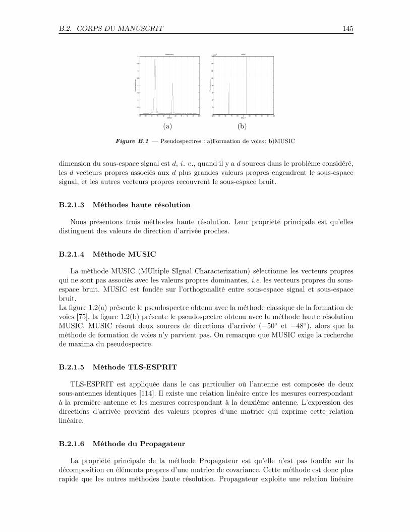
B.2. CORPS DU MANUSCRIT 145
−100 −80 −60 −40 −20 0 20 40 60 80 1000
0.05
0.1
0.15
0.2
0.25
0.3
0.35
0.4Beamforming
DOA(°)
Pse
ud
osp
ectr
um
−100 −80 −60 −40 −20 0 20 40 60 80 1000
2
4
6
8
10
12
14
16x 10
28 MUSIC
DOA (°)
Pse
ud
osp
ectr
um
(a) (b)
Figure B.1 — Pseudospectres : a)Formation de voies ; b)MUSIC
dimension du sous-espace signal est d, i . e., quand il y a d sources dans le problème considéré,les d vecteurs propres associés aux d plus grandes valeurs propres engendrent le sous-espacesignal, et les autres vecteurs propres recouvrent le sous-espace bruit.
B.2.1.3 Méthodes haute résolution
Nous présentons trois méthodes haute résolution. Leur propriété principale est qu’ellesdistinguent des valeurs de direction d’arrivée proches.
B.2.1.4 Méthode MUSIC
La méthode MUSIC (MUltiple SIgnal Characterization) sélectionne les vecteurs propresqui ne sont pas associés avec les valeurs propres dominantes, i.e. les vecteurs propres du sous-espace bruit. MUSIC est fondée sur l’orthogonalité entre sous-espace signal et sous-espacebruit.La figure 1.2(a) présente le pseudospectre obtenu avec la méthode classique de la formation devoies [75], la figure 1.2(b) présente le pseudospectre obtenu avec la méthode haute résolutionMUSIC. MUSIC résout deux sources de directions d’arrivée (−50◦ et −48◦), alors que laméthode de formation de voies n’y parvient pas. On remarque que MUSIC exige la recherchede maxima du pseudospectre.
B.2.1.5 Méthode TLS-ESPRIT
TLS-ESPRIT est appliquée dans le cas particulier où l’antenne est composée de deuxsous-antennes identiques [114]. Il existe une relation linéaire entre les mesures correspondantà la première antenne et les mesures correspondant à la deuxième antenne. L’expression desdirections d’arrivée provient des valeurs propres d’une matrice qui exprime cette relationlinéaire.
B.2.1.6 Méthode du Propagateur
La propriété principale de la méthode Propagateur est qu’elle n’est pas fondée sur ladécomposition en éléments propres d’une matrice de covariance. Cette méthode est donc plusrapide que les autres méthodes haute résolution. Propagateur exploite une relation linéaire
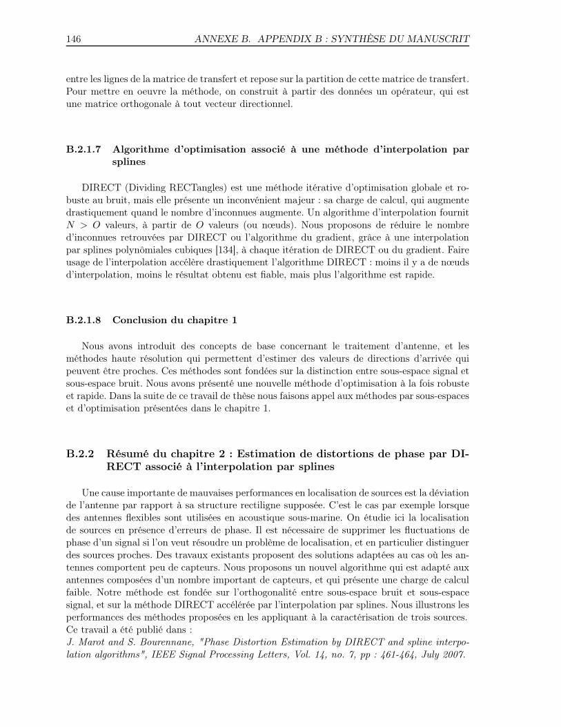
146 ANNEXE B. APPENDIX B : SYNTHÈSE DU MANUSCRIT
entre les lignes de la matrice de transfert et repose sur la partition de cette matrice de transfert.Pour mettre en oeuvre la méthode, on construit à partir des données un opérateur, qui estune matrice orthogonale à tout vecteur directionnel.
B.2.1.7 Algorithme d’optimisation associé à une méthode d’interpolation parsplines
DIRECT (Dividing RECTangles) est une méthode itérative d’optimisation globale et ro-buste au bruit, mais elle présente un inconvénient majeur : sa charge de calcul, qui augmentedrastiquement quand le nombre d’inconnues augmente. Un algorithme d’interpolation fournitN > O valeurs, à partir de O valeurs (ou nœuds). Nous proposons de réduire le nombred’inconnues retrouvées par DIRECT ou l’algorithme du gradient, grâce à une interpolationpar splines polynômiales cubiques [134], à chaque itération de DIRECT ou du gradient. Faireusage de l’interpolation accélère drastiquement l’algorithme DIRECT : moins il y a de nœudsd’interpolation, moins le résultat obtenu est fiable, mais plus l’algorithme est rapide.
B.2.1.8 Conclusion du chapitre 1
Nous avons introduit des concepts de base concernant le traitement d’antenne, et lesméthodes haute résolution qui permettent d’estimer des valeurs de directions d’arrivée quipeuvent être proches. Ces méthodes sont fondées sur la distinction entre sous-espace signal etsous-espace bruit. Nous avons présenté une nouvelle méthode d’optimisation à la fois robusteet rapide. Dans la suite de ce travail de thèse nous faisons appel aux méthodes par sous-espaceset d’optimisation présentées dans le chapitre 1.
B.2.2 Résumé du chapitre 2 : Estimation de distortions de phase par DI-RECT associé à l’interpolation par splines
Une cause importante de mauvaises performances en localisation de sources est la déviationde l’antenne par rapport à sa structure rectiligne supposée. C’est le cas par exemple lorsquedes antennes flexibles sont utilisées en acoustique sous-marine. On étudie ici la localisationde sources en présence d’erreurs de phase. Il est nécessaire de supprimer les fluctuations dephase d’un signal si l’on veut résoudre un problème de localisation, et en particulier distinguerdes sources proches. Des travaux existants proposent des solutions adaptées au cas où les an-tennes comportent peu de capteurs. Nous proposons un nouvel algorithme qui est adapté auxantennes composées d’un nombre important de capteurs, et qui présente une charge de calculfaible. Notre méthode est fondée sur l’orthogonalité entre sous-espace bruit et sous-espacesignal, et sur la méthode DIRECT accélérée par l’interpolation par splines. Nous illustrons lesperformances des méthodes proposées en les appliquant à la caractérisation de trois sources.Ce travail a été publié dans :J. Marot and S. Bourennane, "Phase Distortion Estimation by DIRECT and spline interpo-lation algorithms", IEEE Signal Processing Letters, Vol. 14, no. 7, pp : 461-464, July 2007.
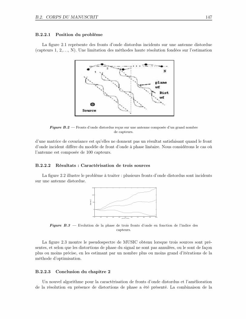
B.2. CORPS DU MANUSCRIT 147
B.2.2.1 Position du problème
La figure 2.1 représente des fronts d’onde distordus incidents sur une antenne distordue(capteurs 1, 2,. . ., N). Une limitation des méthodes haute résolution fondées sur l’estimation
Figure B.2 — Fronts d’onde distordus reçus sur une antenne composée d’un grand nombrede capteurs.
d’une matrice de covariance est qu’elles ne donnent pas un résultat satisfaisant quand le frontd’onde incident diffère du modèle de front d’onde à phase linéaire. Nous considérons le cas oùl’antenne est composée de 100 capteurs.
B.2.2.2 Résultats : Caractérisation de trois sources
La figure 2.2 illustre le problème à traiter : plusieurs fronts d’onde distordus sont incidentssur une antenne distordue.
0 10 20 30 40 50 60 70 80 90 100−50
0
50
100
150
sensor index
phas
e valu
e (°)
Figure B.3 — Evolution de la phase de trois fronts d’onde en fonction de l’indice descapteurs.
La figure 2.3 montre le pseudospectre de MUSIC obtenu lorsque trois sources sont pré-sentes, et selon que les distortions de phase du signal ne sont pas annulées, ou le sont de façonplus ou moins précise, en les estimant par un nombre plus ou moins grand d’itérations de laméthode d’optimisation.
B.2.2.3 Conclusion du chapitre 2
Un nouvel algorithme pour la caractérisation de fronts d’onde distordus et l’améliorationde la résolution en présence de distortions de phase a été présenté. La combinaison de la
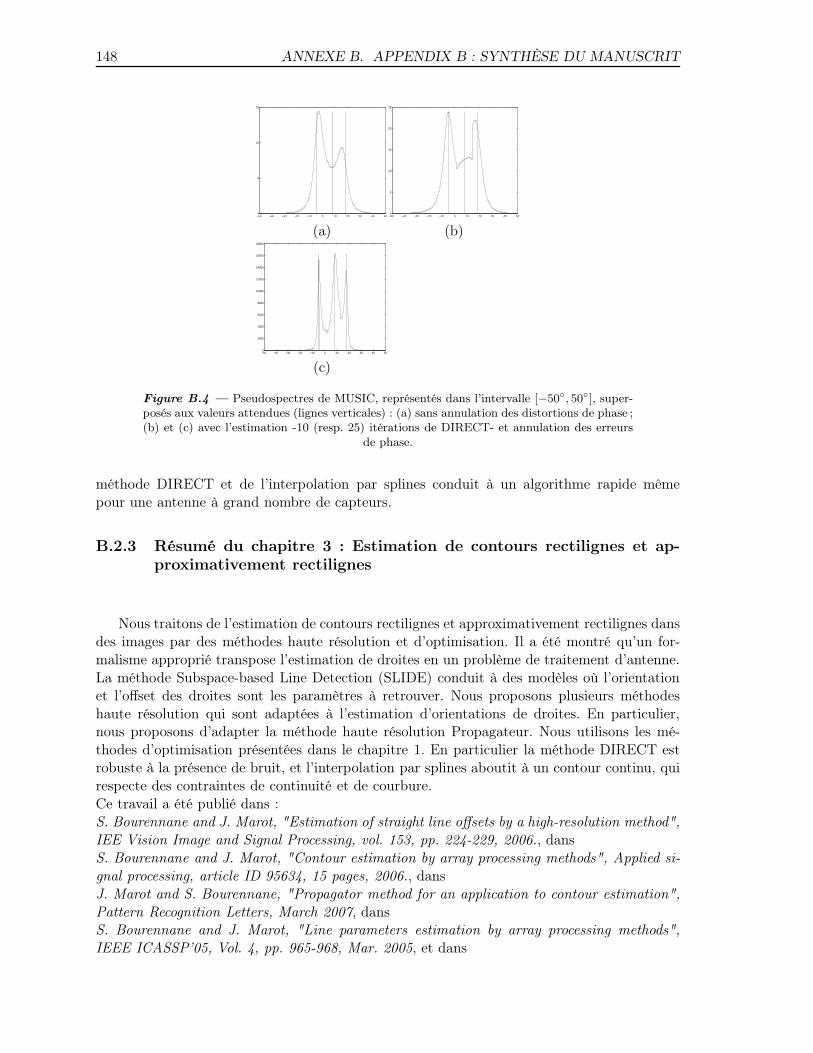
148 ANNEXE B. APPENDIX B : SYNTHÈSE DU MANUSCRIT
−50 −40 −30 −20 −10 0 10 20 30 40 500
5
10
15
−50 −40 −30 −20 −10 0 10 20 30 40 500
5
10
15
20
25
(a) (b)
−50 −40 −30 −20 −10 0 10 20 30 40 500
2000
4000
6000
8000
10000
12000
14000
16000
18000
(c)
Figure B.4 — Pseudospectres de MUSIC, représentés dans l’intervalle [−50◦, 50◦], super-posés aux valeurs attendues (lignes verticales) : (a) sans annulation des distortions de phase ;(b) et (c) avec l’estimation -10 (resp. 25) itérations de DIRECT- et annulation des erreurs
de phase.
méthode DIRECT et de l’interpolation par splines conduit à un algorithme rapide mêmepour une antenne à grand nombre de capteurs.
B.2.3 Résumé du chapitre 3 : Estimation de contours rectilignes et ap-proximativement rectilignes
Nous traitons de l’estimation de contours rectilignes et approximativement rectilignes dansdes images par des méthodes haute résolution et d’optimisation. Il a été montré qu’un for-malisme approprié transpose l’estimation de droites en un problème de traitement d’antenne.La méthode Subspace-based Line Detection (SLIDE) conduit à des modèles où l’orientationet l’offset des droites sont les paramètres à retrouver. Nous proposons plusieurs méthodeshaute résolution qui sont adaptées à l’estimation d’orientations de droites. En particulier,nous proposons d’adapter la méthode haute résolution Propagateur. Nous utilisons les mé-thodes d’optimisation présentées dans le chapitre 1. En particulier la méthode DIRECT estrobuste à la présence de bruit, et l’interpolation par splines aboutit à un contour continu, quirespecte des contraintes de continuité et de courbure.Ce travail a été publié dans :S. Bourennane and J. Marot, "Estimation of straight line offsets by a high-resolution method",IEE Vision Image and Signal Processing, vol. 153, pp. 224-229, 2006., dansS. Bourennane and J. Marot, "Contour estimation by array processing methods", Applied si-gnal processing, article ID 95634, 15 pages, 2006., dansJ. Marot and S. Bourennane, "Propagator method for an application to contour estimation",Pattern Recognition Letters, March 2007, dansS. Bourennane and J. Marot, "Line parameters estimation by array processing methods",IEEE ICASSP’05, Vol. 4, pp. 965-968, Mar. 2005, et dans
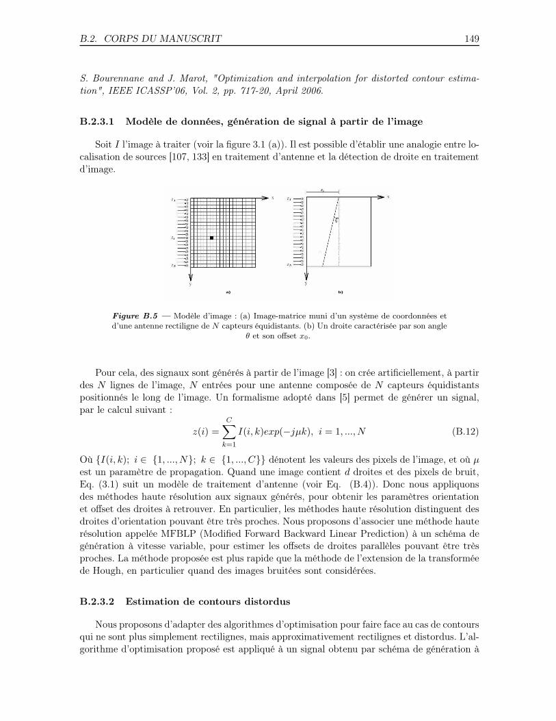
B.2. CORPS DU MANUSCRIT 149
S. Bourennane and J. Marot, "Optimization and interpolation for distorted contour estima-tion", IEEE ICASSP’06, Vol. 2, pp. 717-20, April 2006.
B.2.3.1 Modèle de données, génération de signal à partir de l’image
Soit I l’image à traiter (voir la figure 3.1 (a)). Il est possible d’établir une analogie entre lo-calisation de sources [107, 133] en traitement d’antenne et la détection de droite en traitementd’image.
a) b)
Figure B.5 — Modèle d’image : (a) Image-matrice muni d’un système de coordonnées etd’une antenne rectiligne de N capteurs équidistants. (b) Un droite caractérisée par son angle
θ et son offset x0.
Pour cela, des signaux sont générés à partir de l’image [3] : on crée artificiellement, à partirdes N lignes de l’image, N entrées pour une antenne composée de N capteurs équidistantspositionnés le long de l’image. Un formalisme adopté dans [5] permet de générer un signal,par le calcul suivant :
z(i) =C∑
k=1
I(i, k)exp(−jµk), i = 1, ..., N (B.12)
Où {I(i, k); i ∈ {1, ..., N}; k ∈ {1, ..., C}} dénotent les valeurs des pixels de l’image, et où µest un paramètre de propagation. Quand une image contient d droites et des pixels de bruit,Eq. (3.1) suit un modèle de traitement d’antenne (voir Eq. (B.4)). Donc nous appliquonsdes méthodes haute résolution aux signaux générés, pour obtenir les paramètres orientationet offset des droites à retrouver. En particulier, les méthodes haute résolution distinguent desdroites d’orientation pouvant être très proches. Nous proposons d’associer une méthode hauterésolution appelée MFBLP (Modified Forward Backward Linear Prediction) à un schéma degénération à vitesse variable, pour estimer les offsets de droites parallèles pouvant être trèsproches. La méthode proposée est plus rapide que la méthode de l’extension de la transforméede Hough, en particulier quand des images bruitées sont considérées.
B.2.3.2 Estimation de contours distordus
Nous proposons d’adapter des algorithmes d’optimisation pour faire face au cas de contoursqui ne sont plus simplement rectilignes, mais approximativement rectilignes et distordus. L’al-gorithme d’optimisation proposé est appliqué à un signal obtenu par schéma de génération à
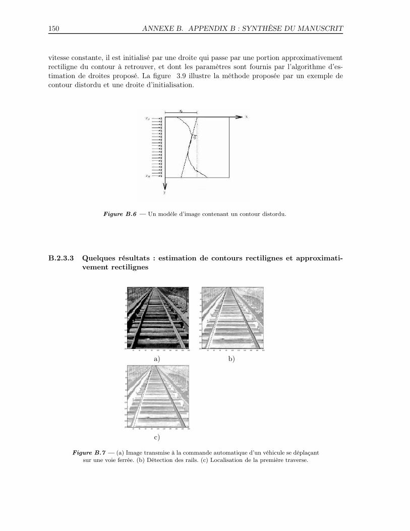
150 ANNEXE B. APPENDIX B : SYNTHÈSE DU MANUSCRIT
vitesse constante, il est initialisé par une droite qui passe par une portion approximativementrectiligne du contour à retrouver, et dont les paramètres sont fournis par l’algorithme d’es-timation de droites proposé. La figure 3.9 illustre la méthode proposée par un exemple decontour distordu et une droite d’initialisation.
Figure B.6 — Un modèle d’image contenant un contour distordu.
B.2.3.3 Quelques résultats : estimation de contours rectilignes et approximati-vement rectilignes
20 40 60 80 100 120 140 160 180 200
20
40
60
80
100
120
140
160
180
20020 40 60 80 100 120 140 160 180 200
20
40
60
80
100
120
140
160
180
200
a) b)
20 40 60 80 100 120 140 160 180 200
20
40
60
80
100
120
140
160
180
200
c)
Figure B.7 — (a) Image transmise à la commande automatique d’un véhicule se déplaçantsur une voie ferrée. (b) Détection des rails. (c) Localisation de la première traverse.
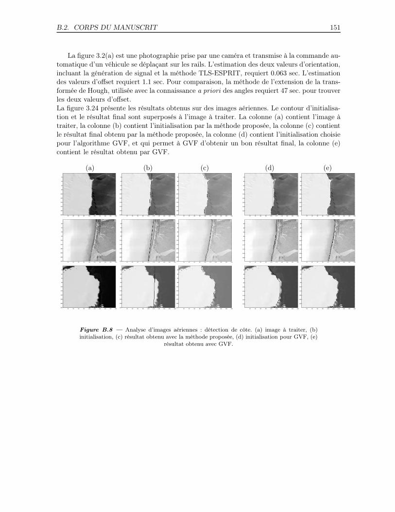
B.2. CORPS DU MANUSCRIT 151
La figure 3.2(a) est une photographie prise par une caméra et transmise à la commande au-tomatique d’un véhicule se déplaçant sur les rails. L’estimation des deux valeurs d’orientation,incluant la génération de signal et la méthode TLS-ESPRIT, requiert 0.063 sec. L’estimationdes valeurs d’offset requiert 1.1 sec. Pour comparaison, la méthode de l’extension de la trans-formée de Hough, utilisée avec la connaissance a priori des angles requiert 47 sec. pour trouverles deux valeurs d’offset.La figure 3.24 présente les résultats obtenus sur des images aériennes. Le contour d’initialisa-tion et le résultat final sont superposés à l’image à traiter. La colonne (a) contient l’image àtraiter, la colonne (b) contient l’initialisation par la méthode proposée, la colonne (c) contientle résultat final obtenu par la méthode proposée, la colonne (d) contient l’initialisation choisiepour l’algorithme GVF, et qui permet à GVF d’obtenir un bon résultat final, la colonne (e)contient le résultat obtenu par GVF.
(a) (b) (c) (d) (e)
20 40 60 80 100 120 140 160 180 200
20
40
60
80
100
120
140
160
180
20020 40 60 80 100 120 140 160 180 200
20
40
60
80
100
120
140
160
180
20020 40 60 80 100 120 140 160 180 200
20
40
60
80
100
120
140
160
180
20020 40 60 80 100 120 140 160 180 200
20
40
60
80
100
120
140
160
180
20 40 60 80 100 120 140 160 180 200
20
40
60
80
100
120
140
160
180
20 40 60 80 100 120 140 160 180 200
20
40
60
80
100
120
140
160
180
20020 40 60 80 100 120 140 160 180 200
20
40
60
80
100
120
140
160
180
20020 40 60 80 100 120 140 160 180 200
20
40
60
80
100
120
140
160
180
20020 40 60 80 100 120 140 160 180 200
20
40
60
80
100
120
140
160
180
20 40 60 80 100 120 140 160 180 200
20
40
60
80
100
120
140
160
180
20 40 60 80 100 120 140 160 180 200
20
40
60
80
100
120
140
160
180
20020 40 60 80 100 120 140 160 180 200
20
40
60
80
100
120
140
160
180
20020 40 60 80 100 120 140 160 180 200
20
40
60
80
100
120
140
160
180
20020 40 60 80 100 120 140 160 180 200
20
40
60
80
100
120
140
160
180
20 40 60 80 100 120 140 160 180 200
20
40
60
80
100
120
140
160
180
Figure B.8 — Analyse d’images aériennes : détection de côte. (a) image à traiter, (b)initialisation, (c) résultat obtenu avec la méthode proposée, (d) initialisation pour GVF, (e)
résultat obtenu avec GVF.
152 ANNEXE B. APPENDIX B : SYNTHÈSE DU MANUSCRIT
B.2.3.4 Conclusion du chapitre 3
Nous avons considéré un problème d’analyse d’image : l’estimation de droites et de contoursapproximativement rectilignes et distordus. Pour cela, nous avons adapté des méthodes parsous-espaces du traitement d’antenne, et des méthodes d’optimisation. Pour transcrire lecontenu de l’image en un signal unidimensionnel, nous avons adopté un schéma de générationà vitesse constante et un schéma de génération à vitesse variable. Ces schémas de générationconduisent à des modèles de signaux où les orientations et offsets des droites sont des valeursde fréquence à estimer. Ces paramètres peuvent être de valeur très proches, et nous considé-rons des environnements bruités. Or, les méthodes haute résolution du traitement d’antennesont censées donner de bons résultats dans ces conditions. Donc, nous avons adapté les mé-thodes TLS-ESPRIT et Propagateur pour estimer l’orientation de droites. En particulier, laversion du propagateur, qui présente l’avantage de ne pas passer par le calcul d’une matricede covariance, présente une charge de calcul faible. Nous avons également adapté la méthodehaute résolution MFBLP à l’estimation de valeurs d’offsets (pouvant être proches) de droitesparallèles.Nous avons proposé une méthode d’optimisation pour estimer des contours distordus, et nousavons adapté l’algorithme d’optimisation du gradient, pour estimer des distortions de phase àpartir du signal généré à partir de l’image. Les distortions de phase sont proportionnelles auxdécalages entre la courbe distordue à retrouver et la droite d’initialisation. Cette procédure estgénéralisée à l’estimation de plusieurs contours par l’association des méthodes Propagateur etdu gradient. Nous proposons également un nouvel algorithme d’optimisation qui est rapide, etconduit à un contour continu. Nous avons comparé les résultats obtenus avec cette méthodeavec les résultats obtenus avec la méthode GVF (Gradient Vector Flow). En particulier, laméthode proposée estime des contours de courbure élevée, et donne de bons résultats avec desphotographies de scènes. Ces méthodes reposent sur la génération de signal sur une antennelinéaire. Nous proposons dans la suite une méthode de génération de signal virtuel sur uneantenne circulaire.
B.2.4 Résumé du chapitre 4 : Estimation de contours circulaires et ap-proximativement circulaires
Les formes circulares sont recherchées couramment en traitement d’images. Nous propo-sons une nouvelle méthode pour estimer plusieurs valeurs de rayons, pouvant être proches, etétendons l’estimation de cercles à l’estimation de contours approximativement circulaires etdistordus. En particulier, nous développons et validons un nouveau modèle pour la générationde signal virtuel par une antenne circulaire.Cette antenne circulaire conduit à des signaux à phase linéaire qui suivent un modèle auquelsont adaptées les méthodes haute résolution. Donc, les mêmes méthodes haute résolutionet d’optimisation que celles qui ont été appliquées dans le cas de l’estimation de contoursrectilignes et approximativement rectilignes peuvent être adaptées à l’estimation de contourscirculaires et approximativement circulaires.Nous proposons une méthode d’estimation du centre par le biais de génération de signalsur une antenne linéaire. Un schéma de génération à vitesse variable sur l’antenne circulaireproposée fournit un signal à phase linéaire, dont les fréquences sont proportionnelles auxvaleurs des rayons des cercles présents dans l’image. La méthode du gradient, ou la méthodeplus robuste combinant DIRECT et interpolation par splines étendent la méthode proposée
B.2. CORPS DU MANUSCRIT 153
à la segmentation de contours étoilés quelconques. L’estimation de contours multiplespouvant ne pas être concentriques est aussi considérée. Pour évaluer les performances desméthodes proposées, nous les comparons à des méthodes moindres carrés, à la transforméede Hough, et à GVF. Nous appliquons la méthode proposée à des images artificielles, et àdes photographies de scènes.Ce travail a été publié dans :
J. Marot and S. Bourennane, "Subspace-Based and DIRECT Algorithms for Distorted Cir-cular Contour Estimation", IEEE trans. on Image Processing, vol. 16, no. 9, pp. 2369-2378,september 2007, dansJ. Marot and S. Bourennane, "Array processing and fast Optimization Algorithms for Distor-ted Circular Contour Retrieval", Advances in signal processing, article ID 57354, 13 pages,february 2007, et dansJ. Marot and S. Bourennane, "Array processing approach for object segmentation in images",IEEE ICASSP’07, Vol. 1, pp. 621-24, April 2007.
B.2.4.1 Position du problème et génération de signal
Position du problème
Nous considérons le problème de l’estimation de rayon, et de l’estimation de distortionsentre un contour étoilé et un cercle qui est une approximation de ce contour. Nous proposonsune antenne circulaire qui permet une génération de signal particulière. Nous mettons en va-leur les propriétés de la phase des signaux générés. Ces signaux suivent des modèles auxquelssont adaptées les méthodes haute résolution du traitement d’antenne, et les méthodes d’op-timisation. La figure 4.1(a) présente une image binaire I comme une matrice de dimensionsN × N . Chaque élément représente un pixel d’image. Un objet dans l’image est composé depixels frontière de valeur 1, et le fond est composé de pixels de valeur 0. L’objet coïncideavec un cercle de rayon r et de centre de coordonnées (lc, mc). La figure 4.1(b) montre unesous-image extraite de l’image de départ, de telle sorte que son extrémité supérieure gaucheest le centre du cercle. Cette sous-image est associée à un repère de coordonnées polaires(ρ, θ). Chaque pixel du contour à retrouver a les coordonnées suivantes : r + ∆ρ, θ. ∆ρ estle décalage entre un pixel du contour et le pixel du cercle qui a la même coordonnée θ. Nousrecherchons des contours étoilés, i . e. des contours décrits par la relation ρ = f(θ), où f estune fonction de [0, 2π] dans R+.
Génération de signal
Nous faisons une analogie entre l’estimation d’un contour circulaire dans une image et lacaractérisation de front d’onde en traitement d’antenne. Notre idée est d’obtenir un signal àphase linéaire à partir d’une image contenant un quart de cercle. Pour cela, nous utilisons uneantenne circulaire. Selon que l’on met en oeuvre un schéma de génération à vitesse constanteou variable, la phase du signal généré est constante ou varie linéairement en fonction de l’indicedes capteurs. Un quart de cercle de rayon r et une antenne circulaire sont représentés sur lafigure 4.2. L’antenne a la forme d’un quart de cercle, centré sur le côté supérieur gauche, et qui
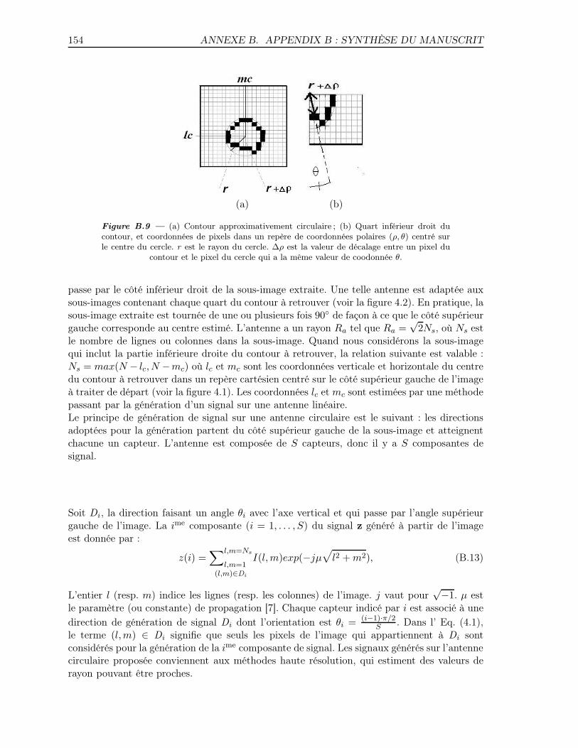
154 ANNEXE B. APPENDIX B : SYNTHÈSE DU MANUSCRIT
(a) (b)
Figure B.9 — (a) Contour approximativement circulaire ; (b) Quart inférieur droit ducontour, et coordonnées de pixels dans un repère de coordonnées polaires (ρ, θ) centré surle centre du cercle. r est le rayon du cercle. ∆ρ est la valeur de décalage entre un pixel du
contour et le pixel du cercle qui a la même valeur de coodonnée θ.
passe par le côté inférieur droit de la sous-image extraite. Une telle antenne est adaptée auxsous-images contenant chaque quart du contour à retrouver (voir la figure 4.2). En pratique, lasous-image extraite est tournée de une ou plusieurs fois 90◦ de façon à ce que le côté supérieurgauche corresponde au centre estimé. L’antenne a un rayon Ra tel que Ra =
√2Ns, où Ns est
le nombre de lignes ou colonnes dans la sous-image. Quand nous considérons la sous-imagequi inclut la partie inférieure droite du contour à retrouver, la relation suivante est valable :Ns = max(N − lc, N −mc) où lc et mc sont les coordonnées verticale et horizontale du centredu contour à retrouver dans un repère cartésien centré sur le côté supérieur gauche de l’imageà traiter de départ (voir la figure 4.1). Les coordonnées lc et mc sont estimées par une méthodepassant par la génération d’un signal sur une antenne linéaire.Le principe de génération de signal sur une antenne circulaire est le suivant : les directionsadoptées pour la génération partent du côté supérieur gauche de la sous-image et atteignentchacune un capteur. L’antenne est composée de S capteurs, donc il y a S composantes designal.
Soit Di , la direction faisant un angle θi avec l’axe vertical et qui passe par l’angle supérieurgauche de l’image. La ime composante (i = 1, . . . , S) du signal z généré à partir de l’imageest donnée par :
z(i) =∑l,m=Ns
l,m=1(l,m)∈Di
I(l,m)exp(−jµ√
l2 + m2), (B.13)
L’entier l (resp. m) indice les lignes (resp. les colonnes) de l’image. j vaut pour√−1. µ est
le paramètre (ou constante) de propagation [7]. Chaque capteur indicé par i est associé à unedirection de génération de signal Di dont l’orientation est θi = (i−1)·π/2
S . Dans l’ Eq. (4.1),le terme (l,m) ∈ Di signifie que seuls les pixels de l’image qui appartiennent à Di sontconsidérés pour la génération de la ime composante de signal. Les signaux générés sur l’antennecirculaire proposée conviennent aux méthodes haute résolution, qui estiment des valeurs derayon pouvant être proches.
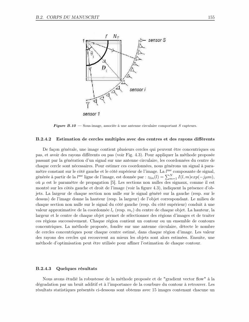
B.2. CORPS DU MANUSCRIT 155
Figure B.10 — Sous-image, associée à une antenne circulaire comportant S capteurs.
B.2.4.2 Estimation de cercles multiples avec des centres et des rayons différents
De façon générale, une image contient plusieurs cercles qui peuvent être concentriques oupas, et avoir des rayons différents ou pas (voir Fig. 4.3). Pour appliquer la méthode proposéepassant par la génération d’un signal sur une antenne circulaire, les coordonnées du centre dechaque cercle sont nécessaires. Pour estimer ces coordonnées, nous générons un signal à para-mètre constant sur le côté gauche et le côté supérieur de l’image. La lme composante de signal,générée à partir de la lme ligne de l’image, est donnée par : zlin(l) =
∑Nm=1 I(l,m)exp(−jµm),
où µ est le paramètre de propagation [5]. Les sections non nulles des signaux, comme il estmontré sur les côtés gauche et droit de l’image (voir la figure 4.3), indiquent la présence d’ob-jets. La largeur de chaque section non nulle sur le signal généré sur la gauche (resp. sur ledessus) de l’image donne la hauteur (resp. la largeur) de l’objet correspondant. Le milieu dechaque section non nulle sur le signal du côté gauche (resp. du côté supérieur) conduit à unevaleur approximative de la coordonnée lc (resp. mc) du centre de chaque objet. La hauteur, lalargeur et le centre de chaque objet permet de sélectionner des régions d’images et de traiterces régions successivement. Chaque région contient un contour ou un ensemble de contoursconcentriques. La méthode proposée, fondée sur une antenne circulaire, détecte le nombrede cercles concentriques pour chaque centre estimé, dans chaque région d’image. Les valeurdes rayons des cercles qui recouvrent au mieux les objets sont alors estimées. Ensuite, uneméthode d’optimisation peut être utilisée pour affiner l’estimation de chaque contour.
B.2.4.3 Quelques résultats
Nous avons étudié la robustesse de la méthode proposée et de "gradient vector flow" à ladégradation par un bruit additif et à l’importance de la courbure du contour à retrouver. Lesrésultats statistiques présentés ci-dessous sont obtenus avec 15 images contenant chacune un
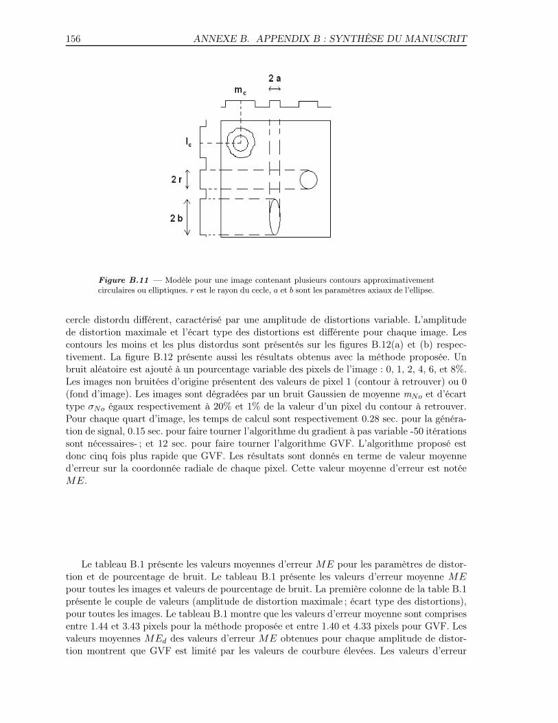
156 ANNEXE B. APPENDIX B : SYNTHÈSE DU MANUSCRIT
Figure B.11 — Modèle pour une image contenant plusieurs contours approximativementcirculaires ou elliptiques. r est le rayon du cecle, a et b sont les paramètres axiaux de l’ellipse.
cercle distordu différent, caractérisé par une amplitude de distortions variable. L’amplitudede distortion maximale et l’écart type des distortions est différente pour chaque image. Lescontours les moins et les plus distordus sont présentés sur les figures B.12(a) et (b) respec-tivement. La figure B.12 présente aussi les résultats obtenus avec la méthode proposée. Unbruit aléatoire est ajouté à un pourcentage variable des pixels de l’image : 0, 1, 2, 4, 6, et 8%.Les images non bruitées d’origine présentent des valeurs de pixel 1 (contour à retrouver) ou 0(fond d’image). Les images sont dégradées par un bruit Gaussien de moyenne mNo et d’écarttype σNo égaux respectivement à 20% et 1% de la valeur d’un pixel du contour à retrouver.Pour chaque quart d’image, les temps de calcul sont respectivement 0.28 sec. pour la généra-tion de signal, 0.15 sec. pour faire tourner l’algorithme du gradient à pas variable -50 itérationssont nécessaires- ; et 12 sec. pour faire tourner l’algorithme GVF. L’algorithme proposé estdonc cinq fois plus rapide que GVF. Les résultats sont donnés en terme de valeur moyenned’erreur sur la coordonnée radiale de chaque pixel. Cette valeur moyenne d’erreur est notéeME.
Le tableau B.1 présente les valeurs moyennes d’erreur ME pour les paramètres de distor-tion et de pourcentage de bruit. Le tableau B.1 présente les valeurs d’erreur moyenne MEpour toutes les images et valeurs de pourcentage de bruit. La première colonne de la table B.1présente le couple de valeurs (amplitude de distortion maximale ; écart type des distortions),pour toutes les images. Le tableau B.1 montre que les valeurs d’erreur moyenne sont comprisesentre 1.44 et 3.43 pixels pour la méthode proposée et entre 1.40 et 4.33 pixels pour GVF. Lesvaleurs moyennes MEd des valeurs d’erreur ME obtenues pour chaque amplitude de distor-tion montrent que GVF est limité par les valeurs de courbure élevées. Les valeurs d’erreur
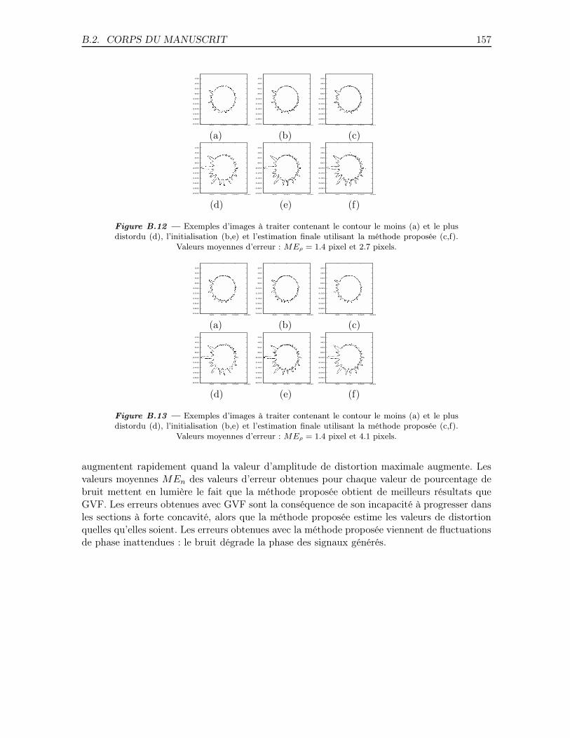
B.2. CORPS DU MANUSCRIT 157
50 100 150 200
20
40
60
80
100
120
140
160
180
20050 100 150 200
20
40
60
80
100
120
140
160
180
20050 100 150 200
20
40
60
80
100
120
140
160
180
200
(a) (b) (c)
50 100 150 200
20
40
60
80
100
120
140
160
180
20050 100 150 200
20
40
60
80
100
120
140
160
180
20050 100 150 200
20
40
60
80
100
120
140
160
180
200
(d) (e) (f)
Figure B.12 — Exemples d’images à traiter contenant le contour le moins (a) et le plusdistordu (d), l’initialisation (b,e) et l’estimation finale utilisant la méthode proposée (c,f).
Valeurs moyennes d’erreur : MEρ = 1.4 pixel et 2.7 pixels.
50 100 150 200
20
40
60
80
100
120
140
160
180
20050 100 150 200
20
40
60
80
100
120
140
160
180
20050 100 150 200
20
40
60
80
100
120
140
160
180
200
(a) (b) (c)
50 100 150 200
20
40
60
80
100
120
140
160
180
20050 100 150 200
20
40
60
80
100
120
140
160
180
20050 100 150 200
20
40
60
80
100
120
140
160
180
200
(d) (e) (f)
Figure B.13 — Exemples d’images à traiter contenant le contour le moins (a) et le plusdistordu (d), l’initialisation (b,e) et l’estimation finale utilisant la méthode proposée (c,f).
Valeurs moyennes d’erreur : MEρ = 1.4 pixel et 4.1 pixels.
augmentent rapidement quand la valeur d’amplitude de distortion maximale augmente. Lesvaleurs moyennes MEn des valeurs d’erreur obtenues pour chaque valeur de pourcentage debruit mettent en lumière le fait que la méthode proposée obtient de meilleurs résultats queGVF. Les erreurs obtenues avec GVF sont la conséquence de son incapacité à progresser dansles sections à forte concavité, alors que la méthode proposée estime les valeurs de distortionquelles qu’elles soient. Les erreurs obtenues avec la méthode proposée viennent de fluctuationsde phase inattendues : le bruit dégrade la phase des signaux générés.
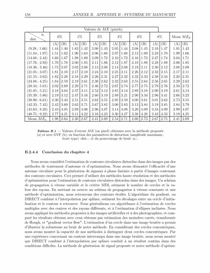
158 ANNEXE B. APPENDIX B : SYNTHÈSE DU MANUSCRIT
Valeurs de ME (pixels)H
HH
HHH
dist.n.
0% 1% 2% 4% 6% 8% Mean MEd
(A) (B) (A) (B) (A) (B) (A) (B) (A) (B) (A) (B) (A) (B)(9.28 ; 1.66) 1.44 1.40 1.83 1.42 2.00 1.43 2.05 1.44 2.08 1.45 2.10 1.47 1.91 1.43
(11.84 ; 1.97) 1.51 1.62 1.96 1.64 2.06 1.66 2.07 1.68 2.12 1.69 2.23 1.70 1.99 1.66(14.68 ; 2.42) 1.68 1.67 1.98 1.69 2.09 1.72 2.10 1.72 2.16 1.73 2.27 1.74 2.04 1.71(17.76 ; 2.93) 1.70 1.78 2.00 1.85 2.11 1.86 2.12 1.87 2.18 1.88 2.28 1.89 2.06 1.85(18.36 ; 3.46) 1.72 2.07 2.02 2.08 2.13 2.08 2.14 2.08 2.19 2.11 2.30 2.12 2.08 2.09(21.05 ; 3.07) 1.81 2.10 2.17 2.10 2.24 2.10 2.25 2.11 2.26 2.12 2.32 2.15 2.17 2.11(21.55 ; 3.62) 1.82 2.28 2.18 2.29 2.26 2.31 2.27 2.32 2.32 2.33 2.38 2.34 2.20 2.31(24.88 ; 4.25) 1.84 2.59 2.19 2.61 2.30 2.62 2.32 2.63 2.55 2.64 2.56 2.65 2.29 2.62(28.34 ; 5.01) 2.02 2.69 2.29 2.71 2.46 2.72 2.67 2.74 2.77 2.75 2.79 2.76 2.50 2.72(31.85 ; 5.21) 2.18 3.04 2.37 3.11 2.52 3.12 2.85 3.14 2.89 3.18 2.90 3.19 2.61 3.13(35.39 ; 5.86) 2.19 3.12 2.47 3.16 2.60 3.19 2.89 3.21 2.90 3.34 2.96 3.41 2.66 3.23(38.90 ; 6.61) 2.30 3.43 2.51 3.51 2.62 3.55 2.95 3.59 3.00 3.61 3.01 3.62 2.73 3.55(42.33 ; 7.42) 2.42 3.69 2.63 3.71 2.67 3.82 3.00 3.83 3.13 3.84 3.19 3.85 2.84 3.79(45.63 ; 8.28) 2.43 4.05 2.89 4.06 2.96 4.07 3.14 4.08 3.20 4.09 3.34 4.09 2.99 4.07(48.75 ; 9.22) 2.77 4.21 3.11 4.22 3.16 4.23 3.30 4.27 3.38 4.28 3.43 4.33 3.19 4.25Mean MEn 1.98 2.64 2.30 2.67 2.41 2.69 2.54 2.71 2.60 2.73 2.67 2.75 2.41 2.69
Tableau B.1 — Valeurs d’erreur ME (en pixel) obtenues avec la méthode proposée(a) et avec GVF (b), en fonction des paramètres de distortion (amplitude maximum ;
écart type) -dist.-, et du pourcentage de bruit -n.-.
B.2.4.4 Conclusion du chapitre 4
Nous avons considéré l’estimation de contours circulaires distordus dans des images par desméthodes de traitement d’antenne et d’optimisation. Nous avons démontré l’efficacité d’uneantenne circulaire pour la génération de signaux à phase linéaire à partir d’images contenantdes contours circulaires. Ceci permet d’utiliser des méthodes haute résolution et des méthodesd’optimisation pour l’estimation de contours circulaires distordus dans des images. Un schémade propagation à vitesse variable et le critère MDL estiment le nombre de cercles et la va-leur des rayons. En mettant en oeuvre un schéma de propagation à vitesse constante et uneméthode d’optimisation, nous retrouvons des contours étoilés. L’algorithme du gradient, ouDIRECT combiné à l’interpolation par splines, estiment les décalages entre un cercle d’initia-lisation et le contour à retrouver. Nous généralisons ces algorithmes à l’estimation de cerclesmultiples avec des centres et des rayons différents, et à l’estimation d’ellipses inclinées. Nousavons appliqué les méthodes proposées à des images artificielles et à des photographies, et com-paré les résultats obtenus avec ceux obtenus par estimation des moindres carrés, transforméede Hough, et "gradient vector flow". L’estimation d’un cercle dans une image bruitée a permisd’illustrer la robustesse au bruit de notre méthode. En considérant des cercles concentriques,nous avons montré la capacité de nos méthodes à distinguer deux cercles concentriques. Parune expérience concernant un contour interrompu dans une image bruitée, nous avons montréque DIRECT combiné à l’interpolation par splines conduit à un résultat continu dans desconditions difficiles. La méthode de génération de signal proposée et notre méthode d’optimi-
B.2. CORPS DU MANUSCRIT 159
sation utilisant le gradient conduit à de meilleurs résultats en terme de biais sur l’estimationde la position des pixels que la méthode GVF, quand on considère des contours à courbure im-portante. Ces expériences montrent que la méthode proposée est rapide et prometteuse pourl’estimation de contours. Une perspective qui se dégage de ce travail consiste en l’estimationde contours circulaires ou elliptiques qui s’intersectent.
B.2.5 Résumé du chapitre 5 : Approximation de tenseur de rang inférieuret filtrage multimodal
Nous présentons des méthodes récentes de filtrage fondées sur l’approximation de ranginférieur pour débruiter des signaux tensoriels. Dans cette approche, les données multicom-posantes sont représentées par des tenseurs, i . e. des tableaux multidimensionnels, et les mé-thodes de filtrage présentées reposent sur l’algèbre multilinéaire. Nous présentons les donnéestensorielles, et un résumé de leur propriétés. Nous introduisons la formulation tensorielle duproblème classique de débruitage, et des notations propres au filtrage tensoriel. Premièrement,nous expliquons comment la SVD tranche par tranche traite successivement chaque compo-sante du tenseur de données. Deuxièmement, nous considérons deux méthodes qui prennenten compte les relations entre chaque matrice tranche du tenseur considéré. Ces deux méthodessont fondées sur le concept de sous-espace signal pour chaque n-mode. La première méthodepour l’estimation de tenseur est fondée sur une PCA (Principal Component Analysis) multi-modale obtenue par une approximation de rang-(K1, . . . ,KN ). La seconde méthode est unenouvelle version tensorielle du filtrage de Wiener. Nous présentons des résultats comparatifsoù les différentes méthodes de filtrage multimodal sont appliquées à la réduction de bruitdans des images couleur, dans les images hyperspectrales, et dans les signaux sismiques multi-composante. Nous présentons une méthode de déploiement de tenseur non orthogonale, qui apour but d’améliorer les résultats du débruitage de données quand des directions principales(lignes de fuite, frontières, limites) sont présentes dans le tenseur à traiter. Nous considéronsune application à l’imagerie hyperspectrale.Ce travail a été publié dans :D. Muti, S. Bourennane and J. Marot, "Lower-Rank Tensor Approximation and MultiwayFiltering", SIAM journal on applied mathematics, accepté Septembre 2007.
B.2.5.1 Les données tensorielles
Les données tensorielles étendent le concept classique de vecteur de données. La mesured’un signal multidimensionnel X par des capteurs multidimensionnels, auquel s’ajoute unbruit N , résulte en un tenseur de données R tel que :
R = X + N . (B.14)
R, X et N sont des tenseurs d’ordre N de RI1×···×IN . Les tenseurs N et X représentent
les partie bruit et signal des données respectivement. Nous supposons que le bruit N estindépendant du signal X , et que le rang n-modal Kn est inférieur à la dimension n-modaleIn (Kn < In, pour tout n = 1 à N). Donc il est possible d’étendre l’approche classique parsous-espaces aux données tensorielles en supposant que, quel que soit le n-mode, l’espacevectoriel E(n) est la somme directe de deux sous-espaces orthogonaux, i . e. E
(n)1 et E
(n)2 , qui
sont définis comme suit :
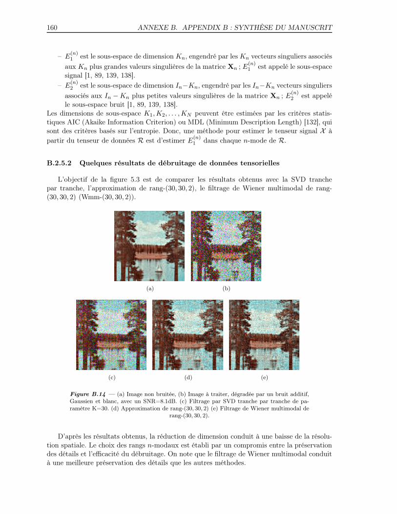
160 ANNEXE B. APPENDIX B : SYNTHÈSE DU MANUSCRIT
– E(n)1 est le sous-espace de dimension Kn, engendré par les Kn vecteurs singuliers associés
aux Kn plus grandes valeurs singulières de la matrice Xn ; E(n)1 est appelé le sous-espace
signal [1, 89, 139, 138].
– E(n)2 est le sous-espace de dimension In−Kn, engendré par les In−Kn vecteurs singuliers
associés aux In − Kn plus petites valeurs singulières de la matrice Xn ; E(n)2 est appelé
le sous-espace bruit [1, 89, 139, 138].Les dimensions de sous-espace K1,K2, . . . ,KN peuvent être estimées par les critères statis-tiques AIC (Akaike Information Criterion) ou MDL (Minimum Description Length) [132], quisont des critères basés sur l’entropie. Donc, une méthode pour estimer le tenseur signal X àpartir du tenseur de données R est d’estimer E
(n)1 dans chaque n-mode de R.
B.2.5.2 Quelques résultats de débruitage de données tensorielles
L’objectif de la figure 5.3 est de comparer les résultats obtenus avec la SVD tranchepar tranche, l’approximation de rang-(30, 30, 2), le filtrage de Wiener multimodal de rang-(30, 30, 2) (Wmm-(30, 30, 2)).
(a) (b)
(c) (d) (e)
Figure B.14 — (a) Image non bruitée, (b) Image à traiter, dégradée par un bruit additif,Gaussien et blanc, avec un SNR=8.1dB. (c) Filtrage par SVD tranche par tranche de pa-ramètre K=30. (d) Approximation de rang-(30, 30, 2) (e) Filtrage de Wiener multimodal de
rang-(30, 30, 2).
D’après les résultats obtenus, la réduction de dimension conduit à une baisse de la résolu-tion spatiale. Le choix des rangs n-modaux est établi par un compromis entre la préservationdes détails et l’efficacité du débruitage. On note que le filtrage de Wiener multimodal conduità une meilleure préservation des détails que les autres méthodes.
B.3. CONCLUSION GÉNÉRALE 161
B.2.5.3 Conclusion du chapitre 5
Une vue d’ensemble de nouvelles méthodes mathématiques dédiées aux données multicom-posantes est présentée. Les données multicomposantes sont représentées comme des tenseurs,i . e. des tableaux multidimensionnels, et les méthodes de filtrage tensoriel qui sont présentéesreposent sur des méthodes d’algèbre linéaire, plus précisément des méthodes par sous-espaces,et des méthodes d’optimisation. Premièrement, nous montrons comment appliquer un filtragepar SVD tranche par tranche. Ensuite, nous présentons trois méthodes qui prennent en compteles relations entre chaque matrice tranche d’un tenseur à traiter.
La première méthode est une PCA multimodale appliquée par une approximation de rang-(K1, . . . ,KN ) au tenseur de données bruité, ou par une troncature de rang-(K1, . . . ,KN ) in-férieur de sa HOSVD (higher order singular value decomposition ou décomposition en valeurssingulières d’ordre supérieur). Cette méthode est fondée sur des statistiques d’ordre deux etrepose sur l’orthogonalité entre le sous-espace bruit et le sous-espace signal dans chaque n-mode. La seconde méthode consiste en une amélioration de la première, dans le sens où ellepermet de traiter une image bruitée par un bruit Gaussien corrélé. Dans ce cas le calcul destatistiques d’ordre deux est remplacé par le calcul de cumulants d’ordre quatre. Nous avonsdécrit une procédure passant par le calcul de cumulants d’ordre quatre qui présente une chargede calcul faible, par l’utilisation d’une matrice tranche de cumulants. Cette méthode a donnéede bons résultats sur des images et des signaux sismiques bruités par un bruit corrélé.La troisième méthode considérée est une version multimodale du filtrage de Wiener. Le nomde cette méthode provient du critère minimisé, une erreur quadratique moyenne, entre le ten-seur signal à retrouver et le tenseur estimé. Un algorithme ALS (Alternating Least Squares oumoindres carrés alternés) a été utilisé pour déterminer de façon optimale les filtres de Wienern-modaux. Les performances de ce filtrage de Wiener multimodal et des résultats comparatifsavec la PCA multimodale ont été présentés dans le cas de la réduction de bruit blanc additifdans des images couleur et dans des signaux sismiques multicomposante.Finalement, nous utilisons la méthode d’estimation de contours rectilignes pour améliorer ledébruitage de données hyperspectrales dans le cas où des directions principales sont présentesdans l’image à traiter. Un déploiement non orthogonal des données, réalisé le long des direc-tions principales des images hyperspectrales, améliore les résultats de débruitage.Nous montrons que quand le déploiement est réalisé le long de directions de frontières dansl’image, on obtient de meilleures performances de débruitage par le filtrage de Wiener mul-tidimensionnel. Les détails sont préservés, ce qui pourrait conduire à de futures applicationsen détection et classification d’objets dans les images hyperspectrales.
B.3 Conclusion générale
Cette thèse est dédiée à l’étude de méthodes par sous-espaces et d’optimisation, appli-quées à des signaux unidimensionnels, bidimensionnels, et multidimensionnel. Nous rappelonsles principes d’un problème en traitement d’antenne, nous prouvons l’intérêt d’une méthoded’optimisation rapide qui combine DIRECT et une méthode d’interpolation par splines pourla résolution d’un problème de caractérisation de sources, quand une antenne avec un grandnombre de capteurs est utilisée et en présence de distortions de phase. En partant d’un forma-lisme dans lequel un signal est généré à partir d’une image, nous avons étendu une méthoded’estimation de contours rectilignes. Nous avons adapté des méthodes existantes de traite-
162 ANNEXE B. APPENDIX B : SYNTHÈSE DU MANUSCRIT
ment d’antenne au problème de l’estimation d’objets de forme quelconque dans des images.Finalement, nous avons présenté les dernières avancées des méthodes de traitement du signaltensoriel et proposé une amélioration dans le cas où des frontières rectilignes sont présentesdans le tenseur à traiter. Pour cela nous avons utilisé la méthode d’estimation de contourrectiligne présentée dans la première partie du manuscrit.
Ainsi, dans la première partie, nous nous sommes concentrés sur des signaux unidimen-sionnels. Dans le chapitre 1, nous avons rappelé les éléments et objectifs d’un problème detraitement d’antenne, la définition d’une antenne en tant qu’ensemble de capteurs, du milieu etdes sources. Nous avons introduit les définitions de la matrice de covariance. Dans l’espace desmesures engendré par les vecteurs propres de la matrice de covariance, nous avons distingué lesous-espace signal (utile) et le sous-espace bruit. Nous avons mis l’accent sur l’orthogonalitéentre sous-espace signal et sous-espace bruit lorsque le signal et le bruit sont décorrélés. Enpartant de cette hypothèse, la méthode par sous-espace MUSIC (MUltiple SIgnal Characte-rization) estime des directions d’arrivée en testant l’orthogonalité entre un modèle de vecteursignal et les vecteurs du sous-espace bruit. Nous avons expliqué les principes d’une nouvelleméthode d’optimisation qui combine soit la méthode du gradient soit la méthode DIRECTcombinée à l’interpolation par splines. Dans le chapitre 2, nous considérons l’estimation dedirections d’arrivée dans le cas où des distortions de phase sont présentes. Nous utilisons lacombinaison de l’algorithme DIRECT (DIviding RECTangles) avec l’interpolation par splinespour estimer des distortions de phase de fronts d’onde. Premièrement, une estimée grossièrede plusieurs directions d’arrivée est obtenue par la méthode MUSIC. Ensuite, pour chaque va-leur estimée, utilisée comme un paramètre d’initialisation, les valeurs de distortions de phaseentre un front d’onde plan et le front d’onde qui donne lieu aux mesures sont estimées parDIRECT combiné à l’interpolation par splines. Les décalages de phase sont supprimés dansles réalisations de signal. Finalement, la méthode MUSIC est appliquée dans un intervalleréduit autour des directions d’arrivée ayant servi d’initialisation. Du fait de l’annulation desdistortions de phase, plusieurs sources peuvent être résolues dans cet intervalle. L’algorithmeproposé a été appliqué à la caractérisation de trois sources dans un environnement bruité.
Dans la seconde partie, nous avons proposé plusieurs méthodes pour des applications enanalyse d’images - données bidimensionnelles. En particulier, nous avons décrit un forma-lisme existant pour la génération de signal à partir d’une image. Dans ce cadre de travail,un contour dans une image est considéré comme un front d’onde, dont la propagation estsimulée via un schéma de propagation (ou schéma de génération de signal). Dans le chapitre3, nous avons rappelé la méthode SLIDE (Subspace-based LIne DEtection) qui utilise l’al-gorithme TLS-ESPRIT (Total Least Square-Estimation of Signal Parameters via RotationalInvariance Techniques) pour retrouver l’orientation de lignes droites. Nous avons proposé uneméthode plus rapide, appelée le Propagateur, qui évite la décomposition en éléments propresde la matrice de covariance, soit en réalisant une partition de cette matrice, soit en travaillantdirectement sur le signal. Le propagateur présente une charge de calcul faible. Pour l’estima-tion de contours rectilignes, nous avons aussi proposé une nouvelle méthode pour l’estimationd’offsets de lignes droites. Cette méthode est plus rapide que l’extension de la transforméede Hough, en particulier quand des images bruitées sont traitées, et distingue des droitesparallèles. Nous avons étendu les méthodes d’estimation de droites à l’estimation de contoursapproximativement rectilignes. Pour cela, nous avons adapté la méthode du gradient à pas
B.3. CONCLUSION GÉNÉRALE 163
variable pour minimiser un critère des moindres carrés entre un signal modèle et un signalgénéré à partir de l’image. Nous avons proposé une généralisation de cette méthode d’opti-misation à l’estimation de plusieurs contours, en minimisant un critère fondé sur l’opérateurdu propagateur. Nous avons proposé une méthode d’optimisation améliorée, qui combine laméthode du gradient et l’interpolation par splines. Cette méthode est rapide et robuste aubruit. Par une comparaison avec la méthode GVF, nous avons insisté sur les capacités de laméthode proposée à retrouver des contours de courbure importante dans un environnementbruité. Les méthodes d’estimation de contours rectilignes et approximativement rectilignesont été appliquées à des images de vision robotique, à des images aériennes et d’imageriemédicale. Dans le chapitre 4, nous avons étendu le travail dédié aux contours rectilignes etapproximativement rectilignes aux contours étoilés. L’aspect le plus nouveau du chapitre 4consiste en la génération d’un signal sur une antenne circulaire : nous adaptons une antennecirculaire à l’image à traiter, pour générer un signal à phase linéaire, et pour pouvoir utiliserdes méthodes haute résolution pour l’estimation de valeurs de rayons de cercles concentriquespouvant être proches. La génération de signal sur une antenne linéaire placée sur les côtés del’image permet de localiser le centre des objets : les sections non nulles des signaux générés surles côtés gauche et supérieur de l’image indiquent la présence d’objets. La génération de signalsur les côtés de l’image donne également accès aux paramètres axiaux d’ellipses. Pour retrou-ver des ellipses inclinées, nous réalisons une rotation de l’image jusqu’à ce que la longueurdes sections non nulles dans les signaux générés sur chaque côté soit de différence maximale.Quand des contours distordus sont attendus, des algorithmes d’optimisation analogues à ceuxappliquées pour l’estimation de contours approximativement rectilignes sont appliqués auxsignaux générés sur l’antenne circulaire. Nous considérons plusieurs cas d’application commeen biométrie, et contrôle non destructif.
La troisième partie est consacrée au traitement du signal tensoriel -de donnéesmutidimensionnelles-, et démontre l’utilité des méthodes d’estimation de directions privilé-giées pour l’amélioration du débruitage par des méthodes par sous-espace. Premièrement, nousavons présenté les dernières avancées en traitement du signal tensoriel. Nous avons rappeléles principes de la troncature de la décomposition en valeurs singulières d’ordre supérieur,la HOSVD-(K1, . . . ,KN ), qui repose sur la définition des dimensions de sous-espace signalK1, . . . ,KN . Nous avons rappelé les principes de l’algorithme d’optimisation ALS (Alterna-ting Least Squares), qui améliore la troncature de la HOSVD-(K1, . . . ,KN ) et en fait uneapproximation de rang-(K1, . . . ,KN ) inférieur d’un tenseur. Nous montrons comment les sta-tistiques d’ordre supérieur, utilisées dans l’approximation de tenseur de rang-(K1, . . . ,KN ) àla place des statistiques d’ordre deux, améliore le débruitage de signal tensoriel dans le casd’un bruit Gaussien corrélé. En particulier, nous proposons une version rapide de cette mé-thode : nous utilisons une matrice tranche de cumulants d’ordre quatre, à la place du tenseurde cumulants complet. Nous donnons des détails sur une version multilinéaire du filtrage deWiener. Le filtrage de Winer multidimensionnel repose sur l’utilisation du sous-espace signalutile. L’estimation des projecteurs sur le sous-espace signal utile, pour chaque n-mode, estréalisée par une boucle ALS (Alternating Least Squares ou moindres carrés alternés). Nousavons réalisé plusieurs expériences sur des images couleur, en considérant en particulier descas où la dimension du sous-espace signal est égale au nombre de canaux dans le mode cou-leur, dans le cas où la dimension du sous-espace signal est sous-estimée, ou dans le cas oùl’image est dégradée par un bruit Gaussien corrélé. Nous avons aussi réalisé du débruitage surdes ondes sismiques multicomposante. Deuxièmement, nous avons proposé une amélioration
164 ANNEXE B. APPENDIX B : SYNTHÈSE DU MANUSCRIT
du débruitage de signal tensoriel, en utilisant le travail dédié à l’estimation de contours recti-lignes : Quand des frontières rectilignes sont présentes dans le tenseur à traiter, nous montronsqu’un déploiement non orthogonal des données, et plus précisément un déploiement selon cesdirections principales, améliore le résultat du débruitage.
Plusieurs perspectives se dégagent de ce travail. La méthode SLIDE a déjà été appliquée àl’estimation de paramètres cinématiques de trajectoires d’objets. Cela a conduit à de bons ré-sultats dans le cas de mouvements à vitesse constante. Les avancées proposées dans la secondepartie concernant l’estimation de contour distordus pourraient être adaptées à la caractérisa-tion de trajectoires à vitesse non constante.Dans le domaine du traitement du signal tensoriel, la méthode proposée de déploiement nonorthogonal de tenseur améliore le rapport signal sur bruit du tenseur signal obtenu. En par-ticulier, les méthodes de traitement du signal tensoriel préservent les détails. Nous pourrionsadapter cette méthode pour une application en détection de cible. En particulier, les donnéeshyperspectrales requièrent un prétraitement tel que la réduction de bruit pour augmenterl’efficacité des algorithmes de classification. En effet, une procédure de réduction de bruitdiminue la variabilité spectrale, ce qui est utilie pour de futures applications en classificationet détection. De plus, la taille importante des données hyperspectrales augmente la charge decalcul et dégrade les résultats de classification. Les images hyperspectrales contiennent desbandes fortement corrélées, ce qui résulte en une redondance spectrale. L’analyse en compo-santes indépendantes (ou Independent Component Analysis, ICA) est appliquée à la réductiondu nombre de bandes spectrales en sélectionnant des composantes spectrales. Il pourrait êtred’un grand intérêt de combiner les algorithmes de filtrage avec ICA, pour un débruitage etune réduction de dimension conjoints.
Liste des figures
1.1 Elements of an array processing problem. ∆ is the inter-sensor distance, θ isthe direction-of-arrival. . . . . . . . . . . . . . . . . . . . . . . . . . . . . . . . 10
1.2 Pseudospectra : a)Beamforming ; b)MUSIC . . . . . . . . . . . . . . . . . . . 16
1.3 Principles of DIRECT method. . . . . . . . . . . . . . . . . . . . . . . . . . . 21
2.1 Distorted wavefronts received on a distorted antenna composed of a large num-ber of sensors. . . . . . . . . . . . . . . . . . . . . . . . . . . . . . . . . . . . . 24
2.2 Evolution of the phase of the three impinging wavefronts as a function of thesensor index. . . . . . . . . . . . . . . . . . . . . . . . . . . . . . . . . . . . . 27
2.3 Pseudospectra of MUSIC, represented in the interval [−50◦, 50◦], superimpo-sed to the expected values (vertical lines) : (a) without cancellation of phasedistortions ; (b) and (c) with the estimation with 10 (resp. 25) iterations ofDIRECT and cancellation of the phase distortions. . . . . . . . . . . . . . . . 27
3.1 The image model (see [4]) : (a) The image-matrix provided with the coordinatesystem and the rectilinear array of N equidistant sensors. (b) A straight linecharacterized by its angle θ and its offset x0. . . . . . . . . . . . . . . . . . . 35
3.2 (a) Image transmitted to the automatic command of a vehicle that is movingon a railway for the servicing of the railways. (b) Detection of the rails for theprogress of the vehicle. (c) Localization of the first crosspiece that the vehiclehas to replace. The process is iterated crosspiece after crosspiece : photography,detection of the rails and detection of the next crosspiece. . . . . . . . . . . . 41
3.3 (a) Noisy image containing a convex polygon the summits of which we aim atdetecting. (b) Superposition of the segments that fit the sides of the polygon,estimated by our method, and the original image. . . . . . . . . . . . . . . . . 41
3.4 The main direction of a set of points . . . . . . . . . . . . . . . . . . . . . . . 42
3.5 (a) Two parallel curves : orientation estimation by Propagator and (b) Offsetestimation by MFBLP, (c) Offset estimation by Hough transform. . . . . . . . 42
3.6 (a) Two nearly parallel curves. (b) Orientation estimation by Propagator,offset estimation by MFBLP. . . . . . . . . . . . . . . . . . . . . . . . . . . . 43
3.7 Proposed method : region segmentation by global threshold. . . . . . . . . . 46
166 LISTE DES FIGURES
3.8 Detection of the pectoral muscle : (a) Processed image (b) Superposition of theinitialization image and the edge enhanced processed image (c) Superpositionof the estimation by automatic threshold and the edge enhanced processedimage (d) Result obtained with levelset method. . . . . . . . . . . . . . . . . . 47
3.9 A model for an image containing a distorted curve. . . . . . . . . . . . . . . . 49
3.10 An image the contour of which exemplifies the distorted curves our method cancope with. . . . . . . . . . . . . . . . . . . . . . . . . . . . . . . . . . . . . . . 55
3.11 (a)Initialization of the method (b)Determination of the vector x̂ (c)Junction ofthe different parts of the curve by determining the coefficients pl . . . . . . . 55
3.12 An image and the steps of the method : Original image, initialization, estima-tion obtained before sticking sections together, final estimation. The methodmanages to return the shifts. . . . . . . . . . . . . . . . . . . . . . . . . . . . 56
3.13 The main results obtained by distorted contour estimation : a)Image to be trea-ted b)Initialization c)Estimation obtained by the proposed method d)Differencebetween the initial image and the estimation . . . . . . . . . . . . . . . . . . . 56
3.14 Distorted contour estimation on a noisy image : a)Image to be treatedb)Initialization c)Estimation obtained by the proposed method d)Superpositionof the initial image and the estimation. . . . . . . . . . . . . . . . . . . . . . . 57
3.15 The case of an image containing two distorted curves : a)Image to be treatedb)Initialization c)Estimation obtained by the proposed method d)Differencebetween the initial image and the estimation . . . . . . . . . . . . . . . . . . . 57
3.16 Results obtained by the method for the estimation of several curves. One curveis a straight line : a)Image to be treated b)Initialization c)Estimation obtainedby the proposed method d)Difference between the initial image and the estimation 58
3.17 A practical situation is simulated. A vehicle and the two sides of the roadare retrieved : a)Initial image b)First estimation of the borders of the roadc)Estimation of the sides of the vehicle d)Refined estimation of the borders ofthe road . . . . . . . . . . . . . . . . . . . . . . . . . . . . . . . . . . . . . . . 58
3.18 Aerial image processing : (a) Initial image ; (b) Result of the edge detector.Proposed method : (c) Superposition of the initial image and the initializa-tion straight line ; (d) Superposition of the initial image and the estimation.GVF method : (e) Initialization ; (f) Superposition of the initial image and theestimation. . . . . . . . . . . . . . . . . . . . . . . . . . . . . . . . . . . . . . 61
3.19 Aerial image processing : (a) Initial image ; (b) Result of the edge detector.Proposed method : (c) Initialization ; (d) Superposition of the initial imageand the estimation. . . . . . . . . . . . . . . . . . . . . . . . . . . . . . . . . . 61
3.20 Hand-made image, common initialization : (a) Example of hand-made image ;(b) Result of the initialization ; (c) Superposition initial image and result ob-tained by the proposed method ; (d) Superposition initial image and resultobtained by GVF. . . . . . . . . . . . . . . . . . . . . . . . . . . . . . . . . . 63
3.21 Combination of gradient algorithm and spline interpolation : increasing numberof nodes permits an increased resolution. . . . . . . . . . . . . . . . . . . . . 65
LISTE DES FIGURES 167
3.22 (a) Two nearly parallel curves. (b) Orientation estimation by Propagator,offset estimation by MFBLP. Distortion retrieval by the proposed optimizationmethod : (c) estimation, (d) superposition estimation and processed. . . . . . 67
3.23 (a) Least distorted contour : initialization, results obtained (b) Most distortedcontour : initialization, results obtained by the proposed method and GVFrespectively. . . . . . . . . . . . . . . . . . . . . . . . . . . . . . . . . . . . . . 68
3.24 Aerial image analysis : coast detection. (a) processed image, (b) initializa-tion, (c) result with the proposed method, (d) initialization for GVF, (e) resultwith GVF. . . . . . . . . . . . . . . . . . . . . . . . . . . . . . . . . . . . . . . 70
3.25 Aerial image analysis : road detection. (a) processed image, (b) initializa-tion, (c) result with the proposed method, (d) initialization for GVF, (e) resultwith GVF. . . . . . . . . . . . . . . . . . . . . . . . . . . . . . . . . . . . . . . 71
3.26 Industrial application : default detection in tissue. (a) processed image, (b)initialization, (c) result with the proposed method, (d) initialization for GVF,(e) result with GVF. . . . . . . . . . . . . . . . . . . . . . . . . . . . . . . . . 71
4.1 (a) Circular-like contour ; (b) Bottom right quarter of the contour and pixelcoordinates in the polar system (ρ, θ) having its origin on the center of thecircle. r is the radius of the circle. ∆ρ is the value of the shift between a pixelof the contour and the pixel of the circle having same coordinate θ. . . . . . . 76
4.2 Sub-image, associated with a circular array composed of S sensors. . . . . . . 77
4.3 Model for an image containing several nearly circular or elliptic features. r isthe circle radius, a and b are the axial parameters of the ellipse. . . . . . . . . 79
4.4 (a) Processed (b) Superposition processed and result obtained after applyinga least-squares method for circle fitting : MEρ = 4.5 pixels, (c) Superpositionprocessed and result obtained after applying the Hough transform : MEρ =0.7 pixel, (d) Superposition processed and result obtained after applying theproposed method : MEρ = 0.3 pixel. . . . . . . . . . . . . . . . . . . . . . . . 82
4.5 (a) Processed, (b) Result (superimposed), with the proposed method for radiusestimation or equivalently with Hough transform or a least-squares fitting me-thod : MEρ = 0.1 (resp. 0.3 for Hough transform and 0.4 for the least-squaresfitting method). . . . . . . . . . . . . . . . . . . . . . . . . . . . . . . . . . . . 83
4.6 Biased center and radius estimation, proposed optimization algorithm usingDIRECT and spline interpolation. (a) Processed (b) Initialisation by the least-squares method, (c) Initialisation by the Hough transform, (d) Initialisation bythe proposed method, (e) Superposition processed and final result, MEρ = 0.9pixel. . . . . . . . . . . . . . . . . . . . . . . . . . . . . . . . . . . . . . . . . . 84
4.7 Examples of processed images containing the less (a) and the most (d) distortedcircles, initialization (b,e) and estimation using the proposed method (c,f).MEρ = 1.4 pixel and 2.7 pixels. . . . . . . . . . . . . . . . . . . . . . . . . . . 85
4.8 Examples of processed images containing the less (a) and the most (d) distortedcircles, initialization (b,e) and estimation using GVF algorithm (c,f). MEρ =1.4 pixel and 4.1 pixels. . . . . . . . . . . . . . . . . . . . . . . . . . . . . . . 86
168 LISTE DES FIGURES
4.9 Multiple circles : (a) Processed (b) Signal generated upon the left side of theimage (c) Initialization (d) Result with gradient method. . . . . . . . . . . . . 87
4.10 Two circles with different centers and same radius. (a) and (b) Processedimages, modulus of the generated signals ; (c) and (d) Superposition proces-sed and result with gradient method. . . . . . . . . . . . . . . . . . . . . . . . 88
4.11 Ellipse (and respectively rotated ellipse) fitting : (a) and (c) Processed ; (b) and(d) Superposition processed and result obtained after applying the proposedmethod for ellipse fitting : MEρ = 0.7 (respectively MEρ = 0.6) pixel. . . . . 89
4.12 (a) Processed image, (b) result of Canny operator (c) Initialisation, (d) Re-sult obtained with gradient method, (e) Result obtained with GVF, (f) Resultobtained with DIRECT combined with spline interpolation. . . . . . . . . . . 90
4.13 (a) Processed image, (b) Initialisation, (c) Result obtained with the proposedoptimization method. . . . . . . . . . . . . . . . . . . . . . . . . . . . . . . . . 91
4.14 (a) Processed image, (b) Initialisation, (c) Result obtained with the proposedoptimization method. . . . . . . . . . . . . . . . . . . . . . . . . . . . . . . . . 91
5.1 ‘Lena’ standard color image and its tensor representation. . . . . . . . . . . . 98
5.2 2nd-mode flattening of tensor A : A2. . . . . . . . . . . . . . . . . . . . . . . 99
5.3 (a) non-noisy image. (b) image to be processed, impaired by an additive whiteGaussian noise, with SNR=8.1dB. (c) channel-by-channel SVD-based filteringof parameter K=30. (d) rank-(30, 30, 2) approximation. (e) Wmm-(30, 30, 2)filtering. . . . . . . . . . . . . . . . . . . . . . . . . . . . . . . . . . . . . . . . 108
5.4 NQE evolution with respect to SNR (dB) : channel-by-channel SVD-basedfiltering of parameter 30 (-◦-), rank-(30, 30, 2) approximation (-�-), Wmm-(30, 30, 2) filtering (-▽-). . . . . . . . . . . . . . . . . . . . . . . . . . . . . . . 109
5.5 (a) non-noisy image. (b) image to be processed, impaired by an additivewhite Gaussian noise, with SNR=8.1dB. (c) channel-by-channel Wiener-basedfiltering of parameter K=30. (d) rank-(30, 30, 3) approximation. (e) Wmm-(30, 30, 3) filtering. . . . . . . . . . . . . . . . . . . . . . . . . . . . . . . . . . 109
5.6 (a) non-noisy image. (b) image to be processed, impaired by an additive whiteGaussian noise, with SNR=8.0dB. (c) channel-by-channel SVD-based filteringof parameter K=19. (d) rank-(19, 19, 3) approximation. (e) Wmm-(19, 19, 3)filtering. . . . . . . . . . . . . . . . . . . . . . . . . . . . . . . . . . . . . . . . 110
5.7 (a) : initial non-noisy image. (b) : initial image with an additive correlatedGaussian noise, SNR = 2.48dB. (c) : HOSVD-(30, 30, 2). (d) : rank-C(30, 30, 2)approximation. (e) : rank−C1(30, 30, 2) approximation. . . . . . . . . . . . . 112
5.8 Evolution of the NQE with respect to the SNR(dB) for each tensor filteringmethod : ◦ : HOSVD-(30, 30, 2) ; ▽ : rank-C(30, 30, 2) ; � : rank-C1(30, 30, 2). 112
5.9 Channels 30 to 34 of the processed multispectral images are presented : (a)-(e) : Non-noisy multispectral image. (f)-(j) : Impaired multispectral image. (k)-(o) : Results obtained with channel-by-channel SVD filtering. (p)-(t) : Resultsobtained with rank-(30,30,30) approximation. . . . . . . . . . . . . . . . . . 113
LISTE DES FIGURES 169
5.10 NQE evolution with respect to SNR (from -1 to 15dB) : channel-by-channelSVD-based filtering of parameter 30 (-◦-), and rank-(30, 30, 30) approximation(-�-). . . . . . . . . . . . . . . . . . . . . . . . . . . . . . . . . . . . . . . . . 114
5.11 (◦) : results obtained with channel-by-channel SVD-based filtering of parameter30 ; (�) : results obtained with rank-(30, 30, 2) approximation ; (a) : evolutionof the mean NQE with respect to SNR (dB) ; (b) evolution of the standarddeviation of NQE with respect to SNR (dB). . . . . . . . . . . . . . . . . . . 115
5.12 non-noisy, impaired, and processed seismic wave : the three polarization com-ponents ; (a)-(c) : components 1, 2 and 3 of the non-noisy seismic wave ;(d)-(f) : components 1, 2 and 3 of the seismic wave, impaired by an addi-tive white Gaussian noise (SNR= -10 dB) ; (g)-(i) : Wiener filtering appliedcomponent by component (Wcc-K), with rank K = 8 ; (j)-(l) : HOSVD-(K1,K2,K3), with (K1,K2,K3)=(8, 8, 3) ; (m)-(o) : multiway Wiener filtering(Wmm-(K1,K2,K3)), with (K1,K2,K3)=(8, 8, 3). . . . . . . . . . . . . . . . . 116
5.13 Evolution of the NQE with respect to the SNR (dB) for each tensor filteringmethod. (▽) : Wiener filtering applied component by component (Wcc-K),with rank K = 8 ; (◦) : HOSVD-(K1,K2,K3), with (K1,K2,K3)=(8, 8, 3) ; (•) :Multiway Wiener filtering (Wmm-(K1,K2,K3)) with (K1,K2,K3)=(8, 8, 3). . 117
5.14 Denoising of a multicomponent seismic wave impaired by an additive correla-ted Gaussian noise (SNR= -2 dB), using multiway filtering based on fourthorder cumulants : comparison of rank−C(8, 8, 3), and rank−C1(8, 8, 3) : (a)-(c) : components 1 to 3 of the non-noisy seismic wave ; (d)-(f) : noised signal ;components 1 to 3 impaired by a correlated Gaussian noise (SNR= -2 dB) ;(g)-(i) : rank−C(8, 8, 3) based filtering ; (j)-(l) : rank−C1(8, 8, 3) based filtering. 118
5.15 Denoising of a multicomponent seismic wave impaired by an additive correlatedGaussian noise, by multiway filtering : Evolution of NQE with respect to SNR(dB) for rank-(8, 8, 3) approximation (�), rank−C1(8, 8, 3) using fourth ordercumulant slice matrix (◦) and rank−C(8, 8, 3) using fourth order cumulants (+).119
5.16 128× 128 × 1 gray image containing : (a) Oblique line, (b) SVD truncation tothe 80th eigenvalue, (c) SVD truncation to the 110th eigenvalue ; (d) Verticalline, (e) SVD truncation to the first eigenvalue. . . . . . . . . . . . . . . . . . 121
5.17 30th spectral band : (a) acquired data, (b) derivative of acquired data, (c)MWFR processed data. . . . . . . . . . . . . . . . . . . . . . . . . . . . . . . 122
5.18 Image HSI02 : (a) noisy tensor, (b) PCA−SWT , (c) MWF and (d) MWFRwith SLIDE estimated angles θk ∈ {0◦, 34◦, 90◦}. (K1 = K2 = 31,K3 = 97). . 123
B.1 Pseudospectres : a)Formation de voies ; b)MUSIC . . . . . . . . . . . . . . . 145
B.2 Fronts d’onde distordus reçus sur une antenne composée d’un grand nombre decapteurs. . . . . . . . . . . . . . . . . . . . . . . . . . . . . . . . . . . . . . . . 147
B.3 Evolution de la phase de trois fronts d’onde en fonction de l’indice des capteurs.147
170 LISTE DES FIGURES
B.4 Pseudospectres de MUSIC, représentés dans l’intervalle [−50◦, 50◦], superposésaux valeurs attendues (lignes verticales) : (a) sans annulation des distortionsde phase ; (b) et (c) avec l’estimation -10 (resp. 25) itérations de DIRECT- etannulation des erreurs de phase. . . . . . . . . . . . . . . . . . . . . . . . . . . 148
B.5 Modèle d’image : (a) Image-matrice muni d’un système de coordonnées et d’uneantenne rectiligne de N capteurs équidistants. (b) Un droite caractérisée parson angle θ et son offset x0. . . . . . . . . . . . . . . . . . . . . . . . . . . . . 149
B.6 Un modèle d’image contenant un contour distordu. . . . . . . . . . . . . . . . 150
B.7 (a) Image transmise à la commande automatique d’un véhicule se déplaçant surune voie ferrée. (b) Détection des rails. (c) Localisation de la première traverse. 150
B.8 Analyse d’images aériennes : détection de côte. (a) image à traiter, (b)initialisation, (c) résultat obtenu avec la méthode proposée, (d) initialisationpour GVF, (e) résultat obtenu avec GVF. . . . . . . . . . . . . . . . . . . . . 151
B.9 (a) Contour approximativement circulaire ; (b) Quart inférieur droit du contour,et coordonnées de pixels dans un repère de coordonnées polaires (ρ, θ) centrésur le centre du cercle. r est le rayon du cercle. ∆ρ est la valeur de décalage entreun pixel du contour et le pixel du cercle qui a la même valeur de coodonnée θ. 154
B.10 Sous-image, associée à une antenne circulaire comportant S capteurs. . . . . . 155
B.11 Modèle pour une image contenant plusieurs contours approximativement cir-culaires ou elliptiques. r est le rayon du cecle, a et b sont les paramètres axiauxde l’ellipse. . . . . . . . . . . . . . . . . . . . . . . . . . . . . . . . . . . . . . 156
B.12 Exemples d’images à traiter contenant le contour le moins (a) et le plus distordu(d), l’initialisation (b,e) et l’estimation finale utilisant la méthode proposée(c,f). Valeurs moyennes d’erreur : MEρ = 1.4 pixel et 2.7 pixels. . . . . . . . . 157
B.13 Exemples d’images à traiter contenant le contour le moins (a) et le plus distordu(d), l’initialisation (b,e) et l’estimation finale utilisant la méthode proposée(c,f). Valeurs moyennes d’erreur : MEρ = 1.4 pixel et 4.1 pixels. . . . . . . . . 157
B.14 (a) Image non bruitée, (b) Image à traiter, dégradée par un bruit additif, Gaus-sien et blanc, avec un SNR=8.1dB. (c) Filtrage par SVD tranche par tranche deparamètre K=30. (d) Approximation de rang-(30, 30, 2) (e) Filtrage de Wienermultimodal de rang-(30, 30, 2). . . . . . . . . . . . . . . . . . . . . . . . . . . 160
Liste des tableaux
2.1 ME and RMSE values over angle estimation for several SNR values. . . . . 28
3.1 Experimental and theoretical data concerning the complexity of the high-resolution based method and the extension of the Hough transform method. . 44
3.2 ME and Std values (in pixel) obtained with the proposed method and GVF versus
amplitude and period values. . . . . . . . . . . . . . . . . . . . . . . . . . . . . 63
3.3 ME values (in pixel) obtained with the proposed method (A) and with GVF (B), ver-
sus distortion (maximum amplitude ; standard deviation) -dist.- and noise percentage
values -n.. . . . . . . . . . . . . . . . . . . . . . . . . . . . . . . . . . . . . . . 68
3.4 Std values (in pixel) obtained with the proposed method (A) and with GVF (B), ver-
sus distortion (maximum amplitude ; standard deviation) -dist.- and noise percentage
values -n.. . . . . . . . . . . . . . . . . . . . . . . . . . . . . . . . . . . . . . . 69
4.1 ME values (in pixel) obtained with the proposed method (a) and with GVF (b), versus
distortion (maximum amplitude ; standard deviation) -dist.-, and noise percentage -n.-. 86
4.2 Real-world images : ME values (in pixel). . . . . . . . . . . . . . . . . . . . . . . 91
B.1 Valeurs d’erreur ME (en pixel) obtenues avec la méthode proposée (a) et avec GVF
(b), en fonction des paramètres de distortion (amplitude maximum ; écart type) -dist.-,
et du pourcentage de bruit -n.-. . . . . . . . . . . . . . . . . . . . . . . . . . . . 158

Bibliographie
[1] K. Abed-Meraim, H. Maître et P. Duhamel, Blind multichannel image restorationusing subspace-based method , dans IEEE International Conf. on Accoustics Systems andSignal Processing , Hong Kong, China, April 6-10, 2003.
[2] K. Abed-Meraim et Y. Hua, Multi-line fitting and straight edge detection using po-lynomial phase signals, Conference Records of the 31st Asilomar Conference on Signal,Systems and Computers, vol. 2, 1997.
[3] H. K. Aghajan, Subspace Techniques for Image Understanding and Computer Vision.,Phd thesis, Stanford University, Stanford, California, USA, Nov. 1995.
[4] H. K. Aghajan et T. Kailath, A subspace fitting approach to super resolution multi-line fitting and straight edge detection, Proc. of the IEEE Int. Conf. on Acoustic, Speechand Signal Processing, vol. 3, 1992.
[5] H. K. Aghajan et T. Kailath, Sensor array processing techniques for super resolutionmulti-line-fitting and straight edge detection , IEEE Transactions on Image Processing,vol. 2, no. 4, pp. 454–465, Oct. 1993.
[6] H. K. Aghajan et T. Kailath, Slide : subspace-based line detection , Proc. of theIEEE Int. Conf. on Acoustic, Speech and Signal Processing, vol. 5, 1993.
[7] H. K. Aghajan et T. Kailath, Slide : Subspace-based line detection , IEEE trans. onPattern Analysis and Machine Intelligence, vol. 16, no. 11, pp. 1057–1073, Nov. 1994.
[8] H. K. Aghajan, B. Khalaj et T. Kailath, Estimation of multiple 2-d uniformmotions by slide : subspace-based line detection , IEEE Transactions on Image Processing,vol. 8, no. 4, pp. 517–526, Apr. 1999.
[9] Y. Ahn et H. Kim, Approximation of circular arcs by bézier curves , Journal of Com-putational and Applied Mathematics, 1997.
[10] Y. Ahn, Y. Kim et Y. Shin, Approximation of circular arcs and of a set curves by beziercurves of high degree, Journal of Computational and Applied Mathematics, vol. 167,no. 2, pp. 405–416, June 2004.
[11] O. Alter et G. Golub, Reconstructing the pathways of a cellular system from genome-scale signals by using matrix and tensor computations, Proc. Nat. Acad. Sci. USA,vol. 102, no. 49, pp. 17559–17564, October 2005.
[12] H. Andrews et C. Patterson, Singular value decomposition and digital image proces-sing , IEEE Trans. on Acoustics, Speech, and Signal Processing, vol. 24, no. 1, pp. 26–53,Feb. 1976.
174 BIBLIOGRAPHIE
[13] H. Andrews et C. Patterson, Singular Value Decomposition (SVD) image coding ,IEEE Trans. on Communications, vol. 24, no. 4, pp. 425–432, April 1976.
[14] I. Atkinson, F. Kamalabadi et D. Jones, Wavelet-based hyperspectral image esti-mation, Proc-IGARS, vol. 2, pp. 743–745, 2003.
[15] J. Aujol, G. Aubert et L. Blanc-Féraud, Wavelet-based level set evolution forclassification of textured images, IEEE Transactions on Image Processing, vol. 12, no. 12,pp. 1634–1641, dec. 2003.
[16] N. Ayache et O. Faugeras, Hyper : a new approach for the recognition and posi-tionning of two-dimensionnal objects, IEEE trans. on Pattern Analysis and MachineIntelligence, vol. 8, no. 1, pp. 44–54, Jan. 1986.
[17] B. Bader et T. Kolda, Algorithm 862 : Matlab tensor classes for fast algorithmprototyping , ACM Transactions on Mathematical Software„ vol. 32, no. 4, December2006.
[18] E. Bala et A. Ertüzün, A multivariate thresholding technique for image denoisingusing multiwavelets, ASP, (pp. 1205–1211), 08 2005.
[19] D. Ballard, Generalizing the hough transform to detect arbitrary shapes, Pattern Re-cognition, vol. 13, no. 2, pp. 111–122, Apr. 1981.
[20] J. Borkowski, B. Matuszewski, J. Mroczka et L.-K. Shark, Geometric matchingof circular features by least-squares fitting , Pattern Recognition Letters, vol. 23, no. 7,pp. 885–894, May 2002.
[21] S. Bourennane et A. Bendjama, Locating wide band acoustic sources using higher-order statistics, Applied Acoustics, vol. 63, no. 3, pp. 235–251, May 2001.
[22] S. Bourennane, A. Benjama et M. Frikel, Seismic wave separation based on higher-order statistics, dans IEEE International Conf. on Digital Signal Processing and itsApplications, Moscow, Russia, 1998.
[23] S. Bourennane et M. Frikel, Localization of the wideband sources with estimationof the antenna shape, IEEE-Workshop on Statistical & Array Processing, 1996.
[24] S. Bourennane et J. Marot, Line parameters estimation by array processing me-thods, Proc. of the IEEE Int. Conf. on Acoustic, Speech and Signal Processing, vol. 4,2005.
[25] S. Bourennane et J. Marot, Contour estimation by array processing methods, EUR-ASIP Journal on Advances on Signal Processing, vol. article ID 95634 15 pages, 2006.
[26] S. Bourennane et J. Marot, Estimation of straight line offsets by a high-resolutionmethod , IEE proceedings Journal on Vision, Image and Signal processing, vol. 153, no. 2,pp. 224–229, Apr. 2006.
[27] S. Bourennane et J. Marot, Optimization and interpolation for distorted contourestimation, Proc. of the IEEE Int. Conf. on Acoustic, Speech and Signal Processing,vol. 2, 2006.
[28] S. Bourennane et J. Marot, Propagator method for an application to contour esti-mation, Pattern Recognition Letters, vol. 28, no. 12, pp. 1556–1562, Sept. 2007.
[29] P. Brigger, J. Hoeg et M. Unser, B-spline snakes : A flexible tool for parametriccontour detection, IEEE Transactions on Image Processing, vol. 9, no. 9, pp. 1484–1496,2000.
BIBLIOGRAPHIE 175
[30] R. Bro, Multi-way analysis in the food industry , PhD thesis, Royal Veterinary andAgricultural University, Denmark, 1998.
[31] J. Caroll et J. Chang, Analysis of individual differences in multidimensional scalingvia n-way generalization of eckart-young decomposition , Psychometrika, vol. 35, no. 3,pp. 283–319, 09 1970.
[32] C. Chang et Q. Du, Estimation of number of spectrally distinct signal sources inhyperspectral imagery , IEEE-TGARS, vol. 42, no. 3, pp. 608–619, 2004.
[33] Y.-C. Chang, B.-K. Shyu, C.-Y. Cho et J.-S. Wang, Adaptive post-processing forregion-based fractal image compression , dans Data Compression Conference, (p. 549),2000.
[34] J. Cheng et S. W. Foo, Dynamic directional gradient vector flow for snakes , IEEETransactions on Image Processing, vol. 15, no. 6, pp. 1563–1571, Jun. 2006.
[35] G. Coath et P. Musumeci, Adaptive arc fitting for ball detection in robocup, Proc.APRS Workshop on Digital Image Computing, 2003.
[36] S. Connell et A. Jain, Template-based online character recognition , Pattern Recog-nition, vol. 34, no. 1, pp. 1–14, Jan. 2001.
[37] J. Crawford, A noniterative method for fitting circular arcs to measured points, Nu-clear Instruments and Methods in Physics Research, 1983.
[38] L. De Lathauwer, Signal Processing Based on Multilinear Algebra, Phd thesis, K.U.Leuven, E.E. Dept. (ESAT), Belgium, Sept. 1997.
[39] L. De Lathauwer, B. De Moor et J. Vandewalle, Dimensionality reduction inhigher-order-only ica, Proc. IEEE Signal Processing Workshop on higher-order Statis-tics, (pp. 316–320), 07 1997.
[40] L. De Lathauwer, B. De Moor et J. Vandewalle, A multilinear singular va-lue decomposition, SIAM Journal on Matrix Analysis and Applications, vol. 21, no. 4,pp. 1253–1278, April 2000.
[41] L. De Lathauwer, B. De Moor et J. Vandewalle, On the best rank-(1) and rank-(r1, . . . , rN ) approximation of higher-order tensors , SIAM Journal on Matrix Analysisand Applications, vol. 21, no. 4, pp. 1324–1342, April 2000.
[42] D. Donoho, De-noising by soft-thresholding , IEEE-IT, vol. 41, pp. 613–627, 1995.
[43] Y. Eckart et G. Young, The approximation of a matrix by another of lower rank ,Psychometrika, vol. 1, pp. 211–218, 1936.
[44] R. J. Ferrari, R. M. Rangayyan, J. E. L. Desautels, R. A. Borges et A. F.
Frère, Automatic identification of the pectoral muscle in mammograms, IEEE trans.on Medical Imaging, vol. 23, no. 2, pp. 232–245, Feb. 2004.
[45] M. A. T. Figueiredo et A. Jain, Unsupervised learning of finite mixture models ,IEEE trans. on Pattern Analysis and Machine Intelligence, vol. 24, no. 3, pp. 381–396,Mar. 2002.
[46] F. Freire et T. Ulrych, Application of SVD to vertical seismic profiling , Geophysics,vol. 53, pp. 778–785, 1988.
[47] W. Gander, G. Golub et R. Strebel, Least-squares fitting of circles and ellipses,BIT, 1994.
176 BIBLIOGRAPHIE
[48] P. Gill et W. Murray, Quasi-newton methods for unconstrained optimization , Journalof Instruments and Mathematical Applications, vol. 9, 1972.
[49] F. Glangeaud et J. Mari, Wave separation, Technip IFP édition, 1994.
[50] D. Goldberg, Genetic Algorithms in Search, Optimization, and Machine Learning ,Addison-Wisley, New-York (USA), 1989.
[51] G. Golub et C. Van Loan, Matrix computations, 3rd ed., Baltimore, The John Hop-kins University Press édition, 1996.
[52] E. Gonen et J. Mendel, Application of cumulants to array processing-part III : blindbeamforming for coherent signal , IEEE Trans. on Signal Processing, vol. 45, no. 9,pp. 2252–64, Sept. 1997.
[53] A. Green, M. Berman et M. Craig, A transformation for ordering multispectral datain terms of image quality with implications for noise removal , IEEE-TGARS, vol. 26,no. 1, pp. 65–74, 1988.
[54] N. Guil, J. Villaba et E. L. Zapata, A fast hough transform for segment detection ,IEEE Transactions on Image Processing, vol. 5, no. 5, pp. 787–792, May 1996.
[55] B. Halder, H. Aghajan et T. Kailath, Propagation diversity enhancement to thesubspace-based line detection algorithm , Proceedings of SPIE, vol. 2424, 1995.
[56] M. Hanke et P. Hansen, Regularization methods for large-scale problems , Survey ofmathematics for Industry, vol. 3, 1993.
[57] R. Harshman et M. Lundy, Research methods for multimode data analysis, (pp. 122–215), Praeger, New York, 1984.
[58] M. Hemon et D. Mace, The use of Karhunen-Loeve transform in seismic data pros-pecting , Geophysical Prospecting, vol. 26, pp. 600–626, 1978.
[59] J. Håstad, Tensor rank is np-complete, Journal of Algorithms, vol. 11, pp. 644–654,september 1990.
[60] K. Hsu, Wave separation and feature extraction of accoustic well-logging waveforme oftriaxial recordings by singular value decomposition , Geophysics, vol. 55, pp. 176–184,1990.
[61] J. Illingworth et J. Kittler, A survey of the hough transform , Proc. of the IEEEInt. Conf. on Computer Vision Graphics and Image Processing, vol. 44, no. 1, pp. 87–116, Oct. 1988.
[62] G. Jackson, I. Mason et S. Greenhalgh, Principal component transforms of triaxialrecordings by singular value decomposition , Geophysics, vol. 56, no. 4, pp. 176–184, 1991.
[63] M. Jansson, A. Swindlehurst et B. Ottersten, Weighted subspace fitting for gene-ral array error models, IEEE trans. on Signal Processing, vol. 46, no. 9, pp. 2484–2498,sep. 1998.
[64] D. Jones, C. Pertunen et B. Stuckman, Lipschitzian optimization without thelipschitz constant , Journal of Optimization Theory and Applications, vol. 79, no. 1,pp. 157–181, Oct. 1993.
[65] V. Karimaki, Effective circle fitting for particle trajectories , Nuclear Instruments andMethods in Physics Research, 1991.
BIBLIOGRAPHIE 177
[66] I. Karoui, R. Fablet, J.-M. Boucher et J.-M. Augustin, Region-based segmen-tation using texture statistics and level-set methods, Proc. of the IEEE Int. Conf. onAcoustic, Speech and Signal Processing, vol. 2, 2006.
[67] N. Karssemeijer, Automated classification of parenchymal patterns in mammograms,Physics in Medicine and Biology, vol. 43, no. 2, pp. 365–378, Feb. 1998.
[68] I. Kasa, A circle fitting procedure and its error analysis , IEEE trans. on Instrumentsand Measures, vol. 25, no. 1, pp. 8–14, Mar. 1976.
[69] M. Kass, A. Witkin et D. Terzopoulos, Snakes : Active contour model , Int. J. ofComputer Vision, vol. 1, no. 4, pp. 321–331, May 1988.
[70] H. Kiers, Towards a standardized notation and terminology in multiway analysis, Jour-nal of Chemometrics, vol. 14, pp. 105–122, 2000.
[71] N. Kiriaty et A. Bruckstein, On navigating between friends and foes, IEEE trans.on Pattern Analysis and Machine Intelligence, vol. 13, no. 6, pp. 602–606, June 1991.
[72] N. Kiryati et A. Bruckstein, What’s in a set of points ? [straight line fitting] , IEEEtrans. on Pattern Analysis and Machine Intelligence, vol. 14, no. 4, pp. 496–500, Apr.1992.
[73] E. Kofidis et P. Regalia, On the best rank-1 approximation of higher-order super-symetric tensors, SIAM Joural on Matrix Analysis and Applications, vol. 23, no. 3,pp. 863–884, March 2002.
[74] T. Kolda, Orthogonal tensor decomposition, SIAM Joural on Matrix Analysis andApplications, vol. 23, no. 1, pp. 243–255, March 2001.
[75] H. Krim et M. Viberg, Two decades of array signal processing research, 1996.
[76] P. Kroonenberg, Three-mode principal component analysis, DSWO press, Leiden,1983.
[77] P. Kroonenberg et J. De Leeuw, Principal component analysis of three-mode databy means of alternating least squares algorithms, Psychometrika, vol. 45, no. 1, pp. 69–97, Mar. 1980.
[78] J. Kruskal, Rank, decomposition, and uniqueness for 3-way and N -way arrays, Mul-tiway Data Analysis, elsevier, Amsterdam, The Netherlands : North Holand édition,1988.
[79] S. M. Kwok, R. Chandrasekhar, Y. Attikiouzel, M. T. Rickard et A. F.
Frère, Automatic pectoral muscle segmentation on mediolateral oblique view mammo-grams, IEEE trans. on Medical Imaging, vol. 23, no. 9, pp. 1129–1140, Feb. 2004.
[80] J. Lacoume, P. Amblard et P. Comon, Statistiques d’ordre supérieur pour le trai-tement du signal , Paris, Masson édition, 1997.
[81] U. Landau, Estimation of a circular arc center and its radius , Proc. of the IEEE Int.Conf. on Computer Vision Graphics and Image Processing, 1986.
[82] X. Liu, Ground roll suppression using the Karhunen-Loeve transform, Geophysics,vol. 64, no. 2, pp. 564–566, 1991.
[83] D. Manolakis, C. Siracusa et G. Shaw, Hyperspectral subpixel target detection usingthe linear mixing model : Analysis of hyperspectral image data, IEEE-TGARS, vol. 39,no. 7, pp. 1392–1409, 2001.
178 BIBLIOGRAPHIE
[84] J. Marot et S. Bourennane, Array processing and fast optimization algorithms fordistorted circular contour retrieval , EURASIP Journal on Advances on Signal Proces-sing, vol. article ID 57354, p. 13 pages, 2007.
[85] J. Marot et S. Bourennane, Phase distortion estimation by direct and spline inter-polation algorithms, IEEE Signal Processing Letters, vol. 14, no. 7, pp. 461–464, 2007.
[86] J. Marot et S. Bourennane, Subspace-based and direct algorithms for distorted circu-lar contour estimation, IEEE Transactions on Image Processing, vol. 16, no. 9, pp. 2369–2378, Sept. 2007.
[87] J. Marot, S. Bourennane et M. Adel, Array processing approach for object seg-mentation in images, Proc. of the IEEE Int. Conf. on Acoustic, Speech and SignalProcessing, vol. 1, 2007.
[88] P. Martin, P. Refregier, F. Galland et F. Guerault, Nonparametric statisti-cal snake based on the minimum stochastic complexity , IEEE Transactions on ImageProcessing, vol. 15, no. 9, pp. 2762–2770, Sept. 2006.
[89] J. Mendel, Tutorial on higher-order statistics (spectra) in signal processing and systemtheory : theoretical results and some applications, dans Proc. of the IEEE , vol. 79, (pp.278–305), March 1991.
[90] J. Munier et G. Y. Delisle, Spatial analysis using new properties of the cross-spectralmatrix , IEEE trans. on Signal Processing, vol. 39, no. 3, pp. 746–749, Mar. 1991.
[91] J. Munier et S. Marcos, Source localization using a distorted antenna, Proc. of theIEEE Int. Conf. on Acoustic, Speech and Signal Processing, vol. 4, 1989.
[92] D. Muti, Traitement du signal tensoriel. Application aux images en couleurs et auxsignaux sismiques., Phd thesis, Institut Fresnel, Université Paul Cézanne, Aix-MarseilleIII, Marseille, France, december 2 2004.
[93] D. Muti et S. Bourennane, Multidimensional estimation based on a tensor decompo-sition, dans IEEE Workshop on Statistical Signal Processing , St Louis, USA, Sept. 28 -Oct. 1, 03.
[94] D. Muti et S. Bourennane, Multidimensional signal processing using lower rank ten-sor approximation, dans IEEE Int. Conf. on Accoustics, Systems and Signal Processing ,Hong Kong, China, April 6-10, 2003.
[95] D. Muti et S. Bourennane, Traitement du signal par décomposition tensorielle, dansGRETSI Symp., Paris, France, September 8-11 2003.
[96] D. Muti et S. Bourennane, Multidimensional filtering based on a tensor approach,Signal Proceesing Journal, Elsevier, vol. 85, no. 12, pp. 2338–2353, May 2005.
[97] D. Muti et S. Bourennane, Multiway filtering based on fourth order cumulants, Ap-plied Signal Processing, EURASIP, vol. 7, pp. 1147–1159, May 2005.
[98] D. Muti, S. Bourennane et J. Marot, Lower-rank tensor approximation and mul-tiway filtering , SIAM Journal on Matrix Analysis and Applications (SIMAX), 2007.
[99] R. Neelamani, H. Choi et R. Baraniuk, Forward : Fourier-wavelet regularized de-convolution for ill-conditioned systems, IEEE Transactions on SP, vol. 52, no. 2, pp. 418–433, Feb. 2004.
[100] A. P.-C. Ng, Direction-of-arrival estimates in the presence of wavelength, gain andphase errors, IEEE trans. on Signal Processing, vol. 4, no. 1, pp. 225–232, jan. 1995.
BIBLIOGRAPHIE 179
[101] P. O’Leary, M. Harker et P. Zsombor-Murray, Direct and least-squares fitting ofcoupled geometric objects for metric vision , IEE proceedings Journal on Vision, Imageand Signal processing, vol. 152, no. 6, pp. 687–694, dec. 2005.
[102] S. Osher et R. Fedkiw, Level Set Methods and Dynamic lmplicit Surfaces, Springer-Verlag, New-York (USA), 2002.
[103] S. Osher et J. Sethian, Fronts propagating with curvature-dependent speed : al-gorithms based on hamilton-jacobi formulations, Journal of Computational Physics,vol. 79, 1988.
[104] H. Othman et S.-E. Qian, Noise reduction of hyperspectral imagery using hybridspatial-spectral derivative-domain wavelet shrinkage, IEEE-TGARS, vol. 44, no. 2,pp. 397–408, 2006.
[105] N. Paragios et R. Deriche, Geodesic active regions and level set methods for super-vised texture segmentation , Int. J. of Computer Vision, vol. 46, no. 3, pp. 223–247, Feb.2002.
[106] L. Parra, C. Spence, P. Sajda, A. Ziehe et K. uller, Unmixing hyperspectraldata, ANIPS, vol. 12, pp. 942–948, 2000.
[107] A. Paulraj et T. Kailath, Eigenstructure methods for direction of arrival estimationin the presence of unknown noise fields, IEEE trans. on Acoustics, Speech and SignalProcessing, vol. 34, no. 1, pp. 13–20, Febr. 1986.
[108] J. Pesquet et E. Moreau, Cumulant-based independence measures for linear mixture,IEEE Transactions on Information Theory, vol. 47, no. 5, pp. 1947–1956, July 2001.
[109] S. Pillai et B. Kwon, Forward/backward spatial smoothing techniques for coherentsignal identification, IEEE trans. on Acoustics, Speech and Signal Processing, vol. 37,no. 1, pp. 8–15, Jan. 1989.
[110] B. Porat et B. Friedlander, Direction finding algorithms based on higher-orderstatistics, IEEE Trans. on Signal Processing, vol. 39, no. 9, pp. 2016–2024, Sept. 1991.
[111] F. Precioso, M. Barlaud, T. Blu et M. Unser, Robust real-time segmentation ofimages and videos using a smooth-spline snake-based algorithm, IEEE Transactions onImage Processing, vol. 14, no. 7, pp. 910–924, July 2005.
[112] C. Preza, M. Miller, L. Thomas Jr. et J. McNally, Regularized method forreconstruction of three-dimensional microscopic objects from optical sections, J. Opt.Soc. Am. A, vol. 9, pp. 219–228, 1992.
[113] L. J. Rickard, R. W. Basedow, E. F. Zalewski, P. R. Silverglate et M. Lan-
ders, HYDICE : an airborne system for hyperspectral imaging , dans Proc. SPIE, Ima-ging Spect. of the Terrestrial Environment, Gregg Vane ; Ed. (edité par G. Vane), vol.1937, (pp. 173–179), 1993.
[114] R. Roy et T. Kailath, Esprit : Estimation of signal parameters via rotational in-variance techniques, IEEE trans. on Acoustics, Speech and Signal Processing, vol. 37,no. 7, pp. 984–995, July 1989.
[115] R. Schmidt, Multiple emitter location and signal parameters estimation, IEEE trans.on Acoustics, Speech and Signal Processing, vol. 4, no. 3, pp. 276–280, Mar. 1983.
[116] L. She et B. Zheng, Multiwavelets based denoising of sar images, dans Proceedings 5thinternational Conference on Signal Processing , (pp. 321–324), Beijing, China, 08 2000.
180 BIBLIOGRAPHIE
[117] J. Sheinvald et N. Kiryati, On the magic of slide, Machine Vision and Applications,vol. 9, no. 5, 1997.
[118] N. Sidiropoulos et R. Bro, On the uniqueness of multilinear decomposition of N-wayarrays, Journal of Chemometrics, vol. 14, pp. 229–239, 2000.
[119] N. Sidiropoulos, R. Bro et G. Giannakis, Parallel factor analysis in sensor arrayprocessing , IEEE Trans. on Signal Processing, vol. 48, no. 8, pp. 2377–2388, August2000.
[120] N. Sidiropoulos, G. Giannakis et R. Bro, Blind parafac receivers for DS-CDMAsystems, IEEE Trans. on Signal Processing, vol. 48, no. 3, pp. 810–823, 2000.
[121] A. Smilde, R. Bro et P. Geladi, Multi-way analysis : Applications in the ChemicalSciences, Wiley, 2004.
[122] C. L. Tisse, L. Martin, L. Torres et M. Robert, Person identification techniqueusing human iris recognition , International Conference on Vision Interface, 2002.
[123] L. Tucker, Some mathematical notes on three-mode factor analysis, Psychometrika,vol. 31, no. 3, pp. 279–311, Sept. 1966.
[124] D. Tufts et R. Kumaresan, Estimation of frequencies of multiple sinusoids : makinglinear prediction perform like maximum likelihood , Proceedings of IEEE, vol. 70, no. 9,pp. 975–989, Sept. 1982.
[125] M. Unser, A. Aldroubi et M. Eden, B-spline signal processing : Part i-theory ; partii-efficient design and applications, IEEE Transactions on Image Processing, vol. 41,no. 2, pp. 821–848, Feb. 1993.
[126] M. Vasilescu et D. Terzopoulos, Multilinear analysis of image ensembles : Tensor-faces, ECCV, (pp. 447–460), 2002.
[127] M. Vasilescu et D. Terzopoulos, Multilinear image analysis for facial recognition ,dans IEEE Int. Conf. on Pattern Recognition (ICPR2002), vol. 2, Quebec city, Canada,11-15, August 2002.
[128] M. Vasilescu et D. Terzopoulos, Multilinear independent components analysis,Learning 2004, Snowbird, UT, 04 2004.
[129] M. Vasilescu et D. Terzopoulos, Multilinear independent components analysis,Proc. IEEE Conf. on Computer Vision and Pattern Recognition (CVPR’05), vol. 1,pp. 547–553, 06 2005.
[130] M. P. Wachowiak et T. M. Peters, Parallel Optimization Approaches for MedicalImage Registration , pp. 781-788, Springer Berlin, Heidelberg, Berlin, 2004.
[131] H. Wang et N. Ahuja, Facial expression decomposition , dans 9th IEEE InternationalConf. on Computer Vision (ICCV2003), vol. 2, Nice, France, 13-16, October 2003.
[132] M. Wax et T. Kailath, Detection of signals by information theoretic criteria, IEEEtrans. on Acoustics, Speech and Signal Processing, vol. 33, no. 2, pp. 387–392, Apr.1985.
[133] R. Williams, S. Prasad et A. Mahalanabis, An improved spatial smoothing tech-nique for bearing estimation in multipath environment , IEEE trans. on Acoustics, Speechand Signal Processing, vol. 36, no. 4, pp. 425–432, Apr. 1988.
[134] G. Wolberg et I. Alfy, Monotonic cubic spline interpolation , Proc. of ComputerGraphics International, 1999.
BIBLIOGRAPHIE 181
[135] X. Xianghua et M. Mirmehdi, Rags : region-aided geometric snake, IEEE Transac-tions on Image Processing, vol. 13, no. 5, pp. 640–652, May 2004.
[136] G. Xu, E. Segawa et S. Tsuji, Robust active contours with intensive parameters ,Pattern Recognition, vol. 27, no. 7, pp. 879–884, 1994.
[137] S. Xu et J. Prince, Gradient vector flow, a new external force for snakes , Proc. of theIEEE Int. Conf. on Computer Vision and Pattern Recognition, 1997.
[138] N. Yuen et B. Friedlander, DOA estimation in multipath : an approach using fourthorder cumulant , IEEE Trans. on Signal Processing, vol. 45, no. 5, pp. 1253–63, 1997.
[139] N. Yuen et B. Friedlander, Asymptotic performance analysis of blind signal copyusing fouth order cumulant , International Jour. Adaptative Contr. Signal Proc., vol. 48,pp. 239–65, Mar. 96.
[140] T. Zhang et G. Golub, Rank-one approximation to high order tensor , SIAM Jouralon Matrix Analysis and Applications, vol. 23, no. 2, pp. 534–550, November 2001.
[141] S. C. Zhu et A. Yuille, Region competition : Unifying snakes, region growing, andbayes/mdl for multiband image segmentation , IEEE trans. on Pattern Analysis andMachine Intelligence, vol. 18, no. 9, pp. 884–900, Sept. 1996.


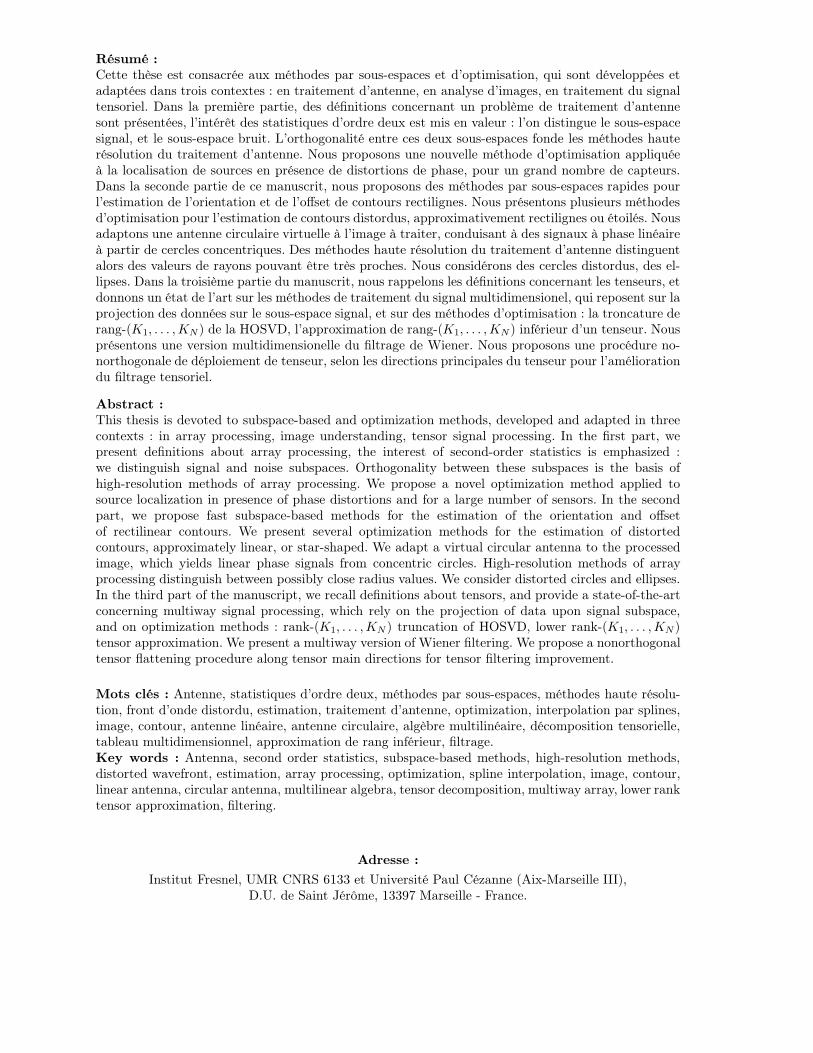
Résumé :
Cette thèse est consacrée aux méthodes par sous-espaces et d’optimisation, qui sont développées etadaptées dans trois contextes : en traitement d’antenne, en analyse d’images, en traitement du signaltensoriel. Dans la première partie, des définitions concernant un problème de traitement d’antennesont présentées, l’intérêt des statistiques d’ordre deux est mis en valeur : l’on distingue le sous-espacesignal, et le sous-espace bruit. L’orthogonalité entre ces deux sous-espaces fonde les méthodes hauterésolution du traitement d’antenne. Nous proposons une nouvelle méthode d’optimisation appliquéeà la localisation de sources en présence de distortions de phase, pour un grand nombre de capteurs.Dans la seconde partie de ce manuscrit, nous proposons des méthodes par sous-espaces rapides pourl’estimation de l’orientation et de l’offset de contours rectilignes. Nous présentons plusieurs méthodesd’optimisation pour l’estimation de contours distordus, approximativement rectilignes ou étoilés. Nousadaptons une antenne circulaire virtuelle à l’image à traiter, conduisant à des signaux à phase linéaireà partir de cercles concentriques. Des méthodes haute résolution du traitement d’antenne distinguentalors des valeurs de rayons pouvant être très proches. Nous considérons des cercles distordus, des el-lipses. Dans la troisième partie du manuscrit, nous rappelons les définitions concernant les tenseurs, etdonnons un état de l’art sur les méthodes de traitement du signal multidimensionel, qui reposent sur laprojection des données sur le sous-espace signal, et sur des méthodes d’optimisation : la troncature derang-(K1, . . . , KN) de la HOSVD, l’approximation de rang-(K1, . . . , KN) inférieur d’un tenseur. Nousprésentons une version multidimensionelle du filtrage de Wiener. Nous proposons une procédure no-northogonale de déploiement de tenseur, selon les directions principales du tenseur pour l’améliorationdu filtrage tensoriel.
Abstract :
This thesis is devoted to subspace-based and optimization methods, developed and adapted in threecontexts : in array processing, image understanding, tensor signal processing. In the first part, wepresent definitions about array processing, the interest of second-order statistics is emphasized :we distinguish signal and noise subspaces. Orthogonality between these subspaces is the basis ofhigh-resolution methods of array processing. We propose a novel optimization method applied tosource localization in presence of phase distortions and for a large number of sensors. In the secondpart, we propose fast subspace-based methods for the estimation of the orientation and offsetof rectilinear contours. We present several optimization methods for the estimation of distortedcontours, approximately linear, or star-shaped. We adapt a virtual circular antenna to the processedimage, which yields linear phase signals from concentric circles. High-resolution methods of arrayprocessing distinguish between possibly close radius values. We consider distorted circles and ellipses.In the third part of the manuscript, we recall definitions about tensors, and provide a state-of-the-artconcerning multiway signal processing, which rely on the projection of data upon signal subspace,and on optimization methods : rank-(K1, . . . , KN) truncation of HOSVD, lower rank-(K1, . . . , KN)tensor approximation. We present a multiway version of Wiener filtering. We propose a nonorthogonaltensor flattening procedure along tensor main directions for tensor filtering improvement.
Mots clés : Antenne, statistiques d’ordre deux, méthodes par sous-espaces, méthodes haute résolu-tion, front d’onde distordu, estimation, traitement d’antenne, optimization, interpolation par splines,image, contour, antenne linéaire, antenne circulaire, algèbre multilinéaire, décomposition tensorielle,tableau multidimensionnel, approximation de rang inférieur, filtrage.Key words : Antenna, second order statistics, subspace-based methods, high-resolution methods,distorted wavefront, estimation, array processing, optimization, spline interpolation, image, contour,linear antenna, circular antenna, multilinear algebra, tensor decomposition, multiway array, lower ranktensor approximation, filtering.
Adresse :
Institut Fresnel, UMR CNRS 6133 et Université Paul Cézanne (Aix-Marseille III),D.U. de Saint Jérôme, 13397 Marseille - France.