Embed Size (px)
Citation preview
Introduction Spectral UQ Solution Methods Example of result Conclusion
Méthodes spectrales pour la propagationd’incertitudes paramétriques dans les
modèles numériques
Olivier Le Maître1 ∗
1LIMSI, CNRSUPR-3251, Orsay, France
28ème Forum ORAP - 14/10/11
∗In collaboration with A. Ern (CEMICS, ENPC), M. Ndjinga and J.-M. Martinez (CEA, Saclay), A. Nouy (GeM,
Centrale Nantes), L. Mathelin (LIMSI, CNRS), O. Knio (JHU & Duke), R. Ghanem (JHU & USC), H. Najm (Sandia)

Introduction Spectral UQ Solution Methods Example of result Conclusion
Outline1 Introduction
Simulation and errorsData uncertaintyAlternative UQ methods
2 Spectral UQGeneralized PC expansionApplication to UQ
3 Solution MethodsNon-Intrusive MethodsStochastic Galerkin Projection
4 Example of result
5 Conclusion
Introduction Spectral UQ Solution Methods Example of result Conclusion
Simulation and errors
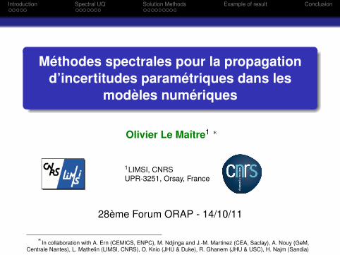
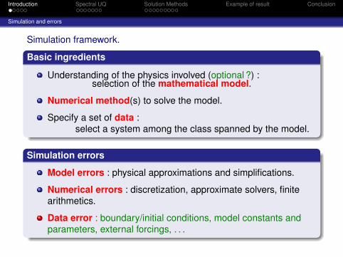
Simulation framework.
Basic ingredients
Understanding of the physics involved (optional ?) :selection of the mathematical model.
Numerical method(s) to solve the model.
Specify a set of data :select a system among the class spanned by the model.
Simulation errors
Model errors : physical approximations and simplifications.
Numerical errors : discretization, approximate solvers, finitearithmetics.
Data error : boundary/initial conditions, model constants andparameters, external forcings, . . .
Introduction Spectral UQ Solution Methods Example of result Conclusion
Simulation and errors
Simulation framework.
Basic ingredients
Understanding of the physics involved (optional ?) :selection of the mathematical model.
Numerical method(s) to solve the model.
Specify a set of data :select a system among the class spanned by the model.
Simulation errors
Model errors : physical approximations and simplifications.
Numerical errors : discretization, approximate solvers, finitearithmetics.
Data error : boundary/initial conditions, model constants andparameters, external forcings, . . .
Introduction Spectral UQ Solution Methods Example of result Conclusion
Data uncertainty
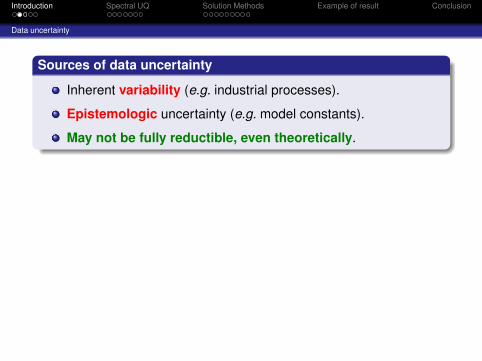
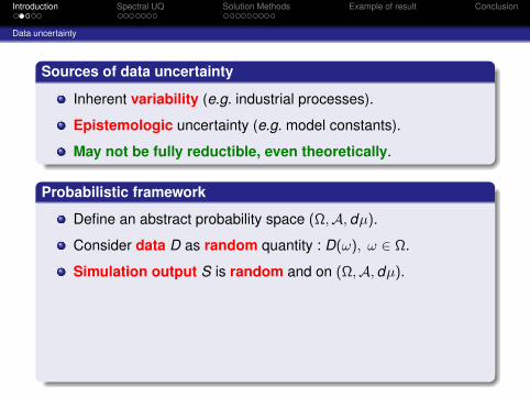
Sources of data uncertainty
Inherent variability (e.g. industrial processes).
Epistemologic uncertainty (e.g. model constants).
May not be fully reductible, even theoretically.
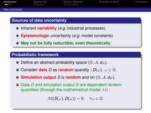
Probabilistic framework
Define an abstract probability space (Ω,A, dµ).
Consider data D as random quantity : D(ω), ω ∈ Ω.
Simulation output S is random and on (Ω,A, dµ).
Data D and simulation output S are dependent randomquantities (through the mathematical model M) :
M(S(ω), D(ω)) = 0, ∀ω ∈ Ω.
Introduction Spectral UQ Solution Methods Example of result Conclusion
Data uncertainty
Sources of data uncertainty
Inherent variability (e.g. industrial processes).
Epistemologic uncertainty (e.g. model constants).
May not be fully reductible, even theoretically.
Probabilistic framework
Define an abstract probability space (Ω,A, dµ).
Consider data D as random quantity : D(ω), ω ∈ Ω.
Simulation output S is random and on (Ω,A, dµ).
Data D and simulation output S are dependent randomquantities (through the mathematical model M) :
M(S(ω), D(ω)) = 0, ∀ω ∈ Ω.
Introduction Spectral UQ Solution Methods Example of result Conclusion
Data uncertainty
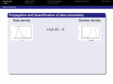
Propagation and Quantification of data uncertainty
Data density
M(S, D) = 0
Solution density
Variability in model output : numerical error bars.
Assessment of predictability.
Support decision making process.
What type of information (abstract quantities, confidenceintervals, density estimations, structure of dependencies, . . .)one needs ?
Introduction Spectral UQ Solution Methods Example of result Conclusion
Data uncertainty
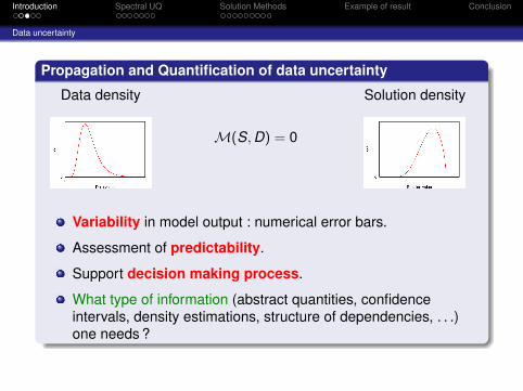
Propagation and Quantification of data uncertainty
Data density
M(S, D) = 0
Solution density
Variability in model output : numerical error bars.
Assessment of predictability.
Support decision making process.
What type of information (abstract quantities, confidenceintervals, density estimations, structure of dependencies, . . .)one needs ?
Introduction Spectral UQ Solution Methods Example of result Conclusion
Alternative UQ methods
Deterministic methods
Sensitivity analysis (adjoint based, AD, . . .) : local.
Perturbation techniques : limited to low order and simple datauncertainty.
Neuman expansions : limited to low expansion order.
Moments method : closure problem (non-Gaussian / non-linearproblems).
Simulation techniques Monte-Carlo
Spectral Methods
Introduction Spectral UQ Solution Methods Example of result Conclusion
Alternative UQ methods
Deterministic methods
Simulation techniques Monte-Carlo
Generate a sample set of data realizations and compute thecorresponding sample set of model ouput.
Use sample set based random estimates of abstractcharacterizations (moments, correlations, . . .).
Plus : Very robust and re-use deterministic codes :(parallelization, complex data uncertainty).
Minus : slow convergence of the random estimates with thesample set dimension.
Spectral Methods
Introduction Spectral UQ Solution Methods Example of result Conclusion
Alternative UQ methods
Deterministic methods
Simulation techniques Monte-Carlo
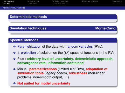
Spectral Methods
Parametrization of the data with random variables (RVs).
⊥ projection of solution on the (L2) space of functions in the RVs.
Plus : arbitrary level of uncertainty, deterministic approach,convergence rate, information contained.
Minus : parametrizations (limited # of RVs), adaptation ofsimulation tools (legacy codes), robustness (non-linearproblems, non-smooth output, . . .).
Not suited for model uncertainty
Introduction Spectral UQ Solution Methods Example of result Conclusion
Alternative UQ methods
Outline1 Introduction
Simulation and errorsData uncertaintyAlternative UQ methods
2 Spectral UQGeneralized PC expansionApplication to UQ
3 Solution MethodsNon-Intrusive MethodsStochastic Galerkin Projection
4 Example of result
5 Conclusion
Introduction Spectral UQ Solution Methods Example of result Conclusion
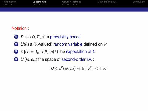
Notation :
1 P := (Θ,Σ, µ) a probability space
2 U(θ) a (R-valued) random variable defined on P3 E [U] =
∫Θ
U(θ)dµ(θ) the expectation of U
4 L2(Θ, dµ) the space of second-order r.v. :
U ∈ L2(Θ, dµ) ⇔ E[U2] < +∞
Introduction Spectral UQ Solution Methods Example of result Conclusion
Generalized PC expansion
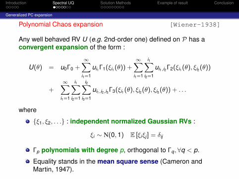
Polynomial Chaos expansion [Wiener-1938]
Any well behaved RV U (e.g. 2nd-order one) defined on P has aconvergent expansion of the form :
U(θ) = u0Γ0 +∞∑
i1=1
ui1Γ1(ξi1(θ)) +∞∑
i1=1
i1∑i2=1
ui1,i2Γ2(ξi1(θ), ξi2(θ))
+∞∑
i1=1
i1∑i2=1
i2∑i3=1
ui1,i2,i3Γ3(ξi1(θ), ξi2(θ), ξi3(θ)) + . . .
where
ξ1, ξ2, . . . : independent normalized Gaussian RVs :
ξi ∼ N(0, 1) E [ξiξj ] = δij
Γp polynomials with degree p, orthogonal to Γq ,∀q < p.
Equality stands in the mean square sense (Cameron andMartin, 1947).
Introduction Spectral UQ Solution Methods Example of result Conclusion
Generalized PC expansion
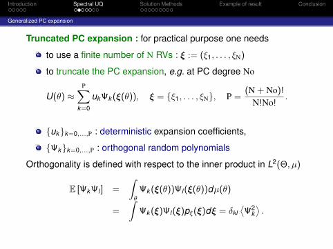
Truncated PC expansion : for practical purpose one needs
to use a finite number of N RVs : ξ := (ξ1, . . . , ξN)
to truncate the PC expansion, e.g. at PC degree No
U(θ) ≈P∑
k=0
ukΨk (ξ(θ)), ξ = ξ1, . . . , ξN, P =(N + No)!
N!No!.
ukk=0,...,P : deterministic expansion coefficients,
Ψkk=0,...,P : orthogonal random polynomials
Orthogonality is defined with respect to the inner product in L2(Θ, µ)
E [ΨkΨl ] =
∫θ
Ψk (ξ(θ))Ψl(ξ(θ))dµ(θ)
=
∫Ψk (ξ)Ψl(ξ)pξ(ξ)dξ = δkl
⟨Ψ2
k⟩.
Introduction Spectral UQ Solution Methods Example of result Conclusion
Generalized PC expansion
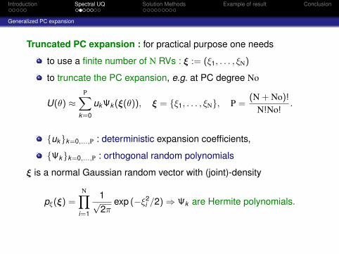
Truncated PC expansion : for practical purpose one needs
to use a finite number of N RVs : ξ := (ξ1, . . . , ξN)
to truncate the PC expansion, e.g. at PC degree No
U(θ) ≈P∑
k=0
ukΨk (ξ(θ)), ξ = ξ1, . . . , ξN, P =(N + No)!
N!No!.
ukk=0,...,P : deterministic expansion coefficients,
Ψkk=0,...,P : orthogonal random polynomials
ξ is a normal Gaussian random vector with (joint)-density
pξ(ξ) =N∏
i=1
1√2π
exp (−ξ2i /2) ⇒ Ψk are Hermite polynomials.
Introduction Spectral UQ Solution Methods Example of result Conclusion
Generalized PC expansion
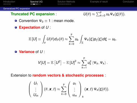
Truncated PC expansion : U(θ) ≈∑P
k=0 ukΨk (ξ(θ)).
Convention Ψ0 ≡ 1 : mean mode.
Expectation of U :
E [U] ≡∫
θ
U(θ)dµ(θ) ≈P∑
k=0
uk
∫Ξ
Ψk (ξ)pξ(ξ)dξ = u0.
Variance of U :
V [U] = E[U2]− E [U]2 ≈
P∑k=1
u2k 〈Ψk ,Ψk 〉 .
Extension to random vectors & stochastic processes : U1...
Um
(θ, x , t) ≈P∑
k=0
u1...
um
k
(x , t) Ψk (ξ(θ)).
Introduction Spectral UQ Solution Methods Example of result Conclusion
Generalized PC expansion
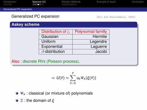
Generalized PC expansion [Xiu and Karniadakis, 2002]
Askey scheme
Distribution of ξi Polynomial famillyGaussian HermiteUniform LegendreExponential Laguerreβ-distribution Jacobi
Also : discrete RVs (Poisson process).
⇒ U(θ) ≈P∑
k=0
ukΨk (ξ(θ))
Ψk : classical (or mixture of) polynomials
Ξ : the domain of ξ
Introduction Spectral UQ Solution Methods Example of result Conclusion
Generalized PC expansion
Outline1 Introduction
Simulation and errorsData uncertaintyAlternative UQ methods
2 Spectral UQGeneralized PC expansionApplication to UQ
3 Solution MethodsNon-Intrusive MethodsStochastic Galerkin Projection
4 Example of result
5 Conclusion
Introduction Spectral UQ Solution Methods Example of result Conclusion
Application to UQ
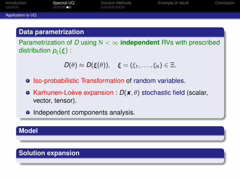
Data parametrization
Parametrization of D using N < ∞ independent RVs with prescribeddistribution pξ(ξ) :
D(θ) ≈ D(ξ(θ)), ξ = (ξ1, . . . , ξN) ∈ Ξ.
Iso-probabilistic Transformation of random variables.
Karhunen-Loève expansion : D(x , θ) stochastic field (scalar,vector, tensor).
Independent components analysis.
Model
Solution expansion
Introduction Spectral UQ Solution Methods Example of result Conclusion
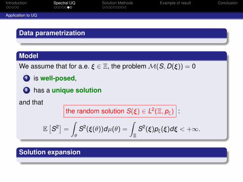
Application to UQ
Data parametrization
ModelWe assume that for a.e. ξ ∈ Ξ, the problem M(S, D(ξ)) = 0
1 is well-posed,
2 has a unique solution
and thatthe random solution S(ξ) ∈ L2(Ξ, pξ) :
E[S2] =
∫θ
S2(ξ(θ))dµ(θ) =
∫Ξ
S2(ξ)pξ(ξ)dξ < +∞.
Solution expansion
Introduction Spectral UQ Solution Methods Example of result Conclusion
Application to UQ
Data parametrization
Model
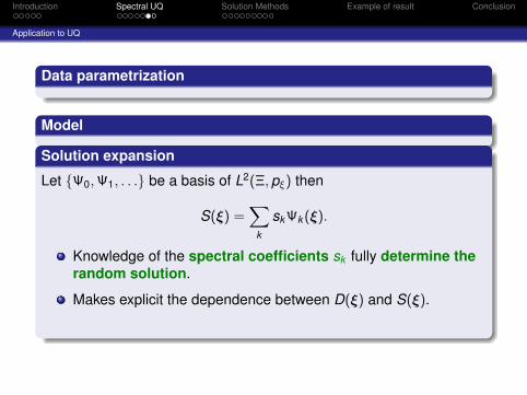
Solution expansion
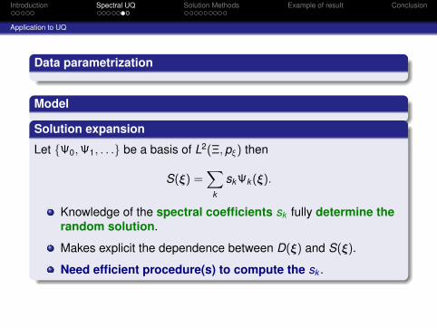
Let Ψ0,Ψ1, . . . be a basis of L2(Ξ, pξ) then
S(ξ) =∑
k
skΨk (ξ).
Knowledge of the spectral coefficients sk fully determine therandom solution.
Makes explicit the dependence between D(ξ) and S(ξ).
Need efficient procedure(s) to compute the sk .
Introduction Spectral UQ Solution Methods Example of result Conclusion
Application to UQ
Data parametrization
Model
Solution expansion
Let Ψ0,Ψ1, . . . be a basis of L2(Ξ, pξ) then
S(ξ) =∑
k
skΨk (ξ).
Knowledge of the spectral coefficients sk fully determine therandom solution.
Makes explicit the dependence between D(ξ) and S(ξ).
Need efficient procedure(s) to compute the sk .
Introduction Spectral UQ Solution Methods Example of result Conclusion
Application to UQ
Outline1 Introduction
Simulation and errorsData uncertaintyAlternative UQ methods
2 Spectral UQGeneralized PC expansionApplication to UQ
3 Solution MethodsNon-Intrusive MethodsStochastic Galerkin Projection
4 Example of result
5 Conclusion
Introduction Spectral UQ Solution Methods Example of result Conclusion
Non-Intrusive Methods
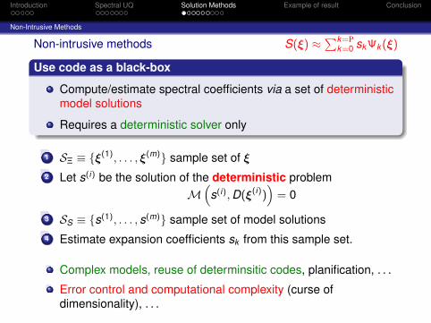
Non-intrusive methods S(ξ) ≈∑k=P
k=0 skΨk (ξ)
Use code as a black-box
Compute/estimate spectral coefficients via a set of deterministicmodel solutions
Requires a deterministic solver only
1 SΞ ≡ ξ(1), . . . , ξ(m) sample set of ξ
2 Let s(i) be the solution of the deterministic problemM(
s(i), D(ξ(i)))
= 0
3 SS ≡ s(1), . . . , s(m) sample set of model solutions4 Estimate expansion coefficients sk from this sample set.
Complex models, reuse of determinsitic codes, planification, . . .
Error control and computational complexity (curse ofdimensionality), . . .
Introduction Spectral UQ Solution Methods Example of result Conclusion
Non-Intrusive Methods
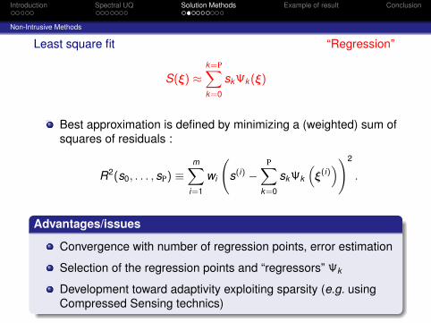
Least square fit “Regression”
S(ξ) ≈k=P∑k=0
skΨk (ξ)
Best approximation is defined by minimizing a (weighted) sum ofsquares of residuals :
R2(s0, . . . , sP) ≡m∑
i=1
wi
(s(i) −
P∑k=0
skΨk
(ξ(i)))2
.
Advantages/issues
Convergence with number of regression points, error estimation
Selection of the regression points and “regressors” Ψk
Development toward adaptivity exploiting sparsity (e.g. usingCompressed Sensing technics)

Introduction Spectral UQ Solution Methods Example of result Conclusion
Non-Intrusive Methods
Non intrusive spectral projection : NISP
S(ξ) ≈k=P∑k=0
skΨk (ξ)
Exploit the orthogonality of the basis :
E[Ψ2
k]sk = 〈S,Ψk 〉 =
∫Ξ
S(ξ)Ψk (ξ)p(ξ)dξ.
Computation of (P + 1) N-dimensional integrals
Use numerical approximates of the form (finite sum) :
〈S,Ψk 〉 ≈NQ∑i=1
w (i)S(ξ(i))
Ψk
(ξ(i))
.
Introduction Spectral UQ Solution Methods Example of result Conclusion
Non-Intrusive Methods
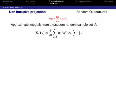
Non intrusive projection Random Quadratures
S(ξ) ≈k=PXk=0
sk Ψk (ξ)
Approximate integrals from a (pseudo) random sample set SS :
〈S,Ψk 〉 ≈1m
m∑i=1
w (i)s(i)Ψk
(ξ(i))
.
MC LHS QMC
Convergence rate
Error estimate
Optimal samplingstrategy
Cost scales in O(m)
Introduction Spectral UQ Solution Methods Example of result Conclusion
Non-Intrusive Methods
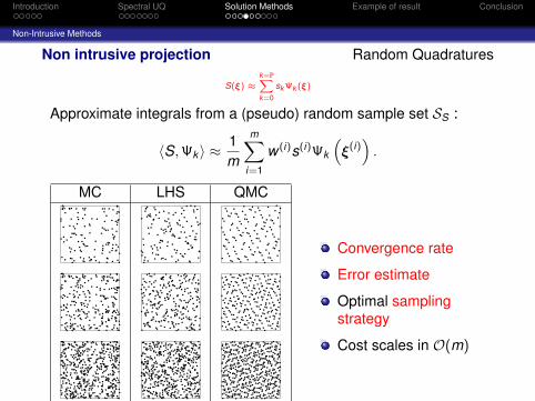
Non intrusive projection Random Quadratures
S(ξ) ≈k=PXk=0
sk Ψk (ξ)
Approximate integrals from a (pseudo) random sample set SS :
〈S,Ψk 〉 ≈1m
m∑i=1
w (i)s(i)Ψk
(ξ(i))
.
MC LHS QMC
Convergence rate
Error estimate
Optimal samplingstrategy
Cost scales in O(m)
Introduction Spectral UQ Solution Methods Example of result Conclusion
Non-Intrusive Methods
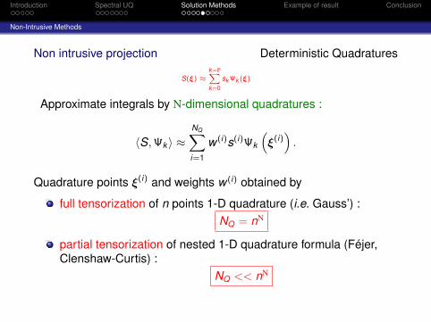
Non intrusive projection Deterministic Quadratures
S(ξ) ≈k=PXk=0
sk Ψk (ξ)
Approximate integrals by N-dimensional quadratures :
〈S,Ψk 〉 ≈NQ∑i=1
w (i)s(i)Ψk
(ξ(i))
.
Quadrature points ξ(i) and weights w (i) obtained by
full tensorization of n points 1-D quadrature (i.e. Gauss’) :NQ = nN
partial tensorization of nested 1-D quadrature formula (Féjer,Clenshaw-Curtis) :
NQ << nN
Introduction Spectral UQ Solution Methods Example of result Conclusion
Non-Intrusive Methods
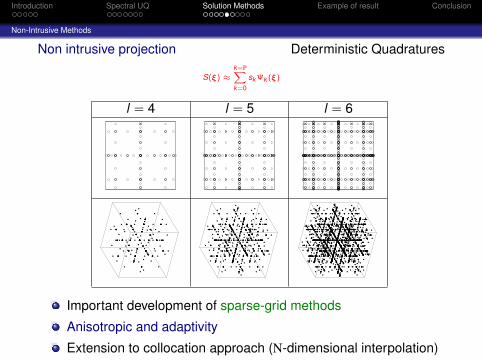
Non intrusive projection Deterministic Quadratures
S(ξ) ≈k=PXk=0
sk Ψk (ξ)
l = 4 l = 5 l = 6
Important development of sparse-grid methods
Anisotropic and adaptivity
Extension to collocation approach (N-dimensional interpolation)
Introduction Spectral UQ Solution Methods Example of result Conclusion
Non-Intrusive Methods
Outline1 Introduction
Simulation and errorsData uncertaintyAlternative UQ methods
2 Spectral UQGeneralized PC expansionApplication to UQ
3 Solution MethodsNon-Intrusive MethodsStochastic Galerkin Projection
4 Example of result
5 Conclusion
Introduction Spectral UQ Solution Methods Example of result Conclusion
Stochastic Galerkin Projection
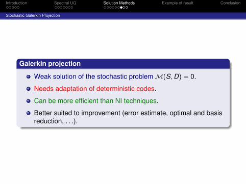
Galerkin projection
Weak solution of the stochastic problem M(S, D) = 0.
Needs adaptation of deterministic codes.
Can be more efficient than NI techniques.
Better suited to improvement (error estimate, optimal and basisreduction, . . .).
Introduction Spectral UQ Solution Methods Example of result Conclusion
Stochastic Galerkin Projection
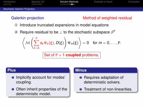
Galerkin projection Method of weighted residual
¬ Introduce truncated expansions in model equations
Require residual to be ⊥ to the stochastic subspace SP⟨M
(P∑
k=0
skΨk (ξ), D(ξ)
)Ψm(ξ)
⟩= 0 for m = 0, . . . , P.
Set of P + 1 coupled problems.
Plus
Implicitly account for modes’coupling.
Often inherit properties of thedeterministic model.
Minus
Requires adaptation ofdeterministic solvers.
Treatment of non-linearities.
Introduction Spectral UQ Solution Methods Example of result Conclusion
Stochastic Galerkin Projection
Outline1 Introduction
Simulation and errorsData uncertaintyAlternative UQ methods
2 Spectral UQGeneralized PC expansionApplication to UQ
3 Solution MethodsNon-Intrusive MethodsStochastic Galerkin Projection
4 Example of result
5 Conclusion
Introduction Spectral UQ Solution Methods Example of result Conclusion
Example of Galerkin projection
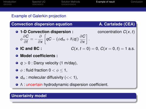
Convection dispersion equation A. Cartalade (CEA)
1-D Convection dispersion : concentration C(x , t)
φ∂C∂t
= − ∂
∂x
[qC − (φdm + Λ|q|) ∂C
∂x
].
IC and BC : C(x , t = 0) = 0, C(x = 0, t) = 1 a.s.
Model coefficients :
q > 0 : Darcy velocity (1 m/day),
φ : fluid fraction 0 < φ ≤ 1,
dm : molecular diffusivity (<< 1),
Λ : uncertain hydrodynamic dispersion coefficient.
Uncertainty model
Introduction Spectral UQ Solution Methods Example of result Conclusion
Example of Galerkin projection
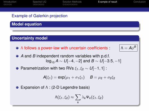
Model equation
Uncertainty model
Λ follows a power-law with uncertain coefficients : Λ = AφB
A and B independent random variables with p.d.f.log10 A ∼ U[−4,−2] and B ∼ U[−3.5,−1]
Parametrization with two RVs ξ1, ξ2 ∼ U[−1, 1] :
A(ξ1) = exp(µ1 + σ1ξ1) B = µ2 + σ2ξ2
Expansion of Λ : (2-D Legendre basis)
Λ(ξ1, ξ2) ≈∑
k
λkΨk (ξ1, ξ2)
Introduction Spectral UQ Solution Methods Example of result Conclusion
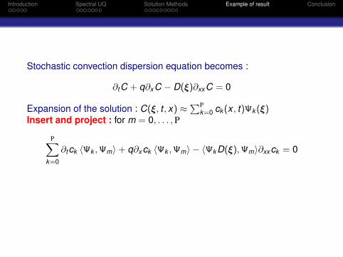
Stochastic convection dispersion equation becomes :
∂tC + q∂xC − D(ξ)∂xxC = 0
Expansion of the solution : C(ξ, t , x) ≈∑P
k=0 ck (x , t)Ψk (ξ)Insert and project : for m = 0, . . . , P
P∑k=0
∂tck 〈Ψk ,Ψm〉+ q∂xck 〈Ψk ,Ψm〉 − 〈Ψk D(ξ),Ψm〉∂xxck = 0
Introduction Spectral UQ Solution Methods Example of result Conclusion
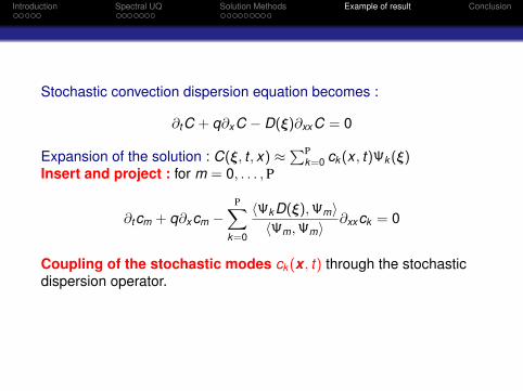
Stochastic convection dispersion equation becomes :
∂tC + q∂xC − D(ξ)∂xxC = 0
Expansion of the solution : C(ξ, t , x) ≈∑P
k=0 ck (x , t)Ψk (ξ)Insert and project : for m = 0, . . . , P
∂tcm + q∂xcm −P∑
k=0
〈Ψk D(ξ),Ψm〉〈Ψm,Ψm〉
∂xxck = 0
Coupling of the stochastic modes ck (x , t) through the stochasticdispersion operator.

Introduction Spectral UQ Solution Methods Example of result Conclusion
Proceed with the deterministic discretization :
Time derivative ∂tck = (cn+1k − cn
k )/∆t +O(∆t)
Implicit scheme with FV scheme with nc spatial cells
P∑k=0
〈ΨkA(ξ),Ψm〉〈Ψm,Ψm〉
cn+1k = b(cn
m), m = 0, . . . , P
where cnk ∈ Rnc and A(ξ) is a random matrix in Rnc×nc
Random matrix expansion A(ξ) =∑P
k=0[A]kΨk (ξ)
P∑k,l=0
Mklm[A]k cn+1l = b(cn
m), Mklm :=〈ΨkΨl ,Ψm〉〈Ψm,Ψm〉
Linear system of (P + 1)× nc equations.
Introduction Spectral UQ Solution Methods Example of result Conclusion
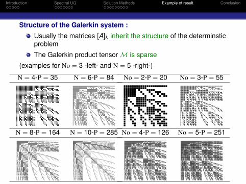
Structure of the Galerkin system :
Usually the matrices [A]k inherit the structure of the determinsticproblem
The Galerkin product tensor M is sparse
(examples for No = 3 -left- and N = 5 -right-)
N = 4-P = 35 N = 6-P = 84
N = 8-P = 164 N = 10-P = 285
No = 2-P = 20 No = 3-P = 55
No = 4-P = 126 No = 5-P = 251
Introduction Spectral UQ Solution Methods Example of result Conclusion
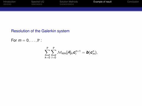
Resolution of the Galerkin system
For m = 0, . . . , P :
P∑k=0
P∑l=0
Mklm[A]k cn+1l = b(cn
m),
Introduction Spectral UQ Solution Methods Example of result Conclusion
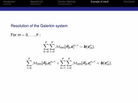
Resolution of the Galerkin system
For m = 0, . . . , P :
P∑k=0
P∑l=0
Mklm[A]k cn+1l = b(cn
m),
P∑l=0
M0lm[A]0cn+1l +
P∑k=1
P∑l=0
Mklm[A]k cn+1l = b(cn
m),
Introduction Spectral UQ Solution Methods Example of result Conclusion
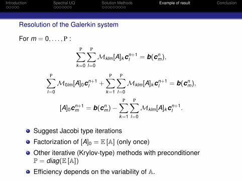
Resolution of the Galerkin system
For m = 0, . . . , P :P∑
k=0
P∑l=0
Mklm[A]k cn+1l = b(cn
m),
P∑l=0
M0lm[A]0cn+1l +
P∑k=1
P∑l=0
Mklm[A]k cn+1l = b(cn
m),
[A]0cn+1m = b(cn
m)−P∑
k=1
P∑l=0
Mklm[A]k cn+1l .
Suggest Jacobi type iterations
Factorization of [A]0 = E [A] (only once)
Other iterative (Krylov-type) methods with preconditionerP = diag(E [A])
Efficiency depends on the variability of A.
Introduction Spectral UQ Solution Methods Example of result Conclusion
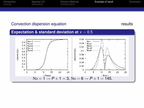
Convection dispersion equation results
Expectation & standard deviation at x = 0.5
No = 1 → P + 1 = 3, No = 6 → P + 1 = 145.

Introduction Spectral UQ Solution Methods Example of result Conclusion
Convection dispersion equation results
Convergence of pdfs at x = 0.5
t = 10h. t = 15h.
Introduction Spectral UQ Solution Methods Example of result Conclusion
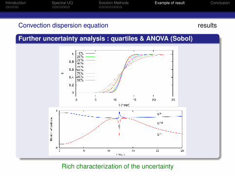
Convection dispersion equation results
Further uncertainty analysis : quartiles & ANOVA (Sobol)
Rich characterization of the uncertainty
Introduction Spectral UQ Solution Methods Example of result Conclusion
Outline1 Introduction
Simulation and errorsData uncertaintyAlternative UQ methods
2 Spectral UQGeneralized PC expansionApplication to UQ
3 Solution MethodsNon-Intrusive MethodsStochastic Galerkin Projection
4 Example of result
5 Conclusion
Introduction Spectral UQ Solution Methods Example of result Conclusion
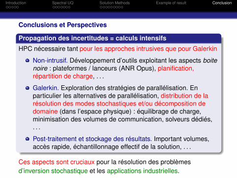
Conclusions et Perspectives
Propagation des incertitudes = calculs intensifs
HPC nécessaire tant pour les approches intrusives que pour Galerkin
Non-intrusif. Développement d’outils exploitant les aspects boitenoire : plateformes / lanceurs (ANR Opus), planification,répartition de charge, . . .
Galerkin. Exploration des stratégies de parallélisation. Enparticulier les alternatives de parallélisation, distribution de larésolution des modes stochastiques et/ou décomposition dedomaine (dans l’espace physique) : équilibrage de charge,minimisation des volumes de communication, solveurs dédiés,. . .
Post-traitement et stockage des résultats. Important volumes,accès rapide, échantillonnage effectif de la solution, . . .
Ces aspects sont cruciaux pour la résolution des problèmesd’inversion stochastique et les applications industrielles.
Introduction Spectral UQ Solution Methods Example of result Conclusion
Conclusions et Perspectives
Perspectives, évolutions et tendances
Le traitement numérique des incertitudes est un domaine derecherche en plein essor.
Réduction du nombre de calculs. Plan d’expérience,échantillonnage préférentiel, sélection de la base de projection,. . .
Adaptation. Utilisation de bases plus ou moins riches surdifférentes portions du domaine physique et paramétrique, . . .
Problématique de la haute-dimension. Bases réduites,tensorisations creuses, séparation et approximation de faiblerang, . . .
Exploitation de bases de données numériques.
Tous ces développements nécessite(ro)nt des efforts deparallélisation.Financements : ANR ASRMEI, ANR TYCHE, GNR MoMaS, Digiteo, DoE, DARPA, Air-Force Lab,
...


![o TI TQOVM M - Cie les petits pas · nwvlm o :w]mv i^mk 6qkwti[ 5wa m\ 2wikpqu 5wa[m ti kwu xiovqm tm 2izlqv lm[ 8tivkpm[ ,mx]q[ !! qt [qovm i][[q zuo]tqvzmumv\ lm[ uq[m[ mv [kvvm](https://img.pdfslide.fr/doc/110x75/5e7ae51d2ff78f15325834dc/o-ti-tqovm-m-cie-les-petits-nwvlm-o-wmv-imk-6qkwti-5wa-m-2wikpqu-5wam-ti.jpg)