Modulational instability in a passivefiber cavity, revisited

D. A. Zezyulin,1,* V. V. Konotop,1 and M. Taki21Centro de Física Teórica e Computacional and Departamento de Física, Universidade de Lisboa,

Avenida Professor Gama, Pinto 2, Lisboa 1649-003, Portugal2Laboratoire de Physique des Lasers, Atomes et Molécules (PHLAM), UMR-CNRS 8523, Université des Sciences et,

Technologies de Lille, 59655 Villeneuve d’Ascq Cedex, France*Corresponding author: zezyulin@cii.fc.ul.pt

Received September 23, 2011; accepted October 24, 2011;posted October 27, 2011 (Doc. ID 155254); published November 28, 2011

Modulation instability in a passive fiber cavity is revisited. We address the problem in the statement with a con-tinuous-time Ikeda map, rather than in the mean-field limit. It is found that plane wave solutions are unstable forboth normal and anomalous dispersion regimes of an optical fiber. The origin of the instability in the continuous-time Ikeda map is in the mode mixing introduced by the beam splitter. The obtained conditions for the instabilitywere compared with ones known for the discrete-time Ikeda map, showing appreciable difference, which, howeverreduces in the mean-field limit. © 2011 Optical Society of AmericaOCIS codes: 190.0190, 190.3100, 190.4360, 190.4370, 230.4320.

Cavities are one of the most widely used types of opticaldevices. They have various experimental implementa-tions and have received a great deal of attention in thecontext of the nonlinear optics. Since the pioneering pa-per [1], it has been well known that the field in cavitiesmay display interesting nonlinear behavior, includingmultistability [1,2] and transitions to aperiodic (chaotic)dynamics [3]. Various types of instabilities induced by theboundary conditions have also been reported in the caseof fibers (with focusing Kerr nonlinearity) operating inthe normal dispersive regime [4,5], or by the transversediffractive effects [6]. The practical importance of pas-sive optical resonators has led to intensive studies ofthese devices, many of which are based on the Lugiato–Lefever model [7]. The latter is obtained in the mean-fieldapproximation (see, e.g., [4,8]) or directly on the originalIkeda map supplied with the nonlinear Schrödinger equa-tion that accounts for spatial evolution of the field alongthe fiber during one circulation [5,6].In this Letter, we address the continuous-time Ikeda

map, accounting also for the field [designated by Aðx; tÞ],whose evolution along the fiber is described by the non-linear Schrödinger (NLS) equation [8]:

Að0; tþ tRÞ ¼ TE þ ReiϕAð1; tÞ; ð1aÞ

Ax ¼ −iAtt þ iσjAj2A: ð1bÞ

Hereafter, we use the units where x is normalized to thecavity length (respectively, 0 ≤ x ≤ 1), t is the time in areference frame moving with the group velocity of thelight, which is c ¼ 1=tR in the chosen units, and E is apump field launched into the cavity. The quantities Rand T (R and T are positive; T2 þ R2 ¼ 1) describe theamplitude reflection and transmission coefficients ofthe beam splitter. ϕ stands for the phase detuning ofthe cavity, and tR is the round-trip time. The model inEqs. (1) is considered for t > 0, which is the most naturalsetting from the experimental point of view.We note that, by defining n ¼ ⌊t=tR⌋, where ⌊ · ⌋ stands

for the integer part, t0 ¼ t − ntR, and Anðx; t0Þ≡ Aðx; t0þ

ntRÞ, the system in Eqs. (1) can be rewritten in the formof the map:

Anþ1ð0; t0Þ ¼ TE þ ReiϕAnð1; t0Þ; ð2aÞ

Anx ¼ −iAn

t0t0 þ iσjAnj2An: ð2bÞ

Equation (2a) connects the field Anþ1ð0; t0Þ at the begin-ning of the ðnþ 1Þth round trip, i.e., at the beam splitter,with its value Anð1; t0Þ at the end of the nth circulation.The temporal evolution of the field is governed by theNLS equation [Eq. (2b)], which must now be consideredon the bounded time interval 0 ≤ t0 ≤ tR.

Modulational instability (MI) of the model in Eq. (1)was addressed in earlier publications only in the mean-field limit, while the system in Eqs. (2) was analyzedboth in the mean-field approximation [9] and in its full“discrete-time” statement [5]. The reason for revisitingthe stability analysis of the original model [Eqs.(1)] istwofold. First, while Eqs. (2) follow from Eqs. (1), asit is indicated above, the inverse is not valid in a generalcase, i.e., the models are not fully equivalent mathemati-cally. Moreover, in this Letter, we show that, in terms ofstability, the models in Eqs. (1) and (2) are different fromthe physical point of view, as well. Meanwhile, we do notquestion the applicability of each one, presuming thatthis should be done for a particular experimental setting.

The stability analysis reported in [5] was performedwith respect to the monochromatic Stokes wavesvn�ðxÞe�iΩt0 . It predicts the onset of MI reflected in expo-nential growth of the Stokes waves during multiplepasses in the cavity: vnþ1

� ðxÞ ¼ qvn�ðxÞ, with the multiplierq, jqj > 1.

The continuity of Aðx; tÞ results in the following condi-tion for the discrete-time model: Anðx; tRÞ ¼ Anþ1ðx; 0Þ.The analysis reported in [5] is consistent with the lattercondition only if vnþ1

� ðxÞ ¼ vn�ðxÞe�iΩtR , i.e., if vn�ðxÞ ¼v�ðxÞe�inΩtR , where v�ðxÞ does not depend on n. In otherwords, jvn�ðxÞj ¼ jv�ðxÞj does not change during subse-quent circulations of the light. This means that no

December 1, 2011 / Vol. 36, No. 23 / OPTICS LETTERS 4623

0146-9592/11/234623-03$15.00/0 © 2011 Optical Society of America

instability in the continuous-time model [Eqs. (1), or inthe model in Eqs. (2), understood as the discrete limitof Eqs. (1), as introduced above] can arise from sucha type of excitation (here we are speaking about linearstability only; the nonlinear study of stability may changethese conclusions). The unstable Stokes waves found in[5] generically correspond to discontinuity of the field intime, from which stems the main difference between themodels of the continuous-time [Eqs. (1)] and the discrete-time [Eqs. (2)] Ikeda maps.Now we turn to the detailed study of the linear stability

of the plane wave solution of Eqs. (1): Aðx; tÞ ¼A0e

iðσA20xþϕ0Þ, where the amplitude A0 and the constant

phase ϕ0 are real and satisfy A0½1 − ReiðϕþσA20Þ�eiϕ0 ¼

TE. Our main finding is that the plane wave solutionis unstable both in normal and anomalous dispersion re-gimes. As in [5], MI is induced by the boundary conditionsof Eq. (1a). However, the modes responsible for instabil-ity of the plane wave solution of Eqs. (1) are essentiallydifferent from ones related to MI of the model in Eqs. (2).We consider a perturbed solution Aðx; tÞ ¼

ðA0 þ uþ ivÞeiðσA20xþϕ0Þ, where uðx; tÞ and vðx; tÞ are real

functions, juj; jvj ≪ A0. Linearization of Eq. (1b) yieldsux ¼ vtt, vx ¼ −utt þ 2σA2

0u, while Eq. (1a) results in

�uð0; tþ tRÞvð0; tþ tRÞ

�¼ R

�cosϕA − sinϕA

sinϕA cosϕA

��uð1; tÞvð1; tÞ

�ð3Þ

(hereafter, ϕA ¼ ϕþ σA20). While u and v were intro-

duced as real-valued functions, we observe that, if arbi-trary complex-valued u and v satisfy the above linearequations, then complex-conjugate functions also do.Hence, the MI occurs if and only if there exist complex-valued uðx; tÞ and vðx; tÞ growing as t → þ∞.The linear stability problem introduced above can be

solved using the Fourier transform (FT) in t (see also themethod employed in [10] for stability of the cavity con-taining dispersive and nonlinear elements). We recallthat, if f ðtÞ is a generalized function, then its FT ~f is afunction of a complex variable s. In particular, if f ðtÞ ¼ept (where p is an arbitrary complex number), then~f ðsÞ ¼ 2πδðs − ipÞ, where δðsÞ is the Dirac delta function.By applying FT to the linear stability equations, we obtain~ux ¼ −s2~v, and ~vx ¼ ðs2 þ 2σA2

0Þ~u. The general solutionof the latter system reads

~uðs; xÞ ¼ −s2ðα1ðsÞeλðsÞx þ α2ðsÞe−λðsÞxÞ; ð4aÞ

~vðs; xÞ ¼ λðsÞðα1ðsÞeλðsÞx − α2ðsÞe−λðsÞxÞ; ð4bÞwhere λ2ðsÞ ¼ −s2ðs2 þ 2σA2

0Þ and α1;2ðsÞ are arbitraryfunctions of s. The FT of (3) yields

�~uð0; sÞ~vð0; sÞ

�¼ eistRR

�cosϕA − sinϕA

sinϕA cosϕA

��~uð1; sÞ~vð1; sÞ

�: ð5Þ

By imposing the constraint in Eq. (5), it is straightforwardto show that the coefficients α1;2ðsÞ are allowed to benonzero only for s satisfying the following equation:

e−istR ¼ R½bðsÞ �ffiffiffiffiffiffiffiffiffiffiffiffiffiffiffiffiffiffib2ðsÞ − 1

q�; ð6Þ

where the function bðsÞ is defined as bðsÞ ¼cosϕA cosh½λðsÞ� − sinϕA sinh½λðsÞ�ðs2 þ σA2

0Þ=λðsÞ. Theplane wave solution of Eqs. (1) is unstable if at least oneroot s ¼ Ωþ iμ of Eq. (6) with μ > 0 is found.

We note that Eq. (6) resembles the results of MI anal-ysis of the model in Eqs. (2) reported in [5]. Namely, itwas found in [5] that the potentially unstable multipliersof the system in Eqs. (2) are given as q� ¼ R½bðΩÞ �ffiffiffiffiffiffiffiffiffiffiffiffiffiffiffiffiffiffiffi

b2ðΩÞ − 1p

�. Notice that, in the latter equation, b dependsnot on the complex variable s but on real Ω, which in thiscontext represents the Stokes wave frequency. Ifjq�j > 1, then MI takes place in the system in Eqs. (2).However, in our case, the requirement of RjbðsÞ �ffiffiffiffiffiffiffiffiffiffiffiffiffiffiffiffiffiffi

b2ðsÞ − 1p

j > 1 is only a necessary condition for the oc-currence of MI, but not a sufficient one, since both sidesof Eq. (6) depend on s. In other words, the requirement ofcontinuity of the field Aðx; tÞ introduces a “filtering:” un-stable frequencies Ω of the discrete-time problem inEqs. (2) generically do not correspond to MI of the con-tinuous-time problem in Eqs. (1). The converse is alsotrue: if s ¼ Ωþ iμ, μ > 0, is a root of Eq. (6), it doesnot guarantee that jq�ðΩÞj > 1.

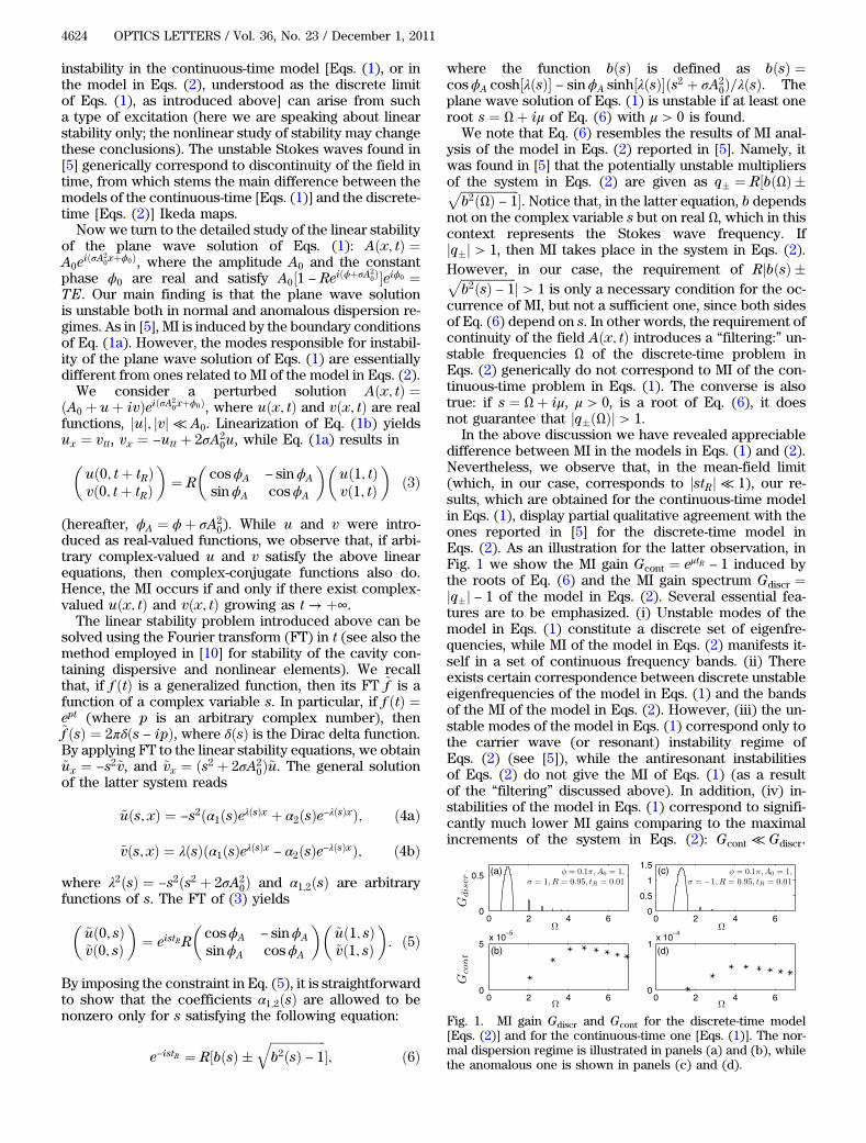
In the above discussion we have revealed appreciabledifference between MI in the models in Eqs. (1) and (2).Nevertheless, we observe that, in the mean-field limit(which, in our case, corresponds to jstRj ≪ 1), our re-sults, which are obtained for the continuous-time modelin Eqs. (1), display partial qualitative agreement with theones reported in [5] for the discrete-time model inEqs. (2). As an illustration for the latter observation, inFig. 1 we show the MI gain Gcont ¼ eμtR − 1 induced bythe roots of Eq. (6) and the MI gain spectrum Gdiscr ¼jq�j − 1 of the model in Eqs. (2). Several essential fea-tures are to be emphasized. (i) Unstable modes of themodel in Eqs. (1) constitute a discrete set of eigenfre-quencies, while MI of the model in Eqs. (2) manifests it-self in a set of continuous frequency bands. (ii) Thereexists certain correspondence between discrete unstableeigenfrequencies of the model in Eqs. (1) and the bandsof the MI of the model in Eqs. (2). However, (iii) the un-stable modes of the model in Eqs. (1) correspond only tothe carrier wave (or resonant) instability regime ofEqs. (2) (see [5]), while the antiresonant instabilitiesof Eqs. (2) do not give the MI of Eqs. (1) (as a resultof the “filtering” discussed above). In addition, (iv) in-stabilities of the model in Eqs. (1) correspond to signifi-cantly much lower MI gains comparing to the maximalincrements of the system in Eqs. (2): Gcont ≪ Gdiscr.

0 2 4 60

0.5

0 2 4 60

5x 10

−5

0 2 4 60

0.5

1

1.5

0 2 4 60

1x 10

−4

(a)

(b)

(c)

(d)

Fig. 1. MI gain Gdiscr and Gcont for the discrete-time model[Eqs. (2)] and for the continuous-time one [Eqs. (1)]. The nor-mal dispersion regime is illustrated in panels (a) and (b), whilethe anomalous one is shown in panels (c) and (d).

4624 OPTICS LETTERS / Vol. 36, No. 23 / December 1, 2011

Finally, (v) in contrast to the model in Eqs. (2), the largestMI gain of the model in Eqs. (1) does not correspond tothe eigenfrequencies with the largest wavelength.Next, we explore Eq. (6) in the limit jsj ≫ A0. Then

λðsÞ ≈ is2 and bðsÞ ≈ cos½ϕþ s2� (here we neglected A0compared to s). Then, to satisfy Eq. (6), it is sufficientto solve the equation e−istR ¼ Rei½ϕþs2�. The roots of thelatter equation can be readily found: s ¼ −tR=2�i

ffiffiffiffiffiffiffiffiffiffiffiffiffiffiffiffiffiffiffiffiffiffiffiffiffiffiffiffiffiffiffiffiffiffiffiffiffiffiffiffiffiffiffiffiffiffiffiffiffiffiffiffi−t2R=4þ ϕþ 2πm − i lnR

q, wherem is any integer. This

result implies that, for sufficiently large m ≫ 1, one canfind a root of Eq. (6) responsible for MI (the imaginarypart of the unstable root will be of the order of

ffiffiffiffiffim

p).

Moreover, not only any background is unstable, but for-mally the MI gain Gcont can acquire any large value. Tounderstand this phenomenon, we recall Eqs. (4), fromwhich one concludes that large roots s correspond tolarge frequencies, which draw the system beyond theparabolic approximation and, hence, are unphysical.Finally, let us discuss the case ϕA ¼ πn, where n is

integer. In this case, bðsÞ ¼ ð−1Þn cosh½λðsÞ�. Analysis per-formed in [5] shows that, in this case, MI of the system inEqs. (2) cannot occur in the normal dispersion regime(i.e., for σ ¼ 1) since jq�j ¼ R for all Ω. On the other hand,we observe that, for ϕA ¼ πn, Eq. (6) is equivalent to analgebraic one:

c2s4 − ½1 − 2σc2A20�s2 þ 2iθsþ θ2 ¼ 0; ð7Þ

where θ ¼ c½lnRþ iπð2mþ nÞ�. By computing the rootsof Eq. (7), one can see that our analysis still predicts theonset of MI in the model in Eqs. (1) for both σ ¼ 1and σ ¼ −1.We also note that Eq. (7) can be obtained with another

approach. For the case ϕA ¼ πn, one can employ the An-satz u ¼ eKtUðx; tÞ and v ¼ eKtVðx; tÞ, where K is definedthrough tRK ¼ lnRþ iπn, and transform the linear stabi-lity equations to Ux ¼ K2V þ 2KVt þ Vtt and Vx ¼−K2U − 2KUt − Utt þ 2σA2

0U , while Eq. (3) acquires theform Uð0; tþ tRÞ ¼ Uð1; tÞ and Vð0; tþ tRÞ ¼ Vð1; tÞ.The latter boundary conditions are not periodic, which,from the physical point of view, results in mixing of theharmonics at the instant of the reflection by the inputmirror. Introducing a new variable τ ¼ xþ ct, and repre-senting U ¼ ϕmðτÞe2πimx and V ¼ ψmðτÞe2πimx, where mis arbitrary integer, we obtain Y 0

m ¼ AmYm, where 0 ¼d=dτ, Ym ¼ colðϕm;ϕ0

m;ψm;ψ 0mÞ, and

Am ¼ 1

c2

0BBB@

0 c2 0 02σA2

0 − K2−2Kc −2πim −1

0 0 0 c2

2πim 1 −K2−2Kc

1CCCA:

By straightforward algebra one can see that, if ν is an ei-genvalue of Am, then s ¼ iðK þ cνÞ is a root of Eq. (7).Returning to the variables ðx; tÞ, one can see thatuðx; tÞ and vðx; tÞ grow in t if there exists a root s ofEq. (7) with a positive imaginary part. We remark that

the solutions uðx; tÞ and vðx; tÞ obtained in this paragraphare represented by Fourier harmonics in x (m is a num-ber of a harmonic), which are “mixed” due to boundaryconditions, which require introducing the variable τ.

To conclude, we have shown that the constant ampli-tude solutions of the continuous-time Ikeda map are in-trinsically unstable in both the normal and anomalousdispersion regimes. Similar to the case of the discrete-time Ikeda map, MI of the continuous-time model istightly related to specific boundary conditions. However,the modes responsible for MI in the continuous-time andthe discrete-time models are different. This difference re-duces (but still does not vanish) in the mean-field limit,i.e., when the evolution of the field inside the cavity dur-ing one round trip can be neglected.

At this stage, only a linear stability analysis has beenperformed. An important issue is to consider the effectsof nonlinear terms beyond the primary linear instabilitythat may lead to the formation of stable dissipative soli-tons. Other important features are the study of stability/instability of periodic solutions appearing in the continu-ous-time model in Eqs. (1) and its comparison with thecorresponding ones of the discrete-timemodel in Eqs. (2),together with the effect of stochastic fluctuations antici-pating the instability by the appearance of precursors [11].To what extent our results can be applied to multimodefiber systems is also an interesting issue. This is in pro-gress and will be published elsewhere.

We are grateful to G. L. Alfimov for useful discussions.D. A. Zezyulin and V. V. Konotop were supported by theFundação para a Ciência e a Tecnologia (FCT) underthe grants SFRH/BPD/64835/2009, PTDC/EEA-TEL/105254/2008, and PEst-OE/FIS/UI0618/2011. M. Taki wassupported by the Centre National de la Recherche Scien-tifique (CNRS), and by the “Conseil Régional Nord-Pas deCalais” and the “Fonds Européen de DéveloppementEconomique des Régions.”

References

1. K. Ikeda, Opt. Commun. 30, 257 (1979).2. H. M. Gibbs, Optical Bistability: Controlling Light with

Light (Academic, 1985).3. K. Ikeda, H. Daido, and O. Akimoto, Phys. Rev. Lett. 45, 709

(1980).4. M. Haelterman, Opt. Lett. 17, 792 (1992).5. S. Coen and M. Haelterman, Phys. Rev. Lett. 79, 4139

(1997).6. D. W. McLaughlin, J. V. Moloney, and A. C. Newell, Phys.

Rev. Lett. 54, 681 (1985).7. L. A. Lugiato and R. Lefever, Phys. Rev. Lett. 58, 2209

(1987).8. M. Tlidi, A. Mussot, E. Louvergneaux, G. Kozyreff, A. G.

Vladimirov, and M. Taki, Opt. Lett. 32, 662 (2007).9. M. Haelterman, S. Trillo, and S. Wabnitz, Opt. Lett. 17, 745

(1992).10. G. Kozyreff, T. Erneux, M. Haelterman, and P. Kockaert,

Phys. Rev. A 73, 063815 (2006).11. G. Agez, M. G. Clerc, and E. Louvergneaux, Phys. Rev. E 77,

026218 (2008).

December 1, 2011 / Vol. 36, No. 23 / OPTICS LETTERS 4625