Ninth International Geostatistics Congress, Oslo, Norway June 11 – 15, 2012

Multidirectional random walk: an alternative to local simulation of Gaussian data Diniz T. Ribeiro1, Evandro M. Cunha Filho2, João F. C. L. Costa3, Débora G. Roldão4 and Tomás B. F. Tamantini5 Abstract Various geostatistical simulation techniques rely on the multiGaussian model. These methods generate equally probable realisations of a Gaussian variable, honouring the first two statistical moments and the spatial variability function g(h) of the Gaussian variable. Currently existing techniques are time consuming to implement and require advanced computational hardware to process real dataset and models with millions of blocks. The paper proposes an alternative simulation technique based on a multidirectional random walk (RW) of Gaussian variables. This method is based on random walks which consider the action of a particle along random directions within a real line. The position of the particle in a determined distance h is described by independent random increments, each one with the same probability, of 50%, to be equal f or –f, where f is the scaling factor of the increments. The increments at a certain distance h have a normal distribution, with mean zero and variance proportional to the distance and to f². The simulation technique proposed is based on random walks starting at a conditioning point (x) and moving to a simulated point (x0), spaced by h, generating an error Yrw(h) as a function of distance h. This error is added to the value Y(x) to obtain the simulated value Ysrw(x+h). For multiple RW from different conditioning points (xi), converging to the same point (x0), the final result of the RW simulation, Ysrw(x0), is the simple kriging estimation of all RW simulations from the conditioning points, Ysrw(xi+hi)). The experimental results show this new methodology honoured both statistical moments of the Gaussian conditioning points faster than sequential algorithms. The scaling factor f can be used for future local simulations (LS) without requiring global simulations (GS).

1 VALE Ferrous Department, Av de Ligação, 3580 – Nova Lima/MG – Brazil, Diniz.Ribeiro@vale.com 2 VALE Ferrous Department, Av de Ligação, 3580 – Nova Lima/MG – Brazil, Evandro.Cunha@vale.com 3 UFRGS, Av. Bento Golçalves, 9500 – Porto Alegre/RS – Brazil, Jfelipe@ufrgs.br 4 VALE Ferrous Department, Av de Ligação, 3580 – Nova Lima/MG – Brazil, Debora.Roldao@vale.com 5 UFMG, Av. Antonio Carlos, 6627 – Belo Horizonte/MG – Brazil, Tomasbft@gmail.com

2

Introduction

The geostatistical simulation techniques have been proposed initially by [14] followed by publications of [9] and [2]. These techniques allow better represent the complexity of natural phenomena through the generation of probabilistic models with multiple equally-probable scenarios. Each simulated scenario represents a realisation of a random function (RF) should honour the heterogeneity and spatial variability of the regionalized variable of a mineral deposit through the reproduction of two statistical moments, mean and variance, and variogram of the regionalized variable. The idea embedded in most geostatistical simulation methods used for simulating continuous variables is to assess the uncertainty in the estimation prior to any guess about the value estimated. Models used in this way aim to replicate the spatial structure of a data set as a whole rather than provide reliable local estimates of an attribute at particular locations. Mine production plans, schedules, and blending strategies require knowledge of grade dispersion. Because kriged estimates are said to be biased in terms of grade dispersion they should not be used for these engineering applications. Equally probable models generated by simulation of the deposit are introduced to overcome this problem. The simulated model is said to be conditionally simulated if it honours values at sampled points and reproduces the same dispersion characteristics of the original data set, i.e. the mean, variance and covariance or variogram. In a conditionally simulated model it is possible to address questions referring to the dispersion of the grades during mining or processing, since the dispersion characteristics of the original data are maintained. The better the spatial continuity and variability of the real deposit can be described, the better the numerically simulated model will be. The simulated data, zsi(x) is the ith realisation of the random function Z(x), in the same way that the real values z(x) are also considered realisations of a random function, both exhibiting the same two first order moments. Simulations which honour sample data at their location are called conditional. Thus, from a perspective of two-point statistics, there is no difference between the real and simulated values. The interesting aspect of conditional simulation is that simulated values can be generated in all geographical positions covering the whole deposit and not only at the sampled sites. The penalty for obtaining this denser grid of values through the deposit is an increase of the estimation error, or, in geostatistical jargon, the variance of the estimation obtained through conditional simulation is higher than the variance obtained using estimation methods. [17] discusses the simulation algorithms developed for petroleum applications. [6] compare the performance in terms of local accuracy (average quality of the estimate) obtained by using various simulation algorithms in distinct data sets, concluding that sequential Gaussian algorithms provide better results than sequential indicator algorithms.

3

A family of geostatistical simulation methods generally called sequential simulation algorithms [8]; [10] differs significantly from the algorithms first introduced (see [12] for a comprehensive discussion). Most of the early methods (turning bands for example) draw random values from unrelated distributions and use some moving window average to imprint spatial correlation. The novelty of sequential methods is the idea of randomly drawing the values from distributions somehow related using the decomposition of the conditional cumulative distribution function (ccdf) of a random function. Geostatistical simulation is used in mineral industry for the economic evaluation of projects and risk analysis. Although widely enshrined in that domain, the geostatistical simulation has its limitations for routine applications due to the large computational time and also because of the need to simulate all the mineral deposit models to generate ergodic simulated models. This paper reports the results of a new simulation algorithm based on random walks with less computational effort. The reduction on computational time allows the use of simulation methods routinely in the mining industry. Random walk simulations can be used to make local simulation practical, using the parameters of the previous study from a global simulation (variography, Gaussian anamorphosis, the search strategy, etc). This local simulation is directly applied during mining phases when there is a constant addition of new data to the original conditioning dataset. A case study using a synthetic Gaussian dataset was used to illustrate the methodology. These 416 samples are isotropic and were collected at a regular grid. The simulations tests used an omnidirectional variogram with one spherical structure, ranging 20 meters, to simulate one Gaussian variable in 10,000 points in two-dimensional dense grid.

Gaussian distribution and random walk

The probability distributions laws are not a pure abstraction without physical sense, but the mathematical expression of the fact that there are laws governing the random phenomena of nature [18]. These laws are established experimentally and directly or indirectly based on experimental data. The normal distribution is the most important of all statistics and has a special feature is a "threshold law" to which all other laws tend their distributions. Many processes in nature lead to the normal distribution, including the measurement errors. The concept of error estimation is applied in geostatistics and simulation techniques using Gaussian transformed variables to the original variables. According to [5], the definition of RW considers a particle performing a random path on a real line. The particle position at time t is described by random independent increments, each having probability ½ equaling 1 and ½ equaling –1.

4

If the increments at distance h have a normal distribution, the random walk is called Brownian motion. [5] defines one dimension Brownian motion to be a random process X(t) such as:

i. with probability 1, X(0) = 0 and X(t) is a continuous function of t; ii. for any t >= 0 and h > 0 the increment X(t+h)-X(t) is normally

distributed with mean 0 and variance h; iii. the increments X(t2)-X(t1) are independent.

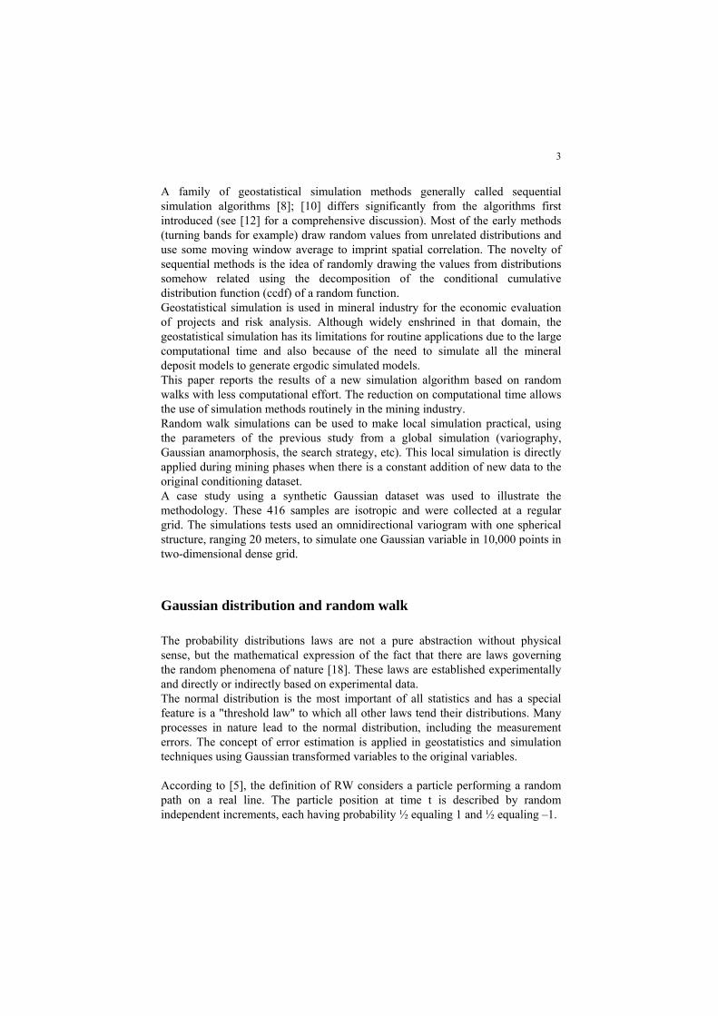
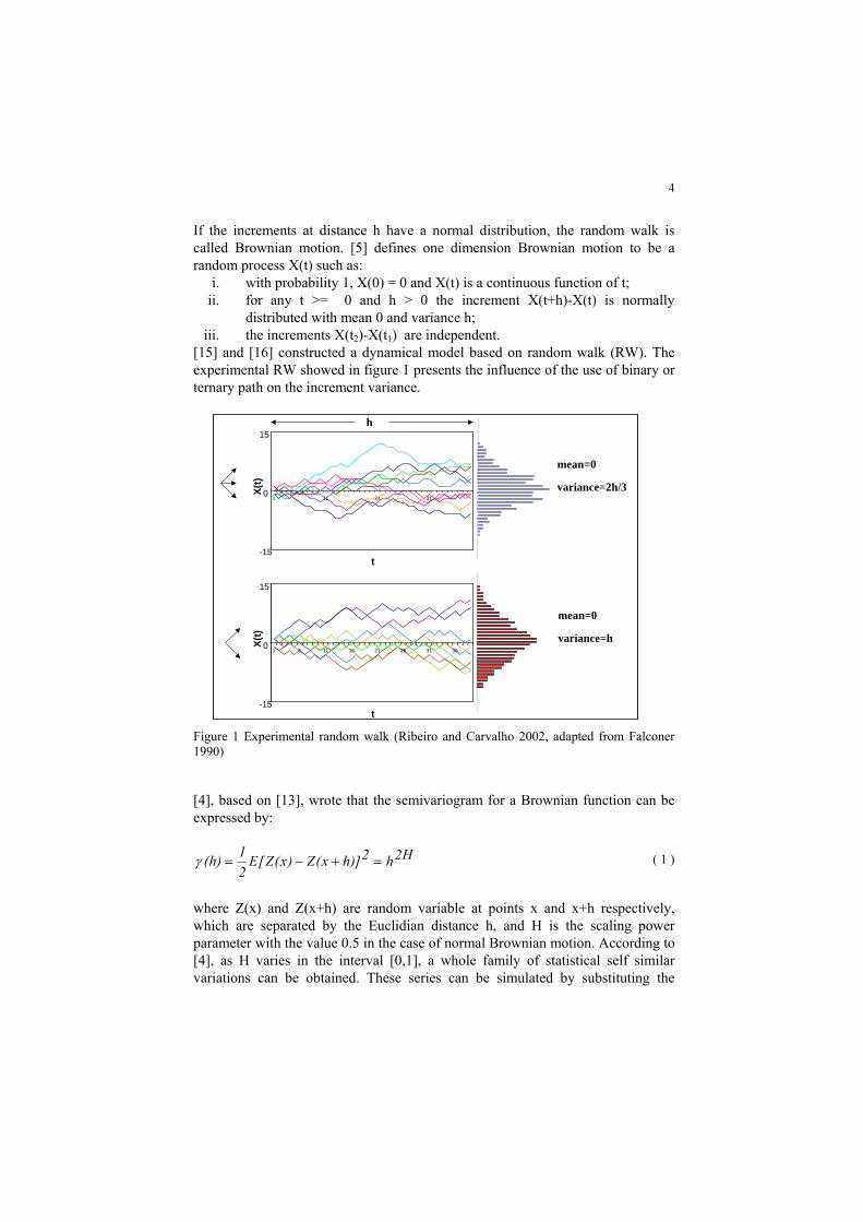
[15] and [16] constructed a dynamical model based on random walk (RW). The experimental RW showed in figure 1 presents the influence of the use of binary or ternary path on the increment variance.

Figure 1 Experimental random walk (Ribeiro and Carvalho 2002, adapted from Falconer 1990)

[4], based on [13], wrote that the semivariogram for a Brownian function can be expressed by:

γ ( ) [ ( ) ( )]h E Z x Z x h h H= − + =12

2 2 ( 1 )

where Z(x) and Z(x+h) are random variable at points x and x+h respectively, which are separated by the Euclidian distance h, and H is the scaling power parameter with the value 0.5 in the case of normal Brownian motion. According to [4], as H varies in the interval [0,1], a whole family of statistical self similar variations can be obtained. These series can be simulated by substituting the

-15

0

15

1 11 21 31

t

X(t)

-15

0

15

1 6 11 16 21 26 31 36

t

X(t)

h

mean=0

variance=2h/3

mean=0

variance=h

5

normally distributed Gaussian error in the equation for Brownian motion by a discrete fractional Gaussian noise.

Conditional Simulation

For a given selective mining unit (SMU) it is possible to evaluate the local uncertainty through the local cumulative distribution function (lcdf) obtained by conditional simulation. Stochastic conditional simulation is able to quantify variability on geological attributes such as grades or any other attribute relevant to a given mining project. Variability can be assessed by constructing multiple equally probable numerical scenarios. The combination of these scenarios can provide an assessment of the so-called space of uncertainty. The most commonly used stochastic conditional simulation algorithms are the Sequential Gaussian [7], Sequential Indicator [1] and the Turning Bands method – TB [14]. The simulation of values of an attribute Z using turning bands, conditional to the original data, is performed in two stages, both running in the Gaussian space. In the first stage, the values obtained at node of a grid are not conditional to the original data (normal). However, they reproduce the covariance model of these data. In the second stage, the values obtained at each location are made conditional to the original data (normal). The final generated values are eventually back-transformed to the original variable space. The method is presented by [3], and is nowadays consolidated and widely used among the geostatistical community within the mining industry. More recently, [11] presents some alternatives for algorithms to simulate values in one given line respecting the related model of covariance. The TB non-conditional simulation methods consist of N lines simulate RF independently with the same covariance C(h). The simulated values at the nodes of regular grid are obtained by projecting each of the N lines spread uniformly. The random variables should be multiGaussian. The results of the conditional simulations, Ycs, is the sum of two independent Gaussian functions. The multiGaussian hypothesis should be checked at least for the bivariate case. i.e verifying biGaussianity from pairs of variables (Y (x), Y (x +h)).

Conditional RW Simulation: preserving the unit variance through background noise

Similarly to TB simulation, the proposal random walk simulation technique is based on conditioning points, generating an error Yrw as a function of distance h

6

which should be added to the value of Y(x) to obtain the simulated value Ysrw(x+h). Although, for cases of multidirectional random walk from more than one conditioning point, simple kriging (SK) weights are used according to:

( ) ( )[ ]∑ +=n

ixxrwixixsrw ii

hYYY00

* λ ( 2 )

where: li is the simple kriging weight; x0 is the point to be simulated; xi is the conditioning point; and n is the number of conditioning points. The conditioning points are honoured and the variability at the simulated grid nodes is proportional to the distance to the sample points. The simulations will be obtained through the summation of different random functions, centered at each sample, weighted by a function of the distance between the grid node and the sample derived from point simple kriging. It can be shown that, for sufficiently large grids, the variance of the final simulation is a linear function of the variance of the random function chosen. The final variance of Ysrw depends on weighting process of variogram function used, configuration of sample distribution and size of the grid. Any estimation based on simple kriging, or any other form of distance weighting interpolation algorithm has the variance of the samples significantly smoothed out. The constants inform how much variance is lost during interpolation. The restore of unit variance was carried out adding random values to the final simulation. The variance can be controlled by simply scaling of the random function. Scaling a function by a factor f will result in a variance multiplied by f². In the case of multidirectional random walk, with n steps of size +f and –f, the scaling factor can be chosen to have the desired variance. Equation 3 resumes the relation between the scaling factor f and the variance of the randoim walk simulation (σ2

Ysrw).

YskY afsrw222 σσ += ( 3 )

where a is the angular coefficient of the regression line between σ2Ysrw versus f2,

σ2Ysk is the simple kriging smoothed variance of all estimated nodes.

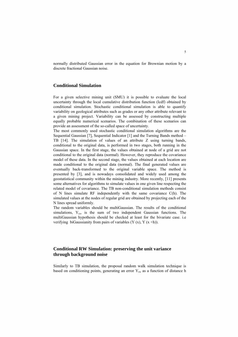
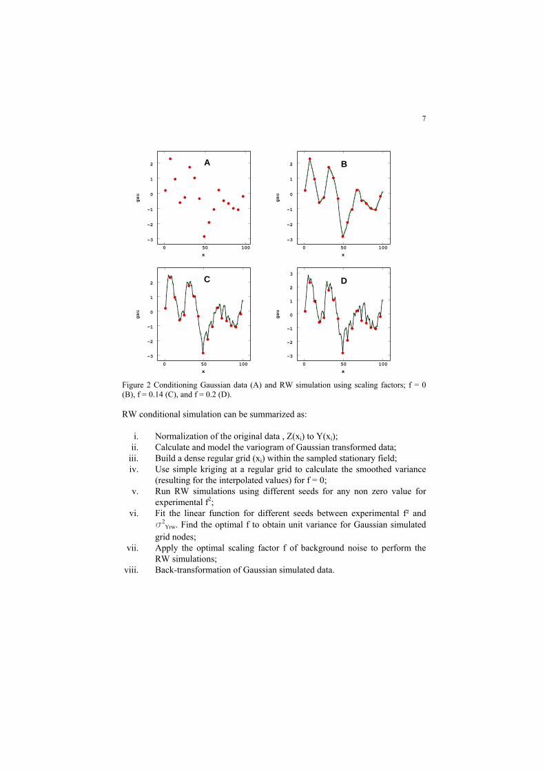
Figure 2 presents one example of RW simulations using Gaussian conditioning points with unit variance (Figure 2A) and the simple kriging results using different scaling factors; f = 0 (Figure 2B), f = 0.14 (Figure 2C), and f = 0.2 (Figure 2D). The respective variance of the simulations for each scaling factors are 0.82, 0.91 and 1.01.

7

Figure 2 Conditioning Gaussian data (A) and RW simulation using scaling factors; f = 0 (B), f = 0.14 (C), and f = 0.2 (D).

RW conditional simulation can be summarized as: i. Normalization of the original data , Z(xi) to Y(xi);

ii. Calculate and model the variogram of Gaussian transformed data; iii. Build a dense regular grid (xi) within the sampled stationary field; iv. Use simple kriging at a regular grid to calculate the smoothed variance

(resulting for the interpolated values) for f = 0; v. Run RW simulations using different seeds for any non zero value for

experimental f2; vi. Fit the linear function for different seeds between experimental f² and

s2Yrw. Find the optimal f to obtain unit variance for Gaussian simulated

grid nodes; vii. Apply the optimal scaling factor f of background noise to perform the

RW simulations; viii. Back-transformation of Gaussian simulated data.

0 50 100 x

-3

-2

-1

0

1

2

gau

0 50 100 x

-3

-2

-1

0

1

2

3 gau

0 50 100 x

-3

-2

-1

0

1

2

gau

0 50 100 x

-3

-2

-1

0

1

2

gau

A B

C D

0 50 100 x

-3

-2

-1

0

1

2

gau

0 50 100 x

-3

-2

-1

0

1

2

3 gau

0 50 100 x

-3

-2

-1

0

1

2

gau

0 50 100 x

-3

-2

-1

0

1

2

gau

A B

C D

8

2D Conditional RW Simulation

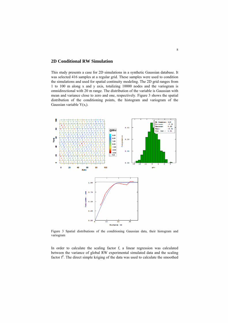
This study presents a case for 2D simulations in a synthetic Gaussian database. It was selected 416 samples at a regular grid. These samples were used to condition the simulations and used for spatial continuity modeling. The 2D grid ranges from 1 to 100 m along x and y axis, totalizing 10000 nodes and the variogram is omnidirectional with 20 m range. The distribution of the variable is Gaussian with mean and variance close to zero and one, respectively. Figure 3 shows the spatial distribution of the conditioning points, the histogram and variogram of the Gaussian variable Y(xi).

Figure 3 Spatial distributions of the conditioning Gaussian data, their histogram and variogram

In order to calculate the scaling factor f, a linear regression was calculated between the variance of global RW experimental simulated data and the scaling factor f2. The direct simple kriging of the data was used to calculate the smoothed

9

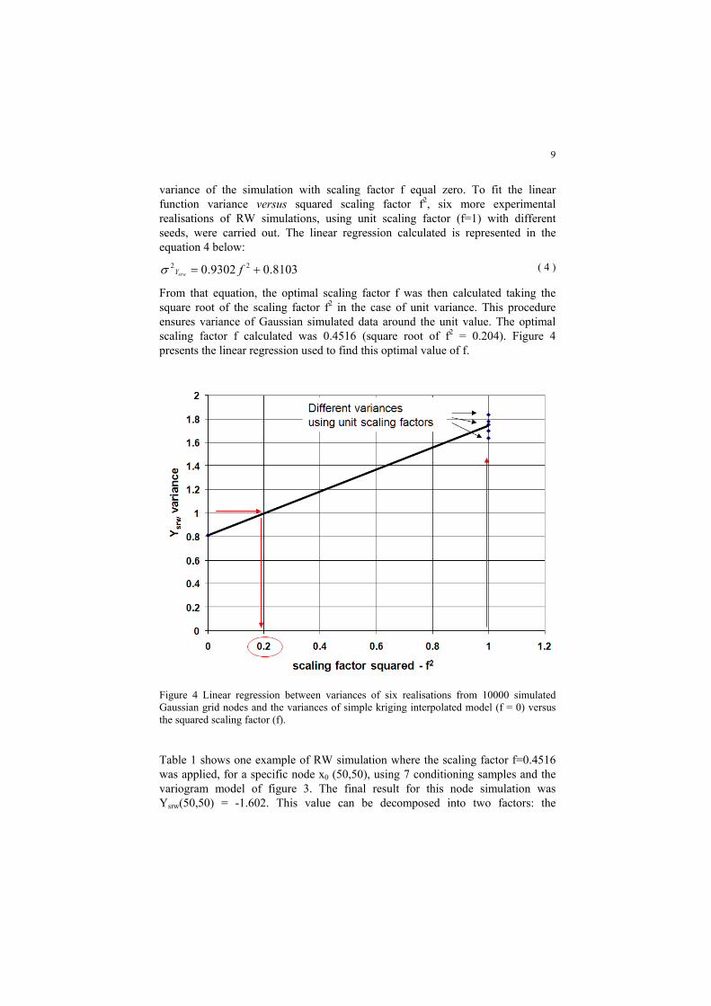
variance of the simulation with scaling factor f equal zero. To fit the linear function variance versus squared scaling factor f2, six more experimental realisations of RW simulations, using unit scaling factor (f=1) with different seeds, were carried out. The linear regression calculated is represented in the equation 4 below:

8103.09302.0 22 += fsrwYσ ( 4 )

From that equation, the optimal scaling factor f was then calculated taking the square root of the scaling factor f2 in the case of unit variance. This procedure ensures variance of Gaussian simulated data around the unit value. The optimal scaling factor f calculated was 0.4516 (square root of f2 = 0.204). Figure 4 presents the linear regression used to find this optimal value of f.

Figure 4 Linear regression between variances of six realisations from 10000 simulated Gaussian grid nodes and the variances of simple kriging interpolated model (f = 0) versus the squared scaling factor (f).

Table 1 shows one example of RW simulation where the scaling factor f=0.4516 was applied, for a specific node x0 (50,50), using 7 conditioning samples and the variogram model of figure 3. The final result for this node simulation was Ysrw(50,50) = -1.602. This value can be decomposed into two factors: the

10

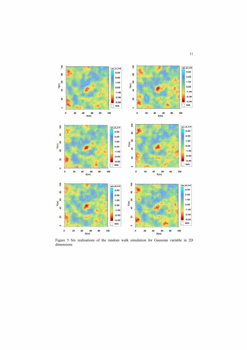
background noise factor, Yrw(50,50) = 0.377, and the simple kriging estimation, Ysk(50,50) = -1.976. This example was extended to a complete 2D grid in order to generate six equally probable scenarios considering a conditional geostatistical RW simulation for the Gaussian variable. Figure 5 shows six simulated images for all 10000 grid nodes used in this example. Data and variogram used to condition these simulations were the ones depicted in figure 3. Images show similarity among the six realisations due to the conditioning data, however differences among realisations are noticed.

Table 1 RW simulation for a specific grid node x0 (50,50) – simple kriging interpolation. C_X and C_Y are data point coordinates. Y(xi) is the normal score at sampled locations. hi is the separation distance from data locations to the grid node being simulated. Yrw(xi+h) is the RW simulated value at the grid node obtained from data i. λi is the simple kriging weight assigned to sample i when interpolating at node x0. Ysrw is the simulated value at the grid node

Sample C_X C_Y Y(xi) hi Yrw(xi+h) λi Ysrw x1 43 47 -0.35 7.6 0.90 -0.03 0.55 x2 45 55 1.13 7.1 1.36 -0.01 2.49 x3 47 51 -1.19 3.2 1.36 0.33 0.17 x4 49 47 -2.85 3.2 -0.45 0.33 -2.52 x5 51 43 -1.93 7.1 -0.45 -0.01 -1.94 x6 51 55 0.03 5.1 -0.45 0.08 0.11 x7 53 51 -2.05 3.2 0.45 0.33 -1.72

node x0 50 50 -1.976 0 0.377 1.05 -1.602

11

Figure 5 Six realisations of the random walk simulation for Gaussian variable in 2D dimensions

12

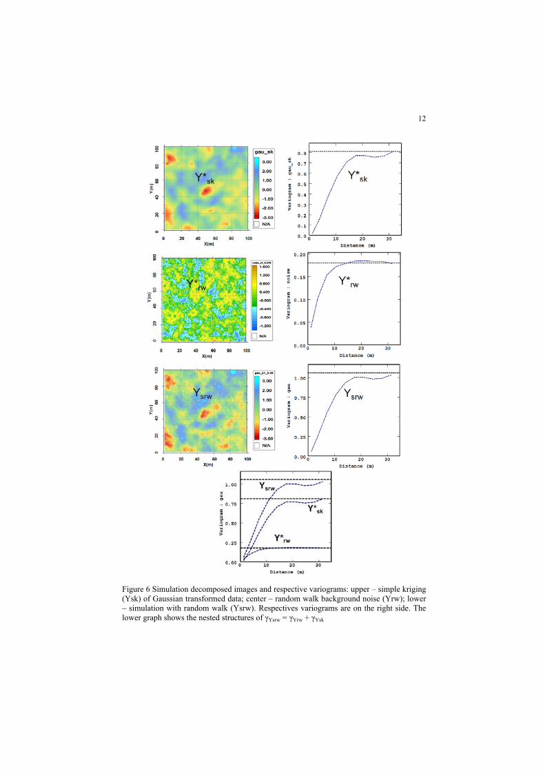
Figure 6 Simulation decomposed images and respective variograms: upper – simple kriging (Ysk) of Gaussian transformed data; center – random walk background noise (Yrw); lower – simulation with random walk (Ysrw). Respectives variograms are on the right side. The lower graph shows the nested structures of γYsrw = γYrw + γYsk

13

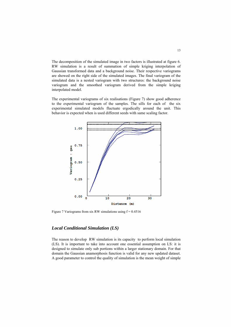
The decomposition of the simulated image in two factors is illustrated at figure 6. RW simulation is a result of summation of simple kriging interpolation of Gaussian transformed data and a background noise. Their respective variograms are showed on the right side of the simulated images. The final variogram of the simulated data is a nested variogram with two structures: the background noise variogram and the smoothed variogram derived from the simple kriging interpolated model. The experimental variograms of six realisations (Figure 7) show good adherence to the experimental variogram of the samples. The sills for each of the six experimental simulated models fluctuate ergodically around the unit. This behavior is expected when is used different seeds with same scaling factor.

Figure 7 Variograms from six RW simulations using f = 0.4516

Local Conditional Simulation (LS)

The reason to develop RW simulation is its capacity to perform local simulation (LS). It is important to take into account one essential assumption on LS: it is designed to simulate only sub portions within a larger stationary domain. For that domain the Gaussian anamorphosis function is valid for any new updated dataset. A good parameter to control the quality of simulation is the mean weight of simple

14

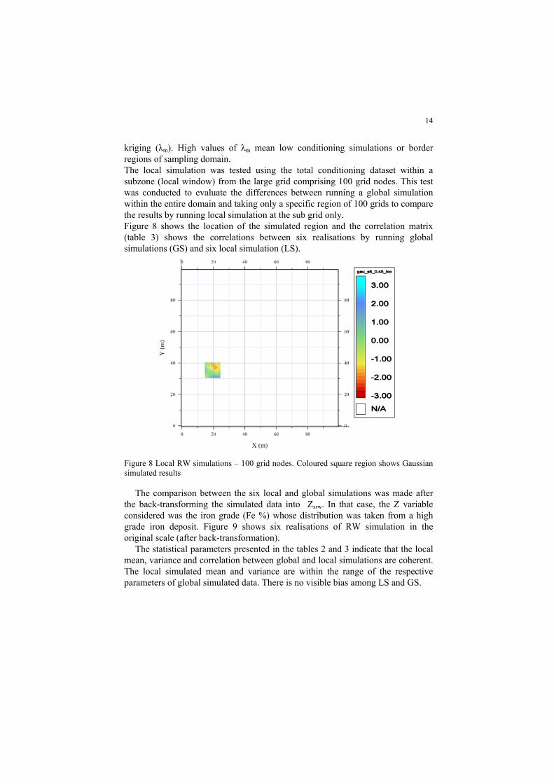
kriging (λm). High values of λm mean low conditioning simulations or border regions of sampling domain. The local simulation was tested using the total conditioning dataset within a subzone (local window) from the large grid comprising 100 grid nodes. This test was conducted to evaluate the differences between running a global simulation within the entire domain and taking only a specific region of 100 grids to compare the results by running local simulation at the sub grid only. Figure 8 shows the location of the simulated region and the correlation matrix (table 3) shows the correlations between six realisations by running global simulations (GS) and six local simulation (LS).

Figure 8 Local RW simulations – 100 grid nodes. Coloured square region shows Gaussian simulated results

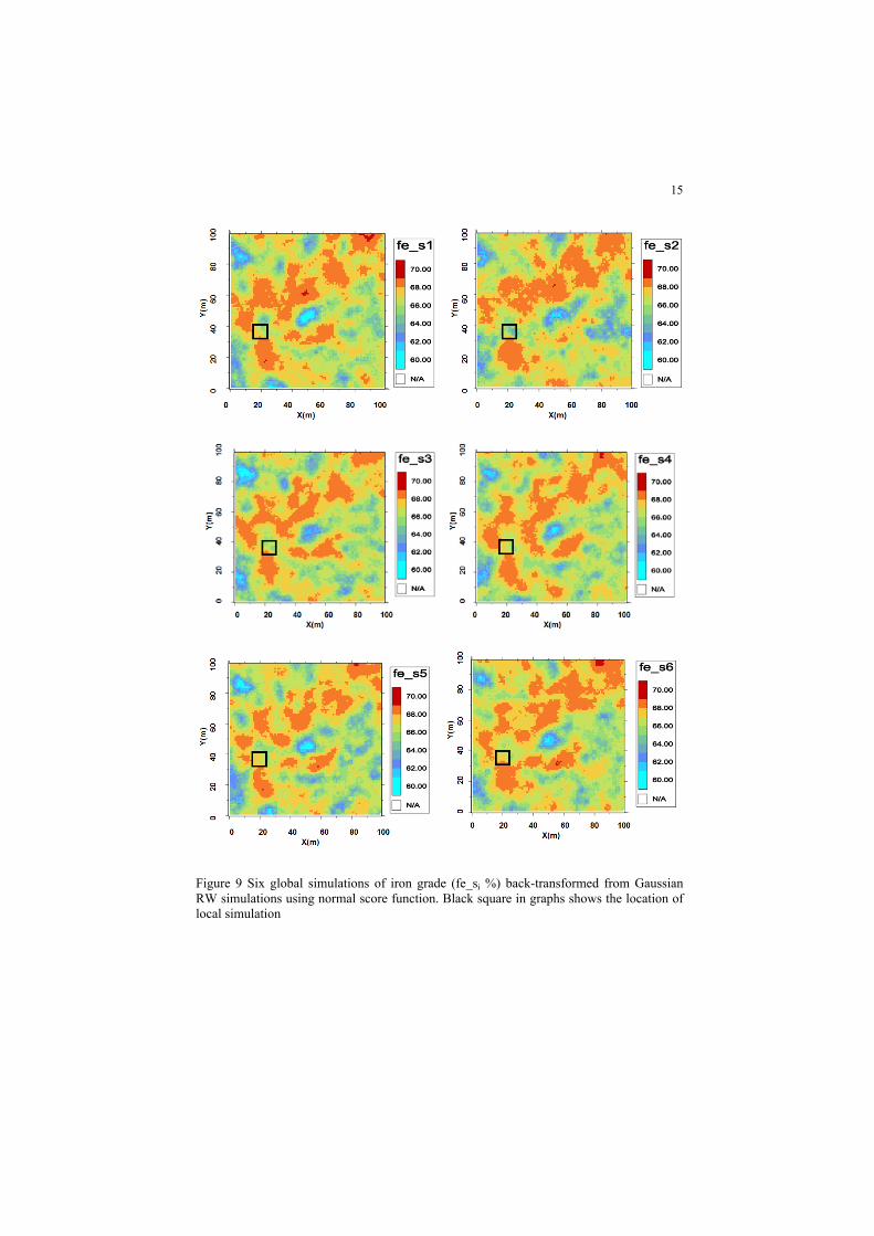
The comparison between the six local and global simulations was made after the back-transforming the simulated data into Zsrw. In that case, the Z variable considered was the iron grade (Fe %) whose distribution was taken from a high grade iron deposit. Figure 9 shows six realisations of RW simulation in the original scale (after back-transformation).

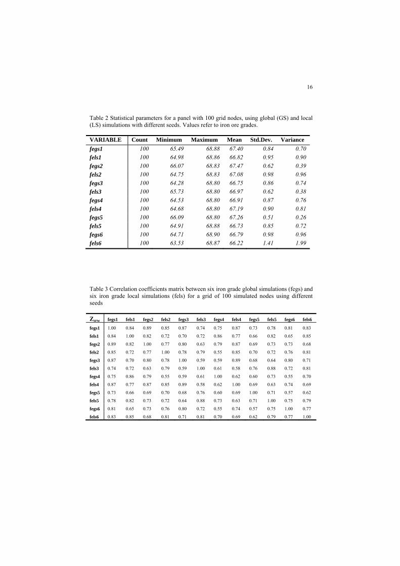
The statistical parameters presented in the tables 2 and 3 indicate that the local mean, variance and correlation between global and local simulations are coherent. The local simulated mean and variance are within the range of the respective parameters of global simulated data. There is no visible bias among LS and GS.

15

Figure 9 Six global simulations of iron grade (fe_si %) back-transformed from Gaussian RW simulations using normal score function. Black square in graphs shows the location of local simulation

16

Table 2 Statistical parameters for a panel with 100 grid nodes, using global (GS) and local (LS) simulations with different seeds. Values refer to iron ore grades.

VARIABLE Count Minimum Maximum Mean Std.Dev. Variance fegs1 100 65.49 68.88 67.40 0.84 0.70 fels1 100 64.98 68.86 66.82 0.95 0.90 fegs2 100 66.07 68.83 67.47 0.62 0.39 fels2 100 64.75 68.83 67.08 0.98 0.96 fegs3 100 64.28 68.80 66.75 0.86 0.74 fels3 100 65.73 68.80 66.97 0.62 0.38 fegs4 100 64.53 68.80 66.91 0.87 0.76 fels4 100 64.68 68.80 67.19 0.90 0.81 fegs5 100 66.09 68.80 67.26 0.51 0.26 fels5 100 64.91 68.88 66.73 0.85 0.72 fegs6 100 64.71 68.90 66.79 0.98 0.96 fels6 100 63.53 68.87 66.22 1.41 1.99

Table 3 Correlation coefficients matrix between six iron grade global simulations (fegs) and six iron grade local simulations (fels) for a grid of 100 simulated nodes using different seeds

Zsrw fegs1 fels1 fegs2 fels2 fegs3 fels3 fegs4 fels4 fegs5 fels5 fegs6 fels6

fegs1 1.00 0.84 0.89 0.85 0.87 0.74 0.75 0.87 0.73 0.78 0.81 0.83

fels1 0.84 1.00 0.82 0.72 0.70 0.72 0.86 0.77 0.66 0.82 0.65 0.85

fegs2 0.89 0.82 1.00 0.77 0.80 0.63 0.79 0.87 0.69 0.73 0.73 0.68

fels2 0.85 0.72 0.77 1.00 0.78 0.79 0.55 0.85 0.70 0.72 0.76 0.81

fegs3 0.87 0.70 0.80 0.78 1.00 0.59 0.59 0.89 0.68 0.64 0.80 0.71

fels3 0.74 0.72 0.63 0.79 0.59 1.00 0.61 0.58 0.76 0.88 0.72 0.81

fegs4 0.75 0.86 0.79 0.55 0.59 0.61 1.00 0.62 0.60 0.73 0.55 0.70

fels4 0.87 0.77 0.87 0.85 0.89 0.58 0.62 1.00 0.69 0.63 0.74 0.69

fegs5 0.73 0.66 0.69 0.70 0.68 0.76 0.60 0.69 1.00 0.71 0.57 0.62

fels5 0.78 0.82 0.73 0.72 0.64 0.88 0.73 0.63 0.71 1.00 0.75 0.79

fegs6 0.81 0.65 0.73 0.76 0.80 0.72 0.55 0.74 0.57 0.75 1.00 0.77

fels6 0.83 0.85 0.68 0.81 0.71 0.81 0.70 0.69 0.62 0.79 0.77 1.00

17

Conclusions

The combined use of random walk, or Brownian motion, and simple kriging allows conditioned simulation of Gaussian data which honour the mean, variance and the variogram of the conditioning data. The final simulated value is summation of two independent factors: the simple kriging estimation of the Gaussian variable and the background noise calculated by simple kriging of multiple RW, starting at the conditioning points and moving until the simulated node. The variance can be controlled by simply scaling a random function. Scaling a function by a factor f will result in a variance multiplied by f². The scaling factor of the background noise f is obtained experimentally through linear regression between f2 and the variance of random walk simulation (Ysrw), using as a constant the variance of smoothed simple kriging estimation. The scaling factor f can be used for future simulations, considering data update, or for local simulations in specific region of the mine. The experimental results indicate that this new methodology honoured both statistical moments of the Gaussian conditioning points faster than sequential algorithms. Future studies can be done considering real data set and multiple structures, different geological domains and multiple variables. Due to its simplicity this algorithm could be easily adapted to traditional algorithms which use Gaussian transforms and simple kriging. This methodology can be used to generate new tools for grade control system updating large model locally. We do not access the reality exactly but we can measure how close we are and manage this risk during the decision making process.

Acknowledgments

We wish to thank VALE S.A. and Lilian Grabellos for all support and authorization to publish this paper.

Bibliography

[1] Alabert, F. (1987). Stochastic Imaging of Spatial Distributions using Hard and Soft Information. MSc Thesis, Stanford University, p. 197.

[2] Chilès, J. P. (1977). Géostatistique des phenoménes non stationnaires. These Doc Ing Nancy, France.

18

[3] Chilès, J. P., & Delfiner, P. (1999). Geostatistics: Modeling Spatial

Uncertainty. Wiley & Sons. [4] Costa, J. F. (1997). Developments in recoverable reserves estimation

and ore body modelling. PhD Thesis, The University of Queensland, Australia.

[5] Falconer, K. (1990). Fractal Geometry. Chichester: John Wiley & Sons Ltd.

[6] Gotway, C. A., & Rutherford, B. M. (1993). Stochastic simulation for imaging spatial uncertainty: comparisonand evaluation of available algorithms. In: M. Armstrong, & P. A. Dowd (Ed.), Geostatistical Simulations (pp. 1-22). Dordrecht: Kluwer Academic Publishers.

[7] Isaaks, E. H. (1990). The Application of Monte Carlo Methods to the Analysis of Spatially Correlated Data. PhD Thesis, Stanford University , p. 213.

[8] Johnson, M. E. (1987). Multivariate Statistical Simulation. New York: Wiley.

[9] Journel, A. G. (1974). Geostatistics for conditional simulation of ore bodies. Economic Geology, v. 69, n° 5, pp. 673-687.

[10] Journel, A. G., & Alabert, F. G. (1989). Non Gaussian data expansion in the Earth Sciences (Vol. 1). Terra Nova.

[11] Lantuéjoul, C. (2002). Geostatistical Simulation: Models and Algorithms. Springer.

[12] Luster, G. R. (1985). Raw Materials for Portland Cement: Applications of conditional simulation of coregionalization. PhD dissertation, Stanford University , p. 531.

[13] Mandelbrodt, B. (1977). The Fractal Geometery of Nature. W. H. Freeman.

[14] Matheron, G. (1973). The Intrinsic Random Functions and Their Applications. Advances in Applied Probability, vol. 5, pp. 439-468.

[15] Ribeiro, D. T., & Carvalho, R. M. (2002). Simulation of weathered iron ore facies: integrating leaching concepts and geostatistical model. In: M. Armstrong, C. Bettini, N. Champigny, A. Galli, & A. Remacre (Ed.), Geostatistics Rio 2000 (pp. 111-115). Dordrecht, Boston, London: Kluwer Academic.

[16] Ribeiro, D. T., Pires, F. R., & Carvalho, R. M. (2002). Supergene iron ore and disorder. Proceedings of Iron Ore 2002 Conference (pp. 81-90). Perth: Australasian Institute of Mining and Metallurgy.

[17] Srivastava, R. M. (1994). An Overview of Stochastic Methods for Reservoir Characterization. In: J. Yarus, & R. Chambers (Ed.), Stochastic Modeling and Geostatistics: Principles, Methods and Case Studies.

19

Computer Applications 3, pp. 3-16. Tulsa: American Association of Petroleum Geologists.

[18] Ventsel, H. (1973). Théorie des Probabilités. Moscow: MIR.