Embed Size (px)
Citation preview
NOTES D’ÉTUDES
ET DE RECHERCHE
DIRECTION GÉNÉRALE DES ÉTUDES ET DES RELATIONS INTERNATIONALES
PRICE SETTING IN THE EURO AREA:
SOME STYLIZED FACTS FROM
INDIVIDUAL CONSUMER PRICE DATA
Emmanuel Dhyne, Luis J. Alvarez, Hervé Le Bihan, Giovanni Veronese, Daniel Dias, Johannes Hoffmann, Nicole Jonker, Patrick Lünnemann, Fabio Rumler and
Jouko Vilmunen
November 2005
NER - E # 136
DIRECTION GÉNÉRALE DES ÉTUDES ET DES RELATIONS INTERNATIONALES DIRECTION DE LA RECHERCHE
PRICE SETTING IN THE EURO AREA:
SOME STYLIZED FACTS FROM
INDIVIDUAL CONSUMER PRICE DATA
Emmanuel Dhyne, Luis J. Alvarez, Hervé Le Bihan, Giovanni Veronese, Daniel Dias, Johannes Hoffmann, Nicole Jonker, Patrick Lünnemann, Fabio Rumler and
Jouko Vilmunen
November 2005
NER - E # 136
Les Notes d'Études et de Recherche reflètent les idées personnelles de leurs auteurs et n'expriment pas nécessairement la position de la Banque de France. Ce document est disponible sur le site internet de la Banque de France « www.banque-France.fr ». Working Papers reflect the opinions of the authors and do not necessarily express the views of the Banque de France. This document is available on the Banque de France Website “www.banque-France.fr”.
1
Price setting in the euro area: Some stylized facts from
Individual Consumer Price Data
Emmanuel Dhyne, Luis J. Álvarez, Hervé Le Bihan, Giovanni Veronese, Daniel Dias, Johannes Hoffmann, Nicole Jonker,
Patrick Lünnemann, Fabio Rumler, Jouko Vilmunen
The views expressed in this paper are those of the authors and do not necessarily reflect the views of the National Central Bank to which they are affiliated. This paper employs individual information on price setting based on a set of euro area country studies, conducted in the context of a Eurosystem project (Inflation Persistence Network, hereafter IPN). The authors belong to National Central Banks that have been involved in the research group of the IPN devoted to the Analysis of Consumer Prices. The contribution of co-authors of country studies – L. Aucremanne, L. Baudry, J. Baumgartner, H. Blijenberg, M. Dias, S. Fabiani, C. Folkertsma, A. Gattulli, E. Glatzer, I. Hernando, J.-R. Kurz-Kim, H. Laakkonen, T. Mathä, P. Neves, R. Sabbatini, P. Sevestre, A. Stiglbauer and S. Tarrieu –, without whom this paper would not have been possible, is strongly acknowledged. The authors would also like to thank the national statistical institutes for providing the data, the members of the IPN, especially I. Angeloni, S. Cecchetti, J. Galí and A. Levin, the participants to the "Inflation Persistence in the Euro Area" ECB conference, especially A. Kashyap, S. Rebelo and R. Reis for their stimulating comments, as well as the participants in the 2005 Annual Meeting of the American Economic Association. The authors would also like to thank an anonymous ECB Working Paper Series' referee for his/her very constructive comments. Corresponding author: [email protected] Authors affiliations: Banque Nationale de Belgique (Dhyne),Banco de España (Álvarez), Banque de France (Le Bihan), Banca d’Italia (Veronese), Banco de Portugal (Dias), Deutsche Bundesbank (Hoffmann), De Nederlandsche Bank (Jonker), Banque Centrale du Luxembourg (Lünnemann), Oesterreichische Nationalbank (Rumler), Suomen Pankki (Vilmunen)
2
Résumé
Cette étude décrit les ajustements de prix de détail dans la zone euro au travers d’un ensemble de
six faits stylisés. Premièrement, pour la plupart des produits, les modifications de prix sont
relativement peu fréquentes : en moyenne, 15 % des prix sont révisés chaque mois dans la zone
euro contre 25 % environ aux États-Unis. Deuxièmement, la fréquence de ces modifications de prix
varie fortement entre produits et entre secteurs (les cas polaires étant les produits pétroliers et les
services). Troisièmement, il existe également une certaine hétérogénéité entre les pays.
Quatrièmement les baisses de prix se produisent presque aussi souvent que les hausses: quatre
changements de prix sur dix sont des baisses. Cinquièmement, les ampleurs des hausses ou des
baisses individuelles de prix sont en moyenne importante, lorsqu’on les compare aux rythmes
d’inflation agrégés ou sectoriels. Sixièmement, la synchronisation entre les agents économiques est
faible.
Par ailleurs, l’étude souligne différents facteurs influençant les ajustements de prix dans la zone
euro tels que la saisonnalité, le type de points de vente, la fiscalité indirecte, l’usage de prix
psychologiques ainsi que le taux d’inflation agrégée ou sectorielle.
Mots-clés: Ajustement des prix; Prix à la consommation, zone euro ; fréquence de changement de
prix.
Classification JEL : E31, D40, C25.
Abstract
This paper documents patterns of price setting at the retail level in the euro area. A set of stylized
facts on the frequency and size of price changes is presented along with an econometric
investigation of their main determinants. Price adjustment in the euro area can be summarized in six
stylized facts. First, prices of most products change rarely. The average monthly frequency of price
adjustment is 15 p.c., compared to about 25 p.c. in the US. Second, the frequency of price changes
is characterized by substantial cross-product heterogeneity and pronounced sectoral patterns: prices
of (oil-related) energy and unprocessed food products change very often, while price adjustments
are less frequent for processed food products, non-energy industrial goods and services. Third,
cross-country heterogeneity exists but is less pronounced. Fourth, price decreases are not
uncommon. Fifth, price increases and decreases are sizeable compared to aggregate and sectoral
inflation rates. Sixth, price changes are not highly synchronized across price-setters. Moreover, the
frequency of price changes in the euro area is related to a number of factors, in particular
seasonality, outlet type, indirect taxation, use of attractive prices as well as aggregate or product-
specific inflation.
Keywords: Price-setting, consumer price, frequency of price change. JEL Classification: E31, D40, C25.
3
Résumé non technique Les prix des biens et des services ne s’ajustent pas immédiatement en réaction aux évolutions de
l’offre et de la demande : l’existence d’un certain degré de rigidité des prix est un fait avéré sur
lequel la modélisation macroéconomique contemporaine s’appuie. De fait, de nombreux modèles
théoriques ont montré l’influence du degré de rigidité des prix sur les ajustements
macroéconomiques qui se produisent à la suite d’un choc, par exemple de politique monétaire.
En dépit de l’importance de ces questions pour la politique monétaire l’évaluation de la rigidité des
prix sur données individuelles est restée à ce jour limitée, en raison principalement du manque de
données disponibles pour une telle analyse. Les études sur données micro-économiques se sont
historiquement concentrées sur des produits spécifiques. A l’occasion de récents projets de
recherche toutefois, plusieurs instituts statistiques ont autorisé l’accès aux relevés de prix utilisés
pour calculer l’indice des prix. Ce type de données présente l’avantage d’offrir une couverture vaste
de la dépense de consommation des ménages. De surcroît les bases de données concernées
contiennent un nombre considérable d’observations qui atteint souvent plusieurs millions. Ce type
de données a été étudié aux Etat-Unis par Bils et Klenow (2004) et pour la plupart des pays de la
zone euro par les participants à un réseau de recherche de l’Eurosystème : l’IPN (Inflation
Persistence Network). La présente étude s’appuie sur les résultats de ce réseau pour caractériser
l’ajustement des prix à la consommation dans les pays de la zone euro. Elle vise aussi à formuler
une comparaison avec les Etats-Unis. A notre connaissance il s’agit de la première étude à fournir
une évaluation quantitative de l’ampleur et de la fréquence des ajustements de prix à l’échelle de la
zone euro. Cette analyse se fonde sur un échantillon de 50 produits précisément identifiés qui
visent à être représentatifs du panier de l’indice de prix à la consommation, concernant 10 pays de
la zone euro.
L’analyse des changements de prix pour ces 50 produits dans les 10 pays concernés met en
évidence les faits stylisés suivants :
1. Au niveau individuel, les changements de prix sont peu fréquents. La fréquence des
changements de prix est d’environ 15% par mois dans la zone euro : en d’autre termes, un mois
donné 15% environ des prix à la consommation sont modifiés. La durée moyenne de fixité des prix
est comprise entre 4 et 5 trimestres. Les changements de prix sont dons moins fréquents qu’aux
Etats-Unis, où la fréquence de changement de prix avoisine 25% par mois et où la durée moyenne
de fixité des prix est de l’ordre de 2 trimestres.
2. Il existe une grande hétérogénéité entre produits dans la fréquence des changements de prix. En
particulier les changements de prix sont très fréquents en ce qui concerne l’énergie (les produits
pétroliers) et les produits alimentaires non transformés, tandis qu’ils sont relativement rares pour les
produits manufacturés et surtout les services.
3. Il existe également une hétérogénéité entre pays dans la rigidité des prix, moins marquée
qu’entre produits. Elle s’explique dans une certaine mesure par des différences dans les structures
de consommation et le traitement statistique des soldes.
4. Les baisses de prix sont un phénomène relativement répandu exception faite du secteur des
services, et il n’y pas de signe d’une rigidité particulière à la baisse des prix. En moyenne 40% des
changements de prix sont des baisses.
4
5. Lorsqu’ils se produisent, les changements de prix (hausse ou baisse) sont d’amplitude
significative, par comparaison par exemple au rythme annuel d’inflation. L’amplitude des baisses
individuelles de prix est voisine de celle des hausses de prix, et atteint environ 10%.
6. La synchronisation des changements de prix entre détaillants apparaît assez faible, au niveau
d’un produit donné, même à l’intérieur d’un pays donné.
Outre ces différents faits stylisés présentant un caractère systématique dans les différents pays
étudiés, les études résumées dans cet article mettent l’accent sur plusieurs caractéristiques
récurrentes. En particulier la fréquence des changements de prix présente dans beaucoup de
secteurs une saisonnalité marquée, même lorsque les conditions fondamentales de l’offre et de la
demande dans le secteur ne sont pas saisonnières par nature. On observe le plus souvent des pics
dans la fréquence des changements de prix en janvier et après l’été. Pour un certain nombre de
produits, les prix tendent à changer exactement tous les douze mois ce qui se manifeste par des
pics dans la fonction de hasard (c'est-à-dire la probabilité de changement de prix
conditionnellement à la durée écoulée depuis le précédent changement de prix). Dans le même
temps, de nombreux travaux soulignent le fait que la probabilité de changement de prix dépend
également de variables micro et macro économiques. La fréquence de changement de prix est
ainsi influencée par le niveau d’inflation agrégée et sectorielle. Cette influence est d’autant plus
manifeste si l’on considère séparément les hausses de prix et les baisses de prix. De surcroît, les
détaillants réagissent de façon assez rapide à des chocs tels que la hausse du prix des intrants ou
la hausses des impôts indirects. La coexistence de détaillants au comportement time-dependent
(dépendance au temps) et au comportement state-dependent (dépendance d’état) se retrouve dans
les résultats d’enquête obtenus par Fabiani et alii (2005).
Enfin, notre étude présente une analyse économétrique en coupe, l’unité d’observation étant le
croisement pays-produit, qui confirme également les résultats des études-pays. Cette analyse
confirme en particulier que l’inflation affecte de façon positive la fréquence des augmentations de
prix et de façon négative la fréquence des baisses de prix. De plus, la fréquence des changements
de prix tend à être également plus élevée pour les produits qui connaissent une forte volatilité de
l’inflation. Cette analyse économétrique montre en outre que lorsque l’on contrôle par les différence
de rythme d’inflation et par les caractéristiques de recueil des données ainsi que les pratiques
commerciales (importance des soldes, des prix « psychologiques », des prix administrés,..) des
différences entre pays existent, que l’on peut vraisemblablement attribuer en partie aux différences
dans la structure du commerce de détail.
Les faits mis en évidence dans cet article peuvent notamment être utilisés pour calibrer et évaluer
des modèles avec rigidité de prix concernant la zone euro. Nos résultats mettent l’accent sur la
grande hétérogénéité intersectorielle de la rigidité des prix. Cela suggère que la prise en compte
explicite d’une telle hétérogénéité dans ces modèles est une piste possible pour améliorer la
compréhension de la dynamique de l’inflation dans la zone euro.
5
Non technical summary
Prices of goods and services do not adjust immediately in response to changing demand and
supply conditions. This fact is not controversial and is a standard assumption in macroeconomic
modeling. In fact, a large strand of theoretical literature has been devoted to analyzing the sources
of price stickiness and the implications of alternative forms of nominal rigidities on the dynamic
behavior of aggregate inflation and output. This literature has shown that the nature of nominal
rigidities determines the response of the economy to a broad range of disturbances and has several
implications for the conduct of monetary policy.
However, despite the relevance of these issues for monetary policy, empirical assessment of price
setting behavior using individual price data has remained relatively limited. This lack of micro-
economic evidence reflects the scarcity of available statistical information on prices at the individual
level. Indeed, most existing micro-studies are quite partial and focus on very specific products or
markets. In recent years, statistical offices have started to make available to researchers large-
scale data sets of individual prices that are regularly collected to compute consumer price indices.
Such data sets are particularly well suited for the analysis of the key features of price setting
behavior given that household consumption expenditure is generally fully covered. Moreover, they
typically contain a huge number of price quotes that add up to reach several millions. Bils and
Klenow (2004) for the US is an example of this line of research. Similar CPI data have also been
exploited for most euro area countries within the framework of the Eurosystem Inflation Persistence
Network (IPN).
This paper, building on IPN evidence, aims at characterizing the basic features of price adjustment
in the euro area economy and its member countries and to compare it, to the extent possible, with
available US evidence. To our knowledge, this paper is the first study to provide quantitative
measures of the frequency and size of price adjustments in the euro area based on the analysis of
50 narrowly defined products, which are representative of the full CPI basket.
Based on the analysis of a common sample of 50 products, several stylized facts have been found:
1. Prices change rarely. The frequency of price changes for the euro area is 15.1 percent
(i.e. on average, a given month 15.1 percent of prices are changed) and the average
duration of a price spell ranges from 4 to 5 quarters. These figures mean that price
adjustment in the euro area is considerably less frequent than in the US,
2. There is a marked degree of heterogeneity in the frequency of price changes across
products. Specifically, price changes are very frequent for energy (oil products) and
unprocessed food, while they are relatively infrequent for non-energy industrial goods
and services.
3. Heterogeneity across countries is relevant but less important than cross-sector
heterogeneity. It is, to some extent, related to differences in the consumption structure
and the statistical treatment of sales.
6
4. There is no evidence of a general downward rigidity in the euro area. In fact, price
decreases are not uncommon, except in services. On average, 40 percent of the price
changes are price reductions.
5. Price changes, either increases or decreases, are sizeable compared to the inflation
rate prevailing in each country. The magnitude of price reductions is roughly similar to
that of price increases.
6. Synchronization of price changes across price-setters does not seem to be large at the
product level, even within the same country.
Some further common patterns of price adjustment data have been observed in the different
country studies summarized in this paper. In particular, there is some evidence of time dependency
in price setting behavior as the frequency of price changes exhibits seasonal patterns, even in
sectors without marked seasonality in their demand and supply conditions. Price changes mostly
occur at the beginning of the year (especially in the service sector) and after the summer period.
Moreover, the hazard function of price changes in most euro area countries is characterized by
mass points every 12 months. However, there are also strong indications of elements of state-
dependent behavior as aggregate and sectoral inflation seem to affect the frequency of price
changes. This impact is further strengthened when price increases and price decreases are
analyzed separately. Additionally, firms appear to respond quickly to shocks such as indirect tax
rate and input price changes. This coexistence of firms with time and state dependent pricing
strategies is also found in the national surveys on price setting summarized in Fabiani et al (2005).
These findings are generally substantiated by a cross-country cross-section econometric analysis of
the 50 products. First, inflation has a positive effect on the frequency of price increases and a
negative effect on the frequency of price decreases. Second, inflation volatility has an impact on the
frequency of price adjustment. Third, there is cross-product and cross-country heterogeneity even
when controlling for differences in inflation and commercial practices (regulated prices, sales,
attractive pricing).
The facts put forward in this paper provide a benchmark against which to calibrate and to assess
micro-founded price setting models in the euro area. In particular, results stress the importance of
sectoral heterogeneity in price setting behavior. This suggests that developing macroeconomic
models that consider explicitly such heterogeneity may improve the understanding of our economic
fluctuations and inflation dynamics.
7
1. INTRODUCTION
Prices of goods and services do not adjust immediately in response to changing demand and
supply conditions. This fact is not controversial and is a standard assumption in macroeconomic
modeling. In fact, a large strand of theoretical literature has been devoted to analyzing the sources
of price stickiness and the implications of alternative forms of nominal rigidities on the dynamic
behavior of inflation and output. This literature has shown that the nature of nominal rigidities
determines the response of the economy to a broad range of disturbances and has several
implications for the conduct of monetary policy.
However, despite the relevance of these issues for monetary policy, empirical assessment of price
setting behavior using individual price data has remained relatively limited. This lack of micro-
economic evidence reflects the scarcity of available statistical information on prices at the individual
level. Indeed, most existing micro-studies are quite partial and focus on very specific products or
markets. Relevant contributions to this literature are Cecchetti (1986) on newsstand prices of
magazines, Lach and Tsiddon (1992) and Eden (2001) on food product prices, Kashyap (1995) on
catalogue prices, Levy et al (1997) on supermarket prices or Genesove (2003) on apartment rents.
In recent years, statistical offices have started to make available to researchers large-scale data
sets of individual prices that are regularly collected to compute consumer price indices. Such data
sets are particularly well suited for the analysis of the key features of price setting behavior given
that household consumption expenditure both in terms of goods and services and type of outlets is
generally fully covered. Moreover, they typically contain a huge number of price quotes that may
add up to several millions. Bils and Klenow (2004) for the US and Baharad and Eden (2004) for
Israel are examples of this line of research. Similar CPI data have also been exploited for most euro
area countries within the framework of the Eurosystem Inflation Persistence Network (IPN). The aim
of this paper is to characterize the basic features of price adjustment in the euro area and its
member countries and to compare it, to the extent possible, with available US evidence. To this
end, we focus on the analysis of 50 narrowly defined products, which are considered to be
approximately representative of the full CPI basket.
The remainder of this paper is organized as follows. Section 2 describes the individual consumer
price data used and discusses the harmonized methodology followed to make country results
comparable. Section 3 presents the stylized facts characterizing price setting behavior in the euro
area. Section 4 is devoted to the determinants of the probability of a price change. A pooled
regression econometric analysis and a summary of findings from individual country studies are
presented. Finally, Section 5 summarizes and points out some issues for further research.
8
2. MICRO CONSUMER PRICE DATA FOR THE EURO AREA
The main objective of this paper is to present some original evidence that characterizes the
dynamics of individual price setting at the euro area level, as well as to perform a cross-country
comparison based on a harmonized approach. Thanks to the unique opportunity offered by the
collective nature of this project and by the nature of the data analyzed, this paper is, to our
knowledge, the first to document price setting behavior for the euro area and to provide quantitative
measures of the degree of price stickiness for the euro area.
The stylized facts documented in this paper are based on evidence from individual price data
recorded at the outlet level in 10 euro area countries: Austria, Belgium, Finland, France, Germany,
Italy, Luxembourg, Netherlands, Portugal, and Spain. These ten countries account for around
97 p.c. of euro area GDP.
The data used for this purpose are the monthly price records underlying the computation of the
Consumer Price Index. These are high-quality data, which cover a large number of items based on
extensive Household Budget Surveys. This type of data has been used to characterize price–setting
patterns in the US, using the data produced by the BLS1.
In the case of the euro area, the collection of individual price reports underlying the computation of
the Harmonized Consumer Price Index (HICP) is done in a decentralized way by the statistical
institutes of each member state. These national collections of price reports are subject to statistical
confidentiality restrictions and are not brought together at Eurostat. Therefore, there is no single
dataset available that provides monthly individual price reports covering a wide variety of products
and services across the entire euro area. For the purpose of the IPN, the national databases were
released by the statistical institutes of each euro area member state on an individual basis to a
specific research team and subject to specific restrictions. Consequently, the analysis of individual
records has first been conducted in a decentralized way by each national research team. The result
of this research is documented in various papers, that exploit to the maximum extent possible the
comparative advantages of each national database (Álvarez, Burriel and Hernando (2005), Álvarez
and Hernando (2004), Aucremanne and Dhyne (2004, 2005), Baudry, Le Bihan, Sevestre and
Tarrieu (2004), Baumgartner, Glatzer, Rumler and Stiglbauer (2005), Dias, Dias and Neves (2004),
Dias, Robalo Marques and Santos Silva (2005), Fougère, Le Bihan, Sevestre (2005), Hoffmann and
Kurz-Kim (2005), Jonker, Blijenberg and Folkertsma (2004), Lünnemann and Mathä (2005b),
Veronese, Fabiani, Gattulli and Sabbatini (2005), Vilmunen and Laakkonen (2005)).
1 The BLS maintains a database called the "CPI Research Database" that is used by Bils and Klenow (2004) and Klenow
and Kryvtsov (2005). This database covers all prices in the Commodities and Services Surveys from January 1988 through December 2003.
9
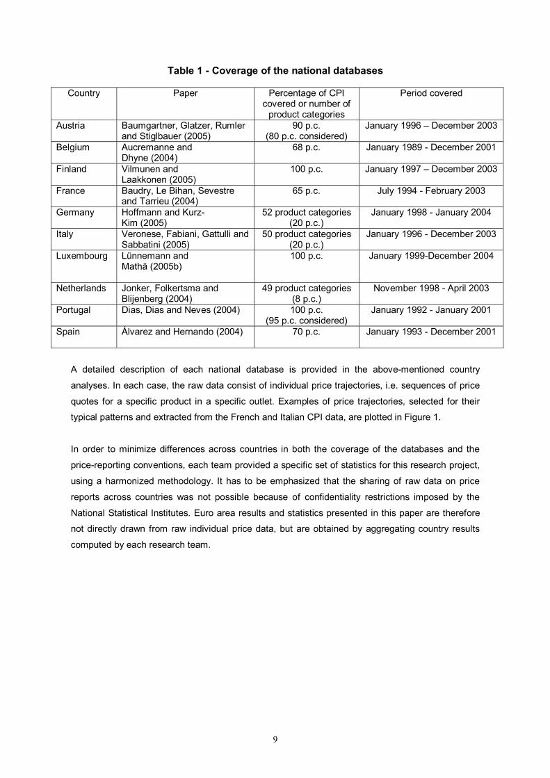
Table 1 - Coverage of the national databases
Country Paper Percentage of CPI covered or number of
product categories
Period covered
Austria Baumgartner, Glatzer, Rumler and Stiglbauer (2005)
90 p.c. (80 p.c. considered)
January 1996 – December 2003
Belgium Aucremanne and Dhyne (2004)
68 p.c. January 1989 - December 2001
Finland Vilmunen and Laakkonen (2005)
100 p.c. January 1997 – December 2003
France Baudry, Le Bihan, Sevestre and Tarrieu (2004)
65 p.c. July 1994 - February 2003
Germany Hoffmann and Kurz-Kim (2005)
52 product categories (20 p.c.)
January 1998 - January 2004
Italy Veronese, Fabiani, Gattulli and Sabbatini (2005)
50 product categories (20 p.c.)
January 1996 - December 2003
Luxembourg Lünnemann and Mathä (2005b)
100 p.c. January 1999-December 2004
Netherlands Jonker, Folkertsma and Blijenberg (2004)
49 product categories (8 p.c.)
November 1998 - April 2003
Portugal Dias, Dias and Neves (2004) 100 p.c. (95 p.c. considered)
January 1992 - January 2001
Spain Álvarez and Hernando (2004)
70 p.c. January 1993 - December 2001
A detailed description of each national database is provided in the above-mentioned country
analyses. In each case, the raw data consist of individual price trajectories, i.e. sequences of price
quotes for a specific product in a specific outlet. Examples of price trajectories, selected for their
typical patterns and extracted from the French and Italian CPI data, are plotted in Figure 1.
In order to minimize differences across countries in both the coverage of the databases and the
price-reporting conventions, each team provided a specific set of statistics for this research project,
using a harmonized methodology. It has to be emphasized that the sharing of raw data on price
reports across countries was not possible because of confidentiality restrictions imposed by the
National Statistical Institutes. Euro area results and statistics presented in this paper are therefore
not directly drawn from raw individual price data, but are obtained by aggregating country results
computed by each research team.
10
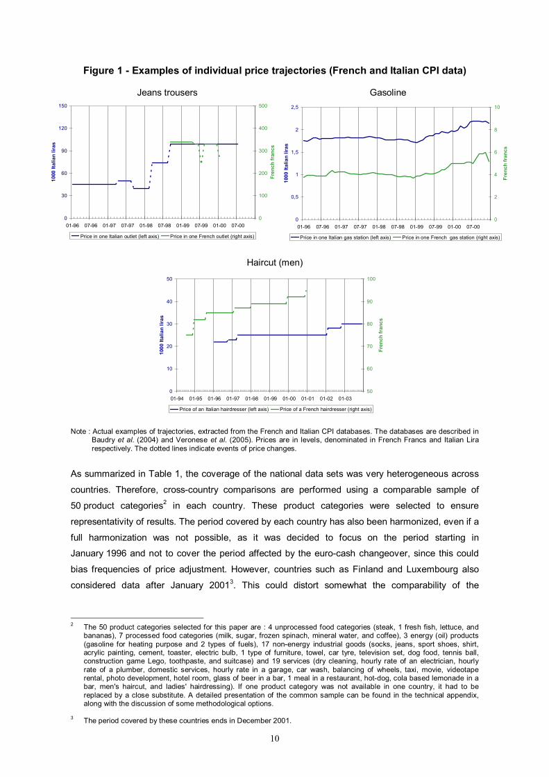
Figure 1 - Examples of individual price trajectories (French and Italian CPI data)
Jeans trousers Gasoline
Haircut (men) Note : Actual examples of trajectories, extracted from the French and Italian CPI databases. The databases are described in
Baudry et al. (2004) and Veronese et al. (2005). Prices are in levels, denominated in French Francs and Italian Lira respectively. The dotted lines indicate events of price changes.
As summarized in Table 1, the coverage of the national data sets was very heterogeneous across
countries. Therefore, cross-country comparisons are performed using a comparable sample of
50 product categories2 in each country. These product categories were selected to ensure
representativity of results. The period covered by each country has also been harmonized, even if a
full harmonization was not possible, as it was decided to focus on the period starting in
January 1996 and not to cover the period affected by the euro-cash changeover, since this could
bias frequencies of price adjustment. However, countries such as Finland and Luxembourg also
considered data after January 20013. This could distort somewhat the comparability of the
2 The 50 product categories selected for this paper are : 4 unprocessed food categories (steak, 1 fresh fish, lettuce, and
bananas), 7 processed food categories (milk, sugar, frozen spinach, mineral water, and coffee), 3 energy (oil) products (gasoline for heating purpose and 2 types of fuels), 17 non-energy industrial goods (socks, jeans, sport shoes, shirt, acrylic painting, cement, toaster, electric bulb, 1 type of furniture, towel, car tyre, television set, dog food, tennis ball, construction game Lego, toothpaste, and suitcase) and 19 services (dry cleaning, hourly rate of an electrician, hourly rate of a plumber, domestic services, hourly rate in a garage, car wash, balancing of wheels, taxi, movie, videotape rental, photo development, hotel room, glass of beer in a bar, 1 meal in a restaurant, hot-dog, cola based lemonade in a bar, men's haircut, and ladies' hairdressing). If one product category was not available in one country, it had to be replaced by a close substitute. A detailed presentation of the common sample can be found in the technical appendix, along with the discussion of some methodological options.
3 The period covered by these countries ends in December 2001.
0
30
60
90
120
150
01-96 07-96 01-97 07-97 01-98 07-98 01-99 07-99 01-00 07-00
1000
Ital
ian
liras
0
100
200
300
400
500
Fren
ch fr
ancs
Price in one Italian outlet (left axis) Price in one French outlet (right axis)
0
0,5
1
1,5
2
2,5
01-96 07-96 01-97 07-97 01-98 07-98 01-99 07-99 01-00 07-00
1000
Ital
ian
liras
0
2
4
6
8
10
Fren
ch fr
ancs
Price in one Italian gas station (left axis) Price in one French gas station (right axis)
0
10
20
30
40
50
01-94 01-95 01-96 01-97 01-98 01-99 01-00 01-01 01-02 01-03
1000
Ital
ian
liras
50
60
70
80
90
100
Fren
ch fr
ancs
Price of an Italian hairdresser (left axis) Price of a French hairdresser (right axis)
11
measures of the average frequency of price changes in these countries and, consequently, in the
euro area as a whole.
To enhance comparability across countries, a common definition of the price level and of what is
considered as a price change has also been used. In the following sections, the price of a specific
product refers to the price per unit of product. As far as our definition of a price change is
concerned, we have labeled as a price change either an observed price change or a forced product
replacement as some countries were unable to discriminate between these events. A more
appropriate but unfeasible treatment of product replacement would have implied a correction for
quality change. Hoffmann and Kurz-Kim (2005) compare unadjusted and quality-adjusted data for
Germany and find quite pronounced differences for some product categories. However, for their full
sample, the differences are still significant but much smaller. Facing a similar issue, Klenow and
Kryvstov (2005) decided to compute the frequency of price changes with and without product
replacement "because it is not clear whether price changes associated to product turnover are what
modelers of sticky prices have in mind".
Despite our commitment to produce comparable statistics, we were not able to fully account for
some national specificities in the collection of price reports. One of the remaining major cross-
country differences we could not avoid is related to the treatment of sales. For some countries,
national statistical institutes report sales prices while in other countries the prices that are reported
during the sales period are prices without rebates. Typically, price changes will appear to be less
frequent and smaller in countries where sales prices are not reported. Therefore, this
methodological difference has to be kept in mind when comparing results across countries.
Finally, the results presented in the following sections need to be analyzed with due regard for the
fact that in the observation period low inflation rates prevailed in all countries considered. Aggregate
inflation for the euro area averaged 1.9 percent y-o-y, while the sectoral inflation rates ranged from
0.9 percent for non-energy industrial goods to 3.0 percent for energy.
3. THE PATTERNS OF PRICE CHANGES IN THE EURO AREA This section describes the patterns of individual price adjustments in the euro area which can be
summarized by six stylized facts. These stylized facts have been established on the basis of seven
main indicators: the frequency of price changes, the average duration of price spells, the frequency
of price increases, the frequency of price decreases, the average size of price increases, the
average size of price decreases and the degree of synchronization of price changes. The
computation of these indicators is detailed in the technical appendix. The euro area figures
presented below are computed by aggregation using country weights from the HICP and (re-scaled)
sectoral weights, so that each national sub-index has the same weight as in the national CPI. Euro
area figures at the product category level for the 50 products of our common sample can be found
in Appendix, in Table A.8.
12
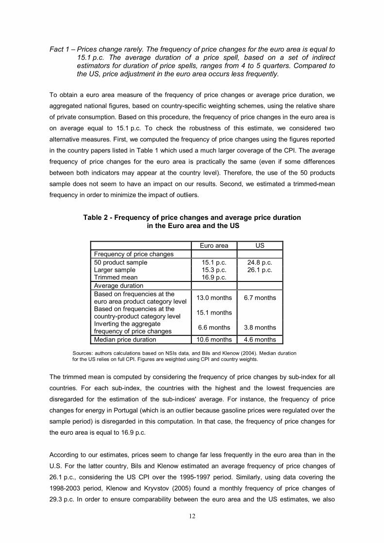
Fact 1 – Prices change rarely. The frequency of price changes for the euro area is equal to 15.1 p.c. The average duration of a price spell, based on a set of indirect estimators for duration of price spells, ranges from 4 to 5 quarters. Compared to the US, price adjustment in the euro area occurs less frequently.
To obtain a euro area measure of the frequency of price changes or average price duration, we
aggregated national figures, based on country-specific weighting schemes, using the relative share
of private consumption. Based on this procedure, the frequency of price changes in the euro area is
on average equal to 15.1 p.c. To check the robustness of this estimate, we considered two
alternative measures. First, we computed the frequency of price changes using the figures reported
in the country papers listed in Table 1 which used a much larger coverage of the CPI. The average
frequency of price changes for the euro area is practically the same (even if some differences
between both indicators may appear at the country level). Therefore, the use of the 50 products
sample does not seem to have an impact on our results. Second, we estimated a trimmed-mean
frequency in order to minimize the impact of outliers.
Table 2 - Frequency of price changes and average price duration in the Euro area and the US
Euro area US Frequency of price changes 50 product sample 15.1 p.c. 24.8 p.c. Larger sample 15.3 p.c. 26.1 p.c. Trimmed mean 16.9 p.c. Average duration Based on frequencies at the euro area product category level 13.0 months 6.7 months
Based on frequencies at the country-product category level 15.1 months
Inverting the aggregate frequency of price changes 6.6 months 3.8 months
Median price duration 10.6 months 4.6 months
Sources: authors calculations based on NSIs data, and Bils and Klenow (2004). Median duration for the US relies on full CPI. Figures are weighted using CPI and country weights.
The trimmed mean is computed by considering the frequency of price changes by sub-index for all
countries. For each sub-index, the countries with the highest and the lowest frequencies are
disregarded for the estimation of the sub-indices' average. For instance, the frequency of price
changes for energy in Portugal (which is an outlier because gasoline prices were regulated over the
sample period) is disregarded in this computation. In that case, the frequency of price changes for
the euro area is equal to 16.9 p.c.
According to our estimates, prices seem to change far less frequently in the euro area than in the
U.S. For the latter country, Bils and Klenow estimated an average frequency of price changes of
26.1 p.c., considering the US CPI over the 1995-1997 period. Similarly, using data covering the
1998-2003 period, Klenow and Kryvstov (2005) found a monthly frequency of price changes of
29.3 p.c. In order to ensure comparability between the euro area and the US estimates, we also
13
computed a US figure relating to our 50 products sample, based on the product-specific estimates
reported in Bils and Klenow (2004), which is very close to the figure for the aggregate given by the
above-mentioned authors.
A similar difference is also observed when focusing on average price durations. The average price
duration is estimated to be of 13 months in the euro area. This figure is based on an indirect
approach, namely inverting the frequency of price changes at the product level for the euro area
and aggregating.4 Based on the 50 products sample in Bils and Klenow (2004), the corresponding
figure for the US is 6.7 months. Note that the aggregation of the implied duration computed at the
product level in each country yields an estimated average price duration of 15.1 months in the euro
area. However, such a measure, which can be considered as an upper bound, is less suited for a
comparison with the US, since the frequency measures in the latter case are consolidated across
states before aggregation across products.
One striking feature is that our estimate of implied duration (13 months) is much larger than the
“pseudo-average duration” which is obtained by inverting the average frequency
(1/0.151 = 6.6 months). As documented in several of the papers listed in Table 1 and as illustrated
in Section 5 of the Technical Appendix, this gap essentially reflects Jensen’s inequality, together
with cross-product heterogeneity. As a result, the inverse frequency is systematically much lower
than the average duration.
Arguably, the implied average durations are affected by outliers, as product categories with a very
low frequency of price changes translate into extremely high implied durations. Therefore, it is
worthwhile to consider the weighted median as an alternative estimator of the typical duration. This
measure gives 10.6 months. The corresponding figure for the US is 4.6 months from Bils and
Klenow (2004), which confirms the contrast with euro area.
The higher frequency of price changes or lower price durations observed in the US can be partly
explained by the slightly higher and slightly more volatile monthly inflation rates observed during the
1996-2001 period in the US compared to the euro area (respective 0.21 p.c. and 0.12 p.c. average
monthly inflation and 0.16 and 0.20 standard deviation of monthly inflation). The observed
difference is, however, simply too pronounced to be explained solely by the differences in the mean
and the variability of aggregate inflation.
Furthermore, the lower euro area frequency of price adjustments cannot be explained by
differences in consumption patterns. The euro area consumption structure is characterized by a
larger share of food products (which are characterized by frequent price changes, see below) and a
smaller share of services (which are characterized by infrequent price changes, see below).
Therefore, the difference in the frequency of price changes would be even larger if both economies
shared the same consumption pattern.
14
Finding lower frequencies of price adjustment and longer durations of price spells in the euro area
than in the US seems therefore to be a robust result of the analysis presented. In addition, this
difference is in line with available indirect estimates on price duration based on macro models. For
instance, in Galí et al. (2003) the baseline estimate for the average duration of a price spell lies
somewhere around 4 to 6 quarters in the euro area, which is approximately twice as high as their
baseline estimate for the US (two to three quarters).
One last finding concerning duration is that in all of the euro area countries there is a noticeable
right-tail of durations. In all datasets considered for the present paper, a small fraction of price spells
with a very long duration of, say, several years is observed. This is exemplified in the lower-right
panel of Figure 1 where it can be seen that the price of the selected haircut from the Italian CPI was
set constant for more than 4 years over the period 1997-2001.
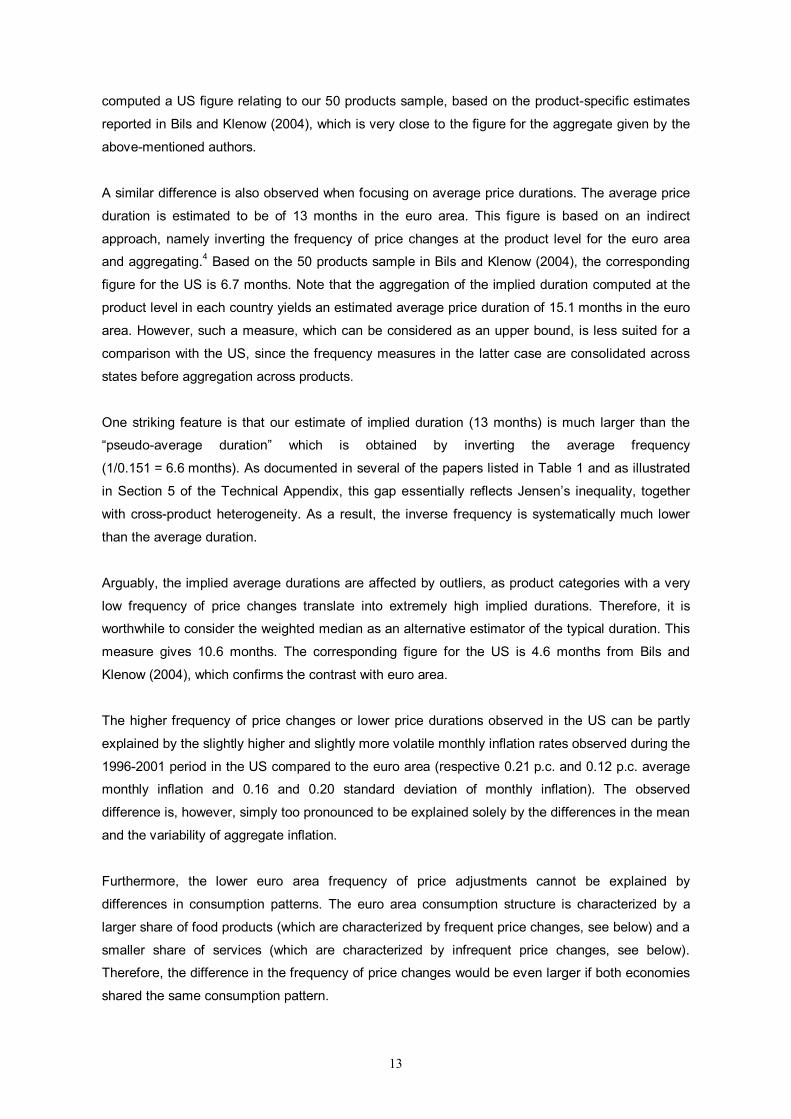
Fact 2 – There is a substantial degree of heterogeneity in the frequency of price changes across products. Price changes are very frequent for energy (oil products) and unprocessed food, while they are relatively infrequent for non-energy industrial goods and services.
Based on the frequency of price changes computed at the product level, a marked amount of
heterogeneity is observed across products, as can be seen in Figure 2, which plots the unweighted
distribution of the pooled frequencies of price changes. Each observation used for this histogram is
the frequency for one product category in one country.
Figure 2 – Distribution of the frequency of price changes
0.00
0.02
0.04
0.06
0.08
0.10
0.12
0.14
0.16
0.18
0.20
[0; 0
.02)
[0.1
; 0.1
2)
[0.2
; 0.2
2)
[0.3
; 0.3
2)
[0.4
; 0.4
2)
[0.5
; 0.5
2)
[0.6
; 0.6
2)
[0.7
; 0.7
2)
[0.8
; 0.8
2)
[0.9
; 0.9
2)
Frequency of price changes (in p.c.)
Den
sity
(in
p.c.
)
Sources: authors calculations on NSIs data. Finland is not included. Unweighted data.
4 See the technical appendix for details on the implied duration approach. The indirect approach is used instead of the
direct measurement of duration because the latter approach involves censoring of the data, in particular for some countries for which the data sample was very short.
15
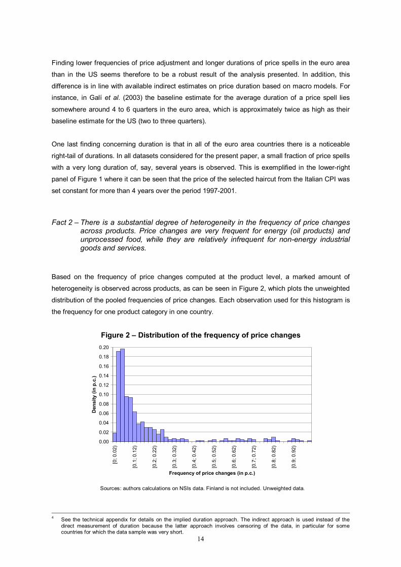
Compared with the US, it seems that the euro area is characterized by more heterogeneity in
pricing behavior. In the euro area, 95 p.c. of the product categories considered are characterized by
an average duration of price spells ranging from 1 to 32 months, whereas the same fraction of
product categories in the US are only characterized by average durations between 1 to 22 months.
Moreover, it can be seen from Figure 3 that the more pronounced heterogeneity observed in the
euro area is mostly associated with the product categories characterized by longer price durations.
Figure 3 – Implied duration of price spells at the product category level - Comparing the euro area with the US
0
5
10
15
20
25
30
0 5 10 15 20 25 30
euro area
US
Sources: NCBs calculations on NSIs data.
16
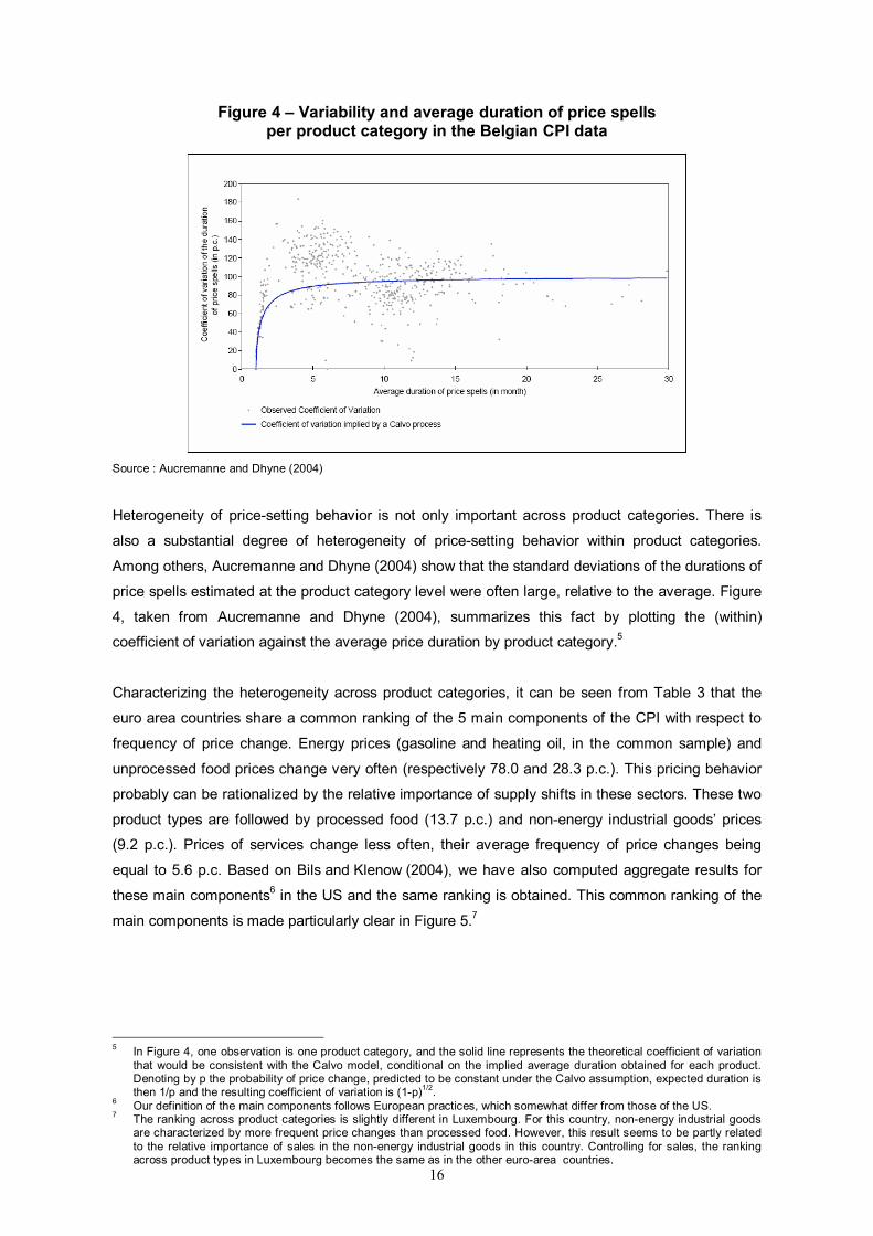
Figure 4 – Variability and average duration of price spells per product category in the Belgian CPI data
Source : Aucremanne and Dhyne (2004)
Heterogeneity of price-setting behavior is not only important across product categories. There is
also a substantial degree of heterogeneity of price-setting behavior within product categories.
Among others, Aucremanne and Dhyne (2004) show that the standard deviations of the durations of
price spells estimated at the product category level were often large, relative to the average. Figure
4, taken from Aucremanne and Dhyne (2004), summarizes this fact by plotting the (within)
coefficient of variation against the average price duration by product category.5
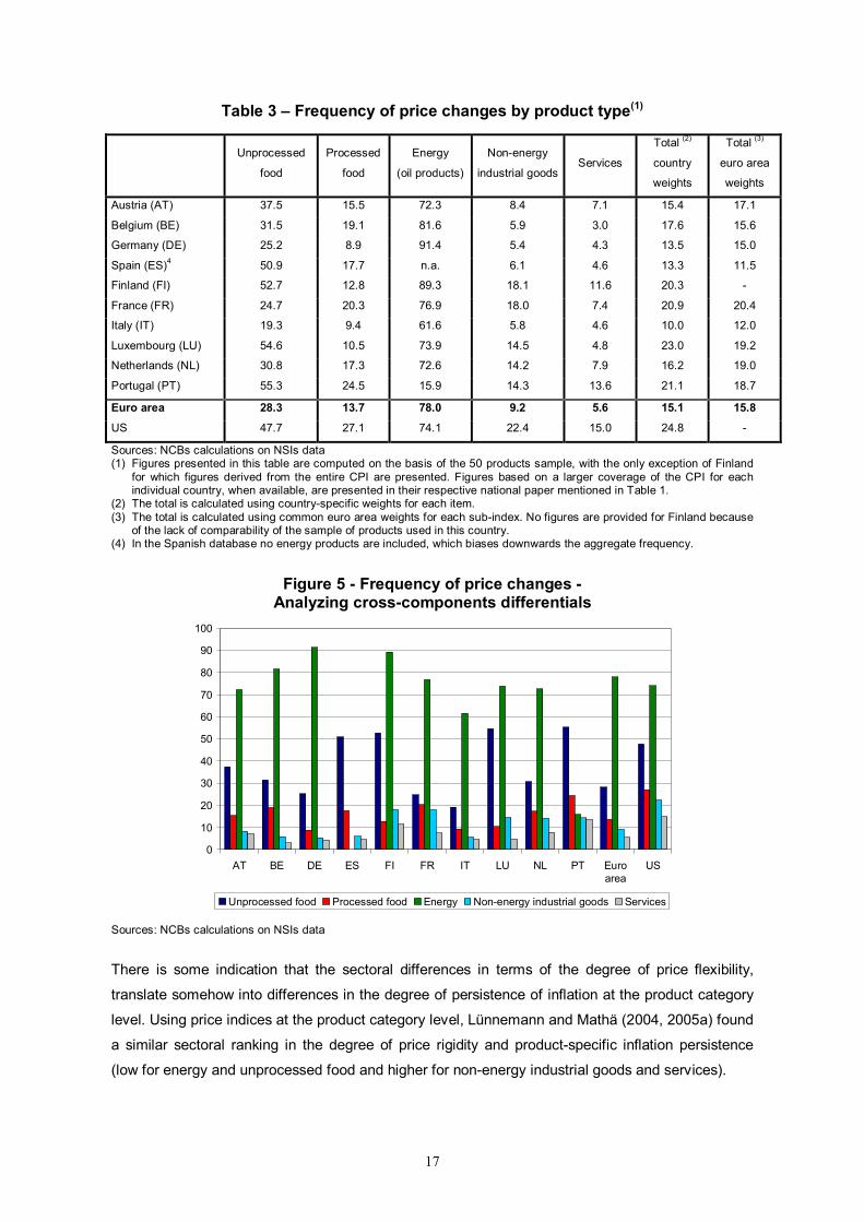
Characterizing the heterogeneity across product categories, it can be seen from Table 3 that the
euro area countries share a common ranking of the 5 main components of the CPI with respect to
frequency of price change. Energy prices (gasoline and heating oil, in the common sample) and
unprocessed food prices change very often (respectively 78.0 and 28.3 p.c.). This pricing behavior
probably can be rationalized by the relative importance of supply shifts in these sectors. These two
product types are followed by processed food (13.7 p.c.) and non-energy industrial goods’ prices
(9.2 p.c.). Prices of services change less often, their average frequency of price changes being
equal to 5.6 p.c. Based on Bils and Klenow (2004), we have also computed aggregate results for
these main components6 in the US and the same ranking is obtained. This common ranking of the
main components is made particularly clear in Figure 5.7
5 In Figure 4, one observation is one product category, and the solid line represents the theoretical coefficient of variation
that would be consistent with the Calvo model, conditional on the implied average duration obtained for each product. Denoting by p the probability of price change, predicted to be constant under the Calvo assumption, expected duration is then 1/p and the resulting coefficient of variation is (1-p)1/2.
6 Our definition of the main components follows European practices, which somewhat differ from those of the US. 7 The ranking across product categories is slightly different in Luxembourg. For this country, non-energy industrial goods
are characterized by more frequent price changes than processed food. However, this result seems to be partly related to the relative importance of sales in the non-energy industrial goods in this country. Controlling for sales, the ranking across product types in Luxembourg becomes the same as in the other euro-area countries.
17
Table 3 – Frequency of price changes by product type(1)
Unprocessed
food
Processed
food
Energy
(oil products)
Non-energy
industrial goodsServices
Total (2)
country
weights
Total (3)
euro area
weights
Austria (AT) 37.5 15.5 72.3 8.4 7.1 15.4 17.1
Belgium (BE) 31.5 19.1 81.6 5.9 3.0 17.6 15.6
Germany (DE) 25.2 8.9 91.4 5.4 4.3 13.5 15.0
Spain (ES)4 50.9 17.7 n.a. 6.1 4.6 13.3 11.5
Finland (FI) 52.7 12.8 89.3 18.1 11.6 20.3 -
France (FR) 24.7 20.3 76.9 18.0 7.4 20.9 20.4
Italy (IT) 19.3 9.4 61.6 5.8 4.6 10.0 12.0
Luxembourg (LU) 54.6 10.5 73.9 14.5 4.8 23.0 19.2
Netherlands (NL) 30.8 17.3 72.6 14.2 7.9 16.2 19.0
Portugal (PT) 55.3 24.5 15.9 14.3 13.6 21.1 18.7
Euro area 28.3 13.7 78.0 9.2 5.6 15.1 15.8
US 47.7 27.1 74.1 22.4 15.0 24.8 -
Sources: NCBs calculations on NSIs data (1) Figures presented in this table are computed on the basis of the 50 products sample, with the only exception of Finland
for which figures derived from the entire CPI are presented. Figures based on a larger coverage of the CPI for each individual country, when available, are presented in their respective national paper mentioned in Table 1.
(2) The total is calculated using country-specific weights for each item. (3) The total is calculated using common euro area weights for each sub-index. No figures are provided for Finland because
of the lack of comparability of the sample of products used in this country. (4) In the Spanish database no energy products are included, which biases downwards the aggregate frequency.
Figure 5 - Frequency of price changes - Analyzing cross-components differentials
0
10
20
30
40
50
60
70
80
90
100
AT BE DE ES FI FR IT LU NL PT Euroarea
US
Unprocessed food Processed food Energy Non-energy industrial goods Services Sources: NCBs calculations on NSIs data
There is some indication that the sectoral differences in terms of the degree of price flexibility,
translate somehow into differences in the degree of persistence of inflation at the product category
level. Using price indices at the product category level, Lünnemann and Mathä (2004, 2005a) found
a similar sectoral ranking in the degree of price rigidity and product-specific inflation persistence
(low for energy and unprocessed food and higher for non-energy industrial goods and services).

18
Fact 3 - Heterogeneity across countries is relevant but less important than cross-sector heterogeneity. It is partly related to the consumption structure and to the statistical treatment of sales.
There also exists a sizeable cross-country variation in the frequency of price change. In the period
1996-2001, on average, it ranged between 10 p.c. in Italy and 23.0 p.c. in Luxembourg. It has to be
mentioned that the results based on the 50 products sample presented in Table 3 are not very
different from the corresponding results based on the complete set of price reports available in each
country. This indicates that 50 products sample is a good approximation of the CPI in the different
countries.
The source of the cross-country variation is likely to be both structural (consumption patterns,
structure of the retail sector8), methodological (e. g. the treatment of sales and of quality adjustment
by each NSI) and a reflection of the differences in the relative importance of regulated prices across
countries.
Part of the cross-country differences can be explained by the consumption structure. When using
the euro area consumption structure to aggregate over products as is done in the last column of
Table 3, differences across countries tend to narrow. Adopting identical consumption patterns
across all euro area countries, the estimates of the average frequency of price changes range from
12 p.c. in Italy to 20.4 p.c. in France. The increase in the frequency of price changes in Italy is due
to the fact that energy, which exhibits a high frequency of price changes, has a relatively low weight
in Italian consumption compared to the euro area average.
Within some of the main components, cross-country differences in the frequency of price
adjustment are still substantial. This is true for energy prices, in spite of their tight dependence on
common oil price developments. In most euro area countries, the prices of oil products change very
often, with the sole exception of Portugal which is characterized by a very low frequency of price
changes in that particular category, which is due to the fact that gasoline prices in Portugal were
administered during the sample period.
For non-energy industrial goods, different treatment and reporting by National Statistical Institutes of
price cuts during sales periods are probably an important factor in explaining the observed
differences in the frequency of price adjustments: in France, which records sales prices, 18 p.c. of
these prices are found to change every month, as opposed to only around 6 p.c. in Belgium,
Germany, Italy and Spain.
Because a higher frequency of price changes in non-energy industrial goods due to the observation
of sales translates into a higher frequency of price changes for the overall CPI, sales could be an
explanatory factor for the difference, in terms of frequency, observed between France and countries
which do not report sales. Based on specific experiments conducted using the French and Austrian
8 Some countries like Italy may have stickier prices due to a larger market share of small traditional outlets.
19
databases, our assessment is that this factor can only account for, at most, 3 p.p. in the overall
frequency of price change. Indeed, with the common sample data for Austria, the overall frequency
of price changes decreases from 15.4 p.c. to 12.9 p.c. when leaving out price changes due to sales,
while for France it decreases from 20.9 p.c. to 18.4 p.c. when leaving out sales and flagged
temporary price cuts. This result is somewhat confirmed using the pooled regression framework of
Section 4.2. Note that Klenow and Kryvtsov (2005) report a frequency of price changes of 23.3 p.c.
on regular prices compared to 29.3 p.c. on all prices.
As far as services are concerned, results are relatively more homogeneous across European
countries, except for Finland and Portugal.
Finally, cross-product heterogeneity seems to dominate cross-country heterogeneity. An analysis of
variance shows that less than 5 p.c. of the variation in the frequency of price changes can be
attributed to country effects, while about 90 p.c. of the variance of the frequency of price changes
relates to product category effects.
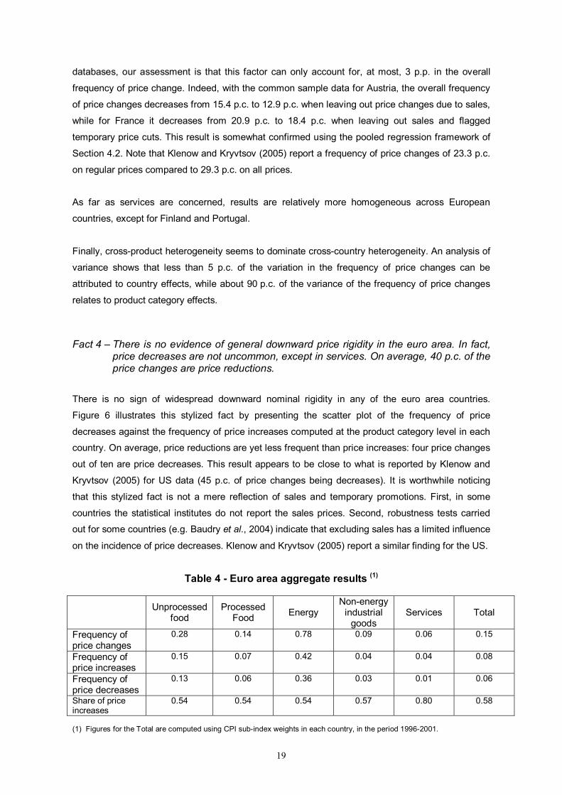
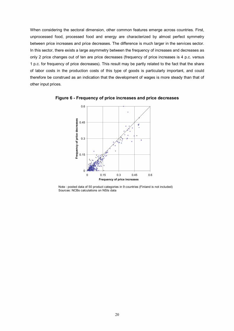
Fact 4 – There is no evidence of general downward price rigidity in the euro area. In fact, price decreases are not uncommon, except in services. On average, 40 p.c. of the price changes are price reductions.
There is no sign of widespread downward nominal rigidity in any of the euro area countries.
Figure 6 illustrates this stylized fact by presenting the scatter plot of the frequency of price
decreases against the frequency of price increases computed at the product category level in each
country. On average, price reductions are yet less frequent than price increases: four price changes
out of ten are price decreases. This result appears to be close to what is reported by Klenow and
Kryvtsov (2005) for US data (45 p.c. of price changes being decreases). It is worthwhile noticing
that this stylized fact is not a mere reflection of sales and temporary promotions. First, in some
countries the statistical institutes do not report the sales prices. Second, robustness tests carried
out for some countries (e.g. Baudry et al., 2004) indicate that excluding sales has a limited influence
on the incidence of price decreases. Klenow and Kryvtsov (2005) report a similar finding for the US.
Table 4 - Euro area aggregate results (1)
Unprocessed food
Processed Food Energy
Non-energy industrial
goods Services Total
Frequency of price changes
0.28 0.14 0.78 0.09 0.06 0.15
Frequency of price increases
0.15 0.07 0.42 0.04 0.04 0.08
Frequency of price decreases
0.13 0.06 0.36 0.03 0.01 0.06
Share of price increases
0.54 0.54 0.54 0.57 0.80 0.58
(1) Figures for the Total are computed using CPI sub-index weights in each country, in the period 1996-2001.
20
When considering the sectoral dimension, other common features emerge across countries. First,
unprocessed food, processed food and energy are characterized by almost perfect symmetry
between price increases and price decreases. The difference is much larger in the services sector.
In this sector, there exists a large asymmetry between the frequency of increases and decreases as
only 2 price changes out of ten are price decreases (frequency of price increases is 4 p.c. versus
1 p.c. for frequency of price decreases). This result may be partly related to the fact that the share
of labor costs in the production costs of this type of goods is particularly important, and could
therefore be construed as an indication that the development of wages is more steady than that of
other input prices.
Figure 6 - Frequency of price increases and price decreases
0
0.15
0.3
0.45
0.6
0 0.15 0.3 0.45 0.6Frequency of price increases
Freq
uenc
y of
pric
e de
crea
ses
Note : pooled data of 50 product categories in 9 countries (Finland is not included) Sources: NCBs calculations on NSIs data
21
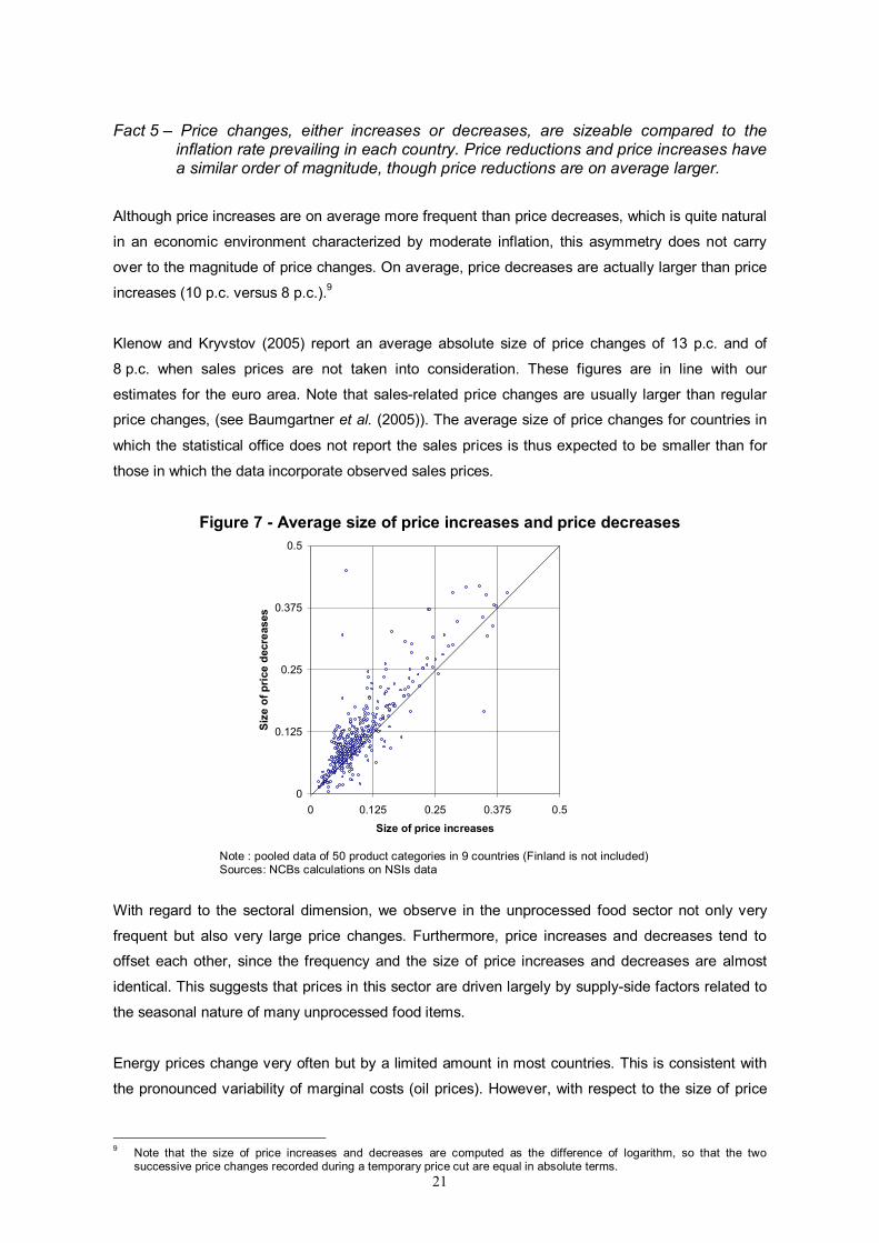
Fact 5 – Price changes, either increases or decreases, are sizeable compared to the inflation rate prevailing in each country. Price reductions and price increases have a similar order of magnitude, though price reductions are on average larger.
Although price increases are on average more frequent than price decreases, which is quite natural
in an economic environment characterized by moderate inflation, this asymmetry does not carry
over to the magnitude of price changes. On average, price decreases are actually larger than price
increases (10 p.c. versus 8 p.c.).9
Klenow and Kryvstov (2005) report an average absolute size of price changes of 13 p.c. and of
8 p.c. when sales prices are not taken into consideration. These figures are in line with our
estimates for the euro area. Note that sales-related price changes are usually larger than regular
price changes, (see Baumgartner et al. (2005)). The average size of price changes for countries in
which the statistical office does not report the sales prices is thus expected to be smaller than for
those in which the data incorporate observed sales prices.
Figure 7 - Average size of price increases and price decreases
0
0.125
0.25
0.375
0.5
0 0.125 0.25 0.375 0.5
Size of price increases
Size
of p
rice
decr
ease
s
Note : pooled data of 50 product categories in 9 countries (Finland is not included) Sources: NCBs calculations on NSIs data
With regard to the sectoral dimension, we observe in the unprocessed food sector not only very
frequent but also very large price changes. Furthermore, price increases and decreases tend to
offset each other, since the frequency and the size of price increases and decreases are almost
identical. This suggests that prices in this sector are driven largely by supply-side factors related to
the seasonal nature of many unprocessed food items.
Energy prices change very often but by a limited amount in most countries. This is consistent with
the pronounced variability of marginal costs (oil prices). However, with respect to the size of price
9 Note that the size of price increases and decreases are computed as the difference of logarithm, so that the two
successive price changes recorded during a temporary price cut are equal in absolute terms.
22
adjustments, this variability is smoothed out by the large incidence of indirect taxation on these
products.
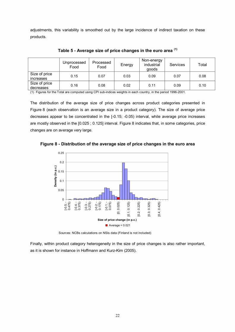
Table 5 - Average size of price changes in the euro area (1)
Unprocessed Food
Processed Food Energy
Non-energy industrial
goods Services Total
Size of price increases 0.15 0.07 0.03 0.09 0.07 0.08
Size of price decreases 0.16 0.08 0.02 0.11 0.09 0.10
(1) Figures for the Total are computed using CPI sub-indices weights in each country, in the period 1996-2001.
The distribution of the average size of price changes across product categories presented in
Figure 8 (each observation is an average size in a product category). The size of average price
decreases appear to be concentrated in the [-0.15; -0.05) interval, while average price increases
are mostly observed in the [0.025 ; 0.125] interval. Figure 8 indicates that, in some categories, price
changes are on average very large.
Figure 8 - Distribution of the average size of price changes in the euro area
Average = 0.021
0
0.05
0.1
0.15
0.2
0.25
[-0.5
; -0.
475)
[-0.4
; -0.
375)
[-0.3
; -0.
275)
[-0.2
; -0.
175)
[-0.1
; -0.
075)
[0; 0
.025
)
[0.1
; 0.1
25)
[0.2
; 0.2
25)
[0.3
; 0.3
25)
[0.4
; 0.4
25)
Size of price change (in p.c.)
Den
sity
(in
p.c.
)
Sources: NCBs calculations on NSIs data (Finland is not included)
Finally, within product category heterogeneity in the size of price changes is also rather important,
as it is shown for instance in Hoffmann and Kurz-Kim (2005).
23
Fact 6 – Synchronization of price changes across price-setters does not seem to be large at the product level, even within the same country.
Using the measure proposed by Fisher and Konieczny (2000), we can assess the degree of
synchronization of price changes at the product level in each country (see point 4 of Technical
Appendix for the formula). This index takes the value 1 in case of perfect synchronization of price
changes, while it takes value 0 in the case of perfectly staggered price changes across price
setters.
As can be seen from Table A.6 in appendix, the degree of synchronization of price changes is, in
general, rather low except for energy prices: the median synchronization ratio across the 50
products in the common sample ranges between 0.13 in Germany and 0.48 in Luxembourg. The
higher ratio observed in Luxembourg compared to Germany probably reflects the difference in the
market’s size upon which the index is computed and the relatively small number of outlets from
which prices are collected in Luxembourg. This is supported by Italian results. Indeed, as shown in
Veronese et al. (2005) in the Italian case, the low synchronization of price changes at the product
level is perfectly compatible with higher synchronization rates computed within a given city.
Dias et al. (2004) suggested a structural interpretation for the Fisher and Konieczny (F&K)
synchronization index. According to these authors, the F&K index can be seen as a method of
moments estimator for the share of firms in the economy that are perfectly synchronized, or, the
other way around, the complement of the F&K index estimates the share of firms in the economy
whose pricing is uniformly staggered. For instance, the F&K index for the energy sector in Portugal
is 0.82. In this sense, one may say that 82 p.c. of the energy retailers in Portugal are synchronized.
Therefore, the hypothesis of uniform price staggering for the energy sector seems to be far from
being realistic. The F&K index can be seen as an alternative to the Klenow and Kryvstov (2005)
variance of inflation decomposition for assessing how far the Uniform Price Staggering hypothesis
is from reality.
4. ACCOUNTING FOR THE FREQUENCY OF PRICE CHANGE 4.1. Individual country evidence This sub-section summarizes the main results on the factors affecting the frequency of price
changes presented in the various country papers. All these findings are summarized in Table 6.
These results were obtained using a wide variety of methodological approaches, considering both
measures of the frequency of price changes and measures of the frequency of price changes
conditional on the duration of price spells. Although the methodological approaches are very
different across countries, most results are very similar.
24
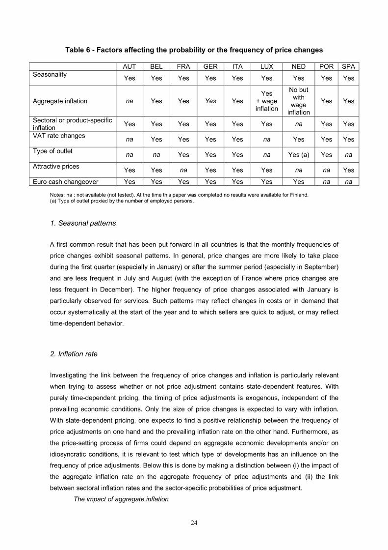
Table 6 - Factors affecting the probability or the frequency of price changes
Notes: na : not available (not tested). At the time this paper was completed no results were available for Finland. (a) Type of outlet proxied by the number of employed persons.
1. Seasonal patterns
A first common result that has been put forward in all countries is that the monthly frequencies of
price changes exhibit seasonal patterns. In general, price changes are more likely to take place
during the first quarter (especially in January) or after the summer period (especially in September)
and are less frequent in July and August (with the exception of France where price changes are
less frequent in December). The higher frequency of price changes associated with January is
particularly observed for services. Such patterns may reflect changes in costs or in demand that
occur systematically at the start of the year and to which sellers are quick to adjust, or may reflect
time-dependent behavior.
2. Inflation rate
Investigating the link between the frequency of price changes and inflation is particularly relevant
when trying to assess whether or not price adjustment contains state-dependent features. With
purely time-dependent pricing, the timing of price adjustments is exogenous, independent of the
prevailing economic conditions. Only the size of price changes is expected to vary with inflation.
With state-dependent pricing, one expects to find a positive relationship between the frequency of
price adjustments on one hand and the prevailing inflation rate on the other hand. Furthermore, as
the price-setting process of firms could depend on aggregate economic developments and/or on
idiosyncratic conditions, it is relevant to test which type of developments has an influence on the
frequency of price adjustments. Below this is done by making a distinction between (i) the impact of
the aggregate inflation rate on the aggregate frequency of price adjustments and (ii) the link
between sectoral inflation rates and the sector-specific probabilities of price adjustment.
The impact of aggregate inflation
AUT BEL FRA GER ITA LUX NED POR SPA Seasonality Yes Yes Yes Yes Yes Yes Yes Yes Yes
Aggregate inflation na Yes Yes Yes Yes Yes
+ wage inflation
No but with
wage inflation
Yes Yes
Sectoral or product-specific inflation Yes Yes Yes Yes Yes Yes na Yes Yes
VAT rate changes na Yes Yes Yes Yes na Yes Yes Yes
Type of outlet na na Yes Yes Yes na Yes (a) Yes na
Attractive prices Yes Yes na Yes Yes Yes na na Yes
Euro cash changeover Yes Yes Yes Yes Yes Yes Yes na na
25
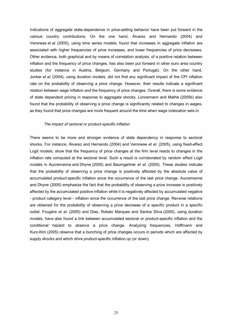
Indications of aggregate state-dependence in price-setting behavior have been put forward in the
various country contributions. On the one hand, Álvarez and Hernando (2004) and
Veronese et al. (2005), using time series models, found that increases in aggregate inflation are
associated with higher frequencies of price increases, and lower frequencies of price decreases.
Other evidence, both graphical and by means of correlation analysis, of a positive relation between
inflation and the frequency of price changes, has also been put forward in other euro area country
studies (for instance in Austria, Belgium, Germany and Portugal). On the other hand,
Jonker et al. (2004), using duration models, did not find any significant impact of the CPI inflation
rate on the probability of observing a price change. However, their results indicate a significant
relation between wage inflation and the frequency of price changes. Overall, there is some evidence
of state dependent pricing in response to aggregate shocks. Lünnemann and Mathä (2005b) also
found that the probability of observing a price change is significantly related to changes in wages,
as they found that price changes are more frequent around the time when wage indexation sets in.
The impact of sectoral or product-specific inflation
There seems to be more and stronger evidence of state dependency in response to sectoral
shocks. For instance, Álvarez and Hernando (2004) and Veronese et al. (2005), using fixed-effect
Logit models, show that the frequency of price changes at the firm level reacts to changes in the
inflation rate computed at the sectoral level. Such a result is corroborated by random effect Logit
models in Aucremanne and Dhyne (2005) and Baumgartner et al. (2005). These studies indicate
that the probability of observing a price change is positively affected by the absolute value of
accumulated product-specific inflation since the occurrence of the last price change. Aucremanne
and Dhyne (2005) emphasize the fact that the probability of observing a price increase is positively
affected by the accumulated positive inflation while it is negatively affected by accumulated negative
- product category level - inflation since the occurrence of the last price change. Reverse relations
are obtained for the probability of observing a price decrease of a specific product in a specific
outlet. Fougère et al. (2005) and Dias, Robalo Marques and Santos Silva (2005), using duration
models, have also found a link between accumulated sectoral or product-specific inflation and the
conditional hazard to observe a price change. Analyzing frequencies, Hoffmann and
Kurz-Kim (2005) observe that a bunching of price changes occurs in periods which are affected by
supply shocks and which drive product-specific inflation up (or down).
26
3. Indirect tax rate changes
Álvarez and Hernando (2004), Aucremanne and Dhyne (2004, 2005), Baudry et al. (2004), Dias,
Dias and Neves (2004), Hoffmann and Kurz-Kim (2005), and Jonker et al. (2004) have all stressed
the impact of indirect tax rate changes on the frequency of price changes. These changes always
lead to temporary increases in the frequency of price changes. As indirect tax rate changes can be
considered as exogenous cost shocks, their impact on the frequency of price changes can be
interpreted as evidence in favor of state-dependent aspects in price setting.
4. Type of outlets
Analyzing the impact of the type of outlet on the frequency of price changes, Baudry et al. (2004),
Dias, Dias and Neves (2004), Jonker et al. (2004)10 and Veronese et al. (2005) point out that the
frequency of price changes tends to be significantly higher in super and hypermarkets than in
traditional corner shops. This finding may reflect differences in the degree of competition, in the
relative importance of menu costs, or in pricing strategies.
5. Attractive pricing
Some country studies have also analyzed the impact of the use of attractive pricing on the
frequency of price adjustments. Attractive pricing could be a source of rigidity as outlets may
(temporarily) decide not to reset their prices in response to a shock because their optimal response
would result in a non-attractive price and a small deviation from optimality might not be very costly.
The use of attractive pricing is a widespread practice. As mentioned by Bergen et al. (2003), more
than 65 p.c. of the prices in the U.S retail food industry ends in 9 cents. Considering the situation in
the euro area, the available empirical evidence also indicates a large use of attractive prices (e.g.
Álvarez and Hernando (2004), Cornille (2003), Folkertsma (2002), Hoffmann and Kurz-Kim (2005)
or Lünnemann and Mathä (2005b)).
As regards the impact of attractive pricing on the price setting behavior of European retailers,
results presented in Álvarez and Hernando (2004), Aucremanne and Dhyne (2005),
Baumgartner et al. (2005) and Lünnemann and Mathä (2005b) indicate that prices that are set at an
attractive level are changed less frequently than ordinary prices.
10 In Jonker et al. (2004), the type of outlet is proxied by the number of employed persons.
27
6. Euro cash changeover
In January 2002, euro area retailers had to change price from the national currency to the euro.
Unlike an indirect tax rate change, the conversion to the euro was not as much a cost shock but
rather a change in the monetary unit that forced firms to express their prices in a new currency.
Moreover, this conversion was announced 2 years in advance and was accompanied by a period of
dual display of prices (prices were quoted both in euro and in the national currency).
The country studies provide ample evidence that (correcting for the change in numéraire) price
changes were more frequent in January 2002 or in the first quarter of 2002. This finding can be
interpreted as an indication of significant menu costs which induced bunching of prices during that
month. However, not all prices changed in January 2002. Most available studies (Baudry et al.
(2004), Baumgartner et al. (2005), Cornille (2003), Jonker et al. (2004), Lünnemann and Mathä
(2005b), Veronese et al. (2005)) show that the euro cash changeover implied an increase of the
frequency of price changes during a 6 month period before and/or after the conversion to the euro.
This lack of a generalized concentration of price changes in January 2002 is not necessarily at odds
with the existence of menu costs, given the widespread practice of dual pricing in the period
surrounding the cash changeover and its subsequent disappearance. It has to be noted that price
revisions associated with the cash changeover were not always upwards but to a significant extent
also downwards.
7. Elapsed duration
Finally, special attention has been paid in several countries on the characterization of the hazard
functions of price changes. Table 7 summarizes the main common characteristics observed across
countries.
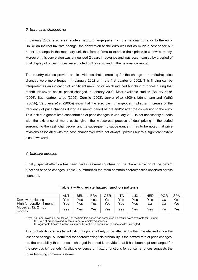
Table 7 – Aggregate hazard function patterns
Notes: na : non-available (not tested). At the time this paper was completed no results were available for Finland.
(a) Type of outlet proxied by the number of employed persons. (b) Aggregate hazard function estimated from the full population of price spells; unweigted.
The probability of a retailer adjusting its price is likely to be affected by the time elapsed since the
last price change. A useful tool for characterizing this probability is the hazard rate of price changes,
i.e. the probability that a price is changed in period k, provided that it has been kept unchanged for
the previous k-1 periods. Available evidence on hazard functions for consumer prices suggests the
three following common features.
AUT BEL FRA GER ITA LUX NED POR SPA Downward sloping Yes Yes Yes Yes Yes Yes Yes na Yes High for duration 1 month Yes Yes Yes Yes Yes Yes na na Yes Modes at 12, 24, 36 months Yes Yes Yes Yes Yes Yes Yes na Yes
28
- Hazard rates for price changes computed from the full sample of price spells display an
overall decreasing pattern in all countries where this type of information has been
analyzed;
- Hazard rates are also characterized by local modes at durations of 12, 24 and 36
months, indicating that a fraction of firms revise their prices on an annual basis;
- Hazard rate for duration one month is typically quite high, reflecting the share of price
spells with very short durations (mainly oil products and unprocessed food retailers).
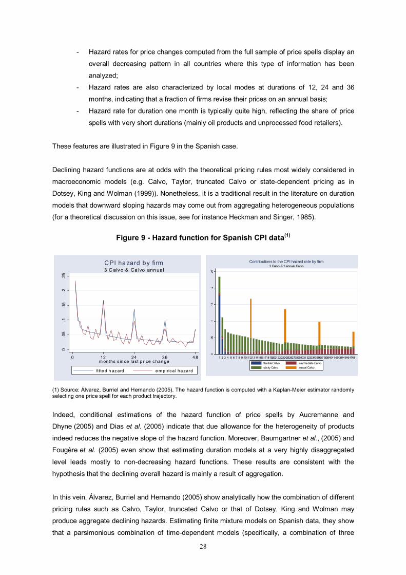
These features are illustrated in Figure 9 in the Spanish case.
Declining hazard functions are at odds with the theoretical pricing rules most widely considered in
macroeconomic models (e.g. Calvo, Taylor, truncated Calvo or state-dependent pricing as in
Dotsey, King and Wolman (1999)). Nonetheless, it is a traditional result in the literature on duration
models that downward sloping hazards may come out from aggregating heterogeneous populations
(for a theoretical discussion on this issue, see for instance Heckman and Singer, 1985).
Figure 9 - Hazard function for Spanish CPI data(1)
0.0
5.1
.15
.2.2
5
0 12 24 36 4 8m onths s in ce last p rice chan ge
fitte d h az ard e m pirica l ha zard
3 C alv o & Ca lvo ann ua lCPI ha zard by firm
0.0
5.1
.15
.2.2
5
1 2 3 4 5 6 7 8 9 10111213141516171819202122232425262728293031 3233343536373839404142434445464748
3 Calvo & 1 annual CalvoContributions to the CPI hazard rate by firm
flexible Calvo intermediate Calvosticky Calvo annual Calvo
(1) Source: Álvarez, Burriel and Hernando (2005). The hazard function is computed with a Kaplan-Meier estimator randomly selecting one price spell for each product trajectory.
Indeed, conditional estimations of the hazard function of price spells by Aucremanne and
Dhyne (2005) and Dias et al. (2005) indicate that due allowance for the heterogeneity of products
indeed reduces the negative slope of the hazard function. Moreover, Baumgartner et al., (2005) and
Fougère et al. (2005) even show that estimating duration models at a very highly disaggregated
level leads mostly to non-decreasing hazard functions. These results are consistent with the
hypothesis that the declining overall hazard is mainly a result of aggregation.
In this vein, Álvarez, Burriel and Hernando (2005) show analytically how the combination of different
pricing rules such as Calvo, Taylor, truncated Calvo or that of Dotsey, King and Wolman may
produce aggregate declining hazards. Estimating finite mixture models on Spanish data, they show
that a parsimonious combination of time-dependent models (specifically, a combination of three
29
different types of Calvo agents -highly flexible, intermediate and sticky- and some so-called annual
Calvo price setters11) is successful in reproducing the empirical hazard rate (see left panel of
Figure 9). However characterizing price-setting rule at the micro level by a combination of a limited
set of time-dependent pricing rules is obviously an approximation. Indeed, evidence of state
dependence was put forward for most euro area countries (see above).
4.2 A pooled regression analysis The evidence collected so far points to various factors potentially relevant in determining the
observed heterogeneity in price setting, including the structure of the retail market, the inflation rate,
and the treatment of sales. The aim of this section is to empirically assess their relative importance.
We exploit the full distribution of product level statistics on price setting (frequency and size of price
changes) in order to perform a set of cross-country regressions.
The frequency (size) of price changes for each category is regressed on product type effects
(unprocessed and processed food, energy, non-energy industrial goods, and services), country
dummies and a set of additional explanatory variables. The latter comprise, first, descriptive
measures on the inflation process at the product category level (mean and standard deviation);
second, an indicator of the incidence of sales or other temporary price offers for each product; third,
the share of large retailers (hypermarkets and large chain stores) selling a specific product; fourth,
an indicator signaling whether the price has a regulated/unregulated nature; last, the share of prices
set at attractive (psychological and threshold) levels (see Table A7 in Appendix , for details).
When conducting regressions to explain fractional response variables such as the frequency of
price changes (freq), linear models are not appropriate because fractions are by nature bounded
between 0 and 1. The most common solution is to model the log-odds ratio,
− freqfreq
1log , as a
linear function of the conditioning variables and to estimate an equation of the form:
ijk
kijkiij xbalfreq ε++= ∑
where xkij are explanatory variables related to product category i (i=1, … 50) in country j (j=1, … 9),
such as a sub-index dummy. In order to measure the marginal effects of each variable on the
frequency, coefficients from these linear regressions are transformed, according to
)1( freqfreqbkk −=β . Such estimates may be evaluated, for instance, at the corresponding
sample averages. The untransformed left-hand side variable can be seen as the aggregation of
binary variables indicating price changes within each product and country group, which suggests
allowing for heteroscedasticity12. An alternative procedure is the quasi-maximum likelihood (QML)
approach, of Papke and Wooldridge (1996). These authors suggest the direct estimation of a
11 The annual Calvo rule states that a certain fraction of firms reset their prices every 12 months, but keep them constant in
between. Annual Calvo agents allow to to explain the spikes at 12, 24, 36,… months. 12 For a robustness check on our findings, we also performed a set of quantile regressions (Least Absolute Deviations) on
the same models which should be less affected by outliers. The results are generally consistent with the ones reported here. Huber type robust regressions are also consistent with results in Table 8.
30
non-linear model where the right-hand side is a non-linear function (typically a cumulative
distribution function of the conditioning variables). Their method involves specifying the observed
frequency as a bounded non-linear function of the conditioning set and maximizing a likelihood
based on the Bernoulli distribution. The corresponding estimator is consistent and asymptotically
normal. We have conducted the analysis using both the standard log-odds model and the Bernoulli
QML approach using the logistic cumulative distribution function. Table 8 reports the results from
the QML estimation, as the marginal effects computed under the former may be inconsistent.
The results of the model (see Table 8) are broadly consistent with the results of the available euro
area country studies summarized in the previous section. More specifically, the frequency of price
changes is found to be significantly affected by the volatility of inflation, although not by its mean.
This is not surprising since higher (lower) inflation should increase (decrease) the frequency of price
increases, but also decrease (increase) the frequency of price reductions (rises). Indeed, the
frequency of price increases is positively affected by inflation and the frequency of price reductions
is negatively related to it.
The rest of the explanatory variables have the same sign for price changes, increases and
decreases. Sales are found to raise the frequency of price changes significantly13 and prices subject
to some form of administrative control are indeed found to change less often, reflecting the annual
nature of public budgets. Surprisingly, use of attractive prices and type of outlet are not significant,
unlike in country studies. This may reflect the lack of detailed information on the market structure at
such a detailed level in some countries, as well as some cross-country heterogeneity in the
definition of these variables.
When controlling for all factors listed above, country and product effects remain significant. For
instance, the country dummies are significant at the 5 p.c. level for 5 countries. The maximum
spread is 15 p.p. (between Austria, –0.065 and Luxembourg, 0.085). This spread is slightly larger
than the one presented in Section 3. However, it has to be stressed that the figures presented in
Table 8 are marginal effects and that they should not be interpreted as contributions to the weighted
frequencies. The magnitude of cross-country differences is smaller when separately considering
frequency of price increases and decreases. While it is not straightforward to disentangle the effects
of data collection procedures, this difference suggests that there is indeed some structural
heterogeneity in price setting within the euro area.
13 Note that this coefficient measures the marginal effect of sales-reporting for the product category concerned, and is
therefore higher than the overall impact of sales-reporting on average frequency (found above to be at most 3 p.p.)
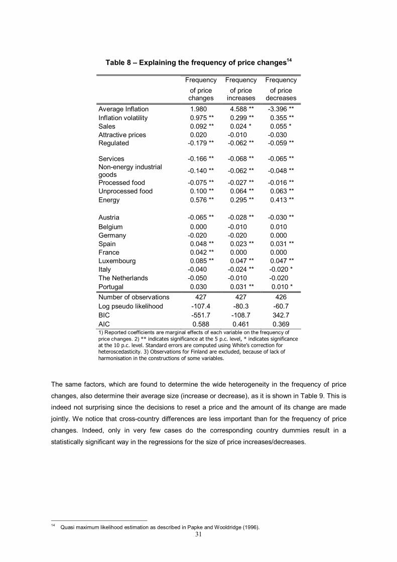
31
Table 8 – Explaining the frequency of price changes14
Frequency Frequency Frequency of price changes
of price increases
of price decreases
Average Inflation -1.980 ** -4.588 ** -3.396 ** Inflation volatility -0.975 ** -0.299 ** -0.355 ** Sales -0.092 ** -0.024 ** -0.055 ** Attractive prices -0.020 ** -0.010 ** -0.030 ** Regulated -0.179 ** -0.062 ** -0.059 ** Services -0.166 ** -0.068 ** -0.065 ** Non-energy industrial goods -0.140 ** -0.062 ** -0.048 **
Processed food -0.075 ** -0.027 ** -0.016 ** Unprocessed food -0.100 ** -0.064 ** -0.063 ** Energy -0.576 ** -0.295 ** -0.413 ** Austria -0.065 ** -0.028 ** -0.030 ** Belgium -0.000 ** -0.010 ** -0.010 ** Germany -0.020 ** -0.020 ** -0.000 ** Spain -0.048 ** -0.023 ** -0.031 ** France -0.042 ** -0.000 ** -0.000 ** Luxembourg -0.085 ** -0.047 ** -0.047 ** Italy -0.040 ** -0.024 ** -0.020 * The Netherlands -0.050 ** -0.010 ** -0.020 * Portugal -0.030 ** -0.031 ** -0.010 * Number of observations 427 427 426 Log pseudo likelihood -107.4 -80.3 -60.7 BIC -551.7 -108.7 342.7 AIC 0.588 0.461 0.369 1) Reported coefficients are marginal effects of each variable on the frequency of price changes. 2) ** indicates significance at the 5 p.c. level, * indicates significance at the 10 p.c. level. Standard errors are computed using White’s correction for heteroscedasticity. 3) Observations for Finland are excluded, because of lack of harmonisation in the constructions of some variables.
The same factors, which are found to determine the wide heterogeneity in the frequency of price
changes, also determine their average size (increase or decrease), as it is shown in Table 9. This is
indeed not surprising since the decisions to reset a price and the amount of its change are made
jointly. We notice that cross-country differences are less important than for the frequency of price
changes. Indeed, only in very few cases do the corresponding country dummies result in a
statistically significant way in the regressions for the size of price increases/decreases.
14 Quasi maximum likelihood estimation as described in Papke and Wooldridge (1996).
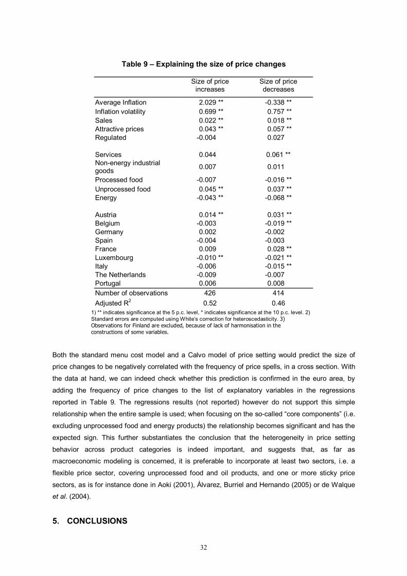
32
Table 9 – Explaining the size of price changes
Size of price
increases Size of price decreases
Average Inflation -2.029 ** -0.338 ** Inflation volatility -0.699 ** -0.757 ** Sales -0.022 ** -0.018 ** Attractive prices -0.043 ** -0.057 ** Regulated -0.004 ** -0.027 ** Services -0.044 ** 0.061 ** Non-energy industrial goods -0.007 ** -0.011 **
Processed food -0.007 ** -0.016 ** Unprocessed food -0.045 ** -0.037 ** Energy -0.043 ** -0.068 ** Austria -0.014 ** -0.031 ** Belgium -0.003 ** -0.019 ** Germany -0.002 ** -0.002 ** Spain -0.004 ** -0.003 ** France -0.009 ** -0.028 ** Luxembourg -0.010 ** -0.021 ** Italy -0.006 ** -0.015 ** The Netherlands -0.009 ** -0.007 ** Portugal -0.006 ** -0.008 ** Number of observations 426 414 Adjusted R2 0.52 0.46
1) ** indicates significance at the 5 p.c. level, * indicates significance at the 10 p.c. level. 2) Standard errors are computed using White’s correction for heteroscedasticity. 3) Observations for Finland are excluded, because of lack of harmonisation in the constructions of some variables.
Both the standard menu cost model and a Calvo model of price setting would predict the size of
price changes to be negatively correlated with the frequency of price spells, in a cross section. With
the data at hand, we can indeed check whether this prediction is confirmed in the euro area, by
adding the frequency of price changes to the list of explanatory variables in the regressions
reported in Table 9. The regressions results (not reported) however do not support this simple
relationship when the entire sample is used; when focusing on the so-called “core components” (i.e.
excluding unprocessed food and energy products) the relationship becomes significant and has the
expected sign. This further substantiates the conclusion that the heterogeneity in price setting
behavior across product categories is indeed important, and suggests that, as far as
macroeconomic modeling is concerned, it is preferable to incorporate at least two sectors, i.e. a
flexible price sector, covering unprocessed food and oil products, and one or more sticky price
sectors, as is for instance done in Aoki (2001), Álvarez, Burriel and Hernando (2005) or de Walque
et al. (2004).
5. CONCLUSIONS
33
This paper makes available for the first time quantitative measures of the frequency and size of
price adjustments within the euro area. To this end, we have taken advantage of the unique
opportunity provided by the Inflation Persistence Network to bring together comparable figures
characterizing price-setting practices for consumer goods and services.
Based on the analysis of a common sample of 50 products, several stylized facts have been found:
1. Prices change rarely. The frequency of price changes for the euro area is 15.1 p.c. and
the average duration of a price spell ranges from 4 to 5 quarters. These figures mean
that price adjustment in the euro area is considerably less frequent than in the US.
2. There is a marked degree of heterogeneity in the frequency of price changes across
products. Specifically, price changes are very frequent for energy (oil products) and
unprocessed food, while they are relatively infrequent for non-energy industrial goods
and services.
3. Heterogeneity across countries is relevant but less important and is, to some extent,
related to differences in the consumption structure and the statistical treatment of sales.
4. There is no evidence of a general downward rigidity in the euro area. In fact, price
decreases are not uncommon, except in services. On average, 40 p.c. of the price
changes are price reductions.
5. Price changes, either increases or decreases, are sizeable compared to the inflation
rate prevailing in each country. The magnitude of price reductions is slightly higher than
that of price increases.
6. Synchronization of price changes across price-setters does not seem to be large at the
product level, even within the same country.
Some further common patterns of price adjustment data have been observed in the various country
studies in this paper. In particular, there is some evidence of time dependency in price-setting
behavior as the frequency of price changes exhibits seasonal patterns, even in sectors without
marked seasonality in the demand and supply conditions. In particular, price changes mostly occur
at the beginning of the year (especially in the services sector) and after the summer period.
Moreover, the hazard function of price changes in most euro area countries is characterized by
mass points every 12 months. However, there are also strong indications of elements of state-
dependent behavior as aggregate and sectoral inflation seem to affect the frequency of price
changes. This impact is further strengthened when price increases and price decreases are
analyzed separately. Additionally, some firms appear to respond quickly to shocks such as indirect
tax rate and input price changes. This coexistence of firms with time and state dependent pricing
strategies is also found in the national surveys on price setting summarized in Fabiani et al. (2005).
34
Finally, national studies also show that firms temporarily increased their frequency of price changes
around the euro-cash changeover period.
These findings are generally substantiated by a cross-country cross-section econometric analysis of
the 50 products. First, inflation has a positive effect on the frequency of price increases and a
negative effect on the frequency of price decreases. Second, inflation volatility has an impact on the
frequency of price adjustment. Third, there is cross-product and cross-country heterogeneity even
when controlling for differences in inflation and commercial practices (regulated prices, sales,
attractive pricing). Cross-product heterogeneity is particularly important since there is a 74 p.p.
difference between the frequency of price changes for oil products and that for services, which may
be related to the heterogeneity in input price developments. Cross-country differences are less
marked and the maximum spread, between Italy and Luxembourg, averages 15 p.p. at the product
category level
The facts put forward in this paper provide a benchmark against which to assess and calibrate
micro-founded price setting models in the euro area. In particular, results in this paper stress the
importance of sectoral heterogeneity in price setting behavior. This suggests that developing
macroeconomic models that consider explicitly such heterogeneity may also improve the
understanding of economic fluctuations and inflation dynamics. In this respect, it seems worthwhile
to build macroeconomic models with at least one sector with flexible price setting and one sector
with sticky prices, as is done in Aoki (2001) or de Walque et al. (2004). Another interesting line of
research does not identify ex ante the heterogeneous sectors but rather infers from micro data the
composition of these sectors, as in Álvarez et al. (2005). These authors consider time dependent
price setters, so a natural extension is to derive micro models also consistent with the available
evidence on state dependent pricing strategies. Further research on micro price data, therefore, has
to clarify whether the uncovered state-dependent features in price setting relate mainly to
idiosyncratic or to macroeconomic developments. If idiosyncratic developments are important then it
is interesting to examine to which extent they are transmitted to the aggregate level. In general, this
research should assess, from a macro perspective, the quantitative importance of state-dependent
relative to time-dependent features.
Further research should also study more thoroughly the available information regarding the size of
the price changes. In particular, the link between the frequency of price changes and the size of the
changes should be examined in more detail. Moreover, a careful study of the distribution of price
changes could address the question whether or not there are backward-looking features in the
price-setting process.
35
REFERENCES
Álvarez, L. and I. Hernando, (2004): "Price Setting Behaviour in Spain. Stylised Facts Using Consumer Price Micro Data", Banco de España, ECB Working Paper Series No 416.
Álvarez, L., Burriel, P. and I. Hernando, (2005): "Do Decreasing Hazard Functions Make Sense?", Banco de España, ECB Working Paper Series No 461.
Aoki, K. (2001): "Optimal Monetary Policy Responses to Relative-Price Changes", Journal of Monetary Economics, Vol 48/1, pp. 55-80.
Aucremanne, L. and E. Dhyne (2004), "How Frequently Do Prices Change? Evidence Based on the Micro Data Underlying the Belgian CPI", ECB Working Paper Series No 331.
Aucremanne, L. and E. Dhyne (2005), "Time-dependent versus State-dependent Pricing: A Panel Data Approach to the Determinants of Belgian Consumer Price Changes.", ECB Working Paper Series No 462.
Baharad E. and B. Eden (2004): "Price Rigidity and Price Dispersion: Evidence from Micro Data", Review of Economic Dynamics, 7, pp 613-641.
Baudry, L., Le Bihan H., Sevestre, P. and S. Tarrieu (2004): "Price Rigidity in France - Evidence from Consumer Price Micro-Data", ECB Working Papers Series No 384.
Baumgartner, J., E. Glatzer, F. Rumler and A. Stiglbauer (2005): "How Frequently Do Consumer Prices Change in Austria? Evidence from Micro CPI Data", ECB Working Paper Series No 523.
Bergen, M., Chen, H. and D. Levy (2003): "Making Sense of Ignoring Cents: Another Implication of Rational Inattention", mimeo.
Bils, M. and P. Klenow (2004): "Some Evidence on the Importance of Sticky Prices", Journal of Political Economy, 112, pp 947-985.
Campbell J.R. and B. Eden (2004), "Rigid prices: evidence from US scanner data ", Vanderbilt University, mimeo.
Cecchetti, S. G. (1986): "The Frequency of Price Adjustment: A Study of the Newsstand Prices of Magazines", Journal of Econometrics, vol 31, 255-274.
Cornille, D. (2003): "The adaptation of prices to the changeover to the euro", National Bank of Belgium Economic Review, 4th Quarter.
De Walque, G., F. Smets, and R. Wouters (2004): “Price Setting in General Equilibrium: Alternative Specifications", mimeo.
Dias, D., C. Robalo Marques, and J. M. C. Santos Silva (2005): "Time or State Dependent Price Setting Rules? Evidence from Portuguese micro data”, Banco de Portugal, mimeo.
Dias, D., C. Robalo Marques, P. Neves, and J. M. C. Santos Silva (2004): "On the Fisher-Konieczny index of price changes synchronization", Banco de Portugal Working Paper 7/04.
Dias, M., Dias, D., and P. Neves (2004): "Stylised Features of Price Setting Behaviour in Portugal: 1992-2001", ECB Working Paper Series No 332.
Dotsey, M., King R. G., and A. L. Wolman (1999): "State-dependent Pricing and the General Equilibrium Dynamics of Money and Output", Quarterly Journal of Economics, Vol 114, pp 655-690.
Eden, B. (2001): "Inflation and Price Adjustment: An analysis of Microdata", Review of Economic Dynamics, 4, pp 607-636.
36
Fabiani, S., M. Druant, I. Hernando, C. Kwapil, B. Landau, C. Loupias, F. Martins, T. Mathae, R. Sabbatini, and A. Stokman (2005) The pricing behaviour of firms in the euro area: New survey evidence, ECB Working Paper Series No 536.
Fisher, T. and J. Konieczny. (2000): "Synchronization of Price Changes by Multiproduct Firms: Evidence from Canadian Newspaper Prices", Economics Letters, 68, 271-277.
Folkertsma, C. K. (2002): "The Euro and Psychological Prices: Simulations of the Worst Case Scenario", De Economist, 150(1), 19-40.
Fougère, D., Le Bihan H. and P. Sevestre (2005), "Heterogeneity in Price Stickiness: a Microeconometric Investigation", ECB Working Paper Series No 536.
Galí, J., Gertler, M. and D. López-Salido (2001): "European Inflation Dynamics", European Economic Review, 45(7), 1237-1270.
Galí, J., Gertler, M. and D. López-Salido (2003): "Erratum to European Inflation Dynamics [European Economic Review 45 (2001), 1237-1270]", European Economic Review, 47(4), 759-760.
Genesove, D. (2003): "The Nominal Rigidity of Apartment Rents", Review of Economics and Statistics, 85(4), 844-853.
Guédès D. (2004) “Impact des ajustements de qualité dans le calcul de l’indice des prix à la consommation” , Insee, document de travail n°F0404.
Heckman, J. and B. Singer (1985), "Social Science Duration Analysis" in Heckman, Singer (Editors), Longitudinal Studies of Labor Market Data, Cambridge University Press.
Hoffmann, J. and J.-R. Kurz-Kim (2005): “Consumer price adjustment under the microscope: Germany in a period of low inflation”, Deutsche Bundesbank, mimeo.
Jonker, N., Blijenberg H. and C. Folkertsma (2004): "Empirical analysis of price setting behaviour in the Netherlands in the period 1998-2003 using micro data ", ECB Working Paper No 413.
Kackmeister, A. (2001): "Has Retail Price Behavior Changed Since 1889? Evidence from Microdata", mimeo.
Kashyap, A. K. (1995): "Sticky Prices: New Evidence from Retail Catalogs", Quarterly Journal of Economics, 245-274.
Klenow, P. and O. Kryvtsov (2004): "State-Dependent or Time-Dependent Pricing: Does it Matter for Recent U.S. Inflation?", mimeo.
Konieczny, J. D. and A. Skrzypacz (2002): "Inflation and Price Setting in a Natural Experiment", mimeo.
Konieczny, J. D. and A. Skrzypacz (2004): "Search, Costly Price Adjustment and the Frequency of Price Changes – Theory and Evidence", mimeo.
Lach S. and D. Tsiddon (1992): "The Behaviour of Prices and Inflation: An Empirical Analysis of Disaggregated Price Data", Journal of Political Economy, 100, 349-389.
Lach S. and D. Tsiddon (1996): "Staggering and Synchronization in Price Setting: Evidence from Multiproduct Firms", American Economic Review, 86, 1175-1196.
Levy, D., M. Bergen, S., Dutta, and R. Venable (1997): "The Magnitude of Menu Costs: Direct Evidence from Large US Supermarket Chains", Quarterly Journal of Economics, 112:3, pp 791–825.
Lünnemann, P. and T. Mathä (2004): "How Persistent is Disaggregated Inflation? An Analysis Across EU countries and HICP sub-indices", ECB Working Paper No 415.
37
Lünnemann, P. and T. Mathä (2005a) "Regulated and Services' Prices and Inflation Persistence", ECB Working Paper No 466.
Lünnemann, P. and T. Mathä (2005b) "Consumer Price Behaviour in Luxembourg: Evidence From Micro CPI data", Banque Centrale du Luxembourg, mimeo.
Papke L.E. and Wooldridge J.M. (1996) “Econometric Methods for Fractional Response with an Application to 401(K) Plan Participation Rates”, Journal of Applied Econometrics, Vol. 11, N.6, p. 619-632.
Ratfai, A. (2003): "The Frequency and Size of Price Adjustment: Microeconomic Evidence", Central European University Economics Working Paper n° 5-2003.
Rogers, J. H. (2002), " Monetary union, price level convergence, and inflation: How close is Europe to the United States?", Board of Governors of the Federal Reserve System, International Finance Discussion Papers, n° 740.
Taylor, J. (1999): "Staggered Price and Wage Setting in Macroeconomics", in Taylor and Woodford (Editors), Handbook of Macroeconomics, vol 1b, North-Holland.
Veronese G, S. Fabiani, A. Gattulli. and R. Sabbatini (2005): "Consumer Price Behaviour In Italy: Evidence From Micro CPI Data", ECB Working Paper No 449.
Vilmunen, J. and H. Laakkonen (2005): "How Often Do Prices Change in Finland ? Evidence from Micro CPI Data", Suomen Pankki, mimeo.
Weiss, Y. (1993): "Inflation and Price Adjustment: A Survey from Findings from Micro Data", in Sheshinsky and Weiss (Editors), Optimal Pricing and the Cost of Price Adjustment, MIT Press.
Wolman A., (1999): "Sticky Prices, Marginal Cost and the Behavior of Inflation", Federal Reserve Bank of Richmond Economic Quarterly, vol 85/4, 29-48.
Wolman A., (2000): "The Frequency and Costs of Individual Price Adjustment", Federal Reserve Bank of Richmond Economic Quarterly, vol 86/4, 1-22.
38
Technical appendix
1. The 50 products common sample
The common sample of 50 product categories is a stratified sample based on the following criteria.
First, the sample had to be representative of the different 2-digit COICOP (Classification Of
Individual COnsumption by Purpose) categories, except for "Health Care Services" (COICOP 06)
and "Education" (COICOP 10) since 8 countries out of 10 had no access to individual price reports
for those two categories. Some goods or services (for instance housing rents, cars, electricity, gas,
water and telecommunication services) were not taken into consideration either for similar reasons.
This could somewhat bias upwards the estimates of the average frequencies of price changes for
some sub-aggregates and for the total15. Note on the other hand that as we observe prices at a
monthly frequency only, we miss intra-month price changes which biases downwards estimate of
the frequency.
Second, for each COICOP category level, the sample had to be representative of the 5 main
components of the CPI: unprocessed food (hereafter UNPF), processed food (hereafter PF),
energy, non-energy industrial goods (hereafter NEIG) and services. Because of the restrictions
mentioned in the first point, what is called energy only covers the price of oil products and what is
called services does not cover heath care, educational or telecommunication services nor rentals.
Using the weights of the different COICOP categories in the euro area HICP in 2000, 50 product
categories were randomly chosen within each stratum from the list of 7-digit COICOP product
categories included in the Belgian CPI - base year 1996. Product categories that are not observed
throughout the entire year by the statistical agency were not taken into account. The following table
summarizes the structure of the stratified sample and presents the 50 selected product categories.
If one of the selected individual products was not covered in a specific country, it was replaced by a
similar product (e.g. hot-dog by hamburger).
As to the period covered for this investigation, it has already been mentioned that, even if full
harmonization was not possible, it had been decided to focus on the period starting in January 1996
and not to include the period affected by the euro-cash changeover, since this could bias
frequencies of price adjustment.
15 On German data, Hoffmann and Kurz-Kim (2004) find that the frequency of changes in rents is significantly smaller than
the frequency of price changes in most other services.
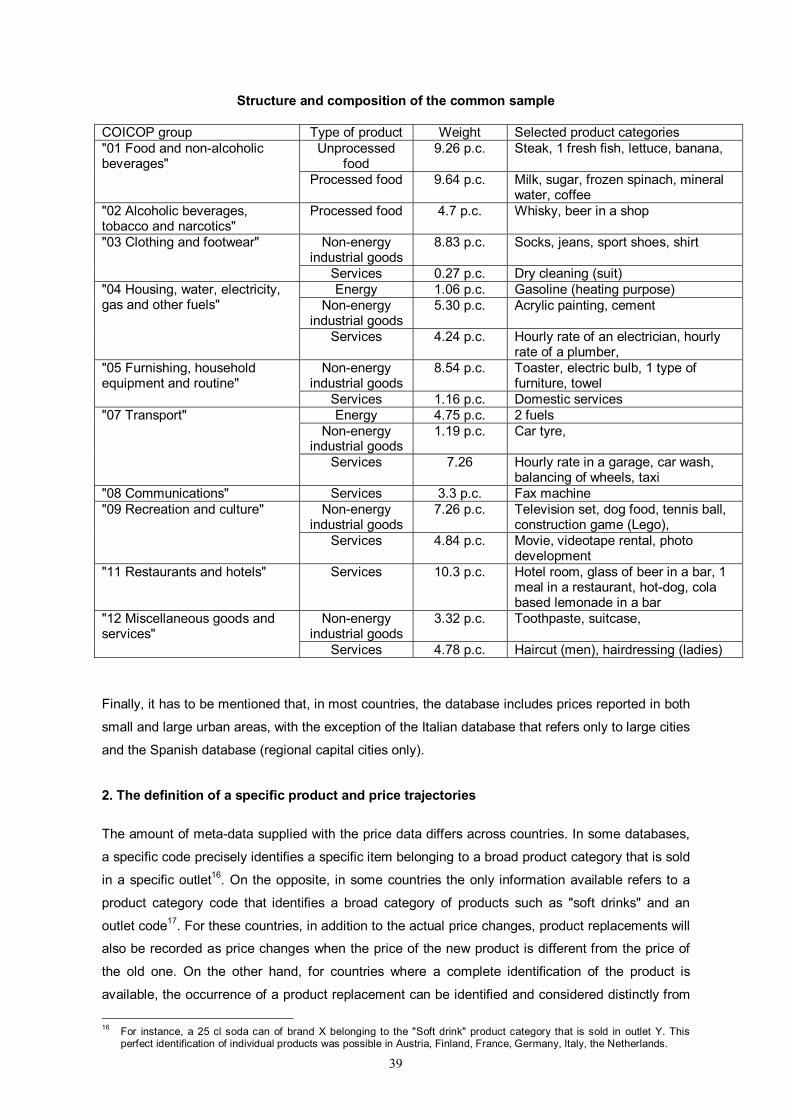
39
Structure and composition of the common sample COICOP group Type of product Weight Selected product categories
Unprocessed food
9.26 p.c. Steak, 1 fresh fish, lettuce, banana, "01 Food and non-alcoholic beverages"
Processed food 9.64 p.c. Milk, sugar, frozen spinach, mineral water, coffee
"02 Alcoholic beverages, tobacco and narcotics"
Processed food 4.7 p.c. Whisky, beer in a shop
Non-energy industrial goods
8.83 p.c. Socks, jeans, sport shoes, shirt "03 Clothing and footwear"
Services 0.27 p.c. Dry cleaning (suit) Energy 1.06 p.c. Gasoline (heating purpose)
Non-energy industrial goods
5.30 p.c. Acrylic painting, cement "04 Housing, water, electricity, gas and other fuels"
Services 4.24 p.c. Hourly rate of an electrician, hourly rate of a plumber,
Non-energy industrial goods
8.54 p.c. Toaster, electric bulb, 1 type of furniture, towel
"05 Furnishing, household equipment and routine"
Services 1.16 p.c. Domestic services Energy 4.75 p.c. 2 fuels
Non-energy industrial goods
1.19 p.c. Car tyre, "07 Transport"
Services 7.26 Hourly rate in a garage, car wash, balancing of wheels, taxi
"08 Communications" Services 3.3 p.c. Fax machine Non-energy
industrial goods 7.26 p.c. Television set, dog food, tennis ball,
construction game (Lego), "09 Recreation and culture"
Services 4.84 p.c. Movie, videotape rental, photo development
"11 Restaurants and hotels" Services 10.3 p.c. Hotel room, glass of beer in a bar, 1 meal in a restaurant, hot-dog, cola based lemonade in a bar
Non-energy industrial goods
3.32 p.c. Toothpaste, suitcase, "12 Miscellaneous goods and services"
Services 4.78 p.c. Haircut (men), hairdressing (ladies)
Finally, it has to be mentioned that, in most countries, the database includes prices reported in both
small and large urban areas, with the exception of the Italian database that refers only to large cities
and the Spanish database (regional capital cities only).
2. The definition of a specific product and price trajectories
The amount of meta-data supplied with the price data differs across countries. In some databases,
a specific code precisely identifies a specific item belonging to a broad product category that is sold
in a specific outlet16. On the opposite, in some countries the only information available refers to a
product category code that identifies a broad category of products such as "soft drinks" and an
outlet code17. For these countries, in addition to the actual price changes, product replacements will
also be recorded as price changes when the price of the new product is different from the price of
the old one. On the other hand, for countries where a complete identification of the product is
available, the occurrence of a product replacement can be identified and considered distinctly from
16 For instance, a 25 cl soda can of brand X belonging to the "Soft drink" product category that is sold in outlet Y. This
perfect identification of individual products was possible in Austria, Finland, France, Germany, Italy, the Netherlands.
40
a price change18. For instance, in the case of the trajectory plotted in the upper-left panel of
Figure 1, it is known that after January 2000 the specific pair of jeans model was no longer sold in
the given outlet.
In order to compute frequencies of price changes that are comparable across countries, it has been
decided to harmonize the treatment of product replacements. To do so, a distinction has been made
between "forced" and "voluntary" product replacements19. We decided to impute a price change for
each forced product replacement. The rationale is that the disappearance of the individual product
(and its replacement) coincides with the end of the last price spell for that particular product.
Overall, this methodological choice probably has a small positive impact on the frequency of price
changes.
3. The treatment of seasonal sales
The statistical treatment of seasonal sales (for instance at the end of the winter or summer season)
differs across countries. While sales prices (i.e. including the rebate) are reported in some
countries20, prices reported during the sales period in other countries21 are prices without the
rebate. An illustration is provided by Figure 1: the price of the specific jeans in the case of France
exhibits a price decrease that lasts for one month in July 1999, due to summer sales. It was not
possible to control for these differences in national methodologies. Therefore, this difference in the
treatment of seasonal sales may have some impact on both the frequency and the size of price
changes, particularly for product categories such as clothing and footwear.
17 This is the case of the Portuguese and Spanish databases. 18 The way price changes and product replacements are treated can have a considerable impact on the estimated
frequency of price changes. Consider for example the case of a product that has a life cycle of one year and the price of which is kept constant during its entire selling period. For such a product, the frequency of price changes is equal to 0 p.c. if the occurrence of a product replacement is not considered as a price change, while it is equal to 8.33 p.c. (once every year) otherwise.
19 For the computation of the CPI, statistical institutes follow the prices of specific products over time. When a consumer price index is defined (typically, during a base year), a stratified sample of products is drawn and is followed from month to month. However, some items may leave the sample because they are not sold anymore (product replacement) or because the outlets where they were sold close (outlet replacement). These items are replaced by new items. Such replacements are designated as "forced" replacements. Alternatively, the Statistical office can periodically revise its sample of products because the consumption habits have changed over time. These replacements are voluntary replacements.
20 Austria, Finland, France, Luxembourg, the Netherlands and Portugal. 21 Belgium, Germany, Italy and Spain. In Germany, only price cuts pre-empting the seasonal sales are observed.
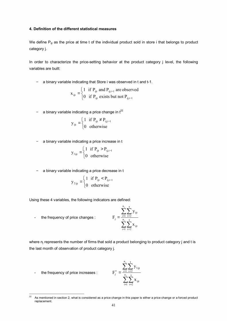
41
4. Definition of the different statistical measures
We define Pijt as the price at time t of the individual product sold in store i that belongs to product
category j.
In order to characterize the price-setting behavior at the product category j level, the following
variables are built:
− a binary variable indicating that Store i was observed in t and t-1.
=−
−
Pnot but exists P if 0observed are P nda P if 1
x1tijijt
1tijijtijt
,
,
− a binary variable indicating a price change in t22
≠
= −
therwiseo 0 P P if 1
y 1tijijtijt
,
− a binary variable indicating a price increase in t
>
= −
therwiseo 0 P P if 1
y 1tijijtijt1
,
− a binary variable indicating a price decrease in t
<
= −
therwiseo 0 P P if 1
y 1tijijtijt2
,
Using these 4 variables, the following indicators are defined:
- the frequency of price changes :
∑∑
∑∑
=
τ
=
=
τ
==j
j
n
1i 2tijt
n
1i 2tijt
j
x
yF
where nj represents the number of firms that sold a product belonging to product category j and t is
the last month of observation of product category j.
- the frequency of price increases :
∑∑
∑∑
=
τ
=
=
τ
=+ =j
j
n
1i 2tijt
n
1i 2tijt1
j
x
yF
22 As mentioned in section 2, what is considered as a price change in this paper is either a price change or a forced product
replacement.
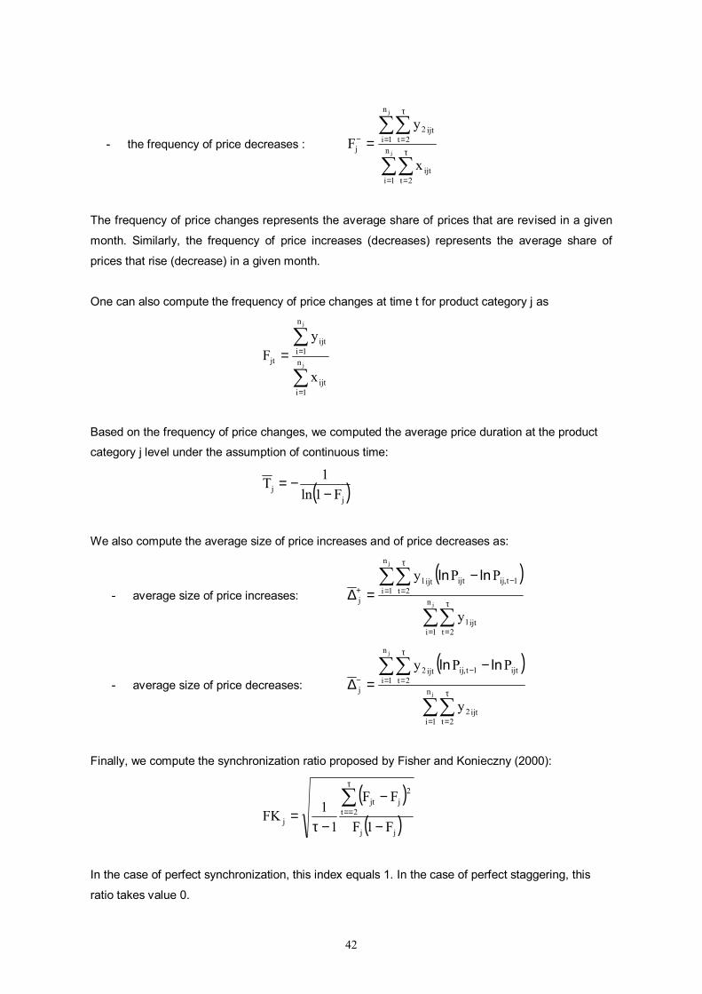
42
- the frequency of price decreases :
∑∑
∑∑
=
τ
=
=
τ
=− =j
j
n
1i 2tijt
n
1i 2tijt2
j
x
yF
The frequency of price changes represents the average share of prices that are revised in a given
month. Similarly, the frequency of price increases (decreases) represents the average share of
prices that rise (decrease) in a given month.
One can also compute the frequency of price changes at time t for product category j as
∑
∑
=
==j
j
n
1iijt
n
1iijt
jt
x
yF
Based on the frequency of price changes, we computed the average price duration at the product
category j level under the assumption of continuous time:
( )jj F1ln
1T−
−=
We also compute the average size of price increases and of price decreases as:
- average size of price increases:
( )
∑∑
∑∑
=
τ
=
=
τ
=−
+−
=∆j
j
n
1i 2tijt1
n
1i 2t1tijijtijt1
j
y
PPy ,lnln
- average size of price decreases:
( )
∑∑
∑∑
=
τ
=
=
τ
=−
−−
=∆j
j
n
1i 2tijt2
n
1i 2tijt1tijijt2
j
y
PPy lnln ,
Finally, we compute the synchronization ratio proposed by Fisher and Konieczny (2000):
( )( )jj
2t
2jjt
j F1F
FF
11FK
−
−
−τ=
∑τ
==
In the case of perfect synchronization, this index equals 1. In the case of perfect staggering, this
ratio takes value 0.
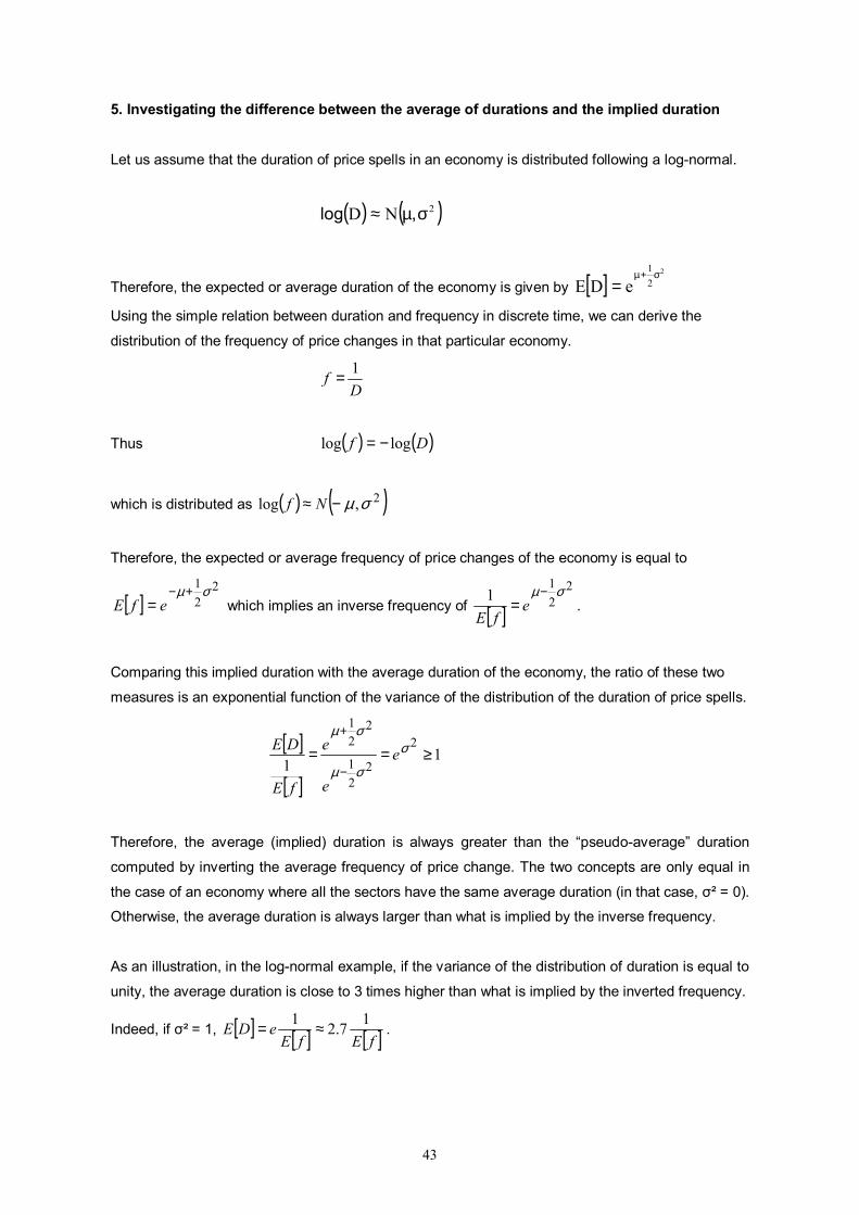
43
5. Investigating the difference between the average of durations and the implied duration
Let us assume that the duration of price spells in an economy is distributed following a log-normal.
( ) ( )2ND σµ≈ ,log
Therefore, the expected or average duration of the economy is given by [ ]2
21
eDEσ+µ
=
Using the simple relation between duration and frequency in discrete time, we can derive the
distribution of the frequency of price changes in that particular economy.
D
f 1=
Thus ( ) ( )Df loglog −=
which is distributed as ( ) ( )2,log σµ−≈ Nf
Therefore, the expected or average frequency of price changes of the economy is equal to
[ ]2
21σµ+−
= efE which implies an inverse frequency of [ ]2
21
1 σµ−= e
fE.
Comparing this implied duration with the average duration of the economy, the ratio of these two
measures is an exponential function of the variance of the distribution of the duration of price spells.
[ ]
[ ]1
12
221
221
≥==−
+σ
σµ
σµ
e
e
e
fE
DE
Therefore, the average (implied) duration is always greater than the “pseudo-average” duration
computed by inverting the average frequency of price change. The two concepts are only equal in
the case of an economy where all the sectors have the same average duration (in that case, σ² = 0).
Otherwise, the average duration is always larger than what is implied by the inverse frequency.
As an illustration, in the log-normal example, if the variance of the distribution of duration is equal to
unity, the average duration is close to 3 times higher than what is implied by the inverted frequency.
Indeed, if σ² = 1, [ ] [ ] [ ]fEfEeDE 17.21 ≈= .
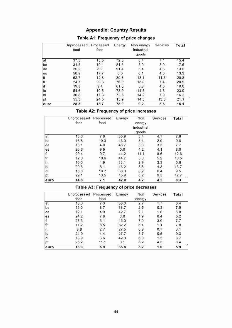
44
Appendix: Country Results Table A1: Frequency of price changes
Unprocessed food
Processed food
Energy Non energy industrial
goods
Services Total
at 37.5 15.5 72.3 8.4 7.1 15.4be 31.5 19.1 81.6 5.9 3.0 17.6de 25.2 8.9 91.4 5.4 4.3 13.5es 50.9 17.7 0.0 6.1 4.6 13.3fi 52.7 12.8 89.3 18.1 11.6 20.3fr 24.7 20.3 76.9 18.0 7.4 20.9it 19.3 9.4 61.6 5.8 4.6 10.0lu 54.6 10.5 73.9 14.5 4.8 23.0nl 30.8 17.3 72.6 14.2 7.9 16.2pt 55.3 24.5 15.9 14.3 13.6 21.1euro 28.3 13.7 78.0 9.2 5.6 15.1
Table A2: Frequency of price increases
Unprocessed food
Processed food
Energy Non energy
industrial goods
Services Total
at 18.6 7.6 35.9 3.4 4.7 7.8be 16.8 10.3 43.0 3.4 2.9 9.8de 13.1 4.0 48.7 3.3 3.3 7.7es 26.6 9.9 0.0 4.2 4.1 8.0fi 29.4 9.7 44.2 11.1 8.6 12.6fr 12.8 10.6 44.7 5.3 5.2 10.5it 10.0 4.9 33.1 2.9 3.3 5.6lu 29.6 6.1 46.2 8.8 4.3 13.7nl 16.8 10.7 30.3 8.2 6.4 9.5pt 29.1 13.5 15.9 8.2 9.3 12.7euro 14.8 7.1 42.0 4.2 4.2 8.3
Table A3: Frequency of price decreases
Unprocessed food
Processed food
Energy Non energy
Services Total
at 18.0 7.3 36.3 2.7 1.7 6.4be 15.0 8.7 38.7 2.5 0.3 7.9de 12.1 4.9 42.7 2.1 1.0 5.8es 24.2 7.8 0.0 1.9 0.4 5.2fi 23.3 3.1 45.0 7.0 3.0 7.7fr 11.2 8.5 32.2 6.4 1.1 7.8it 8.8 2.7 27.5 0.9 0.7 3.1lu 24.9 4.4 27.7 5.7 0.5 9.3nl 13.9 6.6 42.3 6.0 1.5 6.7pt 26.2 11.1 0.1 6.2 4.3 8.4euro 13.3 5.9 35.8 3.2 1.0 5.9
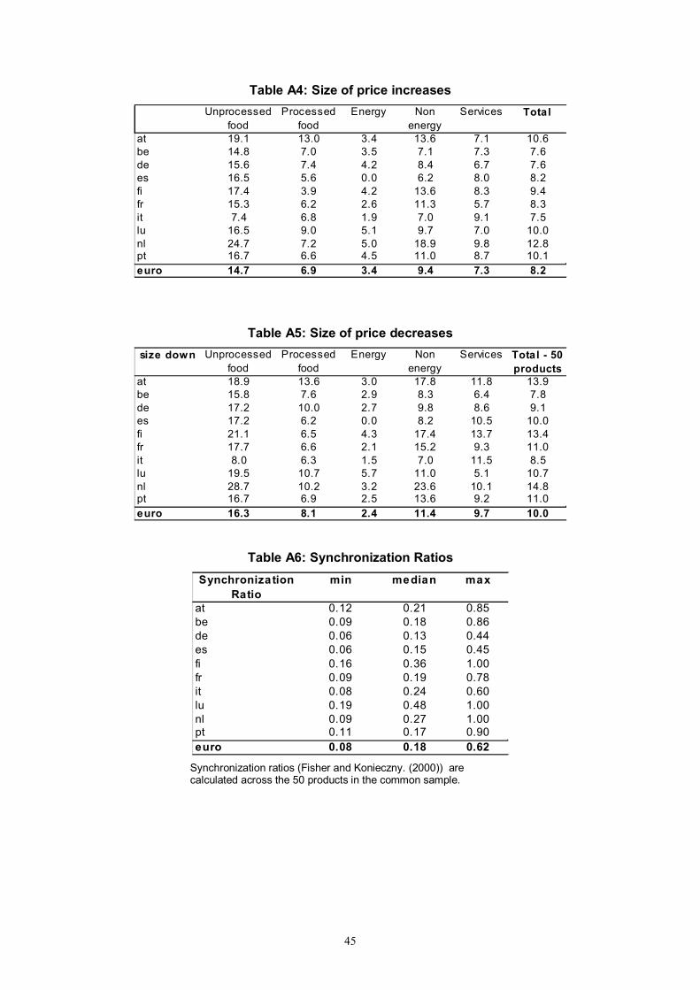
45
Table A4: Size of price increases Unprocessed
foodProcessed
foodEnergy Non
energy Services Total
at 19.1 13.0 3.4 13.6 7.1 10.6be 14.8 7.0 3.5 7.1 7.3 7.6de 15.6 7.4 4.2 8.4 6.7 7.6es 16.5 5.6 0.0 6.2 8.0 8.2fi 17.4 3.9 4.2 13.6 8.3 9.4fr 15.3 6.2 2.6 11.3 5.7 8.3it 7.4 6.8 1.9 7.0 9.1 7.5lu 16.5 9.0 5.1 9.7 7.0 10.0nl 24.7 7.2 5.0 18.9 9.8 12.8pt 16.7 6.6 4.5 11.0 8.7 10.1euro 14.7 6.9 3.4 9.4 7.3 8.2
Table A5: Size of price decreases
size down Unprocessed food
Processed food
Energy Non energy
Services Total - 50 products
at 18.9 13.6 3.0 17.8 11.8 13.9be 15.8 7.6 2.9 8.3 6.4 7.8de 17.2 10.0 2.7 9.8 8.6 9.1es 17.2 6.2 0.0 8.2 10.5 10.0fi 21.1 6.5 4.3 17.4 13.7 13.4fr 17.7 6.6 2.1 15.2 9.3 11.0it 8.0 6.3 1.5 7.0 11.5 8.5lu 19.5 10.7 5.7 11.0 5.1 10.7nl 28.7 10.2 3.2 23.6 10.1 14.8pt 16.7 6.9 2.5 13.6 9.2 11.0euro 16.3 8.1 2.4 11.4 9.7 10.0
Table A6: Synchronization Ratios
Synchronization Ratio
min median max
at 0.12 0.21 0.85be 0.09 0.18 0.86de 0.06 0.13 0.44es 0.06 0.15 0.45fi 0.16 0.36 1.00fr 0.09 0.19 0.78it 0.08 0.24 0.60lu 0.19 0.48 1.00nl 0.09 0.27 1.00pt 0.11 0.17 0.90euro 0.08 0.18 0.62
Synchronization ratios (Fisher and Konieczny. (2000)) are calculated across the 50 products in the common sample.
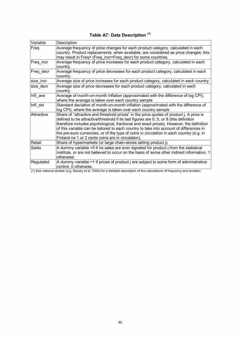
46
Table A7: Data Description (1)
Variable Description Freq Average frequency of price changes for each product category, calculated in each
country. Product replacements, when available, are considered as price changes: this may result in Freq> (Freq_incr+Freq_decr) for some countries.
Freq_incr Average frequency of price increases for each product category, calculated in each country.
Freq_decr Average frequency of price decreases for each product category, calculated in each country.
size_incr Average size of price increases for each product category, calculated in each country.size_decr Average size of price decreases for each product category, calculated in each
country. Infl_ave Average of month-on-month inflation (approximated with the difference of log CPI),
where the average is taken over each country sample Infl_std Standard deviation of month-on-month inflation (approximated with the difference of
log CPI), where the average is taken over each country sample Attractive Share of “attractive and threshold prices” in the price quotes of product j. A price is
defined to be attractive/threshold if its last figures are 0, 5, or 9 (this definition therefore includes psychological, fractional and exact prices). However, the definition of this variable can be tailored to each country to take into account of differences in the pre-euro currencies, or of the type of coins in circulation in each country (e.g. in Finland no 1 or 2 cents coins are in circulation).
Retail Share of hypermarkets (or large chain-stores selling product j). Sales A dummy variable =0 if no sales are ever signaled for product j from the statistical
institute, or are not believed to occur on the basis of some other indirect information, 1 otherwise.
Regulated A dummy variable =1 if prices of product j are subject to some form of administrative control, 0 otherwise.
(1) See national studies (e.g. Baudry et al. 2004) for a detailed description of the calculations of frequency and duration.
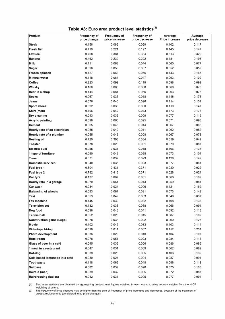
47
Table A8: Euro area product level statistics(1) Product Frequency of
price change Frequency of price increase
Frequency of price decrease
Average Price increase
Average price decrease
Steak 0.158 0.086 0.069 0.102 0.117 Fresh fish 0.419 0.221 0.197 0.145 0.147 Lettuce 0.768 0.384 0.384 0.313 0.322 Banana 0.462 0.239 0.222 0.181 0.198 Milk 0.111 0.063 0.044 0.060 0.077 Sugar 0.096 0.053 0.037 0.052 0.059 Frozen spinach 0.127 0.063 0.056 0.143 0.165 Mineral water 0.118 0.064 0.047 0.093 0.109 Coffee 0.223 0.099 0.119 0.098 0.099 Whisky 0.160 0.085 0.068 0.068 0.078 Beer in a shop 0.144 0.084 0.055 0.063 0.078 Socks 0.067 0.035 0.018 0.146 0.176 Jeans 0.076 0.040 0.026 0.114 0.134 Sport shoes 0.092 0.036 0.030 0.110 0.147 Shirt (men) 0.106 0.042 0.043 0.173 0.176 Dry cleaning 0.043 0.033 0.009 0.077 0.119 Acrylic painting 0.098 0.066 0.025 0.071 0.093 Cement 0.065 0.045 0.014 0.067 0.065 Hourly rate of an electrician 0.055 0.042 0.011 0.062 0.082 Hourly rate of a plumber 0.055 0.045 0.008 0.067 0.073 Heating oil 0.729 0.393 0.334 0.059 0.042 Toaster 0.078 0.028 0.031 0.070 0.087 Electric bulb 0.055 0.031 0.018 0.106 0.138 1 type of furniture 0.090 0.049 0.025 0.073 0.101 Towel 0.071 0.037 0.023 0.128 0.149 Domestic services 0.040 0.035 0.003 0.077 0.061 Fuel type 1 0.804 0.431 0.371 0.030 0.022 Fuel type 2 0.782 0.416 0.371 0.028 0.021 Car tyre 0.137 0.067 0.061 0.068 0.109 Hourly rate in a garage 0.079 0.064 0.013 0.059 0.081 Car wash 0.034 0.024 0.006 0.121 0.169 Balancing of wheels 0.093 0.067 0.021 0.073 0.142 Taxi 0.053 0.049 0.003 0.049 0.037 Fax machine 0.145 0.030 0.082 0.108 0.133 Television set 0.132 0.035 0.068 0.066 0.091 Dog food 0.098 0.048 0.041 0.092 0.118 Tennis ball 0.052 0.025 0.015 0.087 0.109 Construction game (Lego) 0.078 0.033 0.022 0.090 0.123 Movie 0.102 0.045 0.033 0.103 0.114 Videotape hiring 0.020 0.011 0.007 0.152 0.231 Photo development 0.036 0.023 0.010 0.104 0.107 Hotel room 0.078 0.051 0.023 0.084 0.113 Glass of beer in a café 0.045 0.036 0.006 0.086 0.085 1 meal in a restaurant 0.047 0.031 0.009 0.062 0.082 Hot-dog 0.039 0.028 0.005 0.106 0.132 Cola based lemonade in a café 0.030 0.024 0.004 0.087 0.091 Toothpaste 0.118 0.062 0.048 0.096 0.118 Suitcase 0.082 0.039 0.028 0.075 0.108 Haircut (men) 0.039 0.032 0.005 0.072 0.087 Hairdressing (ladies) 0.042 0.035 0.005 0.077 0.094 (1) Euro area statistics are obtained by aggregating product level figures obtained in each country, using country weights from the HICP
weighting structure. (2) The frequency of price changes may be higher than the sum of frequency of price increases and decreases, because of the treatment of
product replacements (considered to be price changes).
Notes d'Études et de Recherche
1. C. Huang and H. Pagès, “Optimal Consumption and Portfolio Policies with an Infinite Horizon: Existence and Convergence,” May 1990.
2. C. Bordes, « Variabilité de la vitesse et volatilité de la croissance monétaire : le cas
français », février 1989. 3. C. Bordes, M. Driscoll and A. Sauviat, “Interpreting the Money-Output Correlation: Money-
Real or Real-Real?,” May 1989. 4. C. Bordes, D. Goyeau et A. Sauviat, « Taux d'intérêt, marge et rentabilité bancaires : le cas
des pays de l'OCDE », mai 1989. 5. B. Bensaid, S. Federbusch et R. Gary-Bobo, « Sur quelques propriétés stratégiques de
l’intéressement des salariés dans l'industrie », juin 1989. 6. O. De Bandt, « L'identification des chocs monétaires et financiers en France : une étude
empirique », juin 1990. 7. M. Boutillier et S. Dérangère, « Le taux de crédit accordé aux entreprises françaises : coûts
opératoires des banques et prime de risque de défaut », juin 1990. 8. M. Boutillier and B. Cabrillac, “Foreign Exchange Markets: Efficiency and Hierarchy,”
October 1990. 9. O. De Bandt et P. Jacquinot, « Les choix de financement des entreprises en France : une
modélisation économétrique », octobre 1990 (English version also available on request). 10. B. Bensaid and R. Gary-Bobo, “On Renegotiation of Profit-Sharing Contracts in Industry,”
July 1989 (English version of NER n° 5). 11. P. G. Garella and Y. Richelle, “Cartel Formation and the Selection of Firms,” December
1990. 12. H. Pagès and H. He, “Consumption and Portfolio Decisions with Labor Income and
Borrowing Constraints,” August 1990. 13. P. Sicsic, « Le franc Poincaré a-t-il été délibérément sous-évalué ? », octobre 1991. 14. B. Bensaid and R. Gary-Bobo, “On the Commitment Value of Contracts under Renegotiation
Constraints,” January 1990 revised November 1990. 15. B. Bensaid, J.-P. Lesne, H. Pagès and J. Scheinkman, “Derivative Asset Pricing with
Transaction Costs,” May 1991 revised November 1991. 16. C. Monticelli and M.-O. Strauss-Kahn, “European Integration and the Demand for Broad
Money,” December 1991. 17. J. Henry and M. Phelipot, “The High and Low-Risk Asset Demand of French Households: A
Multivariate Analysis,” November 1991 revised June 1992. 18. B. Bensaid and P. Garella, “Financing Takeovers under Asymetric Information,” September
1992.
19. A. de Palma and M. Uctum, “Financial Intermediation under Financial Integration and
Deregulation,” September 1992. 20. A. de Palma, L. Leruth and P. Régibeau, “Partial Compatibility with Network Externalities
and Double Purchase,” August 1992.
21. A. Frachot, D. Janci and V. Lacoste, “Factor Analysis of the Term Structure: a Probabilistic Approach,” November 1992.
22. P. Sicsic et B. Villeneuve, « L'afflux d'or en France de 1928 à 1934 », janvier 1993. 23. M. Jeanblanc-Picqué and R. Avesani, “Impulse Control Method and Exchange Rate,”
September 1993. 24. A. Frachot and J.-P. Lesne, “Expectations Hypothesis and Stochastic Volatilities,” July 1993
revised September 1993. 25. B. Bensaid and A. de Palma, “Spatial Multiproduct Oligopoly,” February 1993 revised
October 1994. 26. A. de Palma and R. Gary-Bobo, “Credit Contraction in a Model of the Banking Industry,”
October 1994. 27. P. Jacquinot et F. Mihoubi, « Dynamique et hétérogénéité de l'emploi en déséquilibre »,
septembre 1995. 28. G. Salmat, « Le retournement conjoncturel de 1992 et 1993 en France : une modélisation
VAR », octobre 1994. 29. J. Henry and J. Weidmann, “Asymmetry in the EMS Revisited: Evidence from the Causality
Analysis of Daily Eurorates,” February 1994 revised October 1994. 30. O. De Bandt, “Competition Among Financial Intermediaries and the Risk of Contagious
Failures,” September 1994 revised January 1995. 31. B. Bensaid et A. de Palma, « Politique monétaire et concurrence bancaire », janvier 1994
révisé en septembre 1995. 32. F. Rosenwald, « Coût du crédit et montant des prêts : une interprétation en terme de canal
large du crédit », septembre 1995. 33. G. Cette et S. Mahfouz, « Le partage primaire du revenu : constat descriptif sur longue
période », décembre 1995. 34. H. Pagès, “Is there a Premium for Currencies Correlated with Volatility? Some Evidence
from Risk Reversals,” January 1996. 35. E. Jondeau and R. Ricart, “The Expectations Theory: Tests on French, German and
American Euro-rates,” June 1996. 36. B. Bensaid et O. De Bandt, « Les stratégies “stop-loss” : théorie et application au Contrat
Notionnel du Matif », juin 1996.
37. C. Martin et F. Rosenwald, « Le marché des certificats de dépôts. Écarts de taux à l'émission : l'influence de la relation émetteurs-souscripteurs initiaux », avril 1996.
38. Banque de France - CEPREMAP - Direction de la Prévision - Erasme - INSEE - OFCE,
« Structures et propriétés de cinq modèles macroéconomiques français », juin 1996. 39. F. Rosenwald, « L'influence des montants émis sur le taux des certificats de dépôts », octobre
1996. 40. L. Baumel, « Les crédits mis en place par les banques AFB de 1978 à 1992 : une évaluation
des montants et des durées initiales », novembre 1996. 41. G. Cette et E. Kremp, « Le passage à une assiette valeur ajoutée pour les cotisations
sociales : Une caractérisation des entreprises non financières “gagnantes” et “perdantes” », novembre 1996.
42. S. Avouyi-Dovi, E. Jondeau et C. Lai Tong, « Effets “volume”, volatilité et transmissions
internationales sur les marchés boursiers dans le G5 », avril 1997. 43. E. Jondeau et R. Ricart, « Le contenu en information de la pente des taux : Application au
cas des titres publics français », juin 1997. 44. B. Bensaid et M. Boutillier, « Le contrat notionnel : efficience et efficacité », juillet 1997. 45. E. Jondeau et R. Ricart, « La théorie des anticipations de la structure par terme : test à partir
des titres publics français », septembre 1997. 46. E. Jondeau, « Représentation VAR et test de la théorie des anticipations de la structure par
terme », septembre 1997. 47. E. Jondeau et M. Rockinger, « Estimation et interprétation des densités neutres au risque :
Une comparaison de méthodes », octobre 1997. 48. L. Baumel et P. Sevestre, « La relation entre le taux de crédits et le coût des ressources
bancaires. Modélisation et estimation sur données individuelles de banques », octobre 1997. 49. P. Sevestre, “On the Use of Banks Balance Sheet Data in Loan Market Studies : A Note,”
October 1997. 50. P.-C. Hautcoeur and P. Sicsic, “Threat of a Capital Levy, Expected Devaluation and Interest
Rates in France during the Interwar Period,” January 1998. 51. P. Jacquinot, « L’inflation sous-jacente à partir d’une approche structurelle des VAR : une
application à la France, à l’Allemagne et au Royaume-Uni », janvier 1998. 52. C. Bruneau et O. De Bandt, « La modélisation VAR structurel : application à la politique
monétaire en France », janvier 1998. 53. C. Bruneau and E. Jondeau, “Long-Run Causality, with an Application to International Links
between Long-Term Interest Rates,” June 1998. 54. S. Coutant, E. Jondeau and M. Rockinger, “Reading Interest Rate and Bond Futures Options’
Smiles: How PIBOR and Notional Operators Appreciated the 1997 French Snap Election,” June 1998.
55. E. Jondeau et F. Sédillot, « La prévision des taux longs français et allemands à partir d’un modèle à anticipations rationnelles », juin 1998.
56. E. Jondeau and M. Rockinger, “Estimating Gram-Charlier Expansions with Positivity
Constraints,” January 1999. 57. S. Avouyi-Dovi and E. Jondeau, “Interest Rate Transmission and Volatility Transmission
along the Yield Curve,” January 1999. 58. S. Avouyi-Dovi et E. Jondeau, « La modélisation de la volatilité des bourses asiatiques »,
janvier 1999. 59. E. Jondeau, « La mesure du ratio rendement-risque à partir du marché des euro-devises »,
janvier 1999. 60. C. Bruneau and O. De Bandt, “Fiscal Policy in the Transition to Monetary Union: A
Structural VAR Model,” January 1999. 61. E. Jondeau and R. Ricart, “The Information Content of the French and German Government
Bond Yield Curves: Why Such Differences?,” February 1999. 62. J.-B. Chatelain et P. Sevestre, « Coûts et bénéfices du passage d’une faible inflation à la
stabilité des prix », février 1999. 63. D. Irac et P. Jacquinot, « L’investissement en France depuis le début des années 1980 », avril
1999. 64. F. Mihoubi, « Le partage de la valeur ajoutée en France et en Allemagne », mars 1999. 65. S. Avouyi-Dovi and E. Jondeau, “Modelling the French Swap Spread,” April 1999. 66. E. Jondeau and M. Rockinger, “The Tail Behavior of Stock Returns: Emerging Versus
Mature Markets,” June 1999. 67. F. Sédillot, « La pente des taux contient-elle de l’information sur l’activité économique
future ? », juin 1999. 68. E. Jondeau, H. Le Bihan et F. Sédillot, « Modélisation et prévision des indices de prix
sectoriels », septembre 1999. 69. H. Le Bihan and F. Sédillot, “Implementing and Interpreting Indicators of Core Inflation: The
French Case,” September 1999. 70. R. Lacroix, “Testing for Zeros in the Spectrum of an Univariate Stationary Process: Part I,”
December 1999. 71. R. Lacroix, “Testing for Zeros in the Spectrum of an Univariate Stationary Process: Part II,”
December 1999. 72. R. Lacroix, “Testing the Null Hypothesis of Stationarity in Fractionally Integrated Models,”
December 1999. 73. F. Chesnay and E. Jondeau, “Does correlation between stock returns really increase during
turbulent period?,” April 2000.
74. O. Burkart and V. Coudert, “Leading Indicators of Currency Crises in Emerging Economies,” May 2000.
75. D. Irac, “Estimation of a Time Varying NAIRU for France,” July 2000. 76. E. Jondeau and H. Le Bihan, “Evaluating Monetary Policy Rules in Estimated Forward-
Looking Models: A Comparison of US and German Monetary Policies,” October 2000. 77. E. Jondeau and M. Rockinger, “Conditional Volatility, Skewness, ans Kurtosis: Existence and
Persistence,” November 2000. 78. P. Jacquinot et F. Mihoubi, « Modèle à Anticipations Rationnelles de la COnjoncture
Simulée : MARCOS », novembre 2000. 79. M. Rockinger and E. Jondeau, “Entropy Densities: With an Application to Autoregressive
Conditional Skewness and Kurtosis,” January 2001. 80. B. Amable and J.-B. Chatelain, “Can Financial Infrastructures Foster Economic
Development? ,” January 2001. 81. J.-B. Chatelain and J.-C. Teurlai, “Pitfalls in Investment Euler Equations,” January 2001. 82. M. Rockinger and E. Jondeau, “Conditional Dependency of Financial Series: An Application
of Copulas,” February 2001. 83. C. Florens, E. Jondeau and H. Le Bihan, “Assessing GMM Estimates of the Federal Reserve
Reaction Function,” March 2001. 84. J.-B. Chatelain, “Mark-up and Capital Structure of the Firm facing Uncertainty,” June 2001. 85. B. Amable, J.-B. Chatelain and O. De Bandt, “Optimal Capacity in the Banking Sector and
Economic Growth,” June 2001. 86. E. Jondeau and H. Le Bihan, “Testing for a Forward-Looking Phillips Curve. Additional
Evidence from European and US Data,” December 2001. 87. G. Cette, J. Mairesse et Y. Kocoglu, « Croissance économique et diffusion des TIC : le cas de
la France sur longue période (1980-2000) », décembre 2001. 88. D. Irac and F. Sédillot, “Short Run Assessment of French Economic Activity Using OPTIM,”
January 2002. 89. M. Baghli, C. Bouthevillain, O. de Bandt, H. Fraisse, H. Le Bihan et Ph. Rousseaux, « PIB
potentiel et écart de PIB : quelques évaluations pour la France », juillet 2002. 90. E. Jondeau and M. Rockinger, “Asset Allocation in Transition Economies,” October 2002. 91. H. Pagès and J.A.C. Santos, “Optimal Supervisory Policies and Depositor-Preferences
Laws,” October 2002. 92. C. Loupias, F. Savignac and P. Sevestre, “Is There a Bank Lending Channel in France?
Evidence from Bank Panel Data,” November 2002. 93. M. Ehrmann, L. Gambacorta, J. Martínez-Pagés, P. Sevestre and A. Worms, “Financial
Systems and The Role in Monetary Policy Transmission in the Euro Area,” November 2002.
94. S. Avouyi-Dovi, D. Guégan et S. Ladoucette, « Une mesure de la persistance dans les indices boursiers », décembre 2002.
95. S. Avouyi-Dovi, D. Guégan et S. Ladoucette, “What is the Best Approach to Measure the
Interdependence between Different Markets? ,” December 2002. 96. J.-B. Chatelain and A. Tiomo, “Investment, the Cost of Capital and Monetary Policy in the
Nineties in France: A Panel Data Investigation,” December 2002. 97. J.-B. Chatelain, A. Generale, I. Hernando, U. von Kalckreuth and P. Vermeulen, “Firm
Investment and Monetary Policy Transmission in the Euro Area,” December 2002. 98. J.-S. Mésonnier, « Banque centrale, taux de l’escompte et politique monétaire chez Henry
Thornton (1760-1815) », décembre 2002. 99. M. Baghli, G. Cette et A. Sylvain, « Les déterminants du taux de marge en France et quelques
autres grands pays industrialisés : Analyse empirique sur la période 1970-2000 », janvier 2003.
100. G. Cette and Ch. Pfister, “The Challenges of the “New Economy” for Monetary Policy,”
January 2003. 101. C. Bruneau, O. De Bandt, A. Flageollet and E. Michaux, “Forecasting Inflation using
Economic Indicators: the Case of France,” May 2003. 102. C. Bruneau, O. De Bandt and A. Flageollet, “Forecasting Inflation in the Euro Area,” May
2003. 103. E. Jondeau and H. Le Bihan, “ML vs GMM Estimates of Hybrid Macroeconomic Models
(With an Application to the “New Phillips Curve”),” September 2003. 104. J. Matheron and T.-P. Maury, “Evaluating the Fit of Sticky Price Models,” January 2004. 105. S. Moyen and J.-G. Sahuc, “Incorporating Labour Market Frictions into an Optimising-Based
Monetary Policy Model,” January 2004. 106. M. Baghli, V. Brunhes-Lesage, O. De Bandt, H. Fraisse et J.-P. Villetelle, « MASCOTTE :
Modèle d’Analyse et de préviSion de la COnjoncture TrimesTriellE », février 2004. 107. E. Jondeau and M. Rockinger, “The Bank Bias: Segmentation of French Fund Families,”
February 2004. 108. E. Jondeau and M. Rockinger, “Optimal Portfolio Allocation Under Higher Moments,”
February 2004. 109. C. Bordes et L. Clerc, « Stabilité des prix et stratégie de politique monétaire unique », mars
2004. 110. N. Belorgey, R. Lecat et T.-P. Maury, « Déterminants de la productivité par employé : une
évaluation empirique en données de panel », avril 2004. 111. T.-P. Maury and B. Pluyaud, “The Breaks in per Capita Productivity Trends in a Number of
Industrial Countries,” April 2004.
112. G. Cette, J. Mairesse and Y. Kocoglu, “ICT Diffusion and Potential Output Growth,” April 2004.
113. L. Baudry, H. Le Bihan, P. Sevestre and S. Tarrieu, “Price Rigidity. Evidence from the
French CPI Micro-Data,” September 2004. 114. C. Bruneau, O. De Bandt and A. Flageollet, “Inflation and the Markup in the Euro Area,”
September 2004. 115. J.-S. Mésonnier and J.-P. Renne, “A Time-Varying “Natural” Rate of Interest for the Euro
Area,” September 2004. 116. G. Cette, J. Lopez and P.-S. Noual, “Investment in Information and Communication
Technologies: an Empirical Analysis,” October 2004. 117. J.-S. Mésonnier et J.-P. Renne, « Règle de Taylor et politique monétaire dans la zone euro »,
octobre 2004. 118. J.-G. Sahuc, “Partial Indexation, Trend Inflation, and the Hybrid Phillips Curve,” December
2004. 119. C. Loupias et B. Wigniolle, « Régime de retraite et chute de la natalité : évolution des mœurs
ou arbitrage micro-économique ? », décembre 2004. 120. C. Loupias and R. Ricart, “Price Setting in France: new Evidence from Survey Data,”
December 2004. 121. S. Avouyi-Dovi and J. Matheron, “Interactions between Business Cycles, Stock Markets
Cycles and Interest Rates: the Stylised Facts,” January 2005. 122. L. Bilke, “Break in the Mean and Persistence of Inflation: a Sectoral Analysis of French CPI,”
January 2005. 123. S. Avouyi-Dovi and J. Matheron, “Technology Shocks and Monetary Policy in an Estimated
Sticky Price Model of the US Economy,” April 2005. 124. M. Dupaigne, P. Fève and J. Matheron, “Technology Shock and Employement: Do We Really
Need DSGE Models with a Fall in Hours?,” June 2005. 125. P. Fève and J. Matheron, “Can the Kydland-Prescott Model Pass the Cogley-Nason Test?,”
June 2005. 126. S. Avouyi-Dovi and J. Matheron, “Technology Shocks and Monetary Policy in an Estimated
Sticky Price Model of the Euro Area,” June 2005. 127. O. Loisel, “Central Bank Reputation in a Forward-Looking Model,” June 2005. 128. B. Bellone, E. Gautier et S. Le Coent, « Les marchés financiers anticipent-ils les
retournements conjoncturels ? », juillet 2005. 129. P. Fève, « La modélisation macro-économétrique dynamique », juillet 2005. 130. G. Cette, N. Dromel and D. Méda, “Opportunity Costs of Having a Child, Financial
Constraints and Fertility,” August 2005.
131. S. Gouteron et D. Szpiro, « Excès de liquidité monétaire et prix des actifs », septembre 2005. 132. J. Baude, « L’impact des chocs boursiers sur le crédit en France depuis le milieu des années
quatre-vingt-dix », septembre 2005. 133. R. Bourlès and G. Cette, “A Comparison of Structural Productivity Levels in the Major
Industrialised Countries,” October 2005. 134. T. Grunspan, “The Fed and the Question of Financial Stability: An Empirical Investigation,”
October 2005. 135. S. Fabiani, M. Druant, I. Hernando, C. Kwapil, B. Landau, C. Loupias, F. Martins,
T. Mathä, R. Sabbatini, H. Stahl and A. Stockman, “The Pricing Behaviour of Firms in the Euro Area: New Survey Evidence,” November 2005.
136. E. Dhyne, L. Alvarez, H. Le Bihan, G. Veronese, D. Dias, J. Hoffmann, N. Jonker,
P. Lünnemann, F. Rumler and J. Vilmunen, “Price Setting in the Euro Area: Some Stylized Facts from Individual Consumer Price Data,” November 2005.
Pour tous commentaires ou demandes sur les Notes d'Études et de Recherche, contacter la bibliothèque de la direction de la recherche à l'adresse suivante : For any comment or enquiries on the working Papers, contact the library of the Research Directorate at the following address : BANQUE DE FRANCE 41- 1404 Labolog 75049 Paris Cedex 01 tél : (0)1 42 92 49 55 fax : (0)1 42 92 62 92 email : [email protected]